IZA DP No. 2545

The Effects of Wal-Mart on Local Labor Markets

David NeumarkJunfu ZhangStephen Ciccarella

DI

SC

US

SI

ON

PA

PE

R S

ER

IE

S

Forschungsinstitutzur Zukunft der ArbeitInstitute for the Studyof Labor

January 2007

The Effects of Wal-Mart on

Local Labor Markets

David Neumark University of California, Irvine,

Public Policy Institute of California, NBER and IZA

Junfu Zhang

Clark University

Stephen Ciccarella Cornell University

Discussion Paper No. 2545 January 2007

IZA

P.O. Box 7240 53072 Bonn

Germany

Phone: +49-228-3894-0 Fax: +49-228-3894-180

E-mail: iza@iza.org

Any opinions expressed here are those of the author(s) and not those of the institute. Research disseminated by IZA may include views on policy, but the institute itself takes no institutional policy positions. The Institute for the Study of Labor (IZA) in Bonn is a local and virtual international research center and a place of communication between science, politics and business. IZA is an independent nonprofit company supported by Deutsche Post World Net. The center is associated with the University of Bonn and offers a stimulating research environment through its research networks, research support, and visitors and doctoral programs. IZA engages in (i) original and internationally competitive research in all fields of labor economics, (ii) development of policy concepts, and (iii) dissemination of research results and concepts to the interested public. IZA Discussion Papers often represent preliminary work and are circulated to encourage discussion. Citation of such a paper should account for its provisional character. A revised version may be available directly from the author.

IZA Discussion Paper No. 2545 January 2007

ABSTRACT

The Effects of Wal-Mart on Local Labor Markets*

We estimate the effects of Wal-Mart stores on county-level retail employment and earnings, accounting for endogeneity of the location and timing of Wal-Mart openings that most likely biases the evidence against finding adverse effects of Wal-Mart stores. We address the endogeneity problem using a natural instrumental variables approach that arises from the geographic and time pattern of the opening of Wal-Mart stores, which slowly spread out from the first stores in Arkansas. The employment results indicate that a Wal-Mart store opening reduces county-level retail employment by about 150 workers, implying that each Wal-Mart worker replaces approximately 1.4 retail workers. This represents a 2.7 percent reduction in average retail employment. The payroll results indicate that Wal-Mart store openings lead to declines in county-level retail earnings of about $1.2 million, or 1.3 percent. Of course, these effects occurred against a backdrop of rising retail employment, and only imply lower retail employment growth than would have occurred absent the effects of Wal-Mart. JEL Classification: J21, R12 Keywords: Wal-Mart, location, employment Corresponding author: David Neumark Department of Economics 3151 Social Science Plaza University of California-Irvine Irvine, CA 92697-5100 USA Email: dneumark@uci.edu

* We are grateful to Ron Baiman, Emek Basker, Marianne Bitler, Eric Brunner, Colin Cameron, Wayne Gray, Judy Hellerstein, Hilary Hoynes, Chris Jepsen, Giovanni Peri, Howard Shatz, Betsey Stevenson, Brandon Wall, Jeff Wooldridge, and seminar participants at Brookings, Clark, Cornell, HKU, IZA, PPIC, Stanford, UQAM, UC-Davis, UC-Irvine, UC-Riverside, UC-San Diego, UConn, and USC for helpful comments. We are also grateful to Wal-Mart for providing data on store locations and opening dates, and to Emek Basker for providing her Wal-Mart data set and other code; any requests for Wal-Mart data have to be directed to them. Despite Wal-Mart having supplied some of the data used in this study, the company has provided no support for this research, and had no role in editing or influencing the research as a condition of providing these data. The views expressed are those of the authors, and not those of Wal-Mart. This is a revised version of a preliminary draft presented at the Wal-Mart Economic Impact Research Conference, Washington, DC, November 2005, and of NBER Working Paper No. 11782.

1

I. Introduction

Wal-Mart is more than just another large company. It is the largest corporation in the world, with

total revenues of $285 billion in 2005. It employs over 1.2 million workers in the United States, at about

3,600 stores.1 To put this in perspective, the Wal-Mart workforce represents just under one percent of

total employment and just under ten percent of retail employment in the United States. It exceeds the

number of high school teachers or middle school teachers, and is just under the size of the elementary

school teacher workforce. Wal-Mart is reported to be the nation’s largest grocer, with a 19 percent

market share, and its third-largest pharmacy, with a 16 percent market share (Bianco and Zellner, 2003).

During the past two decades, as Wal-Mart sharply expanded its number of stores in the United

States, it increasingly encountered resistance from local communities. Opponents of Wal-Mart have tried

to block its entry on many grounds, including the prevention of urban sprawl, preservation of historical

culture, protection of the environment and “main-street” merchants, and avoidance of road congestion.2

Yet two of the most commonly-heard criticisms are that Wal-Mart eliminates more retail jobs than it

creates for a community, and that it results in lower wages, especially in retail.3 Wal-Mart executives

dispute these claims, especially with regard to employment. For example: its Vice President Bob

McAdam has argued that there are many locations where Wal-Mart creates jobs in other businesses in

addition to what Wal-Mart itself offers (PBS, 2004); the Wal-Mart web-site Walmartfacts.com trumpets

the positive effects of Wal-Mart stores on retail jobs in the communities where stores open;4 and an

advertisement run in the USA Today, The Wall Street Journal, and The New York Times on January 14,

2005, displayed an open letter from Lee Scott, Wal-Mart President and CEO, stating “This year, we plan

to create more than 100,000 new jobs in the United States.”5 Of course Wal-Mart offers other potential

benefits in the form of lower prices for consumers (Basker, 2005a; Hausman and Leibtag, 2004).

1 See http://www.walmartfacts.com/newsdesk/wal-mart-fact-sheets.aspx#a125 (as of September 8, 2005). 2 See, for example, Bowermaster (1989), Rimer (1993), Nieves (1995), Kaufman (1999), Ingold (2004), and Jacobs (2004). 3 See, for example, Quinn (2000), Norman (2004), and Wal-Mart Watch (2005). 4 See http://www.walmartfacts.com/newsdesk/wal-mart-fact-sheets.aspx (as of December 15, 2005). 5 If this refers to gross rather than net job creation, it could be consistent with Wal-Mart destroying more jobs than it creates.

2

In this paper, we seek to provide a definitive answer regarding whether Wal-Mart creates or

eliminates jobs in the retail sector, relative to what would have happened absent Wal-Mart’s entry. Also,

because of concern over the effects of Wal-Mart on wages, and because policymakers may be interested

in the impact of Wal-Mart on taxable payrolls, we also estimate the effects of Wal-Mart on earnings in the

retail sector, reflecting the combination of influences on employment, wages, and hours. We believe that

our evidence improves substantially on existing studies of these and related questions, most importantly

by implementing an identification strategy that accounts for the endogeneity of store location and timing

and how these may be correlated with future changes in earnings or employment. Indeed, it has been

suggested that Wal-Mart’s explicit strategy was to locate in small towns where the population growth was

increasing (Slater, 2003, p. 92), and it is reasonable to expect that Wal-Mart entered markets where

projected retail growth was strong. If Wal-Mart tends to enter fast-growing areas in booming periods,

then we might expect to observe employment and earnings rising in apparent response to Wal-Mart’s

entry, even if the stores actually have negative effects.

Our identification strategy is driven by a systematic pattern in the openings of Wal-Mart stores.

Sam Walton, the founder of Wal-Mart, opened the first Wal-Mart store in 1962 in Rogers, Arkansas, in

Benton County. Five years later, Wal-Mart had 18 stores with $9 million of annual sales. Wal-Mart first

grew into a local chain store in the northwest part of Arkansas. It then spread to adjacent states such as

Oklahoma, Missouri, and Louisiana. From there, it kept expanding to the rest of the country after closer

markets were largely saturated (Slater, 2003, pp. 28-29). The relationship between Wal-Mart stores’

opening dates and their distance to the headquarters is primarily a result of Wal-Mart’s “saturation”

strategy for growth, which was based on control and distribution of stores, as well as word-of-mouth

advertising. In his autobiography, Sam Walton describes the control and distribution motive as follows:

“[Our growth strategy] was to saturate a market area by spreading out, then filling in. In the early growth years of discounting, a lot of national companies with distribution systems already in place—Kmart, for example—were growing by sticking stores all over the country. Obviously, we couldn’t support anything like that. … We figured we had to build our stores so that our distribution centers, or warehouses, could take care of them, but also so those stores could be controlled. We wanted them within reach of our district managers, and of ourselves here in Bentonville, so we could get out there and look after them. Each store had to be within a day’s

3

drive of a distribution center. So we would go as far as we could from a warehouse and put in a store. Then we would fill in the map of that territory, state by state, county seat by county seat, until we had saturated that market area. … So for the most part, we just started repeating what worked, stamping out stores cookie-cutter style” (Walton, 1992, pp. 110-111). One might wonder whether this need to be near a distribution center requires a steady spreading

out from Arkansas. Why not, for example, open distribution centers further away, and build stores near

them? The explanation seems to lie in the word-of-mouth advertising advantage perceived to result from

the growth strategy Wal-Mart pursued:

“This saturation strategy had all sorts of benefits beyond control and distribution. From the very beginning, we never believed in spending much money on advertising, and saturation helped us to save a fortune in that department. When you move like we did from town to town in these mostly rural areas, word of mouth gets your message out to customers pretty quickly without much advertising. When we had seventy-five stores in Arkansas, seventy-five in Missouri, eighty in Oklahoma, whatever, people knew who we were, and everybody except the merchants who weren’t discounting looked forward to our coming to their town. By doing it this way, we usually could get by with distributing just one advertising circular a month instead of running a whole lot of newspaper advertising” (Walton, 1992, p. 111). Wal-Mart’s practice of growing by “spreading out” geographically means that distance from

Benton County, Arkansas, and time—and more specifically their interaction—help predict when and

where stores opened.6 Thus, the key innovation in this paper is to instrument for the opening of Wal-Mart

stores with interactions between time and the distance between Wal-Mart host counties and Benton

County, Arkansas, where Wal-Mart headquarters are located and the first Wal-Mart store opened.

II. Literature Review

There are a number of studies that address claims about Wal-Mart’s impacts on local labor

markets, emphasizing the retail sector. However, we regard much of this literature as uninformative

about the causal impact of Wal-Mart on retail employment and earnings. First, some of the existing work

is by advocates for one side or the other in local political disputes regarding Wal-Mart’s entry into a

particular market. These studies are often hastily prepared, plagued by flawed methods and arbitrary

assumptions, and sponsored by interested parties such as Wal-Mart itself, its competitors, or union groups

6 For example, Wal-Mart’s expansion did not reach California until 1990. It first entered New England in 1991. In 1995 Wal-Mart opened its first store in Vermont and finally had a presence in all 48 contiguous states.

4

(e.g., Bianchi and Swinney, 2004; Freeman, 2004; and Rodino Associates, 2003), and can hardly be

expected to provide impartial evidence on Wal-Mart’s effects. Hence, they are not summarized here.

There is also an academic literature on the impact of Wal-Mart stores, focusing on the effects of

Wal-Mart openings on local employment, retail prices and sales, poverty rates, and the concentration of

the retailing industry, as well as the impact on existing businesses. This research is limited by three main

factors: the restriction of much of it to small regions (often a single small state); its lack of focus on

employment and earnings effects; and its failure to account for the endogeneity of Wal-Mart locations,

either at all or, in our view, adequately.

Many of these studies, especially the early ones, focus on the effects of Wal-Mart at the regional

level, spurred by the expansion of Wal-Mart into a particular region. Most of these studies focus on the

effects of Wal-Mart on retail businesses and sales, rather than on employment and earnings. The earliest

study, which is typical of much of the research that has followed, is by Stone (1988). He defines the “pull

factor” for a specific merchandise category as the ratio of per capita sales in a town to the per capita sales

at the state level, and examines the changes in the pull factor for different merchandise categories in host

and surrounding towns in Iowa after the opening of Wal-Mart stores. Stone finds that, in host towns, pull

factors for total sales and general merchandise (to which all Wal-Mart sales belong) rise after the arrival

of Wal-Mart. Pull factors for eating and drinking and home furnishing also go up because Wal-Mart

brings in more customers. However, pull factors for grocery, building materials, apparel, and specialty

stores decline, presumably due to direct competition from Wal-Mart. He also finds that small towns

surrounding Wal-Mart towns suffer a larger loss in total sales compared to towns that are further away.7

Related results for other regions—which generally, although not always, point to similar conclusions—

are reported in Keon, et al. (1989), Barnes, et al. (1996), Davidson and Rummel (2000), and Artz and

7 Stone’s study was updated regularly (see, for example, Stone, 1995, 1997), but its central message remained the same: Wal-Mart pulls more customers to the host town, hurts its local competitors, but benefits some other local businesses that do not directly compete with it. Using the same methods, Stone, et al. (2002) show similar results regarding the effects of Wal-Mart Supercenters on existing businesses in Mississippi.

5

McConnon (2001). All of these studies use administrative data, and employ research designs based on

before-and-after comparisons in locations in which Wal-Mart stores did and did not open.8

The studies reviewed thus far do not address the potential endogeneity of the location and timing

of Wal-Mart’s entry into a particular market. In addition, these studies do not focus on the key questions

with which this paper is concerned—the effects of Wal-Mart on retail employment and earnings. A few

studies come closer to the mark. Ketchum and Hughes (1997), studying counties in Maine, recognize the

problem of the endogenous location of Wal-Mart stores in faster-growing regions. They attempt to

estimate the effects of Wal-Mart on employment and earnings using a difference-in-difference-in-

differences (DDD) estimator that compares changes in retail employment and earnings over time in

counties in which Wal-Mart stores did and did not locate, compared to changes for manufacturing and

services. However, virtually none of their estimated changes are statistically significant and the data

appear very noisy, so the results are generally uninformative. More important, their approach does not

address the key endogeneity questions of whether Wal-Mart location decisions were based on anticipated

changes after stores opened, or instead only prior trends that were already different (despite the authors

posing these questions).9 Hicks and Wilburn (2001), studying the impact of Wal-Mart openings in West

Virginia, estimate positive impacts of Wal-Mart stores on retail employment and the number of retail

firms. They do not explicitly account for endogeneity, although they do address the issue. In particular,

they report evidence suggesting that Wal-Mart location decisions are independent of long-term economic

growth rates of individual counties in their sample, and that current and lagged growth have no significant

effect on Wal-Mart’s decision to enter. However, these results do not explicitly address endogeneity with

8 A couple of studies rely on surveys of local businesses rather than administrative data. McGee (1996) reports results from a small-scale survey of small retailers in five Nebraska communities conducted soon after Wal-Mart stores entered. He finds that 53 percent of the responding retailers reported negative effects of Wal-Mart’s arrival on their revenues while 19 percent indicated positive effects. In a survey of Nebraska and Kansas retailers, Peterson and McGee (2000) find that less than a third of the businesses with at least $1 million in annual sales reported a negative effect after Wal-Mart’s arrival, while close to one half of the businesses with less than $1 million in annual sales indicated a negative effect, with negative effects most commonly reported by small retailers in central business districts. The research design in these surveys fails to include a control group capturing changes that might have occurred independently of Wal-Mart openings. In addition, reported assessments by retailers may not reflect actual effects of these openings. 9 The second question can only be addressed via an instrumental variables approach, and the first requires looking at changes in growth rates, not changes in levels; their study only does the latter.

6

respect to future growth. The latter, in particular, could generate apparent positive impacts of Wal-Mart

stores.

In more recent work, Basker (2005b) studies the effects of Wal-Mart on retail employment using

nationwide data. Basker attempts to account explicitly for endogeneity by instrumenting for the actual

number of stores opening in a county in a given year with the planned number. The latter is based on

numbers that Wal-Mart assigns to stores when they are planned; according to Basker, these store numbers

indicate the order in which the openings were planned to occur. She then combines these numbers with

information from Wal-Mart Annual Reports to measure planned openings in each county and year. Her

results indicate that county-level retail employment grows by about 100 in the year of Wal-Mart entry,

but declines to a gain of about 50 jobs in five years as other retail establishments contract or close. In the

meantime, possibly because Wal-Mart streamlines its supply chain, wholesale employment declines by 20

jobs in the longer term.10

The principal problem with this identification strategy, however, is that the instrument is

unconvincing. For the instrument to be valid, two conditions must hold. The first is that planned store

openings should be correlated with (predictive of) actual openings; this condition is not problematic. The

second condition is that the variation in planned openings generates exogenous variation in actual

openings that is uncorrelated with the unobserved determinants of employment that endogenously affect

location decisions. This second condition holds if we assume, to quote Basker, that “the number of

planned Wal-Mart stores … for county j and year t is independent of the error term … and planned Wal-

Mart stores affect retail employment per capita only insofar as they are correlated with the actual

construction of Wal-Mart stores” (2005b, p. 178). The second part of the assumption is potentially

problematic; actual stores should, of course, be the driving influence, although planned stores—even if

10 Using the same instrumental variables strategy, Basker (2005a) estimates the effects of Wal-Mart entry on prices of consumer goods at the city level, finding long-run declines of 8-13 percent in prices of several products including aspirin, detergent, Kleenex, and toothpaste, although it is less clear to us why location decisions would be endogenous with respect to price. Ordinary least squares (OLS) estimation also finds long-run negative effects of Wal-Mart on prices for nine out of ten products, although only three are significant and all are smaller than the IV results. Hausman and Leibtag (2004) study the effects of Wal-Mart on food prices.

7

they do not materialize or do so only with delay—may still affect decisions of other businesses.11 The

first part of the assumption is a more serious concern, though, as it seems most likely that planned

openings will reflect the same unobserved determinants that drive endogenous location as are reflected in

actual openings, and we cannot think of an argument to the contrary (nor does Basker offer one). In this

case if the OLS estimate of the effect of Wal-Mart stores on retail employment is biased upward because

of endogeneity, the instrumental variable (IV) estimate may also be upward biased, and more so than the

OLS estimate.12

Another potential problem is that there is substantial measurement error regarding store openings

in Basker’s data.13 This measurement error arises because Basker (and Goetz and Swaminathan, 2004,

discussed below) had to collect information about Wal-Mart locations and opening dates from a variety of

11 The response of supermarkets in southern California is a telling example. In 2003, after Wal-Mart announced plans to build 40 Supercenters in California to enter the state’s grocery market, supermarket chains in southern California including Albertsons, Ralphs, and Vons immediately sought to lower costs and avoid being undercut by Wal-Mart. Their unionized workers would not accept lower compensation and began a strike that lasted more than four months. Eventually, the union leaders conceded and essentially accepted the supermarkets’ position that cutting labor costs was necessary for competing with Wal-Mart. All of this occurred before Wal-Mart opened its first Supercenter in California (in March 2004). See, for example, Goldman and Cleeland (2003) and Hiltzik (2004). 12 To take a simple example, suppose that the simultaneous model for the change in employment (∆E), planned openings (P), and actual openings (A) is

∆E = αA + ε P = β∆E + υ A = γ∆E + υ + η.

Assume that ε is uncorrelated with υ and η, and that the error terms are uncorrelated with the right-hand side variables. Then υ and η capture random factors aside from employment growth that affect planned and actual openings, and ε reflects other influences on employment growth unrelated to store openings. Employment depends on actual openings (the first assumption made by Basker). Both planned and actual openings are simultaneously determined with employment, but actual openings reflect additional information captured in η, assumed orthogonal to υ either because it reflects additional information not in the information set when P was determined, or simply random variation due to construction delays, zoning disputes, etc., which make actual and planned openings deviate. In this case the asymptotic bias in the OLS estimate of α is

(γ/(1−αγ))·Var(ε)/Var(A) which is positive assuming α < 0 (Wal-Mart reduces employment) and γ (and similarly β) > 0 (employment encourages Wal-Mart openings). The IV estimate of α using P as an instrument for A is asymptotically biased upward, with bias

(β/(1−αγ))·Var(ε)/Cov(A,P). The ratio of the IV bias to the OLS bias is

{β·Var(A)}/{γ·Cov(A,P)} = {β·(γ2Var(∆E) + Var(υ) + Var(η))}/{γ·(γβVar(∆E) + Var(υ))}. If A is based on more information than is P (reflected in η), we would expect β > γ, in which case this ratio

clearly exceeds one (it can do so even if β < γ, because of the Var(υ) term in the numerator), so the upward IV bias exceeds the upward OLS bias. It is also possible, however, that actual openings reflect information about economic conditions not available when planned openings were set, which we might capture by allowing η and ε to be positively correlated. In this case the IV estimate is not necessarily upward biased (but is still almost surely biased). 13 This is detailed in an appendix available from the authors.

8

sources including Wal-Mart editions of the Rand McNally Road Atlas, annual editions of the Directory of

Discount Department Stores, and Wal-Mart Annual Reports, which together do not always pin down the

timing of each store opening. Basker also motivates the IV as correcting for bias from measurement error

in the actual opening dates of Wal-Mart stores. But the same argument against the validity of planned

openings as an instrument applies.

Using various data sources, Goetz and Swaminathan (2004) study the relationship between Wal-

Mart openings between 1987 and 1998 and county poverty rates in 1999, conditional on 1989 poverty

rates (as measured in the 1990 and 2000 Censuses of Population). They also use an IV procedure to

address the endogeneity of Wal-Mart entry, instrumenting for Wal-Mart openings during 1987-1998 in an

equation for county poverty rates in 1999. Their IVs include an unspecified pull factor, access to

interstate highways, earnings per worker, per capita property tax, population density, percentage of

households with more than three vehicles, and number of female-headed households. The results suggest

that county poverty rates increase when Wal-Mart stores open, perhaps because Wal-Mart lowers

earnings (although the authors offer other explanations as well). However, why the IVs should affect

Wal-Mart openings only, and not changes in poverty directly (conditional on Wal-Mart openings), is not

clear, and it is not hard to construct stories in which invalid exclusion restrictions would create biases

towards the finding that Wal-Mart openings increase poverty.14

Our research addresses the four principal shortcomings of the existing research on the effects of

Wal-Mart on local labor markets. First, we estimate the effects of Wal-Mart openings on retail

employment (as well as earnings). Second, we have—we believe—a far more convincing strategy to

account for the potential endogeneity of Wal-Mart openings. Third, we are able to use administrative data

14 For example, consider the use of the number of female-headed households as an IV, and suppose that this variable is positively correlated with changes in poverty rates (because of rising inequality over this period), and also positively correlated with Wal-Mart openings (because they locate in lower-income areas). In this case the IV estimate of the effect of Wal-Mart openings on changes in poverty rates is biased upward because of the positive correlation between the instrument (female-headed households) and the error term in the equation for the change in the poverty rate. In addition, although the authors do not specify how they construct their pull factor, we assume it is similar to the measure described above—a ratio of county to statewide retail sales. Given that this is a dependent variable in other studies of the effects of Wal-Mart, it is hard to justify using it as an IV for Wal-Mart openings.

9

on Wal-Mart openings that eliminate the measurement error in recent work. And finally, we use a data

set that is national in scope.

III. Data

The analysis is done at the county level. Aside from following Basker’s strategy, this strikes us

as a reasonable geographic level of disaggregation in which to detect the effects of Wal-Mart stores—not

so small that many of the effects may occur outside of the geographic unit, and not so large that the

effects may be undetectable.

Employment and Payroll Data

Employment and payroll data are drawn from the U.S. Census Bureau’s County Business Patterns

(CBP).15 CBP is an annual series that provides economic data by industry and county. The series

includes most economic activity, but excludes data on self-employed individuals, employees of private

households, railroad employees, agricultural production workers, and most government employees. CBP

data are extracted from the Business Register, which is a U.S. Census Bureau file of all known single and

multi-establishment companies in the United States. The Business Register includes payroll and

employment data from multiple sources including Census Bureau surveys, the Internal Revenue Service,

the Social Security Administration, and the Bureau of Labor Statistics.

Payroll in the CBP includes salaries, wages, reported tips, commissions, bonuses, vacation

allowances, sick-leave pay, employee contributions to qualified pension plans, and taxable fringe benefits,

and is reported before deductions for Social Security, income tax, insurance, etc.16 It does not include

profit or other compensation earned by proprietors or business partners. Payroll is reported on an annual

basis. The employment measure in the CBP data is a count of jobs, rather than the number of people

employed (in one or more jobs). Employment covers all full- and part-time employees, including officers

and executives, as of the pay period including March 12 of each year. Workers on leave are included,

while proprietors and partners are not. The most significant limitation of the CBP data for studying the

15 A good description of the CBP data is available at http://www.census.gov/epcd/cbp/view/cbpview.html (as of August 15, 2005). 16 Given that it excludes non-taxable fringe benefits, of which the most important is health insurance, we refer to the CBP measure as earnings, rather than compensation.

10

effects of Wal-Mart is that a wage cannot be computed. The CBP data do not even provide a breakdown

of employment into full-time and part-time workers, which would permit calculation of an approximate

wage assuming a given number of hours for full-time and part-time workers. In addition, we cannot tell

whether changes in payrolls reflect changes in pay rates for comparable workers or shifts in skill

composition. As a consequence, these data cannot be used to address questions of the effects of Wal-

Mart on wages. We can, though, estimate Wal-Mart’s effect on total retail payrolls, which is of

independent interest and perhaps somewhat informative about wages when coupled with estimates of

employment effects.

We downloaded CBP data by two-digit SIC major group (three-digit NAICS subsector since

1998) from 1977 through 2002, from the Geospatial and Statistical Data Center at the University of

Virginia (through 2001) and the U.S. Census (for 2002).17 We began with 1977 because CBP data are not

continuously machine-readable for the years 1964-1976, and ended with 2002 because that was the last

year available. As explained below, however, most our analysis goes only through 1995—a period for

which our identification strategy is most compelling.

Samples

We study the retail sector as a whole, as well as the General Merchandising subsector—which

includes Wal-Mart and other general department-style stores. Looking at results for these different retail

sectors is useful for assessing and understanding the results. For example, if Wal-Mart reduces retail

employment, we might expect the employment reduction to show up for the aggregate retail sector, but to

be offset by an increase in general merchandising.18 Some complications arise in working with the CBP

data because by federal law no data can be published that might disclose the operations of an individual

employer. As we look at more disaggregated subsets of industries, it is more likely that data are

suppressed and so our sample becomes smaller. Consequently, we constructed two samples with which

17 Available at http://fisher.lib.virginia.edu/collections/stats/cbp/ (as of April 5, 2005) and http://www.census.gov/epcd/cbp/download/cbpdownload.html (as of April 5, 2005).18 There is no clear prediction for how payroll effects should vary across retail sectors, since workers are presumably quite mobile across these sectors.

11

we could consistently compare at least some retail industry sectors for the same set of observations, as

follows:

• A sample: all county-year observations with complete (non-suppressed) employment and payroll

data for aggregate retail, and in total.

• B sample: all observations in the A sample that also have complete data for the General

Merchandising retail subsector (SIC 53 or NAICS 452) to which Wal-Mart belongs.

Because the rules for whether or not data are disclosed depend on the size of the retail sector and

the size distribution of establishments within it, sample selection is endogenous. We therefore emphasize

results for the A sample, which includes nearly all counties and years. We use the B sample only to

compare estimates for aggregate retail and general merchandising; as long as any biases from selection

into the B sample are similar across retail subsectors, the estimates for aggregate retail and general

merchandising can still be meaningfully compared. However, this analysis of retail subsectors using the

B sample is not a major part of our overall analysis.19

Wal-Mart Store Data

Wal-Mart provided us with administrative data on 3,066 Wal-Mart Discount Stores and

Supercenters.20 The data set contains every Discount Store and Supercenter still in operation in the

United States at the end of fiscal year 2005 (January 31, 2005).21 Variables in the data set include store

number, street address, city, state, ZIP code, square footage, store type, opening date, store hours (e.g.,

open 24 hours), latitude, longitude, county FIPS code, and Metropolitan Statistical Area (MSA) code for

each store. Because employment is measured as of early March in each year, we code store openings as

occurring in the first full calendar year for which they are open. If we instead coded the store opening as

19 Basker (2005b) also focuses on the retail subsector excluding Eating and Drinking Places and Automotive Dealers and Gasoline Service Centers—subsectors that are least likely to compete directly with Wal-Mart. However, constructing data for this subsector results in nearly two-thirds of county-year pairs being discarded because of non-disclosure, in which case endogenous sample selection can be severe. 20 Supercenters are larger stores that include a full line of groceries as well. Unfortunately, we are often missing information on when Discount Stores converted to Supercenters, which is frequent in the latter part of the sample. All we know is the current store type. 21 We also received data identifying a small number of stores (54, as of 2005) that closed. We return to this issue in some of our robustness analyses. This data set also indicated some store relocations within counties, which are treated as continuing stores because Wal-Mart replaced smaller, older stores with larger ones in nearby locations.

12

occurring in the previous calendar year (sometime during which the store did in fact open), in most cases

(unless the store opened before early March) we would be using an employment level prior to the store

opening as a measure of employment post-opening.22

After dropping stores in Alaska and Hawaii, we used 2,211 stores in our main analysis through

1995, and 2,795 stores when we use the full sample period through 2002. By 2005, Wal-Mart also had

551 Sam’s Club stores in the United States (the first opened in 1983), on which we also obtained data,

although the data were less complete (for example, lacking information on square footage). We do most

of our analysis considering the Wal-Mart stores other than Sam’s Clubs, but also some analysis

incorporating information on the latter.23

County-Year File

We constructed a county-year file by first collecting county names and FIPS codes for the 3,141

U.S. counties from the U.S. Census Bureau.24 We then created time-consistent geographical areas which

accounted for merges or splits in counties during the sample period. For counties that split during the

sample period we maintained the definition of the original county, and for counties that merged during the

sample period we created a single corresponding county throughout.25 This leads to a file of 3,094

counties over 19 years (26 years when we use the full sample), to which we merge the CBP and Wal-Mart

data.

County Population Data

County population data for each year were collected from the U.S. Census Population Estimates

Archives.26 These were assigned to the counties.

22 The measurement error corresponding to stores opening in January through early March of the previous year is less important in the IV estimation than in OLS estimation, because the IV estimation identifies the effect from the predicted probability of store openings rather than actual openings, and these predictions typically will not vary much between adjacent years. 23 Sam’s Clubs are different because customers have to become members, like at Costco. The small number of Wal-Mart Neighborhood Markets is not included in any data we have, but the first one did not open until 1998, beyond the sample period used for most of our analysis. 24 Downloaded from http://www.census.gov/datamap/fipslist/AllSt.txt (as of April 5, 2005). 25 The code for creating consistent counties over time through 2000 was provided by Emek Basker, and supplemented by us. 26 Downloaded from http://www.census.gov/popest/archives/ (as of April 5, 2005).

Distance Construction

We compiled latitude and longitude data for each county centroid from the U.S. Census Bureau’s

Census 2000 Gazetteer Files.27 Using the Haversine distance formula, we constructed distance measures

from each county to Wal-Mart headquarters in Benton County, Arkansas, for reasons explained below.28

IV. Empirical Approach and Identification

We estimate models for changes in retail employment and payrolls. We generally capture

increased exposure to Wal-Mart stores via a measure of store openings in a county-year cell—i.e., the

change in the number of stores. We define changes in employment, payrolls, and number of stores on a

per person basis, to eliminate the undue influence of a small number of large employment changes in

extraordinarily large counties. As long as we divide all of these changes by the number of persons in the

county, the estimated coefficient on the Wal-Mart variable still measures the effect of a Wal-Mart store

opening on the change in the level of retail employment or earnings.29 To control for overall income

growth that may affect the level of demand for retail, we include changes in total payrolls per person as a

control variable. In addition, all models include fixed year effects to account for aggregate influences on

changes in retail employment or earnings that might be correlated with Wal-Mart openings, which occur

with greater frequency later in the sample.

We denote the county-level measures of retail employment and payrolls (per person) as Y, the

number of Wal-Mart stores (per person) as WM, total payrolls per person as TP, and year fixed effects (in

year s) as YRs. Indexing by county j (j = 1,…,J) and year t (t = 1,…,T), and defining α, β, γ, and δs as

scalar parameters, our baseline model for the change in the dependent variable for each observation jt is:

(1) .jts

jts

sjtjtjt YRTPWMY εδγβα ++∆+∆+=∆ ∑

In the corresponding model for levels of employment we would certainly also want to include

county fixed effects to account for fixed differences in retail employment or payrolls across counties. The 27 Downloaded from http://www.census.gov/tiger/tms/gazetteer/county2k.txt (as of April 5, 2005). 28 The Haversine distance formula is used for computing distances on a sphere. See Sinnott (1984).

13

29 Let β be the coefficient on the change in the number of Wal-Mart stores per person. Since a one-unit change in the per capita Wal-Mart measure is an increase of one store per person, the effect of a single store opening on retail employment per person is β/population, and the effect on retail employment is β.

latter, however, drop out of a model for first differences of retail employment or payrolls. However, it is

possible that there is systematic variation in these first differences across different regions, corresponding

to faster or slower growth, and our model should allow for this. The most flexible approach would be to

include county fixed effects in the first-difference regressions. However, as explained in the next

subsection, we will be particularly concerned with whether there are systematic differences in the rates of

change of our dependent variables in geographic “rings” centered on Benton County, Arkansas. We

therefore instead estimate more parsimonious models in which we augment equation (1) to include

dummy variables for counties with centroids in rings within a radius of 100 miles from Benton County,

Arkansas, 101-200 miles, 201-300 miles, etc., out to the maximum radius of 1800 miles (denoted DISTi)

as in

(1’) ,jts

jts

si

jti

ijtjtjt YRDISTTPWMY εδϕγβα +++∆+∆+=∆ ∑∑

where φi are also scalar parameters. This model allows for “distance-specific” linear trends in retail

employment and earnings, and is our preferred specification.30

Endogeneity of Wal-Mart Location Decisions and Identification

Consistent estimation of equations (1) or (1’) requires that εjt is uncorrelated with the right-hand-

side variables. If Wal-Mart location decisions are based in part on contemporaneous and future changes

in employment or payrolls, then this condition could be violated. This endogeneity is natural, since it

would be surprising if a company as successful as Wal-Mart did not make location decisions (including

the location and timing of store openings) in a systematic fashion related to current conditions and future

prospects that might be related to both employment and payroll. As but one example, Wal-Mart may

open stores where real estate development and zoning have recently become favorable to retail growth.

Our identification strategy in light of this potential endogeneity is based on the geographic pattern

of Wal-Mart store openings over time. Figure 1 illustrates quite clearly how Wal-Mart stores spread out

geographically throughout the United States, beginning in Arkansas as of 1965, expanding to Oklahoma,

14

30 We verified that results were very similar using county fixed effects instead of these distance-specific fixed effects.

Missouri, and Louisiana by 1970, Tennessee, Kansas, Texas, and Mississippi by 1975, much of the South

and the lower Midwest by 1985, more of the Southeastern seaboard, the plains, and the upper Midwest by

1990, and then, in turn, the Northeast, West Coast, and Pacific Northwest by 1995. After 1995, when the

far corners of the country had been entered, there was only filling in of stores in areas that already had

them. This pattern is what we would expect based on Wal-Mart’s growth strategy, as described earlier in

the quotes from Sam Walton.

This pattern of growth is significant because it generates an exogenous source of variation in the

location and timing of Wal-Mart store openings that provides natural instrumental variables. In particular,

Figure 1 clearly indicates that time and distance from Arkansas (in particular, Benton County) predict

where and when Wal-Mart stores will open. However, this does not necessarily imply that time and

distance can serve as instrumental variables for exposure to Wal-Mart stores. To see this, suppose we

appeal to Figure 1 to posit an equation for Wal-Mart openings of the form

(2) .jts

jts

si

jti

ijtjt YRDISTTPWM ηµλπκ +++∆+=∆ ∑∑

Because equation (1’) already includes the year and distance fixed effects, the time and distance

variables in equation (2) give us no identifying information. However, the model in equation (2) has a

specific implication that is belied by the data. In particular, the additivity of the distance and year effects

implies that differences across years in the probability of Wal-Mart openings are independent of distance

from Benton County. This is illustrated in Figure 2, which depicts openings only, rather than all existing

store locations. It is clear from Figure 2 that in the area near Arkansas openings are concentrated in the

earliest years. In contrast, in the 1981-1985 period openings are more concentrated further away from

Arkansas. This pattern becomes more obvious in the 1986-1990 and 1991-1995 maps, where openings

thin considerably in the area of Wal-Mart’s original growth, and are more common first in Florida, then in

the Southeast and the lower Midwest, and finally in California, the upper Midwest, and the Northeast.

The fact that the rate of openings slows considerably in the Southeast, for example, in the later

years, and increases in areas further away—in a rough sense spreading out from Benton County like a

15

wave (albeit irregular)—contradicts the implication of the additivity of distance and time effects in

equation (2) that the time pattern of Wal-Mart store openings is independent of distance from Benton

County. Instead, it implies that the model for Wal-Mart openings should have a distance-time interaction,

with the probability of openings higher early in the sample period in locations near Benton County, but

higher later in the sample period further away from Benton County. Because this relationship holds

through 1995, when Wal-Mart had begun to saturate border areas, we restrict most of our analysis to this

period, although we also report results using the full sample through 2002. The most flexible form of this

interaction, expanding on equation (2), includes interactions between dummy variables for year and for

the different distance ranges, as in

(3) .)( jts i

jts

jti

sijts

ss

ijt

iijtjt YRDISTYRDISTTPWM ηθµλπκ +×+++∆+=∆ ∑∑∑∑ 31

Given this specification, the endogenous effect of Wal-Mart openings is identified in equation (1’)

by using the distance-time interactions as instruments for exposure to Wal-Mart stores.32 Throughout, we

report standard errors that cluster on state and year. Thus, these standard errors are robust to

31 We also report estimates of a simpler specification that substantially restricts the instrument set, using linear distance interacted with the year dummy variables. 32 Soon after our research was completed, we discovered recent research done concurrently by Dube, et al. (2005), which also exploits the geographic pattern of Wal-Mart openings to identify their effect on retail earnings growth. Aside from focusing only on earnings, this latter paper differs in a couple of ways, including using Basker’s data on Wal-Mart stores rather than administrative data, and restricting the analysis to the 1992-2000 period. The discussion of the maps in Figures 1 and 2, which suggest that Wal-Mart’s “fanning out” growth strategy had run its course after 1995 or so, raises concerns about identification of the effects of Wal-Mart stores using data only from 1992-2000. In addition, Dube, et al., estimate the models in levels—i.e., retail earnings growth on the number of stores (both on a per person basis)—instrumenting for the number of stores with distance-time interactions. However, as Figures 1 and 2 make clear, it is openings that are predicted by the distance-time interaction, not the total number of stores; for example, the number of stores remains high near Benton County late in the sample period. As a consequence, this model is misspecified. If the distance-time interactions appear in the equation for openings (or the first difference for the number of stores), the equation in levels would have to have these interactions multiplied by a linear time trend, which would capture the fact that the number of stores grew faster, for example, at distances far from Benton County late in the sample period.

16

An even more recent paper is Drewianka and Johnson (n.d.), who echo our concern about the IV identification strategy in the more recent period they study (1990-2004). They instead simply control for county-specific trends, and when they do this estimate positive effects on retail employment, paralleling our findings reported below and others in the literature. However, the fact that the IV strategy we use probably makes little sense in a good part of the period they study does not negate the endogeneity problem, which they do not address.

17

heteroscedasticity of the error across state-year cells, and to spatial autocorrelations across counties within

states.33

A few comments regarding identification of the model are in order. First, although there are,

technically speaking, more instruments than are needed to identify the model, overidentifying tests are in

our context uninformative about the validity of the instruments. Conceptually, there is one instrument—

the interaction of distance and time—and all we do here is to use a flexible form of this variable. Were

there a good reason—based, for example, on location strategies gleaned from Sam Walton’s writings—to

think that there were particularly exogenous location decisions in a particular time period or at a specific

distance from Benton County, then arguably one might want to use this information to identify the model,

and test for the validity of distance-time interactions from other periods or further distances using

overidentification tests. Walton’s writings, however, bolstered by the maps in Figure 2, suggest that

distance and time would have acted in a similar fashion throughout the entire period during which Wal-

Mart stores spread to the borders of the United States. Thus, we do not believe that an overidentification

test is informative about the validity of any of our instruments, as the entire set of instruments is either

jointly valid, based on a priori arguments, or it is not.34

Second, in addition to these interactions predicting store openings, the other key condition for our

identification strategy to be valid is that we can exclude distance-time interactions from the models for

changes in retail employment and payrolls. Given that points at a given distance from Benton County are

located on a circle with Benton County at its center, it is not immediately clear why this condition should

not be satisfied. A particular area—say, 500 miles straight east from Benton County—may have

economic conditions or structure that differ from those in Benton County and hence also have

systematically different trends in retail employment or earnings. But there is no obvious reason why all

33 Below, we also report estimates clustering on state only, which also allows temporal autocorrelation. The standard errors are only slightly larger and the qualitative conclusions are unchanged. One problem with this level of clustering is that given the large set of instrumental variables we have, the implicit number of degrees of freedom falls below the number of exclusion restrictions, so we cannot calculate an F-statistic for the exclusion restrictions in the first stage. 34 More generally, suppose there is a continuous instrumental variable Z that is argued to be valid on a priori grounds. One could not create a set of dummy variables corresponding to each value of Z and do an overidentification test to establish the validity of Z as an instrument.

18

points on the circle with radius of 500 miles should exhibit systematically different changes in particular

periods relative to Benton County, aside from the effects of Wal-Mart that—roughly speaking—influence

points at a common distance from Benton County at the same time. Indeed this seems likely to be

particularly true for retail, which should exhibit little or no regional concentration, but instead be roughly

the same across regions with similar levels of income. In contrast, this is less likely to hold for other

industries, which—because they need not be located near their customers—can be regionally

concentrated; manufacturing is the prime example, but the same is true of most other industries. In other

words, for other industries we would have much less confidence in our exclusion restrictions. For this

reason, we do not think it is informative to implement our estimator for other industries as a “falsification

exercise.” Similarly, we have doubts about using it to test for effects on overall employment or earnings,

which may develop differently over different regions.

On the other hand, we cannot completely rule out some correlation of retail activity with the

distance-time interactions, which is why we estimate specifications allowing for different trends for the

“rings” of different radius around Benton County. Of course the most flexible model is the fully saturated

one that includes county-specific fixed effects as well as their interactions with the year fixed effects in

the equations we estimate, allowing for arbitrary differences in the changes in the dependent variables by

county and year. In this case, of course, the distance-time interactions would provide no identifying

information. But even in the absence of attempts to account for endogeneity, a model with unrestricted

time effects for each county would not permit the identification of the effects of Wal-Mart stores. Thus, a

more restricted version of how distance-time interactions enter the employment and earnings equations

would have to be imposed whether or not we were addressing the endogeneity of Wal-Mart openings.

Third, one might view the pattern of roll-out of Wal-Mart stores as indicating that store openings

are exogenous and therefore it is not necessary to correct for endogeneity. However, while the overall

pattern and timing appear to be exogenous, the exact counties in which stores locate are not. That is,

Wal-Mart’s decision to enter an approximate “ring” around Benton County, Arkansas, in a particular

period may be exogenous, but where in the ring they enter is not, and it is this endogeneity with which we

are concerned, and for which our instrument corrects.35

Theoretical Framework Underlying the Specifications

The empirical specifications can be given more rigorous justification in a simple theoretical

model. This model oversimplifies, ignoring a host of issue such as strategic interactions, mobility,

general equilibrium effects, etc.36 But it does demonstrate that the specifications we estimate are

consistent with a simple model of Wal-Mart’s entry decisions and effects on the local labor market in the

retail sector.

Consider the retail sector in each county. We assume that workers cannot move from one county

to another and consumers shop only in their own county. Labor demand in the retail sector is a derived

demand and thus affected by various factors in the market for retail services. For example, factors

shifting the demand curve for retail service (income growth, introduction of new consumer goods, etc.)

will have an impact on labor demand in the retail sector. Similarly, shocks shifting the supply curve for

retail services (technological progress, efficiency gains from better supply-chain and labor management,

etc.) will influence labor demand. Wal-Mart is assumed to affect labor demand in the retail sector

through two channels: (1) its greater efficiency shifts the supply curve for retail services; and (2) its

adoption of technologies changes labor intensiveness in the retail sector. Thus, the labor demand

function in the retail sector in county j at time t can be written as:

(4) ],,...),,(,[ 1 jtjtjtjtjtjtd XooWMwfL −=

where wjt is the wage rate. WMjt measures the exposure to Wal-Mart stores, which is a function of the

number of Wal-Mart stores opened at county j in all years up to year t, where o jt-k measures the number of

19

35 Khanna and Tice (2000, 2001) also noted this geographic pattern of the spread of Wal-Mart stores, which they characterize as a “hub and spoke” distribution system in which “… Wal-Mart establishes a distribution center and fills the surrounding areas with stores. When one center gets overextended, another center is opened to service the fringe stores and provide the means to open new stores further away. Expanding over connected regions in this manner provides Wal-Mart with a significant cost advantage over existing chains in the industry” (2000, p. 751). Based on this pattern, they study the effect of Wal-Mart entry on incumbent firms, treating Wal-Mart entry as exogenous. They use somewhat larger areas than we do (based on the first three digits of zip codes), but even so, decisions as to which of these to enter may be endogenous. 36 For more complex models of Wal-Mart entry and its effects on other competitors, see Holmes (2005) and Jia (2005).

stores that opened in county j in year t-k. Xjt is a vector of exogenous variables that shift supply and

demand in the retail service market and thus affect the equilibrium level of retail services. Xjt includes

both observables such as income growth and unobservables such as introduction of new consumer goods

(e.g., iPods) and broader technology shocks in the retail sector (e.g., on-line shopping).

Labor supply to the retail sector in county j at time t is written as:

(5) .)( jtjts wgL = 37

Initially, Wal-Mart chooses an expansion plan WMPj = (oj1, oj2, …) in county j to maximize future

expected profit from operation in that county:

20

e(6) 1 2( , ,...)

[ ( , ) ( , , )]P

j j j

t ejt jt j jt

tWM o o

r WM X c DIST t wMax ρ=

−∑ ,

where ρt is a discounting factor, Xe

jt is the expected values of all exogenous factors that shift retail supply

and demand of retail services, and wejt the expected wage rate in county j at time t; r(·) and c(·) are the

revenue and cost functions. Costs include not only future wages but also costs related to management,

distribution, and advertising, which are assumed to be a function of time and distance to Wal-Mart

headquarters. For example, management and control costs may have initially been high for areas far from

Wal-Mart’s early stores or distribution centers (or headquarters), but fallen as Wal-Mart’s expansion

reached these areas. DISTj denotes a set of dummy variables indicating the distance between county j and

Wal-Mart headquarters; if there are a total of m “rings” around Wal-Mart headquarters and county j falls

in the nth “ring,” then DISTj is an m-vector with the nth element equal to one and the rest equal to zero.

Solving the maximization problem in equation (6) yields Wal-Mart’s optimal number of new

openings in county j at time t (for all t): * * ( , , ,e e )jt jt j j jo o DIST t X w= , where Xej = (Xe

j1,Xej2, …) and we

j =

(wej1,we

j2, …). Thus, the exposure to Wal-Mart in county j at time t can be written as:

(7) . 1[ ( , , , ), ( , 1, , ),...]e e e ejt jt jt j j j jt j j jWM WM o DIST t X w o DIST t X w∗ ∗

−= −

Substituting (7) into (4), we obtain:

37 This can also depend on other variables that may overlap with X, which we suppress to focus on essentials.

21

e e(8) 1{ , [ ( , , , ), ( , 1, , ),...], }d e ejt jt jt jt j j j jt j j j jtL f w WM o DIST t X w o DIST t X w X∗ ∗

−= − .

Assuming the labor market clears in every time period, the equilibrium condition Ldjt = Ls

jt gives

wage and employment equations as follows:

(9) , }),...],,1,(ˆ),,,(ˆ[{

}),...],,1,(ˆ),,,(ˆ[{

1

1

jtjjjtjjjtjtjtjt

jtjjjtjjjtjtjtjt

XXtDISToXtDISToWMLL

XXtDISToXtDISToWMww

−=

−=∗−

∗∗∗

∗−

∗∗∗

where is evaluated at the equilibrium wage rates, i.e., .

Here we have assumed that, in equilibrium, Wal-Mart’s expectations of exogenous factors and wage rates

equal their realized values:

∗jto ∗

jto ),,,(),,(ˆ ∗∗∗ ≡ jjjjtjjjt wXtDISToXtDISTo

(10) , for all j and all t.* , jtejtjt

ejt wwXX == 38

Denoting ∆ as the first difference of a variable and assuming linear functional forms in (9), we

derive the effects of Wal-Mart on local labor market outcomes from equation (9) as the following:

(11) . }),...],,1,(ˆ),,,(ˆ[{

}),...],,1,(ˆ),,,(ˆ[{

1

1

jtjjjtjjjtjtjtjt

jtjjjtjjjtjtjtjt

XXtDISToXtDISToWMLL

XXtDISToXtDISToWMww

∆−∆=∆

∆−∆=∆∗−

∗∗∗

∗−

∗∗∗

Further assuming that the first difference of exposure to Wal-Mart is simply new store openings,

i.e., , we can rewrite (11) as: ),,(ˆ jjjtjt XtDISToWM ∗≡∆

(12) . ]),,,(ˆ[

]),,,(ˆ[

jtjjjtjtjt

jtjjjtjtjt

XXtDISToLL

XXtDISToww

∆=∆

∆=∆∗∗∗

∗∗∗

Equations (12) and (10) have the following three implications that are consistent with the

empirical framework we use. First, local wages and employment are affected by Wal-Mart openings.

Second, Wal-Mart openings are related to expectations (and realizations) of any factors that affect the

38 For simplicity of exposition, here we impose a rather strong equilibrium condition, which is not absolutely necessary. For example, we may assume that Wal-Mart’s expectations are good enough that their decisions remain optimal ex post. That is, if Wal-Mart opened a store last year based on its prediction of its impact on the local wage rate, some impact must be realized later so that Wal-Mart’s decision in the previous year is still a good one in all years thereafter. Another simple alternative is simply to assume that Wal-Mart can perfectly predict the future, and write this down as an assumption instead of an equilibrium condition.

22

time path of retail services, some of which can be observed and others not.39 And third, Wal-Mart

openings are affected by distance and time; as we saw earlier, distance and time should enter in an

interactive fashion, and this interaction is therefore a candidate IV. We capture this interaction in a very

flexible way via interactions between year and distance dummy variables. We assume that total payrolls

and year fixed effects (and distance fixed effects in equation (1’)) are appropriate controls for ∆Xjt. Thus,

in this simple framework, the equations we estimate can be interpreted as reduced forms for the labor

demand and supply equations, in which Wal-Mart’s presence is endogenous and distance-time

interactions serve as instruments for Wal-Mart openings.

V. Empirical Results

Descriptive Statistics

Descriptive statistics for population, employment, and payroll are reported in Table 1. Most of

the statistics are for the A sample, with the exception of those for general merchandising. The other

(unreported) statistics for the B sample were similar, although counties in the B sample are larger as we

would expect since data are less likely to be suppressed for larger counties and counties with larger retail

sectors. On average, counties have approximately 78,000 residents. The second row indicates that the

data cover 3,032 counties, and that 98 percent of all counties are represented in the A sample. The

average level of aggregate retail employment is 5,659, which is about 5.5 percent of total employment.40

The level of employment in general merchandising is about one-sixth of the retail total, or 966 workers on

average. Average aggregate retail payrolls are around $92 million, and general merchandising payrolls

are about $14 million. Although not reported in the table, average retail payrolls per worker across

counties is around $13,700, and the figure for general merchandising is around $13,100.

39 Notice that all these factors in Xjt, together with Wal-Mart’s entry, also determine the equilibrium prices of retail services/goods. By predicting all the factors affecting the equilibrium level of retail services, Wal-Mart also predicts the equilibrium prices of retail services/goods although the expected prices do not show up in these equations. 40 On average across counties, the employment rate is approximately 0.26 (or 260 per 1,000). From other data sources, if we exclude categories not covered by CBP, the national employment rate is around 0.3. But if employment rates vary by county and counties differ in population, we would not expect the average employment rate across counties to match this exactly.

23

Table 2 provides some descriptive statistics on Wal-Mart stores, as of 1995. As indicated in the

first row, for counties with one or more stores open the average number of stores is 1.43. The second row

indicates that just over half of counties have at least one Wal-Mart store. The remaining rows of the table

report the distribution of number of stores per county (for counties with one or more stores). Around 78

percent of the counties with Wal-Mart stores have only one store, about 13 percent have two stores, and

around four percent have three stores. There is then a smattering of observations with more stores (with a

maximum of 17 stores at the end of the sample period in Harris County, Texas, which includes Houston).

Preliminary Evidence on Endogeneity Bias

Prior to turning to the OLS and IV estimates, it is useful to ask whether we can detect evidence of

endogeneity, and infer something about the direction of endogeneity bias, without relying explicitly on

the identifying assumptions underlying the IV estimation. The key endogeneity problem comes from the

possibility that Wal-Mart store openings are correlated with expected retail employment growth.

However, one way to get some indirect evidence on endogeneity is to look at the relationship between

past growth in retail employment and decisions to open Wal-Mart stores.

A recent study commissioned by Wal-Mart (Global Insight, 2005) uses this approach. It looks at

the counties that Wal-Mart entered, and calculates retail employment per capita growth rates in the five

years preceding Wal-Mart’s entrance. It reports that in 45 percent of these counties growth was faster

than for the nation overall, while in 55 percent it was slower, and on this basis dismisses the endogeneity

problem. However, this calculation is problematic. The discussion of Wal-Mart’s growth strategy

indicates that it is inappropriate to compare growth rates in counties where stores opened to those in

counties nationwide. As the maps in Figures 1 and 2 show, the typical choice about where to open a Wal-

Mart store in any period was not between a county in Arkansas and a county in Idaho. Rather, the correct

comparison for any period is between counties in the approximate geographic region in which stores were

being opened in that period (oversimplifying, on the circle of appropriate radius around Benton County,

Arkansas). That is, we should choose a particular period, identify the region in which many stores were

opening, and ask whether—within that region—stores were opening in fast-growing counties.

24

We pursued this strategy for different selected periods and regions to give a sense of what this

calculation yields throughout the sample. We first focused on store openings in the early 1980s, in states

close to Arkansas, restricting attention to openings in the 1983-1985 period. We computed openings per

state, and chose the ten states with the highest number of openings. These ten states are shaded in the first

map in Figure 3, which clearly shows that these are states in relatively close proximity to Arkansas (as

well as Florida). The map also shows the same openings, in the 1981-1985 period, that were displayed in

Figure 2. The overlaying of these openings and the shaded states makes clear that these were the states in

which openings were concentrated in this period. For each county in these ten states, we computed the

annualized rate of growth of retail employment over the immediately preceding five-year period 1977-

1982 (paralleling the Global Insight calculation). We then estimated linear probability models for

whether Wal-Mart entered a county (opening its first store, which, as Table 2 shows, would be the case

for most openings), as a function of the prior growth rate of retail employment. We add controls for

county population as well as state dummy variables, to account for the effects of population density as

well as other unspecified features of states on store openings. We then did the same for the 1988-1990

period, using retail employment growth from 1982-1987, and the 1993-1995 period, using retail

employment growth from 1987-1992. The corresponding maps are shown in the second and third panels

of Figure 3.

The results, which are reported in Table 3, indicate that Wal-Mart stores in fact entered

counties—among an appropriate comparison group—that had previously had faster retail employment

growth. For the 1993-1995 estimation, the set of ten states with the most openings includes California

and Washington, which are quite far geographically from the other eight states and therefore the

comparison to counties in those other states may not be appropriate; we therefore also show results

excluding these two states. As the table shows, in every case the relationship between prior growth and

whether a store opened is positive (and sometimes significant, although that is not of foremost interest

25

here).41 This evidence does not directly address the issue of endogeneity bias—which concerns the link

between store openings and future retail employment absent store openings.42 But it does show that a

calculation paralleling that used in the Global Insight study, but using an appropriate comparison group,

does in fact suggest that endogeneity is a concern.

First-Stage Estimates

Turning to our main analysis, we first provide information on the first-stage estimates. Figure 4

shows estimates of the coefficients of the distance-time interactions in equation (3), which identify the

model, although for ease of interpretability we present estimates for the change in the number of stores,

rather than the number of stores per person. The omitted distance category is 900-1000 miles. As a

consequence, for each distance range except this one the corresponding panel displays how the

probabilities of store openings vary by year, relative to the pattern for the counties 900-1000 miles from

Benton County, Arkansas. We chose to omit the year 1988, which is in the middle of the sample period,

to make it easier to read off of the figures how openings differ with distance at the beginning and end of

the sample period. The baseline first-stage regression includes 272 distance-time interactions (between

17 year dummy variables and 16 distance dummy variables). In Figure 4, we break these up into the 16

distance groups; the first panel, for example, shows the estimated coefficients of the interactions between

the year dummy variables and the dummy variable for distance 0-100 miles from Benton County.

Starting with the graphs for distances near Benton County, Arkansas, we see that store openings

were more likely early in the sample period, and less likely later on. Conversely, at distances far from

Benton County store openings were much more common later in the sample period. Alternatively, we see

that store openings were much more likely at nearby distances early in the sample, and at farther distances

later in the sample. Thus, these regressions confirm the impression from the maps in Figure 2 that store

41 Growth rates are measured on an annualized basis. Thus, for example, the estimate in column (1) implies that a one-percent higher annual growth rate boosts the probability of a store opening by 0.0044; this is a 2.7 percent increase in the probability of a store opening. 42 For this same reason, it is not sufficient to look at whether there is a change in the growth rate of retail employment as a function of whether a store opened to control for endogeneity, because store openings may be based on predicted future growth that is not simply a deviation from past trends.

26

openings spread out over the sample period, concentrated near Benton County early in the sample period

and farther from Benton County later.

Effects on Retail Sector Employment

We now turn to the OLS and IV estimates. The OLS estimates, of course, identify the effect of

Wal-Mart simply from differences in outcomes in counties and years where stores opened compared to

those where they did not. In contrast, the IV estimates identify the effect from differences in outcomes in

counties and years with a high versus a low predicted probability of store openings, as depicted in Figure

4. Thus, for example, a negative effect of Wal-Mart openings on retail employment will be inferred when

retail employment fell (or grew more slowly) in county-year pairs that were in geographic regions

(defined by circles of given distance around Benton County, Arkansas) and years in which store openings

were more likely, without reference to the actual counties within these regions in which stores opened.

Table 4 turns to the effects of Wal-Mart stores on employment in the retail sector. In this case the

dependent variable is the change in retail employment per person at the county level, and the Wal-Mart

measure is the change in the number of stores per person. We report estimates both excluding and

including distance-specific time trends (equations (1) and (1’)); the latter is our preferred specification.

The OLS estimates in Table 4 point to increases in both aggregate retail and general

merchandising employment associated with Wal-Mart stores opening, with the point estimates in the

range of 42-55.43 These estimates are insensitive to the inclusion of distance-specific trends. For the A

sample, the estimate indicates that a Wal-Mart store opening is associated with an increase in county-level

aggregate retail employment of about 0.8 percent at the mean. The estimate for general merchandising is

slightly greater than the estimate for aggregate retail, for the B sample for which these estimates are

comparable, suggesting that there is at most a small reduction in employment in the rest of the retail

sector; however, the difference is not significant. Finally, note that, as we would expect, the estimated

coefficient of total payrolls per person is positive.

43 The retail estimates are similar to the long-run OLS estimates reported by Basker (2005b).

27

In contrast to the OLS estimates, the IV estimates—which conditional on the identification

strategy being valid are interpretable as causal effects of Wal-Mart openings on retail employment—point

to employment declines in the aggregate retail sector relative to the counterfactual of what would have

happened absent the effects of Wal-Mart.44 Without distance-specific trends, the estimates for the A

sample indicate that a Wal-Mart store opening reduces employment at the county level by about 167

workers. With distance-specific trends the estimate falls to 147. In the B sample the estimates are

smaller by about 35. Since the average number of workers in a Wal-Mart store is about 360 (Basker,

2005b), the estimated employment decline (using a figure of 150, close to the equation (1’) estimate)

implies that each Wal-Mart worker takes the place of 1.4 retail workers. On a county basis, this estimate

implies a 2.7 percent reduction in retail employment attributable to a Wal-Mart store opening. Of course

this need not all come about via Wal-Mart workers literally displacing other workers. Wal-Mart’s entry

into a market may also induce other retailers to try to cut costs by shedding workers. And we reiterate

that these estimates do not imply absolute declines in retail employment, but instead that retail

employment was lower than it would have been had Wal-Mart stores not opened.45

The estimated magnitude strikes us as plausible. First, government data indicate that sales per

employee are much higher at large retailers than at small retailers,46 and a McKinsey study (Johnson,

2002) suggests much higher sales per employee at Wal-Mart than at other large retailers (in 1995, 70

percent higher than Sears, and 36 percent higher than Kmart). In addition, a negative employment effect

would seem to be the natural expectation if Wal-Mart is indeed more efficient and can be profitable while

charging significantly lower prices. Of course, there is potentially a positive effect from Wal-Mart’s

44 The F-statistics for the joint significance in the first-stage regression of the distance-time interactions that serve as instruments range from 4.9 to 12.8 across the different samples and specifications in Table 4. These F-statistics are sometimes small enough that asymptotic results may not apply well (Staiger and Stock, 1997). However, in such cases bias in the IV estimates is in the direction of the OLS bias (Chao and Swanson, 2003), and therefore such bias cannot account for the differences between our IV and OLS results. 45 A good analogy is to the minimum wage literature, where an estimated negative employment effect for teenagers, for example, does not necessarily imply that teen employment will be lower after a minimum wage increase, but instead implies only that it will be lower than it would have been absent the minimum wage increase. 46 See, for example, data from the 2002 Economic Census, at http://factfinder.census.gov/servlet/IBQTable?_bm=y&-geo_id=&-ds_name=EC0244SSSZ1&-_lang=en (as of September 21, 2006).

28

greater efficiency, if lower prices in retail boost consumer demand enough through either income or

substitution effects that overall retail sector employment increases. The estimates suggest, however, that

this is not the case. Also, this “retail scale” effect may be small because the types of products sold at

Wal-Marts and the retail establishments with which they compete may be more likely to be inferior goods,

so that much of the increase in real income stemming from lower prices is spent in other sectors of the

economy (including higher-end retail). Finally, Wal-Mart is currently about one percent of the workforce,

but it was smaller during most of sample period, so this displacement figure does not imply large-scale

employment declines; as noted above, it implies that a store opening results in a 2.7 percent decline in

retail employment.

For general merchandising, the IV estimates continue to point to increases in employment

(sometimes significant), qualitatively similar to the OLS estimates although smaller. We would expect

increases in general merchandising employment since this is the sector in which Wal-Mart is classified.

The evidence that the estimated increase in general merchandising employment is much less than the size

of an average Wal-Mart store suggests that Wal-Mart reduces employment at other employers in the

general merchandising sector, rather than solely in the remainder of the retail sector; of course the

reduction is in relative terms, so it may reflect either contractions or slower employment growth at other

general merchandisers.47 Thus, the estimates are consistent with Wal-Mart reducing overall retail

employment, although shifting its composition somewhat toward general merchandising.

The finding that the OLS estimates of employment effects for the aggregate retail sector are

generally positive, and the IV estimates negative, is consistent with Wal-Mart endogenously locating

stores in places where retail growth is increasing, as we might expect. As shown in the table, there is

always statistically significant evidence of endogeneity bias in the aggregate retail sector. We also reject

47 There is a potentially important implication of this finding for interpreting our estimates. It is possible that our estimated effects of Wal-Mart openings are exaggerated if Wal-Mart stores do not open in isolation but also tend to spur the opening of other large retailers in the same area, in which case we are effectively estimating the impact of more than just Wal-Mart stores, but rather are estimating the effect of the entry of large retailers. (It is unlikely that the issue is one of Wal-Mart opening where other large retailers already exist, given the geographic pattern of Wal-Mart openings. Also, even if this happens on occasion, our IV estimates will not pick up the effects of these other stores, because their openings will not be predicted by the first stage.) But given that general merchandising employment scarcely rises when Wal-Mart stores open, this seems unlikely.

29

exogeneity in the estimates for general merchandising, and the bias still appears to be upward, which is

what we would expect if Wal-Mart enters markets where prospects for general merchandising are good.

However, we should not expect much endogeneity bias in the estimated effect of Wal-Mart on

employment in this particular subsector of retail, and that is reflected in the much smaller difference

between the OLS and IV estimates of the effects of Wal-Mart on general merchandising employment.

Wal-Mart may well have chosen to locate in areas where retail growth was likely to be strong, but the

composition of the retail sector is more likely to be a direct consequence of where Wal-Mart chose to

locate than a determinant of its location decisions.

Effects on Retail Sector Earnings

Table 5 turns to effects on retail sector earnings. The dependent variable is now the change in

retail payrolls per person; again, because the Wal-Mart variable is the change in the number of stores per

person, its estimated coefficient measures the effect of a Wal-Mart opening on total retail payrolls in the

county. The first three columns report results without distance-specific trends, and the last three columns

including these trends. The results are similar in both cases.

The OLS estimates indicate that a Wal-Mart store opening is associated with increases in retail

payrolls of about $0.2 to $0.3 million in aggregate retail and about $0.45 million in the general

merchandising sector. In contrast, the IV estimates indicate that aggregate retail payrolls fall when a Wal-

Mart store opens, by approximately $1.2 to $1.7 million for the A sample; the range is slightly lower for

the B sample. In addition, the evidence is weaker statistically for the B sample and when distance-

specific trends are included. However, the positive effect of Wal-Mart openings on payrolls in general

merchandising remains, although the estimates are smaller than the OLS estimates.

The payroll results largely parallel those for employment. Of course, much of the public debate

over Wal-Mart concerns the levels of wages Wal-Mart pays and whether it drives down wages of

competitors. There is, as yet, no direct evidence on this question. As pointed out earlier, because the

CBP data do not distinguish part-time from full-time workers, the data cannot be used to compute hourly

wages. In addition, the data do not allow any controls for individual worker characteristics that would be

30

required to determine whether wages were changing for comparable workers. Nonetheless, we can put

together the employment and payroll results to draw some inferences. The employment results for the A

sample, for example, indicated that a Wal-Mart store opening reduces retail employment by 167 workers.

As noted earlier, average earnings per retail worker in the sample are $13,700. Combining these two

numbers implies a decline in retail earnings of $2.29 million, which is actually above the payroll estimate

for the A sample (although within one standard error of the estimate). We also estimated models for

changes in retail earnings per worker, with the Wal-Mart variable in this case simply measuring the

change in the number of stores. Consistent with the calculations just discussed, the point estimates were

positive for the A sample (although small—indicating increases of $7 to $44—and insignificant); they

were negative and insignificant for the B sample. Thus, there is certainly no evidence that Wal-Mart

openings reduce retail earnings per worker, although again we remind the reader that the implications for

retail wages are unclear. For example, if Wal-Mart induces a shift toward older workers, or toward full-

time workers, increasing retail earnings per worker could be consistent with a decline in wages rates for

comparable workers.48,49 Regardless, the combined estimates indicate that overall earnings in the retail

sector decline after Wal-Mart stores open.

Robustness and Other Analyses

We next describe some additional analyses exploring the robustness of our results and some other

issues. We focus on the aggregate retail employment estimates for the full (A) sample. The first row of

Table 6 repeats the baseline results from Table 4, for purposes of comparison, and the other analyses

follow.

48 The Global Insight (2005) study reports—based on a representative sample of Wal-Mart workers from October 2004—that 75 percent of the company’s workers are full-time employees, although it does not provide the definition of full-time. (It also states that the company’s full-time and part-time workers are “paid on the same scale” (p. 15), which we presume means the same hourly wage.) This number is close to the retail average share working full-time based on CPS data (http://www.careervoyages.gov/pdf/retail-profile-504.pdf, as of December 21, 2005). 49 In principle, one could study these issues using data from the Current Population Survey (CPS) or the Decennial Census of Population. However, in the CPS most county identifiers are suppressed for reasons of confidentiality. Census data are less attractive because they are not available for each year but only once a decade. Furthermore, in downloadable Census estimates by county from all long-form respondents, neither hours, education, nor income are available by industry.

31

A natural principal concern with our approach is identification. As noted earlier, our

identification requires that there not be shocks to the dependent variable that are common to points on a

circle of given radius around Benton County. We argued that this condition seems likely to hold, since

there is no obvious reason why all points on the circle with radius of, say, 500 miles should exhibit

systematically different changes in particular periods relative to Benton County (aside from the effects of

Wal-Mart). However, for short distances around Benton County it is possible that there are common

shocks, and if it is the differences in retail employment growth between these short distances and greater

distances that identifies the effects of Wal-Mart in our empirical analysis, then we could be picking up a

spurious relationship. In rows 2-4 of Table 6, we present evidence assessing this possibility, dropping all

observations on counties within, in turn, 100, 200, and 300 miles of Benton County. As the table shows,

the results are robust to dropping these counties.

Next, as noted earlier, we have reported standard errors clustered on state and year. In row 5, we

instead report estimates (which are the same) with standard errors clustered on state only, which allows

temporal autocorrelation within and across counties in each state. The standard errors are larger in all

cases, although not by that much, and the statistical conclusions are unchanged. Note also that in column

(2) the standard error changes by less. This is what we would expect if the inclusion of the distance-

specific trends captures sources of dependence between observations on the same county.

We have included a control for total payrolls per person in all of the specifications reported thus

far. Because this variable includes retail payroll, it is potentially endogenous. In rows 6 and 7 we

therefore report two additional specifications: one with retail payrolls subtracted out of total payrolls; and

the other simply dropping the total payrolls control. The qualitative conclusions are very similar,

although both changes—and more so dropping the total payroll control—yields slightly larger negative

effects on retail employment. Next, we drop counties that never had a Wal-Mart store during the sample

period. In this case, identification of the effects of Wal-Mart stores comes only from the time-series

variation in store openings for the set of counties that got a store, providing a potentially “cleaner” control

32

group. The results, reported in row 8, are qualitatively similar, although the estimated negative

employment effects are smaller.

We also consider some other differences in the sample definition. Row 9 reports estimates

dropping the small number of counties with stores that closed; these estimates are very close to the

baseline estimates.50 Following that, row 10 reports estimates extending through the entire period

covered by the data—ending in 2002 rather than 1995—even though, as discussed earlier, the identifying

relationship between time, location, and store openings is strongest through 1995. For the longer period

the evidence suggests sharper declines in retail employment. Thus far we have ignored information on

Sam’s Clubs. We do not necessarily want to treat these as equivalent to other Wal-Mart stores, so we

study them in two ways. First, we omit all counties that had a Sam’s Club at some point during the

sample period; 97 percent of these counties also had a Wal-Mart. Second, we use the full sample but treat

each Sam’s Club store like other Wal-Mart stores. As the table shows in rows 11 and 12, the results

dropping the counties with Sam’s Clubs are qualitatively similar, although the estimated effects are

smaller. The results are quite insensitive to simply treating Sam’s Clubs like other Wal-Mart stores.

To this point we have simply used a count of Wal-Mart stores (on a per capita basis) to measure

exposure to Wal-Mart. But store size varies—for example, counties with smaller populations may get

smaller stores51—and the exposure measure should perhaps take this into account. Thus, we computed an

exposure measure that weights by store size relative to the average store size. These estimates are

reported in row 13, and reveal a somewhat larger effect than that estimated using the baseline

specification for the A sample, but a smaller effect for the B sample. Note, however, that this size

measure is as of the end of the sample period only, and will not pick up things such as the conversion of a

regular store to a Supercenter.

The effects of Wal-Mart stores may depend on the type of area in which they are located. In rural

and less dense counties Wal-Mart’s may have a larger impact because there are fewer other large-scale

50 An alternative is to incorporate information on store closings as reductions in the number of Wal-Mart stores. However, we are skeptical that store closings and openings have symmetric (opposite-sign) effects, and we do not have a natural instrument for store closings. We therefore chose instead to report this sensitivity analysis. 51 This may in part reflect whether or not the Wal-Mart store is a Supercenter.

33

competitors before they enter. Alternatively, in these areas the stores may be more likely to create jobs

because shoppers (and workers) come from other counties. As shown in Figure 5, Wal-Mart stores

originally opened more commonly in rural areas, and over time shifted to more urban areas. (This

classification is based on whether the store opened in what is now classified as an MSA.) Because we do

not have a clean classification of counties located in MSA’s or not, we instead focus on county population,

and estimate the models for two samples: those with above median population at the beginning of the

sample period, and those with below median population. As shown in rows 14 and 15, there is no clear

connection between density and the effects of Wal-Mart stores.

Next, we use a more restricted set of instrumental variables. Specifically, we use linear distance

interacted with year dummy variables, reducing the number of instruments to 17. As reported in row 16,

the estimates are of the same sign, but larger. However, all of the estimates are much less precise, which

is not surprising given the loss of information.52 Nonetheless, the qualitative conclusions are similar with

these restricted sets of instruments.

Finally, we use equations differenced over two and then three years, rather than one year. We do

this for a few reasons. First, there may be some anticipatory effects of Wal-Mart store openings. This

could lead to effects of store openings that are biased towards zero, if the shorter differences do not

include these anticipatory effects (which seem likely to be in the same direction as those occurring after

stores open). Second, the effects of store openings might not all occur within a year. Allowing for longer

differences can pick up longer-term effects, and it is ambiguous whether these are likely to be larger or

smaller.53 Third, because of how we code store openings, in about one-sixth of cases (for stores opening

52 An alternative restriction on the instruments is to use distance dummy variables interacted with a linear time trend. But Figure 4 indicates quite clearly that variation in Wal-Mart store openings at different distances from Benton County (the variation depicted in each panel) is not well approximated by a linear function of time. As another approach to restricting the set of instruments, we used dummy variables for two-year instead of one-year intervals, and for 200-mile distance ranges in defining the distance dummy variables. The corresponding model is estimated for two-year first differences. (This is clear if one first starts with a model in levels with dummy variables for two-year intervals, because these same dummy variables then appear in the model for two-year first differences.) The estimates were qualitatively similar to the baseline estimates, although with larger employment and payroll reductions. 53 In principle, one can study contemporaneous and lagged effects more directly by including lagged store openings as well. However, experimenting with such specifications in the IV setting led to uninformative estimates, because

34

between January and early March) the employment change and store opening may be misaligned, likely

biasing the estimated effect towards zero. By using longer differences, we reduce this problem

substantially. As the estimates in the last two rows of Table 6 show, with two- and three-year differences

the estimates are qualitatively very similar (and were for the other samples, for general merchandising,

and for OLS as well as IV), but always slightly larger in absolute value the longer the differences, as we

might have expected from the first and third considerations discussed above.54

VI. Conclusions and Discussion

Motivated in large part by local policy debates over Wal-Mart store openings, and the large size

of Wal-Mart relative to the retail sector, we estimate the effects of Wal-Mart stores on retail employment

and earnings. Critics have charged that Wal-Mart’s entry into local labor markets reduces employment

and wages, and the company (and others) have countered that these claims are false, and touted Wal-

Mart’s retail job creation effects.

Our analysis emphasizes the importance of accounting for the endogeneity of the location and

timing of Wal-Mart openings that—in our view, and as borne out by the data—is most likely to bias the

evidence against finding adverse effects of Wal-Mart stores. Our strategy for addressing the endogeneity

problem is based on a natural instrumental variables approach that arises because of the geographic and

time pattern of the opening of Wal-Mart stores, which slowly spread out in a wave-like fashion from the

first stores in Arkansas.

The findings in this paper rather strongly belie claims, as well as recent research findings,

suggesting that Wal-Mart store openings lead to increased retail employment. On average, Wal-Mart

store openings reduce retail employment by about 2.7 percent, implying that each Wal-Mart employee

replaces about 1.4 employees in the rest of the retail sector. Driven in part by the employment declines,

retail earnings at the county level also decline as a result of Wal-Mart entry, by about 1.3 percent. It is

predicted values of store openings at different lag lengths were very highly correlated, which is not surprising given the nature of our IV. 54 Finally, although not reported in the table, we also estimated a simpler specification for the change in retail employment per person on the change in the number of Wal-Mart stores (with the latter not on a per capita basis, unlike the rest of the estimates reported in the paper). Both the OLS and IV estimates were qualitatively similar to those reported in Table 4 and the top row of Table 6, and implied similar percentage changes in retail employment.

35

harder to draw any firm conclusions regarding the effects of Wal-Mart on wages, although the data do not

provide any indication that retail earnings per worker are affected by Wal-Mart openings.

Note that the estimated adverse effects on retail employment do not imply that the growth of Wal-

Mart has resulted in lower absolute levels of retail employment. Like in all studies of this type, the

estimates are relative to a counterfactual of what would have happened to retail employment absent the

effects of Wal-Mart. From 1961, the year before the first Wal-Mart store opened, through 2004, the last

full year for which we have a count of the Wal-Mart Discount Stores and Supercenters whose effects we

estimate, retail employment in the United States grew from 5.56 million to 15.06 million, or 271 percent,

considerably faster growth than that of overall employment (242 percent).55 If each of the 3,066 stores

present in January of 2005 reduced retail employment by our estimate of 147 workers (Table 4, column

(4)) relative to the counterfactual, then our estimates imply that, in the absence of Wal-Mart, retail

employment would have instead grown to 15.51 million as of 2004, or 3 percent higher than the observed

figure. So the negative employment effects of Wal-Mart that we estimate simply imply that retail

employment growth was a bit more modest than it would otherwise have been, growing by 271 percent

from 1961 through 2004, rather than 279 percent. The estimates do imply, however, that retail

employment is lower than it would have been in counties that Wal-Mart entered, and hence that Wal-Mart

has negative rather than positive effects on net job creation in the retail sector.

The lower retail employment associated with Wal-Mart does not necessarily imply that Wal-Mart

stores worsen the economic fortunes of residents of the markets that these stores enter. Our results apply

only to the retail sector, and we suspect that there are not aggregate employment effects, at least in the

longer run, as labor shifts to other uses. Wage effects are more plausible, although these may operate

more on the manufacturing side through the buying power that Wal-Mart exerts, as opposed to the retail

side which is a low-wage sector regardless of Wal-Mart—although there are exceptions such as relatively

highly-paid grocery workers who may be harmed from competition with Supercenters. If there are wage

(or employment) effects that arise through cost pressures on Wal-Mart’s suppliers, however, they would

55 See http://data.bls.gov/PDQ/servlet/SurveyOutputServlet?&series_id=CEU4200000001 and ftp://ftp.bls.gov/pub/suppl/empsit.ceseeb1.txt (as of December 22, 2006).

36

not necessarily be concentrated in the counties in which stores open, so that our methods would not

identify them.

Moreover, Wal-Mart entry may also result in lower prices that increase purchasing power, and if

prices are lowered not just at Wal-Mart but elsewhere as well, the gains to consumers may be widespread.

Furthermore, the gains may be larger for lower-income families (Hausman and Leibtag, 2005), although it

is also possible that labor market consequences for these families are also more adverse.

Another line of criticism of Wal-Mart is that through lowering wages it increases the burden on

taxpayers. A report by the Democratic Staff of the Committee on Education and the Workforce of the

U.S. Congress (Miller, 2004) claims that because of Wal-Mart’s low wages, an average Wal-Mart

employee costs federal taxpayers an extra $2,103 in the form of tax credits or deductions, or public

assistance such as healthcare, housing, and energy assistance (see also Dube and Jacobs, 2004). There are

many heroic assumptions needed to construct such estimates, and this is not the place to dissect them.

However, a key implicit assumption is that in the absence of Wal-Mart, employees of the company would

have higher-paying jobs, rather than, for example, no jobs. Thus, the validity of this criticism hinges on

whether Wal-Mart’s entry into a labor market affects overall employment and wages. It is also worth

pointing out that if Wal-Mart causes both earnings and price declines for low-income families, then

taxpayer burden could increase even if the price declines more than offset the earnings declines for these

families, because government programs are typically tied to earnings.

Thus, aside from the question of employment effects, there are numerous remaining questions of

considerable interest regarding the effects of Wal-Mart on labor markets and goods markets, on

consumption, and on social program participation and expense. In addition, of course, there are non-

economic issues that play a role in the debate over Wal-Mart, such as preferences for downtown shopping

districts versus suburban malls. The identification strategy developed in this paper may prove helpful in

estimating the effects of Wal-Mart stores on some of these other outcomes as well.

References

Artz, Georgeanne M., and James C. McConnon, Jr. 2001. “The Impact of Wal-Mart on Host Towns and Surrounding Communities in Maine.” Working Paper, Office of Social and Economic Trend Analysis, Iowa State University. Available at http://www.seta.iastate.edu/retail/publications/artz_narea_paper.pdf (as of September 7, 2005).

Barnes, Nora Ganim, Allison Connell, Lisa Hermenegildo, and Lucinda Mattson. 1996. “Regional Differences in the Economic Impact of Wal-Mart.” Business Horizon 39(4), 21-5.

Basker, Emek. 2005a. “Selling a Cheaper Mousetrap: Wal-Mart’s Effect on Retail Prices.” Journal of Urban Economics 58(2), 203-29.

Basker, Emek. 2005b. “Job Creation or Destruction? Labor Market Effects of Wal-Mart Expansion.” Review of Economics and Statistics 87(1), 174-83.

Bianchi, Dan, and Dan Swinney. 2004. “Wal-Mart: A Destructive Force for Chicago Communities and Companies.” Center for Labor and Community Research. Available at http://www.clcr.org/publications/pdf/walmart_impact_analysis.pdf (as of September 7, 2005).

Bianco, Anthony, and Wendy Zellner. 2003. “Is Wal-Mart Too Powerful.” Business Week, October 6. Available at http://209.157.64.200/focus/f-news/990922/posts (as of October 31, 2005).

Bowermaster, Jon. 1989. “When Wal-Mart Comes to Town.” New York Times, April 2, Section 6, Part 2, p. 28.

Chao, John C., and Norman R. Swanson. 2003. “Alternative Approximations of the Bias and MSE of the IV Estimator under Weak Identification with an Application to Bias Correction.” Cowles Foundation Discussion Paper No. 1418, Yale University.

Davidson, Sharon M., and Amy Rummel. 2000. “Retail Changes Associated with Wal-Mart's Entry into Maine.” International Journal of Retail & Distribution Management 28(4/5), 162-9.

Drewianka, Scott, and Dain Johnson. n.d. “Wal-Mart and Local Labor Markets, 1990-2004.” Unpublished paper, University of Wisconsin—Milwaukee.

Dube, Arindrajit, and Ken Jacobs. 2004. “Hidden Cost of Wal-Mart Jobs: Use of Safety Net Programs by Wal-Mart Workers in California.” Briefing Paper Series, UC Berkeley Labor Center, August.

Dube, Arindrajit, Barry Eidlin, and Bill Lester. 2005. “Impact of Wal-Mart Growth on Earnings throughout the Retail Sector in Urban and Rural Counties.” Unpublished paper, University of California, Berkeley.

Freeman, George. 2004. “Wal-Mart Supercenters: What’s in Store for Southern California?” Los Angeles County Economic Development Corporation, January. Goetz, Stephan J., and Hema Swaminathan. 2004. “Wal-Mart and County-Wide Poverty.” AERS Staff Paper No. 371, Department of Agricultural Economics and Rural Sociology, Pennsylvania State University. Available at http://cecd.aers.psu.edu/pubs/PovertyResearchWM.pdf (as of September 7, 2005). Global Insight. 2005. The Economic Impact of Wal-Mart.

Goldman, Abigail and Nancy Cleeland. 2003. “The Wal-Mart Effect; An Empire Built on Bargains Remakes the Working World.” Los Angeles Times, November 23, Business Desk, Part A, p. 1. Hausman, Jerry. 1978. “Specification Tests in Econometrics.” Econometrica 46(6), 1251-71. Hausman, Jerry, and Ephraim Leibtag. 2004. “CPI Bias from Supercenters: Does the BLS Know that Wal-Mart Exists?” Working Paper No. 10712, National Bureau of Economic Research, Cambridge, Massachusetts.

Hausman, Jerry, and Ephraim Leibtag. 2005. “Consumer Benefits from Increased Competition in Shopping Outlets: Measuring the Effect of Wal-Mart.” Unpublished paper, MIT.

Hicks, Michael J., and Kristy Wilburn. 2001. “The Regional Impact of Wal-Mart Entrance: A Panel Study of the Retail Trade Sector in West Virginia.” Review of Regional Studies 31(3), 305-13. Hiltzik, Michael. 2004. “Golden State; UFCW Sacrifices Workers While Declaring Victory.” Los Angeles Times, March 4, Business Desk, Part C, p. 1.

Holmes, Thomas. 2005. “The Diffusion of Wal-Mart and Economies of Density.” Unpublished paper, University of Minnesota.

Ingold, John. 2004. “Disdain for Wal-Mart Pulls Neighbors Together; Opposition Becomes a Social Phenomenon.” Denver Post, April 18, A Section, p. A-01.

Jacobs, Andrew. 2004. “In a Historic Black Hamlet, Wal-Mart Finds Resistance.” New York Times, March 6, Section A, p. 8.

Jia, Panle. 2005. “What Happens When Wal-Mart Comes to Town: An Empirical Analysis of the Discount Retailing Industry.” Unpublished paper, Yale University.

Johnson, Bradford C. 2002. “Retail: The Wal-Mart Effect.” McKinsey Global Institute.

Kaufman, Leslie. 1999. “Wal-Mart Casts Eye Northward.” New York Times, February 16, Section C, p. 1.

Keon, Thomas, Edward Robb, and Lori Franz. 1989. “Effect of Wal-Mart Stores on the Economic Environment of Rural Communities.” Working Paper, Business and Public Administration Research Center and College of Business and Public Administration, University of Missouri.

Ketchum, Brian A., and James W. Hughes. 1997. “Wal-Mart and Maine: The Effect on Employment and Wages.” Maine Business Indicators 42(3), 6-8.

Khanna, Naveen, and Sheri Tice. 2000. “Strategic Responses of Incumbents to New Entry: The Effect of Ownership Structure, Capital Structure, and Focus.” The Review of Financial Studies, 13(3), 749-79.

Khanna, Naveen, and Sheri Tice. 2001. “The Bright Side of Internal Capital Markets.” Papers and Proceedings of the Sixty-First Annual Meeting of the American Finance Association, 1489-1528.

McGee, Jeffery E. 1996. “When Wal-Mart Comes to Town: A Look at How Local Retailers Respond to the Arrival of the Retailing Giant.” Journal of Business and Entrepreneurship 8(1), 43-52.

Miller, George. 2004. “Everyday Low Wages: The Hidden Price We All Pay for Wal-Mart.” Democratic Staff of the Committee on Education and the Workforce, U.S. House of Representatives. Available at http://edworkforce.house.gov/democrats/WALMARTREPORT.pdf (as of September 7, 2005).

Nieves, Evelyn. 1995. “Our Towns; Taking on Wal-Mart, Ahead of Time.” New York Times, August 1, Section B, p. 5.

Norman, Al. 2004. The Case Against Wal-Mart (Atlantic City, New Jersey: Raphel Marketing).

PBS. 2004. “One, Two, Three, Four … We Don’t Want Your Superstore.” Frontline program: “Is Wal-Mart Good for America?” November 16. Available at http://www.pbs.org/wgbh/pages/frontline/shows/walmart/transform/protest.html (as of September 7, 2005).

Peterson, Mark, and Jeffery E. McGee. 2000. “Survivors of ‘W-day’: An Assessment of the Impact of Wal-Mart’s Invasion of Small Town Retailing Communities.” International Journal of Retail & Distribution Management 28 (4/5), 170-80.

Quinn, Bill. 2000. How Wal-Mart is Destroying America and the World and What You Can Do about It (Berkeley, California: Ten Speed Press).

Rimer, Sara. 1993. “Around New England, Main Street Faces Peril.” New York Times, February 28, Section 1, p. 22.

Rodino Associates. 2003. “Report on Research for Big Box Retail/Superstore Ordinance.” Prepared for Industrial and Commercial Development Division, Community Development Department, City of Los Angeles. Available at http://www.lacity.org/council/cd13/houscommecdev/cd13houscommecdev239629107_04262005.pdf (as of September 7, 2005).

Scott, Lee. 2005. “Wal-Mart and California: A Key Moment in Time for American Capitalism.” Address at Town Hall Los Angeles, February 23. Available at http://www.walmartfacts.com/docs/981_leescottspeechattownhall2-23-05_1492524199.pdf (as of September 7, 2005).

Sinnott, R.W. 1984. “Virtues of the Haversine.” Sky and Telescope 68(2), 159.

Slater, Robert. 2003. The Wal-Mart Decade: How a Generation of Leaders Turned Sam Walton’s Legacy into the World’s #1 Company (New York, New York: Portfolio).

Staiger, Douglas, and James H. Stock. 1997. “Instrumental Variables Regression with Weak Instruments.” Econometrica 65(3), 557-86.

Stone, Kenneth E. 1988. “The Effect of Wal-Mart Stores on Businesses in Host Towns and Surrounding Towns in Iowa.” Working Paper, Department of Economics, Iowa State University. Available at http://www.econ.iastate.edu/faculty/stone/Effect%20of%20Walmart%20-%201988%20paper%20scanned.pdf (as of September 7, 2005).

Stone, Kenneth E. 1995. “Impact of Wal-Mart Stores on Iowa Communities: 1983-93.” Economic Development Review 13(2), 60-9.

Stone, Kenneth E. 1997. “Impact of the Wal-Mart Phenomenon on Rural Communities.” In David P. Ernstes and Dawne M. Hicks, eds., Increasing Understanding of Public Problems and Policies (Chicago, Illinois: Farm Foundation), 189-200.

Stone, Kenneth E., Georgeanne Artz, and Albert Myles. 2002. “The Economic Impact of Wal-Mart Supercenters on Existing Businesses in Mississippi.” Mississippi State University Extension Service, Fall. Available at http://msucares.com/pubs/misc/m1283.pdf (as of September 7, 2005).

Vance, Sandra S., and Roy V. Scott. 1994. Wal-Mart: A History of Sam Walton's Retail Phenomenon (New York, New York: Twayne Publishers).

Wal-Mart Watch. 2005. “Low Prices at What Cost?” Annual Report. Available at http://fivestones.sitestream.com/pdf/2005-annual-report.pdf (as of September 7, 2005).

Walton, Sam. 1992. Made In America: My Story (New York, New York: Doubleday).

Figure 1: Location of Wal-Mart Stores, 1965-2005

* Includes all locations as of January 31, 2005.

Figure 2: Location of Wal-Mart Openings, 1962-2005

* Includes all openings as of January 31, 2005.

Figure 3: Geographic Concentration of Wal-Mart Openings by Period and Geographic Area

Figure 4: First-Stage Results for Change in Number of Stores

0 - 100 Miles

-0.15-0.1

-0.050

0.050.1

0.150.2

0.250.3

1978

1979

1980

1981

1982

1983

1984

1985

1986

1987

1988

1989

1990

1991

1992

1993

1994

1995

Year

Cha

nge

in N

umbe

r of

Stor

es

100 - 200 Miles

-0.15-0.1

-0.050

0.050.1

0.150.2

0.250.3

1978

1979

1980

1981

1982

1983

1984

1985

1986

1987

1988

1989

1990

1991

1992

1993

1994

1995

Year

Cha

nge

in N

umbe

r of

Stor

es

200 - 300 Miles

-0.15-0.1

-0.050

0.050.1

0.150.2

0.250.3

1978

1979

1980

1981

1982

1983

1984

1985

1986

1987

1988

1989

1990

1991

1992

1993

1994

1995

Year

Cha

nge

in N

umbe

r of

Stor

es

300 - 400 Miles

-0.2-0.15

-0.1-0.05

00.05

0.10.15

0.20.25

0.3

1978

1979

1980

1981

1982

1983

1984

1985

1986

1987

1988

1989

1990

1991

1992

1993

1994

1995

Year

Cha

nge

in N

umbe

r of

Stor

es

400 - 500 Miles

-0.2-0.15-0.1

-0.050

0.050.1

0.150.2

0.250.3

1978

1979

1980

1981

1982

1983

1984

1985

1986

1987

1988

1989

1990

1991

1992

1993

1994

1995

Year

Cha

nge

in N

umbe

r of

Stor

es

500 - 600 Miles

-0.2-0.15

-0.1-0.05

00.05

0.10.15

0.20.25

0.3

1978

1979

1980

1981

1982

1983

1984

1985

1986

1987

1988

1989

1990

1991

1992

1993

1994

1995

Year

Cha

nge

in N

umbe

r of

Stor

es

600 - 700 Miles

-0.2-0.15-0.1

-0.050

0.050.1

0.150.2

0.250.3

1978

1979

1980

1981

1982

1983

1984

1985

1986

1987

1988

1989

1990

1991

1992

1993

1994

1995

Year

Cha

nge

in N

umbe

r of

Stor

es

700 - 800 Miles

-0.2-0.15-0.1

-0.050

0.050.1

0.150.2

0.250.3

1978

1979

1980

1981

1982

1983

1984

1985

1986

1987

1988

1989

1990

1991

1992

1993

1994

1995

Year

Cha

nge

in N

umbe

r of

Stor

es

800 - 900 Miles

-0.2-0.15-0.1

-0.050

0.050.1

0.150.2

0.250.3

1978

1979

1980

1981

1982

1983

1984

1985

1986

1987

1988

1989

1990

1991

1992

1993

1994

1995

Year

Cha

nge

in N

umbe

r of

Stor

es

1000 - 1100 Miles

-0.2-0.15-0.1

-0.050

0.050.1

0.150.2

0.250.3

1978

1979

1980

1981

1982

1983

1984

1985

1986

1987

1988

1989

1990

1991

1992

1993

1994

1995

Year

Cha

nge

in N

umbe

r of

Stor

es

1100 - 1200 Miles

-0.2-0.15-0.1

-0.050

0.050.1

0.150.2

0.250.3

1978

1979

1980

1981

1982

1983

1984

1985

1986

1987

1988

1989

1990

1991

1992

1993

1994

1995

Year

Cha

nge

in N

umbe

r of

Stor

es

1200 - 1300 Miles

-0.2-0.15-0.1

-0.050

0.050.1

0.150.2

0.250.3

1978

1979

1980

1981

1982

1983

1984

1985

1986

1987

1988

1989

1990

1991

1992

1993

1994

1995

Year

Cha

nge

in N

umbe

r of

Stor

es

1300 - 1400 Miles

-0.2-0.15-0.1

-0.050

0.050.1

0.150.2

0.250.3

1978

1979

1980

1981

1982

1983

1984

1985

1986

1987

1988

1989

1990

1991

1992

1993

1994

1995

Year

Cha

nge

in N

umbe

r of

Stor

es

1400 - 1500 Miles

-0.2-0.15-0.1

-0.050

0.050.1

0.150.2

0.250.3

1978

1979

1980

1981

1982

1983

1984

1985

1986

1987

1988

1989

1990

1991

1992

1993

1994

1995

Year

Cha

nge

in N

umbe

r of

Stor

es

1500 - 1600 Miles

-0.2-0.15-0.1

-0.050

0.050.1

0.150.2

0.250.3

1978

1979

1980

1981

1982

1983

1984

1985

1986

1987

1988

1989

1990

1991

1992

1993

1994

1995

Year

Cha

nge

in N

umbe

r of

Stor

es

1600 - 1800 Miles

-0.2-0.15-0.1

-0.050

0.050.1

0.150.2

0.250.3

1978

1979

1980

1981

1982

1983

1984

1985

1986

1987

1988

1989

1990

1991

1992

1993

1994

1995

Year

Cha

nge

in N

umbe

r of

Stor

es

Panels show estimated coefficients of radius-year interaction from estimates of equation (3), although estimated for the change in the number of stores rather than the changes in the number of stores per person. The omitted reference categories are 1988 and 900-1000 miles.

Figure 5: Locations of Wal-Mart Openings

Percentage of Wal-Mart Openings in Urban Locations, 1977-1995

0.0%

10.0%

20.0%

30.0%

40.0%

50.0%

60.0%

70.0%

80.0%

90.0%

100.0%

1977

1978

1979

1980

1981

1982

1983

1984

1985

1986

1987

1988

1989

1990

1991

1992

1993

1994

1995

Year

Perc

enta

ge o

f Ope

ning

s

Classification is based on location of store in MSA.

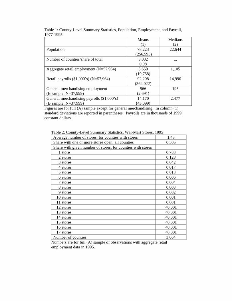
Table 1: County-Level Summary Statistics, Population, Employment, and Payroll, 1977-1995 Means

(1) Medians

(2) Population

78,223 (256,595)

22,644

Number of counties/share of total 3,032 0.98

...

Aggregate retail employment (N=57,964)

5,659 (19,758)

1,105

Retail payrolls ($1,000’s) (N=57,964)

92,208 (364,022)

14,990

General merchandising employment (B sample, N=37,999)

966 (2,691)

195

General merchandising payrolls ($1,000’s) (B sample, N=37,999)

14,170 (43,099)

2,477

Figures are for full (A) sample except for general merchandising. In column (1) standard deviations are reported in parentheses. Payrolls are in thousands of 1999 constant dollars.

Table 2: County-Level Summary Statistics, Wal-Mart Stores, 1995 Average number of stores, for counties with stores 1.43 Share with one or more stores open, all counties 0.505 Share with given number of stores, for counties with stores 1 store 0.783 2 stores 0.128 3 stores 0.042 4 stores 0.017 5 stores 0.013 6 stores 0.006 7 stores 0.004 8 stores 0.003 9 stores 0.002 10 stores 0.001 11 stores 0.001 12 stores <0.001 13 stores <0.001 14 stores <0.001 15 stores <0.001 16 stores <0.001 17 stores <0.001 Number of counties 3,064

Numbers are for full (A) sample of observations with aggregate retail employment data in 1995.

Table 3: Estimated Relationships Between Store Openings and Prior Retail Employment Growth

Openings in:

1983-1985

1988-1990

1993-1995

1993-1995, Excluding CA

and WA (1) (2) (3) (4) Annualized Rate of Growth of Retail Employment in Previous Five-Year Period

0.439***

(0.143)

0.191

(0.177)

0.122

(0.515)

0.407

(0.613)

N 854 615 363 299 Estimates are from linear probability models, with standard errors robust to heteroscedasticity. The states included in each sample are shown in Figure 3. The previous five-year periods corresponding to the three columns are: 1977-1982, 1982-1987, and 1987-1992. County population in the ending year of these five-year periods, and state dummy variables, are included as controls. Growth rates are computed relative to the average at the beginning and end of each period, because there are a handful of observations with retail employment of zero.

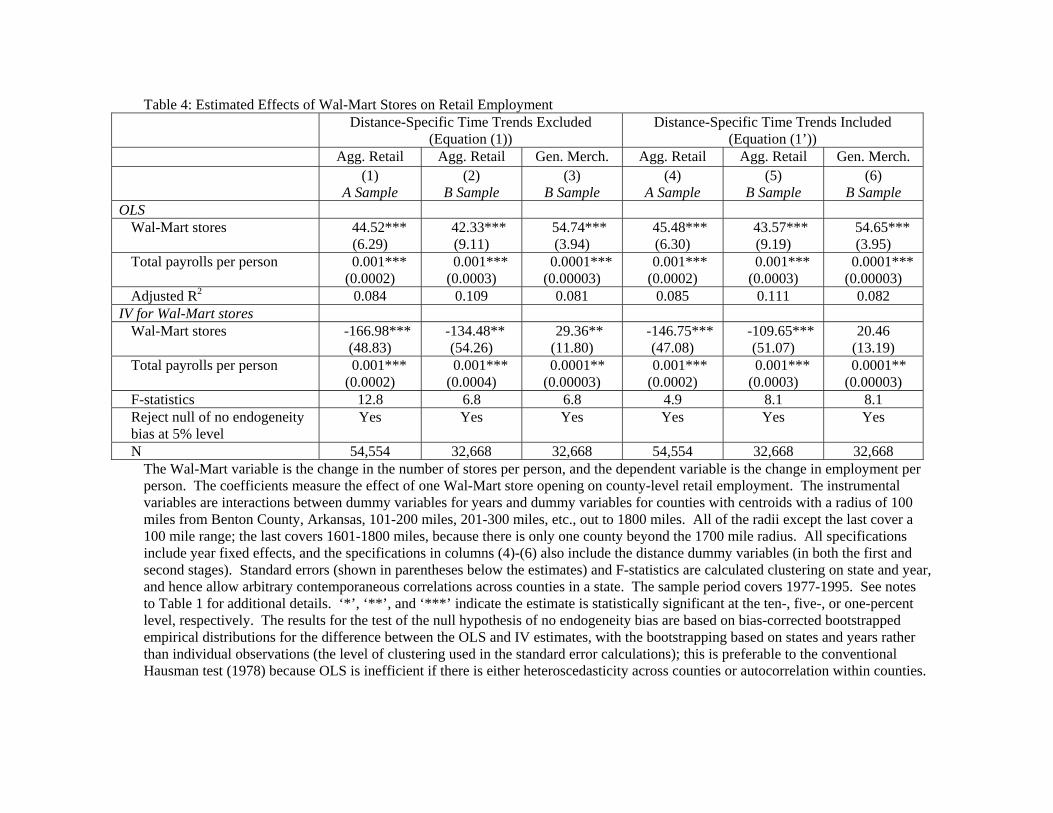
Table 4: Estimated Effects of Wal-Mart Stores on Retail Employment Distance-Specific Time Trends Excluded

(Equation (1)) Distance-Specific Time Trends Included

(Equation (1’)) Agg. Retail Agg. Retail Gen. Merch. Agg. Retail Agg. Retail Gen. Merch.

(1) A Sample

(2) B Sample

(3) B Sample

(4) A Sample

(5) B Sample

(6) B Sample

OLS Wal-Mart stores 44.52***

(6.29) 42.33***

(9.11) 54.74***

(3.94) 45.48***

(6.30) 43.57***

(9.19) 54.65***

(3.95) Total payrolls per person 0.001***

(0.0002) 0.001***

(0.0003) 0.0001***

(0.00003) 0.001***

(0.0002) 0.001***

(0.0003) 0.0001***

(0.00003) Adjusted R2 0.084 0.109 0.081 0.085 0.111 0.082

IV for Wal-Mart stores Wal-Mart stores -166.98***

(48.83) -134.48**

(54.26) 29.36**

(11.80) -146.75***

(47.08) -109.65***

(51.07) 20.46

(13.19) Total payrolls per person

0.001*** (0.0002)

0.001*** (0.0004)

0.0001** (0.00003)

0.001*** (0.0002)

0.001*** (0.0003)

0.0001** (0.00003)

F-statistics 12.8 6.8 6.8 4.9 8.1 8.1Reject null of no endogeneity bias at 5% level

Yes Yes Yes Yes Yes Yes

N 54,554 32,668 32,668 54,554 32,668 32,668The Wal-Mart variable is the change in the number of stores per person, and the dependent variable is the change in employment per person. The coefficients measure the effect of one Wal-Mart store opening on county-level retail employment. The instrumental variables are interactions between dummy variables for years and dummy variables for counties with centroids with a radius of 100 miles from Benton County, Arkansas, 101-200 miles, 201-300 miles, etc., out to 1800 miles. All of the radii except the last cover a 100 mile range; the last covers 1601-1800 miles, because there is only one county beyond the 1700 mile radius. All specifications include year fixed effects, and the specifications in columns (4)-(6) also include the distance dummy variables (in both the first and second stages). Standard errors (shown in parentheses below the estimates) and F-statistics are calculated clustering on state and year, and hence allow arbitrary contemporaneous correlations across counties in a state. The sample period covers 1977-1995. See notes to Table 1 for additional details. ‘*’, ‘**’, and ‘***’ indicate the estimate is statistically significant at the ten-, five-, or one-percent level, respectively. The results for the test of the null hypothesis of no endogeneity bias are based on bias-corrected bootstrapped empirical distributions for the difference between the OLS and IV estimates, with the bootstrapping based on states and years rather than individual observations (the level of clustering used in the standard error calculations); this is preferable to the conventional Hausman test (1978) because OLS is inefficient if there is either heteroscedasticity across counties or autocorrelation within counties.

Table 5: Estimated Effects of Wal-Mart Stores on Retail Payrolls ($1,000’s) Distance-Specific Time Trends Excluded

(Equation (1)) Distance-Specific Time Trends Included

(Equation (1’)) Agg. Retail Agg. Retail Gen. Merch. Agg. Retail Agg. Retail Gen. Merch.

(1) A Sample

(2) B Sample

(3) B Sample

(4) A Sample

(5) B Sample

(6) B Sample

OLS Wal-Mart stores 270.2***

(90.0) 166.4

(145.1) 458.9***

(38.9) 282.2***

(90.7) 182.8 (146.5)

456.4*** (39.0)

Total payrolls per person 0.024*** (0.005)

0.020*** (0.005)

0.001** (0.0003)

0.024*** (0.005)

0.020*** (0.005)

0.001** (0.0003)

Adjusted R2 0.110 0.151 0.067 0.111 0.152 0.068IV for Wal-Mart stores

Wal-Mart stores -1,711.4** (778.1)

-1,669.8* (912.6)

684.3*** (132.2)

-1,219.9* (722.7)

-1,159.8 (826.3)

572.3*** (133.3)

Total payrolls per person

0.023*** (0.005)

0.020*** (0.005)

0.001*** (0.0003)

0.023*** (0.005)

0.020*** (0.005)

0.001** (0.0003)

Reject null of no endogeneity bias at 5% level

Yes Yes Yes Yes No No

N 54,554 32,668 32,668 54,554 32,668 32,668The notes from Table 4 apply. The only difference is that the dependent variable is the change in retail payrolls per person, so the coefficients now measure the effect of one Wal-Mart store opening on county-level retail payrolls (measured in units of thousands of 1999 constant dollars). The F-statistics for the first stage are as reported in Table 4.

Table 6: Estimates of Effects on Retail Employment for Alternative Specifications and Samples Distance-Specific

Time Trends Excluded (Equation (1))

Distance-Specific Time Trends Included

(Equation (1’)) Employment

(1) Employment

(3) 1. Table 4 estimates -166.98***

(48.83) -146.75***

(47.08) 2. Exclude counties within 100 miles of Benton

County (N=53,716) -179.27***

(52.59) -158.82***

(50.52) 3. Exclude counties within 200 miles of Benton

County (N=51,539) -197.59***

(58.22) -176.88***

(56.24) 4. Exclude counties within 300 miles of Benton

County (N=47,321) -207.38***

(64.84) -185.93***

(64.25) 5. Cluster on state only

-166.98*** (55.94)

-146.75*** (47.53)

6. Subtract retail payroll out of total payroll per person control

-174.07*** (45.07)

-153.87*** (41.70)

7. Omit total payroll per person control -181.58*** (46.12)

-162.37*** (42.68)

8. Drop counties that never have a store (N=30,957)

-94.40*** (30.63)

-103.33*** (30.75)

9. Drop counties with closed stores (N=53,746)

-166.68*** (43.15)

-144.46*** (40.10)

10. Through 2002 (N=75,482)

-184.84*** (41.27)

-216.42*** (40.02)

11. Drop counties with Sam’s Clubs (N=49,031)

-150.47*** (43.63)

-131.61*** (40.77)

12. Combine Wal-Mart stores with Sam’s Clubs -161.44*** (42.72)

-143.51*** (39.77)

13. Weighted by store size

-216.12*** (59.53)

-76.90*** (27.84)

14. Counties with above median population (21,000) in 1977 (N=27,290)

-81.13 (57.58)

-104.48* (54.81)

15. Counties with below median population (21,000) in 1977 (N=27,264)

-103.28* (53.48)

-90.95 (55.31)

16. Instrument with linear distance × year dummy variables

[first-stage F-statistic]

-307.82*** (77.18) [12.4]

-338.0*** (78.42)

[7.6] 17. Two-year differences (N=51,429)

-196.48*** (34.73)

-192.96*** (35.21)

18. Three-year differences (N=48,362)

-206.03*** (35.81)

-211.68*** (34.71)

Table reports IV estimates of coefficient on change in number of Wal-Mart stores per person. See notes to Tables 1 and 4. All estimates are for A sample. Sample sizes are the same as in Table 4 unless otherwise noted. Estimated coefficients of total payroll per person variable, where included, are not shown. For the estimates labeled “weighted by store size,” stores are weighted by their square footage (at the end of the sample period) divided by the average square footage for the sample, to maintain comparability with the baseline estimates. The specifications using two- and three-year differences use dummy variables for the distinct two- or three-year periods over which the differences are computed, rather than dummy variables for single years. That way, the same dummy variables appear in the first-differenced and levels regressions.