SimpleMKL - MIT Computer Science and Artificial...

Journal of Machine Learning Research 9 (2008) 2491-2521 Submitted 1/08; Revised 8/08; Published 11/08

SimpleMKL

Alain Rakotomamonjy [email protected]

LITIS EA 4108Universite de Rouen76800 Saint Etienne du Rouvray, France

Francis R. Bach [email protected]

INRIA - WILLOW Project - TeamLaboratoire d’Informatique de l’Ecole Normale Superieure(CNRS/ENS/INRIA UMR 8548)45, Rue d’Ulm, 75230 Paris, France

Stephane Canu [email protected]

LITIS EA 4108INSA de Rouen76801 Saint Etienne du Rouvray, France

Yves Grandvalet [email protected]

Idiap Research Institute, Centre du Parc1920 Martigny, Switzerland∗

Editor: Nello Cristianini

Abstract

Multiple kernel learning (MKL) aims at simultaneously learning a kernel and the associated predic-tor in supervised learning settings. For the support vector machine, an efficient and general multiplekernel learning algorithm, based on semi-infinite linear programming, has been recently proposed.This approach has opened new perspectives since it makes MKL tractable for large-scale problems,by iteratively using existing support vector machine code. However, it turns out that this iterativealgorithm needs numerous iterations for converging towards a reasonable solution. In this paper,we address the MKL problem through a weighted 2-norm regularization formulation with an addi-tional constraint on the weights that encourages sparse kernel combinations. Apart from learningthe combination, we solve a standard SVM optimization problem, where the kernel is defined as alinear combination of multiple kernels. We propose an algorithm, named SimpleMKL, for solvingthis MKL problem and provide a new insight on MKL algorithms based on mixed-norm regular-ization by showing that the two approaches are equivalent. We show how SimpleMKL can beapplied beyond binary classification, for problems like regression, clustering (one-class classifica-tion) or multiclass classification. Experimental results show that the proposed algorithm convergesrapidly and that its efficiency compares favorably to other MKL algorithms. Finally, we illustratethe usefulness of MKL for some regressors based on wavelet kernels and on some model selectionproblems related to multiclass classification problems.

Keywords: multiple kernel learning, support vector machines, support vector regression, multi-class SVM, gradient descent

∗. Also at Heudiasyc, CNRS/Universite de Technologie de Compiegne (UMR 6599), 60205 Compiegne, France.

c©2008 Alain Rakotomamonjy, Francis R. Bach, Stephane Canu and Yves Grandvalet.

RAKOTOMAMONJY, BACH, CANU AND GRANDVALET

1. Introduction

During the last few years, kernel methods, such as support vector machines (SVM) have provedto be efficient tools for solving learning problems like classification or regression (Scholkopf andSmola, 2001). For such tasks, the performance of the learning algorithm strongly depends on thedata representation. In kernel methods, the data representation is implicitly chosen through the so-called kernel K(x,x′). This kernel actually plays two roles: it defines the similarity between twoexamples x and x′, while defining an appropriate regularization term for the learning problem.

Let {xi,yi}`i=1 be the learning set, where xi belongs to some input space X and yi is the target

value for pattern xi. For kernel algorithms, the solution of the learning problem is of the form

f (x) =`

∑i=1

α?i K(x,xi)+b?, (1)

where α?i and b? are some coefficients to be learned from examples, while K(·, ·) is a given positive

definite kernel associated with a reproducing kernel Hilbert space (RKHS) H .In some situations, a machine learning practitioner may be interested in more flexible models.

Recent applications have shown that using multiple kernels instead of a single one can enhance theinterpretability of the decision function and improve performances (Lanckriet et al., 2004a). In suchcases, a convenient approach is to consider that the kernel K(x,x′) is actually a convex combinationof basis kernels:

K(x,x′) =M

∑m=1

dmKm(x,x′) , with dm ≥ 0 ,M

∑m=1

dm = 1 ,

where M is the total number of kernels. Each basis kernel Km may either use the full set of variablesdescribing x or subsets of variables stemming from different data sources (Lanckriet et al., 2004a).Alternatively, the kernels Km can simply be classical kernels (such as Gaussian kernels) with dif-ferent parameters. Within this framework, the problem of data representation through the kernel isthen transferred to the choice of weights dm.

Learning both the coefficients αi and the weights dm in a single optimization problem is knownas the multiple kernel learning (MKL) problem. For binary classification, the MKL problem hasbeen introduced by Lanckriet et al. (2004b), resulting in a quadratically constrained quadratic pro-gramming problem that becomes rapidly intractable as the number of learning examples or kernelsbecome large.

What makes this problem difficult is that it is actually a convex but non-smooth minimizationproblem. Indeed, Bach et al. (2004a) have shown that the MKL formulation of Lanckriet et al.(2004b) is actually the dual of a SVM problem in which the weight vector has been regularizedaccording to a mixed (`2, `1)-norm instead of the classical squared `2-norm. Bach et al. (2004a)have considered a smoothed version of the problem for which they proposed a SMO-like algorithmthat enables to tackle medium-scale problems.

Sonnenburg et al. (2006) reformulate the MKL problem of Lanckriet et al. (2004b) as a semi-infinite linear program (SILP). The advantage of the latter formulation is that the algorithm ad-dresses the problem by iteratively solving a classical SVM problem with a single kernel, for whichmany efficient toolboxes exist (Vishwanathan et al., 2003; Loosli et al., 2005; Chang and Lin, 2001),and a linear program whose number of constraints increases along with iterations. A very nice fea-ture of this algorithm is that is can be extended to a large class of convex loss functions. For instance,Zien and Ong (2007) have proposed a multiclass MKL algorithm based on similar ideas.

2492

SIMPLEMKL

In this paper, we present another formulation of the multiple learning problem. We first departfrom the primal formulation proposed by Bach et al. (2004a) and further used by Bach et al. (2004b)and Sonnenburg et al. (2006). Indeed, we replace the mixed-norm regularization by a weighted`2-norm regularization, where the sparsity of the linear combination of kernels is controlled by a `1-norm constraint on the kernel weights. This new formulation of MKL leads to a smooth and convexoptimization problem. By using a variational formulation of the mixed-norm regularization, weshow that our formulation is equivalent to the ones of Lanckriet et al. (2004b), Bach et al. (2004a)and Sonnenburg et al. (2006).

The main contribution of this paper is to propose an efficient algorithm, named SimpleMKL,for solving the MKL problem, through a primal formulation involving a weighted `2-norm regu-larization. Indeed, our algorithm is simple, essentially based on a gradient descent on the SVMobjective value. We iteratively determine the combination of kernels by a gradient descent wrap-ping a standard SVM solver, which is SimpleSVM in our case. Our scheme is similar to the oneof Sonnenburg et al. (2006), and both algorithms minimize the same objective function. However,they differ in that we use reduced gradient descent in the primal, whereas Sonnenburg et al.’s SILPrelies on cutting planes. We will empirically show that our optimization strategy is more efficient,with new evidences confirming the preliminary results reported in Rakotomamonjy et al. (2007).

Then, extensions of SimpleMKL to other supervised learning problems such as regression SVM,one-class SVM or multiclass SVM problems based on pairwise coupling are proposed. Althoughit is not the main purpose of the paper, we will also discuss the applicability of our approach togeneral convex loss functions.

This paper also presents several illustrations of the usefulness of our algorithm. For instance,in addition to the empirical efficiency comparison, we also show, in a SVM regression probleminvolving wavelet kernels, that automatic learning of the kernels leads to far better performances.Then we depict how our MKL algorithm behaves on some multiclass problems.

The paper is organized as follows. Section 2 presents the functional settings of our MKL prob-lem and its formulation. Details on the algorithm and discussion of convergence and computationalcomplexity are given in Section 3. Extensions of our algorithm to other SVM problems are discussedin Section 4 while experimental results dealing with computational complexity or with comparisonwith other model selection methods are presented in Section 5.

A SimpleMKL toolbox based on Matlab code is available at http://www.mloss.org. Thistoolbox is an extension of our SVM-KM toolbox (Canu et al., 2003).

2. Multiple Kernel Learning Framework

In this section, we present our MKL formulation and derive its dual. In the sequel, i and j areindices on examples, whereas m is the kernel index. In order to lighten notations, we omit to specifythat summations on i and j go from 1 to `, and that summations on m go from 1 to M.

2.1 Functional Framework

Before entering into the details of the MKL optimization problem, we first present the functionalframework adopted for multiple kernel learning. Assume Km,m = 1, ...,M are M positive definitekernels on the same input space X , each of them being associated with an RKHS Hm endowed withan inner product 〈·, ·〉m. For any m, let dm be a non-negative coefficient and H ′

m be the Hilbert space

2493


derived from Hm as follows:

H ′m = { f | f ∈Hm :

‖ f‖Hm

dm< ∞} ,

endowed with the inner product

〈 f ,g〉H ′m =1

dm〈 f ,g〉m .

In this paper, we use the convention that x0 = 0 if x = 0 and ∞ otherwise. This means that, if dm = 0

then a function f belongs to the Hilbert space H ′m only if f = 0∈Hm. In such a case, H ′

m is restrictedto the null element of Hm.

Within this framework, H ′m is a RKHS with kernel K(x,x′) = dm Km(x,x′) since

∀ f ∈H ′m ⊆Hm , f (x) = 〈 f (·),Km(x, ·)〉m

=1

dm〈 f (·),dmKm(x, ·)〉m

= 〈 f (·),dmKm(x, ·)〉H ′m .

Now, if we define H as the direct sum of the spaces H ′m, that is,

H =M

M

m=1

H ′m ,

then, a classical result on RKHS (Aronszajn, 1950) says that H is a RKHS of kernel

K(x,x′) =M

∑m=1

dmKm(x,x′) .

Owing to this simple construction, we have built a RKHS H for which any function is a sumof functions belonging to Hm. In our framework, MKL aims at determining the set of coefficients{dm} within the learning process of the decision function. The multiple kernel learning problemcan thus be envisioned as learning a predictor belonging to an adaptive hypothesis space endowedwith an adaptive inner product. The forthcoming sections explain how we solve this problem.

2.2 Multiple Kernel Learning Primal Problem

In the SVM methodology, the decision function is of the form given in Equation (1), wherethe optimal parameters α?

i and b? are obtained by solving the dual of the following optimizationproblem:

minf ,b,ξ

12‖ f‖2

H +C∑i

ξi

s.t. yi( f (xi)+b)≥ 1−ξi ∀iξi ≥ 0 ∀i .

In the MKL framework, one looks for a decision function of the form f (x)+b = ∑m fm(x)+b,where each function fm belongs to a different RKHS Hm associated with a kernel Km. Accordingto the above functional framework and inspired by the multiple smoothing splines framework of

2494

SIMPLEMKL

Wahba (1990, chap. 10), we propose to address the MKL SVM problem by solving the followingconvex problem (see proof in appendix), which we will be referred to as the primal MKL problem:

min{ fm},b,ξ,d

12 ∑

m

1dm‖ fm‖

2Hm

+C∑i

ξi

s.t. yi ∑m

fm(xi)+ yib≥ 1−ξi ∀i

ξi ≥ 0 ∀i

∑m

dm = 1 , dm ≥ 0 ∀m ,

(2)

where each dm controls the squared norm of fm in the objective function.The smaller dm is, the smoother fm (as measured by ‖ fm‖Hm

) should be. When dm = 0, ‖ fm‖Hm

has also to be equal to zero to yield a finite objective value. The `1-norm constraint on the vectord is a sparsity constraint that will force some dm to be zero, thus encouraging sparse basis kernelexpansions.

2.3 Connections With mixed-norm Regularization Formulation of MKL

The MKL formulation introduced by Bach et al. (2004a) and further developed by Sonnenburget al. (2006) consists in solving an optimization problem expressed in a functional form as

min{ f},b,ξ

12

(

∑m‖ fm‖Hm

)2

+C∑i

ξi

s.t. yi ∑m

fm(xi)+ yib≥ 1−ξi ∀i

ξi ≥ 0 ∀i.

(3)

Note that the objective function of this problem is not smooth since ‖ fm‖Hmis not differentiable at

fm = 0. However, what makes this formulation interesting is that the mixed-norm penalization off = ∑m fm is a soft-thresholding penalizer that leads to a sparse solution, for which the algorithmperforms kernel selection (Bach, 2008). We have stated in the previous section that our problemshould also lead to sparse solutions. In the following, we show that the formulations (2) and (3) areequivalent.

For this purpose, we simply show that the variational formulation of the mixed-norm regular-ization is equal to the weighted 2-norm regularization, (which is a particular case of a more generalequivalence proposed by Micchelli and Pontil 2005), that is, by Cauchy-Schwartz inequality, forany vector d on the simplex:

(

∑m‖ fm‖Hm

)2

=

(

∑m

‖ fm‖Hm

d1/2m

d1/2m

)2

6

(

∑m

‖ fm‖2Hm

dm

)

(

∑m

dm

)

6 ∑m

‖ fm‖2Hm

dm,

2495


where equality is met when d1/2m is proportional to ‖ fm‖Hm

/d1/2m , that is:

dm =‖ fm‖Hm

∑q‖ fq‖Hq

,

which leads to

mindm≥0,∑m dm=1

∑m

‖ fm‖2Hm

dm=

(

∑m‖ fm‖Hm

)2

.

Hence, owing to this variational formulation, the non-smooth mixed-norm objective function ofproblem (3) has been turned into a smooth objective function in problem (2). Although the numberof variables has increased, we will see that this problem can be solved more efficiently.

2.4 The MKL Dual Problem

The dual problem is a key point for deriving MKL algorithms and for studying their convergenceproperties. Since our primal problem (2) is equivalent to the one of Bach et al. (2004a), they leadto the same dual. However, our primal formulation being convex and differentiable, it provides asimple derivation of the dual, that does not use conic duality.

The Lagrangian of problem (2) is

L =12 ∑

m

1dm‖ fm‖

2Hm

+C∑i

ξi +∑i

αi

(

1−ξi− yi ∑m

fm(xi)− yib

)

−∑i

νiξi

+λ(

∑m

dm−1

)

−∑m

ηmdm , (4)

where αi and νi are the Lagrange multipliers of the constraints related to the usual SVM problem,whereas λ and ηm are associated to the constraints on dm. When setting to zero the gradient of theLagrangian with respect to the primal variables, we get the following

(a)1

dmfm(·) = ∑

i

αiyiKm(·,xi) , ∀m,

(b) ∑i

αiyi = 0,

(c) C−αi−νi = 0 , ∀i,

(d) −12

‖ fm‖2Hm

d2m

+λ−ηm = 0 , ∀m .

(5)

We note again here that fm(·) has to go to 0 if the coefficient dm vanishes. Plugging these optimalityconditions in the Lagrangian gives the dual problem

maxαi,λ

∑i

αi−λ

s.t. ∑i

αiyi = 0

0≤ αi ≤C ∀i12 ∑

i, j

αiα jyiy jKm(xi,x j)≤ λ , ∀m .

(6)

2496

SIMPLEMKL

This dual problem1 is difficult to optimize due to the last constraint. This constraint may bemoved to the objective function, but then, the latter becomes non-differentiable causing new diffi-culties (Bach et al., 2004a). Hence, in the forthcoming section, we propose an approach based onthe minimization of the primal. In this framework, we benefit from differentiability which allowsfor an efficient derivation of an approximate primal solution, whose accuracy will be monitored bythe duality gap.

3. Algorithm for Solving the MKL Primal Problem

One possible approach for solving problem (2) is to use the alternate optimization algorithmapplied by Grandvalet and Canu (1999, 2003) in another context. In the first step, problem (2) isoptimized with respect to fm, b and ξ, with d fixed. Then, in the second step, the weight vectord is updated to decrease the objective function of problem (2), with fm, b and ξ being fixed. InSection 2.3, we showed that the second step can be carried out in closed form. However, thisapproach lacks convergence guarantees and may lead to numerical problems, in particular whensome elements of d approach zero (Grandvalet, 1998). Note that these numerical problems can behandled by introducing a perturbed version of the alternate algorithm as shown by Argyriou et al.(2008).

Instead of using an alternate optimization algorithm, we prefer to consider here the followingconstrained optimization problem:

mind

J(d) such thatM

∑m=1

dm = 1, dm ≥ 0 , (7)

where

J(d) =

min{ f},b,ξ

12 ∑

m

1dm‖ fm‖

2Hm

+C∑i

ξi ∀i

s.t. yi ∑m

fm(xi)+ yib≥ 1−ξi

ξi ≥ 0 ∀i .

(8)

We show below how to solve problem (7) on the simplex by a simple gradient method. We willfirst note that the objective function J(d) is actually an optimal SVM objective value. We will thendiscuss the existence and computation of the gradient of J(·), which is at the core of the proposedapproach.

3.1 Computing the Optimal SVM Value and its Derivatives

The Lagrangian of problem (8) is identical to the first line of Equation (4). By setting to zerothe derivatives of this Lagrangian according to the primal variables, we get conditions (5) (a) to (c),from which we derive the associated dual problem

maxα

−12 ∑

i, j

αiα jyiy j ∑m

dmKm(xi,x j)+∑i

αi

with ∑i

αiyi = 0

C ≥ αi ≥ 0 ∀i ,

(9)

1. Note that Bach et al. (2004a) formulation differs slightly, in that the kernels are weighted by some pre-definedcoefficients that were not considered here.

2497


which is identified as the standard SVM dual formulation using the combined kernel K(xi,x j) =

∑m dmKm(xi,x j). Function J(d) is defined as the optimal objective value of problem (8). Because ofstrong duality, J(d) is also the objective value of the dual problem:

J(d) =−12 ∑

i, j

α?i α?

jyiy j ∑m

dmKm(xi,x j)+∑i

α?i , (10)

where α? maximizes (9). Note that the objective value J(d) can be obtained by any SVM algorithm.Our method can thus take advantage of any progress in single kernel algorithms. In particular, if theSVM algorithm we use is able to handle large-scale problems, so will our MKL algorithm. Thus,the overall complexity of SimpleMKL is tied to the one of the single kernel SVM algorithm.

From now on, we assume that each Gram matrix (Km(xi,x j))i, j is positive definite, with alleigenvalues greater than some η > 0 (to enforce this property, a small ridge may be added to thediagonal of the Gram matrices). This implies that, for any admissible value of d, the dual problemis strictly concave with convexity parameter η (Lemarechal and Sagastizabal, 1997). In turn, thisstrict concavity property ensures that α? is unique, a characteristic that eases the analysis of thedifferentiability of J(·).

Existence and computation of derivatives of optimal value functions such as J(·) have beenlargely discussed in the literature. For our purpose, the appropriate reference is Theorem 4.1 inBonnans and Shapiro (1998), which has already been applied by Chapelle et al. (2002) for tuningsquared-hinge loss SVM. This theorem is reproduced in the appendix for self-containedness. Ina nutshell, it says that differentiability of J(d) is ensured by the uniqueness of α?, and by thedifferentiability of the objective function that gives J(d). Furthermore, the derivatives of J(d) canbe computed as if α? were not to depend on d. Thus, by simple differentiation of the dual function(9) with respect to dm, we have:

∂J∂dm

=−12 ∑

i, j

α?i α?

jyiy jKm(xi,x j) ∀m . (11)

We will see in the sequel that the applicability of this theorem can be extended to other SVMproblems. Note that complexity of the gradient computation is of the order of m · n2

SV , with nSV

being the number of support vectors for the current d.

3.2 Reduced Gradient Algorithm

The optimization problem we have to deal with in (7) is a non-linear objective function withconstraints over the simplex. With our positivity assumption on the kernel matrices, J(·) is convexand differentiable with Lipschitz gradient (Lemarechal and Sagastizabal, 1997). The approach weuse for solving this problem is a reduced gradient method, which converges for such functions(Luenberger, 1984).

Once the gradient of J(d) is computed, d is updated by using a descent direction ensuring thatthe equality constraint and the non-negativity constraints on d are satisfied. We handle the equalityconstraint by computing the reduced gradient (Luenberger, 1984, Chap. 11). Let dµ be a non-zeroentry of d, the reduced gradient of J(d), denoted ∇redJ, has components:

[∇redJ]m =∂J

∂dm−

∂J∂dµ

∀m 6= µ , and [∇redJ]µ = ∑m6=µ

(

∂J∂dµ−

∂J∂dm

)

.

2498

SIMPLEMKL

We chose µ to be the index of the largest component of vector d, for better numerical stability(Bonnans, 2006).

The positivity constraints have also to be taken into account in the descent direction. Since wewant to minimize J(·), −∇redJ is a descent direction. However, if there is an index m such thatdm = 0 and [∇redJ]m > 0, using this direction would violate the positivity constraint for dm. Hence,the descent direction for that component is set to 0. This gives the descent direction for updating das

Dm =

0 if dm = 0 and ∂J∂dm− ∂J

∂dµ> 0

−∂J

∂dm+

∂J∂dµ

if dm > 0 and m 6= µ

∑g6=µ,dν>0

(

∂J∂dν−

∂J∂dµ

)

for m = µ .

(12)

The usual updating scheme is d ← d + γD , where γ is the step size. Here, as detailed inAlgorithm 1, we go one step beyond: once a descent direction D has been computed, we firstlook for the maximal admissible step size in that direction and check whether the objective valuedecreases or not. The maximal admissible step size corresponds to a component, say dν, set to zero.If the objective value decreases, d is updated, we set Dν = 0 and normalize D to comply with theequality constraint. This procedure is repeated until the objective value stops decreasing. At thispoint, we look for the optimal step size γ, which is determined by using a one-dimensional linesearch, with proper stopping criterion, such as Armijo’s rule, to ensure global convergence.

In this algorithm, computing the descent direction and the line search are based on the evaluationof the objective function J(·), which requires solving an SVM problem. This may seem very costlybut, for small variations of d, learning is very fast when the SVM solver is initialized with theprevious values of α? (DeCoste and Wagstaff., 2000). Note that the gradient of the cost functionis not computed after each update of the weight vector d. Instead, we take advantage of an easilyupdated descent direction as long as the objective value decreases. We will see in the numericalexperiments that this approach saves a substantial amount of computation time compared to theusual update scheme where the descent direction is recomputed after each update of d. Note that wehave also investigated gradient projection algorithms (Bertsekas, 1999, Chap 2.3), but this turnedout to be slightly less efficient than the proposed approach, and we will not report these results.

The algorithm is terminated when a stopping criterion is met. This stopping criterion can beeither based on the duality gap, the KKT conditions, the variation of d between two consecutivesteps or, even more simply, on a maximal number of iterations. Our implementation, based on theduality gap, is detailed in the forthcoming section.

3.3 Optimality Conditions

In a convex constrained optimization algorithm such as the one we are considering, we have theopportunity to check for proper optimality conditions such as the KKT conditions or the duality gap(the difference between primal and dual objective values), which should be zero at the optimum.From the primal and dual objectives provided respectively in (2) and (6), the MKL duality gap is

DualGap = J(d?)−∑i

α?i +

12

maxm ∑

i, j

α?i α?

jyiy jKm(xi,x j) ,

2499


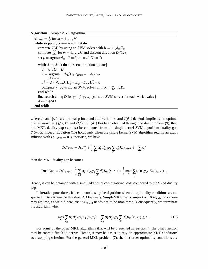
Algorithm 1 SimpleMKL algorithm

set dm = 1M for m = 1, . . . ,M

while stopping criterion not met docompute J(d) by using an SVM solver with K = ∑m dmKm

compute ∂J∂dm

for m = 1, . . . ,M and descent direction D (12).

set µ = argmaxm

dm, J† = 0, d† = d, D† = D

while J† < J(d) do {descent direction update}d = d†, D = D†

ν = argmin{m|Dm<0}

−dm/Dm, γmax =−dν/Dν

d† = d + γmaxD, D†µ = Dµ−Dν, D†

ν = 0compute J† by using an SVM solver with K = ∑m d†

mKm

end whileline search along D for γ ∈ [0,γmax] {calls an SVM solver for each γ trial value}d← d + γD

end while

where d? and {α?i } are optimal primal and dual variables, and J(d?) depends implicitly on optimal

primal variables { f ?m}, b? and {ξ?

i }. If J(d?) has been obtained through the dual problem (9), thenthis MKL duality gap can also be computed from the single kernel SVM algorithm duality gapDGSVM. Indeed, Equation (10) holds only when the single kernel SVM algorithm returns an exactsolution with DGSVM = 0. Otherwise, we have

DGSVM = J(d?)+12 ∑

i, j

α?i α?

jyiy j ∑m

d?mKm(xi,x j)−∑

i

α?i

then the MKL duality gap becomes

DualGap = DGSVM−12 ∑

i, j

α?i α?

jyiy j ∑m

d?mKm(xi,x j)+

12

maxm ∑

i, j

α?i α?

jyiy jKm(xi,x j) .

Hence, it can be obtained with a small additional computational cost compared to the SVM dualitygap.

In iterative procedures, it is common to stop the algorithm when the optimality conditions are re-spected up to a tolerance threshold ε. Obviously, SimpleMKL has no impact on DGSVM, hence, onemay assume, as we did here, that DGSVM needs not to be monitored. Consequently, we terminatethe algorithm when

maxm ∑

i, j

α?i α?

jyiy jKm(xi,x j)−∑i, j

α?i α?

jyiy j ∑m

d?mKm(xi,x j)≤ ε . (13)

For some of the other MKL algorithms that will be presented in Section 4, the dual functionmay be more difficult to derive. Hence, it may be easier to rely on approximate KKT conditionsas a stopping criterion. For the general MKL problem (7), the first order optimality conditions are

2500

SIMPLEMKL

obtained through the KKT conditions:

∂J∂dm

+λ−ηm = 0 ∀m ,

ηm ·dm = 0 ∀m ,

where λ and {ηm} are respectively the Lagrange multipliers for the equality and inequality con-straints of (7). These KKT conditions imply

∂J∂dm

= −λ if dm > 0 ,

∂J∂dm

≥ −λ if dm = 0 .

However, as Algorithm 1 is not based on the Lagrangian formulation of problem (7), λ is notcomputed. Hence, we derive approximate necessary optimality conditions to be used for terminationcriterion. Let’s define dJmin and dJmax as

dJmin = min{dm|dm>0}

∂J∂dm

and dJmax = max{dm|dm>0}

∂J∂dm

,

then, the necessary optimality conditions are approximated by the following termination conditions:

|dJmin−dJmax| ≤ ε and∂J

∂dm≥ dJmax if dm = 0 .

In other words, we are considered at the optimum when the gradient components for all positive dm

lie in a ε-tube and when all gradient components for vanishing dm are outside this tube. Note thatthese approximate necessary optimality conditions are available right away for any differentiableobjective function J(d).

3.4 Cutting Planes, Steepest Descent and Computational Complexity

As we stated in the introduction, several algorithms have been proposed for solving the originalMKL problem defined by Lanckriet et al. (2004b). All these algorithms are based on equivalentformulations of the same dual problem; they all aim at providing a pair of optimal vectors (d,α).

In this subsection, we contrast SimpleMKL with its closest relative, the SILP algorithm ofSonnenburg et al. (2005, 2006). Indeed, from an implementation point of view, the two algorithmsare alike, since they are wrapping a standard single kernel SVM algorithm. This feature makes bothalgorithms very easy to implement. They, however, differ in computational efficiency, because thekernel weights dm are optimized in quite different ways, as detailed below.

Let us first recall that our differentiable function J(d) is defined as:

J(d) =

maxα

−12 ∑

i, j

αiα jyiy j ∑m

dmKm(xi,x j)+∑i

αi

with ∑i

αiyi = 0, C ≥ αi ≥ 0 ∀i ,

and both algorithms aim at minimizing this differentiable function. However, using a SILP approachin this case, does not take advantage of the smoothness of the objective function.

2501


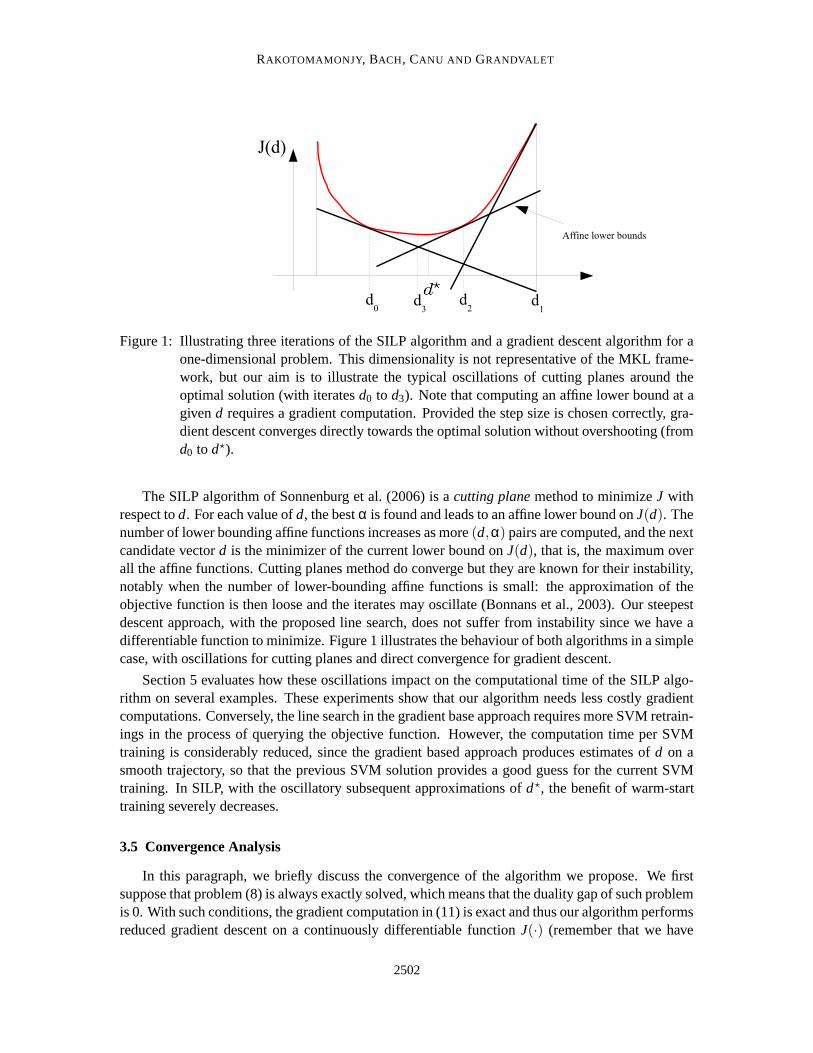
Figure 1: Illustrating three iterations of the SILP algorithm and a gradient descent algorithm for aone-dimensional problem. This dimensionality is not representative of the MKL frame-work, but our aim is to illustrate the typical oscillations of cutting planes around theoptimal solution (with iterates d0 to d3). Note that computing an affine lower bound at agiven d requires a gradient computation. Provided the step size is chosen correctly, gra-dient descent converges directly towards the optimal solution without overshooting (fromd0 to d?).

The SILP algorithm of Sonnenburg et al. (2006) is a cutting plane method to minimize J withrespect to d. For each value of d, the best α is found and leads to an affine lower bound on J(d). Thenumber of lower bounding affine functions increases as more (d,α) pairs are computed, and the nextcandidate vector d is the minimizer of the current lower bound on J(d), that is, the maximum overall the affine functions. Cutting planes method do converge but they are known for their instability,notably when the number of lower-bounding affine functions is small: the approximation of theobjective function is then loose and the iterates may oscillate (Bonnans et al., 2003). Our steepestdescent approach, with the proposed line search, does not suffer from instability since we have adifferentiable function to minimize. Figure 1 illustrates the behaviour of both algorithms in a simplecase, with oscillations for cutting planes and direct convergence for gradient descent.

Section 5 evaluates how these oscillations impact on the computational time of the SILP algo-rithm on several examples. These experiments show that our algorithm needs less costly gradientcomputations. Conversely, the line search in the gradient base approach requires more SVM retrain-ings in the process of querying the objective function. However, the computation time per SVMtraining is considerably reduced, since the gradient based approach produces estimates of d on asmooth trajectory, so that the previous SVM solution provides a good guess for the current SVMtraining. In SILP, with the oscillatory subsequent approximations of d?, the benefit of warm-starttraining severely decreases.

3.5 Convergence Analysis

In this paragraph, we briefly discuss the convergence of the algorithm we propose. We firstsuppose that problem (8) is always exactly solved, which means that the duality gap of such problemis 0. With such conditions, the gradient computation in (11) is exact and thus our algorithm performsreduced gradient descent on a continuously differentiable function J(·) (remember that we have

2502

SIMPLEMKL

assumed that the kernel matrices are positive definite) defined on the simplex {d|∑m dm = 1,dm ≥0}, which does converge to the global minimum of J (Luenberger, 1984).

However, in practice, problem (8) is not solved exactly since most SVM algorithms will stopwhen the duality gap is smaller than a given ε. In this case, the convergence of our reduced gradientmethod is no more guaranteed by standard arguments. Indeed, the output of the approximatelysolved SVM leads only to an ε-subgradient (Bonnans et al., 2003; Bach et al., 2004a). This situationis more difficult to analyze and we plan to address it thoroughly in future work (see for instanceD’Aspremont 2008 for an example of such analysis in a similar context).

4. Extensions

In this section, we discuss how the proposed algorithm can be simply extended to other SVMalgorithms such as SVM regression, one-class SVM or pairwise multiclass SVM algorithms. Moregenerally, we will discuss other loss functions that can be used within our MKL algorithms.

4.1 Extensions to Other SVM Algorithms

The algorithm we described in the previous section focuses on binary classification SVMs, butit is worth noting that our MKL algorithm can be extended to other SVM algorithms with onlylittle changes. For SVM regression with the ε-insensitive loss, or clustering with the one-class softmargin loss, the problem only changes in the definition of the objective function J(d) in (8).

For SVM regression (Vapnik et al., 1997; Scholkopf and Smola, 2001), we have

J(d) =

minfm,b,ξi

12 ∑

m

1dm‖ fm‖

2Hm

+C∑i

(ξi +ξ∗i )

s.t. yi−∑m

fm(xi)−b≤ ε+ξi ∀i

∑m

fm(xi)+b− yi ≤ ε+ξ∗i ∀i

ξi ≥ 0,ξ∗i ≤ 0 ∀i ,

(14)

and for one-class SVMs (Scholkopf and Smola, 2001), we have:

J(d) =

minfm,b,ξi

12 ∑

m

1dm‖ fm‖

2Hm

+1ν` ∑

i

ξi−b

s.t. ∑m

fm(xi)≥ b−ξi

ξi ≥ 0 .

Again, J(d) can be defined according to the dual functions of these two optimization problems,which are respectively

J(d) =

maxα,β

∑i

(βi−αi)yi− ε∑i

(βi +αi)−12 ∑

i, j

(βi−αi)(β j−α j)∑m

dmKm(xi,x j)

with ∑i

(βi−αi) = 0

0≤ αi , βi ≤C, ∀i ,

2503


and

J(d) =

maxα

−12 ∑

i, j

αiα j ∑m

dmKm(xi,x j)

with 0≤ αi ≤1ν`

∀i

∑i

αi = 1 ,

where {αi} and {βi} are Lagrange multipliers.Then, as long as J(d) is differentiable, a property strictly related to the strict concavity of its

dual function, our descent algorithm can still be applied. The main effort for the extension ofour algorithm is the evaluation of J(d) and the computation of its derivatives. Like for binaryclassification SVM, J(d) can be computed by means of efficient off-the-shelf SVM solvers and thegradient of J(d) is easily obtained through the dual problems. For SVM regression, we have:

∂J∂dm

=−12 ∑

i, j

(β?i −α?

i )(β?j −α?

j)Km(xi,x j) ∀m ,

and for one-class SVM, we have:

∂J∂dm

=−12 ∑

i, j

α?i α?

jKm(xi,x j) ∀m ,

where α?i and β?

i are the optimal values of the Lagrange multipliers. These examples illustrate thatextending SimpleMKL to other SVM problems is rather straightforward. This observation is validfor other SVM algorithms (based for instance on the ν parameter, a squared hinge loss or squared-εtube) that we do not detail here. Again, our algorithm can be used provided J(d) is differentiable,by plugging in the algorithm the function that evaluates the objective value J(d) and its gradient.Of course, the duality gap may be considered as a stopping criterion if it can be computed.

4.2 Multiclass Multiple Kernel Learning

With SVMs, multiclass problems are customarily solved by combining several binary classi-fiers. The well-known one-against-all and one-against-one approaches are the two most commonways for building a multiclass decision function based on pairwise decision functions. MulticlassSVM may also be defined right away as the solution of a global optimization problem (Weston andWatkins, 1999; Crammer and Singer, 2001), that may also be addressed with structured-output SVM(Tsochantaridis et al., 2005). Very recently, an MKL algorithm based on structured-output SVM hasbeen proposed by Zien and Ong (2007). This work extends the work of Sonnenburg et al. (2006) tomulticlass problems, with an MKL implementation still based on a QCQP or SILP approach.

Several works have compared the performance of multiclass SVM algorithms (Duan and Keerthi,2005; Hsu and Lin, 2002; Rifkin and Klautau, 2004). In this subsection, we do not deal with thisaspect; we explain how SimpleMKL can be extended to pairwise SVM multiclass implementations.The problem of applying our algorithm to structured-output SVM will be briefly discussed later.

Suppose we have a multiclass problem with P classes. For a one-against-all multiclass SVM,we need to train P binary SVM classifiers, where the p-th classifier is trained by considering allexamples of class p as positive examples while all other examples are considered negative. Fora one-against-one multiclass problem, P(P− 1)/2 binary SVM classifiers are built from all pairs

2504

SIMPLEMKL

of distinct classes. Our multiclass MKL extension of SimpleMKL differs from the binary versiononly in the definition of a new cost function J(d). As we now look for the combination of kernelsthat jointly optimizes all the pairwise decision functions, the objective function we want to optimizeaccording to the kernel weights {dm} is:

J(d) = ∑p∈P

Jp(d) ,

where P is the set of all pairs to be considered, and Jp(d) is the binary SVM objective value for theclassification problem pertaining to pair p.

Once the new objective function is defined, the lines of Algorithm 1 still apply. The gradient ofJ(d) is still very simple to obtain, since owing to linearity, we have:

∂J∂dm

=−12 ∑

p∈P∑i, j

α?i,pα?

j,pyiy jKm(xi,x j) ∀m ,

where α j,p is the Lagrange multiplier of the j-th example involved in the p-th decision function.Note that those Lagrange multipliers can be obtained independently for each pair.

The approach described above aims at finding the combination of kernels that jointly optimizesall binary classification problems: this one set of features should maximize the sum of margins.Another possible and straightforward approach consists in running independently SimpleMKL foreach classification task. However, this choice is likely to result in as many combinations of kernelsas there are binary classifiers.

4.3 Other Loss Functions

Multiple kernel learning has been of great interest and since the seminal work of Lanckriet et al.(2004b), several works on this topic have flourished. For instance, multiple kernel learning has beentransposed to least-square fitting and logistic regression (Bach et al., 2004b). Independently, severalauthors have applied mixed-norm regularization, such as the additive spline regression model ofGrandvalet and Canu (1999). This type of regularization, which is now known as the group lasso,may be seen as a linear version of multiple kernel learning (Bach, 2008). Several algorithms havebeen proposed for solving the group lasso problem. Some of them are based on projected gradient oron coordinate descent algorithm. However, they all consider the non-smooth version of the problem.

We previously mentioned that Zien and Ong (2007) have proposed an MKL algorithm based onstructured-output SVMs. For such problem, the loss function, which differs from the usual SVMhinge loss, leads to an algorithm based on cutting planes instead of the usual QP approach.

Provided the gradient of the objective value can be obtained, our algorithm can be applied togroup lasso and structured-output SVMs. The key point is whether the theorem of Bonnans et al.(2003) can be applied or not. Although we have not deeply investigated this point, we think thatmany problems comply with this requirement, but we leave these developments for future work.

4.4 Approximate Regularization Path

SimpleMKL requires the setting of the usual SVM hyperparameter C, which usually needs tobe tuned for the problem at hand. For doing so, a practical and useful technique is to compute theso-called regularization path, which describes the set of solutions as C varies from 0 to ∞.

2505


Exact path following techniques have been derived for some specific problems like SVMs orthe lasso (Hastie et al., 2004; Efron et al., 2004). Besides, regularization paths can be sampled bypredictor-corrector methods (Rosset, 2004; Bach et al., 2004b).

For model selection purposes, an approximation of the regularization path may be sufficient.This approach has been applied for instance by Koh et al. (2007) in regularized logistic regression.

Here, we compute an approximate regularization path based on a warm-start technique. Sup-pose, that for a given value of C, we have computed the optimal (d?,α?) pair; the idea of a warm-start is to use this solution for initializing another MKL problem with a different value of C. Inour case, we iteratively compute the solutions for decreasing values of C (note that α? has to bemodified to be a feasible initialization of the more constrained SVM problem).

5. Numerical Experiments

In this experimental section, we essentially aim at illustrating three points. The first point isto show that our gradient descent algorithm is efficient. This is achieved by binary classificationexperiments, where SimpleMKL is compared to the SILP approach of Sonnenburg et al. (2006).Then, we illustrate the usefulness of a multiple kernel learning approach in the context of regression.The examples we use are based on wavelet-based regression in which the multiple kernel learningframework naturally fits. The final experiment aims at evaluating the multiple kernel approach in amodel selection problem for some multiclass problems.

5.1 Computation Time

The aim of this first set of experiments is to assess the running times of SimpleMKL.2 First,we compare with SILP regarding the time required for computing a single solution of MKL with agiven C hyperparameter. Then, we compute an approximate regularization path by varying C values.We finally provide hints on the expected complexity of SimpleMKL, by measuring the growth ofrunning time as the number of examples or kernels increases.

5.1.1 TIME NEEDED FOR REACHING A SINGLE SOLUTION

In this first benchmark, we put SimpleMKL and SILP side by side, for a fixed value of thehyperparameter C (C = 100). This procedure, which does not take into account a proper modelselection procedure, is not representative of the typical use of SVMs. It is however relevant for thepurpose of comparing algorithmic issues.

The evaluation is made on five data sets from the UCI repository: Liver, Wpbc, Ionosphere,Pima, Sonar (Blake and Merz, 1998). The candidate kernels are:

• Gaussian kernels with 10 different bandwidths σ, on all variables and on each single variable;

• polynomial kernels of degree 1 to 3, again on all and each single variable.

All kernel matrices have been normalized to unit trace, and are precomputed prior to running thealgorithms.

Both SimpleMKL and SILP wrap an SVM dual solver based on SimpleSVM, an active con-straints method written in Matlab (Canu et al., 2003). The descent procedure of SimpleMKL is

2. All the experiments have been run on a Pentium D-3 GHz with 3 GB of RAM.

2506

SIMPLEMKL

0 2 4 6 8 10 120

0.1

0.2

0.3

0.4d k s

impl

eMK

L

0 20 40 60 80 100 1200

0.1

0.2

0.3

0.4

Iterations

d k SIL

P

0 10 20 30 40 50 60 700

0.1

0.2

0.3

0.4

d k sim

pleM

KL

0 50 100 150 200 250 300 3500

0.1

0.2

0.3

0.4

Iterations

d k SIL

P

Pima Ionosphere

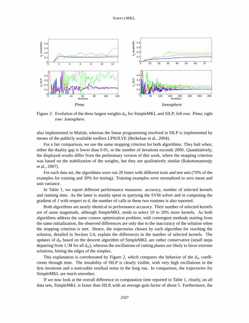
Figure 2: Evolution of the three largest weights dm for SimpleMKL and SILP; left row: Pima; rightrow: Ionosphere.

also implemented in Matlab, whereas the linear programming involved in SILP is implemented bymeans of the publicly available toolbox LPSOLVE (Berkelaar et al., 2004).

For a fair comparison, we use the same stopping criterion for both algorithms. They halt when,either the duality gap is lower than 0.01, or the number of iterations exceeds 2000. Quantitatively,the displayed results differ from the preliminary version of this work, where the stopping criterionwas based on the stabilization of the weights, but they are qualitatively similar (Rakotomamonjyet al., 2007).

For each data set, the algorithms were run 20 times with different train and test sets (70% of theexamples for training and 30% for testing). Training examples were normalized to zero mean andunit variance.

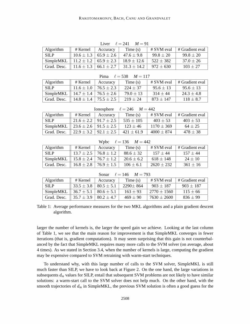
In Table 1, we report different performance measures: accuracy, number of selected kernelsand running time. As the latter is mainly spent in querying the SVM solver and in computing thegradient of J with respect to d, the number of calls to these two routines is also reported.

Both algorithms are nearly identical in performance accuracy. Their number of selected kernelsare of same magnitude, although SimpleMKL tends to select 10 to 20% more kernels. As bothalgorithms address the same convex optimization problem, with convergent methods starting fromthe same initialization, the observed differences are only due to the inaccuracy of the solution whenthe stopping criterion is met. Hence, the trajectories chosen by each algorithm for reaching thesolution, detailed in Section 3.4, explain the differences in the number of selected kernels. Theupdates of dm based on the descent algorithm of SimpleMKL are rather conservative (small stepsdeparting from 1/M for all dm), whereas the oscillations of cutting planes are likely to favor extremesolutions, hitting the edges of the simplex.

This explanation is corroborated by Figure 2, which compares the behavior of the dm coeffi-cients through time. The instability of SILP is clearly visible, with very high oscillations in thefirst iterations and a noticeable residual noise in the long run. In comparison, the trajectories forSimpleMKL are much smoother.

If we now look at the overall difference in computation time reported in Table 1, clearly, on alldata sets, SimpleMKL is faster than SILP, with an average gain factor of about 5. Furthermore, the

2507


Liver ` = 241 M = 91Algorithm # Kernel Accuracy Time (s) # SVM eval # Gradient evalSILP 10.6 ± 1.3 65.9 ± 2.6 47.6 ± 9.8 99.8 ± 20 99.8 ± 20SimpleMKL 11.2 ± 1.2 65.9 ± 2.3 18.9 ± 12.6 522 ± 382 37.0 ± 26Grad. Desc. 11.6 ± 1.3 66.1 ± 2.7 31.3 ± 14.2 972 ± 630 103 ± 27

Pima ` = 538 M = 117Algorithm # Kernel Accuracy Time (s) # SVM eval # Gradient evalSILP 11.6 ± 1.0 76.5 ± 2.3 224 ± 37 95.6 ± 13 95.6 ± 13SimpleMKL 14.7 ± 1.4 76.5 ± 2.6 79.0 ± 13 314 ± 44 24.3 ± 4.8Grad. Desc. 14.8 ± 1.4 75.5 ± 2.5 219 ± 24 873 ± 147 118 ± 8.7

Ionosphere ` = 246 M = 442Algorithm # Kernel Accuracy Time (s) # SVM eval # Gradient evalSILP 21.6 ± 2.2 91.7 ± 2.5 535 ± 105 403 ± 53 403 ± 53SimpleMKL 23.6 ± 2.6 91.5 ± 2.5 123 ± 46 1170 ± 369 64 ± 25Grad. Desc. 22.9 ± 3.2 92.1 ± 2.5 421 ± 61.9 4000 ± 874 478 ± 38

Wpbc ` = 136 M = 442Algorithm # Kernel Accuracy Time (s) # SVM eval # Gradient evalSILP 13.7 ± 2.5 76.8 ± 1.2 88.6 ± 32 157 ± 44 157 ± 44SimpleMKL 15.8 ± 2.4 76.7 ± 1.2 20.6 ± 6.2 618 ± 148 24 ± 10Grad. Desc. 16.8 ± 2.8 76.9 ± 1.5 106 ± 6.1 2620 ± 232 361 ± 16

Sonar ` = 146 M = 793Algorithm # Kernel Accuracy Time (s) # SVM eval # Gradient evalSILP 33.5 ± 3.8 80.5 ± 5.1 2290± 864 903 ± 187 903 ± 187SimpleMKL 36.7 ± 5.1 80.6 ± 5.1 163 ± 93 2770 ± 1560 115 ± 66Grad. Desc. 35.7 ± 3.9 80.2 ± 4.7 469 ± 90 7630 ± 2600 836 ± 99

Table 1: Average performance measures for the two MKL algorithms and a plain gradient descentalgorithm.

larger the number of kernels is, the larger the speed gain we achieve. Looking at the last columnof Table 1, we see that the main reason for improvement is that SimpleMKL converges in feweriterations (that is, gradient computations). It may seem surprising that this gain is not counterbal-anced by the fact that SimpleMKL requires many more calls to the SVM solver (on average, about4 times). As we stated in Section 3.4, when the number of kernels is large, computing the gradientmay be expensive compared to SVM retraining with warm-start techniques.

To understand why, with this large number of calls to the SVM solver, SimpleMKL is stillmuch faster than SILP, we have to look back at Figure 2. On the one hand, the large variations insubsequents dm values for SILP, entail that subsequent SVM problems are not likely to have similarsolutions: a warm-start call to the SVM solver does not help much. On the other hand, with thesmooth trajectories of dm in SimpleMKL, the previous SVM solution is often a good guess for the

2508

SIMPLEMKL

0 20 40 60 80 100 1202

2.5

3

3.5x 10

4O

bjec

tive

valu

e

Iterations

SimpleMKLSILP

0 50 100 150 200 250 300 3500

5000

10000

15000

Obj

ectiv

e va

lue

Iterations

SimpleMKLSILP

Pima Ionosphere

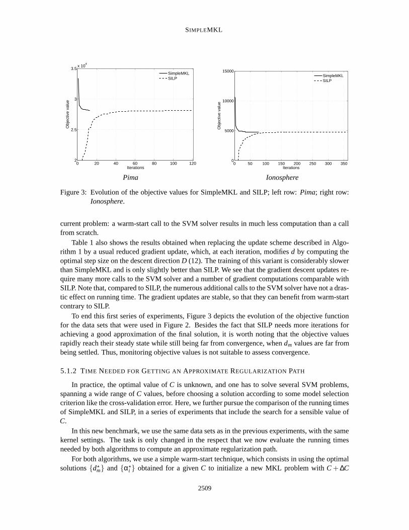
Figure 3: Evolution of the objective values for SimpleMKL and SILP; left row: Pima; right row:Ionosphere.

current problem: a warm-start call to the SVM solver results in much less computation than a callfrom scratch.

Table 1 also shows the results obtained when replacing the update scheme described in Algo-rithm 1 by a usual reduced gradient update, which, at each iteration, modifies d by computing theoptimal step size on the descent direction D (12). The training of this variant is considerably slowerthan SimpleMKL and is only slightly better than SILP. We see that the gradient descent updates re-quire many more calls to the SVM solver and a number of gradient computations comparable withSILP. Note that, compared to SILP, the numerous additional calls to the SVM solver have not a dras-tic effect on running time. The gradient updates are stable, so that they can benefit from warm-startcontrary to SILP.

To end this first series of experiments, Figure 3 depicts the evolution of the objective functionfor the data sets that were used in Figure 2. Besides the fact that SILP needs more iterations forachieving a good approximation of the final solution, it is worth noting that the objective valuesrapidly reach their steady state while still being far from convergence, when dm values are far frombeing settled. Thus, monitoring objective values is not suitable to assess convergence.

5.1.2 TIME NEEDED FOR GETTING AN APPROXIMATE REGULARIZATION PATH

In practice, the optimal value of C is unknown, and one has to solve several SVM problems,spanning a wide range of C values, before choosing a solution according to some model selectioncriterion like the cross-validation error. Here, we further pursue the comparison of the running timesof SimpleMKL and SILP, in a series of experiments that include the search for a sensible value ofC.

In this new benchmark, we use the same data sets as in the previous experiments, with the samekernel settings. The task is only changed in the respect that we now evaluate the running timesneeded by both algorithms to compute an approximate regularization path.

For both algorithms, we use a simple warm-start technique, which consists in using the optimalsolutions {d?

m} and {α?i } obtained for a given C to initialize a new MKL problem with C + ∆C

2509


10−2

10−1

100

101

102

103

0

2

4

6

8

10

12

14

16

18

20

C

num

ber

of s

elec

ted

kern

els

10−2

10−1

100

101

102

103

0

2

4

6

8

10

12

14

16

18

20

C

num

ber

of s

elec

ted

kern

els

10−2

10−1

100

101

102

103

0

0.1

0.2

0.3

0.4

0.5

0.6

0.7

0.8

0.9

1

C

d k

10−2

10−1

100

101

102

103

0

0.1

0.2

0.3

0.4

0.5

0.6

0.7

0.8

0.9

1

C

d k

Pima Wpbc

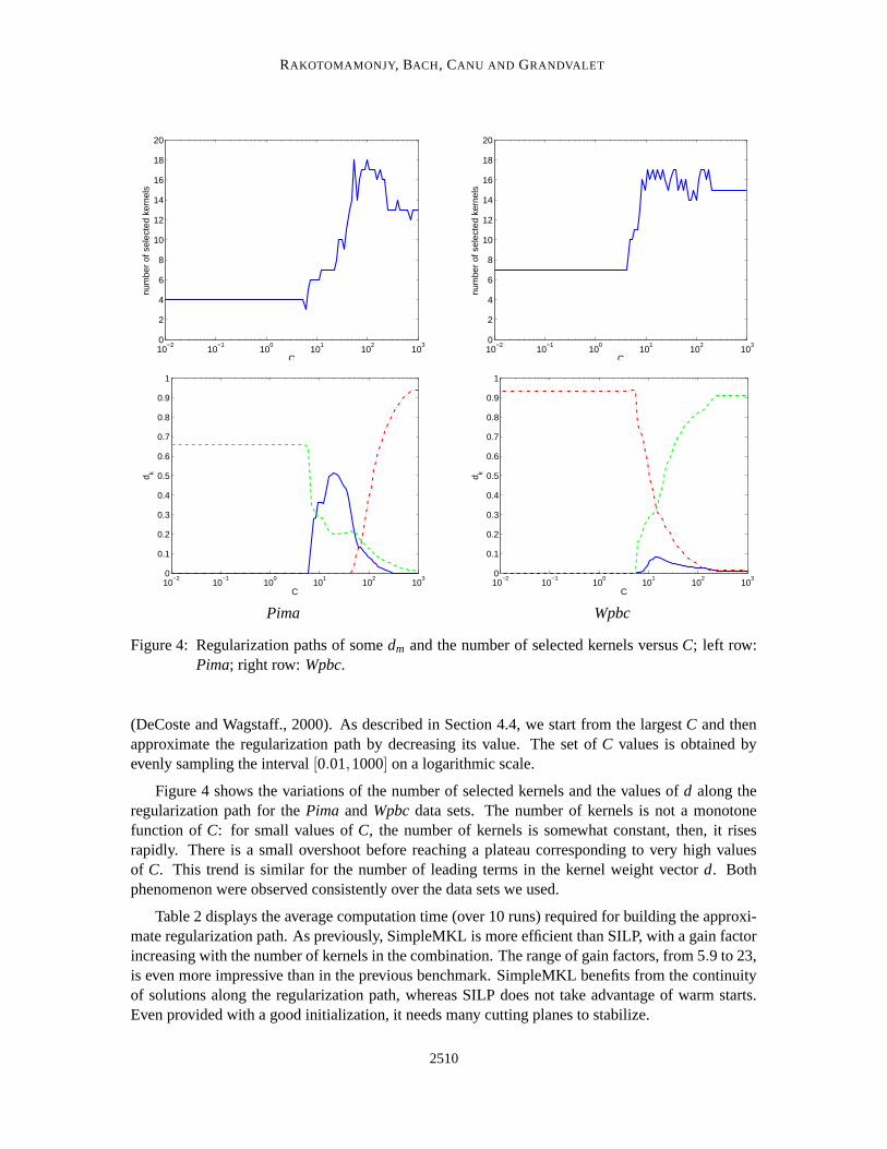
Figure 4: Regularization paths of some dm and the number of selected kernels versus C; left row:Pima; right row: Wpbc.

(DeCoste and Wagstaff., 2000). As described in Section 4.4, we start from the largest C and thenapproximate the regularization path by decreasing its value. The set of C values is obtained byevenly sampling the interval [0.01,1000] on a logarithmic scale.

Figure 4 shows the variations of the number of selected kernels and the values of d along theregularization path for the Pima and Wpbc data sets. The number of kernels is not a monotonefunction of C: for small values of C, the number of kernels is somewhat constant, then, it risesrapidly. There is a small overshoot before reaching a plateau corresponding to very high valuesof C. This trend is similar for the number of leading terms in the kernel weight vector d. Bothphenomenon were observed consistently over the data sets we used.

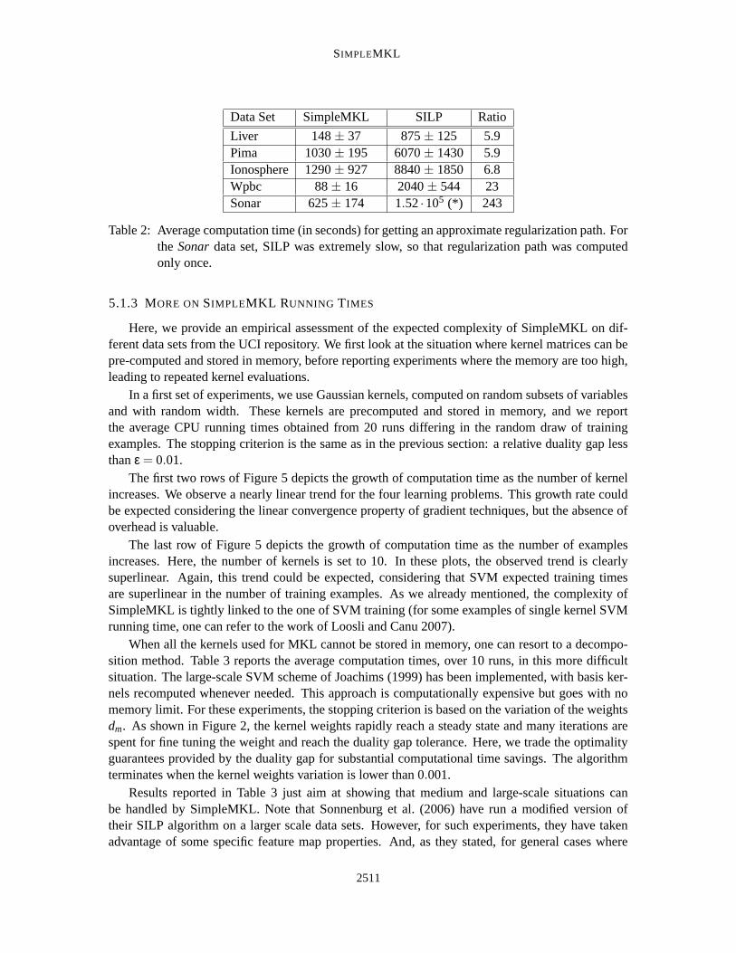
Table 2 displays the average computation time (over 10 runs) required for building the approxi-mate regularization path. As previously, SimpleMKL is more efficient than SILP, with a gain factorincreasing with the number of kernels in the combination. The range of gain factors, from 5.9 to 23,is even more impressive than in the previous benchmark. SimpleMKL benefits from the continuityof solutions along the regularization path, whereas SILP does not take advantage of warm starts.Even provided with a good initialization, it needs many cutting planes to stabilize.

2510

SIMPLEMKL

Data Set SimpleMKL SILP Ratio

Liver 148 ± 37 875 ± 125 5.9Pima 1030 ± 195 6070 ± 1430 5.9Ionosphere 1290 ± 927 8840 ± 1850 6.8Wpbc 88 ± 16 2040 ± 544 23Sonar 625 ± 174 1.52 ·105 (*) 243

Table 2: Average computation time (in seconds) for getting an approximate regularization path. Forthe Sonar data set, SILP was extremely slow, so that regularization path was computedonly once.

5.1.3 MORE ON SIMPLEMKL RUNNING TIMES

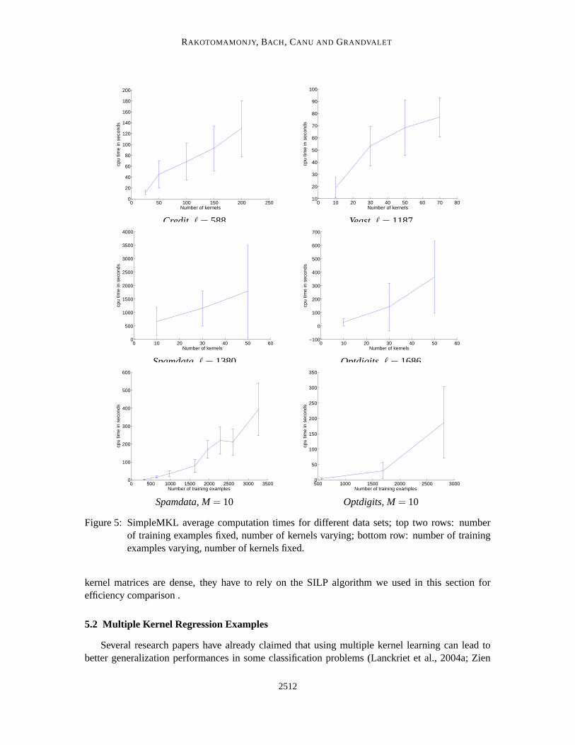
Here, we provide an empirical assessment of the expected complexity of SimpleMKL on dif-ferent data sets from the UCI repository. We first look at the situation where kernel matrices can bepre-computed and stored in memory, before reporting experiments where the memory are too high,leading to repeated kernel evaluations.

In a first set of experiments, we use Gaussian kernels, computed on random subsets of variablesand with random width. These kernels are precomputed and stored in memory, and we reportthe average CPU running times obtained from 20 runs differing in the random draw of trainingexamples. The stopping criterion is the same as in the previous section: a relative duality gap lessthan ε = 0.01.

The first two rows of Figure 5 depicts the growth of computation time as the number of kernelincreases. We observe a nearly linear trend for the four learning problems. This growth rate couldbe expected considering the linear convergence property of gradient techniques, but the absence ofoverhead is valuable.

The last row of Figure 5 depicts the growth of computation time as the number of examplesincreases. Here, the number of kernels is set to 10. In these plots, the observed trend is clearlysuperlinear. Again, this trend could be expected, considering that SVM expected training timesare superlinear in the number of training examples. As we already mentioned, the complexity ofSimpleMKL is tightly linked to the one of SVM training (for some examples of single kernel SVMrunning time, one can refer to the work of Loosli and Canu 2007).

When all the kernels used for MKL cannot be stored in memory, one can resort to a decompo-sition method. Table 3 reports the average computation times, over 10 runs, in this more difficultsituation. The large-scale SVM scheme of Joachims (1999) has been implemented, with basis ker-nels recomputed whenever needed. This approach is computationally expensive but goes with nomemory limit. For these experiments, the stopping criterion is based on the variation of the weightsdm. As shown in Figure 2, the kernel weights rapidly reach a steady state and many iterations arespent for fine tuning the weight and reach the duality gap tolerance. Here, we trade the optimalityguarantees provided by the duality gap for substantial computational time savings. The algorithmterminates when the kernel weights variation is lower than 0.001.

Results reported in Table 3 just aim at showing that medium and large-scale situations canbe handled by SimpleMKL. Note that Sonnenburg et al. (2006) have run a modified version oftheir SILP algorithm on a larger scale data sets. However, for such experiments, they have takenadvantage of some specific feature map properties. And, as they stated, for general cases where

2511


0 50 100 150 200 2500

20

40

60

80

100

120

140

160

180

200

Number of kernels

cpu

time

in s

econ

ds

0 10 20 30 40 50 60 70 8010

20

30

40

50

60

70

80

90

100

Number of kernels

cpu

time

in s

econ

ds

Credit, ` = 588 Yeast, ` = 1187

0 10 20 30 40 50 600

500

1000

1500

2000

2500

3000

3500

4000

Number of kernels

cpu

time

in s

econ

ds

0 10 20 30 40 50 60−100

0

100

200

300

400

500

600

700

Number of kernels

cpu

time

in s

econ

ds

Spamdata, ` = 1380 Optdigits, ` = 1686

0 500 1000 1500 2000 2500 3000 35000

100

200

300

400

500

600

Number of training examples

cpu

time

in s

econ

ds

500 1000 1500 2000 2500 30000

50

100

150

200

250

300

350

Number of training examples

cpu

time

in s

econ

ds

Spamdata, M = 10 Optdigits, M = 10

Figure 5: SimpleMKL average computation times for different data sets; top two rows: numberof training examples fixed, number of kernels varying; bottom row: number of trainingexamples varying, number of kernels fixed.

kernel matrices are dense, they have to rely on the SILP algorithm we used in this section forefficiency comparison .

5.2 Multiple Kernel Regression Examples

Several research papers have already claimed that using multiple kernel learning can lead tobetter generalization performances in some classification problems (Lanckriet et al., 2004a; Zien

2512

SIMPLEMKL

Data Set Nb Examples # Kernel Accuracy (%) Time (s)

Yeast 1335 22 77.25 1130Spamdata 4140 71 93.49 34200

Table 3: Average computation time needed by SimpleSVM using decomposition methods.

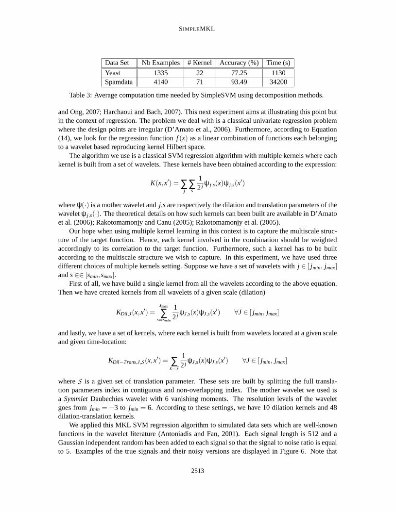
and Ong, 2007; Harchaoui and Bach, 2007). This next experiment aims at illustrating this point butin the context of regression. The problem we deal with is a classical univariate regression problemwhere the design points are irregular (D’Amato et al., 2006). Furthermore, according to Equation(14), we look for the regression function f (x) as a linear combination of functions each belongingto a wavelet based reproducing kernel Hilbert space.

The algorithm we use is a classical SVM regression algorithm with multiple kernels where eachkernel is built from a set of wavelets. These kernels have been obtained according to the expression:

K(x,x′) = ∑j∑

s

12 j ψ j,s(x)ψ j,s(x

′)

where ψ(·) is a mother wavelet and j,s are respectively the dilation and translation parameters of thewavelet ψ j,s(·). The theoretical details on how such kernels can been built are available in D’Amatoet al. (2006); Rakotomamonjy and Canu (2005); Rakotomamonjy et al. (2005).

Our hope when using multiple kernel learning in this context is to capture the multiscale struc-ture of the target function. Hence, each kernel involved in the combination should be weightedaccordingly to its correlation to the target function. Furthermore, such a kernel has to be builtaccording to the multiscale structure we wish to capture. In this experiment, we have used threedifferent choices of multiple kernels setting. Suppose we have a set of wavelets with j ∈ [ jmin, jmax]and s ∈∈ [smin,smax].

First of all, we have build a single kernel from all the wavelets according to the above equation.Then we have created kernels from all wavelets of a given scale (dilation)

KDil,J(x,x′) =

smax

∑s=smin

12 j ψJ,s(x)ψJ,s(x

′) ∀J ∈ [ jmin, jmax]

and lastly, we have a set of kernels, where each kernel is built from wavelets located at a given scaleand given time-location:

KDil−Trans,J,S (x,x′) = ∑s=S

12 j ψJ,s(x)ψJ,s(x

′) ∀J ∈ [ jmin, jmax]

where S is a given set of translation parameter. These sets are built by splitting the full transla-tion parameters index in contiguous and non-overlapping index. The mother wavelet we used isa Symmlet Daubechies wavelet with 6 vanishing moments. The resolution levels of the waveletgoes from jmin = −3 to jmin = 6. According to these settings, we have 10 dilation kernels and 48dilation-translation kernels.

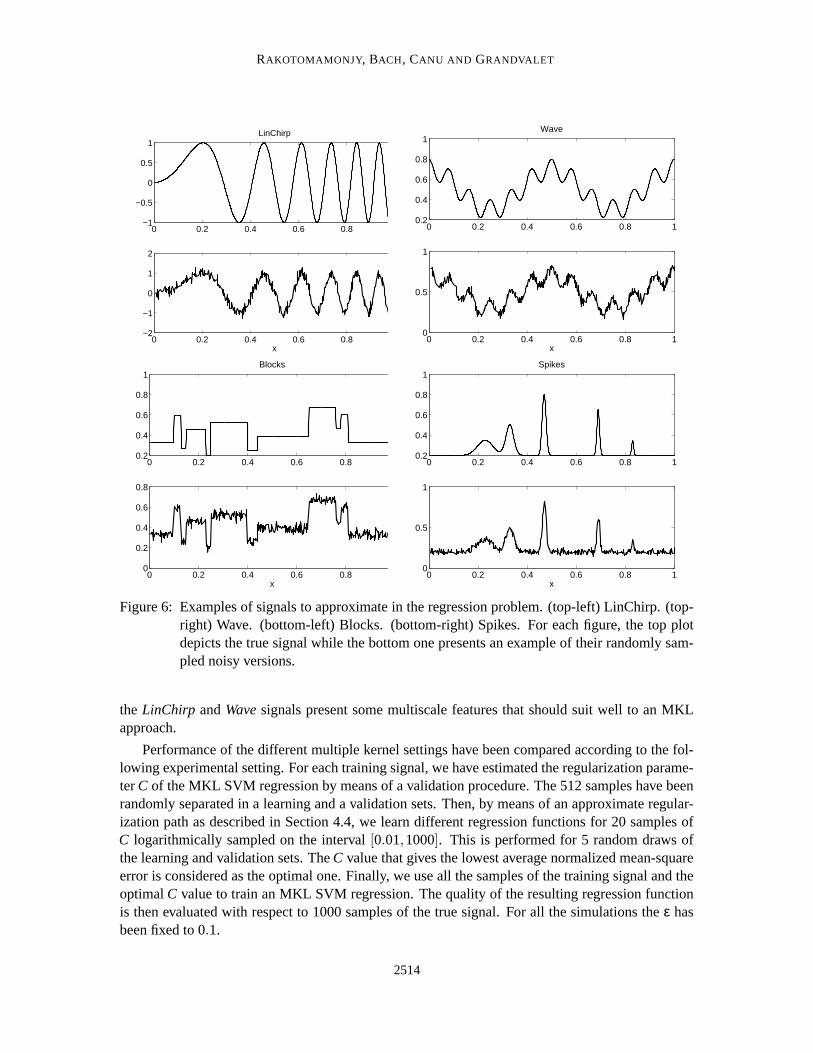
We applied this MKL SVM regression algorithm to simulated data sets which are well-knownfunctions in the wavelet literature (Antoniadis and Fan, 2001). Each signal length is 512 and aGaussian independent random has been added to each signal so that the signal to noise ratio is equalto 5. Examples of the true signals and their noisy versions are displayed in Figure 6. Note that

2513


0 0.2 0.4 0.6 0.8 1−1

−0.5

0

0.5

1LinChirp

0 0.2 0.4 0.6 0.8 1−2

−1

0

1

2

x

0 0.2 0.4 0.6 0.8 10.2

0.4

0.6

0.8

1Wave

0 0.2 0.4 0.6 0.8 10

0.5

1

x

0 0.2 0.4 0.6 0.8 10.2

0.4

0.6

0.8

1Blocks

0 0.2 0.4 0.6 0.8 10

0.2

0.4

0.6

0.8

x

0 0.2 0.4 0.6 0.8 10.2

0.4

0.6

0.8

1Spikes

0 0.2 0.4 0.6 0.8 10

0.5

1

x

Figure 6: Examples of signals to approximate in the regression problem. (top-left) LinChirp. (top-right) Wave. (bottom-left) Blocks. (bottom-right) Spikes. For each figure, the top plotdepicts the true signal while the bottom one presents an example of their randomly sam-pled noisy versions.

the LinChirp and Wave signals present some multiscale features that should suit well to an MKLapproach.

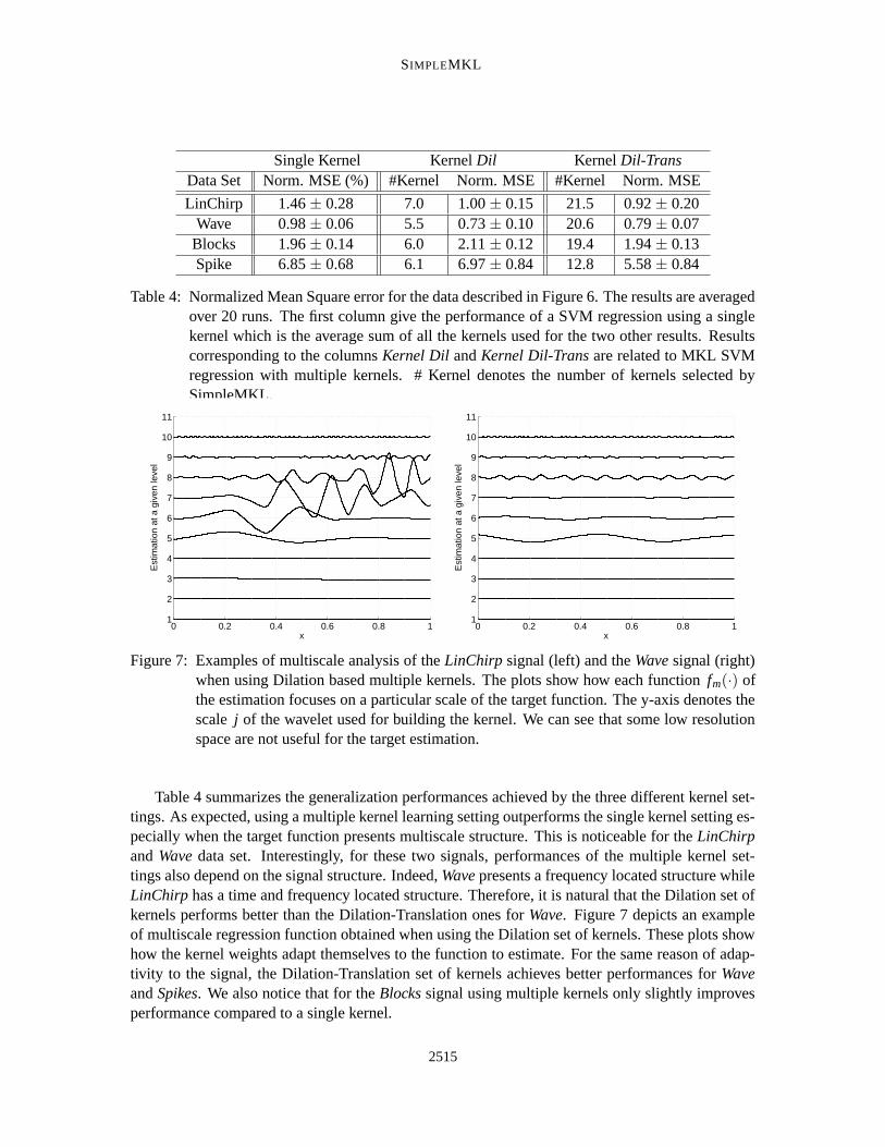
Performance of the different multiple kernel settings have been compared according to the fol-lowing experimental setting. For each training signal, we have estimated the regularization parame-ter C of the MKL SVM regression by means of a validation procedure. The 512 samples have beenrandomly separated in a learning and a validation sets. Then, by means of an approximate regular-ization path as described in Section 4.4, we learn different regression functions for 20 samples ofC logarithmically sampled on the interval [0.01,1000]. This is performed for 5 random draws ofthe learning and validation sets. The C value that gives the lowest average normalized mean-squareerror is considered as the optimal one. Finally, we use all the samples of the training signal and theoptimal C value to train an MKL SVM regression. The quality of the resulting regression functionis then evaluated with respect to 1000 samples of the true signal. For all the simulations the ε hasbeen fixed to 0.1.

2514

SIMPLEMKL

Single Kernel Kernel Dil Kernel Dil-TransData Set Norm. MSE (%) #Kernel Norm. MSE #Kernel Norm. MSE

LinChirp 1.46 ± 0.28 7.0 1.00 ± 0.15 21.5 0.92 ± 0.20Wave 0.98 ± 0.06 5.5 0.73 ± 0.10 20.6 0.79 ± 0.07

Blocks 1.96 ± 0.14 6.0 2.11 ± 0.12 19.4 1.94 ± 0.13Spike 6.85 ± 0.68 6.1 6.97 ± 0.84 12.8 5.58 ± 0.84

Table 4: Normalized Mean Square error for the data described in Figure 6. The results are averagedover 20 runs. The first column give the performance of a SVM regression using a singlekernel which is the average sum of all the kernels used for the two other results. Resultscorresponding to the columns Kernel Dil and Kernel Dil-Trans are related to MKL SVMregression with multiple kernels. # Kernel denotes the number of kernels selected bySimpleMKL.

0 0.2 0.4 0.6 0.8 11

2

3

4

5

6

7

8

9

10

11

x

Est

imat

ion

at a

giv

en le

vel

0 0.2 0.4 0.6 0.8 11

2

3

4

5

6

7

8

9

10

11

x

Est

imat

ion

at a

giv

en le

vel

Figure 7: Examples of multiscale analysis of the LinChirp signal (left) and the Wave signal (right)when using Dilation based multiple kernels. The plots show how each function fm(·) ofthe estimation focuses on a particular scale of the target function. The y-axis denotes thescale j of the wavelet used for building the kernel. We can see that some low resolutionspace are not useful for the target estimation.

Table 4 summarizes the generalization performances achieved by the three different kernel set-tings. As expected, using a multiple kernel learning setting outperforms the single kernel setting es-pecially when the target function presents multiscale structure. This is noticeable for the LinChirpand Wave data set. Interestingly, for these two signals, performances of the multiple kernel set-tings also depend on the signal structure. Indeed, Wave presents a frequency located structure whileLinChirp has a time and frequency located structure. Therefore, it is natural that the Dilation set ofkernels performs better than the Dilation-Translation ones for Wave. Figure 7 depicts an exampleof multiscale regression function obtained when using the Dilation set of kernels. These plots showhow the kernel weights adapt themselves to the function to estimate. For the same reason of adap-tivity to the signal, the Dilation-Translation set of kernels achieves better performances for Waveand Spikes. We also notice that for the Blocks signal using multiple kernels only slightly improvesperformance compared to a single kernel.

2515


Training Set SizeData Set #Classes # examples Medium Large

ABE 3 2323 560 1120DNA 3 3186 500 1000SEG 7 2310 500 1000WAV 3 5000 300 600

Table 5: Summary of the multiclass data sets and the training set size used.

Training set size

Medium Large

Data Set MKL CV MKL CV

ABE 0.73 ± 0.28 (16) 0.96 ± 0.36 0.44 ± 0.67 (11) 0.46 ± 0.20DNA 7.69 ± 0.76 (11) 7.84 ± 0.79 5.59 ± 0.55 (10) 5.59 ± 0.39SEG 6.52 ± 0.76 (10) 6.51 ± 0.99 4.71 ± 0.67 (13) 4.89 ± 0.71WAV 15.18 ± 0.90 (15) 15.43 ± 0.97 14.26 ± 0.68 (8) 14.09 ± 0.55

Table 6: Comparison of the generalization performances of an MKL approach and a cross-validation approach for selecting models in some multiclass problems. We have reportedthe average (over 20 runs) the test set errors of our algorithm while the errors obtained forthe SV approach have been extracted from Duan and Keerthi (2005). Results also dependon the training set sizes.

5.3 Multiclass Problem

For selecting the kernel and regularization parameter of a SVM, one usually tries all pairs of pa-rameters and picks the couple that achieves the best cross-validation performance. Using an MKLapproach, one can instead let the algorithm combine all available kernels (obtained by sampling theparameter) and just selects the regularization parameter by cross-validation. This last experimentaims at comparing on several multi-class data sets problem, these two model selection approaches(using MKL and CV) for choosing the kernel. Thus, we evaluate the two methods on some multi-class data sets taken from the UCI collection: dna, waveform, image segmentation and abe a subsetproblem of the Letter data set corresponding to the classes A, B and E. Some information aboutthe data set are given in Table 5. For each data set, we divide the whole data into a training setand a test set. This random splitting has been performed 20 times. For ease of comparison withprevious works, we have used the splitting proposed by Duan and Keerthi (2005) and available athttp://www.keerthis.com/multiclass.html. Then we have just computed the performance ofSimpleMKL and report their results for the CV approach.

In our MKL one-against-all approach, we have used a polynomial kernel of degree 1 to 3and Gaussian kernel for which σ belongs to [0.5,1,2,5,7,10,12,15,17,20]. For the regularizationparameter C, we have 10 samples over the interval [0.01,10000]. Note that Duan and Keerthi(2005) have used a more sophisticated sampling strategy based on a coarse sampling of σ and C andfollowed by fine-tuned sampling procedure. They also select the same couple of C and σ over allpairwise decision functions. Similarly to Duan and Keerthi (2005), the best hyperparameter C hasbeen tuned according to a five-fold cross-validation. According to this best C, we have learned anMKL all the full training set and evaluated the resulting decision function on the test set.

2516

SIMPLEMKL

The comparison results are summarized on Table 6. We can see that the generalization per-formances of an MKL approach is either similar or better than the performance obtained whenselecting the kernel through cross-validation, even though we have roughly searched the kerneland regularization parameter space. Hence, we can deduce that MKL can favorably replace cross-validation on kernel parameters. This result based on empirical observations is in accordance withsome other works (Lanckriet et al., 2004b; Fung et al., 2004; Kim et al., 2006). However, we thinkthat MKL and thus SimpleMKL in particular, can be better exploited and thus performs better thancross-validation when the kernels have been obtained from heterogeneous source as described forinstance in Lanckriet et al. (2004a); Zien and Ong (2007); Harchaoui and Bach (2007).

6. Conclusion

In this paper, we introduced SimpleMKL, a novel algorithm for solving the Multiple KernelLearning problem. Our formalization of the MKL problem results in a smooth and convex opti-mization problem, which is actually equivalent to other MKL formulations available in the litera-ture. The main added value of the smoothness of our new objective function is that descent methodsbecome practical and efficient means to solve the optimization problem that wraps a single kernelSVM solver. We provide optimality conditions, analyze convergence and computational complexityissues for binary classification. The SimpleMKL algorithm and the resulting analyses can be easilybe transposed to SVM regression, one-class SVM and multiclass SVM to name a few.

We provide experimental evidence that SimpleMKL is significantly more efficient than the state-of-the art SILP approach (Sonnenburg et al., 2006). This efficiency permits to demonstrate theusefulness of our algorithm on wavelet kernel based regression. We also illustrate in multiclassproblems that MKL is a viable alternative to cross-validation for selecting a model.

Possible extensions of this work include other learning problems, such as semi-supervised learn-ing or kernel eigenvalue problem like kernel Fisher discriminant analysis. We also plan to exploretwo different ways to speed up the algorithm. As a first direction, we will investigate ways to obtain abetter the descent direction, for example with second-order methods. Note however that computingthe Hessian needs the derivative of the dual variable with respects to the weights d. This operationrequires solving a linear system (Chapelle et al., 2002) and thus may produce some computationaloverhead. The second direction is motivated by the observation that most of the computational loadis to the computation of the kernel combination. Hence, coordinate-wise optimizers may providepromising routes for improvements.

Acknowledgments

We would like to thank the anonymous reviewers for their useful comments. This work was sup-ported in part by the IST Program of the European Community, under the PASCAL Network ofExcellence, IST-2002-506778. Alain Rakotomamonjy, Francis Bach and Stephane Canu were alsosupported by French grants from the Agence Nationale de la Recherche (KernSig for AR and SC,MGA for FB).

Appendix A.

This appendix addresses the convexity and differentiability issue of our MKL formulation.

2517


A.1 Proof of Convexity of the Weighted Squared Norm MKL Formulation

The convexity of the MKL problem (2) introduced in Section 2.2 will be established if we provethe convexity of

J( f , t) =1t〈 f , f 〉H where f ∈H and t ∈ R

∗+.

Since J( f , t) is differentiable with respects to its arguments, we only have to make sure that thefirst order conditions for convexity are verified. As the convexity of the domain of J is trivial, weverify that, for any ( f , t) and (g,s) ∈H ×R

∗+, the following holds:

J(g,s)≥ J( f , t)+ 〈∇ f J,g− f 〉H +(s− t)∇tJ .

As ∇ f J = 2t f and ∇tJ =− 1

t2 〈 f , f 〉H , this inequality can be written as

1s〈g,g〉H ≥

2t〈 f ,g〉H −

st2 〈 f , f 〉H ,

⇔ 〈t g− s f , t g− s f 〉H ≥ 0 ,

where we used that s and t are positive. The above inequality holds since the scalar product on theleft-hand-side is a norm. Hence problem (2) minimizes the sum of convex functions on a convexset; it is thus convex. Note that when H is a finite dimension space, the function J( f , t) is known asthe perspective of f , whose convexity is proven in textbooks (Boyd and Vandenberghe, 2004).

A.2 Differentiability of Optimal Value Function

The algorithm we propose for solving the MKL problem heavily relies on the differentiabilityof the optimal value of the primal SVM objective function. For the sake of self-containedness,we reproduce here a theorem due to Bonnans and Shapiro (1998) that allows us to compute thederivatives of J(d) defined in (8).

Theorem 1 (Bonnans and Shapiro, 1998) Let X be a metric space and U be a normed space. Sup-pose that for all x ∈ X the function f (x, ·) is differentiable, that f (x,u) and Du f (x,u) the derivativeof f (x, ·) are continuous on X ×U and let Φ be a compact subset of X. Let define the optimalvalue function as v(u) = infx∈Φ f (x,u). The optimal value function is directionally differentiable.Furthermore, if for u0 ∈U, f (·,u0) has a unique minimizer x0 over Φ then v(u) is differentiable atu0 and Dv(u0) = Du f (x0,u0).

References

A. Antoniadis and J. Fan. Regularization by wavelet approximations. J. American Statistical Asso-ciation, 96:939–967, 2001.

A. Argyriou, T. Evgeniou, and M. Pontil. Convex multi-task feature learning. Machine Learning,to appear, 2008.

N. Aronszajn. Theory of reproducing kernels. Trans. Am. Math. Soc., (68):337–404, 1950.

2518

SIMPLEMKL

F. Bach. Consistency of the group Lasso and multiple kernel learning. Journal of Machine LearningResearch, 9:1179–1225, 2008.

F. Bach, G. Lanckriet, and M. Jordan. Multiple kernel learning, conic duality, and the SMO algo-rithm. In Proceedings of the 21st International Conference on Machine Learning, pages 41–48,2004a.

F. Bach, R. Thibaux, and M. Jordan. Computing regularization paths for learning multiple kernels.In Advances in Neural Information Processing Systems, volume 17, pages 41–48, 2004b.

M. Berkelaar, K. Eikland, and P. Notebaert. Lpsolve, Version 5.1.0.0, 2004. URL http://lpsolve.sourceforge.net/5.5/.

D. Bertsekas. Nonlinear Programming. Athena scientific, 1999.

C. Blake and C. Merz. UCI repository of machine learning databases. University of California,Irvine, Dept. of Information and Computer Sciences, 1998. URL http://www.ics.uci.edu/

˜mlearn/MLRepository.html.

F. Bonnans. Optimisation Continue. Dunod, 2006.

J.F. Bonnans and A. Shapiro. Optimization problems with pertubation : A guided tour. SIAMReview, 40(2):202–227, 1998.

J.F. Bonnans, J.C Gilbert, C. Lemarechal, and C.A Sagastizbal. Numerical Optimization Theoreticaland Practical Aspects. Springer, 2003.

S. Boyd and L. Vandenberghe. Convex Optimization. Cambridge University Press, 2004.

S. Canu, Y. Grandvalet, V. Guigue, and A. Rakotomamonjy. SVM and kernel methods Matlab tool-box. LITIS EA4108, INSA de Rouen, Rouen, France, 2003. URL http://asi.insa-rouen.fr/enseignants/˜arakotom/toolbox/index.html.

C-C. Chang and C-J. Lin. LIBSVM: A Library for Support Vector Machines, 2001. Softwareavailable at http://www.csie.ntu.edu.tw/˜cjlin/libsvm.

O. Chapelle, V. Vapnik, O. Bousquet, and S. Mukerjhee. Choosing multiple parameters for SVM.Machine Learning, 46(1-3):131–159, 2002.

K. Crammer and Y. Singer. On the algorithmic implementation of multiclass kernel-based vectormachines. Journal of Machine Learning Research, 2:265–292, 2001.

A. D’Amato, A. Antoniadis, and M. Pensky. Wavelet kernel penalized estimation for non-equispaced design regression. Statistics and Computing, 16:37–56, 2006.

A. D’Aspremont. Smooth optimization with approximate gradient. SIAM Journal on Optimization,To appear, 2008.

D. DeCoste and K. Wagstaff. Alpha seeding for support vector machines. In International Confer-ence on Knowledge Discovery and Data Mining, 2000.

2519


K. Duan and S. Keerthi. Which is the best multiclass svm method? an empirical study. In Multi-ple Classifier Systems, pages 278–285, 2005. URL http://www.keerthis.com/multiclass.html.

B. Efron, T. Hastie, I. Johnstone, and R. Tibshirani. Least angle regression (with discussion). Annalsof statistics, 32(2):407–499, 2004.

G. Fung, M. Dundar, J. Bi, and B. Rao. A fast iterative algorithm for Fisher discriminant using het-erogeneous kernels. In Proceeedins of the 21th International Conference on Machine Learning,2004.

Y. Grandvalet. Least absolute shrinkage is equivalent to quadratic penalization. In L. Niklasson,M. Boden, and T. Ziemske, editors, ICANN’98, volume 1 of Perspectives in Neural Computing,pages 201–206. Springer, 1998.

Y. Grandvalet and S. Canu. Adaptive scaling for feature selection in SVMs. In Advances in NeuralInformation Processing Systems, volume 15. MIT Press, 2003.

Y. Grandvalet and S. Canu. Outcomes of the equivalence of adaptive ridge with least absoluteshrinkage. In M. S. Kearns, S. A. Solla, and D. A. Cohn, editors, Advances in Neural InformationProcessing Systems 11, pages 445–451. MIT Press, 1999.

Z. Harchaoui and F. Bach. Image classification with segmentation graph kernels. In IEEE ComputerSociety Conference on Computer Vision and Pattern Recognition, 2007.

T. Hastie, S. Rosset, R. Tibshirani, and J. Zhu. The entire regularization path for the support vectormachine. Journal of Machine Learning Research, 5:1391–1415, 2004.

C.-W. Hsu and C.-J. Lin. A comparison of methods for multi-class support vector machines. IEEETransactions on Neural Networks, 13:415–425, 2002.

T. Joachims. Making large-scale SVM learning practical. In B. Scholkopf, C. Burges, and A. Smola,editors, Advanced in Kernel Methods - Support Vector Learning, pages 169–184. MIT Press,1999.

S.-J. Kim, A. Magnani, and S. Boyd. Optimal kernel selection in kernel Fisher discriminant analysis.In Proceedings of the 23rd International Conference on Machine Learning (ICML), 2006.

K. Koh, S.-J. Kim, and S. Boyd. An interior-point method for large-scale `1-regularized logisticregression. Journal of Machine Learning Research, 8:1519–1555, 2007.

G. Lanckriet, T. De Bie, N. Cristianini, M. Jordan, and W. Noble. A statistical framework forgenomic data fusion. Bioinformatics, 20:2626–2635, 2004a.

G. Lanckriet, N. Cristianini, L. El Ghaoui, P. Bartlett, and M. Jordan. Learning the kernel matrixwith semi-definite programming. Journal of Machine Learning Research, 5:27–72, 2004b.

C. Lemarechal and C. Sagastizabal. Practical aspects of moreau-yosida regularization : theoreticalpreliminaries. SIAM Journal of Optimization, 7:867–895, 1997.

2520

SIMPLEMKL

G. Loosli and S. Canu. Comments on the ”Core vector machines: Fast SVM training on very largedata sets”. Journal of Machine Learning Research, 8:291–301, February 2007.

G. Loosli, S. Canu, S. Vishwanathan, A. Smola, and M. Chattopadhyay. Boıte a outils SVM simpleet rapide. Revue d’Intelligence Artificielle, 19(4-5):741–767, 2005.

D. Luenberger. Linear and Nonlinear Programming. Addison-Wesley, 1984.

C. Micchelli and M. Pontil. Learning the kernel function via regularization. Journal of MachineLearning Research, 6:1099–1125, 2005.

A. Rakotomamonjy and S. Canu. Frames, reproducing kernels, regularization and learning. Journalof Machine Learning Research, 6:1485–1515, 2005.

A. Rakotomamonjy, X. Mary, and S. Canu. Non parametric regression with wavelet kernels. AppliedStochastics Model for Business and Industry, 21(2):153–163, 2005.

A. Rakotomamonjy, F. Bach, S. Canu, and Y. Grandvalet. More efficiency in multiple kernel learn-ing. In Zoubin Ghahramani, editor, Proceedings of the 24th Annual International Conference onMachine Learning (ICML 2007), pages 775–782. Omnipress, 2007.

R. Rifkin and A. Klautau. In defense of one-vs-all classification. Journal of Machine LearningResearch, 5:101–141, 2004.

S. Rosset. Tracking curved regularized optimization solution paths. In Advances in Neural Infor-mation Processing Systems, 2004.

B. Scholkopf and A. Smola. Learning with Kernels. MIT Press, 2001.

S. Sonnenburg, G. Ratsch, and C. Schafer. A general and efficient algorithm for multiple kernellearning. In Advances in Neural Information Processing Systems, volume 17, pages 1–8, 2005.

S. Sonnenburg, G. Ratsch, C. Schafer, and B. Scholkopf. Large scale multiple kernel learning.Journal of Machine Learning Research, 7(1):1531–1565, 2006.

I. Tsochantaridis, T. Joachims, T. Hofmann, and Y. Altun. Large margin methods for structured andinterdependent output variables. Journal of Machine Learning Research, 6:1453–1484, 2005.

V. Vapnik, S. Golowich, and A. Smola. Support vector method for function estimation, regressionestimation and signal processing. volume Vol. 9. MIT Press, Cambridge, MA, neural informationprocessing systems, edition, 1997.

S. V. N. Vishwanathan, A. J. Smola, and M. Murty. SimpleSVM. In International Conference onMachine Learning, 2003.

G. Wahba. Spline Models for Observational Data. Series in Applied Mathematics, Vol. 59, SIAM,1990.

J. Weston and C. Watkins. Multiclass support vector machines. In Proceedings of ESANN99,Brussels. D. Facto Press, 1999.

A. Zien and C.S. Ong. Multiclass multiple kernel learning. In Proceedings of the 24th InternationalConference on Machine Learning (ICML 2007), pages 1191–1198, 2007.

2521

SimpleMKL - MIT Computer Science and Artificial...

Documents

Transcript of SimpleMKL - MIT Computer Science and Artificial...