Optomecanica cuantica operacional

Por

Christian Ventura VelazquezLic. en Fısica y Matematicas, ESFM-IPN

Tesis sometida como requisito parcial para obtener el grado de

Maestro en Ciencias en la especialidad de Optica

en el

Instituto Nacional de Astrofısica, Optica y ElectronicaAgosto 2015

Tonantzintla, Puebla

Supervisada por:

Dr. Blas Manuel Rodrıguez Lara,Dr. Hector Manuel Moya CessaInvestigadores titulares del INAOE

c©INAOE 2015Derechos reservados

El autor otorga al INAOE el permiso de reproducir ydistribuir copias de esta tesis en su totalidad o en partes.

ii

Abstract

Through this thesis, the standard optomechanical system is studied in three different cases:driven by a monochromatic laser, interacting with the environment, and including a two-levelatom in the cavity. Operator techniques, such a unitary transformations and superoperators, areused to study the three frameworks.

iii

Abstract

iv

Resumen

En esta tesis se estudia el sistema optomecanico estandar en tres escenarios: cuando es bombea-do por un laser monocromatico, cuando el oscilador mecanico interactua con el medio ambiente, ycuando un atomo de dos niveles, qubit, es introducido en la cavidad.

Para estudiar tales escenarios se hace uso de tecnicas operacionales, transformaciones unitariasy superoperadores. Estas tecnicas nos permiten pasar del Hamiltoniano inicial del problema a otrosya conocidos, para los cuales se conocen soluciones aproximadas.

v

Resumen

vi

Dedicatorias y agradecimientos

Dedico esta tesis a:

1. mis padres por siempre darme su apoyo, pero en especial a mi mama por ser mi mejormaestra,

2. a Chofis quien cambio nuestras vidas para bien,

3. y mis mejores amigos, La Plebe XD, con quienes me diverti y aprendı mucho,

Agradezco profundamente a:

1. mis buenos profesores porque con ellos fue sencillo lo difıcil,

2. mis asesores, Dr. Blas y Dr. Hector, por tener paciencia y ensenarme a ser mejor investigador,

3. CONACyT por becarme durante los dos anos de maestrıa y ser siempre puntuales,

4. y la Escuela Superior de Fısica y Matematicas del IPN donde aprendı el gusto por la fısica.

vii

Dedicatorias y agradecimientos

viii

Indice general

Indice general

1. Efectos mecanicos de la luz 11.1. El modelo cuantico . . . . . . . . . . . . . . . . . . . . . . . . . . . . . . . . . . . . 2

2. El sistema optomecanico estandar 52.1. Sistema con bombeo . . . . . . . . . . . . . . . . . . . . . . . . . . . . . . . . . . . 52.2. Amortiguamiento del oscilador mecanico . . . . . . . . . . . . . . . . . . . . . . . . 82.3. Sistema con un qubit . . . . . . . . . . . . . . . . . . . . . . . . . . . . . . . . . . . 10

3. Conclusiones 13

A. Artıculos publicados en revistas internacionales como producto de las investi-gaciones realizadas en esta tesis 15

ix

Indice general

x

Capıtulo 1

Efectos mecanicos de la luz

La luz, originada de fuentes coherentes o incoherentes, produce efectos mecanicos sobre lamateria, debido a que es portadora de momento lineal y angular y, por lo, tanto es capaz de ejercerpresion. John H. Poynting, en su libro de 1910 [1], nos explica como es que la luz ejerce presionsobre los objetos y para esto hace uso del conocimiento que tenemos de los resortes, es decir, cuandolos comprimimos almacenan mas energıa y por lo tanto son capaces de ejercer mayor presion, lomismo sucede con la luz, a menor longitud de onda, λ, mas energıa y puede ejercer mayor presion.

En el siglo XVII, Johanes Kepler [2] observo que las colas de los cometas apuntaban en direccionopuesta al Sol e imagino que la luz del Sol era la causante, con esto comenzo la idea de que laluz era capaz de ejercer alguna clase de fuerza sobre los objetos. Despues, en el siglo XVIII, IsaacNewton concibio a la luz como pequenas partıculas o corpusculos y, gracias a eso, se entendio deforma mas natural su capacidad de transferir momento y, por lo tanto, ejercer presion. Aunque lateorıa newtoniana gano mucha aceptacion, fue hasta el siglo XIX, principalmente con los trabajosde Thomas Young y Augustine Jean Fresnel, que se comprobo que esta era incompleta al no poderexplicar la difraccion, con lo cual la teorıa ondulatoria fue probada y aceptada; pero no se sabıaque tipo de onda era la luz.

A la par, se desarrollaban de forma separada las investigaciones en electricidad y magnetismo,pero en 1865 James Clerk Maxwell [3–5] unio estos dos campos en la teorıa electromagnetica yfue dentro de esta que surgieron matematicamente las ondas electromagneticas cuya velocidad depropagacion resulto ser la velocidad de la luz, c, lo cual llevo a Maxwell a pensar que la luz era unaonda electromagnetica. Entre 1887 y 1888, Heinrich Hertz comprobo experimentalmente [6] quela luz era una onda electromagnetica o radiacion electromagnetica. Maxwell tambien predijo quelas ondas electromagneticas eran portadoras de momento lineal y angular y, por lo tanto, podıanejercer presion sobre la materia. Aunque se realizaron varios experimentos para poder medir dichapresion, fue hasta los primeros anos del siglo XX que Lebedev en Rusia [7] y Nichols y Hull enE.U.A. [8,9] realizaron experimentos mas sofisticados y cuidados con los cuales se midio la presionque ejerce la luz.

Aunque se creıa que la luz era un ente fısico continuo y, por lo tanto, tambien su energıa ymomento, fue hasta el ano 1900 cuando Max Planck, en su investigacion teorica sobre el espectro deradiacion del cuerpo negro, introdujo la hipotesis cuantica [10]. En esta se discretiza a la radiacionen paquetes cuya unidad de energıa elemental es ε = hν, siendo h la constante de Planck y ν lafrecuencia de la luz. La cuantizacion no fue aceptada de inmediato, era una idea revolucionaria,pero Albert Einstein la uso para explicar el efecto fotoelectrico en 1905 [11] y en 1916 encontro queel momento de cada paquete o foton esta cuantizado en multiplos enteros de p = h/λ.

Con la hipotesis de Plank surgio la mecanica cuantica y, con ella, nuevos campos de inves-

1

Capıtulo 1. Efectos mecanicos de la luz

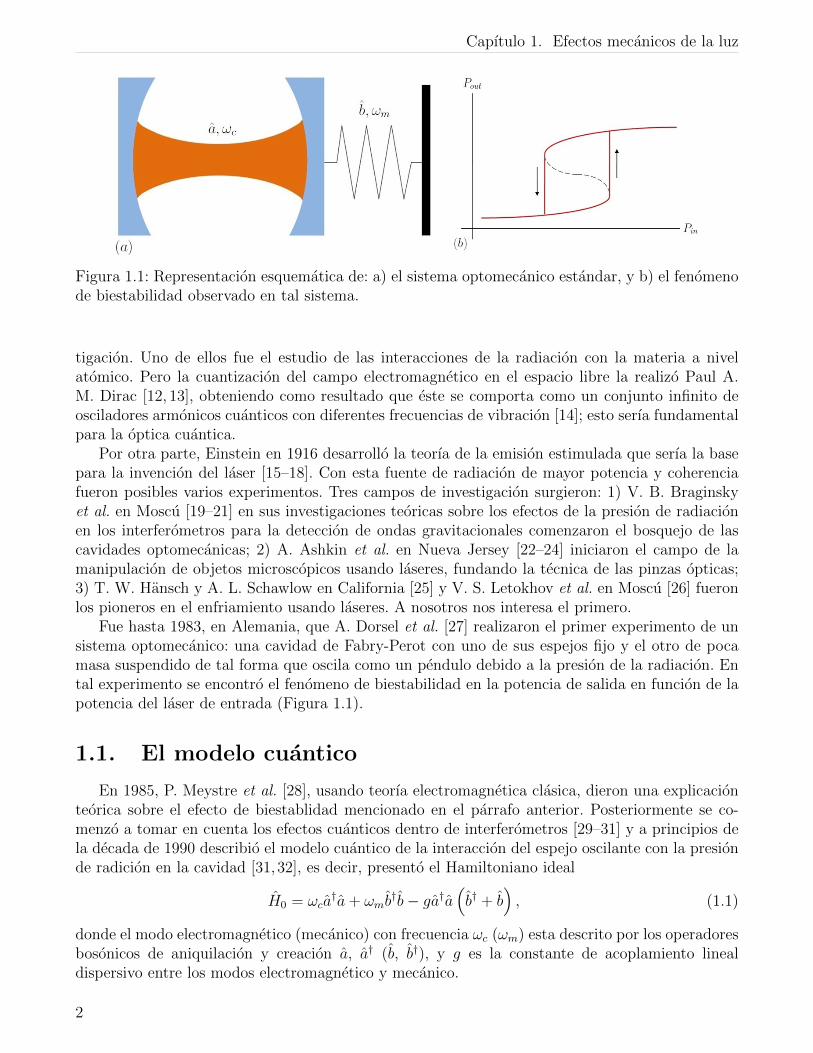
Figura 1.1: Representacion esquematica de: a) el sistema optomecanico estandar, y b) el fenomenode biestabilidad observado en tal sistema.

tigacion. Uno de ellos fue el estudio de las interacciones de la radiacion con la materia a nivelatomico. Pero la cuantizacion del campo electromagnetico en el espacio libre la realizo Paul A.M. Dirac [12, 13], obteniendo como resultado que este se comporta como un conjunto infinito deosciladores armonicos cuanticos con diferentes frecuencias de vibracion [14]; esto serıa fundamentalpara la optica cuantica.

Por otra parte, Einstein en 1916 desarrollo la teorıa de la emision estimulada que serıa la basepara la invencion del laser [15–18]. Con esta fuente de radiacion de mayor potencia y coherenciafueron posibles varios experimentos. Tres campos de investigacion surgieron: 1) V. B. Braginskyet al. en Moscu [19–21] en sus investigaciones teoricas sobre los efectos de la presion de radiacionen los interferometros para la deteccion de ondas gravitacionales comenzaron el bosquejo de lascavidades optomecanicas; 2) A. Ashkin et al. en Nueva Jersey [22–24] iniciaron el campo de lamanipulacion de objetos microscopicos usando laseres, fundando la tecnica de las pinzas opticas;3) T. W. Hansch y A. L. Schawlow en California [25] y V. S. Letokhov et al. en Moscu [26] fueronlos pioneros en el enfriamiento usando laseres. A nosotros nos interesa el primero.

Fue hasta 1983, en Alemania, que A. Dorsel et al. [27] realizaron el primer experimento de unsistema optomecanico: una cavidad de Fabry-Perot con uno de sus espejos fijo y el otro de pocamasa suspendido de tal forma que oscila como un pendulo debido a la presion de la radiacion. Ental experimento se encontro el fenomeno de biestabilidad en la potencia de salida en funcion de lapotencia del laser de entrada (Figura 1.1).

1.1. El modelo cuantico

En 1985, P. Meystre et al. [28], usando teorıa electromagnetica clasica, dieron una explicacionteorica sobre el efecto de biestablidad mencionado en el parrafo anterior. Posteriormente se co-menzo a tomar en cuenta los efectos cuanticos dentro de interferometros [29–31] y a principios dela decada de 1990 describio el modelo cuantico de la interaccion del espejo oscilante con la presionde radicion en la cavidad [31,32], es decir, presento el Hamiltoniano ideal

H0 = ωca†a+ ωmb

†b− ga†a(b† + b

), (1.1)

donde el modo electromagnetico (mecanico) con frecuencia ωc (ωm) esta descrito por los operadoresbosonicos de aniquilacion y creacion a, a† (b, b†), y g es la constante de acoplamiento linealdispersivo entre los modos electromagnetico y mecanico.

2

1.1. El modelo cuantico

Los sistemas optomecanicos son fuertes candidatos para observar efectos cuanticos a macro-escala y tambien para medir con precision fuerzas muy pequenas. Por otra parte, con el sistemacuantico se pueden generar estados enredados, comprimidos, no-Gaussianos, y otra aplicacion esel enfriamiento del oscilador mecanico [33]. En anos recientes, se ha sustituido al espejo oscilantepor una partıcula esferica o un toroide, entre muchos otros entes fısicos [34], para obtener mejoresresultados experimentales.

3

Capıtulo 1. Efectos mecanicos de la luz

4

Capıtulo 2

El sistema optomecanico estandar

Las transformaciones unitarias son una herramienta matematica de gran utilidad porque con-servan la norma y las observables fısicas en el espacio de Hilbert [35]. Sabiendo esto, aplicaremosvarias transformaciones unitarias a tres diferentes escenarios del sistema optomecanico estandar:con bombeo, considerando el amortiguamiento del oscilador mecanico y acoplamiento con un qubit.Los resultados obtenidos revelan diferentes aspectos para cada sistema, por ejemplo, el sistema op-tomecanico es equivalente a un medio Kerr y en presencia de bombeo, con un laser monocromatico,se obtienen comportamientos caracterısticos de un ion atrapado. Por otra parte, cuando tomamosen cuenta el amortiguamiento del oscilador mecanico tenemos que incluir tecnicas de superope-radores en el analisis, es decir, la dinamica del sistema se obtiene con la ecuacion maestra en laforma de Linblad.

2.1. Sistema con bombeo

Consideraremos que el sistema optomecanico se bombea con un laser monocromatico de fre-cuencia ωp. Tal sistema esta descrito por el Hamiltoniano,

Hp = ωca†a+ ωmb

†b− ga†a(b† + b

)+ 2Ω cos (ωpt)

(a† + a

), (2.1)

donde 2Ω es una constante relacionada con la raız cuadrada de la potencia del laser. Usaremos latransformacion unitaria

UR (t) = e−iωpa†at, (2.2)

para movernos al marco definido por el numero de fotones de la cavidad rotando a la frecuenciaωp, es decir,

|ψ〉 = UR (t) |φ〉 . (2.3)

Entonces, sustituyendo en la ecuacion de Schrodinger tenemos

i∂t |φ〉 = U †R (t)[Hp − ωpa†a

]UR (t) |φ〉 , (2.4)

por lo que el Hamiltoniano en el marco rotante es

HR = δa†a+ ωmb†b− ga†a

(b† + b

)+ Ω

[(1 + e2iωpt

)a† +

(1 + e−2iωpt

)a], (2.5)

5

Capıtulo 2. El sistema optomecanico estandar

y en la aproximacion de onda rotante (RWA, por sus siglas en ingles), sin tomar en cuenta losterminos que giran rapido, e±2iωmt, siempre y cuando ωp Ω, el Hamiltoniano (2.5) se reduce ala siguiente expresion

Hc = δa†a+ ωmb†b− ga†a

(b† + b

)+ Ω

(a† + a

), (2.6)

donde δ = ωc − ωp es la sintonıa entre las frecuencia de la cavidad y el laser de bombeo.

Con la finalidad de eliminar los terminos que involucran la intensidad del campo en la cavidad,a†a, y la posicion del oscilador, b† + b, usaremos el operador de desplazamiento en la base deloscilador mecanico,

Db (ε) = exp(εb† − ε†b

), (2.7)

donde ε = α a†a y α ∈ C. Entonces, para α = g/ωm el Hamiltoniano es

HD = D†b

(α a†a

)Hc Db

(α a†a

), (2.8a)

= δa†a− g2

ωm

(a†a)2

+ ωmb†b+ Ω

[a†D†

b(α) + aDb (α)

]. (2.8b)

En esta ecuacion se observa que la interaccion se hace mas complicada, es decir,

D†b

(α a†a

)a†Db

(α a†a

)= a†D†

b(α) , (2.9a)

D†b

(α a†a

)a Db

(α a†a

)= aDb (α) . (2.9b)

Ahora, para movemos al marco definido por la intensidad del campo en la cavidad rotando ala frecuencia de sintonıa δ y el numero de excitaciones mecanicas a la frecuancia ωm, usaremos latransformacion unitaria

Ucm (t) = e−i(δ a†a+ωmb†b)t, (2.10)

entonces tenemos que el Hamiltoniano en el marco rotante es

Hcm = U †cm (t)[HD −

(δ a†a+ ωmb

†b)]Ucm (t) , (2.11a)

= − g2

ωm

(a†a)2

+ Ω[a†eiδtD†

b

(α eiωmt

)+ ae−iδtDb

(α eiωmt

)], (2.11b)

ya que se tiene

U †cm (t) a†D†b

(α) Ucm (t) = a†eiδtD†b

(αeiωmt

), (2.12a)

U †cm (t) a Db (α) Ucm (t) = ae−iδtDb

(αeiωmt

). (2.12b)

Es facil ver que, en ausencia de bombeo, Ω = 0, el Hamiltoniano (2.11b) es equivalente al deun medio Kerr, es decir,

Hcm (Ω = 0) = HK (2.13a)

= − g2

ωm

(a†a)2. (2.13b)

6

2.1. Sistema con bombeo

Por otro lado, vemos que el segundo termino de (2.11b) es equivalente al Hamiltoniano de union atrapado [36], entonces usando las tecnicas de tal sistema podemos desarrollar los operadoresde desplazamiento en la siguiente forma

D†b

(αeiωmt

)= e−|α|

2/2

∞∑p,q=0

1

p!q!

(−αb†

)p (αb)qeiωm(p−q)t, (2.14a)

Db

(αeiωmt

)= e−|α|

2/2

∞∑p,q=0

1

p!q!

(αb†)p (−αb

)qeiωm(p−q)t. (2.14b)

Escogiendo la sintonıa como δ = ±sωm con s ∈ N y aplicando la RWA obtenemos para δ = +sωm,

H+ = HK + Ω e−|α|2/2

a(αb†)s(b†b)

!(b†b+ s

)!Lsb†b

(α2)

+ a†

(b†b)

!(b†b+ s

)!Lsb†b

(α2) (αb)s , (2.15)

y para δ = −sωm,

H− = HK + Ω e−|α|2/2

a(b†b)

!(b†b+ s

)!Lsb†b

(α2) (−αb

)s

+ a†(−αb†

)s (b†b)

!(b†b+ s

)!Lsb†b

(α2) , (2.16)

donde Lmn (x) es el polinomio asociado de Laguerre dado por [37]

Lmn (x) =n∑k=0

(−x)k

k!

(n+m)!

(n− k)! (m+ k)!, m ≥ 0. (2.17)

Para diferentes valores de s es posible obtener diferentes acoplamientos. Por ejemplo, parag ωm, es decir α ≈ 0, tenemos de forma general

H+ ≈ HK +Ω

s!

[a(αb†)s

+ a†(αb)s]

, (2.18a)

H− ≈ HK +Ω

s!

[a(−αb

)s+ a†

(−αb†

)s]. (2.18b)

Si δ = +ωm, obtenemos con (2.18a) el Hamiltoniano efectivo

H(1)+ ≈ HK + αΩ

(ab† + a†b

), (2.19)

el segundo termino es analogo al Hamiltoniano de un divisor de haz, este nos indica que existe unintercambio de energıa entre el campo en la cavidad y el oscilador mecanico, es decir, se puedeenfriar el espejo al transformar sus fonones termicos en fotones del campo en la cavidad [38], pero

7

Capıtulo 2. El sistema optomecanico estandar

Figura 2.1: Representacion esquematica de las transiciones debidas a los Hamiltonianos (2.19) y(2.20), en rojo y azul respectivamente, omitiento el termino Kerr porque ωm α

2 = g2/ωm 1. Laletra n (m) representa el numero de fotones (fonones).

tambien pueden transferir sus estados cuanticos [39]. Con δ = −ωm, segun (2.18b) se tiene elHamiltoniano efectivo

H(1)− ≈ HK − αΩ

(ab+ a†b†

), (2.20)

el segundo termino corresponde a la amplificacion parametrica no degenerada que es capaz degenerar pares de un foton con un fonon [39, 40], pero tambien nos expresa que se pueden enredarcuanticamente el modo optico con el mecanico [39,41].

2.2. Amortiguamiento del oscilador mecanico

Ahora consideraremos al sistema optomecanico sin bombeo pero con el oscilador mecanicoamortiguado. La dinamica del sistema esta dada por la ecuacion maestra,

d

dtρ = −i

[H0, ρ

]+ γLb [ρ] , (2.21)

donde ρ es el operador de densidad del sistema, H0 es dado por los tres primeros terminos de (2.1),la taza de decaimiento del oscilador mecanico es γ y el superoperador de Linblad es dado por

Lb [ρ] = 2bρb† − b†bρ− ρb†b. (2.22)

Usaremos la transformacion unitaria

Uc (t) = e−iωca†at, (2.23)

para movernos al marco definido por el numero de fotones a la frecuencia ωc, es decir,

ρ = U †c (t) ρc Uc (t) . (2.24)

8

2.2. Amortiguamiento del oscilador mecanico

Entonces, la ecuacion maestra queda de la forma

d

dtρc = −i

[Hm, ρc

]+ γLb [ρc] , (2.25)

con

Hm = ωmb†b− ga†a

(b† + b

). (2.26)

Ahora, aplicaremos el operador de desplazamiento (2.7) con ε = β a†a y β ∈ C al operador dedensidad ρc, es decir,

ρc = Db

(βa†a

)ρD D

†b

(βa†a

), (2.27)

sustituyendo en (2.25) tenemos

d

dtρD = −iD†

b

(βa†a

)[Hm, ρc

]+ γLb [ρc]

Db

(βa†a

), (2.28a)

= −i[HD, ρD

]+ γD†

b

(βa†a

)Lb [ρc] Db

(βa†a

), (2.28b)

= −i[HD, ρD

]+ γLb [ρD] + γLa†a [ρD]

+ γβ N [ρD] + γβ∗ N † [ρD] , (2.28c)

donde el Hamiltoniano desplazado es

HD = ε(a†a)2

+ ωmb†b+ a†a

(µb† + µ∗b

). (2.29)

Con los parametros,

ε = 2gRe (β) + ωm |β|2 , (2.30)

µ = g + ωmβ, (2.31)

y el nuevo superoperador N es

N [ρD] = 2a†aρDb† − b†a†aρD − ρDb†a†a. (2.32)

La ecuacion maestra (2.28c) es la que describe la dinamica del sistema en el marco rotantey desplazado. Para conseguir una solucion analıtica consideremos que podemos escribir a ρD (0)como

ρD (0) = ρc (0)⊗ ρm (0) , (2.33)

donde ρc (0) y ρm (0) son los operadores de densidad del campo en la cavidad y del osciladormecanico, respectivamente. Pero, suponiendo que ρc (0) es un campo termico

ρc (0) =∞∑k=0

nk

(n+ 1)k+1|k〉 〈k| , (2.34)

siendo n el numero promedio de fotones en la cavidad, y sustituyendo en (2.29) se obtiene que

β = − g

ωm − iγ. (2.35)

9

Capıtulo 2. El sistema optomecanico estandar

Con lo anterior, la ecuacion maestra (2.28c) pasa a una forma mas simple

d

dtρD = −i

[ωmb

†b, ρD

]+ γLb [ρD] , (2.36)

es decir, el Hamiltoniano efectivo para el campo termico en la cavidad se reduce al del osciladorarmonico mecanico. Finalmente la evolucion temporal del operador de densidad para este caso es

ρD (t) = eLtef(γ)Jt[e−iωmb†btρD (0) eiωmb†bt

], (2.37)

donde se han definido la funcion f (γ) y los superoperadores como

f (γ) =1− e−2γ

2γ, (2.38a)

L [ρ] = −γ(b†bρ+ ρ b†b

), (2.38b)

J [ρ] = 2γ bρ b†. (2.38c)

2.3. Sistema con un qubit

Si un qubit, sistema de dos niveles, es colocado en el sistema optomecanico sin bombeo, entoncesese sistema hıbrido esta descrito por el Hamiltoniano [42–45]

Hh = ωca†a+ ωmb

†b− ga†a(b† + b

)+ω0

2σz + λ

(aσ+ + a†σ−

), (2.39)

donde los dos ultimos terminos son del modelo de Jaynes-Cummings [46]. Siendo ω0 es la frecuenciade transicion del qubit, λ la constante de acoplamiento del quibit con el campo en la cavidad y σjcon j = ±, z las matrices de Pauli.

Nos moveremos al marco definido por el numero de fotones y la energıa del quibit rotando a lafrecuencia de la cavidad, es decir, aplicaremos la transformacion unitaria

Ur (t) = e−iωc(a†a+σz/2)t, (2.40)

con lo cual, el Hamiltoniano en el marco rotante es

Hr = U †r (t)

[Hh − ωc

(a†a+

σz2

)]Ur (t) , (2.41a)

=δ

2σz + ωmb

†b− ga†a(b† + b

)+ λ

(aσ+ + a†σ−

), (2.41b)

donde la sintonıa entre las frecuencias del qubit y la cavidad es δ = ω0 − ωc.Ahora, utilizaremos las transformaciones unitarias por la derecha

T =

(V 00 1

), T † =

(V † 00 1

), (2.42)

donde

V =1√

a†a+ 1a, V † = a†

1√a†a+ 1

, (2.43)

10

2.3. Sistema con un qubit

son los operadores de Susskind-Glogower, que cumplen

V V † = I, (2.44a)

V †V = I− |0〉 〈0| , (2.44b)

siendo I el operador unidad. Por tanto, las transformaciones definidas en (2.42) cumplen

T T † = I2, (2.45a)

T †T = I2 − |0〉 〈0| |e〉 〈e| , (2.45b)

donde I2 es la matriz unidad de tamano 2× 2. Con esto, tenemos que

Hr = T HT T† (2.46a)

=δ

2σz + ωmb

†b+ λ√a†a σx − g

(a†a− |e〉 〈e|

) (b† + b

), (2.46b)

y, reescribiendo el ultimo termino, llegamos al siguiente Hamiltoniano

HT =

[δ

2+

1

2g(b† + b

)]σz + ωmb

†b+ λ√a†aσx − g

(a†a+

1

2

)(b† + b

). (2.47)

Aplicando el operador de desplazamiento,

Db

[g

ωm

(a†a− 1

2

)]= exp

[g

ωm

(a†a− 1

2

)(b† − b

)], (2.48)

para diagonalizar (2.47) en la base de los fotones, obtenemos

HD = D†b

[g

ωm

(a†a− 1

2

)]HT Db

[g

ωm

(a†a− 1

2

)], (2.49a)

=

[δ

2+g

2

(b† + b

)+g2

ωm

(a†a− 1

2

)]σz + ωmb

†b+ λ√a†aσx −

g2

ωm

(a†a− 1

2

)2

. (2.49b)

Por claridad, haremos una rotacion alrededor del σy con la transformacion unitaria

Ry (θ) = e−iθσy =

(cos θ − sin θsin θ cos θ

), (2.50)

entonces

Hry = Ry

(π4

)HDR

†y

(π4

), (2.51a)

= ωmb†b+ ω

(a†a)σz + Ω

(a†a)σx +

g

2

(b† + b

)σx −

g2

ωm

(a†a− 1

2

)2

, (2.51b)

donde las nuevas frecuencias son dependientes del numero de fotones en la cavidad y estan dadaspor

ω(a†a)

= −λ√a†a, (2.52a)

Ω(a†a)

=δ

2+g2

ωm

(a†a− 1

2

). (2.52b)

11

Capıtulo 2. El sistema optomecanico estandar

El Hamiltoniano (2.51b) se comporta como un medio Kerr y con un qubit interactuando conlos modos del oscilador mecanico en el modelo de Jaynes-Cummings sin RWA, siendo ω

(a†a)

lafrecuencia de transicion y Ω

(a†a)

serıa el analogo a la fuerza del bombeo con dependencia en laintensidad del modo optico, a†a.

Finalmente, tenemos que

Hr = T Db

[g

ωm

(a†a− 1

2

)]R†y

(π4

)Hry Ry

(π4

)D†b

[g

ωm

(a†a− 1

2

)]T †, (2.53)

con esto, el operador de evolucion es

U (t) = T Db

[g

ωm

(a†a− 1

2

)]R†y

(π4

)e−iHrytRy

(π4

)D†b

[g

ωm

(a†a− 1

2

)]T †, (2.54)

ya que

H2r = T HrT

†T HrT†, (2.55a)

= T Hr (I2 − |0〉 〈0| |e〉 〈e|) HrT†, (2.55b)

= T H2r T† −[δ

2+ ωmb

†b+ g(b† + b

)]T |0〉 〈0| |e〉 〈e| T †

[δ

2+ ωmb

†b+ g(b† + b

)], (2.55c)

= T H2r T†, (2.55d)

y donde se ha usado

Hr |0〉 |e〉 =

[δ

2+ ωmb

†b+ g(b† + b

)]|0〉 |e〉 , (2.56a)

T |0〉 〈0| |e〉 〈e| T † = 02, (2.56b)

siendo 02 la matriz cero de tamano 2× 2.Luego, podemos usar el hecho de que el termino Kerr de (2.51b) conmuta con los demas

terminos, es decir, reescribimos e−iHryt como

e−iHryt = e−iHKte−iHamt, (2.57)

donde los Hamiltonianos H’s estan dados por

HK = − g2

ωm

(a†a− 1

2

)2

, (2.58a)

Ham = ωmb†b+ ω

(a†a)σz + Ω

(a†a)σx +

g

2

(b† + b

)σx. (2.58b)

Observamos que para e−iHamt no es posible dar una forma cerrada ya que no se ha desarrolladouna RWA adecuada, por el momento.

12

Capıtulo 3

Conclusiones

Usamos metodos puramente algebraicos para estudiar el modelo cuantico del sistema opto-mecanico estandar, descrito por la interaccion dispersiva entre dos modos bosonicos, el electro-magnetico y el mecanico. Mostramos que un desplazamiento en la base del modo mecanico propor-cional al estado de numero del campo electromagnetico, tambien conocida como transformacionde polaron, nos conduce a un modelo efectivo formado por un medio electromagnetico Kerr y elacoplamiento entre ambos modos se vuelve similar al de un ion atrapado. Tomando desarrollosmatematicos aplicados al modelo de un ion atrapado, se mostro que es posible obtener diferentesmodelos de interaccion que permiten enfriamiento mecanico, transferencia de estados cuanticos yamplificacion parametrica no degenerada; esto se logra escogiendo una sintonıa entre las frecuenciasde ambos modos y del bombeo que sea multiplos enteros de la frecuencia del modo mecanico.

Para el caso en que el oscilador mecanico se acopla con el medio ambiente, estudiamos laecuacion maestra de Linblad con tecnicas de superoperadores y obtuvimos un superoperador deevolucion cuando campo electrico inicial es termico.

Finalmente, utilizamos operadores unitarios por la derecha para estudiar el sistema optomecani-co cuantico con un atomo de dos niveles interactuando con el campo electromagnetico de la cavidad.Con esa tecnica encontramos que el campo electromagnetico hace posible el acoplamiento entre elqubit y el modo mecanico de la forma de Jaynes-Cummings sin la aproximacion de onda rotante.

13

Capıtulo 3. Conclusiones

14

Apendice A

Artıculos publicados en revistasinternacionales como producto de lasinvestigaciones realizadas en esta tesis

15

Invited Comment

Operator approach to quantumoptomechanics

C Ventura-Velázquez, B M Rodríguez-Lara and H M Moya-Cessa

Instituto Nacional de Astrofísica, Óptica y Electrónica, Calle Luis Enrique Erro No. 1, Sta. Ma.Tonantzintla, Pue. CP 72840, México

E-mail: bmlara@inaoep.mx

Received 29 September 2014, revised 7 November 2014Accepted for publication 10 November 2014Published 13 May 2015

AbstractWe study the mirror-field interaction in several frameworks: when it is driven, when it is affectedby an environment, and when a two-level atom is introduced in the cavity. By using operatortechniques, we show either how these problems may be solved or how the Hamiltoniansinvolved, via sets of unitary transformations, may be taken to known Hamiltonians for whichthere exist approximate solutions.

Keywords: mirror-field interactions, superoperators, non-classical states

1. Introduction

Light carries momentum and, therefore, it can exert pressureover matter [1, 2], be it from incoherent [3–5] or coherent [6–8] sources. Such radiation pressure allows, for example, thecoupling of mechanical degrees of freedom to electro-magnetic cavity modes in cavities with a moving mirror, bothin the classical [9–11] and quantum regimes [12–16]. The so-called standard optomechanical model in quantum optics ismodeled after a classical Fabry–Pérot resonator where onemirror is free to move in a pendulum-like motion [12]. In thebeginning, the interest in this optomechanical system wasfocused on the detection of gravitational waves. When theeffects of radiation pressure on the device were shown to be adetection issue [14], it became important to beat the standardquantum limit [17, 18]. An interesting solution to this pro-blem is to prepare the mechanical oscillator in a non-Gaussianstate [18–20]; thus quantum state engineering of themechanical mode became important. Furthermore, it is ofgreat interest to test quantum theory with macroscopicdegrees of freedom [21–23], and quantum optomechanicalsystems provide an experimentally feasible testing groundand may even be a viable quantum information plat-form [24, 25].

The canonical quantization of a Fabry–Pérot cavity witha pendulum-like mirror delivers an ideal Hamiltonian in the

form [14, 16, 26, 27],

ω ω= + − +( )H a a b b ga a b bˆ ˆ ˆ ˆ ˆ ˆ ˆ ˆ ˆ , (1)c m† † † †

where the cavity field and mechanical oscillator modes aredescribed by their effective frequencies, ωc and ωm, and

creation (annihilation) operators, a† (a) and b†(b), in that

order. Dispersive linear coupling between the modes occurs,and it is quantified by the coupling constant g. Here, we willrevisit this and aggregated models through an operatorapproach. In the following section, we will show the well-known equivalence between the standard optomechanicalmodel and a Kerr medium. We will also show that the drivenoptomechanical model is similar to a trapped ion, and that isthe reason behind the use of sideband cooling and other ion-trap cavity electrodynamics (QED) techniques to preparemechanical states. We will couple the mechanical mode to anenvironment and introduce superoperator techniques to makethe problem tractable. We will introduce a new result,showing that the open system reduces to a damped mechan-ical oscillator in the case of a thermal electromagnetic fieldmode in the cavity. Finally, we will add a two-level system,interacting with the cavity field under Jaynes–Cummingsdynamics, to the model. We will show that a right unitaryapproach allows us to understand how the electromagneticfield mode mediates coupling between the atom and the

| Royal Swedish Academy of Sciences Physica Scripta

Phys. Scr. 90 (2015) 068010 (6pp) doi:10.1088/0031-8949/90/6/068010

0031-8949/15/068010+06$33.00 © 2015 The Royal Swedish Academy of Sciences Printed in the UK1

mechanical oscillator, but a closed-form time evolutionoperator requires developing an adequate rotating waveapproximation (RWA) compatible with the right unitarytransformations.

2. Standard optomechanical model

The first experimental realization of a classical optomecha-nical cavity consisted of a Fabry–Perot cavity with a fixedmirror and a pendulum-like moving mirror [10]. In thisexperiment and other proposals [27], optical bistability andmirror confinement due to changes in the physical length ofthe cavity induced by radiation pressure were shown. Thisbistable phonemenon was similar to that found in fixed cav-ities filled with nonlinear media [28]. Soon, it was shown thatthe equations of motion of the quantum optomechanicalsystem showed optical bistability due to its equivalence to aKerr medium [29, 30]. Since then, the topic has been revisitedthrough different approaches [31, 32].

2.1. Driven system

Here we are interested in an algebraic approach. For thisreason we will start with the standard Hamiltonian for apumped optomechanical system,

ω ω

Ω ω

= + − +

+ +( )

( )( )

H a a b b ga a b b

t a a

ˆ ˆ ˆ ˆ ˆ ˆ ˆ ˆ ˆ

cos ˆ ˆ , (2)

p c m

p

† † † †

†

where the laser pump frequency is given by ωp and itsstrength by Ω. First, we need to get rid of the time depen-dence, so we move to a frame defined by the cavity fieldphoton number rotating at the pump frequency,

ψ ϕ⟩ = ⟩U t| ˆ ( )| ,R with = ω−U tˆ ( ) eRa ati ˆ ˆp†, such that we can

write the Schrödinger equation as,

⎡⎣ ⎤⎦ϕ ϕ∂ =i U t H U tˆ ( ) ˆ ˆ ( ) . (3)t R p R

Thus the effective Hamiltonian in the new frame,

⎡⎣ ⎤⎦ϕ ω ϕ∂ = −i U t H a a U tˆ ( ) ˆ ˆ ˆ ˆ ( ) , (4)t R p p R† †

is given by the following,

⎡⎣ ⎤⎦

⎡⎣ ⎤⎦

ω

δ ωΩ

= −

= + − +

+ + + +ω ω−

( )( ) ( )

H U t H a a U t

a a b b ga a b b

a a

ˆ ˆ ( ) ˆ ˆ ˆ ˆ ( ),

ˆ ˆ ˆ ˆ ˆ ˆ ˆ ˆ

2ˆ 1 e ˆ 1 e . (5)

R R p p R

p m

t t

† †

† † † †

† 2i 2ip p

Finally, we can make an RWA to eliminate the terms rotatingat twice the pump frequency, ω± te 2i p , and obtain,

δ ω Ω= + − + + +( ) ( )H a a b b ga a b b a aˆ ˆ ˆ ˆ ˆ ˆ ˆ ˆ ˆ2

ˆ ˆ , (6)c p m† † † † †

where the detuning between the pump and cavity field fre-quencies is δ ω ω= − .p c p Now, we want to get rid of theterms involving the cavity field intensity and the canonical

position of the mechanical oscillator. For this, let us define adisplacement on the mechanical oscillator basis,

ξ = ξ ξ−( ) ( )D ˆ e , (7)bb b

ˆˆ ˆ ˆ ˆ† †

where the operator ξ is either a cavity field operator or just acomplex number. If we change into a joint basis defined bysuch a displacement, we arrive at a Hamiltonian closer to ourgoal [33, 34],

⎛⎝⎜

⎞⎠⎟

⎛⎝⎜

⎞⎠⎟

⎡⎣⎢

⎛⎝⎜

⎞⎠⎟

⎛⎝⎜

⎞⎠⎟⎤⎦⎥

ω ω

δω

ω Ωω

ω

=

= − + +

+

( )

H Dga a H D

ga a

a ag

a a b b a Dg

aDg

ˆ ˆ ˆ ˆ ˆ ˆ ˆ ˆ ,

ˆ ˆ ˆ ˆ ˆ ˆ2

ˆ ˆ

ˆ ˆ . (8)

D bm

c bm

pm

m bm

bm

ˆ† † ˆ †

†2

† 2 † † ˆ†

ˆ

Note that moving into the joint-displaced basis defined bythe operator ωD ga aˆ ( ˆ ˆ )b mˆ † helps us to get rid of the lineardispersive mechanical-cavity field modes interaction but

introduces a Kerr term for the cavity field, ( )a aˆ ˆ†2, and

switches the interaction to the driving terms that become

ωa D gˆ ˆ ( )b m†

ˆ†

and ωaD gˆ ˆ ( )b mˆ . In order to reach our goal, wenow move to the rotating frames defined by the intensity inthe cavity field rotating at the detuning frequency and thenumber of excitations in the mechanical mode rotating with

frequency ωm,⎡⎣⎢

⎤⎦⎥= δ ω− +( )U tˆ ( ) ecm

a a b b ti ˆ ˆ ˆ ˆp m

† †

. Thus, we reachour goal,

⎡⎣⎢

⎛⎝⎜

⎞⎠⎟

⎛⎝⎜

⎞⎠⎟⎤⎦⎥

δ ω

ωΩ

ω

ω

= − −

= − +

+

δ ω

δ ω−

( )( )

H U t H a a b b U t

ga a a D

g

a Dg

ˆ ˆ ( ) ˆ ˆ ˆ ˆ ˆ ˆ ( )

ˆ ˆ2

ˆ e ˆ e

ˆe ˆ e . (9)

cm cm D p m cm

m

tb

m

t

tb

m

t

† † †

2† 2 † i ˆ

† i

i ˆ i

p m

p m

Note that in the absence of driving, Ω = 0, the standardoptomechanical Hamiltonian is equivalent to a KerrHamiltonian [29–32], and it has been shown that measuringthe field quadratures of this system delivers informationabout the Wigner characteristic function of the mechanicaloscillator [35]. Furthermore, from such a form it isstraightforward to discuss light squeezing [36], photonblockade [37], and single photon dynamics [38], to mentiona few examples.

In the presence of driving, the second term in the effec-tive Hamiltonian Hcm is quite interesting. Note how similarthese terms are to that of a driven trapped ion [39]; as a matterof fact, if we substituted the cavity field operators with Paulimatrices, we would recover the trapped ion Hamiltonian.Thus, we can use an approach similar to that used in trapped-ion QED and expand the mechanical mode operators into

2

Phys. Scr. 90 (2015) 068010 Invited Comment

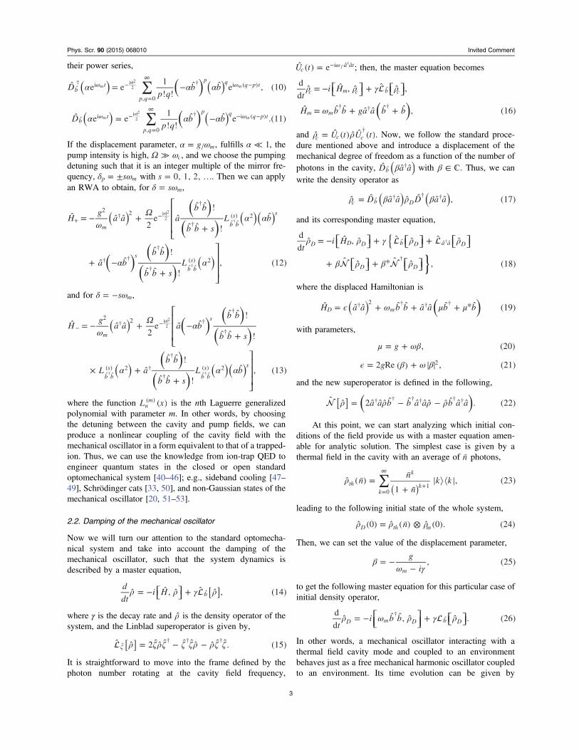
their power series,

∑α α α= −ω ω−

=

∞−α ( )( ) ( )D

p qb bˆ e e

1

! !ˆ ˆ e , (10)b

t

p q

p q q p tˆ† i

, 0

† i ( )m m2

2

∑α α α= −ω ω−

=

∞− −α ( )( ) ( )D

p qb bˆ e e

1

! !ˆ ˆ e .(11)b

t

p q

p q q p tˆ i

, 0

† i ( )m m2

2

If the displacement parameter, α ω= g m, fulfills α ≪ 1, thepump intensity is high, Ω ω≫ c, and we choose the pumpingdetuning such that it is an integer multiple of the mirror fre-quency, δ ω= ±sp m with = …s 0, 1, 2, . Then we can applyan RWA to obtain, for δ ω= s m,

⎡

⎣

⎢⎢⎢⎤

⎦

⎥⎥⎥

ωΩ α α

α α

= − ++

+ −+

+ − α ( )( )

( ) ( )( )

( ) ( )( )

( )

Hg

a a ab b

b b sL b

a bb b

b b sL

ˆ ˆ ˆ2e ˆ

ˆ ˆ !

ˆ ˆ !

ˆ

ˆ ˆˆ ˆ !

ˆ ˆ !, (12)

m b b

s s

s

b b

s

2† 2

†

† ˆ ˆ( ) 2

† †

†

† ˆ ˆ( ) 2

2

2 †

†

and for δ ω= −s m,

⎡

⎣

⎢⎢⎢⎤

⎦

⎥⎥⎥

ωΩ α

α α α

= − + −+

× ++

− − α ( ) ( )( )

( )( )

( )

( ) ( )( )

Hg

a a a bb b

b b s

L ab b

b b sL b

ˆ ˆ ˆ2e ˆ ˆ

ˆ ˆ !

ˆ ˆ !

ˆ

ˆ ˆ !

ˆ ˆ !

ˆ , (13)

m

s

b b

s

b b

s s

2† 2 †

†

†

ˆ ˆ( ) 2 †

†

† ˆ ˆ( ) 2

2

2

† †

where the function L x( )nm( ) is the nth Laguerre generalized

polynomial with parameter m. In other words, by choosingthe detuning between the cavity and pump fields, we canproduce a nonlinear coupling of the cavity field with themechanical oscillator in a form equivalent to that of a trapped-ion. Thus, we can use the knowledge from ion-trap QED toengineer quantum states in the closed or open standardoptomechanical system [40–46]; e.g., sideband cooling [47–49], Schrödinger cats [33, 50], and non-Gaussian states of themechanical oscillator [20, 51–53].

2.2. Damping of the mechanical oscillator

Now we will turn our attention to the standard optomecha-nical system and take into account the damping of themechanical oscillator, such that the system dynamics isdescribed by a master equation,

⎡⎣ ⎤⎦ ρ ρ γ ρ= − + [ ]d

dti Hˆ ˆ , ˆ ˆ ˆ , (14)b

where γ is the decay rate and ρ is the density operator of thesystem, and the Linblad superoperator is given by,

ρ ζρζ ζ ζρ ρζ ζ= − −ζ [ ]ˆ ˆ 2 ˆ ˆ ˆ ˆ ˆ ˆ ˆ ˆ ˆ. (15)ˆ† † †

It is straightforward to move into the frame defined by thephoton number rotating at the cavity field frequency,

= ω−U tˆ ( ) eca ati ˆ ˆf†; then, the master equation becomes

⎡⎣ ⎤⎦ ⎡⎣ ⎤⎦ρ ρ γ ρ

ω

= − +

= + +( )t

i H

H b b ga a b b

d

dˆ ˆ , ˆ ˆ ˆ ,

ˆ ˆ ˆ ˆ ˆ ˆ ˆ , (16)

c m c b c

m m

ˆ

† † †

and ρ ρ= U t U tˆ ˆ ( ) ˆ ˆ ( )c c c†

. Now, we follow the standard proce-dure mentioned above and introduce a displacement of themechanical degree of freedom as a function of the number ofphotons in the cavity, β( )D a aˆ ˆ ˆb

† with β ∈ . Thus, we canwrite the density operator as

ρ β ρ β= ( ) ( )D a a D a aˆ ˆ ˆ ˆ ˆ ˆ ˆ ˆ , (17)c b Dˆ † † †

and its corresponding master equation,

⎡⎣ ⎤⎦ ⎡⎣ ⎤⎦ ⎡⎣ ⎤⎦⎡⎣ ⎤⎦ ⎡⎣ ⎤⎦

ρ ρ γ ρ ρ

β ρ β ρ

= − + +

+ +

ti H

d

dˆ ˆ , ˆ ˆ ˆ ˆ ˆ

ˆ ˆ * ˆ ˆ , (18)

D D D b D a a D

D D

ˆ ˆ ˆ

†

†

where the displaced Hamiltonian is

ϵ ω μ μ= + + +( )( )H a a b b a a b bˆ ˆ ˆ ˆ ˆ ˆ ˆ ˆ * ˆ (19)D m† 2 † † †

with parameters,

μ ωβ= +g , (20)

ϵ β ω β= +g2 Re ( ) , (21)2

and the new superoperator is defined in the following,

ρ ρ ρ ρ= − −( )[ ] a a b b a a b a aˆ ˆ 2 ˆ ˆ ˆ ˆ ˆ ˆ ˆ ˆ ˆ ˆ ˆ ˆ . (22)† † † † † †

At this point, we can start analyzing which initial con-ditions of the field provide us with a master equation amen-able for analytic solution. The simplest case is given by athermal field in the cavity with an average of n photons,

∑ρ =+=

∞

+( )n

n

nk kˆ ( ¯)

¯

1 ¯, (23)th

k

k

k0

1

leading to the following initial state of the whole system,

ρ ρ ρ= ⊗nˆ (0) ˆ ( ¯) ˆ (0). (24)D th m

Then, we can set the value of the displacement parameter,

βω γ

= −−g

i, (25)

m

to get the following master equation for this particular case ofinitial density operator,

⎡⎣⎢

⎤⎦⎥ ⎡⎣ ⎤⎦ρ ω ρ γ ρ= − +

ti b b

d

dˆ ˆ ˆ, ˆ ˆ . (26)D m D b D

†ˆ

In other words, a mechanical oscillator interacting with athermal field cavity mode and coupled to an environmentbehaves just as a free mechanical harmonic oscillator coupledto an environment. Its time evolution can be given by

3

Phys. Scr. 90 (2015) 068010 Invited Comment

standard superoperator techniques [54–57],

⎡⎣⎢

⎤⎦⎥ρ ρ= ω ω−γ

γ− −

tˆ ( ) e e e ˆ (0)e , (27)DLt Jt b bt

Db btˆ ˆ i ˆ ˆ i ˆ ˆ

m m1 e 2

2† †

with the auxiliary superoperators,

ρ γ ρ ρ γ ρ ρ= = − +( )J b b L b b b bˆ ˆ 2 ˆ ˆ ˆ , ˆ ˆ ˆ ˆ . (28)† † †

3. Hybrid qubit-optomechanical model

Recently, it has been proposed to couple a two-level atom tothe standard optomechanical model [58–60]; such a hybridmodel is described by the Hamiltonian,

ω ωω σ λ σ σ

= + − +

+ + +− +

( )( )

H a a b b ga a b b

a a

ˆ ˆ ˆ ˆ ˆ ˆ ˆ ˆ ˆ

2ˆ ˆ ˆ ˆ ˆ , (29)

h c m

z

† † † †

0 †

where the two-level system is described by Pauli matrices, σ jwith = ±j z, , and the transition frequency ω0, and the atom-field coupling is given by the parameter λ. Here, we will firstmove into the frame defined by the photon number and thequbit energy rotating at the cavity field frequency,

= ω σ− +( )U era a ti ˆ ˆ ˆ 2c z†

, such that the effective Hamiltonian is,

δ σ ω λ σ σ= + + +

− +

− +

( )( )H b b a a

ga a b b

ˆ2ˆ ˆ ˆ ˆ ˆ ˆ ˆ

ˆ ˆ ˆ ˆ , (30)

r z m† †

† †

where the detuning between the qubit and cavity field fre-quency is given by δ ω ω= − c0 . We can follow a rightunitary approach [61–63] and rewrite this Hamiltonian in theform,

=H TH Tˆ ˆ ˆ ˆ , (31)r T†

where the auxiliary Hamiltonian is given by the expression,

δ σ ω λ σ= + +

− + + +( ) ( )H b b a a

ga a b b g b b e e

ˆ2ˆ ˆ ˆ ˆ ˆ ˆ

ˆ ˆ ˆ ˆ ˆ ˆ , (32)

T z m x† †

† † †

where we have diagonalized the cavity field part by using theoperators,

⎛⎝⎜

⎞⎠⎟

⎛⎝⎜

⎞⎠⎟= =T V T Vˆ ˆ 0

0 1, ˆ ˆ 0

0 1. (33)

† †

They are right unitary due to the properties of the Susskind–Glogower operators,

=+

=+

Va a

a V aa a

ˆ 1

ˆ ˆ 1ˆ, ˆ ˆ

1

ˆ ˆ 1, (34)

†

† †

†

that fulfill =VVˆ ˆ 1,†but = − ⟩⟨V Vˆ ˆ 1 |0 0|†

. Note that we can

rearrange the following terms in the auxiliary Hamiltonian,

⎜ ⎟⎛⎝

⎞⎠σ

+ − +

= + − − +

( ) ( )( ) ( )

g b b e e ga a b b

g b b g a a b b

ˆ ˆ ˆ ˆ ˆ ˆ

1

2ˆ ˆ ˆ ˆ ˆ

1

2ˆ ˆ , (35)z

† † †

† † †

and use again the displacement operator in terms of thenumber of photons in the field to obtain,

⎜ ⎟ ⎜ ⎟

⎜ ⎟

⎜ ⎟

⎡⎣⎢

⎛⎝

⎞⎠⎤⎦⎥

⎡⎣⎢

⎛⎝

⎞⎠⎤⎦⎥

⎡⎣⎢

⎛⎝

⎞⎠⎤⎦⎥

⎛⎝

⎞⎠

ω ωδ

ωσ ω

λ σω

= − −

= + + + − +

+ − −

( )

H Dg

a a H Dg

a a

gb b

ga a b b

a ag

a a

ˆ ˆ ˆ ˆ1

2ˆ ˆ ˆ ˆ

1

2,

2 2ˆ ˆ ˆ ˆ

1

2ˆ ˆ ˆ

ˆ ˆ ˆ ˆ ˆ1

2. (36)

dm

Tm

mz m

xm

† † †

†2

† †

†2

†2

Now, just for the sake of clarity, we can introduce a rotationaround σy,

θ = θσ−R ( ) e , (37)yi ˆy

and rewrite our initial hybrid optomechanical Hamiltonian as,

⎜ ⎟

⎜ ⎟

⎜ ⎟

⎜ ⎟

⎡⎣⎢

⎛⎝

⎞⎠⎤⎦⎥

⎛⎝

⎞⎠

⎛⎝

⎞⎠

⎡⎣⎢

⎛⎝

⎞⎠⎤⎦⎥

ωπ

πω

= −

× −

H TDg

a a R

H R Dg

a a T

ˆ ˆ ˆ ˆ1

2ˆ

4

ˆ ˆ4

ˆ ˆ ˆ1

2ˆ , (38)

r bm

y

a y bm

ˆ † †

ˆ† † †

with the final auxiliary Hamiltonian given by,

= +H H Hˆ ˆ ˆ . (39)a K am

Note that the effective Kerr medium,

⎜ ⎟⎛⎝

⎞⎠ω

= − −Hg

a aˆ ˆ ˆ1

2, (40)K

m

2†

2

commutes with the rest of the terms,

ω ω σ Ω σ σ= + + + +( )( ) ( )H b b a a a ag

b bˆ ˆ ˆ ˜ ˆ ˆ ˆ ˜ ˆ ˆ ˆ2

ˆ ˆ ˆ , (41)am m z x x† † † †

which can be reinterpreted as a driven two-level atom inter-acting with the mechanical oscillator under the Jaynes–Cummings model [64] without the RWA. The two-leveltransition frequency and driving strength depend on theintensity of the optical mode,

ω λ= −( )a a a a˜ ˆ ˆ ˆ ˆ , (42)† †

⎜ ⎟⎛⎝

⎞⎠Ω δ

ω= + −( )a a

ga a˜ ˆ ˆ

2 2ˆ ˆ

1

2. (43)

m

†2

†

4

Phys. Scr. 90 (2015) 068010 Invited Comment

At this point we could note that,

⎛⎝⎜⎜

⎞⎠⎟⎟

⎡⎣⎢

⎤⎦⎥

⎛⎝⎜⎜

⎞⎠⎟⎟

⎡⎣⎢

⎤⎦⎥

∑

∑

δ ω

δ ω

= − ⊗ ⊗

= − + + +

× ⊗ ⊗

× + + +

=

=

∞

=

∞

( )

( )

H TH T TH e e k k H T

TH T k g b b

e e V V k k

k g b b

TH T

ˆ ˆ ˆ ˆ ˆ ˆ 0 0 ˆ ˆ ,

ˆ ˆ ˆ2

ˆ ˆ

ˆ 0 0 ˆ

2ˆ ˆ ,

ˆ ˆ ˆ , (44)

r T T

k

T

T m

k

m

T

2 2 †

0

†

2 † †

†

0

†

2 †

and write the evolution operator of the total system as,

⎜ ⎟

⎜ ⎟

⎜ ⎟

⎜ ⎟

⎡⎣⎢

⎛⎝

⎞⎠⎤⎦⎥

⎛⎝

⎞⎠

⎛⎝

⎞⎠

⎡⎣⎢

⎛⎝

⎞⎠⎤⎦⎥

ωπ

πω

= −

× −

−U t TDg

a a R R

Dg

a a T

ˆ ( ) ˆ ˆ ˆ ˆ1

2ˆ

4e ˆ

4ˆ ˆ ˆ

1

2ˆ , (45)

bm

yH t

y

bm

ˆ † i ˆ †

ˆ† † †

a

where we can use the fact that the Kerr term commutes,

=− − −e e e , (46)H t H t H ti ˆ i ˆ i ˆa K am

but in the end, it is not possible to provide a closed form

propagator from the term −e H ti ˆam . Working a formal rotatingwave approximation in this scenario is beyond our currentpurpose.

4. Conclusion

We used a purely algebraic approach to revisit the standardquantum optomechanical model describing the linear dis-persive interaction between two bosonic modes, electro-magnetic and mechanical. We showed that a displacement onthe mechanical basis proportional to the number state in theelectromagnetic basis, sometimes called a polaron transfor-mation, delivers a model consisting of an effective electro-magnetic Kerr medium plus a coupling between theelectromagnetic and mechanical modes similar to that foundin a trapped ion. We took advantage of ion-trap QED andshowed that it is possible to implement a series of optical–mechanical couplings that allow trapping, cooling, andparametric coupling phenomena by choosing detuningsbetween the electromagnetic mode and the classical pumpthat are integer multiples of the mechanical frequency.

We also used superoperator techniques to revisit thestandard optomechanical system when the mechanical oscil-lator is coupled to the environment. Here we worked out ageneral expression and gave a closed-form time evolutionsuperoperator for the particular case of a thermal electro-magnetic field.

Finally, we presented a right unitary approach to a systemformed by the addition of a two-level atom interacting withthe electromagnetic mode. This approach makes it simple torealize that the electromagnetic mode enables the coupling

between the two-level system with the mechanical mode in aJaynes–Cummings without the RWA form but also shows usthat it is not possible to provide a closed-form time evolutionoperator unless an adequate approximation scheme isdeveloped.

Acknowledgments

C Ventura Velázquez acknowledges financial support fromCONACyT through the master degree scholarship #294810.

References

[1] Poynting J H 1909 Proc. R. Soc. London, Ser. A 82 560–67[2] Poynting J H 1910 The Pressure of Light (London: E. S.

Gorham)[3] Lebedev P N 1901 Ann. Phys. (Leipzig)) 6 433 –58[4] Nichols E F and Hull G F 1901 Phys. Rev. 12 307–20[5] Lebedev P 1910 Ann. Phys. 32 411–37[6] Letokhov V S 1968 Zh. Eksp. Teor. Fiz. 7 348–51[7] Ashkin A 1970 Phys. Rev. Lett. 24 156–59[8] Dalibard J, Reynaud S and Cohen-Tannoudji C 1984 J. Phys.

B: At. Mol. Phys. 17 4577–94[9] Braginskiı V B and Manukin A B 1967 Zh. Eksp. Teor. Fiz. 52

986–89[10] Dorsel A, McCullen J D, Meystre P, Vignes E and Walther H

1983 Phys. Rev. Lett. 51 1550–53[11] Gozzini A, Maccarrone F, Mango F, Longo I and Barbarino S

1985 J. Opt. Soc. Am. B 2 1841–45[12] Braginskiı V B 1967 Zh. Eksp. Teor. Fiz. 53 1434–41[13] Braginskiı V B and Nazarenko V S 1969 Zh. Eksp. Teor. Fiz.

57 1421–14[14] Caves C M 1980 Phys. Rev. Lett. 45 75–79[15] Jacobs K, Tombesi P, Collett M J and Walls D F 1994 Phys.

Rev. A 49 1961–66[16] Law C K 1995 Phys. Rev. 51 2537–42[17] Caves C M 1981 Phys. Rev. D 23 1693–708[18] Pace A F, Collett M J and Walls D F 1993 Phys. Rev. A 47

3173–89[19] Mancini S and Tombesi P 1994 Phys. Rev. A 49 4055–65[20] Khalili F, Danilishin S, Miao H, Müller-Ebhardt H,

Yang H and Chen Y 2010 Phys. Rev. Lett. 105 070403[21] Leggett A J 1980 Prog. Theor. Phys. Suppl. 69 80–100[22] Bose S, Jacobs K and Knight P L 1999 Phys. Rev. A 59

3204–10[23] Poot M and van der Zant H S J 2012 Phys. Rep. 511 273–335[24] Kippenberg T J and Vahala K J 2008 Science 321 1172–76[25] Marquardt F and Girvin S M 2009 Physics 2 40[26] Moore G T 1970 J. Math. Phys. 11 2679–91[27] Meystre P, Wright E M, McCullen J D and Vignes E 1985

J. Opt. Soc. Am. B 2 1830–40[28] Marburger J H and Felber F S 1978 Phys. Rev. A 17 335–42[29] Hilico L, Courty J M, Fabre C, Giacobino E, Abram I and

Oudar J L 1992 Appl. Phys. B 55 202–09[30] Jackel M T and Reynaud S 1992 Quantum Opt. 4 39–53[31] Rodríguez-Lara B M and Moya-Cessa H 2004 Optical

bistability in a cavity with one moving mirror Proc. 8th Int.Conf. on Squeezed States and Uncertainty Relationspp 354–59

[32] Aldana A, Bruder C and Nunnenkamp A 2013 Phys. Rev. A 88043826

[33] Bose S, Jacobs K and Knight P L 1997 Phys. Rev. A 564175–86

5

Phys. Scr. 90 (2015) 068010 Invited Comment

[34] Ludwig M, Safavi-Naeini A H, Painter O and Marquardt F2012 Phys. Rev. Lett. 109 063601

[35] Rodríguez-Lara B M and Moya-Cessa H 2004 Rev. Mex. Fis.50 213–15

[36] Safavi-Naeini A H, Gröblacher S, Hill J T, Chan J,Aspelmeyer M and Painter O 2013 Nature 500 185–89

[37] Rabl P 2011 Phys. Rev. Lett. 107 063601[38] Tang H X and Vitali D 2014 Phys. Rev. A 89 063821[39] Moya-Cessa H, Soto-Eguibar F, Vargas-Martínez J M,

Juárez-Amaro R and Zúñiga-Segundo A 2012 Phys. Rep.513 229–61

[40] Mancini S, Giovannetti V, Vitali D and Tombesi P 2002 Phys.Rev. Lett. 88 120401

[41] Bhattacharya M, Giscard P L and Meystre P 2008 Phys. Rev. A77 030303

[42] Marshall W, Simon C, Penrose R and Bouwmeester D 2003Phys. Rev. Lett. 91 130401

[43] Hong T, Yang H, Miao H and Chen Y 2013 Phys. Rev. A 88023812

[44] Akram U, Bowen W P and Milburn G J 2013 New J. Phys. 15093007

[45] Xu G F and Law C K 2013 Phys. Rev. A 87 053849[46] Xu X W, Wang H, Zhang J and Liu Y X 2013 Phys. Rev. A 88

063819[47] Bhattacharya M and Meystre P 2007 Phys. Rev. Lett. 99

073601[48] Marquardt F, Chen J P, Clerk A A and Girvin S M 2007 Phys.

Rev. Lett. 99 093902

[49] Wilson-Rae I, Nooshi N, Zwerger W and Kippenberg T J 2007Phys. Rev. Lett. 99 093901

[50] Mancini S, Manʼko V I and Tombesi P 1997 Phys. Rev. A 553042–50

[51] Gu W J, Li G X and Yang Y P 2013 Phys. Rev. A 88 013835[52] Kronwald A and Marquardt F 2013 Phys. Rev. Lett. 111

133601[53] Gu W J, Li G X, Wu S P and Yang Y P 2014 Opt. Express 22

18254–67[54] Phoenix S J D 1990 Phys. Rev. A 41 5132–38[55] Arévalo-Aguilar L M and Moya-Cessa H M 1996 Rev. Mex.

Fis. 42 675–83[56] Arévalo-Aguilar L M and Moya-Cessa H M 1998 Quantum

Semiclass. Opt. 10 671–74[57] Lu H X, Yang J, Zhang Y D and Chen Z B 2003 Phys. Rev. A

67 024101[58] Ian H, Gong Z R, Liu Y X, Sun C P and Nori F 2008 Phys.

Rev. A 78 013824[59] Genes C, Vitali D and Tombesi P 2008 Phys. Rev. A 77

050307[60] Pflanzer A C, Romero-Isart O and Cirac J I 2013 Phys. Rev. A

88 033804[61] Tang Z 1996 Phys. Rev. A 54 154–73[62] Rodríguez-Lara B M, Rodríguez-Méndez D and

Moya-Cessa H 2011 Phys. Lett. A 375 3770–74[63] Rodríguez-Lara B M and Moya-Cessa H M 2013 J. Phys. A:

Math. Theor. 46 095301[64] Jaynes E T and Cummings F W 1963 Proc. IEEE 51 89–109

6

Phys. Scr. 90 (2015) 068010 Invited Comment

Apendice A. Artıculos publicados en revistas internacionales como producto de lasinvestigaciones realizadas en esta tesis

22

Bibliografıa

Bibliografıa

[1] J. H. Poynting, The Pressure of Light. The Romance of Science, New York: E. S. Gorham,1910.

[2] P. Meystre and S. Stenholm, “Introdution to feature on the mechanical effects of light,” J.Opt. Soc. Am. B, vol. 2, pp. 1706–1706, Nov 1985.

[3] J. C. Maxwell, “A dynamical theory of the electromagnetic field,” Phil. Trans. R. Soc. Lond.,vol. 155, pp. 459–512, January 1865.

[4] J. C. Maxwell, A treatise on electricity and magnetism, vol. 1. Oxford: Clarendon Press, 1873.

[5] J. C. Maxwell, A treatise on electricity and magnetism, vol. 2. Oxford: Clarendon Press, 1873.

[6] M. H. Shamos, ed., Great experiments in physiscs, Firsthand accounts from Galileo to Einstein.New York: Dover Publications, 1987.

[7] P. N. Lebedev, “Experimental examination of light pressure,” Ann. der Physik, vol. 311,no. 11, pp. 433–458, 1901.

[8] E. F. Nichols and G. F. Hull, “A preliminary communication on the pressure of heat and lightradiation,” Phys. Rev. (Series I), vol. 13, no. 5, pp. 307–320, 1901.

[9] E. F. Nichols and G. F. Hull, “The pressure due to radiation (second paper),” Phys. Rev.(Series I), vol. 13, no. 5, pp. 26–50, 1903.

[10] M. Planck, “On the law of the energy distribution in the normal spectrum,” Ann. der Physik,vol. 4, pp. 553–563, 1901.

[11] A. Einstein, “Uber einen die erzeugung und verwandlung des lichtes betreffenden heuristis-chen gesichtspunk (on a heuristic viewpoint concerning the generation and transformation oflight),” Ann. der Physik, vol. 17, pp. 132–148, March 1905.

[12] P. A. M. Dirac, “The quantum theory of the emission and absorption of radiation,” Proc. R.Soc. Lond. A, vol. 114, pp. 243–265, March 1 1927.

[13] P. A. M. Dirac, The Principles of Quantum Mechanics. Oxford University Press, 4th ed.,1958.

[14] L. Mandel and E. Wolf, Optical coherence and quantum optics. Cambridge University Press,1st ed., 1995.

[15] W. E. Lamb and R. C. Retherford, “Fine structure of the hydrogen atom by a microwavemethod,” Phys. Rev., vol. 72, pp. 241–243, Aug 1947.

23

Bibliografıa

[16] J. P. Gordon, H. J. Zeiger, and C. H. Townes, “Molecular microwave oscillator and newhyperfine structure in the microwave spectrum of nh3,” Phys. Rev., vol. 95, pp. 282–284, Jul1954.

[17] A. L. Schawlow and C. H. Townes, “Infrared and optical masers,” Phys. Rev., vol. 112,pp. 1940–1949, Dec 1958.

[18] T. Maiman, “Stimulated optical radiation in ruby,” Nature (London), vol. 187, p. 493, 1960.

[19] V. B. Braginskiı and A. B. Manukin, “Ponderomotive effects of electromagnetic radiation,”Sov. Phys. JETP, vol. 25, no. 4, pp. 653–655, 1967.

[20] V. B. Braginskiı and V. S. Nazarenko, “Quantum properties of a macroscopic oscillator,” Sov.Phys. JETP, vol. 30, no. 4, pp. 770–771, 1970.

[21] V. B. Braginskiı, A. B. Manukin, and M. Y. Tikhonov, “Investigation of dissipative ponde-romotive effects of electromagnetic radiation,” Sov. Phys. JETP, vol. 31, no. 5, pp. 829–830,1970.

[22] A. Ashkin, “Acceleration and trapping of particles by radiation pressure,” Phys. Rev. Lett.,vol. 24, no. 4, pp. 156–159, 1970.

[23] A. Ashkin and J. M. Dziedzic, “Optical levitation by radiation pressure,” Appl. Phys. Lett.,vol. 19, no. 8, pp. 283–385, 1971.

[24] A. Ashkin, J. M. Dziedzic, J. E. Bjorkholm, and S. Chu, “Observation of a single-beamgradient force optical trap for dielectric particles,” Opt. Lett., vol. 11, no. 5, pp. 288–290,1986.

[25] T. W. Hansch and A. L. Schawlow, “Cooling of gases by laser radiation,” Optics Communi-cations, vol. 13, no. 1, pp. 68–69, 1975.

[26] V. S. Letokhov and V. G. Minogin, “Cooling and trapping of atoms and molecules by aresonant laser field,” Opt. Commun., 1976.

[27] A. Dorsel, J. D. McCullen, P. Meystre, E. Vignes, and H. Walther, “Optical bistability andmirror confinement induced by radiation pressure,” Phys. Rev. Lett., vol. 51, no. 17, pp. 1550–1553, 1983.

[28] P. Meystre, J. D. McCullen, E. Vignes, and E. M. Wright, “Theory of radiation-pressure-driveninterferometers,” J. Opt. Soc. Am. B, vol. 2, pp. 1830–1840, Nov 1985.

[29] C. M. Caves, “Quantum-mechanical radiation-pressure fluctuations in an interferometer,”Phys. Rev. Lett., vol. 45, no. 2, pp. 75–79, 1980.

[30] C. M. Caves, “Quantum-mechanical noise in an interferometer,” Phys. Rev. D, vol. 23,pp. 1693–1708, Apr 1981.

[31] A. F. Pace, M. J. Collett, and D. F. Walls, “Quantum limits in interferometric detection ofgravitational radiation,” Phys. Rev. A, vol. 47, no. 4, pp. 3173–3189, 1993.

24

Bibliografıa

[32] C. K. Law, “Interaction between a moving mirror and radiation pressure: A hamiltonianformulation,” Phys. Rev. A, vol. 51, no. 3, pp. 2537–2541, 1995.

[33] I. Wilson-Rae, N. Nooshi, W. Zwerger, and T. J. Kippenberg, “Theory of ground state coolingof a mechanical oscillator using dynamical backaction,” Phys. Rev. Lett., vol. 99, p. 093901,Aug 2007.

[34] M. Aspelmeyer, P. Meystre, and K. Schwab, “Quantum optomechanics,” Phys. Today, vol. 65,pp. 29–35, 2012.

[35] R. Penrose, The road to reality: a complete guide to the laws of the universe. U.S.A.: AlfredA. Knoff, 1st ed., 2005.

[36] H. Moya-Cessa, F. Soto-Eguibar, J. M. Vargas-Martınez, R. Juarez-Amaro, and A. Z. . nigaSegundo, “Ion-laser interactions: The most complete solution,” Physics Reports, vol. 513,no. 5, pp. 229 – 261, 2012.

[37] G. B. Arfken and H. J. Weber, Mathematical Methods for Physicists. U.S.A.: Elsevier Acade-mic Press, 6th ed., 2005.

[38] M. Aspelmeyer, T. J. Kippenberg, and F. Marquardt, “Cavity optomechanics,” ar-Xiv:1303.0733v1, 2013.

[39] T. A. Palomaki, J. D. Teufel, R. W. Simmonds, and K. W. Lehnert, “Entangling mechanicalmotion with microwave fields,” Science, vol. 342, pp. 710–713, November 2013.

[40] D. F. Walls and G. J. Milburn, Quantum Optics. Berlin: Springer, 2008.

[41] J. Zhang, K. Peng, and S. L. Braunstein, “Quantum-state transfer from light to macroscopicoscillators,” Phys. Rev. A, vol. 68, p. 013808, 2003.

[42] H. Ian, Z. R. Gong, Y.-x. Liu, C. P. Sun, and F. Nori, “Cavity optomechanical couplingassisted by an atomic gas,” Phys. Rev. A, vol. 78, p. 013824, Jul 2008.

[43] C. Genes, D. Vitali, and P. Tombesi, “Emergence of atom-light-mirror entanglement insidean optical cavity,” Phys. Rev. A, vol. 77, p. 050307, May 2008.

[44] A. C. Pflanzer, O. Romero-Isart, and J. I. Cirac, “Optomechanics assisted by a qubit: Fromdissipative state preparation to many-partite systems,” Phys. Rev. A, vol. 88, p. 033804, Sep2013.

[45] J. Restrepo, C. Ciuti, and I. Favero, “Single-polariton optomechanics,” Phys. Rev. Lett.,vol. 112, p. 013601, 2014.

[46] E. Jaynes and F. Cummings, “Comparison of quantum and semiclassical radiation theorieswith application to the beam maser,” Proceedings of the IEEE, vol. 51, pp. 89–109, Jan 1963.

25