Herramientas en GNU/Linux para estudiantes universitarios · Introducción de ecuaciones y ... •...

Herramientas en GNU/Linux paraestudiantes universitarios

GNUPLOT: herramienta para gráficos defunciones y datos.

Juan José García Rojo

Herramientas en GNU/Linux para estudiantes universitarios: GNUPLOT: herramienta para gráficos defunciones y datos.por Juan José García Rojo

Copyright (c) 2.003 Juan José García Rojo..

<[email protected] >

Se permite la copia, distribución y/o modificación de este documento bajo los términos de la GNU Free documentation Licensse, Versión 1.2

o cualquier otra versión positerior publicada por la Free Software Foundation, sin partes no modificables y sin añadidos en la portada o

contraportada. Una copia de esta licencia se incluye en la sección titulada "GNU Free Documentation License".

Permission is granted to copy, distribute and/or modify this document under the terms of the GNU Free Documentation License, Version 1.2

or any later version published by the Free Software Foundation; with no Invariant Sections, no Front-Cover Texts, and no Back-Cover Texts.

A copy of the license is included in the section entitled "GNU Free Documentation License".

Tabla de contenidos1. Introducción a gnuplot ......................................................................................................................................1

1.1. ¿Qué esgnuplot? ................................................................................................................................11.2. Iniciar y finalizargnuplot ....................................................................................................................1

2. Sintaxis de gnuplot.............................................................................................................................................2

2.1. Introducción de ecuaciones y funciones..................................................................................................22.2. Opciones de representación.....................................................................................................................22.3. Un ejemplo sencillo.................................................................................................................................3

3. Gráficas 2D.........................................................................................................................................................4

4. Gráficas 3D.........................................................................................................................................................6

4.1. Elementos ocultos en 3D.........................................................................................................................64.2. Aumentar la precisión de los gráficos 3D...............................................................................................74.3. Líneas de contorno..................................................................................................................................84.4. Cambiar el punto de vista de una gráfica..............................................................................................10

5. Representaciones paramétricas......................................................................................................................13

5.1. Representaciones paramétricas 2D........................................................................................................135.2. Representaciones paramétricas 3D........................................................................................................14

6. Gráficas en coordenadas polares....................................................................................................................16

7. Representaciones de datos...............................................................................................................................18

7.1. Representación 2D de datos..................................................................................................................187.2. Representación 3D de datos..................................................................................................................20

8. Formatos de salida...........................................................................................................................................24

9. Usos avanzados. Truquillos de gurú...............................................................................................................26

9.1. Guardando y cargando sesiones de un fichero......................................................................................269.2. Scripts degnuplot .............................................................................................................................269.3. Pausas, bucles y animaciones................................................................................................................279.4. Cambiando el aspecto de las gráficas....................................................................................................279.5. Multiples gráficas en una sólo dibujo....................................................................................................289.6. Cambiando el estilo de las líneas..........................................................................................................299.7. Múlitples gráficas en una sola pantalla.................................................................................................29

10. Dónde seguir...................................................................................................................................................31

10.1. Interfaces gráficos................................................................................................................................3110.2. Alternativas libres agnuplot ...........................................................................................................3210.3. Referencias..........................................................................................................................................33

A. GNU Free Documentation License................................................................................................................34

A.1. PREAMBLE.........................................................................................................................................34A.2. APPLICABILITY AND DEFINITIONS.............................................................................................34A.3. VERBATIM COPYING.......................................................................................................................35A.4. COPYING IN QUANTITY..................................................................................................................36A.5. MODIFICATIONS...............................................................................................................................36A.6. COMBINING DOCUMENTS.............................................................................................................37A.7. COLLECTIONS OF DOCUMENTS...................................................................................................38A.8. AGGREGATION WITH INDEPENDENT WORKS..........................................................................38A.9. TRANSLATION ..................................................................................................................................38A.10. TERMINATION.................................................................................................................................39A.11. FUTURE REVISIONS OF THIS LICENSE.....................................................................................39A.12. ADDENDUM: How to use this License for your documents............................................................39

iii

Capítulo 1. Introducción a gnuplot

1.1. ¿Qué esgnuplot?

gnuplot es un programa que permite generar gráficas 2D y 3D. Sus principales virtudes son la facilidad de usoy un acabado de muy alta calidad. En este tutorial nos referiremos a la versióngnuplot 3.7.

Los autores iniciales degnuplot son Thomas Williams y Colin Kelly, quienes decidieron crear un programaque les permitiera visualizar las ecuaciones matemáticas de las clases de electromagnetismo y ecuacionesdiferenciales. Su primera intención fue llamarlo "newplot", pero descubrieron que ya existía otro programa conese mismo nombre, así que utilizaron el homófono (al menos en inglés) "gnuplot ".

gnuplot no tiene ninguna relación con el proyecto GNU ni con la FSF. Actualmente ni es mantenido por laFSF ni está bajo la GPL.gnuplot es software libre en el sentido de que las fuentes están disponibles (y ademásson gratuitas), pero no se permite distribuir versiones modificadas.

gnuplot ofrece las siguientes facilidades:

• Representaciones bidimensionales con distintos estilos (puntos, líneas, barras ...).

• Representaciones tridimensionales (contorno y superficie).

• Facilidades para etiquetar las gráficas, ejes y puntos representados (títulos y etiquetas).

• Permite realizar cálculos con enteros, decimales y complejos.

• Posee un conjunto de funciones predefinidas y permite al usuario definir las suyas propias.

• Ayuda en línea.

• Funciona en distintos SO y permite obtener gráficos en casi cualquier formato.

• Permite trabajo interactivo o en modo comando (batch).

1.2. Iniciar y finalizar gnuplot

La forma más común de utilizargnuplot es de forma interactiva en un entorno gráfico. Para el caso de Linux,desde las X, en un terminal teclear "gnuplot ". Aparece un mensaje de saludo y el prompt degnuplot .

Para salir basta con teclear "quit" o Ctrl-D.

El sistema de ayuda en línea degnuplot se invoca desde el prompt de la aplicación con el comando "help"seguido opcionalmente por el comando u opción de la que se quiere información.

gnuplot posee multitud de opciones cuyos valores se pueden consultar con el comando "show" y se puedencambiar con el comando "set". Para más información sobre todos las opciones disponibles, teclear "help set".

1

Capítulo 2. Sintaxis de gnuplot

2.1. Introducción de ecuaciones y funciones

Paragnuplot la variable independiente se llama X en gráficos bidimensionales, y X e Y en los tridimensionales

En general la sintaxis (y precedencia) a la hora definir fórmulas es la misma que se usa en Java o en C. Ladiferencia más destacada es que los exponentes se expresan precedidos por "**". Se pueden usar paréntesis paracambiar el orden de evaluación. La lista de todos los operadores se puede obtener con "help expressions" y luego"operators" desde el prompt degnuplot .

gnuplot también ofrece un funciones predefinidas. La sintaxis nuevamente es como la de Java o C. A modo deejemplo:

• Funciones trigonométricas: sin, cos, tan. Su argumento es un número en radianes o grados (ver "help angles").El número pi es una constante predefinida: sin(pi/2)=1.

• Inversas de las funciones trigonométricas: asin, acos, atan. Devuelven un ángulo en radianes o grados (ver"help angles").

• Funciones hiperbólicas y sus inversas.

• Logaritmo en base e y su inversa y logaritmo en base 10: log, exp, log10.

• Para ver una lista completa de las funciones disponibles, teclear "help function" en el prompt degnuplot .

El usuario puede definir sus propias constantes y funciones. La definición de una constante es:

• Nombre de la constante ’=’ ecuación. Ejemplos:

• pi = 3.1416

• i = sqrt(-1)

• Para las funciones es semejante: nombre de función ’(’ lista de variables separadas por comas en caso que lafunción tenga más de un parámetro ’)’ ’=’ ecuación.

• f(x) = rand(x)

• min(a,b) = (a < b) ? a : b

2.2. Opciones de representación.

Una de las características degnuplot es la gran cantidad de opciones para conseguir el acabado deseado: tiposde línea y colores utilizados, títulos de ejes y gráfica, clave, etiquetas y flechas... La lista es casi interminable.Existen dos formas de especificar las opciones:

• Utilizando los comandossety showpara establecer y mostrar su valor. Estas opciones se mantienen vigenteshasta que se modifiquen nuevamente con el comandoset

2

Capítulo 2. Sintaxis de gnuplot

• Como parámetros específicos de una orden de representación gráfica (plot y splot). A diferencia del casoanterior, son opciones que sólo afecta a la representación gráfica actual.

2.3. Un ejemplo sencillo

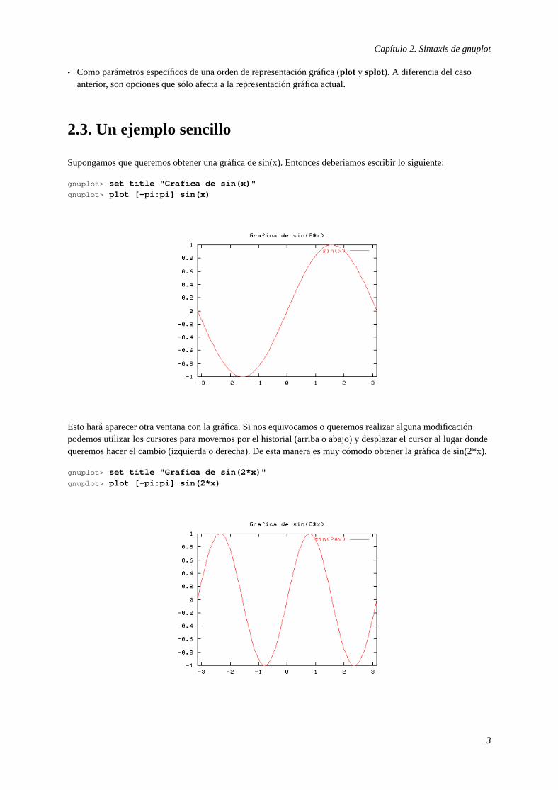
Supongamos que queremos obtener una gráfica de sin(x). Entonces deberíamos escribir lo siguiente:

gnuplot> set title "Grafica de sin(x)"gnuplot> plot [-pi:pi] sin(x)

Esto hará aparecer otra ventana con la gráfica. Si nos equivocamos o queremos realizar alguna modificaciónpodemos utilizar los cursores para movernos por el historial (arriba o abajo) y desplazar el cursor al lugar dondequeremos hacer el cambio (izquierda o derecha). De esta manera es muy cómodo obtener la gráfica de sin(2*x).

gnuplot> set title "Grafica de sin(2*x)"gnuplot> plot [-pi:pi] sin(2*x)

3

Capítulo 3. Gráficas 2D

La orden para realizar representaciones bidimensionales es plot. Su uso más simple es el siguiente:

• plot funcion

Por ejemplo, para representar sin(x)*(1-exp(x)):

• plot sin(x)*(1-exp(x))

Debería aparecer algo parecido a:

Como segundo ejemplo, veamos qué aspecto tiene un coseno hiperbólico

• plot cosh(x)

La escala elegida para esta gráfica no demasiado buena. Nos dice que para valores grandes de X la función tomavalores muy grandes, pero si queremos ver lo que pasa en un entorno de 0, tendremos que cambiar la escala.

4


gnuplot utiliza un mecanismo de autoescalado que ajusta la gráfica de forma que quepa en la superficie dedibujo. La sintaxis para cambiar la escala es la siguiente:

• plot [x1:x2][y1:y2] funcion.

• plot [x1:x2] funcion (para ajustar el eje X).

• plot [][y1:y2] funcion (para ajustar el eje y).

Nótese que si se cambia la escala para un gráfico, permanecerá cambiada para las siguientes representaciones.Para volver a la escala original existen los comandos:

• set xrange [-10:10] para la coordenada X.

• set yrange [-10:10] para la coordenada Y. Al igual que el anterior fija el valor del rango para la coordenadaespecificada.

• set autoscale para permitir que los ejes se autoajusten para que la gráfica quede lo mejor posible dentro delárea de dibujo. Es posible especificar los ejes a los que se permite el autoescalado.

Para más información se deberá consultar la ayuda en línea.

Si se quiere ver el aspecto de la función cosh(x) para y=[0,10]:

• plot [][0,10] cosh(x).

5


El comando para realizar gráficas tridimensionales es splot. Su forma más sencilla es la siguiente:

• splot funcion

Por ejemplo, para representar -x+y+3*cos(y), deberíamos escribir

• splot -x+y+3*cos(y)

Y obtendríamos lo siguiente:

Se puede cambiar la escala de forma similar a lo visto para plot

• splot [x1:x2][y1:y2][z1:z2] funcion

• splot [x1:x2] funcion

• splot [][y1:y2] funcion

• splot [][][z1:z2] funcion

Para modificar los rangos de las variables se pueden usar las opciones "set xrange [x1:x2]", "set yrange [y1:y2]","set zrange [z1:z1]". Es importante recordar que si se modifica un rango para una gráfica, ese mismo rango seutilizará para todas las gráficas posteriores.

Si se desea volver a activar el autoescalado degnuplot se puede hacer tecleando "set autoescale z".

4.1. Elementos ocultos en 3D

Algunas veces los gráficos 3D pueden ser complicados de interpretar porque se mezclan líneas que están enprimer plano con líneas que, si la figura fuera opaca, estarían ocultas. Veamos por ejemplo la siguiente figura.

• splot [-2:2] [-2:2] 2*(x**2 + y**2)*exp(-x**2 - y**2)

6


En esta gráfica se ha usado el comando "set grid" para ver la rejilla inferior. Para intentar hacer más visible lagráfica usaremos el comando "hidden3d":

• set hidden3d

• replot

4.2. Aumentar la precisión de los gráficos 3D

La gráfica anterior da la impresión de ser muy tosca. Para mejorar la apariencia y reducir el aspecto punzante dela gráfica es necesario aumentar la resolución. En las gráficas 2D esto se consigue con el comando "set samples",y para 3D con "set isosamples". Normalmente sólo será necesario aumentar la resolución en gráficos 3D. Lasintaxis del comando es:

• set isosamples tasa_x, tasa_y

Por defecto ambas tasas tienen valor 10, e indican el tamaño de la rejilla de puntos en la que se evalúa la gráfica.Probemos a aumentar la resolución del gráfico:

7


• set isosamples 30,30

• set hidden3d

• splot [-2:2] [-2:2] 2*(x**2 + y**2)*exp(-x**2 - y**2)

• set isosamples 30,30

• replot

Es importante advertir que cuanto mayor sea la resolución del gráfico, más tiempo tardarágnuplot en procesarla gráfica. En general es raro utilizar tasas superiores a 100.

4.3. Líneas de contorno.

Las líneas de contorno también facilitan la visualización de gráficos tridimensionales. Pueden elegirse queaparezcan en un plano, al estilo de líneas de nivel, o directamente sobre la propia gráfica. Los comandosrelacionados con las líneas de contorno son los siguientes:

• set contour base. Dibuja líneas de contorno en un plano en la base de la gráfica.

8


• set contour surface. Dibuja líneas de contorno sobre la propia figura.

• set contour both. Dibuja las líneas de contorno tanto en la base como en la figura.

• set nocontour. Se deja de dibujar las líneas de contorno.

La opción "set contour surface" no está disponible si también se quiere usar hidden3d. A continuación semuestran un par de ejemplos:

• set hidden3d

• set contour base

• splot [-2:2] [-2:2] 2*(x**2 + y**2)*exp(-x**2 - y**2)

• set nohidden3d

• set contour surface

• splot [-2:2] [-2:2] 2*(x**2 + y**2)*exp(-x**2 - y**2)

Si únicamente se desean las líneas de contorno, la opción "set nosurface" hará realidad nuestros deseos. Para más

9


información, consúltese "help set surface". La forma en que se dibujan las líneas de contorno puede variarse conla opción "cntrparam". Por ejemplo si sólo interesan las líneas de contorno para z=.2,.4,.6, se puede conseguirescribiendo el siguiente comando antes de dibujar la gráfica:

• set cntrparam levels discrete .2,.4,.6

Para más información consúltese la ayuda en línea.

4.4. Cambiar el punto de vista de una gráfica

Muchas veces es deseable cambiar el punto de vista de una gráfica. El comando "set view" permite realizar elcambio de perspectiva. La sintaxis es la siguiente:

• set view rot_x,rot_z

• set view rot_x,rot_z,escala,escala_z

• set view „escala

Donde rot_x y rot_z indican los ángulos (en grados) que se debe rotar la gráfica entorno a los ejes X y Z de unsistema de referencia alineado con la pantalla, en que el eje horizontal es el eje X, el vertical es el eje Y, y el ejeZ sería perpendicular al monitor. El tercer número controla la escala de todo el gráfico (actúa como un zoom) yel cuarto sólo la escala del eje Z. Los valores por defecto son "set view 60,30,1,1". Ejemplos:

• set hidden3d

• set isosamples 30

• splot [-2.5:2.5][-2.5,2.5] (x**2+3*y**2)*exp(1-(x**2+y**2))

• set view 40,30

• replot

10


• set view 60,60

• replot

Para ver un ejemplo de escalado:

• set view 60,30,2

• replot

11


12

Capítulo 5. Representaciones paramétricas

gnuplot permite representar ecuaciones paramétricas. Para cambiar al modo paramétrico se debe teclear losiguiente:

• set parametric

Y para volver al modo normal:

• set noparametric

5.1. Representaciones paramétricas 2D

Por ejemplo, para representar las ecuaciones x=5*cos(t), y=2*sin(t):

• set parametric

• set xrange [-6:6]

• set yrange [-6:6]

• set trange [0:2*pi]


• plot 5*cos(t),2*sin(t)

Los valores de xrange e yrange indican los rangos que se van a dibujar en la gráfica, mientras que trange es elrango de valores que va a tomar la variable paramétrica t. Si se indica un rango para el comando plot, este sereferirá al trange. La primera parte de la ecuación paramétrica nos da el valor de X, y la parte tras de la coma elvalor de Y.

Veamos otro ejemplo:

• set xrange [0:8*pi]

13


• set yrange [-.5:2.5]

• plot [0:8*pi] t-sin(t),1-cos(t)

5.2. Representaciones paramétricas 3D

gnuplot también permite realizar gráficos paramétricos tridimensionales. Las variables paramétricas son "u" y"v", y se utilizan xrange, yrange y zrange para determinar el tamaño del gráfico. Los rangos uragne y vrangedeterminan los rangos de las variables paramétricas. Por ejemplo:


• set yrange [-1:1]

• set zrange [-2:2]


• set grid

• splot [-pi:pi][-pi:0] sin(v),cos(u),cos(v)+sin(u)

14


La mayor parte de las opciones para gráficos 3D también se pueden usar en los gráficos paramétricos.

15

Capítulo 6. Gráficas en coordenadas polares

Para representar funciones en coordenadas polares tenemos que activar la opción:

• set polar

Y para volver a un sistema de coordenadas cartesianas:

• set nopolar

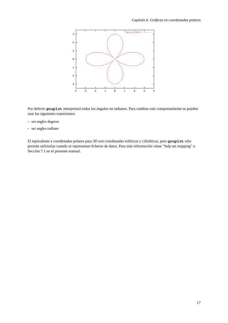
En coordenadas polares la variable t se refiere al ángulo. Se dispone de la opción "set trange [t1:t2]" para indicarel intervalo en el que queremos que se represente nuestra figura. Por defecto se hará entre 0 y 2*pi. El gráfico serepresenta en un área rectangular; las opciones "set xrange" y "set yrange" modificarán tanto la altura como laanchura. Por ejemplo:

• set polar

• plot 3*cos(2*x)

Para modificar el área de representación, para que haya más espacio entorno a la figura:


• set yrange [-3.5:3.5]

• replot

16

Capítulo 6. Gráficas en coordenadas polares

Por defectognuplot interpretará todos los ángulos en radianes. Para cambiar este comportamiento se puedenusar las siguientes expresiones:

• set angles degrees

• set angles radians

El equivalente a coordenadas polares para 3D son coordenadas esféricas y cilíndricas, perognuplot sólopermite utilizarlas cuando se representan ficheros de datos. Para más información véase "help set mapping" oSección 7.1en el presente manual.

17

Capítulo 7. Representaciones de datos

7.1. Representación 2D de datos

Una de las principales características degnuplot es la posibilidad de representar listados de datos numéricos.El siguiente listado son los resultados de calcular el área bajo una curva por métodos numéricos. La primeracolumna es el número de subintervalos utilizados, la segunda la anchura, y la tercera y cuarta columnas son elvalor calculado y el error cometido frente al valor real.

# área.dat# number of subint. - width of subinterval, computed value, abs. error0 1 5 0.006737946999085591 0.5 5.0009765625 0.005761384499085592 0.25 5.00317121193893 0.003566735060151593 0.125 5.00478985229103 0.001948094708057014 0.0625 5.00572403277733 0.00101391422175295 0.03125 5.00622120456923 0.0005167424298555556 0.015625 5.00647715291715 0.0002607940819352457 0.0078125 5.00660694721608 0.0001309997830043498 0.00390625 5.00667229679632 6.56502027673866e-059 0.001953125 5.0067050843668 3.28626322820824e-0510 0.0009765625 5.0067215063061 1.64406929883398e-0511 0.00048828125 5.00672972430911 8.22268997247022e-0612 0.000244140625 5.00673383506831 4.11193077187733e-0613 0.0001220703125 5.00673589088727 2.05611181058885e-0614 6.103515625e-05 5.00673691890656 1.02809252577885e-0615 3.0517578125e-05 5.00673743294363 5.14055459532869e-0716 1.52587890625e-05 5.00673768996904 2.57030048800289e-0717 7.62939453125e-06 5.00673781848355 1.28515534214557e-0718 3.814697265625e-06 5.00673788274127 6.42578132925564e-0819 1.9073486328125e-06 5.00673791487013 3.21289537197345e-0820 9.5367431640625e-07 5.00673793093482 1.60642699142954e-0821 4.76837158203125e-07 5.00673793896686 8.03222910406021e-09

Las líneas que empiezan por# son comentarios y se ignoran. Es conveniente que los datos estén en un fichero,por ejemploarea.dat , aunque también se podrían introducir en el prompt degnuplot . Se obtendría larepresentación gráfica con el siguiente comando:

• plot "area.dat"

18


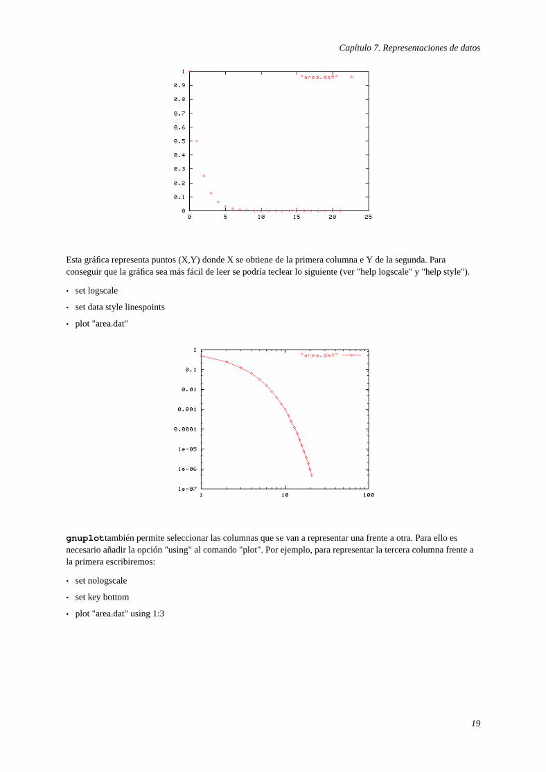
Esta gráfica representa puntos (X,Y) donde X se obtiene de la primera columna e Y de la segunda. Paraconseguir que la gráfica sea más fácil de leer se podría teclear lo siguiente (ver "help logscale" y "help style").

• set logscale

• set data style linespoints

• plot "area.dat"

gnuplot también permite seleccionar las columnas que se van a representar una frente a otra. Para ello esnecesario añadir la opción "using" al comando "plot". Por ejemplo, para representar la tercera columna frente ala primera escribiremos:

• set nologscale

• set key bottom

• plot "area.dat" using 1:3

19


O para representar la tercera columna frente la cuarta:

• plot "area.dat" using 4:3

Hay muchas opciones avanzadas para representar datos. Para mayor información se recomienda consultar laayuda en línea "help plot datafile using".

7.2. Representación 3D de datos

gnuplot permite realizar gráficos tridimensionales de datos. El fichero de entrada ha de tener tres columnas,una por cada coordenada X, Y, Z. Por ejemplo, supongamos que tenemos el siguiente fichero de datos:

# Created by Octave 2.0.16, Mon Jul 15 16:01:06 2002# name: aa# type: matrix# rows: 81# columns: 3-4 -4 256-3 -4 144-2 -4 64-1 -4 160 -4 01 -4 162 -4 643 -4 1444 -4 256

-4 -3 144-3 -3 81-2 -3 36-1 -3 90 -3 01 -3 92 -3 363 -3 814 -3 144

20


-4 -2 64-3 -2 36-2 -2 16-1 -2 40 -2 01 -2 42 -2 163 -2 364 -2 64

-4 -1 16-3 -1 9-2 -1 4-1 -1 10 -1 01 -1 12 -1 43 -1 94 -1 16

-4 0 0-3 0 0-2 0 0-1 0 00 0 01 0 02 0 03 0 04 0 0

-4 1 16-3 1 9-2 1 4-1 1 10 1 01 1 12 1 43 1 94 1 16

-4 2 64-3 2 36-2 2 16-1 2 40 2 01 2 42 2 163 2 364 2 64

-4 3 144-3 3 81-2 3 36-1 3 90 3 01 3 9

21


2 3 363 3 814 3 144

-4 4 256-3 4 144-2 4 64-1 4 160 4 01 4 162 4 643 4 1444 4 256

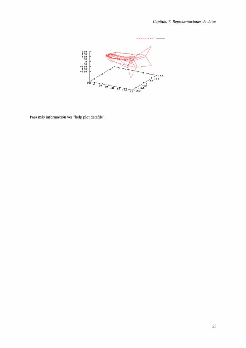
Las dos primeras columnas del fichero son los valores de X e Y donde se ha evaluado la tercera columna, quecorresponde a la funciónf(x,y)=(x**2)*(y**2) . Puede observarse que cada vez que la variable Y cambia de valorse deja una línea en blanco en el fichero de datos. Esto indica agnuplot que no una los puntos que están arribay debajo de la línea en blanco. De esta forma se evita que aparezcan líneas que emborronarían la gráfica. Veamosla gráfica resultante:

• set data style lines

• splot "sdata.mat"

También se podría realizar una representación paramétrica, e incluso en coordenadas cilíndricas o esféricas (otracuestión es que el dibujo tenga sentido).

• set data style lines

• set mapping spherical

• splot "sdata.mat"

22


Para más información ver "help plot datafile".

23

Capítulo 8. Formatos de salida.

Este capítulo describe las distintas formas de obtener los gráficos que se han creado:

• Mostrar la salida por pantalla.

El dispositivo más habitual de gnuplot son las X, al menos al principio para ir viendo los resultados obtenidos.Por defectognuplot mostrará las gráficas en una ventana en las X si están disponibles. En cualquier caso sepueden seleccionar con el comando "set term x11". Otros posibles dispositivos pueden ser "vga" o "dumb".Para más información ver "help term".

• Guardar la salida en un fichero postscript.

Este dispositivo de salida tiene múltiples opciones. Se puede elegir si se quiere postscript encapsulado, tipo ytamaño de las fuentes, etc. Posiblemente sea el terminal más usado para incluir gráficas en trabajos usandoLaTeX. Para más información, "help set term postscript".

• Guardar la salida en un fichero de imagen.

Esta opción es semejante a la anterior. Los formatos de imagen más habituales serán png, jpg, fig.

• Finalmente, también es posible mandar la salida a una impresora.

Para ello será necesario elegir como dispositivo de salida el driver de nuestra impresora.

El nombre del fichero de salida se indica mediante el comando "set output". Veamos un ejemplo en el queguardamos el resultado en un fichero png:

• set output "fichero.ext"

• plot sin(x)

• set output

La primera aparición de "set output" indica que la salida se guardará en el fichero indicado a continuación. Lascomillas dobles son imprescindibles. A continuación se realiza la gráfica y finalmente, el segundo "set output"cierra el fichero. Es muy importante no olvidarse de cerrar el fichero, porque si se realizara otra gráfica, elresultado también se guardaría en el mismo fichero, inutilizandose de esta manera.

Para el caso de enviar la salida a una impresora, o en general postprocesarla con otra aplicación, se deberáindicar como parámetro de "set output" el nombre del comando, precedido por una tubería símbolo (|).

• set output "| lpr -P mi_impresora"

Todas las gráficas que se generen a partir de ese momento se dirigirán al comando "lpr" (imprimir en UN*X).Conviene de todas formas cerrar la salida con "set output" y volverla a abrir entre gráfica y gráfica.

24

Capítulo 8. Formatos de salida.

En general, para ver las posibilidades que ofrece un dispositivo de salida, se debe ejecutar "help term disp",donde disp es el nombre del dispositivo en cuestión. Si se necesita algún dispositivo que no esté disponible, haydos alternativas: recompilargnuplot y añadir el soporte o utilizar otro dispositivo. Como última nota decir quelos distintos tipos de dispositivos únicamente adaptan la salida. Esta tendrá que guardarse luego en un fichero,mostrarse por pantalla o enviarse a un comando de shell para ser postprocesada.

25

Capítulo 9. Usos avanzados. Truquillos de gurú

9.1. Guardando y cargando sesiones de un fichero

gnuplot permite indicar el nombre de un fichero del que leer una serie de comandos. Esto puede ser muy útilpara trabajar en modo batch (por ejemplo, generando gráficas desde un script), o para cargar una configuración ala hora de representar gráficas. El comando para cargar comandos de un fichero es:

• load "fichero.gp"

Y si lo que queremos es trabajar en modo batch, escribiremos desde el prompt delsistema operativo:

• gnuplot fichero.gp

Los comandos en el fichero se deben escribir con la misma sintaxis que si se escribieran desde el prompt degnuplot .

De forma similar, para guardar el estado actual de trabajo teclearemos:

• save "fichero.gp"

En este fichero se guardarán comandos que nos permitirán configurar el estado degnuplot tal y como lotenemos en este momento. También nos guarda las expresiones que hayamos definido (funciones y constantes) yla última gráfica representada.

9.2. Scripts degnuplot

Como hemos podido comprobar, la interfaz degnuplot está completamente orientada a comandos:absolutamente todos los aspectos del programa se controlan desde la línea de comandos. La dificultad deaprender los comandos, el tedio de teclearlos y el largo proceso de prueba y error hasta que conseguimos lagráfica con el aspecto deseado tienen ahora su recompensa: si guardamos en un fichero todas las ordenesnecesarias para obtener nuestra gráfica, habremos creado unscript degnuplot . Con apenas unos pocoscambios en el script, simplemente la función a representar o los datos, podremos obtener nuevas gráficas y todasellas con un aspecto uniforme, ideales para insertar en informe o tesis. Es más, podemos llegar a automatizar elproceso de creación de gráficas.

Es posible la invocación de un script de tres maneras

• Desde el propio prompt degnuplot , con el comando

gnuplot> load "fichero.gp"

• Desde el prompt delshell, tecleando como parámetros una lista de ficheros.gnuplot leerá y ejecutarásecuencialmente estos ficheros.

26


$ gnuplot f1.gp f2.gp ...

• Como un script ejecutable. Esta opción sólo está disponible en sistemas Unix. Para ello hay que dar permisode ejecución al fichero y asegurarse que la primera línea del fichero es la siguiente:

#!/bin/usr/gnuplot

De esta forma cuando se invoque el script desde el shell, este leerá la primera línea y lanzará el programagnuplot para que interprete el resto del fichero.

$ ./gnuplot.gp

9.3. Pausas, bucles y animaciones

En una mismo fichero se puede pedir agnuplot que dibuje varios gráficos, poniendo el comando "pause" entrelas gráficas nos permitirá ver cada gráfica con tranquilidad.

Además, si al final del fichero (o en cualquier momento utilizando "if") se coloca el comando "reread"gnuplot empezará a interpretar otra vez los comandos desde el principio del fichero.

Utilizando "pause" y "reread" se pueden crear animaciones. A modo de ejemplo en el siguiente fichero, sacadode la distribución degnuplot podemos ver una bonita animación: animate.tar (../animate.tar). Una vezdescargado, deberemos extraer los ficheros a un directorio, y desde ese directorio ejecutar "gnuplotanimate.dem".

9.4. Cambiando el aspecto de las gráficas

gnuplot tiene multitud de comandos para personalizar el acabado final de las representaciones gráficas. Acontinuación se muestra un pequeño listado. Para ver todas las posibles opciones, véase "help set".

• Añadir título a una gráfica: set title "titulo de la gráfica"

• Añadir la fecha y hora a una gráfica: set time

• Añadir títulos a los ejes: set xlabel "nombre X" y set ylabel "nombre Y"

• Personalizar la leyenda o eliminarla: set key

• Dibujar flechas en el gráfico: set arrows

• Colocar etiquetas en cualquier punto del gráfico: set labels

• Redimensionar el área de dibujo: set size

• Variar los márgenes del dibujo: set size y set origin

• Mostrar una rejilla de líneas tras la gráfica; set grid

27


• Ocultar y mostrar los ejes: set border, set (x/y)zeroaxis.

• Mostrar y modificar las marcas en los ejes: set (x/y)tics.

• Para que las marcas de los ejes correspondan a días de la semana o meses: set (x/y)dtics, set (x/y)mtics.

• Para que las marcas de los ejes estén por dentro o fuera del dibujo: set ticslevel

9.5. Multiples gráficas en una sólo dibujo.

Para obtener un dibujo con varias graficas en el basta con poner las distintas funciones que se quieren representarseparadas por comas, en el mismo comando "plot".

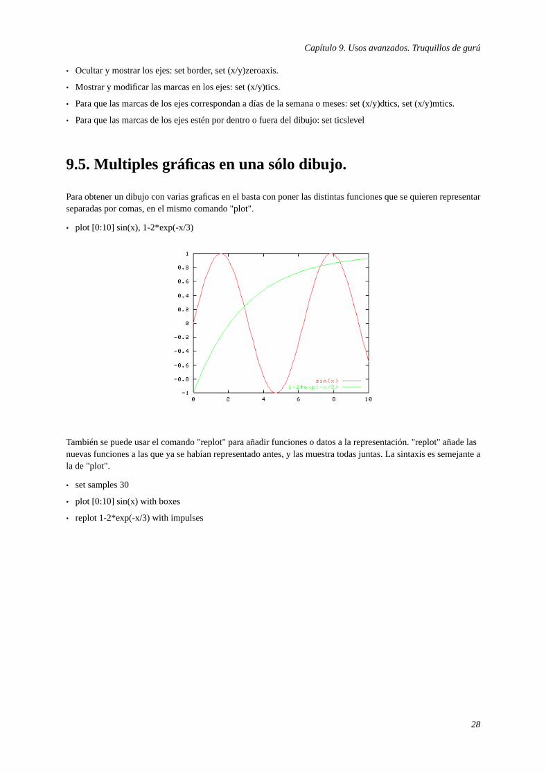
• plot [0:10] sin(x), 1-2*exp(-x/3)

También se puede usar el comando "replot" para añadir funciones o datos a la representación. "replot" añade lasnuevas funciones a las que ya se habían representado antes, y las muestra todas juntas. La sintaxis es semejante ala de "plot".

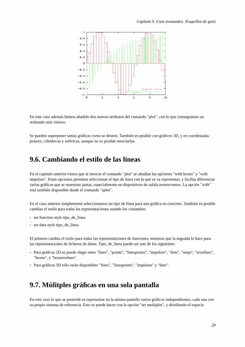
• set samples 30

• plot [0:10] sin(x) with boxes

• replot 1-2*exp(-x/3) with impulses

28


En este caso además hemos añadido dos nuevos atributos del comando "plot", con lo que conseguimos unreslutado más vistoso.

Se pueden superponer tantas gráficas como se deseen. También es posible con gráficos 3D, y en coordenadaspolares, cilíndricas y esféricas, aunque no es posible mezclarlas.

9.6. Cambiando el estilo de las líneas

En el capítulo anterior vimos que al invocar el comando "plot" se añadían las opciones "with boxes" y "withimpulses". Estas opciones permiten seleccionar el tipo de línea con la que se va representar, y facilita diferenciarvarias gráficas que se muestran juntas, especialmente en dispositivos de salida monocromos. La opción "with"está también disponible desde el comando "splot".

En el caso anterior simplemente seleccionamos un tipo de línea para una gráfica en concreto. También es posiblecambiar el estilo para todas las representaciones usando los comandos:

• set function style tipo_de_linea

• set data style tipo_de_linea

El primero cambia el estilo para todas las representaciones de funciones, mientras que la segunda lo hace paralas representaciones de ficheros de datos. Tipo_de_linea puede ser uno de los siguientes:

• Para gráficas 2D se puede elegir entre "lines", "points", "linespoints", "impulses", "dots", "steps", "errorbars","boxes", y "boxerrorbars".

• Para gráficas 3D sólo están disponibles "lines", "linespoints", "impulses" y "dots".

9.7. Múlitples gráficas en una sola pantalla

En este caso lo que se pretende es representar en la misma pantalla varios gráficas independientes, cada una consu propio sistema de referencia. Esto se puede hacer con la opción "set multiplot", y dividiendo el espacio

29


disponible en porciones con "set size" y "set origin". Por ejemplo para dibujar cuatro gráficas en una cuadrícula2x2 haríamos lo siguiente:

• set multiplot

• set size .5,.5

• set origin 0,.5

• plot x

• set origin .5,.5

• plot [0:1] sin(2*pi*x) with boxes

• set origin 0,0

• plot [-5:5] exp(-x**2/5) with steps

• set origin .5,0

• splot [-1:1][-1:1] x**2+y**2

• set nomultiplot

Dependiendo del dispositivo de salida, las gráficas no se dibujarán hasta que se pase a modo normal con "setnomultiplot". En otras las gráficas irán apareciendo pero no se podrá borrar la pantalla (con el comando "clear")o se borrarán todas las gráficas.

Si el dispositivo de salida es el sistema X ("set term x11"), es posible obtener varias gráficas a la vez, cada una ensu propia ventana. Para ello simplemente hay que pasar un parámetro más al comando "set":

• set term x11 n

Donde "n" es un entero, identificador de la ventana X en la que se va a dibujar la gráfica. Si la ventana ya existe,se reutilizará. Si no existe se creará de nuevo. Es posible definir tantas ventanas como sea necesario.

30

Capítulo 10. Dónde seguir.

10.1. Interfaces gráficos

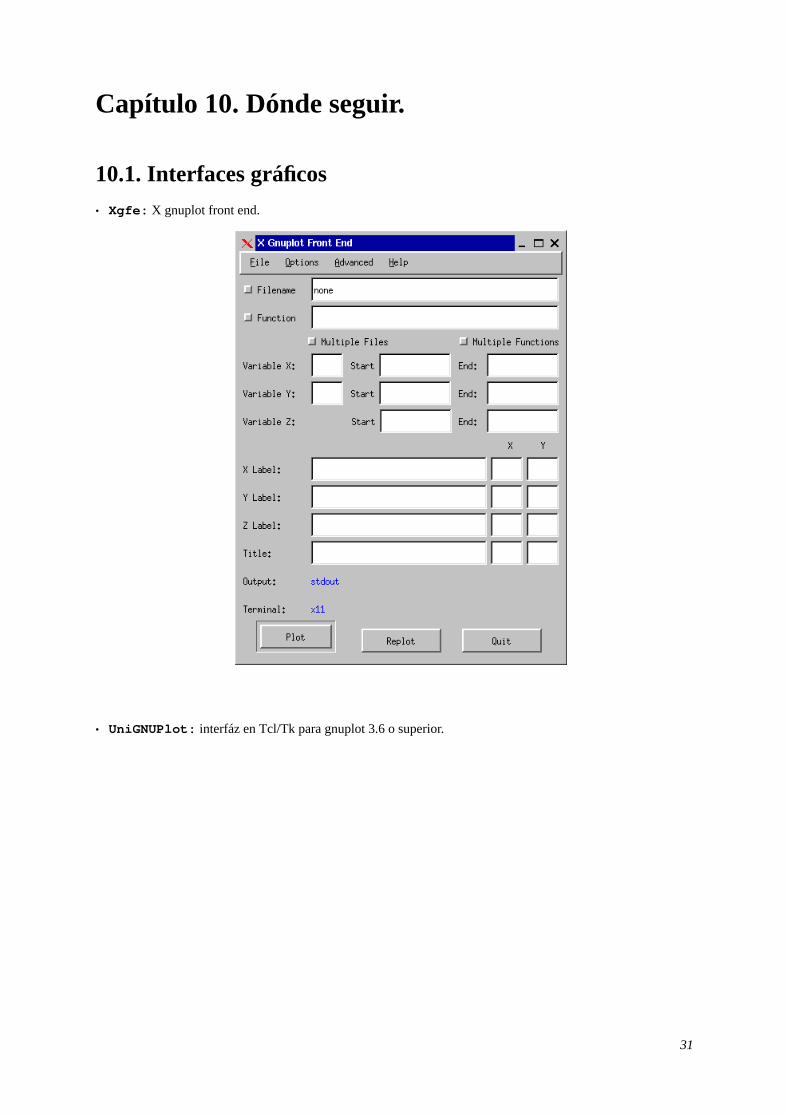
• Xgfe: X gnuplot front end.

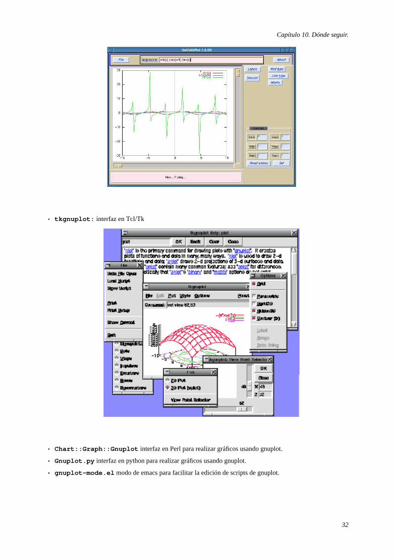
• UniGNUPlot: interfáz en Tcl/Tk para gnuplot 3.6 o superior.

31


• tkgnuplot: interfaz en Tcl/Tk

• Chart::Graph::Gnuplot interfaz en Perl para realizar gráficos usando gnuplot.

• Gnuplot.py interfaz en python para realizar gráficos usando gnuplot.

• gnuplot-mode.el modo de emacs para facilitar la edición de scripts de gnuplot.

32


10.2. Alternativas libres agnuplot

• PGPlot: conjunto de librerías en C y Perl para dibujar gráficas sin esfuerzo.

• XGobi: programa de representación de funciones y datos.

• Graphtool: programa basado en GNOME que tiene como objetivo realizar representaciones gráficas. Estáen fase temprana de desarrollo.

• GNU Plotutils: conjunto de rutinas y utilidades para dibujar gráficas.

• R: programa clónico deS programming language . Permite dibujar gráficos. Basado en línea decomandos.

• Mathplot: únicamente representa funciones, no datos.

• KChart: parte de KOffice, similar a la herramienta de gráficos de Excell.

• ...

10.3. Referencias

Como hemos vistognuplot es altamente personalizable y tiene multitud de parámetros que controlan hasta elmás mínimo detalle de la gráfica representada. Quienes estén interesados en profundizar más en el uso degnuplot , a continuación se muestra una serie de referencias.

• La ayuda en línea: desde el prompt degnuplot tecleando "help".

• La página oficial degnuplot : http://www.gnuplot.info

• Una página que probablemente merezca la pena visitar es:Bernhard Reiter: gnuplot - Scientific Plotting(http://www.usf.uni-osnabrueck.de/~breiter/tools/gnuplot/index.en.html)

Estas dos páginas a su vez contienen listas de enlaces muy interesantes sobregnuplot . Y por supuesto lasfaq

• http://www.ucc.ie/gnuplot/gnuplot-faq.html (http://www.ucc.ie/gnuplot/gnuplot-faq.html)

Programas para facilitar el uso de gnuplot.

• Octave: un lenguaje de alto nivel para realizar cálculo numérico. Semejante a Matlab y prácticamentecompatible.

• El modo gnuplot.el para emacs (viene incluido en las distribuciones degnuplot ).

Finalmente, anunciar que la versión 3.8 degnuplot será liberada de CVS en los próximos meses. Esta versióntrae nuevas características que harán degnuplot un programa aún más interesante :).

33

Apéndice A. GNU Free Documentation LicenseCopyright (C) 2000,2001,2002 Free Software Foundation, Inc. 59 Temple Place, Suite 330, Boston, MA 02111-1307USA Everyone is permitted to copy and distribute verbatim copies of this license document, but changing it is notallowed.

A.1. PREAMBLE

The purpose of this License is to make a manual, textbook, or other functional and useful document "free" in thesense of freedom: to assure everyone the effective freedom to copy and redistribute it, with or without modifyingit, either commercially or noncommercially. Secondarily, this License preserves for the author and publisher away to get credit for their work, while not being considered responsible for modifications made by others.

This License is a kind of "copyleft", which means that derivative works of the document must themselves be freein the same sense. It complements the GNU General Public License, which is a copyleft license designed for freesoftware.

We have designed this License in order to use it for manuals for free software, because free software needs freedocumentation: a free program should come with manuals providing the same freedoms that the software does.But this License is not limited to software manuals; it can be used for any textual work, regardless of subjectmatter or whether it is published as a printed book. We recommend this License principally for works whosepurpose is instruction or reference.

A.2. APPLICABILITY AND DEFINITIONS

This License applies to any manual or other work, in any medium, that contains a notice placed by the copyrightholder saying it can be distributed under the terms of this License. Such a notice grants a world-wide,royalty-free license, unlimited in duration, to use that work under the conditions stated herein. The "Document",below, refers to any such manual or work. Any member of the public is a licensee, and is addressed as "you". Youaccept the license if you copy, modify or distribute the work in a way requiring permission under copyright law.

A "Modified Version" of the Document means any work containing the Document or a portion of it, eithercopied verbatim, or with modifications and/or translated into another language.

A "Secondary Section" is a named appendix or a front-matter section of the Document that deals exclusivelywith the relationship of the publishers or authors of the Document to the Document’s overall subject (or torelated matters) and contains nothing that could fall directly within that overall subject. (Thus, if the Documentis in part a textbook of mathematics, a Secondary Section may not explain any mathematics.) The relationshipcould be a matter of historical connection with the subject or with related matters, or of legal, commercial,philosophical, ethical or political position regarding them.

The "Invariant Sections" are certain Secondary Sections whose titles are designated, as being those of InvariantSections, in the notice that says that the Document is released under this License. If a section does not fit the

34

Apéndice A. GNU Free Documentation License

above definition of Secondary then it is not allowed to be designated as Invariant. The Document may containzero Invariant Sections. If the Document does not identify any Invariant Sections then there are none.

The "Cover Texts" are certain short passages of text that are listed, as Front-Cover Texts or Back-Cover Texts, inthe notice that says that the Document is released under this License. A Front-Cover Text may be at most 5words, and a Back-Cover Text may be at most 25 words.

A "Transparent" copy of the Document means a machine-readable copy, represented in a format whosespecification is available to the general public, that is suitable for revising the document straightforwardly withgeneric text editors or (for images composed of pixels) generic paint programs or (for drawings) some widelyavailable drawing editor, and that is suitable for input to text formatters or for automatic translation to a varietyof formats suitable for input to text formatters. A copy made in an otherwise Transparent file format whosemarkup, or absence of markup, has been arranged to thwart or discourage subsequent modification by readers isnot Transparent. An image format is not Transparent if used for any substantial amount of text. A copy that is not"Transparent" is called "Opaque".

Examples of suitable formats for Transparent copies include plain ASCII without markup, Texinfo input format,LaTeX input format, SGML or XML using a publicly available DTD, and standard-conforming simple HTML,PostScript or PDF designed for human modification. Examples of transparent image formats include PNG, XCFand JPG. Opaque formats include proprietary formats that can be read and edited only by proprietary wordprocessors, SGML or XML for which the DTD and/or processing tools are not generally available, and themachine-generated HTML, PostScript or PDF produced by some word processors for output purposes only.

The "Title Page" means, for a printed book, the title page itself, plus such following pages as are needed to hold,legibly, the material this License requires to appear in the title page. For works in formats which do not have anytitle page as such, "Title Page" means the text near the most prominent appearance of the work’s title, precedingthe beginning of the body of the text.

A section "Entitled XYZ" means a named subunit of the Document whose title either is precisely XYZ orcontains XYZ in parentheses following text that translates XYZ in another language. (Here XYZ stands for aspecific section name mentioned below, such as "Acknowledgements", "Dedications", "Endorsements", or"History".) To "Preserve the Title" of such a section when you modify the Document means that it remains asection "Entitled XYZ" according to this definition.

The Document may include Warranty Disclaimers next to the notice which states that this License applies to theDocument. These Warranty Disclaimers are considered to be included by reference in this License, but only asregards disclaiming warranties: any other implication that these Warranty Disclaimers may have is void and hasno effect on the meaning of this License.

A.3. VERBATIM COPYING

You may copy and distribute the Document in any medium, either commercially or noncommercially, providedthat this License, the copyright notices, and the license notice saying this License applies to the Document arereproduced in all copies, and that you add no other conditions whatsoever to those of this License. You may notuse technical measures to obstruct or control the reading or further copying of the copies you make or distribute.

35


However, you may accept compensation in exchange for copies. If you distribute a large enough number ofcopies you must also follow the conditions in section 3.

You may also lend copies, under the same conditions stated above, and you may publicly display copies.

A.4. COPYING IN QUANTITY

If you publish printed copies (or copies in media that commonly have printed covers) of the Document,numbering more than 100, and the Document’s license notice requires Cover Texts, you must enclose the copiesin covers that carry, clearly and legibly, all these Cover Texts: Front-Cover Texts on the front cover, andBack-Cover Texts on the back cover. Both covers must also clearly and legibly identify you as the publisher ofthese copies. The front cover must present the full title with all words of the title equally prominent and visible.You may add other material on the covers in addition. Copying with changes limited to the covers, as long asthey preserve the title of the Document and satisfy these conditions, can be treated as verbatim copying in otherrespects.

If the required texts for either cover are too voluminous to fit legibly, you should put the first ones listed (as manyas fit reasonably) on the actual cover, and continue the rest onto adjacent pages.

If you publish or distribute Opaque copies of the Document numbering more than 100, you must either include amachine-readable Transparent copy along with each Opaque copy, or state in or with each Opaque copy acomputer-network location from which the general network-using public has access to download usingpublic-standard network protocols a complete Transparent copy of the Document, free of added material. If youuse the latter option, you must take reasonably prudent steps, when you begin distribution of Opaque copies inquantity, to ensure that this Transparent copy will remain thus accessible at the stated location until at least oneyear after the last time you distribute an Opaque copy (directly or through your agents or retailers) of that editionto the public.

It is requested, but not required, that you contact the authors of the Document well before redistributing any largenumber of copies, to give them a chance to provide you with an updated version of the Document.

A.5. MODIFICATIONS

You may copy and distribute a Modified Version of the Document under the conditions of sections 2 and 3above, provided that you release the Modified Version under precisely this License, with the Modified Versionfilling the role of the Document, thus licensing distribution and modification of the Modified Version to whoeverpossesses a copy of it. In addition, you must do these things in the Modified Version:

A. Use in the Title Page (and on the covers, if any) a title distinct from that of the Document, and from those ofprevious versions (which should, if there were any, be listed in the History section of the Document). Youmay use the same title as a previous version if the original publisher of that version gives permission.

B. List on the Title Page, as authors, one or more persons or entities responsible for authorship of themodifications in the Modified Version, together with at least five of the principal authors of the Document(all of its principal authors, if it has fewer than five), unless they release you from this requirement.

C. State on the Title page the name of the publisher of the Modified Version, as the publisher.

36


D. Preserve all the copyright notices of the Document.

E. Add an appropriate copyright notice for your modifications adjacent to the other copyright notices.

F. Include, immediately after the copyright notices, a license notice giving the public permission to use theModified Version under the terms of this License, in the form shown in theAddendumbelow.

G. Preserve in that license notice the full lists of Invariant Sections and required Cover Texts given in theDocument’s license notice.

H. Include an unaltered copy of this License.

I. Preserve the section Entitled "History", Preserve its Title, and add to it an item stating at least the title, year,new authors, and publisher of the Modified Version as given on the Title Page. If there is no section Entitled"History" in the Document, create one stating the title, year, authors, and publisher of the Document asgiven on its Title Page, then add an item describing the Modified Version as stated in the previous sentence.

J.Preserve the network location, if any, given in the Document for public access to a Transparent copy of theDocument, and likewise the network locations given in the Document for previous versions it was based on.These may be placed in the "History" section. You may omit a network location for a work that waspublished at least four years before the Document itself, or if the original publisher of the version it refers togives permission.

K. For any section Entitled "Acknowledgements" or "Dedications", Preserve the Title of the section, andpreserve in the section all the substance and tone of each of the contributor acknowledgements and/ordedications given therein.

L. Preserve all the Invariant Sections of the Document, unaltered in their text and in their titles. Sectionnumbers or the equivalent are not considered part of the section titles.

M. Delete any section Entitled "Endorsements". Such a section may not be included in the Modified Version.

N. Do not retitle any existing section to be Entitled "Endorsements" or to conflict in title with any InvariantSection.

O. Preserve any Warranty Disclaimers.

If the Modified Version includes new front-matter sections or appendices that qualify as Secondary Sections andcontain no material copied from the Document, you may at your option designate some or all of these sections asinvariant. To do this, add their titles to the list of Invariant Sections in the Modified Version’s license notice.These titles must be distinct from any other section titles.

You may add a section Entitled "Endorsements", provided it contains nothing but endorsements of your ModifiedVersion by various parties--for example, statements of peer review or that the text has been approved by anorganization as the authoritative definition of a standard.

You may add a passage of up to five words as a Front-Cover Text, and a passage of up to 25 words as aBack-Cover Text, to the end of the list of Cover Texts in the Modified Version. Only one passage of Front-CoverText and one of Back-Cover Text may be added by (or through arrangements made by) any one entity. If theDocument already includes a cover text for the same cover, previously added by you or by arrangement made bythe same entity you are acting on behalf of, you may not add another; but you may replace the old one, onexplicit permission from the previous publisher that added the old one.

The author(s) and publisher(s) of the Document do not by this License give permission to use their names forpublicity for or to assert or imply endorsement of any Modified Version.

37


A.6. COMBINING DOCUMENTS

You may combine the Document with other documents released under this License, under the terms defined insection 4above for modified versions, provided that you include in the combination all of the Invariant Sectionsof all of the original documents, unmodified, and list them all as Invariant Sections of your combined work in itslicense notice, and that you preserve all their Warranty Disclaimers.

The combined work need only contain one copy of this License, and multiple identical Invariant Sections may bereplaced with a single copy. If there are multiple Invariant Sections with the same name but different contents,make the title of each such section unique by adding at the end of it, in parentheses, the name of the originalauthor or publisher of that section if known, or else a unique number. Make the same adjustment to the sectiontitles in the list of Invariant Sections in the license notice of the combined work.

In the combination, you must combine any sections Entitled "History" in the various original documents,forming one section Entitled "History"; likewise combine any sections Entitled "Acknowledgements", and anysections Entitled "Dedications". You must delete all sections Entitled "Endorsements".

A.7. COLLECTIONS OF DOCUMENTS

You may make a collection consisting of the Document and other documents released under this License, andreplace the individual copies of this License in the various documents with a single copy that is included in thecollection, provided that you follow the rules of this License for verbatim copying of each of the documents inall other respects.

You may extract a single document from such a collection, and distribute it individually under this License,provided you insert a copy of this License into the extracted document, and follow this License in all otherrespects regarding verbatim copying of that document.

A.8. AGGREGATION WITH INDEPENDENT WORKS

A compilation of the Document or its derivatives with other separate and independent documents or works, in oron a volume of a storage or distribution medium, is called an "aggregate" if the copyright resulting from thecompilation is not used to limit the legal rights of the compilation’s users beyond what the individual workspermit. When the Document is included an aggregate, this License does not apply to the other works in theaggregate which are not themselves derivative works of the Document.

If the Cover Text requirement of section 3 is applicable to these copies of the Document, then if the Document isless than one half of the entire aggregate, the Document’s Cover Texts may be placed on covers that bracket theDocument within the aggregate, or the electronic equivalent of covers if the Document is in electronic form.Otherwise they must appear on printed covers that bracket the whole aggregate.

38


A.9. TRANSLATION

Translation is considered a kind of modification, so you may distribute translations of the Document under theterms of section 4. Replacing Invariant Sections with translations requires special permission from theircopyright holders, but you may include translations of some or all Invariant Sections in addition to the originalversions of these Invariant Sections. You may include a translation of this License, and all the license notices inthe Document, and any Warranty Disclaimers, provided that you also include the original English version of thisLicense and the original versions of those notices and disclaimers. In case of a disagreement between thetranslation and the original version of this License or a notice or disclaimer, the original version will prevail.

If a section in the Document is Entitled "Acknowledgements", "Dedications", or "History", the requirement(section 4) to Preserve its Title (section 1) will typically require changing the actual title.

A.10. TERMINATION

You may not copy, modify, sublicense, or distribute the Document except as expressly provided for under thisLicense. Any other attempt to copy, modify, sublicense or distribute the Document is void, and will automaticallyterminate your rights under this License. However, parties who have received copies, or rights, from you underthis License will not have their licenses terminated so long as such parties remain in full compliance.

A.11. FUTURE REVISIONS OF THIS LICENSE

The Free Software Foundation may publish new, revised versions of the GNU Free Documentation License fromtime to time. Such new versions will be similar in spirit to the present version, but may differ in detail to addressnew problems or concerns. See http://www.gnu.org/copyleft/.

Each version of the License is given a distinguishing version number. If the Document specifies that a particularnumbered version of this License "or any later version" applies to it, you have the option of following the termsand conditions either of that specified version or of any later version that has been published (not as a draft) bythe Free Software Foundation. If the Document does not specify a version number of this License, you maychoose any version ever published (not as a draft) by the Free Software Foundation.

A.12. ADDENDUM: How to use this License for yourdocuments

To use this License in a document you have written, include a copy of the License in the document and put thefollowing copyright and license notices just after the title page:

Copyright (c) YEAR YOUR NAME. Permission is granted to copy, distribute and/or modify this document under theterms of the GNU Free Documentation License, Version 1.2 or any later version published by the Free SoftwareFoundation; with no Invariant Sections, no Front-Cover Texts, and no Back-Cover Texts. A copy of the license isincluded in the section entitled "GNU Free Documentation License".

39


If you have Invariant Sections, Front-Cover Texts and Back-Cover Texts, replace the "with...Texts." line withthis:

with the Invariant Sections being LIST THEIR TITLES, with the Front-Cover Texts being LIST, and with theBack-Cover Texts being LIST.

If you have Invariant Sections without Cover Texts, or some other combination of the three, merge those twoalternatives to suit the situation.

If your document contains nontrivial examples of program code, we recommend releasing these examples inparallel under your choice of free software license, such as the GNU General Public License, to permit their usein free software.

40

Herramientas en GNU/Linux para estudiantes universitarios · Introducción de ecuaciones y ... •...

Documents

Transcript of Herramientas en GNU/Linux para estudiantes universitarios · Introducción de ecuaciones y ... •...