El pendulo invertido:

un banco de pruebas para el control no lineal

Javier Aracil and Francisco Gordillo

Escuela Superior de Ingenieros

Universidad de Sevilla

XXV Jornadas de Automatica

Ciudad Real, 8-10 septiembre 2004

Outline

1. Introduction to the inverted pendulum.

2. Potential energy shaping.

3. A damping-pumping strategy.

4. A control law stopping the car for the swing up problem.

5. Periodic oscillations in the inverted pendulum.

6. Conclusions.

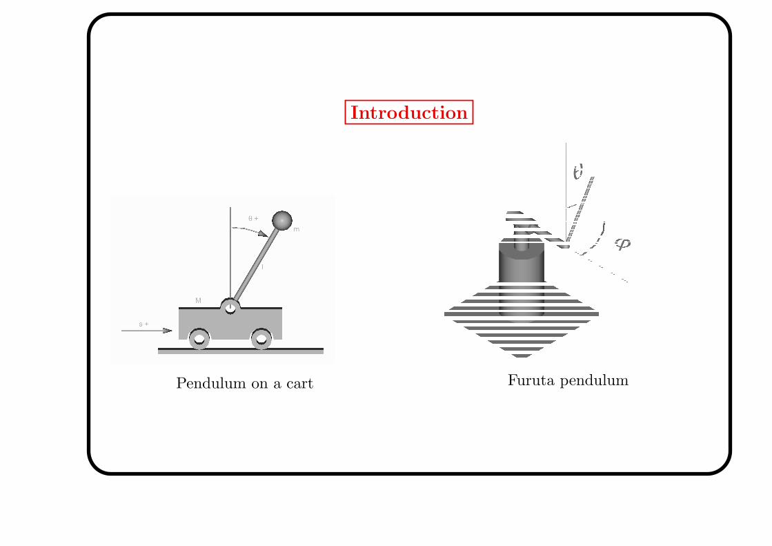
Introduction

Pendulum on a cart Furuta pendulum

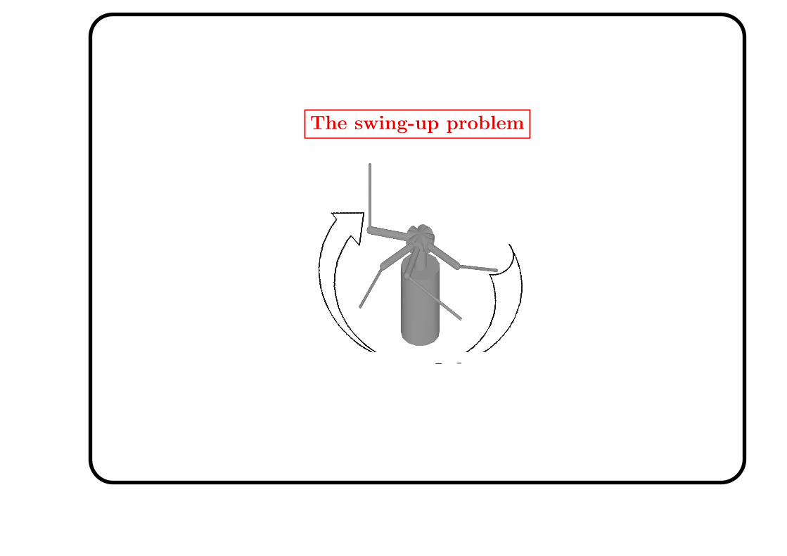
The swing-up problem

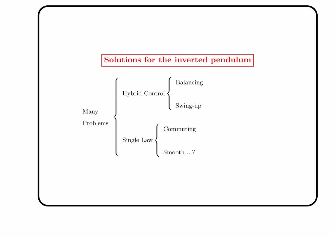
Solutions for the inverted pendulum

Many

Problems

Hybrid Control

Balancing

Swing-up

Single Law

Commuting

Smooth ...?

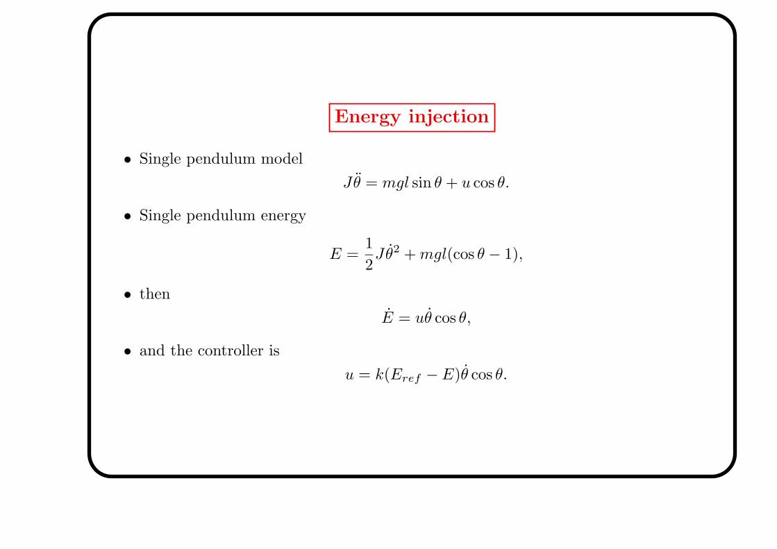
Energy injection

• Single pendulum model

Jθ = mgl sin θ + u cos θ.

• Single pendulum energy

E =1

2Jθ2 + mgl(cos θ − 1),

• then

E = uθ cos θ,

• and the controller is

u = k(Eref − E)θ cos θ.

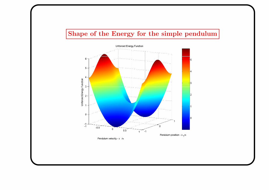
Shape of the Energy for the simple pendulum

Full system model

• Full system model

(Jp + mℓ2)(θ − ϕ2 sin θ cos θ) + mrℓϕ cos θ − mgℓ sin θ = 0

mrℓθ cos θ − mrℓθ2 sin θ + 2(Jp + mℓ2)θϕ sin θ cos θ

+(J + mr2 + (Jp + mℓ2) sin2 θ)ϕ = F.

• Partially linearized model

x1 = x2

x2 = sinx1 − cos x1u

x3 = u

• The best-known swing-up law (M. Wiklund et al., 1993; Astrom and Furuta, 2000)

is based on a dimension 2 model.

• Dimension two model neglects the reaction torques from the pendulum to the arm.

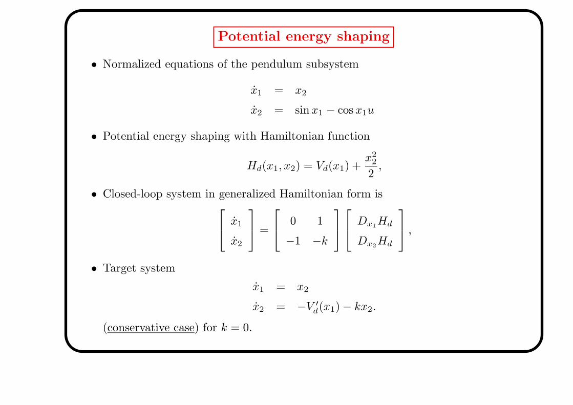
Potential energy shaping

• Normalized equations of the pendulum subsystem

x1 = x2

x2 = sinx1 − cos x1u

• Potential energy shaping with Hamiltonian function

Hd(x1, x2) = Vd(x1) +x2

2

2,

• Closed-loop system in generalized Hamiltonian form is x1

x2

=

0 1

−1 −k

Dx1

Hd

Dx2Hd

,

• Target system

x1 = x2

x2 = −V ′

d(x1) − kx2.

(conservative case) for k = 0.

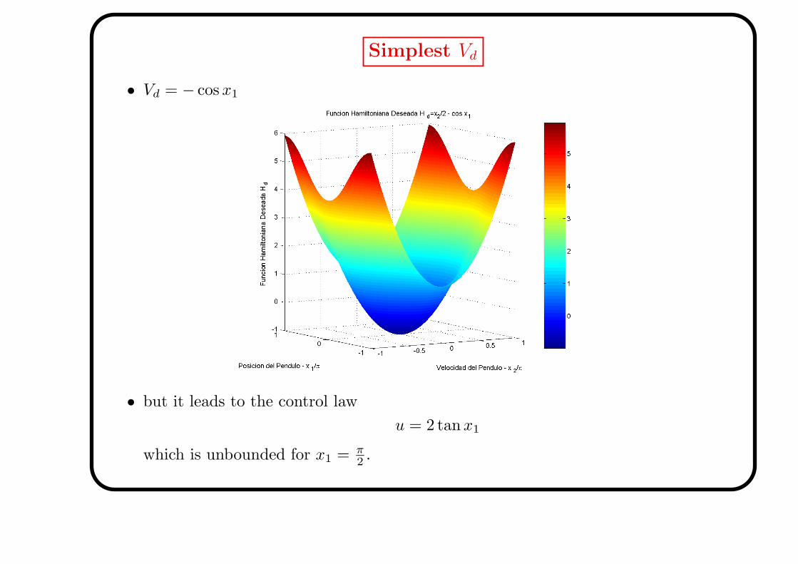
Simplest Vd

• Vd = − cos x1

• but it leads to the control law

u = 2 tanx1

which is unbounded for x1 = π2.

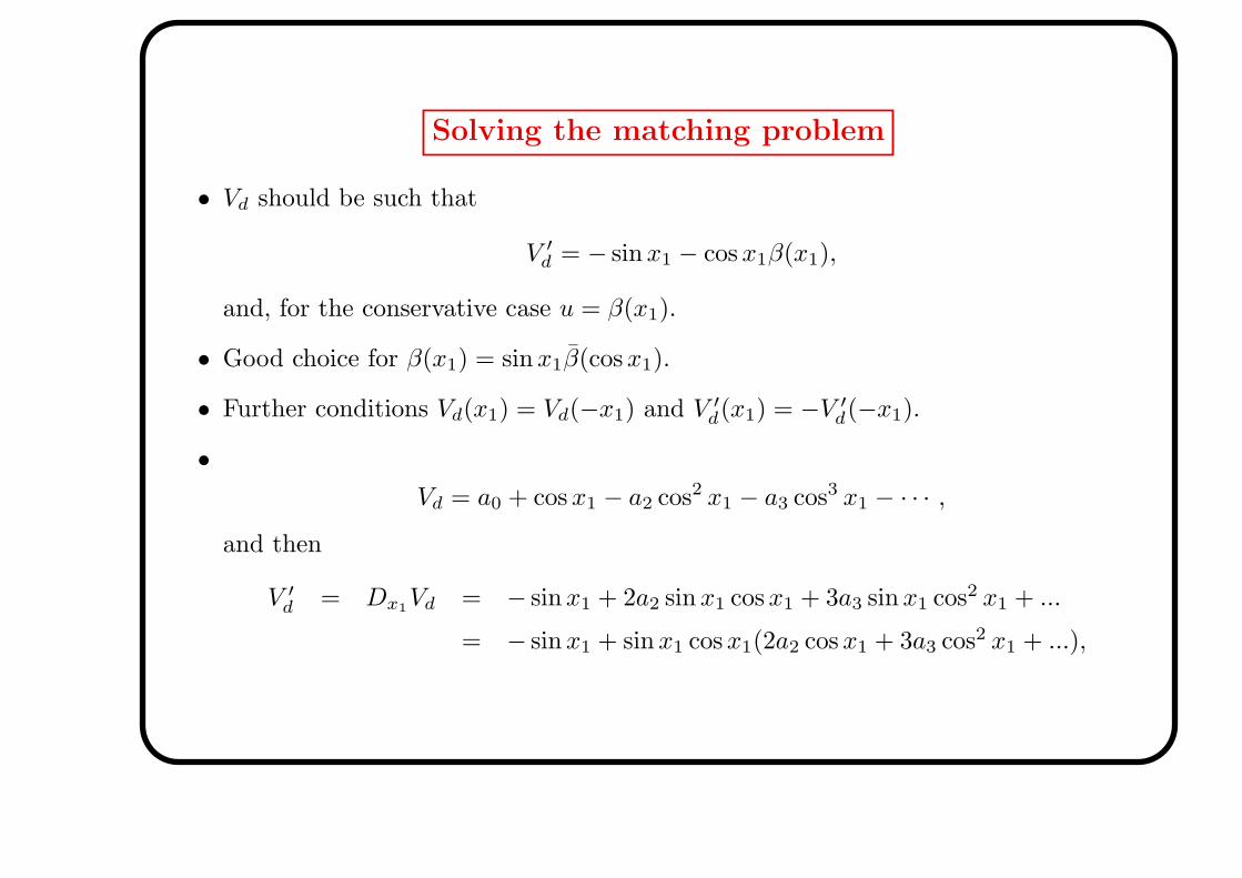
Solving the matching problem

• Vd should be such that

V ′

d = − sinx1 − cos x1β(x1),

and, for the conservative case u = β(x1).

• Good choice for β(x1) = sinx1β(cos x1).

• Further conditions Vd(x1) = Vd(−x1) and V ′

d(x1) = −V ′

d(−x1).

•

Vd = a0 + cos x1 − a2 cos2 x1 − a3 cos3 x1 − · · · ,

and then

V ′

d = Dx1Vd = − sinx1 + 2a2 sinx1 cos x1 + 3a3 sinx1 cos2 x1 + ...

= − sinx1 + sinx1 cos x1(2a2 cos x1 + 3a3 cos2 x1 + ...),

Shape of Hd for different Vd

−10

1

−1

0

1−10

−5

0

5

x2/π

Hd=x

22/2 + cosx

1 − 2cos2x

1

x1/π

Hd

−10

1

−1

0

1−10

−5

0

5

x2/π

Hd=x

22/2 + cosx

1 − 2cos2x

1 − 2cos3x

1

x1/π

Hd

−10

1

−1

0

1−20

−10

0

10

x2/π

Hd=x

22/2 + cosx

1 − 2cos2x

1 − 2cos3x

1 − 2cos4x

1

x1/π

Hd

−10

1

−1

0

1−20

−10

0

10

x2/π

Hd=x

22/2 + cosx

1 − 2cos2x

1 − 2cos3x

1 − 2cos4x

1 − 2cos5x

1

x1/π

Hd

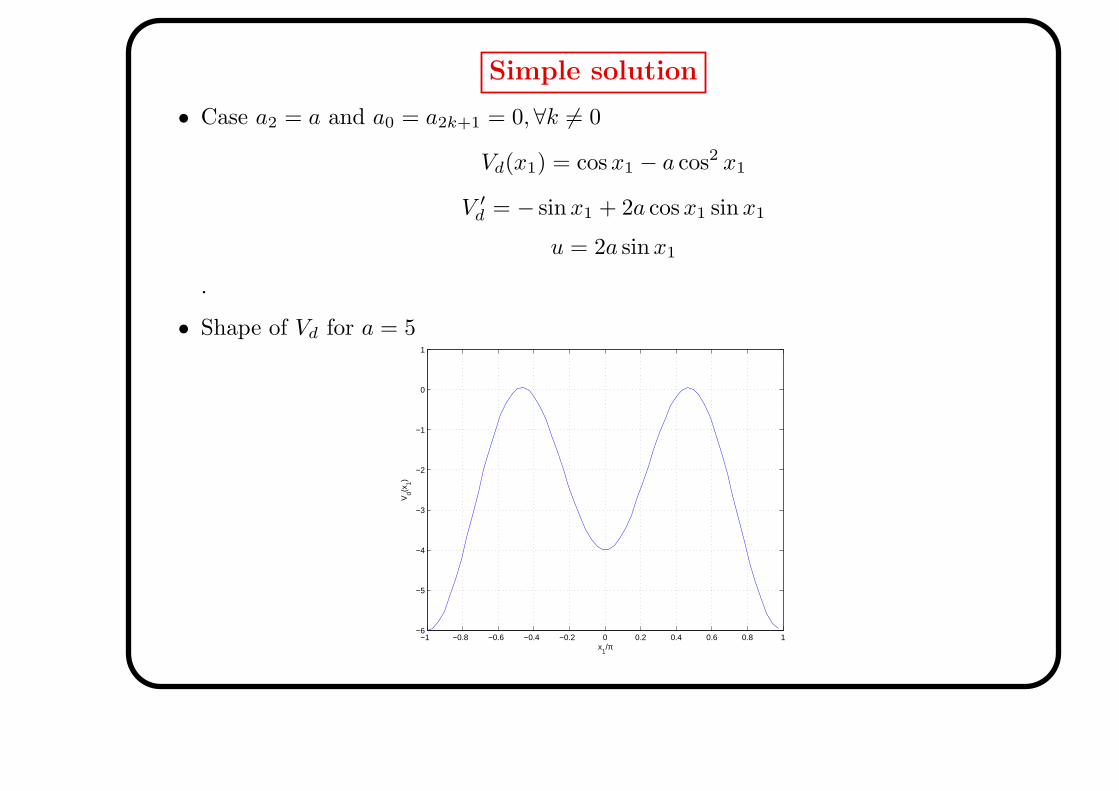
Simple solution

• Case a2 = a and a0 = a2k+1 = 0,∀k 6= 0

Vd(x1) = cos x1 − a cos2 x1

V ′

d = − sinx1 + 2a cos x1 sinx1

u = 2a sin x1

.

• Shape of Vd for a = 5

−1 −0.8 −0.6 −0.4 −0.2 0 0.2 0.4 0.6 0.8 1−6

−5

−4

−3

−2

−1

0

1

x1/π

Vd(x

1)

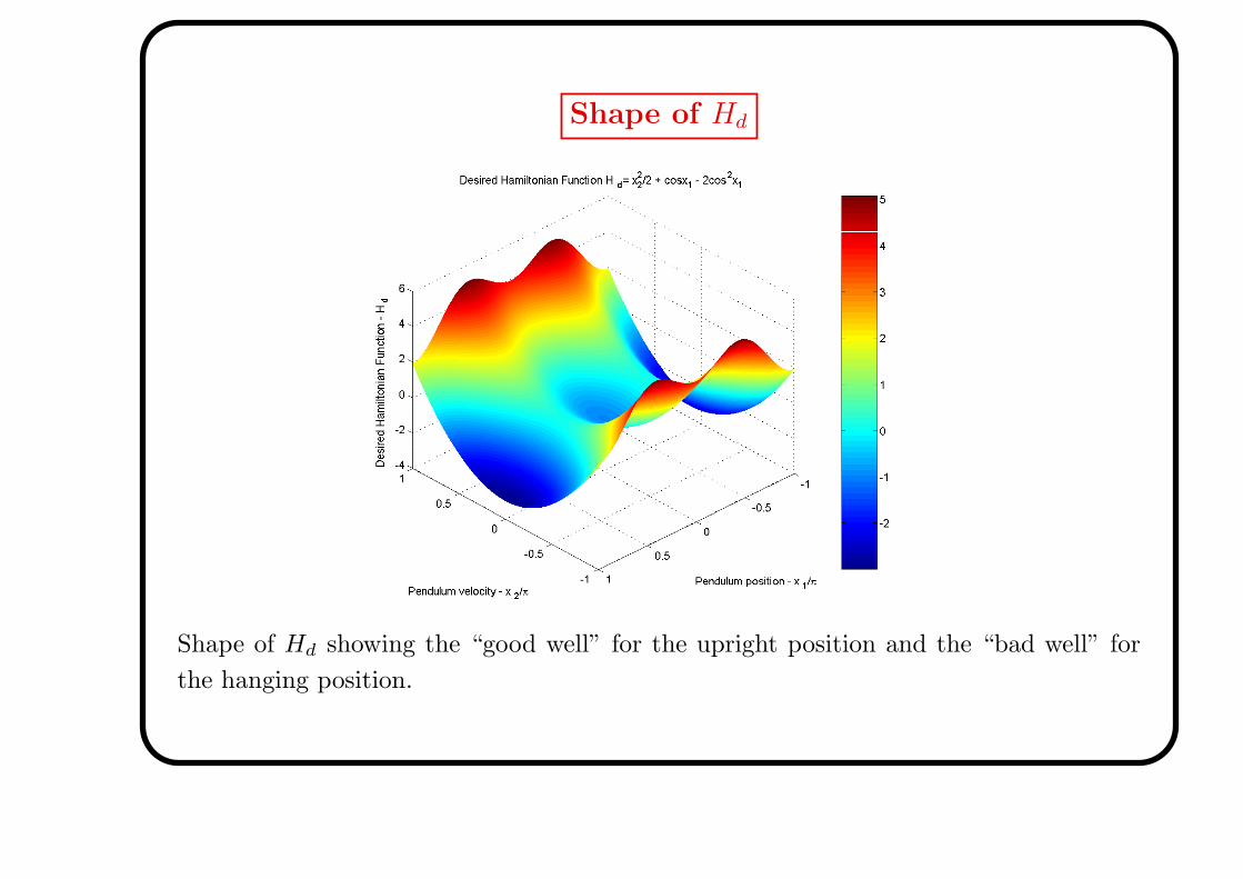
Shape of Hd

Shape of Hd showing the “good well” for the upright position and the “bad well” for

the hanging position.

Shape of Hd

Cut of Hd showing the non-desired “well” for the hanging position.

Shape of Hd

Cut of Hd showing the shape of the kinetic energy.

Adding damping

• x1

x2

=

0 1

−1 −k cos x1

Dx1

Hd

Dx2Hd

,

•

x1 = x2

x2 = −V ′

d(x1) − kx2 cos x1.

• Target system

x1 = x2

x2 = sinx1 − 2a cos x1 sin x1 − kx2 cos x1,

• Feedback law

u = 2a sin x1 + kx2.

However...

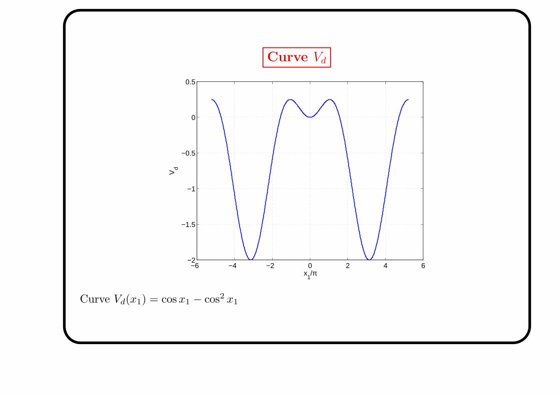
Curve Vd

−6 −4 −2 0 2 4 6−2

−1.5

−1

−0.5

0

0.5

x1/π

Vd

Curve Vd(x1) = cos x1 − cos2 x1

Curve Hd =1

4a

−2 −1.5 −1 −0.5 0 0.5 1 1.5 2−2.5

−2

−1.5

−1

−0.5

0

0.5

1

1.5

2

2.5

x1/π

x 2

Curve Hd(x1, x2) = cos x1 − cos2 x1 + 1

2x2

2 = 1

4a

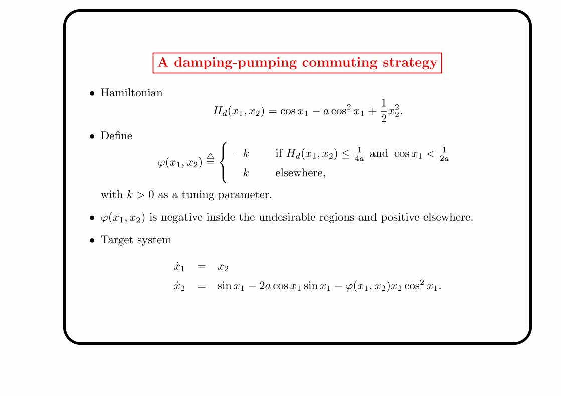
A damping-pumping commuting strategy

• Hamiltonian

Hd(x1, x2) = cos x1 − a cos2 x1 +1

2x2

2.

• Define

ϕ(x1, x2)△=

−k if Hd(x1, x2) ≤1

4aand cos x1 < 1

2a

k elsewhere,

with k > 0 as a tuning parameter.

• ϕ(x1, x2) is negative inside the undesirable regions and positive elsewhere.

• Target system

x1 = x2

x2 = sinx1 − 2a cos x1 sin x1 − ϕ(x1, x2)x2 cos2 x1.

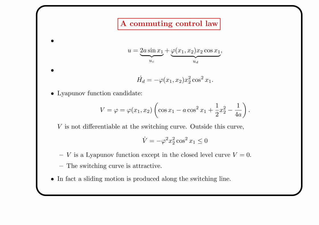
A commuting control law

•

u = 2a sin x1︸ ︷︷ ︸uc

+ ϕ(x1, x2)x2 cos x1︸ ︷︷ ︸ud

,

•

Hd = −ϕ(x1, x2)x22 cos2 x1.

• Lyapunov function candidate:

V = ϕ = ϕ(x1, x2)

(cos x1 − a cos2 x1 +

1

2x2

2 −1

4a

).

V is not differentiable at the switching curve. Outside this curve,

V = −ϕ2x22 cos2 x1 ≤ 0

– V is a Lyapunov function except in the closed level curve V = 0.

– The switching curve is attractive.

• In fact a sliding motion is produced along the switching line.

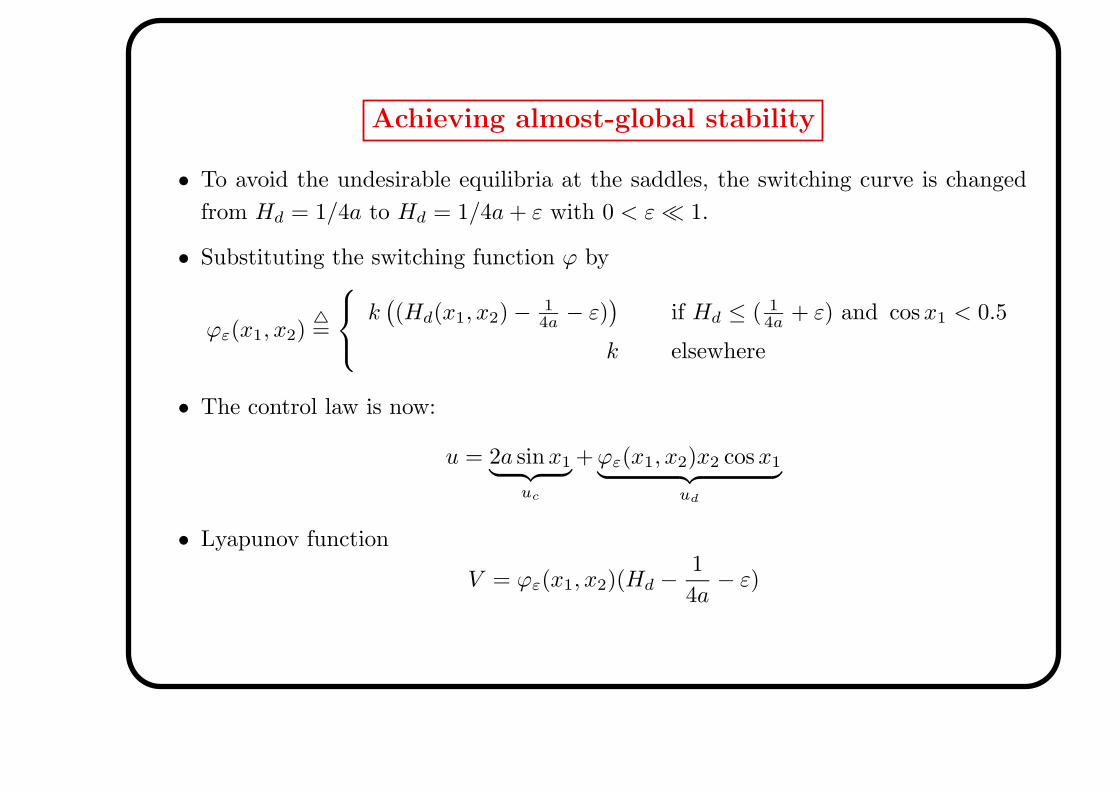
Achieving almost-global stability

• To avoid the undesirable equilibria at the saddles, the switching curve is changed

from Hd = 1/4a to Hd = 1/4a + ε with 0 < ε ≪ 1.

• Substituting the switching function ϕ by

ϕε(x1, x2)△=

k((Hd(x1, x2) −

1

4a− ε)

)if Hd ≤ ( 1

4a+ ε) and cos x1 < 0.5

k elsewhere

• The control law is now:

u = 2a sin x1︸ ︷︷ ︸uc

+ ϕε(x1, x2)x2 cos x1︸ ︷︷ ︸ud

• Lyapunov function

V = ϕε(x1, x2)(Hd −1

4a− ε)

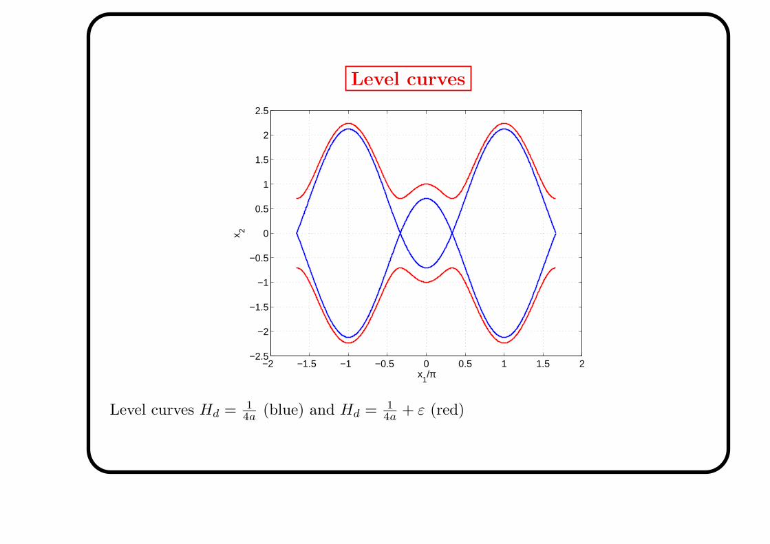
Level curves

−2 −1.5 −1 −0.5 0 0.5 1 1.5 2−2.5

−2

−1.5

−1

−0.5

0

0.5

1

1.5

2

2.5

x1/π

x 2

Level curves Hd = 1

4a(blue) and Hd = 1

4a+ ε (red)

Avoiding the sliding mode

• Sliding motions due to the discontinuity along the level curve Hd = 1

4a+ ε.

• Modify the switching function in such a way that it is equal to zero at both sides

of the switching curve.

• Multiplying function ϕε by abs(Hd(x1, x2)−1

4a− ε), ud will be equal to zero at the

level curve Hd = 1

4a+ ε avoiding the sliding motion.

• New switching function:

ϕε(x1, x2)△=

k(Hd(x1, x2) −1

4a− ε) if cos x1 < 0.5

k elsewhere

Simulations

−1.5 −1 −0.5 0 0.5 1 1.5

−2

0

2

x1/π

x 2

0 10 20 30 40 50−5

0

5

Time [s]

x 1

0 10 20 30 40 50−5

0

5

Time [s]

u

Results of a simulation with a = 1, ε = .25 and k = 0.2. Initial conditions: hanging

position at rest.

Animation

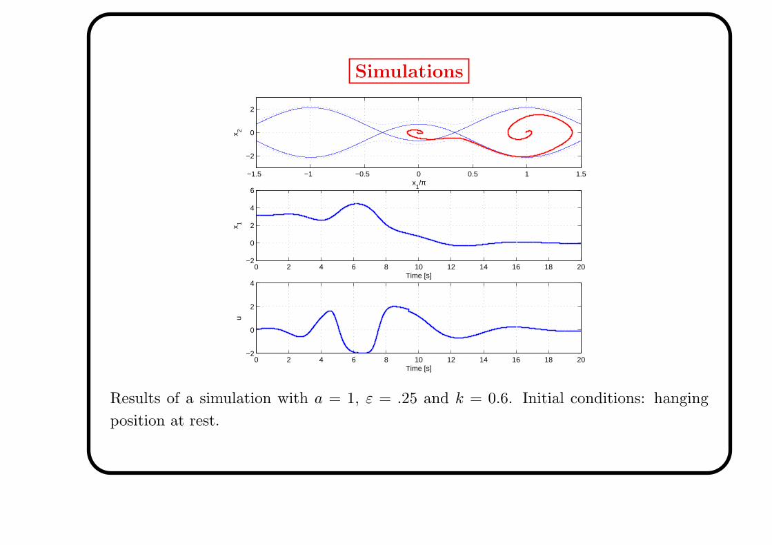
Simulations

−1.5 −1 −0.5 0 0.5 1 1.5

−2

0

2

x1/π

x 2

0 2 4 6 8 10 12 14 16 18 20−2

0

2

4

6

Time [s]

x 1

0 2 4 6 8 10 12 14 16 18 20−2

0

2

4

Time [s]

u

Results of a simulation with a = 1, ε = .25 and k = 0.6. Initial conditions: hanging

position at rest.

Trajectory leaving the well

−0.5 0 0.5 1 1.5 2

−4−2

02

40

10

20

30

40

50

60

70

80

x1/πx

2

Tim

e [s

]

Trajectory leaving the well and reaching the up-right position, for k = 0.2.

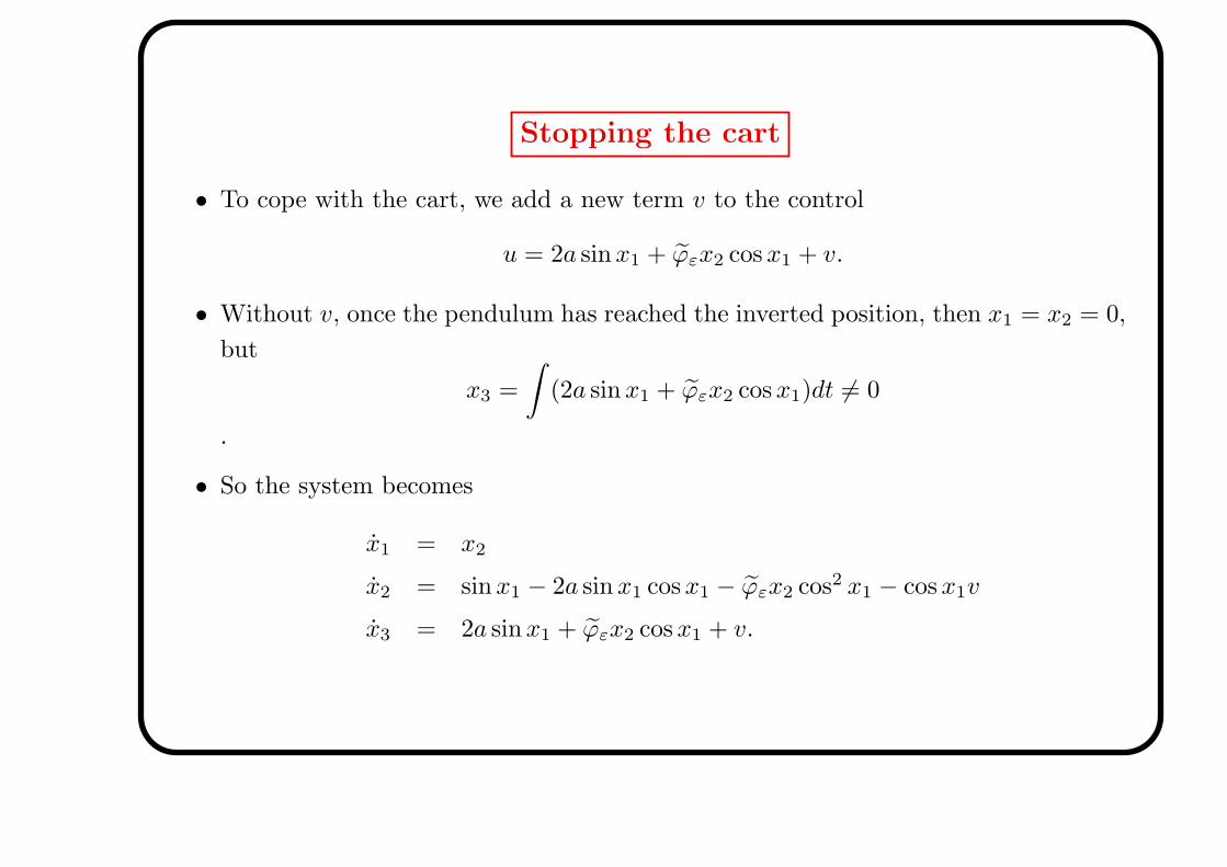
Stopping the cart

• To cope with the cart, we add a new term v to the control

u = 2a sin x1 + ϕεx2 cos x1 + v.

• Without v, once the pendulum has reached the inverted position, then x1 = x2 = 0,

but

x3 =

∫(2a sin x1 + ϕεx2 cos x1)dt 6= 0

.

• So the system becomes

x1 = x2

x2 = sinx1 − 2a sin x1 cos x1 − ϕεx2 cos2 x1 − cos x1v

x3 = 2a sinx1 + ϕεx2 cos x1 + v.

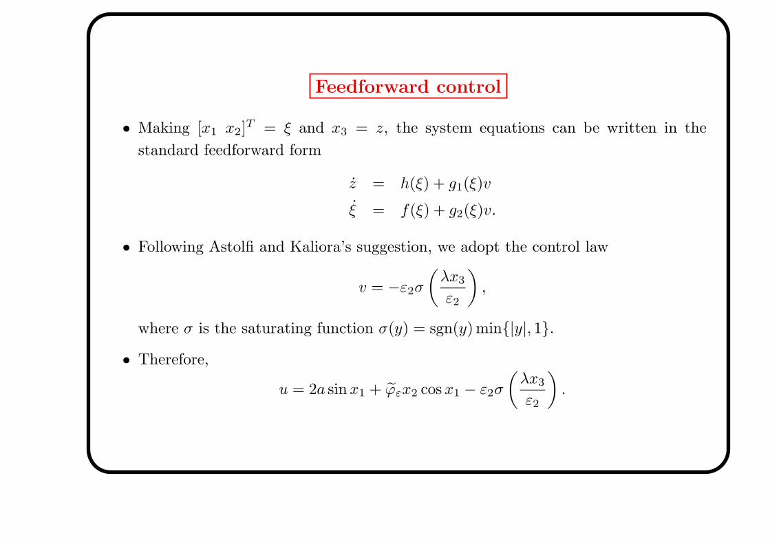
Feedforward control

• Making [x1 x2]T = ξ and x3 = z, the system equations can be written in the

standard feedforward form

z = h(ξ) + g1(ξ)v

ξ = f(ξ) + g2(ξ)v.

• Following Astolfi and Kaliora’s suggestion, we adopt the control law

v = −ε2σ

(λx3

ε2

),

where σ is the saturating function σ(y) = sgn(y) min{|y|, 1}.

• Therefore,

u = 2a sin x1 + ϕεx2 cos x1 − ε2σ

(λx3

ε2

).

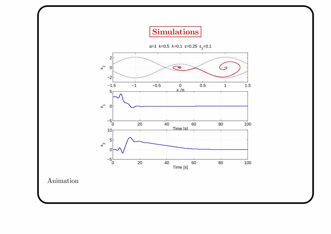
Simulations

−1.5 −1 −0.5 0 0.5 1 1.5

−2

0

2

x1/π

x 2

a=1 k=0.5 λ=0.1 ε=0.25 ε2=0.1

0 20 40 60 80 100−5

0

5

Time [s]

x 1

0 20 40 60 80 100−5

0

5

10

Time [s]

x 3

Animation

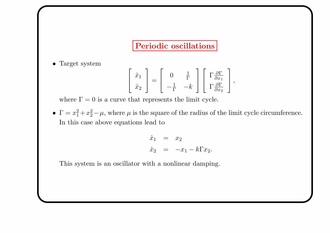
Periodic oscillations

• Target system x1

x2

=

0 1

Γ

− 1

Γ−k

Γ ∂Γ

∂x1

Γ ∂Γ

∂x2

,

where Γ = 0 is a curve that represents the limit cycle.

• Γ = x21 +x2

2−µ, where µ is the square of the radius of the limit cycle circumference.

In this case above equations lead to

x1 = x2

x2 = −x1 − kΓx2.

This system is an oscillator with a nonlinear damping.

Lyapunov function for an oscillating system

• The system of the previous slide has as Lyapunov function V = Γ2/4

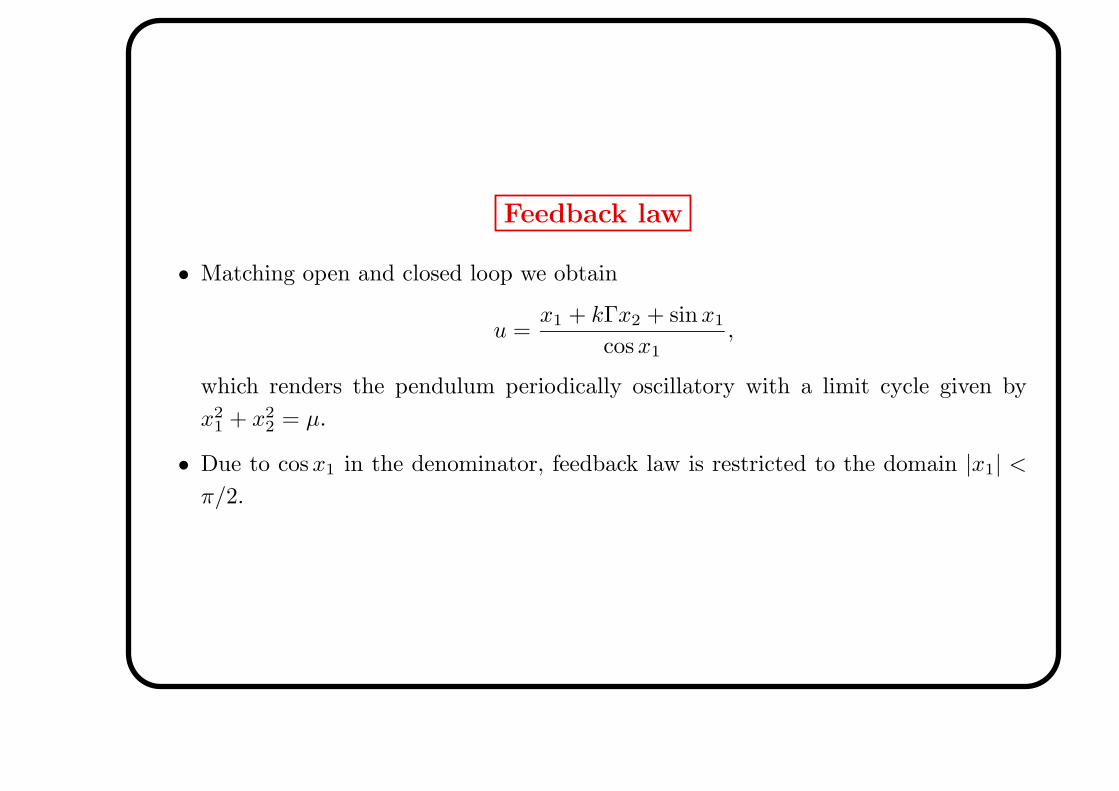
Feedback law

• Matching open and closed loop we obtain

u =x1 + kΓx2 + sinx1

cos x1

,

which renders the pendulum periodically oscillatory with a limit cycle given by

x21 + x2

2 = µ.

• Due to cos x1 in the denominator, feedback law is restricted to the domain |x1| <

π/2.

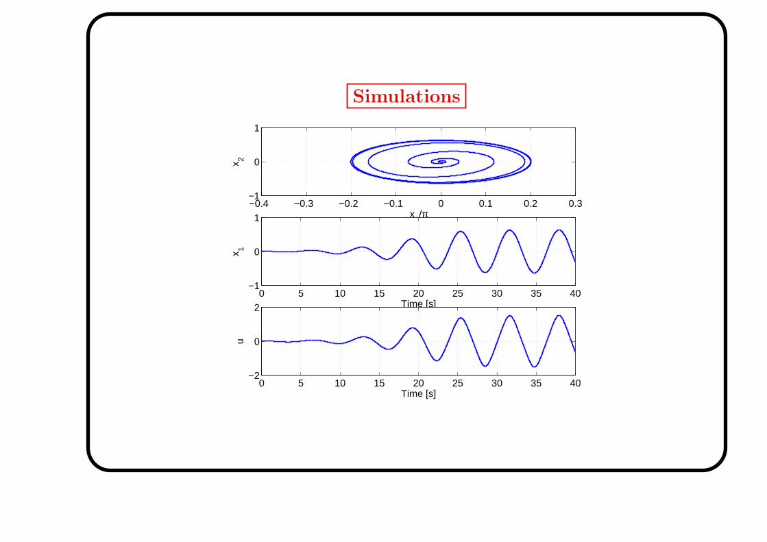
Simulations

−0.4 −0.3 −0.2 −0.1 0 0.1 0.2 0.3−1

0

1

x1/π

x 2

0 5 10 15 20 25 30 35 40−1

0

1

Time [s]

x 1

0 5 10 15 20 25 30 35 40−2

0

2

Time [s]

u

Taking the cart into account

• Add a new term v to the control

u =x1 + kΓx2 + sinx1

cos x1

+ v.

• Closed loop system

x1 = x2

x2 = −x1 − kx2Γ − cos x1v

x3 = x1+kΓx2+sin x1

cos x1

+ v.

• Proceeding in a similar way as for the swing up problem we shoyld adopt the control

law

u =x1 + kΓx2 + sinx1

cos x1

− εσ

(λx3

ε

).

Animation