Article

Vibration-Response-Only Structural HealthMonitoring for Offshore Wind Turbine JacketFoundations via Convolutional Neural Networks

Bryan Puruncajas1,2 , Yolanda Vidal 1,* , Christian Tutivén2

1 Control, Modeling, Identification and Applications (CoDAlab), Department of Mathematics, Escolad’Enginyeria de Barcelona Est (EEBE), Universitat Politècnica de Catalunya (UPC), Campus Diagonal-Besós(CDB), Eduard Maristany, 16, 08019 Barcelona, Spain.

2 Mechatronics Engineering, Faculty of Mechanical Engineering and Production Science (FIMCP), EscuelaSuperior Politécnica del Litoral (ESPOL), Guayaquil, Ecuador.

* Correspondence: yolanda.vidal@upc.edu; Tel.: +34-934-137-309

Version June 15, 2020 submitted to Sensors

Abstract: This work deals with structural health monitoring for jacket-type foundations of offshore1

wind turbines. In particular, a vibration-response-only methodology is proposed based on2

accelerometer data and deep convolutional neural networks. The main contribution of this article3

is twofold: i) a signal-to-image conversion of the accelerometer data into gray scale multi-channel4

images with as many channels as the number of sensors in the condition monitoring system, and5

ii) a data augmentation strategy to diminish the test set error of the deep convolutional neural6

network used to classify the images. The performance of the proposed method is analysed using7

real measurements from a steel jacket-type offshore wind turbine laboratory experiment undergoing8

different damage scenarios. The results, with a classification accuracy over 99%, demonstrate that the9

stated methodology is promising to be utilised for damage detection and identification in jacket-type10

support structures.11

Keywords: structural health monitoring; damage detection; damage identification; offshore wind12

turbine foundation; jacket; signal-to-image conversion; convolutional neural network13

1. Introduction14

Globally, wind power generation capacity has increased exponentially since the early 1990s, and15

as of the end of 2019, this capacity amounted to 650 GW [1]. Whereas onshore wind turbines (WTs)16

have dominated new wind installations during the past, the growth of offshore WTs is poised to17

become the new leader, because of steadier wind, in addition to vast regions where its installation is18

possible. In regard to the global offshore market, the cumulative installations have now reached 23 GW,19

representing 4% of total cumulative installations. Unfortunately, offshore WTs are placed in a harsh20

environment that originates from the wind and the sea conditions [2]. As a consequence, offshore WTs21

require rigorous safety measures because it is extremely complicated to do operation and corrective22

work on these huge WTs placed in remote locations. Given that approaches centered on enhancing23

component reliability are likely to increase capital expenditures, instead system design optimization24

research and development activities should focus on minimizing and, if possible, even eliminating25

unexpected failures. In other words, the wind industry must abandon corrective maintenance (remedy26

failures) and move toward predictive maintenance (repair immediately before failure) to achieve27

maximum availability. Thus, the development of a structural health monitoring (SHM) strategy is28

particularly necessary to achieve this goal.29

Submitted to Sensors, pages 1 – 18 www.mdpi.com/journal/sensors

Version June 15, 2020 submitted to Sensors 2 of 18

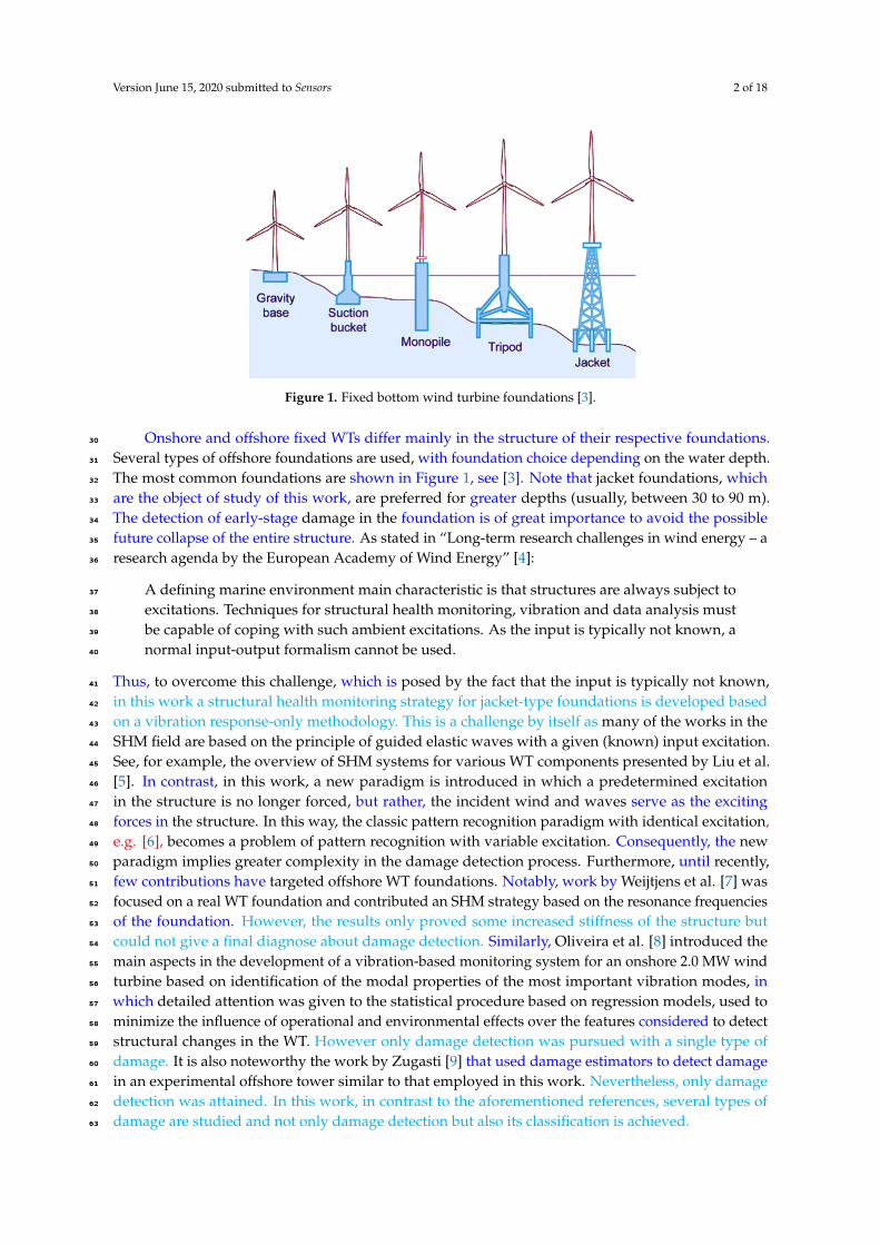
Figure 1. Fixed bottom wind turbine foundations [3].

Onshore and offshore fixed WTs differ mainly in the structure of their respective foundations.30

Several types of offshore foundations are used, with foundation choice depending on the water depth.31

The most common foundations are shown in Figure 1, see [3]. Note that jacket foundations, which32

are the object of study of this work, are preferred for greater depths (usually, between 30 to 90 m).33

The detection of early-stage damage in the foundation is of great importance to avoid the possible34

future collapse of the entire structure. As stated in “Long-term research challenges in wind energy – a35

research agenda by the European Academy of Wind Energy” [4]:36

A defining marine environment main characteristic is that structures are always subject to37

excitations. Techniques for structural health monitoring, vibration and data analysis must38

be capable of coping with such ambient excitations. As the input is typically not known, a39

normal input-output formalism cannot be used.40

Thus, to overcome this challenge, which is posed by the fact that the input is typically not known,41

in this work a structural health monitoring strategy for jacket-type foundations is developed based42

on a vibration response-only methodology. This is a challenge by itself as many of the works in the43

SHM field are based on the principle of guided elastic waves with a given (known) input excitation.44

See, for example, the overview of SHM systems for various WT components presented by Liu et al.45

[5]. In contrast, in this work, a new paradigm is introduced in which a predetermined excitation46

in the structure is no longer forced, but rather, the incident wind and waves serve as the exciting47

forces in the structure. In this way, the classic pattern recognition paradigm with identical excitation,48

e.g. [6], becomes a problem of pattern recognition with variable excitation. Consequently, the new49

paradigm implies greater complexity in the damage detection process. Furthermore, until recently,50

few contributions have targeted offshore WT foundations. Notably, work by Weijtjens et al. [7] was51

focused on a real WT foundation and contributed an SHM strategy based on the resonance frequencies52

of the foundation. However, the results only proved some increased stiffness of the structure but53

could not give a final diagnose about damage detection. Similarly, Oliveira et al. [8] introduced the54

main aspects in the development of a vibration-based monitoring system for an onshore 2.0 MW wind55

turbine based on identification of the modal properties of the most important vibration modes, in56

which detailed attention was given to the statistical procedure based on regression models, used to57

minimize the influence of operational and environmental effects over the features considered to detect58

structural changes in the WT. However only damage detection was pursued with a single type of59

damage. It is also noteworthy the work by Zugasti [9] that used damage estimators to detect damage60

in an experimental offshore tower similar to that employed in this work. Nevertheless, only damage61

detection was attained. In this work, in contrast to the aforementioned references, several types of62

damage are studied and not only damage detection but also its classification is achieved.63

Version June 15, 2020 submitted to Sensors 3 of 18

It is important to note that the SHM standard approach for the problem at hand is usually an64

unsupervised one. That is, as no-one would purposely damage their assets to train a SHM tool, only65

healthy data from the real structure is used. However is unfeasible to correctly identify different66

damage states using solely data obtained during what is assumed to be a healthy state. In this67

framework, detection can be accomplished by using a model of normality or unsupervised models,68

but not classification on the type of damage. The approach proposed in this work is the opposite, that69

is: a supervised approach. Thus data from the damaged structure is required to train the model. In70

practice, this will be accomplished by means of computer models, as the finite element method (FEM).71

The FEM model should be validated with a down-scaled experimental tower (as the one proposed in72

this work). Then the full-scale finite element model would be used to generate healthy (to validate73

with the real asset) and damage samples. Finally, the stated supervised methodology proposed in this74

work can be used. In this work, a satisfactory experimental proof of concept has been conducted with75

the proposed strategy and a laboratory down-scaled WT. However, future work is needed to validate76

the technology in a full-scale and more realistic environment. Some examples of this type of approach77

are given in [10], where bridge damage detection is accomplished by a neural network considering78

errors in baseline finite element models, and [11] where the stated SHM method for an oil offshore79

structure is capable to cope with several types of damage based on a finite element model.80

On the one hand, it has been shown that traditional machine learning requires complex feature81

extraction processes and specialized knowledge, especially for a complex problem such as WT82

condition monitoring [12–14]. Moreover, extracting features with classic machine learning methods83

faces the classic bias-variance dilemma from inference theory. The bias-variance trade-off implies that a84

model should balance under-fitting and over-fitting; that is, the model should be rich enough to express85

underlying structure in the data but simple enough to avoid fitting spurious patterns, respectively.86

On the other hand, in the modern practice of deep learning, very rich models are trained to precisely87

fit (i.e., interpolate) the data. Classically, such models would be considered over-fit, and yet they88

often obtain high accuracy on test data. Thus, this paper proposes to use deep convolutional neural89

networks (CNN) for pattern recognition (classification), avoiding the aforementioned usual problems90

in the literature, e.g. [12–14], related to feature extraction and bias-variance trade-off. In particular,91

we develop a novel damage diagnosis method for WT offshore foundations based on transforming92

condition monitoring multi-vibration-signals into images (with as many channels as sensors) to be93

processed afterward using deep CNN.94

The paper is organized in the following manner. First, in Section 2, the experimental set-up is95

introduced. It consistis in a steel jacket-type offshore WT laboratory structure undergoing different96

damage scenarios. Then, in Section 3, the proposed SHM strategy is described in detail. The approach97

can be summarized by the following steps: i) accelerometer data is gathered, ii) a pre-process is98

designed to extract the maximum amount of information and to obtain a dataset of 24 (that is, the99

same number as accelerometer sensors) channel gray-scale images, iii) 24-channel-input deep CNN100

is designed and trained for classification of the different structural states. In Section 4, the obtained101

results are conferred, showing an exceptional performance, with all considered metrics giving results102

greater than 99%. Lastly, the main conclusions are given in Section 5 as well as future work research103

directions.104

2. Experimental Set-Up105

The laboratory experimental set-up is described in the following. First, a function generator (GW106

INSTEK AF-2005 model) is employed to generate a white noise signal. Then, this signal is amplified107

and applied to a modal shaker (GW-IV47 from Data Physics) that induces the vibration into the108

structure. The general overview of the experimental set-up is shown in Figure 2 (left). The structure is109

2.7 meters tall and composed of three parts:110

1. The top beam (1× 0.6 meters) where the modal shaker is attached to simulate a nacelle mass and111

the effects of wind excitation,112

Version June 15, 2020 submitted to Sensors 4 of 18

2. The tower with three tubular sections connected with bolts,113

3. The jacket, which includes a pyramidal structure made up by 32 bars (S275JR steel) of different114

lengths, sheets (DC01 LFR steel), and other elements such as bolts and nuts.115

It should be noted that different wind speeds are considered by modifying the white noise signal116

amplitude (i.e., scaling the amplitude by 0.5, 1, 2, and 3). To measure vibration, eight triaxial

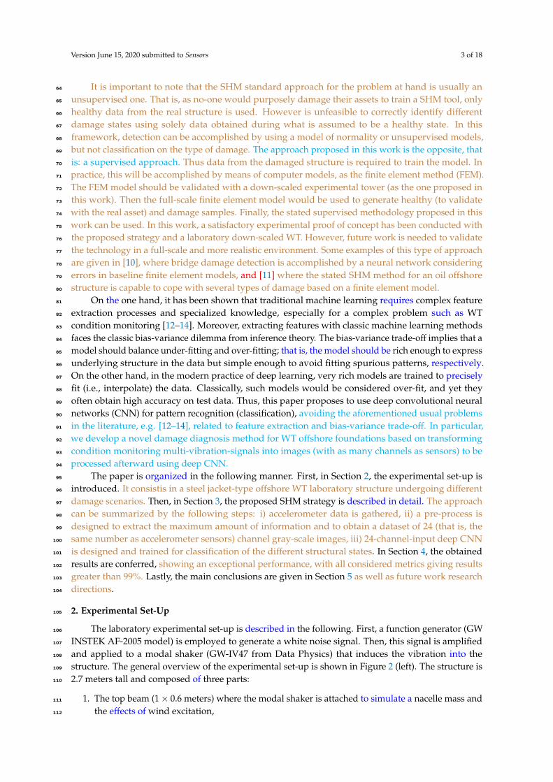
Figure 2. The experimental set-up (left) detailing the location of the damaged bar (red circle). Locationof the sensors on the overall structure (right).

117

accelerometers (PCB R© Piezotronic, model 356A17) are placed on the structure, see Figure 2 (right). The118

optimal number and placement of the sensors is determined according to [9]. The accelerometers are119

connected to six National InstrumentsTM cartridges (NI 9234 model) that are inserted in the National120

Instruments chassis cDAQ-9188. Finally, the Data Acquisition ToolboxTM is employed to configure the121

data acquisition hardware and read the data into MATLAB R©.122

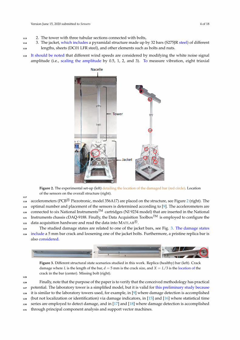
The studied damage states are related to one of the jacket bars, see Fig. 3. The damage states123

include a 5 mm bar crack and loosening one of the jacket bolts. Furthermore, a pristine replica bar is124

also considered.

Figure 3. Different structural state scenarios studied in this work. Replica (healthy) bar (left). Crackdamage where L is the length of the bar, d = 5 mm is the crack size, and X = L/3 is the location of thecrack in the bar (center). Missing bolt (right).

125

Finally, note that the purpose of the paper is to verify that the conceived methodology has practical126

potential. The laboratory tower is a simplified model, but it is valid for this preliminary study because127

it is similar to the laboratory towers used, for example, in [9] where damage detection is accomplished128

(but not localization or identification) via damage indicators, in [15] and [16] where statistical time129

series are employed to detect damage, and in [17] and [18] where damage detection is accomplished130

through principal component analysis and support vector machines.131

Version June 15, 2020 submitted to Sensors 5 of 18

3. Structural Health Monitoring Proposed Methodology132

The proposed SHM strategy follows the steps detailed here. First, the raw time series data are133

collected. Second, the data are pre-processed to obtain a dataset of 24 channel gray-scale images. Third,134

a 24-channel-input CNN is designed and trained for classification of the different structural states. The135

following subsections describe in detail the aforementioned procedure.136

3.1. Data gathering137

The data are gathered in different experiments with a sampling rate of 275.27 Hz and a durationof 60 sec each. Table 1 shows the total number of realized experiments for the corresponding structuralstate (with its corresponding label) and white noise amplitude. A total of K = 100 experiments areconducted. Given the k-th experiment, where k is varied from 1 to K = 100, the raw data are thensaved in the matrix X(k) ∈ M16517×24(R)

X(k) =

x(k)1,1 x(k)1,2 · · · x(k)1,24

x(k)2,1 x(k)2,2 · · · x(k)2,24...

.... . .

...

x(k)16517,1 x(k)16517,2 · · · x(k)16517,24

. (1)

Note that there are as many rows as the number of measurements in each experiment, that is I = 16, 517,and as many columns as the number of sensors, J = 24 (because each column is related to one sensor).Ultimately, the overall data matrix X ∈ M1651700×24(R) is constructed by stacking the matrices thatarise from each different experiment,

X =

X(1)

...X(k)

...X(100)

. (2)

Table 1. Total number of experimental tests for the different white noise (WN) amplitudes and for eachstructural state.

Label Structuralstate 0.5WN 1WN 2WN 3WN

1 Healthy bar 10 tests 10 tests 10 tests 10 tests2 Replica bar 5 tests 5 tests 5 tests 5 tests3 Crack damaged bar 5 tests 5 tests 5 tests 5 tests4 Unlocked bolt 5 tests 5 tests 5 tests 5 tests

138

3.2. Data preprocessing: Scaling, reshaping, augmentation, and signal-to-image conversion139

Data preprocessing is both the initial step and a critical step in machine learning. In this work,140

data reshaping is employed to guarantee that each sample includes multiple measurements from each141

sensor and thus has sufficient information to make a diagnosis regarding the state of the structure.142

Furthermore, a data augmentation strategy is proposed to improve the final test set error of the143

prediction model. It is clear that the signal-to-image conversion as well as the architecture and144

hyperparameters of the deep CNN will play a key role in the damage detection methodology. However,145

Version June 15, 2020 submitted to Sensors 6 of 18

the manner in which these data are scaled, augmented, and reshaped will significantly impact the146

overall performance of the strategy [19].147

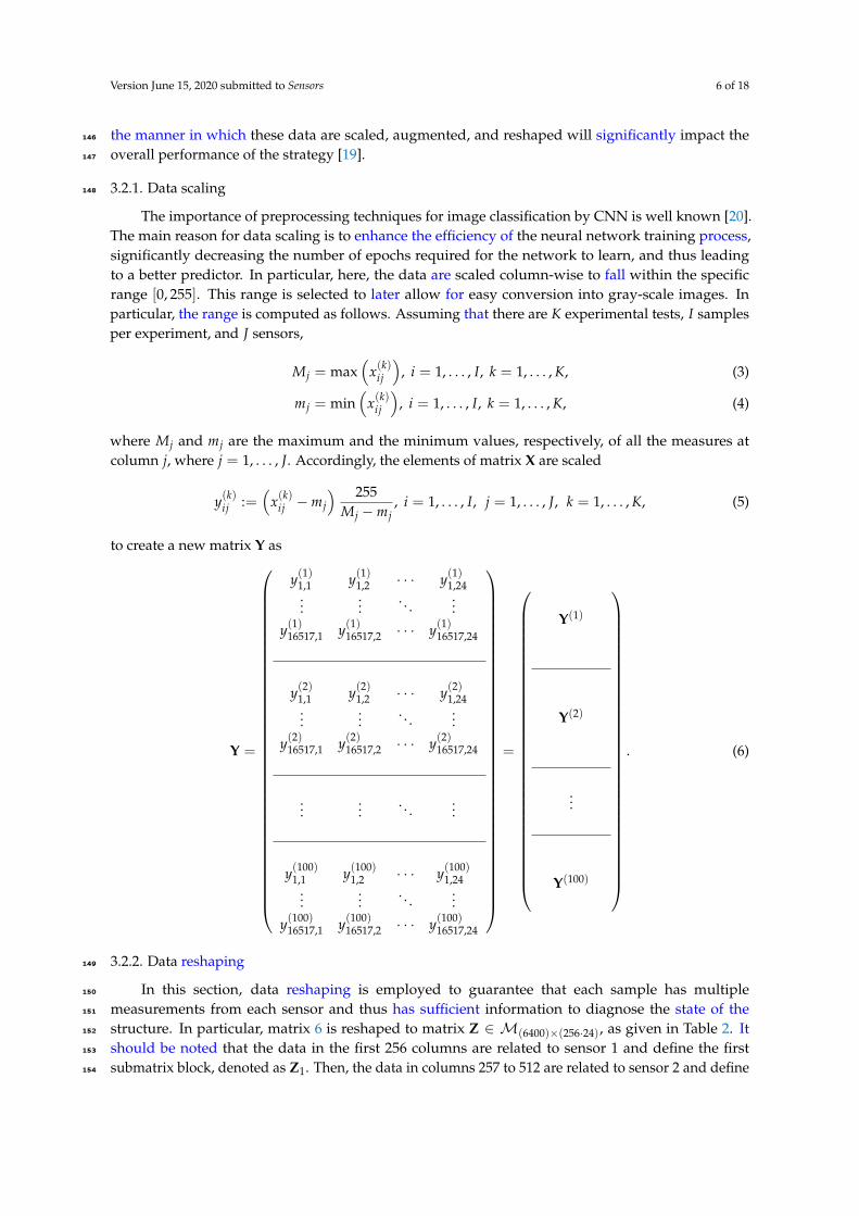
3.2.1. Data scaling148

The importance of preprocessing techniques for image classification by CNN is well known [20].The main reason for data scaling is to enhance the efficiency of the neural network training process,significantly decreasing the number of epochs required for the network to learn, and thus leadingto a better predictor. In particular, here, the data are scaled column-wise to fall within the specificrange [0, 255]. This range is selected to later allow for easy conversion into gray-scale images. Inparticular, the range is computed as follows. Assuming that there are K experimental tests, I samplesper experiment, and J sensors,

Mj = max(

x(k)ij

), i = 1, . . . , I, k = 1, . . . , K, (3)

mj = min(

x(k)ij

), i = 1, . . . , I, k = 1, . . . , K, (4)

where Mj and mj are the maximum and the minimum values, respectively, of all the measures atcolumn j, where j = 1, . . . , J. Accordingly, the elements of matrix X are scaled

y(k)ij :=(

x(k)ij −mj

) 255Mj −mj

, i = 1, . . . , I, j = 1, . . . , J, k = 1, . . . , K, (5)

to create a new matrix Y as

Y =

y(1)1,1 y(1)1,2 · · · y(1)1,24...

.... . .

...

y(1)16517,1 y(1)16517,2 · · · y(1)16517,24

y(2)1,1 y(2)1,2 · · · y(2)1,24...

.... . .

...

y(2)16517,1 y(2)16517,2 · · · y(2)16517,24

......

. . ....

y(100)1,1 y(100)

1,2 · · · y(100)1,24

......

. . ....

y(100)16517,1 y(100)

16517,2 · · · y(100)16517,24

=

Y(1)

Y(2)

...

Y(100)

. (6)

3.2.2. Data reshaping149

In this section, data reshaping is employed to guarantee that each sample has multiple150

measurements from each sensor and thus has sufficient information to diagnose the state of the151

structure. In particular, matrix 6 is reshaped to matrix Z ∈ M(6400)×(256·24), as given in Table 2. It152

should be noted that the data in the first 256 columns are related to sensor 1 and define the first153

submatrix block, denoted as Z1. Then, the data in columns 257 to 512 are related to sensor 2 and define154

Version June 15, 2020 submitted to Sensors 7 of 18

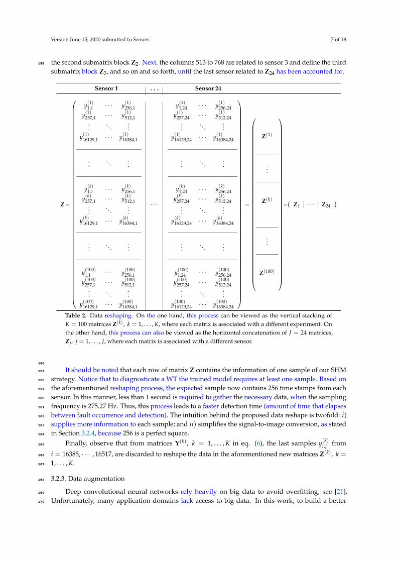
the second submatrix block Z2. Next, the columns 513 to 768 are related to sensor 3 and define the third155

submatrix block Z3, and so on and so forth, until the last sensor related to Z24 has been accounted for.

Sensor 1 . . . Sensor 24

Z =

y(1)1,1 · · · y(1)256,1

y(1)257,1 · · · y(1)512,1...

. . ....

y(1)16129,1 · · · y(1)16384,1

.... . .

...

y(k)1,1 · · · y(k)256,1

y(k)257,1 · · · y(k)512,1...

. . ....

y(k)16129,1 · · · y(k)16384,1

.... . .

...

y(100)1,1 · · · y(100)

256,1

y(100)257,1 · · · y(100)

512,1...

. . ....

y(100)16129,1 · · · y(100)

16384,1

· · ·

y(1)1,24 · · · y(1)256,24

y(1)257,24 · · · y(1)512,24...

. . ....

y(1)16129,24 · · · y(1)16384,24

.... . .

...

y(k)1,24 · · · y(k)256,24

y(k)257,24 · · · y(k)512,24...

. . ....

y(k)16129,24 · · · y(k)16384,24

.... . .

...

y(100)1,24 · · · y(100)

256,24

y(100)257,24 · · · y(100)

512,24...

. . ....

y(100)16129,24 · · · y(100)

16384,24

=

Z(1)

...

Z(k)

...

Z(100)

=(

Z1 · · · Z24)

Table 2. Data reshaping. On the one hand, this process can be viewed as the vertical stacking ofK = 100 matrices Z(k), k = 1, . . . , K, where each matrix is associated with a different experiment. Onthe other hand, this process can also be viewed as the horizontal concatenation of J = 24 matrices,Zj, j = 1, . . . , J, where each matrix is associated with a different sensor.

156

It should be noted that each row of matrix Z contains the information of one sample of our SHM157

strategy. Notice that to diagnosticate a WT the trained model requires at least one sample. Based on158

the aforementioned reshaping process, the expected sample now contains 256 time stamps from each159

sensor. In this manner, less than 1 second is required to gather the necessary data, when the sampling160

frequency is 275.27 Hz. Thus, this process leads to a faster detection time (amount of time that elapses161

between fault occurrence and detection). The intuition behind the proposed data reshape is twofold: i)162

supplies more information to each sample; and ii) simplifies the signal-to-image conversion, as stated163

in Section 3.2.4, because 256 is a perfect square.164

Finally, observe that from matrices Y(k), k = 1, . . . , K in eq. (6), the last samples y(k)i,j from165

i = 16385, · · · , 16517, are discarded to reshape the data in the aforementioned new matrices Z(k), k =166

1, . . . , K.167

3.2.3. Data augmentation168

Deep convolutional neural networks rely heavily on big data to avoid overfitting, see [21].169

Unfortunately, many application domains lack access to big data. In this work, to build a better170

Version June 15, 2020 submitted to Sensors 8 of 18

deep CNN model, a data augmentation strategy is proposed that artificially expands the size of the171

training dataset without actually collecting new data.172

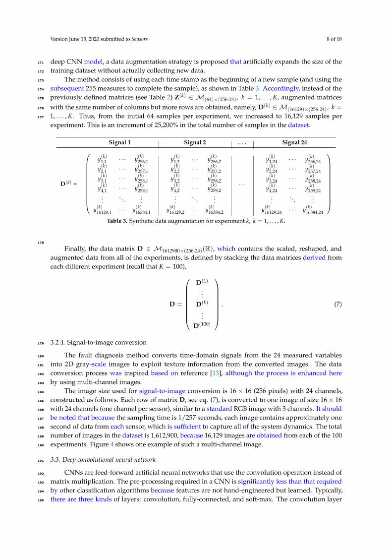
The method consists of using each time stamp as the beginning of a new sample (and using the173

subsequent 255 measures to complete the sample), as shown in Table 3. Accordingly, instead of the174

previously defined matrices (see Table 2) Z(k) ∈ M(64)×(256·24), k = 1, . . . , K, augmented matrices175

with the same number of columns but more rows are obtained, namely, D(k) ∈ M(16129)×(256·24), k =176

1, . . . , K. Thus, from the initial 64 samples per experiment, we increased to 16,129 samples per177

experiment. This is an increment of 25,200% in the total number of samples in the dataset.

Signal 1 Signal 2 . . . Signal 24

D(k) =

y(k)1,1 · · · y(k)256,1

y(k)2,1 · · · y(k)257,1

y(k)3,1 · · · y(k)258,1

y(k)4,1 · · · y(k)259,1...

. . ....

y(k)16129,1 · · · y(k)16384,1

y(k)1,2 · · · y(k)256,2

y(k)2,2 · · · y(k)257,2

y(k)3,2 · · · y(k)258,2

y(k)4,2 · · · y(k)259,2...

. . ....

y(k)16129,2 · · · y(k)16384,2

· · ·

y(k)1,24 · · · y(k)256,24

y(k)2,24 · · · y(k)257,24

y(k)3,24 · · · y(k)258,24

y(k)4,24 · · · y(k)259,24...

. . ....

y(k)16129,24 · · · y(k)16384,24

Table 3. Synthetic data augmentation for experiment k, k = 1, . . . , K.

178

Finally, the data matrix D ∈ M1612900×(256·24)(R), which contains the scaled, reshaped, andaugmented data from all of the experiments, is defined by stacking the data matrices derived fromeach different experiment (recall that K = 100),

D =

D(1)

...D(k)

...D(100)

. (7)

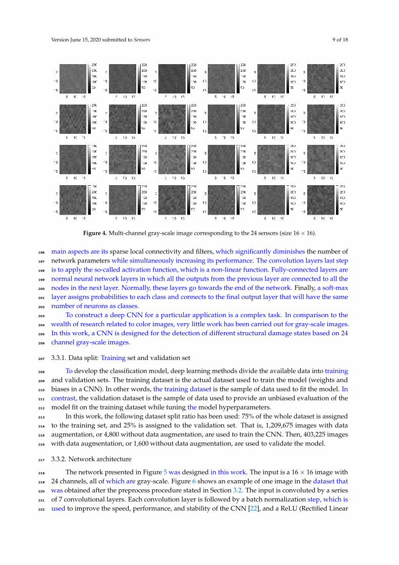
3.2.4. Signal-to-image conversion179

The fault diagnosis method converts time-domain signals from the 24 measured variables180

into 2D gray-scale images to exploit texture information from the converted images. The data181

conversion process was inspired based on reference [13], although the process is enhanced here182

by using multi-channel images.183

The image size used for signal-to-image conversion is 16× 16 (256 pixels) with 24 channels,184

constructed as follows. Each row of matrix D, see eq. (7), is converted to one image of size 16× 16185

with 24 channels (one channel per sensor), similar to a standard RGB image with 3 channels. It should186

be noted that because the sampling time is 1/257 seconds, each image contains approximately one187

second of data from each sensor, which is sufficient to capture all of the system dynamics. The total188

number of images in the dataset is 1,612,900, because 16,129 images are obtained from each of the 100189

experiments. Figure 4 shows one example of such a multi-channel image.190

3.3. Deep convolutional neural network191

CNNs are feed-forward artificial neural networks that use the convolution operation instead of192

matrix multiplication. The pre-processing required in a CNN is significantly less than that required193

by other classification algorithms because features are not hand-engineered but learned. Typically,194

there are three kinds of layers: convolution, fully-connected, and soft-max. The convolution layer195

Version June 15, 2020 submitted to Sensors 9 of 18

Figure 4. Multi-channel gray-scale image corresponding to the 24 sensors (size 16× 16).

main aspects are its sparse local connectivity and filters, which significantly diminishes the number of196

network parameters while simultaneously increasing its performance. The convolution layers last step197

is to apply the so-called activation function, which is a non-linear function. Fully-connected layers are198

normal neural network layers in which all the outputs from the previous layer are connected to all the199

nodes in the next layer. Normally, these layers go towards the end of the network. Finally, a soft-max200

layer assigns probabilities to each class and connects to the final output layer that will have the same201

number of neurons as classes.202

To construct a deep CNN for a particular application is a complex task. In comparison to the203

wealth of research related to color images, very little work has been carried out for gray-scale images.204

In this work, a CNN is designed for the detection of different structural damage states based on 24205

channel gray-scale images.206

3.3.1. Data split: Training set and validation set207

To develop the classification model, deep learning methods divide the available data into training208

and validation sets. The training dataset is the actual dataset used to train the model (weights and209

biases in a CNN). In other words, the training dataset is the sample of data used to fit the model. In210

contrast, the validation dataset is the sample of data used to provide an unbiased evaluation of the211

model fit on the training dataset while tuning the model hyperparameters.212

In this work, the following dataset split ratio has been used: 75% of the whole dataset is assigned213

to the training set, and 25% is assigned to the validation set. That is, 1,209,675 images with data214

augmentation, or 4,800 without data augmentation, are used to train the CNN. Then, 403,225 images215

with data augmentation, or 1,600 without data augmentation, are used to validate the model.216

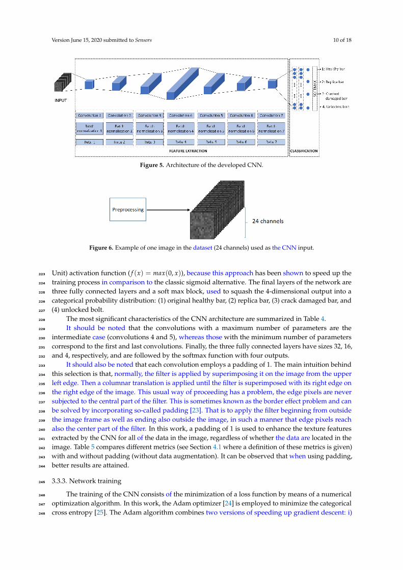
3.3.2. Network architecture217

The network presented in Figure 5 was designed in this work. The input is a 16× 16 image with218

24 channels, all of which are gray-scale. Figure 6 shows an example of one image in the dataset that219

was obtained after the preprocess procedure stated in Section 3.2. The input is convoluted by a series220

of 7 convolutional layers. Each convolution layer is followed by a batch normalization step, which is221

used to improve the speed, performance, and stability of the CNN [22], and a ReLU (Rectified Linear222

Version June 15, 2020 submitted to Sensors 10 of 18

Figure 5. Architecture of the developed CNN.

Figure 6. Example of one image in the dataset (24 channels) used as the CNN input.

Unit) activation function ( f (x) = max(0, x)), because this approach has been shown to speed up the223

training process in comparison to the classic sigmoid alternative. The final layers of the network are224

three fully connected layers and a soft max block, used to squash the 4-dimensional output into a225

categorical probability distribution: (1) original healthy bar, (2) replica bar, (3) crack damaged bar, and226

(4) unlocked bolt.227

The most significant characteristics of the CNN architecture are summarized in Table 4.228

It should be noted that the convolutions with a maximum number of parameters are the229

intermediate case (convolutions 4 and 5), whereas those with the minimum number of parameters230

correspond to the first and last convolutions. Finally, the three fully connected layers have sizes 32, 16,231

and 4, respectively, and are followed by the softmax function with four outputs.232

It should also be noted that each convolution employs a padding of 1. The main intuition behind233

this selection is that, normally, the filter is applied by superimposing it on the image from the upper234

left edge. Then a columnar translation is applied until the filter is superimposed with its right edge on235

the right edge of the image. This usual way of proceeding has a problem, the edge pixels are never236

subjected to the central part of the filter. This is sometimes known as the border effect problem and can237

be solved by incorporating so-called padding [23]. That is to apply the filter beginning from outside238

the image frame as well as ending also outside the image, in such a manner that edge pixels reach239

also the center part of the filter. In this work, a padding of 1 is used to enhance the texture features240

extracted by the CNN for all of the data in the image, regardless of whether the data are located in the241

image. Table 5 compares different metrics (see Section 4.1 where a definition of these metrics is given)242

with and without padding (without data augmentation). It can be observed that when using padding,243

better results are attained.244

3.3.3. Network training245

The training of the CNN consists of the minimization of a loss function by means of a numerical246

optimization algorithm. In this work, the Adam optimizer [24] is employed to minimize the categorical247

cross entropy [25]. The Adam algorithm combines two versions of speeding up gradient descent: i)248

Version June 15, 2020 submitted to Sensors 11 of 18

Layer Ouput size Parameters # of ParametersInput16×16×24 images 16×16×24 - 0

Convolution#132 filters of size 5×5×24 with padding [1 1 1 1] 14×14×32 Weight 5×5×24×32

Bias 1×1×32 19232

Batch Normalization#1 14×14×32 Offset 1×1×32Scale 1×1×32 64

ReLu#1 14×14×32 - 0Convolution#264 filters of size 5×5×24 with padding [1 1 1 1] 12×12×64 Weight 5×5×32×64

Bias 1×1×64 51264

Batch Normalization#2 12×12×64 Offset 1×1×64Scale 1×1×64 128

ReLu#2 12×12×64 - 0Convolution#3128 filters of size 5×5×24 with padding [1 1 1 1] 10×10×128 Weight 5×5×64×128

Bias 1×1×128 204928

Batch Normalization#3 10×10×128 Offset 1×1×128Scale 1×1×128 256

ReLu#3 10×10×128 - 0Convolution#4256 filters of size 5×5×24 with padding [1 1 1 1] 8×8×256 Weight 5×5×128×256

Bias 1×1×256 819456

Batch Normalization#4 8×8×256 Offset 1×1×256Scale 1×1×256 512

ReLu#4 8×8×256 - 0Convolution#5128 filters of size 5×5×24 with padding [1 1 1 1] 6×6×128 Weight 5×5×256×128

Bias 1×1×128 819456

Batch Normalization#5 6×6×128 Offset 1×1×128Scale 1×1×128 256

ReLu#5 6×6×128 - 0Convolution#664 filters of size 5×5×24 with padding [1 1 1 1] 4×4×64 Weight 5×5×128×64

Bias 1×1×64 204864

Batch Normalization#6 4×4×64 Offset 1×1×64Scale 1×1×64 128

ReLu#6 4×4×64 - 0Convolution#732 filters of size 5×5×24 with padding [1 1 1 1] 2×2×32 Weight 5×5×64×32

Bias 1×1×32 51232

Batch Normalization#7 2×2×32 Offset 1×1×32Scale 1×1×32 64

ReLu#7 2×2×32 - 0

Fully connected layer#1 1×1×32 Weight 32×128Bias 32×1 4128

Fully connected layer#2 1×1×16 Weight 16×32Bias 16×1 528

Fully connected layer#3 1×1×4 Weight 4×16Bias 4×1 68

Softmax - - 0classoutput - - 0

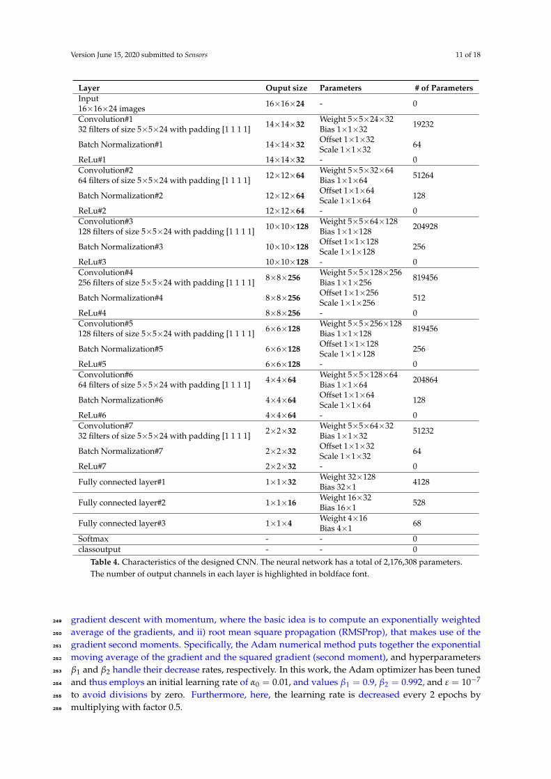
Table 4. Characteristics of the designed CNN. The neural network has a total of 2,176,308 parameters.The number of output channels in each layer is highlighted in boldface font.

gradient descent with momentum, where the basic idea is to compute an exponentially weighted249

average of the gradients, and ii) root mean square propagation (RMSProp), that makes use of the250

gradient second moments. Specifically, the Adam numerical method puts together the exponential251

moving average of the gradient and the squared gradient (second moment), and hyperparameters252

β1 and β2 handle their decrease rates, respectively. In this work, the Adam optimizer has been tuned253

and thus employs an initial learning rate of α0 = 0.01, and values β1 = 0.9, β2 = 0.992, and ε = 10−7254

to avoid divisions by zero. Furthermore, here, the learning rate is decreased every 2 epochs by255

multiplying with factor 0.5.256

Version June 15, 2020 submitted to Sensors 12 of 18

Strategy Accuracy Precision Recall F1 score SpecifityReLu - Padding - L2 regularization 93.81 92.77 93.73 93.22 97.98

Relu - No padding - L2 regularization 93.69 92.73 93.44 93.07 97.92Relu - Padding - No L2 regularization 93.63 92.73 93.82 93.25 97.89

Table 5. Metrics for different CNN architectures without data augmentation. The best metric resultsare highlighted in boldface font.

Convolutional layer initialization is carried out by the so-called Xavier initializer [26].257

Mini-batches of size 75 in the initial dataset and 590 for the augmented dataset are used to update the258

weights.259

Finally, L2 regularization with λ = 10−6 is employed. Table 5 compares the different metrics260

(see Section 4.1 for a definition of these metrics) with and without L2 regularization (without data261

augmentation). It can be observed that when using regularization, better results are obtained because262

regularization reduces high variance in the validation set.263

3.3.4. Network architecture and hyperparameter tuning264

To select the best architecture and to tune the different hyperparameters usually require significant265

computational resources. Because one of the most critical aspects of computational cost is the266

dataset size, in this paper, following the results presented in [27] and [28], the small dataset (without267

augmentation) is used to define the CNN architecture and quickly (coarse) tune the hyperparameters.268

Next, the obtained optimal hyperparameters for the small dataset are used as initial values to finetune269

the hyperparameters with the large dataset (with data augmentation).270

3.3.5. Network implementation271

The stated methodology is coded in MATLAB R© using its Deep Learning ToolboxTM on a laptop272

running the Windows R© 10 operating system, with an Intel Core i7-9750H processor, 16 GB of RAM,273

and an Nvidia GeForce RTXTM2060 graphic card that requires 6 GB of GPU.274

4. Results and Discussion275

4.1. Metrics to evaluate the classification model276

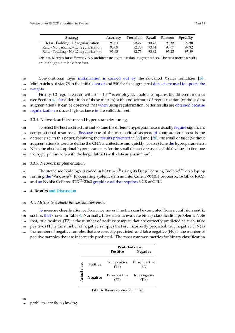
To measure classification performance, several metrics can be computed from a confusion matrix277

such as that shown in Table 6. Normally, these metrics evaluate binary classification problems. Note278

that, true positive (TP) is the number of positive samples that are correctly predicted as such, false279

positive (FP) is the number of negative samples that are incorrectly predicted, true negative (TN) is280

the number of negative samples that are correctly predicted, and false negative (FN) is the number of281

positive samples that are incorrectly predicted. The most common metrics for binary classification

Predicted classPositive Negative

Act

ualc

lass Positive True positive

(TP)False negative

(FN)

Negative False positive(FP)

True negative(TN)

Table 6. Binary confusion matrix.

282

problems are the following.283

Version June 15, 2020 submitted to Sensors 13 of 18

• Accuracy: Proportion of true results (both true positives and true negatives) among the totalnumber of cases examined.

Accuracy =TP+TN

TP+FP+FN+TN• Precision: Proportion of positive results that are true positive.

Precision =TP

TP+FP

• Recall: Proportion of actual positives that are correctly identified as such.

Recall =TP

TP+FN

• Specificity: Proportion of actual negatives that are correctly identified as such.

Specificity =TN

TN+FP

• F1-score: Harmonic mean of the precision and recall.

F1 = 2 · Precision · RecallPrecision + Recall

In a multi-class classification problem, such as that considered in this work, these metrics are also284

applicable using a one-vs.-all approach to compute each metric for each class, see [29]. Essentially, that285

is, to compute the different metrics for each label as if the problem has been reduced to a binary ’label286

X’ versus ’not label X’ situation.287

4.2. Results of the CNN classification method288

To evaluate the developed methodology, this section presents the results obtained from the289

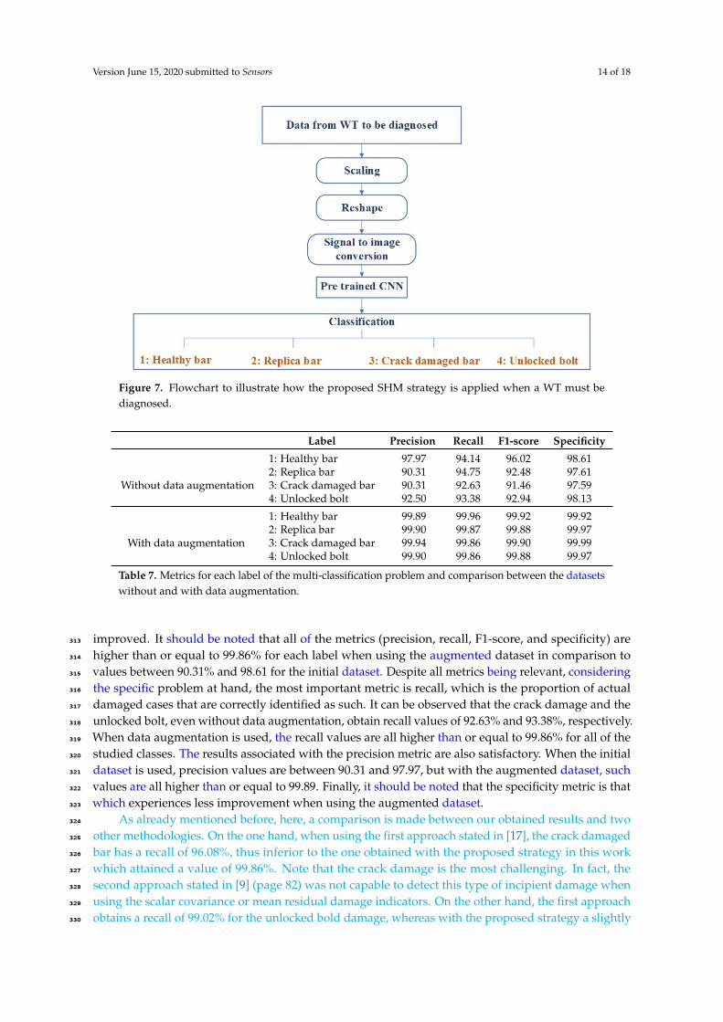
proposed SHM strategy. A flowchart of the proposed approach is given in Figure 7. When a WT must290

be diagnosed, the accelerometer data are scaled, reshaped, and converted into gray-scale images that291

are fed into the already trained CNN, and a classification is obtained to predict the structural state292

condition.293

To thoroughly test the functional characteristics of the algorithm, the datasets with and without294

data augmentation are considered, as well as comparison with two other methodologies given in [17]295

and [9], that make use of the same laboratory structure. The first methodology, given in [17], is based296

on principal component analysis and support vector machines. The second methodology, given in297

[9] (page 67), is based on the well-known damage indicators: covariance matrix estimate, and scalar298

covariance.299

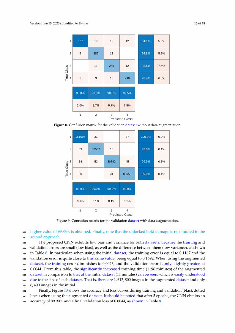
Figures 8 and 9 illustrate the confusion matrices for the validation dataset without and with300

data augmentation, respectively. The rows represent the true class, whereas columns represent the301

predicted class. The precision and false discovery rate are given in the rightmost columns. Finally, the302

recall and false negative rate are given at the bottom rows. An examination of both confusion matrices303

reveals that some misclassifications come from the model confounding the healthy and replica bars304

(labels 1 and 2). However, this level of misclassification is acceptable because both bars are in a healthy305

state. In contrast, some errors are derived from the model misclassifying the crack and unlocked bolt306

damages (labels 3 and 4), which will not detect correctly the type of damage but at least would lead307

to a damage alert. Finally, it should be noted that very few damaged samples (labels 3 and 4) are308

classified as healthy or replica bar (labels 1 and 2).309

From the confusion matrices, the different metrics to evaluate the classification model, see Section310

4.1, are computed and presented in Table 7. The impact of the data augmentation strategy can clearly311

be seen. Although no new experimental data were collected, nonetheless the metrics were significantly312

Version June 15, 2020 submitted to Sensors 14 of 18

Figure 7. Flowchart to illustrate how the proposed SHM strategy is applied when a WT must bediagnosed.

Label Precision Recall F1-score Specificity

Without data augmentation

1: Healthy bar 97.97 94.14 96.02 98.612: Replica bar 90.31 94.75 92.48 97.613: Crack damaged bar 90.31 92.63 91.46 97.594: Unlocked bolt 92.50 93.38 92.94 98.13

With data augmentation

1: Healthy bar 99.89 99.96 99.92 99.922: Replica bar 99.90 99.87 99.88 99.973: Crack damaged bar 99.94 99.86 99.90 99.994: Unlocked bolt 99.90 99.86 99.88 99.97

Table 7. Metrics for each label of the multi-classification problem and comparison between the datasetswithout and with data augmentation.

improved. It should be noted that all of the metrics (precision, recall, F1-score, and specificity) are313

higher than or equal to 99.86% for each label when using the augmented dataset in comparison to314

values between 90.31% and 98.61 for the initial dataset. Despite all metrics being relevant, considering315

the specific problem at hand, the most important metric is recall, which is the proportion of actual316

damaged cases that are correctly identified as such. It can be observed that the crack damage and the317

unlocked bolt, even without data augmentation, obtain recall values of 92.63% and 93.38%, respectively.318

When data augmentation is used, the recall values are all higher than or equal to 99.86% for all of the319

studied classes. The results associated with the precision metric are also satisfactory. When the initial320

dataset is used, precision values are between 90.31 and 97.97, but with the augmented dataset, such321

values are all higher than or equal to 99.89. Finally, it should be noted that the specificity metric is that322

which experiences less improvement when using the augmented dataset.323

As already mentioned before, here, a comparison is made between our obtained results and two324

other methodologies. On the one hand, when using the first approach stated in [17], the crack damaged325

bar has a recall of 96.08%, thus inferior to the one obtained with the proposed strategy in this work326

which attained a value of 99.86%. Note that the crack damage is the most challenging. In fact, the327

second approach stated in [9] (page 82) was not capable to detect this type of incipient damage when328

using the scalar covariance or mean residual damage indicators. On the other hand, the first approach329

obtains a recall of 99.02% for the unlocked bold damage, whereas with the proposed strategy a slightly330

Version June 15, 2020 submitted to Sensors 15 of 18

1 2 3 4

Predicted Class

1

2

3

4Tru

e C

lass

5

8

17

289

11

3

10

11

289

10

12

12

296

627 5.9%

5.2%

7.4%

6.6%

94.1%

94.8%

92.6%

93.4%

2.0% 9.7% 9.7% 7.5%

98.0% 90.3% 90.3% 92.5%

Figure 8. Confusion matrix for the validation dataset without data augmentation.

1 2 3 4

Predicted Class

1

2

3

4Tru

e C

lass

89

14

80

31

80557

52

16

80593

31

37

45

80558

161097 0.0%

0.1%

0.1%

0.1%

100.0%

99.9%

99.9%

99.9%

0.1% 0.1% 0.1% 0.1%

99.9% 99.9% 99.9% 99.9%

Figure 9. Confusion matrix for the validation dataset with data augmentation.

higher value of 99.86% is obtained. Finally, note that the unlocked bold damage is not studied in the331

second approach332

The proposed CNN exhibits low bias and variance for both datasets, because the training and333

validation errors are small (low bias), as well as the difference between them (low variance), as shown334

in Table 8. In particular, when using the initial dataset, the training error is equal to 0.1167 and the335

validation error is quite close to this same value, being equal to 0.1692. When using the augmented336

dataset, the training error diminishes to 0.0026, and the validation error is only slightly greater, at337

0.0044. From this table, the significantly increased training time (1196 minutes) of the augmented338

dataset in comparison to that of the initial dataset (11 minutes) can be seen, which is easily understood339

due to the size of each dataset. That is, there are 1, 612, 800 images in the augmented dataset and only340

6, 400 images in the initial.341

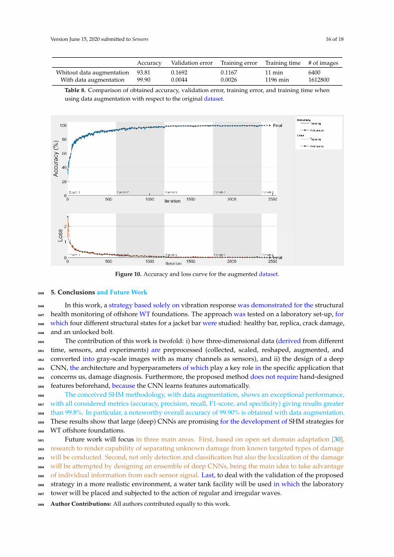
Finally, Figure 10 shows the accuracy and loss curves during training and validation (black dotted342

lines) when using the augmented dataset. It should be noted that after 5 epochs, the CNN obtains an343

accuracy of 99.90% and a final validation loss of 0.0044, as shown in Table 8.344

Version June 15, 2020 submitted to Sensors 16 of 18

Accuracy Validation error Training error Training time # of images

Whitout data augmentation 93.81 0.1692 0.1167 11 min 6400With data augmentation 99.90 0.0044 0.0026 1196 min 1612800

Table 8. Comparison of obtained accuracy, validation error, training error, and training time whenusing data augmentation with respect to the original dataset.

Figure 10. Accuracy and loss curve for the augmented dataset.

5. Conclusions and Future Work345

In this work, a strategy based solely on vibration response was demonstrated for the structural346

health monitoring of offshore WT foundations. The approach was tested on a laboratory set-up, for347

which four different structural states for a jacket bar were studied: healthy bar, replica, crack damage,348

and an unlocked bolt.349

The contribution of this work is twofold: i) how three-dimensional data (derived from different350

time, sensors, and experiments) are preprocessed (collected, scaled, reshaped, augmented, and351

converted into gray-scale images with as many channels as sensors), and ii) the design of a deep352

CNN, the architecture and hyperparameters of which play a key role in the specific application that353

concerns us, damage diagnosis. Furthermore, the proposed method does not require hand-designed354

features beforehand, because the CNN learns features automatically.355

The conceived SHM methodology, with data augmentation, shows an exceptional performance,356

with all considered metrics (accuracy, precision, recall, F1-score, and specificity) giving results greater357

than 99.8%. In particular, a noteworthy overall accuracy of 99.90% is obtained with data augmentation.358

These results show that large (deep) CNNs are promising for the development of SHM strategies for359

WT offshore foundations.360

Future work will focus in three main areas. First, based on open set domain adaptation [30],361

research to render capability of separating unknown damage from known targeted types of damage362

will be conducted. Second, not only detection and classification but also the localization of the damage363

will be attempted by designing an ensemble of deep CNNs, being the main idea to take advantage364

of individual information from each sensor signal. Last, to deal with the validation of the proposed365

strategy in a more realistic environment, a water tank facility will be used in which the laboratory366

tower will be placed and subjected to the action of regular and irregular waves.367

Author Contributions: All authors contributed equally to this work.368

Version June 15, 2020 submitted to Sensors 17 of 18

Funding: This work was partially funded by the Spanish Agencia Estatal de Investigación (AEI) - Ministerio369

de Economía, Industria y Competitividad (MINECO), and the Fondo Europeo de Desarrollo Regional (FEDER)370

through research project DPI2017-82930-C2-1-R; and by the Generalitat de Catalunya through research project371

2017 SGR 388. We gratefully acknowledge the support of NVIDIA Corporation with the donation of the Titan XP372

GPU used for this research.373

Acknowledgments: We thank the three anonymous reviewers for their careful reading of our manuscript and374

their many insightful comments and suggestions.375

Conflicts of Interest: The authors declare no conflict of interest. The founding sponsors had no role in the design376

of the study; in the collection, analyses, or interpretation of data; in the writing of the manuscript; nor in the377

decision to publish the results.378

References379

1. Ohlenforst, K.; Backwell, B.; Council, G.W.E. Global Wind Report 2018. Web page, 2019.380

2. Lai, W.J.; Lin, C.Y.; Huang, C.C.; Lee, R.M. Dynamic analysis of Jacket Substructure for offshore wind381

turbine generators under extreme environmental conditions. Applied Sciences 2016, 6, 307.382

3. Moulas, D.; Shafiee, M.; Mehmanparast, A. Damage analysis of ship collisions with offshore wind turbine383

foundations. Ocean Engineering 2017, 143, 149–162.384

4. Van Kuik, G.; Peinke, J. Long-term research challenges in wind energy-a research agenda by the European Academy385

of Wind Energy; Vol. 6, Springer, 2016.386

5. Liu, W.; Tang, B.; Han, J.; Lu, X.; Hu, N.; He, Z. The structure healthy condition monitoring and fault387

diagnosis methods in wind turbines: A review. Renewable and Sustainable Energy Reviews 2015, 44, 466–472.388

6. Qing, Xinlin and Li, Wenzhuo and Wang, Yishou and Sun, Hu. Piezoelectric transducer-based structural389

health monitoring for aircraft applications. Sensors 2019, 19, 545.390

7. Weijtjens, W.; Verbelen, T.; De Sitter, G.; Devriendt, C. Foundation structural health monitoring of an391

offshore wind turbine: a full-scale case study. Structural Health Monitoring 2016, 15, 389–402.392

8. Oliveira, G.; Magalhães, F.; Cunha, Á.; Caetano, E. Vibration-based damage detection in a wind turbine393

using 1 year of data. Structural Control and Health Monitoring 2018, 25, e2238.394

9. Zugasti Uriguen, E. Design and validation of a methodology for wind energy structures health monitoring.395

PhD thesis, Universitat Politècnica de Catalunya, Jordi Girona, 31, Barcelona, Spain, 2014.396

10. Lee, Jong Jae and Lee, Jong Won and Yi, Jin Hak and Yun, Chung Bang and Jung, Hie Young. Neural397

networks-based damage detection for bridges considering errors in baseline finite element models. Journal398

of Sound and Vibration 2005, 280, 555–578.399

11. Kim, Byungmo and Min, Cheonhong and Kim, Hyungwoo and Cho, Sugil and Oh, Jaewon and Ha,400

Seung-Hyun and Yi, Jin-hak. Structural health monitoring with sensor data and cosine similarity for401

multi-damages. Sensors 2019, 19, 3047.402

12. Stetco, A.; Dinmohammadi, F.; Zhao, X.; Robu, V.; Flynn, D.; Barnes, M.; Keane, J.; Nenadic, G. Machine403

learning methods for wind turbine condition monitoring: A review. Renewable energy 2019, 133, 620–635.404

13. Ruiz, M.; Mujica, L.E.; Alferez, S.; Acho, L.; Tutiven, C.; Vidal, Y.; Rodellar, J.; Pozo, F. Wind turbine fault405

detection and classification by means of image texture analysis. Mechanical Systems and Signal Processing406

2018, 107, 149–167.407

14. Vidal, Y.; Pozo, F.; Tutivén, C. Wind turbine multi-fault detection and classification based on SCADA data.408

Energies 2018, 11, 3018.409

15. Spanos, N.I.; Sakellariou, J.S.; Fassois, S.D. Exploring the limits of the Truncated SPRT method for410

vibration-response-only damage diagnosis in a lab-scale wind turbine jacket foundation structure. Procedia411

engineering 2017, 199, 2066–2071.412

16. Spanos, N.A.; Sakellariou, J.S.; Fassois, S.D. Vibration-response-only statistical time series structural health413

monitoring methods: A comprehensive assessment via a scale jacket structure. Structural Health Monitoring414

2019, p. 1475921719862487.415

17. Vidal Seguí, Y.; Rubias, J.L.; Pozo Montero, F. Wind turbine health monitoring based on accelerometer data.416

9th ECCOMAS Thematic Conference on Smart Structures and Materials, 2019, pp. 1604–1611.417

18. Vidal, Y.; Aquino, G.; Pozo, F.; Gutiérrez-Arias, J.E.M. Structural Health Monitoring for Jacket-Type418

Offshore Wind Turbines: Experimental Proof of Concept. Sensors 2020, 20, 1835.419

Version June 15, 2020 submitted to Sensors 18 of 18

19. Pozo, F.; Vidal, Y.; Serrahima, J. On real-time fault detection in wind turbines: Sensor selection algorithm420

and detection time reduction analysis. Energies 2016, 9, 520.421

20. Pal, K.K.; Sudeep, K. Preprocessing for image classification by convolutional neural networks. 2016 IEEE422

International Conference on Recent Trends in Electronics, Information & Communication Technology423

(RTEICT). IEEE, 2016, pp. 1778–1781.424

21. Chen, X.W.; Lin, X. Big data deep learning: challenges and perspectives. IEEE access 2014, 2, 514–525.425

22. Santurkar, S.; Tsipras, D.; Ilyas, A.; Madry, A. How does batch normalization help optimization? Advances426

in Neural Information Processing Systems, 2018, pp. 2483–2493.427

23. Albawi, S.; Mohammed, T.A.; Al-Zawi, S. Understanding of a convolutional neural network. 2017428

International Conference on Engineering and Technology (ICET). IEEE, 2017, pp. 1–6.429

24. DP, K. Ba J. Adam: a method for stochastic optimization. The international conference on learning430

representations, 2015.431

25. Rusiecki, A. Trimmed categorical cross-entropy for deep learning with label noise. Electronics Letters 2019,432

55, 319–320.433

26. Glorot, X.; Bengio, Y. Understanding the difficulty of training deep feedforward neural networks.434

Proceedings of the thirteenth international conference on artificial intelligence and statistics, 2010, pp.435

249–256.436

27. DeCastro-García, N.; Muñoz Castañeda, Á.L.; Escudero García, D.; Carriegos, M.V. Effect of the Sampling of437

a Dataset in the Hyperparameter Optimization Phase over the Efficiency of a Machine Learning Algorithm.438

Complexity 2019, 2019.439

28. Swersky, K.; Snoek, J.; Adams, R.P. Multi-task bayesian optimization. Advances in neural information440

processing systems, 2013, pp. 2004–2012.441

29. Hossin, M.; Sulaiman, M. A review on evaluation metrics for data classification evaluations. International442

Journal of Data Mining & Knowledge Management Process (IJDKP) 2015, 5, 1–11.443

30. Saito, Kuniaki and Yamamoto, Shohei and Ushiku, Yoshitaka and Harada, Tatsuya. Open set domain444

adaptation by backpropagation. Proceedings of the European Conference on Computer Vision (ECCV),445

2018, pp. 153–168.446

c© 2020 by the authors. Submitted to Sensors for possible open access publication under the terms and conditions447

of the Creative Commons Attribution (CC BY) license (http://creativecommons.org/licenses/by/4.0/).448