New Semi-active Vibration Control with Serial-Sti ness ...

New Semi-active Vibration Controlwith Serial-Stiffness-Switch-System

based on Vibration Energy Harvesting

Dissertationzur Erlangung des akademischen Grades

Doktoringenieur(Dr.-Ing.)

vorgelegt der

Fakultat fur Maschinenbau der

Technischen Universitat Ilmenau

von Herrn

M. Sc. Chaoqing Mingeboren am 15.08.1986 in Shandong, China

1. Gutachter: Prof. Dr.-Ing. Thomas Sattel

2. Gutachter: Prof. Dr. Dr. h.c. Peter Hagedorn

3. Gutachter: Prof. Dr.-Ing. habil. Alexander Fidlin

Tag der Einreichung: 19.06.2018

Tag des offentlichen Teils der wissenschaftlichen Aussprache: 28.08.2018

urn:nbn:de:gbv:ilm1-2018000350

Abstract

This dissertation investigates a novel semi-active vibration control with Serial-Stiffness-Switch-System (4S) based on vibration energy harvesting.

On the basis of the vibration reduction performance analysis for a passive and a semi-active switching system, the problem in the present vibration control systems is statedand 4S concept is consequently put forward. In order to examine its performance, 4Sin open loop control is analyzed firstly and the equivalent stiffness and natural fre-quency of the switching system are derived. Following is the analysis for 4S in closedloop control. A velocity zero-crossing switching law based on vibration energy harvest-ing is used for vibration reduction. This is numerically validated under a harmonicdisturbance. Afterwards, vibration energy harvesting limit is analyzed.

An experimental validation on this novel vibration control strategy is then presentedand a rotational test rig is developed. The test rig uses two ring-arranged electromagnet-plates together with an armature-shaft as two mechanical switches to achieve the con-nection or disconnection of two spiral springs to or from a primary plate. The vibrationenergy harvesting and vibration reduction performance of 4S are tested on this exper-imental system.

Apart from a harmonic disturbance, a nonzero initial velocity vibration is also consid-ered. To improve vibration reduction performance in this case, a new switching law isproposed. By means of phase plane, the transient and steady chattering response of4S are analyzed. The switching law enables a fast transformation of initial vibrationenergy into potential energy equally stored in two springs. This is numerically andexperimentally validated. Additionally, a harmonic disturbance is also exerted on thenew switching law. The results show that 4S has a better positioning performancethan that for the velocity zero-crossing switching law.

Finally, 4S is further applied for shock isolation. The maximum displacement responsereduction during shock and the residual vibration suppression after shock are numer-ically validated. Moreover, the effect of several design parameters of 4S on the shockisolation performance is investigated as well.

Kurzfassung

Diese Dissertation untersucht eine neuartige semi-aktive Schwingungsteuerung miteinem seriellen-Steifigkeit-Schalter-System (4S) basierend auf der Speicherung von Sch-wingungsenergie.

Auf Basis der Schwingungsreduktionsanalyse fur ein passives und ein semi-aktivesSchaltsystem werden Probleme vorhandener Schwingungsteuerungssystemen aufgezeigtund durch das 4S Konzept gelost. Um seine Leistungsfahigkeit zu untersuchen, wirdzunachst 4S im offenen Regelkreis analysiert und die aquivalente Steifigkeit und Eigen-frequenz des Schaltsystems abgeleitet. Es folgt die Analyse fur 4S im geschlossenenRegelkreis. Zur Schwingungsreduzierung wird ein Geschwindigkeits-NulldurchgangsSchaltgesetz verwendet, das auf der Gewinnung von Schwingungsenergie basiert. Dieswird unter einer harmonischen Storung numerisch validiert. Anschließend werdenGrenzen der Energiespeicherung analysiert.

Es folgt eine experimentelle Validierung dieser neuartigen Strategie zur Schwingungss-teuerung vorgestellt und ein drehender Prufstand entwickelt. Der Prufstand verwendetzwei ringformig angeordnete Elektromagnetplatten zusammen mit einer Ankerwelle alszwei mechanische Schalter, um die Verbindung oder Trennung von zwei Spiralfedernmit einem Lasttragheitsmoment zu erreichen. Die Speicherung von Schwingungsen-ergie und die Schwingungsreduktion werden auf diesem Versuchssystem getestet.

Neben einer harmonischen Storung wird auch eine Anfangsgeschwindigkeit ungleichNull berucksichtigt. Um in diesem Fall die Schwingungsreduktion zu verbessern,wird ein neues Schaltgesetz vorgeschlagen. Mit Hilfe der Phasenebene wird das tran-siente und stationar Ratterverhalten von 4S analysiert. Das Schaltgesetz ermoglichteine schnelle Umwandlung der anfanglichen kinetischen Energie, die in beiden Federnzu gleichen Teilen gespeichert wird. Dies ist numerisch und experimentell validiert.Zusatzlich wird einer harmonischen Storung an dem neuen Schaltgesetz getestet, dasein besseres Positionierverhalten als das Geschwindigkeits-Nulldurchgangs Schaltgesetzaufweist.

vi

Schließlich wird 4S zur Schockisolierung eingesetzt. Die maximale Reduzierung desUberschwingens des Wegs beim Schock und die Reduktion der Restschwingungen nachdem Schock werden numerisch validiert. Daruber hinaus wird auch der Einfluss ver-schiedener Designparameter von 4S auf das Isolationsverhalten untersucht.

Acknowledgment

I would like to acknowledge with a deep appreciation for the academic guidance andthe continuous encouragement provided by my supervisor, Professor Thomas Sattel.His patience and inspirational guidance were extremely valuable in the successful com-pletion of this work. His help is far beyond what a normal supervisor could provide,not only limited to academic aspects but also cherish experience in life.

I would also like to sincerely thank Dr.-Ing. Martin Dahlman. He also gives me a lotof advice on this project. It is kind of him to provide this guidance. My thanks alsogo to Dr.-Ing. Ralf Keilig, who has excellent experience in practice and gives me a lotof help with the manufacture of the test rig.

I want to give my thanks to assistant Professor Tom Strola, who is very kind and alsogives me some suggestions for my thesis. Meanwhile, he also encourages me to workfrequently. I am also grateful to my colleagues Dr.-Ing. Oliver Radler, M. Sc. MartinSilge, M. Sc. Aditya Suryadi Tan, M. Sc. Christoph Greiner-Petter, B. E.(Hons) KanuRoss, Dipl.-Ing. Dennis Roeser, Dipl.-Ing. Maria Gadyuchko, Dipl.-Ing. Olga Roeser,Dipl.-Ing. Anton Kochnev. They help me a lot when I worked in the institute atbeginning, not only on academic but also in everyday life. I would also like to thankour technician Mrs Cornelia Hecht, Mr Heiko Rodiger, and our secretary Mrs AnnetteVolk. They have provided a lot of help with my German language and everyday life.

Finally, I would like to sincerely thank my wife, Yulei Zhao. She has taken care ofour child during my PhD studies and supported me a lot. I also show my thanks toour parents for their understanding and support of my pursuit of a PhD degree in aforeign country. I am grateful to my old brother for his encouragement and guidancein my PhD studies as well.

Contents

Acknowledgment vii

1. Introduction 11.1. State of the Art . . . . . . . . . . . . . . . . . . . . . . . . . . . . . . . 1

1.1.1. Vibration Control . . . . . . . . . . . . . . . . . . . . . . . . . . 11.1.2. Variable Stiffness Systems for Vibration Control . . . . . . . . . 6

1.2. Summary of Literature Review . . . . . . . . . . . . . . . . . . . . . . 171.3. Objective . . . . . . . . . . . . . . . . . . . . . . . . . . . . . . . . . . 171.4. Contribution . . . . . . . . . . . . . . . . . . . . . . . . . . . . . . . . . 181.5. Thesis Organization . . . . . . . . . . . . . . . . . . . . . . . . . . . . . 19

2. Novel Semi-active Vibration Control with 4S 212.1. Introduction . . . . . . . . . . . . . . . . . . . . . . . . . . . . . . . . . 212.2. 4S Concept . . . . . . . . . . . . . . . . . . . . . . . . . . . . . . . . . 22

2.2.1. Problem Statement . . . . . . . . . . . . . . . . . . . . . . . . . 222.2.2. Vibration Energy Harvesting Concept . . . . . . . . . . . . . . . 242.2.3. 4S Model . . . . . . . . . . . . . . . . . . . . . . . . . . . . . . 25

2.3. Open Loop Control for 4S . . . . . . . . . . . . . . . . . . . . . . . . . 272.3.1. Numerical Analysis . . . . . . . . . . . . . . . . . . . . . . . . . 272.3.2. Analytical Formulation . . . . . . . . . . . . . . . . . . . . . . . 30

2.4. Closed Loop Control for 4S . . . . . . . . . . . . . . . . . . . . . . . . 322.4.1. Switching Law based on Vibration Energy Harvesting . . . . . . 322.4.2. System Dynamics . . . . . . . . . . . . . . . . . . . . . . . . . . 342.4.3. Numerical Analysis . . . . . . . . . . . . . . . . . . . . . . . . . 35

3. Vibration Energy Harvesting Limit Analysis 413.1. Introduction . . . . . . . . . . . . . . . . . . . . . . . . . . . . . . . . . 413.2. Spectrum Analysis for System Response . . . . . . . . . . . . . . . . . 413.3. Steady State System Response . . . . . . . . . . . . . . . . . . . . . . . 443.4. Necessary Conditions for Vibration Energy Harvesting Limit . . . . . . 48

x Contents

3.5. Numerical Analysis for Vibration Energy Harvesting Limit . . . . . . . 503.5.1. Nonzero Initial Conditions . . . . . . . . . . . . . . . . . . . . . 503.5.2. Zero Initial Conditions . . . . . . . . . . . . . . . . . . . . . . . 513.5.3. Extended Time Numerical Simulation . . . . . . . . . . . . . . . 52

4. Experimental Validation 554.1. Introduction . . . . . . . . . . . . . . . . . . . . . . . . . . . . . . . . . 554.2. Operation Principle and Modeling of Setup . . . . . . . . . . . . . . . . 56

4.2.1. Operation Principle . . . . . . . . . . . . . . . . . . . . . . . . . 564.2.2. Modeling . . . . . . . . . . . . . . . . . . . . . . . . . . . . . . 57

4.3. Setup Construction . . . . . . . . . . . . . . . . . . . . . . . . . . . . . 604.3.1. Mechanical Structure . . . . . . . . . . . . . . . . . . . . . . . . 604.3.2. Power Electronics . . . . . . . . . . . . . . . . . . . . . . . . . . 654.3.3. Lumped System . . . . . . . . . . . . . . . . . . . . . . . . . . . 68

4.4. Experiment . . . . . . . . . . . . . . . . . . . . . . . . . . . . . . . . . 684.4.1. System Parameter Identification . . . . . . . . . . . . . . . . . . 694.4.2. Step Response . . . . . . . . . . . . . . . . . . . . . . . . . . . . 734.4.3. Harmonic Response . . . . . . . . . . . . . . . . . . . . . . . . . 75

5. Improved Switching Law for 4S 815.1. Introduction . . . . . . . . . . . . . . . . . . . . . . . . . . . . . . . . . 815.2. Nonzero Initial Velocity Problem for 4S . . . . . . . . . . . . . . . . . . 815.3. Variable Structure System Control for 4S . . . . . . . . . . . . . . . . . 83

5.3.1. State Trajectory Analysis . . . . . . . . . . . . . . . . . . . . . 835.3.2. New Switching Surface . . . . . . . . . . . . . . . . . . . . . . . 86

5.4. Experimental Verification . . . . . . . . . . . . . . . . . . . . . . . . . 905.4.1. Nonzero Initial Velocity Condition . . . . . . . . . . . . . . . . 905.4.2. Harmonic Excitation . . . . . . . . . . . . . . . . . . . . . . . . 935.4.3. PID Feedback Controlled Switching Law . . . . . . . . . . . . . 93

6. Shock Isolation with 4S 976.1. Introduction . . . . . . . . . . . . . . . . . . . . . . . . . . . . . . . . . 976.2. Harmonic disturbance isolation using 4S . . . . . . . . . . . . . . . . . 97

6.2.1. Modeling . . . . . . . . . . . . . . . . . . . . . . . . . . . . . . 976.2.2. Numerical Analysis . . . . . . . . . . . . . . . . . . . . . . . . . 98

6.3. Shock isolation for 4S . . . . . . . . . . . . . . . . . . . . . . . . . . . . 996.3.1. Shock isolation systems . . . . . . . . . . . . . . . . . . . . . . . 1006.3.2. Shock isolation using 4S without potential energy pre-storage . 1016.3.3. Shock isolation using 4S with potential energy pre-storage . . . 104

6.4. Shock isolation performance analysis of 4S . . . . . . . . . . . . . . . . 1066.4.1. Time domain analysis . . . . . . . . . . . . . . . . . . . . . . . 1066.4.2. Multi-dimension parameters performance analysis of 4S . . . . . 108

7. Summary and Future Work 1117.1. Summary . . . . . . . . . . . . . . . . . . . . . . . . . . . . . . . . . . 1117.2. Future Work . . . . . . . . . . . . . . . . . . . . . . . . . . . . . . . . . 112

Bibliography 113

Contents xi

A. Vibration Energy Limit Analysis 123A.1. Solution for Integration Coefficients . . . . . . . . . . . . . . . . . . . . 123

B. Setup Construction 125B.1. Diameter and Thickness of Armature . . . . . . . . . . . . . . . . . . . 125B.2. Switching Current Measurement of Mechanical Switch . . . . . . . . . . 127

C. Sliding Mode Control 129C.1. Theory Basis . . . . . . . . . . . . . . . . . . . . . . . . . . . . . . . . 129

CHAPTER 1

Introduction

1.1. State of the Art

1.1.1. Vibration Control

Vibration, which generally performs oscillation around a balance position, is a commonmotion phenomenon occurring in nature and human lives. Sometimes high levels ofvibration can be beneficial and desirable, from small equipment such as a loudspeakerto large machines such as tamping machines, vibrating conveyors, and sieves. Butmostly, vibration is unwanted due to creating uncomfortable noise, wasting energy,causing mechanical wear, structural fatigue, and resulting in an increased danger.Therefore, vibration control has been extensively studied by researchers. Vibrationcontrol is understood here as vibration reduction to decrease unwanted oscillations ina protected structure. Generally, this is achieved by a compact connection elementconsisting of a spring, a damper or together with a mass. A fundamental introductionto vibration control is documented in [1], p. 479.

Vibration Control Object

Different mechanical structure configurations among a vibration source, a protectedpayload, a vibration control element, and vibration transmission path, result in threetypes of vibration control, namely, vibration isolation, vibration suppression, and vi-bration absorption see [2] p. 5.

Vibration isolation happens when a vibration control element, namely an isolator,is designed for the connection between a vibration source and a protected structurein order to isolate the vibration source from the system of interest. This is further

2 1. Introduction

categorized as source isolation and receiver isolation. The former refers to a vibrationsource and surrounding environment such as ground and force transmissibility is takeninto consideration as depicted in Fig. 1.1(a). The external force F acting on mass mdenotes a vibration source. The spring k, and damping d make up a vibration isolator.The force transmissibility Fc/F is to assess the source isolation performance. Thelatter is related to a base excitation denoted by x0, x0, and a sensitive structure m asshown in Fig. 1.1(b). Vibration isolation performance is characterized by the motiontransmissibility x/x0 or x/x0. The transmissibility property is strongly decided by thefrequency ratio of the external disturbance frequency Ω to system natural frequencyω0, ω0 =

√k/m, and system damping ratio D = d/(2

√km).

dk

m

F

x

(a)

Fc

dk

m

(b)

x

Vibration Isolator

x0

Figure 1.1.: The models for vibration isolation systems. (a) Source isolation; (b) Re-ceiver isolation.

Vibration absorption is realized by a vibration absorber or a tuned vibrationabsorber, consisting of a reaction mass ma, a spring ka together with an appropri-ate damping da, graphically depicted in Fig. 1.2. A vibration absorber, framed by adotted line, is hung on a protected payload m, whose operation frequency meets theresonant frequency of the vibration absorber. The corresponding theory, various designconfigurations and applications have been documented in [3, 4].

maVibration Absorber

m

dkx

xaF

daka

Figure 1.2.: The model for a vibration absorption system.

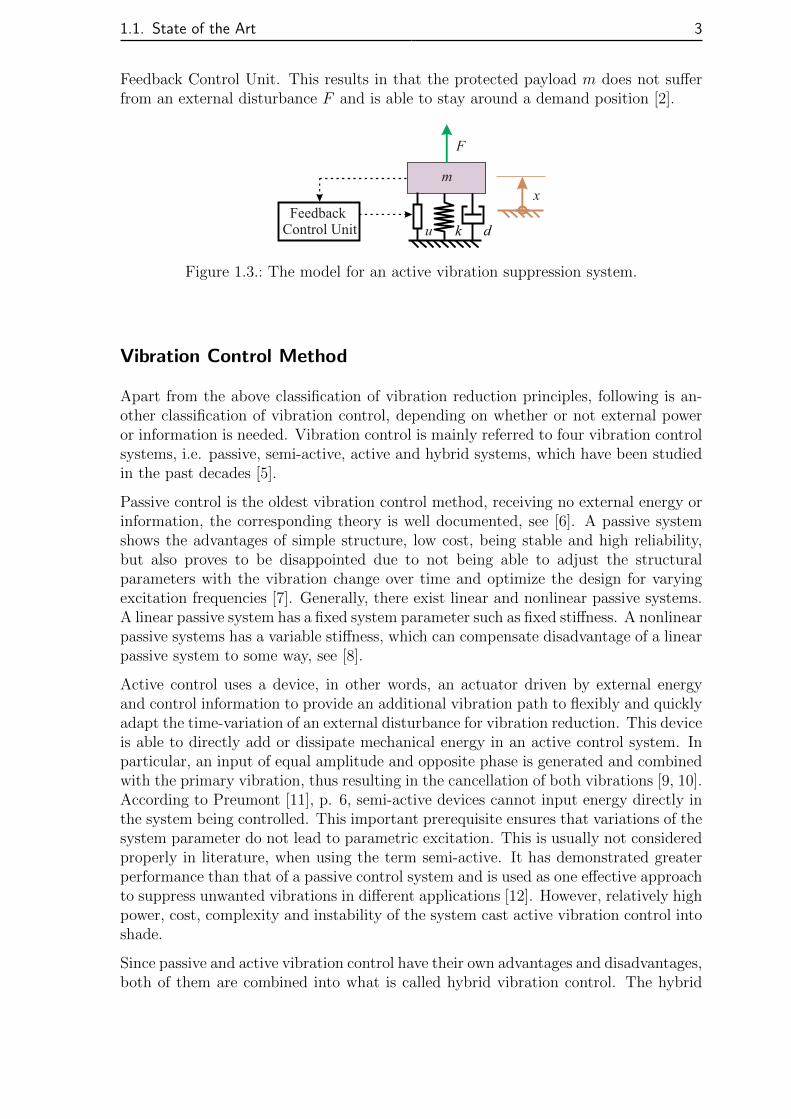
Vibration suppression is to remove an external disturbance directly acting on aprotected payload. This usually occurs through state feedback control as graphicallyillustrated by 1.3. An actuator u acts on the protected payload m responding to

1.1. State of the Art 3

Feedback Control Unit. This results in that the protected payload m does not sufferfrom an external disturbance F and is able to stay around a demand position [2].

dk

m

F

x

u FeedbackControl Unit

Figure 1.3.: The model for an active vibration suppression system.

Vibration Control Method

Apart from the above classification of vibration reduction principles, following is an-other classification of vibration control, depending on whether or not external poweror information is needed. Vibration control is mainly referred to four vibration controlsystems, i.e. passive, semi-active, active and hybrid systems, which have been studiedin the past decades [5].

Passive control is the oldest vibration control method, receiving no external energy orinformation, the corresponding theory is well documented, see [6]. A passive systemshows the advantages of simple structure, low cost, being stable and high reliability,but also proves to be disappointed due to not being able to adjust the structuralparameters with the vibration change over time and optimize the design for varyingexcitation frequencies [7]. Generally, there exist linear and nonlinear passive systems.A linear passive system has a fixed system parameter such as fixed stiffness. A nonlinearpassive systems has a variable stiffness, which can compensate disadvantage of a linearpassive system to some way, see [8].

Active control uses a device, in other words, an actuator driven by external energyand control information to provide an additional vibration path to flexibly and quicklyadapt the time-variation of an external disturbance for vibration reduction. This deviceis able to directly add or dissipate mechanical energy in an active control system. Inparticular, an input of equal amplitude and opposite phase is generated and combinedwith the primary vibration, thus resulting in the cancellation of both vibrations [9, 10].According to Preumont [11], p. 6, semi-active devices cannot input energy directly inthe system being controlled. This important prerequisite ensures that variations of thesystem parameter do not lead to parametric excitation. This is usually not consideredproperly in literature, when using the term semi-active. It has demonstrated greaterperformance than that of a passive control system and is used as one effective approachto suppress unwanted vibrations in different applications [12]. However, relatively highpower, cost, complexity and instability of the system cast active vibration control intoshade.

Since passive and active vibration control have their own advantages and disadvantages,both of them are combined into what is called hybrid vibration control. The hybrid

4 1. Introduction

vibration control system can be used over a wide frequency range, reduces the neededexternal energy compared to a purely active system and still achieves some vibrationreduction if the active control element fails. However, the risk of instability createdby the active element and the degradation over time owing to detuning of the passiveelement still exist in system [13]. Apart from the hybrid control related to passiveand active control, there also exist the ones consisting of passive and semi-active oractive and semi-active control. For example, the hybrid control based on passive plussemi-active control is proposed in [14] in order to enlarge the working frequency range.Khan et al. [15] developed a hybrid combination of active and semi-active control forvibration suppression in order to enable a semi-active magneto-rheological damper towork as close to a fully active device as possible.

Semi-active vibration control uses a device with controllable properties to achieve vari-able system parameters such as stiffness and damping with a low external power sup-ply. This kind of device does not provide an additional vibration path to directly reactagainst an external disturbance for vibration reduction. So a semi-active vibrationcontrol device, differing from active control, will not directly increase or decrease themechanical energy of the system and can be seen as a passive device with controllableproperties [9, 10]. According to Preumont [11], p. 6, semi-active devices cannot inputenergy directly in the system being controlled. This important prerequisite ensuresthat variations of the system parameter do not lead to parametric excitation. This isusually not considered properly in literature, when using the term semi-active. Adjust-ing system parameters based on the measured state feedback signals enables a largerwork frequency range and more flexibility obviously. What’s more, if a control systemfails, a semi-active control mode can still work in a passive case to some extent [16].Different vibration control systems can be grouped as shown in Fig. 1.4.

Vibration Control System

Passive System

Linear Passive

Nonlinear Passive

Semi-active System Active System Hybrid System

Variable Stiffness

Variable Damping

Variable Mass

Passive + Active

Passive + Semi-active

Active + Semi-active

Figure 1.4.: Different vibration control systems.

Variable Stiffness Systems

Through the literature reviewing, it is not difficult to find that the system stiffness playsan important role on vibration control. For instance, if the disturbance frequency islarger than the natural frequency of a vibration control system, vibration isolationworks well. If not, an amplified vibration response is produced on a primary structure,


see [17]. In the case of shock isolation, a damping device can transmit large force to theprimary structure because in traditional dampers high velocity corresponds with highreaction forces, but this will not occur in a stiffness device. Bobrow et al. [18] utilizeda variable stiffness device in an automotive suspension system, where the force trans-mitted through a conventional damper is more than an order of magnitude higherthan the force transmitted through the variable stiffness device. In overcoming thecompromise between minimizing the shock transmission through an isolator and min-imizing the static deflection, a variable stiffness system also performs well, see [19]. Atuned vibration absorber with variable stiffness allows vibration reduction against ex-ternal disturbances with different frequencies and resting in a better primary structureresponse than a passive stiffness counterpart, see [20]. Compared with passive stiff-ness systems, variable stiffness systems, showing more flexibility in shifting the systemfrequency for vibration control, have attracted a lot of researchers.

In fact, variable stiffness systems exist in many engineering areas. For instance, ina microelectromechanical system (MEMS) they are used in a variety of applicationssuch as radio-frequency mechanical filters, energy harvesters, atomic force microscopy,vibration detection sensors, and so on, see [21]. When designing micro-scale tactileprobes, a design trade-off must be made between their stiffness and flexibility, whichneeds variable stiffness probing systems, see [22]. In robotics field, a variable stiffnessactuator, consisting of motor, sensor and spring, is useful for the compliant, robustand dexterous control of different robots [23]. However, variable stiffness systems arelimited to vibration reduction applications in this thesis. These systems have beenwidely studied in mechanical engineering [24], seismic and civil engineering [25, 26],aerospace and aviation [27, 28], vehicle systems [29–31], and so on. More infomationabout variable stiffness design and application is documented by Winthrop [32].

Variable stiffness exists not only in a semi-active system as shown in Fig. 1.4, but also ina nonlinear passive and an active system. A semi-active variable stiffness system uses adevice with controllable properties to achieve variable stiffness. Reversely, a nonlinearpassive system is not controllable and uses a high static and low dynamic property of anonlinear elastic element to achieve stiffness variation. In these systems, nonlinearity isnot easy to model and analyze. Generally, an active system uses an actuator to directlydrive a protected payload to react against an external disturbance, but in some casesthe used actuator drives several elastic elements in a geometrical configuration, whichsupport the protected payload, and their configuration geometry deformation resultsin a variable stiffness. This should be seen as an active variable stiffness, because theactuator adds mechanical energy to the system to some extent. However, this kind ofstiffness variation has been also wrongly defined as semi-active variation stiffness [33].To the authors knowledge through the literature reviewing, there does not exist anobvious classification for a semi-active and an active variable stiffness. Therefore, thisthesis will not clearly distinguish whether a variable stiffness belongs to a semi-activeor an active variable stiffness.

6 1. Introduction

1.1.2. Variable Stiffness Systems for Vibration Control

Modeling for Variable Stiffness Mechanism

System stiffness can be varied continuously or discretely. A variable stiffness vibrationcontrol system can be graphically simplified as in Fig. 1.5. F is taken as an externaldisturbance and m1 stands for a protected payload. x1 is the displacement of thepayload in Fig. 1.5(a), (b) and (c) and x2 is the displacement of connection point.The arrow through the spring in Fig. 1.5(a) implies a spring with selectable stiffnesses.Continuous variable stiffness means that system stiffness is able to achieve an arbitrary

k(u)

F

m1

(b)

x1

(a)

s1

m1

x1

F

F

s1

s2

k1

k2

m1

x1

x2

(c)

k1k2

Figure 1.5.: Simplified representation for a variable stiffness system. (a) Continuousvariable stiffness; (b) Parallel stiffness switching system; (c) Serial stiffnessswitching system.

variation within a range based on the state feedback signals. The system behavior canbe given by Eq. 1.1, according to Fig. 1.5(a).

F = k(u)x , k(u) ∈ [kmin, kmax] (1.1)

where kmin and kmax are the minimum and maximum system stiffness, respectively andu is the control input. For a switched stiffness, namely, discrete stiffness, variable stiff-ness systems use two or more stiffness states to achieve vibration control. In betweenstiffness switching events, the system can be taken as a passive system. As an example,the two-stiffness systems are taken into consideration. They can be categorized intotwo cases and simply depicted as in Fig. 1.5(a), (b) and (c). The first case is that onlytwo stiffness states are chosen in a continuous variable stiffness system for example, k1

and k2. The other is a variable stiffness system with only two springs as depicted inFig. 1.5(b), a parallel spring pair and (c), a serial spring pair. If two stiffness statesare realized by a variable stiffness system as shown in Fig. 1.5(b) or (c), a mechanicalswitch, namely, a clamping device is applied to realize the connection or disconnectionof a spring to or away from the payload m1.

It is not difficult to see that switched stiffness is an alternative to a continuous vari-able stiffness. So in the following documented devices, there does not exist an obvious


boundary between switched stiffness and continuous variable stiffness. From the de-velopment in the last decades, variable stiffness devices are mainly realized by twomethods. One is smart material-based devices and the other is related to commonmechanical elements including mechanical spring, beam, hydraulic/pneumatic spring,and so on.

Smart Material-based Variable Stiffness Devices

A smart material-based device is achieved by changing smart material physical prop-erties such as elastic modulus E. In this method, these materials are generally excitedby an external energy field such as electric field, magnetic field and thermal field andso on, as shown in Fig. 1.6. The energy field intensity is decided by a system statefeedback signal. Examples of such materials include piezo material, Magnetorheolog-ical Elastomer (MRE), Shape Memory Alloy (SMA), and Magnetostrictive material.In some cases, smart materials can be combined with another material to make up acomposite structure.

SmartMaterial

Electric Field Magnetic Field Thermal Field

Variable Stiffness

k(E)

......

Figure 1.6.: Smart material-based stiffness variation.

Piezoelectric material-based variable stiffness devices

Piezoelectric material shows not only the direct piezoelectric effect (electric voltageproduced under external mechanical strain), but also the reverse piezoelectric effect(mechanical deformation produced under external electric voltage). As such, piezoelec-tric materials can build up an actuator or a power source, which result in two differentstiffness variation methods for vibration control, namely, a piezoelectric shunt-basedvariable stiffness devices and an active piezoelectric actuator-based device.

A: Piezo shunt-based variable stiffness devices A piezo shunt circuit acts as a mediumto extract structural vibration energy from a primary structure. When the structuredeforms under an external disturbance, a piezo element, or in other words, a piezotransducer, bonded to the primary structure, also strains and will convert a portionof structural vibration energy into electrical energy. By shunting the piezo transducerto an electrical shunt circuit, the induced electrical energy can be partly dissipated.This method was originally proposed by Hagood et al. [34]. During the shuntingprocess, a desired mechanical strain of the piezo transducer results in an electricalimpedance dependent stiffness variation. Different types of shunt circuits consisting ofresistor, inductance and capacity can result in different stiffness variation principles,see [35]. However, it is pointed out that a switching capacity shunt circuit can realizea variable stiffness device but a switching resistor/inductor shunt circuit is not strictly

8 1. Introduction

a pure variable stiffness device and can be only considered as a frequency-dependentvariable stiffness one, because an electrical element, resistor or inductor, correspondsto a mechanical element, damping or mass.

In theory, one can continuously vary electrical elements such as resistors, capacity inthe circuit and then obtain a continuous variable stiffness system, which has beenalready under a lot of investigations, see [34, 36, 37]. An alternative is to simplyswitch between two stiffness states. Such a configuration for switching stiffness isto operate between an open and a short circuit, which leads to the maximum andminimum system stiffness, see [38]. Clark et al. [39] put forward that a piezo shuntworks better if the on-off stiffness variation can be achieved by a resistive shunt insteadof a pure short circuit. In that research, a cantilevered beam with an attached piezolayer was developed. It is experimentally verified that a layered beam can reach astiffness variation by a factor of 2, if the piezo material is operated in d33 mode.

B: Active piezo actuator-based variable stiffness devices Apart from piezo shunt-basedvariable stiffness devices, an active piezo actuator is also utilized for stiffness variation.In this method, for example, a piezo patch is attached onto a primary structure.Different mechanical deformations of the piezo patch, produced by a required voltageresulting from a feedback controller, lead to a stiffness variation, see [40]. Consideringthe sensing principle of piezo materials, an integrated smart variable stiffness device, aviscoelastic shear layer sandwiched between two layers of a piezo sensor and actuatoris widely investigated. A beam structure in [41, 42] and a flat plate structure in [43]are documented, respectively. The piezo patch is stretched or contracted to change theshear deformation of viscoelastic layer and results in the system stiffness variation.

SMA-based Variable Stiffness Devices

SMA is capable of remembering its original shape and working during two transforma-tion phases, a low temperature martensitic phase and a high temperature austeniticphase. During this process, its mechanical properties such as elastic modulus and yieldstress change significantly, which can be applied to a variable stiffness design [44]. Dif-ferent vibration control applications with variable stiffness built up from SMA aredocumented, see [45, 46]. For instance, a stiffness variation ratio greater than 2.5 wasachieved over a narrow temperature range in [44] and the ratio reaches 4.5 in [46].Williams et al. [47] pointed out that continuous control of the SMA elastic modulusis difficult when temperature is the only control input. Therefore, an on-off actuationmode of SMA elements is applied and four discrete frequencies for a tuned vibrationabsorber, namely, four stiffness, are produced in that research.

The variable stiffness devices based on SMA, although simple in design and inexpensive,still encounter the problem of thermal transformation hysteresis. In contrast to SMAcounterparts, the change of SMP (Shape Memory Polymer) physical properties dueto glass transition does not show hysteresis upon heating and cooling. Moreover,the change can reach an order of magnitude higher than SMA. Therefore, severalvariable stiffness devices built up from both SMA and SMP are designed for vibrationabsorption, where SMA serves as a heating source and strucutural support, and SMPplays a stiffness variation role, see [48, 49]. In [48], a cantilevered beam fabricatedfrom SMA core and SMP sleeves was employed as a variable stiffness spring of a tunedvibration absorber. A frequency variation of 45% is experimentally obtained. Lee et


al. [49] proposed a helical spring structure with SMA wires enclosed in SMP sleevesand documented that a 61.6% change in a systems natural frequency is achieved witha control current of 1.6 A.

MRE-based variable stiffness devices

MRE belongs to the MR material family and is a solid counterpart to magnetorheo-logical fluids (MRF). Exposed to a magnetic field, MRE exhibits a magnetorheologicaleffect, showing a field-dependent physical property, e.g. a tunable elastic modulusand damping [50, 51]. Therefore, MRE can be applied to a variable stiffness device,see [52–54]. A tuned vibration absorber build up of two-layered MRE is developedin [53] and it is experimentally proved that the natural frequency of the absorber isable to change from 55 Hz to 82 Hz. Meanwhile, Deng et al. [53] proposed a morecompact vibration absorber, whose natural frequency varies from 27.5 Hz to 40 Hz.Liao et al. [54] developed a vibration absorber based on a multi-layered MRE, wherea low natural frequency less than 10 Hz is achievable.

Apart from a tunable vibration absorber, MRE is also applied to a vibration isolatorwith a variable stiffness property. Liao et al. [55] developed a tunable stiffness anddamping vibration isolator built up from MRE, where four MRE elements are used.Experimental results indicate that this isolator outperforms its passive counterpartsby a significant reduction of the payload response around the resonant frequency. Li etal. [56] demonstrated a MRE-based vibration isolator with highly adjustable stiffness.It allows a remarkable change of the isolators stiffness up to 16.3 %, which is very helpfulfor the implementation of an adaptive seismic isolation system. A MRE isolator fora seat suspension system is documented in [57]. It is experimentally validated thatthe stiffness of the isolator at a control current of 3 A is about three times as large aswithout an electrical field.

Magnetostrictive material-based variable stiffness devices

The elastic modulus of magnetostrictive material can be also controlled by an externalmagnetic field. Therefore, a variable stiffness spring is also available by means ofmagnetostrictive materials. In [58], tuning magnetic field realizes a stiffness variation of10.86%. Scheidler et al. [59] proposed a variable stiffness spring with magnetostrictivematerial, owning a continuous modulus variation range. The change of the modulusamplitude and frequency, produced by a harmonic current, can reach 21.9 GPa and 500Hz, respectively. Note, that the force exerted on the ends of the spring, also enables astiffness variation to some extent.

Composite beam-based variable stiffness devices

A composite beam described here is a multilayer-material sandwiched structure. Gen-erally, it consists of a constant stiffness material layer and a variable elastic modulusmaterial layer, whose elastic modulus is able to change in response to an applied en-ergy field, see [60]. Therefore, this type of composite beam supplies a possibility fora variable stiffness configuration. In [61], a composite beam with ERF is proposed.It is experimentally proven that the modulus of the composite beam increases withthe electric field strength. Rajamohan et al. [62] developed a MRF layer sandwicheddevice. It enables the natural frequency variation by a factor of 15% and is appliedfor vibration suppression. In [63, 64], a composite beam filled with SMP is presented.

10 1. Introduction

In an experiment, using two different polymer layer thicknesses and beam lengths, thestiffness of the beam at a low temperature is from two to four times greater than thatat a high temperature.

Mechanical Structure-based Variable Stiffness Devices

Variable stiffness devices using a adaptive mechanical structure consisting of commonelements have some advantages of good stability, long life and easily available materials.So smart mechanical structure-based variable stiffness devices have also been under alot of investigation.

Mechanical geometry change is a common technique for the production of variablestiffness devices. Each geometry side represents an elastic element. The deformationof the mechanical geometry driven by an electromechanical actuator leads to a variablestiffness with respect to a deformation angle θ, as shown in Fig. 1.7. There existdifferent configurations based on the number of geometry sides. As an example, afour-spring and two-spring configuration are depicted in in Fig. 1.7.

Mechanical Geometry Change-based Variable Stiffness Devices

Changing Mechanical Geometry

......

VariableStiffness

k(θ)

θ θ

Figure 1.7.: Mechanical geometry change-based stiffness variation.

A: Two-spring configuration Utilizing an actuator, e.g. a stepper motor, to changethe separation distance between two leaf springs allows stiffness variation in a tun-able vibration absorber, see [65]. This device can be applied for the minimization ofthe transient vibration in start-up and shut-down conditions of engines and pumps.Similarly the devices, consisting of two beams supporting two absorber masses andconnected to a primary structure, are also proposed in [66–68]. Through the curvaturechange of each beam, the system stiffness variation is realized. In these devices, theabsorber mass is fixed to the leaf springs or curved beams and can not move throughthem. Hill et al. [69] proposed a double-mass absorber, which allows two masses beingsupported by two rods on the opposite ends. One of rods is threaded and can rotate,the other is smooth, which enables two masses to move in or out. As a result, variablestiffness is achievable through tuning the distance between two masses. Similar struc-tures are also documented in [70, 71]. In [70], a stepper motor is incorporated into amass, which creates the mass motion control. Mirsanei et al. [71] used a slider crankcontrolled by a servo motor to connect two masses. Through the deformation motionof the slider crank, the distance between two masses is changed, which results in avariable stiffness. In [72], two lateral springs are fixed to each side of a shaft, respec-tively and the distance between two fixed points determines the stiffness variation of


the device. This device is applied to vibration absorption and experimentally provento have a large tuned frequency range.

B: Four-spring configuration Varadarajan and Nagarajaiah et.al [33, 73–76] demon-strated a variable stiffness device consisting of four springs in a planar rhombus con-figuration. By means of a linear electromechanical actuator together with a specialinstantaneous frequency control algorithm, a varying stiffness is effectively achievable.A nonlinear stiffness variation can be realized by the deformation angle θ as shownin Fig. 1.7 and a softening or even negative stiffness would be produced at a largerrelative displacment vibration. Fateh et al. [77] presented a variable stiffness bracingsystem comprising four nonlinear steel leaf springs and owning a large stiffness range.This system can alter its stiffness based on the input displacement and protects build-ings against severe vibration and ground movement in seismic vibration control. It isnumerically evaluated and proven to be effective.

C: Other springs configuration Apart from the above configurations, Nagaya [78] pro-posed a single beam together with a mass structure, which is connected to a ball screwwith a movable support. The motion of ball screw creates a variable effective beamlength acting on payload, which results in the system stiffness variation. Based onthe single-rhombus spring configuration, Rafieipour et al. [79] demonstrated a fold-ing variable stiffness device related to multi-rhombus mechanism made of beams andpinned connections. The effective stiffness of the device in the vertical direction isrelated to the geometry of the device and the mechanical properties of each element.This device is applied to a tunable mass damper and characterized remarkably by itsstiffness change capability through an infinite low change of the distance between itssupports. It is experimentally shown that an effective vibration suppression can beachieved using this device compared with a passive counterpart.

Apart from the mechanical geometry, changing the number of active spring coils di-rectly to realize variable stiffness is also documented. In [80], a variable stiffness deviceis achieved by a helical spring and a series of plates, whose tapered edges protrude arearranged among the coils of the spring. Moving the plates towards or away from thespring leads to a change in the number of active spring coils. As a result, the springwill be stiffened or softened. This device works as a vibration absorber for a vehiclesuspension system. In [81], a bi-helical spring with a mechanical arm that engages ordisengages the spring coils was proposed.

Mechanical Switch-based Variable Stiffness Device

Mechanical switch-based variable stiffness devices use high and low stiffness states,which are generally realized by elastic elements together with mechanical switches asshown in Fig. 1.8. A mechanical switch is in fact a kind of friction-based clampingdevice. Here, as an example, a piezo actuator is arranged between two cantilevers towork as a mechanical switch. Elastic elements represent common mechanical springsk here. Two stiffness states k(s) can be produced through the releasing and clampingaction of the mechanical switch denoted by s.

Mechanical friction-based switched variable stiffness device Onoda et al. [27] devel-oped a variable stiffness member structure, consisting of a piezo actuator, a variable-length member and an outer element. The actuator is installed inside the member.The clamping or releasing of the member and the outer element is realized by the

12 1. Introduction

Mechanical Switch

+

VariableStiffness

Clamping Device

k s k(s)

Elastic Elements

......Spring Piezo

Actuator

Baffle

Contact Friction

......ClampingDirection

Figure 1.8.: Mechanical switch-based stiffness variation.

power on-off state of the actuator. As a result, the axial stiffness of the member can bevaried. This device together with a control logic is applied to the vibration suppressionof a truss structure. Yong et al. [28] documented a smart spring device, mainly con-sisting of two parallel springs and a piezo actuator-based clamping device like Fig. 1.8,applied for vibration reduction in helicopter blade. It is experimentally verified thatthe variable stiffness device is capable of suppressing multiple harmonic componentsin rotor vibration. Irie et al. [82, 83] proposed a switched stiffness device using anelectromagnetic clutch to connect or disconnect an additional mechanical spring to oraway from a primary structure for vibration isolation in a seismic environment.

Valve-control-cylinder-based switched variable stiffness device In [84], two controllableMRF dampers are placed in series with two springs and in parallel to two springs,respectively. The switched stiffness can be achieved through the dampers on-off states.Similar switched variable stiffness devices are also developed in [85, 86]. Greiner-Petteret al. [87] and Silge et al. [88] built a switched fluid mechanism, which uses two serialMRF dampers and two serial springs with different stiffness. This system can providefour different stiffness through the on-off state configuration of two fluids dampers.In [89], a variable stiffness and variable damping device, consisting of a MRF fluiddamper with two springs, is proposed for shock absorption. Adjusting the dampersintensity in four discrete levels achieves the stiffness variation.

Apart from the use of MRF dampers together with mechanical springs, a valve-controlled hydraulic cylinder device is developed to manipulate system stiffness in [25,90], where a cylinder piston is connected to a protected primary structure. Due tofluids flowing in a sealed cylinder, it will be stretched easily under an external distur-bance acting on the primary structure. So as to avoid the fluids stretching, a resettingrule for the fulids for a short time is used to take to release the stored potential energy.As a result, the system stiffness can be taken to be variable during the short potentialenergy releasing time phase, see [91]. Bobrow et al. [92–94] used this device for shockisolation. Meanwhile, a variable stiffness feedback control and resetting control areanalyzed and compared in [94]. It is concluded that a resetting control to manipulatethe system stiffness is more effective than the variable stiffness feedback control. Younet al. [29] changed the effective volume by opening and closing the air passages betweenmain cylinder and two subchambers to obtain three stiffness states.

Force Control-based Variable Stiffness Device


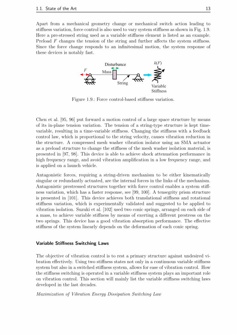
Apart from a mechanical geometry change or mechanical switch action leading tostiffness variation, force control is also used to vary system stiffness as shown in Fig. 1.9.Here a pre-stressed string used as a variable stiffness element is listed as an example.Preload F changes the tension of the string and further affects the system stiffness.Since the force change responds to an infinitesimal motion, the system response ofthese devices is notably fast.

VariableStiffness

k(F)

Mass

String

Disturbance

F

Figure 1.9.: Force control-based stiffness variation.

Chen et al. [95, 96] put forward a motion control of a large space structure by meansof its in-plane tension variation. The tension of a string-type structure is kept time-variable, resulting in a time-variable stiffness. Changing the stiffness with a feedbackcontrol law, which is proportional to the string velocity, causes vibration reduction inthe structure. A compressed mesh washer vibration isolator using an SMA actuatoras a preload structure to change the stiffness of the mesh washer isolation material, ispresented in [97, 98]. This device is able to achieve shock attenuation performance inhigh frequency range, and avoid vibration amplification in a low frequency range, andis applied on a launch vehicle.

Antagonistic forces, requiring a string-driven mechanism to be either kinematicallysingular or redundantly actuated, are the internal forces in the links of the mechanism.Antagonistic prestressed structures together with force control enables a system stiff-ness variation, which has a faster response, see [99, 100]. A tensegrity prism structureis presented in [101]. This device achieves both translational stiffness and rotationalstiffness variation, which is experimentally validated and suggested to be applied tovibration isolation. Suzuki et al. [102] used two conic springs, arranged on each side ofa mass, to achieve variable stiffness by means of exerting a different prestress on thetwo springs. This device has a good vibration absorption performance. The effectivestiffness of the system linearly depends on the deformation of each conic spring.

Variable Stiffness Switching Laws

The objective of vibration control is to rest a primary structure against undesired vi-bration effectively. Using two stiffness states not only in a continuous variable stiffnesssystem but also in a switched stiffness system, allows for ease of vibration control. Howthe stiffness switching is operated in a variable stiffness system plays an important roleon vibration control. This section will mainly list the variable stiffness switching lawsdeveloped in the last decades.

Maximization of Vibration Energy Dissipation Switching Law

14 1. Introduction

The control strategy based on the maximum vibration energy dissipation per vibrationcycle is very famous and originally proposed by Onoda et al. [27] and further improvedin [103]. It can be expressed by

k =

kmax , if xx > 0kmin , if xx < 0

, (1.2)

where k is the real-time stiffness, kmax and kmin are the maximum and minimum systemstiffness, x and x are the displacement and velocity of a protected payload. Theprinciple will be explained in Subsection 2.2.1 in detail and a switching stiffness devicecan be simply modeled as shown in Figure 1.5(b). Generally, the switching betweenthe maximum and the minimum stiffness is physically realized through a clampingdevice in [27, 28, 84, 104] or smart materials, see [55]. Ledezma-Ramirez et al. [19]documented that the control logic is applied to shock isolation and can outperform alinear passive system, if system damping in an vibration isolator is light.

Leitmann et al. [105, 106] proposed a control logic based on Lyapunov stability theoryfor vibration attenuation for a continuous variable stiffness. This control strategyaims to not only accomplish the task of maximizing the vibration energy dissipation,but also prove the stability of the controlled system. A variable stiffness system is akind of variable structure system, so variable structure system control or sliding modecontrol, featuring robustness and effectiveness, is ideal for variable stiffness control.Yang et.al [107] applied a variable stiffness device together with sliding mode controlfor vibration isolation on a seismic-excited building. Therein, a full state feedbackcontroller as well as a special output feedback controller are presented, respectively. Infact, the latter is proved to be the same as the switching law in Eq. (1.2). Sun et al. [86]applied a sliding mode controlled switching law to a vehicle suspension system.

Resetting Actuator-based Switching Law

Resetting actuator-based switching law mainly refers to a valve-controlled cylinderfilled with compressible fluids. Earlier, Bobrow et al. [108, 109] derived the resettingcontrol law based on Lyapunov stability theory, which resets the unstreched lengthof the fluids in the cylinder at each moment when the relative velocity across thedamper reaches zero. The resetting action will release the vibration energy stored inthe cylinder, and allow the damper to dissipate a lot of vibration energy in each motioncycle. More details related to this control logic can be also found in [110]. The systemdynamics can be expressed by

mx+ kx+ k1(x− xs) = 0 , (1.3)

where k1 is the hydraulic spring stiffness due to the net effect of compressible fluids,xs is the unstretched length of the fluids resulting from the vibration of a payload mand k is a constant stiffness. By opening the bypass valve for a short time and thenclosing it, the potential energy stored in the fluids can be transformed into heat. Theresetting control law can be given by

xs = x , if x = 0 . (1.4)

This means that the maximum potential energy stored in cylinder during one vibration


cycle is released and after a short time, the bypass valve is closed and the system stiff-ness will reach k+k1 again. This device has been validated for seismic response controlin a six-storey building, see Yang et al. [111] and a three-storey building in [112].

Acceleration-based Switching Law

A simple on-off variable stiffness switching law based on the acceleration of a primarystructure is applied to base isolation in [83], where a desired acceleration thresholdxthreshold is set initially. If the acceleration of the primary structure is larger thanthe threshold value, an electromagnetic clutch connects an additional device to theprimary structure, and potential energy is stored in the additional device. Whenthe acceleration amplitude decreases below the threshold, the clutch disconnects theadditional device from the primary structure and the stored potential energy will bereleased at once. This control logic can be expressed as

k =

kmax , if x > xthreshold

kmin , if x < xthreshold. (1.5)

where x is the real-time acceleration of the primary structure and xthreshold is the desiredacceleration. In that research, it was experimentally proven that vibration isolation isrealized effectively.

Skyhook Control-based Switching Law

Skyhook control is early proposed for system damping control in [113]. This controllogic based on damping adjustment allows the maximum vibration isolation in a pri-mary structure and has been well documentd in [7]. Cunefare et al. [114] uses thiscontrol logic in stiffness variation for vibration absorption, as expressed in Eq. (1.6).This can be physically interpreted that when a force, produced by a vibration absorber,acts on the primary structure in the opposite direction of base motion, a stiffer springremoves more energy from the base. Conversely, a softer spring is used when the forceacts in the same motion direction of the primary structure. This leads to less energybeing brought into the primary structure.

k =

kmin , if x(xabsorber − x) > 0kmax , if x(xabsorber − x) < 0

, (1.6)

where x stands for the velocity of the primary structure and xabsorber is the velocityof the absorbers mass. This switching law does not guarantee a minimized primarystructure motion, see [115]. The operation of an absorber together with this switchinglaw for vibration absorption of a continuous system such as a beam and a plate, wasconsidered in that research.

In addition, a switched damping together with Skyhook control can also achieve thestiffness variation in a combined device including both a spring and a damping. Forinstance, Liu et al. [84, 85, 116] proposed a stiffness on-off control based on on-offcontrollable damping for vibration isolation in a two-degree-of-freedom system. Thissystem is experimentally proven to have a better isolation performance than a conven-tional variable damping system. In this method, two variable dampers are controlledby the maximum vibration energy dissipation as stated in switching logic (1.2) andSkyhook control logic, respectively.

16 1. Introduction

Due to MRE showing that its stiffness and damping increase monotonically with theincrease of magnetic flux density, Opie et al. [30, 117] developed a vibration isolationdevice, built up from MRE, together with the Skyhook control-based switching law inorder to minimize the absolute velocity of a primary structure. The switching law canbe given by

k =

kmin , if x [P (x− x0) + (x− x0)] 6 0kmax , if x [P (x− x0) + (x− x0)] > 0

, (1.7)

where x, x stand for the displacement and velocity of the primary structure and x0, x0

are the displacement and velocity of base excitation, respectively. P is a non-negativecoefficient dependent on an accurate model of the vibration isolation device. Exper-imental results show that the MRE isolation system reduces the absolute velocity ofthe primary structure by 30% compared to a passive counterpart.

Switching Law for Variable Stiffness Control with a Piezo Shunt

Differing from vibration energy dissipation realized by mechanical structure, piezoshunt-based variable stiffness systems utilize an electrical impedance to dissipate vi-bration energy. How to control the mechanical strain of piezo element and transform aportion of vibration energy into electrical energy and then discharge through a shuntcircuit will be focused on in this subsection.

A: Maximum Strain-based Switching Law The maximum strain of a piezo transducercorresponds to the maximum vibration energy transformation. As a result, when thepiezo transducer reaches the maximum mechanical deformation, it will be switched intoa shunt circuit, short- or resistive-circuit (low stiffness) for a short duration and thendischarged completely. Afterwards, the piezo transducer is switched into open circuit(high stiffness) configuration again. This allows the voltage to be produced furtheracross the electrodes, until the next displacement extreme occurs [37, 118]. It is obviousto see that the piezo transducer stays in the high-stiffness state for most of the vibrationcycle, but it is momentarily pulsed to the low-stiffness state to dissipate the storedenergy. In [119–121], the switch is again synchronized with the displacement extreme.Instead of discharging the piezo transducer, its voltage is quickly inverted via a resonantnetwork. Compared with the above control logic, this one is the most efficient semi-passive technique, but its drawback is the need for an external power supply. In orderto solve the needed external power problem, self-powered piezo structural vibrationcontrol systems are documented in [122, 123].

B: State-switched Switching Law Similar to [37], Clark et.al [39] proposed a state-switched control logic to apply to a shunted piezo transducer to realize vibration en-ergy dissipation, but the difference from the above stated control logic is that thismethod keeps the piezo transducer in each of the high- and low-stiffness states for onequarter-cycle increment, not most of a vibration cycle. When system is moving awayfrom equilibrium and kinetic energy is decreasing, the actuator is in an open-circuitconfiguration, i.e. high stiffness state, and energy is stored in piezo transducer. Whenthe system is moving toward equilibrium and needs to receive energy from the piezotransducer, the transducer will be set to the short-circuit, namely, low stiffness state,this leads to energy dissipation and therefore, vibration control is achievable. In fact,this control logic is the same as Maximum vibration energy dissipation-based controllogic.

1.2. Summary of Literature Review 17

1.2. Summary of Literature Review

From the above literature review, it is concluded that

1. Variable stiffness-based vibration control systems have been widely studied forvibration suppression, vibration isolation, and vibration absorption. Stiffnessvariation can be realized by smart material-based devices and special mechanicalstructures;

2. Continuous variable stiffness can be controlled by a continuous variable energyfield such as magnetic field, temperature field, or force field, acting on a smartmaterial-based or a special mechanical structure. Switched stiffness, on one hand,can be a simple alternative of continuous variable stiffness, where the maximumor minimum stiffness are chosen from a continuous variation range. On the otherhand, it can also be realized by special stiffness state switching devices such asa mechanical switch or a piezo shunt;

3. Many of the variable stiffness systems proposed are active systems, power canflow in both directions, into or out of the vibrational system, although manyauthors define their system as semi-active.

4. The presented concepts of switched stiffness devices for vibration reduction useenergy dissipation to extract the stored potential energy in a different vibrationmode within each vibration cycle of the payload.

5. In current mechanical structures and control concepts for vibration reductionthere are always time spans where part of the repeatedly stored potential energyin the spring is released as kinetic energy of the load mass, extending the settlingtime.

1.3. Objective

The outcome of the literature review, condensed in the summary Sec. 1.2, indicatesthat the current semi-active concepts or devices for vibration reduction use energydissipation, i.e. transformation of kinetic energy into heat, see No. 4 in Section 1.2.Furthermore, in all cases part of the kinetic energy stored as potential energy in springsis released back into the kinetic energy of the mechanical structure, see No. 5 inSection 1.2. In the Mechatronics Group at TU Ilmenau a semi-active system combiningvariable stiffness with damping mechanism, which is controlled by magnetorheologicalvalves, was proposed in [87] and is shown in Fig. 1.10. The concept is chosen andslightly modified by removing the damping elements and using two equal stiffness.Further, feedback control is introduced. These modifications result in a new conceptand system being the starting point of the thesis.

The thesis objective is to investigate the new system for vibration reduction tasks,which means performing vibration reduction without damping and without releasingenergy back into the mechanical structure. Instead of releasing the potential energy,the vibrational energy is stored or harvested in the springs. The idea of vibrationenergy harvesting instead of energy dissipation will be used to counteract disturbance

18 1. Introduction

input force

input piston

magnetorheologicalfluid

output piston

spring

input force

input chamber

mrf valves

output chambers

magnetic field

Figure 1.10.: Variable stiffness and damping mechanism together two magnetorheolog-ical valves [87].

forces like an actuator in vibration compensation. The new system is called 4S as theabbreviation for Serial-Stiffness-Switch-System. In this thesis the principle vibrationalbehavior needs to be investigated in detail and control concepts have to be foundwhich perform in the planed manner. For the analysis and system design, analytical,numerical and experimental approaches are applied.

1.4. Contribution

The authors contribution to extend state of the art in semi-active vibration reductionconcepts and devices is

• Suggestion of a new semi-active vibration reduction concept as outlined in Ob-jectives. The proposed system is able to harvest the vibrational energy intothe springs and use the stored potential energy to work as an actuator againstperturbation forces.

• Analytical, numerical and experimental proof-of-concept for the proposed systemis shown under harmonic force disturbance at supercritical excitation of a payloadmass. It is shown that the system approaches a steady-state response by anappropriate switching law.

• Initial velocity disturbance compensation, namely, shock compensation is provenby the introduction of a new switching law or control law. The numerical and ex-perimental investigations showed that the settling time to the position at rest canbe reduced by the factor of 20 compared to the original velocity-base switchinglaw.

• Shock isolation capability is shown under pre-tensioned springs by numericalsimulation analysis. One outcome is that shock isolation of the system worksin the complete shock response spectrum both in the high as well as the low

1.5. Thesis Organization 19

frequency region. Especially the isolation in the low frequency region, below thefirst eigenfrequency of the mechanical structure, is a novel result and extendscurrent concepts, which work only above the first eigenfrequency. Thus, theproposed system can outperform existing semi-active device concepts.

1.5. Thesis Organization

To conduct a theoretical and experimental study on the proposed novel semi-activevibration control strategy, a simplified model, consisting of a mass and two serial-stiffness-switch elements, is considered throughout this work. The thesis is organizedas follows,

In Chapter 1 the background of this thesis is initially introduced. An overview ofdifferent contributions in the area of variable stiffness devices together with switchinglaws for vibration control is presented. Following is the objective and contributions inthis work.

Chapter 2 contains the information on the modeling, operation principle and systemdynamics of novel semi-active vibration control system. 4S in open loop and closed loopcontrol are numerically analyzed, respectively. The equivalent stiffness and naturalfrequency of the switching system are mathematically formulated and verified throughFast Fourier Transformation. A switching law based on vibration energy harvesting isalso numerically analyzed.

In Chapter 3 vibration energy harvesting limitation is theoretically and numericallyanalyzed. In order to further show the energy harvesting limitation, a long time sim-ulation is carried out.

A rotational setup is designed in Chapter 4. Two ring-arranged electromagnet-platestogether with one armature-shaft work as two mechanical switches. The operationprinciple, modeling, construction and the corresponding experiment are carried out.

To improve the system response, a new switching law based on variable structuresystem control theory is further proposed in Chapter 5. Non-zero initial velocity andharmonic excitation processes are numerically and experimentally verified.

In Chapter 6 shock isolation performance is numerically tested on 4S with the com-parison of a passive and a semi-active system. Considering 4S can harvest vibrationenergy, a potential energy pre-storage is applied before shock.

Finally, the main conclusions from this thesis are summarized in Chapter 7 and rec-ommendations for future work are also made.

CHAPTER 2

Novel Semi-active Vibration Control with 4S

2.1. Introduction

In most of the mentioned vibration control systems in Introduction, there still existunavoidable time instants during a vibration reduction process, where an elastic el-ement releases the stored potential energy, and drives a protected payload to moveagain. This is an intrinsic property of the elastic element and results in an oscillationin the systems to some extent.

In order to solve the problem, a novel semi-active vibration control strategy based onvibration energy harvesting is proposed in this chapter. The basic idea introducedin this chapter is a modification of the idea presented by Greiner-Petter, Tan andSattel [87], where a MRF valve controlled variable stiffness and damping mechanismwas proposed. The modifications include the removal of the damping elements andusing two equal stiffness as was already outlined in Section 1.3 (Objective).

Before introducing the new system or concept, vibration reduction issues about a pas-sive and a semi-active vibration control system are formulated and then a new semi-active vibration control concept related to Serial-Stiffness-Switch-System (4S) is putforward and analyzed. In a preliminary study, 4S in open loop control is analyticallyand numerically interpreted, where the equivalent stiffness and natural frequency ofthe switching system are given. Finally, a velocity zero-crossing switching law basedon vibration energy harvesting is introduced. It is numerically proven that 4S showsvibration energy harvesting and vibration reduction performance. A harmonic dis-turbance will be always exerted on 4S in this chapter. The corresponding theoreticalanalysis is also demonstrated in Min et al. [124].

22 2. Novel Semi-active Vibration Control with 4S

2.2. 4S Concept

Potential energy releasing of an elastic element leads to an acceleration of the protectedpayload once again during a vibration reduction process. This phenomenon will beexplained in the following subsection in detail.

2.2.1. Problem Statement

For the sake of a simple explanation, all elastic elements through the work are denotedas springs. At first, a passive single-degree-of-freedom (SDOF) model is considered, assketched in Fig. 2.1(a). The equation of motion is given by

m1x1 = F − dx1 − kx1 , (2.1)

where x1 is the payload displacement and m1, k and d are mass, stiffness and dampingparameters of the system, respectively. The force F represents the external disturbanceand is considered to be a pulse in this case. The objective of vibration control as

F

0 t

Deceleration

Acceleration

Compression

Extension

(a) (b)

dk

m1

x1

x1

Figure 2.1.: Schematics for m1-k-d-system. (a) Simplified model; (b) Displacementresponse for an external pulse disturbance.

understood here is to achieve vibration reduction, which moves a payload m1 back toits equilibrium position x1 = 0. Multiplying Eq. (2.1) with the velocity x1 results inthe mechanical power balance

m1x1x = Fx1 − dx21 − kxx1 , (2.2)

and can be rewritten asdT

dt= Fx1 − dx2

1 −dU

dt, (2.3)

where T is defined as kinetic energy, T = 12m1x

21 and U is potential energy, U = 1

2kx2

1.In order to achieve vibration reduction, the kinetic energy should not increase, namely,dT/dt < 0. The damping d leads to a permanent reduction of kinetic energy, sincedx2 > 0, ∀x1 6= 0 always holds. To further reduce the kinetic energy T , the potentialenergy U has to increase: dU/dt > 0, ∀t > 0. However, this is not possible to realizefor all time instants in a passive system as depicted in Fig. 2.1(a), because in all

2.2. 4S Concept 23

vibration systems with D = d/(2√km) < 1, there exist not only the time phases with

dU/dt = kx1x1 > 0, denoted by pink area in Fig. 2.1(b), but also the time phases withdU/dt = kx1x1 < 0, denoted by green area. The potential energy stored during thedeceleration phases of the payload m1, kx1x1 > 0, will be completely released in theacceleration phase, kx1x1 < 0.

Using a semi-active vibration control system with two springs, k − ∆k and ∆k tostore potential energy U1 = (k−∆k)x2

1/2 and U2 = ∆kx21/2, together with a specified

switching law between these two springs offers possibilities for vibration reduction asdepicted in Fig. 2.2. One possibility is to use a larger changing rate of potential energyin time phases where the spring decelerates the payload, i.e. for dU/dt > 0 and asmaller changing rate of potential energy is chosen in time phases where the springaccelerates the payload, i.e. at dU/dt < 0, see Onoda et al. [27] and Ledezma-Ramirezet al. [19]. This is similar to the damped passive system in Fig. 2.1(b) by the pink andgreen areas. To do so, in the deceleration phase, when the kinetic energy of payload m1

decreases, both springs are active, depicted by pink area and in the acceleration phase,when the kinetic energy of payload m1 increases, only one spring is taken, as shownby green area. That is to say, during a deceleration phase, d(U1+U2)

dt> 0 and for an

acceleration phase dU1

dt≤ 0. The potential energy U2 will be dissipated in the form of

thermal energy by a damping element ∆d, when the spring ∆k is disconnected from thepayload m1. Finally, the kinetic energy of the payload is removed from the system byrepeatedly switching the springs and vibration reduction performance is achieved. The

F

(a)

F

(b)

ks

kΔ

m

kΔˉ

1

d

ks

kΔ

m

kΔˉ

1

Δ dΔ

x1x1

Figure 2.2.: Schematic of a parallel-stiffness-switch system: (a) k-∆k and ∆k are con-nected to payload m1; (b) Only k-∆k is connected to payload m1.

system behavior has already been investigated under different disturbances, e.g. shockexcitation, see [19] or harmonic excitation, see [32]. The switching law is given bythe changing rate of potential energy, dU/dt = keffx1x1 and describes the resultingswitching stiffness keff

keff =

k if x1x1 > 0k −∆k if x1x1 ≤ 0

. (2.4)

The resultant stiffness keff = k corresponds to the pink areas in Fig. 2.1(b) and keff =k − ∆k to the green ones. In such an arrangement spring ∆k always decelerates thepayload, but spring k −∆k still both decelerates and accelerates the payload m1.


2.2.2. Vibration Energy Harvesting Concept

To avoid this, i.e. to ensure that springs permanently decelerate the payload, anotherway to remove kinetic energy from the system is proposed. Instead of switching betweenacceleration and deceleration time phases, corresponding to the pink and green areasin Fig. 2.1(b), the idea is to use only decelerating phases. Therefore, the two directionsof the payload motion should be split up between two springs k1 and k2. This meansthat the first spring k1 is only active in its increasing extension phase and k2 only activein its increasing compression phase. Thus, for both springs the terms of the changingrate of potential energy should be larger than zero, which is illustrated in Fig. 2.3(b)by the red and blue lines of the time history x1(t) for a passive system m1-k. A way

s1

s2

k1

k2

m1

x1,

x2

F

(a)

Spring 1

0

x

t

Deceleration

Compression

Extension

Spring 2

(b)

x1

Figure 2.3.: Schematic for 4S. (a) 4S model; (b) Connection of two springs over time.

for the concept realization would be to have two springs in series together with twoswitches, according to Fig. 2.3(a), which is called“4S”(Serial-Stiffness-Switch-System).This leads to the necessary conditions, k1x1 ≥ 0 ∧ x1 ≥ 0 for an increasing extensionand k2x1 < 0 ∧ x1 < 0 for an increasing compression. In fact, a similar serial stiffnessstructure has already been proposed by [84], but the operation principle is different. Inthe work presented here, a separation of extension and compression phases takes place,which means that one spring is always under compression and the other always underextension. Consequently, the springs are not active in the system at the same time.The switching law is given by the zero-crossing of velocity, x1, separating time phaseswith x1 ≥ 0 and x1 < 0. Instead of dissipating the stored potential energy in eachvibration cycle and realizing vibration reduction, the kinetic energy of the payload willbe harvested. When the disturbance F vanishes, the stored potential energy can beeither used by the system, working as an actuator, or dissipated similarly to the systemwith the parallel springs in Fig. 2.2(b), by means of opening two switches s1, s2 at thesame time.

2.2. 4S Concept 25

2.2.3. 4S Model

As shown in Fig. 2.3(a), the model comprises of two serial springs k1, k2, payloadm1 and two switches s1, s2, which in fact are two clamping devices. These devicesmight be realized by smart material such as piezoelectric, electromagnetic or magneto-rheological fluids material and govern the operation order of two springs. To begin,the clamping devices are not considered in detail and only simplified as switch s1 ands2 for the analysis. F stands for external excitation, x1 is the displacement of payloadand the displacement of connection point of two springs is symbolized as x2. Bothswitches own two working states, namely, open or close, which result in the connectionor disconnection of each spring to or away from the payload m1. So there exist fourswitching groups between s1 and s2, which produces four different types of systemstiffness k(S) as expressed in Eq. (2.5)

k(S) =

k1 if S(t) = [1, 0]k2 if S(t) = [0, 1]k1k2

k1 + k2

if S(t) = [1, 1]

− if S(t) = [0, 0]

, (2.5)

where k(S) is the stiffness of the switched system and S(t) is defined as a switchingcontrol vector for s1, s2

S(t) = [s1(t), s2(t)] , si(t) ∈ 0, 1 , i = (1, 2) . (2.6)

Here si(t) = 0 means that the ith spring is disconnected away from the payload;Conversely, si(t) = 1 represents the ith spring being connected. The operation orderfor the two switches is also listed in Table 2.1 for ease of interpretation.

Table 2.1.: Operation order of two springs

Control vector (S) Switching condition Spring connection

[1, 1] s1, s2 open k1, k2

[0, 1] s1 closed and s2 open k2

[1, 0] s2 closed and s1 open k1

[0, 0] s1, s2 closed not allowable

Based on Newtons law of motion the dynamics of 4S, sketched in Fig. 2.3(a), can begiven as follows. If S(t) = [1, 0], the system dynamics can be given by

mx1 + k1(x1 − x2) = F , ∧ x2 = x2(tsw,i) , (2.7)

and in case of S(t) = [0, 1] by

mx1 + k2x2 = F , ∧ x2 = x1 − [x1(tsw,i)− x2(tsw,i)] . (2.8)


where tsw,i is the i-th switching time instant with the subscript “sw”. When S(t) =[1, 1], two springs are active and the motion equations can be given as follows,

mx1 = F − k1(x1 − x2) , ∧ k2x2 = k1(x1 − x2) . (2.9)

Each subsystem Eqs. (2.7)-(2.9) behaves as a SDOF system. However, the systemhas three state variables, (x1, x1, x2). The case S(t) = [0, 0], where both of twosprings are not active, is not allowable in practice. In order to have a more compactdescription, Eqs. (2.7)-(2.9) will be combined as

m1x1 + k(S)x1 = F + Fp(S) (2.10)

and

x2(S) =

x2(tsw,i) if S(t) = [1, 0]

x1 − [x1(tsw,i)− x2(tsw,i)] if S(t) = [0, 1]k1

k1 + k2

x1 if S(t) = [1, 1]

− if S(t) = [0, 0]

, (2.11)

where x2(S) is the displacement of the connection point between two springs and theprocess force is defined as Fp(S),

Fp(S) =

k1u2(tsw,i) if S(t) = [1, 0]k2u1(tsw,i) if S(t) = [0, 1]

0 if S(t) = [1, 1]− if S(t) = [0, 0]

, (2.12)

with the deformation of the two springs u1 and u2 defined as

u1 := x1 − x2 , u2 := x2 . (2.13)

In order to realize the compression and extension spring configuration, the switchingcases S(t) = [1, 0] and S(t) = [0, 1] are chosen. At first, the stiffnesses k1 = k2 = k areused in this work considering that a switching behavior is symmetric for S(t) = [1, 0]and S(t) = [0, 1]. Finally, the system dynamics would be further simplified as

m1x1 + kx1 = F + Fp(S) (2.14)

and

x2(S) =

x2(tsw,i) if S(t) = [1, 0]

x1 − [x1(tsw,i)− x2(tsw,i)] if S(t) = [0, 1], (2.15)

and the process force Fp(S) is given by

Fp(S) =

ku2(tsw,i) if S(t) = [1, 0]ku1(tsw,i) if S(t) = [0, 1]

, (2.16)

where it is a piecewise constant force. Note that in Eq. (2.10) the actual spring forcesFk are split into two components, the process force Fp(S), which is constant within a

2.3. Open Loop Control for 4S 27

switching state and the time varying part kx1,

Fk(S) = kx1 − Fp(S) . (2.17)

Yet, no switching law has been proposed. The system can be driven in open loop orclosed loop control.

2.3. Open Loop Control for 4S

In order to preliminarily study the performance of 4S, it will be analyzed under su-percritical disturbance force excitation in open loop control, in which 4S is operatedunder a specified switching sequence and independent of the system state variables,(x1, x1, x2). Investigations of critical and subcritical excitation are left for furtherstudies. Exemplary, the theoretical analysis is done for a supercritical excitation,ηd = 10, in the following chapters.

2.3.1. Numerical Analysis

The numerical analysis is executed under a harmonic disturbance

F (t) = F sin Ωt . (2.18)

When a regular switching between two springs happens in 4S, a switching time periodTsw, in which two springs are active only one time, and the corresponding switchingfrequency Ωsw are defined as

Ωsw =2π

Tsw

. (2.19)

During a switching period Tsw, the time phases where these tow springs k1 or k2 areactive are called T1 or T2, respectively, and then the switching period Tsw = T1 + T2.The two switches s1, s2 are considered to open and close instantaneously. A duty cycleDk1 is defined for k1 as

Dk1 =T1

Tsw

=T1

T1 + T2

, (2.20)

and (1−Dk1) is the duty cycle of k2. The time behaviors of the open loop controlled4S under four different duty cycles are investigated, here Dk1 ∈ [0, 0.1, 0.3, 0.5]. Dueto the complementary choice of the switching states for the two switches, one stiffnessstate sufficiently represents the switching sequence signals. Consequently, only theoperation state of switch s1 is illustrated in Fig. (2.4). For example, if s1 = 0, S(t) =[0, 1] and if s1 = 1, S(t) = [1, 0].

Three different system response frequencies occur in 4S, the natural frequency ω0 ofeach subsystem, m1-k1 or m1-k2, according to Eq. (2.21), here k1 = k2 = k,

ω0 =

√k

m1

, T0 =2π

ω0

. (2.21)


0 1 2 3

0

0.5

1

t/T(a)

s 1

0 1 2 3

0

0.5

1

t/T(b)

0 1 2 3

0

0.5

1

t/T(c)

0 1 2 3

0

0.5

1

t/T(d)

sw sw sw sw

Figure 2.4.: Switching sequences for different duty cycles Dk1. (a) Blue: Dk1 = 0; (b)Red: Dk1 = 0.1; (c) Black: Dk1 = 0.3; (d) Green: Dk1 = 0.5

Table 2.2.: Simulation parameters for open loop controlled 4S.

Name Value Unit Name Value Unit Name Value Unit

F 1 N ηd 10 - x1(0) 0 mm1 1 kg ηsw 500 - x1(0) 0 m/sk 1 N/m Dk1 variable - x2(0) 0 m

the external disturbance frequency Ω and the switching frequency, Ωsw, which will berelated by two quantities, the dimensionless disturbance frequency ηd and the dimen-sionless switching frequency ηsw, according to

ηd =Ω

ω0

, ηsw =Ωsw

ω0

. (2.22)

The system parameters for the numerical analysis are listed in Table 2.2, here thedimensionless switching frequency ηsw is very high compared to the dimensionless dis-turbance frequency ηd. The Eqs. (2.14)-(2.15) can be piecewise integrated analyticallyand solved on an algebraic level by formulating transition conditions between switchingtime instants tsw,i. For the sake of simplicity, the numerical simulation are carried outin MATLAB/Simulink here.

The colors in Fig. 2.4(a)-(d) stand for the different duty cycle Dk1 cases. The systemresponse in terms of the displacement x1 and velocity x1 of the payload and the springdeformations u1 and u2 are shown in Fig. 2.5. There are two columns of subfigures,marketed by a-h, respectively. The cyan lines in Fig. 2.5(a)-(d) represent the zoom-inwindows of the plots given in the right side Fig. 2.5(e)-(h). However, only the curvesfor the duty cycle Dk1 = 0.3 in Fig. 2.5(e)-(h) are plotted because all response curvesfor different Dk1 are similar. In the enlarged Fig. 2.5(e)-(h) a light blue area representss1 = 1, which denotes k1 being active, and a light green area represents s1 = 0 and k2

is active.

Fig. 2.5(a)-(d) show when Dk1 = 0, only u2 varies because only k2 is active. 4S can beseen as a passive undamped m1-k system, whose system response is the superpositionof the free response in terms of system properties and the forced response with respectto an external disturbance. When Dk1 6= 0, 4S is forced to switch based on theswitching sequences shown in Fig. 2.4. The system response of 4S(Red, Black andGreen) are similar to that of the passive undamped system(Blue), but the fundamental


0 5 10 15 20

−0.2

0

0.2

(a)

x1

(m/s

)

(e)9 9.01 9.02 9.03

0.1

0.14

0.18

0 5 10 15 20−0.2

0

0.2

x1(m

)

(b) (f)9 9.01 9.02 9.03

0.06

0.065

0.07

0 5 10 15 20−0.2

0

0.2

(c)

u1(m

)

(g)9 9.01 9.02 9.03

0.015

0.02

0.025

0 5 10 15 20−0.2

0

0.2

t (s)(d)

u2(m

)

t (s)(h)

9 9.01 9.02 9.030.04

0.045

0.05

Dk1= 0Dk1= 0.1Dk1= 0.3Dk1= 0.5= 0s1

= 1s1

Figure 2.5.: System response of 4S at open-loop control for four different duty cycles.(a)-(d) and (e)-(h) are payload velocity, x1, payload displacement, x1,the deformations of two springs, u1 and u2, respectively. Right side is azoomed-in at the cyan line on the left. The colors in (a)-(d) correspond tothe duty cycle colors in Fig. 2.4.


amplitude and period of the system response show differences. With the increase ofDk1 from 0 to 0.5, the fundamental period of 4S also increases, which means thatthe equivalent frequency and stiffness of the switched system decreases. Generally,stiffness and natural frequency are defined for linear systems, so equivalent stiffnessand natural frequency are defined for the switched system here. Fig. 2.5(c)-(d) showthe deformations of the two springs u1, u2. Their response time behaviors seem similarfor different duty cycles, but their amplitudes and periods are different.

In Fig. 2.5(e)-(h) the ratio of light blue area to light green area is equal to 3 : 7, becauseDk1 is equal to 0.3. Due to the switching between two springs, the deformations ofthe two springs show an intermittent variation, but the displacement and velocity ofthe payload m change continuously because of a rapid switching and the inertia of thepayload. In order to further find out the effects of the duty cycle on the deformations ofthe two springs, the equivalent stiffness and natural frequency of the switched system,an analytical investigation is carried out in the following subsection.

2.3.2. Analytical Formulation

In this subsection, the equivalent stiffness keq and equivalent natural frequency ωeq ofthe switched system in open loop control are derived under a simplified assumption.As listed in Table 2.2, for the dimensionless switching frequency ηsw in Eq. (2.22),

ηsw ηd ⇒ Tsw 2π

Ω<

2π

ω0

(2.23)

holds. The constant switching period Tsw = T1 + T2 and the constant time peri-ods T1, T2 are described by three arbitrary switching time instants tsw,2j, tsw,2j+1

and tsw,2j+2 (j = 0, 1, 2...), so Tsw = tsw,2j+2 − tsw,2j, T1 = tsw,2j+1 − tsw,2j andT2 = tsw,2j+2−tsw,2j+1, here j represents the j-th switching period. Due to Tsw and alsoT1 and T2 being short enough compared to systems dynamic and the velocity varyingcontinuously as well, shown in Fig. 2.5(e), the relationships for the average velocityx1 of the payload over the time phases [tsw,2j, tsw,2j+1] and [tsw,2j+1, tsw,2j+2], and thedeformation rates of two springs can be approximately given by

x1(t, T1) ≈ x1(t, T2), ⇒ u1(t, T1) ≈ u2(t, T2) (2.24)

together with Eq. (2.13) and Eq. (2.15). The incremental deformation of spring 1, ∆u1

and that of spring 2, ∆u2 over the above corresponding time phases are given by

∆u1(t, T1) = u1(t, T1)T1 = u1(t, T1)Dk1Tsw , (2.25)

and∆u2(t, T2) = u2(t, T2)T2 = u2(t, T2)(1−Dk1)Tsw , (2.26)

with T2 = Tsw−T1 and Eq. (2.20). Because spring 1 is only active over t ∈ [tsw,2j, tsw,2j+1]and spring 2 over t ∈ [tsw,2j+1, tsw,2j+2], ∆u1 and ∆u2 over t ∈ [tsw,2j, tsw,2j+2], namely,one complete switching period Tsw, can be expressed by

∆u1(t, Tsw) = ∆u1(t, T1) , ∆u2(t, Tsw) = ∆u2(t, T2) . (2.27)


If Tsw is infinitely low, ∆u1 and ∆u2 at an arbitrary time moment t can be given by

limTsw→0

∆u1(t, Tsw) = ∆u1(t), limTsw→0

∆u2(t, Tsw) = ∆u2(t) . (2.28)

With the combination of Eq. (2.27), subsequently inserting Eq. (2.24)-Eq. (2.25), re-arranging the variables and applying Eq. (2.27) and Eq. (2.28) derives the relationshipbetween the deformation differences of the two springs at an arbitrary moment

∆u1(t) =Dk1

1−Dk1

∆u2(t) . (2.29)

If the initial deformations u1(0) = u2(0) = 0 are taken into consideration, the rela-tionship between the deformations u1(t) and u2(t) of the two springs can be given by

u1(t) =Dk1

1−Dk1

u2(t) . (2.30)

The coefficient of Eq. (2.30) agrees with the amplitude behavior of the springs defor-mations as shown in Fig. 2.5(c)-(d) quite well. In order to formulate the equivalentstiffness keq and natural frequency ωeq of the switched system, the energy method isapplied now. The difference of potential energy ∆Ep over Tsw is given by

∆Ep =1

2k[u2

1(tsw,2j+2)− u21(tsw,2j) + u2

2(tsw,2j+2)− u22(tsw,2j)

]. (2.31)

A SDOF system mx + keqx = 0, having equivalent stiffness keq with potential energydifference ∆Epeq and equivalent to the switched system, is looked for

∆Epeq =1

2keq

[x2(tsw,2j+2)− x2(tsw,2j)

], (2.32)

and matches the following conditions

∆Epeq = ∆Ep, x(tsw,2j) = u1(tsw,2j)+u2(tsw,2j), x(tsw,2j+2) = u1(tsw,2j+2)+u2(tsw,2j+2) .(2.33)

Inserting Eqs. (2.30)-(2.32) into Eq. (2.33) leads to the equivalent stiffness

keq

k= 2D2

k1 − 2Dk1 + 1 (2.34)

and the equivalent natural frequency

ωeq

ω0

=√

2D2k1 − 2Dk1 + 1, ωeq =

√keq

m1

, Teq =2π

ωeq

. (2.35)

According to Eq. (2.34)-(2.35), the equivalent stiffness and natural frequency of thisswitched system for open loop control can be depicted in Fig. 2.6. This analyticalapproximation also matches the above numerical simulation results in terms of theequivalent natural frequency ωeq. To further validate the above stated conclusion, thespectral analysis for the displacement response under different duty cycles Dk1 in aninterval of 0.05 from 0 to 1 is carried out through Fast Fourier Transformation (FFT).On the basis of the amplitude-frequency spectrum property, the lowest frequency cor-


responding to the highest amplitude is the equivalent natural frequency of the switchedsystem. The calculated frequency results are normalized by ω0 and shown with thegray points in Fig. 2.6. It is obvious to find that the spectrum analysis and the mathe-

0 0.2 0.4 0.6 0.8 1

0.4

0.6

0.8

1

k eq kω

eq ω0

Dk1

1.2,

keq

kωeq

ω0(Analytical Solution)

ωeq

ω0(Numerical Solution)

Figure 2.6.: The equivalent stiffness and natural frequency of 4S.

matical formulation also agree well. As shown in Fig. 2.6, the profiles of the equivalentstiffness and natural frequency are similar. When Dk1 = 0 and Dk1 = 1, only onespring is active in 4S and the system works as a passive undamped system having theequivalent stiffness keq = k and the equivalent natural frequency ωeq = ω0. In all othercases it is a semi-active system and keq and ωeq change parabolically with the increaseof Dk1. In the minimum at Dk1 = 0.5, keq = 0.5k and ωeq =

√2ω0/2. This means

that at an equal switching time period of two serial springs, T1 = T2, and ηsw 1, thesystem behaves like a linear SDOF system.

2.4. Closed Loop Control for 4S

2.4.1. Switching Law based on Vibration Energy Harvesting

In order to realize vibration energy harvesting performance through vibration reduc-tion, 4S is now analyzed in closed loop control based on the idea already outlined inSubsection 2.2.2 together with Fig. 2.3. Finally, the switching law can be given by

S(t) =

[1, 0] if x1 > 0[0, 1] if x1 < 0

. (2.36)

Inserting Eq. (2.36) into Eq. (2.16) gives the process force Fp

Fp =

k u2(tsw,i) if x1 > 0k u1(tsw,i) if x1 < 0

, (2.37)

for the closed loop controlled 4S. This switching law ensures that for all time instantsthe conditions u1 > 0 and u2 < 0 are valid. This switching between two springs isideal. To consider a physically realizable zero-crossing detection and prevent chattering

2.4. Closed Loop Control for 4S 33

a switching system, the switching law is slightly modified as

S(t) =

[1, 0] if x1z > 0[0, 1] if x1z < 0

, (2.38)

with the use of the zero-order-hold function of velocity, written as

x1z(x1, Ts) =∞∑n=0

x1(nTs)[σ(t− nTs)− σ(t− (n+ 1)Ts)] , n ∈ N , (2.39)

or asx1z(t, Ts) = x1(nTs) , n ∈ N , nTs 6 t < (n+ 1)Ts , (2.40)

where Ts is the sampling period of the system, and σ(t) is the unit step function. Notethat Ts is different from the aforementioned switching period Tsw. The former, Ts, isthe minimal time interval, where the stiffness state is constant, but the latter, Tsw,is constant and is the minimal time interval, where two switching instants can occur.Thus, for a general switching time span Tsw,j (j = 0, 1, 2...), not similar to a regularswitching in an open loop control, it may be variable, namely, Tsw,j ≥ 2Ts, wherej represents the j-th complete stiffness switching in 4S. Therefore, the relationshipbetween the switching rate Ωsw,j and the sampling frequency ωs can be given by

Ωsw,j 61

2ωs , Ωsw,j =

2π

Tsw,j

. (2.41)

One case for the signal discretization is graphically shown in Fig. 2.7, where Ts1 >Ts2 > Ts3. It obviously reveals that the lower the sampling period, the more thediscretized signal represents the original one. The discretization process for velocityresults in a nonideal switching and produces switching delay. As an example, it is

t

T

0

s3

Ts2

Ts1

>0

>

0

>

0

t0

(T )zx1

(T )zx1

(T )zx1

(T )zx1t0 tz

Δtz3

Δtz2=Δtz1

t

(b)(a)

s1

s2

s3

si

Figure 2.7.: Switching decision error for 4S with different sampling period Ts: (b) is apartly zoomed-in picture for (a). Black: original signal; Green: discretizedsignal with sampling period Ts1; Orange: discretized signal with samplingperiod Ts2; Blue: discretized signal with sampling period Ts3.

assumed that for three systems with different sampling time Ts1, Ts2 and Ts3 andtheir velocity controllers start to process at a common time point t0 and they own a


common output at this moment. After one sampling period, different systems havedifferent discretized outputs, x1(t, Ts)z, according to Eq. (4.29). Here x1(t, Ts2)z > 0,x1(t, Ts3)z > 0, but x1(t, Ts1)z < 0. Fig. 2.7(b) shows the switching decision error,which is a partly zoomed-in picture marked by a pink frame in Fig. 2.7(a). Here tzis an ideal velocity zero-crossing moment. For 4S different sampling periods Tsi resultin different switching decision errors ∆tzi, as an example, ∆tz1 = ∆tz2 > ∆tz3 here.As a result, 4S would operate in different stiffness states after the ideal zero-crossingmoment tz. This will further affect the system response.

2.4.2. System Dynamics

Based on the above switching law and discretization principle, the lumped controlsystem dynamics can be written by

m1x1 + kx1 = F + Fp(x1, x2, x1, Ts) , (2.42)

x2 =

x2(tsw,i) if x1z(x1, Ts) ≥ 0

x1 − [x1(tsw,i)− x2(tsw,i)] if x1z(x1, Ts) < 0,

with the process force Fp in Eq. (2.37)

Fp(x1, x2, x1, Ts) =

k u2(tsw,i) if x1z(x1, Ts) ≥ 0k u1(tsw,i) if x1z(x1, Ts) < 0

, (2.43)

with the zero-order-hold function of velocity

x1z(x1, Ts) =∞∑n=0

x1(nTs)[σ(t− nTs)− σ(t− (n+ 1)Ts)] , n ∈ N , (2.44)

orx1z(t, Ts) = x1(nTs) , n ∈ N , nTs ≤ t < (n+ 1)Ts , (2.45)

and the deformations of the two springs

u1 := x1 − x2 , u2 := x2 . (2.46)

This is a nonlinear differential equation system, where the process force Fp contains anonlinear term and is governed by the sampling period Ts as a process parameter. Agraphical interpretation of this semi-active switching system is simplified in Fig. 2.8(a),which shows that the process force Fp can be interpreted as an active force on thepayload. The actual spring forces Fk are derived from Eq. (2.17) and result in

Fk = kx1 − Fp(x1, x2, x1, Ts) , (2.47)

with the time varying part kx1 and the piecewise constant part Fp. Fk and Fp for aharmonic oscillation are graphically depicted in Fig. 2.8(b) and (c). The spring forcecomponents Fk1 and Fk2 are piecewise constant owing to the switching between twosprings. Fp is only mathematically defined and varies at the switching moments andthen acts on a payload with a constant value during each switching state, denotedby blue line, Fp1, and green line, Fp2, in Fig. 2.8(b). So the resultant process force


(a)

F Fp( )1, 1,xx 2x

x1

m1

F

t......

Fk1

Fk2Fp1

Fp2

0 ......

(b)

k

Fp

t......0 ......

(c)

Fp2

Fp1

Figure 2.8.: Simplified representation for 4S and force components: (a) Simplified 4Smodel; (b) Force components: Fk1 — spring force 1, Fk2 — spring force 2,Fp1 — process force 1, Fp2 — process force 2; (c) Resultant process forceFp.

Fp shows a positive and negative pulse-alike increasing in Fig. 2.8(c). For the systemanalysis the resultant force Fres, as the combination of the external disturbance F andthe actual spring force Fk

Fres = F − Fk (2.48)

is considered. Multiplying Eq. (2.48) with the velocity x1, the mechanical power bal-ance can be given by

Pres = PF − Pk. (2.49)

In Subsection 2.2.2 the changing rate of potential energy was assumed to be positivein all time instants. This is equivalent to the instantaneous power Pk into the springsas given by

Pk =dU

dt= Fk x1 = [kx1x1 − Fp(x1, x2, x1, Ts) x1] ≥ 0 . (2.50)

according to Eq. (2.47).


In order to explain how 4S operates in closed loop control, a numerical simulation isexecuted in MATLAB/Simulink. The block diagram for the new semi-active vibrationcontrol system is depicted in Fig. 2.9. The switches s1 and s2 in the Mechanical Unit arecontrolled using the sign of the step-wise discretized velocity x1z of the payload m1. Allparameters for numerical analysis are listed in Table 2.3. Apart from the dimensionless

Table 2.3.: Simulation parameters for 4S in closed loop control.


F 1 N ηd 10 - x1(0) 0 mm1 1 kg ηs 1000 - x2(0) 0 mk 1 N/m x1(0) 0 m/s


s1

s2

k1

k2

m1

F

<0

Mechanical Unit

Sampling Unit Switching Unit

x ,1 (x ,1 x )2x1 x1zS=[0 1]

S=[1 0]

Figure 2.9.: Schematic for 4S in closed loop control

disturbance frequency ηd, defined in Eq. (2.22), the dimensionless sampling frequencyηs, is used here

ηs =ωs

ω0

, ωs =2π

Ts

, (2.51)

together with the sampling frequency ωs. 4S is excited by the harmonic disturbanceaccording to Eq. (2.18). For a passive undamped system, m1x1 + kx1 = F sin Ωt, thesolution is x1(t) = x1hsin(ω0t + ϕ) + x1psin(Ωt) with an initial phase angle ϕ and thedisplacement amplitude x1 consists of the homogeneous displacement amplitude x1h

and the particular displacement amplitude x1p given by

x1h =F

k

ηd

1− η2d

, x1p =F

k

1

1− η2d

. (2.52)

With the simulation parameters according to Table 2.3, this leads to a displacementamplitude of x1 ≈ 11 cm. The simulation results are shown in Fig. 2.10 and Fig. 2.11.One the basis of different qualitative behaviors all plotting curves in Fig. 2.10 aredivided into four time phases and symbolized by A, B, C and D, respectively. Ad-ditionally, zoom-in pictures a, b, c and d are labeled in Fig. 2.10 and the zoom-inpictures are plotted in Fig. 2.11, where the switching sequence between two springsis shown by the colorful backgrounds. In all subfigures, the horizontal axes stand forthe simulation time and the vertical axes represent different system response param-eters including the displacement and velocity of payload x1 and x1, the deformationsof two springs u1 and u2 and so on. In order to better evaluate the performance of4S, a passive undamped system is taken into consideration and the system response atbeginning chosen by orange frame in the right side subfigures are also amplified in theleft side ones of Fig. 2.10.

Fig. 2.10(a)-(b) show the displacement response. It is known that a passive undampedm1-k system response does not decay and always oscillates. For the closed loop con-trolled 4S, the displacement decays fast but not asymptotically like in a passive dampedsystem. After the disturbance vibrations have been reduced, the payload oscillates witha low amplitude (x1 ≈ 1 cm), according to Fig. 2.11 around an equilibrium position.Naturally, 4S shows a better vibration reduction performance than a passive undampedsystem based on Eq. (2.52). As mentioned before, the power of spring forces, Pk, ex-pressed in Eq. (2.50), acting on payload is always positive and the potential energy,hence, always increases and is stored in two springs. So the deformations of the two


springs u1 and u2 will always increase in contrary directions as depicted in Fig. 2.10(c)-(f). This means that one spring is extended and the other compressed. Similar tothe displacement response, the velocity also decays and finally oscillates around anequilibrium position, as shown in Fig. 2.10(g)-(h). The payload chatters around theequilibrium position, which is one common phenomenon existing in a switching system.The force components acting on the payload are shown in Fig. 2.10(i)-(j). Compared

to the spring force of a passive undamped system plotted by the black line, Fk of 4S in-creases pulse-wise due to the alternating switching between two springs. As describedin Fig. 2.10(j), the actual spring force Fk always increases and becomes even largerthan the external disturbance F after a sufficient amount of time. The resultant forceFres on the payload changes significantly and its amplitude rises with the increase ofFk.

Fig. 2.10(k) shows that the mechanical power into the springs is always positive, whilein a passive undamped system its sign changes. Positive power means the potentialenergy of the spring increases. Fig. 2.10(l) shows the moving average value of threepowers, the power P res of the resultant force Fres in Eq. (2.48) acting on the payload, thepower P k of spring force Fk in Eq. (2.47) and the power P F of the external disturbanceF . A moving average filter is applied to calculate the power over 6.283 s, becausethe chattering results in strong oscillations at high frequency and this causes a badreadability. As shown in Fig. 2.10(l), P k is always positive, which means that potentialenergy is always stored in the system. P F and P k are approximately equal, so theresultant power P res is close to zero according to Eq. (2.49) and the kinetic energyof the payload will remains near zero. Consequently, the payload will stay near anequilibrium position.

The detailed information about switching is shown in Fig. 2.11. It is obvious to findthat 4S switches more and more frequently with the increase of time t, which can bedemonstrated by a more and more densely varying colorful background, where blueand green areas stand for switching states S = [1, 0] and S = [0, 1], respectively.At the beginning in section A, marked in Fig. 2.10(a), the springs have not storedmuch potential energy. Therefor, the external disturbance F dominates the systemresponse. This results in a slow switching depending on the disturbance frequency.As mentioned before, the zero-order-hold function, as shown in Fig. 2.7, causes anonideal switching. When the zero-crossing frequently happens due to the enoughlargely stored potential energy, the actual switching would be delayed till the end of asampling period. As a result, the kinetic energy of the payload is not zero any more butincreases till the end of the sampling period. Meanwhile, the newly stored potentialenergy decreases in the sampling period. Finally, the deformations of two springs mightdecrease, not continuously increase any more, denoted by u1 and u2. Whether or notthe potential energy will be continuously stored depends on the ratio of the ideallyand delayed switching state. There are some sampling periods where the potentialenergy is reduced and the other increased, but the sum of potential energy over manysampling periods still increases as shown in the subfigures of Fig. 2.10(d) and (f) withrespect to the spring deformations u1 and u2. Thus, the spring deformations and springforces still increase over time and even larger than the disturbance force in Fig. 2.10(j).This causes the direction of velocity to vary rapidly, and then fast switching occurs.Finally, the two springs are extremely frequently connected to system alternatively.This will need a high dynamic mechanical switch, namely, clamping device to finish the


connection or disconnection of two springs to or away from payload, which should betaken good care. It is important to note that if the steadily increasing potential energybecomes too large, it can be released by using 4S as an actuator or by opening bothswitches at once. In practice there is energy dissipation mechanism which removespotential energy from the springs when both switches are opened at once, which issimilar to that in Fig. 2.2(a)-(b). The small damping can be neglected for systemdynamics analysis in Fig. 2.2(a) but can not be neglected for the vibration energydissipation analysis in Fig. 2.2(b).


−2

0

2

Passive

4S

x1

(cm

)

(a)−2

0

2

(b)

0

1

2

3

u1

(cm

)

(c)0

5

10

15

(d)

−3

−2

−1

0

u2

(cm

)

(e)−15

−10

−5

0

(f)

−20

0

20

x1

(cm

/s)

(g) (h)−20

0

20

−4

−2

0

2

4

Fk (Passive)

Fk (4S)

F(N

)

(i)

FFkFres

(j)

−20

0

20

0 2 4 6−0.2

0

0.2 Pk (Passive)Pk (4S)

P(W

)

t (s)(k)

0 40 80 120 160

−0.2

0

0.2

0.4

0.6

PFPkPres

t (s)(l)

A B C DA

da b c

A B C D

A B C D

A B C D

A B C D

A B C D

Figure 2.10.: Representation for system response for a short and a long time. (a) and(b): Displacement response; (c) and (d): Deformation of spring 1; (e) and(f): Deformation of spring 2; (g) and (h): Velocity response; (i) and (j):Force response, Fk — spring force, F — disturbance, Fres — resultantforce; (k) and (l) Power response, Pk — power of spring force, P k —moving average power of spring force, P F — moving average power ofdisturbance, P res — moving average resultant power


x1

(m)

(a)

0.8

1

1.2

1.4 (b)

−0.1

−0.05

0(c)

0.01

0.02

0.03 (d)

−0.01

0u

1(m

)

1.3

1.4

1.5

1.6

6.85

6.9

6.95

9.22

9.23

10.34

10.35

u2

(m)

−0.5

−0.4

−0.3

−7

−6.9

−9.22

−9.21

−9.2

−10.37

−10.36

−10.35

x1

(m/s

)

−1

0

1

−0.5

0

0.5

−0.1

0

0.1

−0.1

0

0.1

FFk Fres

F(N

)

−10

0

10

−10

0

10

−20

0

20

−20

0

20

PFPk Pres

t (s)

P(W

)

2 2.6−10

0

10

t (s)30.2 30.7

−2

0

2

4

t (s)89.8 90.4

−1

0

1

t (s)160.2 160.8

−1

0

1

2

S=[1 0] S=[0 1]

Figure 2.11.: Partly magnified representation for system response from time phase Ato time phase D. Column (a): System response during time phase A;Column (b): System response during time phase B; Column (c): Systemresponse during time phase C; Column (d): System response during timephase D

CHAPTER 3

Vibration Energy Harvesting Limit Analysis

3.1. Introduction

From Fig. 2.10(d) and (f) in the last chapter, it seems that the deformations of twosprings always increase. This means the potential energy will be always stored insystem, as long as two springs are within their limits of strength. Whether or notthe potential energy is always stored in 4S under a harmonic forced excitation will bediscussed in this chapter.

Firstly, the spectrum analysis for system response under different stored potentialenergy levels is carried out to validate the existence of vibration energy harvestinglimit. Following are the system dynamics analysis with respect to process force Fp

and the analytical solution for the steady state system response. Finally, the vibrationenergy harvesting limit is analytically formulated and the numerical validation is alsoexecuted.

3.2. Spectrum Analysis for System Response

Fig. 2.11 shows that the switching between two springs occurs more and more fre-quently with an increase of the stored potential energy. Whether the phenomena of theswitching with the maximum frequency, will happen depends on the stored potentialenergy level, denoted by u1 or u2, u1 = −u2. If it happens, what does the displacementresponse x1 look like? In order to provide a clear and concise interpretation, spectrumanalysis by means of Fast Fourier Transformation (FFT) is performed for differentpotential energy pre-storage in 4S, namely, u1(0) or u2(0), u1(0) = −u2(0) 6= 0. Ac-cording to Eq. (2.13), a nonzero potential energy pre-storage u2(0) means a nonzeroinitial state variable x2(0), here x1(0) = 0. The model parameters are listed in Table 3.1

42 3. Vibration Energy Harvesting Limit Analysis

Table 3.1.: Simulation parameters for frequency spectrum.


F 1 N ηd 10 - x1(0) 0 mm1 1 kg ηs 1000 - x1(0) 0 m/sk 1 N/m x2(0) variable m

and the spectrum analysis results are shown in Fig. 3.1. With the aim of obtaining acomplete spectrum of the displacement response signal, the time domain response foreach x2(0) lasts for 1000 s based on simulation experience. Here the horizontal axisstands for x2(0) with a logarithmic scale, x2(0) ∈ [−1000, 1] and the vertical axis forthe angular frequency ω. The colorful background denotes the amplitude distributioncorresponding to the displacement response for different x2(0).

On the basis of the amplitude-frequency distribution characteristics, three frequencydomains, where a large amplitude appears, are marked by dot-dash lines A and B insubfigure (a) and further magnified as shown in subfigures (b)-(d). An obvious limit,marked by dot-dash line C in subfigure (a), divide the entire spectrum distributionx1 at different x2(0) into two parts. On the left side of the limit, the spectrum isnot distributed orderly. This means that 4S does not switch periodically, namely,it stays in a transient state. On the right side, the spectrum is distributed orderlywith three obvious frequency components. It is not difficult to see that these are thedisturbance frequency Ω = 10 as listed in Table 3.1, the equivalent natural frequencyof the switched system ωeq = 0.707 according to Eq. (2.35), and the maximal switchingfrequency Ωsw = 500, according to Inequality (2.41). In these cases, on the right sideof the limit, 4S realizes the fastest switching between two stiffness states and switchesin every sampling period Ts. For the limit value of x2(0), marked by dot-dash lineC, x2critical is equal to −32.1524 m. This means that if the stored potential energy,denoted by x2 according to Eq. (2.13), is larger than the value, |x2| > |x2critical|, thesystem goes into steady state response and the displacement response consists of a freeresponse term, disturbance response term, and switching response or chattering term.In order to solve for the steady state response, the analytical formulation is executedin the following sections.

3.2. Spectrum Analysis for System Response 43

(a)

ω

A

B

0

500

1000

-20

-15

-10

-5

(b)

=10

0

5

10

15

-15

-10

-5

0

(c)

ω =0.707

0

0.5

1

-10

-5

0

log(-x2(0))

(d)

=500

0 0.5 1 1.5 2 2.5 3480

500

520

-25

-20

-15

-10

Ω

eq

sw

C

(rad

/s)

ω(r

ad/s

)ω

(rad

/s)

ω(r

ad/s

)

0

-15

C

C

C

Ω

Figure 3.1.: Representation for spectrum analysis for different x2(0): ηd = 10 and ηs =1000. (a) Representation for the spectrum of the entire frequency domain;(b)-(d) Zoomed-in pictures for the partly magnified domains marked bydot-dash lines A and B in (a).


3.3. Steady State System Response

The objective in this section is to deliver an analytical solution for a steady-statesystem response of 4S with velocity switching law, (2.46)-(2.50), under harmonic forcedexcitation F (t). The solution thought of is a steady-state chattering solution switchingbetween both springs with the sampling frequency ωs. The system dynamics is givenby two piecewise linear equations of motion as stated in (2.46)

m1x1 + kx1 = F + Fp (x1, x2, x1, Ts) . (3.1)

Three different fundamental frequencies govern the dynamics of the system in thespecific steady-state condition. The eigenfrequeny ω0 of each subsystem, the excitationfrequency Ω of the forced excitation due to F (t) and the stiffness switching frequencyΩsw. Due to the aformentioned assumption of chattering with the sampling frequency,the switching frequency is half of the sampling frequency Ωsw = 1

2ωs. The way to come

0

Fp2

Fp1

t

(a)

......

Fp,chat,p1

0 t

......

Fp,mean

0

Tsw

t......

Ts

Tsw

Ts

Tsw

Ts

(b)

(c)

321

tsw,2jtsw,2j+1tsw,2j+23:

2:

1:

Fp

Fp,chat,p Fp,chat,p2

Figure 3.2.: Decomposition analysis for process force Fp. (a) Representation for Fp;(b) Representation for Fp,chat,p; (c) Representation forFp,mean.

to an approximative analytical solution is divided into four steps. The first two stepstreat the process force Fp. With the combination of Fig. 2.8(c), Fp can be split intotwo parts during the j-th switching time span Tsw,j

Fp(t) =

Fp1(tsw,2j) = ku2(tsw,2j) , tsw,2j 6 t 6 tsw,2j+1

Fp2(tsw,2j+1) = ku1(tsw,2j+1) , tsw,2j+1 6 t 6 tsw,2j+2, (3.2)

3.3. Steady State System Response 45

andu1 = x1 − x2 , u2 = x2 (3.3)

where three adjacent switching time instants tsw,2j, tsw,2j+1 and tsw,2j+2 are chosen asshown in Fig. 3.3(a). According to Section 2.3.1 and Fig. 2.4, T1,j, T2,j are the timespans, where spring 1 or spring 2 are active, respectively

T1,j = tsw,2j+1 − tsw,2j , T2,j = tsw,2j+2 − tsw,2j+1 . (3.4)

The switching time span is the sum of the time spans of spring 1 and 2

Tsw,j = T1,j + T2,j = tsw,2j+2 − tsw,2j , j = 0, 1, 2, . . . . (3.5)

u2(tsw,2j), u1(tsw,2j+1) are the deformations of the two springs at the switching timeinstants . It works as an active force on the payload m1 according to Eq. (2.42) andFig. 2.8. It represents the piecewise constant parts Fp1 and Fp2 of the spring forces Fk1

and Fk2, see 2.8(b). Numerical simulation results in Fig. 3.1 show, that the processforce contains three fundamental frequencies, the high switching frequency Ωsw andthe low eigenfrequencies ωeq and Ω, respectively. This triggers the approach to dividethe process force into two components

Fp = Fp,mean + Fp,chat,p , (3.6)

where Fp,mean represents the step-like changing mean value and Fp,chat,p the periodicchattering part. Fig. 3.3(b) and (c) shows this decomposition. The high frequencycomponent has the switching frequency Ωsw as its fundamental frequency and can berepresented by a FOURIER series without mean value

Fp,chat,p =∞∑n=1

CncosnΩswt+ SnsinnΩswt , with Ωsw =2nπt

Tsw

, (3.7)

and will be further defined as

Fp,chat,p(t) =

Fp,chat,p1 = ku2s , tsw,2j 6 t 6 tsw,2j+1

Fp,chat,p2 = ku1s , tsw,2j+1 6 t 6 tsw,2j+2, (3.8)

where u1s and u2s represent a stored potential energy level with a fixed value, u1s =−u2s, unlike the deformations u1 and u2 with a variable level in different switchingperiods Tsw,j as shown in Fig. 3.3(a). The step-like changing mean value part Fp,mean

can be obtained as the average over each switching time span

Fp,mean,j =1

Tsw

tsw,2j+1∫tsw,2j

Fp1(tsw,2j)dt+

tsw,2j+2∫tsw,2j+1

Fp2(tsw,2j+1)dt

, t ∈ [tsw,2j, tsw,2j+2] ,

(3.9)To solve Fp,mean,j the process force according to Eq. (3.2) and Eq. (3.3) is substitutedinto Eq. (3.9) and delivers

Fp,mean,j =1

2kx1 (tsw,2j+1) , t ∈ [tsw,2j, tsw,2j+2] . (3.10)


The combination of each part in one function gives the step-like changing mean valuefunction

Fp,mean =∞∑j=1

Fp,mean,j [σ(tsw,2j)− σ(tsw,2j+2)] (3.11)

With this result, step one is finished.

In step two, the step-like changing mean value function Fp,mean is further decomposedinto a low and high frequency component as shown in Fig. 3.3. The low frequencycomponent Fp,low represents free and forced vibration as shown in Fig. 3.3(c) over ashort time, and Fig. 3.3(d) depicts its time behavior over a long time, where the areachosen by a dotted frame is magnified in Fig. 3.3(c). The high frequency componentFp,chat,np belongs to the chattering, however it is non-periodic. Although it seems to beperiodic in a short time as shown in Fig. 3.3(b), in fact it will slowly change with thetime behavior of Fp,low in Fig. 3.3(d). Thus, Fp,mean in Eq. (3.11) can be decomposed

(c)

0

F Tsw

t......

Ts

(b)

0

Tsw

t......

Ts

0

F Tsw

t......

Ts

(a)

p,lowF

t...0 ...

Fp,meanFp,mean

Fp,mean

Fp,chat,np

(d)

Fp,low

Figure 3.3.: Decomposition for the step-like changing mean value function Fp,mean. (a)Representation for Fp,mean; (b) Representation for Fp,chat,np; (c) Represen-tation for Fp,low; (d) The time behavior of Fp,low for a long time.

intoFp,mean = Fp,low + Fp,chat,np , (3.12)

such that Fp,low can be written as

Fp,low =1

2kx1 . (3.13)

With the combination of the first step results, the final decomposition for the process

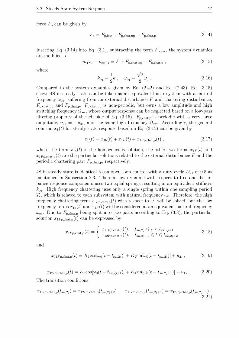
3.3. Steady State System Response 47

force Fp can be given by

Fp = Fp,low + Fp,chat,np + Fp,chat,p . (3.14)

Inserting Eq. (3.14) into Eq. (3.1), subtracting the term Fp,low, the system dynamicsare modified to

m1x1 + keqx1 = F + Fp,chat,np + Fp,chat,p , (3.15)

where

keq =1

2k , ωeq =

√2

2ω0 . (3.16)

Compared to the system dynamics given by Eq. (2.42) and Eq. (2.43), Eq. (3.15)shows 4S in steady state can be taken as an equivalent linear system with a naturalfrequency ωeq, suffering from an external disturbance F and chattering disturbance,Fp,chat,np and Fp,chat,p. Fp,chat,np is non-periodic, but owns a low amplitude and highswitching frequency Ωsw, whose output response can be neglected based on a low-passfiltering property of the left side of Eq. (3.15). Fp,chat,p is periodic with a very largeamplitude, u1s = −u2s, and the same high frequency Ωsw. Accordingly, the generalsolution x1(t) for steady state response based on Eq. (3.15) can be given by

x1(t) = x1h(t) + x1F (t) + x1Fp,chat,p(t) , (3.17)

where the term x1h(t) is the homogeneous solution, the other two terms x1F (t) andx1Fp,chat,p(t) are the particular solutions related to the external disturbance F and theperiodic chattering part Fp,chat,p, respectively.

4S in steady state is identical to an open loop control with a duty cycle Dk1 of 0.5 asmentioned in Subsection 2.3. Therein, low dynamic with respect to free and distur-bance response components uses two equal springs resulting in an equivalent stiffnesskeq. High frequency chattering uses only a single spring within one sampling periodTs, which is related to each subsystem with natural frequency ω0. Therefore, the highfrequency chattering term x1Fp,chat,p(t) with respect to ω0 will be solved, but the lowfrequency terms x1h(t) and x1F (t) will be considered at an equivalent natural frequencyωeq. Due to Fp,chat,p being split into two parts according to Eq. (3.8), the particularsolution x1Fp,chat,p(t) can be expressed by

x1Fp,chat,p(t) =

x11Fp,chat,p(t), tsw,2j 6 t < tsw,2j+1

x12Fp,chat,p(t), tsw,2j+1 6 t 6 tsw,2j+2, (3.18)

and

x11Fp,chat,p(t) = K1cos[ω0(t− tsw,2j)] +K2sin[ω0(t− tsw,2j)] + u2s , (3.19)

x12Fp,chat,p(t) = K3cos[ω0(t− tsw,2j+1)] +K4sin[ω0(t− tsw,2j+1)] + u1s . (3.20)

The transition conditions

x11Fp,chat,p(tsw,2j) = x12Fp,chat,p(tsw,2j+2) , x11Fp,chat,p(tsw,2j+1) = x12Fp,chat,p(tsw,2j+1) ,(3.21)


x11Fp,chat,p(tsw,2j) = x12Fp,chat,p(tsw,2j+2) , x11Fp,chat,p(tsw,2j+1) = x12Fp,chat,p(tsw,2j+1) ,(3.22)

must be satisfied at the time instants tsw,2j, tsw,2j+1 and tsw,2j+2 due to a periodiccharacteristic of the chattering. Here the subscript “11” stands for the time spant ∈ [tsw,2j, tsw,2j+1] and “12” for the time span t ∈ [tsw,2j+1, tsw,2j+2]. According toEqs. (3.18)-(3.22), the coefficients K1, K2, K3, K4 are derived as

K1 = u1s = −K3 , K2 =sin(ω0Ts)

1 + cos(ω0Ts)u1s = −K4 . (3.23)

The homogeneous solution x1h(t) is given by

x1h(t) = K1hcos(ωeq(t− tsw,2j)) +K2hsin(ωeq(t− tsw,2j)) , (3.24)

and the term x1F (t) by

x1F (t) = K1F sin(ηdω0(t− tsw,2j)) , K1F =2F

k(1− 2η2d). (3.25)

Finally, inserting Eqs. (3.18), (3.24) and (3.25) into Eq. (3.17) results in the lumpedformulation for x1(t),

x1(t) = K1hcos(ωeq(t− tsw,2j)) +K2hsin(ωeq(t− tsw,2j)) +K1F sin(ηdω0(t− tsw,2j))+ x1Fp,chat,p(t− tsw,2j) ,

(3.26)where tsw,2j 6 t < tsw,2j+2. For the sake of simple formulation, here it is assumed thattsw,2j = 0, the system goes into steady state. Given are the conditions,

x1(0) = x10 , x1(0) = x10 , x2(0) = x20 , tsw,2j = 0 , (3.27)

so the general solution x1(t) can be determined and the coefficients K1h, K2h are cal-culated as

K1h = x10 , K2h =x10

ωeq

− ω0ηdωeq

K1F −ω0

ωeq

K2 . (3.28)

Finally, the steady state system response is obtained. How to determine u1s, or inother words, seek a vibration energy limit, will be discussed in the next section.

3.4. Necessary Conditions for Vibration EnergyHarvesting Limit

The spring forces become very large with the increase of the stored potential energy asshown in Fig. 2.11. Each spring can only accelerate the payload m1 in one direction,which leads to a unidirectional change of the payload velocity during each sampleperiod Ts. So the sign of the velocity x1, as an example, can change in every sample

3.4. Necessary Conditions for Vibration Energy Harvesting Limit 49

period due to large spring force as shown in Fig. 3.4, where

x1(tsw,2j) > 0 , x1(tsw,2j+1) < 0 , x1(tsw,2j+2) > 0 . (3.29)

Here tsw,2j, tsw,2j+1, and tsw,2j+2 are three adjacent switching time instants with atime internal Ts, namely, T1,j = tsw,2j+1 − tsw,2j = Ts, T2,j = tsw,2j+2 − tsw,2j+1 = Ts

and Tsw,j = 2Ts. In order to find necessary conditions for the velocity components

t... ...0

x1

tsw,2j

T

T2, jT1, j

tsw,2j+1

tsw,2j+2

=Ts =Ts

=2Tssw, j

Figure 3.4.: Representation for the velocity response in one switching period Tsw,j.

due to chattering, free vibration and forced vibration to fulfil the inequality condi-tions Eq. (3.29), the approximative time solution x1(t) from Eq. (3.26) is inserted intoEq. (3.29). Evaluating the three inequality conditions leads to one common inequalitycondition

ω0K2 > ωeq

√K2

1h +K22h + ηdω0|K1F | . (3.30)

Substituting the expressions in Eq. (3.30) by their corresponding amplitudes of velocitycomponents in terms of chattering response ˆx1Fp, free response ˆx1h and disturbanceresponse ˆx1F

ˆx1Fp = ω0K2 , ˆx1h = ωeq

√K2

1h +K22h ,

ˆx1F = ηdω0|K1F | ,

finally results in the necessary conditions for the velocity amplitude of each vibrationcomponent

ˆx1Fp > ˆx1h + ˆx1F . (3.31)

It is concluded that if the chattering amplitude ˆx1Fp produced by the process force Fp

is larger than the sum of the other two parts, the system goes into steady state andwill not harvest vibration energy any more. Out of the inequality (3.30) also necessaryconditions for the system process parameters to obtain steady-state vibrations follow.Substituting the integration constants K1,K2, K3, K4, K1h+,K1h in the inequality(3.30) gives the inequality condition for the initial spring deformations u1s and u1s or


the vibration energy harvesting limit

u1s = −u2s >

1 + cos

(2π

ηs

)sin

(2π

ηs

) (x2

10

4ω0x10

+x10

2ω0

+ηdF

k(η2d − 1)

), (3.32)

where ωep =√

2/2ω0 according to Eq. (3.16). It is obvious when the deformationsof the two springs are larger than a critical value, 4S allows a complete switchingduring 2Ts as depicted in Fig. 3.4 and goes into steady state response. Based on thefundamental inequality principle, Eq. (3.32) can be rewritten as

u1s = −u2s >

1 + cos(2π

ηs

)

sin(2π

ηs

)

(ωeq

ω0

|x10|+ηdF

k(η2d − 1)

). (3.33)

If a zero initial condition is taken into consideration, x1(0) = 0 and x1(0) = 0,Eq. (3.33) will be further rewritten as

u1s = −u2s >

1 + cos(2π

ηs

)

sin(2π

ηs

)

ηd

η2d − 1

F

k. (3.34)

It can be deduced, that the pre-deformation of the springs depend on the static defor-

mation due to the external disturbance Fk

as well as on the dimensionless excitationfrequency ηd and sampling frequency ηs.

3.5. Numerical Analysis for Vibration EnergyHarvesting Limit

In order to validate the above conclusion, the analytical solution for steady state vi-brations according to Eq. (3.26) and the numerical simulation for 4S in the closedloop control with the velocity zero-crossing switching law Eq. 2.42 and Eq. 2.43 un-der several groups of different initial conditions according to Eqs. (3.32)-(3.34) areinvestigated.

3.5.1. Nonzero Initial Conditions

First, nonzero initial conditions, x1(0) 6= 0 and x1(0) 6= 0, are considered. The sim-ulation parameters are listed in Table 3.1, and the initial conditions as expressed inEq. (3.27), x1(0) = x10 = 0.2 m, x1(0) = x10 = 0.35 m/s, are used here as an ex-ample. Based on Eq. (3.32) the critical deformations of two springs are obtained,u1critical ≈ −u2critical = 96.951 m. Here x2(0), namely, u2s, takes four values of -50, -90,-96.951 and -150, which represent different stored potential energy levels. The results

3.5. Numerical Analysis for Vibration Energy Harvesting Limit 51

are depicted in Fig. 3.5. Green line denotes the numerical simulation results in closed

−0.5

0

0.5

(a)

x1(m

)

−0.5

0

0.5

(b)

0 5 10 15 20 25−0.5

0

0.5

t (s)(c)

x1(m

)

0 5 10 15 20 25−0.5

0

0.5

t (s)(d)

Figure 3.5.: System response for different deformations of two springs, u2critical =−96.951 m, x1(0) = 0.2 m and x1(0) = 0.35 m/s. (a) x2(0) = u2s =−50 m; (b) x2(0) = u2s = −90 m; (c) x2(0) = u2s = −96.951 m; (d)x2(0) = us = −150 m. (Green: simulation in closed loop control; Red:analytical solution in open loop control)

loop control, and red line stands for the analytical solution, where 4S switches withinevery sampling period Ts.

Fig. 3.5(a)-(d) show that the analytical steady-state solution always oscillates like apassive system. This phenomena has been mentioned in Subsection 2.3. But thesystem response in closed loop control shows an obvious difference under differentstored potential energies, denoted by u2s. Fig. 3.5(a) shows that when the springdeformation quantity |u2s| < |u2critical|, that is to say, not enough potential energy isstored in the springs, 4S continues responding to the switching law and harvestingvibration energy. As a result, the system chatters around the initial position x1(0).With an increase in the spring deformation u2s, more potential energy is stored in thesystem and it shows a larger amplitude oscillation as illustrated in Fig. 3.5(b). FromFig. 3.5(c)-(d) it is clear to see that if the spring deformation quantity |u2s)| ≥ |u2critical|,namely, enough potential energy is stored in the system, these two system responsecurves match quite well. This means that the system does not harvest vibration energyany longer and acts like an open loop control system and oscillates finally. Thus, itis concluded that vibration energy harvesting limit may occur in the proposed systemgoverned by the switching law according to Eq. (2.38).

3.5.2. Zero Initial Conditions

Apart from nonzero initial conditions, zero initial conditions are also considered here,x1(0) = 0 and x1(0) = 0. According to Eq. (3.34), when the energy harvesting limitoccurs, |u2critical| = 32.1524. Similarly, both the simulation analysis in closed loopcontrol and the analytical solution are executed and the results are shown in Fig. 3.6.


The other parameters are listed in Table 3.1. Like what happens under nonzero initialconditions, when |u2s| ≥ 32.1524, 4S does not harvest kinetic energy any more andoscillates similar to an open loop control system as depicted in Fig. 3.6(c) and (d).Differing from the nonzero initial condition case with a critical limit of |u2critical| =96.951, the free response term disappears in the zero initial condition case, having acritical limit of |u2critical| = 32.1524 as shown in Fig. 3.6(c), according to Eq. (3.26)and Eq. (3.28). 4S oscillates based on the superposition of the disturbance responseand chattering response terms.

−0.1

0

0.1

(a)

x1(m

)

−0.1

0

0.1

(b)

0 5 10 15 20 25−0.1

0

0.1

t (s)(c)

x1(m

)

0 5 10 15 20 25−0.1

0

0.1

t (s)(d)

Figure 3.6.: System response for different deformations of springs, u2critical =−32.1524 m, x1(0) = 0 and x1(0) = 0. (a) x2(0) = u2s = −10 m;(b) x2(0) = u2s = −25 m; (c) x2(0) = u2s = −32.1524 m; (d)x2(0) = u2s = −50 m. (Green: simulation in closed loop control; Red:analytical solution)

3.5.3. Extended Time Numerical Simulation

As shown in Fig. 3.5 and Fig. 3.6, there must exist a vibration energy harvesting limit insystem response. When the system has stored the maximum potential energy, denotedby u2critical, it will go into steady state response. In order to show the entire vibrationenergy harvesting process, from zero to the maximum, the numerical simulation isexecuted for a long time. The model parameters are listed in Table 3.1 and the resultsare depicted in Fig. 3.7. The left side zoomed-in subfigure pairs [(b), (d), (f), (h)]show the free and disturbance response terms, where t ∈ [t0, t0 + 20]. In order tofurther show the chattering response, the right side subfigure pairs [(c), (e), (g), (i)]are drawn at t ∈ [t0 + 10, t0 + 10.05], where t0 = 106 s.

From Fig. 3.7(a) it is obvious that the system harvests the maximum potential energyat t ≈ 9.2× 105 s and then goes into steady state. Afterwards, the displacement of thepayload, x1 and the deformations of two springs, u1 and u2 remain at an equilibrium-like position. Note that this is not a strict equilibrium but chattering around anequilibrium position. As mentioned before, the steady state response consists of a free

3.5. Numerical Analysis for Vibration Energy Harvesting Limit 53

response term with the frequency ωeq, a disturbance response term with the frequencyΩ as depicted in subfigure pairs [(b), (d), (f), (h)], and a chattering response termwith the frequency Ωsw in subfigure pairs [(c), (e), (g), (i)]. When 4S goes into steadystate, a large enough potential energy stored in two springs makes the chatteringvelocity amplitude larger than the sum of the free and disturbance response accordingto Eq. (3.30) and Eq. (3.31). As a result, the sign of velocity will change withinevery sampling period Ts as shown in Fig. 3.7(i). Fig. 3.7(h) shows that similar to thedisplacement response, the velocity of payload x1 also varies periodically.

When the system goes into steady state, the switching law allows 4S to behave like anopen loop controlled system with the duty cycle Dk1 = 0.5 as mentioned in Section 2.3.If Dk1 = 0.5, the entire system can be seen as a passive system with two identicalsprings in serial with each other, where the displacement of payload, x1 is the sum ofthe deformations of two springs, u1 and u2. Meanwhile, the amplitude of the formeris two times that of the latter. The equivalent natural period of the system, markedby Teq in Fig. 3.7(f), is equal to 8.8871 s, which agrees with Eq. (2.35).


0 2 4 6 8 10 12−100

0

100x

1,

u1,

u2

(m)

(a)

70

70.1

70.2

(m)

(b)

70.158

70.16

70.162

(c)

−70.2

−70.1

−70

u2

(m)

(d)

−69.99

−69.988

−69.986

(e)

−0.2

0

0.2

x1

(m)

(f)

0.17

0.175

(g)

−0.5

0

0.5

(m/s

)

(h)t (s)

−0.5

0

0.5

(i)t (s)

( 10 )5

x1

u1

u2

t0+5 t0+10 t0+15 t0+20t0

t0+5 t0+10 t0+15 t0+20t0

t0+5 t0+10 t0+15 t0+20t0

t0+5 t0+10 t0+15 t0+20t0

t0+10 t0+10.02 t0+10.04

t0+10 t0+10.02 t0+10.04

t0+10 t0+10.02 t0+10.04

t0+10 t0+10.02 t0+10.04

u1

x 1

Ts

t0 = 106

Teq

S=[0 1] S=[1 0]

Figure 3.7.: System response for a long time, here t0 = 106 s. (a) Lumped systemresponse for a long time; (b), (d), (f) and (h): Zoomed-in pictures att0 = 106 s marked by dot dash line in (a); (c), (e), (g) and (i): Zoomed-inpictures at t0 + 10 s marked by dot dash line in (b), (d), (f) and (h),respectively.

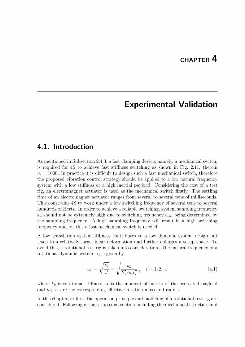
CHAPTER 4

Experimental Validation

4.1. Introduction

As mentioned in Subsection 2.4.3, a fast clamping device, namely, a mechanical switch,is required for 4S to achieve fast stiffness switching as shown in Fig. 2.11, thereinηs = 1000. In practice it is difficult to design such a fast mechanical switch, thereforethe proposed vibration control strategy should be applied to a low natural frequencysystem with a low stiffness or a high inertial payload. Considering the cost of a testrig, an electromagnet actuator is used as the mechanical switch firstly. The settlingtime of an electromagnet actuator ranges from several to several tens of milliseconds.This constrains 4S to work under a low switching frequency of several tens to severalhundreds of Hertz. In order to achieve a reliable switching, system sampling frequencyωs should not be extremely high due to switching frequency ωsw being determined bythe sampling frequency. A high sampling frequency will result in a high switchingfrequency and for this a fast mechanical switch is needed.

A low translation system stiffness contributes to a low dynamic system design butleads to a relatively large linear deformation and further enlarges a setup space. Toavoid this, a rotational test rig is taken into consideration. The natural frequency of arotational dynamic system ω0 is given by

ω0 =

√kθJ

=

√kθ∑mir2

i

, i = 1, 2, ... (4.1)

where kθ is rotational stiffness, J is the moment of inertia of the protected payloadand mi, ri are the corresponding effective rotation mass and radius.

In this chapter, at first, the operation principle and modeling of a rotational test rig areconsidered. Following is the setup construction including the mechanical structure and

56 4. Experimental Validation

electronic part. After that the experiment investigating vibration energy harvestingand vibration reduction performance is carried out.

4.2. Operation Principle and Modeling of Setup

4.2.1. Operation Principle

A compact rotational setup is introduced as shown in Fig. 4.1, where the model inFig. 4.1(a) is added to aid in understanding the rotational setup. Considering the twosprings to be not equal in reality due to a manufacturing error, different stiffness k1

and k2 are used here.

M

DC motor

Coupling

Primary plate

Armature -shaft

Electromagnet -plate 1

Spiral spring 1

Bearing 1

Sensor 2

Sensor 1

Spiral spring 2

Electromagnet -plate 2

Bearing 2

Bearing 3Base

s1

s2

k1

k2

m1

x1,

x2

F

x1

(a) (b)

Connection point

Air gap Bidirectional Electromagnetic Switch

Figure 4.1.: Schematic for 4S setup. (a) Translation model of 4S; (b) Schematic forrotational test rig.

The setup consists of two spiral springs, a primary plate, an armature-shaft, threebearing blocks, two electromagnet-plates and a DC motor. The electromagnet-platehere refers to a circular plate with eight built-magnet cores attached. These eight mag-net cores are distributed evenly in the circumferential direction to produce an evenlydistributed friction force on the armature when they are attracted to the armature.There exist two rotation blocks in the system, the first one is composed of the DC mo-tors rotor, coupling and primary plate, and the second one is the armature-shaft. An

4.2. Operation Principle and Modeling of Setup 57

armature-shaft consists of one armature and one rotation shaft, which are connectedtogether. The armature-shaft and two electromagnet-plates constitute a bidirectionalclamping device, which works as two mechanical switches, in other words, two electro-magnetic switches or one bidirectional electromagnetic switch as marked in Fig. 4.1(b).One end of two spiral springs is fixed on the armature-shaft and the other ends arefixed on the primary plate and the base, respectively.

For a rotation case, the moment of inertia of the system, determined by both of themass and geometry of a rotation block according to Eq. (4.1), plays an important roleon system dynamics. The connection point mass, marked in Fig. 4.1(a), is theoreticallyneglected as mentioned in Subsection 2.2.3. Therefore, in order to satisfy the abovementioned massless condition, two design aspects must be considered. One is that themoment of inertia of the armature-shaft should be as low as possible and the otheris the moment of inertia of the primary plate as high as possible. With the aim ofincreasing the moment of inertia of the primary plate, not only its mass but also itsgeometry variables might be taken into consideration according to Eq. (4.1).

Whether or not two springs are active depends on the attraction between the armature-shaft and two electromagnet-plates. The operation principle can be described as fol-lows. When electromagnet-plate 2 is powered on, the electromagnetic force allowsthe connection of the armature-shaft to the base, namely, s2 is closed as shown inFig. 4.1(a). As a result, spiral spring 2, namely, k2 is blocked and spiral spring 1, k1 isactive and the non-energized electromagnet-plate 1 would follow the primary plate androtate together. Spiral spring 1, k1 would be extended and harvests kinetic energy aspotential energy stored in spring 1 according to the switching law in Eq. (2.38). Whenthe switching between two stiffness states occurs, electromagnet-plate 2 is powered offand electromagnet-plate 1 powered on. The electromagnetic force would connect thearmature-shaft to the primary plate. Consequently, the primary plate, electromagnet-plate 1 and armature-shaft are combined together and driven by the DC motor, namely,s1 is closed and s2 is open as shown in Fig. 4.1(a). At this time phase, spiral spring1, k1 is blocked and spiral spring 2, k2 is active, compressed and would harvest kineticenergy.

4.2.2. Modeling

The lumped model of the rotational setup is depicted in Fig. 4.2(a) with Fig. 4.2(b)being the corresponding translational model. The previously mentioned system refersto a translational model, where the connection point is assumed to be massless. Herea rotational setup is designed. The connection point, namely, the armature-shaft hasmassm2 or moment of inertia, J2, but it is still neglected initially in order to match withthe aforementioned theory analysis. Of course, the moment of inertia of the primaryplate J1 being much larger than J2 makes this more reasonable. The electromagneticforce friction-based clamping device is still simplified to be an ideal switch as denotedby s1 and s2. System damping including viscous damping and Coulomb damping isconsidered. The system dynamics can be expressed as follows. The deformations oftwo spiral springs u1 and u2 can be given by

u1 := θ1 − θ2 , u2 := θ2 , (4.2)


d1

d2

k

J1

s1

s2

θ1

Md

Mfc1

Mfc2

J2

θ2s1k1

m1

F

d M1 fc1

s2k2 d M2 fc2

m2

x1

x2

(a) (b)

θ1

k θ2

ᵟ12

ᵟ12

Figure 4.2.: Simplified model of the 4S setup. (a) Partly simplified rotation model withdamping; (b) Simplified translation model with damping.

where θ1 and θ2 are the rotation angles of the primary plate and the armature-shaft,respectively. Accordingly, the two spiral springs torques Mk1, Mk2 are given by

Mk1 = kθ1u1 , Mk2 = kθ2u2 . (4.3)

The frictional moment Mf includes viscous damping Mfv such as air damping, andCoulomb damping Mfc around a bearing and a sensor. Mf1 can be expressed by

Mf1 = Mfv1 +Mfc1 , Mfv1 = d1(θ1 − θ2) , (4.4)

and Mf2 is given byMf2 = Mfv2 +Mfc2 , Mfv2 = d1θ2 , (4.5)

here Mfc1 and Mfc2 are complicated to formulate and not given. These damping canbe further confirmed in experiments.

When S = [1, 0], electromagnet-plate 1 is powered off and electromagnet-plate 2powered on. The armature-shaft is connected to the base. As a result, spiral spring 2is blocked and spring 1 is active. Similar to the translation model in Subsection 2.2.3,the motion equation of the system will be given by

J1θ1 = Md −Mk1 −Mf1 , θ2 = θ2(tsw,i) , (4.6)

where tsw,i is the ith switching time instant as expressed in Subsection 2.2.3. Md isthe external disturbance torque produced by a DC motor, similar to the disturbanceF depicted in Fig. 4.2(b).

In the case S = [0, 1], where spiral spring 1 is not active but spiral spring 2 active,

4.2. Operation Principle and Modeling of Setup 59

the system dynamics can be given by

J1θ1 = Md −Mk2 −Mf2 , θ2 = θ1 − [θ1(tsw,i)− θ2(tsw,i)] . (4.7)

In order to achieve a pure stiffness system as mentioned in the theory analysis, thefrictional torque Mf should be as low as possible. Similar to the theory model accordingto Eq. (2.15)-Eq. (2.16), a compact formulation for the rotational model can be givenby

J1θ1 + kθθ1 = Md +Mp(S) (4.8)

and

θ2(S) =

θ2(tsw,i) if S(t) = [1, 0]

θ1 − [θ1(tsw,i)− θ2(tsw,i)] if S(t) = [0, 1], (4.9)

and the process torque Mp(S) is given by

Mp(S) =

kθu2 if S(t) = [1, 0]kθu1 if S(t) = [0, 1]

, (4.10)

where kθ1 = kθ2 = kθ and the damping is not considered. Considering the difference oftwo springs and the moment of inertia of armature-shaft J2, the natural frequencies oftwo undamped subsystems, denoted by J1-kθ1 and (J1 + J2)-kθ1 here, differ from theaforementioned one according to Eq. (2.21) and can be given by

ω01 =

√kθ1J1

and ω02 =

√kθ2

J1 + J2

. (4.11)

If J1 J2 and kθ1 ≈ kθ2 are set in design, ω01 ≈ ω02, which agrees with the men-tioned theory model. The attraction and releasing between the electromagnet-plateand armature-shaft creates the switching between two stiffness states. During thisprocess, the armature-shaft moves between two electromagnet-plates in the verticaldirection with an air gap of δ as shown in Fig. 4.2(a), where the armature lies in themiddle of air gap. The linear motion equation of armature in the vertical direction canbe given by

m2δ = Fem , (4.12)

where m2 is the mass of armature and Fem is an electromagnetic force. As such, theneeded motion time tmotion of the proposed mechanical switch can be written as

tmotion =

√2δm2

Fem

. (4.13)

In order to obtain a realizable switching between two stiffness states and reduce theeffect of a switching delay governed by tmotion on the system response, the switchingtime tmotion should be as low as possible, namely,

tmotion Ts . (4.14)

where Ts is the sampling period. To achieve a reliable clamping, the stored potentialenergy, namely, spiral spring torques Mk1 and Mk2 should satisfy with the following


inequality,(Mk1 +Mk2) < Mc . (4.15)

where Mc is defined as the clamping torque or frictional torque produced by the me-chanical switch. It is obvious to see that the stored potential energy denoted by Mk1

and Mk2 must be always lower than an external provided energy partly representedby Mc. If the above condition holds, the spiral spring can be blocked. The clampingtorque Mc can be expressed by

Mc = Femrem , (4.16)

where rem is an effective distance between electromagnet force Fem acting point androtation shaft. The simulation analysis is executed in Matlab/Simulink, where themotion time of the armature-shaft tmotion is not considered initially to simplify thesimulation analysis.

4.3. Setup Construction

4.3.1. Mechanical Structure

For 4S, as a switching system, a mechanical switch is important and would directlydetermine the system performance. As such, the design of a mechanical switch will beexplained in detail in the following subsection.

Mechanical switch unit

The electromagnetic switch is a kind of friction-based clamping device based on anelectromagnetic actuator. Through the attraction and releasing between the armature-shaft and electromagnet-plate, the connection or disconnection of two spiral springsto or from the primary plate can be realized. With the aim of a reliable attrac-tion, the electromagnetic torque should be not only large enough but also evenlydistributed in circumferential direction on the surface of armature. As a result, aring-arranged electromagnet-plate and a hollow armature structure are proposed asshown in Fig. 4.3(a). Eight U-magnets are evenly arranged in an aluminium housingand share one coil to reduce space. Magnetic cores are chosen to be the stacking struc-ture consisting of metal sheets in order to reduce the intensity of eddy current lossesand keep a high flux carrying capacity. The provided static electromagnetic force Fem

can be given by

Fem =B2Aem

2µ0

· n , (4.17)

where Aem is the working area of an electromagnet and n is the number of electromag-nets, here n = 8. µ0 is the vacuum permeability and B is magnetic flux density andcan be given by

B =Θµ0

2δ, Θ = Ni , (4.18)

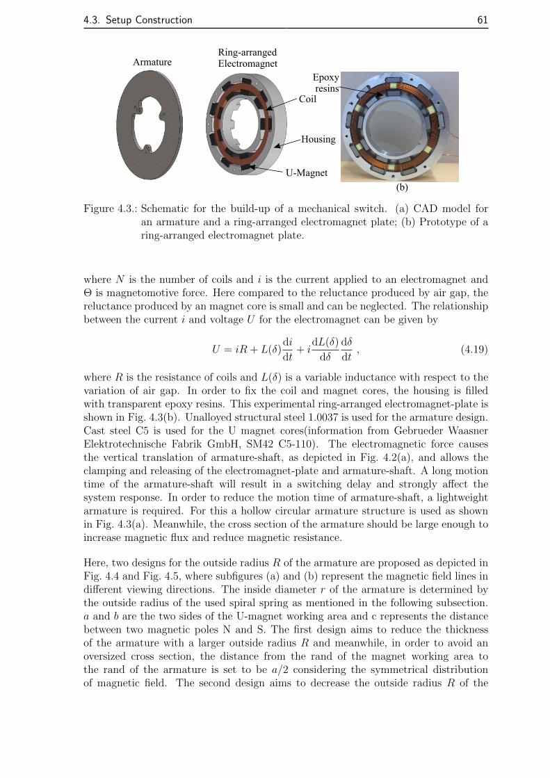
4.3. Setup Construction 61

Coil

U-Magnet

Housing

ArmatureRing-arranged Electromagnet

Epoxy resins

(b)

Figure 4.3.: Schematic for the build-up of a mechanical switch. (a) CAD model foran armature and a ring-arranged electromagnet plate; (b) Prototype of aring-arranged electromagnet plate.

where N is the number of coils and i is the current applied to an electromagnet andΘ is magnetomotive force. Here compared to the reluctance produced by air gap, thereluctance produced by an magnet core is small and can be neglected. The relationshipbetween the current i and voltage U for the electromagnet can be given by

U = iR + L(δ)di

dt+ i

dL(δ)

dδ

dδ

dt, (4.19)

where R is the resistance of coils and L(δ) is a variable inductance with respect to thevariation of air gap. In order to fix the coil and magnet cores, the housing is filledwith transparent epoxy resins. This experimental ring-arranged electromagnet-plate isshown in Fig. 4.3(b). Unalloyed structural steel 1.0037 is used for the armature design.Cast steel C5 is used for the U magnet cores(information from Gebrueder WaasnerElektrotechnische Fabrik GmbH, SM42 C5-110). The electromagnetic force causesthe vertical translation of armature-shaft, as depicted in Fig. 4.2(a), and allows theclamping and releasing of the electromagnet-plate and armature-shaft. A long motiontime of the armature-shaft will result in a switching delay and strongly affect thesystem response. In order to reduce the motion time of armature-shaft, a lightweightarmature is required. For this a hollow circular armature structure is used as shownin Fig. 4.3(a). Meanwhile, the cross section of the armature should be large enough toincrease magnetic flux and reduce magnetic resistance.

Here, two designs for the outside radius R of the armature are proposed as depicted inFig. 4.4 and Fig. 4.5, where subfigures (a) and (b) represent the magnetic field lines indifferent viewing directions. The inside diameter r of the armature is determined bythe outside radius of the used spiral spring as mentioned in the following subsection.a and b are the two sides of the U-magnet working area and c represents the distancebetween two magnetic poles N and S. The first design aims to reduce the thicknessof the armature with a larger outside radius R and meanwhile, in order to avoid anoversized cross section, the distance from the rand of the magnet working area tothe rand of the armature is set to be a/2 considering the symmetrical distributionof magnetic field. The second design aims to decrease the outside radius R of the


N S

ab

N

S

d1min

(b)(a) r

R

a/2

a/2

c

Figure 4.4.: Schematic for the magnetic field lines distribution for the first design.

armature as much as possible. The distance from the rand of the magnet working areato the rand of the armature is nearly zero. The minimum thickness of armature d1min

in Fig. 4.4 and d2min in Fig. 4.5 according to Eq. (B.3) can be given by

d1min ≈ab

2(a+ b), and d2min ≈

ab

a+ 2b, (4.20)

Although d1min is smaller than d2min, it is proven that the armature volume for thefirst design is larger than the second one according to Eq. (B.9). Therefore, the seconddesign is taken.

NS

a

bN

S

d2min

(b)(a)

c

r

R

Figure 4.5.: Schematic for the magnetic field lines distribution for the second design.

Because the armature, not the armature-shaft, moves axially in the working air gapbetween the two electromagnet-plates, a reasonably low axial stiffness of the armatureis able to avoid the reduction of effective normal electromagnetic force acting on thearmature. At the same time, the armature should also be stiff enough to transmitcircumferential torque from the primary plate to rotation shaft, here a triangle springis designed as depicted in Fig. 4.6. Fig. 4.6(a) is the experimental triangle spring andFig. 4.6(b) shows the stress analysis when the maximum axial deformation, equalingto the maximal working air gap between two electromagnet-plates, δ = 1 mm, isapplied to the triangular spring. Except the stress concentration, the design can beaccepted in experiment. A corresponding axial deformation force Fd produced by an


0 0.5 1

x 10-3

0

20

40

60

δ (m)

F(N

)

(a) (b) (c)

7.1917e8Max

6.3926e8

5.5935e8

4.7945e8

3.9954e8

3.1963e8

2.3972e7

1.5982e7

1.9517

d

(Pa)

Figure 4.6.: Schematic for the triangle spring. (a) Experimental triangle spring; (b)Stress analysis for the triangular spring structure; (c) Relationship betweenthe force and the axial deformation as denoted by the working air gap ofelectromagnet δ.

axial deformation of the triangle spring is larger than 45 N as shown in Fig. 4.6(c),which shows the nonlinear relationship between the axial deformation force Fd and theaxial deformation. In fact, the applied working air gap in experiment is about 0.6 mm.This means Fd ≈ 15 N. According to Eq. (4.13), the motion time tmotion of armaturefrom one electromagnet plate to the other can be approximately modified to

tmotion =

√2δm2

Fem − Fd

. (4.21)

Here m2 = 0.33 kg, δ = 0.6 mm and Fem = 35 N according to Eq. (4.17), so the motiontime tmotion of the armature from one electromagnet to the other is 4.5 ms. As a result,the sampling time Ts of the controller should be larger than 4.5 ms. Fig. 4.7 shows theconstruction of the armature-shaft. The armature and triangle spring are connected

Armature

Triangle spring

Rotation shaft

Sleeves

Bolt

Figure 4.7.: Build up of the armature-shaft.

through three bolts and then can be fixed on a rotation shaft through the squeezingof sleeves.


Spring unit

A spiral spring (Gebr. Schmidt Federnspezialfabrik GmbH) is used for potential energystorage on the rotational test rig. The rotational stiffness kθ is given by

kθ =Ebt3

12l, l = πn(Ro +Ri) , (4.22)

where E is the elastic modulus of the spiral spring material; b, t and l are the width,thickness and length of a spiral spring, respectively; Ro and Ri are the outside andinside radius of the spiral spring. The maximum acceptable torque Mkmax can beexpressed by

Mkmax =σbt2

6, (4.23)

where σ is the yield strength of the spiral springs material. As such, the potentialenergy harvesting level of the rotational setup should be lower than Mkmax. The abovespiral spring design principle is from the company. The fixture of a real spiral springis shown in Fig. 4.8, where one end of the spiral spring is fixed on the circular plateby a bolt and the other is inserted into the groove of a sleeve.

Spiralspring

Bolt

Groove

Electromagnet -plate

Figure 4.8.: Fixture of a spiral spring in an electromagnet-plate.

Lumped mechanical setup

The lumped mechanical setup is shown in Fig. 4.9. In order to see the internal structureof 4S, marked by a blue rectangular frame in the upper subfigure, a CAD cross-sectionalview is shown in the lower subfigure. To avoid the spiral spring coils falling off andcontacting the wall of electromagnet-plate due to gravity, the setup is hung verticallyfixed on an aluminum frame. Considering the massless connection point in the theoryanalysis, the moment of inertia of the armature-shaft should be much lower than thatof the primary plate. Thus, an auxiliary rotation block is fixed to the primary plate.After that, the ratio of the moment of inertia of the primary state to that of the


armature-shaft is 15.37. As a result, the moment of inertia of the armature-shaft canbe neglected in modeling.

Sensor and electric drive

Two incremental rotary encoders are used for the angular positioning of the primaryplate and armature-shaft. One is from Hohner Elektrotechnik GmbH, PR90-11C1C-C, and has a resolution of 16384 pulse per turn. The other is from Dr. JohannesHeidenhain GmbH, ROD 426.000B, and owns a resolution of 10000 pulses per turn.According to the aforementioned switching law Eq. (2.38), an accurate switching be-tween two stiffness states requires an accurate real-time acquisition of the angularposition of the primary plate. Therefore, the former is used for the primary plate andthe latter for the armature-shaft. The moment of inertia of the rotary encoders rotorsare 30 (g · cm2) and 26 (g · cm2), respectively. They can be neglected when comparedto the primary plate. The starting torque of two sensors rotors, seen as frictionaltorque, is lower than 0.01 Nm. The two sensors are connected to the output shaft ofa DC motor and the armature-shaft by means of two couplings, respectively.

A graphite brushed DC motor from Maxon Motor GmbH, DCX32L, with the advantageof high reliability, simple control and low cost, is used for the production of an externaldisturbance acting on the primary plate.

4.3.2. Power Electronics

Current control scheme for electromagnet

The current control for electromagnet is schematically shown in Fig. 4.10. In order toreduce electric power loss and overheating, a switching power circuit, Motor ControlShield with BTN8982TA for Arduino(Infineon Company), is applied. It mainly consistsof a H bridge circuit. A hysteresis controller is used to reduce the chattering frequencyresulting from a switching power electronic. The reference current iem, ref , governingthe power on-off states of two electromagnets, is controlled by the switching law. Thehigh-low signal level from the hysteresis controller determines the positive and negativecircuit of H Bridge. As such, a switching voltage is exerted on an electromagnet.

Current control for DC motor

A specified disturbance torque is needed for the validation of vibration reduction per-formance and vibration energy harvesting of the proposed vibration control system.Therefore, the disturbance torque should be accurately provided and controlled. Con-sidering the difficulty and the cost of direct torque control for a DC motor and thelinear relationship between the current in the motor and the output torque, a currentcontrol scheme for the DC motor is applied here. First, the governing equations todescribe the system dynamics of a DC motor are given by

Md = Ktim , (4.24)


Sensor 1

Coupling

DC Motor

Base

Armature-shaft

Auxiliary rotation block

Sensor 2

Aluminium frame

Bearing block 1

Bearing 2

Electromagnet-plate 1

Primary plate


Bearing 3

Spiral spring 1

Spiral spring 2

Primary plate

Armature-shaft

Base



BidirectionalElectromagnetic Switch Air gap

4S

Figure 4.9.: Lumped mechanical setup.


i-

EM iem, ref H Bridge

em

e

Hysteresis Controller

Source: Infineon Company

u1

0

Figure 4.10.: The current control for electromagnet.

and

Ldimdt

+Rim +Keθ1 = U , (4.25)

where Md is the output torque of the DC motor, namely, the disturbance torque asmentioned in Eq. (4.6) and Eq. (4.7). R, L, Kt, Ke are the moment of inertia of themotors rotor, electric resistance, electric inductance, torque constant, and electromo-tive force constant, respectively. In order to obtain the needed torque, a current PIcontrol for the DC motor is applied as shown in Fig. 4.11, where im,ref is the demandcurrent of the DC motor and decided by the reference disturbance torque Md, ref . HereMotor Model 1, marked in Fig. 4.11 is 1/Kt according to Eq. (4.24). Meanwhile, amodel-based voltage feed forward control is added to speed up system response and de-crease the steady state error as well. Due to the angular velocity of the primary plate,θ1 being very low, Motor Model 2 only consists of the electric resistance R accordingto Eq. (4.25).

i-

DC Motor

PI Controller

m

+

MotorModel 2

Amplifier u Uieim, ref

Md, ref MotorModel 1

Figure 4.11.: Current control for the used DC motor.


4.3.3. Lumped System

The lumped system consists of a Mechanical Unit, Velocity Zero-crossing DecisionUnit, Current Control for DC Motor Unit, and Current Control for ElectromagnetUnit, as shown in Fig. 4.12. A specified disturbance torque Md is exerted on themechanical unit, which responds accordingly to the proposed velocity zero-crossingswitching law. Depending on the state variable θ1 feedback control information, theswitching control vector S will govern the power on-off state of two electromagnets.This allows the bidirectional electromagnetic switch, as shown in Fig. 4.9, to connector disconnect two spiral springs to the primary plate. By means of such a system,vibration reduction performance and vibration energy harvesting can be realized.

<0

Mechanical Unit

Sampling

Switching

,(S=[0 1]

S=[1 0] k

J1

d1

d2

s1

s2

θ1

J2

θ2θ1

k θ2

12

ᵟ12

i-

iem1, ref H Bridge

em1

e1


ul

0

ᵟ

ᵟ

i-

iem2, ref

H Bridge

em2

e2


u ᵟ

EM1

l

0

Unit

Unit

θ1 θ1

,θ2 θ2)

Velocity Zero-crossing Decision Unit

θ1 θ1z

i-

DC Motor

im, ref PI Controller

m

+

MotorModel 2

Amplifier u Ue Md

Md, ref MotorModel 1

EM2

Current Control for Electromagnet Unit

Current Control for DC Motor Unit

Figure 4.12.: Schematic for the lumped controlled rotational test rig.

4.4. Experiment

In this section, the experiments to validate the vibration energy harvesting and vi-bration reduction performance of the proposed system are executed using the designparameters listed in Table. 4.1. The rotational stiffness of two spiral springs, kθ1 and kθ2are considered to be equal based on the data sheet from the company (Gebr. SchmidtFedernspezialfabrik GmbH). In fact, these two springs are not the same, as will be for-mulated in the following subsection. The maximum torque for one spiral spring Mkmax

can be calculated according to Eq. (4.23). This will limit the maximum rotation an-gle of the primary plate. The maximum clamping torque Mc represents the working

4.4. Experiment 69

ability of the bidirectional electromagnetic switch and determines the vibration energyharvesting level. The maximum vibration energy harvesting level should be lower thanhalf of Mc in order to obtain a reliable attraction between the electromagnet-plate andarmature-shaft according to Eq. (4.15). The frictional torque of the bearings, Mb isprovided by SKF, 2200 ETN9 and the maximum disturbance torque produced by aDC motor is also provided by Maxon Motor GmbH, DCX32L. According to Eq. (2.38),

Table 4.1.: System Design Parameters.

Name Symbol Value UnitMoment of inertia of the primary plate J1 0.121 kg ·m2

Moment of inertia of the armature-shaft J2 0.008 kg ·m2

Stiffness of spiral spring kθ 0.12 Nm/radFrictional torque of bearing Mb 0.008 NmMax. torque of spiral spring Mkmax 0.677 Nm

Max. clamping torque Mc 1.85 NmMax. disturbance torque Mdmax 0.1 Nm

Dimensionless frequency of the disturbance ηd variable -Dimensionless sampling frequency ηs variable -

the switching law for the rotational test rig can be given by

S(t) =

[1, 0] if θ1z ≥ 0

[0, 1] if θ1z < 0, (4.26)

and

k(t) =

kθ1 if θ1z ≥ 0

kθ2 if θ1z < 0, (4.27)

with the use of the zero-order-hold function of angular velocity Eq. (4.28)

θ1z(θ1, Ts) =∞∑n=0

θ1(nTs)[σ(t− nTs)− σ(t− (n+ 1)Ts)] , n ∈ N , (4.28)

orθ1z(t, Ts) = θ1(nTs) , n ∈ N , nTs ≤ t < (n+ 1)Ts , (4.29)

where Ts is the sampling period of the controller, and σ(t) is the unit step function. Inorder to determine the sampling period Ts, the natural frequency ω0 of each subsystemshould be determined according to Eq. (2.51). This switching law will be tested. Inthe following sections system parameter identification is initially executed.

4.4.1. System Parameter Identification

The current control for a DC motor is tested and as an example, a desired harmonicdisturbance torque,

Md(t) = Ktim sin(Ωt) = Md sin(Ωt) . (4.30)


is applied as shown in Fig 4.13, where Kt is the torque constant of the DC motor,Kt = 0.0585 Nm/A and the current of the motor im is measured. Here the DC motoris connected to the primary plate and they rotate together. It is not difficult to seethat the current controller allows the real-time current to track the reference currentwell and this can be further used for other experiments.

0 0.5 1 1.5-1

-0.5

0

0.5

1

t (s)

i m(A

)

Real-time current

Reference current

Figure 4.13.: Example for the current control of the DC motor.

In order to determine the natural frequency of each subsystem ω0, according to Eq. (2.21)and further set the sampling frequency ωs of the controller accurately, the system pa-rameters such as system stiffness and damping are first identified. In fact, two subsys-tems in experimental analysis, denoted by J1-kθ1 and (J1 + J2)-kθ2, are not the sameas in the theory analysis, m1-k, due to two stiffness being equal, k1 = k2 = k, andthe connection point mass m2 being neglected. Considering there might exist viscousdamping such as air damping and Coulomb friction torque around the bearings andsensors, the hysteresis relationship between the driving torque Md and the rotationangle θ1 of the primary plate is investigated. The results are shown by red points inFig. 4.14(a) and Fig. 4.15(a), where three cycles of rotation for the primary plate ineach figure are carried out. Here i = 1.5 A, Ω = 0.11 rad/s, in order to reach a quasistatic state measurement.

Fig. 4.14(a) shows the results, when spring 1 is active. In this case only the primaryplate rotates and the system moment of inertia is J1. To solve system stiffness, twosets of data, denoted by blue and cyan points, standing for two different rotationdirections, are used for linear regression. The regression lines are denoted by blacklines are shown and demonstrate the linear relationship between the driving torque,namely, the disturbance torque Md as mentioned in Subsection 4.2.2, and the rotationangle θ1. As shown in Fig. 4.14(a), the upper and lower fitting lines are expressed by

Md = 0.1513θ1 + 0.0109 , and Md = 0.1489θ1 − 0.0065. (4.31)

As such, the mean value of the stiffness kθ1 according to Eq. (4.31) is taken as(0.1513+0.1489)/2 ≈ 0.15 Nm/rad and the Coulomb friction torque Mfcl, as mentionedin Subsection 4.2.2, is (0.0109−(−0.0065))/2 = 0.0087 Nm. In order to obtain the vis-cous damping d1 of the subsystem J1-kθ1, a numerical simulation considering Coulombfriction and viscous damping is executed in MATLAB/Simulink and the results areshown in Fig. 4.14(b), where the system responds under non-zero initial conditions.

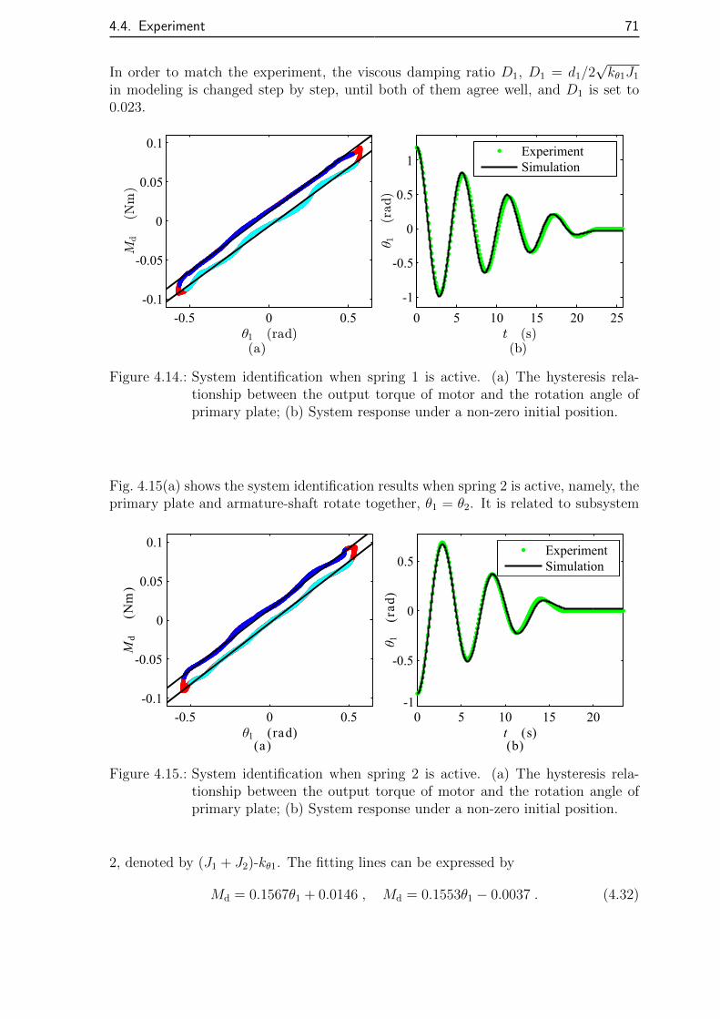
4.4. Experiment 71

In order to match the experiment, the viscous damping ratio D1, D1 = d1/2√kθ1J1

in modeling is changed step by step, until both of them agree well, and D1 is set to0.023.

-0.5 0 0.5

-0.1

-0.05

0

0.05

0.1

θ1 (rad)(a)

Md

(Nm)

0 5 10 15 20 25

-1

-0.5

0

0.5

1

t (s)(b)

θ 1(rad)

ExperimentSimulation

Figure 4.14.: System identification when spring 1 is active. (a) The hysteresis rela-tionship between the output torque of motor and the rotation angle ofprimary plate; (b) System response under a non-zero initial position.

Fig. 4.15(a) shows the system identification results when spring 2 is active, namely, theprimary plate and armature-shaft rotate together, θ1 = θ2. It is related to subsystem

-0.5 0 0.5

-0.1

-0.05

0

0.05

0.1

θ1 (rad)(a)

Md

(Nm

)

0 5 10 15 20

-0.5

0

0.5

t (s)(b)

θ 1(r

ad

)

ExperimentSimulation

-1

Figure 4.15.: System identification when spring 2 is active. (a) The hysteresis rela-tionship between the output torque of motor and the rotation angle ofprimary plate; (b) System response under a non-zero initial position.

2, denoted by (J1 + J2)-kθ1. The fitting lines can be expressed by

Md = 0.1567θ1 + 0.0146 , Md = 0.1553θ1 − 0.0037 . (4.32)


Similar to the analysis for subsystem 1, the mean value of the stiffness kθ2 is takenas 0.156 Nm/rad and the Coulomb friction torque is set to 0.0092 Nm. The nu-merical analysis is also finished and the fitting viscous damping ratio D2, D2 =d2/2

√kθ2(J1 + J2), equals to 0.02.

The system parameter identification is summarized in Table. 4.2. Here Tdsim is thenatural period of the damped subsystems, J1-kθ1-d1 and (J1 +J2)-kθ2-d2, for the simu-lation analysis and Tdexp for the experiment as shown in Fig. 4.14(b) and Fig. 4.15(b).Here the stiffness of two springs slightly differ from the theoretical calculation resultslisted in Table 4.1. The error between the simulation and experimental damped naturalperiod, Tdsim and Tdexp, is low and the system identification parameters can be furtherapplied for other experiment analysis. The sampling period Ts or sampling frequencyωs of the controller can be determined, according to

ωs = ηsω0 , (4.33)

where ηs is set to 100 in experiment, not 1000 as in the theoretical analysis, consider-ing the switching delay td of a mechanical switch. The natural frequency ω01 of theundamped subsystem 1, J1-kθ1, is equal to 1.113 rad/s according to Eq. (4.11). Assuch, the sampling frequency ωs is set be 111.3 rad/s and the sampling time Ts isapproximately equal to 56.45 ms.

Table 4.2.: System Identification Results.

System kθ(Nm/rad) D Mfc(Nm) Tdsim(s) Tdexp(s) Error(%)Subsystem 1 0.15 0.023 0.0087 5.7 5.624 1.34Subsystem 2 0.156 0.02 0.0092 5.57 5.699 2.32

0 20 40 60

0

0.4

0.8

1

t (ms)

i em

(A)

0 20 40 60

t (ms)

iem1

iem2 iem1

iem2

td 21≈ td 24≈

(a) (b)

ms ms

Figure 4.16.: Switching time with respect to current of two electromagnets, iem. (a)Electromagnet 1 is powered on and electromagnet 2 is powered off; (b)Electromagnet 1 is powered off and electromagnet 2 is powered on.

In order to evaluate switching time of a mechanical switch, the current applied tothe two electromagnets is measured as depicted in Fig. 4.16 and a correspondinglycontrolled supply voltage measurement is shown in B.2. Subfigure (a) shows that at

4.4. Experiment 73

beginning the current iem1 of electromagnet 1, denoted by red line, increases slowly dueto coils inductance and then goes into an oscillation state responding to the currentcontrol strategy as depicted in Fig. 4.10, which is a property of a switching powerelectronics and the mean value of the oscillating current is close to a reference currentof 1 A. After an oscillation duration the current iem1 falls off because motion of ar-mature will change the electromotive force, which results in a current decrease untilthe armature and electromagnet are tightly attracted together according to Eq.( 4.19).Therefore, the time span as chosen by two dot-dashed lines can be taken as switch-ing time of the mechanical switch. From subfigure(a) and (b), the switching time oftwo mechanical switches, or in other words, switching delay td is 21 ms and 24 ms,respectively. It is obviously larger than the motion time of armature tmotion, whichdoes not consider the settling time of electronics and the effect of eddy current in anelectromagnet. Of course, this is lower than the chosen sampling time 56.45 ms. Thisis beneficial for an accurate stiffness switching. It means that 4S is able to achieve astiffness switching in one sampling period and further experiments can be executed.

4.4.2. Step Response

In this section, the velocity zero-crossing switching law, according to Eq. (4.27), wouldbe experimentally validated.

First, the step response of the experimental setup is executed. Considering the nominaloutput torque of the used DC motor, a step torque, Md = 0.0585 Nm, namely, im =1 A, is applied as shown in Fig. 4.17. The sampling frequency ηs is initially setto be 100 and the other experiment parameters are shown in Table 4.1. Here thestatic deflection is defined as Md/kθ = 0.0585/0.15 = 0.39 rad. The experiment andsimulation results are shown in Fig. 4.18. Note, that before the step torque is exertedon 4S, the system has begun to switch. Because at beginning θ1 = 0, the switching lawEq. (2.38) leads to the attraction between electromagnet-plate 2 and base. This willresult in a slight shaking of the primary plate and therefore an extremely low amplitudechattering occurs in system. Thus, the initial position and velocity, θ1(0), θ1(0) andθ2(0), θ2(0), can only be approximately equal to zero. This will be slightly adjustedin the simulation model to match the experiment.

0 10 20 28-0.7

0

1

1.7

t (s)

i m(A

)

Figure 4.17.: The step torque exerted on 4S test rig.


Neither like a passive undamped SDOF system nor a passive underdamped one, 4Sperforms without overshoot and oscillation, but the angular displacement of the pri-mary plate θ1 always increases with the deformation of spring 2 denoted by u2. Thedeformation of spring 2 is positive, u2 > 0, differing from the desired working prin-ciple, in which spring 2 should be compressed, u2 < 0. This is because the externaldisturbance Md is positive and large enough such that the primary plate always movesin the positive direction, even if working in the stiffness 2 state. Due to viscous damp-ing and Coulomb damping existing in 4S, the deformation of spring 1, u1 does notreach the maximum deformation of 2Md/kθ1 like a passive undamped SDOF system.Considering the experimental errors, the results can be reasonably accepted.

In order to avoid the risk of 4S failing due a long time operation, the experiment isnot carried out for a long time, but the simulation is executed as depicted in Fig. 4.19.Fig. 4.19(b) shows detail from Fig. 4.19(a), marked by the orange rectangular frameat t = 100 s. It is obvious to see that the primary plate always rotates in a positive

0 10 20 28

0

0.2

0.4

0.6

0.8

t (s)

Dis

pla

cem

ent

(ra

d)

Experiment: u1

Simulation: u1

Experiment: 1

Simulation: 1

Experiment: u2

Simulation: u2

θθ

Static deflection

Switching happens

Figure 4.18.: Step response of 4S: Md = 0.0585 Nm, ηd = 0 and ηs = 100.

direction denoted by the increasing angular position θ1. It starts to rotate in subsystem1, J1-kθ1-d1 and then reaches a peak level quickly at half of a damped natural period,Td/2. Afterwards, due to the deformation of spring 2, u2, being extremely low as shownin Fig. 4.18, and a large constant positive disturbance torque Md, as denoted by themotors current im in Fig. 4.17, the angular velocity of the primary plate θ1 at thisswitching time instant, where the primary plate moves in stiffness 1 state, is so largethat the deformation of spring 1 still increases. This will last until t ≈ 35 s, wherethe deformation of spring 1, u1, reaches a maximum, as marked by pink dashed line inFig. 4.19(b). Meanwhile, the disturbance torque also results in the increase of u2. Theincreasing u2 causes the velocity and kinetic energy of the primary plate to decreaseat the above mentioned switching time instant. Consequently, the released quantity ofstored potential energy in spring 1 will be larger than the harvested quantity of kineticenergy in the following stiffness 1 state. But in spring 2 the harvested kinetic energyis larger than the released potential energy. Finally, u1 starts to decrease and u2 stillincreases after t ≈ 35 s. This continues until steady stat is reached: the kinetic energyat each switching time instant, from stiffness state 1 to 2 or vice versa, are equal,and the energy dissipation due to the system damping can be compensated through

4.4. Experiment 75

the work of the constant disturbance torque acting on the primary plate. Thus, thepotential energy in each spring hardly changes and θ1 stays around an equilibrium-likeposition. Of course, due to the stiffness of two springs not being equal, kθ1 6= kθ2, aslisted in Table 4.2, the final deformations of two springs are not the same, u1 6= u2.

0 50 100

0

0.2

0.4

0.6

0.8

t (s)(a)

Dis

plac

emen

t(r

ad)

0 100 1000 2000 3000

0

0.2

0.4

0.6

0.8

t (s)(b)

Simulation: u1

Simulation:Simulation: u2

1θ

Td / 2

Switching happens

35

Static deflection

Figure 4.19.: Simulation for step response of 4S. (a) Lumped long time simulation; (b)Partly zoomed-in picture for (a).

4.4.3. Harmonic Response

The proposed vibration control system shows vibration energy harvesting and vibra-tion reduction performance under a harmonic disturbance in the above mentionedtheory in chapter 2. Here a harmonic disturbance torque according to Eq. (4.30) isexerted on the primary plate, corresponding to F in Fig. 4.1(a). The experiment andsimulation results are shown in Fig. 4.20, where the vertical axis stands for differentdisplacements including the position of the primary plate θ1, the deformation of spring1, u1 and the deformation of spring 2, u2, and the horizontal axis for the time history.Here the static deflection is defined as Md/kθ = 0.05/0.15 = 0.33 rad. It is clear tosee that the deformations of the two springs increase positively and negatively. Thismeans that potential energy is stored into two springs. The experiment and simulationmatch well in the beginning but a slight difference occurs with the increase of time.This is reasonable, because some switching decision errors due to the delay of the elec-tromagnetic switch, as denoted by tset, occur in experiment. This would enlarge thesystem response difference. What’s more, the primary plate stays around a non-zeroequilibrium-like position, because the system lacks a position feedback control and onlythe velocity is considered according to Eq. (2.38).

Different disturbances

In order to test how an external disturbance affects the system response, differentdisturbance frequencies, ηd and disturbance amplitudes, Md are set, and the resulting


0 20 40 60 80

-0.5

0

0.5

t (s)

Dis

plac

emen

t(r

ad)

Experiment: u1

Simulation: u1

Experiment:Simulation:Experiment: u2

Simulation: u2

1θ1θStatic deflection

Figure 4.20.: System response under a harmonic excitation: Md = 0.05 Nm, ηd = 3and ηs = 100.

experiment and simulation results are shown in Fig. 4.21 - Fig. 4.24.

Fig. 4.21 show the experiment results for the system response under different dis-turbance frequencies. Here the static deflection is defined as Md/kθ = 0.05/0.15 =0.33 rad. It is obvious to see that 4S is able to harvest kinetic energy and show vi-bration reduction performance under different disturbance frequencies. However, thesystem response under a lower frequency disturbance, ηd < 1, shows a high oscillationamplitude, because a lower frequency disturbance would dominate the fundamental fre-quency term of system response. A higher frequency disturbance, ηd > 1, enables morefrequent switching and results in a much smoother system response profile. Meanwhile,a higher frequency disturbance leads to a lower deformation of two springs, namely,a lower stored potential energy. This can be explained on the basis of the low-passfiltering property of second-order system.

-0.6

-0.3

0

0.3

0.6

-0.6

-0.3

0

0.3

0.6

10 20 30t (s)(a)

10 20 30t (s)(b)

0

u1,u

2(r

ad)

1(r

ad)

θ

0

dη = 0.5dη = 1.5

dη = 5dη = 10

u1

u2

Static deflection

Figure 4.21.: Experimental results of the system response under different harmonicdisturbance frequencies ηd: Md = 0.05 Nm and ηs = 100.

4.4. Experiment 77

The simulation results are depicted in Fig. 4.22 and match well with the experimen-tal results. For the angular displacement of the primary plate θ1, there exists littledifference owing to the stiffness variation in experiment.

0

0.3

0.6

-0.6

-0.3

0

0.3

0.6u

1,u

2(r

ad)

-0.6

-0.3

10 20 30t (s)(a)

10 20 30t (s)(b)

0 0

u1

u2

1(r

ad)

θ

dη = 0.5dη = 1.5

dη = 5dη = 10

Static deflection

Figure 4.22.: Simulation of the system response under different harmonic disturbancefrequencies ηd: Md = 0.05 Nm and ηs = 100.

Fig. 4.23 shows the experimental results for the system response under different dis-turbance amplitudes. Obviously, the vibration energy harvesting increases with thedisturbance torque amplitude Md as depicted in Fig. 4.23(a), because the mechanicalpower of the disturbance torque to 4S increases, but the primary plate always keepsa similar equilibrium-like position under different disturbance amplitudes as shown inFig. 4.23(b). Note that there exists a large difference between experiment and sim-

0 10 20 30-1

-0.5

0

0.5

1

t (s)(a)

0 10 20 30-1

-0.5

0

0.5

1

t (s)(b)

= 0.02

u1,u

2(r

ad)

1(r

ad)

M= 0.05M= 0.08M= 0.1M

θ

u1

u2

Figure 4.23.: Experimental results for the system response under different harmonicdisturbance amplitudes Md: ηs = 100 and ηd = 5.

ulation results, when Md = 0.1. Because when the deformations of two springs arelarge, the outside of spiral springs unavoidably touches the wall of the housing as


shown in Fig. 4.8. This changes the stiffness of one spiral spring and further affectsthe deformation of the two springs and the angular displacement of the primary plate.

0 10 20 30-1

-0.5

0

0.5

1

0 10 20 30-1

-0.5

0

0.5

1

t (s)(a)

t (s)(b)

u1,u

2(r

ad)

1(r

ad)

θ

= 0.02M= 0.05M= 0.08M= 0.1M

u1

u2

Figure 4.24.: Simulation results for the system response under different harmonic dis-turbance amplitudes Md: ηs = 100 and ηd = 5.

Different sampling frequencies

As mentioned before, the sampling frequency ωs affects the switching decision errorbetween two springs as depicted in Fig. 2.7 and further affects the system response.Thus, different sampling frequencies are applied here. The experiment and simulationresults are shown in Fig. 4.25 and Fig. 4.26. It clearly shows that an extremely low

-0.5

-0.25

0

0.25

0.5

-0.5

-0.25

0

0.25

0.5sη = 10sη = 40

sη = 80sη = 100sη = 120

0 10 20 30t (s)(a)

0 10 20 30t (s)(b)

u1,u

2(r

ad)

1(r

ad)

θ

u1

u2

Figure 4.25.: Experimental results for the system response under different samplingfrequencies ηs: Md = 0.05 and ηd = 5.

sampling frequency, ηs = 10, lowers the energy harvesting level and results in a larger

4.4. Experiment 79

amplitude oscillation as well, because low sampling frequency increases the switchingdecision error and the disturbance torque Md will dominate system response. With theincrease of the sampling frequency, the stored potential energy increases. When thesampling frequency is large enough, the switching decision error is much lower, namely,the angular velocity of the primary plate would always stay close to zero. This resultsin a low mechanical power of the disturbance torque Md to the system. The storedpotential energy increases slowly with the sampling frequency. Meanwhile, the systemresponse shows up a low amplitude oscillation around an equilibrium-like positionunder a high sampling frequency as shown in Fig. 4.25(b), because the forced vibrationdisappear under a high sampling frequency, for example, ηs = 120. Additionally, theexperiment and simulation match well.

u1

u2

-0.5

-0.25

0

0.25

0.5

-0.5

-0.25

0

0.25

0.5

0 10 20 30 0 10 20 30t (s)(a)

t (s)(b)

1(r

ad)

θ

u1,u

2(r

ad)

sη = 10

sη = 40

sη = 80sη = 100sη = 120

Figure 4.26.: Simulation results for the system response under different sampling fre-quencies ηs: Md = 0.05 and ηd = 5.

CHAPTER 5

Improved Switching Law for 4S

5.1. Introduction

Harmonic excitation as an external disturbance is tested on 4S in the aforementionedchapters and 4S shows vibration energy harvesting and vibration reduction perfor-mance based on the velocity zero-crossing switching law. Apart from a harmonicdisturbance, nonzero initial velocity, in other words, a shock excitation can be alsoseen to be an external disturbance. How 4S responds to a nonzero initial velocitydisturbance will be discussed in this chapter.

Based on the variable structure characteristic of 4S and phase plane, a new switchinglaw is introduced to accelerate the transformation of initial vibration energy into po-tential energy between two springs and improve the vibration reduction performance.This switching law is numerically and experimentally verified. What’s more, due tothe introduction of position feedback in this switching law, 4S can reach a betterequilibrium-like position even under a harmonic excitation.

5.2. Nonzero Initial Velocity Problem for 4S

Vibration control as understood here is to reduce the vibration produced by a nonzeroinitial velocity as shown in Fig. 5.1(a). In order to state the problem and make thecomparison between the simulation analysis and the following experiment, the initialconditions in experiment are applied to the simulation analysis in advance. Meanwhile,several model parameters are also modified to agree with the aforementioned theoryanalysis. Here the stiffness of two spiral springs are seen to be the same, namely, kθ1 =kθ2 = kθ = 0.15 Nm/rad. Similar to a massless connection point in the translationalmodel, the moment of inertia of the armature-shaft, J2, is neglected. The damping,

82 5. Improved Switching Law for 4S

Table 5.1.: Simulation parameters for nonzero initial velocity problem analysis.


Md 0 Nm ηd 0 - θ1(0) -1.75 rad/sJ1 0.121 kg ·m2 ηs 100 - θ2(0) 0 rad

kθ 0.15 Nm/rad θ1(0) 0 rad θ2(0) 0 rad/s

including viscous damping Mfv and Coulomb damping Mfc are also initially neglected.The other simulation parameters are listed in Table 5.1 and the results are shown inFig. 5.1(b).

0 50 100 150 200-2

-1

0

1

2

t (s)

Dis

pla

cem

ent

(ra

d)

Simulation: u1

Simulation: 1

Simulation: u2

θ

(a)

θ1≠ 0(0)

(b)

120

k

J1

d1

d2

s1

s2

θ1

Mfc1

Mfc2

J2

θ2

θ1

k θ2

Figure 5.1.: Numerical analysis for the system response under nonzero initial velocityθ1(0) = −1.75 rad/s, here ηs = 100. (a) Simplified rotational model; (b)Simulation results.

A nonzero initial velocity condition means that the system has a certain amount ofkinetic energy T at the initial time instant. Due to a negative angular velocity ofthe primary plate at the initial time instant, according to the velocity zero-crossingswitching law Eq. (4.27), spiral spring 2, kθ2, is active initially and reaches negativemaximum quickly, u2, as denoted by the red line in Fig. 5.1(b). Afterwards, thedeformation of spring 1, u1 increases and the deformation of spring 2, u2 decreases,until the system goes into a steady state and the initial kinetic energy is transformedinto potential energy equally stored into two spiral springs. Due to sampling frequencyηs not being large enough, here ηs = 100, unlike that in the previously mentionedtheory analysis, ηs = 1000, a large amplitude oscillation happens in steady state. Thisphenomena has been explained in Subsection 4.4.3. The increasing deformations of thetwo springs represent that 4S are still able to harvest vibration energy and transformthe initial kinetic energy into potential energy stored in two springs. Although the

5.3. Variable Structure System Control for 4S 83

velocity zero-crossing switching law allows 4S to reduce vibration and remain at anequilibrium-like position, this needs a long settling time, here t ≈ 120 s as markedby the pink dotted line. How to reduce the settling time will be discussed in thischapter.

5.3. Variable Structure System Control for 4S

A variable structure system (VSS) consists of a group of continuous subsystems and asuitable switching law. These subsystems will be in an active mode or not, dependenton the switching law. A distinguishing feature of VSS control is its ability to resultin a very robust control system. An asymptotically variable structure system can becomposed of two non-asymptotically stable subsystems, see [125, 126]. In fact, 4Swith a velocity zero-crossing switching law is a variable structure system consisting oftwo continuous subsystems, m1-k1 and m1-k2 in a translational model or J1-kθ1 andJ1 + J2-kθ2 in a rotational model, together with a switching surface s = x1 = 0 ors = θ1 = 0. The process force Fp or torque Mp works as a control input u and can bemodified to

Fp(Mp) = u =

u+ = Fp1(Mp1) = ku2 if s = x1(θ1) ≥ 0

u− = Fp2(Mp2) = ku1 if s = x1(θ1) < 0. (5.1)

Note, that u is a control input and u1, u2 are the deformations of the two springs. Howto combine variable structure control and vibration reduction for 4S will be discussedin the following sections.

5.3.1. State Trajectory Analysis

Variable structure system dynamics is generally analyzed by means of phase plane.In order to further study the system response of 4S with the velocity zero-crossingswitching law, the phase portrait with respect to the displacement θ1 and the velocityθ1 of the primary plate is shown in Fig. 5.2. Based on the quantitative behavior thestate trajectory is divided into four phases, Initial Condition A; Phase B, in which thevelocity of the primary plate decreases from maximum to a near-zero value; Phase C,transient chattering state and Phase D, steady chattering state. The state trajectoryinitially moves from the initial condition A and moves into phase B according tothe velocity zero-switching law and then reaches the switching surface s = θ1 = 0.Afterwards, the state trajectory will move below and above the switching surface inthe transient chattering state, Phase C and finally goes into steady chattering state,Phase D.

As mentioned in the last chapter, 4S is split into two subsystems: Subsystem 1, J1-kθ1and Subsystem 2, (J1 + J2)-kθ2. Here the armature-shaft J2 and system damping areneglected for a simplified analysis. As a result, the two subsystems are conservativesystems and energy balance holds in them. The energy balance in the two subsystems


-1.5 -1 -0.5 0.5

-1.5

-1

-0.5

0

0.5

1

( )

(rad/s)

1(0) = -1.751(0) = 0

θθ

1θ

θrad

A

B

C D

Z1Z2

s=θ1=0

Figure 5.2.: State trajectory representation for nonzero initial velocity excitation.

can be expressed as

J1-kθ1 : θ21 + ω0θ

21 = θ2

1(tsw,i) + ω0u21(tsw,i) (5.2)

andJ1-kθ2 : θ2

1 + ω0θ21 = θ2

1(tsw,i+1) + ω0u22(tsw,i+1) , (5.3)

where ω0 =√kθ/J1 and tsw,i, tsw,i+1 are two adjacent switching time instants. The

right sides of Eq. (5.2) and Eq. (5.3), consisting of initial kinetic energy terms θ21(tsw,i),

θ21(tsw,i+1) and potential energy terms ω0u

21(tsw,i), ω0u

21(tsw,i+1) at each switching time

instant tsw,i and tsw,i+1, will govern the phase portrait in the upcoming active subsys-tem. In order to show the state trajectory in detail, the transient chattering state,Phase C and the steady chattering state, Phase D are enlarged, marked by Z1 and Z2

in Fig 5.2. First, the transient chattering state trajectory is drawn in Fig. 5.3.

The state trajectory starts from Initial Condition A with a negative velocity θ1(0) andmoves in Subsystem 2, Phase B, according to the velocity zero-crossing switching law.When the primary plate reaches the maximum negative position, namely, the switchingsurface s = θ1 = 0, it will be accelerated in the reverse direction. As a result, the statetrajectory moves above the switching surface and goes into Subsystem 1 as marked inFig. 5.3. Afterwards, the state trajectory stays in the transient chattering state, PhaseC. In this time phase, because the deformation of spring 2, u2 is much larger than thatof spring 1, u1, the transition velocity, θ1(tsw,i+1), when the state trajectory moves intoSubsystem 1, is larger than that, when the state trajectory moves into Subsystem 2.As a result, u2 decreases and u1 increases, namely, potential energy in subsystem 2decreases and potential energy in subsystem 1 increases. Thus, the radii of subsystem2 trajectories (red lines) decrease and the radii of subsystem 1 trajectories (blue lines)increase as shown by the state trajectory numbers 1, 2, 3. This phenomena will lastfor the time instant, where u1 and u2 are equal, u1 = u1s, u2 = u2s, u1s = u2s, namely,the initial energy is equally divided and stored in the two springs and then 4S goes into


......

0

u1

Subsystem 2

Subsystem 1

1 2 3

1 2 3

s=

0

θ1

θ1

=θ1-θ2

θ1

B

C

=0

Figure 5.3.: State trajectory representation for transient chattering state.

steady chattering state, Phase D. u1s and u2s mean the deformations of two springsin steady chattering state, u1s = u2s. In steady chattering state, 4S will switch itsstiffness state every sampling period Ts as shown in the zoomed-in picture in Fig. 5.4.In Subsection 2.4.1 a translational model was introduced with a velocity zero-crossing

0

Subsystem 1

Subsystem 2

...... u1=u1max=u1s

θ1

θ1

D

s=θ1=0

Figure 5.4.: State trajectory representation for steady chattering state.

switching law, see Eq. (2.36)-Eq. (2.37). An equivalent rotational model was presentedin Subsection 4.2.2.

J1θ1 + kθθ1 = Md +Mp(S) (5.4)

with

θ2(S) =

θ2(tsw,i) if S(t) = [1, 0]

θ1 − [θ1(tsw,i)− θ2(tsw,i)] if S(t) = [0, 1](5.5)


and process torque Mp(S)

Mp(S) =

kθu2 if S = [1, 0]kθu1 if S = [0, 1]

, u1 = θ1 − θ2 , u2 = θ2 . (5.6)

Here, it is assumed that only initial disturbances act on the system, no external forces,namely, Md = 0. The velocity zero-crossing switching law to switch between the twoprocess torques Mp1 and Mp2 is

Mp(t) =

Mp1 = kθu2 if s = θ1 ≥ 0

Mp2 = kθu1 if s = θ1 < 0. (5.7)

Considering the sliding mode control stated in Appendix C.1, the switching conditions = θ1 corresponds to a switching surface s. Next, it is shown that this is indeed asliding surface. To do so, it must be shown that s s < 0 holds for all states (θ1, θ1, θ2).It must be distinguished between two cases, either states above the switching surfaces > 0 and those below it, s < 0. In case of s = θ1 > 0 the necessary condition,s = θ1 < 0 must hold. The equation of motion reads

J1θ1 + kθθ1 = kθθ2 , and θ2 = θ2(tsw,i) (5.8)

This results inθ1 = −ω2

0 (θ1 − θ2) = −ω20 u1 . (5.9)

Because spring 1 is considered to be extended, u1 > 0 holds. This gives

θ1 = −ω20 u1 < 0 , (5.10)

and fulfills the sliding mode condition. An equivalent formulation shows that θ1 =−ω2

0 u2 > 0 for spring 2 in case of s < 0. Overall, ss < 0 is valid. Therefore, a slidingmode motion occurs in 4S with the velocity zero-crossing switching law.

It is not difficult to see that the transient chattering phase is the initial energy redis-tribution phase, since the switching system without damping can be ideally taken asa conservative system. With the aim of more intuitively describing the energy trans-formation process between two springs, their deformations are depicted in Fig. 5.5.After the first half motion cycle, Phase B, the angular velocity of the primary plate,θ1 decreases from the maximum to the minimum and the deformation of spring 2reaches a maximum, denoted by u2max. Afterwards, u2 will decrease, as denoted by(u2max−u2n), and u1 will increase step by step, as denoted by u1n, namely in Phase C,until two deformations are equal and reach u1s and u2s, respectively, in Phase D. Howto avoid a long time transient chattering phase, as marked by a red dotted frame, isof importance to reduce the settling time of the system response.

5.3.2. New Switching Surface

In order to reduce the settling time of the system response, a better switching surfaceshould be able to speed up the initial kinetic energy transformation. So a new switching


k1

k2

k1

k2 k2

k1

k2

k1

......u2max

0

u2max-u21

u11 u1s

u2s

θ1(0)(n)

u1n

u2max-u2n

A B C D

Figure 5.5.: Representation for the potential energy transformation between twosprings.

surface is put forwards = θ1 + ω0θ1 = 0 . (5.11)

As shown in Fig. 5.6, state trajectory (black line) starts from Initial Condition A and

Subsystem 1

s= +ω0

Subsystem 2

0

u1max=u1s

0

θ1 θ1

θ1

θ1

Initial Condition A

B

D

=0

u1=

Figure 5.6.: Representation for new switching surface.

then moves into Subsystem 2 trajectory (red line). When the state trajectory reachesthe switching surface s = θ1 + ω0θ1 = 0 (green line) for the first time, the potentialenergy U and the kinetic energy T are the same as expressed by

θ1 + ω0θ1 = 0 ⇒ T =1

2J1θ

21 =

1

2kθθ

21 =

1

2kθu

21 = U , (5.12)

where u1 = θ1 − θ2. Due to θ2(0) = 0, the deformation of spring 1, u1 is equal to theangular displacement of the primary plate, θ1 at this switching time instant. Accord-ingly, the above conclusion Eq. (5.12) holds. If at this time instant 4S switches intoSubsystem 1 trajectory (blue line), the remaining kinetic energy will be transformedinto potential energy and stored in Subsystem 1. This means that the new switchinglaw allows 4S to finish an equal transformation of the initial kinetic energy betweentwo springs after the first crossing of the switching surface s in Eq. (5.11), namely,u1 = u1max = u1s, u2 = u2s. Consequently, the system can go directly into steadychattering state unlike the old switching law and the transient chattering state, Phase


C as shown in Fig. 5.3, is avoided.

Whether or not a sliding mode motion occurs for the new switching surface s = θ1 +ω0θ1 = 0 will be further analyzed. Base on the necessary condition for the slidingmode control, ss < 0, the following inequalities must be satisfied

If s > 0 ∧ s < 0 ⇒ θ1 + ω0θ1 < 0 (5.13)

andIf s < 0 ∧ s > 0 ⇒ θ1 + ω0θ1 > 0 . (5.14)

With the combination of Eq. (5.7)-Eq. (5.10), it is not difficult to find that Inequali-ties (5.13) and (5.14) do not always hold for the new switching surface s = θ1 +ω0θ1 =0. For example, just after the state trajectory crosses the switching surface for the firsttime and moves into Subsystem 1 as shown in Fig. 5.6, it tends to move away frombut not towards the switching surface, although it still eventually reaches the surface.Thus, the new switching law does not always enable sliding mode motion in 4S. Finally,the new switching law can be given by

S(t) =

[1, 0] if s ≥ 0[0, 1] if s < 0

, (5.15)

where s = θ1 + ω0θ1. Similar to a lumped control system for a translational case asdepicted in Fig. 2.9, the block diagram for 4S with the new switching surface s for arotational case is shown in Fig. 5.7. where sz is discretized like x1z in the translational

<0

Mechanical Unit

Sampling Unit

Switching Unit

sz

S=[0 1]

S=[1 0]

Switching Surface

s=ω0

s

J1

θ1

θ1≠ 0(0)

k θ1

k θ2

θ2

s1

s2

J2

+θ1 θ1

θ ,1 θ1

(θ ,1 θ ,1 θ ,2 θ )2

Variable Structure Controller

Figure 5.7.: Schematic for 4S with new switching law.

model and can be given by

sz(s, Ts) =∞∑n=0

s(nTs)[σ(t− nTs)− σ(t− (n+ 1)Ts)] , n ∈ N , (5.16)

or bys(t, Ts) = s(nTs) , n ∈ N , nTs ≤ t < (n+ 1)Ts , (5.17)


so the switching law in Eq. (5.15) will be slightly modified to

S(t) =

[1, 0] if sz ≥ 0[0, 1] if sz < 0

. (5.18)

Differing from the velocity zero-crossing switching law, the two state variables θ1 and θ1

should be measured as feedback signals. They are further processed through VariableStructure Controller to produce stiffness switching signals to govern the connection ordisconnection of two spiral springs to or away from the primary plate in MechanicalUnit. In order to validate the efficiency of the new switching law, numerical analysisis executed again and the simulation parameters are listed in Table 5.1. Fig. 5.8 showsthat the new switching law largely reduces the settling time of the system responsecompared to the old law as depicted in Fig. 5.1, from t = 120 s to t = 6 s, as markedby a pink dotted line. Fig. 5.9 shows the system state trajectory for the new switching

0 10 20 30 40-2

-1

0

1

2

t (s)

Displacement

(rad)

Simulation: u1Simulation: 1

Simulation: u2

θ

6

Figure 5.8.: Simulation for 4S with new switching law under nonzero initial velocityθ1(0) = −1.75 rad/s, here ηs = 100.

law. Differing from the old switching law, the new switching law allows 4S to avoidthe transient chattering state, Phase C and to go directly into steady chattering state,Phase D as shown in Fig. 5.2.


-2 -1.5 -1 -0.5 0 0.5

-2

-1

1

2

θ1(rad)

(rad/s)s= +ω0θ1 θ1=0

θ1

Figure 5.9.: Phase plane for 4S with new switching law under nonzero initial velocityθ1(0) = −1.75 rad/s, here ηs = 100.

5.4. Experimental Verification

5.4.1. Nonzero Initial Velocity Condition

In order to further verify the new switching law, an experiment under nonzero initialvelocity conditions is carried out.

As mentioned in the theory analysis, the initial angular velocity of the primary plateθ1(0) is equal to −1.75 rad/s and the initial deformation of spring 2, u2(0), u2(0) =θ2(0) = 0. In practice, it is difficult to realize a zero initial position, here θ1(0) = 0 andθ2(0) = −0.08 rad. Because before a nonzero initial velocity disturbance is exertedon 4S, the system has begun to switch. At the beginning θ1 = 0, the switching lawEq. (5.18) leads to an attraction between electromagnet-plate 2 and the base as shownin Fig. 4.1(b). This will result in a slight shaking of the primary plate and therefore anextremely low amplitude chattering occurs in the system. Compared to a high initialkinetic energy, T = 1/2J1θ

21(0) = 0.1853 J, the initial potential energy U , as expressed

by

U =1

2kθu

21(0) , u1(0) = θ1(0)− θ2(0) , (5.19)

is equal to 4.8 × 10−4 J according to Table 5.1 and can be neglected and thereforeEq. (5.12) still holds. As shown in the system parameter identification experiment inSubsection 4.4.1, there exists system damping Mf including viscous damping, D1 =0.023 and D1 = 0.02, and Coulomb damping Mfc1 = 0.0087 Nm and Mfc2 = 0.0092 Nmin setup, but these factors are not considered in the above theory analysis. Therefore,the simulation results under an ideal nonzero initial velocity condition are shown herein order to comparably explain the damping effect on the system response. The resultsare shown in Fig. 5.10, where solid lines stand for the experimental results and square-solid lines for the simulation. Fig. 5.10(a) shows the simulation under an ideal nonzeroinitial velocity condition, which is a partly zoomed-in picture of Fig. 5.8, from t = 0 to

5.4. Experimental Verification 91

(a)

0 2 4 6 8 10 12 14

-1.5

-1

-0.5

0

0.5

1

1.5

t (s)(b)

Displacem

ent(rad)

Experiment: u1Simulation: u1Experiment: 1

Simulation: 1

Experiment: u2Simulation: u2

θ

θ

0 2 4 6 8 10 12 14

-1.5

-1

-0.5

0

0.5

1

1.5

Displacement

(rad)

Figure 5.10.: System response under nonzero initial velocity for new switching law.(a) Simulation under ideal nonzero initial velocity condition θ1(0) =−1.75 rad/s: Mf = 0, θ1(0) = 0 and θ2(0) = 0; (b) Experimental andsimulation results for system response under nonideal initial velocity con-dition θ1(0) = −1.75 rad/s: Mf 6= 0, θ1(0) = 0 and θ2(0) = −0.08 rad.


t = 14 s. Fig. 5.10(b) depicts the simulation and experiment results under a nonidealnonzero initial velocity condition. The initial velocity disturbance, θ1 6= 0, is achievedhere by suddenly pushing the primary plate. Through a preliminary calculation of theslope of an approximately linear (u2-t) curve in the beginning and further adjustmentin simulation model, the initial velocity can be obtained, θ1(0) = −1.75 rad/s. Theseinitial conditions will be eventually adjusted in the simulation model to match theexperiment. This has been also explained in the last chapter.

It is clear to see that 4S with the new switching law can finish the initial kinetic energytransformation equally between two springs in only one switching time phase and thenmoves into steady state. Compared to the no damping condition in Fig. 5.10(a), thestored potential energy in the two springs decreases slightly in experiment due to alow viscous damping and Coulomb damping. Meanwhile, the system is able to remainaround a better equilibrium-like position without fine oscillations. A nonzero initialposition, here θ2(0) = −0.08 rad produces a small difference between the angulardisplacement of the primary plate θ1 and the deformation of spring 2, u2 at beginning.Compared to the system response under the old switching law, the settling time islargely reduced as shown in Fig. 5.1(b). However, this new switching law has thedisadvantage of requiring two state variables feedback information. Additionally, theexperiment agrees with the simulation well as shown in Fig. 5.10(b). In order to show

0 500 1000 1500 2000 2500-1.5

-1

-0.5

0

0.5

1

1.5

t (s)

Displacement

(rad)

Simulation: u1Simulation: 1

Simulation: u2

θ

Figure 5.11.: Long time system response under nonideal nonzero initial velocity con-dition for new switching law at θ1(0) = −1.75 rad/s: Mf 6= 0, θ1(0) = 0and θ2(0) = −0.08 rad.

the long time system response for the new switching law and avoid the risk of the setupfailure under a long time operation, the simulation is instead executed here and theresults are shown in Fig. 5.11. Due to the system damping including viscous dampingand Coulomb damping, the potential energy stored in two springs, denoted by u1

and u2, always decreases to zero, but the primary plate always stays around a zeroequilibrium-like position, namely, θ1 ≈ 0.


5.4.2. Harmonic Excitation

The new switching law outperforms the old switching law under a nonzero initialvelocity condition as shown in Fig. 5.10. Whether or not this new switching lawworks well under a harmonic excitation will be tested here, the results are shown inFig. 5.12, where subfigure(a) is the zoomed-in picture for subfigure(b), marked by anorange frame. Note, that due to a local magnification, the experimental results arenot denoted by lines any more but discrete points as shown in subfigure(a). Here thestatic deflection is defined as Md/kθ = 0.05/0.15 = 0.39 rad. Compared to the systemresponse using the velocity zero-crossing switching law as shown in Fig. 4.20, the systemwith a new switching law benefits from the position feedback control and keeps at abetter zero equilibrium-like position, denoted by black lines θ1 in subfigure (b). Thisreduces the effect of the time delay produced by the used electromagnetic switch onthe positioning performance. In the beginning, the simulation and experiment resultsmatch well as depicted in subfigure(a). Due to the system stiffness and dampingvariation in experiment, the difference between the simulation and experiment increasesslightly with time as shown in subfigure(b). This can be reasonably accepted.

0 20 40 60 80

-0.5

0

0.5

t (s)0 5 10

-0.4

-0.2

0

0.2

0.4

t (s)

Dis

pla

cem

ent

(rad

)

Experiment: u1

Simulation: u1

Experiment: 1

Simulation: 1

Experiment: u2

Simulation: u2

θθ

(a) (b)

Static deflection

Figure 5.12.: System response for new switching law under a harmonic excitation:Md = 0.05 Nm, ηd = 3 and ηs = 100.

5.4.3. PID Feedback Controlled Switching Law

In fact, the velocity zero-crossing switching law in Section 2.4 for 4S works as thederivative control (D control) for the displacement of mass x1 with x1ref = 0 as shownin Fig. 5.13(a), and new switching law works as the combination of the proportionalcontrol (P control) and the derivative control (D control) in Fig. 5.13(b). So a com-plete PID feedback controlled switching law is further introduced here as depicted inFig. 5.13(c). Note that x1 and x1ref in a translation case correspond to θ1 and θ1ref in arotation case. As a new switching decision, PID feedback control of the error between


the reference position and the state variable, x1ref − x1, is introduced

f(x1) = Kp(x1ref − x1) +Ki

t∫0

(x1ref − x1(τ))dτ +Kdd(x1ref − x1)

dt. (5.20)

Similar to the discretized state variable x1 in Eq. (4.28) and the new switching surfaces in Eq. (5.16), f(x1) is also processed discretely and rewritten as

f(x1)z =∞∑n=0

f(x1(nTs))[σ(t− nTs)− σ(t− (n+ 1)Ts)] , n ∈ N , (5.21)

or asf(x1(t, Ts))z = f(x1(nTs)) , n ∈ N , nTs ≤ t < (n+ 1)Ts . (5.22)

As a result, the switching law for the PID controlled system is given by

S(t) =

[0, 1] if f(x1)z < 0[1, 0] if f(x1)z ≥ 0

. (5.23)

Considering both the vibration energy harvesting level and positioning demand, a setof the proportional (P), integral (I) and derivative (D) parts of PID control must bechosen carefully in practice. Unlike the PID control used in a linear system, an increasein PID coefficients of the same proportion will not influence the system response,because a zero-crossing decision is applied on the switching system. This will bedetailed investigated in future.


s1

s2

k1

k2

m1

F

<0

Mechanical Unit

Sampling Unit

Switching Unit

x ,1 (x ,1 x )2

x1

szS=[0 1]

S=[1 0]

Sliding Mode Controller

x1,

x1s=ω x +0 1

s

s1

s2

k1

k2

m1

F

<0

Mechanical Unit

Sampling Unit Switching Unit

x ,1 (x ,1 x )2x1 x1zS=[0 1]

S=[1 0]

(a)

(b)

PID Controller

PDe

(c)

PID Controller

<0

Mechanical Unit

Sampling Unit Switching Unit x1

x ,1(x ,1 x )2+-

x1ref

PID (x )1f (x )1

f zS=[0 1]

S=[1 0] s1

s2

k1

k2

m1

F

+-x1ref

PID Controller

De

+-x1ref

x1

x1

e

Figure 5.13.: Block diagram for different switching laws. (a) Velocity zero-crossingswitching law; (b) Position and velocity switching law; (c) PID feedbackcontrolled switching law.

CHAPTER 6

Shock Isolation with 4S

6.1. Introduction

Shock isolation has been always of interest in technical applications where the negativeeffects of a sudden shock excitation on the protected plants, devices or persons needto be avoided. As analyzed in Section 2.2 in a passive or a variable stiffness systemthere still exists an unavoidable potential energy releasing time phase. Consequently,a protected payload is accelerated and the settling time of system will be extended. Asfor shock isolation, this will extend the residual vibration duration after shock. Thischapter will explore the application of 4S on shock isolation and compare its behaviorto two other shock isolation systems. New insights into the shock isolation behavior ofa PID controlled 4S are concluded.

6.2. Harmonic disturbance isolation using 4S

In order to investigate the vibration isolation performance of 4S, the velocity zero-crossing switching law, according to Eq. (2.38), would be initially tested on 4S undera harmonic base disturbance in this section.

6.2.1. Modeling

For vibration isolation, a base excitation is exerted on 4S as shown in Fig. 6.1. Similarto the force excitation case as mentioned in Section 2.3, 4S has two stiffness workingstates according to the switching law in Eq. (2.36). A compact formulation for the

98 6. Shock Isolation with 4S

s1

s2

k1

k2

m1

x1

x2

x0

Figure 6.1.: Schematic of 4S under base excitation x0.

system dynamics can be expressed by

m1x1 + kx1 = Fp(x1, x2, x1, Ts) + k x0 , (6.1)

and the displacement of the connection point between two serial elements

x2 =

x2(tsw,i)− x0(tsw,i) + x0 if x1z(x1, Ts) ≥ 0x2(tsw,i)− x1(tsw,i) + x1 if x1z(x1, Ts) < 0

, (6.2)

and the process force Fp acting on the mass according to Fig. 2.8(a),

Fp(x1, x2, x1, Ts) =

k u2(tsw,i) if x1z(x1, Ts) ≥ 0k u1(tsw,i) if x1z(x1, Ts) < 0

, (6.3)

with spring deformations u1 and u2 defined by

u1 := x1 − x2 , u2 := x2 − x0 . (6.4)

A harmonic base excitation is applied as follows

x0(t) = x0 sin Ωt , (6.5)

where Ω is the excitation frequency and x0 is the excitation amplitude. The relateddimensionless parameters ηd and ηs are defined in the force excitation case accordingto Eq. (2.22) and Eq. (2.51).


In order to test vibration isolation performance of 4S, numerical analysis is initiallyexecuted in this section. Table 6.1 lists the simulation parameters and Fig. 6.2 showsthe results. As shown in Fig. 6.2(a), 4S together with the velocity zero-crossing switch-ing law can realize vibration isolation. At beginning, t ∈ [0, T0/2] s, T0/2 ≈ 3.15 s, m1

moves in a positive direction and S(0)= [1, 0], where only spring 1 is active, spring 2is blocked. This can be seen by the deep blue line, x1 > 0, and the orange line, x1 > 0,

6.3. Shock isolation for 4S 99

Table 6.1.Simulation parameters for harmonic excitation.

Name Value Unit Name Value Unit Name Value Unitx0 1 m ηd 10 - x1(0) 0 mm1 1 kg ηs 1000 - x1(0) 0 m/sk 1 N/m x2(0) 0 m

0 2 4 6 8 10

-1

-0.5

0

0.5

1

t (s)0 2 4 6 8 10

-0.3

-0.15

0

0.15

0.3

t (s)

x 0(m

/s),

u1,u2,x 1

(m)

x 1(m

)

x0x1

˙

x1u1u2

(a) (b)

3.15 3.15

Figure 6.2.: Harmonic disturbance isolation response. (a) Velocity of mass and baseexcitation; (b) Displacement of mass and deformations of two springs.

respectively. Differing from a desired elongation of spring 1, it is compressed, u1 < 0,because the base velocity is higher than that of the mass. Spring 1 oscillates with thesubsystems natural period T0 into an elongation state u1 > 0, but spring 2 remainsundeformed, u2 = 0.

After the first time of the velocity zero-crossing detection, t = T0/2 ≈ 3.15 s, the twosprings switches into 4S alternatively, where spring 1 is elongated and spring 2 com-pressed. Before the occurance of the stiffness switching, spring 1 has been elongated.Consequently, spring 2 owns a larger oscillating deformation amplitude than spring 1in the following switching process. This leads to a nonzero pseudo equilibrium positionof the mass, depicted by the orange line. Note that it is not a strict equilibrium buta chattering with a low amplitude around an equilibrium position. Additionally, thespring deformations increase and potential energy will be stored in two springs for along time, which was partly formulated in [124].

6.3. Shock isolation for 4S

Section 6.2 shows the vibration isolation capabilities of 4S together with the velocityzero-crossing switching law at a harmonic base disturbance. How to apply effectively4S for shock isolation will be discussed in the following sections.


6.3.1. Shock isolation systems

A shock disturbance via the base can be given by [127]

x0(t) =

x0

2

(1− cos

2π t

τ

), 0 ≤ t ≤ τ

0 , t > τ, Ω = 2π/τ , (6.6)

where the shock input has a duration of τ , an amplitude of x0 and the circular frequencyΩ. Its time behavior is shown in Figure 6.3. Combined with Eq. (2.22), the relationshipbetween τ and T0 can be given by

τ

T0

=ω0

Ω=

1

ηd

. (6.7)

A Shock Isolation System (SIS) needs a fast response to protect the payload and guar-

0

0

x0

t

x0

τ

^

Figure 6.3.: Schematic for shock excitation

antee an accurate repositioning simultaneously. The velocity zero-crossing switchinglaw in Section 6.2, can be interpreted as a derivative feedback control with x1ref = 0as mentioned in Section 5.4.3. Such a feedback control law lacks a repositioning of thepayload m1, as shown in Fig. 6.2(b). This is the reason why a PID feedback controlis introduced here. Since 4S is able to harvest vibration energy and then behaves asan actuator, small quantitities of potential energy pre-storage, u1(0) 6= 0, u2(0) 6= 0, isprovided in 4S before shock to react against shock. Its behavior can be classified as asemi-active, energy harvesting shock isolation system and adjusted to the shock exci-tation Eq. (6.6). With the combination of Eq. (6.4) and Eq. (6.6), the dimensionlesspotential energy pre-storage parameter γ is introduced here

γ := u2(0)/x0 = −u1(0)/x0 = x2(0)/x0 , (6.8)

which denotes the relationship between the potential energy pre-storage and the peakvalue of the shock x0.

In order to evaluate the shock isolation performance of 4S, another two shock isolationsystems are taken into consideration. In fact, these systems have been already men-tioned as shown in Fig. 2.1(a) and Fig. 2.2 in Section 2.2.1. Here a shock disturbancewill be exerted on the base of these systems like that in Fig. 6.2. The first one is apassive system with stiffness k and damping d, Passive Damped System (PDS). Thesecond one is another semi-active vibration control system: Parallel Stiffness Switch


System (PSSS) with two stiffness ∆k and k−∆k in parallel with each other, one damp-ing ∆d and one switch s. For PDS, the dimensionless damping ratio D = d/(2

√km1),

is introduced again. For PSSS, two switching laws are applied in [19]. One is openloop control, where the low stiffness k−∆k is used during shock and the high stiffnessk−∆k+∆k = k after shock. The open loop control stands for a vibration energy non-dissipation system, where the stored potential energy would be distributed betweentwo springs after shock. The other is closed loop control as expressed by Eq. (2.4).For system variable κ, κ = ∆k

k, the stiffness relationship in PSSS can be decided. The

closed-loop controlled PSSS is a vibration energy dissipation system. When switch sis open, the spring ∆k will be connected to the damper ∆d and the stored potentialenergy in the spring will be converted into heat by means of the damper as depictedin Fig. 2.2. As for the closed loop controlled PSSS-SIS, the stiffness switching law ac-cording to Eq. (2.4) allows a low frequency stiffness switching with a switching periodof one fourth of each subsystems natural period compared to 4S-SIS. As for 4S-SIS,both vibration energy harvesting level and repositioning demand need a reasonableset for the proportional, integral and derivative coefficients in practice, Kp, Ki, Kd.According to the energy harvesting switching law Eq. (2.36), the derivative part Kd

could be decided firstly and is set 1 here. After a small quantity of potential energyhas been stored, 4S works as an actuator. How to track the demand position willfurther decide the proportional part Kp and the integral part Ki depending on thepractice experience. All of constant system parameters are listed in Table 6.2. Theused simulation parameters for PSSS are cited from [19]. Repositioning of mass m1

Table 6.2.Simulation parameters for shock isolation with different systems.

Name Value Unit Name Value Unit Name Value Unitx0 1 m Kp 1 - x1ref 0 mτ 1 s Ki 0.05 - x1(0) 0 mm1 1 kg Kd 1 - x1(0) 0 m/sκ 0.5 - ηs 1000 -

∆d 1 Ns/m

after shock requires the reference position x1ref = 0, which enables the payload m1 keepat a zero initial position. The systems have the following design parameters, PDS-SIS:(ηd, D); PSSS-SIS: (ηd); 4S-SIS: (ηd, γ). These parameters will be varied for systembehavior analysis. Note that the variation of ηd at a constant shock duration τ resultsin the variation of the circular natural frequency ω0 and the corresponding stiffness kin all systems. The damping ratio D takes the values of 0 and 1, describing a passiveundamped and damped system, respectively.

6.3.2. Shock isolation using 4S without potential energypre-storage

In this section the shock isolation, residual vibration suppression and repositioningperformances of 4S-SIS without potential energy pre-storage are investigated and com-pared to PDS-SIS and PSSS-SIS. The design parameters of the three systems, ηd, γ and


D are listed in Table 6.3. Without potential energy pre-storage in 4S-SIS, i.e. γ = 0,

Table 6.3.Design parameters fordifferent SISs.

Name Value Unitηd 4, 1, 0.5 -γ 0 -D 0, 1 -

the initial spring deformation is zero, u1 = u2 = 0, according to Eq. (6.8). Thus, theinitial conditions are x1(0) = x2(0) = 0. For PDS-SIS and PSSS-SIS, the initial condi-tions are the same, x1(0) = 0. In these cases, 4S-SIS has a high dimensionless samplingfrequency ηs ηd, e.g. ηs = 1000 as listed in Table 6.2. The simulation results areshown in Fig. 6.4. The subfigure pairs 6.4[(a), (b)], 6.4[(c), (d)] and 6.4[(e), (f)] describethe payload displacement x1 of the three SISs and the spring deformations u1, u2 of4S-SIS at supercritical excitation ηd = 4, resonant excitation ηd = 1 and subcriticalexcitation ηd = 0.5, respectively. All of horizontal axes stand for the time t and theleft-hand side vertical axes denote the payload displacement x1, which is scaled to thepeak value of shock x0. The right-hand side vertical axes represent the spring deforma-tions of 4S-SIS. If x1/x0 < 1, shock isolation happens; or else, x1/x0 > 1 means shockamplification, which should be avoided in a SIS. The payload displacement responseplots 6.4(a), (c), (e) are divided in two time phases, the shock phase (SP) t ∈ [0, 1] sand the residual vibration phase (RVP) t ∈ [1, 5] s.

As shown in Fig. 6.4(a), shock isolation happens in the three SISs only under a su-percritical shock excitation. At a resonant and subcritical excitation in Fig. 6.4(c),(d), there exist shock amplification phenomena. In all cases, Fig. 6.4(a), (c) and (e),PDS-SIS with a critical damping, D = 1, shows the best performance. 4S-SIS owns acomparable behavior to the closed-loop controlled PSSS-SIS in SP in all cases. How-ever, 4S-SIS shows a faster vibration reduction in the residual vibration phase thanthe closed-loop controlled PSSS-SIS. The open-loop controlled PSSS-SIS has a bettershock isolation performance at a supercritical excitation due to a lower stiffness, butlacks a residual vibration reduction and repositioning ability since it only switches toa higher stiffness after shock. Consequently, no vibration energy dissipation occurs inthe open-loop controlled PSSS-SIS and the stored potential energy is only divided intwo springs after shock. This is obviously shown in Fig. 6.4(e). From Fig. 6.4(b), (d)and (f), it is found that at beginning the spring k2, is locked, u2 = 0 until the payloadm1 reaches a velocity reversal for the first time. In the time phase the spring, k1, isfirstly compressed before reaching its elongation state, because the velocity of base islarger than that of the payload. At the final stage of the residual vibration phase bothsprings have almost the same amount of deformations, but one is compressed and theother elongated according to the aforementioned switching law.

It is concluded that 4S-SIS outperforms PSSS-SIS in the residual vibration reductionbut does not show an obvious advantage for shock isolation against the other SISs.To improve the full performance of 4S-SIS a potential energy pre-storage is introducedinto 4S-SIS to react against shock just from the beginning when shock input comes.


0 1 2 3 4 5-2

-1

0

1

2

0 1 2 3-2

-1

0

1

2

0-2

-1

0

1

2

0-2

-1

0

1

2

0-2

-1

0

1

2

0-2

-1

0

1

2

u1,u

2

x/x

max

10

x/x

max

10

x/x

max

10

u1,u

2(m

)(m

)u

1,u

2(m

)

(a) (b)

(d)

(f)

SP RVP

t (s) t (s)

4S-SIS

D=0D=1

PSSS-SIS

OLCShock

PDS-SISSP RVP

1 2 3 4 5(c)

1 2 3 4 5

(e)

1 2 3

1 2 3

u1

u2

CLC

Figure 6.4.: Shock response of different shock isolation systems and deformations oftwo springs of 4S. SP: Shock Phase; RVP: Residual Vibration Phase; CLC:Closed Loop Control; OLC: Open Loop Control. (a), (c) and (e) standfor the displacement response of different shock isolation systems and (b),(d) and (f) for the deformations of two springs((a),(b): ηd = 4; (c),(d):ηd = 1; (e),(f): ηd = 0.5).


6.3.3. Shock isolation using 4S with potential energy pre-storage

As shown in Fig. 6.2, 4S is able to dominate the system response like an actuator ifenough potential energy is stored in two spring. To enable 4S-SIS work as an actuatorand react against shock excitation strongly, a specified amount of potential energypre-storage, γ 6= 0. As an example, γ = −0.5 is set here. All other simulationparameters are the same as that in Section 6.3.2. Therefore, the initial conditionsx1(0) = 0, x2(0) = −0.5, x1(0) = 0 are given for 4S-SIS and x1(0) = 0, x1(0) = 0for PDS-SIS and PSSS-SIS. Fig. 6.5 shows the simulation results. From Fig. 6.5(a),(c) and (e), it is obviously found that 4S-SIS outperforms the other SISs in terms ofshock isolation, no matter if it suffers from a supercritical, a resonant or a subcriticalshock excitation. After shock, the critical PDS-SIS, D = 1, shows a better residualvibration reduction under the resonant and the subcritical excitation, but 4S-SIS alsogoes back to the initial zero position progressively, the repositioning performance isimproved largely compared to that in Section 6.3.2. As shown in Fig. 6.5(b), (d) and(f), a potential energy pre-storage enables 4S-SIS react against shock more initiativelyand makes the final stored potential energy level in different stiffness systems almostequivalent, not like 4S-SIS without potential energy pre-storage in Fig. 6.4(b), (d) and(f).

In order to evaluate whether 4S-SIS with potential energy pre-storage can isolate shockin the low frequency region, namely, ω0 > Ω or T0 < τ or ηd < 1, shock response spectraanalysis [128] for 4S-SIS, PDS-SIS and PSSS-SIS is also done. The results are shown inFig. 6.6. For the spectra analysis, the maximum displacement response during shockis required,

x1S,max = max |x1(t)| , 0 ≤ t ≤ maxτ , T0 = τ ·max1 , ηd , (6.9)

where t is the time. Then shock isolation criterion:x1S,max

x0, is defined by the ratio

of x1S,max to the maximum input peak value x0 in Eq. (6.6). From Fig. 6.6, a criticalPDS-SIS shows a low maximum displacement response near resonance, namely, ηd = 1,but it does not still enable shock isolation at a low frequency region obviously. Thepotential energy pre-storage in 4S-SIS realizes shock isolation in the whole frequencyregion. As aforementioned before, this comes at the price of a high dimensionlesssampling frequency ηs, here ηs = 1000.


0 1 2 3 4 5-2

-1

0

1

2

0 1 2 3-2

-1

0

1

2

0-2

-1

0

1

2

0-2

-1

0

1

2

0-2

-1

0

1

2

t (s)0 1 2 3

-2

-1

0

1

2

t (s)

u1,u

2

x/x

max

10

x/x

max

10

x/x

max

10

u1,u

2(m

)(m

)u

1,u

2(m

)

(a) (b)

(e) (f)

4S-SIS

D=0D=1

PSSS-SIS

OLC

Shock

PDS-SIS

u1

u2

1 2 3(d)

1 2 3 4 5(c)

1 2 3 4 5

CLC

Figure 6.5.: Shock response of different shock isolation systems for different ηd anddeformations of two springs of 4S. SP: Shock Phase; RVP: Residual Vi-bration Phase; CLC: Closed Loop Control; OLC: Open Loop Control. (a),(c) and (e) stand for the displacement response of different shock isolationsystems and (b), (d) and (f) for the deformations of the two springs of 4S((a),(b): ηd = 4; (c),(d): ηd = 1; (e),(f): ηd = 0.5).


0.1 1 100

0.5

1

1.5

2

x 1S

max

/x0m

ax

/τ T0

Low frequency region

High frequency region

=1/ ηd

4S-SIS

D=0D=1

PSSS-SISCLC

OLC

PDS-SIS

Figure 6.6.: Shock response spectra analysis for different SISs. CLC: Closed LoopControl; OLC: Open Loop Control.

6.4. Shock isolation performance analysis of 4S

In the last section, a shock isolation example is analyzed and shows that 4S performswell. However, this superiority relies on the systems parameters, dimensionless distur-bance frequency ηd, dimensionless sampling frequency ηs and dimensionless potentialenergy pre-storage γ. This section will address their effects on the performance of4S.

6.4.1. Time domain analysis

The dimensionless sampling frequency ηs = T0/Ts, according to Eq. (2.51), plays a roleon the stiffness switching decision as mentioned in Section 2.4. Similarly, this alsohappens in a PID feedback controlled 4S.

In order to concisely formulate the shock isolation performance of 4S under different di-mensionless sampling frequencies ηs, the displacement response at a supercritical shockexcitation as an example is done in Fig. 6.7, where ηd = 2π, γ = −0.5 and the othersimulation parameters are listed in Table. 6.2. In SP there exists a minimum samplingfrequency for the shock isolation criterion

x1S,max

x0at ηs = 50, whereas in the residual

vibration phase an increasing sampling frequency improves vibration suppression, be-cause a larger sampling frequency enables a lower stiffness switching decision error asdepicted in Fig. 2.7, of course, here vertical axis stands for f(x1, Ts,i)z according toEq. (5.21). Because each subsystem, m1-k1 or m1-k2, is a conservative system, theoscillation after shock is composed of a forced vibration term due to chattering and afree undamped vibration term.

From Fig. 6.8, it is found thatx1S,max

x0decreases with the increase of the dimensionless

potential energy pre-storage γ, since more potential energy enables 4S react againstshock more initiatively.

6.4. Shock isolation performance analysis of 4S 107

0 5 10 15 20 25-0.2

-0.1

0

0.1

t (s)1

x 1/x

0m

ax

SP

RVP

T0

(n-1)T + τ0 nT + τ0

Maxx 1

Minx 1

sη = 10sη = 50sη = 100sη = 500sη = 1000

Figure 6.7.: Shock response of 4S for different dimensionless sampling frequencies underγ = −0.5 and ηd = 2π. SP: Shock Phase; RVP: Residual Vibration Phase.

0 5 10 15-0.2

0

0.2

0.4

0.6

t (s)

x 1/x

0m

ax

1

RVP

SP

= 0γ

= -0.1γ

= -0.3γ

= -0.5γ= -1γ

Figure 6.8.: Shock response of 4S for different dimensionless potential energy pre-storage γ under ηs = 1000 and ηd = 2π. SP: Shock Phase; RVP: ResidualVibration Phase.


6.4.2. Multi-dimension parameters performance analysis of 4S

Apart from the observation of the shock isolation performance analysis during shock,in order to characterize the residual vibration suppression performance, the maximumdisplacement response x1R,max after shock is defined as

x1R,max =1

2(max x1(t) −min x1(t)) , (n− 1)T0 + τ ≤ t ≤ nT0 + τ , n ∈ N ,

(6.10)where t is the simulation time, 0 ≤ t ≤ nT0 + τ , n is a fixed number. As an example,the parameters in Eq. (6.10) are marked in Fig. 6.7 for n = 3. Similar to the shockisolation criterion

x1S,max

x0, the residual vibration suppression criterion

x1R,max

x0, is defined

here. Following are the effects of the system parameters ηd, ηs, γ on the criteriax1S,max

x0

andx1R,max

x0examined and shown in Fig. 6.9 - Fig. 6.11, where all of subfigures (a) show

the shock isolation performance during shock and (b) show the residual vibrationsupression performance after shock. Depending on the simulation experience, n = 10is chosen for the analysis to ensure a steady state system response for the residualvibration phase.

0.1 1 10

0

0.5

1

1.5

2 During Shock

0.1 1 10-0.2

0

0.2

0.4

0.6 After Shock

x 1S

,max

/x0

max

x 1R

,max

/x0

max

(a)

(b)

IsolationAmplification

Quasi- static

/τ T0 =1/ηd

= -0.5, sη = 100γ

= -0.5,γ

= 0,γ

= 0,γ

sη = 10

sη = 10sη = 100

Figure 6.9.: Shock response of 4S for different natural periods T0 with respect to ηd.

Fig. 6.9 shows the performance of 4S for different dimensionless natural periods τ/T0 =1/ηd. Without potential energy pre-storage, γ = 0, 4S owns the same shock isolationfrequency region, although different dimensionless sampling frequencies, ηs, are ap-plied, denoted by red and orange lines. On the contrary, only if a small quantity ofpotential energy pre-storage is used, 4S has a large isolation frequency region regard-less of different dimensionless sampling frequencies, shown by blue and orange lines.A larger dimensionless sampling frequency enables a lower stiffness switching decision

6.4. Shock isolation performance analysis of 4S 109

error. Consequently, a much smoother shock response spectra and a lower residualvibration response can be obtained as shown in Fig. 6.9(b).

101

102

103

0

0.5

1

1.5 During Shock

101

102

103

-0.2

0

0.2

0.4

0.6

0.8

x 1S

max

/x0

max

x 1R

max

/x0

max

(a)

(b)

ηs

After Shock

20

20

= 0, dη = 0.2γ

= 0,γ

= -0.5,γ

= -0.5,γ

dη = 5

dη = 0.2dη = 5

Figure 6.10.: Shock response of 4S for different dimensionless sampling frequencies ηs.

Fig. 6.10 shows the performance of 4S under different dimensionless sampling frequen-cies ηs. From Fig. 6.10(a), if potential energy pre-storage is provided, γ 6= 0, denotedby black and orange lines, a higher sampling frequency can lead to a smoother shock re-sponse spectra. If not, orange and blue lines, there exists almost no effects of samplingfrequency on the performance. Of course, a variation from a subcritical excitationηd = 0.2 (orange) to a supercritical excitation ηd = 5 (blue), meaning the stiffnessdecrease of 4S, realizes a lower shock response. Fig. 6.10(b) shows whether 4S ownspotential energy pre-storage or not,

x1R,max

x0would be clearly influenced by the dimen-

sionless sampling frequency of 4S. A higher dimensionless sampling frequency enablesa lower residual vibration response. In fact, only if ηs ≥ 20 marked by pink dotted linein Fig. 6.10, 4S outperforms its counterparts by shock isolation performance as shownin Fig. 6.4 and Fig. 6.5.

Figure 6.11 depicts the effect of potential energy pre-storage on the performance.Before discussing the plots, it is revisited that a decreasing dimensionless samplingfrequency, ηs, would results in an increasing stiffness switching decision error accord-ing to Eq. (5.23) and Fig. 2.7. Finally this will affect the system response strongly.Fig. 6.11(a) shows that at a sufficient high dimensionless sampling frequency, hereηs = 100, an increase in potential energy pre-storage improves isolation behavior untilpotential energy over pre-storage makes a shock amplification happen under both sub-critical and supercritical excitation, ηd = 0.2 and ηd = 5 . For a lower dimensionlesssampling frequency, here ηs = 10, an increase in |γ| deteriorates the isolation perfor-mance,

x1S,max

x0. Fig. 6.11(b) obviously shows that with a sufficient high dimensionless


-3 -2.5 -2 -1.5 -1 -0.5 0

0

0.5

1

1.5

2During Shock

-3 -2.5 -2 -1.5 -1 -0.5 0

0

0.5

1

After Shock

x 1S

,max

/x0m

axx 1

R,m

ax/x

0m

ax

(a)

(b)γ

sη = 100sη = 100

sη = 10sη = 10

dη = 5,dη = 0.2,dη = 5,dη = 0.2,

Figure 6.11.: Shock response of 4S for different potential energy pre-storage γ.

sampling frequency, the residual vibration suppression performance can be guaranteed,even at a high potential energy pre-storage. In a word, the dimensionless sampling fre-quency shall be over a threshold value and a reasonable amount of potential energypre-storage should be considered before 4S is taken into practice.

At present, vibration isolation or shock isolation under a base excitation has not yetbeen experimentally considered. This will be further investigated in future.

CHAPTER 7

Summary and Future Work

An investigation of a novel semi-active vibration control strategy with Serial-Stiffness-Switch-System (4S) based on vibration energy harvesting has been presented in thisthesis. This chapter gives overall conclusions of the investigation and puts forwardrecommendations of future work.

7.1. Summary

Vibration control is a classical theme and has been widely studied. Passive, active,semi-active and hybrid vibration control systems have appeared in the past decades.In these systems, system stiffness plays an important role on the system response suchas settling time and working frequency ranges of the system. So, variable stiffnessvibration control systems are of high interest. Variable stiffness devices and variablestiffness switching laws are reviewed. In most of the above mentioned variable stiffnesssystems, during a vibration reduction process there still exist unavoidable time instants,where elastic elements release potential energy, and drive a payload again. This is anintrinsic property of the elastic element and results in an oscillation in the system tosome extent. In order to further reduce this adverse effect of the elastic element onvibration control, a novel semi-active vibration control with a Serial-Stiffness-Switch-System (4S) has been proposed in this thesis.

Firstly, 4S in open loop control under a harmonic disturbance is analyzed. The switch-ing system oscillates based on the superposition of free, forced disturbance and chat-tering response and no vibration reduction occurs. An equivalent stiffness and naturalfrequency are mathematically derived and numerically validated through spectrumanalysis. In order to achieve vibration reduction, a velocity zero-crossing switchinglaw is introduced. It has been numerically proven that this switching law allows 4S

112 7. Summary and Future Work

to harvest vibration energy and temporarily store in two springs, one of which is com-pressed and the other elongated. As a result, 4S can work as an actuator to reactagainst an external disturbance and outperforms its passive counterparts. However,this happens at the cost of a high sampling frequency.

Following is dynamics analysis for 4S in closed loop control. The steady state responseis analytically solved based on the decomposition of process force. Accordingly, vibra-tion energy harvesting limitation is theoretically given and numerically validated.

This vibration control strategy has been also experimentally validated with a rotationaltest rig. This test rig has an easy achievement for a required low natural frequency anda low settling time actuator. Two ring-arranged electromagnet-plates and a armature-shaft structure works as two mechanical switches. Validation of the velocity zero-crossing switching law using the test rig gives good results. 4S is able to harvestvibration energy and achieve vibration reduction under a harmonic disturbance.

In order to improve system response, a new switching law is further proposed by meansof phase plane. This switching law is also experimentally validated under a nonzeroinitial velocity and a harmonic disturbance. The results show that new switching lawenables a lower settling time and a better positioning performance of 4S.

Apart from a force disturbance acting on a payload, a harmonic base and a shockdisturbance are also considered. Compared to its counterparts, a passive or a semi-active switching system, 4S with a potential energy pre-storage shows a perfect shockisolation performance by the maximal displacement response reduction during shock,residual vibration suppression after shock, and an obvious increase of shock isolationregions.

7.2. Future Work

This thesis has given an insight into the use of a novel semi-active vibration controlbased on vibration energy harvesting. However, there are some aspects found duringthe investigation that might be worthy of further study as mentioned below.

• For the sake of simplicity, a switching delay occurring between two springs, is notconsidered in model. The switching delay causes two springs to be simultaneouslyopen and then some potential energy would be released. This will affect systemresponse. For an experimental model, a friction-based switching is also neglected.These two aspects should be further studied.

• A position PID feedback controlled switching law is put forward, but not deeplystudied. How PID coefficients affect vibration energy harvesting and vibrationreduction performance should be further investigated.

• Shock isolation has been numerically investigated but not experimentally vali-dated. An experimental test rig suffering a shock input should be developed.

.

Bibliography

[1] David A. Bies and Colin H. Hansen. Engineering Noise Control: Theory andPractice. Taylor & Francis Group, 3rd edition, 2003.

[2] Daniel J. Inman. Engineering Vibration. Prentice-Hall International, Inc., inter-national edition, 1994.

[3] M. R. Jolly and M. A. Norris. Passive, adaptive and active tuned vibrationabsorbers — a survey. Jornal of Vibration and Acoustics: Transactions of theASME, 117:234–242, 1995.

[4] G. Hima Bindu and A. Siva kumar. A review on the performance of a vibrationabsorber in an active suspension system. International Journal of EngineeringTechnology and Sciences, 2:18–24, 2014.

[5] Tarek Edrees Saaed, George Nikolakopoulos, Jan Erik Jonasson, and Hans Hed-lund. A state-of-the-art review of structural control systems. Jornal of Vibrationand Control, 21(5):919–937, 2016.

[6] Cyril M. Harris and Allan G. Piersol. Harris Shock and Vibration Handbook.McGRAW-HILL, 5th edition, 2002.

[7] Yuyou Liu. Semi-active Damping Control for Vibration Isolation of Base Dis-turbances. PhD thesis, Institute of Sound and Vibration Research, University ofSouthampton, 2004.

[8] R. A. Ibrahim. Recent advances in nonlinear passive vibration isolators. Journalof Sound and Vibration, 314:371–452, 2008.

[9] G. W. Housner, L. A. Bergman, T. K. Caughey, and A. G. Chassiakos. Structuralcontrol: Past, present, and future. Journal of Engineering Mechanics, 123(9):897–971, 1998.

[10] S. G. Luca, F. Chira, and V. O. Rosca. Passive, active and semi-active con-trol systems in civil engineering. Bulletin of the Polytechnic Institute of Jassy:Construction. Architecture Section, 3-4:23–31, 2005.

[11] Andre Preumont. Vibration Control of Active Structures. Springer, 3rd edition,2011.

114 Bibliography

[12] Ugur Aridogan and Ipek Basdogan. A review of active vibration and noise sup-pression of plate-like structures with piezoelectric transducers. Journal of Intel-ligent Material Systems and Structures, 26:1455–1476, 2015.

[13] Y. P. Xiong, J. T. Xing, W. G. Priceb, and X. P. Wang. Hybrid active andpassive control of vibratory power flow in flexible isolation system. Shock andVibration, 7(2000):139–148, 2000.

[14] S. Mohammadi, S. Hatam, and A. Khodayari. Modeling of a hybrid semi-active/passive vibration control technique. Journal of Vibration and Control,21(1):21–28, 2015.

[15] I. U. Khan, D. W., and N. D. Sims. Improving the vibration suppression ca-pabilities of a magneto-rheological damper using hybrid active and semi-activecontrol. Smart Structures and Systems, 25:1–15, 2016.

[16] X. Z. Zhang, X. Y. Wang, W. H. Li, and K Kostidis. Variable stiffness anddamping mr isolator. In 11th Conference on Electrorheological Fluids and Mag-netorheological Suspensions, Journal of Physics: Conference Series, volume 149,pages 1–5, 2009.

[17] Chuan Yang, Xiaowei Yuan, Jie Wu, and Besheng Yang. The research of passivevibration isolation system with broad frequency field. Journal of Vibration andControl, 19(9):1348–1356, 2011.

[18] J. E. Bobrow. High performance damping with a semi-active spring. In ASMEDesign Technical Conferences, Sacramento, CA, 1997. paper DETC97/VIB-3826.

[19] D. F. Ledezma-Ramirez, N. S. Ferguson, and M. J. Brennan. Shock isolationusing an isolator with switchable stiffness. Journal of Sound and Vibration, 330:868 – 882, 2011.

[20] J. Q. Sun, M. R. Jolly, and M. A. Norris. Passive, adaptive and active tunedvibration absorbers: A survey. Journal of Vibration and Acoustic, 117:234–242,1995.

[21] M. L. C. de Laat, H. H. Perez Garza, J. L. Herder, and M. K. Ghatkesar. A reviewon in situ stiffness adjustment methods in mems. Journal of Micromechanics andMicroengineering, 26:1–21, 2016.

[22] Khalid Alblalaihid, Peter Kinnell, Simon Lawes, Dorian Desgaches, and RichardLeach. Performance assessment of a new variable stiffness probing system formicro-cmms. Sensors, 16(492):1–18, 2016.

[23] Sebastian Wolf, Giorgio Grioli, Oliver Eiberger, Werner Friedl, Markus Greben-stein, Hannes Hoppner, Etienne Burdet, Darwin G. Caldwell, and RaffaellaCarloni. Variable stiffness actuators: Review on design and components.IEEE/ASME Transactions on Mechatronics, 21(5):2418–2430, 2016.

[24] E. C. Lee, C. Y. Nian, and Y. S. Tang. Design of a dynamic vibration ab-sorber against vibrations in turning operations. Journal of Materials ProcessingTechnology, 108(3):278–285, 2017.

Bibliography 115

[25] T. Kobori, M. Takahashi, T. Nasu, N. Niwa, and K. Ogasawara. Seismic responsecontrolled structure with active variable stiffness system. Earthquake Engineeringand Structural Dynamics, 22:25–41, 1993.

[26] M. R. Tabeshpour, A. A. Golafshanib, and M. Monzavib. Seismic performanceof a variable stiffness system. Asian Journal of Civil Engineering (Building andHousing), 12(3):375–393, 2010.

[27] J. Onoda, T. Endo, H. Tamaoki, and N. Watanabe. Vibration suppression byvariable-stiffness members. AIAA Journal, 29(6):977 – 983, 1991.

[28] C. Yong, D.G. Zimcik, V.K. Wickramsinghe, and F. Nitzsche. Development ofthe smart spring for active vibraiton control of helicopter blades. Journal ofIntelligent Material Systems and Structures, 15:37 – 47, 2004.

[29] I. Youn and A. Hac. Semi-active suspensions with adaptive capability. Journalof Sound and Vibration, 180:475–492, 1995.

[30] H. P. Du, W. H. Li, and N. Zhang. Semi-active variable stiffness vibration controlof vehicle seat suspension using an mr elastomer isolator. Smart Materials andStructures, 20:1 – 10, 2011.

[31] M. Trikande, N. Karve, R. R, V. Jagirdar, and R. Vasudevan. Semi-active vi-bration control of an 8x8 armored wheeled platform. Journal of Vibration andControl, pages 1–20, 2016.

[32] Michael F. Winthrop. Engineering Tools for Variable Stiffness Vibration Sup-pression and Isolation. PhD thesis, Air Force Institute of Technology, Ohio,USA, 2004.

[33] Sanjay Sahasrabudhe and Satish Nagarajaiah. Effectiveness of variable stiff-ness systems in base-isolated bridges subjected to near-fault earthquakes: Anexperimental and analytical study. Journal of Intelligent Material Systems andStructures, 16:743–756, 2005.

[34] N. W. Hagood and A. von Flotow. Damping of structural vibrations with piezo-electric materials and passive electrical networks. Journal of Sound and Vibra-tion, 146(2):243–268, 1991.

[35] L. R. Corr and W. W. Clark. Similarities between variable stiffness springs andpiezoceramic switching shunts. AIAA Journal, 44(11):2797–2800, 2006.

[36] G. Lesieutre. Vibration damping and control using shunted piezoelectric mate-rials. Shock and Vibration Digest, 30(3):187–195, 1998.

[37] C. Richard, D. Guyomar, D. Audigier, and G. Ching. Semi-passive dampingusing continuous switching of piezoelectric devices. SPIE Conference on PassiveDamping and Isolation, 3672:104–111, 1999.

[38] K. A. Cunefare. State-switched absorber for vibration control of point-excitedbeams. Journal of Intelligent Material Systems and Structures, 13:97–105, 2002.

[39] W.W. Clark. Vibration control with state-switched piezoelectric materials. Jour-nal of Intelligent Material Systems and Structures, 11:263–271, 2000.

116 Bibliography

[40] Ismail Ladipo, Asan G.A. Muthalif, Alif Rozaime, and Ahmad Asyraf. Designand development of an active mass damper for broadband vibration control. InIEEE: 4th International Conference on Mechatronics (ICOM), pages 1–4, 2011.

[41] V. Balamurugan and S. Narayanan. Finite element formulation and active vibra-tion control study on beams using smart contrained layer damping(scld) treat-ment. Journal of Sound and Vibration, 249(2):227–250, 2002.

[42] Feng-Ming Li, Kikuo Kishimoto, Yue-Sheng Wang, Zhao-Bo Chen, and Wen-HuHuang. Vibration control of beams with active constrained layer damping. SmartStructures and Systems, 17:1–10, 2008.

[43] A. Baz and J. Ro. Vibration control of plates with active constrained layerdamping. Smart Materials and Structures, 5:272–280, 1995.

[44] C. Liang and C. A. Rogers. Design of shape memory alloy springs with applica-tions in vibration control. Journal of Intelligent Material Systems and Structures,8:314–322, 1997.

[45] E. Rustighi, M. J. Brennan, and B. R. Mace. A shape memory alloy adaptivetuned vibration absorber: design and implementation. Smart Materials andStructures, 14:19–28, 2005.

[46] Jaakko Heinonen, Ismo Vessonen, Paul Klinge, and Tomi Lindroos. Semi-activevibration control based on shape memory alloy actuators — analysis experimen-tal testing. Journal of Structural Mechanics, 40(1):23–28, 2007.

[47] K. Williams, G. Chiu, and R. Bernhard. Adaptive-passive absorbers using shapememory alloys. Journal of Sound and Vibration, 249(5):835–848, 2002.

[48] Chun-Ying Lee, Chien-Chang Chen, Tze-Hung Yang, and Chih-Jer Lin. Struc-tural vibration control using a tunable hybrid shape memory material vibrationabsorber. Journal of Intelligent Material Systems and Structures, 23(15):1725–1734, 2012.

[49] Chun-Ying Lee and Chung-An Pai. Design and implementation of tunablemulti-degree-of-freedom vibration absorber made of hybrid shape memory helicalsprings. Journal of Intelligent Material Systems and Structures, 27(8):1047–1060,2016.

[50] J. D. Carlson and M. R. Jolly. Mr fluid, foam and elastomer devices. Mecha-tronics, 10(5):55–69, 2000.

[51] Yancheng Li, Jianchun Li, Weihua Li, and Haiping Du. A state-of-the-art reviewon magnetorheological elastomer devices. Smart Materials and Structures, 23:1–24, 2014.

[52] Huaxia Deng, Xinglong Gong, and Lianhua Wang. Development of an adaptivetuned vibration absorber with magnetorheological elastomer. Smart Materialsand Structures, 15:111–116, 2006.

[53] H. X. Deng and X. L. Gong. Adaptive tuned vibration absorber based on magne-torheological elastomer. Journal of Intelligent Material Systems and Structures,18:1205–1210, 2007.

Bibliography 117

[54] Shuaishuai Sun, Huaxia Deng, Jian Yang, Weihua Li, Haiping Du, Gursel Alici,and Masami Nakano. An adaptive tuned vibration absorber based on multilay-ered mr elastomers. Smart Materials and Structures, 24:1–14, 2015.

[55] G. J. Liao, X. L. Gong, S. H. Xuan, C. J. Kang, and L. H. Zong. Developmentof a real-time tunable stiffness and damping vibration isolator based on magne-torheological elastomer. Journal of Intelligent Material Systems and Structures,23(1):25–33, 2012.

[56] Yancheng Li, Jianchun Li, Tongfei Tian, and Weihua Li. A highly adjustablemagnetorheological elastomer base isolator for applications of real-time adaptivecontrol. Smart Structures and Systems, 22:1–18, 2013.

[57] Weihua Li, Xianzhou Zhang, and Haiping Du. Development and simulationevaluation of a magnetorheological elastomer isolator for seat vibration control.Journal of Intelligent Material Systems and Structures, 23(9):1041–1048, 2012.

[58] Mingming Li, Jiheng Li, Xiaoqian Bao, Yangyang Liu, Jiquan Wang, YalongZhao, and Xuexu Gao. Variable stiffness fe82ga13.5al4.5 spring based on mag-netoelastic effect. Applied Physics Letters, 110:1–4, 2017.

[59] J. J. Scheidler, V. M. Asnani, and M. J. Dapino. Dynamically tuned mag-netostrictive spring with electrically controlled stiffness. Smart Materials andStructures, 25:1 – 10, 2016.

[60] G. P. McKnight and W. Barvosa-Carter. Variable stiffness structure. US 7550189B1, 2009.

[61] Y. Choi, A.F. Sprecher, and H. Conrad. Vibration characteristics of a compos-ite beam containing an electrorheological fluid. Journal of Intelligent MaterialSystems and Structures, 1:91 – 104, 1990.

[62] Vasudevan Rajamohan, Ramin Sedaghati, and Subhash Rakheja. Vibration anal-ysis of a multi-layer beam containing magnetorheological fluid. Smart Structuresand Systems, 1:1–12, 2009.

[63] Farhan Gandhi and Sang-Guk Kang. Beams with controllable flexural stiffness.Smart Structures and Systems, 16:1179–1184, 2007.

[64] Gabriel Murray and Farhan Gandhi. Multi-layered controllable stiffness beamsfor morphing: energy, actuation force, and material strain considerations. SmartStructures and Systems, 1:1–11, 2009.

[65] P. l. Walsh and J. S. Lamancusa. A variable stiffness vibration absorber forminimization of transient vibration. Journal of Sound and Vibration, 158(2):195–211, 1992.

[66] P. Bonello an M. J. Brennan and S. J. Elliott. The design of an adaptive tunedvibration absorber with a variable shape stiffness element. Report, Institute ofSound and Vibration Research, University of Southampton, 2004.

[67] M. J. Brennan. Some recent developments in adaptive tuned vibration absorber-s/neutralisers. Shock and Vibrations, 13:531–543, 2006.

118 Bibliography

[68] Philip Bonello. Adaptive Tuned Vibration Absorbers: Design Principles, Con-cepts and Physical Implementation. InTech, 2011.

[69] Simon Hill, Scott Snyder, and Ben Cazzolato. An adaptive vibration absorber.In Acoustics 2002 — Innovation in Acoustics and Vibration, Annual Conferenceof the Australian Acoustical Society, 12 2002.

[70] P. Bonello and K. H. Groves. Vibration control using a beam-like adaptivetuned vibration absorber with an actuator-incorporated mass element. Journalof Mechanical Engineering Science, 223:1555–1567, 2009.

[71] Reza Mirsanei, Aidin Hajikhani, Behzad Peykari, and Jahanbakhsh Hamedi.Developing a new design for adaptive tuned dynamic vibration absorber (atdva)based on smart slider-crank mechanism to control of undesirable vibrations. In-ternational Journal of Mechanical Engineering and Mechatronics, 1(1):80–87,2012.

[72] Zhenbang Xu, Xinglong Gong, and Xianmin Chen. Development of a mechanicalsemi-active vibration absorber. Advances in Vibration Engineering, 10(3):229–238, 2011.

[73] Satish Nagarajaiah. Structural vibration damper with continuously variable stiff-ness. US 6098969, 2000.

[74] Nadathur Varadarajan, Satish Nagarajaiah, and M.ASCE. Wind response con-trol of building with variable stiffness tuned mass damper using empirical modedecomposition hilbert transform. Journal of Engineering Mechanics, 130(4):451–458, 2004.

[75] Satish Nagarajaiah and Sanjay Sahasrabudhe. Seismic response control of smartsliding isolated buildings using variable stiffness systems: an experimental andnumerical study. Earthquake Engineering and Structural Dynamics, 35:177–197,2006.

[76] Satish Nagarajaiah, M. ASCE, and E. Sonmez. Structures with semiactive vari-able stiffness single/multiple tuned mass dampers. Journal of Structural Engi-neering, 133(1):67–77, 2007.

[77] Amir Fateh, Farzad Hejazi, Mohd Saleh Jaafar, and Azlan Bin Adnan b IzianAbd. Karim. Design of a variable stiffness bracing system: Mathematical mod-eling, fabrication, and dynamic analysis. Soil Dynamics and Earthquake Engi-neering, pages 87–101, 2016.

[78] K. Nagaya, A. Kurusu, S. Ikai, and Y. Shi. Vibration control of a structure byusing a tunable absorber and an optimal vibration absorber under auto-tunningcontrol. Journal of Sound and Vibration, 228(4):773–792, 1999.

[79] M. H. Rafieipour, A. K. Ghorbani-Tanha, M. Rahimian, , and R. Mohammadi-Ghazi. A novel semi-active tmd with folding variable stiffness spring. EarthquakeEngineering and Engineering Vibration, 13:509–518, 2014.

[80] James A. Aardema and Macomb Mich. Variable stiffness spring suspension. US4832321, 1989.

Bibliography 119

[81] Arun Ramaratnam and NaderJalili. A switched stiffness approach for structuralvibration control: theory and real-time implementation. Journal of Sound andVibration, 291:258–274, 2006.

[82] Toshihiro Irie, Kiyoshi Shingu, Keita Kitamura, and Yoshihiro Takagi. Responsecontrol of variable stiffness structure using electromagnetic clutch. Journal ofAdvanced Computational Intelligence and Intelligent Informatics, 7(2):101–107,2003.

[83] Toshihiro Irie and Kiyoshi Shingu. Vibraion control of variable rigidity framestructure by magnetic clutch. Journal of Computational Science and Technology,2(3):393–400, 2008.

[84] Y. Liu, H. Mathsuhisa, H. Utsuno, and J.G. Park. Variable damping and stiff-ness vibration control with magnetorheological fluid dampers for two degree-of-freedom system. JSME International Journal Series C, 49:156 – 162, 2006.

[85] Yanqing Liu, Hiroshi Matsuhisa, and Hideo Utsuno. Semi-active vibration isola-tion system with variable stiffness and damping control. Journal of Sound andVibration, 313:16–28, 2008.

[86] S. S. Sun, X. Tang, W. H. Li, and H. P. Du. Advanced vehicle suspension withvariable stiffness and damping mr damper. In IEEE: International Conferenceon Mechatronics, pages 444–448, 2017.

[87] C. Greiner-Petter, A. S. Tan, and T. Sattel. A semi-active magnetorheologi-cal fluid mechanism with variable stiffness and damping. Smart Materials andStructures, 23:1–10, 2014.

[88] Martin Silge, Christoph Greiner-Petter, and Thomas Sattel. A concept for vehiclesuspension systems with variable mechanical impedance based on magnetoandelectrorheological fluid actuators. In Actuator 2014, MESSE BREMEN, pages1–4, 2014.

[89] L. M. Jugulkar, S. Singh, and S. M. Sawant. Analysis of suspension with variablestiffness and variable damping force for automotive applications. Advances inMechanical Engineering, 8(5):1–19, 2016.

[90] T. Kobori and S. Kamagata. Active variable stiffness control: active seismicresponse control. Proceedings U.S.-Italy-Japan Workshop/Symposium on Struc-tural Control and Intelligent Systems, pages 140–153, 1992.

[91] Khiem Thai, Faryar Jabbari, and James E. Bobrow. Structural control via semi-active and hybrid control. In Proceedings of the American Control Conference,pages 6–10, 1997.

[92] James E. Bobrow, Faryar Jabbari, and Khiem Thai. A new approach to shockisolation and vibration suppression using a resetable actuator. Transactions ofthe ASME, 122:570–573, 2000.

[93] J. Leavitt, F. Jabbari, and J. E. Boborw. Optimal control and performanceof variable stiffness devices for structural control. In 2005 American ControlConference, pages 2499–2504, 2005.

120 Bibliography

[94] John Leavitt, James E. Bobrow, and Faryar Jabbari. Design of a 20,000 poundvariable stiffness actuator for structural vibration attenuation. Shock and Vibra-tion, 15:687–696, 2008.

[95] Jay Chung Chen. Response of large space structures with stiffness control. Jour-nal of Spacecraft, 21:463–467, 1984.

[96] J. L. Fanson, J. C. Chen, and T. K. Caughey. Response of large space structureswith stiffness control. In Proceedings of the Workshop on Identification andControl, number 2, pages 351–364, 1985.

[97] Ho-Kyeong Jeong, Jae-Hung Han, Se-Hyun Youn, and Juho Lee. Frequencytunable vibration and shock isolator using shape memory alloy wire actuator.Journal of Intelligent Material Systems and Structures, 25(7):908–919, 2014.

[98] Ho-Kyeong Jeong, Juho Lee, Jae-Hung Han, and N. M. Wereley. Design offrequency-tunable mesh washer isolators using shape memory alloy actuators.Journal of Intelligent Material Systems and Structures, 27(9):1265–1280, 2016.

[99] Mojtaba Azadi, Saeed Behzadipour, and Garry Faulkner. Antagonistic variablestiffness elements. Mechanism and Machine Theory, 44(9):1746–1758, 2009.

[100] Mojtaba Azadi, Saeed Behzadipour, and Simon Guest. A new variable stiff-ness spring using a prestressed mechanism. In Proceedings of the ASME 2010International Design Engineering Technical Conferences and Computers and In-formation in Engineering Conference, pages 1–7, 2010.

[101] Mojtaba Azadi, Saeed Behzadipour, and Garry Faulkner. Performance analysisof a semi-active mount made by a new variable stiffness spring. Journal of Soundand Vibration, 330:2733–2746, 2011.

[102] Yusuke Suzuki and Naoto Abe. Variable stiffness system for semi-active vibrationcontrol by frequency. In SICE Annual Conference 2013, pages 923–928, NagoyaUniversity, Nagoya, Japan, 2013.

[103] J. Onoda, T. Sano, and K. Kamiyama. Active, passive and semiactive vibrationsuppression by stiffness variation. AIAA Journal, 30(12):2922 – 2929, 1992.

[104] Arun Ramaratnam, Nader Jalili, and Darren M. Dawson. Semi-active vibrationcontrol using piezoelectric-based switched stiffness. In Proceeding of the 2004American Control Conference, pages 5461–5466, Boston, Massachusetts, 2004.

[105] G. Leitmann and E. Reithmeier. Semi-active control of a vibrating system bymeans of electrorheological fluids. Dynamics and Control, 3:7 – 33, 1993.

[106] G. Leitmann. Semiactive control for vibration attenuation. Journal of IntelligentMaterial Systems and Structures, 5:841 – 846, 1994.

[107] J. N. Yang, Z. Li, and J. C. Wu. Control of seismic-excited building using activevariable stiffness systems. In Proceedings of the American Control Conference,pages 1083–1088, 06 1994.

[108] James E Bobrow, Faryar Jabbari, and Kiem Thai. An active truss element andcontrol law for vibration suppression. Smart Materials and Structures, 4:264–269,1995.

Bibliography 121

[109] K. Thai, F. Jabbari, and J. E. Bobrow. Vibration suppression through para-metric control: A general framework. In Proceedings of 1995 IMECE (Inter-national Mechanical Engineering Congress and Exposition), San Francisco, CA,1995. ASME.

[110] K. Thai. Parametric methods for vibration suppression. PhD thesis, Universityof California, Irvine, 1997.

[111] J. N. Yang, J.H. Kim, and A. K. Agrawal. Resetting semi-active stiffness damperfor seismic response control. Journal of Structure Engineering, 126(12):1427–33,2000.

[112] J. N. Yang, J. Bobrow, F. Jabbari, J. Leavitt, C. P. Cheng, and P. Y. Lin.Full-scale experimental verification of resetable semi-active stiffness dampers.Earthquake Engineering and Structure Dynamics, 36:1255–1273, 2007.

[113] D. Karnopp, M.J. Crossby, and R.A. Harwood. Vibration control using semi-active force generators. ASME Journal of Engineering for Industry, 96:619–626,1974.

[114] K. A. Cunefare, S. D. Rosa, N. Sadegh, and G. Larson. State-switched absorberfor semi-active structural control. Journal of Intelligent Material Systems andStructures, 11:300–310, 2000.

[115] Mark Horner Holdhusen. The State-switched Absorber Used for Vibration Controlof Continuous Systems. PhD thesis, Georgia Institute of Technology, 02 2005.

[116] Y. Liu, H. Matsuhisa, H. Utsuno, and J.G. Park. Vibration isolation by a variablestiffness and damping system. JSME International Journal Series C, 48:305 –310, 2005.

[117] S. Opie and W. Yim. Design and control of a real-time variable stiffness vibra-tion isolator. In IEEE/ASME International Conference on Advanced IntelligentMechatronics, pages 380–385, 2009.

[118] L. R. Corr and W. W. Clark. Energy dissipation analysis of piezoceramic semi-active vibration control. Journal of Intelligent Material Systems and Structures,12:729–736, 2002.

[119] A. Badel, G. Sebald, D. Guyomar, M. Lallart, E. Lefeuvre, C. Richard, andJ. Qiu. Piezoelectric vibration control by synchronized switching on adaptivevoltage sources: towards wideband semi-active damping. Journal of AcousticSociety American, 119(5):2815–2825, 2006.

[120] E. Lefeuvre, A. Badel, L. Petit, C. Richard, and D. Guyomar. Semi-passivepiezoelectric structural damping by synchronized switching on voltage sources.Journal of Intelligent Material Systems and Structures, 17:653–660, 2006.

[121] D. Guyomarand C. Richard, C. Gehin, and D. Audigier, editors. Proceedingsof the 12th IEEE International Symposium on Applications of Ferroelectrics,volume 2, 2001.

122 Bibliography

[122] Lallart M, Lefeuvre E, Richard C, and Guyomar D. Self-powered circuit forbroadband, multimodal piezoelectric vibration control. Sensors Actuators A,143:377–382, 2008.

[123] Yu-Yin Chen, Dejan Vasic, Francois Costa, Chih-Kung Lee, and Wen-Jong Wu5.Self-powered semi-passive piezoelectric structural damping based on zero-velocitycrossing detection. Smart Materials and Structures, 22:1–12, 2013.

[124] Chaoqing Min, Martin Dahlman, and Thomas Sattel. A concept for semi-activevibration control with a serial-stiffness-switch system. Journal of Sound andVibration, 405:234–250, 2017. doi: doi.org/10.1016/j.jsv.2017.06.007.

[125] V. I. Utkin. Survey paper: Variable structure systems with sliding mode. IEEETransactions on Automatic Control, 22(2):212–222, 1977.

[126] J. Y. Hung, W. B. Gao, and J. C. Hung. Variable structure control: A survey.IEEE Transactions on Industrial Electronics, 40(1):2–22, 1993.

[127] C. Harris and C. Crede. Shock and Vibration Handbook, Vol 1: Baisc Theoryand Measurements. New York: McGraw-Hill, 1996.

[128] C. Harris and C. Crede. Shock and Vibration Handbook, Vol 1: Baisc Theoryand Measurements. New York: McGraw-Hill, 1996.

[129] Vadim Utkin, Juergen Guldner, and Jingxin Shi. Sliding Mode Control in Electro-Mechanical Systems. CRC Press, Taylor & Francis Group, second edition, 2009.

[130] B. Bandyopadhyay, S. Janardhanan, and S.K. Spurgeon. Advances in SlidingMode Control: Concept, Theory and Implementation. Springer, 2013.

[131] Raymond A. DeCarlo, S.H. Zak, and Sergey V. Drakunov. Control System Ad-vanced Methods. CRC Press, Taylor & Francis Group, 2011.

APPENDIX A

Vibration Energy Limit Analysis

A.1. Solution for Integration Coefficients

The high frequency term x11Fp,chat,p(t) will be split into two time spans as expressedin

x11Fp,chat,p(t) = K1cos[ω0(t− tsw,2j)] +K2sin[ω0(t− tsw,2j)] + u2s , (A.1)

x12Fp,chat,p(t) = K3cos[ω0(t− tsw,2j+1)] +K4sin[ω0(t− tsw,2j+1)] + u1s , (A.2)

where u1s = −u2s and the transition conditions for the switching between two springsare given by

x11Fp,chat,p(tsw,2j) = x12Fp,chat,p(tsw,2j+2) , x11Fp,chat,p(tsw,2j+1) = x12Fp,chat,p(tsw,2j+1) ,(A.3)

and

x11Fp,chat,p(tsw,2j) = x12Fp,chat,p(tsw,2j+2) , x11Fp,chat,p(tsw,2j+1) = x12Fp,chat,p(tsw,2j+1) .(A.4)

As a result, four equations are obtained as

K1cos(ω0Ts) +K2sin(ω0Ts) + u2s = K3 + u1s , (A.5)

K1 + u2s = K3cos(ω0Ts) +K4sin(ω0Ts) + u1s , (A.6)

−K1sin(ω0Ts) +K2cos(ω0Ts) = K4 , (A.7)

−K3sin(ω0Ts) +K4cos(ω0Ts) = K2 , (A.8)

124 A. Vibration Energy Limit Analysis

Solving the above equation groups gives the integration coefficients K1, K2, K3, K4.

APPENDIX B

Setup Construction

B.1. Diameter and Thickness of Armature

Two designs for the armature are shown as shown in Fig. 4.4 and Fig. 4.4. Magneticflux Φ through the cross section and the inside of armature for two designs can begiven by

Φ = B · ab = B · 2(a+ b) · d1min , (B.1)

andΦ = B · ab = B · (a+ 2b) · d2min . (B.2)

So, the minimal thickness of armature d1min and d2min can be determined by

d1min ≈ab

2(a+ b), d2min ≈

ab

a+ 2b, (B.3)

where a and b are the two sides of the working area of U-magnet. The volume ofarmature is given by

Va = Aad , (B.4)

where Aa is the area of armature, Aa = π(R2− r2) and d is the thickness. The area ofarmature for Fig. 4.4 is given by

Aa1 = π(X2 + 2Xr) + π(a2 + 2a(X + r)) , (B.5)

and for Fig. 4.5,Aa2 = π(X2 + 2Xr) , (B.6)

where X = 2b+ c. So the volume of the armature Va1 for Fig. 4.4 is given by

Va1 = Aa1d1min , (B.7)

126 B. Setup Construction

and the volume of the armature Va2 for Fig. 4.5 is

Va2 = Aa2d2min . (B.8)

The ratio of Va1 to Va2 is written by

Va1

Va2

=X2 + 2Xr + 2a(X + r) + a2

X2 + 2Xr· a+ 2b

2(a+ b). (B.9)

The geometry parameters of U-magnet cores are informed from the production com-pany Wasserner and the outside parameter of a spiral spring, Va1/Va2 = 1.275 > 1, sothe second design is more reasonable.

B.2. Switching Current Measurement of Mechanical Switch 127

B.2. Switching Current Measurement of MechanicalSwitch

Fig. B.1 shows the voltage and current applied to the used two electromagnets. Due toa chattering voltage signal produced by a switching power electronics, a mean voltageis required to improve a readability as denoted by magenta and cyan lines, Uem1 andUem2. At beginning, iem1 (red line) increases from 0 to the maximum, a high positivevoltage signal is needed. After iem1 reaches the maximum, a medium mean voltageis applied. When electromagnet 2 is powered off, the switching power electronicsoutputs a low level signal (-1), and a correspondingly negative voltage will be appliedto the electromagnet. Consequently, the current iem2 (blue line) quickly decreases to0. Meanwhile, the switching power electronics also outputs a zero level signal andthe applied voltage remains zero as well. A reverse switching state of the mechanicalswitch is shown in Fig. B.1(b).

128 B. Setup Construction

0 20 40 60 80 100 120-1.2

-0.8

-0.4

0

0.4

0.8

1.2

t (s)

i em

(A)

-8

-4

0

4

8

Uem

( V)

iem1iem2

Uem1

Uem2

1

0 20 40 60 80 100 120-1.2

-0.8

-0.4

0

0.4

0.8

1.2

(a)

i em

(A)

-8

-4

0

4

8

Uem

( V)

1

iem1iem2

Uem1

Uem2

(b)

Figure B.1.: Switching current measurement of the used two electromagnets. (a) Onstate of electromagnet 1 and off state of electromagnet 2; (b) On state ofelectromagnet 2 and off state of electromagnet 1.

APPENDIX C

Sliding Mode Control

C.1. Theory Basis

Sliding mode control, a particular class of variable structure system control firstlyintroduced by Emelyanov in 1970 [129], has now become a mature technique for thedesign of robust controllers widely applied in the engineering areas including nonlinear,uncertain and time-delayed systems [130].

In fact, sliding mode control is a high frequency switching feedback control. Thisswitching control law is able to move the system state trajectory onto a demand surfacein the state space. Afterwards, the state trajectory will be always maintained on thissurface. If the state trajectory is above or below the surface, the switching feedbackcontrol will force it to fall or rise and finally, the system state trajectory can onlyslides along this surface for all subsequent time instants. The surface is called slidingmode surface, defining the rule for proper switching and restricting the system statetrajectory. The resulting motion of the state trajectory, passing through sliding surfacefrom above to below or vice versa, is named sliding mode motion [131]. This can beinterpreted as follows. Provided that a general control system is given by

x = f(x, u, t) , x ∈ Rn , u ∈ R , t ∈ R+ , (C.1)

where for the sack of simplicity a single input control u is taken into consideration andit is the function of state variables x , namely, u(x ). There exists a prespecified slidingsurface s, s = s(x ) = s(x1, x2, ..., xm) = 0, m ≤ n and sliding mode controller is givenby

u(x ) =

u+(x ) if s(x ) ≥ 0u−(x ) if s(x ) < 0

. (C.2)

130 C. Sliding Mode Control

Based on the control strategy in Eq. (C.2) the system state trajectory can not onlyreach the desired surface s = 0 but also always stay on it. This leads to the followingnecessary condition,

lims→0+

s ≤ 0 , ∧ lims→0−

s ≥ 0 , (C.3)

or a compact formulationlims→0

ss ≤ 0 . (C.4)

In order to understand the principle well, it is also graphically illustrated in Fig. C.1.The sliding mode surface s = 0 divides the state space into two parts, s > 0 ands < 0. The curve between the point (x0, t0) and (x1, t1) shows that the state trajectoryreaches the state space point (x1, t1) on the prespecified sliding surface s = 0 from the

s = 0

(x , t )0 0

(x , t )1 1

s > 0

s < 0

Figure C.1.: State trajectory representation for sliding mode control

initial state (x0, t0) under a proper switching law according to Eq. (C.2). In slidingmode motion area denoted by saw-tooth-alike lines, if s > 0, the state trajectory isabove the sliding surface, the feedback control u+ results in a negative changing rates as expressed in Eq. (C.3), namely, forces the state trajectory to drop until below thesliding surface. If s < 0, the state trajectory will be driven by the control u− abovethe sliding surface.

So a sliding mode control design consists of two steps. The first step is to decide asliding mode surface s, so that the system state trajectory limited to the surface hasthe wished dynamics. The second step is to choose a switched control u, which willmove the system state to the sliding surface and maintain it on the surface for thesubsequent time instants.

ErklarungIch versichere, dass ich die vorliegende Arbeit ohne unzulassige Hilfe Dritter und ohneBenutzung anderer als der angegebenen Hilfsmittel angefertigt habe. Die aus anderenQuellen direkt oder indirekt ubernommenen Daten und Konzepte sind unter Angabeder Quelle gekennzeichnet.

Bei der Auswahl und Auswertung folgenden Materials haben mir die nachstehendaufgefuhrten Personen in der jeweils beschriebenen Weise unentgeltlich geholfen:

1. Herr Martin Dahlmann hat fachlich und inhaltlich mitgearbeitet zu den Verof-fentlichungen 1 und 2.

Weitere Personen waren an der inhaltlich-materiellen Erstellung der vorliegenden Ar-beit nicht beteiligt. Insbesondere habe ich hierfur nicht die entgeltliche Hilfe vonVermittlungs- bzw. Beratungsdiensten (Promotionsberater oder anderer Personen) inAnspruch genommen. Niemand hat von mir unmittelbar oder mittelbar geldwerte Leis-tungen fur Arbeiten erhalten, die im Zusammenhang mit dem Inhalt der vorgelegtenDissertation stehen.

Die Arbeit wurde bisher weder im In- noch im Ausland in gleicher oder ahnlicher Formeiner Prufungsbehorde vorgelegt.

Ich bin darauf hingewiesen worden, dass die Unrichtigkeit der vorstehenden Erklarungals Tauschungsversuch bewertet wird und gemaß § 7 Abs. 10 der Promotionsordnungden Abbruch des Promotionsverfahrens zur Folge hat.

Ilmenau, den September 18, 2018

New Semi-active Vibration Control with Serial-Sti ness ...

Documents

Transcript of New Semi-active Vibration Control with Serial-Sti ness ...