Universidad Nacional 'JORGE BASADRE GROHMANN' - Docencia en...
57
Universidad Nacional "JORGE BASADRE GROHMANN" 2012 | Cálculo numérico 1 INTRODUCCIÓN Tanto la ciencia y la tecnología nos describen los fenómenos reales mediante modelos matemáticos. El estudio de estos modelos permite un conocimiento más profundo del fenómeno, así como de su evolución futura. Desafortunadamente, no siempre es posible aplicar métodos analíticos clásicos por diferentes razones: La solución formal es tan complicada que hace imposible cualquier interpretación posterior; simplemente no existen métodos analíticos capaces de proporcionar soluciones al problema; no se adecuan al modelo concreto; o su aplicación resulta excesivamente compleja. Para este tipos de casos son útiles las técnicas numéricas, que mediante una labor de cálculo más o menos intensa, conducen a soluciones aproximadas que son siempre numéricos. La importante del cálculo radica en que implica la mayoría de estos métodos hacen que su uso esté íntimamente ligado al empleo de computadores, que mediante la programación nos permite la solución de problemas matemáticos. Para la realización de este trabajo se utilizó el programa MATLAB.
-
Upload
phungquynh -
Category
Documents
-
view
214 -
download
0
Transcript of Universidad Nacional 'JORGE BASADRE GROHMANN' - Docencia en...
Universidad Nacional "JORGE BASADRE GROHMANN" 2012
| Cálculo numérico
1
INTRODUCCIÓN
Tanto la ciencia y la tecnología nos describen los fenómenos reales mediante modelos matemáticos. El estudio de estos modelos permite un conocimiento más profundo del fenómeno, así como de su evolución futura.
Desafortunadamente, no siempre es posible aplicar métodos analíticos clásicos por diferentes razones: La solución formal es tan complicada que hace imposible cualquier interpretación posterior; simplemente no existen métodos analíticos capaces de proporcionar soluciones al problema; no se adecuan al modelo concreto; o su aplicación resulta excesivamente compleja.
Para este tipos de casos son útiles las técnicas numéricas, que mediante una labor de cálculo más o menos intensa, conducen a soluciones aproximadas que son siempre numéricos. La importante del cálculo radica en que implica la mayoría de estos métodos hacen que su uso esté íntimamente ligado al empleo de computadores, que mediante la programación nos permite la solución de problemas matemáticos. Para la realización de este trabajo se utilizó el programa MATLAB.
Universidad Nacional "JORGE BASADRE GROHMANN" 2012
| Cálculo numérico
2
CAPITULO I:
CÁLCULO DE RAÍCES DE ECUACIONES
1. MÉTODO DE LA BISECCIÓN:
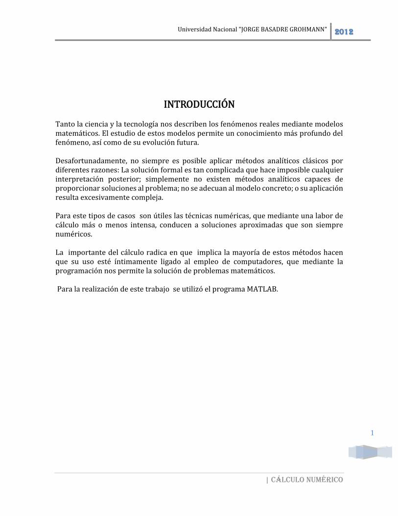
1.1. TEORÍA: En matemáticas, el método de bisección es un algoritmo de búsqueda de raíces que trabaja dividiendo el intervalo a la mitad y seleccionando el subintervalo que tiene la raíz. PROCEDIMIENTO:
Elija valores Iniciales para “a” y “b” de forma tal que lea función cambie de signo sobre el intervalo. Esto se puede verificar asegurándose de que :
𝑓(𝑎) ∗ 𝑓(𝑏) < 0
La primera aproximación a la raíz se determina con la fórmula:
𝑥𝑛 = (𝑎 + 𝑏) / 2
Realizar las siguientes evaluaciones para determinar en que subintervalo se encuentra la raíz:
𝑓(𝑎) ∗ 𝑓(𝑥𝑛) < 0 Entonces 𝑏 = 𝑥𝑛
𝑓(𝑎) ∗ 𝑓(𝑥𝑛) > 0 Entonces 𝑎 = 𝑥𝑛
𝑓(𝑎) ∗ 𝑓(𝑥𝑛) = 0 Entonces 𝑥𝑛 Es la Raíz
Calcule la nueva aproximación:
𝑥𝑛 + 1 = (𝑎 + 𝑏) / 2
Evaluar la aproximación relativa:
| (𝑥𝑛 + 1 − 𝑥𝑛) /𝑥𝑛 + 1 | < 𝐸

Universidad Nacional "JORGE BASADRE GROHMANN" 2012
| Cálculo numérico
3
No. (Falso) Repetir el paso 3, 4 y 5
Sí. (Verdadero) Entonces 𝒙𝒏+𝟏 Es la Raíz
1.2. DIAGRAMA DE FLUJO:
Inicio
f(x), a, b, E
F(a)*f(b)<0v
| b-a|>E
Xap=(a+b)/2
f(a)*f(Xap)=0V
a = b
F
f(a)*f(Xap)<0V
b = Xap
F
a = Xap
Xap
F
No existe la raíz
FIN
Universidad Nacional "JORGE BASADRE GROHMANN" 2012
| Cálculo numérico
4
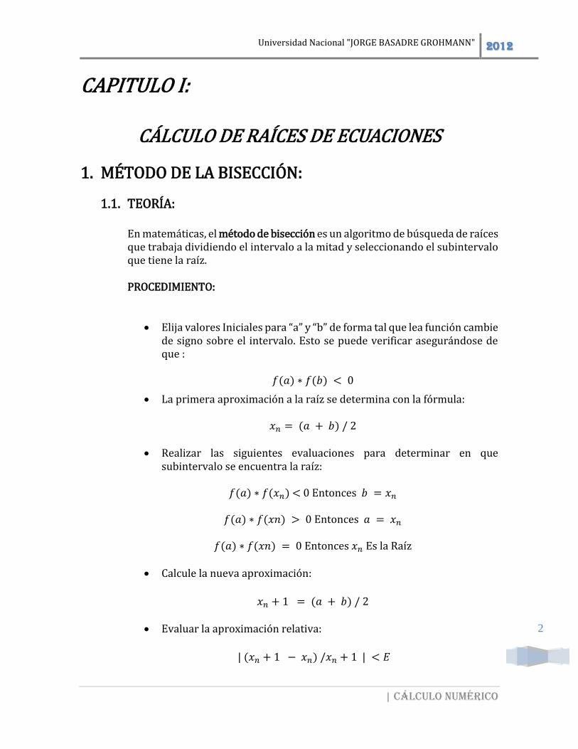
1.3. CÓDIGO DE PROGRAMA:
CÓDIGO EN EL BOTON CALCULAR:
f=get(handles.edit1,'string'); f=inline(f); a=str2double(get(handles.edit2,'string')); b=str2double(get(handles.edit3,'string')); E=str2double(get(handles.edit4,'string')); if f(a)*f(b)< 0 while abs(b-a)>E x=(a+b)/2; if f(a)*f(x)==0 a=b; else if f(a)*f(x)<0 b=x; else a=x; end end set(handles.edit5,'string',x); end else set(handles.edit5,'string','No existe la raiz en el intervalo'); end
CÓDIGO EN EL BOTÓN GRAFICAR: function varargout = pushbutton2_Callback(h, eventdata, handles, varargin) f=get(handles.edit1,'string'); f=inline(f); ezplot(f), grid on
CÓDIGO EN EL BOTÓN SALIR:
function pushbutton6_Callback(hObject, eventdata, handles) close
Universidad Nacional "JORGE BASADRE GROHMANN" 2012
| Cálculo numérico
5
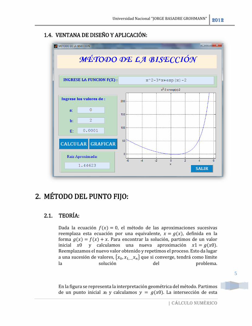
1.4. VENTANA DE DISEÑO Y APLICACIÓN:
2. MÉTODO DEL PUNTO FIJO:
2.1. TEORÍA:
Dada la ecuación 𝑓(𝑥) = 0, el método de las aproximaciones sucesivas reemplaza esta ecuación por una equivalente, 𝑥 = 𝑔(𝑥), definida en la forma 𝑔(𝑥) = 𝑓(𝑥) + 𝑥. Para encontrar la solución, partimos de un valor inicial 𝑥0 y calculamos una nueva aproximación 𝑥1 = 𝑔(𝑥0). Reemplazamos el nuevo valor obtenido y repetimos el proceso. Esto da lugar a una sucesión de valores, {𝑥0, 𝑥1,…,𝑥𝑛} que si converge, tendrá como límite
la solución del problema.
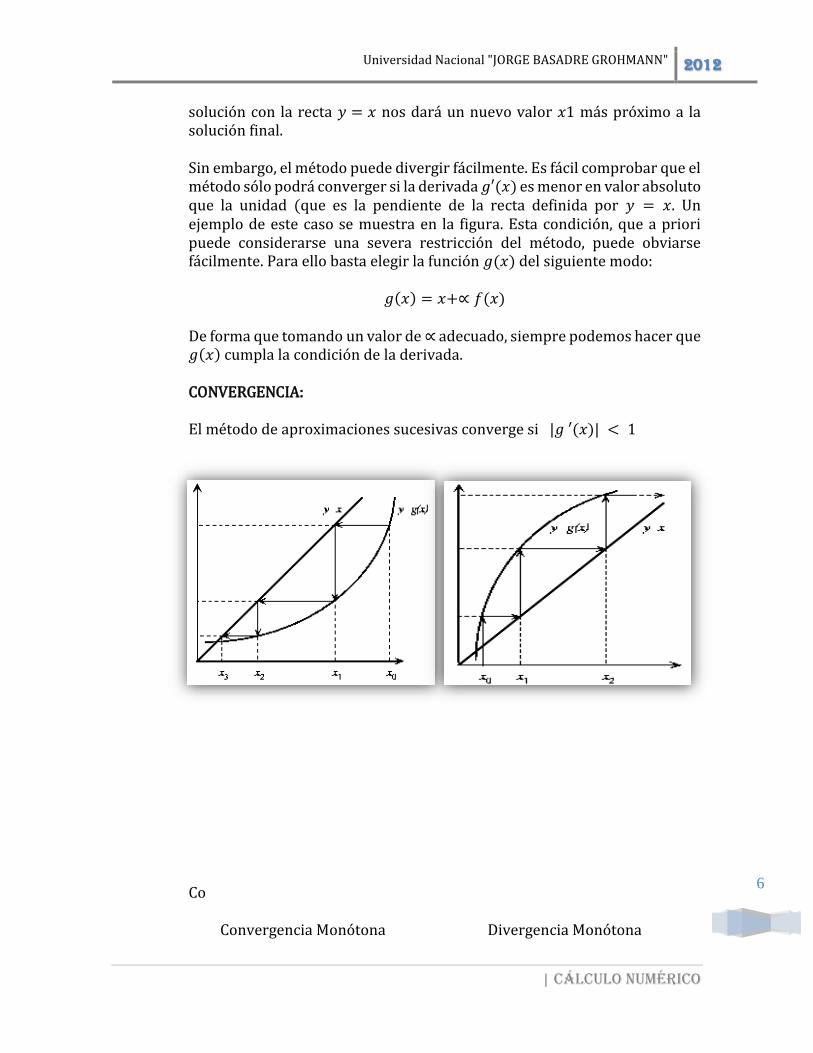
En la figura se representa la interpretación geométrica del método. Partimos de un punto inicial x0 y calculamos 𝑦 = 𝑔(𝑥0). La intersección de esta
Universidad Nacional "JORGE BASADRE GROHMANN" 2012
| Cálculo numérico
6
solución con la recta 𝑦 = 𝑥 nos dará un nuevo valor 𝑥1 más próximo a la solución final.
Sin embargo, el método puede divergir fácilmente. Es fácil comprobar que el método sólo podrá converger si la derivada 𝑔′(𝑥) es menor en valor absoluto que la unidad (que es la pendiente de la recta definida por 𝑦 = 𝑥. Un ejemplo de este caso se muestra en la figura. Esta condición, que a priori puede considerarse una severa restricción del método, puede obviarse fácilmente. Para ello basta elegir la función 𝑔(𝑥) del siguiente modo:
𝑔(𝑥) = 𝑥+∝ 𝑓(𝑥)
De forma que tomando un valor de ∝ adecuado, siempre podemos hacer que 𝑔(𝑥) cumpla la condición de la derivada.
CONVERGENCIA:
El método de aproximaciones sucesivas converge si |𝑔 ′(𝑥)| < 1
Co
Convergencia Monótona Divergencia Monótona
Universidad Nacional "JORGE BASADRE GROHMANN" 2012
| Cálculo numérico
7
𝟎 < 𝐠′(𝐱) < 𝟏 𝐠′(𝐱) > 𝟏
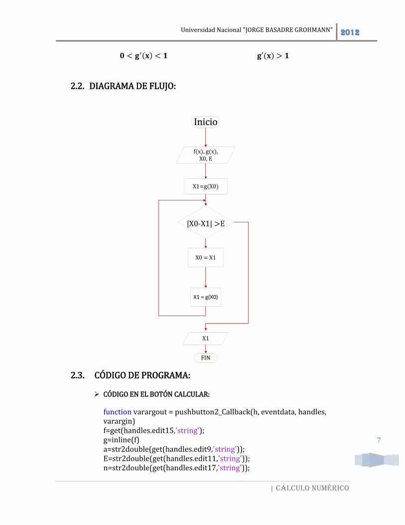
2.2. DIAGRAMA DE FLUJO:
2.3. CÓDIGO DE PROGRAMA:
CÓDIGO EN EL BOTÓN CALCULAR:
function varargout = pushbutton2_Callback(h, eventdata, handles, varargin) f=get(handles.edit15,'string'); g=inline(f) a=str2double(get(handles.edit9,'string')); E=str2double(get(handles.edit11,'string')); n=str2double(get(handles.edit17,'string'));
Inicio
f(x), g(x), X0, E
X1=g(X0)
|X0-X1| >E
X0 = X1
X1 = g(X0)
X1
FIN
Universidad Nacional "JORGE BASADRE GROHMANN" 2012
| Cálculo numérico
8
x1=g(a) k=1; cadena1=sprintf('a = %8.6f valor inicial\n',a); while abs(x1-a)>E&k<n a=x1 x1=g(a) k=k+1 cadena2=sprintf('x%d = %8.6f\n',k-1,x1); cadena1=[cadena1,cadena2]; end
CÓDIGO EN EL BOTÓN GRAFICAR:
function varargout = pushbutton1_Callback(h, eventdata, handles, varargin) funcionf=get(handles.edit1,'string'); f=inline(funcionf); figure(1); ezplot(f),grid on
CÓDIGO EN EL BOTÓN SALIR:
function pushbutton6_Callback(hObject, eventdata, handles) close
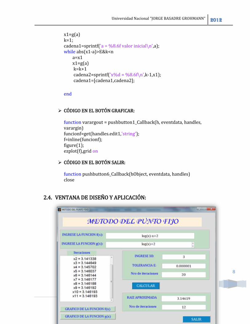
2.4. VENTANA DE DISEÑO Y APLICACIÓN:

Universidad Nacional "JORGE BASADRE GROHMANN" 2012
| Cálculo numérico
9
3. MÉTODO DE NEWTON RAPHSON:
3.1. TEORÍA:
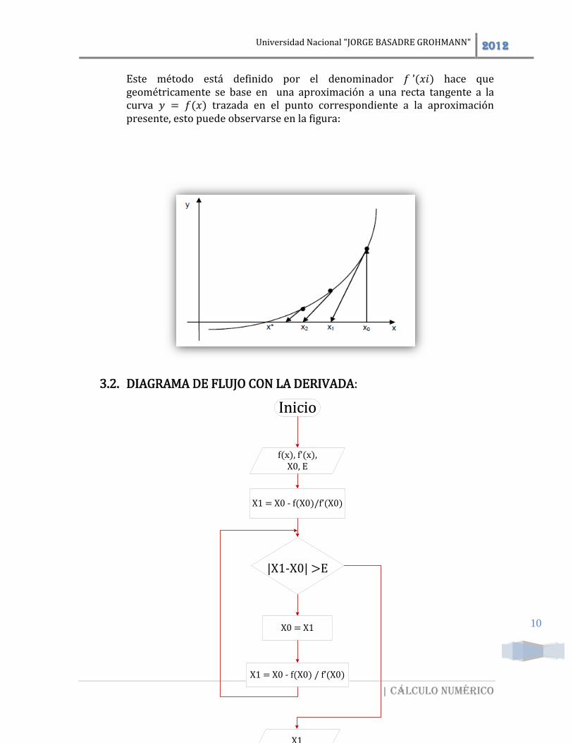
Este método parte de una aproximación inicial 𝑥0 y obtiene una aproximación mejor, 𝑥1, dada por la fórmula:
𝑥1 = 𝑥0 −𝑓(𝑥0)
𝑓′(𝑥0)
Universidad Nacional "JORGE BASADRE GROHMANN" 2012
| Cálculo numérico
10
Este método está definido por el denominador 𝑓 ’(𝑥𝑖) hace que geométricamente se base en una aproximación a una recta tangente a la curva 𝑦 = 𝑓(𝑥) trazada en el punto correspondiente a la aproximación presente, esto puede observarse en la figura:
3.2. DIAGRAMA DE FLUJO CON LA DERIVADA:
Inicio
f(x), f’(x), X0, E
X1 = X0 - f(X0)/f’(X0)
|X1-X0| >E
X0 = X1
X1 = X0 - f(X0) / f’(X0)
X1
FIN
Universidad Nacional "JORGE BASADRE GROHMANN" 2012
| Cálculo numérico
11
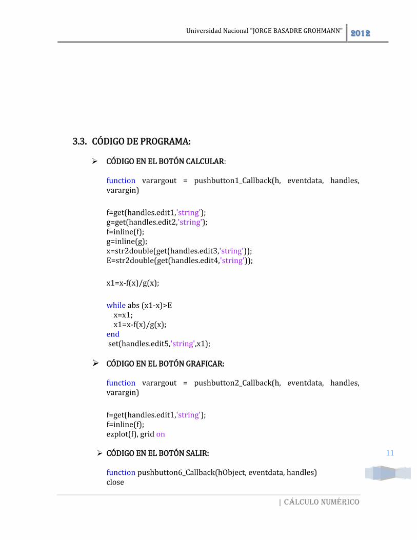
3.3. CÓDIGO DE PROGRAMA: CÓDIGO EN EL BOTÓN CALCULAR:
function varargout = pushbutton1_Callback(h, eventdata, handles, varargin) f=get(handles.edit1,'string'); g=get(handles.edit2,'string'); f=inline(f); g=inline(g); x=str2double(get(handles.edit3,'string')); E=str2double(get(handles.edit4,'string')); x1=x-f(x)/g(x); while abs (x1-x)>E x=x1; x1=x-f(x)/g(x); end set(handles.edit5,'string',x1);
CÓDIGO EN EL BOTÓN GRAFICAR:
function varargout = pushbutton2_Callback(h, eventdata, handles, varargin) f=get(handles.edit1,'string'); f=inline(f); ezplot(f), grid on
CÓDIGO EN EL BOTÓN SALIR:
function pushbutton6_Callback(hObject, eventdata, handles) close

Universidad Nacional "JORGE BASADRE GROHMANN" 2012
| Cálculo numérico
12
3.4. VENTANA DE DISEÑO Y APLICACIÓN:
3.5. SIN INGRESAR LA DERIVADA: f ’(x) DIAGRAMA DE FLUJO:
Inicio
f(x), X0, E
h = 0,00001;df = [f(X0+h) - f(X0)] / h
|X1-X0| >E
X0 = X1
h = 0,00001
X1
FIN
X1 = X0 - f(X0)/df
X1 = X0 - f(X0)/df
Universidad Nacional "JORGE BASADRE GROHMANN" 2012
| Cálculo numérico
13
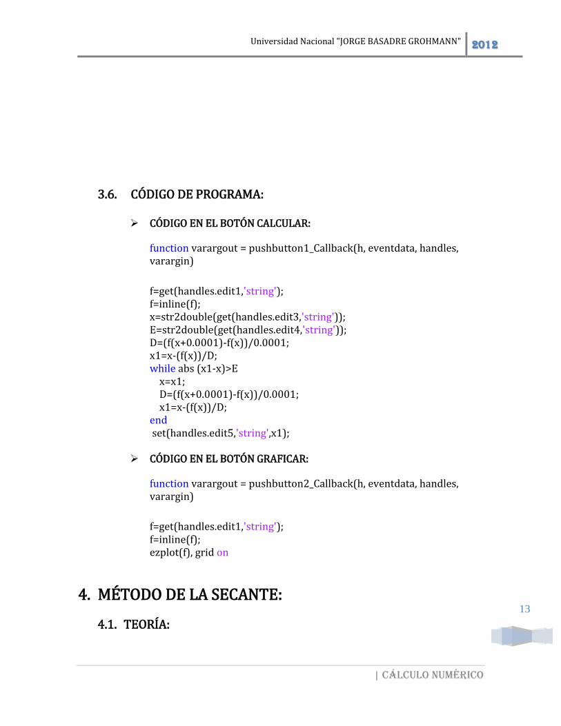
3.6. CÓDIGO DE PROGRAMA:
CÓDIGO EN EL BOTÓN CALCULAR:
function varargout = pushbutton1_Callback(h, eventdata, handles, varargin) f=get(handles.edit1,'string'); f=inline(f); x=str2double(get(handles.edit3,'string')); E=str2double(get(handles.edit4,'string')); D=(f(x+0.0001)-f(x))/0.0001; x1=x-(f(x))/D; while abs (x1-x)>E x=x1; D=(f(x+0.0001)-f(x))/0.0001; x1=x-(f(x))/D; end set(handles.edit5,'string',x1);
CÓDIGO EN EL BOTÓN GRAFICAR:
function varargout = pushbutton2_Callback(h, eventdata, handles, varargin) f=get(handles.edit1,'string'); f=inline(f); ezplot(f), grid on
4. MÉTODO DE LA SECANTE:
4.1. TEORÍA:
Universidad Nacional "JORGE BASADRE GROHMANN" 2012
| Cálculo numérico
14
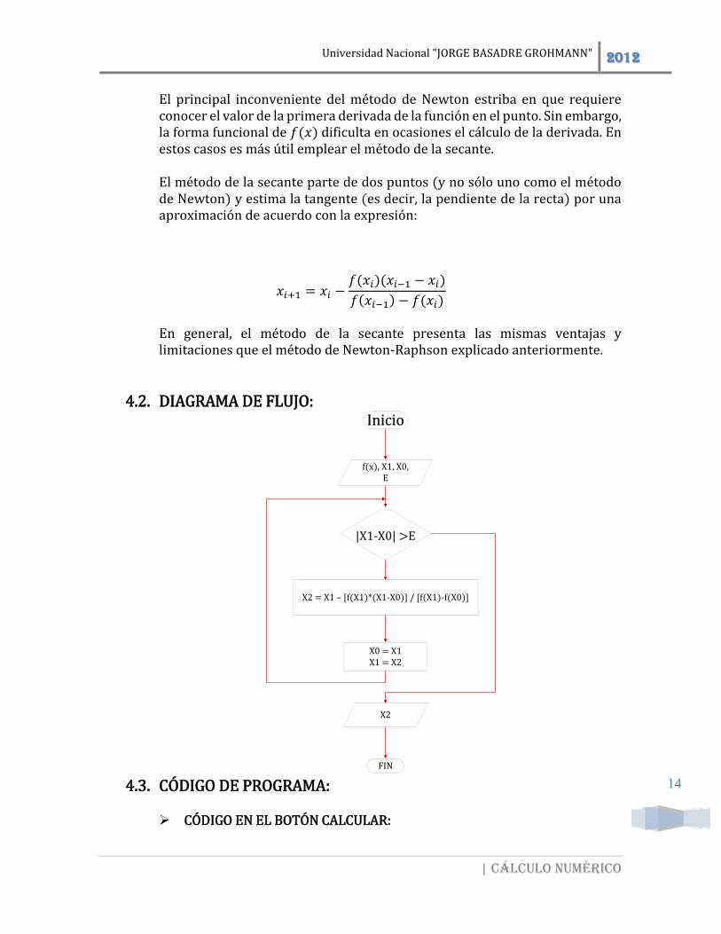
El principal inconveniente del método de Newton estriba en que requiere conocer el valor de la primera derivada de la función en el punto. Sin embargo, la forma funcional de 𝑓(𝑥) dificulta en ocasiones el cálculo de la derivada. En estos casos es más útil emplear el método de la secante.
El método de la secante parte de dos puntos (y no sólo uno como el método de Newton) y estima la tangente (es decir, la pendiente de la recta) por una aproximación de acuerdo con la expresión:
𝑥𝑖+1 = 𝑥𝑖 −𝑓(𝑥𝑖)(𝑥𝑖−1 − 𝑥𝑖)
𝑓(𝑥𝑖−1) − 𝑓(𝑥𝑖)
En general, el método de la secante presenta las mismas ventajas y limitaciones que el método de Newton-Raphson explicado anteriormente.
4.2. DIAGRAMA DE FLUJO:
4.3. CÓDIGO DE PROGRAMA:
CÓDIGO EN EL BOTÓN CALCULAR:
Inicio
f(x), X1, X0, E
|X1-X0| >E
X2 = X1 – [f(X1)*(X1-X0)] / [f(X1)-f(X0)]
X0 = X1X1 = X2
X2
FIN

Universidad Nacional "JORGE BASADRE GROHMANN" 2012
| Cálculo numérico
15
function varargout = pushbutton3_Callback(h, eventdata, handles, varargin) f=inline(get(handles.edit1,'string')); x0=str2double(get(handles.edit2,'string')); x1=str2double(get(handles.edit3,'string')); E=str2double(get(handles.edit4,'string')); while abs(x1-x0)>E x2=x1-(((x1-x0)*f(x1))/(f(x1)-f(x0))); x0=x1; x1=x2; end set(handles.edit5,'string',x2)
CÓDIGO EN EL BOTÓN GRAFICAR:
function varargout = pushbutton4_Callback(h, eventdata, handles, varargin) f=get(handles.edit1,'string'); f=inline(f); ezplot(f), grid on
CÓDIGO EN EL BOTÓN SALIR:
function pushbutton3_Callback(hObject, eventdata, handles) close(secante)
4.4. VENTANA DE DISEÑO y APLICACION:
Universidad Nacional "JORGE BASADRE GROHMANN" 2012
| Cálculo numérico
16
5. MÉTODO DE LIN:
5.1. TEORÍA:
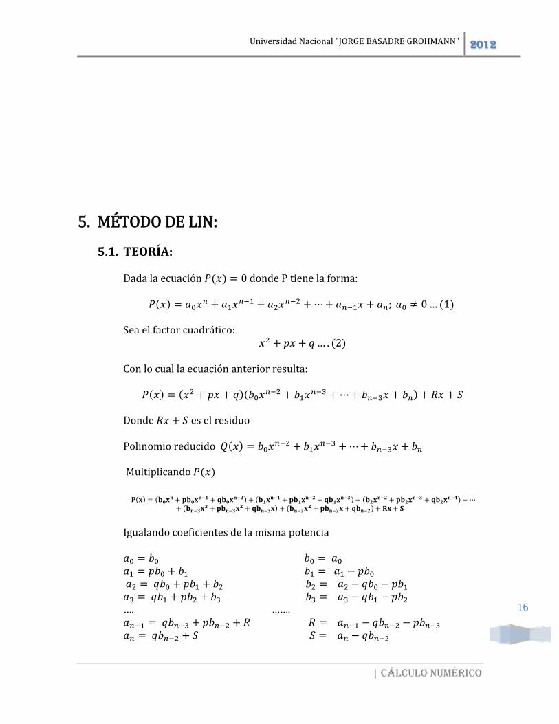
Dada la ecuación 𝑃(𝑥) = 0 donde P tiene la forma:
𝑃(𝑥) = 𝑎0𝑥𝑛 + 𝑎1𝑥
𝑛−1 + 𝑎2𝑥𝑛−2 +⋯+ 𝑎𝑛−1𝑥 + 𝑎𝑛; 𝑎0 ≠ 0… (1)
Sea el factor cuadrático:
𝑥2 + 𝑝𝑥 + 𝑞… . (2) Con lo cual la ecuación anterior resulta:
𝑃(𝑥) = (𝑥2 + 𝑝𝑥 + 𝑞)(𝑏0𝑥𝑛−2 + 𝑏1𝑥
𝑛−3 +⋯+ 𝑏𝑛−3𝑥 + 𝑏𝑛) + 𝑅𝑥 + 𝑆 Donde 𝑅𝑥 + 𝑆 es el residuo Polinomio reducido 𝑄(𝑥) = 𝑏0𝑥
𝑛−2 + 𝑏1𝑥𝑛−3 +⋯+ 𝑏𝑛−3𝑥 + 𝑏𝑛
Multiplicando 𝑃(𝑥)
𝐏(𝐱) = (𝐛𝟎𝐱
𝐧 + 𝐩𝐛𝟎𝐱𝐧−𝟏 + 𝐪𝐛𝟎𝐱
𝐧−𝟐) + (𝐛𝟏𝐱𝐧−𝟏 + 𝐩𝐛𝟏𝐱
𝐧−𝟐 + 𝐪𝐛𝟏𝐱𝐧−𝟑) + (𝐛𝟐𝐱
𝐧−𝟐 + 𝐩𝐛𝟐𝐱𝐧−𝟑 + 𝐪𝐛𝟐𝐱
𝐧−𝟒) + ⋯+ (𝐛𝐧−𝟑𝐱
𝟑 + 𝐩𝐛𝐧−𝟑𝐱𝟐 + 𝐪𝐛𝐧−𝟑𝐱) + (𝐛𝐧−𝟐𝐱
𝟐 + 𝐩𝐛𝐧−𝟐𝐱 + 𝐪𝐛𝐧−𝟐) + 𝐑𝐱 + 𝐒
Igualando coeficientes de la misma potencia 𝑎0 = 𝑏0 𝑏0 = 𝑎0 𝑎1 = 𝑝𝑏0 + 𝑏1 𝑏1 = 𝑎1 − 𝑝𝑏0 𝑎2 = 𝑞𝑏0 + 𝑝𝑏1 + 𝑏2 𝑏2 = 𝑎2 − 𝑞𝑏0 − 𝑝𝑏1 𝑎3 = 𝑞𝑏1 + 𝑝𝑏2 + 𝑏3 𝑏3 = 𝑎3 − 𝑞𝑏1 − 𝑝𝑏2 …. ……. 𝑎𝑛−1 = 𝑞𝑏𝑛−3 + 𝑝𝑏𝑛−2 + 𝑅 𝑅 = 𝑎𝑛−1 − 𝑞𝑏𝑛−2 − 𝑝𝑏𝑛−3 𝑎𝑛 = 𝑞𝑏𝑛−2 + 𝑆 𝑆 = 𝑎𝑛 − 𝑞𝑏𝑛−2
Universidad Nacional "JORGE BASADRE GROHMANN" 2012
| Cálculo numérico
17
En general: 𝑏𝑘 = 𝑎𝑘 − 𝑝𝑏𝑘−1 − 𝑞𝑏𝑘−2; 𝑘 = 0,1,2,3… . 𝑛 − 2 Los residuos están dados por:
𝑅 = 𝑎𝑛−1 − 𝑝𝑏𝑛−2 − 𝑞𝑏𝑛−3
𝑆 = 𝑎𝑛 − 𝑞𝑏𝑛−2
Para que 𝑥2 + 𝑝𝑥 + 𝑞 sea un factor cuadrático R y S tienen que ser cero.
𝑅 = 𝑎𝑛−1 − 𝑝𝑏𝑛−2 − 𝑞𝑏𝑛−3 = 0 𝑒𝑛𝑡𝑜𝑛𝑐𝑒𝑠 𝑝 =𝑎𝑛−1 − 𝑞𝑏𝑛−3
𝑏𝑛−2
𝑆 = 𝑎𝑛 − 𝑞𝑏𝑛−2 = 0 𝑒𝑛𝑡𝑜𝑛𝑐𝑒𝑠 𝑞 =𝑎𝑛𝑏𝑛−2
Se define:
Si ∆𝑝 =𝑅
𝑏𝑛−2 𝑦 ∆𝑞 =
𝑆
𝑏𝑛−2
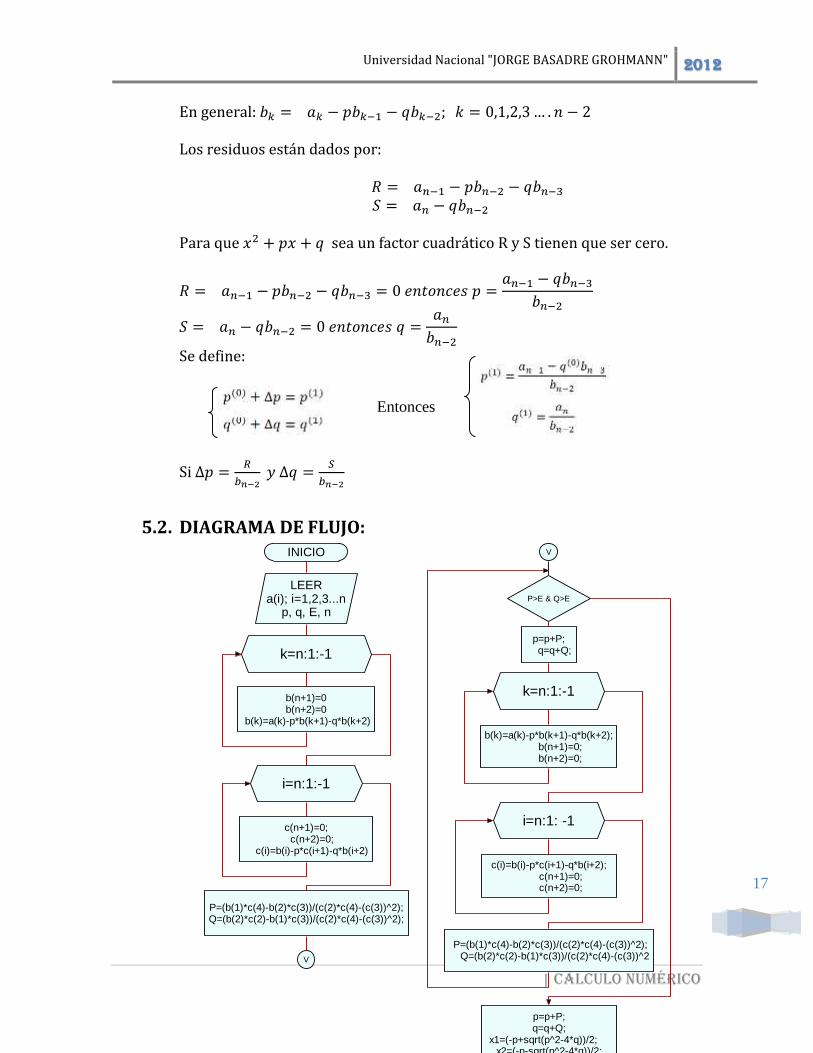
5.2. DIAGRAMA DE FLUJO:
Entonces
INICIO
LEERa(i); i=1,2,3...n
p, q, E, n
k=n:1:-1
b(n+1)=0b(n+2)=0
b(k)=a(k)-p*b(k+1)-q*b(k+2)
i=n:1:-1
c(n+1)=0; c(n+2)=0;
c(i)=b(i)-p*c(i+1)-q*b(i+2)
P=(b(1)*c(4)-b(2)*c(3))/(c(2)*c(4)-(c(3))^2);Q=(b(2)*c(2)-b(1)*c(3))/(c(2)*c(4)-(c(3))^2);
P>E & Q>E
p=p+P; q=q+Q;
k=n:1:-1
b(k)=a(k)-p*b(k+1)-q*b(k+2); b(n+1)=0; b(n+2)=0;
i=n:1: -1
c(i)=b(i)-p*c(i+1)-q*b(i+2); c(n+1)=0; c(n+2)=0;
P=(b(1)*c(4)-b(2)*c(3))/(c(2)*c(4)-(c(3))^2); Q=(b(2)*c(2)-b(1)*c(3))/(c(2)*c(4)-(c(3))^2
V
p=p+P;q=q+Q;
x1=(-p+sqrt(p^2-4*q))/2; x2=(-p-sqrt(p^2-4*q))/2;
ESCRIBIRX1, X2
FIN
V
Universidad Nacional "JORGE BASADRE GROHMANN" 2012
| Cálculo numérico
18
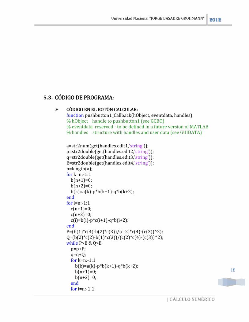
5.3. CÓDIGO DE PROGRAMA: CÓDIGO EN EL BOTÓN CALCULAR:
function pushbutton1_Callback(hObject, eventdata, handles) % hObject handle to pushbutton1 (see GCBO) % eventdata reserved - to be defined in a future version of MATLAB % handles structure with handles and user data (see GUIDATA) a=str2num(get(handles.edit1,'string')); p=str2double(get(handles.edit2,'string')); q=str2double(get(handles.edit3,'string')); E=str2double(get(handles.edit4,'string')); n=length(a); for k=n:-1:1 b(n+1)=0; b(n+2)=0; b(k)=a(k)-p*b(k+1)-q*b(k+2); end for i=n:-1:1 c(n+1)=0; c(n+2)=0; c(i)=b(i)-p*c(i+1)-q*b(i+2); end P=(b(1)*c(4)-b(2)*c(3))/(c(2)*c(4)-(c(3))^2); Q=(b(2)*c(2)-b(1)*c(3))/(c(2)*c(4)-(c(3))^2); while P>E & Q>E p=p+P; q=q+Q; for k=n:-1:1 b(k)=a(k)-p*b(k+1)-q*b(k+2); b(n+1)=0; b(n+2)=0; end for i=n:-1:1
Universidad Nacional "JORGE BASADRE GROHMANN" 2012
| Cálculo numérico
19
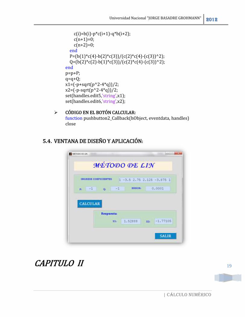
c(i)=b(i)-p*c(i+1)-q*b(i+2); c(n+1)=0; c(n+2)=0; end P=(b(1)*c(4)-b(2)*c(3))/(c(2)*c(4)-(c(3))^2); Q=(b(2)*c(2)-b(1)*c(3))/(c(2)*c(4)-(c(3))^2); end p=p+P; q=q+Q; x1=(-p+sqrt(p^2-4*q))/2; x2=(-p-sqrt(p^2-4*q))/2; set(handles.edit5,'string',x1); set(handles.edit6,'string',x2);
CÓDIGO EN EL BOTÓN CALCULAR: function pushbutton2_Callback(hObject, eventdata, handles) close
5.4. VENTANA DE DISEÑO Y APLICACIÓN:
CAPITULO II
Universidad Nacional "JORGE BASADRE GROHMANN" 2012
| Cálculo numérico
20
SISTEMA DE ECUACIÓN LINEAL
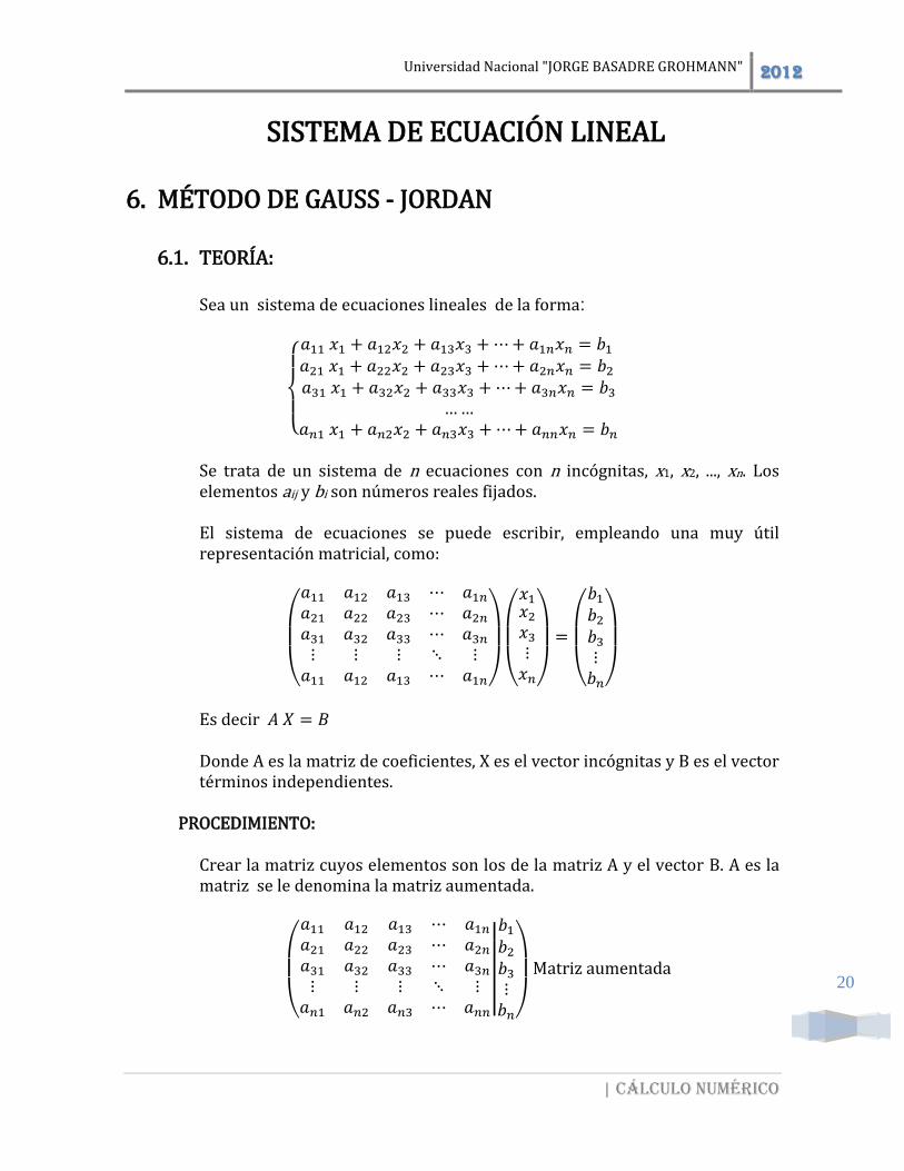
6. MÉTODO DE GAUSS - JORDAN 6.1. TEORÍA:
Sea un sistema de ecuaciones lineales de la forma:
{
𝑎11 𝑥1 + 𝑎12𝑥2 + 𝑎13𝑥3 +⋯+ 𝑎1𝑛𝑥𝑛 = 𝑏1 𝑎21 𝑥1 + 𝑎22𝑥2 + 𝑎23𝑥3 +⋯+ 𝑎2𝑛𝑥𝑛 = 𝑏2 𝑎31 𝑥1 + 𝑎32𝑥2 + 𝑎33𝑥3 +⋯+ 𝑎3𝑛𝑥𝑛 = 𝑏3
……𝑎𝑛1 𝑥1 + 𝑎𝑛2𝑥2 + 𝑎𝑛3𝑥3 +⋯+ 𝑎𝑛𝑛𝑥𝑛 = 𝑏𝑛
Se trata de un sistema de n ecuaciones con n incógnitas, x1, x2, ..., xn. Los elementos aij y bi son números reales fijados.
El sistema de ecuaciones se puede escribir, empleando una muy útil representación matricial, como:
(
𝑎11 𝑎12 𝑎13 ⋯ 𝑎1𝑛𝑎21 𝑎22 𝑎23 ⋯ 𝑎2𝑛𝑎31 𝑎32 𝑎33 ⋯ 𝑎3𝑛⋮ ⋮ ⋮ ⋱ ⋮𝑎11 𝑎12 𝑎13 ⋯ 𝑎1𝑛)
(
𝑥1𝑥2𝑥3⋮𝑥𝑛)
=
(
𝑏1𝑏2𝑏3⋮𝑏𝑛)
Es decir 𝐴 𝑋 = 𝐵
Donde A es la matriz de coeficientes, X es el vector incógnitas y B es el vector términos independientes.
PROCEDIMIENTO:
Crear la matriz cuyos elementos son los de la matriz A y el vector B. A es la matriz se le denomina la matriz aumentada.
(
𝑎11 𝑎12 𝑎13 ⋯ 𝑎1𝑛𝑎21 𝑎22 𝑎23 ⋯ 𝑎2𝑛𝑎31 𝑎32 𝑎33 ⋯ 𝑎3𝑛⋮ ⋮ ⋮ ⋱ ⋮𝑎𝑛1 𝑎𝑛2 𝑎𝑛3 ⋯ 𝑎𝑛𝑛
||
𝑏1𝑏2𝑏3⋮𝑏𝑛)
Matriz aumentada
Universidad Nacional "JORGE BASADRE GROHMANN" 2012
| Cálculo numérico
21
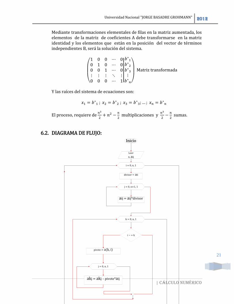
Mediante transformaciones elementales de filas en la matriz aumentada, los elementos de la matriz de coeficientes A debe transformarse en la matriz identidad y los elementos que están en la posición del vector de términos independientes B, será la solución del sistema.
(
1 0 0 ⋯ 00 1 0 ⋯ 00 0 1 ⋯ 0⋮ ⋮ ⋮ ⋱ ⋮0 0 0 ⋯ 1
||
𝑏∗1𝑏∗2𝑏∗3⋮𝑏∗𝑛)
Matriz transformada
Y las raíces del sistema de ecuaciones son:
𝑥1 = 𝑏∗1 ; 𝑥2 = 𝑏∗2 ; 𝑥3 = 𝑏∗3; … ; 𝑥𝑛 = 𝑏∗𝑛
El proceso, requiere de 𝑛3
2+ 𝑛2 −
𝑛
2 multiplicaciones y
𝑛3
2−𝑛
2 sumas.
6.2. DIAGRAMA DE FLUJO:
Inicio
Leer
n, aij
i = 0, n, 1
divisor = aii
j = 0, n+1, 1
aij = aij*divisor
k = 0, n, 1
i ~ = k
pivote = a(k, i)
j = 0, n, 1
akj = akj – pivote*aij
escribir
ai, n+1
FIN
Universidad Nacional "JORGE BASADRE GROHMANN" 2012
| Cálculo numérico
22
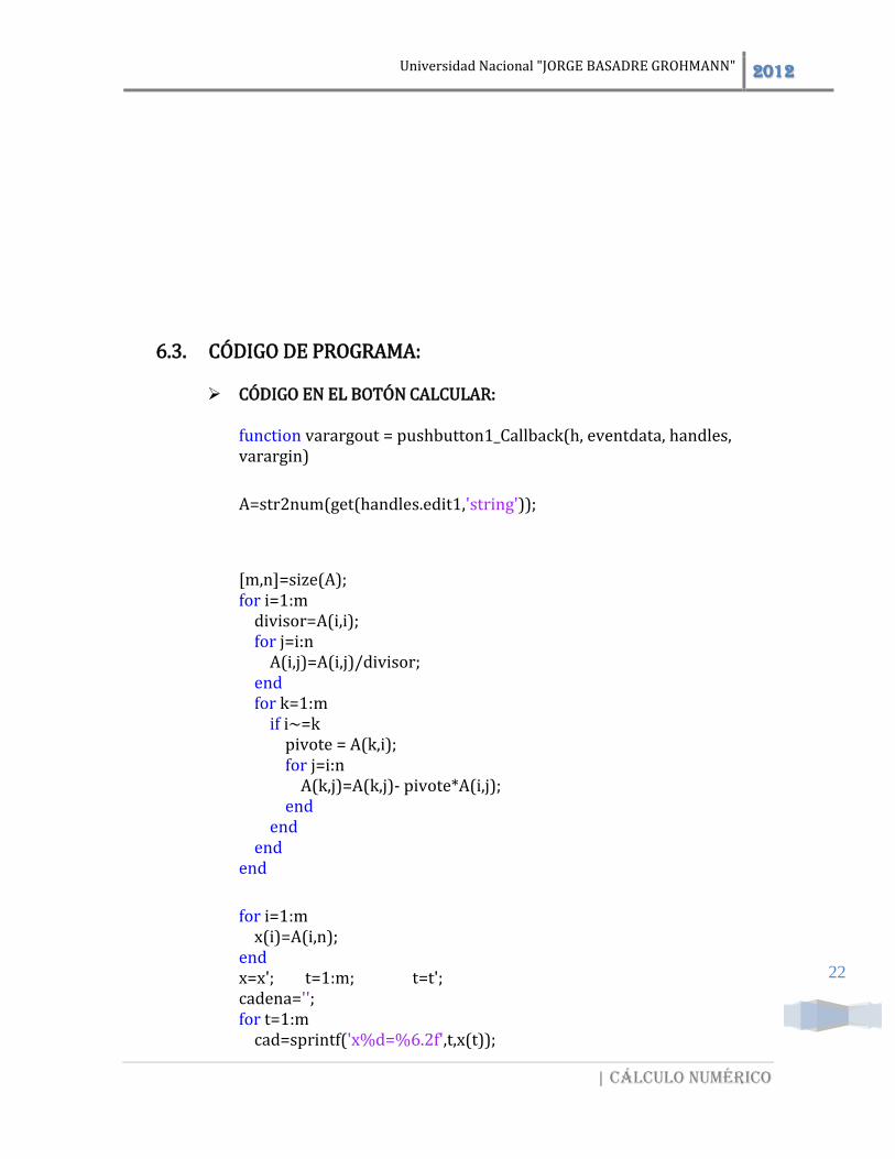
6.3. CÓDIGO DE PROGRAMA:
CÓDIGO EN EL BOTÓN CALCULAR:
function varargout = pushbutton1_Callback(h, eventdata, handles, varargin) A=str2num(get(handles.edit1,'string')); [m,n]=size(A); for i=1:m divisor=A(i,i); for j=i:n A(i,j)=A(i,j)/divisor; end for k=1:m if i~=k pivote = A(k,i); for j=i:n A(k,j)=A(k,j)- pivote*A(i,j); end end end end for i=1:m x(i)=A(i,n); end x=x'; t=1:m; t=t'; cadena=''; for t=1:m cad=sprintf('x%d=%6.2f',t,x(t));
Universidad Nacional "JORGE BASADRE GROHMANN" 2012
| Cálculo numérico
23
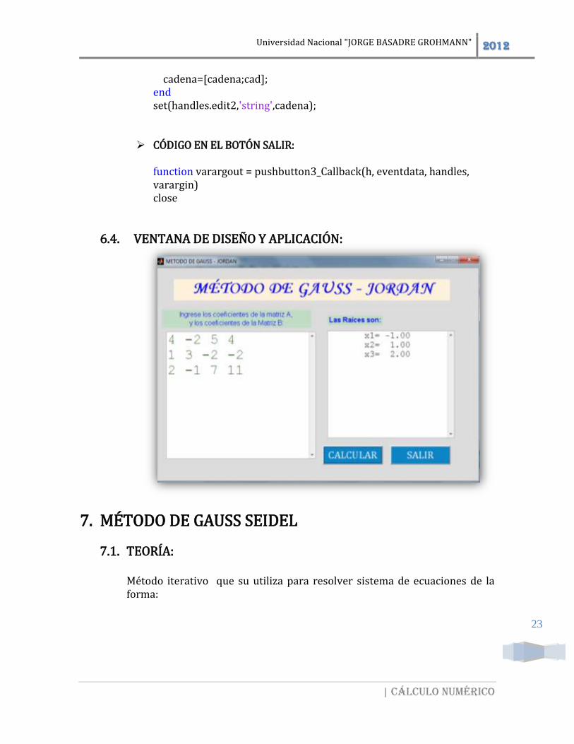
cadena=[cadena;cad]; end set(handles.edit2,'string',cadena);
CÓDIGO EN EL BOTÓN SALIR: function varargout = pushbutton3_Callback(h, eventdata, handles, varargin) close
6.4. VENTANA DE DISEÑO Y APLICACIÓN:
7. MÉTODO DE GAUSS SEIDEL
7.1. TEORÍA: Método iterativo que su utiliza para resolver sistema de ecuaciones de la forma:
Universidad Nacional "JORGE BASADRE GROHMANN" 2012
| Cálculo numérico
24
{
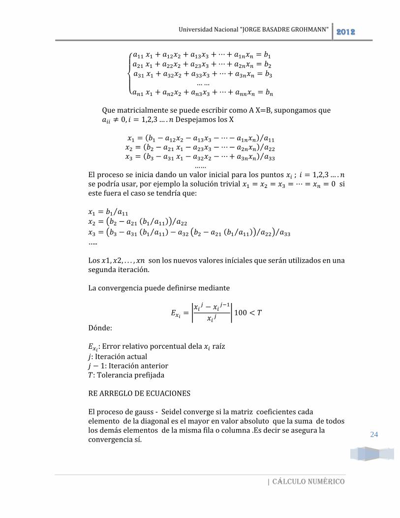
𝑎11 𝑥1 + 𝑎12𝑥2 + 𝑎13𝑥3 +⋯+ 𝑎1𝑛𝑥𝑛 = 𝑏1 𝑎21 𝑥1 + 𝑎22𝑥2 + 𝑎23𝑥3 +⋯+ 𝑎2𝑛𝑥𝑛 = 𝑏2 𝑎31 𝑥1 + 𝑎32𝑥2 + 𝑎33𝑥3 +⋯+ 𝑎3𝑛𝑥𝑛 = 𝑏3
……𝑎𝑛1 𝑥1 + 𝑎𝑛2𝑥2 + 𝑎𝑛3𝑥3 +⋯+ 𝑎𝑛𝑛𝑥𝑛 = 𝑏𝑛
Que matricialmente se puede escribir como A X=B, supongamos que 𝑎𝑖𝑖 ≠ 0, 𝑖 = 1,2,3… . 𝑛 Despejamos los X
𝑥1 = (𝑏1 − 𝑎12𝑥2 − 𝑎13𝑥3 −⋯− 𝑎1𝑛𝑥𝑛) 𝑎11⁄ 𝑥2 = (𝑏2 − 𝑎21 𝑥1 − 𝑎23𝑥3 −⋯− 𝑎2𝑛𝑥𝑛) 𝑎22⁄ 𝑥3 = (𝑏3 − 𝑎31 𝑥1 − 𝑎32𝑥2 −⋯+ 𝑎3𝑛𝑥𝑛) 𝑎33⁄
…… El proceso se inicia dando un valor inicial para los puntos 𝑥𝑖 ; 𝑖 = 1,2,3… . 𝑛 se podría usar, por ejemplo la solución trivial 𝑥1 = 𝑥2 = 𝑥3 = ⋯ = 𝑥𝑛 = 0 si este fuera el caso se tendría que: 𝑥1 = 𝑏1 𝑎11⁄ 𝑥2 = (𝑏2 − 𝑎21 (𝑏1 𝑎11⁄ )) 𝑎22⁄
𝑥3 = (𝑏3 − 𝑎31 (𝑏1 𝑎11⁄ ) − 𝑎32 (𝑏2 − 𝑎21 (𝑏1 𝑎11⁄ )) 𝑎22⁄ ) 𝑎33⁄
….. Los 𝑥1, 𝑥2, . . . , 𝑥𝑛 son los nuevos valores iníciales que serán utilizados en una segunda iteración. La convergencia puede definirse mediante
𝐸𝑥𝑖 = |𝑥𝑖𝑗 − 𝑥𝑖
𝑗−1
𝑥𝑖 𝑗| 100 < 𝑇
Dónde: 𝐸𝑥𝑖: Error relativo porcentual dela 𝑥𝑖 raíz
𝑗: Iteración actual 𝑗 − 1: Iteración anterior 𝑇: Tolerancia prefijada RE ARREGLO DE ECUACIONES El proceso de gauss - Seidel converge si la matriz coeficientes cada elemento de la diagonal es el mayor en valor absoluto que la suma de todos los demás elementos de la misma fila o columna .Es decir se asegura la convergencia sí.

Universidad Nacional "JORGE BASADRE GROHMANN" 2012
| Cálculo numérico
25
|𝑎𝑖𝑖| > ∑𝑎𝑖𝑗
𝑛
𝑖=1𝑗≠𝑖
ó |𝑎𝑖𝑖| > ∑𝑎𝑗𝑖
𝑛
𝑖=1𝑗≠𝑖
7.2. DIAGRAMA DE FLUJO:
Inicio
LeerN, m, aij, bi, vi
k = 1, m, 1
i = 1, n, 1
Xi = Vi
i = 1, n, 1
S = 0
j = 1, n, 1
j ~ = 1
S = S + aij * Xj
vi = (bi-S) / aii
Xi = vi
i = 1, n, 1
escribir
vi
FIN
Universidad Nacional "JORGE BASADRE GROHMANN" 2012
| Cálculo numérico
26
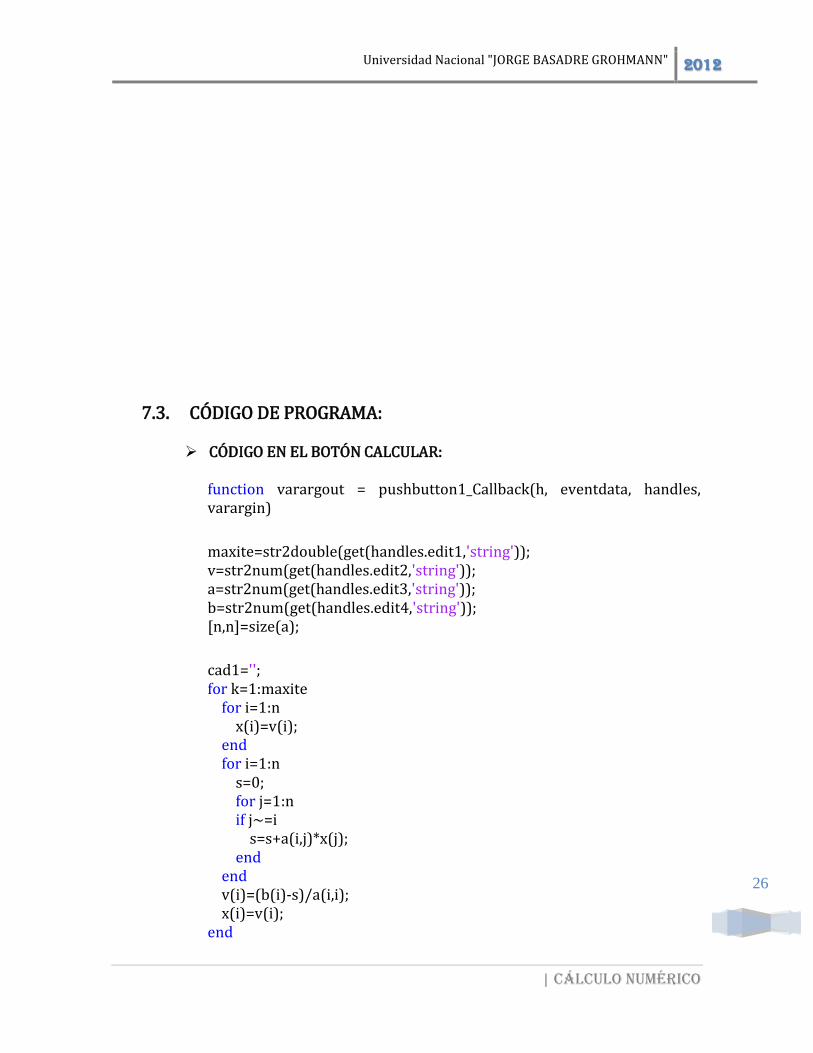
7.3. CÓDIGO DE PROGRAMA:
CÓDIGO EN EL BOTÓN CALCULAR: function varargout = pushbutton1_Callback(h, eventdata, handles, varargin) maxite=str2double(get(handles.edit1,'string')); v=str2num(get(handles.edit2,'string')); a=str2num(get(handles.edit3,'string')); b=str2num(get(handles.edit4,'string')); [n,n]=size(a); cad1=''; for k=1:maxite for i=1:n x(i)=v(i); end for i=1:n s=0; for j=1:n if j~=i s=s+a(i,j)*x(j); end end v(i)=(b(i)-s)/a(i,i); x(i)=v(i); end
Universidad Nacional "JORGE BASADRE GROHMANN" 2012
| Cálculo numérico
27
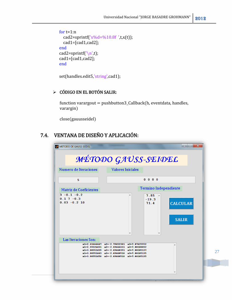
for t=1:n cad2=sprintf('x%d=%10.8f ',t,x(t)); cad1=[cad1,cad2]; end cad2=sprintf('\n',t); cad1=[cad1,cad2]; end set(handles.edit5,'string',cad1);
CÓDIGO EN EL BOTÓN SALIR: function varargout = pushbutton3_Callback(h, eventdata, handles, varargin) close(gauusseidel)
7.4. VENTANA DE DISEÑO Y APLICACIÓN:
Universidad Nacional "JORGE BASADRE GROHMANN" 2012
| Cálculo numérico
28
INTERPOLACIÓN
8. INTERPOLACIÓN LINEAL:
8.1. TEORÍA:
Nos centraremos ahora en el problema de obtener, a partir de una tabla de parejas (𝑥, 𝑓(𝑥)) definida en un cierto intervalo [𝑎, 𝑏], el valor de la función para cualquier x perteneciente a dicho intervalo.
Supongamos que disponemos de las siguientes parejas de datos:
x x0 x1 x2 … xn
y y0 y1 y2 … 𝑦𝑛
El objetivo es encontrar una función continua lo más sencilla posible tal que:
(𝑥𝑖) = 𝑦𝑖 (0 ≤ 𝑖 ≤ 𝑛)
Se dice entonces que la función 𝑓(𝑥) definida por la ecuación es una función de interpolación de los datos representados en la tabla.
Existen muchas formas de definir las funciones de interpolación, lo que da origen a un gran número de métodos (polinomios de interpolación de Newton, interpolación de Lagrange, interpolación de Hermite, etc). Sin embargo, nos centraremos exclusivamente en dos funciones de interpolación:
Los polinomios de interpolación de Lagrange. Las funciones de interpolación splines. Estas funciones son especialmente
importantes debido a su idoneidad en los cálculos realizados con ordenador.
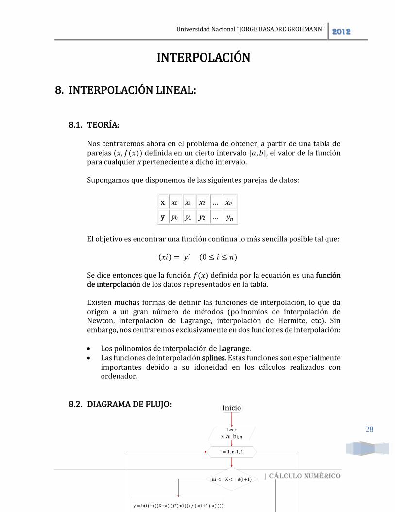
8.2. DIAGRAMA DE FLUJO:
Inicio
Leer
X, ai, bi, n
i = 1, n-1, 1
ai <= X <= a(i+1)
y = b(i)+(((X+a(i))*(b(i))) / (a(i+1)-a(i)))
i = n
Escribiry
FIN
Universidad Nacional "JORGE BASADRE GROHMANN" 2012
| Cálculo numérico
29
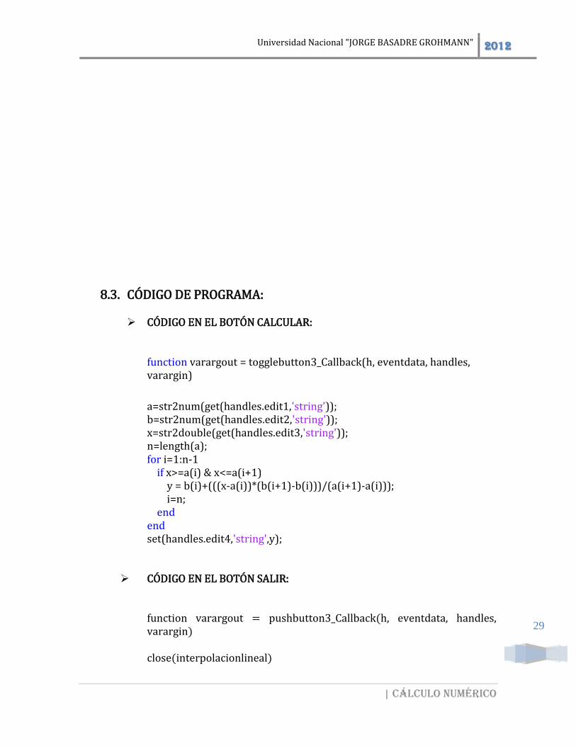
8.3. CÓDIGO DE PROGRAMA:
CÓDIGO EN EL BOTÓN CALCULAR:
function varargout = togglebutton3_Callback(h, eventdata, handles, varargin) a=str2num(get(handles.edit1,'string')); b=str2num(get(handles.edit2,'string')); x=str2double(get(handles.edit3,'string')); n=length(a); for i=1:n-1 if x>=a(i) & x<=a(i+1) y = b(i)+(((x-a(i))*(b(i+1)-b(i)))/(a(i+1)-a(i))); i=n; end end set(handles.edit4,'string',y);
CÓDIGO EN EL BOTÓN SALIR:
function varargout = pushbutton3_Callback(h, eventdata, handles, varargin) close(interpolacionlineal)
Universidad Nacional "JORGE BASADRE GROHMANN" 2012
| Cálculo numérico
30
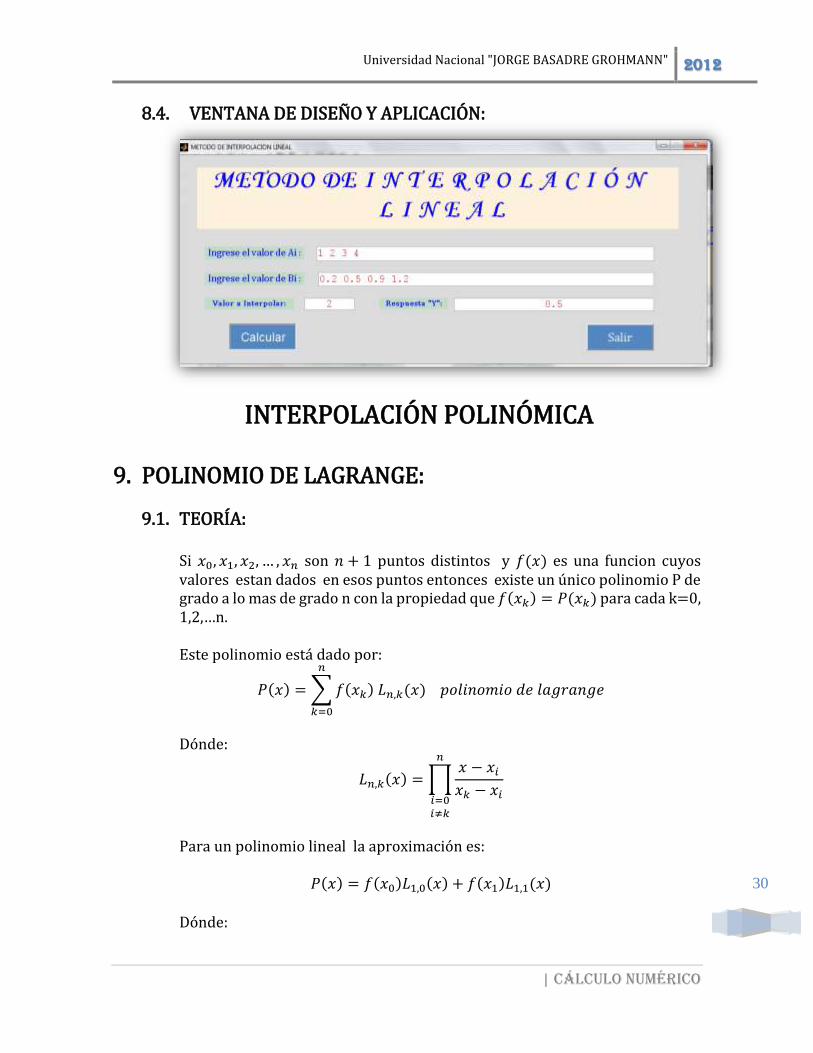
8.4. VENTANA DE DISEÑO Y APLICACIÓN:
INTERPOLACIÓN POLINÓMICA
9. POLINOMIO DE LAGRANGE:
9.1. TEORÍA:
Si 𝑥0, 𝑥1, 𝑥2, … , 𝑥𝑛 son 𝑛 + 1 puntos distintos y 𝑓(𝑥) es una funcion cuyos valores estan dados en esos puntos entonces existe un único polinomio P de grado a lo mas de grado n con la propiedad que 𝑓(𝑥𝑘) = 𝑃(𝑥𝑘) para cada k=0, 1,2,…n. Este polinomio está dado por:
𝑃(𝑥) = ∑𝑓(𝑥𝑘) 𝐿𝑛,𝑘(𝑥) 𝑝𝑜𝑙𝑖𝑛𝑜𝑚𝑖𝑜 𝑑𝑒 𝑙𝑎𝑔𝑟𝑎𝑛𝑔𝑒
𝑛
𝑘=0
Dónde:
𝐿𝑛,𝑘(𝑥) =∏𝑥 − 𝑥𝑖𝑥𝑘 − 𝑥𝑖
𝑛
𝑖=0𝑖≠𝑘
Para un polinomio lineal la aproximación es:
𝑃(𝑥) = 𝑓(𝑥0)𝐿1,0(𝑥) + 𝑓(𝑥1)𝐿1,1(𝑥)
Dónde:
Universidad Nacional "JORGE BASADRE GROHMANN" 2012
| Cálculo numérico
31
𝐿1,0(𝑥) =𝑥 − 𝑥1𝑥0 − 𝑥1
; 𝐿1,1(𝑥) =𝑥 − 𝑥0𝑥1 − 𝑥0
Entonces:
𝑃(𝑥) = (𝑥 − 𝑥1𝑥0 − 𝑥1
)𝑓(𝑥0) + (𝑥 − 𝑥0𝑥1 − 𝑥0
) 𝑓(𝑥1)
Para un polinomio de segundo grado está dado por:
𝑃(𝑥) = 𝑓(𝑥0)𝐿2,0(𝑥) + 𝑓(𝑥1)𝐿2,1(𝑥) + 𝑓(𝑥2)𝐿2,2(𝑥)
Dónde:
𝐿1,0(𝑥) = (𝑥 − 𝑥1𝑥0 − 𝑥1
) (𝑥 − 𝑥2𝑥0 − 𝑥2
)
𝐿2,1(𝑥) = (𝑥 − 𝑥0𝑥1 − 𝑥0
) (𝑥 − 𝑥2𝑥1 − 𝑥2
)
𝐿2,2(𝑥) = (𝑥 − 𝑥0𝑥2 − 𝑥0
) (𝑥 − 𝑥1𝑥2 − 𝑥1
)
Entonces el polinomio para segundo grado es:
𝑃(𝑥) = (𝑥 − 𝑥1𝑥0 − 𝑥1
) (𝑥 − 𝑥2𝑥0 − 𝑥2
) 𝑓(𝑥0) + (𝑥 − 𝑥0𝑥1 − 𝑥0
) (𝑥 − 𝑥2𝑥1 − 𝑥2
) 𝑓(𝑥1) + (𝑥 − 𝑥0𝑥2 − 𝑥0
) (𝑥 − 𝑥1𝑥2 − 𝑥1
) 𝑓(𝑥2)
Donde x es el valor a interpolar.
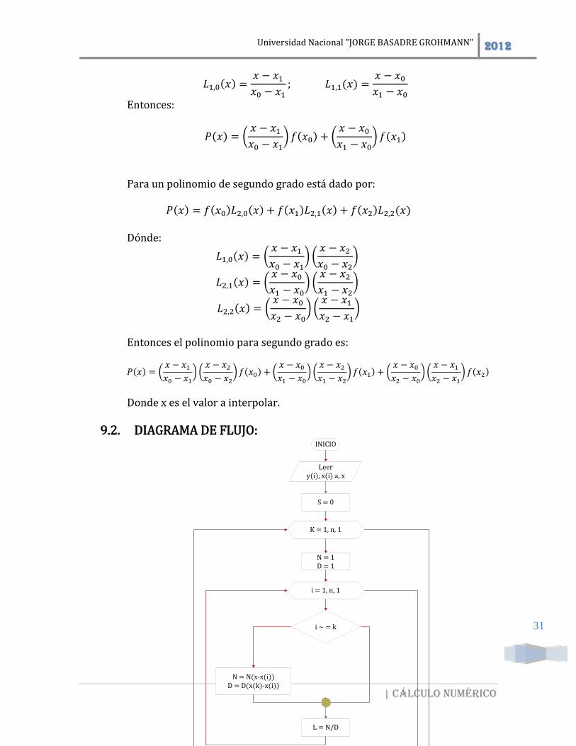
9.2. DIAGRAMA DE FLUJO:
INICIO
Leery(i), x(i) a, x
S = 0
K = 1, n, 1
N = 1D = 1
i = 1, n, 1
i ~ = k
N = N(x-x(i))D = D(x(k)-x(i))
L = N/D
S = S+L(x)*Y(k)
EscribirY0
FIN
Universidad Nacional "JORGE BASADRE GROHMANN" 2012
| Cálculo numérico
32
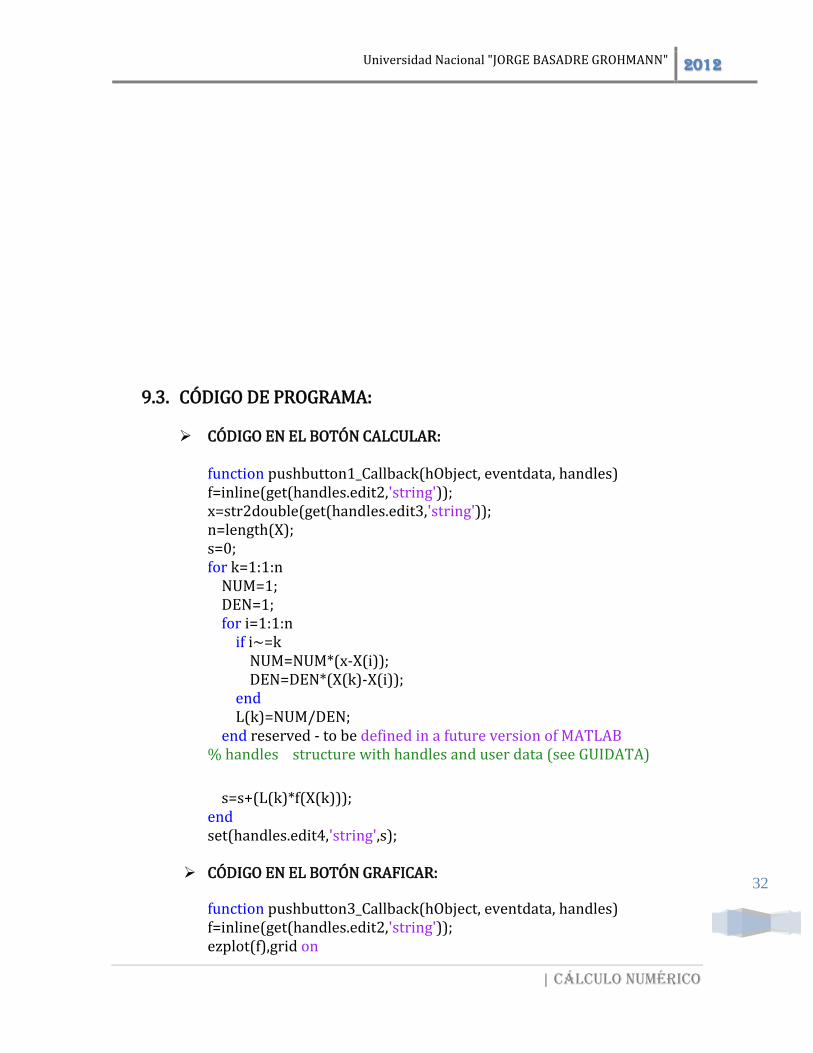
9.3. CÓDIGO DE PROGRAMA:
CÓDIGO EN EL BOTÓN CALCULAR:
function pushbutton1_Callback(hObject, eventdata, handles) f=inline(get(handles.edit2,'string')); x=str2double(get(handles.edit3,'string')); n=length(X); s=0; for k=1:1:n NUM=1; DEN=1; for i=1:1:n if i~=k NUM=NUM*(x-X(i)); DEN=DEN*(X(k)-X(i)); end L(k)=NUM/DEN; end reserved - to be defined in a future version of MATLAB % handles structure with handles and user data (see GUIDATA) s=s+(L(k)*f(X(k))); end set(handles.edit4,'string',s);
CÓDIGO EN EL BOTÓN GRAFICAR:
function pushbutton3_Callback(hObject, eventdata, handles) f=inline(get(handles.edit2,'string')); ezplot(f),grid on
Universidad Nacional "JORGE BASADRE GROHMANN" 2012
| Cálculo numérico
33
CÓDIGO EN EL BOTÓN SALIR:
function varargout = pushbutton3_Callback(h, eventdata, handles, varargin) close(polinomiolagrange)
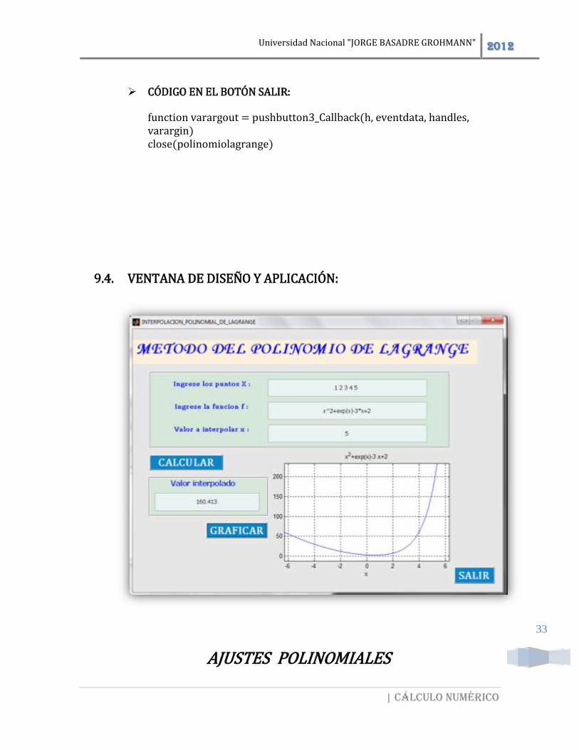
9.4. VENTANA DE DISEÑO Y APLICACIÓN:
AJUSTES POLINOMIALES
Universidad Nacional "JORGE BASADRE GROHMANN" 2012
| Cálculo numérico
34
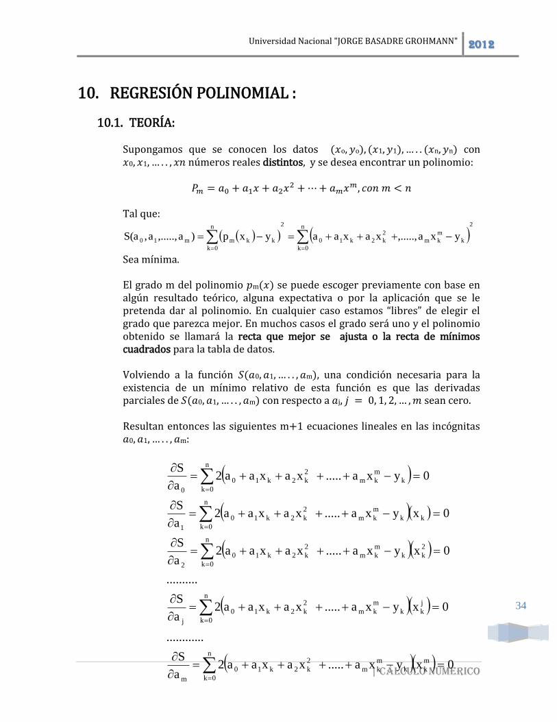
10. REGRESIÓN POLINOMIAL :
10.1. TEORÍA:
Supongamos que se conocen los datos (𝑥o, 𝑦o), (𝑥1, 𝑦1),… . . (𝑥n, 𝑦n) con 𝑥0, 𝑥1, … . . , 𝑥𝑛 números reales distintos, y se desea encontrar un polinomio:
𝑃𝑚 = 𝑎0 + 𝑎1𝑥 + 𝑎2𝑥2 +⋯+ 𝑎𝑚𝑥
𝑚, 𝑐𝑜𝑛 𝑚 < 𝑛 Tal que:
Sea mínima. El grado m del polinomio 𝑝m(𝑥) se puede escoger previamente con base en algún resultado teórico, alguna expectativa o por la aplicación que se le pretenda dar al polinomio. En cualquier caso estamos “libres” de elegir el grado que parezca mejor. En muchos casos el grado será uno y el polinomio obtenido se llamará la recta que mejor se ajusta o la recta de mínimos cuadrados para la tabla de datos. Volviendo a la función 𝑆(𝑎0, 𝑎1, … . . , 𝑎m), una condición necesaria para la existencia de un mínimo relativo de esta función es que las derivadas parciales de 𝑆(𝑎0, 𝑎1, … . . , 𝑎m) con respecto a 𝑎j, 𝑗 = 0, 1, 2, … ,𝑚 sean cero. Resultan entonces las siguientes m+1 ecuaciones lineales en las incógnitas 𝑎0, 𝑎1, … . . , 𝑎m:
2n
0k
k
m
km
2
k2k10
2n
0k
kkmm10 yxa,.....,xaxaayxp)a,.....,a,S(a
0xyxa.....xaxaa2a
S
............
0xyxa.....xaxaa2a
S
..........
0xyxa.....xaxaa2a
S
0xyxa.....xaxaa2a
S
0yxa.....xaxaa2a
S
m
kk
m
km
2
k2k10
n
0km
j
kk
m
km
2
k2k10
n
0kj
2
kk
m
km
2
k2k10
n
0k2
kk
m
km
2
k2k10
n
0k1
k
m
km
2
k2k10
n
0k0
Universidad Nacional "JORGE BASADRE GROHMANN" 2012
| Cálculo numérico
35
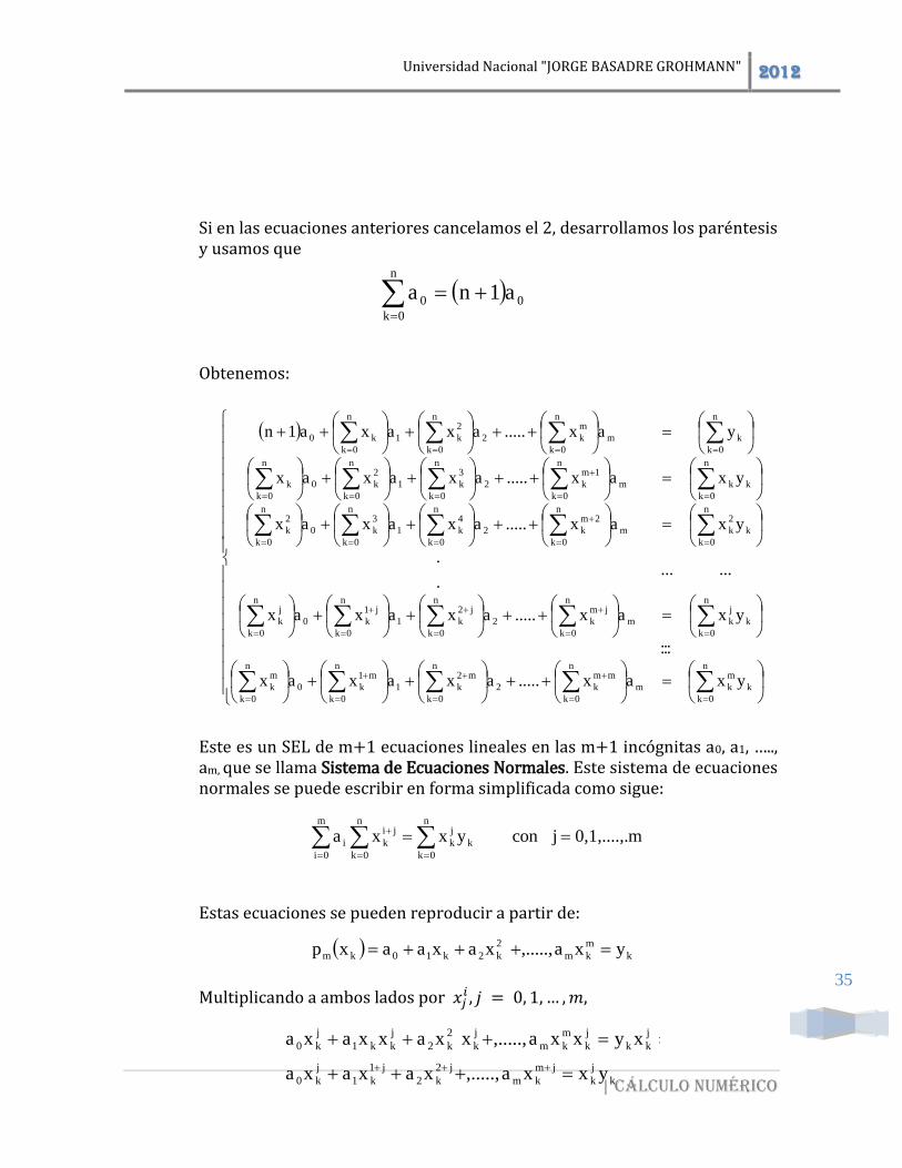
Si en las ecuaciones anteriores cancelamos el 2, desarrollamos los paréntesis y usamos que
Obtenemos:
Este es un SEL de m+1 ecuaciones lineales en las m+1 incógnitas a0, a1, ….., am, que se llama Sistema de Ecuaciones Normales. Este sistema de ecuaciones normales se puede escribir en forma simplificada como sigue:
Estas ecuaciones se pueden reproducir a partir de:
Multiplicando a ambos lados por 𝑥𝑗𝑖 , 𝑗 = 0, 1, … ,𝑚,
0
n
0k
0 a1na
n
0k
k
m
km
n
0k
mm
k2
n
0k
m2
k1
n
0k
m1
k0
n
0k
m
k
n
0k
k
j
km
n
0k
jm
k2
n
0k
j2
k1
n
0k
j1
k0
n
0k
j
k
n
0k
k
2
km
n
0k
2m
k2
n
0k
4
k1
n
0k
3
k0
n
0k
2
k
n
0k
kkm
n
0k
1m
k2
n
0k
3
k1
n
0k
2
k0
n
0k
k
n
0k
km
n
0k
m
k2
n
0k
2
k1
n
0k
k0
yxax.....axaxax
:::
yxax.....axaxax
.......
.
yxax.....axaxax
yxax.....axaxax
yax.....axaxa1n
m0,1,....,.jconyxxan
0k
k
j
k
n
0k
ji
k
m
0i
i
k
m
km
2
k2k10km yxa,.....,xaxaaxp
k
j
k
jm
km
j2
k2
j1
k1
j
k0
j
kk
j
k
m
km
j
k
2
k2
j
kk1
j
k0
yxxa,.....,xaxaxa
xyxxa,.....,xxaxxaxa
Universidad Nacional "JORGE BASADRE GROHMANN" 2012
| Cálculo numérico
36
Sumando sobre k
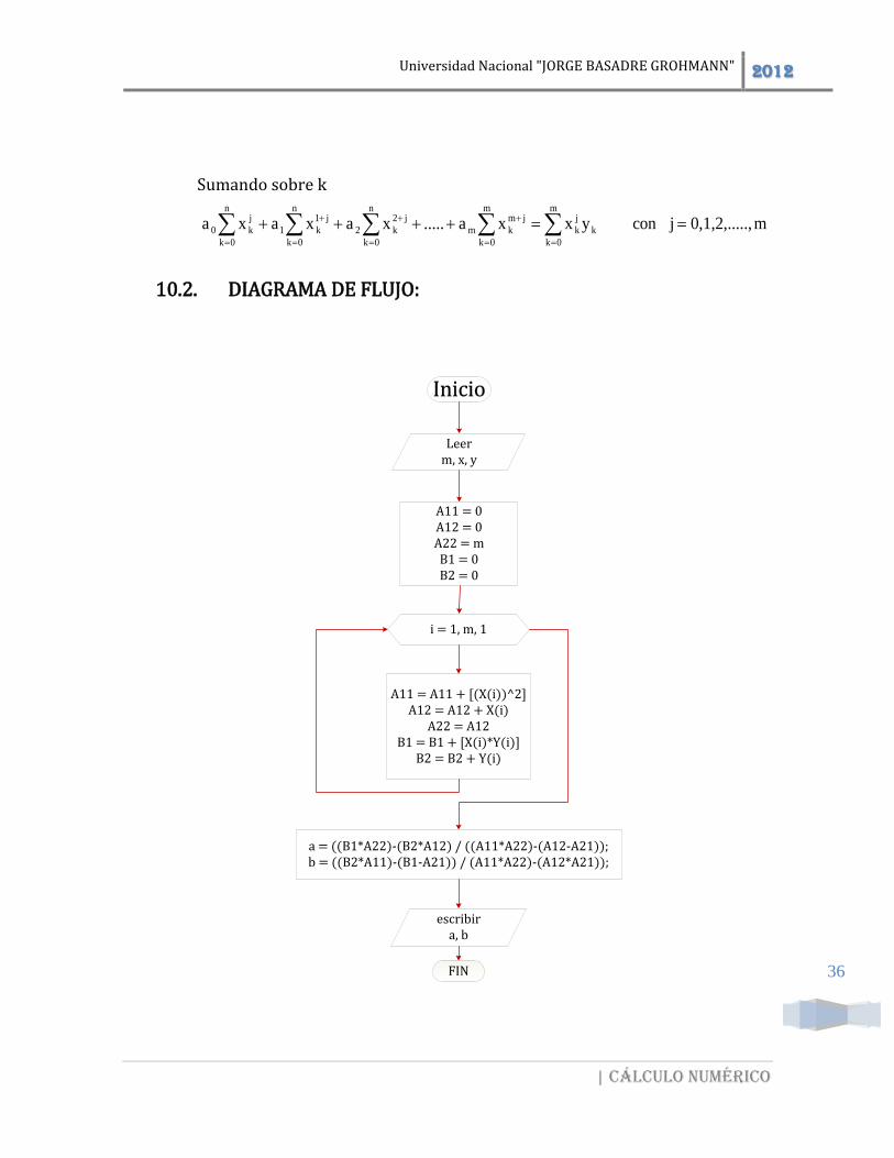
10.2. DIAGRAMA DE FLUJO:
m.,0,1,2,....jconyxxa.....xaxaxam
0k
k
j
k
m
0k
jm
km
n
0k
j2
k2
n
0k
j1
k1
n
0k
j
k0
Inicio
Leerm, x, y
A11 = 0A12 = 0A22 = mB1 = 0B2 = 0
i = 1, m, 1
A11 = A11 + [(X(i))^2]A12 = A12 + X(i)
A22 = A12B1 = B1 + [X(i)*Y(i)]
B2 = B2 + Y(i)
a = ((B1*A22)-(B2*A12) / ((A11*A22)-(A12-A21));b = ((B2*A11)-(B1-A21)) / (A11*A22)-(A12*A21));
escribira, b
FIN
Universidad Nacional "JORGE BASADRE GROHMANN" 2012
| Cálculo numérico
37
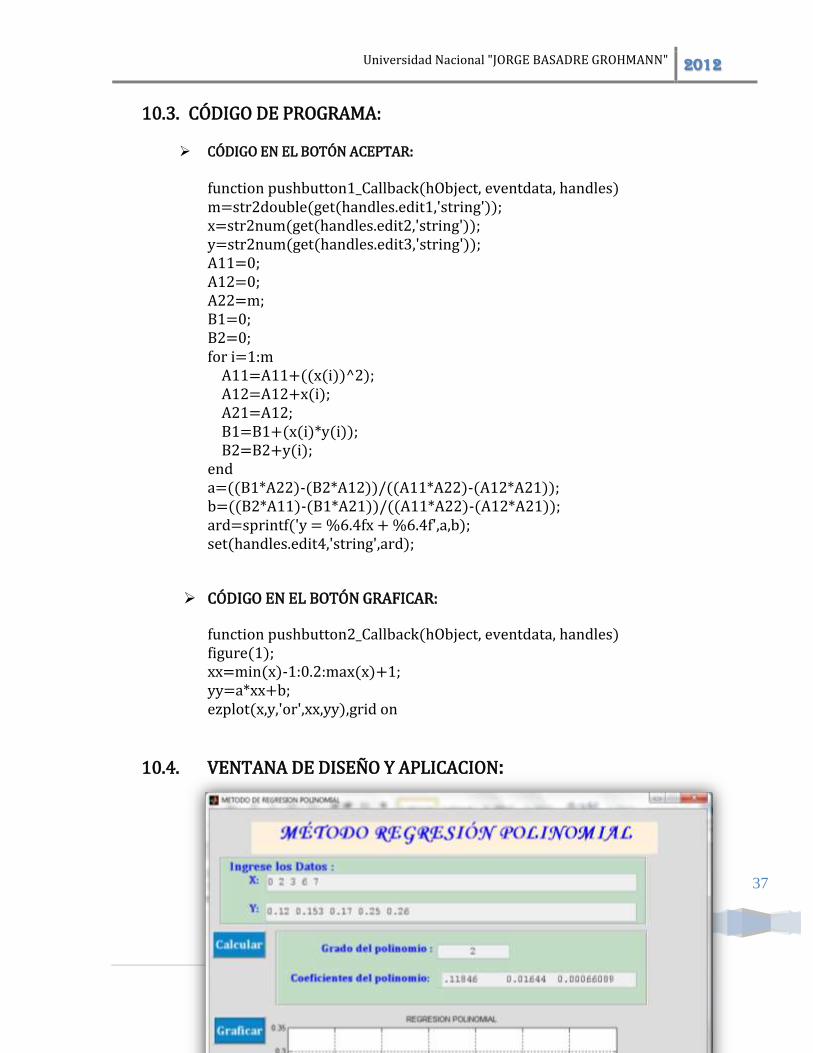
10.3. CÓDIGO DE PROGRAMA:
CÓDIGO EN EL BOTÓN ACEPTAR:
function pushbutton1_Callback(hObject, eventdata, handles) m=str2double(get(handles.edit1,'string')); x=str2num(get(handles.edit2,'string')); y=str2num(get(handles.edit3,'string')); A11=0; A12=0; A22=m; B1=0; B2=0; for i=1:m A11=A11+((x(i))^2); A12=A12+x(i); A21=A12; B1=B1+(x(i)*y(i)); B2=B2+y(i); end a=((B1*A22)-(B2*A12))/((A11*A22)-(A12*A21)); b=((B2*A11)-(B1*A21))/((A11*A22)-(A12*A21)); ard=sprintf('y = %6.4fx + %6.4f',a,b); set(handles.edit4,'string',ard);
CÓDIGO EN EL BOTÓN GRAFICAR:
function pushbutton2_Callback(hObject, eventdata, handles) figure(1); xx=min(x)-1:0.2:max(x)+1; yy=a*xx+b; ezplot(x,y,'or',xx,yy),grid on
10.4. VENTANA DE DISEÑO Y APLICACION:

Universidad Nacional "JORGE BASADRE GROHMANN" 2012
| Cálculo numérico
38
CAPITULO - III
INTEGRACIÓN NUMÉRICA
11. REGLA DEL TRAPECIO:
11.1. TEORÍA:
Este método resulta de sustituir la función 𝑦 = 𝑓(𝑥) por un polinomio de primer grado 𝑃(𝑥) = 𝑎0 + 𝑎1𝑥 en [𝑎, 𝑏] = [𝑥0, 𝑥1] al polinomio 𝑃(𝑥) se le puede representar mediante un polinomio 𝑃(𝑥) se le puede representar mediante un polinomio de Lagrange, es decir:
∫ 𝑓(𝑥)𝑑𝑥 =𝑏
𝑎
∫ 𝑃(𝑥)𝑑𝑥 =𝑥1
𝑥0
∫ [(𝑥 − 𝑥1)
(𝑥0 − 𝑥1)𝑓(𝑥0) +
(𝑥 − 𝑥0)
(𝑥1 − 𝑥0)𝑓(𝑥1)]
𝑥1
𝑥0
𝑑𝑥
Resolviendo:
∫ 𝑓(𝑥)𝑑𝑥 =𝑏
𝑎
ℎ
2[𝑓(𝑥0) − 𝑓(𝑥1)], 𝑑𝑜𝑛𝑑𝑒 ℎ = 𝑥1 − 𝑥0
Generalizando:
∫ 𝑓(𝑥)𝑑𝑥 +𝑏
𝑎
∫ 𝑓(𝑥)𝑑𝑥 + ∫ 𝑓(𝑥)𝑑𝑥 +⋯+∫ 𝑓(𝑥)𝑑𝑥 =𝑥1
𝑥0
∫ 𝑓(𝑥)𝑑𝑥𝑥𝑛
𝑥𝑛−1
𝑥2
𝑥1
𝑥1
𝑥0
Aplicando la regla del trapecio a c/u de las integrales se tiene:
Universidad Nacional "JORGE BASADRE GROHMANN" 2012
| Cálculo numérico
39
∫ 𝑓(𝑥)𝑑𝑥 = lim𝑛→∞
∑𝑓(𝑥𝑛)∆
𝑛
𝑘=1
𝑏
𝑎
𝑥𝑘
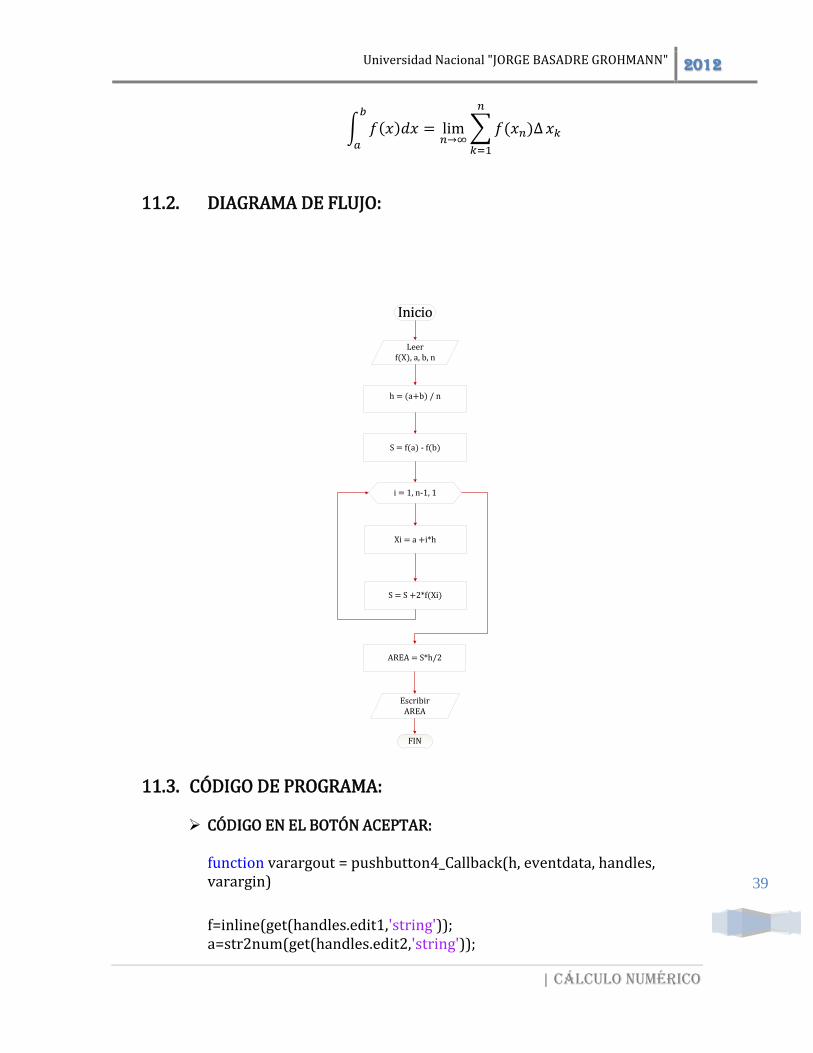
11.2. DIAGRAMA DE FLUJO:
11.3. CÓDIGO DE PROGRAMA: CÓDIGO EN EL BOTÓN ACEPTAR:
function varargout = pushbutton4_Callback(h, eventdata, handles, varargin) f=inline(get(handles.edit1,'string')); a=str2num(get(handles.edit2,'string'));
Inicio
Leerf(X), a, b, n
h = (a+b) / n
S = f(a) - f(b)
i = 1, n-1, 1
Xi = a +i*h
S = S +2*f(Xi)
AREA = S*h/2
EscribirAREA
FIN
Universidad Nacional "JORGE BASADRE GROHMANN" 2012
| Cálculo numérico
40
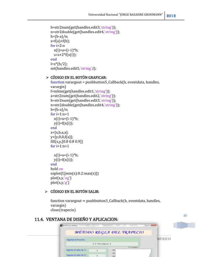
b=str2num(get(handles.edit3,'string')); n=str2double(get(handles.edit4,'string')); h=(b-a)/n; s=f(a)+f(b); for i=2:n x(i)=a+(i-1)*h; s=s+2*f(x(i)); end I=s*(h/2); set(handles.edit5,'string',I);
CÓDIGO EN EL BOTÓN GRAFICAR:
function varargout = pushbutton5_Callback(h, eventdata, handles, varargin) f=inline(get(handles.edit1,'string')); a=str2num(get(handles.edit2,'string')); b=str2num(get(handles.edit3,'string')); n=str2double(get(handles.edit4,'string')); h=(b-a)/n; for i=1:n+1 x(i)=a+(i-1)*h; y(i)=f(x(i)); end x=[x,b,a,a]; y=[y,0,0,f(a)]; fill(x,y,[0.8 0.8 0.9]) for i=1:n+1
x(i)=a+(i-1)*h; y(i)=f(x(i)); end hold on ezplot(f,[min(x):0.2:max(x)]) plot(x,y,'og') plot(x,y,'g')
CÓDIGO EN EL BOTÓN SALIR:
function varargout = pushbutton3_Callback(h, eventdata, handles, varargin) close(trapecio)
11.4. VENTANA DE DISEÑO Y APLICACION:
Universidad Nacional "JORGE BASADRE GROHMANN" 2012
| Cálculo numérico
41
12. REGLA DE SIMPSON 1/3:
12.1. TEORÍA:
La regla de Simpson de 1/3 resulta cuando se sustituye la función y=f(x) por un polinomio de segundo grado es decir:
∫ 𝑓(𝑥)𝑑𝑥 ≈𝑏
𝑎
∫ 𝑃(𝑥)𝑑𝑥 𝑑𝑜𝑛𝑑𝑒 𝑏
𝑎
𝑃(𝑥) = 𝑎0 + 𝑎1𝑥 + 𝑎2𝑥2
En el intervalo [𝑎, 𝑏] = [𝑥0, 𝑥2] al polinomio 𝑃(𝑥) se le puede representar por un polinomio de LaGrange de segundo orden Es decir:
∫ 𝑓(𝑥)𝑑𝑥 ≈𝑏
𝑎
∫ [𝑓(𝑥0)𝐿2,0(𝑥) + 𝑓(𝑥1)𝐿2,1(𝑥) + 𝑓(𝑥2)𝐿2,2(𝑥)]𝑑𝑥𝑏
𝑎
∫ 𝑓(𝑥)𝑑𝑥 ≈𝑏
𝑎
∫ [(𝑥 − 𝑥1𝑥0 − 𝑥1
) (𝑥 − 𝑥2𝑥0 − 𝑥2
) 𝑓(𝑥0) + (𝑥 − 𝑥0𝑥1 − 𝑥0
) (𝑥 − 𝑥2𝑥1 − 𝑥2
) 𝑓(𝑥1) + (𝑥 − 𝑥0𝑥2 − 𝑥0
) (𝑥 − 𝑥1𝑥2 − 𝑥1
) 𝑓(𝑥2)] 𝑑𝑥𝑥1
𝑥0
Resolviendo la integral se obtiene:
∫ 𝑓(𝑥)𝑑𝑥 ≈𝑏
𝑎
ℎ
3[𝑓(𝑥0) + 4𝑓(𝑥1) + 𝑓(𝑥2)], 𝑑𝑜𝑛𝑑𝑒 ℎ =
𝑥2 − 𝑥02
GENERALIZANDO PARA ''n'' INTERVALOS Los intervalos se toman de dos en dos:
∫ 𝑓(𝑥)𝑑𝑥 =𝑏
𝑎
∫ 𝑓(𝑥)𝑑𝑥𝑥2
𝑥0
+∫ 𝑓(𝑥)𝑑𝑥𝑥4
𝑥2
+∫ 𝑓(𝑥)𝑑𝑥𝑥6
𝑥4
+⋯+∫ 𝑓(𝑥)𝑑𝑥𝑥𝑛
𝑥𝑛−2
Aplicando la regla de Simpson de 1/3 para cada integral de tiene:
Universidad Nacional "JORGE BASADRE GROHMANN" 2012
| Cálculo numérico
42
∫ 𝑓(𝑥)𝑑𝑥 ≈𝑏
𝑎
ℎ
3[𝑓(𝑥0) + 4𝑓(𝑥1) + 2𝑓(𝑥2) + 4𝑓(𝑥3) + 2𝑓(𝑥4) + ⋯+ 2𝑓(𝑥𝑛−2) + 4𝑓(𝑥𝑛−1) + 𝑓(𝑥𝑛)]
Dónde:
ℎ =𝑏 − 𝑎
𝑛=𝑥𝑛 − 𝑥0𝑛
; 𝑑𝑜𝑛𝑑𝑒 𝑛 𝑒𝑠 𝑚𝑢𝑙𝑡𝑖𝑝𝑙𝑜 𝑑𝑒 2
𝑥𝑖 = 𝑥0 + 𝑖ℎ; 𝑖 = 1,2,3…𝑛
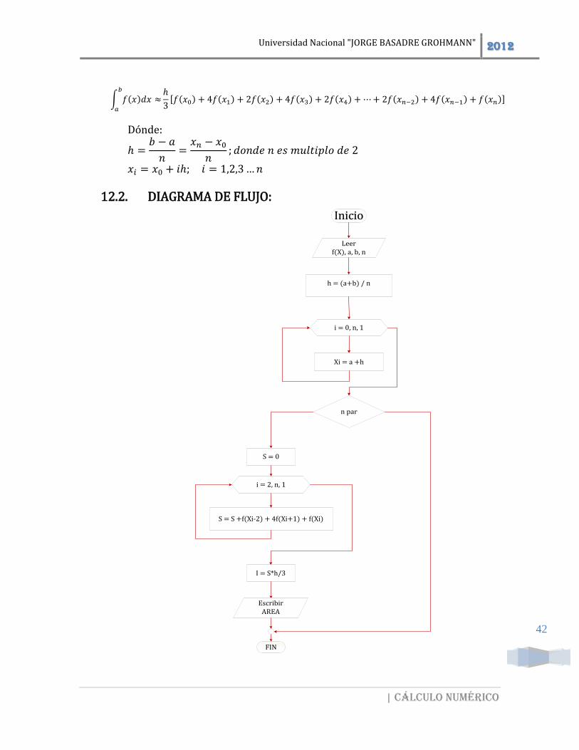
12.2. DIAGRAMA DE FLUJO:
Inicio
Leerf(X), a, b, n
h = (a+b) / n
i = 0, n, 1
Xi = a +h
n par
S = 0
i = 2, n, 1
S = S +f(Xi-2) + 4f(Xi+1) + f(Xi)
I = S*h/3
EscribirAREA
FIN
Universidad Nacional "JORGE BASADRE GROHMANN" 2012
| Cálculo numérico
43
12.3. CÓDIGO DE PROGRAMA:
CÓDIGO EN EL BOTÓN CALCULAR: function varargout = pushbutton1_Callback(h, eventdata, handles, varargin) f=inline(get(handles.edit1,'string')); a=str2double(get(handles.edit2,'string')); b=str2double(get(handles.edit3,'string')); n=str2double(get(handles.edit4,'string')); h=(b-a)/n; for i=1:n+1 x(i)=a+(i-1)*h; end if rem(n,2)==0 s=0; for i=3:2:n+1 s=s+f(x(i-2))+4*f(x(i-1))+f(x(i)) end I=(h/3)*s set(handles.edit5,'string',I); end
CÓDIGO EN EL BOTÓN GRAFICAR:
function varargout = pushbutton2_Callback(h, eventdata, handles, varargin) f=inline(get(handles.edit1,'string')); a=str2double(get(handles.edit2,'string')); b=str2double(get(handles.edit3,'string')); n=str2double(get(handles.edit4,'string')); h=(b-a)/n; s=f(a)+f(b); for i=1:n+1 x(i)=a+((i-1)*h); y(i)=f(x(i)); end x=[x,b,a,a]; y=[y,0,0,f(a)]; fill(x,y,[0.8 0.4 0.9]) for i=1:n+1 x(i)=a+((i-1)*h); y(i)=f(x(i)); line([x(i),x(i)],[0,f(x(i))]); end hold on
Universidad Nacional "JORGE BASADRE GROHMANN" 2012
| Cálculo numérico
44
ezplot(f,[min(x):0.2:max(x)])
CÓDIGO EN EL BOTÓN SALIR: function varargout = pushbutton3_Callback(h, eventdata, handles, varargin) close(sinpson1/3)
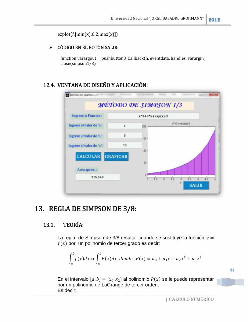
12.4. VENTANA DE DISEÑO Y APLICACIÓN:
13. REGLA DE SIMPSON DE 3/8: 13.1. TEORÍA:
La regla de Simpson de 3/8 resulta cuando se sustituye la función 𝑦 =𝑓(𝑥) por un polinomio de tercer grado es decir:
∫ 𝑓(𝑥)𝑑𝑥 ≈𝑏
𝑎
∫ 𝑃(𝑥)𝑑𝑥 𝑑𝑜𝑛𝑑𝑒 𝑏
𝑎
𝑃(𝑥) = 𝑎0 + 𝑎1𝑥 + 𝑎2𝑥2 + 𝑎3𝑥
3
En el intervalo [𝑎, 𝑏] = [𝑥0, 𝑥2] al polinomio 𝑃(𝑥) se le puede representar por un polinomio de LaGrange de tercer orden. Es decir:
Universidad Nacional "JORGE BASADRE GROHMANN" 2012
| Cálculo numérico
45
∫ 𝑓(𝑥)𝑑𝑥 ≈𝑏
𝑎
∫ [𝑓(𝑥0)𝐿3,0(𝑥) + 𝑓(𝑥1)𝐿3,1(𝑥) + 𝑓(𝑥2)𝐿3,2(𝑥) + 𝑓(𝑥3)𝐿3,3(𝑥)]𝑑𝑥𝑏=𝑥3
𝑎=𝑥0
Resolviendo la integral se obtiene:
∫ 𝐟(𝐱)𝐝𝐱 ≈𝐛
𝐚
𝟑𝐡
𝟖[𝐟(𝐱𝟎) + 𝟑𝐟(𝐱𝟏) + 𝟑𝐟(𝐱𝟐) + 𝐟(𝐱𝟑)], 𝐝𝐨𝐧𝐝𝐞 𝐡 =
𝐱𝟐 − 𝐱𝟎𝟑
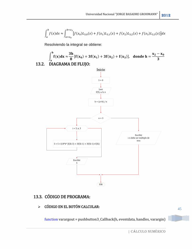
13.2. DIAGRAMA DE FLUJO:
13.3. CÓDIGO DE PROGRAMA:
CÓDIGO EN EL BOTÓN CALCULAR:
function varargout = pushbutton3_Callback(h, eventdata, handles, varargin)
Inicio
Leerf(X), a, b, n
S = 0
h = (a+b) / n
n = 3
i = 3, n, 3
S = S +3/8*h* [f(Xi-3) + 3f(Xi-1) + 3f(Xi-1)+f(Xi)
EscribirS
Escribir« n debe ser múltiplo de
tres
FIN
Universidad Nacional "JORGE BASADRE GROHMANN" 2012
| Cálculo numérico
46
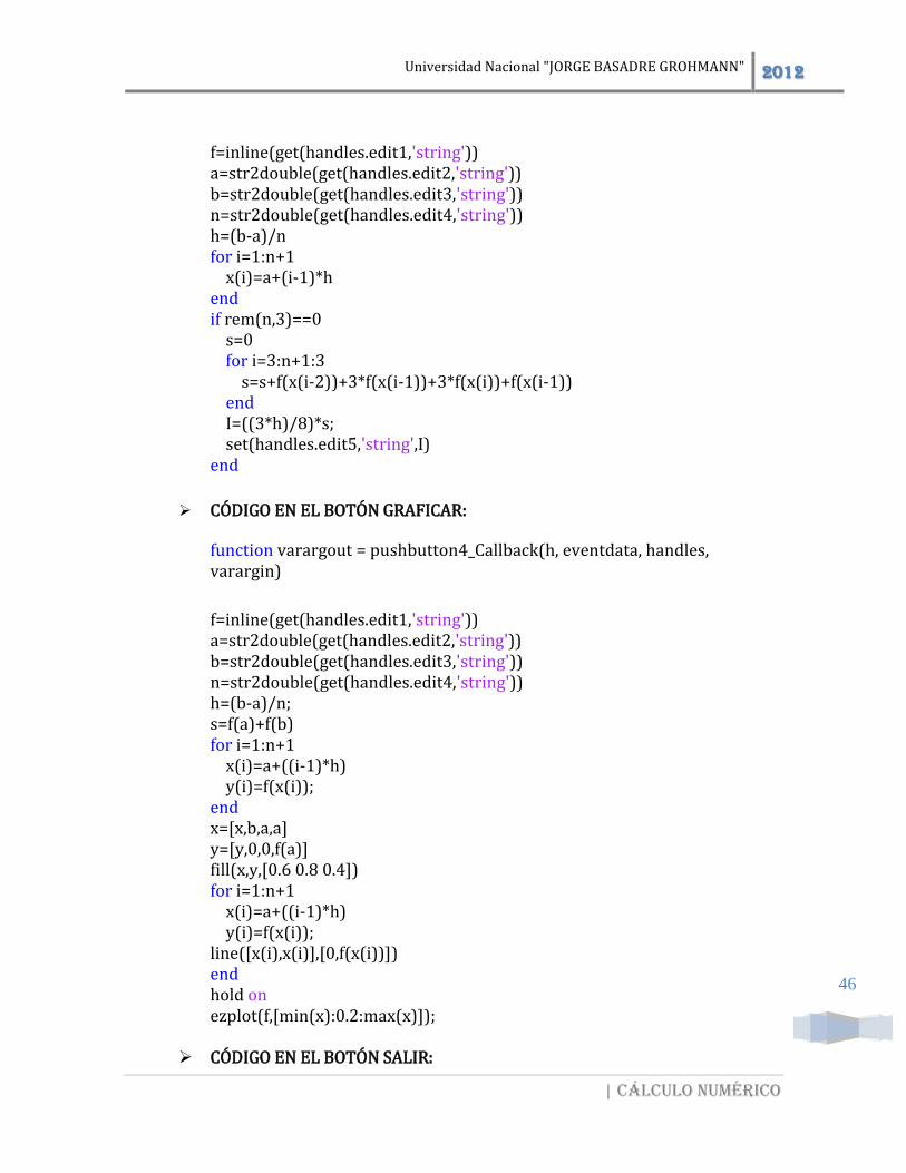
f=inline(get(handles.edit1,'string')) a=str2double(get(handles.edit2,'string')) b=str2double(get(handles.edit3,'string')) n=str2double(get(handles.edit4,'string')) h=(b-a)/n for i=1:n+1 x(i)=a+(i-1)*h end if rem(n,3)==0 s=0 for i=3:n+1:3 s=s+f(x(i-2))+3*f(x(i-1))+3*f(x(i))+f(x(i-1)) end I=((3*h)/8)*s; set(handles.edit5,'string',I) end
CÓDIGO EN EL BOTÓN GRAFICAR:
function varargout = pushbutton4_Callback(h, eventdata, handles, varargin) f=inline(get(handles.edit1,'string')) a=str2double(get(handles.edit2,'string')) b=str2double(get(handles.edit3,'string')) n=str2double(get(handles.edit4,'string')) h=(b-a)/n; s=f(a)+f(b) for i=1:n+1 x(i)=a+((i-1)*h) y(i)=f(x(i)); end x=[x,b,a,a] y=[y,0,0,f(a)] fill(x,y,[0.6 0.8 0.4]) for i=1:n+1 x(i)=a+((i-1)*h) y(i)=f(x(i)); line([x(i),x(i)],[0,f(x(i))]) end hold on ezplot(f,[min(x):0.2:max(x)]);
CÓDIGO EN EL BOTÓN SALIR:
Universidad Nacional "JORGE BASADRE GROHMANN" 2012
| Cálculo numérico
47
function pushbutton5_Callback(hObject, eventdata, handles) close
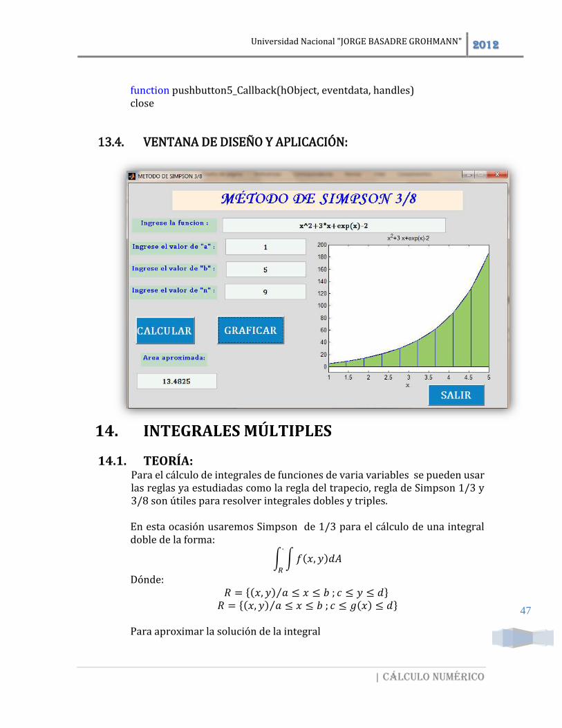
13.4. VENTANA DE DISEÑO Y APLICACIÓN:
14. INTEGRALES MÚLTIPLES
14.1. TEORÍA: Para el cálculo de integrales de funciones de varia variables se pueden usar las reglas ya estudiadas como la regla del trapecio, regla de Simpson 1/3 y 3/8 son útiles para resolver integrales dobles y triples. En esta ocasión usaremos Simpson de 1/3 para el cálculo de una integral doble de la forma:
∫ ∫𝑓(𝑥, 𝑦)𝑑𝐴.
𝑅
Dónde: 𝑅 = {(𝑥, 𝑦) 𝑎 ≤ 𝑥 ≤ 𝑏 ; 𝑐 ≤ 𝑦 ≤ 𝑑⁄ } 𝑅 = {(𝑥, 𝑦) 𝑎 ≤ 𝑥 ≤ 𝑏 ; 𝑐 ≤ 𝑔(𝑥) ≤ 𝑑⁄ }
Para aproximar la solución de la integral
Universidad Nacional "JORGE BASADRE GROHMANN" 2012
| Cálculo numérico
48
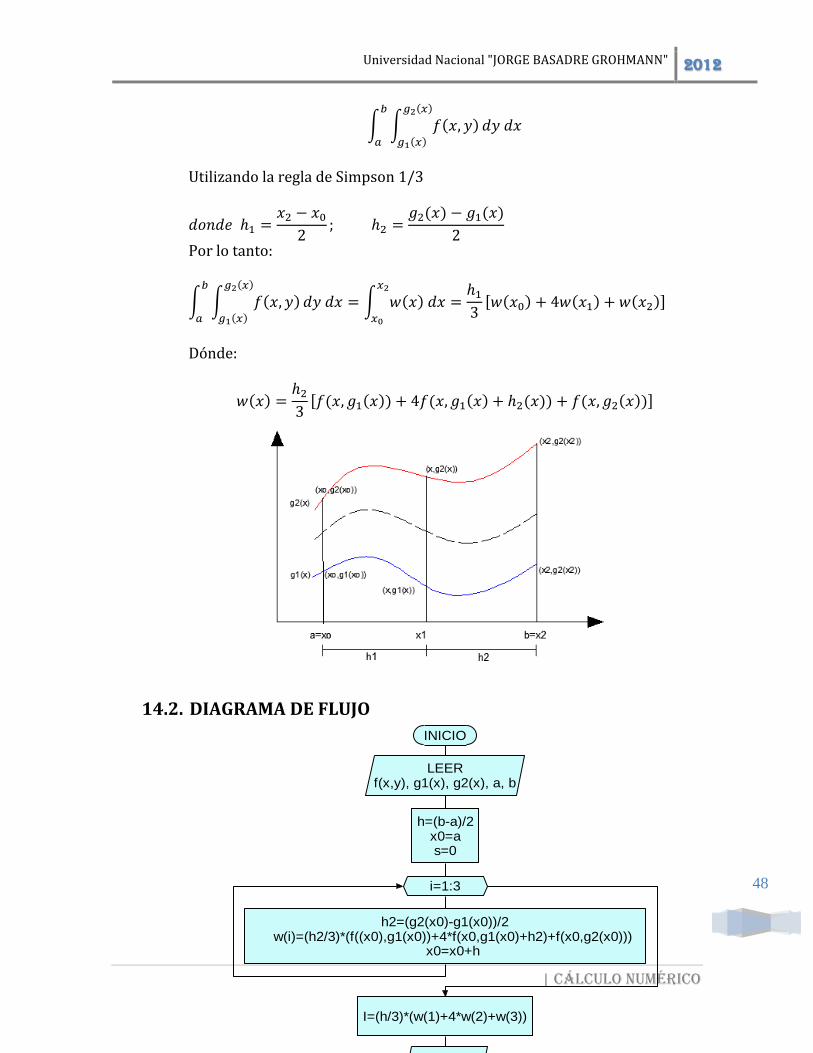
∫ ∫ 𝑓(𝑥, 𝑦)𝑔2(𝑥)
𝑔1(𝑥)
𝑑𝑦 𝑑𝑥𝑏
𝑎
Utilizando la regla de Simpson 1/3
𝑑𝑜𝑛𝑑𝑒 ℎ1 =𝑥2 − 𝑥02
; ℎ2 =𝑔2(𝑥) − 𝑔1(𝑥)
2
Por lo tanto:
∫ ∫ 𝑓(𝑥, 𝑦)𝑔2(𝑥)
𝑔1(𝑥)
𝑑𝑦 𝑑𝑥𝑏
𝑎
= ∫ 𝑤(𝑥) 𝑑𝑥𝑥2
𝑥0
=ℎ13[𝑤(𝑥0) + 4𝑤(𝑥1) + 𝑤(𝑥2)]
Dónde:
𝑤(𝑥) =ℎ23[𝑓(𝑥, 𝑔1(𝑥)) + 4𝑓(𝑥, 𝑔1(𝑥) + ℎ2(𝑥)) + 𝑓(𝑥, 𝑔2(𝑥))]
14.2. DIAGRAMA DE FLUJO
INICIO
LEERf(x,y), g1(x), g2(x), a, b
h=(b-a)/2x0=as=0
i=1:3
h2=(g2(x0)-g1(x0))/2 w(i)=(h2/3)*(f((x0),g1(x0))+4*f(x0,g1(x0)+h2)+f(x0,g2(x0)))
x0=x0+h
I=(h/3)*(w(1)+4*w(2)+w(3))
ESCRIBIRI
FIN
Universidad Nacional "JORGE BASADRE GROHMANN" 2012
| Cálculo numérico
49
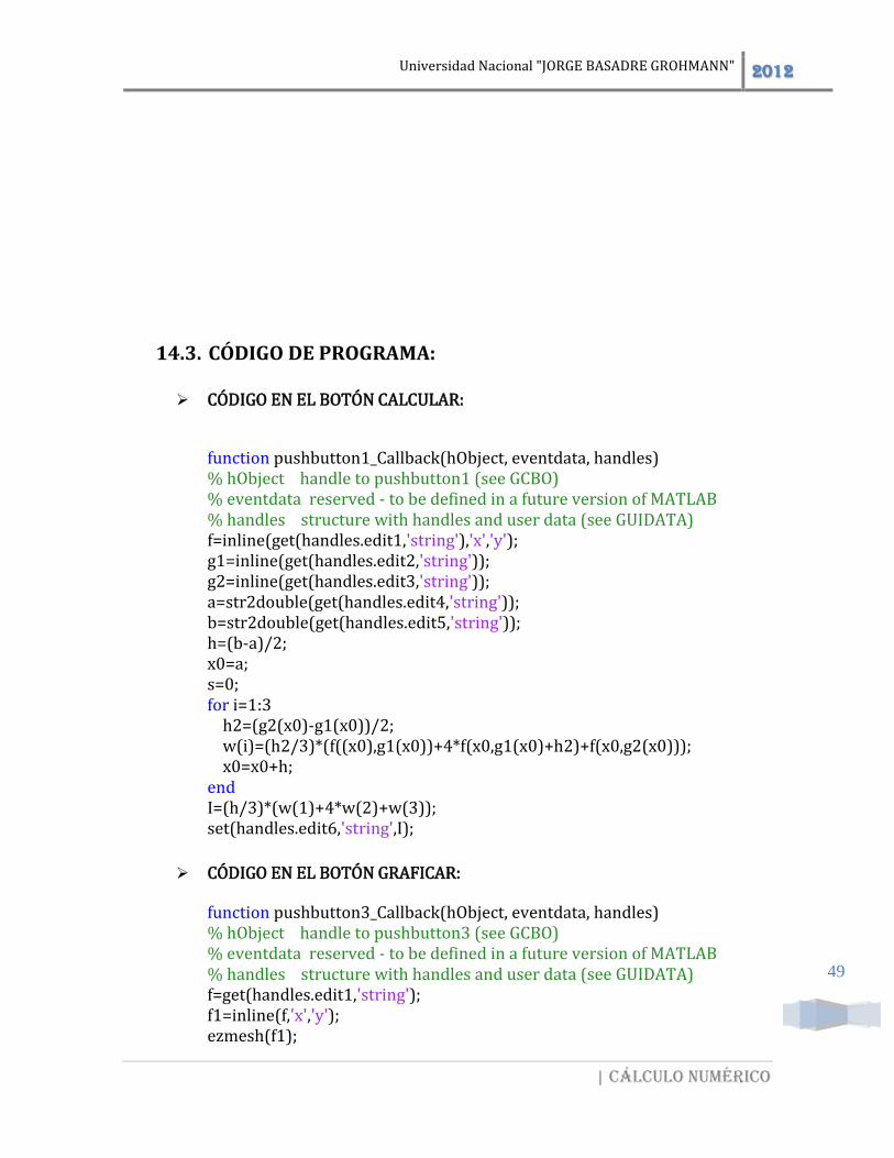
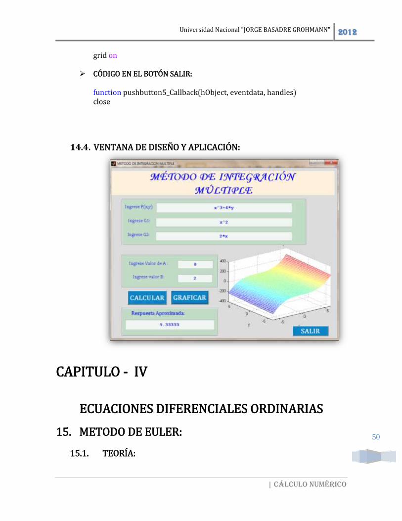
14.3. CÓDIGO DE PROGRAMA:
CÓDIGO EN EL BOTÓN CALCULAR:
function pushbutton1_Callback(hObject, eventdata, handles) % hObject handle to pushbutton1 (see GCBO) % eventdata reserved - to be defined in a future version of MATLAB % handles structure with handles and user data (see GUIDATA) f=inline(get(handles.edit1,'string'),'x','y'); g1=inline(get(handles.edit2,'string')); g2=inline(get(handles.edit3,'string')); a=str2double(get(handles.edit4,'string')); b=str2double(get(handles.edit5,'string')); h=(b-a)/2; x0=a; s=0; for i=1:3 h2=(g2(x0)-g1(x0))/2; w(i)=(h2/3)*(f((x0),g1(x0))+4*f(x0,g1(x0)+h2)+f(x0,g2(x0))); x0=x0+h; end I=(h/3)*(w(1)+4*w(2)+w(3)); set(handles.edit6,'string',I);
CÓDIGO EN EL BOTÓN GRAFICAR:
function pushbutton3_Callback(hObject, eventdata, handles) % hObject handle to pushbutton3 (see GCBO) % eventdata reserved - to be defined in a future version of MATLAB % handles structure with handles and user data (see GUIDATA) f=get(handles.edit1,'string'); f1=inline(f,'x','y'); ezmesh(f1);
Universidad Nacional "JORGE BASADRE GROHMANN" 2012
| Cálculo numérico
50
grid on
CÓDIGO EN EL BOTÓN SALIR:
function pushbutton5_Callback(hObject, eventdata, handles) close
14.4. VENTANA DE DISEÑO Y APLICACIÓN:
CAPITULO - IV
ECUACIONES DIFERENCIALES ORDINARIAS
15. METODO DE EULER:
15.1. TEORÍA:
Universidad Nacional "JORGE BASADRE GROHMANN" 2012
| Cálculo numérico
51
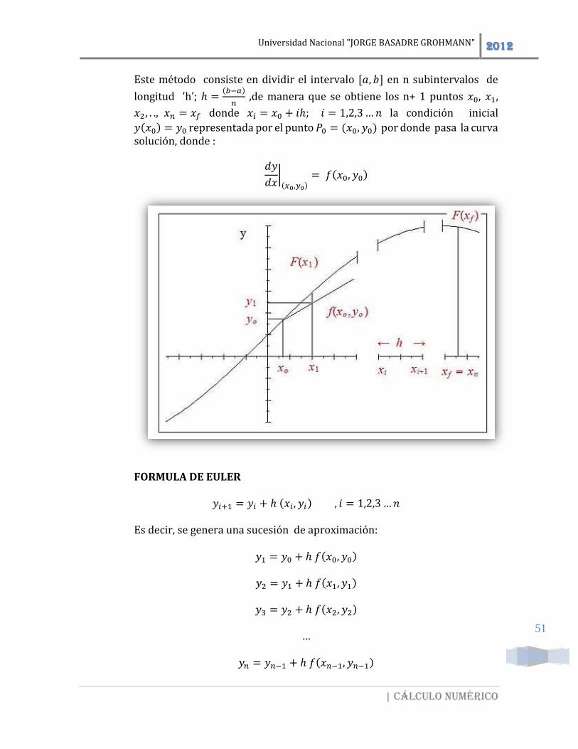
Este método consiste en dividir el intervalo [𝑎, 𝑏] en n subintervalos de
longitud 'h'; ℎ =(𝑏−𝑎)
𝑛 ,de manera que se obtiene los n+ 1 puntos 𝑥0, 𝑥1,
𝑥2, . ., 𝑥𝑛 = 𝑥𝑓 donde 𝑥𝑖 = 𝑥0 + 𝑖ℎ; 𝑖 = 1,2,3…𝑛 la condición inicial
𝑦(𝑥0) = 𝑦0 representada por el punto 𝑃0 = (𝑥0, 𝑦0) por donde pasa la curva solución, donde :
𝑑𝑦
𝑑𝑥|(𝑥0,𝑦0)
= 𝑓(𝑥0, 𝑦0)
FORMULA DE EULER
𝑦𝑖+1 = 𝑦𝑖 + ℎ (𝑥𝑖, 𝑦𝑖) , 𝑖 = 1,2,3…𝑛
Es decir, se genera una sucesión de aproximación:
𝑦1 = 𝑦0 + ℎ 𝑓(𝑥0, 𝑦0)
𝑦2 = 𝑦1 + ℎ 𝑓(𝑥1, 𝑦1)
𝑦3 = 𝑦2 + ℎ 𝑓(𝑥2, 𝑦2)
…
𝑦𝑛 = 𝑦𝑛−1 + ℎ 𝑓(𝑥𝑛−1, 𝑦𝑛−1)
Universidad Nacional "JORGE BASADRE GROHMANN" 2012
| Cálculo numérico
52
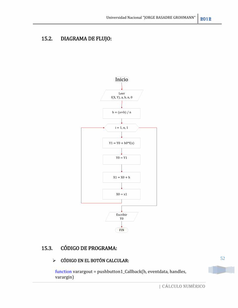
15.2. DIAGRAMA DE FLUJO:
15.3. CÓDIGO DE PROGRAMA:
CÓDIGO EN EL BOTÓN CALCULAR:
function varargout = pushbutton1_Callback(h, eventdata, handles, varargin)
Inicio
Leerf(X, Y), a, b, n, 0
h = (a+b) / n
i = 1, n, 1
Y1 = Y0 + h0*f(x)
Y0 = Y1
X1 = X0 + h
X0 = x1
EscribirY0
FIN
Universidad Nacional "JORGE BASADRE GROHMANN" 2012
| Cálculo numérico
53
f1=get(handles.edit1,'string'); f=inline(f1,'x','y'); x0=str2double(get(handles.edit2,'string')); y0=str2double(get(handles.edit3,'string')); n=str2double(get(handles.edit4,'string')); b=str2double(get(handles.edit5,'string')); h=(b-x0)/n; for i=1:n y0=y0+h*f(x0,y0); x0=x0+h; end set(handles.edit6,'string',y0);
CÓDIGO EN EL BOTÓN ITERACIONES:
function varargout = pushbutton6_Callback(h, eventdata, handles, varargin) f1=get(handles.edit1,'string'); f=inline(f1,'x','y'); x(1)=str2double(get(handles.edit2,'string')); y(1)=str2double(get(handles.edit3,'string')); n=str2double(get(handles.edit4,'string')); b=str2double(get(handles.edit5,'string')); h=(b-x(1))/n; cad1=sprintf('Iter. x %d. %8.4f %8.4f\n',1,x(1),y(1)); for i=1:n y(i+1)=y(i)+h*f(x(i),y(i)); x(i+1)=x(i)+h; cad2=sprintf('%d. %8.4f %8.4f\n',i+1,x(i+1),y(i+1)); cad1=[cad1,cad2]; end set(handles.edit7,'string',cad1);
CÓDIGO EN EL BOTÓN GRAFICAR:
function varargout = pushbutton2_Callback(h, eventdata, handles, varargin) f1=get(handles.edit1,'string'); f=inline(f1,'x','y'); ezmesh(f);
Universidad Nacional "JORGE BASADRE GROHMANN" 2012
| Cálculo numérico
54
grid on
CÓDIGO EN EL BOTÓN SALIR: function pushbutton7_Callback(hObject, eventdata, handles) close
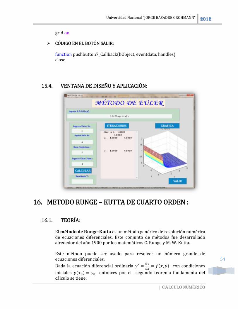
15.4. VENTANA DE DISEÑO Y APLICACIÓN:
16. METODO RUNGE – KUTTA DE CUARTO ORDEN :
16.1. TEORÍA:
El método de Runge-Kutta es un método genérico de resolución numérica de ecuaciones diferenciales. Este conjunto de métodos fue desarrollado alrededor del año 1900 por los matemáticos C. Runge y M. W. Kutta.
Este método puede ser usado para resolver un número grande de ecuaciones diferenciales.
Dada la ecuación diferencial ordinaria 𝑦′ =𝑑𝑦
𝑑𝑥= 𝑓(𝑥, 𝑦) con condiciones
iniciales 𝑦(𝑥0) = 𝑦0 entonces por el segundo teorema fundamenta del cálculo se tiene:
Universidad Nacional "JORGE BASADRE GROHMANN" 2012
| Cálculo numérico
55
∫ 𝑦′𝑑𝑥 = 𝑦(𝑥𝑛+1
𝑥𝑛
𝑥𝑛+1) − 𝑦(𝑥𝑛)
Para aplicar la regla de Simpson de 1/3 a [𝑥𝑛, 𝑥𝑛+1] se le dividió en dos intervalos es decir: Entonces
∫ 𝑦′𝑑𝑥 =𝑥𝑛+1
𝑥𝑛
ℎ/2
3[𝑦′(𝑥𝑛) + 4𝑦
′ (𝑥𝑛 +ℎ
2) + 𝑦′(𝑥𝑛+1)]
Al término 4𝑦′ (𝑥𝑛 +ℎ
2) se le expresa como: 2𝑦′ (𝑥𝑛 +
ℎ
2) + 2𝑦′ (𝑥𝑛 +
ℎ
2)
para aproximar la pendiente de 𝑦′ (𝑥𝑛 +ℎ
2) en el punto promedio (𝑥𝑛 +
ℎ
2)
𝑦(𝑥𝑛+1) = 𝑦(𝑥𝑛) +ℎ
6[𝑦′(𝑥𝑛) + 2𝑦
′ (𝑥𝑛 +ℎ
2) + 2𝑦′ (𝑥𝑛 +
ℎ
2) + 𝑦′(𝑥𝑛+1)]
Pero 𝑦′ = 𝑓(𝑥𝑛, 𝑦𝑛)
Por EULER se tiene que: 𝑦(𝑥𝑛+1) = 𝑦(𝑥𝑛) + ℎ𝑓(𝑥𝑛, 𝑦𝑛) Hacemos cambios de variables: Hagamos 𝑘1 = 𝑦
′(𝑥𝑛) entonces 𝑘1 = 𝑓(𝑥𝑛, 𝑦𝑛)
Hagamos 𝑘2 = 𝑦′ (𝑥𝑛 +ℎ
2) entonces 𝑘2 = 𝑓 (𝑥𝑛 +
ℎ
2, 𝑦(𝑥𝑛 +
ℎ
2)) por
euler : 𝑦 (𝑥𝑛 +ℎ
2) = 𝑦(𝑥𝑛) +
ℎ
2𝑓(𝑥𝑛, 𝑦𝑛) entonces
𝑘2 = 𝑓 (𝑥𝑛 +ℎ
2, 𝑦𝑛 +
ℎ
2𝑘1)
Hagamos 𝑘3 = 𝑦′ (𝑥𝑛 +
ℎ
2) entonces 𝑘3 = 𝑓 (𝑥𝑛 +
ℎ
2, 𝑦(𝑥𝑛 +
ℎ
2)) por
euler 𝑦 (𝑥𝑛 +ℎ
2) = 𝑦(𝑥𝑛) +
ℎ
2𝑦′(𝑥𝑛, 𝑦𝑛) entonces:
𝑘3 = 𝑓 (𝑥𝑛 +ℎ
2, 𝑦𝑛 +
ℎ
2𝑘2)
Hagamos 𝑘4 = 𝑦′(𝑥𝑛 + 1) entonces 𝑘4 = 𝑓 (𝑥𝑛 +
ℎ
2, 𝑦(𝑥𝑛 +
ℎ
2)) por euler
𝑦(𝑥𝑛 + 1) = 𝑦(𝑥𝑛) + ℎ𝑦′ (𝑥𝑛 +
ℎ
2) entonces:
𝑘4 = 𝑓(𝑥𝑛 + 1, 𝑦0 + ℎ𝑘3) Por lo tanto:
𝑦(𝑥𝑛 + 1) = 𝑦𝑛 +ℎ
6[𝑘1 + 2𝑘2 + 3𝑘3 + 𝑘4]
Dónde:
ℎ =𝑥𝑛+1 − 𝑥𝑛
𝑚; 𝑚 𝑒𝑠 𝑒𝑙 𝑛𝑢𝑚𝑒𝑟𝑜 𝑑𝑒 𝑖𝑛𝑡𝑒𝑟𝑣𝑎𝑙𝑜𝑠.
Universidad Nacional "JORGE BASADRE GROHMANN" 2012
| Cálculo numérico
56
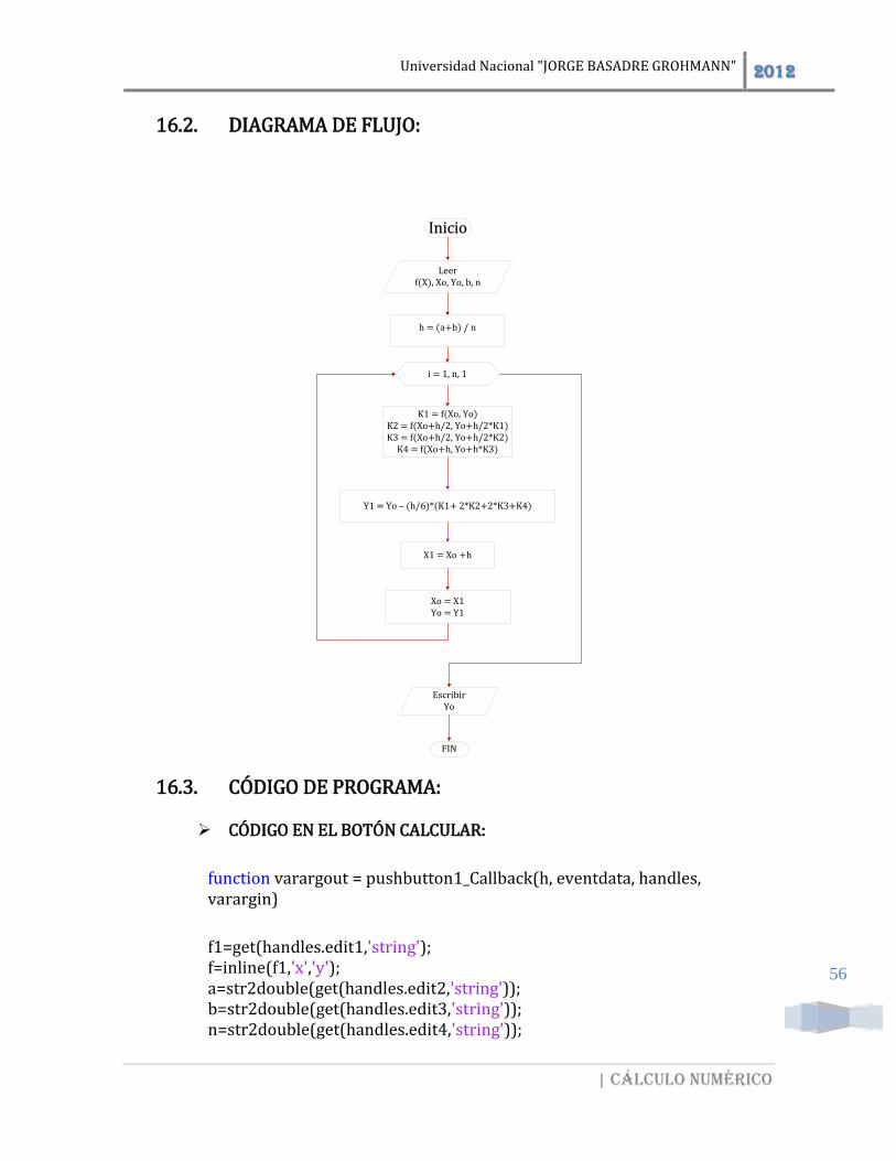
16.2. DIAGRAMA DE FLUJO:
16.3. CÓDIGO DE PROGRAMA:
CÓDIGO EN EL BOTÓN CALCULAR:
function varargout = pushbutton1_Callback(h, eventdata, handles, varargin) f1=get(handles.edit1,'string'); f=inline(f1,'x','y'); a=str2double(get(handles.edit2,'string')); b=str2double(get(handles.edit3,'string')); n=str2double(get(handles.edit4,'string'));
Inicio
Leerf(X), Xo, Yo, b, n
h = (a+b) / n
i = 1, n, 1
K1 = f(Xo, Yo)K2 = f(Xo+h/2, Yo+h/2*K1)K3 = f(Xo+h/2, Yo+h/2*K2)
K4 = f(Xo+h, Yo+h*K3)
Y1 = Yo – (h/6)*(K1+ 2*K2+2*K3+K4)
X1 = Xo +h
Xo = X1Yo = Y1
EscribirYo
FIN
Universidad Nacional "JORGE BASADRE GROHMANN" 2012
| Cálculo numérico
57
y0=str2double(get(handles.edit5,'string')); x0=a; h=(b-a)/n; for i=1:n k1=f(x0,y0); k2=f(x0+h/2,y0+(h/2)*k1); k3=f(x0+h/2,y0+(h/2)*k2); k4=f(x0+h,y0+h*k3); y1=y0+h*(k1+2*k2+2*k3+k4)/6; x1=x0+h; x0=x1; y0=y1; end set (handles.edit6,'string',y1);
CÓDIGO EN EL BOTÓN GRAFICAR:
function pushbutton6_Callback(hObject, eventdata, handles) f1=get(handles.edit1,'string'); f=inline(f1,'x','y'); ezmesh(f); grid on
CÓDIGO EN EL BOTÓN SALIR:
function varargout = pushbutton2_Callback(h, eventdata, handles, varargin) close(kutta1)
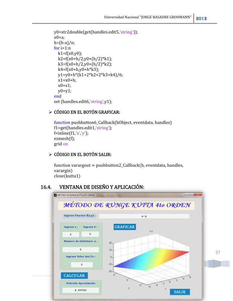
16.4. VENTANA DE DISEÑO Y APLICACIÓN: