TESI DOCTORAL - nlp.lsi.upc.edunlp.lsi.upc.edu/papers/thesis_javierrs.pdf · decisión, si lo que...
157
TESI DOCTORAL Decision Threshold Estimation and Model Quality Evaluation Techniques for Speaker Verification Author: Javier Rodríguez Saeta Director: Francisco Javier Hernando Pericás June 2005
Transcript of TESI DOCTORAL - nlp.lsi.upc.edunlp.lsi.upc.edu/papers/thesis_javierrs.pdf · decisión, si lo que...
TESI DOCTORAL
Decision Threshold Estimation and
Model Quality Evaluation Techniques
for Speaker Verification
Author: Javier Rodríguez Saeta
Director: Francisco Javier Hernando Pericás
June 2005

1
Resumen
El número de aplicaciones biométricas ha experimentado un auge espectacular en los
últimos años. La preocupación por la seguridad se hace cada vez más patente y es en este
contexto en donde el reconocimiento automático de personas por algunos de sus rasgos
característicos tales como huellas, caras, voz o iris, entre otros, juega un papel preponderante.
Cada vez son más los usuarios que demandan este tipo de aplicaciones en un momento en el
que la tecnología comienza a estar ya lo suficientemente madura.
Al mismo tiempo que se busca seguridad, bajo coste y precisión, otros factores relativos
a las aplicaciones biométricas comienzan a crecer paralelamente en importancia. El grado de
intrusividad es, sin duda, un valor en auge a la hora de decidir qué tecnología biométrica es la
más adecuada para la aplicación que se desea llevar a cabo. Y es entonces cuando el
reconocimiento de locutores se presenta como una elección atrayente, por la utilización de la
voz, el método natural de comunicación de las personas, por su capacidad de actuar de forma
remota y por su bajo coste.
El reconocimiento automático de locutores tiene una gran utilidad como método de
reconocimiento a través del teléfono aunque también puede utilizarse como aplicación de
control de acceso presencial o en el análisis forense.
En las aplicaciones de verificación e identificación de locutores pueden distinguirse
diversas etapas. En primer lugar nos encontramos con la fase de parametrización de la señal de
voz, en donde la señal se procesa para ser modelada o comparada. En segundo lugar tenemos la
etapa de aprendizaje de modelos, si se está realizando el entrenamiento, o bien la etapa de
decisión, si lo que se desea es obtener el resultado de una comparación.
Esta tesis doctoral se centra en las etapas de entrenamiento y decisión de un sistema de
verificación de locutores. En este tipo de sistemas, el resultado de la comparación viene
determinado por la existencia de un umbral de decisión. La puntuación obtenida al comparar la
señal de voz con un modelo determinado comportará una verificación positiva si la puntuación
es superior al umbral, o negativa, si es inferior.
Por otro lado, la calidad de las muestras con las que se realiza el proceso de
entrenamiento influirá de manera determinante en las prestaciones del sistema. La detección de
las muestras de baja calidad es también objeto de estudio de esta tesis.
En aplicaciones reales solemos disponer de pocos datos para la estimación del modelo y
el cálculo del umbral. Una complejidad añadida estriba en la dificultad de obtener datos de
impostores. Otro factor negativo ligado a la escasez de datos es que la influencia de muestras
con pequeños ruidos o de baja calidad influirá de forma muy incisiva en las prestaciones.
2
En esta tesis se propone un nuevo sistema de cálculo del umbral de decisión
dependiente del locutor basado estrictamente en locutores clientes de la aplicación, y un método
de detección de aquellas secuencias de voz que afectan de forma negativa al cálculo del umbral.
Además, se proponen también nuevos métodos para determinar la calidad de las muestras de un
modelo. Una de las propuestas más interesantes consiste en evaluar la calidad ‘on-line’, durante
el entrenamiento, de forma que si se detectase alguna muestra que no cumpliese los requisitos
mínimos de calidad, ésta podría ser reemplazada por otra nueva al instante.
Para demostrar la validez de estas propuestas se ha procedido a la grabación de una base
de datos llamada Biotech, multisesión, en castellano, de 184 locutores, especialmente diseñada
para el reconocimiento de locutor.
Por último, se presenta el caso real de una aplicación de un sistema de verificación de
locutores en el que se implementan algunas de las técnicas desarrolladas durante esta tesis. Esta
aplicación consiste en la revocación remota de certificados por medio de la voz.
3
Resum
El nombre d’aplicaciones biomètriques ha experimentat un creixement espectacular en
els darrers anys. La preocupació per la seguretat es fa cada cop més palesa i és en aquest context
a on el reconeixement automàtic de persones per mig dels seus trets característics com poden
ser les emprentes, cares, veu o iris, entre d’altres, juga un paper preponderant. Cada vegada són
més els usuaris que demanen aquest tipus d’aplicacions en un moment en que la tecnologia ha
assolit un grau sufficient de maduresa.
Alhora que es busca seguretat, baix cost i precissió, trobem d’altres factors relatius a les
aplicacions biomètriques que comencen a crèixer paral.lelament en importància. El grau
d’intrusivitat és, sens dubte, un valor en alça quan s’ha de decidir quina tecnologia esdevé la més
adecuada per a l’aplicació que es portarà a terme. I és llavors quan el reconeixement de locutors
es presenta com una elecció molt interessant, degut a la utilització de la veu, el mètode natural
de comunicació de les persones, per la seva capacitat d’actuar de forma remota i pel seu baix
cost.
El reconeixement automàtic de locutors agafa una gran utilitat com a mètode de
reconeixement a travès del telèfon tot i que també es pot fer servir com a aplicació de control
d’accés presencial o a l’anàlisi forense.
A les aplicacions de verificació i identificació de locutors hom pot distingir diverses
etapes. En primer lloc trobem la fase de parametrització del senyal de veu, a on el senyal es
processa per a ser modelat o comparat. En segon lloc tenim l’etapa d’aprenentatge de models, si
s’està fent el procés d’entrenament, o bé l’etapa de decisió, si el que es desitja és obtenir el
resultat d’una comparació.
Aquesta tesi doctoral es centra a les etapes d’entrenament i decisió d’un sistema de
verificació de locutors. En aquest tipus de sistemes, el resultat de la comparació ve determinat
per l’existència d’un llindar de decisió. La puntuació obtinguda en comparar el senyal de veu
amb un model determinat produirà una verificació positiva si la puntuació és superior al llindar,
o negativa, si és inferior.
D’altra banda, la qualitat de les mostres amb les que es realitza el procés d’entrenament
influirà de manera determinant en les prestacions del sistema. La detecció de les mostres de
baixa qualitat és també objecte d’estudi d’aquesta tesi.
En aplicacions reals disposem normalment de poques dades per a l’estimació del model
i el càlcul del llindar. Una complicació afegida es troba en la dificultad d’obtenir dades
d’impostors. Un altre factor negatiu lligat a la manca de dades és que la influència de mostres
amb petits sorolls o de baixa qualitat influirà de forma molt incisiva a les prestacions.
En aquesta tesi es proposa un nou sistema de càlcul del llindar de decisió depenent del
locutor basat estrictament en locutors clients de l’aplicació, i un mètode de detecció d’aquelles

4
seqüències de veu que afecten de forma negativa al càlcul del llindar. D’altra banda, es proposen
també nous mètodes per determinar la qualitat de les mostres d’un model. Una de les propostes
més interessants consisteix en avaluar la qualitat ‘on-line’, mentre es fa l’entrenament, de forma
que si es detectés alguna mostra que no complís els requeriments mínims de qualitat, aquesta
podria ésser reemplaçada per una altra de nova a l’instant.
Per demostrar la validesa d’aquestes propostes s’ha procedit a la gravació d’una base de
dades anomenada BioTech, multisessió, en castellà, de 184 locutors, especialment dissenyada
per al reconeixement de locutor.
Per últim, es presenta el cas real d’una aplicació d’un sistema de verificació de locutors
en el que s’implementen algunes de les tècniques desenvolupades al llarg d’aquesta tesi. Aquesta
aplicació consisteix en la revocació remota de certificats per mig de la veu.
5
Summary
The number of biometric applications has increased a lot in the last few years. In this
context, the automatic person recognition by some physical traits like fingerprints, face, voice or
iris, plays an important role. Users demand this type of applications every time more and the
technology seems already mature.
People look for security, low cost and accuracy but, at the same time, there are many
other factors in connection with biometric applications that are growing in importance.
Intrusiveness is undoubtedly a burning factor to decide about the biometrics we will used for
our application. At this point, one can realize about the suitability of speaker recognition
because voice is the natural way of communicating, can be remotely used and provides a low
cost.
Automatic speaker recognition is commonly used in telephonic applications although it
can also be used in physical access control or in forensics.
Speaker verification and speaker identification have several stages. First of all, one can
find the parameterization stage of the voice signal, where the signal is processed to be modeled
or compared. After that, we find the model estimation if we are training or the decision stage if
we are making a comparison.
This PhD is focused on the training and the decision stages of a speaker verification
system. In these kind of systems, the result of the comparison between a utterance and a model
depends on the decision threshold. The speaker is accepted if the obtained score is above the
threshold and rejected if below.
On the other hand, the quality of the utterances used to train the model will have a high
influence on the performance. The way of detecting low quality utterances is also studied in this
PhD.
In real applications, it is common to have only a few data to estimate the model and the
decision threshold. Furthermore, the non-availability of impostor material is also a negative
aspect. The lack of data makes that low quality utterances or background noises have a great
impact on performance.
In this PhD, a new speaker-dependent threshold estimation method based only on
client data and a method to detect outliers are introduced. Furthermore, new quality evaluation
methods are also proposed. One interesting way of determining the quality of the utterances
consists of detecting quality on-line, during training. By using this method, new quality
utterances from the same speaker can be automatically replaced, in the same training session.

6
In order to test the proposed algorithms and methods, a speaker recognition database
has been recorded. It is a multi-session database in Spanish with 184 speakers. It is called
BioTech and has been especially designed for speaker recognition.
Finally, a case study about a real speaker verification application is introduced. Some
techniques developed in this PhD have been used there. The application consists of a remote
certification revocation by voice.
7
Acknowledgements
This PhD is dedicated to those who have supported me during last years and very
especially to the loving memory of my father, because he was the first to show me the route to
follow in life.
I would like to strongly thank my mother, my sister, my brother, Rafa and his family, my
grandparents, my wife’s family and the rest of my family from Galicia for their help and
support. They have always been there when needed. I also want to thank my friends because
they have given me very special moments with their presence.
Imma, you are my best support. I have to thank you for everything and the list is so
large that I would probably need more than one page. You are part of this work. I love you.
I want to thank my company, Biometric Technologies, and its management staff: Carlos
Morales, Alberto Romagosa and Rafaela López, for trusting in me all these years. This work
could not have been done without them. I do not want to forget about my colleagues Oscar,
José Ángel, Javier, David… because they have helped me to improve my knowledge.
And finally, I would like to give special thanks to my PhD director, Javier, for his
guidance and patience, for becoming a bright beacon in a dark night, for being more than a
director, a friend.

8

9
I want to know God’s thoughts. The rest are
details.
Albert Einstein.
Friends applaud, the comedy is over.
Ludwig von Beethoven, last words.

10
11
Index
1 INTRODUCTION, OBJECTIVES AND STRUCTURE ....................................................... 18
1.1 INTRODUCTION ........................................................................................................................ 18 1.2 OBJECTIVES.............................................................................................................................. 19 1.3 STRUCTURE .............................................................................................................................. 20
2 VOICE AS BIOMETRICS........................................................................................................ 25
2.1 BIOMETRICS ............................................................................................................................. 25 2.1.1 DEFINITIONS ............................................................................................................................. 26 2.1.2 CLASSIFICATION ........................................................................................................................ 28 2.1.3 EVALUATION ............................................................................................................................. 32 2.1.4 APPLICATIONS ........................................................................................................................... 34 2.1.5 PRIVACY...................................................................................................................................... 37 2.2 SPEAKER RECOGNITION .......................................................................................................... 38 2.2.1 SPEECH PRODUCTION............................................................................................................... 38 2.2.2 IDENTIFICATION VS. VERIFICATION....................................................................................... 43 2.2.3 CLASSIFICATION OF SPEAKERS ................................................................................................ 45 2.2.4 APPLICATIONS ........................................................................................................................... 46 2.2.5 MAIN PROBLEMS IN SPEAKER RECOGNITION APPLICATIONS ............................................. 50
3 STATE-OF-THE-ART IN SPEAKER VERIFICATION.......................................................... 55
3.1 PARAMETERIZATION ............................................................................................................... 56 3.1.1 PREPROCESSING ........................................................................................................................ 58 3.1.2 LINEAR PREDICTION CODING (LPC) .................................................................................... 60 3.1.3 MEL-FREQUENCY CEPSTRUM COEFFICIENTS (MFCC)....................................................... 62 3.1.4 CHANNEL COMPENSATION TECHNIQUES .............................................................................. 64 3.2 ACOUSTIC MODELS .................................................................................................................. 66 3.2.1 VECTOR QUANTIZATION (VQ)............................................................................................... 67 3.2.2 DYNAMIC TIME WARPING (DTW)......................................................................................... 69 3.2.3 HIDDEN MARKOV MODELS (HMM)...................................................................................... 70 3.2.4 GAUSSIAN MIXTURE MODELS (GMM).................................................................................. 73 3.2.5 ARTIFICIAL NEURAL NETWORKS (ANN).............................................................................. 75 3.2.6 SUPPORT VECTOR MACHINES (SVM) .................................................................................... 76 3.3 ENROLMENT ............................................................................................................................. 77 3.3.1 MODEL QUALITY ....................................................................................................................... 78 3.3.2 ADAPTATION ............................................................................................................................. 78 3.4 DECISION .................................................................................................................................. 80 3.4.1 NORMALIZATION ...................................................................................................................... 81 3.4.2 THRESHOLDS ............................................................................................................................. 81 3.5 EVALUATION ............................................................................................................................ 82 3.5.1 CAVE ........................................................................................................................................ 83 3.5.2 PICASSO .................................................................................................................................. 83
12
3.5.3 COST250.....................................................................................................................................83 3.5.4 SUPERSID ..................................................................................................................................84 3.6 VERBAL INFORMATION VERIFICATION (VIV)........................................................................84 3.6.1 HIGH-LEVEL INFORMATION ....................................................................................................85
4 DECISION THRESHOLD AND MODEL QUALITY ESTIMATION IN SPEAKER
VERIFICATION...............................................................................................................................89
4.1 INTRODUCTION .........................................................................................................................89 4.1.1 DECISION THRESHOLD ESTIMATION ......................................................................................89 4.1.2 SCORE NORMALIZATION ..........................................................................................................91 4.1.3 MODEL QUALITY EVALUATION ...............................................................................................95 4.2 NEW DECISION THRESHOLD ESTIMATION METHODS .............................................................96 4.2.1 CLIENT SCORES ..........................................................................................................................96 4.2.2 SCORE PRUNING.........................................................................................................................96 4.2.3 SCORE WEIGHTING....................................................................................................................99 4.3 QUALITY MEASURES ...............................................................................................................101 4.3.1 OFF-LINE MEASURES .............................................................................................................. 101 4.3.2 ON-LINE MEASURES ............................................................................................................... 103
5 DATABASES, EXPERIMENTS AND RESULTS.................................................................107
5.1 DATABASES FOR SPEAKER RECOGNITION .............................................................................107 5.1.1 THE POLYCOST DATABASE.................................................................................................... 110 5.1.2 THE BIOTECH DATABASE ..................................................................................................... 111 5.2 EXPERIMENTAL SETUP ...........................................................................................................115 5.3 THRESHOLD ESTIMATION METHODS .....................................................................................117 5.3.1 SCORE PRUNING...................................................................................................................... 117 5.3.2 SCORE WEIGHTING................................................................................................................. 119 5.4 QUALITY EVALUATION METHODS .........................................................................................123 5.5 DISCUSSION .............................................................................................................................128 5.5.1 THRESHOLD ESTIMATION...................................................................................................... 128 5.5.2 QUALITY EVALUATION .......................................................................................................... 129
6 A CASE OF STUDY: THE CERTIVER PROJECT.............................................................133
6.1 INTRODUCTION .......................................................................................................................133 6.1.1 PKI DESCRIPTION .................................................................................................................. 134 6.2 CASE STUDY.............................................................................................................................134 6.3 EXPERIMENTS AND USER SATISFACTION...............................................................................138 6.3.1 DATABASE ............................................................................................................................... 138 6.3.2 EXPERIMENTAL SETUP........................................................................................................... 138 6.3.3 VERIFICATION RESULTS ......................................................................................................... 139 6.4 DISCUSSION .............................................................................................................................140
CONCLUSIONS..............................................................................................................................141
REFERENCES ................................................................................................................................143
13
List of figures
Figure 1. Enrolment and test processes .................................................................................27 Figure 2. Zephyr analysis after [IBG Group]........................................................................32 Figure 3. Example of a DET curve ........................................................................................33 Figure 4. DET curve with EER and minimum DCF points ...................................................34 Figure 5. Multimodal biometric process................................................................................36 Figure 6. Evolution of the biometric market from 2003 to 2008 after [IBG Group] ............36 Figure 7. Biometric market in 2004 after [IBG Group] ........................................................37 Figure 8. Human speech production .....................................................................................39 Figure 9. Human speech production by blocks .....................................................................40 Figure 10. Representation of voiced and unvoiced sounds....................................................41 Figure 11. Discrete time system of human speech production ...............................................42 Figure 12. Representation of the fundamental frequency, the harmonics and the formants .42 Figure 13. Block diagram of a speaker identification system ................................................44
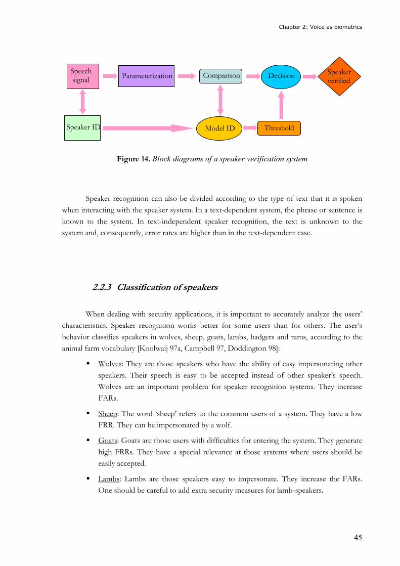
Figure 14. Block diagrams of a speaker verification system .................................................45
Figure 15. Pronunciations of the Spanish word “cero” in different styles ...........................51 Figure 16. Enrolment and test processes ...............................................................................55 Figure 17. Example of a speech signal ..................................................................................57 Figure 18. Representations of a speech signal.......................................................................58 Figure 19. Block diagram of the parameterization stage ......................................................58 Figure 20. Overlapping with a 33% of overlap after [Picone 93] ........................................60 Figure 21. LPC model after [Picone 93] ...............................................................................61 Figure 22. The process of obtaining cepstral vectors............................................................62 Figure 23. Mel-spaced filterbank...........................................................................................63 Figure 24. Spectral subtraction scheme ...............................................................................65 Figure 25. Example of a VQ process .....................................................................................67 Figure 26. Flow diagram of the LBG algorithm....................................................................68 Figure 27. DTW of two energy signals after [Campbell 97] .................................................70 Figure 28. A three state HMM ...............................................................................................71
Figure 29. Example of a GMM ..............................................................................................74
Figure 30. Example of a fully connected ANN.......................................................................75 Figure 31. Density functions for client and impostors ...........................................................80 Figure 32. Combination of speech recognition and speaker verification..............................84 Figure 33. Iterative pruning algorithm..................................................................................98 Figure 34. Non-iterative pruning algorithm ..........................................................................99
Figure 35. Sigmoid function.................................................................................................100 Figure 36. Block diagram for the on-line quality algorithm ...............................................104
Figure 37. Sex distribution in the database .........................................................................113 Figure 38. Percentages of age distribution .........................................................................113 Figure 39. Age distribution ..................................................................................................114 Figure 40. Distribution of speakers regarding to the number of calls ................................114 Figure 41. Block diagram of main parameters for the experimental setup with connected
digit recognition ...........................................................................................................116
14
Figure 42. DET curves for iterative methods in text-dependent speaker verification with 100 clients ........................................................................................................................... 118
Figure 43. Evolution of the EER with the variation of C.................................................... 120 Figure 44. Variation of the weight ( wn ) with respect to the distance ( dn ) between the
scores and the scores mean.......................................................................................... 121 Figure 45. Evolution of the EER with the variation of C..................................................... 122 Figure 46. Comparison of EERs obtained for the BioTech and the Polycost databases .... 123 Figure 47. Quality model classification by groups.............................................................. 125 Figure 48. Certiver’s architecture ....................................................................................... 135 Figure 49. Chain of available CertiVeR processes ............................................................. 136 Figure 50. Scheme of the synchronism between CAs and the CertiVeR site ....................... 137
15
List of tables
Table 1. Comparison of the most important biometrics.........................................................31 Table 2. Scale of LRs and strength of verbal support for the evidence .................................49 Table 3. Error rates for text dependent and text independent experiments ........................117 Table 4. EER for text-dependent and text-independent experiments with baseline and score
pruning methods...........................................................................................................118 Table 5. Comparison of threshold estimation methods in terms of EER.............................119 Table 6. Comparison of threshold estimation methods for the Polycost database .............121 Table 7. Quality groups for a set of speakers......................................................................124 Table 8. Error rates for a set of speakers in connected digit verification experiments.......125 Table 9. Error rates comparison for the on-line method and the leave-one-out method....126 Table 10. Comparison of threshold estimation methods in terms of EER (%) with data from
clients only ...................................................................................................................127 Table 11. Comparison of threshold estimation methods in terms of EER ...........................127
Table 12. Comparison of the EER of threshold estimation methods with 2 impostor utterances .....................................................................................................................127
Table 13. Error rates with speaker-dependent thresholds ...................................................139

16

17
Chapter 1: Introduction, objectives and structure
Chapter 1: Introduction, objectives and structure
18
1 Introduction, objectives and structure
1.1 Introduction
This PhD is focused on the training and the decision stages of a speaker verification
system. The selection of a suitable threshold and the evaluation of the model quality are its
cornerstones. The development of the main tasks takes place in a real environment where there
is not too much data to train speaker models and it is difficult to obtain data from impostors. In
this context, the influence of those scores considered as ‘outliers’ in the estimation of speaker-
dependent thresholds becomes decisive. To mitigate this problem, some new speaker-
dependent threshold estimation methods are proposed. They use only data from clients and
prune or weight client scores.
In connection with the decision threshold problem, one can find that the quality of the
utterances used to train the model must be controlled. A new model quality evaluation method
is introduced. The new method detects low quality utterances and replaces them by new ones
coming from the same speaker getting into great improvement. Furthermore, a new online
method is also introduced here. It evaluates the quality of the training utterances during
enrolment and lets the system to ask the user for more data if quality is not considered as
sufficient, without any additional training session.
New algorithms are tested against the Polycost and mainly the BioTech databases. The
BioTech database has been recorded –among others- by the author. It is a telephonic
multisession database in Spanish. It contains 184 speakers and it is especially designed for
speaker recognition purposes.
The vast majority of the experiments include connected digit recognition although a few
experiments are text-independent. An example of a real application for the revocation of digital
certificates which uses some of the main algorithms developed in this PhD is also included
here.
Chapter 1: Introduction, objectives and structure
19
1.2 Objectives
Main objectives of this PhD include:
� Study of the state-of-the-art in speaker verification accurately analyzing the aspects that
have a great impact on the performance of real-time applications.
� Design and recording of a database suitable for testing speaker verification algorithms.
The database must include connected digits, words, sentences and spontaneous speech.
� Study of the influence of the selection of the acoustic models and their different
topologies depending on the amount and type of speech data.
� Finding a solution to the problem of the scarcity of data in real applications and the
absence of impostor material to estimate a priori speaker-dependent thresholds.
� Detecting low quality utterances in order to be able to replace them by new ones from
the same speaker.
� Solving the problem of determining the model quality a posteriori, once the model is
already created, and the necessity of more sessions to substitute low quality utterances.
� Combining speech and speaker recognition to improve performance and increase
confidence in speaker verification.
� To develop a real application to apply the techniques and algorithms previously
introduced.
Chapter 1: Introduction, objectives and structure
20
1.3 Structure
This PhD is divided into 6 chapters:
• Chapter 1. The first chapter contains a brief introduction, the main objectives of the
PhD and the structure of the contents.
• Chapter 2. This chapter defines what a biometric technology is. It makes a fast view
over the main concepts to take into account when working with biometrics. It classifies
biometrics, explains how to evaluate a biometric application and checks the wide range
of biometric applications that one can find in the market. It also makes a reference to
privacy, a very important factor to consider when deciding the right biometric
technology for our application.
On the other hand, this chapter introduces speaker recognition. First of all, an overview
of the speech production is presented. Then this chapter moves to the explanation of
the differences between identification and verification applications. It classifies the
speakers with regard to their behavior in terms of error rates, talks about main speaker
recognition applications and, to conclude, it shows us the main problems when dealing
with speaker recognition.
• Chapter 3. It describes the different stages of a speaker verification application. First,
one can find the parameterization stage which includes the preprocessing of the speech
data and the search of the coefficients that represent the speech signal. Then, we find a
section which contains the main acoustic models, i.e., Vector Quantization, Dynamic
Time Warping, Hidden Markov Models, Gaussian Mixture Models, Artificial Neural
Networks and Support Vector Machines. The enrollment, which includes model quality
and adaptation, and the decision stage, which introduces normalization and thresholds,
can be found after the acoustic models. Finally, a reference to the main workshops,
institutions, organizations and magazines that contribute to the development and
deployment of speaker recognition technologies is done. To conclude, verbal
information verification systems, those which combines the information from speech
and from the speaker, are analyzed. There is also a comment about the high-level
information of the speech waveform and its raising importance.
• Chapter 4. It includes the new algorithms developed in this PhD. First of all, it revises
the state-of-the-art in decision threshold estimation and model quality evaluation. After
that, score pruning and score weighting methods are discussed in depth. Offline and
online quality measures complete the theoretical content of this chapter.
Chapter 1: Introduction, objectives and structure
21
• Chapter 5. The description of the main databases in speaker recognition is the first
section of this chapter. Special attention is dedicated to the Polycost and to the BioTech
databases, because they are the only ones used in experiments.
The rest of the chapter describes the experimental setup and the results of the
experiments for the score pruning and weighting methods, and for the new ways of
evaluating model quality.
• Chapter 6. It shows a real application with the use of speaker verification. The user is
authenticated by means of a login and then a random 4-digit number is pronounced to
prevent from potential recordings.
Speaker verification is used here to revoke certificates remotely following a centralized
structure. The use of speaker verification saves costs. The architecture of the system is
described in the chapter.

Chapter 1: Introduction, objectives and structure
22

23
Chapter 2: Voice as biometrics

24
Chapter 2: Voice as biometrics
25
2 Voice as biometrics
Speaker recognition is included in the set of biometric technologies. Due to its low
intrusiveness, the possibility of using it remotely and its low cost, voice has become a useful way
of authenticating by personal traits.
One could say that biometric technologies were born in the Ancient Egypt, where
Egyptians made the first classification by dividing slaves according to their color skin, the
height, the age… in order to control them to increase production. Since then, biometric
technologies have suffered from a great evolution and nowadays they are slowly replacing
traditional security systems.
In this chapter we will see an introduction to the main existing biometric applications.
We will study their weaknesses and strengths, their classification and how to measure their
performance.
Furthermore, speaker recognition is also introduced here. Some potential applications
are described as well as the main problems when dealing with this kind of applications.
2.1 Biometrics The word biometric is a combination of two words. The prefix ‘bio-‘ is used in words
related to living things while the suffix ‘-metric’ includes the idea of measurement. One can
guess that the combination of both words refers to the measurement of living things in some
way.
Biometrics is commonly associated to authentication and security. It is able to read,
interpret and manage fingerprints, faces, voices… Although the pivotal advantage of biometric
technologies is the rising security, there are other important aspects to consider here. Another
advantage is the fact that the user does not need to memorize any password. The tools needed
to activate a biometric device belong to the own user!
Biometric devices work by matching individual’s features to some other features
previously obtained from the same individual. They typically achieve high levels of accuracy.
Furthermore error rates can be adjusted to a specific application.
With regard to the level of comparison, one can find two main modes when using
biometrics. If the comparison is from one to many, it is called identification. On the other hand,
the verification occurs in a one-to-one comparison.
Chapter 2: Voice as biometrics
26
One of the most sensitive aspects of the use of biometric technologies is related to
privacy. Some users could consider that biometry reduces privacy. A good discussion about that
can be found in Section 2.1.5.
A very interesting and useful use of biometrics involves its combination with smart
cards and Public Key Infrastructure (PKI). Storing the template on a smart card enhances
individual privacy and increases protection from intentional impostors because the user is who
controls its own templates.
Finally, it is worth noting the enormous range of applications in where biometric
technologies can be introduced. Telephony applications, physical access control or e-commerce
are some of them.
2.1.1 Definitions In order to define what a biometric is, it is first convenient to analyze the ways of
authentication which are possible to find in security applications [Wayman 04]:
• something you know: a secret code, a certain date, a key phrase, a password…
• something you have: a key, a smart card, a memory card, a token…
• something you are: a biometric.
The first way of authentication can be forgotten. Nowadays, people use to memorize
lots of codes, logins or passwords for accessing e-mail, web pages, ATMs… Passwords are
normally easy to crack by using social engineering methods or broken by dictionary attacks.
Furthermore, the same personal code is sometimes used by the user for everything but imagine
that someone knows the code. This person would impersonate the real user! Finally, it is worth
noting that passwords are unable to provide non-repudiation.
On the other hand, the second authentication method could be stolen or get lost. In this
case, if the user realizes about the theft (s)he must suspend the cards, change the lock…
In the third case, the user does not have to memorize anything, cannot loose the way of
authentication and cannot be stolen. The user authenticates herself / himself with biometric
data. It is unlikely to repudiate an access for a user and it is difficult to forge biometrics because
it requires more experience, time, money and technology than any other traditional method
involved in security.
Biometrics measures physical and/or behavioral characteristics of individuals in order to
authenticate or identify them. Some common biometrics are faces, voices, fingerprints… It is
not possible to ensure that each individual has different biometrics. The only that could be
Chapter 2: Voice as biometrics
27
assured is that in a certain population –thousands and even million people- the probability of
finding two identical biometrics tends to zero.
The first division one could establish with biometrics is according to their origin. In
such case, biometrics could be:
� Physical, if it is based in the form or composition of the human body. In this group, it
is possible to find fingerprints, retina, iris, palm and hand geometry, face, ear, hand
veins, bodily odor, thermography, dimensions of head, DNA or pore configuration.
� Behavioral, if it is derived from the measurement of the individual over a period of
time. Behavioral biometrics includes signature, keystroke dynamics or gait, among
others.
Voice is also a biometric which some authors include in the physical group and some
other include in the behavioral group. It should be considered as an intermediate biometric
between the two groups since it could be defined by applying every one of the two definitions
seen before.
Generally, physical biometrics is more accurate than behavioral one. Unlike DNA, all of
them can be executed in real-time.
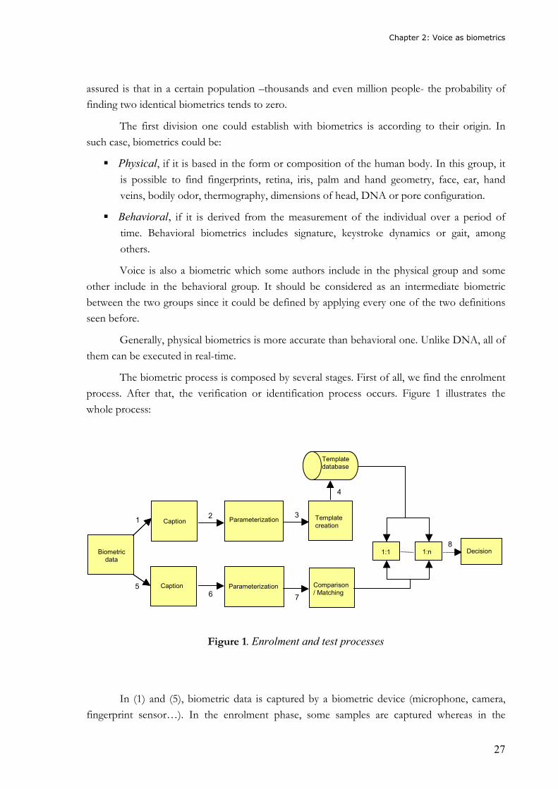
The biometric process is composed by several stages. First of all, we find the enrolment
process. After that, the verification or identification process occurs. Figure 1 illustrates the
whole process:
Figure 1. Enrolment and test processes
In (1) and (5), biometric data is captured by a biometric device (microphone, camera,
fingerprint sensor…). In the enrolment phase, some samples are captured whereas in the
Parameterization
Comparison / Matching
Template
creation
Decision
Caption
Template database
Parameterization
Caption
Biometric data
1:1 1:N
1 Parameterization
Comparison / Matching
Template
creation
Decision
Caption
Template database
Parameterization
Caption
Biometric data
1:1 1:n
2 3
4
5 6 7
8
Chapter 2: Voice as biometrics
28
verification phase, only one sample is captured by the biometric device. The next stage (2 and 6)
is also common for both processes. After the parameterization of the samples, the model or
template is created (3) for the enrolment process. This model will be stored in a database (4).
The model will be compared (8) to the template stored in the database. If it is a
verification process, the comparison will be from 1 to 1. If it is an identification process, the
comparison or search will take place within the whole database. Finally, a decision (9) will be
taken. In an identification process, the result of the comparison will be the user to whom the
biometric data belongs to. The result could also be a score indicating the probability of the
matching and the correlation between the sample and the model.
2.1.2 Classification
Over the next lines, we will see a brief introduction to the most common biometrics
[Wayman 04]. Fingerprints.
They are the most widely and oldest biometric method. Fingerprints have a great
accuracy and have been traditionally connected with security. Despite its criminal concerns,
fingerprints are every time more accepted by users. They use an image of the fingerprint to
extract minutiae, ridges and furrows. Minutiae are local ridge characteristics that can be found at
ridge bifurcations or endings. Two fingerprint matching techniques are normally used: minutiae-
based and correlation-based [Maltoni 03]. Typical scanners used to capture the fingerprint
image include optical, thermal and capacitive. One of the main problems when working with
fingerprints is that the 5% of the population has an impracticable fingerprint.
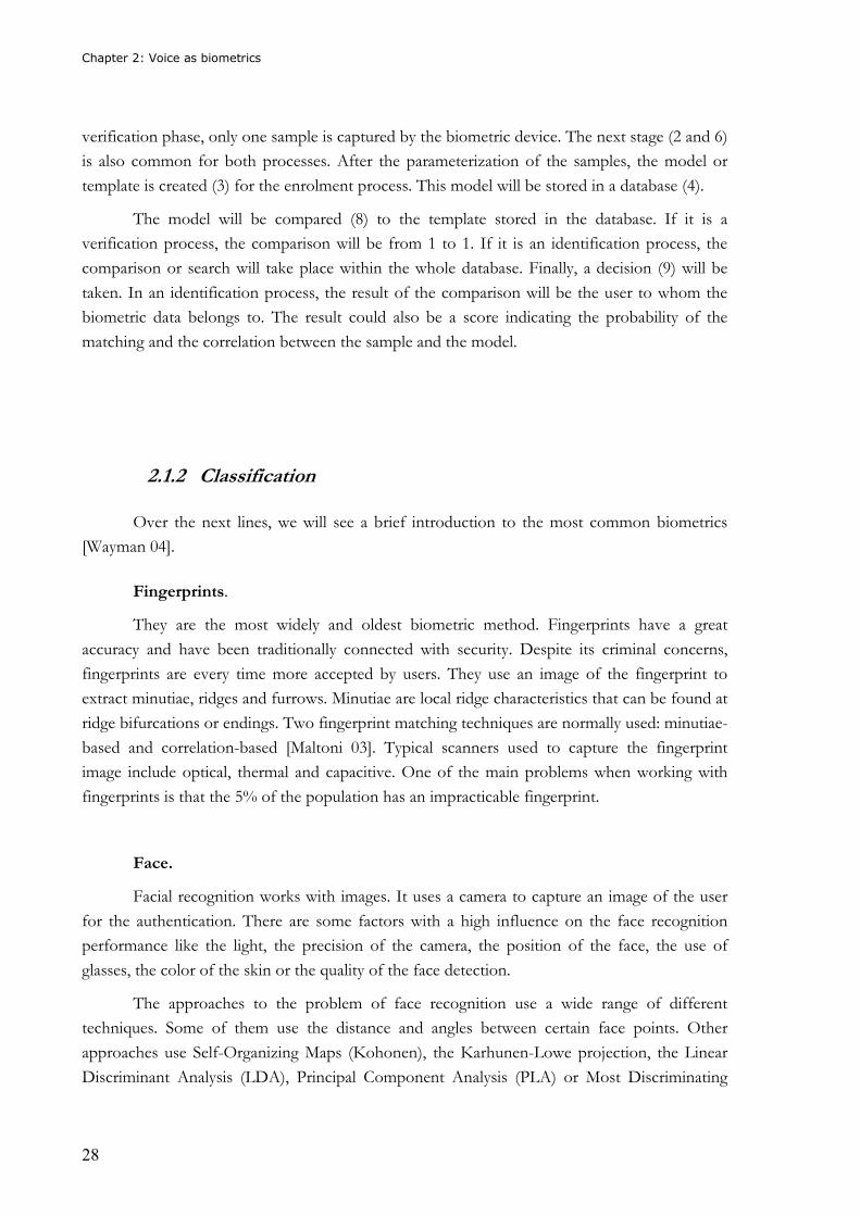
Face.
Facial recognition works with images. It uses a camera to capture an image of the user
for the authentication. There are some factors with a high influence on the face recognition
performance like the light, the precision of the camera, the position of the face, the use of
glasses, the color of the skin or the quality of the face detection.
The approaches to the problem of face recognition use a wide range of different
techniques. Some of them use the distance and angles between certain face points. Other
approaches use Self-Organizing Maps (Kohonen), the Karhunen-Lowe projection, the Linear
Discriminant Analysis (LDA), Principal Component Analysis (PLA) or Most Discriminating
Chapter 2: Voice as biometrics
29
Features (MDF), among others. They are often used in combination with Neural Networks
(NN).
Voice.
Voice is the most natural way of communication. Consequently, it has a high user
acceptance. Speaker recognition can use different channels like the telephone or the
microphone. In commercial applications, it is generally used in combination with voice
recognition. Main speaker recognition topologies are Hidden Markov Models (HMM), Vector
Quantization (VQ), Dynamic Type Warping (DTW) and Neural Networks (NN).
Speaker recognition normally requires more training than other biometrics and can
suffer from reverberation, illnesses or background noises.
Retina.
The retinal scanning is done by a low intensity light source from an optical coupler to
analyze the layer of blood vessels at the back of the eye. It is extremely accurate but requires the
user to look into a receptacle. For this reason, it has a low user acceptance. Furthermore, sensor
costs are high. There are many factors that could affect the performance like the incorrect eye
distance to the camera, an ambient light interference, small pupils or a severe astigmatism.
Iris.
Iris scanning is less intrusive than the retinal scanning. It uses a CCD camera to analyze
the colored ring of tissue that surrounds the pupil. Wavelets are used to extract the two-
dimensional modulation which creates iris patterns. Iris recognition is very stable over time,
very accurate and lets very fast searches. There are some factors that influence its performance
like an inadequate image resolution, contact lenses, corneal reflections or occlusion by
eyelashes.
Hand geometry.
Hand (or palm) geometry analyzes the physical dimensions of a human hand. It is easy
to use and accurate. Furthermore, it adapts itself well with age variations that imply changes in
hand shape. The main problem of this technique concerning performance is the position of the
user regarding the sensor. Height frequently influences the hand position and can elicit
mistakes.
Chapter 2: Voice as biometrics
30
Signature.
Signature recognition studies the way the user signs. Features taken into account are
speed, sign shape, pressure or the degree of inclination of the pen. Signature recognition is
accurate and has a high acceptance because is the natural way of establishing an agreement in
businesses. On the other hand, main problems occur for those users whose signatures are
inconsistent or easy to forge.
It is important to choose the right biometric for every application. There are many
factors which influence in the decision of using one biometrics or another:
� Accuracy. It refers to the error rates given by the corresponding biometrics. It is
expected a high accuracy for every biometrics.
� Stability. The stability measures the performance of a biometric system along time.
Problems with stability can be minimized by adapting new user samples.
� Ease of use. It depends on the type of device used to capture the biometric sample.
A difficult use of biometrics prejudices the user and increases the error rates.
� Intrusiveness. It indicates the user-friendliness of a biometrics. It reflects the
perception of the system by a user.
� Cost. The cost depends on the hardware, the installation, the ease of use, the
maintenance, the database… It is important to take into account the cost, especially
in medium-security applications.
� Security level. It indicates the security level provided by a biometric technology.
� Identification / verification. This parameter informs about the type of speaker
recognition method to use depending on the application.
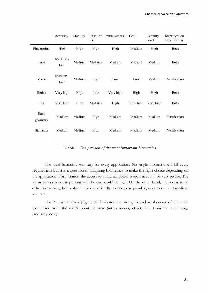
Table 1 summarizes the levels for the main aspects to consider when deciding which
biometric technology is the most suitable one for a certain application:
Chapter 2: Voice as biometrics
31
Accuracy Stability Ease of
use
Intrusiveness Cost Security
level
Identification
/ verification
Fingerprints High High High High Medium High Both
Face Medium -
high Medium Medium Medium Medium Medium Both
Voice Medium -
high Medium High Low Low Medium Verification
Retina Very high High Low Very high High High Both
Iris Very high High Medium High Very high Very high Both
Hand
geometry Medium Medium High Medium Medium Medium Verification
Signature Medium Medium High Medium Medium Medium Verification
Table 1. Comparison of the most important biometrics
The ideal biometric will vary for every application. No single biometric will fill every
requirement but it is a question of analyzing biometrics to make the right choice depending on
the application. For instance, the access to a nuclear power station needs to be very secure. The
intrusiveness is not important and the cost could be high. On the other hand, the access to an
office in working hours should be user-friendly, as cheap as possible, easy to use and medium
accurate.
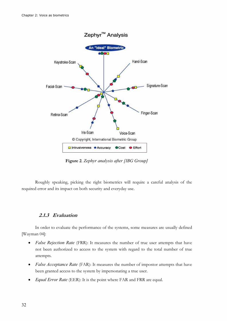
The Zephyr analysis (Figure 2) illustrates the strengths and weaknesses of the main
biometrics from the user’s point of view (intrusiveness, effort) and from the technology
(accuracy, cost):
Chapter 2: Voice as biometrics
32
Figure 2. Zephyr analysis after [IBG Group]
Roughly speaking, picking the right biometrics will require a careful analysis of the
required error and its impact on both security and everyday use.
2.1.3 Evaluation
In order to evaluate the performance of the systems, some measures are usually defined
[Wayman 04]:
• False Rejection Rate (FRR): It measures the number of true user attempts that have
not been authorized to access to the system with regard to the total number of true
attempts.
• False Acceptance Rate (FAR): It measures the number of impostor attempts that have
been granted access to the system by impersonating a true user.
• Equal Error Rate (EER): It is the point where FAR and FRR are equal.
Chapter 2: Voice as biometrics
33
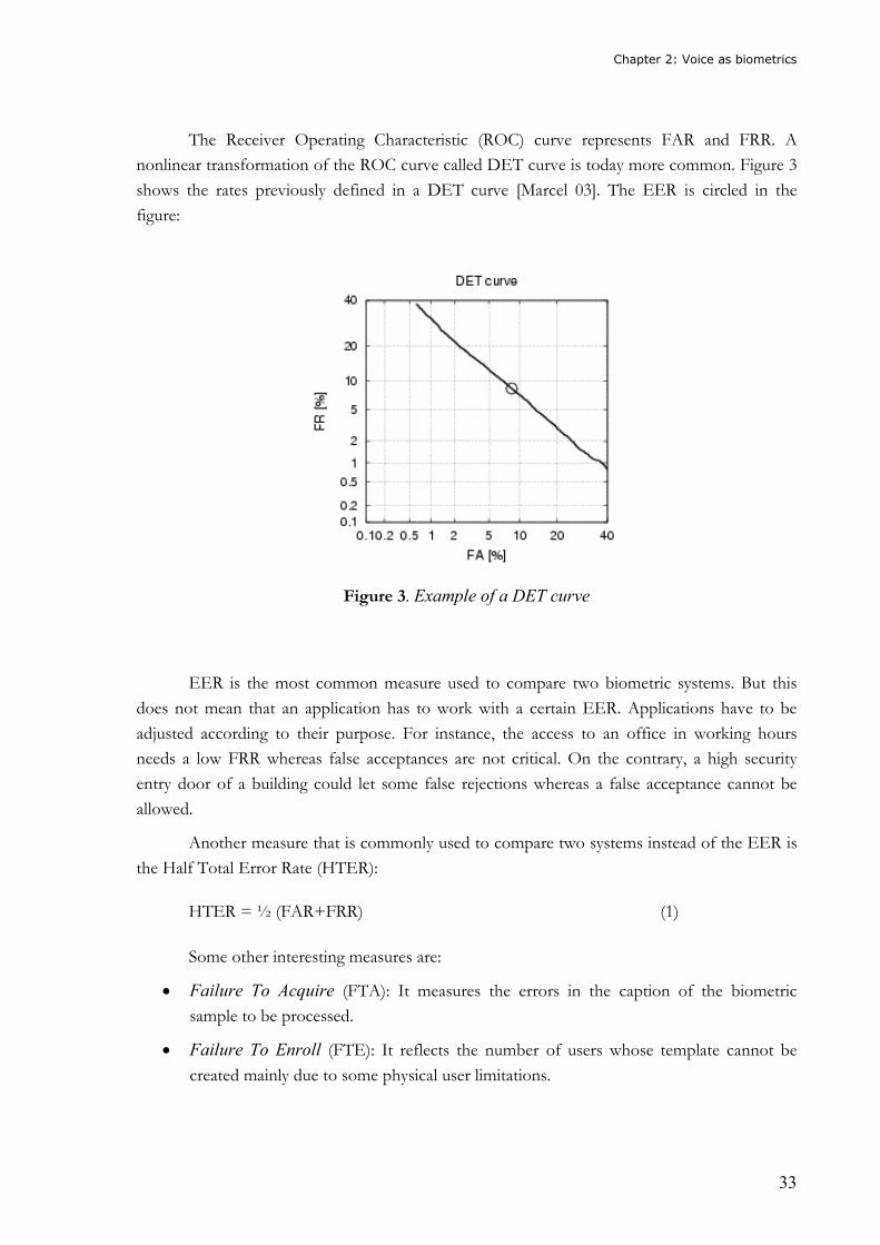
The Receiver Operating Characteristic (ROC) curve represents FAR and FRR. A
nonlinear transformation of the ROC curve called DET curve is today more common. Figure 3
shows the rates previously defined in a DET curve [Marcel 03]. The EER is circled in the
figure:
Figure 3. Example of a DET curve
EER is the most common measure used to compare two biometric systems. But this
does not mean that an application has to work with a certain EER. Applications have to be
adjusted according to their purpose. For instance, the access to an office in working hours
needs a low FRR whereas false acceptances are not critical. On the contrary, a high security
entry door of a building could let some false rejections whereas a false acceptance cannot be
allowed.
Another measure that is commonly used to compare two systems instead of the EER is
the Half Total Error Rate (HTER): HTER = ½ (FAR+FRR) (1)
Some other interesting measures are:
• Failure To Acquire (FTA): It measures the errors in the caption of the biometric
sample to be processed.
• Failure To Enroll (FTE): It reflects the number of users whose template cannot be
created mainly due to some physical user limitations.
Chapter 2: Voice as biometrics
34
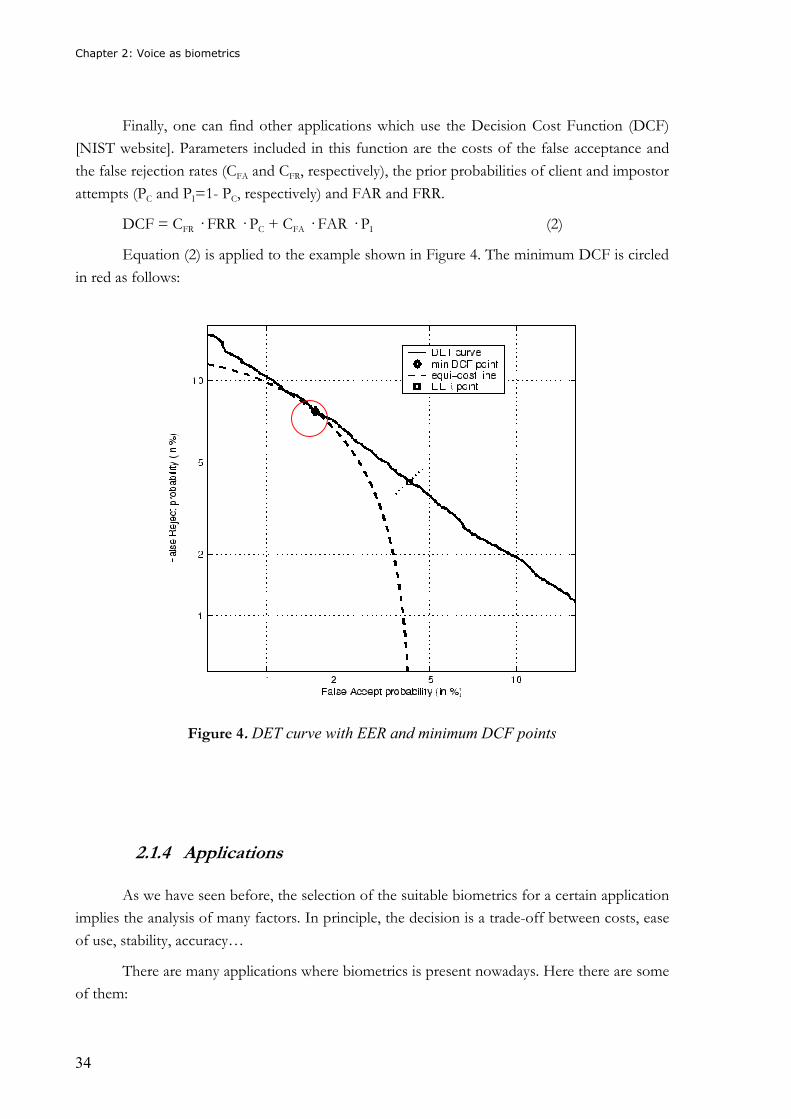
Finally, one can find other applications which use the Decision Cost Function (DCF)
[NIST website]. Parameters included in this function are the costs of the false acceptance and
the false rejection rates (CFA and CFR, respectively), the prior probabilities of client and impostor
attempts (PC and PI=1- PC, respectively) and FAR and FRR.
DCF = CFR � FRR � PC + CFA � FAR � PI (2)
Equation (2) is applied to the example shown in Figure 4. The minimum DCF is circled
in red as follows:
Figure 4. DET curve with EER and minimum DCF points
2.1.4 Applications
As we have seen before, the selection of the suitable biometrics for a certain application
implies the analysis of many factors. In principle, the decision is a trade-off between costs, ease
of use, stability, accuracy…
There are many applications where biometrics is present nowadays. Here there are some
of them:
Chapter 2: Voice as biometrics
35
� Access control to rooms, buildings, offices… This kind of applications is the most
common one. It includes the vast majority of biometric applications. It grants access to
a physical place and can be used with cards, tokens or passwords to increase security.
� ATM use. It is used by banks to reduce fraud. They normally imply a trade-off between
user acceptance, cost and ease of use.
� Travel. They are applications which try to increase security and help frequent travelers.
They also can be used to rent a car, pay in a hotel…
� Telephone transactions. In this case, voice is the only biometrics that can be used in v-
commerce (voice commerce). Telephone banking gathers the most common operations.
The user calls by phone to validate transactions, checking accounts or buy or sell stocks.
� Internet transactions. It consists in a remote access to an application through the
internet. It is expected to be a key element in the development of e-commerce.
� Identity cards. This is a rising application of biometrics. Governments and private
companies are increasingly encouraging the use of cards to authenticate individuals in
order to increase security and privacy.
� Borders control. Countries and governments use also biometrics to control
immigration. Normally it facilitates the task of establishing permissions of access and
increases security. Finally, it is worth noting that biometrics can be combined to increase security levels.
The combination of two or more biometric technologies to authenticate users can be
done sequentially, in parallel or by fusion [Ross 01, Indovina 03]. A biometric system is
sometimes affected by the caption device and it elicits a large variance in the scores. The
fusion of biometrics systems solve this problem and make much more difficult for an
impostor to impersonate a real user.
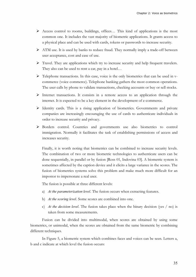
The fusion is possible at three different levels:
a) At the parameterization level. The fusion occurs when extracting features.
b) At the scoring level. Some scores are combined into one.
c) At the decision level. The fusion takes place when the binary decision (yes / no) is
taken from some measurements.
Fusion can be divided into multimodal, when scores are obtained by using some
biometrics, or unimodal, when the scores are obtained from the same biometric by combining
different techniques.
In Figure 5, a biometric system which combines faces and voices can be seen. Letters a,
b and c indicate at which level the fusion occurs:
Chapter 2: Voice as biometrics
36
Figure 5. Multimodal biometric process
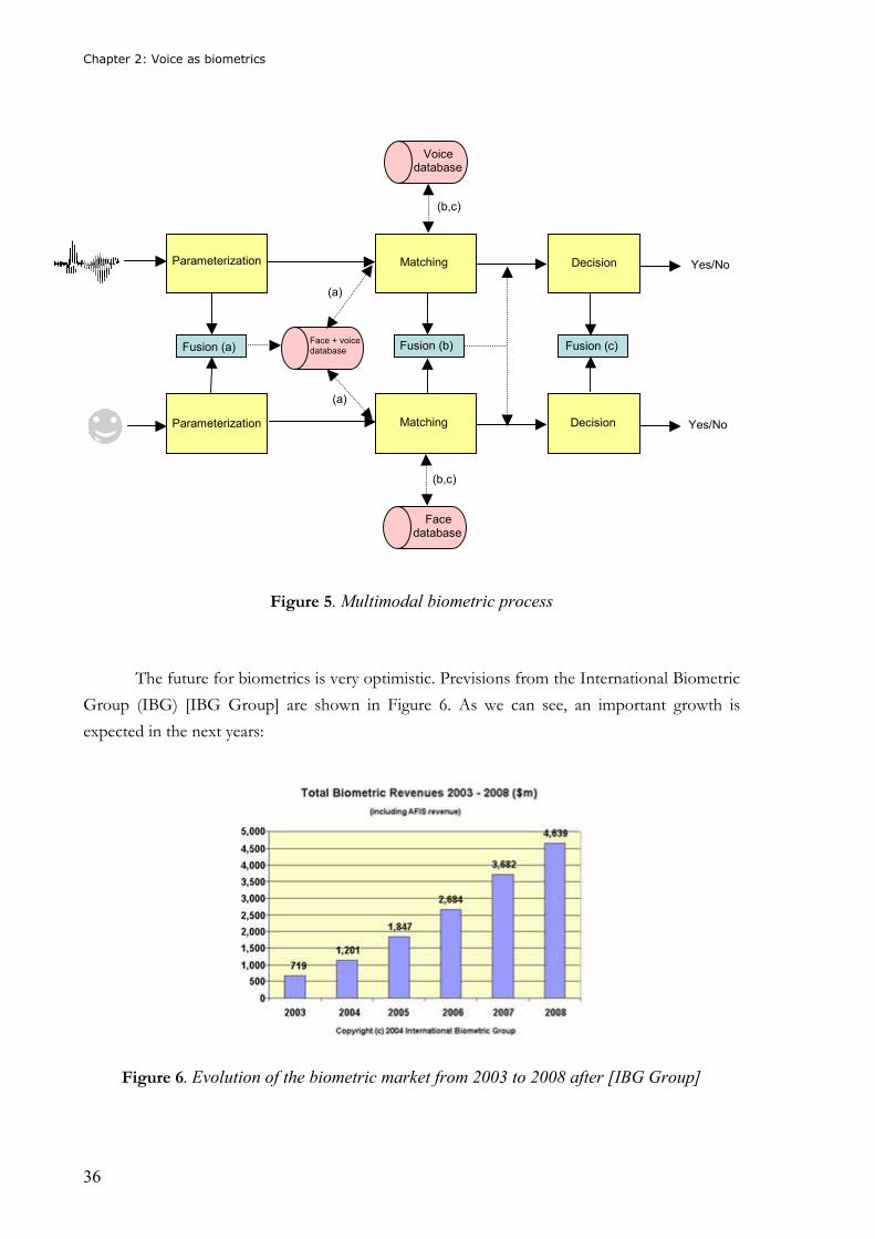
The future for biometrics is very optimistic. Previsions from the International Biometric
Group (IBG) [IBG Group] are shown in Figure 6. As we can see, an important growth is
expected in the next years:
Figure 6. Evolution of the biometric market from 2003 to 2008 after [IBG Group]
Parameterization
Matching Parameterization
Decision Matching
Decision
Fusion (a) Fusion (c) Fusion (b)
Face database
Voice database
Face + voice database
(b,c)
(b,c)
(a)
(a)
Yes/No
Yes/No
Chapter 2: Voice as biometrics
37
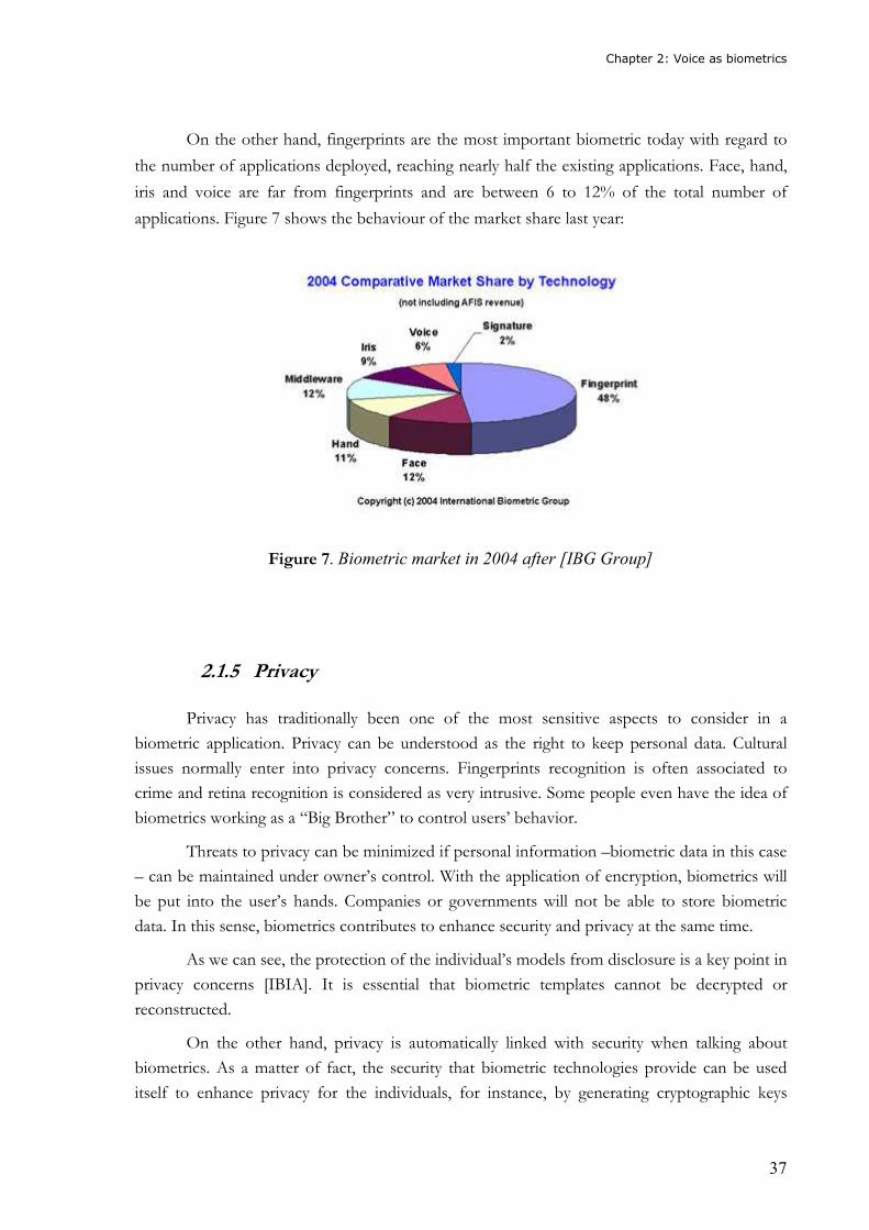
On the other hand, fingerprints are the most important biometric today with regard to
the number of applications deployed, reaching nearly half the existing applications. Face, hand,
iris and voice are far from fingerprints and are between 6 to 12% of the total number of
applications. Figure 7 shows the behaviour of the market share last year:
Figure 7. Biometric market in 2004 after [IBG Group]
2.1.5 Privacy Privacy has traditionally been one of the most sensitive aspects to consider in a
biometric application. Privacy can be understood as the right to keep personal data. Cultural
issues normally enter into privacy concerns. Fingerprints recognition is often associated to
crime and retina recognition is considered as very intrusive. Some people even have the idea of
biometrics working as a “Big Brother” to control users’ behavior.
Threats to privacy can be minimized if personal information –biometric data in this case
– can be maintained under owner’s control. With the application of encryption, biometrics will
be put into the user’s hands. Companies or governments will not be able to store biometric
data. In this sense, biometrics contributes to enhance security and privacy at the same time.
As we can see, the protection of the individual’s models from disclosure is a key point in
privacy concerns [IBIA]. It is essential that biometric templates cannot be decrypted or
reconstructed.
On the other hand, privacy is automatically linked with security when talking about
biometrics. As a matter of fact, the security that biometric technologies provide can be used
itself to enhance privacy for the individuals, for instance, by generating cryptographic keys
Chapter 2: Voice as biometrics
38
based on biometric samples [Uludag 04]. In this case, the biometric template will not be
revealed unless a successful biometric authentication occurs.
These measures probably will help to fight against intentional impostors. One of the
most famous attempts to break down security in biometrics was made by Matsumoto
[Matsumoto 02]. He gained access to a biometric system by means of a gelatin finger. He lifted
the fingerprint from a glass and used a photosensitive circuit board to give “life” to the finger.
With regard to privacy, one has to take into account where biometric data is stored after
being captured or after the template creation. Some biometric applications use to encrypt the
biometric data and store it in a card. The card has to be given to the user. In this case, the use
of Public Key Infrastructure (PKI, see Section 8.1 for a more detailed description) in
combination with biometrics provides the strongest security. The comparison between the
biometric sample and the model takes place inside the card, without having to communicate
with an external device. The process is commonly known as ‘match-on-card’.
Another option consists in storing biometric data in a central database. It is an easy
solution that elicits several disadvantages. Large databases are often costly to maintain and
suffer from a decrease in privacy. Personal biometric information is beyond the control of the
individuals.
2.2 Speaker recognition
2.2.1 Speech production
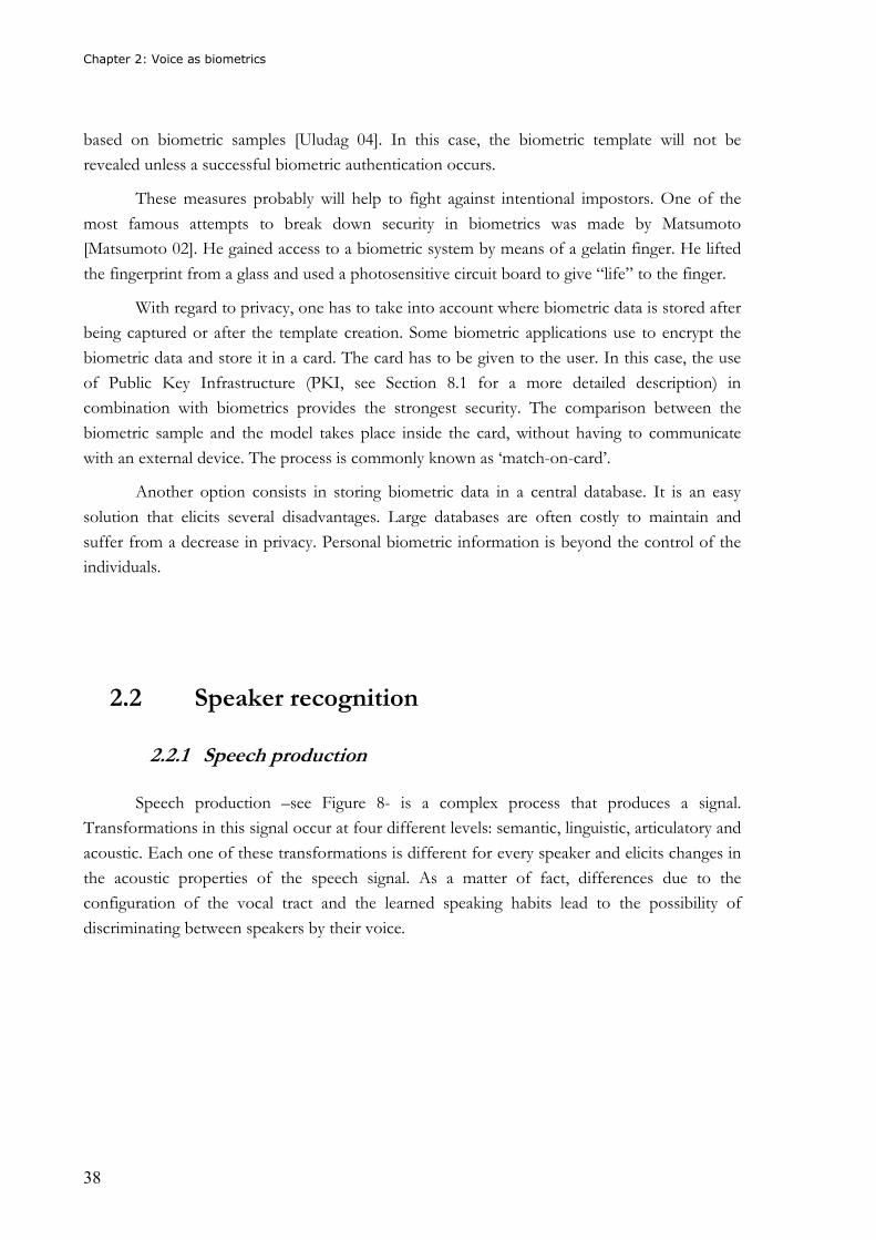
Speech production –see Figure 8- is a complex process that produces a signal.
Transformations in this signal occur at four different levels: semantic, linguistic, articulatory and
acoustic. Each one of these transformations is different for every speaker and elicits changes in
the acoustic properties of the speech signal. As a matter of fact, differences due to the
configuration of the vocal tract and the learned speaking habits lead to the possibility of
discriminating between speakers by their voice.
Chapter 2: Voice as biometrics
39
Figure 8. Human speech production
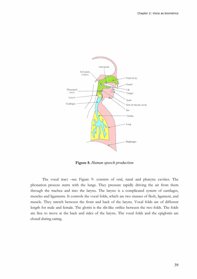
The vocal tract –see Figure 9- consists of oral, nasal and pharynx cavities. The
phonation process starts with the lungs. They pressure rapidly driving the air from them
through the trachea and into the larynx. The larynx is a complicated system of cartilages,
muscles and ligaments. It controls the vocal folds, which are two masses of flesh, ligament, and
muscle. They stretch between the front and back of the larynx. Vocal folds are of different
length for male and female. The glottis is the slit-like orifice between the two folds. The folds
are free to move at the back and sides of the larynx. The vocal folds and the epiglottis are
closed during eating.
Chapter 2: Voice as biometrics
40
Figure 9. Human speech production by blocks
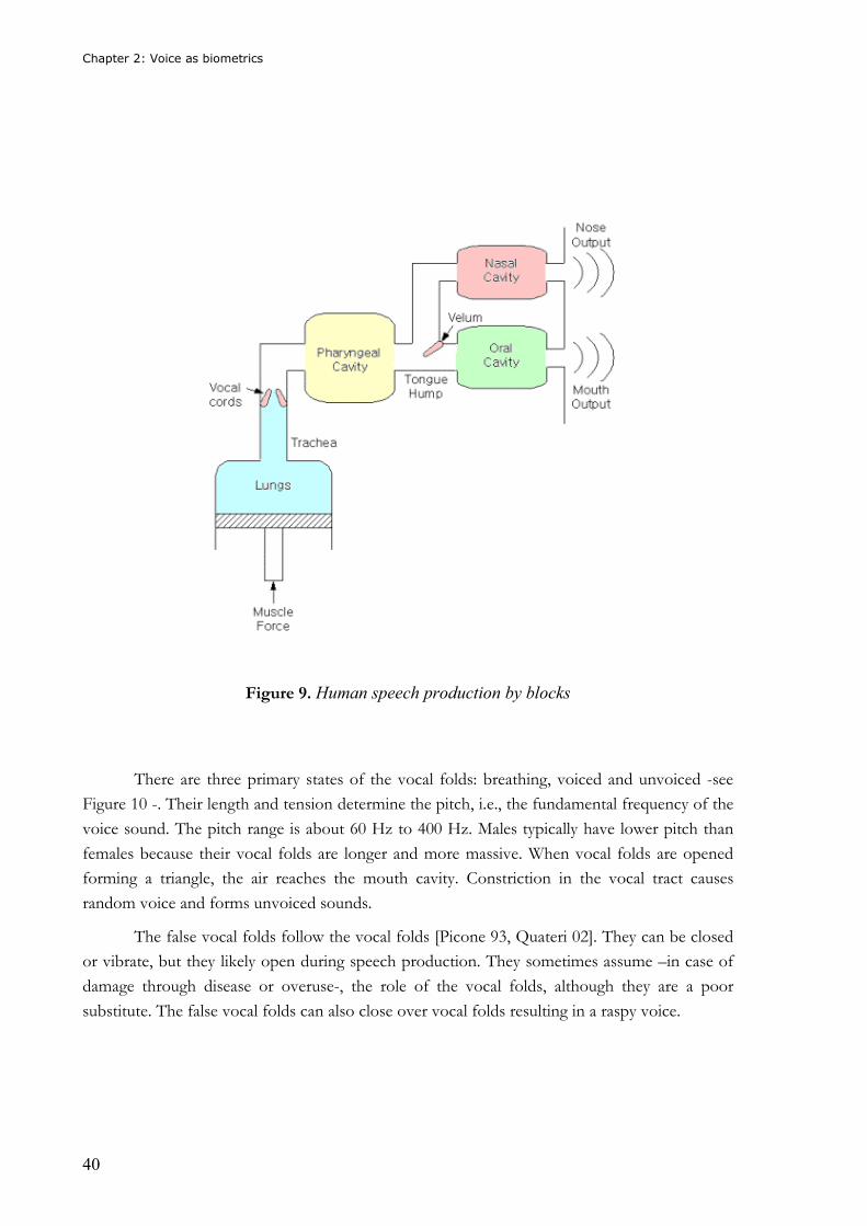
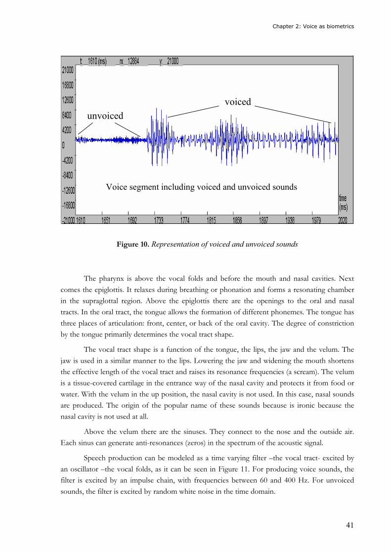
There are three primary states of the vocal folds: breathing, voiced and unvoiced -see
Figure 10 -. Their length and tension determine the pitch, i.e., the fundamental frequency of the
voice sound. The pitch range is about 60 Hz to 400 Hz. Males typically have lower pitch than
females because their vocal folds are longer and more massive. When vocal folds are opened
forming a triangle, the air reaches the mouth cavity. Constriction in the vocal tract causes
random voice and forms unvoiced sounds.
The false vocal folds follow the vocal folds [Picone 93, Quateri 02]. They can be closed
or vibrate, but they likely open during speech production. They sometimes assume –in case of
damage through disease or overuse-, the role of the vocal folds, although they are a poor
substitute. The false vocal folds can also close over vocal folds resulting in a raspy voice.
Chapter 2: Voice as biometrics
41
Figure 10. Representation of voiced and unvoiced sounds
The pharynx is above the vocal folds and before the mouth and nasal cavities. Next
comes the epiglottis. It relaxes during breathing or phonation and forms a resonating chamber
in the supraglottal region. Above the epiglottis there are the openings to the oral and nasal
tracts. In the oral tract, the tongue allows the formation of different phonemes. The tongue has
three places of articulation: front, center, or back of the oral cavity. The degree of constriction
by the tongue primarily determines the vocal tract shape.
The vocal tract shape is a function of the tongue, the lips, the jaw and the velum. The
jaw is used in a similar manner to the lips. Lowering the jaw and widening the mouth shortens
the effective length of the vocal tract and raises its resonance frequencies (a scream). The velum
is a tissue-covered cartilage in the entrance way of the nasal cavity and protects it from food or
water. With the velum in the up position, the nasal cavity is not used. In this case, nasal sounds
are produced. The origin of the popular name of these sounds because is ironic because the
nasal cavity is not used at all.
Above the velum there are the sinuses. They connect to the nose and the outside air.
Each sinus can generate anti-resonances (zeros) in the spectrum of the acoustic signal.
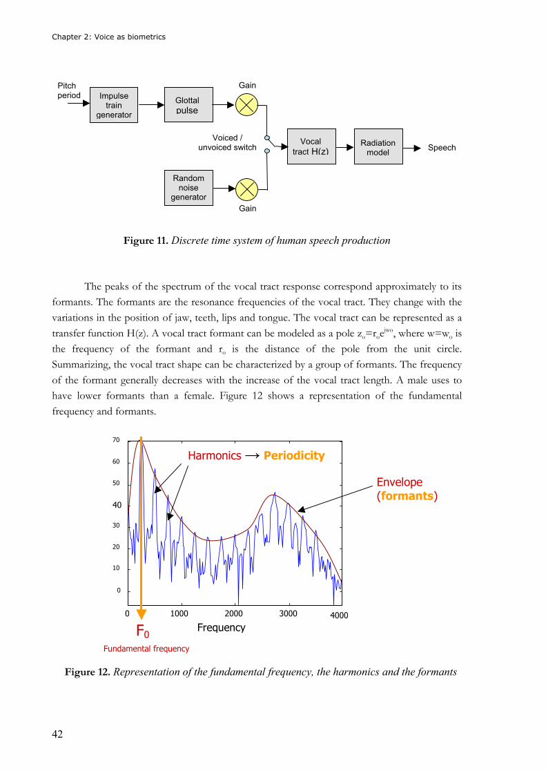
Speech production can be modeled as a time varying filter –the vocal tract- excited by
an oscillator –the vocal folds, as it can be seen in Figure 11. For producing voice sounds, the
filter is excited by an impulse chain, with frequencies between 60 and 400 Hz. For unvoiced
sounds, the filter is excited by random white noise in the time domain.
Voice segment including voiced and unvoiced sounds
unvoiced
voiced
Chapter 2: Voice as biometrics
42
Figure 11. Discrete time system of human speech production
The peaks of the spectrum of the vocal tract response correspond approximately to its
formants. The formants are the resonance frequencies of the vocal tract. They change with the
variations in the position of jaw, teeth, lips and tongue. The vocal tract can be represented as a
transfer function H(z). A vocal tract formant can be modeled as a pole zo=roejwo, where w=wo is
the frequency of the formant and ro is the distance of the pole from the unit circle.
Summarizing, the vocal tract shape can be characterized by a group of formants. The frequency
of the formant generally decreases with the increase of the vocal tract length. A male uses to
have lower formants than a female. Figure 12 shows a representation of the fundamental
frequency and formants.
Figure 12. Representation of the fundamental frequency, the harmonics and the formants
Impulse train
generator
Glottal
pulse
Random noise
generator
Vocal
tract H(z) Radiation model
Speech
Pitch period
Voiced / unvoiced switch
Gain
Gain
0 1000 2000 3000
0
10
20
30
40
50
60
70
Frequency
Envelope (formants)
Harmonics → Periodicity
4000 F0
Fundamental frequency
Chapter 2: Voice as biometrics
43
Nearly all the information one can find in speech is in the range of 200 Hz to 8 KHz.
The telephone bandwith, from 300 Hz to 3400 Hz, contains enough information to consider its
analysis in order to extract speech characteristics. The information included in speech
waveforms can be divided in “high-level” and “low-level” [Quateri 02]. High-level information
refers to clarity, roughness, prosody or dialect. There are very important aspects concerning the
prosody like the pitch intonation or the articulation. Deeper explanation can be found in
Section 3.6.1.
The low-level information is easier to extract by machine than the high-level one. It has
an acoustic origin and it can be measured. Some elements of the low-level information which
include information to recognize a speaker are the vocal tract spectrum, instantaneous pitch,
glottal flow excitation and modulations in formant trajectories.
These characteristics that contain low-level information are fairly similar over short
periods of time, typically from 5 to 100 milliseconds. For this reason, the short-time spectral
analysis is the more suitable one to characterise the speech signal.
2.2.2 Identification vs. verification
Speaker recognition [Atal 76, Doddington 85, Furui 94] is classified into two main
categories: identification and verification. Speaker identification is the process of deciding which
speaker model from a known set of speaker models best characterizes a speaker. On the other
hand, speaker verification is the process of deciding whether a speaker corresponds to a known
voice.
In these processes of identifying or accepting / rejecting speakers, the speaker who is
correctly claiming her / his identity is called claimant, true speaker or target speaker. The
speaker who is trying to impersonate a true user is known as impostor.
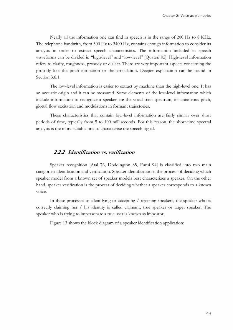
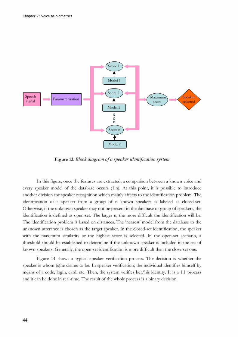
Figure 13 shows the block diagram of a speaker identification application:
Chapter 2: Voice as biometrics
44
Figure 13. Block diagram of a speaker identification system
In this figure, once the features are extracted, a comparison between a known voice and
every speaker model of the database occurs (1:n). At this point, it is possible to introduce
another division for speaker recognition which mainly affects to the identification problem. The
identification of a speaker from a group of n known speakers is labeled as closed-set.
Otherwise, if the unknown speaker may not be present in the database or group of speakers, the
identification is defined as open-set. The larger n, the more difficult the identification will be.
The identification problem is based on distances. The ‘nearest’ model from the database to the
unknown utterance is chosen as the target speaker. In the closed-set identification, the speaker
with the maximum similarity or the highest score is selected. In the open-set scenario, a
threshold should be established to determine if the unknown speaker is included in the set of
known speakers. Generally, the open-set identification is more difficult than the close-set one.
Figure 14 shows a typical speaker verification process. The decision is whether the
speaker is whom (s)he claims to be. In speaker verification, the individual identifies himself by
means of a code, login, card, etc. Then, the system verifies her/his identity. It is a 1:1 process
and it can be done in real-time. The result of the whole process is a binary decision.
Parameterization Speech signal
Score 1
Model 1
Score 2
Model 2
Score n
Model n
Maximum score
Speaker selected
Chapter 2: Voice as biometrics
45
Figure 14. Block diagrams of a speaker verification system
Speaker recognition can also be divided according to the type of text that it is spoken
when interacting with the speaker system. In a text-dependent system, the phrase or sentence is
known to the system. In text-independent speaker recognition, the text is unknown to the
system and, consequently, error rates are higher than in the text-dependent case.
2.2.3 Classification of speakers
When dealing with security applications, it is important to accurately analyze the users’
characteristics. Speaker recognition works better for some users than for others. The user’s
behavior classifies speakers in wolves, sheep, goats, lambs, badgers and rams, according to the
animal farm vocabulary [Koolwaij 97a, Campbell 97, Doddington 98]:
� Wolves: They are those speakers who have the ability of easy impersonating other
speakers. Their speech is easy to be accepted instead of other speaker’s speech.
Wolves are an important problem for speaker recognition systems. They increase
FARs.
� Sheep: The word ‘sheep’ refers to the common users of a system. They have a low
FRR. They can be impersonated by a wolf.
� Goats: Goats are those users with difficulties for entering the system. They generate
high FRRs. They have a special relevance at those systems where users should be
easily accepted.
� Lambs: Lambs are those speakers easy to impersonate. They increase the FARs.
One should be careful to add extra security measures for lamb-speakers.
Parameterization Speech signal
Comparison Decision Speaker verified
Speaker ID Model ID Threshold
Chapter 2: Voice as biometrics
46
� Rams: Rams are the contrary of lambs. They are especially difficult to impersonate.
They increase the performance because they produce really low FARs.
� Badgers: Badgers are just the contrary of wolves. They have a low FAR when they
try to impersonate another speaker.
In a real speaker recognition system, it is important to locate goats and lambs because
they will considerably reduce the system performance; goats due to many false rejections and
lambs due to many false acceptances. It is also worth noting that some users can be classified
into two or more categories. For instance, a speaker could be a sheep-wolf or a goat-badger.
2.2.4 Applications
Identification and verification application have already been studied in Section 2.2.2.
Text-dependent and text-independent cases form another division concerning speaker
recognition applications. There is also one more important aspect to take into account when
dealing with speaker recognition: the channel. Voice applications normally use the telephone or
the microphone. Applications with both handsets abound. Microphone applications are
considered as physical because they require the presence of the users. On the other hand,
telephone applications are classified as remote. It is worth noting that microphone applications
can also be remote. They are commonly used through the Internet. In fact, they have lately got
into much importance because they have often been used to enable transactions by voice with
the recent enormous evolution of the Internet.
The potential for application of speaker recognition includes a wide range of
possibilities [Doddington 98, Saeta 01a, Saeta 01b]. Telephone banking, voice commerce, access
control and transportation services are some of them. Law enforcement is also a very important
application of speaker recognition in order to identify suspects. Security applications are
numerous. Offices, buildings, cars, computers, bank accounts or e-mail addresses are often
controlled by voice and use speaker recognition to gain access to them.
For all of this range of applications, voice is the natural choice because it is one of the
easiest and most natural forms of communication to use. The most important with regard to
speaker recognition applications is that it is expected that this technology will be much more
important in the next future. The mobile penetration in Europe and USA reaches very high
taxes and it will eclipse the number of traditional land lines.
There are lots of real biometric applications. For instance, the Dutch government has
used biometrics to identify immigrants in 2001 by means of the iris scanning [I-News1]. In
some schools in Pennsylvania (USA), fingerprints are used to pay in the school’s restaurant [I-
News2]. Face recognition has also been used in a Super Bowl match to identify criminals among
Chapter 2: Voice as biometrics
47
the assistants [Woodward 2001]. Visa has tested the use of speaker recognition to authenticate
user’s transactions over the Internet and by phone [I-News3].
Some existing applications use speaker recognition in conjunction with speech
recognition to provide an extra security level. The combination of both technologies is called
Verbal Information Verification (VIV) [Li 97, Linares 99, Li 00]. In VIV, speaker utterances are
verified against the information included in the speaker’s profile to decide if the claimed identity
should be accepted or rejected. The extra information provided can consist of birthday, birth
place, address, mother’s maiden name... Speaker and speech recognition can also be combined
with cards, tokens or other biometric technologies. VIV will be studied in Section 3.6.
2.2.4.1 On-site applications
Most common on-site applications with speaker recognition technologies are access
control and time attendance. Speaker verification (SV) is normally the chosen branch of speaker
recognition. SV is often used in combination with a secret code or even with another biometric
technology like face recognition. In an access control application, the purpose consists of
getting access to a protected room or building by using a natural and non-intrusive way. In time
attendance applications, the speaker uses voice to confirm presence.
On-site applications are not the strongest point when dealing with speaker recognition
applications. Remote applications offer a highest potential for voice recognition.
2.2.4.2 Remote applications
As it has been stated before, there are many applications in where speaker recognition
can be used remotely. In fact, speaker recognition is the most suitable biometric technology to
be used when the user and the recognition system are not physically in touch. Furthermore, it is
necessary for visually impaired people [Os 99].
Some potential applications are:
� Telebanking: The use of voice through telephone lines is a very useful tool for financial
applications. Speaker verification can be used to access bank accounts or to buy or sell
stocks. This is known as v-commerce (voice-commerce). Speaker verification can also
be used to reduce fraud in teleshopping. Voice applications use speaker verification in
combination with speech recognition. To enter the system, applications use a
combination of digits to form logins and pins [Ortega 00].
� Telecom applications: Speaker verification is often used to access computers, Personal
Communication Assistants (PDAs) and networks. It is also used in Calling Card
Services to reduce fraud in telephone calls. Another telecom application consists of
Chapter 2: Voice as biometrics
48
accessing the voice mail through speech facilities [Linares 00, Rosenberg 00]. These
applications are often used in combination with Digit Tone Pulse Modulation (DTMF)
or with the identification of the remote terminal (the user’s IP address in a computer or
the caller’s phone number in a telephone call).
� Home Incarceration: An automatic system calls the user when (s)he is supposed to be
at home. The process ensures the authentication of the user and prevents from
impersonation.
� Time attendance: As stated in the previous section, time attendance can also occur
remotely. It is very useful for those companies whose workers are supposed to be
working out of office.
2.2.4.3 Forensics
Speaker recognition is also used in forensic cases [Künzel 94, Gfroerer 03, Pfister 03,
Gonzalez 03, Bimbot 04]. There are many differences between commercial systems and
forensic speaker recognition systems. First of all, in forensic cases there is a so-called non co-
operative speaker, while in commercial applications the speaker cooperates. In forensic
applications, the suspect is recorded without permission. After that, when more voice is
recorded to compare with the evidence (E), the speaker usually tries to disguise voice.
Forensic applications are text-independent while commercial applications are usually
text-dependent (digits, words, sentences...). On the other hand, forensic data is recorded by
phone, with high quality and abundant quantity. In commercial applications, the amount of data
is often a problem because the user wants to train the system with as few data as possible and
the quality is variable. Otherwise, the selection of the speaker thresholds is more important in
forensics. In commercial applications, in case of an error the result can be a financial penalty. In
forensics, an error can lead to the acquittal of a guilty person or to the condemnation of an
innocent one. Finally, it is worth noting that while in commercial applications the number of
users is finite, in forensic applications the set of potential speakers is open, unlimited.
In [Künzel 94, Bimbot 04], it is possible to find the history of forensics. In the
beginning, the recognition process was developed by listening, performed by non-experts
(witnesses) or phoneticians / scientists. After that, the spectrographic analysis emerged and with
it the term “voiceprint”, with regard to the similarity of voice with fingerprints. There is a
controversy with this term because some authors consider that the word “print” must not be
associated to voice. The next step in the evolution of forensics arrived with the introduction of
automatic speaker recognition (ASR) systems [Falcone 94, Nakasone 01, Meuwly 01, Gonzalez
01]. These systems are often semiautomatic and require the handle by expert phoneticians.
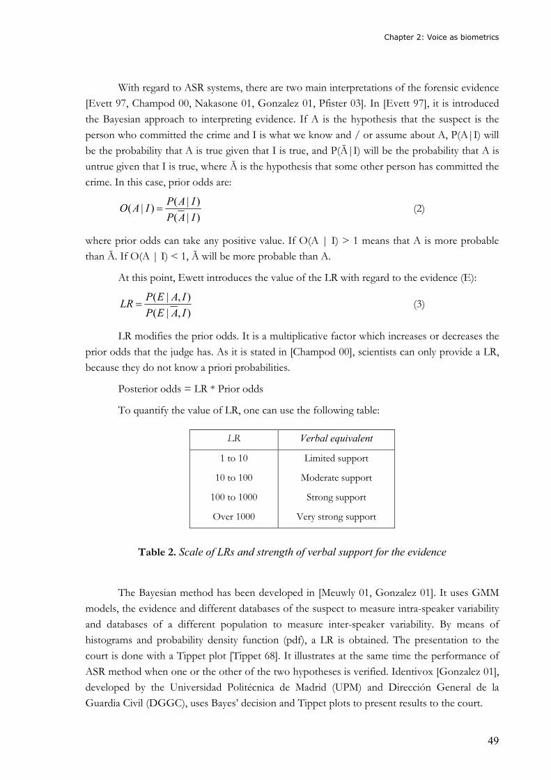
Chapter 2: Voice as biometrics
49
With regard to ASR systems, there are two main interpretations of the forensic evidence
[Evett 97, Champod 00, Nakasone 01, Gonzalez 01, Pfister 03]. In [Evett 97], it is introduced
the Bayesian approach to interpreting evidence. If A is the hypothesis that the suspect is the
person who committed the crime and I is what we know and / or assume about A, P(A|I) will
be the probability that A is true given that I is true, and P(Ā|I) will be the probability that A is
untrue given that I is true, where Ā is the hypothesis that some other person has committed the
crime. In this case, prior odds are:
)|(
)|()|(
IAP
IAPIAO = (2)
where prior odds can take any positive value. If O(A | I) > 1 means that A is more probable
than Ā. If O(A | I) < 1, Ā will be more probable than A.
At this point, Ewett introduces the value of the LR with regard to the evidence (E):
),|(
),|(
IAEP
IAEPLR = (3)
LR modifies the prior odds. It is a multiplicative factor which increases or decreases the
prior odds that the judge has. As it is stated in [Champod 00], scientists can only provide a LR,
because they do not know a priori probabilities.
Posterior odds = LR * Prior odds
To quantify the value of LR, one can use the following table:
LR Verbal equivalent
1 to 10
10 to 100
100 to 1000
Over 1000
Limited support
Moderate support
Strong support
Very strong support
Table 2. Scale of LRs and strength of verbal support for the evidence
The Bayesian method has been developed in [Meuwly 01, Gonzalez 01]. It uses GMM
models, the evidence and different databases of the suspect to measure intra-speaker variability
and databases of a different population to measure inter-speaker variability. By means of
histograms and probability density function (pdf), a LR is obtained. The presentation to the
court is done with a Tippet plot [Tippet 68]. It illustrates at the same time the performance of
ASR method when one or the other of the two hypotheses is verified. Identivox [Gonzalez 01],
developed by the Universidad Politécnica de Madrid (UPM) and Dirección General de la
Guardia Civil (DGGC), uses Bayes’ decision and Tippet plots to present results to the court.
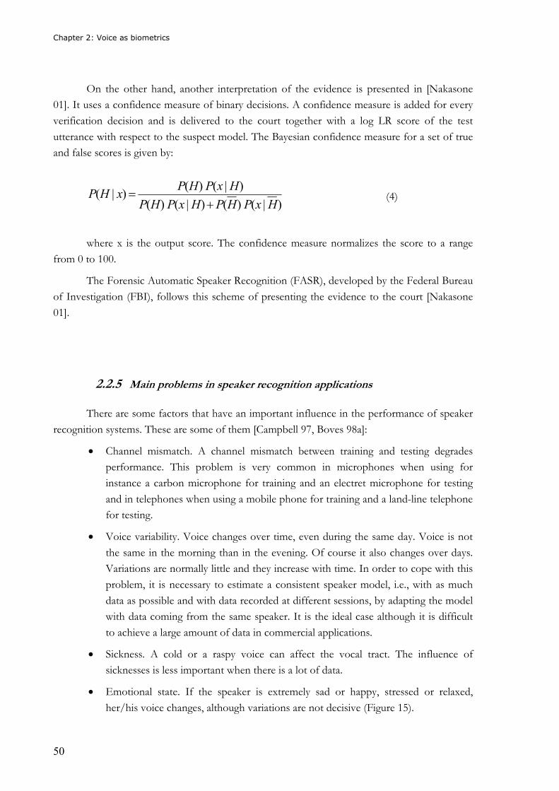
Chapter 2: Voice as biometrics
50
On the other hand, another interpretation of the evidence is presented in [Nakasone
01]. It uses a confidence measure of binary decisions. A confidence measure is added for every
verification decision and is delivered to the court together with a log LR score of the test
utterance with respect to the suspect model. The Bayesian confidence measure for a set of true
and false scores is given by:
)|()()|()(
)|()()|(
HxPHPHxPHP
HxPHPxHP
+= (4)
where x is the output score. The confidence measure normalizes the score to a range
from 0 to 100.
The Forensic Automatic Speaker Recognition (FASR), developed by the Federal Bureau
of Investigation (FBI), follows this scheme of presenting the evidence to the court [Nakasone
01].
2.2.5 Main problems in speaker recognition applications
There are some factors that have an important influence in the performance of speaker
recognition systems. These are some of them [Campbell 97, Boves 98a]:
• Channel mismatch. A channel mismatch between training and testing degrades
performance. This problem is very common in microphones when using for
instance a carbon microphone for training and an electret microphone for testing
and in telephones when using a mobile phone for training and a land-line telephone
for testing.
• Voice variability. Voice changes over time, even during the same day. Voice is not
the same in the morning than in the evening. Of course it also changes over days.
Variations are normally little and they increase with time. In order to cope with this
problem, it is necessary to estimate a consistent speaker model, i.e., with as much
data as possible and with data recorded at different sessions, by adapting the model
with data coming from the same speaker. It is the ideal case although it is difficult
to achieve a large amount of data in commercial applications.
• Sickness. A cold or a raspy voice can affect the vocal tract. The influence of
sicknesses is less important when there is a lot of data.
• Emotional state. If the speaker is extremely sad or happy, stressed or relaxed,
her/his voice changes, although variations are not decisive (Figure 15).
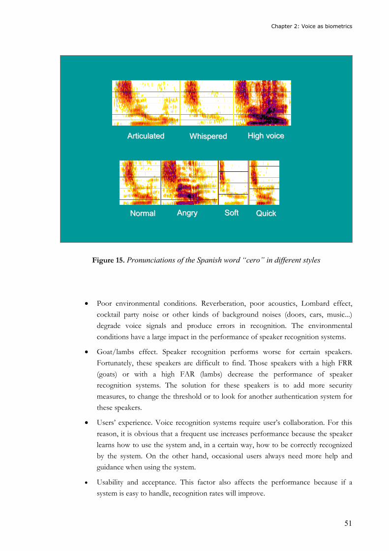
Chapter 2: Voice as biometrics
51
Figure 15. Pronunciations of the Spanish word “cero” in different styles
• Poor environmental conditions. Reverberation, poor acoustics, Lombard effect,
cocktail party noise or other kinds of background noises (doors, cars, music...)
degrade voice signals and produce errors in recognition. The environmental
conditions have a large impact in the performance of speaker recognition systems.
• Goat/lambs effect. Speaker recognition performs worse for certain speakers.
Fortunately, these speakers are difficult to find. Those speakers with a high FRR
(goats) or with a high FAR (lambs) decrease the performance of speaker
recognition systems. The solution for these speakers is to add more security
measures, to change the threshold or to look for another authentication system for
these speakers.
• Users’ experience. Voice recognition systems require user’s collaboration. For this
reason, it is obvious that a frequent use increases performance because the speaker
learns how to use the system and, in a certain way, how to be correctly recognized
by the system. On the other hand, occasional users always need more help and
guidance when using the system.
• Usability and acceptance. This factor also affects the performance because if a
system is easy to handle, recognition rates will improve.
AArrttiiccuullaatteedd WWhhiissppeerreedd HHiigghh vvooiiccee
NNoorrmmaall AAnnggrryy SSoofftt QQuuiicckk

52

53
Chapter 3: State-of-the-art in speaker verification

54
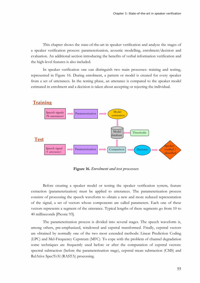
Chapter 3: State-of-the-art in speaker verification
55
3 State-of-the-art in speaker verification
This chapter shows the state-of-the-art in speaker verification and analyze the stages of
a speaker verification process: parameterization, acoustic modelling, enrolment/decision and
evaluation. An additional section introducing the benefits of verbal information verification and
the high-level features is also included.
In speaker verification one can distinguish two main processes: training and testing,
represented in Figure 16. During enrolment, a pattern or model is created for every speaker
from a set of utterances. In the testing phase, an utterance is compared to the speaker model
estimated in enrolment and a decision is taken about accepting or rejecting the individual.
Figure 16. Enrolment and test processes
Before creating a speaker model or testing the speaker verification system, feature
extraction (parameterization) must be applied to utterances. The parameterization process
consists of processing the speech waveform to obtain a new and more reduced representation
of the signal, a set of vectors whose components are called parameters. Each one of these
vectors represents a segment of the utterance. Typical lengths of these segments go from 10 to
40 milliseconds [Picone 93].
The parameterization process is divided into several stages. The speech waveform is,
among others, pre-emphasized, windowed and cepstral transformed. Finally, cepstral vectors
are obtained by normally one of the two most extended methods: Linear Prediction Coding
(LPC) and Mel-Frequency Cepstrum (MFC). To cope with the problem of channel degradation
some techniques are frequently used before or after the computation of cepstral vectors:
spectral subtraction (before the parameterization stage), cepstral mean subtraction (CMS) and
RelAtive SpecTrAl (RASTA) processing.
Parameterization Speech signals (N utterances)
Speaker verified / identified
Model estimation
Thresholds Model database
Speech signal (1 utterance)
Parameterization Comparison Decision
Training
Test
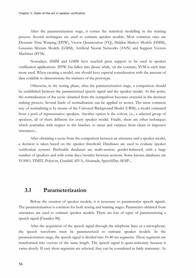
Chapter 3: State-of-the-art in speaker verification
56
After the parameterization stage, it comes the statistical modelling in the training
process. Several techniques are used to estimate speaker models. Most common ones are
Dynamic Time Warping (DTW), Vector Quantization (VQ), Hidden Markov Models (HMM),
Gaussian Mixture Models (GMM), Artificial Neural Networks (ANN) and Support Vectors
Machines (SVM).
Nowadays, HMM and GMM have reached great support to be used in speaker
verification applications. DTW has fallen into disuse while, on the contrary, SVM is each time
more used. When creating a model, one should have especial consideration with the amount of
data available to dimensionate the statistics of the prototype.
Otherwise, in the testing phase, after the parameterization stage, a comparison should
be established between the parameterized speech signal and the speaker model. At this point,
the normalization of the score obtained from the comparison becomes essential in the decision
making process. Several kinds of normalization can be applied to scores. The most common
way of normalizing is by means of the Universal Background Model (UBM), a model estimated
from a pool of representative speakers. Another option is the cohort, i.e., a selected group of
speakers, all of them different for every speaker model. Finally, there are other techniques
which normalize with respect to the handset, to mean and variance from client or impostor
utterances...
After obtaining a score from the comparison between an utterance and a speaker model,
a decision is taken based on the speaker threshold. Databases are used to evaluate speaker
verification systems. Preferable databases are multi-session, gender-balanced, with a large
number of speakers and with some days/months between sessions. Some known databases are
YOHO, TIMIT, Polycost, Gandalf, SIVA, Ahumada, SpeechDat, SESP...
3.1 Parameterization
Before the creation of speaker models, it is necessary to parameterize speech signals.
The parameterization is common for both testing and training stages. Parameters obtained from
utterances are used to estimate speaker models. There are lots of types of parameterizing a
speech signal [Faundez 00].
After the acquisition of the speech signal through the telephone lines or a microphone,
the speech waveform must be parameterized to estimate speaker models. In the
parameterization stage, the speech signal is divided into 10-40 ms segments. These segments are
transformed into vectors of the same length. The speech signal is quasi-stationary because it
varies slowly. If very short segments are selected, they can be considered as fairly stationary. As
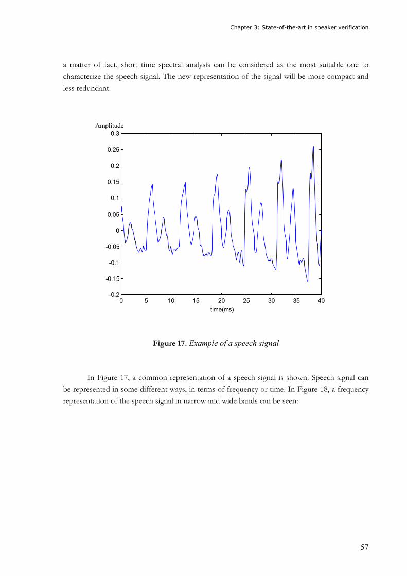
Chapter 3: State-of-the-art in speaker verification
57
a matter of fact, short time spectral analysis can be considered as the most suitable one to
characterize the speech signal. The new representation of the signal will be more compact and
less redundant.
Figure 17. Example of a speech signal
In Figure 17, a common representation of a speech signal is shown. Speech signal can
be represented in some different ways, in terms of frequency or time. In Figure 18, a frequency
representation of the speech signal in narrow and wide bands can be seen:
Amplitude
0 5 10 15 20 25 30 35 40-0.2
-0.15
-0.1
-0.05
0
0.05
0.1
0.15
0.2
0.25
0.3
time(ms)
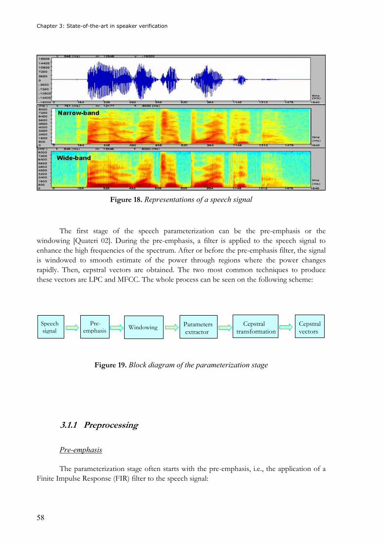
Chapter 3: State-of-the-art in speaker verification
58
Figure 18. Representations of a speech signal
The first stage of the speech parameterization can be the pre-emphasis or the windowing [Quateri 02]. During the pre-emphasis, a filter is applied to the speech signal to enhance the high frequencies of the spectrum. After or before the pre-emphasis filter, the signal is windowed to smooth estimate of the power through regions where the power changes rapidly. Then, cepstral vectors are obtained. The two most common techniques to produce these vectors are LPC and MFCC. The whole process can be seen on the following scheme:
Figure 19. Block diagram of the parameterization stage
3.1.1 Preprocessing
Pre-emphasis
The parameterization stage often starts with the pre-emphasis, i.e., the application of a Finite Impulse Response (FIR) filter to the speech signal:
Speech signal
Pre- emphasis Windowing Parameters
extractor Cepstral transformation
Cepstral vectors
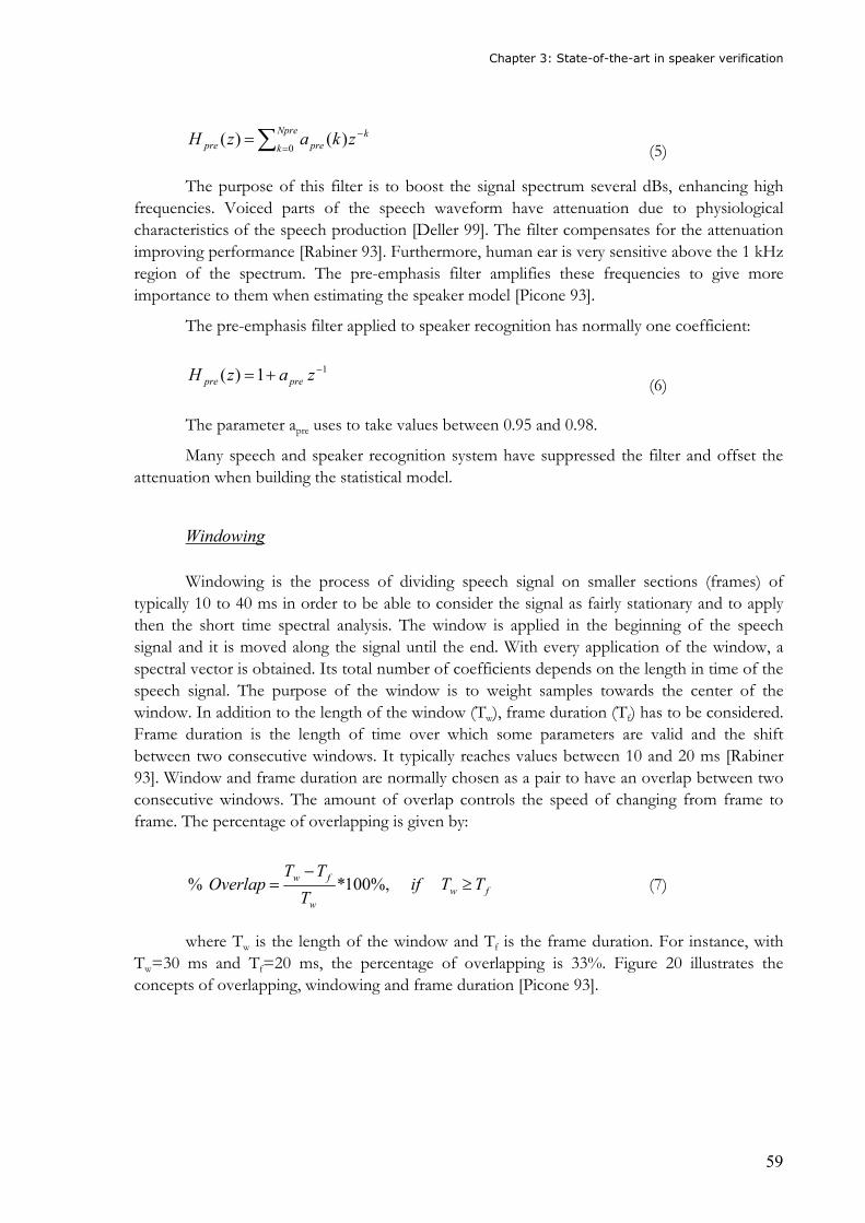
Chapter 3: State-of-the-art in speaker verification
59
kNpre
k prepre zkazH −
=∑= )()(0 (5)
The purpose of this filter is to boost the signal spectrum several dBs, enhancing high
frequencies. Voiced parts of the speech waveform have attenuation due to physiological characteristics of the speech production [Deller 99]. The filter compensates for the attenuation improving performance [Rabiner 93]. Furthermore, human ear is very sensitive above the 1 kHz region of the spectrum. The pre-emphasis filter amplifies these frequencies to give more importance to them when estimating the speaker model [Picone 93].
The pre-emphasis filter applied to speaker recognition has normally one coefficient:
11)( −+= zazH prepre (6)
The parameter apre uses to take values between 0.95 and 0.98.
Many speech and speaker recognition system have suppressed the filter and offset the attenuation when building the statistical model.
Windowing
Windowing is the process of dividing speech signal on smaller sections (frames) of
typically 10 to 40 ms in order to be able to consider the signal as fairly stationary and to apply then the short time spectral analysis. The window is applied in the beginning of the speech signal and it is moved along the signal until the end. With every application of the window, a spectral vector is obtained. Its total number of coefficients depends on the length in time of the speech signal. The purpose of the window is to weight samples towards the center of the window. In addition to the length of the window (Tw), frame duration (Tf) has to be considered. Frame duration is the length of time over which some parameters are valid and the shift between two consecutive windows. It typically reaches values between 10 and 20 ms [Rabiner 93]. Window and frame duration are normally chosen as a pair to have an overlap between two consecutive windows. The amount of overlap controls the speed of changing from frame to frame. The percentage of overlapping is given by:
fww
fw TTifT
TTOverlap ≥
−= %,100*% (7)
where Tw is the length of the window and Tf is the frame duration. For instance, with Tw=30 ms and Tf=20 ms, the percentage of overlapping is 33%. Figure 20 illustrates the concepts of overlapping, windowing and frame duration [Picone 93].
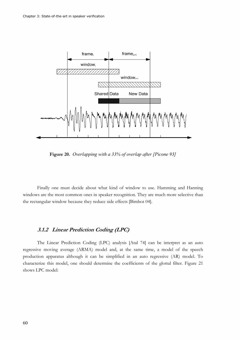
Chapter 3: State-of-the-art in speaker verification
60
Figure 20. Overlapping with a 33% of overlap after [Picone 93]
Finally one must decide about what kind of window to use. Hamming and Hanning
windows are the most common ones in speaker recognition. They are much more selective than
the rectangular window because they reduce side effects [Bimbot 04].
3.1.2 Linear Prediction Coding (LPC)
The Linear Prediction Coding (LPC) analysis [Atal 74] can be interpret as an auto
regressive moving average (ARMA) model and, at the same time, a model of the speech
production apparatus although it can be simplified in an auto regressive (AR) model. To
characterize this model, one should determine the coefficients of the glottal filter. Figure 21
shows LPC model:
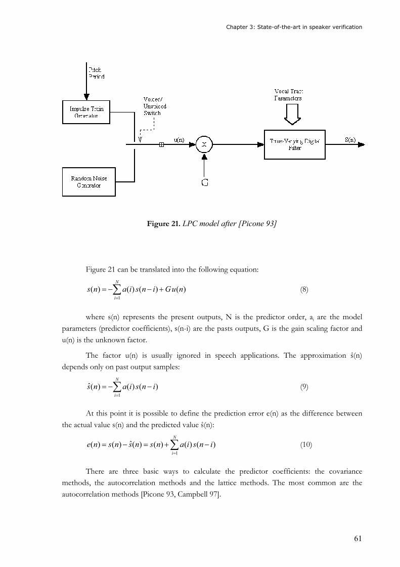
Chapter 3: State-of-the-art in speaker verification
61
Figure 21. LPC model after [Picone 93]
Figure 21 can be translated into the following equation:
∑=
+−−=N
i
nuGinsians1
)()()()( (8)
where s(n) represents the present outputs, N is the predictor order, ai are the model
parameters (predictor coefficients), s(n-i) are the pasts outputs, G is the gain scaling factor and
u(n) is the unknown factor.
The factor u(n) is usually ignored in speech applications. The approximation ŝ(n)
depends only on past output samples:
∑=
−−=N
i
insians1
)()()(ˆ (9)
At this point it is possible to define the prediction error e(n) as the difference between
the actual value s(n) and the predicted value ŝ(n):
∑=
−+=−=N
i
insiansnsnsne1
)()()()(ˆ)()( (10)
There are three basic ways to calculate the predictor coefficients: the covariance
methods, the autocorrelation methods and the lattice methods. The most common are the
autocorrelation methods [Picone 93, Campbell 97].
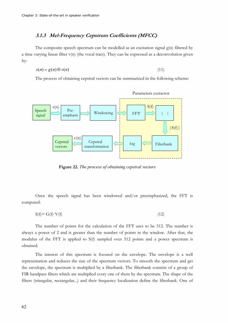
Chapter 3: State-of-the-art in speaker verification
62
3.1.3 Mel-Frequency Cepstrum Coefficients (MFCC) The composite speech spectrum can be modelled as an excitation signal g(n) filtered by
a time varying linear filter v(n) (the vocal tract). They can be expressed as a deconvolution given
by:
)()()( nvngns ⊗= (11)
The process of obtaining cepstral vectors can be summarized in the following scheme:
Figure 22. The process of obtaining cepstral vectors
Once the speech signal has been windowed and/or preemphasized, the FFT is
computed: S(f)= G(f)�V(f) (12) The number of points for the calculation of the FFT uses to be 512. The number is
always a power of 2 and is greater than the number of points in the window. After that, the
modulus of the FFT is applied to S(f) sampled over 512 points and a power spectrum is
obtained.
The interest of this spectrum is focused on the envelope. The envelope is a well
representation and reduces the size of the spectrum vectors. To smooth the spectrum and get
the envelope, the spectrum is multiplied by a filterbank. The filterbank consists of a group of
FIR bandpass filters which are multiplied every one of them by the spectrum. The shape of the
filters (triangular, rectangular...) and their frequency localization define the filterbank. One of
Speech signal
Pre- emphasis Windowing FFT
Cepstral transformation
Cepstral vectors
s(n)
| |
Filterbank log
S(f)
|S(f)|
c(n)
Parameters extractor
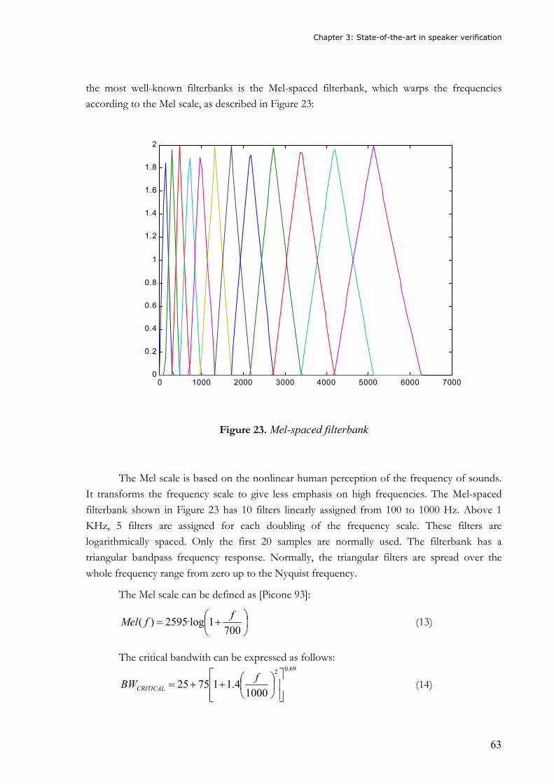
Chapter 3: State-of-the-art in speaker verification
63
the most well-known filterbanks is the Mel-spaced filterbank, which warps the frequencies
according to the Mel scale, as described in Figure 23:
Figure 23. Mel-spaced filterbank
The Mel scale is based on the nonlinear human perception of the frequency of sounds.
It transforms the frequency scale to give less emphasis on high frequencies. The Mel-spaced
filterbank shown in Figure 23 has 10 filters linearly assigned from 100 to 1000 Hz. Above 1
KHz, 5 filters are assigned for each doubling of the frequency scale. These filters are
logarithmically spaced. Only the first 20 samples are normally used. The filterbank has a
triangular bandpass frequency response. Normally, the triangular filters are spread over the
whole frequency range from zero up to the Nyquist frequency.
The Mel scale can be defined as [Picone 93]:
+=700
1·log2595)(f
fMel (13)
The critical bandwith can be expressed as follows:
69.02
10004.117525
++=f
BWCRITICAL (14)
0 1000 2000 3000 4000 5000 6000 70000
0.2
0.4
0.6
0.8
1
1.2
1.4
1.6
1.8
2
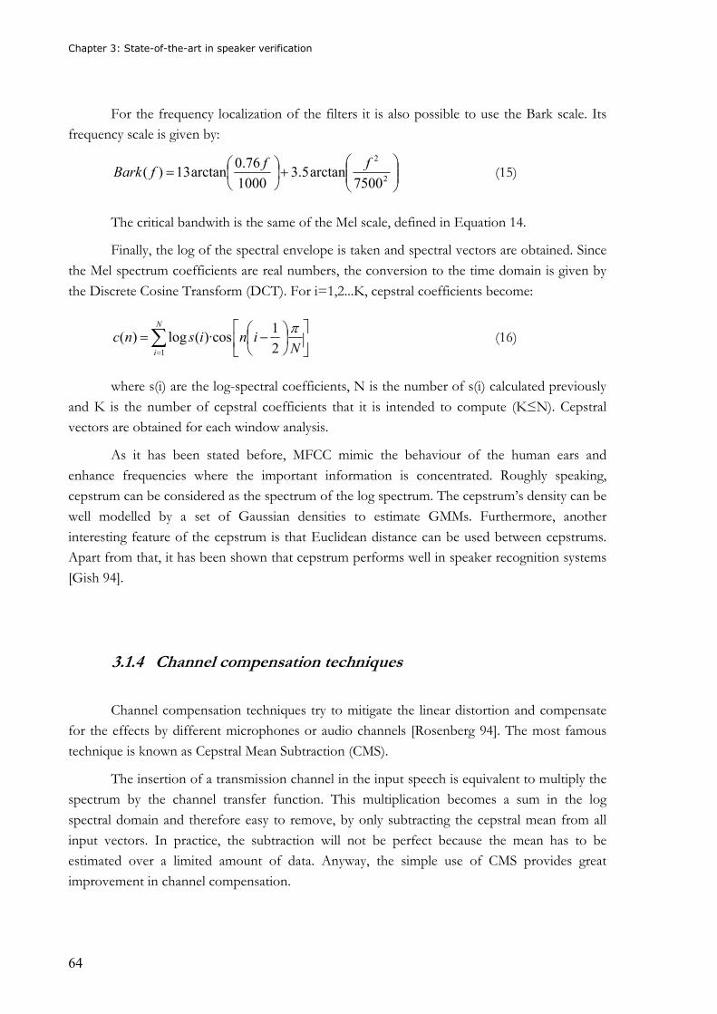
Chapter 3: State-of-the-art in speaker verification
64
For the frequency localization of the filters it is also possible to use the Bark scale. Its
frequency scale is given by:
+
=2
2
7500arctan5.3
1000
76.0arctan13)(
fffBark (15)
The critical bandwith is the same of the Mel scale, defined in Equation 14.
Finally, the log of the spectral envelope is taken and spectral vectors are obtained. Since
the Mel spectrum coefficients are real numbers, the conversion to the time domain is given by
the Discrete Cosine Transform (DCT). For i=1,2...K, cepstral coefficients become:
∑=
−=N
i Ninisnc
1 2
1)·cos(log)(
π (16)
where s(i) are the log-spectral coefficients, N is the number of s(i) calculated previously
and K is the number of cepstral coefficients that it is intended to compute (K≤N). Cepstral
vectors are obtained for each window analysis.
As it has been stated before, MFCC mimic the behaviour of the human ears and
enhance frequencies where the important information is concentrated. Roughly speaking,
cepstrum can be considered as the spectrum of the log spectrum. The cepstrum’s density can be
well modelled by a set of Gaussian densities to estimate GMMs. Furthermore, another
interesting feature of the cepstrum is that Euclidean distance can be used between cepstrums.
Apart from that, it has been shown that cepstrum performs well in speaker recognition systems
[Gish 94].
3.1.4 Channel compensation techniques
Channel compensation techniques try to mitigate the linear distortion and compensate
for the effects by different microphones or audio channels [Rosenberg 94]. The most famous
technique is known as Cepstral Mean Subtraction (CMS).
The insertion of a transmission channel in the input speech is equivalent to multiply the
spectrum by the channel transfer function. This multiplication becomes a sum in the log
spectral domain and therefore easy to remove, by only subtracting the cepstral mean from all
input vectors. In practice, the subtraction will not be perfect because the mean has to be
estimated over a limited amount of data. Anyway, the simple use of CMS provides great
improvement in channel compensation.
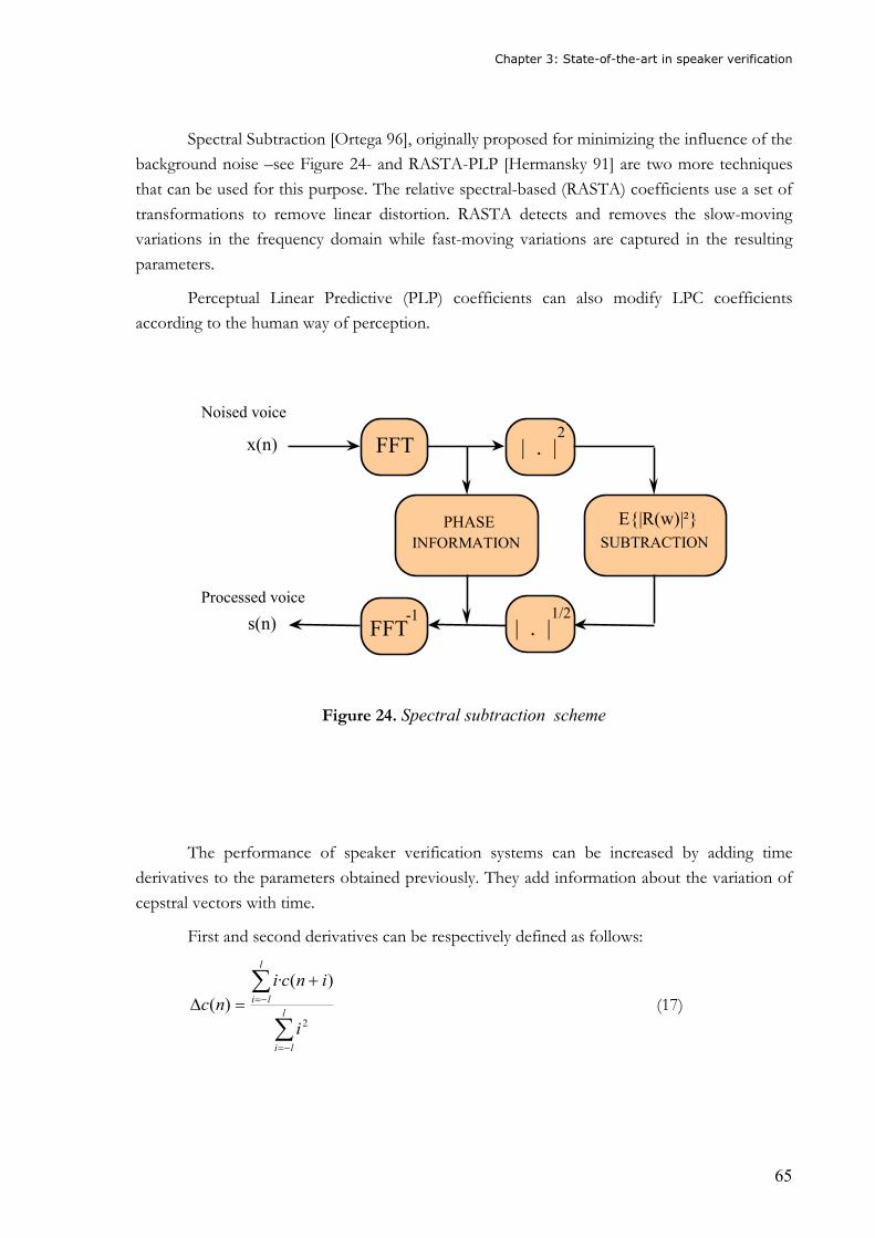
Chapter 3: State-of-the-art in speaker verification
65
Spectral Subtraction [Ortega 96], originally proposed for minimizing the influence of the
background noise –see Figure 24- and RASTA-PLP [Hermansky 91] are two more techniques
that can be used for this purpose. The relative spectral-based (RASTA) coefficients use a set of
transformations to remove linear distortion. RASTA detects and removes the slow-moving
variations in the frequency domain while fast-moving variations are captured in the resulting
parameters.
Perceptual Linear Predictive (PLP) coefficients can also modify LPC coefficients
according to the human way of perception.
Figure 24. Spectral subtraction scheme
The performance of speaker verification systems can be increased by adding time
derivatives to the parameters obtained previously. They add information about the variation of
cepstral vectors with time.
First and second derivatives can be respectively defined as follows:
∑
∑
−=
−=
+=∆
l
li
l
li
i
inci
nc2
)(·
)( (17)
FFT
FFT -1
PHASE
INFORMATION SUBTRACTION
E{|R(w)|²}
| . | 2
| . | 1/2
Noised voice
x(n)
Processed voice
s(n)
Chapter 3: State-of-the-art in speaker verification
66
∑
∑
−=
−=
+∆=∆∆
l
li
l
li
i
inci
nc2
)(·
)( (18)
They are also known as delta and delta-delta parameters. Log energy is often discarded
while its deltas are normally included.
RASTA is similar to CMS but it also attenuates a small band of low modulation
frequencies. Furthermore, it attenuates high modulation frequencies too.
On the other hand, nonlinear distortion cannot be removed with CMS or RASTA
techniques. There are other cases where mismatched conditions between training and testing
elicit serious problems. They are mainly caused by the use of different handsets for both
processes. To compensate for the distortion introduced, handset channel normalization
techniques are frequently used [Reynolds 95, Reynolds 97, Heck 00b].
3.2 Acoustic models
Speaker models are created from features extracted from speech signals. The first step
in order to estimate a model from speech utterances is the selection of a model topology. There
are two types of models: template and stochastic models [Campbell 97].
In template models, the observation is assumed to be an imperfect replica of the
template. The best alignment of observed frames with the template is obtained by minimizing a
distance d. The pattern matching, i.e., the computation of a similarity measure of the input
feature vectors against the model, is deterministic.
Template (non-parametric) models are the most intuitive ones due to the introduction
of the concept of distance. Some examples of template models are VQ, NN or DTW. They also
can be divided into time-dependent, for instance DTW or time-independent, like VQ. Time-
dependent template models include the variability in the human speaking rate while time-
independent ones ignore temporal variations.
Otherwise, stochastic models measure the likelihood of an observation given the
speaker model. This observation is a random vector with a conditional pdf. The estimated pdf
can be a parametric or a non-parametric model [Gish 94]. If the model is parametric, a specific
pdf is assumed. If the model is non-parametric, minimal assumptions regarding the pdf are
assumed. In stochastic models, the pattern matching is probabilistic.
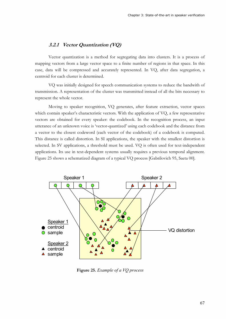
Chapter 3: State-of-the-art in speaker verification
67
3.2.1 Vector Quantization (VQ) Vector quantization is a method for segregating data into clusters. It is a process of
mapping vectors from a large vector space to a finite number of regions in that space. In this
case, data will be compressed and accurately represented. In VQ, after data segregation, a
centroid for each cluster is determined.
VQ was initially designed for speech communication systems to reduce the bandwith of
transmission. A representation of the cluster was transmitted instead of all the bits necessary to
represent the whole vector.
Moving to speaker recognition, VQ generates, after feature extraction, vector spaces
which contain speaker’s characteristic vectors. With the application of VQ, a few representative
vectors are obtained for every speaker: the codebook. In the recognition process, an input
utterance of an unknown voice is ‘vector-quantized’ using each codebook and the distance from
a vector to the closest codeword (each vector of the codebook) of a codebook is computed.
This distance is called distortion. In SI applications, the speaker with the smallest distortion is
selected. In SV applications, a threshold must be used. VQ is often used for text-independent
applications. Its use in text-dependent systems usually requires a previous temporal alignment.
Figure 25 shows a schematized diagram of a typical VQ process [Gabrilovich 95, Saeta 00].
Speaker 1
Speaker 1centroidsample
Speaker 2centroidsample
Speaker 2
VQ distortion
Figure 25. Example of a VQ process
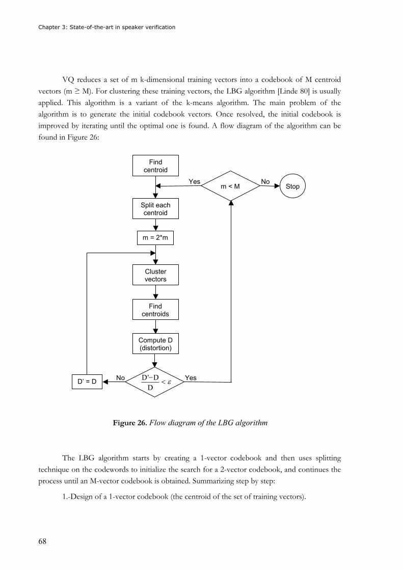
Chapter 3: State-of-the-art in speaker verification
68
VQ reduces a set of m k-dimensional training vectors into a codebook of M centroid
vectors (m ≥ M). For clustering these training vectors, the LBG algorithm [Linde 80] is usually
applied. This algorithm is a variant of the k-means algorithm. The main problem of the
algorithm is to generate the initial codebook vectors. Once resolved, the initial codebook is
improved by iterating until the optimal one is found. A flow diagram of the algorithm can be
found in Figure 26:
Findcentroid
Split eachcentroid
Clustervectors
Findcentroids
Compute D(distortion)
ε<−D
D'D
Stop
D’ = D
m = 2*m
No
Yes
Yes
Nom < M
Figure 26. Flow diagram of the LBG algorithm
The LBG algorithm starts by creating a 1-vector codebook and then uses splitting
technique on the codewords to initialize the search for a 2-vector codebook, and continues the
process until an M-vector codebook is obtained. Summarizing step by step:
1.-Design of a 1-vector codebook (the centroid of the set of training vectors).
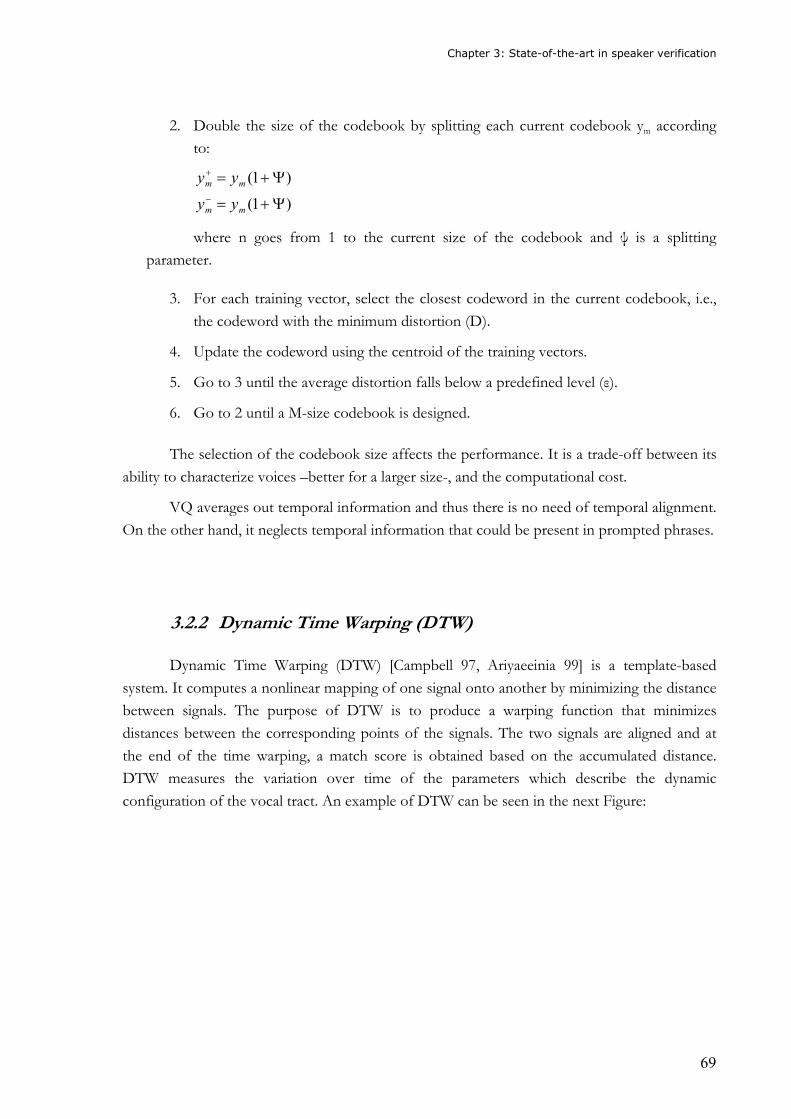
Chapter 3: State-of-the-art in speaker verification
69
2. Double the size of the codebook by splitting each current codebook ym according
to:
)1(
)1(
Ψ+=
Ψ+=−
+
mm
mm
yy
yy
where n goes from 1 to the current size of the codebook and ψ is a splitting
parameter.
3. For each training vector, select the closest codeword in the current codebook, i.e.,
the codeword with the minimum distortion (D).
4. Update the codeword using the centroid of the training vectors.
5. Go to 3 until the average distortion falls below a predefined level (ε).
6. Go to 2 until a M-size codebook is designed. The selection of the codebook size affects the performance. It is a trade-off between its
ability to characterize voices –better for a larger size-, and the computational cost.
VQ averages out temporal information and thus there is no need of temporal alignment.
On the other hand, it neglects temporal information that could be present in prompted phrases.
3.2.2 Dynamic Time Warping (DTW) Dynamic Time Warping (DTW) [Campbell 97, Ariyaeeinia 99] is a template-based
system. It computes a nonlinear mapping of one signal onto another by minimizing the distance
between signals. The purpose of DTW is to produce a warping function that minimizes
distances between the corresponding points of the signals. The two signals are aligned and at
the end of the time warping, a match score is obtained based on the accumulated distance.
DTW measures the variation over time of the parameters which describe the dynamic
configuration of the vocal tract. An example of DTW can be seen in the next Figure:
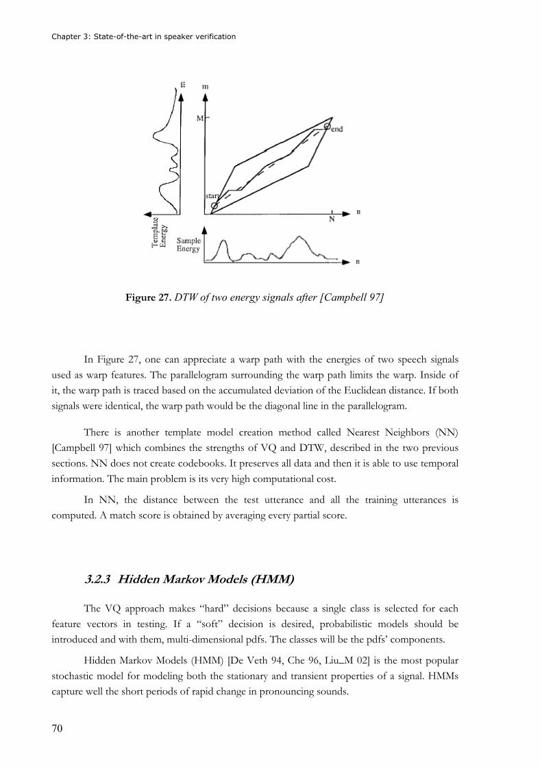
Chapter 3: State-of-the-art in speaker verification
70
Figure 27. DTW of two energy signals after [Campbell 97]
In Figure 27, one can appreciate a warp path with the energies of two speech signals
used as warp features. The parallelogram surrounding the warp path limits the warp. Inside of
it, the warp path is traced based on the accumulated deviation of the Euclidean distance. If both
signals were identical, the warp path would be the diagonal line in the parallelogram. There is another template model creation method called Nearest Neighbors (NN)
[Campbell 97] which combines the strengths of VQ and DTW, described in the two previous
sections. NN does not create codebooks. It preserves all data and then it is able to use temporal
information. The main problem is its very high computational cost.
In NN, the distance between the test utterance and all the training utterances is
computed. A match score is obtained by averaging every partial score.
3.2.3 Hidden Markov Models (HMM)
The VQ approach makes “hard” decisions because a single class is selected for each
feature vectors in testing. If a “soft” decision is desired, probabilistic models should be
introduced and with them, multi-dimensional pdfs. The classes will be the pdfs’ components.
Hidden Markov Models (HMM) [De Veth 94, Che 96, Liu_M 02] is the most popular
stochastic model for modeling both the stationary and transient properties of a signal. HMMs
capture well the short periods of rapid change in pronouncing sounds.
Chapter 3: State-of-the-art in speaker verification
71
The structure of a HMM [Klevans 97] is composed by a set of states with transitions
between each state. For each transition from a state, a probability of taking that transition is
assigned. These probabilities sum one. They are essentially stochastic finite state machines
which output a symbol each time they depart from a state. The symbol is probabilistically
determined, each state contains a probability distribution of the possible output states. The
sequence of states is not directly observable. That is the reason why they are called “hidden”.
An example of a HMM sequence can be observed at Figure 28:
Figure 28. A three state HMM
There are some parameters which define a HMM:
N = the number of states in the model;
S = {s1, s2,..., sN}, the states in the model;
P = the number of output symbols;
A = {aij}, aij = P( sj(t+1) | si(t) ), the matrix of transition probabilities;
B = {bj(k)}, bj(k) = P( vk(t) | sj(t) ), the output symbol probability distribution at state j
where {vk} is the set of output symbols;
π = { πi}, πi = P( si(t) = 0 ), the initial state distribution.
For the example shown in Figure 28, N=M=3, S = {s1, s2, s3}, A = {a11, a22, a33, a12, a23,
a13} and B = {b1, b2, b3}
Each state sj has an output distribution defined by the vector A. The probability of
emitting a symbol in the state sj is given by {aij}. There is not necessarily a correspondence
between an observation and a state, but each state has a probability of having produced the
s1 s3 s2
a11 a22 a33
a12 a13
a23
b1 b2 b3
Chapter 3: State-of-the-art in speaker verification
72
observation. Observations can only be used for computing the probabilities of different state
sequences.
There are many different topologies for HMM. The following two topologies are very
common:
- Ergotic HMM. It contains transitions to and from every state with P(aij) > 0
- LR-HMM. Left-to-right HMM is a derivation of an ergotic model. It is an
absorbing state that cannot be exited once entered. In SV, LR-HMM is often
used in phrase prompted cases.
When dealing with HMMs, one can also find three basic problems:
1. The recognition problem: Given a model and a sequence of observations, what is the
probability that the sequence has been generated by the model? The solution to this
problem can be found by using the forward-backward algorithm.
2. The decoding problem: Given a model and a sequence of observations, what is the
most likely sequence of states that have produced the sequence of observations? The
problem can be solved by using the Viterbi algorithm.
3. The learning (training) problem: Given a model and a topology, how can the model
parameters be adjusted to maximize the probability of generating the observations? The
solution can be found with the Baum-Welch or forward-backward algorithms.
The solution to the first problem, the evaluation problem, can be used for recognition
tasks by comparing new speech signals to a model. The solution to the second problem can be
used for applications in which each state has a specific meaning. Finally, the solution to the
training problem will let to estimate HMM.
Variance flooring [Melin 98, Melin 99b] has also to be considered when producing
HMMs. During iterations registered in the Expectation-Maximization (EM) algorithm, it is
possible to limit the minimum level of variance during the initialization and the re-estimation
processes.
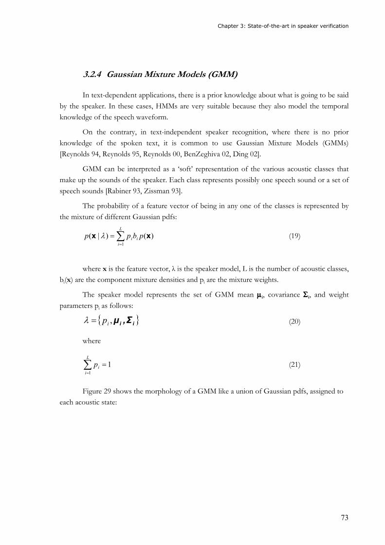
Chapter 3: State-of-the-art in speaker verification
73
3.2.4 Gaussian Mixture Models (GMM)
In text-dependent applications, there is a prior knowledge about what is going to be said
by the speaker. In these cases, HMMs are very suitable because they also model the temporal
knowledge of the speech waveform.
On the contrary, in text-independent speaker recognition, where there is no prior
knowledge of the spoken text, it is common to use Gaussian Mixture Models (GMMs)
[Reynolds 94, Reynolds 95, Reynolds 00, BenZeghiva 02, Ding 02].
GMM can be interpreted as a ‘soft’ representation of the various acoustic classes that
make up the sounds of the speaker. Each class represents possibly one speech sound or a set of
speech sounds [Rabiner 93, Zissman 93].
The probability of a feature vector of being in any one of the classes is represented by
the mixture of different Gaussian pdfs:
)()|(1
xx pbpp i
L
ii∑
=
=λ (19)
where x is the feature vector, λ is the speaker model, L is the number of acoustic classes,
bi(x) are the component mixture densities and pi are the mixture weights.
The speaker model represents the set of GMM mean µµµµi, covariance ΣΣΣΣi, and weight
parameters pi as follows:
{ }ii Σ,µ,ip=λ (20) where
∑=
=L
iip
1
1 (21)
Figure 29 shows the morphology of a GMM like a union of Gaussian pdfs, assigned to
each acoustic state:
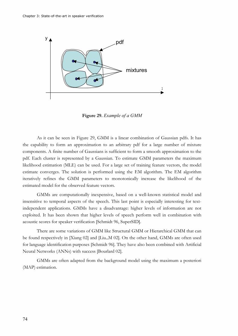
Chapter 3: State-of-the-art in speaker verification
74
Figure 29. Example of a GMM
As it can be seen in Figure 29, GMM is a linear combination of Gaussian pdfs. It has
the capability to form an approximation to an arbitrary pdf for a large number of mixture
components. A finite number of Gaussians is sufficient to form a smooth approximation to the
pdf. Each cluster is represented by a Gaussian. To estimate GMM parameters the maximum
likelihood estimation (MLE) can be used. For a large set of training feature vectors, the model
estimate converges. The solution is performed using the EM algorithm. The EM algorithm
iteratively refines the GMM parameters to monotonically increase the likelihood of the
estimated model for the observed feature vectors.
GMMs are computationally inexpensive, based on a well-known statistical model and
insensitive to temporal aspects of the speech. This last point is especially interesting for text-
independent applications. GMMs have a disadvantage: higher levels of information are not
exploited. It has been shown that higher levels of speech perform well in combination with
acoustic scores for speaker verification [Schmidt 96, SuperSID].
There are some variations of GMM like Structural GMM or Hierarchical GMM that can
be found respectively in [Xiang 02] and [Liu_M 02]. On the other hand, GMMs are often used
for language identification purposes [Schmidt 96]. They have also been combined with Artificial
Neural Networks (ANNs) with success [Bourlard 02].
GMMs are often adapted from the background model using the maximum a posteriori
(MAP) estimation.
x
y pdf
mixtures
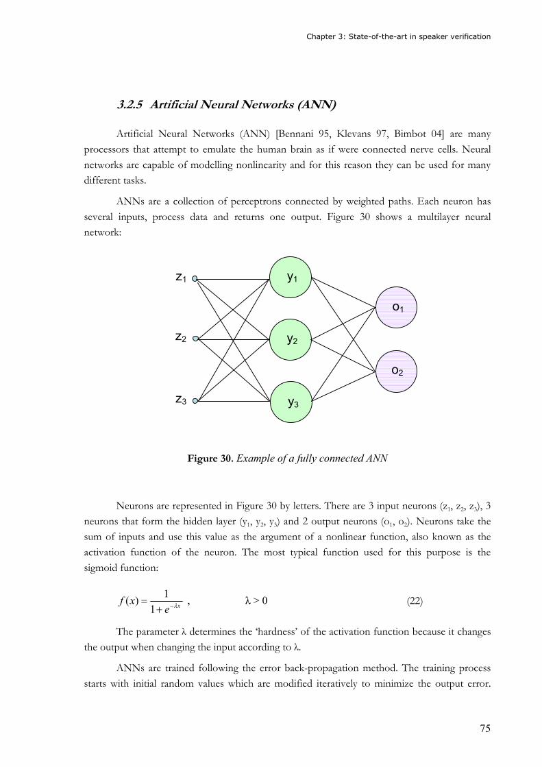
Chapter 3: State-of-the-art in speaker verification
75
3.2.5 Artificial Neural Networks (ANN)
Artificial Neural Networks (ANN) [Bennani 95, Klevans 97, Bimbot 04] are many
processors that attempt to emulate the human brain as if were connected nerve cells. Neural
networks are capable of modelling nonlinearity and for this reason they can be used for many
different tasks.
ANNs are a collection of perceptrons connected by weighted paths. Each neuron has
several inputs, process data and returns one output. Figure 30 shows a multilayer neural
network:
Figure 30. Example of a fully connected ANN
Neurons are represented in Figure 30 by letters. There are 3 input neurons (z1, z2, z3), 3
neurons that form the hidden layer (y1, y2, y3) and 2 output neurons (o1, o2). Neurons take the
sum of inputs and use this value as the argument of a nonlinear function, also known as the
activation function of the neuron. The most typical function used for this purpose is the
sigmoid function:
xexf λ−+=1
1)( , λ > 0 (22)
The parameter λ determines the ‘hardness’ of the activation function because it changes
the output when changing the input according to λ.
ANNs are trained following the error back-propagation method. The training process
starts with initial random values which are modified iteratively to minimize the output error.
z1
z3
z2
y1
y2
y3
o1
o2
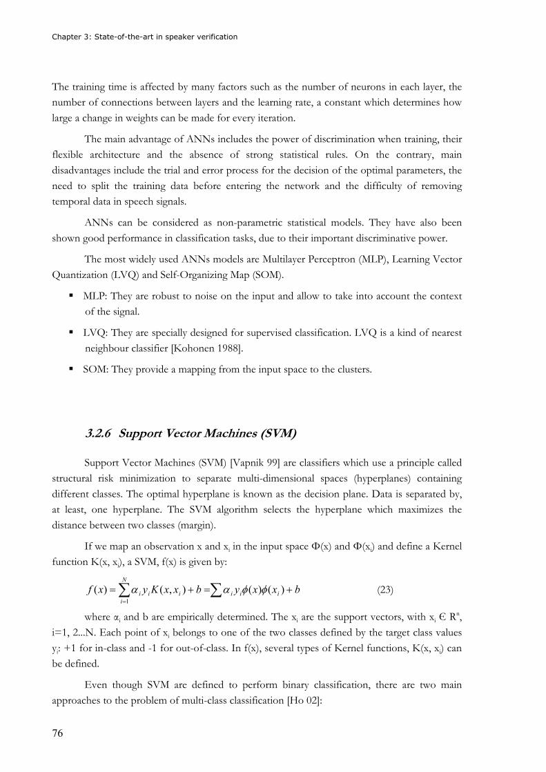
Chapter 3: State-of-the-art in speaker verification
76
The training time is affected by many factors such as the number of neurons in each layer, the
number of connections between layers and the learning rate, a constant which determines how
large a change in weights can be made for every iteration.
The main advantage of ANNs includes the power of discrimination when training, their
flexible architecture and the absence of strong statistical rules. On the contrary, main
disadvantages include the trial and error process for the decision of the optimal parameters, the
need to split the training data before entering the network and the difficulty of removing
temporal data in speech signals.
ANNs can be considered as non-parametric statistical models. They have also been
shown good performance in classification tasks, due to their important discriminative power.
The most widely used ANNs models are Multilayer Perceptron (MLP), Learning Vector
Quantization (LVQ) and Self-Organizing Map (SOM).
� MLP: They are robust to noise on the input and allow to take into account the context
of the signal.
� LVQ: They are specially designed for supervised classification. LVQ is a kind of nearest
neighbour classifier [Kohonen 1988].
� SOM: They provide a mapping from the input space to the clusters.
3.2.6 Support Vector Machines (SVM)
Support Vector Machines (SVM) [Vapnik 99] are classifiers which use a principle called
structural risk minimization to separate multi-dimensional spaces (hyperplanes) containing
different classes. The optimal hyperplane is known as the decision plane. Data is separated by,
at least, one hyperplane. The SVM algorithm selects the hyperplane which maximizes the
distance between two classes (margin).
If we map an observation x and xi in the input space Φ(x) and Φ(xi) and define a Kernel
function K(x, xi), a SVM, f(x) is given by:
∑∑ +=+==
bxxybxxKyxf iii
N
iiii )()(),()(
1
φφαα (23)
where αi and b are empirically determined. The xi are the support vectors, with xi Є Rn,
i=1, 2...N. Each point of xi belongs to one of the two classes defined by the target class values
yi: +1 for in-class and -1 for out-of-class. In f(x), several types of Kernel functions, K(x, xi) can
be defined.
Even though SVM are defined to perform binary classification, there are two main
approaches to the problem of multi-class classification [Ho 02]:
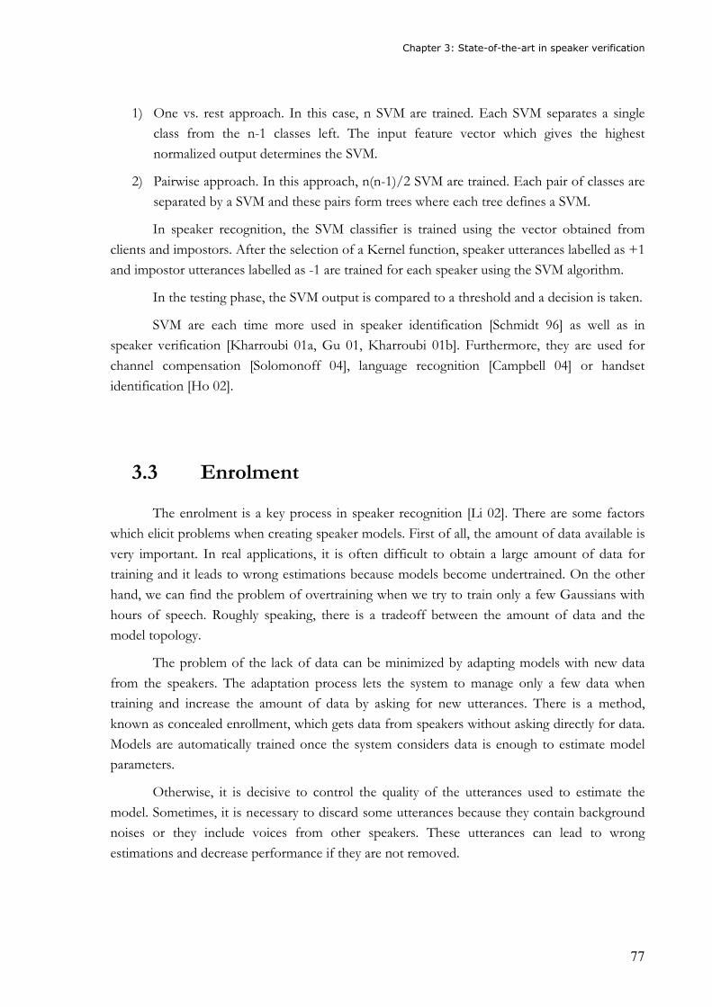
Chapter 3: State-of-the-art in speaker verification
77
1) One vs. rest approach. In this case, n SVM are trained. Each SVM separates a single
class from the n-1 classes left. The input feature vector which gives the highest
normalized output determines the SVM.
2) Pairwise approach. In this approach, n(n-1)/2 SVM are trained. Each pair of classes are
separated by a SVM and these pairs form trees where each tree defines a SVM.
In speaker recognition, the SVM classifier is trained using the vector obtained from
clients and impostors. After the selection of a Kernel function, speaker utterances labelled as +1
and impostor utterances labelled as -1 are trained for each speaker using the SVM algorithm.
In the testing phase, the SVM output is compared to a threshold and a decision is taken.
SVM are each time more used in speaker identification [Schmidt 96] as well as in
speaker verification [Kharroubi 01a, Gu 01, Kharroubi 01b]. Furthermore, they are used for
channel compensation [Solomonoff 04], language recognition [Campbell 04] or handset
identification [Ho 02].
3.3 Enrolment
The enrolment is a key process in speaker recognition [Li 02]. There are some factors
which elicit problems when creating speaker models. First of all, the amount of data available is
very important. In real applications, it is often difficult to obtain a large amount of data for
training and it leads to wrong estimations because models become undertrained. On the other
hand, we can find the problem of overtraining when we try to train only a few Gaussians with
hours of speech. Roughly speaking, there is a tradeoff between the amount of data and the
model topology.
The problem of the lack of data can be minimized by adapting models with new data
from the speakers. The adaptation process lets the system to manage only a few data when
training and increase the amount of data by asking for new utterances. There is a method,
known as concealed enrollment, which gets data from speakers without asking directly for data.
Models are automatically trained once the system considers data is enough to estimate model
parameters.
Otherwise, it is decisive to control the quality of the utterances used to estimate the
model. Sometimes, it is necessary to discard some utterances because they contain background
noises or they include voices from other speakers. These utterances can lead to wrong
estimations and decrease performance if they are not removed.
Chapter 3: State-of-the-art in speaker verification
78
3.3.1 Model quality
The quality of a model mainly depends on the reliability and variability of the utterances
and on the training and test conditions. It is crucial that the speaker model includes the most
discriminative speaker characteristics. When estimating the model, it is ideal to obtain as more
training utterances as possible to estimate the model in an efficient manner. However, in real
applications, one can normally afford one or two enrolment sessions only. In this context, it is
important to control the content and quality of the recorded voice samples, when the enrolment
process is ‘open’, i.e., when the speaker is talking and the utterances are being recorded.
Model quality measures evaluate how discriminative a model is by comparing client
and/or impostor utterances against the model. Some approaches to the problem of model
quality evaluation have traditionally dealt with outliers, i.e., those client scores which are distant
with respect to the mean in terms of LLR. They use the distance between the training model
and the utterances used to estimate the model. The ‘leave-one-out’ method [Gu 00] has the
problem of an excessive computational cost while other methods use only data from impostors.
More about model quality evaluation can be found in Section 4.3.
3.3.2 Adaptation
The adaptation process [Reynolds 00, Mirghafori 02] consists of using one or more
speaker utterances to train a certain speaker model. These utterances are supposed to belong to
the speaker and are used to update the model and improve performance. With adaptation, we
intend to mitigate the variation of voice over time. In real applications, it is common to obtain
only a few data from speakers. The adaptation is used then to achieve new data and better
estimate the speaker models [Matsui 96, Farrell 02].
There are several types of adaptation. When the transcription of the adaptation data is
known, we are dealing with supervised adaptation. On the contrary, when the transcription is
unknown the process is known as unsupervised adaptation [Barras 04]. If the adaptation takes
place incrementally, the process is defined as incremental adaptation [Fredouille 00] while if it
takes place in one session is called static adaptation.
The most well-known methods [Ahn 00, Mariethoz 02] in speaker adaptation are
maximum A-Posteriori (MAP) [Lee 93] and Maximum Likelihood Linear Regression (MLLR).
3.3.2.1 Maximum A-Posteriori (MAP)
Maximum A-Posteriori (MAP) [Gauvain 94] incorporates prior information of the
previously trained speaker model. It is an efficient technique when training data is scarce. MAP
Chapter 3: State-of-the-art in speaker verification
79
assumes that the parameters Θ of the distribution p(X|Θ) are a random variable with a prior
distribution p(Θ). The purpose is to select Θ̂ in order to maximize its posterior probability
density as follows:
)()|(maxargˆ ΘΘ=ΘΘ
pXp (24) Concerning the incremental enrollment, MAP adaptation lets to reestimate HMM
parameters even when adaptation data is not available for some states.
The main problem is the selection of the prior information because its estimation needs
a large amount of data to obtain good estimations of HMM parameters in case of missing
adaptation data.
3.3.2.2 Maximum Likelihood Linear Regression (MLLR)
In Maximum Likelihood Linear Regression (MLLR) [Leggetter 95], the model
parameters are transformed to adapt the model to a new speaker. MLLR estimates a set of
linear transformations for the mean and variance parameters of a speaker model in order to
better fit new incoming data.
Regression based transformations are used to tune HMM parameters and tied between
several mixture components of the HMM. These transformations need enough data to be
estimated.
3.3.2.3 Limited training data
When training data is scarce, the speaker models are usually estimated from a previous
speaker independent model. They are obtained by adapting the speaker independent model
from data coming from every speaker. In this case, it is important the amount of data used to
estimate the global speaker independent model as well as the data available for every speaker.
There are different approaches to deal with the estimation from a speaker independent
model with limited training data:
� MAP: The speaker independent model is adapted for every speaker parameter of the
speaker dependent model from the training data.
� MLLR: The speaker independent model is adapted by using regression-based
transformations.
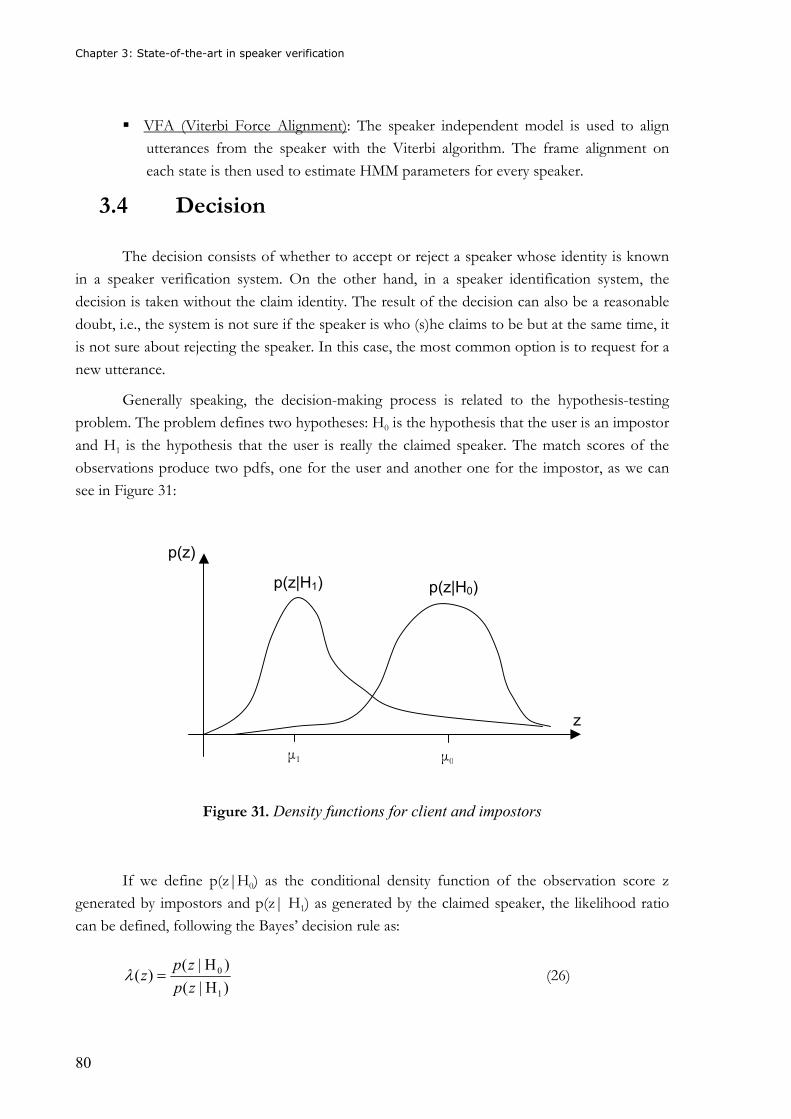
Chapter 3: State-of-the-art in speaker verification
80
� VFA (Viterbi Force Alignment): The speaker independent model is used to align
utterances from the speaker with the Viterbi algorithm. The frame alignment on
each state is then used to estimate HMM parameters for every speaker.
3.4 Decision
The decision consists of whether to accept or reject a speaker whose identity is known
in a speaker verification system. On the other hand, in a speaker identification system, the
decision is taken without the claim identity. The result of the decision can also be a reasonable
doubt, i.e., the system is not sure if the speaker is who (s)he claims to be but at the same time, it
is not sure about rejecting the speaker. In this case, the most common option is to request for a
new utterance.
Generally speaking, the decision-making process is related to the hypothesis-testing
problem. The problem defines two hypotheses: H0 is the hypothesis that the user is an impostor
and H1 is the hypothesis that the user is really the claimed speaker. The match scores of the
observations produce two pdfs, one for the user and another one for the impostor, as we can
see in Figure 31:
Figure 31. Density functions for client and impostors
If we define p(z|H0) as the conditional density function of the observation score z
generated by impostors and p(z| H1) as generated by the claimed speaker, the likelihood ratio
can be defined, following the Bayes’ decision rule as:
)H|(
)H|()(
1
0
zp
zpz =λ (26)
z
p(z)
p(z|H1) p(z|H0)
µ1 µ0
Chapter 3: State-of-the-art in speaker verification
81
The conditional density function p(z|H0) of the claimed speaker is estimated from the
speaker scores and the conditional density function p(z|H1) of the impostor is estimated from
other speakers’ scores.
3.4.1 Normalization
Before the decision making process, a score should be obtained from the comparison of
the speaker’s utterance against a certain model. The decision process is difficult to tune and it
strongly depends on the distribution of other speaker’s scores, the environmental effects, the
speech distortion...
Normalization can be defined as the process of making a relative similarity measure
[Matsui 94, Matsui 95, Liu_W 98, Gravier 98]. This measure compensates for the score
variability. This variability surges for two main factors: the nature of the enrolment data, the
mismatch between training and test conditions, and the interspeaker variability [Bimbot 04].
On one hand, when talking about the nature of the enrolment data we refer to the
utterance duration, the background noise, the phonetic content or the quality of the speech data
used to train the model.
On the other hand, two factors mainly contribute to the mismatch between training and
testing conditions: the intraspeaker variability produced by the speaker him/herself, and
changes in environmental conditions regarding the transmission channel or the acoustic
conditions.
Finally, the interspeaker variability is the third factor to consider here. It influences the
scores obtained although it is not directly measurable. The interspeaker variability affects the
reliability of decision boundaries.
3.4.2 Thresholds
In real speaker verification applications, the speaker dependent thresholds should be
estimated a priori, using the speech collected during the speaker models training. Besides, the
client utterances must be used to train the model and also to estimate the threshold because
data is scarce. It is not possible to use different utterances for both stages. Finally, the threshold
should be speaker dependent to include speaker peculiarities. More details can be found in
Chapter 4.
Chapter 3: State-of-the-art in speaker verification
82
3.5 Evaluation
In the last decade, several projects, institutions and workshops have strongly
contributed to the development of speaker recognition. Publications in the speaker recognition
area have exponentially increased and helped to fix the state-of-the-art and the standards.
Furthermore, new databases especially designed for speaker recognition have supported
researchers in their investigations about speaker tasks. European speaker recognition projects
like CAVE, Picasso or Cost250; American ones like SuperSID, institutions like the National
Institute of Standards and Technology (NIST) or speaker recognition workshops have
developed new algorithms and made uncountable experiments.
Since 1994, four speaker recognition workshops have been held. The first one,
celebrated in Martigny (Switzerland), was titled Workshop on Automatic Speaker Recognition
Identification Verification. The second one took place four years later, in 1998, in Avignon
(France) with the name RLA2C: Speaker Recognition and its Commercial and Forensic
Applications. As the number of papers, applications and attendees increased with every
workshop, the next one started three years later, in 2001, in Crete (Greece), and due to the year
of celebration it was titled 2001: A Speaker Odyssey. The fourth one was held in 2004 in
Toledo (Spain) and kept the reference to the name of the workshop given three years before:
Odyssey’04: The Speaker and Language Recognition workshop. The fifth workshop will
probably take place in 2006, only two years before the last one, clearly showing the increasing
interest in speaker recognition.
The four workshops have contributed to the development of speaker recognition with
hundreds of publications and have become a reference for the people working in the field.
There are also many other workshops linked to speech in general or to biometrics which
have also been important for the development of speaker recognition. Among others, one can
name Eurospeech, ICASSP, ICSLP, Eusipco, AVBPA or ICBA. Furthermore, magazines like
the Proceedings of the IEEE, the Speech Communication or the Digital Speech Processing
(DSP) have become a reference for speaker recognition research.
On the other hand, some institutions like the NIST [NIST website, Doddington 00,
Martin 02, Przybocki 04] have collaborated to the standarization of speaker recognition and
have developed a crucial role in evaluation. NIST has been coordinating evaluation campaigns
providing test sets for researchers, tools for data manipulation and standard ways for measuring
errors. NIST prepares evaluation sets of speech material which are given to companies,
institutions or universities that want to test their speaker recognition algorithms. Blind results
are returned to NIST and NIST finds out the error rates. Final results are shown to participants.
NIST evaluation campaigns drive the technology forward and determine the state-of-the-art.
NIST not only works with speaker verification and identification but also develops speaker
detection, segmentation and tracking.
Chapter 3: State-of-the-art in speaker verification
83
There are also other institutions, like the ESCA, which have provided financial and/or
institutional support to events related to speaker recognition.
Databases are also important for evaluating the performance of speaker recognition.
Main databases are presented in Section 4.
Finally, speaker recognition projects, or biometric projects like Cost275 or BIOSEC,
have found new algorithms to decrease error rates. The most important projects are referenced
through the following lines.
3.5.1 CAVE The CAller VErification in Banking and Telecommunications (CAVE) [Jaboulet 98,
Bimbot 98, Melin 99] was a two-year project which started in 1995 with the participation of
several companies and institutions in Europe. The technical objectives were the design and
implementation of telephone demonstrators with the use of speaker verification. The CAVE
project studied the impact of the HMM topology, the type of acoustic analysis, the flooring
factor and the number of enrolment sessions.
3.5.2 PICASSO The PICASSO project [Bimbot 99] was a 30-month European project which started in
1998 as the successor of the CAVE project. It was participated by some European companies.
The purpose of the PICASSO project was, among others, the integration of speech and speaker
recognition technologies in order to secure the access to financial transactions by telephone.
Main tasks in the PICASSO project were related to client model estimation with limited data,
client and world model synchronous alignment, score normalization, threshold setting,
incremental enrolment and password customization.
3.5.3 Cost250 Cost250 [Godfrey 94, Lindberg 96, Melin 99a, Hernando 00] was a European project
which involved 14 countries. It was developed from 1995 to 1999. The main objectives of the
Cost250 project were the study of applications of speaker verification, the creation of databases,
the development of speaker recognition algorithms and the establishment of assessment
procedures. The Polycost database was developed as part of the project [Nordstrom 98].
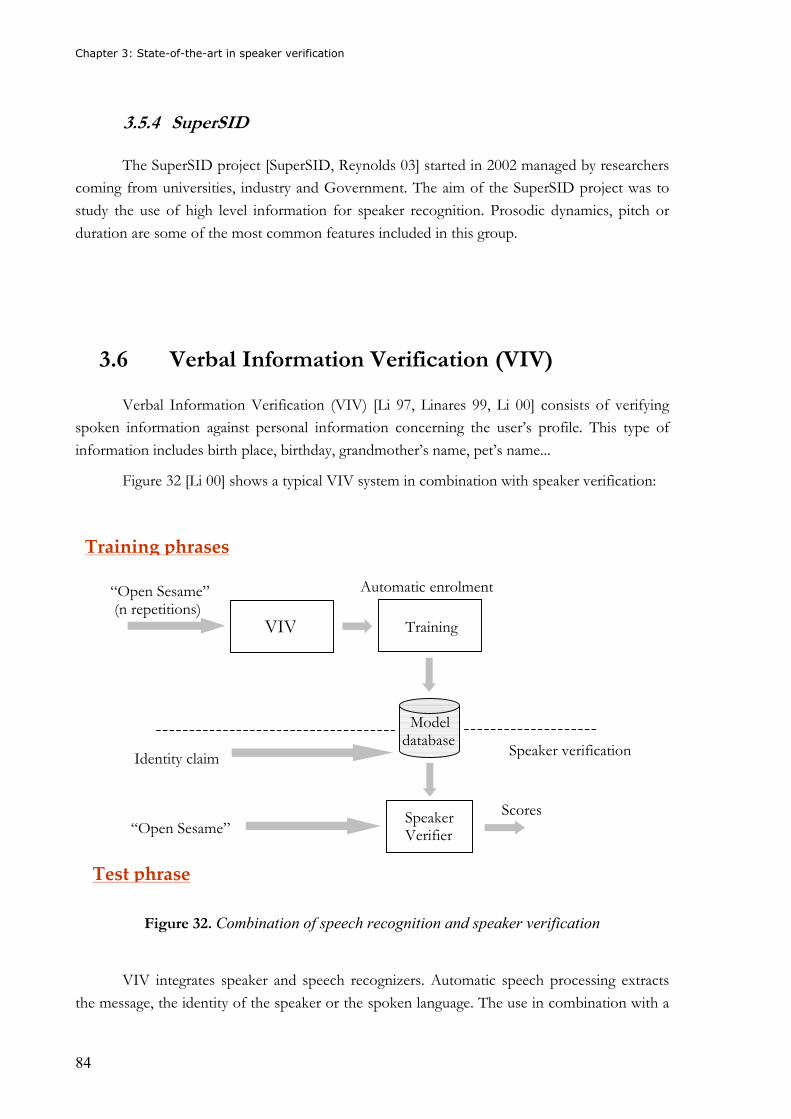
Chapter 3: State-of-the-art in speaker verification
84
3.5.4 SuperSID The SuperSID project [SuperSID, Reynolds 03] started in 2002 managed by researchers
coming from universities, industry and Government. The aim of the SuperSID project was to
study the use of high level information for speaker recognition. Prosodic dynamics, pitch or
duration are some of the most common features included in this group.
3.6 Verbal Information Verification (VIV)
Verbal Information Verification (VIV) [Li 97, Linares 99, Li 00] consists of verifying
spoken information against personal information concerning the user’s profile. This type of
information includes birth place, birthday, grandmother’s name, pet’s name...
Figure 32 [Li 00] shows a typical VIV system in combination with speaker verification:
Figure 32. Combination of speech recognition and speaker verification
VIV integrates speaker and speech recognizers. Automatic speech processing extracts
the message, the identity of the speaker or the spoken language. The use in combination with a
VIV
Model database
Training
Speaker Verifier
Training phrases
“Open Sesame” (n repetitions)
Scores
Automatic enrolment
Test phrase
“Open Sesame”
Identity claim Speaker verification
Chapter 3: State-of-the-art in speaker verification
85
speaker recognizer can provide substantial improvement for speaker recognition applications
[Li 98, Linares 98, Heck 02]. Its use becomes especially interesting for users in speaker
verification to establish a claimed identity. It is also very useful in phrase-prompted cases and in
the wide used text-dependent recognition systems based in connected digits [Rosenberg 96].
Speech and speaker scores can be combined to provide more confident results [Heck
02] such as:
kerspeaspeechT Λ+Λ=Λ ω (27)
where Λspeech is the score obtained from the speech recognizer, Λspeaker is the score
obtained from the speaker recognizer, w is an adjustable parameter empirically determined and
ΛT is the combined score.
3.6.1 High-level information
Low-level information has traditionally been used in speaker recognition. Lately, high-
level has acquired importance for researchers. The SuperSID project [SuperSID, Reynolds 03]
has contributed to the raising interest in high-level features [Andrews 01a, Andrews 01b, Weber
02].
The use of certain words or an idiolect [Doddington 01], particular speaker habits when
talking, the pitch, the duration of pauses in speech, the accent, the long-term energy or the
conversational style, are some examples of high-level features.
The increase of voice mining applications has contributed to the development of
speaker recognition based on high-level information. While low-level features are very sensitive
to noise, high-level features are more robust to acoustic degradation.
High-level information can be obtained from four different levels:
� Prosodic: From features derived from pitch, energy…
� Phonetic: With the use of phone sequences to model the speaker pronunciation.
� Idiolect: By using word sequences to model specific use of certain words.
� Linguistic: Modeling the conversation style by means of linguistic patterns.
The combination of low- and high-level has been shown very effective in speaker
recognition applications [Ezzaidi 01, Arcienaga 01, Campbell 03].

86
87
Chapter 4: Decision threshold and model quality estimation in speaker verification

88
Chapter 4: Decision threshold and model quality estimation in speaker verification
89
4 Decision threshold and model quality estimation in speaker verification
4.1 Introduction
In development tasks, the threshold is usually set a posteriori. However, in real
applications, the threshold must be set a priori. Furthermore, a speaker-dependent threshold
can sometimes be used because it better reflects speaker peculiarities and intra-speaker
variability than a speaker-independent threshold. The speaker dependent threshold estimation
method uses to be a linear combination of mean, variance or standard deviation from clients
and/or impostors.
Human-machine interaction can elicit some unexpected errors during training due to
background noises, distortions or strange articulatory effects. An unknown channel aggravates
the problem [Kimball 97]. Furthermore, the more training data available, the more robust
model can be estimated. However, in real applications, one can normally afford very few
enrolment sessions. In this context, the impact of those utterances affected by adverse
conditions becomes more important in such cases where a great amount of data is not available
[Hussain 97]. Score pruning (SP) [Chen 03, Saeta 03a, Saeta 03b] techniques which will be
introduced in this chapter suppress the effect of non-representative scores, removing them and
contributing to a better estimation of means and variances in order to set the speaker dependent
threshold. The main problem is that in a few cases the elimination of certain scores can produce
unexpected errors in mean or variance estimation. In these cases, new threshold estimation
methods based on weighting the scores reduce the influence of the non-representative ones.
The methods use a sigmoid function to weight the scores according to the distance from the
scores to the estimated scores mean.
The threshold estimation problem is in connection with the quality of the utterances
used to estimate the model. If an utterance has not a sufficient degree of quality, it can become
an outlier and lead to errors when estimating statistical parameters. In this chapter, two ways of
controlling the quality of the models are described. First of all, the off-line evaluation permits to
control quality a posteriori, once the speaker model is estimated. Secondly, the on-line quality
evaluation method tests the quality of the samples during the enrollment session. In this case, it
is possible to ask the user for more samples if we consider quality is not high enough.
4.1.1 Decision threshold estimation
Several approaches have been proposed to automatically estimate a priori speaker
dependent thresholds. Conventional methods have faced the scarcity of data and the problem
Chapter 4: Decision threshold and model quality estimation in speaker verification
90
of an a priori decision, using client scores, impostor data, a speaker independent threshold or
some combination of them. In [Furui 81], one can find an estimation of the threshold as a linear
combination of impostor scores mean ( µI ) and standard deviation from impostors σI as
follows:
βσµα +−=Θ )( II (28)
where α and β should be obtained empirically.
Three more speaker dependent threshold estimation methods similar to (28) are
introduced in (29), (30) and (31) [Lindberg 98, Pierrot 98]:
2
II σαµ +=Θ (29)
where 2ˆX
σ is the variance estimation of the impostor scores, and:
CI µαµα )1( −+=Θ (30)
)( ICSI µµα −+Θ=Θ (31)
where µc is the client scores mean, ΘSI is the speaker independent threshold and α is a
constant, different for every equation and empirically determined. Equation (31) is considered
as a fine adjustment of a speaker independent threshold.
Another expression introduced in [Chen 03] encompasses some of these approaches:
CII µασβµα )1()( −++=Θ (32)
where α and β are constants which have to be optimized from a pool of speakers.
Other approaches to speaker dependent threshold estimation are based on a
normalization of client scores (SM) by mean (µI) and standard deviation (σI) from impostor
scores [Mirghafori 02]. This approach is based on Znorm [Gravier 98] –see Section 4.1.2.3 for
details-:
I
IMnormM
SS
σµ−
=, (33)
It should also be mentioned another threshold normalization technique such as Hnorm
[Reynolds 97], which makes use of a handset-dependent normalization –see Section 4.1.2.5-.
Some other methods are based on FAR and FRR curves [Zhang 99]. Speaker utterances
used to train the model are also employed to obtain the FRR curve. On the other hand, a set of
impostor utterances is used to obtain the FAR curve. The threshold is adjusted to equalize both
curves.
There are also other approaches [Surendran 00] based on the difficulty of obtaining
impostor utterances which fit the client model, especially in phrase-prompted cases. In these
cases, it is difficult to secure the whole phrase from impostors. The solution is to use the
distribution of the ‘units’ of the phrase or utterance rather than the whole phrase. The units are
obtained from other speakers or different databases.
Chapter 4: Decision threshold and model quality estimation in speaker verification
91
On the other hand, it is worth noting that there are other methods which use different
estimators for mean and variance. With the selection of a high percentage of frames and not all
of them, those frames which are out of range of typical frame likelihood values are removed. In
[Bimbot 97], two of these methods can be observed, classified according to the percentage of
used frames. Instead of employing all frames, one of the estimators uses 95% most typical
frames discarding 2.5% maximum and minimum frame likelihood values. An alternative is to
use 95% best frames, removing 5% minimum values.
4.1.2 Score normalization
Normalization techniques [Tran 01] can be classified into different groups. Some
normalization techniques follow the Bayesian approach while other techniques standardise the
impostor score distribution. Furthermore, some of them are speaker-centric and some others
are impostor-centric. Normally, impostor-centric normalization techniques are used because it
is normally easier to compute impostor score distributions in real applications.
4.1.2.1 World model
The world model normalization [Carey 91, Higgins 91] is derived from the Bayesian
approach. If we consider an utterance X and a speaker model λc, the likelihood ratio can be
defined as:
)|(
)|(
Xp
XpL
c
c
λλ
= (34)
where )|( Xp cλ is the probability that X belongs to the claimed speaker model (λc) and
)|( Xp cλ is the probability that X does not belong to λc.
If we apply Bayes’ rule in its log form, discarding prior probabilities, the likelihood ratio
can be defined as follows:
)|(log)|(log ccR XpXpL λλ −= (35)
In world model normalization, the model cλ is estimated from a very large set of
speakers. The world model is also called Universal Background Model (UBM) [Reynolds 95,
Reynolds 97]. The UBM is normally a large GMM (over 256 mixtures) and is trained on a large
number of speakers in order to create a speaker-independent model. It is important to
accurately select the set of speakers to cover the acoustics space of potential impostors and not
to overweight the model for certain speakers.
Chapter 4: Decision threshold and model quality estimation in speaker verification
92
In some applications, speaker models are adapted from the UBM. This is especially
useful when only a few data is available to train the speaker model.
4.1.2.2 Cohorts
The cohort normalization [Higgins 91, Matsui 93, Reynolds 95, Reynolds 97] replaces
the large set of speakers used to create the world model by a cohort of speakers. A probability
of the cohort is used instead of the probability of the UBM. The main disadvantage of this
normalization technique is that computational cost is increased with respect to the world model.
The cohort is different for every impostor and comes determined by two main factors:
its size and its composition. If the cohort is composed by a large set of speakers, it can be
considered as impostor-centric while if it is composed by a smaller set of speakers, it is
considered as speaker-centric.
With regard to the composition, a cohort can be formed by the closest speakers to the
claimed speaker from the impostor population, by the farthest ones or by a balanced mix of the
farthest and the closest speakers. In principle, the cohort is calculated during training. There is a
special case, called Unconstrained Cohort Normalization (UCN) [Auckentaler 00], where the
cohort speakers are selected during testing.
A cohort formed by the closest impostors is defined in [Higgins 91]:
)|(logmax)|(log 00
2λλ
λλXpXpL cR
≠−= (36)
where λ0 represents the cohort.
In [Rossenberg 92], a subset of the impostor models is used to represent the population
close to the claimed speaker. In [Reynolds 95], the arithmetic mean is used to normalize speaker
scores:
−= ∑=
B
iicR Xp
BXpL
1
)|(1
log)|(log3
λλ (37)
where B is the size of the final background speaker set.
On the other hand, if the claimed speaker is also included in the cohort we find [Matsui
93]:
∑=
−=B
iicR XpXpL
0
)|(log)|(log4
λλ (38)
If the geometric mean is used instead of the arithmetic mean, the following equation is
obtained [Liu_C 96]:
∑=
−=B
iicR Xp
BXpL
1
)|(log1
)|(log4
λλ (39)
This equation can also be applied to VQ.
Chapter 4: Decision threshold and model quality estimation in speaker verification
93
Other normalization techniques that use cohorts are introduced in [Markov 98] or in
[Tran 03], where fuzzy logic is applied to score normalization.
4.1.2.3 Znorm
Zero normalization (Znorm) [Gravier 98, Auckentaller 00, Bimbot 04] estimates mean
and variance from a set of impostors to normalize a LLR. The formula is:
I
IZ
XpL
norm σµλ −
=))|(log(
(40)
where X is the speech utterance, λ is the speaker model, µI is the estimated mean from
impostors and σI the estimated variance from impostors.
In Znorm, impostor utterances are tested against the speaker model and an impostor
similarity score distribution is obtained. Znorm is performed off-line, during training.
4.1.2.4 Tnorm
Test normalization (Tnorm) [Navratil 03, Bimbot 04] uses impostor models instead of
impostor speech utterances to estimate impostor score distribution. The incoming speech
utterance is compared to the speaker model and to the impostor models. That is the difference
with regard to Znorm. Tnorm also follows the equation (40).
Tnorm has to be performed on-line, during testing. It can be considered as a test-
dependent normalization technique while Znorm is considered as a speaker-dependent one. In
both cases, the use of variance provides a good approximation for the impostor distribution.
Furthermore, Tnorm has the advantage of matching between test and normalization
because the same utterances are used for both purposes. That is not the case for Znorm.
4.1.2.5 Hnorm
Handset normalization (Hnorm) [Reynolds 96, Reynolds 97, Heck 97] is a variant of
Znorm that normalizes scores according to the handset. This normalization is very important
especially in those cases where there is a mismatch between training and testing.
Since handset information is not provided for each speaker utterance, a maximum
likelihood classifier is implemented with a GMM for each handset [Reynolds 97]. With this
classifier, we decide which handset is related to the speaker utterance and we obtain mean and
variance parameters from impostor utterances. The normalization can be applied as follows:
Chapter 4: Decision threshold and model quality estimation in speaker verification
94
)(
)())|(log(
handset
handset
I
IH
XpL
norm σµλ −
= (41)
where µI and σI are respectively the mean and variance obtained from the speaker model
against impostor utterances recorded with the same handset type, and p(X|λ) is the likelihood
ratio score.
There is also a normalization called HTnorm, a variant of Tnorm, which includes
handset-dependent impostor models to estimate the parameters used for score normalization.
In [Ho 02], Hnorm is implemented with SVM.
4.1.2.6 Cnorm
Cellular normalization (Cnorm) [Bimbot 04] makes a blind clustering of the
normalization data followed by a handset normalization where each cluster represents a
handset.
This normalization performs well for text-independent speaker recognition and besides,
makes the method and the impostor distribution simple, based only on mean and standard
deviation.
4.1.2.7 Dnorm
Dnorm [Ben 02] generates data by using the world model and the Monte-Carlo method.
The normalization is done by following the equation:
)|(2
))|(log(
λλλ
KL
XpL
normD = (42)
where log(p(X|λ)) is the LLR of the utterance X against the speaker model λ and
KL2( λ|λ ) represents the estimate of the symmetrized Kullback-Leibler (KL) distance between
client and world models. The Monte-Carlo method uses client and world models to obtain a set
of client and impostor data to estimate the KL distance.
Chapter 4: Decision threshold and model quality estimation in speaker verification
95
4.1.3 Model quality evaluation
In real applications, only one or two enrolment sessions are usually available. In this
context, it is important to control the content and quality of the recorded voice samples, when
the enrolment process is ‘open’, i.e., when the speaker is talking and the utterances are being
recorded or at least one should establish a way to measure the quality of the samples used to
train the model a posteriori, in order to locate those models which are not well estimated.
We introduce in this chapter a new model quality measure in order to detect reduced
quality models. The measure is applied to the enrollment data in combination with an algorithm
to find the less representative utterances for every speaker. Once these outliers are located, they
can be suppressed or replaced by new ones. The selection of suitable data in the training period
causes an important improvement in the performance of a speaker verification system in terms
of Equal Error Rate (EER).
In this chapter, a classification of speaker models according to their quality is also
introduced. The classification will provide a method to validate good quality models and to
detect reduced quality models. Models are placed into different groups depending on the degree
of similarity of their utterances with their respective models. We will define four levels of quality
in our experiments. Applying these techniques will result in a substantial improvement of the
performance by adding new data or by retraining the model without the presence of outliers.
The method overcomes these two problems but, as it happens with the first two
methods, it needs the speaker model to evaluate quality.
The methods explained above estimate the quality of the training utterances once the
model is created, i.e., off-line. In such case, it is not possible to ask the user for more utterances
during the training session if necessary. A new training session must be started. That was
especially unusable in applications where only one or two enrolment sessions were allowed. A
new on-line quality method based on a male and a female Universal Background Model (UBM)
is introduced. The two models act as a reference for new utterances and show if they belong to
the same speaker and provide a measure of its quality at the same time.
In the on-line quality evaluation, when an undesired utterance is located, the system asks
the user for a new one. The method compares an utterance against a male and a female UBM,
previously estimated from a collected corpus. Two scores are obtained. These scores are used to
locate the utterance with respect to the UBMs. In principle, utterances from the same speaker
are similar enough between them so when a new utterance is compared against the UBMs, the
score should be similar to the ones obtained before for the rest of the speaker utterances. This
is the basis of the on-line quality model method.
Chapter 4: Decision threshold and model quality estimation in speaker verification
96
4.2 New decision threshold estimation methods
4.2.1 Client scores
The use of impostor data to estimate the speaker verification threshold creates
difficulties in real applications. In general, it is not easy to obtain data from impostors for
certain uses, for instance in phrase-prompted cases. Furthermore, it is very difficult to select the
impostors in a right way, because they could become clients in the future. To solve these
problems, a new speaker dependent threshold estimation [Saeta 03b] based on data from clients
only is defined. Like the expressions in Section 4.1.1, it is a linear combination of mean and
standard deviation estimations, but in this case it uses only data from clients. It is very similar to
(29), but employs standard deviation instead of variance and uses also the client mean from
LLR scores. The client mean estimation is adjusted by means of the client standard deviation
estimation and α, as follows:
CC σαµ −=Θ (43)
where µC is the client scores mean, σc is the standard deviation from clients and α is a
constant empirically determined.
4.2.2 Score pruning
The main problem when there are only a few utterances available is that some of them
could produce non-representative scores. This is common when an utterance contains
background noises, is recorded with a very different handset or simply when the speaker is sick,
tired...
The presence of outliers can elicit wrong estimations of mean and variance of client
scores. The influence of outliers becomes even more significant if the standard deviation or the
variance are multiplied by a constant, like in expressions (29) and (43). The threshold of some
speakers is probably wrong fixed due to the outliers. In this way, our goal is to minimize their
presence.
Pruning is a technique which has been previously applied to frames [Besacier 98a,
Besacier 98b, Besacier 98c]. It has been used in the parameterization stage to cut off certain
frames in order to improve the performance of speaker recognition. The concept of Score
Pruning [Chen 03, Saeta 03a, Saeta 03b, Saeta 04b] is here used as a suitable method to remove
outliers and obtain better estimations of means and variances. Once computed, it decides if the
estimations will improve with the exclusion of one or several scores from this computation.
Roughly speaking, our idea consists of removing those scores which can lead to a wrong
Chapter 4: Decision threshold and model quality estimation in speaker verification
97
estimation because they are outliers. Of course, in some cases, we will not obtain any
improvement removing the outliers.
For this purpose, we introduce an algorithm that sets mean and standard deviation
estimations. It begins to consider the most distant score with respect to the mean, and will
continue with the second most distant if necessary. The main questions here will be: 1) how to
decide the elimination of a score, and 2) when to stop the algorithm.
To solve the first question, we use a parameter to control the difference between the
standard deviation estimation with and without the most distant score, the potential outlier. We
define ∆ as the percentage of variation of the standard deviation from which we consider to
discard a score. ∆ will decide if the score is considered as an outlier or not. If the percentage of
variation exceeds ∆, we confirm this score as an outlier.
In the case we have decided that a score is non-representative, we recalculate mean and
standard deviation estimations without it. At this point, we look for the next most distant score.
A second question appears: when to stop the iterations. To answer this question is necessary to
define σmin as the flooring standard deviation, i.e., the minimum standard deviation from which
we decide to stop the process. If σmin is reached, the algorithm stops.
This algorithm will be referred to as SP1 in order to distinguish it from posterior
variants. To tune SP1, we introduce SP2. The difference with SP1 is that if the percentage is
lower than ∆, but the standard deviation is still higher than the predefined maximum standard
deviation, σmax, this score is also considered as an outlier. Furthermore, if the variation of the
standard deviation is higher than ∆ or than σmax, and σmin has not been reached yet, we start a
new iteration.
The algorithm proposed here is similar to the one introduced in [Chen 03]. In this case,
we add some threshold values like a maximum and minimum standard deviation and some
additional conditions to link these values. We consider that it is necessary to establish some kind
of threshold values to better control the pruning, apart from the stopping condition ∆, because
our experiments have shown to us that an excessive pruning elicits a decrease in performance.
The iterative algorithms SP1 and SP2 will be compared in this work with other two non-
iterative methods that will be referred as SP3 and SP4. They remove a fixed percentage of
scores. SP3 automatically employs the most typical scores and discards a percentage of α most
distant scores with respect to the mean. SP4 removes a percentage β of maximum and
minimum scores. SP3 and SP4 are similar to the method of frame discarding used in [Bimbot
97].
Our goal is to compare the proposed methods to the baseline. It is worth noting that
SP1 and SP2 are iterative score pruning methods, whereas SP3 and SP4 are fixed score pruning
methods.
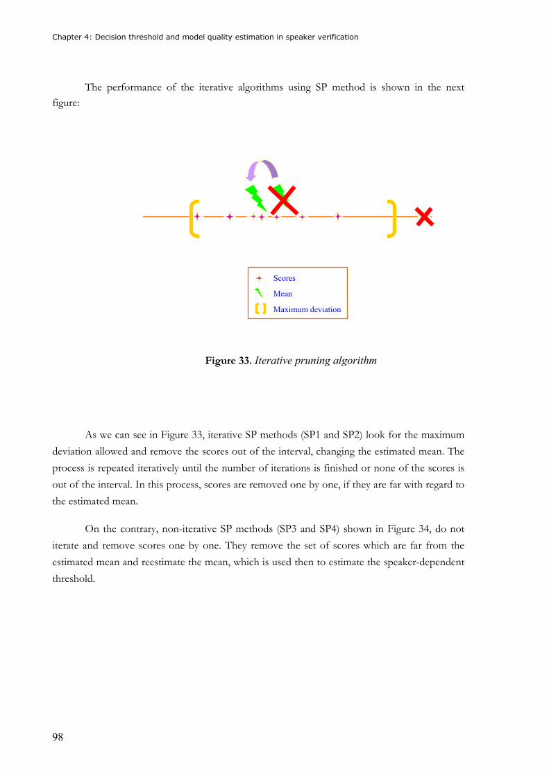
Chapter 4: Decision threshold and model quality estimation in speaker verification
98
The performance of the iterative algorithms using SP method is shown in the next
figure:
Figure 33. Iterative pruning algorithm
As we can see in Figure 33, iterative SP methods (SP1 and SP2) look for the maximum
deviation allowed and remove the scores out of the interval, changing the estimated mean. The
process is repeated iteratively until the number of iterations is finished or none of the scores is
out of the interval. In this process, scores are removed one by one, if they are far with regard to
the estimated mean.
On the contrary, non-iterative SP methods (SP3 and SP4) shown in Figure 34, do not
iterate and remove scores one by one. They remove the set of scores which are far from the
estimated mean and reestimate the mean, which is used then to estimate the speaker-dependent
threshold.
Scores
Mean
Maximum deviation
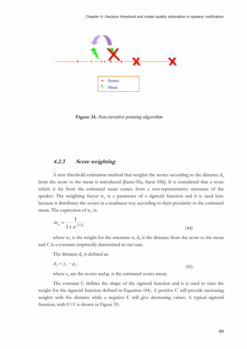
Chapter 4: Decision threshold and model quality estimation in speaker verification
99
Figure 34. Non-iterative pruning algorithm
4.2.3 Score weighting
A new threshold estimation method that weights the scores according to the distance dn
from the score to the mean is introduced [Saeta 05a, Saeta 05b]. It is considered that a score
which is far from the estimated mean comes from a non-representative utterance of the
speaker. The weighting factor wn is a parameter of a sigmoid function and it is used here
because it distributes the scores in a nonlinear way according to their proximity to the estimated
mean. The expression of wn is:
ndCne
w−+
=1
1
(44)
where wn is the weight for the utterance n, dn is the distance from the score to the mean
and C is a constant empirically determined in our case.
The distance dn is defined as:
snn sd µ−= (45)
where sn are the scores and µs is the estimated scores mean.
The constant C defines the shape of the sigmoid function and it is used to tune the
weight for the sigmoid function defined in Equation (44). A positive C will provide increasing
weights with the distance while a negative C will give decreasing values. A typical sigmoid
function, with C=1 is shown in Figure 35:
Scores Mean
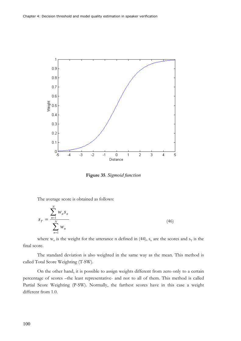
Chapter 4: Decision threshold and model quality estimation in speaker verification
100
Figure 35. Sigmoid function
The average score is obtained as follows:
∑
∑
=
==N
nn
N
nnn
T
w
sws
1
1
(46)
where wn is the weight for the utterance n defined in (44), sn are the scores and sT is the
final score.
The standard deviation is also weighted in the same way as the mean. This method is
called Total Score Weighting (T-SW).
On the other hand, it is possible to assign weights different from zero only to a certain
percentage of scores –the least representative- and not to all of them. This method is called
Partial Score Weighting (P-SW). Normally, the farthest scores have in this case a weight
different from 1.0.
Chapter 4: Decision threshold and model quality estimation in speaker verification
101
4.3 Quality measures
4.3.1 Off-line measures
In the study of model quality, some approaches have been previously shown in
literature. In [Gu 00], a model quality checking method called ‘leave-one-out’ is introduced. It
uses N-1 utterances from a total of N utterances to train the model. N scores are obtained by
testing every utterance against the model. The model that yields the highest score on the test
utterance is the most representative model. The lowest scores belong to utterances which can
be considered as outliers. The whole process is repeated N times, one for each model. The main
disadvantage of this method is its excessive computational cost.
Another different approach [Koolwaij 00] to check model quality introduces the
distance Z between LLR scores from clients and from impostors for a given model:
{ }I
ICZσ
µµ −=
,0max (47)
where µC is the mean LLR score on client utterances of the given model and µI and σI
are, respectively, the mean and standard deviation of LLR scores on a set of impostor
utterances. Z shows how discriminative a model is. If Z is close to zero, a low discrimination is
expected. The method has the problem of using impostor data, which is often difficult to
obtain.
A new algorithm to determine the quality level of a speaker model is proposed in [Saeta
04d]. Once the model is estimated from an initial set of utterances, the next step consists in
checking the model quality and deciding if it is high enough. If not, the less representative
score/utterance is replaced by another one. The model quality measure is applied again and a
new decision is taken until the quality becomes higher than a certain value or the maximum
number of iterations is reached. If N is the number of client model utterances, the maximum
number of iterations for this client will be the whole part of N/5. This number has been
empirically determined from a pool of speakers. The minimum N from which we decide to use
our method will be N=5.
In order to apply the proposed algorithm, we introduce here a new model quality
measure. We define sn as a LLR score obtained by testing a utterance against its own model. We
assume that a utterance has an acceptable degree of quality when it surpasses the following
interval:
CCns ασµ −≥ (48) where µC and σC are the mean and standard deviation of LLR scores on the utterances
used to train the model. The coefficient α is empirically determined.
Chapter 4: Decision threshold and model quality estimation in speaker verification
102
The method is applied to the enrolment data in combination with an algorithm to find
the less representative utterances for every speaker. Once these outliers are located, they can be
suppressed or replaced by new ones coming from the same speaker. It classifies the speaker
models according to their quality. The classification will detect reduced quality models. Models
will be placed into different groups depending on the degree of similarity of their utterances
with their respective models.
A possible classification for the speaker models could be by means of the definition of
four quality measures depending on the number of LLR scores nS that accomplishes Equation
(48):
%85:·%90%95:·
%85%90:·%95:·
<≥>
≥>≥
SS
SS
nIVnII
nIIInI
A model belongs to a certain quality level according to these percentages of utterances.
For instance, quality I means that the 95% of the LLR scores (sn) used to train the model fulfils
the condition defined in Equation (48). If a speaker model is included in quality groups I or II,
we consider that the quality is enough for our experiments and do not use the algorithm.
Otherwise we iterate and stop when nS ≥ 90%.
This method is especially important when it is difficult to obtain data from impostors,
for instance in phrase-prompted cases. When using words or phrases as passwords –except in
connected digits-, this method will be generally more suitable than the one explained before
which employed Z to determine the model discrimination, because that method used data from
impostors.
On the other hand, in comparison with the ‘leave-one-out’ method, the last method is
more effective in terms of computational cost. If N is the number of client model utterances,
the ‘leave-one-out’ method trains N models per client to evaluate quality while the method
shown in (48) trains, as maximum, the whole part of [N/5]. This number is chosen
experimentally by analyzing real training processes. We decide that at least 4 of every 5
utterances reach the minimum quality level. For this reason, only one utterance of every 5 could
be replaced.
But the problem of the last method is that it is not possible to ask the user for new data
until the model is already estimated. And this inconvenience is especially critical when we use
only one session for training or when we are in the second session of a two-session enrolment
process. If there are some low quality utterances, we loose the opportunity of obtaining more
voice samples from the speaker when (s)he is just recording them. It could lead to wrong
estimated or undertrained models.
Chapter 4: Decision threshold and model quality estimation in speaker verification
103
Anyway, like the rest of the methods explained here, it could not be used before the
model estimation because it uses the scores obtained against the client model. In these methods,
it is necessary to estimate the model first and then apply the quality measures.
4.3.2 On-line measures
The main disadvantage of the approaches explained in the previous section is that they
estimate the model first and then they apply quality measures. In such case, it is not possible to
ask the user for more utterances if the system realizes –through quality measures- that some of
them do not accomplish the minimum degree of quality required. In this section, a new on-line
quality method [Saeta 05b, Saeta 05c] is introduced to detect non-profitable or non-
representative utterances coming from an impostor or from the own speaker. If some
utterances do not reach the minimum level of quality required, it is not possible to ask the user
for more utterances on-line. A new session should be started.
With on-line model quality measures this problem is solved because the decision about
the quality level of an utterance is taken before estimating the speaker model and, what is more
important, before adding this utterance to the training process.
The algorithm works as follows:
1. Obtain LLR scores { s1m, s2m, s3m...} and { s1f, s2f, s3f...} from incoming utterances { U1,
U2, U3...} against { UBMm, UBMf }
2. Estimate { µm , µf } from the previous scores
3. Ask for a new utterance Un and obtain { snm, snf } against { UBMm, UBMf }
4. Calculate a distance dmf = | µm - snm | + | µf - snf |
5. If dmf ≤ Θ, quality is considered as sufficient. If dmf > Θ, then go to 3
First of all, we obtain a pair of scores for every utterance {U1, U2, U3...}, one against a
male UBMm and another one against a female UBMf. From the moment we obtain some new
utterances, we estimate the mean { µm , µf } for every pair of scores. Thus, a comparison takes
place when new incoming utterances (Un) are obtained for the speaker. They should not be far
–in terms of LLR- from that estimated mean if they really belong to the speaker.
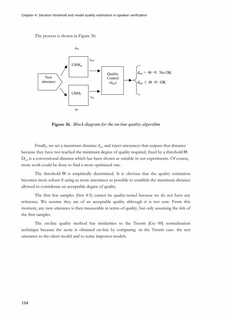
Chapter 4: Decision threshold and model quality estimation in speaker verification
104
The process is shown in Figure 36:
Figure 36. Block diagram for the on-line quality algorithm
Finally, we set a maximum distance dmf and reject utterances that surpass that distance
because they have not reached the minimum degree of quality required, fixed by a threshold Θ.
Dmf is a conventional distance which has been shown as suitable in our experiments. Of course,
more work could be done to find a more optimized one.
The threshold Θ is empirically determined. It is obvious that the quality estimation
becomes more robust if using as more utterances as possible to establish the maximum distance
allowed to considerate an acceptable degree of quality.
The first few samples (first 4-5) cannot be quality-tested because we do not have any
reference. We assume they are of an acceptable quality although it is not sure. From this
moment, any new utterance is then measurable in terms of quality, but only assuming the risk of
the first samples.
The on-line quality method has similarities to the Tnorm [Gu 00] normalization
technique because the score is obtained on-line by comparing -in the Tnorm case- the test
utterance to the client model and to some impostor models.
UBMm
UBMf
Quality
Control
(dmf)
dmf > Θ � No OK
dmf ≤ Θ � OK
New
utterance
µm
µf
snm
snf

105
Chapter 5: Databases, experiments and results

106
Chapter 5: Databases, experiments and results
107
5 Databases, experiments and results
5.1 Databases for speaker recognition
The presence of good databases is essential for the development of speaker recognition.
There are many databases but they are sometimes originally created for speech recognition
purposes. Conventional databases use to work with clean speech and sometimes with only one
session from the speaker. Nowadays, mono-session databases are practically discarded and it is
desired that samples are corrupted by noise in order to be closer to real conditions.
Some important parameters to determine the quality of a database are the number of
speakers, the number of sessions per speaker, the type of handset, the age and sex balance or
the time between sessions for the same speaker. To simulate a real system, these parameters
have to be considered, especially to study temporal intra-speaker variability and handset
variability.
Main databases are going to be seen through the next lines. These databases are mainly
supplied by the European Language Resources Association (ELRA), the Linguistic Data
Consortium (LDC) and the Oregon Graduate Institute (OGI):
TIMIT and variants
The TIMIT database contains read speech. It has 630 speakers reading 10 phonetically
rich sentences of the 8 main dialects of American English in a single session. It was recorded by
the Massachusetts Institute of Technology (MIT), SRI International and Texas Instruments,
Inc. (TI).
The FFMTIMIT was recorded by playing the original TIMIT and recording the voice
signal with a secondary microphone. The NTIMIT was collected by transmitting all 6300
original TIMIT recordings through a telephone handset. On the other hand, the CTIMIT was
collected by playing TIMIT speech into a cellular telephone in a moving van. Finally, HTIMIT
was created by playing TIMIT through different telephone handsets and recording the output
signal.
YOHO
The YOHO database is a microphonic database collected by ITT over a 3-month
period in an office environment. It has 138 speakers, 106 male and 32 female. YOHO contains
prompted digit sequences in 4 enrollment sessions and 10 test sessions per speaker.
Chapter 5: Databases, experiments and results
108
SESP
It is a telephone speech database recorded in Dutch by KLN. It has 45 speakers (23
male, 22 female) recorded in 21 to 32 sessions per speaker. Speakers used different handsets
and locations. The SESP 2 has 84 male and 64 female.
TIDIGITS
TIDIGITS contains connected digit sequences and was collected at Texas Instruments,
Inc. (TI), in English and by microphone. It has 326 speakers (111 men, 114 women, 50 boys
and 51 girls). They have 77 digit sequences each.
KING-92
The KING corpus contains collected speech from 51 male speakers through two
different handsets: a telephone one and a high-quality microphone. There are 10 sessions per
speaker over some weeks of recordings.
Gandalf
It is also a telephone speech database especially designed for speaker recognition and
recorded in Swedish. It has 86 speakers, 48 male and 38 female. It has also 83 impostors, 51
male and 32 female. The number of sessions per speaker varies between 17 and 29, along a 6-
month period. It contains digits, sentences and spontaneous speech.
SIVA
It is an Italian telephonic database with 691 speakers. There are 436 clients -207 male
and 229 female-, and 255 impostors, 128 male and 127 female. The SIVA database contains
digits, words and sentences in a number of sessions which varies from 1 to 26.
Switchboard
The Switchboard corpus (1 and 2) has been recorded in American English. It is a
telephonic database which only has spontaneous speech. The Switchboard-1 has more than 500
speakers while the Switchboard-2 has more than 600 speakers for both phases I and II. The
number of sessions per speaker goes from 1 to 25.
Chapter 5: Databases, experiments and results
109
SpeechDat
The SpeechDat has been mainly designed for telephone speech recognition. It has been
recorded in several European languages. It has 5000 speakers who have called from the PSTN
and 1000 speakers from a mobile telephone network. It has also a speaker verification database
in English with 120 gender-balanced speakers and 20 sessions per speaker.
Ahumada
The Ahumada database has been recorded in Spanish. It is a telephone and microphone
speech database with 184 speakers, 104 males and 80 females. The minimum interval between
sessions is of 15 days. It has 3 sessions per speaker for the microphone speech and 3 more for
the telephone speech.
TelVoice
TelVoice is a telephone speech database in Spanish. It has 59 speakers, 39 male and 20
female. The number of sessions varies for every speaker. Each session has 85 seconds of speech
material. There are 7 digit utterances -3 of them equal for all the speakers-, 2 sentences and 15
seconds of spontaneous speech.
LoCoMic
It is a microphone speech database recorded in Swiss French. It has 22 speakers.
PolyVar
PolyVar is a subset of the SpeechDat database. It has 71 speakers recorded by phone in
several sessions, 43 male and 28 female. It has also 72 more speakers recorded in a single
session.
VeriVox
The VeriVox database contains microphone speech from 50 male Swedish speakers
recorded in a single database.
Chapter 5: Databases, experiments and results
110
CSLU Speaker recognition corpus
It is a telephone speech database in English. It has 100 speakers, 47 male and 53 female,
with approximately 12 sessions per speaker. It contains digits, prompted phrases and
monologue in home and office environments. The sessions were recorded over a 2-year period.
XM2VTS
The XM2VTS database has the microphone speech and the face image of each one of
the 295 individuals. Every subject has recorded 4 sessions at a 30 days interval.
BANCA
The BANCA database contains video and speech data from 52 individuals in 5 different
languages, 26 male and 26 female. It has 12 sessions in 3 different scenarios.
5.1.1 The Polycost database The Polycost database has also been used for the experiments in this work. It was
recorded by the participants of the COST250 Project. It is a telephone speech database with
134 speakers, 74 male and 60 female. Almost each speaker has between 6 and 15 sessions of
one minute of speech. Most speakers were recorded during 2-3 months. The 85% of the
speakers are between 20 and 35 years old. Speakers are recorded in English and in their mother
tongue. Calls are made from the Public Switched Telephone Network (PSTN).
Each session contains 14 items: 4 repetitions of a 7-digit client code, five 10-digit
sequences, 2 fixed sentences, 1 international phone number and 2 more items of spontaneous
speech in speaker’s mother tongue. For our experiments, we will use only digit utterances in
English.
The Polycost database includes an annotation file for every utterance and there are also
documents which define the guidelines for experiments in order to be able to establish
comparisons between different speaker recognition systems.

Chapter 5: Databases, experiments and results
111
5.1.2 The BioTech database
One of the databases used in this work has been recorded –among others- by the author
and has been especially designed for speaker recognition. It is called the BioTech database and
it belongs to the company Biometric Technologies, S.L. It includes land-line and mobile
telephone sessions. A total number of 184 speakers were recorded by phone, 106 male and 78
female. It is a multi-session database in Spanish, with 520 calls from the Public Switched
Telephone Network (PSTN) and 328 from mobile telephones. One hundred speakers have at
least 5 or more sessions. The average number of sessions per speaker is 4.55. The average time
between sessions per speaker is 11.48 days.
On the next page we can see the data given to the participants in recordings. Each
session included:
� different sequences of 8-digit numbers, repeated twice. They were the Spanish
personal identification number and that number the other way round. There
were also two more digits: 45327086 and 37159268.
� different sequences of 4-digit numbers, repeated twice. They were one random
number and the fixed number 9014.
� different isolated words: bodega, petaca, llorar, lechuza, jefes, romántico.
� different sentences: Los tiempos felices de la humanidad son las páginas vacías
de la historia; el genio es un rayo cuyo trueno se prolonga durante siglos; en la
pelea se conoce al soldado y en la victoria al caballero; para obtener éxito en el
mundo hay que parecer loco y ser sabio; and el miedo es para el espíritu tan
saludable como el baño para el cuerpo.
� 1 minute long read paragraph (see next page).
� 1 minute of spontaneous speech, suggesting to talk about something related to
what the user could see around, what (s)he had done at the weekend, the latest
book read or the latest film seen.
Next to the page containing what to say, there were some basic instructions and advises.
Some of them were:
� To say the numbers digit by digit.
� To try to make one phone call per week, changing the day during the week and
the hour of the phone call.
� To make at least 6 phone calls, 3 from the PSTN and 3 from a mobile phone.
� Not to phone from very noisy places or when talking to another person.
� To continue anyway in case of a mistake.
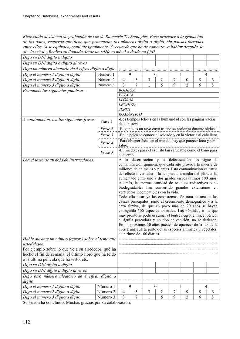
Chapter 5: Databases, experiments and results
112
Bienvenido al sistema de grabación de voz de Biometric Technologies. Para proceder a la grabación de los datos, recuerde que tiene que pronunciar los números dígito a dígito, sin pausas forzadas entre ellos. Si se equivoca, continúe igualmente. Y recuerde que ha de comenzar a hablar después de oír la señal. ¿Realiza su llamada desde un teléfono móvil o desde un fijo? Diga su DNI dígito a dígito Diga su DNI dígito a dígito al revés Diga un número aleatorio de 4 cifras dígito a dígito .................. .................. .................. .................. Diga el número 1 dígito a dígito Número 1 9 0 1 4
Diga el número 2 dígito a dígito Número 2 4 5 3 2 7 0 8 6
Diga el número 3 dígito a dígito Número 3 3 7 1 5 9 2 6 8 BODEGA PETACA LLORAR LECHUZA JEFES
Pronuncie las siguientes palabras :
ROMÁNTICO
Frase 1 -Los tiempos felices en la humanidad son las páginas vacías
de la historia
Frase 2 -El genio es un rayo cuyo trueno se prolonga durante siglos.
Frase 3 -En la pelea se conoce al soldado y en la victoria al caballero
Frase 4 -Para obtener éxito en el mundo, hay que parecer loco y ser
sabio.
A continuación, lea las siguientes frases:
Frase 5 -El miedo es para el espíritu tan saludable como el baño para
el cuerpo.
Lea el texto de su hoja de instrucciones. A la desertización y la deforestación les sigue la
contaminación química, que cada año provoca la muerte de
millones de animales y plantas. Esta contaminación es causa
del efecto invernadero: la temperatura media del planeta ha
aumentado entre uno y dos grados en los últimos 100 años.
Además, la enorme cantidad de residuos radiactivos o no
biodegradables han convertido grandes extensiones en
vertederos incompatibles con la vida.
Todo ello destruye los ecosistemas. Se trata de una de las
causas principales, junto al crecimiento demográfico y a la
caza furtiva, de que en poco más de 20 años se hayan
extinguido 500 especies animales. Las pérdidas, a las que
muy pronto se podrían sumar el buitre negro, el lince ibérico,
el águila pescadora y un tipo de esturión, no se detienen.
En los próximos 30 años pueden desaparecer de la faz de la
Tierra una cuarta parte de las especies animales y vegetales,
a un ritmo de 100 diarias. Hable durante un minuto (aprox.) sobre el tema que usted desee. Por ejemplo sobre lo que ve a su alrededor, qué ha
hecho el fin de semana, el último libro que ha leído
o la última película que ha visto, etc.
..................................................................................................
..................................................................................................
..................................................................................................
..................................................................................................
Diga su DNI dígito a dígito Diga su DNI dígito a dígito al revés Diga otro número aleatorio de 4 cifras dígito a dígito .................. .................. .................. ..................
Diga el número 1 dígito a dígito Número 1 9 0 1 4
Diga el número 2 dígito a dígito Número 2 4 5 3 2 7 9 8 6
Diga el número 3 dígito a dígito Número 3 3 7 1 5 9 2 6 8
Su sesión ha concluido. Muchas gracias por su colaboración.
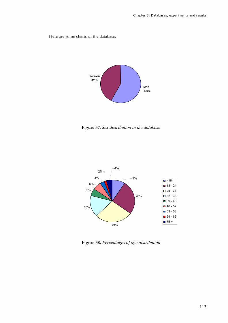
Chapter 5: Databases, experiments and results
113
Here are some charts of the database:
Women
42%
Men
58%
Figure 37. Sex distribution in the database
26%
29%
16%
5%
6%
3%
2%4%
9%<18
18 - 24
25 - 31
32 - 38
39 - 45
46 - 52
53 - 58
59 - 65
65 +
Figure 38. Percentages of age distribution
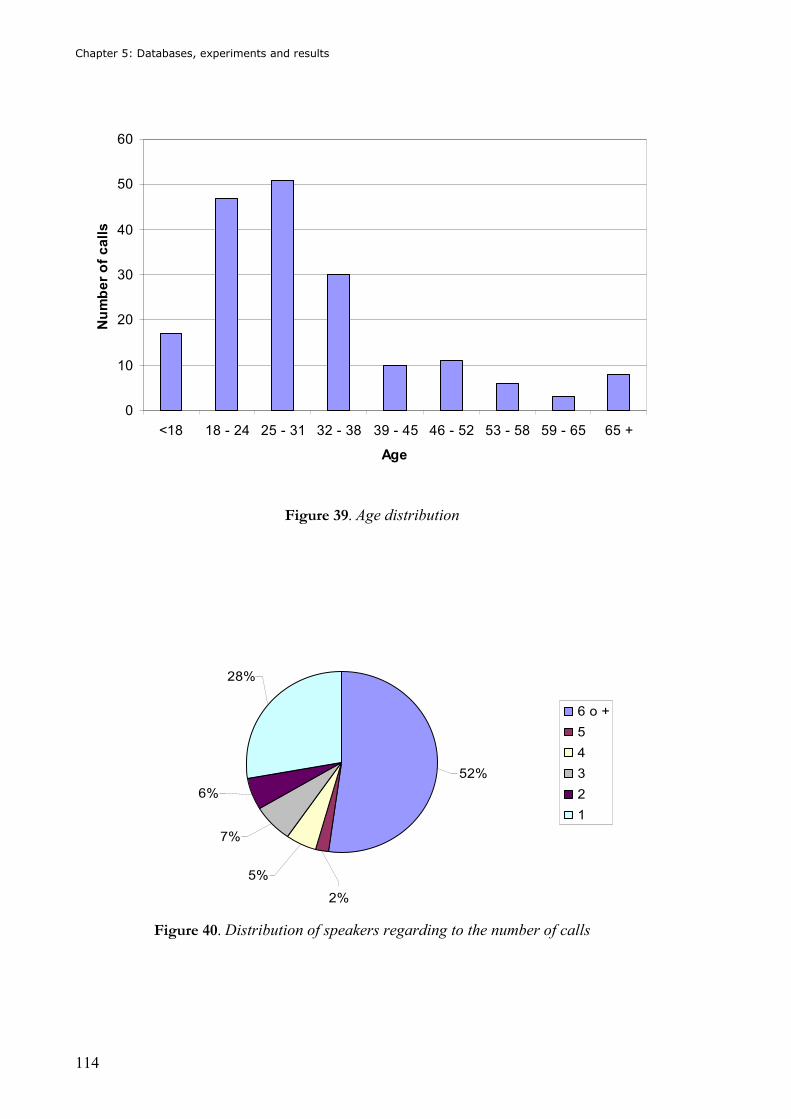
Chapter 5: Databases, experiments and results
114
0
10
20
30
40
50
60
<18 18 - 24 25 - 31 32 - 38 39 - 45 46 - 52 53 - 58 59 - 65 65 +
Age
Number of calls
Figure 39. Age distribution
2%
5%
7%
6%
52%
28%
6 o +
5
4
3
2
1
Figure 40. Distribution of speakers regarding to the number of calls
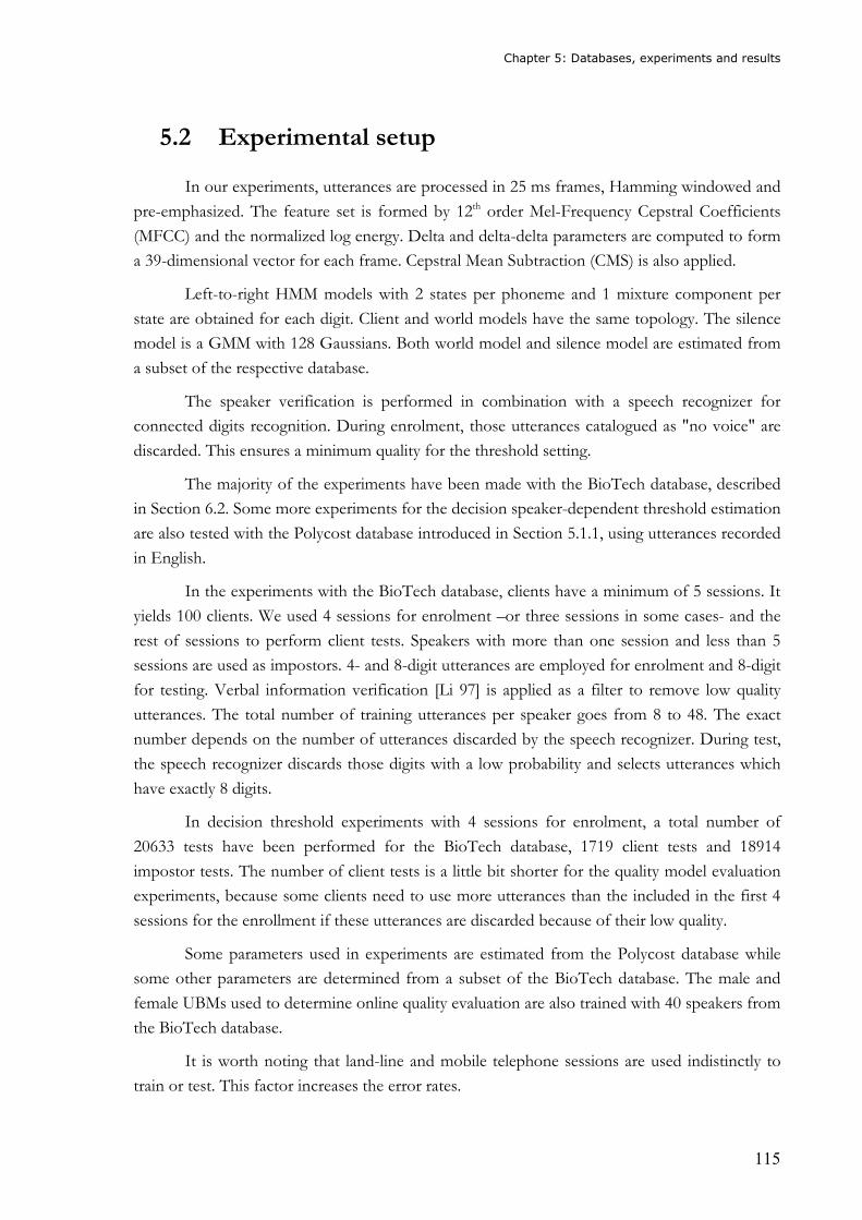
Chapter 5: Databases, experiments and results
115
5.2 Experimental setup
In our experiments, utterances are processed in 25 ms frames, Hamming windowed and
pre-emphasized. The feature set is formed by 12th order Mel-Frequency Cepstral Coefficients
(MFCC) and the normalized log energy. Delta and delta-delta parameters are computed to form
a 39-dimensional vector for each frame. Cepstral Mean Subtraction (CMS) is also applied.
Left-to-right HMM models with 2 states per phoneme and 1 mixture component per
state are obtained for each digit. Client and world models have the same topology. The silence
model is a GMM with 128 Gaussians. Both world model and silence model are estimated from
a subset of the respective database.
The speaker verification is performed in combination with a speech recognizer for
connected digits recognition. During enrolment, those utterances catalogued as "no voice" are
discarded. This ensures a minimum quality for the threshold setting.
The majority of the experiments have been made with the BioTech database, described
in Section 6.2. Some more experiments for the decision speaker-dependent threshold estimation
are also tested with the Polycost database introduced in Section 5.1.1, using utterances recorded
in English.
In the experiments with the BioTech database, clients have a minimum of 5 sessions. It
yields 100 clients. We used 4 sessions for enrolment –or three sessions in some cases- and the
rest of sessions to perform client tests. Speakers with more than one session and less than 5
sessions are used as impostors. 4- and 8-digit utterances are employed for enrolment and 8-digit
for testing. Verbal information verification [Li 97] is applied as a filter to remove low quality
utterances. The total number of training utterances per speaker goes from 8 to 48. The exact
number depends on the number of utterances discarded by the speech recognizer. During test,
the speech recognizer discards those digits with a low probability and selects utterances which
have exactly 8 digits.
In decision threshold experiments with 4 sessions for enrolment, a total number of
20633 tests have been performed for the BioTech database, 1719 client tests and 18914
impostor tests. The number of client tests is a little bit shorter for the quality model evaluation
experiments, because some clients need to use more utterances than the included in the first 4
sessions for the enrollment if these utterances are discarded because of their low quality.
Some parameters used in experiments are estimated from the Polycost database while
some other parameters are determined from a subset of the BioTech database. The male and
female UBMs used to determine online quality evaluation are also trained with 40 speakers from
the BioTech database.
It is worth noting that land-line and mobile telephone sessions are used indistinctly to
train or test. This factor increases the error rates.
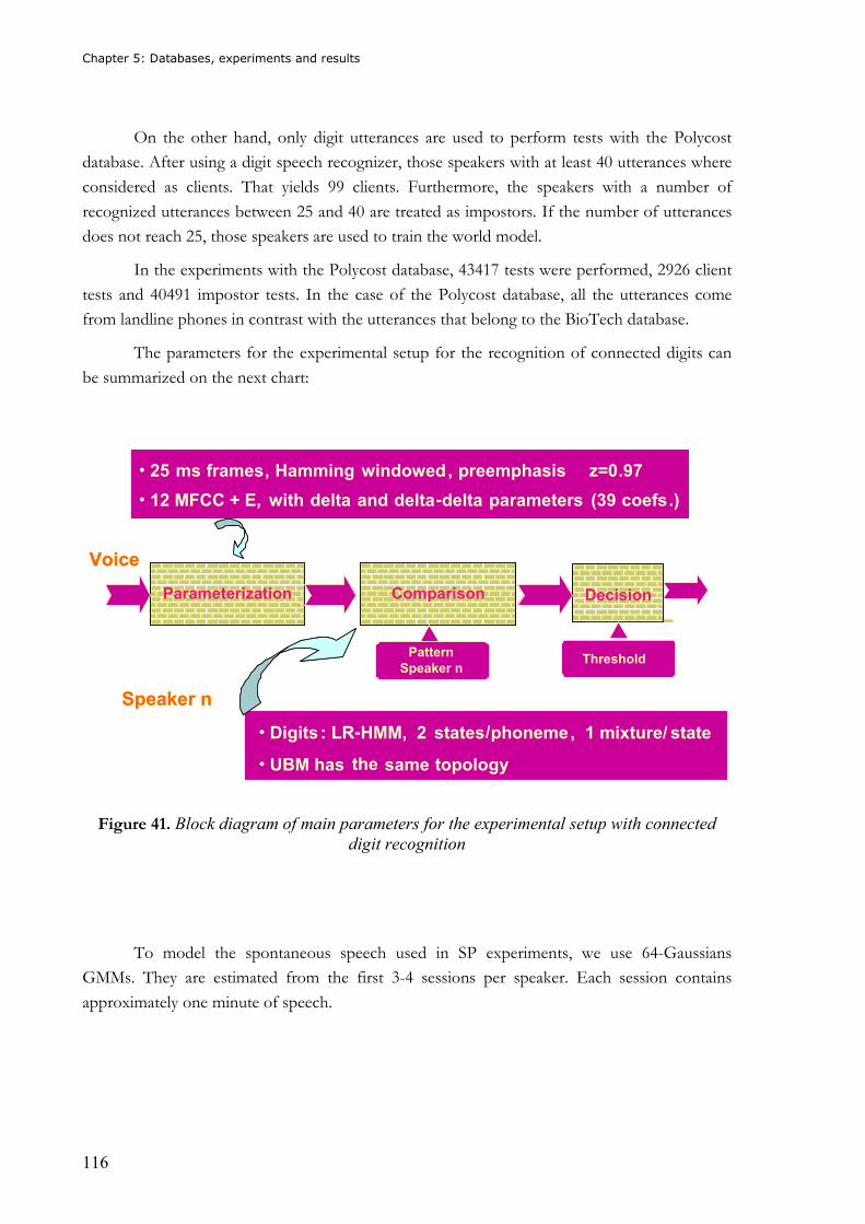
Chapter 5: Databases, experiments and results
116
On the other hand, only digit utterances are used to perform tests with the Polycost
database. After using a digit speech recognizer, those speakers with at least 40 utterances where
considered as clients. That yields 99 clients. Furthermore, the speakers with a number of
recognized utterances between 25 and 40 are treated as impostors. If the number of utterances
does not reach 25, those speakers are used to train the world model.
In the experiments with the Polycost database, 43417 tests were performed, 2926 client
tests and 40491 impostor tests. In the case of the Polycost database, all the utterances come
from landline phones in contrast with the utterances that belong to the BioTech database.
The parameters for the experimental setup for the recognition of connected digits can
be summarized on the next chart:
• 25 ms frames, Hamming windowed, preemphasis z=0.97
• 12 MFCC + E, with delta and delta-delta parameters (39 coefs.)
Parameterization Decision
Voice
Pattern
Speaker n
Comparison
Speaker n
• Digits : LR-HMM, 2 states/phoneme, 1 mixture/ state
• UBM has the same topology
Threshold
• 25 ms frames, Hamming windowed, preemphasis z=0.97
• 12 MFCC + E, with delta and delta-delta parameters (39 coefs.)
Parameterization Decision
Voice
Pattern
Speaker n
Comparison
Speaker n
• Digits : LR-HMM, 2 states/phoneme, 1 mixture/ state
• UBM has the same topology
Threshold
Figure 41. Block diagram of main parameters for the experimental setup with connected digit recognition
To model the spontaneous speech used in SP experiments, we use 64-Gaussians
GMMs. They are estimated from the first 3-4 sessions per speaker. Each session contains
approximately one minute of speech.
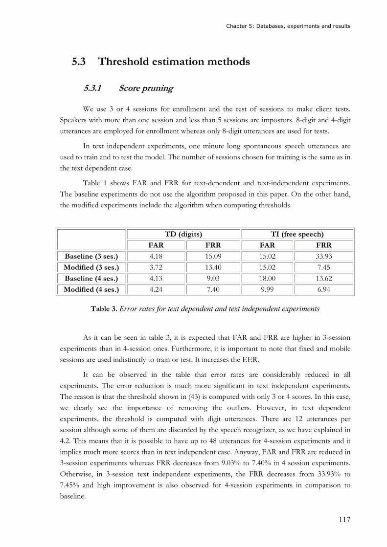
Chapter 5: Databases, experiments and results
117
5.3 Threshold estimation methods
5.3.1 Score pruning
We use 3 or 4 sessions for enrollment and the rest of sessions to make client tests.
Speakers with more than one session and less than 5 sessions are impostors. 8-digit and 4-digit
utterances are employed for enrollment whereas only 8-digit utterances are used for tests.
In text independent experiments, one minute long spontaneous speech utterances are
used to train and to test the model. The number of sessions chosen for training is the same as in
the text dependent case.
Table 1 shows FAR and FRR for text-dependent and text-independent experiments.
The baseline experiments do not use the algorithm proposed in this paper. On the other hand,
the modified experiments include the algorithm when computing thresholds.
TD (digits) TI (free speech)
FAR FRR FAR FRR
Baseline (3 ses.) 4.18 15.09 15.02 33.93
Modified (3 ses.) 3.72 13.40 15.02 7.45
Baseline (4 ses.) 4.13 9.03 18.00 13.62
Modified (4 ses.) 4.24 7.40 9.99 6.94
Table 3. Error rates for text dependent and text independent experiments
As it can be seen in table 3, it is expected that FAR and FRR are higher in 3-session
experiments than in 4-session ones. Furthermore, it is important to note that fixed and mobile
sessions are used indistinctly to train or test. It increases the EER.
It can be observed in the table that error rates are considerably reduced in all
experiments. The error reduction is much more significant in text independent experiments.
The reason is that the threshold shown in (43) is computed with only 3 or 4 scores. In this case,
we clearly see the importance of removing the outliers. However, in text dependent
experiments, the threshold is computed with digit utterances. There are 12 utterances per
session although some of them are discarded by the speech recognizer, as we have explained in
4.2. This means that it is possible to have up to 48 utterances for 4-session experiments and it
implies much more scores than in text independent case. Anyway, FAR and FRR are reduced in
3-session experiments whereas FRR decreases from 9.03% to 7.40% in 4 session experiments.
Otherwise, in 3-session text independent experiments, the FRR decreases from 33.93% to
7.45% and high improvement is also observed for 4-session experiments in comparison to
baseline.
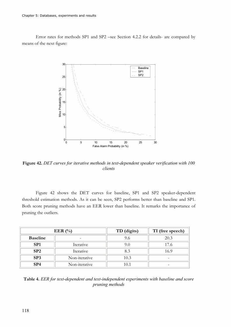
Chapter 5: Databases, experiments and results
118
Error rates for methods SP1 and SP2 –see Section 4.2.2 for details- are compared by
means of the next figure:
0 5 10 15 20 25 300
5
10
15
20
25
30
False Alarm Probability (in %)
Miss Probability (in %
)
Baseline
SP1
SP2
Figure 42. DET curves for iterative methods in text-dependent speaker verification with 100 clients
Figure 42 shows the DET curves for baseline, SP1 and SP2 speaker-dependent
threshold estimation methods. As it can be seen, SP2 performs better than baseline and SP1.
Both score pruning methods have an EER lower than baseline. It remarks the importance of
pruning the outliers.
EER (%) TD (digits) TI (free speech)
Baseline - 9.6 20.3
SP1 Iterative 9.0 17.6
SP2 Iterative 8.3 16.9
SP3 Non-iterative 10.3 -
SP4 Non-iterative 10.1 -
Table 4. EER for text-dependent and text-independent experiments with baseline and score pruning methods
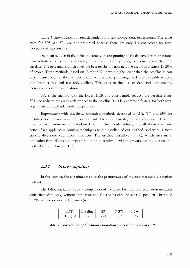
Chapter 5: Databases, experiments and results
119
Table 4 shows EERs for text-dependent and text-independent experiments. The error
rates for SP3 and SP4 are not presented because there are only 4 client scores for text-
independent experiments.
As it can be seen in the table, the iterative score pruning methods have lower error rates
than non-iterative ones. Even more, non-iterative score pruning performs worse than the
baseline. The percentage which gives the best results for non-iterative methods discards 15-20%
of scores. These methods, based on [Bimbot 97], have a higher error than the baseline in our
experiments, because they remove scores with a fixed percentage and they probably remove
significant scores, and not only outliers. This leads to the loss of data and consequently
increases the error in estimations.
SP2 is the method with the lowest EER and considerably reduces the baseline error.
SP1 also reduces the error with respect to the baseline. This is a common feature for both text-
dependent and text-independent experiments.
Experiments with threshold estimation methods described in (28), (29) and (30) for
text-dependent cases have been carried out. They perform slightly better than our baseline
threshold estimation method based on data from clients only, although not all of them perform
better if we apply score pruning techniques to the baseline of our method, and what is more
critical, they need data from impostors. The method described in (30), which uses mean
estimation from clients and impostors - but not standard deviation or variance, has become the
method with the lowest EER.
5.3.2 Score weighting
In this section, the experiments show the performance of the new threshold estimation
methods.
The following table shows a comparison of the EER for threshold estimation methods
with client data only, without impostors and for the baseline Speaker-Dependent Threshold
(SDT) method defined in Equation (43):
SDT Baseline SP T-SW P-SW
EER (%) 5.89 3.21 3.03 3.73
Table 5. Comparison of threshold estimation methods in terms of EER
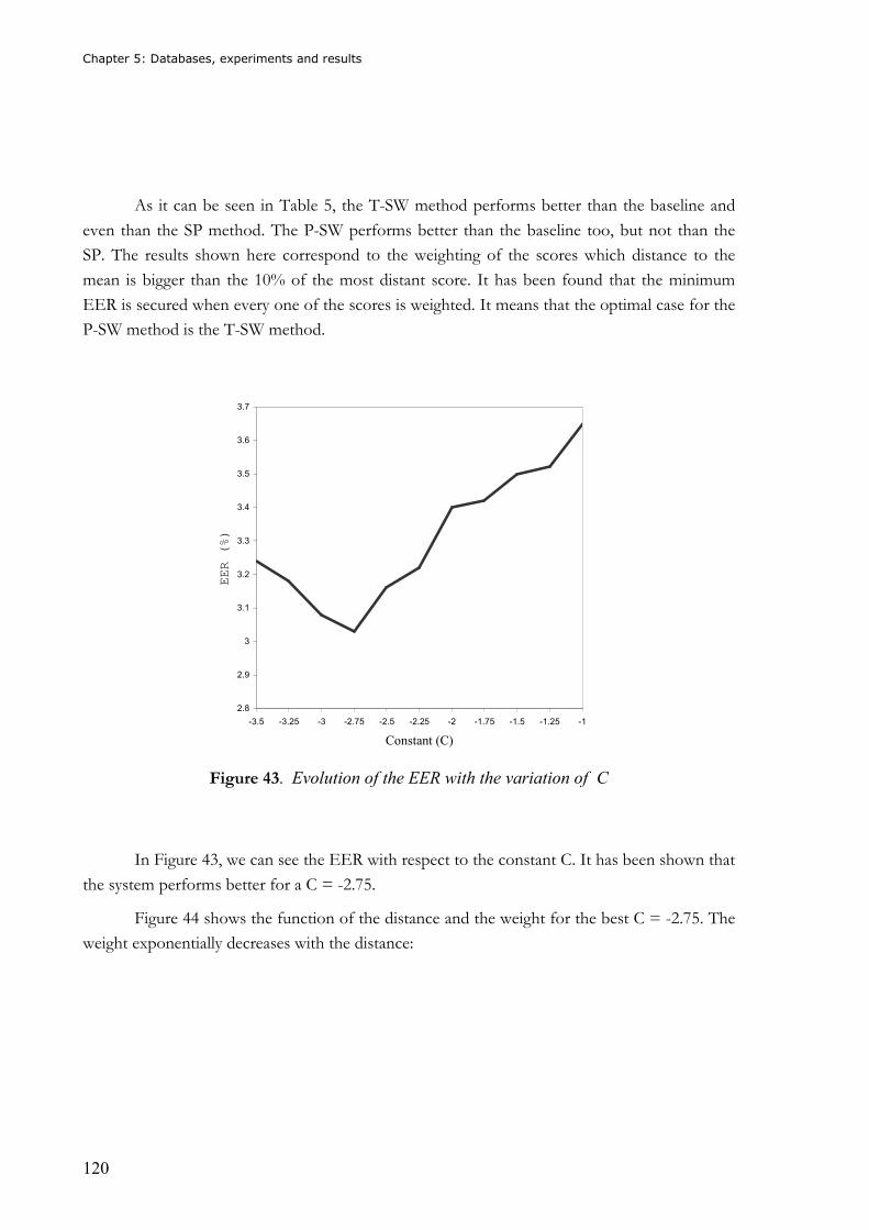
Chapter 5: Databases, experiments and results
120
As it can be seen in Table 5, the T-SW method performs better than the baseline and
even than the SP method. The P-SW performs better than the baseline too, but not than the
SP. The results shown here correspond to the weighting of the scores which distance to the
mean is bigger than the 10% of the most distant score. It has been found that the minimum
EER is secured when every one of the scores is weighted. It means that the optimal case for the
P-SW method is the T-SW method.
2.8
2.9
3
3.1
3.2
3.3
3.4
3.5
3.6
3.7
-3.5 -3.25 -3 -2.75 -2.5 -2.25 -2 -1.75 -1.5 -1.25 -1
Constant (C)
EER (%)
Figure 43. Evolution of the EER with the variation of C
In Figure 43, we can see the EER with respect to the constant C. It has been shown that
the system performs better for a C = -2.75.
Figure 44 shows the function of the distance and the weight for the best C = -2.75. The
weight exponentially decreases with the distance:
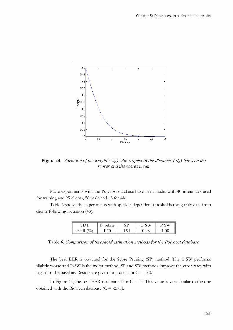
Chapter 5: Databases, experiments and results
121
Figure 44. Variation of the weight ( wn ) with respect to the distance ( dn ) between the scores and the scores mean
More experiments with the Polycost database have been made, with 40 utterances used
for training and 99 clients, 56 male and 43 female.
Table 6 shows the experiments with speaker-dependent thresholds using only data from
clients following Equation (43):
SDT Baseline SP T-SW P-SW
EER (%) 1.70 0.91 0.93 1.08
Table 6. Comparison of threshold estimation methods for the Polycost database
The best EER is obtained for the Score Pruning (SP) method. The T-SW performs
slightly worse and P-SW is the worst method. SP and SW methods improve the error rates with
regard to the baseline. Results are given for a constant C = -3.0.
In Figure 45, the best EER is obtained for C = -3. This value is very similar to the one
obtained with the BioTech database (C = -2.75).
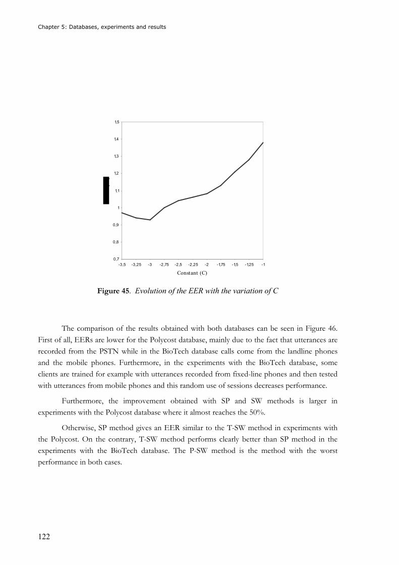
Chapter 5: Databases, experiments and results
122
0,7
0,8
0,9
1
1,1
1,2
1,3
1,4
1,5
-3,5 -3,25 -3 -2,75 -2,5 -2,25 -2 -1,75 -1,5 -1,25 -1
Constant (C)
Figure 45. Evolution of the EER with the variation of C
The comparison of the results obtained with both databases can be seen in Figure 46.
First of all, EERs are lower for the Polycost database, mainly due to the fact that utterances are
recorded from the PSTN while in the BioTech database calls come from the landline phones
and the mobile phones. Furthermore, in the experiments with the BioTech database, some
clients are trained for example with utterances recorded from fixed-line phones and then tested
with utterances from mobile phones and this random use of sessions decreases performance.
Furthermore, the improvement obtained with SP and SW methods is larger in
experiments with the Polycost database where it almost reaches the 50%.
Otherwise, SP method gives an EER similar to the T-SW method in experiments with
the Polycost. On the contrary, T-SW method performs clearly better than SP method in the
experiments with the BioTech database. The P-SW method is the method with the worst
performance in both cases.
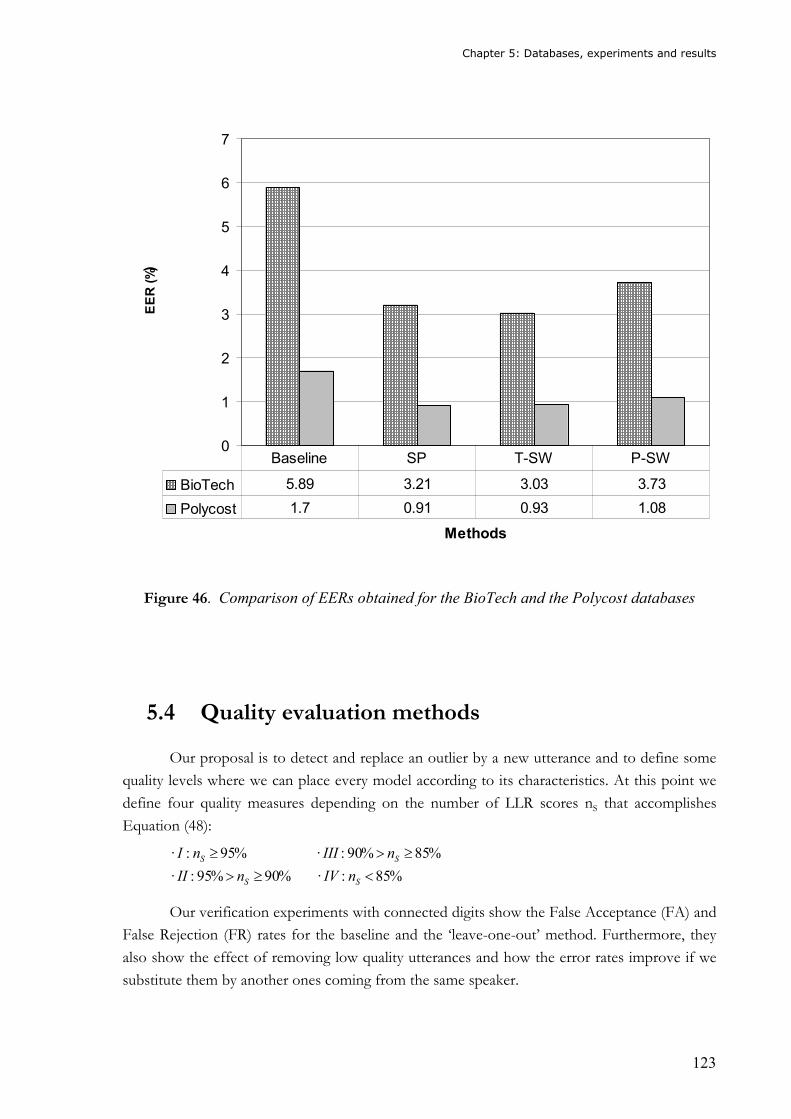
Chapter 5: Databases, experiments and results
123
0
1
2
3
4
5
6
7
Methods
EER (%)
BioTech 5.89 3.21 3.03 3.73
Polycost 1.7 0.91 0.93 1.08
Baseline SP T-SW P-SW
Figure 46. Comparison of EERs obtained for the BioTech and the Polycost databases
5.4 Quality evaluation methods
Our proposal is to detect and replace an outlier by a new utterance and to define some
quality levels where we can place every model according to its characteristics. At this point we
define four quality measures depending on the number of LLR scores nS that accomplishes
Equation (48):
%85:·%90%95:·
%85%90:·%95:·
<≥>
≥>≥
SS
SS
nIVnII
nIIInI
Our verification experiments with connected digits show the False Acceptance (FA) and
False Rejection (FR) rates for the baseline and the ‘leave-one-out’ method. Furthermore, they
also show the effect of removing low quality utterances and how the error rates improve if we
substitute them by another ones coming from the same speaker.
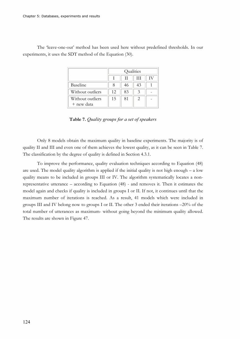
Chapter 5: Databases, experiments and results
124
The ‘leave-one-out’ method has been used here without predefined thresholds. In our
experiments, it uses the SDT method of the Equation (30).
Qualities
I II III IV
Baseline 8 46 43 1
Without outliers 12 83 3 -
Without outliers + new data
15 81 2 -
Table 7. Quality groups for a set of speakers
Only 8 models obtain the maximum quality in baseline experiments. The majority is of
quality II and III and even one of them achieves the lowest quality, as it can be seen in Table 7.
The classification by the degree of quality is defined in Section 4.3.1.
To improve the performance, quality evaluation techniques according to Equation (48)
are used. The model quality algorithm is applied if the initial quality is not high enough – a low
quality means to be included in groups III or IV. The algorithm systematically locates a non-
representative utterance – according to Equation (48) - and removes it. Then it estimates the
model again and checks if quality is included in groups I or II. If not, it continues until that the
maximum number of iterations is reached. As a result, 41 models which were included in
groups III and IV belong now to groups I or II. The other 3 ended their iterations –20% of the
total number of utterances as maximum- without going beyond the minimum quality allowed.
The results are shown in Figure 47.
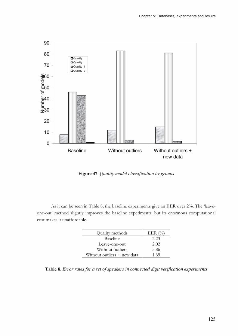
Chapter 5: Databases, experiments and results
125
Figure 47. Quality model classification by groups
As it can be seen in Table 8, the baseline experiments give an EER over 2%. The ‘leave-
one-out’ method slightly improves the baseline experiments, but its enormous computational
cost makes it unaffordable.
Quality methods EER (%)
Baseline 2.23 Leave-one-out 2.02
Without outliers 5.86 Without outliers + new data 1.39
Table 8. Error rates for a set of speakers in connected digit verification experiments
0
10
20
30
40
50
60
70
80
90
Baseline Without outliers Without outliers +
new data
Number of models
Quality I
Quality II
Quality III
Quality IV
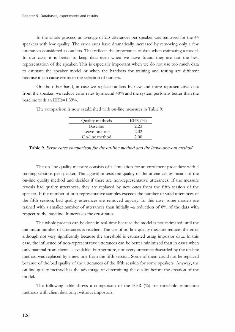
Chapter 5: Databases, experiments and results
126
In the whole process, an average of 2.3 utterances per speaker was removed for the 44
speakers with low quality. The error rates have dramatically increased by removing only a few
utterances considered as outliers. That reflects the importance of data when estimating a model.
In our case, it is better to keep data even when we have found they are not the best
representation of the speaker. This is especially important when we do not use too much data
to estimate the speaker model or when the handsets for training and testing are different
because it can cause errors in the selection of outliers.
On the other hand, in case we replace outliers by new and more representative data
from the speaker, we reduce error rates by around 40% and the system performs better than the
baseline with an EER=1.39%.
The comparison is now established with on-line measures in Table 9:
Quality methods EER (%) Baseline 2.23
Leave-one-out 2.02 On-line method 2.00
Table 9. Error rates comparison for the on-line method and the leave-one-out method
The on-line quality measure consists of a simulation for an enrolment procedure with 4
training sessions per speaker. The algorithm tests the quality of the utterances by means of the
on-line quality method and decides if there are non-representative utterances. If the measure
reveals bad quality utterances, they are replaced by new ones from the fifth session of the
speaker. If the number of non-representative samples exceeds the number of valid utterances of
the fifth session, bad quality utterances are removed anyway. In this case, some models are
trained with a smaller number of utterances than initially –a reduction of 8% of the data with
respect to the baseline. It increases the error rates.
The whole process can be done in real-time because the model is not estimated until the
minimum number of utterances is reached. The use of on-line quality measure reduces the error
although not very significantly because the threshold is estimated using impostor data. In this
case, the influence of non-representative utterances can be better minimized than in cases when
only material from clients is available. Furthermore, not every utterance discarded by the on-line
method was replaced by a new one from the fifth session. Some of them could not be replaced
because of the bad quality of the utterances of the fifth session for some speakers. Anyway, the
on-line quality method has the advantage of determining the quality before the creation of the
model.
The following table shows a comparison of the EER (%) for threshold estimation
methods with client data only, without impostors:
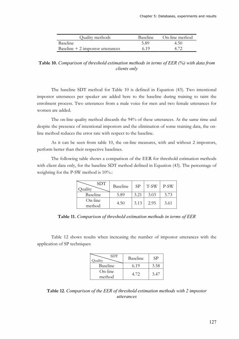
Chapter 5: Databases, experiments and results
127
Quality methods Baseline On-line method Baseline 5.89 4.50 Baseline + 2 impostor utterances 6.19 4.72
Table 10. Comparison of threshold estimation methods in terms of EER (%) with data from clients only
The baseline SDT method for Table 10 is defined in Equation (43). Two intentional
impostor utterances per speaker are added here to the baseline during training to taint the
enrolment process. Two utterances from a male voice for men and two female utterances for
women are added.
The on-line quality method discards the 94% of these utterances. At the same time and
despite the presence of intentional impostors and the elimination of some training data, the on-
line method reduces the error rate with respect to the baseline.
As it can be seen from table 10, the on-line measures, with and without 2 impostors,
perform better than their respective baselines.
The following table shows a comparison of the EER for threshold estimation methods
with client data only, for the baseline SDT method defined in Equation (43). The percentage of
weighting for the P-SW method is 10%.:
SDT Quality
Baseline SP T-SW P-SW
Baseline 5.89 3.21 3.03 3.73 On-line method
4.50 3.13 2.95 3.61
Table 11. Comparison of threshold estimation methods in terms of EER
Table 12 shows results when increasing the number of impostor utterances with the
application of SP techniques:
SDT
Quality Baseline SP
Baseline 6.19 3.58 On-line method
4.72 3.47
Table 12. Comparison of the EER of threshold estimation methods with 2 impostor utterances
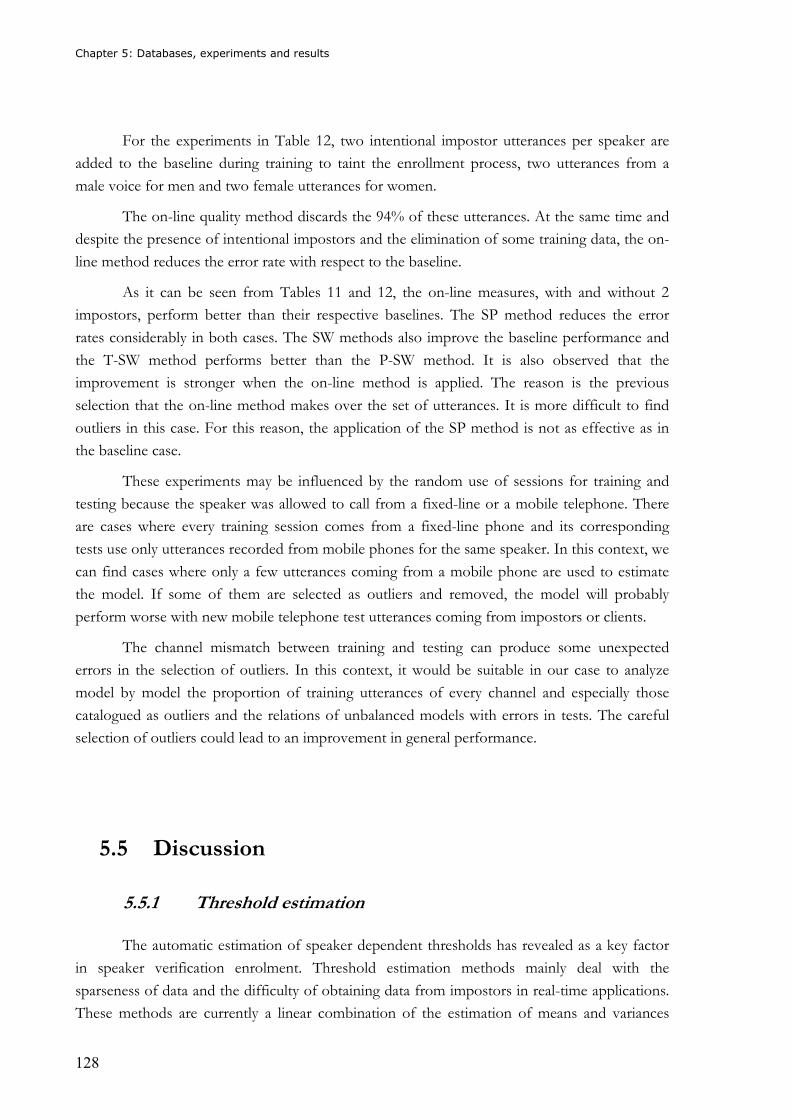
Chapter 5: Databases, experiments and results
128
For the experiments in Table 12, two intentional impostor utterances per speaker are
added to the baseline during training to taint the enrollment process, two utterances from a
male voice for men and two female utterances for women.
The on-line quality method discards the 94% of these utterances. At the same time and
despite the presence of intentional impostors and the elimination of some training data, the on-
line method reduces the error rate with respect to the baseline.
As it can be seen from Tables 11 and 12, the on-line measures, with and without 2
impostors, perform better than their respective baselines. The SP method reduces the error
rates considerably in both cases. The SW methods also improve the baseline performance and
the T-SW method performs better than the P-SW method. It is also observed that the
improvement is stronger when the on-line method is applied. The reason is the previous
selection that the on-line method makes over the set of utterances. It is more difficult to find
outliers in this case. For this reason, the application of the SP method is not as effective as in
the baseline case.
These experiments may be influenced by the random use of sessions for training and
testing because the speaker was allowed to call from a fixed-line or a mobile telephone. There
are cases where every training session comes from a fixed-line phone and its corresponding
tests use only utterances recorded from mobile phones for the same speaker. In this context, we
can find cases where only a few utterances coming from a mobile phone are used to estimate
the model. If some of them are selected as outliers and removed, the model will probably
perform worse with new mobile telephone test utterances coming from impostors or clients.
The channel mismatch between training and testing can produce some unexpected
errors in the selection of outliers. In this context, it would be suitable in our case to analyze
model by model the proportion of training utterances of every channel and especially those
catalogued as outliers and the relations of unbalanced models with errors in tests. The careful
selection of outliers could lead to an improvement in general performance.
5.5 Discussion
5.5.1 Threshold estimation
The automatic estimation of speaker dependent thresholds has revealed as a key factor
in speaker verification enrolment. Threshold estimation methods mainly deal with the
sparseness of data and the difficulty of obtaining data from impostors in real-time applications.
These methods are currently a linear combination of the estimation of means and variances
Chapter 5: Databases, experiments and results
129
from clients and/or impostor scores. When we have only a few utterances to create the model,
the right estimation of means and variances from client scores becomes a real challenge.
The SP method alleviates the problem of a low number of utterances. It removes
outliers and contributes to better estimations. Experiments from our database with a hundred
clients have shown an important reduction in error rates. The improvements have been higher
in text independent experiments than in text dependent experiments because the first ones use
only a few scores. In these cases, the influence of outliers is more relevant. Furthermore, lower
error rates have been obtained for iterative score pruning methods, whereas non-iterative
methods perform worse than the baseline.
Although the SP methods try to mitigate main problems by removing the outliers,
another problem arises when only a few scores are available. In these cases, the suppression of
some scores worsens estimations. For this reason, weighting threshold methods introduced here
use the whole set of scores but weighting them in a nonlinear way according to the distance to
the estimated mean. Weighting threshold estimation methods based on a nonlinear function
improve the baseline speaker dependent threshold estimation methods when using data from
clients only. The T-SW method is even more effective than the SP ones in the experiments with
the BioTech database, where there is often a mismatched handset between training and testing.
On the contrary, with the Polycost database, where the same handset (landline network) is used,
both of them perform very similar.
5.5.2 Quality evaluation
The new off-line model quality evaluation method lets the classification of models into
different categories according to the number of LLR client scores which exceeds a certain
threshold. It outperforms the ‘leave-one-out’ method in terms of computational cost and it has
the advantage of using only data from clients, which is strongly recommended when dealing
with words or phrases as passwords and it is difficult to obtain data from impostors.
Our empirical results have shown that the elimination of those utterances that reduce
quality increases the error rates if these utterances are not replaced by new ones that better
reflect speaker features. The impact of removing data becomes very significant and suggests us
to be careful when selecting outliers and removing the utterances, especially if we are not able
to replace them by more speaker data.
On the other hand, some systems use to train the speaker in very few sessions.
Furthermore, the number of utterances tends to be small. In this case, even when it is detected
that an utterance has a bad quality or comes from an intentional impostor, it is not possible to
ask the speaker for a new one. The new on-line model quality evaluation algorithm has the
Chapter 5: Databases, experiments and results
130
advantage of estimating quality without needing the speaker model. It implies that the quality
can be measured on-line. In our experiments, the method was capable of rejecting 94% of
intentional impostor utterances while preserving client utterances. The best on-line quality
performance was achieved with a threshold that used impostor data. The use of the on-line
quality evaluation method would result in a more substantial improvement with respect to the
baseline if some more impostor utterances were used to estimate the speaker model instead of
the two utterances used in the experiments.
The analysis of results should take into account that the random choice of handset to
train and test deteriorates the general performance and probably yields some unexpected errors
when deciding if a utterance can be considered as an outlier or not. If we are able to replace
those utterances catalogued as outliers by new ones coming from the speaker, the baseline
system is outperformed by 40%.

131
Chapter 6: A case of study: the CertiVeR project

132
Chapter 6: A case of study: the CertiVeR Project
133
6 A case of study: the CertiVeR Project
6.1 Introduction
During these last years, Internet has become an important vehicle for commercial
transactions. However, despite its current magnitude and scope, users are still reticent to use it
for most transactions. Therefore, there is still a great potential for e-commerce to grow. But for
this to happen, users need to feel much safer while doing a commercial transaction through
Internet.
In order to increase security, it is necessary to validate the identity of the subjects being
involved in a transaction.
A digital certificate identifies the user who signs a transaction. Digital certificates
provide us the option to either encrypt data, to produce an e-signature or both. Electronic
signatures provide authenticity – i.e. proof ownership. However, authenticity on its own is not
enough to provide trust. A credible service needs to provide authenticity and validity at the
same time. For validity we understand the proof that ownership of a certificate is valid at a
specific time.
This means that if you are using digital certificates to sign sensitive information or high
value transactions, you need to be able to verify that the signature was valid at the time it was
carried out – i.e. the certificate used to sign had not been cancelled.
The validation of digital certificates in real time is a task that can be accomplished by
CertiVeR [CertiVeR, Medina 03, Saeta 04a, Saeta 04c]. CertiVeR is a consortium of European
companies funded by the TEN-Telecom project under the auspices of the European
Commission. The aim of CertiVeR is to offer a certification revocation service, with the
corresponding On-line Certificate Status Protocol (OCSP) publication. The OCSP technology is
designed to validate the status of a certificate in real time. CertiVeR may also be in charge of
managing the process for the revocation, suspension or rehabilitation of certificates.
The revocation or suspension of a certificate is necessary when a certificate is lost or
stolen. In such case, one of the fastest and most available mechanisms to cancel the use of a
certificate is a telephone communication. However, such mechanism needs to be secured so
that a speaker can only cancel her/his own certificates.
In order to guarantee speaker’s identity, CertiVeR uses speaker verification technologies.
The usage of these technologies allows us to authenticate the user who is making the request
for revocation.
The maturity of speaker recognition technologies, the very little intrusiveness and the
possibility of remote validations in real-time have suggested CertiVeR the use of speaker
verification for its revocation module.
Chapter 6: A case of study: the CertiVeR Project
134
6.1.1 PKI description
As we have pointed out before, users need a higher degree of security in their
commercial transactions. To provide assurance about its source and integrity it is convenient to
develop a robust PKI, which derives in the use of digital signature. The electronic signature
substitutes the manual signature and allows the recipient of a digitally signed communication to
determine whether this communication has changed after it was digitally signed. The system
runs with a public-private key pair previously created by the sender.
At this point, we encounter the problem of ensuring the identity of the person who
holds a key pair. A certification authority (CA) is a trusted third person or entity that certifies
that the public key of a public-private key pair used to create digital signatures belongs to the
subscriber.
Once the identity of the subscriber is verified, the CA issues a certificate. Then if the
subscriber finds that the certificate is accurate, the certificate may be published in a repository,
an electronic database of certificates accessible to anyone.
If a private key is compromised or lost, the corresponding certificate has to be
suspended or revoked.
If using the traditional model of work, the public key and the certificate are placed in the
certificate revocation list (CRL), a file published by the CA containing a list of certificates that
have been revoked before their expiration date.
6.2 Case study
CertiVeR –see architecture in Figure 48- has its origin in the fact that the deployment of
the use of electronic signatures in e-commerce and in any transaction that has important value
associated with, requires the verification of the signature policy, which includes the validation of
all the certificates in the signer’s certification path. In most of the cases, this verification may be
done on the basis of CRLs, with a frequency of publication ranging from one hour to one day.
In some applications, like the financial ones, the latency between the time that a certificate may
have been revoked and the time the new CRL will be released may result in the unsuitability of
this mechanism to check the validity of a certificate.
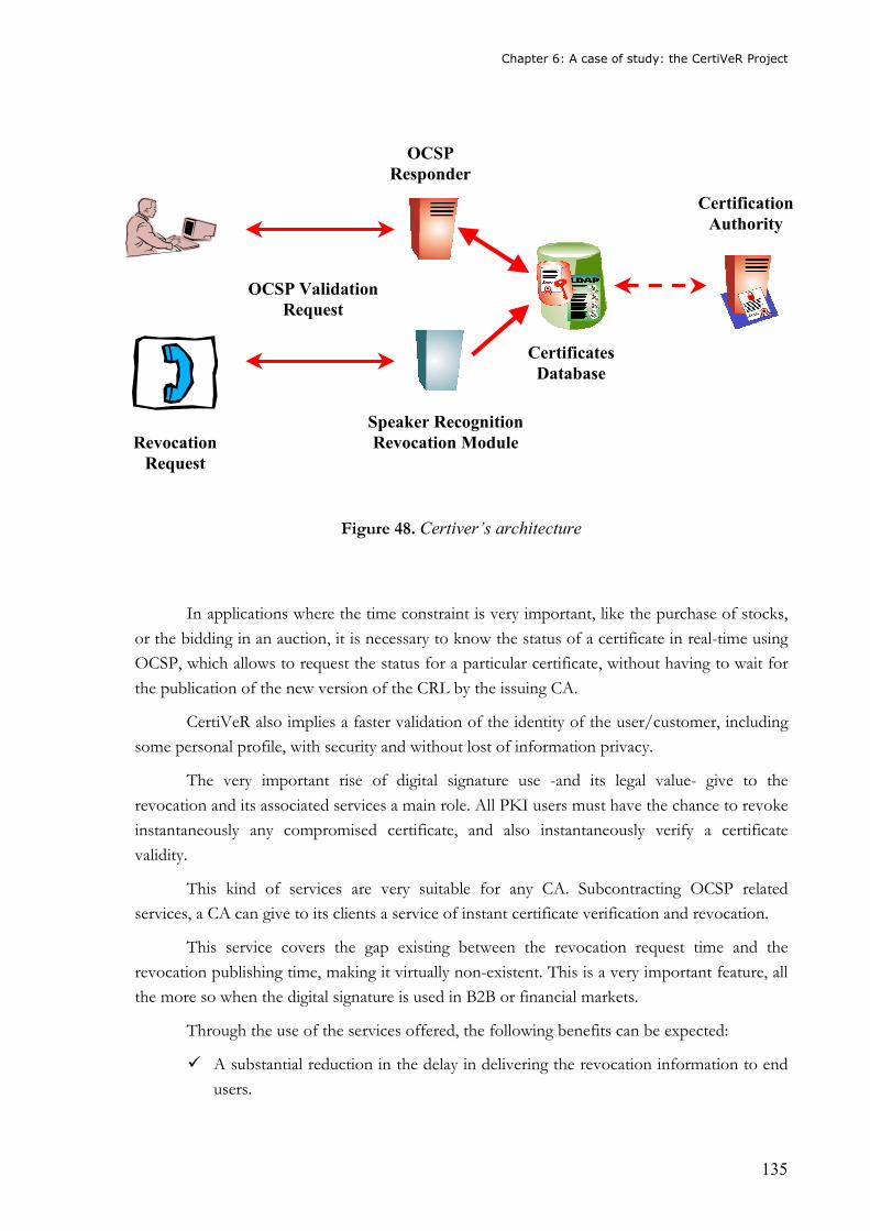
Chapter 6: A case of study: the CertiVeR Project
135
Figure 48. Certiver’s architecture
In applications where the time constraint is very important, like the purchase of stocks,
or the bidding in an auction, it is necessary to know the status of a certificate in real-time using
OCSP, which allows to request the status for a particular certificate, without having to wait for
the publication of the new version of the CRL by the issuing CA.
CertiVeR also implies a faster validation of the identity of the user/customer, including
some personal profile, with security and without lost of information privacy.
The very important rise of digital signature use -and its legal value- give to the
revocation and its associated services a main role. All PKI users must have the chance to revoke
instantaneously any compromised certificate, and also instantaneously verify a certificate
validity.
This kind of services are very suitable for any CA. Subcontracting OCSP related
services, a CA can give to its clients a service of instant certificate verification and revocation.
This service covers the gap existing between the revocation request time and the
revocation publishing time, making it virtually non-existent. This is a very important feature, all
the more so when the digital signature is used in B2B or financial markets.
Through the use of the services offered, the following benefits can be expected:
� A substantial reduction in the delay in delivering the revocation information to end
users.
Certification
Authority
Speaker Recognition
Revocation Module Revocation
Request
OCSP Validation
Request
OCSP
Responder
Certificates
Database
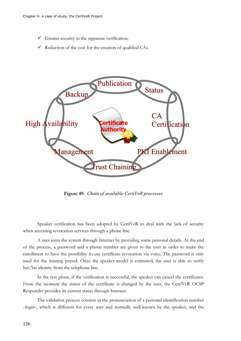
Chapter 6: A case of study: the CertiVeR Project
136
� Greater security in the signature verification.
� Reduction of the cost for the creation of qualified CAs.
Figure 49. Chain of available CertiVeR processes
Speaker verification has been adopted by CertiVeR to deal with the lack of security
when accessing revocation services through a phone line.
A user joins the system through Internet by providing some personal details. At the end
of the process, a password and a phone number are given to the user in order to make the
enrollment to have the possibility to use certificate revocation via voice. The password is only
used for the training period. Once the speaker model is estimated, the user is able to verify
her/his identity from the telephone line.
In the test phase, if the verification is successful, the speaker can cancel the certificates.
From the moment the status of the certificate is changed by the user, the CertiVeR OCSP
Responder provides its current status through Internet.
The validation process consists in the pronunciation of a personal identification number
–login-, which is different for every user and normally well-known by the speaker, and the
Certificate Authority
PPuubblliiccaattiioonn SSttaattuuss
BBaacckkuupp
HHiigghh AAvvaaiillaabbiilliittyy
MMaannaaggeemmeenntt
CCAA
CCeerrttiiffiiccaattiioonn
TTrruusstt CChhaaiinniinngg
PPKKII EEnnaabblleemmeenntt
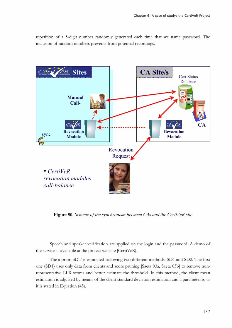
Chapter 6: A case of study: the CertiVeR Project
137
repetition of a 5-digit number randomly generated each time that we name password. The
inclusion of random numbers prevents from potential recordings.
Figure 50. Scheme of the synchronism between CAs and the CertiVeR site
Speech and speaker verification are applied on the login and the password. A demo of
the service is available at the project website [CertiVeR].
The a priori SDT is estimated following two different methods: SD1 and SD2. The first
one (SD1) uses only data from clients and score pruning [Saeta 03a, Saeta 03b] to remove non-
representative LLR scores and better estimate the threshold. In this method, the client mean
estimation is adjusted by means of the client standard deviation estimation and a parameter α, as
it is stated in Equation (43).
CA Site/s Cert Status
Database
CA
CertiVeR Sites
• CertiVeR revocation modules call-balance
Revocation
Request
Revocation
Module
Manual
Call-
Center
Revocation
Module sync
h
Chapter 6: A case of study: the CertiVeR Project
138
The second method (SD2) proposed here to estimate the threshold uses data from
clients and impostors [Lindberg 98, Pierrot 98] according to Equation (30).
6.3 Experiments and user satisfaction
6.3.1 Database
A Spanish database called BioTech presented in [Saeta 03a, Saeta 03b] has been used to
test the performance of the system because the number of real tests obtained up to this
moment was not high enough to be considered as valid and statistically reliable data. The
database belongs to the company Biometric Technologies, S.L. It has 184 speakers and has
been especially designed for speaker recognition.
6.3.2 Experimental setup
Utterances are processed in 25 ms frames, Hamming windowed and pre-emphasized.
The feature set is formed by 12th order Mel-Frequency Cepstral Coefficients (MFCC) and the
normalized log energy. Delta and delta-delta parameters are computed to form a 39-dimensional
vector for each frame. Cepstral Mean Subtraction (CMS) is also applied.
Left-to-right HMM models with 2 states per phoneme and 1 mixture per state are
obtained for each digit. Client and world models have the same topology.
The speaker verification is performed in combination with a speech recognizer for
connected digits. During enrollment, those utterances catalogued as "no voice" are discarded.
This selection ensures a minimum quality for the threshold setting.
Fixed-line and mobile telephone sessions are used indistinctly to train or test. This
factor increases the error rate.
Two kinds of tests have been carried out with the database. The first one uses 8-digit
utterances and the second one 4-digit utterances. The speech recognizer discards those digits
with a low probability and selects utterances which have exactly 8 digits or 4 digits respectively.
Our experiments include speakers with a minimum of 5 recorded sessions for the
enrollment. It yields 100 clients, but two of them did not pass the speech recognizer test which
finally makes 98 clients. We use 4 sessions of 8- and 4-digit utterances for the enrollment and
the rest of sessions to perform client tests. Speakers with more than one session and less than 5
sessions are impostors. 8-digit and 4-digit utterances are employed for enrollment. We train the
model with a number of utterances from 15 to 48.
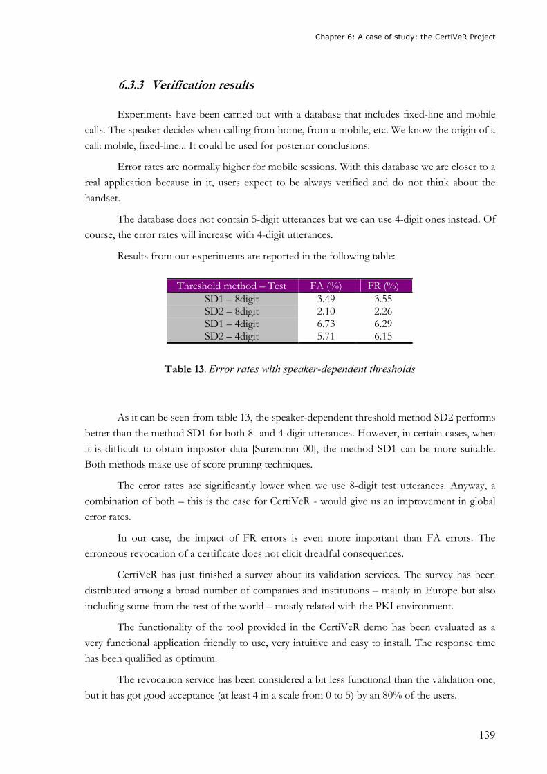
Chapter 6: A case of study: the CertiVeR Project
139
6.3.3 Verification results
Experiments have been carried out with a database that includes fixed-line and mobile
calls. The speaker decides when calling from home, from a mobile, etc. We know the origin of a
call: mobile, fixed-line... It could be used for posterior conclusions.
Error rates are normally higher for mobile sessions. With this database we are closer to a
real application because in it, users expect to be always verified and do not think about the
handset.
The database does not contain 5-digit utterances but we can use 4-digit ones instead. Of
course, the error rates will increase with 4-digit utterances.
Results from our experiments are reported in the following table:
Threshold method – Test FA (%) FR (%) SD1 – 8digit 3.49 3.55 SD2 – 8digit 2.10 2.26 SD1 – 4digit 6.73 6.29 SD2 – 4digit 5.71 6.15
Table 13. Error rates with speaker-dependent thresholds
As it can be seen from table 13, the speaker-dependent threshold method SD2 performs
better than the method SD1 for both 8- and 4-digit utterances. However, in certain cases, when
it is difficult to obtain impostor data [Surendran 00], the method SD1 can be more suitable.
Both methods make use of score pruning techniques.
The error rates are significantly lower when we use 8-digit test utterances. Anyway, a
combination of both – this is the case for CertiVeR - would give us an improvement in global
error rates.
In our case, the impact of FR errors is even more important than FA errors. The
erroneous revocation of a certificate does not elicit dreadful consequences.
CertiVeR has just finished a survey about its validation services. The survey has been
distributed among a broad number of companies and institutions – mainly in Europe but also
including some from the rest of the world – mostly related with the PKI environment.
The functionality of the tool provided in the CertiVeR demo has been evaluated as a
very functional application friendly to use, very intuitive and easy to install. The response time
has been qualified as optimum.
The revocation service has been considered a bit less functional than the validation one,
but it has got good acceptance (at least 4 in a scale from 0 to 5) by an 80% of the users.
Chapter 6: A case of study: the CertiVeR Project
140
6.4 Discussion
The growing importance of e-commerce demands nowadays more security to deploy
each of its advantages. Users need to be confident on their commercial transactions.
One of the greater problems with the digital certificates is the delay from the moment a
certificate is being revoked until the list of certificates is brought up to date. To solve this
problem, CertiVeR offers a certification revocation service in real-time. Moreover, CertiVeR
reduces the cost for certificate authorities and increases security by using speaker verification to
validate users’ identities.
From the moment the user/speaker is registered in the system through the Internet,
(s)he is able to enroll with a phone call. Once the voice profile is loaded for the speaker, it is
possible to access to revocation services.
The performance of the speaker verification module has been evaluated with some tests
with a database in Spanish which includes fixed-line and mobile phone sessions for every
speaker. The composition of the database concerning the handset is similar to a real system.
141
Conclusions
� There is a strong influence of the decision threshold setting on the performance of
speaker verification applications. In real applications, the threshold must be
established a priori, must be speaker-dependent and is often estimated with very few
data from the speakers. Furthermore, in contrast to conventional estimation
methods, no data from impostors uses to be available. These factors elicit many
errors not only in model estimation but also in threshold setting. A way to estimate
the decision threshold from client data only has revealed as very useful for certain
applications.
� In the process of decision threshold estimation in speaker verification, there are
sometimes one or several scores that are very different from the majority of the
scores obtained against the model. These scores are called outliers and lead to errors
in threshold setting. To mitigate the outliers’ problem, a method of iteratively
remove (prune) the most distant scores with regard to the estimated scores mean
has been shown as effective in our experiments.
� An alternative to the score pruning method has also been tested with promising
results. The score weighting methods take a softer decision and work better than the
score pruning methods in certain cases. Partial score weighting methods perform
worse than total score weighting ones because they are really a particular case of the
total score weighting methods. Further work will consist of comparing score
pruning and weighting methods in depth to detect in which cases it is better to use
one or another.
� The off-line model quality evaluation method introduced here outperforms the
previous existing methods and reduces the computational cost. It replaces low
quality utterances by new ones from the same speaker. It also classifies model
quality into four different groups. This classification lets the system to detect those
speakers which models are not of sufficient quality.
� An on-line model quality evaluation method has also been defined in this PhD. It
has the advantage of asking the user for more utterances during enrolment, without
needing another extra training session. This is very important in real applications
where only very few enrolment sessions are affordable.
� Score prunings methods for speaker verification have been used in combination
with speech recognition to implement a real case. A European project called

142
CertiVeR uses speaker verification for the revocation of certificates. It is also
possible to check the status of the certificates to see if they have been suspended or
revoked.
143
References
[Ahn 00] Ahn, S., Kan, S., and Ko, H., “Effective Speaker Adaptations for Speaker Verification”, ICASSP’00, Vol. 2, pp. 1081-1084, 2000
[Andrews 01a] Andrews, W.D., Kohler, M.A., and Campbell, J.P., “Phonetic Speaker Recognition”, Eurospeech’01, pp. 2517-2520, 2001
[Andrews 01b] Andrews, W.D., Kohler, M.A., Campbell, J.P., and Godfrey, J.J., "Phonetic, Idiolectal and Acoustic Speaker Recognition", 2001: A Speaker Odyssey, The Speaker Recognition Workshop, pp. 55-63, 2001
[Ariyaeeinia 99] Ariyaeeinia, A.M., Sivakumaran, P. , Pawlewski, M., and Loomes, M.J., “Dynamic Weighting of the Distortion Sequence in Text-Dependent Speaker Verification” , Eurospeech’99, pp. 967-970, 1999
[Atal 74] Atal, B.S. , “Effectiveness of Linear Prediction Characteristics of the Speech Wave for Automatic Speaker Identification and Verification”, Journal Acoustics Society of America, vol. 55, no. 6, pp. 1304-1312, 1974
[Atal 76] Atal, B.S., “Automatic Recognition of Speakers from their Voices”, Proceedings of the IEEE, vol. 64, pp. 460-475, 1976
[Arcienega 01] Arcienega, M., and Drygajlo, A., “Pitch-Dependent GMMs for Text-Independent Speaker Recognition Systems”, Eurospeech’01, pp. 2821-2824, 2001
[Auckentaler 00] Auckentaler, R., Carey, M., and Lloyd-Thomas, H., “Score Normalization for Text-Independent Speaker Verification Systems”, Digital Signal Processing, Vol. 10, pp. 42-54, 2000
[Barras 04] Barras, C., Meignier, S., Gauvain, J.L., "Unsupervised Online Adaptation for Speaker Verification over the Telephone", Speaker Odyssey’04, pp. 157-160, 2004
[Bellot 00] Bellot, O., Matrouf, D., and Bonastre, J., “Additive and Convolutional Noises Compesation for Speaker Recognition”, ICSLP’00, vol. II, pp. 799-802, 2000
[Ben 02] Ben, M., Blouet, R., and Bimbot, F., “A Monte-Carlo Method for Score Normalization in Automatic Speaker Verification using Kullback-Leibler Distances,” ICASSP’02, pp. 689-692, 2002
[Bennani 95] Bennani, Y., and Gallinari, P., “Neural Networks for Discrimination and Modelization of Speakers”, Speech Communication, vol. 17, pp. 159-175, 1995
[BenZeghiva 02] BenZeghiva M.F., and Bourlard, H., “User-Customized Password Speaker Verification Based on HMM/ANN and GMM Models”, ICSLP’02, pp. 1317-1320, 2002
144
[Besacier 98a] Besacier, L., and Bonastre, J.F., “Frame Pruning for Speaker Recognition”, ICSLP’98, pp. 765-768, 1998
[Besacier 98b] Besacier, L., and Bonastre, J.F., “Time and Frequency Pruning for Speaker Identification”, Proc. RLA2C Avignon, pp. 106-109, 1998
[Besacier 98c] Besacier, L. and Bonastre, J.F., “Frame Pruning for Automatic Speaker Identification”, Eusipco’98, vol I, pp. 367-370, 1998
[Bimbot 97] Bimbot, F., and Genoud, D., “Likelihood Ratio Adjustment for the Compensation of Model Mismatch in Speaker Verification”, Eurospeech’97, pp. 1387-1390, 1997
[Bimbot 98] Bimbot, F., Huntter, H.P., Jaboulet, C., Koolwaaij, J. , Lindberg J., and Pierrot, J.B., “An Overview of the Cave Project Research Activities in Speaker Verification”, Proc. RLA2C Avignon, pp. 215-218, 1998
[Bimbot 99] Bimbot, F., Blomberg, M., Boves, L., Chollet, G. , Jaboulet, C., Jacob, B., Kharroubi, J., Koolwaaij, J., Lindberg, J., Mariethoz, J., Mokbel, C., and Mokbel, H., “An Overview of the PICASSO Project Research Activities in Speaker Verification for Telephone Applications”, Proc. COST-250 Roma, 1999
[Bimbot 04] Bimbot, F., Bonastre, F.J., Fredouille, C., Gravier, G., Magrin, I., Meignier, S., Merlin, T., Ortega-García, J., Petrovska, D., and Reynolds, D., “A Tutorial on Text-Independent Speaker Verification”, Eusipco’04, pp. 430-451, 2004
[BioGrup] The Biometric Group, http://www.biometricgroup.com/
[Bourlard 02] H. Bourlard, and M. Faouzi BenZeghiva, “User-Customized Password Speaker Verification Based on HMM/ANN and GMM Models”, ICSLP’02, pp.1317-1320, 2002
[Boves 98a] Boves, L., “Commercial Applications of Speaker Verification: Overview and Critical Success Factors”, Proc. RLA2C Avignon, pp. 150-159, 1998
[Boves 98b] Boves, L., and Koolwaaij, J., “Speaker Verification in www Applications”, Proc. RLA2C Avignon, pp. 178-193, 1998
[Campbell 97] Campbell, J.A., “Speaker Recognition : A Tutorial”, Proceedings of the IEEE, vol. 85, n. 9, pp. 1437-1462, 1997
[Campbell 03] Campbell, J.P., Reynolds, D.A., and Dunn, R.B., “Fusion High- and Low-Level Features for Speaker Recognition”, Eurospeech’03, pp.2665-2668, 2003
[Campbell 04] Campbell, W. M., Singer, E., Torres-Carrasquillo, P. A., and Reynolds, D. A., “Language Recognition with Support Vector Machines”, Speaker Odyssey’04, pp. 41-44, 2004
[Carey 91] Carey, M., and Perris, E., “A Speaker Verification Using Alpha-Nets”, ICASSP’91, pp.397-400, 1991
145
[Carey 97] Carey, M. J. , Parris, E. S., Bennett, S.J., and Lloyd-Thomas, H., “A Comparison of Model Estimation Techniques for Speaker Verification”, ICASSP’97, pp. 1083-1086, 1997
[Champod 00] Champod, C., Meuwly, D., "The Inference of Identity in Forensic Speaker Recognition", Speech Communication, Vol. 31, No. 2-3, 2000, pp. 193-203, 2000
[Che 96] Che, C., Lin, Q., and Yuk, D-S., “An HMM Approach to Text-Prompted Speaker Verification”, ICASSP’96, pp. 673-676, 1996
[Chen 03] Chen, K., “Towards Better Making a Decision in Speaker Verification”, Pattern Recognition, 36, pp. 329-346, 2003
[CertiVeR] The CertiVeR Project, http://www.certiver.com
[Colombi 96] Colombi, J.M., Ruck, D.W., Rogers, S.K., Oxley, M., and Anderson, T.R., “Cohort Selection and Word Grammer Effects for Speaker Recognition”, ICASSP’96, pp. 95-98, 1996
[De Veth 94] De Veth, J., and Bourlard, H., “Comparison of Hidden Markov Model Techniques for Automatic Speaker Verification”, ESCA Workshop on Automatic Speaker Recognition Identification and Verification, pp. 11-14, 1994
[Deller 99] Deller, J.R., Hansen, J.H.L., and Proakis, J.G., “Discrete-Time Processing of Speech Signals”, Wiley-IEEE Press, 1999
[Ding 02] Ding, P. , Liu, Y., and Xu, B. , “Factor Analyzed Gaussian Mixture Models for Speaker Identification”, ICSLP’02, pp. 1341-1344, 2002
[Doddington 85] Doddington, G. , “Speaker Recognition –Identifying People by their Voices”, Proceedings of the IEEE, vol. 73, pp. 1651-1663, 1985
[Doddington 98] Doddintong, G., Liggget W., Martin A., Przybocki M., and Reynolds D.A., “SHEEP, GOATS, LAMBS and WOLVES: A Statistical Analysis of Speaker Performance in the NIST 1998 Speaker Recognition Evaluation”, ICSLP’98, Vol. 4, pp.1351-1354, 1998
[Doddington 00] Doddington, G.R. , Przybocky, M.A., Martin, A.F., and Reynolds, D.A., “The NIST Speaker Recognition Evaluation - Overview, Methodology, Systems, Results, Perspective”, Speech Communication, Vol. 31, pp. 225-254, 2000
[Doddington 01] Doddington, G., “Speaker Recognition based on Idiolectal Differences between Speakers”, Eurospeech’01, pp. 2521-2524, 2001
[Evett 97] Evett, I., “Towards a Uniform Framework for Reporting Opinions in Forensic Science Casework”, European Academy of Forensic Sciences, vol. 38, no. 3, pp. 198-202, 1997
[Ezzaidi 01] Ezzaidi, H., Rouat, J., and O’Shaughnessy, D., “Towards Combining Pitch and MFCC for Speaker Identification Systems”, Eurospeech’01, pp. 2825-2828, 2001
146
[Falcone 94] Falcone, M., and De Sario, N. “A PC Speaker Identification System for Forensic Use: IDEM”, ESCA Workshop on Automatic Speaker Recognition Identification and Verification, pp. 169-172, 1994
[Farrell 02] Farrell K., “Speaker Verification With Data Fusion and Model Adaptation” , ICSLP’02, pp. 585-588, 2002
[Faundez 00] Faundez, M. , “A Comparative Study of Several Parameterization for Speaker Recognition”, Eusipco’00, pp. 1161-1164, 2000
[Fredouille 00] Fredouille, C., Mariethoz, J., Jaboulet, C., Hennebert, J., and Bonastre, J.-F., “Behavior of a Bayesian Adaptation Method for Incremental Enrollment in Speaker Verification”, ICASSP’00, pp. 1197-1200, 2000
[Furui 81] Furui, S., “Cepstral Analysis for Automatic Speaker Verification”, IEEE Trans. on Acoustics, Speech and Signal Processing, vol. 29, no. 2, pp. 254-272, 1981
[Furui 94] Furui, S. , “An Overview of Speaker Recognition Technology”, ESCA Workshop on Automatic Speaker Recognition Identification and Verification, pp. 1-9, 1994
[Gabrilovich 95] Gabrilovich, E. and Berstein, A.D., “Speaker Recognition: Using a Vector Quantization Approach for Robust Text-Independent Speaker Identification”, Technical Report DSP Group, Inc., Santa Clara, California, 1995
[Gauvain 94] Gauvain, J-L., and Lee, C-H, “Maximum a Posteriori Estimation for Multivariate Gaussian Mixture Observations of Markov Chains”. IEEE Trans. Speech and Audio Processing 2, pp. 291-298, 1994
[Gfroerer 03] Gfroerer, S., “Auditory-Instrumental Forensic Speaker Recognition”, Eurospeech’03, pp. 705-708, 2003
[Gish 94] Gish, H. , and Schmidt, M. , “Text - Independent Speaker Identification”, Proc. of IEEE Signal Processing Magazine, pp. 18-32, 1994
[Godfrey 94] Godfrey, J., Graff D., and Martin, A.. "Public Databases for Speaker Recognition and Verification", ESCA Workshop on Automatic Speaker Recognition Identification and Verification, pp. 39-42, 1994
[González 01] González, J., Ortega, J., and Lucena, J.J., “On the Application of the Bayesian Framework to Real Forensic Conditions with GMM-based Systems”, 2001: A Speaker Odyssey, The Speaker Recognition Workshop, pp.135-138, 2001
[González 03] González, J., Garcia-Romero D., García-Gomar, M., Ramos, D., and Ortega J., “Robust Likelihood Ratio Estimation in Bayesian Forensic Speaker Recognition”, Eurospeech’03, pp. 693-696, 2003
[Gravier 98] Gravier, G., and Chollet, G., “Comparison of Normalization Techniques for Speaker Verification”, Proc. RLA2C Avignon, pp.97-100, 1998
[Gu 00] Gu, Y., Jongebloed, H., Iskra, D., Os, E., and Boves, L., “Speaker Verification in Operational Environments-Monitoring for Improved
147
Service Operation”, ICSLP’00, Vol. II, pp. 450-453, 2000
[Gu 01] Gu, Y., and Thomas, T. “A Text-independent Speaker Verification System Using Support Vector Machines Classifier”, Eurospeech’01, pp. 1765-1769, 2001
[Heck 97] Heck, L.P., and Weintraub, M., “Handset Dependent Background Models for Robust Text-Independent Speaker Recognition”, ICASSP’97, pp. 1071-1074, 1997
[Heck 00a] Heck, L., and Mirghafory, N., “On-Line Unsupervised Adaptation in Speaker Verification” , ICSLP’00, vol. II, pp. 454-457, 2000
[Heck 00b] Heck, L.P. , Konig, Y. , Kemal, M., and Weintraub, M., “Robustness to Telephone Handset Distortion in Speaker Recognition by Discriminative Feature Design”, Speech Communication, vol. 31, pp. 181-192, 2000
[Heck 02] Heck, L. , and Genoud, D. , “Combining Speaker and Speech Recognition Systems”, ICSLP’02, pp. 1369-1372, 2002
[Hermansky 91] Hermansky, H., Morgan, N., Bayya, A., and Kohn, P., “Compensation for the Effect of Communication Channel in Auditory-Like Analysis of Speech (RASTA-PLP)”, Eurospeech’91, pp. 1367-1370, 1991
[Hernando 00] Hernando, J., García, C., Rodríguez, L., González, J., and Ortega, J., “Reconocimiento de Locutor en Telefonía: Actividades del Proyecto europeo COST 250”, SEAF 2000
[Higgins 91] Higgins, A., Bahler, L., and Porter, J., "Speaker Verification Using Randomized Phrase Prompting", Digital Signal Processing, 1991, Vol. 1, pages 89-106, 1991
[Ho 02] Ho, P., “A Handset Identifier Using Support Vector Machines”, ICSLP’02, pp. 2333-2336, 2002
[Hussain 97] Hussain, S., McInnes, F. R., and Jack, M. A., “Improved Speaker Verification System With Limited Training Data On Telephone Quality Speech”, Eurospeech’97, pp. 835-838, 1997
[I-News1] http://security.itworld.com/4360/IDG010418dutch/page_1.html
[I-News2] http://www.cbsnews.com/stories/2001/01/24/national/main266789.shtml
[I-News3] http://www.computerworld.com/securitytopics/security/story/0,10801,75553,00.html
[IBG Group] International Biometrics Group. Website: www.biometricgroup.com/
[IBIA] International Biometric Industry Association. Website: www.ibia.org
[Indovina 03] Indovina, M., Uludag, U., Snelick R., Mink A., and Jain, A.K., “Multimodal Biometric Authentication Methods: A COTS approach”, Workshop on Multimodal User Authentication, MMUA’03, pp. 99-106, 2003
148
[Jaboulet 98] Jaboulet, C., Koolwaaij, J., Lindberg, J., Pierrot, J.B., and Bimbot, F., “The Cave - WP4 Generic Speaker Verification System”, Proc. RLA2C Avignon, pp. 202-205, 1998
[Kharroubi 01a] Kharroubi, J., Petrovska-Delacrétaz D., and Chollet G., “Combining GMM's with Support Vector Machines for Text-independent Speaker Verification”, Eurospeech’01, pp. 1761-1764, 2001
[Kharroubi 01b] Kharroubi, J., Petrovska-Delacrétaz D., and Chollet G., “Text-independent Speaker Verification Using Support Vector Machines", 2001: A Speaker Odyssey, The Speaker Recognition Workshop, pp. 51-54, 2001
[Kimball 97] Kimball, O., Schmidt, M., Gish, H., and Waterman, J., “Speaker Verification with Limited Enrollment Data”, Eurospeech’97, pp. 967-970, 1997
[Klevans 97] Klevans, R., and Rodman, R., “Voice Recognition”, Artech House, Inc., Norwood, MA, 1997
[Koolwaaij 97a] Koolwaaij, J., and Boves, L., “A New Procedure for Classifying Speakers in Speaker Verification Systems”, Eurospeech’97, pp. 2355-2358, 1997
[Koolwaaij 97b] Koolwaaij, J., and Boves, L., “On the Independence of Digits in Connected Digit Strings”, Eurospeech’97, pp. 2351-2354, 1997
[Koolwaaij 00] Koolwaaij, J., Boves, L., Os, E. den, and Jongebloed, H., “On Model Quality and evaluation in Speaker Verification”, ICASSP’00, pp. 3759-3762, 2000
[Künzel 94] Künzel, H.J., “Current Approaches to Forensic Speaker Recognition”, ESCA Workshop on Automatic Speaker Recognition, Identification and Verification, pp. 135-138, 1994
[Lee 93] Lee, C.H, and Gauvain, J.-L., "Speaker Adaptation based on MAP Estimation of HMM Parameters", ICASSP’93, vol. II, pp. 558-561, 1993
[Leggetter 95] Leggetter, C.J., and Woodland, P.C., “Maximum Likelihood Linear Regression for Speaker Adaptation of Continuous Density Hidden Markov Models”, Computer Speech and Language, vol. 9, no. 2, pp. 171-185, 1995
[Li 97] Li, Q., Juang, B.H., Zhou, Q., and Lee, C.H., “Verbal Information Verification”, Eurospeech’97, 839-842, 1997
[Li 98] Li, Q., and Juang, B-H., “Speaker Verification Using Verbal Information Verification for Automatic Enrollment”, ICASSP’98, pp. 133-136, 1998
[Li 00] Li, Q., Juang, B.H., Zhou, Q., and Lee C.H., “Automatic Verbal Information for User Authentication”, Transactions on Speech and Audio Processing, vol. 4, no. 1, pp. 56-60, 2000
[Li 02] Li, Q., Jiuang, H., Zhou, Q. , and Zheng, J., “Automatic Enrollment for Speaker Authentication”, ICSLP’02, pp. 1373-1376, 2002
149
[Linares 98] Linares, L.R., and Mateo, C.G, “A Novel Technique for the Combination of Utterance and Speaker Verification Systems in a Text-Dependent Speaker Verification Task”, ICSLP’98, vol. II, pp. 213-216, 1998
[Linares 99] Rodríguez, L., Tesis doctoral. “Estudio y Mejora de Sistemas de Reconocimiento de Locutores Mediante el Uso de Información Verbal y Acústica en un Nuevo Marco Experimental”, Universidade de Vigo, 1999
[Linares 00] Linares, L.R., and Mateo, C.G, “Application of Speaker Authentication Technology to a Telephone Dialogue System”, ICSLP’00, pp. 1187-1190, 2000
[Lindberg 96] Lindberg, J., Melin, H., Lundin, F., and Sundberg, E. (Eds). "Speaker Recognition in Telephony: Survey of Databases," COST 250, Working Group 2 Annual Report, June 1996. Available:
http://baldo.fub.it/cost250/
[Lindberg 98] Lindberg, J., Koolwaaij, J., Hutter, H.P., Genoud, D., Pierrot, J.B., Blomberg, M., and Bimbot, F., “Techniques for A Priori Decision Threshold Estimation in Speaker Verification”, Proc. RLA2C Avignon, pp. 89-92, 1998
[Linde 80] Linde, Y., Buzo, A., and Gray, R.M., “An Algorithm for Vector Quantizer Design”, IEEE Transactions on Communications, vol. 28, pp. 84-95, 1980
[Liu_C 96] Liu, C.S., Wang, H.C., and Lee, C.H., “Speaker Verification using Normalized Log-Likelihood Score”, Transactions on Speech and Audio Processing, vol. 4, no. 1, pp. 56-60, 1996
[Liu_W 98] Liu, W., Isobe, T., and Mukawa, N., “On Optimum Normalization Method Used for Speaker Verification”, ICSLP’98, pp. , 1998
[Liu_M 02] Liu, M. , Chang, E. , and Dai, B. , “Hierarchical Gaussian Mixture Model for Speaker Verification”, ICSLP’02, pp. 1353-1356, 2002
[Maltoni 03] Maltoni, D., Maio, D., Jain, A.K., and Prabhakar, S., “Handbook of Fingerprint Recognition”, Springer Verlag, 2003
[Marcel 03] Marcel, C., “Multimodal Identity Verification at IDIAP”, IDIAP-Com 03-04, 2003
[Mariéthoz 02] Mariéthoz, J., and Bengio, S., “A Comparative Study of Adaptation Methods for Speaker Verification” , ICSLP’02, pp. 581-584, 2002
[Markov 98] Markov, K., and Nakagawa, S., "Text-independent Speaker Recognition Using Non-linear Frame Likelihood Transformation", Speech Communication, vol. 24, pp. 193-209 1998
[Martin 02] Martin, A.F., and Przybocki, M. A, “NIST's Assessment of Text Independent Speaker Recognition Performance”, Cost 275 Workshop 2002
150
[Matsui 93] Matsui, T., and Furui S., "Concatenated Phoneme Models for Text-Variable Speaker Recognition", ICASSP’93, pp. 391-394, 1993
[Matsui 94] Matsui, T., and Furui, S., “Similarity Normalization Method for Speaker Verification Based on a Posteriori Probability”, ESCA Workshop on Automatic Speaker Recognition Identification and Verification, pp. 59-62, 1994
[Matsui 95] Matsui, T., and Furui, S., “Likelihood Normalization for Speaker Verification Using a Phoneme- and Speaker- Independent Model”, Speech Communication, vol. 17, pp. 109-116, 1995
[Matsui 96] Matsui, T., Furui, S., and Nishitani, T., “Robust Methods of Updating Model and A Priori Threshold in Speaker Verification”, ICASSP’96, pp. 97-100, 1996
[Matsumoto 02] Matsumoto, T., Matsumoto, H., Yamada, K., and Hoshino, S., “Impact of Artificial ‘Gummy Fingers’ on Fingerprint Systems”, SPIE’02, pp. 275-289, 2002
[Medina 03] Medina, M., Manso, O., and López-Baena, A.J., "Certificate Status Publication: Economical factors", Ultimate Leading Edge International IT Conferences & Expos , Toronto, 2003
[Melin 98] Melin, H., Koolwaaij, J.W., Lindberg, J., and Bimbot, F., “A Comparative Evaluation of Variance Flooring Techniques in HMM-based Speaker Verification”, ICSLP’98, vol. 5, pp. 1903-1906, 1998
[Melin 99a] Melin, H., “Databases for Speaker Recognition: Activities in COST250 Working Group 2”, COST-250 Roma 1999
[Melin 99b] Melin, H., and Lindberg, J., “Variance Flooring, Scaling and Tying for Text-Dependent Speaker Verification”, Eurospeech’99, pp. 1975-1978, 1999
[Meuwly 01] Meuwly, D., and Drygajlo, A., “Forensic Speaker Recognition Based on a Bayesian Framework and Gaussian Mixture Modelling (GMM)”, 2001: A Speaker Odyssey, The Speaker Recognition Workshop, pp. 145-148, 2001
[Mirghafori 02] Mirghafori, N., and Heck L., “An Adaptive Speaker Verification System with Speaker Dependent A Priori Decision Thresholds”, ICSLP’02, pp. 589-592, 2002
[Nakasone 01] Nakasone, H., and Beck, S.D., “Forensic Automatic Speaker Recognition”, 2001: A Speaker Odyssey, The Speaker Recognition Workshop, pp. 139-142, 2001
[Navratil 03] Navratil, J. and Ramaswamy, G.N., “The Awe and Mystery of T-norm”, Eurospeech’03, pp. 2009-2012, 2003
[NIST website] NIST website. http://www.nist.gov/speech/tests/spk/index.htm
[Nordstrom 98] Nordström T., Melin H, and Lindberg J., “A Comparative Study of
151
Speaker Verification Systems using the Polycost Database”, ICSLP’98, vol. 4, pp. 1359-1362, 1998
[Ortega 96] Ortega-García, J., Tesis Doctoral: “Técnicas de Mejora de Voz Aplicadas a Sistemas de Reconocimiento de Locutores”, Universidad Politécnica de Madrid, 1996
[Ortega 00] J. Ortega-García, Rodríguez, J.G. , and Merino , D.T. , “Phonetic Consistency in Spanish for Pin_Based Speaker Verification System”, ICSLP’02, vol. II, pp. 262-265, 2000
[Os 99] Os, E.den, Jongebloed, H., Stijsiger, A., and Boves, L., “Speaker Verification as a User-friendly Access for The Visually Impaired”, Eurospeech’99, pp. 13-16, 1999
[Pfister 03] Pfister, B., and Beutler, R., “Estimating the Weight of Evidence in Forensic Speaker Verification”, Eurospeech’03, pp. 693-696, 2003
[Picone 93] Picone, J.W., “Signal Modelling Techniques in Speech Recognition”. Proc. IEEE 81, pp. 1215-1247, 1993
[Pierrot 98] Pierrot, J.B., Lindberg, J., Koolwaaij, J., Hutter, H.P., Genoud, D., Blomberg, M., and Bimbot, F., “A Comparison of A Priori Threshold Setting Procedures for Speaker Verification in the CAVE Project”, Proc. ICASSP’98, pp. 125-128, 1998
[Przybocki 04] Przybocki, M., and Martin, A.F., "NIST Speaker Recognition Evaluation Chronicles", Speaker Odyssey’04, pp. 15-22, 2004
[Quateri 02] Quateri, T.F., “Discrete-Time Speech Signal Processing. Principles and Practice”, Prentice Hall Signal Processing Series, 2002
[Rabiner 93] Rabiner, L., and Juang B.-H., “Fundamentals of Speech Recognition”, Prentice-Hall, 1993
[Raman 94] Raman, V., and Naik, J., “Noise Reduction for Speech Recognition and Speaker Verification in Mobile Telephony”, ICSLP 1994
[Reynolds 94] Reynolds, D.A. , “Speaker identification and Verification Using Gaussian Mixture Speaker Models”, ESCA Workshop on Automatic Speaker Recognition Identification and Verification, pp. 27-30, 1994
[Reynolds 95] Reynolds, D.A. , “Speaker Identification and Verification Using Gaussian Mixture Speaker Models”, Speech Communication, vol. 17, pp. 91-108, 1995
[Reynolds 96] Reynolds, D., "The Effect of Handset Variability on Speaker Recognition Performance: Experiments on the Switchboard Corpus", ICASSP’96, pp. 113-116, 1996
[Reynolds 97] Reynolds, D.A., “Comparison of Background Normalization Methods for Text-Independent Speaker Verification”, Proc. Eurospeech’97, pp. 963-966, 1997
152
[Reynolds 00] Reynolds, D.A., Quatieri, T.F., and Dunn, R.B., “Speaker Verification Using Adapted Gaussian Mixture Models”, Digital Signal Processing, vol. 10, pp. 19-41, 2000
[Reynolds 03] Reynolds, D., Andrews, W., Campbell, J., Navratil, J., Peskin, B., Adami, A., Jin, Q., Klusacek, D., Abramson, J., Mihaescu, R., Godfrey, J., Jones, D., and Xiang, B., “ The SuperSID Project: Exploiting High-level Information for High-accuracy Speaker Recognition”, ICASSP’03, pp.784-787, 2003
[Rosenberg 92] Rosenberg, A.E., DeLong, J., Lee, C-H., Juang, B-H. and Soong, F.K., “The Use of Cohort Normalized Scores for Speaker Verification”, ICSLP’92, pp. 599-602, 1992
[Rosenberg 94] Rosenberg, A., C-H., and Soong, F.K. , “Cepstral Channel Normalization Techniques for HMM-Based Speaker Verification”, ICSLP’94, pp. 1835-1838, 1994
[Rosenberg 96] Rosenberg, A.E., and Parthasarathy, S., “Speaker Background Models for Connected Digit Password Speaker Verification”, ICASSP’96, pp. 81-84, 1996
[Rosenberg 00] Rosenberg, A.E., Parthasar S., Rosenberg, A.E. , Parthasarathy, S., Hirschberg, J. and Whittaker S. ,“Foldering VoiveMail Messages by Caller Using Text Independent Speaker Recognition”, ICSLP’00, pp.474-477, 2000
[Ross 01] Ross, A., Jain, A.K., Qian, J.Z., “Information Fusion in Biometrics”, Proc. 4th International Conference in Audio- and Video-based Biometric Person Authentication (AVBPA), ed. Springer-Verlag, pp. 354-359, 2001
[Saeta 00] Saeta, J.R., “InCar User Identification for Personalized Infotainment – Virtual Home Environment”, Master Thesis, 2001
[Saeta 01a] Saeta, J.R., Koechling,, C., and Hernando J., “A VQ Speaker Identification System in Car Environment for Personalized Infotainment”, 2001: A Speaker Odyssey, The Speaker Recognition Workshop, pp.129 – 132, 2001
[Saeta 01b] Saeta, J.R. , Koechling, C., and Hernando, J., “Speaker Identification for Car Infotainment Applications”, Eurospeech’01, pp.779 – 782, 2001
[Saeta 03a] Saeta, J.R., and Hernando, J., “Estimación a Priori de Umbrales Dependientes del Locutor”, in Actas del II Congreso de la Sociedad Española de Acústica Forense (SEAF) 2003, ed. Ceysa, pp.123-128, Barcelona, 2003
[Saeta 03b] Saeta, J.R. and Hernando, J., “Automatic Estimation of A Priori Speaker Dependent Thresholds in Speaker Verification”, Proc. 4th International Conference in Audio- and Video-based Biometric Person Authentication (AVBPA), ed. Springer-Verlag, pp. 70-77, 2003.
153
[Saeta 04a] Saeta, J.R., Hernando, J., Manso, O., and Medina, M., “Securing Certificate Revocation through Speaker Verification: the CertiVeR Project”, Second COST 275 Workshop, Biometrics on the Internet: Fundamentals, Advances and Applications, pp.47-50, 2004.
[Saeta 04b] Saeta, J.R., and Hernando, J., “On the Use of Score Pruning in Speaker Verification for Speaker Dependent Threshold Estimation”, Speaker Odyssey’04, pp. 215-218, 2004.
[Saeta 04c] Saeta, J.R., J. Hernando, Manso, O., and Medina, M., “Applying Speaker Verification to Certificate Revocation”, Speaker Odyssey’04, pp. 381-384, 2004
[Saeta 04d] Saeta, J.R., and Hernando, J., “Model Quality Evaluation during Enrollment for Speaker Verification”, ICSLP’04, pp.352-355, 2004.
[Saeta 05a] Saeta, J.R., and Hernando, J., “New Speaker-Dependent Threshold Estimation Method in Speaker Verification based on Weighting Scores”, Proceedings of the 3th Internacional Conference on Non-Linear Speech Processing, NoLisp’05, pp. 34-41, 2005.
[Saeta 05b] Saeta, J.R., and Hernando, J., “Assessment of On-Line Quality and Threshold Estimation in Speaker Verification”, accepted for publication on IEICE Transactions on Information and Systems Society, 2005
[Saeta 05c] Saeta, J.R., and Hernando, J., “A New On-Line Model Quality Evaluation Method for Speaker Verification”, Proceedings 5th International Conference on Audio-and Video-Based Biometric Person Authentication (AVBPA), Ed. Springer Verlag, 2005
[Schmidt 96] Schmidt M., Gish H., “Speaker identification via support vector classifiers”, ICASSP 96, pp. 105-108. 1996
[Solomonoff 04] Solomonoff, A., Quillen, C., and Campbell, W.M., “Channel Compensation for SVM Speaker Recognition”, Speaker Odyssey’04, pp. 41-44, 2004
[SuperSID] SuperSID Project website, www.clsp.jhu.edu/ws2002/groups/supersid/
[Surendran 00] Surendran, A.C., and Lee, C.H., “A Priori Threshold Selection for Fixed Vocabulary Speaker Verification Systems”, ICSLP’00, vol. II, pp.246-249, 2000
[Tippet 68] Tippet, C.F., Emerson, V.J., and Fereday M.J., et al. “The Evidential Value of the Comparison of Paint Flakes from Sources Other than Vehicles”, Journal of the Forensic Science Society, vol. 8, pp. 61-65., 1968
[Tran 01] Tran, D., and Wagner, M., “A Generalised Normalisation Method for Speaker Verification”, A Speaker Odyssey, The Speaker Recognition Workshop, pp. 73-76, 2001
[Tran 03] Tran, D., and Wagner, M., and Lau, Y.W., “Fuzzy Normalization Methods
154
for Utterance Verification”, IES’03, pp. 39-43, 2003
[Uchibe 00] Uchibe, T., Kuroiwa, S., and Higuchi, N., “Determination of Threshold for Speaker Verification Using Speaker Adapting Gain in Likelihood During Training”, ICSLP’00, vol. II, pp. 326-3292000
[Uludag 04] Uludag, U., Pankanti, S., Prabhakar. S., Jain, A.K., “Biometric Cryptosystems: Issues and challenges”, Proceedings of the IEEE, vol. 92, pp. 948-960, 1992
[Van Vuuren 98] Van Vuuren, S., and Hermansky, H., “Mess: A Modular, Efficient Speaker Verification System”, Proc. RLA2C Avignon, pp. 198-201, 1998
[Vapnik 99] Vapnik, V., “Three Remarks on the Support Vector Method of Function Estimation”, in Advances in Kernel Methods: Support Vector Learning, pp. 25-41, 1999
[Wayman 04] Wayman, J., Jain, A.K., Maltoni, D., and Maio, D., “Biometric Systems: Technology, Design and Performance Evaluation”, Ed. Springer Verlag, 2004
[Weber 02] Weber, F., Manganaro, L., Peskin, B., and Shriberg, E., “Using Prosodic and Lexical Information for Speaker Identification”, ICASSP’02, pp. 141-144, 2002
[Woodward 01] Woodward, J.D., “Super Bowl Surveillance: Facing Up to Biometrics”, 2001
[Xiang 02] Xiang, B. , and Berger, T. , “Structural Gaussian Mixture Models for Efficient Text-Independent Speaker Verification”, ICSLP’02, pp.1325-1328, 2002.
[Zhang 99] Zhang, W.D., Yiu, K.K., Mak, M.W., Li, C.K., and He, M.X., “A Priori Threshold Determination for Phrase-Prompted Speaker Verification”, Proc. Eurospeech’99, pp. 1203-1206, 1999
[Zissman 93] Zissman, M. A. "Automatic Language Identification Using Gaussian Mixture and Hidden Markov Models", ICASSP’93, Vol.2, pp. 399-402, 1993.

155