Métodos Numéricos en Recursos

Hídricos

Sesión 5:

Álgebra Lineal Numérica.

Universidad Nacional Agraria la Molina Escuela de Postgrado

Maestría en Ingeniería de Recursos Hídricos

Eusebio Ingol Blanco, Ph.D., A.M.ASCE

Introducción • A matrix consists of a rectangular array of elements

represented by a single symbol (example: [A]).

• An individual entry of a matrix is an element (example:

a23)

3333232131

2323222121

1313212111

bxaxaxa

bxaxaxa

bxaxaxa

3

2

1

3

2

1

333231

232221

131211

b

b

b

x

x

x

aaa

aaa

aaa

Column

row

Introducción • A horizontal set of elements is called a row and a

vertical set of elements is called a column.

• The first subscript of an element indicates the row

while the second indicates the column.

• The size of a matrix is given as m rows by n columns,

or simply m by n (or m x n).

• 1 x n matrices are row vectors.

• m x 1 matrices are column vectors.

Matrices Especiales

• Matrices where m=n are called square matrices.

• There are a number of special forms of square

matrices:

Symmetric

A

5 1 2

1 3 7

2 7 8

Diagonal

A

a11

a22

a33

Identity

A

1

1

1

Upper Triangular

A

a11 a12 a13

a22 a23

a33

Lower Triangular

A

a11

a21 a22

a31 a32 a33

Banded

A

a11 a12

a21 a22 a23

a32 a33 a34

a43 a44

Operación con Matrices

• Two matrices are considered equal if and only if

every element in the first matrix is equal to every

corresponding element in the second. This means the

two matrices must be the same size.

• Matrix addition and subtraction are performed by

adding or subtracting the corresponding elements.

This requires that the two matrices be the same size.

• Scalar matrix multiplication is performed by

multiplying each element by the same scalar.

Multiplicación con Matrices

• The elements in the matrix [C] that results from

multiplying matrices [A] and [B] are calculated

using:

c ij aikbkjk1

n

Inversa y Transpuesta de una Matriz

• The inverse of a square, nonsingular matrix [A] is

that matrix which, when multiplied by [A], yields

the identity matrix.

– [A][A]-1=[A]-1[A]=[I]

• The transpose of a matrix involves transforming its

rows into columns and its columns into rows.

– (aij)T=aji

Representación del Algebra Lineal

• Matrices provide a concise notation for

representing and solving simultaneous

linear equations:

a11x1 a12x2 a13x3 b1

a21x1 a22x2 a23x3 b2

a31x1 a32x2 a33x3 b3

a11 a12 a13

a21 a22 a23

a31 a32 a33

x1

x2

x3

b1

b2

b3

[A]{x}{b}

Representación del Algebra Lineal

• MATLAB provides two direct ways to solve systems of linear algebraic equations [A]{x}={b}:

– Left-division x = A\b

– Matrix inversion x = inv(A)*b

• The matrix inverse is less efficient than left-division and also only works for square, non-singular systems.

Método de Grafico

• For small sets of simultaneous equations,

graphing them and determining the location of

the intercept provides a solution.

Método de Grafico

• Graphing the equations can also show

systems where:

a) No solution exists

b) Infinite solutions exist

c) System is ill-conditioned

Determinantes

• The determinant D=|A| of a matrix is formed from the coefficients of [A].

• Determinants for small matrices are:

• Determinants for matrices larger than 3 x 3 can be very complicated.

11 a11 a11

2 2a11 a12

a21 a22

a11a22 a12a21

3 3

a11 a12 a13

a21 a22 a23

a31 a32 a33

a11

a22 a23

a32 a33

a12

a21 a23

a31 a33

a13

a21 a22

a31 a32

Regla de Cramer

• Cramer’s Rule states that each unknown in

a system of linear algebraic equations may

be expressed as a fraction of two

determinants with denominator D and with

the numerator obtained from D by replacing

the column of coefficients of the unknown

in question by the constants b1, b2, …, bn.

Regla de Cramer

• Find x2 in the following system of equations:

• Find the determinant D

• Find determinant D2 by replacing D’s second column with b

• Divide

0.3x1 0.52x2 x3 0.01

0.5x1 x2 1.9x3 0.67

0.1x1 0.3x2 0.5x3 0.44

D

0.3 0.52 1

0.5 1 1.9

0.1 0.3 0.5

0.31 1.9

0.3 0.50.52

0.5 1.9

0.1 0.51

0.5 1

0.1 0.4 0.0022

D2

0.3 0.01 1

0.5 0.67 1.9

0.1 0.44 0.5

0.30.67 1.9

0.44 0.50.01

0.5 1.9

0.1 0.51

0.5 0.67

0.1 0.44 0.0649

x2 D2

D

0.0649

0.0022 29.5

Eliminación Naive Gauss

• For larger systems, Cramer’s Rule can become

unwieldy.

• Instead, a sequential process of removing

unknowns from equations using forward

elimination followed by back substitution may

be used - this is Gauss elimination.

• “Naive” Gauss elimination simply means the

process does not check for potential problems

resulting from division by zero.

Eliminación Naive Gauss

• Forward elimination

– Starting with the first row, add or subtract

multiples of that row to eliminate the first

coefficient from the second row and

beyond.

– Continue this process with the second row

to remove the second coefficient from the

third row and beyond.

– Stop when an upper triangular matrix

remains.

• Back substitution

– Starting with the last row, solve for the

unknown, then substitute that value into

the next highest row.

– Because of the upper-triangular nature of

the matrix, each row will contain only one

more unknown.

Integración

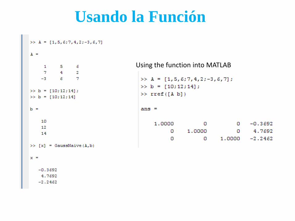
Usando la Función

Using the function into MATLAB