UNIVERSIDAD COMPLUTENSE DE MADRID …de libertad en la conexi´on af´ın. En concreto, la...
181
UNIVERSIDAD COMPLUTENSE DE MADRID FACULTAD DE CIENCIAS FÍSICAS Departamento de Física Teórica TESIS DOCTORAL New models for extreme gravitational systems Nuevos modelos asociados a sistemas gravitacionales extremos MEMORIA PARA OPTAR AL GRADO DE DOCTOR PRESENTADA POR Jorge Gigante Valcárcel Director José Alberto Ruiz Cembranos Madrid 2019 ©Jorge Gigante Valcárcel, 2018
Transcript of UNIVERSIDAD COMPLUTENSE DE MADRID …de libertad en la conexi´on af´ın. En concreto, la...
UNIVERSIDAD COMPLUTENSE DE MADRID FACULTAD DE CIENCIAS FÍSICAS
Departamento de Física Teórica
TESIS DOCTORAL
New models for extreme gravitational systems
Nuevos modelos asociados a sistemas gravitacionales extremos
MEMORIA PARA OPTAR AL GRADO DE DOCTOR
PRESENTADA POR
Jorge Gigante Valcárcel
Director
José Alberto Ruiz Cembranos
Madrid 2019
©Jorge Gigante Valcárcel, 2018
New models for extreme gravitationalsystems
Nuevos modelos asociados a sistemas gravitacionales extremos
Author: Supervisor:Jorge Gigante Valcarcel Jose Alberto Ruiz Cembranos
Departamento de Fısica Teorica, Facultad de Ciencias Fısicas,Universidad Complutense de Madrid.


To all my family.
A toda mi familia.


Acknowledgments
This work has been supported by the MINECO (Spain) Project Nos. FIS2014-52837-P, FPA2014-53375-C2-1-P, FIS2016-78859-P (AEI/FEDER, UE) and Consolider-Ingenio MULTIDARK Grant. No. CSD2009-00064.

Contents
Abbreviations IX
Abstract XI
Resumen XIII
1 Introduction to post-Riemannian geometries 1
1.1 Motivation and generalities . . . . . . . . . . . . . . . . . . . . . . . . 1
1.2 Riemann-Cartan manifolds: the space-time torsion . . . . . . . . . . 4
1.3 Poincare gauge theory of gravity . . . . . . . . . . . . . . . . . . . . . 6
1.4 Motion of test particles in the Poincare gauge theory . . . . . . . . . 10
1.5 The Dirac equation in the presence of torsion . . . . . . . . . . . . . 12
1.6 Teleparallelism . . . . . . . . . . . . . . . . . . . . . . . . . . . . . . 14
1.7 Gravitation with non-propagating torsion: the Einstein-Cartan theory 16
2 Vacuum solutions of the Poincaré gauge theory 19
2.1 The Baekler solution: torsion and confinement type of potential . . . 19
2.2 New torsion black hole solutions in Poincare gauge theory . . . . . . 27
2.3 Extended Reissner-Nordstrom solutions sourced by dynamical torsion 45
2.4 Fermion dynamics in torsion theories . . . . . . . . . . . . . . . . . . 53
3 Singularities and stability conditions 73
3.1 Stability and singular geometries . . . . . . . . . . . . . . . . . . . . 73
VII

VIII CONTENTS
3.2 Singularities and n-dimensional black holes in torsion theories . . . . 79
3.3 Stability in quadratic torsion theories . . . . . . . . . . . . . . . . . . 99
4 Einstein-Yang-Mills systems 115
4.1 Introduction to Einstein-Yang-Mills theory . . . . . . . . . . . . . . . 115
4.2 Einstein-Yang-Mills-Lorentz black holes . . . . . . . . . . . . . . . . . 127
4.3 Correspondence between Einstein-Yang-Mills-Lorentz systems and dy-namical torsion models . . . . . . . . . . . . . . . . . . . . . . . . . . 133
Conclusions 139
Appendices 143
A Expressions of the Poincaré gauge field equations 143
B Torsion and curvature collineations 147
C SU(2) gauge connection in static and spherically symmetric space-times 151
Publications 155
Bibliography 157
Abbreviations
BH Black Hole
BK Bartnik McKinnon
BR Belinfante Rosenfeld
EC Einstein Cartan
EH Einstein Hilbert
EYM Einstein Yang Mills
GR General Relativity
LC Levi Civita
PG Poincare Gauge
RC Riemann Cartan
RN Reissner Nordstrom
YM Yang Mills
IX

Abstract
A large number of classes of modified theories of gravity have been developed fora long time. They have attracted much attention from physicists, since they showdifferent aspects concerning gravitational interaction. In fact, these aspects mayextend the role of gravity not only at large scales but at microscopic regimes, sothat they have been systematically related to fundamental issues such as the occur-rence of space-time singularities, the loss of renormalizability or the origin of theaccelerated expansion of the universe, among others. Despite the successful predic-tions and the highly tested accuracy of General Relativity (GR) in describing thegravitational phenomena, the absence of an appropriate explanation for these issueshas stimulated the investigation of new alternative models of gravitation.
The extension of the conventional approach can be addressed by the introduc-tion into the gravitational action of higher order corrections depending on the metrictensor alone. Such a procedure preserves the geometric structure of the space-timeand potentially yields new propagating degrees of freedom related to metric, whichmeans that not only the phenomenological compatibility with GR must be consid-ered by the new framework but also the viability of its stability conditions. On theother hand, it is also possible to define a more complex geometry by the modifica-tion of the affine connection. Namely, the Levi-Civita connection of GR is subject tothe fulfillment of two independent constraints: the conservation of the metric tensorunder parallel transport and the vanishing of its antisymmetric component. Hence,in this case there is an increase in the number of degrees of freedom contained in theconnection, which can involve new geometrical and dynamical effects in the space-time. Furthermore, from a theoretical point of view, the resulting post-Riemanniangeometry can be related to the existence of a new fundamental symmetry in na-ture by applying the gauge principles. This scheme leads to the appearance of newtheories of gravitation, such as the Metric-Affine or the Poincare Gauge theory.
In the present thesis, we use these notions to investigate the nature and theimplications of the space-time torsion in the framework of the Poincare Gauge the-ory. Thereby, we deal with a metric-compatible asymmetric connection and analysethe foundations and viability of different models within this framework. First, inChapter 1, we present an introduction of the specific motivations to consider a post-
XI

Riemannian regime, by emphasizing the most relevant consequences and differencesfrom the standard case of GR. The intrinsic relation between torsion and the spindensity tensor of matter is especially remarkable. It is also worthwhile to stressthe potential effects of the torsion tensor on the propagation and motion of Diracparticles, as well as its dynamical contribution to the geometry of space-time. Inthis regard, we describe in Chapter 2 the most relevant configurations provided bya dynamical torsion in a vacuum space-time. These types of scenarios allow anassessment to be made of the possible roles assumed by torsion and furthermore ofthe characteristic effects involved in its interaction with matter fields. We presentnew black hole solutions for both the cases with massless and massive torsion, whichintroduce significant corrections to the Schwarzschild solution of GR. The existenceof a dynamical axial mode related to torsion highlights the relevance of these solu-tions, since this is the unique component implicated in the interaction with Diracfields, according to the minimal coupling principle. On the other hand, the newgeometry can modify additional fundamental constraints, such as the appearanceof space-time singularities or instabilities. Therefore, in Chapter 3, we revise thesingularity theorems of pseudo-Riemannian geometry and study this issue withinthe new framework, in order to extend their general applicability and address theappropriate changes in the presence of torsion. By focusing on a particular set of as-sumptions, we also perform an intensive analysis to find new ghost and tachyon-freeconditions related to torsion, which must be satisfied by the Lagrangian coefficientsto avoid unsuitable instabilities. Finally, in Chapter 4, we extrapolate the externalsymmetries provided by post-Riemannian geometry to construct new models withinthe Einstein-Yang-Mills theory of internal symmetry groups, which focuses on theinteraction between gravity and non-Abelian gauge fields. Indeed, the search of acorrespondence between both approaches allows the simplification of the complexityinvolved by the highly nonlinear character of these elements, which in turn facili-tates the obtention of different non-Abelian exact solutions to the field equations.Appendix A is devoted to the expressions of the general field equations inducedby curvature and torsion in the gauge formalism, which associate both geometricalquantities with the energy-momentum and spin density tensors of matter. In ad-dition, the space-time symmetries applied to simplify the extreme difficulty of thefield equations and to categorize the resulting new black hole solutions are present inAppendix B, whereas a detailed derivation of the SU(2) gauge connection in staticand spherically symmetric space-times is shown in Appendix C.
The results achieved in this thesis provide new bases and methodologies to de-scribe and measure the possible existence of a space-time torsion in the universe.Since this quantity appears to be directly connected to the intrinsic angular momen-tum of elementary particles, it is expected to generate negligible effects at macro-scopic scales. Therefore, the focusing on extreme gravitational systems that mayintensify such effects is especially relevant to overcome these observational issues.
XII

Resumen
Un gran numero de teorıas de gravedad modificada se ha venido desarrollando desdehace decadas. Debido a las multiples propiedades teoricas que proporcionan alcampo gravitatorio, estas han atraıdo la atencion de muchos investigadores desde susinicios. Dichas propiedades pueden modificar el papel de la gravedad y extenderlo, nosolo a gran escala, sino tambien a un regimen microscopico, por lo que se han venidorelacionando sistematicamente con cuestiones fundamentales como la ocurrencia desingularidades en el espacio-tiempo, la perdida de renormalizabilidad o el origen dela expansion acelerada del universo. A pesar de las exitosas predicciones de la Teorıade la Relatividad General (GR) y de su caracter predictivo altamente probado, laausencia de una solucion adecuada a estas cuestiones ha estimulado la investigacionde nuevos modelos alternativos de la gravedad.
La extension del marco teorico convencional puede realizarse mediante la intro-duccion en la accion gravitacional de correcciones geometricas de orden superior de-pendientes del tensor metrico. Este procedimiento preserva la estructura geometricadel espacio-tiempo y agrega nuevos grados de libertad a la teorıa, lo que significaque no solo es importante asegurar la compatibilidad con GR desde un punto devista fenomenologico, sino tambien su propia estabilidad dinamica. Por otro lado,tambien es posible definir una geometrıa mas compleja introduciendo nuevos gradosde libertad en la conexion afın. En concreto, la conexion afın de Levi-Civita presenteen GR satisface dos ligaduras, al implicar la conservacion de la metrica bajo el trans-porte paralelo y omitir la inclusion de una componente antisimetrica. Los grados delibertad geometricos resultantes al liberar el cumplimiento de cualesquiera de estasdos condiciones, sumados a los ya existentes en el marco teorico estandar, puedendar lugar a nuevos efectos dinamicos en el espacio-tiempo. Desde un punto de vistateorico, esta nueva geometrıa postRiemanniana puede relacionarse con una nuevasimetrıa fundamental aplicando los principios de invariancia gauge. Este enfoque hadado lugar al nacimiento de nuevas teorıas de la gravitacion, como la Teorıa MetricaAfın o la Teorıa Gauge de Poincare.
En la presente tesis, usamos estas nociones para investigar la naturaleza y lasposibles implicaciones derivadas de una torsion espacio-temporal en el marco dela Teorıa Gauge de Poincare. De esta forma, consideraremos una conexion afın
XIII

asimetrica que preserve la metrica y analizaremos los fundamentos y la viabilidadde diferentes modelos sujetos a estas directrices. En primer lugar, en el Capıtulo1, introducimos detalladamente las motivaciones para considerar un nuevo regimenpostRiemanniano, destacando sus consecuencias mas relevantes y sus diferencias conrespecto al caso estandar de GR. En este sentido, la relacion existente entre el tensormomento angular de espın de la materia y la torsion del espacio-tiempo es especial-mente destacable dentro de este nuevo marco teorico. Asimismo, senalamos losposibles efectos dinamicos producidos por la torsion en la propagacion de partıculasde Dirac y en la propia geometrıa del espacio-tiempo. A este respecto, en el Capıtulo2, describimos las configuraciones geometricas mas relevantes originadas por la ex-istencia de una torsion dinamica en el vacıo. Estos tipos de escenarios permitenevaluar las propiedades fısicas de dicha magnitud geometrica y sus efectos en lainteraccion con la materia. El hallazgo de nuevas soluciones de tipo agujero ne-gro, asociadas a los casos con torsion no masiva y masiva, se incluye tambien eneste capıtulo. Estos resultados muestran correcciones significativas a la solucionde vacıo de Schwarzschild de GR proporcionadas por la torsion. La existencia deun modo de torsion axial dinamico aumenta la relevancia de estas soluciones, altratarse de la unica componente de la torsion capaz de interaccionar con camposde Dirac, de acuerdo al principio de acoplamiento mınimo. Por otro lado, en elregimen postRiemanniano, otras condiciones fundamentales pueden verse alteradas,como la ocurrencia de singularidades o de inestabilidades fısicas. Por tanto, enel Capıtulo 3, revisamos los teoremas de singularidades presentes en la geometrıapseudoRiemanniana y estudiamos su generalizacion al caso con torsion. Del mismomodo, imponiendo una serie de restricciones sobre la torsion y la metrica, llevamosa cabo un exhaustivo analisis para determinar nuevas condiciones de estabilidad dela teorıa, las cuales pueden describirse mediante sencillas ligaduras entre los coefi-cientes del lagrangiano. Por ultimo, en el Capıtulo 4, hacemos uso de todas estasnociones teoricas de invariancia gauge asociadas a simetrıas externas para construirnuevos modelos de campos de Einstein-Yang-Mills asociados a simetrıas internas,los cuales describen la dinamica de campos gauge no abelianos en espacio-tiempocurvo bajo el marco de la GR. La busqueda de una correspondencia entre ambos en-foques permite simplificar de manera notable su complejidad matematica, provistapor el caracter altamente no lineal de sus elementos, lo que facilita la obtencion dediferentes soluciones exactas a las ecuaciones de Einstein-Yang-Mills.
El Apendice A contiene las expresiones generales de las ecuaciones de camposinducidas por los tensores de curvatura y torsion en el formalismo gauge, las cualesasocian estas magnitudes geometricas con los tensores de energıa-impulso y densidadde espın de la materia. Las simetrıas espacio-temporales aplicadas para simplificar lacomplejidad de estas ecuaciones y para categorizar las nuevas soluciones de tipo agu-jero negro se presentan en el Apendice B, mientras que en el Apendice C se muestraen detalle el analisis para la obtencion de una conexion gauge de SU(2) simplificada,en presencia de un espacio-tiempo curvo estatico y esfericamente simetrico.
XIV

Los resultados alcanzados en esta tesis proporcionan nuevas bases y metodologıaspara describir y medir la posible existencia de una torsion espacio-temporal en eluniverso. Al tratarse de una magnitud directamente conectada con el momentoangular intrınseco de las partıculas elementales, se espera que en general produzcaefectos despreciables a gran escala. Por lo tanto, el estudio de sistemas gravita-cionales extremos que puedan intensificar sus efectos es especialmente relevante a lahora de intentar superar estas limitaciones observacionales.
XV


Chapter 1
Introduction to post-Riemanniangeometries
1.1 Motivation and generalities
Since the early twentieth century, General Relativity (GR) has been established asthe theory that best and most deeply describes, from a phenomenological point ofview, the gravitational field and its interaction with matter. Since its inceptions, thetheory formulated by Albert Einstein completely modified the general understandingof the universe. The most fascinating postulate assumed by Einstein’s approachwas the fact that the universe itself acquires a non-vanishing curvature due to thepresence of gravity and matter fields. Furthermore, its theoretical bases led tothe conclusion that this effect is naturally modulated by the energy-momentumproperties of matter, in a form that it is preserved in all reference frames, accordingto the principle of general covariance [1].
From a mathematical point of view, the model was developed in terms of Rie-mannian geometry by establishing a correspondence between space-time and a dif-ferentiable manifold endowed with a curvature tensor, which is associated with thegravitational field. Such a description involves the existence of a metric tensor anda metric-compatible affine connection in a form that all the geometrical quantitiesdefined on the manifold can be expressed in terms of them. These elements enablethe definition of the distance and parallel transport concepts within the manifold.Thereby, one of the assumptions of the theory is the vanishing of the antisymmetricpart of the affine connection, so that it can be written in terms of the metric tensor:
Γλ µν = 12g
λρ (∂µgνρ + ∂νgµρ − ∂ρgµν) , (1.1)
where latin and greek indices refer to anholonomic and coordinate basis, respectively.
1
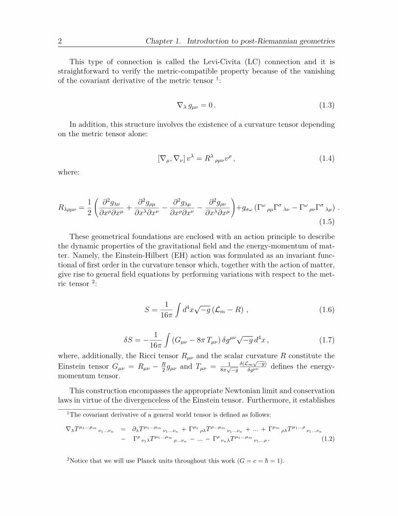
2 Chapter 1. Introduction to post-Riemannian geometries
This type of connection is called the Levi-Civita (LC) connection and it isstraightforward to verify the metric-compatible property because of the vanishingof the covariant derivative of the metric tensor 1:
∇λ gµν = 0 . (1.3)
In addition, this structure involves the existence of a curvature tensor dependingon the metric tensor alone:
[∇µ,∇ν ] vλ = Rλρµνv
ρ , (1.4)
where:
Rλρµν = 12
(∂2gλν∂xρ∂xµ
+ ∂2gρµ∂xλ∂xν
− ∂2gλµ∂xρ∂xν
− ∂2gρν∂xλ∂xµ
)+gσω (Γω ρµΓσ λν − Γω ρνΓσ λµ) .
(1.5)
These geometrical foundations are enclosed with an action principle to describethe dynamic properties of the gravitational field and the energy-momentum of mat-ter. Namely, the Einstein-Hilbert (EH) action was formulated as an invariant func-tional of first order in the curvature tensor which, together with the action of matter,give rise to general field equations by performing variations with respect to the met-ric tensor 2:
S = 116π
∫d4x√−g (Lm −R) , (1.6)
δS = − 116π
∫(Gµν − 8π Tµν) δgµν
√−g d4x , (1.7)
where, additionally, the Ricci tensor Rµν and the scalar curvature R constitute theEinstein tensor Gµν = Rµν − R
2 gµν and Tµν = 18π√−g
δ(Lm√−g)
δgµνdefines the energy-
momentum tensor.
This construction encompasses the appropriate Newtonian limit and conservationlaws in virtue of the divergenceless of the Einstein tensor. Furthermore, it establishes
1The covariant derivative of a general world tensor is defined as follows:
∇λTµ1...µmν1...νn = ∂λT
µ1...µmν1...νn + Γµ1
ρλTρ...µm
ν1...νn + ... + ΓµmρλT
µ1...ρν1...νn
− Γρ ν1λTµ1...µm
ρ...νn − ... − Γρ νnλTµ1...µm
ν1...ρ . (1.2)
2Notice that we will use Planck units throughout this work (G = c = ~ = 1).

1.1. Motivation and generalities 3
a complete correspondence between gravitation and the geometry of space-time byassigning the physical trajectories to a geodesic motion in absence of external forces[2].
A large number of further implications were also originally studied and predictedby scientists by means of the theory, like for example the equivalence principle,orbital precession of macroscopic bodies, deflection of light, gravitational redshiftand lensing, time dilation or the existence of black holes (BHs) and gravitationalwaves, among others [3]. All these events have been systematically tested evennowadays, providing a strong supporting evidence of its accuracy and precision[4, 5].
Nevertheless, from a theoretical point of view, there exist additional issues thatpresumably require going beyond GR towards a more complete theory of gravity.Some of these fundamental problems are the impossibility of renormalizing the EHaction unlike that given by other quantum field theories and the existence of un-avoidable space-time singularities [6, 7].
Numerous attempts have been accomplished to address these questions and for-mulate an improved modified theory of gravity, even in the framework of Rieman-nian geometry [8–10]. Many of these new schemes, in fact, modify the gravityaction by aggregating higher order corrections, which are at least quadratic in thecurvature tensor. But additional modifications can be introduced in the realm ofpost-Riemannian geometry, which incorporates new degrees of freedom into thegeometric structure of the manifold. Specifically, as mentioned previously, the an-tisymmetric and non-metricity components of the affine connection are assumed tovanish in the standard case, but this situation changes in the presence of an affinelyconnected metric space-time. In such a case, the components of the affine connectionare expressed in the following way 3:
Γλ µν = Γλ µν +Kλµν + Lλ µν , (1.8)
where Kλµν represents a metric-compatible component depending on the antisym-
metric part of the connection and Lλ µν is related to non-metricity. By definingT λ µν = 2Γλ [µν] as the stressed antisymmetric component and Qλµν = ∇λgµν as thenon-metricity part of the affine connection, then the previous quantities are writtenas follows:
Kλµν = 1
2(T λ µν − Tµ λ ν − Tν λ µ) , (1.9)
3We use notation with tilde to denote quantities depending on torsion and without tilde for thetorsion-free components of such quantities.
4 Chapter 1. Introduction to post-Riemannian geometries
Lλ µν = 12(Qλ
µν −Qµλν −Qν
λµ) . (1.10)
Note that these post-Riemannian components possess a tensorial character, whereasthe Riemannian part of the connection still changes inhomogeneously under an in-finitesimal coordinate transformation xµ → x′µ = xµ + ξµ:
Γλ µν → Γ′λ µν = ∂xλ
∂x′ρ∂x′σ
∂xµ∂x′ω
∂xνΓρ σω + ∂2x′ρ
∂xµ∂xν∂xλ
∂x′ρ. (1.11)
Then, the antisymmetric part T λ µν of the affine connection always transformsas a tensor and it is called torsion tensor, whereas the resulting piece Kλ
µν on theconnection is called contortion tensor. On the other hand, the tensorial nature of themetric and the covariant derivative is appropriately induced on the non-metricitycomponent.
In analogy to the rest of the extended theories of gravity, these geometrical char-acteristics define additional scalar invariants into the gravitational action and hencemodify the dynamical aspects provided by the gravitational field. Nevertheless, it isexpected that these higher order corrections produce neglected effects at low energyscales and thus they are remarkable only around extreme gravitational systems.
1.2 Riemann-Cartan manifolds: the space-timetorsion
The particular case of an affinely connected metric manifold with a metric-compatibleconnection is named Riemann-Cartan (RC) manifold. Hence, these types of topo-logical spaces are characterized by a vanishing non-metricity tensor:
Qλµν = 0 . (1.12)
The resulting geometric structure is then provided by a metric tensor and anasymmetric affine connection that preserves lengths and angles under parallel trans-port. Since the affine connection is directly connected to the definition of the covari-ant derivative, the presence of an antisymmetric component within such a connectionintroduces deep geometrical consequences. First, it is straightforward to notice thechange on the commutation relations of the covariant derivatives:
[∇µ, ∇ν ] vλ = Rλρµν v
ρ + T ρ µν ∇ρvλ , (1.13)
1.2. Riemann-Cartan manifolds: the space-time torsion 5
where:
Rλρµν = ∂µΓλ ρν − ∂νΓλ ρµ + Γλ σµΓσ ρν − Γλ σνΓσ ρµ . (1.14)
Thereby, it is important to distinguish between the Riemann curvature and theRC curvature. The latter also satisfies its proper Bianchi identities in the RC space-time 4:
Rλ[µνρ] + ∇[µT
λνρ] + T σ [µν T
λρ]σ = 0 , (1.16)
∇[σ|Rλρ|µν] − T ω [σµ|R
λρω|ν] = 0 , (1.17)
and allows the existence of a non-vanishing antisymmetric component of the Riccitensor:
R[µν] = 12 ∇λT
λµν+
12(∇µT
λνλ −∇νT
λµλ
)+1
2 TλρλT
ρµν+
14(TµλρT
ρλν − TνλρT ρλ µ
).
(1.18)
Furthermore, the torsion tensor provides a sort of displacement of vectors alonginfinitesimal paths that generally involves the breaking of standard parallelograms,in a way that their translational closure failure proportionally depends on the men-tioned tensor [11, 12]. Suppose two vectors ελ1 and ελ2 at a given point xλ, thenthe following identity describes the open contour of the infinitesimal parallelogramconstructed by them in the presence of torsion:
(xλ + ελ2 + ε′λ1
)−(xλ + ελ1 + ε′λ2
)= T λ µν ε
µ1εν2 , (1.19)
with ε′λ1 and ε′λ2 the resulting vectors obtained by the parallel transport of ελ1 andελ2 , at the point of coordinates xλ + ελ2 and xλ + ελ1 , in the direction of ελ2 and ελ1 ,respectively. This quality represents an important and singular geometrical effect,since it cannot be yielded by any other quantity, but only by the torsion tensor.
In addition, these features allow the establishment of an equivalence betweentorsion and dislocation defects of three-dimensional crystal lattices [13–15]. The RCmanifold then may be considered as an effective geometrical construction arising
4Note that the torsion tensor also implies a non-trivial relation under the following exchange ofindices of the RC curvature:
Rλρµν − Rµνλρ = 32(Rλ[ρµν] + Rρ[µλν] + Rµ[ρλν] + Rν[ρµλ]
). (1.15)

6 Chapter 1. Introduction to post-Riemannian geometries
from a microscopic structure endowed with dislocation defects, which are describedby torsion in the limit where they form a continuous distribution.
In order to establish a general classification of torsion, it can be decomposed intoits respective irreducible parts under the Lorentz group [16, 17]. Namely, a tracevector Tµ, an axial vector Sµ and a traceless and also pseudotraceless tensor qλ µν :
T λ µν = 13(δλ νTµ − δλ µTν
)+ 1
6 gλρε ρσµνS
σ + qλ µν , (1.20)
where ε ρσµν is the four-dimensional LC symbol. From a phenomenological point ofview, this sort of geometrical classification can be associated with a large number ofphysically relevant configurations, such as the minimal coupling between the Diracfields and the axial vector or the vanishing of its tensorial modes in a spatiallyhomogeneous and isotropic universe, as is assumed by the cosmological principle[18, 19].
By taking into account these notions, it is possible to construct a large class ofscalar invariants from the RC curvature and the torsion tensor and define a modifiedgravitational action in the framework of the RC geometry. It means that the RCspace-time constitutes the kinematical arena of every type of extended theory ofgravity with torsion. On the other hand, the dynamical aspects of torsion alsodepend on the order of such geometrical invariants included in the Lagrangian.Specifically, the full linear case describes a non-propagating torsion tied to materialsources, whereas higher order corrections describe a Lagrangian with propagatingtorsion, which generally involves dynamical effects in vacuum.
1.3 Poincare gauge theory of gravity
From a theoretical point of view, the most consistent and successful description oftorsion is formulated in the framework of the Poincare Gauge (PG) theory of gravity[20–22]. Just as its name indicates, this theory represents a gauge approach to grav-ity based on the semidirect product of the Lorentz group and the space-time trans-lations, in analogy to the unitary irreducible representations of relativistic particleslabeled by their spin and mass, respectively. Then not only an energy-momentumtensor of matter arises from this approach, but also a non-trivial spin density tensorthat operates as source of torsion, providing an appropriate correspondence betweenthe respective gauge potentials and their corresponding field strength tensors.
Hence, the model requires gauging the external degrees of freedom consisting ofrotations and translations, which are represented by the Poincare group ISO(1, 3).This means that a gauge connection containing two principal independent variablesis introduced in order to describe the gravitational field as a gauge field. These
1.3. Poincare gauge theory of gravity 7
quantities constitute the gauge potentials related to the generators of translationsand local Lorentz rotations, respectively:
Aµ = ea µPa + ωab µJab , (1.21)where ea µ is the vierbein field and ωab µ is the spin connection, which satisfy thefollowing relations with the metric and the affine connection [23]:
gµν = ea µ ebν ηab , (1.22)
ωab µ = ea λ ebρ Γλ ρµ + ea λ ∂µ e
bλ . (1.23)
Thus, the vierbein field and the affine connection act as translational and ro-tational type potentials, respectively. Moreover, the mentioned gauge connectionassociated with the group ISO(1, 3) defines a 2-form curvature, Fµν = ∂µAν −∂νAµ − i[Aµ, Aν ], which can be expressed in the following way:
Fµν = F aµνPa + F ab
µνJab , (1.24)with F a
µν = ∂µeaν − ∂νea µ + ωab µe bν − ωab ν ebµ and F ab
µν = ∂µωabν − ∂νωab µ +
ωac ν ωbcµ − ωac µ ωb cν .
As with other well-known gauge theories, the field strength tensor character-izes the properties of the gravitational interaction, which in the PG framework arepotentially modified by the presence of torsion. In particular, it is related to thetorsion and the curvature tensor as follows:
F aµν = ea λ T
λνµ , (1.25)
F abµν = ea λe
bρ R
λρµν . (1.26)
Hence, whereas curvature is related to the rotation of a vector along an in-finitesimal path over the space-time, torsion is related to the translation and theyappropriately constitute the field strengths of the rotation and the translation group,respectively.
In contrast with the regular Yang-Mills (YM) theories of internal symmetrygroups, the complexity provided by the external symmetry group ISO(1, 3) allowsthe definition of a greater number of scalar invariants from the curvature and torsiontensors. From a theoretical point of view, these types of geometrical quantities

8 Chapter 1. Introduction to post-Riemannian geometries
are essential since they yield kinetic and interaction terms into the gravitationalaction. In general, by excluding parity violating terms, it is possible to construct sixindependent quadratic scalar invariants of curvature and three of torsion, besides thelinear one given by the Ricci scalar. Therefore, the most general parity preservingaction quadratic in the field strength tensors can be written as 5:
S = 116π
∫d4x√−g[Lm − R− a1R
2 + (a3 − a1) RλρµνRµνλρ + a2RλρµνR
λρµν
+a4RλρµνRλµρν + a5RµνR
µν + (a6 + 4a1) RµνRνµ
+αTλµνT λµν + β TλµνTµλν + γ T λ λνT
µµν], (1.27)
where a1, a2, a3, a4, a5, a6, α, β and γ are constant parameters. Although the theoret-ical and experimental research for restrictions on the values of these coefficients stillpersists, they are in principle subject to the requirement of a viable set of stabilityconditions and to the constraints given by the experimental evidence. In any case,for deriving the field equations, it is possible to dismiss one of the coefficients asso-ciated with the scalars of curvature and reduce the set of parameters by applyingthe Gauss-Bonnet theorem in four-dimensional RC space-times, without loss of gen-erality [25, 26]. Specifically, the following combination quadratic in the curvaturetensor acts as a total derivative of a certain vector V µ in the gravitational action:
√−g
(R2 + RλρµνR
µνλρ − 4RµνRνµ)
= ∂µVµ . (1.28)
Then, in order to derive the general field equations of the quadratic PG theoryit is sufficient to perform variations with respect to the gauge potentials, resultingthe following outcome:
X1µ ν + 16πθµ ν = 0 , (1.29)
X2[µλ]ν + 16πSλµ ν = 0 , (1.30)
where X1µ ν and X2[µλ]ν are tensorial functions depending on the RC curvature and
the torsion tensor, which are defined in Appendix A, whereas θµ ν and Sλµ ν are thecanonical energy-momentum tensor and the spin density tensor, respectively, whichare defined as follows:
θµν = ea µ
16π√−gδ (Lm
√−g)
δea ν, (1.31)
5For an exhaustive study on the class of quadratic PG Lagrangians including parity violatingterms, see reference [24].

1.3. Poincare gauge theory of gravity 9
Sλµν = ea λe
bµ
16π√−gδ (Lm
√−g)
δωab ν. (1.32)
This variational procedure is a direct consequence of the gauge invariance of thePoincare group, whose non-Abelian nature is also present in the physical model invirtue of the highly nonlinear character shown by the field equations (1.29) and(1.30). In addition, the canonical energy-momentum tensor derived from this ap-proach is not generally symmetric in the presence of torsion and the spin densitytensor is antisymmetric in its first pair of indices. Moreover, it is straightforward toobtain from the field equations the following conservation laws for these tensors:
∇νθµν +Kλρµθ
ρλ + Rλρνµ Sλρν = 0 , (1.33)
∇µSλρµ + 2Kσ
[λ|µS|ρ]σµ − θ[λρ] = 0 . (1.34)
Thereby, both quantities act as sources of gravity and represent the translationaland rotational currents, respectively. They constitute the natural generalizationof the conserved Noether currents associated with the external translations androtations of the Poincare group in a Minkowski space-time, as expected [27]:
∂νθµν = 0 , (1.35)
∂µJλρµ = 0 , (1.36)
where Jλρ µ is the total angular momentum density, which is decomposed into anorbital part and an intrinsic part (i.e. the spin density tensor):
Jλρµ = Mλρ
µ + Sλρµ , (1.37)
with Mλρµ = x[λ θρ]
µ the resulting orbital angular momentum density, whose diver-gence is trivially proportional to the antisymmetric part of the canonical energy-momentum tensor:
∂µMλρµ = θ[ρλ] . (1.38)
Since the addition of total derivatives into the total Lagrangian preserves theinvariance of the mentioned conservation laws, it turns out that the canonical cur-rents are not uniquely defined and it is possible to establish fundamental relationsbetween them. In particular, as is shown, the canonical energy-momentum tensor

10 Chapter 1. Introduction to post-Riemannian geometries
generally contains an antisymmetric component even when the notions of curvatureand torsion are neglected (i.e. in the framework of Special Relativity), but it ispossible to relocalize it by applying a symmetrization procedure [28]:
Tµν = θµν − ∂λSµν λ − 2∂λSλ (µν) . (1.39)
In fact, we denote such a symmetric quantity as Tµν because it was also shownthat, by replacing the ordinary derivatives by torsion-free covariant derivatives, itactually coincides with the energy-momentum tensor defined from GR [29]. In virtueof this procedure, it is also common to designate this tensor as the Belinfante-Rosenfeld (BR) energy-momentum tensor. The generalization to RC space-timesgives rise to the following expression [30]:
Tµν = θµν −?
∇λSµνλ − 2
?
∇λSλ
(µν) , (1.40)
with?
∇λ = ∇λ − T ρ λρ.
Thus, whereas the symmetric BR tensor represents the energy-momentum dis-tribution of matter in GR, this situation does not hold in the PG theory of gravitydue to the dynamical character of the spin density tensor in the presence of torsion.On the contrary, such a role falls on the canonical energy-momentum tensor, so thesymmetric energy-momentum tensor of GR must be replaced by this quantity.
1.4 Motion of test particles in the Poincare gaugetheory
As previously stressed, the presence of a space-time torsion generalizes the conserva-tion laws associated with the energy-momentum and spin density tensors of matter,in such a form that these currents completely coincide with the ones derived fromGR when the latter vanishes:
∇νθµν = 0 , (1.41)
θ[µν] = 0 . (1.42)
This result is a direct consequence of the deep relation existing between thetorsion field and the intrinsic angular momentum of matter in the realm of thePG theory, where it operates as a source of torsion. It means that it is crucial to

1.4. Motion of test particles in the Poincare gauge theory 11
distinguish between the motion of spinning and spinless particles when consideringthe physical trajectories of test bodies from this approach. Indeed, neither the curvesof extremal length given by the geodesic equations:
d2xµ
ds2 + Γµ λρdxλ
ds
dxρ
ds= 0 , (1.43)
nor the straightest lines defined by the parallel transport of a vector to itself in termsof the autoparallel equations:
d2xµ
ds2 + Γµ λρdxλ
ds
dxρ
ds= 0 , (1.44)
can represent the general motion of matter in the presence of a space-time torsion.Conversely, whereas the former can only be related to spinless particles, the latterdoes not distinguish between particles with a different spin and then the torsiontensor affects the motion of particles with and without spin in the same way.
An appropriate expression, however, can be obtained by the conservation laws(1.33) and (1.34) by integrating over a three-dimensional spacelike section of theworld tube involving the particle and employing the semiclassical approximation[2, 31]:
∫∂ν(√−g θµν
)d3x′ +
∫Γµ λρθλρ
√−g d3x′
= −∫Kλρ
µθρλ√−g d3x′ −
∫Rλρσ
µ Sλρσ√−g d3x′ , (1.45)
with:
∫∂ν(√−g θµν
)d3x′ = d
dt
∫θµt√−g d3x′ , (1.46)
by the Gauss theorem. Then, by defining the four-momentum pµ and the net spinangular momentum Sλρ, of the particle with four-velocity uµ, in terms of the propertime s along its world line:
pλuρ = dt
ds
∫θλρ√−g d3x′ , (1.47)
Sλρuσ = dt
ds
∫Sλρσ√−g d3x′ , (1.48)
the expression (1.45) involves the following equations of motion:

12 Chapter 1. Introduction to post-Riemannian geometries
dpµ
ds+ Γµ λρ pλuρ +Kλρ
µpρuλ + RλρσµSλρuσ = 0 . (1.49)
As can be seen, an additional generalized Lorentz force emerges depending onthe intrinsic angular momentum of matter and the torsion tensor, which is containedin the RC curvature and the contortion component. This force potentially yieldsdeviations from the geodesic trajectories and it represents another fundamental dif-ference with the standard approach of GR. In this sense, it is straightforward tocheck that, for spinless matter (i.e. Sλρ = 0), the equations of motion reduce to thesame geodesic equations of GR.
Nevertheless, since the spin of elementary particles is of the order of the Planckconstant, it is expected that the strength of this force yields effects too tiny tobe measured, as occurs in the context of other well-known gravitational theoriesframed beyond GR. From an experimental point of view, this means the difficultyin proving the possible existence of a non-vanishing dynamical torsion in the space-time. Moreover, it has been argued the possibility of measuring torsion effects bymaking use of a macroscopic rotating gyroscope (i.e. a gyroscope with vanishingnet spin) [32]. Even so, the insufficiency of these types of arguments has beensystematically pointed out because of the uncoupling between torsion and the orbitalangular momentum of such gyroscopes [33, 34]. This situation changes when apolarized system with a net elementary particle spin is considered, although thispossibility still requires more research and development, in order to generate anappreciable effect on its trajectories [35–37].
On the other hand, torsion is induced on the vierbein field by the field equationsand thereby it can also operate on the geodesic motion of ordinary matter via the LCconnection. This fact may involve additional effects to detect the possible existenceof this geometric field.
1.5 The Dirac equation in the presence of torsion
The Dirac equation describes the wave function of spin 1/2 particles. It representsa crucial tool to analyse the influence of gravity on these sorts of particles. Froma mathematical point of view, although general coordinate transformations do nothave spinor representations, these fields can be described by the representations(0, 1/2)⊕(1/2, 0) associated with the Lorentz group [38]. Therefore, a Lorentz spinconnection ωµ is introduced in order to establish a well-defined covariant Diracequation and to provide the dynamics of the spinor fields on a general space-time:
ωµ = i ωab µ [γa, γb] , (1.50)
1.5. The Dirac equation in the presence of torsion 13
where ωab µ coincides with the Expression (1.23) when the coupling with torsion isconsidered and γa are the four constant Dirac matrices.
Then, it is possible to perform the following covariant derivative of a Dirac spinor:
∇µΨ = ∂µΨ− ωab µ [γa, γb] Ψ . (1.51)
In the minimal coupling, the ordinary derivative is simply replaced by this sort ofcovariant derivative, which includes the torsion tensor and therefore it can operateon Dirac spinors. Thereby, the generalized Dirac Lagrangian of a spinor with massm minimally coupled to torsion is written in the following way [18]:
LDirac = i
2(Ψ γµ∇µΨ− ∇µΨ γµΨ− 2imΨΨ
), (1.52)
where Ψ = Ψ†γ0 is the Dirac adjoint. By performing the hermitian conjugation of theExpression (1.51) and multiplying by γ0 from the right, the identity (γa)† = γ0γaγ0
implies the covariant derivative of a Dirac adjoint:
∇µΨ = ∂µΨ + ωab µΨ [γa, γb] , (1.53)
and separates the metric and torsion contributions into the Dirac Lagrangian asfollows:
LDirac = i
2(Ψ γµ∇µΨ−∇µΨ γµΨ− eaµeb λecρKλ
ρµΨ γa, [γb, γc]Ψ− 2imΨΨ).
(1.54)
Therefore, in the minimal coupling, the interaction term between torsion and theDirac spinor depends on the anticommutator γa, [γb, γc]. It is possible to computethis factor by considering the properties of the product of three gamma matrices:
γaγbγc = ηabγc + ηbcγa − ηacγb + iεabcdγdγ
5 , (1.55)
where γ5 = i4!ε
abcdγaγbγcγd is the fifth gamma matrix, that additionally satisfies thefollowing properties:
(γ5)†
= γ5 , (1.56)
(γ5)2
= I4 , (1.57)

14 Chapter 1. Introduction to post-Riemannian geometries
γ5, γa
= 0 . (1.58)
By taking into account these conditions, one obtains the following outcome:
γa, [γb, γc] = 4iεabc dγdγ5 , (1.59)
which means that the mentioned interaction term constitutes a totally antisymmetricquantity coupled to the component of the Lorentz spin connection depending ontorsion:
LDirac = i
2(Ψ γµ∇µΨ−∇µΨ γµΨ + 2iελρµνTλρµΨγ5γνΨ− 2imΨΨ
). (1.60)
Indeed, the resulting Dirac Lagrangian can be expressed in a more compact formin terms of the axial component of torsion:
LDirac = i
2(Ψ γµ∇µΨ−∇µΨ γµΨ + 2iΨγ5γµSµΨ− 2imΨΨ
). (1.61)
This result yields an explicit interaction between torsion and Dirac spinors de-pending on the axial vector alone, so that the presence of the rest of the irreducibleparts of the torsion tensor does not alter itself. Such components may only enterimplicitly in the interaction if they are induced on the vierbein field present in theLagrangian. On the other hand, since there is still no experimental evidence on theexistence of the torsion field, the formulation of other Lagrangians non-minimallycoupled to torsion may be viable [39, 40]. These types of configurations introducecorrections into the interaction scheme and enable an active role of the additionalmodes of torsion in the presence of fermions.
1.6 Teleparallelism
As was indicated previously, a general PG model of gravity is commonly charac-terized by the presence of both curvature and torsion by means of RC geometry.Nevertheless, certain degenerate cases arise when the restriction of vanishing someof these quantities is applied. For example, the linear PG Lagrangian reduces tothe conventional EH Lagrangian if the condition of a vanishing torsion tensor is im-posed, which means that the resulting approach is completely determined in termsof Riemannian geometry (i.e. in terms of the LC connection). On the other hand, it
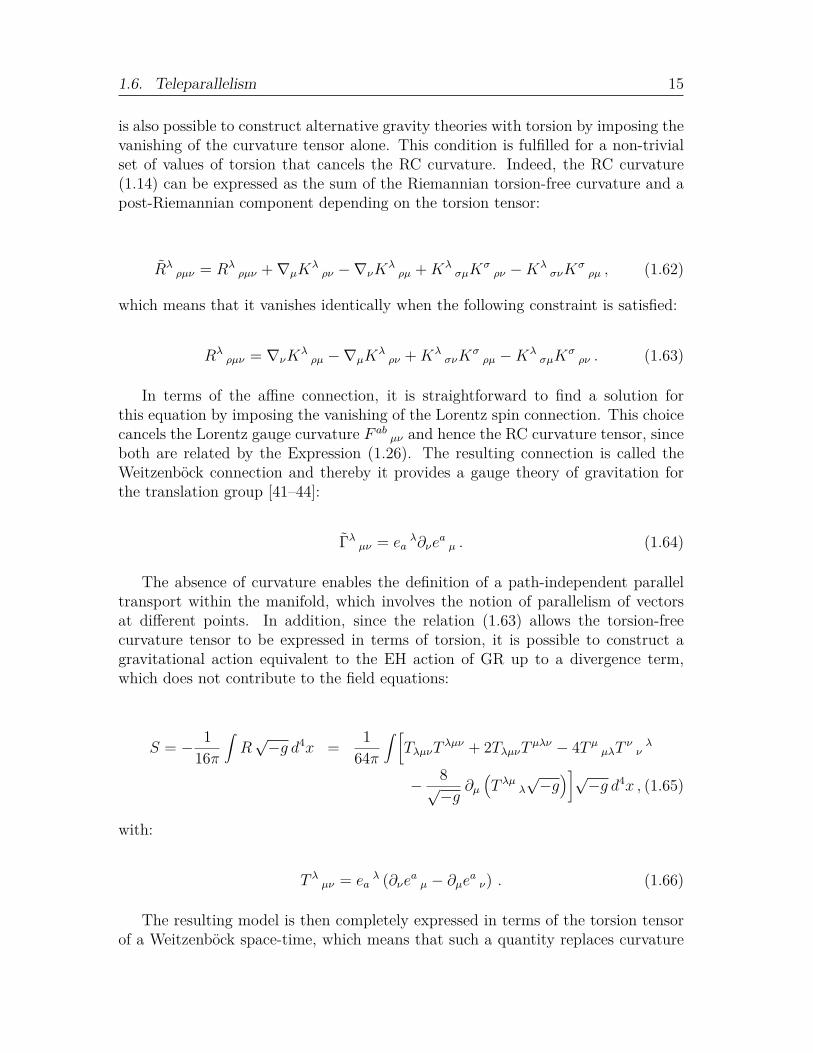
1.6. Teleparallelism 15
is also possible to construct alternative gravity theories with torsion by imposing thevanishing of the curvature tensor alone. This condition is fulfilled for a non-trivialset of values of torsion that cancels the RC curvature. Indeed, the RC curvature(1.14) can be expressed as the sum of the Riemannian torsion-free curvature and apost-Riemannian component depending on the torsion tensor:
Rλρµν = Rλ
ρµν +∇µKλρν −∇νK
λρµ +Kλ
σµKσρν −Kλ
σνKσρµ , (1.62)
which means that it vanishes identically when the following constraint is satisfied:
Rλρµν = ∇νK
λρµ −∇µK
λρν +Kλ
σνKσρµ −Kλ
σµKσρν . (1.63)
In terms of the affine connection, it is straightforward to find a solution forthis equation by imposing the vanishing of the Lorentz spin connection. This choicecancels the Lorentz gauge curvature F ab
µν and hence the RC curvature tensor, sinceboth are related by the Expression (1.26). The resulting connection is called theWeitzenbock connection and thereby it provides a gauge theory of gravitation forthe translation group [41–44]:
Γλ µν = eaλ∂νe
aµ . (1.64)
The absence of curvature enables the definition of a path-independent paralleltransport within the manifold, which involves the notion of parallelism of vectorsat different points. In addition, since the relation (1.63) allows the torsion-freecurvature tensor to be expressed in terms of torsion, it is possible to construct agravitational action equivalent to the EH action of GR up to a divergence term,which does not contribute to the field equations:
S = − 116π
∫R√−g d4x = 1
64π
∫ [TλµνT
λµν + 2TλµνT µλν − 4T µ µλT ν ν λ
− 8√−g
∂µ(T λµ λ
√−g)]√−g d4x , (1.65)
with:
T λ µν = eaλ (∂νea µ − ∂µea ν) . (1.66)
The resulting model is then completely expressed in terms of the torsion tensorof a Weitzenbock space-time, which means that such a quantity replaces curvature

16 Chapter 1. Introduction to post-Riemannian geometries
in order to describe the gravitational field. Likewise, the corresponding energy-momentum tensor derived from this approach does not act as a source of curvature,but as a source of torsion.
From a phenomenological point of view, teleparallelism provides an equivalentdescription of gravity to GR in terms of the mentioned translational field strengthtensor, which is shown to be completely determined by the vierbein field. Thisfact reveals that curvature and torsion are simply alternative ways of describingthe conventional gravitational field. In this sense, teleparallelism does not involvenew physics related to torsion. Nevertheless, both approaches are conceptuallydifferent, since the geometrical correspondence existing in GR between curvatureand gravitation does not hold in a teleparallel model based on torsion. Indeed,following the geometric structure of GR, the trajectories of free-falling particlespresent in a curved space-time results in a geodesic motion depending on the LCconnection:
dpµ
ds+ Γµ λρ pλuρ = 0 , (1.67)
whereas the introduction of a Weitzenbock connection Γµ λρ with vanishing curvaturederives straightforwardly in the following expression [45, 46]:
uλ∇λpµ = Tλ
µρ p
λuρ , (1.68)where uλ∇λp
µ = dpµ
ds+ Γµ λρ pλuρ is the four-acceleration of the particle in the
consequent Weitzenbock space-time. Then, the equations of motion are modified ina form where the torsion tensor plays the role of a gravitational force operating onthe particle, instead of a purely geometrical effect such as the one given by curvaturein the regular case.
1.7 Gravitation with non-propagating torsion: theEinstein-Cartan theory
Another singular case of the PG theory arises when the higher order correctionspresent in the Lagrangian are excluded from the final scheme. Indeed, in the sameway that the EH action is related to the Ricci scalar depending on the metric tensoralone, in a first-order approximation it is possible to generalize this action by meansof the Ricci scalar defined on a RC space-time, providing the so called Einstein-Cartan (EC) theory [21]:
S = 116π
∫d4x√−g
(Lm − R
), (1.69)

1.7. Gravitation with non-propagating torsion: the Einstein-Cartan theory 17
where:
R = R + 14TλµνT
λµν + 12TλµνT
µλν − T µ µλT ν ν λ − 2∇λTρλ
ρ . (1.70)
In this case, the Lagrangian contains, besides the torsion-free Ricci scalar and atotal derivative, a particular combination of the three independent quadratic scalarinvariants of torsion, that are computed into the field equations by performing vari-ations with respect to the gauge potentials, as usual. Accordingly, this analysis leadto the following field equations:
Gµν = 8π θνµ , (1.71)
δµνgλσT ρ ρσ − gλνT ρ ρµ − gλσT ν µσ = 16π Sµ λν . (1.72)
The first equation provides higher order corrections in the torsion tensor to theRiemannian component of the Einstein tensor. Consequently, it generally involvesthe existence of a non-vanishing antisymmetric component of the canonical energy-momentum tensor. In addition, the second equation associates directly the torsionand the spin density tensor of matter sources by an algebraic relation, rather thanby a differential expression for the torsion field. This leads to a non-dynamicalcharacter for torsion under the EC theory, which prevents this quantity to propagatein a vacuum configuration and forces it to vanish when the spin density tensor iszero. Therefore, it can only generate physical effects inside spinning matter andinfluence directly on other sources through a spin-spin contact interaction.
Furthermore, the standard decomposition (1.40) of the canonical energy-momentumtensor into the totally symmetrized energy-momentum tensor and the spin densitytensor allows the vierbein equation (1.71) to be rewritten as the standard Einsteinequation of GR with an additional geometric correction quadratic in the torsion ten-sor (i.e. in the spin density tensor since both torsion and spin are directly related byEquation (1.72)). Indeed, within this model, it is straightforward to express torsionas a tensorial function of the spin density tensor as follows:
T λ µν = 8π(2Sνµ λ + δλ µS
ρνρ − δλ νSρ µρ
), (1.73)
whereas the Einstein tensor in the presence of torsion is split into its torsion-freecomponent and an extended piece depending on torsion in the following way:
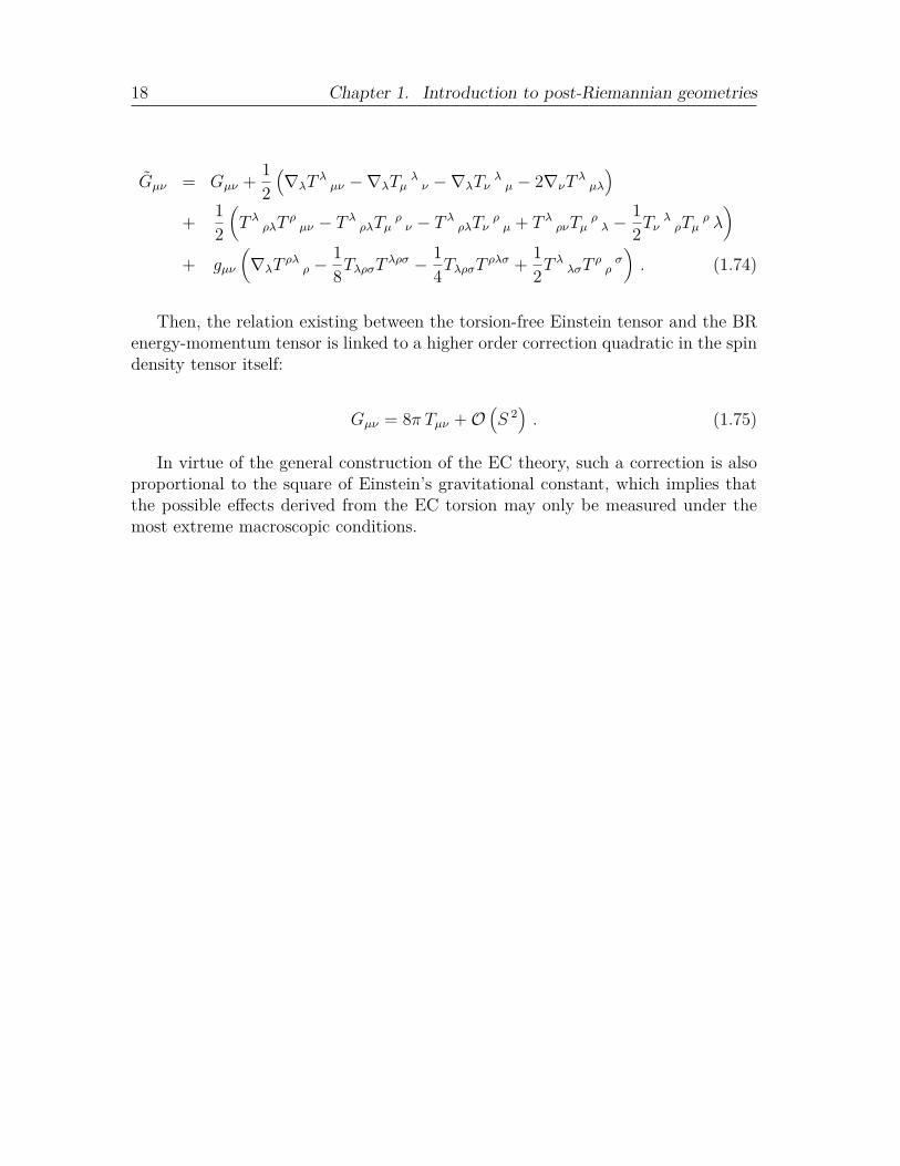
18 Chapter 1. Introduction to post-Riemannian geometries
Gµν = Gµν + 12(∇λT
λµν −∇λTµ
λν −∇λTν
λµ − 2∇νT
λµλ
)+ 1
2
(T λ ρλT
ρµν − T λ ρλTµ ρ ν − T λ ρλTν ρ µ + T λ ρνTµ
ρλ −
12Tν
λρTµ
ρ λ)
+ gµν
(∇λT
ρλρ −
18TλρσT
λρσ − 14TλρσT
ρλσ + 12T
λλσT
ρρσ). (1.74)
Then, the relation existing between the torsion-free Einstein tensor and the BRenergy-momentum tensor is linked to a higher order correction quadratic in the spindensity tensor itself:
Gµν = 8π Tµν +O(S 2). (1.75)
In virtue of the general construction of the EC theory, such a correction is alsoproportional to the square of Einstein’s gravitational constant, which implies thatthe possible effects derived from the EC torsion may only be measured under themost extreme macroscopic conditions.

Chapter 2
Vacuum solutions of the Poincaregauge theory
2.1 The Baekler solution: torsion and confine-ment type of potential
On account of the general PG field equations (1.29) and (1.30), the propagatingcharacter of torsion demands the presence of higher order curvature terms in thegravitational action. Indeed, the variational procedure derived from these termsgives rise to a set of differential expressions for the torsion field. This means thepossible existence of a propagating torsion even in absence of matter sources (i.e. inphysical configurations with vanishing energy-momentum and spin density tensors).From a fundamental point of view, this feature represents a deep aspect in the natureof torsion, which may also produce significant effects under these conditions in thegeometry of the space-time.
In particular, Birkhoff’s theorem of GR establishes that the only vacuum solu-tion to the Einstein field equations with spherical symmetry is the Schwarzschildsolution [47]. However, in the realm of PG gravity, this theorem is satisfied onlyin certain cases [48, 49]. Then, by considering the general PG Lagrangian with dy-namical torsion, the approach leads to a large class of gravitational models endowedwith a vacuum structure where an extensive number of particular and fundamentaldifferences may arise. This fact evinces that the search and analysis of exact solu-tions are essential in order to improve the understanding and physical consequencesof this field.
One of the most primary and remarkable solutions is the so called Baekler solu-tion [50]. It constitutes an exact vacuum solution with propagating torsion, whichrefers to a PG Lagrangian whose limit to the regular gravitational model takes place
19

20 Chapter 2. Vacuum solutions of the Poincare gauge theory
in the framework of teleparallel geometry to a first approximation [51, 52]:
S = − 132π
∫ (2T µ µλT ν ν λ − TλµνT λµν −
14κ RλρµνR
λρµν)√−g d4x , (2.1)
where κ is a coupling constant provided by the supplementary and presumably veryweak gravitational interaction. Thereby, the action is divided into a first term con-nected with the long-range Einstein type of gravity that comprises the Schwarzschildsolution and a YM-like factor depending on the curvature tensor that introducesslight corrections to this approach, which means a richer structure than the onepresent in Einstein’s theory.
The corresponding field equations associated with this model are then describedby the following system:
14δµ
ν(2T λ λσT ρ ρ σ − 4∇λT
ρρλ − TλρσT λρσ
)+∇µT
λλν +∇λTµ
νλ
= 14κ
(14δµ
νRλρτσRλρτσ − RλρµσR
λρνσ)−Kν
λµTρρλ −KλρµT
λρν , (2.2)
2κ(δµ
νT ρ ρλ − gλνT ρ ρ µ + T λν µ − Tµ νλ
)= ∇ρRµ
λρν +KλσρRµ
σρν −KσµρRσ
λρν .
(2.3)
As can be seen, in the limit of teleparallelism, the curvature tensor disappearsfrom the variational equations and torsion operates as the unique geometrical quan-tity describing the gravitational field. Furthermore, the resulting Lagrangian withvanishing curvature encompasses the Schwarzschild metric as a solution and itpresents an agreement with the standard tests of GR up to the fourth order inthe post-Newtonian approximation [53]. In fact, although the expression of such aLagrangian does not coincide exactly with the one given by the equivalent versionof GR in teleparallelism, its deviations do not yield any difference for the case ofstatic and isotropic space-times. Accurately, these deviations can be computed bythe subtraction of the mentioned Lagrangians:
S = 164π
∫ (TλµνT
λµν − 2TλµνT µλν)√−g d4x , (2.4)
or, equivalently:
S = 1128π
∫SµS
µ√−g d4x , (2.5)
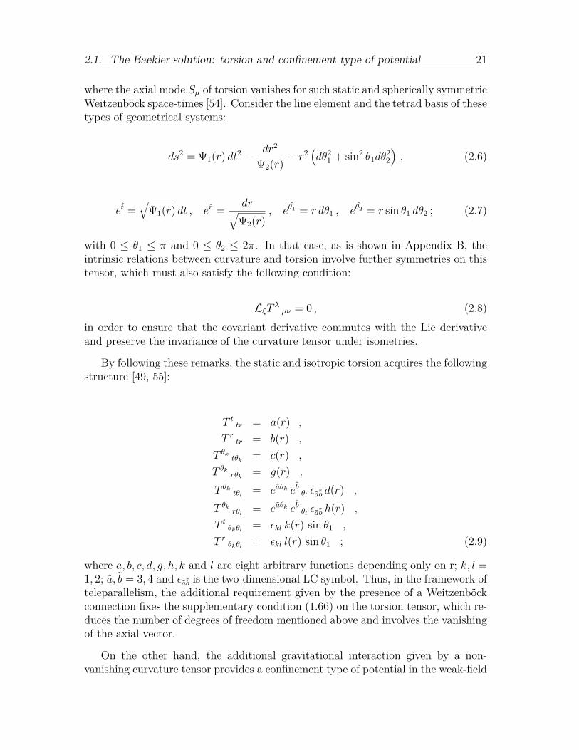
2.1. The Baekler solution: torsion and confinement type of potential 21
where the axial mode Sµ of torsion vanishes for such static and spherically symmetricWeitzenbock space-times [54]. Consider the line element and the tetrad basis of thesetypes of geometrical systems:
ds2 = Ψ1(r) dt2 − dr2
Ψ2(r) − r2(dθ2
1 + sin2 θ1dθ22
), (2.6)
et =√
Ψ1(r) dt , er = dr√Ψ2(r)
, eθ1 = r dθ1 , eθ2 = r sin θ1 dθ2 ; (2.7)
with 0 ≤ θ1 ≤ π and 0 ≤ θ2 ≤ 2π. In that case, as is shown in Appendix B, theintrinsic relations between curvature and torsion involve further symmetries on thistensor, which must also satisfy the following condition:
LξT λ µν = 0 , (2.8)in order to ensure that the covariant derivative commutes with the Lie derivativeand preserve the invariance of the curvature tensor under isometries.
By following these remarks, the static and isotropic torsion acquires the followingstructure [49, 55]:
T t tr = a(r) ,
T r tr = b(r) ,
T θk tθk = c(r) ,
T θk rθk = g(r) ,
T θk tθl = eaθk eb θl εab d(r) ,
T θk rθl = eaθk eb θl εab h(r) ,
T t θkθl = εkl k(r) sin θ1 ,
T r θkθl = εkl l(r) sin θ1 ; (2.9)
where a, b, c, d, g, h, k and l are eight arbitrary functions depending only on r; k, l =1, 2; a, b = 3, 4 and εab is the two-dimensional LC symbol. Thus, in the framework ofteleparallelism, the additional requirement given by the presence of a Weitzenbockconnection fixes the supplementary condition (1.66) on the torsion tensor, which re-duces the number of degrees of freedom mentioned above and involves the vanishingof the axial vector.
On the other hand, the additional gravitational interaction given by a non-vanishing curvature tensor provides a confinement type of potential in the weak-field
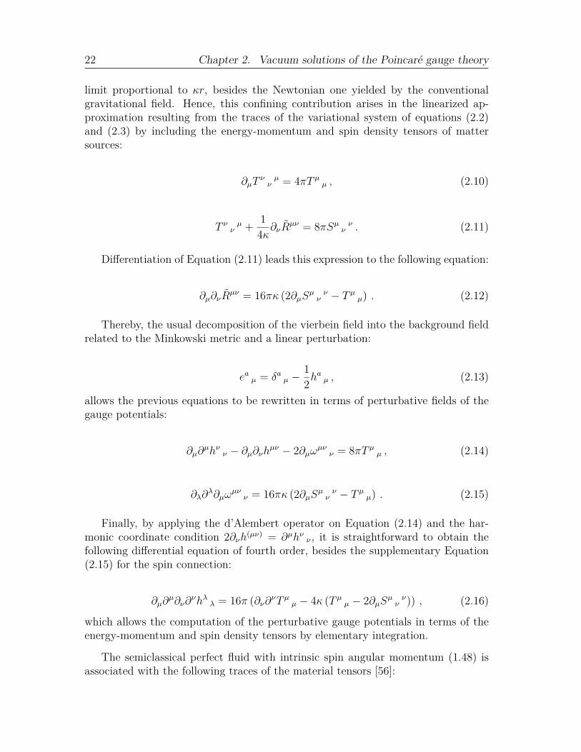
22 Chapter 2. Vacuum solutions of the Poincare gauge theory
limit proportional to κr, besides the Newtonian one yielded by the conventionalgravitational field. Hence, this confining contribution arises in the linearized ap-proximation resulting from the traces of the variational system of equations (2.2)and (2.3) by including the energy-momentum and spin density tensors of mattersources:
∂µTννµ = 4πT µ µ , (2.10)
T ν νµ + 1
4κ∂νRµν = 8πSµ ν ν . (2.11)
Differentiation of Equation (2.11) leads this expression to the following equation:
∂µ∂νRµν = 16πκ (2∂µSµ ν ν − T µ µ) . (2.12)
Thereby, the usual decomposition of the vierbein field into the background fieldrelated to the Minkowski metric and a linear perturbation:
ea µ = δa µ −12h
aµ , (2.13)
allows the previous equations to be rewritten in terms of perturbative fields of thegauge potentials:
∂µ∂µhν ν − ∂µ∂νhµν − 2∂µωµν ν = 8πT µ µ , (2.14)
∂λ∂λ∂µω
µνν = 16πκ (2∂µSµ ν ν − T µ µ) . (2.15)
Finally, by applying the d’Alembert operator on Equation (2.14) and the har-monic coordinate condition 2∂νh(µν) = ∂µhν ν , it is straightforward to obtain thefollowing differential equation of fourth order, besides the supplementary Equation(2.15) for the spin connection:
∂µ∂µ∂ν∂
νhλ λ = 16π (∂ν∂νT µ µ − 4κ (T µ µ − 2∂µSµ ν ν)) , (2.16)
which allows the computation of the perturbative gauge potentials in terms of theenergy-momentum and spin density tensors by elementary integration.
The semiclassical perfect fluid with intrinsic spin angular momentum (1.48) isassociated with the following traces of the material tensors [56]:
2.1. The Baekler solution: torsion and confinement type of potential 23
T µ µ = − ρ , (2.17)
Sµ νν = 0 , (2.18)
where ρ is the matter density, which in the weak-field approximation describes amass m concentrated in an arbitrary point of coordinates r. Then, by substitutingthe expression of the traces of the material tensors into the previous system ofequations:
∆∆hλ λ = 64πκm(
1− ∆4κ
)δ(r) , (2.19)
∆∂µωµν ν = 16πκmδ(r) . (2.20)
By standard integration it is straightforward to find the following weak-fieldsolutions:
hλ λ = −4mr
+ c1 + 8mκr + c2r2 , (2.21)
∂µωµν
ν = 4mκr
+ c3 , (2.22)
with rmin ≤ r ≤ rmax, whereas c1, c2 and c3 are integration constants determined byboundary conditions in this domain. Apart from the Newtonian potential associatedwith torsion in hλ λ, the additional pieces depending on r allude to a confinementtype of potential related to the curvature tensor, which points out the existence ofnew type of exact vacuum solutions distinct from the Schwarzschild solution of thestandard case.
These solutions must then fulfill the general field equations (2.2) and (2.3) as-sociated with Lagrangian (2.1). In virtue of the highly nonlinear character of theseequations, additional symmetry constraints are particularly imposed, as the pres-ence of a static and spherically symmetric space-time. In such a case, the metric andtorsion tensors acquire the form (2.6) and (2.9), respectively. Thereby, besides thetwo functions associated with the metric, the SO(3)-symmetrical torsion containseight degrees of freedom, which means that the problem of solving the variationalequations turns out to be still very complicated and additional restrictions are re-quired.
Specifically, two principal constraints are also applied in order to simplify theproblem. First, a reflection invariance is imposed on the torsion tensor (i.e. torsion

24 Chapter 2. Vacuum solutions of the Poincare gauge theory
is invariant under the group O(3)), which involves the vanishing of the functionsd(r), h(r), k(r) and l(r). In addition, the so called double duality ansatz allows thecancellation of the derivative of the curvature tensor in Expression (2.3) and thesimplification of this equation [57]:
Rλρµν = 14 ελραβεµνγσR
αβγσ + 4κ gµ[λgρ]ν . (2.23)
By contracting indices, this restriction also implies the constancy of the Ricciscalar:
R = 12κ , (2.24)
which means that all the possible solutions derived from this ansatz share this geo-metrical constraint. In particular, the Baekler solution can be easily found with thefollowing components of the metric and torsion tensors:
a(r) = m
r2Ψ(r) , b(r) = m
r2 , c(r) = − m
r2 , g(r) = m
r2Ψ(r) ; (2.25)
Ψ1(r) = Ψ2(r) ≡ Ψ(r) = 1− 2mr
+ κr2 . (2.26)
Therefore, the metric is a Schwarzschild-de Sitter type and carries both torsionand curvature. Indeed, the components of the latter can be represented by thefunction Φ(r) = m
rΨ(r) and the following matrix:
F abcd = κ
1 0 0 0 0 00 1 + Φ(r) 0 0 0 Φ(r)0 0 1 + Φ(r) 0 −Φ(r) 00 0 0 1 0 00 0 Φ(r) 0 1− Φ(r) 00 −Φ(r) 0 0 0 1− Φ(r)
, (2.27)
where the components of the six rows and columns of the matrix are labeled in theorder (01, 02, 03, 23, 31, 12).
As can be seen, the correction given by the new parameter κ to the conventionalgravitational field acts as a cosmological constant in the field equations and thesystem reduces to the Schwarzschild solution of teleparallelism in the limit where
2.1. The Baekler solution: torsion and confinement type of potential 25
κ → 0. Hence, it shows the expected behaviour of the gravitational potentialspresented previously and fulfills the standard tests of GR.
In addition, it can be generalized in the presence of external Coulomb electromag-netic fields generated by both electric and magnetic charges qe and qm, respectively,by replacing the metric function Ψ(r) in the following way [58]:
Ψ(r) = 1− 2mr
+ q2e + q2
m
r2 + κr2 . (2.28)
Furthermore, the same class of solution with double duality properties and con-finement type of potential can be extended to the axisymmetric case by considering aSO(3)-symmetrical torsion [59–62]. These results improve the understanding on thenew gravitational interaction considered by the action (2.1) and confer the role of aneffective cosmological constant to curvature, even when a pure constant parameteris not present in the Lagrangian.
On the other hand, other exact vacuum solutions related to different PG modelsuncovered by Birkhoff’s theorem have been additionally found [63–66]. Some ofthem are not totally determined by the respective variational equations, giving riseto solutions with a high geometrical freedom and depending on arbitrary functions.This fact notably reduces the appropriate physical consistency of these models, incontrast with the particular quadratic PG theory studied above.
Finally, a large number of works on cosmology and gravitational radiation havealso been accomplished in the framework of the PG theory. They implement thedynamical aspects of the torsion field into the gravitational arena and show in generalinteresting differences with respect to the standard regime, such as the transfer ofthe metric singularities to the torsion tensor or the acceleration pattern for theexpansion of the universe analogous to the one given by a cosmological constant,among others (see [22, 63, 67, 68] and references therein).


JCAP01(2017)014
ournal of Cosmology and Astroparticle PhysicsAn IOP and SISSA journalJ
New torsion black hole solutions inPoincare gauge theory
Jose A.R. Cembranosa,b and Jorge Gigante Valcarcela
aDepartamento de Fısica Teorica I, Universidad Complutense de Madrid,Av. Complutense s/n, E-28040 Madrid, Spain
bFaculdade de Ciencias da Universidade de Lisboa,Campo Grande, P-1749-016 Lisbon, Portugal
E-mail: [email protected], [email protected]
Received September 15, 2016Accepted December 24, 2016Published January 9, 2017
Abstract. We derive a new exact static and spherically symmetric vacuum solution in theframework of the Poincare gauge field theory with dynamical massless torsion. This theoryis built in such a form that allows to recover General Relativity when the first Bianchiidentity of the model is fulfilled by the total curvature. The solution shows a Reissner-Nordstrom type geometry with a Coulomb-like curvature provided by the torsion field. Itis also shown the existence of a generalized Reissner-Nordstrom-de Sitter solution whenadditional electromagnetic fields and/or a cosmological constant are coupled to gravity.
Keywords: gravity, modified gravity, astrophysical black holes, neutron stars
ArXiv ePrint: 1608.00062
c© 2017 IOP Publishing Ltd and Sissa Medialab srl doi:10.1088/1475-7516/2017/01/014
JCAP01(2017)014
Contents
1 Introduction 1
2 Quadratic Poincare gauge gravity model 2
3 Field equations 5
4 Solutions 8
5 Equations of motion 10
6 Conclusions 11
A Energy-momentum conservation 13
1 Introduction
General Relativity (GR) is the most successful and accurate theory of classical gravity fromthe last century. Its outstanding description of the gravitational interaction as a purelygeometrical effect of the space-time together with a large number of experimental evidenceshas exalted it as the fundamental theoretical basis for modern astrophysics and cosmology [1].Even nowadays, its elemental foundations and further implications are continually beingreviewed and tested, as in the case of the recent discovery of gravitational waves from a binaryblack hole system [2]. Nevertheless, extensions of GR have always attracted much attentiondue to the deep related fundamental concepts and open questions still unsolved by the theory,as the formulation of a consistent quantum field approach to gravity, the understanding ofspace-time singularities or the nature of dark energy, dark matter or inflation in the veryearly Universe [3–6].
Another open issue consists in providing correctly the foundations of the angular mo-mentum of gravitating sources and its suitable conservation laws in presence of a dynamicalspace-time within the same framework. Specifically, the intrinsic angular momentum of mat-ter must be represented by a spin density tensor and therefore it may be expected to have itassociated with a fundamental geometrical quantity. However, in standard GR, it does notcouple to any distinctive geometrical property, so it is analysed possible modifications of thetheory according to these lines.
In this sense, Poincare Gauge (PG) theory provides the most elegant and promisingextension of GR, in the framework of a Riemann-Cartan (RC) manifold (i.e. a manifoldendowed with curvature and torsion), in order to couple the spin of particles to the torsion ofthe space-time [7, 8]. Indeed, within this model, both energy-momentum and spin tensors ofgravitating matter act as sources of the interaction. In addition, the role of torsion dependson the order of the field strength tensors included in the Lagrangian: whereas the full linearcase involves a non-propagating torsion (i.e. tied to spinning material sources), higher ordercorrections describe a Lagrangian with dynamical torsion [9, 10].
Furthermore, the vacuum structure of the space-time also differs depending on this crit-ical role, especially when a certain class of PG models provides the existence of propagating
– 1 –
JCAP01(2017)014
torsion modes in vacuum. Specifically, Birkhoff’s theorem establishing that the only vacuumsolution with spherical symmetry is the Schwarzschild solution, is satisfied only in certaincases of the PG theory [11, 12]. In this work, we consider a particular PG theory described bya Lagrangian of first and second order in the curvature terms, which reduces to ordinary GRwhen torsion satisfies a general condition connected to the first Bianchi identity. Only in sucha case, it loses its physical relevance. It is shown that within this framework, the Birkhoff’stheorem is not satisfied and a new analytical SO(3) spherically symmetric and static vac-uum solution with dynamical torsion emerges. This solution describes a Reissner-Nordstromtype configuration characterized exclusively for its mass and the torsion field contribution, inanalogy to the electric charge in Maxwell’s theory. Thus, by this contribution of the torsionfield to the space-time geometry, neither other physical sources nor electromagnetic fieldsare necessary to generate this type of solutions. On the other hand, we also stress that itis always possible to find a generalized Reissner-Nordstrom-de Sitter solution endowed withboth electric and magnetic charges, as well as with a cosmological constant within this con-struction. Finally, the equations of motion for a general test particle in such a space-time areobtained from the respective conservation law of the energy-momentum tensor of matter.
This work is organized as follows. First, in section II, we briefly present the generalmathematical foundations of PG theory paying spetial attention to our model. Field equa-tions and analyses of general solutions beyond the Birkhoff’s theorem for GR and differentclasses of PG theories are shown in section III. Our new analytical solution within this frame-work, as well as its natural generalization to include external Coulomb electric and magneticfields with a non-vanishing cosmological constant are presented and analysed in section IV. Insection V, we obtain from the general conservation law of the energy-momentum tensor, theequations of motion for a test particle belonging to a RC manifold connected to our model.Finally, we present the conclusions of our work in section VI. A general demonstration forthe conservation law of the energy-momentum tensor is also presented in appendix A.
Before proceeding to the main discussion and general results, we briefly introduce thenotation and physical units to be used throughout this article. Latin a, b and greek µ, νindices refer to anholonomic and coordinate basis, respectively. We use notation with tildefor magnitudes including torsion (i.e. defined within a RC manifold) and without tilde fortorsionless objects. Finally, we will use Planck units (G = c = ~ = 1).
2 Quadratic Poincare gauge gravity model
A model of PG gravity requires gauging the external degrees of freedom consisting of rota-tions and translations, which are represented by the Poincare group ISO(1, 3). Therefore,a gauge connection containing two principal independent variables is introduced in order todescribe the gravitational field. These quantities constitute the gauge potentials related tothe generators of translations and local Lorentz rotations, respectively:
Aµ = ea µPa + ωabµJab , (2.1)
where ea µ is the vierbein field and ωabµ the spin connection, which satisfy the following
relations with the metric g and the affine connection Γ within the RC manifold [13]:
gµν = ea µ ebν ηab , (2.2)
ωabµ = ea λ e
bρ Γλρµ + ea λ ∂µ e
bλ . (2.3)
– 2 –

JCAP01(2017)014
Note that in a RC manifold the affine connection constitutes a metric-compatible con-nection (i.e. ∇λ gµν = 0). Moreover, it can split into the Levi-Civita connection and the socalled contortion tensor in the following way:
Γλµν = Γλ
µν +Kλµν . (2.4)
Additionally, Pa are the generators of the space-time translations and Jab the generatorsof the space-time rotations, which satisfy the following commutative relations:
[Pa, Pb] = 0 , (2.5)
[Pa, Jbc] = i ηa[b Pc] , (2.6)
[Jab, Jcd] =i
2(ηad Jbc + ηcb Jad − ηdb Jac − ηac Jbd) . (2.7)
Then, the corresponding ISO(1, 3) gauge field strength tensor defined by Fµν = ∂µAν −∂νAµ − i[Aµ, Aν ] takes the form:
Fµν = F aµνPa + F ab
µνJab , (2.8)
with F aµν = ∂µe
aν−∂νe
aµ+ωab
µe bν−ωabν ebµ , and F ab
µν = ∂µωab
ν−∂νωab
µ+ωacν ω
bcµ−
ωacµ ω
bcν .
As in the case of other known gauge theories, the field strength tensor characterizes theproperties of the gravitational interaction, that in the PG framework are potentially modifiedby the presence of torsion. In particular, it is related to the torsion and the curvature of thespace-time as follows:
F aµν = ea λ T
λνµ , (2.9)
F abµν = ea λe
bρ R
λρµν , (2.10)
where T λµν and Rλρ
µν are the components of the torsion and the curvature tensor respec-tively:
T λµν = 2Γλ
[µν] , (2.11)
Rλρµν = ∂µΓ
λρν − ∂ν Γ
λρµ + Γλ
σµΓσρν − Γλ
σνΓσρµ . (2.12)
These components modify the commutative relations of the covariant derivatives for ageneral vector field vλ over a RC manifold in the following way:
[∇µ, ∇ν ] vλ = Rλ
ρµν vρ + T ρ
µν ∇ρvλ , (2.13)
with ∇µ vλ = ∂µ v
λ + Γλρµ v
ρ.Hence, whereas curvature is related to the rotation of a vector along an infinitesimal
path over the space-time, torsion is related to the translation and it has deep geometricalimplications, such as breaking infinitesimal parallelograms on the manifold [14]. Furthermore,the RC manifold may be regarded as an effective geometrical construction arising from amicroscopic structure endowed with dislocation defects, which are described by torsion inthe limit where they form a continuous distribution [15, 16]. In this sense, it is expectedthat the field strength tensor defined within this RC manifold gives rise to the pattern ofdislocations density in terms of a dynamical torsion (i.e. even in the absence of matter fields).
– 3 –
JCAP01(2017)014
In addition, both curvature and torsion tensors can also be classified by the decompo-sition into their irreducible parts under the Lorentz group [17, 18]. Especially, torsion canbe divided into three irreducible components given by distinct contributions: a trace vector,an axial vector and a traceless and also pseudotraceless tensor. From a phenomenologicalpoint of view, this sort of geometrical classification can be associated with a large number ofphysically relevant situations, such as the coupling between the Dirac fields and the totallyantisymmetric part of the torsion or the vanishing of its tensorial modes in a spatially ho-mogeneous and isotropic universe, as it is assumed by the cosmological principle (see [19] fora more detailed account and alternative classifications). However, there exist more complexsystems that require the non-vanishing of the rest of the modes, such as the given by a generalstatic and spherically symmetric space-time, which is deeply considered in this work.
In the basic version of the PG theory, the presence of torsion is sourced by the spin ofmatter, so that it introduces new independent characteristics from the standard theory andit achieves a dynamical role defining an invariant Lagrangian quadratic in the field strengthtensors. In this work, we focus on a PG model whose second order contributions are onlydue to the existence of this kind of non-vanishing and also massless torsion:
S =1
16π
∫d4x
√−g
[Lm − R − 1
4(d1 + d2) R
2 − 1
4(d1 + d2 + 4c1 + 2c2) RλρµνR
µνλρ
+c1RλρµνRλρµν + c2RλρµνR
λµρν + d1RµνRµν + d2RµνR
νµ
], (2.14)
where c1, c2, d1 and d2 are four constant parameters. Note that in order to construct theExpression (2.14), we can use the identity R = R − 2∇λT
ρλρ +
14TλµνT
λµν + 12TλµνT
µλν −Tµ
µλTννλ, which allows to rewrite the general PG Lagrangian with massless torsion in
terms of the torsionless Einstein-Hilbert Lagrangian.
In the elementary case where torsion does not propagate, all these constants vanish andthe action leads to the standard Einstein theory. However, as it is remarked above, we areinterested in the presence of higher order curvature terms in the action because in such acase, torsion becomes dynamical. Furthermore, in the limit where the first Bianchi identityof GR still holds for the total curvature (i.e. Rλ
[µνρ] = 01), then the Lagrangian leads to thesum of the Einstein-Hilbert Lagrangian and the Gauss-Bonnet term. As it is well known, thelatter is a topological invariant in the four dimensional case, so it does not contribute to thefield equations and the theory coincides locally with GR.
According to the first Bianchi identity in a RC space-time [20]:
Rλ[µνρ] + ∇[µT
λνρ] + T σ
[µν Tλρ]σ = 0 , (2.18)
1The symmetric and antisymmetric parts of a generic covariant tensor Aa1...aq are denoted by parenthesisand brackets, respectively:
Aa1...aq = A(a1...aq) +A[a1...aq ] , (2.15)
with:
A(a1...aq) =1
q!
∑
π
Aaπ(1)...aπ(q), (2.16)
and
A[a1...aq ] =1
q!
∑
π
δπAaπ(1)...aπ(q), (2.17)
where the sum is taken over all permutations π of 1, . . . , q and δπ is +1 for even permutations and −1 for oddpermutations.
– 4 –

JCAP01(2017)014
the Expression (2.14) reduces to the regular gravity action when ∇[µTλνρ]+T σ
[µν Tλρ]σ = 0.
Note that this expression does not imply the vanishing of the torsion tensor, but a lessconstraining condition fulfilled by this quantity for recovering GR.
3 Field equations
In order to derive the field equations, we may simplify the expression above without loss ofgenerality applying the Gauss-Bonnet theorem in RC spaces [21, 22]. Indeed, the followingterm is a total derivative of a certain vector V µ:
√−g(R2 + RλρµνR
µνλρ − 4RµνRνµ)= ∂µV
µ . (3.1)
Then (2.14) is locally equivalent to the following action:
S =1
16π
∫d4x
√−g
[Lm − R − 1
2(2c1 + c2) RλρµνR
µνλρ + c1RλρµνRλρµν (3.2)
+c2RλρµνRλµρν + d1Rµν
(Rµν − Rνµ
)].
In the absence of matter, i.e. Lm = 0, Birkhoff’s theorem is satisfied only in certaincases of the PG theory [11, 12]. We observe that our particular PG model does not generallysatisfy this theorem, so the analysis of new static and spherically symmetric vacuum solutionsto the field equations is necessary.
Before computing the vacuum equations, we define the following geometric quantities:
Gµν =Rµ
ν − R
2δµ
ν , (3.3)
T1µν = RλρµσR
λρνσ − 1
4δµ
νRλρτσRλρτσ , (3.4)
T2µν = RλρµσR
λνρσ + RλρσµRλσρν − 1
2δµ
νRλρτσRλτρσ , (3.5)
T3µν = RλρµσR
νσλρ − 1
4δµ
νRλρτσRτσλρ , (3.6)
H1µν = Rν
λµρRλρ + RλµR
λν − 1
2δµ
νRλρRλρ , (3.7)
H2µν = Rν
λµρRρλ + RλµR
νλ − 1
2δµ
νRλρRρλ , (3.8)
C1µλν =∇ρRµ
λρν +KλσρRµ
σρν − KσµρRσ
λρν , (3.9)
C2µλν =∇ρ
(Rµ
νλρ−Rµρλν
)+Kλ
σρ
(Rµ
νσρ−Rµρσν
)−Kσ
µρ
(Rσ
νλρ−Rσρλν
), (3.10)
C3µλν =∇ρR
ρνλµ +Kλ
σρRρνσ
µ − KσµρR
ρνλσ , (3.11)
Y 1µλν = δµ
ν∇ρRλρ−∇µR
λν+δµνKλ
σρRσρ+Kρ
µρRλν−Kν
µρRλρ−Kλ
ρµRρν , (3.12)
Y 2µλν = δµ
ν∇ρRρλ−∇µR
νλ+δµνKλ
σρRρσ+Kρ
µρRνλ−Kν
µρRρλ−Kλ
ρµRνρ . (3.13)
It is worthwhile to stress that all these quantities have a tensor character induced bythe nature of the curvature and the torsion tensors, so that the physics equations dependingon them retain the same form independently of the choice of coordinates on the manifold,according to the principle of general covariance.
– 5 –
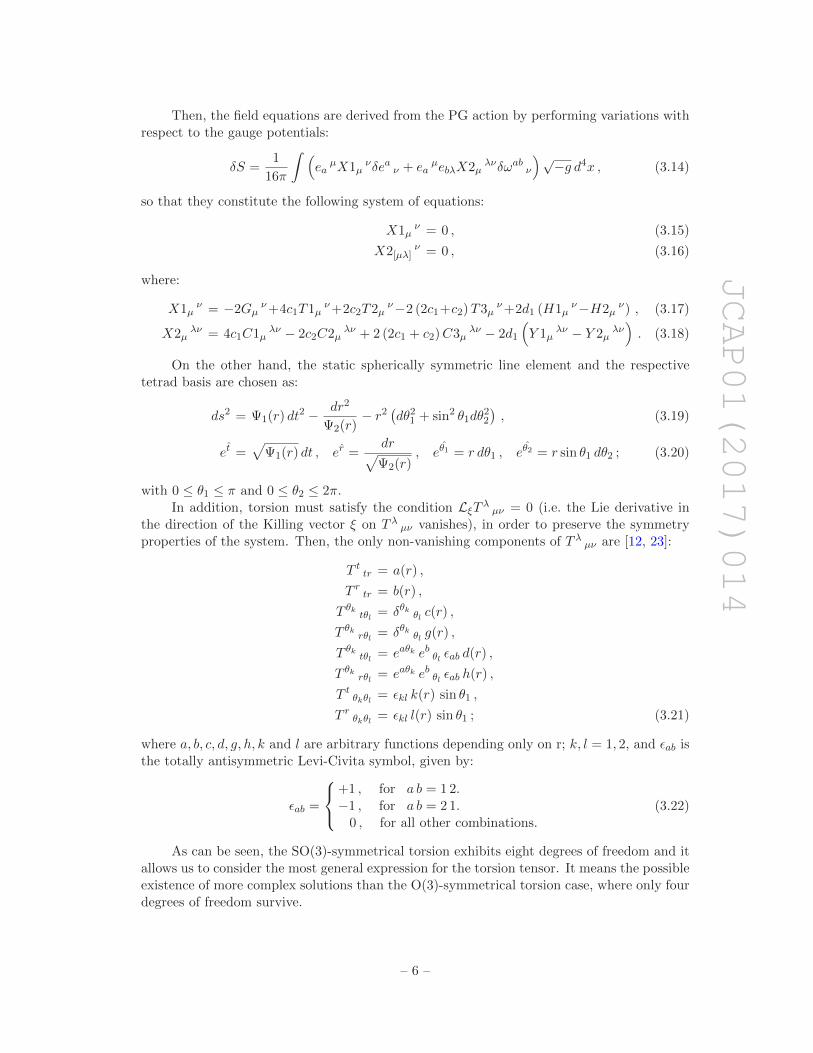
JCAP01(2017)014
Then, the field equations are derived from the PG action by performing variations withrespect to the gauge potentials:
δS =1
16π
∫ (ea
µX1µνδea ν + ea
µebλX2µλνδωab
ν
)√−g d4x , (3.14)
so that they constitute the following system of equations:
X1µν = 0 , (3.15)
X2[µλ]ν = 0 , (3.16)
where:
X1µν = −2Gµ
ν+4c1T1µν+2c2T2µ
ν−2 (2c1+c2)T3µν+2d1 (H1µ
ν−H2µν) , (3.17)
X2µλν = 4c1C1µ
λν − 2c2C2µλν + 2 (2c1 + c2)C3µ
λν − 2d1
(Y 1µ
λν − Y 2µλν). (3.18)
On the other hand, the static spherically symmetric line element and the respectivetetrad basis are chosen as:
ds2 = Ψ1(r) dt2 − dr2
Ψ2(r)− r2
(dθ21 + sin2 θ1dθ
22
), (3.19)
et =√Ψ1(r) dt , er =
dr√Ψ2(r)
, eθ1 = r dθ1 , eθ2 = r sin θ1 dθ2 ; (3.20)
with 0 ≤ θ1 ≤ π and 0 ≤ θ2 ≤ 2π.In addition, torsion must satisfy the condition LξT
λµν = 0 (i.e. the Lie derivative in
the direction of the Killing vector ξ on T λµν vanishes), in order to preserve the symmetry
properties of the system. Then, the only non-vanishing components of T λµν are [12, 23]:
T ttr = a(r) ,
T rtr = b(r) ,
T θktθl = δθk θl c(r) ,
T θkrθl = δθk θl g(r) ,
T θktθl = eaθk eb θl ǫab d(r) ,
T θkrθl = eaθk eb θl ǫab h(r) ,
T tθkθl = ǫkl k(r) sin θ1 ,
T rθkθl = ǫkl l(r) sin θ1 ; (3.21)
where a, b, c, d, g, h, k and l are arbitrary functions depending only on r; k, l = 1, 2, and ǫab isthe totally antisymmetric Levi-Civita symbol, given by:
ǫab =
+1 , for a b = 12.−1 , for a b = 21.0 , for all other combinations.
(3.22)
As can be seen, the SO(3)-symmetrical torsion exhibits eight degrees of freedom and itallows us to consider the most general expression for the torsion tensor. It means the possibleexistence of more complex solutions than the O(3)-symmetrical torsion case, where only fourdegrees of freedom survive.
– 6 –

JCAP01(2017)014
Nevertheless, it is possible to impose an additional restriction involving these torsioncomponents by taking the trace of eq. (3.16) in the weak-field approximation:
(4c1+c2+d1)∇ρR[λρ] = 2c1Kµνρ
(Rνλρµ − Rρµνλ
)+
3
2c2Kµνρ
(Rµ[ρνλ] + Rρ[µλν]
)
+d1
(Kµρ
λR[µρ]+T ρµρR
[λµ])−(4c1+c2+d1)K
λνρR
[νρ] . (3.23)
Then, by neglecting torsion terms of second order, only the first term of the equationcontributes. The equations of motion for the torsion tensor in linear approximation read
∇µ∇µT νλν + ∇µ∇νT
νµλ − ∇µ∇λT
νµν = 0 , (3.24)
for theories with 4c1 + c2 + d1 6= 0.In terms of the torsion components, this constraint is equivalent to the relation:
b(r) = rc ′(r) + c(r) +p
r
√Ψ1(r)
Ψ2(r), (3.25)
where p is an integration constant.In addition to a cosmological constant, we only focus on suitable solutions that may
exist in presence of Coulomb electric and magnetic fields, as in the standard Einstein-Maxwellframework of GR, so the solutions are restricted to verify Ψ1(r) = Ψ2(r) ≡ Ψ(r) in order tosatisfy the Maxwell’s equations in the RC manifold. These restrictions substantially simplifythe problem. In any case, the field equations constitute a highly nonlinear system involvinga large number of degrees of freedom and it forms an underdetermined system with differentclasses of solutions. We will require a final additional condition: suitable solutions must takean appropriate form referred to the rotated basis ϑa = Λa
beb, given by the following vector
fields:
ϑt =1
2
[Ψ(r) + 1] dt+
[1 − 1
Ψ(r)
]dr
;
ϑr =1
2
[Ψ(r) − 1] dt+
[1 +
1
Ψ(r)
]dr
;
ϑθ1 = r dθ1 ;
ϑθ2 = r sin θ1 dθ2 . (3.26)
This orthogonal coframe has already been used in previous literature to simplify the formof the Baekler solution, that belongs to a different class of PG models containing an O(3)-symmetrical torsion [24]. Especially, besides to its considerable simplification of the solution,it has the advantage of leading to a conformally flat Lorentz connection [25, 26]. In our case,we expect that the rotated Lorentz connection defined on the RC manifold recovered itsMinkowski values for the vanishing of the free parameters associated with the torsion tensorand then the remaining physical configuration reduced to GR. Note that, in order to reachthis limit, it is not necessary that each component of torsion vanishes identically, but onlythe fulfillment of the first Bianchi identity of GR for the total curvature, as remarked in theprevious section.
At the same time, any solution F abc referring to the mentioned orthogonal coframe can
be written as follows:
F ttr =
1
2
[1 + Ψ(r)] a(r) +
[1 − 1
Ψ(r)
]b(r)
;
– 7 –

JCAP01(2017)014
F rtr =
1
2
[1 +
1
Ψ(r)
]b(r) − [1 − Ψ(r)] a(r)
;
F θ1tθ1
= F θ2tθ2
=1
2
[1 +
1
Ψ(r)
]c(r) + [1 − Ψ(r)] g(r)
;
F θ1rθ1
= F θ2rθ2
=1
2
[1 + Ψ(r)] g(r) −
[1 − 1
Ψ(r)
]c(r)
;
F θ2tθ1
= −F θ1tθ2
=1
2
[1 +
1
Ψ(r)
]d(r) + [1 − Ψ(r)]h(r)
;
F θ2rθ1
= −F θ1rθ2
=1
2
[1 + Ψ(r)]h(r) −
[1 − 1
Ψ(r)
]d(r)
;
F tθ1θ2
=1
2r2
[1 + Ψ(r)] k(r) +
[1 − 1
Ψ(r)
]l(r)
;
F rθ1θ2
=1
2r2
[1 +
1
Ψ(r)
]l(r) − [1 − Ψ(r)] k(r)
. (3.27)
Therefore, in order to obtain a class of suitable non-singular solutions (excluding thepoint r = 0), the components of the torsion tensor must satisfy the following relations:
b(r) = a(r)Ψ(r) , c(r) = − g(r)Ψ(r) , d(r) = −h(r)Ψ(r) , l(r) = k(r)Ψ(r) . (3.28)
We find out that these constraints also involve the vanishing of the three independentquadratic torsion invariants (i.e. Tλµν T
λµν = Tλµν Tµλν = Tµ
µλ Tννλ = 0).
4 Solutions
By taking into account all these remarks, the following SO(3)-symmetric vacuum solutioncan be easily found for c1 = − d1/4 and c2 = − d1/2:
a(r) =Ψ′(r)2Ψ(r)
, b(r) =Ψ′(r)2
, c(r) =Ψ(r)
2r, g(r) = − 1
2r,
d(r) =κ
r, h(r) = − κ
rΨ(r), k(r) = l(r) = 0 ; (4.1)
with
Ψ(r) = 1 − 2m
r+
d1κ2
r2. (4.2)
Hence, the relation (3.25) is completely fulfilled and the constant p vanishes.This solution describes a Reissner-Nordstrom type geometry, supported only by the
metric and torsion fields rather than an electric or magnetic source. The new contribution isproportional to the square of the new parameter κ. Indeed, this parameter determines theintensity of the strength tensor corresponding to the torsion:
F abcd =
0 0 0 0 0 00 0 −κ/2r2 0 −κ/2r2 00 κ/2r2 0 0 0 −κ/2r2
−κ/r2 0 0 − 1/r2 0 00 κ/2r2 0 0 0 −κ/2r2
0 0 κ/2r2 0 κ/2r2 0
, (4.3)
– 8 –

JCAP01(2017)014
where the six rows and columns of the matrix are labeled the components in the order (01,02, 03, 23, 31, 12).
The values above for the Lagrangian coefficients and their respective signs define thestrength and properties of the torsion field in the PG framework. In existing literature, partic-ular results containing a certain set of viable coefficient combinations for the purely masslessPG theory have been developed under the linear field approximation requiring the absenceof both ghost and tachyon modes [27] or only the ghost-free condition [28, 29]. Nevertheless,it has also been shown that the Hamiltonian constraint formalism differs from these resultswhere the highly nonlinear effects of the PG theory are included [30]. Furthermore, someother authors have pointed out several mistakes and incompleteness in various of the men-tioned analyses, reaching important contradictions with the commented conclusions [31, 32].In this sense, the stability of these models is still an open issue.
On the other hand, by following our constraints (3.25) and (3.28), we note that anyother combination for the constant parameters of eq. (2.14) involves a vacuum configurationdescribed strictly by the Schwarzschild metric. Hence, in the present case, there is a uniquecombination that allows a vacuum configuration different from the Schwarzschild geometry.It is the Reissner-Nordstrom solution above. Moreover, by solving the field equations it ispossible to demonstrate this statement even for the case Ψ1(r) 6= Ψ2(r). It is also shown thatthe torsion decreases at infinity and the metric is asymptotically flat. So the correspondingNewtonian limit is satisfied by the solution as demanded by different approaches [33].
It is also straightforward to notice that the condition ∇[µTλνρ]+T σ
[µν Tλρ]σ = 0 is ful-
filled for this solution when κ = 0. In such a case, although the rest of the non-vanishing com-ponents of the torsion tensor still remain, the Action (3.2) is equivalent to the Einstein-Hilbertone and the GR approach is totally recovered. These non-vanishing components yield an inertRC spin connection and curvature, which emerge to the physical structure only when the pa-rameter κ switches on and the torsion becomes dynamical. This fact contrasts with the alter-native ways of recovering the regular gravity action given by the rest of the PG models presentin previous literature, such as the mentioned Baekler solution where this limit is carried outin the framework of teleparallelism [34]. Teleparallel Gravity is the gauge theory for thetranslation group based on the curvature-free Weitzenbock connection and it is constructedin such a form that provides an equivalent description of gravity to GR, but in terms of torsionso that there exist conceptual differences between them (see [35] for a recent overview).
Additionally, the expression for the Lorentz connection referred to ϑa exhibits a similarproperty to its counterpart of the Baekler solution. It takes Minkowski values within the RCmanifold for κ = 0 and it does not depend on any other magnitude in such a case:
A = − κ
rJθφ dt+
κ
rΨ(r)Jθφ dr+
1
2
(Jrθ − Jtθ
)dθ+sin θ
[1
2
(Jrφ − Jtφ
)+ cot θJθφ
]dφ . (4.4)
This solution can be trivially generalized to include the existence of a non-vanishingcosmological constant Λ and Coulomb electromagnetic fields produced by both electric andmagnetic charges qe and qm, respectively. For this purpose, it is assumed that photons aredecoupled from torsion as it is dictated by the minimum coupling principle. Then, it is easyto extend the solution by modifying the metric function Ψ(r) by the following expression:
Ψ(r) = 1 − 2m
r+
d1κ2 + q2e + q2m
r2+
Λ
3r2 . (4.5)
As can be seen, the term derived by the dynamical torsion has the same structurethan the terms provided by the electric and magnetic monopole charges and it is possible to
– 9 –
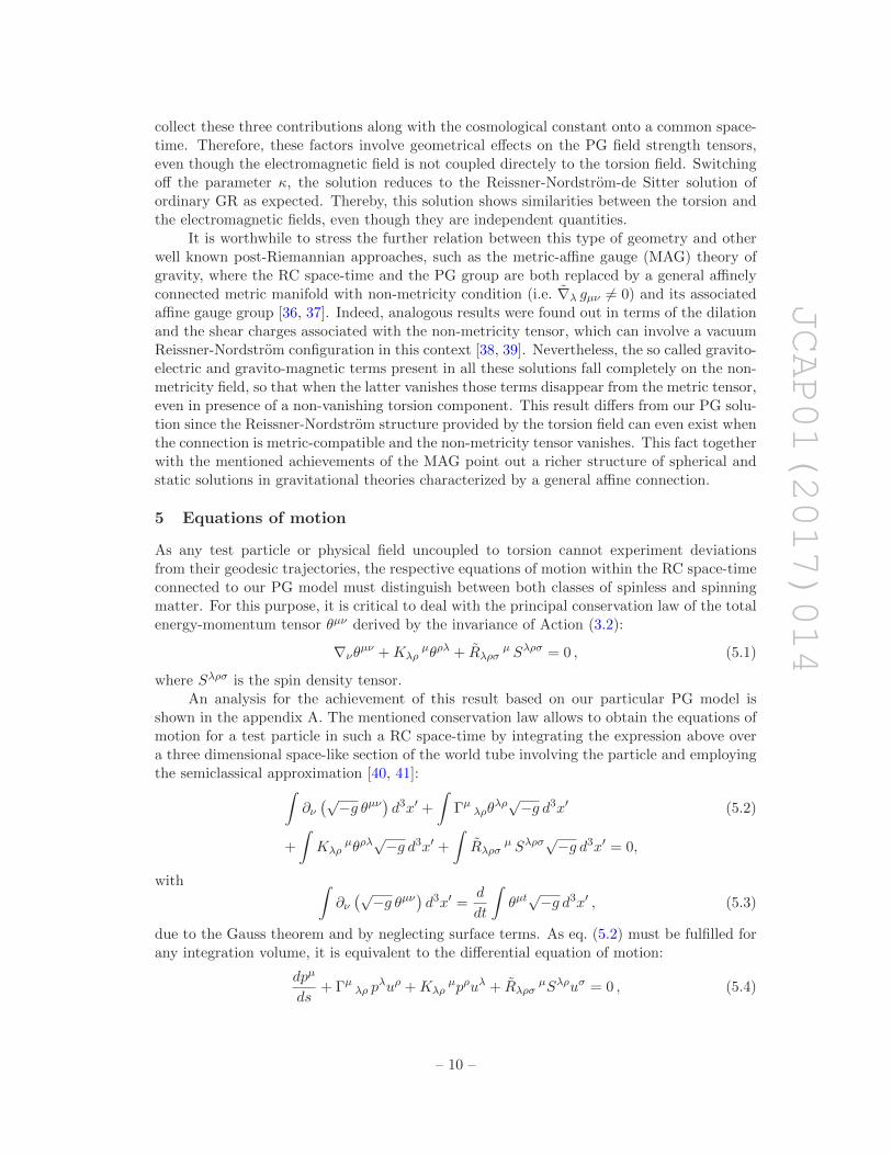
JCAP01(2017)014
collect these three contributions along with the cosmological constant onto a common space-time. Therefore, these factors involve geometrical effects on the PG field strength tensors,even though the electromagnetic field is not coupled directely to the torsion field. Switchingoff the parameter κ, the solution reduces to the Reissner-Nordstrom-de Sitter solution ofordinary GR as expected. Thereby, this solution shows similarities between the torsion andthe electromagnetic fields, even though they are independent quantities.
It is worthwhile to stress the further relation between this type of geometry and otherwell known post-Riemannian approaches, such as the metric-affine gauge (MAG) theory ofgravity, where the RC space-time and the PG group are both replaced by a general affinelyconnected metric manifold with non-metricity condition (i.e. ∇λ gµν 6= 0) and its associatedaffine gauge group [36, 37]. Indeed, analogous results were found out in terms of the dilationand the shear charges associated with the non-metricity tensor, which can involve a vacuumReissner-Nordstrom configuration in this context [38, 39]. Nevertheless, the so called gravito-electric and gravito-magnetic terms present in all these solutions fall completely on the non-metricity field, so that when the latter vanishes those terms disappear from the metric tensor,even in presence of a non-vanishing torsion component. This result differs from our PG solu-tion since the Reissner-Nordstrom structure provided by the torsion field can even exist whenthe connection is metric-compatible and the non-metricity tensor vanishes. This fact togetherwith the mentioned achievements of the MAG point out a richer structure of spherical andstatic solutions in gravitational theories characterized by a general affine connection.
5 Equations of motion
As any test particle or physical field uncoupled to torsion cannot experiment deviationsfrom their geodesic trajectories, the respective equations of motion within the RC space-timeconnected to our PG model must distinguish between both classes of spinless and spinningmatter. For this purpose, it is critical to deal with the principal conservation law of the totalenergy-momentum tensor θµν derived by the invariance of Action (3.2):
∇νθµν +Kλρ
µθρλ + Rλρσµ Sλρσ = 0 , (5.1)
where Sλρσ is the spin density tensor.An analysis for the achievement of this result based on our particular PG model is
shown in the appendix A. The mentioned conservation law allows to obtain the equations ofmotion for a test particle in such a RC space-time by integrating the expression above overa three dimensional space-like section of the world tube involving the particle and employingthe semiclassical approximation [40, 41]:
∫∂ν
(√−g θµν)d3x′ +
∫Γµ
λρθλρ√−g d3x′ (5.2)
+
∫Kλρ
µθρλ√−g d3x′ +
∫Rλρσ
µ Sλρσ√−g d3x′ = 0,
with ∫∂ν
(√−g θµν)d3x′ =
d
dt
∫θµt
√−g d3x′ , (5.3)
due to the Gauss theorem and by neglecting surface terms. As eq. (5.2) must be fulfilled forany integration volume, it is equivalent to the differential equation of motion:
dpµ
ds+ Γµ
λρ pλuρ +Kλρ
µpρuλ + RλρσµSλρuσ = 0 , (5.4)
– 10 –

JCAP01(2017)014
where we have used the following definitions
θλρ =dt
ds
∫pλuρ
√−g d3x′ , (5.5)
and
Sλρσ =dt
ds
∫Sλρuσ
√−g d3x′ . (5.6)
Here, s is the proper time along the particle world line, pµ the four-momentum of theparticle and uµ its four-velocity. Therefore, the presence of a dynamical torsion in the space-time and the interaction between the curvature and the spin of matter originate in general,a generalized Lorentz force acting on this type of matter. Thus, this force potentially yieldsdeviations from the geodesic trajectories. Of course, this generally non-geodesic motion turnsout to be another essential difference with gravitational theories endowed with vanishingtorsion, such as ordinary GR. Nevertheless, for spinless matter with Sλρ = 0 and pλ ∝ uλ,the equations of motion reduce to the same geodesic equations of GR.
This fundamental difference might be used in order to prove experimentally the possibleexistence of a non-vanishing dynamical torsion in the space-time. Nevertheless, it is expectedto yield too tiny effects to be measured, as occurs with the rest of the well known PG models.Additionally, torsion is induced on the vierbein field by the field equations and thereby itcan also operate on the geodesic motion of ordinary matter via the Levi-Civita connection.In particular, for a standard Reissner-Nordstrom geometry, the respective point charges havewell known consequences on the geodesic paths of test particles and light rays [42].
Presumably, the effects of this type of geometry are also very small at astrophysics orcosmological scales, because of the vanishing of the spin density tensor in the most macro-scopical bodies. However, this situation may differ around extreme gravitational systems asneutron stars or black holes with intense magnetic fields and sufficiently oriented elementaryspins. In such a case, it is expected that the RC space-time described by the PG theorymodulates these events.
Further analyses can be performed by comparing the gravitational interaction of thespin and the orbital angular momentum of a rotating rigid test body [43, 44]. In this sense,it is especially interesting their natural extension towards the MAG theory when the motionof a rotating and deformable test body is considered [45]. All these achievements allow tosystematically study the behaviour of gravitating matter with microstructure and to establishadditional differences between a large extreme gravitational systems, such as the one presentin our PG model and the one previously mentioned supported by MAG.
6 Conclusions
In the present work, we have investigated the PG theory with massless torsion based on agravitational model directly connected to GR when the dynamical role of torsion is frozenvia the first Bianchi identity. In the general case, this approach allows the torsion tensor toconstitute a dynamical degree of freedom. We have shown that the vacuum structure of thetheory may differ from the Einstein’s theory and, specifically, distinct classes of solutions canexist besides the Schwarzschild solution given by the Birkhoof’s theorem within the standardframework of GR. Hence, in order to improve the understanding of such a theory of gravity,the search and analysis of exact solutions are fundamental.
– 11 –

JCAP01(2017)014
The large degree of symmetry assumed and the requirement of the existence of a suit-able electromagnetic-like vacuum structure analogous to the Einstein-Maxwell framework to-gether with the use of a convenient rotated basis allow to reduce notably the difficulty of thehighly nonlinear nature present in the theory. Under these requirements, we have obtaineda new static and spherically symmetric vacuum solution. This solution provides a Reissner-Nordstrom type geometry with a SO(3)-symmetrical torsion depending on a parameter κ andit has been deduced without the use of the double duality ansatz for the RC curvature, oftenemployed in previous literature in order to restrict the PG field equations into a very highlysimplified system [46]. Its existence shows the dynamical character of the torsion field, whichcan even be induced on the metric tensor via the field equations generating a distinct classof solutions, beyond the Schwarzschild scheme and the Birkhoff’s theorem of GR.
The corresponding generalized Reissner-Nordstrom-de Sitter configuration is also ob-tained when external electromagnetic fields and a non-vanishing cosmological constant areincluded, by analogy with the standard case. In this scheme, the torsion field contributionis perfectly distinguishable from the rest of physical degrees of freedom and the solutionreduces to the standard case when its dynamical role is switched off. Therefore, the solutionpresents similarities between the torsion and the electromagnetic fields. It is expected thatthese similarities still remain in more general systems, such as axisymmetric space-times.
The foundations presented in this article have also been employed in previous worksfor the analysis and the achievement of exact solutions in extended models of gravity, suchas the well known Einstein-Yang-Mills theory. The results obtained in this work show theflexibility and usefulness of the method described in [47, 48]. Furthermore, the recurrenceof the fundamental schemes derived by our analyses in the extensive MAG framework isalso remarked. It shows deeper relations between the solutions and the vacuum structureprovided by these approaches, which improve their physical understanding and applicability.Specifically, the role of the non-metricity present in MAG has been typically categorizedinto earlier eppochs of the universe, whereas the one of the torsion field is expected torepresent a larger number of physical scenarios, even in our current universe, such as extremegravitational systems described by neutron stars or black holes with intense spin densities.
Finally, the equations of motion for a general test particle are derived and the differenceswith the geodesic trajectories of GR are stressed. These differences are also very important tounderstand the physical properties and further implications of our solution. Their theoreticalconsequences or observational effects in astrophysics and cosmology will be studied in futurework.
Acknowledgments
We would like to thank Prado Martin Moruno and Teodor Borislav Vasilev for helpful discus-sions. This work has been supported in part by the MINECO (Spain) projects FIS2014-52837-P, FPA2014-53375-C2-1-P, and Consolider-Ingenio MULTIDARK CSD2009-00064. J.A.R.C.acknowledges financial support from the Jose Castillejo award (2015).
– 12 –

JCAP01(2017)014
A Energy-momentum conservation
The conservation law for the total energy-momentum tensor associated with our model canbe obtained directly from the PG Lagrangian:
S =1
16π
∫d4x
√−g
Lm − R (A.1)
+d14
[2RλρµνR
µνλρ − RλρµνRλρµν − 2RλρµνR
λµρν + 4Rµν
(Rµν − Rνµ
)].
We can obtain this result by the computation of the torsion-free divergence acting onthe vierbein equation:
∇νX1µν=d1
[Rλρµσ
(∇νR
λσρν − ∇νRλρνσ − ∇νR
λνρσ + 2∇νRνσλρ
)+ 2
(Rλν − Rνλ
)∇νRλµ (A.2)
+1
2Rλρωσ
(∇µR
λρωσ+2∇µRλωρσ−2∇µR
ωσλρ)
−2(Rλρ−Rρλ
)∇µRλρ+2
(Rλρ−Rρλ
)∇νR
νλµρ
+2Rνλµρ∇ν
(Rλρ−Rρλ
)+2Rλµ∇ν
(Rλν−Rνλ
)+∇νRλρµσ
(Rλσρν−Rλρνσ−Rλνρσ+2Rνσλρ
)].
The information of the additional field equation X2[µλ]ν = − 16πSλµ
ν , can be intro-duced in the equation above with the result:
∇νX1µν=16πRλρσµ Sλρσ + d1
Rλ
ρµσ
[Kρ
ων
(Rλ
ωνσ + 2Rνσωλ + Rλ
νωσ − Rλσων
)
−Kωλν
(Rω
ρνσ + 2Rνσρω + Rω
νρσ − Rωσρν
)+ 2δσλ∇ν
(Rρν − Rνρ
)− 2∇λ
(Rρσ − Rσρ
)
+2δσλKρων
(Rων−Rνω
)+2Kν
λν
(Rρσ−Rσρ
)−2Kσ
λν
(Rρν−Rνρ
)−2Kρ
νλ
(Rνσ−Rσν
)]
+∇νRλρµσ
(Rλσρν − Rλρνσ − Rλνρσ + 2Rνσλρ
)+
1
2∇µRλρνσ
(Rλρνσ + 2Rλνρσ − 2Rνσλρ
)
−2(Rλρ − Rρλ
)∇µRλρ + 2
(Rλρ − Rρλ
)∇νR
νλµρ + 2Rν
λµρ∇ν
(Rλρ − Rρλ
)
+2Rλµ∇ν
(Rλν − Rνλ
)+ 2
(Rλν − Rνλ
)∇νRλµ
, (A.3)
where
Rλρµσδ
σλ∇ν
(Rρν − Rνρ
)+ Rλµ∇ν
(Rλν − Rνλ
)(A.4)
= Rνλµρ∇ν
(Rλρ − Rρλ
)− Rλ
ρµσ∇λ
(Rρσ − Rσρ
)= 0 .
First, we focus on the differential form of Riemann tensors and express the torsion-freeoperator ∇ in terms of ∇ and the contortion tensor:
∇σRλρµν = ∇σRλρµν +KωλσRωρµν +Kω
ρσRλωµν +KωµσRλρων +Kω
νσRλρµω . (A.5)
Thus, by simplifying the resulting expression and rearranging terms, we obtain thefollowing equation:
∇νX1µν = d1
∇νRλρµσ
(Rλσρν − Rλρνσ − Rλνρσ + 2Rνσλρ
)+
1
2∇µRλρνσ
(Rλρνσ + 2Rλνρσ − 2Rνσλρ
)
+2Rλρµσ
[δσλK
ρων
(Rων−Rνω
)+Kν
λν
(Rρσ−Rσρ
)−Kσ
λν
(Rρν−Rνρ
)−Kρ
νλ
(Rνσ−Rσν
)]
+1
2
(Kω
λµRωρνσ +KωρµRλωνσ +Kω
νµRλρωσ +KωσµRλρνω
)(Rλρνσ + 2Rλνρσ − 2Rνσλρ
)
+(Kω
µνRλρωσ +KωσνRλρµω
)(Rλσρν − Rλρνσ − Rλνρσ + 2Rνσλρ
)+2
(Rλρ − Rρλ
)∇νR
νλµρ
−2(Rλρ − Rρλ
)∇µRλρ + 2
(Rλρ − Rρλ
)∇ρRλµ
+ 16πRλρσµ Sλρσ . (A.6)
– 13 –

JCAP01(2017)014
According to the second Bianchi identity for a RC manifold, the components of theRiemann tensor satisfy [20]:
∇[λ|Rσρ|µν] − Tω
[λµ|Rσρω|ν] = 0 , (A.7)
so that we can simplify even more terms and obtain the following expression:
∇νX1µν = d1
1
2
(Kω
ρµRλωνσ − KωλµRρωνσ
)(Rλρνσ + 2Rλνρσ − 2Rνσλρ
)− 2
(Rλρ − Rρλ
)∇µRλρ
+2(Rλρ−Rρλ
)(∇νR
νλµρ−Kν
λσRσ
νµρ+KωνλR
νρµω−Kν
σνRσ
ρµλ+∇ρRλµ−RνµKν
λρ
)
+1
2
(Rλρω(ν|Tµ
ω|σ) + Rλρω(νT
ωσ)µ + Rλρω(νTσ)
ωµ − ∇(ν|Rλρµ|σ)
)(Rλρνσ − 2Rνσλρ
)
+Rλρµω
[Tω
νσRλ(νσ)ρ+2T(νσ)
ωRλ[νσ]ρ+T(νσ)ω(2Rνσλρ−Rλρνσ
)]+16πRλρσµ Sλρσ . (A.8)
The last factors vanish because of the contraction between the symmetric and anti-symmetric parts of the tensors above. Then, by repeating the same procedure on the Riccitensors:
∇νX1µν = d1
[1
2
(Kω
ρµRλωνσ−KωλµRρωνσ
)(Rλρνσ+2Rλνρσ−2Rνσλρ
)+2Kω
λµRρλRωρ
+2(Rλρ − Rρλ
)Kω
νµRνλωρ + 8R[λρ]Kω
ν(λRνρ)µω
]+ 16πRλρσµ S
λρσ , (A.9)
where, once again, the contraction R[λρ]Kων(λR
νρ)µω = 0. On the other hand, the anti-
symmetric part of the energy-momentum tensor is related via the vierbein equation to thefollowing quantity:
X1[µν] =d12
[Rλρ
νσ
(Rλµρσ−2Rµσλρ
)−Rν
σλρ
(Rρσλµ−2Rλρµσ
)+2
(RµλRλ
ν−RλµRνλ
)
+2(Rλρ − Rρλ
)(Rνλµρ − Rµλνρ
)]. (A.10)
Therefore, it is straightforward to express this torsion-free divergence into a very conciseform:
∇νX1µν = KλρµX1λρ + 16πRλρσµ S
λρσ , (A.11)
and the general conservation law of the total energy-momentum tensor states from the equa-tion X1µν = − 16πθµν in the following way:
∇νθµν +Kλρµθ
ρλ + Rλρσµ Sλρσ = 0 . (A.12)
References
[1] C.M. Will, The confrontation between general relativity and experiment,Living Rev. Rel. 17 (2014) 4 [arXiv:1403.7377] [INSPIRE].
[2] Virgo and LIGO Scientific collaborations, B.P. Abbott et al., Observation of gravitationalwaves from a binary black hole merger, Phys. Rev. Lett. 116 (2016) 061102[arXiv:1602.03837] [INSPIRE].
[3] S. Capozziello and M. De Laurentis, Extended theories of gravity, Phys. Rept. 509 (2011) 167[arXiv:1108.6266] [INSPIRE].
– 14 –
JCAP01(2017)014
[4] A. De Felice and S. Tsujikawa, f(R) theories, Living Rev. Rel. 13 (2010) 3 [arXiv:1002.4928][INSPIRE].
[5] E. Berti et al., Testing general relativity with present and future astrophysical observations,Class. Quant. Grav. 32 (2015) 243001 [arXiv:1501.07274] [INSPIRE].
[6] P. Avelino et al., Unveiling the dynamics of the universe, Symmetry 8 (2016) 70[arXiv:1607.02979] [INSPIRE].
[7] T.W.B. Kibble, Lorentz invariance and the gravitational field, J. Math. Phys. 2 (1961) 212[INSPIRE].
[8] F.W. Hehl, P. Von Der Heyde, G.D. Kerlick and J.M. Nester, General relativity with spin andtorsion: foundations and prospects, Rev. Mod. Phys. 48 (1976) 393 [INSPIRE].
[9] Yu. N. Obukhov, V.N. Ponomarev and V.V. Zhytnikov, Quadratic Poincare gauge theory ofgravity: a comparison with the general relativity theory, Gen. Rel. Grav. 21 (1989) 1107[INSPIRE].
[10] Y.N. Obukhov, Poincare gauge gravity: selected topics,Int. J. Geom. Meth. Mod. Phys. 3 (2006) 95 [gr-qc/0601090] [INSPIRE].
[11] D.E. Neville, Birkhoff theorems for R+R2 gravity theories with torsion,Phys. Rev. D 21 (1980) 2770 [INSPIRE].
[12] R. Rauch and H.T. Nieh, Birkhoff’s theorem for general Riemann-Cartan type R+R2 theoriesof gravity, Phys. Rev. D 24 (1981) 2029 [INSPIRE].
[13] J. Yepez, Einstein’s vierbein field theory of curved space, arXiv:1106.2037 [INSPIRE].
[14] V. de Sabbata and M. Gasperini, Introduction to gravitation, World Scientific, Singapore(1985).
[15] V. de Sabbata and C. Sivaram, Spin and torsion in gravitation, World Scientific, Singapore(1994).
[16] F.S.N. Lobo, G.J. Olmo and D. Rubiera-Garcia, Crystal clear lessons on the microstructure ofspacetime and modified gravity, Phys. Rev. D 91 (2015) 124001 [arXiv:1412.4499] [INSPIRE].
[17] R. Gambini and L. Herrera, Einstein-Cartan theory in the spin coefficient formalism,J. Math. Phys. 21 (1980) 1449.
[18] K. Hayashi and T. Shirafuji, Gravity from Poincare gauge theory of the fundamental particles1. Linear and quadratic Lagrangians, Prog. Theor. Phys. 64 (1980) 866 [Erratum ibid. 65(1981) 2079] [INSPIRE].
[19] S. Capozziello, G. Lambiase and C. Stornaiolo, Geometric classification of the torsion tensor inspace-time, Annalen Phys. 10 (2001) 713 [gr-qc/0101038] [INSPIRE].
[20] T. Ortın, Gravity and strings, Cambridge University Press, Cambridge U.K. (2004).
[21] H.T. Nieh, Gauss-Bonnet and Bianchi identities in Riemann-Cartan type gravitationaltheories, J. Math. Phys. 21 (1980) 1439 [INSPIRE].
[22] K. Hayashi and T. Shirafuji, Gravity from Poincare gauge theory of the fundamental particles5. The extended Bach-Lanczos identity, Prog. Theor. Phys. 65 (1981) 525 [INSPIRE].
[23] S. Sur and A.S. Bhatia, Constraining torsion in maximally symmetric (sub)spaces,Class. Quant. Grav. 31 (2014) 025020 [arXiv:1306.0394] [INSPIRE].
[24] P. Baekler, A spherically symmetric vacuum solution of the quadratic Poincare gauge fieldtheory of gravitation with newtonian and confinement potentials, Phys. Lett. B 99 (1981) 329[INSPIRE].
[25] P. Bakler, R. Hecht, F.W. Hehl and T. Shirafuji, Mass and spin of exact solutions of thePoincare gauge theory, Prog. Theor. Phys. 78 (1987) 16 [INSPIRE].
[26] F. Gronwald and F.W. Hehl, On the gauge aspects of gravity, gr-qc/9602013 [INSPIRE].
– 15 –

JCAP01(2017)014
[27] R. Kuhfuss and J. Nitsch, Propagating modes in gauge field theories of gravity,Gen. Rel. Grav. 18 (1986) 1207 [INSPIRE].
[28] E. Sezgin, Class of ghost free gravity Lagrangians with massive or massless propagating torsion,Phys. Rev. D 24 (1981) 1677 [INSPIRE].
[29] K. Fukuma, S. Miyamoto, T. Nakano, T. Ohtani and Y. Tamura, Massless Lorentz gauge fieldconsistent with Einstein’s gravitation theory: the case α+ 3a/2 = β − 2a/3 = γ + 3a/2 = 0,Prog. Theor. Phys. 73 (1985) 874 [INSPIRE].
[30] H.-J. Yo and J.M. Nester, Hamiltonian analysis of Poincare gauge theory: higher spin modes,Int. J. Mod. Phys. D 11 (2002) 747 [gr-qc/0112030] [INSPIRE].
[31] M. Blagojevic and M. Vasilic, Extra gauge symmetries in a weak field approximation of anR+ T 2 +R2 theory of gravity, Phys. Rev. D 35 (1987) 3748 [INSPIRE].
[32] R. Battiti and M. Toller, Zero mass normal modes in linearized Poincare gauge theories,Lett. Nuovo Cim. 44 (1985) 35 [INSPIRE].
[33] H.-H. Chen, D.-C. Chern, R.-R. Hsu, J.M. Nester and W.-B. Yeung, Asymptotically newtonianconditions for Poincare gauge theory, Prog. Theor. Phys. 79 (1988) 77 [INSPIRE].
[34] F.W. Hehl, Y. Ne’eman, J. Nitsch and P. Von der Heyde, Short range confining component in aquadratic Poincare gauge theory of gravitation, Phys. Lett. B 78 (1978) 102 [INSPIRE].
[35] Y.-F. Cai, S. Capozziello, M. De Laurentis and E.N. Saridakis, f(T ) teleparallel gravity andcosmology, Rept. Prog. Phys. 79 (2016) 106901 [arXiv:1511.07586] [INSPIRE].
[36] F.W. Hehl, J.D. McCrea, E.W. Mielke and Y. Ne’eman, Metric affine gauge theory of gravity:field equations, Noether identities, world spinors and breaking of dilation invariance,Phys. Rept. 258 (1995) 1 [gr-qc/9402012] [INSPIRE].
[37] M. Blagojevic and F.W. Hehl, Gauge theories of gravitation, arXiv:1210.3775 [INSPIRE].
[38] R. Tresguerres, Exact vacuum solutions of four-dimensional metric affine gauge theories ofgravitation, Z. Phys. C 65 (1995) 347 [INSPIRE].
[39] F.W. Hehl and A. Macias, Metric affine gauge theory of gravity 2. Exact solutions,Int. J. Mod. Phys. D 8 (1999) 399 [gr-qc/9902076] [INSPIRE].
[40] A. Papapetrou, Non-symmetric stress-energy-momentum tensor and spin-density,Phil. Mag. 7 (1949) 937.
[41] F.W. Hehl, How does one measure torsion of space-time?, Phys. Lett. A 36 (1971) 225.
[42] E. Hackmann, V. Kagramanova, J. Kunz and C. Lammerzahl, Analytic solutions of thegeodesic equation in higher dimensional static spherically symmetric space-times,Phys. Rev. D 78 (2008) 124018 [Erratum ibid. 79 (2009) 029901] [arXiv:0812.2428][INSPIRE].
[43] W.R. Stoeger and P.B. Yasskin, Can a macroscopic gyroscope feel torsion?,Gen. Rel. Grav. 11 (1979) 427.
[44] P.B. Yasskin and W.R. Stoeger, Propagation equations for test bodies with spin and rotation intheories of gravity with torsion, Phys. Rev. D 21 (1980) 2081 [INSPIRE].
[45] D. Puetzfeld and Y.N. Obukhov, Propagation equations for deformable test bodies withmicrostructure in extended theories of gravity, Phys. Rev. D 76 (2007) 084025[Erratum ibid. D 79 (2009) 069902] [arXiv:0707.2819] [INSPIRE].
[46] E.W. Mielke, Reduction of the Poincare gauge field equations by means of a duality rotation,J. Math. Phys. 25 (1984) 663 [INSPIRE].
[47] J.A.R. Cembranos and J.G. Valcarcel, Einstein-Yang-Mills-Lorentz black holes,arXiv:1501.07234 [INSPIRE].
[48] J.A.R. Cembranos and J.G. Valcarcel, Correspondence between Einstein-Yang-Mills-Lorentzsystems and dynamical torsion models, arXiv:1605.07664 [INSPIRE].
– 16 –

Physics Letters B 779 (2018) 143–150
Contents lists available at ScienceDirect
Physics Letters B
www.elsevier.com/locate/physletb
Extended Reissner–Nordström solutions sourced by dynamical torsion
Jose A.R. Cembranos a,b, Jorge Gigante Valcarcel a,∗a Departamento de Física Teórica I and UPARCOS, Universidad Complutense de Madrid, E-28040 Madrid, Spainb Departamento de Física, Universidade de Lisboa, P-1749-016 Lisbon, Portugal
a r t i c l e i n f o a b s t r a c t
Article history:Received 1 September 2017Received in revised form 27 November 2017Accepted 29 January 2018Available online 6 February 2018Editor: M. Trodden
Keywords:Black HolesGravityTorsionPoincaré Gauge theory
We find a new exact vacuum solution in the framework of the Poincaré Gauge field theory with massive torsion. In this model, torsion operates as an independent field and introduces corrections to the vacuum structure present in General Relativity. The new static and spherically symmetric configuration shows a Reissner–Nordström-like geometry characterized by a spin charge. It extends the known massless torsion solution to the massive case. The corresponding Reissner–Nordström–de Sitter solution is also compatible with a cosmological constant and additional U (1) gauge fields.
© 2018 The Authors. Published by Elsevier B.V. This is an open access article under the CC BY license (http://creativecommons.org/licenses/by/4.0/). Funded by SCOAP3.
1. Introduction
The fundamental relation of the energy and momentum of matter with the space–time geometry is one of the most important foun-dations of General Relativity (GR). Namely, the energy-momentum tensor acts as the source of gravity, which is appropriately described in terms of the curvature tensor. In an analogous way, it may be expected that the intrinsic angular momentum of matter may also act as an additional source of the interaction and extend such a geometrical scheme.
Poincaré Gauge (PG) theory of gravity is the most consistent extension of GR that provides a suitable correspondence between spin and the space–time geometry by assuming an asymmetric affine connection defined within a Riemann–Cartan (RC) manifold (i.e. endowed with curvature and torsion) [1,2]. It represents a gauge approach to gravity based on the semidirect product of the Lorentz group and the space–time translations, in analogy to the unitary irreducible representations of relativistic particles labeled by their spin and mass, respectively. Then not only an energy-momentum tensor of matter arises from this approach, but also a non-trivial spin density tensor that operates as source of torsion and allows the existence of a gravitating antisymmetric component of the former, which may induce changes in the geometrical structure of the space–time, as the rest of the components of the mentioned tensor. This fact contrasts with the established by GR, where all the possible geometrical effects occurred in the Universe can be only provided by a symmetric component of the energy-momentum tensor, despite the existence of dynamical configurations endowed with asymmetric energy-momentum tensors [3,4].
Accordingly, a gauge invariant Lagrangian can be constructed from the field strength tensors to introduce the extended dynamical effects of the gravitational field. In this sense, it is well-known that the role of torsion depends on the order of the mentioned field strength tensors present in the Lagrangian, in a form that only quadratic or higher order corrections in the curvature tensor involve the presence of a non-trivial dynamical torsion, whose effects can propagate even in a vacuum space–time.
Likewise, the distinct restrictions on the Lagrangian parameters lead to a large class of gravitational models where an extensive number of particular and fundamental differences may arise. For example, in analogy to the standard approach of GR, it was shown that the Birkhoff’s theorem is satisfied only in certain cases of the PG theory [5,6]. Indeed, the dynamical role of the new degrees of freedom involved in such a theory can modify the space–time geometry and even predominate in their respective domains of applicability. The
* Corresponding author.E-mail addresses: [email protected] (J.A.R. Cembranos), [email protected] (J.G. Valcarcel).
https://doi.org/10.1016/j.physletb.2018.01.0810370-2693/© 2018 The Authors. Published by Elsevier B.V. This is an open access article under the CC BY license (http://creativecommons.org/licenses/by/4.0/). Funded by SCOAP3.

144 J.A.R. Cembranos, J.G. Valcarcel / Physics Letters B 779 (2018) 143–150
search and study of exact solutions are therefore essential in order to improve the understanding and physical interpretation of the new framework.
A large class of exact solutions have been found since the formulation of the theory, especially for the case of static and spherically symmetric vacuum space–times, where one of the most primary and remarkable solutions is the so called Baekler solution, associated with a sort of PG models that encompass a weak-field limit with an additional confinement type of potential besides the Newtonian one [7], giving rise to a Schwarzschild–de Sitter geometry in analogy to the effect caused by the presence of a cosmological constant in the regular gravity action [8]. Furthermore, additional results have also been systematically obtained for a large class of PG configurations, such as axisymmetric space–times, cosmological systems or generalized gravitational waves (see [2,9–11] and references therein).
Recently, the authors of this work found a new exact solution with massless torsion associated with a PG model containing higher order corrections quadratic in the curvature tensor, in such a way that the standard framework of GR is naturally recovered when the total curvature satisfies the first Bianchi identity of the latter. This construction ensures that all the new propagating degrees of freedom introduced by the model fall on the torsion field, so that this quantity extend the domain of applicability of the standard case. Thus, it was shown that the regular Schwarzschild geometry provided by the Birkhoff’s theorem of GR can be replaced by a Reissner–Nordström (RN) space–time with RC Coulomb-like curvature when this sort of dynamical torsion is considered [12]. This result contrasts with other post-Riemannian solutions, such as the derived in the framework of the Metric-Affine Gauge (MAG) theory, where the non-metricity tensor can involve an analogous vacuum RN configuration [13,14]. In addition, it is reasonable to expect that such a configuration may be extended for the case where additional non-vanishing mass modes of the torsion tensor are present in the Lagrangian, in order to analyze the equivalent PG model with massive torsion. As we will show, we have found the associated RN solution with massive torsion and generalized the previous approach according to the scheme performed in that simpler case.
This paper is organized as follows. First, in Section 2, we introduce our PG model with massive torsion and briefly describe its general mathematical foundations. The analysis and application of the resulting field equations in the static spherically symmetric space–time is shown in Section 3, in order to find the appropriate vacuum solutions for the selected case. In section 4, we present the required new PG solution with massive torsion and extend our previous results related to the massless case. We present the conclusions of our work in Section 5. Finally, we detail in Appendix A the geometrical quantities involved in the vacuum field equations associated with this model.
Before proceeding to the main discussion and general results, we briefly introduce the notation and physical units to be used through-out this article. Latin a, b and greek μ, ν indices refer to anholonomic and coordinate basis, respectively. We use notation with tilde for magnitudes including torsion and without tilde for torsion-free quantities. On the other hand, we will denote as Pa the generators of the space–time translations as well as Jab the generators of the space–time rotations and assume their following commutative relations:
[Pa, Pb] = 0 , (1)
[Pa, Jbc] = i ηa[b Pc] , (2)
[ Jab, Jcd] = i
2(ηad Jbc + ηcb Jad − ηdb Jac − ηac Jbd) . (3)
Finally, we will use Planck units (G = c = h = 1) throughout this work.
2. Quadratic Poincaré gauge gravity model with massive torsion
We start from the general gravitational action associated with our original PG model and incorporate the three independent quadratic scalar invariants of torsion into this expression, which represent the mass terms of the mentioned quantity:
S = 1
16π
∫d4x
√−g[Lm − R − 1
4(d1 + d2) R2 − 1
4(d1 + d2 + 4c1 + 2c2) Rλρμν Rμνλρ + c1 Rλρμν Rλρμν
+c2 Rλρμν Rλμρν + d1 Rμν Rμν + d2 Rμν Rνμ + α Tλμν T λμν + β Tλμν T μλν + γ T λλν T μ
μν], (4)
where c1, c2, d1, d2, α, β and γ are constant parameters.The field strength tensors above derive from the gauge connection of the Poincaré group ISO(1, 3), which can be expressed in terms of
the generators of translations and local Lorentz rotations in the following way:
Aμ = eaμ Pa + ωab
μ Jab , (5)
where eaμ is the vierbein field and ωab
μ the spin connection of a RC manifold, related to the metric tensor and the metric-compatible affine connection as usual [15]:
gμν = eaμ eb
ν ηab , (6)
ωabμ = ea
λ ebρ λρμ + ea
λ ∂μ ebλ . (7)
The affine connection is decomposed into the torsion-free Levi-Civita connection and a contortion component, which transforms as a tensor due to the tensorial nature of torsion since it describes the antisymmetric part of the affine connection:
λμν = λ
μν + K λμν . (8)
Thus, the presence of torsion potentially introduces changes in the properties of the gravitational interaction and it involves the fol-lowing ISO(1, 3) gauge field strength tensors:

J.A.R. Cembranos, J.G. Valcarcel / Physics Letters B 779 (2018) 143–150 145
F aμν = ea
λ T λνμ , (9)
F abμν = ea
λebρ Rλρ
μν , (10)
where T λμν and Rλρ
μν are the components of the torsion and the curvature tensor, respectively:
T λμν = 2λ [μν] , (11)
Rλρμν = ∂μλ
ρν − ∂νλρμ + λ
σμσρν − λ
σνσρμ . (12)
Therefore, within this framework, torsion appears naturally related to the translations whereas curvature is related to the rotations, as expected. Furthermore, both quantities can decompose into distinct modes by computing their irreducible representations under the Lorentz group [16,17]. Specifically, torsion can be divided into three irreducible components: a trace vector Tμ , an axial vector Sμ and a traceless and also pseudotraceless tensor qλ
μν :
T λμν = 1
3
(δλ
ν Tμ − δλμTν
) + 1
6gλρε ρσμν Sσ + qλ
μν , (13)
where ε ρσμν is the four-dimensional Levi-Civita symbol.Hence, each of the cited modes can be massive or massless, what can be implemented in the general action of the theory by introducing
the corresponding explicit torsion square pieces, as it is shown in the Expression (4). Then, the extended field equations can be derived by performing variations with respect to the gauge potentials, as usual. In addition, the resulting system of equations can be simplified without loss of generality by the Gauss–Bonnet theorem in RC spaces [18,19]. Namely, the following combination quadratic in the curvature tensor acts as a total derivative of a certain vector V μ in the previous gravitational action:
√−g(
R2 + Rλρμν Rμνλρ − 4Rμν Rνμ)
= ∂μV μ . (14)
Thereby, this constraint allows to reduce the gravitational action and to obtain the following system of variational equations:
X1μν + 16πθμ
ν = 0 , (15)
X2[μλ] ν + 16π Sλμν = 0 , (16)
where X1μν and X2[μλ] ν are tensorial functions depending on the RC curvature and the torsion tensor, which are defined in Appendix A,
whereas θμν and Sλμ
ν are the canonical energy-momentum tensor and the spin density tensor, respectively:
θμν = ea
μ
16π√−g
δ(Lm
√−g)
δeaν
, (17)
Sλμν = ea
λebμ
16π√−g
δ(Lm
√−g)
δAabν
. (18)
These quantities act as sources of gravity and constitute the natural generalization of the conserved Noether currents associated with the external translations and rotations of the Poincaré group in a Minkowski space–time [20]. Indeed, it is straightforward to note from the field equations above the fulfillment of the following conservation laws:
∇νθμν + Kλρμθρλ + Rλρνμ Sλρν = 0 , (19)
∇μSλρμ + 2K σ [λ|μS |ρ]σ μ − θ[λρ] = 0 . (20)
Therefore, the canonical energy-momentum tensor generally contains an antisymmetric component even when the notions of curvature and torsion are neglected (i.e. in the framework of Special Relativity):
∂νθμν = 0 , (21)
∂μMλρμ + ∂μSλρ
μ = 0 , (22)
where Mλρμ = x[λ θρ] μ is the orbital angular momentum density, whose divergence is trivially proportional to the mentioned antisym-
metric part of the canonical energy-momentum tensor:
∂μMλρμ = θ[ρλ] . (23)
Thus, as it is shown, there exists a complete correspondence between the main currents of matter sources and the space–time geometry in the framework of PG theory. However, the theoretical construction present in GR encodes all the possible geometrical effects, derived by the presence of the gravitational field, only into the symmetric part of the canonical energy-momentum tensor of matter. Specifically, it postulates the symmetrized Belinfante–Rosenfeld energy-momentum tensor as the unique material quantity coupled to gravity [21]:
Tμν = θμν − ∇λ Sμνλ − ∇λ Sλ
μν − ∇λ Sλνμ , (24)
and omits from the gravitational scheme all the possible dynamical contributions provided by the rest of features of matter. Some remark-able implications derived by this post-Riemannian approach involve the prevention of space–time singularities and the generation of an accelerating cosmological expansion in terms of the torsion field, among others [22–26]. In this sense, apart from its potential influence in

146 J.A.R. Cembranos, J.G. Valcarcel / Physics Letters B 779 (2018) 143–150
the cosmological and astrophysical arena, the space–time torsion represents a fundamental quantity that may improve our understanding on the correspondence between geometry and physics, what it means that any kind of dynamical aspect associated with it may be crucial to identify its different roles or to detect it.
Concerning the vacuum structure of the theory, the material tensors above vanish and it is sufficient to deal with the following system of equations:
X1μν = 0 , (25)
X2[μλ] ν = 0 . (26)
It is straightforward to note that the standard approach of GR is completely recovered when the first Bianchi identity of such a theory is fulfilled by the total curvature (i.e. Rλ [μνρ] = 0) and all the mass coefficients of torsion vanish. However, in the massless torsion solution [12], it was shown that such a limit can be obtained by switching off the dynamical axial component of the torsion tensor, so that even for the case where both the trace vector and the tensorial component of torsion are massless, the same procedure may be trivially applied in presence of a massive axial component of torsion.
3. Space–time symmetries and consistency constraints
In order to solve the vacuum field equations of the theory for a static and spherically symmetric space–time, we consider the corre-sponding line element and tetrad basis as follows:
ds2 = 1(r)dt2 − dr2
2(r)− r2
(dθ2
1 + sin2 θ1dθ22
), (27)
et = √1(r)dt , er = dr√
2(r), eθ1 = r dθ1 , eθ2 = r sin θ1 dθ2 ; (28)
with 0 ≤ θ1 ≤ π and 0 ≤ θ2 ≤ 2π .The intrinsic relations between curvature and torsion involve that the latter is also influenced by the space–time symmetries and it
must satisfy the condition Lξ T λμν = 0 (i.e. the Lie derivative in the direction of the Killing vector ξ on T λ
μν vanishes). Indeed, this constraint ensures that the covariant derivative commutes with the Lie derivative, what in turn preserves the invariance of the curvature tensor under isometries.
Therefore, the static spherically symmetric torsion acquires the following structure [6,27]:
T ttr = a(r) ,
T rtr = b(r) ,
T θktθl = δθk
θl c(r) ,
T θkrθl = δθk
θl g(r) ,
T θktθl = eaθk eb
θl εab d(r) ,
T θkrθl = eaθk eb
θl εab h(r) ,
T tθkθl = εkl k(r) sin θ1 ,
T rθkθl = εkl l(r) sin θ1 ; (29)
where a, b, c, d, g, h, k and l are eight arbitrary functions depending only on r; k, l = 1, 2, and εab is the two-dimensional Levi-Civita symbol:
εab =⎧⎨⎩
+1 , for a b = 1 2,
−1 , for a b = 2 1,
0 , for all other combinations.(30)
These symmetry properties strongly reduce the possible classes of solutions, but even though the field equations constitute a highly nonlinear system involving a large number of degrees of freedom, so that the problem turns out to be still very complicated and further-more underdetermined. In fact, one of the features associated with a large number of PG models is the existence of a high geometrical freedom, where it is possible to find solutions depending on arbitrary functions and thereby underdetermined by the variational equations [28–30]. It is worthwhile to stress that, for the particular case given by the presence of a dynamical massless torsion, the traceless of the tetrad field equations requires the vanishing of the torsion-free scalar curvature, which in turn represents a strong geometrical constraint involving the degrees of freedom of the metric tensor alone. Furthermore, in presence of an external Coulomb electric field, the compati-bility with the Maxwell field equations in spherically symmetric space–times requires the additional constraint given by 1 = 2, so that in this case the geometry acquires the form of a RN space–time and such a type of arbitrariness does not emerge, in contrast with other PG models with explicit torsion square pieces. In this sense, as previously stressed, we simply extend our previous results with massless torsion to a generic PG model with these torsion square corrections, what it means an easy way to obtain solutions due to the analyses performed in that simpler case. On the other hand, it is worthwhile to emphasize that the existence and unicity of solutions within these torsion models can be established under appropriate energy conditions [31].

J.A.R. Cembranos, J.G. Valcarcel / Physics Letters B 779 (2018) 143–150 147
According to the massless torsion scheme, it is always possible to impose an additional constraint by applying the weak-field approxi-mation for the torsion tensor through the trace of Eq. (26). This restriction ensures that our PG model appropriately encompasses such a limit. Then, by neglecting torsion terms of second order, the equations of motion for the torsion tensor in linear approximation read
∇μ∇μT νλν + ∇μ∇ν T νμ
λ − ∇μ∇λT νμν = 2α + β + 3γ + 2
4c1 + c2 + 2d1T ν
λν . (31)
In the special case where 2α + β + 3γ + 2 = 0, it turns out that the mass modes of torsion do not contribute to the weak-field approximation and then this constraint reduces to the following relation among the torsion and metric components:
b(r) = rc ′(r) + c(r) + p
r
√1(r)
2(r), (32)
where p is an integration constant.In analogy to the massless torsion case [12], we demand the condition 1 = 2 ≡ (r) to guarantee the compatibility requirement
with external electric and magnetic fields, as in the standard Einstein–Maxwell framework of GR. Finally, we also require the avoidance of undesirable singularities from any solution F a
bc referred to the rotated basis ϑa = abeb given by the following vector fields:
ϑ t = 1
2
[(r) + 1] dt +
[1 − 1
(r)
]dr
;
ϑ r = 1
2
[(r) − 1] dt +
[1 + 1
(r)
]dr
;
ϑθ1 = r dθ1 ;ϑθ2 = r sin θ1 dθ2 . (33)
Accordingly, in order to avoid geometrical divergences in the roots of the metric function (r), the following relations among the torsion components are taken into account:
b(r) = a(r)(r) , c(r) = − g(r)(r) , d(r) = −h(r)(r) , l(r) = k(r)(r) . (34)
It is worthwhile to note that these constraints involve the vanishing of the three independent quadratic torsion invariants. Namely, in terms of its irreducible components:
TμT μ = SμSμ = qλμν qλμν = 0 . (35)
Furthermore, the additional quartic torsion invariants also vanish under these conditions:
TμTν SμSν = T λTρ qμνλqμνρ = Sλ Sρ qμνλqμνρ = T λ Sρ qμνλqμνρ = 0 , (36)
TλTμTν qλμν = Sλ SμSν qλμν = TλTμSν qλμν = Tλ SμSν qλμν = 0 , (37)
Tσ qμνρ qμνλ qλρσ = Sσ qμνρ qμνλ qλ
ρσ = qμνλ qμνρ qσωλ qσω
ρ = qλσμ qλων qσρν qω
ρμ = 0 . (38)
4. Solutions
By taking into account the previous remarks, the following constraints among the metric and torsion components are necessarily imposed together with the field equations and the basic space–time symmetry properties, in order to establish an appropriate physical consistency to the regarded PG model:
1 = 2 ≡ (r) , (39)
b(r) = rc ′(r) + c(r) + p
r, (40)
b(r) = a(r)(r) , c(r) = − g(r)(r) , d(r) = −h(r)(r) , l(r) = k(r)(r) . (41)
Note that these requirements do not demand the additional assumption of the double duality ansatz, usually considered by many au-thors due to its strong simplification of the field equations into a particular easier form [32]. Indeed, from a physical point of view, there is not any compelling reason to apply such a higher restriction, but a particular mathematical reduction in the difficulty of the computations, what in certain cases usually involves a loss of accuracy and generality that are incompatible with other possible configurations.
Then, the original model is appropriately simplified, and the following SO(3)-symmetric vacuum solution can be easily found for c1 = − d1/4 , c2 = − d1/2, α = 1
2 (1 − β) and γ = − 1:
a(r) = ′(r)2(r)
+ wr
(r), b(r) = ′(r)
2+ wr , c(r) = (r)
2r+ wr
2, g(r) = − 1
2r− wr
2(r),
d(r) = κ
r, h(r) = − κ
r(r), k(r) = l(r) = 0 ; (42)
with

148 J.A.R. Cembranos, J.G. Valcarcel / Physics Letters B 779 (2018) 143–150
(r) = 1 − 2m
r+ d1κ
2
r2, (43)
w = (1 − 2β)
d1. (44)
It is straightforward to note that the solution belongs to the special case where the contribution of the mass modes to the weak-field approximation of the torsion field is negligible. Then the relation (32) is completely fulfilled by taking p = 0. In addition, the trace vector and the tensorial component of torsion remain massless whereas the axial mode becomes massless for β = 1
2 , what it means that our previous RN solution with massless torsion is recovered in such a case. This is an expected result, since it is shown that the dynamical behavior of torsion falls on the mentioned mode. Indeed, the axial component of torsion acts as a Coulomb-like potential depending on the parameter κ , which is related to the existence of a spin charge, in analogy to the relation between torsion and its spinning sources. Its geometrical effect is induced on the metric tensor by modifying the regular Schwarzschild vacuum structure of GR with the RN space–time associated with the following RC curvature tensor:
F abcd =
⎛⎜⎜⎜⎜⎜⎜⎝
− w 0 0 0 0 00 − w χ−(r)/2 −χ+(r) (κ/2r2) 0 −χ+(r) (κ/2r2) −w χ+(r)/20 χ+(r) (κ/2r2) − w χ−(r)/2 0 w χ+(r)/2 −χ+(r) (κ/2r2)
−κ/r2 0 0 − (1/r2 + w/2
)0 0
0 χ−(r) (κ/2r2) − w χ+(r)/2 0 −3w ζ(r)/2 −χ−(r) (κ/2r2)
0 w χ+(r)/2 χ−(r) (κ/2r2) 0 χ−(r) (κ/2r2) −3w ζ(r)/2
⎞⎟⎟⎟⎟⎟⎟⎠
, (45)
where the six rows and columns of the matrix are labeled the components in the order (01, 02, 03, 23, 31, 12) and the following functions have been defined:
χ±(r) = 1 ± wr2
(r), (46)
ζ(r) = 1 + wr2
3(r). (47)
Then, according to the first Bianchi identity in a RC space–time [33], the solution reduces to the standard Schwarzschild geometry of GR when ∇[μT λ
νρ] + T σ [μν T λρ]σ = 0, namely when the parameter κ of the axial component vanishes.
It is also straightforward to notice the absence of singularities, excluding the point r = 0, in the six independent quadratic scalar invariants defined from the curvature tensor, as expected from relations (34):
R2 = 4
r4
(1 + 6wr2
)2, (48)
Rλρμν Rλρμν = 4
r4
(1 − κ2 + 2wr2
(1 + 3wr2
)), (49)
Rλρμν Rμνλρ = 4
r4
(1 − 2κ2 + 2wr2
(1 + 3wr2
)), (50)
Rλρμν Rλμρν = 2
r4
(1 − κ2 + 2wr2
(1 + 3wr2
)), (51)
Rμν Rμν = 2
r4
(1 + κ2 + 6wr2
(1 + 3wr2
)), (52)
Rμν Rνμ = 2
r4
(1 − κ2 + 6wr2
(1 + 3wr2
)). (53)
On the other hand, the solution leads to a specific set of values for the Lagrangian coefficients, which should additionally define a viable and stable gravitational theory. According to the unitary and causality requirements, this consistency demands the absence of both ghosts and tachyons in the particle spectrum of the model, what has been systematically carried out by distinct approaches for the case of massive propagating torsion as well as for the case with zero-mass modes, where extra gauge symmetries can appear besides the fundamental Poincaré gauge symmetry [35,36,34,37–40]. Nevertheless it should be noted that, apart from some particular differences and disagreements in their conclusions, all these approaches are not developed as perturbative analyses around any specific curved background which may be induced by the presence of a dynamical torsion, but on a rigid flat space–time where the possible effects of the torsion field are completely neglected. In fact, as can be seen, within our PG model the presence of a non-vanishing propagating torsion modifies the vacuum structure with the above RN geometry, where the axial component of the torsion tensor emerges in the metric tensor and hence it cannot be unilaterally excluded from the background. Furthermore, it is straightforward to note from (31) that our PG model encompasses a weak-field approximation for the torsion field that cannot be separated from the background space–time (i.e. the torsion-free covariant derivatives of the Expression (31) cannot be replaced by ordinary derivatives). Therefore, there exists a strong limitation around the cited stability studies, what it means that future analyses should be performed in order to examine the stability of these types of PG models.
Additionally, the solution can be naturally generalized to include the existence of a non-vanishing cosmological constant and Coulomb electromagnetic fields with electric and magnetic charges qe and qm respectively, which are decoupled from torsion under the assumption of the minimum coupling principle. This simple extension is obtained by modifying the metric function (r) by the following expression:

J.A.R. Cembranos, J.G. Valcarcel / Physics Letters B 779 (2018) 143–150 149
(r) = 1 − 2m
r+ d1κ
2 + q2e + q2
m
r2+
3r2 . (54)
Thereby, the solution shows similarities between the torsion and the electromagnetic fields, even though they are independent quan-tities. Note that it is referred to an extensive and regular PG theory, unlike other monopole-type solutions that can be constructed by modifying the model towards a different approach embedded within the complex Einstein–Yang–Mills theory [41].
The mass factors present in the solution may also involve corrections in the motion of spinning matter. Nevertheless, these deviations from the geodesic motion of ordinary matter are expected to be very small at astrophysics or cosmological scales, because of the vanishing of the spin density tensor in the most macroscopical bodies. This situation may differ around extreme gravitational systems as neutron stars or black holes with intense magnetic fields and sufficiently oriented elementary spins. In such a case, it is expected that the RC space–time described by the PG theory modulates these events. In addition, the influence of the mass of torsion on Dirac fields depends on the coupling considered between these and the torsion tensor. For Dirac fields minimally coupled to torsion, it turns out that only the axial vector carries out the interaction, whereas the trace vector and the tensorial mode are completely decoupled [42]. However, as can be seen from our RN solution, the parameter of mass associated with the axial mode falls on the rest of components of the torsion tensor, what it means that its effects may only be induced on Dirac fields non-minimally coupled to torsion.
5. Conclusions
In the present work, we have extended the correspondence between torsion and vacuum RN geometries in the framework of PG theory with massive torsion. This correspondence was first stressed in a previous work for the particular case given by a dynamical massless torsion alone, that can be associated with a PG model that contains quadratic order corrections in the curvature tensor [12]. Similar foundations were also introduced in [43,44] in order to find an alternative method to solve the Einstein–Yang–Mills equations in extended gravitational theories. We investigate its generalization to the case with non-vanishing torsion mass modes by including the respective explicit torsion square pieces in the gravitational action. Then, we obtain the corresponding RN solution with massive torsion by imposing the appropriate space–time symmetries on the metric and torsion tensor, as well as additional consistency constraints in order to avoid all the possible unsuitable singularities and encompass the weak-field limit associated with torsion in a framework compatible with external Coulomb electric and magnetic fields, as in the standard case of GR.
In this scheme, the dynamical role of the torsion tensor is carried out by its axial mode, in a way that this mode can be massive or massless, whereas the mass modes of the trace vector and of the tensorial component remain vanishing. The presence of such a non-vanishing mass modifies the rest of the torsion components of the solution and it may introduce deviations in the trajectories of spinning matter. Nevertheless, it is shown that for the case of Dirac fields the non-minimal coupling to torsion is necessary. Even though, it is expected that the possible consequent effects are negligible at macroscopic scales and they may become significant only at extremely high densities.
Finally, the corresponding Reissner–Nordström–de Sitter solution with cosmological constant and external electromagnetic fields is also obtained, by analogy with the standard case. The existence of these sorts of configurations reveals the dynamical role of the space–time torsion and provides new features associated with this field, what involves a richer vacuum structure of post-Riemannian gravitational theories endowed with both curvature and torsion.
Acknowledgements
The authors acknowledge F. W. Hehl for useful discussions. This work was partly supported by the projects FIS2014-52837-P (Spanish MINECO) and FIS2016-78859-P (AEI/FEDER, UE), and Consolider-Ingenio MULTIDARK CSD2009-00064.
Appendix A. Expressions of the field equations
The Lagrangian (4) imposes the vanishing of the tensors X1μν and X2μ
λν in vacuum, whose expressions can be written as:
X1μν = −2Gν
μ + 4c1T 1μν + 2c2T 2μ
ν − 2 (2c1 + c2) T 3μν + 2d1
(H1μ
ν − H2μν) + α I1μ
ν + β I2μν + γ I3μ
ν , (A.1)
X2μλν =
T μλν + 4c1C1μ
λν − 2c2C2μλν + 2 (2c1 + c2) C3μ
λν − 2d1(Y 1μ
λν − Y 2μλν
) − α Z1μλν − β Z2μ
λν − γ Z3μλν ,
(A.2)
where it is given the explicit dependence with the following geometrical quantities:
Gμν = Rμ
ν − R
2δμ
ν , (A.3)
T 1μν = Rλρμσ Rλρνσ − 1
4δμ
ν Rλρτσ Rλρτσ , (A.4)
T 2μν = Rλρμσ Rλνρσ + Rλρσμ Rλσρν − 1
2δμ
ν Rλρτσ Rλτρσ , (A.5)
T 3μν = Rλρμσ Rνσλρ − 1
4δμ
ν Rλρτσ Rτσλρ , (A.6)
H1μν = Rν
λμρ Rλρ + Rλμ Rλν − 1
2δμ
ν Rλρ Rλρ , (A.7)

150 J.A.R. Cembranos, J.G. Valcarcel / Physics Letters B 779 (2018) 143–150
H2μν = Rν
λμρ Rρλ + Rλμ Rνλ − 1
2δμ
ν Rλρ Rρλ , (A.8)
I1μν = 4
(TλρμT λρν + ∇λTμ
νλ − K ρμλTρ
νλ − 1
4δμ
ν Tλρσ T λρσ
), (A.9)
I2μν = 2
(TλρμT νρλ + TλρμT ρλν + ∇λT λν
μ − ∇λT νλμ + K ρ
μλ
(T νλ
ρ − T λνρ
) − 1
2δμ
ν Tλρσ T ρλσ
), (A.10)
I3μν = 2
(T ν
μλT ρρ
λ − ∇μT λλ
ν − K νμλT ρ
ρλ − 1
2δμ
ν(T λ
λσ T ρρ
σ − 2∇λT ρρ
λ))
, (A.11)
T μλν = δμ
ν gλσ T ρρσ − gλν T ρ
ρμ − gλσ T νμσ , (A.12)
C1μλν = ∇ρ Rμ
λρν + K λσρ Rμ
σρν − K σμρ Rσ
λρν , (A.13)
C2μλν = ∇ρ
(Rμ
νλρ − Rμρλν
)+ K λ
σρ
(Rμ
νσρ − Rμρσν
)− K σ
μρ
(Rσ
νλρ − Rσρλν
), (A.14)
C3μλν = ∇ρ Rρνλ
μ + K λσρ Rρνσ
μ − K σμρ Rρνλ
σ , (A.15)
Y 1μλν = δμ
ν∇ρ Rλρ − ∇μ Rλν + δμν K λ
σρ Rσρ + K ρμρ Rλν − K ν
μρ Rλρ − K λρμ Rρν , (A.16)
Y 2μλν = δμ
ν∇ρ Rρλ − ∇μ Rνλ + δμν K λ
σρ Rρσ + K ρμρ Rνλ − K ν
μρ Rρλ − K λρμ Rνρ , (A.17)
Z1μλν = 4T λν
μ , (A.18)
Z2μλν = 2
(T νλ
μ − T λνμ
), (A.19)
Z3μλν = gλν T ρ
ρμ − δμν gλσ T ρ
ρσ . (A.20)
References
[1] F.W. Hehl, P. von der Heyde, G.D. Kerlick, J.M. Nester, Rev. Mod. Phys. 48 (1976) 393.[2] M. Blagojevic, F.W. Hehl, Gauge Theories of Gravitation: A Reader with Commentaries, 2013.[3] A. Papapetrou, Philos. Mag. 40 (1949) 937.[4] D.W. Sciama, Proc. Camb. Philol. Soc. 54 (1958) 72.[5] D.E. Neville, Phys. Rev. D 21 (1980) 2770.[6] R. Rauch, H.T. Nieh, Phys. Rev. D 24 (1981) 2029.[7] A. Held, General Relativity and Gravitation, 1980.[8] P. Baekler, Phys. Lett. B 99 (1981) 329.[9] Y.N. Obukhov, V.N. Ponomariev, V.V. Zhytnikov, Gen. Relativ. Gravit. 21 (1989) 1107.
[10] Y.N. Obukhov, Phys. Rev. D 95 (8) (2017) 084028.[11] M. Blagojevic, B. Cvetkovic, Phys. Rev. D 95 (10) (2017) 104018.[12] J.A.R. Cembranos, J.G. Valcarcel, J. Cosmol. Astropart. Phys. 1701 (01) (2017) 014.[13] R. Tresguerres, Z. Phys. C 65 (1995) 347.[14] F.W. Hehl, A. Macias, Int. J. Mod. Phys. D 8 (1999) 399.[15] J. Yepez, arXiv:1106.2037, 2011.[16] R. Gambini, L. Herrera, J. Math. Phys. 21 (1980) 1449.[17] K. Hayashi, T. Shirafuji, Prog. Theor. Phys. 64 (1980) 866, Erratum: Prog. Theor. Phys. 65 (1981) 2079.[18] H.T. Nieh, J. Math. Phys. 21 (1980) 1439.[19] K. Hayashi, T. Shirafuji, Prog. Theor. Phys. 65 (1981) 525.[20] Y. Kosmann-Schwarzbach, The Noether Theorems, 2011.[21] L. Rosenfeld, Mém. Acad. R. Belg. 18 (1940) 1.[22] N.J. Poplawski, Phys. Rev. D 85 (2012) 107502.[23] J. Magueijo, T.G. Zlosnik, T.W.B. Kibble, Phys. Rev. D 87 (6) (2013) 063504.[24] H. Chen, F.H. Ho, J.M. Nester, C.H. Wang, H.J. Yo, J. Cosmol. Astropart. Phys. 0910 (2009) 027.[25] A.V. Minkevich, Phys. Lett. B 678 (2009) 423.[26] J. Lu, G. Chee, J. High Energy Phys. 1605 (2016) 024.[27] S. Sur, A.S. Bhatia, Class. Quantum Gravity 31 (2014) 025020.[28] H.J. Lenzen, Gen. Relativ. Gravit. 17 (1985) 1137.[29] C.M. Chen, D.C. Chern, J.M. Nester, P.K. Yang, V.V. Zhytnikov, Chin. J. Phys. 32 (1994) 29.[30] V.V. Zhytnikov, Gen. Relativ. Gravit. 28 (1996) 137.[31] J.A.R. Cembranos, J.G. Valcarcel, F.J. Maldonado Torralba, J. Cosmol. Astropart. Phys. 1704 (04) (2017) 021.[32] E.W. Mielke, J. Math. Phys. 25 (1984) 663.[33] T. Ortín, Gravity and Strings, 2004.[34] R. Kuhfuss, J. Nitsch, Gen. Relativ. Gravit. 18 (1986) 1207.[35] E. Sezgin, Phys. Rev. D 24 (1981) 1677.[36] K. Fukuma, S. Miyamoto, T. Nakano, T. Ohtani, Y. Tamura, Prog. Theor. Phys. 73 (1985) 874.[37] H.J. Yo, J.M. Nester, Int. J. Mod. Phys. D 11 (2002) 747.[38] M. Blagojevic, M. Vasilic, Phys. Rev. D 35 (1987) 3748.[39] R. Battiti, M. Toller, Lett. Nuovo Cimento 44 (1985) 35.[40] T.B. Vasilev, J.A.R. Cembranos, J.G. Valcarcel, P. Martín-Moruno, Eur. Phys. J. C 77 (11) (2017) 755.[41] S. Nakariki, J. Math. Phys. 32 (1991) 1612.[42] F.W. Hehl, B.K. Datta, J. Math. Phys. 12 (1971) 1334.[43] J.A.R. Cembranos, J.G. Valcarcel, Eur. Phys. J. C 77 (12) (2017) 853.[44] J.A.R. Cembranos, J.G. Valcarcel, Phys. Rev. D 96 (2) (2017) 024025.
Prepared for submission to JCAP
Fermion dynamics in torsiontheories
J.A.R. Cembranosa J. Gigante Valcarcela F.J. MaldonadoTorralbab
aDepartamento de Física Teórica, Universidad Complutense de Madrid,E-28040 Madrid, Spain.bDepartment of Mathematics and Applied Mathematics, University of Cape Town,Rondebosch 7701, Cape Town, South Africa.
E-mail: [email protected], [email protected], [email protected]
Abstract. In this work we have studied the non-geodesical behaviour of particles with spin1/2 in Poincaré gauge theories of gravity, via the WKBmethod and the Mathisson-Papapetrouequation. We have analysed the relation between the two approaches and we have arguedthe different advantages associated with the WKB approximation. Within this approach, wehave calculated the trajectories in a particular Poincaré gauge theory, discussing the viabilityof measuring such a motion.
arX
iv:1
805.
0957
7v2
[gr
-qc]
14
Jun
2018

Contents
1 Introduction 1
2 Mathematical structure of Poincaré gauge theories 2
3 WKB method 3
4 Mathisson-Papapetrou method 5
5 Raychaudhuri equation 8
6 Calculations within the Reissner-Nordström geometry induced by torsion 9
7 Conclusions 14
A Acceleration components 15
B Acceleration at low κ 16
1 Introduction
There is no doubt that General Relativity (GR) is one of the most successful theories inPhysics, with a solid mathematical structure and experimental confirmation [1, 2]. As amatter of fact, we are still measuring for the first time some phenomena that was predictedby the theory a hundred years ago, like gravitational waves [3]. Nevertheless it presents someproblems that need to be addressed. For example, it cannot be formulated as a renormalizableand unitary Quantum Field Theory. Also, the introduction of spin matter in the energy-momentum tensor of GR may be cumbersome, since we have to add new formalisms, likethe spin connection. These problems can be solved by introducing a gauge approach tothe gravitational theories. This task was addressed by Sciama and Kibble in [4] and [5],respectively, where they started to introduce the idea of a Poincaré Gauge (PG) formalismfor gravitational theories. Following this description one finds that the connection must becompatible with the metric, but not necessarily symmetric. Therefore, it appears a non-vanishing torsion field, that is consequence of the asymmetric character of the connection.For an extensive review of the theories that arise through this reasoning see [6].
Since these kinds of theories were established, there has been a lot of discussion onhow would particles behave in a spacetime with a torsion background. In the case of scalarparticles, it is clear to see that they should follow geodesics, since the covariant derivativeof a scalar field does not depend on the affine connection. In addition, by assuming theminimum coupling principle, we have that light keeps moving along null geodesics, as in thestandard framework of GR. This is because it is impossible to perform the minimally couplingprescription for the Maxwell’s field while maintaining the U (1) gauge invariance [7]. Thereforethe Maxwell equations remain in the same form. The most differential part occurs when wetry to predict how particles with spin 1/2 should move within this background. This questiondeserves a deeper analysis, mainly because these kinds of physical trajectories differ from theones predicted by GR, and if we are able to measure such differences, we will be devising a
– 1 –

method to determine the possible existence of a torsion field in our universe. Furthermore, ifwe know the corresponding equations of motion we can also calculate the strength of this field,although we already have some constraints thanks to torsion pendulums and cosmographyobservations [8, 9]. In [10] we find a comprehensive review of all the proposals that have beenmade to explain this behaviour. Nevertheless, even nowadays there is no consensus aboutwhich one explains it more properly. Here, we will outline the most important suggestions:
• In 1971, Ponomariev [11] proposed that the test particles move along autoparallels(curves in which the velocity is parallel transported along itself with the total connec-tion). There was no reason given, but surprisingly this has been a recurrent proposalin the posterior literature [12, 13].
• Hehl [14], also in 1971, obtained the equation of motion via the energy-momentumconservation law, in the single-point approximation, i.e. only using first order terms inthe expansion used to solve the energy-momentum equation. He also pointed out thattorsion could be measured by using spin 1/2 particles.
• In 1981, Audretsch [15] analysed the movement of a Dirac electron in a spacetimewith torsion. He employed the WKB approximation, and obtained the same resultsthat Rumpf had obtained two years earlier via an unconventional quantum mechanicalapproach [16]. It was with this article that the coupling between spin and torsion wasunderstood.
• In 1991, Nomura, Shirafuji and Hayashi [17] computed the equations of motion bythe application of the Mathisson-Papapetrou (MP) method to expand the energy-momentum conservation law. They obtained the equations at first order, which arethe ones that Hehl had already calculated, but also made the second order approxima-tion, finding the same spin precession as Audretsch.
In order to clarify these ideas we organise the article as follows. First, in section 2 we introducethe mathematical structure of PG theories, and establish the conventions. Then, in the twofollowing sections we review the WKB approximation by Audretsch and the MP approachby Nomura et al., comparing them and presenting the reasons to consider the former for ourprincipal calculations. In the fifth section we present the Raychaudhuri equation in the WKBapproximation, and use one of its parameters as an indicator of the strength of the spin-torsion coupling. In section 6 we compute the acceleration and the respective trajectories ofan electron in a particular solution, and compare it with the geodesical behaviour predictedby GR. The final section is devoted to conclusions and future applications.
2 Mathematical structure of Poincaré gauge theories
In this section, we give an introduction to the gravitational theories endowed with a non-symmetric connection that still fulfills the metricity condition. The most interesting factabout these theories is that they appear naturally as a gauge theory of the Poincaré Group [6,18], making their formalism closer to that of the Standard Model of Particles, thereforepostulating it as a suitable candidate to explore the quantization of gravity. We will use thesame convention as [15] in order to simplify the discussion.
Since the connection is not necessarily symmetric, the torsion may be different from zero
T ρµν = Γ ρ
[µν] . (2.1)
– 2 –

For an arbitrary connection, that meets the metricity condition, there exists a relation withthe Levi-Civita connection
Γ ρµν = Γ ρ
µν +K ρµν , (2.2)
whereK ρµν = T ρνµ + T ρµν − T ρ
µν (2.3)
is the contortion tensor. Here, the upper index˚denotes the quantities associated with theLevi-Civita connection.
Since the curvature tensors depend on the connection, there is a relation between theones defined throughout the Levi-Civita connection and the general ones. For the Riemanntensor we have
R σµνρ = R σ
µνρ + ∇νK σµρ − ∇ρK σ
µν −K σαν K
αµρ +K σ
αρ Kα
µν . (2.4)
By contraction we can obtain the expression for the Ricci tensor
Rµρ = Rµρ + ∇σK σµρ − ∇ρK σ
µσ −K σασ K
αµρ +K σ
αρ Kα
µσ , (2.5)
and the scalar curvature
R = gµρRµρ = R+ ∇ρK σσρ −K σ
ασ Kρ αρ +K α
σρ Kσ
µα . (2.6)
Here we have just exposed all of these concepts in the usual spacetime coordinates.Nevertheless, it is customary in PG theories to make calculations in the tangent space, thatwe assume in terms of the Minkowski metric ηab. At each point of the spacetime we will havea different tangent space, that it is defined through a set of orthonormal tetrads (or vierbein)eαa , that follow the relations
eµaeµb = ηab, eµaeνa = gµν , e a
µ eνa = gµν , e aµ e
µb = ηab, (2.7)
where the latin letters refer to the tangent space and the greek ones to the spacetime coordi-nates. It is clear that if these properties hold, then
gµν = e aµ e
bν ηab. (2.8)
All the calculations from now on will be considered in gravitational theories characterized bythis geometrical background.
3 WKB method
In this section we summarize the results obtained by Audtresch in [15], where he calculatedthe precession of spin and the trajectories of Dirac particles in torsion theories. The startingpoint is the Dirac equation of a spinor field minimally coupled to torsion
i~(γµ∇µΨ +
1
4K[αβδ]γ
αγβγδΨ
)−mΨ = 0, (3.1)
where the γα are the modified gamma matrices, related to the standard ones by the vierbein
γα = eαaγa, (3.2)
– 3 –
and Ψ is a general spinor state.It is worthwhile to note that the contribution of torsion to the Dirac equation is propor-
tional to the antisymmetric part of the torsion tensor, therefore, a torsion field with vanishingantisymmetric component will not couple to the Dirac field. This is usually known as inerttorsion. Since there is no analytical solution to Equation (3.1), we need to make approxi-mations in order to solve it. As it is usual in Quantum Mechanics, we can use the WKBexpansion to obtain simpler versions of this equation.
So, we can expand the general spinor in the following way
Ψ (x) = eiS(x)~ (−i~)nan (x) , (3.3)
where we have used the Einstein sum convention (with n going from zero to infinity). Wehave also assumed that S (x) is real and an (x) are spinors. As every approximation, it has alimited range of validity. In this case, we can use it as long as R−1 λB, where λB is the deBroglie wavelength of the particle. This constraint expresses the fact that we cannot appliedthe mentioned approximation in presence of strong gravitational fields and that we cannotconsider highly relativistic particles.
If we insert the expansion into the Dirac equation we obtain the following expressionsfor the zero and first order in ~:
(γµ∇µS +m
)a0 (x) = 0, (3.4)
and (γµ∇µS +m
)a1 (x) = −γµ∇µa0 −
1
4K[αβδ]γ
αγβγδa0. (3.5)
We then assume that the four-momentum of the particles is orthogonal to the surfaces ofconstant S (x), and introduce it as
pµ = −∂µS. (3.6)
Then, if we stick to the lowest order, as a consequence of Equation (3.4), the particles willfollow geodesics, as one might expect. But, what happens if we consider the first order in ~?For the explicit calculations we refer the reader to [15], we will just state the definitions andgive the main results.
To obtain the equation for spin precession we have considered the spin density tensor as
Sµν =ΨσµνΨ
ΨΨ, (3.7)
where the σµν are the modified spin matrices, given by
σαβ =i
2
[γα, γβ
]. (3.8)
Then, we can obtain the spin vector from this density
sµ =1
2εµναβuνSαβ, (3.9)
where εµναβ is the modified Levi-Civita tensor, related to the usual one by the vierbein
εµναβ = eµaeνbeαceβdεabcd, (3.10)
– 4 –
and uµ represents the velocity of the particle
uµ =dxµ
dt= x′µ. (3.11)
Via the WKB expansion, we find that we can write the lowest order of the spin vector as
sµ0 = b0γ5γµb0, (3.12)
where b0 is the a0 spinor but normalised.With these definitions, we can compute the evolution of the spin vector
uα∇αsµ0 = 3K [µβδ]s0 δuβ. (3.13)
On the other hand, the calculation of the acceleration of the particle comes from the splittingof the Dirac current via the Gordon decomposition and from the identification of the veloc-ity with the normalised convection current. Then it can be shown that the non-geodesicalbehaviour is governed by the following expression
aµ = vε∇εvµ =~
4mespRµναβb0σ
αβb0vν , (3.14)
where Rµναβ refers to the intrinsic part of the Riemann tensor associated with the totallyantisymmetric component of the torsion tensor:
Γ λµν = Γ λ
µν + 3T[µνα]gαλ. (3.15)
Unlike most of the literature exposed in the introduction, the expression (3.14) does not havean explicit contortion term coupled to the spin density tensor, hence all the torsion informationis encrypted into the mentioned part of the Riemann tensor. Finally, it is worthwhile to notethat the standard case of GR is naturally recovered for inert torsion, as expected.
4 Mathisson-Papapetrou method
In this section we will study another way to obtain the evolution of the spin vector and theacceleration of a test body. It was first explored by Mathisson [19], and later formalisedby Papapetrou [20], while studying the motion of extended bodies. Normally, the equationsof motion are calculated using the energy-momentum conservation law. Nevertheless, in anextended body we need to integrate this tensor over the spacelike surface orthogonal to itsmovement. We can simplify that by applying a multipole expansion and regarding only thelower-order terms. This approach was considered in the single-point approximation by Hehlin his well-known article [14]. In addition, Nomura, Shirafuji and Hayashi developed thepole-dipole approximation, also known as the Fock-Papapetrou method in GR, in [17].
In order to develop this method we consider an extended body, whose center of massdescribes a timelike trajectory defined by Xµ(s), with velocity uµ(s), where s is the propertime. For the vector describing a general point of the body we will use the notation yµ.Then, the vector that goes from the center of mass to any point of the body will be denotedas δxµ = yµ −Xµ, having δx0 = 0.
With these remarks, we can define the following integrals over the spatial hypersurfaceorthogonal to the trajectory:
Mµν = u0∫Tµνdx3, (4.1)
– 5 –

andMρµν = −u0
∫δxρTµνdx3, (4.2)
where Tµν denotes the energy-momentum tensor. Indeed, these quantities are known as themonopole and dipole moments. The rest of the multipole moments can be defined just byadding another δxµ to the (4.2) integral each time.
If we assume that our extended body is small, then the integral in the multipole momentswill be very small. In this sense we introduce the single point approximation
Mµν 6= 0, Mρµν = 0, ... , (4.3)
and the pole-dipole approximation
Mµν 6= 0, Mρµν 6= 0, Mλρµν = 0, ... . (4.4)
For the first approximation, one obtains the following equation after integrating the energy-momentum conservation law
dpµ
ds+ Γ µ
νρ Mνρ −KρµνM[νρ] −1
2RρµσνNνρσ = 0, (4.5)
where pµ is the momentum and Nνρσ is known as the spin current, that is defined as
Nρµν = −u0∫Sµνρdx3, (4.6)
with Sµνρ being the variation of the matter Lagrangian with respect to the spin connection.Through integration of ∂ν (xρTµν) and ∂ρ (xσSµνρ) it can be calculated that
Mµν = pµuν . (4.7)
On the other hand, we define the intrinsic spin as
Sµν = Nµνρuρ, (4.8)
and consider that the momentum is proportional to the velocity, as in the WKB approxima-tion, hence
M[µν] = 0. (4.9)
Thus, we can obtain the single-point approximation equations, that we have adapted to theconvention used in the WKB method
uν∇νsµ = 0, (4.10)
aµ = uρ∇ρuµ =1
2mespRµλρσS
ρσuλ, (4.11)
Sµνuν = 0. (4.12)
The first equation provides the evolution of the spin vector, the second one shows the ac-celeration term and the last one constitutes a consistency constraint, known as the Piranicondition [21]. This condition is usually imposed in order to solve the propagating equations,and assures the conservation of mass along the trajectory. Nevertheless it is not a consequenceof a conservation law, since although it is a sufficient condition for mass conservation, it is not
– 6 –
a necessary one. Furthermore it cannot be derived from any other general equation involvedby the theory, only by assuming the appropriate estimations such as the WKB method, inwhich this condition can be naturally derived from Equation (3.4).
Nevertheless, this approach provides some remarkable consequences, as already pointedout by Nomura et al. First of all, the equation of the evolution of the spin vector does notcoincide with the resulting one from the WKB approximation. Secondly, and more important,in the single-point approximation the spin density tensor vanishes for Dirac particles, due tothe antisymmetric character of the mentioned tensor. Therefore, under these conditions, theDirac particles would just behave as spinless particles. Such a result is an implication ofthe introduction of the Pirani condition, and it is often used as an argument to analyse itsimplementation [6]. That is why we will explore the next order in the multiple expansion,known as the pole-dipole approximation. In this case we have the following equation, obtainedby integration on the spacelike surface of the energy-momentum conservation law
dpµ
ds+ Γ µ
ρσ Mρσ − ∂ν Γ µ
ρσ Mν(ρσ) −K µ
ρσ M[ρσ] + ∂νK
µρσ M
ν[ρσ] − 1
2RσµνρNρσν = 0. (4.13)
In a similar way as in the previous approximation, the values of Mµν and Mµνρ can beobtained by integrating ∂ν (xρTµν), ∂ρ (xσSµνρ) and ∂ν (xρxσTµν) over the spacelike surface.Now the equations can be modified by the criteria previously explained, in order to reach theWKB assumptions. Nevertheless, in this case, the fact that the momentum is proportional tothe velocity does not imply the vanishing for the evolution of the spin density tensor. Afterapplying the mentioned conditions one obtains
uα∇αsµ = 3K [µβδ]sδuβ, (4.14)
mespuε∇εuµ +
1
2Kµρσuε∇εSρσ −
(∇µKνρσ
)Sνρuσ −
1
2RµλρσS
ρσuλ = 0, (4.15)
Sµνuν = 0. (4.16)
As we can see, the equation of the spin vector has the same form than the one obtained viathe WKB approximation, therefore the first problem with the single-point approximation issolved. Also, in this case, the antisymmetry of the spin current tensor does not imply thevanishing of the spin density tensor, so that the resulting trajectory will be non-geodesic, asexpected.
On the other hand, we can observe that all the differences with the single-point approx-imation vanish when we set the axial component of torsion to zero. This occurs because inthe third term of Equation (4.15) the two non-antisymmetric indexes are contracted with anantisymmetric tensor, therefore
(∇µKνρσ)Sνρuσ =(∇µK [νρσ]
)Sνρuσ. (4.17)
Hence, if we have inert torsion this term vanishes, since the axial mode is proportional tothe totally antisymmetric contortion. Moreover, Equation (4.14) recovers the form of thesingle-point approximation, which means that the Equation (4.9) is now valid, and so thesecond term of Equation (4.15) vanishes. As previously stressed, these conditions imply thatthe Dirac particles will follow geodesics.
Now that we have studied the two approaches, we can see which one is more appropriatein order to calculate the acceleration and trajectories of Dirac particles. First of all, it is clearthat the single-point approximation of the MP method must be discarded, since it does not
– 7 –
reflect the appropriate coupling between gravity and spin. One could think that the pole-dipole approximation is the one to follow, since it stipulates a non-geodesical behaviour andhaving inert torsion implies geodesical one, which is compatible with the minimally couplingprescription for Dirac fields. Nevertheless, even imposing the Pirani condition (which iscontroversial from the start) the set of Equations (4.14)-(4.16) is not complete, in the sensethat the number of unknown quantities is higher than the number of equations. The readermight not agree with us in this point because, if we count the mentioned expressions we seethat the set is completed. The question is that we have already simplified those equations,particularly the one that gives us the spin vector evolution. In the MP method, this equationis subject to an arbitrary constant, that is usually set to 1 for Dirac particles, in order toobtain the same results of the WKB approximation. So, in the end, the MP method byitself gives us an ambiguous result. On the other hand, the WKB method gives an explicitexpression for the spin density tensor, that can be derived from Quantum Mechanics, andalso the evolution of spin is directly given without assuming additional constraints beyondthe WKB expansion. Therefore, the Pirani condition does not need to be imposed, it holdsnaturally by applying this method. That is why we have chosen this approximation to studythe Dirac particles from now on. First of all, we will see this non-geodesical motion appliedto a congruence of curves.
5 Raychaudhuri equation
One way of studying the consequences of the non-geodesical behaviour is to analyse theevolution of a congruence of the resulting curves throughout the Raychaudhuri equation.Also, this will provide more clues about the singular behaviour of these particles, and willhelp us to assure previous conclusions reached by the authors in [22]. It is known thatKilling vectors define a static frame that will allow us to measure the dynamical quantitieswith respect to it [23]. Nevertheless, in general, an arbitrary spacetime will not have Killingvectors, therefore we do not have a preferred frame to measure the acceleration. In this case,the best one can do is to measure the relative acceleration of two close bodies, which is studiedby the analysis of the behaviour of congruences of timelike curves.
If we observe the evolution of a congruence of curves, we will study the Raychaudhuriequation. To obtain this equation, we decompose the covariant derivative of the tangentvector of a congruence of curves, Bµν = ∇νvµ, into its antisymmetric component ωµν , knownas vorticity, a traceless symmetric σµν , usually referred as shear, and its trace θ, also knownas expansion, such as
Bµν =1
3θhµν + σµν + ωµν , (5.1)
where hµν is the projection of the metric into the spacial subspace orthogonal to the tangentvector. Then, it can be seen that [23]
vρ∇ρθ =dθ
ds= −1
3θ2 − σµρσµρ
+ ωµρωµρ − Rρϕvρvϕ + ∇µ(vν∇νvµ
), (5.2)
which is the equation under analysis.
– 8 –
Then, if we substitute the acceleration given in Equation (3.14) into the Raychaudhuriequation, we obtain
vρ∇ρθ =dθ
ds= −1
3θ2 − ΣµρΣµρ + ωµρωµρ − Rρϕvρvϕ +
~4mesp
∇µ(Rµναβb0σ
αβb0vν). (5.3)
It is clear that the only difference with respect to the geodesical movement is the accelerationterm. Let us analyse it in more detail:
∇µ(Rµναβb0σ
αβb0vν)
=(∇µRµναβ
)b0σ
αβb0vν + Rµναβ
[∇µ(b0σ
αβb0
)]vν
+ Rµναβb0σαβb0∇µvν , (5.4)
where we have used the Leibniz rule for the covariant derivative. Let us study the differentcontributions separately.
For the third term we have that:
Rµναβb0σαβb0∇µvν = Rµναβb0σ
αβb0∇µvν = Rµναβb0σαβb0
(1
3θhµν + Σµν + ωµν
). (5.5)
Since the two contracted indexes µ and ν of the Riemann tensor are antisymmetric and thetensors h and Σ are symmetric we have that:
Rµναβb0σαβb0∇µvν = Rµναβb0σ
αβb0ωµν . (5.6)
One interesting feature is that if we consider a congruence orthonormal to an spacelike hy-persurface, the shear is null, therefore this term of the Raychaudhuri equation is identicallyzero.
For the first and the second one we cannot find any simplification. In any case, theappearance of focal points will occur when
Rρϕvρvϕ ≥ Aνvν , (5.7)
whereAν =
~4mesp
∇µ(Rµναβb0σ
αβb0
). (5.8)
As explained at the beginning of this section, this term gives us the contribution of torsion tothe relative acceleration between two spin 1/2 particles, making it a good indicator to see thedifference with respect to a geodesical behaviour. Therefore, we can make a more rigorousapproach to the singular behaviour of these particles. In [22] the authors claim that theappearance of n-dimensional black/white hole regions was a good criteria for the occurrenceof singularities, even for the Dirac particles, given that the difference with the geodesicalmovement were not so strong near the event horizon. Now we can say that this will be agood criteria as long as Aν 1, which is what we expect in plausible spacetimes with Diracparticles.
6 Calculations within the Reissner-Nordström geometry induced by tor-sion
In this section we will calculate the acceleration and trajectories of electrons in a Reissner-Nordström solution obtained by two of the authors in the framework of PG field theory of
– 9 –

gravity, with the following vacuum action [24, 25]:
S =c4
16πG
∫d4x√−g
[−R+
d12RλρµνR
µνλρ − d14RλρµνR
λρµν
−d12RλρµνR
λµρν + d1Rµν (Rµν −Rνµ)
]. (6.1)
The exact metric of the solution is
ds2 = f (r) dt2 − 1
f (r)dr2 − r2
(dθ2 + sin2θdϕ2
), (6.2)
where
f (r) = 1− 2m
r+d1κ
2
r2. (6.3)
From now on we will consider d1 = 1, which simplifies the computations.In order to know the total and modified connection we need to have the values of the non-vanishing torsion components, which are:
T ttr = a(r)
2 = f(r)4f(r) ,
T rtr = b(r)
2 = f(r)4 ,
Tθj
tθi= δ
θjθi
c(r)2 = δ
θjθi
f(r)4r ,
Tθj
rθi= δ
θjθi
g(r)2 = −δθjθi
14r ,
Tθj
tθi= eaθjebθiεab
d(r)2 = eaθjebθiεab
κ2r ,
Tθj
rθi= eaθjebθiεab
h(r)2 = −eaθjebθiεab
κ2rf(r) ,
(6.4)
where we have made the identification θ1, θ2 = θ, ϕ, εab is the Levi-Civita symbol, andthe dot ˙ means the derivative with respect to the radial coordinate. Also, since the definitionof the torsion tensor in the mentioned article differs from our conventions, all the componentsare divided by 2 with respect to the ones in there.Now, with the components of the metric and the torsion tensors, we can calculate the modifiedconnection and therefore the Riemann tensor of Equation (3.14), in order to obtain theacceleration. Moreover, we know that the b0 and b0 are the lowest order in ~ of the generalspinor state Ψ. Then we can use that the most general form of a positive energy solution ofthe Dirac equation for b0 and b0 is [26]
b0 =
cos(α2
)
eiβsin(α2
)
00
; b0 =
(cos(α2
), e−iβsin
(α2
), 0, 0
); (6.5)
where the angles give the direction of the spin of the particle−→n =
(sin (α) cos (β) , sin (α) sin (β) , cos (α)
). (6.6)
– 10 –

Before calculating the acceleration, let us use this form of the spinor to calculate thecorresponding spin vector. Using Equation (3.12) we have
sµ =
0
−sin (α) cos (β)√f (r)
− sin(α)sin(β)r
− cos(α)csc(θ)r
; sµ =(
0, sin(α)cos(β)√f(r)
, rsin (α) sin (β) , rsin (θ) cos (α)).
(6.7)With all this we can calculate the acceleration for the special case of the solution. To
ease the reading of this paper, the acceleration components can be found in the Appendix A.It is worthwhile to note that the only components of the torsion tensor that contribute to theacceleration are those related to the functions d(r) and h(r). This is important, because ifwe set the κ constant to zero, any torsion component does not contribute to the acceleration.Therefore, in this case the torsion tensor is inert, since the axial vector is zero, as expected.On the other hand, The above expressions are complex and it is difficult to understand theirbehaviour intuitively. In this sense, it is interesting to study two relevant cases that simplifythe equations:
• Low values of κ:If we consider a realistic physical implementation of this solution, in order to avoidnaked singularities, we expect low values of the parameter ξ = κ
m2 . Indeed, ξ is the di-mensionless parameter which controls the contribution of the torsion tensor. Therefore,if we consider the acceleration, we can see that it is a good approximation to consideronly up to first order in an expansion of the acceleration in terms of ξ. These resultscan be found in the Appendix B.
• Asymptotic behaviour:It is interesting to study what happens at the asymptotic limit r → ∞, in order toobserve what is the leading term and compare its strengh with other effects on theparticle. We obtain the following:
limr→∞
at ' m2ξ~2mespr
(sin(α) sin(β)θ′(s) + sin(θ) cos(α)ϕ′(s)
), (6.8)
limr→∞
ar ' m2ξ~2mespr
(sin(α) sin(β)θ′(s) + sin(θ) cos(α)ϕ′(s)
), (6.9)
limr→∞
aθ ' m~2mespr3
[−mξr′(s)
(sin(α) sin(β) +m2ξ cos(α)
)
+ mξt′(s)(sin(α) sin(β) +m2ξ cos(α)
)
− 2 sin(α) cos(β) sin(θ)ϕ′(s)], (6.10)
limr→∞
aϕ ' m~ csc(θ)
2mespr3[mξr′(s)
(m2ξ sin(α) sin(β)− cos(α)
)
+ mξt′(s)(cos(α)−m2ξ sin(α) sin(β)
)+ 2 sin(α) cos(β)θ′(s)
]. (6.11)
Where we have used the viability condition (6.18), because as we will see, that is aneccesary condition for the semiclassical aproximation.
– 11 –
We can observe that the time and radial components follow a r−1 pattern, while theangular components follow a r−3 behaviour. Hence, in the first components the torsioneffect goes asymptotically to zero at a lower rate than the strength provided by theconventional gravitational field. Meanwhile in the angular ones, it goes at a higher rate.
It is interesting to analyse the two components of the acceleration that are non-zero in GR,aθ and aϕ, to reach a deeper understanding. They read
aθ|κ=0 =m~ sin(θ)
2mespr3√
1− 2mr
(sϕr′(s) + 2srϕ′(s)
), (6.12)
and
aϕ|κ=0 =m~ csc(θ)
2mespr3√
1− 2mr
(sθr′(s) + 2srθ′(s)
), (6.13)
where we have used the expression of the spin vector (6.7) to simplify the equations. As we cansee, the form of the two equations is very similar, and can be made equal by establishing theidentifications sin(θ)↔ csc(θ), and ϕ↔ θ. For two of them we observe that the spin-gravitycoupling acts as a cross-product force, in the sense that the acceleration is perpendicular tothe direction of the velocity and the spin vector.Now, to measure the torsion contribution in the acceleration we shall compare the accelerationfor κ = 0 and for arbitrary values of κ. In this sense, we define a new dimensionless parameteras the fraction between the acceleration for a finite value of κ and the one given by κ = 0:
Bµ(κ) =aµ
aµ|κ=0. (6.14)
As we have stated before, the viability condition (6.18) implies that
cos(α)θ′(s)− sin(α) sin(β) sin(θ)ϕ′(s) = 0, (6.15)
so at|κ=0 and = ar|κ=0 vanish identically. This means that we cannot study these two compo-nents of the Bµ parameter. Nevertheless, we can still measure it in the angular coordinates.Let us explore two examples, that are shown in Figure 1. There we represent different compo-nents of Bµ in function of κ for a fixed position and two different spin and velocity directions.
As can be seen, this gives rise to some interesting features, that we would like to address.First of all, it is worthwhile to stress that there is nothing in the form of the metric or in theunderlying theory that stops us from taking negative values of κ, in contrast with the usualelectromagnetic version of the solution. We can observe that as we take higher absolute valuesfor κ we find that the acceleration caused by the spacetime torsion is directed in the oppositedirection of the one produced by the gravitational coupling, reaching significant differencesfor large κ. This is expected since we have chosen a strong coupling between spin and torsion.
Now, we go one step forward and calculate the trajectory of the particle, using Equa-tion (3.14) and having in mind the spinor evolution equation (3.13), which can be rewrittenas
vµ∇µb0 = 0. (6.16)
– 12 –

Figure 1: We have considered a black hole of 24 solar masses and a particle located near theexternal event horizon in the θ = π/2 plane, at a radial distance of 2m+ ε, where ε = m/10.The position in ϕ is irrelevant because the acceleration does not depend on this coordinate.For the Bθ case, we assume that the particle has radial velocity equal to 0.8, and that thedirection of the spin is in the ϕ direction. The rest of the velocity components are zero exceptfor vt = (8.8κ + 0.3)−1/2. It is clear from (6.12) and (6.13) that we can only calculate therelative acceleration in the θ direction. For the Bϕ case the velocity is in the θ direction,and has the same modulus as before. Again, the rest of the components are zero except forvt = 1.3(8.8κ + 0.3)−1/2. The spin has only a radial component, therefore the accelerationwould be in the ϕ direction.
For the exact Reissner-Nordström geometry supported by torsion, we find several interestingfeatures. First, in order to maintain the semiclassical approximation and the positive energyassociated with the spinor, two conditions must be fulfilled:
f (r) Lf (r) , (6.17)
where L = 3.3 · 10−8 m−1, so that in the units we are using the derivative of f (r) is at leasttwo orders of magnitude below the value of f (r).The other one is (
b0σrβb0
)vβ = 0. (6.18)
The first one is a consequence of the method that we are applying: if both curvature and tor-sion are strong then the interaction is also strong, and the WKB approximation fails. This oneis a purely metric condition, since it comes from the Levi-Civita part of the Riemann tensor,so it will be the same for all the spherically symmetric solutions. The second one is the radialcomponent of the Pirani condition, that was explained in section 4. We have solved the aboveequations numerically for different scenarios, obtaining the results that are shown in Figure 2.
We have chosen the same trajectories analysed in the discussion of the acceleration. Thatdiscussion shows that any difference from the geodesical behaviour in the radial coordinatewould be an exclusive consequence of the torsion-spin coupling, with no presence of GR
– 13 –

(a) Trajectory at 35 km of the event horizon. (b) Relative position between the two particles.
Figure 2: For this numerical computation we have used a black hole with 24 solar massesand κ = 10, with the electron located outside the external event horizon in the θ = π/2plane. We have assumed an electron with radial velocity of 0.9 and initial spin aligned inthe ϕ direction. All the rest of the initial conditions are the same than the ones presented inFigure 1.
terms, since the acceleration term in this coordinate depends on κ. Indeed it is possibleto have situations under which the geodesics and the trajectories of spin 1/2 particles aredistanced due to this effect, even by starting at the same point. If we are able to measuresuch a difference experimentally, we could have an idea of the specific values of the torsionfield present in this particular geometry.
7 Conclusions
Motivated by the lack of consensus on how Dirac particles propagate in torsion theories, wereview the two main formulations for this purpose and compare them. We reach the con-clusion that the WKB method is more consistent for the mentioned task, since it does notneed any additional condition, like the Pirani one, in order to solve the resulting equations.In addition, it seems a better approach to treat the intrinsic spin dynamic from the Diracequation than from a classical equation like the MP one.
After that, we have written the Raychaudhuri equation for the spin particles and defineda new parameter to measure the non-geodesical behaviour. In contrast with just the acceler-ation given by Equation (3.14), this parameter constitutes a well-defined physical criterion inorder to distinguish observationally the existence of a non-zero torsion, since it quantifies thedifference of the acceleration with respect to the geodesical one measured by nearby observers.
Finally, we have applied the WKB method to a specific geometrical solution of PG grav-ity and analysed the results. Within the asymptotic behaviour at large distances, where theWKB approximation holds, the torsion effects are typically much smaller than the contribu-tion given by the Levi-Civita connection. Therefore, it is interesting to find scenarios wherethis component is not present. In this particular case, we have found a cross-product behaviourof the gravitational interaction, i.e. an acceleration induced that is perpendicular to the spin
– 14 –

direction of the particle and to its velocity when torsion is absent. Therefore differences fromgeodesical behaviours in other directions can only be consequence of the torsion contribution.
With this fact in mind, we have found a situation where we can appreciate qualitativedifferences between the geodesical movement and the trajectories of spin 1/2 particles, asshown in Figure 2. However, this different dynamics needs an important magnitude of thetorsion coupling in order to be observed. To have a realistic situation that can be explainedthrough the studied metric, we would need a neutron-star like system, where we have a largeconcentration of spin aligned particles due to a magnetic field inside the star. In such a case,we could try to observe the difference of angles between photons and neutrinos coming fromthe same source behind the neutron star. This and other studies will be analysed in futureworks following the computations developed in this article.
A Acceleration components
Here we present the components of the acceleration calculated following the prescriptiondiscussed in section 6.
at = − κ~
2mespr2(κ−2mr+r2
r2
)3/2
√κ− 2mr + r2
r2sin(α) cos(β)r′(s)
− θ′(s) [sin(α) sin(β) (r −m) + κr cos(α)]
+ sin(θ)ϕ′(s) [cos(α) (m− r) + κr sin(α) sin(β)]
(A.1)
ar = − ~2mespr4 (κ− 2mr + r2)
r
√κ− 2mr + r2
r2[θ′(s)
(cos(α)
(2m2r2 −mr3 − 3mκr + κ2
− κ2r4 + κr2)
+ κr3 sin(α) sin(β)(m− r))
+ sin(θ)ϕ′(s)(sin(α) sin(β)
(−2m2r2 +mr3
+ 3mκr − κ2 + κ2r4 − κr2)
+ κr3 cos(α)(m− r))]
+ κ sin(α) cos(β)(κ− 2mr + r2
)2t′(s)
, (A.2)
aθ = − ~ sin(θ)
4mespr7(κ−2mr+r2
r2
)3/2
−2 csc(θ)r′(s)
[cos(α)
(2m2r2 −mr3 − 3mκr + κ2 − κ2r4 + κr2
)
+ κr3 sin(α) sin(β)(m− r)]− 2r
(−κ+ 2mr − r2
)[
sin(α) cos(β)(2mr − κ)
√κ− 2mr + r2
r2ϕ′(s)
− κ csc(θ)t′(s) (sin(α) sin(β)(r −m) + κr cos(α))
], (A.3)
– 15 –

aϕ = − ~ csc(θ)
4mespr7(κ−2mr+r2
r2
)3/2
2r′(s)
[sin(α) sin(β)
(2m2r2 −mr3 − 3mκr + κ2 − κ2r4 + κr2
)
− κr3 cos(α)(m− r)]
+ 2r(κ− 2mr + r2
)[
sin(α) cos(β)(κ− 2mr)
√κ− 2mr + r2
r2θ′(s)
+ κt′(s) (cos(α)(m− r) + κr sin(α) sin(β))
](A.4)
B Acceleration at low κ
Here we display the acceleration components at first order of the dimensionless parameterξ = κ/m2, as indicated in section 6.
at = − ξm2~
2(mespr(r − 2m)
√1− 2m
r
)[
sin(α) cos(β)
√1− 2m
rr′(s)
+(m− r)(sin(α) sin(β)θ′(s) + cos(α) sin(θ)ϕ′(s)
)]
+O(ξ2), (B.1)
ar =m~√
1− 2mr
2mespr2(cos(α)θ′(s)− sin(α) sin(β) sin(θ)ϕ′(s)
)
− ξm2~
4(mespr4
√1− 2m
r
)[θ′(s)
(2r2 sin(α) sin(β)(m− r) + cos(α)(2r − 5m)
)
+ sin(θ)ϕ′(s)(2r2 cos(α)(m− r) + sin(α) sin(β)(5m− 2r)
)
+ 2r sin(α) cos(β)
√1− 2m
r(r − 2m)t′(s)
]+O
(ξ2), (B.2)
aθ = − m~2mespr4
cos(α)r′(s)√
1− 2mr
+ 2r sin(α) cos(β) sin(θ)ϕ′(s)
+m2~ξ
4mespr5(r − 2m)√
1− 2mr
[r′(s)
(2r2 sin(α) sin(β)(m− r) + cos(α)(2r − 3m)
)
+ r sin(α)(r − 2m)
(2 cos(β) sin(θ)
√1− 2m
rϕ′(s)− 2 sin(β)(m− r)t′(s)
)]
+ O(ξ2), (B.3)
– 16 –

aϕ =m~ sin(α) csc(θ)
2mespr4
sin(β)r′(s)√
1− 2mr
+ 2r cos(β)θ′(s)
+m2~ξ csc(θ)
4mespr5√
1− 2mr (r − 2m)
[r′(s)
(2r2 cos(α)(m− r) + sin(α) sin(β)(3m− 2r)
)
+ r(r − 2m)
(−2 sin(α) cos(β)
√1− 2m
rθ′(s)− 2 cos(α)(m− r)t′(s)
)]
+ O(ξ2). (B.4)
Acknowledgments
This work was partly supported by the projects FIS2014-52837-P (Spanish MINECO), FIS2016-78859-P (AEI/FEDER, UE), Consolider-Ingenio MULTIDARK CSD2009-00064. FJMT ac-knowledges financial support from the National Research Foundation grants 99077 2016-2018(Ref. No. CSUR150628121624), 110966 (Ref. No. BS170509230233), and the NRF IPRR(Ref. No. IFR170131220846).
References
[1] R. M. Wald, General Relativity. Chicago: The University of Chicago Press (1984).
[2] C. M. Will, The Confrontation between General Relativity and Experiment, Living Rev. Rel.9:3 (2005).
[3] B. P. Abbott et al. (LIGO Scientific Collaboration and Virgo Collaboration), Observation ofGravitational Waves from a Binary Black Hole Merger, Phys. Rev. Lett. 116, 061102 (2016).
[4] D. W. Sciama, On the analogy between charge and spin in general relativity, RecentDevelopments in General Relativity. Warsaw: Polish Scientific Publishers, p.415 (1962).
[5] T. W. Kibble, Lorentz invariance and the gravitational field, J. Math. Phys. 2(2), 212 (1961).
[6] M. Blagojević and F. W. Hehl, Gauge Theories of Gravitation, Imperial College Press, London(2013).
[7] F. W. Hehl, P. von der Heyde, G. D. Kerlick and J. M. Nester, General Relativity with spinand torsion: Foundations and prospects, Rev. Mod. Phys. 48, 393 (1976).
[8] V. A. Kostelecky, N. Russell and J. Tasson, New Constraints on Torsion from LorentzViolation, Phys. Rev. Lett. 100, 111102 (2008).
[9] A. de la Cruz-Dombriz, P.K.S. Dunsby, O. Luongo and L. Reverberi, Model-independent limitsand constraints on extended theories of gravity from cosmic reconstruction techniques, JCAP12, 042 (2016).
[10] Hehl, F. W., Obukhov, Y. N., and Puetzfeld, D., On Poincaré gauge theory of gravity, itsequations of motion, and Gravity Probe B. Phys. Lett. A 377(31), 1775 (2013).
[11] V. N. Ponomariev, Observables effects of torsion in spacetime, Bull. Acad. Pol. Sci., Ser. Sci.,Math., Astron. Phys. 19: No. 6, 545 (1971).
[12] H. Kleinert, Universality principle for orbital angular momentum and spin in gravity withtorsion, Gen. Rel. Grav. 32(7), 1271 (2000).
– 17 –

[13] Y. Mao, M. Tegmark, A. Guth, S. Cabi, Constraining Torsion with Gravity Probe B, Phys.Rev. D 76, 104029 (2007).
[14] F.W. Hehl, How does one measure torsion of space-time?, Phys. Lett. A 36(3), 225 (1971).
[15] J. Audretsch, Dirac electron in space-times with torsion: Spinor propagation, spin precession,and nongeodesic orbits, Phys. Rev. D 24(6), 1470 (1981); J. Audretsch, Phys. Rev. D 25, 605(1982) (Erratum).
[16] H. Rumpf, in: P.G. Bergmann, V. de Sabbata (Eds.), Cosmology and Gravitation: Spin,Torsion, Rotation and Supergravity, Plenum, New York, pp. 93 (1980).
[17] K. Nomura, T. Shirafuji, K. Hayashi, Spinning test particles in spacetime with torsion, Prog.Theor. Phys. 86(6), 1239 (1991).
[18] I. L. Shapiro, Physical aspects of the spacetime torsion, Phys. Rep. 357(2), 113 (2002).
[19] M. Mathisson, Neue Mechanik materieller Systeme, Acta Phys. Polon. 6, 163 (1937).
[20] A. Papapetrou, Spinning test particles in general relativity. I, Proc. Roy. Soc. Lond. A, 209 248(1951).
[21] F. Pirani, On the physical significance of the Riemann tensor, Acta Phys. Polon. 15, 389 (1956).
[22] J. A. R. Cembranos, J. Gigante Valcarcel and F. J. Maldonado Torralba, Singularities andn-dimensional black-holes in torsion theories, JCAP 04, 021 (2017).
[23] S. W. Hawking and G. F. R. Ellis, The large scale structure of space-time, Cambridge:Cambridge University Press (1973).
[24] J. A. R. Cembranos and J. Gigante Valcarcel, New torsion black hole solutions in Poincarégauge theory, JCAP 01, 014 (2017).
[25] J. A. R. Cembranos and J. Gigante Valcarcel, Extended Reissner-Nordström solutions sourcedby dynamical torsion, Phys. Lett. B 779, 143 (2018).
[26] P. M. Alsing, G. J. Stephenson Jr., P. Kilian, Spin-induced non-geodesic motion, gyroscopicprecession, Wigner rotation and EPR correlations of massive spin-1/2 particles in agravitational field, arXiv:0902.1396 (2009).
– 18 –

Chapter 3
Singularities and stabilityconditions
3.1 Stability and singular geometries
Besides the study of fundamental symmetries and exact vacuum solutions providedby a particular theory of gravitation, it is crucial to analyse other consistency prop-erties of the new framework, like the occurrence of space-time singularities andphysical instabilities. In this sense, it is expected to achieve an extension of thestandard results and theorems referred to these issues in GR, when the presence ofa space-time torsion is assumed.
Primarily, from a mathematical point of view, it is a well-known fact that undercertain regular conditions every pseudo-Riemannian manifold inevitably developsspace-time singularities, in a way that its respective geodesics cannot be extendedto arbitrary values of the affine parameter [7, 69]. This geodesic incompleteness canbe trivially and independently classified as timelike, null or spacelike 1, in function ofthe nature of the distinct geodesic curves defined within the differentiable manifold.Then, the standard singularity theorems focus on three kinds of critical conditions,in order to characterize the generic situations under which the system irremediablydevelops singular points:
• Global consistency on the causal structure.
• Energy constraint.
• Gravity strong enough to trap a region.1On account of the physical irrelevance of spacelike geodesics, only timelike and null geodesic
completeness are really interesting from a physical point of view.
73

74 Chapter 3. Singularities and stability conditions
First, the requirement of a coherent causal structure demands the absence ofclosed timelike curves, in order to ensure a well-defined chronological order whereevery event is appropriately preceded by a cause. In addition, it ensures the existenceof a family of hypersurfaces orthogonal to a set of congruences, for the case of timelikegeodesics as well as for null geodesics, which means the vanishing of the vorticitytensor associated with these types of congruences [70].
The second kind of condition underlays from a restriction on curvature thatproduces a significant convergence of neighbouring geodesics. It may be expressedin terms of the following inequality involving the Ricci tensor and an arbitrary non-spacelike vector vµ:
Rµνvµvν ≥ 0 , (3.1)
which in turn, for timelike geodesics, can be trivially related to the energy-momentumtensor via the Einstein field equations of GR:
Tµνvµvν ≥ T µ µv
νvν , (3.2)
or, weakly, for null geodesics:
Tµνvµvν ≥ 0 . (3.3)
Indeed, for ordinary matter satisfying the relations above, it is straightforwardto appreciate the attractive nature of gravity in terms of the Raychaudhuri equation[71]. Namely, for a congruence of timelike geodesics parametrized by proper time τ ,the propagation equation reads:
dθ
dτ= − θ
2
3 − σµνσµν + ωµνω
µν −Rµνvµvν , (3.4)
and for a congruence of null geodesics with affine parameter p:
dθ
dp= − θ
2
2 − σµνσµν + ωµνω
µν −Rµνvµvν , (3.5)
where θ, σµν and ωµν denote the expansion scalar, shear and vorticity, respectively.Therefore, since the shear and vorticity tensors are purely spatial, the evolution ofa set of congruences with vanishing vorticity is characterized by an irremediabledecrease of the expansion scalar and a natural convergence of geodesics.
Finally, by the third kind of condition, there must exist a closed spacelike surfacesuch that the respective ingoing and outgoing null geodesics orthogonal to it convergeand thus they get trapped inside a succession of surfaces of smaller area. This surface
3.1. Stability and singular geometries 75
is then called closed trapped surface and is a reflection of the mentioned attractivebehaviour of gravity, provided by the energy conditions above, when the density ofmatter reaches a critical value.
Thereby, different combinations and possibilities involving these principal condi-tions give rise to a breakdown of the geodesic completeness present in the space-timemanifold. For example, the original version of the Penrose theorem includes the fol-lowing relation among the cited general conditions [72]:
Theorem 1. Every space-time characterized by a pseudo-Riemannian manifold Mendowed with a metric tensor g cannot be null geodesically complete if:
i) Rµνvµvν ≥ 0 for all null vectors vµ.
ii) There is a non-compact Cauchy surface H inM (i.e. H is intersected by everyinextensible and non-spacelike curve exactly once).
iii) There is a closed trapped surface J in M.
Likewise, the posterior Hawking theorem considers the following composition[73]:
Theorem 2. Space-time is not timelike geodesically complete if:
i) Rµνvµvν ≥ 0 for every non-spacelike vector vµ.
ii) There exists a compact spacelike three-surface S without edge.
iii) The unit normals to S are everywhere converging (or everywhere diverging)on S.
It is important to note that these general conditions lead to a geodesic incom-pleteness even without the requirement of solving the gravitational field equationsand, furthermore, without the presence of a particular space-time symmetry. Itmeans that any kind of deviation from a special symmetry existing in a system can-not prevent the appearance of singularities. On the other hand, their geometricalimplications can be trivially applied in two essential situations: the final configura-tion after the gravitational collapse of stars and other massive bodies, as well as theinitial state of the present universe.
Additional types of singular events uncovered by the concept of geodesic in-completeness, such as particular divergences of scalar invariants defined from thecurvature tensor, may appear within a space-time manifold. The existence of thiswide variety of space-time singularities evinces, however, that GR is not a complete
76 Chapter 3. Singularities and stability conditions
gravitational theory, since it loses its consistency and predictability in such points.In this regard, it is expected that these issues may be regularized in the realm of aquantum field theory of gravity.
In the same way, the inclusion of higher order corrections into the gravitationalaction may potentially introduce fundamental instabilities, namely ghosts and/ortachyons that violate unitary and causality, respectively. From a mathematicalpoint of view, the presence of ghost fields in the particle spectrum of the theory isrelated to Lagrangian densities with negative kinetic terms, which leads to a classicalHamiltonian unbounded from below and to a set of states with negative norm in thequantum regime, whereas the existence of negative mass terms indicates a tachyonicbehaviour characterized by an inadmissible propagation faster than light.
In order to prevent these problems, at an initial approach, the Lagrangian co-efficients must satisfy the appropriate restrictions in the linear field approximation.For this purpose, a linearization procedure is applied over the gravitational actionaround a particular background space-time and the resulting dynamic terms areanalysed.
This procedure has been carried out by different authors in the framework ofquadratic PG theory around the Minkowski vacuum by the spin-projection operatorformalism, which allows the corresponding geometrical degrees of freedom to be splitinto different spin modes in a systematic way and enables the evaluation of the signsof the poles of the propagators and of their associated residues. The resulting statesare then denoted as JP , where J and P refer to spin and parity, respectively.
In general, by considering the possible massive character of torsion, the analysisalso distinguishes between the completely massive case and the case with zero-massmodes. The latter involves additional gauge symmetries in the linearized regimethat reduce the available physical degrees of freedom of the particle spectrum, whichmeans that these cases must be examined separately [74].
The results for the viability of the theory with massive torsion are shown in table3.1 [75–77], where the quadratic Lagrangian (1.27) has been rewritten by the Gauss-Bonnet theorem and by a reformulation of its coefficients to simplify the expressionsof the propagators:
L = Lm − λR + 16 (2p+ q − 6r) RλρµνR
µνλρ + 16 (2p+ q) RλρµνR
λρµν
+ 23 (p− q) RλρµνR
λµρν + (s+ t) RµνRµν + (s− t) RµνR
νµ
+ 112 (4a+ b+ 3λ)TλµνT λµν + 1
6 (2a− b+ 3λ)TλµνT µλν
+ 13 (2c− a− 3λ)T λ λνT µ µ ν . (3.6)
3.1. Stability and singular geometries 77
The same analysis can be achieved by canceling the fourth order pole in all thespin sectors for the case with massless torsion [78]. In this sense, the Lagrangianacquires the following structure:
L = Lm −R + 16 (q − 4r) RλρµνR
µνλρ + 16 (2r + q) RλρµνR
λρµν
+ 23 (r − q) RλρµνR
λµρν − 2rRµν
(Rµν − Rνµ
). (3.7)
Alternative works focusing on the occurrence of the mentioned extra gauge sym-metries related to a torsion field with zero-mass modes and neglecting the require-ment of vanishing fourth order poles reach completely different stability conditions[79–82], which means that there still exists an important disagreement around thesemodels. Furthermore, as previously stressed, they are not developed as perturbativeanalyses around any specific curved background which may be induced by the pres-ence of a dynamical torsion, but on a rigid flat space-time where the possible effectsof the torsion field are completely neglected. In this sense, the stability conditionsof the PG theory is still an open issue.
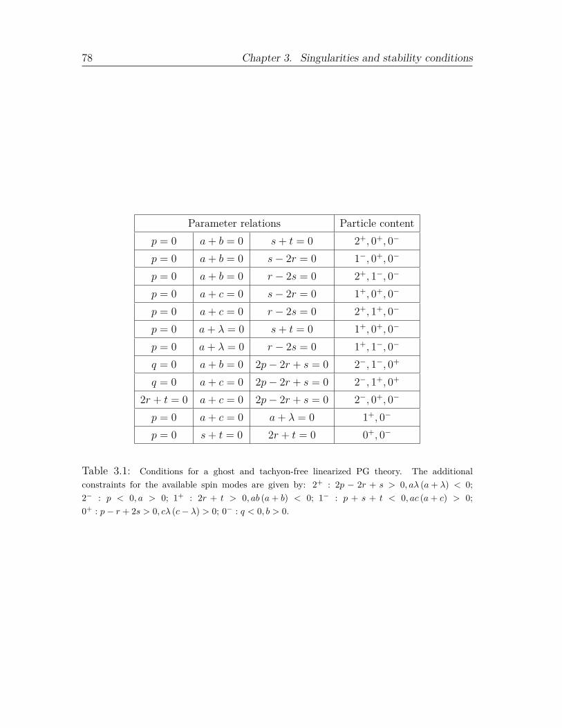
78 Chapter 3. Singularities and stability conditions
Parameter relations Particle contentp = 0 a+ b = 0 s+ t = 0 2+, 0+, 0−
p = 0 a+ b = 0 s− 2r = 0 1−, 0+, 0−
p = 0 a+ b = 0 r − 2s = 0 2+, 1−, 0−
p = 0 a+ c = 0 s− 2r = 0 1+, 0+, 0−
p = 0 a+ c = 0 r − 2s = 0 2+, 1+, 0−
p = 0 a+ λ = 0 s+ t = 0 1+, 0+, 0−
p = 0 a+ λ = 0 r − 2s = 0 1+, 1−, 0−
q = 0 a+ b = 0 2p− 2r + s = 0 2−, 1−, 0+
q = 0 a+ c = 0 2p− 2r + s = 0 2−, 1+, 0+
2r + t = 0 a+ c = 0 2p− 2r + s = 0 2−, 0+, 0−
p = 0 a+ c = 0 a+ λ = 0 1+, 0−
p = 0 s+ t = 0 2r + t = 0 0+, 0−
Table 3.1: Conditions for a ghost and tachyon-free linearized PG theory. The additionalconstraints for the available spin modes are given by: 2+ : 2p − 2r + s > 0, aλ (a+ λ) < 0;2− : p < 0, a > 0; 1+ : 2r + t > 0, ab (a+ b) < 0; 1− : p + s + t < 0, ac (a+ c) > 0;0+ : p− r + 2s > 0, cλ (c− λ) > 0; 0− : q < 0, b > 0.

JCAP04(2017)021
ournal of Cosmology and Astroparticle PhysicsAn IOP and SISSA journalJ
Singularities and n-dimensional blackholes in torsion theories
J.A.R. Cembranos, J. Gigante Valcarceland F.J. Maldonado Torralba
Departamento de Fısica Teorica I, Universidad Complutense de Madrid,E-28040 Madrid, Spain
E-mail: [email protected], [email protected], [email protected]
Received January 20, 2017Revised March 7, 2017Accepted March 28, 2017Published April 11, 2017
Abstract. In this work we have studied the singular behaviour of gravitational theories withnon symmetric connections. For this purpose we introduce a new criteria for the appearanceof singularities based on the existence of black/white hole regions of arbitrary codimensiondefined inside a spacetime of arbitrary dimension. We discuss this prescription by increas-ing the complexity of the particular torsion theory under study. In this sense, we startwith Teleparallel Gravity, then we analyse Einstein-Cartan theory, and finally dynamicaltorsion models.
Keywords: GR black holes, modified gravity
ArXiv ePrint: 1609.07814
c© 2017 IOP Publishing Ltd and Sissa Medialab srl doi:10.1088/1475-7516/2017/04/021
JCAP04(2017)021
Contents
1 Introduction 1
2 Singularity theorems in General Relativity 3
3 Black hole regions 6
4 General aspects of theories with torsion 8
5 Singularities in Teleparallel Gravity 8
6 Singularities in Einstein-Cartan theory 10
7 Singularities in dynamical torsion theories 14
8 Conclusions 16
1 Introduction
In a physical theory, a singularity is commonly known as a “place” where some of the variablesused in the description of the system diverge. For example, we find this in the singularity inr = 0 of the Coulombian potential V = K q
r . This kind of behaviour appears mainly becausethe theory is not valid in the considered region or we have assumed a simplification. In theprevious example the singularity arises due to the fact that we are considering the chargedparticle as a point and neglecting the quantum effects.
In General Relativity (GR), one might expect to observe singularities when the com-ponents of the tensors that describe the curvature of the spacetime diverge. This meansthat the curvature is higher than 1
l2p, where lp is the Planck length, so we need to have into
account the quantum effects, which are not considered in this theory. However, there aresituations where this behaviour is given as a result of the chosen coordinates. This is thecase of the “singularity” in r = 2M in the Schwarzschild metric. For this reason, another cri-teria, proposed by Penrose [1], is used to define a singularity: geodesic incompleteness. Thephysical interpretation of this condition is the existence of free falling observers that appearor disappear out of nothing. This is “strange” enough to consider it a sufficient condition toassure that there is a singularity.
Already in the first solutions of Einstein equations there are “places” where the com-ponents of the curvature tensors diverge, like in r = 0 in the Schwarzschild metric and t = 0in the Friedmann-Lemaıtre-Robertson-Walker (FLWR) metric, but it was thought that thiswas a consequence of the excessive symmetry of the solutions, as it occurs in many situationsin classical mechanics or electromagnetism. The first attempt of proving a singularity the-orem was made by Raychaudhuri [2] in 1955, in an article where he introduced his famousequation, which is essential in the later development of singularity theorems. Ten years later,Penrose formulated the first singularity theorem that does not assume any symmetry [1] (fora recent review see [3]). It is also the first to use geodesic incompleteness in the definition ofa singularity. This theorem showed that the singularity in r = 0 of the Schwarzschild metricis also present under non symmetrical gravitational collapses.
– 1 –

JCAP04(2017)021
The same happens with the singularity in t = 0 of the FLRW metric, but this time is aconsequence of a theorem stated by Hawking a year later [4], which predicts that, under threephysically realistic conditions, all past directed timelike geodesics have finite length, thereforeevery particle of the Universe (hence the Universe itself) had a beginning. The mentionedconditions are that the action of the Ricci tensor over a timelike vector is greater or equalthan cero, which it is interpreted as the attractive nature of gravity, that the Universe isglobally hyperbolic and there is an hypersurface with positive initial expansion. Althoughwe have said that the conditions are physically realistic, since it was measured the acceleratedexpansion of the Universe [5], the convergence condition fails.
In general, all singularity theorems follow the same pattern, made explicit by Senovillain [6]:
Theorem 1.1. (Pattern singularity “theorem”). If the spacetime satisfies:
1) A condition on the curvature.
2) A causality condition.
3) An appropriate initial and/or boundary condition.
Then there are null or timelike inextensible incomplete geodesics.
Let us stop for a moment and analyse the configuration of the theorems. When thesingularity theorems are derived, no assumptions are made on the underlying physical theory,that is, the one that links the matter and energy content with the structure of the spacetime.This means that they are valid, not only for GR, but for all the modifications that change theEinstein-Hilbert action. It is worth mentioning that the first condition can be reformulatedusing the field equations of the theory, obtaining what is known as the energy conditions.These conditions are dependent of the considered theory, therefore they will differ from oneto another, e.g., in GR they are formulated in terms of the energy-stress tensor only, while inf(R) theories there are some extra terms related to the curvature [7]. Since we are working in aLorentzian manifold, we have to endow it with an affine structure, which is implicitly assumedto be the Levi-Civita one, as it is postulated in GR, given by the Christoffel symbols [8],
Γρµν =1
2gρσ (∂µgνσ + ∂νgµσ − ∂σgµν) . (1.1)
This is the unique connection that is covariantly conserved [9], ∇ρgµν = 0, and symmetric,Γρµν = Γρνµ.
A metric has D(D + 1)/2 components in a D-dimensional Lorentzian manifold, as itis a symmetric 2-covariant tensor. On the other hand, a general connection has D3 com-ponents which are, in principle, completely independent degrees of freedom. Out of the D3
components, D2(D − 1)/2 reside in the antisymmetric part
T ρµν ≡ Γρµν − Γρνµ, (1.2)
which is known as torsion. The rest of degrees of freedom, D2(D + 1)/2, are encoded in thenon-metricity tensor
Mρµν = ∇ρgµν . (1.3)
One might wonder if it is possible to modify the gravitational theory by setting these tensorsto be different from zero, i.e. postulating a connection that it is not Levi-Civita. Certainlyit is, although we have to take into account some considerations:
– 2 –
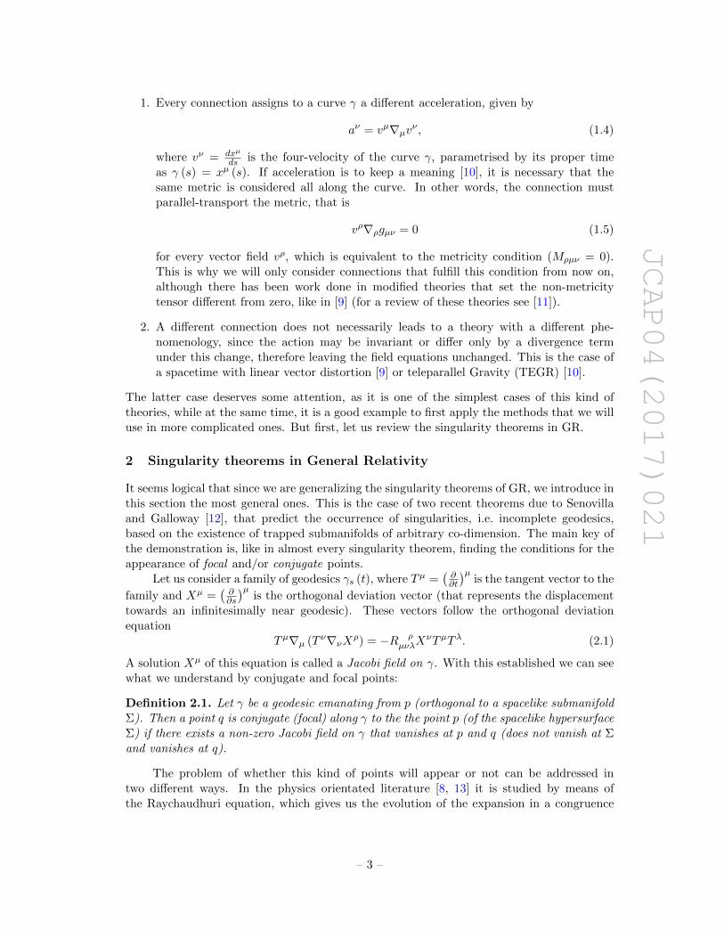
JCAP04(2017)021
1. Every connection assigns to a curve γ a different acceleration, given by
aν = vµ∇µvν , (1.4)
where vν = dxµ
ds is the four-velocity of the curve γ, parametrised by its proper timeas γ (s) = xµ (s). If acceleration is to keep a meaning [10], it is necessary that thesame metric is considered all along the curve. In other words, the connection mustparallel-transport the metric, that is
vρ∇ρgµν = 0 (1.5)
for every vector field vρ, which is equivalent to the metricity condition (Mρµν = 0).This is why we will only consider connections that fulfill this condition from now on,although there has been work done in modified theories that set the non-metricitytensor different from zero, like in [9] (for a review of these theories see [11]).
2. A different connection does not necessarily leads to a theory with a different phe-nomenology, since the action may be invariant or differ only by a divergence termunder this change, therefore leaving the field equations unchanged. This is the case ofa spacetime with linear vector distortion [9] or teleparallel Gravity (TEGR) [10].
The latter case deserves some attention, as it is one of the simplest cases of this kind oftheories, while at the same time, it is a good example to first apply the methods that we willuse in more complicated ones. But first, let us review the singularity theorems in GR.
2 Singularity theorems in General Relativity
It seems logical that since we are generalizing the singularity theorems of GR, we introduce inthis section the most general ones. This is the case of two recent theorems due to Senovillaand Galloway [12], that predict the occurrence of singularities, i.e. incomplete geodesics,based on the existence of trapped submanifolds of arbitrary co-dimension. The main key ofthe demonstration is, like in almost every singularity theorem, finding the conditions for theappearance of focal and/or conjugate points.
Let us consider a family of geodesics γs (t), where Tµ =(∂∂t
)µis the tangent vector to the
family and Xµ =(∂∂s
)µis the orthogonal deviation vector (that represents the displacement
towards an infinitesimally near geodesic). These vectors follow the orthogonal deviationequation
Tµ∇µ (T ν∇νXρ) = −R ρµνλX
νTµT λ. (2.1)
A solution Xµ of this equation is called a Jacobi field on γ. With this established we can seewhat we understand by conjugate and focal points:
Definition 2.1. Let γ be a geodesic emanating from p (orthogonal to a spacelike submanifoldΣ). Then a point q is conjugate (focal) along γ to the the point p (of the spacelike hypersurfaceΣ) if there exists a non-zero Jacobi field on γ that vanishes at p and q (does not vanish at Σand vanishes at q).
The problem of whether this kind of points will appear or not can be addressed intwo different ways. In the physics orientated literature [8, 13] it is studied by means ofthe Raychaudhuri equation, which gives us the evolution of the expansion in a congruence
– 3 –
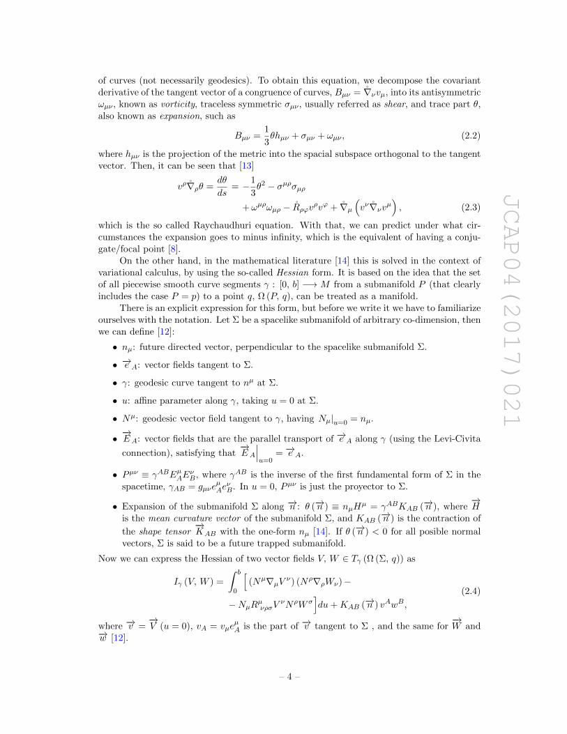
JCAP04(2017)021
of curves (not necessarily geodesics). To obtain this equation, we decompose the covariantderivative of the tangent vector of a congruence of curves, Bµν = ∇νvµ, into its antisymmetricωµν , known as vorticity, traceless symmetric σµν , usually referred as shear, and trace part θ,also known as expansion, such as
Bµν =1
3θhµν + σµν + ωµν , (2.2)
where hµν is the projection of the metric into the spacial subspace orthogonal to the tangentvector. Then, it can be seen that [13]
vρ∇ρθ =dθ
ds= −1
3θ2 − σµρσµρ
+ωµρωµρ − Rρϕvρvϕ + ∇µ(vν∇νvµ
), (2.3)
which is the so called Raychaudhuri equation. With that, we can predict under what cir-cumstances the expansion goes to minus infinity, which is the equivalent of having a conju-gate/focal point [8].
On the other hand, in the mathematical literature [14] this is solved in the context ofvariational calculus, by using the so-called Hessian form. It is based on the idea that the setof all piecewise smooth curve segments γ : [0, b] −→ M from a submanifold P (that clearlyincludes the case P = p) to a point q, Ω (P, q), can be treated as a manifold.
There is an explicit expression for this form, but before we write it we have to familiarizeourselves with the notation. Let Σ be a spacelike submanifold of arbitrary co-dimension, thenwe can define [12]:
• nµ: future directed vector, perpendicular to the spacelike submanifold Σ.
• −→e A: vector fields tangent to Σ.
• γ: geodesic curve tangent to nµ at Σ.
• u: affine parameter along γ, taking u = 0 at Σ.
• Nµ: geodesic vector field tangent to γ, having Nµ|u=0 = nµ.
• −→EA: vector fields that are the parallel transport of −→e A along γ (using the Levi-Civita
connection), satisfying that−→EA
∣∣∣u=0
= −→e A.
• Pµν ≡ γABEµAEνB, where γAB is the inverse of the first fundamental form of Σ in the
spacetime, γAB = gµνeµAe
νB. In u = 0, Pµν is just the proyector to Σ.
• Expansion of the submanifold Σ along −→n : θ (−→n ) ≡ nµHµ = γABKAB (−→n ), where
−→H
is the mean curvature vector of the submanifold Σ, and KAB (−→n ) is the contraction of
the shape tensor−→KAB with the one-form nµ [14]. If θ (−→n ) < 0 for all posible normal
vectors, Σ is said to be a future trapped submanifold.
Now we can express the Hessian of two vector fields V, W ∈ Tγ (Ω (Σ, q)) as
Iγ (V, W ) =
∫ b
0
[(Nµ∇µV ν) (Nρ∇ρWν)−
−NµRµνρσV
νNρW σ]du+KAB (−→n ) vAwB,
(2.4)
where −→v =−→V (u = 0), vA = vµe
µA is the part of −→v tangent to Σ , and the same for
−→W and
−→w [12].
– 4 –

JCAP04(2017)021
The reader might be wondering what is the connection between the Hessian and theconjugate and focal points. The next theorem clears all doubts [15].
Theorem 2.2. Let Σ be a spacelike submanifold and γ a causal curve orthogonal to Σ, thenthe submanifold Σ does not have focal points along γ if and only if the Hessian is semi-positive
definite, having Iγ (V, V ) = 0 only if−→V is proportional to
−→N on γ.
To assure the appearance of focal points to a hypersurface of arbitrary co-dimension Σ,Senovilla and Galloway develop a curvature condition.
Proposition 2.3. Let Σ be a spacelike submanifold of co-dimension m in a Lorentzian man-ifold of dimension n, and let nµ be a future-pointing normal to Σ. If θ (−→n ) ≡ (m− n) c < 0,and the curvature tensor satisfies the inequality
RµνρσNµNρP νσ ≥ 0 (2.5)
along γ, then there is a point focal to Σ along γ at or before q = γ(u = 1
c
), given that the
curve had arrived so far.
This condition can be interpreted as a manifestation of the attractive character ofgravity.
Based on this focalisation theorem, Senovilla and Galloway prove a generalisation of thePenrose and Hawking-Penrose theorem. The first result predicts the incompleteness of nullgeodesics:
Theorem 2.4. Let (M, g) contain a non-compact Cauchy hypersurface S and a closed futuretrapped submanifold Σ of arbitrary co-dimension. If the curvature condition holds alongevery future directed null geodesic emanating orthogonally from Σ, then (M, g) is future nullgeodesically incomplete.
The second theorem is based on the Hawking-Penrose lemma, which is valid for arbitrarydimension, that states that this three conditions cannot all hold:
• Every inextensible causal geodesic contains a pair of conjugate points.
• There are not closed timelike curves (chronology condition).
• there is an achronal set Σ such that E+ (Σ) is compact.
It is an established result [8, 13] that the first statement holds if Rµνvµvν ≥ 0 for every non-
spacelike vector vµ. When applied to timelike vectors it is known as the timelike convergencecondition, while in the case of null ones it is called the null convergence condition. Usingthe Einstein field equations we can rewrite these conditions in terms of the energy momen-tum tensor Tµν . The equivalent of the timelike convergence is the strong energy condition,Tµνv
µvν ≥ 12T , and for the null one the weak energy condition, Tµνv
µvν ≥ 0, where T is thetrace of the energy-momentum tensor.
Now we can review the generalization of the H-P theorem:
Theorem 2.5. If the chronology, generic, timelike and null convergence conditions holdand there is a closed future trapped submanifold Σ of arbitrary co-dimension such that thecurvature condition holds along every null geodesic emanating orthogonally from Σ, then thespacetime is causal geodesically incomplete.
– 5 –

JCAP04(2017)021
Sketch of the proof. First of all, it has to be proven that the existence of closed trappedsubmanifolds leads to the existence of an achronal set with the properties mentioned in thelemma [12]. Once the H-P lemma is proved, this theorem can be easily deduced, as it isexplained in [13].
3 Black hole regions
We know from experience, e.g. the Schwarzschild metric, that the existence of incomplete nullgeodesics leads to the appearance of black holes, that are regions of the spacetime that oncean observer enters them, it cannot leave. This applies to all timelike and null curves, not justgeodesics. This is usually known as the cosmic censorship conjecture, which is a concept thatPenrose introduced in 1969. It basically states that singularities cannot be naked, that meansthat they cannot be seen by an outside observer. However, how can we express this conceptmathematically? The answer lies in the concept of conformal compactification, which can bedefined as [18]:
Definition 3.1. Let (M, g) and(M, g
)be two spacetimes. Then
(M, g
)is said to be a
conformal compactification of M if and only if the following properties are met:
1. M is an open submanifold of M with smooth boundary ∂M = J . This boundary isusually denoted conformal infinity.
2. There exists a smooth scalar field Ω on M , such that gµν = Ω2gµν on M , and so thatΩ = 0 and its gradient dΩ 6= 0 on J .
If additionally, every null geodesic in M acquires a future and a past endpoint on J , thespacetime is called asymptotically simple. Also, if the Ricci tensor is zero in a neighbourhoodof J the spacetime is said to be asymptotically empty.
In a conformal compactification, J is composed by two null hypersurfaces, J + and J −,known as future null infinity and past null infinity respectively.
In order to establish the definition of black hole, we need to introduce two more con-cepts [8]:
Definition 3.2. A spacetime (M, g) is said to be asymptotically flat if there is an asymptot-ically empty spacetime (M ′, g′) and a neighbourhood U ′ of J ′, such that U ′ ∩M ′ is isometricto an open set U of M .
Definition 3.3. Let (M, g) be an asymptotically flat spacetime with conformal compactifica-
tion(M, g
). Then M is called (future) strongly asymptotically predictable if there is an
open region V ⊂ M , with J− (J +) ∩M ⊂ V , such that V is globally hyperbolic.
This definition does not require the condition of the endpoints of the null geodesics,meaning that this kind of spacetimes can be singular. Nevertheless, if a spacetime is asymp-totically predictable, then the singularities are not naked, i.e. are not visible from J +.
Now we can establish what we understand by a black hole:
Definition 3.4. A strongly asymptotically predictable spacetime (M, g) is said to containa black hole if M is not contained in J− (J +). The black hole region, B, is defined to beB = M − J− (J +) and its boundary, ∂B, is known as the event horizon.
– 6 –
JCAP04(2017)021
Intuitively, we think that a particle in a closed trapped surface cannot scape to J +,meaning that it is part of the black hole region of the spacetime. Nevertheless, this is nottrue in general. In the next proposition we establish the conditions that ensure the existenceof black holes when we have a closed future trapped submanifold of arbitrary co-dimension:
Proposition 3.5. Let (M, g) be a strongly asymptotically predictable spacetime of dimensionn, and Σ a closed future trapped submanifold of arbitrary co-dimension m in M . If thecurvature condition holds along every future directed null geodesic emanating orthogonallyfrom Σ, then Σ cannot intersect J− (J +), i.e. Σ is in the black hole region B of M .1
Proof. This proof is similar to the one of proposition 12.2.2 by Wald [8]. Let us supposethat Σ intersects J− (J +). Then, in the conformal compactification M , we would have thatJ+ (Σ) ∩ J + 6= ∅. On other hand, we know that the spatial infinity i0, the point of thecompactification where the future (past) complete spacelike geodesics end (begin), is notin the causal future of any point in M . Therefore it follows trivially that i0 /∈ J+ (Σ).Since M is strongly asymptotically predictable, there is a globally hyperbolic region V inthe compactification such that J− (J +) ∩M ⊂ V . From basic topology we have that the
intersection of two closed sets is closed, therefore Λ = Σ ∩(J− (J +) ∩M
)is closed, where
clearly Λ ⊂ Σ and Λ ⊂ V . In addition, a closed subset of a compact is also compact,so from the compactness of Σ we deduce that Λ is compact. It is an standard result ofLorentzian geometry that, in a globally hyperbolic space, the causal future of a compactset is closed [8], so, in this case, we have that J+ (Λ) is closed in V . This means that itcontains all of its limit points, therefore since i0 /∈ J+ (Λ), there is an open neighbourhoodof i0 that does not intersect J+ (Λ), and so, an open region of J + that does not intersectJ+ (Λ). It is known that a connected set cannot contain a subset with no boundary (exceptfor the empty set and the set itself) [19]. As we have already proved, J+ (Λ) ∩ J + isnot equal to J +. Since J + is connected, it follows that there must be a point q ∈ J +
in ∂J+ (Λ). In the proof of the generalised Penrose theorem we used that in a globallyhyperbolic spacetime ∂J+ (Λ) = E+ (Λ), so in the compactification M there is a null geodesicγ connecting p ∈ Λ ⊂ Σ with q. Furthermore, using the theorem 51 of O’Neill [14], we seethat this null geodesic must be orthogonal to Σ and not contain any focal point of Σ beforeq, as otherwise we would have that q ∈ I+ (Λ) and therefore q /∈ E+ (Λ). With respect to themetric g of M , γ is also a null geodesic orthogonal to Σ with no focal point of Σ, but nowγ is future complete [8]. Although, since Σ is future trapped one has θ (−→n ) ≡ (m− n) c < 0for any future-pointing null normal one-form nµ [12]. Now, let (m− n)C be the maximumvalue of all possible θ (−→n ) on the compact Σ. Then, using the proposition 3.5, we have thatevery null geodesic emanating orthogonally from Σ will have a focal point at or before theaffine parameter reaches the value 1
C . This clearly leads to a contradiction, therefore theassumption is false.
This proposition will help us to study the singularities in theories of gravitation thatinclude torsion. But first, let us introduce the main aspects of these theories.
1Analogously, it can be defined a past strongly asymptotically predictable space time, and then the propo-sition would predict the existence of white hole regions,B = M − J+
(J−), that are regions that particles
cannot enter, only exit.
– 7 –

JCAP04(2017)021
4 General aspects of theories with torsion
In this section, we introduce the geometrical background of gravitational theories that allow anon symmetric connection that still fulfills the metricity condition. The interesting fact aboutthese theories is that they appear naturally as a gauge theory of the Poincare Group [20],making their formalism closer to that of the Standard Model of Particles, and hence makingit a good candidate to explore the quantization of gravity.
Since the connection is not necessarily symmetric, the torsion can be different fromzero. For an arbitrary connection, that meets the metricity condition, there exists a relationbetween it and the Levi-Civita connection
Γρµν = Γρµν −Kρµν , (4.1)
where
Kρµν =
1
2
(T ρµν − T ρ
µ ν − T ρν µ
)(4.2)
is the contortion tensor.Since the curvature tensors depend on the connection, there is a relation between the
ones defined throughout the Levi-Civita connection and the general ones. For the Riemanntensor we have [21]
Rσµνρ = Rσµνρ − ∇νKσµρ + ∇ρKσ
µν−−Kσ
ανKαµρ +Kσ
αρKαµν ,
(4.3)
where the upper index˚denotes the Levi-Civita quantities. By contraction we can obtainthe expression for the Ricci tensor
Rµρ = Rµρ − ∇σKσµρ + ∇ρKσ
µσ−−Kσ
ασKαµρ +Kσ
αρKαµσ,
(4.4)
and the scalar curvatureR = gµρRµρ = R− ∇ρKσ
σρ−−Kσ
ασKαρρ +Kα
σρKσµα.
(4.5)
All the theories that we will consider from now on will follow these geometrical properties,the only change would be the underlying physical theory.
5 Singularities in Teleparallel Gravity
TEGR is a degenerate case of the Poincare gauge theories, since it is a gauge theory of thetranslation group only. Any gauge theory including these transformations will differ fromthe usual internal gauge models in many ways, the most significant being the presence of atetrad field [22]. Given a nontrivial tetrad haµ, it is possible to define a connection known asWeitzenbock connection
Γρµν = h ρa ∂µh
aµ, (5.1)
that presents torsion, but no curvature. With this tetrad field we can also construct theLevi-Civita connection, taking into account that the metric can be expressed as
gµν = ηabhaµh
bν , (5.2)
where ηab is the Lorentz-Minkowski metric, and using the usual definition, as seen in equa-tion (1.1).
– 8 –

JCAP04(2017)021
The relation between these two connections is given by equation (4.1). The Lagrangiandensity of this gravitational theory can be written as
L =hc4
16πGSµνρTµνρ, (5.3)
where h = det(haµ), and
Sµνρ = −Sµρν ≡ 1
2(Kνρµ + gµρT σνσ + gµνT σρσ) , (5.4)
which is usually known as superpotential.Using the relation between the Weitzenbock and the Levi-Civita connection in equa-
tion (4.1) we can express this Lagrangian as
L = L − ∂µ(hc4
8πGT νµν
), (5.5)
where L is the Einstein-Hilbert Lagrangian of GR. Since they are equal except for a totaldivergence, the same field equations arise. Therefore it is a theory equivalent to GR, as itcan be seen for example when one studies the junction conditions [36].
The field equations can be obtained by taking variations of the Lagrangian. Expressingthem in pure spacetime form, we have
∂σ(hS σν
µ
)− 4πG
c4(ht νµ
)= 0, (5.6)
where
ht νµ =hc4
4πGΓσρµS
ρνσ + δ νµ L (5.7)
is the canonical energy-momentum pseudotensor of the gravitational field. Although this isthe simplest framework for a theory with torsion, it is helpful for introducing the methodsthat we will use in more general cases. In that sense, the next considerations are general,and can be applied in all the theories of gravitation.
In GR we have considered geodesic incompleteness as a criterium of the appearanceof singularities, based on the fact that causal geodesics are the trajectories of free-fallingobservers. Therefore, we wish to modify this criteria by terms of these trayectories in thetheory that we are considering. We will say that our spacetime is singular if the domainof the affine parameter of at least one curve that follow any free-falling observer (includingphotons) is different from R. For spacetimes in which we can define a conformal boundary,as the ones considered in section 3, this can be stated in the following way:
Definition 5.1. A spacetime (M, g), endowed with a conformal compactification, is said tobe singular if at least one non-spacelike curve has an endpoint outside the conformal infinity.
Before continuing, it is useful to define two important classes of curves, which coincidein the case of the Levi-Civita connection [24]:
• Autoparallel curves: these are the curves in which its tangent vector vµ is paralleltransported to itself, that is:
vµ∇µvν = 0. (5.8)
– 9 –

JCAP04(2017)021
The differential equation of the autoparallels is, under a suitable choice of the affineparameter:
dvµ
dt+ Γµρσv
ρvσ = 0, (5.9)
which only takes into account the symmetric part of the connection.
• Extremal curves: these are the ones that extremise the length with respect to themetric of the manifold. It is worth mentioning that the length only depends on themetric, and not on the torsion. In order to see what are the equations of these curveswe recall a standard result from Lorentzian geometry, that can be used as a definition:
Theorem 5.2. Let γ be a smooth timelike curve connecting two points p, q ∈M . Thenthe necessary and sufficient condition that γ locally maximizes the length between p andq over smooth one parameter variations is that γ is a geodesic with no point conjugateto p between p and q.
Then, the differential equations of these curves are the same of the Levi-Civita geodesics:
dvµ
dt+ Γµρσv
ρvσ = 0, (5.10)
The trajectories of free-falling observers in theories different from GR do not follow thesecurves in general. Nevertheless, in TEGR they do. The equation of motion for free fallingobservers, scalar particles, is [22]:
dvµdt
+ Γρσµvρvσ = 0, (5.11)
which is equivalent todvµ
dt+ Γµρσv
ρvσ = 0. (5.12)
Therefore they follow extremal curves, which are the autoparallels of the Levi-Civitaconnection.
It is particular interesting to discuss this issue for photons. It has been stated thatMaxwell equations do not couple to torsion in the minimal approach. However, in TEGRthe electromagnetic field is able to couple to torsion without violating gauge invariance [10].Using the relation between the Levi-Civita and the Weitzenbock connection, one can verifythat the teleparallel version of Maxwell’s equations are completely equivalent with the usualMaxwell’s equations in the context of GR. This means that they move according to thegeodesic equation of GR, and so the causal structure is the same as in GR.
This discussion is more general. In fact, the equivalence between TEGR and GR meansthat all the singularity theorems developed in GR apply to this theory also. Therefore, thecausal convergence and the curvature condition remain the same, although the expressionfor the Riemann and Ricci tensor change as discussed in the previous section, specifically inequations (4.3), (4.4).
6 Singularities in Einstein-Cartan theory
The Einstein-Cartan (EC) theory of gravitation is the most recognised theory that includestorsion [23, 24]. The main reason to introduce this theory is the fact that it allows to consider
– 10 –
JCAP04(2017)021
massive spinning fields in a natural way, while maintaining all the experimental success ofGR. This theory arises when searching for a gravitational Lagrangian linear in the curvatureterm Rλ ρµν . The geometrical structure is the one analysed in section 4.
The field equations are obtained by varying the Lagrangian of this theory with respectto the metric and the contortion:
Rµν −1
2Rgµν = κΣµν (6.1)
andSµνρ = κτµνρ, (6.2)
whereS ρµν = T ρ
µν + δρµTσ
νσ − δρνT σµσ (6.3)
is the modified torsion tensor. At this point, we might wonder what are the trajectories ofthe free-falling observers, in order to establish some singularity theorems.
Since it is impossible to perform the minimally coupling prescription for the Maxwell’sfield while maintaining the U (1) gauge invariance, the Maxwell equations are the same asin GR. Therefore, they move following null extremal curves, and so the causal structureis determined by the metric structure, just like in GR. Also, from the minimally coupleprocedure, it follows that particles with no spin, represented by scalar fields, do not feeltorsion as well, since the covariant derivative of a scalar field is just its partial derivative.This means that the test particles follow the geodesics of the Levi-Civita connection, whichallow us to generalise trivially the singularity theorems. Just like in TEGR, the causalconvergence and the curvature conditions remain the same, it just changes the expression forthe Levi-Civita Riemann and Ricci tensors, as given by equations (4.3), (4.4).
In any case, even for trajectories decoupled from torsion, energy conditions are modified.Although the curvature condition is the same as in GR, these conditions change due to thefact that the field equations are different. Since equation (6.2) is purely algebraic we cansubstitute everywhere spin with torsion. Now we split the Einstein tensor into the Levi-Civita (Gµν) part and the rest, and we change the torsion terms by means of equation (6.2),obtaining
Gµν = κσµν , (6.4)
where σµν is the combined energy-momentum tensor
σµρ = Σµρ −∇σKσµρ +∇ρKσ
µσ −KσασK
αµρ +Kσ
αρKαµσ+
+1
2gµρ
(∇αKσ
σα +KσασK
αρρ −Kα
σρKσµα
).
(6.5)
Now, by using equation (6.4) we can write the energy conditions. The strong energycondition can be expressed as
σµνvµvν ≥ 1
2σ, (6.6)
where σ = gµν σµν . And for the weak energy condition we have
σµνvµvν ≥ 0. (6.7)
It is interesting noting that when the torsion is zero, one recovers the energy conditions ofGR, as one would expect, since the contortion tensor involved in equation (6.5) also vanishes.
– 11 –

JCAP04(2017)021
So far we have analysed the singular behaviour of photons and spinless particles, butit is more interesting to study the behaviour of spinning fields. This question has alreadybeen addressed in the literature, mainly following two approaches. The first one is to studythe singular behaviour of particular cosmological models using the energy conditions andthe modified Raychaudhuri equation for non symmetric connection derived by Stewart andHajicek [25] (for a review of this approach see [24]). These studies try to obtain plausiblecosmological models that are singularity free. Nevertheless, they come to the conclusion thatit is necesary to have regions with high spin density to observe a behaviour different fromGR, and to avoid the singularities. On the other hand, Esposito [26] proved a singularitytheorem for EC theory based on the incompleteness of autoparallel curves. He considers thiscriteria to be sufficient to establish the singular character of a spacetime.
In those two approaches, the argument is based on the modified Raychaudhuri equationfor non-symmetric metric connections. The main difference comes, as one would expect, froma change in the antisymmetric part of the decomposition mentioned in equation (2.2), sincenow Bµν is defined throughout the total connection. Then, the equation can be expressed asfollows:
vρ∇ρθ =dθ
dτ= −1
3θ2 − σµρσµρ
+ (ωµρ + Sµν) (ωµρ + Sµν)−Rρϕvρvϕ, (6.8)
where Sµν is a tensor that is usually defined through the following relation with the modifiedtorsion tensor [26]
S ρµν = Sµνv
ρ. (6.9)
The problem with this reasoning is that the spin particles do not follow in general autoparal-lels curves of the total connection, so there might be situations where there is incompletenessof this kind of curves but no singular spin trajectories. Nevertheless, one could have thecuriosity of knowing which is the Raychadhuri equation for the spin test particles. We willknow study how we can expressing, making an study valid for all the Poincare gauge theoriesof gravity.
All the analysis of these trajectories up to this point, which are reviewed in [27], havea thing in common: after some algebra, they can all be expressed in the form
aµ = vρ∇ρvµ
= C
(~m
)f(Rµλρσs
ρσvλ +K µρσ vρvσ
), (6.10)
where C is a constant, m is the mass of the particle, and we have made explicit the Planckconstant. The tensor sρσ is the internal spin tensor, related to the spin sµ of the particle by
sµ =1
2εµνρσvνsρσ, (6.11)
where εµνρσ is the totally antisymmetric Levi-Civita tensor, which is normalised with thesquare root of the metric, as it is usual in a Lorentzian manifold. The function f representsa linear combination of different contractions of the tensors involved in the expression, de-pending on the analysis chosen. The connection with respect it is calculated the Riemmanntensor in brackets is also dependent of the analysis, but it is always one constructed with theLevi Civita and linear combinations of torsion related quantities.
– 12 –

JCAP04(2017)021
When writing the Raychaudhuri equation we choose to make it with respect to the Levi-Civita connection, since it is analogous to the expression in terms of the total connection,and in this way we avoid introducing new terms to the decomposition in equation (2.2). Withthat in mind we have that
vρ∇ρθ =dθ
ds= −1
3θ2 − σµρσµρ + ωµρωµρ − Rρϕvρvϕ
+C
(~m
)∇µ(Rµλρσs
ρσvλ +K µρσ vρvσ
). (6.12)
Using this equation we could predict the appearance of focal/conjugate points in a congruenceof this timelike curves, just by imposing a generalised curvature condition
Rρϕvρvϕ − C
(~m
)∇µ[f(Rµλρσs
ρσvλ +K µρσ vρvσ
)]≥ 0, (6.13)
that must hold for every timelike vector vµ. Nevertheless, there are some issues with thisapproach. First of all, this is only valid for congruences of curves that have the same spinorientation for all the test particles, hence limiting the analysis. On the other hand, weknow for the singularity theorems in GR that the existence of focal/conjugate points is nota sufficient condition for the appearance of singularities. We also need global conditionsthat allow us to reach a contradiction with the completeness of the curves. Since we areconsidering non-geodesical behaviour, the theorems that allow us to make that contradictionare no longer valid, and we cannot predict the singularities. That is why in this article wepropose another approach, based on the result of the appearance of black/white hole regionsin an arbitrary Lorentzian manifold.
It is clear from the previous analysis that spinning particles do not follow extremalcurves. However, independently of how torsion affects these particles, they will follow timelikecurves, since they are massive and we assume that locally (in a normal neighbourhood of apoint) nothing can be faster than light (null geodesics). Hence, it would be interesting to seeunder what circumstances we have non-geodesical timelike singularities. For that, we recoverthe definition of an n-dimensional black/white hole given in section 3. From this definition,we conclude that if this kind of structures exist in our spacetime, we would have timelikecurves (including non-geodesics) that do not have endpoints in the conformal infinity, sincefor the case of black holes, the spacetime M is not contained in J− (J +), while for whiteholes, M is not contained in J+ (J −). This is exactly the extended definition of singularitythat we have given in section 5. Considering this, we establish the following theorem:
Theorem 6.1. Let (M, g) be a strongly asymptotically predictable spacetime of dimension n,and Σ a closed future trapped submanifold of arbitrary co-dimension m in M . If the curvaturecondition holds along every future directed null geodesic emanating orthogonally from Σ, thensome timelike curves in M would not have endpoints in the conformal infinity, hence M is asingular spacetime (definition 5.1).
From a physical point of view, one might wonder if one of the incomplete timelike curvesactually represents the trajectory of a spin particle. From equation (6.10), which representsthe non-geodesical behaviour, we see that the only possible way that all the trajectories haveendpoints in the conformal infinity is that there are huge values of the curvature and torsionnear the event horizon, which in a physically plausible scenario it is not possible. This iswhy we consider it a more physically relevant theorem for the singular behaviour of the spinparticles, since it is strongly related to the actual trajectories.
– 13 –

JCAP04(2017)021
7 Singularities in dynamical torsion theories
So far, the two torsion theories that we have analysed are part of a set of theories knownas Poincare Gauge Gravity (PG) [24, 28]. The reason why there are many theories underthis premise is because we can construct a large number of invariants from the curvatureand torsion tensors, and therefore a general gravitational Lagrangian has the complicatedform of a sum of all available invariants of proper dimension. The coefficients in the sum canbe arranged to obtain different gravitational theories (for some criteria on the election andstability of a large class of these PG Lagrangians see [28–31]).
In this section, we will study a PG theory of gravity, hence it has the same geometricalbackground explained in section 4, with the following vacuum Lagrangian [32]:
S =c4
16πG
∫d4x√−g
[2Λ− R−
− 1
2(2c1 + c2)RλρµνR
µνλρ + c1RλρµνRλρµν+
+ c2RλρµνRλµρν + d1Rµν (Rµν −Rνµ)
].
(7.1)
One interesting feature about this theory is that if we set the torsion to be zero, we recoverGR. Then, it is expected to involve slight modifications to the standard theory in terms ofthe torsion tensor alone.
The field equations can be derived from this action by performing variations with respectto the gauge potentials Aµ, which are related to the translations and Lorentz rotationsgenerators of the Poincare group in the following way:
Aµ = eaµPa + ωabµJab, (7.2)
where eaµ is the vierbein field and ωabµ is the spin connection [32]. The generators Pa andJab follow the usual commutation relations:
[Pa, Pb] = 0, (7.3)
[Pa, Jbc] = iηa[bP c], (7.4)
[Jab, Jcd] =i
2(ηadJbc + ηcbJad − ηdbJac − ηacJbd) . (7.5)
With that procedure we obtain the field equations:
G νµ = − 1
2Λδ νµ + 2c1T1 ν
µ + c2T2 νµ −
− (2c1 + c2)T3 νµ + d1
(H1 ν
µ −H2 νµ
) (7.6)
and
2c1C1 ν[µλ] − c2C2 ν
[µλ] + (2c1 + c2)C3 ν[µλ] − d1
(Y 1 ν
[µλ] − Y 2 ν[µλ]
)= 0, (7.7)
– 14 –

JCAP04(2017)021
where the functions T,H,C, Y depend on the Riemann and torsion tensor and theircontractions:
T1 νµ ≡ RλρµσRλρνσ −
1
4δ νµ RλρασR
λρασ,
T2 νµ ≡ RλρµσRλνρσ +RλρσµR
λσρν − 1
2δ νµ RλρασR
λαρσ,
T3 νµ ≡ RλρµσRνσλρ −
1
4δ νµ RλρασR
ασλρ,
H1 νµ ≡ RνλµρRλρ +RλµR
λν − 1
2δ νµ RλρR
λρ,
H2 νµ ≡ RνλµρRρλ +RλµR
νλ − 1
2δ νµ RλρR
ρλ,
C1 λνµ ≡ ∇ρR λρν
µ +KλσρR
σρνµ −Kσ
µρRλρν
σ ,
C2 λνµ ≡ ∇ρ
(R νλρµ −R ρλν
µ
)+Kλ
σρ
(R νσρµ −R ρσν
µ
)−Kσ
µρ
(R νλρσ −R ρλν
σ
),
C3 λνµ ≡ ∇ρRρνλµ +Kλ
σρRρνσ
µ −KσµρR
ρνλσ,
Y 1 λνµ ≡ δ ν
µ ∇ρRλρ − ∇µRλν + δ νµ K
λσρR
σρ +KρµρR
λν −KνµρR
λρ −KλρµR
ρν ,
Y 2 λνµ ≡ δ ν
µ ∇ρRρλ − ∇µRνλ + δ νµ K
λσρR
ρσ +KρµρR
νλ −KνµρR
ρλ −KλρµR
νρ.
(7.8)
As we have explained, the only difference between this theory and EC are the fields equations.This means that the curvature conditions remain the same, and so does the proposition aboutthe appearance of black holes. Nevertheless, the energy conditions change.
In equation (7.6) we have already isolated the Levi-Civita Einstein tensor G, thereforewe can consider the right side of the equation as an effective energy-momentum tensor
Gµν = Tµν . (7.9)
This leads us to the energy conditions for this theory:
• Strong energy condition:
Tµνvµvν ≥1
2T (7.10)
for every timelike vector vµ.
• Weak energy condition:
Tµνvµvν ≥ 0 (7.11)
for every null vector vµ.
These conditions depend on some intricate functions of the curvature tensor, and itmakes us think that probably it is better in this case (and also in EC) to evaluate theconditions directly calculating the torsion-free Riemann and Ricci tensor of the consideredmetric. However, expressing them in this form makes us realise of some curious facts aboutthe theory.
It is interesting to note that in GR a vacuum solution always meets the energy con-ditions. In this theory though, the situation is different. For example, we can arrange thecoefficients in a way that the spacetime contains a closed trapped submanifold of codimension2 (closed trapped surface) and yet be a singularity free spacetime. This is impossible for a
– 15 –
JCAP04(2017)021
vacuum solution in GR (if the generic condition holds), since in this kind of solutions theRicci tensor is identically zero.
Let us now explore a specific case. First, we set all the coefficients to zero except ford1. Observing the field equations, we see that the second one can be solved by setting theRicci tensor to be zero. In that case, the first equation is just:
Gµν = 0, (7.12)
which is the vacumm field equation in GR. This means that flat Ricci solutions (Rµν = 0)recover the same metrics that GR. However, this is not true for an arbitrary connection, sincethe equations that relate the Ricci tensor with the Levi-Civita one must hold. Therefore,this statement would be true for connections that follow the equation
∇σKσµρ − ∇ρKσ
µσ +KσασK
αµρ −Kσ
αρKαµσ = 0. (7.13)
At first sight, one might think that the only solution to this equation is a zero contortiontensor, hence obtaining a torsion-free spacetime. However, let us for example take K0
10 =−K1
00 = 1 and the rest to be zero. Then it is easy to see that the previous equation holds.Therefore, with a suitable connection we can recover all the metrics of the vacuum solutionsof GR in a torsion theory.
The interesting fact is that, although the metrics are the same as in GR, and hence verywell known spacetimes that describe satisfactorily many physical situations, the underlyingtheory is different, and so the matter and energy content and the motion of particles willdiffer from GR. Nevertheless, as we have seen, we can still apply the GR singularity theoremsto scalar fields and photons, and the black hole formalism for the rest of particles. Since themetric is the same, the conditions of the appearance of timelike and null singularities andblack/white hole regions would be the same as in GR. So in this case, we can establish thatthe presence of torsion does not change the singular behaviour of the spacetime.
Although this was a rather special case, it is possible to recover some famous metricswith a more general election of the coefficients. This is the case of a recent solution by twoof the authors [32], where a Reissner-Norstrom solution is found setting the coefficients to bec1 = −d1/4 and c2 = −d1/2. Since this is a black hole solution, we can study the singularbehaviour of spin particles within this framework.
8 Conclusions
In this work we have studied how to extend the tools used in GR to deduce the appearanceof singularities to theories of gravitation that include torsion. In order to study that, wehave first reviewed two modern singularity theorems by Senovilla and Galloway. For ourpurposes, the interesting part about these theorems is the curvature condition that theyobtain to predict the existence of focal points of a spacelike submanifold. We have used thatresult to prove the proposition 3.5, that gives us the necessary conditions for the appearanceof black/white hole regions of arbitrary dimension in a spacetime. With that established, wehave analysed three particular theories. In the case of TEGR we have obtained equivalentresults to GR, although the expression for the curvature tensors change, as one might expect.In EC theory we have seen that for minimally coupled scalar fields and photons we can usethe results proved in GR. For the rest of particles, we consider the existence of black/whitehole as an indicator of the singular character of their trajectories. In this case we also obtain
– 16 –

JCAP04(2017)021
their energy conditions. For the dynamical torsion example we have made a similar analysisof that of EC theory. We have obtained the same geometrical results, although the energyconditions change, leading to some interesting behaviours. For instance, we have shown thatin a vacuum solution we can have a violation of the energy conditions, something that cannothappen in GR or EC theory. Furthermore, we analyse a particular Lagrangian and obtainthat we can reproduce all the metric structure of the vacuum solutions of GR in theorieswith torsion.
The formalism that we have developed can be used in other modified gravity theories,as long as the inner structure is a Lorentzian manifold, using the following considerations.As we have already discussed, a minimally coupled scalar field in these theories will followtimelike geodesics, so we can use the singularity theorems of GR that are based on incompletetimelike geodesics, such as the Hawking theorem. On the other hand, we have been using thefact that in the theories that we have considered, photons follow null geodesics. This is notnecessarily true for all the torsion theories, since in some of them we can couple the Maxwellequations to torsion non-minimally and still preserve the gauge invariance [33]. Nevertheless,this would mean that we can still use the black hole formalism, because they would not followspacelike curves. Here we can see how powerful this result is, because it allows us to predictthe singular behaviour of any non-spacelike curve, which includes coupled photons, spinningparticles or non-minimal coupled fields.
Moreover, we have used the cosmic censorship as a plausible condition in torsion theories.In any case, it would be very interesting to study the possible creation of naked singularitiesin these theories under physical realistic conditions [35], and to test with concrete examples ifspinning particles would reach the black/white hole regions. In order to conclude if the spincan advert singularities in torsion theories, it is useful to work in the semiclassical limit ofthe Dirac wave function via the WKB approximation, as treated in [34]. Using the equationof motion given by Audretsch we can simulate numerically the movement of spin particlesaround the event horizon. Work is in progress along this line.
Acknowledgments
This work has been supported in part by the MINECO (Spain) projects FIS2014-52837-P,FPA2014-53375-C2-1-P, and Consolider-Ingenio MULTIDARK CSD2009-00064.
References
[1] R. Penrose, Gravitational collapse and space-time singularities, Phys. Rev. Lett. 14 (1965) 57[INSPIRE].
[2] A. Raychaudhuri, Relativistic cosmology. 1., Phys. Rev. 98 (1955) 1123 [INSPIRE].
[3] J.M.M. Senovilla and D. Garfinkle, The 1965 Penrose singularity theorem, Class. Quant. Grav.32 (2015) 124008 [arXiv:1410.5226] [INSPIRE].
[4] S. Hawking, The Occurrence of singularities in cosmology. II, Proc. Roy. Soc. Lond. A 295(1966) 490 [INSPIRE].
[5] Supernova Search Team collaboration, A.G. Riess et al., Observational evidence fromsupernovae for an accelerating universe and a cosmological constant, Astron. J. 116 (1998)1009 [astro-ph/9805201] [INSPIRE].
[6] J.M.M. Senovilla, Singularity Theorems and Their Consequences, Gen. Rel. Grav. 30 (1998)701.
– 17 –
JCAP04(2017)021
[7] F.D. Albareti, J.A.R. Cembranos, A. de la Cruz-Dombriz and A. Dobado, On the non-attractivecharacter of gravity in f(R) theories, JCAP 07 (2013) 009 [arXiv:1212.4781] [INSPIRE].
[8] R.M. Wald, General Relativity, The University of Chicago Press, Chicago (1984).
[9] J.B. Jimenez and T.S. Koivisto, Spacetimes with vector distortion: inflation from generalisedWeyl geometry, Phys. Lett. B 756 (2016) 400.
[10] R. Aldrovandi and J.G. Pereira, An introduction to teleparallel gravity, Instituto de FisicaTeorica, UNSEP, Sao Paulo (2010).
[11] F.W. Hehl, J.D. McCrea, E.W. Mielke and Y. Ne’eman, Metric affine gauge theory of gravity:field equations, Noether identities, world spinors and breaking of dilation invariance, Phys.Rept. 258 (1995) 1 [gr-qc/9402012] [INSPIRE].
[12] G.J. Galloway and J.M.M. Senovilla, Singularity theorems based on trapped submanifolds ofarbitrary co-dimension, Class. Quant. Grav. 27 (2010) 152002 [arXiv:1005.1249] [INSPIRE].
[13] S.W. Hawking and G.F.R. Ellis, The large scale structure of space-time, Cambridge UniversityPress, Cambridge (1973).
[14] B. O’Neill, Semi-Riemannian geometry with applications to Relativity, Academic PressLimited, London (1983).
[15] M. Kriele, Spacetime: foundations of General Relativity and Differential Geometry,Springer-Verlag (1999).
[16] M.A. Javaloyes and M. Sanchez, An introduction to Lorentzian Geometry and its applications,XVI Escola de Geometria Diferencial, Sao Paulo (2010).
[17] M. Sanchez, Recent progress on the notion of global hyperbolicity, in Advances in LorentzianGeometry Vol. 2 (2011).
[18] J. Frauendiener, Conformal Infinity, Living Rev. Rel. 7 (2004) 1.
[19] J. Munkres, Topology, Prentice Hall (2000).
[20] M. Blagojevic and F.W. Hehl, Gauge Theories of Gravitation, Imperial College Press, London(2013).
[21] I.L. Shapiro, Physical aspects of the space-time torsion, Phys. Rept. 357 (2002) 113[hep-th/0103093] [INSPIRE].
[22] V.C. De Andrade, L.C.T. Guillen and J.G. Pereira, Teleparallel gravity: an Overview,gr-qc/0011087 [INSPIRE].
[23] V. de Sabbata and M. Gasperini, Introduction to gravitation, World Scientific, Singapore(1985).
[24] F.W. Hehl, P. Von Der Heyde, G.D. Kerlick and J.M. Nester, General Relativity with Spin andTorsion: foundations and Prospects, Rev. Mod. Phys. 48 (1976) 393 [INSPIRE].
[25] J.M. Stewart and P. Hajicek, Can spin avert singularities?, Nature 244 (1973) 96 [INSPIRE].
[26] G. Esposito, Mathematical Structures of Space-time, Fortsch. Phys. 40 (1992) 1[gr-qc/9506088] [INSPIRE].
[27] F.W. Hehl, Y.N. Obukhov and D. Puetzfeld, On Poincare gauge theory of gravity, its equationsof motion and Gravity Probe B, Phys. Lett. A 377 (2013) 1775 [arXiv:1304.2769] [INSPIRE].
[28] Yu. N. Obukhov, V.N. Ponomarev and V.V. Zhytnikov, Quadratic Poincare gauge theory ofgravity: a comparison with the general relativity theory, Gen. Rel. Grav. 21 (1989) 1107[INSPIRE].
[29] D.E. Neville, Gravity Lagrangian with ghost free curvature-squared terms, Phys. Rev. D 18(1978) 3535 [INSPIRE].
– 18 –

JCAP04(2017)021
[30] E. Sezgin and P. van Nieuwenhuizen, New Ghost Free Gravity Lagrangians with PropagatingTorsion, Phys. Rev. D 21 (1980) 3269 [INSPIRE].
[31] E. Sezgin, Class of Ghost Free Gravity Lagrangians With Massive or Massless PropagatingTorsion, Phys. Rev. D 24 (1981) 1677 [INSPIRE].
[32] J.A.R. Cembranos and J.G. Valcarcel, New torsion black hole solutions in Poincare gaugetheory, JCAP 01 (2017) 014 [arXiv:1608.00062] [INSPIRE].
[33] S. Hojman, M. Rosenbaum, M.P. Ryan and L.C. Shepley, Gauge Invariance, Minimal Couplingand Torsion, Phys. Rev. D 17 (1978) 3141 [INSPIRE].
[34] J. Audretsch, Dirac Electron in Space-times With Torsion: Spinor Propagation, SpinPrecession and Nongeodesic Orbits, Phys. Rev. D 24 (1981) 1470 [INSPIRE].
[35] A. de la Cruz-Dombriz, P.K.S. Dunsby, O. Luongo and L. Reverberi, Model-independent limitsand constraints on extended theories of gravity from cosmic reconstruction techniques, JCAP12 (2016) 042 [arXiv:1608.03746] [INSPIRE].
[36] A. de la Cruz-Dombriz, P.K.S. Dunsby and D. Saez-Gomez, Junction conditions in extendedTeleparallel gravities, JCAP 12 (2014) 048 [arXiv:1406.2334] [INSPIRE].
– 19 –
Eur. Phys. J. C (2017) 77:755 DOI 10.1140/epjc/s10052-017-5331-6
Regular Article - Theoretical Physics
Stability in quadratic torsion theories
Teodor Borislavov Vasileva, Jose A. R. Cembranosb, Jorge Gigante Valcarcelc, Prado Martín-Morunod
Departamento de Física Teórica I, Universidad Complutense de Madrid, 28040 Madrid, Spain
Received: 13 July 2017 / Accepted: 24 October 2017© The Author(s) 2017. This article is an open access publication
Abstract We revisit the definition and some of the char-acteristics of quadratic theories of gravity with torsion. Westart from a Lagrangian density quadratic in the curvatureand torsion tensors. By assuming that General Relativityshould be recovered when the torsion vanishes and investi-gating the behaviour of the vector and pseudo-vector torsionfields in the weak-gravity regime, we present a set of neces-sary conditions for the stability of these theories. Moreover,we explicitly obtain the gravitational field equations usingthe Palatini variational principle with the metricity conditionimplemented via a Lagrange multiplier.
1 Introduction
General relativity (GR) radically changed our understandingof the universe. The predictions of this elegant theory havebeen confirmed up to the date [1,2]. In order to fit extragalac-tic and cosmological observational data, however, the pres-ence of a non-vanishing cosmological constant and six timesmore dark matter than ordinary matter have to be assumedin this framework [3]. In addition, the observed value of thiscosmological constant differs greatly from the value expectedfor the vacuum energy. On the other hand, while the strongand electroweak forces are renormalisable gauge theories,that is not the case for GR, and the compatibility of GR withthe quantum realm is still a matter of debate. Given this situa-tion, there has been a renewed interest in alternative theoriesof gravity, which modify the predictions of GR.
A particular approach to formulating alternative theoriesof gravity involves an extension of the geometrical treatmentthat covers the microscopic properties of matter [4]. It shouldbe noted that the mass is not enough to characterize particles
a e-mail: [email protected] e-mail: [email protected] e-mail: [email protected] e-mail: [email protected]
at the quantum level given that they have another indepen-dent label, that is, the spin. Whereas at macroscopic scales theenergy-momentum tensor is enough to describe the source ofgravity, a description of the spacetime distribution of the spindensity is needed at microscopic scales. Moreover, there aremacroscopic configurations that may also need a descriptionof the spin distribution, as super-massive objects (e.g. blackholes or neutron stars with nuclear polarisation). In this spirit,a new geometrical concept should be related to the spin dis-tribution in the same way that spacetime curvature is relatedto the energy-momentum distribution. Torsion is a naturalcandidate for this purpose [4,5] and an important advantageof a theory of gravity with torsion is that it can be formulatedas a gauge theory [6–8].
Since 1924 many authors have considered theories ofgravity in a Riemann–Cartan U4 spacetime. In this manifoldthe non-vanishing torsion can be coupled to the intrinsic spindensity of matter and, in this way, the spin part of the Poincarégroup can change the geometry of the manifold as the energy-momentum tensor does it. The first attempt to introduce tor-sion in a theory of gravity was the Einstein–Cartan theory,which is a reformulation of GR in a U4 spacetime. In thistheory the scalar curvature of the Einstein–Hilbert actionis constructed from a U4 connection instead of using theChristoffel symbols. However, the resulting theory was notcompletely satisfactory because the field equations relate thetorsion and its source in an algebraic way and, therefore, tor-sion is not dynamical. Hence the torsion field vanishes in vac-uum and the Einstein–Cartan theory collapses to GR exceptfor unobservable corrections to the energy-momentum ten-sor [4]. In order to obtain a theory with propagating torsion,we need to consider an action that is at least quadratic in thecurvature tensors [4,6–11]. Moreover, an important advan-tage of adding quadratic terms R2 to the Einstein–Hilbertaction is the possibility of making the theory renormalisable[9]. In addition, it can be shown [4,6] that, considering agauge description, the torsion and curvature tensors corre-spond to the field-strength tensors of the gauge potentials of
123

755 Page 2 of 16 Eur. Phys. J. C (2017) 77:755
the Poincaré group (e aμ ,w ab
μ ), which are the vierbein andthe local Lorentz connection, respectively. Thus, a pure R2
gauge theory of gravity has some resemblance to electroweakand strong theories.
From an experimental point of view there have been manyattempts to detect torsion or to set an upper bound to itsgravitational effects. One of the most debated attempts wasthe use of the Gravity Probe B experiment to measure tor-sion effects [12]. Nevertheless, this experiment was criticizedbecause torsion will never couple to the gyroscopes installedin the satellite [13]. Therefore, this probe cannot measurethe gravitational effects due to torsion. On the other hand,other unsuccessful experiments aimed to constrain torsionwith accurate measurements on the perihelion advance andthe orbital geodetic effect of a satellite [14]. The experimen-tal difficulty is the need of dealing with elementary particleswith spin to obtain a maximal coupling with torsion.
In this paper we present a self-contained introduction toquadratic theories of gravity with torsion in the geometri-cal approach (gauge treatment is not considered). We partlyrecover well-known results about the stability of these theo-ries using simple methods. Therefore, we simplify the exis-tent mathematical treatment and reinforce the critical dis-cussion as regards some controversial results published inthe literature.
The paper is organized as follows: In Sect. 2 we present ageneral introduction to the basic concepts on general affinegeometries and introduce the conventions used throughoutthe paper. In Sect. 3 we present our main results. In the firstplace, we consider a Lagrangian density quadratic in the cur-vature and torsion tensors. In Sect. 3.1 we discuss the dif-ferent methods presented in the literature to obtain the fieldequations and explicitly derive them in the Palatini formal-ism. In Sect. 3.2 we obtain conditions on the parameters of theLagrangian necessary to avoid large deviations from GR andinstabilities. Then, in Sect. 3.3, we analyse the Lagrangiandensity with the aim of setting necessary conditions for avoid-ing ghost and tachyon instabilities. The conclusions are sum-marized in Sect. 4. We relegate some calculations and fur-ther comments to the appendices: in Appendix A we includethe Gauss–Bonnet term in Riemann–Cartan geometries; inAppendix B we include detailed expressions necessary toobtain the equations of the dynamics using the Palatini for-malism; in Appendix C we discuss the source terms of theseequations; and, in Appendix D, we include relevant expres-sions for the study of the vector and pseudo-vector torsionfields around Minkowski.
2 Basic concepts and conventions
The geometric structure of a manifold can be catalogued bythe properties of the affine connection. A general affine con-
nection Γ provides three main characteristics: curvature, tor-sion, and non-metricity. Combinations of these quantities inthe affine connection generate the geometric structure [5]. InGR it is assumed that the spacetime geometry is described bya Riemannian manifold, thus the affine connection reducesto the so-called Levi-Civita connection and the gravitationaleffects are only produced by the consequent curvature interms of the metric tensor alone. Nevertheless, in a gen-eral geometrical theory of gravity the gravitational effectsare generated by the whole connection, which involves apost-Riemannian approach described by curvature, torsionand non-metricity. In this scheme, there are many ways todeal with torsion and non-metricity due to different conven-tions. For that reason, it is important to set the conventionsand definitions used throughout this work. Thus, the notationassumed for the symmetric and the antisymmetric part of atensor A is
A(μ1...μs ) ≡ 1
s!∑
π∈P(s)
Aπ(μ1)···π(μs ), (1)
A[μ1...μs ] ≡ 1
s!∑
π∈P(s)
sgn(π)Aπ(μ1)···π(μs ), (2)
respectively, where P(s) is the set of all the permutationsof 1, . . . , s and sgn(π) is positive for even permutationswhereas it is negative for odd permutations.
In the first place, the Cartan torsion is defined as the anti-symmetric part of the affine connection as [4,15–17]
Tμ·νσ ≡ Γμ·[νσ ]. (3)
Note that a dot appears below the index μ to indicate theposition that it takes when it is lowered with the metric. Asthe difference of two connections transforms as a tensor, theCartan torsion is a tensor. Thus, from now on we call it justthe torsion and emphasise that it cannot be eliminated with asuitable change of coordinates.
In the second place, non-metricity can also be describedby a third rank tensor. This is
Qρμν ≡ ∇ρgμν, (4)
where ∇ is the covariant derivative defined from the affineconnection Γ . The non-metricity tensor is usually split intoa trace vector ωρ ≡ 1
4 Qν
ρν· , called the Weyl vector [18], and
a traceless part Qρμν ,
Qρμν = wρgμν + Qρμν. (5)
It should be noted that there are manifolds with non-metricitywhere the cancellation of the ωρ or the traceless part of Qare demanded.
123

Eur. Phys. J. C (2017) 77:755 Page 3 of 16 755
Since the general connection Γ is asymmetric in the lasttwo indices, a convention is needed for the covariant deriva-tive of a tensor. Let Aμ1···μr· ··· · ν1···νs be the components of a tensortype (r, s), then
∇ρ Aμ1···μr· ··· · ν1···νs ≡ ∂ρ A
μ1···μr· ··· · ν1···νs
+r∑
i=1
Γμi·λρ A
μ1·λ·μr· ··· · ν1···νs
−s∑
j=1
Γ λ·ν jρAμ1···μr
· ··· · ν1·λ·νs . (6)
It is important to emphasise the syntax of the lower indicesin the affine connections, that is, the index ρ of the derivativeis written in the last position in the affine connection.
Using the definitions presented in this section, the generalconnection Γ is written as [4,15,19]
Γ μ·νσ = Γ μ·νσ + Wμ·νσ , (7)
with Γμ·νσ the Levi-Civita connection,
Γ μ·νσ = 1
2gμρΔαβγ
σνρ ∂αgβγ , (8)
which is expressed in a compact form by the permutationtensor [20]
Δαβγσνρ = δ α
σ δ βν δ γ
ρ + δ αν δ β
ρ δ γσ − δ α
ρ δ βσ δ γ
ν , (9)
and the additional tensor Wμ.νσ defined by the following
expression:
Wμ·νσ = Kμ.νσ + 1
2
(Qμ·νσ − Q μ
σ ·ν − Q μν·σ
), (10)
where Kμ.νσ is called the contortion tensor,
Kμ.νσ = Tμ
.νσ − T μν.σ − T μ
σ .ν . (11)
Note that Qρμν is symmetric in the last two indices, whileTμ·νσ is antisymmetric in these indices. However, the contor-tion, Kμ
.νσ , is antisymmetric in the first pair of indices. Thisproperty ensures the existence of a metric-compatible con-nection when the non-metricity tensor vanishes.
Furthermore, it is useful to write the torsion through itsthree irreducible components. These are [19]
(i) the trace vector Tμ.νμ ≡ Tν ;
(ii) the pseudo-trace axial vector Sν ≡ εαβσνTαβσ ;(iii) the tensor qα
.βσ , which satisfies qα.βα = 0 and
εαβσνqαβσ = 0.
Thus, the torsion field can be rewritten as
T α·βμ = 1
3(Tβδα
μ − Tμδαβ) + 1
6gασ εσβμνS
ν + qα·βμ . (12)
The introduction of these new geometrical degrees of free-dom leads to the generalisation of the usual definition of thecurvature tensor in the Riemann spacetime, [∇ρ,∇σ ]Vμ =Rμ·νρσV ν , by the following commutative relations associatedwith a connection Γ :
[∇ρ, ∇σ ]Vμ = Rμ·νρσVν + 2T α·ρσ ∇αV
μ, (13)
where the curvature tensor reads
Rμ·νρσ = ∂ρΓ μ·νσ − ∂σ Γ μ·νρ + Γμ·λρΓ λ·νσ − Γ
μ·λσ Γ λ·νρ . (14)
Using Eq. (7), the curvature tensor can be rewritten as
Rμ·νρσ = Rμ·νρσ + ∇ρWμ·νσ − ∇σW
μ·νρ + Wμ·λρW
λ·νσ
−Wμ·λσW
λ·νρ, (15)
with Rμ·νρσ the curvature tensor of the Riemann spacetime,commonly called the Riemann tensor, and ∇ the covariantderivative constructed from the Levi-Civita connection.
On the other hand, the generalisation of the two Bianchiidentities can be computed from Eq. (14). Taking into accountEq. (3), the new Bianchi identities are
Rμ·[νρσ ] = 2∇[ρTμ
·νσ ] − 4T λ·[νρTμ·σ ]λ, (16)
∇[μ| Rα·β|νρ] = −2T λ·[μν| Rα·β|ρ]λ . (17)
Moreover, it is well known that not all the components ofthe curvature tensor (14) are independent. By definition, thistensor is antisymmetric in the last pair of indices Rμ·νρσ =Rμ
·ν[ρσ ]. A simple calculation using Eq. (15) shows that
R(μν)ρσ = ∇[ρQσ ]μν + T λ·ρσ Qλμν. (18)
Thus, when the connection is set to be metric-compatible,the curvature tensor is also antisymmetric in the first pairof indices. The symmetry of the curvature tensor under theexchange of pair of indices depends on the torsion and non-metricity tensors. In general, for non-trivial values for thosetensors, this symmetry does not hold. However, there areparticular conditions under which the exchange symmetry isrecovered for non-trivial values.
From now on we consider a metric-compatible connec-tion, focusing our attention only on curvature and torsion.We denote by a hat the objects constructed from a metric-compatible connection with torsion:
Γ ≡ Γ
∣∣∣Q=0
. (19)
123

755 Page 4 of 16 Eur. Phys. J. C (2017) 77:755
All the conventions and identities that we have already pre-sented are, of course, still valid. The Ricci tensor and thescalar curvature are obtained with the usual contractions,Rμν = Rσ·μσν and R = gμν Rμν . However, the absence ofsymmetry in the exchange of pair of indices in Eq. (14) allowsthe Ricci tensor Rμν to be non-symmetric. Indeed, the anti-symmetric part of this tensor is
R[μν] = ∇ρ(T ρ·μν + δρμTν − δρ
νTμ) − 2TρTρ·μν . (20)
In view of this identity, a modified torsion tensor can bedefined
T ρ·μν ≡ T ρ·μν + δρμTν − δρ
νTμ, (21)
and a modified covariant derivative can be introduced,
∇ρ ≡ ∇ρ − 2Tρ. (22)
Hence the antisymmetric part of the Ricci tensor is rewrittenas
R[μν] = ∇ρ
T ρ·μν. (23)
It should be stressed the importance of this modified deriva-tive for vectors, since ∂μ(
√−gAμ) = √−g∇μAμ, for anyvector Aμ.
3 Quadratic theory of gravity
As we have already argued in the introduction, we are goingto consider an action that is quadratic in the curvature tensor,in order to obtain a theory with propagating torsion [4,6–11].Excluding parity violating pieces, a total of six independentscalars can be formed from the curvature tensor (14) andits contractions. In addition, three other scalars can be con-structed from the torsion tensor (3). On the other hand, theGauss–Bonnet action is known to lead to a total divergencein a 4-dimensional Riemannian manifold and, therefore, itdoes not produce any contribution through the variationalprocess of the action. It is worth noting that the Gauss–BonnetLagrangian does not contribute to the field equations even in aRiemann–Cartan geometry [6,21].1 Therefore, the terms R2,Rνσ Rσν , and Rμνρσ Rρσμν in the Lagrangian density are notindependent. Throughout this work, we are going to considerthe quadratic Lagrangian density from Poincaré gauge theoryof gravity, as written in Refs. [6,7,10,11]. This is
1 We include the definition of the Gauss–Bonnet action in the presenceof the torsion and check this property in Appendix A, since incompatibledefinitions are used throughout the literature.
Lg = −λR + 1
12(4a + b + 3λ)TμνρT
μνρ
+ 1
6(−2a + b − 3λ)TμνρT
νρμ
+ 1
3(−a + 2c − 3λ)T λ·μλT
·μρρ
+ 1
6(2p + q)Rμνρσ R
μνρσ
+ 1
6(2p + q − 6r)Rμνρσ R
ρσμν
+ 2
3(p − q)Rμνρσ R
μρνσ
+ (s + t)Rνσ Rνσ + (s − t)Rνσ R
σν , (24)
with λ,a, b, c, p,q, r , s and t the free parameters of the theory.The particular combinations of the parameters that appear inthe Lagrangian density have been chosen for conveniencewithout loss of generality. Note that the scalar curvature isalso included, which is the only term present in the Einstein–Cartan theory. The procedure to obtain the field equationsof this Lagrangian density is summarized in Sect. 3.1. Inaddition, parity violating pieces can also be assumed in anatural way in the Lagrangian density leading to interestingresults; see Refs. [8,22].
In this work we are interested in the stability of theoriesof gravity with dynamical torsion that avoid large deviationsfrom the predictions of GR where this theory is satisfactory.In this spirit, we focus on quadratic theories, because thatis the minimal modification leading to dynamical torsion,and we will not assume that all the components obtainedby the irreducible decomposition of the torsion necessarilypropagate. In order to study the stability of the theory, we willfocus on two regimes where the metric and torsion degreesof freedom completely decoupled from each other throughthe consideration of the following conditions:
(a) GR must be recovered when the torsion vanishes.(b) The theory must be stable in the weak-gravity regime.
Note that condition (a) implies both that the general relativis-tic predictions will be recovered when the torsion is small andthat the theory is stable at least when the torsion vanishes.This condition will be imposed in Sect. 3.2 by means of thegeometrical structure of the manifold, whereas the secondcondition will be investigated in Sect. 3.3 considering thepropagation of the torsion modes in a Minkowki space. Bothconditions have been studied separately in the literature usingdifferent approaches; see Refs. [6–8].
3.1 Field equations
The field equations of the Lagrangian density (24) have tobe obtained, as usual, from a variational principle where the
123
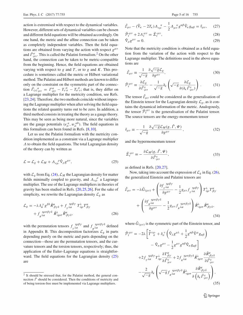
Eur. Phys. J. C (2017) 77:755 Page 5 of 16 755
action is extremised with respect to the dynamical variables.However, different sets of dynamical variables can be chosenand different field equations will be obtained accordingly. Onone hand, the metric and the affine connection can be takenas completely independent variables. Then the field equa-tions are obtained from varying the action with respect gμν
and Γ σ·μν . This is called the Palatini formalism.2 On the otherhand, the connection can be taken to be metric-compatiblefrom the beginning. Hence, the field equations are obtainedvarying with respect to g and T , or to g and K . This pro-cedure is sometimes called the metric or Hilbert variationalmethod. The Palatini and Hilbert methods are known to differonly on the constraint on the symmetric part of the connec-tion Γ(s)
σ·μν = Γ σ·μν − T μν.σ − T μ
σ .ν ; that is, they differ ona Lagrange multiplier for the metricity condition, see Refs.[23,24]. Therefore, the two methods coincide without impos-ing the Lagrange multiplier when after solving the field equa-tions the related quantity turns out to be zero. In addition, athird method consists in treating the theory as a gauge theory.This may be seen as being more natural, since the variablesare the gauge potentials (e a
μ ,w abμ ). The field equations in
this formalism can been found in Refs. [8,10].Let us use the Palatini formalism with the metricity con-
dition implemented as a constraint via a Lagrange multiplierΛ to obtain the field equations. The total Lagrangian densityof the theory can by written as
L = Lg + LM + Λ ρνμ· ∇ρg
μν, (25)
with Lg from Eq. (24), LM the Lagrangian density for matterfields minimally coupled to gravity, and Λ
ρνμ· a Lagrange
multiplier. The use of the Lagrange multipliers in theories ofgravity has been studied in Refs. [20,25,26]. For the sake ofsimplicity, we rewrite the Lagrangian density Lg as
Lg = −λ δ γα gβδ Rα·βγ δ + f ηρβγ
T λα T λ·ηρT α·βγ
+ f ηρσβγ δ
R λα Rλ·ηρσ Rα·βγ δ, (26)
with the permutation tensors f ηρβγ
T λα and f ηρσβγ δ
R λα defined
in Appendix B. This decomposition factorizes Lg in partsdepending purely on the metric and parts depending on theconnection—those are the permutation tensors, and the cur-vature tensors and the torsion tensors, respectively; thus, theapplication of the Euler–Lagrange equations is straightfor-ward. The field equations for the Lagrangian density (25)are
2 It should be stressed that, for the Palatini method, the general con-nection Γ should be considered. Then the conditions of metricity andof being torsion-free must be implemented via Lagrange multipliers.
Eμν − (∇κ − 2Tκ)Λ κνμ· − 1
2Λ κ
μν·gαβ∇κgαβ = τμν, (27)
P ·μντ + 2Λ·μν
τ = Σ ·μντ , (28)
∇ρgμν = 0. (29)
Note that the metricity condition is obtained as a field equa-tion from the variation of the action with respect to theLagrange multiplier. The definitions used in the above equa-tions are
Eμν ≡ 1√−g
∂√−gLg
∂gμν, (30)
P ·μντ ≡ ∂Lg
∂Γ τ·μν
− 1√−g∂κ
(√−g
∂Lg
∂(∂κ Γ τ·μν)
). (31)
The tensor Eμν could be considered as the generalisation ofthe Einstein tensor for the Lagrangian density Lg , as it con-tains the dynamical information of the metric. Analogously,the tensor P ·μν
τ is the generalisation of the Palatini tensor.The source tensors are the energy-momentum tensor
τμν ≡ − 1√−g
∂√−gLM (g, Γ , Ψ )
∂gμν, (32)
and the hypermomentum tensor
Σ ·μντ ≡ − ∂LM (g, Γ , Ψ )
∂Γ τ·μν
, (33)
as defined in Refs. [20,27].Now, taking into account the expression of Lg in Eq. (26),
the generalized Einstein and Palatini tensors are
Eμν = −λG(μν) +⎛⎝∂ f ηρβγ
T λα
∂gμν− 1
2gμν f
ηρβγ
T λα
⎞⎠ T λ·ηρT α·βγ
+⎛⎝∂ f ηρσβγ δ
R λα
∂gμν− 1
2gμν f
ηρσβγ δ
R λα
⎞⎠ Rλ·ηρσ R
α·βγ δ,
(34)
where G(μν) is the symmetric part of the Einstein tensor, and
P ·μντ = −2λ
[
T νμ·σ + δ ν
σ
(∇λg
μλ + 1
2gαβ∇μgαβ
)
− ∇σ gμν − 1
2gμνgαβ∇σ gαβ
]
+2 f ηρβγ
T λα T λ·ηρ∂T α·βγ
∂Γ τ·μν
+ 2 f ηρσβγ δ
R λα Rλ·ηρσ
∂ Rα·βγ δ
∂Γ τ·μν
− 2√−g∂κ
⎛⎝√−g f ηρσβγ δ
R λα Rλ·ηρσ
∂ Rα·βγ δ
∂(∂κ Γ τ·μν
)⎞⎠ ,
(35)
123

755 Page 6 of 16 Eur. Phys. J. C (2017) 77:755
respectively. The full expressions of these tensors in termsof the free parameters of the Lagrangian density are shownin Appendix B.
As the metricity condition has arisen as a field equation,from now on we can consider a metric-compatible connectionΓ . Then the field equations (27) and (28) reduce to
Eμν − ∇κΛ κνμ· = τμν (36)
P ·μντ + 2Λ·μν
τ = Σ ·μντ . (37)
To obtain the final expression for the field equations, theLagrange multiplier Λ must be solved from Eqs. (36) and(37). To this end, note that a generic third rank tensor A canalways be written as
Aαβγ = Δμνρβαγ
(Aμ(νρ) − A[μν]ρ
)(38)
where Δμνρβαγ is defined in Eq. (9). As Λ
ρνμ· is symmetric in
the first two indices, we can solve from Eq. (36)
Λμνρ = 1
2Δαβγ
νμρ
(Σα(βγ ) − Pα(βγ )
). (39)
Thus, the field equations become
Eμν − 1
2Δαβγ
νμκ∇κ (Σα(βγ ) − Pα(βγ )
) = τμν , (40)
Δαβγνμκ
(Σ[αβ]γ − P[αβ]γ
) = 0. (41)
These are the general expressions of the field equations ofany theory of gravity with metricity and torsion. This set ofequations is obviously equivalent to the equations obtainedfrom a Hilbert variational principle over the variables (g, K )
or (g, T ), as can easily be checked. Now, taking into accountthe calculations showed in Appendix B for the Lagrangiandensity (24), these equations are
−λ
(G(μν) − 2∇κ
T (μν)κ
)
+ 1
12(4a + b + 3λ)
(2TαβμT
αβ·ν − TμαβT
·αβν
− 1
2gμνTαβρT
αβρ
)
+ 1
6(−2a + b − 3λ)
(TαβμT
βα·ν − 1
2gμνTαβρT
βρα
)
+ 1
3(−a + 2c − 3λ)
(TμTν − 1
2gμνTαT
α
)
+ 1
6(2p + q)
[2Rαβλμ R
αβλ·ν − 1
2gμν Rαβλσ R
αβλσ
− 4∇κ(∇λ
Rκ(μν)λ + T · λβ
(μ Rν)κλβ
)]+ 1
6(2p + q − 6r)
[2Rα(μ|βλ R
βλα·|ν)
−1
2gμν Rαβλσ R
λσαβ
− 4∇κ(∇λ
Rλ(μν)κ + T · λβ
(μ| Rλβ|ν)κ
)]+ 2
3(p − q)
[2Rα(μ|βλ R
αβ·λ|ν) + Rαλσμ R
ασλν
− Rμαλσ R·λασν − 1
2gμν Rαβλσ R
αβλσ
− 2∇κ(∇λ
Rκ(μν)λ − 2T ·λβκ Rβ(μν)λ
+ 2T ·λβ(μ Rν)βλκ − 2T ·λβ
(μ| Rκβλ|ν)
)]+ (s + t)
[R λ
μ· Rνλ + Rλ·μ Rλν − 1
2gμν Rαβ R
αβ
+∇κ(gμν∇λ
Rκλ + ∇κ R(μν) − ∇(μ Rν)κ
−∇(μ| Rκ|ν) + 1
2T λ
(μ|κ· R|ν)λ − 1
2T λ
κ(μ· Rν)λ
− 1
2T λ
(μν)· Rκλ
)]
+ (s − t)
[R λ
μ· Rλν + Rλ·μ Rνλ − 1
2gμν Rαβ R
βα
+∇κ(gμν∇λ
Rλκ
+∇κ R(μν) − ∇(μ Rν)κ
−∇(μ| Rκ|ν) + 1
2T λ
(μ|κ· Rλ|ν)
− 1
2T λ
κ(μ|· Rλ|ν) − 1
2T λ
(μν)· Rλκ
)]
= τμν + 1
2Δαβγ
νμκ ∇κΣα(βγ ) (42)
and
−2λ
T νμτ + 1
6(4a + b + 3λ)T[τμ]ν
− 1
6(−2a + b − 3λ)
(T[μτ ]ν + Tνμτ
)+ 1
3(−a + b − 3λ)gν[τTμ]
+ 2
3(2p + q)
(∇κ
Rτμνκ − T ·λκν Rτμλκ
)+ 2
3(2p + q − 6r)
(∇κ
Rνκτμ − T ·λκν Rλκτμ
)+ 4
3(p − q)
(∇κ
Rκ[τμ]ν − ∇κRν[τμ]κ − 2T ·λκ
ν Rκ[τμ]λ)
+ (s + t)(
2gν[τ∇κRμ]κ − 2∇[τ Rμ]ν + T λ
ν·[τ Rμ]λ)
+ (s − t)(
2gν[τ |∇κRκ|μ] − 2∇[τ | Rν|μ] + T λ
ν·[τ | Rλ|μ])
= Σ[τμ]ν . (43)
For an interpretation of the right sides of both field equa-tions, see Appendix C.
123
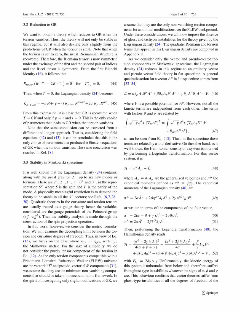
Eur. Phys. J. C (2017) 77:755 Page 7 of 16 755
3.2 Reduction to GR
We want to obtain a theory which reduces to GR when thetorsion vanishes. Thus, the theory will not only be stable inthis regime, but it will also deviate only slightly from thepredictions of GR when the torsion is small. Note that whenthe torsion is set to zero, the usual Riemannian structure isrecovered. Therefore, the Riemann tensor is now symmetricunder the exchange of the first and the second pair of indicesand the Ricci tensor is symmetric. From the first Bianchiidentity (16), it follows that
Rμνρσ
(Rμνρσ − 2Rμρνσ
) = 0 for T α·βγ = 0. (44)
Then, when T = 0, the Lagrangian density (24) becomes
Lg∣∣T=0 = −λ R+(p−r) Rμνρσ R
μνρσ +2 s RμνRμν . (45)
From this expression, it is clear that GR is recovered whenT = 0 if and only if p = r and s = 0. This is the only choiceof parameters that leads to GR when the torsion vanishes.
Note that the same conclusion can be extracted from adifferent and longer approach. That is, considering the fieldequations (42) and (43), it can be concluded that this is theonly choice of parameters that produce the Einstein equationsof GR when the torsion vanishes. The same conclusion wasreached in Ref. [8].
3.3 Stability in Minkowski spacetime
It is well known that the Lagrangian density (24) contains,along with the usual graviton 2+, up to six new modes ortorsions. These are 2+, 2−, 1+, 1−, 0+ and 0−, in the repre-sentation SP where S is the spin and P is the parity of themode. A physically meaningful restriction is to demand thetheory to be stable in all the SP sectors; see Refs. [6,7,28–30]. Quadratic theories in the curvature and torsion tensorsare usually treated as a gauge theory, hence the variablesconsidered are the gauge potentials of the Poincaré group(e a
μ ,w abμ ). Then the stability analysis is made through the
construction of the spin projection operators.In this work, however, we consider the metric formula-
tion. We will examine the decoupling limit between the tor-sion and curvature degrees of freedom. Thus, in view of Eq.(15), we focus on the case where gμν = ημν , with ημν
the Minkowski metric. For the sake of simplicity, we donot consider the purely tensor component of the torsion inEq. (12). As the only torsion components compatible with aFriedmann–Lemaître–Robertson–Walker (FLRW) universeare the vectorialT i and pseudo-vectorial Si components [31],we assume that they are the minimum non-vanishing compo-nents that should be taken into account in this framework. Inthe spirit of investigating only slight modifications of GR, we
assume that they are the only non-vanishing torsion compo-nents for a minimal modification over the FLRW background.Under these considerations, we will now impose the absenceof ghost and tachyon instabilities for the theory given by theLagrangian density (24). The quadratic Riemann and torsionterms that appear in this Lagrangian density are computed inAppendix D.
As we consider only the vector and pseudo-vector tor-sion components in Minkowski spacetime, the Lagrangiandensity (24) reduces in this regime to an ordinary vectorand pseudo-vector field theory in flat spacetime. A generalquadratic action for a vector Aμ in flat spacetime comes from[32–34]
L = α∂μAν∂μAν +β∂μAν∂
ν Aμ + γ ∂μAμ∂ν A
ν −V, (46)
where V is a possible potential for Aμ. However, not all thekinetic terms are independent from each other. The termswith factors β and γ are related by∫ √−g d4x (∇μA
μ)2 =∫ √−g d4x
(∇μAν∇ν Aμ
+Rμν AμAν
), (47)
as can be seen from Eq. (13). Thus, in flat spacetime theseterms are related by a total derivative. On the other hand, as iswell known, the Hamiltonian density of a system is obtainedby performing a Legendre transformation. For this vectorsystem, it is
H = πμ Aμ − L, (48)
where Aμ ≡ ∂0Aμ are the generalized velocities and πμ thecanonical momenta defined as πμ ≡ ∂L
∂ Aμ . The canonicalmomenta of the Lagrangian density (46) are
πμ = 2α Aμ + 2βημν∂ν A0 + 2γ ημ0∂αA
α, (49)
or written in terms of the components of the four-vector,
π0 = 2(α + β + γ ) A0 + 2γ ∂i Ai , (50)
π i = 2α Ai − 2βδi j∂ j A0 . (51)
Then, performing the Legendre transformation (48), theHamiltonian density reads
H = (π0 − 2γ ∂i Ai )2
4(α + β + γ )− (π i + 2β∂i A0)
2
4α+ β
2Fi j F
i j
+α(∂i A0)2 − (α + β)(∂i A j )
2 − γ (∂i Ai )2 + V , (52)
with Fi j = 2∂[i A j]. Unfortunately, the kinetic energy ofthis system is unbounded from below and, therefore, suffersfrom ghost-type instabilities whatever the signs of α, β and γ
are. This behaviour confirms that vector theories suffer fromghost-type instabilities if all the degrees of freedom of the
123

755 Page 8 of 16 Eur. Phys. J. C (2017) 77:755
four-vector Aμ propagates (see Refs. [32,33]). Hence, a nec-essary condition for the absence of this kind of instabilitiesis to make the scalar mode non-dynamical. Alternatively, thevector degrees of freedom can be frozen and propagate onlythe scalar mode, but this corresponds to a scalar theory ratherthan a vectorial one. To remove the scalar mode, the freeparameters of the theory must be chosen in such a way thatthe canonical momenta given in Eq. (50) vanish. Since ∂0A0
and ∂i Ai are independent quantities, the only possibility tocancel out the contribution of ∂i Ai to the canonical momentaof the scalar mode is to set γ = 0. In addition, α + β = 0 isalso needed to remove the contributions of the two remainingkinetic terms in the Lagrangian density (46) to the dynamicsof the scalar mode. With these conditions, the kinetic termsin the vector Lagrangian density becomes a Maxwell-typeFμνFμν that only propagates the spatial degrees of freedomof the four-vector Aμ. This conclusion is in agreement withthe well-known fact that the only ghost-free vector theoryin flat spacetime is the Maxwell–Proca Lagrangian density.Then the Hamiltonian density can be positive-defined withα = −β < 0. For a more detailed discussion on this itemsee Ref. [34].
Back to the Lagrangian density (24), when the metric cor-responds to the Minkowski spacetime the expression reducesto
Lg = 16
9(p + s + t)∂μTν∂
μT ν + 16
9(p − 2r)∂μTν∂
νTμ
+ 16
9(p − r + 5s − t)∂μT
μ∂νTν − 1
9t∂μSν∂
νSμ
+ 1
9(2r + t)∂μSν∂
μSν + 1
18(3q − 4r)∂μS
μ∂νSν
+ 8
27(p − q − 3t)εμνρσ ∂ρTμ∂νSσ − V(T, S), (53)
where V(T, S) are potential-type terms of the torsion fields;see Appendix D. As discussed previously, the free parametersp, q, r , s and t must be carefully selected to produce ghost-free kinetic terms, i.e. Maxwell-type kinetic terms for thetrace four-vector Tμ and pseudo-trace four-vector Sμ. Aftersuitable integrations by parts the expression above simplifiesto
Lg = 8
9(p + s + t)Fμν(T )Fμν(T )
+ 1
18(2r + t)Fμν(S)Fμν(S) + 1
6q∂μS
μ∂νSν
+ 16
3(p − r + 2s)∂μT
μ∂νTν − V(T, S) . (54)
Since we have two dynamical fields, there are two canonicalmomenta. These are
πμT ≡ ∂Lg
∂(∂0Tμ)= 32
9(p + s + t)F0μ(T )
+ 32
3η0μ(p − r + 2s)∂αT
α, (55)
πμS ≡ ∂Lg
∂(∂0Sμ)= 2
9(2r + t)F0μ(S) + 1
3η0μq∂αS
α . (56)
Written in terms of the scalar and vectorial degrees of free-dom of the four-vectors we have
π0T = 32
3(p − r + 2s)∂αT
α , (57)
π iT = 32
9(p + s + t)
(T i − ∂ i T 0
), (58)
π0S = 1
3q ∂αS
α, (59)
π iS = 2
9(2r + t)
(Si − ∂ i S0
). (60)
As here we have two fields with their own kinetic terms, weneed to ensure that neither of them introduces a ghost. Thus,to remove the scalar T 0 and pseudo-scalar S0 degrees offreedom, we consider p−r+2s = 0 and q = 0, respectively.Then the Hamiltonian density reads
Hg = − 9
64
(π iT )2
(p + s + t)− 8
9(p + s + t)Fi j (T )Fi j (T )
− 9
4
(π iS)
2
2r + t− 1
18(2r + t)Fi j (S)Fi j (S)
+π iT ∂i To + π i
S∂i So + V(T, S) . (61)
The kinetic energy can be bounded from below with the extraconditions of p + s + t < 0 and 2r + t < 0 for the vecto-rial and pseudo-vectorial torsion fields, respectively. Theseconditions are summarised in Table 1.
On the other hand, we now require the absence of tachyoninstabilities. In the first place, we consider the weak torsionfields regime, that is, the regime where the quadratic termsin torsion fields lead the evolution of the potential. Thus, thepotential in the Lagrangian density (54) takes the form
V(T, S) = −2
3(c + 3λ)TμT
μ − 1
24(b + 3λ)SμS
μ + O(3);(62)
see Appendix D. Note that the mass terms in an actionfor a vector field comes from a potential of type V (φ) ∝12m
2φμφμ. Hence, the roles of the masses m2 for the vectorand pseudo-vector torsion fields are played by the combina-tions of the coupling constants b, c and λ. For these combi-nations, the correct sign must be taken for the spatial compo-nents to avoid tachyon-like instabilities. In our convention,φμφμ = φ2
0 − φ 2, then the combinations c+ 3λ and b+ 3λ
must be positive to ensure a well-behaved vector and pseudo-vector sector, respectively (see Table 1). In summary, withthese simple arguments we have found a set of conditionsfor the ghost and tachyon stability of the Lagrangian density(24) at the decoupling limit and the weak torsion regime,summarized in Table 1.
123

Eur. Phys. J. C (2017) 77:755 Page 9 of 16 755
Table 1 Conditions over the free parameters of the Lagrangian density (24) for stability and reduction to GR when the torsion vanishes
Tμ Sμ Description
Ghost-free p − r + 2s = 0 q = 0 To remove the scalar/pseudo-scalar mode and to ensure awell-posed kinetic termp + s + t < 0 2r + t < 0
Tachyon-free (Weak torsion) c + 3λ > 0 b + 3λ > 0 To have a positive-defined quadratic potential V(2)
Tachyon-free (General torsion) p + 3s = 0 p + 3s = 0 To cancel V(4) and to make V(2) positive-defined
c + 3λ > 0 b + 3λ > 0
Reduction to GR when T α·μν = 0 p − r = 0
s = 0
In Refs. [6,7], Sezgin and Nieuwenhuizen provided adetailed analysis of the stability of the Lagrangian density(24) for the weak torsion field regime. These two articles werethe first systematic stability analysis of this kind of theories,made with the spin projectors formalism, and they are a keyreference point in this issue. The conclusions they showedfor the 1− torsions are compatible with those obtained here.Their ghost-free condition is the same we have obtainedhere, and the tachyon-free condition is compatible. On theother hand, for the 1+ sector both conclusions are, how-ever, incompatible. While the condition obtained for a well-defined kinetic term for Sμ in this section is 2r + t < 0, theyclaim that 2r + t > 0 is needed. It is worth noting that otherauthors have suggested that the analysis carried out by Sez-gin and Nieuwenhuizen is not restrictive enough to ensure aghost- and tachyon-free spectrum; see Refs. [28,29]. In fact,in Ref. [28] the authors pointed out that they even obtaina different expression of the spin projector operator for thepseudo-vector mode. Furthermore, they argue the relevanceof considering the additional condition for the absence ofp−4 poles in all spin sectors, which is not done in the anal-ysis of Refs. [6,7]. In Ref. [35], Fabbri analyses the stabil-ity of the most general quadratic gravitational action withtorsion and Dirac fields by demanding, in addition, a con-sistent decoupling between curvature and torsion that pre-serves continuity in the torsionless limit, concluding that theonly non-vanishing component of the torsion is given by thepseudo-vector mode and that parity-violating terms are notallowed in the Lagrangian density. Nevertheless, due to somelack of clarity in the existing literature, a deeper analysis ofthe origins of these differences is not available yet.
Let us now go beyond the weak torsion regime whenanalysing the potential V . Thus, higher orders in the potentialcan dominate its evolution. The highest order that appears inthe potential is quartic, symbolically V(4),
V(4)(T, S) = −64
27(p − r + 2s)TαT
αTβTβ
− 1
108(p − r + 2s)SαS
αSβ Sβ
− 8
81(2p + 3q − 4r + 2s)TαS
αTβ Sβ
− 8
81(p + r + 4s)TαT
αSβ Sβ. (63)
As there are terms mixing the vector and pseudo-vector fields,we note that the potential can be diagonalized in the followingbasis:
V(4) =⎛⎝ TαT α
SαSα
TαSα
⎞⎠ V(4)
(TαT α SαSα TαSα
), (64)
with V(4) a 3 × 3 matrix. The eigenvalues of V(4) are
λ1 = − 8
81(2p + 3q − 4r + 2s), (65)
λ2 = −79
72
(p − r + 2s + √
A)
, (66)
λ3 = −79
72
(p − r + 2s − √
A)
, (67)
with
A = 1
7112
(586249p2 − 1168402pr + 586249r2
+ 2349092ps − 2332708rs + 2357284s2)
. (68)
For a positive-defined quadratic form, the three eigenvaluesmust be positive. Since we are only interested in the vec-tor and pseudo-vector torsion degrees of freedom, we canassume p − r + 2s = 0 and q = 0, which are the conditionsfound for making the scalar and pseudo-scalar mode non-dynamic, respectively. Then the expressions of the eigenval-ues reduce to
λ1 = 16
81(p + 3s), (69a)
λ2 = − 8
81(p + 3s), (69b)
λ3 = 8
81(p + 3s). (69c)
123
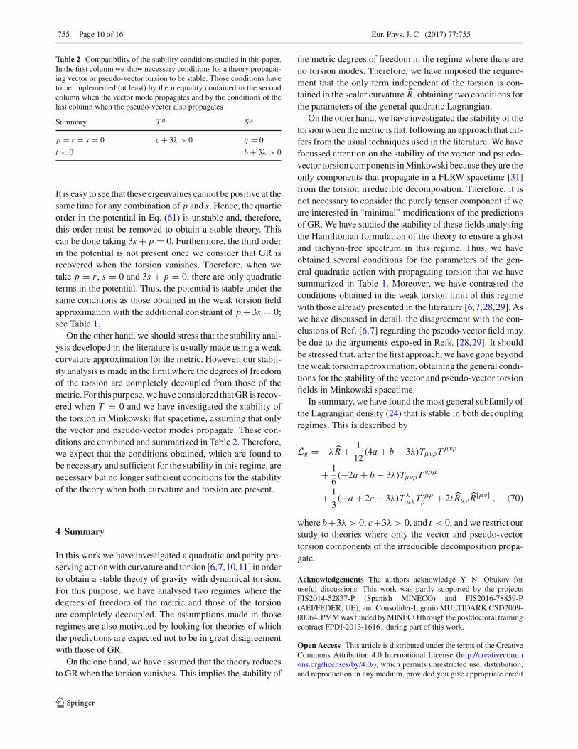
755 Page 10 of 16 Eur. Phys. J. C (2017) 77:755
Table 2 Compatibility of the stability conditions studied in this paper.In the first column we show necessary conditions for a theory propagat-ing vector or pseudo-vector torsion to be stable. Those conditions haveto be implemented (at least) by the inequality contained in the secondcolumn when the vector mode propagates and by the conditions of thelast column when the pseudo-vector also propagates
Summary Tμ Sμ
p = r = s = 0 c + 3λ > 0 q = 0
t < 0 b + 3λ > 0
It is easy to see that these eigenvalues cannot be positive at thesame time for any combination of p and s. Hence, the quarticorder in the potential in Eq. (61) is unstable and, therefore,this order must be removed to obtain a stable theory. Thiscan be done taking 3s + p = 0. Furthermore, the third orderin the potential is not present once we consider that GR isrecovered when the torsion vanishes. Therefore, when wetake p = r , s = 0 and 3s + p = 0, there are only quadraticterms in the potential. Thus, the potential is stable under thesame conditions as those obtained in the weak torsion fieldapproximation with the additional constraint of p + 3s = 0;see Table 1.
On the other hand, we should stress that the stability anal-ysis developed in the literature is usually made using a weakcurvature approximation for the metric. However, our stabil-ity analysis is made in the limit where the degrees of freedomof the torsion are completely decoupled from those of themetric. For this purpose, we have considered that GR is recov-ered when T = 0 and we have investigated the stability ofthe torsion in Minkowski flat spacetime, assuming that onlythe vector and pseudo-vector modes propagate. These con-ditions are combined and summarized in Table 2. Therefore,we expect that the conditions obtained, which are found tobe necessary and sufficient for the stability in this regime, arenecessary but no longer sufficient conditions for the stabilityof the theory when both curvature and torsion are present.
4 Summary
In this work we have investigated a quadratic and parity pre-serving action with curvature and torsion [6,7,10,11] in orderto obtain a stable theory of gravity with dynamical torsion.For this purpose, we have analysed two regimes where thedegrees of freedom of the metric and those of the torsionare completely decoupled. The assumptions made in thoseregimes are also motivated by looking for theories of whichthe predictions are expected not to be in great disagreementwith those of GR.
On the one hand, we have assumed that the theory reducesto GR when the torsion vanishes. This implies the stability of
the metric degrees of freedom in the regime where there areno torsion modes. Therefore, we have imposed the require-ment that the only term independent of the torsion is con-tained in the scalar curvature R, obtaining two conditions forthe parameters of the general quadratic Lagrangian.
On the other hand, we have investigated the stability of thetorsion when the metric is flat, following an approach that dif-fers from the usual techniques used in the literature. We havefocussed attention on the stability of the vector and psuedo-vector torsion components in Minkowski because they are theonly components that propagate in a FLRW spacetime [31]from the torsion irreducible decomposition. Therefore, it isnot necessary to consider the purely tensor component if weare interested in “minimal” modifications of the predictionsof GR. We have studied the stability of these fields analysingthe Hamiltonian formulation of the theory to ensure a ghostand tachyon-free spectrum in this regime. Thus, we haveobtained several conditions for the parameters of the gen-eral quadratic action with propagating torsion that we havesummarized in Table 1. Moreover, we have contrasted theconditions obtained in the weak torsion limit of this regimewith those already presented in the literature [6,7,28,29]. Aswe have discussed in detail, the disagreement with the con-clusions of Ref. [6,7] regarding the pseudo-vector field maybe due to the arguments exposed in Refs. [28,29]. It shouldbe stressed that, after the first approach, we have gone beyondthe weak torsion approximation, obtaining the general condi-tions for the stability of the vector and pseudo-vector torsionfields in Minkowski spacetime.
In summary, we have found the most general subfamily ofthe Lagrangian density (24) that is stable in both decouplingregimes. This is described by
Lg = −λR + 1
12(4a + b + 3λ)TμνρT
μνρ
+ 1
6(−2a + b − 3λ)TμνρT
νρμ
+ 1
3(−a + 2c − 3λ)T λ·μλT
·μρρ + 2t Rμν R
[μν] , (70)
where b+3λ > 0, c+3λ > 0, and t < 0, and we restrict ourstudy to theories where only the vector and pseudo-vectortorsion components of the irreducible decomposition propa-gate.
Acknowledgements The authors acknowledge Y. N. Obukov foruseful discussions. This work was partly supported by the projectsFIS2014-52837-P (Spanish MINECO) and FIS2016-78859-P(AEI/FEDER, UE), and Consolider-Ingenio MULTIDARK CSD2009-00064. PMM was funded by MINECO through the postdoctoral trainingcontract FPDI-2013-16161 during part of this work.
Open Access This article is distributed under the terms of the CreativeCommons Attribution 4.0 International License (http://creativecommons.org/licenses/by/4.0/), which permits unrestricted use, distribution,and reproduction in any medium, provided you give appropriate credit
123

Eur. Phys. J. C (2017) 77:755 Page 11 of 16 755
to the original author(s) and the source, provide a link to the CreativeCommons license, and indicate if changes were made.Funded by SCOAP3.
Appendices
Appendix A: The Gauss–Bonnet term in Riemann–Cartan geometries
We have noted that there is no agreement about the expressionof the Gauss–Bonnet term in a Riemann–Cartan manifoldthroughout the literature, probably due to several misprints.Therefore, in this appendix, we present the correct expressionfor the Gauss–Bonnet action. This is
SGB =∫
d4x√−g
(R2 − 4Rνσ R
σν + Rμνρσ Rρσμν
).
(A.1)
One can easily check that this is the correct order ofthe indices focussing attention on the vectorial and pseudo-vectorial torsion fields in the weak curvature approximation.In this regime we have
gμν = ημν + hμν,
gμν = ημν − hμν . (A.2)
Let us now prove that, order by order in the fields hαβ, Tα andSα , the term (A.1) leads to a total divergence. The expressionsof Rμ·νρσ , Rνσ and R in terms of h are well known in linearizedgravity [36]. These are
Rμ·νρσ = 1
2
(∂ρ∂νh
μσ + ∂μ∂σ hνρ − ∂ρ∂μhνσ
− ∂σ ∂νhμρ
), (A.3)
Rνσ = 1
2
(∂μ∂νh
μσ + ∂σ ∂μh
μν − hσν − ∂σ ∂νh
), (A.4)
R = ∂μ∂νhμν − h , (A.5)
with = ∂μ∂μ. Then, from Eq. (15), it is clear that inthe action (A.1) will appear a Gauss–Bonnet term for theLevi-Civita connection, terms quadratic in torsion and a termmixing torsion and h terms. This action can be expressed as
SGB = S(1)GB(∂h) + S(2)
GB(∂T, ∂S, T, S)
+ S(3)GB(∂h, ∂T, T, S). (A.6)
The first term on the r.h.s. of this equation is known to beinvariant. Nevertheless, this invariance can be proven withan explicit calculation from Eqs. (A.3), (A.4) and (A.5) withthe appropriate boundary conditions on h. The second termis calculated with the results of Appendix D. It can be seenthat
S(2)GB =
∫d4x
√−g
[32
9(∂ρTν∂
νT ρ − ∂αTα∂βT
β)
− 2
9(∂αS
α∂β Sβ − ∂αSβ∂β Sα) + 64
27∂α
(T αTβT
β)
+ 4
27∂α
(T αSβ S
β + 2SαTβ Sβ)
+ 8
9εμνρσ ∂νSσ ∂μTρ
]. (A.7)
After integration by parts, the expression above leads to atotal divergence. Taking the torsion to be zero at the boundaryof U4, S(2)
GB is identically zero. Finally, the third term on the
r.h.s. of Eq. (A.6), S(3)GB(∂h, ∂T, T, S), is analysed using Eqs.
(D.27), (D.28) and (D.29) for the torsion part and (A.3), (A.4)and (A.5) for the metric dependent part. Thus,
S(3)GB =
∫d4x
√−g[4h∂αT
α − 4∂μ∂νhμν∂αT
α
+ 32
3
(∂σ ∂μh
σμ∂αTα − h∂αT
α)
+ 8
3
(∂ρ∂νh∂ρT ν − ∂μ∂νh
μσ ∂σ Tν)]
. (A.8)
Note that there are no mixing terms between ∂h and ∂S or ST ,as expected from parity conservation. After some algebraicalmanipulations and integration by parts, the equation for S(3)
GBvanishes. Hence, we have checked the invariance of an actionupon addition of the action (A.1) in the weak curvature limit.As was pointed by Nieh [21], the Gauss–Bonnet term willremain invariant even in a curved non-flat metric gμν . But,for this work, the invariance in weak field limit is sufficient.
Appendix B: Variations in the Palatini formalism
The Palatini formalism for varying the action consists in tak-ing the metric gμν and the generic connection Γ σ·αβ as thedynamical variables. So, it is useful to rewrite the action interms of those variables. Some useful well-known relationsfor considering that variation are
gμαδgαν = −gανδgμα, δ√−g = −1
2gμνδg
μν . (B.9)
Thus, one can easily obtain
∂μ
√−g = 1
2
√−ggαβ∇μgαβ + √−gΓ α·αμ . (B.10)
Let us know consider the variation of the action written interms of the Lagrangian density (26). This is
Lg = −λ δ γα gβδ Rα·βγ δ + f ηρβγ
T λα T λ·ηρT α·βγ
+ f ηρσβγ δ
R λα Rλ·ηρσ Rα·βγ δ, (B.11)
123
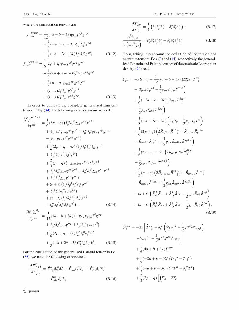
755 Page 12 of 16 Eur. Phys. J. C (2017) 77:755
where the permutation tensors are
f ηρβγ
T λα = 1
12(4a + b + 3λ)gλαg
ηβgργ
+ 1
6(−2a + b − 3λ)δ
γλ δ η
α gρβ
+ 1
3(−a + 2c − 3λ)δ
ρλ δ γ
α gηβ, (B.12)
f ηρσβγ δ
R λα = 1
6(2p + q)gλαg
ηβgργ gσδ
+ 1
6(2p + q − 6r)δ γ
λ δ ρα gηδgσβ
+ 2
3(p − q)gλαg
ηγ gρβgσδ
+ (s + t)δ ρλ δ γ
α gηβgσδ
+ (s − t)δ ρλ δ γ
α gηδgσβ. (B.13)
In order to compute the complete generalized Einsteintensor in Eq. (34), the following expressions are needed:
∂ f ηρσβγ δ
R λα
∂gμν= 1
6(2p + q)
(δ ημ δ β
ν gλαgργ gσδ
+ δ ρμ δ γ
ν gλαgηβgσδ + δ σ
μ δ ην gλαg
ηβgργ
− gαμgλνgηβgργ gσδ
)+ 1
6(2p + q − 6r)
(δ ημ δ δ
ν δγ
λ δ ρα gσβ
+ δ σμ δ β
ν δγ
λ δ ρα gηδ
)+ 2
3(p − q)
(−gλμgανgηγ gρβgσδ
+ δ ημ δ γ
ν gλαgρβgσδ + δ ρ
μ δ βν gλαg
νγ gσδ
+ δ σμ δ δ
ν gλαgνγ gρβ
)+ (s + t)
(δ ημ δ β
ν δρ
λ δ γα gσδ
+ δ σμ δ δ
ν δρ
λ δ γα gηβ
)+ (s − t)
(δ ημ δ δ
ν δρ
λ δ γα gσβ
+δ σμ δ β
ν δρ
λ δ γα gηδ
), (B.14)
∂ f ηρβγ
T λα
∂gμν= 1
12(4a + b + 3λ)
(−gλμgανgηβgργ
+ δ ημ δ β
ν gλαgργ + δ ρ
μ δ γν gλαg
ηβ)
+ 1
6(2p + q − 6r)δ γ
λ δ ηα δ ρ
μ δ βν
+ 1
3(−a + 2c − 3λ)δ
ρλ δγ
α δ ημ δβ
ν . (B.15)
For the calculation of the generalized Palatini tensor in Eq.(35), we need the following expressions:
∂ Rα·βγ δ
∂Γ τ·μν
= Γ α·τγ δμ
β δ νδ − Γ α·τδδ
μβ δ ν
γ + Γμ·βδδ
ατ δ ν
γ
− Γμ·βγ δ α
τ δ νδ , (B.16)
∂T α·βγ
∂Γ τ·μν
= 1
2
(δατ δ
μβ δν
γ − δατ δν
βδμγ
), (B.17)
∂ Rα·βγ δ
∂(∂κ Γ τ·μν
) = δκγ δα
τ δμβ δν
δ − δκδ δα
τ δμβ δν
γ . (B.18)
Then, taking into account the definition of the torsion andcurvature tensors, Eqs. (3) and (14), respectively, the general-ized Einstein and Palatini tensors of the quadratic Lagrangiandensity (24) read
Eμν = −λG(μν) + 1
12(4a + b + 3λ)
(2TαβμT
αβ·ν
− TμαβT·αβν − 1
2gμνTαβρT
αβρ
)
+ 1
6(−2a + b − 3λ)
(TαβμT
βα·ν
− 1
2gμνTαβρT
βρα
)
+ 1
3(−a + 2c − 3λ)
(TμTν − 1
2gμνTαT
α
)
+ 1
6(2p + q)
(2Rαβλμ R
αβλ·ν − Rμαλσ R
·αλσν
+ Rαμλσ Rα·λσν − 1
2gμν Rαβλσ R
αβλσ
)
+ 1
6(2p + q − 6r)
(2Rα(μ|βλRβλα·
|ν)
− 1
2gμν Rαβλσ R
λσαβ
)
+ 2
3(p − q)
(2Rα(μ|βλ R
αβ·λ|ν) + Rαλσμ R
ασλν
− Rμαλσ R·λασν − 1
2gμν Rαβλσ R
αλβσ
)
+ (s + t)
(R λ
μ· Rνλ + Rλ·μ Rλν − 1
2gμν Rαβ R
αβ
)
+ (s − t)
(R λ
μ· Rλν + Rλ·μ Rνλ − 1
2gμν Rαβ R
βα
),
(B.19)
P ·μντ = −2λ
[
T νμ·σ + δ ν
σ
(∇λg
μλ + 1
2gαβ∇μgαβ
)
−∇σ gμν − 1
2gμνgαβ∇σ gαβ
]
+ 1
6(4a + b + 3λ)T ·μν
τ
+ 1
6(−2a + b − 3λ)
(Tμν·
τ − T νμ·τ
)+ 1
3(−a + b − 3λ)
(δ ντ Tμ − δ μ
τ T ν)
+ 2
3(2p + q)
[(∇κ − 2Tκ
123

Eur. Phys. J. C (2017) 77:755 Page 13 of 16 755
+ 1
2gαβ∇κgαβ
)R·μνκ
τ − T ν·λκ R·μλκτ
]
+ 2
3(2p + q − 6r)
[(∇κ − 2Tκ
+ 1
2gαβ∇κgαβ
)R[νκ]·μ
τ − T ν·λκ R[λκ]·μ
τ
]
+ 8
3(p − q)
[(∇κ − 2Tκ + 1
2gαβ∇κgαβ
)R·[κν]μ
τ
− T ν·λκ R·[κλ]μτ
]+ (s + t)
[2δ ν
τ
(∇κ − 2Tκ + 1
2gαβ∇κgαβ
)Rμκ
− 2
(∇τ − 2Tτ + 1
2gαβ∇τ gαβ
)Rμν + T ν·λτ R
μλ
]
+ (s − t)
[2δ ν
τ
(∇κ − 2Tκ + 1
2gαβ∇κgαβ
)Rκμ
− 2
(∇τ − 2Tτ + 1
2gαβ∇τ gαβ
)Rνμ + T ν·λτ R
λμ
].
(B.20)
Appendix C: Source tensors
In order to understand the r.h.s. of the field equations (42) and(43), it is necessary to make a distinction between the Hilbertdefinition of the energy-momentum tensor and the definitioncarried through in Eq. (32). Hilbert’s definition is made in aRiemannian V4 spacetime and, therefore, there is a depen-dence of the matter Lagrangian density on ∂g introduced bythe Levi-Civita connection. This definition is
τμν ≡ − 1√−g
δ√−gLM (g, ∂g, Ψ )
δgμν
= − 1√−g
(∂√−gLM
∂gμν− ∂κ ∂
√−gLM
∂(∂κgμν)
). (C.21)
Nevertheless, in the Palatini formalism this dependence on∂g does not exist, since the matter Lagrangian depends ong and Γ as independent variables. Therefore, the energy-momentum tensor is as in Eq. (32). This is
τμν ≡ − 1√−g
∂√−gLM (g, Γ , Ψ )
∂gμν. (C.22)
There is a clear difference between the two definitions.However, when the metricity condition is implemented,
the connection Γ becomes Γ = Γ + K and, therefore, thereappears a dependence on ∂g in the definition (32). The termΔ
αβγνμκ ∇κ
Σα(βγ ) in the r.h.s. of Eq. (42) takes into accountthis new dependence, which is not present in the originaldefinition of τμν . To check the consistency of this argument,
let us take
δ√−gLM (g, ∂g, T, Ψ )
δgμν=
(∂√−gLM
∂gμν− ∂κ ∂
√−gLM
∂(∂κgμν)
)
=(
∂√−gLM
∂gμν
−∂κ ∂√−gLM
∂Γ·(βγ )α
∂Γ·(βγ )α
∂(∂κgμν)
),
(C.23)
where different tensors have been defined in Eqs. (8), (32)and (33). This leads to
− 1√−g
δ√−gLM (g, ∂g, T, Ψ )
δgμν= τμν+1
2Δαβγ
νμκ ∇κΣα(βγ ) .
(C.24)
The r.h.s. of Eq. (C.24) is exactly the expression on ther.h.s. of Eq. (42), while the l.h.s. is similar to Hilbert’sdefinition of the energy-momentum tensor (C.21). Indeedτμν + 1
2Δαβγνμκ∇κ
Σα(βγ ) is the generalisation of Hilbert’sdefinition of the energy-momentum tensor to the Riemann–Cartan U4 spacetime.
On the other hand, Σ[τμ]ν is related to the contortion ten-sor, which is the remaining part of the connection, see Ref.[27]. Thus, the r.h.s. of Eq. (43) corresponds to the spin dis-tribution tensor
S·μνσ ≡ −∂LM (g, ∂g, T, Ψ )
∂K σ·μν
, (C.25)
as defined in Refs. [4,27].
Appendix D: Vector and pseudo-vector torsion in theweak-gravity regime
In this appendix we are going to take the vector Tμ andpseudo-vector Sμ torsion components as the only non-vanishing torsion fields and calculate the expressions neededfor the analysis carried out in Sect. 3.3.
Assuming that the only non-vanishing components of thetorsion tensor in the decomposition (12) are the vector Tμ andpseudo-vector Sμ torsion components, the expression for thecontortion tensor (11) can be rewritten as
Kμ.νσ = 2
3gμλ(Tνgλσ − Tλgνσ ) + 1
6gμαεανσγ S
γ . (D.26)
123
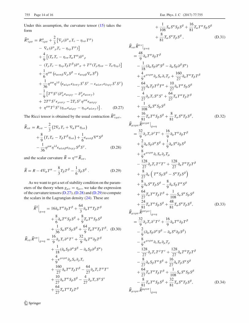
755 Page 14 of 16 Eur. Phys. J. C (2017) 77:755
Under this assumption, the curvature tensor (15) takes theform
Rμ.νρσ = Rμ
.νρσ + 2
3
[∇ρ(δμσ Tν − ηνσ T
μ)
− ∇σ (δμρTν − ηνρT
μ)]
+ 4
9
[(Tσ Tν − ηνσ TαT
α)δμρ
− (TρTν − ηνρTβTβ)δμ
σ + Tμ(Tρηνσ − Tσ ηνρ)]
+ 1
6ημα
(εανσβ∇ρS
β − εανρβ∇σ Sβ)
+ 1
36ημαηλδ
(εαλρτ εδνσγ S
τ Sγ − εαλστ εδνργ Sτ Sγ
)− 1
9
[T αSγ (δμ
σ εανργ − δμρεανσγ )
+ 2TμSγ ερνσγ − 2TνSγ ημαεασργ
+ ημαT λSγ (ηνσ εαλργ − ηνρεαλσγ )]. (D.27)
The Ricci tensor is obtained by the usual contraction Rμ.νμσ ,
Rνσ = Rνσ − 2
3
(2∇σ Tν + ∇αT
αηνσ
)+ 8
9
(TνTσ − TβT
βηνσ
) + 1
6εανσβ∇αSβ
− 1
36ημαηλδεαλσβεδνμγ S
β Sγ , (D.28)
and the scalar curvature R = ηνσ Rνσ ,
R = R − 4∇αTα − 8
3TβT
β − 1
6Sβ S
β . (D.29)
As we want to get a set of stability condition on the param-eters of the theory when gμν = ημν , we take the expressionof the curvature tensors (D.27), (D.28) and (D.29) to computethe scalars in the Lagrangian density (24). These are
R2∣∣∣g=η
= 16∂αTα∂βT
β + 64
3∂αT
αTβTβ
+ 8
6∂αT
αSβ Sβ + 8
9TαT
αSβ Sβ
+ 1
36SαS
αSβ Sβ + 64
9TαT
αTβTβ, (D.30)
Rνσ Rνσ
∣∣g=η
= 16
9∂μTν∂
μT ν + 32
9∂αT
α∂βTβ
+ 1
18(∂αSβ∂αSβ − ∂αSβ∂β Sα)
+ 4
9εμνρσ ∂μSσ ∂ρTν
+ 160
27∂αT
αTβTβ − 64
27∂μTνT
μT ν
+ 10
27∂αT
αSβ Sβ − 4
27∂μTνS
μSν
+ 64
27TαT
αTβTβ
+ 1
108SαS
αSβ Sβ + 16
81TαT
αSβ Sβ
+ 8
81TαS
αTβ Sβ , (D.31)
Rνσ Rσν
∣∣g=η
= 48
9∂αT
α∂βTβ
− 1
18(∂αSβ∂αSβ − ∂αSβ∂β Sα)
+ 4
9εμνρσ ∂μSσ ∂νTρ + 160
27∂αT
αTβTβ
− 64
27∂αTβT
βT α + 10
27∂αT
αSβ Sβ
− 4
27∂μTνS
μSν + 64
27TαT
αTβTβ
+ 1
108SαS
αSβ Sβ
+ 16
81TαT
αSβ Sβ + 8
81TαS
αTβ Sβ, (D.32)
Rμνρσ Rμνρσ
∣∣g=η
= 32
9∂ρTν∂
ρT ν + 16
9∂αT
α∂βTβ
+ 2
9∂αSβ∂αSβ + 1
9∂αS
α∂β Sβ
+ 8
9εμνρσ ∂νSσ ∂ρTμ
− 128
27∂ρTνT
ρT ν + 128
27∂αT
αTβTβ
+ 8
27∂α
(T αSβ S
β − SαTβ Sβ)
+ 8
9∂αS
αTβ Sβ − 8
9∂αSβT
αSβ
+ 64
27TαT
αTβTβ + 1
108SαS
αSβ Sβ
+ 24
81TαT
αSβ Sβ + 48
81TαS
αTβ Sβ, (D.33)
Rμνρσ Rρσμν
∣∣g=η
= 32
9∂ρTν∂
νT ρ + 16
9∂αT
α∂βTβ
− 2
9(∂αSβ∂αSβ − ∂αS
α∂β Sβ)
− 8
9εμνρσ ∂νSσ ∂μTρ
− 128
27∂ρTνT
ρT ν + 128
27∂αT
αTβTβ
− 8
27∂αSβT
αSβ + 16
27∂αTβ S
αSβ
+ 64
27TαT
αTβTβ + 1
108SαS
αSβ Sβ
− 8
81TαT
αSβ Sβ + 32
81TαS
αTβ Sβ, (D.34)
Rμνρσ Rμρνσ
∣∣g=η
123
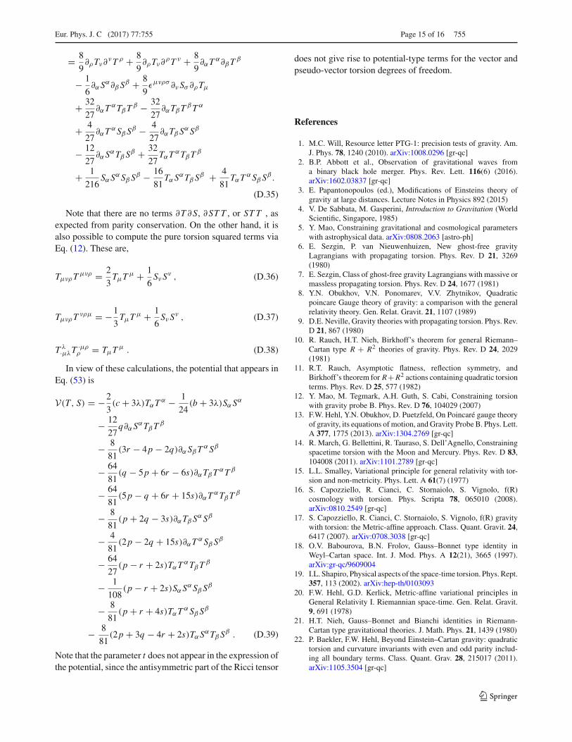
Eur. Phys. J. C (2017) 77:755 Page 15 of 16 755
= 8
9∂ρTν∂
νT ρ + 8
9∂ρTν∂
ρT ν + 8
9∂αT
α∂βTβ
− 1
6∂αS
α∂β Sβ + 8
9εμνρσ ∂νSσ ∂ρTμ
+ 32
27∂αT
αTβTβ − 32
27∂αTβT
βT α
+ 4
27∂αT
αSβ Sβ − 4
27∂αTβ S
αSβ
− 12
27∂αS
αTβ Sβ + 32
27TαT
αTβTβ
+ 1
216SαS
αSβ Sβ − 16
81TαS
αTβ Sβ + 4
81TαT
αSβ Sβ.
(D.35)
Note that there are no terms ∂T ∂S, ∂ST T , or ST T , asexpected from parity conservation. On the other hand, it isalso possible to compute the pure torsion squared terms viaEq. (12). These are,
TμνρTμνρ = 2
3TμT
μ + 1
6SνS
ν , (D.36)
TμνρTνρμ = −1
3TμT
μ + 1
6SνS
ν , (D.37)
T λ·μλT·μρρ = TμT
μ . (D.38)
In view of these calculations, the potential that appears inEq. (53) is
V(T, S) = −2
3(c + 3λ)TαT
α − 1
24(b + 3λ)SαS
α
− 12
27q∂αS
αTβTβ
− 8
81(3r − 4p − 2q)∂αSβT
αSβ
− 64
81(q − 5p + 6r − 6s)∂αTβT
αT β
− 64
81(5p − q + 6r + 15s)∂αT
αTβTβ
− 8
81(p + 2q − 3s)∂αTβ S
αSβ
− 4
81(2p − 2q + 15s)∂αT
αSβ Sβ
− 64
27(p − r + 2s)TαT
αTβTβ
− 1
108(p − r + 2s)SαS
αSβ Sβ
− 8
81(p + r + 4s)TαT
αSβ Sβ
− 8
81(2p + 3q − 4r + 2s)TαS
αTβ Sβ . (D.39)
Note that the parameter t does not appear in the expression ofthe potential, since the antisymmetric part of the Ricci tensor
does not give rise to potential-type terms for the vector andpseudo-vector torsion degrees of freedom.
References
1. M.C. Will, Resource letter PTG-1: precision tests of gravity. Am.J. Phys. 78, 1240 (2010). arXiv:1008.0296 [gr-qc]
2. B.P. Abbott et al., Observation of gravitational waves froma binary black hole merger. Phys. Rev. Lett. 116(6) (2016).arXiv:1602.03837 [gr-qc]
3. E. Papantonopoulos (ed.), Modifications of Einsteins theory ofgravity at large distances. Lecture Notes in Physics 892 (2015)
4. V. De Sabbata, M. Gasperini, Introduction to Gravitation (WorldScientific, Singapore, 1985)
5. Y. Mao, Constraining gravitational and cosmological parameterswith astrophysical data. arXiv:0808.2063 [astro-ph]
6. E. Sezgin, P. van Nieuwenhuizen, New ghost-free gravityLagrangians with propagating torsion. Phys. Rev. D 21, 3269(1980)
7. E. Sezgin, Class of ghost-free gravity Lagrangians with massive ormassless propagating torsion. Phys. Rev. D 24, 1677 (1981)
8. Y.N. Obukhov, V.N. Ponomarev, V.V. Zhytnikov, Quadraticpoincare Gauge theory of gravity: a comparison with the generalrelativity theory. Gen. Relat. Gravit. 21, 1107 (1989)
9. D.E. Neville, Gravity theories with propagating torsion. Phys. Rev.D 21, 867 (1980)
10. R. Rauch, H.T. Nieh, Birkhoff’s theorem for general Riemann–Cartan type R + R2 theories of gravity. Phys. Rev. D 24, 2029(1981)
11. R.T. Rauch, Asymptotic flatness, reflection symmetry, andBirkhoff’s theorem for R+R2 actions containing quadratic torsionterms. Phys. Rev. D 25, 577 (1982)
12. Y. Mao, M. Tegmark, A.H. Guth, S. Cabi, Constraining torsionwith gravity probe B. Phys. Rev. D 76, 104029 (2007)
13. F.W. Hehl, Y.N. Obukhov, D. Puetzfeld, On Poincaré gauge theoryof gravity, its equations of motion, and Gravity Probe B. Phys. Lett.A 377, 1775 (2013). arXiv:1304.2769 [gr-qc]
14. R. March, G. Bellettini, R. Tauraso, S. Dell’Agnello, Constrainingspacetime torsion with the Moon and Mercury. Phys. Rev. D 83,104008 (2011). arXiv:1101.2789 [gr-qc]
15. L.L. Smalley, Variational principle for general relativity with tor-sion and non-metricity. Phys. Lett. A 61(7) (1977)
16. S. Capozziello, R. Cianci, C. Stornaiolo, S. Vignolo, f(R)cosmology with torsion. Phys. Scripta 78, 065010 (2008).arXiv:0810.2549 [gr-qc]
17. S. Capozziello, R. Cianci, C. Stornaiolo, S. Vignolo, f(R) gravitywith torsion: the Metric-affine approach. Class. Quant. Gravit. 24,6417 (2007). arXiv:0708.3038 [gr-qc]
18. O.V. Babourova, B.N. Frolov, Gauss–Bonnet type identity inWeyl–Cartan space. Int. J. Mod. Phys. A 12(21), 3665 (1997).arXiv:gr-qc/9609004
19. I.L. Shapiro, Physical aspects of the space-time torsion. Phys. Rept.357, 113 (2002). arXiv:hep-th/0103093
20. F.W. Hehl, G.D. Kerlick, Metric-affine variational principles inGeneral Relativity I. Riemannian space-time. Gen. Relat. Gravit.9, 691 (1978)
21. H.T. Nieh, Gauss–Bonnet and Bianchi identities in Riemann-Cartan type gravitational theories. J. Math. Phys. 21, 1439 (1980)
22. P. Baekler, F.W. Hehl, Beyond Einstein–Cartan gravity: quadratictorsion and curvature invariants with even and odd parity includ-ing all boundary terms. Class. Quant. Grav. 28, 215017 (2011).arXiv:1105.3504 [gr-qc]
123

755 Page 16 of 16 Eur. Phys. J. C (2017) 77:755
23. J.L. Safko, M. Tsamparlis, Variational methods with torsion ingeneral relativity. Phys. Lett. A 60, 1 (1977)
24. J.L. Safko, F. Elston, Lagrange multipliers and gravitational theory.J. Math. Phys. 17, 1531 (1976)
25. V.N. Ponomariev, Tseytlin, Correct use of Palatini principle in grav-ity theory. Vestnik Mosk. Univ. (ser. fiz. astr.) 6, 57 (1978)
26. W. Kopczynski, The Palatini principle with constraints. Bulletin del’académie Polonaise des sciences, Série de sciences math. astr. etphys. 23, 4 (1975)
27. F.W. Hehl, G.D. Kerlick, P. Von der Heyde, On hypermomentumin general relativity III. Coupling hypermomentum to geometry. Z.Naturforsch. 31A, 823 (1976)
28. R. Kuhfuss, J. Nitsch, Propagating modes in gauge field theoriesof gravity. Gen. Relat. Gravit. 18, 1207 (1986)
29. M. Blagojevic, M. Vasilic, Extra gauge symmetries in a weak-fieldapproximation of an R + T 2 + R2 theory of gravity. Phys. Rev. D35(12) (1987)
30. D.E. Neville, Gravity Lagrangian with ghost-free curvature-squared terms. Phys. Rev. D 18, 3535 (1978)
31. H. Gonner, F. Mueller-Hoissen, Spatially homogeneous andisotropic spaces in theories of gravitation with torsion. Class.Quant. Gravit. 1, 651 (1984)
32. N.L. Gagne, Hamiltonian constraint analysis of vector field theo-ries with spontaneous Lorentz symmetry breaking. Colby College(2008)
33. J. Beltrán Jiménez, A.L. Maroto, Viability of vector-tensor theoriesof gravity. JCAP 0902, 025 (2009). arXiv:0811.0784 [astro-ph]
34. G. Esposito-Farese, C. Pitrou, J.P. Uzan, Vector theories in cosmol-ogy. Phys. Rev. D 81, 063519 (2010). arXiv:0912.0481 [gr-qc]
35. L. Fabbri, A discussion on the most general torsion-gravity withelectrodynamics for Dirac spinor matter fields. Int. J. Geom. Meth.Mod. Phys. 12(09), 1550099 (2015). arXiv:1409.2007 [gr-qc]
36. H. Stephani, Relativity: An Introduction to Special and GeneralRelativity (Cambridge University Press, London, 2004)
123

Chapter 4
Einstein-Yang-Mills systems
4.1 Introduction to Einstein-Yang-Mills theory
Einstein-Yang-Mills (EYM) theory constitutes the general framework to describe thenature as well as the interaction of non-Abelian gauge fields and conventional gravi-tation. Thus, this theory describes the phenomenology of YM fields [83], such as theelectro-weak model or the strong nuclear force associated with quantum chromody-namics, in the presence of a curved space-time and it represents the most naturalgeneralization of the Einstein-Maxwell theory.
Therefore, in principle, the search for non-Abelian systems and heterogeneousBHs in the framework of GR would be admissible. Nevertheless, according to theno-hair conjecture, the structure of a stationary BH is completely determined by itsmass, its orbital angular momentum and its Abelian charge, which means a strongconjectural restriction on the possible existence of BH configurations endowed withYM fields. Despite this assumption, a large number of EYM BHs were systematicallyfound out and classified as counterexamples that manifestly violated it, showing upa notable and richer structure than the ones expected from the Abelian sector [84].
From a mathematical point of view, a gauge field over a pseudo-Riemannianmanifold M is associated with a Lie group G and is described by a connection1-form A in the principal bundle P (M,G), which takes values on the Lie algebra:
Aµ = Aaµ Ta , (4.1)
with Ta the respective generators of such Lie algebra, which satisfy the followingcompleteness relation:
[Ta, Tb] = ifabc Tc , (4.2)
115

116 Chapter 4. Einstein-Yang-Mills systems
where the coefficients fabc are the so called structure constants.
The gauge connection (4.1) defines a covariant derivative on the tangent bundleof G and a 2-form gauge curvature F , which constitutes the YM propagating fieldplaying the role of carrier of the interaction:
Dµ = ∇µ − i [Aµ, · ] , (4.3)
Fµν = ∂µAν − ∂νAµ − i [Aµ, Aν ] . (4.4)
Then, by considering an arbitrary vector vλ, the following commutation relationis satisfied:
[Dµ, Dν ] vλ = Rλρµν v
ρ − i[Fµν , v
λ]. (4.5)
The behaviour of these components under a gauge transformation S ∈ G:
Aµ → A′
µ = S−1AµS + iS−1∂µS , (4.6)
Fµν → F′
µν = S−1FµνS , (4.7)allows the construction of minimal coupling actions by the standard procedure:
S = − 116π
∫(R− tr FµνF µν)
√−g d4x . (4.8)
The metric tensor and the gauge connection represent the main variables in thisapproach and their variations lead to the general EYM equations:
Dµ Fµν = 0 , (4.9)
Gµν = 8πTµν , (4.10)
where Tµν = 14π tr
(14gµνFλρF
λρ − FµρFν ρ)
is the energy-momentum tensor asso-ciated with the YM field. Furthermore, the divergenceless of the Einstein tensorimplies the same for the energy-momentum tensor of the YM field, which also sat-isfies the following identity from its propagating equation (4.9):
DµDν Fµν = 0 . (4.11)

4.1. Introduction to Einstein-Yang-Mills theory 117
Indeed, this quantity is proportional to the contraction of the commutator ofthe covariant derivatives and the gauge curvature, which vanishes identically sincethe Ricci tensor constitutes a symmetric quantity in Riemannian geometry and thecommutator of two field strength tensors is zero:
12 [Dµ, Dν ]F µν = RµνF
µν − i
2 [Fµν , F µν ] . (4.12)
In order to solve the EYM field equations, it is possible to simplify the problem byapplying a suitable set of internal gauge transformations that preserve the invarianceof the gauge connection under space-time symmetries [85]. Specifically, the changein the gauge potential Aµ → A′µ = Aµ − LξAµ under the infinitesimal coordinatetransformation xµ → x′µ = xµ+ξµ can be compensated by the following infinitesimalgauge transformation:
A′µ → Aµ = A′µ + ∂µω − i [Aµ, ω] , (4.13)
where ∂µω − i [Aµ, ω] = LξAµ implies the equality Aµ = Aµ in the present gauge.Such a gauge condition represents a strong constraint for the covariant componentof the connection that can be solved in special cases, like the one given by the gaugegroup SU(2) in the presence of a static and spherically symmetric space-time (seeAppendix C for a detailed resolution within this context). In this sense, the finalexpression for the gauge connection acquires the following structure [86]:
A = p(r) τ3 dt+ u(r) τ3 dr + (v(r) τ1 + w(r) τ2) dθ1
+ (cot θ1 τ3 + v(r) τ2 − w(r) τ1) sin θ1dθ2 , (4.14)
with p, u, v and w four arbitrary functions depending on r and τii=1,2,3 the gener-ators related to SU(2), which obey the standard commutation relations:
[τi, τj] = iεijkτk . (4.15)
In addition, besides the strong simplification provided by this symmetry con-dition, the remaining group of residual gauge transformations still preserves thisansatz and may restrict even more the number of degrees of freedom involved inthe problem. In this case, the gauge transformation V1 = eiα(r)τ3 with α′(r) = u(r)allows the vanishing of the spatial component A3
r without changing the structure of(4.14).
Thereby, the corresponding gauge curvature associated with this simple ansatzreads:
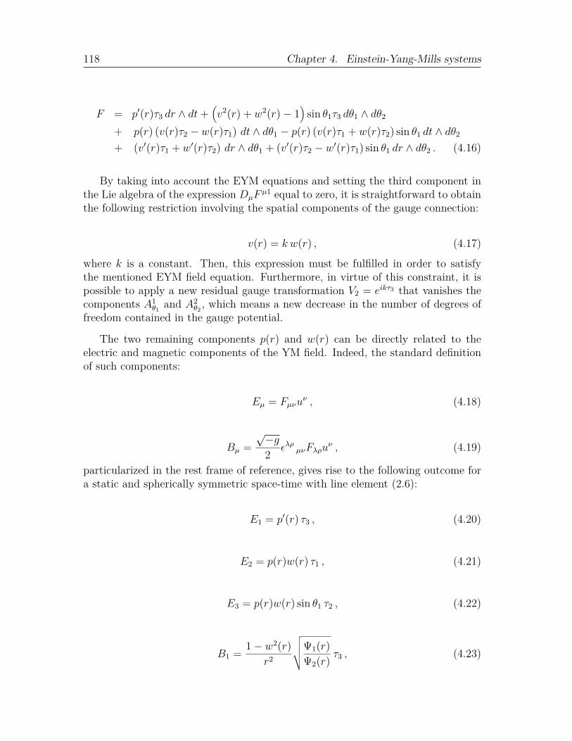
118 Chapter 4. Einstein-Yang-Mills systems
F = p′(r)τ3 dr ∧ dt+(v2(r) + w2(r)− 1
)sin θ1τ3 dθ1 ∧ dθ2
+ p(r) (v(r)τ2 − w(r)τ1) dt ∧ dθ1 − p(r) (v(r)τ1 + w(r)τ2) sin θ1 dt ∧ dθ2
+ (v′(r)τ1 + w′(r)τ2) dr ∧ dθ1 + (v′(r)τ2 − w′(r)τ1) sin θ1 dr ∧ dθ2 . (4.16)
By taking into account the EYM equations and setting the third component inthe Lie algebra of the expression DµF
µ1 equal to zero, it is straightforward to obtainthe following restriction involving the spatial components of the gauge connection:
v(r) = k w(r) , (4.17)
where k is a constant. Then, this expression must be fulfilled in order to satisfythe mentioned EYM field equation. Furthermore, in virtue of this constraint, it ispossible to apply a new residual gauge transformation V2 = eikτ3 that vanishes thecomponents A1
θ1 and A2θ2 , which means a new decrease in the number of degrees of
freedom contained in the gauge potential.
The two remaining components p(r) and w(r) can be directly related to theelectric and magnetic components of the YM field. Indeed, the standard definitionof such components:
Eµ = Fµνuν , (4.18)
Bµ =√−g2 ελρ µνFλρu
ν , (4.19)
particularized in the rest frame of reference, gives rise to the following outcome fora static and spherically symmetric space-time with line element (2.6):
E1 = p′(r) τ3 , (4.20)
E2 = p(r)w(r) τ1 , (4.21)
E3 = p(r)w(r) sin θ1 τ2 , (4.22)
B1 = 1− w2(r)r2
√√√√Ψ1(r)Ψ2(r) τ3 , (4.23)
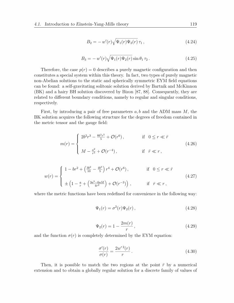
4.1. Introduction to Einstein-Yang-Mills theory 119
B2 = −w′(r)√
Ψ1(r)Ψ2(r) τ1 , (4.24)
B3 = −w′(r)√
Ψ1(r)Ψ2(r) sin θ1 τ2 . (4.25)
Therefore, the case p(r) = 0 describes a purely magnetic configuration and thenconstitutes a special system within this theory. In fact, two types of purely magneticnon-Abelian solutions to the static and spherically symmetric EYM field equationscan be found: a self-gravitating solitonic solution derived by Bartnik and McKinnon(BK) and a hairy BH solution discovered by Bizon [87, 88]. Consequently, they arerelated to different boundary conditions, namely to regular and singular conditions,respectively.
First, by introducing a pair of free parameters a, b and the ADM mass M , theBK solution acquires the following structure for the degrees of freedom contained inthe metric tensor and the gauge field:
m(r) =
2b2r3 − 8b3r5
5 +O(r6) , if 0 ≤ r r
M − a2
r3 +O(r−4) , if r r ,
(4.26)
w(r) =
1− br2 +
(3b2
10 −4b3
5
)r4 +O(r6) , if 0 ≤ r r
±(1− a
r+(
3a2−6aM4r2
)+O(r−3)
), if r r ,
(4.27)
where the metric functions have been redefined for convenience in the following way:
Ψ1(r) = σ2(r)Ψ2(r) , (4.28)
Ψ2(r) = 1− 2m(r)r
, (4.29)
and the function σ(r) is completely determined by the EYM equation:
σ′(r)σ(r) = 2w′ 2(r)
r. (4.30)
Then, it is possible to match the two regions at the point r by a numericalextension and to obtain a globally regular solution for a discrete family of values of

120 Chapter 4. Einstein-Yang-Mills systems
n an bn Mn
1 0.8933 0.4537 0.82862 8.8638 0.6517 0.97133 58.9290 0.6970 0.99534 366.2000 0.7048 0.99925 2246.8000 0.7061 0.9998
Table 4.1: Parameters of the BK solution.
the parameters, which can be labeled by a natural number n (see table 4.1 to checkthe first values of the family an, bn,Mn, from n = 1 to n = 5).
The geometry shows three principal regions that evince the richer structure pro-vided by the interaction between gravity and non-Abelian gauge fields: a high den-sity region characterized by an intense YM field strength, a near-field zone wherethe metric is approximately a Reissner-Nordstrom (RN) type with unit magneticcharge and a far-field region where this charge decays asymptotically to zero andthe metric resembles the Schwarzschild geometry with mass Mn. The balance be-tween the attractive component of the gravitational field and the repulsive forcesapplied by the SU(2) field allows the existence of this equilibrium configuration andprevents the formation of singularities in the space-time.
As can be seen from Fig. 4.1, the contrast existing between these zones becomeseven more remarkable for higher values of n, where it is worthwhile to stress thefast increase of the ADM mass and the corresponding transition to heavier self-gravitating states within this context. Furthermore, this parameter also providesthe number of nodes of the function w(r), which moreover is bounded within theinterval [−1, 1].
The BH configuration also constitutes a discrete family of solutions and presentsthe same geometrical pattern with the cited transition zones, but it includes theexistence of a regular event horizon provided by the following singular boundaryconditions:
Ψ2(r) =
r2h−(w2
h−1)2
r3h
(r − rh) +O((r − rh)2
), if r ≈ rh
1− 2Mr
+ 2a2
3r4 +O(r−5) , if rh r ,
(4.31)

4.1. Introduction to Einstein-Yang-Mills theory 121
Figure 4.1: Obtained from [84]. w(r) and the effective mass m(r) for the lowest BK solution.
w(r) =
wh + whr
3h(w2
h−1)r2h−(w2
h−1)2 (r − rh) +O
((r − rh)2
), if r ≈ rh
±(1− a
r+ 3a2−6aM
4r2 +O(r−3)), if rh r ,
(4.32)
where the parameter rh indicates the location of the event horizon of the solutionand wh the value of function w(r) at r = rh. In addition, the interior region inthe vicinity r ≈ 0 of the essential singularity can be numerically matched by threedistinct types of local solutions (see [84] for further details on interior solutions).
The existence of these regular and BH solutions constitutes the first exampleof a self-gravitating system coupled to a non-Abelian gauge field and also the firstmanifest violation of the no-hair conjecture in the framework of the EYM theory.Nevertheless, a large class of analytical and numerical studies have been showntheir instability under small spherically symmetric perturbations and, furthermore,in the nonlinear regime [89–92], which strongly questions its validity as a viableconfiguration in nature.
On the other hand, from a theoretical point of view, a large variety of extendedsolutions to the EYM equations have also been systematically found by differentauthors, including the application of higher rank non-Abelian groups or the incor-poration of a cosmological constant and external fields into the general action, suchas the dilaton and the Higgs fields [93–99], which represents a considerable numberof examples and theoretical illustrations within this field.
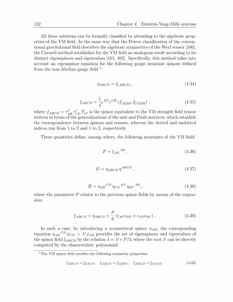
122 Chapter 4. Einstein-Yang-Mills systems
All these solutions can be formally classified by attending to the algebraic prop-erties of the YM field. In the same way that the Petrov classification of the conven-tional gravitational field describes the algebraic symmetries of the Weyl tensor [100],the Carmeli method establishes for the YM field an analogous result according to itsdistinct eigenspinors and eigenvalues [101, 102]. Specifically, this method takes intoaccount an eigenspinor equation for the following gauge invariant spinors definedfrom the non-Abelian gauge field 1:
ηABCD = ξ(ABCD) , (4.34)
ξABCD = 14ε
EF ε GH (fAEBF fCGDH) , (4.35)
where fABCD = τµAB
τ νCD
Fµν is the spinor equivalent to the YM strength field tensorwritten in terms of the generalizations of the unit and Pauli matrices, which establishthe correspondence between spinors and tensors, whereas the dotted and undottedindices run from 1 to 2 and 1 to 2, respectively.
These quantities define, among others, the following invariants of the YM field:
P = ξABAB , (4.36)
G = ηABCD ηABCD , (4.37)
H = ηABCD ηCD
EF ηEFAB , (4.38)
where the parameter P relates to the previous spinor fields by means of the expres-sion:
ξABCD = ηABCD + P
6 (εACεBD + εADεBC) . (4.39)
In such a case, by introducing a symmetrical spinor φAB, the correspondingequation ηAB
CD φCD = λ′ φAB provides the set of eigenspinors and eigenvalues ofthe spinor field ξABCD by the relation λ = λ′+P/3, where the root λ′ can be directlycomputed by the characteristic polynomial:
1The YM spinor field satisfies the following symmetry properties:
ξABCD = ξBACD , ξABCD = ξABDC , ξABCD = ξCDAB . (4.33)

4.1. Introduction to Einstein-Yang-Mills theory 123
p(λ′) = λ′ 3 −Gλ′/2−H/3 . (4.40)
Hence, the classification scheme of the principal spinor ξABCD reduces to thealternative and simpler classification of the totally symmetric spinor ηABCD. Thedistinct families of eigenspinors and eigenvalues allow the YM field to be catego-rized in a systematic way, which in fact improves the physical understanding of theEYM solutions. In table 4.2, the possible algebraic symmetry types are displayed,according to the number of degenerate eigenvalues and linearly independent spinors,as well as to the value of the invariant P . Note that, for each symmetry type, it ispossible to express the quantity ξABCD in terms of up to four arbitrary one-indexspinors LA,MA, NA and KA.
This algebraic structure points out the existence of different degenerate levels,in the sense that possible transitions with a consequent loss of generality can occur(see diagram 4.2).
The particularization to the purely magnetic SU(2) gauge field in a static andspherically symmetric geometry can then be accomplished by computing the com-ponents of the associated YM spinors and their gauge invariants. By consideringthe line element defined by Expression (2.6) and the gauge curvature (4.16) withp(r) = v(r) = 0, these components are:
η1111 = ξ1111 , (4.41)
η2222 = ξ2222 , (4.42)
η1122 = 112r2
((w2(r)− 1)2
r2 −Ψ2(r)w′ 2(r)), (4.43)
ξ1111 = ξ2222 , (4.44)
ξ2222 = 14r2
(Ψ2(r)w′ 2(r)− (w2(r)− 1)2
r2
), (4.45)
ξ1122 = 14r2
(Ψ2(r)w′ 2(r) + (w2(r)− 1)2
r2
), (4.46)
ξ1212 = − Ψ2(r)w′ 2(r)4r2 , (4.47)
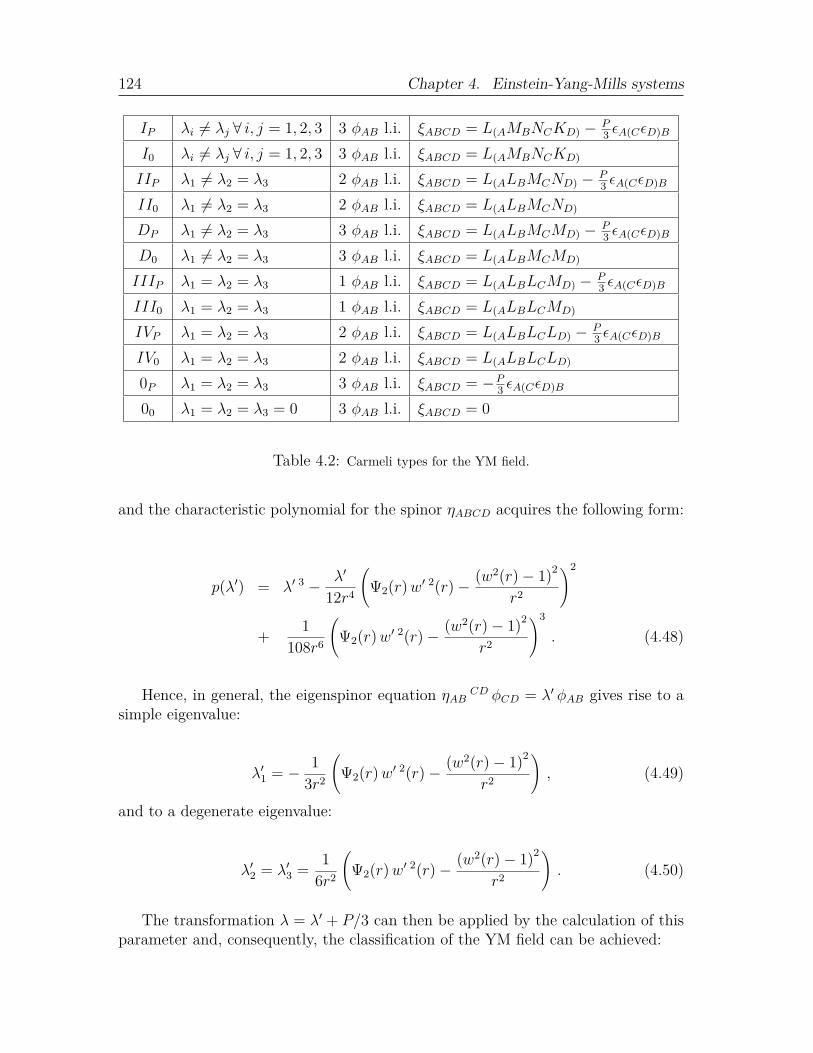
124 Chapter 4. Einstein-Yang-Mills systems
IP λi 6= λj ∀ i, j = 1, 2, 3 3 φAB l.i. ξABCD = L(AMBNCKD) − P3 εA(CεD)B
I0 λi 6= λj ∀ i, j = 1, 2, 3 3 φAB l.i. ξABCD = L(AMBNCKD)
IIP λ1 6= λ2 = λ3 2 φAB l.i. ξABCD = L(ALBMCND) − P3 εA(CεD)B
II0 λ1 6= λ2 = λ3 2 φAB l.i. ξABCD = L(ALBMCND)
DP λ1 6= λ2 = λ3 3 φAB l.i. ξABCD = L(ALBMCMD) − P3 εA(CεD)B
D0 λ1 6= λ2 = λ3 3 φAB l.i. ξABCD = L(ALBMCMD)
IIIP λ1 = λ2 = λ3 1 φAB l.i. ξABCD = L(ALBLCMD) − P3 εA(CεD)B
III0 λ1 = λ2 = λ3 1 φAB l.i. ξABCD = L(ALBLCMD)
IVP λ1 = λ2 = λ3 2 φAB l.i. ξABCD = L(ALBLCLD) − P3 εA(CεD)B
IV0 λ1 = λ2 = λ3 2 φAB l.i. ξABCD = L(ALBLCLD)
0P λ1 = λ2 = λ3 3 φAB l.i. ξABCD = −P3 εA(CεD)B
00 λ1 = λ2 = λ3 = 0 3 φAB l.i. ξABCD = 0
Table 4.2: Carmeli types for the YM field.
and the characteristic polynomial for the spinor ηABCD acquires the following form:
p(λ′) = λ′ 3 − λ′
12r4
(Ψ2(r)w′ 2(r)− (w2(r)− 1)2
r2
)2
+ 1108r6
(Ψ2(r)w′ 2(r)− (w2(r)− 1)2
r2
)3
. (4.48)
Hence, in general, the eigenspinor equation ηABCD φCD = λ′ φAB gives rise to a
simple eigenvalue:
λ′1 = − 13r2
(Ψ2(r)w′ 2(r)− (w2(r)− 1)2
r2
), (4.49)
and to a degenerate eigenvalue:
λ′2 = λ′3 = 16r2
(Ψ2(r)w′ 2(r)− (w2(r)− 1)2
r2
). (4.50)
The transformation λ = λ′ + P/3 can then be applied by the calculation of thisparameter and, consequently, the classification of the YM field can be achieved:

4.1. Introduction to Einstein-Yang-Mills theory 125
Figure 4.2: Diagram of classification of YM fields.
λ1 = (w2(r)− 1)2
2r4 , (4.51)
λ2 = λ3 = Ψ2(r)w′ 2(r)2r2 , (4.52)
with:
P = 12r2
(2Ψ2(r)w′ 2(r) + (w2(r)− 1)2
r2
). (4.53)
i) λ1 6= λ2 = λ3
In this case, there exist three linearly independent eigenspinors and a non-vanishing gauge invariant P :
Bφ =
1 0
0 − 1
,
1 00 1
,
0 11 0
. (4.54)
Therefore, the YM field constitutes a type DP and is associated with isolatedgravitating systems. Note that the embedded RN solution with unit magneticcharge, given by the condition w(r) = 0, also belongs to this class of symmetry.

126 Chapter 4. Einstein-Yang-Mills systems
ii) λ1 = λ2 = λ3
In this case, there exist only one degenerate eigenvalue on account of the relation:
Ψ2(r)w′ 2(r) = (w2(r)− 1)2
r2 , (4.55)
which additionally involves the vanishing of the completely symmetric spinor ηABCDand the simplification of the gauge invariant:
P = 3 (w2(r)− 1)2
2r4 . (4.56)
The number of linearly independent eigenspinors is once again three, whichmeans that the YM field reduces to a type 0P if w(r) 6= ±1 or to a type 00 ifw(r) = ±1, namely if the YM field vanishes identically and the solution coincideswith the Schwarzschild solution:
Bφ =
1 0
0 1
,
1 00 − 1
,
0 11 0
. (4.57)

Eur. Phys. J. C (2017) 77:853 https://doi.org/10.1140/epjc/s10052-017-5425-1
Regular Article - Theoretical Physics
Einstein–Yang–Mills–Lorentz black holes
Jose A. R. Cembranosa, Jorge Gigante Valcarcelb
Departamento de Física Teórica I, Universidad Complutense de Madrid, 28040 Madrid, Spain
Received: 5 July 2016 / Accepted: 23 November 2017© The Author(s) 2017. This article is an open access publication
Abstract Different black hole solutions of the coupledEinstein–Yang–Mills equations have been well known fora long time. They have attracted much attention from math-ematicians and physicists since their discovery. In this work,we analyze black holes associated with the gauge Lorentzgroup. In particular, we study solutions which identify thegauge connection with the spin connection. This ansatzallows one to find exact solutions to the complete systemof equations. By using this procedure, we show the equiv-alence between the Yang–Mills–Lorentz model in curvedspace-time and a particular set of extended gravitational the-ories.
1 Introduction
The dynamical interacting system of equations related tonon-abelian gauge theories defined on a curved space-timeis known as Einstein–Yang–Mills (EYM) theory. Thus, thistheory describes the phenomenology of Yang–Mills fields[1] interacting with the gravitational attraction, such as theelectro-weak model or the strong nuclear force associatedwith quantum chromodynamics. The EYM model constitutesa paradigmatic example of the non-linear interactions relatedto gravitational phenomenology. Indeed, the evolution of aspherical symmetric system obeying these equations can bevery rich. Its dynamics is opposite to the one predicted byother models, such as the ones provided by the Einstein–Maxwell (EM) equations, whose static behaviour is enforcedby a version of the Birkhoff theorem.
For instance, in the four-dimensional space-time, theEYM equations associated with the gauge group SU (2) sup-port a discrete family of static self-gravitating solitonic solu-tions, found by Bartnik and McKinnon [2]. There are alsohairy black hole (BH) solutions, as was shown by Bizon
a e-mail: [email protected] e-mail: [email protected]
[3–5]. They are known as colored black holes and can belabeled by the number of nodes of the exterior Yang–Millsfield configuration. Although the Yang–Mills fields do notvanish completely outside the horizon, these solutions arecharacterized by the absence of a global charge. This featureis opposite to the one predicted by the standard BH unique-ness theorems related to the EM equations, whose solutionscan be classified solely with the values of the mass, (electricand/or magnetic) charge and angular momentum evaluatedat infinity. In any case, the EYM model also supports theReissner–Nordström BH as an embedded abelian solutionwith global electric and/or magnetic charge [6]. It is alsointeresting to mention that there are a larger variety of solu-tions associated with different generalizations of the EYMequations extended with dilaton fields, higher curvature cor-rections, Higgs fields, merons or cosmological constants (see[7,8] and the references therein).
In this work, we are interested in finding solutions of theEYM equations associated with the Lorentz group as gaugegroup. The main motivation for considering such a gaugesymmetry is offered by the spin connection dynamics. Thisconnection is introduced for a consistent description of spinorfields defined on curved space-times. Although general coor-dinate transformations do not have spinor representations [9],they can be described by the representations associated withthe Lorentz group. In addition, they can be used to definealternative theories of gravity [10].
We shall impose the requirement that the spin connectionis dynamical and its evolution is determined by the Yang–Mills action related to the SO(1, n − 1) symmetry, where nis the number of dimensions of the space-time. In order tocomplete the EYM equations, we shall assume that gravita-tion is described by the metric of a Lorentzian manifold. Weshall find vacuum analytic solutions to the EYM system bychoosing a particular ansatz, which will relate the spin con-nection to the gauge connection. Therefore, this assumptionprovides additional gravitational degrees of freedom besidesthe ones given by the standard case, so that all the BH con-
123
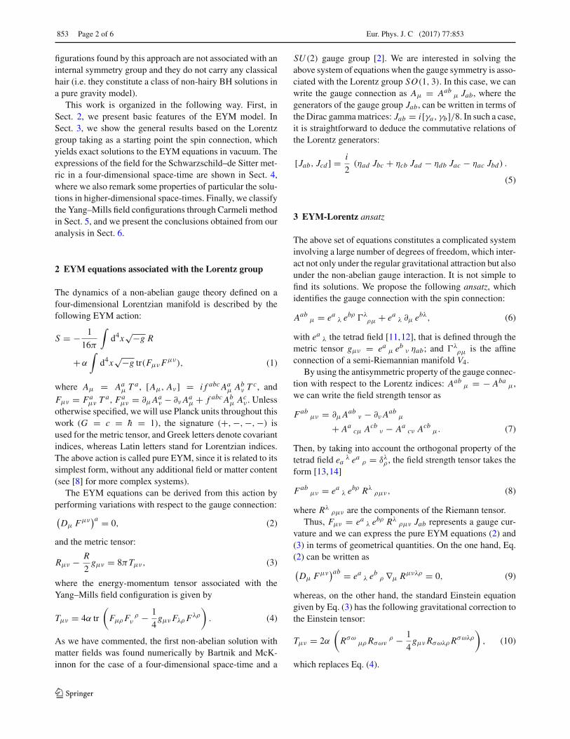
853 Page 2 of 6 Eur. Phys. J. C (2017) 77:853
figurations found by this approach are not associated with aninternal symmetry group and they do not carry any classicalhair (i.e. they constitute a class of non-hairy BH solutions ina pure gravity model).
This work is organized in the following way. First, inSect. 2, we present basic features of the EYM model. InSect. 3, we show the general results based on the Lorentzgroup taking as a starting point the spin connection, whichyields exact solutions to the EYM equations in vacuum. Theexpressions of the field for the Schwarzschild–de Sitter met-ric in a four-dimensional space-time are shown in Sect. 4,where we also remark some properties of particular the solu-tions in higher-dimensional space-times. Finally, we classifythe Yang–Mills field configurations through Carmeli methodin Sect. 5, and we present the conclusions obtained from ouranalysis in Sect. 6.
2 EYM equations associated with the Lorentz group
The dynamics of a non-abelian gauge theory defined on afour-dimensional Lorentzian manifold is described by thefollowing EYM action:
S = − 1
16π
∫d4x
√−g R
+α
∫d4x
√−g tr(FμνFμν), (1)
where Aμ = Aaμ T a , [Aμ, Aν] = i f abc Aa
μ Abν T
c, andFμν = Fa
μν Ta , Fa
μν = ∂μAaν − ∂ν Aa
μ + f abc Abμ Ac
ν . Unlessotherwise specified, we will use Planck units throughout thiswork (G = c = h = 1), the signature (+,−,−,−) isused for the metric tensor, and Greek letters denote covariantindices, whereas Latin letters stand for Lorentzian indices.The above action is called pure EYM, since it is related to itssimplest form, without any additional field or matter content(see [8] for more complex systems).
The EYM equations can be derived from this action byperforming variations with respect to the gauge connection:(Dμ Fμν
)a = 0, (2)
and the metric tensor:
Rμν − R
2gμν = 8πTμν, (3)
where the energy-momentum tensor associated with theYang–Mills field configuration is given by
Tμν = 4α tr
(FμρF
ρν − 1
4gμνFλρF
λρ
). (4)
As we have commented, the first non-abelian solution withmatter fields was found numerically by Bartnik and McK-innon for the case of a four-dimensional space-time and a
SU (2) gauge group [2]. We are interested in solving theabove system of equations when the gauge symmetry is asso-ciated with the Lorentz group SO(1, 3). In this case, we canwrite the gauge connection as Aμ = Aab
μ Jab, where thegenerators of the gauge group Jab, can be written in terms ofthe Dirac gamma matrices: Jab = i[γa, γb]/8. In such a case,it is straightforward to deduce the commutative relations ofthe Lorentz generators:
[Jab, Jcd ] = i
2(ηad Jbc + ηcb Jad − ηdb Jac − ηac Jbd) .
(5)
3 EYM-Lorentz ansatz
The above set of equations constitutes a complicated systeminvolving a large number of degrees of freedom, which inter-act not only under the regular gravitational attraction but alsounder the non-abelian gauge interaction. It is not simple tofind its solutions. We propose the following ansatz, whichidentifies the gauge connection with the spin connection:
Aabμ = ea λ e
bρ λρμ + ea λ ∂μ ebλ, (6)
with ea λ the tetrad field [11,12], that is defined through themetric tensor gμν = ea μ eb ν ηab; and λ
ρμ is the affineconnection of a semi-Riemannian manifold V4.
By using the antisymmetric property of the gauge connec-tion with respect to the Lorentz indices: Aab
μ = − Abaμ,
we can write the field strength tensor as
Fabμν = ∂μA
abν − ∂ν A
abμ
+ Aacμ Acb
ν − Aacν Acb
μ. (7)
Then, by taking into account the orthogonal property of thetetrad field ea λ ea ρ = δλ
ρ , the field strength tensor takes theform [13,14]
Fabμν = ea λ e
bρ Rλρμν, (8)
where Rλρμν are the components of the Riemann tensor.
Thus, Fμν = ea λ ebρ Rλρμν Jab represents a gauge cur-
vature and we can express the pure EYM equations (2) and(3) in terms of geometrical quantities. On the one hand, Eq.(2) can be written as(Dμ Fμν
)ab = ea λ eb
ρ ∇μ Rμνλρ = 0, (9)
whereas, on the other hand, the standard Einstein equationgiven by Eq. (3) has the following gravitational correction tothe Einstein tensor:
Tμν = 2α
(Rσω
μρRσωνρ − 1
4gμνRσωλρR
σωλρ
), (10)
which replaces Eq. (4).
123
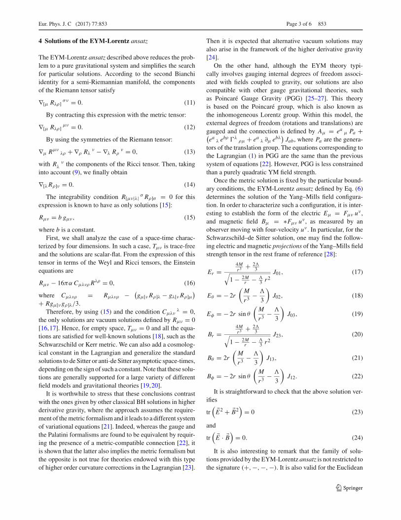
Eur. Phys. J. C (2017) 77:853 Page 3 of 6 853
4 Solutions of the EYM-Lorentz ansatz
The EYM-Lorentz ansatz described above reduces the prob-lem to a pure gravitational system and simplifies the searchfor particular solutions. According to the second Bianchiidentity for a semi-Riemannian manifold, the componentsof the Riemann tensor satisfy
∇[μ Rλρ] σν = 0. (11)
By contracting this expression with the metric tensor:
∇[μ Rλρ] μν = 0. (12)
By using the symmetries of the Riemann tensor:
∇μ Rμνλρ + ∇ρ Rλ
ν − ∇λ Rρν = 0, (13)
with R νλ the components of the Ricci tensor. Then, taking
into account (9), we finally obtain
∇[λRρ]ν = 0. (14)
The integrability condition R[μν|λ| σ Rρ]σ = 0 for thisexpression is known to have as only solutions [15]:
Rμν = b gμν, (15)
where b is a constant.First, we shall analyze the case of a space-time charac-
terized by four dimensions. In such a case, Tμν is trace-freeand the solutions are scalar-flat. From the expression of thistensor in terms of the Weyl and Ricci tensors, the Einsteinequations are
Rμν − 16πα CμλνρRλρ = 0, (16)
where Cμλνρ = Rμλνρ − (gμ[νRρ]λ − gλ[νRρ]μ
)+ Rgμ[νgρ]λ/3.
Therefore, by using (15) and the condition Cμλνλ = 0,
the only solutions are vacuum solutions defined by Rμν = 0[16,17]. Hence, for empty space, Tμν = 0 and all the equa-tions are satisfied for well-known solutions [18], such as theSchwarzschild or Kerr metric. We can also add a cosmolog-ical constant in the Lagrangian and generalize the standardsolutions to de Sitter or anti-de Sitter asymptotic space-times,depending on the sign of such a constant. Note that these solu-tions are generally supported for a large variety of differentfield models and gravitational theories [19,20].
It is worthwhile to stress that these conclusions contrastwith the ones given by other classical BH solutions in higherderivative gravity, where the approach assumes the require-ment of the metric formalism and it leads to a different systemof variational equations [21]. Indeed, whereas the gauge andthe Palatini formalisms are found to be equivalent by requir-ing the presence of a metric-compatible connection [22], itis shown that the latter also implies the metric formalism butthe opposite is not true for theories endowed with this typeof higher order curvature corrections in the Lagrangian [23].
Then it is expected that alternative vacuum solutions mayalso arise in the framework of the higher derivative gravity[24].
On the other hand, although the EYM theory typi-cally involves gauging internal degrees of freedom associ-ated with fields coupled to gravity, our solutions are alsocompatible with other gauge gravitational theories, suchas Poincaré Gauge Gravity (PGG) [25–27]. This theoryis based on the Poincaré group, which is also known asthe inhomogeneous Lorentz group. Within this model, theexternal degrees of freedom (rotations and translations) aregauged and the connection is defined by Aμ = ea μ Pa +(ea λ ebρ λ
ρμ + ea λ ∂μ ebλ)Jab, where Pa are the genera-
tors of the translation group. The equations corresponding tothe Lagrangian (1) in PGG are the same than the previoussystem of equations [22]. However, PGG is less constrainedthan a purely quadratic YM field strength.
Once the metric solution is fixed by the particular bound-ary conditions, the EYM-Lorentz ansatz defined by Eq. (6)determines the solution of the Yang–Mills field configura-tion. In order to characterize such a configuration, it is inter-esting to establish the form of the electric Eμ = Fμν uν ,and magnetic field Bμ = ∗Fμν uν , as measured by anobserver moving with four-velocity uν . In particular, for theSchwarzschild–de Sitter solution, one may find the follow-ing electric and magnetic projections of the Yang–Mills fieldstrength tensor in the rest frame of reference [28]:
Er =4Mr3 + 2
3√1 − 2M
r − 3 r2
J01, (17)
Eθ = − 2r
(M
r3 −
3
)J02, (18)
Eφ = − 2r sin θ
(M
r3 −
3
)J03, (19)
Br =4Mr3 + 2
3√1 − 2M
r − 3 r2
J23, (20)
Bθ = 2r
(M
r3 −
3
)J13, (21)
Bφ = − 2r sin θ
(M
r3 −
3
)J12. (22)
It is straightforward to check that the above solution ver-ifies
tr( E2 + B2
)= 0 (23)
and
tr( E · B
)= 0. (24)
It is also interesting to remark that the family of solu-tions provided by the EYM-Lorentz ansatz is not restricted tothe signature (+,−,−,−). It is also valid for the Euclidean
123

853 Page 4 of 6 Eur. Phys. J. C (2017) 77:853
case (+,+,+,+). For the latter signature, the correspondinggauge group is SO (4) and the associated generators satisfythe following commutation relations:
[Jab, Jcd ] = i
2(δad Jbc + δcb Jad − δdb Jac − δac Jbd) .
(25)
The above solutions can also be generalized to a space-time with an arbitrarily higher number of dimensions. Forthe n-dimensional case, the assumption of the ansatz (6) inthe EYM equations (2), (3) and (4) is equivalent to work withthe following gravitational action in the Palatini formalism:
S =∫
dnx√−g
− 1
16πR + 2n/2−3αRλρμνR
λρμν
,
(26)
where n = n and n = n − 1 for even and odd n.In such a case, the quadratic Yang–Mills correction takes
the form of the one associated with a cosmological constant,in a similar way to certain solutions of modified gravity theo-ries, as the Boulware–Deser solution in Gauss–Bonnet grav-ity [29]. For instance, for a de Sitter geometry, the Riemanncurvature tensor is given by
Rλρμν = 2
(n − 2)(n − 3)
(gλμ gρν − gλν gρμ
). (27)
In this case, the geometrical correction associated with theYang–Mills configuration given by Eq. (10) takes the form
Tμν = − 2n/2α 2 (n − 1) (n − 4)
(n − 2)2 (n − 3)2 gμν. (28)
Therefore, Tμν = 0 is a particular result associated withthe four-dimensional space-time.
On the other hand, the equivalence between the Yang–Mills–Lorentz model in curved space-time and a pure gravi-tational theory is not restricted to Einstein gravity. For exam-ple, in the five-dimensional case, we can study the gravita-tional model defined by the following action in the Palatiniformalism:
SG =∫
d5x√−g
α0 + α1R + α2R
2
− 4α3RμνRμν + α4RλρμνR
λρμν. (29)
The above expression includes not only the cosmologi-cal constant (proportional to α0) and the Einstein–Hilbertterm (proportional to α1), but also quadratic contributionsof the curvature tensor (proportional to α2, α3 and α4). Inthis case, the addition of the Yang–Mills action under therestriction of the Lorentz ansatz (6) is equivalent to workwith the same gravitational model given by Eq. (29) with thefollowing redefinition of α4:
αYM4 = α4 + α
2. (30)
It is particularly interesting to consider the model withα2 = α3 = αYM
4 . In such a case, the higher order contri-bution in the equivalent gravitational system is proportionalto the Gauss–Bonnet term. As is well known, this latter termreduces to a topological surface contribution for n = 4, butit is dynamical for n ≥ 5. In particular, according to theBoulware–Deser solution, the metric associated with the cor-responding equations takes the simple form
ds2 = A2(r) dt2 − dr2
A2(r)− r2d2
3, (31)
where d23 is the metric of a unitary three-sphere, and A2(r)
is given by
A2(r) = 1 + r2
4ϒ+ σ
r2
4ϒ
√1 + 16ϒM
r4 + 4ϒ
3, (32)
with α0/α1 = −2, α2/α1 = ϒ , and σ = 1 or σ = −1.Therefore, from the EYM point of view, the Yang–Mills fieldcontribution modifies the metric solution in a very non-trivialway. We can study the limit ϒ → 0 in the Boulware–Desermetric. It is interesting to note that it does not necessarilymean a weak coupling regime of the EYM interaction, sinceαYM
4 → 0 does not imply α → 0. It is convenient to distin-guish between the branchσ = −1 andσ = 1. The first choicerecovers the Schwarzschild–de Sitter solution for ϒ = 0:
A2σ=−1(r) 1 − 2M
r2
(1 − 2ϒ
3
)
−
6
(1 − ϒ
3
)r2 + 8M2ϒ
r6 . (33)
When this metric is deduced from the equations corre-sponding to a pure gravitational theory, the new contribu-tions from finite values of ϒ are usually interpreted as shortdistance corrections of high-curvature terms in the Einstein–Hilbert action. From the EYM model point of view, thesecorrections originate with the Yang–Mills contribution inter-acting with the gravitational attraction.
On the other hand, the metric solution takes the followingform in the EYM weak coupling limit for the value σ = 1:
A2σ=1(r) 1 + 2M
r2
(1 − 2ϒ
3
)
+
6
(1 + 3
ϒ− ϒ
3
)r2 − 8M2ϒ
r6 . (34)
The corresponding geometry does not recover theSchwarzschild–de Sitter limit when ϒ → 0, and it showsghost instabilities.
123
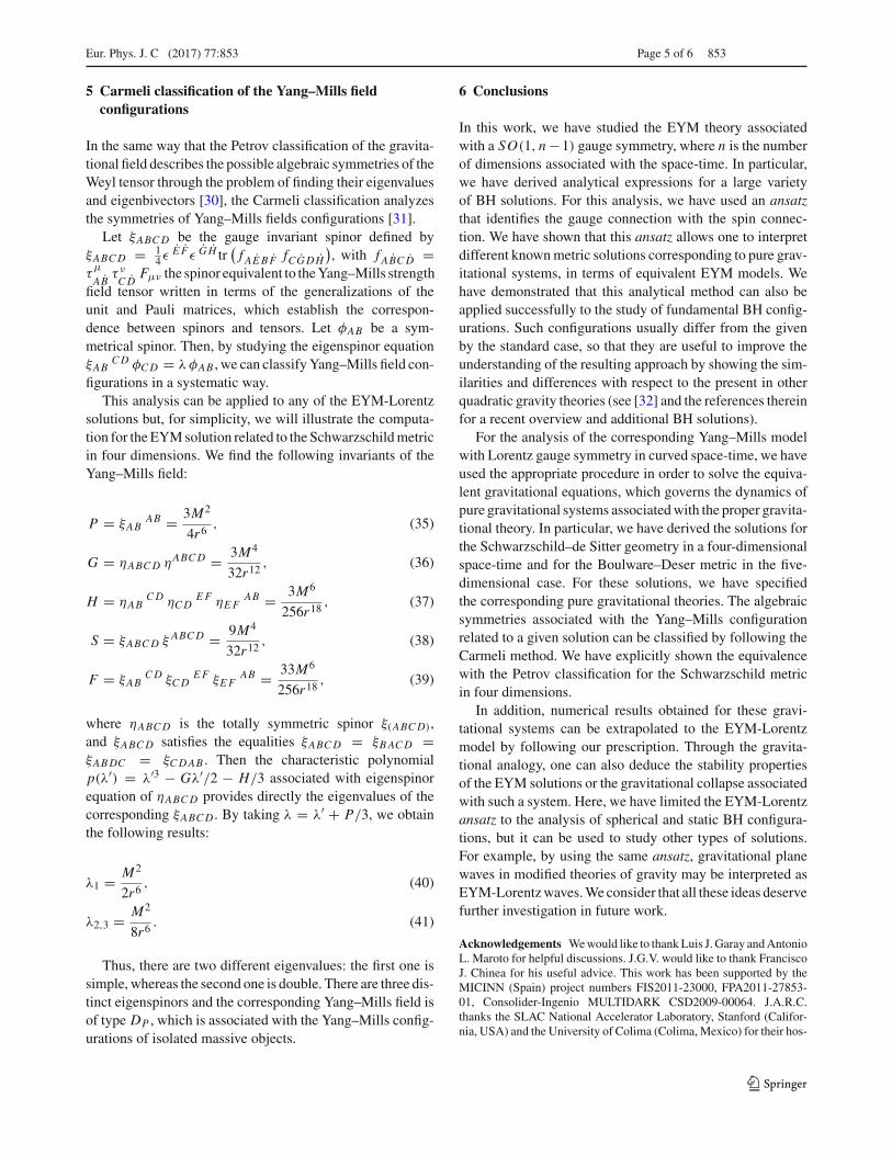
Eur. Phys. J. C (2017) 77:853 Page 5 of 6 853
5 Carmeli classification of the Yang–Mills fieldconfigurations
In the same way that the Petrov classification of the gravita-tional field describes the possible algebraic symmetries of theWeyl tensor through the problem of finding their eigenvaluesand eigenbivectors [30], the Carmeli classification analyzesthe symmetries of Yang–Mills fields configurations [31].
Let ξABCD be the gauge invariant spinor defined byξABCD = 1
4ε E Fε G H tr(f AE B F fCGDH
), with f ABC D =
τμ
ABτ ν
C DFμν the spinor equivalent to the Yang–Mills strength
field tensor written in terms of the generalizations of theunit and Pauli matrices, which establish the correspon-dence between spinors and tensors. Let φAB be a sym-metrical spinor. Then, by studying the eigenspinor equationξAB
CD φCD = λ φAB , we can classify Yang–Mills field con-figurations in a systematic way.
This analysis can be applied to any of the EYM-Lorentzsolutions but, for simplicity, we will illustrate the computa-tion for the EYM solution related to the Schwarzschild metricin four dimensions. We find the following invariants of theYang–Mills field:
P = ξABAB = 3M2
4r6 , (35)
G = ηABCD ηABCD = 3M4
32r12 , (36)
H = ηABCD ηCD
EF ηEFAB = 3M6
256r18 , (37)
S = ξABCD ξ ABCD = 9M4
32r12 , (38)
F = ξABCD ξCD
EF ξEFAB = 33M6
256r18 , (39)
where ηABCD is the totally symmetric spinor ξ(ABCD),and ξABCD satisfies the equalities ξABCD = ξBACD =ξABDC = ξCDAB . Then the characteristic polynomialp(λ′) = λ′3 − Gλ′/2 − H/3 associated with eigenspinorequation of ηABCD provides directly the eigenvalues of thecorresponding ξABCD . By taking λ = λ′ + P/3, we obtainthe following results:
λ1 = M2
2r6 , (40)
λ2,3 = M2
8r6 . (41)
Thus, there are two different eigenvalues: the first one issimple, whereas the second one is double. There are three dis-tinct eigenspinors and the corresponding Yang–Mills field isof type DP , which is associated with the Yang–Mills config-urations of isolated massive objects.
6 Conclusions
In this work, we have studied the EYM theory associatedwith a SO(1, n−1) gauge symmetry, where n is the numberof dimensions associated with the space-time. In particular,we have derived analytical expressions for a large varietyof BH solutions. For this analysis, we have used an ansatzthat identifies the gauge connection with the spin connec-tion. We have shown that this ansatz allows one to interpretdifferent known metric solutions corresponding to pure grav-itational systems, in terms of equivalent EYM models. Wehave demonstrated that this analytical method can also beapplied successfully to the study of fundamental BH config-urations. Such configurations usually differ from the givenby the standard case, so that they are useful to improve theunderstanding of the resulting approach by showing the sim-ilarities and differences with respect to the present in otherquadratic gravity theories (see [32] and the references thereinfor a recent overview and additional BH solutions).
For the analysis of the corresponding Yang–Mills modelwith Lorentz gauge symmetry in curved space-time, we haveused the appropriate procedure in order to solve the equiva-lent gravitational equations, which governs the dynamics ofpure gravitational systems associated with the proper gravita-tional theory. In particular, we have derived the solutions forthe Schwarzschild–de Sitter geometry in a four-dimensionalspace-time and for the Boulware–Deser metric in the five-dimensional case. For these solutions, we have specifiedthe corresponding pure gravitational theories. The algebraicsymmetries associated with the Yang–Mills configurationrelated to a given solution can be classified by following theCarmeli method. We have explicitly shown the equivalencewith the Petrov classification for the Schwarzschild metricin four dimensions.
In addition, numerical results obtained for these gravi-tational systems can be extrapolated to the EYM-Lorentzmodel by following our prescription. Through the gravita-tional analogy, one can also deduce the stability propertiesof the EYM solutions or the gravitational collapse associatedwith such a system. Here, we have limited the EYM-Lorentzansatz to the analysis of spherical and static BH configura-tions, but it can be used to study other types of solutions.For example, by using the same ansatz, gravitational planewaves in modified theories of gravity may be interpreted asEYM-Lorentz waves. We consider that all these ideas deservefurther investigation in future work.
Acknowledgements We would like to thank Luis J. Garay and AntonioL. Maroto for helpful discussions. J.G.V. would like to thank FranciscoJ. Chinea for his useful advice. This work has been supported by theMICINN (Spain) project numbers FIS2011-23000, FPA2011-27853-01, Consolider-Ingenio MULTIDARK CSD2009-00064. J.A.R.C.thanks the SLAC National Accelerator Laboratory, Stanford (Califor-nia, USA) and the University of Colima (Colima, Mexico) for their hos-
123

853 Page 6 of 6 Eur. Phys. J. C (2017) 77:853
pitality during the latest stages of the preparation of this manuscript, andthe support of the Becas Complutense del Amo program and the UCMConvenio 2014 program for professors.
Open Access This article is distributed under the terms of the CreativeCommons Attribution 4.0 International License (http://creativecommons.org/licenses/by/4.0/), which permits unrestricted use, distribution,and reproduction in any medium, provided you give appropriate creditto the original author(s) and the source, provide a link to the CreativeCommons license, and indicate if changes were made.Funded by SCOAP3.
References
1. C.N. Yang, R. Mills, Phys. Rev. 96, 191–195 (1954)2. R. Bartnik, J. McKinnon, Phys. Rev. Lett. 61, 141 (1988)3. P. Bizon, Phys. Rev. Lett 64, 2844 (1990)4. M.S. Volkov, D.V. Gal’tsov, Sov. J. Nucl. Phys. 51, 747 (1990)5. H.P. Kuenzle, A.K.M. Masood-ul-Alam, J. Math. Phys. 31, 928
(1990)6. P.B. Yasskin, Phys. Rev. D 12, 2212 (1975)7. F. Canfora, F. Correa, A. Giacomini, J. Oliva, Phys. Lett. B 722,
364–371 (2013)8. M.S. Volkov, D.V. Galt’sov, Phys. Rep. 319, 1–83 (1999)9. F.W. Hehl, P. Heyde, G.D. Kerlick, J.M. Nester, Rev. Mod. Phys.
48, 393–416 (1976)10. D.W. Sciama, Rev. Mod. Phys. 36, 463–469 (1964)11. C.W. Misner, K.S. Thorne, J.A. Wheeler, Gravitation (W.H. Free-
man, San Francisco, 1973)12. R.M. Wald, General Relativity (University of Chicago Press,
Chicago, Illinois, United States, 1984)
13. R. Utiyama, Phys. Rev. 101, 1597–1607 (1956)14. J. Yepez, arXiv: 1106.2037V1 (2011)15. H.G. Loos, R.P. Treat, Phys. Lett. A 26, 91–92 (1967)16. E. Fairchild Jr., Phys. Rev. D 16, 2438–2447 (1977)17. G. Debney, E.E. Fairchild, S.T.C. Siklos, Gen. Relativ. Gravity 9,
879 (1978)18. L. Yi-Fen, T. Cheng-Lung, Acta Phys. Pol. B 10, 893–899 (1979)19. J.A.R. Cembranos, A. de la Cruz-Dombriz, P.J. Romero, Int. J.
Geom. Methods Mod. Phys. 11, 1450001 (2014)20. A.I.P. Conf. Proc. 1458, 439 (2011)21. K.S. Stelle, Gen. Relativ. Gravity 9, 353 (1978)22. Yu.N Obukhov, V.N. Ponomariev, V.V. Zhytnikov, Gen. Relativ.
Gravity 21, 1107–1142 (1989)23. M. Borunda, B. Janssen, M. Bastero-Gil, JCAP 0811, 008 (2008)24. H. Lu, A. Perkins, C.N. Pope, K.S. Stelle, Phys. Rev. Lett. 114(17),
171601 (2015)25. T.W.B. Kibble, J. Math. Phys. 2, 212–221 (1961)26. K. Hayashi, T. Shirafuji, Prog. Theor. Phys. 64, 866 (1980) [Erra-
tum: Prog. Theor. Phys. 65, 2079 (1981)]27. M. Blagojevic, F.W. Hehl, Gauge Theories of Gravitation: A
Reader with Commentaries (Imperial College Press, London, UK,2013)
28. A.A. Tseytlin, Phys. Rev. D 26, 3327–3341 (1982)29. D. Boulware, S. Deser, Phys. Rev. Lett. 55, 2656–2660 (1985)30. A.Z. Petrov, Gen. Relativ. Gravity 32, 1665 (2000)31. M. Carmeli,Classical Fields: General Relativity and Gauge Fields
(John Wiley & Sons, Hoboken, New Jersey, United States, 1982)32. S. Capozziello, M. De Laurentis, Phys. Rep. 509, 167 (2011)
123

Correspondence between Einstein-Yang-Mills-Lorentz systemsand dynamical torsion models
Jose A. R. Cembranos1,2,* and Jorge Gigante Valcarcel1,†1Departamento de Física Teórica I, Universidad Complutense de Madrid, E-28040 Madrid, Spain
2Departamento de Física, Universidade de Lisboa, P-1749-016 Lisbon, Portugal(Received 23 January 2017; published 17 July 2017)
In the framework of Einstein-Yang-Mills theories, we study the gauge Lorentz group and establish aparticular correspondence between this case and a certain class of theories with torsion within Riemann-Cartan space-times. This relation is specially useful in order to simplify the problem of finding exactsolutions to the Einstein-Yang-Mills equations. The applicability of the method is divided into twoapproaches: one associated with the Lorentz group SOð1; n − 1Þ of the space-time rotations, and anotherone with its subgroup SOðn − 2Þ. Solutions for both cases are presented by the explicit use of thiscorrespondence and, interestingly, for the last one by imposing on our ansatz the same kind of rotation andreflection symmetry properties as for a nonvanishing space-time torsion. Although these solutions werefound in previous literature by a different approach, our method provides an alternative way to obtain them,and it may be used in future research to find other exact solutions within this theory.
DOI: 10.1103/PhysRevD.96.024025
I. INTRODUCTION
Research of the Einstein-Yang-Mills (EYM) model hasshown it to be a field of successful results. In the same waythat we can find solutions in general relativity (GR) withAbelian gauge bosons [1], we can also find more generalsolutions in the presence of non-Abelian vector fieldswith a large number of interesting properties, despite thenonhair conjecture [2]. The first non-Abelian solution inthe presence of curved space-time was found numericallyby Bartnik and McKinnon in the four-dimensional staticspherically symmetric EYM-SUð2Þ theory [3]. It is aparticlelike system, unlike the Abelian case given by theUð1Þ gauge group of the Einstein-Maxwell theory, wheresuch a distribution is prohibited, but the same EYM modeldoes also contain a black hole configuration [4].Increasing the number n of dimensions of the space-
time, new exact solutions for the EYM-SOðn − 2Þ casewere found by the Wu-Yang ansatz [5]. In our work, wearrive to the same result by making use of a spinconnection–like ansatz with Yang-Mills (YM) chargeand applying the standard class of symmetry conditionsas those assigned to the fundamental geometrical quantitiesof a Riemann-Cartan (RC) manifold (i.e., curvature andtorsion).From a mathematical point of view, any gauge field over
a pseudo-Riemannian manifoldM (i.e., coupled to gravity)is associated with a Lie group G and is expressed by aconnection 1-form A in the principal bundle PðM;GÞ,which takes values on the Lie algebra. This gauge con-nection defines a covariant derivative on the tangent bundle
of G and the subsequent 2-form gauge curvature F, whichconstitutes the physical field playing the role of carrier ofan interaction (i.e., the YM field if G is a non-Abelian Liegroup) [6],
Dμ ¼ ∇μ þiσ½Aμ; ·; ð1Þ
Fμν ¼ ∂μAν − ∂νAμ −iσ½Aμ; Aν; ð2Þ
where σ is related to the coupling constant.Then, the following commutating relation is satisfied:
½Dμ; Dνvλ ¼ Rλρμνvρ þ
iσ½Fμν; vλ; ð3Þ
where Rλρμν ¼ ∂μΓλ
ρν − ∂νΓλρμ þ Γλ
ωμΓωρν − Γλ
ωνΓωρμ are the
components of the Riemann tensor derived from the Levi-Civita connection and vλ is an arbitrary vector.Their behavior under a gauge transformation S ∈ G
allows us to construct minimal coupling actions. In termsof their components, it is given by the following rules:
Aμ → A0μ ¼ S−1AμS − iσS−1∂μS; ð4Þ
Fμν → F0μν ¼ S−1FμνS: ð5Þ
On the other hand, RC space-times incorporate thenotion of torsion as the antisymmetric part of the affineconnection on the manifold,
*[email protected]†[email protected]
PHYSICAL REVIEW D 96, 024025 (2017)
2470-0010=2017=96(2)=024025(6) 024025-1 © 2017 American Physical Society

Tλμν ¼ 2 ~Γλ
½μν: ð6Þ
Note that the notation with a tilde refers to elementsdefined within the RC manifold and with the absence of atilde to elements defined within the torsion-free pseudo-Riemannian manifold. Additionally, according to the cor-respondence used by our method, the same conventionapplies to quantities depending on torsionlike components(i.e., corrections in the gauge potentials that are referredto internal symmetry groups and have similar algebraicsymmetries in analogy to the torsion tensor).Although the affine connection does not transform like a
tensor under a general change of coordinates, its antisym-metric part does (i.e., torsion is a third-rank tensor, and itcannot be locally vanished if it has not associated anabsolute zero value). Furthermore, whereas curvature isrelated to the rotation of a vector along an infinitesimal pathover the space-time, torsion is related to the translation andhas deep geometrical implications, such as breaking infini-tesimal parallelograms on the manifold [7].Thus, unlike the torsion-free case where the geometry is
completely described by the metric (i.e., the affine con-nection corresponds to the Levi-Civita connection), thepresence of torsion introduces independent characteristicsand modifies the expression of the affine connection in thefollowing form:
~Γλρμ ¼ Γλ
ρμ þ Kλρμ; ð7Þ
where Kλρμ ¼ 1
2ðTλ
ρμ − Tμλρ þ Tρμ
λÞ is the so-called con-tortion tensor and fulfillsKλ
ρμ ¼ −Kρλμ, in order to preserve
the metricity condition ~∇λgμν ¼ 0 (i.e., the total covariantderivative of the metric tensor vanishes identically).One of the most fundamental aspects of introducing
these new geometrical characteristics within a physicaltheory of space-time and matter beyond GR is its main roleas a dynamical field if higher order curvature and torsionterms are included in the Lagrangian. Whereas the so-calledEinstein-Cartan theory only incorporates first-order correc-tions in the Lagrangian, and therefore no propagating torsionis allowed, second-order corrections describe a Lagrangianwith dynamical torsion depending on ten parameters [8,9].In the present work, we use these notions about the EYM
theory and the quadratic gravitation theory with propagat-ing torsion to bridge the gap between both in a very specialcase. Indeed, under a simple class of additional restrictions,we shall see that our assumptions allow us to obtaindifferent classes of exact solutions to the EYM equationsand to study other possible configurations in such a case.In this sense, the primary starting point of our analysis isbased on the study of noncompact Lie groups. Althoughthese constructions are related to nonunitary theories, oneinteresting aspect of this type of group is the possibility ofestablishing a correspondence between the theory understudy and a set of modified theories of gravity with
propagating space-time torsion, as is developed in thiswork. Indeed, the standard theory of gravity and the largerpart of its extensions belong to this group. Following ourdiscussion, we establish original dynamical constraints inorder to simplify and to classify all the possible solutionsderived by the approach described in the manuscript.This paper is organized as follows. Section II presents
the general EYM-Lorentz field equations, as well as theseequations under the spin connection–like ansatz and itsassociation with a particular quadratic gravitational theoryof second order in the curvature term with dynamicaltorsion. The general expressions for the metric and thetorsion tensor under rotations and reflections in the staticspherically symmetric space-time are shown in Sec. III. Weapply these particular conditions and find the respectivesolutions for the torsionlike and torsionless cases in Sec. IV.Finally, the conclusions obtained from our analysis arepresented in Sec. V.
II. EYM-LORENTZ ANSATZ AND CONDITIONS
We will use Planck units throughout this work(G ¼ c ¼ ℏ ¼ 1Þ and consider for our study the followingLagrangian:
S ¼ −1
16π
ZðR − trFμνFμνÞ ffiffiffiffiffiffi
−gp
dnx; ð8Þ
where theminimal coupling is assumed.Note that dependingon the character of the gauge formalism and its correspond-ing group of transformations assumed by the approach,this action can be framed either on a modified gravity modelor on a systemof interactionbetweengauge fields and regulargravity. Specifically, gauging external or internal degrees offreedom is related to a large class of gauge gravity modelsbased on space-time symmetries and to YM theories,respectively. In the present case, we consider both analyseswith the external SOð1; n − 1Þ group and the internalSOðn − 2Þ, in order to obtain a class of general constraintsthat allows us to classify their possible solutions under theappropriate correspondence conditions.Therefore, the general equations derived from this action
by performing variations with respect to the metric tensorand the gauge connection of the groups under considerationare
ðDμFμνÞab ¼ 0; ð9Þ
Gμν ¼ 8πTμν; ð10Þ
where Gμν ¼ Rμν − R2gμν is the Einstein tensor and
Tμν ¼ 14π trð14 gμνFλρFλρ − FμρFν
ρÞ, whereas latin a, b andgreek μ, ν indices run from 0 to n − 1 and refer to ananholonomic and coordinate basis, respectively. Furthermore,the divergencelessness of the Einstein tensor implies thefollowing conservation law:
CEMBRANOS and GIGANTE VALCARCEL PHYSICAL REVIEW D 96, 024025 (2017)
024025-2

∇μTμν ¼ 0: ð11Þ
These field equations typically constitute a complicatednonlinear system of equations, and additional constraintsare usually required in order to simplify the problem andto focus on particular cases. Then, by taking into accountthese lines, we assign the following spin connection–likeansatz to the gauge connection:
Aabμ ¼ Qðeaλebρ ~Γλ
ρμ þ eaλ∂μebλÞ: ð12Þ
This expression usually represents a spin connection on aRC space-time (i.e., a curved space-time with torsion), so itcan be regarded as the gauge field generated by localLorentz transformations in such a case. Alternatively, underthe EYM framework associated with internal gauge groups,it is always possible to select any particular ansatz in orderto describe the respective YM field, so in this formalism wewill start from the same mathematical expression and findembedded non-Abelian SOðn − 2Þ solutions.The gauge connection can be written as Aμ ¼ Aab
μJab,where Jab ¼ i½γa; γb=8 are the generators of the Lorentzgauge group, which satisfy the following commutativerelations:
½Jab; Jcd ¼i2ðηadJbc þ ηcbJad − ηdbJac − ηacJbdÞ: ð13Þ
By using the antisymmetric property of the gaugeconnection with respect to the Lorentz indices,Aab
μ ¼ −Abaμ, we can write the field strength tensor as
Fabμν ¼ ∂μAab
ν − ∂νAabμ þ
1
σðAa
cμAcbν − Aa
cνAcbμÞ:
ð14Þ
Finally, by taking into account the orthogonal propertyof the tetrad field eaλeaρ ¼ δλρ and setting σ ¼ Q, the fieldstrength tensor takes the form [10,11]
Fabμν ¼ Qeaλebρ ~R
λρμν; ð15Þ
where ~Rλρμν coincides with the general expression of the
components of the Riemann tensor over a RC space-time.Rewriting the above action under the spin connection–
like ansatz, it turns out that it coincides with the followingquadratic gravity action in presence of torsion:
S ¼ −1
16π
ZðR − 2~n=2−3Q2 ~Rλρμν
~RλρμνÞ ffiffiffiffiffiffi−g
pdnx; ð16Þ
with ~n ¼ n and ~n ¼ n − 1 for even and odd n.Therefore, Eqs. (9) and (10) for such a case can be
expressed in terms of geometrical quantities, respectively,as follows:
∂ρ~Rμ
λνρ þ Γρωρ
~Rμλνω þ ~Γλ
ωρ~Rμ
ωνρ − ~Γωμρ~Rω
λνρ ¼ 0;
ð17Þ
Rμν −R2gμν ¼ 2~n=2Q2ðgμν ~Rλρωτ
~Rλρωτ − 4 ~Rλρμω
~RλρνωÞ:
ð18Þ
Thus, if a certain class of space-time symmetries areimposed, then not only the condition Lξgμν ¼ 0 must besatisfied, but also LξTλ
μν ¼ 0 (i.e., the Lie derivative in thedirection of the Killing field ξ on Tλ
μν vanishes) in order topreserve the reasonable curvature and torsion symmetries.
III. SPHERICAL AND REFLECTIONSYMMETRIES
The metric of a n-dimensional static spherically sym-metric space-time can be written as
ds2 ¼ AðrÞdt2 − dr2
BðrÞ − r2dΩ2n−2; ð19Þ
where dΩn−2 ¼ dθ21þP
n−2i¼2
Qi−1j¼1 sin
2 θjdθ2i , with 0≤θn−2 ≤ 2π and 0 ≤ θk ≤ π,1 ≤ k ≤ n − 3.We assumen ≥ 4.Then, it can be shown that the only nonvanishing
components of Tλμν are [12,13]
Tttr ¼ aðrÞ;
Trtr ¼ bðrÞ;
Tθktθl ¼ δθkθlcðrÞ;
Tθkrθl ¼ δθkθlgðrÞ;
Tθktθl ¼ eaθkebθlϵabdðrÞ; if n ¼ 4;
Tθkrθl ¼ eaθkebθlϵabhðrÞ; if n ¼ 4;
Ttθkθl ¼ ϵklkðrÞ sin θ1; if n ¼ 4;
Trθkθl ¼ ϵkllðrÞ sin θ1; if n ¼ 4;
Tθkθlθm ¼ eaθkebθle
cθmϵabcfðrÞ; if n ¼ 5; ð20Þ
where a, b, c, d, g, h, k, and l are arbitrary functionsdepending only on r; k, l ¼ 1, 2, and ϵab, ϵabc are the totallyantisymmetric Levi-Civita symbol of second and thirdorder, respectively.Therefore, in addition to the two functions associated
with the metric, for n ¼ 4 dimensions, there are still a totalnumber of eight unknown independent functions to solvethe field equations. Furthermore, imposing reflection sym-metry [i.e., Oð3Þ spherical symmetry] requires that dðrÞ,hðrÞ, kðrÞ, and lðrÞ vanish, so that the number reducesto four.
CORRESPONDENCE BETWEEN EINSTEIN-YANG-MILLS- … PHYSICAL REVIEW D 96, 024025 (2017)
024025-3

IV. SOLUTIONS
In order to categorize all the possible solutions, we canrewrite Eq. (17) in the following form:
∇ρRμλνρ þ∇ρTμ
λνρ þ Kλωρ
~Rμωνρ − Kω
μρ~Rω
λνρ ¼ 0; ð21Þ
where Tλρμν ¼ ∇μKλ
ρν −∇νKλρμ þ Kλ
σμKσρν − Kλ
σνKσρμ
coincides with the torsion contribution to the curvaturetensor of the RC space-time, so that we can distinguishbetween the torsion-free and the torsion parts if it isrequired.On the other hand, according to the second Bianchi
identity for a pseudo-Riemannian manifold, the compo-nents of the Riemann tensor in such a manifold satisfy
∇½λjRωρjμν ¼ 0: ð22Þ
By contracting this expression with the metric tensor andconsidering the above form of the mentioned field equa-tion, it is straightforward to obtain the following conditionfor our model:
2∇½μRνρ ¼ ∇λTμνρλ þ 2Kω½μjλ ~Rνωρ
λ: ð23Þ
In addition, the conservation law (11) turns out to beequivalent to the following expression:
1
2∇νRþ∇λTμν
μλ þ Kωμλ~Rνω
μλ − Kωνλ~Rω
λ ¼ 0: ð24Þ
These expressions are shown as generic conditions ofthis model, and they will allow us to classify all the possibleconfigurations in the most important cases.Before distinguishing between torsionless and nonvan-
ishing torsionlike cases, let us summarize the respectiveassumptions that allow us to establish and to obtain thedistinct classes of solutions according to our discussion.The starting point is the mapping defined in Eq. (12), whichcoincides with the well-known spin connection of a givenspace-time. This quantity has typically been used in orderto describe appropriately the dynamics of the fermion fieldson a general space-time. It has also been used in the mostimportant gauge theories of gravity, such as the well-knownLorentz gauge gravity or the Poincaré gauge gravity, sinceit gives rise to a Lorentz gauge curvature which is propor-tional to the Riemann tensor, as is shown in Eq. (15).Continuing with our analysis, when the nonvanishing
torsionlike Oðn − 1Þ symmetric and the purely magneticcases are considered in an-dimensional static and sphericallysymmetric space-time, the system of equations given byEq. (17) and Eq. (18) together with the constraints (23)and (24) will allow us to find the mentioned embeddedSOðn − 2Þ solutions. It is straightforward to check thedimension of this gaugegroupbycomputing the independent
connection components of the solutions, giving rise to adimension of ðn − 2Þðn − 3Þ=2, as expected.
A. Torsionless case
For the torsionless SOð1; n − 1Þ case, the followingconstraint is satisfied:
∇½λRρν ¼ 0; ð25Þ
with
½∇½μ;∇νjRλjρ ¼ −R½μνjλωRjρω: ð26Þ
Thus, the existence of the integrability conditionR½μνjλωRjρω ¼ 0 allows us to solve this equation and obtainthe following solutions [14]:
Rμν ¼ bgμν; ð27Þ
where b is a constant.Therefore, the only possible geometries for this torsion-
less case correspond to Einstein manifolds. Note that thetracelessness of the torsion-free Einstein tensor in fourdimensions implies that b ¼ 0, so these solutions satisfyRμν ¼ 0 (i.e., the space-time is Ricci-flat). On the otherhand, by increasing the number of dimensions, the cor-rections to the gravitational field act as a cosmologicalconstant in the Einstein equations [15].
B. Nonvanishing torsionlike case
The condition (23) equal to zero enables the existence ofEinstein manifold solutions even for the case of an externalsymmetry group SOð1; n − 1Þ in the presence of a non-vanishing space-time torsion. However, other geometriesare allowed according to the generic conditions (23)and (24).Particularly, for a n-dimensional static spherically sym-
metric space-time, if we simplify the problem using theprevious considerations and restrict to the internal gaugegroup SOðn − 2Þ, it is possible to find the following purelymagnetic black hole solutions to the resulting EYMequations with Oðn − 1Þ symmetric torsionlike tensor(rotation and reflection symmetric):
Tttr ¼
A0ðrÞ2AðrÞ ; Tθk
rθk ¼ −1
r;
Trtr ¼ Tθk
tθk ¼ Tθkθlθm ¼ 0; ð28Þ
with
CEMBRANOS and GIGANTE VALCARCEL PHYSICAL REVIEW D 96, 024025 (2017)
024025-4

AðrÞ ¼ BðrÞ ¼(1 − 2m
r2 −2Q2lnðrÞ
r2 ; if n ¼ 5
1 − 2mrn−3 − 2~n=2−2 ðn−3ÞQ2
ðn−5Þr2 ; if n ≠ 5.
ð29Þ
Although these geometries are asymptotically flat, forn ¼ 5 and n ≥ 6 dimensions their Arnowitt-Deser-Misner(ADM) mass [16] diverges as lnðrÞ and rn−5, respectively.Nevertheless, solutions with finite ADMmass are found byincluding higher-order terms of the YM hierarchy in theLagrangian [17,18].The nonvanishing components of the field strength
tensor are
Fabθiθj ¼ Qeθi
aeθjb ~Rθiθj
θiθj ; ð30Þ
with ~Rθiθjθiθj ¼ − 1
r2.For n ¼ 4 dimensions, the system reduces to the
EYM-SOð2Þ case, which is indeed equivalent to themagnetic Einstein-Maxwell solution because of the iso-morphism between SOð2Þ and the Uð1Þ group. On theother hand, for n ≥ 5 dimensions the existence of theseEYM-SOðn − 2Þ solutions describes the coupling of anontrivial YM magnetic field to gravity.It has also been shown by different ways that these
solutions have a number of interesting properties, andthey are compatible with the existence of a cosmologicalconstant and Maxwell fields, as well as with other modifiedtheories of gravity, such as Gauss-Bonnet gravity [5,19].This work completes our previous study on EYM theory
presented in [15]. More general solutions may be foundusing this method, especially for n ¼ 4 dimensions sincethe LξTλ
μν ¼ 0 condition allows a richer structure than forany other number of dimensions.
V. DISCUSSION AND SUMMARY
In this article, we have presented a new method to findexact solutions to the EYM-Lorentz theory based on thecorrespondence between the EYM system and a certainclass of quadratic gravity theories in the presence oftorsion, under the restriction introduced by the spin con-nection–like ansatz. The available configurations can becategorized into the torsionless and the nonvanishingtorsionlike cases, according to general conditions. Forthe torsionless branch, it is shown that the only possiblegeometries correspond to Einstein manifolds associatedwith the external group SOð1; n − 1Þ, whereas for thenonvanishing torsionlike branch, the method allows us todistinguish the mentioned external group of symmetriesfrom the internal SOðn − 2Þ, and other families ofembedded solutions emerge. These solutions describe asort of purely magnetic black hole with YM charge, andthey were found earlier by different approaches [5,19].
Note that these results are derived from similar math-ematical expressions, but they refer to completely differentapproaches. Namely, from a gauge-theoretical approach, itis a well-known fact that the presence of a space-timetorsion requires gauging the external degrees of freedomconsisting of rotations and translations in a way that bothcurvature and torsion are inexorably related to the rotationand the translation noncompact groups, respectively [8,9].Furthermore, as previously stressed, the displacement ofa vector along an infinitesimal path in a RC manifoldinvolves a breaking of the consequent parallelogramsdefined on such a manifold, in a way that its translationalclosure failure proportionally depends on the torsion tensor[7]. Therefore, the embedding of the SOðn − 2Þ groupcorresponds to a distinct configuration where the resultinggauge connections are accordingly related to an internalsymmetry group, and the additional torsionlike degrees offreedom contained in the latter do not represent a space-time torsion but a third-rank tensor with similar algebraicsymmetries that provides a purely magnetic black holesolution to the variational equations. Indeed, it is straight-forward to check from the nonvanishing torsionlike com-ponents of this solution that the corresponding SOðn − 2Þgauge connection and its associated field strength tensor
can be written as Aμ ¼ A ~a ~bμJ ~a ~b and Fμν ¼ F ~a ~b
μνJ ~a ~b,
respectively, with ~a; ~b ¼ 2;…; n − 1. Thus, it is clear thatthese quantities are connected to the mentioned gaugegroup instead of an external symmetry group related to thespace-time rotations or translations.On the other hand, further implications arise when
considering the coupling with matter fields. For instance,if we study the dynamics of a Dirac fermion within thesolution given by Eqs. (28) and (29), the behavior iscompletely different than that which occurred in thepresence of a space-time torsion, where the fermion wouldirremediably suffer the associated spin connection.However, in the first case, the fermion would interact withthe SOðn − 2Þ gauge interaction depending on its particularmultiplet representation (for n > 4) or charge (for n ¼ 4).In the simplest case, it could even be a singlet (n > 4) orneutral (zero charge), so it would not interact with the newgauge force.This fact contrasts with some publications that do not
bear in mind these fundamental relations, and wrongly tryto identify the space-time torsion with YM or electromag-netic fields (see Fallacy 9 on page 267 of reference [20]).Thus, our SOðn − 2Þ solution is not covered by this sort offallacy, in the same way as the Mazharimousavi-Halilsoysolution since both solutions coincide and represent thesame type of configuration.Finally, it is worthwhile to stress that distinct classes of
EYM-Lorentz systems that are physically meaningful maybe found using our ansatz, especially in n ¼ 4 dimensionsbecause the LξTλ
μν ¼ 0 condition could allow for morecomplex solutions. Additionally, for the development of
CORRESPONDENCE BETWEEN EINSTEIN-YANG-MILLS- … PHYSICAL REVIEW D 96, 024025 (2017)
024025-5

this aim, the general condition ~∇λgμν ¼ 0 still holds, but itcould be also possible to deal with the same analysisrelaxing this restriction in order to find different EYMsystems related to this geometrical property. Within thisframework, an interesting and simple case might arise fromthe Weyl-Cartan geometry, where the nonmetricity con-dition is expressed as ~∇λgμν ¼ wλgμν so that the number ofirreducible decomposition pieces of nonmetricity reducesto the Weyl 1-form w [21]. Further research following theselines of study will be addressed in the future.
ACKNOWLEDGMENTS
We would like to thank Luis J. Garay and Antonio L.Maroto for helpful discussions. This work has beensupported in part by the MINECO (Spain) ProjectNos. FIS2014-52837-P, FPA2014-53375-C2-1-P,FIS2016-78859-P (AEI/FEDER, UE), and Consolider-Ingenio MULTIDARK Grant. No. CSD2009-00064. J.A. R. C. acknowledges financial support from a JoseCastillejo grant (2015). J. G. V. acknowledges support froma MULTIDARK summer student fellowship (2015).
[1] H. Stephani, D. Kramer, M. MacCallum, C. Hoenselaers,and E. Herlt, Exact Solutions to Einstein’s Field Equations(Cambridge University Press, Cambridge, England 2009),2nd ed.
[2] M. S. Volkov and D. V. Galt’sov, Phys. Rep. 319, 1 (1999).[3] R. Bartnik and J. McKinnon, Phys. Rev. Lett. 61, 141
(1988).[4] P. Bizon, Phys. Rev. Lett. 64, 2844 (1990).[5] S. Habib Mazharimousavi and M. Halilsoy, Phys. Lett. B
659, 471 (2008).[6] C. N. Yang and R. Mills, Phys. Rev. 96, 191 (1954).[7] V. de Sabbata and M. Gasperini, Introduction to Gravitation
(World Scientific, Singapore, 1985).[8] F. W. Hehl, P. von der Heyde, G. D. Kerlick, and J. M.
Nester, Rev. Mod. Phys. 48, 393 (1976).[9] Yu. N. Obukhov, V. N. Ponomariev, and V. V. Zhytnikov,
Gen. Relativ. Gravit. 21, 1107 (1989).[10] R. Utiyama, Phys. Rev. 101, 1597 (1956).
[11] J. Yepez, arXiv:1106.2037.[12] R. Rauch and H. T. Nieh, Phys. Rev. D 24, 2029 (1981).[13] S. Sur and A. S. Bhatia, Classical Quantum Gravity 31,
025020 (2014).[14] H. G. Loos and R. P. Treat, Phys. Lett. 26A, 91 (1967).[15] J. A. R. Cembranos and J. Gigante, arXiv:1501.07234.[16] R. Arnowitt, S. Deser, and C.W. Misner, Gravitation: An
Introduction to Current Research (Wiley, New York, 1962).[17] E. Radu and D. H. Tchrakian, Phys. Rev. D 73, 024006
(2006).[18] E. Radu and D. H. Tchrakian, arXiv:0907.1452.[19] S. Habib Mazharimousavi and M. Halilsoy, J. Cosmol.
Astropart. Phys. 12 (2008) 005.[20] M. Blagojevic and F.W. Hehl, Gauge Theories of
Gravitation: A Reader with Commentaries (ImperialCollege Press, London, 2013).
[21] F. W. Hehl, J. D. McCrea, E. W. Mielke, and Y. Ne’eman,Phys. Rep. 258, 1 (1995).
CEMBRANOS and GIGANTE VALCARCEL PHYSICAL REVIEW D 96, 024025 (2017)
024025-6
Conclusions
In this thesis, we have researched the possible implications derived by the existence ofan antisymmetric component of the affine connection in the universe. The resultingconfiguration can be naturally described by a RC manifold endowed with curvatureand torsion. This quantity may potentially introduce a large number of physicaleffects in the space-time and reveal new features of the gravitational field, beyondthe conventional approach of GR. By attending to the conservation laws of thematerial tensors, the spin density tensor arises as a natural source of torsion andallows the introduction of an antisymmetric component of the energy-momentumtensor into the geometrical scheme. In addition, the dynamical character of torsionis subject to the presence of the corresponding kinetic terms in the gravitationalaction (e.g. higher order curvature terms), although it is possible to formulatetheories provided with a non-propagating torsion bound by spinning sources, likethe EC theory, among others. These general foundations can also be systematizedas a gauge approach to gravity in the framework of the PG theory, leading to anappropriate correspondence between the gauge potentials and the field strengthtensors, that gives rise to the expected conservation laws for the energy-momentumand spin density tensors.
Encouraged by the consistency of the mentioned approach, we have focused ondifferent aspects of the space-time torsion. Since we noticed the existence of certainmodels that provide, in the realm of teleparallelism, an equivalent description ofgravitation such as the one given by GR, we concentrated on the investigation ofnew dynamical aspects arising from torsion. It is worthwhile to stress the extensivework available along these lines, where the search for particular vacuum solutions hasprovided new insights into the different roles assumed by torsion. However, it wasshown that various of these solutions present underlying problems, like the existenceof an underdetermined geometry or the absence of an axial mode that propagatesin a reasonable way at large distances, which involves a fundamental difficulty inmeasuring the possible effects occurred on Dirac particles minimally coupled totorsion. In this sense, one of the most important results achieved in this thesis isthe finding of a new exact vacuum solution with a non-vanishing axial mode thatbehaves as a Coulomb-like potential and provides an explicit RN geometry. Hence, itconstitutes a new geometrical configuration that is compatible with the Newtonian
139
140 Conclusions
limit and, furthermore, which can yield dynamical effects on matter via the metricand torsion tensors. Indeed, the existing correspondence between spin and torsioninvolves specific effects on the behaviour of those spinning particles coupled to thisgeometric quantity. Such a behaviour can be quantified for the case of spin 1/2particles minimally coupled to torsion by means of the WKB method, especiallywithin post-Riemannian geometries induced by an axial component of the torsiontensor. By performing a numerical analysis, we have noticed interesting differencesbetween the geodesic motion and the trajectories of these kinds of particles withinthe RN space-time provided by torsion, in a way that all the possible deviations fromthe standard case of GR are completely switched off in absence of a dynamical axialmode. Their magnitude depends on the value of both the spin charge associatedwith the source of torsion and the coupling constant that determines the fundamentalstrength of the interaction. In any case, it is expected to note significant effects onlyat extremely high densities of spinning matter, such as neutron stars or specific BHscharacterized by an intense torsion field.
On the other hand, additional implications of the space-time torsion have alsobeen analysed in this work. In particular, we have addressed the extension of thesingularity theorems of GR to the case of RC manifolds endowed with torsion.First, it is straightforward to note that the notion of geodesic incompleteness canbe generalized for the mentioned case by modifying the standard energy conditionvia the vierbein equation induced by the curvature and torsion tensors. The newgravitational action can give rise to the violation of such a condition and avoidthe occurrence of singularities, for both cases of non-propagating torsion coupledto matter fields and dynamical torsion. Furthermore, the previously stressed dif-ferences between the geodesic motion of ordinary matter uncoupled to torsion andthe trajectories of the rest of spinning matter mean that our analyses must alsodeal with a possible incompleteness of non-geodesic curves. For this purpose, weestablish a new theorem based on a class of conditions general enough to involve theexistence of curves with endpoints outside the conformal infinity of the RC manifoldand, therefore, characterized by a singular behaviour.
Additionally, we have analysed the stability of torsion in a Minkowski space-time. In a first approximation, we have assumed the vanishing of its purely tensorcomponent, in order to focalize our study on a homogeneous and isotropic case.Then, we obtain the corresponding ghost and tachyon-free conditions associatedwith the axial and trace vectorial modes in both their weak and general regimes.We note the existence of a high degree of compatibility with respect to the standardstability models presented in the literature, although some observations must beremarked. First, the algebraic conditions for the 1+ sector related to the axialmode are just the opposite to the resulting ones from those models. Moreover,as mentioned above, our starting assumptions involve an important restriction onthe possible values of the Lagrangian coefficients, which means that the releaseof several of these constraints allows the number of viable PG Lagrangians to be
Conclusions 141
extended. Specifically, it is significant to note that the omission of a perturbativeanalysis around a specific curved background may change the concluding results,since the presence of a dynamical torsion in the metric tensor involves additionalinteraction terms in the field equations, even in the weak-field limit derived fromthese equations. In this sense, we consider that this dichotomy deserves furtherinvestigation in future work.
All these results concerning the torsion field have been obtained by applying thegauge principles to the external degrees of freedom consisting of rotations and trans-lations. Nevertheless, it is possible to establish a particular correspondence betweenthis approach and the EYM theory of internal symmetry groups. Concretely, wedefine torsionlike components related to the embedding of the special orthogonalgroup, which match the consequent EYM action to the one given by a PG La-grangian defined by the combination of the torsion-free Ricci scalar and the squareof the RC curvature. This mathematical relation can be used to impose the sametypes of torsion symmetries to the new components and to reduce the complexityof the EYM equations notably. The advantages of this correspondence are stressedby the obtention of a set of purely magnetic BH solutions derived by rotation andreflection symmetric torsionlike components, which were found in previous literatureby the application of the Wu-Yang ansatz. A simple analysis of the non-Abeliansector shows a divergence of the ADM mass, which suggests the search of alternativeEYM configurations with viable mass and energy parameters.
Finally, it is also worthwhile to point out some additional prospects of research,as the possible implication of the torsion field at cosmological scales (e.g. constitut-ing an extra geometrical quantity in the framework of a cosmological perturbationtheory [103]) or its contribution in the establishment of post-Riemannian axisym-metric configurations. In this regard, the Newman-Janis algorithm may be usefulto construct different classes of PG rotating BH solutions from their correspondingnon-rotating counterparts [104], but its applicability has been questioned recently forthe case of modified theories of gravity, on account of the introduction of unsuitablepathologies in the metric tensor [105]. Therefore, we appreciate that the develop-ment of deeper analyses following these lines must also be addressed in posteriorworks.
To conclude, it is gratifying to note that the results presented in this thesis pro-vide new insights concerning post-Riemannian geometry and matter fields. This fun-damental relation constitutes the foundations of gravitation and hence the presentwork represents an attempt to elucidate the possible existence of different, still un-known, aspects and properties of the gravitational field.


Appendix A
Expressions of the Poincare gaugefield equations
The Lagrangian (1.27) imposes the vanishing of the tensors X1µ ν and X2µ λν invacuum, whose expressions can be written as:
X1µ ν = −2Gνµ + 4a2T1µ ν + 2a4T2µ ν + 4a3T3µ ν + 2a5H1µ ν
+ 2a6H2µ ν + α I1µ ν + β I2µ ν + γ I3µ ν , (A.1)
X2µ λν =?
T µλν + 4a2C1µ λν − 2a4C2µ λν − 4a3C3µ λν − 2a5Y 1µ λν
− 2a6Y 2µ λν − αZ1µ λν − β Z2µ λν − γ Z3µ λν , (A.2)
where it is given the explicit dependence with the following geometrical quantities:
Gµν = Rµ
ν − R
2 δµν , (A.3)
T1µ ν = RλρµσRλρνσ − 1
4δµνRλρτσR
λρτσ , (A.4)
T2µ ν = RλρµσRλνρσ + RλρσµR
λσρν − 12δµ
νRλρτσRλτρσ , (A.5)
T3µ ν = RλρµσRνσλρ − 1
4δµνRλρτσR
τσλρ , (A.6)
143

144 Appendix A. Expressions of the Poincare gauge field equations
H1µ ν = RνλµρR
λρ + RλµRλν − 1
2δµνRλρR
λρ , (A.7)
H2µ ν = RνλµρR
ρλ + RλµRνλ − 1
2δµνRλρR
ρλ , (A.8)
I1µ ν = 4(∇λTµ
νλ +KλρµTλρν − 1
4δµνTλρσT
λρσ), (A.9)
I2µ ν = 2(∇λT
λνµ −∇λT
νλµ +Kλρµ
(T νρλ + T ρλν
)− 1
2δµνTλρσT
ρλσ), (A.10)
I3µ ν = −2(∇µT
λλν +Kν
λµTρρλ + 1
2δµν(T λ λσT
ρρσ − 2∇λT
ρρλ))
, (A.11)
?
T µλν = δµ
νgλσT ρ ρσ − gλνT ρ ρµ − gλσT ν µσ , (A.12)
C1µ λν = ∇ρRµλρν +Kλ
σρRµσρν −Kσ
µρRσλρν , (A.13)
C2µ λν = ∇ρ
(Rµ
νλρ − Rµρλν)
+Kλσρ
(Rµ
νσρ − Rµρσν)−Kσ
µρ
(Rσ
νλρ − Rσρλν),
(A.14)
C3µ λν = ∇ρRρνλ
µ +KλσρR
ρνσµ −Kσ
µρRρνλ
σ , (A.15)
Y 1µ λν = δµν∇ρR
λρ −∇µRλν + δµ
νKλσρR
σρ +KρµρR
λν −KνµρR
λρ −KλρµR
ρν ,(A.16)
Y 2µ λν = δµν∇ρR
ρλ −∇µRνλ + δµ
νKλσρR
ρσ +KρµρR
νλ −KνµρR
ρλ −KλρµR
νρ ,(A.17)
Z1µ λν = 4T λν µ , (A.18)

145
Z2µ λν = 2(T νλ µ − T λν µ
), (A.19)
Z3µ λν = gλνT ρ ρµ − δµ νgλσT ρ ρσ . (A.20)


Appendix B
Torsion and curvaturecollineations
The introduction of additional degrees of freedom into the affine connection demandsa generalization of the standard symmetry conditions, in order to extend this notionto the whole geometric structure provided by the new gravitational framework. Inparticular, it is possible to reach a fundamental symmetry constraint involving thetorsion field, similar to the one existing in Riemannian geometry for the metrictensor.
Let be W µ1...µmν1...νn an arbitrary world tensor defined within a RC manifold.
Then, it is possible to construct its Lie derivative in the direction of a Killing vectorξ in terms of the LC connection as follows:
LξW µ1···µmν1··· νn = W µ1···µm
λ··· νn∇ν1ξλ + · · ·+W µ1···µm
ν1···λ∇νnξλ
− W λ···µmν1··· νn∇λ ξ
µ1 − · · · −W µ1···λν1··· νn∇λ ξ
µm
+ ξλ∇λWµ1···µm
ν1··· νn . (B.1)
It is straightforward to note that the torsion-free covariant derivative and the Liederivative commute when the latter is applied with respect to an arbitrary Killingvector ξ. Indeed, the respective commutator acting on a general world tensor canbe easily computed in the following way:
[∇ρ,Lξ]W µ1···µmν1··· νn = ∇ρ LξW µ1···µm
ν1··· νn − Lξ∇ρWµ1···µm
ν1··· νn , (B.2)
where:
147
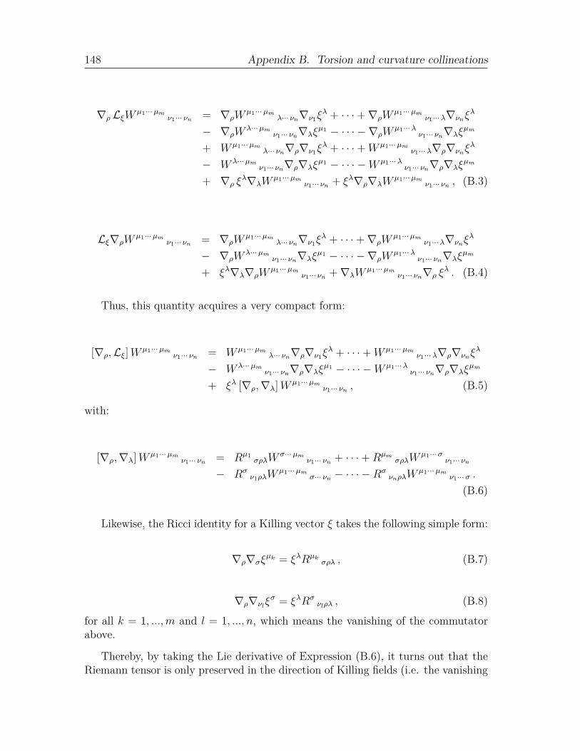
148 Appendix B. Torsion and curvature collineations
∇ρ LξW µ1···µmν1··· νn = ∇ρW
µ1···µmλ··· νn∇ν1ξ
λ + · · ·+∇ρWµ1···µm
ν1···λ∇νnξλ
− ∇ρWλ···µm
ν1··· νn∇λξµ1 − · · · − ∇ρW
µ1···λν1··· νn∇λξ
µm
+ W µ1···µmλ··· νn∇ρ∇ν1ξ
λ + · · ·+W µ1···µmν1···λ∇ρ∇νnξ
λ
− W λ···µmν1··· νn∇ρ∇λξ
µ1 − · · · −W µ1···λν1··· νn∇ρ∇λξ
µm
+ ∇ρ ξλ∇λW
µ1···µmν1··· νn + ξλ∇ρ∇λW
µ1···µmν1··· νn , (B.3)
Lξ∇ρWµ1···µm
ν1··· νn = ∇ρWµ1···µm
λ··· νn∇ν1ξλ + · · ·+∇ρW
µ1···µmν1···λ∇νnξ
λ
− ∇ρWλ···µm
ν1··· νn∇λξµ1 − · · · − ∇ρW
µ1···λν1··· νn∇λξ
µm
+ ξλ∇λ∇ρWµ1···µm
ν1··· νn +∇λWµ1···µm
ν1··· νn∇ρ ξλ . (B.4)
Thus, this quantity acquires a very compact form:
[∇ρ,Lξ]W µ1···µmν1··· νn = W µ1···µm
λ··· νn∇ρ∇ν1ξλ + · · ·+W µ1···µm
ν1···λ∇ρ∇νnξλ
− W λ···µmν1··· νn∇ρ∇λξ
µ1 − · · · −W µ1···λν1··· νn∇ρ∇λξ
µm
+ ξλ [∇ρ,∇λ]W µ1···µmν1··· νn , (B.5)
with:
[∇ρ,∇λ]W µ1···µmν1··· νn = Rµ1
σρλWσ···µm
ν1··· νn + · · ·+RµmσρλW
µ1···σν1··· νn
− Rσν1ρλW
µ1···µmσ··· νn − · · · −Rσ
νnρλWµ1···µm
ν1···σ .
(B.6)
Likewise, the Ricci identity for a Killing vector ξ takes the following simple form:
∇ρ∇σξµk = ξλRµk
σρλ , (B.7)
∇ρ∇νlξσ = ξλRσ
νlρλ , (B.8)
for all k = 1, ...,m and l = 1, ..., n, which means the vanishing of the commutatorabove.
Thereby, by taking the Lie derivative of Expression (B.6), it turns out that theRiemann tensor is only preserved in the direction of Killing fields (i.e. the vanishing

149
of the Lie derivative of the metric tensor implies the vanishing of the Lie derivativeof the Riemann tensor):
LξRλρµν = 0 . (B.9)
These properties can be easily extended to the case of quantities dependingon torsion. Specifically, the notion of a general covariant derivative endowed withtorsion requires that the latter satisfies the same symmetry condition as the metrictensor:
LξT λ µν = 0 , (B.10)
in order to maintain the corresponding commutation relations:
[∇ρ,Lξ
]= 0 . (B.11)
Therefore, the application of the Lie derivative to the generalized commutationrelations of covariant derivatives within a RC manifold:
[∇µ, ∇ν ] vλ = Rλρµν v
ρ + T ρ µν ∇ρvλ , (B.12)
involves the preserving of the RC curvature along an arbitrary Killing vector pro-vided the fulfillment of the condition (B.10):
LξRλρµν = 0 . (B.13)


Appendix C
SU(2) gauge connection in staticand spherically symmetricspace-times
In the context of EYM theory, the gauge condition ∂µω−i [Aµ, ω] = LξAµ constitutesa strong symmetry constraint to simplify the expression of the gauge connection,especially when it concerns gravitational systems and fields endowed with a highdegree of symmetry. In this sense, the particular case of non-Abelian SU(2) fieldscoupled to a four-dimensional static and spherically symmetric space-time representsa fundamental configuration where such a constraint can be fulfilled.
Hence, we start from the expression of the line element:
ds2 = Ψ1(r) dt2 − dr2
Ψ2(r) − r2(dθ2
1 + sin2 θ1dθ22
), (C.1)
and the respective family of Killing vectors satisfying the Lie algebra of the rotationgroup SO(3):
ξµ(1) = cos θ2δµθ1 − cot θ1 sin θ2δ
µθ2 , (C.2)
ξµ(2) = − sin θ2δµθ1 − cot θ1 cos θ2δ
µθ2 , (C.3)
ξµ(3) = δµθ2 . (C.4)
Let η =[ξ(m), ξ(n)
]be the resulting Killing field from the commutation relations
151

152Appendix C. SU(2) gauge connection in static and spherically symmetric space-times
of the Killing vectors above (i.e. η = εmnp ξ(p), with m,n, p = 1, 2, 3). Then, the
original gauge condition can be expressed in the following way:
εmnp(∂µω(p) − i
[Aµ, ω(p)
])= L[ξ(m),ξ(n)]Aµ , (C.5)
where:
LηAµ = Lξ(m)
(∂µω(n) − i
[Aµ, ω(n)
])− Lξ(n)
(∂µω(m) − i
[Aµ, ω(m)
]). (C.6)
By expanding and rearranging terms, it is straightforward to obtain the followingconsistency constraint involving the gauge variables ω(m) = ωi(m)τi alone:
Lξ(m)ω(n) − Lξ(n)ω(m) − i[ω(m), ω(n)
]− εmn pω(p) = 0 . (C.7)
As is shown, these variables take values in the Lie algebra, so that it is possibleto impose a general transformation law for these quantities under gauge transfor-mations S ∈ SU(2):
ω(m) → ω′
(m) = S−1ω(m)S + iξµ(m)S−1∂µS . (C.8)
Indeed, this transformation rule preserves the symmetry gauge condition, whichmeans that every pair
(Aµ, ω(m)
)that is a solution of the mentioned expression can
be trivially changed to another pair(A
′µ, ω
′
(m)
)by the action of S and still satisfy
this condition:
S−1(∂µω(m) − i
[Aµ, ω(m)
])S = S−1Lξ(m)AµS . (C.9)
Therefore, it is possible to consider ω(3) = Φ(θ2)f i(r, θ1) τi and to perform a gaugetransformation S1 = eif
i(r,θ1) τi∫
Φ(θ2)dθ2 without modifying our general requirements,which implies the vanishing of this component and the consequent conservation rulefor the potential:
∂θ2Aµ = 0 . (C.10)
In addition, Equation (C.7) allows us to find the rest of the components, whichmust fulfill the following system of equations:
∂θ2ω(1) − ω(2) = 0 , (C.11)

153
∂θ2ω(2) + ω(1) = 0 , (C.12)
[ω(1), ω(2)
]= cos θ2∂θ1ω(2) + sin θ2∂θ1ω(1)
+ cot θ1(cos θ2∂θ2ω(1) − sin θ2∂θ2ω(2)
). (C.13)
It is straightforward to note that the solution of Equations (C.11) and (C.12)can be expressed as follows:
ω(1) = X(θ1) cos θ2 + Y (θ1) sin θ2 , (C.14)
ω(2) = Y (θ1) cos θ2 −X(θ1) sin θ2 , (C.15)where X and Y are arbitrary functions, defined on the Lie algebra, whose possibledependence on the coordinate r has been omitted. Such a restriction simplifies theproblem notably and it is compatible, as outlined below, with the existence of anansatz solution for the gauge connection.
In general, the gauge transformation rules (C.8) fix the respective transforma-tions of the mentioned functions:
X → X′ = S−1XS + iS−1∂θ1S , (C.16)
Y → Y′ = S−1Y S − i cot θ1S
−1∂θ2S . (C.17)
Once again, it is possible to consider X as a function independent of θ1 andto apply a new gauge transformation S2 = eiXθ1 , which involves the vanishing ofthis function. Then, we are led to deal only with the function Y ; indeed, becauseof our previous choice to vanish ω(3) it is not possible to perform a new gaugetransformation depending on θ2 which cancels this function simultaneously.
Therefore, Equation (C.13) reduces to the following differential condition:
dY (θ1)dθ1
+ Y (θ1) cot θ1 = 0 , (C.18)
whose general solution can be written in the following way:
Y (θ1) = c iτisin θ1
, (C.19)

154Appendix C. SU(2) gauge connection in static and spherically symmetric space-times
with c i three integration constants, which can also be simplified by the applicationof an additional gauge transformation S3 = ei ((c 2/c 3)τ1−(c 1/c 3)τ2), in order to cancelc 1 and c 2.
In summary, our analyses lead to the following structure for the gauge variables:
ω(1) = sin θ2
sin θ1c 3τ3 , (C.20)
ω(2) = cos θ2
sin θ1c 3τ3 , (C.21)
ω(3) = 0 . (C.22)
By substituting these factors in the general symmetry condition for the gaugeconnection:
c i∂µ
(sin θ2
sin θ1
)+εi jkAjµc k
(sin θ2
sin θ1
)= ∂θ1A
iµ cos θ2+Aiθ1∂µ cos θ2−Aiθ2∂µ (cot θ1 sin θ2) ,
(C.23)
c i∂µ
(cos θ2
sin θ1
)+εi jkAjµc k
(cos θ2
sin θ1
)= − ∂θ1A
iµ sin θ2−Aiθ1∂µ sin θ2−Aiθ2∂µ (cot θ1 cos θ2) .
(C.24)
Thus, the resulting system of equations can be trivially solved and it shows that,in the present gauge, the YM connection is described by the following ansatz:
A = p(r) τ3 dt+ u(r) τ3 dr + (v(r) τ1 + w(r) τ2) dθ1
+ (cot θ1 τ3 + v(r) τ2 − w(r) τ1) sin θ1dθ2 , (C.25)
where p, u, v and w are four arbitrary functions depending on the coordinate r.

Publications
1. Einstein-Yang-Mills-Lorentz black holes, J. A. R. Cembranos and J. G. Val-carcel, Eur. Phys. J. C 77, no. 12, 853 (2017).
2. Correspondence between Einstein-Yang-Mills-Lorentz systems and dynamicaltorsion models, J. A. R. Cembranos and J. G. Valcarcel, Phys. Rev. D 96,no. 2, 024025 (2017).
3. New torsion black hole solutions in Poincare gauge theory, J. A. R. Cembranosand J. G. Valcarcel, JCAP 1701, no. 01, 014 (2017).
4. Singularities and n-dimensional black holes in torsion theories, J. A. R. Cem-branos, J. G. Valcarcel and F. J. Maldonado Torralba, JCAP 1704, no. 04,021 (2017).
5. Stability in quadratic torsion theories, T. B. Vasilev, J. A. R. Cembranos, J.G. Valcarcel and P. Martin-Moruno, Eur. Phys. J. C 77, no. 11, 755 (2017).
6. Extended Reissner-Nordstrom solutions sourced by dynamical torsion, J. A. R.Cembranos and J. G. Valcarcel, Phys. Lett. B 779, 143 (2018).
7. Fermion dynamics in torsion theories, J. A. R. Cembranos, J. G. Valcarceland F. J. Maldonado Torralba, arXiv preprint gr-qc: 1805.09577 (2018).
155


Bibliography
[1] S. Weinberg. Gravitation and Cosmology: Principles and Applications of theGeneral Theory of Relativity. John Wiley & Sons (1972).
[2] A. Papapetrou. Non-symmetric stress-energy-momentum tensor and spin-density. Philosophical Magazine, 7: 937-946 (1949).
[3] C. W. Misner, K. S. Thorne and J. A. Wheeler. Gravitation. W. H. Freeman(1973).
[4] C. M. Will. The confrontation between general relativity and experiment.Living Reviews in Relativity, 17: 4-117 (2014).
[5] B. P. Abbott et al. (LIGO Scientific and Virgo Collaborations). Observation ofgravitational waves from a binary black hole merger. Physical Review Letters,116, 061102: 1-16 (2016).
[6] R. M. Wald. General Relativity. University of Chicago Press (1984).
[7] S. W. Hawking and G. F. R. Ellis. The Large Scale Structure of Space-Time.Cambridge University Press (1973).
[8] S. Nojiri and S. D. Odintsov. Unified cosmic history in modified gravity: fromF(R) theory to Lorentz non-invariant models. Physics Reports, 505: 59-144(2011).
[9] A. De Felice and S. Tsujikawa. f(R) theories. Living Reviews in Relativity, 13:3-161 (2010).
[10] T. Padmanabhan and D. Kothawala. Lanczos-Lovelock models of gravity.Physics Reports, 531: 115-171 (2013).
[11] V. de Sabbata and M. Gasperini. Introduction to Gravitation. World Scientific(1985).
[12] T. Ortın. Gravity and Strings. Cambridge University Press (2004).
[13] V. de Sabbata and C. Sivaram. Spin and Torsion in Gravitation. WorldScientific (1994).
157

158 BIBLIOGRAPHY
[14] F. W. Hehl and Y. N. Obukhov. Elie Cartan’s torsion in geometry and infield theory, an essay. Annales de la Fondation Louis de Broglie, 32: 157-194(2007).
[15] F. S. N. Lobo, G. J. Olmo and D. Rubiera-Garcia. Crystal clear lessons onthe microstructure of spacetime and modified gravity. Physical Review D, 91,124001: 1-7 (2015).
[16] R. Gambini and L. Herrera. Einstein-Cartan theory in the spin coefficientformalism. Journal of Mathematical Physics, 21: 1449-1454 (1980).
[17] K. Hayashi and T. Shirafuji. Gravity from Poincare gauge theory of the funda-mental particles I. Linear and quadratic Lagrangians. Progress of theoreticalphysics, 64: 866-882 (1980).
[18] I. L. Shapiro. Physical aspects of the space-time torsion. Physics Reports, 357:113-213 (2002).
[19] M. Tsamparlis. Cosmological principle and torsion. Physics Letters A, 75:27-28 (1979).
[20] T. W. B. Kibble. Lorentz invariance and the gravitational field. Journal ofMathematical Physics, 2: 212-221 (1961).
[21] F. W. Hehl, P. von der Heyde, G. D. Kerlick and J. M. Nester. Generalrelativity with spin and torsion: foundations and prospects. Reviews of ModernPhysics, 48: 393-416 (1976).
[22] M. Blagojevic and F. W. Hehl. Gauge Theories of Gravitation: A Reader withCommentaries. Imperial College Press, (2013).
[23] J. Yepez. Einstein’s vierbein field theory of curved space. arXiv preprint gr-qc,1106.2037: 1-21 (2011).
[24] P. Baekler and F. W. Hehl. Beyond Einstein-Cartan gravity: quadratic torsionand curvature invariants with even and odd parity including all boundaryterms. Classical and Quantum Gravity, 28, 215017: 1-11 (2011).
[25] H. T. Nieh. Gauss-Bonnet and Bianchi identities in Riemann-Cartan typegravitational theories. Journal of Mathematical Physics, 21: 1439-1441 (1980).
[26] K. Hayashi and T. Shirafuji. Gravity from Poincare gauge theory of the fun-damental particles V. The extended Bach-Lanczos identity. Progress of theo-retical physics, 65: 525-532 (1981).
[27] Y. Kosmann-Schwarzbach. The Noether Theorems. Springer-Verlag (2011).
BIBLIOGRAPHY 159
[28] F. J. Belinfante. On the current and the density of the electric charge, theenergy, the linear momentum and the angular momentum of arbitrary fields.Physica, 7: 449-474 (1940).
[29] L. Rosenfeld. Sur le tenseur d’impulsion-energie. Academie Royale de Belgique,Memoires de la classe des sciences, 18: 1-30 (1940).
[30] W. Kopczynski, J. D. McCrea and F. W. Hehl. The metric and the canon-ical energy-momentum currents in the Poincare gauge theory of gravitation.Physics Letters A, 135: 89-91 (1989).
[31] F. W. Hehl. How does one measure torsion of space-time? Physics Letters A,36: 225-226 (1971).
[32] Y. Mao, M. Tegmark, A. H. Guth and S. Cabi. Constraining torsion withGravity Probe B. Physical Review D, 76, 104029: 1-26 (2007).
[33] W. R. Stoeger and P. B. Yasskin. Can a macroscopic gyroscope feel a torsion?General Relativity and Gravitation, 76: 427-431 (1979).
[34] F. W. Hehl, Y. N. Obukhov and D. Puetzfeld. On Poincare gauge theory ofgravity, its equations of motion, and Gravity Probe B. Physics Letters A, 377:1775-1781 (2013).
[35] J. H. Simpson. Nuclear gyroscopes. Astronautics & Aeronautics, 2: 42-48(1964).
[36] W.-T. Ni. Spin, torsion and polarized test-body experiments. Proceedingsof the International School and Symposium on Precision Measurement andGravity Experiment, 531-540 (1983).
[37] W.-T. Ni. Searches for the role of spin and polarization in gravity. Reports onProgress in Physics, 73, 056901: 1-24 (2010).
[38] W.-K. Tung. Group Theory in Physics. World Scientific (1985).
[39] Y. N. Obukhov, A. J. Silenko and O. V. Teryaev. Spin-torsion coupling andgravitational moments of Dirac fermions: theory and experimental bounds.Physical Review D, 90, 124068: 1-13 (2014).
[40] R. T. Hammond. Upper limit on the torsion coupling constant. PhysicalReview D, 52: 6918-6921 (1995).
[41] C. Møller. Conservation laws and absolute parallelism in general relativity.Det Kongelige Danske Videnskabernes Selskab, Matematisk-Fysiske Skrifter,1: 1-50 (1961).

160 BIBLIOGRAPHY
[42] K. Hayashi and T. Shirafuji. New general relativity. Physical Review D, 19:3524-3553 (1979).
[43] V. C. de Andrade, L. C. T. Guillen and J. G. Pereira. Teleparallel gravity: anoverview. arXiv preprint gr-qc, 0011087: 1-10 (2000).
[44] Y. F. Cai, S. Capozziello, M. De Laurentis and E. N. Saridakis. f(T) teleparallelgravity and cosmology. Reports on Progress in Physics, 79, 106901: 1-121(2016).
[45] V. C. de Andrade and J. G. Pereira. Gravitational Lorentz force and thedescription of the gravitational interaction. Physical Review D, 56: 4689-4695(1997).
[46] H. I. Arcos and J. G. Pereira. Torsion gravity: a reappraisal. InternationalJournal of Modern Physics D, 13: 2193-2240 (2004).
[47] G. D. Birkhoff. Relativity and Modern Physics. Harvard University Press(1977).
[48] D. E. Neville. Birkhoff theorems for R + R 2 gravity theories with torsion.Physical Review D, 21: 2770-2775 (1980).
[49] R. Rauch and H. T. Nieh. Birkhoff’s theorem for general Riemann-Cartan-typeR +R 2 theories of gravity. Physical Review D, 24: 2029-2048 (1981).
[50] P. Baekler. A spherically symmetric vacuum solution of the quadratic Poincaregauge field theory of gravitation with Newtonian and confinement potentials.Physics Letters B, 99: 329-332 (1981).
[51] P. von der Heyde. Is gravitation mediated by the torsion of spacetime?Zeitschrift fur Naturforschung A, 31: 1725-1726 (1976).
[52] F. W. Hehl, Y. Ne’eman, J. Nitsch and P. von der Heyde. Short-range confiningcomponent in a quadratic Poincare gauge theory of gravitation. Physics LettersB, 78: 102-106 (1978).
[53] M. Schweizer and N. Straumann. Poincare gauge theory of gravitation andthe binary pulsar 1913 + 16. Physics Letters A, 71: 493-495 (1979).
[54] W. Scherrer. Zur linearen feldtheorie III. Zeitschrift fur Physik, 141: 374-385(1955).
[55] S. Sur and A. S. Bhatia. Constraining torsion in maximally symmetric(sub)spaces. Classical and Quantum Gravity, 31, 025020: 1-22 (2014).
[56] J. Weyssenhoff and A. Raabe. Relativistic dynamics of spin-fluids and spin-particles. Acta Physica Polonica, 9: 7-18 (1947).

BIBLIOGRAPHY 161
[57] E. W. Mielke. Reduction of the Poincare gauge field equations by means of aduality rotation. Journal of Mathematical Physics, 25: 663-668 (1984).
[58] C. H. Lee. A spherically symmetric electro-vacuum solution of the Poincaregauge field theory of gravitation. Physics Letters B, 130: 257-259 (1983).
[59] J. D. McCrea. A NUT-like solution of the quadratic Poincare gauge fieldequations. Physics Letters A, 100: 397-399 (1984).
[60] P. Baekler and F. W. Hehl. A charged Taub-NUT metric with torsion: a newaxially symmetric solution of the Poincare gauge field theory. Physics LettersA, 100: 392-396 (1984).
[61] J. D. McCrea, P. Baekler and M. Gurses. A Kerr-like solution of the Poincaregauge field equations. Il Nuovo Cimento B, 99: 171-177 (1987).
[62] P. Baekler, M. Gurses, F. W. Hehl and J. D. McCrea. The exterior gravi-tational field of a charged spinning source in the Poincare gauge theory: aKerr-Newman metric with dynamic torsion. Physics Letters A, 128: 245-250(1988).
[63] Y. N. Obukhov, V. N. Ponomariev and V. V. Zhytnikov. Quadratic Poincaregauge theory of gravity: a comparison with the general relativity theory. Gen-eral Relativity and Gravitation, 21: 1107-1142 (1989).
[64] H. J. Lenzen. On spherically symmetric fields with dynamic torsion in gaugetheories of gravitation. General Relativity and Gravitation, 17: 1137-1151(1985).
[65] C. M. Chen, D. C. Chern, J. M. Nester, P. K. Yang and V. V. Zhytnikov.Poincare gauge theory Schwarzschild-de Sitter solutions with long range spher-ically symmetric torsion. Chinese Journal of Physics, 32: 29-40 (1994).
[66] V. V. Zhytnikov. Double duality and hidden gauge freedom in the Poincaregauge theory of gravitation. General Relativity and Gravitation, 28: 137-162(1996).
[67] Y. N. Obukhov. Gravitational waves in Poincare gauge gravity theory. PhysicalReview D, 95, 084028: 1-12 (2017).
[68] M. Blagojevic and B. Cvetkovic. Generalized pp waves in Poincare gaugetheory. Physical Review D, 95, 104018: 1-10 (2017).
[69] S. W. Hawking and R. Penrose. The Nature of Space and Time. PrincetonUniversity Press (1996).
[70] E. Poisson. A Relativist’s Toolkit: The Mathematics of Black-Hole Mechanics.Cambridge University Press (2004).
162 BIBLIOGRAPHY
[71] A. Raychaudhuri. Relativistic cosmology. I. Physical Review, 98: 1123-1126(1955).
[72] R. Penrose. Gravitational collapse and space-time singularities. Physical Re-view Letters, 14: 57-59 (1965).
[73] S. W. Hawking. The occurrence of singularities in cosmology. III. Causalityand singularities. Proceedings of the royal society of London A, 300: 187-201(1967).
[74] M. Blagojevic and M. Vasilic. Extra gauge symmetries in a weak-field approx-imation of an R+T 2 +R 2 theory of gravity. Physical Review D, 35: 3748-3759(1987).
[75] D. E. Neville. Gravity Lagrangian with ghost-free curvature-squared terms.Physical Review D, 18: 3535-3543 (1978).
[76] E. Sezgin and P. van Nieuwenhuizen. New ghost-free gravity Lagrangians withpropagating torsion. Physical Review D, 21: 3269-3280 (1980).
[77] E. Sezgin. Class of ghost-free gravity Lagrangians with massive or masslesspropagating torsion. Physical Review D, 24: 1677-1680 (1981).
[78] R. Kuhfuss and J. Nitsch. Propagating modes in gauge field theories of gravity.General Relativity and Gravitation, 18: 1207-1227 (1986).
[79] S. Miyamoto, T. Nakano, T. Ohtani and Y. Tamura. Linear approximationfor the massless Lorentz gauge field. Progress of Theoretical Physics, 69: 1236-1240 (1983).
[80] M. Fukui and J. Masukawa. Massless torsion fields. II. The case α+2a/3 = 0.Progress of Theoretical Physics, 73: 75-83 (1985).
[81] K. Fukuma, S. Miyamoto, T. Nakano, T. Ohtani and Y. Tamura. MasslessLorentz gauge field consistent with Einstein’s gravitation theory. The caseα + 3a/2 = β − 2a/3 = γ + 3a/2 = 0. Progress of Theoretical Physics, 73:874-883 (1985).
[82] R. Battiti and M. Toller. Zero-mass normal modes in linearized Poincare gaugetheories. Lettere al Nuovo Cimento, 44: 35-39 (1985).
[83] C. N. Yang and R. L. Mills. Conservation of isotopic spin and isotopic gaugeinvariance. Physical Review, 96: 191-195 (1954).
[84] M. S. Volkov and D. V. Gal’tsov. Gravitating non-Abelian solitons and blackholes with Yang-Mills fields. Physics Reports, 319: 1-83 (1999).

BIBLIOGRAPHY 163
[85] P. Forgacs and N. S. Manton. Space-time symmetries in gauge theories. Com-munications in Mathematical Physics, 72: 15-35 (1980).
[86] E. Witten. Some exact multipseudoparticle solutions of classical Yang-Millstheory. Physical Review Letters, 38: 121-124 (1977).
[87] R. Bartnik and J. McKinnon. Particlelike solutions of the Einstein-Yang-MillsEquations. Physical Review Letters, 61: 141-144 (1988).
[88] P. Bizon. Colored black holes. Physical Review Letters, 64: 2844-2847 (1990).
[89] N. Straumann and Z. H. Zhou. Instability of the Bartnik-McKinnon solutionof the Einstein-Yang-Mills equations. Physics Letters B, 237: 353-356 (1990).
[90] N. Straumann and Z. H. Zhou. Instability of a colored black hole solution.Physics Letters B, 243: 33-35 (1990).
[91] Z. H. Zhou and N. Straumann. Nonlinear perturbations of Einstein-Yang-Millssolitons and non-Abelian black holes. Nuclear Physics B, 360: 180-196 (1991).
[92] M. S. Volkov and D. V. Gal’tsov. Odd-parity negative modes of Einstein-Yang-Mills black holes and sphalerons. Physics Letters B, 341: 279-285 (1995).
[93] D. V. Gal’tsov and M. S. Volkov. Charged non-Abelian SU(3) Einstein-Yang-Mills black holes. Physics Letters B, 274: 173-178 (1992).
[94] H. P. Kunzle. Analysis of the static spherically symmetric SU(n) Einstein-Yang-Mills equations. Communications in Mathematical Physics, 162: 371-397(1994).
[95] B. Kleihaus, J. Kunz and A. Sood. Charged SU(N) Einstein-Yang-Mills blackholes. Physics Letters B, 418: 284-293 (1998).
[96] B. Kleihaus, J. Kunz, A. Sood and M. Wirschins. Sequences of globally regularand black hole solutions in SU(4) Einstein-Yang-Mills theory. Physical ReviewD, 58, 084006: 1-16 (1998).
[97] G. Lavrelashvili and D. Maison. Regular and black hole solutions of Einstein-Yang-Mills dilaton theory. Nuclear Physics B, 410: 407-422 (1993).
[98] T. Torii, K. Maeda and T. Tachizawa. Cosmic colored black holes. PhysicalReview D, 52: R4272-R4276 (1995).
[99] M. S. Volkov, N. Straumann, G. V. Lavrelashvili, M. Heusler and O. Brodbeck.Cosmological analogues of the Bartnik-McKinnon solutions. Physical ReviewD, 54: 7243-7251 (1996).
164 BIBLIOGRAPHY
[100] A. Z. Petrov. The classification of spaces defining gravitational fields. GeneralRelativity and Gravitation, 32: 1665-1685 (2000).
[101] M. Carmeli. Classical Fields: General Relativity and Gauge Theory. JohnWiley & Sons (1982).
[102] M. Carmeli, K. Huleihil and E. Leibowitz. Gauge Fields: Classification andEquations of Motion. World Scientific (1989).
[103] V. F. Mukhanov, H. A. Feldman and R. H. Brandenberger. Theory of cosmo-logical perturbations. Physics Reports, 215: 203-333 (1992).
[104] E. T. Newman and A. I. Janis. Note on the Kerr spinning-particle metric.Journal of Mathematical Physics, 6: 915-917 (1965).
[105] D. Hansen and N. Yunes. Applicability of the Newman-Janis algorithm toblack hole solutions of modified gravity theories. Physical Review D, 88,104020: 1-9 (2013).