PONTIFICIA UNIVERSIDAD CATÓLICA DE PERÚ...

PONTIFICIA UNIVERSIDAD CATÓLICA DE PERÚ

FACULTAD DE CIENCIAS E INGENIERÍA

CUANTIFICACIÓN DE LA EROSIÓN HÍDRICA EN EL PERÚ Y

LOS COSTOS AMBIENTALES ASOCIADOS

Tesis para obtener el grado de magister en Ingeniería Civil, presentada por:

ROSAS BARTURÉN, Miluska Anthuannet

Asesorada por:

PhD. GUTIERREZ LLANTOY, Ronald Roger

Lima, 3 de Marzo del 2016

ii

Agradecimientos:

Deseo agradecer a Dios por darme la oportunidad de terminar mis estudios de posgrado, además

agradezco a CONCYTEC como institución que fomenta la investigación en nuestro país y

financia el desarrollo de jóvenes profesionales, finalmente agradezco a la Pontificia Universidad

Católica del Perú por todos los conocimientos impartidos y por la orientación profesional para

culminar exitosamente el trabajo de investigación.

iii

TABLA DE CONTENIDOS

CAPITULO 1: EL PROBLEMA DE INVESTIGACIÓN…………………………. ….. 1

1. Planteamiento del problema y justificación ………………………………….1

2. Objetivos de la investigación ………………………………………………...1

3. Metodología y plan de trabajo ……………………………………………….2

CAPÍTULO 2: ………………………………………………………………………….. 3

“On a RUSLE-based methodology to estimate hydraulic erosion rates at country scale in

developing countries”

CAPÍTULO 3: ………………………………………………………………………… 19

“Sediment yield changes in the Peruvian Andes for the year 2030”

CAPÍTULO 4: ………………………………………………………………………… 28

“On the need of erosion control regulatory framework in Peru”

iv

RESUMEN EJECUTIVO

Se presenta a la erosión de suelos como un problema latente alrededor del mundo,

esta situación se agrava en los países en desarrollo por la falta de información actualizada,

como es el caso del Perú. Por ello esta investigación tiene como objetivo plantear una

metodología para cuantificar la tasa de erosión actual y futura a nivel nacional y escala de

cuenca para así poder plantear lineamientos de regulación ante las pérdidas económicas que

esta genera.

El Capítulo 1 presenta la problemática, los objetivos y alcances de investigación.

Además se detalla la metodología para llevar a cabo los fines propuestos, mostrando el

producto del proceso de investigación (3 papers científicos).

El Capítulo 2 presenta el primer paper titulado: On a RUSLE-based methodology to

estimate hydraulic erosion rates at country scale in developing countries, que plantea una

metodología para estimar la erosión de suelos a escala nacional ante un contexto de escases

de información básica como ocurre en los países en desarrollo. Tiene como producto mapas

de la tasa de erosión de suelos en el Perú para los años 1990, 2000 y 2010 a una resolución

de 5km.

El Capítulo 3 muestra el segundo paper cuyo título es: Sediment yield changes in

the Peruvian Andes for the year 2030, cuyo objetivo es mostrar la significancia de la

cantidad de sedimentos producidas en los Andes peruanos con una proyección al año 2030.

Se evaluaron 2 escenarios adicionales, el primero que incluye el desarrollo de la actividad

minera en el país y el segundo donde se presentan las áreas de protección ambiental.

El Capítulo 4 está conformado por el tercer paper: On the need of erosion control

regulatory framework in Peru, en el cual se detalla la importancia de una regulación en

términos de erosión, basando esta afirmación en la pérdida económica inducida como fuente

de contaminación no puntual. Tiene como casos de estudio la cuenca del río Santa y del río

Jequetepeque. Esta estimación económica envuelve la pérdida de nutrientes y el costo por la

eliminación de sedimentos en la cuenca.

1

CAPITULO 1: EL PROBLEMA DE INVESTIGACIÓN

1 Planteamiento del problema y justificación

La pérdida de suelos por causa de erosión hídrica es un problema que se agrava,

especialmente en los países en desarrollo, debido a la falta de información actualizada,

como es el caso del Perú. Los últimos estudios al respecto fueron realizados por el Instituto

Nacional de Recursos Naturales (INRENA) en 1996 y solo proveen información cualitativa

de los procesos erosivos, es así que este estudio tiene como objetivo cuantificar el riesgo de

la erosión en el país y definir lineamientos preliminares para su control. En primer lugar se

identificará la metodología que se adecua a las condiciones climáticas y a la disponibilidad

de información para obtener resultados a escala regional y, subsecuentemente, de cuenca.

Luego se cuantificará la tasa de erosión actual y proyectada, lo que permitirá realizar una

estimación económica para así, plantear los lineamientos necesarios para su regulación.

2 Objetivos de la investigación

2.1 Objetivo general:

El objetivo general del proyecto es estimar y cuantificar la tasa de erosión hídrica en

países en desarrollo, siendo Perú el caso de estudio, con el fin de desarrollar un marco de

regulación.

2.2 Objetivos específicos:

- Estudiar las modelos aplicables a escala regional y a escala de cuenca.

- Estimar la tasa de erosión hídrica en nuestro país y realizar una

proyección futura.

- Realizar una valoración económica de los costos inducidos por la

erosión hídrica a escala de cuenca y diseñar preliminarmente los lineamientos para

regulación en materia de control de erosión.

2.3 Alcances:

Se cuantificará el riesgo de erosión hídrica de suelos (no incluye erosión en bancos

ni fallas masivas). Se identificará el/los modelo(s) adecuado(s) a las condiciones climáticas

y a la data disponible para realizará una cuantificación a escala regional y a escala de

cuencas (cuenca del río Santa). Finalmente, se plantearán los lineamientos para regular el

control de la erosión en el país.

2

3 Metodología y plan de trabajo

A continuación se presentan las actividades para el desarrollo de la investigación:

1. Problemática y estado del arte

1.1 Antecedentes de erosión de suelos a nivel nacional: Investigar a cerca

de la problemática actual de la pérdida de suelos por la acción de la erosión hídrica.

Recopilar información de estudios realizados en el país.

1.2 Antecedentes de erosión de suelos a nivel internacional: Recopilación

de información de modelos aplicados en otros países.

2. Metodología para la cuantificación de erosión.

2.1 Recopilación de información nacional disponible: información tanto de

entidades nacionales como internacionales. Incluye data meteorológica, uso de

suelo, data geológica, información topográfica, etc.

2.2 Detalle de los modelos existentes para la cuantificación de la erosión a

escala regional (RUSLE) y a escala de cuenca (WEEP, SWAT y LISEM). Se

recopilará información acerca de los datos de entrada, escalas aplicables, teoría del

modelo y resultados obtenidos.

2.3 Detalle de los modelos existentes de inferencia (proyección futura)

entre ellos: modelo de regresión y modelo de transición de Markov.

3. Cuantificación de erosión hídrica de suelos en el país.

3.1 Modelamiento de la erosión a escala regional: se aplicarán los modelos

que se adecuen a nuestras condiciones climáticas y topográficas. Se realizará una

estimación del riesgo de erosión actual y proyectada a nivel nacional.

3.2 Modelamiento de la erosión a escala de cuenca: Se aplicarán los

modelos adecuados a la cuenca del río Rímac. Se estimará el riesgo actual y

proyectado.

4. Propuesta para la regulación de erosión en el país.

Se plantearán lineamientos y normativas para la regulación de la erosión

hídrica de suelos, a partir del modelamiento realizado. Previamente se realizará

una cuantificación económica se las perdidas inducidas por erosión de suelos.

5. Elaboración de papers.

Se presentarán dos (3) papers exponiendo el producto de la

investigación, cuyos títulos serán: “On a RUSLE-based methodology to

estimate hydraulic erosion rates at country scale in developing countries”,

“Sediment yield changes in the Peruvian Andes for the year 2030” y “On the

need of erosion control regulatory framework in Peru”.

3

CAPITULO 2:

On a RUSLE-based methodology to estimate hydraulic erosion

rates at country scale in developing countries

Reviews in Environmental Science and Bio/Technology manuscript No.(will be inserted by the editor)

A RUSLE-based method to estimate soil erosion rates atcountry scale in developing countries

Miluska A. Rosas · Ronald R. Gutierrez

Received: date / Accepted: date

Abstract This study proposes a RUSLE-based method to estimate soil erosion rates atcountry scale for developing countries, which commonly exhibit temporal and spatial limita-tions in ground-based measurements of the fundamental parameters describing such model.The method proposed herein mainly uses up-to-date publicly available datasets. Likewise,it elaborates on the preprocessing of such data, focuses on the R and C factor of the RUSLEmodel because they are critical parameters for the model in developing countries, and sug-gests the use of the sediment delivery ratio as a proxy parameter to validate the RUSLEmodel. The method is explained through a direct application to Peru, and subsequently ero-sion rate maps at 5-km resolution are obtained. Our results show that Peru is facing an steadyincrease of soil erosion rates (19 mill ton/year for 1990, 26 mill ton/year for 2000, and41 mill ton/year for 2010) which are mainly induced by changes in land use. It is expectedthat Peru keeps such trend because it is increasing its infrastructure portfolio and the areasdevoted to concessions for the extractive industry, and its urban population is rapidly grow-ing. Possibly, such is also the case in many developing countries. In the light of our results,we believe that the method has the potential to provide decision makers for an objectiveinformation to better manage soil resources in developing countries.

Keywords hydraulic soil erosion · sediment yield · data scarcity · RUSLE · land use change

1 Introduction1

Hydraulic soil erosion usually displays complex interactions between geomorphological fea-2

tures and processes (e.g., rain splash erosion, sheetwash erosion, rill, interrill and gully ero-3

sion, mass movement, channel erosion [1]), and anthropological controls (e.g., increasing4

M. A. RosasPontificia Universidad Catolica del Peru, Av. Universitaria 1801, San Miguel, Lima 32, PeruTel.: +511-626-4660E-mail: [email protected]

R. R. GutierrezPontificia Universidad Catolica del Peru, Av. Universitaria 1801, San Miguel, Lima 32, PeruTel.: +511-626-4660E-mail: [email protected]

2 Miluska A. Rosas, Ronald R. Gutierrez

population, deforestation, land cultivation, construction, uncontrolled grazing, among oth-5

ers). As a result, in many instances, fertile topsoil is removed [2] and/or sediments are trans-6

ported over the landscape and water bodies [3]. Thus, hydraulic soil erosion is commonly7

associated to economic losses in several countries all around the world [4], and thereby rep-8

resents a societal concern [5,6].9

In the past decades many conceptual, empirical, and physically based soil erosion models10

have been developed. Empirical models (e.g., Watem-Sedem [7], AGNPS [8], SWAT [9])11

are mainly based on field relations of statistical significance. They are based on the Revised12

Universal Soil Loss Equation (RUSLE) which has the capability to estimate sheetwash and13

rill erosion [10,11] and thus, is useful for identifying the sources of sediments and providing14

valuable information to catchment managers and decision makers [12].15

Copious field, experimental and numerical modeling studies aimed to quantify hydraulic16

soil erosion rates (ERs) have been performed in developed countries [13,14], at plot, micro-17

catchment, catchment (through sediment yield and budgeting work), country [15–17] and,18

global scale [18]. Notwithstanding these achievements, the understanding of the effects of19

scale in soil erosion observations is not clear yet [17].20

Very few studies have addressed the quantification ERs in developing countries [2,19,20],21

probably because of the fact that they lack or face limitations on the availability of both22

spatial and temporal ground-based measurements and field relations being required to esti-23

mate ERs, and an appropriate erosion control regulatory framework. In this context, publicly24

available data from satellite sensors, which offer a unique global observational platform for25

managing land, water, agriculture, and ecosystem functions [21–23], and to which soil ero-26

sion is closely related, has the potential to provide fundamental information to estimate ERs27

in developing countries. Despite exhibiting such potential, however, it is still fare to state that28

the prospective social benefits of free available satellite data have not been fully achieved yet29

[23], and apparently, such is also the case of other global data sets (e.g., up-to-date datasets30

published by Japan Space System, FAO Land Water Division, World Soil Museum, etc.) that31

describe the fundamental parameters of the RUSLE model.32

The objective of this research is two fold. Firstly, to propose a methodology to estimate ERs33

in developing countries by combining up-to-date global publicly available data from satel-34

lite measurements, global models (e.g., soil, land cover, deforestation, among others), and35

conventional ground-based source data managed by public local agencies; and secondly, to36

apply the proposed method to develop ER country scale maps for Peru. This country exhibits37

marked soil erosion spatial variability due to particular topographic and climate conditions38

induced by the tropical Andes which triggers convective storms in the arid highlands [24,39

25], the Amazon rainforest which covers around 60% of its territory, the occurrence of se-40

vere rainstorms when El Nino Southern Oscillation hit the arid coastal area [26,27], and41

the fact that the Peruvian economy relies on its natural resources (i.e., mining, petroleum,42

gas) [28,29]. Likewise, global models suggest that Peru will face variations in precipitation43

patterns due to global warming [30]. Despite such critical aspects, to the best of our knowl-44

edge, no quantitative study of soil erosion exist in Peru, the last soil erosion country official45

map was published in 1996 and only provides qualitative information about the matter [31].46

Moreover, past research have highlighted the fact that Peru exhibits limitations in the avail-47

ability of climatological and hydrological data to estimate the variation of sediment yield48

(SY) and its relationship with ER and other factors [24,32].49

This paper is organized as follows: section 2 describes the sources and evolution of the50

global and local basic data that RUSLE model requires, and elaborates on the methodology51

we propose. Section 3 presents the results and model validation, and finally, section 4 covers52

A RUSLE-based method to estimate soil erosion rates at country scale in developing countries 3

the main conclusions and remarks.53

54

2 Data and Method55

2.1 Availability of global and local data sets56

The RUSLE model allows for quantifying ERs for a variety of agricultural practices, soil57

types and climatic conditions, and therefore, meteorological, geological, topographical, and58

land cover information are required. In recent years, several remote sensing technology mis-59

sions (e.g., Landsat and altimetry missions, hydrologic missions like Global Precipitation60

Measurement, NASA’s Gravity Recovery and Climate Experiment mission, and NASA’s61

anticipated Surface Water and Ocean Topography mission) have focused in measuring these62

environmental parameters [23]. In the last five years the measured data has markedly im-63

proved in terms of availability and resolution (see Table 1). Historic estimates of ER at64

country scale may be limited to back the year 1990 due to resolution limitations from satel-65

lite data and data scarcity from local agencies. Thus, for the case of Peru, ER was quantified66

for the years 1990, 2000, and 2010 and the input source data is presented in Table 1.67

Table 1 Input data used to estimate Peruvian ER maps for the years 1990, 2000 and 2010

Item Name Source Resolution Year

A Global Precipitation Climatology Project (GPCP) data [33] NOAA 2.5◦ 1979 - 2009B Tropical Rainfall Measuring Mission (TRMM) [34] NASA 0.25◦ 1998 - 2010C Rainfall data Autoridad Nacional del Agua, ANA Monthly VariesD Sand, silt and clay content maps [35] ISRIC - World Soil Information 1 km 2013E Organic carbon content map [35] ISRIC - World Soil Information 1 km 2013F ASTER Digital Elevation Model [36] Japan Space System and NASA 30 m 2009 - 2011G Global Forest Canopy Height [37] ORNL DAAC from NASA 1 km 2011H Global Land Use/Land Cover images (15 classes) [38] USGS EROS Data Center 0.1◦ 1992-93I The Global Land Cover Facility (16 classes) [39] MODIS Land Cover 0.25′ 2001 y 2011J Global Land Cover Share Database (10 classes) [40] FAO, Land and Water Division 1km 2014K Ecological Peruvian map (shapefiles) Oficina Nacional de Evaluacin de Recursos Naturales, ONERN 1997L Vegetative Cover Peruvian map (shapefiles) Ministerio del Ambiente, MINAM 2010M Sediment load data, Gallito Ciego reservoir, Jequetepeque basin Instituto Nacional de Recursos Naturales, INRENA Monthly Oct. 1987 - Sep. 2009N Sediment load data, Poechos reservoir, Chira basin Autoridad Nacional del Agua, ANA Annual 1976 - 2009O Sediment load data, Condorcerro station, Santa basin Chavimochic Special Project Daily 1999 - 2010

68

The Global Energy and Water Exchange program and the Tropical Rainfall Measuring Mis-69

sion probably represent the most reliable sources of global and free available precipitation70

data. They were launched to quantify the distribution of global precipitation around the71

globe and estimate monthly rainfall in global coverage to validate global climate models.72

The former (item A in table 1) provides data from January 1979 through the present [33]73

and combines satellite IR data from Geostationary imagers, sounding data from the TIROS74

Operational Vertical Sounder and the Atmospheric Infrared sounder, microwave imager data75

from the Special Sensor Microwave Imagers, and surface rain gage data [41,42]. The latter76

(item B in table 1) is a joint mission between NASA and the Japan Aerospace Exploration77

and measured rainfall and energy exchange of tropical and subtropical regions of the world78


since 1997 [34]. On the other hand, precipitation data from local meteorological agencies79

requires having at least a ten-year data length of anticipation to the year of interest [43].80

For the case of Peru, monthly rainfall data (item C in Table 1) was collected from 151, 132,81

and 76 meteorological stations for the years 1990, 2000, and 2010, respectively. In others82

countries, meteorological data might be collected from local agencies, e.g. Servicio Mete-83

orologico Nacional in Argentina [44], Malaysian Meteorological Department in Malaysia84

[20], Instituto Nacional de Recursos Hidraulicos in Dominican Republic [45] and Islamic85

republic of Iran meteorological organization [19]. Commonly, in developing countries, the86

lack of available and continuous rainfall data collection is evident, such is the case of Peru,87

where information has been defined as uncertain, incomplete and not representative on spa-88

tial distribution [46].89

Likewise, based on validated satellite data, soil property data (items D and E) have been gen-90

erated by ISRIC - World Soil Information as a result of international collaboration among91

the University of Sao Paulo, SOTER China, AGR Canada, INEGI Mexico, etc. to obtain92

soil information maps at 1-km resolution. This source has noncommercial purposes and the93

initiatives to serve as a link between global and local soil mapping [35].94

Some digital elevation models for the entire globe have been produced to provide accessi-95

bility of high quality elevation data. One of the most up to date information is the ASTER96

Global Digital Elevation Model (item F in table 1) which was released by NASA and the97

Ministry of Economy, Trade and Industry of Japan in June 2009, and covers 99% of Earth’s98

surface [36]. This data is available in both ArcInfo ASCII and GeoTiff format to facilitate99

its access.100

Land cover data has mainly been developed by local agencies (e.g. Instituto Nacional de101

Tecnologia Agropecuaria in Argentina [44], Agriculture Department in Malaysia [20] Sec-102

retaria de Estado de Medio Ambiente y Recursos Naturales in Dominican Republic [45],103

Ministerio del Ambiente in Peru, etc.); however, such information is not publicly available104

in some developing countries as they try to benefit by selling their data [47]. Therefore, the105

Global Land Cover Share Database launched by FAO (item J in Table 1) is recommended106

as the main information source to estimate the spatial and temporal variability of the land107

cover. This stems on the fact that, in contrast with the other sources (i.e., items H and I in108

Table 1), this one represents the most up-to-date available data and provides for valuable in-109

formation about the dominant land cover class and its density in each cell (i.e. a pixel). This110

variable might be the most time sensible factor in Peru, because as a developing country, it111

is rapidly increasing its volume of infrastructure, and the areas devoted to concessions for112

the logging, mining, gas and oil industries, and therefore, significant changes in land use are113

expected in the short and medium terms [29,24].114

2.2 Model structure115

2.2.1 Data preprocessing116

Satellite data processing, in many instances, involves filling data gaps, standardizing param-117

eters and interpolating [48], and depending on data characteristics and resolution, multiple118

regression, correlation coefficient, mean bias error, and root-mean-square error methods are119

commonly used to validate satellite data[18,49,50]. ERs quantification requires analyzing120

two groups of datasets, namely: rainfall (i.e., ground station, and satellite data) and land121

cover.122

For the case of Peru, rainfall data from ground stations was spatially interpolated by using123


Kriging and a Gaussian semi-variogram model [51]. Thus, the resulting raster resolution was124

0.25◦, which is equal to the TRMM resolution (Table 1). Subsequently, rainfall data from125

satellite data was validated with local information and evaluated in regions with similar cli-126

matic patterns (i.e. Coastal, Andean, and Amazonian areas). The correlation coefficient (r)127

and the mean bias error (MBE) were estimated in each region in monthly steps. Commonly,128

if r > 0.5 and MBE < 0.5, the data is considered to be reliable in relative terms [50,49].129

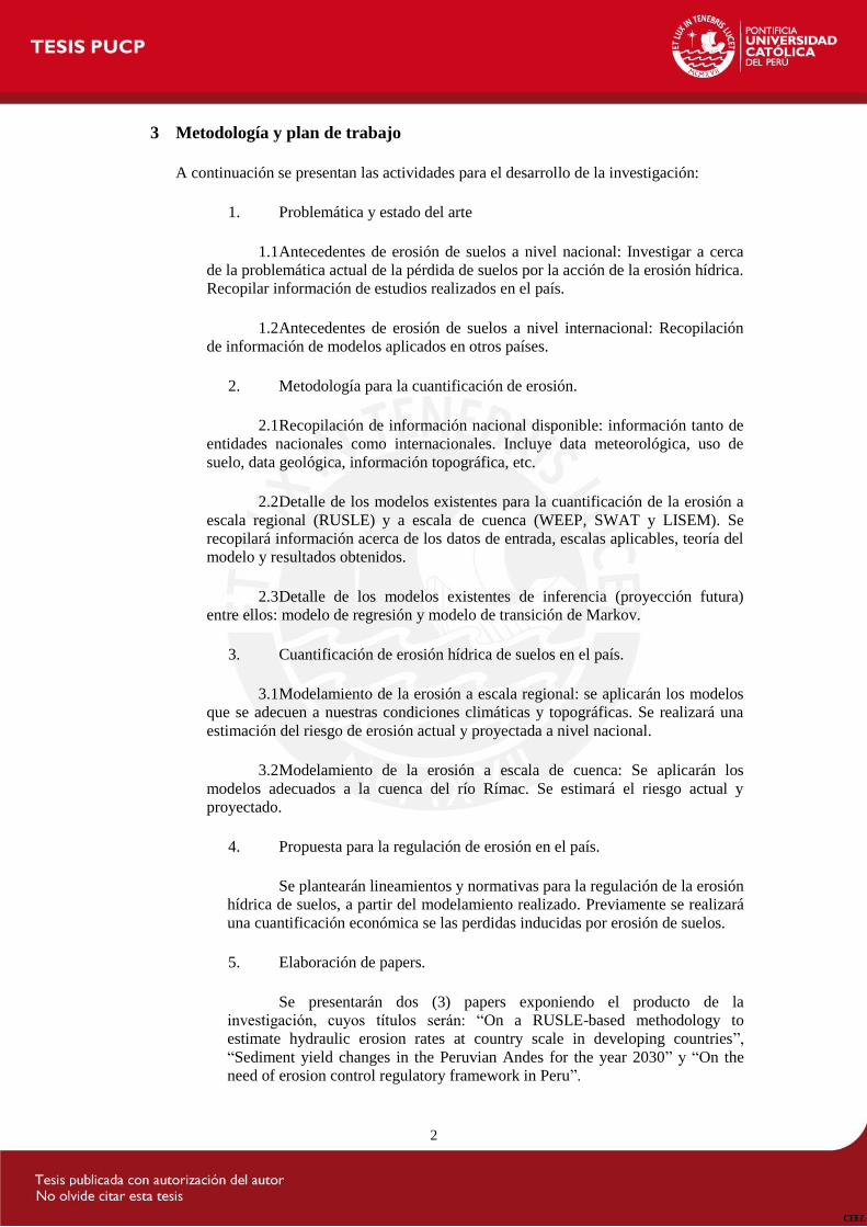
Figure 1 shows that the 85% of the validated stations located in the coastal area have an130

acceptable r > 0.5 and approximately 60% of them have a MBE < 0.5. Similarly, in the131

Andean area, 50% of the stations have a r > 0.5 and the majority of them (> 90%) present132

acceptable MBE. Similarly, in the Amazonian area, the majority of the stations (> 90%)133

present acceptable r and MBE.

Fig. 1 Satellite rainfall validation analysis. The country was divided in three geographical regions, namely:Coastal (western), Andean (central), and Amazonian (eastern) regions. n represents the number of mete-orological stations being analyzed in each region. Blue, black and green circle marks represent the stationslocated in the Northern, Central and Southern Peru, respectively. Dotted lines represent the acceptable thresh-old of MBE (< 0.5) and r (> 0.5).

134

For the case of Peru, land cover information, which comprises global land cover databases135

(items H through L in Table 1), was re-categorized in order to standardize the number of136

classes based on the Global Land Cover Share Database (10-class land cover). This op-137

eration is probably necessary for most of the developing countries due to the prevailing138

resolution of the free available data.139

140

2.2.2 The RUSLE model141

Several studies have addressed the definition of the RUSLE model and the variables that142

define it (Eq. 1); however, most of these studies do not focus on identifying the sensibility143


of the model in contexts where basic data is limited. The RUSLE model is mathematically144

defined by Eq. 1.145

A = R×K×L×S×C×P (1)

where A is the annual soil erosion (t ha−1 year−1); R is the rainfall erosivity factor which is146

expressed in MJ mm ha−1 h−1 year−1; K is the soil erodibility factor (t h MJ−1 mm−1); L is147

the slope length factor; S is the slope steepness factor; C is the cover management factor; and148

P is the conservation supporting practices factor (L, S, C and P are dimensionless). These149

variables can be categorized as static (i.e., features that remain constant in time such as K,150

L and S) and dynamic (i.e., time sensitive variables such as R, C and P). The later variables151

deserve special attention as they are scarce or inexistent in developing countries.152

To estimate the R factor (Eq. 2), past studies (e.g. [11]) recommend using the Fournier index153

(F) in regions where information scarcity is an issue.154

155

F = 1N ∑

Nj=1

(∑

12i=1

p2i

p

)(2)

In Eq. 2, pi is the monthly rainfall, p is the mean annual rainfall and N is the number of156

years being evaluated. To obtain the R factor, we applied both the Arnoldus (RA, Eq. 3)157

and the Renard and Freimund (RRF , Eq.4). These relationships were developed for different158

geographical contexts [11], however it has been commonly used to estimate R factor in159

contexts where no detailed climate data exists [52].160

RA = 0.264F1.50 (3)161

RRF = 0.07397F1.847 (4)

Thus, for the case of Peru, two sets of scenarios were evaluated, the first one using RA in162

the whole country, and the second one using RRF solely in the coastal region because it is163

only applicable to regions exhibiting low precipitation rates [11]. Such is the case of the164

Peruvian coastal region that is classified as Ea23 and Aa22 arid land areas, based on the165

Meigs classification scheme [53].166

In developing countries, the K factor, which is mathematically defined by Eq. 5, can be ob-167

tained by using the Wishmer and Smith equation [54]. The K factor depends upon the soil168

organic matter content (OM), particle size parameter (M), soil structure (s) and permeability169

(p). In this way, M is estimated by multiplying the (% silt + % sand) by (100%clay), and170

later a factor of 1.8 is applied to obtain OM from organic carbon content data (item E in171

Table 1) as suggested by [55]. This procedure was applied for Peru.172

173

K = 10−2[2.1×10−4 (12−OM)M1.14+3.25(s−2)+2.5(p−3)]/7.59 (5)

The L (Eq. 6 through 8) and S (Eq. 9) factors are typically obtained from a Digital Elevation174

Model. In the aforementioned equations, θ represents the slope angle.175

176

L =(

λ

22.13

)m(6)

177

m = β

1+β(7)

178

β = sinθ/0.08963×(sinθ)0.8+0.56

(8)

179

S =

{10.8sinθ +0.03, i f tanθ < 0.0916.8sinθ −0.5, i f tanθ ≥ 0.09 (9)


180

The C factor is based on descriptions of cropping and cover management practices and181

their influence on soil loss [54], and is mathematically defined by Eq. 10. This factor is182

determined by the prior-land use subfactor (PLU), the canopy-cover subfactor (CC), the183

surface-cover subfactor (SC), the surface-roughness subfactor (SR), and the soil moisture184

subfactor (SM). Table 2 presents commonly used values to estimate this spatial sensitive185

factor, although for more details on the quantification of the aforementioned subfactors, the186

reader is kindly referred to [54].187

C = PLU×CC×SC×SR×SM (10)

Table 2 Subfactors detail from C factor

C = PLU×CC×SC×SR×SM [54]

PLU =C f ×Cb× exp(−cur×Bur)

C f :surface-soil consolidation factorC f = 0.45 (cropland areas)C f = 1 (all the land cover types)Cb : effectiveness of subsurface residue in consolidationBur : mass density of live and deat rootscur : calibration coefficients of the subsuface residues

CC = 1−Fc× exp(−0.1×H)Fc : fraction of land surface covered by canopyH : canopy height

SC = exp{−b×Sp×

(0.24Ru

)} b : empirical coefficientb = 0.035 (erosion in cropland areas)b = 0.025 (interrill erosion)Sp : percentage of land area covered by surface coverRu : surface roughness

SR = exp{−0.66(Ru−0.24)

}Ru : surface roughness

SM = 1 Assumed value in context with limited data

188

The P factor (Eq. 11) represents the conservation practice in the cropland area and ranges189

from 0 up to 1, and only depends on the local slope (sc, in percent). The highest value is190

assigned to areas with no conservation practices [54]. For the case of Peru, we assumed191

that contouring practices takes place in moderate ridge heights because the limited collected192

information, which is not the case in others agricultural practices, such as strip-cropping and193

terraces that require more detailed data [43].194

P =

23.132(7− sc)

4 +0.45, i f sc < 712.26(sc−7)1.5 +0.45, i f sc ≥ 71.0, i f sc ≥ 20

(11)

2.2.3 Data post-processing195

Commonly, data post-processing encompasses two main steps, namely: [1] defining the out-196

put resolution based on the scale of the region evaluated and the objective of the study [18,197

17]; and [2] denoising raw data (mainly C facator) resulting from a downscaling operation.198

A resolution of 5 km (0.045◦), which lays between the lower and upper data sources reso-199

lution (see Table 1) is probably the best choice for most of the developing countries. It is200

important to mention that a finer resolution increases the noise at the raw data mean while a201


coarser resolution would result in losing information [56].202

For the case of Peru, some C factor pixels, mainly located in the Amazonian region, pre-203

sented a high bias error and a negligible variance error. These instances represented 0.15% of204

the whole data and were re-categorized by the k-Nearest Neighbors algorithm appropriately205

clustering the data (k is the neighborhood size). By following an observational criterion, the206

parameter k was fixed to a 5-pixel size to ovoid over-clustering the data.207

2.3 Model validation208

Most of the studies on estimating ERs do not provide a systematic methodology to calibrate209

the RUSLE model. Herein we propose using the sediment delivery ratio (SDR) as a proxy210

parameter to calibrate the RUSLE model at a country scale. SDR has been widely applied211

to validate the ER estimates when basic information is limited [52,43,2]. It represents the212

ratio between SY and ER, and is mathematically defined by Eq. 12 in which SLP (in %) is213

the slope of the main stream channel.214

SDR = 0.627SLP0.403 (12)

For model validation purposes, it is important to select gauging stations proving SY data215

that appropriately represents the country’s meteorological and topographical spatial vari-216

ability. Commonly, erosion model results are accepted when the SY rates differ less than217

20% from measured SY data [52]. For Peru, SY was quantified for: [1] three watersheds218

running towards the Pacific Ocean (i.e., Jequetepeque, Chira, and Santa rivers), and [2] the219

whole Eastern Peruvian Andes. The former estimates were compared with those from the220

corresponding gauging stations (items M, N and O in Table 1). Likewise, the latter were221

compared to those obtained by Latrubesse and Restrepo [32], i.e. 1113 mill Ton/year of222

sediments for the Eastern Peruvian Andes.223

3 Results and Discussion224

As shown in this paper, free satellite data provides valuable information to estimate ERs at225

country scale. However, the access to such data is currently difficult as they are not easily226

identifiable through common search portals such as Google. Apparently, globalizing satel-227

lite information for the all of potential end users around the world is still pending [22,23,228

47].229

Equations 1 through 11 were used to build eight, four and twelve SE scenarios for the years230

1990, 2000 and 2010, respectively (Table 3) and, subsequently, a spatial analysis was per-231

formed to obtain ER national maps at 5-km resolution for those years.232

The results of the scenarios presented in Table 3 were validated using SY measurements233

(items M, N and O in Table 1). Figure 2 shows the results in the Jequetepeque, Chira and234

Santa watersheds as well as those obtained by Latrubesse and Restrepo [32]. In Figure 2,235

the black line shows the temporal variation of measured SY rates; likewise, the gray shadow236

strip represents the acceptable area limited by upper and lower 20% deviation margins.237

Our results revealed that the SY rates in the Santa (10415 km2), Chira (6343 km2), and Je-238

quetepeque rivers (3317 km2) are proportional to the basin area. Past studies show that SY239

both increase and decrease as a function of drainage area [17]. Likewise, the highest SY rate240

corresponds to the year 1998 which is related to a severe El Nino event that occur in such241

year.242


Table 3 Scenarios evaluated for the years 1990, 2000 and 2010

Year: 1990R factor C and P factors

Scenarios Source Equation Source

Scenario 1.1 GPCP Arnoldus USGS EROS Data CenterScenario 1.2 GPCP Arnoldus ONERMScenario 2.1 GPCP Renard and Freimund USGS EROS Data CenterScenario 2.2 GPCP Renard and Freimund ONERMScenario 3.1 Ground Stations Arnoldus USGS EROS Data CenterScenario 3.2 Ground Stations Arnoldus ONERMScenario 4.1 Ground Stations Renard and Freimund USGS EROS Data CenterScenario 4.2 Ground Stations Renard and Freimund ONERM

Year: 2000

Scenario 1 GPCP Arnoldus MODIS Land CoverScenario 2 GPCP Renard and Freimund MODIS Land CoverScenario 3 Ground Stations Arnoldus MODIS Land CoverScenario 4 Ground Stations Renard and Freimund MODIS Land Cover

Year: 2010

Scenario 1.1 TRMM Arnoldus MINAMScenario 1.2 TRMM Arnoldus FAOScenario 1.3 TRMM Arnoldus MODIS Land CoverScenario 2.1 TRMM Renard and Freimund MINAMScenario 2.2 TRMM Renard and Freimund FAOScenario 2.3 TRMM Renard and Freimund MODIS Land CoverScenario 3.1 Ground Stations Arnoldus MINAMScenario 3.2 Ground Stations Arnoldus FAOScenario 3.3 Ground Stations Arnoldus MODIS Land CoverScenario 4.1 Ground Stations Renard and Freimund MINAMScenario 4.2 Ground Stations Renard and Freimund FAOScenario 4.3 Ground Stations Renard and Freimund MODIS Land Cover

Note: K, L and S are static factors.

In most of the instances, the scenarios in which the R factor was obtained from meteorolog-243

ical ground measurements (gray point markers in Fig. 2), SY estimates lay outside of the244

acceptable area. On the other hand, the scenarios in which the RRF factor is used as input245

parameter (blue, black and red points markers in Fig. 2), SY estimates lay inside the accept-246

able area.247

As expected, the accuracy of the results from the aforementioned scenarios exhibit both248

temporal and spatial variability. For example, for the year 1990, scenario 2.1 (black points249

in Figs. 2.a and 2.b) results on SY = 0.34 mill m3/year in Jequetepeque basin which lays250

inside the acceptable area, and SY = 0.57 mill m3/year in Chira basin which lays outside251

the acceptable area. Similarly, for the year 2000, scenario 2 (blue points in Figs. 2.a-b), SY252

rates of 3.53 and 6.36 mill m3/year were obtained in the Jequetepeque and Chira basins re-253

spectively, which lay close to acceptable area. Likewise, in the Amazonian region (Fig. 2.d),254

the SY estimate from scenario 2 is located inside the acceptable area; in contrast, in the255

Santa basin (Fig. 2.c) the SY rate is lower than the acceptable range. For the year 2010, SY256

estimates from scenarios 2.1 (red points) and 2.2 (black points) are acceptable in the Pacific257

basins; however, results from scenario 2.1 (red points) lay outside the acceptance area in the258

Amazonian region (Fig. 2.d). Most of the SY estimates in Chira basin (Fig. 2.b) lay outside259


the acceptable area, this performance is possibly triggered by El Nino Southern Oscillation260

which plays an important role in the erosion processes in the Peruvian northern coast [26].261

In conclusion, the scenario 2.1 is acceptable for the year 1990, scenario 2 for the year 2000,262

and scenario 2.2 for the year 2010. Figure 3 and Online Resource 1 (in kmz format) present263

the country ER maps obtained from such scenarios.

Fig. 2 Validation of the RUSLE model scenarios for the years 1990, 2000 and 2010 for: (a) Jequetepeque,(b) Chira, (c) Santa, and (d) Eastern Peruvian Andes. The black line represents SY data from gauging stationsand the gray strip, the acceptable area which is bounded by the upper and lower 20% deviation from the blackline. Gray points shows the scenarios 3.1 to 4.2 for the year 1990, scenarios 3 to 4 for the year 2000, andscenarios 3.1 to 4.3 for the year 2010. Triangle markers represent scenarios 1.1 and 1.2 for 1990, scenario 1for the year 2000 and scenarios 1.1 to 1.3 for the year 2010. Black points represent the scenario 2.1 in 1990and 2.2 in 2010. Red points represent scenarios 2.2 in 1990 and 2.1 in 2010. The blue points present thescenarios 2 in 2000 and 2.3 in 2010.

264

The 1990 map (Fig. 3.a) shows that in most of the territory, especially in the Amazonian re-265

gion, ER was < 10 ton/ha/year. This result has a similar order of magnitude to that from the266

climatic erosion potential index published in 1993 [16] which presents a scale of erosion of267

10 ton/ha for the whole Amazonian region. Our results for Andean (20−100 ton/ha/year)268

and the Amazonian regions (10 ton/ha/year) are also comparable to those of the global269

yearly averaged ER map of [18].270

The 1990, 2000 and 2010 ER maps we obtained (Fig. 3.a-c) show that the highest ER es-271

timates (> 50 ton/ha/year) are located in the Andean region. These results are explained272


by the fact that this region presents steep slopes and periods of high rainfall which have an273

essential role in the production of SY and SE [1]. High ERs are also observed in the coastal274

area which are the result of an increase in the C factor, i.e. land use change, induced by an275

steadily growing of farming and urban areas, and population (e.g., from 2007 to 2014, the276

Peruvian population that lived in the coastal area grew from 54.6% through 63.4%) [57–60].277

Likewise, the coastal region is characterized as a high activity seismic region in which endo-278

genic processes (i.e. earthquakes) and exogenic processes (i.e., soil erosion and landslides)279

are positively correlated [61,62]. Conversely, low ERs are observed in the Amazonian re-280

gion where the dense vegetative land cover inhibits SE to progress.281

A temporal and spatial analysis of ER from reveals that moderate ERs (10−50 ton/ha/year)282

have notably increased in the the western Peruvian Andes and along the coast region for the283

periods 1990-2000 (Fig. 3.d) and 2000-2010 (Fig. 3.e). These changes are mainly triggered284

by changes in land use [63].285

For the year 2010, Moquegua and Apurimac provinces (which are located in the southern286

Peruvian region, as shown in Fig. 3.f) have been severely affected by erosion in the 60%287

of their area approximately (Fig. 4). This scenario can potentially get worse if the illegal288

mining practices and SE are not properly controlled.289

The national erosion rate shows an steady increase for the years 1990 (19×106 ton/year),290

2000 (26× 106 ton/year), and 2010 (41× 106 ton/year) and it is expected to keep such291

trend because changes in land use are expected due to the increase of areas granted to the292

extractive industry [29]. Mining, for example, commonly triggers dry-land hill-slopes areas293

which are highly sensitive to generate significant amounts of SY even during relatively low294

rainfall intensities [1]. Under the light of these results, we believe that a erosion control reg-295

ulatory framework is possibly needed in Peru.296

In recent years, some scientific and intergovernmental groups have highlighted the need to297

advance broad open data policies and practices, and foster the increased use of Earth ob-298

servation data [47]. We believe that the method we elaborate herein not only contributes to299

these ends but also has the potential to become an initial standard frame to quantify ERs in300

developing countries, and subsequently guide the decisions ans actions to manage their soil301

resources.302

4 Conclusions303

This study elaborates on a RUSLE-based method to obtain national erosion rate maps for de-304

veloping countries. It combines up-to-date global publicly available data from satellite mea-305

surements, global soil and land cover models, and conventional ground-based data. Thus, it306

is pursued globalizing the societal benefits of satellite remote sensing data which potentially307

overcomes those of conventional ground-based measurements in developing countries. The308

method proposes the use of the sediment delivery ratio as a proxy parameter to validate309

the RUSLE model, and is successfully applied to obtain ER country maps for Peru. The310

results show that Peru faces an steady increase of ERs 1990 (19× 106 ton/year for 1990,311

26× 106 ton/year for 2000, and 41× 106 ton/year for 2010) and, apparently, it will keep312

such trend because its economy relies mainly on extractive industries, it is expanding its in-313

frastructure portfolio, and its urban population is growing. Probably such is also the case of314

many developing countries. Thus, this proposed method has the potential to guide decision315

makers towards a better soil resources management in such countries.316

Although our results are in the same order of magnitude as previous global scale erosion317

rates maps, future studies to quantify country R, K, and C factors are needed. Some devel-318


Fig. 3 RUSLE model output for Peru at 5-km resolution. Maps (a), (b) and (c) show erosion rates for theyears 1990, 2000 and 2010, respectively. Map (d) presents the ER gradient between the years 1990 and 2000,and map (e), those for the years 2000 and 2010. Figure (f) shows the Peruvian political map (gray shadowsrepresent the Coastal, Andean, and Amazonian regions).

oping countries are already going in such direction.319

In the light of our results, we believe that an erosion control regulatory framework should320

be seriously considered for Peru.321

Supporting Information322

Interactive Peruvian soil erosion maps for the years 1990, 2000 and 2010 in .kmz format.323

Acknowledgements Authors thank the financial support provided by the Consejo Nacional de Ciencia y324

Tecnologia, and the valuable data provided by the Servicio Nacional de Meteorologia e Hidrologia and the325

Instituto Geofisico del Peru. The authors also appreciate the technical discussions with Dr. Waldo Lavado and326

Dr. Sergio Morera.327

References328

1. K. Michaelides, G.J. Martin, Journal of Geophysical Research 117 (2012)329


Fig. 4 Categorical distribution of soil erosion in Peruvian provinces for the year 2010. Green, yellow andred bars represent slight (< 10 ton/ha/year), moderate (10− 50 ton/ha/year), and severe erosion rates(> 50 ton/ha/year), respectively.

2. J. Onyando, P. Kisoyan, M. Chemelil, Water Resources Management 19, 133 (2005)330

3. Pierre Y. Julien, Erosion and sedimentation (Cambridge University Press, New York, USA, 2010)331

4. R. Evans, Applied Geography (22), 187 (2002)332

5. M.O. Ribaudo, in The Management of Water Quality and Irrigation Technologies, ed. by J. Albiac,333

A. Dinar (Earthscan, 2009)334

6. G.K. AAyele, A.A. Gessess, M.B. Addisie, S.A. Tilahum, T.Y. Tebebu, D.B. Tenessa, C.F. Langendoen,335

Eddy J. nad Nicholson, T.S. Steenhuis, Land Degradation and Development pp. n/a–n/a (2015)336

7. A. Van Rompaey, G. Verstraeten, K. Van Oost, G. Govers, J. Poesen, Earth Surface Processes and Land-337

forms 26(11), 12211236 (2001). URL doi: 10.1002/esp.275338

8. R. Young, C. Onstad, D. Bosch, W. Anderson, Journal of Soil and Water Conservation 44(2), 168 (1989)339

9. A. de Roo, C. Wesseling, C. Ritsema, Hydrological Processes 10(8), 1107 (1996)340

10. J. de Vente, J. Poesen, G. Verstraeten, G. Govers, M. Vanmaercke, A. Van Rompaey, M. Arabkhedri,341

C. Boix-Fayos, Earth-Science Reviews (127), 16 (2013)342

11. K.G. Renard, J.R. Freimund, Journal of Hydrology 157, 287 (1994)343

12. W. Merritt, R. Letcher, A. Jakeman, Environmental Modelling and Software 18(89), 761 (2003)344

13. J. Boardman, J. Poesen, (John Wiley and Sons, 2006)345

14. R. Morgan, M. Nearing, Handbook of Erosion Modelling (Wiley-Blackwell, UK, 2011)346

15. N. Bellin, V. Vanacker, B. van Wesemael, A. Sole-Benet, M. Bakker, Catena 87(2), 190 (2011)347

16. M. Kirkby, N. Cox, CATENA 1-4, 333 (1995)348

17. A. Cerda, R. Brazier, M. Nearing, J. de Vente, CATENA 102 (2013)349

18. V. Naipal, C. Reick, J. Pongratz, K. Van Oost, Geoscientific Model Development 8, 2893 (2015)350

19. M. Masoudi, Risk Assessment and Remedial Measure of Land Degradation, in parts of Southern Iran351

(LAP LAMBERT Academic Publishing, Saarbucken, USA, 2010)352

20. A. Shamshad, C. Leow, A. Ramlah, W. Wan Hussin, S. Mohd. Sanusi, International Journal of Applied353

Earth Observation and Geoinformation 10(3), 239 (2008)354

21. E.F. Wood, J.K. Roundy, T.J. Troy, L.P.H. van Beek, M.F.P. Bierkens, E. Blyth, A. de Roo, P. Dll, M. Ek,355

J. Famiglietti, D. Gochis, N. van de Giesen, P. Houser, P.R. Jaff, S. Kollet, B. Lehner, D.P. Lettenmaier,356

C. Peters-Lidard, M. Sivapalan, J. Sheffield, A. Wade, P. Whitehead,357

22. F. Hossain, Bullletin of the American Meteorological Society 93, 1633 (2012)358

23. Hossain F., EOS Earth Planet and Space 96 (2015)359

24. S.B. Morera, T. Condom, P. Vauchel, J.L. Guyot, C. Galvez, , A. Crave, Hydrology and Earth System360

Sciences 17(11), 4641 (2013). DOI 10.5194/hess-17-4641-2013. URL http://www.hydrol-earth-syst-361

sci.net/17/4641/2013/362

25. R. Espinoza, J.M. Martinez, M. Le Texier, J.L. Guyot, P. Fraizy, P.R. Meneses, E. de Oliveira, Journal of363

South American Earth Sciences 1(10) (2012)364


26. W.H. Quinn, V.T. Neal, S.E. Antunez De Mayolo, Journal of Geophysical Research 92(C13),365

1444914461 (1987). URL 10.1029/JC092iC13p14449366

27. K. Takahashi, A. Montecinos, K. Goubanova, B. Dewitte, Geophysical Research Letters 38(10) (2011).367

L10704368

28. A.J. Vuohelainen, L. Coad, T.R. Marthews, Y. Malhi, T.J. Killeen, Environmental Management 50(4),369

645 (2012). DOI 10.1007/s00267-012-9901-y370

29. OXFAM, Geographies of conflict: Mapping overlaps between extractive industries and agricultural land371

uses in Ghana and Peru. Tech. rep., OXFAM America, USA (2014)372

30. M. Vuille, B. Francou, P. Wagnon, I. Juen, G. Kaser, B.G. Mark, R.S. Bradley, Earth-Science Reviews373

89, 70 (2008)374

31. Instituto Nacional de Recursos Naturales, Memoria Descriptiva: Mapa de Erosion de los Suelos del375

Peru. (Ministerio de Agricultura, Lima, Peru, 1996)376

32. E.M. Latrubesse, J.D. Restrepo, Geomorphology 216, 225 (2014)377

33. R. Adler, G. Huffman, A. Chang, R. Ferraro, P. Xie, J. Janowiak, B. Rudolf, U. Schneider, S. Curtis,378

D. Bolvin, A. Gruber, J. Susskind, P. Arkin, Journal of Hydrometeorology 4, 1147 (2003)379

34. G. Huffman, R. Adler, D. Bolvin, G. Gu, E. Nelkin, K. Bowman, Y. Hong, E. Stocker, D. Wolff, Journal380

of Hydrometeorology 8(1), 38 (2007)381

35. ISRIC World Soil Information. SoilGrids: an automated system for global soil mapping. Available for382

download at http://soilgrids1km.isric.org. (2013)383

36. METI and NASA. ASTER Global Digital Elevation Model (ASTER GDEM) . Available for download384

at http://gdem.ersdac.jspacesystems.or.jp/ (2011)385

37. ORNL DAAC. 8 km Global Land Cover Data Set Derived from AVHRR. Available for download at386

http://webmap.ornl.gov/wcsdown/index.jsp (2011)387

38. T. Loveland, B. Reed, J. Brown, D. Ohlen, J. Zhu, L. Yang, J. Merchant, International Journal of Remote388

Sensing 21(6/7), 303 (2000)389

39. S. Channan, K. Collins, W.R. Emanuel, Global mosaics of the standard MODIS land cover type data390

(University of Maryland and the Pacific Northwest National Laboratory, College Park, Maryland, USA,391

2011)392

40. J. Latham, R. Cumani, I. Rosati, M. Bloise, Global Land Cover SHARE database Beta-Release Version393

1.0 (Food and Agriculture Organization of the United Nations,FAO, Rome, Italy, 2014)394

41. R.F. Adler, G.J. Huffman, A. Chang, R. Ferraro, P.P. Xie, J. Janowiak, B. Rudolf, U. Schneider, S. Curtis,395

D. Bolvin, A. Gruber, J. Susskind, P. Arkin, E. Nelkin, Journal of Hydrometeorology 4, 1147 (2003)396

42. G.L. Stephens, T. L’Ecuyer, R. Forbes, A. Gettlemen, J.C. Golaz, A. Bodas-Salcedo, K. Suzuki,397

P. Gabriel, J. Haynes, Journal of Geophysical Research: Atmospheres 115 (2010). D24398

43. V. Jetten, M. Maneta, in Handbook of erosion modelling, ed. by M. R.P.C., N. M.A. (Wiley Blackwell399

Publishing, 2011)400

44. G.E. Frey, H.E. Fassolab, A.N. Pachas, S.M. Colcombetb, Luis an Lacortec, O. Prezd, M. Renkowe, S.T.401

Warrenf, F.W. Cubbage, Agricultural Systems 105(1), 21 (2012)402

45. L. Brandimarte, A. Brath, A. Castellarin, G. Di Baldassarre, Physics and Chemistry of the Earth 34, 209403

(2009)404

46. G. Kasera, I. Juen, C. Georgesa, J. Gomez, W. Tamayo, Journal of Hydrology 282, 130 (2003)405

47. R. Showstack, EOS 96 (2015)406

48. C. Bonilla, K.L. Vidal, Journal of Hydrology 410, 126 (2011)407

49. S.H. Franchito, A.C. Vasquez, J. Coronado, Journal of Geophysical Research: Atmospheres 114(D2)408

(2009)409

50. Z.D. Adeyewa, K. Nakamura, J. Appl. Met. 42(2), 331 (2003)410

51. Fonseca, Sigfredo E. and Reategui, Pamela, Elaboracion de mapas de isoyetas - Ambito politico admin-411

istrativo y unidades hidrograficas. (Autoridad Nacional del Agua, ANA, Lima, Peru, 2012)412

52. L. Hui, C. Xiaoling, K.J. Lim, C. Xiaobin, M. Sagong, Journal of Earth Science 21(6), 941 (2010)413

53. S.E. Nicholson, Dryland Climatology (Cambridge University Press, United Kingdom, 2011)414

54. K. Renard, G. Foster, G. Weesies, D. McCool, D. Yoder, Predicting Soil Erosion by Water: A Guide to415

Conservation Planning with the Revised Universal Soil Loss Equation. United States Department of416

Agriculture (1997)417

55. Soil Survey Staff, Kellogg Soil Survey Laboratory Methods Manual. Soil Survey Investigations Report418

No. 42, Version 5.0. U.S. Department of Agriculture, Natural Resources Conservation Service (2014)419

56. L. Martin-Fernandez, M. Martinez-Nunez, Sciences of the Total Environment 409, 3114 (2011)420

57. M. Paulet Iturri, C. Amay Leon, La conservacion de seulos en la sierra de Peru. Sistematizacion de la421

experiencia de Pronamachs en la lucha contra la desertificacion (IIICA Consorcio tecnico, Lima, Peru,422

1999)423

58. World Development Indicators: Agricultural inputs. Tech. rep., The World Bank Group, USA (2015)424


59. Direccion general de seguimiento y evaluacion de politicas, Informe de Seguimiento Agroeconomico I425

Trimestre 2015 (Ministerio de Agricultura y Riego, Lima, Peru, 2015)426

60. Instituto Nacional de Estadistica e Informatica, Peru: Poblacion estimada al 30 de junio y tasa de crec-427

imiento de las ciudades capitales, por departamento, 2014 (INEI, Peru, 2014)428

61. A. Scheidegger, Geomorphology 5, 213 (1992)429

62. A. Scheidegger, N. Ai, Tectonophysics 126(2-4), 285 (1986)430

63. N. Ramankutty, A. Evan, C. Monfreda, J. Foley, Global Biogeochemical Cycles 22, 1 (2008)431

19

CAPITULO 3:

Sediment yield changes in the Peruvian Andes for the year 2030

Sediment yield changes in the Peruvian Andes for the year 2030

Miluska A. Rosas1, Ronald R. Gutierrez2

1Graduate Student, School of Civil Engineering, Pontifical Catholic University of Peru2Associate Professor, School of Civil Engineering, Pontifical Catholic University of Peru

Abstract

The amount of sediment yield produce in the Peruvian Andes have a high significance speciallyin the Amazon basin, however few studies have addressed to quantify the volume of sedimentsin a country and continental scale for the next years. To estimate the sediment yield for the year2030, a land cover change model has been build, which is based on 1990, 2000 and 2010 landcover/land use maps. This model predict three scenarios: the normal scenario, the scenario inwhich the mining activity is included, and the scenario that presents protected areas. Our resultspredict that the volume of sediments produced in the Amazon basin (2115Ton/year) will behigher than in the Pacific basin (932ton/year) for the year 2030, also the scenario that includesthe mining activities induce an increase of sediments in both basins, conversely, the scenario thatincludes the protected areas inhibit the soil erosion process.

Keywords: soil erosion, sediment yield, land cover change, Amazon basin

1. Introduction1

Sediment yield (SY) is the result of erosion and deposition processes within a basin, which is2

basically controlled by local topography, soil and weather properties, land cover and land use,3

catchment morphology, drainage network characteristics, among others [1], which commonly4

induces the lost of fertile topsoil for agriculture and the siltation of streams and lakes [2].5

The Amazon river carries a significant amount of suspended sediment load from the South Amer-6

ica continent [1]. Limited number of studies have quantified SY in the upper Amazon (tropical7

rivers), which comprises the territories of Peru and Bolivia.Latrubesse and Restrepo [3] esti-8

mated that this region approximately produces 60% of the SY in the whole Andes, in addition9

Rosas and Gutierrez [4] obtained Peruvian erosion rate (ER) maps for the year 1990, 2000 and10

2010, these results provide valuable information to indirectly quantify the SY in such region.11

Peru is affected by the El Nino/La Nina Southern Oscillation which is the main source of tem-12

perature and climate variability [4, 5], in addition, Peru is a developing country and significant13

change in land use cover is expected in the medium term [6]. However, few studies exist about14

future predictions induced by global warming, land use change and urban growth in the country.15

Some researchers have highlighted the fact that the dataset is not representative and insufficient16

to obtain reliable future estimates in developing countries, in the light of this context, [7] men-17

tions that the satellite data have the capability to face this gap in time and spatial terms.18

Land cover/land use distribution is the most sensitive variable to estimate ER [4], land cover19

change models are used in many studies of human impacts on the environment, e.g. deforesta-20

tion practices, some of this models are based on logistic regression, multi-layer perceptron neural21

Preprint submitted to Geomorphology December 4, 2015

network and K-nearest neighbor machine learning algorithm, among others [8].22

The purpose of this this paper is quantifying the SY in the Pacific basin and Amazon region in the23

Peruvian territory for the year 2030, the impacts of three scenarios have been analyzed, namely:24

normal, including mining practices and including protected areas. Firstly, land cover change25

scenarios for Peru have been built in the IDRISI platform for the year 2030, subsequently, with26

the purpose to indirectly quantify the SY in the Pacific basin and Amazon region, the Revised27

Universal Soil Loss Equation (RUSLE) and the sediment delivery ratio (SDR) methodologies28

have been applied. RUSLE is widely used to predict SE around the world [9] and SY is usually29

obtained from erosion rate (ER) estimates by applying the SDR methodology in limited data30

contexts [10].31

2. Materials and Methods32

2.1. Land cover change model33

2.1.1. Data source34

To the best of our knowledge, information about the land cover change in Peru for the next35

decades does not exists, the last official land use map was published in 2010 and it classify the36

area in 39 types of lands.37

The data used herein comprises the main drivers driver of land change, which commonly occurs38

near to vial infrastructure, cities and human economic activities (e.g. mining practices in the case39

of Peru). Geographical, topographical, and land cover information were collected to represent40

these drivers (Table 1), such data was obtain from Peruvian public agencies and free available41

satellite international sources.42

Table 1: Input data used

Item Name Source Resolution Year

A Digital Elevation Model Japan Space System 30 m 2009 - 2011B Principal cities (shapefile) Ministerio Nacional de Educacion, MED - 2011C Major roads (shapefile) Ministerio Nacional de Transporte y Comunicaciones, MTC - 2011D Actual and projected mining areas (shapefile) Ministerio de Energia y Minas - 2011E Protected areas (shapefile) Ministerio Nacional del Ambiente, MINAM - 2011F Global Land Use/Land Cover images (15 classes) USGS EROS Data Center 0.1◦ 1992-93G The Global Land Cover Facility (16 classes) MODIS Land Cover 0.25′ 2001H Global Land Cover Share Database (10 classes) FAO, Land and Water Division 1km 2014

In order to compare the changes between the land cover maps for the year 1990, 2000 and43

2010 (items F, G and H in Table 1, the data was reclassified to harmonize the land cover number44

and classes. Eight land cover classes have been defined: urban and built, wooded wetland, snow45

and ice, tree covered (TC), woody savannas (WS), grassland and shrubs (GS), cropland (CR) and46

barren or sparsely (BS), table 2 shows a description of each land cover class.47

2.1.2. Model structure48

A prediction model structure has been build in IDRISI Selva software with the tools of the49

Land Change Modeler (LCM) platform. LCM in an empirically process that involves: change50

analysis, transition potential modeling and change prediction, which is based on the historical51

change between two time-periods with the purpose of building future scenarios [8].52

Firstly, the land cover changes between the years 1990 and 2000 has been analyzed, the LCM53

2

Table 2: Description of the land covers selected

Land cover classes Description

Urban and built Lands covered by buildings and other infrastructure.Wooded wetland Lands with a permanent mixture of water and herbaceous or woody vegeta-

tion that cover extensive areas. The vegetation can be present in either salt,brackish, or fresh water.

Snow and ice Lands under snow and/or ice cover throughout the year.Tree covered (TC) Land dominated by trees with a percent canopy cover of greater than 60% and

height exceeding 2 meters.Woody savannas (WS) lands with herbaceous and other understory systems, and with forest canopy

cover between 3060%. The forest cover height exceeds 2 meters.Grassland and shrubs (GS) Lands with herbaceous types of cover. Tree and shrub cover is less than 10%.Cropland (CR) Lands covered with temporary crops followed by harvest and a bare soil period.Barren or sparsely (BS) Lands of exposed soil, sand, rocks, or snow and never has more than 10%

vegetated cover during any time of the year.

platform has identified two important transitions: from TC to GS and from WS to GS , however,54

due to the mining activity increase in the country, three additional transitions have been consid-55

ered, from TC to BS , from GS to BS and from CR to BS .56

To built the transition sub-models, the variables have been selected by a tested based on the57

Cramer factor, which is a measure of inter-correlation of two variables and it is based on good-58

ness of fit Pearson’s chi-squared statistic models [11]. Cramer values lower than 0.15 are un-59

acceptable and values upper 0.4 has a high level of significance [8] (see Fig. 1). The variables60

have been gathered in two categories: static and dynamic, the former are calculated ones in the61

beginning of the modeling process, and the later are re-calculated in each time step (two years)62

[12]. Static variables are composed by elevation and slope (from item A in table 1), and dynamic63

variables are composed by distances to cities (from item B in table 1), distance to roads (from64

item C in table 1), and distance to the actual mining areas (from item B in table 1). Additionally,65

the variable likehood to BS has been added with LCM platform with the purpose of modeling66

the impact of the mining activity. Each transition has been modeled using the multi-layer percep-67

tion neural network which has the capability to evaluate multiple transitions in one model using68

Markov chains [8, 13].69

2.1.3. Model Validation70

The performance of the model prediction for the year 2010, has been evaluated by the receiver71

operating characteristic (ROC) curve, which is commonly applied in land cover change studies to72

measures the agreement of the predicted and the observed values of change, in terms of the true73

positives (correct change) against the false positives (errors) in the predicted model, models whit74

ROC value upper 0.5 have a high significance [14, 15, 16]. Additionally, a pixel-by-pixel com-75

parison, has been calculated, between the observed (item H in table 1 Figure 2.a) and predicted76

land cover map for the year 2010. Such comparison is composed by three measures of precision,77

namely: hits (model predicted change and it change), false alarm (model predict change and it78

persisted), and misses (model predicted persistence and it changed), it provide more information79

and a spatial distribution of errors [17].80

2.2. Model scenarios 203081

For the year 2030, three predictive model scenarios have been tested, namely: normal scenario,82

mining activity scenario (scenario A) and protected areas scenario (scenario B). Normal scenario83

3

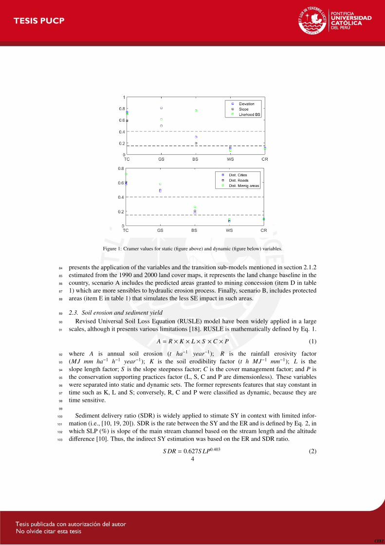
Figure 1: Cramer values for static (figure above) and dynamic (figure below) variables.

presents the application of the variables and the transition sub-models mentioned in section 2.1.284

estimated from the 1990 and 2000 land cover maps, it represents the land change baseline in the85

country, scenario A includes the predicted areas granted to mining concession (item D in table86

1) which are more sensibles to hydraulic erosion process. Finally, scenario B, includes protected87

areas (item E in table 1) that simulates the less SE impact in such areas.88

2.3. Soil erosion and sediment yield89

Revised Universal Soil Loss Equation (RUSLE) model have been widely applied in a large90

scales, although it presents various limitations [18]. RUSLE is mathematically defined by Eq. 1.91

A = R × K × L × S ×C × P (1)

where A is annual soil erosion (t ha−1 year−1); R is the rainfall erosivity factor92

(MJ mm ha−1 h−1 year−1); K is the soil erodibility factor (t h MJ−1 mm−1); L is the93

slope length factor; S is the slope steepness factor; C is the cover management factor; and P is94

the conservation supporting practices factor (L, S, C and P are dimensionless). These variables95

were separated into static and dynamic sets. The former represents features that stay constant in96

time such as K, L and S; conversely, R, C and P were classified as dynamic, because they are97

time sensitive.98

99

Sediment delivery ratio (SDR) is widely applied to stimate SY in context with limited infor-100

mation (i.e., [10, 19, 20]). SDR is the rate between the SY and the ER and is defined by Eq. 2, in101

which SLP (%) is slope of the main stream channel based on the stream length and the altitude102

difference [10]. Thus, the indirect SY estimation was based on the ER and SDR ratio.103

S DR = 0.627S LP0.403 (2)4

The main databases to obtain SE and SY for the year 2030 are the land cover change predicted104

(see section 2.1) and the Peruvian precipitation 2030 map provided by Servicio nacional de105

meteorologia y recursos hidricos (Senamhi). For details on the data bases and quantification ER106

and SY, the reader is kindly referred to Rosas and Gutierrez [4].107

3. Results and Discussion108

The land cover change model has been built with five recalculation stages (time step: two109

years) in the LCM platform to obtain the predicted land cover map for the year 2010 (Fig. 2b).110

This model presents high ROC values: 0.63 in the coastal area, 0.72 in highland and 0.94 in the111

rain-forest. Additionally, the model predicted (Fig. 2.b) and observed data (Fig. 2.a) have been112

compared pixel by pixel and the model predicted show just 4% of hits (Fig. 2.c). These results113

suggest that the model has the ability of predict the general spatial patterns (ROC > 0.5), but it114

is not the case for the exact temporal sequence prediction of the change, this is described as one115

of the difficulties in land cover change models [21].

Figure 2: Observed (a) and predicted (b) Peruvian land cover map for the year 2010. The pixel by pixel validation map(c) shows the hits in red, the false alarm in green and the misses in gray

116

This model has been applied to obtain the three land cover model scenarios (Fig. 3), and117

subsequently the SE maps for the year 2030 (Fig. 4) by applying the RUSLE equation (for details118

see section 2.3). Figure 4.b show a notably increase of severe SE rate (> 100ton/ha/year) in the119

highland region, conversely, in the case of SE controlled by protecting some natural areas (Fig.120

4.c) the rates decrease.121

122

Applaying the SDR relationship, SY rates have been obtained for the Peruvian Pacific basin123

and the Amazon basin for the three predicted scenarios, figure 5 shows that the amount of SY in124

the Amazon basin is higher than Pacific basin all the scenarios.125

5

Figure 3: Predicted land cover maps for the year 2030. Normal scenario (a), scenario A (b), which includes miningactivities and scenario B (c), which includes protected areas.

Figure 4: Soil erosion for the year 2030. Normal scenario (a), scenario A (b), which includes mining activities andscenario B (c), which includes protected areas.

4. Conclusion126

This study presents a methodology to indirectly quantify SY along the Peruvian Andes, based127

on land cover change predictions with the purpose to fill the gap of data from ground stations128

and provide valuable information for decision makers in terms of SE and SY regulation.129

Our study clearly reflects that need to obtain prediction maps for the future years, e.g. 2050,130

which should include global warming aspects and the increase of economic activities in Peruvian131

context.132

6

Figure 5: SY rates for the Peruvian Amazon and Pacific basin (x106Ton/year). The figure presents the rate for thenormal scenario (circles), scenario A (including areas granted to mining activities) and scenario B (including protectedareas)

Acknowledgement133

Authors are gratefully acknowledged the financial support provided by the by Concytec which134

is the Spanish acronym for the National Science Foundation in Peru.135

References136

[1] J. D. Restrepo, B. Kjerfve, M. Hermelin, J. C. Restrepo, Factors controlling sediment yield in a major South137

American drainage basin: the Magdalena River, Colombia, Journal of Hydrology 316 (2006) 213–232.138

[2] M. R. Rahman, Z. Shi, C. Chongfa, Soil erosion hazard evaluationAn integrated use of remote sensing, GIS and139

statistical approaches with biophysical parameters towards management strategies, Ecological Modelling (2009)140

1724–1734.141

[3] E. M. Latrubesse, J. D. Restrepo, Sediment yield along the Andes: continental budget, regional variations, an142

comparisons with other basins from orogenic mountain belts, Geomorphology 216 (2014) 225–233.143

[4] M. A. Rosas, R. R. Gutierrez, On a methodology to estimate hydraulic erosion rates in developing countries,144

Science of the Total Environment (2015).145

[5] J. M. Wallace, E. M. Rasmusson, T. Mitchell, E. S. Kousky, V. E.and Sarachik, H. von Storch, On the structure146

and evolution of enso-related climate variability in the tropical pacific: Lessons from toga, Journal of Geophysical147

Research 103 (1998) 14,241–14.259.148

[6] A. van Soesbergen, M. Mulligan, Modelling multiple threats to water security in the Peruvian Amazon using the149

WaterWorld policy support system, Earth System Dynamics Discussions 4 (2013) 567–594.150

[7] Hossain F., Data for all: Using satellite observations for social good, EOS Earth Planet and Space 96 (2015).151

[8] J. R. Eastman, IDRISI Selva Manual, Clark University, 2012.152

[9] L. Martin-Fernandez, M. Marinez-Nunez, An empirical approach to estimate soil erosion risk in spain, Science of153

the Total Environment 409 (2011) 31143123.154

7

[10] L. Hui, C. Xiaoling, K. J. Lim, C. Xiaobin, M. Sagong, Assessment of Soil Erosion and Sediment Yield in Liao155

Watershed, Jiangxi Province, China, Using USLE, GIS, and RS, Journal of Earth Science 21 (2010) 941–953.156

[11] H. Cramer, Mathematical Methods of Statistics, Princeton: Princeton University Press, 1946.157

[12] B. S. Soares-Filho, G. C. Cerqueira, C. L. Pennachin, DINAMICA - a stochastic cellular automata model designed158

to simulate the landscape dynamics in an Amazonian colonization frontier, Ecological Modeling 154 (2002) 217–159

235.160

[13] C. M. Almeida, M. Battyb, A. M. Vieira Monteiroa, G. Camaraa, B. S. Soares-Filhoc, G. C. Cerqueirac, C. L.161

Pennachind, Stochastic cellular automata modeling of urban land use dynamics: empirical development and esti-162

mation, Computers, Environment and Urban Systems 27 (2003) 481509.163

[14] T. Wassenaar, P. Gerber, P. Verburg, M. Rosales, I. M., H. Steinfeld, Projecting land use changes in the Neotropics:164

The geography of pasture expansion into forest, Global Environmental Change 17 (2007) 86–104.165

[15] R. G. Pontius, L. Schneider, Land-cover change model validation by an ROC method for the Ipswich watershed,166

Massachusetts, USA, Agriculture, Ecosystems and Environment 85 (2001) 239–248.167

[16] R. G. Pontius, L. Schneider, Unplanned land clearing of Colombian rainforests: Spreading like disease?, Landscape168

and Urban Planning 77 (2006) 240–254.169

[17] A. Comber, P. Fisher, C. Brunsdon, A. Khmag, Spatial analysis of remote sensing image classification accuracy,170

Remote Sensing of Environment 127 (2012) 237–246.171

[18] V. Naipal, C. Reick, J. Pongratz, K. Van Oost, Improving the global applicability of the RUSLE model adjustment172

of the topographical and rainfall erosivity factors, Geoscientific Model Development 8 (2015) 2893–2913.173

[19] V. Jetten, M. Maneta, Calibration of erosion models, in: M. R.P.C., N. M.A. (Eds.), Handbook of erosion modelling,174

Wiley Blackwell Publishing, 2011.175

[20] J. Onyando, P. Kisoyan, M. Chemelil, Estimation of Potential Soil Erosion for River Perkerra Catchment in Kenya,176

Water Resources Management 19 (2005) 133–143.177

[21] I. M. D. Rosa, D. Purves, C. J. Souza, R. M. Ewers, Predictive Modelling of Contagious Deforestation in the178

Brazilian Amazon, Plos One 8 (2013).179

8

28

CAPITULO 4:

On the need of erosion control regulatory framework in Peru

On the need of erosion control regulatory framework in Peru(Spanish version)

Miluska A. Rosas

Graduate Student, School of Civil Engineering, Pontifical Catholic University of Peru

Abstract

La erosion de suelos es considerada como una fuente no puntual de contaminacion de los cuerposde agua, los gastos que puede generar a largo plazo son significativos y mas aun en los paıses endesarrollo que no cuentan con un marco regulatorio como en el caso del Peru. Se han evaluadodos cuencas de gran interes nacional en terminos de produccion agrıcola, interes industrial yeconomico, que son, la cuenca del rıo Santa y de rıo Jequetepeque. A partir de nuestro estudiose estimo una perdida $12.4 millones para la cuenca de Santa y $427 millones en la cuenca delJequetepeque, causada por la perdida de nutrientes para la actividad agrıcola (on-site) y por laeliminacion del volumen de sedimentos transportados hacia los cuerpos de agua (off-site). Sibien las costos son elevados, no se han considerado otros factores que tambien intervienen en elcontexto de la cuenca. Nuestro estudio refleja la necesidad de un marco regulatorio en terminosde erosion de suelos.

Keywords: erosion de suelos, GeoWEPP, contaminacion no puntual, nutrientes, sedimentos

1. Introduccion1

Peru es un paıs en vıas de desarrollo por lo tanto el aumento de areas destinadas a actividades2

agrıcolas, extraccion de materia prima e infraestructura es inminente, estas actividades generan3

contaminacion de fuentes no puntuales o difusas en los cuerpos de agua cuyas consecuencias4

son a largo plazo. La contaminacion no puntual, a diferencia de las fuentes puntuales que son:5

vertimiento de desagues, plantas de tratamiento, industrias, etc; no ha sido un tema de interes6

en terminos de contaminacion ambiental y perdidas economicas que esta genera [1]. Este tipo7

de contaminacion no esta limitado a un canal o tuberıa, sino que generalmente es causada por8

escorrentıa, precipitacion excesiva o filtraciones que transporta los contaminantes hacia los cuer-9

pos de agua[2]. La erosion de suelos (ES) es considerada como una contaminacion no puntual, y10

puede ser la fuente de cuantiosas perdidas economicas, tanto para paıses desarrollados [3], como11

en vıas de desarrollo, como es el caso de Zimbabwe ($117 millones) [4], Indonesia ($ 406 mil-12

lones) [5] y Kenya ($ 390 millones) [6]. En el caso de la agricultura, el arrastre de sedimentos13

causa de la perdida de nutrientes lo que implicarıa costos adicionales en el uso de fertilizantes, el14

nuevo punto de equilibrio en la curva de oferta y demanda implica un aumento de precio y una15

disminucion en la produccion [7].16

Las perdidas economicas provocadas por la ES han sido clasificadas en dos grupos: on-site y off-17

site [8], la primera corresponde a perdidas en el mismo lugar donde ocurre la erosion, como por18

ejemplo perdidas de nutrientes, perdida biologica-quımica, perdida de produccion. Las perdidas19

Preprint submitted to Elsevier February 24, 2016

off-site se generan fuera del area de influencia del proceso de erosion, estos son: sedimentos en20

los cuerpos de agua, inundaciones, deslizamientos, deterioro de infraestructura, perdida de en21

proceso de tratamiento de agua, entre otros.22

Nuestro estudio, se basa en la cuantificacion del gasto economico generado por la erosion de sue-23

los en dos cuencas de interes nacional, que son, la cuenca del rıo Santa mediante la metodologıa24

RUSLE (Revised Universal Soil Loss Equation) y la cuenca del rıo Jequetepeque en donde se25

aplico la plataforma GeoWEPP (Geo-spatial interface for Water Erosion Prediction Project), las26

cuales poseen un gran potencial agrıcola y de generacion de agua para consumo humano, con27

el objetivo de mostrar la necesidad de un marco regulatorio en terminos de erosion de suelos28

para el Peru. La seccion 2, muestra la metodologıa y los datos recolectados para realizar una29

cuantificacion on-site (perdida de nutrientes) y una off-site (sedimentos en cuerpos de agua) para30

la cuenca del rıo Santa y Jequetepeque, los resultados y una discusion de ellos se presentan en la31

seccion 3 y la seccion 4 muestra las conclusiones del estudio.32

2. Datos y metodologıa33

2.1. Erosion y produccion de sedimentos en el rıo Santa34

Muchos estudios han utilizado la ecuacion de RUSLE para estimar la tasa de erosion en una35

cuenca determinada, esta seccion muestra la metodologıa para su aplicacion en el contexto de36

informacion limitada. RUSLE es matematicamente definida por la Eq. 1.37

A = R × K × L × S ×C × P (1)

donde A es la erosion anual de suelos (t ha−1 year−1); R es el factor de erosividad por precip-38

itacion (MJ mm ha−1 h−1 year−1); K es el factor de erodabilidad de suelo (t h MJ−1 mm−1); L el39

el factor de longitud de pendiente; S es el factor de pendiente; C es el factor de cobertura; y P40

es el factor de practicas de conservacion (L, S, C y P son adimensionales) [9].41

42

Para obtener el factor R, se aplico la ecuacion de Arnoldus (RA, Ec. 2) y la de Renard and43

Freimund (RRF , Ec.3). Estas relaciones fueron desarrolladas en diferentes contextos geograficos44

[10], sin embargo son comunmente usadas para estimar R en contextos donde no existe infor-45

macion detallada [11].46

RA = 0.264F1.50 (2)47

RRF = 0.07397F1.847 (3)

El factor K fue obtenido a traves de la ecuacion de Wishmer and Smith [12] que depende48

del contenido organico en el suelo (OM), el parametro de tamano de partıcula (M), estructura49

de suelo (s) y permeabilidad (p). M se obtiene de la multiplicacion de (% limo + % arena) by50

(100–%arcilla). Por otro lado factores L y S fueron obtenidos con el modelo digital de elevacion51

(DEM por sus siglas en ingles).52

El factor C esta basado en descripciones de cobertura vegetal y uso de suelo, y su influencia en53

la perdida de suelo [12], y esta matematicamente definido por Ec. 4. Este factor envuelve el54

sub-factor de prior-land use (PLU), el sub-factor canopy-cover (CC), el sub-factor surface-cover55

(S C), el sub-factor surface-roughness (S R), y el sub-factor soil moisture (S M). Para mas detalles56

acerca de este factor, el lector puede referirse a [12].57

C = PLU ×CC × S C × S R × S M (4)2

El factor P representa las practicas de conservacion en areas de cultivo y de pastoreo, con un58

rango de 0.0 a 1.0, y depende unicamente de sc, la pendiente local en porcentaje. Los valores59

altos son asignados a areas donde no se aplican practicas conservativas [12].60

Para mas detalles del calculo de cada factor y las fuentes de informacion para la estimacion de61

la tasa de erosion en el Peru, se recomienda al lector remitirse a Rosas and Gutierrez [14] y [12].62

La cuenca del rıo Santa descarga naturalmente al Oceano Pacıfico y segun la Autoridad Nacional63

del Agua (ANA) es parte de la Unidad Hidrografica 137 con un area de 11 596.5 Km2 [13]. Se64

ubica entre los 7.9 y 10.2 de latitud sur y los 78.6 y 77.2 de longitud oeste, ademas comprende65

altitudes desde el nivel del mar hasta los 6768 msnm que correspondiente al Nevado Huascaran.66

A partir del estudio de Rosas and Gutierrez [14], quienes construyeron el mapa de distribucion67

espacial de erosion a escala nacional a una resolucion de 5km, se ha obtenido el mapa de ES de68

la cuenca del rıo Santa (fig. 1.b). Respecto al punto de control ubicado a 8.65 latitud sur y 78.2569

longitud oeste, presentando una tasa de ES de 5.24 × 106 Ton/ano. Ademas con la metodologıa70

de Sediment Delivery Ratio [15] se presenta una tasa de sedimentos trasportados de 4.38 × 10671

Ton/ano.72

73

2.2. Erosion y produccion de sedimentos en el rıo Jequetepeque74

WEPP es un software desarrollado por USDA-ARS con el fin de reemplazar las ecuaciones75

empıricas para estimar las tasas de erosion hıdrica y transporte de sedimentos [16]. En proyecto76

WEPP se inicio en el ano 1985 y fue lanzado en el ano 1989. El modelo realiza simulaciones77

de procesos fısicos, tales como, erosion de suelos, escorrentıa, transporte y acumulacion de78

sedimentos a escala de cuenca y parcela para zonas de campos de cultivo, zonas de pastoreo,79

bosques y areas urbanas. Ha sido aplicado con una alta aceptacion tanto en los Estados Unidos80

[17] como al rededor del mundo [18]. El GeoWEPP se desarrolla con el fin de crear una81

herramienta que relacione las bondades del WEPP como modelo tradicional y la informacion82

geo-espacial [19], lo cual atiende la necesidad de los usuarios en terminos de planificacion de83

conservacion de agua y suelo a escala espacial y temporal.84

WEPP se basa en en tres grupos de informacion: informacion climatologica, data de elevacion85

de superficie e informacion de tipo y uso de suelos; los cuales seran detallados brevemente a86

continuacion, para mayor detalle de las ecuaciones involucradas en este modelo, sugerimos al87

lector remitirse a Ascough et al. [20] y Minkowski and Renschler [21].88

89

Data meteorologica. GeoWEPP, ademas de presentar informacion de estaciones mete-90

orologicas ubicadas en los Estados Unidos, cuenta con ciertas estaciones distribuidas en la91

superficie terrestre. Para nuestro caso, se ha considerado la data correspondiente a la estacion92

Cajamarca (- 15.47 latitud sur, -71.92 longitud oeste y 8266 msnm de altitud) que se localiza en93

una region aledana a la cuenca del rıo Jequetepeque. Esta informacion tiene una longitud de 1494

anos y comprende datos diarios de precipitacion, temperatura maxima y mınima, viento, punto95

de rocıo y radiacion solar [21].96

97

Data topografica. Se recolecto informacion de ASTER Global Digital Elevation Model98

publicado por la Nasa y el Ministerio de Economıa, Comercio e Industria de Japon, que provee99

data de elevacion del 99% de la superficie terrestre a una resolucion de 30 m de tamano de pixel.100

Dicha informacion debe ser convertida a formato ASCII para ser leıdo por el modelo.101

102

3

Uso y tipo de suelos. La base de datos para el uso de suelos fue Land Cover Share data, la103

cual fue publicada por la FAO en el ano 2014 y contiene la distribucion espacial de 10 diferentes104

clases de uso de suelo. Respecto a la data de tipo de suelo se obtuvo a partir del mapa mundial105

taxonomico de suelos USDA publicado por el World Soil Information en el ano 2014 a una106

resolucion de 1km de tamano de pixel.107

108

La cuenca del rıo Jequetepeque descarga en la cuenca del Pacıfico y abarca una extension109

aproximada de 4 360 Km2. Se ubica entre los 6.8 y 7.56 de latitud sur y los 78.36 y 78.7 de110

longitud oeste, ademas comprende altitudes desde el nivel del mar hasta los 4 000 msnm111

Luego de incorporar la informacion de entrada al GeoWEPP, se obtuvo un mapa de distribucion112

espacial de tasa de erosion a una resolucion de 60 m de tamano de pixel (ver figura 1.c), con113

un punto de control ubicado a -7.24 latitud sur y -73.15 longitud oeste. El modelo evaluo 448114

subcuencas con un area mınima de 10 Km2 (1000 Ha) y una longitud mınima de curso de agua115

de 100 m. La Tabla 1 muestra los resultados del modelo en la cuenca del rıo Jequetepeque, que116

muestran una tasa de ES promedio anual de 7.9 × 108 Ton/ano y 2.6 × 108 Ton/ano de transporte117

de sedimentos.118

119

Table 1: Reultados del modelo GeoWEPP para la cuenca de rıo JequetepequeTotal contributing area to outlet 322 075.39 haAvg. Ann. total hillslope soil loss 789 492 172.3 ton/yrAvg. Ann. total channel soil loss 3 325 251 626.5 ton/yrAvg. Ann. sediment discharge from outlet 260 264 164.0 ton/yrAvg. Ann. Sed. delivery per unit area of watershed 808.1 Ton/ha/yr

Figure 1: Mapas de erosion. (a) Mapa de ubicacion de las cuencas del rıo Santa y Jequetepeque. (b) Mapa de erosion delrıo Santa en Ton/ha/ano para el ano 2010. (c) Mapa de erosion para el rıo Jequetepeque en Ton/ha/ano.

2.3. On-site: perdidas economicas por nutrientes120

El calculo se basa en la cuantificacion de los nutrientes por tipo de suelo erosionado en la121

cuenca, luego, se le asignara el costo del fertilizante utilizado para reponer las perdidas [22].122

4

Los nutrientes evaluados seran potasio (K) y fosforo (P).123

Se cuenta con el mapa peruano de capacidad de uso mayor (CUM) de suelos publicado por el124

Instituto Nacional de Recursos Naturales, las Tablas 2 y 3 muestra las caracterısticas de cada125

clase en el area de interes.126

127

Table 2: Capacidad de uso mayor (CUM) en la cuenca del rıo Santa. Cantidad de nutrientes y materia organica. Launidad ppm corresponde a 1mg de nutriente por kg de suelo.

CUM Materia organica (%) P (ppm) K (ppm)A2s (r) 1.4 12.8 256A3se (r) 1.7 1.7 174A3sec (r) 2.12 3.7 93C3se 2.92 1.8 110P2se 7.73 7.4 118P2sec 7.73 7.4 118P3se 2.18 2.0 2.91P3sec 7.73 7.4 118Xse 2.73 1.5 40Xle 2.73 1.5 40

Table 3: Capacidad de uso mayor (CUM) en la cuenca del rıo Jequetepeque. Cantidad de nutrientes y materia organica.La unidad ppm corresponde a 1mg de nutriente por kg de suelo.

CUM Materia organica (%) P (ppm) K (ppm)A2s (r) 1.4 12.8 256A3se (r) 1.7 1.7 174A3sec (r) 2.12 3.7 93F3se 4.49 4.7 37P1s 7.73 7.4 118P3se 2.18 2.0 2.91P3sec 7.73 7.4 118Xs 0.28 1.0 324Xse 2.73 1.5 40Xle 2.73 1.5 40

La clase y costo del fertilizante se obtuvo a partir del informe anual de precios de venta de fer-128

tilizantes publicado por la Gerencia regional de agricultura de la region de La Libertad, ubicada129

al norte de la cuenca evaluada, para el 2010. El fertilizante seleccionado es el Compuesto NPK130

(contiene 20% de nitrogeno, 20% de P y 20% de K) con un costo de S./89.5 la bolsa de 50 kg.131

2.4. Off-site: perdidas economicas por sedimentos en cuerpos de agua132

El calculo se basa en la cuantificacion economica de las partidas de las obras civiles de133

remocion de sedimento y transporte hacia la escombrera o deposito [23]. A partir de costos134

actuales para actividades civiles, se ha considerado un valor de $1.35/m3 para la partida135

de remocion en terreno natural considerando un material estandar de excavacion y un valor136

aproximado de $3.0/m3 por transporte y eliminacion a escombrera para ambas cuencas.137

138

5

3. Resultados y discusion139

A partir de la base de datos mencionada se obtuvo el mapa de distribucion espacial de cada140

nutriente en la cuenca del rıo Santa y Jequetepeque y los costos que estos representan (fig. 2 y 3).141

142

Figure 2: Costo inducido por perdida de nutrientes, potasio (K) y fosforo (P) en S./ha/ano para la cuenca de rıo Santa.

Figure 3: Costo inducido por perdida de nutrientes, potasio (K) y fosforo (P) en S./ha/ano para la cuenca de rıo Jequete-peque.

La tabla 4 presenta los costos estimados por perdidas on-site y off-site para la cuenca del143

rıo Santa y Jequetepeque, dando un valor total aproximado de $12.4 y $427 millones al ano144

respectivamente. El valor de la cuenca es muy elevado respecto al costo en la cuenca de rıo145

Santa, este efecto esta probablemente relacionado a la accion del Fenomeno El Nino que incide146

en la costa norte del Peru y por la existencia del reservorio de Gallito Ciego, localizado en dicha147

cuenca.148

6

Table 4: Costos ambientales por erosion de suelos y arrastre de sedimentos.Cuenca Costo On-site Costo off-site Costo total Costo unitario

$USD/ano $USD/ano $USD/ano $USD/harıo Santa 5.2 × 106 7.2 × 106 12.4 × 106 11.9

rıo Jequetepeque 0.12 × 106 427.2 × 106 427.3×106 1288

4. Conclusiones149

El estudio se ha basado en la estimacion economica de ES por perdidas de nutrientes y sed-150

imentos en los cuerpos de agua, aun ası es necesario realizar una estimacion mas detallada in-151

cluyendo factores y agentes adicionales que cumplen un papel importante en la cuenca de Santa,152

como por ejemplo infraestructura existente e industrias de potabilizacion de agua. Nuestros re-153

sultados reflejan la importancia de realizar un estudio a largo plazo que evalue las perdidas en154

los anos futuros en las diferentes cuencas de nuestro paıs, de esta manera se considera urgente el155

desarrollo de un marco regulatorio que detenga el avance de los procesos erosivos como fuente156

de contaminacion no puntual.157

References158

[1] M. O. Ribaudo, Non-point pollution regulation approaches in the us, in: J. Albiac, A. Dinar (Eds.), The Manage-159

ment of Water Quality and Irrigation Technologies, Earthscan, 2009.160

[2] National Service Center for Environmental Publications, Protecting Water Quality from Agricultural Runoff Clean161

Water Is Everybody’s Business, Technical Report, EPA United States Environment Protection Agency, USA, 2005.162

[3] M. O. Ribaudo, Reducing Soil Erosion: Offsite Benefits, Technical Report 561, Natural Resource Economics163

Division, Economic Research Service, U.S. Department of Agriculture, Washington, D.C., 1986.164

[4] M. Stocking, The Cost of soil erosion in Zimbabwe in terms of the loss of three major nutrients, Technical Report165

3, FAO, Rome, 1986.166

[5] W. Magrath, P. Arens, The costs of soil erosion on Java: A natural resource accounting approach, Technical Report167

18, The World Bank, Washington, 1989.168

[6] M. Cohen, M. Brown, S. K.D., Estimating the environmental costs of soil erosion at multiple scales in Kenya using169

emergy synthesis, Agric. Ecosyst. Environ. 114 (2006) 249–269.170

[7] T. S. Telles, S. C. Falci Dechen, L. G. A. de Souza, M. d. F. Guimaraes, Valuation and assessment of soil erosion171

costs, Scientia Agricola (2013) 209–216.172

[8] T. S. Telles, M. d. F. Guimaraes, S. C. Falci Dechen, The cost of soil erosion, R. Bras. Ci. Solo (2011) 287–298.173

[9] V. Jetten, M. Maneta, Calibration of erosion models, in: M. R.P.C., N. M.A. (Eds.), Handbook of erosion modelling,174

Wiley Blackwell Publishing, 2011.175

[10] K. G. Renard, J. R. Freimund, Using monthly precipitation data to estimate the R-factor in the revised USLE,176

Journal of Hydrology 157 (1994) 287–306.177

[11] L. Hui, C. Xiaoling, K. J. Lim, C. Xiaobin, M. Sagong, Assessment of Soil Erosion and Sediment Yield in Liao178

Watershed, Jiangxi Province, China, Using USLE, GIS, and RS, Journal of Earth Science 21 (2010) 941–953.179

[12] K. Renard, G. Foster, G. Weesies, D. McCool, D. Yoder, Predicting Soil Erosion by Water: A Guide to Conservation180

Planning with the Revised Universal Soil Loss Equation, United States Department of Agriculture, 1997.181

[14] M. A. Rosas, R. R. Gutierrez, On a methodology to estimate hydraulic erosion rates in developing countries,182

Science of the Total Environment (2015).183

[13] R. Villanueva, Caracterısticas de la cuenca del rıo Santa, Union Internacional para la Conservacion de la Naturaleza184

(UICN SUR), Huaraz, Peru, 2011.185

[15] J. Onyando, P. Kisoyan, M. Chemelil, Estimation of potential soil erosion for river perkerra catchment in kenya,186

Water Resources Management 19 (2005) 133–143.187

[16] J. Laflen, W. Elliot, D. Flanagen, C. Meyer, N. M.A., WEPP - Predicting water erosion using a process-based188

model, Journal of Soil and Water Conservation 52 (1997) 96–102.189

[17] C. S. Renschler, J. Harbor, Soil erosion assessment tools from point to regional scales - the role of geomorphologists190

in land management research and implementation, Geomorphology 47 (2002) 189 – 209.191

7

[18] L. Pieri, M. Bittelli, J. Q. Wu, S. Dun, D. C. Flanagan, P. R. Pisa, F. Ventura, F. Salvatorelli, Using the Water Erosion192

Prediction Project (WEPP) model to simulate field-observed runoff and erosion in the Apennines mountain range,193

Italy, Journal of Hydrology 336 (2007) 84–97.194

[19] C. S. Renschler, Designing geo-spatial interfaces to scale process models:the GeoWEPP approach, Hidrological195

Processes 17 (2013) 1005–1017.196

[20] J. Ascough, C. Baffaut, M. Nearing, B. Liu, The WEPP Watershed Model: Hydrology and Erosion, American197

Society of Agricultural Engineers 40 (1997) 921 – 933.198

[21] M. Minkowski, C. Renschler, GeoWEPP for ArcGIS 9.x Full Version Manual, Department of Geography The State199

University of New York at Buffalo, New York, USA, 2009.200

[22] L. Hein, Assessing the cost of land degradation: a case study for the Puentes catchment, southeast Spain, Land201

Degradation and Development 18 (2007) 631–642.202

[23] W. Rodrigues, Valoracao economica dos impactos ambientais de tecnologias de plantio em regiao de Cerrados., R.203

Econ. Sociol. Rural 43 (2005) 135–153.204

8

PONTIFICIA UNIVERSIDAD CATÓLICA DE PERÚ...

Documents

Transcript of PONTIFICIA UNIVERSIDAD CATÓLICA DE PERÚ...