PhD Thesis

CONTRIBUTIONS TO THE STUDY OF POOL BOILING AND

SPRAY EVAPORATION ON HORIZONTAL TUBES

Author

D. Ángel Álvarez Pardiñas

Thesis Director

Prof. Dr. José Fernández Seara

Área de Máquinas e Motores Térmicos

Vigo, 2016

This thesis applies for the degree of “Doutor con Mención Internacional”

Agradecementos

Semella que remata este proceso que foi tan longo e tan cheo de reveses, pero tamén de moi bos momentos e moi boas persoas que axudaron dunhas ou outras maneiras. Tamén cheo de aprendizaxe, porque algo debín de aprender neste proceso de converterme en Doutor. É tamén cheo de cousas que agradecer.

Ao meu director de tese, José Fernández Seara. É certo que ás veces nos pos en situacións extremas, de traballo contra reloxo e sen descanso, pero consegues que todos e cada un dos que pasamos polas túas mans saibamos defendernos en calquera situación e que aprendamos máis do que un doutorado esixe.

Aos meus compañeiros de laboratorio. Aos novos e aos vellos. Rubén, Fran, Diego, Javi, Iago Novo e Iago Vello, Marta, Alex, Xandre, Alberto, Carolina... Pasamos moitas horas xuntos, moitas situacións difíciles (incluso perigosas) e algún ata tivo que aturar un berro meu; pero podo prometer e prometo que unha das razóns polas que quedaría sen dúbida nese laboratorio é por seguir compartindo momentos convosco.

Ás “vellas glorias” de Industriais e agregados. Prometo seguir encargándome da xestión deste grupo. Porque nunca nos falte unha xuntanza ao ano onde podamos seguir contándonos as nosas boas novas e os nosos éxitos.

Aos que considero como os meus mellores amigos e espero que sexa recíproco. Charlos, Varela, Coru, Lastres, Flisplis, Sandra, Maciu e Cane. Sempre estivestes aí e sei que vos terei dunha forma ou outra na miña vida. Por moitos anos e moitas vivencias (e visitas a Noruega).

A Raquel, porque non sei que dicir que ti non saibas… Ti fuches un apoio sen o cal non estaría aquí tan cedo. Fuches o final desta gran etapa e a persoa coa que vou compartir a vindeira e toda unha vida. Gracias por non dubidar e por demostrar que se fai falla iremos xuntos ao fin do mundo.

Á familia, que nunca falla. Mamá, papá e Carmela. Sempre apoiándome, sendo igual o destino escollido. Gracias aos tres (e tamén á abuela) por ser os meus confidentes e axudarme a tomar decisións difíciles. E gracias, pais, por darme a oportunidade de chegar a este punto da miña formación, sobre todo persoal. Son o que son por vós e non teño queixa ningunha do resultado. Non reclamarei nin pedirei a devolución ou o cambio.

Abstract

Refrigeration cannot stay aside from the environmental and energy challenges that humanity is about to face in the coming years. Montreal’s Protocol and later revisions marked the beginning of usage restrictions of CFCs and HCFCs, due to environmental issues such as ozone layer depletion and global warming. R134a and other HFCs will be soon phased out due to their global warming potential (GWP). Natural refrigerants such as CO2, ammonia or hydrocarbons appear as interesting alternatives from environmental and performance points of view. The high pressures of CO2 systems, the toxicity of ammonia or the flammability of hydrocarbons are important disadvantages of these fluids. Natural refrigerants combined with more efficient systems should be the investigation line followed in the future.

Falling film evaporators, also known as spray evaporators, have been widely employed in petrochemical industry, desalination processes and OTEC (Ocean Thermal Energy Conversion) systems. The experience in other fields such as heat pumps and refrigeration is limited, but falling film evaporators appear as an interesting alternative to flooded evaporators due to potential benefits in terms of refrigerant charge reduction and heat transfer improvement. In addition, the boiling temperature increase caused by hydrostatic head in flooded evaporators is avoided, the temperature approach between refrigerant and cooled fluid decreases and the efficiency of the cycle improves and the evaporators can be of smaller size. The main drawback of falling film evaporators is that the design of the distribution system is critical and, if incorrect, may cause heat transfer deterioration due to dryout of the falling film.

Falling film evaporators in refrigeration systems are heat exchangers with a shell-and-tube structure. Spray nozzles or other spreading devices distribute liquid refrigerant over the first rows of tubes of a tube bundle. Part of the refrigerant boils on the top row, cooling the fluid flowing inside the tubes, and the rest forms a film that flows to the following row. This boiling and flowing process occurs from one row to the next one. The exceeding refrigerant is collected at the bottom of the evaporator and recirculated to the distribution unit (with intermediate conditioning steps if needed).

A large number of parameters affect the performance of falling film evaporators, but authors disagree about the effect of each of them. Those with a higher influence are heat flux, film flow rate, geometry of the tube, refrigerant properties and distribution system. The use of enhanced tubes enhances heat transfer if compared to plain tubes. In addition, most enhanced tubes delay film breakdown, maintaining the surface wet. Only those geometries that limit liquid axial movement, such as low-finned tubes with a high concentration of fins, should be avoided in these systems.

An experimental setup available in the laboratory was redesigned in order to allow spray evaporation tests. These tests consist in distributing the liquid refrigerant, in conditions very close to saturation, on the tested tube/s, simulating the situation that occurs in spray evaporators.

The main modification developed was to include a liquid distribution system to distribute the liquid refrigerant. The system was designed to allow testing different types of spreading devices. Among the different possibilities, full cone nozzles have been selected. The equipment permits different spacings between the nozzles, as well as choosing between two positions for the tube that receives the refrigerant from the nozzles. In addition, it allows comparing the heat transfer coefficients obtained when the tested tube receives the liquid refrigerant directly from the nozzles and when the liquid refrigerant falls by gravity from a conditioning tube above the tested one.

The experimental setup does not follow a typical vapour compression cycle. Instead, pool boiling/spray evaporation and condensation occur at the same pressure and refrigerant flows from one shell-and-tube heat exchanger to the other due to the differences of density between liquid and vapour refrigerant. This configuration allows, on the one hand, testing very different conditions and refrigerants and, on the other hand, discarding the effect of lubricants on the heat transfer coefficients determined.

The test rig is prepared for tubes of nominal external diameters up to 20 mm, but we tested tubes of nominal external diameter 3/4” (19.05 mm), which are widely extended in shell-and-

tube heat exchangers. We chose tubes with plain and enhanced external surfaces, and the material depends on the refrigerant used (compatibility refrigerant – material).

The compatibility with ammonia was the main consideration during the selection of materials for building the experimental setup. Thus, we used stainless steel (AISI-316L) in almost every component.

As previously mentioned, due to the working principle of the experimental facility, a wide range of condensation and evaporation conditions can be tested. We chose liquid temperatures between 0 and 10 ºC for our pool boiling and spray evaporation tests, common temperatures in water chillers. This range of temperatures allowed using water as secondary fluid both for condensing the vapour refrigerant at the condenser tubes and for vaporising the liquid at the evaporator tubes. The use of water is very convenient since its properties are very accurately determined using the temperatures measured.

The experimental facility stabilises the refrigerant pool temperature or the liquid distribution temperature (boiling saturation pressure), for pool boiling and spray evaporation tests, respectively. The distributed liquid refrigerant flow rate is also controlled accurately, maintaining the rest of the conditions constant. The temperatures and flow rates of the secondary fluids can also be regulated and stabilised at the values needed for each test.

The experimental setup allowed measuring the conditions (temperature, pressure and flow rate) of the refrigerant and secondary fluids. Several sensors were also included to determine the conditions of the distributed refrigerant.

We designed an experimental methodology to obtain pool boiling and spray evaporation heat transfer coefficients. The methodology is based on determining the different thermal resistances of the overall heat transfer process that occurs at the tubes.

The design of experiments has focused on studying the boiling heat transfer coefficients under temperature conditions close to those found at water chillers, and with the largest range of heat fluxes possible. We have conceived a specific experimental methodology to analyse the influence of the impingement effect on the heat transfer coefficients with distribution of the liquid refrigerant.

Pool boiling tests consisted in registering the values measured by the different sensors of the test rig, keeping constant the mean heating water temperature and flow rate through the tube and the refrigerant pool temperature. Except for special sets of experiments, a group of tests (constant pool temperature) started with the maximum mean heating water temperature possible. When stationary conditions were achieved, data were registered for a minimum of 15 minutes. After that, the mean heating water temperature was lowered and fixed at the next testing condition. When finished a group of tests, a new was began at another refrigerant pool temperature, repeating the procedure explained in the previous lines.

In spray evaporation experiments there are two new parameters to be considered: the relative position between the tested tube and the distribution tube and the liquid refrigerant distributed mass flow rate. The relative position of the tested tube and the distribution tube was introduced as a new experimental variable because other authors observed that the liquid droplet impingement effect could enhance heat transfer. Thus, we should expect differences in the heat transfer performance between those tubes that receive refrigerant directly from the distribution devices and those that are wetted by the excess liquid from the row of tubes placed above them. Therefore, we have designed two different spray evaporation tests to illustrate these two possibilities. The first tests, named ST tests, consist in distributing the refrigerant directly from the nozzles to the tested tube, being the distance from the tip of the nozzle to the tube axis 59 mm. In the second tests, named SB tests, the refrigerant is distributed on the same tube, which works as a conditioning tube, forming a film that falls to the tube placed underneath (distance of 45 mm between tube axes). No heating water circulates through the conditioning tube to prevent liquid refrigerant from vaporising before falling to the tested tube.

We started with ST tests. The liquid refrigerant distribution temperature was fixed and, for each group of tests, the mean heating water temperature started at the maximum value achievable by the experimental test rig. Then, the liquid refrigerant distribution flow rate was set at the maximum of the experimental set points considered, which was different for each of the refrigerants tested. When stationary conditions were achieved, data were registered for a minimum of 15 minutes. After that, the liquid refrigerant distribution flow rate was lowered and

the process repeated. When all the flow rates were tested, the mean heating water temperature was lowered and fixed at the next testing condition and the sequence of tests was repeated. Once finished ST tests, we repeated the whole process with SB tests.

Independently of the kind of tests, the heating water flow rate was kept as high as possible to minimise the inner thermal resistance at the evaporator tubes, reduce the uncertainty of the heat transfer coefficients and homogenise the boiling process along the tube (similar wall temperature conditions). The cooling water flow rate was kept as low as possible to increase the cooling water temperature difference between the inlet and the outlet of the condenser tube/s and to calculate with more accuracy the heat flow at this heat exchanger.

We explain the calculation method to determine the heat transfer coefficients from the experimental data from the test rig. The methodology is based on the separation of all the thermal resistances that are part of the overall heat transfer process occurring in heat exchangers. Prior to including the refrigerant pump in the refrigerant cycle and taking into account the working principle of the experimental test rig and the good insulation applied, the overall thermal resistance was accurately calculated with the heat flow at the condenser. After its installation, we observed that the heat flow at the evaporator tubes was seen to match the electric power delivered to the heating water at the electric boiler.

We also detail the method to estimate the fraction of liquid refrigerant reaching the studied tubes under spray conditions and defined the enhancement factor to compare the heat transfer coefficients calculated for different tubes and different boiling process, at the same conditions.

The results shown include uncertainties and these uncertainties prove the quality and reliability of the results. There is an appendix in the document that explains the process followed to calculate these uncertainties, which is based on the Guide to the Expression of Uncertainty in Measurements.

We performed validation experiments to check the assumptions considered at the calculation process. The validation process has been successful and, thus, the heat transfer coefficients obtained with this experimental facility and procedure result from a convenient process.

We show the pool boiling heat transfer coefficients obtained experimentally for this thesis. The refrigerants studied have been R134a and ammonia. With the former we tested copper tubes of plain and enhanced surfaces (Turbo-B and Turbo-BII+); and with the latter we tested titanium tubes of plain and enhanced surface (Trufin 32 f.p.i.).

We observed that the vast majority of our experimental results are included in the nucleate boiling region of Nukiyama’s boiling curve, where the slope is steep and heat flux increases rapidly with superheating.

Concerning the pool boiling heat transfer coefficients, we observed that they generally increase with increasing saturation temperatures, being constant the heat flux. We also observed for all the tubes except for Turbo-B that pool boiling heat transfer coefficients rise as the heat flux rises, independently of the saturation temperature. This effect was clearer with the plain tubes.

With ammonia we also tested the influence of hysteresis on the nucleation process. Several works of the literature show different results when experiments were conducted in increasing heat flux direction and in decreasing heat flux direction. We confirmed the existence of this hysteresis effect and that it is more important with the enhanced surface tested (Trufin 32 f.p.i.). However, our experiments show that increasing heat flux tests are time-dependent, i.e. the heat transfer coefficients obtained when the experimentation process follows an increasing heat flux direction rise (even when the test conditions remain constant) until they reach a value very close to that obtained with the decreasing heat flux tests.

We compared our experimental results with well-known correlations from different works from the literature. In the case of plain tubes, the best agreement existed with Gorenflo and Kenning correlation with R134a and with Mostinski correlation with ammonia.

The surface enhancement techniques are more effective with R134a than with ammonia. With R134a, the surface enhancement factors are as high as 11.8 and 7 with the Turbo-B and Turbo-BII+, respectively. In contrast, with ammonia the surface enhancement factor is never greater than 1.3.

We included the photographic reports of the pool boiling of ammonia on the plain tube and the Trufin 32 f.p.i. tube. The pictures show the increase of density of nucleation sites and of the bubble diameters as the heat flux increases. The visual differences between tubes are very slight, confirming the surface enhancement factor results determined.

Concerning spray evaporation, we studied R134a and ammonia with plain tubes. The tubes used with R134a were made of copper and the tubes used with ammonia were made of titanium.

We observed that the vast majority of our spray evaporation experimental results are included in the nucleate boiling region of the boiling curve. The slope of the boiling curve is steep, i.e. heat flux increases rapidly with superheating.

Spray evaporation heat transfer coefficients with R134a and the copper tube increase, generally, if the heat flux is higher, independently of the mass flow rate of the film per side and meter of tube. We also observed that the effect of the mass flow rate on the heat transfer coefficients is negligible.

The spray evaporation heat transfer coefficients obtained with R134a and the tube placed directly underneath the refrigerant distribution tube (ST tests) are, on average, 13.2% greater than those determined with the tube that receives refrigerant from the conditioning tube (SB tests), if kept the heat flux and distributed mass flow rate constant. The heat transfer enhancement occurs due to the liquid droplet impingement effect.

We compared spray evaporation and pool boiling under similar conditions and we observed that spray evaporation enhances heat transfer only if the heat flux is low (lower than 20000 W/m2). Enhancement is never higher than 60%. The results concerning heat transfer enhancement are in line with others shown in the specialised literature.

An analysis of the photographs taken during the experiments allowed confirming the existence of dry patches on the tube. Dryout occurred even when the distributed refrigerant was significantly greater than the amount of refrigerant that vaporised on the tube (overfeed rates well over 1).

The spray evaporation heat transfer coefficients with ammonia and the titanium tube depend on both heat flux and mass flow rate of refrigerant per side and meter of tube. Generally, they increase as the heat flux increases, but this trend is even opposite under conditions of high heat flux and low mass flow rate.

We observed that the spray evaporation heat transfer coefficients obtained with ammonia and the tube placed directly underneath the refrigerant distribution tube (ST tests) are, on average, 38.7% higher than those determined with the tube that receives refrigerant from the conditioning tube (SB tests). Droplet impingement effect is responsible of this effect.

From the comparison of spray evaporation and pool boiling of ammonia on the plain tube, we concluded that spray evaporation enhances importantly heat transfer. Spray enhancement factors are well over 1, particularly when the refrigerant on the tested tube arrived directly from the nozzles (ST tests). The maximum enhancement factor has been over 6 and the best results occurred in the low heat flux range (up to 20000 W/m2).

We analysed the snapshots taken when conducting the tests and the most important conclusion is that we could confirm that dry patches occurred under certain conditions. Dryout explains some of the tendencies we obtained from our experimental results. However, we calculated the overfeed ratio for the conditions of the tests shown in the photographs and realised that dryout occurred even when the overfeed rates greater than 1.

The experimental results obtained make clear the importance of having a proper distribution of the liquid refrigerant on the tubes of spray evaporators. Thus, developed a computer programme, based on a geometric study, to optimise the design of liquid distribution systems with spray nozzles. The programme calculates the percentage of liquid distributed by a given spray nozzle that reaches a generic tube, defining concepts such as those of the theoretical and real limit angles from a nozzle to a tube or the dimensionless column factor.

We also developed a parametric analysis with a 1-meter-long tube bundle with 8 rows and 8 tubes per row (7 for even rows in staggered pitch layout), varying parameters such as the horizontal and vertical pitch, the tube bundle pattern, the spray nozzle angle, etc. We observed

that, in general, 60º nozzles lead to an even distribution and more efficient use of the liquid distributed. However, they require a larger distance between the spray nozzles and the first row of the tube bundle to optimise distribution and, thus, there is an important part of the shell that must be clear of tubes. The performance of systems with 90º nozzles is slightly lower, but the distance required is also shorter and they are convenient from that point of view.

The parametrical analysis proves that the even distribution of liquid on the different columns of inline tube bundles is easier than when the pattern is staggered. In fact, staggered tube bundles seem unsuitable for this kind of distribution systems with nozzles and without intermediate devices. Only when staggered bundles had a high horizontal pitch between tubes of the same row was high (2 in this case), we observed a convenient distribution between the different columns. However, an increase of this horizontal pitch leads to the loss of compactness of staggered bundles, which is the main advantage of such tube pattern.

Resumo

O sector da refrixeración non pode permanecer alleo aos retos medioambientais e enerxéticos aos que se enfrontará a humanidade nos vindeiros anos. Os protocolos de Montreal e posteriores revisións marcaron o comezo das restrición do uso de refrixerantes clorofluorocarbonados (CFCs) e hidrocloroflorocluorocarbonados (HCFCs) debido á destrución da capa de ozono. O R134a e outros refrixerantes tipo hidrofluorocarbonados (HFCs) están eliminándose gradualmente debido ao seu potencial de quecemento global (GWP). Os refrixerantes naturais, como CO2, o amoníaco ou os hidrocarburos, semellan alternativas interesantes aos anteriores desde os puntos de vista medioambiental e de eficiencia. Porén, as elevadas presións dos sistemas de CO2, a toxicidade do amoníaco ou a inflamabilidade dos hidrocarburos son as súas principais desvantaxes. A combinación de refrixerantes naturais e sistemas máis eficientes é a liña de investigación a seguir no futuro.

Os evaporadores de caída de película, tamén coñecidos como evaporadores en spray, teñen sido amplamente utilizados na industria petroquímica, en procesos de desalgado de augas e en sistemas de conversión de enerxía cas diferencias térmicas do océano (OTEC). A experiencia con estes equipos noutros campos como as bombas de calor ou a refrixeración é limitado, pero estes aparecen como unha interesante alternativa aos evaporadores inundados, debido a que poden implicar unha diminución da carga de refrixerante ou unha mellora da transmisión de calor. Ademais, evítase o aumento da temperatura de ebulición que aparece nos evaporadores inundados debido á presión hidrostática; redúcese a diferenza de temperatura entre o refrixerante e o fluído a arrefriar, co que mellora a eficiencia do ciclo termodinámico; e redúcese o tamaño dos evaporadores. A maior desvantaxe dos evaporadores con caída de película é que o deseño do sistema de distribución é crítico e pode implicar un empeoramento da transmisión de calor debido á aparición de zonas secas na película de líquido refrixerante.

Os evaporadores de caída de película en sistemas de refrixeración son intercambiadores de tipo carcasa e tubos. Boquillas de spray ou outros sistemas de distribución reparten o líquido refrixerante sobre as primeiras filas do banco de tubos. Parte do refrixerante vaporiza sobre a fila superior, arrefriando o fluído que circula polo interior dos tubos, mentres que o resto forma unha película que avanza ao seguinte tubo. Este proceso de vaporización e avance continúa ao longo do banco de tubos. O exceso de refrixerante recóllese na parte inferior do evaporador e recircúlase á unidade de distribución (con acondicionamentos intermedios se son necesarios).

A eficiencia dos evaporadores con caída de película vese afectada por un gran número de parámetros, pero os diferentes autores están en desacordo acerca do efecto de cada un deles. Os parámetros con maior influencia son a densidade de fluxo de calor, o caudal másico distribuído, a xeometría dos tubos, as propiedades do refrixerante e o tipo de sistema de distribución. Os tubos con superficies melloradas fan que a transmisión de calor sexa máis eficiente, se os comparamos cos tubos lisos. Ademais, estas superficies soen retrasar a aparición de zonas secas, aínda que hai que evitar aquelas que limitan o movemento axial do líquido, tales como os tubos con aletas integradas e elevada densidade de aletas.

Redeseñouse un equipo experimental existente no laboratorio para permitir a realización de ensaios de evaporación en spray. A particularidade destes ensaios é que hai que distribuír un líquido refrixerante, en condicións moi próximas ás de líquido saturado, sobre o tubo ou tubos ensaiados, simulando as condicións que ocorren en evaporadores en spray.

A principal modificación realizada foi a inclusión do sistema de distribución de líquido para o refrixerante. O sistema deseñouse para que fose versátil e permitise o emprego de diferentes sistemas de distribución. De entre as diferentes posibilidades, escolléronse as boquillas de spray tipo “full cone”. O equipo permite modificar a distancia entre as boquillas, así como seleccionar entre dúas posicións para o tubo que recibe o refrixerante das mesmas. No equipo tamén se poden comparar os coeficientes de transmisión de calor para os tubos que reciben o líquido refrixerante directamente desde o sistema de distribución co daqueles tubos alimentados polo fluído restante dun tubo superior (tubo de acondicionamento).

O equipo experimental non segue un ciclo de compresión de vapor típico. En cambio, os procesos de condensación e vaporización (con caída de película ou inundada) ocorren á

mesma presión e de forma simultánea (en cadanseu intercambiador). O refrixerante flúe dun intercambiador de calor a outro debido ás diferencias de densidade entre o líquido e o vapor de refrixerante. Esta configuración permite, por un lado, probar un amplo rango de refrixerantes e condicións e, por outro lado, evitar a presencia de lubricante durante a determinación dos coeficientes de transmisión de calor.

O banco de ensaios está preparado para tubos de ata 20 mm de diámetro nominal exterior. Para estes ensaios seleccionamos tubos de 3/4" (19,05 mm) de diámetro exterior, cuxo uso está moi estendido en intercambiadores de calor de carcasa e tubos. Escollemos tubos con superficies exteriores lisa e mellorada, e o material dos mesmos depende do refrixerante empregado, buscando a compatibilidade entre ambos.

A compatibilidade co amoníaco foi a consideración principal á hora de seleccionar os materiais para construír o equipo experimental. Por iso, empregouse aceiro inoxidable tipo AISI-316L na maioría dos compoñentes.

Como se mencionou anteriormente, debido ao principio de funcionamento do equipo experimental pódese probar un amplo rango de condicións de condensación e evaporación/ebulición. Escollemos temperaturas de líquido entre 0 ºC e 10 ºC para os ensaios de ebulición inundada e de evaporación en spray, que son temperaturas típicas en arrefriadoras de auga. Este rango de temperaturas permite empregar auga como fluído secundario tanto para condensar o vapor de refrixerante nos tubos do condensador como para vaporizar el líquido refrixerante en los tubos del evaporador. O emprego de auga é moi interesante xa que se coñecen as súas propiedades con moita precisión a partir da temperatura.

O equipo experimental controla a temperatura de piscina de líquido ou a temperatura de distribución de líquido refrixerante para os ensaios de ebulición inundada e evaporación en spray, respectivamente. Tamén se pode axustar o caudal másico de líquido refrixerante distribuído mantendo o resto de condicións constantes. As temperaturas e caudais dos fluídos secundarios tamén se poden regular e estabilizar con precisión en función do ensaio.

Os diferentes sensores de temperatura, presión e caudal que existen no banco de ensaios permiten medir as condicións do refrixerante e dos fluídos secundarios. Durante as modificacións do equipo, houbo que incluír novos sensores para determinar as condicións do refrixerante distribuído.

Deseñamos unha metodoloxía experimental para obter os coeficientes de transmisión de calor dos procesos de ebulición inundada e evaporación en spray. Esta metodoloxía baséase en determinar as diferentes resistencias térmicas do proceso global de transferencia de calor.

O deseño dos experimentos centrouse en estudar os coeficientes de transmisión de calor baixo condicións de temperatura preto das que existen en arrefriadoras de auga, e co maior rango de densidades de fluxo de calor posible. Desenvolvemos unhas metodoloxía experimental específica para analizar o efecto do impacto do líquido nos coeficientes de transmisión de calor nos evaporadores en spray.

Nos ensaios de ebulición inundada rexistráronse valores dos diferentes sensores da bancada experimental, mantendo constante a temperatura media e o caudal da auga de quecemento que pasa polo tubo do evaporador, así como a temperatura da piscina de líquido refrixerante. Excepto para algún experimento con finalidade específica, cada grupo de ensaios a temperatura de piscina constante comeza co valor máximo de auga de quecemento (máxima densidade de fluxo de calor). Cando se alcanza o estado estacionario, rexístranse datos por un mínimo de 15 minutos. Despois, redúcese o valor da temperatura media da auga de quecemento e fíxase na seguinte condición de ensaio. Cando finalizan os ensaios a unha temperatura de piscina de líquido, modifícase esta e comézase un novo grupo de ensaios, repetindo o procedemento anterior.

Nos experimentos de evaporación en spray hai dous novos parámetros a considerar: a posición relativa entre o tubo ensaiado e o tubo de distribución e o caudal másico de líquido refrixerante distribuído. A posición relativa introduciuse xa que hai traballos da literatura especializada nos que se indica que o impacto do líquido refrixerante sobre o tubo pode mellorar a transmisión de calor. Por iso, debemos agardar diferenzas nos coeficientes de transmisión de calor entre os tubos que reciben refrixerante directamente dos equipos de distribución e os que reciben o refrixerante doutros tubos. Deseñamos dous tipos de

experimentos de evaporación en spray para ilustrar estas dúas posibilidades. No primeiro tipo de ensaios, denominados ensaios ST, o tubo ensaiado localízase directamente debaixo dos equipos de distribución, sendo a distancia entre a punta das boquillas e o centro do tubo ensaiado igual a 59 mm. No segundo tipo de ensaios, denominados ensaios SB, o refrixerante distribúese sobre o tubo anterior, que neste caso traballa como tubo de acondicionamento. Sobre el fórmase unha película de líquido que cae no tubo ensaiado, que está 45 mm por debaixo do de acondicionamento. Polo tubo de acondicionamento non circula auga de quecemento para evitar a vaporización do líquido refrixerante distribuído.

O proceso comeza cos ensaios ST. A temperatura do líquido refrixerante distribuído fíxase, e establécese a temperatura media da auga de quecemento máxima que se pode alcanzar co equipo experimental. Tamén é necesario axustar o caudal de líquido refrixerante distribuído nun dos valores a ensaiar. Cando se alcanza o estado estacionario, rexístranse datos por un mínimo de 15 minutos. Despois modifícase o valor do caudal e se repite o proceso. Cando finaliza o grupo de ensaios a unha mesma temperatura media da auga de quecemento, redúcese este parámetro ata a seguinte condición de ensaio e repítese a secuencia. Unha vez rematados os ensaios ST, procédese de igual xeito cos ensaios SB.

Independentemente do tipo de experimentos, mantívose o caudal de auga de quecemento polos tubos do evaporador nun valor elevado para minimizar a resistencia térmica do proceso de convección interior, reducir a incertidume dos coeficientes de transmisión de calor determinados e homoxeneizar o proceso de ebulición ao longo do tubo (temperaturas de parede semellantes en todo o tubo). O caudal de auga de arrefriamento estableceuse nun valor baixo para aumentar a diferenza de temperaturas neste fluído entre a entrada e a saída dos tubos do condensador e calcular con maior precisión os fluxos de calor no intercambiador.

O método de cálculo dos coeficientes de transmisión de calor a partir dos datos rexistrados polos sensores da bancada está detallado no documento. A metodoloxía baséase na separación das resistencias térmicas que do proceso global de transmisión de calor. Antes de incluír a bomba de refrixerante no ciclo e tendo en conta o principio de funcionamento do equipo experimental e o bo illamento do mesmo, podíase calcular a resistencia térmica global nos tubos do evaporador co fluxo de calor no condensador. De todos os xeitos, trala instalación da bomba foi necesario modificar isto. Observouse que o fluxo de calor transferido no evaporador correspondíase á potencia eléctrica transmitida na caldeira á auga de quecemento dos tubos do evaporador.

Desenvolveuse un método para o cálculo da fracción de líquido refrixerante do total distribuído que chega aos tubos ensaiados baixo condicións de evaporación en spray. Tamén definimos dous parámetros para a determinación dos factores de mellora derivados do emprego de tubos con superficies melloradas con respecto aos tubos lisos e derivados da utilización de técnicas de spray con respecto aos evaporadores inundados, ás mesmas condicións de ensaio.

Os resultados que se mostran na tese levan asociadas as incertidumes para probar a calidade e fiabilidade dos mesmos. Inclúese un anexo no que se explica o proceso para o cálculo destas incertidumes, o cal está baseado na Guía para a Expresión da Incertidume nas Medidas.

Os ensaios de validación permitiron comprobar as hipóteses consideradas para o proceso de cálculo. A validación realizouse con éxito e, polo tanto, os coeficientes de transmisión de calor obtidos con este equipo e procedemento experimental son resultado dun proceso conveniente.

Os coeficientes de transmisión de calor dos procesos de ebulición inundada incluídos nesta tese de doutoramento corresponden aos refrixerantes R134a e amoníaco. Co primeiro deles ensaiamos tubos de cobre de superficie lisa e mellorada (Turbo-B e Turbo-BII+) e co segundo os tubos foron de titanio, con superficie lisa e mellorada (Trufin 32 f.p.i.).

A gran maioría dos nosos resultados experimentais de ebulición inundada están incluídos dentro da zona de ebulición nucleada da curva de ebulición de Nukiyama, onde a pendente é pronunciada e a densidade de fluxo de calor medra rapidamente con pequenos aumentos da diferencia de temperaturas entre a parede e o refrixerante.

En xeral, os coeficientes de transmisión de calor en ebulición inundada aumentan conforme aumenta a temperatura de saturación (sendo constante a densidade de fluxo de calor). Para

todos os tubos excepto no caso do Turbo-B, ao medrar a densidade de fluxo de calor increméntanse os coeficientes de transmisión de calor, independentemente da temperatura de saturación. Este efecto observouse máis claramente para os tubos lisos.

Con amoníaco tamén se fixeron ensaios para analizar a histérese no proceso de nucleación. Varios traballos da literatura mostran que, para unhas mesmas condicións, chéganse a diferentes valores dos coeficientes de transmisión de calor segundo os ensaios se realicen en sentido ascendente ou descendente da densidade de fluxo de calor. Confirmamos a existencia deste efecto e que é máis importante en superficies melloradas (Trufin 32 f.p.i.). De todos os xeitos, os nosos experimentos demostran que é un efecto que depende do tempo, xa que os coeficientes de transmisión de calor obtidos na secuencia de experimentos con densidade de fluxo ascendente van aumentando pese a que se manteñan as condicións de ensaio constantes. Ademais, tenden ao valor obtido durante os ensaios realizados en sentido decrecente da densidade de fluxo de calor.

A comparación dos resultados experimentais obtidos cos tubos lisos con correlacións da literatura mostrou que as que mellor se axustan son a de Gorenflo e Kenning no caso do R134a e a de Mostinski no caso do amoníaco.

Os tubos de superficie mellorada demostraron ser máis efectivos co refrixerante R134a que con amoníaco. Deste xeito, os factores de mellora chegaron a valores de 11,8 e 7 co Turbo-B e Turbo-BII+, respectivamente. Por el contrario, con amoníaco e o Trufin 32 f.p.i. o factor de mellora nunca superou 1,3.

As gravacións levadas a cabo para os ensaios de ebulición inundada de amoníaco sobre os tubos de titanio serviron para complementar os resultados experimentais obtidos. As capturas dos vídeos mostran que efectivamente existe un aumento do densidade de puntos de nucleación e dos diámetros das burbullas ao aumentar a densidade de fluxo de calor. As diferencias visuais entre os tubos, a igualdade de condicións de ensaio, son moi lixeiras. Isto confirma os valores próximos á unidade do factores de mellora calculados.

En canto á evaporación en spray, estudamos os refrixerante R134a e amoníaco sobre os mesmos tubos lisos utilizados para os ensaios de ebulición inundada. Observamos que, ao igual que ocorrera no caso da ebulición inundada, a maioría dos ensaios realizados atópanse dentro da rexión de ebulición nucleada da curva de ebulición.

Os coeficientes de transmisión de calor no caso da evaporación en spray de R134a sobre o tubo liso de cobre aumentan, xeralmente, co aumento da densidade de fluxo de calor e independentemente do caudal másico de refrixerante distribuído polas boquillas. Tamén observamos que o efecto que ten o caudal másico sobre a transferencia de calor, dentro do rango ensaiado, é desprezable. Observouse que o incremento dos coeficientes de transmisión de calor en evaporación en spray debidos ao impacto do líquido sobre o tubo ensaiado é, de media 13,2%.

Comparáronse os resultados experimentais de evaporación en spray e ebulición inundada, mantendo unhas condicións experimentais semellantes. Observouse que a evaporación en spray mellora os coeficientes de transmisión de calor sempre e cando a densidade de fluxo de calor sexa baixa (inferior a 20000 W/m2). A mellora obtida nunca superou o 60%. As tendencias e resultados calculados están en liña con outros que se atopan en traballos da literatura especializada.

Un análise das imaxes gravadas durante estes ensaios permitiu confirmar a existencia de zonas secas sobre o tubo. A rotura da película ocorreu incluso cando o caudal másico de refrixerante distribuído era claramente superior ao caudal másico que evapora no tubo (taxa de sobrealimentado ben por enriba da unidade).

Os coeficientes de transmisión de calor na evaporación en spray de amoníaco e o tubo de titanio dependen tanto da densidade de fluxo de calor e do caudal másico de refrixerante distribuído. En xeral, cando aumenta a densidade de fluxo calor increméntanse os coeficientes de transmisión de calor. Pola outra parte, esta tendencia é a contraria con condicións de elevada densidade de fluxo de calor e baixo caudal distribuído.

O efecto do impacto do líquido sobre o tubo do evaporador é superior no caso do amoníaco que no do R134a. Esta diferenza entre o tubo que recibe o refrixerante directamente das

boquillas e o que o recibe da película que se forma no tubo de acondicionamento cuantificouse nun 38.7% de media.

A comparación de evaporación en spray e ebulición inundada no caso do amoníaco e o tubo liso serve para afirmar que se mellora a transmisión de calor ca primeira. Os factores de mellora debido ao spray son ben superiores a 1, en particular nos casos para os que o refrixerante chega aos tubos directamente das boquillas. Os maiores factores de mellora foron superiores a 6 e ocorreron con densidades de fluxo de calor inferiores a 20000 W/m2.

Da análise das imaxes tomadas durante os experimentos de evaporación en spray con amoníaco e tubo liso extráese a conclusión de que existen zonas secas sobre o tubo baixo certas condicións experimentais. A rotura de película explica moitas das tendencias e resultados determinados. De todos os xeitos, a taxa de sobrealimentado é superior a 1 nas condicións nas que aparecen zonas secas.

Os resultados experimentais obtidos serven para darse de conta da importancia que ten unha distribución de líquido apropiada e suficiente sobre os tubos dos evaporadores en spray. É por iso que desenvolvemos un programa informático, baseado nun estudo xeométrico, para optimizar os deseño dos sistemas de distribución de líquido con boquillas de spray. O programa calcula a porcentaxe do total do líquido distribuído por un sistema de sprays dado que chega a un tubo calquera do intercambiador. Para iso definíronse conceptos como o dos ángulos límite teóricos e reais entre boquilla e tubo ou o do factor de columna adimensional.

Para probar o programa desenvolvido, levamos a cabo unha análise paramétrica para 1 banco de tubos de 1 m de longo, con 8 filas de tubos con 8 tubos por fila (7 tubos nas filas pares dos bancos de tubos triangulares). Variamos parámetros tales como o “pitch” horizontal e vertical entre tubos, a disposición do banco de tubos, o ángulo de cono do spray, etc. Observamos que, en xeral, as boquillas de 60º levan a unha distribución moi ben repartida e eficiente do líquido distribuído. De todas formas, requiren unha distancia entre a boquilla e a primeira fila de tubos máis longa que outras boquillas para optimizar a distribución e, polo tanto, unha parte importante da carcasa quedaría libre de tubos con esta distribución. O funcionamento dos sistemas de boquillas de 90º é lixeiramente peor, pero a distancia requirida é menor e polo tanto resulta conveniente para intercambiadores.

A análise paramétrica demostra que a distribución homoxénea do líquido entre as diferentes columnas nos bancos de tubos cadrados é máis sinxela que en bancos de tubos triangulares. De feito, os triangulares semellan pouco convenientes para este tipo de sistemas de boquillas e sen distribuidores intermedios. Soamente cando os bancos triangulares teñen un “pitch” horizontal entre tubos elevado (2 no noso caso) observamos unha distribución homoxénea. De todos os xeitos, este incremento do “pitch” fai que os bancos de tubos triangulares perdan a súa principal bondade, que é a súa compactidade.

I

Contents

CONTENTS .................................................................................................................................... I

LIST OF FIGURES ........................................................................................................................ V

LIST OF TABLES ........................................................................................................................ XI

NOMENCLATURE ..................................................................................................................... XIII

CHAPTER 1 INTRODUCTION ..................................................................................................... 1 1.1. FALLING FILM EVAPORATION ......................................................................................... 2 1.2. FALLING FILM EVAPORATOR VS. FLOODED EVAPORATOR: ADVANTAGES AND

DISADVANTAGES .............................................................................................................. 3 1.3. FALLING FILM AROUND HORIZONTAL TUBES .............................................................. 4 1.4. HORIZONTAL INTERTUBE FALLING FILM ...................................................................... 5

1.4.1. Flow patterns ........................................................................................................... 5 1.4.2. Transition between flow modes ............................................................................... 8 1.4.3. Entrainment ........................................................................................................... 10

1.5. DRY PATCHES AND FALLING FILM BREAKDOWN ...................................................... 12 1.6. HEAT TRANSFER COEFFICIENTS: THEORETICAL AND ANALYTICAL WORKS ....... 15 1.7. HEAT TRANSFER COEFFICIENTS: EXPERIMENTAL WORKS AND CORRELATIONS ..

.......................................................................................................................................... 17 1.7.1. Plain tubes (smooth tubes) .................................................................................... 17 1.7.2. Enhanced tubes ..................................................................................................... 19 1.7.3. Solutions to dry patches ........................................................................................ 23

1.8. GENERAL CONSIDERATIONS ....................................................................................... 25 1.8.1. Flow modes and transitions ................................................................................... 25 1.8.2. Film dryout ............................................................................................................. 25 1.8.3. Film flow rate ......................................................................................................... 25 1.8.4. Heat flux ................................................................................................................. 26 1.8.5. Distribution method ................................................................................................ 26 1.8.6. Enhanced tubes ..................................................................................................... 26 1.8.7. Other considerations.............................................................................................. 26

1.9. CONCLUSIONS ................................................................................................................ 27 REFERENCES ............................................................................................................................ 28

CHAPTER 2 EXPERIMENTAL FACILITY ................................................................................. 33 2.1. EXPERIMENTAL SETUP PHILOSOPHY ......................................................................... 34 2.2. EXPERIMENTAL FACITILITY DESCRIPTION................................................................. 36

2.2.1. Experimental facility ............................................................................................... 36 2.2.2. Distribution tube calculation ................................................................................... 38

2.3. DATA ACQUISITION SYSTEM ........................................................................................ 42 2.4. ESPECIFICATIONS OF THE TUBES EMPLOYED ......................................................... 44 2.5. CONCLUSIONS ................................................................................................................ 47 REFERENCES ............................................................................................................................ 48

CHAPTER 3 EXPERIMENTAL METHODOLOGY ..................................................................... 49 3.1. CONVECTION HEAT TRANSFER COEFFICIENTS ....................................................... 50 3.2. BOILING EXPERIMENTS ................................................................................................. 53

3.2.1. Pool boiling experiments ....................................................................................... 53 3.2.2. Spray evaporation experiments ............................................................................. 53

3.3. DATA REDUCTION .......................................................................................................... 55 3.3.1. Refrigerant side heat transfer coefficient determination ........................................ 55 3.3.2. Inner heat transfer coefficients .............................................................................. 56 3.3.3. Mass flow rate reaching the tubes ......................................................................... 57 3.3.4. Enhanced surface enhancement factor ................................................................. 59 3.3.5. Spray evaporation enhancement factor ................................................................. 60

3.4. UNCERTAINTY DETERMINATION .................................................................................. 61

II

3.5. EXPERIMENTAL FACILITY VALIDATION ....................................................................... 62 3.6. CONCLUSIONS ................................................................................................................ 71 REFERENCES ............................................................................................................................ 72

CHAPTER 4 POOL BOILING OF PURE REFRIGERANTS: R134A AND AMMONIA ............. 73 4.1. POOL BOILING OF R134A ON PLAIN TUBE .................................................................. 74

4.1.1. Refrigerant side heat transfer coefficients ............................................................. 74 4.1.2. Comparison with correlations ................................................................................ 76

4.2. POOL BOILING OF R134A ON ENHANCED SURFACES .............................................. 79 4.2.1. Refrigerant side heat transfer coefficients on Turbo-B .......................................... 79 4.2.2. Refrigerant side heat transfer coefficients on Turbo-BII+ ...................................... 80 4.2.3. Comparison with experimental works from the literature ...................................... 82 4.2.4. Surface enhancement factors ................................................................................ 83

4.3. POOL BOILING OF AMMONIA ON PLAIN TUBE ............................................................ 85 4.3.1. Refrigerant side heat transfer coefficients ............................................................. 85 4.3.2. Comparison with correlations ................................................................................ 86 4.3.3. Hysteresis .............................................................................................................. 87 4.3.4. Photographic report ............................................................................................... 89

4.4. POOL BOILING OF AMMONIA ON ENHANCED TUBE .................................................. 91 4.4.1. Refrigerant side heat transfer coefficients on Trufin 32 f.p.i .................................. 91 4.4.2. Surface enhancement factors ................................................................................ 92 4.4.3. Hysteresis .............................................................................................................. 93 4.4.4. Photographic report ............................................................................................... 96

4.5. CONCLUSIONS ................................................................................................................ 98 REFERENCES ............................................................................................................................ 99

CHAPTER 5 SPRAY EVAPORATION OF PURE REFRIGERANTS: R134A AND AMMONIA ................................................................................................................................................... 101 5.1. SPRAY EVAPORATION OF R134A ON PLAIN TUBE .................................................. 102

5.1.1. Spray evaporation heat transfer coefficients ....................................................... 102 5.1.2. Spray enhancement factors ................................................................................. 105 5.1.3. Photographic report ............................................................................................. 107

5.2. SPRAY EVAPORATION OF AMMONIA ON PLAIN TUBE ............................................ 111 5.2.1. Spray evaporation heat transfer coefficients ....................................................... 111 5.2.2. Spray enhancement factors ................................................................................. 115 5.2.3. Photographic report ............................................................................................. 117

5.3. CONCLUSIONS .............................................................................................................. 121 REFERENCES .......................................................................................................................... 122

CHAPTER 6 OPTIMISATION OF THE NOZZLE DISTRIBUTION SYSTEM IN SHELL-AND-TUBE EVAPORATORS ............................................................................................................ 123 6.1. INTRODUCTION ............................................................................................................. 124 6.2. AIM OF THE STUDY AND PREVIOUS CONSIDERATIONS ........................................ 126 6.3. GEOMETRIC CALCULATIONS ...................................................................................... 127

6.3.1. Characterisation of the spray produced by a full cone nozzle ............................. 127 6.3.2. Optimal position of adjacent nozzles and 1 nozzle system ................................. 129 6.3.3. Optimal position of adjacent nozzles and multiple nozzle systems ..................... 131 6.3.4. Repositioning of the distribution systems and their nozzles ................................ 134 6.3.5. Liquid distribution from a nozzle to a generic tube. Limit angles ......................... 135 6.3.6. Liquid flow rate reaching a generic tube .............................................................. 139

6.4. PROGRAMME FOR THE CALCULATION OF HEAT EXCHANGERS .......................... 142 6.4.1. Inputs ................................................................................................................... 142 6.4.2. Calculation process ............................................................................................. 143 6.4.3. Outputs ................................................................................................................ 143

6.5. PARAMETRIC ANALYSIS .............................................................................................. 146 6.5.1. Input parameters .................................................................................................. 146 6.5.2. Results ................................................................................................................. 146

6.6. CONCLUSIONS .............................................................................................................. 155 REFERENCES .......................................................................................................................... 156

III

CHAPTER 7 GENERAL CONCLUSIONS AND FUTURE WORKS ........................................ 157 7.1. GENERAL CONCLUSIONS............................................................................................ 158 7.2. FUTURE WORKS ........................................................................................................... 160

APPENDIX A UNCERTAINTY DETERMINATION .................................................................. 161 A.1. GENERAL FEATURES ................................................................................................... 162 A.2. UNCERTAINTIES OF DIRECTLY MEASURED MEASURANDS .................................. 163

A.2.1. Uncertainty of temperatures ................................................................................ 163 A.2.2. Uncertainty of refrigerant pressures .................................................................... 163 A.2.3. Uncertainty of water volumetric flow rates ........................................................... 163 A.2.4. Uncertainty of the electric power at the electric boiler ......................................... 163 A.2.5. Uncertainty of the distributed liquid refrigerant mass flow rate ........................... 163 A.2.6. Uncertainty of the distributed liquid refrigerant density ....................................... 163 A.2.7. Uncertainty of lengths and diameters .................................................................. 163

A.3. PROPAGATED UNCERTAINTIES ................................................................................. 164 A.3.1. Uncertainty of the mean heating water temperature ........................................... 164 A.3.2. Uncertainty of the heating water temperature difference between inlet and outlet ... ............................................................................................................................. 164 A.3.3. Uncertainty of the heating water properties ......................................................... 164 A.3.4. Uncertainty of the heating water mass flow rate ................................................. 165 A.3.5. Uncertainty of the heating water heat flow .......................................................... 165 A.3.6. Uncertainty of heat exchange areas .................................................................... 166 A.3.7. Uncertainty of the heating water heat fluxes ....................................................... 166 A.3.8. Uncertainty of the cooling water mean temperature ............................................ 167 A.3.9. Uncertainty of the cooling water temperature difference between outlet and inlet ... ............................................................................................................................. 167 A.3.10. Uncertainty of the cooling water properties ......................................................... 167 A.3.11. Uncertainty of the cooling water mass flow rate .................................................. 168 A.3.12. Uncertainty of the cooling water heat flow ........................................................... 168 A.3.13. Uncertainty of the liquid refrigerant mean temperature ....................................... 169 A.3.14. Uncertainty of the temperature difference at each end of the evaporator section .... ............................................................................................................................. 169 A.3.15. Uncertainty of the logarithmic mean temperature difference at the evaporator .. 169 A.3.16. Uncertainty of the overall thermal resistance at the evaporator .......................... 170 A.3.17. Uncertainty of the heating water Reynolds number in the evaporator tube ........ 170 A.3.18. Uncertainty of the heating water Prandtl number ................................................ 171 A.3.19. Uncertainty of the Darcy-Weisbach friction factor ............................................... 172 A.3.20. Uncertainty of the heating water Nusselt number with plain tube ....................... 172 A.3.21. Uncertainty of the heating water Nusselt number with enhanced tubes ............. 173 A.3.22. Uncertainty of the heating water convection HTC in tubes ................................. 174 A.3.23. Uncertainty of the inner thermal resistance ......................................................... 174 A.3.24. Uncertainty of the tube wall thermal resistance ................................................... 175 A.3.25. Uncertainty of the outer thermal resistance ......................................................... 175 A.3.26. Uncertainty of the outer convection HTC on tubes .............................................. 176 A.3.27. Uncertainty of the temperature at the inner tube wall .......................................... 176 A.3.28. Uncertainty of the temperature at the outer tube wall ......................................... 177 A.3.29. Uncertainty of the superheating at the outer tube wall ........................................ 177 A.3.30. Uncertainty of the enhanced surface enhancement factor .................................. 178 A.3.31. Uncertainty of the spray evaporation enhancement factor .................................. 178 A.3.32. Uncertainty of the distance from the tip of the nozzle to the tangents on the tubes . ............................................................................................................................. 179 A.3.33. Uncertainty of the spray cone diameter at the distance z from the tip of the nozzle . ............................................................................................................................. 179 A.3.34. Uncertainty of the angle formed by the tangents to the tube from the nozzle ..... 180 A.3.35. Uncertainty of the projected tube radius at a distance z from the tip of the nozzle ... ............................................................................................................................. 180 A.3.36. Uncertainty of the projected tube lengthwise dimension at a distance z from the tip of the nozzle ......................................................................................................................... 181 A.3.37. Uncertainty of the projected area of tube reached from the distribution system . 181 A.3.38. Uncertainty of the spray cone area of n nozzles at a distance z ......................... 181

IV

A.3.39. Uncertainty of the mass flow rate reaching the top of the tube ........................... 182 A.3.40. Uncertainty of the film flow rate at each side per meter of tube .......................... 182 A.3.41. Uncertainty of the liquid refrigerant properties .................................................... 183 A.3.42. Uncertainty of the film flow Reynolds number at the top of the tube ................... 183 A.3.43. Uncertainty of the liquid refrigerant overfeed ratio .............................................. 184

V

List of Figures

Figure 1.1. Horizontal tube falling film evaporator ......................................................................... 2

Figure 1.2. Falling film evaporation, simplified model as described in [4] ..................................... 4

Figure 1.3. Intertube flow patterns in Hu and Jacobi [9]. a) Droplet mode. b) Droplet-column mode. c) Inline column mode. d) Staggered column mode. e) Column-sheet mode. f) Sheet mode ........................................................................................................................................ 6

Figure 1.4. Droplet deflection entrainment as described in reference [16] ................................. 10

Figure 1.5. Dry patch formation and film breakdown on a plate, as described in reference [40] 12

Figure 1.6. Thermal regions in a falling film. a) Two regions (reference [47]). b) Three regions (reference [48]). c) Four regions (reference [49]) ................................................................... 15

Figure 1.7. Distribution methods used by Fujita and Tsutsui [24]. a) Sintered tube. b) Perforated tube. c) Perforated plate ......................................................................................................... 18

Figure 1.8. HTCs vs. film Re number in a single array, as described in reference [21], and bundle effect, as observed in reference [11] .......................................................................... 21

Figure 1.9. Tube bundle with liquid catchers, as described in references [64,65]. ..................... 23

Figure 1.10. Tube bundles with interior spraying tubes. a) Triangular-pitch (reference [69]). b) Square-pitch (reference [70]) ................................................................................................. 24

Figure 2.1. Experimental test rig for condensation and pool boiling experiments ...................... 34

Figure 2.2. Isometric view of the experimental test rig model ..................................................... 35

Figure 2.3. Photographs of the experimental facility. a) Front. b) Back ...................................... 35

Figure 2.4. Sketch of the experimental test rig ............................................................................ 36

Figure 2.5. Viewing and recording process for pool boiling and spray evaporation tests ........... 38

Figure 2.6. a) Circular wide angle full cone nozzles chosen. b) Nozzles connected to the distribution tube ...................................................................................................................... 39

Figure 2.7. Nozzle-tube system. a) Front view. b) Top view ....................................................... 40

Figure 2.8. Optimal distance between two adjacent nozzles, for the considered tube and distance .................................................................................................................................. 41

Figure 2.9. Main screen of the programme developed in LabVIEW 8.5 ..................................... 43

Figure 2.10. Plain tubes used. a) Copper tube. b) Titanium tube ............................................... 44

Figure 2.11. Photographs of the Turbo-B tube. a) External surface. b) Cross section ............... 44

Figure 2.12. Photographs of the Turbo-BII+ tube. a) External surface. b) Cross section ........... 45

Figure 2.13. Photographs of the Trufin 32 f.p.i. tube. a) External surface. b) Cross section ...... 46

Figure 3.1. Original Wilson plot ................................................................................................... 51

Figure 3.2. Types of spray evaporation tests. Left, liquid refrigerant on the tube directly from the nozzle (ST tests). Right, liquid refrigerant from a conditioning tube (SB tests) ..................... 54

Figure 3.3. Nozzle-tube system. a) Front view. b) Top view ....................................................... 58

Figure 3.4. Optimal distance between two adjacent nozzles, for the considered tube and distance .................................................................................................................................. 59

Figure 3.5. Heat flow at the condenser vs. heat flow at the evaporator of R134a pool boiling experiments developed with the cooper plain tube at the evaporator ................................... 62

Figure 3.6. Heat flow at the condenser vs. heat flow at the evaporator of R134a pool boiling experiments developed with the cooper Turbo-B tube at the evaporator .............................. 63

VI

Figure 3.7. Heat flow at the condenser vs. heat flow at the evaporator of R134a pool boiling experiments developed with the cooper Turbo-BII+ tube at the evaporator .......................... 63

Figure 3.8. Electric power at the electric boiler vs. heat flow at the evaporator obtained at the specific validation experiments under pool boiling of ammonia and with a titanium plain tube ................................................................................................................................................ 64

Figure 3.9. Electric power at the electric boiler vs. heat flow at the evaporator obtained at the ammonia pool boiling experiments with a titanium plain tube ................................................ 65

Figure 3.10. Electric power at the electric boiler vs. heat flow at the evaporator obtained at the ammonia pool boiling experiments with a titanium Trufin 32 f.p.i. ......................................... 65

Figure 3.11. Electric power at the electric boiler vs. heat flow at the evaporator obtained at the R134a spray evaporation experiments with a copper plain tube ........................................... 66

Figure 3.12. Electric power at the electric boiler at the electric boiler vs. heat flow at the evaporator obtained at the ammonia spray evaporation experiments with a titanium plain tube ........................................................................................................................................ 66

Figure 3.13. Temperature of the distributed liquid R134a vs. saturation temperature at the pressure in the refrigerant tank .............................................................................................. 68

Figure 3.14. Temperature of the distributed liquid ammonia vs. saturation temperature at the pressure in the refrigerant tank .............................................................................................. 68

Figure 3.15. Spray cone angles obtained with R134a and different distributed flow rates. a) 1000 kg/h. b) 1250 kg/h. c) 1500 kg/h.................................................................................... 69

Figure 3.16. Spray cone angles obtained with ammonia and different distributed flow rates. a) 450 kg/h. b) 550 kg/h. c) 650 kg/h. d) 750 kg/h. e) 850 kg/h ................................................. 70

Figure 4.1. Nukiyama boiling curve, Nichrome wire, d = 0.535 mm, water temperature = 100 °C (reference [4]) ......................................................................................................................... 74

Figure 4.2. Heat flux on the outer surface of the copper plain tube vs. surface superheating, under R134a pool boiling conditions, with the different saturation temperatures tested ....... 75

Figure 4.3. R134a pool boiling HTCs vs. heat flux on the outer surface of the copper plain tube, with the different saturation temperatures tested ................................................................... 75

Figure 4.4. Section of the copper tube chosen for the roughness determination ....................... 76

Figure 4.5. R134a pool boiling HTCs obtained with correlations vs. experimental pool boiling HTCs from this work, with a copper plain tube and under the same conditions .................... 78

Figure 4.6. Heat flux on the outer surface of the copper Turbo-B tube vs. surface superheating, under R134a pool boiling conditions, with the different saturation temperatures tested ....... 79

Figure 4.7. R134a pool boiling HTCs vs. heat flux on the outer surface of the copper Turbo-B tube, with R134a and with the different saturation temperatures tested ................................ 80

Figure 4.8. Heat flux on the outer surface of the copper Turbo-BII+ tube vs. surface superheating, under R134a pool boiling conditions, with the different saturation temperatures tested ...................................................................................................................................... 81

Figure 4.9. R134a pool boiling HTCs vs. heat flux on the outer surface of the copper Turbo-BII+ tube, with the different saturation temperatures tested .......................................................... 81

Figure 4.10. R134a pool boiling HTCs vs. heat flux on the outer surface of the copper enhanced tubes, both from our experimental results and from other works of the literature ................. 82

Figure 4.11. Surface enhancement factor vs. heat flux on the outer surface of the copper Turbo-B tube, with R134a and with the different saturation temperatures tested ............................ 84

Figure 4.12. Surface enhancement factor vs. heat flux on the outer surface of the copper Turbo-BII+ tube, with R134a and with the different saturation temperatures tested ........................ 84

Figure 4.13. Heat flux on the outer surface of the titanium plain tube vs. surface superheating, under ammonia pool boiling conditions, with the different saturation temperatures tested ... 85

VII

Figure 4.14. Ammonia pool boiling HTCs vs. heat flux on the outer surface of the titanium plain tube, with the different saturation temperatures tested .......................................................... 86

Figure 4.15. Ammonia pool boiling HTCs obtained with correlations vs. experimental pool boiling HTCs from this work, with a titanium plain tube and under the same conditions ....... 87

Figure 4.16. Heat flux on the outer surface of the titanium plain tube vs. surface superheating, under ammonia pool boiling conditions (10 ºC), with both decreasing and increasing heat flux tests ........................................................................................................................................ 88

Figure 4.17. Ammonia pool boiling HTCs vs. heat flux on the outer surface of the titanium plain tube, for both decreasing and increasing heat flux tests, at a pool temperature of 10 ºC ..... 88

Figure 4.18. Detail photographs of the ammonia pool boiling process on a titanium plain tube with different heat fluxes on the outer surface and pool temperature of 10 ºC. a) 3300 W/m2. b) 11000 W/m2. c) 19200 W/m2. d) 29900 W/m2. e) 42100 W/m2. f) 47900 W/m2 ................ 89

Figure 4.19. Unstable nucleation sites during an experiment at the transition between natural convection and nucleate boiling (heat flux of 7700 W/m2) ..................................................... 90

Figure 4.20. Heat flux on the outer surface of the titanium Trufin 32 f.p.i. tube vs. surface superheating, under ammonia pool boiling conditions, with the different saturation temperatures tested ............................................................................................................... 91

Figure 4.21. Ammonia pool boiling HTCs vs. heat flux on the outer surface of the titanium Trufin 32 f.p.i. tube, with the different saturation temperatures tested ............................................. 92

Figure 4.22. Surface enhancement factor vs. heat flux if compared the titanium Trufin 32 f.p.i. tube to the plain tube, with ammonia as refrigerant and with the different saturation temperatures tested ............................................................................................................... 93

Figure 4.23. Heat flux on the outer surface of the titanium Trufin 32 f.p.i. tube vs. surface superheating, under ammonia pool boiling conditions, with decreasing and increasing heat flux tests and with the different saturation temperatures ....................................................... 94

Figure 4.24. Ammonia pool boiling HTCs vs. heat flux on the surface of the titanium Trufin 32 f.p.i. tube, for both decreasing and increasing heat flux tests, with the different saturation temperatures .......................................................................................................................... 94

Figure 4.25. Temperatures of the pool of refrigerant and the heating water vs. time at the special tests for studying the stability during hysteresis ........................................................ 95

Figure 4.26. Heat flux on the outer surface of the titanium Trufin 32 f.p.i. tube vs. surface superheating, under ammonia pool boiling conditions (10 ºC), with decreasing and increasing heat flux and hysteresis stability tests .................................................................. 95

Figure 4.27. Detail photographs of the ammonia pool boiling process on the titanium Trufin 32 f.p.i tube with different heat fluxes on the outer surface and pool temperature of 10 ºC. a) 3700 W/m2. b) 10200 W/m2. c) 17600 W/m2. d) 28400 W/m2. e) 38500 W/m2. f) 50600 W/m2

................................................................................................................................................ 97

Figure 5.1. Heat flux on the outer surface of the copper plain tube vs. surface superheating, under R134a ST spray evaporation tests, with the different mass flow rates per side and per meter of tube and with a refrigerant distribution temperature of 10 ºC ................................ 102

Figure 5.2. Spray evaporation HTCs vs. heat flux on the outer surface of the copper plain tube, under R134a ST spray evaporation tests, with the different mass flow rates per side and per meter of tube and with a refrigerant distribution temperature of 10 ºC ................................ 103

Figure 5.3. Heat flux on the outer surface of the copper plain tube vs. surface superheating, under R134a SB spray evaporation test, with the different mass flow rates per side and per meter of tube and with a refrigerant distribution temperature of 10 ºC ................................ 104

Figure 5.4. Spray evaporation HTCs vs. heat flux on the outer surface of the copper plain tube, under R134a SB spray evaporation tests, with the different mass flow rates per side and per meter of tube and with a refrigerant distribution temperature of 10 ºC ................................ 104

VIII

Figure 5.5. Spray evaporation HTCs vs. heat flux on the outer surface of the copper plain tube, under R134a ST and SB spray evaporation tests, with the different mass flow rates per side and per meter of tube and with a refrigerant distribution temperature of 10 ºC ................... 105

Figure 5.6. Spray enhancement factors vs. heat flux on the outer surface of the copper plain tube, under R134a ST spray evaporation tests, with the different mass flow rates per side and per meter of tube and with a refrigerant distribution temperature of 10 ºC ................... 106

Figure 5.7. Spray enhancement factors vs. heat flux on the outer surface of the copper plain tube, under R134a SB spray evaporation tests, with the different mass flow rates per side and per meter of tube and with a refrigerant distribution temperature of 10 ºC ................... 106

Figure 5.8. Spray evaporation and pool boiling HTCs vs. heat flux of R134a on the outer surface of a copper plain tube obtained by Moeykens [5] ................................................................ 107

Figure 5.9. Dripping active sites with R134a and the copper plain tube as a function of the mass flow rate per side and per meter of tube, Γ, under nearly adiabatic conditions. a) Γ = 0.0093 kg/m·s. b) Γ = 0.0116 kg/m·s. c) Γ = 0.0139 kg/m·s ............................................................ 108

Figure 5.10. Dripping active sites with R134a and the copper plain tube as a function of heat flux, q, with mass flow rate per side and per meter of tube, Γ = 0.0093 kg/m·s. a) q = 4300 W/m2. b) q = 12200 W/m2. c) q = 27400 W/m2.................................................................... 109

Figure 5.11. Dripping active sites with R134a and the copper plain tube as a function of heat flux, q, with mass flow rate per side and per meter of tube, Γ = 0.0139 kg/m·s. a) q = 4400 W/m2. b) q = 12700 W/m2. c) q = 28200 W/m2.................................................................... 109

Figure 5.12. Dry patches on the copper plain tube with R134a. a) Γ = 0.0139 kg/m·s and q = 4400 W/m2. b) Γ = 0.0139 kg/m·s and q = 12700 W/m2. c) Γ = 0.0093 kg/m·s and q = 20400 W/m2. c) Γ = 0.0093 kg/m·s and q = 27400 W/m2 ................................................................ 110

Figure 5.13. Heat flux on the outer surface of the titanium plain tube vs. surface superheating, under ammonia ST spray evaporation tests, with the different mass flow rates per side and per meter of tube and with a refrigerant distribution temperature of 10 ºC .......................... 111

Figure 5.14. Spray evaporation HTCs vs. heat flux on the outer surface of the titanium plain tube, under ammonia ST spray evaporation tests, with the different mass flow rates per side and per meter of tube and with a refrigerant distribution temperature of 10 ºC ................... 112

Figure 5.15. Heat flux on the outer surface of the titanium plain tube vs. surface superheating, under ammonia SB spray evaporation tests, with the different mass flow rates per side and per meter of tube and with a refrigerant distribution temperature of 10 ºC .......................... 113

Figure 5.16. Spray evaporation HTCs vs. heat flux on the outer surface of the titanium plain tube, under ammonia SB spray evaporation tests, with the different mass flow rates per side and per meter of tube and with a refrigerant distribution temperature of 10 ºC ................... 114

Figure 5.17. Spray evaporation HTCs vs. heat flux on the outer surface of the titanium plain tube, under ammonia ST and SB spray evaporation tests, with the different mass flow rates per side and per meter of tube and with a refrigerant distribution temperature of 10 ºC ..... 115

Figure 5.18. Spray evaporation HTCs obtained with the correlation of Zeng and Chyu [8] vs. our experimental spray evaporation HTCs with ammonia and a titanium plain tube ................. 116

Figure 5.19. Spray enhancement factors vs. heat flux on the outer surface of the titanium plain tube, under ammonia ST spray evaporation tests, with the different mass flow rates per side and per meter of tube and with a refrigerant distribution temperature of 10 ºC ................... 116

Figure 5.20. Spray enhancement factors vs. heat flux on the outer surface of the titanium plain tube, under ammonia SB spray evaporation tests, with the different mass flow rates per side and per meter of tube and with a refrigerant distribution temperature of 10 ºC ................... 117

Figure 5.21. Dripping active sites with ammonia and the titanium plain tube as a function of the mass flow rate per side and per meter of tube, Γ, under adiabatic conditions. a) Γ = 0.0042 kg/m·s. b) Γ = 0.0061 kg/m·s. c) Γ = 0.0078 kg/m·s ............................................................ 118

Figure 5.22. Dripping active sites with ammonia and the titanium plain tube as a function of heat flux, q, with mass flow rate per side and per meter of tube, Γ = 0.0051 kg/m·s. a) q = 10000 W/m2. b) q = 24800 W/m2. c) q = 38800 W/m2.................................................................... 118

IX

Figure 5.23. Dripping active sites with ammonia and the titanium plain tube as a function of heat flux, q with mass flow rate per side and per meter of tube, Γ = 0.0071 kg/m·s. a) q = 10200 W/m2. b) q = 25600 W/m2. c) q = 44400 W/m2.................................................................... 119

Figure 5.24. Dry patches on the titanium plain tube with ammonia. a) Γ = 0.0042 kg/m·s and q = 0 W/m2. b) Γ = 0.0042 kg/m·s and q = 35200 W/m2. c) Γ = 0.0071 kg/m·s and q = 0 W/m2. c) Γ = 0.0071 kg/m·s and q = 44400 W/m2 .............................................................................. 119

Figure 5.25. Nucleate boiling and bubbles entrained by drops on the titanium plain tube with ammonia. a) Γ = 0.0051 kg/m·s and q = 31700 W/m2. b) Γ = 0.0061 kg/m·s and q = 33000 W/m2. c) Γ = 0.0071 kg/m·s and q = 34600 W/m2. c) Γ = 0.0078 kg/m·s and q = 44300 W/m2

.............................................................................................................................................. 120

Figure 6.1. Combined liquid distribution system and liquid-vapour separator from reference [1] .............................................................................................................................................. 124

Figure 6.2. Distribution system proposed in patent US 2014/0366574 A1 [6] .......................... 125

Figure 6.3. Representation of the spray cone produced by a spray nozzle and coordinate systems used throughout the study ..................................................................................... 127

Figure 6.4. Representation of a nozzle spreading refrigerant on a general tube ...................... 128

Figure 6.5. Position between adjacent nozzles. a) Distance greater than the optimal. b) Distance lower than the optimal .......................................................................................................... 129

Figure 6.6. Optimal distance between adjacent nozzles ........................................................... 130

Figure 6.7. Position between adjacent nozzles of multi nozzle systems. a) Nozzles in a square nozzle pattern. b) Squares in a equilateral triangle nozzle pattern ...................................... 132

Figure 6.8. Recalculation of the position between adjacent circular nozzles and their nozzle systems ................................................................................................................................ 134

Figure 6.9. Theoretical limit angles from a given nozzle to a generic tube ............................... 136

Figure 6.10. Effect of the nozzle angle on the limit angles from a nozzle to a generic tube ..... 137

Figure 6.11. Effect of the interaction between tubes on the limit angles from a nozzle to a generic tube .......................................................................................................................... 138

Figure 6.12. Definition of the real limit tube angles from the real spray limit angles ................. 138

Figure 6.13. Representation of the differential area of a tube accessible from a nozzle .......... 140

Figure 6.14. Position and numbering of the tubes in the bundle. a) Inline tube pattern. b) Staggered tube pattern ........................................................................................................ 142

Figure 6.15. Flow chart of the calculation process of the programme ...................................... 143

Figure 6.16. 3D-plot of the tube bundle, the shell and the spray cones for each solution ........ 144

Figure 6.17. 2D representation of the real limit angles for each tube of the bundle and for a representative nozzle of each nozzle system ...................................................................... 144

Figure 6.18. Percentage of the total flow rate distributed that reaches the inline tube bundles considered, as a function of the number of nozzle systems, the horizontal pitch of the tube bundle and the cone angle of the spray nozzles .................................................................. 147

Figure 6.19. Percentage of the total flow rate distributed that reaches the staggered tube bundles considered, as a function of the number of nozzle systems, the horizontal pitch of the tube bundle and the cone angle of the spray nozzles.................................................... 147

Figure 6.20. Optimal distance between the first row of tubes and the nozzles (spray cone origin) as a function of the number of nozzle systems, the horizontal pitch of the tube bundle and the cone angle of the spray nozzles ..................................................................................... 148

Figure 6.21. Optimal number of nozzles of the whole distribution system as a function of the number of nozzle systems, the horizontal pitch of the tube bundle and the cone angle of the spray nozzles ....................................................................................................................... 149

X

Figure 6.22. Dimensionless column factor vs. the numbering of the column of tubes, for an inline pattern bundle with horizontal pitch of 1.25 and vertical pitch of 1.25, and as a function of the number of nozzle systems and the cone angle of the spray nozzles .................................. 150

Figure 6.23. Dimensionless column factor vs. the numbering of the column of tubes, for an inline pattern bundle with horizontal pitch of 1.5 and vertical pitch of 1.5, and as a function of the number of nozzle systems and the cone angle of the spray nozzles .................................. 150

Figure 6.24. Dimensionless column factor vs. the numbering of the column of tubes, for an inline pattern bundle with horizontal pitch of 2 and vertical pitch of 2, and as a function of the number of nozzle systems and the cone angle of the spray nozzles .................................. 151

Figure 6.25. Dimensionless column factor vs. the numbering of the column of tubes, for a staggered pattern bundle with horizontal pitch of 1.25 and vertical pitch of 1.08 (60º angle), and as a function of the number of nozzle systems and the cone angle of the spray nozzles .............................................................................................................................................. 151

Figure 6.26. Dimensionless column factor vs. the numbering of the column of tubes, for a staggered pattern bundle with horizontal pitch of 1.5 and vertical pitch of 1.3 (60º angle), and as a function of the number of nozzle systems and the cone angle of the spray nozzles ... 152

Figure 6.27. Dimensionless column factor vs. the numbering of the column of tubes, for a staggered pattern bundle with horizontal pitch of 2 and vertical pitch of 1.73 (60º angle), and as a function of the number of nozzle systems and the cone angle of the spray nozzles ... 153

Figure 6.28. Dimensionless column factor vs. the numbering of the column of tubes, for a staggered pattern bundle with horizontal pitch of 2 and vertical pitch of 1 (45º angle), and as a function of the number of nozzle systems and the cone angle of the spray nozzles ........ 153

XI

List of Tables

Table 1.1. Review of experimental works on falling film evaporation intertube flow patterns and falling film breakdown. .............................................................................................................. 5

Table 1.2. Review of experimental works on falling film evaporation HTCs ............................... 17

Table 2.1. Main characteristics of the chosen spray nozzles ...................................................... 39

Table 2.2. Features and accuracy of the different sensors used ................................................ 42

Table 2.3. Geometrical characteristics of the 3D microfinned tubes ........................................... 45

Table 2.4. Geometrical characteristics of the Trufin 32 f.p.i. tube ............................................... 46

Table 3.1. Average and maximum deviation between the heat flows determined in the experiments with the copper tubes and R134a under pool boiling; and average and maximum uncertainties of these heat flows ........................................................................... 64

Table 3.2. Average and maximum deviation between the electric power and the heating water heat flow determined in the experiments with the titanium tubes and ammonia under pool boiling; and average and maximum uncertainties of the electric power and heat flow .......... 67

Table 3.3. Average and maximum deviation between the electric power and the heating water heat flow determined in the experiments with the cooper and titanium tubes under spray evaporation; and average and maximum uncertainties of the electric power and heat flow . 67

Table 4.1. Mean roughness height, Ra, per profile and arithmetic mean of Ra for the 10 profiles ................................................................................................................................................ 76

Table 4.2. Comparison of the experimental pool boiling HTCs (R134a and copper plain tube) with those calculated with correlations ................................................................................... 78

Table 4.3. Comparison of the experimental pool boiling HTCs determined with R134a and the copper Turbo-B tube with those from studies obtained with boiling enhanced tubes ............ 83

Table 4.4. Comparison of the experimental pool boiling HTCs determined with R134a and the copper Turbo-BII+ tube with those from studies obtained with boiling enhanced tubes ....... 83

Table 4.5. Comparison of the experimental pool boiling HTCs (ammonia and titanium plain tube) with those calculated with correlations ................................................................................... 87

Table 6.1. RAuseless as a function of the nozzle pattern and the number of nozzle systems ..... 133

Table 6.2. Horizontal and vertical pitches analysed in the parametric analysis ........................ 146

Table 6.3. Maximum dimensionless column factor for each inline tube bundle as a function of the horizontal and vertical pitch, the number of nozzle systems and the cone angle of the spray nozzles ....................................................................................................................... 154

Table 6.4. Maximum dimensionless column factor for each staggered tube bundle as a function of the horizontal and vertical pitch, the number of nozzle systems and the cone angle of the spray nozzles ....................................................................................................................... 154

XII

XIII

Nomenclature

ROMAN SYMBOLS

A Area (m2)

a Uncertainty range of a sensor

cp Specific heat capacity of the liquid (J/kg·K)

d Diameter (m)

dist Distance (m)

f Function

FS Full scale

G Total effective acceleration (m/s2)

g Gravity acceleration (m/s2)

h Heat transfer coefficient (W/m2·K)

hlv Latent heat of vaporization (J/kg)

k Thermal conductivity (W/m·K)

L Tube length (m)

M Molar mass (kg/mol)

ṁ Mass flow rate (kg/s)

m(z) Projected dimension (m)

n Number (dimensionless)

O Origin of a spray cone

P Tube pitch (m)

PD Pressure drop (Pa)

p Pressure (Pa)

q Heat flow (W)

q Heat flux (W/m2)

qidp Breakdown criterion heat flux (W/m2)

R Thermal resistance (K/W)

r Radius (m)

r(z) Projected dimension (m)

Ra Average height roughness (µm)

Rp Peak roughness (µm)

s Tube spacing, distance from the nozzle to the top of the tube (m)

T Temperature (ºC, K)

u Velocity (m/s)

XIV

u(xk) Uncertainty of a general physical magnitude

v Volumetric flow rate (m3/s)

w width (m)

x Distance along the heating surface (m)

xk General physical magnitude

z' Distance from the nozzle to the tangents on the tube (m)

GREEK SYMBOLS

α Spray angle in the XZ plane (º, rad)

β Nozzle angle (º, rad), contact angle (º)

γ Deflection angle (º), thermal diffusion rate (m2/s)

Γ Film flow rate at each side of the tube per meter (kg/m·s)

δ Film thickness (m)

ζ Volumetric film flow rate at one side per meter of tube (m3/m·s)

θ Deflection critical angle, spray angle in parallel plane to Z=0 (º, rad)

λ Instability wavelength, distance between adjacent jets/droplets (m)

μ Dynamic viscosity (Pa·s)

ν Kinematic viscosity (m2/s)

ξ Capillary constant (m)

ρ Density (kg/m3)

σ Surface tension (N/m)

φ Spray angles translated to the tube (º, rad)

Φ Angular position at the tube (º)

FITTING CONSTANTS

a1, a2 Equation (1.19)

b1, b2, b3, b4 Equation (1.21)

C Equation (3.5)

cw Equation (4.3)

e1, e2 Equation (1.29)

f1, f2 Equation (1.33)

i1, i2, i3, i4 Equation (1.67)

j1, j2 Equation (1.72)

m1, m2 Equation (1.74)

n Equation (1.7)

o1, o2 Equation (1.76)

XV

SUBSCRIPTS AND SUPERSCRIPTS

array Array of tubes

b Boiling

bdl Bundle of tubes

boiler Boiler

bubble Bubble

bulk Bulk

cl Column

const Constant

crit Critical

cw Cooling water

dist Distributed

div Division

dr Drop

dry Dry

dryout Dryout

e Evaporation

en Enhanced

end End

evap Evaporator

f Film

fd Fully developed

ff Falling film

foul Fouling

g Gas

hor Horizontal

i Inner

im Impingement

in Inlet

j Jet

l Liquid

lim Limit

max Maximum

n Reduced velocity exponent

nozzle Nozzle

XVI

o Outer

opt Optimal

out Outlet

ov Overall

p Primary drops

pb Pool boiling

peak Peak

pl Plain

proj Projected

r Row

real Real

rec Recalculated

red Reduced

s Saturation

sensor Sensor

sf Surface

SH Superheating

sp Spray

st Stagnation

sys System

t Tube

td Thermal developing

th Theoretical

threshold Dryout onset

top Top

total Total

u Unstable

useful Useful

useless Useless

v Vapour

ver Vertical

w Wall

wet Wet

x Distance along the heating surface

* Dimensionless

XVII

― Average

DIMENSIONLESS NUMBERS

B Empirical bundle factor (dimensionless)

c Primary drop constant (dimensionless)

cd Drag coefficient (dimensionless)

F Wet area fraction (dimensionless)

Fcol Column factor (dimensionless)

Gt-s Tube specific factor (dimensionless)

Ga* Modified Galileo number (dimensionless)

K Transition dimensionless number (dimensionless)

Kff Falling film multiplier (dimensionless)

Kmidp Breakdown criterion (dimensionless)

Kp Liquid film superheat parameter (dimensionless)

Nu Nusselt number (dimensionless)

OF Overfeed ratio (dimensionless)

Pr Prandtl number (dimensionless)

pred Reduced pressure (dimensionless)

RAuseless Useless area fraction (dimensionless)

Re Reynolds number (dimensionless)

RPF Row performance factor (dimensionless)

STC Sieder and Tate correlation constant (dimensionless)

Θ Dimensionless heat flux (dimensionless)

Λ Dimensionless length scale (dimensionless)

XVIII

1

Chapter 1

Introduction Refrigeration cannot stay aside from the environmental and energy challenges that

humanity is about to face in the coming years. Montreal’s Protocol and later revisions marked the beginning of usage restrictions of CFCs and HCFCs, due to environmental issues such as ozone layer depletion. R134a and other HFCs will be soon phased out due to their global warming potential (GWP). Natural refrigerants such as CO2, ammonia or hydrocarbons appear as interesting alternatives from environmental and performance points of view. The high pressures of CO2 systems, the toxicity of ammonia or the flammability of hydrocarbons are important disadvantages of these fluids [1]. Natural refrigerants combined with more efficient systems should be the investigation line followed in the future.

Falling film evaporators, also known as spray evaporators, have been widely employed in petrochemical industry, desalination processes and OTEC (Ocean Thermal Energy Conversion) systems. The experience in other fields such as heat pumps and refrigeration is limited, but falling film evaporators should outperform flooded evaporators in terms of refrigerant charge reduction and heat transfer improvement [2].

The sections included in the introduction to this thesis focus on horizontal-tube falling film evaporators for its use in refrigeration heat exchangers. It includes a short description of these evaporators, as well as their advantages and disadvantages compared with flooded evaporators. It continues explaining the conclusions of works concerning falling film shape on tubes, intertube flow patterns and breakdown of this falling film. An overview is included of experimental and theoretical works on shell-side heat transfer coefficients (HTCs) in falling film evaporators as a function of parameters such as heat flux, distribution system, etc. Experimental works also compare spray evaporation and pool boiling. This chapter finishes with some general considerations that could be helpful in the design of falling film evaporators.

Chapter 1 Introduction

2

1.1. FALLING FILM EVAPORATION

Falling film evaporators in refrigeration systems are heat exchangers with a shell-and-tube structure, as shown in Figure 1.1. Spray nozzles or other spreading devices distribute liquid refrigerant over the first rows of tubes of a tube bundle. Part of the refrigerant boils on the top row, cooling the fluid flowing inside the tubes, and the rest forms a film that flows to the following row. This boiling and flowing process occurs from one row to the next one. The exceeding refrigerant is collected at the bottom of the evaporator and recirculated to the distribution unit (with intermediate conditioning steps if needed).

Figure 1.1. Horizontal tube falling film evaporator

The falling film evaporation process is controlled by two heat transfer mechanisms, which can co-exist. Conduction and/or convection across the liquid film control the process at low heat fluxes, being the heat transfer performance a function of the film thickness and regime (laminar or turbulent). Nucleate boiling, which improves the performance of the process, occurs at heat fluxes over an onset value. Bubbles form right beside the heat exchange surface and run through the refrigerant film until they reach the interface.

Chapter 1 Introduction

3

1.2. FALLING FILM EVAPORATOR VS. FLOODED EVAPORATOR: ADVANTAGES AND DISADVANTAGES

The main difference between falling film and flooded evaporators lies in how the shell-side liquid reaches the external surface of tubes. In the former, the refrigerant is distributed on the tube bundle by spray nozzles or another distribution device, and in the latter, the tubes are immersed in a liquid refrigerant pool. This difference explains several advantages of falling film evaporators over flooded evaporators, such as:

Lower refrigerant charge is needed, interesting in operation costs and safety.

Higher HTCs can be achieved.

The boiling temperature increase caused by hydrostatic head in flooded evaporators is avoided.

The closer temperature approach between refrigerant and cooled fluid improves the cycle thermodynamic efficiency.

Smaller size evaporators can be designed.

Oil removal is simpler.

Falling film evaporators present as well some disadvantages, which are listed below:

A special liquid distribution system is needed and should guarantee the complete wetting of the tube bundle with low overfeed degree, to minimize the refrigerant charge and the pumping power consumption.

The vapour refrigerant flow could affect the distribution and cause dry patches (film breakdown).

If dry patches occur, HTCs diminish significantly.

The design experience for falling film evaporators is insufficient.

The design of a falling film evaporator in reference [2], for its use in a chemical plant to replace a flooded evaporator, illustrates these potential advantages. A more compact shell-and-tube evaporator was obtained, with less tubes, smaller diameter, half its building cost and approximately 20 times less charge of ammonia. Freeze-up was also avoided and a closer temperature approach achieved.

Chapter 1 Introduction

4

1.3. FALLING FILM AROUND HORIZONTAL TUBES

The refrigerant falling film that forms on the evaporator tubes cools the fluid that flows inside them by evaporating part of this refrigerant. Figure 1.2 depicts the theoretical physical model of a falling film (laminar regime) around a horizontal tube. Moalem and Sideman [3] stated that the thickness of the film is maximum at the stagnation point, decreases with Φ, is minimum at Φ = 90º and increases again when approaching the bottom of the tube. For the mass transfer in the film they noted the tendency is the opposite. Sideman et al. [4] defended that mass transfer is almost independent of the angular position on the tube and assume that an incorrect initial value of mass transfer at the stagnation point was considered in reference [3].

Figure 1.2. Falling film evaporation, simplified model as described in [4]

The falling film thickness theoretical approach from reference [3] was confirmed by Jafar et al. [5], where the results of numerical simulations developed with CFD software are shown. The authors of references [6,7] included two expressions, obtained from a numerical study, to calculate the mean velocity in the film, (1.1), and the film thickness, (1.2), as a function of the angular position. Their results agreed with those from the works previously mentioned but were greater than their own experimental values. Neglecting the effect of heat loss and entrainment in the numerical study was the reason for this difference, according to the authors.

sin4sin tlgl rgu - (1.1)

2sin4 gltl gr -

(1.2)

Chapter 1 Introduction

5

1.4. HORIZONTAL INTERTUBE FALLING FILM

This section explains the most important issues on intertube falling films in horizontal shell-and-tube evaporators. Experimental works concerning this topic have been listed in Table 1.1.

Table 1.1. Review of experimental works on falling film evaporation intertube flow patterns and falling film breakdown.

Author(s) Fluid(s) Tube(s) Notes

Mitrovic [8] Isopropyl alcohol, Water

Plain Three intertube flow modes (droplet, column and sheet). Transitions between them.

Hu and Jacobi [9,10] Water, 2 ethylene glycol solutions,

hydraulic oil, ethyl alcohol

Plain Five intertube flow modes (droplet, droplet-column, column, column-sheet and sheet). Correlations for the transitions experimentally determined, Ref=a1·Ga*a

2. Active site distance depends on film flow rate, fluid properties and intertube distance.

Habert [11] R134a, R236fa Plain, condensation (Wieland Gewa-C+LW),

two boiling (Wieland Gewa-B4, Wolverine

Turbo-EDE2)

Falling film breakdown determination based on heat transfer results [40]. Correlation for the onset of breakdown. Negligible effect of refrigerant on breakdown onset. Enhanced tubes delay falling film breakdown.

Christians [12] R134a, R236fa 2 boiling (Wolverine Turbo-B5, Wieland

Gewa-B5)

Negligible effect of saturation temperature, tube or refrigerant on flow mode transitions. Measured active sites separation, between λc and λu. Falling film breakdown determination as [10,40]. Ref,threshold correlation includes a tube geometric factor.

Armbruster and Mitrovic [13]

Isopropyl alcohol, Water

Plain Active site distance correlation, includes the effect of tube diameter.

Ganic and Roppo [14] Subcooled distilled water

Plain Tube spacing and falling film flow rate affect flow patterns, but not active site distance. Site distances smaller than those predicted by Taylor instability. Breakdown heat flux increases with Ref and tube spacing.

Taghavi-Tafreshi and Dhir [15]

Highly viscous silicone oils

Plain Active site distances for highly viscous fluids greater than theoretical.

Yung et al. [16] Water, ethyl alcohol, ammonia

Plain Formula to define the most likely wavelength (active site distance). n=2 thin film, n=3 thick films. Flow mode transition between droplet and column modes, depends on the fluid. Study entrainment causes.

Honda et al. [17] R113, methanol, n-propanol

Bundle of low-finned tubes

Study of transitions between flow modes. Definition of transition dimensionless number, K.

Roques et al. [18-20] Water-ethylene glycol solutions

Plain, three low-finned, two boiling and three

condensation

Flow maps and transition correlations based on Ref=a1·Ga*a

2.

Roques [21] R134a Plain, three boiling (Wolverine Turbo-

BIIHP, Wieland Gewa-B, UOP High-Flux)

Flow patterns analysis under adiabatic and non-adiabatic conditions. Transitions difficult to identify due to low viscosity of refrigerant. Transitions affected by nucleate boiling. Falling film breakdown varies with heat flux and film Reynolds number. Visual determination. Correlations that relate Ref and qf,dryout.

Zaitsev et al. [22] Water, 10% aqueous ethyl alcohol solution,

FC72

Vertical plate Falling film breakdown caused mainly by thermocapillary forces. Breakdown dimensionless number definition, function of Ref.

Ganic and Getachew [23]

Water, ethanol Plain, porous Porous surface prevents from the formation of dry patches.

Fujita and Tsutsui [24] R11 Plain Falling film breakdown study in a tube bundle. Dry patches in bottom tubes first (receive less flow rate due to evaporation). Correlation for the breakdown heat flux.

Ribatski and Thome [25]

R134a Plain Developed the criterion to determine falling film breakdown through heat transfer results. Correlation to predict Ref,threshold.

1.4.1. Flow patterns

As aforementioned, in horizontal tube falling film evaporators, refrigerant is distributed to the top row of tubes, forms films around the tubes and falls to the following rows. The flow between

Chapter 1 Introduction

6

a row and the next is called intertube flow and its flow pattern is of great importance since it affects the falling film HTCs and the appearance of dry patches. Mitrovic [8] classified the existing flow patterns into three: droplet mode (Figure 1.3a), with intermittent flow of fluid between tubes; jet mode (Figure 1.3d), with discrete intertube continuous columns of liquid; and sheet mode (Figure 1.3f), with an unbroken film of liquid between consecutive tubes. He stated that the existence of one or another flow rate depends on film flow rate, liquid properties and intertube distance. Hu and Jacobi [9] classified them into five groups: droplet mode (Figure 1.3a), droplet-column mode (Figure 1.3b), column mode (inline type in Figure 1.3c and staggered type in Figure 1.3d), column-sheet mode (Figure 1.3e) and sheet mode (Figure 1.3f). The division between inline and staggered column mode was first seen in this work.

Figure 1.3. Intertube flow patterns in Hu and Jacobi [9]. a) Droplet mode. b) Droplet-column mode. c) Inline column mode. d) Staggered column mode. e) Column-sheet mode. f) Sheet mode

1.4.1.1. Sheet mode

According to references [9,11], the sheet mode is the most convenient for falling film evaporation, because it involves a lower probability of dry patch formation and higher HTCs. In the same line, Christians [12] states that the optimum from a flow pattern perspective is to choose a refrigerant that achieves the sheet mode at the lowest Reynolds number. However, sheet mode requires more energy to feedback the excess liquid to the distributor. Sideman et al. [4] determined analytically and experimentally the mass transfer rate of a sheet intertube flow and saw it depended slightly on the film Reynolds number up to 600. Experimental results showed an increase of these average mass transfer rates for higher Reynolds numbers. Sideman and co-workers observed that increasing the intertube spacing changes the sheet to droplet mode, but the average mass transfer coefficient is multiplied by two.

1.4.1.2. Active site spacing in droplet and jet modes

In droplet and jet modes, the flow occurs at fixed-spaced active sites. The distance between them affects heat transfer of an evaporator. Even though droplet mode and jet mode are well-differenced flow patterns, the separation between active sites in both cases has been identically

Chapter 1 Introduction

7

explained by the Taylor instability theory. Taylor instability appears between two fluids of different densities, when the lighter fluid pushes the heavier. According to reference [26], if the wavelength of the perturbation is lower than a critical wavelength, surface tension stabilises this perturbation. Equation (1.3) defines the critical wavelength, λc, for planar geometries. The fastest growth of a perturbation happens for the most unstable wavelength (also called most

dangerous wavelength), λu, which is related to the λc by a constant ( 3 according to reference

[26]). Hu and Jacobi [9,10] expect that λu is the distance between active sites (λ in Figure 1.3). Armbruster and Mitrovic [13] proposed a different correlation for λ, (1.4), which predicted the results they obtained experimentally within ±7.5%, and depended on the film Reynolds and modified Galileo numbers. Ref and Ga* general definitions are (1.5) and (1.6), respectively. However, Armbruster and Mitrovic [13] defined their film Reynolds number as half this value.

21glc G - (1.3)

28.0

25.0f 2*GaRe122

tglu dg

-

(1.4)

4Re (1.5)

g43*Ga

(1.6)

Sideman et al. [4] determined experimentally that, with Reynolds numbers under 150, the average distance between drop-formation sites increased. For greater Ref and complete wetting of the tube, the distance remained practically constant. This distance also increased with increasing surface tension, drop frequency and distance between tubes according to reference [27]. In contrast, Ganic and Roppo [14] stated that tube spacing or falling film flow rate affected flow patterns but not the separation between active sites. They also observed smaller separations than those calculated by Taylor instability theory. In contrast, Taghavi-Tafreshi and Dhir [15] concluded that the wavelength values with high viscosity fluids were greater than those predicted (calculated for inviscid fluids). Yung et al. [16] proposed a different formula for λ with inviscid fluids, (1.7), where n is 2 for thin liquid films and 3 for thick liquid films. Equations (1.8) and (1.9), included in reference [28], are two formulae for λc and λu, respectively, that neglect the effect of vapour density and define new parameters such as the dimensionless tube radius rt* (1.10) and the dimensionless wavelength λ* (1.11). ξ stands for the capillary constant (1.12).

gn l 2 (1.7)

2** 2112tc r

(1.8)

*

*

**

491.1

491.1

467.01

467.0316.2c

t

tu

r

r

(1.9)

tt rr *

(1.10)

*

(1.11)

Chapter 1 Introduction

8

g (1.12)

Hu and Jacobi [9] noted that the spacing between droplets or jets increases with increasing tube diameter, decreases with increasing falling film flow rate and depends on the fluid properties. Intertube distance causes first a reduction of the spacing between active sites and then an increase, according to the same work. The results calculated by equation (1.7) overpredicted their experimental results and in reference [10], Hu and Jacobi suggested correlations function of film Reynolds and modified Galileo numbers. They proposed (1.13) with Ref under 50, (1.14) with Ref over 100, and a general correlation, (1.15). Λ stands for the dimensionless length scale, defined by equation (1.16). The experimental and numerical results obtained by Jafar et al. [29] followed the trend described by Hu and Jacobi [10]. However, they stated that the spacing between active sites decreases with increasing tube diameters.

41*f

* GaRe863.0836.0 -

(1.13)

41** Ga8575.0 -

(1.14)

1212

*

*f

*f*

41

41

41

Ga8575.0

GaRe863.0836.01

GaRe863.0836.0

-

-

-

(1.15)

2*21132t

r

(1.16)

Christians [12] measured as well the active site spacing for the column mode with two boiling enhanced tubes (Wolverine [30] Turbo-B5 and Wieland [31] Gewa-B5) and two refrigerants (R134a and R236fa) and observed that this spacing was between λc and λu. The departure site distance was independent of the tube studied, but was higher for R236fa than for R134a (probably due to the lower surface tension and viscosity of R236fa). His measurements were accurately predicted by the correlations (1.7) of Yung et al. [16], and (1.15) of Hu and Jacobi [10] (deviation inside ±3%).

1.4.1.3. Flow patterns in jet mode and shape of the jets

As aforementioned, Hu and Jacobi [9] were the first to classify the jet mode (column mode) into staggered pattern, Figure 1.3d, and inline pattern, Figure 1.3c. They observed that inline pattern appeared with lower Ref than staggered pattern. With staggered pattern, in agreement with references [8,14], crests (zones of thicker liquid films) occur between two jet impingements, and valleys (thinner films) appear beneath these impingements. With inline jet pattern, low Reynolds numbers lead to crests beneath the impingements (valleys between them) and high Reynolds numbers lead to a similar film but with a smaller crest between the impingement zone and the valley. Hu and Jacobi [9] analysed the shape of the jets (diameter), and observed that it decreased as the distance between tubes increased.

1.4.2. Transition between flow modes

Transitions between different flow patterns have been widely studied, but no general flow map exists. Yung et al. [16] presented a correlation for the falling film flow rate of transition between droplet and jet mode, (1.17), function of the instability wavelength λ, (1.7), the diameter of primary drops dp, (1.18), and a coefficient c that depends on the fluid (3 for water and alcohol). In contrast, Dhir and Taghavi-Tafreshi [32] found independent the transition of the fluid properties. Mitrovic [8] established the transition between droplet and jet modes at Reynolds numbers of 150 – 200 and between jet and sheet modes at 315 – 600. This differs from the

Chapter 1 Introduction

9

value proposed by Moalem and Sideman [27] for droplet-jet transition, 430 – 650. Ganic and Roppo [14] stated that this transition depends not only on falling film flow rate, but also on tube spacing. Another issue detailed in several works such as [9,11-13,18,32] is that transitions occur differently when the film flow rate increases and when it decreases, i.e. hysteresis exists. However, hysteresis is negligible according to [33].

33 2681.0 lpl d

(1.17)

gcd lp (1.18)

Hu and Jacobi [9] obtained experimental transitions between falling film flow modes for five different fluids and realised that they depended on four dimensionless numbers: film Reynolds, Galileo, Ohnesorge and dimensionless tube spacing (ratio between tube spacing and tube diameter). However, they developed correlations as (1.19) which only took into account Ref and Ga*. For engineering use, considering no hysteresis or intermediate flow modes, a1 and a2 for the sheet-jet transition are 1.431 and 0.234, respectively, and for the droplet-jet transition are 0.084 and 0.302, respectively.

2*1f GaRe

aa

(1.19)

Honda et al. [17] studied experimentally the transitions with horizontal low-finned tubes in a tube bundle with R113, methanol and n-propanol. They defined a dimensionless number K, (1.20), which has a value for each transition and is independent of tube separation. Roques and co-workers [18-20] developed flow maps with different water-ethylene glycol mixtures, plain tubes and several enhanced tubes, which were: 3 low-finned tubes (19, 26 and 40 f.p.i.), 2 boiling tubes (Wolverine [30] Turbo-BII HP and Wieland [31] Gewa-B) and 3 condensation tubes (Wolverine [30] Turbo-CSL, Wieland [31] Gewa-C and Hitachi [34] Thermoexcel-C). The authors correlated their results by formulae based on (1.19) and compared with the transition values of references [9,17]. a1 depends on the dimensionless tube spacing, s/dt, as expressed in (1.21).

4341Γ σρgK l (1.20)

342

3211 ttt dsbdsbdsbba (1.21)

Roques [21] studied the flow pattern transitions of R134a, under adiabatic and non-adiabatic conditions, with a plain tube and three boiling enhanced tubes (Wolverine [30] Turbo-BII HP, Wieland [31] Gewa-B and UOP [35] High-Flux). He stated that the distinction between flow modes was complicated due to the low viscosity of R134a. He also correlated his experimental data with formulae based on (1.19). The perturbation in the falling film caused by nucleate boiling affects transitions, being needed a greater falling film flow rate to achieve the same flow mode as under adiabatic conditions. Similarly, Christians [12] analysed the transitions between flow modes for R134a and R236fa with two boiling enhanced tubes (Wolverine [30] Turbo-B5 and Wieland [31] Gewa-B5), at three saturation temperatures. Transitions are almost independent of saturation temperature, type of tube and refrigerant, except for that between column/sheet and sheet mode, which occurred at higher Reynolds number with the Gewa-B5 than with the Turbo-B5.

Wang and Jacobi [36] developed a theoretical approach to determine flow mode transitions based on the thermodynamic equivalence of two flow modes at their transition. Their results show that the Reynolds number at which these transitions occur depends not only on Ga*, but also on tube spacing. The authors used previous experimental data to support their work, but they realised about its limitations concerning hysteresis or the boundary between staggered and inline jet modes.

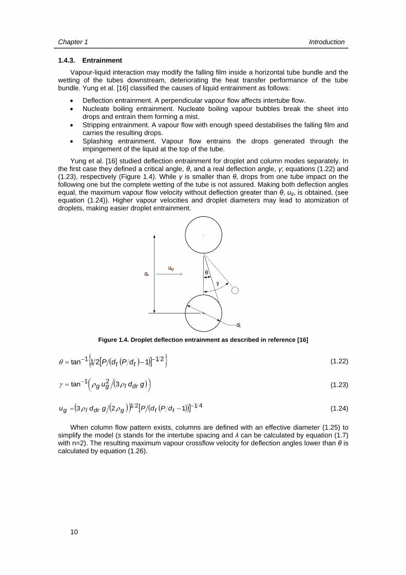
Chapter 1 Introduction

10

1.4.3. Entrainment

Vapour-liquid interaction may modify the falling film inside a horizontal tube bundle and the wetting of the tubes downstream, deteriorating the heat transfer performance of the tube bundle. Yung et al. [16] classified the causes of liquid entrainment as follows:

Deflection entrainment. A perpendicular vapour flow affects intertube flow.

Nucleate boiling entrainment. Nucleate boiling vapour bubbles break the sheet into drops and entrain them forming a mist.

Stripping entrainment. A vapour flow with enough speed destabilises the falling film and carries the resulting drops.

Splashing entrainment. Vapour flow entrains the drops generated through the impingement of the liquid at the top of the tube.

Yung et al. [16] studied deflection entrainment for droplet and column modes separately. In the first case they defined a critical angle, θ, and a real deflection angle, γ; equations (1.22) and (1.23), respectively (Figure 1.4). While γ is smaller than θ, drops from one tube impact on the following one but the complete wetting of the tube is not assured. Making both deflection angles equal, the maximum vapour flow velocity without deflection greater than θ, ug, is obtained, (see equation (1.24)). Higher vapour velocities and droplet diameters may lead to atomization of droplets, making easier droplet entrainment.

Figure 1.4. Droplet deflection entrainment as described in reference [16]

211 121tan tt dPdP (1.22)

gdu drlgg 3tan 21

(1.23)

4121 123 ttgdrlg dPdPgdu (1.24)

When column flow pattern exists, columns are defined with an effective diameter (1.25) to simplify the model (s stands for the intertube spacing and λ can be calculated by equation (1.7) with n=2). The resulting maximum vapour crossflow velocity for deflection angles lower than θ is calculated by equation (1.26).

Chapter 1 Introduction

11

4121* 28 sgd lcl

(1.25)

4121

* 2costan4

sgcdgu gdclg

(1.26)

According to Yung et al. [16], if γ > θ within a tube bundle, the entrained liquid may impinge on adjacent tubes and no decrease of the heat transfer performance should be observed. Ilyushchenko et al. [37] studied analytically and experimentally drop entrainment within a tube bundle and outside it and observed that it depends on the operation parameters and the tube bundle size.

Czikk [38] studied deflection and entrainment with sheet mode. He tested ammonia in a heat exchanger and measured deflection angles varying vapour flow rates and film Reynolds numbers. He defined the critical angle with the ratio of tube diameter to pitch.

Chapter 1 Introduction

12

1.5. DRY PATCHES AND FALLING FILM BREAKDOWN

The appearance of dry patches, i.e. breakdown of the falling film, has been widely studied due to its adverse effect on the heat transfer performance and stability of the flow at falling film evaporators. For sake of simplicity, in Table 1.1 we have included the main ideas on falling film breakdown of several works from the literature.

Hsu et al. [39] affirmed that dry patches occur due to the shear of vapour flows. When boiling or evaporation exist, the film becomes thinner and breakdown may happen. Moreover, the surface tension at the interface and its variation with temperature may also lead to the destruction of the falling film. Hartley and Murgatroyd [40] developed an analytical study about dry patches on flat surfaces and with isothermal conditions. They obtained the minimum film thickness and falling film flow rate that assure no film breakdown using two criteria: force balance at the stagnation point (G at Figure 1.5) and minimum power (energy) in a laterally unrestrained liquid film. They also stated that contact angle affects the formation of dry patches and minimum falling film flow rate.

Figure 1.5. Dry patch formation and film breakdown on a plate, as described in reference [40]

Hartley and Murgatroyd [40] applied both criteria to a laminar film flowing vertically under gravity, a case for which experimental data were available. A good agreement existed between the minimum flow rate and film thickness calculated by the power criterion and the experimental data from Dukler and Bergelin [41]. The comparison was also acceptable with the results from Bessler [42].

El-Genk and Saber [43] incorporated the velocity distribution and the profile of stable liquid rivulets (the columns of liquid surrounding dry patches, Figure 1.5) into the analytical model. Zuber and Staub [44] considered the effect of heat flux on the appearance of dry patches and noted that the forces present in the stagnation point are associated to the turning of kinetic energy into static pressure, to surface tension, to thermocapillary and to evaporation.

Hartley and Murgatroyd [40] had already considered the first two. Thermocapillary effect occurs due to the temperature difference at the interface, which causes a non-uniformity of the surface tension and movement along the free surface [39]. With evaporation, vapour sucks up the liquid that surrounds it, enlarging dry patches. A force balance at the stagnation point led Zauber and Staub [44] to the minimum film thickness and minimum falling film flow rate that prevented from the appearance of dry patches; and to the maximum heat flux at a surface, for a given film thickness and falling film flow rate, that could be applied without causing the film breakdown. They also stated that the contact angle (wettability) determines which force is

Chapter 1 Introduction

13

mainly involved in the stability of dry patches. In contrast, Zaitsev et al. [22] observed that the breakdown of the film depends on thermocapillary forces and neglected the effect of the contact angle at non-isothermal conditions. They defined a breakdown dimensionless criterion, Kmidp, which depends on the qidp and fluid properties; and correlated it by equation (1.27), which is a function of film Reynolds number. qdp stands for the heat flux needed to cause the first stable dry patch in the film.

0.65f

32 Re155.0

gcdTdqKm pidpidp

(1.27)

The breakdown phenomenon was also studied in falling films on horizontal tubes. Ganic and Roppo [14] determined experimentally the breakdown heat flux ranges for plain tubes with subcooled water and observed that they increased with increasing film Reynolds numbers and with tube spacing (if droplet mode or splashing were not present). Similar experiments are described by Ganic and Getachew [23] for water and ethanol on horizontal plain and porous tubes. The authors of this work stated that the porous surface maintained the tube wet for higher heat flux values. They also explained the breakdown phenomenon with the thermocapillary effect, stating that the lower local temperature (higher surface tension) available in the crests than in the valleys provokes the fluid transfer from the valleys to the crests.

Ganic and Getachew [23] and Chen et al. [45] conclude that enhanced surfaces on tubes prevent dry patches from appearing. Chen et al. [45] also stated that with enhanced vertical tubes and R11, the breakdown heat flux remained constant with Ref. Falling film breakdown was also studied by Fujita and Tsutsui [24]. They first observed dryout at the bottom rows of the bundle, since less falling film flow rate reached them due to evaporation on tubes placed upstream. They correlated their experimental results on breakdown heat flux by equation (1.28).

fRe048.0dryoutq (1.28)

Roques [21] tested a plain tube and three boiling enhanced tubes (Wolverine [30] Turbo-BII HP, Wieland [31] Gewa-B and UOP [35] High-Flux) to determine the appearance of dry patches varying heat flux and film Reynolds number. The author considered that, with a fixed heat flux, the dryout Reynolds number was related to the appearance of a dry patch at the middle of the tube. The dryout Reynolds number was correlated by formulae such as (1.29). However, it is clear that the first dry areas should appear at even higher Reynolds numbers. Ref,threshold (threshold Reynolds number) indicates the lowest Ref for which no sharp decrease of the HTCs occurs, and was defined as two times Ref,dryout. Plain tubes suffered film breakdown at higher Ref than the enhanced tubes, which agrees with the conclusions from references [23,24,45].

21f,dryoutRe eqe (1.29)

Ribatski and Thome [25] changed the threshold Reynolds number criterion. They focused on the significant decrease of the HTCs when film breakdown occurs. Equation (1.30) defines mathematically the criterion developed. Kff is the falling film multiplier, (1.31) and separates the effect of dryout on the HTCs from the effect of heat flux. The authors correlated the experimental Ref,threshold obtained with R134a and a plain tube using equation (1.32).

05.01

1

,1

,1,

jffnj

jffnjjff

Kn

Kn

K

(1.30)

pbffff hhK (1.31)

Chapter 1 Introduction

14

47.0

235thresholdf, 10·93.6Re

lvvl hq

(1.32)

Habert [11] extended the study of the threshold Reynolds number using two refrigerants (R134a and R236fa) with a plain, a condensation enhanced tube (Wieland [31] Gewa-C+LW), and two boiling enhanced tubes (Wieland [31] Gewa-B4 and Wolverine [30] Turbo-EDE2). He determined Ref,threshold with the criterion developed by Ribatski and Thome [25]. He observed no effect of the refrigerant on the Ref,threshold and a delay in film breakdown when using enhanced tubes. Although his results fitted correlation (1.29), developed by Roques [21], this equation mismatches the adiabatic case, for which the threshold Reynolds number should be 0. Habert formulated correlations with the general form of (1.33), which takes better into account the effect the refrigerant properties on the Ref,threshold than (1.32). For the Gewa-C+LW tube, the reduced pressure was also included in (1.33), multiplying the right term of the equation.

21thresholdf,Re f

lvlt hdqf (1.33)

Threshold Reynolds number and the appearance of dry patches were also studied by Christians [12] with two boiling enhanced tubes (Wolverine [30] Turbo-B5 and Wieland [31] Gewa-B5) and R134a and R236fa. The criterion employed to define Ref,threshold was basically that from Ribatski and Thome [25] or Habert [11]. As Habert, Christians stated that the influence of the refrigerant viscosity on the threshold Reynolds is greater than the influence of the difference between the refrigerant liquid and vapour densities, used by Ribatski and Thome [25]. Therefore, the correlation defined by Christians [12], (1.34), follows the form of (1.33), adding a geometric factor, Gt-s, different for each tube. The geometric factors were determined correlating the pool boiling experimental HTCs gathered in references [11,12,21].

175.004.1thresholdf, 721.20Re

stlvlt Ghdq

(1.34)

Chapter 1 Introduction

15

1.6. HEAT TRANSFER COEFFICIENTS: THEORETICAL AND ANALYTICAL WORKS

According to most theoretical works, falling film evaporation HTCs depend on the film thermal region analysed. Kocamustafaogullary and Chen [46] or Liu et al. [47] distinguished two regions. The heat transfer performance differs between regions only for tube bundles, according to reference [46], defining a thermally developing region and a thermally developed region. Kocamustafaogullary and Chen stated that HTCs depend on the position of the tube in the bundle, decreasing from one tube to the next. Liu et al. [47] named the regions stagnation zone and free film zone (Figure 1.6a).

Figure 1.6. Thermal regions in a falling film. a) Two regions (reference [47]). b) Three regions (reference [48]). c) Four regions (reference [49])

Three regions were distinguished in the film around tubes in works such as [48,50]. Chyu and Bergles [50] described a short impingement zone, with high HTCs; a larger thermal developing zone, where the fluid is superheated and no evaporation occurs; and a fully developed region, where evaporation at the interface exists and even nucleate boiling can take place. Fujita and Tsutsui [48] stated that the existing regions are a developing region, a shorter transition region and a developed region (Figure 1.6b). They differentiate between laminar and turbulent falling films. Fujita and Tsutsui supported their model with the acceptable agreement they found between it and their experimental results.

Chyu and Bergles [49] stated that the film is divided into four regions (Figure 1.6c) and established correlations for the HTCs at each region. First, a stagnation region, where the liquid reaches the tube, (1.35). Then, an impingement flow region, with high HTCs and where laminar boundary layer, (1.36), or turbulent boundary layer, (1.37), can occur. They defined Rex as seen in equation (1.38) and found the transition between laminar and turbulent regimes at 4.5·105. After it, a thermal developing region, (1.39). Finally, a fully developed region, where evaporation takes place at the liquid-vapour interface. They proposed two models to calculate the HTCs in this region, but that taken from reference [51] agreed better with experimental results. This model distinguished between laminar (1.40), wavy-laminar (1.41) and turbulent (1.42) regimes in the film. The average HTC in the film is obtained by equation (1.43) and the size of each region, in angular portion of tube, by equation (1.44). They also proved that at least the first three regions must exist and that the fully developed region might not occur for very high falling film flow rates.

Chapter 1 Introduction

16

5.0max

31Pr03.1 wuwxduudkh jjst (1.35)

0.5x

31 RePr73.0kxhim (1.36)

0.8x

31 RePr037.0kxhim (1.37)

vxux maxxRe (1.38)

slimtd

tdimtdtdtd

TT

qqh imtd

tdim

0,0,,

(1.39)

111

3431

312

61.0;Re10.1

gk

ghfd

(1.40)

06.1111

3422.0

312

Pr145061.0;Re822.0

gk

ghfd

(1.41)

06.14.065.0331

2Pr1450;RePr108.3

k

ghfd

(1.42)

tdfdimtdtdstimimstst hhhhh 1 (1.43)

31

5431;2;6.0

grrwrw ttdtitst

(1.44)

Barba and Felice [52] developed another theoretical approach considering non-boiling conditions, constant film thickness and turbulent thin films on horizontal tubes. They provided a dimensionless formula, (1.45), for the calculation of the average HTCs. Experimental data from several authors deviated from these theoretical results a ±10% on average.

5Pr1;5000Re1500;PrRe046.0 f47.00.18

f

312

kgh

(1.45)

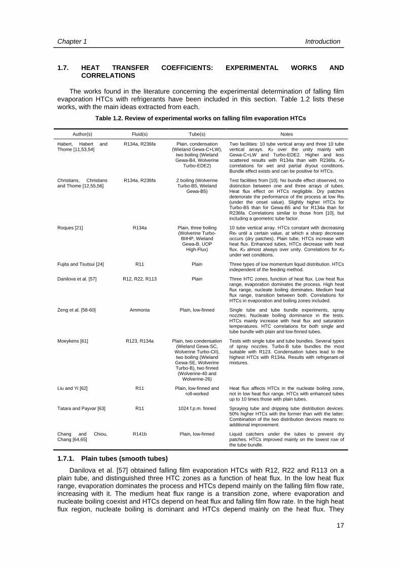
Chapter 1 Introduction

17

1.7. HEAT TRANSFER COEFFICIENTS: EXPERIMENTAL WORKS AND CORRELATIONS

The works found in the literature concerning the experimental determination of falling film evaporation HTCs with refrigerants have been included in this section. Table 1.2 lists these works, with the main ideas extracted from each.

Table 1.2. Review of experimental works on falling film evaporation HTCs

Author(s) Fluid(s) Tube(s) Notes

Habert, Habert and Thome [11,53,54]

R134a, R236fa Plain, condensation (Wieland Gewa-C+LW),

two boiling (Wieland Gewa-B4, Wolverine

Turbo-EDE2)

Two facilities: 10 tube vertical array and three 10 tube vertical arrays. Kff over the unity mainly with Gewa-C+LW and Turbo-EDE2. Higher and less scattered results with R134a than with R236fa. Kff correlations for wet and partial dryout conditions. Bundle effect exists and can be positive for HTCs.

Christians, Christians and Thome [12,55,56]

R134a, R236fa 2 boiling (Wolverine Turbo-B5, Wieland

Gewa-B5)

Test facilities from [10]. No bundle effect observed, no distinction between one and three arrays of tubes. Heat flux effect on HTCs negligible. Dry patches deteriorate the performance of the process at low Ref (under the onset value). Slightly higher HTCs for Turbo-B5 than for Gewa-B5 and for R134a than for R236fa. Correlations similar to those from [10], but including a geometric tube factor.

Roques [21] R134a Plain, three boiling (Wolverine Turbo-

BIIHP, Wieland Gewa-B, UOP

High-Flux)

10 tube vertical array. HTCs constant with decreasing Ref until a certain value, at which a sharp decrease occurs (dry patches). Plain tube, HTCs increase with heat flux. Enhanced tubes, HTCs decrease with heat flux. Kff almost always over unity. Correlations for Kff

under wet conditions.

Fujita and Tsutsui [24] R11 Plain Three types of low momentum liquid distribution. HTCs independent of the feeding method.

Danilova et al. [57] R12, R22, R113 Plain Three HTC zones, function of heat flux. Low heat flux range, evaporation dominates the process. High heat flux range, nucleate boiling dominates. Medium heat flux range, transition between both. Correlations for HTCs in evaporation and boiling zones included.

Zeng et al. [58-60] Ammonia Plain, low-finned Single tube and tube bundle experiments, spray nozzles. Nucleate boiling dominance in the tests. HTCs mainly increase with heat flux and saturation temperatures. HTC correlations for both single and tube bundle with plain and low-finned tubes.

Moeykens [61] R123, R134a Plain, two condensation (Wieland Gewa-SC,

Wolverine Turbo-CII), two boiling (Wieland Gewa-SE, Wolverine Turbo-B), two finned (Wolverine-40 and

Wolverine-26)

Tests with single tube and tube bundles. Several types of spray nozzles. Turbo-B tube bundles the most suitable with R123. Condensation tubes lead to the highest HTCs with R134a. Results with refrigerant-oil mixtures.

Liu and Yi [62] R11 Plain, low-finned and roll-worked

Heat flux affects HTCs in the nucleate boiling zone, not in low heat flux range. HTCs with enhanced tubes up to 10 times those with plain tubes.

Tatara and Payvar [63] R11 1024 f.p.m. finned Spraying tube and dripping tube distribution devices. 50% higher HTCs with the former than with the latter. Combination of the two distribution devices means no additional improvement.

Chang and Chiou, Chang [64,65]

R141b Plain, low-finned Liquid catchers under the tubes to prevent dry patches. HTCs improved mainly on the lowest row of the tube bundle.

1.7.1. Plain tubes (smooth tubes)

Danilova et al. [57] obtained falling film evaporation HTCs with R12, R22 and R113 on a plain tube, and distinguished three HTC zones as a function of heat flux. In the low heat flux range, evaporation dominates the process and HTCs depend mainly on the falling film flow rate, increasing with it. The medium heat flux range is a transition zone, where evaporation and nucleate boiling coexist and HTCs depend on heat flux and falling film flow rate. In the high heat flux region, nucleate boiling is dominant and HTCs depend mainly on the heat flux. They

Chapter 1 Introduction

18

correlated the film evaporation and film boiling experimental HTCs by equations (1.46) and (1.47), respectively. The dimensionless numbers needed are defined from equation (1.48) to (1.54). ζ stands for the volumetric film flow rate.

48.032.00.24ef,*

0.22ef,ef, PrReRe035.0Nu tds

(1.46)

48.072.00.22bf,

3bf, PrKpRe1032.1Nu

(1.47)

kgh31

2ef,Nu

(1.48)

kgh vl

21bf,Nu

(1.49)

4Re ef, (1.50)

31

2f,e*Re

ghq llv

(1.51)

Pr (1.52)

21bf,Re vlllv ghq

(1.53)

21Kp vls gp (1.54)

Fujita and Tsutsui [24] tested plain tube arrays with R11, using three types of liquid distributors: a porous sintered tube (Figure 1.7a), a tube with small holes at the bottom (Figure 1.7b) and a plate with a row of small holes aligned with the array (Figure 1.7c). They stated that when a complete wetting of the tubes existed, the worst HTCs appeared at the top tube of the array due to the non-uniformity of the film on it. They also observed that the HTCs were independent of the feeding method. They proposed a correlation for the calculation of the Nusselt number for the first tube of the tube array, (1.55), and another for the rest of the tubes, (1.56). Nusselt and Reynolds numbers are defined in (1.57) and (1.5), respectively.

Figure 1.7. Distribution methods used by Fujita and Tsutsui [24]. a) Sintered tube. b) Perforated tube. c) Perforated plate

2125.00.3

f32

fPrRe008.0ReNu

(1.55)

Chapter 1 Introduction

19

2125.00.3

f32

fPrRe01.0ReNu

(1.56)

kgh31

2Nu

(1.57)

Zeng et al. [58-60] focused on the falling film evaporation of ammonia on plain tubes. Experiments with a single plain tube show a HTC increase with increasing heat fluxes and saturation temperatures, proving the dominance of nucleate boiling under the tested conditions. Besides, HTCs varied with falling film flow rate, nozzle height and nozzle type only at the highest saturation temperature tested. HTCs increased when the first two parameters increased and were higher for the standard-angle nozzles than for the wide-angle nozzles. They correlated their experimental results by (1.58), being Θ the dimensionless heat flux, (1.59), and pred the reduced pressure (1.60). Nusselt and Reynolds numbers are calculated from (1.57) and (1.5), respectively.

753.0385.0278.00.039f

PrRe0518.0Nu red

p

(1.58)

kTTdq sct (1.59)

csred ppp (1.60)

Zeng et al. analysed as well the heat transfer performance and bundle effect of tube bundles, both square-pitch and triangular-pitch, with ammonia. They stated that spray evaporation HTCs in a tube bundle can be up to 50% greater than under pool boiling. According to the authors, impingement of spray explains the greater HTCs of the tubes of the top row, regardless of the kind of tube bundle. They detected differences in spray evaporation HTCs between both pitches only under certain conditions. Equations (1.61) and (1.62) predict the experimental results for square-pitch and triangular-pitch tube bundles, respectively.

722.0261.0209.00.00399f

PrRe0495.0Nu red

p

(1.61)

704.0456.0296.00.049f

PrRe0678.0Nu red

p

(1.62)

Moeykens [61] includes experimental values of pool boiling and spray evaporation with R134a and a multi-tube test facility with plain tubes. HTCs depended on heat flux and not on feed flow rate (until the appearance of dryout), indicating the occurrence of nucleate boiling. They achieved the best performance with the tube of smallest diameter. High-pressure drop nozzles enhance heat transfer compared to low-pressure drop nozzles, but they need a greater pumping power and number of nozzles.

1.7.2. Enhanced tubes

Zeng and Chyu [58] analysed as well the heat transfer performance of spray evaporation of ammonia with low-finned tubes. A single low-finned tube led to HTCs up to 2.5 times as high as a plain tube. HTCs also increased with saturation temperature and heat flux, marking the dominance of nucleate boiling. Single tube HTCs were correlated by (1.63). Nu is calculated by equation (1.57), Re by equation (1.5), Θ by equation (1.59) and pred by equation (1.60). Concerning low-finned tube bundles, both triangular-pitch and square-pitch, the highest HTCs occurred at the top row, diminishing row by row. Tube bundle HTCs increased as well with heat flux and saturation temperature, and were clearly higher for the square-pitch than for the triangular-pitch tube bundle. The authors recommended (1.64) and (1.65) to predict HTCs of square-pitch and triangular-pitch low-finned tube bundles, respectively.

Chapter 1 Introduction

20

034.1323.0193.00.0058f

PrRe0568.0Nu red

p

(1.63)

773.0127.0108.00.00035f

PrRe0622.0Nu red

p

(1.64)

758.0179.0147.00.034f

PrRe00566.0Nu red

p

(1.65)

Liu and Yi [62] compared the performance of plain tubes and two types of enhanced tubes, low-finned tubes and roll-worked tubes, with R11. Single tube HTCs were independent of Ref, except for the low-finned tube and low Ref, at which a sharp HTC decrease was observed, probably due to film breakdown. Convection prevailed at the low heat flux zone and they detected no effect of heat flux on HTCs. In contrast, when nucleate boiling dominated, the effect of heat flux was clear. HTCs achieved with the enhanced tubes were up to 10 times those with the plain tube. The authors also tested an array of three roll-worked tubes and observed a negligible difference among them in heat transfer performance.

Tatara and Payvar [63] developed a study with R11 and a small tube bundle of 1024 f.p.m. enhanced tubes, two types of distribution devices (liquid drip tubes and spray tubes) and a vapour inlet line. Spray tube distribution led to HTCs 50% greater than dripping distribution. The combination of both distribution systems meant no additional improvement. The authors observed no effect of heat flux on HTCs in the heat flux range studied, which coincides with the convective heat flux range from Liu and Yi [62]. The overfeed ratio (ratio of liquid mass distributed at the test facility to the liquid vaporised mass), was seen to have a positive influence on the heat transfer performance. However, the authors advise against an overfeed excess, which could lead to losing the advantage of falling film evaporators over flooded evaporators.

The behaviour of R123, a substitute refrigerant for R11, was analysed in Moeykens [61] with triangular-pitch tube bundles of plain tubes, Turbo-CII condensation tubes and Turbo-B boiling tubes (Wolverine [30]). The types of nozzles tested had a negligible effect on the heat transfer performance. HTCs in the plain tube bundle increased slightly with heat flux, meanwhile they diminished with heat flux for the Turbo-CII and increased first and then decreased for the Turbo-B. Enhancement factors even greater than 10 were obtained with Turbo-B and between 3 and 6 with Turbo-CII. A row-by-row study was also conducted, observing that the HTCs decreased slightly from row to row with plain and Turbo-B tube bundles, but they diminished sharply in the Turbo-CII tube bundle. In conclusion, Moeykens recommended the use of Turbo-B tube bundles with R123.

Concerning the falling film heat transfer performance of R134a on horizontal tubes, Moeykens [61] developed experiments with the multitube facilities and the following types of tubes: plain tubes, two condensation tubes (Wieland [31] Gewa-SC and Wolverine [30] Turbo-CII), two boiling tubes (Wieland [31] Gewa-SE and Wolverine [21] Turbo-B), and two finned tubes (Wolverine [30] 40 f.p.i. and 26 f.p.i.). HTCs were slightly influenced by heat flux, pointing to the existence of simultaneous convective evaporation and nucleate boiling in the range tested. The highest enhancement factors were achieved for condensation tubes (slightly over 3), followed by evaporation tubes (slightly under 3) and finned tubes (between 2 and 3 and better with Wolverine [30] 26 f.p.i). He also compared the performance of circular spray nozzles and square spray nozzles on a triangular-pitch arrangement of Wolverine [30] 40 f.p.i tubes. He observed that HTCs depended on the nozzle orifice size. A row-by-row analysis was also conducted, for with he defined the Row Performance Factor (RPF) using equation (1.66). The RPF varied from one row to the next one, more steeply with higher heat fluxes, smaller orifice sizes and lower feed flow rates, due to the inefficient distribution and the proneness to dryout of these tubes. Spray evaporation HTCs were greater than pool boiling HTCs, except for those tests with the lowest feed flow rates and high heat fluxes.

bdlr hhRPF (1.66)

Moeykens [61] employed a bundle test facility to study the bundle performance and the RPF behaviour of 5 different triangular-pitch tube bundles using Wolverine [30] Turbo-CII, Turbo-B

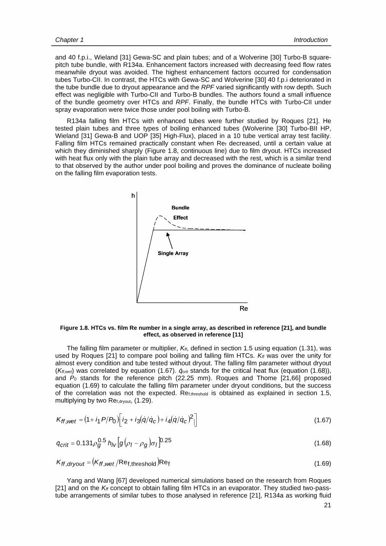
Chapter 1 Introduction

21

and 40 f.p.i., Wieland [31] Gewa-SC and plain tubes; and of a Wolverine [30] Turbo-B square-pitch tube bundle, with R134a. Enhancement factors increased with decreasing feed flow rates meanwhile dryout was avoided. The highest enhancement factors occurred for condensation tubes Turbo-CII. In contrast, the HTCs with Gewa-SC and Wolverine [30] 40 f.p.i deteriorated in the tube bundle due to dryout appearance and the RPF varied significantly with row depth. Such effect was negligible with Turbo-CII and Turbo-B bundles. The authors found a small influence of the bundle geometry over HTCs and RPF. Finally, the bundle HTCs with Turbo-CII under spray evaporation were twice those under pool boiling with Turbo-B.

R134a falling film HTCs with enhanced tubes were further studied by Roques [21]. He tested plain tubes and three types of boiling enhanced tubes (Wolverine [30] Turbo-BII HP, Wieland [31] Gewa-B and UOP [35] High-Flux), placed in a 10 tube vertical array test facility. Falling film HTCs remained practically constant when Ref decreased, until a certain value at which they diminished sharply (Figure 1.8, continuous line) due to film dryout. HTCs increased with heat flux only with the plain tube array and decreased with the rest, which is a similar trend to that observed by the author under pool boiling and proves the dominance of nucleate boiling on the falling film evaporation tests.

Figure 1.8. HTCs vs. film Re number in a single array, as described in reference [21], and bundle effect, as observed in reference [11]

The falling film parameter or multiplier, Kff, defined in section 1.5 using equation (1.31), was used by Roques [21] to compare pool boiling and falling film HTCs. Kff was over the unity for almost every condition and tube tested without dryout. The falling film parameter without dryout (Kff,wet) was correlated by equation (1.67). qcrit stands for the critical heat flux (equation (1.68)), and P0 stands for the reference pitch (22.25 mm). Roques and Thome [21,66] proposed equation (1.69) to calculate the falling film parameter under dryout conditions, but the success of the correlation was not the expected. Ref,threshold is obtained as explained in section 1.5, multiplying by two Ref,dryout, (1.29).

243201, 1 ccwetff qqiqqiiPPiK

(1.67)

25.05.0131.0 lgllvgcrit ghq

(1.68)

fthresholdf,,, ReRewetffdryoutff KK (1.69)

Yang and Wang [67] developed numerical simulations based on the research from Roques [21] and on the Kff concept to obtain falling film HTCs in an evaporator. They studied two-pass-tube arrangements of similar tubes to those analysed in reference [21], R134a as working fluid

Chapter 1 Introduction

22

and with two distribution conditions, uniform/homogeneous liquid distribution and heterogeneous distribution. The authors recommend a bottom-to-top arrangement evaporator when uniform liquid feed exists, in terms of HTCs and Ref,threshold. The highest HTCs coefficients occurred with the Wolverine [30] Turbo-EHP, but not the best Kff. They also proposed flooding the bottom rows of the evaporator to improve the heat transfer performance. The simulation stated that the evaporator performance diminishes and more dry-patches occur with maldistribution of the refrigerant (defined by the flow maldistribution coefficient).

Habert and Thome [11,53] extended the existing database of HTCs with refrigerants and tubes under falling film evaporation. They tested a condensation enhanced tube (Wieland [31] Gewa-C+LW), two boiling enhanced tubes (Wieland [31] Gewa-B4 and Wolverine [30] Turbo-EDE2), and a plain tube with R134a and R236fa. They used the experimental facility from Roques [21], unmodified first and with two tube arrays in parallel later. Falling film HTCs behaved similarly to those from Roques [21], increasing with heat flux with plain and condensation tubes (Gewa-C+LW) and decreasing with boiling tubes (Gewa-B4 and Turbo-EDE2). The authors observed that Kff diminished as the heat flux increased under almost every condition, but was greater than 1 with all the enhanced tubes (mainly with Gewa-C+LW and Turbo-EDE2). R134a led to better and less scattered HTCs than R236fa. In addition, liquid deflection, which was negligible with R134a, tended to occur with R236fa.

Habert and Thome used equation (1.70), defined by Ribatski and Thome [25], to correlate the experimental HTCs obtained both in wet and partially wet conditions. F stands for the apparent wet area fraction and was defined in reference [25] as the ratio between the tube surface covered by the liquid film, Awet, to the total tube surface, Atotal (equation (1.71)).

FhFhh drywetff 1 (1.70)

totalwet AAF (1.71)

Ribatski and Thome [25] correlated F as a function of Ref, as stated in equation (1.72). Habert and Thome [11,54] predicted accurately their results of apparent wet area using different fitting constants for each tube-refrigerant combination studied. However, they stated that it needs too many experimental constants and they proposed equation (1.73). They also suggested the removal of hdry from correlation (1.70), since it is negligible compared to hwet. Ribatski and Thome [25] defined equation (1.74) to substitute the formula previously proposed by Roques [21] to calculate Kff,wet.

2f1Rej

jF

(1.72)

thresholdf,f

thresholdf,fthresholdf,f

ReRe1

ReReReReF

(1.73)

2'''1,m

cwetff qqmK (1.74)

The modified test facility described in Habert [11] was used to study the bundle effect under falling film with the same tubes and refrigerants. HTCs were maximum at a certain Ref, denoted as Ref,peak (Figure 1.8, discontinuous line). However, these bundle results were very scattered and in some cases very low due to the premature appearance of dry patches caused by the liquid maldistribution in the bundle. Equation (1.75) correlates the bundle effect on those tubes and conditions with no film breakdown. B stands for the empirical bundle factor, obtained by equation (1.76). The fitting constants and Ref,peak depended on the tube-refrigerant combination. Equation (1.75) was only satisfactory with plain tubes and both refrigerants.

arraybdl hBh (1.75)

Chapter 1 Introduction

23

2peakf,f2 ReRe1 exp1

ooB

(1.76)

Additional falling film HTCs were included in the works developed by Christians and Thome [12,55], obtained for Wolverine [30] Turbo-B5 and for Wieland [31] Gewa-B5 tubes with R134a and R236fa. They developed their tests in the experimental facility used by Habert [11]. Contrary to the conclusions from [11,53], Christians and Thome found no bundle effect on the falling film HTCs. In fact, they made no distinction between the results obtained using the array arrangement or the bundle arrangement. Experimental HTCs were independent of heat flux or film Reynolds number meanwhile no film breakdown occurred, confirming the trends detailed in the works from Roques [21] or Habert and Thome [11,53]. The falling film HTCs were slightly higher with Turbo-B5 tubes than with Gewa-B5 tubes, and with R134a than with R236fa. Christians and Thome [12,56] proposed correlation (1.77) to predict the falling film HTCs obtained and enclosed not only in their works, but also in references [11,21,55]. The correlation depends on Gt-s (tube geometric factor, explained in section 1.5). Concerning the prediction of the partial dryout falling film HTCs, F was calculated by (1.73), as defined by Habert and Thome [11,54], and the HTCs were the result of multiplying it by hwet.

2449.10328.0

2410623.9stgllvlttwet Ghdqkdh

(1.77)

The falling film multiplier, Kff, was also determined by Christians and Thome [12,55] with the different tube-refrigerant combinations tested. Kff varied with heat flux, due to its influence on pool boiling HTCs. Both refrigerants led to similar falling film multipliers. The correlation proposed by Christians and Thome to predict Kff, (1.78), is also a function of Gt-s.

024.06204.04585.0

233.65

stcgltff GqqqdgK

(1.78)

1.7.3. Solutions to dry patches

The main inconvenient concerning falling film evaporation is the breakdown of the falling film and dry patch appearance. If dryout occurs, the performance of spray evaporators decreases, losing an advantage over flooded evaporators. Increasing the film flow rate or decreasing the heat flux may prevent dryout. The implementation of liquid collectors or catchers under the tubes (Figure 1.9) has been also proposed as a solution.

Figure 1.9. Tube bundle with liquid catchers, as described in references [64,65].

To our best knowledge, Chang and Chiou [64] were the first to mention liquid catchers for falling film evaporators. They tested a tube bundle with five plain tubes under pool boiling, spray

Chapter 1 Introduction

24

evaporation without liquid catchers and spray evaporation with liquid catchers. They noticed that at the narrow gap between tube and collector, the boiling process was different, with bubbles that squeezed and flattened against the walls, then coalesced and caused intermittent small dry-patches. HTCs improved sharply on the lowest row and were greater than under pool boiling in the whole heat flux range tested. Chang [65] presented similar results with a bundle of low-finned tubes. He observed a slight performance deterioration with liquid catchers at the tube placed right beneath the distribution nozzle. Awad and Negeed [7] analysed mathematically the improvement associated to the addition of liquid catchers under falling film and found that this heat transfer enhancement was higher with larger gaps between tube and catcher. They carried out the analysis at the gap considering pool boiling conditions and the correlation proposed by Cooper [68].

Another possible solution to dry patches was studied by Chang and co-workers and consists in distributing liquid refrigerant using sprays located inside the tube bundle, as can be seen in references [69-72]. The authors state that spray evaporation outperforms pool boiling, using R141b as refrigerant, both in triangular-pitch and square-pitch tube bundles, when introduced into these bundles spraying tubes with orifices of 1 mm of diameter and 90º of cone angle (Figure 1.10). They have also analysed the effect of the spraying incident angle on the heat transfer performance of tube bundles, observing a maximum at 60º. Up to the date of redaction of this PhD, the last work of this investigation group consisted in determining, both theoretically and experimentally, the optimal cone angle for interior spraying tubes as a function of the tube diameter and the distance between the spraying and the sprayed tubes.

Figure 1.10. Tube bundles with interior spraying tubes. a) Triangular-pitch (reference [69]). b) Square-pitch (reference [70])

NHeater Heater

HeaterHeater

Heater Heater

N

HeaterHeater

Heater Heater

a b

Chapter 1 Introduction

25

1.8. GENERAL CONSIDERATIONS

1.8.1. Flow modes and transitions

Up to five intertube flow patterns have been described, but mainly three are distinguished: sheet, jet (column) and droplet modes. According to references [8,9,17,18], the flow pattern depends on film flow rate and liquid properties (Dhir and Taghavi-Tafreshi [32] disagreed about the latter). Concerning intertube distance, references [4,8] explained that sheet mode occurs when this parameter is small, and changes to jet and droplet modes as it increases. In Roques et al. [18] the effects of heat flux and nucleate boiling were also pointed out.

Habert [11] stated that sheet mode is the most convenient for falling film evaporation, since it involves less possibilities of film breakdown and Hu and Jacobi [9,10] that the best HTCs are achieved under this flow mode. However, higher refrigerant charges and pumping power are needed to recirculate the excess liquid. Dryout may not occur under jet or droplet flow patterns if the distance between column/droplet active sites is minimised. References [4,9,27] noted that this distance depends on intertube spacing, film flow rate and fluid properties, increasing as the first two increase and as the third decreases. In contrast, Ganic and Roppo [14] observed no influence of intertube distance and film flow rate on it and Taghavi-Tafreshi and Dhir [15] determined it depends only on viscosity.

1.8.2. Film dryout

Film breakdown has been widely studied due to the important effect it has on the falling film evaporator performance. References [11,21,24,40,44] defended the important role of film flow rate on the film breakdown and references [11,21,24] of the liquid properties too. Moreover, references [40,44] described different behaviours depending on the contact angle, in opposition to the conclusions from Zaitsev et al. [22]. In references [11,21,24,44] the minimum film flow rate to avoid film breakdown was seen to depend as well on heat flux. Normally, wetting improves with enhanced tubes if compared to plain tubes, as stated in references [11,12,21,23]. However, some tubes such as low-finned or those with very complex external structures are not recommended, since they restrict the liquid axial movement and are prone to dryout [53,58,62].

Dryout occurs primarily at the lowest tube rows inside tube bundles, due to the reduction of the film flow rate caused by evaporation or liquid entrainment. Increasing the liquid overfeed has been proposed as a solution to this problem, but other ideas have been suggested. Yang and Wang [67] observed an improvement of the tube bundle performance by flooding the lowest rows and Tatara and Payvar [63] analysed the effect of implementing extra distribution devices within the tube bundle. According to references [64,65], HTCs were enhanced including liquid catchers beneath the tubes, since dryout was prevented. Another solution is to include interior spraying tubes in tube bundles, since it improves refrigerant distribution, minimizing the appearance of dry patches (references [69-72]).

1.8.3. Film flow rate

The effect film flow rate has on the falling film evaporation HTCs depends mainly on the existence or not of nucleate boiling in the falling film, at least when no dry-patches occur. Under non-boiling conditions, references [14,57] observed an increase of the HTCs with film flow rate. In contrast, Chyu and Bergles [49] reported a HTC deterioration with falling film flow rate due to thickening of the film. Under boiling conditions, no dependency between film flow rate and HTCs was stated in references [11,21,57,61,62].

As mentioned above, low film flow rates may lead to dry patch formation and the authors from references [11,21,24,62] noted that, when dry-patches exist, wetting improves by increasing the film flow rate. Thus, the control of the film flow rate is important for the correct performance of falling film evaporators (reference [63]). The chosen bundle geometry may also facilitate liquid distribution. Normally, triangular-pitch leads to more compact evaporators and square-pitch to more uniform refrigerant distribution. Zeng and co-workers [58,59,60] stated that triangular-pitch plain tube bundles performed better, meanwhile with low-finned tubes, square-pitch bundles attained better HTCs. In contrast, Moeykens [61] observed no differences between both arrangements.

Chapter 1 Introduction

26

1.8.4. Heat flux

Under non-boiling conditions, HTCs remained constant with heat flux, as stated in references [24,57,62]. However, Fujita and Tsutsui [24] affirmed that heat flux conditioned the minimum film flow rate to prevent dry-patch formation. Under boiling conditions, the effect of heat flux on HTCs depends mainly on the tube analysed. For plain tubes, references [11,21,57,58,61,62] agreed that HTCs increase with heat flux. This trend is unclear for enhanced surfaces. According to references [11,58,61,62], with condensation or low-finned tubes, HTCs increase when the heat flux rises. Normally, with enhanced boiling tubes, HTCs decrease or remain constant with heat flux (references [11,12,21,61]).

1.8.5. Distribution method

Different refrigerant distribution methods were described and studied in the literature, and they can be classified into low momentum and high momentum methods. Among the low momentum solutions, it is worth pointing out:

Perforated tube. At the bottom without a stabilizing tube in reference [24] and with stabilizing tube in references [8,9,10]. Perforated tube all around the surface used in reference [63].

Open box with perforated bottom in reference [20].

Perforated plate in reference [24].

Perforated vertical narrow tanks and stabilizing tubes in reference [13].

Perforated rectangular box with foams inside and half tube with sharp edge in reference [11,12,21,25,53,55].

Sintered tubes in reference [24].

Distribution tube with a slot at the top part in reference [49].

Tube-in-tube distributor in reference [57].

Distribution tray with a slot in reference [47,62].

High momentum solutions comprise spray nozzles, which were employed in references [2,46,53,58,59,64,65]. Falling film HTCs and wetting of tubes improve with high momentum distribution devices, particularly with liquids of low wettability. In addition, low momentum distribution systems need a more precise alignment than spray nozzles. However, the liquid fed with spray nozzles is difficult to quantify and a significant part of the fluid leaves the tube bundle. A solution can be the use of square plume nozzles, which need less liquid excess to feed a bundle but are more expensive (reference [61]).

1.8.6. Enhanced tubes

Enhanced tubes delay the appearance of dry patches if compared to plain tubes (references [21,23,24,45]). However, these enhanced surfaces should have as few axial liquid movement restrictions as possible, to favour the refrigerant distribution on tubes. No specific enhanced tubes exist for falling film, so the tubes tested were those prepared for processes such as pool boiling or condensation, or low-finned tubes. Moeykens [61] stated that low-finned tubes are prone to dryout and maldistribution, particularly as the number of fins per meter increases. Pool boiling and condensation tubes lead to important enhancements in the HTCs and the best solution depends on the refrigerant.

1.8.7. Other considerations

Saturation temperature. References [57,58] state that HTCs increase when the saturation temperature increases.

Nozzle height: Its small influence over HTCs is mainly reported. However, references [14,61] agree that a slight increase of the HTCs can occur with nozzle height.

Vapour flow: The design of correct vapour outlets is of a great importance for two reasons. First, the pernicious influence vapour entrainment can have on the liquid distribution over tubes, according to references [16,39]. Second, the benefit vapour flow may cause on the heat transfer performance of a tube bundle with falling film evaporation, as stated in reference [63].

Chapter 1 Introduction

27

1.9. CONCLUSIONS

This chapter encloses the results of works of the literature concerning falling film evaporation of refrigerants on horizontal tubes. The main conclusions drawn are listed in the following paragraphs.

Falling film evaporators for refrigeration systems can substitute satisfactorily flooded evaporators due to their potential benefits in operation costs, safety, thermodynamic efficiency, refrigerant charge or size. However, special attention must be paid to refrigerant distribution to avoid dryout and deterioration of the HTCs.

A large number of parameters affect the performance of falling film evaporators, but authors disagree about the effect of each of them. Those with a higher influence are heat flux, film flow rate, geometry of the tube, refrigerant properties and distribution system.

Sheet mode between tubes is recommended to prevent film breakdown, but an important pumping power may be needed to achieve it. Droplet or column intertube flow modes do not necessarily lead to dryout.

The use of enhanced tubes improves falling film HTCs compared to plain tubes. In addition, most enhanced tubes delay film breakdown, maintaining the surface wet. Only geometries that limit liquid axial movement, such as low-finned tubes with a high concentration of fins, should be avoided in these systems.

A large number of empirical correlations have been included in the literature, but the accuracy of the predictions is normally limited to very specific experimental conditions.

Chapter 1 Introduction

28

REFERENCES

[1] B.O. Bolaji, Z. Huan, Ozone depletion and global warming: Case for the use of natural refrigerant – a review, Renewable and Sustainable Energy Reviews. 18 (2013) 49-54.

[2] Z.H. Ayub, M. Chyu, A.H. Ayub, Case study: Limited charge shell and tube ammonia spray evaporator with enhanced tubes, Applied Thermal Engineering. 26 (2006) 1334-1338.

[3] D. Moalem, S. Sideman, Theoretical analysis of a horizontal condenser-evaporator tube, International Journal of Heat and Mass Transfer. 19 (1976) 259-270.

[4] S. Sideman, H. Horn, D. Moalem, Transport characteristics of films flowing over horizontal smooth tubes, International Journal of Heat and Mass Transfer. 21 (1978) 285-294.

[5] F.A. Jafar, G.R. Thorpe, Ö.F. Turan, Liquid film falling on horizontal circular cylinders, Proceedings of the 16th Australasian fluid mechanics conference, Crown Plaza, Gold Coast, Australia, 2007, pp. 1193-2000.

[6] M.M. Awad, E.R. Negeed, Enhancement of Evaporation of Falling Liquid Film on Horizontal Tube Bundle, in: Proceedings of the international water technology conference, IWTC12, Alexandria, Egypt, 2008, pp. 193-221.

[7] M.M. Awad, E.R. Negeed, Heat transfer enhancement of falling film evaporation on a horizontal tube bundle, in: Proceedings of the international water technology conference, IWTC13, Hurghada, Egypt, 2009, pp. 1461-1478.

[8] J. Mitrovic, Influence of tube spacing and flow rate on heat transfer from a horizontal tube to a falling liquid film, in: Proceedings of the 8th international heat transfer conference, San Francisco, USA, 1986, pp. 1949-1956.

[9] X. Hu, A.M. Jacobi, The intertube falling-film modes: Transition, hysteresis, and effect on heat transfer, Ph.D. Thesis, University of Illinois at Urbana–Champaign, Urbana, IL, 1995.

[10] X. Hu, A.M. Jacobi, Departure-site spacing for liquid droplets and jets falling between horizontal circular tubes, Experimental Thermal and Fluid Science. 16 (1998) 322-331.

[11] M. Habert, Falling film evaporation on a tube bundle with plain and enhanced tubes, Ph.D. thesis, École Polytechnique Fédérale de Lausanne, Switzerland, 2009

[12] M. Christians, Heat transfer and visualization of falling film evaporation on a tube bundle, Ph.D. thesis, École Polytechnique Fédérale de Lausanne, Switzerland, 2010.

[13] R. Armbruster, J. Mitrovic, Patterns of falling film flow over horizontal smooth tubes, in: Proceedings of the 10th international heat transfer conference, Brighton, UK, 1994, pp. 275-280.

[14] E.N. Ganic, M.N. Roppo, An experimental study of falling liquid film breakdown on a horizontal cylinder during heat transfer, Journal of Heat Transfer. 102 (1980) 342-346.

[15] K. Taghavi-Tafreshi, V.K. Dhir, Taylor instability in boiling, melting and condensation or evaporation, International Journal of Heat and Mass Transfer. 23 (1980) 1433-1445.

[16] D. Yung, E.N. Ganic, J.J. Lorenz, Vapor/liquid interaction and entrainment in falling film evaporators, Journal of Heat Transfer. 102 (1980) 20-25.

[17] H. Honda, S. Nozu, Y. Takeda, Flow characteristics of condensation on a vertical column of horizontal tubes, in: Proceedings of the ASME-JSME thermal engineering joint conference, Honolulu, Hawái, 1987, pp. 517-524.

[18] J. Roques, V. Dupont, J.R. Thome, Falling Film Transitions on Plain and Enhanced Tubes, Journal of Heat Transfer. 124 (2002) 491-499.

[19] J. Roques, J.R. Thome, Falling film transitions between droplet, column, and sheet flow modes on a vertical array of horizontal 19 fpi and 40 fpi low-finned tubes, Heat Transfer Engineering. 24 (2003) 40-45.

[20] J.F. Roques, J.F. Thome, Flow patterns and phenomena for falling films on plain and enhanced tube arrays, in: Proceedings of the third international conference on compact heat

Chapter 1 Introduction

29

exchangers and enhancement technology for the process industries. Davos, Switzerland, 2001, pp. 391-398.

[21] J.F. Roques, Falling film evaporation on a single tube and on a tube bundle, Ph.D. thesis, École Polytechnique Fédérale de Lausanne, Switzerland, 2004.

[22] D.V. Zaitsev, O.A. Kabov, V.V. Cheverda, N.S. Bufetov, The effect of wave formation and wetting angle on the thermocapillary breakdown of a falling liquid film, High Temperature. 42 (2004) 450-456.

[23] E.N. Ganic, D. Getachew, Effects of surface condition and working fluid on liquid film breakdown during heat transfer, in: Proceedings of the 8th international heat transfer conference, San Francisco, vol. 4, 1986, pp. 1931-1936.

[24] Y. Fujita, M. Tsutsui, Experimental investigation of falling film evaporation on horizontal tubes, Heat Transfer-Japanese Research. 27 (1998) 609-618.

[25] G. Ribatski, J.R. Thome, Experimental study on the onset of local dryout in an evaporating falling film on horizontal plain tubes, Experimental Thermal and Fluid Science. 31 (2007) 483-493.

[26] D.H. Sharp, An overview of Rayleigh-Taylor instability, Physica D. 12 (1984) 3-18.

[27] D. Moalem, S. Sideman, A.E. Dukler, Dripping characteristics in a horizontal tube film evaporator, Desalination. 27 (1978) 117-127.

[28] R. Li, R. Harris, On the dominant unstable wavelength during film boiling on a horizontal cylinder of small diameter, Journal of Heat Transfer. 115 (1993) 498-501.

[29] F.A. Jafar, G.R. Thorpe, Ö.F. Turan, Flow mode characterisation of liquid films falling on horizontal plain cylinders, in: Proceedings of the seventh international conference on CFD in the minerals and process industries, Melbourne, Australia, 2009, pp. 1-6.

[30] www.wlv.com

[31] http://www.wieland-thermalsolutions.de/

[32] V. Dhir, K. Taghavi-Tafreshi, Hydrodynamic transition during dripping of a liquid from underside of a horizontal tube, ASME paper. 81 (1981).

[33] J.R. Thome, Falling film evaporation, in: Wolverine Heat Transfer Engineering Data Book III, 2009.

[34] http://www.hitachi-cable.co.jp

[35] http://www.uop.com/equipment/heat-transfer-distillation/high-flux-tubing/

[36] X. Wang, A.M. Jacobi, A thermodynamic basis for predicting falling-film mode transitions, International Journal of Refrigeration. 43 (2014) 123-132.

[37] V.V. Ilyushchenko, V.L. Podbereznyi, S.I. Golub, Interaction of spraying liquid and vapour in horizontal-tube film evaporators, Desalination. 74 (1989) 391-400.

[38] A.M. Czikk, Fluid dymamic and heat transfer studies of OTEC heat exchangers, in: Proceedings of the fifth ocean thermal energy conversion conference, Miami Beach, Florida, 1978, pp. 181-236.

[39] Y.Y. Hsu, F.T. Simon, J.F. Lad, Destruction of a thin liquid film flowing over a heating surface, NASA Report (1963).

[40] D.E. Hartley, W. Murgatroyd, Criteria for the break-up of thin liquid layers flowing isothermally over solid surfaces, International Journal of Heat and Mass Transfer. 7 (1964) 1003-1015.

[41] A.E. Dukler, O.P. Bergelin, Characteristics of flow in falling liquid films, Chemical Engineering Progress. 48 (1952) 557-563.

[42] R. Bressler, Experiments on the evaporation of thin liquid films, Zeitschrift des vereines deutscher ingenieure. 100 (1958) 630-638.

Chapter 1 Introduction

30

[43] M.S. El-Genk, H.H. Saber, Minimum thickness of a flowing down liquid film on a vertical surface, International Journal of Heat and Mass Transfer. 44 (2001) 2809-2825.

[44] N. Zuber, F.W. Staub, Stability of dry patches forming in liquid films flowing over heated surfaces, International Journal of Heat and Mass Transfer. 9 (1966) 897-905.

[45] J.C. Chen, K. Tuzla, Q. Wang, Falling film evaporation of refrigerants, 10th International Heat Transfer Conference. 6 (1994) 169-173.

[46] G. Kocamustafaogullari, I.Y. Chen, Horizontal tube evaporators: Part I. Theoretically-based correlations, International Communications in Heat and Mass Transfer. 16 (1989) 487-499.

[47] Z. Liu, Q. Zhu, Y. Chen, Evaporation heat transfer of falling water film on a horizontal tube bundle, Heat Transfer Asian Research. 31 (2002) 42-55.

[48] Y. Fujita, M. Tsutsui, Experimental and analytical study of evaporation heat transfer in falling films on horizontal tubes, 135 (1994) 175-175.

[49] M. Chyu, A.E. Bergles, An analytical and experimental study of falling-film evaporation on a horizontal tube, Journal of Heat Transfer. 109 (1987) 983-990.

[50] M. Chyu, A.E. Bergles, Falling film evaporation on a horizontal tube, Multiphase flow and heat transfer, ASME HTD 47, 1985, pp. 39-48.

[51] K.R. Chun, R.A. Seban, Performance prediction of falling-film evaporators, Journal of Heat Transfer. 94 (1972) 432-436.

[52] D. Barba, R. Di Felice, Heat transfer in turbulent flow on a horizontal tube falling film evaporator. A theoretical approach, Desalination. 51 (1984) 325-333.

[53] M. Habert, J.R. Thome, Falling-film evaporation on tube bundle with plain and enhanced tubes—Part I: Experimental results, Experimental Heat Transfer. 23 (2010) 259-280.

[54] M. Habert, J.R. Thome, Falling-film evaporation on tube bundle with plain and enhanced tubes—Part II: New prediction methods, Experimental Heat Transfer. 23 (2010) 281-297.

[55] M. Christians, J.R. Thome, Falling film evaporation on enhanced tubes, part 1: Experimental results for pool boiling, onset-of-dryout and falling film evaporation, International Journal of Refrigeration. 35 (2012) 300-312.

[56] M. Christians, J.R. Thome, Falling film evaporation on enhanced tubes, part 2: Prediction methods and visualization, International Journal of Refrigeration. 35 (2012) 313-324.

[57] G.N. Danilova, V.G. Burkin, V.A. Dyundin, Heat transfer in spray-type refrigerator evaporators. Heat Transfer Soviet Research. 8 (1976) 105-113.

[58] X. Zeng, M. Chyu, Heat transfer and fluid flow study of ammonia spray evaporators, Texas Tech University, Lubbock, Texas, USA, 1995.

[59] X. Zeng, M. Chyu, Z.H. Ayub, Experimental investigation on ammonia spray evaporator with triangular-pitch plain-tube bundle, Part I: tube bundle effect, International Journal of Heat and Mass Transfer. 44 (2001) 2299-2310.

[60] X. Zeng, M. Chyu, Z.H. Ayub, Experimental investigation on ammonia spray evaporator with triangular-pitch plain-tube bundle, Part II: evaporator performance, International Journal of Heat and Mass Transfer. 44 (2001) 2081-2092.

[61] S.A. Moeykens, Heat transfer and fluid flow in spray evaporators with application to reducing refrigerant inventory, Iowa State University of Science and Technology, Iowa, USA, 1994.

[62] Z. Liu, J. Yi, Enhanced evaporation heat transfer of water and R-11 falling film with the roll-worked enhanced tube bundle, Experimental Thermal and Fluid Science. 25 (2001) 447-455.

[63] R. Tatara, P. Payvar, Measurement of spray boiling refrigerant coefficients in an integral-fin tube bundle segment simulating a full bundle, International Journal of Refrigeration. 24 (2001) 744-754.

Chapter 1 Introduction

31

[64] T. Chang, J.S. Chiou, Spray evaporation heat transfer of R-141b on a horizontal tube bundle, International Journal of Heat and Mass Transfer. 42 (1999) 1467-1478.

[65] T. Chang, Effects of nozzle configuration on a shell-and-tube spray evaporator with liquid catcher, Applied Thermal Engineering. 26 (2006) 814-823.

[66] J. Roques, J.R. Thome, Falling films on arrays of horizontal tubes with R-134a, Part II: flow visualization, onset of dryout, and heat transfer predictions, Heat Transfer Engineering. 28 (2007) 415-434.

[67] L. Yang, W. Wang, The heat transfer performance of horizontal tube bundles in large falling film evaporators, International Journal of Refrigeration. 34 (2011) 303-316.

[68] M.G. Cooper, Saturation nucleate pool boiling - a simple correlation, in: Proceedings of the first UK National Conference on Heat Transfer, 1984, pp. 785-793.

[69] T. Chang, C. Lu, J. Li, Enhancing the heat transfer performance of triangular-pitch shell-and-tube evaporators using an interior spray technique, Applied Thermal Engineering. 29 (2009) 2527-2533.

[70] T. Chang, J. Li, C. Liang, Heat transfer enhancement of square-pitch shell-and-tube spray evaporator using interior spray nozzles, Heat Transfer Engineering. 32 (2011) 14-19.

[71] R. Li, T. Chang, C. Liang, Effects of spray axis incident angle on heat transfer performance of rhombus-pitch shell-and-tube interior spray evaporator, Journal of Mechanical Science and Technology. 26 (2012) 681-688.

[72] T. Chang, L. Yu, Optimal nozzle spray cone angle for triangular-pitch shell-and-tube interior spray evaporator, International Journal of Heat and Mass Transfer. 85 (2015) 463-472.

33

Chapter 2

Experimental facility This chapter focuses on the experimental facility used to test pool boiling and spray

evaporation of refrigerants on horizontal tubes. We modified and prepared an existing experimental facility to allow testing spray evaporation processes. First, the experimental setup and the different devices involved in each test are described. Then, the distribution system used for spray evaporation tests is detailed. After that, the acquisition data system, the sensors employed and the software developed are explained. The chapter ends with the main characteristics of the different tubes studied.

The modification of this experimental test rig was part of the project INC 841C INTESPRAY: “Nuevo intercambiador de gran volumen con sistema de refrigeración por esprayado y sistema de recirculación del fluido sobrante”, developed in collaboration with the company INTEGASA and Xunta de Galicia. This project is included in a line of investigation in which we have studied different heat transfer processes occurring in shell-and-tube heat exchangers and have determined their HTCs.

The process of adapting the experimental test rig was developed in two stages. The first stage is described in the paper Á.Á. Pardiñas, J. Fernández-Seara, S. Bastos and F.J. Uhía, Diseño, construcción y validación de un equipo experimental para el estudio de la evaporación en spray, included in the proceedings of the “VII Congreso Ibérico y V Congreso Iberoamericano de Ciencias y Técnicas del Frío” (Tarragona, Spain, 2014) [1]. The second stage is detailed in the paper Á.Á. Pardiñas, J. Fernández-Seara and R. Diz, Test rig for experimental evaluation of spray evaporation heat transfer coefficients, of the 24th IIR International Congress of Refrigeration (Yokohama, Japan, 2015) [2].

Chapter 2 Experimental facility

34

2.1. EXPERIMENTAL SETUP PHILOSOPHY

Several works had been done in our laboratory to study heat transfer processes occurring in shell-and-tube heat exchangers. The experimental test rig available in the laboratory (Figure 2.1) was designed for studying condensation and pool boiling of refrigerants.

Figure 2.1. Experimental test rig for condensation and pool boiling experiments

The experimental setup was redesigned in order to allow spray evaporation tests. These tests consist in distributing the liquid refrigerant, in conditions very close to saturation, on the tested tube/s, simulating the situation that occurs in spray evaporators.

The main modification developed was to include a liquid distribution system to distribute the liquid refrigerant. The system was designed to allow testing different types of spreading devices. Among the different possibilities, full cone nozzles have been selected. The equipment permits different spacings between the nozzles, as well as choosing two distances between the nozzles and the tubes. We can also compare the HTCs obtained when the tested tube receives the liquid refrigerant directly from the nozzles and when the liquid refrigerant falls by gravity from a conditioning tube above the tested one.

The equipment does not follow a typical vapour compression cycle. Instead, pool boiling/spray evaporation and condensation occur at the same pressure and refrigerant flows from one shell-and-tube heat exchanger to the other due to the differences of density between liquid and vapour refrigerant. This configuration allows, on the one hand, testing very different conditions and refrigerants and, on the other hand, discarding the effect of lubricants on HTCs.

The test rig is prepared for tubes of nominal external diameters up to 20 mm, but we tested tubes of nominal external diameter 3/4” (19.05 mm), which are widely extended in shell-and-tube heat exchangers. We chose tubes with plain and enhanced external surfaces, and the material depends on the refrigerant used (compatibility refrigerant–material).

The compatibility with ammonia was the main consideration during the selection of materials for building the experimental setup.

As previously mentioned, the working principle of the experimental facility allows testing a wide range of condensation and evaporation conditions. We chose liquid temperatures between 0 and 10 ºC for our pool boiling and spray evaporation tests, common temperatures in water chillers. This range of temperatures allowed using water as secondary fluid both for condensing the vapour refrigerant at the condenser tubes and for vaporising the liquid at the evaporator tubes. Water is very convenient since its properties are very accurately determined using the temperatures measured.

Chapter 2 Experimental facility

35

The experimental facility stabilises the refrigerant pool temperature or the liquid distribution temperature (boiling saturation pressure), for pool boiling and spray evaporation tests, respectively. The distributed liquid refrigerant flow rate is also controlled accurately, maintaining the rest of the conditions constant. The temperatures and flow rates of the secondary fluids can also be regulated and stabilised at the values needed for each test.

The experimental setup allowed measuring the conditions (temperature, pressure and flow rate) of the refrigerant and secondary fluids. Several sensors were also included to determine the conditions of the distributed refrigerant.

A SolidWorks model was developed in order to introduce the modifications (mainly the distribution system) in the existing test rig. An isometric view is shown in Figure 2.2.

Figure 2.2. Isometric view of the experimental test rig model

Figure 2.3 shows two photographs of the experimental setup once finished. The facility does not follow completely the 3D model developed. In particular, the refrigerant pump position was changed to improve its performance. The photographs also show the process of insulation, which was carefully developed to minimise the heat transfer to the surroundings.

Figure 2.3. Photographs of the experimental facility. a) Front. b) Back

a b

Chapter 2 Experimental facility

36

2.2. EXPERIMENTAL FACITILITY DESCRIPTION

2.2.1. Experimental facility

Figure 2.4 shows the layout of the experimental facility used for pool boiling and spray evaporation tests. It consists mainly of a boiling test section, composed of a shell-and-tube evaporator connected to a heating water loop; a condensation test section, composed of a shell-and-tube condenser connected to a cooling water loop; and a refrigerant distribution system.

Figure 2.4. Sketch of the experimental test rig

The condenser and the evaporator consist of a 6-mm-thick horizontal cylindrical body and blind flanges made of stainless steel (AISI-316L). The condenser has an external diameter of 168.3 mm and an internal total length of 1895 mm. The evaporator has an external diameter of 200 mm and an internal total length of 1530 mm. Both ends of the tubes installed at the condenser and evaporator protrude from the blind flanges.

Chapter 2 Experimental facility

37

The refrigerant distribution system consists mainly of a 12 l refrigerant tank, also made of stainless steel (AISI-316L), an ammonia refrigerant pump, and a distribution tube with nozzles.

Independently of the test developed, liquid refrigerant vaporises on the evaporator tube/s due to the heat transferred by the heating water that flows through it/them. The generated vapour leaves the evaporator through 4 AISI 316L ports (inner/outer diameter 30/33 mm) located at the top. Then, it flows through an AISI 316L stainless steel flexible hose (DN 40 mm) and reaches the upper part of the condenser, where it enters through 4 AISI 316L ports (inner/outer diameter 30/33 mm), to guarantee a proper vapour distribution.

Vapour condenses on the condenser tube/s, transferring heat to the cooling water that circulates through it/them. Gravity drives the liquid refrigerant out from the condenser through a single port and an AISI 316L pipe (inner/outer diameter 10/12 mm). At this point is where pool boiling and spray evaporations tests differ.

In pool boiling tests, the refrigerant tank is left aside (V2 and V4 closed, and V1 in L position, Figure 2.4), and the liquid refrigerant enters the evaporator through 4 ports placed at its bottom part (AISI 316L). The liquid refrigerant forms a pool and floods the tested tube/s.

In spray evaporation tests, the distribution system is completely integrated into the refrigerant loop (V2 and V4 open, and V1 in T position, Figure 2.4). The liquid refrigerant from the condenser ends up in the refrigerant tank, where it is sucked by the refrigerant pump. Valves V2 and V3 (Figure 2.4) are manually regulated to control the refrigerant distributed flow rate. After this, the liquid refrigerant flows through an AISI 316L stainless steel duct (inner/outer diameter 15/18 mm), and is finally divided into two flows to enter the evaporator through both flanges. This solution allows reducing the pressure drop and homogenising the flow rate distributed by each nozzle.

An AISI 316L stainless steel distribution tube (inner/outer diameter 22/25 mm) is placed inside the evaporator and receives the liquid refrigerant from the tubes that reach both flanges of the evaporator. The distribution tube has threaded female connections (1/4”) where the distribution nozzles are attached. A thorough explanation of the distribution tube and nozzles is included in section 2.2.2.

The distribution nozzles spread liquid refrigerant on the tube/s at the evaporator. Part of the refrigerant vaporises due to the heat transferred by the heating water flowing through the evaporator tube/s and the excess liquid refrigerant leaves the evaporator through 4 AISI 316 L ports placed at the bottom part of the evaporator and returns to the refrigerant tank.

The heating water loop, used to vaporise the liquid refrigerant at the evaporator, consists of a water reservoir, a centrifugal pump and an electric boiler. Water from the reservoir is sucked by the centrifugal pump and discharged into the electric boiler. The heating water flow rate is controlled by means of two manually regulated valves and a bypass circuit to the tank. The electric boiler (maximum 12 kW) heats the water and the heat delivered is regulated by a power controller connected to a PC. The heating water leaves the electric boiler and flows through the evaporator tube/s, transferring heat to the refrigerant. After leaving the tube/s, it closes the loop by returning to the water reservoir.

The cooling water loop is in charge of condensing the vapour refrigerant on the condenser tube/s. The main components of this cycle are a water reservoir, a centrifugal pump and a plate heat exchanger. Water from the reservoir is sucked by the centrifugal pump and discharged to the plate heat exchanger. The cooling water flow rate is controlled by means of two manually regulated valves and a bypass circuit to the tank. In the plate heat exchanger, the cooling water transfers heat to an auxiliary cooling loop. Then, it flows through the tube/s placed at the condenser, absorbs heat from the refrigerant, and returns to the water tank.

Both the condenser and the evaporator are equipped with 6 sight glasses each, that allow lighting, viewing and recording the processes that occur there. Figure 2.5 shows a photograph of the recording equipment for pool boiling and spray evaporation processes.

Chapter 2 Experimental facility

38

Figure 2.5. Viewing and recording process for pool boiling and spray evaporation tests

2.2.2. Distribution tube calculation

As explained in section 2.2.1, a distribution system was included in the experimental facility to allow testing spray evaporation. The distribution system designed is a tube with threaded female connections (1/4”) used to attach the spreading devices (nozzles). The following paragraphs detail the design process of the system.

The distribution of refrigerant on the tube bundle of a spray evaporator is a key factor for its correct performance, since the appearance of dry zones on the tubes may cause an important deterioration of heat transfer. In the scientific literature, different distribution methods have been proposed and studied, and they can be classified into low momentum and high momentum [3].

Liquid distribution with low momentum systems is mainly caused by the effect of gravity; i.e. the liquid falls from the device to the surface (tube) placed directly beneath. Thus, the distribution system must be placed over each and every column of the tube bundle, properly aligned, in order to assure the liquid feed.

High momentum solutions include spray nozzles and these systems have been seen to improve heat transfer and wetting of tubes. They seem more appropriate for industrial equipment since alignment is not a critical issue and a same nozzle may distribute liquid to more than one column of tubes. However, part of this liquid may leave the bundle and it is difficult to quantify the fraction of the total flow rate that reaches each tube. The aptitude of nozzles to be used in industrial equipment explains that these were chosen for the distribution system of the experimental facility.

According to the Engineer’s Guide to Spray Technology [4], there are many types of nozzles available in the market. They can be mainly classified into two groups, function of the spray pattern produced by the nozzle: hollow cone nozzles and full cone nozzles. Hollow cone nozzles produce an annulus of liquid; i.e. part of the area right beneath the nozzle receives no liquid at all. On the other hand, full cone nozzles distribute liquid forming a spray that fills the area covered completely and homogeneously, so they appear as the most appropriate for this application.

From the different shapes of cones available in the market, we have selected circular nozzles. Circular cone nozzles distribute liquid with axial symmetry, describing circles in those planes perpendicular to the nozzle axis. Axial symmetry explains two of the main characteristics of round cone nozzles. The first is that no specific positioning is needed in order to feed a certain area. The second one concerns the necessity of overlapping a fraction of the liquid distributed by two or more nozzles in order to feed an area (tube bundle). In addition, another part of the flow rate leaves the bundle due to the same reason.

Chapter 2 Experimental facility

39

Concerning the cone angle, the possibilities are standard and wide angle nozzles. We have chosen wide angle nozzles in order to cover the full length of the evaporator minimising the number of nozzles needed.

Among the different kind of nozzles available in the market, HH14W (Spray Systems Co.) fulfil the features of being full cone nozzles with a wide angle cone of circular shape. Table 2.1 (reference [5]) includes their main features and Figure 2.6a shows a picture of the selected nozzles.

Table 2.1. Main characteristics of the chosen spray nozzles

Model HH14W

Company Spray Systems Co.

Type Full cone

Shape Circular

Nominal cone angle (º) 120

Nominal orifice diameter (mm) 3.58

Maximum free passage diameter (mm) 1.60

Nozzle pressure drop (kPa) function of the distributed volumetric flow rate (m3/s)

18.2810·17.5 vPDnozzle

Figure 2.6. a) Circular wide angle full cone nozzles chosen. b) Nozzles connected to the distribution tube

Once defined the kind of nozzles to be studied, we solved the problem of driving the refrigerant to each of them with the distribution tube (Figure 2.6b). It has threaded female connections (1/4”) to attach the nozzles, maintaining them at a fixed distance. However, it was necessary to calculate the optimal distance between nozzles to cover the tested tube/s. The optimisation method is a modification of another by Zeng and Chyu [6] and the following assumptions are considered:

Homogeneous distribution of the fluid throughout the cone; i.e. if chosen a portion of the

total surface covered by a spray, the flow rate impinging on that surface is the result of

multiplying the total spray flow rate by the ratio of the chosen surface to the total surface

covered by the cone.

The spray cone of a nozzle is straight at the sides, unaffected by gravity in the range of

distances studied.

a b

Chapter 2 Experimental facility

40

The shape of the cone is perfectly circular.

There is no interaction between the flows distributed by two or more nozzles that reach

a certain area.

The splashing rate is neglected.

In the experimental facility, the distribution tube should be placed in the vertical plane containing the axis of the evaporator. If the tested tube is placed directly underneath, we have a situation similar to that represented in Figure 2.7. An angle α, calculated following equation (2.1), is defined by the tangents to the tested tube from the origin of the spray nozzle (considered at the tip of the nozzle). The tube diameter, dt, was considered as 19.05 mm (3/4”) and the distance from the tip of the nozzle, s, was set at 49.5 mm. This distance is constrained by the evaporator dimensions.

Figure 2.7. Nozzle-tube system. a) Front view. b) Top view

222sin tt dsd (2.1)

Considering a nozzle with a cone angle β, if β is greater than α, part of the fluid does not impinge on the tube. The tangency spots are positioned at a vertical distance z’ from the origin of the cone, calculated by equation (2.2). The diameter of the circle of spray at z’, dsp(z’), is obtained by equation (2.3).

2sin12' tdsz (2.2)

2tan'2' zzdsp (2.3)

Taking into account the length of the evaporator, one nozzle is insufficient to distribute the liquid refrigerant on the tube/s tested. When a distribution system consists of more than one nozzle, the distance between them (between the threaded connections available in the distribution tube) should be short enough to fully cover the surface with liquid, but minimising the areas reached by two adjacent nozzles and the amount of refrigerant that leaves the evaporator without touching the tube/s. This distance is the optimal distance, distopt in Figure 2.8, and it is calculated with equation (2.4). r(z’) is determined by equation (2.5).

a b

Chapter 2 Experimental facility

41

Figure 2.8. Optimal distance between two adjacent nozzles, for the considered tube and distance

22 ''21' zdzrzddist spspopt

(2.4)

2tan'' zzr (2.5)

For the chosen nozzles, distance to the tested tube and tube diameter, the distribution tube was designed with threaded connections for 9 nozzles and 165 mm between the centres of two adjacent connections.

A reasonable concern could be whether the flow rate is equally distributed by all the nozzles. To discard this possibility we have calculated the pressure drop along the distribution tube and nozzle connections and compared it with the pressure drop of the nozzles, provided by the manufacturer. The ratio of the pressure drop of the nozzles to that along the distribution tube is equal to or greater than 10. Taking into account that the liquid is introduced by both ends of the evaporator, we calculated that the differences between the flow rates distributed by the nozzles are lower than 5%.

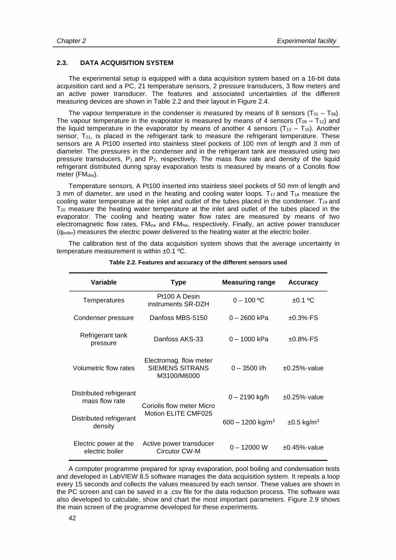
Chapter 2 Experimental facility

42

2.3. DATA ACQUISITION SYSTEM

The experimental setup is equipped with a data acquisition system based on a 16-bit data acquisition card and a PC, 21 temperature sensors, 2 pressure transducers, 3 flow meters and an active power transducer. The features and associated uncertainties of the different measuring devices are shown in Table 2.2 and their layout in Figure 2.4.

The vapour temperature in the condenser is measured by means of 8 sensors (T01 – T08). The vapour temperature in the evaporator is measured by means of 4 sensors (T09 – T12) and the liquid temperature in the evaporator by means of another 4 sensors (T13 – T16). Another sensor, T21, is placed in the refrigerant tank to measure the refrigerant temperature. These sensors are A Pt100 inserted into stainless steel pockets of 100 mm of length and 3 mm of diameter. The pressures in the condenser and in the refrigerant tank are measured using two pressure transducers, P1 and P2, respectively. The mass flow rate and density of the liquid refrigerant distributed during spray evaporation tests is measured by means of a Coriolis flow meter (FMdist).

Temperature sensors, A Pt100 inserted into stainless steel pockets of 50 mm of length and 3 mm of diameter, are used in the heating and cooling water loops. T17 and T18 measure the cooling water temperature at the inlet and outlet of the tubes placed in the condenser. T19 and T20 measure the heating water temperature at the inlet and outlet of the tubes placed in the evaporator. The cooling and heating water flow rates are measured by means of two electromagnetic flow rates, FMcw and FMhw, respectively. Finally, an active power transducer (qboiler) measures the electric power delivered to the heating water at the electric boiler.

The calibration test of the data acquisition system shows that the average uncertainty in temperature measurement is within ±0.1 ºC.

Table 2.2. Features and accuracy of the different sensors used

Variable Type Measuring range Accuracy

Temperatures Pt100 A Desin

instruments SR-DZH 0 – 100 ºC ±0.1 ºC

Condenser pressure Danfoss MBS-5150 0 – 2600 kPa ±0.3%·FS

Refrigerant tank pressure

Danfoss AKS-33 0 – 1000 kPa ±0.8%·FS

Volumetric flow rates Electromag. flow meter SIEMENS SITRANS

M3100/M6000 0 – 3500 l/h ±0.25%·value

Distributed refrigerant mass flow rate

Coriolis flow meter Micro Motion ELITE CMF025

0 – 2190 kg/h ±0.25%·value

Distributed refrigerant density

600 – 1200 kg/m3 ±0.5 kg/m3

Electric power at the electric boiler

Active power transducer Circutor CW-M

0 – 12000 W ±0.45%·value

A computer programme prepared for spray evaporation, pool boiling and condensation tests and developed in LabVIEW 8.5 software manages the data acquisition system. It repeats a loop every 15 seconds and collects the values measured by each sensor. These values are shown in the PC screen and can be saved in a .csv file for the data reduction process. The software was also developed to calculate, show and chart the most important parameters. Figure 2.9 shows the main screen of the programme developed for these experiments.

Chapter 2 Experimental facility

43

Figure 2.9. Main screen of the programme developed in LabVIEW 8.5

The programme allows regulating some of the most important parameters of the sensor by means of PIDs. It controls the temperature of the distributed liquid refrigerant or pool of refrigerant actuating over an analogue output of the acquisition card that drives an electronic valve placed at the auxiliary cooling loop. Another analogue output is in charge of regulating the mean heating water temperature (and therefore the logarithmic mean temperature difference at the evaporator).

Chapter 2 Experimental facility

44

2.4. ESPECIFICATIONS OF THE TUBES EMPLOYED

Five different commercially available tubes have been studied: two plain tubes, an integral-fin tube and two 3D microfinned tubes. These tubes have been provided by INTEGASA, a heat exchanger manufacturing company located in Vigo (Spain).

The plain tubes employed have 3/4” nominal external diameter and are made of copper (Cu) and titanium (Ti). The copper tube (Figure 2.10a) has external and internal diameters of 18.87 and 16.75 mm, respectively and the titanium tube (Figure 2.10b) of 19.05 and 17.2 mm, respectively.

Figure 2.10. Plain tubes used. a) Copper tube. b) Titanium tube

The tested 3D microfinned tubes are a Turbo-B and a Turbo-BII+, made of copper (Cu) and commercialised by the company WOLVERINE TUBE INC. Both tubes have modified external surface, designed for enhancing boiling heat transfer. Figure 2.11a and Figure 2.12b show the external surfaces of the Turbo-B and the Turbo-BII+ tubes, respectively. Even though these tubes are also available with smooth internal surface, the chosen tubes are also internally enhanced, as can be seen in Figure 2.11b and Figure 2.12b. The main geometrical characteristics of both tubes are included in Table 2.3.

Figure 2.11. Photographs of the Turbo-B tube. a) External surface. b) Cross section

a b

a b

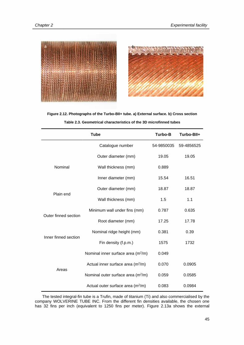
Chapter 2 Experimental facility

45

Figure 2.12. Photographs of the Turbo-BII+ tube. a) External surface. b) Cross section

Table 2.3. Geometrical characteristics of the 3D microfinned tubes

Tube Turbo-B Turbo-BII+

Catalogue number 54-9850035 59-4856525

Nominal

Outer diameter (mm) 19.05 19.05

Wall thickness (mm) 0.889

Inner diameter (mm) 15.54 16.51

Plain end

Outer diameter (mm) 18.87 18.87

Wall thickness (mm) 1.5 1.1

Outer finned section

Minimum wall under fins (mm) 0.787 0.635

Root diameter (mm) 17.25 17.78

Inner finned section

Nominal ridge height (mm) 0.381 0.39

Fin density (f.p.m.) 1575 1732

Areas

Nominal inner surface area (m2/m) 0.049

Actual inner surface area (m2/m) 0.070 0.0905

Nominal outer surface area (m2/m) 0.059 0.0585

Actual outer surface area (m2/m) 0.083 0.0984

The tested integral-fin tube is a Trufin, made of titanium (Ti) and also commercialised by the company WOLVERINE TUBE INC. From the different fin densities available, the chosen one has 32 fins per inch (equivalent to 1250 fins per meter). Figure 2.13a shows the external

a b

Chapter 2 Experimental facility

46

surfaces of the Trufin 32 f.p.i. tube and Figure 2.13b the inner surface, which in this case is smooth. The main geometrical characteristics of the tube are included in Table 2.4.

Figure 2.13. Photographs of the Trufin 32 f.p.i. tube. a) External surface. b) Cross section

Table 2.4. Geometrical characteristics of the Trufin 32 f.p.i. tube

Tube Trufin 32 f.p.i.

Nominal

Outer diameter (mm) 19.05

Wall thickness (mm) 0.635

Fin thickness (mm) 0.965

Inner diameter (mm) 15.85 (16.45)

Outer finned section

Minimum wall under fins (mm) 0.787

Root diameter (mm) 17.25

Fin pitch (mm) 0.8

Fin density (f.p.m.) 1250

Fin width base (mm) 0.5

Fin width tip (mm) 0.3

Fin flank angle (º) 4

Areas

Nominal inner surface area (m2/m) 0.0498

Nominal outer surface area (m2/m) 0.0598

Actual outer surface area (m2/m) 0.1535

The thermal conductivity of the copper employed is 386 W/m·K and its density 8890 kg/m3. Concerning titanium, its thermal conductivity is 21.9 W/m·K and its density 4507 kg/m3.

a b

Chapter 2 Experimental facility

47

2.5. CONCLUSIONS

The experimental facility used to study pool boiling and spray evaporation on horizontal tubes was described in this chapter. The sensors placed all over the test rig allow determining the HTCs of such processes. The test rig consists mainly of a shell-and-tube evaporator, connected to a heating water loop; a shell-and-tube condenser, connected to a cooling water loop; and a liquid distribution system. Both heat exchangers work at a same pressure, with the refrigerant flowing from one to another due to natural convection.

We focused specially on the liquid distribution system and on the way it was calculated and designed. The system includes a tank, a refrigerant pump, and a distribution tube with wide angle circular cone full nozzles. It allows testing different distributed liquid refrigerant flow rates for the spray evaporation tests.

The types of tubes tested, all of ¾” (19.05 mm) nominal outer diameter, were two plain tubes (titanium and copper), two 3D microfinned copper tubes (Turbo-B and Turbo-BII+) and a 2D finned titanium tube (Trufin 32 f.p.i.). We included the geometrical characteristics of the tubes, as well as photographs of their inner and outer surfaces.

Chapter 2 Experimental facility

48

REFERENCES

[1] Á.Á. Pardiñas, J. Fernández-Seara, S. Bastos, F.J. Uhía, Diseño, construcción y validación de un equipo experimental para el estudio de la evaporación en spray, in: Proceedings of the VII Congreso Ibérico y V Congreso Iberoamericano de Ciencias y Técnicas del Frío, Tarragona, Spain, 2014.

[2] Á.Á. Pardiñas, J. Fernández-Seara, R. Diz, Test rig for experimental evaluation of spray evaporation heat transfer coefficients, in: Proceedings of the 24th IIR International Congress of Refrigeration, Yokohama, Japan, 2015.

[3] J. Fernández-Seara, Á.Á. Pardiñas, Refrigerant falling film evaporation review: description, fluid dynamics and heat transfer, Applied Thermal Engineering. 64 (2014) 155-171.

[4] Engineer’s Guide to Spray Technology, Spraying Systems Co., U.S.A., 2000.

[5] http://www.spray.com/cat75/hydraulic/files/31.html

[6] X. Zeng, M. Chyu, Heat transfer and fluid flow study of ammonia spray evaporators, Texas Tech University, Lubbock, Texas, USA, 1995.

49

Chapter 3

Experimental methodology This chapter describes the experimental methodology and the data reduction process to

determine pool boiling and spray evaporation HTCs for the different refrigerants and tubes studied with the available experimental setup.

First, a short overview of the Wilson plot method to determine HTCs is done. After that, the experimental methodology and conditions followed for each test are detailed, pointing out the major differences between pool boiling and spray evaporation tests. Then, the calculation methods to obtain the most important parameters, such as the refrigerant side HTCs or the mass flow rates distributed on a certain surface, are described. Finally, the results of some validation experiments are shown in order to support the experimental results obtained with this experimental test rig and following this methodology and data reduction process.

Some of the main ideas detailed in this section were included in conference contributions such as Á.Á. Pardiñas, J. Fernández-Seara, S. Bastos and F.J. Uhía, Diseño, construcción y validación de un equipo experimental para el estudio de la evaporación en spray, included in the proceedings of the “VII Congreso Ibérico y V Congreso Iberoamericano de Ciencias y Técnicas del Frío” (Tarragona, Spain, 2014) [1]; Á.Á. Pardiñas, J. Fernández-Seara and R. Diz, Test rig for experimental evaluation of spray evaporation heat transfer coefficients, from the 24th IIR International Congress of Refrigeration (Yokohama, Japan, 2015) [2]; or Á.Á. Pardiñas, J. Fernández-Seara, S. Bastos and R. Diz, Experimental boiling heat transfer coefficients of R-134a on two boiling enhanced tubes, from the 8th World Conference on Experimental Heat Transfer, Fluid Mechanics, and Thermodynamics (Lisbon, Portugal, 2013) [3].

Chapter 3 Experimental methodology

50

3.1. CONVECTION HEAT TRANSFER COEFFICIENTS

Convection is the heat transfer mechanism that occurs between a solid and a fluid that have different temperatures. Convection consists of simultaneous heat and mass transfer; i.e. conduction takes place between the different fluid particles, but the energy transport is mainly caused by the macroscopic fluid movement.

Describing convection from an analytical point of view is complex and involves mass, momentum and energy equations, geometrical issues and fluid properties. Therefore, except for those cases with simple geometries and fluid flow conditions, the study is faced using Newton’s law of cooling. According to this law, convection heat flow is directly proportional to the surface in contact with the fluid, A, by the convection HTC, h, by difference between the temperature of the surface, Tsf, and the temperature of the bulk, Tbulk, as seen in equation (3.1).

bulksf TThAq (3.1)

Based on Newton’s law of cooling, for a certain geometry and fluid flow conditions, the convection HTCs can be obtained experimentally by fixing a certain heat flow and measuring the heat exchange area, and the temperature difference between the surface and the bulk. However, this methodology requires measuring the temperature at the surface, which normally varies from one point to another, and the existence of temperature sensors on it may modify the fluid flow. This problem is even more challenging when the surface cannot be easily reached, as normally happens with heat exchangers.

Wilson [4] proposed an alternative to this methodology which does not need placing temperature sensors on the heat exchange surface. His method consists in determining the overall thermal resistance of the whole heat exchange process, simple to obtain experimentally, and separating it in the different thermal resistances of the process. With a proper design of experiments, each HTC can be calculated.

In shell-and-tube condensers, for which the original method was proposed, the overall thermal resistance, Rov, results from adding up the thermal resistances corresponding to outer convection, Ro, to tube wall, Rw, to inner convection, Ri, and to fouling on the inner and outer surfaces of the tube, Rfoul,i and Rfoul,o, respectively (equation (3.2)).

oofoulwifouliov RRRRRR ,, (3.2)

For a tube, taking into account the typical expressions for the convection and conduction thermal resistances, the overall thermal resistance can be expressed as in equation (3.3), where ho and hi stand for the outer and inner convection HTCs, respectively; do and di for the outer and inner tube diameters, respectively; L for the length of the tube; and Ao and Ai the outer and inner tube surfaces, respectively.

ooofoul

t

ioifoul

iiov

AhR

Lk

ddR

AhR

1

2

ln1,,

(3.3)

The overall thermal resistance can be also calculated as a function of the overall HTC referred to the inner/outer surface of the tubes, Ui/o, and the area corresponding to the inner/outer diameter of the tube, Ai/o, as written in equation (3.4).

oioiov

AUR

//

1

(3.4)

Taking into account the conditions of condensation processes, Wilson considered that the variations in the overall thermal resistance when changing the inner fluid flow rate are mainly due to inner thermal resistance variations, being the remaining thermal resistances constant.

Chapter 3 Experimental methodology

51

Wilson observed that for a fully developed turbulent flow through a circular tube, the convection HTC was directly proportional to what he called reduced velocity, ured, which depended on the inner diameter of the tube and on the fluid properties. The inner convection HTC could be obtained by equation (3.5), where C is a fitting constant and n and exponent which should be determined experimentally.

nredi uCh

(3.5)

If we combine equations (3.3) and (3.5) and group the constant thermal resistances we obtain equation (3.6). This equation shows that the overall thermal resistance is a linear function, and the experimental results are represented as in Figure 3.1.

constn

rediov R

uACR

11

(3.6)

Figure 3.1. Original Wilson plot

If a certain mass flow rate of cooling fluid, ṁcf, is used in the condenser, the thermal resistance can be calculated dividing the logarithmic mean temperature difference at the condenser, LMTD, by the heat flow exchanged, q, as stated in equation (3.7). The heat flow and the LMTD can be calculated from experimental data following equations (3.8) and (3.9), respectively. In the previous equations, Tv is the temperature of the vapour; Tcf,in and Tcf,out, are the temperatures of the cooling fluid at the inlet and at the outlet of the tube, respectively; and cp,fl, is the specific heat capacity of the cooling fluid.

q

LMTDRov

(3.7)

incfoutcfcfpcf TTcmq ,,, (3.8)

Chapter 3 Experimental methodology

52

outcfv

incfv

outcfvincfv

TT

TT

TTTTLMTD

,

,

,,

ln

(3.9)

If the reduced velocity exponent, n, is known, the different values of the thermal resistance can be represented against 1/ured

n and can be adjusted with a linear regression (equation (3.6)). Then, the constant C and the ΣRconst are determined and the outer and inner HTCs are calculated by equations (3.5) and (3.10), respectively. Wilson stated that the exponent n that best adjusted his experimental results was 0.82.

ofoultifoulconst

oo

RRRR

Ah

,,

1

(3.10)

The original Wilson method could be adapted to other heat exchangers under the following hypothesis: the thermal resistance of one of the fluids remains almost constant as the other varies. This first approach was modified by different authors in order to make it more accurate and versatile, since that hypothesis is not always as valid as it seems. A thorough review of the different works and modifications developed on this subject is included in Fernández-Seara et al. [5].

Chapter 3 Experimental methodology

53

3.2. BOILING EXPERIMENTS

In this subsection we explain the experimental procedure followed both for obtaining pool boiling and spray evaporation HTCs with our experimental setup. The general methodology is shown in the first part, meanwhile in the second part the special features concerning spray evaporation tests are detailed.

3.2.1. Pool boiling experiments

Prior to any set of tests (tube/fluid combination), we paid special care on removing incondensable gases (air) from the refrigerant loop. Once removed the air and charged with refrigerant, we checked that the temperature and pressure measurements at the refrigerant side coincided with saturation conditions.

The pool boiling HTCs were calculated using the values of the sensors placed at the evaporator section, including the refrigerant side (T13 to T16 in Figure 2.4) and the heating water loop (T19 and T20 in Figure 2.4). The experiments were designed with the aim of obtaining the refrigerant side HTCs at constant pool boiling temperatures and varying the heat flux as much as possible.

Each test consisted in registering the values measured by the different sensors of the test rig, keeping constant the mean heating water temperature and flow rate through the tube and the refrigerant pool temperature. Except for special sets of experiments, which will be explained when needed, a group of tests (constant pool temperature) started with the maximum mean heating water temperature possible. When stationary conditions were achieved, data were registered for a minimum of 15 minutes. After that, the mean heating water temperature was lowered and fixed at the next testing condition. When finished a group of tests, a new was began at another refrigerant pool temperature, repeating the procedure explained in the previous lines.

The temperature of the pool of refrigerant was fixed by adjusting the heat absorbed by the cooling water circulating through the condenser tubes. The mean heating water temperature was adjusted by regulating the heat transferred to the heating water at the electric boiler through Joule effect. The electric power at the electric boiler was controlled by means of a power regulator and a PID.

The heating water flow rate was kept as high as possible to minimise the inner thermal resistance at the evaporator tubes, reduce the uncertainty of the HTCs and homogenise the boiling process along the tube (similar wall temperature conditions). The cooling water flow rate was kept as low as possible to increase the cooling water temperature difference between the inlet and the outlet of the condenser tube/s and to calculate with more accuracy the heat flow at this heat exchanger.

The refrigerant pool temperatures considered for these tests, independently of the refrigerant and tube utilised, were of 10, 7 and 4 ºC. These temperatures are typical in water chiller units. Concerning the range of mean heating water temperatures, it depended on the tube, the refrigerant and the pool temperature. Therefore, this range is indicated for each case with the experimental results.

3.2.2. Spray evaporation experiments

In spray evaporation experiments there are two new parameters to be considered: the relative position between the tested tube and the distribution tube and the distributed liquid refrigerant mass flow rate. In addition, instead of fixing the refrigerant pool temperature at the evaporator, we fixed the temperature of the refrigerant at the tank (measured by sensor T21 in Figure 2.4), which was in good agreement with the temperatures measured at the sensors placed at the lowest part of the evaporator (T13 to T16 in Figure 2.4).

The relative position of the tested tube and the distribution tube was introduced as a new experimental variable because other authors observed that the liquid droplet impingement effect could enhance heat transfer [6]. Thus, we should expect differences in the heat transfer performance between those tubes that receive refrigerant directly from the distribution devices and those that are wetted by the excess liquid from the row of tubes placed above them.

Chapter 3 Experimental methodology

54

Therefore, we have designed two different spray evaporation tests to illustrate these two possibilities, as depicted in Figure 3.2. The first tests (Figure 3.2 left), from now on ST tests, consist in distributing the refrigerant directly from the nozzles to a tube, being the distance from the tip of the nozzle to the centre of the tube 59 mm. In the second tests (Figure 3.2 right), named SB tests, the refrigerant is distributed on the same tube (conditioning tube), forming a film that falls to the tube placed underneath (distance of 45 mm between centres). No heating water circulates through the conditioning tube to prevent liquid refrigerant from vaporising before falling to the tested tube.

Figure 3.2. Types of spray evaporation tests. Left, liquid refrigerant on the tube directly from the nozzle (ST tests). Right, liquid refrigerant from a conditioning tube (SB tests)

We started with ST tests. The liquid refrigerant distribution temperature was fixed and, for each group of tests, the mean heating water temperature started at the maximum value achievable by the experimental test rig. Then, the distributed liquid refrigerant flow rate was set at the maximum of the experimental set points considered, which was different for each of the refrigerants tested. When stationary conditions were achieved, data were registered for a minimum of 15 minutes. After that, the distributed liquid refrigerant flow rate was lowered and the process repeated. When all the flow rates were tested, the mean heating water temperature was lowered and fixed at the next testing condition and the sequence of tests was repeated. Once finished ST tests, we repeated the whole process with SB tests.

Most of the variables involved in the experiments were controlled as for pool boiling test. Concerning the temperature of the distributed liquid refrigerant, it was fixed by adjusting the heat absorbed by the cooling water that circulates through the condenser tubes. The liquid refrigerant flow rate distributed was regulated manually by means of the two valves installed for that purpose.

The temperature of the distributed liquid refrigerant considered for these tests, independently of the refrigerant and tube utilised, was 10 ºC. The distributed liquid refrigerant flow rates tested were a function of the refrigerant used. With R134a they were 1000 kg/h, 1250 kg/h and 1500 kg/h and with ammonia these were 450 kg/h, 550 kg/h, 650kg/h, 750 kg/h and 850 kg/h. The range of the mean heating water temperatures depended on the refrigerant and on the distributed liquid refrigerant flow rate. Therefore, this range is indicated for each case with the experimental results.

Chapter 3 Experimental methodology

55

3.3. DATA REDUCTION

3.3.1. Refrigerant side heat transfer coefficient determination

We have calculated the refrigerant side (spray evaporation and pool boiling) HTCs from the data measured in the experimental facility and from the refrigerant and water properties from REFPROP 8.0 Database [7].

Taking into account the working principle of the experimental test rig and the good insulation applied, the heat flow transferred from the refrigerant to the cooling water at the condenser tube/s, qcw, calculated by equation (3.11), should be equal to that transferred from the heating water to the refrigerant at the evaporator tube/s, qhw, determined by equation (3.12). In these equations, ṁcw and ṁhw stand for the mass flow rates of the cooling water and heating water, respectively; cp,cw and cp,hw stand for the specific heat capacity of the cooling and heating water (evaluated at the mean temperature of each loop), respectively; Tcw,in and Tcw,out stand for the cooling water temperatures measured at the inlet and outlet of the tube/s at the condenser, respectively; and Thw,in and Thw,out stand for the heating water temperatures measured at the inlet and outlet of the tube/s at the evaporator, respectively.

incwoutcwcwpcwcw TTcmq ,,, (3.11)

outhwinhwhwphwhw TTcmq ,,, (3.12)

Prior to including the refrigerant pump in the refrigerant cycle, the agreement between the heat flow with (3.11) and (3.12) was very good, and pool boiling HTCs were calculated with the heat flow at the condenser tubes. This was very convenient, since the heat flow at the condenser was determined very accurately and the heating water flow rate could be kept high to reduce the inner thermal resistance at the evaporation tubes and to homogenise the boiling process. This method was applied to all the copper tubes under pool boiling.

However, the aforementioned condition was no longer satisfied with spray evaporation tests. We installed an active power transducer and the heat flow at the evaporator tubes was seen to match the electric power delivered to the heating water at the electric boiler. The uncertainty of the electric power was also seen to be lower, and the HTCs were obtained with it.

The overall thermal resistance at the evaporator tube/s is calculated by equation (3.13), where LMTDevap stands for the logarithmic mean temperature difference at the evaporator, which is calculated by equation (3.14). In this last equation Tl is the liquid refrigerant temperature, independently of the type of test developed, and Thw,in and Thw,out are the heating water temperatures measured at the inlet and outlet of the tube/s at the evaporator, respectively

evap

evapevapov

q

LMTDR ,

(3.13)

outhwl

inhwl

outhwlinhwlevap

TT

TT

TTTTLMTD

,

,

,,

ln

(3.14)

The overall thermal resistance can be also calculated by adding all the thermal resistances involved in the boiling process, as shown in equation (3.15). We neglect the effect of fouling at the inner and outer surfaces of the tube/s, Rfoul,i and Rfoul,o, respectively, because the tubes were thoroughly and regularly cleaned. Therefore, the overall thermal resistance can be obtained by equation (3.16).

Chapter 3 Experimental methodology

56

ooofoulwifoul

iievapov

AhRRR

AhR

11,,,

(3.15)

oow

iievapov

AhR

AhR

11,

(3.16)

Ai and Ao stand for the inner and outer heat exchange areas, respectively. We have also tested tubes with enhanced surfaces and their heat exchange areas are very difficult to quantify accurately. It is a common practice to calculate these areas using the nominal inner and outer diameters of the original plain tubes. Independently of the type of enhanced tube, the areas are calculated by equations (3.17) and (3.18). di and do are the inner and outer diameters of the evaporator tube/s and L the length.

LdA ii (3.17)

LdA oo (3.18)

The thermal resistance of the tube wall, Rw, is determined by equation (3.19). In this equation, kt is the tube wall thermal conductivity. The diameters of enhanced tubes are also considered as the nominal diameters of the original plain tube.

Lk

ddR

t

iow

2

ln

(3.19)

The inner convection HTC, hi, is also obtained from experimental data using typical correlations for forced convection heat transfer in plain and enhanced tubes. This issue is further explained in subsection 3.3.2.

Once determined all the variables included in the overall thermal resistance, the boiling HTCs are calculated by reordering equation (3.16) in a convenient manner (equation (3.20)). This equation is identical for plain tubes and enhanced tubes. For the latter, we talk about boiling HTCs referred to the nominal outer surface.

oii

tevapov

o

AAh

RR

h

1

1

,

(3.20)

The superheating of the tube wall, ΔTSH, is calculated using equation (3.21). Tw,o stands for the temperature at the outer tube wall, which is obtained with equation (3.22).

lowSH TTT , (3.21)

oo

evaplow

hA

qTT ,

(3.22)

3.3.2. Inner heat transfer coefficients

In this study we focus on boiling HTCs on tubes, but in order to determine them precisely, we need to properly characterise the thermal resistance of the process that occurs inside them. General correlations can lead to uncertainties in the determination of secondary fluid HTCs. Another option is the Wilson method and modifications, which have been frequently applied as indirect tools to obtain accurate correlations for those HTCs.

Chapter 3 Experimental methodology

57

Previous studies were developed in our laboratory to determine the validity of employing a general correlation, such as that of Petukhov [8], for forced convection HTCs in fully developed turbulent flow through smooth tubes. These studies, detailed in the doctoral thesis of Uhía [9], aimed to obtain the fitting constants for the inner HTCs using as functional form the aforementioned Petukhov correlation, (3.23). The Darcy-Weisbach friction factor, f, is calculated by (3.24). In these equations Ci stands for the Petukhov correlation fitting constant, Recw and Prcw stand for the dimensionless Reynolds and Prandtl numbers of the water flowing in the tube, kcw stands for the water thermal conductivity and di for the inner diameter of the tube.

i

cw

cw

cwcwiipli

d

k

f

fCPetukhovFCh

1Pr87.1207.1

PrRe8

32,

(3.23)

264.1Reln79.0 cwf

(3.24)

The closer Ci is to 1, the better the agreement between the experimental data and this general correlation. Uhía [9] reported a deviation of 2.3% between them and, consequently, considered Ci equal to the unity in his studies. Taking into account this study, which was developed with basically the same experimental facility, we considered the same correlation in order to determine the inner convection HTCs for our experimental studies with tubes of smooth inner surface. The uncertainty was estimated as 5%.

Concerning the tubes with enhanced internal surface, Turbo-B and Turbo-BII+, the manufacturer proposes the correlation by Sieder and Tate [10], equation (3.25), to calculate the inner convection HTCs. The experimental constant, STC, is also proposed by the manufacturer. 0.058 and 0.075 are the STC values for the Turbo-B and Turbo-BII+ tubes, respectively.

i

hw

w

hwhwhweni

d

kSTCh

14.0318.0

, PrRe

(3.25)

3.3.3. Mass flow rate reaching the tubes

The distribution conditions of the nozzle devices are such that only part of the liquid refrigerant spread reaches the studied tube/s. The procedure to determine this fraction is based on a method described by Zeng and Chyu [11] and follows the study explained in subsection 2.2.2. For the sake of facilitating its understanding, it will be repeated here.

The following assumptions are considered:

Homogeneous distribution of the fluid throughout the cone; i.e. if chosen a portion of the

total surface covered by a spray, the flow rate impinging on that surface is the result of

multiplying the total spray flow rate by the ratio of the chosen surface to the total surface

covered by the cone.

The spray cone of a nozzle is straight at the sides, unaffected by gravity in the range of

distances studied.

The shape of the cone is perfectly circular.

There is no interaction between the flows distributed by two or more nozzles that reach

a certain area.

The splashing rate is neglected.

In the experimental facility, the distribution tube is placed in the vertical plane containing the axis of the evaporator. If the tested tube is placed directly underneath, we have a situation similar to that represented in Figure 3.3. An angle α is defined by the tangents to the tested tube from the origin of the spray nozzle, which was considered at the tip of the nozzle, and is calculated following equation (3.26). The tube diameter, dt, was considered as 19.05 mm (3/4”) and the distance from the tip of the nozzle, which depends on the size of the evaporator shell, was set at 49.5 mm.

Chapter 3 Experimental methodology

58

Figure 3.3. Nozzle-tube system. a) Front view. b) Top view

222sin tt dsd (3.26)

Considering a nozzle with a cone angle β, if β is greater than α, part of the fluid does not impinge on the tube. The tangency spots are positioned at a vertical distance z’ from the origin of the cone, calculated by equation (3.27). The diameter of the circle of spray at z’, dsp(z’), is obtained by equation (3.28).

2sin12' tdsz (3.27)

2tan'2' zzdsp (3.28)

Only that part of the spray cone between the tangents reaches the tube. Therefore, when calculating the fraction of the total liquid that impinges on the tube, we should consider the area of the intersection between the tube and the spray cone, projected on a plane normal to the nozzle axis at the distance z’ from the origin of the spray cone. This area, Aproj(z’), striped in Figure 3.3b, is obtained by equation (3.29). r(z’) and m(z’) are calculated by equations (3.30) and (3.31), respectively.

''22'''2arcsin' 2 zrzmzdzdzrzA spspproj

(3.29)

2tan'' zzr (3.30)

22 '4'' zrzdzm sp

(3.31)

Taking into account the length of the evaporator, one nozzle is insufficient to distribute the liquid refrigerant on the tube/s tested. When a distribution system consists of more than one nozzle, the distance between them (between the threaded connections available in the distribution tube) should be short enough to fully cover the surface with liquid, but minimising the areas reached by two adjacent nozzles and the amount of refrigerant that leaves the evaporator without touching the tube/s. This distance is the optimal distance, distopt in Figure 3.4, and it is calculated with equation (3.32). r(z’) is determined by equation (3.30).

a b

Chapter 3 Experimental methodology

59

Figure 3.4. Optimal distance between two adjacent nozzles, for the considered tube and distance

22 ''21' zdzrzddist spspopt

(3.32)

For the chosen nozzles, distance to the tested tube and tube diameter, the distribution tube was designed with threaded connections for 9 nozzles and 165 mm between the centres of two adjacent connections.

The mass flow rate reaching the top of the tube under these conditions, ṁtop, is calculated using equation (3.33). The projected area of the tube, An,proj, that can be achieved by the nozzle system is determined with equation (3.34). Generally, this mass flow rate can be defined in a dimensionless way by the Reynolds number, as seen in equation (3.35), where Γ stands for the mass flow rate at the top of the tube per unit of tube length and per tube side (equation (3.36)).

4'' 2

, zdnzAmm spprojndisttop

(3.33)

LzrzA projn '2',

(3.34)

ltop 4Re , (3.35)

Lmtop 2 (3.36)

Finally, the mass flow rate reaching the top of the tube is compared with the amount of liquid refrigerant per unit of time that vaporises during each experiment, me, by the overfeed ratio (OF in equation (3.37)). The vaporised mass flow rate is obtained with equation (3.38), being hlv the refrigerant latent heat of vaporisation.

etop mmOF (3.37)

lvevape hqm (3.38)

3.3.4. Enhanced surface enhancement factor

To quantify the enhancement due to the use of enhanced surfaces, compared to a plain tube, we defined the surface enhancement factor, EFsf. As shown in equation (3.39), it compares the pool boiling HTCs for the enhanced surface with those for the corresponding plain tube (same nominal outer diameter), at the same heat flux, q, pool temperature, Tl, and refrigerant.

Chapter 3 Experimental methodology

60

refTqploenosf

lhhEF

,,,,

(3.39)

3.3.5. Spray evaporation enhancement factor

According to several works from the literature, spray evaporation can lead to an enhancement of the boiling heat transfer, if compared to pool boiling under similar conditions. This enhancement is quantified by a spraying enhancement factor, EFsp,Γ, determined with equation (3.40). It compares the spray evaporation HTCs, at a certain liquid refrigerant mass flow rate, to those under pool boiling, at the same heat flux, q, refrigerant temperature, Tl, tube and refrigerant. We have determined ho,pb in each case using the correlations obtained from our own experimental data.

tuberefTqpbosposp

lhhEF

,,,,,,, (3.40)

Chapter 3 Experimental methodology

61

3.4. UNCERTAINTY DETERMINATION

The simple presentation of the boiling HTCs leaves this information incomplete. By presenting the uncertainties related to their determination, we give an idea of the quality and reliability of these results. Uncertainty is a parameter associated with the estimated value of a physical magnitude, measured or calculated, that indicates the range of values were the actual value of this physical magnitude should be. In this work we have developed an uncertainty determination procedure based on the Evaluation of measurement data – Guide to the expression of uncertainty measurement (GUM) [12]. The results determined are included throughout the document with their uncertainties as error bars. The determination of the uncertainties of each parameter is detailed in Appendix A.

Chapter 3 Experimental methodology

62

3.5. EXPERIMENTAL FACILITY VALIDATION

The experimental facility validation issues can be classified into those concerning the heat flows, measured and calculated at the different loops of the experimental test rig and with the different kinds of experiments; and those concerning spray distribution.

As aforementioned, prior to including the distribution system in the experimental test rig, the pool boiling HTCs were determined by means of the heat flow transferred from the refrigerant to the cooling water flowing through the condenser tubes. This was possible since the only heat flows that existed in the refrigerant loop were the heat flow transferred from the heating water to the refrigerant at the evaporator and the heat flow transferred from the refrigerant to the cooling water at the condenser. The heat transfer from the ambient to the refrigerant was neglected due to the convenient insulation of the test rig.

Figure 3.5, Figure 3.6 and Figure 3.7 compare the two heat flows at the condenser and evaporator tubes, determined during the experiments with the copper plain tube, the copper Turbo-B tube and the copper Turbo-BII+ tube, respectively. The average deviation for any of these cases is close to 10% and the uncertainties, shown as error bars, are clearly lower at the cooling water heat flow than at the heating water heat flow. More details on deviations and uncertainties are given in Table 3.1.

Figure 3.5. Heat flow at the condenser vs. heat flow at the evaporator of R134a pool boiling experiments developed with the cooper plain tube at the evaporator

+10%

0

1000

2000

3000

4000

0 1000 2000 3000 4000

qcw

[W]

qhw [W]

Chapter 3 Experimental methodology

63

Figure 3.6. Heat flow at the condenser vs. heat flow at the evaporator of R134a pool boiling experiments developed with the cooper Turbo-B tube at the evaporator

Figure 3.7. Heat flow at the condenser vs. heat flow at the evaporator of R134a pool boiling experiments developed with the cooper Turbo-BII+ tube at the evaporator

+10%

0

1000

2000

3000

4000

5000

6000

0 1000 2000 3000 4000 5000 6000

qcw

[W]

qhw [W]

+10%

0

1000

2000

3000

4000

5000

6000

0 1000 2000 3000 4000 5000 6000

qcw

[W]

qhw [W]

Chapter 3 Experimental methodology

64

Table 3.1. Average and maximum deviation between the heat flows determined in the experiments with the copper tubes and R134a under pool boiling; and average and maximum uncertainties of

these heat flows

Deviation between heat flows [%]

Uncertainties qhw [%] Uncertainties qcw [%]

Tube Average Maximum Average Maximum Average Maximum

Plain 12.2 35.2 40.7 108.9 4.2 7.1

Turbo-B 8.35 30.3 15.4 36.6 3.3 5.7

Turbo-BII+ 11.2 32.3 16.5 46.8 3.1 3.8

When included the distribution system in the experimental test rig, we needed to change the method to determine the overall thermal resistance and the HTCs. Considering the good insulation of the heating water circuit, we assumed that, under stationary conditions, all the heat flow absorbed by this fluid inside the electric boiler, measured through the active power transducer, is transferred to the refrigerant in the evaporator by the heating water. We checked this statement with validation tests, developed under pool boiling conditions, saturation temperatures of 10 ºC and 5 ºC and using ammonia and the titanium plain tube. A particularity of these tests is that we kept the heating water mass flow rate low in order to increase the temperature difference of the heating water at the inlet and outlet and to calculate the heating water heat flow accurately.

Figure 3.8 compares the electric power at the electric boiler and the heat flow of the heating water at the evaporator tubes. The discrepancies between both are on average lower than 2.4% and never greater than 8%. We concluded that the overall thermal resistance could be accurately calculated using the electric power at the electric boiler. We also confirmed that the uncertainties associated to the electric power at the electric boiler are lower than the uncertainties of the heating water heat flow (on average ±1.5% and ±7.2%, respectively).

Figure 3.8. Electric power at the electric boiler vs. heat flow at the evaporator obtained at the specific validation experiments under pool boiling of ammonia and with a titanium plain tube

0

1000

2000

3000

4000

5000

0 1000 2000 3000 4000 5000

qboile

r[W

]

qhw [W]

+5%

-5%

Chapter 3 Experimental methodology

65

We also checked the validity of the assumption with the results of the pool boiling tests with ammonia (Figure 3.9 and Figure 3.10), spray evaporation with R134a (Figure 3.11) and spray evaporation with ammonia (Figure 3.12). More details on average and maximum deviations and uncertainties of the ammonia pool boiling tests and of the spray evaporation tests are included in Table 3.2 and Table 3.3, respectively.

Figure 3.9. Electric power at the electric boiler vs. heat flow at the evaporator obtained at the ammonia pool boiling experiments with a titanium plain tube

Figure 3.10. Electric power at the electric boiler vs. heat flow at the evaporator obtained at the ammonia pool boiling experiments with a titanium Trufin 32 f.p.i.

+5%

0

1000

2000

3000

4000

5000

6000

0 1000 2000 3000 4000 5000 6000

qboile

r[W

]

qhw [W]

-5%

+5%

0

1000

2000

3000

4000

5000

6000

0 1000 2000 3000 4000 5000 6000

qboile

r[W

]

qhw [W]

-

Chapter 3 Experimental methodology

66

Figure 3.11. Electric power at the electric boiler vs. heat flow at the evaporator obtained at the R134a spray evaporation experiments with a copper plain tube

Figure 3.12. Electric power at the electric boiler at the electric boiler vs. heat flow at the evaporator obtained at the ammonia spray evaporation experiments with a titanium plain tube

0

1000

2000

3000

0 1000 2000 3000

qboile

r[W

]

qhw [W]

+5%

-5%

-5%

0

1000

2000

3000

4000

5000

0 1000 2000 3000 4000 5000

qboile

r[W

]

qhw [W]

+5%

Chapter 3 Experimental methodology

67

Table 3.2. Average and maximum deviation between the electric power and the heating water heat flow determined in the experiments with the titanium tubes and ammonia under pool boiling; and

average and maximum uncertainties of the electric power and heat flow

Deviation between heat flows [%]

Uncertainties qboiler [%] Uncertainties qhw [%]

Tube Average Maximum Average Maximum Average Maximum

Plain 4.1 22.0 1.9 3.5 18.7 85.1

Trufin 32 f.p.i.

7.2 32.2 1.4 3.7 25.5 81.6

Table 3.3. Average and maximum deviation between the electric power and the heating water heat flow determined in the experiments with the cooper and titanium tubes under spray evaporation;

and average and maximum uncertainties of the electric power and heat flow

Deviation between heat flows [%]

Uncertainties qboiler [%] Uncertainties qhw [%]

Tube Average Maximum Average Maximum Average Maximum

Copper plain

2.8 10.5 0.5 1.3 11.7 17.6

Titanium plain

6.7 36.6 1.4 2.6 20.3 79.3

Concerning the validation of the distribution system, we focused on two features: the proximity to saturation conditions of the distributed refrigerant and the cone angles formed by the nozzles.

Spray evaporation tests consisted in distributing the liquid refrigerant at conditions very close to saturation, as occurs in vapour compression refrigeration systems with spray evaporators. To validate this condition in our experimental facility, we compared the arithmetic mean of the temperatures measured by the sensors placed at the low part of the evaporator (T13 – T16 in Figure 2.4), to the saturation temperature that corresponds to the pressure measured at the refrigerant tank (P2 in Figure 2.4). To calculate the latter, we used the REFPROP 8.0 database [7]. There was a good agreement between both, independently of the refrigerant, as shown in Figure 3.13 and Figure 3.14 for R134a and ammonia, respectively.

Chapter 3 Experimental methodology

68

Figure 3.13. Temperature of the distributed liquid R134a vs. saturation temperature at the pressure in the refrigerant tank

Figure 3.14. Temperature of the distributed liquid ammonia vs. saturation temperature at the pressure in the refrigerant tank

Regarding the spray cone angle, we checked that it was close to the value available in the manufacturer catalogue, which for these nozzles is 120º. This is crucial in our experimental facility, particularly if the determined angle is lower than the expected value, because it would mean that dry patches may occur independently of the heat flux applied on the tube surface.

8

9

10

11

12

8 9 10 11 12

Tl[º

C]

T(P2) [ºC]

8

9

10

11

12

8 9 10 11 12

Tl[º

C]

T(P2) [ºC]

Chapter 3 Experimental methodology

69

To determine the cone angle we analysed the videos recorded of the different experiments. At each distributed refrigerant flow rate, we analysed 3 randomly chosen snapshots. By means of a video analyser tool we approximated the spray cone angle of each snapshot. For further calculations we considered the arithmetic mean of the angles of the 3 snapshots with each flow rate.

Figure 3.15 shows a picture for each flow rate condition with R134a as refrigerant. All of them are very close to the manufacturer value (120º) and therefore the distribution system worked as designed. The spray cone angles considered were 120º at 1000 kg/h, 122º at 1250 kg/h and 124º at 1500 kg/h. Figure 3.16 describes the analogous study with ammonia as refrigerant and again the spray cone angles are equal to or greater than the manufacturer value. In this case, the spray cone angles considered were 120º at 450 kg/h, 125º at 550 kg/h and 130º at 650 kg/h, 750 kg/h and 850 kg/h.

Figure 3.15. Spray cone angles obtained with R134a and different distributed flow rates. a) 1000 kg/h. b) 1250 kg/h. c) 1500 kg/h

a b

c

Chapter 3 Experimental methodology

70

Figure 3.16. Spray cone angles obtained with ammonia and different distributed flow rates. a) 450 kg/h. b) 550 kg/h. c) 650 kg/h. d) 750 kg/h. e) 850 kg/h

b a

d c

e

Chapter 3 Experimental methodology

71

3.6. CONCLUSIONS

In this section we have described the experimental methodology to determine refrigerant pool boiling and spray evaporation HTCs on horizontal tubes. The methodology is based on the separation of the thermal resistances that are part of the overall heat transfer process occurring in heat exchangers.

The design of experiments focused on studying the boiling HTCs under temperature conditions close to those found at water chillers, and with the largest range of heat fluxes possible. We conceived a specific experimental methodology to analyse the influence of the impingement effect on the HTCs with distribution of the liquid refrigerant.

After that, we have explained the calculation method to determine the HTCs from the experimental data from the test rig. Experimental data obtained are mainly temperatures, pressures, flow rates (mass and volumetric) and electric power. We have detailed the method to estimate the fraction of liquid refrigerant reaching the studied tubes under spray conditions and defined the enhancement factor to compare the HTCs calculated for different tubes and different boiling process, at the same conditions.

The results from following subsections include uncertainties and these uncertainties prove their quality and reliability. The determination of the uncertainties is based on the Guide to the Expression of Uncertainty in Measurements [12].

Finally, we have performed validation experiments to check the assumptions considered at the calculation process. The validation process was successful, as shown in the different charts of this subsection. Therefore, the results obtained with this experimental facility and procedure, included further in this document, result from a convenient and validated process.

Chapter 3 Experimental methodology

72

REFERENCES

[1] Á.Á Pardiñas, J. Fernández-Seara, S. Bastos, F.J. Uhía, Diseño, construcción y validación de un equipo experimental para el estudio de la evaporación en spray, in: Proceedings of the VII Congreso Ibérico y V Congreso Iberoamericano de Ciencias y Técnicas del Frío. Tarragona, Spain, 2014.

[2] Á.Á Pardiñas, J. Fernández-Seara, R. Diz, Test rig for experimental evaluation of spray evaporation heat transfer coefficients, in: Proceedings of the 24th IIR International Congress of Refrigeration. Yokohama, Japan, 2015.

[3] Á.Á. Pardiñas, J. Fernández-Seara, S. Bastos, R. Diz, Experimental boiling heat transfer coefficients of R-134a on two boiling enhanced tubes, in: Proceedings of the 8th World Conference on Experimental Heat Transfer, Fluid Mechanics, and Thermodynamics. Lisbon, Portugal, 2013.

[4] E.E. Wilson, A basis of rational design of heat transfer apparatus, ASME Journal of Heat Transfer. 37 (1915) 47-70.

[5] J. Fernández-Seara, F.J. Uhía, J. Sieres, A. Campo, A general review of the Wilson plot method and its modifications to determine convection coefficients in heat exchange devices, Applied Thermal Engineering. 27 (2007) 2745-2757.

[6] X. Zeng, M. Chyu, Z.H. Ayub, Experimental investigation on ammonia spray evaporator with triangular-pitch plain-tube bundle, Part I: Tube bundle effect, International Journal of Heat and Mass Transfer. 44 (2001) 2299-2310.

[7] E.W. Lemmon, M.O. McLinden, M.L. Huber, NIST Reference Fluid Thermodynamic and Transport Properties Database (REFPROP), 8.0th ed. National Institute of Standards and Technology, 2008.

[8] B.S. Petukhov, Heat Transfer and Friction Factor in Turbulent Pipe Flow with Variable Physical Properties, Advanced Heat Transfer. 6 (1970) 503-564.

[9] F.J. Uhía, Aportaciones al Estudio de la Condensación de Refrigerantes Puros y Mezclas sobre Tubos Lisos y Mejorados, 2010.

[10] E.N. Sieder, G.E. Tate, Heat Transfer and Pressure Drop of Liquids in Tubes, Industrial and Engineering Chemistry. 28 (1936) 1429-1435.

[11] X. Zeng, M. Chyu, Heat transfer and fluid flow study of ammonia spray evaporators, Texas Tech University, Lubbock, Texas, USA, 1995.

[12] Bureau International des Poids et Mesures, Joint Committee for Guides in Metrology (JCGM), Evaluation of Measurement Data - Guide to the Expression of Uncertainty in Measurement (GUM), 2008.

73

Chapter 4

Pool boiling of pure refrigerants: R134a and

ammonia This chapter explains the pool boiling HTCs determined with the experimental test rig and

procedure previously described. The refrigerants tested were R134a and ammonia, and the tubes were made of copper and titanium, depending on the refrigerant-material compatibility; and with plain and enhanced surfaces.

With each combination tube-refrigerant, we show the heat flux determined versus the tube wall superheat to check in which area of the boiling curve our processes are. We also show how pool boiling HTCs depend on heat flux and on the saturation temperature. In addition, with ammonia we illustrate the effect of nucleation hysteresis on HTCs.

When possible, the HTCs obtained in this work are compared with those from works found in the specialised literature. We also show the improvement in heat transfer performance obtained, under the same conditions, with the different enhanced tubes.

We include a photographic report of the ammonia pool boiling processes on both the plain and the enhanced tube. The pictures cover the full range of heat fluxes studied.

Some of the results here detailed appear in the journal paper Á.Á. Pardiñas, J. Fernández-Seara, C. Piñeiro-Pontevedra and S. Bastos, Experimental Determination of the Boiling Heat Transfer Coefficients of R-134a and R-417A on a Smooth Copper Tube, Heat Transfer Engineering 35 (2014) 1424-1434 [1]. There are also other results in conference contributions such as Á.Á. Pardiñas, J. Fernández-Seara, S. Bastos and R. Diz, Experimental boiling heat transfer coefficients of R-134a on two boiling enhanced tubes, included in the proceedings of the “8th World Conference on Experimental Heat Transfer, Fluid Mechanics, and Thermodynamics” (Lisbon, Portugal, 2013) [2]; and Á.Á. Pardiñas, J. Fernández-Seara and R. Diz, Experimental study on heat transfer coefficients of spray evaporation and pool boiling on plain tubes, of the 24th IIR International Congress of Refrigeration (Yokohama, Japan, 2015) [3].

Chapter 4 Pool boiling of pure refrigerants: R134a and ammonia

74

4.1. POOL BOILING OF R134a ON PLAIN TUBE

In this subsection, we present the results obtained with pool boiling tests of R134a on the copper plain tube. We conducted tests with the pool of refrigerant at 10 ºC, 7 ºC and 4 ºC, varying the LMTD at the evaporator from 3 K and 8.5 K (at steps of 0.5 K). With these conditions, the heat flux ranged from 4800 W/m2 to 33200 W/m2. The velocity of the heating water was 4 m/s, approximately, and the Reynolds number ranged from 47200 to 64100. Thus, the flow was fully developed turbulent and the application of the correlation shown in subsection 3.3.2 for the plain tube was suitable. The heating water HTCs ranged from 12600 W/m2·K to 14600 W/m2·K, approximately.

4.1.1. Refrigerant side heat transfer coefficients

Nukiyama [4] was the first to study and represent the boiling heat transfer curves (Figure 4.1) and that is the reason why the curves used to represent these processes are normally called Nukiyama curves. Currently, it is more common to represent the surface superheating instead of the surface temperature (Thome [5]). Nukiyama curves represent the trends of boiling heat transfer regimes: natural convection, nucleate boiling, transition boiling and film boiling. The curve in Figure 4.1 covers the first two regions, which are those expected in flooded evaporators or spray evaporators, and, therefore, we focus on those two processes. Natural convection is characterised by slight increases of the heat flux as the surface superheating rises. At a certain point, called onset of nucleate boiling, this process starts to occur. In nucleate boiling, a slight increase in the surface superheating leads to an important increase in heat flux. This region is more interesting from a heat transfer point of view, as higher HTCs are expected if kept the surface superheating constant.

Figure 4.1. Nukiyama boiling curve, Nichrome wire, d = 0.535 mm, water temperature = 100 °C (reference [4])

Based on the Nukiyama general curve, we analysed the heat flux vs. surface superheating curves of each tube-refrigerant combination tested. The reason is to detect in which region of the curve is each test and to better understand the results. Figure 4.2 represents the boiling curve of the pool boiling process of R134a on a smooth copper tube. From the lowest surface superheating to the highest, the process is in the nucleate boiling region, independently of the refrigerant pool temperature. Therefore, the heat flux increases rapidly with slight increase of the surface superheating. If fixed the surface superheating, the heat flux is slightly higher if the pool temperature increases.

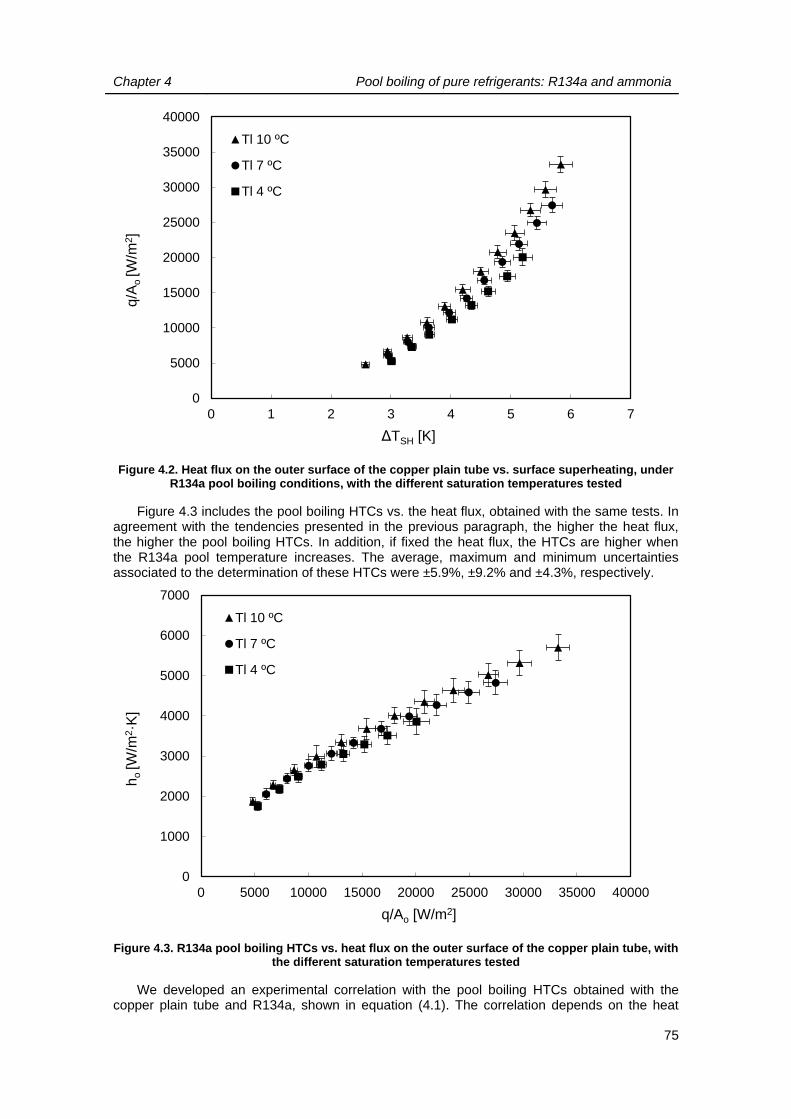
Chapter 4 Pool boiling of pure refrigerants: R134a and ammonia

75

Figure 4.2. Heat flux on the outer surface of the copper plain tube vs. surface superheating, under R134a pool boiling conditions, with the different saturation temperatures tested

Figure 4.3 includes the pool boiling HTCs vs. the heat flux, obtained with the same tests. In agreement with the tendencies presented in the previous paragraph, the higher the heat flux, the higher the pool boiling HTCs. In addition, if fixed the heat flux, the HTCs are higher when the R134a pool temperature increases. The average, maximum and minimum uncertainties associated to the determination of these HTCs were ±5.9%, ±9.2% and ±4.3%, respectively.

Figure 4.3. R134a pool boiling HTCs vs. heat flux on the outer surface of the copper plain tube, with the different saturation temperatures tested

We developed an experimental correlation with the pool boiling HTCs obtained with the copper plain tube and R134a, shown in equation (4.1). The correlation depends on the heat

0

5000

10000

15000

20000

25000

30000

35000

40000

0 1 2 3 4 5 6 7

q/A

o[W

/m2]

ΔTSH [K]

Tl 10 ºC

Tl 7 ºC

Tl 4 ºC

0

1000

2000

3000

4000

5000

6000

7000

0 5000 10000 15000 20000 25000 30000 35000 40000

ho

[W/m

2·K

]

q/Ao [W/m2]

Tl 10 ºC

Tl 7 ºC

Tl 4 ºC

Chapter 4 Pool boiling of pure refrigerants: R134a and ammonia

76

flux, q, and on the reduced pressure, pred (related to the saturation temperature), which were the parameters varied and controlled during the experiments. The coefficient of determination of the correlation is R2 = 0.99 and the average absolute deviation between the experimental data and the correlation is 0.5%.

48.057.09.44redo pqh

(4.1)

4.1.2. Comparison with correlations

Many works from the specialised literature focus on the study of the HTCs of pool boiling of refrigerants on tubes. In contrast with other processes, such as condensation on a tube or forced convection inside a tube, pool boiling correlations differ importantly from one study to another. The reason is the large number of parameters that have an important effect on this process and that should be under control, such as heat flux, reduced pressure, tube roughness, refrigerant surface tension, tube material, etc.

To properly apply some correlations from the literature, we determined the roughness of the copper tube. The technique used was the profilometry (profilometer DEKTAK 150) and we chose a random section of the tube, shown in Figure 4.4. We measured 10 profiles at the external surface and the arithmetic averages of the absolute distances from the midlines to the profiles, often denoted as Ra, appear in Table 4.1. From these experiments we determined the mean Ra for the 10 profiles, which resulted to be 0.326416 µm. It is important to notice that the resolution of the profilometer is 0.472 μm/sample, the same order of magnitude as the result measured. Therefore, the roughness determination method should be improved.

Figure 4.4. Section of the copper tube chosen for the roughness determination

Table 4.1. Mean roughness height, Ra, per profile and arithmetic mean of Ra for the 10 profiles

Profile Ra [µm] Profile Ra [µm]

1 0.28795 6 0.35028

2 0.29918 7 0.30707

3 0.29136 8 0.3544

4 0.31104 9 0.34509

5 0.27414 10 0.44365

Mean 0.326416

Chapter 4 Pool boiling of pure refrigerants: R134a and ammonia

77

We selected well-known correlations of the literature to compare our experimental results. These correlations were equation (4.2), of Stephan and Preusser [6]; equation (4.3), of Cooper [7]; equation (4.4), of Ribatski and Saiz Jabardo [8]; and equation (4.5), of Gorenflo and Kenning [9]. In these equations, kl stands for the thermal conductivity of the liquid refrigerant at saturation conditions; dbubble for the bubble departure diameter (equation (4.6)); ρl and ρg for the refrigerant density at liquid and gas saturation conditions, respectively; cp,l for the specific heat capacity of the liquid refrigerant at saturation conditions; σ for the surface tension of the liquid refrigerant at saturation conditions; hlv for the refrigerant latent heat of vaporization; q for the heat flux on the outer surface of the tube; Ts for the saturation temperature in Kelvin; M for the molar mass of the refrigerant; pred for the reduced pressure; and g for the acceleration of gravity. In addition, there are several constants in these equations, such as cw, that depends on the material of the tube. For Cooper [7], this constant is 95 when the tube is of copper and 55 when the tube is of stainless steel. For Ribatski and Saiz Jabardo [8], it equals 100 with copper, 95 with brass and 85 with stainless steel. Rp is the surface peak roughness, which according to Kotthoff and Gorenflo [10] should be replaced by the mean roughness height, Ra, divided by 0.4. Finally, β stands for the contact angle and according to Stephan and Preusser [6] is 35º with refrigerants.

674.0371.0

2

2,

22

35.0

2,

2162.0,

1565.01.0

satl

b

l

lplblv

blpl

l

l

lpl

l

g

b

lo

Tk

qd

k

cdh

dc

k

k

c

d

kh

(4.2)

67.055.0log2.012.05.0 log qppMch redRp

redwo

(4.3)

2.03.09.02.08.045.05.0 log redp

redredwo qRappMch

(4.4)

25.0

152

0

2.03.095.0

0 1

4.17.0

3.0

copperp

wp

red

redredred

p

refo

ck

ck

Ra

Ra

p

ppp

q

qhh

red

(4.5)

glb

gd

2146.0

(4.6)

In Figure 4.5 we compare our experimental results with those from the aforementioned correlations and in Table 4.2 we include the deviation range between our experimental data and each correlation, as well as the arithmetic mean of the deviations between the predicted and the experimental HTCs in absolute value. The figure shows that, except for Stephan and Preusser [6] correlation, most of our experimental results are correlated within ±30%, being the correlation from Gorenflo and Kenning [9] the one with the best agreement.

Chapter 4 Pool boiling of pure refrigerants: R134a and ammonia

78

Figure 4.5. R134a pool boiling HTCs obtained with correlations vs. experimental pool boiling HTCs from this work, with a copper plain tube and under the same conditions

Table 4.2. Comparison of the experimental pool boiling HTCs (R134a and copper plain tube) with those calculated with correlations

Correlation Arithmetic mean of the

deviations in absolute value (%) Deviation range (%)

Stephan and Preusser [6]

36.4 -44.3 – -31.1

Cooper [7] 20.2 8.2 – 29.5

Ribatski and Saiz Jabardo [8]

27.5 -37.2 – -18.8

Gorenflo and Kenning [9]

13.1 -29.6 – 9.0

0

1000

2000

3000

4000

5000

6000

7000

8000

0 1000 2000 3000 4000 5000 6000 7000 8000

hcorr

[W/m

2·K

]

hexp [W/m2·K]

Stephan and Preusser

Cooper

Ribatski and Saiz Jabardo

Gorenflo and Kenning

+10%

+30%+20%

-10%

-20%

-30%

Chapter 4 Pool boiling of pure refrigerants: R134a and ammonia

79

4.2. POOL BOILING OF R134a ON ENHANCED SURFACES

In this subsection, we present the results obtained with the pool boiling tests of R134a on two copper tubes with boiling enhanced surfaces, a Turbo-B and an Turbo-BII+. We conducted tests with the pool of refrigerant at 10 ºC, 7 ºC and 4 ºC, varying the LMTD at the evaporator from 1 K to 6 K (at steps of 0.5 K) with the Turbo-B tube, and from 1 K to 5 K (at steps of 0.5 K). With these conditions, the heat flux ranged from 11100 W/m2 to 61400 W/m2 with the former, and from 8900 W/m2 to 59800 W/m2 with the latter. With the Turbo-B tube, the velocity of the heating water was 3.9 m/s and the Reynolds number ranged from 40000 to 55100. Thus, the flow was fully developed turbulent and the application of the correlation shown in subsection 3.3.2 for the enhanced tube was suitable. With this tube, the heating water HTCs ranged from 22800 W/m2·K to 27000 W/m2·K, approximately. Concerning the Turbo-BII+ tube, the velocity of the heating water was 3.5 m/s and the Reynolds number ranged from 37900 to 51200. Thus, the flow was fully developed turbulent and the application of the correlation shown in subsection 3.3.2 for the enhanced tube was suitable. With this tube, the heating water HTCs ranged from 26600 W/m2·K to 31200 W/m2·K, approximately.

4.2.1. Refrigerant side heat transfer coefficients on Turbo-B

Figure 4.6 represents the boiling curve of the pool boiling process of R134a on a Turbo-B copper tube. From the lowest surface superheating to the highest, the process is in the nucleate boiling region, independently of the refrigerant pool temperature. Therefore, the heat flux increases rapidly with slight increase of the surface superheating. In addition, due to the enhanced surface, the nucleate boiling process is achieved at surface superheating values as low as 0.3 K. The effect of the refrigerant pool temperature is almost negligible on the curves.

Figure 4.6. Heat flux on the outer surface of the copper Turbo-B tube vs. surface superheating, under R134a pool boiling conditions, with the different saturation temperatures tested

Figure 4.7 represents the pool boiling HTCs vs. the heat flux, obtained under the same conditions as in the previous case. In contrast with the results obtained with the plain tube, the pool boiling HTCs decrease as the heat flux increases. The effect of the pool temperature on the HTCs, if fixed the heat flux, is negligible. The average, maximum and minimum uncertainties associated to the determination of these HTCs were ±11.9%, ±19.4% and ±8.4%, respectively.

0

10000

20000

30000

40000

50000

60000

70000

0 0.5 1 1.5 2 2.5 3 3.5

q/A

o[W

/m2]

ΔTSH [K]

Tl 10 ºC

Tl 7 ºC

Tle 4 ºC

Chapter 4 Pool boiling of pure refrigerants: R134a and ammonia

80

Figure 4.7. R134a pool boiling HTCs vs. heat flux on the outer surface of the copper Turbo-B tube, with R134a and with the different saturation temperatures tested

We developed an experimental correlation with the pool boiling HTCs obtained with the copper Turbo-B tube and R134a, shown in equation (4.7). The correlation depends on the heat flux, q, and on the reduced pressure, pred (related to the saturation temperature), which were the parameters varied and controlled during the experiments. We observe in the correlation, as was done with the experimental results, that the effect of the reduced pressure on the correlation is very low (exponent 0.03). The coefficient of determination of the correlation is R2 = 0.94 and the average absolute deviation between the experimental data and the correlation is 4.5%.

03.025.0510·3.3redo pqh

(4.7)

4.2.2. Refrigerant side heat transfer coefficients on Turbo-BII+

Figure 4.8 represents the boiling curve of the pool boiling process of R134a on a Turbo-BII+ copper tube. The process is in the nucleate boiling region, independently of the surface superheating and of the refrigerant pool temperature. Therefore, the heat flux increases rapidly with slight increase of the surface superheating. In addition, due to the enhanced surface, the nucleate boiling process occurs at surface superheating values as low as 0.5 K. The effect of the temperature of the pool of refrigerant is almost negligible on the curves.

Figure 4.9 shows the pool boiling HTCs vs. the heat flux, obtained under the same conditions as in the previous case. In contrast with the results obtained with the Turbo-B tube, the pool boiling HTCs increase as the heat flux increases, up to a heat flux close to 30000 W/m2, and then remain constant. The effect of the pool temperature on the HTCs, if fixed the heat flux, is not negligible at the low heat flux range (up to 30000 W/m2, approximately). The average, maximum and minimum uncertainties associated to the determination of these HTCs were ±9.4%, ±12.7% and ±8.0%, respectively.

0

5000

10000

15000

20000

25000

30000

35000

40000

45000

0 10000 20000 30000 40000 50000 60000 70000

ho

[W/m

2·K

]

q/Ao [W/m2]

Tl 10 ºC

Tl 7 ºC

Tl 4 ºC

Chapter 4 Pool boiling of pure refrigerants: R134a and ammonia

81

Figure 4.8. Heat flux on the outer surface of the copper Turbo-BII+ tube vs. surface superheating, under R134a pool boiling conditions, with the different saturation temperatures tested

Figure 4.9. R134a pool boiling HTCs vs. heat flux on the outer surface of the copper Turbo-BII+ tube, with the different saturation temperatures tested

We developed an experimental correlation, equation (4.8) with the pool boiling HTCs obtained with the copper Turbo-BII+ tube and R134a. It depends on the heat flux, q, and on the reduced pressure, pred, which were the parameters varied and controlled during the experiments. The coefficient of determination of the correlation is R2 = 0.76 and the average absolute deviation between the experimental data and the correlation is 5.2%.

0

10000

20000

30000

40000

50000

60000

70000

0 0.5 1 1.5 2 2.5 3

q/A

o[W

/m2]

ΔTSH [K]

Tl 10 ºC

Tl 7 ºC

Tl 4 ºC

0

5000

10000

15000

20000

25000

30000

0 10000 20000 30000 40000 50000 60000 70000

ho

[W/m

2·K

]

q/Ao [W/m2]

Tl 10 ºC

Tl 7 ºC

Tl 4 ºC

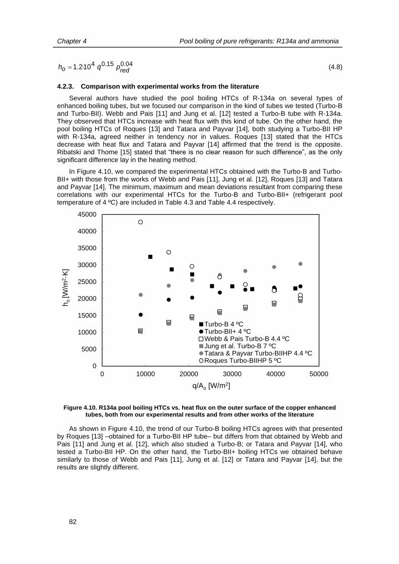
Chapter 4 Pool boiling of pure refrigerants: R134a and ammonia

82

04.015.0410·2.1redo pqh

(4.8)

4.2.3. Comparison with experimental works from the literature

Several authors have studied the pool boiling HTCs of R-134a on several types of enhanced boiling tubes, but we focused our comparison in the kind of tubes we tested (Turbo-B and Turbo-BII). Webb and Pais [11] and Jung et al. [12] tested a Turbo-B tube with R-134a. They observed that HTCs increase with heat flux with this kind of tube. On the other hand, the pool boiling HTCs of Roques [13] and Tatara and Payvar [14], both studying a Turbo-BII HP with R-134a, agreed neither in tendency nor in values. Roques [13] stated that the HTCs decrease with heat flux and Tatara and Payvar [14] affirmed that the trend is the opposite. Ribatski and Thome [15] stated that “there is no clear reason for such difference”, as the only significant difference lay in the heating method.

In Figure 4.10, we compared the experimental HTCs obtained with the Turbo-B and Turbo-BII+ with those from the works of Webb and Pais [11], Jung et al. [12], Roques [13] and Tatara and Payvar [14]. The minimum, maximum and mean deviations resultant from comparing these correlations with our experimental HTCs for the Turbo-B and Turbo-BII+ (refrigerant pool temperature of 4 ºC) are included in Table 4.3 and Table 4.4 respectively.

Figure 4.10. R134a pool boiling HTCs vs. heat flux on the outer surface of the copper enhanced tubes, both from our experimental results and from other works of the literature

As shown in Figure 4.10, the trend of our Turbo-B boiling HTCs agrees with that presented by Roques [13] –obtained for a Turbo-BII HP tube– but differs from that obtained by Webb and Pais [11] and Jung et al. [12], which also studied a Turbo-B; or Tatara and Payvar [14], who tested a Turbo-BII HP. On the other hand, the Turbo-BII+ boiling HTCs we obtained behave similarly to those of Webb and Pais [11], Jung et al. [12] or Tatara and Payvar [14], but the results are slightly different.

0

5000

10000

15000

20000

25000

30000

35000

40000

45000

0 10000 20000 30000 40000 50000

ho

[W/m

2·K

]

q/Ao [W/m2]

Turbo-B 4 ºCTurbo-BII+ 4 ºCWebb & Pais Turbo-B 4.4 ºCJung et al. Turbo-B 7 ºCTatara & Payvar Turbo-BIIHP 4.4 ºCRoques Turbo-BIIHP 5 ºC

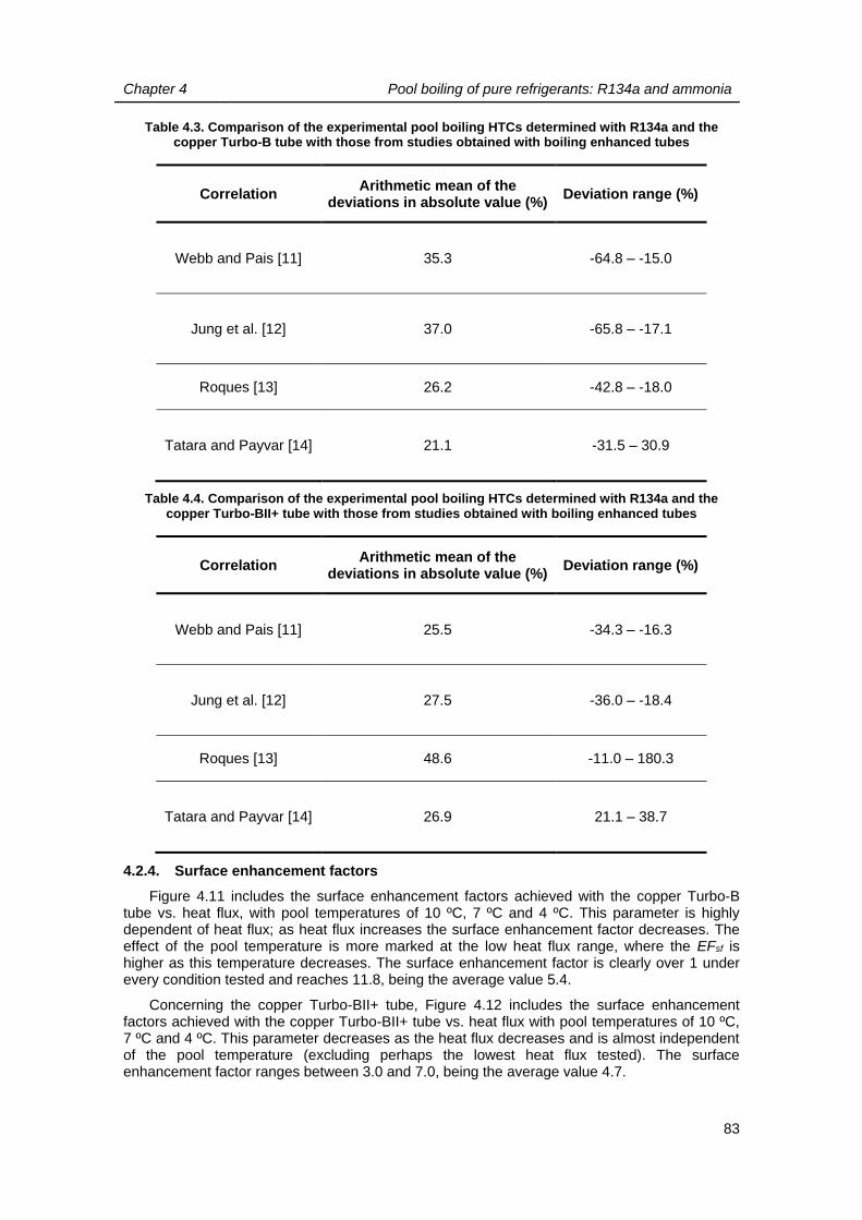
Chapter 4 Pool boiling of pure refrigerants: R134a and ammonia

83

Table 4.3. Comparison of the experimental pool boiling HTCs determined with R134a and the copper Turbo-B tube with those from studies obtained with boiling enhanced tubes

Correlation Arithmetic mean of the

deviations in absolute value (%) Deviation range (%)

Webb and Pais [11] 35.3 -64.8 – -15.0

Jung et al. [12] 37.0 -65.8 – -17.1

Roques [13] 26.2 -42.8 – -18.0

Tatara and Payvar [14] 21.1 -31.5 – 30.9

Table 4.4. Comparison of the experimental pool boiling HTCs determined with R134a and the copper Turbo-BII+ tube with those from studies obtained with boiling enhanced tubes

Correlation Arithmetic mean of the

deviations in absolute value (%) Deviation range (%)

Webb and Pais [11] 25.5 -34.3 – -16.3

Jung et al. [12] 27.5 -36.0 – -18.4

Roques [13] 48.6 -11.0 – 180.3

Tatara and Payvar [14] 26.9 21.1 – 38.7

4.2.4. Surface enhancement factors

Figure 4.11 includes the surface enhancement factors achieved with the copper Turbo-B tube vs. heat flux, with pool temperatures of 10 ºC, 7 ºC and 4 ºC. This parameter is highly dependent of heat flux; as heat flux increases the surface enhancement factor decreases. The effect of the pool temperature is more marked at the low heat flux range, where the EFsf is higher as this temperature decreases. The surface enhancement factor is clearly over 1 under every condition tested and reaches 11.8, being the average value 5.4.

Concerning the copper Turbo-BII+ tube, Figure 4.12 includes the surface enhancement factors achieved with the copper Turbo-BII+ tube vs. heat flux with pool temperatures of 10 ºC, 7 ºC and 4 ºC. This parameter decreases as the heat flux decreases and is almost independent of the pool temperature (excluding perhaps the lowest heat flux tested). The surface enhancement factor ranges between 3.0 and 7.0, being the average value 4.7.

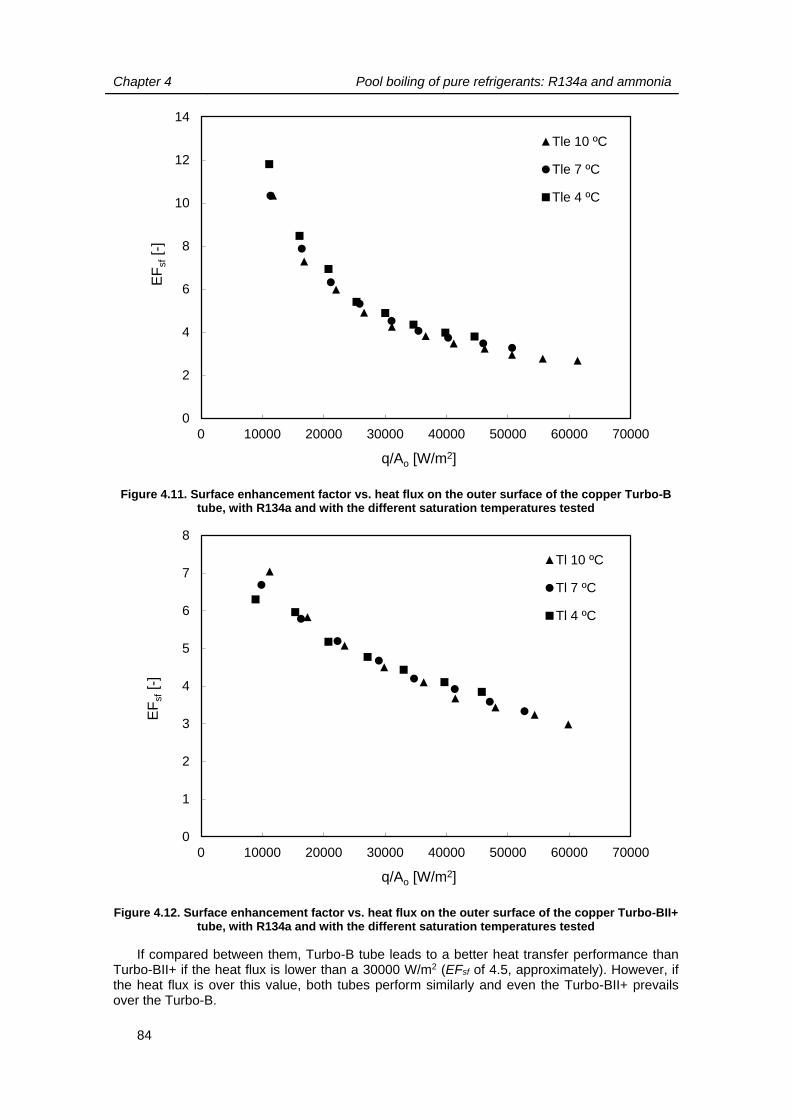
Chapter 4 Pool boiling of pure refrigerants: R134a and ammonia

84

Figure 4.11. Surface enhancement factor vs. heat flux on the outer surface of the copper Turbo-B tube, with R134a and with the different saturation temperatures tested

Figure 4.12. Surface enhancement factor vs. heat flux on the outer surface of the copper Turbo-BII+ tube, with R134a and with the different saturation temperatures tested

If compared between them, Turbo-B tube leads to a better heat transfer performance than Turbo-BII+ if the heat flux is lower than a 30000 W/m2 (EFsf of 4.5, approximately). However, if the heat flux is over this value, both tubes perform similarly and even the Turbo-BII+ prevails over the Turbo-B.

0

2

4

6

8

10

12

14

0 10000 20000 30000 40000 50000 60000 70000

EF

sf[-

]

q/Ao [W/m2]

Tle 10 ºC

Tle 7 ºC

Tle 4 ºC

0

1

2

3

4

5

6

7

8

0 10000 20000 30000 40000 50000 60000 70000

EF

sf[-

]

q/Ao [W/m2]

Tl 10 ºC

Tl 7 ºC

Tl 4 ºC

Chapter 4 Pool boiling of pure refrigerants: R134a and ammonia

85

4.3. POOL BOILING OF AMMONIA ON PLAIN TUBE

In this subsection, we present the results obtained with pool boiling tests of ammonia on the titanium plain tube. We conducted tests with the pool of refrigerant at 10 ºC, 7 ºC and 4 ºC, varying the LMTD at the evaporator from 4 K and 15 K (at steps of 1 K). With these conditions, the heat flux ranged from 2800 W/m2 to 56600 W/m2. The velocity of the heating water was 2.4 m/s, approximately, and the Reynolds number ranged from 29400 to 45800. Thus, the flow was fully developed turbulent and the application of the correlation shown in subsection 3.3.2 for the plain tube was suitable. The heating water HTCs ranged from 8200 W/m2·K to 10200 W/m2·K, approximately.

4.3.1. Refrigerant side heat transfer coefficients

Figure 4.13 represents the boiling curve of the pool boiling process of ammonia on a smooth titanium tube. Independently of the temperature of the pool of refrigerant, heat flux rises with surface superheating throughout the studied range. At the low surface superheating region, natural convection dominates the process and at the high surface superheating area nucleate boiling occurs and heat flux increases rapidly with it. Figure 4.13 also shows that if the ammonia pool temperature decreases, the transition between both regions occurs at a higher surface superheating.

Figure 4.13. Heat flux on the outer surface of the titanium plain tube vs. surface superheating, under ammonia pool boiling conditions, with the different saturation temperatures tested

Figure 4.14 includes the pool boiling HTCs vs. the heat flux, obtained under the same conditions as in the previous case. As the heat flux decreases, so do the pool boiling HTCs, and if fixed the heat flux, the HTCs are higher when the ammonia pool temperature increases. The average, maximum and minimum uncertainties associated to the determination of these HTCs were ±4.2%, ±10.5% and ±1.6%, respectively.

0

10000

20000

30000

40000

50000

60000

70000

0 1 2 3 4 5 6 7 8

q/A

o[W

/m2]

ΔTSH [K]

Tl 10 ºC

Tl 7 ºC

Tl 4 ºC

Chapter 4 Pool boiling of pure refrigerants: R134a and ammonia

86

Figure 4.14. Ammonia pool boiling HTCs vs. heat flux on the outer surface of the titanium plain tube, with the different saturation temperatures tested

We developed an experimental correlation with the pool boiling HTCs obtained with the titanium plain tube and ammonia, shown in equation (4.9). The correlation depends on the heat flux, q, and on the reduced pressure, pred, which were the parameters varied and controlled during the experiments. The coefficient of determination of the correlation is R2 = 0.99 and the average absolute deviation between the experimental data and the correlation is 5.0%.

31.177.035.87redo pqh

(4.9)

4.3.2. Comparison with correlations

We selected well-known correlations of the literature to compare our experimental results. Three of them have already been presented in subsection 4.1.2, such as equation (4.2), of Stephan and Preusser [6]; equation (4.3), of Cooper [7]; and equation (4.5), of Gorenflo and Kenning [9]. For this refrigerant–tube combination we also included equation (4.10), of Mostinski [16]. In addition to all the variables of the equations from subsection 4.1.2, in equation (4.10) pcrit stands for the critical pressure (in kPa). We did not determine the roughness of the titanium tube and we estimated it as for the copper tube (0.326416 µm). Cooper [7] gives cw values for copper and stainless steel, but not for titanium, so we consider it equal to that for stainless steel.

102.117.07.069.0 1048.100417.0

redredredcrito pppqph

(4.10)

Figure 4.15 shows the pool boiling HTCs calculated with the aforementioned correlations vs. the experimental ones for the titanium plain tube and ammonia. The deviation range and the arithmetic mean of the absolute deviation between the predicted and the experimental HTCs appear in Table 4.5. The figure shows the large scattering that exists between the correlations, particularly for those of Cooper [7] and Gorenflo and Kenning [9]. The reason could lie in the fact that the tube is made of titanium, a material that was not studied by any of them. The correlation of Mostinski [16] has the best agreement with the experimental results, followed closely by that of Stephan and Preusser [6].

0

1000

2000

3000

4000

5000

6000

7000

8000

9000

10000

0 10000 20000 30000 40000 50000 60000

ho

[W/m

2·K

]

q/Ao [W/m2]

Tl 10 ºC

Tl 7 ºC

Tl 4 ºC

Chapter 4 Pool boiling of pure refrigerants: R134a and ammonia

87

Figure 4.15. Ammonia pool boiling HTCs obtained with correlations vs. experimental pool boiling HTCs from this work, with a titanium plain tube and under the same conditions

Table 4.5. Comparison of the experimental pool boiling HTCs (ammonia and titanium plain tube) with those calculated with correlations

Correlation Arithmetic mean of the

deviation in absolute value (%) Deviation range (%)

Stephan and Preusser [6]

12.7 -17.3 – 20.5

Cooper [7] 70.4 28.4 – 101.6

Gorenflo and Kenning [9]

44.2 -55.3 – -35.4

Mostinski [16] 10.7 -27.2 – 10.2

4.3.3. Hysteresis

Nucleation hysteresis is a process that occurs at pool boiling processes, and that consists in a delay of the transition from natural convection to nucleate boiling, i.e. the surface superheating is greater than that expected for a certain heat flux under nucleate boiling (Poniewski and Thome, [17]). The existence of hysteresis in ammonia pool boiling is documented in works such as that from Kuprianova [18].

0

2000

4000

6000

8000

10000

12000

0 2000 4000 6000 8000 10000 12000

hcorr

[W/m

2·K

]

hexp [W/m2·K]

Stephan_PreusserCooperMostinskiGorenflo and Kenning

+10%

+30%+60%

-10%

-60%

-30%

Chapter 4 Pool boiling of pure refrigerants: R134a and ammonia

88

Figure 4.16. Heat flux on the outer surface of the titanium plain tube vs. surface superheating, under ammonia pool boiling conditions (10 ºC), with both decreasing and increasing heat flux tests

Figure 4.17. Ammonia pool boiling HTCs vs. heat flux on the outer surface of the titanium plain tube, for both decreasing and increasing heat flux tests, at a pool temperature of 10 ºC

With ammonia we developed tests to study nucleation hysteresis, i.e. we distinguished between those results obtained decreasing the heat flux on the evaporator tube and those obtained increasing the heat flux on the evaporator tube. Decreasing heat flux tests (explained in subsection 3.2.1) started with the maximum mean heating water temperature possible. When achieved steady state, we registered data for a minimum of 15 minutes. After that, we lowered

0

10000

20000

30000

40000

50000

60000

70000

0 1 2 3 4 5 6 7 8

q/A

o[W

/m2]

ΔTSH [K]

Tl 10 ºC Decrease

Tl 10 ºC Increase

0

2000

4000

6000

8000

10000

0 10000 20000 30000 40000 50000 60000

ho

[W/m

2·K

]

q/Ao [W/m2]

Tl 10 ºC Decrease

Tl 10 ºC Increase

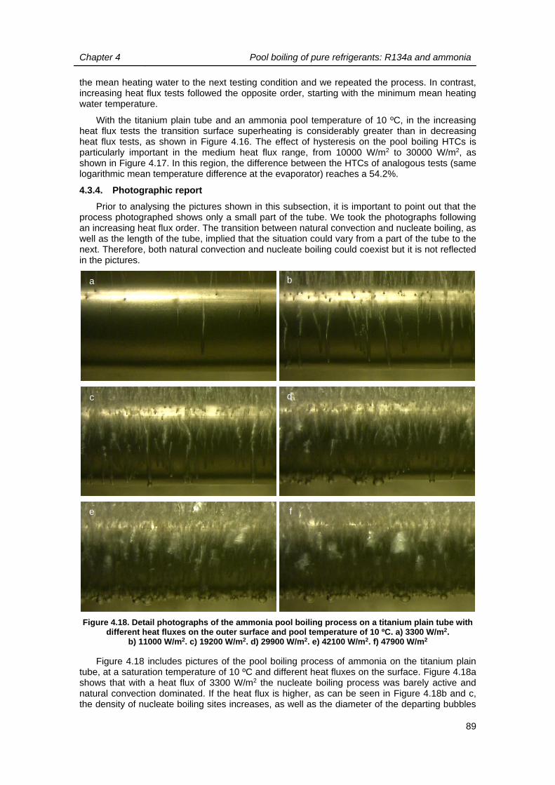
Chapter 4 Pool boiling of pure refrigerants: R134a and ammonia

89

the mean heating water to the next testing condition and we repeated the process. In contrast, increasing heat flux tests followed the opposite order, starting with the minimum mean heating water temperature.

With the titanium plain tube and an ammonia pool temperature of 10 ºC, in the increasing heat flux tests the transition surface superheating is considerably greater than in decreasing heat flux tests, as shown in Figure 4.16. The effect of hysteresis on the pool boiling HTCs is particularly important in the medium heat flux range, from 10000 W/m2 to 30000 W/m2, as shown in Figure 4.17. In this region, the difference between the HTCs of analogous tests (same logarithmic mean temperature difference at the evaporator) reaches a 54.2%.

4.3.4. Photographic report

Prior to analysing the pictures shown in this subsection, it is important to point out that the process photographed shows only a small part of the tube. We took the photographs following an increasing heat flux order. The transition between natural convection and nucleate boiling, as well as the length of the tube, implied that the situation could vary from a part of the tube to the next. Therefore, both natural convection and nucleate boiling could coexist but it is not reflected in the pictures.

Figure 4.18. Detail photographs of the ammonia pool boiling process on a titanium plain tube with different heat fluxes on the outer surface and pool temperature of 10 ºC. a) 3300 W/m2.

b) 11000 W/m2. c) 19200 W/m2. d) 29900 W/m2. e) 42100 W/m2. f) 47900 W/m2

Figure 4.18 includes pictures of the pool boiling process of ammonia on the titanium plain tube, at a saturation temperature of 10 ºC and different heat fluxes on the surface. Figure 4.18a shows that with a heat flux of 3300 W/m2 the nucleate boiling process was barely active and natural convection dominated. If the heat flux is higher, as can be seen in Figure 4.18b and c, the density of nucleate boiling sites increases, as well as the diameter of the departing bubbles

a b

c d

e f

Chapter 4 Pool boiling of pure refrigerants: R134a and ammonia

90

(Figure 4.18d). In Figure 4.18e and f the nucleate boiling process is generalised all over the tube surface, confirming the results shown in previous subsections.

At the low heat flux region (7700 W/m2) we also observed that nucleation sites were not stable, and appeared and disappeared continually (Figure 4.19).

Figure 4.19. Unstable nucleation sites during an experiment at the transition between natural convection and nucleate boiling (heat flux of 7700 W/m2)

a b

c

Chapter 4 Pool boiling of pure refrigerants: R134a and ammonia

91

4.4. POOL BOILING OF AMMONIA ON ENHANCED TUBE

In this subsection, we present the results obtained with pool boiling tests of ammonia on the titanium integral-fin tube Trufin 32 f.p.i. We conducted tests with the pool of refrigerant at 10 ºC, 7 ºC and 4 ºC, varying the LMTD at the evaporator from 4 K and 15 K (at steps of 1 K). With these conditions, the heat flux ranged from 3600 W/m2 to 60000 W/m2. The velocity of the heating water with these tests was 2.6 m/s, approximately, and the Reynolds number ranged from 30800 to 49300. Thus, the flow was fully developed turbulent and the application of the correlation shown in subsection 3.3.2 for the plain tube was suitable. The heating water HTCs ranged from 8900 W/m2·K to 11200 W/m2·K, approximately.

4.4.1. Refrigerant side heat transfer coefficients on Trufin 32 f.p.i

Figure 4.20 represents the boiling curve of the pool boiling process of ammonia on the titanium Trufin 32 f.p.i. tube. Independently of the temperature of the pool of refrigerant, heat flux rises with surface superheating throughout the studied range. As shown with the plain tube, the natural convection and the nucleate boiling areas appear, but the transition between them occurs at a slightly lower surface superheating than with the plain tube (between 1 and 2 K).

Figure 4.20. Heat flux on the outer surface of the titanium Trufin 32 f.p.i. tube vs. surface superheating, under ammonia pool boiling conditions, with the different saturation temperatures

tested

Figure 4.21 illustrates the pool boiling HTCs vs. the heat flux obtained in decreasing heat flux order, with the titanium Trufin 32 f.p.i. tube and ammonia pool temperatures of 10 ºC, 7 ºC and 4 ºC. In this case, HTCs also increase either if the heat flux or the ammonia pool temperature is higher. The average, maximum and minimum uncertainties associated to the determination of these HTCs were ±5.5%, ±14.0% and ±1.9%, respectively.

0

10000

20000

30000

40000

50000

60000

70000

0 1 2 3 4 5 6 7

q/A

o[W

/m2]

ΔTSH [K]

Tl 10 ºC Dec

Tl 7 ºC Dec

Tl 4 ºC Dec

Chapter 4 Pool boiling of pure refrigerants: R134a and ammonia

92

Figure 4.21. Ammonia pool boiling HTCs vs. heat flux on the outer surface of the titanium Trufin 32 f.p.i. tube, with the different saturation temperatures tested

We developed an experimental correlation with the pool boiling HTCs obtained with the titanium Trufin 32 f.p.i. tube and ammonia, shown in equation (4.11). The correlation depends on the heat flux, q, and on the reduced pressure, pred, which were the parameters varied and controlled during the experiments. The exponents for both parameters agree with those determined in equation (4.9) for the titanium plain tube. The coefficient of determination of the correlation is R2 = 0.99 and the average absolute deviation between the experimental data and the correlation is 5.5%.

31.177.046.110redo pqh

(4.11)

4.4.2. Surface enhancement factors

Figure 4.22 includes the surface enhancement factors achieved with the Trufin 32 f.p.i. tube vs. heat flux, with pool temperatures of 10 ºC, 7 ºC and 4 ºC. It shows that this parameter, generally, is independent of the heat flux. This conclusion is in agreement with the correlation we obtained, which has the same exponents for both the heat flux and reduced pressure and only the fitting constant changes. The effect of the ammonia pool temperature is more marked at the low heat flux range, where the EFsf is clearly higher as this temperature decreases. The surface enhancement factor is greater than or equal to 1 under every condition tested and reaches 1.3, being the average value 1.2.

0

2000

4000

6000

8000

10000

12000

14000

16000

0 10000 20000 30000 40000 50000 60000 70000

ho

[W/m

2·K

]

q/Ao [W/m2]

Tl 10 ºC Dec

Tl 7 ºC Dec

Tl 4 ºC Dec

Chapter 4 Pool boiling of pure refrigerants: R134a and ammonia

93

Figure 4.22. Surface enhancement factor vs. heat flux if compared the titanium Trufin 32 f.p.i. tube to the plain tube, with ammonia as refrigerant and with the different saturation temperatures tested

There are not many experimental works of the specialised literature focused on pool boiling enhancement with ammonia as refrigerant. Djundin et al. [19] studied experimentally the HTCs on a plain steel tube and several enhanced tubes. Mechanical grooves improved pool boiling heat transfer between 30% and 60%. Djundin and co-workers also studied a porous aluminium layer on the tube, which led to an enhancement of 40%; and a fluorocarbon layer with spots placed randomly on the surface of the tube, which led to improvements between 300% and 400% if compared to the plain tube. Danilova et al [20] analysed ammonia pool boiling on different horizontal steel tubes with aluminium coatings and, according to their results, these coatings can improve heat transfer between 100% and 400% if compared to the plain tube used as reference.

The enhancement factors obtained by Djundin et al. [19] with the grooved tube are very similar to the improvement we achieved with our Trufin 32 f.p.i. tube. However, the rest of the enhancement strategies from both works clearly outperform our results.

4.4.3. Hysteresis

In a similar way we did with the titanium plain tube, we analysed the nucleation hysteresis with ammonia and the titanium Trufin 32 f.p.i. tube. Figure 4.23 shows the heat flux vs. surface superheating curves determined with the decreasing and increasing heat flux tests, at pool temperatures of 10 ºC, 7 ºC and 4 ºC. In the increasing heat flux tests the transition surface superheating is considerably greater than in decreasing heat flux tests. In addition, hysteresis is higher as the pool temperature decreases, as depicted in Figure 4.23.

The effect of hysteresis on the pool boiling HTCs is particularly important in the medium heat flux range, from 10000 W/m2 to 30000 W/m2, as shown in Figure 4.24. The difference between the HTCs of analogous tests (same logarithmic mean temperature difference at the evaporator) reaches 172%. This value is greater than the maximum difference determined with the plain tube, which was 54%. This behaviour agrees with the conclusion stated in Poniewski and Thome [17] concerning the higher effect of hysteresis on enhanced boiling surfaces than on smooth surfaces.

0.0

0.2

0.4

0.6

0.8

1.0

1.2

1.4

1.6

0 10000 20000 30000 40000 50000 60000 70000

EF

sf[-

]

q/Ao [W/m2]

Tle 10 ºC

Tle 7 ºC

Tle 4 ºC

Chapter 4 Pool boiling of pure refrigerants: R134a and ammonia

94

Figure 4.23. Heat flux on the outer surface of the titanium Trufin 32 f.p.i. tube vs. surface superheating, under ammonia pool boiling conditions, with decreasing and increasing heat flux

tests and with the different saturation temperatures

Figure 4.24. Ammonia pool boiling HTCs vs. heat flux on the surface of the titanium Trufin 32 f.p.i. tube, for both decreasing and increasing heat flux tests, with the different saturation temperatures

While performing the increasing heat flux series at ammonia pool temperature of 10 ºC and LMTD at the evaporator of 10 K, even though the conditions were stable, the heat flow at the evaporator increased. Therefore, we conducted a special kind of experiment to check this trend. This test consisted in reaching this specific condition following an increasing heat flux path and maintaining it constant for a long period (more than 10 hours), as shown in Figure 4.25.

0

10000

20000

30000

40000

50000

60000

70000

0 2 4 6 8 10

q/A

o[W

/m2]

ΔTSH [K]

Tl 10 ºC Dec

Tl 10 ºC Inc

Tl 7 ºC Dec

Tl 7 ºC Inc

Tl 4 ºC Dec

Tl 4 ºC Inc

0

2000

4000

6000

8000

10000

12000

14000

16000

0 10000 20000 30000 40000 50000 60000 70000

ho

[W/m

2·K

]

q/Ao [W/m2]

Tl 10 ºC Dec

Tl 10 ºC Inc

Tl 7 ºC Dec

Tl 7 ºC Inc

Tl 4 ºC Dec

Tl 4 ºC Inc

Chapter 4 Pool boiling of pure refrigerants: R134a and ammonia

95

Figure 4.25. Temperatures of the pool of refrigerant and the heating water vs. time at the special tests for studying the stability during hysteresis

Figure 4.26. Heat flux on the outer surface of the titanium Trufin 32 f.p.i. tube vs. surface superheating, under ammonia pool boiling conditions (10 ºC), with decreasing and increasing heat

flux and hysteresis stability tests

Figure 4.26 shows the heat flux vs. surface superheating evolution of this experiment and compares it to the increasing and decreasing heat flux series (ammonia pool temperature of 10 ºC). As shown in the chart, the heat flux increased and the surface superheating decreased, even though the conditions were constant, starting from an experimental value close to the

0

5

10

15

20

25

0 10000 20000 30000 40000 50000

T[º

C]

t [s]

Tl

Thw,mean

Thw,inlet

Thw,outlet

0

10000

20000

30000

40000

50000

60000

70000

0 1 2 3 4 5 6 7

q/A

o[W

/m2]

ΔTSH [K]

Tl 10 ºC Dec

Tl 10 ºC Inc

Hysteresis

Chapter 4 Pool boiling of pure refrigerants: R134a and ammonia

96

increasing heat flux curve and ending at another close to the decreasing heat flux curve. This result suggests that the effect of nucleation hysteresis diminishes as the time passes.

4.4.4. Photographic report

Figure 4.27 includes pictures of the pool boiling process of ammonia on the titanium Trufin 32 f.p.i. tube, at a saturation temperature of 10 ºC and different heat fluxes on the surface. Figure 4.27a and b show that, with heat fluxes of 3700 W/m2 and 10200 W/m2, the nucleate boiling process was barely active and natural convection dominated in the part of the tube filmed. If the heat flux is higher, as can be seen in Figure 4.27c and d, the density of nucleate boiling sites and diameter of the departing bubbles increase, and the nucleate boiling process is generalised all over the tube surface. The boiling process is even more active in Figure 4.27e and f, which agrees with the experimental HTCs determined.

Chapter 4 Pool boiling of pure refrigerants: R134a and ammonia

97

Figure 4.27. Detail photographs of the ammonia pool boiling process on the titanium Trufin 32 f.p.i tube with different heat fluxes on the outer surface and pool temperature of 10 ºC. a) 3700 W/m2.

b) 10200 W/m2. c) 17600 W/m2. d) 28400 W/m2. e) 38500 W/m2. f) 50600 W/m2

a b

c d

e f

Chapter 4 Pool boiling of pure refrigerants: R134a and ammonia

98

4.5. CONCLUSIONS

In this chapter we have shown the pool boiling HTCs obtained experimentally for this thesis. The refrigerants studied were R134a and ammonia. With the former we tested copper tubes of plain and enhanced surfaces (Turbo-B and Turbo-BII+); and with the latter we tested titanium tubes of plain and enhanced surface (Trufin 32 f.p.i.).

We have observed that the vast majority of our experimental results are included in the boiling region of the boiling curve, where the slope is steep and heat flux increases rapidly with superheating.

Concerning the pool boiling HTCs, we have observed that they generally increase with increasing saturation temperatures, being constant the heat flux. Another trend observed for all the tubes except for Turbo-B is that pool boiling HTCs rise as the heat flux rises, independently of the saturation temperature. This effect was clearer with the plain tubes.

With ammonia we also tested the influence of hysteresis on the nucleation process. We confirmed its existence and that it is more important with the enhanced surface tested with ammonia. However, our experiments have shown that increasing heat flux tests are time-dependent, i.e. the HTCs obtained when the experimentation process follows an increasing heat flux trend rise with time until they reach a value very close to that obtained with the diminishing heat flux tests.

We have compared our experimental results with well-known correlations from different works from the literature. In the case of plain tubes, the best agreement existed with Gorenflo and Kenning [9] correlation with R134a and with Mostinski [16] correlation with ammonia.

The surface enhancement techniques were more effective with R134a than with ammonia. With R134a, the surface enhancement factors were as high as 11.8 and 7 with the Turbo-B and Turbo-BII+, respectively. In contrast, with ammonia the EFsf was never greater than 1.3.

Finally, we have included the photographic reports of the pool boiling of ammonia on the plain tube and the Trufin 32 f.p.i. tube. The pictures show the increase of density of nucleation sites and of the bubble diameters as the heat flux increases. The visual differences between tubes are very slight, confirming the results determined experimentally.

Chapter 4 Pool boiling of pure refrigerants: R134a and ammonia

99

REFERENCES

[1] Á.Á. Pardiñas, J. Fernández-Seara, C. Piñeiro-Pontevedra, S. Bastos, Experimental determination of the boiling heat transfer coefficients of R-134a and R-417A on a smooth copper tube, Heat Transfer Engineering. 35 (2014) 1424-1434.

[2] Á.Á. Pardiñas, J. Fernández-Seara, S. Bastos, R. Diz, Experimental boiling heat transfer coefficients of R-134a on two boiling enhanced tubes, in: Proceedings of the 8th World Conference on Experimental Heat Transfer, Fluid Mechanics, and Thermodynamics. Lisbon, Portugal, 2013.

[3] Á.Á. Pardiñas, J. Fernández-Seara, R. Diz, Experimental study on heat transfer coefficients of spray evaporation and pool boiling on plain tubes, in: Proceedings of the 24th IIR International Congress of Refrigeration. Yokohama, Japan, 2015.

[4] S. Nukiyama, The maximum and minimum values of the heat Q transmitted from metal to boiling water under atmospheric pressure, International Journal of Heat and Mass Transfer. 27 (1984) 959-970.

[5] J.R. Thome, Boiling heat transfer on external surfaces, in: Wolverine Heat Transfer Engineering Data Book III, 2009.

[6] K. Stephan, P. Preusser, Wärmeübergang und maximale Wärmestromdichte beim Behältersieden binärer und ternärer Flüssigkeitsgemische. Chemie Ingenieur Technik. 51 (1979) 649-679.

[7] M.G. Cooper, Heat flow rates in saturated nucleate pool boiling - a wide ranging examination using reduced properties, Advances in Heat Transfer. 16 (1984).

[8] G. Ribatski, J.M. Saiz Jabardo, Experimental Study of Nucleate Boiling of Halocarbon Refrigerants on Cylindrical Surfaces, International Journal of Heat and Mass Transfer. 46 (2003) 4439-4451.

[9] D. Gorenflo, D.B.R. Kenning, Pool Boiling. Chapter H2, VDI Heat Atlas, second ed. Springer, Berlin, 2010.

[10] S. Kotthoff, D. Gorenflo, Pool boiling heat transfer to hydrocarbons and ammonia: a state-of-the-art review, International Journal of Refrigeration. 31 (2008) 573-602.

[11] R.L. Webb, C. Pais, Nucleate pool boiling data for five refrigerants on plain, integral-fin and enhanced tube geometries, International Journal of Heat and Mass Transfer. 35 (1992) 1893-1904.

[12] D. Jung, K. An, J. Park, Nucleate boiling heat transfer coefficients of HCFC22, HFC134a, HFC125, and HFC32 on various enhanced tubes, International Journal of Refrigeration. 27 (2004) 202-206.

[13] J.F. Roques, Falling film evaporation on a single tube and on a tube bundle. Ph.D. thesis, École Polytechnique Fédérale de Lausanne, 2004.

[14] R.A. Tatara, P. Payvar, Pool boiling of pure R134a from a single Turbo-BII-HP tube, International Journal of Heat and Mass Transfer. 43 (2000) 2233-2236.

[15] G. Ribatski, J.R. Thome, Nucleate boiling heat transfer of R134a on enhanced tubes, Applied Thermal Engineering. 26 (2006) 1018-1031.

[16] I.L. Mostinski, Application of the rule of corresponding states for calculation of heat transfer and critical heat flux, Teploenergetika. 4 (1963) 66.

[17] M.E. Poniewski, J.R. Thome, Nucleate boiling on micro-structured surfaces. Heat Transfer Research, Inc. (HITRI), Texas, 2008.

[18] A.V. Kuprianova, Heat transfer with pool boiling of ammonia on horizontal tubes, Kholod. Tekh. 11 (1970) 40-44.

[19] V.A. Djundin, A.G. Soloviyov, A.V. Borisanskaja, J.A. Vol’nykh, Influence of the type of surface on heat transfer in boiling, Kholod. Tekh. 5 (1984) 33-37.

Chapter 4 Pool boiling of pure refrigerants: R134a and ammonia

100

[20] G.N. Danilova, V.A. Djundin, A.V. Borishanskaya, A.G. Soloviyov, J.A. Vol’nykh, A.A. Kozyrev, Effect of surface conditions on boiling heat transfer of refrigerants in shell-and-tube evaporators, Heat Transfer-Soviet Research. 22 (1990) 56-65.

101

Chapter 5

Spray evaporation of pure refrigerants: R134a and

ammonia In this section we detail the experimental spray evaporation HTCs obtained with our

experimental setup and procedure. As with pool boiling, we tested R134a and ammonia, but the tubes were only of plain surfaces, either of copper or titanium.

Each combination tube-refrigerant was tested for two different situations: with the liquid refrigerant distributed directly on the tested tube (ST) and with the tested tube receiving liquid refrigerant from a tube placed above it (SB). In this chapter, we show the heat flux determined versus the tube wall superheat and the spray evaporation HTCs versus the heat flux, in both cases as a function of the liquid refrigerant flow rate distributed. We also compare the experimental results obtained with the tubes tested at the two situations to analyse the effect of the refrigerant impingement on heat transfer.

A photographic report is included in this chapter of the spray evaporation processes studied. The pictures cover different experimental conditions and describe processes such as the formation of dry patches, which help to explain some of the results determined.

We also show the enhancement factors achieved by spray evaporation, if compared with pool boiling, at the same testing conditions, refrigerant and tube surface.

Some of the results here detailed were stated in the conference contribution Á.Á. Pardiñas, J. Fernández-Seara and R. Diz, Experimental study on heat transfer coefficients of spray evaporation and pool boiling on plain tubes, from the 24th IIR International Congress of Refrigeration (Yokohama, Japan, 2015) [1].

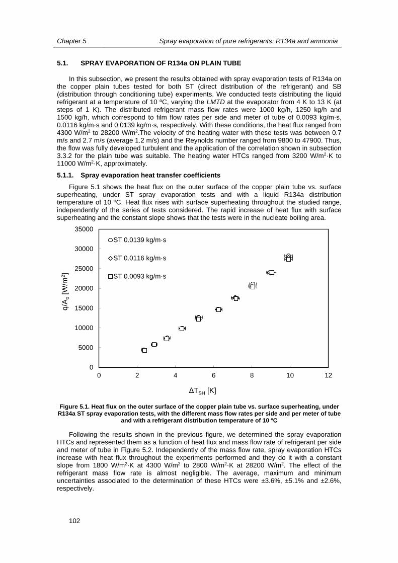
Chapter 5 Spray evaporation of pure refrigerants: R134a and ammonia

102

5.1. SPRAY EVAPORATION OF R134a ON PLAIN TUBE

In this subsection, we present the results obtained with spray evaporation tests of R134a on the copper plain tubes tested for both ST (direct distribution of the refrigerant) and SB (distribution through conditioning tube) experiments. We conducted tests distributing the liquid refrigerant at a temperature of 10 ºC, varying the LMTD at the evaporator from 4 K to 13 K (at steps of 1 K). The distributed refrigerant mass flow rates were 1000 kg/h, 1250 kg/h and 1500 kg/h, which correspond to film flow rates per side and meter of tube of 0.0093 kg/m·s, 0.0116 kg/m·s and 0.0139 kg/m·s, respectively. With these conditions, the heat flux ranged from 4300 W/m2 to 28200 W/m2.The velocity of the heating water with these tests was between 0.7 m/s and 2.7 m/s (average 1.2 m/s) and the Reynolds number ranged from 9800 to 47900. Thus, the flow was fully developed turbulent and the application of the correlation shown in subsection 3.3.2 for the plain tube was suitable. The heating water HTCs ranged from 3200 W/m2·K to 11000 W/m2·K, approximately.

5.1.1. Spray evaporation heat transfer coefficients

Figure 5.1 shows the heat flux on the outer surface of the copper plain tube vs. surface superheating, under ST spray evaporation tests and with a liquid R134a distribution temperature of 10 ºC. Heat flux rises with surface superheating throughout the studied range, independently of the series of tests considered. The rapid increase of heat flux with surface superheating and the constant slope shows that the tests were in the nucleate boiling area.

Figure 5.1. Heat flux on the outer surface of the copper plain tube vs. surface superheating, under R134a ST spray evaporation tests, with the different mass flow rates per side and per meter of tube

and with a refrigerant distribution temperature of 10 ºC

Following the results shown in the previous figure, we determined the spray evaporation HTCs and represented them as a function of heat flux and mass flow rate of refrigerant per side and meter of tube in Figure 5.2. Independently of the mass flow rate, spray evaporation HTCs increase with heat flux throughout the experiments performed and they do it with a constant slope from 1800 W/m2·K at 4300 W/m2 to 2800 W/m2·K at 28200 W/m2. The effect of the refrigerant mass flow rate is almost negligible. The average, maximum and minimum uncertainties associated to the determination of these HTCs were ±3.6%, ±5.1% and ±2.6%, respectively.

0

5000

10000

15000

20000

25000

30000

35000

0 2 4 6 8 10 12

q/A

o[W

/m2]

ΔTSH [K]

ST 0.0139 kg/m·s

ST 0.0116 kg/m·s

ST 0.0093 kg/m·s

Chapter 5 Spray evaporation of pure refrigerants: R134a and ammonia

103

Figure 5.2. Spray evaporation HTCs vs. heat flux on the outer surface of the copper plain tube, under R134a ST spray evaporation tests, with the different mass flow rates per side and per meter

of tube and with a refrigerant distribution temperature of 10 ºC

We developed an experimental correlation with the spray evaporation HTCs obtained with ST tests, copper plain tube and R134a, shown in equation (5.1). The correlation depends on the heat flux, q, and on the mass flow rate of refrigerant per side and per meter of tube, Γ, which were the parameters varied and controlled during the experiments. The coefficient of determination of the correlation is R2 = 0.98 and the average absolute deviation between the experimental data and the correlation is 2.1%.

04.021.068.391 qho (5.1)

Figure 5.3 shows the heat flux on the outer surface of the copper plain tube vs. surface superheating, under SB spray evaporation tests and with a liquid R134a distribution temperature of 10 ºC. Independently of the series of tests considered, heat flux rises with surface superheating throughout the studied range, as happened with ST tests, but the values are slightly lower than in that case. The constant and steep slope of the curve defined by heat flux vs. surface superheating shows that the tests were in the nucleate boiling area.

Figure 5.4 describes the relation between SB spray evaporation HTCs with heat flux and mass flow rate of refrigerant per side and meter of tube. Spray evaporation HTCs increase with heat flux under the experimental conditions tested, independently of the mass flow rate, from 1600 W/m2·K at 5100 W/m2 to 2300 W/m2·K at 20500 W/m2. As with the ST experiments, the effect of the refrigerant mass flow rate is almost negligible. The average, maximum and minimum uncertainties associated to the determination of these HTCs were ±3.4%, ±4.6% and ±2.4%, respectively.

0

500

1000

1500

2000

2500

3000

3500

0 5000 10000 15000 20000 25000 30000 35000

ho

[W/m

2·K

]

q/Ao [W/m2]

ST 0.0139 kg/m·s

ST 0.0116 kg/m·s

ST 0.0093 kg/m·s

Chapter 5 Spray evaporation of pure refrigerants: R134a and ammonia

104

Figure 5.3. Heat flux on the outer surface of the copper plain tube vs. surface superheating, under R134a SB spray evaporation test, with the different mass flow rates per side and per meter of tube

and with a refrigerant distribution temperature of 10 ºC

Figure 5.4. Spray evaporation HTCs vs. heat flux on the outer surface of the copper plain tube, under R134a SB spray evaporation tests, with the different mass flow rates per side and per meter

of tube and with a refrigerant distribution temperature of 10 ºC

We developed an experimental correlation with the spray evaporation HTCs obtained with SB tests, copper plain tube and R134a, shown in equation (5.2). The correlation depends on the heat flux, q, and on the mass flow rate of refrigerant per side and per meter of tube, Γ, which were the parameters varied and controlled during the experiments. The coefficient of

0

5000

10000

15000

20000

25000

0 2 4 6 8 10

q/A

o[W

/m2]

ΔTSH [K]

SB 0.0139 kg/m·s

SB 0.0116 kg/m·s

SB 0.0093 kg/m·s

0

500

1000

1500

2000

2500

0 5000 10000 15000 20000 25000

ho

[W/m

2·K

]

q/Ao [W/m2]

SB 0.0139 kg/m·s

SB 0.0116 kg/m·s

SB 0.0093 kg/m·s

Chapter 5 Spray evaporation of pure refrigerants: R134a and ammonia

105

determination of the correlation is R2 = 0.98 and the average absolute deviation between the experimental data and the correlation is 1.9%.

07.023.072.314 qho (5.2)

Figure 5.5 compares the spray evaporation HTCs vs. heat flux obtained with the tube placed directly underneath the refrigerant distribution tube (ST tests) to those determined with the tube that receives refrigerant from another placed over it (SB tests). The general trends observed with heat flux and flow rates are similar, but the HTC values with the ST tests are between 10.9% and 16.6% (average 13.2%) greater than with the second. The reason to this could lie in a decrease of the liquid refrigerant mass flow rate of SB tests due to splashing on the tube placed right above it. However, as seen in Figure 5.4, SB test HTCs are not affected by the distributed mass flow rate. Another explanation to this difference could come from the liquid droplet impingement effect. According to Zeng et al. [2] or Tatara and Payvar [3], high momentum devices, as the nozzles we tested, improve the wetting of the target surface and the high velocity of the liquid distributed enhances heat transfer.

Figure 5.5. Spray evaporation HTCs vs. heat flux on the outer surface of the copper plain tube, under R134a ST and SB spray evaporation tests, with the different mass flow rates per side and per

meter of tube and with a refrigerant distribution temperature of 10 ºC

5.1.2. Spray enhancement factors

Figure 5.6 illustrates the spray enhancement factor of R134a and plain copper tube vs. heat flux, with ST experiments and as a function of the mass flow rate of refrigerant per side and meter of tube. Spray evaporation enhances heat transfer if compared to pool boiling only in the low heat flux range (up to 17500 W/m2), being the maximum enhancement factor of 1.7 (0.0139 kg/m·s and 4300 W/m2). At higher heat fluxes, pool boiling slightly outperforms spray evaporation and the minimum enhancement factor is close to 0.9 (0.0093 kg/m·s and 27400 W/m2).

0

500

1000

1500

2000

2500

3000

3500

0 5000 10000 15000 20000 25000 30000 35000

ho

[W/m

2·K

]

q/Ao [W/m2]

ST 0.0139 kg/m·s

ST 0.0116 kg/m·s

ST 0.0093 kg/m·s

SB 0.0139 kg/m·s

SB 0.0116 kg/m·s

SB 0.0093 kg/m·s

Chapter 5 Spray evaporation of pure refrigerants: R134a and ammonia

106

Figure 5.6. Spray enhancement factors vs. heat flux on the outer surface of the copper plain tube, under R134a ST spray evaporation tests, with the different mass flow rates per side and per meter

of tube and with a refrigerant distribution temperature of 10 ºC

Figure 5.7. Spray enhancement factors vs. heat flux on the outer surface of the copper plain tube, under R134a SB spray evaporation tests, with the different mass flow rates per side and per meter

of tube and with a refrigerant distribution temperature of 10 ºC

Similarly, Figure 5.7 includes the spray enhancement factor of R134a and plain copper tube vs. heat flux, with SB experiments and as a function of the mass flow rate of refrigerant per side and meter of tube. The enhancement achieved with SB tests is lower in this case than with ST

0

0.2

0.4

0.6

0.8

1

1.2

1.4

1.6

1.8

0 5000 10000 15000 20000 25000 30000

EF

sp,Γ

[-]

q/Ao [W/m2]

ST 0.0139 kg/m·s

ST 0.0116 kg/m·s

ST 0.0093 kg/m·s

0

0.2

0.4

0.6

0.8

1

1.2

1.4

1.6

0 5000 10000 15000 20000 25000

EF

sp,Γ

[-]

q/Ao [W/m2]

SB 0.0139 kg/m·s

SB 0.0116 kg/m·s

SB 0.0093 kg/m·s

Chapter 5 Spray evaporation of pure refrigerants: R134a and ammonia

107

tests. In fact, the surface enhancement factor is greater than or equal to 1 only up to a heat flux of 12500 W/m2, approximately. The maximum and minimum enhancement factors obtained under these conditions are 1.4 (0.0139 kg/m·s and 5000 W/m2) and 0.8 (0.0093 kg/m·s and 20100 W/m2), respectively.

In the PhD thesis developed by Roques [4], the author also compares the HTCs obtained with pool boiling and falling film evaporation (low momentum distribution device) of R134a on a tube bundle of copper tubes of the same diameter as ours. The HTCs presented in this work for both processes are greater than our results. In the case of falling film (spray evaporation) the explanation to this difference could lie in the film Reynolds number, which in some of our experiments is lower than the dryout onset Reynolds number. However, there is not an apparent explanation in the case of pool boiling. In the PhD thesis, the author states that the spray enhancement factor ranges from 1 to 1.5, very close to the range we determined (except when dry patches dominated on the tube surface).

Another interesting work concerning spray evaporation of R134a on copper tubes is that from Moeykens [5]. The HTCs obtained by this author, shown in Figure 5.8, are in the same range of values of our own and they were obtained under similar experimental conditions. As we observe in the figure, pool boiling outperforms spray evaporation at a heat flux between 20000 and 25000 W/m2. This heat flux is close to that corresponding to a spray enhancement factor of 1 in our ST tests.

Figure 5.8. Spray evaporation and pool boiling HTCs vs. heat flux of R134a on the outer surface of a copper plain tube obtained by Moeykens [5]

5.1.3. Photographic report

Figure 5.9 includes pictures of the flow mode that occurs when distributing R134a on the copper plain tube as a function of the mass flow rate of refrigerant distributed, at a saturation temperature of 10 ºC and under nearly adiabatic conditions (negligible heat flux). The distance between actives sites among the range of distributed mass flow rates tested remains almost unchanged. With mass flow rates of 0.0093 kg/m·s and 0.0116 kg/m·s (Figure 5.9a and Figure 5.9b, respectively) the distance is 8.5 mm, approximately; and with a mass flow rate of 0.0139 kg/m·s it is 7.5 mm. The difference between the pictures lies in the intertube flow mode. Meanwhile with the lowest mass flow rate droplets occur (Figure 5.9a), columns appear with the other two (Figure 5.9b and Figure 5.9c) and we talk about a droplet-column mode.

Chapter 5 Spray evaporation of pure refrigerants: R134a and ammonia

108

Figure 5.9. Dripping active sites with R134a and the copper plain tube as a function of the mass flow rate per side and per meter of tube, Γ, under nearly adiabatic conditions. a) Γ = 0.0093 kg/m·s.

b) Γ = 0.0116 kg/m·s. c) Γ = 0.0139 kg/m·s

The distribution system with nozzles involves that the active sites move longitudinally. Therefore, the determination of the distance between active sites from the pictures was complicated and varied from snapshot to snapshot. We compared these distances with those calculated using equation (5.3), developed by Yung et al. [6] and based on the Taylor instability theory. According to the authors of that work, n = 2 with thin films. The values obtained with this equation are 8 mm, and therefore in between the ones we determined.

gn l 2 (5.3)

In Figure 5.10, we also focused on the falling film flow mode keeping fixed the mass flow rate of refrigerant at 0093 kg/m·s and varying the heat flux. An increase in the heat flux leads to an increase of the distance between active sites, particularly when it goes from 12200 W/m2 to 27400 W/m2. We conducted a similar analysis with the mass flow rate of 0.0139 kg/m·s, as seen in Figure 5.11, and the conclusion is similar. To explain this behaviour we must focus on the overfeed factor, OF, defined in subsection 3.3.3 as the ratio of the mass flow rate reaching the top of the tube to the mass flow rate that vaporises. As the heat flux increases, the OF factor decreases and, therefore, there is less liquid refrigerant left after boiling to drip from the tube and several dripping sites should merge in order to form a new dripping site.

From the previous figures we can also conclude that dry patches are present in our R134a and copper tube spray evaporation tests, especially as the heat flux increases. We have a closer look to that effect in the pictures included in Figure 5.12. Figure 5.12a shows the film with Γ = 0.0139 kg/m·s and heat flux of 4400 W/m2, which covers the surface on the tube. In contrast, when the heat flux increases to 12700 W/m2 the film breaks down and certain regions of the tube are uncovered by liquid refrigerant (Figure 5.12b). As we increase the heat flux and decrease the mass flow rate on the tube, the dry fraction of the tube increases (Figure 5.12c, Γ = 0.0093 kg/m·s and heat flux of 20400 W/m2) and at certain conditions the wet areas are limited to very small patches (Figure 5.12d, Γ = 0.0093 kg/m·s and heat flux of 27400 W/m2).

a b

c

Chapter 5 Spray evaporation of pure refrigerants: R134a and ammonia

109

Figure 5.10. Dripping active sites with R134a and the copper plain tube as a function of heat flux, q, with mass flow rate per side and per meter of tube, Γ = 0.0093 kg/m·s. a) q = 4300 W/m2.

b) q = 12200 W/m2. c) q = 27400 W/m2

Figure 5.11. Dripping active sites with R134a and the copper plain tube as a function of heat flux, q, with mass flow rate per side and per meter of tube, Γ = 0.0139 kg/m·s. a) q = 4400 W/m2.

b) q = 12700 W/m2. c) q = 28200 W/m2

a b

c

a b

c

Chapter 5 Spray evaporation of pure refrigerants: R134a and ammonia

110

Figure 5.12. Dry patches on the copper plain tube with R134a. a) Γ = 0.0139 kg/m·s and q = 4400 W/m2. b) Γ = 0.0139 kg/m·s and q = 12700 W/m2. c) Γ = 0.0093 kg/m·s and q = 20400 W/m2.

c) Γ = 0.0093 kg/m·s and q = 27400 W/m2

We employed the correlation from Ribatski and Thome [7], equation (5.4), to determine the maximum Reynolds number at which dryout occurred in their tests, Ref,threshold. In the equation, q stands for the heat flux on the outer surface of the tube, ρl and ρl stand for the densities of the liquid and vapour refrigerant, respectively, and hlv stands for the refrigerant latent heat of vaporisation.

47.0

235thresholdf, 10·93.6Re

lvvl hq

(5.4)

We considered the conditions of heat flux from the pictures shown in Figure 5.12. With q = 4400 W/m2 (Figure 5.12a), the dryout onset Reynolds number is 237, which is just what we have at the top of the tube, 236, confirming the non-dryout conditions. With q = 12700 W/m2 (Figure 5.12b), the dryout onset Reynolds number from the correlation is 392, much higher than the Reynolds number at the top, 236. Therefore, dry patches are expected, even when the overfeed factor is 7 under these conditions. Similarly, with q = 20400 W/m2 (Figure 5.12c) and q = 27400 W/m2 (Figure 5.12d) the determined film Reynolds numbers, 157 and 158, respectively, are clearly lower than the dryout onset Reynolds numbers, 489 and 562, respectively. Consequently, the correlation predicts the appearance of the dry patches observed in those figures.

a b

c d

Chapter 5 Spray evaporation of pure refrigerants: R134a and ammonia

111

5.2. SPRAY EVAPORATION OF AMMONIA ON PLAIN TUBE

In this subsection, we present the results obtained with spray evaporation tests of ammonia on the titanium plain tubes tested for both ST (direct distribution of the refrigerant) and SB (distribution through conditioning tube) experiments. We conducted tests distributing the liquid refrigerant at a temperature of 10 ºC, varying the LMTD at the evaporator from 4 K to 15 K (at steps of 1 K). The distributed refrigerant mass flow rates were 450 kg/h, 550 kg/h, 650 kg/h, 750 kg/h and 850 kg/h, which correspond to film flow rates per side and meter of tube of 0.0042 kg/m·s, 0.0051 kg/m·s, 0.0061 kg/m·s, 0.0071 kg/m·s and 0.0078 kg/m·s, respectively. With these conditions, the heat flux ranged from 2600 W/m2 to 44400 W/m2.The velocity of the heating water with these tests was 2.4 m/s, approximately, and the Reynolds number ranged from 31900 to 43700. Thus, the flow was fully developed turbulent and the application of the correlation shown in subsection 3.3.2 for the plain tube was suitable. The heating water HTCs ranged from 8500 W/m2·K to 10000 W/m2·K, approximately.

5.2.1. Spray evaporation heat transfer coefficients

Figure 5.13 shows the heat flux on the outer surface of the titanium plain tube vs. surface superheating, under ST spray evaporation tests and with a liquid ammonia distribution temperature of 10 ºC. Heat flux rises with surface superheating throughout the studied range, independently of the series of tests considered. In contrast with pool boiling tests, the slope of each set of data is almost constant, pointing out that nucleate boiling occurs with much lower surface superheating values than under pool boiling (subsection 4.3.1). We observe that with the lowest mass flow rates tested (Γ = 0.0042 kg s-1 m-1 and Γ = 0.0051 kg s-1 m-1) the slope of the curves decreases if the heat flux is high. This effect shows a heat transfer deterioration, which could be caused by the dryout of the film on the tube.

Figure 5.13. Heat flux on the outer surface of the titanium plain tube vs. surface superheating, under ammonia ST spray evaporation tests, with the different mass flow rates per side and per

meter of tube and with a refrigerant distribution temperature of 10 ºC

Concerning the spray evaporation HTCs, we represented them in Figure 5.14 vs. heat flux and as a function of the mass flow rate distributed. At the low heat flux range (up to 10000 W/m2, approximately) HTCs increase rapidly from 5000 W/m2·K to 8000 W/m2·K, approximately, independently of the film flow rate per side and meter of tube (Γ). With higher heat fluxes, the results depend on Γ. On the one hand, the HTCs at tests developed with Γ from 0.0061 kg/m·s to 0.0078 kg/m·s keep increasing as the heat flux increases. On the other hand, with Γ = 0.0051 kg/m·s, HTCs remain almost constant as heat flux rises, and with

0

5000

10000

15000

20000

25000

30000

35000

40000

45000

50000

0 1 2 3 4 5 6

q/A

o[W

/m2]

ΔTSH [K]

ST 0.0078 kg/m·s

ST 0.0071 kg/m·s

ST 0.0061 kg/m·s

ST 0.0051 kg/m·s

ST 0.0042 kg/m·s

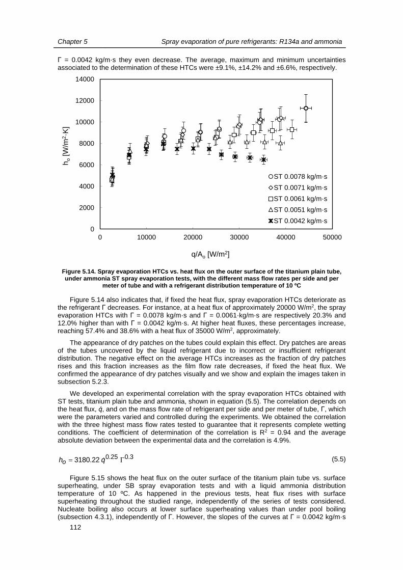
Chapter 5 Spray evaporation of pure refrigerants: R134a and ammonia

112

Γ = 0.0042 kg/m·s they even decrease. The average, maximum and minimum uncertainties associated to the determination of these HTCs were ±9.1%, ±14.2% and ±6.6%, respectively.

Figure 5.14. Spray evaporation HTCs vs. heat flux on the outer surface of the titanium plain tube, under ammonia ST spray evaporation tests, with the different mass flow rates per side and per

meter of tube and with a refrigerant distribution temperature of 10 ºC

Figure 5.14 also indicates that, if fixed the heat flux, spray evaporation HTCs deteriorate as the refrigerant Γ decreases. For instance, at a heat flux of approximately 20000 W/m2, the spray evaporation HTCs with Γ = 0.0078 kg/m·s and Γ = 0.0061·kg/m·s are respectively 20.3% and 12.0% higher than with Γ = 0.0042 kg/m·s. At higher heat fluxes, these percentages increase, reaching 57.4% and 38.6% with a heat flux of 35000 W/m2, approximately.

The appearance of dry patches on the tubes could explain this effect. Dry patches are areas of the tubes uncovered by the liquid refrigerant due to incorrect or insufficient refrigerant distribution. The negative effect on the average HTCs increases as the fraction of dry patches rises and this fraction increases as the film flow rate decreases, if fixed the heat flux. We confirmed the appearance of dry patches visually and we show and explain the images taken in subsection 5.2.3.

We developed an experimental correlation with the spray evaporation HTCs obtained with ST tests, titanium plain tube and ammonia, shown in equation (5.5). The correlation depends on the heat flux, q, and on the mass flow rate of refrigerant per side and per meter of tube, Γ, which were the parameters varied and controlled during the experiments. We obtained the correlation with the three highest mass flow rates tested to guarantee that it represents complete wetting conditions. The coefficient of determination of the correlation is R2 = 0.94 and the average absolute deviation between the experimental data and the correlation is 4.9%.

3.025.022.3180 qho (5.5)

Figure 5.15 shows the heat flux on the outer surface of the titanium plain tube vs. surface superheating, under SB spray evaporation tests and with a liquid ammonia distribution temperature of 10 ºC. As happened in the previous tests, heat flux rises with surface superheating throughout the studied range, independently of the series of tests considered. Nucleate boiling also occurs at lower surface superheating values than under pool boiling (subsection 4.3.1), independently of Γ. However, the slopes of the curves at Γ = 0.0042 kg/m·s

0

2000

4000

6000

8000

10000

12000

14000

0 10000 20000 30000 40000 50000

ho

[W/m

2·K

]

q/Ao [W/m2]

ST 0.0078 kg/m·s

ST 0.0071 kg/m·s

ST 0.0061 kg/m·s

ST 0.0051 kg/m·s

ST 0.0042 kg/m·s

Chapter 5 Spray evaporation of pure refrigerants: R134a and ammonia

113

and Γ = 0.0051 kg/m·s are clearly lower than with the other three mass flow rates and this effect is again caused by the appearance of dry patches on the tested tube.

Figure 5.15. Heat flux on the outer surface of the titanium plain tube vs. surface superheating, under ammonia SB spray evaporation tests, with the different mass flow rates per side and per

meter of tube and with a refrigerant distribution temperature of 10 ºC

The spray evaporation HTCs obtained with SB spray evaporation experiments vs. the heat flux on outer surface of the titanium tube, with ammonia as refrigerant and the different mass flow rates distributed appear in Figure 5.16. Γ determines the dependence between heat fluxes and spray evaporation HTCs. When Γ = 0.0042 kg/m·s, the HTCs increase with heat flux only up to 5900 W/m2 and then decrease sharply and remain constant. The same happens when Γ = 0.0051 kg/m·s, but the change of trend occurs at higher heat flux (15600 W/m2). With the remaining mass flow rates, the increasing tendency lasts up to heat fluxes over 20000 W/m2 and then spray evaporation HTCs remain constant The average, maximum and minimum uncertainties associated to the determination of these HTCs were ±6.8%, ±13.1% and ±3.8%, respectively.

As happened with ST tests, Figure 5.16 indicates that, if fixed the heat flux, spray evaporation HTCs deteriorate as the refrigerant Γ decreases. For instance, at a heat flux of approximately 20000 W/m2, the spray evaporation HTCs with Γ = 7.8·10-3 kg/m·s and Γ = 6.1·10-3 kg/m·s are respectively 92.4% and 73.9% higher than with Γ = 4.2·10-3 kg/m·s. With an approximate heat flux of 30000 W/m2, these percentages reach 72.4% and 66.6%. Dry patches seem to be the reason of the HTC deterioration, but the process could not be recorded under SB tests due to the limitations of the viewing sections.

0

5000

10000

15000

20000

25000

30000

35000

40000

45000

50000

0 1 2 3 4 5 6 7 8

q/A

o[W

/m2]

ΔTSH [K]

SB 0.0078 kg/m·s

SB 0.0071 kg/m·s

SB 0.0061 kg/m·s

SB 0.0051 kg/m·s

SB 0.0042 kg/m·s

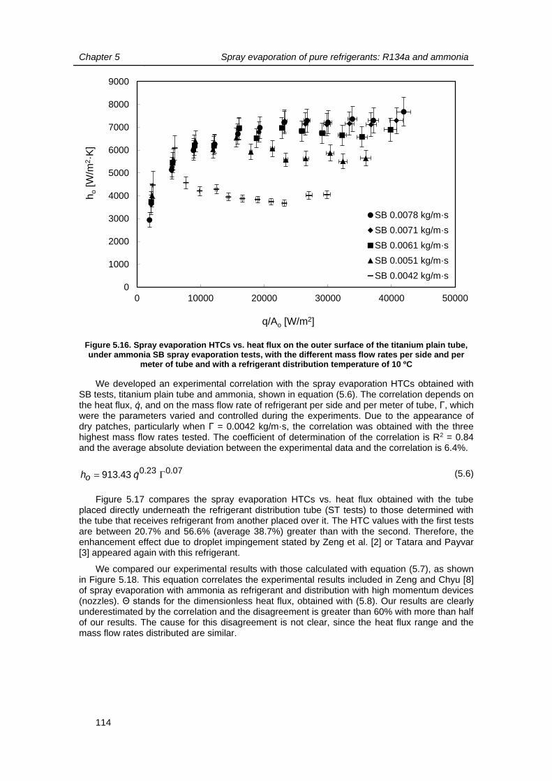
Chapter 5 Spray evaporation of pure refrigerants: R134a and ammonia

114

Figure 5.16. Spray evaporation HTCs vs. heat flux on the outer surface of the titanium plain tube, under ammonia SB spray evaporation tests, with the different mass flow rates per side and per

meter of tube and with a refrigerant distribution temperature of 10 ºC

We developed an experimental correlation with the spray evaporation HTCs obtained with SB tests, titanium plain tube and ammonia, shown in equation (5.6). The correlation depends on the heat flux, q, and on the mass flow rate of refrigerant per side and per meter of tube, Γ, which were the parameters varied and controlled during the experiments. Due to the appearance of dry patches, particularly when Γ = 0.0042 kg/m·s, the correlation was obtained with the three highest mass flow rates tested. The coefficient of determination of the correlation is R2 = 0.84 and the average absolute deviation between the experimental data and the correlation is 6.4%.

07.023.043.913 qho (5.6)

Figure 5.17 compares the spray evaporation HTCs vs. heat flux obtained with the tube placed directly underneath the refrigerant distribution tube (ST tests) to those determined with the tube that receives refrigerant from another placed over it. The HTC values with the first tests are between 20.7% and 56.6% (average 38.7%) greater than with the second. Therefore, the enhancement effect due to droplet impingement stated by Zeng et al. [2] or Tatara and Payvar [3] appeared again with this refrigerant.

We compared our experimental results with those calculated with equation (5.7), as shown in Figure 5.18. This equation correlates the experimental results included in Zeng and Chyu [8] of spray evaporation with ammonia as refrigerant and distribution with high momentum devices (nozzles). Θ stands for the dimensionless heat flux, obtained with (5.8). Our results are clearly underestimated by the correlation and the disagreement is greater than 60% with more than half of our results. The cause for this disagreement is not clear, since the heat flux range and the mass flow rates distributed are similar.

0

1000

2000

3000

4000

5000

6000

7000

8000

9000

0 10000 20000 30000 40000 50000

ho

[W/m

2·K

]

q/Ao [W/m2]

SB 0.0078 kg/m·s

SB 0.0071 kg/m·s

SB 0.0061 kg/m·s

SB 0.0051 kg/m·s

SB 0.0042 kg/m·s

Chapter 5 Spray evaporation of pure refrigerants: R134a and ammonia

115

Figure 5.17. Spray evaporation HTCs vs. heat flux on the outer surface of the titanium plain tube, under ammonia ST and SB spray evaporation tests, with the different mass flow rates per side and

per meter of tube and with a refrigerant distribution temperature of 10 ºC

753.0385.0278.00.039f

PrRe0518.0Nu red

p

(5.7)

kTTdq sct (5.8)

5.2.2. Spray enhancement factors

Figure 5.19 illustrates the spray enhancement factor of ammonia and plain titanium tube vs. heat flux, with ST experiments and as a function of the mass flow rate of refrigerant per side and meter of tube. Spray evaporation enhances heat transfer if compared to pool boiling under every condition tested. This statement is particularly true in the low heat flux range (up to 20000 W/m2). The maximum spray enhancement factor is 6.2 (0.0042 kg/m·s and 2600 W/m2) and the minimum 1.1 (0.0042 kg/m·s and 35200 W/m2).

Similarly, Figure 5.20 includes the spray enhancement factor of ammonia and plain titanium tube vs. heat flux, with SB experiments and as a function of the mass flow rate of refrigerant per side and meter of tube. In this case there are some conditions, particularly with Γ = 0.0042 kg/m·s and Γ = 0.0051 kg/m·s, at which pool boiling outperforms spray evaporation, i.e. the spray enhancement factor is lower than 1. The maximum and minimum enhancement factors obtained under these conditions are 5.6 (0.0042 kg/m·s and 2500 W/m2) and 0.8 (0.0042 kg/m·s and 29800 W/m2), respectively.

Our experimental results concerning spray enhancement are in agreement with Zeng and Chyu [8], who observed that spray evaporation HTCs in a tube bundle can be up to a 50% greater than under pool boiling.

0

2000

4000

6000

8000

10000

12000

14000

0 10000 20000 30000 40000 50000

ho

[W/m

2·K

]

q/Ao [W/m2]

ST 0.0078 kg/m·s

ST 0.0061 kg/m·s

ST 0.0042 kg/m·s

SB 0.0078 kg/m·s

SB 0.0061 kg/m·s

SB 0.0042 kg/m·s

Chapter 5 Spray evaporation of pure refrigerants: R134a and ammonia

116

Figure 5.18. Spray evaporation HTCs obtained with the correlation of Zeng and Chyu [8] vs. our experimental spray evaporation HTCs with ammonia and a titanium plain tube

Figure 5.19. Spray enhancement factors vs. heat flux on the outer surface of the titanium plain tube, under ammonia ST spray evaporation tests, with the different mass flow rates per side and

per meter of tube and with a refrigerant distribution temperature of 10 ºC

-60%

0

2000

4000

6000

8000

10000

12000

0 2000 4000 6000 8000 10000 12000

hcorr

[W/m

2·K

]

hexp [W/m2·K]

0

1

2

3

4

5

6

7

0 10000 20000 30000 40000 50000

EF

sp,Γ

[-]

q/Ao [W/m2]

ST 0.0078 kg/m·s

ST 0.0071 kg/m·s

ST 0.0061 kg/m·s

ST 0.0051 kg/m·s

ST 0.0042 kg/m·s

Chapter 5 Spray evaporation of pure refrigerants: R134a and ammonia

117

Figure 5.20. Spray enhancement factors vs. heat flux on the outer surface of the titanium plain tube, under ammonia SB spray evaporation tests, with the different mass flow rates per side and

per meter of tube and with a refrigerant distribution temperature of 10 ºC

5.2.3. Photographic report

Figure 5.21 includes pictures of the flow mode that occurs when distributing ammonia on the titanium plain tube as a function of the mass flow rate of refrigerant distributed, at a saturation temperature of 10 ºC and under adiabatic conditions (no heat flux). As the mass flow rate distributed increases from 0.0042 kg/m·s (Figure 5.21a) to 0.0061 kg/m·s (Figure 5.21b) the distance between active dripping sites decreases from 35.8 mm to 25.4 mm, approximately, and the shape of the falling liquid is in between columns and drops. Liquid columns become more clear in Figure 5.21c, taken with Γ = 0.0078 kg/m·s, but the distance between the columns increased slightly (26.5 mm). However, in between the columns of this last situation, active dripping sites are present.

The determination of the distance between active sites from the pictures was very complicated since the active sites move longitudinally due to the characteristics and direction of the flow caused by the nozzles. Taking into account this, we compared them with the distances calculated using equation (5.4), developed by Yung et al. [6] and based on the Taylor instability theory. According to the authors of that work, ammonia films are considered thin films and, therefore, n = 2. The values obtained with this equation are 19.5 mm, and therefore in the same order of magnitude than the ones we obtained, particularly with the highest mass flow rates.

In Figure 5.22, we also focused on the falling film flow mode keeping fixed the mass flow rate of refrigerant at 0.0051 kg/m·s and varying the heat flux. An increase in the heat flux leads to slight differences in the distance between active sites, but the dripping rate decreases. Figure 5.23 shows an analogous study, but developed with a mass flow rate of refrigerant at 0.0071 kg/m·s. In this case, the increase of heat flux has a negligible effect on both the dripping rate and the distance between active sites. To explain this different behaviour we focus on the overfeed factor, OF, defined in subsection 3.3.3 as the ratio of mass flow rate reaching the top of the tube to the mass flow rate that vaporises. OF is much lower with 0.0051 kg/m·s, and therefore there is less liquid refrigerant left after boiling to drip from the tube.

0

1

2

3

4

5

6

0 5000 10000 15000 20000 25000 30000 35000 40000 45000

EF

sp,Γ

[-]

q/Ao [W/m2]

SB 0.0078 kg/m·s

SB 0.0071 kg/m·s

SB 0.0061 kg/m·s

SB 0.0051 kg/m·s

SB 0.0042 kg/m·s

Chapter 5 Spray evaporation of pure refrigerants: R134a and ammonia

118

Figure 5.21. Dripping active sites with ammonia and the titanium plain tube as a function of the mass flow rate per side and per meter of tube, Γ, under adiabatic conditions. a) Γ = 0.0042 kg/m·s.

b) Γ = 0.0061 kg/m·s. c) Γ = 0.0078 kg/m·s

Figure 5.22. Dripping active sites with ammonia and the titanium plain tube as a function of heat flux, q, with mass flow rate per side and per meter of tube, Γ = 0.0051 kg/m·s. a) q = 10000 W/m2.

b) q = 24800 W/m2. c) q = 38800 W/m2

a b

c

a b

c

Chapter 5 Spray evaporation of pure refrigerants: R134a and ammonia

119

Figure 5.23. Dripping active sites with ammonia and the titanium plain tube as a function of heat flux, q with mass flow rate per side and per meter of tube, Γ = 0.0071 kg/m·s. a) q = 10200 W/m2.

b) q = 25600 W/m2. c) q = 44400 W/m2

We expected the existence of dry patches on the tube due to the HTCs we obtained. We confirmed them visually. Figure 5.24 includes four photographs taken at our experimental facility to illustrate dryout. With Γ = 4.2·10-3 kg/m·s and no heat flux on the surface (Figure 5.24a) the film is unperturbed. In contrast, dry patches appeared with the same film flow rate and a heat flux on the surface of 35200 W m-2 (Figure 5.24b). Figure 5.24c and Figure 5.24d represent analogous situations with Γ = 7.1·10-3 kg/m·s, but dry areas do not occur at this film flow rate.

Figure 5.24. Dry patches on the titanium plain tube with ammonia. a) Γ = 0.0042 kg/m·s and q = 0 W/m2. b) Γ = 0.0042 kg/m·s and q = 35200 W/m2. c) Γ = 0.0071 kg/m·s and q = 0 W/m2.

c) Γ = 0.0071 kg/m·s and q = 44400 W/m2

We employed the correlation from Ribatski and Thome [7], equation (5.4), to determine the maximum Reynolds number at which dryout occurred in their tests. We considered the conditions of heat flux from the pictures shown in Figure 5.24. With q = 35200 W/m2 (Figure 5.24b), the dryout onset Reynolds number is 236, which is clearly greater than the one we

a b

c

a a b

d c

Chapter 5 Spray evaporation of pure refrigerants: R134a and ammonia

120

determined from our experimental measurements, 110.3. Therefore, the existence of dryout is in agreement with their correlation. With q = 44400 W/m2 (Figure 5.24d), the dryout onset Reynolds number from the correlation is 263, again higher than that we obtained, 183. However, in this case we did not observe or confirm dryout in our experiments.

Finally, we also checked visually that in our experiments nucleate boiling occurred. In the pictures taken of the pool boiling processes (subsections 4.3.4 and 4.4.4) bubbles can be easily visualised in the liquid that surrounds the tube. In contrast, the thin film around the tubes under spray evaporation makes difficult viewing nucleate boiling. However, we detected bubbles in the drops that fell from the tube, as can be seen in all the pictures from Figure 5.25.

Figure 5.25. Nucleate boiling and bubbles entrained by drops on the titanium plain tube with ammonia. a) Γ = 0.0051 kg/m·s and q = 31700 W/m2. b) Γ = 0.0061 kg/m·s and q = 33000 W/m2.

c) Γ = 0.0071 kg/m·s and q = 34600 W/m2. c) Γ = 0.0078 kg/m·s and q = 44300 W/m2

a b

c d

Chapter 5 Spray evaporation of pure refrigerants: R134a and ammonia

121

5.3. CONCLUSIONS

In this chapter we have shown the spray evaporation HTCs obtained experimentally for this thesis. The refrigerants studied were R134a and ammonia. With the former we tested copper tubes of plain external surface and with the latter titanium tubes of plain external surface.

We have observed that the vast majority of our experimental results were included in the boiling region of the boiling curve, where the slope is steep and heat flux increases rapidly with superheating. However, the slope is slightly slower in some cases, pointing out the existence of dry patches.

Concerning the spray evaporation HTCs with R134a and the copper tube, we have observed that they generally increase if the heat flux is higher, independently of the mass flow rate of the film per side and meter of tube. We have also observed that the effect of the mass flow rate on the HTCs is negligible.

The spray evaporation heat transfer coefficients obtained with R134a and the tube placed directly underneath the refrigerant distribution tube (ST tests) are, on average, 13.2% greater than those determined with the tube that receives refrigerant from the conditioning tube (SB tests), if kept the heat flux and distributed mass flow rate constant. The heat transfer enhancement occurs due to the liquid droplet impingement effect.

We compared spray evaporation and pool boiling, with R134a, under similar conditions. We have observed that spray evaporation enhances heat transfer only if the heat flux is low (lower than 20000 W/m2) and this enhancement has never been higher than 60%. These results concerning enhancement are in line with what Roques [4] or Moeykens [5] stated.

An analysis of the photographs taken during the experiments allowed confirming the existence of dry patches on the tubes and explained the heat transfer deterioration found. Dryout occurred even when the distributed refrigerant was significantly greater than the amount of refrigerant that vaporised on the tube (overfeed rates well over 1).

Concerning the spray evaporation HTCs with ammonia and the titanium tube, we have observed that they depend on both the heat flux and the mass flow rate of refrigerant per side and meter of tube. Generally, they increase as the heat flux increases, but this trend was even opposite under conditions of high heat flux and low mass flow rate.

We observed that the spray evaporation heat transfer coefficients obtained with ammonia and the tube placed directly underneath the refrigerant distribution tube (ST tests) are, on average, 38.7% higher than those determined with the tube that receives refrigerant from the conditioning tube (SB tests). Droplet impingement effect is responsible of this effect.

From the comparison of spray evaporation and pool boiling of ammonia on the plain tube, we have concluded that spray evaporation enhances importantly heat transfer. Spray enhancement factors are well over 1, particularly when the refrigerant on the tested tube arrives directly from the nozzles (ST tests). The maximum enhancement factor was over 6 and the best results occurred in the low heat flux range (up to 20000 W/m2). Zeng and Chyu [8] stated as well that spray evaporation with ammonia enhances heat transfer, even though in lower magnitude than what we observed. Our results are underpredicted by their experimental correlation.

We have analysed the snapshots taken when conducting the tests and the most important conclusion is that dry patches occurred under certain conditions. Dryout explains some of the tendencies we obtained from our experimental results.

Chapter 5 Spray evaporation of pure refrigerants: R134a and ammonia

122

REFERENCES

[1] Á.Á. Pardiñas, J. Fernández-Seara, R. Diz, Experimental study on heat transfer coefficients of spray evaporation and pool boiling on plain tubes, in: Proceedings of the 24th IIR International Congress of Refrigeration, Yokohama, Japan, 2015.

[2] X. Zeng, M. Chyu, Z.H. Ayub, Experimental investigation on ammonia spray evaporator with triangular-pitch plain-tube bundle, Part I: Tube bundle effect, International Journal of Heat and Mass Transfer. 44 (2001) 2299-2310.

[3] R. Tatara, P. Payvar, Measurement of spray boiling refrigerant coefficients in an integral-fin tube bundle segment simulating a full bundle, International Journal of Refrigeration. 24 (2001) 744-754.

[4] J.F. Roques, Falling film evaporation on a single tube and on a tube bundle, Ph.D. thesis, École Polytechnique Fédérale de Lausanne, Switzerland, 2004.

[5] S.A. Moeykens, Heat transfer and fluid flow in spray evaporators with application to reducing refrigerant inventory, Iowa State University of Science and Technology, Iowa, USA, 1994.

[6] D. Yung, E.N. Ganic, J.J. Lorenz, Vapor/liquid interaction and entrainment in falling film evaporators, Journal of Heat Transfer. 102 (1980) 20-25.

[7] G. Ribatski, J.R. Thome, Experimental study on the onset of local dryout in an evaporating falling film on horizontal plain tubes, Experimental Thermal and Fluid Science. 31 (2007) 483-493.

[8] X. Zeng, M. Chyu, Heat transfer and fluid flow study of ammonia spray evaporators, Texas Tech University, Lubbock, Texas, USA, 1995.

123

Chapter 6

Optimisation of the nozzle distribution system in shell-

and-tube evaporators In this chapter we focus on the distribution of liquid on spray (falling film) shell-and-tube

evaporators. It starts with an analysis of different systems, proposed mainly in patents, to distribute refrigerant on the tube bundles. This analysis suggests that most of the existing systems are based on low momentum techniques. As a result, we study the layout to optimize refrigerant distribution with nozzles (high momentum devices). The optimization study is based on geometry and trigonometry and completes and delves into previous research found in the specialized literature on this topic.

The study starts with the definition of the spray cone formed by full cone nozzles and of the area of a general tube from the bundle reached by the nozzle. It continues calculating the optimal position of the nozzles for a particular tube bundle and how this optimal position must be adapted as a function of the actual length of the tube bundle.

To continue, in this chapter we present the computer programme developed to apply the previously described model to real tube bundles. We also include a parametric analysis to show how the different distribution indicators are affected by parameters such as the tube bundle pattern, the distance between tubes, the nozzle cone angle or the number of nozzle systems.

Chapter 6 Optimisation of the nozzle distribution system in shell-and-tube evaporators

124

6.1. INTRODUCTION

The distribution of refrigerant on the tube bundle of an evaporator is a key factor for its correct performance, since the appearance of dry zones on the tubes may cause an important deterioration of heat transfer. In the scientific literature, different distribution methods have been proposed and studied, and they can be classified into low momentum and high momentum.

As explained in section 1.8.5, several low momentum solutions distribute liquid by the effect of gravity; i.e. it falls from the device to the surface (tube) placed directly beneath. This means that the distribution system must be placed over each and every column of the tube bundle, properly aligned, in order to assure the liquid feed. In contrast, high momentum solutions (spray nozzles) distribute the liquid with a much higher velocity. These systems have been seen to improve heat transfer and wetting of tubes, and they seem more appropriate for industrial equipment, since alignment is not a critical issue and a same nozzle may distribute liquid to more than one column of tubes inside the bundle. However, a part of this liquid may leave the bundle and it is difficult to quantify which fraction of the flow rate reaches each tube.

Independently of the kind of method used, there has been great effort to optimise the distribution systems for shell-and-tube evaporators, as shows the large list of patents available on the topic. One of the first approaches we have found is that from Hartfield and Sanborn [1], in the United States Patent number US 5,561,987. The authors claimed a distribution system which can be classified into the low momentum group and that includes also a liquid-vapour separator (Figure 6.1). In the patent, they state several possible configurations for the distribution device itself, which go from a tree of tubes with orifices to wavy-shaped plates that should increase the size of the droplets that reach the evaporator tubes.

Figure 6.1. Combined liquid distribution system and liquid-vapour separator from reference [1]

The previous work describes the necessity of immersing the last rows of tubes of the evaporator tube bundle in liquid refrigerant, since film breakdown is more likely to occur on them. This idea is further described in patent US 5,839,294, where Chiang et al. [2] claim the invention of a system combining pool boiling and spray evaporation. According to the authors, the liquid is distributed by the spray dispensers due to the refrigerant flow loop differential pressure. In addition, the system leads to a refrigerant charge reduction without any pump or similar system for recirculation. However, oil recovery from the evaporator seems an important issue of this loop which was not considered or mentioned by the authors.

Gupte [3] presents the main distribution challenges to be faced as a function of the pattern of the tube bundle. Staggered tube bundles, which are very typically used in shell-and-tube heat exchangers to reduce their size, have a very high pressure drop of the refrigerant vapour, which explains that inline tube bundles appear as an option. In addition, the liquid flow rate distributed in staggered tube patterns spreads out among more tubes than with inline tube bundles, which means that dry patches are more likely to appear in the first case. However, according to Gupta,

Chapter 6 Optimisation of the nozzle distribution system in shell-and-tube evaporators

125

inline tube bundles have also more complex distribution systems and part of the refrigerant may leave the bundle without reaching any tube. In this patent, the author suggests an inline pattern distribution system to direct the refrigerant from the nozzles.

Liu and Liu [4] claimed in the United States patent US 2008/0149311 A1 that a main issue concerning spray evaporators is to maximize the number of tubes dedicated to heat transfer in the shell. To do so they propose several layouts of the tubes all over the shell and, in between the tubes, distribution units (plates) of different shapes with holes or slots. Liu et al. [5] suggest an extended distributor system to improve wetting. To finish with this kind of low dripping distributors, Christians et al. [6] propose a different configuration (Figure 6.2) that includes channels aligned with each and every tube column. The authors also state that, in order to homogenise distribution, these channels could be filled with a porous media. Vapour slots are also present in the system to evacuate the vapour fraction that comes with the liquid refrigerant.

Figure 6.2. Distribution system proposed in patent US 2014/0366574 A1 [6]

As seen up to this moment, the main distribution devices on the aforementioned works were of low momentum type. However, there is an important innovative work concerning nozzles for refrigerant distribution in tube bundles, as seen in reference [7]. Chang and Yu show the possibility of introducing tubes with nozzles machined in their wall throughout the tube bundle. In this way, if the nozzles are properly positioned, dry patches are more likely to be prevented. In addition, liquid impingement, which has been seen to have a positive effect on heat transfer, occurs all over the tube bundle and not only on the uppermost row of tubes. The main disadvantage of this system lies in the fact that one of each 4 positions of the tube bundle where a heat transfer tube should be, is occupied by a nozzle tube.

The control of the vapour flow is another important issue concerning refrigerant distribution, as reviewed in section 1.4.3. In the United States patent US 6,293,112 B1, Moeykens et al. [8] suggest different tube bundle layouts to form vapour channels that should allow vapour drainage from it. De Larminat et al. [9] propose an alternative to solve this problem, which consists in covering the distribution system and tube bundle with a hood. Thus, cross flow should be prevented. The authors also claim that this hood should minimize the amount of liquid droplets entrained that reach the suction line.

Chapter 6 Optimisation of the nozzle distribution system in shell-and-tube evaporators

126

6.2. AIM OF THE STUDY AND PREVIOUS CONSIDERATIONS

From the analysis shown in the previous subsection we concluded that there is a general trend of focusing on low momentum distribution techniques. These techniques lead to very complicated structures and layouts of the shell, where groups of tube bundles and distributors are placed. From our point of view, the reason why nozzles are underused is due to the challenge of positioning them to achieve a homogeneous and complete distribution, minimising the liquid that leaves the tube bundle without reaching any of its tubes. This challenge motivated the study presented in this section, which main aim was to optimise the nozzle system or systems needed for a certain tube bundle. To satisfy this we developed a mathematical model based on the geometry of the spray cones that result from using nozzles when distributing refrigerant.

When designing the refrigerant distribution system with spray nozzles, a designer should take into account several considerations. The system should cover all the available surface of the tube bundle seen from above. Moreover, the distribution has to be homogeneous, i.e., each column of tubes of the tube bundle should receive a similar fraction of the whole flow rate distributed. Thus, dry patches may be prevented by distributing the proper amount of liquid without involving high overfeed on other columns and high recirculation rates of excess liquid. Furthermore, the fraction of the flow rate that reaches an area where two or more adjacent nozzles distribute refrigerant (overlapping) or where there are no tubes (fluid lost) should be minimum. Further issues to take into consideration could be minimising the number of nozzles systems (groups of nozzles placed at the same plane), minimising the total number of nozzles used, etc.

Taking into account these considerations, the selection of the type of nozzle to be used is crucial. According to the Engineer’s guide to spray technology [10], there are plenty of different nozzle types available in the market, which can be mainly classified into hollow cone nozzles and full cones nozzles. This classification attends to the spray pattern produced by the nozzle. Hollow cone nozzles produce an annulus of liquid; i.e. part of the area right beneath this type of nozzles receives no liquid at all. On the other hand, full cone nozzles distribute liquid forming a spray that fills the area covered completely and homogeneously. Thus, the characteristics of this last option makes it appropriate for this application.

Full cone nozzles produce sprays with different shapes depending on the manufacturer, but the most common ones are round cone nozzles and square cone nozzles. Round cone nozzles distribute liquid with axial symmetry, describing circles in every plain normal to the longitudinal nozzle axis. This kind of symmetry leads to two of the main characteristics of round cone nozzles. The first is that no specific alignment is needed in order to feed a certain area, which is very convenient from the point of view of industrial processes or heat exchangers. The second one concerns the necessity of overlapping a fraction of the liquid distributed by two or more nozzles in order to feed an area (tube bundle). In addition, another part of the flow rate leaves the bundle due to the same reason.

In contrast, square cone nozzles produce cones without axial symmetry, describing squares instead of circles in every plain perpendicular to the nozzle axis. Therefore, the shape of the cone at the fed zone depends on the positioning angle of the nozzle and these nozzles require a certain alignment process to work in the expected manner. However, the main advantage of square over round nozzles is also associated with their non-axial symmetry. If the system is properly designed, no overlapping is needed in order to feed a certain bundle, which means that the flow rate arriving to the bundle is more uniform. Moreover, the shape of the spray adapts better to tube bundles and the flow rate that leaves the bundle is minimised.

In the following chapters, round and square full cone nozzles and the sprays produced by them will be further studied.

Chapter 6 Optimisation of the nozzle distribution system in shell-and-tube evaporators

127

6.3. GEOMETRIC CALCULATIONS

6.3.1. Characterisation of the spray produced by a full cone nozzle

The first issue that must be defined in order to characterise geometrically a spray is the determination of the origin of the spray, O, which should correspond to the place of spray where the size of the cone is 0. If we analyse the size of the spray (diameter in case of a circular nozzle) at the tip of the nozzle it is not equal to 0 and technically cannot be considered as origin. According to references [10,11], the origin of the cone, for calculation considerations, is placed at the orifice or outlet of the nozzle, which is a few millimetres upstream from the tip. However, for the sake of simplicity in the representation of the different cases, the origin (O in Figure 6.3) appears at the tip of the nozzle and is considered at a generic position (xO,yO,0).

Figure 6.3. Representation of the spray cone produced by a spray nozzle and coordinate systems used throughout the study

The interest in defining geometrically a spray is to determine whether a point of the space receives liquid from a nozzle or not. This definition will be later applied to tube bundles in heat exchangers and to determine the flow rate distributed to each tube or portion of tube. In order to define the geometry of a spray full cone, we considered the following assumptions:

The spray flow distributed by a nozzle is treated as a whole, and not as individual drops

or jets of liquid.

Homogeneous distribution of the fluid throughout the cone; i.e. if chosen a portion of the

total surface covered by a spray, the flow rate impinging on that surface is the result of

multiplying the total spray flow rate by the ratio of the chosen surface to the total surface

covered by the cone.

The spray from a nozzle is straight at the sides, unaffected by gravity in the range of

distances studied.

The shape of the cones is a perfect circle/square.

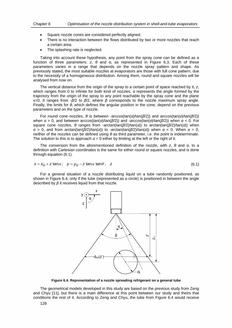
Chapter 6 Optimisation of the nozzle distribution system in shell-and-tube evaporators

128

Square nozzle cones are considered perfectly aligned.

There is no interaction between the flows distributed by two or more nozzles that reach

a certain area.

The splashing rate is neglected.

Taking into account these hypothesis, any point from the spray cone can be defined as a function of three parameters: z, θ and α, as represented in Figure 6.3. Each of these parameters varies in a range that depends on the nozzle spray pattern and shape. As previously stated, the most suitable nozzles at evaporators are those with full cone pattern, due to the necessity of a homogeneous distribution. Among them, round and square nozzles will be analysed from now on.

The vertical distance from the origin of the spray to a certain point of space reached by it, z, which ranges from 0 to infinite for both kind of nozzles. α represents the angle formed by the trajectory from the origin of the spray to any point reachable by the spray cone and the plane x=0. It ranges from -β/2 to β/2, where β corresponds to the nozzle maximum spray angle. Finally, the limits for θ, which defines the angular position in the cone, depend on the previous parameters and on the type of nozzle.

For round cone nozzles, θ is between -arccos(tan(α)/tan(β/2)) and arccos(tan(α)/tan(β/2)) when α > 0, and between arccos(tan(α)/tan(β/2)) and -arccos(tan(α)/tan(β/2)) when α < 0. For square cone nozzles, θ ranges from -arctan(tan(β/2)/tan(α)) to arctan(tan(β/2)/tan(α)) when α > 0, and from arctan(tan(β/2)/tan(α)) to -arctan(tan(β/2)/tan(α)) when α < 0. When α = 0, neither of the nozzles can be defined using θ as third parameter, i.e. the point is indeterminate. The solution to this is to approach α = 0 either by limiting at the left or the right of it.

The conversion from the aforementioned definition of the nozzle, with z, θ and α, to a definition with Cartesian coordinates is the same for either round or square nozzles, and is done through equation (6.1).

zzyyzxx oo ;tantan;tan (6.1)

For a general situation of a nozzle distributing liquid on a tube randomly positioned, as shown in Figure 6.4, only if the tube (represented as a circle) is positioned in between the angle described by β it receives liquid from that nozzle.

Figure 6.4. Representation of a nozzle spreading refrigerant on a general tube

The geometrical models developed in this study are based on the previous study from Zeng and Chyu [11], but there is a main difference at this point between our study and theirs that conditions the rest of it. According to Zeng and Chyu, the tube from Figure 6.4 would receive

Chapter 6 Optimisation of the nozzle distribution system in shell-and-tube evaporators

129

liquid from the nozzle on all its upper surface. From our point of view, that would only be true if the distance between the tube and origin of the spray, z1, were infinite. Our statement lies in the fact that any part of the spray cone that is out of the angle formed by the tangents from the spray origin to the tube is lost for that tube. In Figure 6.4 we represent one of those tangents, which “touches” the tube at a distance z’ from the nozzle. At that distance, the “diameter” of the spray cone is calculated with equation (6.2). The “diameter” represents a real diameter in the case of circular full cone nozzles and the side of the square in case of square full cone nozzles.

2tan'2' zzdsp (6.2)

6.3.2. Optimal position of adjacent nozzles and 1 nozzle system

As stated in section 6.2, due to the axial symmetry of round full cone nozzles, they need to be positioned in a certain manner that leads to the full coverage of the heat transfer tube or tube bundle, minimising the flow that is not useful (lost out of the tube bundle or overlapped with an adjacent nozzle. This issue does not occur with square full cone nozzles, and that is the reason why we will first focus on the former.

In Figure 6.5 we represent a generic tube bundle, projected on a plane normal to the nozzle axis at a distance z’ from the origin of the sprays. z’ coincides with the distance in the z axis between the origin of spray and the points of tangency of the external tubes of the uppermost row of the tube bundle. If there is only one nozzle system (row of nozzles), it could happen that the distance between adjacent nozzles (distnozzle in Figure 6.5) leads to a small area of bundle fed by two nozzles, but also leads to uncovered or unreached areas (Auncovered in Figure 6.5a). Thus, we do not fulfil the consideration stated in section 6.2 concerning the need of covering all the reachable area of the bundle.

Figure 6.5. Position between adjacent nozzles. a) Distance greater than the optimal. b) Distance lower than the optimal

The opposite situation is shown in Figure 6.5b, where the distance between adjacent nozzles leads to spray cones that fully cover the first row of the tube bundle, but with a high fraction of overlapping between them (Auseless,2).

dsp(z )

dis

t nozzle

dis

t nozzle

wbdl

Auncovered

dsp(z )

dis

t nozzle

dis

t nozzle

wbdl

Auseless,1

Auseless,2

Auseful

a b

Chapter 6 Optimisation of the nozzle distribution system in shell-and-tube evaporators

130

There should be an optimal distance at which all the considerations are fulfilled. This optimal situation is graphically shown in Figure 6.6, where adjacent nozzles intersect exactly at the limit of the tube bundle, defined by the tangencies of the tubes placed at the edges of the uppermost row of the bundle. The area of each spray nozzle that is neither lost nor overlapped (Auseful) has a square shape. This last statement will be mathematically verified in the following paragraphs.

Figure 6.6. Optimal distance between adjacent nozzles

The objective of the nozzle system is to cover the first row of the tube bundle minimising the “useless” area. This could be mathematically expressed with the ratio of useless area, RAuseless, as shown in equation (6.3). Auseful can be obtained with equation (6.4), where wbdl(z’) stands for the width of the tube bundle at a plane normal to the spray nozzle axis at z’ from the spray cone origin. Asp(z’) is the area covered by the spray produced by one nozzle at the same plane, calculated with equation (6.5).

''

1'

''

'

'

zA

zA

zA

zAzA

zA

zARA

sp

useful

sp

usefulsp

sp

uselessuseless

(6.3)

nozzlebdluseful distzwzA '' (6.4)

22'' zdzA spsp

(6.5)

If we consider that the tangent from the origin of the spray to the external tubes of the first row forms an angle α with the plane that contains the spray nozzle row, x = 0, equation (6.6) is true. In addition, there is a right-angled triangle formed by wbdl(z’)/2, distnozzle/2 and dsp(z’)/2. Thus, equation (6.3) can be rearranged, resulting in equation (6.7).

dsp(z )

dis

t nozzle

dis

t nozzle

wbdl

Auseful

Auseless,1

Auseless,2

Chapter 6 Optimisation of the nozzle distribution system in shell-and-tube evaporators

131

tan2

'

2tan2

''

zwzdz bdlsp

(6.6)

222

tan2tantan2tan

41 uselessRA

(6.7)

The ratio of useless area depends on α, and therefore we derived equation (6.7) and equal it to 0 to calculate the possible minimum. We evaluated the second derivative with this possible minimum and verified that in the range where α occurs, (-β/2, β/2). The second derivative in that range is always positive. The value of α that minimises the ratio is shown in equation (6.8). With this equation and the previous ones we prove that the optimal distnozzle is equal to wbdl(z’) and can be calculated by (6.9). nt,1 stands for the number of tubes of the first of the first row of the tube bundle; distt,r stands for the distance in the x axis between the centres of consecutive tubes of the same row of the tube bundle; and dt stands for the outer diameter of the tubes.

2

2tan2tan

(6.8)

sin1' ,1, trttbdlnozzle ddistnzwdist (6.9)

The fact that the optimal distnozzle is equal to wbdl(z’) points out that the optimal shape of the useful area (Auseful in Figure 6.6) is a square. Thus, we can easily conclude that the optimal distance between square shape nozzles should be exactly the same as with circular shape nozzles, but without any useless areas (RAuseless = 0).

6.3.3. Optimal position of adjacent nozzles and multiple nozzle systems

The use of a singular nozzle system simplifies the distribution, but can be inefficient from several points of view. First, for wide tube bundles, the distance between the nozzles and the tube bundle to optimise distribution would be very high and a large part of the shell of the heat exchanger would be wasted. In addition, the minimum RAuseless with 1 nozzle system is 0.363, high compared with other possibilities that will be analysed in this subsection.

When a distribution system consists of more than 1 nozzle system, overlapping can occur between 3 or more adjacent nozzles. This would deteriorate the distribution of refrigerant and rapidly increase the RAuseless, and therefore it must be prevented. To achieve that, the intersection between more than 2 adjacent nozzles should be punctual, as shown in Figure 6.7.

Having multiple nozzle systems involves not only optimising the distance between nozzles of the same nozzle system, but also the distance between nozzles systems and how these are positioned. According to Zeng and Chyu [11], the nozzle pattern can be square (Figure 6.7a) or following an equilateral triangle (Figure 6.7b). Zeng and Chyu state that the latter makes better use of the liquid refrigerant than the former, i.e. RAuseless is lower with the triangular pattern. However, the geometrical model is slightly different in that study and, thus, we include our own mathematical proof.

Chapter 6 Optimisation of the nozzle distribution system in shell-and-tube evaporators

132

Figure 6.7. Position between adjacent nozzles of multi nozzle systems. a) Nozzles in a square nozzle pattern. b) Squares in a equilateral triangle nozzle pattern

If the nozzles are positioned following a square pattern, the situation is similar to that described for 1 nozzle system (section 6.3.2). The useful part of the area covered by each spray cone describes a square inscribed in the circle and α depends on the nozzle angle β as stated in equation (6.8). In this case the optimal distance between nozzles of the same system, distnozzle, is a function of the number of nozzle systems, nsyst, and is also equal to the distance between nozzle systems, distsyst, as calculated with equation (6.10).

systtrttsystnozzle nddistndistdist sin1 ,1, (6.10)

The RAuseless for this pattern, calculated with equation (6.11) and independent of the number of nozzle systems, equals 0.363. This equation is solved taking into account the right-angled triangle formed by distnozzle, distsyst and dsp(z’).

363.02

12'

1'

'1

2

zd

distdist

zA

zARA

sp

systnozzle

sp

usefuluseless

(6.11)

If the nozzles are positioned following an equilateral triangle pattern, the situation is shown in Figure 6.7b. The useful part of the area covered by each spray cone depends on the relative position of the nozzle system to the whole distribution system. If the nozzle system is internal (surrounded by two nozzle systems) the useful part is the hexagon inscribed in the circle formed by the spray cone. If the nozzle is external, the hexagon is truncated by the limit of the tube bundle. Thus, RAuseless should evaluate both possibilities. The method we propose consists in considering the summation of the useful area of one nozzle of each nozzle system (striped area in Figure 6.7b) and divide it by the summation of the area of the cone of spray of each of these nozzles at z’ from the origin of the sprays (equation (6.12)). wbdl(z’) stands for the width of the tube bundle at the plane normal to the nozzle axis at z’ from the spray cone origin and is a result of equation (6.9). However, in this case (triangular nozzle pattern) the distance between nozzles of the same nozzle system, distnozzle, is not equal to wbdl(z’).

Auseful

dsp(z )

dis

t nozzle

wbdl

distsyst

Auseful

dis

t nozzle

dis

t nozzle

wbdl

distsyst

dsp(z )

a b

Chapter 6 Optimisation of the nozzle distribution system in shell-and-tube evaporators

133

22'

'1

'

'1

zdn

distzw

zA

zARA

spsyst

nozzlebdl

sp

usefuluseless

(6.12)

If we apply trigonometry to Figure 6.7b, we observe that the relation expressed in equation (6.13) is true. Rearranging this equation, the optimal relation between both angles is that from equation (6.14). Solving triangles we calculate distnozzle with equation (6.15), which depends on the number of nozzle systems, nsyst. If combined the 4 previous equations, we observe that RAuseless depends on nsyst as pointed out in equation (6.16).

tan2

6sin'

2tan2

''

zdzdz

spsp

(6.13)

2

2tantan

(6.14)

313

'

syst

bdlnozzle

n

zwdist

(6.15)

syst

systuseless

n

nRA

13

2

31

(6.16)

Finally, equation (6.17) evaluates the optimal distance between nozzle systems if nozzles are positioned following the equilateral triangular pattern.

6

3

26tan nozzlenozzle

systdistdist

dist

(6.17)

Table 6.1 compares the useless areas of the optimal distribution systems as a function of the number of nozzles systems and of the nozzle pattern. On the one hand, when the pattern is square, RAuseless is independent of nsyst. On the other hand, when the pattern follows an equilateral triangle, RAuseless diminishes as the number of nozzle systems increases. Therefore, we conclude that the equilateral triangle nozzle pattern outperforms the square nozzle pattern if the nsyst is greater than 1. The theoretical minimum of RAuseless is 0.173, obtained applying the limit as nsyst approaches the infinity in equation (6.16).

Table 6.1. RAuseless as a function of the nozzle pattern and the number of nozzle systems

RAuseless

nsyst Square nozzle pattern Triangle nozzle pattern

1

0.363

-

2 0.311

3 0.265

4 0.242

5 0.228

∞ 0.173

Chapter 6 Optimisation of the nozzle distribution system in shell-and-tube evaporators

134

The question of the suitability of one nozzle pattern or another with square full cone nozzles does not require a further analysis, since the square nozzle pattern adapts perfectly to the spray cone of these nozzles. In contrast, an equilateral triangle nozzle pattern would lead to overlapping of the sprays from adjacent nozzles systems.

6.3.4. Repositioning of the distribution systems and their nozzles

From the optimal distance between nozzles of the same nozzle system, calculated in the two previous subsections, it is possible to calculate the number of nozzles per system, nnozzle, needed to distribute liquid on a tube bundle of length Lbdl. For square nozzles or systems with one row of circular nozzles, it comes from equation (6.18). Unless the quotient inside the ceiling function in equation (6.18) is an integer, the distance between these nozzles needs to be recalculated by equation (6.19). Equation (6.20) evaluates nnozzle for circular nozzles and more than one nozzle system and equation (6.21) recalculates the distance between them.

nozzlebdlnozzle distLn ceiling (6.18)

nozzlebdlrecnozzle nLdist , (6.19)

5.0 ceiling nozzlebdlnozzle distLn (6.20)

5.0, nozzlebdlrecnozzle nLdist (6.21)

The new situation is that the distnozzle,rec is lower than or equal to the optimal, independently of the distribution system or nozzle. In case it is lower and if kept the distance between the centre of any tube of the first row and the origin of the sprays, z1, there would be overlapping and fluid loss (only with circular nozzles) as shown in Figure 6.5b. This situation is unavoidable with square nozzles, since any change in their position or a decrease of z1 would lead to uncovered regions of the tube bundle that should be accessible from the nozzles. Concerning circular nozzles, we propose a method to rearrange them, reducing overlapping and fluid loss.

Figure 6.8. Recalculation of the position between adjacent circular nozzles and their nozzle systems

dis

t nozzle

,re

c

dis

t nozzle

,re

c

wbdl

distsyst,rec

dsp,rec(z rec)

Lb

dl

Chapter 6 Optimisation of the nozzle distribution system in shell-and-tube evaporators

135

The method is iterative and starts assuming that the accessible area from the new nozzle system should have the same width as the optimal one, i.e. wbdl remains constant. Another aim of the recalculation is to have punctual intersections between every three adjacent spray cones at z’rec, as shown in Figure 6.8. Solving triangles we reach equation (6.22), which indicates how wbdl depends on dsp,rec(z’rec) and distnozzle,rec. If we rearrange it, we obtain a second degree equation, from which is possible to determine dsp,rec(z’rec).

2

'1

22

'1

,

2,

2,

recrecspsyst

recnozzlerecrecspsystbdl

zdn

distzdnw

(6.22)

In case of having more than one nozzle system, the distance between them, distsyst,rec, is calculated with equation (6.23). At this point it is possible to recalculate the spray angle αrec, described by tangent from the origin of a nozzle to the most external tube of the first row of the tube bundle, with equation (6.24).

2,

2,,

,22

'

2

'

recnozzlerecrecsprecrecsprecsyst

distzdzddist

(6.23)

2

'

22

'

2tanarctan

,

2,

2,

recrecsp

recnozzlerecrecsp

rec zd

distzd

(6.24)

If we introduce αrec in equation (6.9), we recalculate the width of the surface accessible from the rearranged distribution system, wbdl,rec. If wbdl,rec differs from wbdl, assumed at the beginning of the iteration, in more than a certain tolerated value, we repeat the process with the recalculated width. Once the difference is lower than the stated tolerance, we consider valid the rearranged nozzle system/s. In addition, equation (6.25) allows calculating the distance in the z axis between the origin of the sprays and the centre of any tube of the first row, z1.

rec

trecrecsp dzdz

cos

2

2tan2

',1

(6.25)

If we assume that all the flow inside the limits of the tube bundle (inside wbdl) will eventually reach a tube, we can calculate the actual RAuseless of the resulting distribution system with equation (6.26).

22'

'1

'

'1

recspsyst

nozzlerecbdl

recsp

recusefuluseless

zdn

distzw

zA

zARA

(6.26)

6.3.5. Liquid distribution from a nozzle to a generic tube. Limit angles

Once evaluated the optimal distribution systems for the tube bundle as a whole, it is interesting to determine how much liquid reaches each tube of the tube bundle or each column of tubes. Figure 6.9 represents a situation where the lth nozzle from the kth nozzle system generates a spray cone with origin in Ok,l and distributes liquid on a generic tube from the mth

Chapter 6 Optimisation of the nozzle distribution system in shell-and-tube evaporators

136

row and nth column of the tube bundle. The upper part of Figure 6.9 shows a view of the system from the side (perpendicular to the tube axis) and the lower part shows a top view (perpendicular to the nozzle axis). The axis of the tube is positioned at horizontal and vertical distances xk,l,m,n and zk,l,m,n from the origin of the spay cone, respectively.

Figure 6.9. Theoretical limit angles from a given nozzle to a generic tube

If we consider a plane parallel to y = 0 containing Ok,l and assume that the nozzle angle β = 180º (π rad) and that there are no obstacles in between the nozzle and the tube, this tube receives liquid directly from the nozzle in an area limited by the tangents from the origin of the spray to the tube. The angles described by these tangents and the nozzle axis, and with these assumptions, are denoted as theoretical αlim. αlim,th,1(k,l,m,n) and αlim,th,2(k,l,m,n) are calculated with equations (6.27) and (6.28), respectively. They correspond to analogous angles on the tube surface, named as φlim,th,1(k,l,m,n) and φlim,th,2(k,l,m,n) and determined with equations (6.29) and (6.30), respectively.

2

,,,2

,,,

,,,,,,),,,(1,lim,2

arcsinarctan

nmlknmlk

tnmlknmlknmlkth

zx

dzx

(6.27)

2

,,,2

,,,

,,,,,,),,,(2,lim,2

arcsinarctan

nmlknmlk

tnmlknmlknmlkth

zx

dzx

(6.28)

23),,,(1,lim,),,,(1,lim, nmlkthnmlkth (6.29)

x

z

yα

Ok,l

Om,n

φlim,th,1(k,l,m,n)

αlim,th,2(k,l,m,n)

xk,l,m,n

dt

x

y

zθ

φlim,th,2(k,l,m,n)

zk,l,m

,n

Ok,l

αlim,th,1(k,l,m,n)

Chapter 6 Optimisation of the nozzle distribution system in shell-and-tube evaporators

137

2),,,(2,lim,),,,(2,lim, nmlkthnmlkth (6.30)

These theoretical limit angles are true if the assumptions previously stated are true. However, real nozzles or actual tube bundles do not fulfil these assumptions. In the following paragraphs we explain the method proposed to determine the real limit angles from that nozzle to the tube.

As aforementioned, we assumed that nozzle had a nozzle angle β equal to 180º (π rad). This means that any tube of the bundle is accessible from any nozzle. However, the typical commercial nozzles have nozzle angles between 30º and 120º. Thus, there are tubes that receive no liquid from a particular nozzle. Figure 6.10 shows the different situations that can occur between the nozzle and the tube.

Figure 6.10. Effect of the nozzle angle on the limit angles from a nozzle to a generic tube

First, the tube positioned at the mth row and nth column has its theoretical limit angles outside the interval formed by –β/2 and β/2. This means that the tube is inaccessible from that nozzle. Second, the tube positioned at the mth row and nth+1 column has one of its theoretical limit angles (αlim,th,1(k,l,m,n+1)) outside the interval formed by –β/2 and β/2 and another one inside it (αlim,th,2(k,l,m,n)). Consequently, the tube is partially reachable from the nozzle. The real limit angles are not equal to the theoretical limit angles, or at least not both of them. αlim,r,1(k,l,m,n+1) is in this case equal to –β/2. Third, the tubes positioned in the mth row and nth+2 and nth+3 columns have both theoretical limit angles inside the interval formed by –β/2 and β/2. Thus, these tubes are totally accessible from this nozzle and the real limit angles are equal to theoretical limit angles.

At this stage, it is necessary to check if there is any interaction (another tube) between the studied tube and the nozzle. Figure 6.10 shows the ideal situation where there are no interactions between them. Figure 6.11 describes several forms of blocking that may occur between the tubes of a tube bundle. The continuous lines represent the real limits of the spray and the dotted lines represent the theoretical ones, in case they differ from the real ones.

Tube

m,n

Tube

m,n+1

Tube

m,n+2

Tube

m,n+3

Ok,l

x

z

yα

zk,l,1

,n

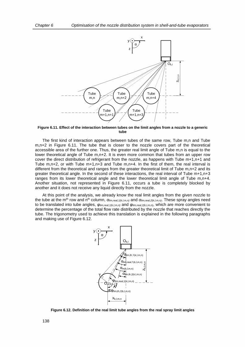
Chapter 6 Optimisation of the nozzle distribution system in shell-and-tube evaporators

138

Figure 6.11. Effect of the interaction between tubes on the limit angles from a nozzle to a generic tube

The first kind of interaction appears between tubes of the same row, Tube m,n and Tube m,n+2 in Figure 6.11. The tube that is closer to the nozzle covers part of the theoretical accessible area of the further one. Thus, the greater real limit angle of Tube m,n is equal to the lower theoretical angle of Tube m,n+2. It is even more common that tubes from an upper row cover the direct distribution of refrigerant from the nozzle, as happens with Tube m+1,n+1 and Tube m,n+2, or with Tube m+1,n+3 and Tube m,n+4. In the first of them, the real interval is different from the theoretical and ranges from the greater theoretical limit of Tube m,n+2 and its greater theoretical angle. In the second of these interactions, the real interval of Tube m+1,n+3 ranges from its lower theoretical angle and the lower theoretical limit angle of Tube m,n+4. Another situation, not represented in Figure 6.11, occurs a tube is completely blocked by another and it does not receive any liquid directly from the nozzle.

At this point of the analysis, we already know the real limit angles from the given nozzle to the tube at the mth row and nth column, αlim,real,1(k,l,m,n) and αlim,real,2(k,l,m,n). These spray angles need to be translated into tube angles, φlim,real,1(k,l,m,n) and φlim,real,2(k,l,m,n), which are more convenient to determine the percentage of the total flow rate distributed by the nozzle that reaches directly the tube. The trigonometry used to achieve this translation is explained in the following paragraphs and making use of Figure 6.12.

Figure 6.12. Definition of the real limit tube angles from the real spray limit angles

Tube

m,n

Ok,l

x

z

yα

zk,l,1

,n

Tube

m+1,n+3

Tube

m+1,n+1

Tube

m,n+2

Tube

m,n+4

x

z

yα

Ok,l

Om,n

xk,l,m,n

zk,l,m

,n

φlim,real,1(k,l,m,n)

φlim,th,2(k,l,m,n)

T

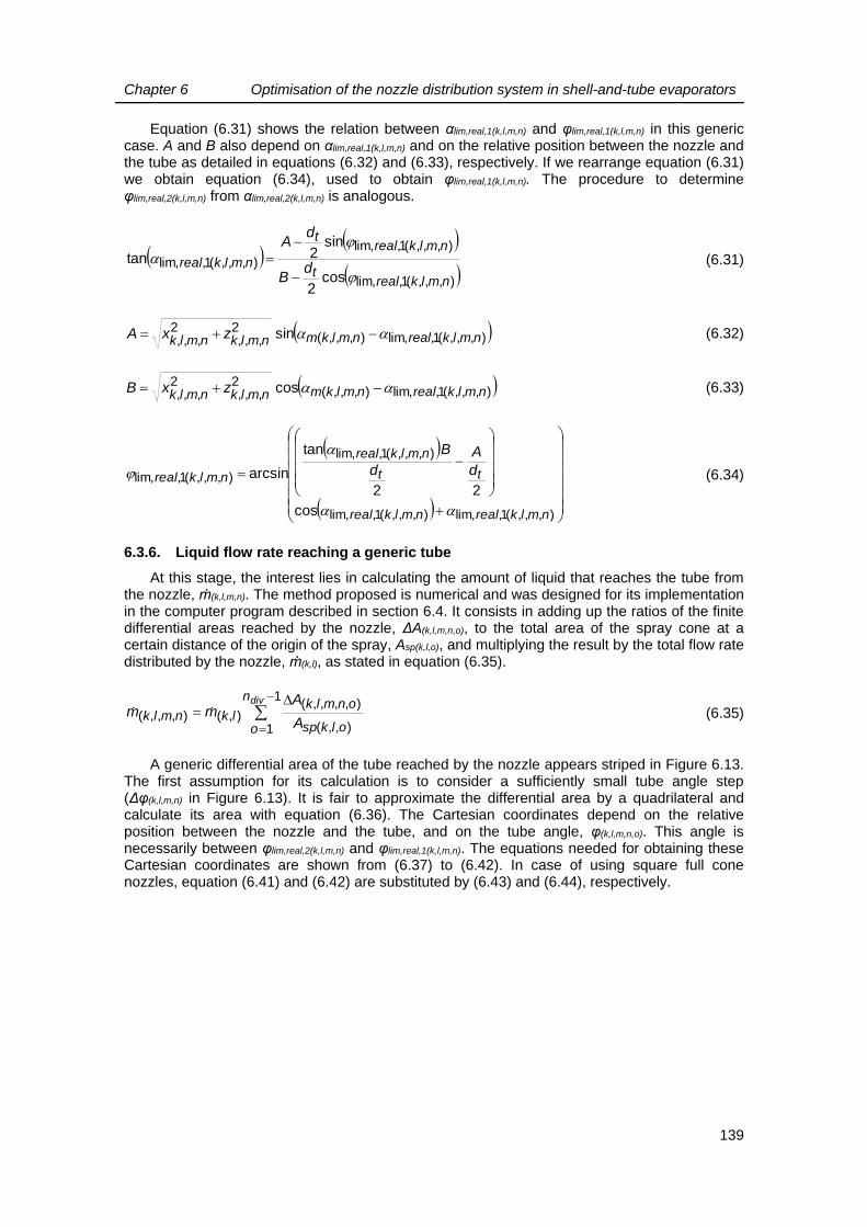
Chapter 6 Optimisation of the nozzle distribution system in shell-and-tube evaporators

139

Equation (6.31) shows the relation between αlim,real,1(k,l,m,n) and φlim,real,1(k,l,m,n) in this generic case. A and B also depend on αlim,real,1(k,l,m,n) and on the relative position between the nozzle and the tube as detailed in equations (6.32) and (6.33), respectively. If we rearrange equation (6.31) we obtain equation (6.34), used to obtain φlim,real,1(k,l,m,n). The procedure to determine φlim,real,2(k,l,m,n) from αlim,real,2(k,l,m,n) is analogous.

),,,(1,lim,

),,,(1,lim,

),,,(1,lim,cos

2

sin2tan

nmlkrealt

nmlkrealt

nmlkreal dB

dA

(6.31)

),,,(1,lim,),,,(2

,,,2

,,,sin nmlkrealnmlkmnmlknmlk

zxA

(6.32)

),,,(1,lim,),,,(2

,,,2

,,,cos nmlkrealnmlkmnmlknmlk

zxB

(6.33)

),,,(1,lim,),,,(1,lim,

),,,(1,lim,

),,,(1,lim,

cos

22

tan

arcsin

nmlkrealnmlkreal

tt

nmlkreal

nmlkreald

A

d

B

(6.34)

6.3.6. Liquid flow rate reaching a generic tube

At this stage, the interest lies in calculating the amount of liquid that reaches the tube from the nozzle, m(k,l,m,n). The method proposed is numerical and was designed for its implementation in the computer program described in section 6.4. It consists in adding up the ratios of the finite differential areas reached by the nozzle, ΔA(k,l,m,n,o), to the total area of the spray cone at a certain distance of the origin of the spray, Asp(k,l,o), and multiplying the result by the total flow rate distributed by the nozzle, m(k,l), as stated in equation (6.35).

1

1 ),,(

),,,,(),(),,,(

divn

o olksp

onmlklknmlk

A

Amm

(6.35)

A generic differential area of the tube reached by the nozzle appears striped in Figure 6.13. The first assumption for its calculation is to consider a sufficiently small tube angle step (Δφ(k,l,m,n) in Figure 6.13). It is fair to approximate the differential area by a quadrilateral and calculate its area with equation (6.36). The Cartesian coordinates depend on the relative position between the nozzle and the tube, and on the tube angle, φ(k,l,m,n,o). This angle is necessarily between φlim,real,2(k,l,m,n) and φlim,real,1(k,l,m,n). The equations needed for obtaining these Cartesian coordinates are shown from (6.37) to (6.42). In case of using square full cone nozzles, equation (6.41) and (6.42) are substituted by (6.43) and (6.44), respectively.

Chapter 6 Optimisation of the nozzle distribution system in shell-and-tube evaporators

140

Figure 6.13. Representation of the differential area of a tube accessible from a nozzle

2

1,,,,1,,,,,,,,,,,,

1,,,,,,,,),,,,(

onmlkonmlkonmlkonmlk

onmlkonmlkonmlk

yyyy

xxA

(6.36)

onmlkt

nmlkonmlkd

xx ,,,,,,,,,,, sin2

(6.37)

onmlkt

nmlkonmlkd

xx ,,,,,,,1,,,, sin2

(6.38)

onmlkt

nmlkonmlkd

zz ,,,,,,,,,,, cos2

(6.39)

onmlkt

nmlkonmlkd

zz ,,,,,,,1,,,, cos2

(6.40)

2,,,,

22,,,,,,,,

2tanonmlkonmlkonmlk

xzy

(6.41)

21,,,,

221,,,,1,,,,

2tan

onmlkonmlkonmlk

xzy

(6.42)

2tan,,,,,,,,onmlkonmlk

zy

(6.43)

2tan1,,,,1,,,,

onmlkonmlkzy

(6.44)

The area of the spray cone at a distance of the origin of the spray, Asp(k,l,o), also depends on the kind of nozzles used. Equation (6.45) evaluates the area for circular full cone nozzles, and equation (6.46) for square full cone nozzles.

x

z

yα

zk,l,m

,n,o

zk,l,m

,n,o

+1

xk,l,m,n,o

xk,l,m,n,o+1

φ(k,l,m,n,o)

xk,l,m,n

zk,l,m

,n

Chapter 6 Optimisation of the nozzle distribution system in shell-and-tube evaporators

141

2

,,,,1,,,,),,(, 2tan

2

onmlkonmlkolksp

zzA

(6.45)

2

,,,,1,,,,),,(, 2tan

24

onmlkonmlkolksp

zzA

(6.46)

If we assume that the flow rate coming from a nozzle to a tube is unaffected by the flow reaching the same tube from another nozzle and that the flows are cumulative, we obtain all the flow rate that reaches a generic tube, m(m,n) with equation (6.47). If we follow equation (6.48), we calculate the flow rate distributed on each column of tubes, m(n).

syst nozzle

n

k

n

lnmlknm mm

1 1),,,(),(

(6.47)

rown

mnmn mm

1,),()(

(6.48)

Finally, we developed a dimensionless column factor, Fcol(n) to evaluate how evenly distributed the liquid among the different columns of the tube bundle is. For the calculation of this column factor we use equation (6.49). In this equation, mmin represents the minimum among the mass flow rates received by any of the columns of the tube bundle. The closer this factor is to the unity in all the columns of the tube bundle, the better distributed the fluid is along the tube bundle and the less overfeed on some columns is needed to prevent dryout on others.

min

)()(

m

mF

nncol

(6.49)

Chapter 6 Optimisation of the nozzle distribution system in shell-and-tube evaporators

142

6.4. PROGRAMME FOR THE CALCULATION OF HEAT EXCHANGERS

The calculation methods described in the previous section are tedious and repetitive, particularly if the heat exchanger is large and has an important number of tubes. Consequently, we developed a programme in MATLAB software where the characteristics of the tube bundle (number of tubes, distance between them, type of pitch, etc.) are introduced, and returns the layout of different optimal distribution systems and how the flow is distributed on the different tubes and columns of tubes.

6.4.1. Inputs

The inputs that the user can introduce in the programme are mainly associated with the dimensions, disposition and number of tubes of the tube bundle. The list of inputs and their explanation is:

Tube diameter (in meters).

Type of pitch. It is possible to select between inline (Figure 6.14a) and staggered tube layout (Figure 6.14b).

Number of tube rows.

Number of tubes per row (number of columns). If the chosen pitch is staggered, even rows have a tube less than odd rows.

Horizontal pitch. It is a factor that defines the distance between consecutive tubes of the same row by multiplying the diameter of the tube (see Figure 6.14).

Vertical pitch. It is a factor that defines the distance between consecutive rows by multiplying the diameter of the tube (see Figure 6.14).

Type of nozzle. The possible choices are circular full cone nozzles and square full cone nozzles.

Nozzle angle vector (β). In this vector the user introduces the cone angles of the nozzles to be evaluated by the programme. The default values included in the vector are 60º, 90º and 120º.

Maximum number of nozzle systems. The user must define the maximum number of nozzle systems (rows of spray nozzles) to be considered by the programme.

Tube length. Length of the tubes dedicated to heat exchange.

Expected shell diameter. Input that the programme uses to discard solutions that need a large distance between the spray nozzles and the tube bundle.

Figure 6.14. Position and numbering of the tubes in the bundle. a) Inline tube pattern. b) Staggered tube pattern

Tube

1,1

Tube

1,3

Tube

1,ncol

Tube

2,1

Tube

2,3

Tube

2,ncol

Tube

nrow,1

Tube

nrow,3

Tube

nrow,ncol

Phor·dt

Pver·

dt

Pver·

dt

Tube

1,1

Tube

1,3

Tube

1,ncol

Tube

nrow,1

Tube

nrow,3

Tube

nrow,ncol

Phor·dt

Pver·

dt

Phor·dt/2

Tube

3,1

Tube

3,3

Tube

3,ncol

Tube

2,2

Tube

2,4

Tube

nrow-1,2

Tube

nrow-1,4

a b

Chapter 6 Optimisation of the nozzle distribution system in shell-and-tube evaporators

143

6.4.2. Calculation process

The calculation process programmed follows the ideas described in subsection 6.3. We have included a flow chart in Figure 6.15 to summarise it. Once the inputs are introduced, the programme selects the first spray cone angle of the vector and starts studying the distribution with one nozzle system. Then, it calculates the number of nozzles needed for that inputs and the best relative position between the bundle and the nozzles. After that, it determines the limit angles, both theoretical and real, for each tube and from each of the spray nozzles. These angles allow calculating the percentage of the flow rate distributed by the nozzles that reaches each tube and each column of tubes. The next step is to increase the number of nozzle systems in one unit (up to the maximum, nsyst,max) and to repeat the process. If the maximum is reached, the programme checks the spray nozzle vector, selects the next value (if any) and does over the calculations.

Figure 6.15. Flow chart of the calculation process of the programme

6.4.3. Outputs

The outputs that the programme returns can be classified into graphical outputs and data outputs. Similar graphics to that shown in Figure 6.16 are obtained for each of the possible

INPUTS

Spray nozzle β

Nozzle systems nsyst

Position of the nozzles and tube bundle

Limit angles

% flow rate per tube and column

OUTPUTS

Maximum nozzle systems?

Another nozzle angle?

NO

YES

YES

NO

Chapter 6 Optimisation of the nozzle distribution system in shell-and-tube evaporators

144

spray nozzle angle-nozzle systems combinations. They represent the tube bundle and the expected shell, as well as the origin of the different spray nozzles and the cones they produce.

Figure 6.16. 3D-plot of the tube bundle, the shell and the spray cones for each solution

Another graphical output from the programme is the graph shown in Figure 6.17. This graph represents the real limit angles for each tube of the bundle and for a representative nozzle of each nozzle system. It gives the user an idea on the distribution of the liquid on the different columns, particularly interesting with staggered pitch tube bundles, and of the possible interactions between tubes.

Figure 6.17. 2D representation of the real limit angles for each tube of the bundle and for a representative nozzle of each nozzle system

Chapter 6 Optimisation of the nozzle distribution system in shell-and-tube evaporators

145

Finally, the programme registers the most important data outputs in a .xls file. The list of saved variables includes:

Input values.

Vector of spray nozzle angles.

Distances between nozzle systems and between spray nozzles of the same nozzle system.

Relative position between the distribution system and the tube bundle.

Number of spray nozzles per nozzle system and total number of nozzles of the heat exchanger.

Percentage of the total flow rate distributed that reaches each tube directly from the distribution system.

Chapter 6 Optimisation of the nozzle distribution system in shell-and-tube evaporators

146

6.5. PARAMETRIC ANALYSIS

We used the programme developed to perform a parametric analysis to study how the different inputs (tube bundle and spray nozzle characteristics) affect the even distribution of the liquid on a bundle consisting of 8 rows of tubes and 8 tubes per row and with a length of 1 m. In this subsection we detail the inputs considered and the range of values for each of them, as well as the results attained and the discussion of these results.

6.5.1. Input parameters

We analysed the effect of varying part of the variables that the programme includes, listed in subsection 6.4.1. Others were kept constant to simplify the analysis. Among the variables that remained constant is the outer diameter of the tubes, at 3/4” (19.05 mm); the number of rows of the bundle, at 8; the number of tubes of each row, at 8 (staggered tube bundles have 7 tubes if the row is even numbered); the length of the shell-and-tube heat exchanger, at 1 m; and the type of nozzle, considered as circular full cone nozzle throughout the analysis. The nozzle angles studied were 60º, 90º and 120º, available with almost any manufacturer. The tube patterns were both inline and staggered. The horizontal and vertical pitches, depended on the tube pattern, as shown in Table 6.2. Those combinations from Table 6.2 that are in black are incompatible. Finally, the number of nozzle systems was 1, 2 or 3.

Table 6.2. Horizontal and vertical pitches analysed in the parametric analysis

TUBE BUNDLE INLINE PITCH STAGGERED PITCH

(60º) STAGGERED PITCH

(45º)

Horizontal Pitch Vertical Pitch

1.25 1.25 1.08

1.5 1.5 1.3

2 2 1.73 1

6.5.2. Results

Figure 6.18 shows the percentage of the total flow rate distributed that reaches the inline tube bundles considered, as a function of the number of nozzle systems, the horizontal pitch of the tube bundle and the cone angle of the spray nozzles. Generally, this percentage increases if the horizontal pitch decreases, as there is a smaller amount of liquid that flows in between the columns of tubes. The other trend observed is that the amount of liquid reaching the tubes rises with the smallest spray nozzles (60º). The effect of the number of nozzles systems on the percentage of flow reaching the tubes depends on the rest of variables, but it is normally higher with 1 and with 3 nozzle systems than with 2 nozzles systems.

Similarly, Figure 6.19 depicts the situation with the different staggered tube bundles analysed. The fraction of the distributed liquid that does not reach any tube of the bundle diminishes as the nozzle cone angle decreases. The percentage of flow reaching the tubes is maximum with 1.5 horizontal pitch bundles, if kept constant the other parameters. Excluding the situation of 60º spray cone angles, the liquid reaching the tubes increases if the vertical pitch decreases, independently of the number of nozzle systems and with 2 of horizontal pitch.

Chapter 6 Optimisation of the nozzle distribution system in shell-and-tube evaporators

147

Figure 6.18. Percentage of the total flow rate distributed that reaches the inline tube bundles considered, as a function of the number of nozzle systems, the horizontal pitch of the tube bundle

and the cone angle of the spray nozzles

Figure 6.19. Percentage of the total flow rate distributed that reaches the staggered tube bundles considered, as a function of the number of nozzle systems, the horizontal pitch of the tube bundle

and the cone angle of the spray nozzles

From the previous figures we concluded that 60º cone angle nozzles are the best from the point of view of increasing the flow rate reaching the bundle. However, in Figure 6.20 we observe that the distance between the nozzles and the first row of tubes of the bundle that

40%

50%

60%

70%

80%

90%

100%

0 1 2 3 4

Perc

enta

ge

flo

w r

eachin

g tube b

un

dle

[%

]

nsyst [-]

Inline_1.25_β = 60º Inline_1.25_β = 90º Inline_1.25_β = 120º

Inline_1.5_β = 60º Inline_1.5_β = 90º Inline_1.5_β = 120º

Inline_2_β = 60º Inline_2_β = 90º Inline_2_β = 120º

30%

40%

50%

60%

70%

80%

90%

100%

0 1 2 3 4

Perc

enta

ge

flo

w r

eachin

g tube b

un

dle

[%

]

ndist [-]

Staggered_1.25_1.08_β = 60º Staggered_1.25_1.08_β = 90º

Staggered_1.25_1.08_β = 120º Staggered_1.5_1.3_β = 60º

Staggered_1.5_1.3_β = 90º Staggered_1.5_1.3_β = 120º

Staggered_2_1.73_β = 60º Staggered_2_1.73_β = 90º

Staggered_2_1.73_β = 120º Staggered_2_1_β = 60º

Staggered_2_1_β = 90º Staggered_2_1_β = 120º

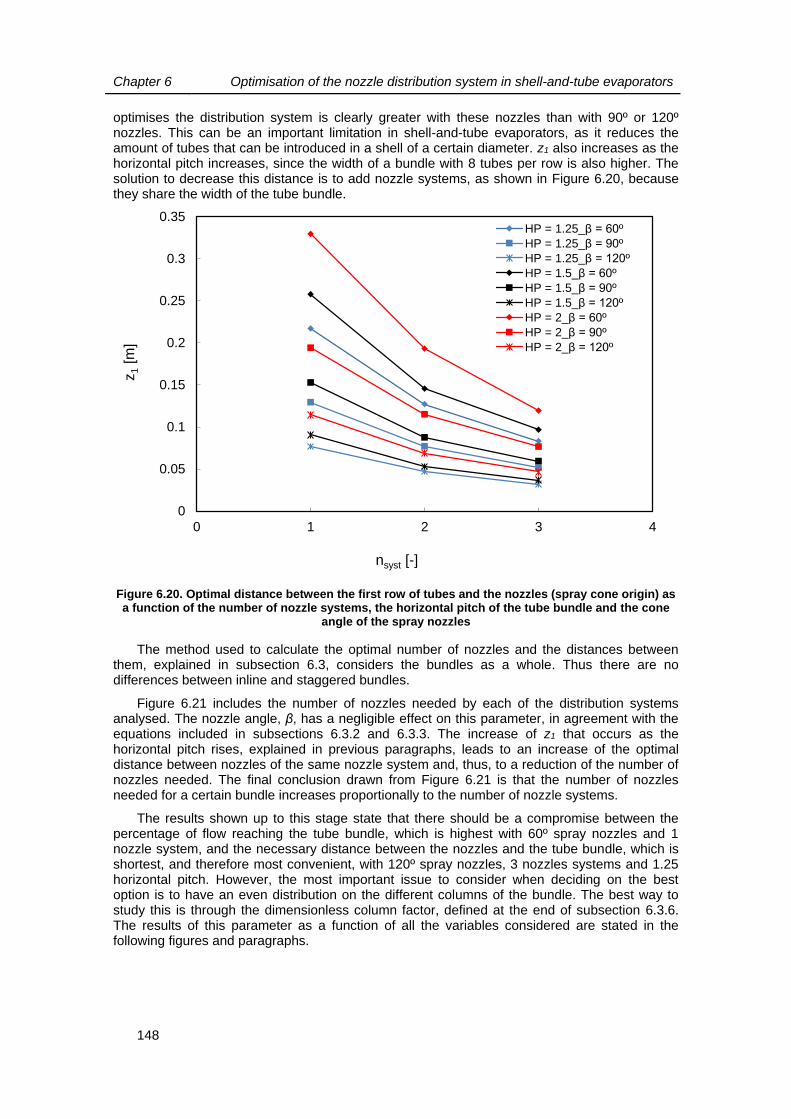
Chapter 6 Optimisation of the nozzle distribution system in shell-and-tube evaporators

148

optimises the distribution system is clearly greater with these nozzles than with 90º or 120º nozzles. This can be an important limitation in shell-and-tube evaporators, as it reduces the amount of tubes that can be introduced in a shell of a certain diameter. z1 also increases as the horizontal pitch increases, since the width of a bundle with 8 tubes per row is also higher. The solution to decrease this distance is to add nozzle systems, as shown in Figure 6.20, because they share the width of the tube bundle.

Figure 6.20. Optimal distance between the first row of tubes and the nozzles (spray cone origin) as a function of the number of nozzle systems, the horizontal pitch of the tube bundle and the cone

angle of the spray nozzles

The method used to calculate the optimal number of nozzles and the distances between them, explained in subsection 6.3, considers the bundles as a whole. Thus there are no differences between inline and staggered bundles.

Figure 6.21 includes the number of nozzles needed by each of the distribution systems analysed. The nozzle angle, β, has a negligible effect on this parameter, in agreement with the equations included in subsections 6.3.2 and 6.3.3. The increase of z1 that occurs as the horizontal pitch rises, explained in previous paragraphs, leads to an increase of the optimal distance between nozzles of the same nozzle system and, thus, to a reduction of the number of nozzles needed. The final conclusion drawn from Figure 6.21 is that the number of nozzles needed for a certain bundle increases proportionally to the number of nozzle systems.

The results shown up to this stage state that there should be a compromise between the percentage of flow reaching the tube bundle, which is highest with 60º spray nozzles and 1 nozzle system, and the necessary distance between the nozzles and the tube bundle, which is shortest, and therefore most convenient, with 120º spray nozzles, 3 nozzles systems and 1.25 horizontal pitch. However, the most important issue to consider when deciding on the best option is to have an even distribution on the different columns of the bundle. The best way to study this is through the dimensionless column factor, defined at the end of subsection 6.3.6. The results of this parameter as a function of all the variables considered are stated in the following figures and paragraphs.

0

0.05

0.1

0.15

0.2

0.25

0.3

0.35

0 1 2 3 4

z1

[m]

nsyst [-]

HP = 1.25_β = 60º

HP = 1.25_β = 90º

HP = 1.25_β = 120º

HP = 1.5_β = 60º

HP = 1.5_β = 90º

HP = 1.5_β = 120º

HP = 2_β = 60º

HP = 2_β = 90º

HP = 2_β = 120º

Chapter 6 Optimisation of the nozzle distribution system in shell-and-tube evaporators

149

Figure 6.21. Optimal number of nozzles of the whole distribution system as a function of the number of nozzle systems, the horizontal pitch of the tube bundle and the cone angle of the spray

nozzles

Figure 6.22 includes the dimensionless column factor vs. the position of the column of tubes for an inline tube bundle of 1.25 horizontal pitch and 1.25 vertical pitch, as a function of the number of nozzle systems and of β. As a reminder, due to the definition of the bundle and taking into account that it is of inline type, there are tubes only in odd columns. The best distribution system according to this factor is that with 60º nozzles and 1 nozzle system, because its column factor is always in the range between 1 and 1.29. Those distribution systems with 90º nozzles seem also very convenient, independently of the number of distribution systems. In these cases Fcol is never higher than 1.35 and, therefore, the liquid is fairly well distributed all over the tube bundle. In contrast, this dimensionless number increases when β = 120º and reaches values close to 1.7.

A similar situation is shown in Figure 6.23 with an inline tube bundle with horizontal pitch of 1.5 and vertical pitch of 1.5. The performance of distribution systems with 120º nozzles improves for this tube bundle, which is wider. The options with 60º and 90º nozzles and 1 nozzle system are also convenient from the point of view of the dimensionless column factor, with maximums of 1.32 and 1.3, respectively.

0

5

10

15

20

25

30

35

40

45

0 1 2 3 4

nozzle

s [-]

nsyst [-]

HP = 1.25_β = 60º

HP = 1.25_β = 90º

HP = 1.25_β = 120º

HP = 1.5_β = 60º

HP = 1.5_β = 90º

HP = 1.5_β = 120º

HP = 2_β = 60º

HP = 2_β = 90º

HP = 2_β = 120º

Chapter 6 Optimisation of the nozzle distribution system in shell-and-tube evaporators

150

Figure 6.22. Dimensionless column factor vs. the numbering of the column of tubes, for an inline pattern bundle with horizontal pitch of 1.25 and vertical pitch of 1.25, and as a function of the

number of nozzle systems and the cone angle of the spray nozzles

Figure 6.23. Dimensionless column factor vs. the numbering of the column of tubes, for an inline pattern bundle with horizontal pitch of 1.5 and vertical pitch of 1.5, and as a function of the number

of nozzle systems and the cone angle of the spray nozzles

The wider the tube bundle, the worse the dimensionless column factor, as we observe if we compare the results for an inline tube bundle of Phor = 2 and Pver = 2, shown in Figure 6.24, to those from previous figures. The best solutions are again those with β = 60º and β = 90º nozzles

0.6

0.8

1

1.2

1.4

1.6

1.8

0 2 4 6 8 10 12 14 16

Fcol[-

]

Column [-]

β = 60º & nsyst = 1 β = 60º & nsyst = 2 β = 60º & nsyst = 3

β = 90º & nsyst = 1 β = 90º & nsyst = 2 β = 90º & nsyst = 3

β = 120º & nsyst = 1 β = 120º & nsyst = 2 β = 120º & nsyst = 3

0.6

0.8

1

1.2

1.4

1.6

1.8

2

0 2 4 6 8 10 12 14 16

Fcol[-

]

Column [-]

β = 60º & nsyst = 1 β = 60º & nsyst = 2 β = 60º & nsyst = 3

β = 90º & nsyst = 1 β = 90º & nsyst = 2 β = 90º & nsyst = 3

β = 120º & nsyst = 1 β = 120º & nsyst = 2 β = 120º & nsyst = 3

Chapter 6 Optimisation of the nozzle distribution system in shell-and-tube evaporators

151

and 1 nozzle system. The maximum dimensionless column factor for any of these solutions never exceeds 1.44.

Figure 6.24. Dimensionless column factor vs. the numbering of the column of tubes, for an inline pattern bundle with horizontal pitch of 2 and vertical pitch of 2, and as a function of the number of

nozzle systems and the cone angle of the spray nozzles

Figure 6.25. Dimensionless column factor vs. the numbering of the column of tubes, for a staggered pattern bundle with horizontal pitch of 1.25 and vertical pitch of 1.08 (60º angle), and as

a function of the number of nozzle systems and the cone angle of the spray nozzles

0.4

0.6

0.8

1

1.2

1.4

1.6

1.8

2

2.2

2.4

2.6

0 2 4 6 8 10 12 14 16

Fcol[-

]

Column [-]

β = 60º & nsyst = 1 β = 60º & nsyst = 2 β = 60º & nsyst = 3

β = 90º & nsyst = 1 β = 90º & nsyst = 2 β = 90º & nsyst = 3

β = 120º & nsyst = 1 β = 120º & nsyst = 2 β = 120º & nsyst = 3

0

3

6

9

12

15

0 2 4 6 8 10 12 14 16

Fcol[-

]

Column [-]

β = 60º & nsyst = 1 β = 60º & nsyst = 2 β = 60º & nsyst = 3

β = 90º & nsyst = 1 β = 90º & nsyst = 3

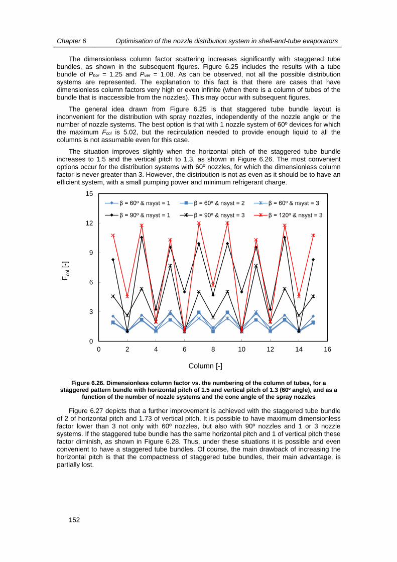
Chapter 6 Optimisation of the nozzle distribution system in shell-and-tube evaporators

152

The dimensionless column factor scattering increases significantly with staggered tube bundles, as shown in the subsequent figures. Figure 6.25 includes the results with a tube bundle of Phor = 1.25 and Pver = 1.08. As can be observed, not all the possible distribution systems are represented. The explanation to this fact is that there are cases that have dimensionless column factors very high or even infinite (when there is a column of tubes of the bundle that is inaccessible from the nozzles). This may occur with subsequent figures.

The general idea drawn from Figure 6.25 is that staggered tube bundle layout is inconvenient for the distribution with spray nozzles, independently of the nozzle angle or the number of nozzle systems. The best option is that with 1 nozzle system of 60º devices for which the maximum Fcol is 5.02, but the recirculation needed to provide enough liquid to all the columns is not assumable even for this case.

The situation improves slightly when the horizontal pitch of the staggered tube bundle increases to 1.5 and the vertical pitch to 1.3, as shown in Figure 6.26. The most convenient options occur for the distribution systems with 60º nozzles, for which the dimensionless column factor is never greater than 3. However, the distribution is not as even as it should be to have an efficient system, with a small pumping power and minimum refrigerant charge.

Figure 6.26. Dimensionless column factor vs. the numbering of the column of tubes, for a staggered pattern bundle with horizontal pitch of 1.5 and vertical pitch of 1.3 (60º angle), and as a

function of the number of nozzle systems and the cone angle of the spray nozzles

Figure 6.27 depicts that a further improvement is achieved with the staggered tube bundle of 2 of horizontal pitch and 1.73 of vertical pitch. It is possible to have maximum dimensionless factor lower than 3 not only with 60º nozzles, but also with 90º nozzles and 1 or 3 nozzle systems. If the staggered tube bundle has the same horizontal pitch and 1 of vertical pitch these factor diminish, as shown in Figure 6.28. Thus, under these situations it is possible and even convenient to have a staggered tube bundles. Of course, the main drawback of increasing the horizontal pitch is that the compactness of staggered tube bundles, their main advantage, is partially lost.

0

3

6

9

12

15

0 2 4 6 8 10 12 14 16

Fcol[-

]

Column [-]

β = 60º & nsyst = 1 β = 60º & nsyst = 2 β = 60º & nsyst = 3

β = 90º & nsyst = 1 β = 90º & nsyst = 3 β = 120º & nsyst = 3

Chapter 6 Optimisation of the nozzle distribution system in shell-and-tube evaporators

153

Figure 6.27. Dimensionless column factor vs. the numbering of the column of tubes, for a staggered pattern bundle with horizontal pitch of 2 and vertical pitch of 1.73 (60º angle), and as a

function of the number of nozzle systems and the cone angle of the spray nozzles

Figure 6.28. Dimensionless column factor vs. the numbering of the column of tubes, for a staggered pattern bundle with horizontal pitch of 2 and vertical pitch of 1 (45º angle), and as a

function of the number of nozzle systems and the cone angle of the spray nozzles

To summarise these results we prepared Table 6.3 and Table 6.4, which include the maximum column factors, Fcol,max, for the different distribution systems and with all the inline and

0

2

4

6

8

10

12

0 2 4 6 8 10 12 14 16

Fcol[-

]

Column [-]

β = 60º & nsyst = 1 β = 60º & nsyst = 2 β = 60º & nsyst = 3

β = 90º & nsyst = 1 β = 90º & nsyst = 2 β = 90º & nsyst = 3

β = 120º & nsyst = 2 β = 120º & nsyst = 3

0

1

2

3

4

5

6

0 2 4 6 8 10 12 14 16

Fcol[-

]

Column [-]

β = 60º & nsyst = 1 β = 60º & nsyst = 2 β = 60º & nsyst = 3

β = 90º & nsyst = 1 β = 90º & nsyst = 2 β = 90º & nsyst = 3

β = 120º & nsyst = 1 β = 120º & nsyst = 2 β = 120º & nsyst = 3

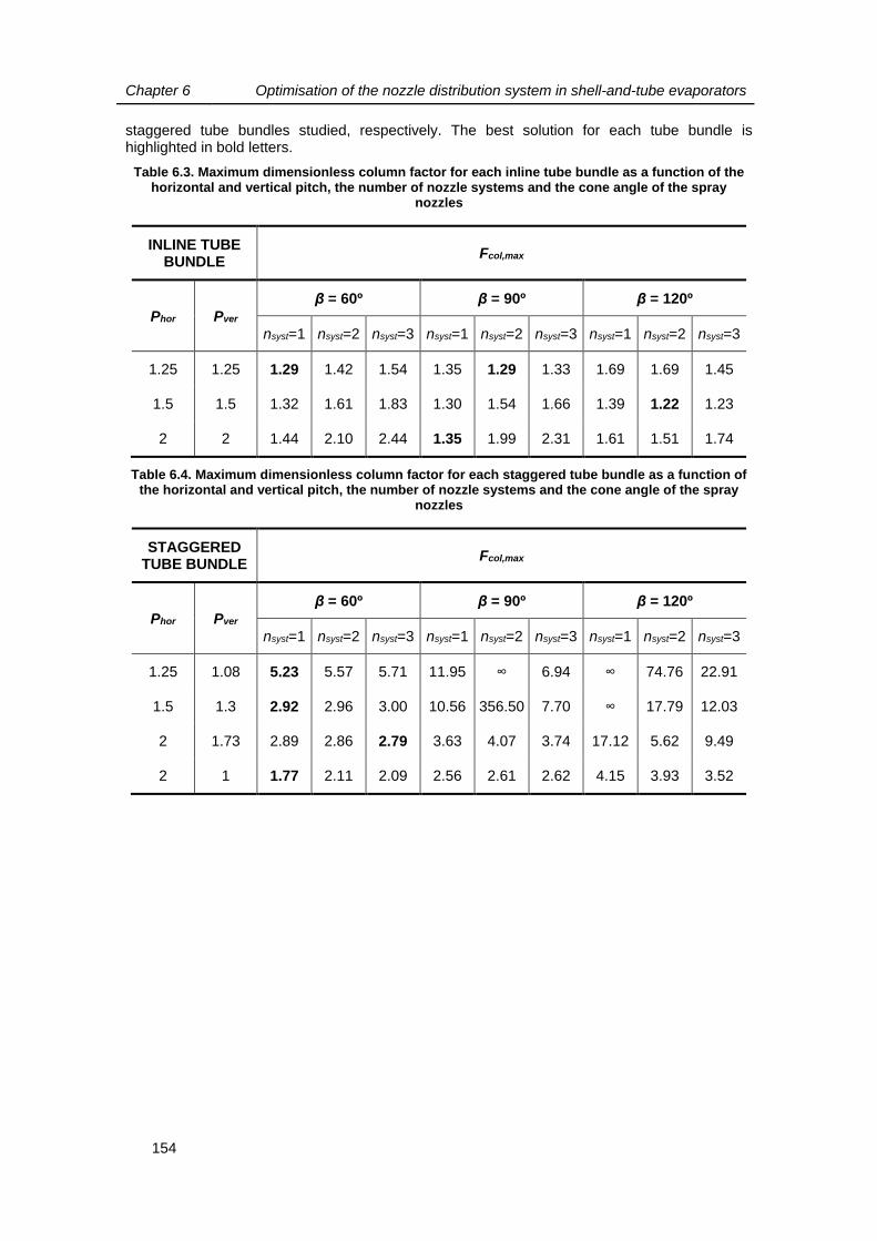
Chapter 6 Optimisation of the nozzle distribution system in shell-and-tube evaporators

154

staggered tube bundles studied, respectively. The best solution for each tube bundle is highlighted in bold letters.

Table 6.3. Maximum dimensionless column factor for each inline tube bundle as a function of the horizontal and vertical pitch, the number of nozzle systems and the cone angle of the spray

nozzles

INLINE TUBE BUNDLE

Fcol,max

Phor Pver

β = 60º β = 90º β = 120º

nsyst=1 nsyst=2 nsyst=3 nsyst=1 nsyst=2 nsyst=3 nsyst=1 nsyst=2 nsyst=3

1.25 1.25 1.29 1.42 1.54 1.35 1.29 1.33 1.69 1.69 1.45

1.5 1.5 1.32 1.61 1.83 1.30 1.54 1.66 1.39 1.22 1.23

2 2 1.44 2.10 2.44 1.35 1.99 2.31 1.61 1.51 1.74

Table 6.4. Maximum dimensionless column factor for each staggered tube bundle as a function of the horizontal and vertical pitch, the number of nozzle systems and the cone angle of the spray

nozzles

STAGGERED TUBE BUNDLE

Fcol,max

Phor Pver

β = 60º β = 90º β = 120º

nsyst=1 nsyst=2 nsyst=3 nsyst=1 nsyst=2 nsyst=3 nsyst=1 nsyst=2 nsyst=3

1.25 1.08 5.23 5.57 5.71 11.95 ∞ 6.94 ∞ 74.76 22.91

1.5 1.3 2.92 2.96 3.00 10.56 356.50 7.70 ∞ 17.79 12.03

2 1.73 2.89 2.86 2.79 3.63 4.07 3.74 17.12 5.62 9.49

2 1 1.77 2.11 2.09 2.56 2.61 2.62 4.15 3.93 3.52

Chapter 6 Optimisation of the nozzle distribution system in shell-and-tube evaporators

155

6.6. CONCLUSIONS

In this chapter we have shown a state of the art of different distribution systems patented and applied in spray evaporators. We have observed that the main focus was on systems with low momentum devices. Due to the potential benefits on HTCs and on wetting of using high momentum devices, in this chapter we have focused on the optimization of distribution systems with spray nozzles for shell-and-tube evaporators.

The next stage of this chapter has been the study, using geometry and trigonometry, of the optimal distribution system as a function of the tube bundle dimensions and the characteristics of the nozzles used. We have also detailed the process followed to determine the percentage of liquid distributed by a given spray nozzle that reaches a generic tube, defining concepts such as those of the theoretical and real limit angles from a nozzle to a tube or the dimensionless column factor.

We have also developed a parametric analysis with the computer programme prepared for optimising distribution systems. The inputs for the study have been: 1-meter-long tube bundle, 8 rows and 8 tubes per row (7 for even rows in staggered pitch layout), different horizontal and vertical pitches, inline and staggered tube bundle pattern, 3 different spray nozzle angles, etc. We have observed that, in general, 60º nozzles lead to an even distribution and more efficient use of the liquid distributed. However, they require a larger distance between the spray nozzles and the first row of the tube bundle to optimise distribution and, thus, there is an important part of the shell that must be clear of tubes. The performance of systems with 90º nozzles is slightly lower, but the distance required is also shorter and they are convenient from that point of view.

We have determined that the even distribution of liquid on the different columns of inline tube bundles is easier than when the pattern is staggered. In fact, staggered tube bundles seem unsuitable for this kind of distribution systems with nozzles and without intermediate devices. Only when the horizontal pitch between tubes of the same row was high (2 in this case), we have observed a convenient distribution between the different columns. However, an increase of this horizontal pitch leads to the loss of compactness of staggered bundles, which is the main advantage of such tube pattern.

Chapter 6 Optimisation of the nozzle distribution system in shell-and-tube evaporators

156

REFERENCES

[1] J.P. Hartfield, D.F. Sanborn, Falling film evaporator with vapor-liquid separator, US 5,561,987, October 8, 1996.

[2] R.H.L. Chiang, J.L. Esformes, E.A. Huenniger, Chiller with hybrid falling film evaporator, US 5,839,294, November 24, 1998.

[3] N.S. Gupte, Heat exchanger of the type of a falling-film evaporator having refrigerant distribution system, E.P. 1 030 154 B1, 06.04.2005.

[4] C.H. Liu, C.C. Liu, Spray type heat Exchange device, US 2008/0149311 A1, June 26, 2008.

[5] C.C. Liu, Y.Z. Hu, H.T. Cheng, Spray type heat-exchanging unit, US 8,561,675 B2, October 22, 2013.

[6] M. Christians, J.L. Esformes, S. Bendapudi, M. Bezon, X. Qiu, S.P. Breen, Evaporator and liquid distributor, US 2014/0366574, December 18, 2014.

[7] T.B. Chang, L.Y. Yu, Optimal nozzle spray cone angle for triangular-pitch shell-and-tube interior spray evaporator, International Journal of Heat and Mass Transfer. 85 (2015) 463-472.

[8] S.A. Moeykens, J.W. Larson, J.P. Hartfield, H.K. Ring, Falling film evaporator for a vapor compression refrigeration chiller, US 6,293,112 B1, September 25, 2001.

[9] P. De Larminat, L. Le Cointe, J.F. Judge, S. Kulankara, Falling film evaporator, US 7,849,710 B2, December 14, 2010.

[10] Engineer’s Guide to Spray Technology, Spraying Systems Co., U.S.A., 2000.

[11] X. Zeng, M. Chyu, Heat transfer and fluid flow study of ammonia spray evaporators, Texas Tech University, Lubbock, Texas, USA, 1995.

157

Chapter 7

General conclusions and future works

This chapter begins with the main conclusions drawn from the theoretical and experimental studies developed for this thesis.

This document finishes with a brief explanation of the future works that will be developed to continue with this line of research focused on HTC determination in phase change processes (condensation and evaporation/boiling).

Chapter 7 General conclusions and future works

158

7.1. GENERAL CONCLUSIONS

The conclusions we have drawn from the different works developed during this study are listed below.

1. We have performed a thorough literature review on the main characteristics and particularities of the boiling process of refrigerants on horizontal tubes when the refrigerant is distributed on the tubes by means of different devices, such as nozzles, perforated plates, etc. We have analysed the main variables that have an effect on this process, normally called spray or falling film evaporation.

2. We have modified an existing experimental setup which had been designed to determine HTCs of condensation and pool boiling of refrigerants on horizontal tubes. The modification we have developed consisted in including a liquid refrigerant distribution system that was specifically dimensioned and built for this experimental test rig. The system includes a tank, a refrigerant pump, and a distribution tube with wide angle circular full cone nozzles.

3. We have designed an experimental methodology based on the separation of thermal resistances to study boiling HTCs of refrigerants on horizontal tubes, both under flooded or refrigerant distribution conditions. We have conceived a specific experimental methodology to analyse the influence of the impingement effect on HTCs with distribution of the liquid refrigerant. We have also developed a systematic methodology to determine the uncertainties of the different variables measured and calculated, based on the Guide to the Expression of Uncertainty in Measurements (GUM). The different assumptions considered for this experimental methodology have been successfully validated with specific tests.

4. We have shown the pool boiling HTCs obtained with R134a as refrigerant and copper tubes of plain and enhanced outer surfaces (Turbo-B and Turbo-BII+ of Wolverine Tube Inc.). The vast majority of our experimental results are included in the nucleate boiling region of the boiling curve. Pool boiling HTCs increase both with saturation temperatures (reduced pressure) and with heat flux (except for Turbo-B). We have compared our plain tube results with well-known correlations found in works of the specialised literature and we have observed the large discrepancies that exist among them, confirming how difficult it is to determine accurately the HTCs associated to this process.

5. The pool boiling tests developed with ammonia on titanium tubes with plain and integral- fin (Trufin 32 f.p.i.) outer surfaces have covered both the natural convective and nucleate boiling regions of the boiling curve. The HTCs obtained increase with increasing heat fluxes and saturation temperatures. We have also tested the influence of hysteresis on the nucleation process. We have confirmed its existence and that it is more important with the integral-fin tube than with the plain tube. However, our experiments have shown that increasing heat flux tests are time-dependent, i.e. the HTCs obtained when the experimentation process follows an increasing heat flux trend rise with time until they reach a value very close to that obtained with the diminishing heat flux tests, even when the test conditions remained constant. Our pool boiling HTCs with ammonia have been complemented with photographic reports that confirm the main experimental results.

6. The surface enhancement techniques under pool boiling have been more effective with R134a than with ammonia. With R134a, the surface enhancement factors have been as high as 11.8 and 7 with the Turbo-B and Turbo-BII+, respectively. In contrast, with ammonia, the EFsf has never been greater than 1.3.

7. We have studied spray evaporation with R134a and copper plain tube and we have observed that the HTCs generally increase if the heat flux is higher, independently of the mass flow rate of the film per side and meter of tube. We have also observed that the effect of the mass flow rate on the HTCs is negligible. The spray evaporation HTCs obtained with R134a and the tube placed directly underneath the refrigerant distribution tube (ST tests) are, on average, 13.2% greater than those determined with the tube that receives refrigerant from the conditioning tube (SB tests), if kept the heat flux and distributed mass flow rate constant. The heat transfer enhancement occurs due to the liquid droplet impingement effect. We have compared spray evaporation and pool boiling, with R134a, plain copper tube and under similar conditions and we have observed that spray evaporation enhances heat transfer only in the low

Chapter 7 General conclusions and future works

159

heat flux range. The enhancement has never been greater than 60% and the results are in line with other works from the specialised literature. An analysis of the photographs taken during the experiments have confirmed the existence of dry patches on the tubes and explained the heat transfer deterioration found at the high heat flux range.

8. We have performed spray evaporation tests with ammonia and titanium plain tubes and we have noted that the HTCs depend on both the heat flux and the mass flow rate of refrigerant per side and meter of tube. Generally, they increase with increasing heat fluxes, but this trend is even opposite under conditions of high heat flux and low mass flow rate. We have observed that the spray evaporation HTCs obtained with ammonia and the tube placed directly underneath the refrigerant distribution tube (ST tests) are, on average, 38.7% higher than those determined with the tube that receives refrigerant from the conditioning tube (SB tests). Droplet impingement effect is responsible of this effect. From the comparison of spray evaporation and pool boiling of ammonia on the plain tube, we have concluded that spray evaporation enhances importantly heat transfer, particularly in the low heat flux range. Spray enhancement factors have been over 1 under almost every condition and have reached values over 6. The photographic report of the process has verified the existence of dry patches under certain conditions that coincide with the lowest spray enhancement factors.

9. The experimental results obtained made clear the importance of having a proper distribution of the liquid refrigerant on the tubes of spray evaporators. Thus, we have developed a computer programme, based on a geometric study, to optimise the design of liquid distribution systems with spray nozzles.

10. We have performed a parametric analysis with the programme developed for a tube bundle of a given number of rows, tubes per row and length. We have observed that, in general, 60º nozzles lead to an even distribution and efficient use of the distributed liquid. However, they require a large distance to the first row of the bundle to optimise distribution and, thus, there is an important part of the shell that must be clear of tubes. The performance of systems with 90º nozzles is slightly lower, but the distance required is also shorter and they are convenient from this point of view. We have also determined that the even distribution of liquid on the different columns of inline tube bundles is easier than when the pattern is staggered. In fact, staggered tube bundles seem unsuitable for this kind of distribution systems with nozzles and without intermediate devices. Only when the horizontal pitch between tubes of the same row was high (2 in this case), we have observed a convenient distribution between the different columns. However, an increase of this horizontal pitch leads to the loss of compactness of staggered bundles, which is the main advantage of such tube pattern.

Chapter 7 General conclusions and future works

160

7.2. FUTURE WORKS

The line of research in which this work is enclosed continues in our laboratory. Some of the works that will be developed in the future are listed below.

1. Different tubes with enhanced outer surfaces will be tested under pool boiling conditions. The refrigerants on which we will focus in future studies are natural refrigerants, particularly ammonia. At this moment we are conducting slight modifications in the test rig to extend the test conditions to lower temperatures and, thus, have a larger range of saturation temperatures/reduced pressures.

2. Spray evaporation tests will be performed with the same enhanced tubes used for pool boiling tests. We will also study the process with different spray nozzles, such as square full cone nozzles, or low momentum distribution devices.

3. We will design an auxiliary test rig to conduct the experimental validation of the programme developed for the optimisation of the distribution system.

4. We will continue with the condensation tests that were developed during previous stages of this line of research by testing new enhanced surfaces for ammonia.

161

Appendix A

Uncertainty determination In this appendix we detail the uncertainty analysis prepared for the most important

parameters and fluid properties. It is based on the application of the general uncertainty propagation expression, as stated in the Evaluation of measurement data – Guide to the expression of uncertainty measurement (GUM). The output of this appendix is normally expressed with the results determined in form of error bars.

Appendix A Uncertainty determination

162

A.1. GENERAL FEATURES

The simple presentation of the boiling HTCs leaves this information incomplete. By including the uncertainties related with their determination, we give an idea of the quality and reliability of these results. Uncertainty is a parameter associated with the estimated value of a physical magnitude, measured or calculated, that indicates the range of values were the actual value of this physical magnitude should be. In this work we have developed an uncertainty determination procedure based on the Evaluation of measurement data – Guide to the expression of uncertainty measurement (GUM).

According to the GUM, a certain physical magnitude or measurand can be directly measured or determined from other quantities by a certain function. These other quantities can be also treated as measurands and they are classified depending on their origin: measured or from external sources.

If a measurand, xk, is the result of n independent determinations xki, a convenient estimation

of the measurand is the arithmetic mean of these independent determinations, as seen in equation (A.1).

n

i

ikk x

nx

1

1

(A.1)

The uncertainty can be classified into two categories: type A and type B. On the one hand, type A uncertainty, uA(xk), results from the statistical analysis of a series of measurements. On the other hand, type B uncertainty, uB(xk) is any other component of the uncertainty, including previously measured data, manufacturer specifications, data from calibration reports, etc. The total uncertainty of the magnitude, u(xk), results from adding the previous two (equation (A.2)).

222kBkAk xuxuxu

(A.2)

The best estimation of the type A uncertainty is the experimental standard deviation of the mean, calculated with equation (A.3).

n

ik

ikkA xx

nnxu

1

2

1

1

(A.3)

Type B uncertainties are detailed for each situation, since they depend on the experimental sensors utilised or the correlations considered. As a general fact, type B uncertainties from experimental devices, uB,sensor, are estimated from the manufacturer specifications and considering a uniform distribution in the device uncertainty range, ±a, as seen in equation (A.4).

3, axu ksensorB (A.4)

When the measurand, for instance y, is not directly measured, but calculated from others by a certain function f, the uncertainty of this measurand results from the law of propagation of uncertainty. The general equation to determine this uncertainty is (A.5).

kk

kxu

x

fyu 2

2

(A.5)

In following paragraphs, the determination of the uncertainties associated with the different physical magnitudes is detailed. The number of measurements n was of 100 for all the experiments developed.

Appendix A Uncertainty determination

163

A.2. Uncertainties of directly measured measurands

A.2.1. Uncertainty of temperatures

The estimation of the temperature is obtained by the arithmetic mean of the measured values, following equation (A.1). The uncertainty of the temperature is determined using the general equation (A.2), being type A and B uncertainties calculated with the general equations (A.3) and (A.4), respectively. All the temperature sensors used in the test rig are Pt100 A Class thermorresistances (Table 2.2). Taking into account the manufacturer specifications and the calibration process, we considered the device uncertainty range of ±0.1 K.

A.2.2. Uncertainty of refrigerant pressures

The estimation of the pressure is obtained by the arithmetic mean of the measured values, following equation (A.1). The uncertainty of the pressure is determined using the general equation (A.2), being type A and B uncertainties calculated with the general equations (A.3) and (A.4), respectively. The pressure transducers used in the test rig are of high accuracy sensors (Table 2.2). Taking into account the manufacturer specifications, we considered the device uncertainty range of approximately ±8 kPa.

A.2.3. Uncertainty of water volumetric flow rates

The estimation of the volumetric flow rate is obtained by the arithmetic mean of the measured values, following equation (A.1). The uncertainty of the volumetric flow rate is determined using the general equation (A.2), being type A and B uncertainties calculated with the general equations (A.3) and (A.4), respectively. The volumetric flowmeter used in the test rig are electromagnetic flow meters (Table 2.2). Taking into account the manufacturer specifications, we considered the device uncertainty range of ±0.5% of the measured value.

A.2.4. Uncertainty of the electric power at the electric boiler

The estimation of the electric power delivered to the heating water at the electric boiler is obtained by the arithmetic mean of the measured values, following equation (A.1). The uncertainty of the electric power is determined using the general equation (A.2), being type A and B uncertainties calculated with the general equations (A.3) and (A.4), respectively. The power meter used in the test rig is an active power transducer (Table 2.2). Taking into account the manufacturer specifications, we considered the device uncertainty range of ±0.45% of the measured value.

A.2.5. Uncertainty of the distributed liquid refrigerant mass flow rate

The estimation of the distributed liquid refrigerant mass flow rate is obtained by the arithmetic mean of the measured values, following equation (A.1). The uncertainty of the mass flow rate is determined using the general equation (A.2), being type A and B uncertainties calculated with the general equations (A.3) and (A.4), respectively. The flow meter used in the test rig is a Coriolis Effect mass flow meter (Table 2.2). Taking into account the manufacturer specifications, we considered the device uncertainty range of ±0.25% of the measured value.

A.2.6. Uncertainty of the distributed liquid refrigerant density

The estimation of the distributed liquid refrigerant density is obtained by the arithmetic mean of the measured values, following equation (A.1). The uncertainty of the density is determined using the general equation (A.2), being type A and B uncertainties calculated with the general equations (A.3) and (A.4), respectively. The density sensor used in the test rig is the Coriolis Effect mass flow meter (Table 2.2). Taking into account the manufacturer specifications, we considered the device uncertainty range of ±0.5 kg/m3.

A.2.7. Uncertainty of lengths and diameters

The lengths, distances and diameters were measured only once, and therefore we consider the measured value as the best estimation. As a consequence, there are no uncertainties type A. The uncertainty is only of type B. Concerning lengths and distances, the measuring device was a meter tape and the uncertainty range is ±0.001 m. For the diameters the measurements were conducted with a calliper and the uncertainty range is ±0.00005 m.

Appendix A Uncertainty determination

164

A.3. Propagated uncertainties

A.3.1. Uncertainty of the mean heating water temperature

The mean heating water temperature is calculated by equation (A.6). The arithmetic mean of the values calculated with this equation is the best estimation. Applying the law of propagation of uncertainties (equation (A.5)), we determine the uncertainty of this physical magnitude, as shown in equation (A.7). The partial derivatives needed are calculated in equation (A.8).

2

,, outhwinhwhw

TTT

(A.6)

2,

2

,

2,

2

,outhw

outhw

hwinhw

inhw

hwhw Tu

T

TTu

T

TTu

(A.7)

5.0,,

outhw

hw

inhw

hw

T

T

T

T

(A.8)

A.3.2. Uncertainty of the heating water temperature difference between inlet and outlet

The heating water temperature difference between inlet and outlet is calculated by equation (A.9). The arithmetic mean of the values calculated with this equation is the best estimation. Applying the law of propagation of uncertainties (equation (A.5)), we determine the uncertainty of this physical magnitude, as shown in equation (A.10). The partial derivatives needed are calculated in equation (A.11).

outhwinhwhw TTT ,, (A.9)

2,

2

,

2,

2

,outhw

outhw

hwinhw

inhw

hwhw Tu

T

TTu

T

TTu

(A.10)

1,,

outhw

hw

inhw

hw

T

T

T

T

(A.11)

A.3.3. Uncertainty of the heating water properties

Heating water properties are obtained using REFPROP 8.0 database, as previously stated. The estimations of the water properties are obtained by the arithmetic mean of the calculated values, following equation (A.1), and their uncertainties by equation (A.2). In this case, type A uncertainty occurs due to the propagation of the uncertainty of the mean heating water temperature (equations (A.12), (A.14), (A.16) and (A.18)). Type B uncertainty depends on the formulae employed by REFPROP to calculate the properties (equations (A.13), (A.15), (A.17) and (A.19)).

hwhwhwhwhwhwA TTuTu

(A.12)

hwhwBu 0001.0 (A.13)

Appendix A Uncertainty determination

165

hwhwhwhwhwhwA TTuTu

(A.14)

hwhwBu 01.0 (A.15)

hwhwphwhwhwphwpA TcTuTccu ,,,

(A.16)

hwphwpB ccu ,, 001.0 (A.17)

hwhwhwhwhwhwA TkTuTkku

(A.18)

hwhwB kku 015.0 (A.19)

A.3.4. Uncertainty of the heating water mass flow rate

The heating water mass flow rate is calculated by equation (A.20). The arithmetic mean of the values calculated with this equation is the best estimation. Applying the law of propagation of uncertainties (equation (A.5)), we determine the uncertainty of this physical magnitude, as shown in equation (A.21). The partial derivatives needed are calculated in equations (A.22) and (A.23).

hwhwhw vm (A.20)

22

22

hwhw

hwhw

hw

hwhw vu

v

mu

mmu

(A.21)

hwhw

hw vm

(A.22)

hwhw

hw

v

m

(A.23)

A.3.5. Uncertainty of the heating water heat flow

The heating water heat flow is calculated by equation (A.24). The arithmetic mean of the values calculated with this equation is the best estimation. Applying the law of propagation of uncertainties (equation (A.5)), we determine the uncertainty of this physical magnitude, as shown in equation (A.25). The partial derivatives needed are calculated in equations (A.26), (A.27) and (A.28).

hwhwphwhw Tcmq , (A.24)

22

2,

2

,

22

hwhw

hwhwp

hwp

hwhw

hw

hwhw Tu

T

qcu

c

qmu

m

qqu

(A.25)

Appendix A Uncertainty determination

166

hwhwphw

hw Tcm

q

,

(A.26)

hwhwhwp

hw Tmc

q

,

(A.27)

hwhwphw

hw mcT

q ,

(A.28)

A.3.6. Uncertainty of heat exchange areas

The heat exchange areas, either of the inner or the outer surface of a plain tube, are calculated by equation (A.29). The lengths, distances and diameters were measured only once, and therefore we consider the area calculated as the best estimation. Applying the law of propagation of uncertainties (equation (A.5)), we determine the uncertainties of these physical magnitudes, as shown in equation (A.30). The partial derivatives needed are calculated in equations (A.31) and (A.32).

LdA oioi // (A.29)

22

/2/

2

/

// Lu

L

Adu

d

AAu oi

oioi

oioi

(A.30)

Ld

A

oi

oi

/

/

(A.31)

oioi d

L

A/

/

(A.32)

A.3.7. Uncertainty of the heating water heat fluxes

The heating water heat fluxes, referred either to the inner and outer surfaces, are calculated by equation (A.33). The arithmetic means of the values calculated with these equations are the best estimation. Applying the law of propagation of uncertainties (equation (A.5)), we determine the uncertainties of these physical magnitudes, as shown in equation (A.34). The partial derivatives needed are calculated in equations (A.35) and (A.36).

oioihwoihw Aqq //,/, (A.33)

2/

2

/

/,22

/,/, oi

oi

oihwhw

hw

oihwoihw Au

A

qqu

q

qqu

(A.34)

oihw

oihwA

q

q/

/,1

(A.35)

Appendix A Uncertainty determination

167

2/

/oihw

oi

hw AqA

q

(A.36)

A.3.8. Uncertainty of the cooling water mean temperature

The mean cooling water temperature is calculated by equation (A.37). The arithmetic mean of the values calculated with this equation is the best estimation. Applying the law of propagation of uncertainties (equation (A.5)), we determine the uncertainty of this physical magnitude, as shown in equation (A.38). The partial derivatives needed are calculated in equation (A.39).

2

,, outcwincwcw

TTT

(A.37)

2,

2

,

2,

2

,outcw

outcw

cwincw

incw

cwcw Tu

T

TTu

T

TTu

(A.38)

5.0,,

outcw

cw

incw

cw

T

T

T

T

(A.39)

A.3.9. Uncertainty of the cooling water temperature difference between outlet and inlet

The cooling water temperature difference between outlet and inlet is calculated by equation (A.40). The arithmetic mean of the values calculated with this equation is the best estimation. Applying the law of propagation of uncertainties (equation (A.5)), we determine the uncertainty of this physical magnitude, as shown in equation (A.41). The partial derivatives needed are calculated in equation (A.42).

incwoutcwcw TTT ,, (A.40)

2,

2

,

2,

2

,outcw

outcw

cwincw

incw

cwcw Tu

T

TTu

T

TTu

(A.41)

1,,

incw

cw

outcw

cw

T

T

T

T

(A.42)

A.3.10. Uncertainty of the cooling water properties

Cooling water properties are obtained using REFPROP 8.0 database, as previously stated. The estimations of the water properties are obtained by the arithmetic mean of the calculated values, following equation (A.1), and their uncertainties by equation (A.2). In this case, type A uncertainty occurs due to the propagation of the uncertainty of the mean heating water temperature (equations (A.43), (A.45), (A.47) and (A.49)). Type B uncertainty depends on the formulae employed by REFPROP to calculate the properties (equations (A.44), (A.46), (A.48) and (A.50)).

cwcwcwcwcwcwA TTuTu (A.43)

Appendix A Uncertainty determination

168

cwcwBu 0001.0 (A.44)

cwhwcwcwhwcwA TTuTu (A.45)

cwcwBu 01.0 (A.46)

cwcwpcwcwcwpcwpA TcTuTccu ,,, (A.47)

cwpcwpB ccu ,, 001.0 (A.48)

cwcwcwcwcwcwA TkTuTkku (A.49)

cwcwB kku 015.0 (A.50)

A.3.11. Uncertainty of the cooling water mass flow rate

The cooling water mass flow rate is calculated by equation (A.51). The arithmetic mean of the values calculated with this equation is the best estimation. Applying the law of propagation of uncertainties (equation (A.5)), we determine the uncertainty of this physical magnitude, as shown in equation (A.52). The partial derivatives needed are calculated in equations (A.53) and (A.54).

cwcwcw vm (A.51)

22

22

cwcw

cwcw

cw

cwcw vu

v

mu

mmu

(A.52)

cwcw

cw vm

(A.53)

cwcw

cw

v

m

(A.54)

A.3.12. Uncertainty of the cooling water heat flow

The cooling water heat flow is calculated by equation (A.55). The arithmetic mean of the values calculated with this equation is the best estimation. Applying the law of propagation of uncertainties (equation (A.5)), we determine the uncertainty of this physical magnitude, as shown in equation (A.56). The partial derivatives needed are calculated in equations (A.57), (A.58) and (A.59).

cwcwpcwcw Tcmq , (A.55)

22

2,

2

,

22

cwcw

cwcwp

cwp

cwcw

cw

cwcw Tu

T

qcu

c

qmu

m

qqu

(A.56)

Appendix A Uncertainty determination

169

cwcwpcw

cw Tcm

q

,

(A.57)

cwcwcwp

cw Tmc

q

,

(A.58)

cwcwpcw

cw mcT

q ,

(A.59)

A.3.13. Uncertainty of the liquid refrigerant mean temperature

Independently of the type of experiments, pool boiling or spray evaporation, the liquid refrigerant mean temperature is calculated by equation (A.60). The arithmetic mean of the values calculated with this equation is the best estimation. Applying the law of propagation of uncertainties (equation (A.5)), we determine the uncertainty of this physical magnitude, as shown in equation (A.61). The partial derivatives needed are calculated in equation (A.62).

4

16151413 TTTTTl

(A.60)

216

2

16

213

2

13Tu

T

TTu

T

TTu ll

l

(A.61)

25.01613

T

T

T

T ll

(A.62)

A.3.14. Uncertainty of the temperature difference at each end of the evaporator section

The temperature difference at each end of the evaporator section is calculated by equation (A.63). The arithmetic mean of the values calculated with this equation is the best estimation. Applying the law of propagation of uncertainties (equation (A.5)), we determine the uncertainty of this physical magnitude, as shown in equation (A.64). The partial derivatives needed are calculated in equation (A.65).

loutinhwend TTT /,2/1, (A.63)

22

2/1,2/,

2

/,

2/1,2/1, l

l

endoutinhw

outinhw

endend Tu

T

TTu

T

TTu

(A.64)

12/1,

/,

2/1,

l

end

outinhw

end

T

T

T

T

(A.65)

A.3.15. Uncertainty of the logarithmic mean temperature difference at the evaporator

The logarithmic mean temperature difference at the evaporator is calculated by equation (A.66). The arithmetic mean of the values calculated with this equation is the best estimation. Applying the law of propagation of uncertainties (equation (A.5)), we determine the uncertainty of this physical magnitude, as shown in equation (A.67). The partial derivatives needed are calculated in equations (A.68) and (A.69).

Appendix A Uncertainty determination

170

2,1,

2,1,

ln endend

endend

TT

TTLMTD

(A.66)

22,

2

2,

21,

2

1,end

endend

endTu

T

LMTDTu

T

LMTDLMTDu

(A.67)

22,1,

1,2,1,2,1,

1, ln

ln

endend

endendendendend

end TT

TTTTT

T

LMTD

(A.68)

22,1,

2,2,1,2,1,

2, ln

ln

endend

endendendendend

end TT

TTTTT

T

LMTD

(A.69)

A.3.16. Uncertainty of the overall thermal resistance at the evaporator

The overall thermal resistance at the evaporator is calculated by equation (A.70). The arithmetic mean of the values calculated with this equation is the best estimation. Applying the law of propagation of uncertainties (equation (A.5)), we determine the uncertainty of this physical magnitude, as shown in equation (A.71). The partial derivatives needed are calculated in equations (A.72) and (A.73).

evapov

q

LMTDR

(A.70)

22

22

evapevap

ovovov qu

q

RLMTDu

LMTD

RRu

(A.71)

evap

ov

qLMTD

R 1

(A.72)

2evapevap

ov

q

LMTD

q

R

(A.73)

A.3.17. Uncertainty of the heating water Reynolds number in the evaporator tube

The heating water Reynolds number in the evaporator tube is calculated by equation (A.74). The arithmetic mean of the values calculated with this equation is the best estimation. Applying the law of propagation of uncertainties (equation (A.5)), we determine the uncertainty of this physical magnitude, as shown in equation (A.75). The partial derivatives needed are calculated in equations (A.76), (A.77), (A.78) and (A.79).

ihw

hwhw

d

v

4Re

(A.74)

Appendix A Uncertainty determination

171

22

22

22

22

ReRe

ReRe

Re

hwhw

hwi

i

hw

hwhw

hwhw

hw

udud

uvuv

u

(A.75)

hwi

hwhw

dv

4Re

(A.76)

hwihw

hw

d

v

4Re

(A.77)

hwi

hw

i

hw

d

v

d

2

4Re

(A.78)

2

4Re

hwi

hw

hw

hw

d

v

(A.79)

A.3.18. Uncertainty of the heating water Prandtl number

The heating water Prandtl number is calculated by equation (A.80). The arithmetic mean of the values calculated with this equation is the best estimation. Applying the law of propagation of uncertainties (equation (A.5)), we determine the uncertainty of this physical magnitude, as shown in equation (A.81). The partial derivatives needed are calculated in equations (A.82), (A.83) and (A.84).

hw

hwhwphw

k

c ,Pr

(A.80)

22

22

2,

2

,

Pr

PrPr

Pr

hwhw

hw

hwhw

hwhwp

hwp

hw

hw

kuk

ucuc

u

(A.81)

hw

hw

hwp

hw

kc

,

Pr

(A.82)

hw

hwp

hw

hw

k

c ,Pr

(A.83)

Appendix A Uncertainty determination

172

2

,Pr

hw

hwhwp

hw

hw

k

c

k

(A.84)

A.3.19. Uncertainty of the Darcy-Weisbach friction factor

The Darcy-Weisbach friction factor with a plain tube is calculated by equation (A.85). The arithmetic mean of the values calculated with this equation is the best estimation. The uncertainty of this physical magnitude is calculated applying the propagation of uncertainties (equation (A.5)) and adding the uncertainty due to the use of the model to calculate it, which was estimated from our own experience and results as 5% of the calculated value (equation (A.86)). The partial derivatives needed are calculated in equations (A.87) and (A.88).

264.1Reln79.0 hwf

(A.85)

22

22

modmod

ReRe

ff

hwhw

uf

uf

fu

(A.86)

hw

hwhw

f

Re

79.064.1Reln79.02

Re

3

(A.87)

1mod

f

f

(A.88)

A.3.20. Uncertainty of the heating water Nusselt number with plain tube

The heating water Nusselt number with plain tube is calculated by equation (A.89). The arithmetic mean of the values calculated with this equation is the best estimation. The uncertainty of this physical magnitude is calculated applying the propagation of uncertainties (equation (A.5)) and adding the uncertainty due to the use of the model to calculate it, which was estimated from our own experience and results as 5% of the calculated value (equation (A.90)). The partial derivatives needed are calculated in equations (A.91), (A.92), (A.93) and (A.94).

1Pr87.1207.1

PrRe8

325.0,

hw

hwhwpli

f

fNu

(A.89)

22

,22

,

22

,22

,

,

,,

modmod

PrPr

ReRe

plipli

NuNu

plihw

hw

pli

plihw

hw

pli

pli

uNu

uNu

fuf

Nuu

Nu

Nuu

(A.90)

1Pr87.1207.1

Pr8

Re 325.0

,

hw

hw

hw

pli

f

fNu

(A.91)

Appendix A Uncertainty determination

173

2

325.0

2

1

32

322

1

,

1Pr87.1207.18

81Pr

16

7.12

1Pr8

7.1207.1

PrRe

hw

hw

hw

hwhw

pli

f

ff

f

f

Nu

(A.92)

2

325.0

312

1

322

1

,

1Pr87.1207.18

3

Pr2

8Pr7.121Pr

87.1207.1Re

Pr

hw

hwhwhwhw

hw

pli

f

fff

Nu

(A.93)

1mod

,

,

pliNu

pliNu

(A.94)

A.3.21. Uncertainty of the heating water Nusselt number with enhanced tubes

The heating water Nusselt number with plain tube is calculated by equation (A.95). The arithmetic mean of the values calculated with this equation is the best estimation. The uncertainty of this physical magnitude is calculated applying the propagation of uncertainties (equation (A.5)) and adding the uncertainty due to the use of the model to calculate it, which was estimated from our own experience and results as 5% of the calculated value (equation (A.96)). The partial derivatives needed are calculated in equations (A.97), (A.98), (A.99), (A.100) and (A.101).

14.0318.0

, PrRe

wall

hwhwhweni

T

TSTCNu

(A.95)

22

,

22

,22

,

22

,22

,

,

,,

modmod

PrPr

ReRe

enieni

NuNu

eni

wallwall

enihw

hw

eni

hwhw

enihw

hw

eni

eni

uNu

TuT

NuTu

T

Nu

uNu

uNu

Nuu

(A.96)

14.0312.0,

PrRe8.0Re

wall

hwhwhw

hw

eni

T

TSTC

Nu

(A.97)

Appendix A Uncertainty determination

174

14.0328.0,

PrRe3

1

Pr

wall

hwhwhw

hw

eni

T

TSTC

Nu

(A.98)

86.0

14.0

318.0, PrRe14.0

hw

wall

hwhw

hw

eniT

T

STC

T

Nu

(A.99)

28.0

86.014.0318.0, PrRe14.0

wall

wallhwhwhw

wall

eni

T

TTSTC

T

Nu

(A.100)

1mod

,

,

eniNu

eniNu

(A.101)

A.3.22. Uncertainty of the heating water convection HTC in tubes

Either with plain tubes or enhanced tubes, the heating water convection HTC in tubes is calculated by equation (A.102). The arithmetic mean of the values calculated with this equation is the best estimation. Applying the law of propagation of uncertainties (equation (A.5)), we determine the uncertainty of this physical magnitude, as shown in equation (A.103). The partial derivatives needed are calculated in equations (A.104), (A.105) and (A.106).

i

hwenplienpli

d

kNuh

/,/,

(A.102)

22

/,

22

/,2/,

2

/,

/,

/,

ii

enpli

hwhw

enplienpli

enpli

enpli

enpli

dud

h

kuk

hNuu

Nu

h

hu

(A.103)

i

hw

enpli

enpli

d

k

Nu

h

/,

/,

(A.104)

i

enpli

hw

enpli

d

Nu

k

h /,/,

(A.105)

2

/,/,

i

hwenpli

i

enpli

d

kNu

d

h

(A.106)

A.3.23. Uncertainty of the inner thermal resistance

Either with plain tubes or enhanced tubes, the inner thermal resistance is calculated by equation (A.107). The arithmetic mean of the values calculated with this equation is the best estimation. Applying the law of propagation of uncertainties (equation (A.5)), we determine the uncertainty of this physical magnitude, as shown in equation (A.108). The partial derivatives needed are calculated in equations (A.109) and (A.110).

Appendix A Uncertainty determination

175

ienplienpli

AhR

/,/,

1

(A.107)

22

/,2/,

2

/,

/,/, i

i

enplienpli

enpli

enplienpli Au

A

Rhu

h

RRu

(A.108)

2/,

/,

/, 1

enpliienpli

enpli

hAh

R

(A.109)

2/,

/, 1

ienplii

enpli

AhA

R

(A.110)

A.3.24. Uncertainty of the tube wall thermal resistance

Either with plain tubes or enhanced tubes, the tube wall thermal resistance is calculated by equation (A.111). The arithmetic mean of the values calculated with this equation is the best estimation. Applying the law of propagation of uncertainties (equation (A.5)), we determine the uncertainty of this physical magnitude, as shown in equation (A.112). The partial derivatives needed are calculated in equations (A.113), (A.114) and (A.115).

Lk

ddR

t

iot

2

ln

(A.111)

22

22

22

LuL

Rdu

d

Rdu

d

RRu t

ii

to

o

tt

(A.112)

oto

t

dLkd

R

2

1

(A.113)

iti

t

dLkd

R

2

1

(A.114)

22

ln

Lk

dd

L

R

t

iot

(A.115)

A.3.25. Uncertainty of the outer thermal resistance

Either with plain tubes or enhanced tubes and neglecting fouling thermal resistances, the outer thermal resistance is calculated by equation (A.116). The arithmetic mean of the values calculated with this equation is the best estimation. Applying the law of propagation of uncertainties (equation (A.5)), we determine the uncertainty of this physical magnitude, as shown in equation (A.117)The partial derivatives needed are calculated in equation (A.118).

tenpliovenplo RRRR /,/, (A.116)

Appendix A Uncertainty determination

176

22

/,

2/,

2

/,

/,22

/,

/,

tt

enplo

enplienpli

enploov

ov

enplo

enplo

RuR

R

RuR

RRu

R

R

Ru

(A.117)

1/,

/,

/,/,

t

enplo

enpli

enplo

ov

enplo

R

R

R

R

R

R

(A.118)

A.3.26. Uncertainty of the outer convection HTC on tubes

Either with plain tubes or enhanced tubes, the outer (refrigerant side) convection HTC on tubes is calculated by equation (A.119). The arithmetic mean of the values calculated with this equation is the best estimation. Applying the law of propagation of uncertainties (equation (A.5)), we determine the uncertainty of this physical magnitude, as shown in equation (A.120). The partial derivatives needed are calculated in equations (A.121) and (A.122).

enplooenplo

RAh

/,/,

1

(A.119)

2/,

2

/,

/,22

/,/, enplo

enplo

enploo

o

enploenplo Ru

R

hAu

A

hhu

(A.120)

2/,

/, 1

oenploo

enplo

ARA

h

(A.121)

2/,

/,

/, 1

enplooenplo

enplo

RAR

h

(A.122)

A.3.27. Uncertainty of the temperature at the inner tube wall

The temperature at the inner tube wall is calculated by equation (A.123). The arithmetic mean of the values calculated with this equation is the best estimation. Applying the law of propagation of uncertainties (equation (A.5)), we determine the uncertainty of this physical magnitude, as shown in equation (A.124). The partial derivatives needed are calculated in equations (A.125), (A.126), (A.127) and (A.128).

ienpli

evaphwiw

Ah

qTT

/,,

(A.123)

Appendix A Uncertainty determination

177

22

,2/,

2

/,

,

22

,22

,

,

ii

iwenpli

enpli

iw

evapevap

iwhw

hw

iw

iw

AuA

Thu

h

T

quq

TTu

T

T

Tu

(A.124)

1,

hw

iw

T

T

(A.125)

ienplievap

iw

Ahq

T

/,

, 1

(A.126)

ienpli

evap

enpli

iw

Ah

q

h

T

2/,

/,

,

(A.127)

enplii

evap

i

iw

hA

q

A

T

/,2

,

(A.128)

A.3.28. Uncertainty of the temperature at the outer tube wall

The temperature at the outer tube wall is calculated by equation (A.129). The arithmetic mean of the values calculated with this equation is the best estimation. Applying the law of propagation of uncertainties (equation (A.5)), we determine the uncertainty of this physical magnitude, as shown in equation (A.130). The partial derivatives needed are calculated in equations (A.131), (A.132) and (A.133).

evaptiwow qRTT ,, (A.129)

22

,22

2,

2

,

,, t

t

owevap

evap

woiw

iw

owow Ru

R

Tqu

q

TTu

T

TTu

(A.130)

1,

l

ow

T

T

(A.131)

tevap

owR

q

T

,

(A.132)

evapt

owq

R

T

,

(A.133)

A.3.29. Uncertainty of the superheating at the outer tube wall

The superheating at the outer tube wall is calculated by equation (A.134). The arithmetic mean of the values calculated with this equation is the best estimation. Applying the law of propagation of uncertainties (equation (A.5)), we determine the uncertainty of this physical

Appendix A Uncertainty determination

178

magnitude, as shown in equation (A.135). The partial derivatives needed are calculated in equation (A.136).

lowSH TTT , (A.134)

22

2,

2

,l

l

SHow

ow

SHSH Tu

T

TTu

T

TTu

(A.135)

1,

l

SH

ow

SH

T

T

T

T

(A.136)

A.3.30. Uncertainty of the enhanced surface enhancement factor

The enhanced surface enhancement factor under pool boiling is calculated by equation (A.137). The arithmetic mean of the values calculated with this equation is the best estimation. Applying the law of propagation of uncertainties (equation (A.5)), we determine the uncertainty of this physical magnitude, as shown in equation (A.138). The partial derivatives needed are calculated in equations (A.139) and (A.140).

refTqploenosf

lhhEF

,,,, (A.137)

2,

2

,

2,

2

,plo

plo

sfeno

eno

sfsf hu

h

EFhu

h

EFEFu

(A.138)

ploeno

sf

hh

EF

,,

1

(A.139)

2,

,

,plo

eno

plo

sf

h

h

h

EF

(A.140)

A.3.31. Uncertainty of the spray evaporation enhancement factor

The spray evaporation enhancement factor is calculated by equation (A.141). The arithmetic mean of the values calculated with this equation is the best estimation. Applying the law of propagation of uncertainties (equation (A.5)), we determine the uncertainty of this physical magnitude, as shown in equation (A.142). The partial derivatives needed are calculated in equations (A.143) and (A.144).

tuberefTqpbosposp

lhhEF

,,,,,,, (A.141)

2,

2

,

,2,,

2

,,

,, pbo

pbo

spspo

spo

spsp hu

h

EFhu

h

EFEFu

(A.142)

Appendix A Uncertainty determination

179

pbospo

sp

hh

EF

,,,

, 1

(A.143)

2,

,,

,

,

pbo

spo

pbo

sp

h

h

h

EF

(A.144)

A.3.32. Uncertainty of the distance from the tip of the nozzle to the tangents on the tubes

The distance from the tip of the nozzle to the tangents on the tubes is calculated by equation (A.145). The distances and diameters were measured only once, and therefore we consider the calculated distance as the best estimation. Applying the law of propagation of uncertainties (equation (A.5)), we determine the uncertainty of this physical magnitude, as shown in equation (A.146). The partial derivatives needed are calculated in equations (A.147) and (A.148).

o

o

ds

sdsz

2

(A.145)

22

22

oo

dud

zsu

s

zzu

(A.146)

2

2

2

21

o

o

ds

d

s

z

(A.147)

22

2

22

1

ooo ds

s

ds

s

d

z

(A.148)

A.3.33. Uncertainty of the spray cone diameter at the distance z from the tip of the nozzle

The spray cone diameter at the distance z from the tip of the nozzle is calculated by equation (A.149). The distances and diameters were measured only once, and therefore we consider the calculated diameter as the best estimation. Applying the law of propagation of uncertainties (equation (A.5)), we determine the uncertainty of this physical magnitude, as shown in equation (A.150). The partial derivatives needed are calculated in equations (A.151) and (A.152). Even though the nozzle angle β was stated by the manufacturer, we developed validation experiments to check them (see section 3.5). From these experiments we concluded that the nozzle angle depends on the refrigerant, and we also observed that it is not completely constant during the experiments. We also evaluated the uncertainty of the nozzle angle through video recording, which was estimated in ±2º.

2tan2 zzdsp (A.149)

22

zuz

zdzdu

spsp

(A.150)

Appendix A Uncertainty determination

180

2tan2

z

zdsp

(A.151)

2cos2

zzdsp

(A.152)

A.3.34. Uncertainty of the angle formed by the tangents to the tube from the nozzle

The angle formed by the tangents to the tube from the nozzle is calculated by equation (A.153). The distances and diameters were measured only once, and therefore we consider the calculated angle as the best estimation. Applying the law of propagation of uncertainties (equation (A.5)), we determine the uncertainty of this physical magnitude, as shown in equation (A.154). The partial derivatives needed are calculated in equations (A.155) and (A.156).

2

2arcsin2

o

o

ds

d

(A.153)

22

22

sus

dud

u oo

(A.154)

22

22

21

o

o

oo

ds

ds

d

s

d

(A.155)

22

22

21

o

o

o

o

ds

ds

d

d

s

(A.156)

A.3.35. Uncertainty of the projected tube radius at a distance z from the tip of the nozzle

The projected tube radius at a distance z from the tip of the nozzle is calculated by equation (A.157). The distances and diameters were measured only once, and therefore we consider the calculated value as the best estimation. Applying the law of propagation of uncertainties (equation (A.5)), we determine the uncertainty of this physical magnitude, as shown in equation (A.158). The partial derivatives needed are calculated in equations (A.159) and (A.160).

zzr 2tan (A.157)

22

22

zuz

zru

zrzru

(A.158)

2cos2 2

zzr

(A.159)

Appendix A Uncertainty determination

181

2tan

z

zr

(A.160)

A.3.36. Uncertainty of the projected tube lengthwise dimension at a distance z from the tip of the nozzle

The projected tube lengthwise dimension at a distance z from the tip of the nozzle is calculated by equation (A.161). The lengths, distances and diameters were measured only once, and therefore we consider the area calculated as the best estimation. Applying the law of propagation of uncertainties (equation (A.5)), we determine the uncertainty of this physical magnitude, as shown in equation (A.162). The partial derivatives needed are calculated in equations (A.163) and (A.164).

22 4 zrzdzm sp

(A.161)

22

22

zruzr

zmzdu

zd

zmzmu sp

sp

(A.162)

22 44 zrzd

zd

zd

zm

sp

sp

sp

(A.163)

22 4 zrzd

zr

zr

zm

sp

(A.164)

A.3.37. Uncertainty of the projected area of tube reached from the distribution system

The projected area of tube reached from the distribution system is calculated by equation (A.165). The lengths, distances and diameters were measured only once, and therefore we consider the area calculated as the best estimation. Applying the law of propagation of uncertainties (equation (A.5)), we determine the uncertainty of this physical magnitude, as shown in equation (A.166). The partial derivatives needed are calculated in equations (A.167) and (A.168).

LzrzA twn 2, (A.165)

2

2,2

2,

, LuL

zAzru

zr

zAzAu

twntwntwn

(A.166)

Lzr

zA twn2

,

(A.167)

zr

L

zA twn2

,

(A.168)

A.3.38. Uncertainty of the spray cone area of n nozzles at a distance z

The spray cone area of n nozzles at a distance z is calculated by equation (A.169). The distances and diameters were measured only once, and therefore we consider the area

Appendix A Uncertainty determination

182

calculated as the best estimation. Applying the law of propagation of uncertainties (equation (A.5)), we determine the uncertainties of these physical magnitudes, as shown in equation (A.170). The partial derivative needed is calculated in equation (A.171).

2,4

zdnzA spspn

(A.169)

2

2,

, zduzd

zAzAu sp

sp

spnspn

(A.170)

spsp

spndn

zd

zA

2

,

(A.171)

A.3.39. Uncertainty of the mass flow rate reaching the top of the tube

The mass flow rate reaching the top of the tube is calculated by equation (A.172). The arithmetic mean of the values calculated with this equation is the best estimation. Applying the law of propagation of uncertainties (equation (A.5)), we determine the uncertainties of these physical magnitudes, as shown in equation (A.173). The partial derivatives needed are calculated in equation (A.174), (A.175) and (A.176).

zA

zAmm

spn

twndisttop

,

,

(A.172)

2,

2

,

2,

2

,

22

zAuzA

m

zAuzA

mmu

m

m

mu

spnspn

top

twntwn

topdist

dist

top

top

(A.173)

zA

zA

m

m

spn

twn

dist

top

,

,

(A.174)

zA

m

zA

m

spn

dist

twn

top

,,

(A.175)

2,

,

, zA

zAm

zA

m

spn

twndist

spn

top

(A.176)

A.3.40. Uncertainty of the film flow rate at each side per meter of tube

The film flow rate at each side per meter of the tube is calculated by equation (A.177). The arithmetic mean of the values calculated with this equation is the best estimation. Applying the law of propagation of uncertainties (equation (A.5)), we determine the uncertainties of these physical magnitudes, as shown in equation (A.178). The partial derivatives needed are calculated in equation (A.179) and (A.180).

Appendix A Uncertainty determination

183

L

mtop

2

(A.177)

22

22

LuL

mum

u toptop

(A.178)

Lmtop 2

1

(A.179)

22L

m

L

top

(A.180)

A.3.41. Uncertainty of the liquid refrigerant properties

Liquid refrigerant properties are obtained using REFPROP 8.0 database, as previously stated. The estimations of the liquid refrigerant properties are obtained by the arithmetic mean of the calculated values, following equation (A.1), and their uncertainties by equation (A.2). In this case, type A uncertainty occurs due to the propagation of the uncertainty of the liquid refrigerant water temperature (equations (A.181), (A.183), (A.185), (A.187) and (A.189)). Type B uncertainty depends on the formulae employed by REFPROP to calculate the properties (equations (A.182), (A.184), (A.186), (A.188) and (A.190)).

lrefllrefrefA TTuTu (A.181)

;0002.0;0005.0 717717134134 RRBaRaRB uu (A.182)

lrefllrefrefA TTuTu (A.183)

;005.0;015.0 717717134134 RRBaRaRB uu (A.184)

lrefpllrefprefpA TcTuTccu ,,,

(A.185)

;02.0;01.0 717,717,134,134, RpRpBaRpaRpB ccuccu (A.186)

lrefllrefrefA TkTuTkku (A.187)

;002.0;05.0 717717134134 RRBaRaRB kkukku (A.188)

lreflvllreflvreflvA ThTuThhu ,,, (A.189)

;002.0;05.0 717,717,134,134, RlvRlvBaRlvaRlvB hhuhhu (A.190)

A.3.42. Uncertainty of the film flow Reynolds number at the top of the tube

The film flow Reynolds number at the top of the tube is calculated by equation (A.191). The arithmetic mean of the values calculated with this equation is the best estimation. Applying the law of propagation of uncertainties (equation (A.5)), we determine the uncertainties of these

Appendix A Uncertainty determination

184

physical magnitudes, as shown in equation (A.192). The partial derivatives needed are calculated in equation (A.193) and (A.194).

reftop

4Re ,

(A.191)

22

,22

,,

ReReRe ref

ref

toptoptop uuu

(A.192)

ref

top

4Re ,

(A.193)

2

, 4Re

refref

top

(A.194)

A.3.43. Uncertainty of the liquid refrigerant overfeed ratio

The liquid refrigerant overfeed ratio is calculated by equation (A.195). The arithmetic mean of the values calculated with this equation is the best estimation. Applying the law of propagation of uncertainties (equation (A.5)), we determine the uncertainties of these physical magnitudes, as shown in equation (A.196). The partial derivatives needed are calculated in equation (A.197), (A.198) and (A.199).

reflvevap

top

hq

mOF

,

(A.195)

22

22

22

lvlv

boilerevap

toptop

huh

OFqu

q

OFmu

m

OFOFu

(A.196)

lvevaptop hqm

OF 1

(A.197)

lvevap

top

evap hq

m

q

OF

2

(A.198)

2lvevap

top

lv hq

m

h

OF

(A.199)