Basic aspects of LibreOffice Calc.

M.C. María Marcela González Canales Espacio Nuevas Tecnologías de la Información y Comunicación

Universidad de Sonora Enero 2015

Traducción: Mónica López Ceballos

1

Table of contents

1. Introduction. ............................................................................................................................... 2

1.1. Installing LibreOffice Calc on Windows. ................................................................................. 2

1.2. Running LibreOffice Calc on Windows. ................................................................................... 3

2. Spreadsheet ................................................................................. ¡Error! Marcador no definido.

3. Work area. .................................................................................................................................. 5

3.1.1. Cells. ...................................................................................................................................... 6

3.1.1.1. Basic format of a cell. ................................................................................................. 6

3.1.2. Conditional formatting. ........................................................................................................ 7

3.2. Inserting rows, columns and cells. .......................................................................................... 7

3.3. Deleting rows, columns and cells. ........................................................................................... 8

3.4. Modifying row height and column width. .............................................................................. 9

4. Data. .......................................................................................................................................... 10

4.1. Organizing data...................................................................................................................... 10

4.2. Formulas. ............................................................................................................................... 11

4.3. Functions ................................................................................................................................ 11

5. Graphs. ......................................................................................... ¡Error! Marcador no definido.

6. Bibliographic references. .......................................................................................................... 16

2

1. Introduction.

LibreOffice is an office suite of Free Software (a person has the liberty to run, copy, distribute, study, change and better the software) that includes tools like word processor (WRITER), spreadsheet (CALC), presentations (IMPRESS), diagrams and drawings (DRAW), database (BASE) and mathematical equations (MATH).

It’s available for operating systems and architectures: Microsoft Windows, Linux and Mac OS X.

It supports numerous file formats produced by other office programs.

It allows itself to be broadened by installing extensions and templates.

1.1. Installing LibreOffice Calc on Windows.

To install it, it is necessary to download LibreOffice from its official website

(https://es.libreoffice.org/descarga/libreoffice-estable/). Once we have

obtained the corresponding file for our System, we begin by running the

installer

Once the step above has been done, the assistant will ask for what is to be

installed and the location where it will be saved.

3

1.2. Running LibreOffice Calc on Windows.

Once office suite LibreOffice Calc has been installed, it can be started up from the start menu, programs and locating LibreOfice.org 4.2. (Figure 1) or from the icon that was generated at the time of installation.

Figure 1 starting up LibreOffice.org Calc from the start menu

LibreOffice Calc’s main window (see Figure 2) shows the following

elements:

Title bar: The default shows the name Untitled 1 until the spreadsheet

is saved with the desired name.

Standard tool bar: Actions that we want to do with the spreadsheet.

Format bar: Common elements for the presentation and text design.

Formula bar: Shows the active cell’s coordinates as well as the operators

used in a formula or function.

Status bar: Shows the details of all the spreadsheets in a book as well as

the active spreadsheet.

Barra de título

Barra Estándar

Barra de formato

Barra de fórmulas

4

Figure 2 Tool bars for LibreOffice.org

For practical ends, this tutorial will focus on using some of the basic functions of LibreOffice Calc.

2. Spreadsheet LibreOffice’s official site specified the spreadsheet as “a number of individual sheets, each one of which contains a block of cells organized in rows and columns.” It is also considered a potent and versatile calculator, which not only works with numbers but it comes with functions to process information and visualize the results as well. Its capacity to execute complex numerical functions makes it so it is especially handy in mathematics, statistics or economy. When creating a new document on LibreOffice Calc, The document is assigned the name Untitled 1 and the succesive documents on the same session (as long as the program is open it’ll be one session) will be named Untitled 2, etc. This name will be modified once the document is saved with the desired name.

Barra de menú

5

A new document on LibreOffice Calc is composed of one spreadsheet, which comes with different options that can be applied to it, (see Figure 3). These options can be seen by right-clicking on the sheet.

Figure 3 Spreadsheet options on Calc.

Spreadsheets created in other applications like Microsoft Excel can be opened

here as well so documents can be saved with the extension .xlsx.

3. Work area. Documents created on LibreOffice Calc are made up of sheets, and sheets are made up of rows and columns.

Rows are identified with numbers and are the divisions located

horizontally .

Columns are the divisions located vertically, they’re identified with

letters .

Cells are the area formed when a row and a column intersect. In these cells we can put text, numbers, formulas, graphs, illustrations, etc. All cells come with a reference point on the sheet, (see Figure 4).

6

The range for Calc is an área of data in selected cells. In it we can do operations. We can identify it as B5: C6.

Figure 4 Locate active cell and edit in the formula bar.

The button helps us enter information into a cell while the button

cancels the given instruction. The Esc key also cancels an instruction.

3.1.1. Cells.

3.1.1.1. Basic format of a cell. Text format.

To change the font of a cell or range, there are various ways to do so:

From the standard bar, select the option Format-> Cell, just as it is

shown in the image below

Right-click on the cell and select the option cell format.

From the format bar, directly selecting the fin you wish to use.

Indicador de

Columnas Indicador

de Filas

Nombre de

la Celda

7

Using the keyboard shortcut with the letter combo.

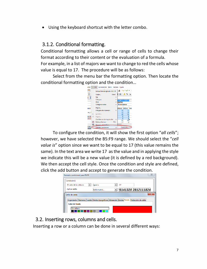
3.1.2. Conditional formatting. Conditional formatting allows a cell or range of cells to change their

format according to their content or the evaluation of a formula.

For example, in a list of majors we want to change to red the cells whose

value is equal to 17. The procedure will be as follows:

Select from the menu bar the formatting option. Then locate the

conditional formatting option and the condition…

To configure the condition, it will show the first option “all cells”;

however, we have selected the B5:F9 range. We should select the “cell

value is” option since we want to be equal to 17 (this value remains the

same). In the text area we write 17 as the value and in applying the style

we indicate this will be a new value (it is defined by a red background).

We then accept the cell style. Once the condition and style are defined,

click the add button and accept to generate the condition.

3.2. Inserting rows, columns and cells. Inserting a row or a column can be done in several different ways:

8

Select the cell where you want to insert the new row, which will then be added on top of the selected cell row. In the column’s case, the new column is added on the left, as shown in Figure 5.

Figure 5 Inserting Row or Column from selected Cell.

From the indicator of the row number or the column letter. Right-click on the row number (1, 2, 3…) where you want to insert the new row keeping in mind that it will be added above the selected row, (see Figure 6). For the column, we right-click on the letter we want to add the row in, which will be added on the left side.

Figure 6 Indicator bar for Rows and Columns.

Go to menu, insert and selecting submenu Rows or Columns.

3.3. Deleting rows, columns and cells. To delete a row or column, once selected, press Supr or Del.

To delete one or several rows or columns completely, you must:

Select the row, by clicking on its number, or the column, by clicking

on its letter.

Right-click on the desired area and selecting the option delete rows

or columns, as appropriate.

9

3.4. Modifying row height and column width. When creating a new spreadsheet, LibreOffice.org Calc will define the

height of its rows by its contents, while the column width stays the same.

So if the contents of a cell are too big to fit into the column width they will

invade the next cell over, as long as it’s empty, otherwise the data will be

hidden.

To modify the height of one row or a group of rows, there are two options:

Directly on the row, on the numbering area, place your cursor on the

union between rows. Your cursor will change into a double-headed

arrow ( ), then press and hold the left button (a message will pop up

showing the actual height) and drag it until you reach the desired

height. For the columns, it’s the same process for their width, (see Figura

7).

Figura 7 Defining row height with the mouse.

The default width for a column is 2.27 centímetros. To modify the

width, you can right-click on any column’s header and pull up the

shortcut menu (see Figure 9) or from the menu bar (see Figure 8). To modify

row height, a similar process is followed.

10

Figure 8 Shortcut menu for column width

Figure 9 Menu bar

Right-click on numbering area for rows

4. Data. In cells, you may type in text, numbers, dates and time; the given data

will show up in two places: on the active cell and in the formula bar, as

shown in Figura 10.

Figura 10 Areas where data is shown.

4.1. Organizing data. To organize a data column in LibreOffice.org Calc, just right-click on one

of the cells in the column you want to organize, then click on one of the

button to sort in ascending order (smallest to largest) or descending

order (largest to smallest) .

You can also organize data by clicking on the menu option

followed by the option , this will make a window pop up as

shown in Figure 11 which shows the name of the column with the active

cell, in this case cell H5. Then we will choose ascending or descending

order.

11

Figure 11. Organizing data.

4.2. Formulas.

Formulas in LibreOffice are expressions that are used to perform

calculations or process values, resulting in a new value. Generally, a

formula is a sequence formed by values taken from other cells. Several

different operations are available to do, such as adding (+), subtracting

(-), dividing(/), and multiplying(*). Formulas will always start with the

equal sign (=). For examples, the sum of several numbers: the syntaxis

is =6+5+3+2 and the result will be shown on the active cell (B2), as shown

in Figure 12

Figure 12 Use of the sum formula.

4.3. Functions

Functions are fomulas incorporated into LibreOffice that execute

calculations using specific values, called arguments, in a determined

12

order or structure. Functions can be used to execute simple or complex

operations.

Functions are expressions predefined by the program or user that

operate with one or more values, cells, ranges and/or functions, and

that puts out a result that will be used to calculate the formula that

contains it; for example, the IF function. The IF function in LibreOffice

Calc evaluates whether a determined condition is met or not, putting a

value to the cell that contains the formula. Function syntaxis =IF(logical

test, value if true, value if false). See Figure 13.

o Logical_test: Is the condition being evaluated, like a cell having a

value that is bigger or smaller than the value of another cell. For

example, we can evaluate if a cell contains the variation

percentage lower than 10.

o Value_if_true: In the case that the logical test comes up TRUE, in

this argument we will specify what value will be shown in the

formula cell. For example, we can write the text “Low

Graduation” for the case that the condition is met. NOTE: the test

must go in quotations.

o Value_if_false: In the opposite case –the condition is not met and

the logical test results FALSE- in this argument we will specify the

value shown in the formula cell. For example, we can write the

text “High Graduation” in the case the condition is not met.

Figure 13 Use of the conditional function IF

Operations’ descriptors - Negation (as in -1) % Percentage

13

^ Exponential * and / Multiplication and division + and – Adding and subtracting & connects two text chains (concatenation) = < > <= >=<> Comparison (equal, less than, more than, less than or equal to,

more than or equal to, different)

5. Graphs A graph is a representation of a series of data, generally numeric, using lines, surfaces or symbols to see the relation between these series of data and thus, facilitate the analysis of a vast amount of information. The use of graphs tells us more than a series of data classified by rows and columns. To create a graph in LibreOffice Calc from the menu bar, it is necessary to

select the Insert option, locating the option right after to select

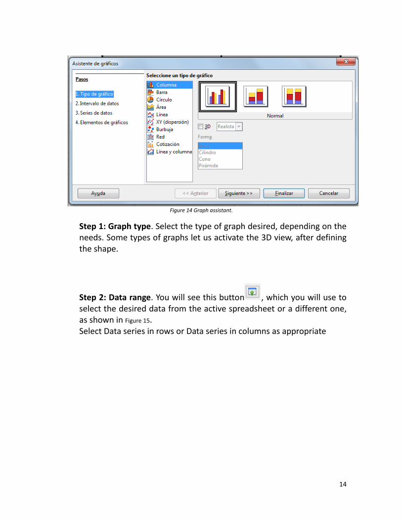
the option from the menu. There are different types of graphs to create in LibreOffice Calc, but this time, we will see how to create a bar graph using the graph assistant (see

Figure 14), there are 4 steps to follow once the assistant implement.

14

Figure 14 Graph assistant.

Step 1: Graph type. Select the type of graph desired, depending on the needs. Some types of graphs let us activate the 3D view, after defining the shape.

Step 2: Data range. You will see this button , which you will use to select the desired data from the active spreadsheet or a different one, as shown in Figure 15. Select Data series in rows or Data series in columns as appropriate

15

Figure 15 Data range

Step 3: Data series. You can add or delete the graph’s data series or change the order in which they’re shown, as indicated in the next figure.

o The previous option allows you to select the cell containing the

tag of the selected series in the Data series list. o The option Categories allows you to select the data tags that will

be shown as categories in each series. Do keep in mind that the

16

Category tags will be applied to all series. Different categories for each series cannot be defined.

Step 4: Graph elements. The last step of the assistant allows us to choose titles, legends and grid configuration as needed (see Figure 16)

Figure 16 Graph format, titles.

Once all previous points have been defined, we click on done to see

our graph.

6. Bibliographic References. LibreOffice The Document Foundation (s/f). LibreOffice Primeros Pasos con Calc Recuperado el 03

septiembre de 2014. de https://www.aplicateca.es/Resources/45c94dcb-1ca4-4523-8133-

e089d0721780/LibreOffice%20-%20Manual%20Usuario%20Calc.pdf.

Help libreoffice org (2014). Instrucciones para utilizar LibreOffice Calc Recuperado el 03 septiembre de 2014

de https://help.libreoffice.org/Calc/Instructions_for_Using_Calc/es