LABORATORIO DE SEÑALES Y...

EPS-UCIIIM 18-IX-07 Departamento de Teoría de Señal y Comunicaciones

LABORATORIO DE SEÑALES Y COMUNICACIONES

Ingeniería Técnica de Telecomunicación

Sistemas de Telecomunicación Apellidos Nombre No de matrícula o DNI Grupo 61 Firma


LABORATORIO DE SEÑALES Y COMUNICACIONES (Tiempo: 2 horas.)

No escriba en las zonas con recuadro grueso

No

Apellidos

1 2

Nombre

3 4

No de matrícula o DNI Grupo________________

Firma:

T

NOTA: En el anexo, al final del examen, están las ayudas de MATLAB para todas las funciones que se utilizan a lo largo de las distintas preguntas. E1.- Se tiene una señal cuyo espectro en frecuencia es el que sigue:

Dicha señal se muestrea a una tasa de 1000 muestras/seg. y se pasa por la siguiente función de matlab (considere que se adquieren el número suficiente de muestras para procesar correctamente la señal).

function y = filtrado(x) b=fir1(16,0.4); y=filter(b,1,x);

a) Dibuje el espectro en hertzios de la señal resultante y(t). Indique claramente la frecuencia superior de la señal resultante. Considere el filtro de caída ideal. (1 punto).

b) Reescriba el código de la función filtrado, tal que agregando SOLO 1 línea y usando la función interp o la función decimate, el espectro de la señal y(t) sea igual al espectro de la señal x(t). Los coeficientes del


filtro FIR no deben ser alterados. Que consideraciones hay que tener con la frecuencia de reconstrucción? (1.5 puntos)

EPS-UCIIIM 18-IX-07 Departamento de Teoría de Señal y Comunicaciones E2.- Se generan 2 ventanas, la primera tipo rectangular de 50 puntos, y la segunda triangular de 101 puntos, ambas de amplitud máxima 1: Rectangular)

Triangular)

Indique cual de los siguientes espectros en frecuencia corresponde a las ventanas anteriormente generadas (0.25 puntos) y razone el motivo de su selección (1 punto): Nota: Los espectros en frecuencia de las ventanas han sido normalizados y centrados entre –π y π. a)

b)

Con estas ventanas se enventana una señal

€

f (x) =sin(x)x

Cuyo espectro en frecuencia es:


Relacione (0.25 punto) y justifique (1 punto) los siguientes espectros resultantes con las ventanas generadas anteriormente. a)

b)

EPS-UCIIIM 18-IX-07 Departamento de Teoría de Señal y Comunicaciones E.3

a) Codifique el programa Matlab bits(M) que genera un vector con M bits estadísticamente independientes y probabilidades 0.5 (ocurrir 1) y 0.5 (ocurrir 0) (1 punto)

b) Suponga que, utilizando el comando x=wave_gen(b, cod_linea, Rb)

generamos un código de línea x con los bits b del apartado anterior. El parámetro cod_linea indica el código de línea utilizado y puede tomar los siguientes valores: ‘unipolar_nrz’, ‘unipolar_rz’ o ‘manchester’. El régimen binario Rb es de 1000 bits/s. Una vez generada la secuencia x para los tres códigos de línea anteriores, se dibuja la densidad espectral de potencia de cada uno de ellos, obteniéndose las siguientes gráficas:

( A )

( B )

( C )

Indique cuál es la gráfica correspondiente a cada código y

justifique su respuesta (1.5 puntos)

EPS-UCIIIM 18-IX-07 Departamento de Teoría de Señal y Comunicaciones E4.- Mediante el siguiente código se pretende simular la transmisión y recepción de un sistema de comunicaciones en banda base:

%% Transmisor SAMPLING_FREQ = 40000; bitsXmuestra = 4; x = sin(2*pi*400*(1:100)/SAMPLING_FREQ); x_pcm = a2d(x, bitsXmuestra); Rb = 1000; x_tx =K* tx(x_pcm,’ unipolar_nrz’,Rb); %% Canal+Receptor gain = 1; BW = 19000; noise_power = [0.01 0.02 0.05 0.1 0.2 0.5 1 2 5 10]; for i = 1:10 y = channel(x_tx,gain,noise_power(i),BW); x_rx_d=rx(y,’ unipolar_nrz’); x_rx = d2a(x_rx_d,bitsXmuestra); pot_ruido(i) = calcula_potencia_ruido(x,x_rx); end plot(noise_power,pot_ruido, '*-');

a) Para K = 2 y noise_power = 1, calcule la Eb/N0 del sistema. (0.5 puntos) b) ¿Qué señales utilizaría para calcular la probabilidad de error del sistema? Justifique su respuesta. Escriba una rutina en Matlab que implemente el cálculo de dicha probabilidad. (0.5 puntos) c) Escriba una rutina en Matlab que implemente la función calcula_potencia_ruido. ¿Qué ruidos afectarán a la señal recibida? (0.5 puntos) d) El código del enunciado devuelve la siguiente gráfica:

Interprete los resultados de la figura. ¿En qué zona predomina el ruido de cuantificación? ¿Y el ruido del canal? ¿Para qué valores de potencia de ruido

EPS-UCIIIM 18-IX-07 Departamento de Teoría de Señal y Comunicaciones del canal considera que merece la pena aumentar el número de bits por muestra para reducir la potencia de la señal de error? (1 punto) Nota: la frecuencia de muestreo es 40 veces superior al régimen binario, por lo que el rango de frecuencias de trabajo es desde –20 KHz hasta 20 KHz.


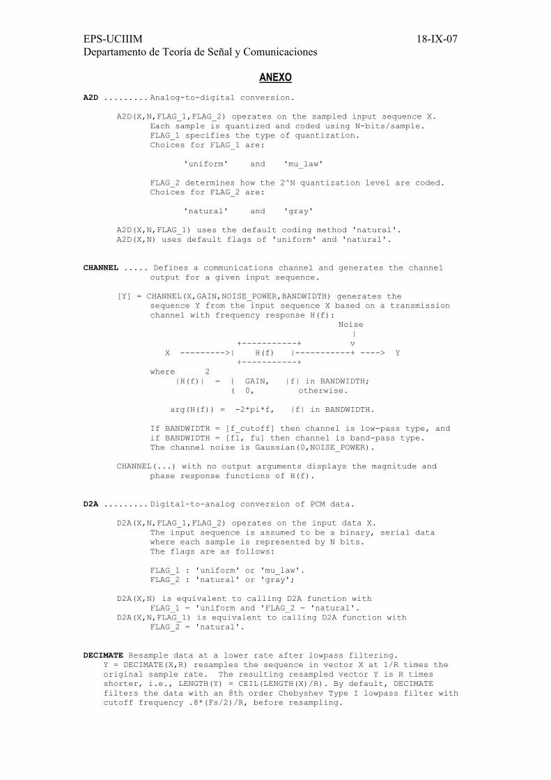
ANEXO A2D ......... Analog-to-digital conversion. A2D(X,N,FLAG_1,FLAG_2) operates on the sampled input sequence X. Each sample is quantized and coded using N-bits/sample. FLAG_1 specifies the type of quantization. Choices for FLAG_1 are: 'uniform' and 'mu_law' FLAG_2 determines how the 2^N quantization level are coded. Choices for FLAG_2 are: 'natural' and 'gray' A2D(X,N,FLAG_1) uses the default coding method 'natural'. A2D(X,N) uses default flags of 'uniform' and 'natural'. CHANNEL ..... Defines a communications channel and generates the channel output for a given input sequence. [Y] = CHANNEL(X,GAIN,NOISE_POWER,BANDWIDTH) generates the sequence Y from the input sequence X based on a transmission channel with frequency response H(f): Noise | +-----------+ v X --------->| H(f) |-----------+ ----> Y +-----------+ where 2 |H(f)| = { GAIN, |f| in BANDWIDTH; ( 0, otherwise. arg(H(f)) = -2*pi*f, |f| in BANDWIDTH. If BANDWIDTH = [f_cutoff] then channel is low-pass type, and if BANDWIDTH = [fl, fu] then channel is band-pass type. The channel noise is Gaussian(0,NOISE_POWER). CHANNEL(...) with no output arguments displays the magnitude and phase response functions of H(f). D2A ......... Digital-to-analog conversion of PCM data. D2A(X,N,FLAG_1,FLAG_2) operates on the input data X. The input sequence is assumed to be a binary, serial data where each sample is represented by N bits. The flags are as follows: FLAG_1 : 'uniform' or 'mu_law'. FLAG_2 : 'natural' or 'gray'; D2A(X,N) is equivalent to calling D2A function with FLAG_1 = 'uniform and 'FLAG_2 = 'natural'. D2A(X,N,FLAG_1) is equivalent to calling D2A function with FLAG_2 = 'natural'. DECIMATE Resample data at a lower rate after lowpass filtering. Y = DECIMATE(X,R) resamples the sequence in vector X at 1/R times the original sample rate. The resulting resampled vector Y is R times shorter, i.e., LENGTH(Y) = CEIL(LENGTH(X)/R). By default, DECIMATE filters the data with an 8th order Chebyshev Type I lowpass filter with cutoff frequency .8*(Fs/2)/R, before resampling.

EPS-UCIIIM 18-IX-07 Departamento de Teoría de Señal y Comunicaciones Y = DECIMATE(X,R,N) uses an N'th order Chebyshev filter. For N greater than 13, DECIMATE will produce a warning regarding the unreliability of the results. See NOTE below. Y = DECIMATE(X,R,'FIR') uses a 30th order FIR filter generated by FIR1(30,1/R) to filter the data. Y = DECIMATE(X,R,N,'FIR') uses an Nth FIR filter. Note: For better results when R is large (i.e., R > 13), it is recommended to break R up into its factors and calling DECIMATE several times. FILTER One-dimensional digital filter. Y = FILTER(B,A,X) filters the data in vector X with the filter described by vectors A and B to create the filtered data Y. The filter is a "Direct Form II Transposed" implementation of the standard difference equation: a(1)*y(n) = b(1)*x(n) + b(2)*x(n-1) + ... + b(nb+1)*x(n-nb) - a(2)*y(n-1) - ... - a(na+1)*y(n-na) If a(1) is not equal to 1, FILTER normalizes the filter coefficients by a(1). FILTER always operates along the first non-singleton dimension, namely dimension 1 for column vectors and non-trivial matrices, and dimension 2 for row vectors. [Y,Zf] = FILTER(B,A,X,Zi) gives access to initial and final conditions, Zi and Zf, of the delays. Zi is a vector of length MAX(LENGTH(A),LENGTH(B))-1, or an array with the leading dimension of size MAX(LENGTH(A),LENGTH(B))-1 and with remaining dimensions matching those of X. FILTER(B,A,X,[],DIM) or FILTER(B,A,X,Zi,DIM) operates along the dimension DIM. FIR1 FIR filter design using the window method. B = FIR1(N,Wn) designs an N'th order lowpass FIR digital filter and returns the filter coefficients in length N+1 vector B. The cut-off frequency Wn must be between 0 < Wn < 1.0, with 1.0 corresponding to half the sample rate. The filter B is real and has linear phase. The normalized gain of the filter at Wn is -6 dB. B = FIR1(N,Wn,'high') designs an N'th order highpass filter. You can also use B = FIR1(N,Wn,'low') to design a lowpass filter. If Wn is a two-element vector, Wn = [W1 W2], FIR1 returns an order N bandpass filter with passband W1 < W < W2. You can also specify B = FIR1(N,Wn,'bandpass'). If Wn = [W1 W2], B = FIR1(N,Wn,'stop') will design a bandstop filter. If Wn is a multi-element vector, Wn = [W1 W2 W3 W4 W5 ... WN], FIR1 returns an order N multiband filter with bands 0 < W < W1, W1 < W < W2, ..., WN < W < 1. B = FIR1(N,Wn,'DC-1') makes the first band a passband. B = FIR1(N,Wn,'DC-0') makes the first band a stopband. B = FIR1(N,Wn,WIN) designs an N-th order FIR filter using the N+1 length vector WIN to window the impulse response. If empty or omitted, FIR1 uses a Hamming window of length N+1.

EPS-UCIIIM 18-IX-07 Departamento de Teoría de Señal y Comunicaciones For a complete list of available windows, see the help for the WINDOW function. KAISER and CHEBWIN can be specified with an optional trailing argument. For example, B = FIR1(N,Wn,kaiser(N+1,4)) uses a Kaiser window with beta=4. B = FIR1(N,Wn,'high',chebwin(N+1,R)) uses a Chebyshev window with R decibels of relative sidelobe attenuation. For filters with a gain other than zero at Fs/2, e.g., highpass and bandstop filters, N must be even. Otherwise, N will be incremented by one. In this case the window length should be specified as N+2. By default, the filter is scaled so the center of the first pass band has magnitude exactly one after windowing. Use a trailing 'noscale' argument to prevent this scaling, e.g. B = FIR1(N,Wn,'noscale'), B = FIR1(N,Wn,'high','noscale'), B = FIR1(N,Wn,wind,'noscale'). You can also specify the scaling explicitly, e.g. FIR1(N,Wn,'scale'), etc. INTERP Resample data at a higher rate using lowpass interpolation. Y = INTERP(X,R) resamples the sequence in vector X at R times the original sample rate. The resulting resampled vector Y is R times longer, LENGTH(Y) = R*LENGTH(X). A symmetric filter, B, allows the original data to pass through unchanged and interpolates between so that the mean square error between them and their ideal values is minimized. Y = INTERP(X,R,L,CUTOFF) allows specification of arguments L and CUTOFF which otherwise default to 4 and .5 respectively. 2*L is the number of original sample values used to perform the interpolation. Ideally L should be less than or equal to 10. The length of B is 2*L*R+1. The signal is assumed to be band limited with cutoff frequency 0 < CUTOFF <= 1.0. [Y,B] = INTERP(X,R,L,CUTOFF) returns the coefficients of the interpolation filter B. RX .......... Receiver function implementation using matched filter. RX( Y, TYPE ) filters the sequence Y using a matched filter structure based on the parameter of TYPE. The output of the filter is then sampled and compared to a threshold (set by the program). Allowed choices for the TYPE parameter are: ------------------------------------------- BASEBAND: 'polar_nrz' 'polar_rz' 'bipolar_rz' 'bipolar_nrz' 'triangle' 'manchester' 'unipolar_nrz' 'unipolar_rz' BAND-PASS: 'ask' 'psk' RX( Y, TYPE, Ti, FLAG_DIFF, B_ORIGINAL ) with the last three being optional parameters that can be specified in any order and combination. Ti ........... : initial sampling instant for detection. Thus filter output will be sampled at Ti, (Ti+Tb), (Ti+2Tb), ... (default: Ti = Tb). FLAG ......... : 'diff' or 'no_diff' specifies differential encoding (default: 'no_diff'). B_ORIGINAL ... : original binary sequence for BER computation (default: BER will not computed). IF THE "Ti" PARAMETER IS NEGATIVE, THEN THE EYE DIAGRAM AT THE FILTER OUTPUT WILL BE DISPLAYED AND YOU CAN INTERACTIVELY SPECIFY "Ti" AND "Threshold" PARAMETERS FOR THE DETECTOR. TX .......... Transmitter function.

EPS-UCIIIM 18-IX-07 Departamento de Teoría de Señal y Comunicaciones TX(B,LINECODE) will generates samples of the waveform for baseband transmission in LINECODE binary signalling format using default value for Rb. Allowed choices for the LINECODE parameter are: -------------------- 'unipolar_nrz' 'unipolar_rz' 'polar_nrz' 'polar_rz' 'bipolar_nrz' 'bipolar_rz' 'manchester' 'triangle' TX(B,MODULATION,fc) generates samples of a band-pass waveform using MODULATION type digital modulation with fc representing carrier frequency. For FSK, fc must be of the form [f0 f1]. Allowed choices for the MODULATION parameter are: ---------------------- 'ask' 'psk' 'fsk' B : binary input sequence. There are two optional flags that specify: Rb : binary data rate (default=BINARY_DATA_RATE) ; FLAG : if FLAG = 'no_diff" no differential encoding (default), if FLAG = 'diff' differential encoding is used. See alse WAVE_GEN, MODULATE, DIFF_ENC. WAVE_GEN .... Generates a waveform coded in binary signalling formats. X = WAVE_GEN(B,LINECODE,Rb) will generate samples of the time waveform X using LINECODE binary signalling format. The allowed selections for the LINECODE parameter are: 'unipolar_nrz' 'unipolar_rz' 'polar_nrz' 'polar_rz' 'bipolar_nrz' 'bipolar_rz' 'manchester' 'triangle' 'nyquist' 'duobinary' 'mod_duobinary' B : binary input sequence. Rb : binary data rate specified in Hz, e.g 2000. The pulse amplitude is set to 1 such that any other scaling has to be done externally. X = WAVE_GEN(B,LINECODE) is the same but uses the default binary data rate specified by the variable "BINARY_DATA_RATE". [X,t] = WAVE_GEN(...) returns sampled values of the waveform, where X is the sampled values and "t" is the vector of time values at which the samples in "X" are defined.

LABORATORIO DE SEÑALES Y...

Documents

Transcript of LABORATORIO DE SEÑALES Y...