DEMANDAS LATENTES Y COMPORTAMIENTO DE VIAJE EN …
49
5 DEMANDAS LATENTES Y COMPORTAMIENTO DE VIAJE EN LA CIUDAD. Medición del impacto de incentivos fiscales en el consumo de vehículos de bajas emisiones y Medición del impacto del uso mixto de suelo y densidad de puntos de interés en el comportamiento de viaje. . POR: JORGE ANDRES URRUTIA MOSQUERA Tesis presentada a la Facultad de Gobierno de la Universidad del Desarrollo para optar al grado de Doctor en Ciencias de la Complejidad Social. PROFESOR GUÍA: Sr. RODRIGO VLADISLAV TRONCOSO OLCHEVSKAIA. Ph. D PROFESORES CO-GUIA: Sr. JORGE ALBERTO FABREGA LOCOA. Ph. D Noviembre, 2019 SANTIAGO DE C HILE
Transcript of DEMANDAS LATENTES Y COMPORTAMIENTO DE VIAJE EN …

5
DEMANDAS LATENTES Y COMPORTAMIENTO DE VIAJE EN LA CIUDAD.
Medición del impacto de incentivos fiscales en el consumo de vehículos de bajas emisiones
y Medición del impacto del uso mixto de suelo y densidad de puntos de interés en el
comportamiento de viaje.
.
POR: JORGE ANDRES URRUTIA MOSQUERA
Tesis presentada a la Facultad de Gobierno de la Universidad del Desarrollo para optar al grado de
Doctor en Ciencias de la Complejidad Social.
PROFESOR GUÍA:
Sr. RODRIGO VLADISLAV TRONCOSO OLCHEVSKAIA. Ph. D
PROFESORES CO-GUIA:
Sr. JORGE ALBERTO FABREGA LOCOA. Ph. D
Noviembre, 2019
SANTIAGO DE C HILE

6
© Se autoriza la reproducción de fragmento de esta obra para fines académicos o de investigación,
siempre que se incluya la referencia bibliográfica.

7
AGRADECIMIENTOS
Parte de esta investigación fue financiada por la vicerrectoría de investigación de la Universidad del
Desarrollo, a través de fondos concursables: Proyecto de investigación interno D2325-1002. 2017 y
por el centro de investigación en Complejidad Social de la Universidad del Desarrollo (CICS-UDD)
Agradezco especialmente a mis supervisores, Jorge Fábrega, Rodrigo Troncoso y Elisabetta Cherchi,
por ser extremadamente accesibles y solidarios en este proceso. Gracias por toda su ayuda e
inspiración.
Agradezco al académico de la Pontificia Universidad Católica de Chile Luis Ignacio Rizzi, por los
consejos recibidos en la etapa inicial de la primera parte de la investigación y al académico Francisco
Martínez Concha, académico de la Universidad de Chile, por sus discusiones, debates y asesorías en
la fase inicial de la segunda parte de esta investigación.
Finalmente, agradezco a mi familia y amigos, en especial a mi esposa Angela por su apoyo a lo largo
de estos años.

8
Contenido RESUMEN ......................................................................................................................................... 9
CAPÍTULO I ................................................................................................................................... 10
1. INTRODUCCIÓN ............................................................................................................... 10
CAPÍTULO II .................................................................................................................................. 13
2. Paper 1. Impact of fiscal incentives in the consumption of low emission vehicles. ........ 13
2.1 Introduction ..................................................................................................................... 14
2.2. Data collection ................................................................................................................. 15
2.2.1 Questionnaire and survey methodology ........................................................................... 15
2.2.2 Descriptive analyses ......................................................................................................... 17
2.3. Stated Choice of type of engine ...................................................................................... 19
2.3.1. Modelling approach ......................................................................................................... 19
2.3.2 Models results .................................................................................................................. 19
2.3.3 Trade-offs between attributes ........................................................................................... 21
2.4. Agreement to subsidy policies ........................................................................................ 21
2.4.1 Modelling approach .......................................................................................................... 21
2.4.2 Models results .................................................................................................................. 22
2.5. Conclusions ...................................................................................................................... 24
2.6. References. ....................................................................................................................... 25
CAPÍTULO III ................................................................................................................................ 30
3. Paper 2. Impact of mixed land use and density of interest points in travel behavior.
Empirical study, the case of Santiago, Chile. ................................................................................ 30
3.1. Introduction ..................................................................................................................... 31
3.2. Literature review ............................................................................................................. 32
3.3. Methods, case and study data ......................................................................................... 34
3.3.1. Methods ..................................................................................................................... 34
3.3.2. Case study and data description ...................................................................................... 37
3.3.3. Description of data and variables .............................................................................. 38
3.4. Results .............................................................................................................................. 39
3.4.1. Land use and zonal location attribute. ............................................................................. 39
3.4.2. Differences between location zones according to attribute density. ............................... 42
3.4.3. Estimation of Poisson regression models .................................................................. 43
3.5. Conclusion ........................................................................................................................ 50
3.6. References ........................................................................................................................ 51

9
RESUMEN
Esta tesis consistió en modelar empíricamente el comportamiento del consumidor en el mercado de
autos y el comportamiento de viaje de los individuos en el ámbito urbano. Para el primer caso, en
particular se evalúa el impacto y la eficacia de diferentes incentivos fiscales y el efecto contrario del
descuento en vehículos convencionales en la compra de vehículos eléctricos e híbridos. La
investigación tiene como foco de análisis los países en vía de desarrollo, para lo cual se toma como
caso de estudio la ciudad de Santiago de Chile y se estimaron modelos elección discreta Logit
Multinomial y Logit Mixto, usando datos de preferencias declaradas.
Respecto al comportamiento de viaje de los usuarios en el ámbito urbano, se investiga el impacto que
genera el uso mixto de suelo y la densidad de puntos de interés en zonas de localización residencial
en el número de viaje esperado para tres dimensiones de viaje (viajes de subsistencia, viajes de
mantenimiento y discrecionales) y tres modos de transporte (viajes en transporte público, particular
o privado y no motorizado). El análisis emplea los datos de viajes más recientes de la encuesta Origen
Destino de Santiago de Chile (EOD-2012) y puntos de interés (atributos zonales de localización)
extraídos de OpenStreetMap.
Esta tesis se desarrolla en formato de dos artículos. El primero titulado “Impact of fiscal incentives
in the consumption of low emission vehicles”, contribuye en la literatura en tres aspectos:
(a) Evalúa el efecto que los subsidios en el precio de compra tienen sobre la preferencia por los
vehículos con bajas emisiones, explícitamente contabilizando el efecto en el ingreso.
(b) Evalúa específicamente el atractivo relativo entre una exención del IVA frente a la exención del
impuesto de compra, así como la devolución del impuesto sobre la renta, para la adopción de
vehículos eléctricos e híbridos.
(c) Propone acciones y recomendaciones concretas de posibles políticas públicas, con una mayor
aceptación entre los compradores potenciales, con el objetivo de reducir la emisión de gases de efecto
invernadero derivados de vehículos de uso privado, obtenidos directamente de los consumidores
potenciales.
El Segundo artículo titulado “Impact of mixed land use and density of interest points in travel
behavior. Empirical study, the case of Santiago, Chile”, ofrece dos aportes a la literatura:
(a) Aporte metodológico, el cual consiste en determinar la distribución de uso de suelo de la ciudad,
así como la distribución de las densidades de puntos de interés (atributos zonales de localización),
con datos abiertos, que luego pueden ser usados para la estimación de modelos de generación de
viajes, replicable en cualquier lugar a diferentes escalas.
(b), Determinar el tipo de impacto que presenta el uso mixto del suelo, así como los atributos zonales
de localización en la generación de viajes en las tres dimensiones para los tres modos de transporte,
siendo un nuevo insumo que se suma a las evidencias empíricas de la literatura y en la posibilidad de
recomendar políticas públicas, contextualizadas a las realidades de las características de las diversas
ciudades de países no desarrollados, bajo la premisa de crecimiento inteligente y el desarrollo
compacto de las ciudades.
10
CAPÍTULO I
1. INTRODUCCIÓN
En esta tesis se responden dos preguntas centrales. La primera respecto al comportamiento de los
consumidores, la cual, se centra en evaluar la adopción de vehículos de bajas emisiones. La segunda
respecto al comportamiento de los usuarios de transporte, enfocada en medir el impacto que tiene el
uso mixto de suelo y la densidad de puntos de interés, en el número esperado de viajes en zonas de
localización residencial.
En el ámbito del comportamiento de los consumidores, se evalúa el impacto de políticas públicas
destinadas a mitigar el efecto del cambio climático y, en específico, a reducir las emisiones de gases
de efecto invernadero producidas por los automóviles privados, para lo cual se estudia la eficacia de
diferentes incentivos fiscales y el efecto contrario del descuento en vehículos convencionales en la
compra de vehículos eléctricos e híbridos. Esta investigación está dirigida específicamente a los
países en desarrollo, tomando como caso particular la ciudad de Santiago de Chile, usando datos de
encuestas de preferencias declaradas.
Respecto al comportamiento de los usuarios, se investiga el impacto que genera tener usos mixtos de
suelo y altas densidades de puntos de interés en zonas de localización residencial en el
comportamiento de viaje. En particular en el número de viajes esperados para tres dimensiones de
viaje (viajes de subsistencia, viajes de mantenimiento y discrecionales) y tres modos de transporte
(viajes en transporte público, particular o privado y no motorizado). El análisis emplea los datos de
viajes más recientes de la encuesta Origen Destino de Santiago de Chile (EOD-2012) y puntos de
interés (atributos zonales de localización) extraídos de OpenStreetMap.
Esta tesis es importante, dada la necesidad contextualizada de explorar, evaluar y recomendar
opciones de políticas que ayuden en la gestión de la mitigación de los niveles de contaminación y
congestión en las ciudades, como es el caso de Santiago de Chile. También es importante porque
permite conocer los impactos que tiene sobre la movilidad y el desarrollo urbano, las regulaciones
sobre uso de suelo, así como la provisión eficiente de servicios públicos, infraestructura de transporte
y escuelas, que pueden ser usados como una hoja de ruta para el diseño de ciudades sustentables y su
marco regulatorio en políticas de uso de suelo y de transporte contextualizadas.
La eficiencia de los incentivos fiscales en la adopción de vehículos de baja contaminación, han sido
estudiados en Horne, Jaccard y Tiedemann (2005); Potoglou y Kanaroglou,(2007); Bjerkan et al.,
(2016), Langbroek et al., (2016), Diamond, (2009); Chandra, Gulati & Kandlikar, (2010); Beresteanu
& Li (2011); Gallagher & Muehlegger, (2011) ; Jenn et al., (2013); Jin et al., (2014); Gass al., (2014);
Fridstrøm et al., (2014), Fridstrøm, (2014); Figenbaum & Kolbenstved, (2013); Assum et al., (2014),
Tal & Nicholas, (2016 ); van Wee y La Croix, (2018). Una revisión reciente se puede encontrar en
Hardman, S. (2019). Sin embargo, ninguno de estos estudios incluye información sobre qué
mecanismo es más atractivo para la operacionalización del subsidio, no consideran también el efecto
de los descuentos ofrecidos por los vendedores de vehículos convencionales para mantener su cuota
de mercado, como una forma de competir con la reducción del precio de los vehículos de baja
contaminación.
Por otro lado, la incidencia del uso mixto de suelo y la densidad de puntos de interés (atributos zonales
de localización), han sido investigado en Ewing & Cervero (2010), Cervero & Duncan,(2003), Crane
& Crepeau, (1998), Handy 1996, McCormick & Shiell (2011), Cao et al (2007), Cervero & Duncan

11
(2006) y Næss, (2005), Chatman (2003), quienes sugieren que ciudades con uso mixto de suelo y una
alta densidad de servicios cerca del lugar de vivienda, inducen el transporte no motorizado y
aumentan la probabilidad de reducir la cantidad de viajes en auto particular. Los análisis y discusiones
toman como referencia los viajes realizados por diferentes modos de transporte, sin considerar el
impacto del uso mixto de suelo, no solo en la partición modal del viaje, sino también, en la partición
modal por dimensión de viaje, como, por ejemplo, indagar sobre las implicancias del uso de suelo en
los viajes de subsistencia, mantenimiento y discrecionales, realizados en transporte público, no
motorizados y en vehículos de uso particular; en cambio Litman & Steele, (2012), Litman, (2010),
Cervero, & Murakami. (2010), McCormack & Shiell (2011), sugieren que el comportamiento de
viaje, puede cambiar al promoverse un uso más eficiente de la capacidad vial existente en cada ciudad,
mejorando las opciones de viaje en transporte público y afectando la propiedad de vehículos de uso
particular. Engebretsen, Næss, & Strand (2018), sugieren que el comportamiento de los viajes es
altamente dependiente del contexto y las características estructurales urbanas. Las investigaciones
anteriores usan como fuente principal datos de encuestas para caracterizar los atributos del entorno,
por lo que se considera que esto imposibilita incluir todos los atributos disponibles en las zonas, que
pueden tener igual o mayor impacto en el análisis. Es aquí que consideramos que caracterizar los
entornos urbanos o zonas basados en datos abiertos como los extraídos con OpenStreetMap, permite
considerar en el análisis todas las opciones disponibles y no sólo las que los usuarios puedan reportar
basados en sus experiencias. Es por eso que esta tesis aporta en llenar los vacíos mencionados
anteriormente y contribuye en dos áreas específicas:
La primera se orienta en establecer acciones y políticas públicas destinadas a mitigar el efecto del
cambio climático y, en particular, a reducir las emisiones de gases de efecto invernadero producidas
por los automóviles privados para lo cual contribuye en tres aspectos:
(a) Evalúa el efecto que los subsidios en el precio de compra tienen sobre la preferencia por los
vehículos con bajas emisiones, explícitamente contabilizando el efecto en el ingreso.
(b) evalúa específicamente el atractivo relativo entre una exención del IVA frente a la exención del
impuesto de compra, así como la devolución del impuesto sobre la renta, para la adopción de
vehículos eléctricos e híbridos.
(c) Propone acciones y recomendaciones concretas de posibles políticas públicas, con una mayor
aceptación entre los compradores potenciales, con el objetivo de reducir la emisión de gases de efecto
invernadero derivados de vehículos de uso privado, obtenidos directamente de los consumidores
potenciales.
La segunda área se orienta a sugerir políticas que permitan el diseño de ciudades sustentables y su
marco regulatorio en uso de suelo y transporte, para lo cual también se contribuye en dos aspectos:
(a) De tipo metodológico, el cual consiste en determinar la distribución de uso de suelo de la ciudad,
así como la distribución de las densidades de puntos de interés (atributos zonales de localización),
con datos abiertos, que luego pueden ser usados para la estimación de modelos de generación de
viajes, replicable en cualquier lugar a diferentes escalas.
(b), consiste en determinar el tipo de impacto que presenta el uso mixto del suelo, así como los
atributos zonales de localización en la generación de viajes en las tres dimensiones para los tres modos
de transporte, siendo un nuevo insumo que se suma a las evidencias empíricas de la literatura y en la
posibilidad de recomendar políticas públicas, contextualizadas a las realidades de las características
de las diversas ciudades de países no desarrollados, bajo la premisa de crecimiento inteligente y el
desarrollo compacto de las ciudades.

12
Los métodos de modelación de comportamiento usados para responder las preguntas sobre el efecto
de los incentivos en la adopción de vehículos de bajas emisiones y sobre el impacto del uso mixto de
suelo y la densidad de puntos de interés sobre el comportamiento de viaje, responden a una
perspectiva común que le dan coherencia a la tesis. Estos consisten en modelar el comportamiento
mediante modelos econométricos de elección discreta, como los modelos lotig multinomial, probit
ordinal, logit mixto y los modelos de regresión de Poisson. Los tres primeros consisten en modelar la
utilidad aleatoria de los individuos, que en esta tesis modela los consumos de vehículos de bajas
emisiones, y el último, modela el recuento de ocurrencia de un evento, en nuestro caso los viajes por
partición modal para tres dimensiones de viaje.
Los principales resultados respecto a los incentivos fiscales indican que los incentivos tienen un efecto
positivo en el consumo de vehículos de bajas emisiones, en particular los resultados revelan que, en
el caso de los vehículos eléctricos, las personas son más sensibles a la autonomía y al incentivo en
comparación con los vehículos convencionales e híbridos. La demanda de vehículos convencionales
es menos sensible al valor del descuento ofrecido por el automóvil en comparación con el valor de
los incentivos presentados para los vehículos eléctricos e híbridos, lo que sugiere que los individuos
presentan una alta sensibilidad a una posible política de subsidio en la compra.
Los resultados del impacto del uso mixto de suelo y la densidad de puntos de interés sobre el
comportamiento de viaje, sugieren que, en el caso de los viajes de subsistencia, por cada 1% de
aumento en una unidad de medida del uso mixto de suelo, el cambio porcentual esperado de los viajes
en transporte público aumenta en un 8,2%. y en un 54,7 % para los viajes no motorizados y disminuye
los viajes particulares en un 24,4%. Para los viajes de mantenimiento el uso mixto de suelo, por cada
1% de aumento en la unidad de medida, manteniendo todas las demás variables constantes, se genera
un aumento del 46,4% y 45,7% en el número de viajes esperados en transporte público y no
motorizado respectivamente, y una disminución del 61,7% en el transporte privado.
Las densidades de puntos de interés que generan mayor impacto en los viajes de mantenimiento son
la densidad de clínicas y hospitales, por cada aumento de 1% en la unidad de medida, manteniendo
las demás variables constante, la magnitud porcentual del impacto en el número de viaje esperado en
transporte público es de 197%; 50,6% en el transporte privado y de 95% en los viajes no motorizados.
Este documento se divide en tres partes, el capítulo 1, es la introducción, los capítulos 2 y 3,
corresponden a dos paper, debido que la presente tesis se ha desarrollado en formato de artículos. En
consecuencia, el capítulo 2 presenta el primer paper titulado “Impact of fiscal incentives in the
consumption of low emission vehicles” y el capítulo 3 presenta el segundo paper titulado “ Impact of
mixed land use and density of points of interest in travel behavior. Empirical study in the case of
Santiago de Chile.”.

13
CAPÍTULO II
2. Paper 1. Impact of fiscal incentives in the consumption of low emission
vehicles.
Jorge Urrutia-Mosqueraa, Elisabetta Cherchib, Jorge Fábregaa, Ángel S. Marreroc
aCentro de investigación en Complejidad Social (CICS). Universidad del Desarrollo. Chile bNewcastle University - School of Engineering, Cassie Building, Newcastle upon Tyne, NE1 7RU, UK cUniversidad de La Laguna, Tenerife, Spain
Abstract
The problem of climate change is forcing countries to establish actions to reduce their emissions. Due
to the high emissions produced by the transportation sector, one of the most implemented policies
worldwide is the economic incentive to purchase electric and hybrid vehicles. Nonetheless, the
adoption of these policies in developing countries is scarce or null and there are no studies that
investigate the impact of economic incentives in the potential demand for low emission vehicles. In
this paper, we aim to cover this gap. In that sense, Chile is a good case-study, for being an emerging
country with the highest level of penetration of electric and hybrid vehicles in the market and with
better import scenarios according to the free trade agreements signed with EE, Europe and Asia.
Using data from a stated choice experiment, specifically built to collect individuals’ preferences for
incentives to low emission vehicles, a mixed logit model was estimated and results used to compute
willingness to pay. In parallel, a contingent evaluation experiment was conducted to elicit individuals’
willingness to pay for two specific policies, involving different ways to provide fiscal incentives:
exemption of VAT versus exemption of purchase tax, and the return of income taxes.
Results show that individuals are more sensitive to autonomy and incentives in the case of electric
vehicles in relation to conventional/hybrid type. Likewise, results show that on the side of incentives,
focused on an exemption from VAT payment and any type of sales and purchase tax 72% of
individuals would be willing to purchase an electric vehicle, and 76% of individuals would be willing
to purchase a hybrid vehicle. These results point to a dormant demand for electric vehicles waiting
for an adequate incentive policy.
Key words: low emission vehicles; economic incentives; policies stated preference; discrete choice
model.

14
2.1 Introduction
The problem of climate change has motivated the nations, member of the Framework Convention
about climate change, to establish actions and public policies aiming to mitigate the effect of climate
change, and in particular, to reduce the greenhouse gas emission produced by private cars. Several
policies have been put in place to stimulate the adoption and use of electric and hybrid vehicles, as a
way to reduce CO2 emission, MP2.5 concentrations and O3 produced by the private use of
automotive ground. Countries such as Norway, United States, Netherlands, France, Japan, South
Korea, Germany, and England, have been the pioneers in testing diverse policies and incentives
including fiscal incentives, and have regularly monitored the diffusion of this market over the last
decades. The situation is very different in the developing countries. In Latin America in particular,
there is no official data on the market share of electric and hybrid vehicles. However, newspapers in
the most important countries of the region (Brazil, Chile, Argentina, Mexico and Colombia) report
that the current market share is of the order of 0.00001%; an insignificant value compared to the
United States and Europe where the lowest market share is of the order of 1,6%. Moreover, in Latin
America, there is no evidence of a political agenda that encourages the adoption of this type of
vehicles, with the exception of Mexico and Costa Rica that have incorporated government initiatives
to exempt tax and VAT payment of electric and hybrid vehicles.
There is a particularly vast literature about the demand for low emission vehicles, a recent review can
be found at Hardman (2019). Several studies, within this vast literature, have explicitly considered
the effect of fiscal incentives in the adoption of electric and hybrid vehicles. These incentives refer
to: subsidies to purchase price (Kwon et al., 2018, Diamond 2009, Jenn et al., 2013, Jin et al., 2014,
Fridstrøm et al., 2014, Assum et al., 2014, Ewing, & Sarigöllü 1998, Ewing, & Sarigöllü 2000,
Bjerkan, et al 2016, Wang et al. 2018), special taxes for electric and hybrid vehicles (Chandra et
al., 2010, Gass et al., 2014, Assum et al., 2014, Tal & Nicholas, 2016, Bjerkan, et al 2016) , gas tax
(Horne, Jaccard, & Tiedemann. 2005, Caulfield et al. 2010, Bjerkan, et al 2016), subsidies to clean
fuels and energy (Kwon et al. 2018, Beresteanu & Li, 2011, Gallagher & Muehlegger, 2011,
Fridstrøm et al., 2014, Fridstrøm, 2014,, Bjerkan, et al 2016), taxes on specific emissions, tax
reduction on the purchase of electric and hybrid vehicles, exemption for electric and hybrid vehicles
from paying roads use fees, discount on the electric tariff, exemption for buyers of electric vehicles
from paying driver's licenses (Brand et al. 201, Wee et al., 2018, Bjerkan, et al 2016, Langbroek, et
al 2016, Wang, Li, & Zhao. 2017), subsidies to charger installation (Kwon et al. 2018, Figenbaum &
Kolbenstved, 2013, Tang & Pan. 2017).
The most important findings from these works indicate that, for potential buyers of low emission
vehicles, the most effective monetary incentives are the fiscal policies that affect car ownership, such
as purchase subsidies and purchase tax reduction; and in the case of vehicle owners, the most effective
monetary incentives are those oriented to the operation and use of the vehicle, such as discounts on
the electric charge rate, exempt from the payment of the fees for using roads and highways to electric
and hybrid vehicles. However, none of these studies investigate which mechanism is more attractive
for the operationalization of the subsidy, they do not consider also the effect of the discounts offered
by conventional vehicle sellers to maintain their markup quota, as a way to compete with the reduction
of the price of low pollution vehicles. We believe that including these elements in the analysis helps
to improve the understanding of consumer behaviour, and to shed light into the fiscal mechanisms
that would be less expensive and more effective for governments, in terms of implementation, and
that positively impact potential demand of low emission vehicles.

15
Since monetary incentives impact the purchase capability, several papers (Potoglou & Kanaroglou,
2007; Sangkapichai & Saphores, 2009; Caulfield et al., 2010; Saarenpää, et al., 2013; Morton et al.,
2017) have tested if income affects the preference for low emission cars. However, none of these
works have explicitly tested for income effect (i.e. if the marginal utility of income change with level
of available income). In the context of low emission vehicles, at our best knowledge, Mabit and
Fosgerau (2011) and Jensen et al. (2014) are the only ones who tested income effect, but they do not
study explicitly the impact of incentives. None of these two studies found a significant income effect,
maybe because their work is applied in Denmark, a wealthy country. Studies on a different choice
context showed that income effect can play an important role in developing countries.
All these studies on electric vehicles have been carried out in developed countries, as these are were
the EV market started. Soto et al. (2018) is the only paper that studies electric vehicles (EV) and
hybrid vehicles (HV) penetration in South America, but this does not include economic incentives
and not income effect. Its main finding indicates that users have a high sensitivity to the purchase
price, the cost of refuelling and the need for a greater presence of fuel stations.
In this work, we aim to contribute to this literature and share some light on the efficacy of different
fiscal incentives and the counter effect of discount on conventional vehicles on the purchase of EV.
This research is targeted specifically to developing countries. The study of fiscal incentives in
developing countries opens up interesting research questions, due to the different level of economic
wealth compared to US and European countries, and consequently different impact on a large segment
of population with low income.
Our study uses data collected in Santiago of Chile, the capital city of the country, which has the largest
private automotive park in Chile. The city of Santiago suffers high levels of pollution especially in
the winter period; at this period restrictions on the circulation of private vehicles are implemented, in
order to reduce the levels of particulate matter (MP2).
The contribution of this investigation lies in three aspects. First, it evaluates the effect that subsidies
on purchase price has on the preference for low emission vehicles, explicitly accounting for income
effect. Second, it specifically evaluates the relative attractiveness between an exemption of VAT
versus exemption of purchase tax, as well as the return of income taxes, for the adoption of electric
and hybrid vehicles. Third, as far as we know, this is the first work of this kind in a country with a
developing economy (like in Latin American).
The rest of the article is organized in the following way. Section 2 discusses the questionnaire and
survey methodology. Section 3 presents the main modeling approach; the structure of the model and
results. Section 4 presents the agreement of two specific subsidy policies on the willingness to buy
low-pollution vehicles. Section 5 presents an integral discussion of results while section 6 summarizes
the main conclusions.
2.2. Data collection
2.2.1 Questionnaire and survey methodology
The data used in this study have been collected in the city of Santiago de Chile that is by far the
largest city in the country. According to 2017 population census, the city houses a total of 6.310.000
people, compared to an overall population in Chile of 17.574.003 As a consequence of that, Santiago
is also the city with the largest use of private vehicles in the country, with around 56% of the trips
16
made by private vehicles, according to figures published in March 2016 by the Civil Identification
Registry.
The questionnaire used to collect the data is articulated in 6 parts. Section 1 included information
about driving frequency (namely the number of times the car is used in a week), driving distance (i.e.
the average daily distance travelled) and the main purpose the vehicle is used for. Section 2 contained
the stated choice experiment and Section 3 information about the attractiveness of the fiscal policies
for low emission vehicles. In section 4, respondents were asked to report their level of agreement or
disagreement with respect to a set of statements on environmental concerns or pro-environmental
inclinations. Finally, Section 5 asked key socio-economic information, such as civil status and age,
education level, size of the household and more importantly the respondent’s income. This paper
focuses on the stated choices and the attractiveness of the fiscal policies.
The stated choice experiment (Section 2) consists of a choice among three alternatives: a conventional
car, an electric vehicle (EV) and a hybrid vehicle (HEV). Since this study focuses on the impact of
incentives, the alternatives were described in terms of purchase price, fiscal incentive offered by the
government (subsidy) for electric and hybrid cars and discount purchase for the conventional vehicles
offered by dealers (these are not subsidies). We also included the driving range, because this has been
found a key attribute in all studies on EV. Pilot tests were conducted initially including also fuel and
electricity costs, charging network and time to charging the vehicles. In the pilot tests respondents
were also explicitly asked to indicate which attributes they considered the most important in their
choices. Results showed that the three attributes purchase price, fiscal incentive/discount and range
were by far the most important. It was then decided to focus the experiment only on these attributes
and describe the other before the experiment and kept them fixed across the choice tasks. Non-
monetary attributes, such as the use of exclusive lanes or free parking spots, were not considered
because this policy will be not realistic for the Chilean context, given that parking is operated by
private companies.
The stated choice experiment was based on a fractional factorial experimental design, allowing for
interactions and quadratic effects. The three attributes included in the design were all with three
levels. The values have been defined based on the real values in the Chilean market. At the time the
survey was carried out, the only electric and hybrid vehicles available in Chile were of average size
(like Nissan Leaf, Yundai Ioniq or Toyota Prius). Purchase price and driving range in the experiment
refer then to an average vehicle.
After completed the stated choice experiment, respondents were also asked (Section 3) to indicate
their willingness (very much, indifferent, very little or I do not know) to buy a hybrid or electric
vehicle for two specific incentive policies:
Policy 1: return of the value paid in the income tax, the difference between the cost of the commercial
value of an electric vehicle versus a conventional one.
Policy 2: exemption of the VAT payment and any other type of tax on the purchase and sale of electric
and hybrid vehicles.
The final survey was run between October and December 2017. Respondents were contacted in their
homes, in workplaces and malls. Participation was on a voluntary base, no incentives were given to
participate. The only condition to be eligible was that respondents need to be 30 years old or more,
own a car or express the intention to buy a car in the next coming months and have a net monthly
income of at least 1020 USD. The final survey included 525 individuals. Of these, 23 were excluded
from the analysis since presented incomplete information due to a technical problem or inconsistent

17
information in the information. Table 1 reports a summary of the main socio-economic characteristics
of the sample and a comparison with the national figures.
2.2.2 Descriptive analyses
This section reports a descriptive analysis of the main information collected in the survey. Table 1
shows a summary of the socio-demographic characteristics of the sample. The sample is not
representative of the population. By design, the largest proportion of individuals in the sample are
young people (between 30 and 40), highly educated, with medium-high income. This condition in the
sample was necessary for the public surveyed to have the purchasing power given the price of the
three types of vehicles compared.
Table 1. Socio-demographic characteristics
Sample Chilean
population*
Gender:
Female 47% 51%
Male 53% 49%
Age
30-40 47% 35%
40-50 24% 22%
50-60 21% 17%
More than 60 8% 26%
Educational level
Incomplete secondary education 4% 18%
Complete secondary education 7% 36%
Incomplete university education 10% 11%
Complete Technical Education 15% 12%
Complete university education 50% 20%
Postgraduate studies 14% 3%
Average monthly net income
678.3 $ US – 1204.7 $ US 29% 55%
1206.1 $ US – $20052.6 US 34% 27%
2054 $ US – 3435.6 $ US 24% 9%
3437.1 $ US – 5789.4 $ US 11% 6%
More than 5789.4 $ US 2% 3%
(*). Source: Own elaboration, from the Socio-economic survey CASEN 2017 and Income supplementary
survey INE 2017
Table 2. Trips characteristics in the sample
Male Female
main purpose the vehicle is used for
% %
Shopping
trips
29,2% 41,08%
Trips to
work
53,66% 43,93
Travel for
leisure
31,78% 35.96%
Long trips 26,79% 29,28%

18
Figures 2 and 3 show the frequency of renewal time and the frequency of vehicle use. 35% of the
sample reported that they change car after 3-4 years of usage and 38% after 5-6 years of usage, which
means that 73% of the sample plan to renovate their vehicles after 3 to 6 years. Figure 7 shows that
the majority of the sample use the vehicle 3-4 times a week, and male tend to use car much more than
female (73% of men versus 59% of women use more than 3 times a week).
Figure 2. Information on renewal time. Figure 3. Information on driving frequency
Figures 4 to 7 show respondents agreements to the two incentive policies tested. Results indicate that
the second policy (exemption of the VAT payment and any other type of tax on the purchase and sale
of electric and hybrid vehicles) seems to be more attractive than the first policy (return of the value
paid in the income tax). 55% of the sample said to be willing to purchase an EV (figure 4), and 63%
(figure 5) a hybrid vehicle if policy 1 is implemented. If the policy is the exemption of VAT payment
and any other type of taxes, instead, 72% (figure 6) of the sample declared to be willing to buy an
electric vehicle and 76% (figure 7) a hybrid vehicle. This result is consistent with the psychological
literature that reports that people prefer an immediate discount compared to a promise of a future
discount.
Figure 4. Level according to Policy 1. EV Figure 5. Level according to Policy 1. HEV
Figure 6. Level according to Policy 2. EV Figure 7. Level according to Policy 2. HEV
7%
37%
36%
20%
[Between 1and 2 years]
[Between 3and 4 years]
[Between 5and 6 years]
[More than 6years]
27%
67%
5%
1%
41%
56%
3% 0%0%
10%
20%
30%
40%
50%
60%
70%
80%
[From 1 to 2
Times per Week]
[From 3 to 4
Times per Week]
[From 5 to 6
Times per Week]
[All week]
Male famele

19
2.3. Stated Choice of type of engine
2.3.1. Modelling approach
For the choice of the type of engine (electric, hybrid or conventional), given the nature of the choice
experiment, where respondents are asked to choose one option over a set of 3 mutually exclusive
alternatives, in multiple scenarios, we used a typical mixed logit model with panel effect (ML) that
allows accounting for intra-observation correlation (Train, 2009) in a discrete choice context. Mixed
Logit models ground on the theory of random utility (McFadden, 1981) that assumes that an
individual q, choosing among a finite set of j alternatives will evaluate all the characteristics of each
alternative and will choose the option that provides her/him the highest utility. The evaluation of the
alternative might be different among individuals depending on their socio-economic characteristics
(SE) and other factors that are unknown to the modeler and/or to the respondents themselves.
Consequently, the utility function for the alternative j in the situation of election t can be written as:
𝑈𝑗𝑞𝑡 = 𝐴𝑆𝐶𝑗 + 𝛽𝑗𝐴𝑇𝑉𝑗𝑞
𝑡 + 𝛿𝑆𝐸𝑞 + 𝛾𝑗(𝐴𝑇𝑉𝑗𝑞𝑡 ∗ 𝑆𝐸𝑞) + 𝜂𝑗𝑞 + 휀𝑗𝑞
𝑡 (1)
Where 𝐴𝑆𝐶𝑗 is the alternative specific constant, 𝛽𝑗 , 𝛿, 𝛾𝑗 are vectors of coefficients associated with
the characteristics of the alternatives (𝐴𝑇𝑉𝑗𝑞𝑡 ) and the socio-economic characteristics (SEq) of the
individuals. 𝜂𝑗𝑞 is a random term distributed Normal Mabit and Fosgerau (2011), with mean zero and
standard deviation 𝜎𝑗, that takes into consideration the panel correlation . 휀𝑗𝑞𝑡 is the error component,
identically and identically distributed EV1 among scenarios and individual. The probability of
choosing the sequence of alternatives j = {𝑗1, … , 𝑗𝑇 } is the integral of logit probability LP( )
conditional on the random term :
𝑃𝑗𝑞 = ∫ 𝐿𝑃(𝜂)𝑑(𝜂) (2)
Where 𝐿𝑃(𝜂), is the conditional mixed logit probability of the choice sequence of the different vehicle
alternatives evaluated at the parameters (𝜂), and it takes the following form:
𝐿𝑃𝑗𝑞 = ∏exp (𝑈𝑗𝑞
𝑡 ( 𝜂𝑗𝑞))
∑ exp (𝑈𝑘𝑞𝑡 ( 𝜂𝑗𝑘))𝑘
𝑡
(3)
2.3.2 Models results
The results of the estimated multinomial Mixed Logit (ML) models are presented in Table 3. The first
two models (ML1 and ML2) differ in the way we tested the incentives. Since the incentive and the
discount are expressed in terms of % to be applied to the purchase price, we firstly tested if what
respondents evaluated was the price minus the amount of the discount/incentive (ML1) or the amount
of the discount/incentive separated from the actual price of the vehicle (ML2).
Results show that model ML2 is significantly superior (both Akaike and BIC measures are lower) to
model ML1, meaning that the economic incentives are not seen only as a net reduction in the purchase
price, but the type of incentive received also has a significant impact in the choice of low emission
20
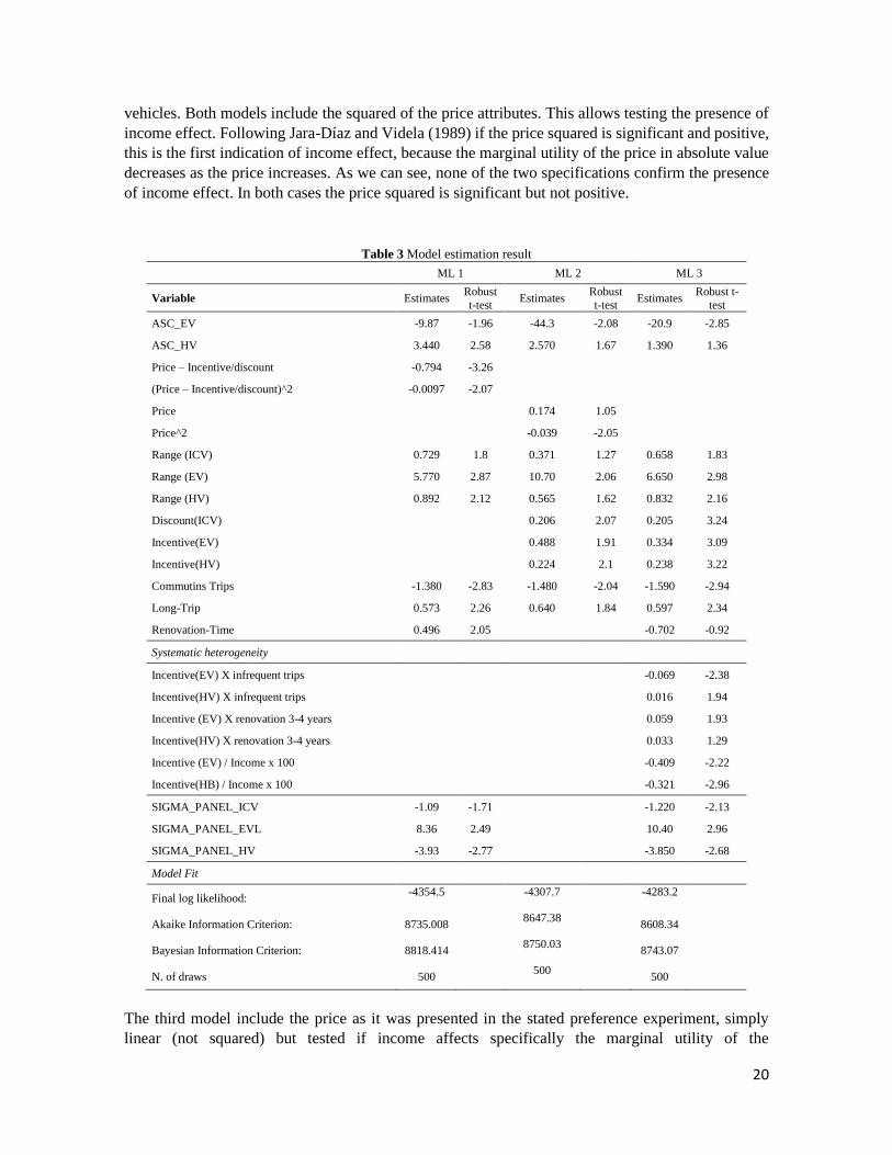
vehicles. Both models include the squared of the price attributes. This allows testing the presence of
income effect. Following Jara-Díaz and Videla (1989) if the price squared is significant and positive,
this is the first indication of income effect, because the marginal utility of the price in absolute value
decreases as the price increases. As we can see, none of the two specifications confirm the presence
of income effect. In both cases the price squared is significant but not positive.
Table 3 Model estimation result
ML 1 ML 2 ML 3
Variable Estimates Robust
t-test Estimates
Robust
t-test Estimates
Robust t-
test
ASC_EV -9.87 -1.96 -44.3 -2.08 -20.9 -2.85
ASC_HV 3.440 2.58 2.570 1.67 1.390 1.36
Price – Incentive/discount -0.794 -3.26
(Price – Incentive/discount)^2 -0.0097 -2.07
Price 0.174 1.05
Price^2 -0.039 -2.05
Range (ICV) 0.729 1.8 0.371 1.27 0.658 1.83
Range (EV) 5.770 2.87 10.70 2.06 6.650 2.98
Range (HV) 0.892 2.12 0.565 1.62 0.832 2.16
Discount(ICV) 0.206 2.07 0.205 3.24
Incentive(EV) 0.488 1.91 0.334 3.09
Incentive(HV) 0.224 2.1 0.238 3.22
Commutins Trips -1.380 -2.83 -1.480 -2.04 -1.590 -2.94
Long-Trip 0.573 2.26 0.640 1.84 0.597 2.34
Renovation-Time 0.496 2.05 -0.702 -0.92
Systematic heterogeneity
Incentive(EV) X infrequent trips -0.069 -2.38
Incentive(HV) X infrequent trips 0.016 1.94
Incentive (EV) X renovation 3-4 years 0.059 1.93
Incentive(HV) X renovation 3-4 years 0.033 1.29
Incentive (EV) / Income x 100 -0.409 -2.22
Incentive(HB) / Income x 100 -0.321 -2.96
SIGMA_PANEL_ICV -1.09 -1.71 -1.220 -2.13
SIGMA_PANEL_EVL 8.36 2.49 10.40 2.96
SIGMA_PANEL_HV -3.93 -2.77 -3.850 -2.68
Model Fit
Final log likelihood: -4354.5
-4307.7
-4283.2
Akaike Information Criterion: 8735.008 8647.38
8608.34
Bayesian Information Criterion: 8818.414 8750.03
8743.07
N. of draws 500 500
500
The third model include the price as it was presented in the stated preference experiment, simply
linear (not squared) but tested if income affects specifically the marginal utility of the

21
discount/incentive. It includes a term that is the discount divided income. This has a negative
coefficient, meaning that the marginal utility for the discount/incentive diminishes as income
increases. The model includes other significant interaction with incentives and discounts. In
particular, respondents who plan to change their car within two years are more sensitive to
incentives/discount. Respondents who travel once or twice a week are less sensitive to incentives to
electric vehicles and more for hybrid vehicles. We note that all the linear effects are significant and
with the right sign. In particular the economic incentive (subsidy of purchase), in case of electric and
hybrid vehicles and the discount in the case of conventional vehicles, have a positive effect. The price
has of course a significant negative effect, while the range a significant positive effect and for the EV
is 10 times higher than for the conventional cars and 8 times higher than for the HV.
2.3.3 Trade-offs between attributes
Table 4 shows the trade-off between attributes computed using model ML2. The trade-off between
an attribute and the price represents the willingness to pay for an improvement in that attribute. Since
our specification includes incentives/discount, the willingness to pay computed refers to the full price
(i.e. before any incentives or discount).
Table 4. Willingness to pay $UD
ML 2
Range (ICV, km/$US) 13,22
Range (EV,km/$US) 21,45
Range (HV,km/$US) 16,87
Long-Trip (Number of trips/$US) 19,16
2.4. Agreement to subsidy policies
2.4.1 Modelling approach
To measure the impact of two specific subsidy policies on the willingness to buy low-pollution
vehicles, we used ordered probit models, where Pq is the probability that individual q is very willing,
indifferent or unwilling to buy a low pollution vehicle,as a function of their SE characteristics. The
model assumes the form:
𝑃𝑞(𝐴 = 1) = Φ (𝐴𝑞(𝑆𝐸𝑞 , 𝜂𝐴)) (4)
𝑃𝑞(𝐴 = 2) = Φ (𝐴𝑞(𝑆𝐸𝑞 , 𝜂𝐴)) − Φ (𝐴𝑞(𝑆𝐸𝑞 , 𝜂𝐴−1))
𝑃𝑞(𝐴 = 3) = 1 − Φ (𝐴𝑞(𝑆𝐸𝑞 , 𝜂𝐴−1))
where A are thresholds defined respectively as: very willing, unwilling, it does not matter.
The two policies tested are: (1) return of the amount paid in the income tax, (2) exemption from VAT
and any other type of tax. Different models were estimated for the willing to buy a BEV and a HEV,
the variable available for purchase and as explanatory variables the socio-economic characteristics of
the individuals and variables associated with the use of the vehicle. The response variable has 4
ordered categories: 1) Very willing, 2) Indifferent, 3) Unwilling.

22
2.4.2 Models results
Table 5 reports the results of the estimation of the Probit models.
2.4.2.1 TPW, Based on the two subsidy policies.
An ordered probit model is estimated to measure to willingness-to-pay for low-pollution vehicles
according to two possible subsidy policies. The policies are (1) the return of the amount paid through
the income tax and (2) the exemption from VAT and any other tax on the purchase and trading sale
of electric and hybrid vehicles. In the model, the response variable (dependent variable) is the degree
of preference for a particular option and the explanatory variables are the socio-economic
characteristics of the individuals and variables associated with the use of the vehicle.
The response variable has three ordered categories. Individuals were asked the following question:
(1) If the subsidy policy is the return of the purchase price difference between an electric or
hybrid vehicle and a conventional vehicle, through the income tax. ¿How willing are you to
pay for this type of vehicle?
(2) If the subsidy policy is an exemption from VAT and any other tax on the purchase and trading
sale of electric and hybrid vehicles. ¿How willing are you to pay for this type of vehicle?
Respondents could answer the question by choosing one of three ordered alternatives: "very much",
"indifferent" and "very little”.
The explanatory variables considered are: marital status, age range, educational level, household
size, gender, income range, as well as variables associated with the use of the vehicle: driving
frequency, vehicle-renewal time and frequency of use according to the purpose of the trip.
Table 5 presents the estimation results of the four ordered probit models estimated (P1_EV, P1_HB,
P2_EV, P2_HB). Each model corresponds to one of the two policies and type of vehicle (electric and
hybrid) evaluated. Row one of Table 5, reports the predicted probability of answering the first
category (very much) for each model. The rest of the rows correspond to the parameters of the
variables considered in the estimation. Column one in each estimated model reports the coefficients
and test statistics (in brackets); column two reports the marginal effects for the first category (very
much); that is, the probabilities: Pr(P1_EV = 1), Pr(P1_HB = 1), Pr(P2_EV = 1) and Pr(P2_HB= 1).
As expected, the predicted probabilities for the first category, both for electric and hybrid vehicles
and the two policies, are consistent with the results of the descriptive statistics reported in Figures 2
to 5. This reinforces the idea that buyers prefer incentives that generate immediate and non-future
payments.
On the other hand, regarding the marital status, the marginal effects of policy one indicate that being
divorced decreases the probability of responding “very much” by 11% for electric vehicles and 3%
for hybrid vehicles. In the case of policy two the effects are similar. Being divorced decreases the
probability of responding “very much” by 3% for electric vehicles and 2.5% for hybrid vehicles.

23
Table 5. Predicted probabilities and marginal effects from the estimated ordered probit model
P1_EV P1_HB P2_EV P2_HB
Variable Value
Marginal
Eff Value
Marginal
Eff Value
Marginal
eff Value
Marginal
Eff
TPW = 1 TPW = 1 TPW = 1 TPW = 1
Predicted Probabilities
Pr (P1_EV = very much) =
0.5462
Pr (P1_HB = very much) =
0.5789
Pr (P2_EV = very much) =
0.7012
Pr (P2_HB = very much) =
0.7354
Civilstatus
Married - - -0,258(-4,7) -4,4% - - -0,109(-1,7) -0,7%
Divorced -0,853 (-3,7) -11% -0,469(-6,2) -7% -0,54( -6,1) -3% -0,528(-5,9) -2,5%
Other - - -1,308(-5.6) --11% - -1,087(-4,5) -3,2%
Widower -0,161(-3,1) -8% -0,285(-2.0) 4,7% -0,536(-2,6) -3,3% -0,305(-1,8) -1,7%
Age
40 to 49 years old 0,106(2,1) 12% 0,218(4,0) 3,3% 3,10(5,2) 2,9% 0,353(5,5) 1,9%
50 to 59 years old - - 0,219(3,5) 4% - - 0,572(7,8) 3%
More of 60 years old - - 0,311(3,4) 5,1% 0,249(2,5) 2,2% 0,492(4,7) 3%
Academic background
Incoplete Sec Edu -0,446(-2,7) -12% 0,606(3,3) 13% -0,420(-2,4) -8,2% 0,859(3,9) 9%
Sec Edu - - 0,590(3,1) 13% - - - -
Incomplete Education T/U -0,655(-4,2) -17% - - -0,640(3,9) -11% 0,371(1,7) 2,4%
Complete Technical
Education -0,308(-2,0) -9% 0,396(2,3) 8% -0,863(-5,3) -13% - -
Universitary Education -0,790(-5,3) -19% 0,660(3.7) 6% -0,825(-5,2) -12% - -
Postgraduate -1,012(-
6,53) -22% 0,384(4,96) 10% -0,998(-6,0) -13% - -
Householdsize Two people 0,524(6,9) 10% 0,373(4.8) 6% 0,768(8,9) 9,4% 0,289(3,4) 3,3%
Three people - - - - - - -
four people 2,73(3,5) 4% - 0,311(3,4) 0,6% -0,158(-1,8) -1,2%
Five people 0,860(7,0) 1% -0,138(-1.8) -1,8% -0,401(-3,9) -2,5% -1,43(-12,0) -4,1%
Six or more people -0,675(-4,6) -6% 0,821(6.5) 2,6% 1,108(7,8) 1,6% 0,547(3,9) 7,6%
Gender -0,855(-5,1) -3,6%
Femele 0,060(2,1) 1% 0,086(2,2) 1,3% 0,210(4,6) 1,7% - -
Driving Frequency
3 to 4 occasions week - - - - - - 0,323(4,0) 1,7%
4 to 5 occasions week - - - - - - - -
More than 5 occasions a
week 0,08(1,8) 1,5% - - - - - -
Jobtrips - -
Frequent -0,08(1,9) -1,6% 0,136(2,3) 2% - - 0,122(2,0) 0,5%
Little - - - - - - -
Never - - - - - - 0,112(1,7) 0%
Shoppingtrips
Frequent 0,194(3,8) 19% 0,285(5,5) 4,4% - - 0,213(3,6) 1%
Little - - 0,017(3,0) 2% - - 0,153(2,1) 0,8%
Never - - - - - - -
Recreationaltrips
Frequent 0,095(197) 9% -0,185(-3,6) -3% - - -0,108(-1,8) -0,6%
Little - - -0,250(-4,1) -4% -0,166(-2,4) --1,3% -0,148(-2,1) -0,9%
Never - - - - - - -
Longtrips
Frequent 0,125(2,5) 2,2% 0,117(2,3) 0,9% 0,179(3,1) 1,4% 0,157(2,6) 0,9%
Little 0,155(3,2) 2,8% 0,184(2,7) 1,8% 0,213(3,8) 1,7% 0,127(2,2) 0,7%
Renewalyears
After 3 to 4 two years of
use -0,156(-2,0) -3,2% - - - - - -
After 5 to 6 two years of
use -0,143(-1,8) -2,9% - - - - - -
After more than 6 years of
use - - - - - - - -
Income_Ct
678,3 $ US – 1204,7 $ US 0,163(1,9) 3% - - 0,289(2,4) 2,3% 0,198(1,6) 1,2%
1206,1 $ US – 20052,6 $U - - - - - - - -
2054 $ US – 3435,6 $ US - - - - - - - -
3437,1 $ US – 5789,4 $US 0,22(2,1) 4,4% - - 0,287(2,0) 2% - -
More than 5789,4 $ US - - - - 0,289(2,2) 2% - -
Model Fit
Final log likelihood: -5725,4834 -5345,0557 -4044,3191 -3803,1845
Akaike Criterio: 11550,97 10782,07 8180,638 7698,369

24
Regarding the age, the marginal effects of policy one for electric vehicles were only significant for
the 40-49 age range. In this range, the policy increases the probability of responding “very much” by
12%. The marginal effects of the policy for hybrid vehicles were significant for the 30-39, 40-49 and
50-59 age ranges. Specifically, in relation to the lowest age range (30-39), being between 40 and 49
and between 50-59 years old increases the probability of responding “very much” by 3.3% and 5.1%,
respectively.
In relation to the income, the marginal effects of policy one indicates that being in the upper class (X
to X US dollars) in relation to lower class (0 to 677 US dollars) increases the probability of responding
“very much” by 1.2% for electric vehicles and 6% for hybrid vehicles. In the case of policy two, the
increase of the probability ranges between 1.2% and 2.2% for electric and hybrid vehicles,
respectively.
These results suggest that policy two, which offers incentives that generate immediately or advance
payments, is the most attractive policy for future buyers.
2.5. Conclusions
This work aimed to shed light on (1) the effect of incentives for EV and HV versus/discount for
conventional one in the choice of the type of engine and (2) the attractiveness of two possible subsidy
policies in the context of Chile. The results reveal that in the case of electric vehicles, individuals are
more sensitive to the autonomy and the incentive in comparison to conventional and hybrid vehicles.
The demand for conventional vehicles is less sensitive to the value of discount offered by automotive
in comparison to the value of incentives presented for electric and hybrid vehicles. This result is
interesting because although there has been a discount campaign by the automotive to capture clients
of high range vehicles to counter the breakthrough of hybrid and electric vehicles a subsidy of the
price of purchase will make the buyers more sensitive to this type of incentive.
In the case of the incentive (Subsidy for EV and HV, discount for ICV), it is of the order of 0.334,
0.238 and 0.205, In brief, individuals present high sensitivity to a possible subsidy policy on the
purchase.
Specifically, in the case of electric vehicles, vehicle buyers are willing to pay between $21,45 US for
one more kilometer of autonomy per load. In the case of hybrid vehicles, individuals are willing to
pay between $16,87 US for more kilometer of autonomy per complete load. In the case of
conventional vehicles between $13,22 US per complete load, taking the results of the second
estimated model.
What is more, it shows that the barriers that most concern in the context of Chile are the absence of
electrolytes with 67%, battery cost with 78% being the highest, the value of the car with 66%, the
type of charging and the autonomy of the vehicles obtained a percentage inferior to 50.
The respondents reported a renewal time after 3 to 4 years of use and 38% after 5 and 6 years of use,
which means that 73% of the surveyed are willing to renovate their vehicles after 3 to 6 years of use;
this information is of great importance. It provides us with the terms in which the impact of the
renewal of the automotive fleet, with low-emission vehicles, would be seen when an eventual subsidy
policy was implemented in the country.
We consider a limitation of the study the size of the sample used, although this reflects the
characteristics of the population, we believe that a bigger sample will allow to capture the
heterogeneity of individuals and validate the interactions that where none significant. Another

25
limitation in the research is the absence of real data of electric and hybrid vehicle sales that would
allow the prediction of the market share with the obtained parameters. The official sales data for low-
emission vehicles that exist in Chile do not report the figures by type of low-emission vehicle. this
lack of discrimination in data makes it impossible to estimate the market share with our estimated
model. These limitations have generated two lines of future work:
The first line of work is aimed at forecasting the market share, under the assumption that the diffusion
of low emission vehicles in Chile follows a diffusion process similar to another country that is
comparable in some relevant socioeconomic aspects. We intend to use their sales data, to estimate the
market share of this type of vehicle in Santiago, Chile.
The before is motivated by two key elements: a) in Chile the demand for electric and hybrid vehicles
is practically zero in the present, thus there is no reference to estimate any prognostic b) the prevailing
need to test the sensibility of the demand in the face of the proposed incentives.
The second line of work is to increase the sample size to identify segments of the population more
sensitive to different types of incentives given the heterogeneity of individuals. This will allow
proposals for targeted incentives to segments of the population.
Expression de appreciation.
The research was financed by the vice-rectory of research of the Universidad del Desarrollo, through
competitive funds. Internal Investigation Project D2325-1002. 2017.
The author thanks Professor Luis Ignacio Rizzi at the transport department of the Pontifical Catholic
University of Chile, for the advices received during the first phases of the research.
2.6. References.
Adnan, N., Nordin, S. M., Rahman, I., Vasant, P. M., & Noor, A. (2017). A comprehensive review
on theoretical framework‐based electric vehicle consumer adoption research. International Journal of
Energy Research, 413, 317-335.
Assum, T., Kolbenstvedt, M., & Figenbaum, E. (2014). The future of electromobility in Norway–
some stakeholder perspectives. TØI report, 1385/2014.
Beresteanu, A., & Li, S. (2011). Gasoline prices, government support, and the demand for hybrid
vehicles in the United States. International Economic Review, 521, 161-182.
Bjerkan, K. Y., Nørbech, T. E., & Nordtømme, M. E. (2016). Incentives for promoting battery electric
vehicle (BEV) adoption in Norway. Transportation Research Part D: Transport and Environment, 43,
169-180.
Brand, C., Anable, J., & Tran, M. (2013). Accelerating the transformation to a low carbon passenger
transport system: The role of car purchase taxes, feebates, road taxes and scrappage incentives in the
UK.Transportation Research Part A: Policy and Practice, 49, 132-148.
Bunch, D. S., Bradley, M., Golob, T. F., Kitamura, R., & Occhiuzzo, G. P. (1993). Demand for clean-
fuel vehicles in California: a discrete-choice stated preference pilot project. Transportation Research
Part A: Policy and Practice, 273, 237-253.

26
Caulfield, B., Farrell, S., & McMahon, B. (2010). Examining individuals preferences for hybrid
electric and alternatively fuelled vehicles. Transport Policy, 176, 381-387.
Chandra, A., Gulati, S., & Kandlikar, M. (2010). Green drivers or free riders? An analysis of tax
rebates for hybrid vehicles. Journal of Environmental Economics and management, 602, 78-93.
Cherchi, E., & J. de D. Ortúzar, J. (2006). On fitting mode specific constants in the presence of new
options in RP/SP models. Transportation Research Part A: Policy and Practice, 401, 1-18.
Clinton, B., Brown, A., Davidson, C., & Steinberg, D. (2015). Impact of direct financial incentives
in the emerging battery electric vehicle market: A preliminary analysis. National Renewable Energy
Laboratory, Department of Economics, University of Colorado–Boulder.
Diamond, D. (2009). The impact of government incentives for hybrid-electric vehicles: Evidence
from US states. Energy Policy, 373, 972-983.
Ewing, G. O., & Sarigöllü, E. (1998). Car fuel-type choice under travel demand management and
economic incentives. Transportation Research Part D: Transport and Environment, 36, 429-444.
Ewing, G., & Sarigöllü, E. (2000). Assessing consumer preferences for clean-fuel vehicles: A discrete
choice experiment. Journal of public policy & marketing, 191, 106-118.
Figenbaum, E., & Kolbenstvedt, M. (2013). Electromobility in Norway-experiences and
opportunities with Electric Vehicles No. 1281/2013.
Vegard Østli, Kjell Werner Johansen & Yin-yen Tseng. (2014). Vehicle or fuel taxation for
greenhouse gas abatement? An empirical modelling. Transmod. Transportøkonomisk institutt (TØI).
Working paper 50661.
Fridstrøm, L., & Alfsen, K. (2014). Norway's path to sustainable transport. TØI rapport, 1321, 2014.
Gallagher, K. S., & Muehlegger, E. (2011). Giving green to get green? Incentives and consumer
adoption of hybrid vehicle technology. Journal of Environmental Economics and management, 611,
1-15.
Gass, V., Schmidt, J., & Schmid, E. (2014). Analysis of alternative policy instruments to promote
electric vehicles in Austria. Renewable Energy, 61, 96-101.
Hackbarth, A., & Madlener, R. (2013). Consumer preferences for alternative fuel vehicles: A discrete
choice analysis. Transportation Research Part D: Transport and Environment, 25, 5-17.
Hardman, S. (2019). Understanding the impact of reoccurring and non-financial incentives on plug-
in electric vehicle adoption–A review. Transportation Research Part A: Policy and Practice, 119, 1-
14.
Hidrue, M. K., Parsons, G. R., Kempton, W., & Gardner, M. P. (2011). Willingness to pay for electric
vehicles and their attributes. Resource and Energy Economics, 333, 686-705.
Hoen, A., & Koetse, M. J. (2014). A choice experiment on alternative fuel vehicle preferences of
private car owners in the Netherlands. Transportation Research Part A: Policy and Practice, 61, 199-
215.

27
Horne, M., Jaccard, M., & Tiedemann, K. (2005). Improving behavioral realism in hybrid energy-
economy models using discrete choice studies of personal transportation decisions. Energy
Economics, 271, 59-77.
Instituto Nacional de Estadística (INE). Supplementary Income Survey 2017.
Instituto Nacional de Estadística (INE). Yearbook, vehicular park in Circulation 2017.
Jara-Díaz, S. R., & Videla, J. (1989). Detection of income effect in mode choice: theory and
application. Transportation Research Part B: Methodological, 236, 393-400.
Jenn, A., Azevedo, I. L., & Ferreira, P. (2013). The impact of federal incentives on the adoption of
hybrid electric vehicles in the United States. Energy Economics, 40, 936-942.
Jensen, A. F., Cherchi, E., & de Dios Ortúzar, J. (2014). A long panel survey to elicit variation in
preferences and attitudes in the choice of electric vehicles. Transportation, 41(5), 973-993.
Jensen, A. F., Cherchi, E., & Mabit, S. L. (2013). On the stability of preferences and attitudes before
and after experiencing an electric vehicle. Transportation Research Part D: Transport and
Environment, 25, 24-32.
Jin, L., Searle, S., & Lutsey, N. (2014). Evaluation of state-level US electric vehicle incentives. The
International Council on Clean Transportation.
Krause, R. M., Lane, B. W., Carley, S., & Graham, J. D. (2016). Assessing demand by urban
consumers for plug-in electric vehicles under future cost and technological scenarios. International
Journal of Sustainable Transportation, 108, 742-751.
Krupa, J. S., Rizzo, D. M., Eppstein, M. J., Lanute, D. B., Gaalema, D. E., Lakkaraju, K., &
Warrender, C. E. (2014). Analysis of a consumer survey on plug-in hybrid electric vehicles.
Transportation Research Part A: Policy and Practice, 64, 14-31.
Kwon, Y., Son, S., & Jang, K. (2018). Evaluation of incentive policies for electric vehicles: An
experimental study on Jeju Island. Transportation Research Part A: Policy and Practice, 116, 404-
412.
Lai, I. K., Liu, Y., Sun, X., Zhang, H., & Xu, W. (2015). Factors influencing the behavioural intention
towards full electric vehicles: An empirical study in Macau. Sustainability, 79, 12564-12585.
Lane, B., & Potter, S. (2007). The adoption of cleaner vehicles in the UK: exploring the consumer
attitude–action gap. Journal of cleaner production, 15(11-12), 1085-1092.
Langbroek, J. H., Franklin, J. P., & Susilo, Y. O. (2016). The effect of policy incentives on electric
vehicle adoption. Energy Policy, 94, 94-103.
Lieven, T. (2015). Policy measures to promote electric mobility–A global perspective. Transportation
Research Part A: Policy and Practice, 82, 78-93.

28
McFadden, D., 1981. Econometric models of probabilistic choice. In: Manski, C.F., McFadden, D.
(Eds.), Structural Analysis of Discrete Data with Econometric Applications. The MIT Press,
Cambridge, Massachusetts.
Mersky, A. C., Sprei, F., Samaras, C., & Qian, Z. S. (2016). Effectiveness of incentives on electric
vehicle adoption in Norway. Transportation Research Part D: Transport and Environment, 46, 56-68.
Ministerio de Desarrollo Social (2014). Resultados Encuesta Casen 2017.
Morton, C., Anable, J., & Brand, C. (2014). Policy making under uncertainty in electric vehicle
demand. Proceedings of the ICE-Energy, 1673, 125-138.
Morton, C., Lovelace, R., & Anable, J. (2017). Exploring the effect of local transport policies on the
adoption of low emission vehicles: Evidence from the London Congestion Charge and Hybrid
Electric Vehicles. Transport Policy, 60, 34-46
Ortúzar, J. de D., Willumsen, L.G., 1994. Modelling Transport, 2nd Edition. Wiley, Chichester.
Peters, A., & Dütschke, E. (2014). How do consumers perceive electric vehicles? A comparison of
German consumer groups. Journal of Environmental Policy & Planning, 163, 359-377.
Plötz, P., Schneider, U., Globisch, J., & Dütschke, E. (2014). Who will buy electric vehicles?
Identifying early adopters in Germany. Transportation Research Part A: Policy and Practice, 67, 96-
109.
Potoglou, D., & Kanaroglou, P. S. (2007). Household demand and willingness to pay for clean
vehicles. Transportation Research Part D: Transport and Environment, 124, 264-274.
Qiu, Y. Q., Zhou, P., & Sun, H. C. (2019). Assessing the effectiveness of city-level electric vehicle
policies in China. Energy Policy, 130, 22-31.
Rezvani, Z., Jansson, J., & Bodin, J. (2015). Advances in consumer electric vehicle adoption research:
A review and research agenda. Transportation research part D: transport and environment, 34, 122-
136.
Rietmann, N., & Lieven, T. (2019). How policy measures succeeded to promote electric mobility–
Worldwide review and outlook. Journal of Cleaner Production, 206, 66-75.
Rudolph, C. (2016). ¿Cómo pueden los incentivos para automóviles eléctricos afectar las decisiones
de compra ?. Política de Transporte, 52 , 113-120.
Saarenpää, J., Kolehmainen, M., & Niska, H. (2013). Geodemographic analysis and estimation of
early plug-in hybrid electric vehicle adoption. Applied Energy, 107, 456-464.
Sangkapichai, M., & Saphores, J. D. (2009). Why are Californians interested in hybrid cars?. Journal
of environmental planning and management, 521, 79-96.
Santos, G., & Davies, H. (2019). Incentives for quick penetration of electric vehicles in five European
countries: Perceptions from experts and stakeholders. Transportation Research Part A: Policy and
Practice. …. Number and page!

29
SECTRA (2015). Encuesta origen destino de viajes 2012. Technical report, Ministerio de Transportes
y Telecomunicaciones, Santiago, Chile.
Sierzchula, W., Bakker, S., Maat, K., & van Wee, B. (2014). The influence of financial incentives
and other socio-economic factors on electric vehicle adoption. Energy Policy, 68, 183-194.
Sovacool, B. K., & Hirsh, R. F. (2009). Beyond batteries: An examination of the benefits and barriers
to plug-in hybrid electric vehicles (PHEVs) and a vehicle-to-grid (V2G) transition. Energy Policy,
373, 1095-1103.
Tal, G., & Nicholas, M. (2016). Exploring the impact of the federal tax credit on the plug-in vehicle
market. Transportation Research Record, 2572 95-102.
Train, K.E., 2009. Discrete Choice Methods with Simulation. Cambridge University Press.
Wang, N., Pan, H., & Zheng, W. (2017). Assessment of the incentives on electric vehicle promotion
in China. Transportation Research Part A: Policy and Practice, 101, 177-189.
Wang, N., Tang, L., & Pan, H. (2017). Effectiveness of policy incentives on electric vehicle
acceptance in China: A discrete choice analysis. Transportation Research Part A: Policy and
Practice, 105, 210-218.
Wang, N., Tang, L., & Pan, H. (2019). A global comparison and assessment of incentive policy on
electric vehicle promotion. Sustainable Cities and Society, 44, 597-603.
Wang, N., Tang, L., & Pan, H. (2019). A global comparison and assessment of incentive policy on
electric vehicle promotion. Sustainable Cities and Society, 44, 597-603.
Wang, S., Fan, J., Zhao, D., Yang, S., & Fu, Y. (2016). Predicting consumers’ intention to adopt
hybrid electric vehicles: using an extended version of the theory of planned behavior
model. Transportation, 431, 123-143.
Wang, S., Li, J., & Zhao, D. (2017). The impact of policy measures on consumer intention to adopt
electric vehicles: Evidence from China. Transportation Research Part A: Policy and Practice, 105,
14-26.
Wang, S., Wang, J., Li, J., Wang, J., & Liang, L. (2018). Policy implications for promoting the
adoption of electric vehicles: Do consumer’s knowledge, perceived risk and financial incentive policy
matter?. Transportation Research Part A: Policy and Practice, 117, 58-69.
Wee, S., Coffman, M., & La Croix, S. (2018). Do electric vehicle incentives matter? Evidence from
the 50 US states. Research Policy, 479, 1601-1610.
Zhang, X., Xie, J., Rao, R., & Liang, Y. (2014). Policy incentives for the adoption of electric vehicles
across countries. Sustainability, 611, 8056-8078.
Ziegler, A. (2012). Individual characteristics and stated preferences for alternative energy sources
and propulsion technologies in vehicles: A discrete choice analysis for Germany. Transportation
Research Part A: Policy and Practice, 468, 1372-1385.

30
CAPÍTULO III
3. Paper 2. Impact of mixed land use and density of interest points in travel behavior.
Empirical study, the case of Santiago, Chile.
Jorge Urrutia-Mosqueraa, Rodrigo Troncosob , Luz Ángela Flórez-Calderónc
aComplexity Research Center (CICS), Universidad del Desarrollo, Santiago de Chile bFaculty of Government, Universidad del Desarrollo, Santiago de Chile
cDepartment of Transportation and Logistics Engineering, Pontificia Universidad Católica de Chile
Abstract
In this research, we studied how mixed land use and the density of points of interest affect travel
behavior. The analysis considers three travel dimensions (subsistence travel, maintenance, and
discretionary travel) and three modes of transport (travel by public, private and non-motorized
transport), in areas with different mixed land use and density of points of interest. The analysis uses
the most recent travel data from the Origin-Destination of Santiago City (EOD-2012) survey and
points of interest (zonal location attributes) extracted from OpenStreetMap. The Poisson models
estimated show that, for the three dimensions of trips and the three means of transport, the mixed land
use is the one that generates the greatest marginal effect on travel behavior, compared to the density
of points of interest considered in the analysis. The results of the models also indicate that, in the case
of subsistence travel, if you want to encourage public and non-motorized transport, urban and
transport decisions should be aimed at strengthening metro and bike stations, as well as offering
higher kindergarten density. In the case of maintenance trips, the attributes with the greatest marginal
effect on these types of trips for the three modes of transportation are the points of interest associated
with health. For discretionary trips, the attributes with the greatest marginal effect are those associated
with infrastructure, and to a lesser extent those associated with green areas. These findings are
important considerations for the design of sustainable cities and their regulatory framework in land
use and transportation policies.
Key words: Mixed land use, Density of points of interest, Travel behavior, Poisson models.

31
3.1. Introduction
The regulations that define the use of land for different areas of a city, as well as the regulations on
transport planning policies, interact with each other, impacting the number of trips generated and
attracted for modal partition between different areas or city zones, inducing patterns of travel behavior
in the inhabitants. The impact on travel generated by the use of land in a specific area, is largely
determined by the uniform and mixed or unique distribution of land use defined for each zone of a
city (For example: equal proportion of residential, commercial use , industrial, state, green areas, etc.,
or only uses of residential, commercial or industrial type), and by the presence in greater or lesser
degree of density of points of interest in the zone, related to aspects such as transportation, health,
education, commerce, employment and open spaces (example: density of different access roads, bus
stops, subway stations, school density, density of clinics, hospitals, density of banking services,
business density, open spaces, etc.), understood as zone attributes. International evidence on land use
and travel behavior reveals that mobility challenges, as well as the coordination of transport with land
use in developing countries, are significantly different compared to the richest and most developed
countries.
In the latter, land use policies are aimed at encouraging the use of public transport, non-motorized
trips and discouraging the use of private vehicles, in line with the intelligent growth and compact
development of cities. After reviewing the literature on land use and travel behavior, the present study
reports on the impacts of mixed land use and the density of localization attributes on the of trips
generated by public, private and non-motorized transportation in a developing country, taking as a
case study, the city of Santiago of Chile, for three dimensions of travel, defined as: a) subsistence
travel (work and education trips), b) maintenance trips (travel for purchases, personal procedures,
medical visits, etc.), c) discretionary trips (trips related to leisure, social or personal reasons), taking
as an analysis unit the administrative political division (Communes), using mobility data from the
Survey Origin-Destination (EOD2012), as well as land use data and zonal attributes extracted from
OpenStreetMap (OSMs), using ArcGIS software version 10.4.1 (geographic information system),
with Wgs84 coordinate system, South Zone 19S, at the communal level. International evidence on
the impact of mixed land use on public transportation indicates that travel behavior can change by
promoting efficient use of existing road capacity, improving travel options, affecting the property and
the rate of motorization (Litman & Steele, 2012 and Litman, 2010). Cervero & Duncan (2003) and
Crane & Crepeau (1998), also indicate that one of the positive effects of having well-connected
streets, as well as mixed land use and retail activities closer to residences, induces non-motorized
transport. It is also reported that using the land efficiently reduces dependence on the private vehicle,
contributing to reducing user transaction costs, in terms of shortening the distances travelled and
travel times for the realization of daily activities (Litman, 2016).
Our results for the Chilean capital, indicates that, for the subsistence travel dimension (work and
study trips), the mixed use of land positively impacts the trips generated in public and non-motorized
transport, and negatively the travel by private transport. In the case of mixed land use, for every 1%
increase in the value of the entropy index (a proxy for measuring the distribution of mixed land use),
the expected percentage change of the total trips generated by public transport is 8,2% controlling for
the other variable. The expected percentage change in total trips generated by private cars decreases
by 24,4%, and the expected percentage change in the total of trips by non-motorized subsistence
increases by 54.7% for every 1% increase in the value of the entropy index, controlling for the other
variables. In the case of the dimension of maintenance trips (trips for purchases, personal procedures,
medical visits, etc.), the mixed use of land, also impacts positively the trips generated by public and

32
non-motorized transport, and in a negative way the private trips. For every 1% increase in the value
of the entropy index, the expected percentage change of trips generated by public transport is 46,4%,
controlling for the other variables; the expected percentage change in trips generated by private cars
decreases by 61,7%, and the expected percentage change in non-motorized subsistence trips increases
by 45.7% for every 1% increase in the value of the entropy index, controlling for the other variables.
Regarding the dimension of discretionary trips (trips referring to leisure, social or personal reasons),
the mixed use of land, positively impacts public transport trips and proved to be non-significant for
trips in private vehicles and not motorized. In the case of public transport, for every 1% increase in
the value of the entropy index, the expected percentage change in trips generated by public transport
is 114%, controlling for the other variables.
The results for the other variables, referred to the density of points of interest (the zonal attributes),
indicate that the attributes that generate large impacts on the percentage change factor in trips made
by each mode, for the three dimensions of trips analyzed, are the attributes associated with transport,
accessibility and education. These results suggest that impacting travel behavior, especially non-
motorized trips, and public transport, depends not only on the existing transport infrastructure but
also on factors associated with the spatial distribution of goods and services in the different location
residential areas: The uniform and mixed distribution of land, which ultimately is what allows
individuals and households access to goods and services near residential environments.
The contribution of this research lies in two aspects; The first is of a methodological type, which
consists in determining the distribution of land use in the city, the distribution of the densities of
points of interest (zonal location attributes), with Open Access data, which can then be used for the
estimation of travel generation models, replicable anywhere in different scales; by the time of the
literature review, the vast majority of the works characterize the use of land and zonal attributes
through data from surveys.
The second aspect consists in determining the type of impact that mixed land use presents as well as
zonal attributes of residential location, in the generation of trips in public, private and non-motorized
transport, in three dimensions of trips. As far as we know, this is the first such work that has been
realized in a developing country that considers these three dimensions of travel, being a new input
that adds to the empirical evidence of literature and the possibility of recommending public policies,
contextualized to the realities of the characteristics of the various cities of developing countries, under
the premise of smart growth and the compact development of cities.
3.2. Literature review
From the point of view of transport planning policies and intelligent urban development, the mixed
land use, as well as the density of points of interest that shape the tangible zonal attributes in different
urban areas, play a transcendental role in the generation or attraction of trips by modal partition,
which, in turn, determine the travel behavior of a city, generating different mobility cultures.
Consequently, the papers that study the impact of mixed land use and the density of points of interest
in travel behavior have produced results in different directions depending on the type of country
analyzed (developed or developing country), and according to the characteristics of the city. Most
studies in the area suggest that there are three key factors that impact travel behavior: (1) The
configuration of land use, (2) accessibility and (3) the characteristics of the environment, this last
33
factor being under discussion and study, given that different empirical findings report positive and
negative effects according to the mode of travel analyzed.
Regarding the effect of the land use configuration (a type of use, or mixed use), on the travel behavior,
the works of Ewing & Cervero (2010), Cervero & Duncan (2003), Crane & Crepeau, ( 1998), Handy
(1996), McCormick & Shiell (2011), Cao et al (2007), Cervero & Duncan (2006) and Næss, 2005,
Chatman (2003), made in countries like USA, United Kingdom, Canada and Holland, suggest that
cities with mixed land use and a high density of services near the place of housing, induce non-
motorized transport and increase the probability of reducing the amount of trips by private car. In the
analysis and discussions taken as reference, the trips made by different mode of transport, without
considering the impact of the mixed use of land, not only in the modal partition of the trip, but also,
in the modal partition by travel dimension, such as the implications of land use in subsistence,
maintenance and discretionary trips, carried out by public transport, non-motorized and by vehicles
for private use. Litman & Steele, (2012), Litman (2010), Cervero & Murakami (2010), McCormack
& Shiell (2011), place special emphasis on accessibility; they suggest that travel behavior may change
by promoting more efficient use of existing road capacity in each city, improving travel options by
public transport and affecting the ownership of private vehicles.
Another important effect of accessibility in travel behavior, indicates that cities with denser road
network environments and better local accessibility, are negatively associated with the use of private
vehicles, since the traffic effect modulates the use of private vehicle Næss (2005). The
characterization of accessibility in most cases is based on user experiences, through established
preference surveys, this excludes other available accessibility alternatives, which are not considered
by users, because each user of public transport, not motorized or for private use, normally considers
the options that he uses frequently, discarding other options, of equal or better effective mobility.
We consider that characterizing urban environments or areas based on open data such as those
extracted with OpenStreetMap, allows us to consider in the analysis all available options and not only
those that users can report based on their experience.
Regarding the characteristics of the neighborhood, Cao, Handy & Mokhtarian (2006), indicate that
the characteristics of the neighborhood impact the frequency of travel by foot and that the commercial
characteristics in each neighborhood facilitate shopping trips by foot. Frank et al (2007), indicate that
the travel distance of private vehicles is explained by the neighborhood selection and individual
preferences, controlling for demographic variables, therefore, the attitudinal predisposition for the
type of neighborhood, such as real characteristics of the built environment in which one lives,
influence the choice of walking and the distances travelled. Engebretsen, Næss, & Strand (2018),
report that the magnitude of the influence of various urban structural features on travel behavior is
highly context dependent and Cao et al. (2009), finds that both the preferences of individuals and the
characteristics of the built environment explain the variation in non-motorized trips, compared to
other types of travel. Bagley & Mokhtarian (2002), report that the type of residential location had
little impact on travel demand and that travel variable are generally inelastic in regards to the change
in measures of the built environment.
Finally, Ewing & Cervero (2010), through a meta-analysis study, reveal four important findings: (1)
In most cases, travel behavior tends to be inelastic depending on the measurements of the built and
elastic environment regarding the change in land use and accessibility conditions. Regarding the
change in land use and accessibility conditions, (2) the number of miles travelled by private vehicles
are strongly related to the measures of accessibility to destinations and the design variables of the
street network, ( 3) walking is strongly related to measures of diversity of land use or mixed land use

34
and the number of destinations within walking distance and (4) the use of buses and trains are related
to proximity to traffic and the design variables of the street network.
The main findings of the empirical studies of specialized literature reported in the previous paragraphs
confirm a consensus on the impact of mixed land use on travel behavior, however, despite the existing
consensus, the reported works do not investigate these impacts in the three dimensions of trips and
for the three modes of transport defined. Another lacking element identified is the fact that the results
of the impact of the characteristics of the environment, the points of interest, or the zonal attributes
of residential location as they are called by the different sources, are heterogeneous and vary
depending on the characteristics of the city and the context, accessibility conditions, the
characteristics or attributes of the zones, the specification of the variables in the model, and the types
of data analyzed. Consequently, we identify some gaps as: (1) All reported studies use data from
declared preference surveys to characterize neighborhoods, although it is a widely used and validated
instrument in the literature, it permeates a high degree of subjectivity of respondents, excluding of
the analysis, other options of attributes available in each zone, which may be equally or better than
those informed by the respondents, regarding to its impact on the three dimensional of trip, for the
three modes of transport.
(2) All studies report a single travel dimension, this does not allow to examine the differences in the
impact on travel behavior of the same variable that may be the cause of the heterogeneity of reported
results, which is why this study aims to fill the gap in the literature by examining the impact of mixed
land use and the density of points of interest in the three dimensions of travel (Subsistence,
maintenance and discretionary). Our hypotheses are:
H1 - The mixed use of land has a positive impact on the expected number of trips by public and non-
motorized transport for the three dimensions of trips and a negative impact on the trips expected on
private transport.
H2- The impact of the density of the points of interest associated with transport is different in the
three travel dimensions and the three modes of transport, and the impact of the density of points of
interest associated with each travel dimension is different in the three modes of transport.
3.3. Methods, case and study data
3.3.1. Methods
According to Handy (1996), travel behavior studies contributes to understanding how and why zonal
attributes are linked to travel and help quantify the potential impact of land use on travel generated in
different trips generation zones, the number of daily trips made by people and/or the home, the modes
used, the duration, as well as the distances travelled.
Given the nature of the trip count and the adjustment of the dependent variable (Number of trips
generated by mode and dimension), to a Poisson probability distribution, the impact of land use and
zonal attributes in travel behavior will be analyzed under the estimation of Poisson regression models.
Some works in the literature that have based their analysis on the estimation of these models and used
the entropy index, as a proxy of measuring mixed land use, and densities of points of interest, as a
proxies for measuring zonal attributes, can be consulted in Englin, & Cameron (1996), Ma & Goulias
(1999), Cao et al (2006), Kipperberg et al (2019), Hezaveh, Arvin & Cherry (2019). The regression
model analysis is complemented by a descriptive analysis, through data visualization, that

35
characterizes the travel behavior, based on the purposes of the travel activities taking as a focus of
analysis the Reichman postulates (1975, pp. 143-152); he classifies them in: Subsistence trips (work,
school, school), maintenance trips (purchases, staff, appointment) and discretionary trips (visit, free
time).
3.3.1.1. Poisson regression model.
The Poisson regression model is a type of regression analysis to model countable data, under the
assumption that the explained variable follows a Poisson distribution. A crucial assumption in
empirical modelling is that the mean and variance must be the same, although this assumption is the
exception and not the rule (Kleinbaum et al 1988), our data set used, validates the overdispersion test,
which allows the estimation of Poisson regression models instead of negative binomial models, since
it is true that the mean is equal to the variance in our data set.
According to Kleinbaum et al (1988), the expectation and variance of Y given X is defined as
𝜆 = 𝐸 ( 𝑌|𝑋) = 𝑒𝑥´𝛽 (1)
Then:
𝑙𝑛 𝐸 ( 𝑌|𝑋) = 𝑥´𝛽 (2)
Where Y, represents the expected trip count given a distribution Z of land use and a density of points
of interest X, and with probability function defined as:
𝑃𝑟𝑜𝑏( 𝑌 = 𝑦𝑖|𝑋 = 𝑥𝑖) =𝑒𝜆𝜆𝑖
𝑦𝑖
𝑦𝑖; ∀ 𝑦𝑖 = 0,1,2 … . 𝑛 (3)
Considering a sample of N observations, the probability is defined as:
𝑃𝑟𝑜𝑏( 𝑦1,… 𝑦𝑁 |𝑥1, … 𝑥𝑁) = ∏𝑒𝑦𝑖𝑥´𝑖𝛽𝑒−𝑒𝑥´𝑖𝛽
𝑦𝑖!
𝑵
𝑖=1 (4)
It’s log-likelihood function is given by:
ℒ = ∑[ 𝑒𝑦𝑖𝑥´𝑖𝛽 − 𝑒𝑥´𝑖𝛽 − ln (𝑦𝑖!)]
𝑁
𝑖=𝑁
(5)
The calculation of the marginal effects is obtained from the expression 7, which captures the change
in the conditional mean
𝐸(𝑌|𝑋) = 𝑒𝑥′𝛽 = 𝑒(𝛽0+𝛽1𝑥1+⋯+𝛽𝑘𝑥𝑘) (6)
Thus, as we are interested in knowing the impact of the measure of mixed land use and the density of
zonal attributes, in travel behavior, a good indicator, is to measure the percentage change in the
𝐸(𝑦|𝑥), which measures the expected travel count for a unit change 𝛿, of the attribute 𝑥𝑘, by keeping
the other attributes constant. Therefore, if we define 𝐸(𝑦|𝑥, 𝑥𝑘), as the expected trip count for a given
zonal attribute 𝑥 for a value of𝑥𝑘, and define 𝐸(y|𝑥, 𝑥𝑘 + 𝛿), the waiting count, or the semi elasticity
after increasing 𝑥𝑘 for a unitary change 𝛿, so:

36
𝐸(𝑦|𝑥, 𝑥𝑘 + 𝛿,)
𝐸(𝑦|𝑥, 𝑥𝑘) = 𝑒𝛽𝑘𝛿 (7)
The estimation of the previous parameter can be interpreted as: For a change of 𝛿 in 𝑥𝑘, the expected
travel count increases by a factor of 𝑒(𝛽𝑘∗𝛿), keeping all other variables constant.
And the percentage change, or the semi elasticity in the expected travel count for a change of 𝛿 in 𝑥𝑘
, It is expressed as:
100 ∗𝐸(𝑦|𝑥, 𝑥𝑘 + 𝛿,)− 𝐸(𝑦|𝑥, 𝑥𝑘)
𝐸(𝑦|𝑥, 𝑥𝑘) = 100 ∗ [exp(𝛽𝑘 ∗ 𝛿) − 1] (8)
The specification of the estimated model based on the variables considered in the study are shown in
section 4.3.
3.3.1.2. Measures of mixed land use
In transport and urban planning, land use is considered as the economic and social activity that a
territorial planning instrument defines for different areas in a city allowing the transformation of the
natural environment into a built environment. Such activities can be of a single type, such as
residential activity, or a combination of activities called mixed land use, such as residential,
commercial, industrial, services, green areas, etc.
There are several ways to measure mixed land use in a city, the most widely used in specialized
literature for its easy interpretation is the entropy index, which measures mixed land use, or the
proportion of a type of land use in a given area or zone, so this index indicates the extent of mixed
land development based on the combination of different uses defined in an area (Garrison & Paulson
1973, Attaran 1986, Miller and Quigley 1990, Ding, et al 2017; Ewing & Cervero, 2010; Zhang et al
2013; Zhang et al 2014). Equation 9 describes the index.
𝐸𝐼𝑧 = − ∑𝑝𝑖∗ln (𝑝𝑖)
ln (𝑘)𝑘𝑖=1 (9)
0 ≤ 𝐸𝐼𝑧 ≤ 1
Where
𝐸𝐼𝑧: Entropy index of the area.
𝑝𝑖: The proportion of a type of land use.
𝑘: Is the number of land use categories included in the calculation of the index.
The value 1 indicates a uniform distribution of land use or categories (mixed use) and 0 indicates a
single use.
3.3.1.3. Measurement of localization zone attributes.
According to specialized literature (Handy 1996, Litman & Steele 2012, Litman 2010, Schirmer et al
2014, Cervero & Duncan, 2003 Ding et al 2017), in our study, zonal attributes were characterized as
densities of different points of interest of variables associated with the transport, health, education,

37
commerce, and green areas, extracted from OpenStreetMap (OSMs), using ArcGIS software version
10.4.1 (geographic information system), with Wgs84 coordinate system, South Zone 19S. Communal
level Points of interest (POIs) are attractive places for the public that can be created by urban planners
and policymakers or generated by a market reaction and can be located in buildings or abroad, and
are commonly abstracted as points in space (Schirmer et al 2014).
3.3.2. Case study and data description
Santiago is the capital of the largest metropolitan region of Chile, with an approximate area of
640km2. It is the city with the largest number of inhabitants (6,310,000 inhabitants according to the
2017 population census), the city with the largest proportion of the private car park (39,3%),
according to figures from the National Statistics Institute INE, (2017), and the only city in the country
with a multimodal transport system that also concentrates the greatest amount and diversity of
economic activity in the country.
In the last decade the city of Santiago has begun to encourage the use of public transport and the
generation of non-motorized trips. The State has made great efforts in the construction and adaptation
of transport infrastructure such as new public transport corridors, increase of bus stops and routes,
construction and adaptation of cycleway routes, as well as the adaptation of pedestrian spaces (DTPM.
Management reports Ministry of Transportation and Telecommunications, Government of Chile,
2016); However, the mobility reports of the destination survey of Santiago de Chile (SECTRA. 2012
OD Survey) show that between 2001 and 2012, the use of the private vehicle increased by 5,1%,
while the number of Travel on foot and by public transport decreased by 10.1%. These aspects make
the city an important case study to be analyzed, given the diversity of attributes and distribution of
land use in different areas or communes of the city. Figure 1 shows the map of Santiago of Chile, city
used as a case study, and Table 1 shows the summary statistics of the variables used in the estimation
of the models.
Figure 1: Municipalities of Santiago to be considered for analysis. (Source: Own elaboration in Arcgis, based on
OpenStreetMap and map obtained from http://www.delegacionsantiago.gov.cl)
38
3.3.3. Description of data and variables
According to the literature, in this study, the set of variables used for the estimates contains a variable
that measures the mixed use of soil, called entropy index (EI), a set of densities of points of interest
that represent the Zonal location attributes and a set of variables associated with travel behavior. For
the calculation of the entropy index, 6 land uses classified as Residential, industrial, commercial,
state, open spaces, green areas and other uses were considered. In the case of the points of interest
used as a proxy for the zonal attributes of location, five groups of variables of points of interest (IDPs)
were considered, associated with transport, education, health, commerce, leisure, and free-time
activities. Thus, the set of urban variables considered in the analysis were: (a). Transportation
(Density of available bus stops, density of subway stations, density of fuel stations, parking density
available, density of primary, secondary, tertiary, pedestrian and cycle routes), (b). Health (Density
of pharmacies, Clinics, Other health centres), (c). Commercial (density of banks and restaurants), d.
Educational (density of schools and kindergarten), (e). Leisure and free time (parks and green areas).
In the estimation of the models, we use the database of the Destination Origin Survey of Santiago de
Chile (EOD-2012), which, so far, is the most recent official mobility data. This survey contains
96,013 trips of 40,889 users, a representative at the municipal level. Our research only considers the
51.819 trips made on weekdays, of 22.541 inhabitants surveyed, for 32 municipalities (see Figure 1),
as it is the period of time where the three dimensions of trips analyzed are developed. The variables
used in this data set were the total trips in public, private and non-motorized transportation generated
by each commune and the motorization rate at the communal level and the average income. The
population density data at the community level was obtained from the population and housing census
of the national statistical institute INE, (2017).

39
Variable Median Mean SD
Trips (in thousands) * Public transport 97.200 132.088 91.749
Private transport 85.300 138,656 122.452
Non-motorized trips 150.500 181.600 101.276
Land Use (Rank of 0-1) EI (Entropy index) 0,56 0,54 0,18
Vehicle ownership TM (Motorization Rate-Vehicles per home) 0,45 0,76 0,70
Access roads (Roads per km²) Primary roads 8,09 8,63 6,62
Secondary roads 5,33 7,39 5,04
Tertiary roads 6,30 7,58 4,16
Pedestrian streets 0,30 1,32 2,48
Cycleway 0,48 0,78 0,79
Transport infrastructure Bus stop per km² 25,92 24,00 12,73
Subway stations per km² 0,12 0,25 0,35
Fuel stations per km² 0,50 0,67 0,62
Health Points of Interest (Point/km) Parking 0,42 0,87 1,22
Pharmacy 1,05 1,68 2,07
Clinics 0,09 0,19 0,24
Hospital 0,13 0,17 0,17
Other health 0,53 0,88 1,23
Commercial points of interest (Point/km) Bank 0,56 1,13 1,88
Restaurant 2,50 4,97 8,28
Supermarket 0,67 0,70 0,48
Educational Points of Interest (Point/km) Schools 4,29 3,95 2,45
Kindergarten 1,93 1,92 0,90
Open spaces and green areas (Point/km) Park 2,58 3,79 3,27
Socioeconomic Variables (in thousands) Population density (habitants per km²) 8091 7447 4118
Table 1. Descriptive statistics of the variables.
Source: Own elaboration. *The descriptive statistics contain the expansion factor.
3.4. Results
3.4.1. Land use and zonal location attribute.
Figure 2 shows the entropy index (EI) values used as a proxy for measuring the mixed land use for
the 32 communes or zones used in the analysis. Figure 2 shows that 9 of the 32 zones have an entropy
index greater than or equal to 0,7, ten of them have an entropy index value 0,5 ≤ 𝐸𝐼 < 0,7; the rest
of the zones have entropy index values 0,2 ≤ 𝐸𝐼 < 0,5. As described in the methods section, areas

40
with values close to 1, are areas that tend to have a uniform and mixed-use of land, and those that
have a value close to zero, are areas that have a single land use. In the case of Santiago de Chile, the
use of land defined for communes or areas, with single-use, of residence type. This fact has
implications in the type of trip that is generated in these zones; these zones are expected to be zones
of greater generation of subsistence trips, especially for work reasons, as they are mostly residential
land use zones.
Figure 2. Entropy index by commune. Figure 3: Motorization rate/Vehicles per home
Source: Own elaboration Source: Own elaboration
Figures 4 to 9 show the density of points of interest used as a proxy for zonal location attributes, said
attributes were selected based on what was reported in the literature on residential location and land
use, especially as reported by Schirmer (2014); These figures contain information on the number of
points of interest per km2, in each zone. As described in the data and variables section, the attributes
are associated with the most relevant components that, according to the literature, consider individuals
or households in the residential location. These attributes are associated with aspects of health,
education, commerce, transportation and green areas. The values of the graphs are standardized so
that the attribute density of each zone can be compared with the general average. Regarding the health
attributes, shown in Figure 6, it is observed that only 5 of the 32 communes have standard deviations
above average in all health attributes; in the case of commercial type, only 4 of the 32 zones, present
standard deviations (SD), above the average. In the case of education-type attributes, 14 of the 32
zones present above-average deviations; and in the case of free areas and open spaces, 10 of the 32
communes present above-average deviations.
If we compare the results of Figure 2 with those of Figure 3, we observe that the communes of
Vitacura, San Joaquín, Lo Barnechea and Independencia, are the communes that have a higher
motorization rate, and entropy index values between 0,3 and 0,5, although they are not communes
with a single type of land use, they are not communes that have a uniform and mixed distribution of
land, which may be an indicator of correlation between the propensity to use more type private
vehicles instead of public transport.
0,00 0,10 0,20 0,30 0,40 0,50 0,60 0,70 0,80 0,90
Cerrillos
Cerro Navia
Conchalí
El Bosque
Estación Central
Huechuraba
Independencia
La Cisterna
La Florida
La Granja
La Pintana
La Reina
Las Condes
Lo Barnechea
Lo Espejo
Lo Prado
Macul
Maipú
Ñunoa
Pedro Aguirre Cerda
Peñalolén
Providencia
Pudahuel
Quilicura
Quinta Normal
Recoleta
Renca
San Joaquín
San Miguel
San Ramón
Santiago
Vitacura
0 0,5 1 1,5 2 2,5 3 3,5
Cerrillos
Cerro Navia
Conchalí
El Bosque
Estación Central
Huechuraba
Independencia
La Cisterna
La Florida
La Granja
La Pintana
La Reina
Las Condes
Lo Barnechea
Lo Espejo
Lo Prado
Macul
Maipú
Ñunoa
Pedro Aguirre Cerda
Peñalolén
Providencia
Pudahuel
Quilicura
Quinta Normal
Recoleta
Renca
San Joaquín
San Miguel
San Ramón
Santiago
Vitacura

41
Figure 4. SD of the density of transport infrastructure interest points. Figure 5. SD of the density of points of interest, access roads.
Source: Own elaboration Source: Own elaboration
The results suggest that, concerning to the zonal attributes referred to education, only 43% of the
analyzed zones are densely rich in attributes compared to the average; 31% are related to attributes
referred to open spaces and green areas; only 10% are in the health area. Regarding transport
infrastructure, only 18% present deviations above the average in three attributes considered in the
analysis, as the cycleway density only 31% of the zones present deviations above the average and in
the density of pedestrian streets, only 28% of the zones present above-average deviations, these being
the areas with the highest entropy index, which could be suggesting a relationship between high
entropy values (uniform distribution of land use) and higher options present for non-motorized trips.
Figure 6. SD, density of health points of interest. Figure 7. SD, density of educational points of interest Source: Own elaboration Source: Own elaboration
-4,0 -2,0 0,0 2,0 4,0 6,0 8,0 10,0
Cerrillos
Cerro Navia
Conchalí
El Bosque
Estación Central
Huechuraba
Independencia
La Cisterna
La Florida
La Granja
La Pintana
La Reina
Las Condes
Lo Barnechea
Lo Espejo
Lo Prado
Macul
Maipú
Ñunoa
Pedro Aguirre Cerda
Peñalolén
Providencia
Pudahuel
Quilicura
Quinta Normal
Recoleta
Renca
San Joaquín
San Miguel
San Ramón
Santiago
Vitacura
Pharmacy Clinics Hospital Other health
-2,5 -2,0 -1,5 -1,0 -0,5 0,0 0,5 1,0 1,5 2,0 2,5
Cerrillos
Cerro Navia
Conchalí
El Bosque
Estación Central
Huechuraba
Independencia
La Cisterna
La Florida
La Granja
La Pintana
La Reina
Las Condes
Lo Barnechea
Lo Espejo
Lo Prado
Macul
Maipú
Ñunoa
Pedro Aguirre Cerda
Peñalolén
Providencia
Pudahuel
Quilicura
Quinta Normal
Recoleta
Renca
San Joaquín
San Miguel
San Ramón
Santiago
Vitacura
kindergarten School

42
Figure 8. SD, density of Commercial interest points Figure 9. SD, density of Open spaces and green areas
Source: Own elaboration Source: Own elaboration
3.4.2. Differences between location zones according to attribute density.
Figure 10 shows a heat map of Pearson's correlations between the number of trips generated per mode,
in aggregate form, with mixed land use, and the different zonal location attributes. The Figure shows
that trips between different modes correlate positively with each other, however, the entropy index
correlates positively with trips on public transport, negatively with trips on private transport, the
correlation with non-motorized trips is not clear by this instrument, which will be revealed with the
estimation of the models. It should be noted that the correlation analysis examines trips in an
aggregate form without being discriminated against in the three dimensions (subsistence,
maintenance, and discretionary trips) with which the Poisson model is estimated.
In the same line of analysis, the same figure shows that the relationship between the entropy index
and the motorization rate is of a negative type, this would imply as indicated in the specialized
literature, that a mixed-use of land is one of the factors that help to reduce dependence on the use of
private vehicles. This implication will be examined with the estimated models. In the case of Figures
11 and 12, they show a heat map of Euclidean distances, which highlights the differences between
the density of zonal attributes between communes. As it can be seen in the figures, communes such
as La Florida, Las Condes, Maipú, Ñuñoa, Santiago, Providencia, and Pudahuel, are very different
communes from the others, in the aggregate of the density of zonal attributes per square kilometer.
Qualitatively, it could be said that they are richer zones in zonal location attributes, this element is
expected to have an impact on travel behavior.
-1,0 0,0 1,0 2,0 3,0 4,0 5,0
Cerrillos
Cerro Navia
Conchalí
El Bosque
Estación Central
Huechuraba
Independencia
La Cisterna
La Florida
La Granja
La Pintana
La Reina
Las Condes
Lo Barnechea
Lo Espejo
Lo Prado
Macul
Maipú
Ñunoa
Pedro Aguirre Cerda
Peñalolén
Providencia
Pudahuel
Quilicura
Quinta Normal
Recoleta
Renca
San Joaquín
San Miguel
San Ramón
Santiago
Vitacura
Restaurant Bank -1,5 -1,0 -0,5 0,0 0,5 1,0 1,5 2,0 2,5 3,0 3,5
Cerrillos
Cerro Navia
Conchalí
El Bosque
Estación Central
Huechuraba
Independencia
La Cisterna
La Florida
La Granja
La Pintana
La Reina
Las Condes
Lo Barnechea
Lo Espejo
Lo Prado
Macul
Maipú
Ñunoa
Pedro Aguirre Cerda
Peñalolén
Providencia
Pudahuel
Quilicura
Quinta Normal
Recoleta
Renca
San Joaquín
San Miguel
San Ramón
Santiago
Vitacura
Promedio
SD

43
Figure 10. Heat map of correlations between variables Figure 11. Heat map for zones with similar attribute density.
Source: Own elaboration Source: Own elaboration
Figure 12. Heat map difference between zones
Source: Own elaboration
3.4.3. Estimation of Poisson regression models
As an illustration, a general version of the models specified for the first dimension of the trip analyzed
(Subsistence trips) will be shown, for the three modes of transport, with the data considered. The
models for the other dimensions are specified under the same logic of the specifications shown, with
their respective variables indicated in the results tables. So, in the case of subsistence trips, the
specifications are:
𝐸(𝑃𝑢𝑏𝑙𝑖𝑐 𝑇𝑟𝑖𝑝) = 𝑒(𝛽0+𝛽𝐸𝐼𝐸𝐼+𝛽𝑃𝑟𝑃𝑟𝑖𝑚𝑎𝑟𝑦 𝑅𝑜𝑎𝑑+𝛽𝑆𝑒𝑆𝑒𝑐𝑢𝑛𝑑𝑎𝑟𝑦 𝑅𝑜𝑎𝑑+𝛽𝑇𝑒𝑟𝑇𝑒𝑟𝑡𝑖𝑎𝑟𝑦 𝑅𝑜𝑎𝑑+𝛽𝐵𝑢𝑠𝐵𝑢𝑠_𝑠𝑡𝑜𝑝+
𝛽𝑆𝑢𝑏𝑤𝑆𝑢𝑏𝑤𝑎𝑦 𝑠𝑡𝑎𝑡𝑖𝑜𝑛𝑠+𝛽𝑆𝑐ℎ𝑆𝑐ℎ𝑜𝑜𝑙+𝛽𝐾𝑖𝑛𝐾𝑖𝑛𝑑𝑒𝑟𝑔𝑎𝑟𝑡𝑒𝑛+𝛽𝐷𝑒𝑛𝐷𝑒𝑛𝑠𝑖𝑡𝑦) (10)
𝐸(𝑃𝑟𝑖𝑣𝑎𝑡𝑒 𝑇𝑟𝑖𝑝) = 𝑒(𝛽0+𝛽𝐸𝐼𝐸𝐼+ 𝛽𝑇𝑚𝑇𝑚+𝛽𝑃𝑟𝑃𝑟𝑖𝑚𝑎𝑟𝑦 𝑅𝑜𝑎𝑑+𝛽𝑆𝑒𝑆𝑒𝑐𝑢𝑛𝑑𝑎𝑟𝑦 𝑅𝑜𝑎𝑑+𝛽𝑇𝑒𝑟𝑇𝑒𝑟𝑡𝑖𝑎𝑟𝑦 𝑅𝑜𝑎𝑑+𝛽𝐹𝑢𝑒𝑙𝐹𝑢𝑒𝑙𝑠𝑡𝑎𝑡𝑖𝑜𝑛+
+𝛽𝑆𝑐ℎ𝑆𝑐ℎ𝑜𝑜𝑙+𝛽𝐾𝑖𝑛𝐾𝑖𝑛𝑑𝑒𝑟𝑔𝑎𝑟𝑡𝑒𝑛+𝛽𝐷𝑒𝑛𝐷𝑒𝑛𝑠𝑖𝑡𝑦) (11)
𝐸(𝑁𝑜 𝑚𝑜𝑡𝑜𝑟𝑖𝑧𝑒𝑑 𝑇𝑟𝑖𝑝) = 𝑒(𝛽0+𝛽𝐸𝐼𝐸𝐼+ 𝛽𝑇𝑒𝑟𝑇𝑒𝑟𝑡𝑖𝑎𝑟𝑦 𝑅𝑜𝑎𝑑+𝛽𝑃𝑒𝑑𝑃𝑒𝑑𝑒𝑠𝑡𝑟𝑖𝑎𝑛+ 𝛽𝐶𝑦𝑐𝑙𝑒𝐶𝑦𝑐𝑙𝑒𝑤𝑎𝑦
+𝛽𝑆𝑐ℎ𝑆𝑐ℎ𝑜𝑜𝑙+𝛽𝐾𝑖𝑛𝐾𝑖𝑛𝑑𝑒𝑟𝑔𝑎𝑟𝑡𝑒𝑛+𝛽𝐷𝑒𝑛𝐷𝑒𝑛𝑠𝑖𝑡𝑦) (12)

44
Table 2 shows the results of estimates for subsistence travel (travel for education and work) generated
by public, private, and non-motorized transport. In the case of the number of trips generated by public
transport, it is observed that the entropy index, which measures mixed land use, as well as tertiary
roads, (which in the case of Santiago de Chile, are considered as central roads of urban centers or
sub-centers whose purpose is to allow accessibility to services and commerce located at its edges);
the density of subway stations, kindergarten density, and population density, positively impact the
number of trips expected on public transport. The other variables such as the density of primary roads
(which in the case of Santiago de Chile are considered as inter-communal roads between different
urban zones at the regional level); density of secondary roads (connecting roads between the different
urban zones of an inter-commune), proved to be non-significant.
The density of bus stops, as well as the density of schools, negatively impact the number of trips
expected on public transport. Under that same line, the variables that present the greatest impact are
the measurement of mixed land use (IE), subway stations and kindergarten density. In the case of
population density, the effect is almost null and negative. Three elements of discussion in these results
are: a) The fact that the density of bus stops negatively impacts the number of trips expected on public
transport, we consider that although a higher density of bus stops represents a factor accessibility key,
this fact can also become an element that causes a negative marginal utility for users, because many
bus stops involve a greater number of stops followed and increased perception of travel times due to
stop times for loading and unloading of passengers; b) Secondly, the fact that the density of schools
negatively impacts the expected number of trips by public transport becomes a scenario of opportunity
to boost non-motorized trips to school as seen in the results, logic indicates that a greater equipment
of services near the residences shorten the distances and therefore the times of trips, what allows to
make routes on foot or in bicycles. And c) Finally, and very importantly, the fact that the density of
subway stations, as well as the density of kindergarten positively impact the expected trips on public
transport for subsistence travel, means that parents with children of age school can move to their
places of work being able to take their minor children to their educational institutions, using the public
transport service.
In the case of private car trips, the variables with the greatest impact on the expected count of private
transportation trips are the entropy index, with a negative impact, the motorization rate, with a positive
impact and the kindergarten presences with positive impact. In the case of non-motorized trips, the
variables with the greatest impact are the measurement of mixed land use (EI), with a positive impact,
kindergarten density with positive impact and School density, with a positive impact.
Table 3, which measures the percentage change in the expected number of trips by public transport,
shows that in the case of mixed land use for every 1% increase in a unit of measure, keeping all other
variables constant, the change percentage in the expected travel count increases by 8,2%. In the case
of the variation in a unit of measurement of tertiary roads densities, while the other variables remain
constant, the percentage change in the number of trips expected increases by 1,6%. In the case of the
density of subway stations and kindergarten, due to a variation in the unit of measure, of the density
of these attributes in one zone, keeping the other variables constant, the expected count increases by
35,2% and 7,9% respectively.

45
Public Trips Private Trips Non-motorized Trips
Variable Value Variable Value Variable Value
Constant 0,850(2,3) *** Constant 1,326 (1,8) ** Constant 0,771(10) ***
EI 0,016(3,69) *** EI -0,227(-2,5) *** EI 0,4368(3,6) ***
Primary - TM 0,214(4,8) *** Tertiary 0,014(2,2) ***
Secondary - Primary 0,035(5,48) *** Pedestrian -0,014(-1,5) *
Tertiary 0,008(3,50) *** Secondary 0,016(2,9) *** Cycleway 0,139(4,6) ***
Bus stop -0,082(-3,5) *** Tertiary -0,014(-2,2) *** School 0,030(1,9) **
Subway stations 0,301(7,3) *** Fuel stations - Kindergarten -0,129(-2,6) ***
School 0,026(1,8) ** Parking 0,045(2,8) ***
Kindergarten 0,076(2,1) *** School -0,321(-8,1) ***
Density Population -3,E-05(-1,64)** Kindergarten 0,031 (4) ***
Density Population -1,E-05(-1,7) **
N 4130 2152 1029
Log likelihood -6521,6742 -4066,5572
-1861,3784
Deviance goodness-of-fit 1756,515 1743,693 715,8861
Prob > chi2 1 1 1
Pearson goodness-of-fi 2484,070 2047,392 841,1836
Prob > chi2 1 0,9253 1
AIC 13061,35 8155,114 3736,757
Signif 0.05*** 0.1** 0,2* Table 2. Parameters of the Poisson Regression model, for subsistence trip
Source: Own elaboration
Semi-elasticity in Public Trips
E(Y/X)
Semi-elasticity in Private Trips
E(Y/X)
Semi-elasticity in Non-motorized Trips
E(Y/X)
Variable % Variable % Variable %
EI 8,2% EI -24,4% EI 54,7%
Primary - TM 19,3% Tertiary 4,3%
Secondary - Primary 3,6% Pedestrian 1%
Tertiary 1,6% Secondary 1,60% Cycleway 14,9%
Bus stop -0,8% Tertiary -1,40% School 3%
Subway stations 35,2% Fuel stations - Kindergarten -13,8%
School 2,70% Parking 3,1%
Kindergarten 7,9% School -4,6%
kindergarten 27,5%
Table 3. Semi elasticity or percentage change factor, for subsistence trips. Source: Own elaboration
In the case of private car trips, for each increase in the unit of measure of mixed land use, the
percentage of trips expected in private car, decreases by 24%, keeping the other variables constant.
In the case of the motorization rate, and the presence of kindergarten, the percentage change in the
expected count, keeping the other variables constant increases by 19,3% and 27,5% respectively.

46
In the case of non-motorized trips, the impact on the percentage of expected trips, the measurement
of mixed land use, tertiary roads, pedestrian paths, cycleway and school density, is 54,7% , 4,3%, 1%,
14,3%, 3% and in the case of kindergarten density, the expected count for non-motorized trips
decreases by 13,8%.
The previous results suggest that, if you want to positively impact the use of public transport,
increasing the density of the subway line system contributes greatly to this purpose and that zones
with mixed land use significantly reduce dependence on the use of private vehicles. We also consider
that regardless of the effects that the socio-economic spatial distribution of the population and the
spatial segregation of the city may have, improving the equipment of goods and services in the zones
(zonal location attributes), contributes to generating shorter routes, for subsistence trips on public
transport. These findings call on urban and transportation planners to think about regulations that
allow mixed land uses, as well as land-use policies that allow for a greater provision of public
services, a better spatial distribution of goods and services, to make viable the insertion of more
people to the public transport system and the use of bicycles for daily trips over short distances.
Table 4 shows the results of the estimates, for maintenance trips (trips for purchase reasons, personal
procedures, visits to the doctor, etc.) generated in the three modes of transport (public, private and
non-motorized transport). As expected, when comparing the direction of the sign of the variables
related to mixed land use, the variables related to transport and the variables related to maintenance
activities, the following is observed: a) mixed-use land impacts positively on trips generated by public
transport and non-motorized transport, and negatively impacts private transport trips. b) The density
of roads positively impacts the maintenance trips made in the three modes of transport, c) The
supermarket density positively impacts the trips made in private transport and negatively the trips
made in public transport, and it is not significant in the case of non-motorized trips; d) In the case of
the density of hospitals and clinics, the impact is positive for trips generated in all three modes, and
the density of pharmacies positively impacts trips generated by public and non-motorized transport
and it is not significant for trips in private vehicles.
Two important elements in these results are the fact that, like subsistence travel, having mixed land
use positively impacts non-motorized trips and public transportation trips, and negatively impacts
private car trips; These results partially validate our hypotheses so far. The second important element
is the fact that, for this type of travel, transport infrastructure variables do not positively impact travel
in all three modes. For example, in the case of public transport, the density of subway stations and
supermarkets does not positively impact maintenance trips in this mode. A possible intuitive
explanation to this fact is that people do not use public transport to make large purchases of
supermarket, but do use the private vehicle to carry out merchandise activities.
The magnitude of the changes is reported in Table 5, which shows the semi elasticity, for these
variables.

47
Public Trips Private Trips Non-motorized Trips
Variable Value Variable Value Variable Value
Constant 1,286 (20) *** Constant 1,441(19) *** Constant 1,027(19,36) ***
EI 0.623(5.5) *** EI - 0,480(-3,59) *** EI 0,374(3,52) ***
Primary 0.037(5.4) *** TM 0,062(1,73) Tertiary 0,012(2,1) ***
Secondary - Primary 0,020(2,16) *** Pedestrian 0,010(1,89) **
Tertiary - Secondary - Cycleway 0,130(3,61) ***
Bus stop - Tertiary 0,025(2,97) *** Pharmacy 0,091(2,17) ***
Subway stations -0.195(-2.4) *** Fuel stations - Clinics -
Supermarket -0,486(6.0) *** Parking 0,064(1,73)** Hospital 0,669(3,45) ***
Pharmacy -0.325(-5.0) *** Supermarket 0,177(2,52) *** Other/health 0,042(1,79) **
Clinics 1.086(5.1) *** Pharmacy - Bank 0,038(1,48) *
Hospital - Clinics - Supermarket -
Other/health 0.103(5.16) *** Hospital 0,409(1,62)* - -
Bank 0.194(4.6) *** Other/health 0,121(3,29) *** - -
Density Population 2,E-05(2.7) *** Bank - - -
- -
Density
Population 2,E-05(1,85)** - -
N 1300 1504 1495
Log likelihood -22077,068 -3348,2488 -3025,9785
Deviance goodness-of-fit 696,157 1614,397 1496,891
Prob > chi2 1 0,60463 0,6020
Pearson goodness-of-fi 852,3 16,81145 1763,745
Prob > chi2 1 0,6312 0,8254
AIC 4433,414 6716,498 6058,298
Signif 0,5*** 0.1** 0,2* Table 4. Parameters of the Poisson Regression model, for maintenance trips
Source: Own elaboration
Semi-elasticity in
Public Trip E(Y/X)
Semi-elasticity in Private
Trip E(Y/X)
Semi-elasticity in Non-
motorized Trip E(Y/X)
Variable % Variable % Variable %
EI 46,4% EI -61,7% EI 45,7%
Primary 3,8% TM 6% Tertiary 1%
Secondary - Primary 1,9% Pedestrian 1%
Tertiary - Secondary - Cycleway 14%
Bus stop - Tertiary 2,5% Pharmacy 9%
Subway stations -17,7% Fuel stations - Clinics -
Supermarket -38,5% Parking 6,6% Hospital 95%
Pharmacy -27,7% Supermarket 16,3% Other/health 4%
Clinics 196,3% Pharmacy - Bank 4%
Hospital - Clinics - Supermarket -
Other/health 10,8% Hospital 50,6% - -
Bank 21,4% Other/health 13% - -
- Bank -
Table 5. Semi elasticity or percentage change factor, for maintenance trips. Source: Own elaboration

48
Semi-elasticity values reported in Table 5, indicate that the greatest impact on maintenance trips is
generated by mixed land use and densities of interest points in the health area. It is observed that, in
the case of mixed land use, for every 1% increase in the unit of measure, keeping all other variables
constant, mixed land use generates an increase of 46,4% and 45,7% in the number of trips expected
in public and non-motorized transport respectively, and a 61,7% decrease in trips made by private
car.
In the case of the density of clinics and hospitals, for each 1% increase in the unit of measure, keeping
the other variables constant, the percentage magnitude of the impact on the expected number of trips
by public transport is 197%; 50,6% on private transport and 95% on non-motorized trips. In line with
the results of the first travel dimension (subsistence travel), the results suggest that improving the
equipment of services (improving or equipping with zonal attributes) in the different areas or
municipalities of the city, generate great impacts on travel behavior in the users transport system,
giving greater space and opportunities to public transport and non-motorized trips.
In the light of these results, we consider that those responsible for urban planning and transport should
concentrate their efforts on improving the equipment of goods and services in all zones, these
improvements contribute to improving the quantity and therefore the quality of attributes zonal; this
fact guarantees a free mobility and in equal conditions to the entire city independent of the socio-
economic conditions of each zone.
Finally, Tables 6 and 7, present the results for discretionary trips (Free trips, or leisure activities), for
the three modes of transport and report results consistent with results obtained in the two dimensions
of trips already analyzed. Consequently, it is observed that mixed land use positively impacts
discretionary trips made on public transport, however, it is no longer significant for private and non-
motorized travel. Park density positively impacts trips in private and non-motorized transport and is
not significant for trips in public transport. Table 7 indicates that for each 1% variation in the unit of
measure of mixed land use, keeping all other variables constant, the percentage change in the expected
number of discretionary trips on public transport increases by 114%. The other attributes associated
with the leisure activities are less than 5% for the three modes of transport.
Under these findings, when comparing hypothesis one, we find that, in the three dimensions of travel,
mixed land use positively impacts the expected number of trips on public transport. In the case of
non-motorized trips only in two out of the three dimensions this impact is positive, being not
significant in the dimension of discretionary trips. In the case of private transportation trips, mixed
land use negatively impacts the dimensions of subsistence and maintenance trips, and is not
significant for discretionary trips, which is consistent with the results reported by Chatman (2003) ,
McCormack & Shiell (2011), Cao et al (2007), Cervero & Duncan (2006) and Næss, (2005),
discussed in the literature review, and go in the opposite direction to those reported by Cao &
Mokhtarian (2005) , who indicates that there are significant associations between travel behavior and
changes in environmental attributes, and that the results are different depending on the type of
analysis. In this study, we verify that this difference is due more to the travel dimension and not to
the type of analysis.
When comparing the results with hypothesis two, we find that the impact of the density of points of
interest, associated with transport infrastructure, in particular, the density of subway stations, is
positive in the subsistence travel dimension and negative in maintenance trips. In the case of bus
stops, the impact is negative on subsistence trips and positive on maintenance trips. On the other hand,
the densities of points of interest specific to each dimension, such as kindergarten density, are positive
for public and private transport trips and negative for non-motorized trips. In the case of the School,

49
the impact is positive for trips in public and non-motorized transport and negative for trips in private
cars. We deduce that the above is largely due to the fact that each travel dimension is related to
different activities that require different attributes between dimensions and specific to each
dimension, and to a small extent to the particularities of each zone or city.
Public Trips Private Trips Non-motorized Trips
Variable Value Variable Value Variable Value
Constant 0,541(3,2)*** Constant 1,254(7,8) *** Constant 1,320(9,9) ***
EI 0,761(3,0) *** EI - EI -
Primary 0,025(2,0) *** TM 0,232(2,5) *** Pedestrian 0,016(1,55) **
Secondary - Primary 0,031(13,7) *** Tertiary 0,049(2,02) ***
Tertiary - Secondary 0,029(14,9) *** Cycleway 0,118(1,8)**
Bus stop 0,006(1,3)** Tertiary 0,017(7,7) *** Restaurant 0,044(1,9)**
Subway stations - Fuel stations 0,249(12,1) *** Park 0,022(2,96) ***
Park - Parking 0,030(2,7) ***
Density Population -2,E-05(-2,04)***
Restaurant -0,011(-1,4)** Restaurant 0,014(10,7) *** - -
Density Population 2,E-07(-1,6)** Park 0,021(6,1) *** - -
Density
Population -6,E-05(-17,9) ***
N 254 329 398
Log likelihood -453,7711 -718,2100 -710,1413
Deviance goodness-of-fit 154,352 3758364 229,6938
Prob > chi2 1 0,0128 1
Pearson goodness-of-fi 174,8833 4092794 262,9392
Prob > chi2 0,9997 0,5004 1
AIC 929,5423 1458,177 1436,283
Signif 0,5*** 0.1** 0,2*
Table 6. Parameters of the Poisson Regression model, for discretionary trips Source: Own elaboration
Semi-elasticity in Public Trips E(Y/X)
Semi-elasticity in Private Trips
E(Y/X)
Semi-elasticity in Non-motorized
Trips E(Y/X)
Variable % Variable % Variable %
EI 114% EI - EI -
Primary 3% TM 26,1% Pedestrian 1,6%
Secondary - Primary 3,1% Tertiary 4,8%
Tertiary - Secondary 3% Cycleway 12,6%
Bus stop 0,6% Tertiary 1,7% Restaurant 4,3%
Subway stations - Fuel stations 22% Park 2,2%
Park - Parking 3,1%
Restaurant 2% Restaurant 1,4%
- - Park 2,1%
Table 7. Semi elasticity or percentage change factor, for discretionary trips. Source: Own elaboration

50
Therefore, it is reasonable to think that, if cities less dependent on vehicles for private use are wanted,
urban planning and transport policies should favor zones with mixed and uniform land use, as well
as equip zones with a greater amount of points of interest linked to each travel dimension, specially
the dimensions of subsistence and maintenance, which are those that are greatly impacted by the
mixed-use of land and points of interest.
3.5. Conclusion
We studied the impact of mixed land use and the density of points of interest in travel behavior, in
the case of Santiago of Chile, for the dimensions of subsistence, maintenance and discretionary travel,
for three modes of transport (Public, private and non-motorized), using descriptive analysis,
estimation of Poisson regression models and semi-elastic measures.
Descriptive analysis indicates that, in the studied areas, only 43% of the communes have a density of
points of interest associated with education, above average. 31% of the zones have a density of points
of interest associated with green areas and open spaces above the average. In turn, only 10% of the
communes analyzed have a density of points of interest in the health area that are higher than average.
In terms of transport infrastructure, only 18% of the communes have a density of points of interest
above average; 31% have densities of cycle interest points above average roads and finally, only 28%
of communes have the density of pedestrian roads, above average. These results suggest a great
opportunity to improve equipment for the city, in communes with a lower density of points of interest.
The main results of the models indicate that, in the case of subsistence trips, for every 1% increase in
a unit of measure of mixed land use, the expected percentage change of trips by public transport
increased by 8%, and by 54.7% for non-motorized trips and private travel decreases by 24.4%. For
maintenance trips, the mixed-use of land, for every 1% increase in the unit of measure, keeping all
other variables constant, generates an increase of 46,4% and 45,7% in the number of trips expected
in public and non-motorized transport respectively, and a 61,7% decrease in private transport.
The points of interest that have the greatest impact on subsistence travel are the density of metro
stations and kindergarten, with semi-elastic values of 35,2% and 27,5% respectively.
The point of interest densities that generate the greatest impact on maintenance trips are the density
of clinics and hospitals, for each 1% increase in the unit of measure, keeping the other variables
constant, the percentage magnitude of the impact on the number of Expected trip by public transport
is 197%; 50.6% on private transport and 95% on non-motorized trips.
In the case of discretionary travel, policy and planning efforts should be oriented towards the
construction of cycleways (bike lanes), pedestrian paths and, to a lesser extent, green areas and parks.
These findings are important for the design of sustainable cities and their regulatory framework in
land use and transport policies. We believe that our results open new research pathways. For example,
the second phase of our research will focus on studying the impact of mixed land use and the density
of points of interest on subsistence travel times on public transport, and on the number of expected
intra-zonal maintenance trips.
51
3.6. References
Attaran, M. (1986). Industrial diversity and economic performance in US areas. The Annals of
Regional Science, 20(2), 44-54.
Bagley, M. N., & Mokhtarian, P. L. (2002). The impact of residential neighborhood type on travel
behavior: A structural equations modelling approach. The Annals of regional science, 36(2), 279-297.
Cao, X. J., Mokhtarian, P. L., & Handy, S. L. (2009). The relationship between the built environment
and nonwork travel: A case study of Northern California. Transportation Research Part A: Policy
and Practice, 43(5), 548-559.
Cao, X. Y. (2015). Examining the relationship between neighborhood built environment and travel
behavior: a review from the US perspective. Urban Planning International, 30(4), 46-52.
Cao, X., Handy, S. L., & Mokhtarian, P. L. (2006). The influences of the built environment and
residential self-selection on pedestrian behavior: evidence from Austin, TX. Transportation, 33(1),
1-20.
Cao, X., Mokhtarian, P. L., & Handy, S. L. (2007). Do changes in neighborhood characteristics lead
to changes in travel behavior? A structural equation modelling approach. Transportation, 34(5), 535-
556.
Cervero, R., & Duncan, M. (2003). Walking, bicycling, and urban landscapes: evidence from the San
Francisco Bay Area. American journal of public health, 939, 1478-1483.
Cervero, R., & Duncan, M. (2006). 'Which Reduces Vehicle Travel More: Jobs-Housing Balance or
Retail-Housing Mixing? Journal of the American planning association, 72(4), 475-490.
Cervero, R., & Murakami, J. (2010). Effects of built environments on vehicle miles travelled:
evidence from 370 US urbanized areas. Environment and planning A, 42(2), 400-418.
Chatman, D. G. (2003). How density and mixed uses at the workplace affect personal commercial
travel and commute mode choice. Transportation Research Record, 1831(1), 193-201.
Crane, R., & Crepeau, R. (1998). Does neighborhood design influence travel?: A behavioral analysis
of travel diary and GIS data. Transportation Research Part D: Transport and Environment, 3(4), 225-
238.
Ding, C., Liu, C., Zhang, Y., Yang, J., & Wang, Y. (2017). Investigating the impacts of built
environment on vehicle miles travelled and energy consumption: Differences between commuting
and non-commuting trips. Cities, 68, 25-36.
Ding, C., Wang, D., Liu, C., Zhang, Y., & Yang, J. (2017). Exploring the influence of built
environment on travel mode choice considering the mediating effects of car ownership and travel
distance. Transportation Research Part A: Policy and Practice, 100, 65-80.
Engebretsen, Ø., Næss, P., & Strand, A. (2018). Residential location, workplace location and car
driving in four Norwegian cities. European planning studies, 26(10), 2036-2057.

52
Englin, J., & Cameron, T. A. (1996). Augmenting travel cost models with contingent behavior
data. Environmental and Resource Economics, 7(2), 133-147.
Ewing, R., & Cervero, R. (2010). Travel and the built environment: A meta-analysis. Journal of the
American planning association, 76(3), 265-294.
Frank, L. D., Saelens, B. E., Powell, K. E., & Chapman, J. E. (2007). Stepping towards causation: do
built environments or neighborhood and travel preferences explain physical activity, driving, and
obesity? Social science & medicine, 65(9), 1898-1914.
Garrison, C.B. and A. Paulson (1973). "An Entropy Measure of the Geographic Concentration of
Economic Activity." Economic Geography, 49: 319-324.
Handy, S. (1996). Methodologies for exploring the link between urban form and travel
behavior. Transportation Research Part D: Transport and Environment, 1(2), 151-165.
Hezaveh, A. M., Arvin, R., & Cherry, C. R. (2019). A geographically weighted regression to estimate
the comprehensive cost of traffic crashes at a zonal level. Accident Analysis & Prevention, 131, 15-
24.
Kipperberg, G., Onozaka, Y., Bui, L. T., Lohaugen, M., Refsdal, G., & Sæland, S. (2019). The impact
of wind turbines on local recreation: Evidence from two travel cost method–contingent behavior
studies. Journal of Outdoor Recreation and Tourism, 25, 66-75.
Kleinbaum, D. G., Kupper, L. L., Muller, K. E., & Nizam, A. (1988). Applied regression analysis
and other multivariable methods (Vol. 601). Belmont, CA: Duxbury Press.
Litman, T. (2010). Where we want to be: Home location preferences and their implications for smart
growth.
Litman, T. (2016). Selling Smart Growth: Communicating the Direct Benefits of More Accessible,
Multi-Modal Locations to Households, Businesses and Governments.
Litman, T., & Steele, R. (2012). Land use impacts on transport: How land use factors affect travel
behavior.
Ma, J., & Goulias, K. G. (1999). Application of Poisson regression models to activity frequency
analysis and prediction. Transportation research record, 1676(1), 86-94.
McCormack, G. R., & Shiell, A. (2011). In search of causality: a systematic review of the relationship
between the built environment and physical activity among adults. International journal of
behavioral nutrition and physical activity, 81, 125.
Miller, Vincent P. & John Quigley (1990). "Segregation by racial and demographic group: Evidence
from the San Francisco Bay Area." University of California Transportation Centre, Paper #14.
Næss, P. (2005). Residential location affects travel behavior: but how and why? The case of
Copenhagen metropolitan area. Progress in Planning, 63(2), 167-257.Regional Science, 20: 44-54.
Reichman, S 1976 Travel adjustments and life styles a behavioral approach Behavioral travel demand
models, 143 152.

53
Schirmer, P. M., van Eggermond, M. A., & Axhausen, K. W. (2014). The role of location in
residential location choice models: a review of literature. Journal of Transport and Land Use, 7(2),
3-21.
SECTRA. O-D Survey from 2012. Planning and Development Coordination, Transport and
Telecommunications Ministry, Government of Chile, 2015.
Wang, D., & Zhou, M. (2017). The built environment and travel behavior in urban China: A literature
review. Transportation Research Part D: Transport and Environment, 52, 574-585.
Zhang, Y., Li, Y., Yang, X., Liu, Q., & Li, C. (2013). Built environment and household electric bike
ownership: insights from Zhongshan metropolitan area, China. Transportation research
record, 2387(1), 102-111.
Zhang, Y., Wu, W., Li, Y., Liu, Q., & Li, C. (2014). Does the built environment make a difference?
An investigation of household vehicle use in Zhongshan Metropolitan Area,
China. Sustainability, 6(8), 4910-4930.