atvs.ii.uam.esatvs.ii.uam.es/audias/files/20120614MiriamMorenoMoreno.pdf · Resumen En este...
149
Universidad Autónoma de Madrid Escuela politécnica superior Proyecto fin de carrera RECONOCIMIENTO BIOMÉTRICO BASADO EN IMÁGENES SIMULADAS EN LA BANDA DE ONDAS MILIMÉTRICAS Ingeniería de Telecomunicación Miriam Moreno Moreno Junio 2012
Transcript of atvs.ii.uam.esatvs.ii.uam.es/audias/files/20120614MiriamMorenoMoreno.pdf · Resumen En este...
Universidad Autónoma de MadridEscuela politécnica superior
Proyecto fin de carrera
RECONOCIMIENTO BIOMÉTRICOBASADO EN IMÁGENES
SIMULADAS EN LA BANDA DEONDAS MILIMÉTRICAS
Ingeniería de Telecomunicación
Miriam Moreno MorenoJunio 2012


RECONOCIMIENTO BIOMÉTRICOBASADO EN IMÁGENES
SIMULADAS EN LA BANDA DEONDAS MILIMÉTRICAS
AUTOR: Miriam Moreno MorenoTUTOR: Julián Fiérrez Aguilar
Área de Tratamiento de Voz y SeñalesDpto. de Tecnología Electrónica y de las Comunicaciones
Escuela Politécnica SuperiorUniversidad Autónoma de Madrid
Junio 2012
i


Abstract
Abstract
In this M.Sc. Thesis, a biometric recognition system based on images simulated at the millimeterwave band of the electromagnetic spectrum is implemented and tested. In particular, bodygeometry information obtained from the silhouette of the body is used to determine the user’sidentity.
In order to achieve this goal, firstly, some existing human body imaging technologies work-ing beyond the visible spectrum are revised. Specifically the X-ray, infrared, millimeter andsubmillimeter wave imaging technologies are considered. The benefits and drawbacks of eachtechnology as well as their biometric applications are also studied.
Secondly, the generation of a new database is carried out. This database, called BIOGIGA,is composed of simulated images of people at 94GHz (within the millimeter wave band). Thegeneration of this database was motivated by the lack of public databases of images of peopleat the mentioned spectral band. This lack is due to the recent development of imaging systemsat that band and to the privacy concerns these images present.
After that, the implementation of a biometric system based on the images of BIOGIGA isperformed, including a feature selection module that considerably improves the error rates of thesystem. The main novelty of the proposed system with respect to another approaches alreadypublished, is that it is based on different geometric measures extracted from the silhouette ofthe body, such as the height, the wingspan, the waist width, the chest width, etc. This highlyreduces the computational cost of the system.
In the experimental section, by performing several experiments, the performance of the sys-tem under different conditions is evaluated. The effects of different conditions on the performanceof the system are analyzed.
Lastly, once the system is tested, the conclusions drawn throughout the work are presentedtogether with the future work proposals.
Key words
Millimeter wave images, 94 GHz, image simulation, synthetic database, biometrics, biometricrecognition, biometric system, image processing, body geometry, distance-based features, featureextraction, feature selection, SFFS algorithm, identification, verification.
iii
Resumen
En este proyecto se implementa y evalúa un sistema de reconocimiento biométrico basado enimágenes simuladas en la banda de ondas milimétricas. En concreto, para determinar la iden-tidad del usuario, se ha usado información de la geometría del cuerpo humano, obtenida de lasilueta del cuerpo.
Para lograr este objetivo, en primer lugar, se han revisado las diferentes tecnologías decaptura de imagen fuera del espectro visible. Concretamente se estudian las tecnologías derayos-X, infrarrojo, ondas milimétricas y submilimétricas. Asimismo se estudian las ventajas einconvenientes de cada una así como sus aplicaciones en biometría.
En segundo lugar, se llevó a cabo la generación de una base de datos. Esta base de datos,llamada BIOGIGA, está compuesta de imágenes simuladas de personas a 94 GHz (frecuenciadentro de la banda de las ondas milimétricas). La generación de esta base de datos se viomotivada por la carencia de bases de datos públicas de imágenes en esta banda espectral. Estacarencia es debida al reciente desarrollo de los sistemas de captura de imagen en esa banda y alos problemas de privacidad que presentan dichas imágenes.
Después, se realiza la implementación de un sistema biométrico basado en las imágenes deBIOGIGA, incluyendo una etapa de selección de características que mejora considerablementeel rendimiento del sistema. La gran novedad del sistema propuesto con respecto a otros yapublicados, es que está basado en diferentes medidas geométricas extraídas de la silueta delcuerpo, como la estatura, la envergadura, la anchura de la cintura, del pecho, etc. Este enfoquereduce considerablemente el coste computacional del sistema.
En la sección experimental del proyecto, mediante la realización de varios experimentos, seevalúa el rendimiento del sistema bajo diferentes condiciones. Se analiza la influencia de dichascondiciones sobre el rendimiento del sistema.
Finalmente, una vez que el sistema se ha evaluado, se presentan las conclusiones extraídas alo largo del trabajo junto con las propuestas de trabajo futuro.
Palabras Clave
Imágenes en la banda de ondas milimétricas, 94 GHz, simulación de imágenes, base de datossintética, biometría, reconocimiento biométrico, sistema biométrico, procesamiento de imágenes,geometría del cuerpo humano, características basadas en distancias, extracción de características,selección de características, algoritmo SFFS, identificación, verificación.
iv

Agradecimientos
"Los cambios son siempre buenos, nos ayudan a evaluar y buscar prioridades, nos ayudan areencontrarnos con lo que realmente deseamos para nuestra vida y para ello necesitamos elvalor para aceptar que terminó una etapa de nuestra vida para dar comienzo a otra". Sin laoportunidad que me brindó Javier Ortega no habría dado paso a esta etapa, que ahora acaba,de trabajo, aprendizaje y crecimiento tanto profesional como personal que he experimentado enel Biometric Recognition Group - ATVS, muchas gracias Javier.
Por supuesto mil gracias a Julián, no sólo por ser mi tutor del proyecto, sino tambiénmi consejero, compañero de viaje y en ocasiones confidente, maquinota tú! Me has enseñadomultitud de cosas en el terreno de investigación, pero más incluso en el personal. Ha sido unplacer tenerte como tutor. La temporada de pádel no acaba aquí, eh?
No podía faltar a continuación mi querido Rubén, mi RunVera, quien me bautizó como LaMoren. Siempre has estado ahí para todas mis consultas sin negarte a atenderme en ningúnmomento. Además has tenido la paciencia de aguantarme en nuestro viaje a Baltimoren +Washington + NYC y eso ya es un logro. Cangreg palits, La gente está muy loca, Absolutely!,You are very welcome, Moren que no te enteras!, What the tiem?, Oh my God!, pringued!, Temola? son tus famosas frases que no olvidaré. Además eres sevillano-salsero �. Pero he dedecirte que te libraste de aparecer en Desagradacimientos por los pelos ;).
Peter ToMe , has sido una de las personas que más me han ayudado en el laboratorio, sobretodo cuando me peleaba con LATEX(si ahora lo entiendo un poco más es gracias a ti). Sufrimosjuntos en el verano BioID y disfrutamos, al menos yo, con nuestras charlas replanteándonosnuestras vidas. Me has gastado el apodo de Moren de tanto decirlo junto con tu versiónsofisticada, Super Moren Station . Y encima eres fujitsu-salsero! OMG! Pero por favor, nome pongas más caritas rojas �.
Gracias al resto de ATVSianos, en especial a: Dani (¿por qué vais vestidos? ), Galbally(mujer de bellas piernas), Javi Manga (Javi, no somos unos alcohólicos! ), Iñaki Perri (com-pañero de pádel y NYC host), Javi Pájaro (el más cuerdo del lab, no estantería!), Marta (consus pócimas y Hello Kitty dominará el mundo, no dejes que Peter y RunVera te hinchen apelotazos ni frutazos!), Ruifang (OMG! You know you are my hero, you canNOT dissapearnow ;), Ram (I want you to speak Spanish. See you in all the ATVS-parties! :P), Mary Gates(crack!, lo que ha ganado USA, la ciencia y la gastronomía contigo!), Almudena (te echamosde menos everyday, me parece muy fuerte que ya casi no te veamos, gracias por ser así, y portus pegatinas!), Rudolf (Bubu, I am not Marta! I am Miriam Morena Morena). Gracias a JBpor tu ayuda con algunos temas del PFC y mucha suerte en USA! Y cómo no, gracias a misqueridísimas Sara y Sandra que me han ayudado, escuchado y aconsejado tanto, gracias porestar ahí, en los buenos y en los malos momentos, no sé que haría sin vosotras. Y gracias atodos los proyectandos que han pasado por el ATVS y a los que se encuentran proyectando,mucho ánimo! Darwin, Fer (no pierdas esa sonrisa) y Silvia (envidio tu pelo, echaré de menoslos momentos chicas en el lab a última hora ;). Aunque no ATVSiano, gracias a Richard porhaber sido un LATEXassistant y por ser fotógrafo más que amateur (hay que planear la siguientesesión con Barbie Moren).
v

Creo que siempre me quedaré corta dando las gracias a mis padres, Ana y Pedro, pilaresfundamentales en mi vida, que siempre han estado ahí, apoyándome incondicionalmente, con laúnico deseo de verme feliz. Por supuesto, debo dar las gracias a esa persona que tanto me dio ytanto hizo por mí sin esperar nada a cambio, gracias Álex. Gracias a mis abuelos y tíos. Graciastambién a Tomasa (y a sus comiditas), y a Ana y Miguel. Mención especial a tíoDavid, y sobretodo a Marisa, gracias por nuestras charlas y por tu compresión, tú me entiendes casi mejor quenadie. A mis tías paternas por estar pendientes de mí y por los dulces que han preparado paracelebrar el fin de este proyecto.
Gracias a mis viej@s amig@s : Susana, Almudena, María y Raquel, sé que siempre puedocontar con vosotras a pesar de que nos puedan separar miles de kilómetros o de que nuestras vidashayan cambiado. Cuidado con las despedidas de soltera! David, espero que nunca te conviertasen ex-amigo, ya verás que en la próxima partida tendremos las mejores cartas, gracias por tusconversaciones. Amelia, cómo me alegro de haberme apuntado al British Council! Así puedeconocerte. Gracias por mantener esta amistad tan bonita. Ana, qué sabia eres, gracias por tusconsejos, entendimiento y ánimos. Nos vemos por Madrid o por Segovia :).
Gracias a mis telec@s o cuasi-telec@s: Sandra F. Huertas (de las mejores personas queconozco, muak!), Xe (siempre mirando al futuro), Pablo (top model de mi proyecto), Álvaro(me enseñaste a trabajar en equipo), Eva (tú sí que vales!), Pilar (nos vemos! pero fuera de launi! Eh?), Arturo (keep in touch! ), Tamara, Antonio, Javi (gran monologuista :), Noe, MaríaDavó, Sandra Díaz, Patri (nos queda tanto por vivir ;), Ana (Cocktail Girls Party again!), D. deCastro (conquistando U.K.), Moni (suerte en Amsterdam y no dejes el Body Combat!), Héctor(No hay huevos!), Kiri, Miguel, Diego, Davor (:P), Jose...
Gracias a mis físic@s/químic@s : Merche (a otra cosa mariposa ;), Fran (qué gran amigoeres!), Lorena (ejemplo a seguir), Rodrigo (la paciencia personificada), Isadora (somos física yquímica, pepis !), Nicoleta (suerte en Portugal!)...
Gracias a mis salser@s : Jorge (a.k.a. Ken), Elisa (Ángeles de Robin o princesa Peach),Katsu (Ryu), Isa (me encanta hablar contigo!), Bea (el salero y carácter personificado), Aarón(mujer! ), Marti (la gracia hecha mujer), Pablo (super Mario), Pablo (pádel professional), Fany(Ángeles de Robin), Robin (UAM, Handyman, Diversia, Sacedón...), Fadi (cómo me marea bailarcontigo :P), Miguel (gran avance bailando), Fabri (bachatero), Fer (ritmo en las venas), salseroscursos anteriores...
Por supuesto gracias a todos mis modelos, que colaboraron donando sus medidas corporalesa la ciencia �: Ana, Pedro, Álex, Mery Mery, Ruifang, Jorge, Pablo, Antonio, Bader, Tamara,Julius, Sandra F. Huertas, Álvaro, Xe, Laura, Javi Pérez, Arturo, Cristina, Iciar, Julio, Marisa,David, Shaomei, María Davó, Patri, Paco, Rudolf, Jose, Bruno, Richard, Eva, Sara Antequera,Belma, Santi, Marta, Jaime, Sara García-Nina, Fátima, Sandra Uceda, María Lucena, Chino,Alejandro Huerta, Julia, Isa, Julián, Rubén, Sandra Díaz y María Puertas.
Y gracias a todo aquél que habiendo leído todo esto, no haya encontrado su nombre, simple-mente se me pasó. Ya sólo por haber leído esta parrafada se merece mi agradecimiento.
MUCHAS GRACIAS A TODOS
vi
Shoot for your dreams.Work hard, follow your heart,
and piece by piece,it may just someday come together.
Ve tras tus sueños.Trabaja duro, sigue a tu corazón,
y poco a poco,todo podría acabar en su lugar.
Erica FuchsCarnegie Mellon University, USA
El trabajo de investigación que ha dado lugar a este Proyecto Fin de Carrera fuedesarrollado en el Área de Tratamiento de Voz y Señales, Departamento de Tec-nología Electrónica y de las Comunicaciones, Escuela Politécnica Superior, Univer-sidad Autónoma de Madrid.
vii


A mis padres.
A Álex.
ix


Contents
Index of Figures xiv
Index of Tables xvii
Abbreviations xix
1 Introduction 1
1.1 Motivation of the Project . . . . . . . . . . . . . . . . . . . . . . . . . . . . . . . 1
1.2 Objectives . . . . . . . . . . . . . . . . . . . . . . . . . . . . . . . . . . . . . . . . 2
1.3 Methodology . . . . . . . . . . . . . . . . . . . . . . . . . . . . . . . . . . . . . . 3
1.4 Memory organization . . . . . . . . . . . . . . . . . . . . . . . . . . . . . . . . . . 4
1.5 Contributions . . . . . . . . . . . . . . . . . . . . . . . . . . . . . . . . . . . . . . 5
2 State of the Art in Biometrics Beyond the VIS 7
2.1 Introduction . . . . . . . . . . . . . . . . . . . . . . . . . . . . . . . . . . . . . . . 7
2.1.1 Taxonomy . . . . . . . . . . . . . . . . . . . . . . . . . . . . . . . . . . . . 8
2.1.2 Fundamentals . . . . . . . . . . . . . . . . . . . . . . . . . . . . . . . . . . 9
2.2 X-ray Imaging . . . . . . . . . . . . . . . . . . . . . . . . . . . . . . . . . . . . . . 10
2.2.1 Transmission X-ray Imaging . . . . . . . . . . . . . . . . . . . . . . . . . . 10
2.2.2 Backscatter X-ray Imaging . . . . . . . . . . . . . . . . . . . . . . . . . . 10
2.3 Infrared Imaging . . . . . . . . . . . . . . . . . . . . . . . . . . . . . . . . . . . . 11
2.3.1 Near Infrared Imaging . . . . . . . . . . . . . . . . . . . . . . . . . . . . . 12
2.3.2 Medium Wave Infrared Imaging . . . . . . . . . . . . . . . . . . . . . . . . 12
2.3.3 Long Wave Infrared Imaging . . . . . . . . . . . . . . . . . . . . . . . . . 13
2.4 Millimeter and Submillimeter Wave Imaging . . . . . . . . . . . . . . . . . . . . . 14
2.4.1 Millimeter Wave Imaging (MMW) . . . . . . . . . . . . . . . . . . . . . . 14
2.4.2 Submillimeter Wave Imaging (SMW) . . . . . . . . . . . . . . . . . . . . . 16
3 MMW Images Databases 21
3.1 Introduction . . . . . . . . . . . . . . . . . . . . . . . . . . . . . . . . . . . . . . . 21
3.2 TNO Database . . . . . . . . . . . . . . . . . . . . . . . . . . . . . . . . . . . . . 22
xi
CONTENTS
3.2.1 Image Acquisition and characteristics . . . . . . . . . . . . . . . . . . . . . 22
3.2.2 Description of the database . . . . . . . . . . . . . . . . . . . . . . . . . . 23
3.3 BIOGIGA Database . . . . . . . . . . . . . . . . . . . . . . . . . . . . . . . . . . 24
3.3.1 Generation of the Database . . . . . . . . . . . . . . . . . . . . . . . . . . 24
3.3.2 Description of the database . . . . . . . . . . . . . . . . . . . . . . . . . . 25
4 System, design and development 31
4.1 Introduction to Biometric Systems . . . . . . . . . . . . . . . . . . . . . . . . . . 31
4.2 Image Segmentation . . . . . . . . . . . . . . . . . . . . . . . . . . . . . . . . . . 32
4.3 Boundary Extraction . . . . . . . . . . . . . . . . . . . . . . . . . . . . . . . . . . 34
4.4 Landmark Generation . . . . . . . . . . . . . . . . . . . . . . . . . . . . . . . . . 34
4.5 Feature Generation . . . . . . . . . . . . . . . . . . . . . . . . . . . . . . . . . . . 36
4.6 Feature Selection . . . . . . . . . . . . . . . . . . . . . . . . . . . . . . . . . . . . 36
4.7 Matching . . . . . . . . . . . . . . . . . . . . . . . . . . . . . . . . . . . . . . . . 38
4.8 Decision . . . . . . . . . . . . . . . . . . . . . . . . . . . . . . . . . . . . . . . . . 38
5 Experiments and Results 39
5.1 Performance Evaluation of Biometric Systems . . . . . . . . . . . . . . . . . . . . 39
5.1.1 Performance Evaluation in Verification Mode . . . . . . . . . . . . . . . . 39
5.1.2 Performance Evaluation in Identification Mode . . . . . . . . . . . . . . . 41
5.2 Experiments and results obtained by Alefs et al. . . . . . . . . . . . . . . . . . . . 42
5.3 Feature Analysis . . . . . . . . . . . . . . . . . . . . . . . . . . . . . . . . . . . . 43
5.3.1 Ranking of features according to their discrimination power . . . . . . . . 43
5.3.2 Discrimination Power Analysis . . . . . . . . . . . . . . . . . . . . . . . . 44
5.4 Experiments to assess different problems . . . . . . . . . . . . . . . . . . . . . . . 45
5.4.1 Effects . . . . . . . . . . . . . . . . . . . . . . . . . . . . . . . . . . . . . . 45
5.4.2 Notation . . . . . . . . . . . . . . . . . . . . . . . . . . . . . . . . . . . . . 46
5.5 Experiment 1: Baseline Performance . . . . . . . . . . . . . . . . . . . . . . . . . 46
5.5.1 Protocol Description . . . . . . . . . . . . . . . . . . . . . . . . . . . . . . 47
5.5.2 Results . . . . . . . . . . . . . . . . . . . . . . . . . . . . . . . . . . . . . 47
5.5.3 Discussion . . . . . . . . . . . . . . . . . . . . . . . . . . . . . . . . . . . . 47
5.6 Experiment 2: Clothing and Angle Var. between Train and Test . . . . . . . . . 49
5.6.1 Protocol Description . . . . . . . . . . . . . . . . . . . . . . . . . . . . . . 49
5.6.2 Results . . . . . . . . . . . . . . . . . . . . . . . . . . . . . . . . . . . . . 51
5.6.3 Discussion . . . . . . . . . . . . . . . . . . . . . . . . . . . . . . . . . . . . 51
5.7 Experiment 3: Clothing and Angle Variability in Training . . . . . . . . . . . . . 52
5.7.1 Protocol Description . . . . . . . . . . . . . . . . . . . . . . . . . . . . . . 52
xii CONTENTS
CONTENTS
5.7.2 Results . . . . . . . . . . . . . . . . . . . . . . . . . . . . . . . . . . . . . 52
5.7.3 Discussion . . . . . . . . . . . . . . . . . . . . . . . . . . . . . . . . . . . . 52
5.8 Experiment 4: Number of Train and Test Images . . . . . . . . . . . . . . . . . . 55
5.8.1 Protocol Description . . . . . . . . . . . . . . . . . . . . . . . . . . . . . . 55
5.8.2 Results . . . . . . . . . . . . . . . . . . . . . . . . . . . . . . . . . . . . . 55
5.8.3 Discussion . . . . . . . . . . . . . . . . . . . . . . . . . . . . . . . . . . . . 58
5.9 Conclusions . . . . . . . . . . . . . . . . . . . . . . . . . . . . . . . . . . . . . . . 60
5.9.1 Effect of Variability between Train and Test, and within Train . . . . . . 60
5.9.2 Effect of the Number of Train and Test Images . . . . . . . . . . . . . . . 60
5.9.3 Effect of the Feature Selection . . . . . . . . . . . . . . . . . . . . . . . . . 60
5.9.4 Analysis of the Selected Features . . . . . . . . . . . . . . . . . . . . . . . 62
5.9.5 Final Remarks . . . . . . . . . . . . . . . . . . . . . . . . . . . . . . . . . 63
6 Conclusions and Future Work 65
6.1 Conclusions . . . . . . . . . . . . . . . . . . . . . . . . . . . . . . . . . . . . . . . 65
6.2 Future Work . . . . . . . . . . . . . . . . . . . . . . . . . . . . . . . . . . . . . . 67
References 68
A Introducción 73
A.1 Motivación del proyecto . . . . . . . . . . . . . . . . . . . . . . . . . . . . . . . . 73
A.2 Objetivos . . . . . . . . . . . . . . . . . . . . . . . . . . . . . . . . . . . . . . . . 74
A.3 Metodología . . . . . . . . . . . . . . . . . . . . . . . . . . . . . . . . . . . . . . . 75
A.4 Organización de la memoria . . . . . . . . . . . . . . . . . . . . . . . . . . . . . . 76
A.5 Contribuciones . . . . . . . . . . . . . . . . . . . . . . . . . . . . . . . . . . . . . 77
B Conclusiones y trabajo futuro 79
B.1 Conclusiones . . . . . . . . . . . . . . . . . . . . . . . . . . . . . . . . . . . . . . 79
B.2 Trabajo Futuro . . . . . . . . . . . . . . . . . . . . . . . . . . . . . . . . . . . . . 81
C Project Budget 83
D Schedule of Conditions 85
E Publications 89
CONTENTS xiii


List of Figures
2.1 Electromagnetic spectrum showing the different spectral bands between the mi-crowaves and the X-rays. . . . . . . . . . . . . . . . . . . . . . . . . . . . . . . . . 7
2.2 (a) Face images acquired at VIS and at IR band. (b) Body images acquired atVIS and at MMW band. . . . . . . . . . . . . . . . . . . . . . . . . . . . . . . . . 8
2.3 A taxonomy of imaging technologies beyond visible spectrum. . . . . . . . . . . . 8
2.4 Sensor received temperature from an object (apparent temperature of the object). 9
2.5 Images acquired at different spectral bands. . . . . . . . . . . . . . . . . . . . . . 9
2.6 Dental radiographs used for human identification. . . . . . . . . . . . . . . . . . . 10
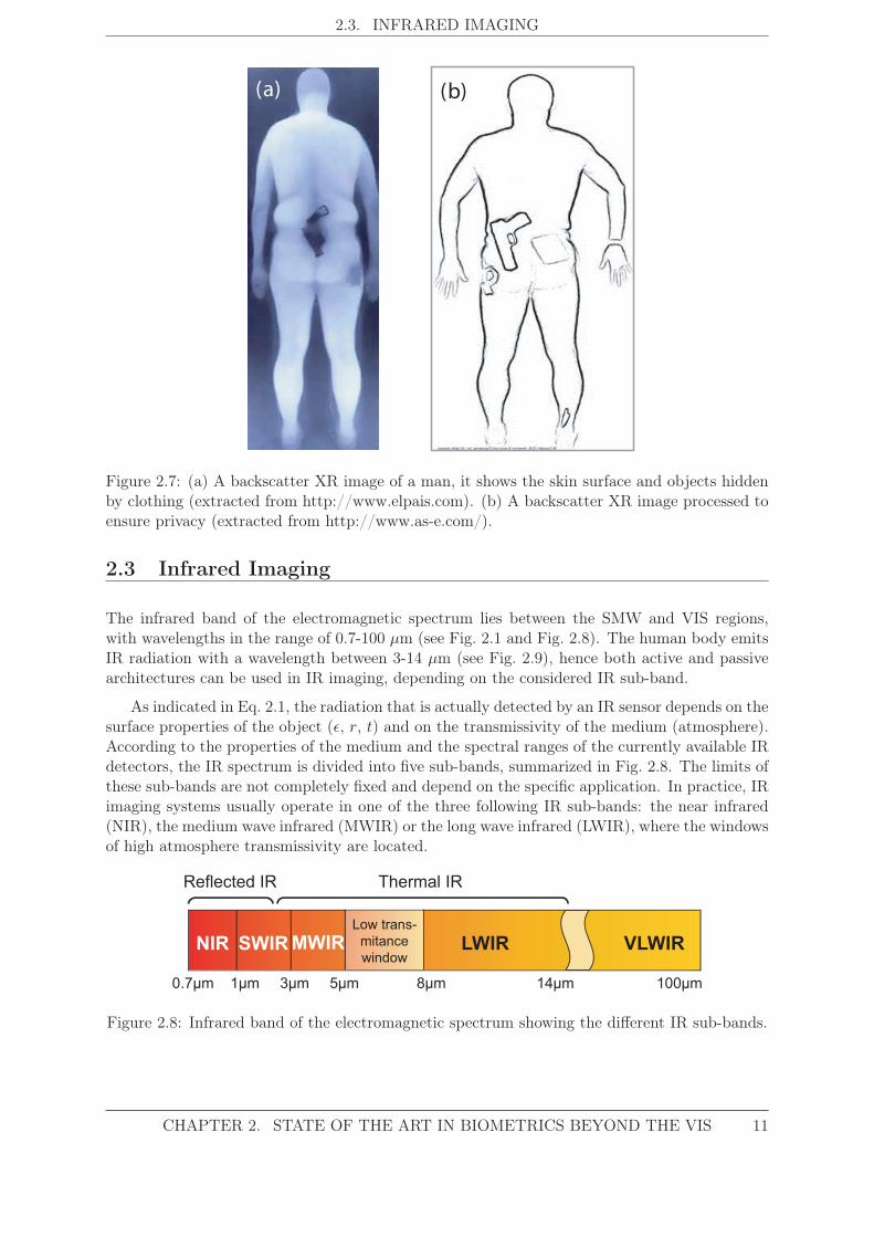
2.7 (a) A backscatter XR image of a man. (b) A backscatter XR image processed toensure privacy. . . . . . . . . . . . . . . . . . . . . . . . . . . . . . . . . . . . . . 11
2.8 Infrared band of the electromagnetic spectrum showing the different IR sub-bands. 11
2.9 Power Spectral Density of a body at 310K (37°C) and a body at 373K (100°C). . 12
2.10 Face and hand images acquired at NIR, MWIR and LWIR bands. . . . . . . . . . 13
2.11 Images acquired with PMMW imaging systems. . . . . . . . . . . . . . . . . . . . 15
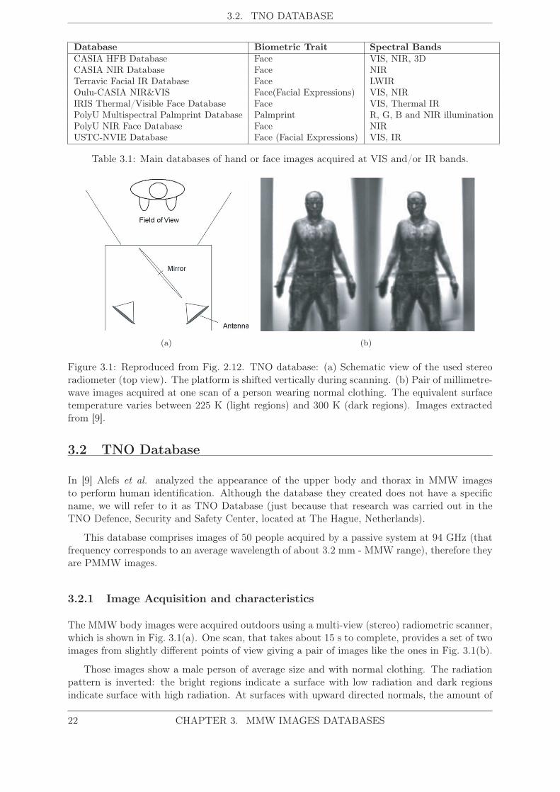
2.12 (a) Schematic view of stereo radiometer (top view). (b) Pair of millimeter-waveimages acquired at one scan of a person wearing normal clothing. . . . . . . . . . 16
2.13 Images acquired with AMMW imaging systems. . . . . . . . . . . . . . . . . . . . 17
2.14 Images acquired with PSMW imaging systems. . . . . . . . . . . . . . . . . . . . 17
2.15 Images acquired with ASMW imaging systems. . . . . . . . . . . . . . . . . . . . 18
3.1 TNO database: (a) Schematic view of the stereo radiometer used (top view). (b)Pair of millimeter-wave images acquired at one scan of a person wearing normalclothing. . . . . . . . . . . . . . . . . . . . . . . . . . . . . . . . . . . . . . . . . . 22
3.2 TNO database: Facial images acquired at VIS and at 94 GHz for one person withdifferent face occlusions. . . . . . . . . . . . . . . . . . . . . . . . . . . . . . . . . 23
3.3 BIOGIGA database: Tree showing the different kinds of images simulated foreach user. . . . . . . . . . . . . . . . . . . . . . . . . . . . . . . . . . . . . . . . . 25
3.4 BIOGIGA database: VIS image and body models of one user. . . . . . . . . . . . 27
3.5 BIOGIGA database: Synthetic images simulated at 94 GHz with an orientationangle of 0°. . . . . . . . . . . . . . . . . . . . . . . . . . . . . . . . . . . . . . . . 28
3.6 BIOGIGA database: Synthetic images simulated at 94 GHz with an orientationangle of -10°and +10°. . . . . . . . . . . . . . . . . . . . . . . . . . . . . . . . . . 29
xv

LIST OF FIGURES
3.7 BIOGIGA database: Histograms of the age, height, waist circumference and armlength of the users that form BIOGIGA. . . . . . . . . . . . . . . . . . . . . . . . 30
4.1 Architecture of a generic biometric system working either in verification or iden-tification mode. . . . . . . . . . . . . . . . . . . . . . . . . . . . . . . . . . . . . . 32
4.2 Feature extraction in our system. . . . . . . . . . . . . . . . . . . . . . . . . . . . 33
4.3 Segmentation process in our system. . . . . . . . . . . . . . . . . . . . . . . . . . 34
4.4 Boundary extraction in our system. . . . . . . . . . . . . . . . . . . . . . . . . . . 35
4.5 Landmark generation in our system. . . . . . . . . . . . . . . . . . . . . . . . . . 36
4.6 Body boundary, landmarks and distances extracted among them from the imageof one subject. . . . . . . . . . . . . . . . . . . . . . . . . . . . . . . . . . . . . . 37
5.1 Probability density functions and probability distributions of genuine users andimpostors. . . . . . . . . . . . . . . . . . . . . . . . . . . . . . . . . . . . . . . . . 40
5.2 A generic DET curve. . . . . . . . . . . . . . . . . . . . . . . . . . . . . . . . . . 40
5.3 A generic CMC curve. . . . . . . . . . . . . . . . . . . . . . . . . . . . . . . . . . 41
5.4 MMW images used in Alefs et al. to perform biometric recognition and thecorresponding recognition results. . . . . . . . . . . . . . . . . . . . . . . . . . . . 42
5.5 Mean normalized value of the feature vector of 7 randomly selected users. . . . . 44
5.6 Two-dimensional representation of the discrimination power of the extracted fea-tures. . . . . . . . . . . . . . . . . . . . . . . . . . . . . . . . . . . . . . . . . . . 45
5.7 Experiment 1 (Baseline Performance): CMC curves. . . . . . . . . . . . . . . . . 48
5.8 Experiment 1 (Baseline Performance): DET curves. . . . . . . . . . . . . . . . . . 48
5.9 Experiment 2 (Clothing and Angle Variability between Train and Test): CMCcurves. . . . . . . . . . . . . . . . . . . . . . . . . . . . . . . . . . . . . . . . . . . 50
5.10 Experiment 2 (Clothing and Angle Variability between Train and Test): DETcurves. . . . . . . . . . . . . . . . . . . . . . . . . . . . . . . . . . . . . . . . . . . 50
5.11 Experiment 3 (Clothing and Angle Variability in Training): CMC curves. . . . . 53
5.12 Experiment 3 (Clothing and Angle Variability in Training): DET curves. . . . . . 53
5.13 Experiment 4 (Number of Train and Test Images): CMC curves, considering allthe features. . . . . . . . . . . . . . . . . . . . . . . . . . . . . . . . . . . . . . . . 56
5.14 Experiment 4 (Number of Train and Test Images): CMC curves, consideringSFFS-selected features. . . . . . . . . . . . . . . . . . . . . . . . . . . . . . . . . . 56
5.15 Experiment 4 (Number of Train and Test Images): DET curves, considering allthe features. . . . . . . . . . . . . . . . . . . . . . . . . . . . . . . . . . . . . . . . 57
5.16 Experiment 4 (Number of Train and Test Images): DET curves, consideringSFFS-selected features. . . . . . . . . . . . . . . . . . . . . . . . . . . . . . . . . . 57
5.17 Experiment 4 (Number of Train and Test Images): EER values obtained usingdifferent number of train and test images. . . . . . . . . . . . . . . . . . . . . . . 59
5.18 Histograms of features selected by the SFFS algorithm. . . . . . . . . . . . . . . . 62
xvi LIST OF FIGURES
List of Tables
2.1 Properties of the most important IR sub-bands. . . . . . . . . . . . . . . . . . . . 13
2.2 Properties of MMW and SMW imaging operating with passive or active architecture. 18
3.1 Main databases of hand or face images acquired at VIS and/or IR bands. . . . . 22
3.2 BIOGIGA database: Main parameters and body measures taken from each sub-ject used to create his/her corresponding 3D body model in MakeHuman. . . . . 24
5.1 Experiment 1 (Baseline Performance): Identification, verification and SFFS fea-ture selection numerical results. . . . . . . . . . . . . . . . . . . . . . . . . . . . . 48
5.2 Experiment 2 (Clothing and Angle Variability between Train and Test): Identifi-cation, verification and SFFS feature selection numerical results. . . . . . . . . . 50
5.3 Comparison of Experiment 1 (Baseline Performance) vs Experiment 2 (Clothingand Angle Variability between Train and Test). . . . . . . . . . . . . . . . . . . . 51
5.4 Comparison of Experiment 1 (Baseline Performance) vs Experiment 3 (Clothingand Angle Variability in Training). . . . . . . . . . . . . . . . . . . . . . . . . . . 53
5.5 Comparison of Experiment 1 (Baseline Performance) vs Experiment 4 (Numberof Train and Test Images). . . . . . . . . . . . . . . . . . . . . . . . . . . . . . . . 55
5.6 Experiments 1, 2, 3 and 4: Identification, verification and SFFS feature selectionnumerical results. . . . . . . . . . . . . . . . . . . . . . . . . . . . . . . . . . . . . 61
xvii

Abbreviations
• AI: Active Indoors (referring to imaging system).Active imaging system working indoors. See AMMW or ASMW.
• AMMW: Active Millimeter Wave (Imaging System).Imaging system that emits millimeter wave radiation to the scene and then collects thereflected radiation to form the image.
• AO: Active Outdoors (referring to imaging system).Active imaging system working outdoors. See AMMW or ASMW.
• ASMW: Active Subillimeter Wave (Imaging System).Imaging system that emits submillimeter wave radiation to the scene and then collects thereflected radiation to form the image.
• cr : With Clothing (from the Spanish expression "con ropa").Abbreviation used to describe the clothing condition of a user in the images used in theexperiments.
• CMC: Cumulative Match Curve.Curve that graphically shows the identification performance of a biometric system. It plotsthe rank-n recognition rate (See R-n) versus n (being n the number of the candidatesconsidered at the beginning of the list).
• DET: Detection Error Tradeoff Curve.Curve widely used to show graphically the verification performance of a biometric system.It plots the FRR versus the FAR for all the different threshold values with logarithmicaxes.
• EER: Equal Error Rate.Error rate at which both error rates (FRR and FAR) coincide, for a certain thresholdvalue.
• FAR: False Acceptance Rate.Probability that an impostor is accepted by a biometric system as a genuine user.
• FRR: False Rejection Rate.Probability that a genuine user is rejected by a biometric system.
• IR: Infrared.Electromagnetic radiation with wavelength in the range of 0.7-100 μm (4.3·1014-3·1012 Hz).
• LWIR: Long Wave Infrared.Infrared radiation with wavelength in the range of 8-14 μm.
• MMW: Millimeter Waves.Electromagnetic radiation that, together with the submillimeter waves, fills the gap betweenthe infrared and microwave bands in the electromagnetic spectrum. Millimeter waves lie inthe band of 1-10 mm (300-30 GHz). Clothing is highly transparent to the MMW radiation.
• MWIR: Medium Wave Infrared.Infrared radiation with wavelength in the range of 3-5 μm.
• NIR: Near Infrared.Infrared radiation with wavelength in the range of 0.7-1 μm.
• PCA: Principal Component Analysis.Mathematical procedure that uses an orthogonal transformation to convert a set of obser-vations of possibly correlated variables into a set of values of linearly uncorrelated variablescalled principal components.
• PI: Passive Indoors (referring to imaging system).Passive imaging system working indoors. See PMMW or PSMW.
• PDF: Probability Density Function.Function that describes the relative likelihood for a random variable to take on a givenvalue.
• PMMW: Passive Millimeter Wave (Imaging System).Imaging system that collects natural millimeter wave radiation that has been emitted andreflected from the scene, to form the image.
• PO: Passive Outdoors (referring to imaging system).Passive imaging system working outdoors. See PMMW or PSMW.
• PSMW: Passive Submillimeter Wave (Imaging System).Imaging system that collects natural submillimeter wave radiation that has been emittedand reflected from the scene, to form the image.
• R-1 : Rank-1 Recognition Rate.Number of users correctly identified by a biometric system with the first candidate of thelist given by the system over the total number of users.
• R-5 : Rank-5 Recognition Rate.Number of users correctly identified by a biometric system with any of the 5 first candidatesof the list given by the system over the total number of users.
• R-n : Rank-n Recognition Rate.Number of users correctly identified by a biometric system with any of the n first candidatesof the list given by the system over the total number of users.
• ROC: Receiving Operating Characteristic.Curve employed to plot the performance of a biometric system. It plots the TPR versusthe FAR.
• SFFS: Sequential Floating Forward Selection.Feature Selection algorithm. It is a suboptimal searching technique, an iterative processin which, in each iteration, a new set of features (whose choice is based on the results ofprevious subsets) is used to compute a certain criterion. This is done until the criteriondoes not improve.
• SMW: Submillimeter Waves.Electromagnetic radiation that, together with the millimeter wave radiation, fills the gapbetween the infrared and microwave bands in the electromagnetic spectrum. Submillimeterwaves lie in the range of 0.1-1 mm (0.3-3 THz). Clothing is partially transparent to theSMW radiation.

• SNR: Signal to Noise Ratio.Measure that compares the level of a desired signal to the level of background noise. It isdefined as the ratio of signal power to the noise power.
• sr : Without Clothing (from the Spanish expression "sin ropa").Abbreviation used to describe the clothing condition of a user in the images used in theexperiments.
• SWIR: Short Wave Infrared.Infrared radiation with wavelength in the range of 1-3 μm.
• VIS: Visible Spectrum.Portion of the electromagnetic spectrum that is visible to the human eye. Electromagneticradiation in this range of wavelengths (400-700 nm) is usually called light.
• TPR: True Positive Rate or Sensitivity.Rate of genuine attemps accepted by the biometric system. It corresponds to 1-FRR.
• VLWIR: Very Long Wave Infrared.Infrared radiation with wavelength in the range of 14-100 μm.
• XR: X-ray.Electromagnetic radiation with a wavelength that lies between 0.01-10 nm (3·1019-3·1016Hz).
The following abbreviations have been used: Sect. (section) and Fig. (figure).

1Introduction
1.1 Motivation of the Project
Biometric Recognition is the process that allow to associate an identity with an individualautomatically, using one or more physical or behavioral characteristics that are inherent in theindividual [1, 2]. There are many features that have been used in biometric identification:fingerprint, signature, handwriting, iris, voice, face, hand, etc. Some of these biometric traits,such as ear, face, hand or gait, are usually acquired with cameras working at frequencies withinthe visible band of the electromagnetic spectrum. Those images are affected by factors such aslighting conditions and occlusions (caused by clothing, makeup, hair, etc.).
To overcome these limitations, imposed by the use of images acquired in the visible spectrum(VIS), researchers in biometrics and security [3] have proposed the use of images acquired inother spectral ranges, namely X-ray (XR) [4], infrared (IR) [5], millimeter waves (MMW) andsubmillimeter waves (SMW) [6]. In addition to overcome, to some extent, the limitations ofimages at VIS, pictures taken beyond the visible spectrum have an extra advantage: they aremore robust to attacks against biometric systems than other kind of images and other biometrictraits.
The spectral band proposed in this project to capture images of biometric features is the onecorresponding to the millimeter waves (frequency between 30 and 300 GHz) [7]. The significanceof this type of radiation lies in:
• Its ability to penetrate clothing and other occlusions.
• It is innocuous to health.
• The recent development that the GHz-THz imaging systems are experiencing (specially inthe area of security).
Unlike imaging technology in the visible or infrared band, GHz-THz technology is underdevelopment [8]. This fact, together with the privacy issues that the body images in this bandpresent, have caused that, to date, there are no public databases with images of people acquiredin that frequency range. In fact, so far there is only one published work on biometric recognition
1

1.2. OBJECTIVES
based on GHz images [9]. For all the above, in the current project the generation of a databaseis proposed as a key task, this database comprises simulated images of people at 94 GHz [10].Then, we will make use of such images to develop a biometric recognition system.
This project is motivated by the advantages offered by the images acquired in the range ofmillimeter waves and the kind of scenarios where they are acquired:
• Millimeter waves are completely innocuous. Imaging in this band can be done passively(collecting the radiation naturally emitted by the human body in that band and the onereflected by the environment) or actively (illuminating the body with emitting sourcesat those frequencies and collecting the reflected radiation). In no case this radiationconstitutes a hazard to health.
• The transparency of clothing and other non-polar dielectric materials to this radiation.This is the main advantage for biometric recognition because it prevents unwanted occlu-sions in the images.
• The non-invasiveness of such imaging systems. The cooperation required by the user forthe acquisition of these images is minimal.
• The possibility of recognition at a distance and/or on the move.
• The possibility of integrating the biometric recognition system in security systems such asportals and other weapons detection devices.
• The ease of fusion with other biometric traits like face.
By contrast, images acquired in this band have some drawbacks such as:
• They require extremely expensive acquisition equipments, given their recent development.
• The privacy issues caused by this kind of images (mainly because of transparency of cloth-ing).
1.2 Objectives
The project objectives are summarized in three points:
• Creation of a database of simulated images of real people in the millimeter wave band.The first milestone of the project is the generation of such images as an alternative topurchasing equipment to capture images at GHz and given the absence of free distributiondatabase of such images.
• Development of a biometric recognition system based on the above images. This systemwill have several modules: image processing, most distinctive feature extraction, featureselection, similarity measures and decision maker.
• Evaluation of the previous system by performing different experiments. The main pur-pose of the experiments is to quantify the influence of different conditions on the systemperformance. Conditions of interest include pose and clothing variation between train andtest data and the amount of train data.
2 CHAPTER 1. INTRODUCTION

1.3. METHODOLOGY
1.3 Methodology
The work methodology is divided in the following steps:
Literature Survey.
• The first step will be a study of different imaging systems outside the visible range, par-ticularly those used for biometric purposes.
• Here we review the state of the art in biometric systems based on images acquired outsidethe visible range.
• To complete the survey phase, the basic techniques of digital image processing will bestudied through the material of the Telecommunications Engineering course AdvancedTopics in Signal Processing, by studying the book [11] and performing some of its examples.
Generation of a synthetic database of real people to 94 GHz. This was done incollaboration with the AMS group at the Autonomous University of Barcelona. This stage hasseveral steps:
• Obtaining body measurements of real people.
• Body model generation from these measurements using a specific software for it.
• Export of the above models to another application where images of such models are simu-lated at the radiation frequency chosen.
Development of a biometric identification proprietary system. This system will usethe features extracted from the images generated in the previous stage. The development willinclude the following steps:
• Preprocessing of the images.
• Feature extraction.
• Similarity measure.
• Decision-making.
Experiments for the optimization of the system. These experiments focus on theselection of features. They are performed to obtain a set of representative and distinctivefeatures of each user to increase the performance of the system.
Evaluation of the system by performing different experiments.
Evaluation of results and drawing conclusions.
Documentation of work performed.
• Description of followed steps.
• Analysis of results, evaluation.
• Possible future work.
CHAPTER 1. INTRODUCTION 3

1.4. MEMORY ORGANIZATION
1.4 Memory organization
The present document is structured in 6 chapters as follows:
Chapter 1: Introduction. This chapter presents the subject of this project, the main reasonsthat have encouraged us to develop this work, the objectives to be obtained, the methodologyfollowed and the memory organization.
Chapter 2: State of the art of biometrics beyond the visible spectrum. This chap-ter reviews some of the existing human body imaging technologies working beyond the visiblespectrum: 1) X-ray, 2) infrared and 3) millimeter and submillimeter wave imaging technologies,and their biometric applications.
Chapter 3: Databases of MMW images. In this chapter two databases of images acquiredin the millimeter wave band are described: 1) the one acquired and used in [9] and 2) BIOGIGA,which is the database generated within this project and the one used to develop and test thebiometric system [12].
Chapter 4: System, Design and Development. The fourth chapter, after a brief in-troduction to biometric systems, details the different stages of the design and development ofthe implemented biometric system: from the preprocessing of the input images to the identitydecision.
Chapter 5: Experiments and Results. In this chapter, firstly, a summary of the per-formance evaluation of biometric systems is presented. Then, the experimental protocols andthe classifier employed in the experiments are described. Finally, the results obtained in eachexperiment are presented and analyzed.
Chapter 6: Conclusions and Future Work. Conclusions are finally drawn in this lastchapter along with the possible future work.
Finally, the following sections are at the end of the dissertation: the Bibliography and thefollowing appendices: Introducción (compulsory translation into Spanish of the Chapter 1),Conclusiones y trabajo futuro (compulsory translation into Spanish of the Chapter 6), Projectbudget, the Schedule of Conditions and the published articles.
4 CHAPTER 1. INTRODUCTION

1.5. CONTRIBUTIONS
1.5 Contributions
The contributions of this M.Sc. Thesis can be summarized in the following points:
• Summary of the state of the art of the biometric recognition research works that make useof images acquired out of the visible spectrum.
• Study of the main advantages and drawbacks of the images acquired at each spectral band.
• The innovative use of images acquired at the millimeter wave band as biometric traits.
• Generation of a synthetic database composed of simulated images of people at 94 GHz.
• Development and implementation of a recognition system based on the previous images.
• Evaluation of the results obtained through our system, under different conditions, to drawthe appropriate conclusions about its performance and behavior.
During the project development several articles have been generated and accepted in differentnational and international conferences:
• Miriam Moreno-Moreno, Julian Fierrez, and Javier Ortega-Garcia. Millimeter- and Submi-llimeter-Wave Imaging Technologies for Biometric Purposes. In Proceedings of XXIV Sim-posium Nacional de Union Científica Internacional de Radio, September 2009 [13].
• Miriam Moreno-Moreno, Julian Fierrez, and Javier Ortega-Garcia. Biometrics Beyond theVisible Spectrum: Imaging Technologies and Applications. In Proceedings of BioIDMulti-comm 2009, volume 5707 of LNCS, pages 154-161. Springer, September 2009 [14].
• Miriam Moreno-Moreno, Julian Fierrez, Pedro Tome, and Javier Ortega-Garcia. Análisisde Escenarios para Reconocimiento Biométrico a Distancia Adecuados para la Adquisi-ción de Imágenes MMW. In Proceedings of XXV Simposium Nacional de Union CientíficaInternacional de Radio, September 2010 [15].
• Miriam Moreno-Moreno, Julian Fierrez, Pedro Tome, Ruben Vera-Rodriguez, Josep Par-ron, and Javier Ortega-Garcia. BIOGIGA: Base de datos de imágenes sintéticas de per-sonas a 94 GHz con Fines Biométricos. In Proceedings of XXVI Simposium Nacional deUnion Científica Internacional de Radio, September 2011 [12].
• Miriam Moreno-Moreno, Julian Fierrez, Ruben Vera-Rodriguez, and Josep Parron. Distan-ce-based Feature Extraction for Biometric Recognition of Millimeter Wave Body Images.In Proceedings of 45th IEEE International Carnahan Conference on Security Technology,pages 326-331, October 2011 [16].
• Miriam Moreno-Moreno, Julian Fierrez, Ruben Vera-Rodriguez, and Josep Parron. Simu-lation of Millimeter Wave Body Images and its Application to Biometric Recognition. InProceedings of SPIE Defense, Security and Sensing 2012, volume 8362. April 2012 [17].
CHAPTER 1. INTRODUCTION 5

2State of the Art in
Biometrics Beyond the Visible Spectrum
2.1 Introduction
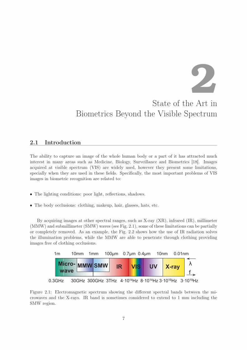
The ability to capture an image of the whole human body or a part of it has attracted muchinterest in many areas such as Medicine, Biology, Surveillance and Biometrics [18]. Imagesacquired at visible spectrum (VIS) are widely used, however they present some limitations,specially when they are used in these fields. Specifically, the most important problems of VISimages in biometric recognition are related to:
• The lighting conditions: poor light, reflections, shadows.
• The body occlusions: clothing, makeup, hair, glasses, hats, etc.
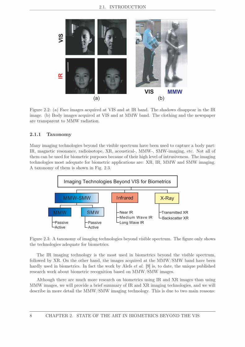
By acquiring images at other spectral ranges, such as X-ray (XR), infrared (IR), millimeter(MMW) and submillimeter (SMW) waves (see Fig. 2.1), some of these limitations can be partiallyor completely removed. As an example, the Fig. 2.2 shows how the use of IR radiation solvesthe illumination problems, while the MMW are able to penetrate through clothing providingimages free of clothing occlusions.
0.3GHz 30GHz 300GHz 3THz 4·1014Hz 8·1014Hz 3·1016Hz 3·1019Hz
IR VISMicro-
waveUV X-ray
1m 10mm 1mm 100μm 0.7μm 0.4μm 10nm 0.01nm
f
λMMW SMW
Figure 2.1: Electromagnetic spectrum showing the different spectral bands between the mi-crowaves and the X-rays. IR band is sometimes considered to extend to 1 mm including theSMW region.
7
2.1. INTRODUCTION
VIS
IRV
IS
MMW(a) (b)
Figure 2.2: (a) Face images acquired at VIS and at IR band. The shadows disappear in the IRimage. (b) Body images acquired at VIS and at MMW band. The clothing and the newspaperare transparent to MMW radiation.
2.1.1 Taxonomy
Many imaging technologies beyond the visible spectrum have been used to capture a body part:IR, magnetic resonance, radioisotope, XR, acoustical-, MMW-, SMW-imaging, etc. Not all ofthem can be used for biometric purposes because of their high level of intrusiveness. The imagingtechnologies most adequate for biometric applications are: XR, IR, MMW and SMW imaging.A taxonomy of them is shown in Fig. 2.3.
Imaging Technologies Beyond VIS for Biometrics
X-Ray Infrared MMW-SMW
Near IR Medium Wave IR Long Wave IR Passive
Active Passive Active
MMW SMW
Transmitted XR
Backscatter XR
Figure 2.3: A taxonomy of imaging technologies beyond visible spectrum. The figure only showsthe technologies adequate for biometrics.
The IR imaging technology is the most used in biometrics beyond the visible spectrum,followed by XR. On the other hand, the images acquired at the MMW/SMW band have beenhardly used in biometrics. In fact the work by Alefs et al. [9] is, to date, the unique publishedresearch work about biometric recognition based on MMW/SMW images.
Although there are much more research on biometrics using IR and XR images than usingMMW images, we will provide a brief summary of IR and XR imaging technologies, and we willdescribe in more detail the MMW/SMW imaging technology. This is due to two main reasons:
8 CHAPTER 2. STATE OF THE ART IN BIOMETRICS BEYOND THE VIS
2.1. INTRODUCTION
• The biometric recognition system developed in this project is based on MMW images.
• The advantages of MMW images in biometrics (see Sect. 1.1).
2.1.2 Fundamentals
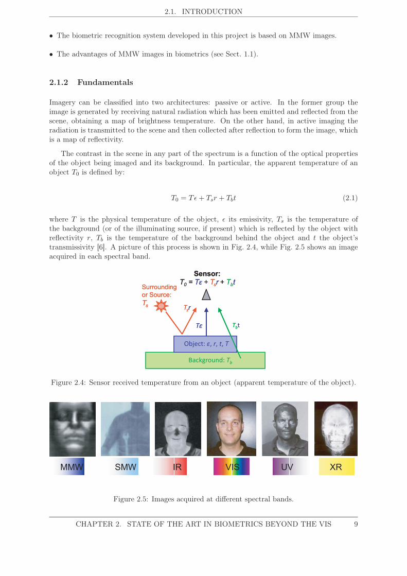
Imagery can be classified into two architectures: passive or active. In the former group theimage is generated by receiving natural radiation which has been emitted and reflected from thescene, obtaining a map of brightness temperature. On the other hand, in active imaging theradiation is transmitted to the scene and then collected after reflection to form the image, whichis a map of reflectivity.
The contrast in the scene in any part of the spectrum is a function of the optical propertiesof the object being imaged and its background. In particular, the apparent temperature of anobject T0 is defined by:
T0 = Tε+ Tsr + Tbt (2.1)
where T is the physical temperature of the object, ε its emissivity, Ts is the temperature ofthe background (or of the illuminating source, if present) which is reflected by the object withreflectivity r, Tb is the temperature of the background behind the object and t the object’stransmissivity [6]. A picture of this process is shown in Fig. 2.4, while Fig. 2.5 shows an imageacquired in each spectral band.
Background: Tb
Object: ɛ, r, t, T
Surrounding
or Source:
Ts
Tsr
Tɛ Tbt
Sensor:T
0= Tɛ + T
sr + T
bt
Background: Tb
Object: ɛ, r, t, T
Surrounding
or Source:
Ts
Tsr
Tɛ Tbt
Sensor:T
0= Tɛ + T
sr + T
bt
Figure 2.4: Sensor received temperature from an object (apparent temperature of the object).
MMW SMW IR VIS UV XR
Figure 2.5: Images acquired at different spectral bands.
CHAPTER 2. STATE OF THE ART IN BIOMETRICS BEYOND THE VIS 9

2.2. X-RAY IMAGING
2.2 X-ray Imaging
X-radiation have a wavelength in the range of 10-0.01 nm (3·1016-3·1019 Hz) and enough energyto pass through cloth and human tissues. In addition to cloth penetration, XR imaging pro-vides high image resolution. However, this technology presents some disadvantages: low speed,limitation to very short distances and the health safety concerns it raises because of using ion-izing radiation. The natural background X-radiation is too weak to form an image, thereforeactive imaging is required in both XR imaging modalities: transmission and backscatter X-rayimaging. X-rays are commonly produced by accelerating charged particles.
2.2.1 Transmission X-ray Imaging
Conventional X-ray radiographic systems used for medical purposes produce images relying onthis kind of imaging: a uniform X-ray beam incident on the patient interacts with the tissuesof the body, producing a variable transmitted X-ray flux dependent on the attenuation alongthe beam paths. An X-ray-sensitive detector captures the transmitted fraction and converts theX-rays into a visible projection image. Only a few works on biometric identification makinguse of the conventional X-rays can be found: Shamir et al. [19] perform biometric identificationusing knee X-rays while Chen et al. [4] present an automatic method for matching dental radio-graphs (see Fig. 2.6). These knee or dental X-rays are difficult to forge and present additionaladvantages: they can be used in forensic identification where the soft tissues are degraded.
Figure 2.6: Dental radiographs used for human identification, extracted from Chen et al. [4].
2.2.2 Backscatter X-ray Imaging
In this technique the XR scattered photons, instead of transmitted photons, are used to constructthe image [20]. This technology utilizes high energy X-rays that are more likely to scatter thanpenetrate materials as compared to lower-energy X-ray used in medical applications. However,this kind of radiation is able to penetrate some materials, such as cloth. A person is scanned bymoving a single XR beam over her/his body. The backscattered beam from a known positionallows a realistic image to be reconstructed. As only scattered X-rays are used, the registeredimage is mainly a view of the surface of the scanned person, i.e. her nude form. As the imageresolution is high, these images present privacy issues. Some companies (e.g. AS&E) ensureprivacy by applying an algorithm to the raw images so that processed images reveal only anoutline of the scanned individual. Raw and processed backscatter XR images are shown inFig. 2.7. According to our knowledge, there are no works on biometrics using backscatter X-rayimages. The application of this technique includes medical imaging [21] and passenger screeningat airports and homeland security [22]. There are currently different backscatter X-ray imagingsystems available on the market to screen people (e.g. AS&E, Rapiscan Systems).
10 CHAPTER 2. STATE OF THE ART IN BIOMETRICS BEYOND THE VIS
2.3. INFRARED IMAGING
(a) (b)
Figure 2.7: (a) A backscatter XR image of a man, it shows the skin surface and objects hiddenby clothing (extracted from http://www.elpais.com). (b) A backscatter XR image processed toensure privacy (extracted from http://www.as-e.com/).
2.3 Infrared Imaging
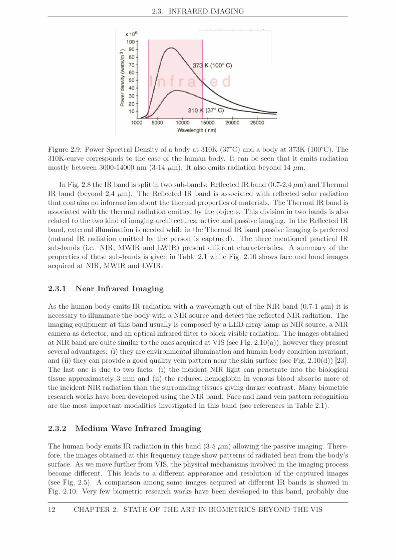
The infrared band of the electromagnetic spectrum lies between the SMW and VIS regions,with wavelengths in the range of 0.7-100 μm (see Fig. 2.1 and Fig. 2.8). The human body emitsIR radiation with a wavelength between 3-14 μm (see Fig. 2.9), hence both active and passivearchitectures can be used in IR imaging, depending on the considered IR sub-band.
As indicated in Eq. 2.1, the radiation that is actually detected by an IR sensor depends on thesurface properties of the object (ε, r, t) and on the transmissivity of the medium (atmosphere).According to the properties of the medium and the spectral ranges of the currently available IRdetectors, the IR spectrum is divided into five sub-bands, summarized in Fig. 2.8. The limits ofthese sub-bands are not completely fixed and depend on the specific application. In practice, IRimaging systems usually operate in one of the three following IR sub-bands: the near infrared(NIR), the medium wave infrared (MWIR) or the long wave infrared (LWIR), where the windowsof high atmosphere transmissivity are located.
0.7μm 1μm 3μm 5μm 8μm 14μm 100μm
NIR SWIR MWIR LWIR VLWIR-
mitance
window
Reflected IR Thermal IR
Low transLow trans-
mitance
window
Figure 2.8: Infrared band of the electromagnetic spectrum showing the different IR sub-bands.
CHAPTER 2. STATE OF THE ART IN BIOMETRICS BEYOND THE VIS 11
2.3. INFRARED IMAGING
Figure 2.9: Power Spectral Density of a body at 310K (37°C) and a body at 373K (100°C). The310K-curve corresponds to the case of the human body. It can be seen that it emits radiationmostly between 3000-14000 nm (3-14 μm). It also emits radiation beyond 14 μm.
In Fig. 2.8 the IR band is split in two sub-bands: Reflected IR band (0.7-2.4 μm) and ThermalIR band (beyond 2.4 μm). The Reflected IR band is associated with reflected solar radiationthat contains no information about the thermal properties of materials. The Thermal IR band isassociated with the thermal radiation emitted by the objects. This division in two bands is alsorelated to the two kind of imaging architectures: active and passive imaging. In the Reflected IRband, external illumination is needed while in the Thermal IR band passive imaging is preferred(natural IR radiation emitted by the person is captured). The three mentioned practical IRsub-bands (i.e. NIR, MWIR and LWIR) present different characteristics. A summary of theproperties of these sub-bands is given in Table 2.1 while Fig. 2.10 shows face and hand imagesacquired at NIR, MWIR and LWIR.
2.3.1 Near Infrared Imaging
As the human body emits IR radiation with a wavelength out of the NIR band (0.7-1 μm) it isnecessary to illuminate the body with a NIR source and detect the reflected NIR radiation. Theimaging equipment at this band usually is composed by a LED array lamp as NIR source, a NIRcamera as detector, and an optical infrared filter to block visible radiation. The images obtainedat NIR band are quite similar to the ones acquired at VIS (see Fig. 2.10(a)), however they presentseveral advantages: (i) they are environmental illumination and human body condition invariant,and (ii) they can provide a good quality vein pattern near the skin surface (see Fig. 2.10(d)) [23].The last one is due to two facts: (i) the incident NIR light can penetrate into the biologicaltissue approximately 3 mm and (ii) the reduced hemoglobin in venous blood absorbs more ofthe incident NIR radiation than the surrounding tissues giving darker contrast. Many biometricresearch works have been developed using the NIR band. Face and hand vein pattern recognitionare the most important modalities investigated in this band (see references in Table 2.1).
2.3.2 Medium Wave Infrared Imaging
The human body emits IR radiation in this band (3-5 μm) allowing the passive imaging. There-fore, the images obtained at this frequency range show patterns of radiated heat from the body’ssurface. As we move further from VIS, the physical mechanisms involved in the imaging processbecome different. This leads to a different appearance and resolution of the captured images(see Fig. 2.5). A comparison among some images acquired at different IR bands is showed inFig. 2.10. Very few biometric research works have been developed in this band, probably due
12 CHAPTER 2. STATE OF THE ART IN BIOMETRICS BEYOND THE VIS

2.3. INFRARED IMAGING
IR Spectral Range Archi- IR camera Image Applications
bands (μm) tecture cost Properties in Biometrics
Near IR Low, VIS came- Good quality, body Face [5] and Hand
(NIR) ra also sensitive condition invariant Vein [23] Recognition
Medium Wave IR Good quality, sensiti- Face [24] and Hand
(MWIR) ve to body conditions Vein [25] Recognition
Long Wave IR Low contrast, sensiti- Face [27] and Hand
(LWIR) ve to body conditions Vein [23] Recognition
0,7-1
3 - 5
8 - 14
High
Low
Active
Passive
Passive
Table 2.1: Properties of the most important IR sub-bands.
NIR MWIR LWIR
(a) (b) (c)
(d) (e) (f)
HA
ND
VE
INF
AC
E
Figure 2.10: Face and hand images acquired at NIR, MWIR and LWIR bands: (a) face at NIR,(b) face at MWIR, (c) face at LWIR, (d) palm at NIR, (e) back of the hand at MWIR and (f)back of the hand at LWIR. The images are extracted respectively from [5], [24], [26], [23], [25]and [23].
to the high cost of MWIR cameras. Buddharaju et al. [24] performed face recognition from thethermal imprint of the facial vascular network obtained at the MWIR band. Thermal images ofpalm dorsa vein acquired in MWIR have been also used to identify individuals [25].
2.3.3 Long Wave Infrared Imaging
Although human body emits IR radiation in both MWIR and LWIR bands, LWIR (8-14 μm)is usually preferred due to: (i) much higher emissions in it, and (ii) the low cost of LWIRcameras. No external illumination is required in this band. Body images acquired at LWIR arequite similar to those acquired in MWIR. Both kinds of images are often called thermograms.Fig. 2.10(c, f) shows images acquired at this band. Recognition of faces from images obtainedat this band has become an area of growing interest [26, 27]. However the algorithms theyused do not differ very much from the algorithms used in the VIS band. Works on vein patternrecognition have been developed at this band as well [23]. In contrast with NIR; LWIR can onlycapture large veins, not necessary at the skin surface, because large veins carry a higher amountof blood giving a higher temperature. In addition, most of the LWIR images have low levels ofcontrast and they are sensitive to ambient and body condition.
CHAPTER 2. STATE OF THE ART IN BIOMETRICS BEYOND THE VIS 13
2.4. MILLIMETER AND SUBMILLIMETER WAVE IMAGING
2.4 Millimeter and Submillimeter Wave Imaging
MMW and SMW radiation fill the gap between the IR and the microwaves (see Fig. 2.1).Specifically, millimeter waves lie in the band of 30-300 GHz (10-1 mm) and the SMW regimelies in the range of 0.3-3 THz (1-0.1 mm).
MMW and SMW radiation can penetrate through many commonly used nonpolar dielectricmaterials such as paper, plastics, wood, leather, hair and even dry walls with little attenuation[28, 29]. Clothing is highly transparent to the MMW radiation and partially transparent to theSMW radiation [30]. Above 30 GHz, the transmission of the atmosphere varies strongly as afunction of frequency due to water vapour and oxygen [6, 31]. There are relatively transparentwindows centered at 35, 94, 140 and 220 GHz in the MMW range and less transparent windows inthe SMW region located at: 0.34, 0.67, 1.5, 2, 2.1, 2.5, 3.4 and 4.3 THz. Atmosphere attenuationis further increased in poor weather. Liquid water extremely attenuates submillimeter waveswhile MMW radiation is less attenuated (millions of times) in the presence of clouds, fog, smoke,snow, and sand storms than VIS or IR radiation.
Consequently, natural applications of MMW and SMW imaging include security screening,non-destructive inspection, and medical and biometrics imaging. Low visibility navigation isanother application of MMW imaging [7]. The detection of concealed weapons has been themost developed application of MMW/SMW imaging systems so far, in contrast to the biometricsarea, where there is only a published research work.
Although most of the radiation emitted by the human body belongs to the MWIR and LWIRbands, it emits radiation in the SMW and MMW regions as well (the tails of the 310K-curveon the right in Fig. 2.9). This allows passive imaging. A key factor in MMW and SMW passiveimaging is the sky illumination. This makes images acquired in indoor and outdoor environ-ments to have very different contrast when working with passive systems. Outdoors radiometrictemperature contrast can be very large (due to the difference between the temperature of thefloor, which is warm ∼ 300 K, and the sky, which is cold ∼ 100 K), but it is very small indoors.In passive imaging operating indoors, the signal to noise ratio (SNR) of the existing cameras isbarely enough for coarse object detection, being usually insufficient for identification (as neededfor biometrics). There are two solutions to overcome this problem: (i) cooling the detectoror alternatively (ii) using active imaging. Cooling the detector improves the sensitivity but itmakes the camera more expensive and difficult to use.
In active imaging, the source that illuminates the scene produces much higher power levelthan the emitted from the scene, so it can be considered as an object at very high temperature. Ifthe source is incoherent and physically large, active imaging is equivalent to passive imaging withthe surroundings at very high temperature, and hence results in much greater contrast withinthe image. If the source is small, active imaging becomes more complicated. In any case, thepower level of the radiation source in active imaging strongly affects the detection resolution. Inaddition to higher resolution than passive imaging, active imaging provides higher SNR, highersignal levels, and the ability to obtain depth information in the scene.
2.4.1 Millimeter Wave Imaging (MMW)
Passive MMW Imaging (PMMW)
There have been many research groups working on passive MMW imaging (PMMW) since itsearly developments. Most of them have constructed prototype radiometers that work at afrequency range centered at 35 GHz [32] or at 94 GHz [8, 28, 33, 34]. The images obtainedwith PMMW imaging systems have low resolution compared to VIS and IR images. This low
14 CHAPTER 2. STATE OF THE ART IN BIOMETRICS BEYOND THE VIS

2.4. MILLIMETER AND SUBMILLIMETER WAVE IMAGING
(a) (d)
Outdoors PMMW Indoors PMMW
Outdoors PMMW
Indoors PMMW
(b)
(c)
Figure 2.11: Images acquired with PMMW imaging systems. (a) Outdoors PMMW image (94GHz) of a man carrying a gun in a bag. (b-c) Indoors and outdoors PMMW image of a face. (d)Indoors PMMW image (94 GHz) of a man with a gun concealed under clothing. These figureinsets are extracted from: www.vision4thefuture.org (a-c), and www.alfaimaging.com (d). Allthe people were dressed.
resolution is a consequence of the longer wavelengths used relative to the aperture size of thesensor’s collection optics. Further, images acquired indoors will present less contrast than thoseacquired outdoors, as it is shown in Fig. 2.11. There are multiple commerical PMMW cameras(e.g. Quinetiq, Brijot, Alfa Imaging, Sago Systems, Millivision, and View Systems).
The applications of most of the cited works are the detection of concealed weapons or vi-sion under adverse weather conditions. To date, the unique published biometric application ofMMW/SMW is the one by Alefs et al. [9]. Specifically, they use a PMMW system (a multi-viewstereo radiometric scanner that operates at 94 GHz) schematically shown in Fig. 2.12(a), obtain-ing the images in Fig. 2.12(b). The details of mentioned work (the characteristics of the databasecomposed by these images, the approaches followed to perform the biometric recognition andthe recognition results) will be briefly presented throughout the document.
Active MMW Imaging (AMMW)
Active MMW imaging (AMMW) has gained more and more attention during the last few yearsfor indoor security applications [35, 36, 37, 38]. Sheen et al. [35] demonstrated an AMMW imageroperating at 27-33 GHz and good quality images were obtained (see Fig. 2.13(a)). Derham et al.[36] showed the performance of a prototype AMMW imaging system operating at 60 GHz thatuses the frequency-encoding technique. Timms et al. [37] developed a 190 GHz active imagingsystem.
In the active systems, as the image is formed collecting the transmitted and then reflectedradiation from the emitting source, the appareance of the images acquired indoors and outdoorsis the same (the surrounding temperature does not affect as in the case of PMMW imaging).
CHAPTER 2. STATE OF THE ART IN BIOMETRICS BEYOND THE VIS 15

2.4. MILLIMETER AND SUBMILLIMETER WAVE IMAGING
(a) (b)
Figure 2.12: (a) Schematic view of stereo radiometer (top view). The platform is shifted ver-tically during scanning. (b) Pair of millimetre-wave images acquired at one scan of a personwearing normal clothing. The equivalent surface temperature varies between 225K (light regions)and 300K (dark regions). Images extracted from [9].
Several images obtained with AMMW imaging systems are shown in Fig. 2.13. The higherquality of the images acquired with active systems, when compared with PMMW systems, isclearly noticeable. Again, most of AMMW imaging systems are used as security portals (seeFig. 2.13(d)). Some AMMW imagers are currently available on the market (Agilent and L3-Communications). Agilent’s MMW imaging system works at 30 GHz and has a transverseresolution of 1 cm. L-3 Provision MMW body screening portal (Fig. 2.13(d)) has been usedsince 2007 at some airports (see example images in Fig. 2.13(b and c). However, no biometricapplication of AMMW imaging has emerged so far.
2.4.2 Submillimeter Wave Imaging (SMW)
The shorter the radiation wavelength is, the better image resolution is available, and henceSMW imaging would provide better resolution than MMW imaging. On the other hand, as thewavelength decreases, the penetration capability decreases. Further, the technology needed inthe SMW imaging systems is much less mature than the MMW technology [39].
Passive SMW Imaging (PSMW)
In passive SMW imaging (PSMW) the contrast in the image depends on the operation frequency:at frequencies below 0.5 THz it will be dominated by the reflectivity of the items, while atfrequencies of 0.5 THz and above, it will be dominated by the emissivity of the objects andtheir physical temperature (similar to thermography). This statement agrees with Fig. 2.9:as the frequency increases (wavelength decreases) the power density of a body at a non-nulltemperature also is bigger.
Some of the more relevant and recent research works on PSMW imaging include [40] and[41]. Luukanen et al. [40] developed an imaging system working at 0.1-1 THz. Shen et al. [41]performed detection and segmentation of concealed objects in images acquired with the imagingsystem described in [40]. They obtain good quality images as it can be seen in Fig. 2.14(a).Fig. 2.14(b) shows another PSMW image of a man with a spanner hidden under his T-shirt(acquired at 1.5 THz [42]). These two images show that cloth is less transparent to submilliter
16 CHAPTER 2. STATE OF THE ART IN BIOMETRICS BEYOND THE VIS

2.4. MILLIMETER AND SUBMILLIMETER WAVE IMAGING
(a)
In/Out AMMW
(b) (c)
In/Out AMMW In/Out AMMW
(d)
Figure 2.13: Images acquired with AMMW imaging systems (the appearance of the imagesis the same in both scenes, indoors and outdoors). (a) AMMW image acquired at 27-33GHz of a dressed man carrying two handguns. (b) and (c) AMMW images of a dressedwoman, both acquired by the L3-Communications screening portal, that is shown in (d).These figure insets are extracted from: [35] (a), while (b), (c) and (d) are all extracted fromhttp://www.kelowna.com/2010/04/08/kelowna-airport-using-full-body-scanner/.
(a) (b)
PSMW PSMW
Figure 2.14: Images acquired with PSMW imaging systems. (a) PSMW image (0.1-1 THz) ofa man with concealed objects beneath his jacket. (b) PSMW image (1.5 THz) of a man with aspanner under his T-shirt. These figure insets are extracted from: [41] (a) and [42] (b).
waves than to MMW radiation (collar and folds of the weave are visible). A passive systemrequired to penetrate all type of clothing should operate below 0.3-0.5 THz [30, 6].
The higher resolution of SMW images compared to MMW makes SMW more suitable forbiometric recognition applications. However the partial clothing opacity to SMW radiationwould hinder the performance of biometric systems. To the best of our knowledge, no biometricworks have been performed using PSMW imaging.
Regarding commercial PSMW imaging systems, Thruvision currently produces what it seemsto be the only commercially available passive THz imaging system.
CHAPTER 2. STATE OF THE ART IN BIOMETRICS BEYOND THE VIS 17
2.4. MILLIMETER AND SUBMILLIMETER WAVE IMAGING
2 mm 2 mm
(c) (d)
VISASMW ASMW
(a) (b)
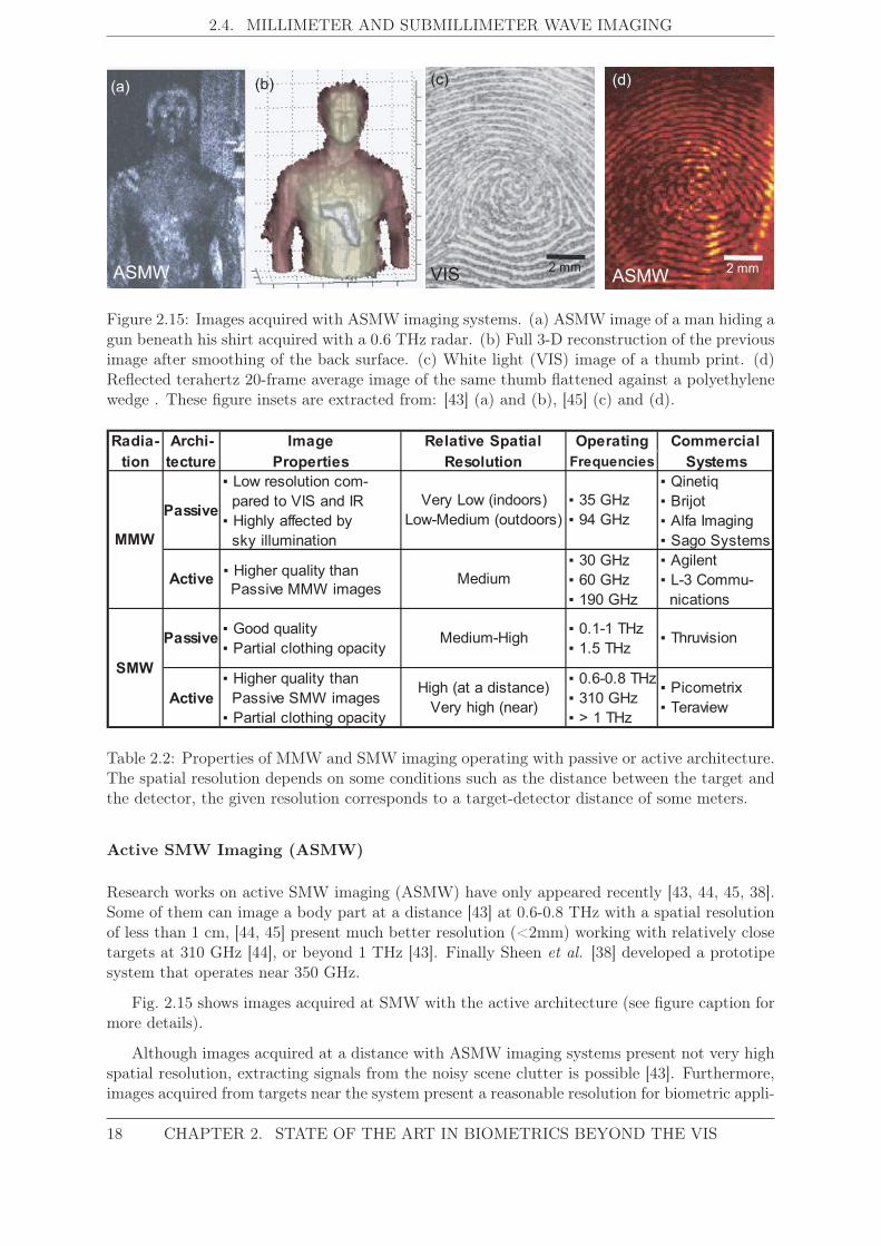
Figure 2.15: Images acquired with ASMW imaging systems. (a) ASMW image of a man hiding agun beneath his shirt acquired with a 0.6 THz radar. (b) Full 3-D reconstruction of the previousimage after smoothing of the back surface. (c) White light (VIS) image of a thumb print. (d)Reflected terahertz 20-frame average image of the same thumb flattened against a polyethylenewedge . These figure insets are extracted from: [43] (a) and (b), [45] (c) and (d).
Frequencies
Radia- Archi- Image Relative Spatial Operating Commercial
tion tecture Properties Resolution Systems
▪ Low resolution com- ▪ Qinetiq
pared to VIS and IR ▪ Brijot
▪ Highly affected by ▪ Alfa Imaging
sky illumination ▪ Sago Systems
▪ 30 GHz ▪ Agilent
▪ 60 GHz ▪ L-3 Commu-
▪ 190 GHz nications
▪ Higher quality than ▪ 0.6-0.8 THz
Passive SMW images ▪ 310 GHz
▪ Partial clothing opacity ▪ > 1 THz
MMW
PassiveVery Low (indoors)
Low-Medium (outdoors)
▪ 35 GHz
▪ 94 GHz
Active_Passive MMW images
Medium
SMW
Passive▪ Good quality
▪ Partial clothing opacityMedium-High
▪ 0.1-1 THz
▪ 1.5 THz▪ Thruvision
ActiveHigh (at a distance)
Very high (near)
▪ Picometrix
▪ Teraview
▪ Higher quality than
Table 2.2: Properties of MMW and SMW imaging operating with passive or active architecture.The spatial resolution depends on some conditions such as the distance between the target andthe detector, the given resolution corresponds to a target-detector distance of some meters.
Active SMW Imaging (ASMW)
Research works on active SMW imaging (ASMW) have only appeared recently [43, 44, 45, 38].Some of them can image a body part at a distance [43] at 0.6-0.8 THz with a spatial resolutionof less than 1 cm, [44, 45] present much better resolution (<2mm) working with relatively closetargets at 310 GHz [44], or beyond 1 THz [43]. Finally Sheen et al. [38] developed a prototipesystem that operates near 350 GHz.
Fig. 2.15 shows images acquired at SMW with the active architecture (see figure caption formore details).
Although images acquired at a distance with ASMW imaging systems present not very highspatial resolution, extracting signals from the noisy scene clutter is possible [43]. Furthermore,images acquired from targets near the system present a reasonable resolution for biometric appli-
18 CHAPTER 2. STATE OF THE ART IN BIOMETRICS BEYOND THE VIS

2.4. MILLIMETER AND SUBMILLIMETER WAVE IMAGING
cations, as it is shown in Fig. 2.15(d) . This fingerprint acquired at 4.3 THz has enough qualityto allow the identification of an individual. On the other hand, the imaging system is quitecomplicated, and it works only in laboratory environments. Active terahertz imaging systemsare available providing high resolution (Picometrix) and additional spectroscopic information(Teraview).
To sum up, the image properties, relative spatial resolution, the operating frequencies aswell as examples of commercial systems for each MMW/SMW architecture are summarized inTable 2.2.
CHAPTER 2. STATE OF THE ART IN BIOMETRICS BEYOND THE VIS 19

2.4. MILLIMETER AND SUBMILLIMETER WAVE IMAGING
20 CHAPTER 2. STATE OF THE ART IN BIOMETRICS BEYOND THE VIS

3MMW Images Databases
3.1 Introduction
In order to develop and to test a biometric recognition system, the availability of biometricdatabases is essential. Furthermore, the biometric databases should be large enough and sta-tistically significant in order to achieve an objective and differentiating comparison among thedifferent algorithms developed in the biometric recognition field.
In the particular case of the proposed research, public databases composed of images acquiredout of the VIS band already exist. Most of them contain images acquired at (i) one IR sub-band, (ii) at VIS and one IR sub-band, or (iii) at several VIS and IR sub-bands (multispectraldatabases). As expected, the hand and the face are the most common traits in these databases.Some of these databases are included in Table 3.1.
Unfortunately the MMW imaging technology is not as mature as the VIS or the IR one.In fact, in comparison with them, it is in its infancy. In addition to this, the privacy concernsthe MMW body images present, difficult the acquisition of databases containing body imagesat that spectral range. As a result, there are only two databases of MMW body images:
• TNO Database. This database is the one created and used by Alefs et al. in [9] (the onlybiometric recognition research based on MMW images published so far).
• BIOGIGA Database. This is the database generated within this project with the pur-pose of designing, developing and testing the biometric system presented throughout thedocument.
In the following, the generation of these databases, the characteristics of their images as wellas the contents of each database will be described. As the BIOGIGA database is the one usedin this project, it will be described in more detail.
21
3.2. TNO DATABASE
Database Biometric Trait Spectral BandsCASIA HFB Database Face VIS, NIR, 3DCASIA NIR Database Face NIRTerravic Facial IR Database Face LWIROulu-CASIA NIR&VIS Face(Facial Expressions) VIS, NIRIRIS Thermal/Visible Face Database Face VIS, Thermal IRPolyU Multispectral Palmprint Database Palmprint R, G, B and NIR illuminationPolyU NIR Face Database Face NIRUSTC-NVIE Database Face (Facial Expressions) VIS, IR
Table 3.1: Main databases of hand or face images acquired at VIS and/or IR bands.
(a) (b)
Figure 3.1: Reproduced from Fig. 2.12. TNO database: (a) Schematic view of the used stereoradiometer (top view). The platform is shifted vertically during scanning. (b) Pair of millimetre-wave images acquired at one scan of a person wearing normal clothing. The equivalent surfacetemperature varies between 225 K (light regions) and 300 K (dark regions). Images extractedfrom [9].
3.2 TNO Database
In [9] Alefs et al. analyzed the appearance of the upper body and thorax in MMW imagesto perform human identification. Although the database they created does not have a specificname, we will refer to it as TNO Database (just because that research was carried out in theTNO Defence, Security and Safety Center, located at The Hague, Netherlands).
This database comprises images of 50 people acquired by a passive system at 94 GHz (thatfrequency corresponds to an average wavelength of about 3.2 mm - MMW range), therefore theyare PMMW images.
3.2.1 Image Acquisition and characteristics
The MMW body images were acquired outdoors using a multi-view (stereo) radiometric scanner,which is shown in Fig. 3.1(a). One scan, that takes about 15 s to complete, provides a set of twoimages from slightly different points of view giving a pair of images like the ones in Fig. 3.1(b).
Those images show a male person of average size and with normal clothing. The radiationpattern is inverted: the bright regions indicate a surface with low radiation and dark regionsindicate surface with high radiation. At surfaces with upward directed normals, the amount of
22 CHAPTER 3. MMW IMAGES DATABASES

3.2. TNO DATABASE
reflected radiation is smaller than the amount reflected from surfaces with downward directednormals. This is due to the fact that the sky has a low temperature compared to the floor.Therefore surfaces with upward directed normals are presented with a bright value. Metallicobjects typically appear bright. The background consists of a metal surface that is positionedtilted toward the sky providing a strong contrast to the foreground. Cavities and surfaces withdownward directed normal vectors typically provide MMW hot spots, i.e. small dark regions,e.g. eyes and chin. On the contrary, the nose and forehead provide the opposite contrast (theyappear white in the MMW image).
3.2.2 Description of the database
The dataset is composed of MMW images from 50 people, all of them are male. Each man wasasked to stand in front of the scanner with the head and the arms positioned at a fixed rack andtwo recordings were made. Each recording contains two images (see Fig. 3.1(b)), each recordingwith a different pose:
• The first one with the head and the body recorded in frontal view.
• The second one with the head turned leftward.
This was done to increase viewpoint dependent variations. The second recording providesimages with side view of the head and some small changes in the appearance of the frontal torso.
A second set of images was recorded with the same people, poses and viewpoints, but nowwearing different facial clutter configurations, so that a large part of the face was occludedusing an artificial beard or balaclava. The Fig. 3.2 shows the effect of this clutter in VIS andMMW images. Images Fig. 3.2(a) and (b) display VIS images while (c) and (d) display thecorresponding MMW images, which are only slightly influenced by the use of the clutter, beingthe head pose the main influence on the appearance on MMW images.
To summarize, in the TNO database, four images pairs were acquired per person: twodifferent poses with each two different facial clutter configurations. This gives a total of 50 ×4× 2 = 400 images for this database.
Figure 3.2: TNO database: Facial images acquired at VIS, (a) and (b), and at 94 GHz, (c) and(d), for one person with different face occlusions. Images extracted from [9].
CHAPTER 3. MMW IMAGES DATABASES 23

3.3. BIOGIGA DATABASE
3.3 BIOGIGA Database
The corpus of the BIOGIGA database consists of synthetic images at 94 GHz of the body of50 individuals. The images are the result of simulations carried out on corporal models attwo types of scenarios (outdoors, indoors) and with two kinds of imaging systems (passive andactive). These corporal models were previously generated based on body measurements takenfrom real subjects.
3.3.1 Generation of the Database
The generation of the database was carried out jointly at the Universidad Autónoma de Madrid(UAM) and Universidad Autónoma de Barcelona (UAB) [12]. The process to generate theimages that compose the database can be divided into the following stages:
1. Acquisition of body measures of each person.
2. Generation of the 3D body model of each user based on such measures.
3. Simulation of the images at 94 GHz from each model in the two types of scenarios (in-door/outdoor) and with two types of imaging systems (passive/active).
Corporal Measures
In order to have realistic 3D body models, a set of body measures of each person was taken.These measures are specified in Table 3.2. Some pictures of each subject were also taken in thevisible spectrum (with a conventional digital camera).
Main Parameters Corporal MeasuresGender Neck circ. Waist circ.
Age Height Nape to waistTone Upper arm circ. Waist to hip
Weight Upper arm length Shoulder to NeckHeight Lowerarm length Upperleg height
Wrist circ. Lowerleg heightFront chest dist. Calf circ.
Bust circ. Angle circ.Underbust circ. Thigh circ.
Hips circ.
Table 3.2: BIOGIGA database: Main parameters and body measures taken from each subjectused to create his/her corresponding 3D body model in MakeHuman. The abbreviation circ.means circumference.
Corporal Model
The body model of each subject was obtained using the free software MakeHuman1, which allowsto generate images of human bodies in 3D. For each person, his or her main parameters and bodymeasurements (see Table 3.2) were introduced through the menus available for it. Subsequentlythe 3D model was compared with the picture previously taken to verify that the obtained modelcorresponds to the body of the concerned person.
1http://www.makehuman.org/
24 CHAPTER 3. MMW IMAGES DATABASES
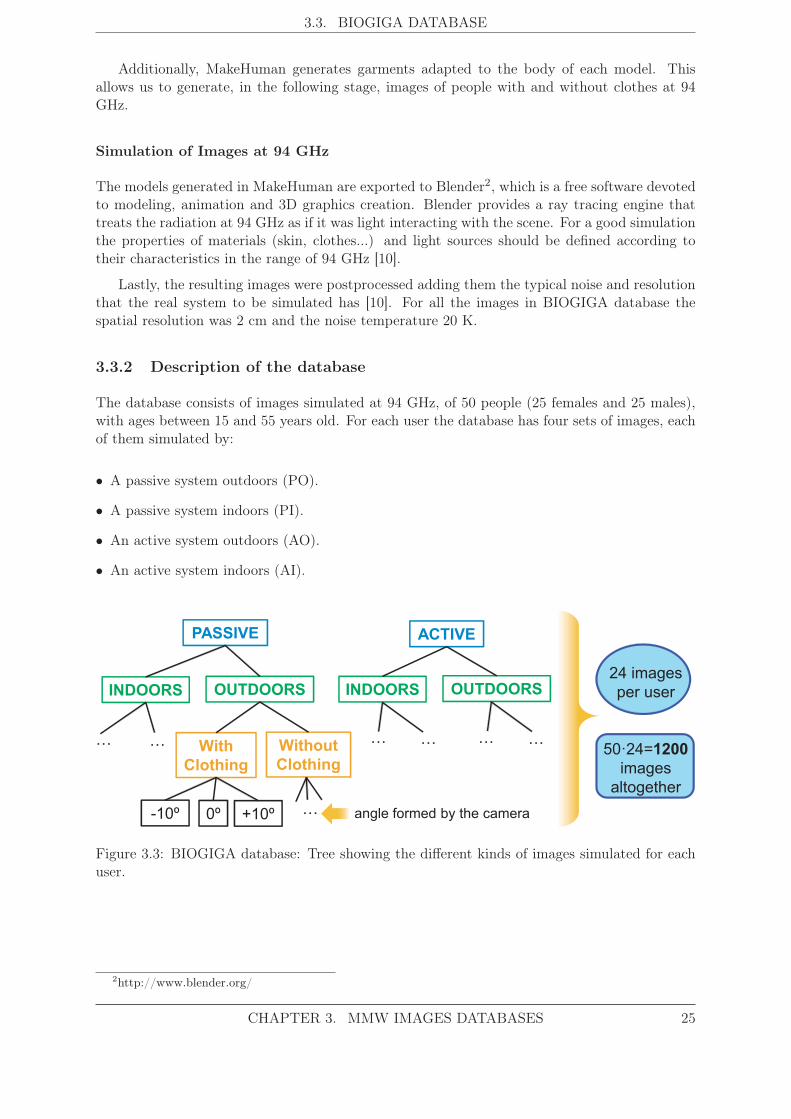
3.3. BIOGIGA DATABASE
Additionally, MakeHuman generates garments adapted to the body of each model. Thisallows us to generate, in the following stage, images of people with and without clothes at 94GHz.
Simulation of Images at 94 GHz
The models generated in MakeHuman are exported to Blender2, which is a free software devotedto modeling, animation and 3D graphics creation. Blender provides a ray tracing engine thattreats the radiation at 94 GHz as if it was light interacting with the scene. For a good simulationthe properties of materials (skin, clothes...) and light sources should be defined according totheir characteristics in the range of 94 GHz [10].
Lastly, the resulting images were postprocessed adding them the typical noise and resolutionthat the real system to be simulated has [10]. For all the images in BIOGIGA database thespatial resolution was 2 cm and the noise temperature 20 K.
3.3.2 Description of the database
The database consists of images simulated at 94 GHz, of 50 people (25 females and 25 males),with ages between 15 and 55 years old. For each user the database has four sets of images, eachof them simulated by:
• A passive system outdoors (PO).
• A passive system indoors (PI).
• An active system outdoors (AO).
• An active system indoors (AI).
24 images
per user
50·24=1200
images
altogether
PASSIVE ACTIVE
INDOORS OUTDOORS INDOORS OUTDOORS
With
Clothing
Without
Clothing
-10º 0º +10º
… …
…
…… ……
angle formed by the camera
Figure 3.3: BIOGIGA database: Tree showing the different kinds of images simulated for eachuser.
2http://www.blender.org/
CHAPTER 3. MMW IMAGES DATABASES 25

3.3. BIOGIGA DATABASE
For each user and each of the previous sets the following data was generated:
• Images of the human 3D model with clothing and an angle formed by the camera of -10°, 0°and +10°.
• Images of the human 3D model without clothing and an angle formed by the camera of -10°,0° and +10°.
According to what is stated above (which is schematically show in Fig. 3.3), for each user thedatabase has 4×2×3=24 images at 94 GHz. Hence, the total number of images in BIOGIGAis 50×24=1200. Fig. 3.4 shows the VIS image and the 3D body models of one subject whileFig. 3.5 and Fig. 3.6 display most of the images simulated at 94 GHz of the same user.
There are certain features of the images at 94 GHz that can be highlighted. These featuresare related to (i) the influence of clothing and (ii) the contrast and relative level of each imagetype.
Firstly, regarding the influence of the clothing, it is hardly noticeable in the pictures, infact, the images simulated at 94 GHz from the model with clothes and from the model withoutclothes are almost the same. The effect of clothing is slightly observed only in some regions,where the fabric is thicker or where there are folds or several layers of clothing. This occursin the neck of the shirt and the waist, being more noticeable in images simulated with passivesystems outdoors.
Secondly, concerning the contrast in the images, among the images simulated with passivesystems, the simulated outdoors have a higher contrast than the simulated indoors. This is dueto the greater temperature difference between the sky (100 K) and the floor (300 K) as it wasexplained in Sect. 2.4 and Sect. 3.2.1. As it happens in the images of TNO database, thePMMW images of BIOGIGA present a dark color in regions oriented to the floor and light graycolor in parts of the body oriented to the sky (see Sect. 3.2.1). However, indoors, the body hasa much more uniform color as the surrounding temperature has no major variations. On theother hand, the images simulated with active systems show a higher radiometric temperaturelevel (are darker) because the person is radiated with an external source not natural, collectingthe radiation once it has been reflected by the person. For the same reason there is almost nodifference between the images simulated indoors and outdoors for active acquisition.
Finally, Fig. 3.7 displays four histograms of different parameters or body measures takenfrom the subjects that form the database: (i) the age, (ii) the height, (iii) the waist circumference,and (iv) the arm length.
26 CHAPTER 3. MMW IMAGES DATABASES
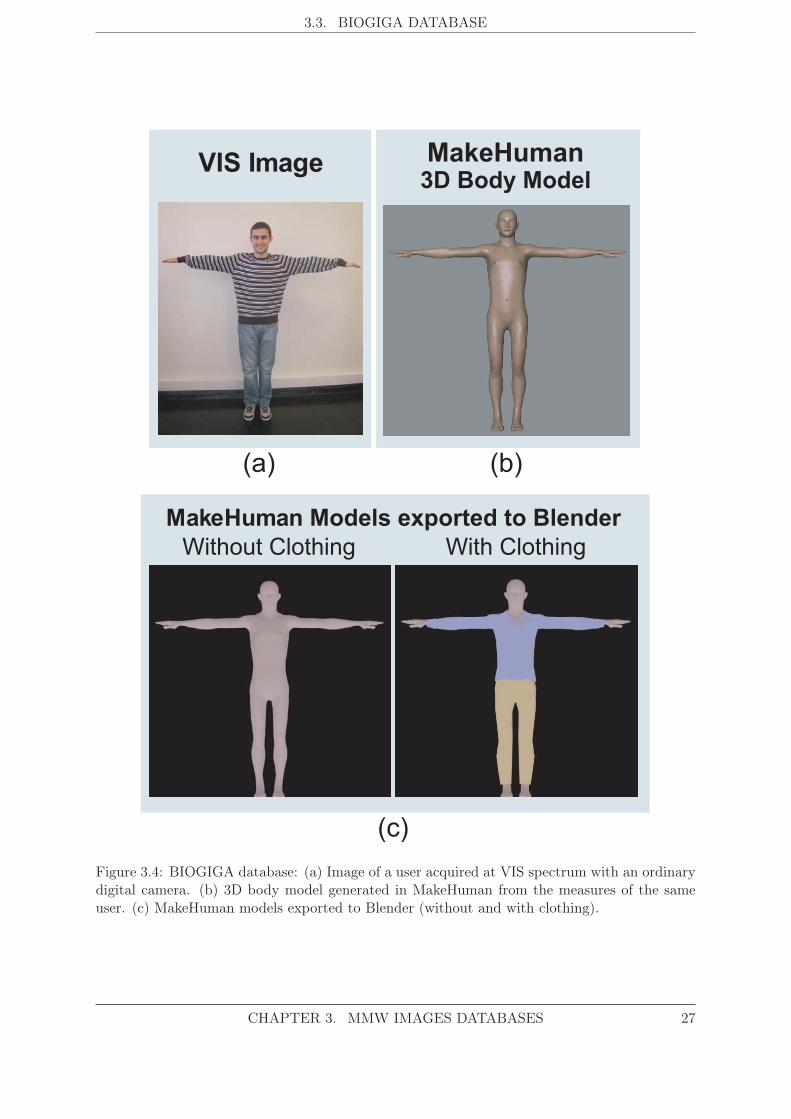
3.3. BIOGIGA DATABASE
VIS Image
MakeHuman Models exported to Blender
Without Clothing With Clothing
MakeHuman3D Body Model
(a) (b)
(c)
Figure 3.4: BIOGIGA database: (a) Image of a user acquired at VIS spectrum with an ordinarydigital camera. (b) 3D body model generated in MakeHuman from the measures of the sameuser. (c) MakeHuman models exported to Blender (without and with clothing).
CHAPTER 3. MMW IMAGES DATABASES 27
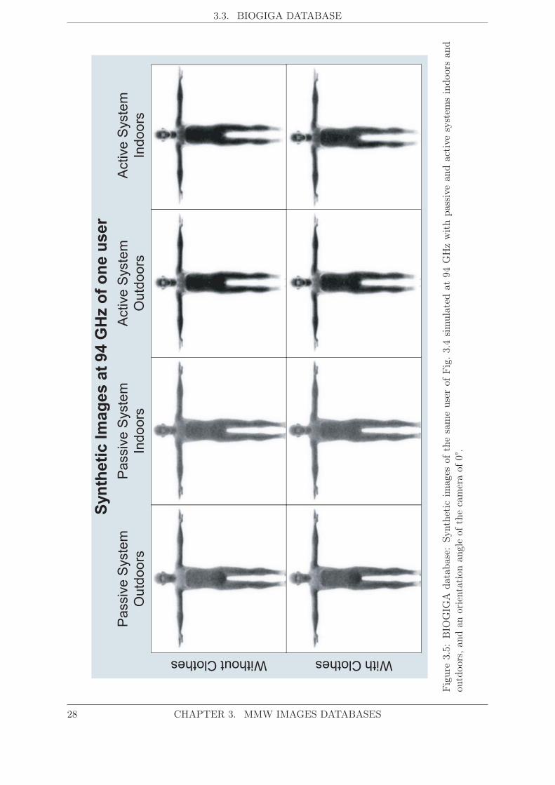
3.3. BIOGIGA DATABASE
Pa
ssiv
eS
yste
m
Ou
tdo
ors
Pa
ssiv
eS
yste
m
Ind
oo
rs
Active
Syste
m
Ou
tdo
ors
Active
Syste
m
Ind
oo
rs
WithoutClothes WithClothes
Syn
theti
cIm
ag
es
at
94 G
Hz o
f o
ne
user
Fig
ure
3.5:
BIO
GIG
Ada
taba
se:
Synt
heti
cim
ages
ofth
esa
me
user
ofFig
.3.
4si
mul
ated
at94
GH
zw
ith
pass
ive
and
acti
vesy
stem
sin
door
san
dou
tdoo
rs,a
ndan
orie
ntat
ion
angl
eof
the
cam
era
of0°
.
28 CHAPTER 3. MMW IMAGES DATABASES
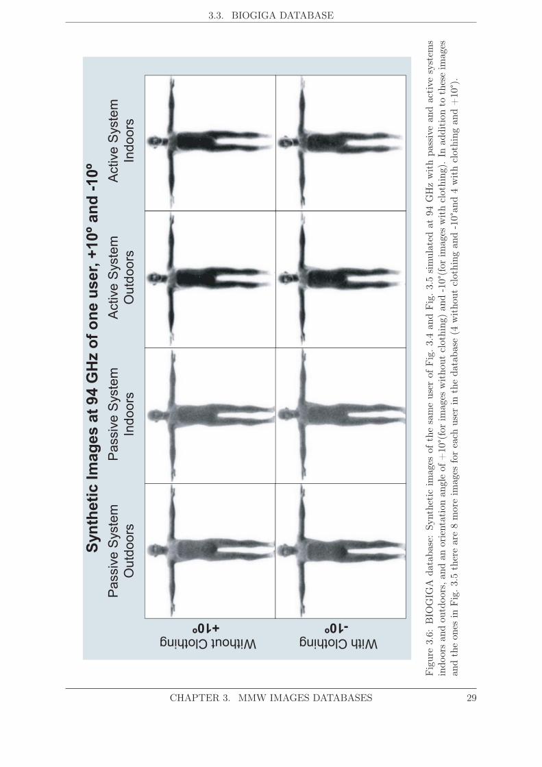
3.3. BIOGIGA DATABASE
Pa
ssiv
eS
yste
m
Ou
tdo
ors
Pa
ssiv
eS
yste
m
Ind
oo
rs
Active
Syste
m
Ou
tdo
ors
Active
Syste
m
Ind
oo
rsWithoutClothing
+10º
WithClothing
-10º
Syn
theti
cIm
ag
es
at
94 G
Hz o
f o
ne
user,
+10º
an
d -
10º
Fig
ure
3.6:
BIO
GIG
Ada
taba
se:
Synt
heti
cim
ages
ofth
esa
me
user
ofFig
.3.
4an
dFig
.3.
5si
mul
ated
at94
GH
zw
ith
pass
ive
and
acti
vesy
stem
sin
door
san
dou
tdoo
rs,a
ndan
orie
ntat
ion
angl
eof
+10
°(fo
rim
ages
wit
hout
clot
hing
)an
d-1
0°(f
orim
ages
wit
hcl
othi
ng).
Inad
diti
onto
thes
eim
ages
and
the
ones
inFig
.3.5
ther
ear
e8
mor
eim
ages
for
each
user
inth
eda
taba
se(4
wit
hout
clot
hing
and
-10°
and
4w
ith
clot
hing
and
+10
°).
CHAPTER 3. MMW IMAGES DATABASES 29

3.3. BIOGIGA DATABASE
Age Height
Waist Circumference Arm Length
Figure 3.7: BIOGIGA database: Histograms of the age, height, waist circumference and armlength of the users that form BIOGIGA.
30 CHAPTER 3. MMW IMAGES DATABASES
4System, design and development
The aim of this project is the development of a new biometric system based on images acquiredat the MMW band. This system has several modules: image processing, most distinctive featureextraction, feature selection, similarity computation and decision maker. After a brief introduc-tion to biometric systems, this chapter describes the modules that constitute the proposed anddeveloped biometric system.
4.1 Introduction to Biometric Systems
A biometric system is the combination of devices, databases and processes that allow the recog-nition of an individual using one or more of his/her biometric features. The block diagram of ageneric biometric system is shown in Fig. 4.1.
Once the user has been enrolled, biometric systems can operate in two modes:
• Verification Mode. The user claims an identity and presents his or her biometric trait,then the system determines if the real identity of the user corresponds to the identityclaimed by him or her.
• Identification Mode. The user only presents his or her biometric trait without claimingany identity, then the system tries to find his or her identity.
In the acquisition stage (see Fig. 4.1) the biometric trait is captured. In our case, thebiometric trait is the MMW image of the body. After that, the image is processed obtaining amore suitable image to perform the feature extraction, which is the following step in Fig. 4.1.Next, the vector containing the features of the input image is compared with the feature vector ofthe claimed user (verification mode) or with all the feature vectors in the database (identificationmode). Finally, a decision based on the result of that comparison is made.
The acquisition stage (which, in this work, corresponds to the simulation of the MMWimages) was already explained in Sect. 3.3. The rest of the modules of the system are describedin the next subsections: the image segmentation (Sect. 4.2) belongs to the preprocessing while theboundary extraction (Sect. 4.3), landmark generation (Sect. 4.4), feature generation (Sect. 4.5)
31

4.2. IMAGE SEGMENTATION
Acquisition PreprocessingFeature
ExtractionMatching Decision
Database
Claimed
identity
Accepted
or
Rejected
Feature
Vector
Figure 4.1: Architecture of a generic biometric system working either in verification or identifi-cation mode.
and feature selection (Sect. 4.6) are part of the feature extraction module. In Sect. 4.7 (matching)the similarity measure used to perform the comparison between feature vectors is introduced.The value of that similarity measure determines the final decision given by the system (Sect. 4.8).
It is worth mentioning that our system is based on the geometry of the user’s body while thesystem developed by Alefs et al. in [9] is based on a holistic approach over the grayscale aftervarious dimensionality reduction techniques. Specifically, in our system, the features extractedfrom the images are based on distances between points of the silhouette of the body or betweenpoints inside the silhouette. In fact, the use of anthropometric indications to recognize peoplestarted in the XIX century [46]. Moreover, there are biometric systems based on the geometryof the hand [47]. The process followed to obtain the features is depicted in Fig. 4.2.
4.2 Image Segmentation
The image segmentation is the main step of the image preprocessing module. In this processthe input image is binarized, separating the background from the body. A characteristic of theimages simulated by passive systems is the different gray level they present in different parts ofthe body. The ones oriented to the floor (e.g. the abdomen) are much darker than the onesoriented to the sky (e.g. the feet). This fact considerably hinders the segmentation process.This problem was overcome performing the segmentation in two steps:
• Border detection.
• Morphological operations.
The image segmentation comprises several steps, which are shown in Fig. 4.3. After invertingthe gray level of the image (see Fig. 4.3(b)), a Canny border detector (whose parameters arepreviously tuned) is applied to the image (obtaining an image such as the one in Fig. 4.3(c)).Next, various morphological operations are conducted on the resulting border image to closethe body boundary. These morphological operations consists of closing operations with differentstructural elements in different areas of the image (head, arms, from arms to calf, and feet). Theresulting image is shown in see Fig. 4.3(d). Finally, the body contour, and any other contour, arefilled, obtaining a binary image consisting of a white body, maybe some small white connectedcomponents and a black background. An example image after this segmentation process is shownin Fig. 4.3(e).
32 CHAPTER 4. SYSTEM, DESIGN AND DEVELOPMENT

4.2. IMAGE SEGMENTATION
Inp
ut Im
ag
eS
eg
me
nta
tio
nC
on
tou
r, r
efe
ren
ce
po
ints
an
d s
ke
leto
nR
adia
l D
ista
nce
Featu
reS
ele
ction
Fe
atu
reG
en
era
tio
nM
axim
aa
nd
Min
ima
De
tectio
nL
an
dm
ark
s
21
fea
ture
sfe
atu
res
(a)
(b)
(c)
(d)
(h)
(g)
(f)
(e)
3-1
4
Fig
ure
4.2:
Feat
ure
extr
acti
onin
our
syst
em:
(a)
Ori
gina
lim
age
(ofa
subj
ect
wit
hcl
othi
ngan
da
cam
era
angl
eof
-10°
),(b
)se
gmen
ted
imag
e,(c
)co
ntou
r,re
fere
nce
poin
tsan
dba
sic
skel
eton
,(d
)ra
dial
dist
ance
from
each
refe
renc
epo
int
toev
ery
poin
tof
the
cont
our
(one
curv
epe
rre
fere
nce
poin
t),
(e)
addi
tion
ofpo
ints
wit
hm
axim
uman
dm
inim
umdi
stan
cefr
omth
ere
fere
nce
poin
ts,
(f)
all
land
mar
ks,
(g)
dist
ance
sus
edto
form
the
feat
ure
vect
or(w
ith
21co
mpo
nent
s),a
nd(h
)th
efin
alse
lect
edfe
atur
esaf
ter
appl
ying
the
SFFS
algo
rith
m(b
etw
een
3an
d14
com
pone
nts)
.
CHAPTER 4. SYSTEM, DESIGN AND DEVELOPMENT 33
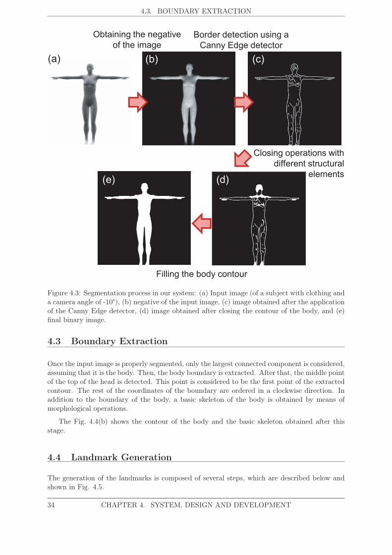
4.3. BOUNDARY EXTRACTION
(a) (b) (c)
(d)(e)
Obtaining the negative
of the image
Border detection using a
Canny Edge detector
Filling the body contour
Closing operations with
different structural
elements
Figure 4.3: Segmentation process in our system: (a) Input image (of a subject with clothing anda camera angle of -10°), (b) negative of the input image, (c) image obtained after the applicationof the Canny Edge detector, (d) image obtained after closing the contour of the body, and (e)final binary image.
4.3 Boundary Extraction
Once the input image is properly segmented, only the largest connected component is considered,assuming that it is the body. Then, the body boundary is extracted. After that, the middle pointof the top of the head is detected. This point is considered to be the first point of the extractedcontour. The rest of the coordinates of the boundary are ordered in a clockwise direction. Inaddition to the boundary of the body, a basic skeleton of the body is obtained by means ofmorphological operations.
The Fig. 4.4(b) shows the contour of the body and the basic skeleton obtained after thisstage.
4.4 Landmark Generation
The generation of the landmarks is composed of several steps, which are described below andshown in Fig. 4.5.
34 CHAPTER 4. SYSTEM, DESIGN AND DEVELOPMENT
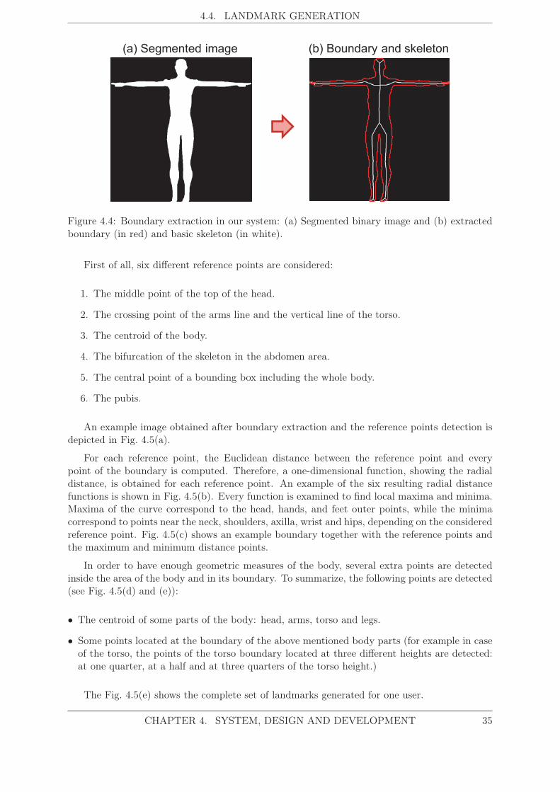
4.4. LANDMARK GENERATION
(a) Segmented image (b) Boundary and skeleton
Figure 4.4: Boundary extraction in our system: (a) Segmented binary image and (b) extractedboundary (in red) and basic skeleton (in white).
First of all, six different reference points are considered:
1. The middle point of the top of the head.
2. The crossing point of the arms line and the vertical line of the torso.
3. The centroid of the body.
4. The bifurcation of the skeleton in the abdomen area.
5. The central point of a bounding box including the whole body.
6. The pubis.
An example image obtained after boundary extraction and the reference points detection isdepicted in Fig. 4.5(a).
For each reference point, the Euclidean distance between the reference point and everypoint of the boundary is computed. Therefore, a one-dimensional function, showing the radialdistance, is obtained for each reference point. An example of the six resulting radial distancefunctions is shown in Fig. 4.5(b). Every function is examined to find local maxima and minima.Maxima of the curve correspond to the head, hands, and feet outer points, while the minimacorrespond to points near the neck, shoulders, axilla, wrist and hips, depending on the consideredreference point. Fig. 4.5(c) shows an example boundary together with the reference points andthe maximum and minimum distance points.
In order to have enough geometric measures of the body, several extra points are detectedinside the area of the body and in its boundary. To summarize, the following points are detected(see Fig. 4.5(d) and (e)):
• The centroid of some parts of the body: head, arms, torso and legs.
• Some points located at the boundary of the above mentioned body parts (for example in caseof the torso, the points of the torso boundary located at three different heights are detected:at one quarter, at a half and at three quarters of the torso height.)
The Fig. 4.5(e) shows the complete set of landmarks generated for one user.
CHAPTER 4. SYSTEM, DESIGN AND DEVELOPMENT 35
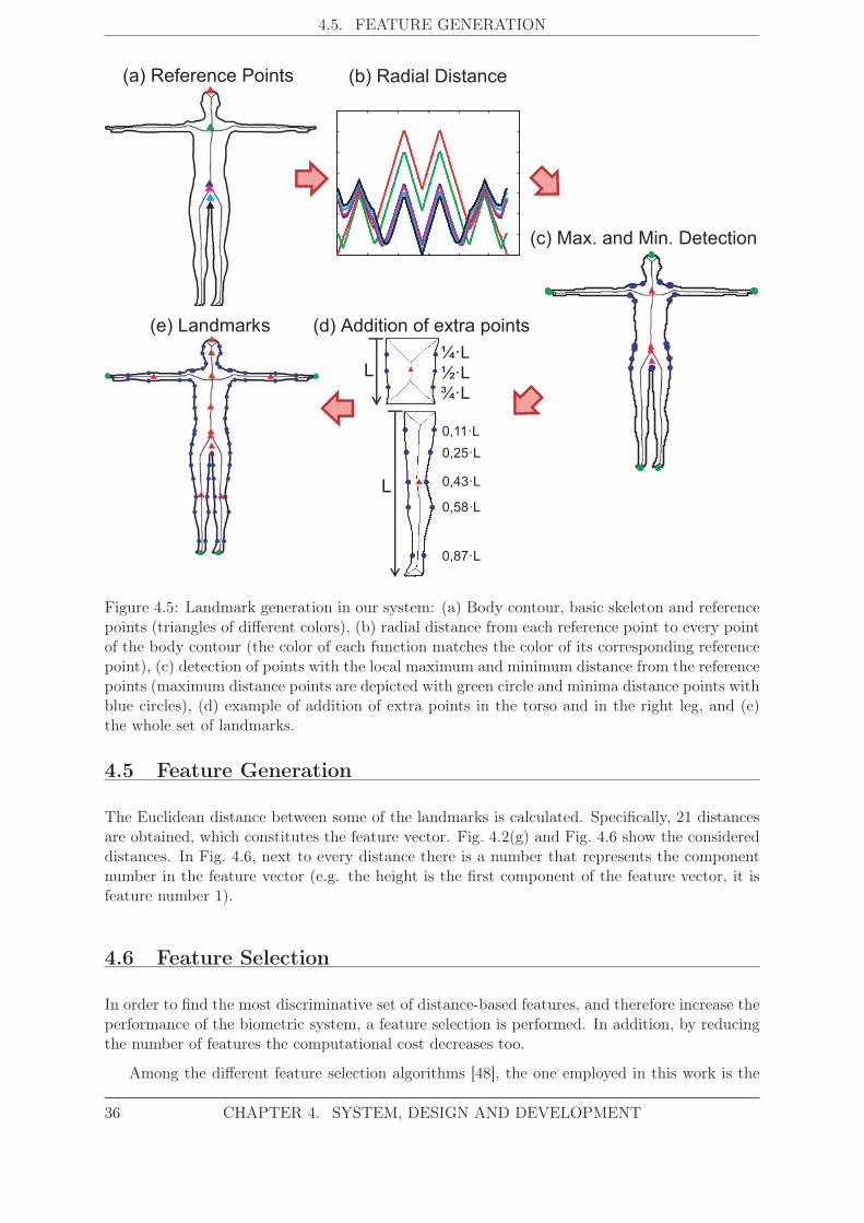
4.5. FEATURE GENERATION
(a) Reference Points (b) Radial Distance
(e) Landmarks
¼·L
½·L
¾·L
L
0,11·L
0,25·L
0,43·L
0,58·L
0,87·L
L
(c) Max. and Min. Detection
(d) Addition of extra points
Figure 4.5: Landmark generation in our system: (a) Body contour, basic skeleton and referencepoints (triangles of different colors), (b) radial distance from each reference point to every pointof the body contour (the color of each function matches the color of its corresponding referencepoint), (c) detection of points with the local maximum and minimum distance from the referencepoints (maximum distance points are depicted with green circle and minima distance points withblue circles), (d) example of addition of extra points in the torso and in the right leg, and (e)the whole set of landmarks.
4.5 Feature Generation
The Euclidean distance between some of the landmarks is calculated. Specifically, 21 distancesare obtained, which constitutes the feature vector. Fig. 4.2(g) and Fig. 4.6 show the considereddistances. In Fig. 4.6, next to every distance there is a number that represents the componentnumber in the feature vector (e.g. the height is the first component of the feature vector, it isfeature number 1).
4.6 Feature Selection
In order to find the most discriminative set of distance-based features, and therefore increase theperformance of the biometric system, a feature selection is performed. In addition, by reducingthe number of features the computational cost decreases too.
Among the different feature selection algorithms [48], the one employed in this work is the
36 CHAPTER 4. SYSTEM, DESIGN AND DEVELOPMENT

4.6. FEATURE SELECTION
1
2
3
4
5
6
7
8
9
10m 11m 12m
13m 14m
15
16
17
18
19m
20m
21m
Figure 4.6: Body boundary, landmarks and distances extracted among them of the subject andconditions of Fig. 4.2. These distances form the 21D feature vector. The number next to everydistance is the component number in the feature vector. The ones whose number appears witha subindex m are calculated as the average of that distance and the analog one of the rightextremity. Red triangles represent the reference points and centroids of head, arms, legs andtorso. Blue circles represent landmarks on the silhouette of the body (some of the them haveminimum distance to the reference points). Green circles represent landmarks with maximumdistance from the reference points.
Sequential Floating Forward Selection (SFFS) [49]. This suboptimal searching technique is aniterative process in which, in each iteration, a new set of features (whose choice is based onthe results of previous subsets) is used to compute a certain criterion. This is done until thecriterion does not improve. For more details see [48, 49, 50]. In our case the criterion is relatedto the performance of the system, in particular, is to minimize the value of the EER (EqualError Rate), magnitude which will be introduced in Sect. 5.1.
Once the features are selected, the feature vector has, depending on the experiment, between
CHAPTER 4. SYSTEM, DESIGN AND DEVELOPMENT 37
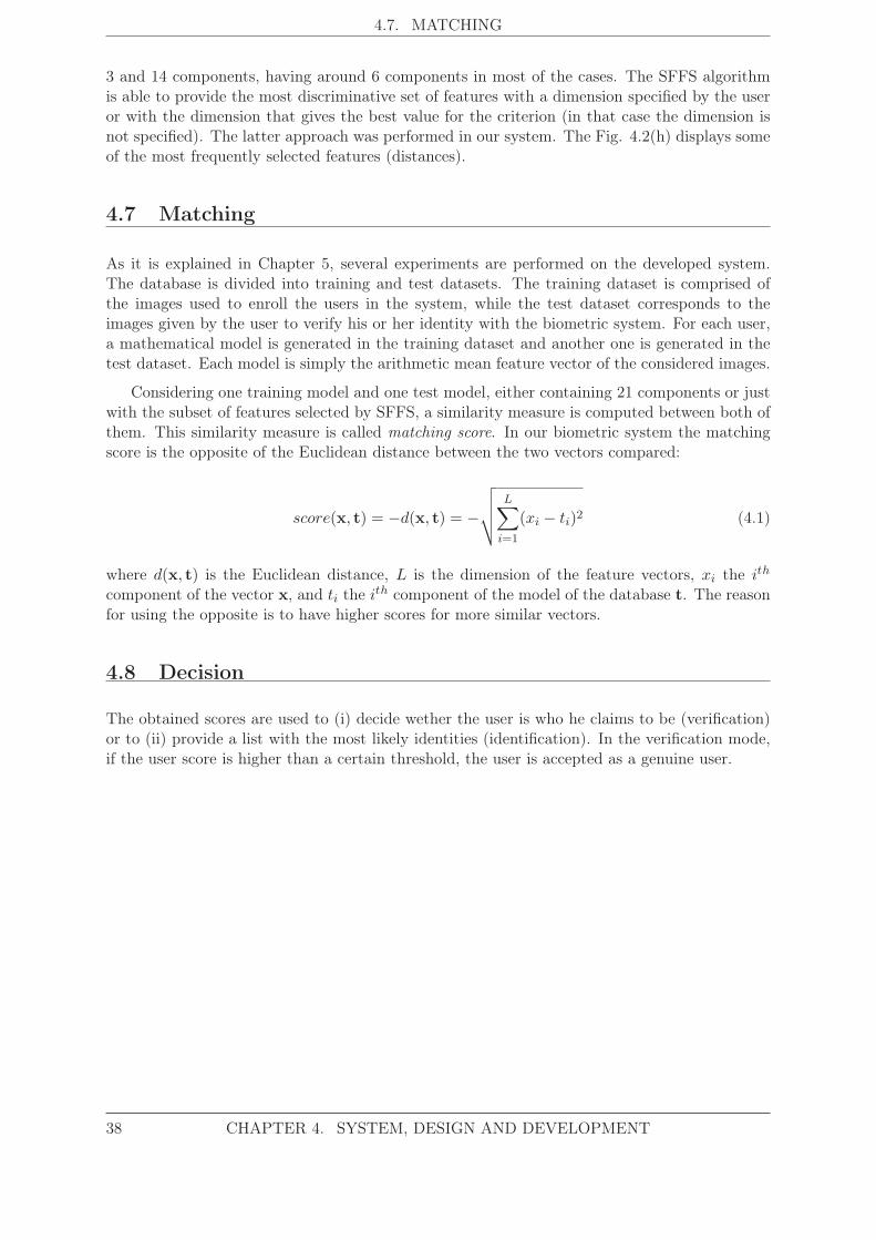
4.7. MATCHING
3 and 14 components, having around 6 components in most of the cases. The SFFS algorithmis able to provide the most discriminative set of features with a dimension specified by the useror with the dimension that gives the best value for the criterion (in that case the dimension isnot specified). The latter approach was performed in our system. The Fig. 4.2(h) displays someof the most frequently selected features (distances).
4.7 Matching
As it is explained in Chapter 5, several experiments are performed on the developed system.The database is divided into training and test datasets. The training dataset is comprised ofthe images used to enroll the users in the system, while the test dataset corresponds to theimages given by the user to verify his or her identity with the biometric system. For each user,a mathematical model is generated in the training dataset and another one is generated in thetest dataset. Each model is simply the arithmetic mean feature vector of the considered images.
Considering one training model and one test model, either containing 21 components or justwith the subset of features selected by SFFS, a similarity measure is computed between both ofthem. This similarity measure is called matching score. In our biometric system the matchingscore is the opposite of the Euclidean distance between the two vectors compared:
score(x, t) = −d(x, t) = −√√√√ L∑
i=1
(xi − ti)2 (4.1)
where d(x, t) is the Euclidean distance, L is the dimension of the feature vectors, xi the ith
component of the vector x, and ti the ith component of the model of the database t. The reasonfor using the opposite is to have higher scores for more similar vectors.
4.8 Decision
The obtained scores are used to (i) decide wether the user is who he claims to be (verification)or to (ii) provide a list with the most likely identities (identification). In the verification mode,if the user score is higher than a certain threshold, the user is accepted as a genuine user.
38 CHAPTER 4. SYSTEM, DESIGN AND DEVELOPMENT

5Experiments and Results
This chapter is structured as follows. First, the performance evaluation of biometric systems isbriefly introduced. Then, in order to have recognition results to compare with, the experimentscarried out by Alefs et al. in [9] and their results are presented. Next, an analysis of the extractedfeatures in our system is provided. Finally, verification and identification experiments, conductedover the developed system, are described. These experiments are intended to assess differentproblems. Each experiment includes protocol description, presentation of results and discussion.All the experiments were performed using (i) the 21 features extracted, and (ii) the featuresselected by the SFFS algorithm.
In the feature analysis, as well as in all the experiments, only images simulated by a passivesystem indoors and outdoors are considered. The results are shown exclusively for passiveoutdoors images, for indoors the results are quite similar. The same analysis for images simulatedby active systems (indoors and outdoors) will be part of future work, in which a different imagesegmentation should be followed due to clearly visible differences between the images simulatedby passive and active systems (e.g. the last ones present higher contrast).
5.1 Performance Evaluation of Biometric Systems
Once the system is implemented, an evaluation of its performance is desirable. This is donethrough quantitative measures, obtained from experiments, that reveal how well the systemworks and allow to compare its performance with the performance of other biometric systems.
5.1.1 Performance Evaluation in Verification Mode
When working in verification mode two main metrics are used to quantify the performance ofthe biometric system:
• The False Acceptance Rate (FAR), which is the probability that an impostor is acceptedby the system as a genuine user.
• The False Rejection Rate (FRR), that reflects the probability that a genuine user is rejectedby the system.
39
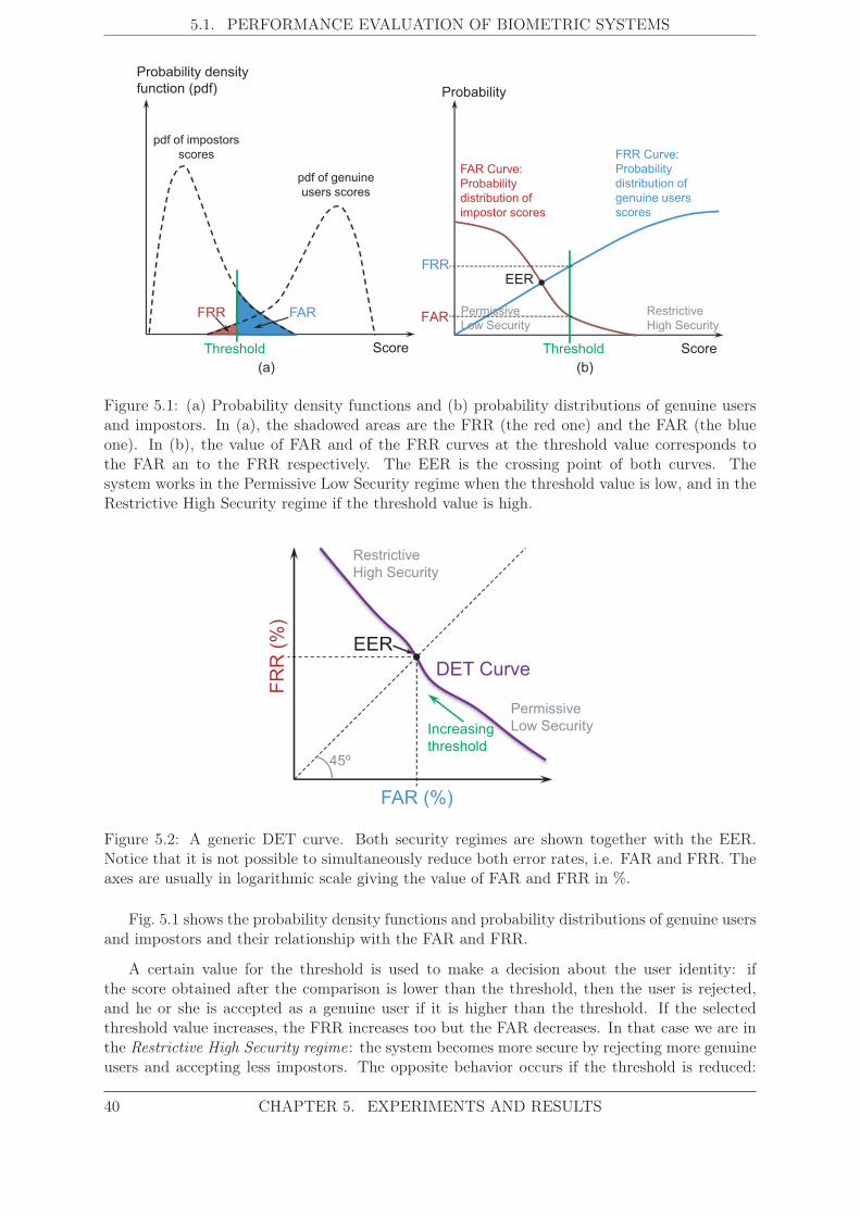
5.1. PERFORMANCE EVALUATION OF BIOMETRIC SYSTEMS
Score ScoreThreshold
FRR FAR
pdf of impostors
scores
pdf of genuine
users scores
EER
Threshold
FRR
FAR
FAR Curve:
Probability
distribution of
impostor scores
FRR Curve:
Probability
distribution of
genuine users
scores
Probability
Probability density
function (pdf)
Restrictive
High Security
Permissive
Low Security
(a) (b)
Figure 5.1: (a) Probability density functions and (b) probability distributions of genuine usersand impostors. In (a), the shadowed areas are the FRR (the red one) and the FAR (the blueone). In (b), the value of FAR and of the FRR curves at the threshold value corresponds tothe FAR an to the FRR respectively. The EER is the crossing point of both curves. Thesystem works in the Permissive Low Security regime when the threshold value is low, and in theRestrictive High Security regime if the threshold value is high.
EER
FR
R (
%)
FAR (%)
DET Curve
Increasing
threshold
Permissive
Low Security
Restrictive
High Security
45º
EER
Figure 5.2: A generic DET curve. Both security regimes are shown together with the EER.Notice that it is not possible to simultaneously reduce both error rates, i.e. FAR and FRR. Theaxes are usually in logarithmic scale giving the value of FAR and FRR in %.
Fig. 5.1 shows the probability density functions and probability distributions of genuine usersand impostors and their relationship with the FAR and FRR.
A certain value for the threshold is used to make a decision about the user identity: ifthe score obtained after the comparison is lower than the threshold, then the user is rejected,and he or she is accepted as a genuine user if it is higher than the threshold. If the selectedthreshold value increases, the FRR increases too but the FAR decreases. In that case we are inthe Restrictive High Security regime: the system becomes more secure by rejecting more genuineusers and accepting less impostors. The opposite behavior occurs if the threshold is reduced:
40 CHAPTER 5. EXPERIMENTS AND RESULTS

5.1. PERFORMANCE EVALUATION OF BIOMETRIC SYSTEMS
the FRR decreases and the FAR increases, being in the Permissive Low Security regime: thesystem becomes less secure accepting more impostors. This is graphically shown in Fig. 5.1(b).
There is a value of the threshold for which the FAR and the FRR coincide. The value ofboth rates at that threshold is known as the Equal Error Rate (EER) and is the most widelyused parameter to evaluate the performance of a biometric system working in verification mode.Plotting the FRR versus the FAR for all the different threshold values with logarithmic axes,gives the so-called DET curve (Detection Error Tradeoff curve) [51]. This curve is a commonway to graphically represent the behavior of a biometric system, where the EER corresponds tothe point where the DET curve and the bisector of the first quadrant intersect each other (SeeFig. 5.2). The closer the curve is to the origin (and therefore the lower the EER is), the betterthe system is.
5.1.2 Performance Evaluation in Identification Mode
In identification mode, the sytem compares the model (or feature vector) created from the inputdata with all the models (or features vectors) stored in the database. Then, a ranked list ofcandidates is returned. At the top of the list is located the candidate that produces the highestscore, followed by the candidate that provides the second highest score, and so on. If the mostsimilar model corresponds to the input identity, then a successful identification has happened.
For this mode, the error measure is computed as the rate of correctly identified users. TheRank-1 recognition rate (R-1 ) is the number of users correctly identified with the first candidateof the list over the total number of users, N, the Rank-n recognition rate (R-n) is the number ofusers correctly identified with any of the n first candidates of the list, over N. The R-1 and R-5are the most used recognition rates in identification mode.
The performance of a system working in identification mode is graphically shown by meansof the so-called CMC (Cumulative Match Curve) (See Fig. 5.3). This curve plots the R-n versusn (being n the number of the candidates considered at the beginning of the list). The CMC isan increasing function whose value increases from the R-1 at the beginning (where n=1, onlythe first user of the list is considered) to 1 at the end (where n=N, all the users are considered,hence the user is one of them). The closer to 1 the CMC is, the better the system is.
0 5 10 15 20 25 30 35 40 45 50 55 60 65 70 75 80 85 90 95 1000.75
0.8
0.85
0.9
0.95
1
Rank
Ra
nk R
eco
gn
itio
n R
ate
R-5
R-1
Figure 5.3: A generic CMC curve. The Rank-1 and Rank-5 recognition rates are indicated. Inthis case the total number of users is 100.
CHAPTER 5. EXPERIMENTS AND RESULTS 41
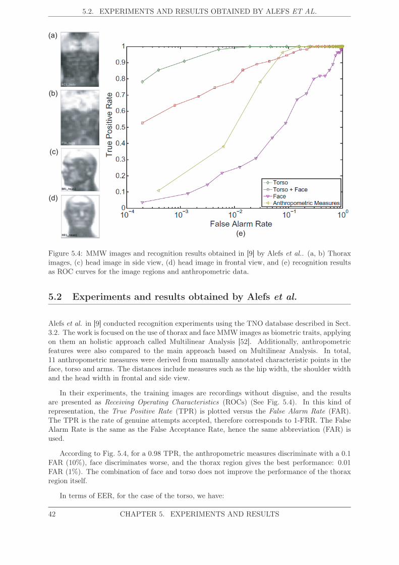
5.2. EXPERIMENTS AND RESULTS OBTAINED BY ALEFS ET AL.
(a)
(b)
(c)
(d)
(e)
Figure 5.4: MMW images and recognition results obtained in [9] by Alefs et al.. (a, b) Thoraximages, (c) head image in side view, (d) head image in frontal view, and (e) recognition resultsas ROC curves for the image regions and anthropometric data.
5.2 Experiments and results obtained by Alefs et al.
Alefs et al. in [9] conducted recognition experiments using the TNO database described in Sect.3.2. The work is focused on the use of thorax and face MMW images as biometric traits, applyingon them an holistic approach called Multilinear Analysis [52]. Additionally, anthropometricfeatures were also compared to the main approach based on Multilinear Analysis. In total,11 anthropometric measures were derived from manually annotated characteristic points in theface, torso and arms. The distances include measures such as the hip width, the shoulder widthand the head width in frontal and side view.
In their experiments, the training images are recordings without disguise, and the resultsare presented as Receiving Operating Characteristics (ROCs) (See Fig. 5.4). In this kind ofrepresentation, the True Positive Rate (TPR) is plotted versus the False Alarm Rate (FAR).The TPR is the rate of genuine attempts accepted, therefore corresponds to 1-FRR. The FalseAlarm Rate is the same as the False Acceptance Rate, hence the same abbreviation (FAR) isused.
According to Fig. 5.4, for a 0.98 TPR, the anthropometric measures discriminate with a 0.1FAR (10%), face discriminates worse, and the thorax region gives the best performance: 0.01FAR (1%). The combination of face and torso does not improve the performance of the thoraxregion itself.
In terms of EER, for the case of the torso, we have:
42 CHAPTER 5. EXPERIMENTS AND RESULTS

5.3. FEATURE ANALYSIS
TPR = 0.98 when FAR = 0.01 (5.1)
then the FRR is:
FRR = 1− TPR = 1− 0.98 = 0.02 (5.2)
and therefore, as the EER is the value of FRR and FAR when they coincide, the EER must hasa value between 1 and 2%:
EER(Thorax) ∈ [1, 2]% (5.3)
The exact value of the EER is difficult to obtain from the given graphical results. Finallyfrom Fig. 5.4 we can also observe that the other approaches give worse EERs:
EER(Thorax) < EER(Anthropometric Measures) < EER(Torso + Face) < EER(Face) (5.4)
5.3 Feature Analysis
Before computing the recognition capabilities of the developed system, some experimental vali-dations are performed on the extracted features to:
• Determine wether they are discriminative enough.
• Find the most discriminative ones.
• Quantify their discrimination power.
5.3.1 Ranking of features according to their discrimination power
Fig. 5.5(a) represents the mean value and the standard deviation (as an error bar) of eachnormalized component (distance) of the feature vector, for seven subjects (a different color andsymbol for each subject) randomly selected from the 50 available. As it can be seen, somecomponent values are quite different from one subject to another, while others are more similar.Moreover, the error bars overlap in some cases. To determine the most discriminative features,the components of the feature vector are ranked in descending order of degree of discrimination.For this purpose two magnitudes are calculated:
• The average separation between the mean values of each component from all subjects.
• The overlap between the error bars of the same component among all subjects.
The most discriminative feature will be the one with the largest average separation and thelowest overlap among different users. Hence, the features are ranked in descending order of theirdiscrimination power. This magnitude can be considered as the value of the quotient:
discrimination power =average separation between mean values
overlap of errors bars(5.5)
CHAPTER 5. EXPERIMENTS AND RESULTS 43

5.3. FEATURE ANALYSIS
1 2 3 4 5 6 7 8 9 10 11 12 13 14 15 16 17 18 19 20 210
0.1
0.2
0.3
0.4
0.5
0.6
0.7
0.8
0.9
1
Features
Me
an
No
rma
lize
d V
alu
e
17 6 16 2 4 20 12 21 10 3 1 5 9 14 11 13 15 19 18 80
0.1
0.2
0.3
0.4
0.5
0.6
0.7
0.8
0.9
1
Ranked Features
Me
an
No
rma
lize
d V
alu
e
(a) (b)
7
Figure 5.5: Mean normalized value of the feature vector of 7 randomly selected users. Eachuser vector has a different color and symbol. In (a) the features are ordered according to theirnumber while in (b) they are ranked in descending order of their discrimination power.
Fig. 5.5(b) shows the feature vector for the same seven subjects of Fig. 5.5(a) once itscomponents have been ordered. Although the Fig. 5.5(b) shows the feature vector for 7 users,the ranking was conducted taking into account the vectors from all the 50 subjects. It can be seenthe decreasing separation between mean values and the increasing overlap. The initial featurenumber (the same one as the one in Fig. 4.6) is written below the x axis with bold numbers. Itis worth noting that the four most discriminative features (the first four in Fig. 5.5(b)) are:
• Feature #1: the height.
• Feature #17: approximately the waist width.
• Feature #5: the distance between the centroid of the body and the pubis.
• Feature #6: the legs length.
The least discriminative one corresponds to feature #7, which is the height of the head. Fur-thermore, the three best features and the worst one, obtained for images simulated by passivesystems outdoors, are the same ones when using images simulated indoors. It is not surprisingthat the height of the head is the least discriminating feature due to the process followed toobtain the 3D-body model from the body measures of real subjects. The head height was notconsidered, so all the models present approximately the same head height in their 3D bodymodel used to simulate MMW images.
5.3.2 Discrimination Power Analysis
With the purpose of better assessing the discrimination power of the features, they are plottedin 2D graphs in Fig. 5.6:
• Fig. 5.6(a) plots the second PCA (Principal Component Analysis) component vs the firstPCA component of the 300 feature vectors (6 per user), having used all the 21D vectorsto obtain the PCA transformation matrix.
44 CHAPTER 5. EXPERIMENTS AND RESULTS
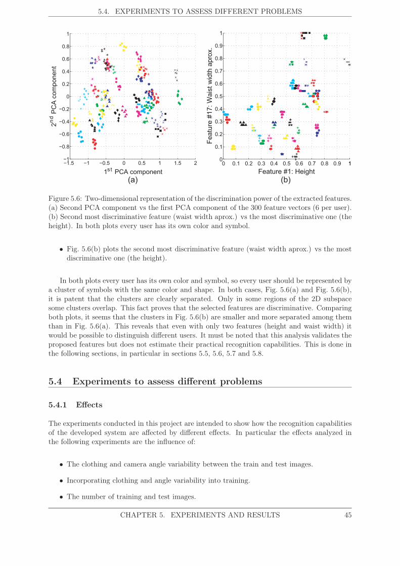
5.4. EXPERIMENTS TO ASSESS DIFFERENT PROBLEMS
(a) (b)
−1.5 −1 −0.5 0 0.5 1 1.5 2−1
−0.8
−0.6
−0.4
−0.2
0
0.2
0.4
0.6
0.8
1
1 PCA component
2 P
CA
com
ponent
0 0.1 0.2 0.3 0.4 0.5 0.6 0.7 0.8 0.9 110
0.1
0.2
0.3
0.4
0.5
0.6
0.7
0.8
0.9
1
Feature #1: Height
Featu
re #
17: W
ais
t w
idth
apro
x.
nd
s t
Figure 5.6: Two-dimensional representation of the discrimination power of the extracted features.(a) Second PCA component vs the first PCA component of the 300 feature vectors (6 per user).(b) Second most discriminative feature (waist width aprox.) vs the most discriminative one (theheight). In both plots every user has its own color and symbol.
• Fig. 5.6(b) plots the second most discriminative feature (waist width aprox.) vs the mostdiscriminative one (the height).
In both plots every user has its own color and symbol, so every user should be represented bya cluster of symbols with the same color and shape. In both cases, Fig. 5.6(a) and Fig. 5.6(b),it is patent that the clusters are clearly separated. Only in some regions of the 2D subspacesome clusters overlap. This fact proves that the selected features are discriminative. Comparingboth plots, it seems that the clusters in Fig. 5.6(b) are smaller and more separated among themthan in Fig. 5.6(a). This reveals that even with only two features (height and waist width) itwould be possible to distinguish different users. It must be noted that this analysis validates theproposed features but does not estimate their practical recognition capabilities. This is done inthe following sections, in particular in sections 5.5, 5.6, 5.7 and 5.8.
5.4 Experiments to assess different problems
5.4.1 Effects
The experiments conducted in this project are intended to show how the recognition capabilitiesof the developed system are affected by different effects. In particular the effects analyzed inthe following experiments are the influence of:
• The clothing and camera angle variability between the train and test images.
• Incorporating clothing and angle variability into training.
• The number of training and test images.
CHAPTER 5. EXPERIMENTS AND RESULTS 45

5.5. EXPERIMENT 1: BASELINE PERFORMANCE
The first experiment is carried out to obtain the baseline performance of the system, thenthree more experiments are conducted to analyze the previous effects (one experiment per effect).The results obtained in each experiment will be compared with the baseline performance, andfinally the results will be compared with the other experiments’ results.
5.4.2 Notation
For each user, the BIOGIGA database has 6 MMW images simulated with a passive systemoutdoors:
• 3 images of the user wearing clothing and a camera angle of of -10°, 0° and +10°.
• 3 images of the user without clothing and a camera angle of of -10°, 0° and +10°
With these six kinds of images there is a large casuistry of experiments that can be carried out.We will focus on some relevant cases.
In order to have a compact notation, we will refer to each possible case with these abbrevia-tions:
• Number of train and test images: #train images : #test images.
• Clothing: Images of a user without clothing will be denoted as sr, and cr will be used forimages of users wearing clothing. (These abbreviations come from the Spanish expressions"sin ropa" (without clothing) and "con ropa" (with clothing)).
• Angles: They will be denoted with different letters: a , b and c, and with an asterisk (* ).Each letter does not refer to a specific angle, but they will be used only to show whetherthe considered angle is the same to other angle referred before or not. The asterisk is usedto express that the three possible angles are considered. The three letters and the asteriskwill appear as subindexes.
For instance:
• For the experiment in which there are two train images, both with clothing, but withdifferent angle, and there is only one test image without clothing having any of the threeangles, then, we will have 2:1 and (cra, crb) : sr∗.
• For the experiment in which there are two train images, both with clothing, but withdifferent angle, and there is only one test image with clothing too, having an angle differentto the angles of the train images, then, we will have 2:1 and (cra, crb) : crc.
5.5 Experiment 1: Baseline Performance
The aim of this initial experiment is to compute the baseline performance of the system. Thisperformance is established as a reference performance to compare with next experiments’ be-havior.
46 CHAPTER 5. EXPERIMENTS AND RESULTS

5.5. EXPERIMENT 1: BASELINE PERFORMANCE
5.5.1 Protocol Description
To obtain the baseline performance, two different types of experiments are considered, both ofthem favorable to the system:
1. Experiment 1-1: One train and one test image, both with the same clothing condition:both images with clothing, or both without clothing.
2. Experiment 1-2: One train and one test image, both with the same camera angle: bothwith -10°, 0° or +10°.
Notice that due to the scarcity of images, when we consider images both with the same clothingcondition, they will have different angle, and viceversa. There will be 12 different combinationsfor the first case and 6 for the second case:
• For experiment 1-1 (same clothing condition) cra : crb (gives 6) and sra : srb (gives other6)
• For experiment 1-2 (same camera angle): cra : sra (gives 3) and sra : cra (gives 3 too).
5.5.2 Results
The identification and verification performances are shown in Table 5.1 as numerical results.The features selected by the SFFS algorithm are also included in the table. In this table, aswell as in the tables of the remaining experiments, the selected features appear in the order theywere selected. Moreover, the most frequently selected features are presented in bold font. Theidentification performance is plotted in Fig. 5.7 as CMC curves while the Fig. 5.8 shows theDETs curves (verification).
5.5.3 Discussion
The R-1 and R-5 are higher than 0.99 (99%) in all cases, revealing a very good identificationperformance of the system. Regarding the verification performance, the EER is quite low(around 1%) if all the 21 features are considered. When applying the SFFS algorithm, differentfeatures are selected in each experiment, providing improved values of the EER (0.33% and0.03%).
Comparing the results of the experiment with the same clothing condition (exp.1-1) versusthe results of the experiment with same angle (exp.1-2), we obtain that:
• When considering all the features, the identification as well as the verification perfor-mances, are slightly higher with the same clothing condition.
• When considering only the features selected by the SFFS algorithm, the identificationand the verification performances, are both higher with the same camera angle (speciallythe EER is much lower: from 0.33% to 0.03%).
Anyway, these behaviors are not completely representative because of (i) the small size of thedatabase, and (ii) the differences in the performances are small.
Concerning the feature selection, there are four features that are selected in both expe-riments: the height (feat.#1), the waist width (feat.#17), the chest width (feat.#16) and the
CHAPTER 5. EXPERIMENTS AND RESULTS 47
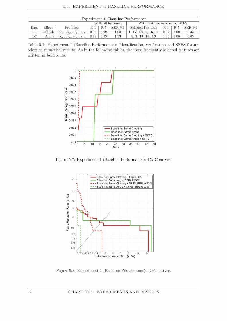
5.5. EXPERIMENT 1: BASELINE PERFORMANCE
Experiment 1: Baseline PerformanceWith all features With features selected by SFFS
Exp. Effect Protocols R-1 R-5 EER(%) Selected Features R-1 R-5 EER(%)1-1 =Cloth cra : crb, sra : srb 0.99 0.99 1.00 1, 17, 14, 4, 16, 12 0.99 1.00 0.331-2 =Angle cra : sra, sra : cra 0.99 0.99 1.33 2, 1, 17, 14, 16 1.00 1.00 0.03
Table 5.1: Experiment 1 (Baseline Performance): Identification, verification and SFFS featureselection numerical results. As in the following tables, the most frequently selected features arewritten in bold fonts.
0 5 10 15 20 25 30 35 40 45 500.99
0.991
0.992
0.993
0.994
0.995
0.996
0.997
0.998
0.999
1
Rank
Ra
nk R
eco
gn
itio
n R
ate
Baseline: Same Clothing
Baseline: Same Angle
Baseline: Same Clothing + SFFS
Baseline: Same Angle + SFFS
Figure 5.7: Experiment 1 (Baseline Performance): CMC curves.
0.02 0.05 0.1 0.2 0.5 1 2 5 10 20 40 60
0.02
0.05
0.1
0.2
0.5
1
2
5
10
20
40
False Acceptance Rate (in %)
Fals
e R
eje
ction R
ate
(in
%)
Baseline: Same Clothing, EER=1.00%
Baseline: Same Angle, EER=1.33%
Baseline: Same Clothing + SFFS, EER=0.33%
Baseline: Same Angle + SFFS, EER=0.03%
Figure 5.8: Experiment 1 (Baseline Performance): DET curves.
48 CHAPTER 5. EXPERIMENTS AND RESULTS

5.6. EXPERIMENT 2: CLOTHING AND ANGLE VAR. BETWEEN TRAIN AND TEST
elbow-neck distance (feat.#14). These features are not exactly the same as the four most dis-criminative ones of Fig. 5.5(b). That is because the SFFS selects the most discriminative setof features for each experiment. That is, a group of uncorrelated features that optimizes theverification performance for an specific protocol. This group does not necessarily match themost discriminative features when considering them independently, which are the first four ofFig. 5.5(b): the height (feat.#1), the waist width (feat.#17), the waist-pubis distance (feat.#5)and the leg length (feat.#6).
The obtained results are similar and even better to those obtained by Alefs et al. in [9](with an EER around 1-2%). However, it must be noticed that, in general, the high perfor-mance obtained is partially due to the fact that the images are synthetic. In addition, the hugeimprovement in the verification results when selecting features, can be also due to the fact thatthe SFFS algorithm uses all the images involved in the experiment and optimizes the EER onthem. Rigorously, the SFFS algorithm should be applied to an independent development dataset. Due to the small size of the data base, that was not possible in our experiments. Anyway,although the error rates are optimistically biased, the main objective was to identify the mostdiscriminative features, which has been done even without considering that development set.
5.6 Experiment 2: Clothing and Angle Variability between Trainand Test
One of the main advantages of using MMWs in biometric recognition is their ability to passthrough clothing and other dielectric materials. The first purpose of this experiment is toquantify the effect of clothing in the recognition performance using MMW images, whichshould be very little due to the almost total transparency of clothing in this spectral band.
The second aim of this experiment is to assess the influence of the camera angle in theperformance of the system. This is a situation very common in the practice because the userdoes not always stay in front of the imaging system maintaining the same angle.
5.6.1 Protocol Description
For each user the BIOGIGA database counts with 3 images without clothing (and differentangles) and 3 more with clothing (and different angles too). Therefore, to compute the effectof the clothing in the recognition performances, the system will be trained with an image withclothing and tested with an image without it, and viceversa. Specifically, this protocol will beused: cra : srb (6 different combinations) and sra : crb (other 6 combinations) (see Sect. 5.4.2for notation).
Notice that the previous protocols are:
• Equal to the ones used in the experiment 1-1 (baseline performance with the same clothcondition): cra : crb and sra : srb, but changing the clothing in the right side of the colon(bold letters).
• Equal to the ones used in the experiment 1-2 (baseline performance with the same cameraangles): cra : sra and sra : cra, but changing the angle in the right side of the colon (boldletters).
CHAPTER 5. EXPERIMENTS AND RESULTS 49

5.6. EXPERIMENT 2: CLOTHING AND ANGLE VAR. BETWEEN TRAIN AND TEST
Experiment 2: Clothing and Angle Variability between Train and TestWith all features With features selected by SFFS
Exp. Effect Protocols R-1 R-5 EER(%) Selected Features R-1 R-5 EER(%)2 �=Cloth, �=Angle cra : srb, sra : crb 0.98 0.99 1.33 1, 17, 16, 14, 4 0.97 1.00 0.50
Table 5.2: Experiment 2 (Clothing and Angle Variability between Train and Test): Identification,verification and SFFS feature selection numerical results.
0 5 10 15 20 25 30 35 40 45 500.99
0.991
0.992
0.993
0.994
0.995
0.996
0.997
0.998
0.999
1
Rank
Ra
nk R
eco
gn
itio
n R
ate
Baseline: Same Clothing
Baseline: Same Angle
Train−Test Var.: Clothing & Angle Var.
Baseline: Same Clothing + SFFS
Baseline: Same Angle + SFFS
Train−Test Var.: Clothing & Angle Var.+ SFFS
Figure 5.9: Experiment 2 (Clothing and Angle Variability between Train and Test): CMCcurves.
0.02 0.05 0.1 0.2 0.5 1 2 5 10 20 40 60
0.02
0.05
0.1
0.2
0.5
1
2
5
10
20
40
False Acceptance Rate (in %)
Fa
lse
Re
jectio
n R
ate
(in
%)
Baseline: Same Clothing, EER=1.00%
Baseline: Same Angle, EER=1.33%
Train−Test Var.: Clothing & Angle Var., EER=1.33%
Baseline: Same Clothing + SFFS, EER=0.33%
Baseline: Same Angle + SFFS, EER=0.03%
Train−Test Var.: Clothing & Angle Var.+ SFFS, EER=0.50%
Figure 5.10: Experiment 2 (Clothing and Angle Variability between Train and Test): DETcurves.
50 CHAPTER 5. EXPERIMENTS AND RESULTS

5.6. EXPERIMENT 2: CLOTHING AND ANGLE VAR. BETWEEN TRAIN AND TEST
Exp.1 (Baseline Performance) vs Exp.2 (Clothing and Angle Variability between Train and Test)With all features With features selected by SFFS
Exp. Effect Protocols R-1 R-5 EER(%) Selected Features R-1 R-5 EER(%)1-1 =Cloth cra : crb, sra : srb 0.99 0.99 1.00 1, 17, 14, 4, 16, 12 0.99 1.00 0.331-2 =Angle cra : sra, sra : cra 0.99 0.99 1.33 2, 1, 17, 14, 16 1.00 1.00 0.032 �=Cloth, �=Angle cra : srb, sra : crb 0.98 0.99 1.33 1, 17, 16, 14, 4 0.97 1.00 0.50
Table 5.3: Comparison of Experiment 1 (Baseline Performance) vs Experiment 2 (Clothingand Angle Variability between Train and Test): Identification, verification and SFFS featureselection numerical results. The different parameters between the protocols of exp.1-1 and exp.2and between the exp.1-2 and exp.2 are in bold letters. The underlined results correspond tobest results obtained so far. Again, the most frequently selected features are in bold fonts.
Therefore:
• By comparing the results from exp.2 vs the results from exp.1-1 we will obtain theinfluence of the clothing.
• By comparing the results from exp.2 vs the results from exp.1-2 we will obtain theinfluence of the angle.
5.6.2 Results
The recognition performances of exp.2 are presented in Table 5.2, in a CMC curve (Fig. 5.9) andin a DET curve (Fig. 5.10). In both figures the baseline curves are also plotted for reference.
5.6.3 Discussion
As it was already explained, to assess the influence of the clothing, we should compare theresults obtained in exp.2 with the ones obtained in the exp.1-1 (the one with the same clothcondition in Table 5.1). On the other hand, to evaluate the effect of the camera angle, theresults of exp.2 should be compared with the results of exp.1-2 (that has the same angle).
To better compare the results see Table 5.3 where the results of experiment 1 (exp.1-1 andexp.1-2) and experiment 2 are summarized. According to these results (exp.1-1 vs exp.2), it canbe seen that the clothing variability worsens a little the performance of the system, as it wasexpected: the almost-inappreciable influence of the clothing in the images only slightly reducesthe performance of the system. In verification mode the EER increases from 1.00% to 1.33%when all the features are used, and from 0.33% to 0.50% when the SFFS algorithm is applied.
To quantify the effect of the change in the angle between the train and the test images,we should compare the results of the experiment 2 with the results of the experiment 1-2 (seeTable 5.3). The results show that when having different angle the performance is approximatelythe same if the 21 features are considered, and decreases significantly when the SFFS-selectedfeatures are used (in that case the EER increases from 0.03% to 0.50%). This is not surprisingbecause when the camera angle is different between the train and the test images, then, somefeatures (body measures taken from the silhouette of the body) change, specifically the horizontalmeasures, reducing the performance of the system. In fact, among all the experiments performedso far, the one that provides the best performance is the one with the same angle in the trainand test images using SFFS (recognition rates R-1=R-5=1.00=100%, and EER=0.03%, whichare underlined in Table 5.3).
CHAPTER 5. EXPERIMENTS AND RESULTS 51

5.7. EXPERIMENT 3: CLOTHING AND ANGLE VARIABILITY IN TRAINING
As a result we can conclude that the proposed system is very robust against clothing variability,but no so effective under angle variability.
Finally, the features selected by the SFFS algorithm are approximately the same ones asthe ones selected in both baseline experiments.
5.7 Experiment 3: Clothing and Angle Variability in Training
Only one training image per user has been used in the previous experiments, however, it ispossible to use more than one, if available. Furthermore, these training images can present dif-ferent properties among them. The aim of this experiment is quantify the effect of incorporatingclothing and/or angle variability into and among the training images.
5.7.1 Protocol Description
In order to assess the clothing and/or angle variability in the training images there are manypossible protocols that can be taken into account. We will consider the ones below, all of themuse two images per user as training set and only one test image:
• Experiment 3-1: Same clothing condition and different angle in the training images:(cra, crb) : crc and the same without clothing: (sra, srb) : src (6 combinations in total).
• Experiment 3-2: Different clothing condition and same angle in the training images:(cra, sra) : crb and (cra, sra) : srb (12 combinations in total).
• Experiment 3-2: Different clothing condition and different angle in the trainingimages: (cra, srb) : crb/c and (cra, srb) : sra/c (24 combinations in total).
As explained in Sect. 4.7, in order to generate the model of multiple feature vectors, we justtake the mean feature vector.
5.7.2 Results
The Table 5.4 includes the recognition and feature selection numerical results of the experiment3. To better compare those results with the baseline performances, the results of the baselineare also included in the table. The identification performance of experiment 3 is graphicallyshown as CMC curves in Fig. 5.11, while verification performance is presented as DET curvesin Fig 5.12.
5.7.3 Discussion
The R-1 and R-5 is 0.99 or higher while the EER is lower than 1.50% for all the cases ofexperiment 3. This proves an excellent performance of the system under these conditions.
When comparing the results with the baseline performance, it can be seen that the iden-tification performance of the experiment 3 is quite similar to the baseline’s. However, for theverification performances, there are different behaviors depending on the use of (i) all the fea-tures or (ii) the ones selected by SFFS, and depending on the specific protocol. When all thefeatures are considered:
52 CHAPTER 5. EXPERIMENTS AND RESULTS

5.7. EXPERIMENT 3: CLOTHING AND ANGLE VARIABILITY IN TRAINING
Exp.1 (Baseline Performance) vs Exp.3 (Clothing and Angle Var. in Training)With all features With features selected by SFFS
Exp. Effect Protocols R-1 R-5 EER(%) Selected Features R-1 R-5 EER(%)1-1 =Cloth cra : crb, sra : srb 0.99 0.99 1.00 1, 17, 14, 4, 16, 12 0.99 1.00 0.331-2 =Angle cra : sra, sra : cra 0.99 0.99 1.33 2, 1, 17, 14, 16 1.00 1.00 0.033-1 =Cloth (cra, crb) : crc, (sra, srb) : src 0.99 0.99 1.00 1,17,4,16,13,12,2,11,10,8,21 1.00 1.00 0.123-2 =Angle (cra, sra) : crb, (cra, sra) : srb 0.99 0.99 1.49 1,17,14,4,16,11,13,12 0.99 1.00 0.223-3 �=Cloth, �=Angle (cra, srb) : crb/c, (cra, srb) : sra/c 0.99 0.99 1.42 17,14,4,6,1,11,21,12,15,13,10,7,2,8 0.99 1.00 0.19
Table 5.4: Comparison of Experiment 1 (Baseline Performance) vs Experiment 3 (Clothing andAngle Var. in Training): Identification, verification and SFFS feature selection numerical results.
0 5 10 15 20 25 30 35 40 45 500.99
0.991
0.992
0.993
0.994
0.995
0.996
0.997
0.998
0.999
1
Rank
Rank R
ecognitio
n R
ate
Baseline: Same Clothing
Baseline: Same Angle
Training Var.: Same Clothing
Training Var.: Same Angle
Training Var.: Different Clothing and Angle
Baseline: Same Clothing + SFFS
Baseline: Same Angle + SFFS
Training Var.: Same Clothing + SFFS
Training Var.: Same Angle + SFFS
Training Var.: Different Clothing and Angle + SFFS
Figure 5.11: Experiment 3 (Clothing and Angle Variability in Training): CMC curves.
0.02 0.05 0.1 0.2 0.5 1 2 5 10 20 40 60
0.02
0.05
0.1
0.2
0.5
1
2
5
10
20
40
False Acceptance Rate (in %)
Fals
e R
eje
ction R
ate
(in
%)
Baseline: Same Clothing, EER=1.00%
Baseline: Same Angle, EER=1.33%
Training Var.: Same Clothing, EER=1.00%
Training Var.: Same Angle, EER=1.49%
Training Var.: Different Clothing and Angle, EER=1.42%
Baseline: Same Clothing+SFFS, EER=0.33%
Baseline: Same Angle + SFFS, EER=0.03%
Training Var.: Same Clothing+SFFS, EER=0.12%
Training Var.: Same Angle+SFFS, EER=0.22%
Training Var.: Different Clothing and Angle+SFFS, EER=0.19%
Figure 5.12: Experiment 3 (Clothing and Angle Variability in Training): DET curves.
CHAPTER 5. EXPERIMENTS AND RESULTS 53

5.7. EXPERIMENT 3: CLOTHING AND ANGLE VARIABILITY IN TRAINING
• The verification performance of exp.3-1 (EER=1.00%) is the same as the baseline’s one.
• In exp.3-2 the train images present the same angle (a) but different clothing conditionsamong them. The effect of the clothing is very low as we have shown in previous experi-ments (see Sect. 5.6). Although the angle is the same for both train images, is different tothe test image’s one. This provides an effective angle for the train model, which is moredifferent to the test model’s one, and therefore the EER is higher (worse, EER=1.49%)than the EER of the baseline experiments (EER= 1.00% and EER=1.33%). For example,if a=-10° and b=0° the effective angle of the train model would be -10°, quite different tothe test model’s one, b=0°.
• Finally for the exp.3-3, the train images present different angle and clothing conditionamong them, and some times different angle and/or clothing condition to the test image.Thus, although this case seems to be the worst one, actually it is an intermediate situationwhen considering the train and the test model. Both models will be more similar than inthe exp.3-2 but much more different than in the exp.3-1. Therefore, the EER has a valueslightly lower (better, EER=1.42%) than the exp.3-2’s one (EER=1.49%).
If only the features selected by SFFS are used, then the results are the following ones:
• The EER for the three cases is approximately an order of magnitude better than the EERobtained considering all the features. This is probably due to the fact that when the mostdiscriminative features are selected, the ones most affected by the angle difference and theclothing, are discarded. As a result the EER is highly improved.
• For the three cases of experiment 3, the EER is lower (EER=0.12%, 0.22%, 0.19%)than the baseline exp.1-1’s one (EER=0.33%), and higher than the baseline exp.1-2’s one(EER=0.03%). This may be explained taking into account that in exp.1-1 the differenceof angle is very high (angle a vs angle b), while in the exp.3-1, 3-2, 3-3 the difference inthe angle between the train and test model is not so high. The opposite situation occurswhen the comparison is made with exp.1-2 (the train and test model are quite similar dueto the same value of angle (a) and there is very little influence due to clothing).
As a result we can conclude that to compensate for the lack of robustness against pose variation,we can incorporate enrollment based on multiple poses.
Regarding the selection of features, the higher the angle difference between the train andtest model is, the fewer features are selected: in exp.3-3 the difference is between (a+b)/2(effective angle of the train model) and b or c having 14 selected features, in exp.3-1 thedifference is a little bit higher (between (a+b)/2 and c), having 11 selected features, andfinally, in exp.3-2, the difference in angle is the highest one (between a and b) having only 8selected features. The features most frequently selected are: feat.#1 (height), feat.#17 (waistwidth), feat.#11 (lowerarm width), feat.#4 (the distance between the axilla and the centroidof the body), feat.#13 (lowerarm length) and feat.#12 (upperarm width). The height and thewaist width are the only features that also belongs to the most discriminative features whenconsidering them independently (feat.#1, #17, #5 and #6, see Fig. 5.5(b)).
54 CHAPTER 5. EXPERIMENTS AND RESULTS
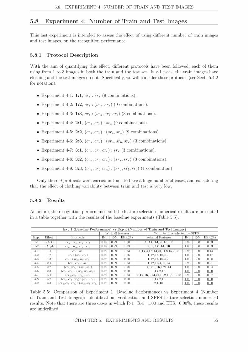
5.8. EXPERIMENT 4: NUMBER OF TRAIN AND TEST IMAGES
5.8 Experiment 4: Number of Train and Test Images
This last experiment is intended to assess the effect of using different number of train imagesand test images, on the recognition performance.
5.8.1 Protocol Description
With the aim of quantifying this effect, different protocols have been followed, each of themusing from 1 to 3 images in both the train and the test set. In all cases, the train images haveclothing and the test images do not. Specifically, we will consider these protocols (see Sect. 5.4.2for notation):
• Experiment 4-1: 1:1, cr∗ : sr∗ (9 combinations).
• Experiment 4-2: 1:2, cr∗ : (sr∗, sr∗) (9 combinations).
• Experiment 4-3: 1:3, cr∗ : (sra, srb, src) (3 combinations).
• Experiment 4-4: 2:1, (cr∗, cr∗) : sr∗ (9 combinations).
• Experiment 4-5: 2:2, (cr∗, cr∗) : (sr∗, sr∗) (9 combinations).
• Experiment 4-6: 2:3, (cr∗, cr∗) : (sra, srb, src) (3 combinations).
• Experiment 4-7: 3:1, (cra, crb, crc) : sr∗ (3 combinations).
• Experiment 4-8: 3:2, (cra, crb, crc) : (sr∗, sr∗) (3 combinations).
• Experiment 4-9: 3:3, (cra, crb, crc) : (sra, srb, src) (1 combination).
Only these 9 protocols were carried out not to have a huge number of cases, and consideringthat the effect of clothing variability between train and test is very low.
5.8.2 Results
As before, the recognition performance and the feature selection numerical results are presentedin a table together with the results of the baseline experiments (Table 5.5).
Exp.1 (Baseline Performance) vs Exp.4 (Number of Train and Test Images)With all features With features selected by SFFS
Exp. Effect Protocols R-1 R-5 EER(%) Selected Features R-1 R-5 EER(%)1-1 =Cloth cra : crb, sra : srb 0.99 0.99 1.00 1, 17, 14, 4, 16, 12 0.99 1.00 0.331-2 =Angle cra : sra, sra : cra 0.99 0.99 1.33 2, 1, 17, 14, 16 1.00 1.00 0.034-1 1:1 cr∗ : sr∗ 0.99 0.99 1.33 1,17,4,16,14,21,11,8,15,2,12 0.98 1.00 0.444-2 1:2 cr∗ : (sr∗, sr∗) 0.99 0.99 1.56 1,17,14,16,4,21 1.00 1.00 0.174-3 1:3 cr∗ : (sra, srb, src) 0.98 0.99 2.00 1,17,14,16,4,21 1.00 1.00 0.084-4 2:1 (cr∗, cr∗) : sr∗ 0.99 0.99 1.33 1,17,16,4,13,14 0.99 1.00 0.214-5 2:2 (cr∗, cr∗) : (sr∗, sr∗) 0.99 0.99 1.78 1,17,2,16,4,21,14 1.00 1.00 0.044-6 2:3 (cr∗, cr∗) : (sra, srb, src) 0.98 0.99 2.00 1,17,2,16 1.00 1.00 0.004-7 3:1 (cra, crb, crc) : sr∗ 0.99 0.99 1.33 1,17,16,6,14,21,10,2,11,8,15,12 0.99 1.00 0.074-8 3:2 (cra, crb, crc) : (sr∗, sr∗) 0.99 0.99 2.00 1,17,2,16 1.00 1.00 0.004-9 3:3 (cra, crb, crc) : (sra, srb, src) 0.98 0.99 2.00 2,1,16 1.00 1.00 0.00
Table 5.5: Comparison of Experiment 1 (Baseline Performance) vs Experiment 4 (Numberof Train and Test Images): Identification, verification and SFFS feature selection numericalresults. Note that there are three cases in which R-1=R-5=1.00 and EER=0.00%, these resultsare underlined.
CHAPTER 5. EXPERIMENTS AND RESULTS 55
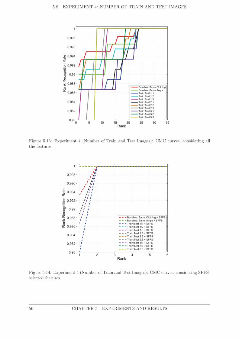
5.8. EXPERIMENT 4: NUMBER OF TRAIN AND TEST IMAGES
0 5 10 15 20 25 30 350.98
0.982
0.984
0.986
0.988
0.99
0.992
0.994
0.996
0.998
1
Rank
Rank R
ecognitio
n R
ate
Baseline: Same Clothing
Baseline: Same Angle
Train:Test 1:1
Train:Test 1:2
Train:Test 1:3
Train:Test 2:1
Train:Test 2:2
Train:Test 2:3
Train:Test 3:1
Train:Test 3:2
Train:Test 3:3
Figure 5.13: Experiment 4 (Number of Train and Test Images): CMC curves, considering allthe features.
1 2 3 4 5 60.98
0.982
0.984
0.986
0.988
0.99
0.992
0.994
0.996
0.998
1
Rank
Ra
nk R
eco
gn
itio
n R
ate
Baseline: Same Clothing + SFFS
Baseline: Same Angle + SFFS
Train:Test 1:1 + SFFS
Train:Test 1:2 + SFFS
Train:Test 1:3 + SFFS
Train:Test 2:1 + SFFS
Train:Test 2:2 + SFFS
Train:Test 2:3 + SFFS
Train:Test 3:1 + SFFS
Train:Test 3:2 + SFFS
Train:Test 3:3 + SFFS
Figure 5.14: Experiment 4 (Number of Train and Test Images): CMC curves, considering SFFS-selected features.
56 CHAPTER 5. EXPERIMENTS AND RESULTS

5.8. EXPERIMENT 4: NUMBER OF TRAIN AND TEST IMAGES
0.02 0.05 0.1 0.2 0.5 1 2 5 10 20 40 60
0.02
0.05
0.1
0.2
0.5
1
2
5
10
20
40
False Acceptance Rate (in %)
Fa
lse
Re
jectio
n R
ate
(in
%)
Baseline: Same Clothing, EER=1.00%
Baseline: Same Angle, EER=1.33%
Train:Test 1:1, EER=1.33%
Train:Test 1:2, EER=1.56%
Train:Test 1:3, EER=2.00%
Train:Test 2:1, EER=1.33%
Train:Test 2:2, EER=1.78%
Train:Test 2:3, EER=2.00%
Train:Test 3:1, EER=1.33%
Train:Test 3:2, EER=2.00%
Train:Test 3:3, EER=2.00%
Figure 5.15: Experiment 4 (Number of Train and Test Images): DET curves, considering all thefeatures.
0.02 0.05 0.1 0.2 0.5 1 2 5 10
0.02
0.05
0.1
0.2
0.5
1
2
5
10
20
40
False Acceptance Rate (in %)
Fals
e R
eje
ction R
ate
(in
%)
Baseline: Same Clothing+SFFS, EER=0.33%
Baseline: Same Angle+SFFS, EER=0.03%
Train:Test 1:1 + SFFS, EER=0.44%
Train:Test 1:2 + SFFS, EER=0.17%
Train:Test 1:3 + SFFS, EER=0.08%
Train:Test 2:1 + SFFS, EER=0.21%
Train:Test 2:2 + SFFS, EER=0.04%
Train:Test 2:3 + SFFS,−EER=0.00%−
Train:Test 3:1 + SFFS, EER=0.07%
Train:Test 3:2 + SFFS,−EER=0.00%−
Train:Test 3:3 + SFFS,−EER=0.00%−
Figure 5.16: Experiment 4 (Number of Train and Test Images): DET curves, considering SFFS-selected features. Note that there are three cases in which EER=0.00% (they are marked withtwo dashes in the legend), therefore the corresponding DET curves are a point in the originwhich is not visible in this plot.
CHAPTER 5. EXPERIMENTS AND RESULTS 57
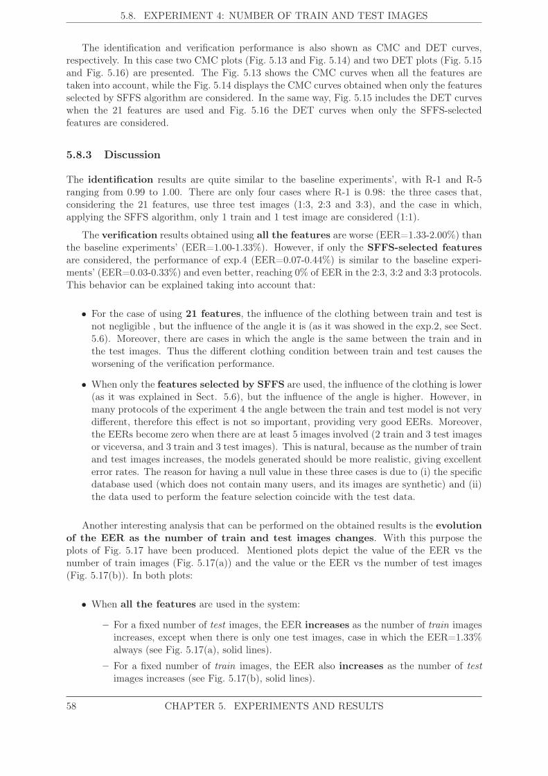
5.8. EXPERIMENT 4: NUMBER OF TRAIN AND TEST IMAGES
The identification and verification performance is also shown as CMC and DET curves,respectively. In this case two CMC plots (Fig. 5.13 and Fig. 5.14) and two DET plots (Fig. 5.15and Fig. 5.16) are presented. The Fig. 5.13 shows the CMC curves when all the features aretaken into account, while the Fig. 5.14 displays the CMC curves obtained when only the featuresselected by SFFS algorithm are considered. In the same way, Fig. 5.15 includes the DET curveswhen the 21 features are used and Fig. 5.16 the DET curves when only the SFFS-selectedfeatures are considered.
5.8.3 Discussion
The identification results are quite similar to the baseline experiments’, with R-1 and R-5ranging from 0.99 to 1.00. There are only four cases where R-1 is 0.98: the three cases that,considering the 21 features, use three test images (1:3, 2:3 and 3:3), and the case in which,applying the SFFS algorithm, only 1 train and 1 test image are considered (1:1).
The verification results obtained using all the features are worse (EER=1.33-2.00%) thanthe baseline experiments’ (EER=1.00-1.33%). However, if only the SFFS-selected featuresare considered, the performance of exp.4 (EER=0.07-0.44%) is similar to the baseline experi-ments’ (EER=0.03-0.33%) and even better, reaching 0% of EER in the 2:3, 3:2 and 3:3 protocols.This behavior can be explained taking into account that:
• For the case of using 21 features, the influence of the clothing between train and test isnot negligible , but the influence of the angle it is (as it was showed in the exp.2, see Sect.5.6). Moreover, there are cases in which the angle is the same between the train and inthe test images. Thus the different clothing condition between train and test causes theworsening of the verification performance.
• When only the features selected by SFFS are used, the influence of the clothing is lower(as it was explained in Sect. 5.6), but the influence of the angle is higher. However, inmany protocols of the experiment 4 the angle between the train and test model is not verydifferent, therefore this effect is not so important, providing very good EERs. Moreover,the EERs become zero when there are at least 5 images involved (2 train and 3 test imagesor viceversa, and 3 train and 3 test images). This is natural, because as the number of trainand test images increases, the models generated should be more realistic, giving excellenterror rates. The reason for having a null value in these three cases is due to (i) the specificdatabase used (which does not contain many users, and its images are synthetic) and (ii)the data used to perform the feature selection coincide with the test data.
Another interesting analysis that can be performed on the obtained results is the evolutionof the EER as the number of train and test images changes. With this purpose theplots of Fig. 5.17 have been produced. Mentioned plots depict the value of the EER vs thenumber of train images (Fig. 5.17(a)) and the value or the EER vs the number of test images(Fig. 5.17(b)). In both plots:
• When all the features are used in the system:
– For a fixed number of test images, the EER increases as the number of train imagesincreases, except when there is only one test images, case in which the EER=1.33%always (see Fig. 5.17(a), solid lines).
– For a fixed number of train images, the EER also increases as the number of testimages increases (see Fig. 5.17(b), solid lines).
58 CHAPTER 5. EXPERIMENTS AND RESULTS
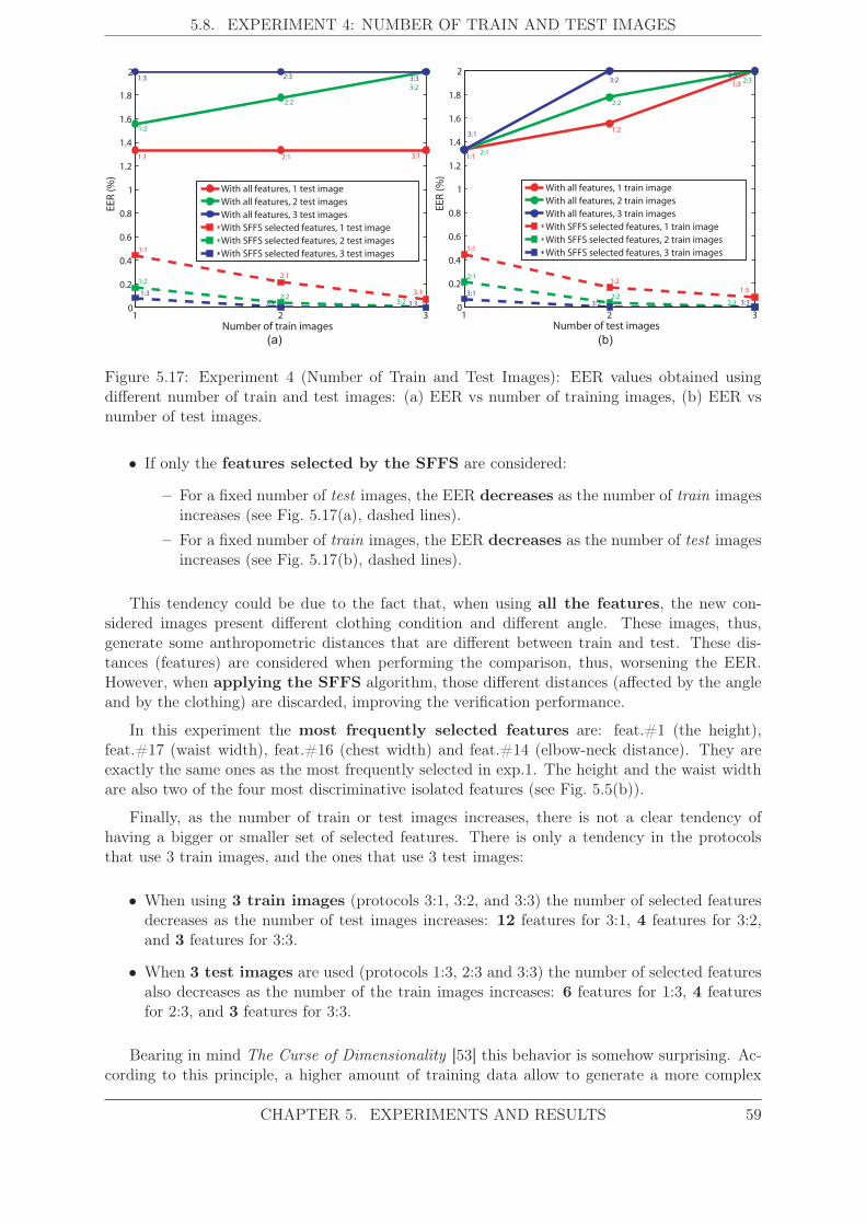
5.8. EXPERIMENT 4: NUMBER OF TRAIN AND TEST IMAGES
(a) (b)
1 2 30
0.2
0.4
0.6
0.8
1
1.2
1.4
1.6
1.8
2
Number of train images
EER
(%)
With all features, 1 test imageWith all features, 2 test imagesWith all features, 3 test imagesWith SFFS selected features, 1 test imageWith SFFS selected features, 2 test imagesWith SFFS selected features, 3 test images
1:3
1:2
1:1
2:3
2:2
2:1
3:33:2
3:1
1:1
1:2
1:3
2:1
2:22:3
3:1
3:33:2
1 2 30
0.2
0.4
0.6
0.8
1
1.2
1.4
1.6
1.8
2
Number of test images
EER
(%)
With all features, 1 train imageWith all features, 2 train imagesWith all features, 3 train imagesWith SFFS selected features, 1 train imageWith SFFS selected features, 2 train imagesWith SFFS selected features, 3 train images
3:1
2:11:1
3:2
2:2
1:2
3:31:3 2:3
1:1
2:1
3:1
1:2
2:23:2
1:3
3:32:3
Figure 5.17: Experiment 4 (Number of Train and Test Images): EER values obtained usingdifferent number of train and test images: (a) EER vs number of training images, (b) EER vsnumber of test images.
• If only the features selected by the SFFS are considered:
– For a fixed number of test images, the EER decreases as the number of train imagesincreases (see Fig. 5.17(a), dashed lines).
– For a fixed number of train images, the EER decreases as the number of test imagesincreases (see Fig. 5.17(b), dashed lines).
This tendency could be due to the fact that, when using all the features, the new con-sidered images present different clothing condition and different angle. These images, thus,generate some anthropometric distances that are different between train and test. These dis-tances (features) are considered when performing the comparison, thus, worsening the EER.However, when applying the SFFS algorithm, those different distances (affected by the angleand by the clothing) are discarded, improving the verification performance.
In this experiment the most frequently selected features are: feat.#1 (the height),feat.#17 (waist width), feat.#16 (chest width) and feat.#14 (elbow-neck distance). They areexactly the same ones as the most frequently selected in exp.1. The height and the waist widthare also two of the four most discriminative isolated features (see Fig. 5.5(b)).
Finally, as the number of train or test images increases, there is not a clear tendency ofhaving a bigger or smaller set of selected features. There is only a tendency in the protocolsthat use 3 train images, and the ones that use 3 test images:
• When using 3 train images (protocols 3:1, 3:2, and 3:3) the number of selected featuresdecreases as the number of test images increases: 12 features for 3:1, 4 features for 3:2,and 3 features for 3:3.
• When 3 test images are used (protocols 1:3, 2:3 and 3:3) the number of selected featuresalso decreases as the number of the train images increases: 6 features for 1:3, 4 featuresfor 2:3, and 3 features for 3:3.
Bearing in mind The Curse of Dimensionality [53] this behavior is somehow surprising. Ac-cording to this principle, a higher amount of training data allow to generate a more complex
CHAPTER 5. EXPERIMENTS AND RESULTS 59

5.9. CONCLUSIONS
model (a higher dimension model, or a vector with more features), obtaining a better perfor-mance. However, our results show that, when there are more training (or test) data available,we obtain better results by considering less features. This could be due to the fact that, whenthere are more training (or test) data, the most discriminative features selected by the SFFSalgorithm (mainly features #1, #17, #16 and #2 in the five mentioned protocols) become morerelevant over the rest, while the rest of features are discarded in the feature selection process.
5.9 Conclusions
The Table 5.6 displays the identification and verification rates of all the performed experiments.The color scale used in the cells that contain the R-1, R-5 and EER, allow to identify theworst results (in red), the best results (in green) and results in between (in yellow and orange).The best results are obtained for experiments 4-6, 4-8 and 4-9 using the SFFS algorithm (R-1=1.00 and EER=0.00%), while the worst ones are obtained for exp.4-3 and 4-6 without SFFS(R-1=0.98 and EER=2.00%).
From the analysis carried out throughout the experiments, and from the Table 5.6, there aresome important conclusions that can be drawn. They are stated below.
5.9.1 Effect of Variability between Train and Test, and within Train
The effect of different clothing condition between train and test is more noticeable whenthe 21 features are considered, and it is very low if only the SFFS-selected features are used (seeresults of exp.1-1 and exp. 2 in Table 5.6).
The effect of the angle difference between train and test is just the opposite: it isnearly negligible if all the features are used, and it is higher if the SFFS is applied (see resultsof exp.1-2 and exp.2 in Table 5.6). Also, the angle difference between train and test degradesmuch more the performance compared to clothing variability.
Finally, we have seen that, incorporating various feature vectors with different poses forcreating the train models, is a good way to overcome this lack of robustness against posevariation between train and test.
5.9.2 Effect of the Number of Train and Test Images
The use of an increasing number of train and/or test images to perform the recognition experi-ments, worsens the performance of the system when all the features are considered (which canbe explained as more training/test data implies more variability among them in our protocols),but, as expected, it improves the performance if the feature selection is performed (see resultsof exp.4 in Table 5.6).
5.9.3 Effect of the Feature Selection
The selection of features by means of the SFFS algorithm considerably improves the EER,the R-1 and the R-5 are also improved, but not so much. This is because the SFFS has theminimization of the EER as optimization criterion.
The CMC curves of all the experiments are considerably improved when the feature selec-tion is performed, reaching all of them a R-1 of almost 1.00 after the selection (the exact valuehas been rounded to two decimals in the tables, but not in the plots).
60 CHAPTER 5. EXPERIMENTS AND RESULTS

5.9. CONCLUSIONS
R-1
R-5
EE
R (
%)
# S
el.
Fe
at.
Se
lecte
d F
ea
tu
re
sR
-1R
-5E
ER
(%
)
1-1
=C
loth
cr
a:c
rb,
sr
a:s
rb
0,9
91
,00
1,0
06
1,
17
, 1
4,
4,
16
, 1
20
,99
1,0
00
,33
1-1
1-2
=A
ng
lecr
a:s
ra,
sr
a:c
ra
0,9
90
,99
1,3
35
2,
1,
17
, 1
4,
16
1,0
01
,00
0,0
31
-2
2
Clo
th
ing
& a
ng
le
va
r.
be
tw
ee
n
tra
in a
nd
te
st
≠C
loth
, ≠
An
gle
cr
a:s
rb,
sr
a:c
rb
0,9
90
,99
1,3
35
1,
17
, 1
4,
4,
16
0,9
71
,00
0,5
02
3-1
=C
loth
(cr
a,c
rb):
cr
c,
(sr
a,s
rb):
sr
c0
,99
0,9
91
,00
11
1,
17
, 4
, 1
6,
13
, 1
2,
2,
11
,
10
, 8
, 2
11
,00
1,0
00
,12
3-1
3-2
=A
ng
le(c
ra,s
ra):
cr
b,
(cr
a,s
ra):
sr
b1
,00
1,0
01
,49
81
, 1
7,
14
, 4
, 1
6,
11
, 1
3,
12
0,9
91
,00
0,2
23
-2
3-3
≠C
loth
, ≠
An
gle
(cr
a,s
rb):
cr
b/c,
(sr
a,c
rb):
sr
b/c
0,9
91
,00
1,4
21
41
7,
14
, 4
, 6
, 1
, 1
1,
21
, 1
2,
15
, 1
3,
10
, 7
, 2
, 8
0,9
91
,00
0,1
93
-3
4-1
1:1
cr
*:s
r*
0,9
90
,99
1,3
31
11
, 1
7,
4,
16
, 1
4,
21
, 1
1,
8,
15
, 2
, 1
20
,98
1,0
00
,44
4-1
4-2
1:2
cr
*:
(sr
*,s
r*)
0,9
90
,99
1,5
66
1,
17
, 1
4,
16
, 4
, 2
11
,00
1,0
00
,17
4-2
4-3
1:3
cr
*:
(sr
*,s
r*,s
r*)
0,9
80
,99
2,0
06
1,
17
, 1
4,
16
, 4
, 2
11
,00
1,0
00
,08
4-3
4-4
2:1
(cr
*,c
r*):
sr
*0
,99
0,9
91
,33
61
, 1
7,
16
, 4
, 1
3,
14
0,9
91
,00
0,2
15
-1
4-5
2:2
(cr
*,c
r*):
(sr
*,s
r*)
0,9
90
,99
1,7
87
1,
17
, 2
, 1
6,
4,
21
, 1
41
,00
1,0
00
,04
5-2
4-6
2:3
(cr
*,c
r*):
(sr
*,s
r*,s
r*)
0,9
80
,99
2,0
04
1,
17
, 2
, 1
61
,00
1,0
00
,00
5-3
4-7
3:1
(cr
a,c
rb,c
rc):
sr
*0
,99
0,9
91
,33
12
1 ,
17
, 1
6,
6,
14
, 2
1,
10
, 2
,
11
, 8
, 1
5,
12
0,9
91
,00
0,0
76
-1
4-8
3:2
(cr
a,c
rb,c
rc):
(sr
*,s
r*)
0,9
90
,99
2,0
04
1,
17
, 2
, 1
61
,00
1,0
00
,00
6-2
4-9
3:3
(cr
a,c
rb,c
rc):
(sr
a,s
rb,s
rc)
0,9
90
,98
2,0
03
2,
1,
16
1,0
01
,00
0,0
06
-3
Exp
.E
ffe
ct
Pro
to
co
ls
Wit
h a
ll f
ea
ture
s
Ba
se
lin
e
Clo
th
ing
& a
ng
le
va
ria
bil
ity
in
tra
inin
g
Nu
mb
er o
f tra
in
& t
est i
ma
ge
s
Wit
h f
ea
ture
s se
lect
ed
by
SF
FS
Exp
.
Table 5.6: Experiments 1, 2, 3 and 4: Identification, verification and SFFS feature selectionnumerical results. The results are presented in shadowed cells with colors ranging from red(worst results) to green (best results), considering separately each type of result (R-1, R-5 andEER). The slightly different color between some cells that contain the same value is due to thefact that the color shadowing does not take into account the decimals rounding. The worst andbest results are also written in bold font.
CHAPTER 5. EXPERIMENTS AND RESULTS 61
5.9. CONCLUSIONS
(a) (b)
1 2 3 4 5 6 7 8 9 10 11 12 13 14 15 16 17 18 19 20 210
1
2
3
4
5
6
7
8
9
10
11
12
13
14
15
Features
Tim
es S
elec
ted
1 17 5 6 9 16 14 2 11 4 13 20 15 12 19 21 18 10 8 3 70
1
2
3
4
5
6
7
8
9
10
11
12
13
14
15
Ranked Features
Tim
es S
elec
ted
Figure 5.18: Histograms of features selected by the SFFS algorithm.: (a) Histogram with thefeatures regularly ordered, (b) Histogram with the features ordered in the same way as inFig. 5.5(b) (in decreasing order of the discrimination power of each feature.)
There is an interesting behavior that present all the DET curves when the feature selectionis applied: they change from having a horizontal appearance to have a vertical one closer tothe origin (with a more negative slope, see for example Fig. 5.12). This is a consequence of theminimization of the EER in the feature selection process. This change in the shape of the DETcurves provides the system with a higher security: the False Acceptance Rate is reduced whilethe False Rejection Rate is increased.
5.9.4 Analysis of the Selected Features
In addition to the comments made in each experiment’s section about the feature selection, weperform an additional analysis here. The Fig. 5.18(a) is a histogram of the features selected inthe experiments. It reveals that the feature most frequently selected corresponds to feat.#1 (theheight) selected 15 times, followed by the features #17 (waist width) and #16 (chest width),both selected 14 times. The features #5 (centroid of the body-pubis distance), #9 (thigh length),#18 (hips width), #19 (thigh width) and #20 (calf width) were not selected in any experiment.
The Fig. 5.18(b) displays the same histogram, but the x axis contains, in bold font, the fea-tures ranked in decreasing order of their discrimination power (the same order as in Fig. 5.5(b)).If the features were uncorrelated, the bars would gradually decrease as we move along the xaxis in the mentioned figure, being the most frequently selected the first ones (the individuallymost discriminative ones), and the least frequently selected the last ones (the individually leastdiscriminative ones). Although the bars approximately decrease as we move along the x axis,there are some gaps corresponding to features not selected or almost not selected. For instance,features #5 (centroid of the body-pubis distance), #6 (legs length) and #9 (thigh length), whichare some of the individually most discriminative features, are not selected by the SFFS algo-rithm. This reveals that these features, even having a high discrimination power, are not selectedbecause they are correlated with features previously selected during the selection process (theydo not add new discriminant information). In particular, it seems obvious that the mentionedfeatures (which are mainly lengths) are highly correlated with the height, which was previouslyselected.
62 CHAPTER 5. EXPERIMENTS AND RESULTS

5.9. CONCLUSIONS
5.9.5 Final Remarks
We should remark one more time that all the results are not totally representative due to (i)the small size of the database, and (ii) the differences in the performances are small. Moreover,the obtained results are optimistically biased due to three main reasons: (i) the low numberof users (only 50) in the database, (ii) the synthetic nature of the images that comprise thedatabase, (iii) the use of the same data to develop the system (in particular to select the mostdiscriminative set of features by means of the SFFS algorithm) and to test it.
In any case, in spite of the previous limitations, it was possible to quantify the influence ofthe different effects (clothing/angle variability between train and test, in train, and the numberof train/test images) and to identify the most discriminative set of features in each case, whichwas the main objective in this work.
CHAPTER 5. EXPERIMENTS AND RESULTS 63

5.9. CONCLUSIONS
64 CHAPTER 5. EXPERIMENTS AND RESULTS
6Conclusions and Future Work
6.1 Conclusions
Nowadays the security and defense is becoming more and more important in our society. Forthis reason, many screening portals have been installed in certain places such as airport securitycheckpoints. One of the latest kind of portals acquires body images in the millimeter wavesspectral band (MMW). These portals provide images of the surface of the body revealing if theuser conceals arms or drugs under his/her garment. The integration of a biometric system, basedon MMW images, in this kind of portals, would also allow to identify people (terrorists amongthem) previously enrolled in the system. Moreover, the use of this kind of radiation and portalsto obtain MMW images presents many advantages (millimeter waves are innocuous, they canpenetrate the clothing, these portals are not invasive, they enable the recognition at a distanceand/or on the move and also the fusion with other biometrics traits simultaneously acquired,such as the face or the gait).
In this project, firstly, a new method to simulate images of people at 94 GHz (frequencywithin the MMW band) has been proposed and used to generate a synthetic database. Thisdatabase, called BIOGIGA, is composed of 1200 images simulated at 94 GHz of 50 users in twotypes of scenarios with two types of imaging systems.
Secondly, a biometric recognition system, based on certain images of BIOGIGA, has beendesigned and implemented. In the development of the system we have proposed a featureextraction method based on the detection of relevant points of the body, followed by the measureof 21 distances among them. These distances form the feature vector of every image.
Afterwards, several identification and verification experiments were performed to test thedeveloped system. Each experiment is carried out under different conditions regarding theclothing condition, the camera angle and the number of train and test images used. Eachexperiment was performed twice: (ii) making use of the 21 features, and (ii) using only the mostdiscriminative set of features (obtained by the SFFS algorithm).
The obtained results provide information about the influence of (i) the different conditions,and (ii) the feature selection, on the system performance:
• The effect of different clothing condition between train and test worsens the system per-formance, being this worsening more noticeable when the 21 features are considered, and
65

6.1. CONCLUSIONS
very small if only the SFFS-selected features are used.
• The effect of the camera angle difference between train and test also reduces the perfor-mance of the system, but in the opposite way: the worsening is nearly negligible if all thefeatures are used, and it is higher if the SFFS is applied.
• Incorporating various feature vectors with different poses for creating the train models, isa good way to overcome the lack of robustness against pose variation between train andtest.
• The use of an increasing number of train and/or test images to perform the recognitionexperiments, (i) worsens the performance of the system when all the features are considered(due to the fact that more training/test data implies more variability among them in ourprotocols), and (ii) improves it if the feature selection is performed (as it was expected).
• The selection of features highly improves the verification performance, however, the iden-tification performance is only slightly improved.
• The CMC curves (identification performance plots) are extremely improved when thefeature selection is performed.
• When applying feature selection, the DET curves (verification performance plots) becomecloser to the origin and have a more negative slope, providing the system with a lower (bet-ter) EER (verification Equal Error Rate) and with higher security (the False AcceptanceRate is reduced while the False Rejection Rate is increased).
The features more frequently selected in the experiments correspond to: the height, thewaist width, the chest width and the elbow-neck distance (in that order). However, the featureswith the highest discrimination power are the height, the waist width, the distance between thecentroid of the body and the pubis, and the legs length (in that order). This mismatch betweenboth sets of features is due to the correlation among some features of the second set (for examplethe height, the legs length and the distance between the centroid of the body and the pubis arehighly correlated).
The recognition performance obtained in the experiments is excellent in both, identificationand verification modes: the Rank-1 recognition rate has a value between 0.98 and 1.00 (i.e.,98% and 100% respectively), while the EER ranges between 0.00% and 2.00%. These valuesare similar and even better than the ones obtained by Alefs et al. in [9] (the only biometricrecognition work based on MMW images published so far). In that work, a EER varying between1.00% and 2.00% is obtained. Nevertheless, the results obtained in our experiments are nottotally representative (due to the small size of the database, 50 users, and the little differencesamong the obtained performances). In fact, the error rates are optimistically biased. This iscaused by (i) the small number of users, (ii) the images are synthetic, and (iii) the selection offeatures was performed using all the available data (and not exclusively data from a developmentset).
As stated, the limitations of this work are related to the special characteristics of the databaseused. The BIOGIGA’s images are limited when compared to the real images acquired in practice.However, the synthetic images are very similar to the ones really captured at 94 GHz. Also, thesynthetic images used are based on real measures from people. Therefore, the proposed featurescan be directly applied and are useful for practical MMW images. Moreover, the experimentsperformed using the BIOGIGA database have provided qualitatively results about the effects ofthe different conditions and of the feature selection on the system performance, which was oneof the main purposes of this project.
66 CHAPTER 6. CONCLUSIONS AND FUTURE WORK
6.2. FUTURE WORK
6.2 Future Work
As future work, the following research lines are proposed:
• The development of a system similar to the one presented here, that makes use of imagessimulated with MMW active systems (BIOGIGA also contains this kind of images, butthey were not used in this project).
• The generation of a database of real images acquired within the MMW band (and ifpossible, with images of the same users acquired in the VIS and IR band too, obtaining aMultispectral Database).
• The adaptation of the proposed system to be able to operate with real MMW images. Inthis task, and in the first one, the image segmentation module should be tuned to the newkind of images.
• The design and development of alternative biometric systems that only make use of someparts of the MMW body image (such as the face, the thorax, etc. as it was done in [9]).
• The fusion of different biometric traits acquired at MMW band.
• The fusion of biometric trait(s) acquired at MMW band with (the same or different) trait(s)acquired at other spectral band(s) (i.e. the development of a Multispectral BiometricSystem).
• The use of information extracted from MMW images (such as anthropometric measures) toincrease the performance of traditional systems with medium-high recognition performance(Soft Biometrics).
• Integration of a biometric system based on real MMW images in a MMW screening portal.
CHAPTER 6. CONCLUSIONS AND FUTURE WORK 67


Bibliography
[1] A.K. Jain, A. Ross, and S. Prabhakar. An introduction to biometric recognition. Circuitsand Systems for Video Technology, IEEE Transactions on, 14(1):4 – 20, jan. 2004.
[2] A.K. Jain, A. Ross, and S. Pankanti. Biometrics: a tool for information security. InformationForensics and Security, IEEE Transactions on, 1(2):125–143, june 2006.
[3] National Academy Press, editor. Airline Passenger Security Screening: New Technolo-gies and Implementation Issues, chapter Biometrics at a Distance: Issues, Challenges, andProspects, pages 3–21. National Academy Press, 1996.
[4] Hong Chen and Anil K. Jain. Dental biometrics: Alignment and matching of dental radio-graphs. IEEE Transactions on Pattern Analysis and Machine Intelligence, 27:1319–1326,2005.
[5] S.Z. Li, RuFeng Chu, ShengCai Liao, and Lun Zhang. Illumination invariant face recognitionusing near-infrared images. Pattern Analysis and Machine Intelligence, IEEE Transactionson, 29(4):627–639, 2007.
[6] R. Appleby and R.N. Anderton. Millimeter-wave and submillimeter-wave imaging for se-curity and surveillance. Proceedings of the IEEE, 95(8):1683 –1690, aug. 2007.
[7] L. Yujiri, M. Shoucri, and P. Moffa. Passive millimeter wave imaging. Microwave Magazine,IEEE, 4(3):39 – 50, sept. 2003.
[8] J.N. Mait, D.A. Wikner, M.S. Mirotznik, J. van der Gracht, G.P. Behrmann, B.L. Good,and S.A. Mathews. 94-GHz imager with extended depth of field. Antennas and Propagation,IEEE Transactions on, 57(6):1713 –1719, june 2009.
[9] B.G. Alefs, R.J.M. den Hollander, F.A. Nennie, E.H. van der Houwen, M. Bruijn, W. van derMark, and J.C. Noordam. Thorax biometrics from Millimetre-Wave images. Pattern Recog-nition Letters, 31(15):2357–2363, 2010.
[10] Josep Parron, Hector Rossel, Pedro de Paco, Gary Junkin, and Oscar Menendez. Millimeter-Wave Scene Simulation using Blender. In Proceedings of XXV Simposium Nacional deUnion Cientifica Internacional de Radio, URSI 2010, September 2010.
[11] Rafael C. Gonzalez, Richard E. Woods, and Steven L. Eddins. Digital Image ProcessingUsing MATLAB. Prentice-Hall, Inc., Upper Saddle River, NJ, USA, 2003.
[12] Miriam Moreno-Moreno, Julian Fierrez, Pedro Tome, Ruben Vera-Rodriguez, Josep Parron,and Javier Ortega-Garcia. BIOGIGA: Base de datos de imágenes sintéticas de personasa 94 GHz con fines biométricos. In Proceedings of XXVI Simposium Nacional de UnionCientifica Internacional de Radio, September 2011.
[13] Miriam Moreno-Moreno, Julian Fierrez, and Javier Ortega-Garcia. Millimeter- andSubmillimeter-Wave Imaging Technologies for Biometric Purposes. In Proceedings of XXIVSimposium Nacional de Union Cientifica Internacional de Radio, September 2009.
69

BIBLIOGRAPHY
[14] Miriam Moreno-Moreno, Julian Fierrez, and Javier Ortega-Garcia. Biometrics Beyondthe Visible Spectrum: Imaging Technologies and Applications. In Proceedings of BioID-Multicomm 2009, volume 5707 of LNCS, pages 154–161. Springer, September 2009.
[15] Miriam Moreno-Moreno, Julian Fierrez, Pedro Tome, and Javier Ortega-Garcia. Análisisde Escenarios para Reconocimiento Biométrico a Distancia Adecuados para la Adquisi-ción de Imágenes MMW. In Proceedings of XXV Simposium Nacional de Union CientificaInternacional de Radio, September 2010.
[16] Miriam Moreno-Moreno, Julian Fierrez, Ruben Vera-Rodriguez, and Josep Parron.Distance-based Feature Extraction for Biometric Recognition of Millimeter Wave BodyImages. In Proceedings of 45th IEEE International Carnahan Conference on Security Tech-nology, pages 326–331, October 2011.
[17] Miriam Moreno-Moreno, Julian Fierrez, Ruben Vera-Rodriguez, and Josep Parron. Simu-lation of Millimeter Wave Body Images and its Application to Biometric Recognition. InProceedings of SPIE Defense, Security and Sensing 2012, volume 8362, April 2012.
[18] Austin Richards. Alien Vision: Exploring the Electromagnetic Spectrum with Imaging Tech-nology, Second Edition. SPIE Press, 1st ed. 2010. corr. 2nd printing edition, edition, 2011.
[19] Lior Shamir, Shari Ling, Salim Rahimi, Luigi Ferrucci, and Ilya G. Goldberg. Biometricidentification using knee x-rays. Int. J. Biometrics, 1(3):365–370, March 2009.
[20] R.H. Bossi, K.D. Friddell, and J.M. Nelson. Backscatter x-ray imaging. Materials Evalua-tion, 46(11):1462–7, Oct. 1988.
[21] Eric Jude L. Morris, Frank A. Dibianca, Hemant Shukla, and Daya Gulabani. A backscat-tered x-ray imager for medical applications. In Medical Imaging 2005: Physics of MedicalImaging, volume 5745, pages 113–120. SPIE, February 2005.
[22] Alex Chalmers. Three applications of backscatter x-ray imaging technology to homelanddefense. In Sensors, and Command, Control, Communications, and Intelligence (C3I)Technologies for Homeland Security and Homeland Defense IV, volume 5778, pages 113–120. SPIE, March 2005.
[23] Lingyu Wang and Graham Leedham. Near- and far- infrared imaging for vein patternbiometrics. Advanced Video and Signal Based Surveillance, IEEE Conference on, 0:52,2006.
[24] Pradeep Buddharaju, Ioannis T. Pavlidis, Panagiotis Tsiamyrtzis, and Mike Bazakos.Physiology-based face recognition in the thermal infrared spectrum. IEEE Trans. PatternAnal. Mach. Intell., 29(4):613–626, April 2007.
[25] Chih-Lung Lin and Kuo-Chin Fan. Biometric verification using thermal images of palm-dorsa vein patterns. Circuits and Systems for Video Technology, IEEE Transactions on,14(2):199 – 213, feb. 2004.
[26] Xin Chen, Patrick J. Flynn, and Kevin W. Bowyer. IR and visible light face recognition.Comput. Vis. Image Underst., 99(3):332–358, September 2005.
[27] Andrea Selinger and Diego A. Socolinsky. Face recognition in the dark. Computer Visionand Pattern Recognition Workshop, 8:129, 2004.
[28] R.L. Howald, G. Clark, J. Hubert, and D. Ammar. Millimeter waves: The evolving scene.In Technologies for Homeland Security, 2007 IEEE Conference on, pages 234 –239, may2007.
70 BIBLIOGRAPHY

BIBLIOGRAPHY
[29] Hai-Bo Liu, Hua Zhong, N. Karpowicz, Yunqing Chen, and Xi-Cheng Zhang. Terahertzspectroscopy and imaging for defense and security applications. Proceedings of the IEEE,95(8):1514 –1527, aug. 2007.
[30] J. E. Bjarnason, T. L. J. Chan, A. W. M. Lee, M. A. Celis, and E. R. Brown. Millimeter-wave, terahertz, and mid-infrared transmission through common clothing. Applied PhysicsLetters, 85(4):519–521, 2004.
[31] M.J. Rosker and H.B. Wallace. Imaging through the atmosphere at terahertz frequencies.In Microwave Symposium, 2007. IEEE/MTT-S International, pages 773 –776, june 2007.
[32] G.N. Sinclair, P.R. Coward, R.N. Anderton, R. Appleby, T. Seys, and P. Southwood. De-tection of illegal passengers in lorries using a passive millimetre wave scanner. In SecurityTechnology, 2002. Proceedings. 36th Annual 2002 International Carnahan Conference on,pages 167 – 170, 2002.
[33] M. Sato, T. Hirose, T. Ohki, H. Sato, K. Sawaya, and K. Mizuno. 94-GHz band high-gainand low-noise amplifier using inp-hemts for passive millimeter wave imager. In MicrowaveSymposium, 2007. IEEE/MTT-S International, pages 1775 –1778, june 2007.
[34] B. Kapilevich, B. Litvak, M. Einat, and O. Shotman. Passive mm-wave sensor for in-doorand out-door homeland security applications. In Sensor Technologies and Applications,2007. SensorComm 2007. International Conference on, pages 20 –23, oct. 2007.
[35] D.M. Sheen, D.L. McMakin, and T.E. Hall. Three-dimensional millimeter-wave imagingfor concealed weapon detection. Microwave Theory and Techniques, IEEE Transactions on,49(9):1581 –1592, sep 2001.
[36] T. Derham, H. Kamoda, T. Iwasaki, and T. Kuki. Active mmw imaging system using thefrequency-encoding technique. In Microwave Conference, 2007. KJMW 2007. Korea-Japan,pages 181 –184, nov. 2007.
[37] G.P. Timms, J.D. Bunton, M.L. Brothers, and J.W. Archer. 190 GHz millimetre-waveimaging using mmic-based heterodyne receivers. In Wireless Broadband and Ultra WidebandCommunications, 2007. AusWireless 2007. The 2nd International Conference on, page 32,aug. 2007.
[38] D.M. Sheen, D.L. McMakin, T.E. Hall, and R.H. Severtsen. Active millimeter-wave stand-off and portal imaging techniques for personnel screening. In Technologies for HomelandSecurity, 2009. HST ’09. IEEE Conference on, pages 440 –447, 11-12 2009.
[39] Douglas T. Petkie, Corey Casto, Frank C. De Lucia, Steven R. Murrill, Brian Redman,Richard L. Espinola, Charmaine C. Franck, Eddie L. Jacobs, Steven T. Griffin, Carl E.Halford, Joe Reynolds, Sean O’Brien, and David Tofsted. Active and passive imaging inthe thz spectral region: phenomenology, dynamic range, modes, and illumination. J. Opt.Soc. Am. B, 25(9):1523–1531, 2008.
[40] A. Luukanen, E.N. Grossman, A.J. Miller, P. Helisto, J.S. Penttila, H. Sipola, andH. Seppa. An ultra-low noise superconducting antenna-coupled microbolometer with aroom-temperature read-out. Microwave and Wireless Components Letters, IEEE, 16(8):464–466, aug. 2006.
[41] Xilin Shen, C.R. Dietlein, E. Grossman, Z. Popovic, and F.G. Meyer. Detection and seg-mentation of concealed objects in terahertz images. Image Processing, IEEE Transactionson, 17(12):2465 –2475, dec. 2008.
BIBLIOGRAPHY 71
BIBLIOGRAPHY
[42] Arttu Luukanen, Leif Grönberg, Kari Kataja, Mikko Leivo, Tuomas Haarnoja, Anssi Rauti-ainen, Panu Helistö, Hannu Sipola, , and Heikki Seppä. Stand-off contraband identificationusing passive thz imaging. In EDA IEEMT Workshop 2008, 2008.
[43] K.B. Cooper, R.J. Dengler, N. Llombart, T. Bryllert, G. Chattopadhyay, E. Schlecht, J. Gill,C. Lee, A. Skalare, I. Mehdi, and P.H. Siegel. Penetrating 3-d imaging at 4- and 25-m rangeusing a submillimeter-wave radar. Microwave Theory and Techniques, IEEE Transactionson, 56(12):2771 –2778, dec. 2008.
[44] A. Tamminen, J. Ala-Laurinaho, and A.V. Raisanen. Indirect holographic imaging at 310ghz. In Radar Conference, 2008. EuRAD 2008. European, pages 168 –171, oct. 2008.
[45] A.W.M. Lee, B.S. Williams, S. Kumar, Qing Hu, and J.L. Reno. Real-time imaging using a4.3-thz quantum cascade laser and a 320 /spl times/ 240 microbolometer focal-plane array.Photonics Technology Letters, IEEE, 18(13):1415 –1417, july 2006.
[46] Alphonse Bertillon and Gallus Muller. Alphonse Bertillon’s Instructions For Taking Des-criptions For The Identification Of Criminals And Others, by Means Of AnthropometricIndications (1889). Kessinger Publishing, 1889.
[47] Javier Burgués. Reconocimiento de personas basado en imágenes de la mano. Master’sthesis, Universidad Autónoma de Madrid, July 2010.
[48] Luis Carlos Molina, Lluís Belanche, and Àngela Nebot. Feature selection algorithms: Asurvey and experimental evaluation. In Proceedings of the 2002 IEEE International Confer-ence on Data Mining, ICDM ’02, pages 306–, Washington, DC, USA, 2002. IEEE ComputerSociety.
[49] P. Pudil, J. Novovicová, and J. Kittler. Floating Search Methods in Feature Selection.Pattern Recognition Letters, 15(11):1119 – 1125, 1994.
[50] Sergios Theodoridis and Konstantinos Koutroumbas. Pattern Recognition, Third Edition.Academic Press, 3 edition, March 2006.
[51] A. Martin, G. Doddington, T. Kamm, M. Ordowski, and M. Przybocki. The DET curvein assessment of detection task performance. In Proceedings of the European Conference onSpeech Communication and Technology, volume 1, pages 1895–1898, 1997.
[52] M. Vasilescu and Demetri Terzopoulos. Multilinear analysis of image ensembles: Ten-sorfaces. In Anders Heyden, Gunnar Sparr, Mads Nielsen, and Peter Johansen, editors,Computer Vision ECCV 2002, volume 2350 of Lecture Notes in Computer Science, pages447–460. Springer Berlin / Heidelberg, 2002.
[53] Christopher M. Bishop. Pattern Recognition and Machine Learning (Information Scienceand Statistics). Springer, 1st ed. 2006. corr. 2nd printing edition, October 2007.
72 BIBLIOGRAPHY

AIntroducción
A.1 Motivación del proyecto
Se denomina reconocimiento biométrico al proceso que permite asociar una identidad con unindividuo de forma automática, haciendo uso de una o varias características físicas o de com-portamiento, inherentes al individuo [1, 2]. Son muchas las características que se han venidousando en reconocimiento biométrico: huella dactilar, firma manuscrita, iris, voz, cara, mano,etc. Algunos de estos rasgos biométricos tales como la oreja, la cara, la mano o la forma deandar, se adquieren normalmente con cámaras que trabajan en frecuencias pertenecientes a labanda visible del espectro electromagnético. Tales imágenes se ven afectadas por factores comolas condiciones de iluminación y las oclusiones (provocadas por la ropa, el maquillaje, el pelo,etc.).
Con el fin de superar estas limitaciones, impuestas por el uso de imágenes adquiridas enel espectro visible (VIS), investigadores en biometría y seguridad [3] han propuesto el uso deimágenes adquiridas en otros rangos espectrales, a saber: rayos X (RX) [4], infrarrojo (IR) [5],ondas milimétricas (MMW) y submilimétricas (SMW) [6]. Además de solventar hasta ciertopunto las limitaciones de las imágenes en el visible, las imágenes tomadas más allá del espectrovisible presentan una ventaja extra: son más robustas frente ataques contra sistemas biométricosque otras imágenes o rasgos biométricos.
La banda espectral propuesta en este proyecto para capturar imágenes de rasgos biométricoses la correspondiente a la de las ondas milimétricas (de frecuencia entre 30 y 300 GHz) [7]. Laimportancia de este tipo de radiación se halla en:
• Su capacidad para atravesar la ropa y otras oclusiones.
• Es inocua para la salud.
• El reciente desarrollo que están experimentando los sistemas de GHz-THz en aplicacionesde captura de imágenes (especialmente en el área de seguridad).
Al contrario de lo que ocurre con la tecnología de captura de imágenes en el visible o infra-rrojo, la tecnología de GHz-THz está en pleno desarrollo [8]. Este hecho, junto con los problemas
73

A.2. OBJETIVOS
de privacidad que presentan las imágenes corporales en esa banda, han hecho que hasta la fechano existan bases de datos públicas con imágenes de personas adquiridas en ese rango de fre-cuencias. De hecho sólo existe un trabajo publicado hasta el momento sobre reconocimientobiométrico basado en imágenes de GHz [9]. Por todo lo anterior, en el actual proyecto se pro-pone, como una de las tareas fundamentales, la obtención de imágenes simuladas de personasa 94 GHz [10]. A continuación se hará uso de tales imágenes para desarrollar un sistema dereconocimiento biométrico.
El presente proyecto está motivado por las ventajas que presentan las imágenes en la bandade milimétricas y los escenarios de su adquisición:
• La inocuidad de tal radiación. La obtención de imágenes en esa banda se puede realizarde forma pasiva (recogiendo la radiación que de forma natural emite el cuerpo humano enesa banda y que refleja del entorno) o de forma activa (iluminando el cuerpo con fuentesemisoras a esas frecuencia y recogiendo la radiación reflejada). En ningún caso suponeriesgo para la salud.
• La transparencia de la vestimenta y otros materiales dieléctricos no polares a esta radiación.Ésta es la principal ventaja para el reconocimiento biométrico ya que evita las oclusionesindeseadas en las imágenes.
• La no invasividad de los sistemas de captura de este tipo de imágenes. La cooperaciónrequerida por el usuario para la adquisición de estas imágenes es mínima.
• La posibilidad de reconocimiento a distancia y/o en movimiento.
• La posibilidad de la integración del sistema de reconocimiento en sistemas de seguridadcomo portales y otros dispositivos de detección de armas.
• Facilidad de fusión con otros rasgos biométricos como la cara.
Por el contrario, las imágenes adquiridas en esta banda cuentan con algunos inconvenientescomo:
• El hecho de requerir de equipos de adquisición extremadamente caros, dado el recientedesarrollo de los mismos.
• Los problemas de privacidad que causan las imágenes que producen (transparentes a laropa).
A.2 Objetivos
Los objetivos del proyecto se resumen en tres puntos:
• Generación de una base de datos de imágenes simuladas de personas reales en la banda deondas milimétricas. El primer hito del proyecto es la generación de tales imágenes, comoalternativa a la compra de equipos de captura de imágenes a GHz y dada la no existenciade base de datos de libre distribución de este tipo de imágenes.
• Desarrollo de un sistema de reconocimiento biométrico basado en las imágenes anterio-res. Dicho sistema contará con varios módulos: procesado de las imágenes, extracción decaracterísticas más distintivas, medidas de similitud y decisor.
74 APPENDIX A. INTRODUCCIÓN
A.3. METODOLOGÍA
• Evaluación del sistema anterior mediante la realización de diferentes experimentos. Elobjetivo principal de los experimentos es cuantificar la influencia de las condiciones decada experimento sobre el rendimiento del sistema. Las condiciones de interés incluyenvariabilidad de pose y ropa entre los datos de entrenamiento y de test, y la cantidad dedatos de entrenamiento.
A.3 Metodología
La metodología de trabajo se divide en las siguientes etapas:
Etapa de estudio y documentación.
• Como primer paso se realizará un estudio de los diferentes sistemas de adquisición deimágenes fuera del rango visible, en especial de los usados con fines biométricos.
• A continuación se realizará una revisión del estado del arte en sistemas de reconocimientobiométrico basados en imágenes tomadas fuera del rango visible.
• Para completar la fase de documentación se estudiarán las técnicas básicas de procesadodigital de imágenes a través del material de la asignatura de Ingeniería de Telecomuni-cación Temas Avanzados en Procesado de Señal, a través del estudio del libro [11] y de larealización de algunos de sus ejemplos prácticos.
Generación de una base de datos sintética de personas reales a 94 GHz. Estose realizó en colaboración con el grupo AMS de la Universidad Autónoma de Barcelona. Estaetapa cuenta con varios pasos:
• Obtención de medidas corporales de personas reales.
• Generación de modelos corporales a partir de esas medidas usando un software específicopara ello.
• Exportación de los anteriores modelos a otra aplicación donde se obtendrán las imágenesde tales modelos en el escenario y a la frecuencia de radiación elegidos.
Desarrollo de un sistema propietario de identificación biométrica. Este sistemautilizará características extraídas de las imágenes generadas en la etapa anterior. Este desarrollocontará con los siguientes pasos:
• Preprocesado de las imágenes.
• Extracción de características.
• Medida de similitud.
• Toma de decisión.
Experimentos para la optimización del sistema. Estos experimentos se centran en laselección de características. Se realizan para obtener un conjunto de características representa-tivo y distintivo de cada usuario que permita incrementar el rendimiento del sistema.
Evaluación del sistema mediante la realización diferentes experimentos.
Evaluación de resultados y extracción de conclusiones.
Documentación del trabajo realizado.
APPENDIX A. INTRODUCCIÓN 75

A.4. ORGANIZACIÓN DE LA MEMORIA
• Descripción de los pasos seguidos.
• Análisis de resultados, evaluación.
• Posible trabajo futuro.
A.4 Organización de la memoria
Este documento está estructurado en 6 capítulos como se describe a continuación:
Capítulo 1: Introducción. Este capítulo presenta el tema del proyecto, las razones prin-cipales que nos han llevado a desarrollar este trabajo, los objetivos a alcanzar, la metodologíaseguida y la organización de la memoria.
Capítulo 2: Estado del Arte en Biometría fuera del Espectro Visible. Este capítulohace una revisión de algunas de las tecnologías de captura de imágenes del cuerpo humano queoperan fuera del espectro visible: tecnología en las bandas de 1) rayos-X, 2) Infrarrojos y de 3)ondas milimétricas y submilimétricas, así como sus aplicaciones biométricas.
Capítulo 3: Bases de datos de imágenes en MMW. En este capítulo se describen dosbases de datos adquiridas en la banda de las ondas milimétricas: 1) la adquirida y usada en [9]y 2) BIOGIGA, que es la base de datos generada en este proyecto y la usada para desarrollar yevaluar el sistema biométrico [12].
Capítulo 4: Sistema propuesto: diseño y desarrollo. El capítulo cuarto, tras una breveintroducción a los sistemas biométricos, detalla las diferentes etapas del diseño y desarrollo delsistema biométrico implementado: desde el preprocesado de las imágenes de entrada hasta ladecisión sobre la identidad.
Capítulo 5: Experimentos y Resultados. En este capítulo, primero se presenta un resumende la evaluación de los sistemas biométricos. Después se describen los protocolos experimentalesy el clasificador utilizado. Finalmente se presentan y analizan los resultados obtenidos en cadaexperimento.
Capítulo 6: Conclusiones y Trabajo Futuro. Finalmente se extraen las conclusiones eneste capítulo y se propone el posible trabajo futuro.
Por último, las siguientes secciones se hallan al final de la memoria: Bibliografía y losapéndices siguientes: Introducción (traducción obligatoria al español del capítulo 1), Conclu-siones y Trabajo Futuro (traducción obligatoria al español del capítulo 6), Presupuesto, Pliegode Condiciones y Publicaciones.
76 APPENDIX A. INTRODUCCIÓN
A.5. CONTRIBUCIONES
A.5 Contribuciones
Las contribuciones de este proyecto fin de carrera se pueden resumir en los siguientes puntos:
• Resumen del estado del arte sobre los trabajos de investigación de reconocimiento biométricoque hacen uso de imágenes adquiridas fuera del espectro visible.
• Estudio de las principales ventajas e inconvenientes de las imágenes adquiridas en cadabanda espectral.
• El uso innovador de imágenes adquiridas en la banda de las ondas milimétricas como rasgobiométrico.
• Generación de una base de datos sintética compuesta de imágenes simuladas de personasa 94 GHz.
• Desarrollo e implementación de un sistema de reconocimiento biométrico basado en lasimágenes anteriores.
• Evaluación de los resultados obtenidos con nuestro sistema para extraer conclusiones ade-cuadas sobre su rendimiento y comportamiento bajo diferentes condiciones.
Durante el desarrollo de este proyecto han sido publicados varios artículos aceptados encongresos nacionales e internacionales:
• Miriam Moreno-Moreno, Julian Fierrez, and Javier Ortega-Garcia. Millimeter- and Submi-llimeter-Wave Imaging Technologies for Biometric Purposes. In Proceedings of XXIV Sim-posium Nacional de Union Científica Internacional de Radio, September 2009 [13].
• Miriam Moreno-Moreno, Julian Fierrez, and Javier Ortega-Garcia. Biometrics Beyond theVisible Spectrum: Imaging Technologies and Applications. In Proceedings of BioIDMulti-comm 2009, volume 5707 of LNCS, pages 154-161. Springer, September 2009 [14].
• Miriam Moreno-Moreno, Julian Fierrez, Pedro Tome, and Javier Ortega-Garcia. Análisisde Escenarios para Reconocimiento Biométrico a Distancia Adecuados para la Adquisi-ción de Imágenes MMW. In Proceedings of XXV Simposium Nacional de Union CientíficaInternacional de Radio, September 2010 [15].
• Miriam Moreno-Moreno, Julian Fierrez, Pedro Tome, Ruben Vera-Rodriguez, Josep Par-ron, and Javier Ortega-Garcia. BIOGIGA: Base de datos de imágenes sintéticas de per-sonas a 94 GHz con Fines Biométricos. In Proceedings of XXVI Simposium Nacional deUnion Científica Internacional de Radio, September 2011 [12].
• Miriam Moreno-Moreno, Julian Fierrez, Ruben Vera-Rodriguez, and Josep Parron. Distance-based Feature Extraction for Biometric Recognition of Millimeter Wave Body Images.In Proceedings of 45th IEEE International Carnahan Conference on Security Technology,pages 326-331, October 2011 [16].
• Miriam Moreno-Moreno, Julian Fierrez, Ruben Vera-Rodriguez, and Josep Parron. Simu-lation of Millimeter Wave Body Images and its Application to Biometric Recognition. InProceedings of SPIE Defense, Security and Sensing 2012, volume 8362. April 2012 [17].
APPENDIX A. INTRODUCCIÓN 77

BConclusiones y trabajo futuro
B.1 Conclusiones
Hoy en día, la seguridad y defensa están cobrando cada vez mayor importancia. Por esta razónse han instalado portales de seguridad o escáneres corporales en lugares tales como controles deseguridad de aeropuertos. Uno de los últimos tipos de portales adquiere imágenes del cuerpo depersonas en la banda de las ondas milimétricas (MMW). Estos portales proporcionan imágenesde la superficie del cuerpo, revelando si el usuario oculta armas o drogas bajo su vestimenta. Laintegración de un sistema biométrico basado en imágenes de MMW, en este tipo de portales,permitiría además, identificar personas (entre ellas terroristas) previamente registradas en elsistema. Además, el uso de este tipo de radiación y de portales para obtener imágenes en labanda de MMW presentan muchas ventajas (las ondas milimétricas son inocuas, pueden penetrarla ropa, los portales no son invasivos, permiten el reconocimiento a distancia y/o en movimientoy, adicionalmente, la fusión con otros rasgos biométricos adquiridos simultáneamente, como lacara o forma de andar).
En el presente proyecto, primero, se ha propuesto un nuevo método para simular imágenesde personas a 94 GHz (frencuencia en la banda MMW). Este método se ha usado para generaruna base de datos sintética, llamada BIOGIGA, compuesta por 1200 imágenes simuladas a 94GHz de 50 usuarios en dos tipos de escenarios con dos tipos de sistemas de captura de imagen.
En segundo lugar, se ha diseñado e implementado un sistema biométrico basado en ciertasimágenes de BIOGIGA. En el desarrollo de este sistema se ha propuesto un método de extracciónde características basado en la detección de puntos característicos del cuerpo, seguido de lamedida de 21 distancias entre dichos puntos. Estas distancias forman el vector de característicasde cada imagen.
Después, se realizaron diferentes experimentos de identificación y verificación para evaluarel sistema desarrollado. Cara experimento se llevó a cabo bajo diferentes condiciones relativasa la ropa, el ángulo de la cámara y el número de imágenes de train y test. Cada experimentose realizó dos veces: (ii) haciendo uso de las 21 características, y (ii) usando sólo el conjunto decaracterísticas más discriminativo (obtenido mediante el algoritmo SFFS).
Los resultados obtenidos proporcionan información sobre la influencia que tienen, sobre elrendimiento del sistema, (i) las diferentes condiciones mencionadas, y (ii) la selección de carac-
79
B.1. CONCLUSIONES
terísticas:
• El efecto de llevar ropa en las imágenes de train y no en las de test (o viceversa) empeorael rendimiento del sistema, siendo el empeoramiento más notable cuando se consideranlas 21 características, y mucho menor si sólo se usan las características seleccionadas porSFFS.
• El efecto de tener diferente ángulo de cámara entre las imágenes de test y de train tambiénreduce el rendimiento del sistema, pero de manera contraria: el empeoramiento es casidespreciable si se consideran todas las características, y es mayor cuando se aplica elalgoritmo SFFS.
• Incorporar varios vectores de características con diferentes poses para crear los modelosde entrenamiento, es una forma de superar la falta de robustez frente a la variabilidad depose entre los datos de entrenamiento y de test
• El uso de un mayor número de imágenes de entrenamiento y/o test al realizar los experi-mentos de reconocimiento, (i) disminuye el rendimiento del sistema cuando se considerantodas las características (debido al hecho de que tener más datos de entrenamiento/testimplica mayor variabilidad entre ellos en nuestros protocolos) y, (ii) lo aumenta si se realizala selección de características (como es de esperar).
• La selección de características mejora considerablemente la el rendimiento de verificación,sin embargo, el rendimiento de identificación sólo mejora ligeramente.
• Las curvas CMC (representación gráfica del rendimiento de identificación) se ven altamentemejoradas cuando se realiza la selección de características.
• Al aplicar la seleción de características, las curvas DET (gráficas que muestran el rendimientode verificación) mejoran acercándose al origen y teniendo una pendiente más negativa,dotando al sistema de una menor (mejor) EER (Equal Error Rate, tasa de igual error enverificación) y de una mayor seguridad (la probabilidad de falsa aceptación disminuye y lade falso rechazo aumenta).
Las características seleccionadas más frecuentemente corresponden a: la altura, la anchurade la cintura, del pecho y la distancia entre el codo y el cuello (en ese orden). Sin embargo, lascaracterísticas con el mayor poder de discriminación son la altura, la anchura de la cintura, ladistancia entre el centroide del cuerpo y el pubis y la longitud de las piernas (en ese orden). Ladiscordancia entre ambos conjuntos de características es debida a la correlación entre algunascaracterísticas del segundo grupo (por ejemplo la altura, la longitud de las piernas y la distanciadesde el centroide del cuerpo y el pubis están altamente correlacionadas).
El rendimiento de reconocimiento obtenido en los experimentos es excelente en ambos mo-dos, identificación y verificación: la tasa Rank-1 recognition rate tiene un valor entre 0.98 y1.00 (0.98% y 100% respectivamente), mientras que la EER varía entre 0.00% y 2.00%. Estosvalores son similares e incluso mejores que los obtenidos por Alefs. et al. en [9] (el único tra-bajo publicado hasta ahora sobre reconocimiento biométrico basado en imágenes de MMW). Enese trabajo se obtiene una EER en el rango de 1.00%-2.00%. De todas maneras, los resulta-dos obtenidos en nuestros experimentos no son totalmente representativos (debido al pequeñotamaño de la base de datos, 50 usuarios, y a que las diferencias de rendimiento obtenidas enlos diferentes experimentos son pequeñas). De hecho, las tasas de error están sesgadas de formaoptimista. Esto es debido a (i) el bajo número de usuarios, (ii) el hecho de que las imágenes sonsintéticas, y (iii) que la selección de características se realizó usando todos los datos disponibles(y no usando exclusivamente datos de un conjunto de desarrollo).
80 APPENDIX B. CONCLUSIONES Y TRABAJO FUTURO

B.2. TRABAJO FUTURO
Como se ha explicado, las limitaciones de este trabajo están relacionadas con las caracterís-ticas especiales de la base de datos usada. Las imágenes de BIOGIGA son limitadas cuando secomparan con las imágenes reales adquiridas en la práctica. Sin embargo, las imágenes sintéti-cas son muy similares a las realmente capturadas a 94 GHz. Además, las imágenes sintéticasusadas están basadas en medidas reales de las personas. Por tanto, las características propues-tas se pueden aplicar directamente y son útiles para imágenes reales en la banda de MMW.Adicionalmente, los experimentos realizados usando la base de datos BIOGIGA han propor-cionado resultados cualitativos sobre los efectos de las diferentes condiciones y de la selecciónde características sobre el rendimiento del sistema, que era uno de los principales objetivos delproyecto.
B.2 Trabajo Futuro
Como trabajo futuro, se proponen las siguientes líneas de investigación:
• El desarrollo de un sistema similar al propuesto aquí, que haga uso de imágenes simuladascon sistemas activos (BIOGIGA también contiene ese tipo de imágenes, pero no fueronusadas en este proyecto).
• La generación de una base de datos de imágenes reales adquiridas en la banda de MMW(y si es posible, también con imágenes de los mismos usuarios capturadas en la banda delVIS y del IR, creando así un Base de Datos Multiespectral).
• La adaptación del sistema aquí desarrollado para que opere con imágenes reales en labanda de MMW. En esta tarea, así como en la primera, el módulo de segmentación de laimagen debe ser adaptado al nuevo tipo de imágenes.
• El diseño y desarrollo de sistemas biométricos alternativos que hagan uso sólo de algunaspartes de las imágenes de MMW (como la cara, el tórax, etc. como se realizó en [9]).
• La fusión de diferentes rasgos biométricos adquiridos en la banda de MMW.
• La fusión de rasgo(s) biométrico(s) adquirido(s) en la banda MMW con rasgo(s) (iguale(s)o diferente(s)) adquirido(s) en otras bandas (i.e. desarrollo de un Sistema BiométricoMultiespectral).
• El uso de información extraída de imágenes en la banda de MMW (como medidas antropométri-cas) para aumentar el rendimiento de otros sistemas biométricos tradicionales con rendimientode medio-alto (Soft Biometrics).
• La integración de un sistema de reconocimiento biométrico basado en imágenes reales enla banda de MMW en un escáner corporal que trabaje en esa banda espectral.
APPENDIX B. CONCLUSIONES Y TRABAJO FUTURO 81


CProject Budget
1) Ejecución Material• Compra de ordenador personal (Software incluido) 2.000 �
• Alquiler de impresora láser 250 �
• Material de oficina 150 �
• Total de ejecución material 2.400 �
2) Gastos generales• 16% sobre Ejecución Material 384 �
3) Beneficio Industrial• 6% sobre Ejecución Material 144 �
4) Honorarios Proyecto• 2500 horas a 15 �/ hora 37500 �
5) Material fungible• Gastos de impresión 250 �
• Encuadernación 100 �
6) Subtotal del presupuesto• Subtotal Presupuesto 40778 �
7) I.V.A. aplicable• 18% Subtotal Presupuesto 7340 �
8) Total presupuesto• Total Presupuesto 48118 �
Madrid, Junio 2012
El Ingeniero Jefe de Proyecto
Fdo.: Miriam Moreno Moreno
Ingeniero Superior de Telecomunicación
83

DSchedule of Conditions
Pliego de condiciones
Este documento contiene las condiciones legales que guiarán la realización, en este proyecto, deReconocimiento Biométrico Basado en Imágenes simuladas en la banda de Ondas Milimétricas.En lo que sigue, se supondrá que el proyecto ha sido encargado por una empresa cliente a unaempresa consultora con la finalidad de realizar dicho sistema. Dicha empresa ha debido desar-rollar una línea de investigación con objeto de elaborar el proyecto. Esta línea de investigación,junto con el posterior desarrollo de los programas está amparada por las condiciones particularesdel siguiente pliego.
Supuesto que la utilización industrial de los métodos recogidos en el presente proyecto hasido decidida por parte de la empresa cliente o de otras, la obra a realizar se regulará por lassiguientes:
Condiciones generales.
1. La modalidad de contratación será el concurso. La adjudicación se hará, por tanto, a laproposición más favorable sin atender exclusivamente al valor económico, dependiendo delas mayores garantías ofrecidas. La empresa que somete el proyecto a concurso se reservael derecho a declararlo desierto.
2. El montaje y mecanización completa de los equipos que intervengan será realizado total-mente por la empresa licitadora.
3. En la oferta, se hará constar el precio total por el que se compromete a realizar la obray el tanto por ciento de baja que supone este precio en relación con un importe límite sieste se hubiera fijado.
4. La obra se realizará bajo la dirección técnica de un Ingeniero Superior de Telecomunicación,auxiliado por el número de Ingenieros Técnicos y Programadores que se estime preciso parael desarrollo de la misma.
5. Aparte del Ingeniero Director, el contratista tendrá derecho a contratar al resto del per-sonal, pudiendo ceder esta prerrogativa a favor del Ingeniero Director, quien no estaráobligado a aceptarla.
85
6. El contratista tiene derecho a sacar copias a su costa de los planos, pliego de condiciones ypresupuestos. El Ingeniero autor del proyecto autorizará con su firma las copias solicitadaspor el contratista después de confrontarlas.
7. Se abonará al contratista la obra que realmente ejecute con sujeción al proyecto que sirvióde base para la contratación, a las modificaciones autorizadas por la superioridad o a lasórdenes que con arreglo a sus facultades le hayan comunicado por escrito al IngenieroDirector de obras siempre que dicha obra se haya ajustado a los preceptos de los pliegosde condiciones, con arreglo a los cuales, se harán las modificaciones y la valoración de lasdiversas unidades sin que el importe total pueda exceder de los presupuestos aprobados.Por consiguiente, el número de unidades que se consignan en el proyecto o en el presupuesto,no podrá servirle de fundamento para entablar reclamaciones de ninguna clase, salvo enlos casos de rescisión.
8. Tanto en las certificaciones de obras como en la liquidación final, se abonarán los trabajosrealizados por el contratista a los precios de ejecución material que figuran en el presupuestopara cada unidad de la obra.
9. Si excepcionalmente se hubiera ejecutado algún trabajo que no se ajustase a las condicionesde la contrata pero que sin embargo es admisible a juicio del Ingeniero Director de obras, sedará conocimiento a la Dirección, proponiendo a la vez la rebaja de precios que el Ingenieroestime justa y si la Dirección resolviera aceptar la obra, quedará el contratista obligado aconformarse con la rebaja acordada.
10. Cuando se juzgue necesario emplear materiales o ejecutar obras que no figuren en el pre-supuesto de la contrata, se evaluará su importe a los precios asignados a otras obras omateriales análogos si los hubiere y cuando no, se discutirán entre el Ingeniero Directory el contratista, sometiéndolos a la aprobación de la Dirección. Los nuevos precios con-venidos por uno u otro procedimiento, se sujetarán siempre al establecido en el puntoanterior.
11. Cuando el contratista, con autorización del Ingeniero Director de obras, emplee materialesde calidad más elevada o de mayores dimensiones de lo estipulado en el proyecto, o sustituyauna clase de fabricación por otra que tenga asignado mayor precio o ejecute con mayoresdimensiones cualquier otra parte de las obras, o en general, introduzca en ellas cualquiermodificación que sea beneficiosa a juicio del Ingeniero Director de obras, no tendrá derechosin embargo, sino a lo que le correspondería si hubiera realizado la obra con estricta sujecióna lo proyectado y contratado.
12. Las cantidades calculadas para obras accesorias, aunque figuren por partida alzada en elpresupuesto final (general), no serán abonadas sino a los precios de la contrata, según lascondiciones de la misma y los proyectos particulares que para ellas se formen, o en sudefecto, por lo que resulte de su medición final.
13. El contratista queda obligado a abonar al Ingeniero autor del proyecto y director de obrasasí como a los Ingenieros Técnicos, el importe de sus respectivos honorarios facultativospor formación del proyecto, dirección técnica y administración en su caso, con arreglo alas tarifas y honorarios vigentes.
14. Concluida la ejecución de la obra, será reconocida por el Ingeniero Director que a tal efectodesigne la empresa.
15. La garantía definitiva será del 4
16. La forma de pago será por certificaciones mensuales de la obra ejecutada, de acuerdo conlos precios del presupuesto, deducida la baja si la hubiera.
86 APPENDIX D. SCHEDULE OF CONDITIONS

17. La fecha de comienzo de las obras será a partir de los 15 días naturales del replanteo oficialde las mismas y la definitiva, al año de haber ejecutado la provisional, procediéndose si noexiste reclamación alguna, a la reclamación de la fianza.
18. Si el contratista al efectuar el replanteo, observase algún error en el proyecto, deberácomunicarlo en el plazo de quince días al Ingeniero Director de obras, pues transcurridoese plazo será responsable de la exactitud del proyecto.
19. El contratista está obligado a designar una persona responsable que se entenderá con elIngeniero Director de obras, o con el delegado que éste designe, para todo relacionadocon ella. Al ser el Ingeniero Director de obras el que interpreta el proyecto, el contratistadeberá consultarle cualquier duda que surja en su realización.
20. Durante la realización de la obra, se girarán visitas de inspección por personal facultativode la empresa cliente, para hacer las comprobaciones que se crean oportunas. Es obligacióndel contratista, la conservación de la obra ya ejecutada hasta la recepción de la misma,por lo que el deterioro parcial o total de ella, aunque sea por agentes atmosféricos u otrascausas, deberá ser reparado o reconstruido por su cuenta.
21. El contratista, deberá realizar la obra en el plazo mencionado a partir de la fecha delcontrato, incurriendo en multa, por retraso de la ejecución siempre que éste no sea debidoa causas de fuerza mayor. A la terminación de la obra, se hará una recepción provisionalprevio reconocimiento y examen por la dirección técnica, el depositario de efectos, el inter-ventor y el jefe de servicio o un representante, estampando su conformidad el contratista.
22. Hecha la recepción provisional, se certificará al contratista el resto de la obra, reservándosela administración el importe de los gastos de conservación de la misma hasta su recepcióndefinitiva y la fianza durante el tiempo señalado como plazo de garantía. La recepcióndefinitiva se hará en las mismas condiciones que la provisional, extendiéndose el actacorrespondiente. El Director Técnico propondrá a la Junta Económica la devolución de lafianza al contratista de acuerdo con las condiciones económicas legales establecidas.
23. Las tarifas para la determinación de honorarios, reguladas por orden de la Presidenciadel Gobierno el 19 de Octubre de 1961, se aplicarán sobre el denominado en la actual-idad "Presupuesto de Ejecución de Contrata" y anteriormente llamado "Presupuesto deEjecución Material" que hoy designa otro concepto.
Condiciones particulares.
La empresa consultora, que ha desarrollado el presente proyecto, lo entregará a la empresacliente bajo las condiciones generales ya formuladas, debiendo añadirse las siguientes condicionesparticulares:
1. La propiedad intelectual de los procesos descritos y analizados en el presente trabajo,pertenece por entero a la empresa consultora representada por el Ingeniero Director delProyecto.
2. La empresa consultora se reserva el derecho a la utilización total o parcial de los resultadosde la investigación realizada para desarrollar el siguiente proyecto, bien para su publicacióno bien para su uso en trabajos o proyectos posteriores, para la misma empresa cliente opara otra.
3. Cualquier tipo de reproducción aparte de las reseñadas en las condiciones generales, biensea para uso particular de la empresa cliente, o para cualquier otra aplicación, contarácon autorización expresa y por escrito del Ingeniero Director del Proyecto, que actuará enrepresentación de la empresa consultora.
APPENDIX D. SCHEDULE OF CONDITIONS 87

4. En la autorización se ha de hacer constar la aplicación a que se destinan sus reproduccionesasí como su cantidad.
5. En todas las reproducciones se indicará su procedencia, explicitando el nombre del proyecto,nombre del Ingeniero Director y de la empresa consultora.
6. Si el proyecto pasa la etapa de desarrollo, cualquier modificación que se realice sobre él,deberá ser notificada al Ingeniero Director del Proyecto y a criterio de éste, la empresaconsultora decidirá aceptar o no la modificación propuesta.
7. Si la modificación se acepta, la empresa consultora se hará responsable al mismo nivel queel proyecto inicial del que resulta el añadirla.
8. Si la modificación no es aceptada, por el contrario, la empresa consultora declinará todaresponsabilidad que se derive de la aplicación o influencia de la misma.
9. Si la empresa cliente decide desarrollar industrialmente uno o varios productos en los queresulte parcial o totalmente aplicable el estudio de este proyecto, deberá comunicarlo a laempresa consultora.
10. La empresa consultora no se responsabiliza de los efectos laterales que se puedan pro-ducir en el momento en que se utilice la herramienta objeto del presente proyecto para larealización de otras aplicaciones.
11. La empresa consultora tendrá prioridad respecto a otras en la elaboración de los proyectosauxiliares que fuese necesario desarrollar para dicha aplicación industrial, siempre que nohaga explícita renuncia a este hecho. En este caso, deberá autorizar expresamente losproyectos presentados por otros.
12. El Ingeniero Director del presente proyecto, será el responsable de la dirección de la apli-cación industrial siempre que la empresa consultora lo estime oportuno. En caso contrario,la persona designada deberá contar con la autorización del mismo, quien delegará en él lasresponsabilidades que ostente.
88 APPENDIX D. SCHEDULE OF CONDITIONS
EPublications
All publications available at http://atvs.ii.uam.es/
Title: Millimeter- and Submillimeter-Wave Imaging Technologies for Biometric Purposes.Authors: Miriam Moreno-Moreno, Julian Fierrez, and Javier Ortega-Garcia.Published in: Proceedings of XXIV Simposium Nacional de Union Científica Internacional de Radio,September 2009.
Title: Biometrics Beyond the Visible Spectrum: Imaging Technologies and Applications.Authors: Miriam Moreno-Moreno, Julian Fierrez, and Javier Ortega-Garcia.Published in: Proceedings of BioIDMulticomm 2009, volume 5707 of LNCS, pages 154-161. Springer,September 2009.
Title: Análisis de Escenarios para Reconocimiento Biométrico a Distancia Adecuados para laAdquisición de Imágenes MMW.Authors: Miriam Moreno-Moreno, Julian Fierrez, Pedro Tome, and Javier Ortega-Garcia.Published in: Proceedings of XXV Simposium Nacional de Union Científica Internacional de Radio,September 2010.
Title: BIOGIGA: Base de datos de imágenes sintéticas de personas a 94 GHz con Fines Biométricos.Authors: Miriam Moreno-Moreno, Julian Fierrez, Pedro Tome, Ruben Vera-Rodriguez, Josep Parron,and Javier Ortega-Garcia.Published in: Proceedings of XXVI Simposium Nacional de Union Científica Internacional de Radio,September 2011.
Title: Distance-based Feature Extraction for Biometric Recognition of Millimeter Wave Body Images.Authors: Miriam Moreno-Moreno, Julian Fierrez, Ruben Vera-Rodriguez, and Josep Parron.Published in: Proceedings of 45th IEEE International Carnahan Conference on Security Technology,pages 326-331, October 2011.
Title: Simulation of Millimeter Wave Body Images and its Application to Biometric Recognition.Authors: Miriam Moreno-Moreno, Julian Fierrez, Ruben Vera-Rodriguez, and Josep Parron.Published in: Proceedings of SPIE Defense, Security and Sensing 2012, volume 8362. April 2012.
89
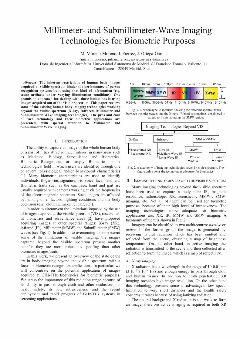
0.3GHz 30GHz 300GHz 3THz 4·1014Hz 8·1014Hz 3·1016Hz 3·1019Hz
IR VISMicro-
waveUV X-ray
1m 10mm 1mm 100μm 0.7μm 0.4μm 10nm 0.01nm
f
�MMW SMW
Millimeter- and Submillimeter-Wave Imaging Technologies for Biometric Purposes
M. Moreno-Moreno, J. Fierrez, J. Ortega-Garcia {miriam.moreno, julian.fierrez, javier.ortega}@uam.es
Dpto. de Ingeniería Informática. Universidad Autónoma de Madrid. C/ Francisco Tomás y Valiente, 11 Cantoblanco – 28049 Madrid, Spain.
Abstract- The inherent restrictions of human body images acquired at visible spectrum hinder the performance of person recognition systems built using that kind of information (e.g. scene artifacts under varying illumination conditions). One promising approach for dealing with those limitations is using images acquired out of the visible spectrum. This paper reviews some of the existing human body imaging technologies working beyond the visible spectrum (X-ray, Infrared, Millimeter and Submillimeter Wave imaging technologies). The pros and cons of each technology and their biometric applications are presented, with special attention to Millimeter and Submillimeter Wave imaging.
I. INTRODUCTION
The ability to capture an image of the whole human body or a part of it has attracted much interest in many areas such as Medicine, Biology, Surveillance and Biometrics. Biometric Recognition, or simply Biometrics, is a technological field in which users are identified through one or several physiological and/or behavioural characteristics [1]. Many biometric characteristics are used to identify individuals: fingerprint, signature, iris, voice, face, hand, etc. Biometric traits such as the ear, face, hand and gait are usually acquired with cameras working at visible frequencies of the electromagnetic spectrum. Such images are affected by, among other factors, lighting conditions and the body occlusion (e.g., clothing, make up, hair, etc.).
In order to circumvent the limitations imposed by the use of images acquired at the visible spectrum (VIS), researchers in biometrics and surveillance areas [2] have proposed acquiring images at other spectral ranges: X-ray (XR), infrared (IR), Millimeter (MMW) and Submillimeter (SMW) waves (see Fig. 1). In addition to overcoming to some extent some of the limitations of visible imaging, the images captured beyond the visible spectrum present another benefit: they are more robust to spoofing than other biometric images/traits.
In this work, we present an overview of the state of the art in body imaging beyond the visible spectrum, with a focus on biometric recognition applications. In particular, we will concentrate on the potential application of images acquired at GHz-THz frequencies for biometric purposes. We stress the importance of this radiation range because of its ability to pass through cloth and other occlusions, its health safety, its low intrusiveness, and the recent deployment and rapid progress of GHz-THz systems in screening applications.
Fig. 1. Electromagnetic spectrum showing the different spectral bands between the microwaves and the X-rays. IR band is sometimes considered to
extend to 1 mm including the SMW region.
Fig. 2. A taxonomy of imaging technologies beyond visible spectrum. The figure only shows the technologies adequate for biometrics.
II. IMAGING TECHNOLOGIES BEYOND THE VISIBLE SPECTRUM
Many imaging technologies beyond the visible spectrum have been used to capture a body part: IR, magnetic resonance, radioisotope, XR, acoustical-, MMW-, SMW-imaging, etc. Not all of them can be used for biometric purposes because of their high level of intrusiveness. The imaging technologies more adequate for biometric applications are: XR, IR, MMW and SMW imaging. A taxonomy of them is shown in Fig. 2.
Imagery can be classified in two architectures: passive or active. In the former group the image is generated by receiving natural radiation which has been emitted and reflected from the scene, obtaining a map of brightness temperature. On the other hand, in active imaging the radiation is transmitted to the scene and then collected after reflection to form the image, which is a map of reflectivity.
A. X-ray Imaging X-radiation has a wavelength in the range of 10-0.01 nm
(3·1016-3·1019 Hz) and enough energy to pass through cloth and human tissues. In addition to cloth penetration, XR imaging provides high image resolution. On the other hand this technology presents some disadvantages: low speed, limitation to very short distances and the health safety concerns it raises because of using ionizing radiation.
The natural background X-radiation is too weak to form an image, therefore active imaging is required in both XR
Imaging Technologies Beyond VIS
X-Ray Infrared MMW-SMW
Transmitted XR Backscatter XR
Near IR Medium Wave IR Long Wave IR Passive
ActivePassiveActive
MMW SMW

IR Spectral Range Archi- IR camera Image Applications
bands (μm) tecture cost Properties in Biometrics
Near IR Low, VIS came- Good quality, body Face [8] and Hand
(NIR) ra also sensitive condition invariant, Vein [9] Recognition
Medium Wave IR Good quality, sensiti- Face [10] and Hand
(MWIR) ve to body conditions Vein [11] Recognition
Long Wave IR Low contrast, sensiti- Face [12] and Hand
(LWIR) ve to body conditions Vein [9] Recognition
0,7-1
3 - 5
8 - 14
High
Low
Active
Passive
Passive
imaging modalities: transmission and backscatter X-ray imaging. The first one is the technique used in conventional X-ray radiographic systems, where XR photons transmitted through the body are detected to form the image. In the backscatter XR, the scattered photons are used to construct the image providing mainly a view of the surface of the scanned person [3]. Backscatter XR imaging technology has no tissue penetration.
There are very few works on biometric identification making use of XR imaging: Shamir et al. [4] perform biometric identification using knee X-rays while Chen et al.[5] present an automatic method for matching dental radiographs. According to our knowledge, there are no works on biometrics using backscatter X-ray images. The application of this technique includes medical imaging [6] and passenger screening at airports and homeland security [7]. There are currently different backscatter X-ray imaging systems available on the market (e.g. AS&E, Rapiscan Systems) to screen people.
B. Infrared Imaging The infrared band of the electromagnetic spectrum lies
between the SMW and VIS regions, its wavelength is in the range of 0.7 µm - 1 mm. The human body emits IR radiation with a wavelength between 3-14 µm, hence both active and passive architectures can be used in IR imaging.
The radiation that is actually detected by an IR sensor depends on the surface properties of the object and of the medium (atmosphere). According to the properties of the medium and the spectral ranges of the currently available IR detectors, the IR spectrum is divided into five parts. However IR imaging systems usually operate in one of the three following IR bands: the near infrared (NIR), the medium wave infrared (MWIR) or the long wave infrared (LWIR), where the high transmissivity atmosphere windows are located. Imaging objects within these IR-bands presents different characteristics. A summary of the properties of these bands is showed in Table 1. Many biometric research works have been developed using NIR, MWIR and LWIR imaging systems. Face and hand vein pattern recognition are the most important biometric modalities investigated in these three bands (see references in Table 1). Images acquired at any of these bands are, to some extent, environmental illumination invariant. Specifically images at NIR are body condition invariant and can provide good quality vein patterns near the skin surface [9], but external NIR illumination is required. Images acquired at MWIR and LWIR show patterns of radiated heat from the body's surface (often called thermograms). Very few biometric works have been developed in MWIR [10, 11], probably due to the high cost of MWIR cameras. LWIR cameras are much cheaper but, in contrast with NIR, LWIR can only capture large veins. Additionally, most of the LWIR images have low levels of contrast, being also sensitive to ambient and body condition [9].
C. Millimeter and Submillimeter Wave Imaging MMW and SMW radiation fill the gap between the IR
and the microwaves (see Fig. 1). Specifically, millimeter waves lie in the band of 30-300 GHz (10-1 mm) and the SMW regime lies in the range of 0.3-3 THz (1-0.1 mm).
Table 1. Properties of the most important IR bands.
MMW and SMW radiation can penetrate through many commonly used nonpolar dielectric materials such as paper, plastics, wood, leather, hair and even dry walls with little attenuation [13, 14]. Clothing is highly transparent to the MMW radiation and partially transparent to the SMW radiation [15]. Above 30 GHz, the transmission of the atmosphere varies strongly as a function of frequency due to water vapour and oxygen [16, 17]. There are relatively transparent windows centered at 35, 94, 140 and 220 GHz in the MMW range and less transparent windows in the SMW region located at: 0.34, 0.67, 1.5, 2, 2.1, 2.5, 3.4 and 4.3 THz. Atmosphere attenuation is further increased in poor weather. Liquid water extremely attenuates submillimeter waves while MMW radiation is less attenuated (millions of times) in the presence of clouds, fog, smoke, snow, and sand storms than VIS or IR radiation.
Consequently, natural applications of MMW and SMW imaging include security screening, non-destructive inspection, and medical and biometrics imaging. Low visibility navigation is another application of MMW imaging [18]. The detection of concealed weapons has been the most developed application of MMW/SMW imaging systems so far, in contrast to the biometrics area, where no research works have been produced.
Although most of the radiation emitted by the human body belongs to the MWIR and LWIR bands, it emits radiation in the SMW and MMW regions as well. This allows passive imaging. A key factor in MMW and SMW passive imaging is the sky illumination. This makes images acquired in indoor and outdoor environments to have very different contrast when working with passive systems. Outdoors radiometric temperature contrast can be very large, but it is very small indoors. In passive imaging operating indoors the signal to noise ratio (SNR) of the existing cameras is barely enough for coarse object detection, being usually insufficient for identification (as needed for biometrics). There are two solutions to overcome this problem: (i) cooling the detector or alternatively (ii) using active imaging. Cooling the detector improves the sensitivity but it makes the camera more expensive and difficult to use.
In active imaging, the source that illuminates the scene produces much higher power level than the emitted from the scene, so it can be considered as an object at very high temperature. If the source is incoherent and physically large, active imaging is equivalent to passive imaging with the surroundings at very high temperature, and hence results in much greater contrast within the image. If the source is small, active imaging becomes more complicated. In any case, the power level of the radiation source in active imaging strongly affects the detection resolution. In addition to higher resolution than passive imaging, active imaging provides higher SNR, higher signal levels, and the ability to obtain depth information in the scene.
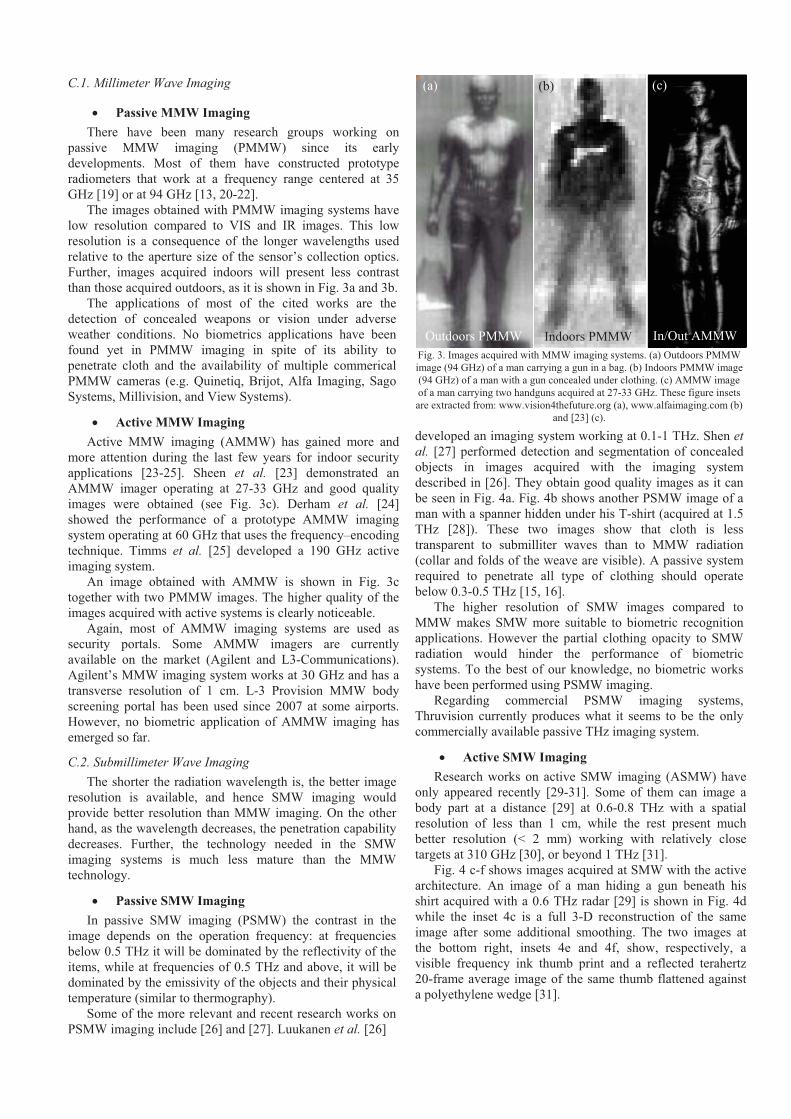
C.1. Millimeter Wave Imaging
� Passive MMW Imaging There have been many research groups working on
passive MMW imaging (PMMW) since its early developments. Most of them have constructed prototype radiometers that work at a frequency range centered at 35 GHz [19] or at 94 GHz [13, 20-22].
The images obtained with PMMW imaging systems have low resolution compared to VIS and IR images. This low resolution is a consequence of the longer wavelengths used relative to the aperture size of the sensor’s collection optics. Further, images acquired indoors will present less contrast than those acquired outdoors, as it is shown in Fig. 3a and 3b.
The applications of most of the cited works are the detection of concealed weapons or vision under adverse weather conditions. No biometrics applications have been found yet in PMMW imaging in spite of its ability to penetrate cloth and the availability of multiple commerical PMMW cameras (e.g. Quinetiq, Brijot, Alfa Imaging, Sago Systems, Millivision, and View Systems).
� Active MMW Imaging Active MMW imaging (AMMW) has gained more and
more attention during the last few years for indoor security applications [23-25]. Sheen et al. [23] demonstrated an AMMW imager operating at 27-33 GHz and good quality images were obtained (see Fig. 3c). Derham et al. [24] showed the performance of a prototype AMMW imaging system operating at 60 GHz that uses the frequency–encoding technique. Timms et al. [25] developed a 190 GHz active imaging system.
An image obtained with AMMW is shown in Fig. 3c together with two PMMW images. The higher quality of the images acquired with active systems is clearly noticeable.
Again, most of AMMW imaging systems are used as security portals. Some AMMW imagers are currently available on the market (Agilent and L3-Communications). Agilent’s MMW imaging system works at 30 GHz and has a transverse resolution of 1 cm. L-3 Provision MMW body screening portal has been used since 2007 at some airports. However, no biometric application of AMMW imaging has emerged so far.
C.2. Submillimeter Wave Imaging The shorter the radiation wavelength is, the better image
resolution is available, and hence SMW imaging would provide better resolution than MMW imaging. On the other hand, as the wavelength decreases, the penetration capability decreases. Further, the technology needed in the SMW imaging systems is much less mature than the MMW technology.
� Passive SMW Imaging In passive SMW imaging (PSMW) the contrast in the
image depends on the operation frequency: at frequencies below 0.5 THz it will be dominated by the reflectivity of the items, while at frequencies of 0.5 THz and above, it will be dominated by the emissivity of the objects and their physical temperature (similar to thermography). Some of the more relevant and recent research works on PSMW imaging include [26] and [27]. Luukanen et al. [26]
Fig. 3. Images acquired with MMW imaging systems. (a) Outdoors PMMW image (94 GHz) of a man carrying a gun in a bag. (b) Indoors PMMW image (94 GHz) of a man with a gun concealed under clothing. (c) AMMW image of a man carrying two handguns acquired at 27-33 GHz. These figure insets are extracted from: www.vision4thefuture.org (a), www.alfaimaging.com (b)
and [23] (c).
developed an imaging system working at 0.1-1 THz. Shen etal. [27] performed detection and segmentation of concealed objects in images acquired with the imaging system described in [26]. They obtain good quality images as it can be seen in Fig. 4a. Fig. 4b shows another PSMW image of a man with a spanner hidden under his T-shirt (acquired at 1.5 THz [28]). These two images show that cloth is less transparent to submilliter waves than to MMW radiation (collar and folds of the weave are visible). A passive system required to penetrate all type of clothing should operate below 0.3-0.5 THz [15, 16].
The higher resolution of SMW images compared to MMW makes SMW more suitable to biometric recognition applications. However the partial clothing opacity to SMW radiation would hinder the performance of biometric systems. To the best of our knowledge, no biometric works have been performed using PSMW imaging.
Regarding commercial PSMW imaging systems, Thruvision currently produces what it seems to be the only commercially available passive THz imaging system.
� Active SMW Imaging Research works on active SMW imaging (ASMW) have
only appeared recently [29-31]. Some of them can image a body part at a distance [29] at 0.6-0.8 THz with a spatial resolution of less than 1 cm, while the rest present much better resolution (< 2 mm) working with relatively close targets at 310 GHz [30], or beyond 1 THz [31].
Fig. 4 c-f shows images acquired at SMW with the active architecture. An image of a man hiding a gun beneath his shirt acquired with a 0.6 THz radar [29] is shown in Fig. 4d while the inset 4c is a full 3-D reconstruction of the same image after some additional smoothing. The two images at the bottom right, insets 4e and 4f, show, respectively, a visible frequency ink thumb print and a reflected terahertz 20-frame average image of the same thumb flattened against a polyethylene wedge [31].
(a) (b) (c)
Outdoors PMMW Indoors PMMW In/Out AMMW
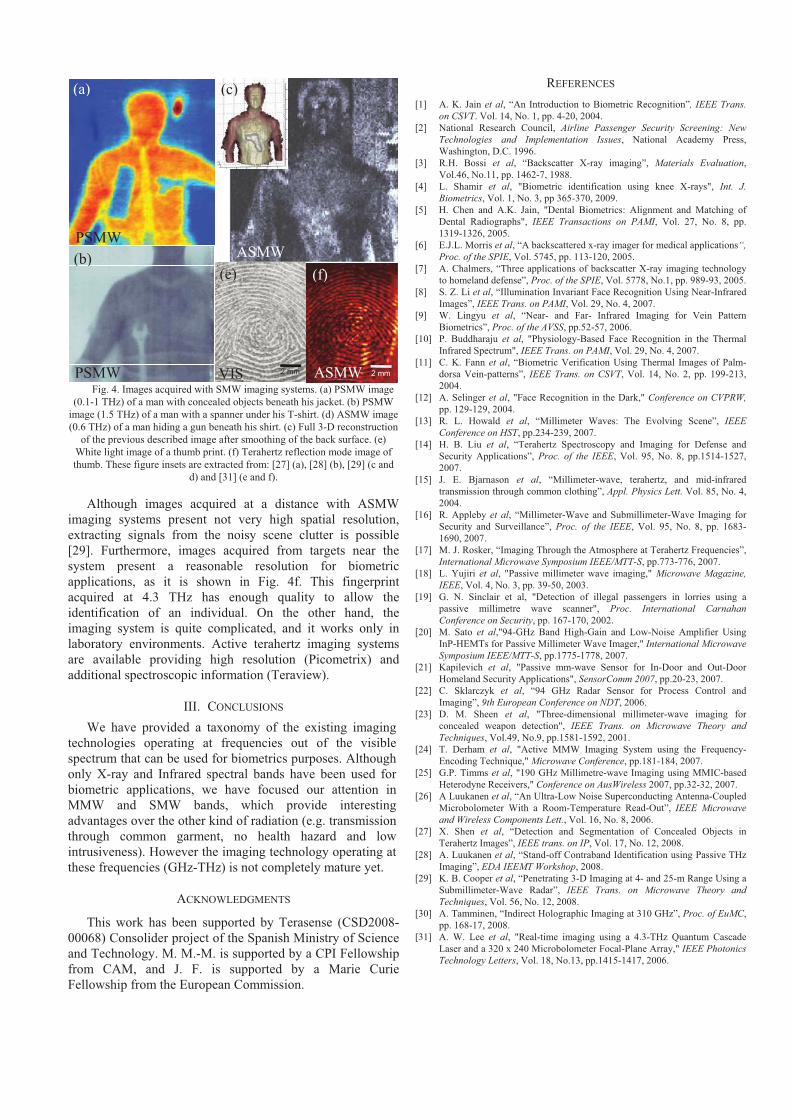
Fig. 4. Images acquired with SMW imaging systems. (a) PSMW image (0.1-1 THz) of a man with concealed objects beneath his jacket. (b) PSMW
image (1.5 THz) of a man with a spanner under his T-shirt. (d) ASMW image (0.6 THz) of a man hiding a gun beneath his shirt. (c) Full 3-D reconstruction
of the previous described image after smoothing of the back surface. (e) White light image of a thumb print. (f) Terahertz reflection mode image of thumb. These figure insets are extracted from: [27] (a), [28] (b), [29] (c and
d) and [31] (e and f).
Although images acquired at a distance with ASMW imaging systems present not very high spatial resolution, extracting signals from the noisy scene clutter is possible [29]. Furthermore, images acquired from targets near the system present a reasonable resolution for biometric applications, as it is shown in Fig. 4f. This fingerprint acquired at 4.3 THz has enough quality to allow the identification of an individual. On the other hand, the imaging system is quite complicated, and it works only in laboratory environments. Active terahertz imaging systems are available providing high resolution (Picometrix) and additional spectroscopic information (Teraview).
III. CONCLUSIONS
We have provided a taxonomy of the existing imaging technologies operating at frequencies out of the visible spectrum that can be used for biometrics purposes. Although only X-ray and Infrared spectral bands have been used for biometric applications, we have focused our attention in MMW and SMW bands, which provide interesting advantages over the other kind of radiation (e.g. transmission through common garment, no health hazard and low intrusiveness). However the imaging technology operating at these frequencies (GHz-THz) is not completely mature yet.
ACKNOWLEDGMENTS
This work has been supported by Terasense (CSD2008-00068) Consolider project of the Spanish Ministry of Science and Technology. M. M.-M. is supported by a CPI Fellowship from CAM, and J. F. is supported by a Marie Curie Fellowship from the European Commission.
REFERENCES
[1] A. K. Jain et al, “An Introduction to Biometric Recognition”, IEEE Trans. on CSVT. Vol. 14, No. 1, pp. 4-20, 2004.
[2] National Research Council, Airline Passenger Security Screening: New Technologies and Implementation Issues, National Academy Press, Washington, D.C. 1996.
[3] R.H. Bossi et al, “Backscatter X-ray imaging”, Materials Evaluation,Vol.46, No.11, pp. 1462-7, 1988.
[4] L. Shamir et al, "Biometric identification using knee X-rays", Int. J. Biometrics, Vol. 1, No. 3, pp 365-370, 2009.
[5] H. Chen and A.K. Jain, "Dental Biometrics: Alignment and Matching of Dental Radiographs", IEEE Transactions on PAMI, Vol. 27, No. 8, pp. 1319-1326, 2005.
[6] E.J.L. Morris et al, “A backscattered x-ray imager for medical applications“, Proc. of the SPIE, Vol. 5745, pp. 113-120, 2005.
[7] A. Chalmers, “Three applications of backscatter X-ray imaging technology to homeland defense”, Proc. of the SPIE, Vol. 5778, No.1, pp. 989-93, 2005.
[8] S. Z. Li et al, “Illumination Invariant Face Recognition Using Near-InfraredImages”, IEEE Trans. on PAMI, Vol. 29, No. 4, 2007.
[9] W. Lingyu et al, “Near- and Far- Infrared Imaging for Vein Pattern Biometrics”, Proc. of the AVSS, pp.52-57, 2006.
[10] P. Buddharaju et al, "Physiology-Based Face Recognition in the Thermal Infrared Spectrum", IEEE Trans. on PAMI, Vol. 29, No. 4, 2007.
[11] C. K. Fann et al, “Biometric Verification Using Thermal Images of Palm-dorsa Vein-patterns”, IEEE Trans. on CSVT, Vol. 14, No. 2, pp. 199-213, 2004.
[12] A. Selinger et al, "Face Recognition in the Dark," Conference on CVPRW, pp. 129-129, 2004.
[13] R. L. Howald et al, “Millimeter Waves: The Evolving Scene”, IEEE Conference on HST, pp.234-239, 2007.
[14] H. B. Liu et al, “Terahertz Spectroscopy and Imaging for Defense and Security Applications”, Proc. of the IEEE, Vol. 95, No. 8, pp.1514-1527, 2007.
[15] J. E. Bjarnason et al, “Millimeter-wave, terahertz, and mid-infrared transmission through common clothing”, Appl. Physics Lett. Vol. 85, No. 4, 2004.
[16] R. Appleby et al, “Millimeter-Wave and Submillimeter-Wave Imaging for Security and Surveillance”, Proc. of the IEEE, Vol. 95, No. 8, pp. 1683-1690, 2007.
[17] M. J. Rosker, “Imaging Through the Atmosphere at Terahertz Frequencies”, International Microwave Symposium IEEE/MTT-S, pp.773-776, 2007.
[18] L. Yujiri et al, "Passive millimeter wave imaging," Microwave Magazine, IEEE, Vol. 4, No. 3, pp. 39-50, 2003.
[19] G. N. Sinclair et al, "Detection of illegal passengers in lorries using a passive millimetre wave scanner", Proc. International Carnahan Conference on Security, pp. 167-170, 2002.
[20] M. Sato et al,"94-GHz Band High-Gain and Low-Noise Amplifier Using InP-HEMTs for Passive Millimeter Wave Imager," International Microwave Symposium IEEE/MTT-S, pp.1775-1778, 2007.
[21] Kapilevich et al, "Passive mm-wave Sensor for In-Door and Out-Door Homeland Security Applications", SensorComm 2007, pp.20-23, 2007.
[22] C. Sklarczyk et al, “94 GHz Radar Sensor for Process Control and Imaging”, 9th European Conference on NDT, 2006.
[23] D. M. Sheen et al, "Three-dimensional millimeter-wave imaging for concealed weapon detection", IEEE Trans. on Microwave Theory and Techniques, Vol.49, No.9, pp.1581-1592, 2001.
[24] T. Derham et al, "Active MMW Imaging System using the Frequency-Encoding Technique," Microwave Conference, pp.181-184, 2007.
[25] G.P. Timms et al, "190 GHz Millimetre-wave Imaging using MMIC-based Heterodyne Receivers," Conference on AusWireless 2007, pp.32-32, 2007.
[26] A Luukanen et al, “An Ultra-Low Noise Superconducting Antenna-Coupled Microbolometer With a Room-Temperature Read-Out”, IEEE Microwave and Wireless Components Lett., Vol. 16, No. 8, 2006.
[27] X. Shen et al, “Detection and Segmentation of Concealed Objects in Terahertz Images”, IEEE trans. on IP, Vol. 17, No. 12, 2008.
[28] A. Luukanen et al, “Stand-off Contraband Identification using Passive THz Imaging”, EDA IEEMT Workshop, 2008.
[29] K. B. Cooper et al, “Penetrating 3-D Imaging at 4- and 25-m Range Using a Submillimeter-Wave Radar”, IEEE Trans. on Microwave Theory and Techniques, Vol. 56, No. 12, 2008.
[30] A. Tamminen, “Indirect Holographic Imaging at 310 GHz”, Proc. of EuMC,pp. 168-17, 2008.
[31] A. W. Lee et al, "Real-time imaging using a 4.3-THz Quantum Cascade Laser and a 320 x 240 Microbolometer Focal-Plane Array," IEEE Photonics Technology Letters, Vol. 18, No.13, pp.1415-1417, 2006.
2 mm 2 mm
(a)
(b)
(c)
(e) (f)
PSMW
PSMW VIS
ASMW
ASMW
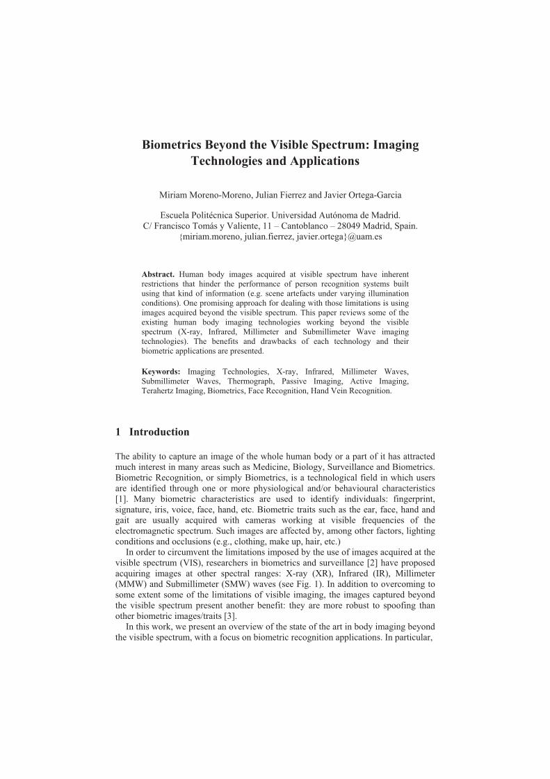
Biometrics Beyond the Visible Spectrum: Imaging Technologies and Applications
Miriam Moreno-Moreno, Julian Fierrez and Javier Ortega-Garcia
Escuela Politécnica Superior. Universidad Autónoma de Madrid.
C/ Francisco Tomás y Valiente, 11 – Cantoblanco – 28049 Madrid, Spain. {miriam.moreno, julian.fierrez, javier.ortega}@uam.es
Abstract. Human body images acquired at visible spectrum have inherent restrictions that hinder the performance of person recognition systems built using that kind of information (e.g. scene artefacts under varying illumination conditions). One promising approach for dealing with those limitations is using images acquired beyond the visible spectrum. This paper reviews some of the existing human body imaging technologies working beyond the visible spectrum (X-ray, Infrared, Millimeter and Submillimeter Wave imaging technologies). The benefits and drawbacks of each technology and their biometric applications are presented.
Keywords: Imaging Technologies, X-ray, Infrared, Millimeter Waves, Submillimeter Waves, Thermograph, Passive Imaging, Active Imaging, Terahertz Imaging, Biometrics, Face Recognition, Hand Vein Recognition.
1 Introduction
The ability to capture an image of the whole human body or a part of it has attracted much interest in many areas such as Medicine, Biology, Surveillance and Biometrics. Biometric Recognition, or simply Biometrics, is a technological field in which users are identified through one or more physiological and/or behavioural characteristics [1]. Many biometric characteristics are used to identify individuals: fingerprint, signature, iris, voice, face, hand, etc. Biometric traits such as the ear, face, hand and gait are usually acquired with cameras working at visible frequencies of the electromagnetic spectrum. Such images are affected by, among other factors, lighting conditions and occlusions (e.g., clothing, make up, hair, etc.)
In order to circumvent the limitations imposed by the use of images acquired at the visible spectrum (VIS), researchers in biometrics and surveillance [2] have proposed acquiring images at other spectral ranges: X-ray (XR), Infrared (IR), Millimeter (MMW) and Submillimeter (SMW) waves (see Fig. 1). In addition to overcoming to some extent some of the limitations of visible imaging, the images captured beyond the visible spectrum present another benefit: they are more robust to spoofing than other biometric images/traits [3].
In this work, we present an overview of the state of the art in body imaging beyond the visible spectrum, with a focus on biometric recognition applications. In particular,
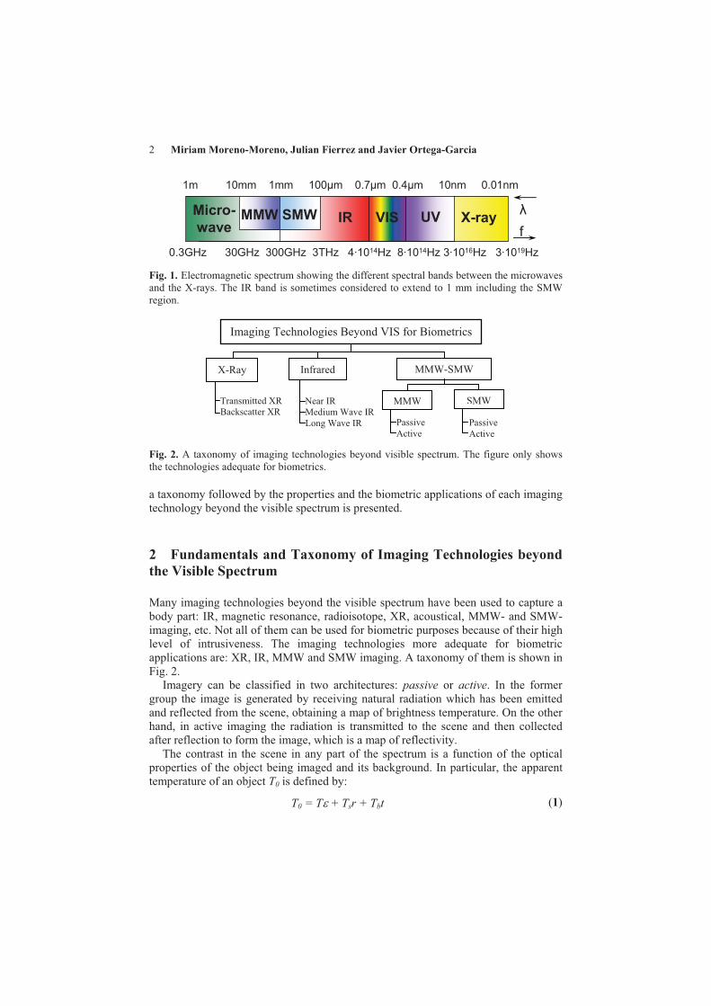
2 Miriam Moreno-Moreno, Julian Fierrez and Javier Ortega-Garcia
0.3GHz 30GHz 300GHz 3THz 4·1014Hz 8·1014Hz 3·1016Hz 3·1019Hz
IR VISMicro-
waveUV X-ray
1m 10mm 1mm 100μm 0.7μm 0.4μm 10nm 0.01nm
f
�MMW SMW
Fig. 1. Electromagnetic spectrum showing the different spectral bands between the microwaves and the X-rays. The IR band is sometimes considered to extend to 1 mm including the SMW region.
Fig. 2. A taxonomy of imaging technologies beyond visible spectrum. The figure only shows the technologies adequate for biometrics.
a taxonomy followed by the properties and the biometric applications of each imaging technology beyond the visible spectrum is presented.
2 Fundamentals and Taxonomy of Imaging Technologies beyond the Visible Spectrum
Many imaging technologies beyond the visible spectrum have been used to capture a body part: IR, magnetic resonance, radioisotope, XR, acoustical, MMW- and SMW-imaging, etc. Not all of them can be used for biometric purposes because of their high level of intrusiveness. The imaging technologies more adequate for biometric applications are: XR, IR, MMW and SMW imaging. A taxonomy of them is shown in Fig. 2.
Imagery can be classified in two architectures: passive or active. In the former group the image is generated by receiving natural radiation which has been emitted and reflected from the scene, obtaining a map of brightness temperature. On the other hand, in active imaging the radiation is transmitted to the scene and then collected after reflection to form the image, which is a map of reflectivity.
The contrast in the scene in any part of the spectrum is a function of the optical properties of the object being imaged and its background. In particular, the apparent temperature of an object T0 is defined by:
T0 = T� + Tsr + Tbt (1)
Imaging Technologies Beyond VIS for Biometrics
X-Ray Infrared MMW-SMW
Transmitted XR Backscatter XR
Near IR Medium Wave IR Long Wave IR Passive
Active Passive Active
MMW SMW

Biometrics Beyond the Visible Spectrum: Imaging Technologies and Applications 3
where T is the physical temperature of the object, � its emissivity, Ts is the temperature of the background which is reflected by the object with reflectivity r, Tb is the temperature of the background behind the object and t the object’s transmissivity [4].
3 X-ray Imaging
X-radiation have a wavelength in the range of 10-0.01 nm (3·1016-3·1019 Hz) and enough energy to pass through cloth and human tissues. In addition to cloth penetration, XR imaging provides high image resolution. On the other hand, this technology presents some disadvantages: low speed, limitation to very short distances and the health safety concerns it raises because of using ionizing radiation.
The natural background X-radiation is too weak to form an image, therefore active imaging is required in both XR imaging modalities: transmission and backscatter X-ray imaging. X-rays are commonly produced by accelerating charged particles. Transmission X-ray Imaging. Conventional X-ray radiographic systems used for medical purposes produce images relying on this kind of imaging: a uniform X-ray beam incident on the patient interacts with the tissues of the body, producing a variable transmitted X-ray flux dependent on the attenuation along the beam paths. An X-ray-sensitive detector captures the transmitted fraction and converts the X-rays into a visible projection image.
Only a few works on biometric identification making use of the conventional X-rays can be found: Shamir et al. [5] perform biometric identification using knee X-rays while Chen et al. [6] present an automatic method for matching dental radiographs (see Fig. 3a-c). These knee or dental X-rays are difficult to forge and present additional advantages: they can be used in forensic identification where the soft tissues are degraded. Backscatter X-ray Imaging. In this technique the XR scattered photons, instead of transmitted photons, are used to construct the image [7]. This technology utilizes high energy X-rays that are more likely to scatter than penetrate materials as compared to lower-energy X-ray used in medical applications. However, this kind of radiation is able to penetrate some materials, such as cloth.
A person is scanned by moving a single XR beam over her body. The backscattered beam from a known position allows a realistic image to be reconstructed. As only scattered X-rays are used, the registered image is mainly a view of the surface of the scanned person, i.e. her nude form. As the image resolution is high, these images present privacy issues. Some companies (e.g. AS&E) ensure privacy by applying an algorithm to the raw images so that processed images reveal only an outline of the scanned individual. Raw and processed backscatter XR images are shown in Fig. 3d and e.
According to our knowledge, there are no works on biometrics using backscatter X-ray images. The application of this technique includes medical imaging [8] and passenger screening at airports and homeland security [9]. There are currently
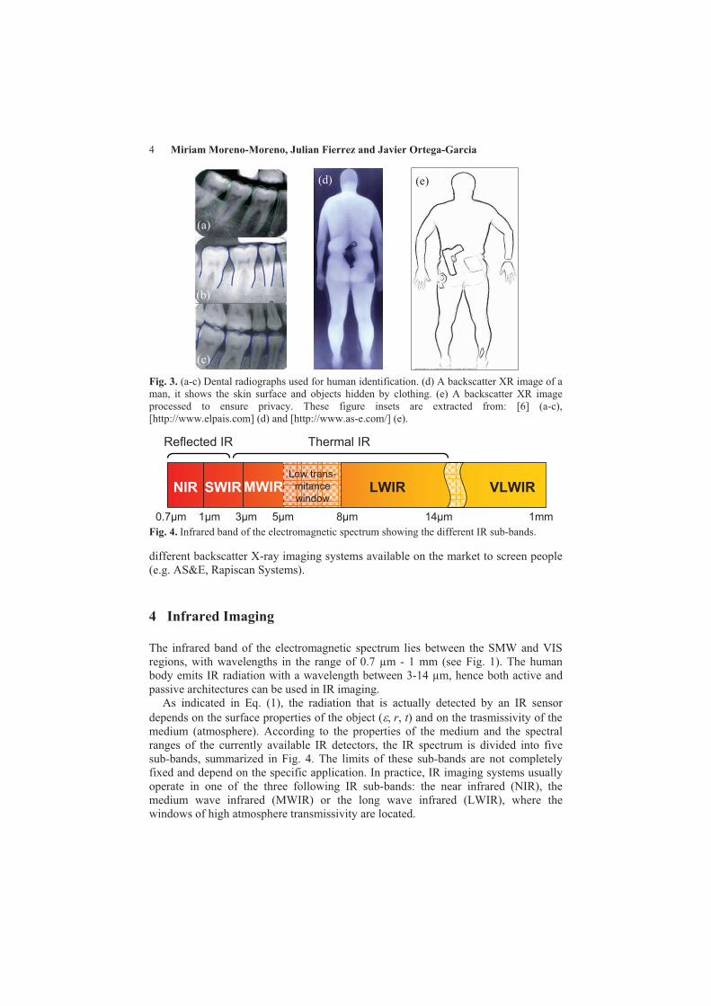
4 Miriam Moreno-Moreno, Julian Fierrez and Javier Ortega-Garcia
0.7μm 1μm 3μm 5μm 8μm 14μm 1mm
NIR SWIR MWIR LWIR VLWIRLow trans-
mitance
window
Reflected IR Thermal IR
Fig. 3. (a-c) Dental radiographs used for human identification. (d) A backscatter XR image of a man, it shows the skin surface and objects hidden by clothing. (e) A backscatter XR image processed to ensure privacy. These figure insets are extracted from: [6] (a-c), [http://www.elpais.com] (d) and [http://www.as-e.com/] (e).
Fig. 4. Infrared band of the electromagnetic spectrum showing the different IR sub-bands. different backscatter X-ray imaging systems available on the market to screen people (e.g. AS&E, Rapiscan Systems).
4 Infrared Imaging
The infrared band of the electromagnetic spectrum lies between the SMW and VIS regions, with wavelengths in the range of 0.7 µm - 1 mm (see Fig. 1). The human body emits IR radiation with a wavelength between 3-14 µm, hence both active and passive architectures can be used in IR imaging.
As indicated in Eq. (1), the radiation that is actually detected by an IR sensor depends on the surface properties of the object (�,�r, t) and on the trasmissivity of the medium (atmosphere). According to the properties of the medium and the spectral ranges of the currently available IR detectors, the IR spectrum is divided into five sub-bands, summarized in Fig. 4. The limits of these sub-bands are not completely fixed and depend on the specific application. In practice, IR imaging systems usually operate in one of the three following IR sub-bands: the near infrared (NIR), the medium wave infrared (MWIR) or the long wave infrared (LWIR), where the windows of high atmosphere transmissivity are located.
(d) (e)
(a)
(b)
(c)
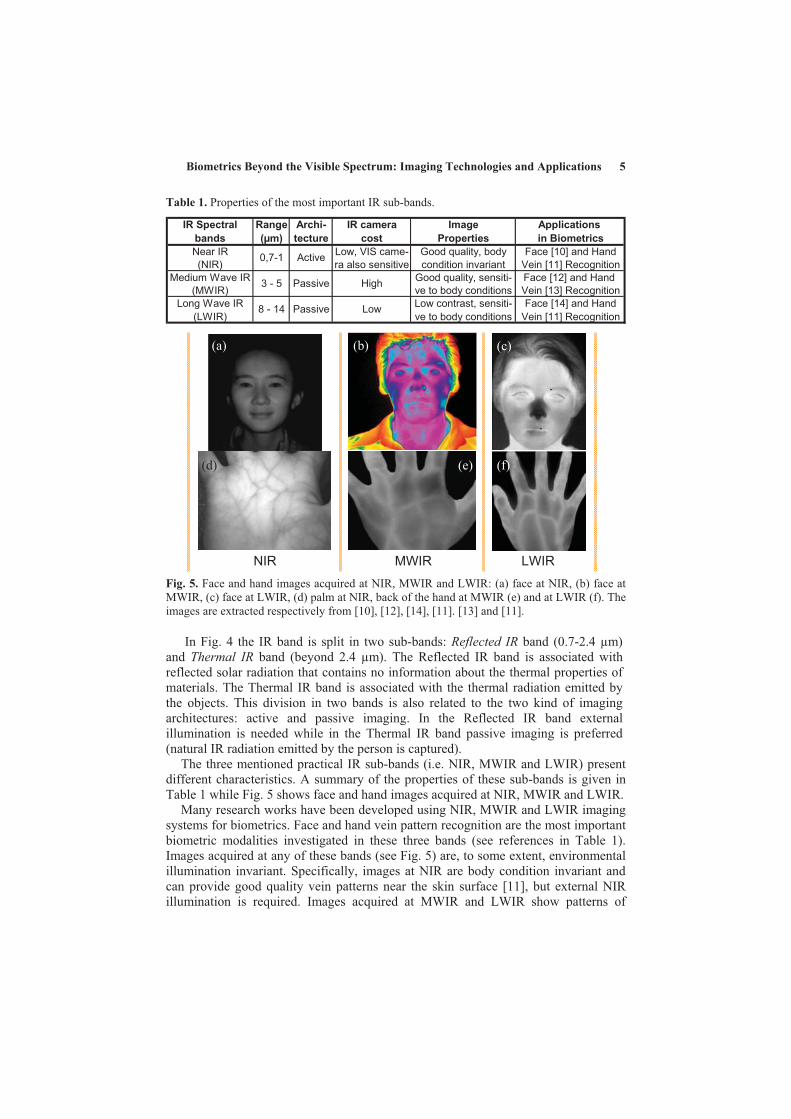
Biometrics Beyond the Visible Spectrum: Imaging Technologies and Applications 5
Table 1. Properties of the most important IR sub-bands.
IR Spectral Range Archi- IR camera Image Applications
bands (μm) tecture cost Properties in Biometrics
Near IR Low, VIS came- Good quality, body Face [10] and Hand
(NIR) ra also sensitive condition invariant Vein [11] Recognition
Medium Wave IR Good quality, sensiti- Face [12] and Hand
(MWIR) ve to body conditions Vein [13] Recognition
Long Wave IR Low contrast, sensiti- Face [14] and Hand
(LWIR) ve to body conditions Vein [11] Recognition
0,7-1
3 - 5
8 - 14
High
Low
Active
Passive
Passive
NIR MWIR LWIR
Fig. 5. Face and hand images acquired at NIR, MWIR and LWIR: (a) face at NIR, (b) face at MWIR, (c) face at LWIR, (d) palm at NIR, back of the hand at MWIR (e) and at LWIR (f). The images are extracted respectively from [10], [12], [14], [11]. [13] and [11].
In Fig. 4 the IR band is split in two sub-bands: Reflected IR band (0.7-2.4 µm) and Thermal IR band (beyond 2.4 µm). The Reflected IR band is associated with reflected solar radiation that contains no information about the thermal properties of materials. The Thermal IR band is associated with the thermal radiation emitted by the objects. This division in two bands is also related to the two kind of imaging architectures: active and passive imaging. In the Reflected IR band external illumination is needed while in the Thermal IR band passive imaging is preferred (natural IR radiation emitted by the person is captured).
The three mentioned practical IR sub-bands (i.e. NIR, MWIR and LWIR) present different characteristics. A summary of the properties of these sub-bands is given in Table 1 while Fig. 5 shows face and hand images acquired at NIR, MWIR and LWIR.
Many research works have been developed using NIR, MWIR and LWIR imaging systems for biometrics. Face and hand vein pattern recognition are the most important biometric modalities investigated in these three bands (see references in Table 1). Images acquired at any of these bands (see Fig. 5) are, to some extent, environmental illumination invariant. Specifically, images at NIR are body condition invariant and can provide good quality vein patterns near the skin surface [11], but external NIR illumination is required. Images acquired at MWIR and LWIR show patterns of
(a)
(d)
(b) (c)
(e) (f)

6 Miriam Moreno-Moreno, Julian Fierrez and Javier Ortega-Garcia
radiated heat from the body's surface (often called thermograms). Very few biometric works have been developed in MWIR [12, 13], probably due to the high cost of MWIR cameras. LWIR cameras are much cheaper but, in contrast with NIR, LWIR can only capture large veins. Additionally, most of the LWIR images have low levels of contrast, being also sensitive to ambient and body condition [11].
5 Millimeter and Submillimeter Wave Imaging
MMW and SMW radiation fill the gap between the IR and the microwaves (see Fig. 1). Specifically, MMW band spreads from 30 to 300 GHz (10-1 mm) while the SMW band lies in the range of 0.3-3 THz (1-0.1 mm) [4].
The use of MMW/SMW of radiation within imaging systems is currently an active field of research due to some of its interesting properties [15-20]. The penetration through clothing and other nonpolar dielectric materials even at stand off ranges is one of the most important MMWs and SMWs abilities. Hence, security screening (detection of concealed weapons under clothing), nondestructive inspection and medical and biometric imaging are the most relevant applications of MMW/SMW imaging. Another application of MMW imaging is low visibility navigation (due to the low attenuation of MMWs under adverse weather).
Images acquired at MMW/SMW frequencies have lower resolution than IR or VIS images due to larger wavelength. Further, MMW and, specially, SMW imaging technologies are not as mature as the IR or VIS imaging technologies, which restricts the quality of the resulting images. On the other hand, SMW images have better spatial resolution than MMW images (SMW wavelength is smaller), but SMW clothing penetration is lower compared to MMW. In any case, images acquired with passive or with active systems present different characteristics (see Table 2). Different Passive MMW (PMMW), Active MMW (AMMW), Passive SMW (PSMW) and Active SMW (ASMW) images are shown in Fig. 6. As MMW and SMW images
Table 2. Properties of MMW and SMW imaging operating with passive or active architecture. The spatial resolution depends on some conditions such as the distance between the target and the detector, the given resolution corresponds to a target-detector distance of some meters.
Radia- Archi- Image Relative Spatial Operating Commercial
tion tecture Properties Resolution Frequencies Systems
� Low resolution com- � Qinetiq
pared to VIS and IR � Brijot
� Highly affected by � Alfa Imaging
sky illumination � Sago Systems
� 30 GHz � Agilent
� 60 GHz � L-3 Commu-
� 190 GHz nications
� Higher quality than � 0.6-0.8 THz
Passive SMW images � 310 GHz
� Partial clothing opacity � > 1 THz
� 0.1-1 THz
� 1.5 THz� Thruvision
ActiveHigh (at a distance)
Very high (near)
� Picometrix
� Teraview
SMW
Passive� Good quality
� Partial clothing opacityMedium-High
MMW
PassiveVery Low (indoors)
Low-Medium (outdoors)
� 35 GHz
� 94 GHz
Active� Higher quality than
_Passive MMW imagesMedium
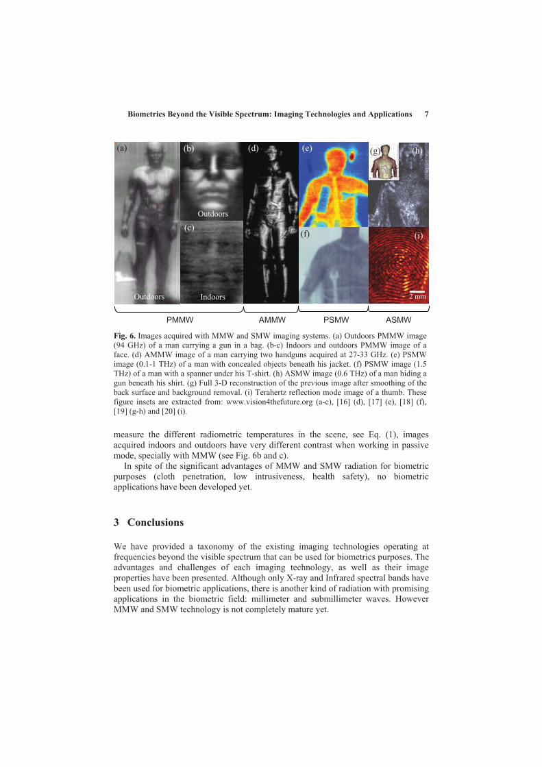
Biometrics Beyond the Visible Spectrum: Imaging Technologies and Applications 7
PMMW AMMW PSMW ASMW
Fig. 6. Images acquired with MMW and SMW imaging systems. (a) Outdoors PMMW image (94 GHz) of a man carrying a gun in a bag. (b-c) Indoors and outdoors PMMW image of a face. (d) AMMW image of a man carrying two handguns acquired at 27-33 GHz. (e) PSMW image (0.1-1 THz) of a man with concealed objects beneath his jacket. (f) PSMW image (1.5 THz) of a man with a spanner under his T-shirt. (h) ASMW image (0.6 THz) of a man hiding a gun beneath his shirt. (g) Full 3-D reconstruction of the previous image after smoothing of the back surface and background removal. (i) Terahertz reflection mode image of a thumb. These figure insets are extracted from: www.vision4thefuture.org (a-c), [16] (d), [17] (e), [18] (f), [19] (g-h) and [20] (i). measure the different radiometric temperatures in the scene, see Eq. (1), images acquired indoors and outdoors have very different contrast when working in passive mode, specially with MMW (see Fig. 6b and c).
In spite of the significant advantages of MMW and SMW radiation for biometric purposes (cloth penetration, low intrusiveness, health safety), no biometric applications have been developed yet.
3 Conclusions
We have provided a taxonomy of the existing imaging technologies operating at frequencies beyond the visible spectrum that can be used for biometrics purposes. The advantages and challenges of each imaging technology, as well as their image properties have been presented. Although only X-ray and Infrared spectral bands have been used for biometric applications, there is another kind of radiation with promising applications in the biometric field: millimeter and submillimeter waves. However MMW and SMW technology is not completely mature yet.
(e)
(f)
(g) (h)
2 mm
(i)
Outdoors
(c)
Outdoors Indoors
(a) (b) (d)

8 Miriam Moreno-Moreno, Julian Fierrez and Javier Ortega-Garcia
Acknowledgments. This work has been supported by Terasense (CSD2008-00068) Consolider project of the Spanish Ministry of Science and Technology. M. M.-M. is supported by a CPI Fellowship from CAM, and J. F. is supported by a Marie Curie Fellowship from the European Commission.
References
1. Jain, A. K. et al.: An Introduction to Biometric Recognition, IEEE Trans. on CSVT. Vol. 14, No. 1, pp. 4-20 (2004).
2. National Research Council, Airline Passenger Security Screening: New Technologies and Implementation Issues, National Academy Press, Washington, D.C. (1996).
3. Galbally, J. et al.: Fake Fingertip Generation from a Minutiae Template, in Proc. Intl. Conf. on Pattern Recognition, ICPR, IEEE Press, (2008).
4. Appleby, R. et al.: Millimeter-Wave and Submillimeter-Wave Imaging for Security and Surveillance, Proc. of the IEEE, Vol. 95, No. 8, pp. 1683-1690 (2007).
5. Shamir, L. et al.: Biometric identification using knee X-rays, Int. J. Biometrics, Vol. 1, No. 3, pp 365-370 (2009).
6. Chen, H. and Jain, A.K.: Dental Biometrics: Alignment and Matching of Dental Radiographs, IEEE Transactions on PAMI, Vol. 27, No. 8, pp. 1319-1326 (2005).
7. Bossi, R.H. et al.: Backscatter X-ray imaging, Materials Evaluation, Vol.46, No. 11, pp. 1462-7 (1988).
8. Morris, E.J.L. et al.: A backscattered x-ray imager for medical applications, Proc. of the SPIE, Vol. 5745, pp. 113-120 (2005).
9. Chalmers, A.: Three applications of backscatter X-ray imaging technology to homeland defense, Proc. of the SPIE, Vol. 5778, No. 1, pp. 989-93 (2005).
10. Li, S. Z. et al.: Illumination Invariant Face Recognition Using Near-Infrared Images, IEEE Trans. on PAMI, Vol. 29, No. 4, pp.627-639 (2007).
11. Lingyu, W. et al.: Near- and Far- Infrared Imaging for Vein Pattern Biometrics, Proc. of the AVSS, pp.52-57 (2006).
12. Buddharaju, P. et al.: Physiology-Based Face Recognition in the Thermal Infrared Spectrum, IEEE Trans. on PAMI, Vol. 29, No. 4, pp.613-626 (2007).
13. Fann, C. K. et al.: Biometric Verification Using Thermal Images of Palm-dorsa Vein-patterns, IEEE Trans. on CSVT, Vol. 14, No. 2, pp. 199-213 (2004).
14. Chen, X. et al.: IR and visible light face recognition, Computer Vision and Image Understanding, Vol. 99, No. 3, pp. 332-358, (2005).
15. Kapilevich, B. et al.: Passive mm-wave Sensor for In-Door and Out-Door Homeland Security Applications, SensorComm 2007, pp.20-23 (2007).
16. Sheen, D. M. et al.: Three-dimensional millimeter-wave imaging for concealed weapon detection, IEEE Trans. on Microwave Theory and Techniques, Vol.49, No. 9, pp.1581-1592, (2001).
17. Shen, X. et al.: Detection and Segmentation of Concealed Objects in Terahertz Images, IEEE trans. on IP, Vol. 17, No. 12, (2008).
18. Luukanen, A. et al.: Stand-off Contraband Identification using Passive THz Imaging, EDA IEEMT Workshop, (2008).
19. Cooper, K. B. et al.: Penetrating 3-D Imaging at 4- and 25-m Range Using a Submillimeter-Wave Radar, IEEE Trans. on Microwave Theory and Techniques, Vol. 56, No. 12 (2008).
20. Lee, A. W. et al.: Real-time imaging using a 4.3-THz Quantum Cascade Laser and a 320 x 240 Microbolometer Focal-Plane Array, IEEE Photonics Technology Letters, Vol. 18, No. 13, pp.1415-1417 (2006).
ANÁLISIS DE ESCENARIOS PARARECONOCIMIENTO BIOMÉTRICO ADISTANCIA ADECUADOS PARA LAADQUISICIÓN DE IMÁGENES MMW
M. Moreno-Moreno, J. Fierrez, P. Tome, J. Ortega-Garcia.{miriam.moreno, julian.fierrez, pedro.tome, javier.ortega}@uam.es
Avda. Francisco Tomás y Valiente, 11 - Campus de Cantoblanco - 28049 Madrid, Spain
Abstract— Con objeto de analizar en qué medida puede ayudarel uso de imágenes adquiridas en el rango de ondas milimétricas(MMW) al reconocimiento biométrico de personas a distancia,se presenta un análisis experimental de tres escenarios condiferentes distancias de captura adecuadas para la adquisiciónde imágenes MMW. En concreto se realizan experimentos dereconocimiento facial a corta, media y larga distancia entrela cámara y el sujeto a identificar, siendo los escenarios demedia y larga distancia los más adecuados para las capturas enMMW. Los tres escenarios consideran plantillas registradas encondiciones controladas, y para su estudio se usan datos del NISTMultiple Biometric Grand Challenge. Este enfoque permite: 1)aproximarnos al problema del reconocimiento biométrico deimágenes en MMW como complemento a biometrías tradicionalescomo es el reconocimiento facial, y 2) entender los factores demayor variabilidad que afectan al reconocimiento de personas adistancia, que serán los factores a compensar con las tecnologíascomplementarias al reconocimiento, como MMW. El análisis deescenarios se realiza cuantitativamente de dos maneras. Primerose analiza el contenido de información en caras segmentadas enlos diferentes escenarios. A continuación se evalúa el rendimientoen cada escenario de tres comparadores, uno comercial, y dosaproximaciones estándar usando características (PCA y DCT)y comparadores (SVM y GMM) tradicionales. Los resultadosmuestran hasta qué punto las características de la adquisicióninfluyen en el rendimiento de la verificación del reconocimientofacial a distancia, y esto sirve de punto de partida para compren-der en qué medida pueden ayudar al reconocimiento tecnologíascomplementarias como MMW.
I. INTRODUCCIÓN
Las imágenes adquiridas a frecuencias de milimétricas
(MMW) presentan propiedades únicas, que permiten su apli-
cación en diferentes ámbitos (seguridad, inspección no in-
trusiva, medicina y biometría entre otras) [1], [2]. A pesar
del actual desarrollo de los sistemas de adquisición de este
tipo de imágenes [3], [4], no existe ninguna base de datos de
imágenes de personas en este rango espectral. Ello es debido,
en parte, a los problemas de privacidad que presentan dichas
imágenes. Este hecho limita considerablemente el desarrollo
de sistemas biométricos basados en imágenes adquiridas en
este rango espectral, los cuales necesitan un número suficiente
de imágenes de diferentes usuarios. Dado que la adquisición de
estas imágenes se realiza a diferentes distancias y puesto que
no existe ninguna base de datos de imágenes en MMW, el tra-
bajo presentado se aproxima al problema del reconocimiento
biométrico de personas con imágenes en MMW, pero usando
imágenes adquiridas en el visible en un escenario similar al de
la adquisición de imágenes en MMW. En concreto el artículo
realiza un análisis de tres escenarios para reconocimiento
facial a distancia.
La cara y el iris son dos de los rasgos biométricos usados
actualmente en muchas aplicaciones de reconocimiento de
usuario a distancia [5], [6]. Una nueva línea de investigación
que está ganando popularidad se centra en el uso de estos
rasgos biométricos en escenarios menos controlados de una
manera no-invasiva incluyendo adquisición en movimiento
("On the Move") y a distancia ("At a Distance") [7]. Este
tipo de escenarios está todavía en su infancia y se necesita
mucha investigación y desarrollo para alcanzar los niveles
de precisión y de rendimiento que requieren las aplicaciones
prácticas.
El nuevo campo de la biometría a distancia se ha hecho
posible primordialmente gracias a: 1) los recientes avances
en los sensores, y 2) los nuevos algoritmos y métodos para
tratar con factores variables (e.g. iluminación, movimiento,
pose, distancia a la cámara), que en este caso están menos
controlados que en las situaciones consideradas comúnmente
en biometría.
Como resultado del interés en estas aplicaciones biométri-
cas a distancia, hay un número creciente de trabajos de
investigación que estudian cómo compensar las principales
degradaciones encontradas en escenarios no controlados [8].
Sin embargo, apenas existe conocimiento experimental sobre
los factores de variabilidad en escenarios específicos, que
puedan ayudar en la creación de métodos robustos para la
biometría a distancia (diseñada para aplicaciones específicas
de importancia práctica). La contribución de este artículo es
hacia este fin, analizando cuantitativamente tres escenarios
del reconocimiento facial a distancia, a saber: corta, media
y larga distancia entre el usuario y la cámara; siendo los
escenarios de media y larga distancia los más adecuados para
incorporar imágenes del cuerpo en MMW. Este análisis se
realiza a dos niveles: 1) los principales datos estadísticos de

a) Corta distancia b) Media distancia c) Larga distancia
MMW MMW
Fig. 1. Ejemplo de imágenes de los tres escenarios: a) corta distancia, b) media distancia, y c) larga distancia.
la información de contenido, y 2) el rendimiento de varios
sistemas de reconocimiento: uno comercial, y dos basados
en características (PCA, DCT) y comparadores tradicionales
(SVM, GMM).
Los escenarios bajo estudio han sido extraídos de NIST
Multiple Biometric Grand Challenge [9], el cual se centra
en el reconocimiento biométrico a distancia usando el iris y
la cara. En particular, usamos un subconjunto de estos datos
compuesto de imágenes de un total de 112 usuarios adquiridos
a diferentes distancias y condiciones variables de iluminación,
pose/ángulo de la cara, y expresión facial.
Este análisis de escenarios para una biometría tradicional,
como es el reconocimiento facial, permite comprender las
limitaciones de la tecnología actual y sirve de punto de partida
para ver en qué medida la tecnología MMW puede solventar
dichas limitaciones.
El artículo se estructura como sigue. La Sec. II describe
los conjuntos de datos y escenarios bajo estudio. La Sec.
III analiza los principales datos estadísticos de los escena-
rios. La Sec. IV estudia el rendimiento de los tres sistemas
de reconocimiento considerados en los diferentes escenarios.
Finalmente la Sec. V muestra los resultados experimentales y
esboza el trabajo futuro.
II. DEFINICIÓN DE LOS ESCENARIOS
Los tres escenarios considerados son: 1) "corta" distancia,
en la que los hombros pueden estar presentes; 2) "media"
distancia, incluyendo la parte superior del cuerpo; y 3) "larga"
distancia, incluyendo el cuerpo entero (ver Fig. 1). En esta
figura, además de un par de imágenes en cada escenario en
el rango visible, se muestran dos imágenes adquiridas en el
rango de MMW mediante un radiómetro trabajando a 94 GHz,
cortesía de AlfaImaging1. Una de ellas (a media distancia) se
adquirió en exteriores y la otra (a larga distancia) en interiores.
Se comprueba el parecido de ambos tipos de imágenes (en
visible y en MMW) en los escenarios de media y larga
distancia, de ahí el interés en el análisis del reconocimiento
biométrico usando imágenes en el visible en estos escenarios,
1http://www.alfaimaging.com/
como base sobre la que comparar en qué medida puede
ayudar al reconocimiento clásico la incorporación de imágenes
adquiridas en el rango de los GHz.
Usando estos tres escenarios generales, hemos marcado
manualmente las 3482 imágenes de los 147 usuarios presentes
en la base de datos NISR MBGC v2.0 Face Stills [9]. Algunas
se muestran en la Fig. 1. Una porción del conjunto de imágenes
fue desechada (360 imágenes de 89 usuarios), porque la cara
estaba ocluída o la iluminación degradaba completamente la
imagen de la cara. Además, aunque esta información no se usa
en el presente artículo, todas las imágenes fueron marcadas
como adquiridas en interiores o exteriores.
Finalmente, para posibilitar experimentos de verificación
considerando el registro con imágenes adquiridas a corta dis-
tancia y realizando experimentos de evaluación en escenarios
a corta, media y larga distancia, mantenemos sólo los usuarios
con al menos dos imágenes a corta y al menos una imagen
en los otros dos escenarios. El proceso de selección de datos
está resumido en la Tabla I, donde se puede observar que los
tres escenarios considerados resultan en 112 usuarios y 2964
imágenes.
III. ANÁLISIS DE ESCENARIOS: DATOS
ESTADÍSTICOS
Primero se segmentan y se localizan las caras (áreas rect-
angulares) en los tres escenarios usando el software VeriLook
SDK (ver Sec. IV-A). Los resultados de la segmentación se
muestran en la Tabla II, donde los errores de segmentación cre-
cen significativamente según la distancia cara-cámara aumenta,
desde sólo un 1.43% en corta distancia a un 82.57% en larga
distancia. Los errores de segmentación en este caso significan
que el software VeriLook no puede encontrar la cara en la
imagen. Para todas las caras detectadas por VeriLook, llevamos
a cabo una comprobación visual, donde se observaron 3 y
10 errores de segmentación para media y larga distancia
respectivamente.
Estos errores de segmentación fueron corregidos manual-
mente marcando los ojos. El área de la cara se estimó
basándose en la distancia marcada entre los ojos.

Núm. Corta Media Larga ImágenesTotal
usuarios distancia distancia distancia Rechazadas
147 1539 870 713 360 3482
Al menos 2 imágenes Al menos 1 imagenpor usuario por usuario112 1468 836 660 2964
TABLE I
NÚMERO DE IMÁGENES DE CADA ESCENARIO DEFINIDAS DEL NIST
MBGC V2.0 FACE VISIBLE STILLS.
Corta Media Larga ImágenesTotal
distancia distancia distancia Rechazadas
Núm. Imágenes 1468 836 660 360 3324Errores 21 151 545 848
Errores(%) 1.43% 18.06% 82.57%
TABLE II
RESULTADOS DE SEGMENTACIÓN BASADOS EN ERRORES PRODUCIDOS
POR EL EXTRACTOR DE CARAS DE VERILOOK SDK.
Se comprobó que el tamaño de las caras segmentadas
decrece con la distancia de adquisición. En concreto el tamaño
promedio de la cara (en píxeles) para cada escenario es: 988
× 988 para corta, 261 × 261 para media, y 78 × 78 para
larga distancia.
Otro dato estadístico que calculamos para los tres escena-
rios es el promedio del índice de calidad proporcionado por
VeriLook (0 = mínima, 100 = máxima): 73.93 para corta,
68.77 para media, y 66.50 para larga distancia (ver Fig. 2,
calculados sólo para las caras correctamente segmentadas por
VeriLook). Como afirman los proveedores de VeriLook, este
índice de calidad considera factores como la iluminación, pose
y expresión.
IV. ANÁLISIS DE ESCENARIOS: EVALUACIÓN DE
RENDIMIENTO DE VERIFICACIÓN
A. Sistemas de Reconocimiento Facial
• VeriLook SDK. Sistema de reconocimiento facial comer-
cial desarrollado por Neurotechnology2.
• PCA-SVM system. Este sistema de verificación usa PCA
(Principal Component Analysis). El sistema usa imágenes
normalizadas y recortadas, para entrenar un espacio de
vectores PCA donde el 96% de la varianza se mantiene.
Esto conduce a un sistema donde el espacio original de 5120
dimensiones se reduce a 249 dimensiones. Las compara-
ciones entre caras se calculan en este espacio de vectores
PCA usando un clasificador SVM con núcleo lineal.
• DCT-GMM system. Este sistema de verificación usa
imágenes de caras divididas en bloques, resultando en 285
bloques por cara segmentada. Se obtiene un vector de
características de cada bloque aplicando la Transformada
Discreta del Coseno (DCT); de la que sólo los 15 primeros
coeficientes se mantienen. Los bloques se usan para derivar
un modelo global GMM Ωw y un modelo adaptado al
usuario GMM Ωc [10]. De experimentos previos se obtuvo
2http://www.neurotechnology.com/
50 55 60 65 70 75 80 85 90 95 1000
50
100
150Medida de Calidad VeriLook
Corta distanciaMedia distanciaLarga distancia
66.50 68.77 73.93
Fig. 2. Histograma de las medidas de calidad producidas por VeriLook SDK.
que usando (M = 1024) componentes de mezcla por
GMM se obtenían los mejores resultados. El vector de
características obtenido con la DCT de cada bloque se
compara con ambos Ωw y Ωc para producir una puntuación
de similitud logarítmica.
B. Protocolo Experimental
• Close2close. Este protocolo nos dará una idea sobre el
rendimiento de los sistemas en condiciones ideales (ambas:
registro y evaluación usando imágenes a corta distancia).
Alrededor de la mitad de los datos (754 imágenes) se usa
para el ajuste del sistema (entrenamiento del subespacio
PCA, SVM, etc.), y el resto (714 imágenes) se usa para
evaluar el rendimiento.
• Close2medium, y close2far. Estos dos protocolos usan
como conjunto de datos de ajuste el conjunto completo de
datos a corta distancia (1468 imágenes de la cara). Para
evaluar el rendimiento de los sistemas, usamos los otros
dos conjuntos de datos: 836 imágenes a media distancia
para close2medium, y 680 imágenes a larga distancia para
close2far.
C. Resultados
En la Fig. 3 se muestra el rendimiento de verificación para
los tres escenarios considerados: close2close, close2medium,
y close2far. Primero observamos que VeriLook es el mejor
de los tres sistemas en close2close con una Equal Error Rate
(EER) alrededor de 7%. Al mismo tiempo este sistema comer-
cial es el que más se degrada en condiciones no controladas,
con una EER cercana a 40% en close2far, mucho peor que
los otros dos sistemas más sencillos. Este resultado corrobora
la importancia de analizar y tratar adecuadamente los factores
de variabilidad que surgen en la biometría a distancia.
Es evidente el empeoramiento que sufre el rendimiento de
verificación de los sistemas al pasar del escenario de corta
distancia al de media distancia y muy especialmente al pasar
al escenario de larga distancia (ver Fig. 3). Una posible
mejora del rendimiento en estos dos últimos escenarios (a
media y larga distancia) es la fusión de rasgos biométricos
adquiridos en el espectro visible (en este caso la cara) con
rasgos adquiridos en el rango de MMW (como pueda ser la
imagen del contorno del cuerpo, dada la transparencia de la
vestimenta a esas frecuencias) [11].
También se observa en la Fig. 3 que el sistema basado en
GMM funciona mejor a larga distancia que los otros sistemas,
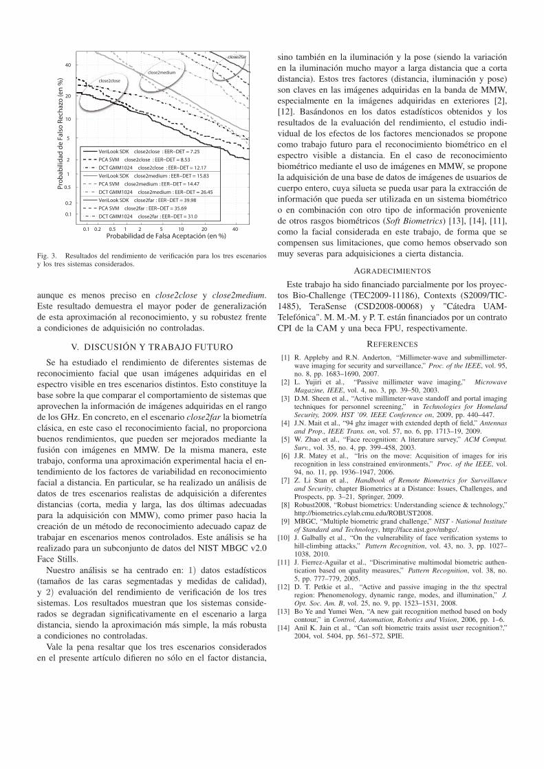
Fig. 3. Resultados del rendimiento de verificación para los tres escenariosy los tres sistemas considerados.
aunque es menos preciso en close2close y close2medium.
Este resultado demuestra el mayor poder de generalización
de esta aproximación al reconocimiento, y su robustez frente
a condiciones de adquisición no controladas.
V. DISCUSIÓN Y TRABAJO FUTURO
Se ha estudiado el rendimiento de diferentes sistemas de
reconocimiento facial que usan imágenes adquiridas en el
espectro visible en tres escenarios distintos. Esto constituye la
base sobre la que comparar el comportamiento de sistemas que
aprovechen la información de imágenes adquiridas en el rango
de los GHz. En concreto, en el escenario close2far la biometría
clásica, en este caso el reconocimiento facial, no proporciona
buenos rendimientos, que pueden ser mejorados mediante la
fusión con imágenes en MMW. De la misma manera, este
trabajo, conforma una aproximación experimental hacia el en-
tendimiento de los factores de variabilidad en reconocimiento
facial a distancia. En particular, se ha realizado un análisis de
datos de tres escenarios realistas de adquisición a diferentes
distancias (corta, media y larga, las dos últimas adecuadas
para la adquisición con MMW), como primer paso hacia la
creación de un método de reconocimiento adecuado capaz de
trabajar en escenarios menos controlados. Este análisis se ha
realizado para un subconjunto de datos del NIST MBGC v2.0
Face Stills.
Nuestro análisis se ha centrado en: 1) datos estadísticos
(tamaños de las caras segmentadas y medidas de calidad),
y 2) evaluación del rendimiento de verificación de los tres
sistemas. Los resultados muestran que los sistemas conside-
rados se degradan significativamente en el escenario a larga
distancia, siendo la aproximación más simple, la más robusta
a condiciones no controladas.
Vale la pena resaltar que los tres escenarios considerados
en el presente artículo difieren no sólo en el factor distancia,
sino también en la iluminación y la pose (siendo la variación
en la iluminación mucho mayor a larga distancia que a corta
distancia). Estos tres factores (distancia, iluminación y pose)
son claves en las imágenes adquiridas en la banda de MMW,
especialmente en la imágenes adquiridas en exteriores [2],
[12]. Basándonos en los datos estadísticos obtenidos y los
resultados de la evaluación del rendimiento, el estudio indi-
vidual de los efectos de los factores mencionados se propone
como trabajo futuro para el reconocimiento biométrico en el
espectro visible a distancia. En el caso de reconocimiento
biométrico mediante el uso de imágenes en MMW, se propone
la adquisición de una base de datos de imágenes de usuarios de
cuerpo entero, cuya silueta se pueda usar para la extracción de
información que pueda ser utilizada en un sistema biométrico
o en combinación con otro tipo de información proveniente
de otros rasgos biométricos (Soft Biometrics) [13], [14], [11],
como la facial considerada en este trabajo, de forma que se
compensen sus limitaciones, que como hemos observado son
muy severas para adquisiciones a cierta distancia.
AGRADECIMIENTOS
Este trabajo ha sido financiado parcialmente por los proyec-
tos Bio-Challenge (TEC2009-11186), Contexts (S2009/TIC-
1485), TeraSense (CSD2008-00068) y "Cátedra UAM-
Telefónica". M. M.-M. y P. T. están financiados por un contrato
CPI de la CAM y una beca FPU, respectivamente.
REFERENCES
[1] R. Appleby and R.N. Anderton, “Millimeter-wave and submillimeter-wave imaging for security and surveillance,” Proc. of the IEEE, vol. 95,no. 8, pp. 1683–1690, 2007.
[2] L. Yujiri et al., “Passive millimeter wave imaging,” MicrowaveMagazine, IEEE, vol. 4, no. 3, pp. 39–50, 2003.
[3] D.M. Sheen et al., “Active millimeter-wave standoff and portal imagingtechniques for personnel screening,” in Technologies for HomelandSecurity, 2009. HST ’09. IEEE Conference on, 2009, pp. 440–447.
[4] J.N. Mait et al., “94 ghz imager with extended depth of field,” Antennasand Prop., IEEE Trans. on, vol. 57, no. 6, pp. 1713–19, 2009.
[5] W. Zhao et al., “Face recognition: A literature survey,” ACM Comput.Surv., vol. 35, no. 4, pp. 399–458, 2003.
[6] J.R. Matey et al., “Iris on the move: Acquisition of images for irisrecognition in less constrained environments,” Proc. of the IEEE, vol.94, no. 11, pp. 1936–1947, 2006.
[7] Z. Li Stan et al., Handbook of Remote Biometrics for Surveillanceand Security, chapter Biometrics at a Distance: Issues, Challenges, andProspects, pp. 3–21, Springer, 2009.
[8] Robust2008, “Robust biometrics: Understanding science & technology,”http://biometrics.cylab.cmu.edu/ROBUST2008.
[9] MBGC, “Multiple biometric grand challenge,” NIST - National Instituteof Standard and Technology, http://face.nist.gov/mbgc/.
[10] J. Galbally et al., “On the vulnerability of face verification systems tohill-climbing attacks,” Pattern Recognition, vol. 43, no. 3, pp. 1027–1038, 2010.
[11] J. Fierrez-Aguilar et al., “Discriminative multimodal biometric authen-tication based on quality measures,” Pattern Recognition, vol. 38, no.5, pp. 777–779, 2005.
[12] D. T. Petkie et al., “Active and passive imaging in the thz spectralregion: Phenomenology, dynamic range, modes, and illumination,” J.Opt. Soc. Am. B, vol. 25, no. 9, pp. 1523–1531, 2008.
[13] Bo Ye and Yumei Wen, “A new gait recognition method based on bodycontour,” in Control, Automation, Robotics and Vision, 2006, pp. 1–6.
[14] Anil K. Jain et al., “Can soft biometric traits assist user recognition?,”2004, vol. 5404, pp. 561–572, SPIE.
BIOGIGA: BASE DE DATOS DE IMÁGENESSINTÉTICAS DE PERSONAS A 94 GHZ CON
FINES BIOMÉTRICOS
M. Moreno-Moreno(1), J. Fierrez(1), P. Tome(1), R. Vera-Rodriguez(1), J. Parron(2), J. Ortega-Garcia(1)
{miriam.moreno, julian.fierrez, pedro.tome, ruben.vera}@uam.es, [email protected], [email protected](1)Dpto. Tecnología Electrónica y de las Comunicaciones. Universidad Autónoma de Madrid (UAM). 28049 Madrid, Spain.(2)Dpto. Telecomunicació i d’Enginyeria de Sistemes. Universitat Autònoma de Barcelona (UAB). 08193 Barcelona, Spain.
Resumen—The baseline corpus of a new database, calledBioGiga, acquired in the framework of the Terasense ConsoliderProject, is presented. The corpus consists of synthetic imagesat 94 GHz of the body of 50 individuals. The images are theresult of simulations carried out on corporal models at twotypes of scenarios (outdoors, indoors) and with two kinds ofimaging systems (passive and active). These corporal modelswere previously generated based on body measurements takenfrom the subjects. In this contribution, the methodology followedand the tools used to generate the database are outlined.Furthermore, the contents of the corpus (data and statistics)as well as its applications are described.
I. INTRODUCCIÓN
Se denomina reconocimiento biométrico al proceso que
permite asociar una identidad con un individuo de forma
automática, haciendo uso de una o varias características
físicas o de comportamiento, inherentes al individuo [1]. Son
muchas las características que se han usado en reconocimiento
biométrico: huella dactilar, firma manuscrita, iris, voz, cara,
mano, etc. Algunos de estos rasgos biométricos tales como la
oreja, la cara, la mano o la forma de andar, son adquiridos
tradicionalmente con cámaras que trabajan en el espectro
visible. Tales imágenes se ven afectadas por factores como
las condiciones de iluminación y las oclusiones (provocadas
por la ropa, el maquillaje, el pelo, etc.)
Con el fin de superar estas limitaciones, impuestas por
el uso de imágenes adquiridas en el espectro visible, in-
vestigadores en biometría y seguridad [2] han propuesto el
uso de imágenes adquiridas en otros rangos espectrales, a
saber: rayos X [3], infrarrojo [4], ondas milimétricas (MMW)
y submilimétricas (SMW) [5]. Además de solventar hasta
cierto punto las limitaciones de las imágenes en el visible, las
imágenes tomadas más allá del espectro visible presentan una
ventaja extra: son más robustas frente ataques contra sistemas
biométricos que otras imágenes.
La banda espectral propuesta en este trabajo para capturar
imágenes de rasgos biométricos es la correspondiente a la de
las ondas milimétricas (de frecuencia entre 30 y 300 GHz) [6].
La importancia de este tipo de radiación se halla en: 1) su
capacidad para atravesar la ropa y otras oclusiones, 2) su
inocuidad, y 3) el reciente desarrollo que están experimentan-
do los sistemas de GHz-THz en aplicaciones de captura de
imágenes (especialmente en el área de seguridad). Al contrario
de lo que ocurre con la tecnología de captura de imágenes
en el visible o infrarrojo, la tecnología de GHz-THz está
en pleno desarrollo [7]. Este hecho, junto con los problemas
de privacidad que presentan las imágenes corporales en esa
banda, han hecho que, hasta la fecha, no existan bases de datos
públicas con imágenes de personas adquiridas en ese rango
de frecuencias. De hecho sólo existe un trabajo publicado
hasta el momento sobre reconocimiento biométrico basado
en imágenes de GHz [8].
Por todo lo anterior en este trabajo se describe la generación
de una base de datos de imágenes simuladas de personas a
94 GHz, así como su contenido. El objetivo de esta base de
datos es su futuro uso en el desarrollo de sistemas biométricos
basados en dichas imágenes.
El artículo se estructura como sigue. La Sec. II introduce
brevemente los diferentes sistemas de captación de imágenes
en el rango de milimétricas existentes en el mercado actual-
mente. Además se describe el único sistema de reconocimien-
to biométrico basado en imágenes capturadas en la banda de
las MMW. La Sec. III resume el proceso llevado a cabo para
generar la base de datos: obtención del modelo corporal de
cada persona a partir de medidas corporales y metodología
usada para la simulación de imágenes a 94GHz a partir de
tal modelo. A continuación, en la Sec. IV, se describe el
contenido y características principales de la base de datos.
Finalmente en la Sec. V se resume el trabajo realizado, las
aplicaciones de esta base de datos y se esboza el trabajo
futuro.
II. TRABAJOS Y SISTEMAS RELACIONADOS
Las MMW y SMW presentan diferentes propiedades que
las hacen muy apropiadas para su uso en sistemas de adquisi-
ción de imágenes. La más importante de todas ellas es la
penetración a través de la ropa y otros materiales dieléctricos
no polares, incluso a distancia. Esta propiedad ha sido, en gran
medida, la responsable del actual desarrollo de la tecnología
de captura de imágenes en la banda de MMW y de SMW. De
hecho, existe una serie de sistemas comerciales de captura de
imágenes en este rango espectral.
A. Sistemas de captura de imágenes en la banda de MMWy SMW
Tanto en el rango espectral de las MMW/SMW como en
los restantes, existen fundamentalmente dos tipos de sistemas
de captura de imágenes: pasivos y activos. En los primeros
las imágenes son generadas a partir de la radiación natural
que ha sido emitida y reflejada por el escenario, obteniendo
como imagen un mapa de temperatura. En cambio, en los
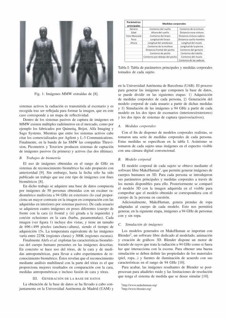
Fig. 1: Imágenes MMW extraídas de [8].
sistemas activos la radiación es transmitida al escenario y es
recogida tras ser reflejada para formar la imagen, que en este
caso corresponde a un mapa de reflectividad.
Dentro de los sistemas pasivos de captura de imágenes en
MMW existen múltiples radiómetros en el mercado, como por
ejemplo los fabricados por Quinetiq, Brijot, Alfa Imaging y
Sago Systems. Mientras que entre los sistemas activos cabe
citar los comercializados por Agilent y L-3 Communications.
Finalmente, en la banda de las SMW las compañías Thruvi-
sion, Picometrix y Teraview producen sistemas de captación
de imágenes pasivos (la primera) y activos (las dos últimas).
B. Trabajos de biometría
El uso de imágenes obtenidas en el rango de GHz en
sistemas de reconocimiento biométrico ha sido propuesto con
anterioridad [9]. Sin embargo, hasta la fecha sólo ha sido
publicado un trabajo que use este tipo de imágenes con fines
biométricos [8].
En dicho trabajo se adquiere una base de datos compuesta
por imágenes de 50 personas obtenidas con un escáner ra-
diométrico multivista a 94 GHz en exteriores (lo cual propor-
ciona un mayor contraste en la imagen en comparación con las
adquiridas en interiores por sistemas pasivos). De cada usuario
se adquieren cuatro imágenes en poses diferentes (cuerpo de
frente con la cara (i) frontal y (ii) girada a la izquierda) y
con/sin oclusiones en la cara (barba, pasamontañas). Cada
imagen (ver figura 1) incluye dos vistas, y tiene un tamaño
de 696×499 píxeles (anchura×altura), siendo el tiempo de
adquisición 15s. La temperatura equivalente de las imágenes
varía entre 225K (regiones claras) y 300K (regiones oscuras).
Finalmente Alefs et al. explotan las características biométri-
cas del cuerpo humano presentes en las imágenes descritas.
En concreto se hace uso del tórax, de la cara y de medi-
das antropométricas, para llevar a cabo experimentos de re-
conocimiento biométrico. Éstos revelan que el reconocimiento
mediante análisis multilineal con la parte del tórax es el que
proporciona mejores resultados en comparación con la cara,
medidas antropométricas e incluso fusión de cara y tórax.
III. GENERACIÓN DE LA BASE DE DATOS
La obtención de la base de datos se ha llevado a cabo con-
juntamente en la Universidad Autónoma de Madrid (UAM) y
Género Contorno del cuello Contorno de la cintura
Edad Altura del cuello Distancia nuca-cintura
Tono Muscular Contorno del brazo Distancia cintura-cadera
Peso Longitud del brazo Distancia cuello-hombro
Altura Longitud del antebrazo Longitud del muslo
Contorno de la muñeca Longitud de la pierna
Distancia frontal del pecho Contorno del gemelo
Contorno de pecho Contorno del tobillo
Contorno por debajo del pecho Contorno del muslo
Contorno de las caderas
Parámetros
principalesMedidas corporales
Tabla I: Tabla de parámetros principales y medidas corporales
tomados de cada sujeto.
en la Universidad Autónoma de Barcelona (UAB). El proceso
para generar las imágenes que componen la base de datos,
se puede dividir en las siguientes etapas: 1) Adquisición
de medidas corporales de cada persona, 2) Generación del
modelo corporal de cada usuario a partir de dichas medidas
y 3) Simulación de las imágenes a 94 GHz a partir de cada
modelo en los dos tipos de escenarios (interiores/exteriores)
y los dos tipos de sistemas de captura (pasivos/activos).
A. Medidas corporales
Con el fin de disponer de modelos corporales realistas, se
tomaron una serie de medidas corporales de cada persona.
Estas medidas se especifican en la tabla I. Asimismo se
tomaron de cada sujeto unas imágenes en el espectro visible
con una cámara digital convencional.
B. Modelo corporal
El modelo corporal de cada sujeto se obtuvo mediante el
software libre MakeHuman1, que permite generar imágenes de
cuerpos humanos en 3D. Para cada persona se introdujeron
sus parámetros principales y medidas corporales a través de
los menús disponibles para ello. Posteriormente se comparó
el modelo 3D con la imagen adquirida en el visible para
comprobar que el modelo obtenido se correspondiera con el
cuerpo de la persona en cuestión.
Adicionalmente, MakeHuman, genera prendas de ropa
adaptadas al cuerpo de cada modelo. Esto nos permitirá
generar, en la siguiente etapa, imágenes a 94 GHz de personas
con y sin ropa.
C. Simulación de imágenes
Los modelos generados en MakeHuman se importan con
Blender2, un software libre dedicado al modelado, animación
y creación de gráficos 3D. Blender dispone un motor de
trazado de rayos que trata la radiación a 94 GHz como si fuera
luz que interacciona con la escena. Para obtener una buena
simulación se deben definir las propiedades de los materiales
(piel, ropa...) y fuentes de iluminación de acuerdo con sus
características en el rango de 94 GHz [10].
Para acabar, las imágenes resultantes de Blender se post-
procesan para añadirles ruido y las limitaciones de resolución
que tenga el sistema de medida que se desee simular [10].
1http://www.makehuman.org/2http://www.blender.org/

Imagen VIS Modelos MakeHuman
Sistema Pasivo en
Exteriores
Sistema Pasivo en
Interiores
Sistema Ac�vo en
Exteriores
Sistema Ac�vo en
Interiores
Co
n r
op
a
Sin ropa Con ropa
Imágenes a 94 GHz Blender
Sin
ro
pa
Fig. 2: Imágenes correspondientes a un usuario: imagen en el visible (arriba izquierda), modelos generados con MakeHuman
(arriba derecha) e imágenes a 0o de orientación de la cámara en los cuatro sistemas considerados (abajo).
IV. DESCRIPCIÓN DE LA BASE DE DATOS
La base de datos está formada por imágenes simuladas,
a 94 GHz, de 50 personas (25 hombres y 25 mujeres), con
edades comprendidas entre los 15 y 55 años. Para cada sujeto
se disponen de cuatro grupos de imágenes:
Imágenes simuladas con un sistema pasivo en exteriores.
Imágenes simuladas con un sistema pasivo en interiores.
Imágenes simuladas con un sistema activo en exteriores.
Imágenes simuladas con un sistema activo en interiores.
Dentro cada grupo anterior, se generaron, para cada usuario,
las siguientes variantes de imágenes:
Imágenes del modelo con ropa y ángulo formado por la
cámara de -10o, 0o y +10o.
Imágenes del modelo sin ropa y ángulo formado por la
cámara de -10o, 0o y +10o.
Según lo anterior, para cada usuario, la base de datos cuenta
con 4×2×3=24 imágenes a 94 GHz. Por tanto, la base de
datos está compuesta por 50×24=1200 imágenes.
La figura 2 muestra algunas de las imágenes correspondi-
entes a un sujeto:
Imagen en el visible.
Modelos generados con MakeHuman sin ropa y con ropa.
Imágenes simuladas a 94 GHz con Blender para cada tipo
de sistema (pasivo/activo) y escenario(exteriores/interiores),
todas con un ángulo de orientación de la cámara de 0o.
Se pueden resaltar algunas características de las imágenes
a 94 GHz con respecto a (i) la influencia de la ropa y
(ii) el contraste y nivel relativo de cada tipo de imagen.
La vestimenta apenas se aprecia en las imágenes, de hecho,
las imágenes simuladas a 94 GHz a partir del modelo con
ropa y sin ropa son prácticamente iguales. Únicamente se
observa ligeramente el efecto de la ropa en algunas regiones,
correspondientes a lugares donde el tejido es más grueso o
existen pliegues o varias capas de ropa. Esto ocurre en el
cuello de la camiseta y la cintura, siendo más notorio en las
imágenes de sistemas pasivos en exteriores.

Entre las imágenes simuladas con sistemas pasivos, las
simuladas en exteriores presentan un mayor contraste que
las simuladas en interiores, debido a la mayor diferencia de
temperatura entre el cielo (100K) y el suelo (300K). Para
exteriores, por tanto, las partes orientadas hacia el suelo
presentan color oscuro (caliente) y las orientadas hacia el
cielo color claro (frío). En cambio, en interiores el cuerpo
presenta un color mucho más uniforme pues la temperatura
del entorno no tiene grandes variaciones. Por otro lado, las
imágenes simuladas con sistemas activos muestran un nivel
de temperatura radiométrica mayor (son más oscuras) puesto
que se radia a la persona con una fuente externa no natural,
recogiendo esa radiación una vez ha sido reflejada por la
persona. Por la misma razón no existen apenas diferencias
entre las imágenes simuladas en exteriores e interiores.
Por último, en la figura 3 se recogen dos histogramas, uno
correspondiente a la distribución de edades de los sujetos
que forman la base de datos y el otro correspondiente a la
distribución de alturas de los mismos.
V. CONCLUSIONES
Uno de los principales problemas que se pueden encontrar a
la hora de desarrollar y evaluar un sistema de reconocimiento
biométrico es la carencia de bases de datos con un número
alto de usuarios y de muestras por usuario. Esto ocurre
especialmente con las imágenes de personas en el rango de
las MMW y SMW.
En este trabajo se ha presentado una visión general de
los diferentes sistemas de captura de imágenes en la banda
espectral de las MMW y SMW, así como de los trabajos
de reconocimiento biométrico que hacen uso de este tipo
de imágenes. Asimismo se ha presentado la base de datos
sintética BioGiga, formada por imágenes simuladas a 94
GHz de 50 usuarios en dos escenarios con dos sistemas de
captura de imagen. Se ha descrito el proceso de generación
de BioGiga así como sus principales características.
La principal aplicación de esta base de datos es la de su uso
para el desarrollo de sistemas de reconocimiento biométrico
basados en este tipo de imágenes. En concreto, a partir
de estas imágenes se pueden extraer diferentes característi-
cas representativas de cada individuo con las que realizar
experimentos de reconocimiento. Asimismo, al disponer de
diferentes tipos de imágenes para cada usuario, se puede
realizar fusión a diferentes niveles para mejorar el rendimiento
del sistema. Adicionalmente, el uso de este tipo de imágenes
sintéticas permite la evaluación de vulnerabilidades de sis-
temas biométricos, basados en esas imágenes, frente a ataques
externos.
Como trabajo futuro se prevé el uso a corto plazo de BioGi-
ga para desarrollar un sistema de reconocimiento biométrico
basado en tales imágenes. Cuanto mayor sea la población
que forma la base de datos, más representativos serán los
resultados obtenidos, por lo que la ampliación del número
de usuarios sería muy deseable. Del mismo modo, disponer
de otros rasgos biométricos de los mismos usuarios resul-
taría muy interesante para ser usados, conjuntamente con las
imágenes a 94 GHz, en el mismo sistema y aumentar así su
tasa de reconocimiento. Por esto resultaría muy interesante
adquirir, de los mismos usuarios, otros rasgos como la cara,
huella dactilar, etc.
15 20 25 30 35 40 45 50 550
2
4
6
8
10
Edad (años)
Nú
mero
de s
uje
tos
15 20 25 30 35 40 45 50 550
10
20
30
40
50
Su
jeto
s a
cu
mu
lad
os
155 160 165 170 175 180 1850
2
4
6
Altura (cm)
Nú
mero
de s
uje
tos
155 160 165 170 175 180 1850
20
40
60
Su
jeto
s a
cu
mu
lad
os
Fig. 3: Histograma de edades y de alturas de los 50 sujetos
que forman la base de datos BioGiga.
AGRADECIMIENTOS
Este trabajo ha sido financiado parcialmente por los proyec-
tos Bio-Challenge (TEC2009-11186), Contexts (S2009/TIC-
1485), TeraSense (CSD2008-00068) y ”Cátedra UAM-
Telefónica". M. M.-M., P.T. y R.V. son financiados por un
contrato CPI de la CAM, una beca FPU y un contrato Juan
de la Cierva, respectivamente.
REFERENCIAS
[1] A.K. Jain et al., “Biometrics: a tool for information security,” Infor-mation Forensics and Security, IEEE Transactions on, vol. 1, no. 2, pp.125–143, june 2006.
[2] Stan Z. Li et al., Airline Passenger Security Screening: New Tech-nologies and Implementation Issues, chapter Biometrics at a Distance:Issues, Challenges, and Prospects, pp. 3–21, National Academy Press,1996.
[3] Hong Chen and Anil K. Jain, “Dental biometrics: Alignment andmatching of dental radiographs,” IEEE Transactions on Pattern Analysisand Machine Intelligence, vol. 27, pp. 1319–1326, 2005.
[4] S.Z. Li et al., “Illumination invariant face recognition using near-infrared images,” Pattern Analysis and Machine Intelligence, IEEETransactions on, vol. 29, no. 4, pp. 627–639, 2007.
[5] R. Appleby and R.N. Anderton, “Millimeter-wave and submillimeter-wave imaging for security and surveillance,” Proceedings of the IEEE,vol. 95, no. 8, pp. 1683–1690, aug. 2007.
[6] L. Yujiri et al., “Passive millimeter wave imaging,” MicrowaveMagazine, IEEE, vol. 4, no. 3, pp. 39–50, sept. 2003.
[7] J.N. Mait et al., “94-ghz imager with extended depth of field,” Antennasand Propagation, IEEE Transactions on, vol. 57, no. 6, pp. 1713–1719,june 2009.
[8] B.G. Alefs et al., “Thorax biometrics from millimetre-wave images,”Pattern Recognition Letters, vol. 31, no. 15, pp. 2357–2363, 2010.
[9] Miriam Moreno-Moreno et al., “Biometrics beyond the visible spec-trum: Imaging technologies and applications,” in Proceedings of BioID-Multicomm 2009. September 2009, vol. 5707 of LNCS, pp. 154–161,Springer.
[10] J. Parron et al., “Millimeter-wave scene simulation using blender,” inProceedings of XXV Simposium Nacional de Unión Científica Interna-cional de Radio, September 2010.

Distance-based Feature Extraction for Biometric Recognitionof Millimeter Wave Body Images
Miriam Moreno-Moreno, Julian Fierrezand Ruben Vera-Rodriguez
ATVS - Biometric Recognition GroupUniversidad Autonoma de Madrid, EPS
C/ Francisco Tomas y Valiente, 11. 28049 Madrid. Spain{miriam.moreno, julian.fierrez, ruben.vera}@uam.es
Josep Parron
AMS - Antenna and Microwave Systems GroupUniversitat Autonoma de Barcelona
Campus de la UAB, 08193 Bellaterra, Barcelona, [email protected]
Abstract—In this work a complete process of feature ex-traction for biometric recognition of Millimeter Wave bodyimages is described. The scope of this work is to find asmall set of distance-based features that can be used inbody geometry authentication obtaining good error rates. Thisapproach constitutes a feature-based alternative to the holisticrecognition methods already proposed on the mentioned kindof images. The system is tested on a database comprising 1200synthetic images at 94 GHz of the body of 50 individuals. Theresults prove that the use of a small number distance-basedfeatures provide good class separation.
Keywords-millimeter wave images; 94 GHz; syntheticdatabase; image processing; body geometry; distance-basedfeatures; feature extraction; feature selection.
I. INTRODUCTION
Many of the biometric characteristics used to identify indi-
viduals, such as ear, face, hand, and gait, are extracted from
images acquired by cameras working at visible frequencies
of the electromagnetic spectrum. Such images are affected
by, among others factors, lighting conditions and the body
occlusion (e.g. clothing, make up, hair, etc.) In order to cir-
cumvent these limitations, researchers have proposed the use
of images acquired at others spectral ranges: X-ray, infrared,
millimeter (MMW) and submillimeter (SMW) waves [1].
The images captured beyond the visible spectrum overcome,
to some extent, some of the mentioned limitations; further-
more, they are more robust to spoofing than other biometric
images/traits. Among the spectral bands out of the visible
spectrum, the millimeter waves (with frequency in the band
of 30-300 GHz) present interesting properties that can be
exploited in biometrics [2]: ability to pass through cloth
and other occlusions, its health safety, its low intrusiveness,
and the recent deployment and rapid progress of GHz-THz
systems in screening applications. In spite of the previous
advantages, to date, there is only one published research
work that performs biometric recognition using that kind
of images, using a holistic recognition approach [3]. This
shortage of biometric recognition research based on MMW
images is due, in part, to the lack of databases of images of
people acquired at GHz. This lack is a consequence of: (i)
the privacy concern these images present, and (ii) most of
the imaging systems working at the MMW/SMW band are
either in prototype form or not easily accesible for research.
In this contribution we proposed and study new meth-
ods for processing and feature extraction for MMW body
images. First, a database composed by synthetic images of
the body of 50 individuals is generated. After processing
the images, different distance-based features are extracted
from some landmarks related to the silhouette of the body.
Finally, some experimental validations are performed to
determine the most discriminative features, and its discrim-
ination power.
The paper is structured as follows. The baseline corpus
and the main characteristics of the used database are briefly
presented in Sect. II. Sect. III describes all the steps followed
to obtain the feature vector: image segmentation, boundary
extraction, landmark generation and feature vector construc-
tion. The evaluation of the selected features is performed in
Sect. IV, where a cualitative and a quantitative analysis is
carried out. Conclusions are finally drawn in Sect. V together
with future work.
Main Parameters Corporal MeasuresGender Neck circ. Waist circ.
Age Height Nape to waistTone Upper arm circ. Waist to hip
Weight Upper arm length Shoulder to NeckHeight Lowerarm length Upperleg height
Wrist circ. Lowerleg heightFront chest dist. Calf circ.
Burst circ. Angle circ.Underburst circ. Thigh circ.
Hips circ.
Table IMAIN PARAMETERS AND BODY MEASURES FOR EACH SUBJECT.
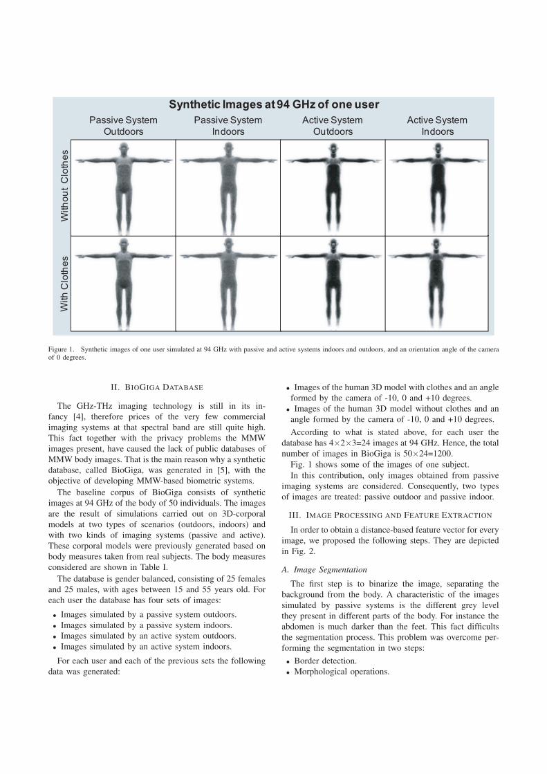
Passive System
Outdoors
Passive System
Indoors
Active System
Outdoors
Active System
Indoors
With
ou
tC
loth
es
With
Clo
the
s
Synthetic Images at 94 GHz of one user
Figure 1. Synthetic images of one user simulated at 94 GHz with passive and active systems indoors and outdoors, and an orientation angle of the cameraof 0 degrees.
II. BIOGIGA DATABASE
The GHz-THz imaging technology is still in its in-
fancy [4], therefore prices of the very few commercial
imaging systems at that spectral band are still quite high.
This fact together with the privacy problems the MMW
images present, have caused the lack of public databases of
MMW body images. That is the main reason why a synthetic
database, called BioGiga, was generated in [5], with the
objective of developing MMW-based biometric systems.
The baseline corpus of BioGiga consists of synthetic
images at 94 GHz of the body of 50 individuals. The images
are the result of simulations carried out on 3D-corporal
models at two types of scenarios (outdoors, indoors) and
with two kinds of imaging systems (passive and active).
These corporal models were previously generated based on
body measures taken from real subjects. The body measures
considered are shown in Table I.
The database is gender balanced, consisting of 25 females
and 25 males, with ages between 15 and 55 years old. For
each user the database has four sets of images:
• Images simulated by a passive system outdoors.
• Images simulated by a passive system indoors.
• Images simulated by an active system outdoors.
• Images simulated by an active system indoors.
For each user and each of the previous sets the following
data was generated:
• Images of the human 3D model with clothes and an angle
formed by the camera of -10, 0 and +10 degrees.
• Images of the human 3D model without clothes and an
angle formed by the camera of -10, 0 and +10 degrees.
According to what is stated above, for each user the
database has 4×2×3=24 images at 94 GHz. Hence, the total
number of images in BioGiga is 50×24=1200.
Fig. 1 shows some of the images of one subject.
In this contribution, only images obtained from passive
imaging systems are considered. Consequently, two types
of images are treated: passive outdoor and passive indoor.
III. IMAGE PROCESSING AND FEATURE EXTRACTION
In order to obtain a distance-based feature vector for every
image, we proposed the following steps. They are depicted
in Fig. 2.
A. Image Segmentation
The first step is to binarize the image, separating the
background from the body. A characteristic of the images
simulated by passive systems is the different grey level
they present in different parts of the body. For instance the
abdomen is much darker than the feet. This fact difficults
the segmentation process. This problem was overcome per-
forming the segmentation in two steps:
• Border detection.
• Morphological operations.

Segmenta�on
Contour, ref. points and skeleton
Radial Distance Maxima and Minima Detec�on
Landmarks
Feature Extrac�on
21D Feature Vector
0 500 1000 1500 2000 2500 30000
100
200
300
400
500
600
700
ImageInput (a)
(b)
(c)
(d)
(h)
(g)
(f)
(e)
Figure 2. Main steps followed in our system to extract features. Original image (of a subject with clothing and a camera angle of -10 degrees) (a),segmented image (b), contour, reference points and skeleton (c), radial distance from each reference point to the contour (one curve per reference point)(d), addition of points with maximum and minimum distance from the reference points (e), all landmarks (f), distances used to form the feature vector (g)and the 21D feature vector (h).
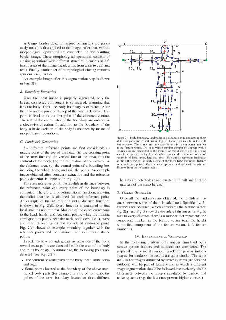
A Canny border detector (whose parameters are previ-
ously tuned) is first applied to the image. After that, various
morphological operations are conducted on the resulting
border image. These morphological operations consists of
closing operations with different structural elements in dif-
ferent areas of the image (head, arms, from arms to calf, and
feet). Finally another set of morphological closing removes
spurious irregularities.
An example image after this segmentation step is shown
in Fig. 2(b)
B. Boundary Extraction
Once the input image is properly segmented, only the
largest connected component is considered, assuming that
it is the body. Then, the body boundary is extracted. After
that, the middle point of the top of the head is detected. This
point is fixed to be the first point of the extracted contour.
The rest of the coordinates of the boundary are ordered in
a clockwise direction. In addition to the boundary of the
body, a basic skeleton of the body is obtained by means of
morphological operations.
C. Landmark Generation
Six different reference points are first considered: (i)
middle point of the top of the head, (ii) the crossing point
of the arms line and the vertical line of the torso, (iii) the
centroid of the body, (iv) the bifurcation of the skeleton in
the abdomen area, (v) the central point of a bounding box
including the whole body, and (vi) the pubis. An example
image obtained after boundary extraction and the reference
points detection is depicted in Fig. 2(c).
For each reference point, the Euclidean distance between
the reference point and every point of the boundary is
computed. Therefore, a one-dimensional function, showing
the radial distance, is obtained for each reference point.
An example of the six resulting radial distance functions
is shown in Fig. 2(d). Every function is examined to find
local maxima and minima. Maxima of the curve correspond
to the head, hands, and feet outer points, while the minima
correspond to points near the neck, shoulders, axilla, wrist
and hips, depending on the considered reference point.
Fig. 2(e) shows an example boundary together with the
reference points and the maximum and minimum distance
points.
In order to have enough geometric measures of the body,
several extra points are detected inside the area of the body
and in its boundary. To summarize, the following points are
detected (see Fig. 2(f)):
• The centroid of some parts of the body: head, arms, torso
and legs.
• Some points located at the boundary of the above men-
tioned body parts (for example in case of the torso, the
points of the torso boundary located at three different
1
2
3
4
5
6
7
8
9
10m 11m 12m
13m 14m
15
16
17
18
19m
20m
21m
Figure 3. Body boundary, landmarks and distances extracted among themof the subjects and conditions of Fig. 2. These distances form the 21Dfeature vector. The number next to every distance is the component numberin the feature vector. The ones whose number component appears with asubindex m are calculated as the average of that distance and the analogone of the right extremity. Red triangles represent the reference points andcentroids of head, arms, legs and torso. Blue circles represent landmarkson the silhouette of the body (some of the them have minimum distanceto the reference points). Green circles represent landmarks with maximumdistance from the reference points.
heights are detected: at one quarter, at a half and at three
quarters of the torso height.)
D. Feature Generation
Once all the landmarks are obtained, the Euclidean dis-
tance between some of them is calculated. Specifically, 21
distances are obtained, which constitutes the feature vector.
Fig. 2(g) and Fig. 3 show the considered distances. In Fig. 3,
next to every distance there is a number that represents the
component number in the feature vector (e.g. the height
is the first component of the feature vector, it is feature
number 1).
IV. EXPERIMENTAL VALIDATION
In the following analysis only images simulated by a
passive system indoors and outdoors are considered. The
graphical results are shown exclusively for passive indoors
images, for outdoors the results are quite similar. The same
analysis for images simulated by active systems (indoors and
outdoors) will be part of future work, in which a different
image segmentation should be followed due to clearly visible
differences between the images simulated by passive and
active systems (e.g. the last ones present higher contrast).

2 4 6 8 10 12 14 16 18 20 210
0.1
0.2
0.3
0.4
0.5
0.6
0.7
0.8
0.9
1
Features
Mea
n N
orm
aliz
ed V
alue
0
0.1
0.2
0.3
0.4
0.5
0.6
0.7
0.8
0.9
1
Ranked Features
Mea
n N
orm
aliz
ed V
alue
1 3 5 7 9 11 13 15 17 19 17 6 16 2 4 20 12 21 10 3 71 5 9 14 11 13 15 19 18 8
(a) (b)
Figure 4. Mean normalized value of the feature vector of 7 randomly selected users. Each user vector has a different color and symbol.
A. Evaluation of Features
Fig. 4(a) represents the mean value and the standard
deviation (as an error bar) of each normalized component
(distance) of the feature vector, for seven subjects (a differ-
ent color and symbol for each subject) randomly selected
from the 50 available. As it can be seen, some component
values are quite different from one subject to another, while
others are more similar. On the other hand, the error bars
overlap in some cases. To determine the most discriminative
features, the components of the feature vector are ranked
in descending order of degree of discrimination. For this
purpose two magnitudes are calculated:
• The average separation between the mean values of
each component from all subjects.
• The overlap between the error bars of the same com-
ponent among all subjects.
The most discriminative feature will be the one with
the largest average separation and the lowest overlap
among different users. Hence, the features are ranked
in descending order of the value of the quotient
average separation/overlap. Fig. 4(b) shows the feature
vector for the same seven subjects of Fig. 4(a) once its com-
ponents have been ordered. Although the Fig. 4(b) shows the
feature vector for 7 users, the ranking was conducted taking
into account the vectors from all the 50 subjects. It can be
seen the decreasing separation between mean values and the
increasing overlap. The initial feature number (the same one
as the one in Fig. 3) is written below the x axis with bold
numbers. It is worth noting that the three most discriminative
components (the three first ones in Fig. 4(b)) are: (i) the
1st (height), (ii) the 17th (waist width aprox.) and (iii) the
5th (the distance between the centroid of the body and the
pubis). The least discriminative one corresponds to feature
7th (height of the head). Furthermore, these four features
(three best ones and the worst one) obtained for images
simulated by passive systems outdoors are the same ones
when using images simulated indoors. It is not surprising
that the height of the head is the least discriminating feature
due to the process followed to obtain the 3D-body model
from the body measures of real subjects. The head height
was not considered, so all the models present approximately
the same head height in their 3D body model used to
simulate MMW images.
B. Discrimination Power Analysis
With the purpose of better assessing the discrimination
power of the features, they are plotted in 2D graphs in Fig. 5:
• Fig. 5(a) plots the second PCA component vs the first
PCA component of the 300 feature vectors (6 per user),
having used all the 21D vectors to obtain the PCA
transformation matrix.
• Fig. 5(b) plots the second most discriminative feaure
(waist width aprox.) vs the most discriminative one (the
height).
In both plots every user has its own color and symbol, so
every user should be represented by a cluster of symbols
with the same color and shape. In both cases, Fig. 5(a)
and Fig. 5(b), it is patent that the clusters are clearly
separated. Only in some regions of the 2D subspace some
clusters overlap. This fact proves that the selected features
are discriminative. Comparing both plots, it seems that the
clusters in Fig. 5(b) are smaller and more separated among
them than in Fig. 5(a). This reveals that even with only two
features (height and waist width) it would be possible to
distinguish different users. It must be noted that this analysis
validates the proposed features but does not estimate their
practical recognition capabilities. For doing so classification
experiments should be performed, which will be conducted
in future work.
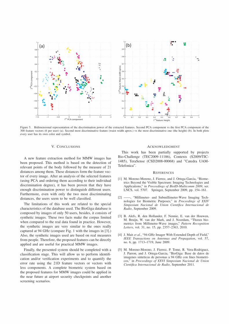
−1.5 −1 −0.5 0 0.5 1 1.5 2−1
−0.8
−0.6
−0.4
−0.2
0
0.2
0.4
0.6
0.8
1
1 PCA component
2
PCA
com
pone
nt
0 0.1 0.2 0.3 0.4 0.5 0.6 0.7 0.8 0.9 10
0.1
0.2
0.3
0.4
0.5
0.6
0.7
0.8
0.9
1
1st feature: Height17
th fe
atur
e: W
aist
wid
th a
prox
.s t
nd
(a) (b)
Figure 5. Bidimensional representation of the discrimination power of the extracted features. Second PCA component vs the first PCA component of the300 feature vectors (6 per user) (a). Second most discriminative feature (waist width aprox.) vs the most discriminative one (the height) (b). In both plotsevery user has its own color and symbol.
V. CONCLUSIONS
A new feature extraction method for MMW images has
been proposed. This method is based on the detection of
relevant points of the body followed by the measure of 21
distances among them. These distances form the feature vec-
tor of every image. After an analysis of the selected features
(using PCA and ordering them according to their individual
discrimination degree), it has been proven that they have
enough discrimination power to distinguish different users.
Furthermore, even with only the two most discriminating
distances, the users seem to be well classified.
The limitations of this work are related to the special
characteristics of the database used. The BioGiga database is
composed by images of only 50 users, besides, it consists of
synthetic images. These two facts make the corpus limited
when compared to the real data found in practice. However,
the synthetic images are very similar to the ones really
captured at 94 GHz (compare Fig. 1 with the images in [3].)
Also, the synthetic images used are based on real measures
from people. Therefore, the proposed features can be directly
applied and are useful for practical MMW images.
Finally, the presented system should be completed with a
classification stage. This will allow us to perform identifi-
cation and/or verification experiments and to quantify the
error rate using the 21D feature vectors or vectors with
less components. A complete biometric system based on
the proposed features for MMW images could be applied in
the near future at airport security checkpoints and another
screening scenarios.
ACKNOWLEDGMENT
This work has been partially supported by projects
Bio-Challenge (TEC2009-11186), Contexts (S2009/TIC-
1485), TeraSense (CSD2008-00068) and ”Catedra UAM-
Telefonica”.
REFERENCES
[1] M. Moreno-Moreno, J. Fierrez, and J. Ortega-Garcia, “Biome-trics Beyond the Visible Spectrum: Imaging Technologies andApplications,” in Proceedings of BioID-Multicomm 2009, ser.LNCS, vol. 5707. Springer, September 2009, pp. 154–161.
[2] ——, “Millimeter- and Submillimeter-Wave Imaging Tech-nologies for Biometric Purposes,” in Proceedings of XXIVSimposium Nacional de Union Cientifica Internacional deRadio, September 2009.
[3] B. Alefs, R. den Hollander, F. Nennie, E. van der Houwen,M. Bruijn, W. van der Mark, and J. Noordam, “Thorax bio-metrics from Millimetre-Wave images,” Pattern RecognitionLetters, vol. 31, no. 15, pp. 2357–2363, 2010.
[4] J. Mait et al., “94-GHz Imager With Extended Depth of Field,”IEEE Transactions on Antennas and Propagation, vol. 57,no. 6, pp. 1713–1719, June 2009.
[5] M. Moreno-Moreno, J. Fierrez, P. Tome, R. Vera-Rodriguez,J. Parron, and J. Ortega-Garcia, “BioGiga: Base de datos deimagenes sinteticas de personas a 94 GHz con fines biometri-cos,” in Proceedings of XXVI Simposium Nacional de UnionCientifica Internacional de Radio, September 2011.
Simulation of Millimeter Wave Body Imagesand its Application to Biometric Recognition
Miriam Moreno-Morenoa, Julian Fierreza, Ruben Vera-Rodrigueza and Josep Parronb
aBiometrics Research Lab.-ATVS, EPS, Universidad Autonoma de Madrid, Campus deCantoblanco, C/ Francisco Tomas y Valiente 11, 28049 Madrid, Spain
bAntenna and Microwave Systems Group-AMS, Universitat Autonoma de Barcelona, CampusUAB, Bellaterra, 08193 Barcelona, Spain
ABSTRACT
One of the emerging applications of the millimeter-wave imaging technology is its use in biometric recognition.This is mainly due to some properties of the millimeter-waves such as their ability to penetrate through clothingand other occlusions, their low obtrusiveness when collecting the image and the fact that they are harmless tohealth. In this work we first describe the generation of a database comprising 1200 synthetic images at 94 GHzobtained from the body of 50 people. Then we extract a small set of distance-based features from each imageand select the best feature subsets for person recognition using the SFFS feature selection algorithm. Finallythese features are used in body geometry authentication obtaining promising results.
Keywords: Millimeter wave images, 94 GHz, image simulation, synthetic database, biometrics, image process-ing, body geometry, distance-based features, feature extraction, feature selection, SFFS algorithm, verification.
1. INTRODUCTION
Biometric Recognition is the process that allow to associate an identity with an individual automatically, usingone or more physical or behavioral characteristics that are inherent in the individual.1,2 Many of these biometriccharacteristics used to identify individuals, such as ear, face, hand, and gait, are extracted from images acquiredby cameras working at visible frequencies of the electromagnetic spectrum. Such images are affected by, amongothers factors, lighting conditions and the body occlusion (e.g. clothing, make up, hair, etc.). In order tocircumvent these limitations, researchers have proposed the use of images acquired at others spectral ranges:X-ray, infrared, millimeter (MMW) and submillimeter (SMW) waves.3 The images captured beyond the visiblespectrum overcome, to some extent, some of the mentioned limitations; furthermore, they are more robustto spoofing than other biometric images/traits. Among the spectral bands out of the visible spectrum, themillimeter waves (with frequency in the band of 30-300 GHz) present interesting properties that can be exploitedin biometrics:4 ability to pass through cloth and other occlusions, its health safety, its low intrusiveness, and therecent deployment and rapid progress of GHz-THz systems in screening applications. In spite of the previousadvantages, to date, there is only one published research work that performs biometric recognition using thatkind of images, using a holistic recognition approach.5 This shortage of biometric recognition research basedon MMW images is due, in part, to the lack of databases of images of people acquired at GHz. This lack is aconsequence of: (i) the privacy concern these images present, and (ii) most of the imaging systems working atthe MMW/SMW band are either in prototype form or not easily accessible for research.
For all above, in this contribution it is first described the generation and content of BIOGIGA, a new databasecomposed of simulated images of people at 94 GHz. Then, we present a new biometric system based on that
Further author information: (Send correspondence to M.M.M.)M.M.M.: E-mail: [email protected].: E-mail: [email protected].: E-mail: [email protected].: E-mail: [email protected]

Main Parameters Corporal Measures
Gender Neck circ. Waist circ.Age Height Nape to waistTone Upper arm circ. Waist to hipWeight Upper arm length Shoulder to NeckHeight Lowerarm length Upperleg height
Wrist circ. Lowerleg heightFront chest dist. Calf circ.
Burst circ. Angle circ.Underburst circ. Thigh circ.
Hips circ.Table 1. Main parameters and body measures for each subject.
kind of images totally different and complementary to the only one published so far. Our system is based on thegeometry while the other one was based on a holistic approach over the grayscale after various dimensionalityreduction techniques.5 Finally, some verification experiments are performed to determine the performance andbehavior of the developed system. An analysis of the features extracted and selected from the images is alsocarried out.
The paper is structured as follows. The generation, baseline corpus and the main characteristics of the useddatabase are presented in Sect. 2. Sect. 3 presents the developed biometric system, describing all its modules:from the preprocessing of the input images to the identity decision. The evaluation of the biometric system isperformed in Sect. 4, where the results of some verification and feature selection experiments are shown andanalyzed. Conclusions are finally drawn in Sect. 5 together with future work.
2. BIOGIGA DATABASE
The corpus of the BIOGIGA database consists of synthetic images at 94 GHz of the body of 50 individuals. Theimages are the result of simulations carried out on corporal models at two types of scenarios (outdoors, indoors)and with two kinds of imaging systems (passive and active). These corporal models were previously generatedbased on body measurements taken from the subjects.
2.1 Generation of the Database
The generation of the database was carried out jointly at the Universidad Autnoma de Madrid (UAM) andUniversidad Autnoma de Barcelona (UAB).6 The process to generate the images that compose the database canbe divided into the following stages: 1) Acquisition of body measures of each person, 2) Generation of the 3Dbody model of each user based on such measures, and 3) Simulation of the images at 94 GHz from each modelin the two types of scenarios (indoor/outdoor) and two types of capture systems (passive/active).
2.1.1 Corporal Measures
In order to have realistic 3D body models, a set of body measures of each person was taken. These measures arespecified in Table 1. Some pictures of each subject were also taken in the visible spectrum with a conventionaldigital camera).
2.1.2 Corporal Model
The body model of each subject was obtained using the free software MakeHuman∗, which allows you to generateimages of human bodies in 3D. For each person his or her main parameters and body measurements (see Table 1)were introduced through the menus available for it. Subsequently the 3D model was compared with the picturepreviously taken to verify that the obtained model corresponds to the body the concerned person.
Additionally, MakeHuman generates garments adapted to the body of each model. This allows us to generate,in the following stage, images of people with and without clothes at 94 GHz.
∗http://www.makehuman.org/

Passive System
Outdoors
Passive System
Indoors
Active System
Outdoors
Active System
Indoors
Without
Clo
the
sSynthetic Images at 94 GHz of one user
With
Clo
the
s
Figure 1. Synthetic images of one user simulated at 94 GHz with passive and active systems indoors and outdoors, andan orientation angle of the camera of 0 degrees.
2.1.3 Simulation of Images at 94 GHz
The models generated in MakeHuman are imported to Blender†, which is a free software devoted to modeling,animation and 3D graphics creation. Blender provides a ray tracing engine that treats the radiation at 94 GHzas if it were light interacting with the scene. For a good simulation the properties of materials (skin, clothes ...)and light sources should be defined according to their characteristics in the range of 94 GHz.7
Lastly, the resulting images were postprocessed adding them the typical noise and resolution that the realsystem to be simulated has.7
2.2 Database Description
The database consists of images simulated at 94 GHz, of 50 people (25 females and 25 males), with ages between15 and 55 years old. For each user the database has four sets of images, each of them simulated by:
• A passive system outdoors (PO).
• A passive system indoors (PI).
• An active system outdoors (AO).
• An active system indoors (AI).
For each user and each of the previous sets the following data was generated:
• Images of the human 3D model with clothes and an angle formed by the camera of -10, 0 and +10 degrees.
• Images of the human 3D model without clothes and an angle formed by the camera of -10, 0 and +10 degrees.
According to what is stated above, for each user the database has 4×2×3=24 images at 94 GHz. Hence, thetotal number of images in BIOGIGA is 50×24=1200. Fig. 1 shows some of the images of one subject. In thiscontribution, only images obtained from passive imaging systems outdoors are considered.
†http://www.blender.org/
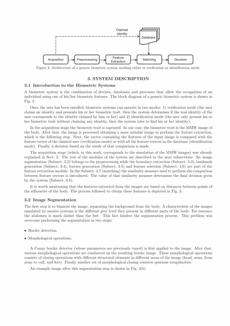
Acquisition PreprocessingFeature
ExtractionMatching Decision
Database
Claimed
identity
Figure 2. Architecture of a generic biometric system working either in verification or identification mode.
3. SYSTEM DESCRIPTION
3.1 Introduction to the Biometric Systems
A biometric system is the combination of devices, databases and processes that allow the recognition of anindividual using one of his/her biometric features. The block diagram of a generic biometric system is shown inFig. 2
Once the user has been enrolled, biometric systems can operate in two modes: 1) verification mode (the userclaims an identity and presents his or her biometric trait, then the system determines if the real identity of theuser corresponds to the identity claimed by him or her) and 2) identification mode (the user only present his orher biometric trait without claiming any identity, then the system tries to find his or her identity).
In the acquisition stage the biometric trait is captured. In our case, the biometric trait is the MMW image ofthe body. After that, the image is processed obtaining a more suitable image to perform the feature extraction,which is the following step. Next, the vector containing the features of the input image is compared with thefeature vector of the claimed user (verification mode) or with all the feature vectors in the database (identificationmode). Finally, a decision based on the result of that comparison is made.
The acquisition stage (which, in this work, corresponds to the simulation of the MMW images) was alreadyexplained in Sect. 2. The rest of the modules of the system are described in the next subsections: the imagesegmentation (Subsect. 3.2) belongs to the preprocessing while the boundary extraction (Subsect. 3.3), landmarkgeneration (Subsect. 3.4), feature generation (Subsect. 3.5) and feature selection (Subsect. 3.6) are part of thefeature extraction module. In the Subsect. 3.7 (matching) the similarity measure used to perform the comparisonbetween feature vectors is introduced. The value of that similarity measure determines the final decision givenby the system (Subsect. 3.8).
It is worth mentioning that the features extracted from the images are based on distances between points ofthe silhouette of the body. The process followed to obtain these features is depicted in Fig. 3.
3.2 Image Segmentation
The first step is to binarize the image, separating the background from the body. A characteristic of the imagessimulated by passive systems is the different grey level they present in different parts of the body. For instancethe abdomen is much darker than the feet. This fact hinders the segmentation process. This problem wasovercome performing the segmentation in two steps:
• Border detection.
• Morphological operations.
A Canny border detector (whose parameters are previously tuned) is first applied to the image. After that,various morphological operations are conducted on the resulting border image. These morphological operationsconsists of closing operations with different structural elements in different areas of the image (head, arms, fromarms to calf, and feet). Finally another set of morphological closing removes spurious irregularities.
An example image after this segmentation step is shown in Fig. 3(b)

Input Image SegmentationContour, reference points
and skeletonRadial Distance
Feature Selection Feature Generation Maxima and Minima
DetectionLandmarks
21
features
~6
features
(a) (b) (c) (d)
(h) (g) (f) (e)
Figure 3. Main steps followed in our system to extract features. Original image (of a subject with clothing and a cameraangle of -10 degrees) (a), segmented image (b), contour, reference points and skeleton (c), radial distance from eachreference point to the contour (one curve per reference point) (d), addition of points with maximum and minimumdistance from the reference points (e), all landmarks (f), distances used to form the feature vector (g) and the finalselected features after applying the SFFS algorithm (h).
3.3 Boundary Extraction
Once the input image is properly segmented, only the largest connected component is considered, assuming thatit is the body. Then, the body boundary is extracted. After that, the middle point of the top of the head isdetected. This point is fixed to be the first point of the extracted contour. The rest of the coordinates of theboundary are ordered in a clockwise direction. In addition to the boundary of the body, a basic skeleton of thebody is obtained by means of morphological operations.
3.4 Landmark Generation
Six different reference points are first considered: (i) middle point of the top of the head, (ii) the crossing point ofthe arms line and the vertical line of the torso, (iii) the centroid of the body, (iv) the bifurcation of the skeletonin the abdomen area, (v) the central point of a bounding box including the whole body, and (vi) the pubis. Anexample image obtained after boundary extraction and the reference points detection is depicted in Fig. 3(c).
For each reference point, the Euclidean distance between the reference point and every point of the boundaryis computed. Therefore, a one-dimensional function, showing the radial distance, is obtained for each referencepoint. An example of the six resulting radial distance functions is shown in Fig. 3(d). Every function is examinedto find local maxima and minima. Maxima of the curve correspond to the head, hands, and feet outer points, whilethe minima correspond to points near the neck, shoulders, axilla, wrist and hips, depending on the consideredreference point. Fig. 3(e) shows an example boundary together with the reference points and the maximum andminimum distance points.
In order to have enough geometric measures of the body, several extra points are detected inside the area ofthe body and in its boundary. To summarize, the following points are detected (see Fig. 3(f)):
• The centroid of some parts of the body: head, arms, torso and legs.
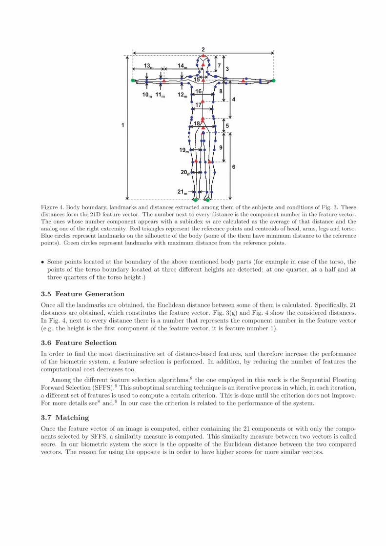
1
2
3
4
5
6
7
8
9
10m 11m 12m
13m 14m
15
16
17
18
19m
20m
21m
Figure 4. Body boundary, landmarks and distances extracted among them of the subjects and conditions of Fig. 3. Thesedistances form the 21D feature vector. The number next to every distance is the component number in the feature vector.The ones whose number component appears with a subindex m are calculated as the average of that distance and theanalog one of the right extremity. Red triangles represent the reference points and centroids of head, arms, legs and torso.Blue circles represent landmarks on the silhouette of the body (some of the them have minimum distance to the referencepoints). Green circles represent landmarks with maximum distance from the reference points.
• Some points located at the boundary of the above mentioned body parts (for example in case of the torso, thepoints of the torso boundary located at three different heights are detected: at one quarter, at a half and atthree quarters of the torso height.)
3.5 Feature Generation
Once all the landmarks are obtained, the Euclidean distance between some of them is calculated. Specifically, 21distances are obtained, which constitutes the feature vector. Fig. 3(g) and Fig. 4 show the considered distances.In Fig. 4, next to every distance there is a number that represents the component number in the feature vector(e.g. the height is the first component of the feature vector, it is feature number 1).
3.6 Feature Selection
In order to find the most discriminative set of distance-based features, and therefore increase the performanceof the biometric system, a feature selection is performed. In addition, by reducing the number of features thecomputational cost decreases too.
Among the different feature selection algorithms,8 the one employed in this work is the Sequential FloatingForward Selection (SFFS).9 This suboptimal searching technique is an iterative process in which, in each iteration,a different set of features is used to compute a certain criterion. This is done until the criterion does not improve.For more details see8 and.9 In our case the criterion is related to the performance of the system.
3.7 Matching
Once the feature vector of an image is computed, either containing the 21 components or with only the compo-nents selected by SFFS, a similarity measure is computed. This similarity measure between two vectors is calledscore. In our biometric system the score is the opposite of the Euclidean distance between the two comparedvectors. The reason for using the opposite is in order to have higher scores for more similar vectors.

3.8 Decision
The obtained scores are used to (i) decide wether the user is who he or she is claiming or not (verification) or to(ii) provide a list with the most likely identities (identification). In both cases, if the user’s score is higher thana certain threshold, the user is accepted as a genuine user.
4. EXPERIMENTS
4.1 Performance Evaluation of a Biometric System
Once the system is implemented, an evaluation of its performance is desirable. This is done through quantitativemeasures, obtained from experiments, that reveal how well the system works and allow us to compare itsperformance with the performance of other biometric systems.
Although the developed system works in both kind of operational modes (verification and identification),the experiments and results shown below are obtained only when working in verification mode. In that casetwo main metrics are used to quantify the performance of the biometric system: 1) the False Acceptance Rate(FAR), which is the probability that an impostor is accepted by the system as a genuine one, and 2) the FalseReject Rate (FRR), that reflects the probability that a genuine user is rejected by the system.
As the threshold value increases, the FRR increases too but the FAR decreases (the system becomes moresecure by rejecting more genuine users and accepting less impostors). There is a value of the threshold for whichthe FAR and the FRR coincides. The value of both rates at that threshold is known as the Equal Error Rate(EER) and is the most widely used parameter to evaluate the performance of a biometric system working inverification mode. Plotting the FRR versus the FAR for all the different threshold values, gives the so-called DETcurve (Detection Error Tradeoff curve).10 This curve is an common way to graphically represent the behaviourof a biometric system, where the EER corresponds to the point where the DET curve and the bisector intersecteach other (See Fig. 5(a)). The closer the curve is to the origin (and therefore the lower the EER is), the betterthe system is.
4.2 Experimental Protocol
Although the BIOGIGA database contains 6 PO, 6 PI, 6 AO and 6 AI images per user, in the following analysisonly PO and PI images are considered. The graphical results will be shown exclusively for PO images, for PIimages the results are quite similar. The same analysis for images simulated by active systems (AO and AIimages) will be part of future work, in which a different image segmentation should be followed due to clearlyvisible differences between the images simulated by passive and active systems (e.g. the last ones present highercontrast).
We consider three different experimental protocols: 1) protocol 1:3, 2) protocol 2:3, and 3) protocol 3:3,where the first number refers to the number of training images considered per user, and the second number tothe number of test images per user. The training images are the ones that the system previously have of eachuser and are used to enroll the user into the system, while the test images are the ones given by the user whenhe or she tries to be accepted by the system. In our experiments all the training images are images simulatedwith clothes, and the test images without clothes (in order to have the most challenging scenario with severemismatch between enrollment and testing regarding clothing).
A mathematical model for each user is generated in the training and in the test set. Each model is simplythe arithmetic mean feature vector of the considered images. Finally, the user test model is compared to thetraining model of each user in the database obtaining the corresponding score.
The experiments are carried out following the previous protocols in two ways: (i) considering all the com-ponents in the feature vector of the images, and (ii) after applying the SFFS algorithm, considering only thefeatures selected by it. In short, there will be 6 different kind of experiments: each of then corresponds to aprotocol working with all features or only with the selected ones.
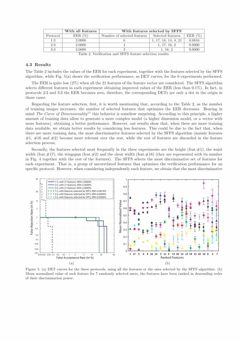
With all features With features selected by SFFS
Protocol EER (%) Number of selected features Selected features EER (%)
1:3 2.0000 6 1, 17, 16, 14, 4, 21 0.0816
2:3 2.0000 4 1, 17, 16, 2 0.0000
3:3 2.0000 3 1, 16, 2 0.0000Table 2. Verification and SFFS feature selection results.
4.3 Results
The Table 2 includes the values of the EER for each experiment, together with the features selected by the SFFSalgorithm, while Fig. 5(a) shows the verification performance, as DET curves, for the 6 experiments performed.
The EER is quite low (2%) when all the 21 features of the feature vector are considered. The SFFS algorithmselects different features in each experiment obtaining improved values of the EER (less than 0.1%). In fact, inprotocols 2:3 and 3:3 the EER becomes zero, therefore, the corresponding DETs are only a dot in the origin inthose cases.
Regarding the feature selection, first, it is worth mentioning that, according to the Table 2, as the numberof training images increases, the number of selected features that optimizes the EER decreases. Bearing inmind The Curse of Dimensionality11 this behavior is somehow surprising. According to this principle, a higheramount of training data allow to generate a more complex model (a higher dimension model, or a vector withmore features), obtaining a better performance. However, our results show that, when there are more trainingdata available, we obtain better results by considering less features. This could be due to the fact that, whenthere are more training data, the most discriminative features selected by the SFFS algorithm (mainly features#1, #16 and #2) become more relevant over the rest, while the rest of features are discarded in the featureselection process.
Secondly, the features selected most frequently in the three experiments are the height (feat.#1), the waistwidth (feat.#17), the wingspan (feat.#2) and the chest width (feat.#16) (they are represented with its numberin Fig. 4 together with the rest of the features). The SFFS selects the most discriminative set of features foreach experiment. That is, a group of uncorrelated features that optimizes the verification performance for anspecific protocol. However, when considering independently each feature, we obtain that the most discriminative
0.01 0.02 0.05 0.1 0.2 0.5 1 2 5 10 20 40 0.01
0.02
0.05
0.1
0.2
0.5
1
2
5
10
20
40
False Acceptance Rate (in %)
Fals
e Re
ject
ion
Rate
(in
%)
1:3, with 21 features, EER=2.0000%2:3, with 21 features, EER=2.0000%3:3, with 21 features, EER=2.0000%1:3, with features selected by SFFS, EER=0.0816%2:3, with features selected by SFFS, EER=0.0000%3:3, with features selected by SFFS, EER=0.0000%
(a)
0
0.1
0.2
0.3
0.4
0.5
0.6
0.7
0.8
0.9
1
Ranked Features
Mea
n N
orm
aliz
ed V
alue
17 6 16 2 4 20 12 21 10 3 71 5 9 14 11 13 15 19 18 8
(b)
Figure 5. (a) DET curves for the three protocols, using all the features or the ones selected by the SFFS algorithm. (b)Mean normalized value of each feature for 7 randomly selected users, the features have been ranked in descending orderof their discrimination power.
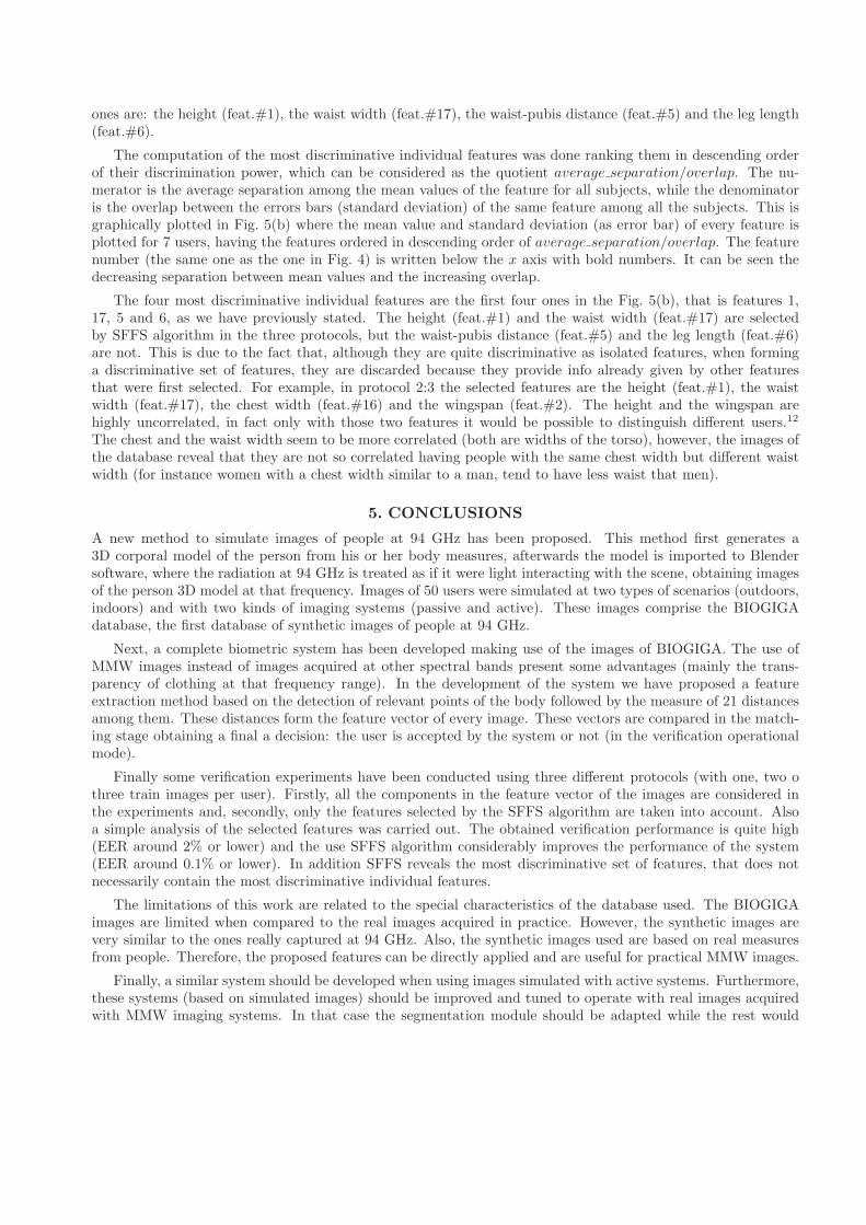
ones are: the height (feat.#1), the waist width (feat.#17), the waist-pubis distance (feat.#5) and the leg length(feat.#6).
The computation of the most discriminative individual features was done ranking them in descending orderof their discrimination power, which can be considered as the quotient average separation/overlap. The nu-merator is the average separation among the mean values of the feature for all subjects, while the denominatoris the overlap between the errors bars (standard deviation) of the same feature among all the subjects. This isgraphically plotted in Fig. 5(b) where the mean value and standard deviation (as error bar) of every feature isplotted for 7 users, having the features ordered in descending order of average separation/overlap. The featurenumber (the same one as the one in Fig. 4) is written below the x axis with bold numbers. It can be seen thedecreasing separation between mean values and the increasing overlap.
The four most discriminative individual features are the first four ones in the Fig. 5(b), that is features 1,17, 5 and 6, as we have previously stated. The height (feat.#1) and the waist width (feat.#17) are selectedby SFFS algorithm in the three protocols, but the waist-pubis distance (feat.#5) and the leg length (feat.#6)are not. This is due to the fact that, although they are quite discriminative as isolated features, when forminga discriminative set of features, they are discarded because they provide info already given by other featuresthat were first selected. For example, in protocol 2:3 the selected features are the height (feat.#1), the waistwidth (feat.#17), the chest width (feat.#16) and the wingspan (feat.#2). The height and the wingspan arehighly uncorrelated, in fact only with those two features it would be possible to distinguish different users.12
The chest and the waist width seem to be more correlated (both are widths of the torso), however, the images ofthe database reveal that they are not so correlated having people with the same chest width but different waistwidth (for instance women with a chest width similar to a man, tend to have less waist that men).
5. CONCLUSIONS
A new method to simulate images of people at 94 GHz has been proposed. This method first generates a3D corporal model of the person from his or her body measures, afterwards the model is imported to Blendersoftware, where the radiation at 94 GHz is treated as if it were light interacting with the scene, obtaining imagesof the person 3D model at that frequency. Images of 50 users were simulated at two types of scenarios (outdoors,indoors) and with two kinds of imaging systems (passive and active). These images comprise the BIOGIGAdatabase, the first database of synthetic images of people at 94 GHz.
Next, a complete biometric system has been developed making use of the images of BIOGIGA. The use ofMMW images instead of images acquired at other spectral bands present some advantages (mainly the trans-parency of clothing at that frequency range). In the development of the system we have proposed a featureextraction method based on the detection of relevant points of the body followed by the measure of 21 distancesamong them. These distances form the feature vector of every image. These vectors are compared in the match-ing stage obtaining a final a decision: the user is accepted by the system or not (in the verification operationalmode).
Finally some verification experiments have been conducted using three different protocols (with one, two othree train images per user). Firstly, all the components in the feature vector of the images are considered inthe experiments and, secondly, only the features selected by the SFFS algorithm are taken into account. Alsoa simple analysis of the selected features was carried out. The obtained verification performance is quite high(EER around 2% or lower) and the use SFFS algorithm considerably improves the performance of the system(EER around 0.1% or lower). In addition SFFS reveals the most discriminative set of features, that does notnecessarily contain the most discriminative individual features.
The limitations of this work are related to the special characteristics of the database used. The BIOGIGAimages are limited when compared to the real images acquired in practice. However, the synthetic images arevery similar to the ones really captured at 94 GHz. Also, the synthetic images used are based on real measuresfrom people. Therefore, the proposed features can be directly applied and are useful for practical MMW images.
Finally, a similar system should be developed when using images simulated with active systems. Furthermore,these systems (based on simulated images) should be improved and tuned to operate with real images acquiredwith MMW imaging systems. In that case the segmentation module should be adapted while the rest would
remain the same. These systems will allow us to perform identification and/or verification experiments with realimages and could be applied in the near future at airport security checkpoints and another screening scenarios.
ACKNOWLEDGMENTS
This work has been partially supported by projects Bio-Challenge (TEC2009-11186), Contexts (S2009/TIC-1485), TeraSense (CSD2008-00068) and “Catedra UAM-Telefonica”.
REFERENCES
1. Jain, A., Ross, A., and Prabhakar, S., “An introduction to biometric recognition,” Circuits and Systems forVideo Technology, IEEE Transactions on 14, 4 – 20 (jan. 2004).
2. Jain, A. et al., “Biometrics: a tool for information security,” Information Forensics and Security, IEEETransactions on 1, 125–143 (june 2006).
3. Moreno-Moreno, M., Fierrez, J., and Ortega-Garcia, J., “Biometrics Beyond the Visible Spectrum: ImagingTechnologies and Applications,” in [Proceedings of BioID-Multicomm 2009 ], LNCS 5707, 154–161, Springer(September 2009).
4. Moreno-Moreno, M., Fierrez, J., and Ortega-Garcia, J., “Millimeter- and Submillimeter-Wave ImagingTechnologies for Biometric Purposes,” in [Proceedings of XXIV Simposium Nacional de Union CientificaInternacional de Radio, URSI 2009 ], (September 2009).
5. Alefs, B., den Hollander, R., Nennie, F., van der Houwen, E., Bruijn, M., van der Mark, W., and Noordam, J.,“Thorax biometrics from Millimetre-Wave images,” Pattern Recognition Letters 31(15), 2357–2363 (2010).
6. Moreno-Moreno, M., Fierrez, J., Tome, P., Vera-Rodriguez, R., Parron, J., and Ortega-Garcia, J., “BioGiga:Base de Datos de Imagenes Sinteticas de Personas a 94 GHz con Fines Biometricos,” in [Proceedings of XXVISimposium Nacional de Union Cientifica Internacional de Radio, URSI 2011 ], (September 2011).
7. Parron, J., Rossel, H., de Paco, P., Junkin, G., and Menendez, O., “Millimeter-Wave Scene Simulation usingBlender,” in [Proceedings of XXV Simposium Nacional de Union Cientifica Internacional de Radio, URSI2010 ], (September 2010).
8. Molina, L. C., Belanche, L., and Nebot, A., “Feature selection algorithms: A survey and experimentalevaluation,” in [Proceedings of the 2002 IEEE International Conference on Data Mining ], ICDM ’02, 306–,IEEE Computer Society, Washington, DC, USA (2002).
9. Pudil, P., Novovicov, J., and Kittler, J., “Floating Search Methods in Feature Selection,” Pattern Recogni-tion Letters 15(11), 1119 – 1125 (1994).
10. Martin, A., Doddington, G., Kamm, T., Ordowski, M., and Przybocki, M., “The DET curve in assessmentof detection task performance,” in [Proceedings of the European Conference on Speech Communication andTechnology ], 1, 1895–1898 (1997).
11. Bishop, C. M., [Pattern Recognition and Machine Learning (Information Science and Statistics) ], Springer,1st ed. 2006. corr. 2nd printing ed. (Oct. 2007).
12. Moreno-Moreno, M., Fierrez, J., Vera-Rodriguez, R., and Parron, J., “Distance-based Feature Extractionfor Biometric Recognition of Millimeter-Wave Body Images,” in [Proceedings of 45th IEEE InternationalCarnahan Conference on Security Technology ], 326–331 (October 2011).