Download - SOME SIMPLE MATHEMATICAL MODELS OF …diposit.ub.edu/dspace/bitstream/2445/65452/2/memoria.pdfSome simple mathematical models of tumor growth 2 Cancer Cancer is the general name for

Treball final de grau

GRAU DE

MATEMÀTIQUES

Facultat de Matemàtiques

Universitat de Barcelona

SOME SIMPLE MATHEMATICAL MODELS OF TUMOR GROWTH

Elisabet Oter Perrote

Director: Alex Haro Provinciale Realitzat a: Departament de Matemàtica

Aplicada i Anàlisi. UB

Barcelona, 29 de gener de 2015

Some simple mathematical models of tumor growth

Contents

1 Introduction 3

2 Cancer 4

2.1 Types . . . . . . . . . . . . . . . . . . . . . . . . . . . . . . . . . . 4

2.2 Impact in our society . . . . . . . . . . . . . . . . . . . . . . . . . . 4

2.3 Mathematics and tumors . . . . . . . . . . . . . . . . . . . . . . . . 6

3 Biological study of the models 7

3.1 The simplest model . . . . . . . . . . . . . . . . . . . . . . . . . . . 7

3.2 Types of growing . . . . . . . . . . . . . . . . . . . . . . . . . . . . 7

3.3 Proliferative and quiescent cells . . . . . . . . . . . . . . . . . . . . 9

3.4 Cytotoxic and cytostatic drugs . . . . . . . . . . . . . . . . . . . . . 10

3.5 Tumor growth under angiogenic control . . . . . . . . . . . . . . . . 11

4 Mathematical study of the models 13

4.1 The simplest models . . . . . . . . . . . . . . . . . . . . . . . . . . 13

4.2 Logistic power . . . . . . . . . . . . . . . . . . . . . . . . . . . . . . 15

4.3 Gompertz law for tumor growth . . . . . . . . . . . . . . . . . . . . 26

4.4 Cytotoxic and cytostatic drugs . . . . . . . . . . . . . . . . . . . . . 31

4.5 Tumor growth under angiogenic control . . . . . . . . . . . . . . . . 39

5 Conclusion 44

A General results of differential equations 45

A.1 Properties of an α− ω limit set . . . . . . . . . . . . . . . . . . . . 45

A.2 Bendixon criterion . . . . . . . . . . . . . . . . . . . . . . . . . . . 45

A.3 Poincare-Bendixon theorem . . . . . . . . . . . . . . . . . . . . . . 45

A.4 Picard’s existence theorem . . . . . . . . . . . . . . . . . . . . . . . 46

A.5 Peano existence theorem . . . . . . . . . . . . . . . . . . . . . . . . 46

1


Abstract

The aim of this final project is to understand and analyze some mathe-matical models of tumor growth. This is divided in three parts: firstly, it isexposed an introduction to cancer and the important vocabulary, secondly, itis explained biologically the models of tumor growth and finally, it is analyzedmathematically the models with the biological conclusions.

2


1 Introduction

The principal motivation of this final project is the interest in applied mathematics.Of all the courses I have studied the ones that have arouse my curiosity the mostare ’Mathematical models and Dynamic systems’ and ’Differential equations’. Inparticular, what I liked was the chance to extract conclusions from other sciencesas physics or economics by mathematical study. For that reason, I have based myproject on these fields. We also have to say these courses are much related to themathematical modelling, so with this project I will be able to strength and increasemy knowledge in all of these subjects.

When the topic was proposed to me, it seemed interesting the possibility ofintroduce myself in the cancer’s study, since it is so present in the current society.Besides, it attracted attention to me the relation it could have with mathematics.

Lots of times, what happens is that in different fields such as physics or chemistry,a topic is investigated but not in a deep mathematical way. In other words, it mightbe said that the relations between the different branches should be more joined fora better analysis of both.

Therefore, this project is based on the understanding of several growth models oftumors based on differential equations and it is attempted to give a better mathe-matical explanation of the proposed models in the chapter 1 of the paper [1]: Somemathematical models of tumor growth. Since I had only an unclear idea of whatthe cancer was at a biological level, it has been required to study in depth somereferences the paper was offering to understand the biological part.

The project consist of three parts:

• The first one gives a brief introduction on what the cancer is, points out thetypes of tumors and which ones are studied and gathers some information ofthe impact of the cancer in our society. Furthermore, it gives an explanationof the relation of cancer and mathematics, and the important vocabularyrequired for a better understanding of the whole study.

• The second part explains the exhibited models biologically on the paper [1]using its references and others that I thought they were interesting to ex-tend the information. Beginning with the simplest models of one variableand continuing with three models of two variables. Adding references wherenecessary, for the interest of the reader to study the topic in depth.

• The aim of the third and final part is to understand mathematically themodels exposed previously, show alternative proofs and extend results of [1],proof details that are left in [1], use a program to exemplify the results andobtain conclusions from a biological point of view.

3


2 Cancer

Cancer is the general name for a group of more than 100 diseases.

2.1 Types

Most cancers are named for the organ or type of cell in which they start. In thisproject we divide cancer in two categories:

• Solid tumors: central nervous system cancers, carcinoma, sarcoma.

• Others: leukemia, lymphoma and meyloma.

We will study mathematical models for the first types of cancer, that is thereason why we are interested in the origin of them. It is helpful to know whathappens when normal cells become cancer cells.

The human body is made up of many types of cells. These cells grow and splitin to produce more cells in a controlled way as they are needed to keep the bodyhealthy. When cells become old or damaged, they die (die by apoptosis, theprogrammed death of cells) and are replaced with new cells.

However, sometimes this orderly process goes wrong. The genetic material(DNA) of a cell can become damaged or changed, producing mutations that af-fect normal cell growth and division. When this happens, cells do not die whenthey should and new cells form when the body does not need them. Moreover,this new cells grow up quicker than the normal ones and they use high quantityof energy. The extra cells may form a mass of tissue called a tumor. For moredetailed information see [8].

2.2 Impact in our society

To show the impact of cancer in our society it is presented a sum of graphics. Firstof all, two of them compare the cancer with another diseases ( this informationcomes from the paper [10] ):

% of total deceasescaused by...

Spain (2012)

Diseases related withcirculatory system

30.3

Cancer 27.5Diseases related withrespiratory system

11.7

As we can see cancer is the second cause of death in Spain on 2012 with 27.5% ofthe total deceases.

4


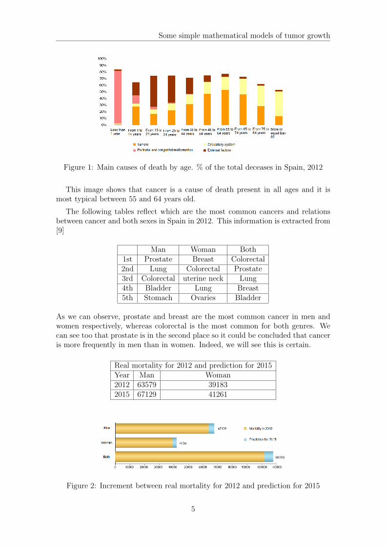
Figure 1: Main causes of death by age. % of the total deceases in Spain, 2012

This image shows that cancer is a cause of death present in all ages and it ismost typical between 55 and 64 years old.

The following tables reflect which are the most common cancers and relationsbetween cancer and both sexes in Spain in 2012. This information is extracted from[9]

Man Woman Both1st Prostate Breast Colorectal2nd Lung Colorectal Prostate3rd Colorectal uterine neck Lung4th Bladder Lung Breast5th Stomach Ovaries Bladder

As we can observe, prostate and breast are the most common cancer in men andwomen respectively, whereas colorectal is the most common for both genres. Wecan see too that prostate is in the second place so it could be concluded that canceris more frequently in men than in women. Indeed, we will see this is certain.

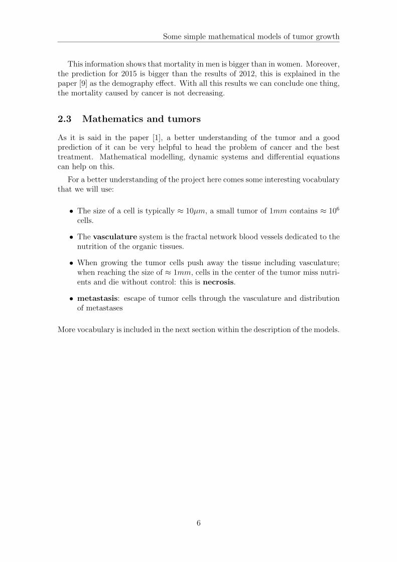
Real mortality for 2012 and prediction for 2015Year Man Woman2012 63579 391832015 67129 41261

Figure 2: Increment between real mortality for 2012 and prediction for 2015

5


This information shows that mortality in men is bigger than in women. Moreover,the prediction for 2015 is bigger than the results of 2012, this is explained in thepaper [9] as the demography effect. With all this results we can conclude one thing,the mortality caused by cancer is not decreasing.

2.3 Mathematics and tumors

As it is said in the paper [1], a better understanding of the tumor and a goodprediction of it can be very helpful to head the problem of cancer and the besttreatment. Mathematical modelling, dynamic systems and differential equationscan help on this.

For a better understanding of the project here comes some interesting vocabularythat we will use:

• The size of a cell is typically ≈ 10µm, a small tumor of 1mm contains ≈ 106

cells.

• The vasculature system is the fractal network blood vessels dedicated to thenutrition of the organic tissues.

• When growing the tumor cells push away the tissue including vasculature;when reaching the size of ≈ 1mm, cells in the center of the tumor miss nutri-ents and die without control: this is necrosis.

• metastasis: escape of tumor cells through the vasculature and distributionof metastases

More vocabulary is included in the next section within the description of the models.

6


3 Biological study of the models

We will explain from the biological point some models of tumor growth that areshown in the work [1].

3.1 The simplest model

All the models that are shown in this work are based in the Lotka-Volterra model.Here N(t) represent the population of cells and d

dtN(t) is the evolution of N(t) when

t is growing. When this happen N(t) increases because new cells are born and atthe same time others are dying. This mathematically represented is: N(t) multiplya function b(t), called the birth rate, and N(t) is multiplied by d(t), a functionwhich is the death rate. Finally, N(0) is the initial population of cells:

d

dtN(t) = N(t)(b(t)− d(t)) = N(t)r(t), N(0) = N0 (3.1)

3.2 Types of growing

r(t) is a function that control the growing of the population of cells and this isstrongly connected with access to nutrients and space availability. For that reasonwe will take a non linear function of N : R. It is called the bulk growth rate sor(t) = R(N(t)) then the equation of (3.1) will be:

d

dtN(t) = N(t)R(N(t)), N(0) = N0 (3.2)

Let be r > 0 the intrinsic birth rate in conditions where nutrients and space isfreely available, then R satisfies one of the two conditions:

(a)R(0) = r > 0, R′(·) < 0, lim

N→∞R(N) = 0

(b)R(0) = r > 0, R′(·) < 0, R(K) = 0 for a certain K

Both of them has the condition R′(·) < 0 which represents that R is a decreasingfunction. In fact, at the same time that cells are growing, they grow slowly bythe past of time. The first one represent the unlimited growth and the secondone the limited growth by K, the maximal tumor size called the carrying capacity.Moreover, R is C1 in (0,∞).

The work in [1] shows different non-linearities. The first one is the Verhulstequation:

R(N) = r

(1− N

K

), K > 0

7


This equation takes into account that resources are limited and this fact tendsto slow the growth of cells. Verhulst introduces the logistic model which says thatthe populations growth rate is not constant but rather depends on the size of thepopulation in a non-increasing way and vanishing when the population reaches themaximal capacity, this is K. The parameter r controls the velocity of the growth.

The Verhulst equation could be extended as:

R(N) = r

[1−

(N

K

)a], a > 0, K > 0

it is known as the logistic power. By introducing an additional degree of freedom awe can obtain an improvement that fits better the data.

The second non-linearity is the Gompertz law:

R(N) = b log

(K

N

)The idea of Gompertz was that the growth rate should decrease exponentially

in time. We can observe :limN→0

R(N) =∞

and this is the point why the Gompertz law is criticized, because this means thatwhen the population of cells is disappearing, the growth rate is infinity. It isbounded by the total cell cycle duration, so it is positive to assume large num-ber of cells as it is said in paper [1].

A relation between Gompertz law and logistic power is the one that follow.

Proposition 1. The Gompertz law is the limit when a −→ 0 of the logistic powerlaw with b = ra

Proof. Firstly, we substitute b = ra in b log(KN

). When N = K both functions are

equal to 0. We suppose N 6= K.

lima→0

1−(NK

)aa · log(K

N)

this is 00

and since 1−(NK

)aand a · log(K

N) are differentiable we can use l’Hopital’s

rule. Then:

lima→0

(−N

K

)alog(N

K)

log(KN

)=−1 ·

(− log K

N

)log K

N

= 1

Proposition 2. If R(N) = bN−a and a = 13

then the solution of (3.2) is compatiblewith the linear growth of the radius , i.e., N(t) ≈ rt3 with r = 1

3b when t→∞ with

t0 = 0.

8


Proof. We consider R(N) = bN−a then

d

dtN(t) = N(t)bN(t)−a ⇒ d

dtN = NbN−a ⇒

⇒ Na−1dN = bdt⇒∫ N

N0

Na−1dN =

∫ t

0

bdt⇒ Na]NN0= abt⇒ N(t) = a

√abt+Na

0

as a = 13:

limt→∞

N(t) ≈ 1

3bt3 = rt3

A general result of existence and uniqueness of one dimension is:

Theorem 1. Let h : I → R be a continuous function in the interval I, and considerthe differential equation N = h(N). Assume that the set of zeros of h is discrete(the zeros are isolated). Assume that, for any zero z0, the integral∫ N

N0

dN

h(N)

is divergent (for z close to z0). Then, the solution N(t) of the equation N = h(N)with initial condition (t0, N

0) exists and is unique.

Proof. We suppose N is not a singular point so h(N) 6= 0. Then:

N = h(N)⇒ 1

h(N)= dt⇒

∫ N

N0

1

h(N)dN =

∫ t

t0

dt⇒∫ N

N0

1

h(N)= t− t0

as a result H(N)]NN0 = t − t0 where H is a primitive of 1h. We can conclude

N(t) =(H]NN0

)−1(t − t0), H

−1 exists because 1h6= 0 then H−1 6= 0 ⇒ H is

monotonic. So N(t) exists.

For every N0 we have: ∫ N

N0

dN

h(N)

the integral is convergent, this means:∫ N

N0dNh(N)

which is the time that N0 takes toget N is finite.

3.3 Proliferative and quiescent cells

As we have said a tumor is formed by new cells that are muted, we also said thatthey grow quicker than the healthy ones. But not all tumors cells grow up in thesame way. If this happen, a cell cycle around 24 hours would make a tumor of 106

cells after less than one month, that is a tumor of 10cm.

9


That is the reason why we differentiate at least two types of cells: proliferative(cells which grow up) and quiescent (in specific terms, either slowly growing or notgrowing at all).

We consider the function F (P ) which represents the growth of proliferative cells.In our case we will take logistic power and Gompertz law.

Moreover, a tumor exhibits a layer of quiescent cells which are thought to ariseas proliferating cells lose access to nutrients. In the same way, quiescent cells dieafter sufficient lack of nutrient, this is expressed by −dQ (d the death rate). Inaddition, it is known that quiescent cells may become proliferating cells again. Sothere will be an exchange of proliferative and quiescent cells, this is expressed asbP − cQ, where bP represents the cells that became quiescent and −cQ the onesthat transform to proliferative −cQ.

This happen also with proliferative cells, that is why −bP + cQ is added in theequation of the evolution of proliferative cells, P .

It is considered a linear transition between P and Q and Q and P , a good reasonis explained in [6]: whatever is the way of transferring from P to Q or in reverse, itmay be expressed as a Taylor series in P , and this expression has a linear leadingterm.

So a proliferative-quiescent model would be expressed as:

P = F (P )− bP + cQ, proliferative cells

Q = bP − cQ− dQ, quiescent cells(3.3)

The size of the tumor is defined by

N(t) = P (t) +Q(t)

3.4 Cytotoxic and cytostatic drugs

Now that we have seen a model of how a tumor grows, it is time to present anothermodel which has the aim of vanishing this tumor.

As proliferative cells are the ones that affect more the growing of N , most of thetherapies target proliferative cells populations. This could be done in two ways:

• One is controlling the transition of cells. If they stay in a quiescent cells theywill not grow up. Proteins that block proliferation are cyclins, they are calledcytostatic drugs and the concentration of this drug will be denoted as cstat inthe model.

• The second way is by killing directly proliferative cells. This is target withcytotoxic drugs. The concentration of this drug is named as ctox.

and they are called chemotherapies. And now we present the next model:

P = F (P )− (b+ cstat)P + cQ− ctoxP, proliferative cells

Q = (b+ cstat)P − cQ− dQ, quiescent cells(3.4)

10


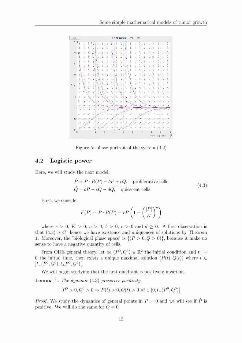
Figure 3: Mean tumor diameter (MTD). MTD observed (pink circles), individ-ual predictions (solid black line), and population predictions on the basis of meanparameter values (dashed green line) for 3 individuals

A practice example based in a P −Q model was done it by [3]. Which is a modelthat successfully described the time course of tumor growth inhibition for patientswith low-grade gliomas. See Figure 3

Remark 1. A recent discovery on 2014 Weizmann Institute scientists reveals thata hormone which keeps us alert also suppresses the spread of cancer [5]. One of itsconclusions is that it could be more efficient to administer certain anticancer drugsat night.

3.5 Tumor growth under angiogenic control

Angiogenesis is the formation of new blood vessels as a response to necrosis. Thenecrotic cells emit Vascular Endothelial Growth Factors (VEGF, a protein producedby cells) which induce the development of neovasculature.

The next model that we present was developed by Hahnfeldt [4]. It is basedon the idea of considering K, the carrying capacity, a dynamic variable. Here Krepresents the vasculature of the tumor, because the nutrients that are supplied fromvasculature, controls the maximal size of the tumor. Now we call K the ’angiogeniccapacity’.

The equation for N (the size of the tumor) is considered the Gompertz equation.For the evolution of K it takes into account: natural vascular loss due to naturalendothelial cells death, stimulation by the tumor via molecules (such as VEGF)and inhibition of the vasculature by the tumor. Then the equation of K is:

d

dtK(t) = cS(N,K)− dI(N,K)

where S and I are functions which stimulate and inhibit K. For the stimulatoryterm is common used: S(N,K) = N . Which at the end should not influence toomuch the qualitative behavior of the system. The inhibition therm is linked withthe radius and the volume of the tumor.

11


In summary, the equation studied by Hahnfeldt is:

d

dtN = bN log

(K

N

)d

dtK = cN − dN2/3K.

(3.5)

12


4 Mathematical study of the models

In this section, we will analyze mathematically the models presented in the pre-vious section. Wolfram Mathematica, PPLANE and DFIELD (which are softwareprograms for the interactive analysis of ordinary differential equations) has beenhelped us to check out our results.

4.1 The simplest models

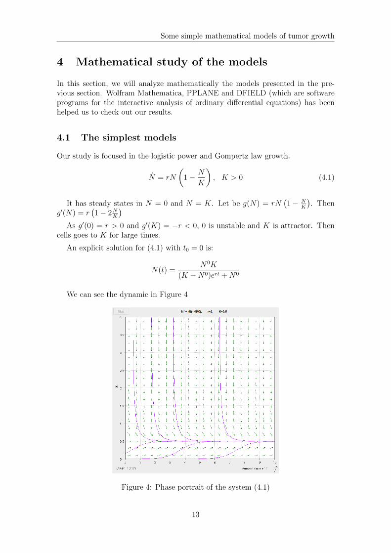
Our study is focused in the logistic power and Gompertz law growth.

N = rN

(1− N

K

), K > 0 (4.1)

It has steady states in N = 0 and N = K. Let be g(N) = rN(1− N

K

). Then

g′(N) = r(1− 2N

K

)As g′(0) = r > 0 and g′(K) = −r < 0, 0 is unstable and K is attractor. Then

cells goes to K for large times.

An explicit solution for (4.1) with t0 = 0 is:

N(t) =N0K

(K −N0)ert +N0

We can see the dynamic in Figure 4

Figure 4: Phase portrait of the system (4.1)

13


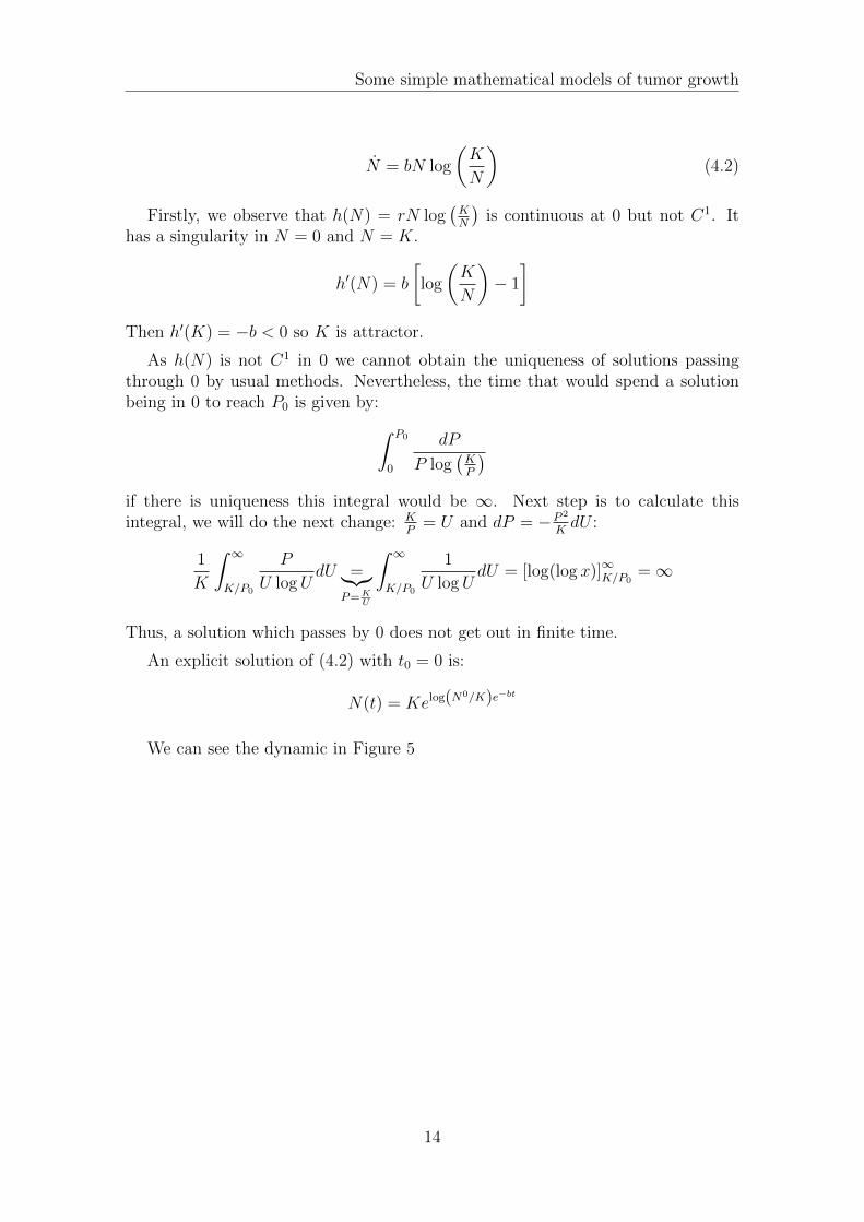
N = bN log

(K

N

)(4.2)

Firstly, we observe that h(N) = rN log(KN

)is continuous at 0 but not C1. It

has a singularity in N = 0 and N = K.

h′(N) = b

[log

(K

N

)− 1

]Then h′(K) = −b < 0 so K is attractor.

As h(N) is not C1 in 0 we cannot obtain the uniqueness of solutions passingthrough 0 by usual methods. Nevertheless, the time that would spend a solutionbeing in 0 to reach P0 is given by:∫ P0

0

dP

P log(KP

)if there is uniqueness this integral would be ∞. Next step is to calculate thisintegral, we will do the next change: K

P= U and dP = −P 2

KdU :

1

K

∫ ∞K/P0

P

U logUdU =︸︷︷︸

P=KU

∫ ∞K/P0

1

U logUdU = [log(log x)]∞K/P0

=∞

Thus, a solution which passes by 0 does not get out in finite time.

An explicit solution of (4.2) with t0 = 0 is:

N(t) = Kelog(N0/K)e−bt

We can see the dynamic in Figure 5

14


Figure 5: phase portrait of the system (4.2)

4.2 Logistic power

Here, we will study the next model:

P = P ·R(P )− bP + cQ, proliferative cells


First, we consider

F (P ) = P ·R(P ) = rP

(1−

(|P |K

)a)where r > 0, K > 0, a > 0, b > 0, c > 0 and d ≥ 0. A first observation is

that (4.3) is C1 hence we have existence and uniqueness of solutions by Theorem1. Moreover, the ’biological phase space’ is (P > 0, Q > 0), because it make nosense to have a negative quantity of cells.

From ODE general theory, let be (P 0, Q0) ∈ R2 the initial condition and t0 =0 the initial time, then exists a unique maximal solution (P (t), Q(t)) where t ∈]t−(P 0, Q0), t+P

0, Q0)[.

We will begin studying that the first quadrant is positively invariant.

Lemma 1. The dynamic (4.3) preserves positivity

P 0 > 0, Q0 > 0⇒ P (t) > 0, Q(t) > 0 ∀t ∈ [0, t+(P 0, Q0)[

Proof. We study the dynamics of general points in P = 0 and we will see if P ispositive. We will do the same for Q = 0.

15


A general point in P = 0 has the next form: (0, α) with α > 0 Then,

P = F (0)− b · 0 + cα = 0 + 0 + cα > 0

For Q = 0 we have the general point (β, 0) with β > 0

Q = bβ − c · 0− d · 0 > 0

Lemma 1 will be used for more systems, it will be useful to find a proof forgeneral F (P ).

Observation 1. The lemma (1) can be proved for general functions F (P ) with thiscondition:

F (0) = 0

Proof. This is solved in the same way as in the lemma (1). It will be provedstudying the dynamic in P = 0:

A general point in P = 0 has the next form: (0, α) with α > 0 Then,

P = F (0)− b · 0 + cα = 0 · 0 + 0 + cα > 0

Q does not depend on F (P ) so Q > 0 is solved in the proof of lemma (1).

With the next lemma we will see that solutions are defined for all t > 0, thusproving t+(P 0, Q0) = +∞. This will be proved by finding a positively invariantregion: Let be φ(t;x0, y0) the solution given by a system of ODE x = f(x, y) andy = g(x, y) in an open set D ⊂ R2, then a domain γ+(x0, y0) = φ(t;x0, y0); t ∈(0, t+(x0, y0)[ ⊂ U is positively invariant set if for all (P,Q) ∈ U γ+(P,Q) stay inU .

If U is compact and positively invariant then t+(P 0, Q0) =∞In this case the positively invariant region will be triangles, legs of the triangle

will be axis P = 0 and Q = 0. We just have to find the hypotenuse. In fact, finda slope m ∈ (0,∞) for a straight line Q = L −mP and conditions of L ∈ (0,∞)where the dynamics of this line, that would be transversal to the model, head insidethe triangle. In other words, ⟨(

P , Q), (m, 1)

⟩< 0

The process to find a correct m is consider a general Q = L−mP and a function

g(P ) =⟨(P , Q

), (m, 1)

⟩and impose that g(0) < 0.

g(P ) =⟨(P , Q

), (m, 1)

⟩= −cL−dL+cLm+bP−bmP+cmP+dmP−cm2P+mF [P ]

16


Notice that F (P ) = P ·R(P ), then:

g(0) = −cL− dL+ cLm⇒ −cL− dL+ cLm < 0⇔ m <(c+ d)L

cL= 1 +

d

c

The minimum value of 1 + dc

is 1 (this happens when d = 0) so we can concludem ∈ (0, 1), our election is m = 0.5.

Lemma 2. Let L0 = P∗0.5c+d

(0.5b+ 0.25c+ 0.5d+ 0.5r − 0.5

(P∗K

)ar)> 0 with P∗ =

K(

2b+c+2d+2r(2+2a)r

)(1/a). Then ∀L > L0 and ∀P ∈ (0, 2L):⟨(

P , Q),

(1

2, 1

)⟩< 0

Proof. As we have seen Q = L− 0.5P .⟨(P , Q), (1

2, 1)⟩

=⟨(F (P )− bP + cQ, bP − cQ− dQ), (1

2, 1)⟩

= −0.5cL − dL +

0.5bP + 0.25cP + 0.5dP + 0.5Pr − 0.5P(PK

)ar

Let G(P ) be equal to the last equation. We will search if G has a maximum:G′(P ) = 0.5b+ 0.25c+ 0.5d+ 0.5r − 0.5

(PK

)ar − 0.5a

(PK

)ar then

G′(P ) = 0⇔ P∗ = K(

2b+c+2d+2r(2+2a)r

)(1/a)is the possible maximum

G′′(P ) = −((0.5a(P/K)ar)/P )− (0.5a2(P/K)ar)/P < 0

In particular G′′(P∗) < 0

Consequently, G(P ) has a maximum at (P∗, G(P∗)) we will see when G(P∗) < 0is negative

G(P∗) = −0.5cL− dL+ 0.5bP∗ + 0.25cP∗ + 0.5dP∗ + 0.5P∗r − 0.5P∗

(P∗K

)a

r

G(P∗) < 0⇔ L > P∗0.5c+d

(0.5b+ 0.25c+ 0.5d+ 0.5r − 0.5

(P∗K

)ar)

Corollary 1. Solutions of (4.3) are defined for all t > 0.

Proof. Let be (P 0, Q0) an initial condition inside the triangle, as it is positivelyinvariant and compact solutions are defined for all t > 0.

Next step is to find the steady states.

Lemma 3. The point (0, 0) is always a steady state. And when bd < r(c + d)

we have another fixed point (P ,Q) =(K a

√1− bd

r(c+d), bKc+d

a

√1− bd

r(c+d)

)in the first

quadrant.

Proof. We have steady states when P = 0 and Q = 0.

Q = 0⇔ Q =bP

c+ d

17


P = 0⇔ P

(r

(1− P

K

)a

− b+cb

c+ d

)= 0⇒

⇒ P = 0 or r

(1− P

K

)a

− b+cb

c+ d= 0

P = 0⇒ Q = 0, then (0, 0) is a fixed point.

r(1− P

K

)a − b + cbc+d

= 0 ⇒ P := K a

√1− bd

r(c+d)⇒ Q := bP

c+dP then (P ,Q) is

another fixed point when 1− bdr(c+d)

> 0⇔ bd < r(c+ d)

Furthermore, we will classify the steady states paying attention to the conditionthat we have found, for that reason the next two lemmas and the observationdifferentiate between bd < r(c+ d), bd < r(c+ d) and bd = r(c+ d).

Lemma 4. The zero steady state (0, 0) is an attracting node if bd > (c+ d)r

Proof. The linearized equation in (0, 0) is:(P

Q

)=

(r − b cb −c− d

)(PQ

)

So the characteristic polynomial is x2− (−b− c− d+ r)x+ (r− b)(−c− d)− bc.Therefore the eigenvalues are:

λ =1

2

(−b− c− d+ r −

√(b+ c+ d− r)2 − 4(bd− cr − dr)

)µ =

1

2

(−b− c− d+ r +

√(b+ c+ d− r)2 − 4(bd− cr − dr)

)First, we notice that ∆ > 0

∆ = (b + c + d − r)2 − 4((r − b)(−c − d) − bc) = (r − b)2 + (−c − d)2 + 2(r −b)(−c− d)− 4(r − b)(−c− d) + 4bc = (r − b+ c+ d)2 + 4bc > 0

Then the eigenvalues are real. It is time to analyze the sign of λ and µ, thereforewe will analyze (r − b)(−c− d)− bc = bd− cr − dr

bd− cr − dr > 0⇔ bd > (c+ d)r

In the meanwhile

bd− cr − dr > 0⇔ −4(bd− cr − dr) < 0⇒

⇒√

(b+ c+ d− r)2 − 4(bd− cr − dr) < |b+ c+ d− r|

Moreover, when bd > (c+ d)r:

−b−c−d+r < −b−c−d+bd

c+ d<−bc− bd− (c+ d)2 + bd

c+ d=−bc− (c+ d)2

c+ d< 0

18


So we have 0 > −b− c− d + r >√

(b+ c+ d− r)2 − 4(bd− cr − dr) then µ isnegative.

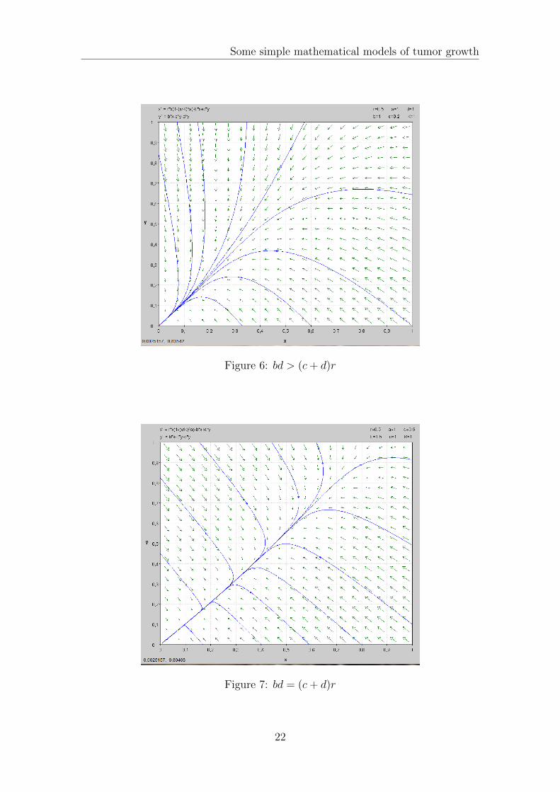
In summary when bd > (c+ d)r, λ and µ are negative then the zero steady stateis an attracting node. We can see the dynamic in Figure 6.

The proof that the zero steady state is a node will be repeated in more steadystates, a general proof of this fact will be useful.

Observation 2. Let be M a general matrix with the form:(A BC D

)With A,B,C,D ∈ R and BC > 0. M has the characteristic polynomial: x2− (A+D)x+ (AD −BC). Then ∆ > 0.

Proof.

∆ = (A+D)2 − 4(AD −BC) = A2 +D2 + 2AD − 4AD + 4BC =

= A2 +D2 − 2AD + 4BC = (A−D)2 + 4BC > 0

Lemma 5. If bd < (c + d)r the zero steady state is a saddle point and the stablemanifold is not in the first quadrant. Moreover, the other steady state (P ,Q) is anattracting node.

Proof. Using the notation of the previous lemma, we have:

λ =1

2

(−b− c− d+ r −

√(b+ c+ d− r)2 − 4(bd− cr − dr)

)µ =

1

2

(−b− c− d+ r +

√(b+ c+ d− r)2 − 4(bd− cr − dr)

)We proceed in the same way as in the previous lemma

bd− cr − dr < 0⇔ bd < (c+ d)r

In fact,bd− cr − dr < 0⇔ −4(bd− cr − dr) > 0⇒

⇒√

(b+ c+ d− r)2 − 4(bd− cr − dr) > |b+ c+ d− r|

And now we differentiate two cases:

• b+ c+ d− r > 0

b+ c+ d− r > 0⇔ −b− c− d+ r < 0⇒

⇒√

(b+ c+ d− r)2 − 4(bd− cr − dr) > −b− c− d+ r ⇒ µ > 0

In this case, λ is negative.

19


• b+ c+ d− r < 0

b+ c+ d− r < 0⇔ −b− c− d+ r > 0⇒√(b+ c+ d− r)2 − 4(bd− cr − dr) > −b− c− d+ r ⇒ λ < 0

In this case, µ is positive.

Overall, when bd < (c + d)r: λ is negative and µ is positive then the zero steadystate is a saddle point.

Now we will study the eigenvector of λ (which is the stable manifold becauseλ < 0):

−−c− d+ 12

(b+ c+ d− r +

√(b+ c+ d− r)2 − 4(bd− cr − dr)

)b

, 1

= (u, v)

We will see that u is negative so the eigenvector will not be in the first quadrant.

u = −−c− d+ 1

2

(b+ c+ d− r +

√(b+ c+ d− r)2 − 4(bd− cr − dr)

)b

=

=c+ d− b+ r −

√(−b− c− d+ r)2 + 4[(r − b)(−c− d)− bc]

2b=

=r − b+ c+ d−

√(r − b+ c+ d)2 + 4bc

2b

Looking at√

(r − b+ c+ d)2 + 4bc >√

(r − b+ c+ d)2 = r− b+ c+ d, the lastequality is clearly less than 0.

Finally, we will see that the non-zero steady state is an attracting node whenbd < (c+ d)r.

The linearized equation in (P ,Q) is:

(P

Q

)=

(−ar + bd

c+d(1 + a)− b c

b −c− d

)(P − PQ−Q

)= M

(P − PQ−Q

)We will use the next notation to define the eigenvalues:

tr M = −ar + bdc+d

(1 + a)− b− c− d

detM =(−ar + bd

c+d(1 + a)− b

)(−c− d)− cb = a(−bd+ (c+ d)r)

The characteristic polynomial of M is: x2 − (tr M)x+ detM . Then, the eigen-values are:

γ =1

2

(tr M +

√(tr M)2 − 4 detM

)20


η =1

2

(tr M −


)bc > 0 hence γ and η are real because ∆ > 0, it is proved in Observation 2.

Moreover, we study detM to classify γ and η

detM > 0⇔ a(−bd+ (c+ d)r) > 0⇔ −bd+ (c+ d)r > 0⇔ bd < (c+ d)r

Then detM > 0⇒ −4 detM < 0√(tr M)2 − 4 detM < |tr M |

In addition, we should observe when bd < (c + d)r ⇒ tr M < 0. Becausebd < (c+ d)r ⇔ detM > 0 and now we have:

tr M = −ar +bd

c+ d(1 + a)− b− c− d < − cb

c+ d− c− d < 0

So,√

(tr M)2 − 4 detM < tr M ⇒ γ < 0 and as tr M < 0 and

−√

(tr M)2 − 4 detM < 0 then η < 0.

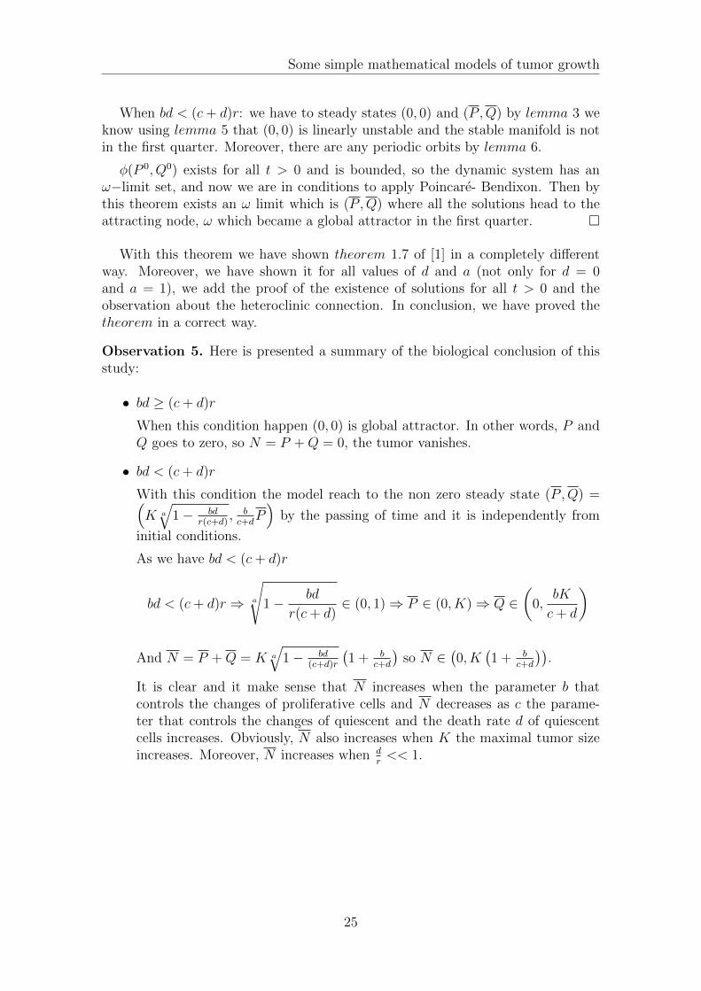
To sum up when bd < (c + d)r, γ and η are negative, thus the non-zero steadystate is an attracting node. We can see the dynamic in Figure 8.

Observation 3. The dynamic system has a heteroclinic connection between (0, 0)and (P ,Q) when bd < (c+ d)r.

Proof. By lemma 1 and 2 the unstable manifold of (0, 0) head to the first quadrant.All the points in the first quadrant of the unstable manifold has α−limit (0, 0) whichhas ω−limit (P ,Q) (for notation see Appendix A.1). We can see this connection inFigure 8

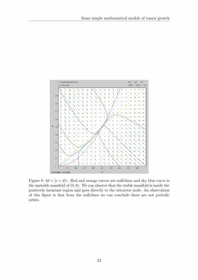
Observation 4. When bd = (c+ d)r then (P ,Q) = (0, 0) and λ is negative and µis 0, so (P ,Q) is not hyperbolic.We can see the dynamic in Figure 7.

Pictures show the transition between the conditions bd < r(c+ d), bd < r(c+ d)and bd = r(c + d). We can see the dynamic in each case, red points are steadystates,blue lines are orbits and green arrows are tangent vectors of the orbits.

Now it is time to study the general behavior of this dynamic system. To achievethis we will study if we can find periodic orbits in the first quadrant.

Lemma 6. The system do not have periodic orbits.

Proof. We will differentiate two cases:

• bd ≥ (c+ d)r

We just have one steady state in the first quarter and this zero steady state isan attracting node. We know by Appendix A.1 that if there is a periodic orbit,this should be around this point but this is impossible because we studied thedynamic in lemma 1. So we can conclude there are not periodic orbit in thefirst quadrant.

21


Figure 6: bd > (c+ d)r

Figure 7: bd = (c+ d)r

22


Figure 8: bd < (c+ d)r. Red and orange curves are nullclines and sky blue curve isthe unstable manifold of (0, 0). We can observe that the stable manifold is inside thepositively invariant region and goes directly to the attractor node. An observationof this figure is that from the nullclines we can conclude there are not periodicorbits.

23


• bd < (c+ d)r

By lemma 4 in this case we have two steady states. By Bendixon criterionAppendix A.2 we know that if there is a periodic orbit this will be in a regionwhere divergence changes the sign. For this reason, we will search the curvewhere divergence is zero. If the dynamic of P is positive we have been shownthe lemma.

Div =dP

dP+dQ

dQ= F ′(P )− b− c− d = r − b− c− d− (1 + a)r

(P

K

)a

We distinguish two cases

(a) If r − b− c− d ≤ 0 then Div < 0 in the first quadrant.

(b) If r − b− c− d > 0 then,

Div = 0when P1 = K a

√r − b− c− d

(1 + a)r

Let us see which is the dynamics of the general points (P1, Q) with Q > 0and α > 0:

P = F (P1)− bP1 + cQ = P1

(r − b− r P

a1

Ka

)+ cQ =

= P1

[r − b− r

(r − b− c− d

(1 + a)r

)]+ cQ =

= P1

(a(r − b) + c+ d

1 + a

)+ cQ >︸︷︷︸

r−b−c−d>0

P1(c+ d) + cQ > 0

Then P > 0. Now we can say that a periodic orbit does not cross theline (P1, Q) with Q > 0.

We could have done this last proof by studying the nullclines, but doing it byour method of divergence we could observe that there are dissipative regions.

Theorem 2. When bd ≥ (c+ d)r: (0, 0) is global attractor in the first quarter andthere are not periodic orbits.

When bd < (c+ d)r: (P ,Q) is global attractor in the first quarter and there arenot periodic orbits.

Proof. When bd ≥ (c + d)r: (0, 0) is the unique fixed point in the first quarter bylemma 4 and we have shown that there are any periodic orbits by lemma 6. Usinglemmas 1, 2 and 6 all the orbits are delimited using positively invariant triangles,hence exists an ω−limit set. Then by Poincare-Bendixon (see Appendix A.3) existsan ω limit (0, 0) where all the solutions head to this ω.

24


When bd < (c+ d)r: we have to steady states (0, 0) and (P ,Q) by lemma 3 weknow using lemma 5 that (0, 0) is linearly unstable and the stable manifold is notin the first quarter. Moreover, there are any periodic orbits by lemma 6.

φ(P 0, Q0) exists for all t > 0 and is bounded, so the dynamic system has anω−limit set, and now we are in conditions to apply Poincare- Bendixon. Then bythis theorem exists an ω limit which is (P ,Q) where all the solutions head to theattracting node, ω which became a global attractor in the first quarter.

With this theorem we have shown theorem 1.7 of [1] in a completely differentway. Moreover, we have shown it for all values of d and a (not only for d = 0and a = 1), we add the proof of the existence of solutions for all t > 0 and theobservation about the heteroclinic connection. In conclusion, we have proved thetheorem in a correct way.

Observation 5. Here is presented a summary of the biological conclusion of thisstudy:

• bd ≥ (c+ d)r

When this condition happen (0, 0) is global attractor. In other words, P andQ goes to zero, so N = P +Q = 0, the tumor vanishes.

• bd < (c+ d)r

With this condition the model reach to the non zero steady state (P ,Q) =(K a

√1− bd

r(c+d), bc+d

P)

by the passing of time and it is independently from

initial conditions.

As we have bd < (c+ d)r

bd < (c+ d)r ⇒ a

√1− bd

r(c+ d)∈ (0, 1)⇒ P ∈ (0, K)⇒ Q ∈

(0,

bK

c+ d

)

And N = P +Q = K a

√1− bd

(c+d)r

(1 + b

c+d

)so N ∈

(0, K

(1 + b

c+d

)).

It is clear and it make sense that N increases when the parameter b thatcontrols the changes of proliferative cells and N decreases as c the parame-ter that controls the changes of quiescent and the death rate d of quiescentcells increases. Obviously, N also increases when K the maximal tumor sizeincreases. Moreover, N increases when d

r<< 1.

25


4.3 Gompertz law for tumor growth

In this section, we consider the Gompertz law for R(P ) then:

F (P ) =

rP ln

(KP

)if P 6= 0;

0 if P = 0.

P = F (P )− bP + cQ, proliferative cells


where K > 0, b > 0, c > 0, r > 0 and d ≥ 0. Moreover, the ’biological phasespace’ is (P > 0, Q > 0). One observation is that (4.4) is continuous in (0, Q)(for any Q > 0)but it is not C1 in this point.

This system will be studied as the previous one. Firstly, we will see that solutionsare defined for all t > 0.


P 0 > 0, Q0 > 0⇒ P (t) > 0, Q(t) > 0 ∀t ∈ [0, t+(P 0, Q0)[

Proof. It is proved for general functions with F (0) = 0 in Observation 1

It is time to show that solutions are defined for all t > 0. As (0, ·) is not of classC1 the way of solving this task will have an extra respect to lemma 2, this is toavoid that (0, ·) is attractor. We will prove it by searching two straight lines withthe next form: Q = L −mP . The objective is to find one straight line near (0, 0)and another not near (0, 0) where the dynamic head inside the first quadrant. Aswe have said in the previous model this means:⟨(

P , Q), (m1, 1)

⟩> 0

⟨(P , Q

), (m2, 1)

⟩< 0

For both cases we have:

g(P ) =⟨(P , Q

), (m, 1)

⟩= −cL−dL+cLm+bP−bmP+cmP+dmP−cm2P+mF [P ]

Notice that F (0) = 0, then:

g(0) = −cL− dL+ cLm

So for the second case we could impose m2 = 0.5.

For the first case we have:

−cL− dL+ cLm1 > 0⇔ m1 >(c+ d)L

cL= 1 +

d

c

26


so m1 ∈ [1,∞) then we will impose m1 = 2 + dc> 1 + d

c

Here we have to study also

g(2L) = 2bL− cL− dL− 2bLm+ 3cLm+ 2dLm− 2cLm2 + 2Lmr log

[K

2L

]=

= 2mrL log

[K

2L

]−(−2b+c+d+2bm−3cm−2dm+2cm2)L = AL log

(K

2L

)−BL

We observed that limP→0+ g′(P ) = ∞ so the slope near 0 by the right is positive.

Also it is noticed:limL→∞

g(2L) = −∞

So we have to impose some condition on L for having g(2L) > 0.

As g(2L) = 0 when L = 0 or L = K2e−

BA . We just have to impose L < K

2e−

BA

Lemma 8. Let be m = 2 + dc> 0, A = 2mr > 0 and B = −2b + c + d + 2bm −

3cm− 2dm+ 2cm2.

Then ∀L < K2e−

BA and ∀P ∈ (0, 2L) and Q = L−mP :⟨(

P , Q)

(m, 1)⟩> 0

Proof. As g is a concave function, g(0) > 0 for m = 2 + dc, g(2L) > 0 (as we have

seen before) and limP→0+ g′(P ) =∞ then⟨(

P , Q)(

2 +d

c, 1

)⟩> 0

Lemma 9. Let

L0 =1

12c+ d

(0.5bP∗ + 0.25cP∗ + 0.5dP∗ + 0.5rP∗ log

[K

P∗

])> 0

with P∗ = ebr+ 0.5c

r+ d

r−1K. Then ∀L > L0 and ∀P ∈ (0, 2L) and Q = L− 0.5P :⟨(

P , Q)(1

2, 1

)⟩< 0

Proof. The proof has the same steps as the proof of lemma 2. The only differenceis F (P )⟨(

P , Q) (

12, 1)⟩

= −0.5cL− dL+ 0.5bP + 0.25cP + 0.5dP + 0.5Pr log[KP

]Let G(P ) be equal to the last equation. Then:

G′(P ) = 0.5b+ 0.25c+ 0.5d− 0.5r + 0.5r log

[K

P

]27


G′(P ) = 0⇔ P∗ = ebr+ 0.5c

r+ d

r−1K

P∗ is a possible extrema.

G′′(P ) = −0.5r

P< 0 ∀P

In particular, G′′(P∗) < 0, hence G has a maximum in (P∗, G(P∗)). The aim is tofind conditions of L where G(P∗) < 0.

G(P∗) < 0⇔ L > L0 =1

12c+ d

(0.5bP∗ + 0.25cP∗ + 0.5dP + 0.5rP∗ log

[K

P∗

])


Proof. The proof is the same as in corollary 1.

Lemma 10. (P , Q) =(Ke−

dbr(c+d) , bK

c+de−

dbr(c+d)

)is the unique steady state and it is

an attracting node.

Proof. It is easy to find the steady state

Q = 0⇔ Q =bP

c+ d

P = 0⇔ F (P )− bP + cQ = 0⇔ log

(K

P

)=b

r− cb

r(c+ d)⇒

⇒ P = Ke−db

r(c+d)

The linearized equation in (P , Q) is

(P

Q

)=

(− r(c+d)+bc

c+bc

b −c− d

)(P − PQ−Q

)= M

(P − PQ− Q

)

tr M = − r(c+d)+bcc+b

− c− d < 0

det M = − r(c+d)+bcc+b

· (−c− d)− bc = r(c+ d) + bc− bc > 0

as bc > 0 the study of the discriminant in Observation 2 show that is positive.Then eigenvalues are real.

With this information eigenvalues are negative, hence (P , Q) is an attractingnode.

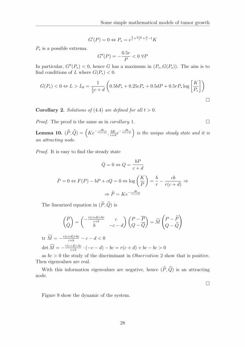
Figure 9 show the dynamic of the system.

28


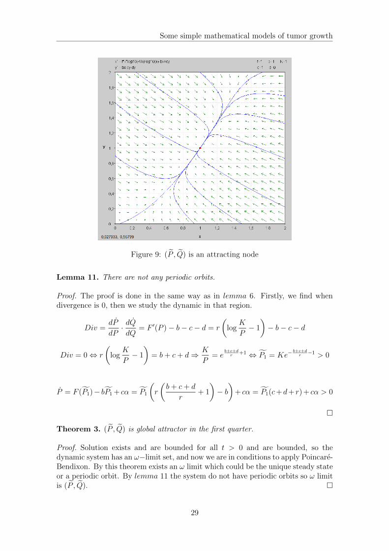
Figure 9: (P , Q) is an attracting node

Lemma 11. There are not any periodic orbits.

Proof. The proof is done in the same way as in lemma 6. Firstly, we find whendivergence is 0, then we study the dynamic in that region.

Div =dP

dP· dQdQ

= F ′(P )− b− c− d = r

(log

K

P− 1

)− b− c− d

Div = 0⇔ r

(log

K

P− 1

)= b+ c+ d⇒ K

P= e

b+c+dr

+1 ⇔ P1 = Ke−b+c+d

r−1 > 0

P = F (P1)− bP1 + cα = P1

(r

(b+ c+ d

r+ 1

)− b)

+ cα = P1(c+d+ r) + cα > 0

Theorem 3. (P , Q) is global attractor in the first quarter.

Proof. Solution exists and are bounded for all t > 0 and are bounded, so thedynamic system has an ω−limit set, and now we are in conditions to apply Poincare-Bendixon. By this theorem exists an ω limit which could be the unique steady stateor a periodic orbit. By lemma 11 the system do not have periodic orbits so ω limitis (P , Q).

29


This dynamics model is not studied in [1] but we find interesting to study thesame model (4.3) but with different R(P ).

Observation 6. Here comes an abstract of the biological conclusions:

The model reach to (P , Q) =(Ke−

dbr(c+d) , bK

c+de−

dbr(c+d)

)which is independently

from initial conditions.

db

r(c+ d)≥ 0⇒ − db

r(c+ d)≤ 0⇒ e−

dbr(c+d) ∈ (0, 1]⇒ P ∈ (0, K]

In the same way, Q = bPc+d∈(0, bK

c+d

]. Then

N = P + Q = P

(1 +

b

c+ d

)∈(

0, K

(1 +

b

c+ d

)]It is clear that N increases when the parameter b that controls the changes ofproliferative cells and N decreases as c the parameter that controls the changes ofquiescent and the death rate d of quiescent cells increases. N also increases whenK the maximal tumor size increases. Moreover, N increases when d

r<< 1. Our

final conclusions are the same with the logistic power model.

30


4.4 Cytotoxic and cytostatic drugs

Here we will analyze the next model:

P = F (P )− (b+ cstat)P + cQ− ctoxP, proliferative cells

Q = (b+ cstat)P − cQ− dQ, quiescent cells(4.5)

Where F (P ) is the same as in subsection 4.2 Logistic Power. Also r > 0, a > 0,K >, b > 0, c > 0,cstat > 0, ctox and d ≥ 0.

To simplify the study of the model we will consider b1 = b+ cstat + ctox > 0 andb2 = b+ cstat > 0. But the final results are expressed in the notation of (4.5).

P = F (P )− b1P + cQ, proliferative cells

Q = b2P − cQ− dQ, quiescent cells(4.6)

As in the other cases we will begin studying the positivity of the first quadrant.


P 0 > 0, Q0 > 0⇒ P (t) > 0, Q(t) > 0 ∀t > 0

Proof. It is proved in Observation 1 we just have to change b by b1 in the firstequation and b by b2 in the second equation.

Here we find a positively invariant triangle to proof that solutions are defined forall t > 0. As in the other cases the aim is to find a slope m ∈ (0,∞) for a straightline Q = L−mP and conditions of L ∈ (0,∞) where the dynamic of this line, thatwould be transversal to the model, head inside the rectangle. In other words,⟨(

P , Q), (m, 1)

⟩< 0

Then,

g(P ) =⟨(P , Q

), (m, 1)

⟩= −cL−dL+cLm+b2P−b1mP+cmP+dmP−cm2P+mF [P ]

Then g(0) = −cL− dL+ cLm so this is exactly the same as for the first model wehave studied so we propose m = 0.5

Lemma 13. Let

L0 =P∗

0.5c+ d

(−0.5b1 + b2 + 0.25c+ 0.5d+ 0.5r − 0.5

(P∗K

)a

r

)> 0

with P∗ = K(−2b1+4b2+c+2d+2r

(2+2a)r

) 1a. Then ∀L > L0, ∀P ∈ (0, 2L) and and Q =

L− 0.5P : ⟨(P , Q

)(1

2, 1

)⟩< 0

31


Proof. The proof is the same as in lemma 2 but with one difference, now G1(P )will be:

−0.5cL− dL− 0.5b1P + b2P + 0.25cP + 0.5dP + 0.5Pr − 0.5P

(P

K

)a

r

We just have to substitute the parameter 0.5b in G(P ) by −0.5b1 + b2.


Lemma 14. The point (0, 0) is always a steady state. And when (b+cstat+ctox)d <(c+ d)r − cctox we have another fixed point

(P ,Q) =

(K a

√1− (b+ cstat + ctox)d+ cctox

r(c+ d),(b+ cstat)K

c+ da

√1− (b+ cstat + ctox)d+ cctox

r(c+ d)

)

in the first quadrant.

Proof. We have steady states when P = 0 and Q = 0.

Q = 0⇔ Q =b2P

c+ d

P = 0⇔ P

(r

(1− P

K

)a

− b1 +cb2c+ d

)= 0⇒

P = 0 or P =

(K a

√1 +−b1d+ c(b2 − b1)

r(c+ d)

)So (0, 0) is a steady state and when 1 + −b1d+c(b2−b1)

r(c+d)> 0 we have another steady

state (P , b2Pc+d

)

1 +−b1d+ c(b2 − b1)

r(c+ d)> 0⇔ b1d < (c+ d)r + c(b2 − b1)

Next point is classify the steady states.

Lemma 15. The zero steady state (0, 0) is an attracting node if (b+ cstat + ctox)d >(c+ d)r − cctox

Proof. The linearized equation in (0, 0) is:(P

Q

)=

(r − b1 cb2 −c− d

)(PQ

)

So the characteristic polynomial is x2−(−b1−c−d+r)x+(r−b1)(−c−d)−b2c.Therefore the eigenvalues are:

32


λ =1

2

(−b1 − c− d+ r −

√(b1 + c+ d− r)2 − 4[(r − b1)(−c− d)− b2c]

)µ =

1

2

(−b1 − c− d+ r +

√(b1 + c+ d− r)2 − 4[(r − b1)(−c− d)− b2c]

)First, we notice that as b2c > 0 then ∆ > 0 (proved in Observation 2), hence the

eigenvalues are real.

It is time to analyze the sign of λ and µ, therefore we will analyze (r− b1)(−c−d)− b2c = b1c− b2c+ b1d− cr − dr = (b1 − b2)c+ b1d− (c+ d)r

(b1 − b2)c+ b1d− (c+ d)r > 0⇔ b1d > (c+ d)r + (b2 − b1)c

In the meanwhile

(b1 − b2)c+ b1d− (c+ d)r > 0⇔ −4((b1 − b2)c+ b1d− (c+ d)r) < 0⇒

⇒√

(b1 + c+ d− r)2 − 4((b1 − b2)c+ b1d− (c+ d)r) < |b1 + c+ d− r|

Moreover, when b1d > (c+ d)r + (b2 − b1)c(⇒ r < b1d+(b1−b2)c

c+d

)we have:

−b1 − c− d+ r < −b1 − c− d+b1d+ (b1 − b2)c

c+ d=

=−b1(c+ d)− (c+ d)2 + b1d+ (b1 − b2)c

c+ d=−(c+ d)2 − b2c

c+ d< 0

So we conclude

0 > −b1 − c− d+ r >√

(b1 + c+ d− r)2 − 4((b1 − b2)c+ b1d− (c+ d)r)

then µ is negative.

In summary when b1d > (c+ d)r+ c(b2− b1), λ and µ are negative then the zerosteady state is an attracting node. We can see the dynamic in Figure 10.

Lemma 16. If (b+ cstat + ctox)d < (c+ d)r− cctox the zero steady state is a saddlepoint and the stable manifold is not in the first quadrant. Moreover, the other steadystate (P ,Q) is an attracting node.

Proof. Using the notation of the previous lemma, we have:

λ =1

2

(−b1 − c− d+ r −

√(b1 + c+ d− r)2 − 4[(r − b1)(−c− d)− b2c]

)µ =

1

2

(−b1 − c− d+ r +

√(b1 + c+ d− r)2 − 4[(r − b1)(−c− d)− b2c]

)We proceed in the same way as in the previous lemma

(b1 − b2)c+ b1d− (c+ d)r < 0⇔ b1d < (c+ d)r + (b2 − b1)c

33


In fact,

(b1 − b2)c+ b1d− (c+ d)r < 0⇔ −4((b1 − b2)c+ b1d− (c+ d)r) > 0⇒

⇒√

(b1 + c+ d− r)2 − 4((b1 − b2)c+ b1d− (c+ d)r) > |b1 + c+ d− r|

And now we differentiate two cases:

• b1 + c+ d− r > 0

b1 + c+ d− r > 0⇔ −b1 − c− d+ r < 0⇒

⇒√

(b1 + c+ d− r)2 − 4((b1 − b2)c+ b1d− (c+ d)r) > −b1−c−d+r ⇒ µ > 0

In this case, λ is negative.

• b+ c+ d− r < 0

b1 + c+ d− r < 0⇔ −b1 − c− d+ r > 0⇒√(b1 + c+ d− r)2 − 4((b1 − b2)c+ b1d− (c+ d)r) > −b1−c−d+r ⇒ λ < 0

In this case, µ is positive.

Overall, when b1d < (c + d)r + c(b2 − b1): λ is negative and µ is positive then thezero steady state is a saddle point.

Now we will study the eigenvector of λ (which is the stable manifold becauseλ < 0):

(−b1 − c− d− r +

√b21 − 2b1c+ 4b2c+ c2 − 2b1d+ 2cd+ d2 − 2b1r + 2cr + 2dr + r2

2b2, 1

)= (u, v)

We will see that u is negative so the eigenvector will not be in the first quadrant.

u = −b1 − c− d− r +√b21 − 2b1c+ 4b2c+ c2 − 2b1d+ 2cd+ d2 − 2b1r + 2cr + 2dr + r2

2b2=

=−b1 + c+ d+ r −

√b21 + 4b2c− 2b1(c+ d+ r) + (c+ d+ r)2

2b2=

=−b1 + c+ d+ r −

√4b2c+ (c+ d+ r − b1)

2b2

Looking at√

4b2c+ (c+ d+ r − b1) > −b1 +c+d+r, the last equality is clearlyless than 0.

Finally, we will see that the non-zero steady state is an attracting node whenb1d < (c+ d)r + (b2 − b1)c.

The linearized equation in (P ,Q) is:

34


(P

Q

)=

(−ar + b1d+(b1−b2)c

c+d(1 + a)− b1 c

b2 −c− d

)(P − PQ−Q

)= M

(P − PQ−Q

)We will use the next notation to define the eigenvalues:

tr M = −ar + b1d+(b1−b2)cc+d

(1 + a)− b1 − c− d

detM =(−ar + b1d+(b1−b2)c

c+d(1 + a)− b1

)(−c− d)− cb2 = ar(c+ d)− a(−b2c+

b1(c+ d))

The characteristic polynomial of M is: x2 − (tr M)x+ detM . Then, the eigen-values are:

γ =1

2

(tr M +


)η =

1

2

(tr M −


)γ and η are real because ∆ > 0, it is proved in Observation 2.

Moreover, we study detM to classify γ and η.

detM > 0⇔ ar(c+ d)− a(−b2c+ b1(c+ d)) > 0⇔ b1d < (c+ d)r + c(b2 − b1)

Then detM > 0⇒ −4 detM < 0√(tr M)2 − 4 detM < |tr M |

In addition, we should observe when b1d < (c + d)r + c(b2 − b1) ⇒ tr M < 0.Because b1d < (c+ d)r + c(b2 − b1)⇔ detM > 0 and now we have:

tr M = −ar +b1d+ (b1 − b2)c

c+ d(1 + a)− b1 − c− d < −

cb

c+ d− c− d < 0

So,√

(tr M)2 − 4 detM < tr M ⇒ γ < 0 and as tr M < 0 and

−√

(tr M)2 − 4 detM < 0 then η < 0.

To sum up when b1d < (c + d)r + c(b2 − b1), γ and η are negative, thus thenon-zero steady state is an attracting node. We can see the dynamic in Figure 12.

Observation 7. When (b+cstat +ctox)d = (c+d)r−cctox the non zero steady statebecame the zero steady state. Moreover, γ = 0 and η < 0 then the steady state isnot hyperbolic. We can see the dynamic in Figure 11.

Figures 10, 11 and 12 show the transition between the conditions in parameters.We can see the dynamic in each case, red points are steady states,blue lines areorbits, green arrows are tangent vectors of the orbits and red and orange curves arenullclines. We can observe that there could not be periodic orbits by the nullclines.

35


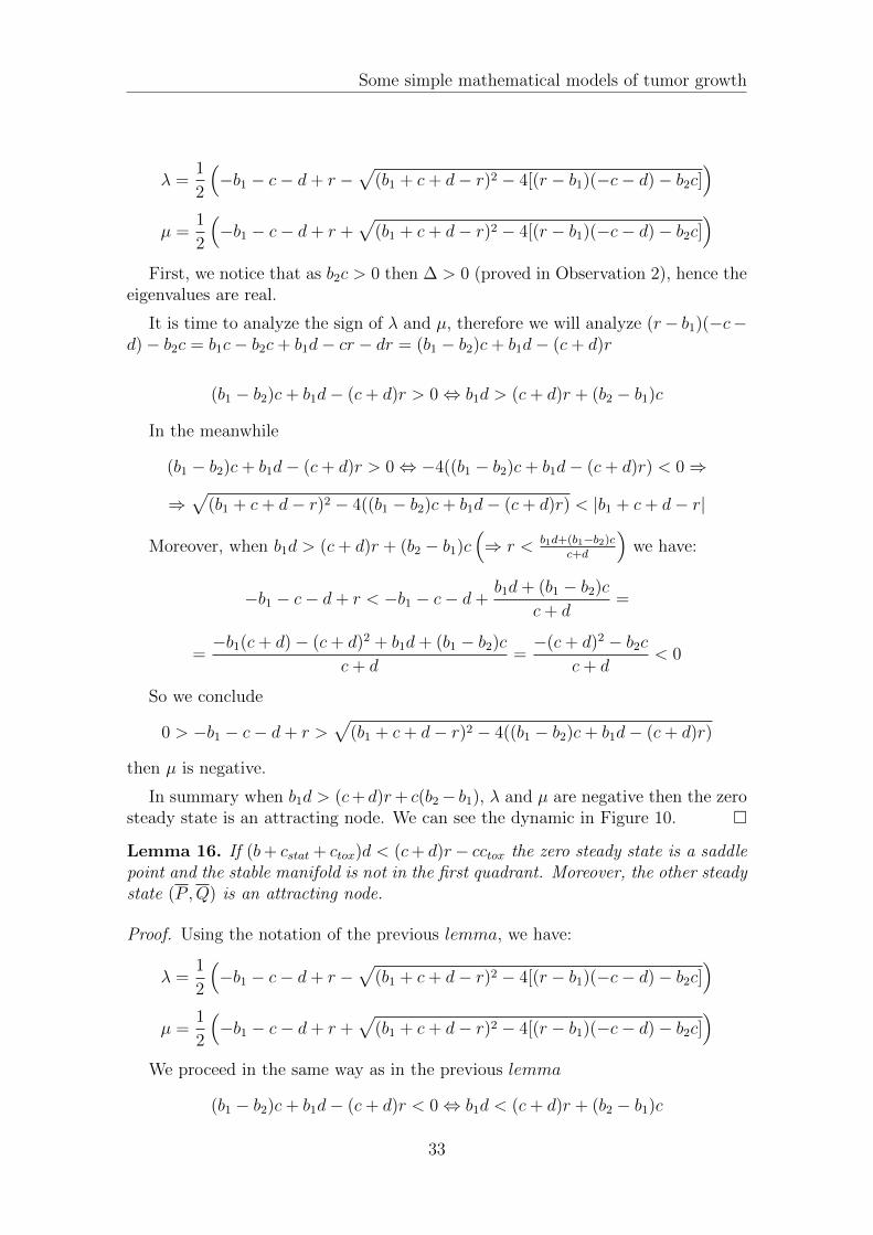
Figure 10: (b+ cstat + ctox)d > (c+ d)r − cctox

Figure 11: (b+ cstat + ctox)d = (c+ d)r − cctox

36


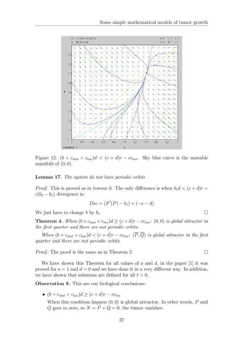
Figure 12: (b + cstat + ctox)d < (c + d)r − cctox. Sky blue curve is the unstablemanifold of (0, 0).

Lemma 17. The system do not have periodic orbits

Proof. This is proved as in lemma 6. The only difference is when b1d < (c+ d)r +c(b2 − b1) divergence is:

Div = (F ′(P )− b1) + (−c− d)

We just have to change b by b1.

Theorem 4. When (b+ cstat + ctox)d ≥ (c+ d)r− cctox: (0, 0) is global attractor inthe first quarter and there are not periodic orbits.

When (b+ cstat + ctox)d < (c+ d)r − cctox: (P ,Q) is global attractor in the firstquarter and there are not periodic orbits.

Proof. The proof is the same as in Theorem 2

We have shown this Theorem for all values of a and d, in the paper [1] it wasproved for a = 1 and d = 0 and we have done it in a very different way. In addition,we have shown that solutions are defined for all t > 0.

Observation 8. This are our biological conclusions:

• (b+ cstat + ctox)d ≥ (c+ d)r − cctoxWhen this condition happen (0, 0) is global attractor. In other words, P andQ goes to zero, so N = P +Q = 0, the tumor vanishes.

37


• (b+ cstat + ctox)d < (c+ d)r − cctoxWith this condition the model reach to the non zero steady state (P ,Q) =(K a

√1− bd

r(c+d)− (cstat+ctox)d+cctox

r(c+d), (b+cstat)

c+dP)

, it is independently from initial

conditions.

As we have (b+ cstat + ctox)d < (c+ d)r − cctox then

a

√1− bd

r(c+ d)− (cstat + ctox)d+ cctox

r(c+ d)∈ (0, 1)⇒

⇒ P ∈ (0, K)⇒ Q ∈(

0,(b+ cstat)K

c+ d

)And N = P +Q = K a

√1− (b+cstat)d

r(c+d)− ctox

r

(1 + (b+cstat)

c+d

)so N ∈

(0, K

(1 + (b+cstat)K

c+d

)).

It is clear that cytotoxic drugs are always efficient (because when ctox increases,N decreases. Moreover, when cstat or b + cstat increases, N increases, but infact the cells that increases are the quiescent ones. N decreases as c theparameter that controls the changes of quiescent and the death rate d ofquiescent cells increases. Obviously, N also increases when K the maximaltumor size increases. Also, N increases when d

r<< 1.

38


4.5 Tumor growth under angiogenic control

Now, we will analyze the next dynamical system

d

dtN = bN log

(K

N

)d

dtK = cN(t)− dN2/3K

(4.7)

with b > 0, c > 0 and d > 0. We should observe that (4.7) is continuous in (0, 0)but it is not C1 in this point. Moreover, the phase space is (N > 0, K > 0).

In this case, we will begin with the study of nullclines, it will help us for followinglemmas and to study the general behavior.

Lemma 18. Horizontal nullclines on the curve K = cdN1/3 are −→ when N ∈(

0,(cd

)3/2)and ←− when N ∈

((cd

)3/2,∞)

.

Proof. The process to find nullclines or zero-growth isoclines is to calculate curveswhere K is 0 and then work out the dynamic N in this curve and finally study this’new’ N to determine which is the direction of the nullcline.

K = 0⇔ K =c

dN1/3

Now, substituting K = cdN1/3 in N we obtain:

N = bN log( cdN−2/3

)(bN log

(cdN−2/3, 0

))is the vector of the field in general points

(N, c

dN1/3

). We

will analyze bN log(cdN−2/3

)to determine the direction of the nullclines.

bN log( cdN−2/3

)= 0⇔ N = 0 or N =

( cd

)3/2as we assume N > 0, negative solution is not considered.

limN→∞

bN log( cdN−2/3

)= −∞

f(N) = bN log(cdN−2/3

)with N ≥ 0 is a function with two zeros N = 0 and

N =(cd

)3/2. The limit when N → ∞ is −∞ the image for N ∈

((cd

)3/2,∞)

will

be negative so nullclines would be←−. Finally, to determine which is the image for(0,(cd

)3/2)is enough to calculate which is the sign of one point in that interval:

f(1

2·( cd

)3/2) = b

1

2

( cd

)3/2log(22/3

)> 0

as it is positive for N ∈(

0,(cd

)3/2)f(N) will be positive and nullclines would be

−→. Horizontal nullcline is the orange curve in Figure 13.

39


Lemma 19. Vertical nullclines on the curve N = K(c − dK2/3) are ↑ when K ∈((0, c

d

)3/2)and ↓ when N ∈

((cd

)3/2,∞)

.

Proof. The process to find nullclines or zero-growth isoclines is to calculate curveswhere N is 0 and then work out the dynamic K in this curve and finally study this’new’ K to determine which is the direction of the nullcline.

N ⇔ bN log

(K

N

)= 0⇔ N = 0 or log

(K

N

)= 0

N=0 then K = 0 so (0, 0) is the vector field on general points (0, K) then N = 0 isan invariant straight line.

log(KN

)= 0 ⇔ N = K. Then K = K(c − dK2/3), vector (0, K(c − dK2/3)) of

the field in (K,K). Next step is analyze g(K) = K(c− dK2/3):

g(K) = 0⇔ K = 0 or K =( cd

)3/2as we assume K > 0, negative solution is not considered.

limK→∞

K(c− dK2/3) = −∞

g(K) with K ≥ 0is a function with two zeros. As the limit when K → ∞ of g is

−∞ then the image for K ∈ ((cd

)3/2,∞) is negative, then nullclines on N = K will

be ↓. As there are only two zeros in g(K): 0 and(cd

)3/2. To determine the sign of

the image in that interval is enough to calculate which is the sign of the image ofone point in that interval:

g

(1

2·( cd

)3/2)=

1

2·( cd

)3/2(c−

(1

2

)2/3

c

)> 0

Then for K ∈ (0,(cd

)3/2) nullclines on N = K will be ↑. Vertical nullcline is the red

curve in Figure 13.

This will help us to study the existence of solutions.


N0 > 0, K0 > 0⇒ N(t) > 0, K(t) > 0 ∀t ∈ [0, t+(N0, K0)[

Proof. By lemma 19 N = K is the vertical nullcline. We will see that dynamic ofN in K > N > 0 is positive.

N = bN log

(K

N

)as K > N ⇔ K

N> 1⇔ log K

N> 0⇔ N > 0

40


In the same way, horizontal nullclines are K = cdN1/3 by lemma 18, so we will

analyze the dynamic of K in the region K < cdN1/3.

K = cN − dN2/3K > cN − dN2/3 c

dN1/3 = cN − cN = 0

Solutions of (4.7) are defined ∀t ∈ [0, t+(P 0, Q0)[. Another interesting study isto find positively invariant regions, it will provide us that solutions are defined forall t > 0.

Lemma 21. Regions K ≥ N ∩ K ≤ cdN1/3 and K ≤ N ∩ K ≥ c

dN1/3 are

positively invariant.

Proof. Directions of the nullclines K = N and K = cdN1/3 head inside this region,

so all orbits that goes through a nullcline stay inside this region.

Corollary 4. Solutions are defined for all t > 0.

Proof. We study K when cdN1/3 < K:

c

dN1/3 < K ⇔ K = cN − dN2/3K < 0

Also we study N when K < N

K < N ⇔ K

N< 1⇔ log

(K

N

)< 0⇔ N < 0

So it is possible to construct a positively invariant rectangle with K >(cd

)3/2,

N >(cd

)3/2and N 6= K(this is to avoid the point N = K as it is a vertical nullcline

N = 0) where all the solutions head inside the rectangle.

The next step is to find steady states and the behavior.

Lemma 22. (N , K) =((

cd

)3/2,(cd

)3/2)is the unique steady state and it is an

attracting node.

Proof. Steady states are the intersection of nullclines, then we have the system:K = c

dN1/3

K = N

as K > 0 and N > 0, the solution is K = N =(cd

)3/2Subsequently, we will see that it is an attracting node.

The linearized equation in (N , K) is:(N

K

)=

(−b b13c −c

)(N − NK − K

)= M

(N − NK − K

)

41


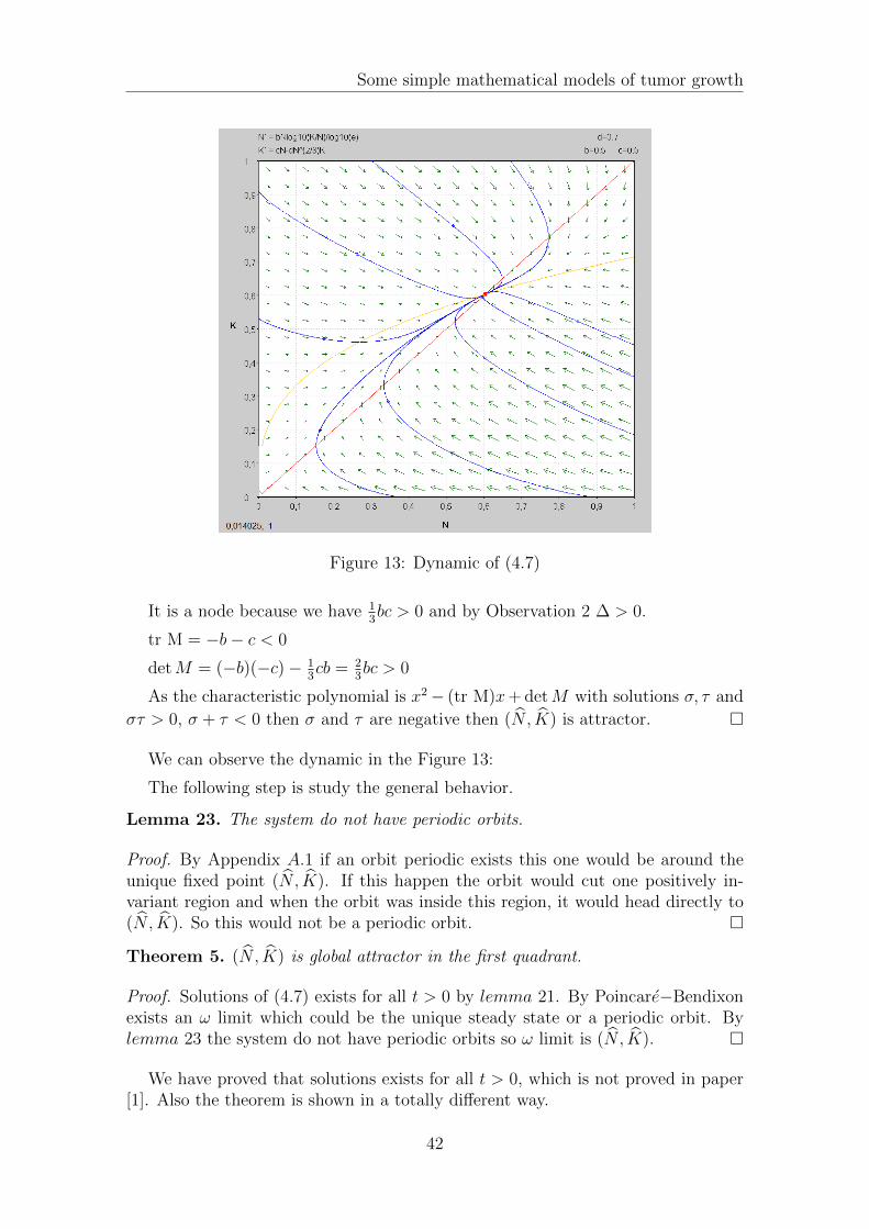
Figure 13: Dynamic of (4.7)

It is a node because we have 13bc > 0 and by Observation 2 ∆ > 0.

tr M = −b− c < 0

detM = (−b)(−c)− 13cb = 2

3bc > 0

As the characteristic polynomial is x2− (tr M)x+ detM with solutions σ, τ and

στ > 0, σ + τ < 0 then σ and τ are negative then (N , K) is attractor.

We can observe the dynamic in the Figure 13:

The following step is study the general behavior.

Lemma 23. The system do not have periodic orbits.

Proof. By Appendix A.1 if an orbit periodic exists this one would be around theunique fixed point (N , K). If this happen the orbit would cut one positively in-variant region and when the orbit was inside this region, it would head directly to(N , K). So this would not be a periodic orbit.

Theorem 5. (N , K) is global attractor in the first quadrant.

Proof. Solutions of (4.7) exists for all t > 0 by lemma 21. By Poincare−Bendixonexists an ω limit which could be the unique steady state or a periodic orbit. Bylemma 23 the system do not have periodic orbits so ω limit is (N , K).

We have proved that solutions exists for all t > 0, which is not proved in paper[1]. Also the theorem is shown in a totally different way.

42


Observation 9. Biological conclusions

The model reach to the non zero steady state (N , K) =((

cd

)3/2,(cd

)3/2)by the

passing of time and it is independently from initial conditions. From this pointwe can conclude that number of cells and carrying vasculature increases when cincreases and decreases when d increases.

43


5 Conclusion

To begin with, I would like to emphasize the choice of the subject was the best Icould select. I did not know almost anything about it, nevertheless, I am pleasedto say I have learnt a lot from it as well as it has inspired me a desire to find outmore about cancer. In addition, I feel satisfied at mathematical level, it is trueit is always possible to work more, but it is also true the study of cancer is veryextensive, so there are an infinity of works about this topic, mainly specialized inalmost every type of cancer. That is the reason reaching the whole points in theproject could be a very difficult task.

Overall, I have consolidate and broaden the knowledge of modelling and differ-ential equations. Furthermore, I have been able to practice English and to increasemy scientific vocabulary. To finish, I would like to highlight the elaboration of thisfinal project has helped me to achieve an improvement of mathematical and writinglanguage skills.

Acknowledgments

I also think the choice of my tutor Alex Haro was very adequate. He alwayshelped me very much and thanks to him I believe I have become much more self-sufficient and proactive, that is why I wish to acknowledge him. Moreover, I wouldlike to thank my family and friends for supporting me throughout this project.

44


A General results of differential equations

A.1 Properties of an α− ω limit set

Firstly, we will define what is a α−ω limit set of an orbit. Let be X : U ⊂ Rn −→ Rn

a vector field, Cr (with r ≥ 1). And let be x ∈ U :

•

ω(x) =y ∈ U |∃(tn)n +∞ : lim

n→∞φ(tn, x) = y

= ∩t>0φ([t,+∞[, x)

•α(x) =

y ∈ U |∃(tn)n −∞ : lim

n→∞φ(tn, x) = y

Theorem 6. Let X : U ⊂ Rn → Rn a vector field, Cr (with r ≥ 1). And let bex ∈ U with [0,∞[⊂ I(x), and it is supposed that exists a compact K ⊂ U withγ(x) = φ(t, x)|t ∈ [0,∞[ ⊂ K. Then ω(x) is:

• not empty

• compact

• connected

• invariant by X.

A.2 Bendixon criterion

A theorem that permits one to establish the absence of closed trajectories of dy-namical systems in the plane, defined by the equation

x′ = P (x, y), y′ = Q(x, y). (A.1)

The criterion was first formulated by I. Bendixson as follows: If in a simply-connected domain G the expression P ′x +Q′y has constant sign (i.e. the sign remainsunchanged and the expression vanishes only at isolated points or on a curve), thenthe system A.1 has no closed trajectories in the domain G.

A.3 Poincare-Bendixon theorem

Theorem 7. Let be X : U ⊂ R2 −→ R2 a vectorial field, Cr (with r ≥ 1). And letbe x ∈ U , we suppose that:

1. γ+(x) ⊂ K ⊂ U,with K compact

2. X has a finit number of fixed points in ω(x)

45


Then

a If ω(x) does not have fixed points then ω(x) is a periodic orbit.

b If ω(x) have only fixed points then ω(x) is a fixed point.

c If ω(x) has singular and regular points then ω(x) is the union of fixed points andthe orbits that connect them.

A.4 Picard’s existence theorem

If f is continuous function that satisfies the Lipschitz condition |f(x, t)− f(y, t)| ≤L|x−y| in a surrounding of (x0, t0) ∈ Ω ⊂ Rn×R = (x, t) : |x−x0| < b, |t−t0| < a,then the differential equation

dx

dt= f(x, t)

x(t0) = x0

has a unique solution x(t) in the interval |t − t0| < d, where d = min(a, b/B),B = sup|f(t, x)|.

A.5 Peano existence theorem

Let be an open substet R × R with f : D → R a continuous function and y′(x) =f(x, y(x)) a continuous, explicit first-order differential equation defined on D, thenevery initial value problem y(x0) = y0 for f with (x0, y0) ∈ D has a local solutionz : I → R where I is a neighbourhood of x0 ∈ R, such that z′(x) = f(x, z(x)) forall x ∈ I

The solution need not be unique: one and the same initial value (x0, y0) maygive rise many different solutions z.

46


References

[1] Benoıt Perthame, Some mathematical models of tumor growth. Universite Pierreet Marie Curie-Paris 6, Paris, 2014.

[2] Philip Hahnfeldt, Dipak Panigrahy, Judah Folkman and Lynn Hlatky, Tu-mor Development under Angiogenic Signaling: A Dynamical Theory of Tu-mor Growth, Treatment Response, and Postvascular Dormancy. Department ofAdult Oncology, Dana-Farber Cancer Institute and Joint Center for RadiationTherapy [P. H., L. H.], and Division of Pediatric Surgery, Children’s Hospital[D. P., J. F.], Harvard Medical School, Boston, Massachusetts, 1999.

[3] Benjamin Ribba, A Tumor Growth Inhibition Model for Low-Grade GliomaTreated with Chemotherapy or Radiotherapy. PhD thesis University of Aix-Marseille, Paris, 2011.

[4] Sebastien Benzekry, Modeling and mathematical analysis of anti-cancer ther-apies for metastatic cancers. INRIA, Project-team NUMED, Ecole NormaleSuperieure de Lyon 1999.

[5] Amit Zeisel and Hadas Cohen-Dvashi, Diurnal suppression of EGFR sig-nalling by glucocorticoids and implications for tumour progression and treatment.Karolinska Institutet, Weizmann Institute of Science, 2014.

[6] Doroty I.Wallace and Xinyue Guo Properties of Tumor Spheroid Growth Exhib-ited by Simple Mathematical Models. Department of Mathematics, DartmouthCollege, Hanover, NH, USA, 2013.

[7] Alex Haro, Apuntes de la asignatura ecuaciones diferenciales. Universitat deBarcelona, Spain, 2013.

[8] National Cancer Institute, What is cancer? Types , www.cancer.gov,www.aecc.es

[9] Sociedad Espanola de Oncologıa Medica, Las Cifras del Cancer en Espana 2014.2014.

[10] Instituto Nacional de Estadıstica, Notas de prensa: Defunciones segun laCausa de Muerte. 2014.

47