
UNIVERSIDAD TÉCNICA DE AMBATO FACULTAD …repositorio.uta.edu.ec/bitstream/123456789/24788/1/Tesis...
297
UNIVERSIDAD TÉCNICA DE AMBATO FACULTAD DE INGENIERÍA CIVIL Y MECÁNICA CARRERA DE INGENIERÍA CIVIL TRABAJO EXPERIMENTAL PREVIO A LA OBTENCIÓN DEL TÍTULO DE INGENIERO CIVIL Tema: “ CÁLCULO DEL DIAGRAMA MOMENTO – CURVATURA POR EL MÉTODO DE FIBRAS PARA SECCIONES DE HORMIGÓN ARMADO Y PERFILES DE ACERO EMPLEANDO UN SOFTWARE DE PROGRAMACIÓN ESPECIALIZADO.” AUTOR: JOSÉ CARLOS FREIRE NAVAS. TUTORA: Ing. Mg. CHRISTIAN MEDINA Ambato – Ecuador 2017
Transcript of UNIVERSIDAD TÉCNICA DE AMBATO FACULTAD …repositorio.uta.edu.ec/bitstream/123456789/24788/1/Tesis...

UNIVERSIDAD TÉCNICA DE AMBATO
FACULTAD DE INGENIERÍA CIVIL Y MECÁNICA
CARRERA DE INGENIERÍA CIVIL
TRABAJO EXPERIMENTAL PREVIO A LA OBTENCIÓN DEL
TÍTULO DE INGENIERO CIVIL
Tema:
“CÁLCULO DEL DIAGRAMA MOMENTO – CURVATURA POR EL
MÉTODO DE FIBRAS PARA SECCIONES DE HORMIGÓN ARMADO Y
PERFILES DE ACERO EMPLEANDO UN SOFTWARE DE
PROGRAMACIÓN ESPECIALIZADO.”
AUTOR: JOSÉ CARLOS FREIRE NAVAS.
TUTORA: Ing. Mg. CHRISTIAN MEDINA
Ambato – Ecuador
2017

II
CERTIFICACIÓN DEL TUTOR
Yo, Ing. Mg. Christian Medina, Certifico que el presente trabajo bajo el tema:
“CÁLCULO DEL DIAGRAMA MOMENTO – CURVATURA POR EL MÉTODO
DE FIBRAS PARA SECCIONES DE HORMIGÓN ARMADO Y PERFILES DE
ACERO EMPLEANDO UN SOFTWARE DE PROGRAMACIÓN
ESPECIALIZADO” es de autoría del Sr. José Carlos Freire Navas, el mismo que ha
sido realizado bajo mi supervisión y tutoría.
Es todo cuanto puedo certificar en honor a la verdad.
Ambato, Enero del 2017
________________________________
Ing. Mg. Christian Medina.
III
AUTORÍA
Yo, José Carlos Freire Navas con C.I: 180446493-9, egresado de la Facultad de
Ingeniería Civil y Mecánica de la Universidad Técnica de Ambato, certifico por medio
de la presente que el trabajo con el tema: “CÁLCULO DEL DIAGRAMA
MOMENTO – CURVATURA POR EL MÉTODO DE FIBRAS PARA SECCIONES
DE HORMIGÓN ARMADO Y PERFILES DE ACERO EMPLEANDO UN
SOFTWARE DE PROGRAMACIÓN ESPECIALIZADO”, es de mi completa
autoría.
Ambato, Enero del 2017
________________________________
José Carlos Freire Navas.

IV
DERECHOS DE AUTOR
Autorizo a la Universidad Técnica de Ambato, para que haga de este Trabajo
Experimental o parte de él, un documento disponible para su lectura, consulta y
procesos de investigación, según las normas de la Institución.
Cedo los Derechos en línea patrimoniales de mi Trabajo Experimental con fines de
difusión pública, además apruebo la reproducción de éste Trabajo Experimental dentro
de las regulaciones de la Universidad, siempre y cuando ésta reproducción no suponga
una ganancia económica y se realice respetando mis derechos de autor.
Ambato, Enero del 2017
Autor
________________________________
Freire Navas José Carlos
V
APROBACIÓN DEL TRIBUNAL DE GRADO
Los miembros del tribunal examinador aprueban el informe de investigación, sobre el
tema: “CÁLCULO DEL DIAGRAMA MOMENTO – CURVATURA POR EL
MÉTODO DE FIBRAS PARA SECCIONES DE HORMIGÓN ARMADO Y
PERFILES DE ACERO EMPLEANDO UN SOFTWARE DE PROGRAMACIÓN
ESPECIALIZADO”, del egresado José Carlos Freire Navas de la Facultad de
Ingeniería Civil y Mecánica.
Ambato, Enero del 2017.
Para constancia firman.
Ing. Mg. Juan Garcés Ing. Mg. Jorge Cevallos
VI
DEDICATORIA
A DIOS, por haberme permitido alcanzar una de mis metas.
A mi Querido Padre, por ser siempre un maestro, por compartir momentos de alegría
y tristeza y más que todo compartir todos sus conocimiento.
A mi Querida Madre, por siempre una amiga y un apoyo incondicional en cada etapa
de mi vida.
A mi Querida Hermana, por siempre brindarme su amor y cariño, tú siempre serás la
razón y el motivo de todos mis esfuerzos.
A mis Queridas tíos que han sido una segunda madre, que han estado con migo desde
la niñez y me han brindado un poco de su amor.

VII
AGRADECIMIENTO
A DIOS, por siempre ser mi fortaleza en cada momento de mi vida.
A mis PADRES, por haberme dado la vida y siempre haber sido mi apoyo
incondicional.
A mi HERMANA, por haberme ayudado en la realización de este proyecto.
A cada uno de los integrantes de mi FAMILIA, por brindarme su apoyo que va más
allá del deber.
A mi Tutor Ing. Christian Medina por su asesoría y enseñanza de conocimientos en la
consecución de este proyecto.
A mis AMIGOS, COMPAÑEROS y HERMANOS de toda la vida, por todo ese apoyo
incondicional.

VIII
ÍNDICE DE CONTENIDOS
A.- PAGINAS PRELIMINARES
UNIVERSIDAD TÉCNICA DE AMBATO.......................... ¡Error! Marcador no definido.
AUTORÍA...................................................................................................................III
DERECHOS DE AUTOR ........................................................................................... IV
APROBACIÓN DEL TRIBUNAL DE GRADO ...........................................................V
DEDICATORIA ......................................................................................................... VI
AGRADECIMIENTO................................................................................................VII
ÍNDICE DE CONTENIDOS .................................................................................... VIII
ÍNDICE DE FIGURAS ............................................................................................... XI
ÍNDICE DE TABLAS ................................................................................................ XV
GLOSARIO DE SIMBOLOS....................................................................................XVI
RESUMEN EJECUTIVO .........................................................................................XVI
B.- TEXTO
CAPÍTULO I ................................................................................................................ 1
ANTECEDENTES ........................................................................................................ 1
1.1 TEMA DEL TRABAJO EXPERIMENTAL .......................................................... 1
1.2 ANTECEDENTES .............................................................................................. 1
1.3 JUSTIFICACIÓN ................................................................................................ 3
1.4 OBJETIVOS: ...................................................................................................... 4
1.4.1 Objetivo General: ................................................................................................ 4
1.4.2 Objetivos Específicos: .......................................................................................... 4
CAPÍTULO II............................................................................................................... 5
FUNDAMENTACIÓN .................................................................................................. 5
2.1 FUNDAMENTACIÓN TEÓRICA ....................................................................... 5
2.1.1 Hormigón ............................................................................................................ 5
2.1.1.1 Modelo de Whitney.............................................................................................. 5
2.1.1.2 Modelo de Mander ............................................................................................... 6
2.1.1.2.1 Modelo de Mander para hormigón no confinado ............................................. 6
2.1.1.2.2 Modelo de Mander para hormigón confinado.................................................. 8
2.1.2 Acero .................................................................................................................12
2.1.2.1 Modelo elastoplástico..........................................................................................13
2.1.2.2 Modelo trilineal ..................................................................................................14
2.1.2.3 Modelo de curva completa...................................................................................14

IX
2.1.2.3.1 Modelo de Park y Paulay ..................................................................................15
2.1.3 Hormigón armado..................................................................................................15
2.1.4 Diagrama momento - curvatura ..............................................................................15
2.1.4.1 Curvatura ...........................................................................................................17
2.1.4.2 Construcción del diagrama momento - curvatura...................................................18
2.1.4.2.1 Método manual ...........................................................................................19
2.1.4.2.2 Método de fibras o dovelas...........................................................................22
2.1.4.2.3 Método para perfiles de acero .......................................................................23
2.1.5 Software de programación especializado ..............................................................26
2.2 HIPÓTESIS........................................................................................................27
2.3 SEÑALAMIENTO DE VARIABLES ..................................................................28
CAPÍTULO III ......................................................................................................... 289
METODOLOGÍA ..................................................................................................... 289
3.1 NIVEL O TIPO DE INVESTIGACIÓN ...............................................................29
3.2 POBLACIÓN Y MUESTRA ...............................................................................29
3.2.1 Población ...........................................................................................................29
3.2.2 Muestra ..............................................................................................................29
3.2.2.1 Tipos de secciones de hormigón armado...............................................................29
3.2.2.2 Tipos de secciones de perfiles de acero.................................................................29
3.3 OPERACIÓN DE VARIABLES..........................................................................30
3.3.1 Variable independiente ........................................................................................30
3.3.2 Variable dependiente...........................................................................................31
3.4 PLAN DE RECOLECCIÓN DE INFORMACIÓN ...............................................33
3.5 PLAN DE PROCESAMIENTO Y ANÁLISIS......................................................34
CAPÍTULO IV.......................................................................................................... 345
ANÁLISIS E INTERPRETACIÓN DE RESULTADOS ................................................ 345
4.1 RECOLECCIÓN DE DATOS .............................................................................35
4.1.1 Resolución manual..............................................................................................35
4.1.1.1 Diagrama momento – curvatura de una sección rectangular sometida a
flexocompresión. ...........................................................................................................35
4.1.1.1.1 Gráfico del diagrama momento – curvatura en el software de programación especializado .................................................................................................................50
4.1.1.1.2 Comparación del diagrama momento – curvatura en Sap2000.........................52
4.1.1.2 Diagrama momento – curvatura de una sección de perfil de acero W sometida a
flexocompresión. ...........................................................................................................58
X
4.1.1.2.1 Gráfico del diagrama momento – curvatura en el software de programación especializado .................................................................................................................66
4.1.1.2.2 Comparación del diagrama momento – curvatura en Sap2000.........................68
4.2 ANÁLISIS DE RESULTADOS...........................................................................73
4.2.1 Sección rectangular de hormigón armado sometido a flexocompresión. ..................73
4.2.2 Sección rectangular de hormigón armado sometido a flexión. ................................77
4.2.3 Sección circular de hormigón armado sometido a flexocompresión. .......................81
4.2.4 Sección W de perfil de acero sometido a flexocompresión. ....................................85
4.2.5 Sección W de perfil de acero sometido a flexión. ..................................................89
4.2.6 Sección C de perfil de acero sometido a flexocompresión. .....................................93
4.2.7 Sección C de perfil de acero sometido a flexión. ...................................................97
4.2.8 Sección tubo rectangular de perfil de acero sometido a flexocompresión............... 101
4.2.9 Sección tubo rectangular de perfil de acero sometido a flexión. ............................ 105
4.2.10 Sección tubo circular de perfil de acero sometido a flexocompresión. ................... 109
4.2.11 Sección tubo circular de perfil de acero sometido a flexión. ................................. 113
4.2.12 Sección ángulos de perfil de acero sometido a flexocompresión. .......................... 117
4.2.13 Sección ángulos de perfil de acero sometido a flexocompresión. .......................... 121
4.3 VERIFICACIÓN DE HIPÓTESIS ..................................................................... 125
CAPÍTULO V ........................................................................................................... 125
CONCLUSIONES Y RECOMENDACIONES.......................................................... 125
5.1 CONCLUSIONES ............................................................................................ 126
5.2 RECOMENDACIONES ................................................................................... 127
C.- MATERIALES DE REFERENCIA
1. BIBLIOGRAFÍA .............................................................................................. 128
2. ANEXOS ......................................................................................................... 130

XI
ÍNDICE DE FIGURAS
Figura 2. 1: Modelo de Whitney para el hormigón armado. ....................................... 6
Figura 2. 2: Modelo de Mander para el hormigón confinado y no confinado. ........... 7
Figura 2. 3: Forma esquemática el área de concreto confinado y no confinado de una
sección rectangular. .................................................................................................... 11
Figura 2. 4: Factor de confinamiento, "" para elementos cuadrados
y rectangulares............................................................................................................ 12
Figura 2. 5: Modelo elastoplástico para el acero. ..................................................... 13
Figura 2. 6: Modelo trilineal para el acero................................................................ 14
Figura 2. 7: Modelo de Park y Paulay para el acero. ................................................ 15
Figura 2. 8: Curvatura de un elemento...................................................................... 18
Figura 2. 9: Deformación de un modelo bilineal en función de la definición de la
rótula plástica. ............................................................................................................ 19
Figura 2. 10: Diagrama esfuerzo – deformación para diferentes tipos de acero
estructural. .................................................................................................................. 24
Figura 2. 11: Cálculo del diagrama momento – curvatura para perfiles de acero. ... 26
Figura 4. 1: Diagrama esfuerzo – deformación de la sección rectangular……………….35
Figura 4. 2: Diagrama esfuerzo – deformación del acero..................................................38
Figura 4. 3: Sección rectangular de hormigón armado .....................................................40
Figura 4. 4: Método de fibras para la zona de compresión en una sección rectangular de
hormigón armado. ..........................................................................................................44 Figura 4. 5: Método de fibras para la zona de tensión en una sección rectangular de
hormigón armado. ..........................................................................................................47
Figura 4. 6: Equilibrio de Fuerzas ..................................................................................48
Figura 4. 7: Diagrama momento – curvatura resolución manual. ......................................50
Figura 4. 8: Ingreso de datos en el software de programación especializado. .....................51
Figura 4. 9: Diagrama momento - curvatura en el software de programación especializado.
.....................................................................................................................................52
Figura 4. 10: Pantalla de inicio del software especializado. ..............................................53
Figura 4. 11: Pasos para definir el material. ....................................................................53
Figura 4. 12: Pantalla para definir el material. .................................................................54
Figura 4. 13: Pasos para definir la sección. .....................................................................55
Figura 4. 14: Pantalla para definir la sección. ..................................................................55
Figura 4. 15: Pantalla secundaria para definir la sección. .................................................56
Figura 4. 16: Diagrama momento – curvatura de la sección. ............................................56
Figura 4. 17: Diagrama esfuerzo – deformación de la sección de perfil de acero................58
Figura 4. 18: Sección de perfil de acero W24X103. ..........................................................58
Figura 4. 19: Diagrama esfuerzo – deformación del acero................................................59
Figura 4. 20: Fuerza de compresión o tracción por áreas ..................................................61
Figura 4. 21: Distancia hacia cada fuerza para el cálculo de momentos .............................63
Figura 4. 22: Diagrama momento – curvatura resolución manual. ....................................66
Figura 4. 23: Ingreso de datos en el software de programación especializado. ...................67

XII
Figura 4. 24: Diagrama momento - curvatura en el software de programación especializado.
.....................................................................................................................................68
Figura 4. 25: Pantalla para definir el material A36. .........................................................69
Figura 4. 26: Pasos para definir la sección. .....................................................................70
Figura 4. 27: Pantalla para definir la sección. ..................................................................70
Figura 4. 28: Pantalla secundaria para definir la sección. .................................................71
Figura 4. 29: Diagrama momento – curvatura de la sección. ............................................71
Figura 4. 30: Dimensiones de la sección rectangular sometido a flexocompresión. ............73
Figura 4. 31: Pantalla de introducción de datos en el Software para una sección rectangular
sometido a flexocompresión. ..........................................................................................74 Figura 4. 32: Diagrama momento – curvatura del Software para una sección rectangular
sometido a flexocompresión. ..........................................................................................75
Figura 4. 33: Pantalla de introducción de datos en el software especializado para una
sección rectangular sometido a flexocompresión. .............................................................76
Figura 4. 34: Diagrama momento – curvatura del software especializado. .........................76
Figura 4. 35: Diagrama momento – curvatura entre los dos Softwares. .............................77
Figura 4. 36: Dimensiones de la sección rectangular sometido a flexión. ..........................78 Figura 4. 37: Pantalla de introducción de datos en el Software para una sección rectangular
sometido a flexión. .........................................................................................................78
Figura 4. 38: Diagrama momento – curvatura del software para una sección rectangular
sometido a flexión. .........................................................................................................79 Figura 4. 39: Pantalla de introducción de datos software especializado para una sección
rectangular sometido a flexión. .......................................................................................80
Figura 4. 40: Diagrama momento – curvatura del software. .............................................80
Figura 4. 41: Diagrama momento – curvatura entre los dos softwares. ..............................81
Figura 4. 42: Dimensiones de la sección circular sometido a flexocompresión. .................82
Figura 4. 43: Pantalla de introducción de datos en el Software para una sección circular
sometido a flexocompresión. ..........................................................................................82 Figura 4. 44: Diagrama momento – curvatura del software para una sección circular
sometido a flexocompresión. ..........................................................................................83
Figura 4. 45: Pantalla de introducción de datos software especializado para una sección
circular sometido a flexocompresión. ..............................................................................84
Figura 4. 46: Diagrama momento – curvatura del software. .............................................84
Figura 4. 47: Diagrama momento – curvatura entre los dos softwares. ..............................85
Figura 4. 48: Dimensiones de la sección w sometido a flexocompresión. ..........................86 Figura 4. 49: Pantalla de introducción de datos en el Software para una sección W sometido
a flexocompresión. .........................................................................................................86
Figura 4. 50: Diagrama momento – curvatura del software para una sección W sometido a
flexocompresión. ...........................................................................................................87 Figura 4. 51: Pantalla de introducción de datos software especializado para una sección W
sometido a flexocompresión. ..........................................................................................88
Figura 4. 52: Diagrama momento – curvatura del software. .............................................88
Figura 4. 53: Diagrama momento – curvatura entre los dos softwares. ..............................89
Figura 4. 54: Dimensiones de la sección w sometido a flexión. ........................................90
Figura 4. 55: Pantalla de introducción de datos en el Software para una sección W sometido
a flexión. .......................................................................................................................90

XIII
Figura 4. 56: Diagrama momento – curvatura del software para una sección W sometido a
flexión...........................................................................................................................91
Figura 4. 57: Pantalla de introducción de datos software especializado para una sección W
sometido a flexión. .........................................................................................................92
Figura 4. 58: Diagrama momento – curvatura del software. .............................................92
Figura 4. 59: Diagrama momento – curvatura entre los dos softwares. ..............................93
Figura 4. 60: Dimensiones de la sección C sometido a flexocompresión. ..........................94 Figura 4. 61: Pantalla de introducción de datos en el Software para una sección C sometido
a flexocompresión. .........................................................................................................94
Figura 4. 62: Diagrama momento – curvatura del software para una sección C sometido a
flexocompresión. ...........................................................................................................95 Figura 4. 63: Pantalla de introducción de datos software especializado para una sección C
sometido a flexocompresión. ..........................................................................................96
Figura 4. 64: Diagrama momento – curvatura del software. .............................................96
Figura 4. 65: Diagrama momento – curvatura entre los dos softwares. ..............................97
Figura 4. 66: Dimensiones de la sección C sometido a flexión. ........................................98
Figura 4. 67: Pantalla de introducción de datos en el Software para una sección C sometido
a flexión. .......................................................................................................................98 Figura 4. 68: Diagrama momento – curvatura del software para una sección C sometido a
flexión...........................................................................................................................99
Figura 4. 69: Pantalla de introducción de datos software especializado para una sección C
sometido a flexión. ....................................................................................................... 100
Figura 4. 70: Diagrama momento – curvatura del software. ........................................... 100
Figura 4. 71: Diagrama momento – curvatura entre los dos softwares. ............................ 101
Figura 4. 72: Dimensiones de la sección tubo rectangular sometido a flexocompresión. ... 102 Figura 4. 73: Pantalla de introducción de datos en el Software para una sección tubo
rectangular sometido a flexocompresión. ....................................................................... 102
Figura 4. 74: Diagrama momento – curvatura del software para una sección tubo rectangular
sometido a flexocompresión. ........................................................................................ 103 Figura 4. 75: Pantalla de introducción de datos software especializado para una sección tubo
rectangular sometido a flexocompresión. ....................................................................... 104
Figura 4. 76: Diagrama momento – curvatura del software. ........................................... 104
Figura 4. 77: Diagrama momento – curvatura entre los dos softwares. ............................ 105
Figura 4. 78: Dimensiones de la sección tubo rectangular sometido a flexión. ................. 106
Figura 4. 79: Pantalla de introducción de datos en el Software para una sección tubo
rectangular sometido a flexión. ..................................................................................... 106 Figura 4. 80: Diagrama momento – curvatura del software para una sección tubo rectangular
sometido a flexión. ....................................................................................................... 107 Figura 4. 81: Pantalla de introducción de datos software especializado para una sección tubo
rectangular sometido a flexión. ..................................................................................... 108
Figura 4. 82: Diagrama momento – curvatura del software. ........................................... 108
Figura 4. 83: Diagrama momento – curvatura entre los dos softwares. ............................ 109
Figura 4. 84: Dimensiones de la sección tubo circular sometido a flexocompresión. ........ 110 Figura 4. 85: Pantalla de introducción de datos en el Software para una sección tubo circular
sometido a flexocompresión. ........................................................................................ 110

XIV
Figura 4. 86: Diagrama momento – curvatura del software para una sección tubo circular
sometido a flexocompresión. ........................................................................................ 111
Figura 4. 87: Pantalla de introducción de datos software especializado para una sección tubo
circular sometido a flexocompresión. ............................................................................ 112
Figura 4. 88: Diagrama momento – curvatura del software. ........................................... 112
Figura 4. 89: Diagrama momento – curvatura entre los dos softwares. ............................ 113
Figura 4. 90: Dimensiones de la sección tubo circular sometido a flexión. ...................... 114 Figura 4. 91: Pantalla de introducción de datos en el Software para una sección tubo circular
sometido a flexión. ....................................................................................................... 114
Figura 4. 92: Diagrama momento – curvatura del software para una sección tubo circular
sometido a flexión. ....................................................................................................... 115 Figura 4. 93: Pantalla de introducción de datos software especializado para una sección tubo
circular sometido a flexión............................................................................................ 116
Figura 4. 94: Diagrama momento – curvatura del software. ........................................... 116
Figura 4. 95: Diagrama momento – curvatura entre los dos softwares. ............................ 117
Figura 4. 96: Dimensiones de la sección ángulo sometido a flexocompresión.................. 118
Figura 4. 97: Pantalla de introducción de datos en el Software para una sección ángulo
sometido a flexocompresión. ........................................................................................ 118 Figura 4. 98: Diagrama momento – curvatura del software para una sección ángulo
sometido a flexocompresión. ........................................................................................ 119
Figura 4. 99: Pantalla de introducción de datos software especializado para una sección
ángulo sometido a flexocompresión. ............................................................................. 120
Figura 4. 100: Diagrama momento – curvatura del software. ......................................... 120
Figura 4. 101: Diagrama momento – curvatura entre los dos softwares. .......................... 121
Figura 4. 102: Dimensiones de la sección ángulo sometido a flexión. ............................. 122 Figura 4. 103: Pantalla de introducción de datos en el Software para una sección ángulo
sometido a flexión. ....................................................................................................... 122
Figura 4. 104: Diagrama momento – curvatura del software para una sección ángulo
sometido a flexión. ....................................................................................................... 123 Figura 4. 105: Pantalla de introducción de datos software especializado para una sección
ángulo sometido a flexión. ............................................................................................ 124
Figura 4. 106: Diagrama momento – curvatura del software. ......................................... 124
Figura 4. 107: Diagrama momento – curvatura entre los dos softwares. .......................... 125
XV
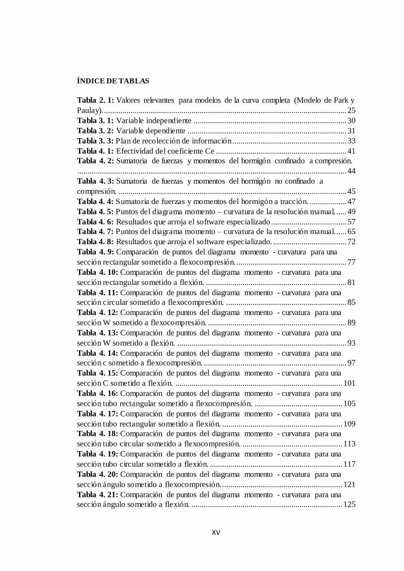
ÍNDICE DE TABLAS
Tabla 2. 1: Valores relevantes para modelos de la curva completa (Modelo de Park y
Paulay)........................................................................................................................ 25
Tabla 3. 1: Variable independiente ........................................................................... 30
Tabla 3. 2: Variable dependiente .............................................................................. 31
Tabla 3. 3: Plan de recolección de información ........................................................ 33
Tabla 4. 1: Efectividad del coeficiente Ce ................................................................ 41
Tabla 4. 2: Sumatoria de fuerzas y momentos del hormigón confinado a compresión.
.................................................................................................................................... 44
Tabla 4. 3: Sumatoria de fuerzas y momentos del hormigón no confinado a
compresión. ................................................................................................................ 45
Tabla 4. 4: Sumatoria de fuerzas y momentos del hormigón a tracción. .................. 47
Tabla 4. 5: Puntos del diagrama momento – curvatura de la resolución manual. ..... 49
Tabla 4. 6: Resultados que arroja el software especializado..................................... 57
Tabla 4. 7: Puntos del diagrama momento – curvatura de la resolución manual. ..... 65
Tabla 4. 8: Resultados que arroja el software especializado. .................................... 72
Tabla 4. 9: Comparación de puntos del diagrama momento - curvatura para una
sección rectangular sometido a flexocompresión. ...................................................... 77
Tabla 4. 10: Comparación de puntos del diagrama momento - curvatura para una
sección rectangular sometido a flexión. ..................................................................... 81
Tabla 4. 11: Comparación de puntos del diagrama momento - curvatura para una
sección circular sometido a flexocompresión. ........................................................... 85
Tabla 4. 12: Comparación de puntos del diagrama momento - curvatura para una
sección W sometido a flexocompresión. .................................................................... 89
Tabla 4. 13: Comparación de puntos del diagrama momento - curvatura para una
sección W sometido a flexión. ................................................................................... 93
Tabla 4. 14: Comparación de puntos del diagrama momento - curvatura para una
sección c sometido a flexocompresión. ...................................................................... 97
Tabla 4. 15: Comparación de puntos del diagrama momento - curvatura para una
sección C sometido a flexión. .................................................................................. 101
Tabla 4. 16: Comparación de puntos del diagrama momento - curvatura para una
sección tubo rectangular sometido a flexocompresión. ........................................... 105
Tabla 4. 17: Comparación de puntos del diagrama momento - curvatura para una
sección tubo rectangular sometido a flexión. ........................................................... 109
Tabla 4. 18: Comparación de puntos del diagrama momento - curvatura para una
sección tubo circular sometido a flexocompresión. ................................................. 113
Tabla 4. 19: Comparación de puntos del diagrama momento - curvatura para una
sección tubo circular sometido a flexión. ................................................................. 117
Tabla 4. 20: Comparación de puntos del diagrama momento - curvatura para una
sección ángulo sometido a flexocompresión. ........................................................... 121
Tabla 4. 21: Comparación de puntos del diagrama momento - curvatura para una
sección ángulo sometido a flexión. .......................................................................... 125

XVI
GLOSARIO DE SIMBOLOS
𝐴𝑏 = Área de la sección de la barra de refuerzo transversal.
𝐴𝑒 = Área confinada efectiva para Asx y Asy dependiendo si la sección es paralela
al eje x o al eje y.
𝐴𝑠 = Área de refuerzo a tensión.
𝐴𝑠𝑝 = Área de refuerzo transversal
𝐴𝑠𝑥, 𝐴𝑠𝑦 = Área de refuerzo transversal paralela al eje x o y.
𝐴𝑠′ = Área de refuerzo a compresión.
𝑏 = Base de una sección rectangular.
𝑏𝑖 = Desplazamiento del brazo de palanca inferior.
𝑏𝑠 = Desplazamiento del brazo de palanca superior.
𝑏𝑟 = Distancia a cada fuerza.
𝑏′ = Base del núcleo confinado de la sección.
𝑏𝑐 = Ancho de concreto confinado de una sección rectangular.
𝐶𝑒 = Factor de efectividad del confinamiento.
𝐶𝑡 : Distancia del centro de gravedad de la sección a la fibra más traccionada.
𝑐 = Distancia medida desde la fibra extrema en compresión al eje neutro.
𝑐 = Distancia medida desde el eje neutro a la zona de tensión.
𝑑 = Distancia entre la fibra extrema en compresión hasta el centroide del refuerzo
transversal en tracción.
𝑑𝑠 = Diámetro de los estribos.
𝑑′ = Distancia entre la fibra extrema en compresión hasta el centroide del refuerzo
transversal en compresión.
𝐸 = Módulo de elasticidad del acero.
𝐸𝑐 = Módulo de elasticidad del concreto.
𝐸𝑠𝑒𝑐 = Modulo secante del concreto confinado asociado al esfuerzo máximo.
𝐹𝑐 = Fuerza del concreto confinado a compresión.
𝐹𝑛𝑐 = Fuerza del concreto no confinado a compresión.
𝐹𝑡 = Fuerza del concreto confinado a tracción.
𝑓𝑐 = Esfuerzo del concreto inconfinado.
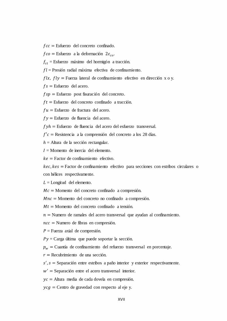
XVII
𝑓𝑐𝑐 = Esfuerzo del concreto confinado.
𝑓𝑐𝑜 = Esfuerzo a la deformación 2𝜀𝑐𝑜.
𝑓𝑐𝑡 = Esfuerzo máximo del hormigón a tracción.
𝑓𝑙 = Presión radial máxima efectiva de confinamiento.
𝑓𝑙𝑥, 𝑓𝑙𝑦 = Fuerza lateral de confinamiento efectivo en dirección x o y.
𝑓𝑠 = Esfuerzo del acero.
𝑓𝑠𝑝 = Esfuerzo post fisuración del concreto.
𝑓𝑡 = Esfuerzo del concreto confinado a tracción.
𝑓𝑢 = Esfuerzo de fractura del acero.
𝑓𝑦 = Esfuerzo de fluencia del acero.
𝑓𝑦ℎ = Esfuerzo de fluencia del acero del esfuerzo transversal.
𝑓′𝑐 = Resistencia a la comprensión del concreto a los 28 días.
ℎ = Altura de la sección rectangular.
𝐼 = Momento de inercia del elemento.
𝑘𝑒 = Factor de confinamiento efectivo.
𝑘𝑒𝑐, 𝑘𝑒𝑠 = Factor de confinamiento efectivo para secciones con estribos circulares o
con hélices respectivamente.
𝐿 = Longitud del elemento.
𝑀𝑐 = Momento del concreto confinado a compresión.
𝑀𝑛𝑐 = Momento del concreto no confinado a compresión.
𝑀𝑡 = Momento del concreto confinado a tensión.
𝑛 = Numero de ramales del acero transversal que ayudan al confinamiento.
𝑛𝑐𝑐 = Numero de fibras en compresión.
𝑃 = Fuerza axial de compresión.
𝑃𝑦 = Carga última que puede soportar la sección.
𝑝𝑤 = Cuantía de confinamiento del refuerzo transversal en porcentaje.
𝑟 = Recubrimiento de una sección.
𝑠′ , 𝑠 = Separación entre estribos a paño interior y exterior respectivamente.
𝑤 ′ = Separación entre el acero transversal interior.
𝑦𝑐 = Altura media de cada dovela en compresión.
𝑦𝑐𝑔 = Centro de gravedad con respecto al eje y.
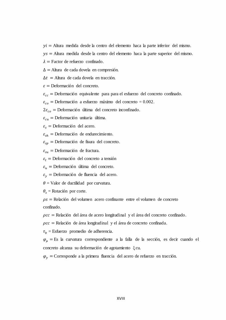
XVIII
𝑦𝑖 = Altura medida desde la centro del elemento haca la parte inferior del mismo.
𝑦𝑠 = Altura medida desde la centro del elemento haca la parte superior del mismo.
𝜆 = Factor de refuerzo confinado.
∆ = Altura de cada dovela en compresión.
∆𝑡 = Altura de cada dovela en tracción.
𝜀 = Deformación del concreto.
𝜀𝑐𝑐 = Deformación equivalente para para el esfuerzo del concreto confinado.
𝜀𝑐𝑜 = Deformación a esfuerzo máximo del concreto = 0.002.
2𝜀𝑐𝑜 = Deformación última del concreto inconfinado.
𝜀𝑐𝑢 = Deformación unitaria última.
𝜀𝑠 = Deformación del acero.
𝜀𝑠ℎ = Deformación de endurecimiento.
𝜀𝑠𝑝 = Deformación de fisura del concreto.
𝜀𝑠𝑢 = Deformación de fractura.
𝜀𝑡 = Deformación del concreto a tensión
𝜀𝑢 = Deformación última del concreto.
𝜀𝑦 = Deformación de fluencia del acero.
𝜃 = Valor de ductilidad por curvatura.
𝜃𝑠 = Rotación por corte.
𝜌𝑠 = Relación del volumen acero confinante entre el volumen de concreto
confinado.
𝜌𝑐𝑐 = Relación del área de acero longitudinal y el área del concreto confinado.
𝜌𝑐𝑐 = Relación de área longitudinal y el área de concreto confinada.
𝜏𝑏 = Esfuerzo promedio de adherencia.
𝜑𝜇 = Es la curvatura correspondiente a la falla de la sección, es decir cuando el
concreto alcanza su deformación de agotamiento cu.
𝜑𝑦 = Corresponde a la primera fluencia del acero de refuerzo en tracción.
XIX
RESUMEN EJECUTIVO
El presente trabajo se fundamenta en la investigación del diagrama momento curvatura
de secciones de hormigón armado y perfiles de acero (tipo W, tipo C, tubo circular,
tubo rectangular, ángulos) sometidas a esfuerzos de flexión y flexocompres ió n
mediante un análisis y calculo por el método de Fibras o Dovelas, para lo cual se
realizó la codificación de un software especializado en la obtención de dicho diagrama.
El programa computacional requiere secciones y características específicas del
material a calcular, las mismas que siguiendo parámetros establecidos en los teoremas
de Mander, Park y Paulay permitirán crear el diagrama momento curvatura de
cualquier tipo de sección impuesta.
1
CAPÍTULO I
ANTECEDENTES
1.1 TEMA DEL TRABAJO EXPERIMENTAL
CÁLCULO DEL DIAGRAMA MOMENTO – CURVATURA POR EL MÉTODO
DE FIBRAS PARA SECCIONES DE HORMIGÓN ARMADO Y PERFILES DE
ACERO EMPLEANDO UN SOFTWARE DE PROGRAMACIÓN
ESPECIALIZADO.
1.2 ANTECEDENTES
A lo largo de la historia, investigadores de todo el mundo especialmente de Estados
Unidos como Charles Culver (1960) han realizado modelos matemáticos para el
cálculo del diagrama momento – curvatura. La cual tiene como importancia conocer
la capacidad de un elemento y la ductilidad de la estructura, para ello es necesario
aplicar modelos de cálculo para el acero Park y Paulay (1975) y hormigón Mander
(1988) los cuales ayudaran a construir de mejor manera los diagramas de momento -
curvatura.
En Ecuador alrededor del 60% de las edificaciones de hormigón armado son
susceptibles al colapso por acciones sísmicas, gran número de las estructuras yacen
construidas hace más de 40 años y sin supervisión de expertos por estas características
mencionadas el país en los últimos años ha sufrido grandes pérdidas económicas con
el colapso de las estructuras a causa de fuerzas sísmicas por ello las autoridades han
tomado medidas creando nuevas normas de construcción. [1]
En las normas actuales (NEC 2015) lo que se desea es evaluar el desempeño de una
elemento con el análisis estático no lineal el cual sirve para predecir demandas de
deformaciones que representan de una manera aproximada la redistribución de fuerzas
2
internas que se producen en un elemento para ello se debe conocer cómo se comportan
los elementos es ahí donde se aplica la relación momento – curvatura. [2]
En el cálculo de la relación momento – curvatura se utiliza diversos esquemas de
cálculo que están basados en compatibilidad de deformaciones y equilibrio de fuerzas
y momentos [3], el modelo que mejor se aplica para el cálculo del diagrama momento
- curvatura es el método de fibras o dovelas.
En la universidad se puede observar la investigación de Ing. Mg. Cristian Medina cuya
tesis “Estudio de la relación momento – curvatura como herramienta para entender el
comportamiento de secciones de hormigón armado” será de apoyo para la
determinación de los modelos del hormigón y acero. [4]

3
1.3 JUSTIFICACIÓN
El diagrama momento – curvatura empezó a ser estudiado en 1960 en la Univers idad
de Bethlehem, Pensilvania el cual inicio con las ecuaciones de equilib r io,
compatibilidad y la relación de adherencia del concreto – acero [5], pero no fue hasta
1982 que debido a resultados experimentales el método propuesto por Park se acercó
a la realidad y dio lugar al estudio de la capacidad de ductilidad de un elemento
confinado y no confinado. [1]
En el diseño estructural especialmente en el proyecto sísmico se debe realizar
diagramas momento-curvatura de las secciones de los elementos que la componen,
para de esta manera lograr el concepto de ductilidad a nivel seccional y cumplir con la
demanda obtenida en el diseño sismo-resistente de una estructura. [6]
Para conocer el diagrama de momento – curvatura es necesario apoyarse en el uso de
software especializado en el análisis estructural, para calcular los diagramas de
deformación y graficar los métodos elásticos. La obtención de estos parámetros se
llevará a cabo mediante un código de programación en un software.
En el País el Diseño Basado en Desempeño está convirtiéndose en una alternativa de
cálculo para el ingeniero, ya que explica los niveles de daño esperados durante la vida
útil de la estructura [7]. Para lo cual es necesario conjeturar el diagrama momento –
curvatura para conocer la capacidad de un elemento pero a su vez el cálculo manual
del mismo se convierte en modelo monótono y extenso, por ello es necesario construir
un software que ayude con el cómputo del diagrama y de esta manera reducir el tiempo
de deducción.
La implementación de este programa ofrecerá a los estudiantes de Ingeniería Civil de
la Universidad Técnica de Ambato una herramienta de cálculo para la obtención del
diagrama momento – curvatura y por consiguiente aportará información sobre el
comportamiento de las secciones de hormigón armado y perfiles de acero.
4
1.4 OBJETIVOS:
1.4.1 Objetivo General:
Calcular del diagrama momento – curvatura por el método de fibras para
secciones de hormigón armado y perfiles de acero empleando un software de
programación especializado.
1.4.2 Objetivos Específicos:
- Determinar la respuesta no-lineal de las secciones tipo circular y rectangular
de hormigón armado.
- Determinar la respuesta no-lineal de la secciones tipo W, tipo C, tubo circular,
tubo rectangular y ángulos de perfiles de acero.
- Comparar los resultados obtenidos del programa con métodos manuales y
software de cálculo estructural.
5
CAPÍTULO II
FUNDAMENTACIÓN
2.1 FUNDAMENTACIÓN TEÓRICA
La investigación se basa el cálculo del diagrama momento curvatura para secciones de
hormigón armado y perfiles de acero para lo cual se requiere conocer conceptos de
hormigón, acero, modelos de cálculo, y demás aspectos mencionados a continuación.
2.1.1 Hormigón
El hormigón está compuesto por varios materiales tales como cemento, agregado fino,
agregado grueso, agua y aditivos. El comportamiento estructural del hormigón puede
ser expresado en la relación esfuerzo – deformación, para lo cual se realiza pruebas
estándar de compresión estas consisten en aplicar una fuerza de compresión a cilindros
de 15 cm. de diámetro por 30 cm. de alto, de acuerdo al ensayo ASTM C469. La
resistencia a tracción del hormigón es muy baja pero tampoco indispensable por lo
cual en el presente documento se realizara el cálculo respectivo en su pertinente lugar.
[8]
Para entender el comportamiento del hormigón es necesario basarse en modelos
matemáticos ya definidos que se conocerá a continuación.
2.1.1.1 Modelo de Whitney
El modelo propone reemplazar la variación de esfuerzos parabólicos por un bloque
rectangular uniforme. Este bloque se usa para representar cualquier esfuerzo que exista
en el concreto. Whitney explica que mientras la variación de esfuerzos en el concreto
es prácticamente lineal ante cargas bajas, y parabólico para cargas intermedias, se
asumirá la forma rectangular cuando se acerque a la carga máxima. [9]

6
Figura 2. 1: Modelo de Whitney para el hormigón armado.
Fuente: José Freire
2.1.1.2 Modelo de Mander
Para realizar la curva esfuerzo - deformación del concreto se deberá apoyar en modelos
propuesto por investigadores que desear representar el comportamiento de dicho
material por lo cual se apoyará en el modelo de Mander (1988) para el concreto
confinado y no confinado.
2.1.1.2.1 Modelo de Mander para hormigón no confinado
Mander para el hormigón no confinado propone un estudio constructivo que define al
material inconfinado dichos parámetros se observan a continuación.

7
Figura 2. 2: Modelo de Mander para el hormigón confinado y no confinado.
Fuente: Mander et al. 1988.
Para una deformación del material
𝜀 ≤ 𝜀𝑐𝑜 (2.1)
𝑓𝑐 = 𝜀 ∗ 𝐸𝑐 (2.2)
Para una deformación del material
𝜀𝑐𝑜 ≤ 𝜀 ≤ 2𝜀𝑐𝑜 (2.3)
𝑓𝑐 = 𝑓′ 𝑐∗𝑥∗𝑟
𝑟−1+𝑥𝑟 (2.4)
Para una deformación del material
2𝜀𝑐𝑜 ≤ 𝜀 ≤ 𝜀𝑠𝑝 (2.5)
𝑓𝑐 = 𝑓𝑐𝑜 + (𝑓𝑐𝑝 + 𝑓𝑐𝑜)(𝜀−2𝜀𝑐𝑜 )
(𝜀𝑠𝑝−2𝜀𝑐𝑜 ) (2.6)

8
𝑥 = 𝜀
𝜀𝑐𝑐 (2.7)
𝑟 = 𝐸𝑐
𝐸𝑐 −𝐸𝑠𝑒𝑐 (2.8)
𝐸𝑠𝑒𝑐 = 𝑓′𝑐
𝜀𝑐𝑐 (2.9)
Donde:
𝜀 = Deformación del concreto inconfinado
𝑓𝑐 = Esfuerzo del concreto inconfinado
𝐸𝑐 = Módulo de elasticidad del concreto
𝐸𝑠𝑒𝑐 = Modulo secante
𝜀𝑐𝑜 = Deformación a esfuerzo máximo del concreto = 0.002
2𝜀𝑐𝑜 = Deformación última del concreto inconfinado
𝜀𝑠𝑝 = Deformación de fisura del concreto
𝑓′𝑐 = Resistencia a la comprensión del concreto a los 28 días
𝑓𝑐𝑜 = Esfuerzo a la deformación 2𝜀𝑐𝑜
𝑓𝑠𝑝 = Esfuerzo post fisuración del concreto
2.1.1.2.2 Modelo de Mander para hormigón confinado
Este modelo está definido por una curva continua, y también considera que el efecto
del confinamiento no solo incrementa la capacidad de deformación del concreto, sino
también la resistencia a compresión del concreto. Es aplicable para secciones
circulares y rectangulares o cuadradas. [10]
Para una deformación del material
𝜀 ≤ 𝜀𝑐𝑜 (2.10)
𝑓𝑐 = 𝜀 ∗ 𝐸𝑐 (2.11)
9
Para una deformación del material
𝜀𝑐𝑜 ≤ 𝜀 ≤ 𝜀𝑐𝑢 (2.12)
𝑓𝑐 = 𝑓′ 𝑐∗𝑥∗𝑟
𝑟−1+𝑥𝑟 (2.13)
𝑥 = 𝜀
𝜀𝑐𝑐 (2.14)
𝑟 = 𝐸𝑐
𝐸𝑐 −𝐸𝑠𝑒𝑐 (2.15)
𝜀𝐶𝐶 = 𝜀𝐶𝑂 [1 + 5(𝑓𝑐𝑐
𝑓′ 𝑐− 1)] (2.16)
Donde:
𝑓𝑐𝑐 = Resistencia máxima del concreto confinado
𝜀 = Deformación del concreto confinado
𝐸𝑐 = Módulo de elasticidad del concreto
𝐸𝑠𝑒𝑐 = Modulo secante del concreto confinado asociado al esfuerzo máximo
𝜀𝑐𝑜 = Deformación a esfuerzo máximo del concreto
𝜀𝑐𝑢 = Deformación unitaria última
𝑓′𝑐 = Resistencia a la comprensión del concreto a los 28 días
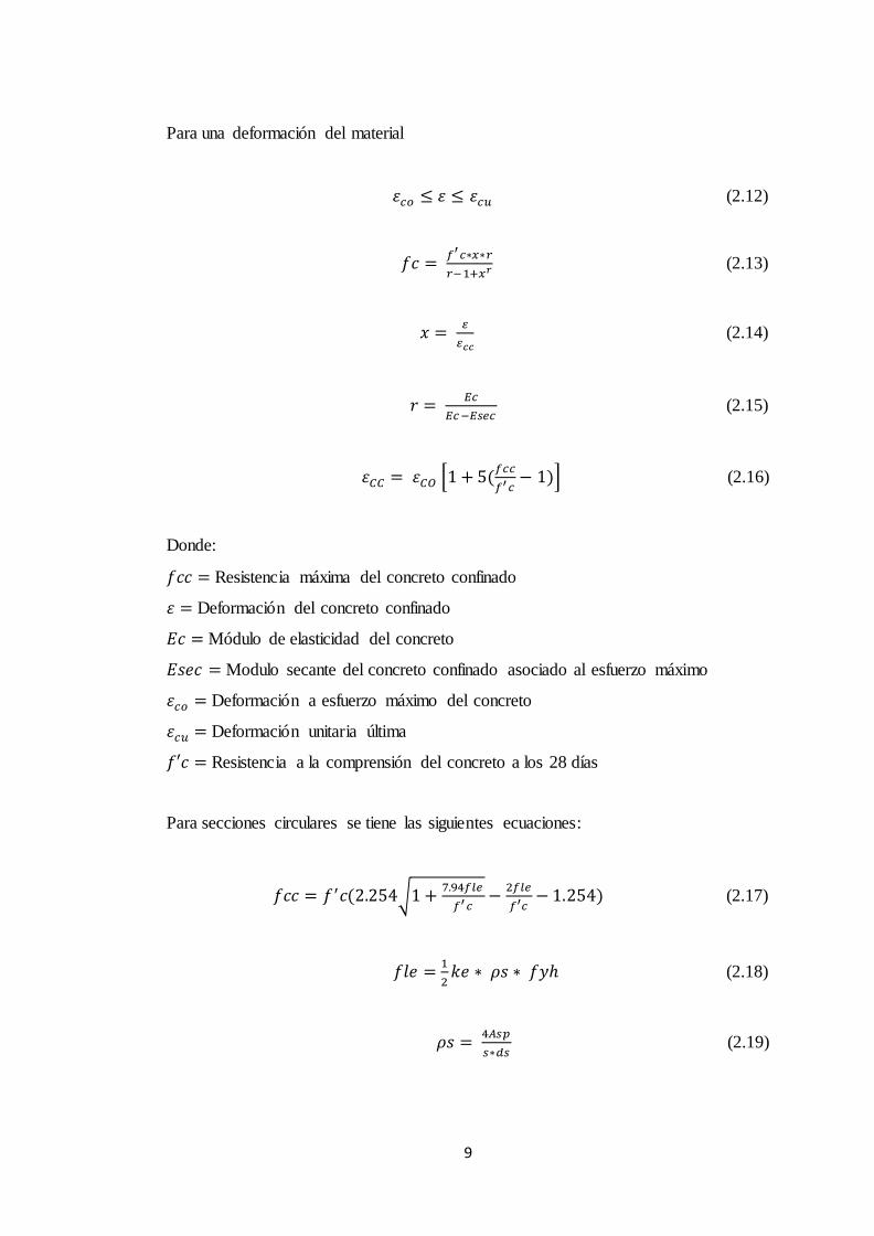
Para secciones circulares se tiene las siguientes ecuaciones:
𝑓𝑐𝑐 = 𝑓 ′𝑐(2.254√1 +7.94𝑓𝑙𝑒
𝑓′ 𝑐−
2𝑓𝑙𝑒
𝑓′𝑐− 1.254) (2.17)
𝑓𝑙𝑒 =1
2𝑘𝑒 ∗ 𝜌𝑠 ∗ 𝑓𝑦ℎ (2.18)
𝜌𝑠 = 4𝐴𝑠𝑝
𝑠∗𝑑𝑠 (2.19)

10
𝑘𝑒𝑐 = (1−
𝑠′
2𝑑𝑠)2
1−𝜌𝑐𝑐 (2.20)
𝑘𝑒𝑠 = 1−
𝑠′
2𝑑𝑠
1−𝜌𝑐𝑐 (2.21)
Donde:
𝐴𝑠𝑝 = Área de refuerzo transversal
𝜌𝑠 = Relación del volumen acero confinante entre el volumen de concreto
confinado.
𝜌𝑐𝑐 = Relación del área de acero longitudinal y el área del concreto confinado
𝑑𝑠 = Diámetro de los estribos.
𝑘𝑒 = Factor de confinamiento efectivo
𝑘𝑒𝑐, 𝑘𝑒𝑠 = Factor de confinamiento efectivo para secciones con estribos circulares o
con hélices respectivamente.
𝑠′ , 𝑠 = Separación entre estribos a paño interior y exterior respectivamente.
Para secciones rectangulares se tiene las siguientes ecuaciones:
𝑓𝑐𝑐 = 𝜆𝑓′𝑐 (2.22)
𝑓𝑙𝑥 = 𝐴𝑠𝑥
𝑠∗𝑑𝑐∗ 𝑘𝑒 ∗ 𝑓𝑦ℎ (2.23)
𝑓𝑙𝑦 = 𝐴𝑠𝑦
𝑠∗𝑏𝑐∗ 𝑘𝑒 ∗ 𝑓𝑦ℎ (2.24)
𝐴𝑒 = (𝑏𝑐 ∗ 𝑑𝑐 − ∑ 𝑤𝑖2
6
𝑛𝑖=1 )(1 −
𝑠′
2𝑏𝑐)(1 −
𝑠′
2𝑑𝑐) (2.25)
𝑘𝑒 = (1−∑
𝑤 𝑖2
6∗𝑏𝑐∗𝑑𝑐𝑛𝑖=1 )(1−
𝑠′
2𝑏𝑐)(1−
𝑠′
2𝑑𝑐)
1 −𝜌𝑐𝑐 (2.26)
Donde:
𝑓𝑦ℎ = Esfuerzo de fluencia del acero del esfuerzo transversal
𝜆 = Factor de refuerzo confinado

11
𝜌𝑐𝑐 = Relación de área longitudinal y el área de concreto confinada
𝐴𝑒 = Área confinada efectiva para Asx y Asy dependiendo si la sección es paralela
al eje x o al eje y
𝐴𝑠𝑥, 𝐴𝑠𝑦 = Área de refuerzo transversal paralela al eje x o y
𝑓𝑙𝑥, 𝑓𝑙𝑦 = Fuerza lateral de confinamiento efectivo en dirección x o y
𝑠′ , 𝑠 = Separación entre estribos a paño interior y exterior respectivamente.
Figura 2. 3: Forma esquemática el área de concreto confinado y no confinado de una
sección rectangular.
Fuente: Núcleo efectivo de concreto confinado para una sección rectangular,
(Mander et al. 1988).

12
Figura 2. 4: Factor de confinamiento, "" para elementos cuadrados
y rectangulares
Fuente: Mander et al. 1988.
2.1.2 Acero
El acero es la fusión de varios elementos entre los principales hierro y carbón y como
secundarios cobre, cromo, cobalto, bronce, aluminio, estaño y zinc el porcentaje de los
materiales mencionados ayudan con sus propiedades físicas y mecánicas tales como
resistencia, dureza, corrosión, elasticidad entre otros.
El acero como barras es muy utilizado para formar el hormigón armado ya que es el
componente ideal para unirse al hormigón simple y de esta manera resistir
solicitaciones de cortante y torsión. [11]
El acero estructural laminado se utiliza para estructuras metálicas obtenido por una
laminación en caliente y conformación en frio del cual resultan varios perfiles pero
para el documento en estudio se trabajará con perfiles tipo I, C, tubos circular y
rectangular y además ángulos.
El acero de refuerzo es un material que posee una gran resistencia a tensión, cualidad
por la cual se usa para resistir principalmente los esfuerzos de tensión que se inducen
en los elementos estructurales de concreto reforzado por las acciones de diseño.

13
Además, cuando los esfuerzos de compresión actuantes son grandes, comúnmente se
usa refuerzo longitudinal a compresión que trabaja en conjunto con el concreto para
resistirlas, aunque para tal finalidad el refuerzo debe estar debidamente restringido
contra pandeo. [10]
Para describir la conducta del acero existen modelos que simulan el comportamiento
del acero estructural por lo cual a continuación se mencionarán los modelos más
utilizados.
2.1.2.1 Modelo elastoplástico
El modelo elastoplastico es el más sencillo pero a su vez el más práctico de todos.
Como se observa a continuación está formado por dos líneas rectas, la primera línea
recta corresponde a un comportamiento elástico y la segunda recta paralela al eje de
deformación pertenece a un comportamiento plástico [12], por lo cual se ignora la
resistencia superior de fluencia y el aumento en el esfuerzo debido al endurecimiento
por deformación. [9]
Figura 2. 5: Modelo elastoplástico para el acero.
Fuente: Allauca Leonidas, Desempeño sísmico de un edificio aporticado de cinco
pisos diseñado con las normas peruanas de edificaciones, 2006.
14
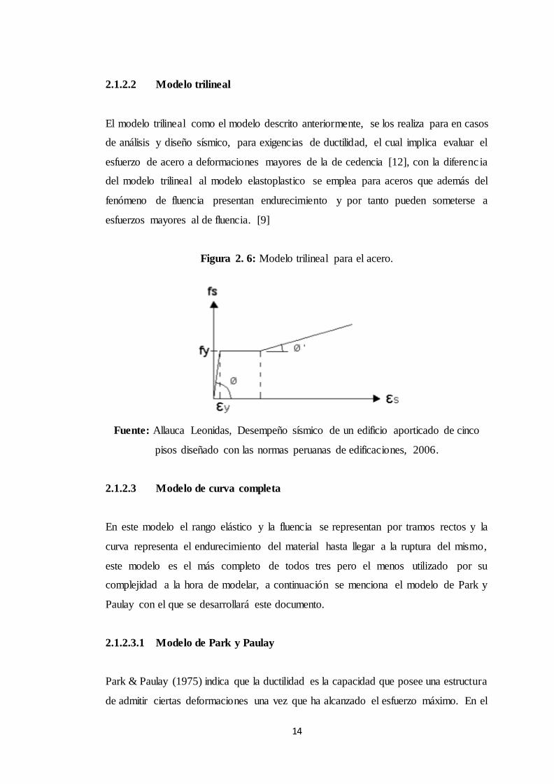
2.1.2.2 Modelo trilineal
El modelo trilineal como el modelo descrito anteriormente, se los realiza para en casos
de análisis y diseño sísmico, para exigencias de ductilidad, el cual implica evaluar el
esfuerzo de acero a deformaciones mayores de la de cedencia [12], con la diferenc ia
del modelo trilineal al modelo elastoplastico se emplea para aceros que además del
fenómeno de fluencia presentan endurecimiento y por tanto pueden someterse a
esfuerzos mayores al de fluencia. [9]
Figura 2. 6: Modelo trilineal para el acero.
Fuente: Allauca Leonidas, Desempeño sísmico de un edificio aporticado de cinco
pisos diseñado con las normas peruanas de edificaciones, 2006.
2.1.2.3 Modelo de curva completa
En este modelo el rango elástico y la fluencia se representan por tramos rectos y la
curva representa el endurecimiento del material hasta llegar a la ruptura del mismo,
este modelo es el más completo de todos tres pero el menos utilizado por su
complejidad a la hora de modelar, a continuación se menciona el modelo de Park y
Paulay con el que se desarrollará este documento.
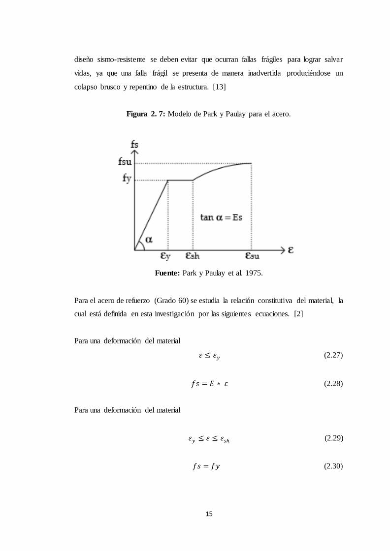
2.1.2.3.1 Modelo de Park y Paulay
Park & Paulay (1975) indica que la ductilidad es la capacidad que posee una estructura
de admitir ciertas deformaciones una vez que ha alcanzado el esfuerzo máximo. En el
15
diseño sismo-resistente se deben evitar que ocurran fallas frágiles para lograr salvar
vidas, ya que una falla frágil se presenta de manera inadvertida produciéndose un
colapso brusco y repentino de la estructura. [13]
Figura 2. 7: Modelo de Park y Paulay para el acero.
Fuente: Park y Paulay et al. 1975.
Para el acero de refuerzo (Grado 60) se estudia la relación constitutiva del material, la
cual está definida en esta investigación por las siguientes ecuaciones. [2]
Para una deformación del material
𝜀 ≤ 𝜀𝑦 (2.27)
𝑓𝑠 = 𝐸 ∗ 𝜀 (2.28)
Para una deformación del material
𝜀𝑦 ≤ 𝜀 ≤ 𝜀𝑠ℎ (2.29)
𝑓𝑠 = 𝑓𝑦 (2.30)

16
Para una deformación del material
𝜀𝑠ℎ ≤ 𝜀 ≤ 𝜀𝑠𝑢 (2.31)
𝑓𝑠 = 𝑓𝑦 [𝑚(𝜀− 𝜀𝑠ℎ)+2
60(𝜀− 𝜀𝑠ℎ)+2+
(𝜀− 𝜀𝑠ℎ)(60−𝑚)
2(30𝑟+1)²] (2.32)
𝑚 =(
𝑓𝑠𝑢
𝑓𝑦)(30𝑟+1)2−60𝑟 −1
15𝑟² (2.33)
𝑟 = 𝜀𝑠𝑢 − 𝜀𝑠ℎ (2.34)
Donde:
𝜀 = Deformación del acero
𝑓𝑠 = Esfuerzo del acero
𝑓𝑦 = Esfuerzo de fluencia del acero
𝑓𝑢 = Esfuerzo de fractura del acero
𝜀𝑦 = Deformación de fluencia
𝜀𝑠ℎ = Deformación de endurecimiento
𝜀𝑠𝑢 = Deformación de fractura
𝐸 = Módulo de elasticidad del acero
Para construir la relación esfuerzo – deformación del acero se debe iniciar de
parámetros establecidos para lo cual se basará en la hipótesis de PRIESTLEY,
2007 para un refuerzo del acero grado 60.
La hipótesis dice que para 𝑓𝑦 = 420 𝑀𝑝𝑎 se tiene los siguientes parámetros:
𝜀𝑦 = 0.002 (2.35)
𝜀𝑠ℎ = 0.008 (2.36)
𝜀𝑠𝑢 = 0.11 (2.37)
𝑓𝑢/𝑓𝑦 = 1.50 (2.38)
𝐸 = 2043000 𝑘𝑔/𝑐𝑚² (2.39)

17
2.1.3 Hormigón armado
El hormigón armado es la unión de dos materiales el hormigón simple y acero de
refuerzo, el trabajo integrado realizado por los dos materiales debido a la adherencia
entre ellos tiene el objetivo de resistir esfuerzos de compresión y tracción. [11]
El hormigón simple resiste a esfuerzos a compresión mientras el acero de refuerzo
resiste esfuerzos a tracción por ello el elemento conformado se transforma en una pieza
de mayor ductilidad dando lugar a una deformación precedente a una falla.
2.1.4 Diagrama momento – curvatura
Para el diseño de elementos de hormigón armado es ineludible lograr un
comportamiento dúctil frente a cargas gravitacionales y solicitaciones sísmicas de ahí
considerar características carga versus deformación de una sección transversal de un
elemento y por lo cual es de suma importancia elaborar el diagrama momento –
curvatura.
2.1.4.1 Curvatura
Al aplicar momentos en los extremos y fuerzas axiales iguales a un elemento de
hormigón armado que se encuentra inicialmente recto, se puede observar que los
planos laterales de la sección seguirán planos después de aplicar el momento flector.
[13]
La distancia al eje neutro será el radio de curvatura R como se muestra en la siguiente
figura. Usando las relaciones planteadas por Park y Paulay (1978) logramos encontrar
la curvatura, considerando un elemento de longitud dx de la siguiente manera. [13]
𝑑𝑥
𝑅=
𝜀𝑐 𝑑𝑥
𝑘𝑑=
𝜀𝑠𝑑𝑥
𝑑(1−𝑘) (2.40)
1
𝑅=
𝜀𝑐
𝑘𝑑=
𝜀𝑠
𝑑(1−𝑘) (2.41)

18
1
𝑅= 𝜑 (2.42)
𝜑 =𝜀𝑐
𝑘𝑑=
𝜀𝑠
𝑑(1−𝑘 )=
𝜀𝑐+𝜀𝑠
𝑑 (2.43)
Figura 2. 8: Curvatura de un elemento.
Fuente: Ottazzi Gianfranco, Material de Apoyo para la Enseñanza de los Cursos de
Diseño y Comportamiento del Concreto Armado, 2004.
Para llegar a conocer la ductilidad y resistencia máxima de un elemento es necesario
la obtención del factor de ductilidad de curvatura al relacionar la curvatura última con
la curvatura de fluencia:
𝜇𝜑 = 𝜑𝜇
𝜑𝑦 (2.44)
Donde:
𝜑𝜇 : Es la curvatura correspondiente a la falla de la sección, es decir cuando el concreto
alcanza su deformación de agotamiento cu.
𝜑𝑦: Corresponde a la primera fluencia del acero de refuerzo en tracción. [14]
2.1.4.2 Construcción del diagrama momento - curvatura
La relación momento – curvatura de una sección transversal es la capacidad de un
elemento en razón de la variación de la dirección de una curva entre dos puntos para
19
los diagramas esfuerzo – deformación del hormigón simple y acero y de esta manera
conocer cuál es la capacidad de ductilidad por curvatura y la máxima capacidad a
flexión del elemento. [15]
2.1.4.2.1 Método manual
Existen varios métodos de cálculo que comparten la misma filosofía tal como
compatibilidad de deformaciones y equilibrio de fuerzas y momentos, por lo cual se
ha simplificado la metodología para la obtención del diagrama momento – curvatura
realizando un proceso manual con ecuaciones aproximadas que se asemeje al
comportamiento verdadero de un elemento. [3]
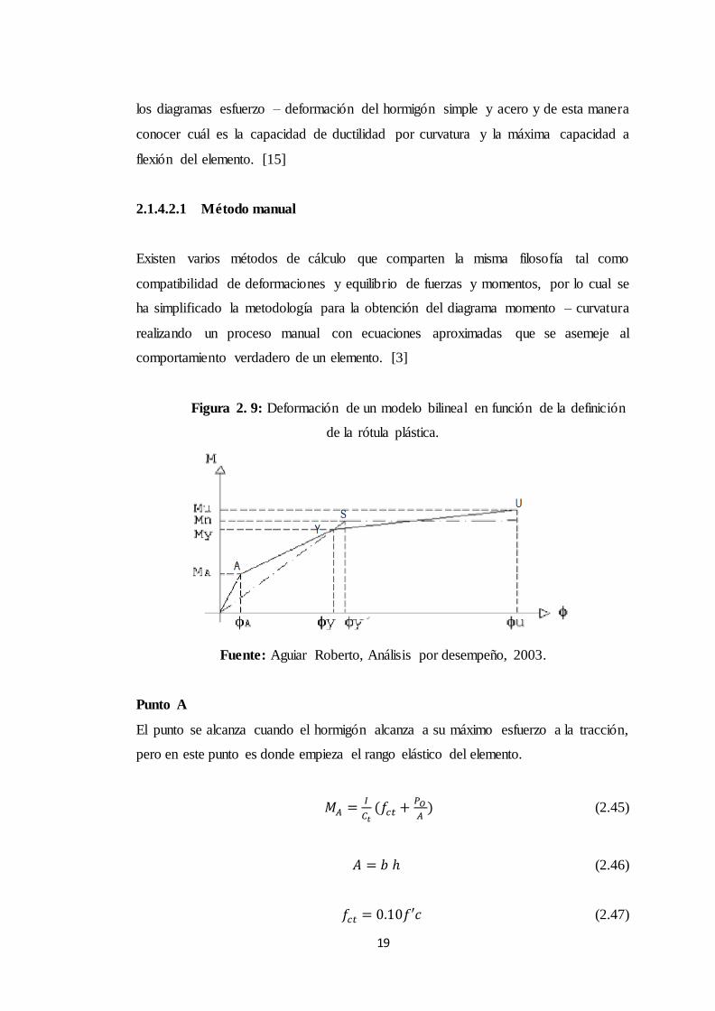
Figura 2. 9: Deformación de un modelo bilineal en función de la definición
de la rótula plástica.
Fuente: Aguiar Roberto, Análisis por desempeño, 2003.
Punto A
El punto se alcanza cuando el hormigón alcanza a su máximo esfuerzo a la tracción,
pero en este punto es donde empieza el rango elástico del elemento.
𝑀𝐴 =𝐼
𝐶𝑡(𝑓𝑐𝑡 +
𝑃𝑂
𝐴) (2.45)
𝐴 = 𝑏 ℎ (2.46)
𝑓𝑐𝑡 = 0.10𝑓′𝑐 (2.47)

20
𝐶𝑡 =ℎ
2 (2.48)
∅𝐴 =𝑀𝐴
𝐸𝐶 𝐼 (2.49)
𝐼 = 𝑏 ℎ³
12 (2.50)
Donde:
𝑀𝐴 : Momento en el punto A
𝐼 : Momento de inercia del elemento
𝐶𝑡 : Distancia del centro de gravedad de la sección a la fibra más traccionada.
𝑓𝑐𝑡 : Esfuerzo máximo del hormigón a tracción.
𝑏 : Base de la sección
ℎ : Altura de la sección.
𝑃𝑜 : Fuerza axial de compresión.
Las demás variables ya han sido definidas anteriormente.
Punto Y
Este punto se obtiene cuando el acero a tracción alcanza su fluencia.
𝑀𝑌 = 0.5𝑓 ′𝑐𝑏𝑑2[(1 + 𝛽𝑐 − 𝜂)𝜂𝑜 + (2 − 𝜂)𝑃𝑡 + (𝜂 − 2𝛽𝑐)𝛼𝑐𝑃𝑡′] (2.51)
𝛽𝑐 =𝑑′
𝑑 (2.52)
𝜂 =0.75
1+𝛼𝑦(
𝜀𝑐
𝜀𝑜)0.7 (2.53)
𝛼𝑦 =𝜀𝑦
𝜀𝑜 (2.54)
𝜂𝑜 = 𝑃𝑜
𝑏𝑑𝑓′𝑐 (2.55)
𝑃𝑡 =𝐴𝑠 𝑓𝑦
𝑏𝑑𝑓′𝑐 (2.56)

21
𝑃𝑡′ =
𝐴𝑠′ 𝑓𝑦
𝑏𝑑𝑓′𝑐 (2.57)
𝜀𝑐 = 𝜙𝑦(𝑑 − 𝜀𝑦) (2.58)
𝛼𝑐 = (1 − 𝛽𝑐) 𝜀𝑐
𝜀𝑦− 𝛽𝑐 ≤ 1 (2.59)
𝜙𝑦 = [1.05 + (𝐶2 − 1.05)𝜂𝑜
0.03]
𝜀𝑦
(1−𝑘)𝑑 (2.60)
𝑘 = √(𝑃𝑡 + 𝑃𝑡′)2 1
4𝛼𝑦²+ (𝑃𝑡 + 𝛽𝑐𝑃𝑡
′)1
𝛼𝑦− (𝑃𝑡 + 𝑃𝑡
′)1
2𝛼𝑦 (2.61)
𝐶2 = 1 +0.45
(0.84+𝑃𝑡) (2.62)
Donde:
𝑑′ : Recubrimiento de la armadura a compresión.
𝐴𝑠 : Armadura a tracción.
𝐴𝑠′ : Armadura a compresión.
Las demás variables ya han sido definidas anteriormente.
Punto U
Este punto se obtiene cuando el hormigón llega a su máxima deformación útil a
compresión.
𝑀𝑢 = (1.24 − 0.15𝑃𝑡 − 0.5𝜂𝑜)𝑀𝑦 (2.63)
𝜙𝑢 = 𝜇𝜙 𝜙𝑦 (2.64)
𝜇𝜙 = (𝜀𝑝
𝜀𝑜)0.218 𝑝𝑤−2.15 ≤ 1 (2.65)
𝜀𝑝 = 0.5𝜀𝑏 + 0.5√𝜀𝑏2 + 𝜃𝑠² (2.66)
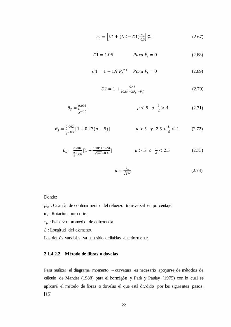
22
𝜀𝑏 = [𝐶1 + (𝐶2 − 𝐶1)𝜂𝑜
0.3] ∅𝑌 (2.67)
𝐶1 = 1.05 𝑃𝑎𝑟𝑎 𝑃𝑡 ≠ 0 (2.68)
𝐶1 = 1 + 1.9 𝑃𝑡2.4 𝑃𝑎𝑟𝑎 𝑃𝑡 = 0 (2.69)
𝐶2 = 1 +0.45
(0.84+2𝑃𝑡′−𝑃𝑡) (2.70)
𝜃𝑆 =0.002𝐿
𝑑−0.5
𝜇 < 5 𝑜 𝐿
𝑑> 4 (2.71)
𝜃𝑆 =0.002𝐿
𝑑−0.5
[1 + 0.27(𝜇 − 5)] 𝜇 > 5 𝑦 2.5 <𝐿
𝑑< 4 (2.72)
𝜃𝑆 =0.002𝐿
𝑑−0.5
[1 +0.185 (𝜇−5)
√𝑝𝑤−0.4] 𝜇 > 5 𝑜
𝐿
𝑑< 2.5 (2.73)
𝜇 =𝜏𝑏
√𝑓′𝑐 (2.74)
Donde:
𝑝𝑤 : Cuantía de confinamiento del refuerzo transversal en porcentaje.
𝜃𝑠 : Rotación por corte.
𝜏𝑏 : Esfuerzo promedio de adherencia.
𝐿 : Longitud del elemento.
Las demás variables ya han sido definidas anteriormente.
2.1.4.2.2 Método de fibras o dovelas
Para realizar el diagrama momento – curvatura es necesario apoyarse de métodos de
cálculo de Mander (1988) para el hormigón y Park y Paulay (1975) con lo cual se
aplicará el método de fibras o dovelas el que está dividido por los siguientes pasos:
[15]
23
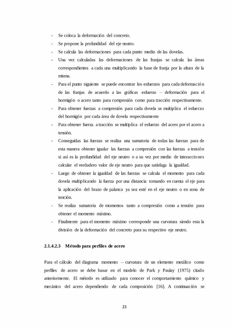
- Se coloca la deformación del concreto.
- Se propone la profundidad del eje neutro.
- Se calcula las deformaciones para cada punto medio de las dovelas.
- Una vez calculadas las deformaciones de las franjas se calcula las áreas
correspondientes a cada una multiplicando la base de franja por la altura de la
misma.
- Para el punto siguiente se puede encontrar los esfuerzos para cada deformación
de las franjas de acuerdo a las gráficas esfuerzo – deformación para el
hormigón o acero tanto para compresión como para tracción respectivamente.
- Para obtener fuerzas a compresión para cada dovela se multiplica el esfuerzo
del hormigón por cada área de dovela respectivamente
- Para obtener fuerza a tracción se multiplica el esfuerzo del acero por el acero a
tensión.
- Conseguidas las fuerzas se realiza una sumatoria de todas las fuerzas para de
esta manera obtener igualar las fuerzas a compresión con las fuerzas a tensión
si así es la profundidad del eje neutro o a su vez por medio de interacciones
calcular el verdadero valor de eje neutro para que satisfaga la igualdad.
- Luego de obtener la igualdad de las fuerzas se calcula el momento para cada
dovela multiplicando la fuerza por una distancia tomando en cuenta el eje para
la aplicación del brazo de palanca ya sea esté en el eje neutro o en zona de
tención.
- Se realiza sumatoria de momentos tanto a compresión como a tensión para
obtener el momento máximo.
- Finalmente para el momento máximo corresponde una curvatura siendo esta la
división de la deformación del concreto para su respectivo eje neutro.
2.1.4.2.3 Método para perfiles de acero
Para el cálculo del diagrama momento – curvatura de un elemento metálico como
perfiles de acero se debe basar en el modelo de Park y Paulay (1975) citado
anteriormente. El método es utilizado para conocer el comportamiento químico y
mecánico del acero dependiendo de cada composición [16]. A continuación se

24
mencionará los pasos para obtener el diagrama momento - curvatura de una sección
de perfil de acero.
- Se escoge la sección con cual trabajar ya sea esta tipo I, tipo C, tubo circular,
tubo rectangular o ángulos.
- Luego se selecciona el modelo del comportamiento del acero para con el cual
trabajar entre estos tenemos los modelos elastoplástico, trilineal y un modelo
de curva completa como el modelo de Park y Paulay (1975) mencionados
anteriormente.
- Se elige el tipo de acero con el que trabajar ya sea A36, A992, A913(50),
A709(50), A572, A709(70W) entre los más comunes.
- Adoptado el tipo de acero obtenemos los valores de fy, fu, y, sh y su para
obtener la relación esfuerzo deformación con el método Park y Paulay (1975).
Figura 2. 10: Diagrama esfuerzo – deformación para diferentes tipos de acero
estructural.
Fuente: Altos Hornos de México (AHMSA), Manual de diseño para la construcción
con acero, 2013.

25
Tabla 2. 1: Valores relevantes para modelos de la curva completa (Modelo de Park y
Paulay).
TABLA DE VALORES RELEVANTES PARA LOS MODELOS DE LA CURVA COMPLETA
fy fu y sh su
Ksi kg/cm² Ksi kg/cm²
A36 36 2531.05 58 4077.80 0.00124 0.020 0.200
A992 50 3515.35 65 4569.95 0.00172 0.015 0.17
A572 50 3515.35 65 4569.95 0.00172 0.015 0.175
A913(50) 50 3515.35 60 4218.42 0.00172 0.015 0.170
A709(50) 50 3515.35 65 4569.95 0.00172 0.015 0.170
A709(70W) 70 4921.49 85 5976.09 0.00241 0.015 0.170
Fuente: Altos Hornos de México (AHMSA), Manual de diseño para la construcción
con acero, 2013.
- Se coloca la deformación del acero.
- Se calcula las deformaciones para cada punto medio de las fibras partiendo
desde el eje neutro de la sección.
- Una vez calculadas las deformaciones de las franjas se calcula las áreas
correspondientes a cada una multiplicando la base de franja por la altura de la
misma.
- Para el punto siguiente se puede encontrar los esfuerzos para cada deformación
de las franjas de acuerdo a la gráfica esfuerzo – deformación para el acero tanto
para compresión como para tracción respectivamente.
- Para obtener fuerzas a compresión o a tracción para cada dovela se multip l ica
el esfuerzo del acero por cada área de fibra respectivamente
- Se calcula el momento para cada dovela está multiplicando la fuerza por una
distancia teniendo en cuenta en el punto de aplicación del brazo de palanca ya
se esté en el eje neutro o en zona de tensión.
- Finalmente para la calcular la curvatura se aplica la siguiente fórmula.

26
Figura 2. 11: Cálculo del diagrama momento – curvatura para perfiles de acero.
Fuente: Mora Edgar, Comportamiento de estructuras de acero con y sin disipadores
de energía tipo TADAS, ubicadas en la ciudad de Quito, por el método del espectro
de capacidad, 2015.
𝜙 = 𝜀𝑡
𝑦𝑖=
𝜀𝑐
𝑦𝑠 (2.75)
Donde:
𝑦𝑖 ∶ Altura medida desde la centro del elemento haca la parte inferior del mismo.
𝑦𝑠 ∶ Altura medida desde la centro del elemento haca la parte superior del mismo.
Las demás variables ya han sido definidas anteriormente.
2.1.5 Software de programación especializado
Para el desarrollo del tema es necesario acudir a un software de programación que
ayude con el cálculo del diagrama momento – curvatura para lo cual se trabajará con
Matlab ya que es una de las mejores herramientas para el análisis matemático numérico
y gráfico.
El software Matlab es una plataforma virtual para principalmente trabajar con matrices
aunque también existe la posibilidad de trabajar con números reales y complejos en un
lenguaje de programación enfocado hacia el análisis de problemas numéricos para lo
cual es necesario guiarse en una metodología de cálculo. [17]

27
Figura # 2.12: Proceso de resolución de problemas en Matlab.
Fuente: Rodríguez Luis, Análisis numérico básico. Un enfoque algorítmico con el
soporte de Matlab, 2011.
El problema tiene como propósito obtener un resultado favorable siguiendo pasos
lógicos para su resolución.
En la etapa de análisis es indispensable estudiar y entender el problema. Entre sus
principales características se tiene las variables, datos requeridos y los procesos
matemáticos que intervienen.
En la etapa de diseño, una vez conocido las variables el siguiente paso es elegir un
método numérico apropiado para resolver el modelo matemático con la elaboración de
un algoritmo. [18]
En la etapa de instrumentación en sí se desarrollará los programas y funciones en un
lenguaje computacional hasta llegar al resultado esperado.
Además de los procesos mencionados precedentemente se debe complementar con un
a revisión desde el análisis hasta los resultados cruzando por el diseño e
instrumentación para de esta manera comprobar, retroalimentar y perfeccionar el
cálculo.
2.2 HIPÓTESIS
El uso de un software especial permite determinar el diagrama momento – curvatura
por el método de fibras para secciones de hormigón armado y perfiles de acero.
28
2.3 SEÑALAMIENTO DE VARIABLES
Variable Dependiente
Diagrama momento – curvatura para secciones de hormigón armado y perfiles de
acero.
Variable Independiente
Uso de un software especializado.

29
CAPÍTULO III
METODOLOGÍA
3.1 NIVEL O TIPO DE INVESTIGACIÓN
La investigación que se aplica en este documento es de nivel aplicativo y descriptivo.
Nivel aplicativo ya que se realiza un software que ayude al cálculo de problemas
matemáticos de los ingenieros y estudiantes de la Facultad de Ingeniería Civil y
Mecánica de la Universidad Técnica de Ambato.
Nivel descriptivo debido a que se manifiesta información del diagrama momento –
curvatura y modelos de cálculo para los diagramas esfuerzo – deformación del
hormigón y acero. Además cuenta con información sobre el lenguaje de programación
que utiliza MATLAB.
3.2 POBLACIÓN Y MUESTRA
3.2.1 Población
- Secciones de hormigón armado y perfiles de acero
3.2.2 Muestra
3.2.2.1 Tipos de secciones de hormigón armado
- Circular
- Rectangular
3.2.2.2 Tipos de secciones de perfiles de acero
- W

30
- C
- Tubo circular
- Tubo rectangular
- Ángulos
3.3 OPERACIÓN DE VARIABLES
3.3.1 Variable independiente
Uso del software
Tabla 3. 1: Variable independiente
Conceptualización
Dimensiones
Indicadores
Ítems
Técnicas e
instrumento
Conjunto de
procesos
informáticos que
permiten realizar
determinadas tareas
en una
computadora
Programación
Métodos de
cálculo
¿Cuáles son
los parámetros
necesarios para
efectuar la
codificación?
- Investigac ión
bibliográfica
- Instrumentación
- Documentos
Agilizar
procesos de
cálculo
Rapidez
¿Cómo un
software
favorece con
los procesos de
cálculo?
- Investigac ión
bibliográfica
- Investigac ión
experimental
- Instrumentación
- Documentos
Fuente: José Freire
31
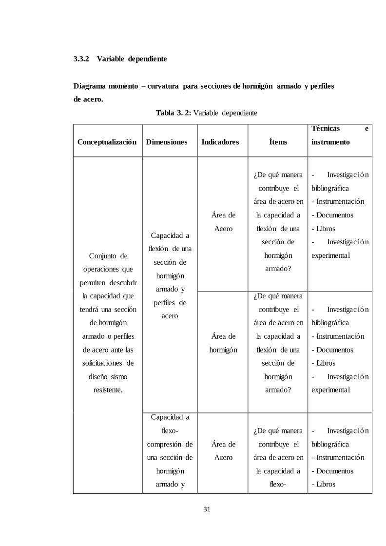
3.3.2 Variable dependiente
Diagrama momento – curvatura para secciones de hormigón armado y perfiles
de acero.
Tabla 3. 2: Variable dependiente
Conceptualización
Dimensiones
Indicadores
Ítems
Técnicas e
instrumento
Conjunto de
operaciones que
permiten descubrir
la capacidad que
tendrá una sección
de hormigón
armado o perfiles
de acero ante las
solicitaciones de
diseño sismo
resistente.
Capacidad a
flexión de una
sección de
hormigón
armado y
perfiles de
acero
Área de
Acero
¿De qué manera
contribuye el
área de acero en
la capacidad a
flexión de una
sección de
hormigón
armado?
- Investigac ión
bibliográfica
- Instrumentación
- Documentos
- Libros
- Investigac ión
experimental
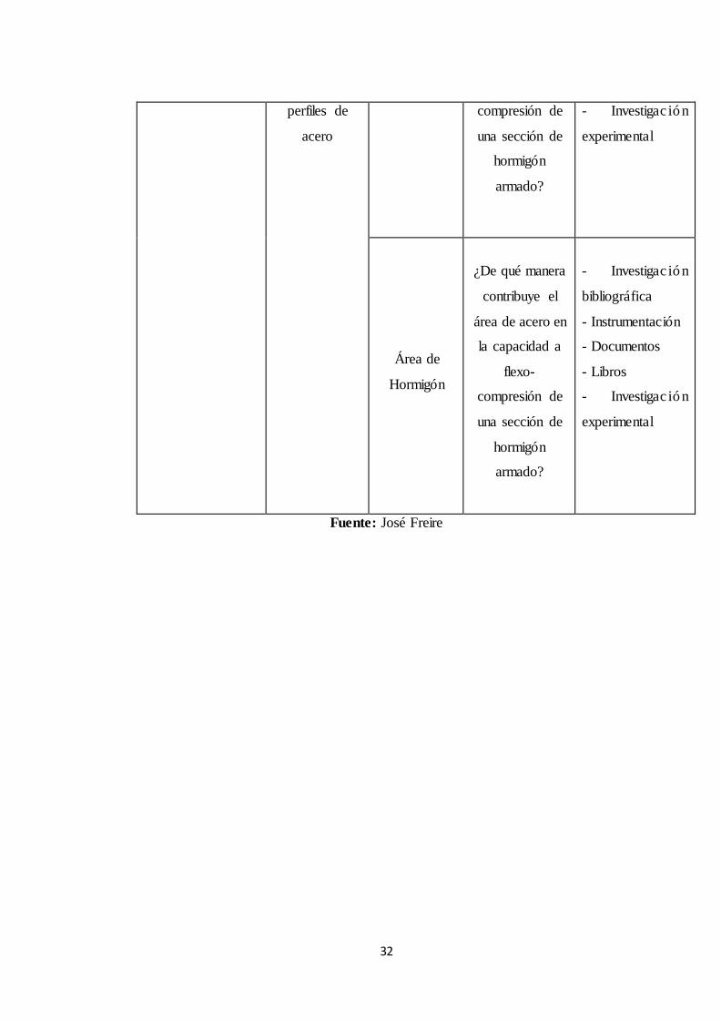
Área de
hormigón
¿De qué manera
contribuye el
área de acero en
la capacidad a
flexión de una
sección de
hormigón
armado?
- Investigac ión
bibliográfica
- Instrumentación
- Documentos
- Libros
- Investigac ión
experimental
Capacidad a
flexo-
compresión de
una sección de
hormigón
armado y
Área de
Acero
¿De qué manera
contribuye el
área de acero en
la capacidad a
flexo-
- Investigac ión
bibliográfica
- Instrumentación
- Documentos
- Libros
32
perfiles de
acero
compresión de
una sección de
hormigón
armado?
- Investigac ión
experimental
Área de
Hormigón
¿De qué manera
contribuye el
área de acero en
la capacidad a
flexo-
compresión de
una sección de
hormigón
armado?
- Investigac ión
bibliográfica
- Instrumentación
- Documentos
- Libros
- Investigac ión
experimental
Fuente: José Freire

33
3.4 PLAN DE RECOLECCIÓN DE INFORMACIÓN
Tabla 3. 3: Plan de recolección de información
PREGUNTAS BÁSICAS
EXPLICACIÓN
1. ¿Para qué?
- Obtener los diagramas momento –
curvatura para comprender de mejor
manera el comportamiento de
secciones de hormigón armado y
perfiles de acero.
- Definir la relación esfuerzo
deformación del hormigón y del acero
estructural con modelos de cálculos
definidos.
2. ¿De qué personas u objetos?
- De secciones de hormigón armado y
perfiles de acero.
3. ¿Sobre qué aspectos?
- Área de Acero.
- Área de Hormigón.
- Carga Vertical.
4. ¿Quién?
- José Carlos Freire Navas.
5. ¿Dónde?
- Biblioteca de la Facultad de Ingenie r ía
Civil y Mecánica de la Univers idad
Técnica de Ambato.
6. ¿Cómo?
- Investigación Bibliográfica
- Normas ACI-318, FEMA 356, AISC,
INEN, ASTM.
Fuente: José Freire

34
3.5 PLAN DE PROCESAMIENTO Y ANÁLISIS
El plan de procesamiento y análisis de información consiste en un procedimiento
estructurado de forma siguiente:
- Revisión de la Investigación Bibliográfica
- Realizar el diagrama momento – curvatura para cada sección de hormigón
armado y perfil de acero de forma manual utilizando los modelos de cálculo
definidos.
- Codificar en Matlab los ejercicios realizados de forma manual hasta obtener la
gráfica deseada y de esta manera crear un software.
- Planteamiento de Conclusiones y Recomendaciones en base a los resultados
obtenidos.

35
CAPÍTULO IV
ANÁLISIS E INTERPRETACIÓN DE RESULTADOS
4.1 RECOLECCIÓN DE DATOS
4.1.1 Resolución manual
4.1.1.1 Diagrama momento – curvatura de una sección rectangular sometida
a flexocompresión.
Figura 4. 1: Diagrama esfuerzo – deformación de la sección rectangular.
Fuente: José Freire
Datos
h=30 cm, b=30 cm, r=3.00 cm, As1=3.39 cm², As2=2.26 cm², As3=3.39 cm²,
As (estribo) = 0.79 cm² @ 10 cm, f’c= 240 kg/cm², fy = 4200 kg/cm², P=20.0 t,
Es = 2043000 Kg/cm².
Para el cálculo del diagrama momento - curvatura se debe asignar un valor inicial de
deformación del concreto c = 0.0005 para encontrar el valor verdadero de c (distancia
medida desde la fibra extrema en compresión al eje neutro) por una serie de
interacciones.

36
Para c = 0.0005 tenemos c = 3.0763 cm
Calculo del peralte efectivo (d)
𝑑 = ℎ − 𝑟
𝑑 = 30 𝑐𝑚 − 3 𝑐𝑚
𝑑 = 27 𝑐𝑚
Módulo elástico del concreto (Ec)
1.00 kg/cm² = 0.0981 Mpa
𝑓′𝑐 =240𝑘𝑔/𝑐𝑚² ∗ 0.0981 𝑀𝑝𝑎
1.00𝑘𝑔/𝑐𝑚²
𝑓′𝑐 = 23.544 𝑀𝑝𝑎
𝐸𝑐 = 4.7√𝑓′𝑐
𝐸𝑐 = 4.7√23.544
𝐸𝑐 = 22.80541 𝐺𝑝𝑎 = 228054.15 𝑘𝑔/𝑐𝑚²
Deformación de fluencia del acero (y)
𝑦 = 𝑓𝑦
𝐸𝑠
𝑦 = 4200 𝑘𝑔/𝑐𝑚²
2043000 𝑘𝑔/𝑐𝑚²
𝑦 = 0.0021
Deformación del acero As1
𝑠1 = (𝑐 − 𝑟) ∗ 𝑐
𝑐
𝑠1 = (3.0763𝑐𝑚 − 3.0𝑐𝑚) ∗ 0.0005
3.0763𝑐𝑚
𝑠1 = 0.00001240

37
Deformación del acero As2
𝑠2 = (ℎ/2 − 𝑐) ∗ 𝑐
𝑐
𝑠2 = (30𝑐𝑚/2 − 3.0763𝑐𝑚) ∗ 0.0005
3.0763𝑐𝑚
𝑠2 = 0.001937
Deformación del acero As3
𝑠3 = (𝑑 − 𝑐) ∗ 𝑐
𝑐
𝑠3 = (27.0𝑐𝑚 − 3.0763𝑐𝑚) ∗ 0.0005
3.0763𝑐𝑚
𝑠3 = 0.00388
Esfuerzo del acero
Para calcular el esfuerzo del acero se debe aplicar el modelo de Park y Paulay de la
siguiente manera.
Para fy = 4200 kg/cm² existe los siguientes datos previos para el diagrama esfuerzo
deformación.
𝑦 = 0.002, 𝑠ℎ = 0.008, 𝑠𝑢 = 0.110, 𝑓𝑠𝑢/𝑓𝑦 = 1.5

38
Figura 4. 2: Diagrama esfuerzo – deformación del acero.
Fuente: José Freire
Para 𝑠 ≤ 𝑦
𝑓𝑠 = 𝑠 ∗ 𝐸𝑠
Para 𝑦 ≤ 𝑠 ≤ 𝑠ℎ
𝑓𝑠 = 𝑓𝑦
Para 𝑠ℎ ≤ 𝑠 ≤ 𝑠𝑢
𝑟 = 𝑠𝑢 − 𝑠ℎ
𝑟 = 0.110 − 0.008
𝑟 = 0.102
𝑚 =
(𝑓𝑠𝑢𝑓𝑦
)(30𝑟 + 1) 2 − 60𝑟 − 1
15𝑟²
𝑚 = 1.5((30 ∗ 0.102) + 1)2 − (60 ∗ 0.102) − 1
15(0.102)²
𝑚 = 112.811
𝑓𝑠 = 𝑓𝑦[𝑚(𝑠 − 𝑠ℎ) + 2
60(𝑠 − 𝑠ℎ) + 2+
(𝑠 − 𝑠ℎ)(60 − 𝑚)
2(30𝑟 + 1)2 ]

39
𝑓𝑠1 = 𝑠1 ∗ 𝐸𝑠
𝑓𝑠1 = 0.00001240 ∗ 2043000 𝑘𝑔/𝑐𝑚²
𝑓𝑠1 = 25.28 𝑘𝑔/𝑐𝑚²
𝑓𝑠2 = 𝑠2 ∗ 𝐸𝑠
𝑓𝑠2 = 0.00193 ∗ 2043000 𝑘𝑔/𝑐𝑚²
𝑓𝑠2 = 3951.18 𝑘𝑔/𝑐𝑚²
𝑓𝑠3 = 𝑓𝑦
𝑓𝑠3 = 4200 𝑘𝑔/𝑐𝑚²
Fuerza del acero F1
𝐹1 = 𝑓𝑠1 ∗ 𝐴𝑠1
𝐹1 = 25.283𝑘𝑔/𝑐𝑚² ∗ 3.39𝑐𝑚²
𝐹1 = 914.20 𝑘𝑔
Fuerza del acero F2
𝐹2 = 𝑓𝑠2 ∗ 𝐴𝑠2
𝐹2 = 3951.18𝑘𝑔/𝑐𝑚² ∗ 2.26𝑐𝑚²
𝐹2 = 9492.00 𝑘𝑔
Fuerza del acero F3
𝐹3 = 𝑓𝑠3 ∗ 𝐴𝑠3
𝐹3 = 4200𝑘𝑔/𝑐𝑚² ∗ 3.39𝑐𝑚²
𝐹3 = 14238.00 𝑘𝑔
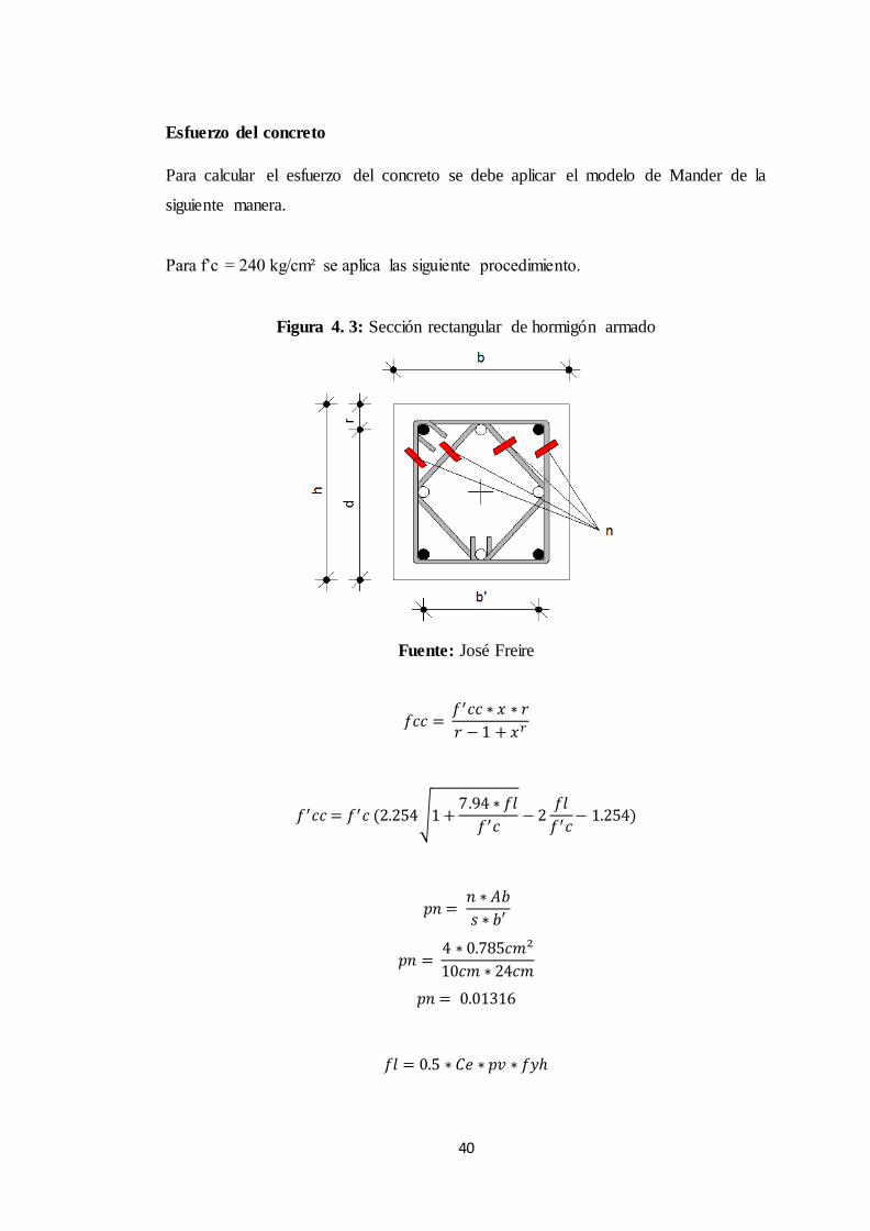
40
Esfuerzo del concreto
Para calcular el esfuerzo del concreto se debe aplicar el modelo de Mander de la
siguiente manera.
Para f’c = 240 kg/cm² se aplica las siguiente procedimiento.
Figura 4. 3: Sección rectangular de hormigón armado
Fuente: José Freire
𝑓𝑐𝑐 = 𝑓′𝑐𝑐 ∗ 𝑥 ∗ 𝑟
𝑟 − 1 + 𝑥𝑟
𝑓′𝑐𝑐 = 𝑓′𝑐 (2.254√1 +7.94 ∗ 𝑓𝑙
𝑓′𝑐− 2
𝑓𝑙
𝑓′𝑐− 1.254)
𝑝𝑛 = 𝑛 ∗ 𝐴𝑏
𝑠 ∗ 𝑏′
𝑝𝑛 = 4 ∗ 0.785𝑐𝑚²
10𝑐𝑚 ∗ 24𝑐𝑚
𝑝𝑛 = 0.01316
𝑓𝑙 = 0.5 ∗ 𝐶𝑒 ∗ 𝑝𝑣 ∗ 𝑓𝑦ℎ

41
fyh = 4200 kg/cm² = 412.02 Mpa
Tabla 4. 1: Efectividad del coeficiente Ce
EFECTIVIDAD DEL CONFINAMIENTO Ce
Sección Ce
Bien confinada 1.00
Circular Mayor a 0.95
Rectangular 0.75 a 0.85
Muros estructurales 0.50
Fuente: Priestley, Displacement-Based Seismic Design of Structures, 2007
𝑓𝑙 = 0.5 ∗ 𝐶𝑒 ∗ 𝑝𝑛 ∗ 𝑓𝑦ℎ
𝑓𝑙 = 0.5 ∗ 0.85 ∗ 0.01316 ∗ 412.02𝑀𝑝𝑎
𝑓𝑙 = 2.305 𝑀𝑝𝑎
𝑓′𝑐𝑐 = 𝑓′𝑐 (2.254√1 +7.94 ∗ 𝑓𝑙
𝑓′𝑐− 2
𝑓𝑙
𝑓′𝑐− 1.254)
𝑓′𝑐𝑐 = 22.805𝑀𝑝𝑎(2.254√1 +7.94 ∗ 2.305𝑀𝑝𝑎
22.805𝑀𝑝𝑎− 2
2.305𝑀𝑝𝑎
22.805𝑀𝑝𝑎− 1.254)
𝑓′𝑐𝑐 = 36.617 𝑀𝑝𝑎 = 373.26 𝑘𝑔/𝑐𝑚²
𝑥 = 𝑐
𝑐𝑐
𝑐𝑐 = 0.002 ∗ (1 + 5(𝑓′𝑐𝑐
𝑓′𝑐− 1))
𝑐𝑐 = 0.002 ∗ (1 + 5(36.617
22.805− 1))
𝑐𝑐 = 0.00755
𝑥 = 𝑐
𝑐𝑐
𝑥 = 0.0005
0.00755
𝑥 = 0.066

42
𝑟 = 𝐸𝑐
𝐸𝑐 − 𝐸𝑠𝑒𝑐
𝐸𝑐 = 5000√𝑓′𝑐
𝐸𝑐 = 5000√22.805 𝑀𝑝𝑎
𝐸𝑐 = 24261.079 𝑀𝑝𝑎
𝐸𝑠𝑒𝑐 = 𝑓′𝑐𝑐
𝑐𝑐
𝐸𝑠𝑒𝑐 = 36.617 𝑀𝑝𝑎
0.00755
𝐸𝑠𝑒𝑐 = 4848.20 𝑀𝑝𝑎
𝑟 = 𝐸𝑐
𝐸𝑐 − 𝐸𝑠𝑒𝑐
𝑟 = 24261.079 𝑀𝑝𝑎
24261.079 𝑀𝑝𝑎 − 4848.20 𝑀𝑝𝑎
𝑟 = 1.249
𝑓𝑐 = 𝑓′𝑐𝑐 ∗ 𝑥 ∗ 𝑟
𝑟 − 1 + 𝑥𝑟
𝑓𝑐𝑐 = 373.26 𝑘𝑔/𝑐𝑚² ∗ 0.066 ∗ 1.249
1.249 − 1 + 0.0661.249
𝑓𝑐𝑐 = 10.691 𝑀𝑝𝑎 = 108.98 𝑘𝑔/𝑐𝑚²
Esfuerzo de compresión del hormigón no confinado (f’c)
𝑓𝑐 = 𝑓′𝑐 ∗ 𝑥 ∗ 𝑟
𝑟 − 1 + 𝑥𝑟
𝑓𝑐 = 22.805 𝑘𝑔/𝑐𝑚² ∗ 0.066 ∗ 1.249
1.249 − 1 + 0.0661.249
𝑓𝑐 = 6.874 𝑀𝑝𝑎 = 70.077 𝑘𝑔/𝑐𝑚²

43
Calculo de fibras del hormigón
Para el siguiente paso se debe imponer el número de fibras con el que se quiere trabajar
ncc = 10 fibras
∆ = 𝑐
𝑛𝑐𝑐
∆ = 3.0763
10
∆ = 0.30763 𝑐𝑚
Deformación del hormigón a compresión (c)
𝑐 = (𝑐 − 𝑌𝑐1) ∗ 𝑐
𝑐
𝑌𝑐1 =𝑐
𝑛
𝑌𝑐1 =3.0763
10
𝑌𝑐1 = 0.3076 𝑐𝑚
𝑐 = (𝑐 − 𝑌𝑐1) ∗ 𝑐
𝑐
𝑐 = (3.0763 − 0.3076) ∗ 0.0005
3.0763
𝑐 = 0.00045

44
Figura 4. 4: Método de fibras para la zona de compresión en una sección rectangular
de hormigón armado.
Fuente: José Freire
Con los valores obtenidos se procede a calcular la fuerza y momento para cada una de
las alturas para un hormigón confinado y no confinado.
Tabla 4. 2: Sumatoria de fuerzas y momentos del hormigón confinado a compresión.
SUMATORIA DE FUERZAS Y MOMENTOS DEL HORMIGÓN CONFINADO A COMPRESIÓN
N
yc (cm)
xc (cm)
x (cm)
fc (kg/cm²)
Área (cm²)
Fc (kg)
Mc (kg.cm)
1 0.15382 0.00048 0.062891 104.309 0 0 0
2 0.46145 0.00043 0.056271 94.706 0 0 0
3 0.76908 0.00038 0.049651 84.7788 0 0 0
4 1.07671 0.00033 0.04303 74.5228 0 0 0
5 1.38434 0.00028 0.03641 63.935 0 0 0
6 1.69197 0.00023 0.02979 53.015 6.214126 329.44216 8337.5
7 1.9996 0.00018 0.02317 41.7659 6.214126 259.53872 6488.6
8 2.30723 0.00013 0.01655 30.1952 6.214126 187.63701 4633.3
9 2.61486 7.5E-05 0.00993 18.318 6.214126 113.83055 2775.8
10 2.92249 2.5E-05 0.00331 6.16312 6.214126 38.298406 922.13
ΣFc = 928.74685 23157
Fuente: José Freire.
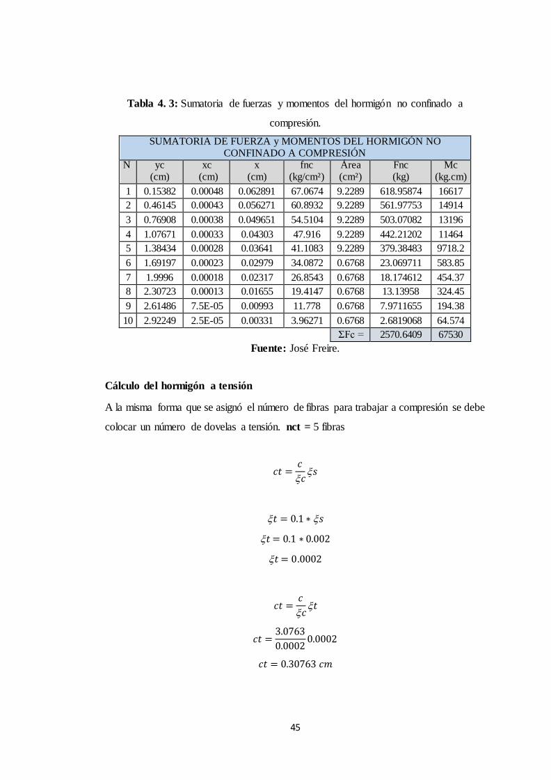
45
Tabla 4. 3: Sumatoria de fuerzas y momentos del hormigón no confinado a
compresión.
SUMATORIA DE FUERZA y MOMENTOS DEL HORMIGÓN NO CONFINADO A COMPRESIÓN
N
yc (cm)
xc (cm)
x (cm)
fnc (kg/cm²)
Área (cm²)
Fnc (kg)
Mc (kg.cm)
1 0.15382 0.00048 0.062891 67.0674 9.2289 618.95874 16617
2 0.46145 0.00043 0.056271 60.8932 9.2289 561.97753 14914
3 0.76908 0.00038 0.049651 54.5104 9.2289 503.07082 13196
4 1.07671 0.00033 0.04303 47.916 9.2289 442.21202 11464
5 1.38434 0.00028 0.03641 41.1083 9.2289 379.38483 9718.2
6 1.69197 0.00023 0.02979 34.0872 0.6768 23.069711 583.85
7 1.9996 0.00018 0.02317 26.8543 0.6768 18.174612 454.37
8 2.30723 0.00013 0.01655 19.4147 0.6768 13.13958 324.45
9 2.61486 7.5E-05 0.00993 11.778 0.6768 7.9711655 194.38
10 2.92249 2.5E-05 0.00331 3.96271 0.6768 2.6819068 64.574
ΣFc = 2570.6409 67530
Fuente: José Freire.
Cálculo del hormigón a tensión
A la misma forma que se asignó el número de fibras para trabajar a compresión se debe
colocar un número de dovelas a tensión. nct = 5 fibras
𝑐𝑡 =𝑐
𝑐𝑠
𝑡 = 0.1 ∗ 𝑠
𝑡 = 0.1 ∗ 0.002
𝑡 = 0.0002
𝑐𝑡 =𝑐
𝑐𝑡
𝑐𝑡 =3.0763
0.00020.0002
𝑐𝑡 = 0.30763 𝑐𝑚

46
∆𝑡 = 𝑐𝑡
𝑛𝑐𝑡
∆𝑡 = 0.3076
5
∆𝑡 = 0.0615
Deformación del hormigón a tracción ( t)
𝑡 = 𝑌𝑡 ∗ 𝑡
𝑐𝑡
𝑡 = 0.0615𝑐𝑚 ∗ 0.0002
0.3076𝑐𝑚
𝑡 = 0.00004
Esfuerzo del hormigón confinado a tracción (ft)
𝑓𝑡 = 𝐸𝑡 ∗ 𝑡
𝐸𝑡 = 2𝑓𝑐𝑐
𝑜
𝐸𝑡 = 2 ∗ 373.266 𝑘𝑔/𝑐𝑚²
0.002
𝐸𝑡 = 373266.97 𝑘𝑔/𝑐𝑚²
𝑓𝑡 = 𝐸𝑡 ∗ 𝑡
𝑓𝑡 = 373266.97𝑘𝑔/𝑐𝑚² ∗ 0.0002
𝑓𝑡 = 14.931 𝑘𝑔/𝑐𝑚²
Fuerza del hormigón confinado a tracción (Ft)
𝐹𝑡 = 𝑓𝑡 ∗ 𝑏 ∗ ∆
𝐹𝑡 = 19.931𝑘𝑔/𝑐𝑚² ∗ 30𝑐𝑚 ∗ 0.0615𝑐𝑚
𝐹𝑡 = 27.558 𝑘𝑔

47
Figura 4. 5: Método de fibras para la zona de tensión en una sección rectangular de
hormigón armado.
Fuente: José Freire
Al igual que el hormigón confinado y no confinado se procede a realizar una tabla de
fuerza y momento para cada una de las alturas para un hormigón a tracción.
Tabla 4. 4: Sumatoria de fuerzas y momentos del hormigón a tracción.
SUMATORIA DE FUERZA Y MOMENTOS DEL HORMIGÓN A TRACCIÓN
n yc
(cm) Δt
(cm) ft
(kg/cm²) Área (cm²)
Ft (kg)
Mt (kg.cm)
1 0.03076 2.2E-05 5.333333 1.84578 9.84416 235.20589
2 0.09229 6.7E-05 16 1.84578 29.53248 703.80067
3 0.15382 0.00011 26.66667 1.84578 49.2208 1169.9728
4 0.21534 0.00016 37.33333 1.84578 68.90912 1633.7222
5 0.27687 0.0002 48 1.84578 88.59744 2095.0489
ΣFc = 246.104 5837.7503
Fuente: José Freire.

48
Verificación de equilibrio
Figura 4. 6: Equilibrio de Fuerzas
Fuente: José Freire.
𝑃 + 𝛴𝐹𝑐 + 𝛴𝐹𝑛𝑐 = 𝐹1 + 𝐹2 + 𝐹3 + 𝛴𝐹𝑡
20000𝑘𝑔 + 928.7𝑘𝑔 + 2570.6𝑘𝑔 = 85.71𝑘𝑔 + 8929.67𝑘𝑔 + 14238.00𝑘𝑔 + 5837.75𝑘𝑔
23499.49𝑘𝑔 = 23.499.39 𝑘𝑔
Momento
𝑀 = (𝑃 − 𝐹2)((ℎ/2) − 𝑟) − 𝐹1(𝑑 − 𝑟) + 𝛴𝑀𝑐 + 𝛴𝑀𝑛𝑐 − 𝛴𝑀𝑡
𝑀 = (20000 − 8929.67)((30/2) − 3) − 85.7(27 − 3) + 23157.2 + 67530.1 − 5837.75
𝑀 = 1983170541 𝑘𝑔/𝑐𝑚2 = 1.983 𝑡/𝑚²
Curvatura
∅ = 𝑐
𝑐
∅ = 0.0005
3.0763
∅ = 0.0163
De esta manera se calcula el valor de momento y curvatura para una deformación del
concreto de 0.0005 el cual corresponde a un solo punto, para resolver los demás puntos

49
se debe aumentar la deformación del concreto en 0.0005 hasta encontrar la falla de la
sección de la siguiente manera.
Tabla 4. 5: Puntos del diagrama momento – curvatura de la resolución manual.
TABLA DEL DIAGRAMA MOMENTO - CURVATURA
xc (cm)
c (cm)
M (tn) θ
0.00 0.00 0.00 0.00
0.0005 3.0763 1.98 0.0163
0.001 6.6682 3.4748 0.018
0.0015 4.74 3.5 0.0351
0.002 4.21 3.7957 0.0506
0.0025 3.9628 4.0367 0.0662
0.003 3.8022 4.2347 0.0821
0.0035 3.6904 4.3989 0.098
0.004 3.6077 4.5362 0.1141
0.0045 3.5438 4.6518 0.1302
0.005 3.4927 4.7498 0.1464
0.0055 3.4405 4.8388 0.1631
0.006 3.4062 4.9101 0.1794
0.0065 3.377 4.9709 0.1958
0.007 3.3519 5.023 0.2121
0.0075 3.3299 5.068 0.2285
0.008 3.3105 5.1066 0.2449
0.0085 3.2932 5.1394 0.2614
0.009 3.2778 5.1679 0.2779
0.0095 3.2638 5.1918 0.2944
0.01 3.2512 5.2124 0.3109
0.0105 3.2396 5.2291 0.3274
0.011 3.229 5.2434 0.344
0.0115 3.2192 5.2549 0.3606
0.012 3.2102 5.2639 0.3771
0.0125 3.2018 5.2704 0.3937
Fuente: José Freire.
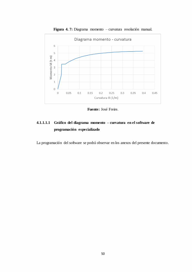
50
Figura 4. 7: Diagrama momento – curvatura resolución manual.
Fuente: José Freire.
4.1.1.1.1 Gráfico del diagrama momento – curvatura en el software de
programación especializado
La programación del software se podrá observar en los anexos del presente documento.
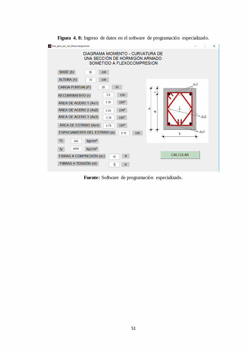
51
Figura 4. 8: Ingreso de datos en el software de programación especializado.
Fuente: Software de programación especializado.

52
Figura 4. 9: Diagrama momento - curvatura en el software de programación
especializado.
Fuente: Fuente: Software de programación especializado.
4.1.1.1.2 Comparación del diagrama momento – curvatura en Sap2000.
Ingresamos a la plataforma virtual de Sap2000.

53
Figura 4. 10: Pantalla de inicio del software especializado.
Fuente: Impresión de pantalla del software especializado.
Definimos el material hormigón en este caso f’c = 240 kg/cm²
Figura 4. 11: Pasos para definir el material.
Fuente: Impresión de pantalla del software especializado.

54
Figura 4. 12: Pantalla para definir el material.
Fuente: Impresión de pantalla del software especializado.
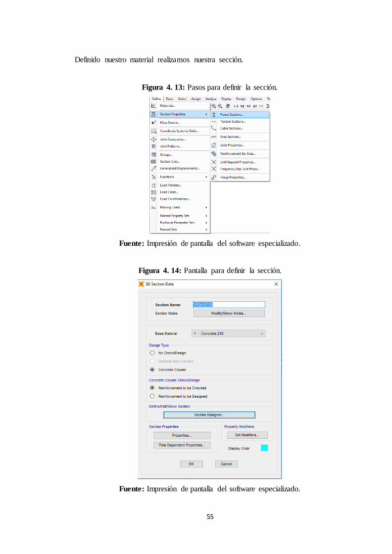
55
Definido nuestro material realizamos nuestra sección.
Figura 4. 13: Pasos para definir la sección.
Fuente: Impresión de pantalla del software especializado.
Figura 4. 14: Pantalla para definir la sección.
Fuente: Impresión de pantalla del software especializado.

56
Figura 4. 15: Pantalla secundaria para definir la sección.
Fuente: Impresión de pantalla del software especializado.
Figura 4. 16: Diagrama momento – curvatura de la sección.
Fuente: Impresión de pantalla del software especializado.
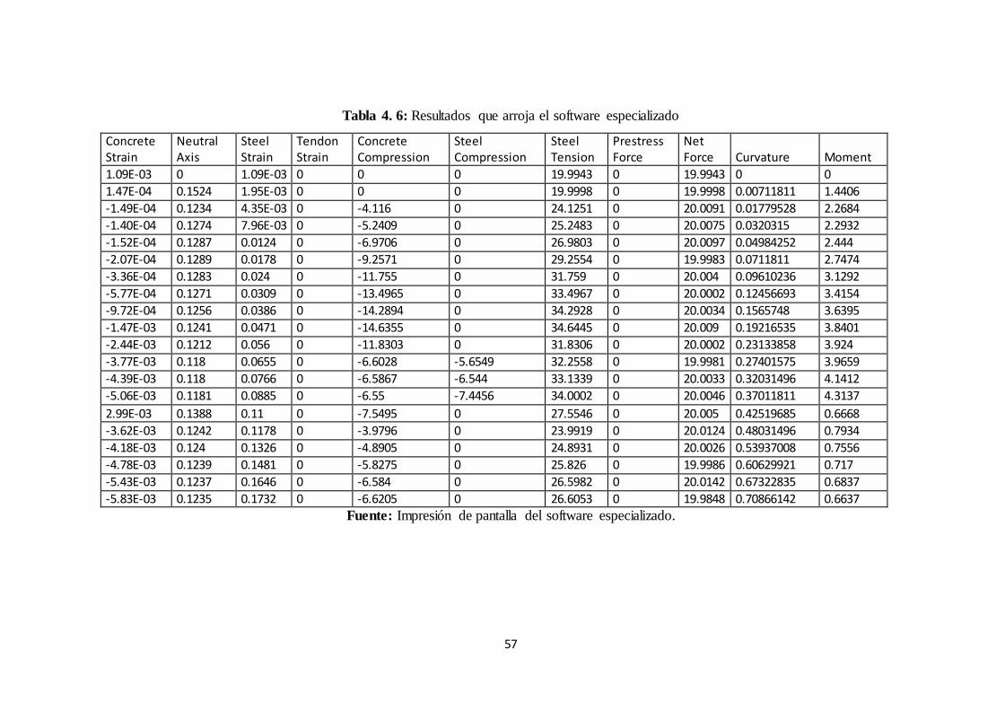
57
Tabla 4. 6: Resultados que arroja el software especializado
Concrete Strain
Neutral Axis
Steel Strain
Tendon Strain
Concrete Compression
Steel Compression
Steel Tension
Prestress Force
Net Force Curvature Moment
1.09E-03 0 1.09E-03 0 0 0 19.9943 0 19.9943 0 0
1.47E-04 0.1524 1.95E-03 0 0 0 19.9998 0 19.9998 0.00711811 1.4406
-1.49E-04 0.1234 4.35E-03 0 -4.116 0 24.1251 0 20.0091 0.01779528 2.2684
-1.40E-04 0.1274 7.96E-03 0 -5.2409 0 25.2483 0 20.0075 0.0320315 2.2932
-1.52E-04 0.1287 0.0124 0 -6.9706 0 26.9803 0 20.0097 0.04984252 2.444
-2.07E-04 0.1289 0.0178 0 -9.2571 0 29.2554 0 19.9983 0.0711811 2.7474
-3.36E-04 0.1283 0.024 0 -11.755 0 31.759 0 20.004 0.09610236 3.1292
-5.77E-04 0.1271 0.0309 0 -13.4965 0 33.4967 0 20.0002 0.12456693 3.4154
-9.72E-04 0.1256 0.0386 0 -14.2894 0 34.2928 0 20.0034 0.1565748 3.6395
-1.47E-03 0.1241 0.0471 0 -14.6355 0 34.6445 0 20.009 0.19216535 3.8401
-2.44E-03 0.1212 0.056 0 -11.8303 0 31.8306 0 20.0002 0.23133858 3.924
-3.77E-03 0.118 0.0655 0 -6.6028 -5.6549 32.2558 0 19.9981 0.27401575 3.9659
-4.39E-03 0.118 0.0766 0 -6.5867 -6.544 33.1339 0 20.0033 0.32031496 4.1412
-5.06E-03 0.1181 0.0885 0 -6.55 -7.4456 34.0002 0 20.0046 0.37011811 4.3137
2.99E-03 0.1388 0.11 0 -7.5495 0 27.5546 0 20.005 0.42519685 0.6668
-3.62E-03 0.1242 0.1178 0 -3.9796 0 23.9919 0 20.0124 0.48031496 0.7934
-4.18E-03 0.124 0.1326 0 -4.8905 0 24.8931 0 20.0026 0.53937008 0.7556
-4.78E-03 0.1239 0.1481 0 -5.8275 0 25.826 0 19.9986 0.60629921 0.717
-5.43E-03 0.1237 0.1646 0 -6.584 0 26.5982 0 20.0142 0.67322835 0.6837
-5.83E-03 0.1235 0.1732 0 -6.6205 0 26.6053 0 19.9848 0.70866142 0.6637
Fuente: Impresión de pantalla del software especializado.

58
4.1.1.2 Diagrama momento – curvatura de una sección de perfil de acero W
sometida a flexocompresión.
Figura 4. 17: Diagrama esfuerzo – deformación de la sección de perfil de acero.
Fuente: José Freire
Datos
Nombre del perfil = W24x103 AISC d=62.30 cm, b1=28.86 cm, b2=28.86 cm,
tw=1.40 cm, tf1=2.49 cm², tf2=2.49 cm², P = 100 tn, Acero= A36,
Es = 2043000 Kg/cm².
Centro de gravedad con respecto a y (ycg)
Figura 4. 18: Sección de perfil de acero W24X103.
Fuente: José Freire
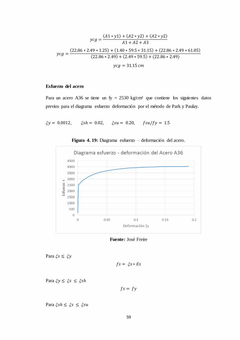
59
𝑦𝑐𝑔 =(𝐴1 ∗ 𝑦1) + (𝐴2 ∗ 𝑦2) + (𝐴2 ∗ 𝑦2)
𝐴1 + 𝐴2 + 𝐴3
𝑦𝑐𝑔 =(22.86 ∗ 2.49 ∗ 1.25) + (1.40 ∗ 59.5 ∗ 31.15) + (22.86 ∗ 2.49 ∗ 61.05)
(22.86 ∗ 2.49) + (2.49 ∗ 59.5) + (22.86 ∗ 2.49)
𝑦𝑐𝑔 = 31.15 𝑐𝑚
Esfuerzo del acero
Para un acero A36 se tiene un fy = 2530 kg/cm² que contiene los siguientes datos
previos para el diagrama esfuerzo deformación por el método de Park y Paulay.
𝑦 = 0.0012, 𝑠ℎ = 0.02, 𝑠𝑢 = 0.20, 𝑓𝑠𝑢/𝑓𝑦 = 1.5
Figura 4. 19: Diagrama esfuerzo – deformación del acero.
Fuente: José Freire
Para 𝑠 ≤ 𝑦
𝑓𝑠 = 𝑠 ∗ 𝐸𝑠
Para 𝑦 ≤ 𝑠 ≤ 𝑠ℎ
𝑓𝑠 = 𝑓𝑦
Para 𝑠ℎ ≤ 𝑠 ≤ 𝑠𝑢
60
𝑟 = 𝑠𝑢 − 𝑠ℎ
𝑟 = 0.20 − 0.002
𝑟 = 0.198
𝑚 =
(𝑓𝑠𝑢𝑓𝑦
)(30𝑟 + 1) 2 − 60𝑟 − 1
15𝑟²
𝑚 = 1.5((30 ∗ 0.198) + 1)2 − (60 ∗ 0.198) − 1
15(0.198)²
𝑚 = 109.141
𝑓𝑠 = 𝑓𝑦[𝑚(𝑠 − 𝑠ℎ) + 2
60(𝑠 − 𝑠ℎ) + 2+
(𝑠 − 𝑠ℎ)(60 − 𝑚)
2(30𝑟 + 1)2 ]
𝑓𝑠1 = 𝑠1 ∗ 𝐸𝑠
𝑓𝑠1 = 0.0001 ∗ 2043000 𝑘𝑔/𝑐𝑚²
𝑓𝑠1 = 204.30 𝑘𝑔/𝑐𝑚²
Carga última (Py)
𝑃𝑦 = 𝐴 ∗ 𝑓𝑦
𝑃𝑦 = ((22.86 ∗ 2.49) + (1.40 ∗ 57.32) + (22.86 ∗ 2.49)) ∗ 2530
𝑃𝑦 = 491049.72 𝑘𝑔 = 491.04 𝑡𝑛
Desplazamiento del brazo de palanca inferior (bi)
𝑏𝑖 = 𝑦𝑐𝑔 ∗ (1 +𝑝
𝑝𝑦)
𝑏𝑖 = 31.15 ∗ (1 +100
491.04)
𝑏𝑖 = 37.49 𝑐𝑚
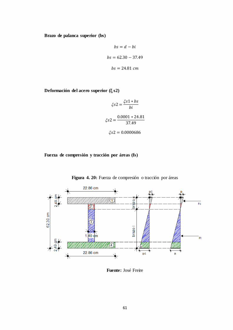
61
Brazo de palanca superior (bs)
𝑏𝑠 = 𝑑 − 𝑏𝑖
𝑏𝑠 = 62.30 − 37.49
𝑏𝑠 = 24.81 𝑐𝑚
Deformación del acero superior ( s2)
𝑠2 =𝑠1 ∗ 𝑏𝑠
𝑏𝑖
𝑠2 =0.0001 ∗ 24.81
37.49
𝑠2 = 0.0000686
Fuerza de compresión y tracción por áreas (fs)
Figura 4. 20: Fuerza de compresión o tracción por áreas
Fuente: José Freire

62
𝑓𝑐 = 𝑠2 ∗ 𝐸𝑠
𝑓𝑐 = 0.0000686 ∗ 2043000
𝑓𝑐 = 140.14 𝑘𝑔/𝑐𝑚²
𝐹𝑐1 = (𝑓𝑐 + (𝑓𝑐 ∗ (𝑏𝑠 − 𝑡𝑓1)
𝑏𝑠)) ∗
𝑡𝑓1
2∗ 𝑏1
𝐹𝑐1 = (140.14 + (140.14 ∗ (24.81 − 2.49)
24.81)) ∗
2.49
2∗ 22.86
𝐹𝑐1 = 7307.80 𝑘𝑔
𝐹𝑐2 = (𝑓𝑐 ∗ (𝑏𝑠 − 𝑡𝑓1)
𝑏𝑠) ∗
(𝑏𝑠 − 𝑡𝑓1)
2∗ 𝑡𝑤
𝐹𝑐2 = (140.14 ∗ (24.81 − 2.49)
24.81) ∗
(24.81 − 2.49)
2∗ 1.40
𝐹𝑐2 = 1899.60 𝑘𝑔
𝑓𝑡 = 𝑠 ∗ 𝐸𝑠
𝑓𝑡 = 0.0001 ∗ 2043000
𝑓𝑡 = 204.30 𝑘𝑔/𝑐𝑚²
𝐹𝑡1 = (𝑓𝑡 ∗ (𝑏𝑖 − 𝑡𝑓2)
𝑏𝑖) ∗
(𝑏𝑖 − 𝑡𝑓2)
2∗ 𝑡𝑤
𝐹𝑡1 = (204.30 ∗ (37.49 − 2.49)
37.49) ∗
(37.49 − 2.49)
2∗ 1.40
𝐹𝑡1 = 4673.80 𝑘𝑔
𝐹𝑡2 = (𝑓𝑡 + (𝑓𝑡 ∗ (𝑏𝑖 − 𝑡𝑓2)
𝑏𝑖)) ∗
𝑡𝑓2
2∗ 𝑏2
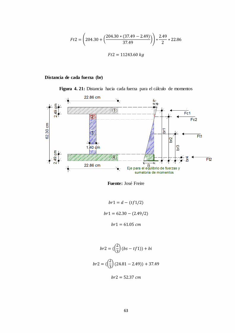
63
𝐹𝑡2 = (204.30 + (204.30 ∗ (37.49 − 2.49)
37.49)) ∗
2.49
2∗ 22.86
𝐹𝑡2 = 11243.60 𝑘𝑔
Distancia de cada fuerza (br)
Figura 4. 21: Distancia hacia cada fuerza para el cálculo de momentos
Fuente: José Freire
𝑏𝑟1 = 𝑑 − (𝑡𝑓1/2)
𝑏𝑟1 = 62.30 − (2.49/2)
𝑏𝑟1 = 61.05 𝑐𝑚
𝑏𝑟2 = ((2
3) (𝑏𝑠 − 𝑡𝑓1)) + 𝑏𝑖
𝑏𝑟2 = ((2
3) (24.81 − 2.49)) + 37.49
𝑏𝑟2 = 52.37 𝑐𝑚
64
𝑏𝑟3 = ((1
3) (𝑏𝑖 − 𝑡𝑓2)) + 𝑡𝑓2
𝑏𝑟3 = ((1
3) (37.49 − 2.49)) + 2.49
𝑏𝑟3 = 14.16 𝑐𝑚
𝑏𝑟4 =𝑡𝑓2
2
𝑏𝑟4 =2.49
2
𝑏𝑟4 = 1.245 𝑐𝑚
Momento (M)
𝑀 = (𝐹𝑐1 ∗ 𝑏𝑟1) + (𝐹𝑐2 ∗ 𝑏𝑟2) + (𝐹𝑡1 ∗ 𝑏𝑟3) + (𝐹𝑡2 ∗ 𝑏𝑟4)
𝑀 = (7307.80 ∗ 61.05) + (1899.60 ∗ 52.37) + (4673.80 ∗ 14.16) + (11243.60 ∗ 1.245)
𝑀 = 465581.25 𝑘𝑔. 𝑐𝑚 = 4.6558 𝑡𝑛. 𝑚
Curvatura
∅ = 𝑐
𝑏𝑖
∅ = 0.0001
0.3749
∅ = 0.000266
De esta manera se calcula el valor de momento y curvatura para una deformación del
acero de 0.0001 el cual corresponde a un solo punto, para resolver los demás puntos
se debe aumentar la deformación del concreto en 0.0001 hasta la deformación última
del acero en el caso del acero A36 se tiene una u = 0.20.
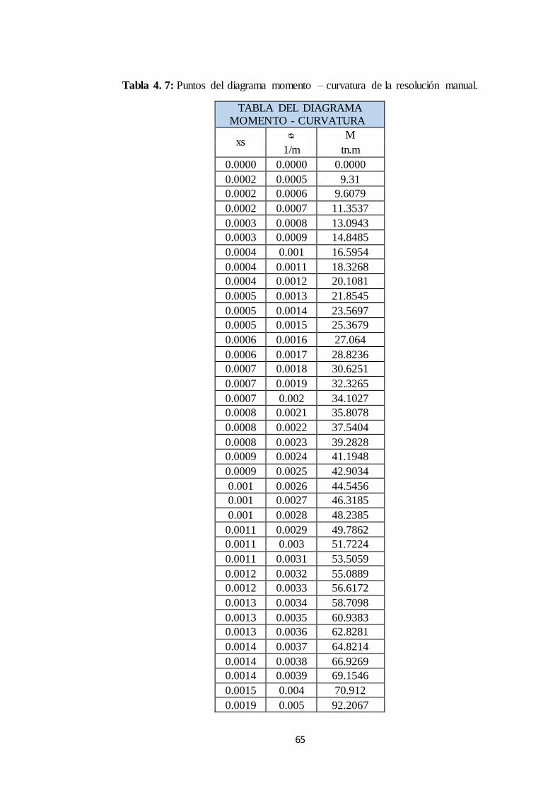
65
Tabla 4. 7: Puntos del diagrama momento – curvatura de la resolución manual.
TABLA DEL DIAGRAMA MOMENTO - CURVATURA
xs ᴓ M
1/m tn.m
0.0000 0.0000 0.0000
0.0002 0.0005 9.31
0.0002 0.0006 9.6079
0.0002 0.0007 11.3537
0.0003 0.0008 13.0943
0.0003 0.0009 14.8485
0.0004 0.001 16.5954
0.0004 0.0011 18.3268
0.0004 0.0012 20.1081
0.0005 0.0013 21.8545
0.0005 0.0014 23.5697
0.0005 0.0015 25.3679
0.0006 0.0016 27.064
0.0006 0.0017 28.8236
0.0007 0.0018 30.6251
0.0007 0.0019 32.3265
0.0007 0.002 34.1027
0.0008 0.0021 35.8078
0.0008 0.0022 37.5404
0.0008 0.0023 39.2828
0.0009 0.0024 41.1948
0.0009 0.0025 42.9034
0.001 0.0026 44.5456
0.001 0.0027 46.3185
0.001 0.0028 48.2385
0.0011 0.0029 49.7862
0.0011 0.003 51.7224
0.0011 0.0031 53.5059
0.0012 0.0032 55.0889
0.0012 0.0033 56.6172
0.0013 0.0034 58.7098
0.0013 0.0035 60.9383
0.0013 0.0036 62.8281
0.0014 0.0037 64.8214
0.0014 0.0038 66.9269
0.0014 0.0039 69.1546
0.0015 0.004 70.912
0.0019 0.005 92.2067

66
0.0022 0.006 92.2067
0.0027 0.0071 92.2067
0.003 0.008 92.2067
0.0034 0.009 92.2067
0.0038 0.0101 92.2067
0.0077 0.0205 92.2067
0.0118 0.0314 92.2067
0.0154 0.041 92.2067
0.02 0.0533 92.2067
0.025 0.0667 93.5443
0.04 0.1067 128.8108
0.05 0.1334 138.3908
0.0667 0.1778 149.4372
0.10 0.2667 162.0983
0.20 0.5334 174.8302
Fuente: José Freire.
Figura 4. 22: Diagrama momento – curvatura resolución manual.
Fuente: José Freire.
4.1.1.2.1 Gráfico del diagrama momento – curvatura en el software de
programación especializado
La programación del software se podrá observar en los anexos del presente documento.

67
Figura 4. 23: Ingreso de datos en el software de programación especializado.
Fuente: Software de programación especializado.
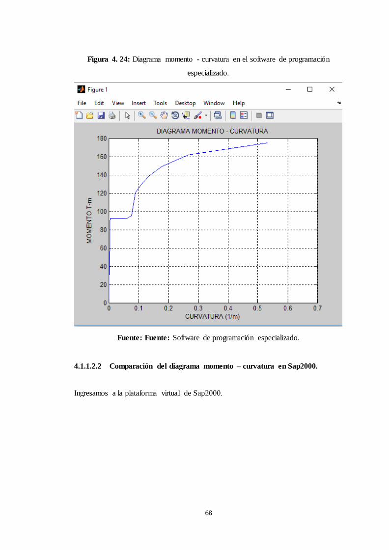
68
Figura 4. 24: Diagrama momento - curvatura en el software de programación
especializado.
Fuente: Fuente: Software de programación especializado.
4.1.1.2.2 Comparación del diagrama momento – curvatura en Sap2000.
Ingresamos a la plataforma virtual de Sap2000.
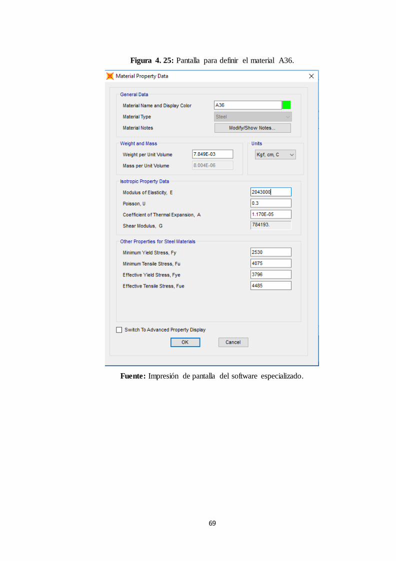
69
Figura 4. 25: Pantalla para definir el material A36.
Fuente: Impresión de pantalla del software especializado.
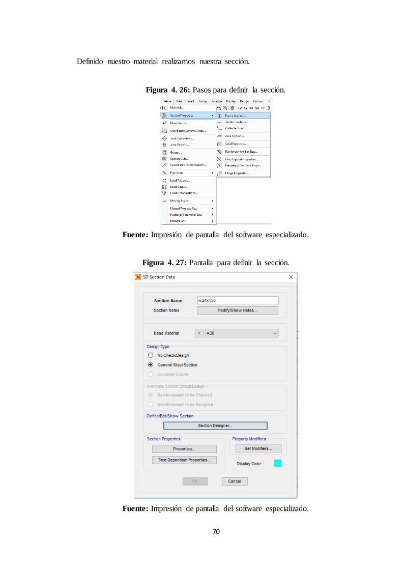
70
Definido nuestro material realizamos nuestra sección.
Figura 4. 26: Pasos para definir la sección.
Fuente: Impresión de pantalla del software especializado.
Figura 4. 27: Pantalla para definir la sección.
Fuente: Impresión de pantalla del software especializado.

71
Figura 4. 28: Pantalla secundaria para definir la sección.
Fuente: Impresión de pantalla del software especializado.
Figura 4. 29: Diagrama momento – curvatura de la sección.
Fuente: Impresión de pantalla del software especializado.
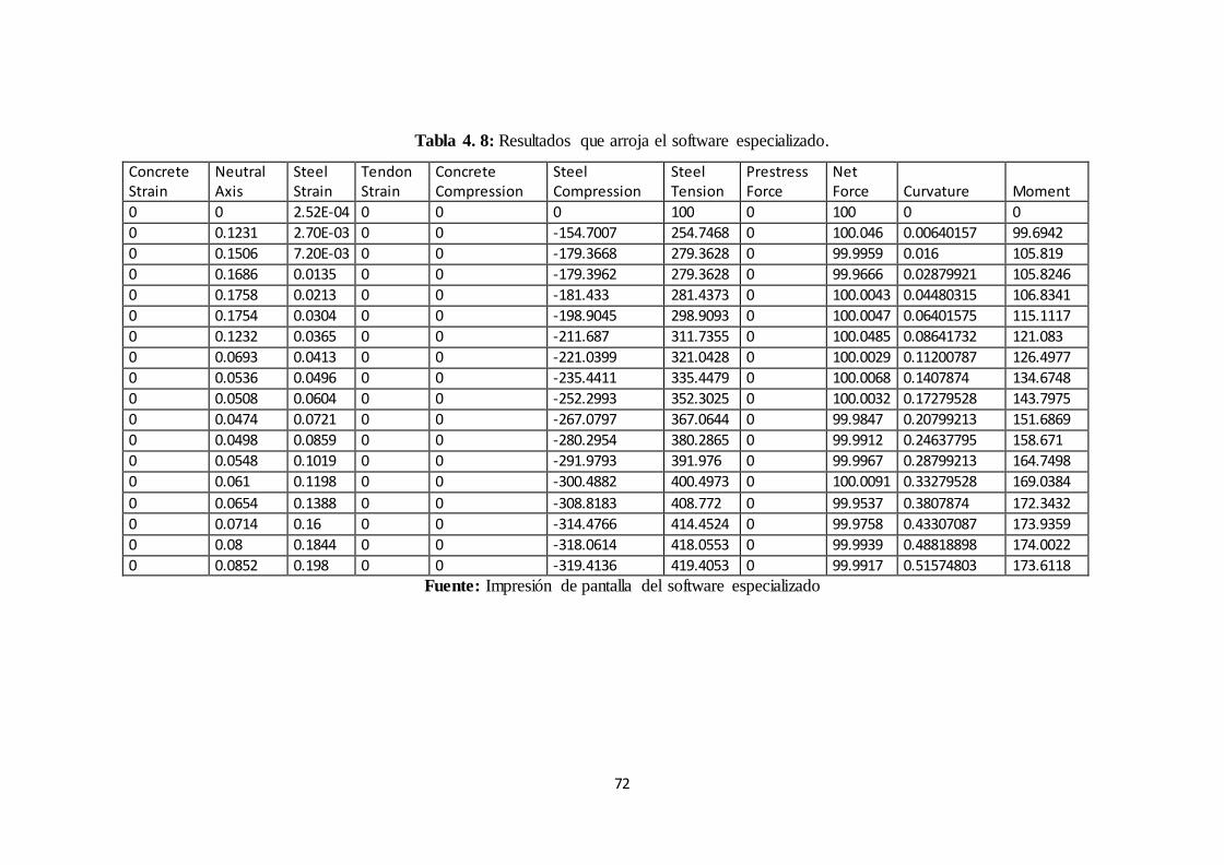
72
Tabla 4. 8: Resultados que arroja el software especializado.
Concrete Strain
Neutral Axis
Steel Strain
Tendon Strain
Concrete Compression
Steel Compression
Steel Tension
Prestress Force
Net Force Curvature Moment
0 0 2.52E-04 0 0 0 100 0 100 0 0
0 0.1231 2.70E-03 0 0 -154.7007 254.7468 0 100.046 0.00640157 99.6942
0 0.1506 7.20E-03 0 0 -179.3668 279.3628 0 99.9959 0.016 105.819
0 0.1686 0.0135 0 0 -179.3962 279.3628 0 99.9666 0.02879921 105.8246
0 0.1758 0.0213 0 0 -181.433 281.4373 0 100.0043 0.04480315 106.8341
0 0.1754 0.0304 0 0 -198.9045 298.9093 0 100.0047 0.06401575 115.1117
0 0.1232 0.0365 0 0 -211.687 311.7355 0 100.0485 0.08641732 121.083
0 0.0693 0.0413 0 0 -221.0399 321.0428 0 100.0029 0.11200787 126.4977
0 0.0536 0.0496 0 0 -235.4411 335.4479 0 100.0068 0.1407874 134.6748
0 0.0508 0.0604 0 0 -252.2993 352.3025 0 100.0032 0.17279528 143.7975
0 0.0474 0.0721 0 0 -267.0797 367.0644 0 99.9847 0.20799213 151.6869
0 0.0498 0.0859 0 0 -280.2954 380.2865 0 99.9912 0.24637795 158.671
0 0.0548 0.1019 0 0 -291.9793 391.976 0 99.9967 0.28799213 164.7498
0 0.061 0.1198 0 0 -300.4882 400.4973 0 100.0091 0.33279528 169.0384
0 0.0654 0.1388 0 0 -308.8183 408.772 0 99.9537 0.3807874 172.3432
0 0.0714 0.16 0 0 -314.4766 414.4524 0 99.9758 0.43307087 173.9359
0 0.08 0.1844 0 0 -318.0614 418.0553 0 99.9939 0.48818898 174.0022
0 0.0852 0.198 0 0 -319.4136 419.4053 0 99.9917 0.51574803 173.6118
Fuente: Impresión de pantalla del software especializado

73
4.2 ANÁLISIS DE RESULTADOS
4.2.1 Sección rectangular de hormigón armado sometido a flexocompresión.
Datos:
h=30 cm, b=30 cm, r=4.00 cm, As1=3.39 cm², As2=2.26 cm², As3=3.39 cm²,
As (estribo) = 0.79 cm² @ 10 cm, f’c= 240 kg/cm², fy = 4200 kg/cm², P=20.0 t,
Figura 4. 30: Dimensiones de la sección rectangular sometido a flexocompresión.
Fuente: José Freire

74
Figura 4. 31: Pantalla de introducción de datos en el Software para una sección
rectangular sometido a flexocompresión.
Fuente: Impresión de pantalla del software.
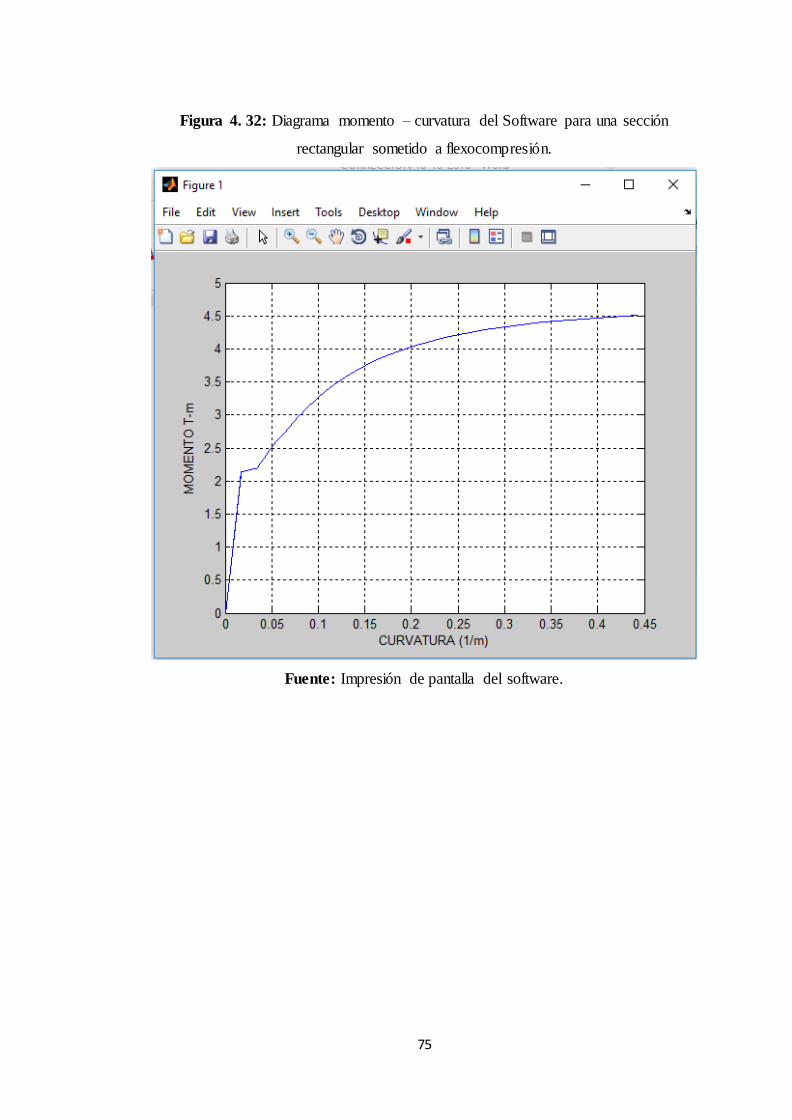
75
Figura 4. 32: Diagrama momento – curvatura del Software para una sección
rectangular sometido a flexocompresión.
Fuente: Impresión de pantalla del software.

76
Figura 4. 33: Pantalla de introducción de datos en el software especializado para una
sección rectangular sometido a flexocompresión.
Fuente: Impresión de pantalla del software especializado.
Figura 4. 34: Diagrama momento – curvatura del software especializado.
Fuente: Impresión de pantalla del software especializado.

77
Figura 4. 35: Diagrama momento – curvatura entre los dos Softwares.
Fuente: José Freire
Tabla 4. 9: Comparación de puntos del diagrama momento - curvatura para una
sección rectangular sometido a flexocompresión.
Comparación de resultados
Parámetro Software
especializado Software Diferencia Porcentaje (%)
Momento último (tn.m)
4.31 4.50 0.19 4.22
curvatura última (1/m)
0.37 0.44 0.07 15.90
Fuente: José Freire
4.2.2 Sección rectangular de hormigón armado sometido a flexión.
Datos:
h=30 cm, b=25 cm, r=4.00 cm, As1=3.39 cm², As2=3.39 cm², As (estribo) =
0.79 cm² @ 10 cm, f’c= 240 kg/cm², fy = 4200 kg/cm².

78
Figura 4. 36: Dimensiones de la sección rectangular sometido a flexión.
Fuente: José Freire
Figura 4. 37: Pantalla de introducción de datos en el Software para una sección
rectangular sometido a flexión.
Fuente: Impresión de pantalla del software.

79
Figura 4. 38: Diagrama momento – curvatura del software para una sección
rectangular sometido a flexión.
Fuente: Impresión de pantalla del software.

80
Figura 4. 39: Pantalla de introducción de datos software especializado para una
sección rectangular sometido a flexión.
Fuente: Impresión de pantalla del software especializado.
Figura 4. 40: Diagrama momento – curvatura del software.
Fuente: Impresión de pantalla del software especializado.

81
Figura 4. 41: Diagrama momento – curvatura entre los dos softwares.
Fuente: José Freire
Tabla 4. 10: Comparación de puntos del diagrama momento - curvatura para una
sección rectangular sometido a flexión.
Comparación de resultados
Parámetro Software
especializado Software Diferencia Porcentaje (%)
Momento último (tn.m)
5.05 5.10 0.05 0.98
curvatura
última (1/m) 0.37 0.36 0.01 2.77
Fuente: José Freire
4.2.3 Sección circular de hormigón armado sometido a flexocompresión.
Datos:
d=30 cm, r=4.00 cm, As1=1.54cm², Nv= 8 varillas As (estribo) = 0.79 cm² @
10 cm, f’c= 240 kg/cm², fy = 4200 kg/cm², P = 20.0 tn.
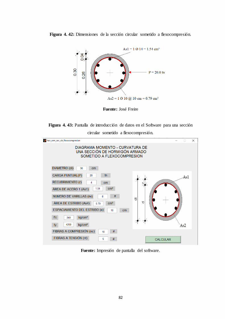
82
Figura 4. 42: Dimensiones de la sección circular sometido a flexocompresión.
Fuente: José Freire
Figura 4. 43: Pantalla de introducción de datos en el Software para una sección
circular sometido a flexocompresión.
Fuente: Impresión de pantalla del software.
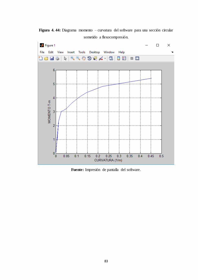
83
Figura 4. 44: Diagrama momento – curvatura del software para una sección circular
sometido a flexocompresión.
Fuente: Impresión de pantalla del software.
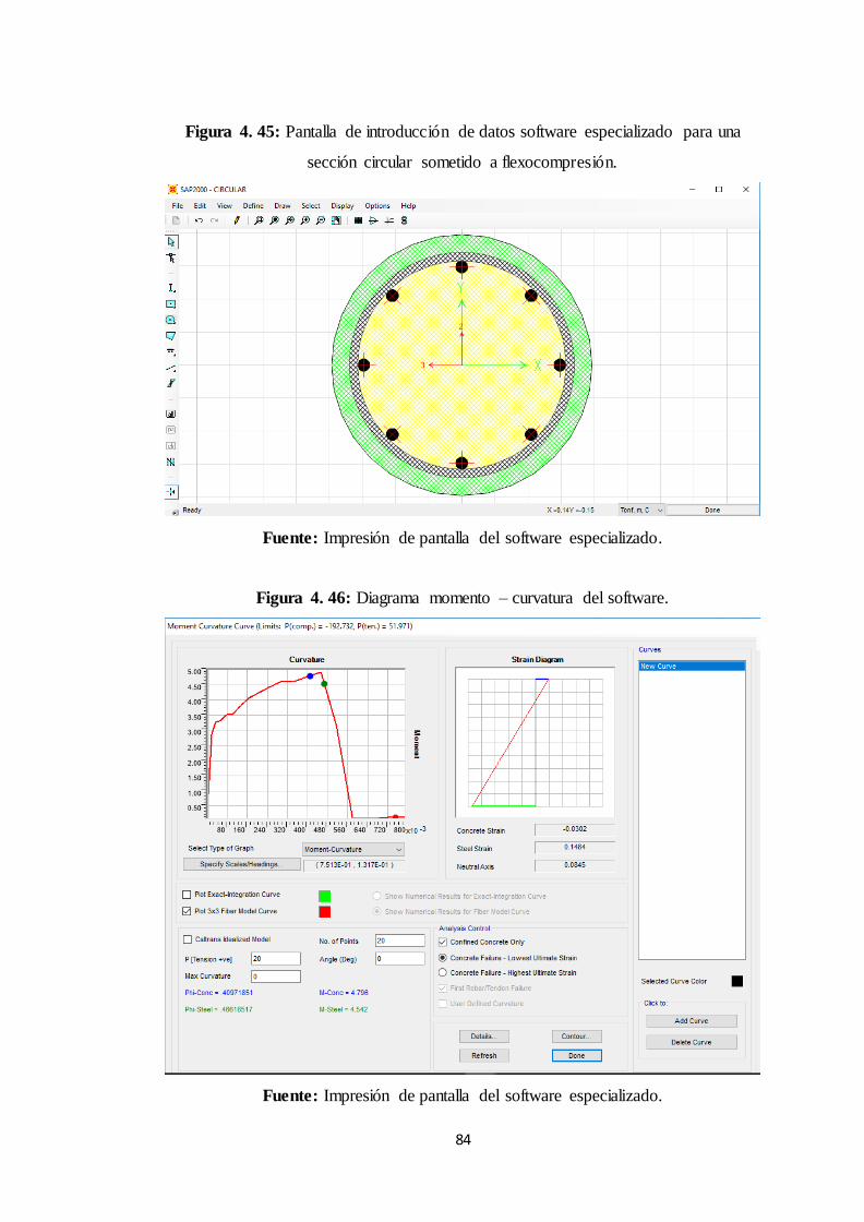
84
Figura 4. 45: Pantalla de introducción de datos software especializado para una
sección circular sometido a flexocompresión.
Fuente: Impresión de pantalla del software especializado.
Figura 4. 46: Diagrama momento – curvatura del software.
Fuente: Impresión de pantalla del software especializado.

85
Figura 4. 47: Diagrama momento – curvatura entre los dos softwares.
Fuente: José Freire
Tabla 4. 11: Comparación de puntos del diagrama momento - curvatura para una
sección circular sometido a flexocompresión.
Comparación de resultados
Parámetro Software
especializado Software Diferencia Porcentaje (%)
Momento último (tn.m)
4.90 5.40 0.50 9.25
curvatura
última (1/m) 0.45 0.45 0.00 0.00
Fuente: José Freire
4.2.4 Sección W de perfil de acero sometido a flexocompresión.
Datos:
Nombre del perfil = W24x103 AISC d=62.30 cm, b1=28.86 cm, b2=28.86 cm,
tw=1.40 cm, tf1=2.49 cm², tf2=2.49 cm², P = 100 tn, Acero= A36.
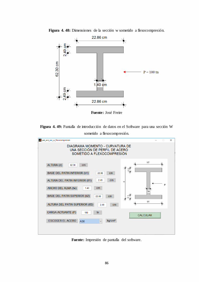
86
Figura 4. 48: Dimensiones de la sección w sometido a flexocompresión.
Fuente: José Freire
Figura 4. 49: Pantalla de introducción de datos en el Software para una sección W
sometido a flexocompresión.
Fuente: Impresión de pantalla del software.
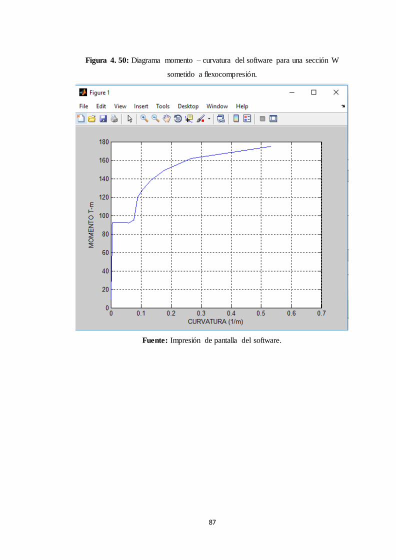
87
Figura 4. 50: Diagrama momento – curvatura del software para una sección W
sometido a flexocompresión.
Fuente: Impresión de pantalla del software.

88
Figura 4. 51: Pantalla de introducción de datos software especializado para una
sección W sometido a flexocompresión.
Fuente: Impresión de pantalla del software especializado.
Figura 4. 52: Diagrama momento – curvatura del software.
Fuente: Impresión de pantalla del software especializado.
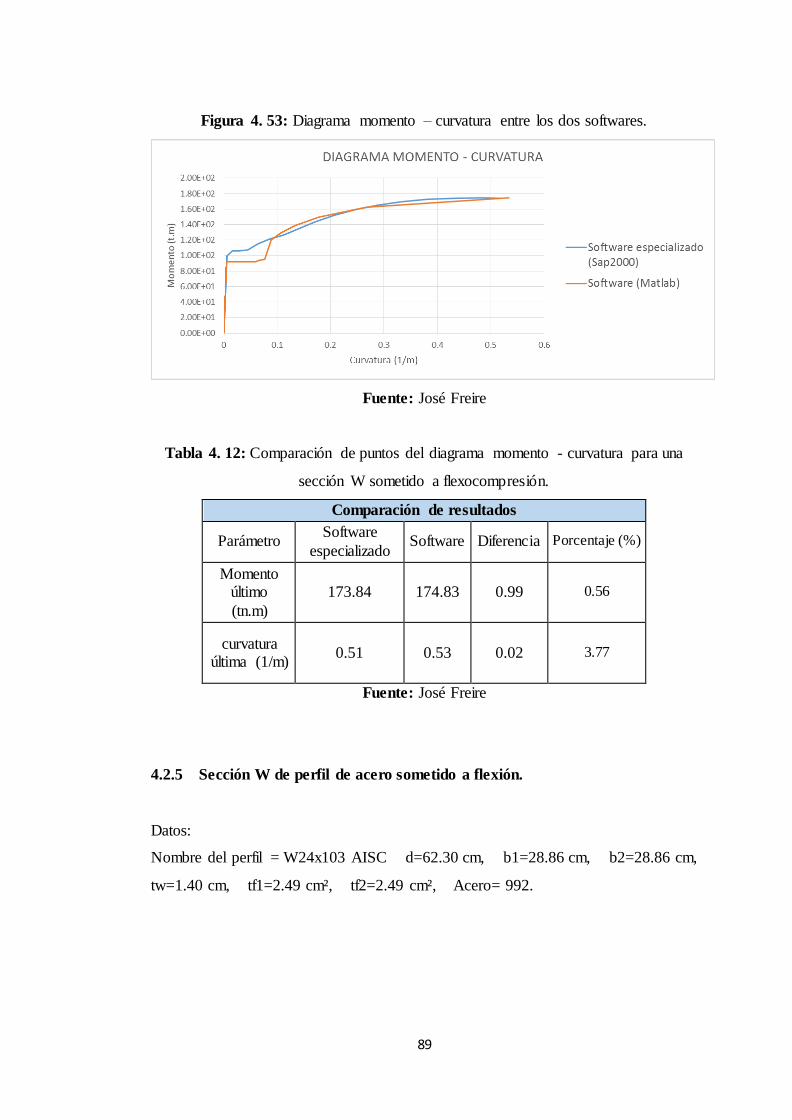
89
Figura 4. 53: Diagrama momento – curvatura entre los dos softwares.
Fuente: José Freire
Tabla 4. 12: Comparación de puntos del diagrama momento - curvatura para una
sección W sometido a flexocompresión.
Comparación de resultados
Parámetro Software
especializado Software Diferencia Porcentaje (%)
Momento último
(tn.m)
173.84 174.83 0.99 0.56
curvatura última (1/m)
0.51 0.53 0.02 3.77
Fuente: José Freire
4.2.5 Sección W de perfil de acero sometido a flexión.
Datos:
Nombre del perfil = W24x103 AISC d=62.30 cm, b1=28.86 cm, b2=28.86 cm,
tw=1.40 cm, tf1=2.49 cm², tf2=2.49 cm², Acero= 992.
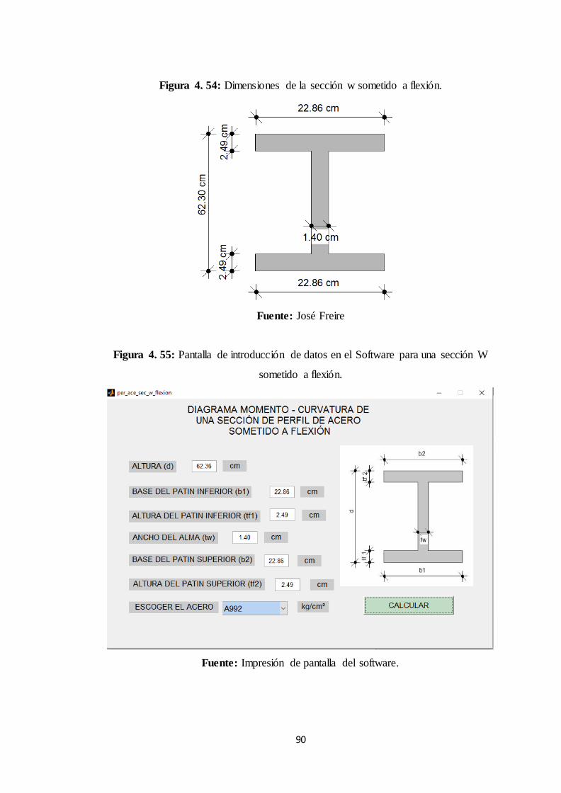
90
Figura 4. 54: Dimensiones de la sección w sometido a flexión.
Fuente: José Freire
Figura 4. 55: Pantalla de introducción de datos en el Software para una sección W
sometido a flexión.
Fuente: Impresión de pantalla del software.
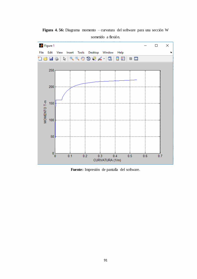
91
Figura 4. 56: Diagrama momento – curvatura del software para una sección W
sometido a flexión.
Fuente: Impresión de pantalla del software.
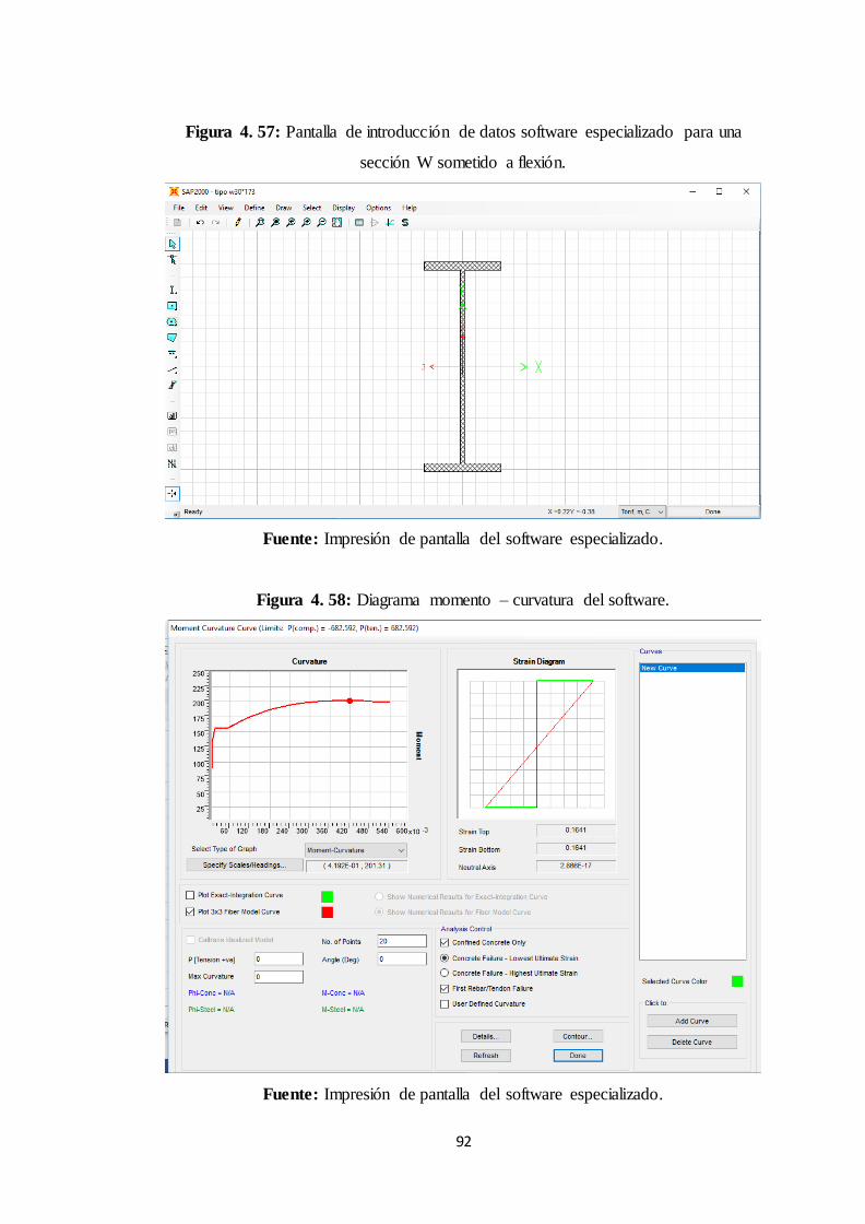
92
Figura 4. 57: Pantalla de introducción de datos software especializado para una
sección W sometido a flexión.
Fuente: Impresión de pantalla del software especializado.
Figura 4. 58: Diagrama momento – curvatura del software.
Fuente: Impresión de pantalla del software especializado.
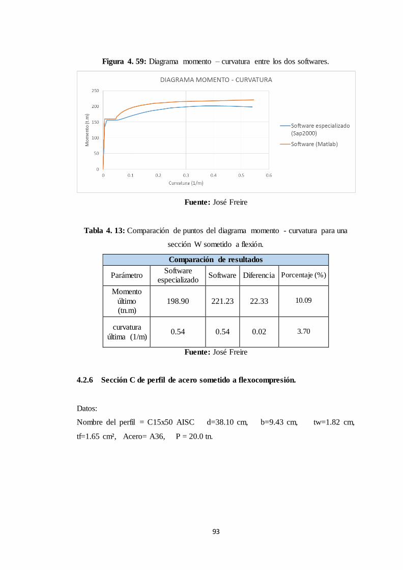
93
Figura 4. 59: Diagrama momento – curvatura entre los dos softwares.
Fuente: José Freire
Tabla 4. 13: Comparación de puntos del diagrama momento - curvatura para una
sección W sometido a flexión.
Comparación de resultados
Parámetro Software
especializado Software Diferencia Porcentaje (%)
Momento
último (tn.m)
198.90 221.23 22.33 10.09
curvatura
última (1/m) 0.54 0.54 0.02 3.70
Fuente: José Freire
4.2.6 Sección C de perfil de acero sometido a flexocompresión.
Datos:
Nombre del perfil = C15x50 AISC d=38.10 cm, b=9.43 cm, tw=1.82 cm,
tf=1.65 cm², Acero= A36, P = 20.0 tn.
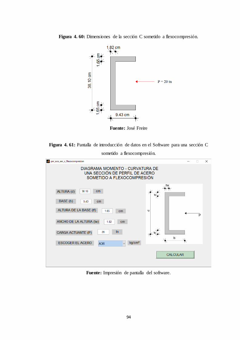
94
Figura 4. 60: Dimensiones de la sección C sometido a flexocompresión.
Fuente: José Freire
Figura 4. 61: Pantalla de introducción de datos en el Software para una sección C
sometido a flexocompresión.
Fuente: Impresión de pantalla del software.

95
Figura 4. 62: Diagrama momento – curvatura del software para una sección C
sometido a flexocompresión.
Fuente: Impresión de pantalla del software.
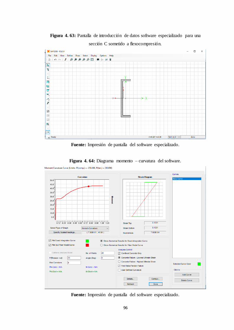
96
Figura 4. 63: Pantalla de introducción de datos software especializado para una
sección C sometido a flexocompresión.
Fuente: Impresión de pantalla del software especializado.
Figura 4. 64: Diagrama momento – curvatura del software.
Fuente: Impresión de pantalla del software especializado.

97
Figura 4. 65: Diagrama momento – curvatura entre los dos softwares.
Fuente: José Freire
Tabla 4. 14: Comparación de puntos del diagrama momento - curvatura para una
sección c sometido a flexocompresión.
Comparación de resultados
Parámetro Software
especializado Software Diferencia Porcentaje (%)
Momento último
(tn.m)
42.34 43.84 1.50 3.42
curvatura última (1/m)
1.05 0.96 0.09 9.37
Fuente: José Freire
4.2.7 Sección C de perfil de acero sometido a flexión.
Datos:
Nombre del perfil = C15x50 AISC d=38.10 cm, b=9.43 cm, tw=1.82 cm,
tf=1.65 cm², Acero= A572.
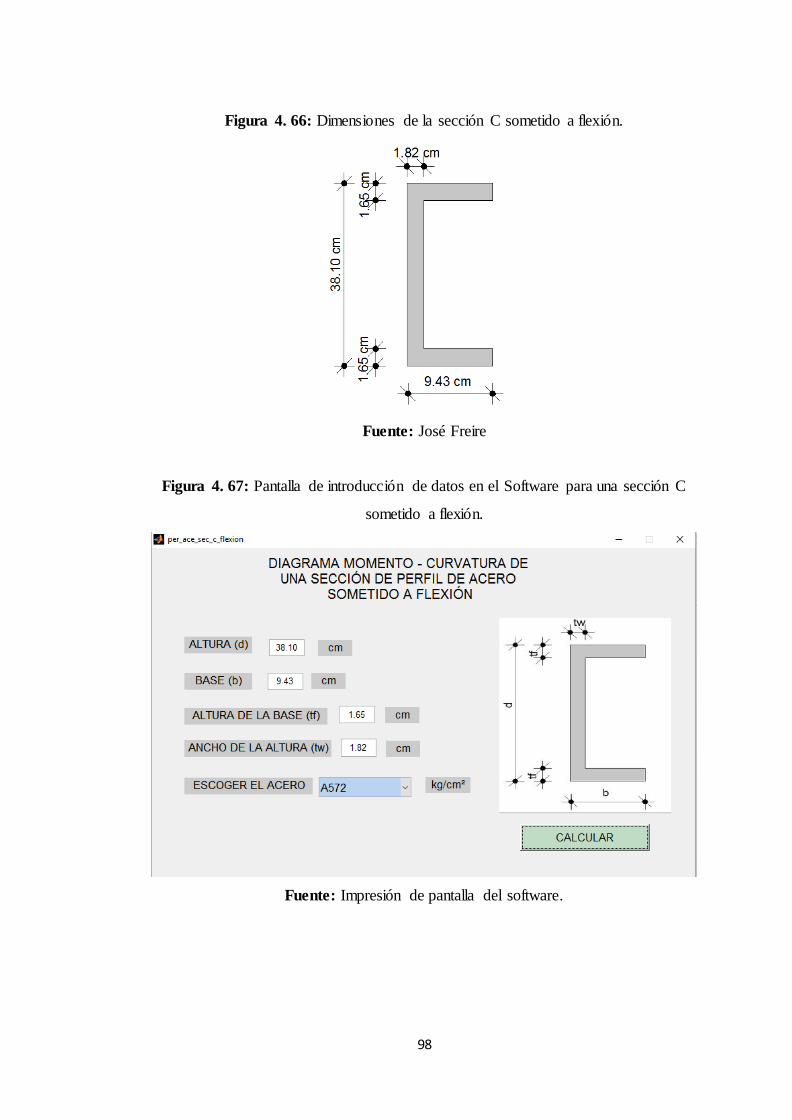
98
Figura 4. 66: Dimensiones de la sección C sometido a flexión.
Fuente: José Freire
Figura 4. 67: Pantalla de introducción de datos en el Software para una sección C
sometido a flexión.
Fuente: Impresión de pantalla del software.

99
Figura 4. 68: Diagrama momento – curvatura del software para una sección C
sometido a flexión.
Fuente: Impresión de pantalla del software.

100
Figura 4. 69: Pantalla de introducción de datos software especializado para una
sección C sometido a flexión.
Fuente: Impresión de pantalla del software especializado.
Figura 4. 70: Diagrama momento – curvatura del software.
Fuente: Impresión de pantalla del software especializado.

101
Figura 4. 71: Diagrama momento – curvatura entre los dos softwares.
Fuente: José Freire
Tabla 4. 15: Comparación de puntos del diagrama momento - curvatura para una
sección C sometido a flexión.
Comparación de resultados
Parámetro Software
especializado Software Diferencia Porcentaje (%)
Momento último
(tn.m)
47.47 56.19 8.72 15.51
curvatura última (1/m)
0.93 0.89 0.04 4.49
Fuente: José Freire
4.2.8 Sección tubo rectangular de perfil de acero sometido a flexocompresión.
Datos:
Nombre del perfil = 16x16 AISC d=40.64 cm, b=40.64 cm, tw=1.59 cm, tf=1.59
cm², Acero= A913(50), P = 40.0 tn.

102
Figura 4. 72: Dimensiones de la sección tubo rectangular sometido a
flexocompresión.
Fuente: José Freire
Figura 4. 73: Pantalla de introducción de datos en el Software para una sección tubo
rectangular sometido a flexocompresión.
Fuente: Impresión de pantalla del software.

103
Figura 4. 74: Diagrama momento – curvatura del software para una sección tubo
rectangular sometido a flexocompresión.
Fuente: Impresión de pantalla del software.

104
Figura 4. 75: Pantalla de introducción de datos software especializado para una
sección tubo rectangular sometido a flexocompresión.
Fuente: Impresión de pantalla del software especializado.
Figura 4. 76: Diagrama momento – curvatura del software.
Fuente: Impresión de pantalla del software especializado.

105
Figura 4. 77: Diagrama momento – curvatura entre los dos softwares.
Fuente: José Freire
Tabla 4. 16: Comparación de puntos del diagrama momento - curvatura para una
sección tubo rectangular sometido a flexocompresión.
Comparación de resultados
Parámetro Software
especializado Software Diferencia Porcentaje (%)
Momento último
(tn.m)
157.76 161.53 3.77 2.33
curvatura última (1/m)
0.83 0.80 0.03 3.75
Fuente: José Freire
4.2.9 Sección tubo rectangular de perfil de acero sometido a flexión.
Datos:
Nombre del perfil = 16x16 AISC d=40.64 cm, b=40.64 cm, tw=1.59 cm, tf=1.59
cm², Acero= A992.

106
Figura 4. 78: Dimensiones de la sección tubo rectangular sometido a flexión.
Fuente: José Freire
Figura 4. 79: Pantalla de introducción de datos en el Software para una sección tubo
rectangular sometido a flexión.
Fuente: Impresión de pantalla del software.

107
Figura 4. 80: Diagrama momento – curvatura del software para una sección tubo
rectangular sometido a flexión.
Fuente: Impresión de pantalla del software.
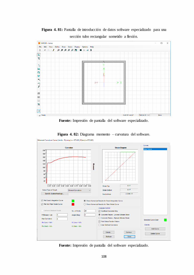
108
Figura 4. 81: Pantalla de introducción de datos software especializado para una
sección tubo rectangular sometido a flexión.
Fuente: Impresión de pantalla del software especializado.
Figura 4. 82: Diagrama momento – curvatura del software.
Fuente: Impresión de pantalla del software especializado.

109
Figura 4. 83: Diagrama momento – curvatura entre los dos softwares.
Fuente: José Freire
Tabla 4. 17: Comparación de puntos del diagrama momento - curvatura para una
sección tubo rectangular sometido a flexión.
Comparación de resultados
Parámetro Software
especializado Software Diferencia Porcentaje (%)
Momento último (tn.m)
157.09 162.39 5.30 3.26
curvatura
última (1/m) 0.87 0.83 0.04 4.81
Fuente: José Freire
4.2.10 Sección tubo circular de perfil de acero sometido a flexocompresión.
Datos:
Nombre del perfil = Pipe 12 AISC d=32.38 cm, tw=1.90 cm, Acero= A572,
P=30 tn.
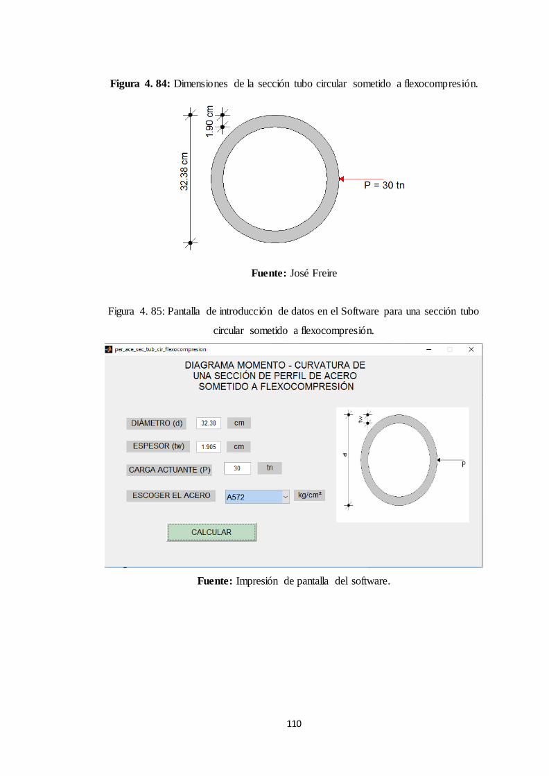
110
Figura 4. 84: Dimensiones de la sección tubo circular sometido a flexocompresión.
Fuente: José Freire
Figura 4. 85: Pantalla de introducción de datos en el Software para una sección tubo
circular sometido a flexocompresión.
Fuente: Impresión de pantalla del software.

111
Figura 4. 86: Diagrama momento – curvatura del software para una sección tubo
circular sometido a flexocompresión.
Fuente: Impresión de pantalla del software.

112
Figura 4. 87: Pantalla de introducción de datos software especializado para una
sección tubo circular sometido a flexocompresión.
Fuente: Impresión de pantalla del software especializado.
Figura 4. 88: Diagrama momento – curvatura del software.
Fuente: Impresión de pantalla del software especializado.

113
Figura 4. 89: Diagrama momento – curvatura entre los dos softwares.
Fuente: José Freire
Tabla 4. 18: Comparación de puntos del diagrama momento - curvatura para una
sección tubo circular sometido a flexocompresión.
Comparación de resultados
Parámetro Software
especializado Software Diferencia Porcentaje (%)
Momento último
(tn.m)
77.80 83.01 5.21 6.27
curvatura última (1/m)
1.00 1.01 0.01 0.99
Fuente: José Freire
4.2.11 Sección tubo circular de perfil de acero sometido a flexión.
Datos:
Nombre del perfil = Pipe 12 AISC d=32.38 cm, tw=1.90 cm, Acero= A36.

114
Figura 4. 90: Dimensiones de la sección tubo circular sometido a flexión.
Fuente: José Freire
Figura 4. 91: Pantalla de introducción de datos en el Software para una sección tubo
circular sometido a flexión.
Fuente: Impresión de pantalla del software.

115
Figura 4. 92: Diagrama momento – curvatura del software para una sección tubo
circular sometido a flexión.
Fuente: Impresión de pantalla del software.
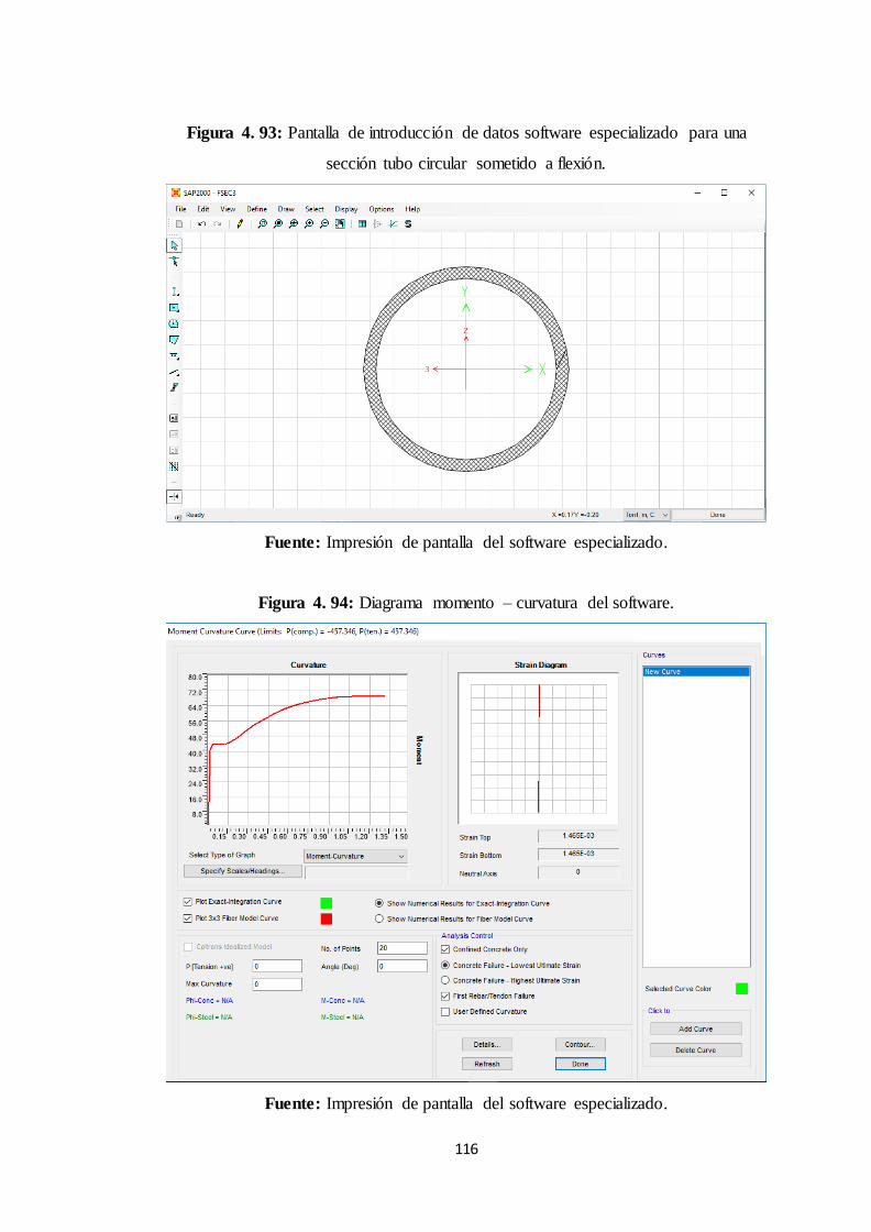
116
Figura 4. 93: Pantalla de introducción de datos software especializado para una
sección tubo circular sometido a flexión.
Fuente: Impresión de pantalla del software especializado.
Figura 4. 94: Diagrama momento – curvatura del software.
Fuente: Impresión de pantalla del software especializado.
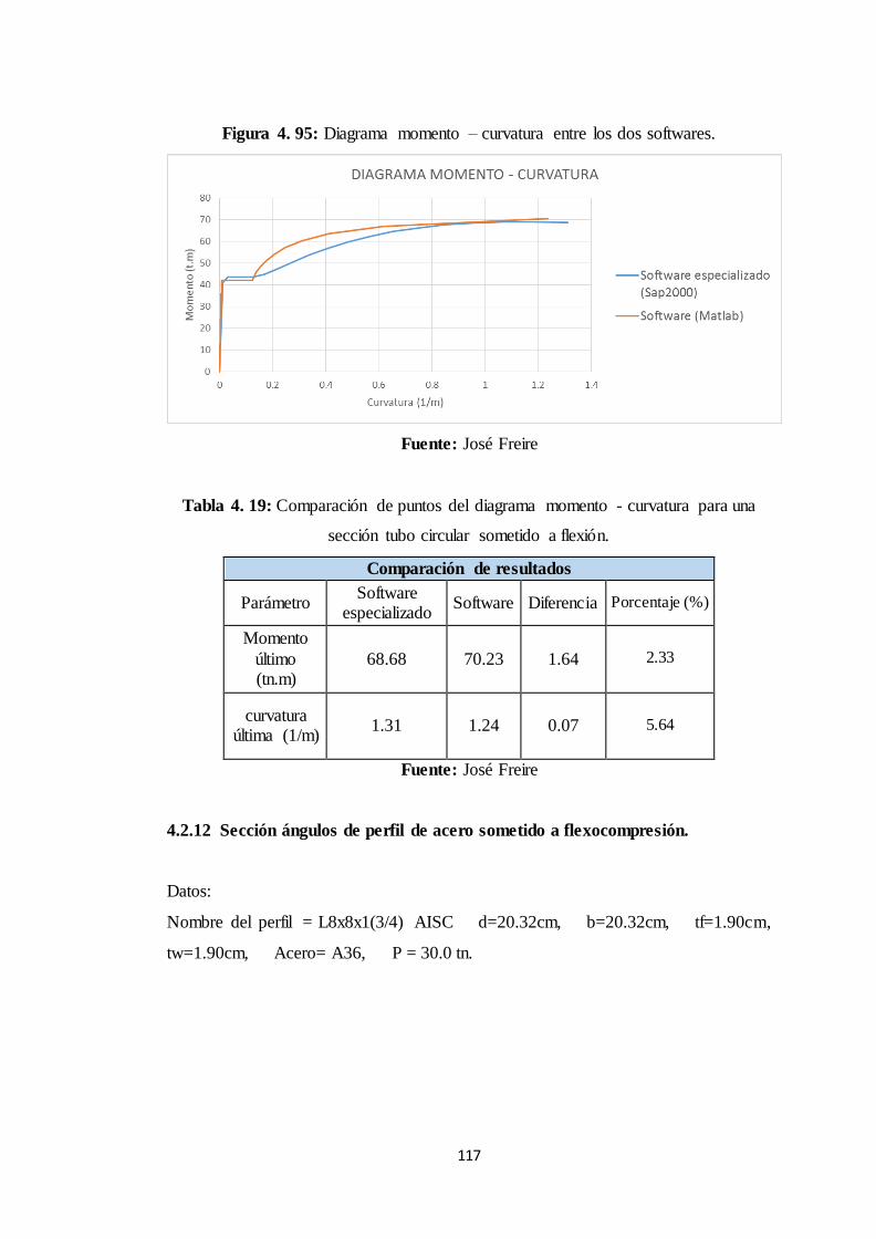
117
Figura 4. 95: Diagrama momento – curvatura entre los dos softwares.
Fuente: José Freire
Tabla 4. 19: Comparación de puntos del diagrama momento - curvatura para una
sección tubo circular sometido a flexión.
Comparación de resultados
Parámetro Software
especializado Software Diferencia Porcentaje (%)
Momento
último (tn.m)
68.68 70.23 1.64 2.33
curvatura última (1/m)
1.31 1.24 0.07 5.64
Fuente: José Freire
4.2.12 Sección ángulos de perfil de acero sometido a flexocompresión.
Datos:
Nombre del perfil = L8x8x1(3/4) AISC d=20.32cm, b=20.32cm, tf=1.90cm,
tw=1.90cm, Acero= A36, P = 30.0 tn.
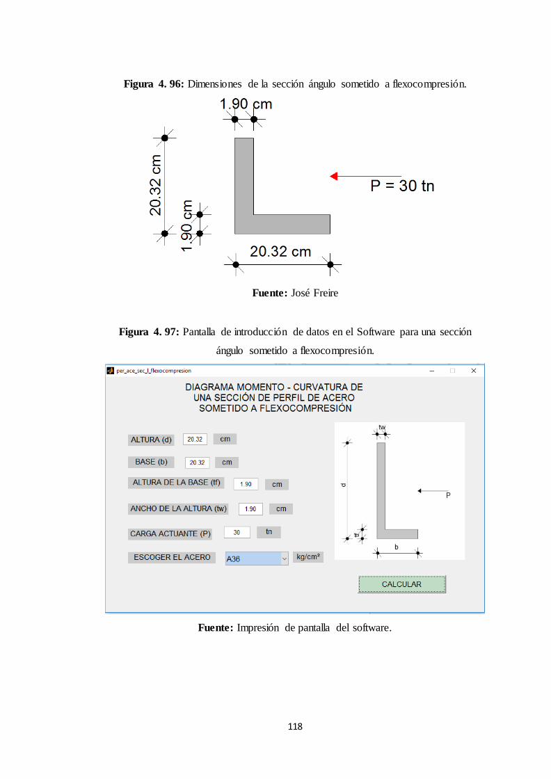
118
Figura 4. 96: Dimensiones de la sección ángulo sometido a flexocompresión.
Fuente: José Freire
Figura 4. 97: Pantalla de introducción de datos en el Software para una sección
ángulo sometido a flexocompresión.
Fuente: Impresión de pantalla del software.

119
Figura 4. 98: Diagrama momento – curvatura del software para una sección ángulo
sometido a flexocompresión.
Fuente: Impresión de pantalla del software.

120
Figura 4. 99: Pantalla de introducción de datos software especializado para una
sección ángulo sometido a flexocompresión.
Fuente: Impresión de pantalla del software especializado.
Figura 4. 100: Diagrama momento – curvatura del software.
Fuente: Impresión de pantalla del software especializado.

121
Figura 4. 101: Diagrama momento – curvatura entre los dos softwares.
Fuente: José Freire
Tabla 4. 20: Comparación de puntos del diagrama momento - curvatura para una
sección ángulo sometido a flexocompresión.
Comparación de resultados
Parámetro Software
especializado Software Diferencia Porcentaje (%)
Momento último (tn.m)
14.26 14.37 0.11 0.765
curvatura
última (1/m) 1.57 1.46 0.11 7.53
Fuente: José Freire
4.2.13 Sección ángulos de perfil de acero sometido a flexocompresión.
Datos:
Nombre del perfil = L8x8x1(3/4) AISC d=20.32cm, b=20.32cm, tf=1.90cm,
tw=1.90cm, Acero= A709(70W).

122
Figura 4. 102: Dimensiones de la sección ángulo sometido a flexión.
Fuente: José Freire
Figura 4. 103: Pantalla de introducción de datos en el Software para una sección
ángulo sometido a flexión.
Fuente: Impresión de pantalla del software.

123
Figura 4. 104: Diagrama momento – curvatura del software para una sección ángulo
sometido a flexión.
Fuente: Impresión de pantalla del software.

124
Figura 4. 105: Pantalla de introducción de datos software especializado para una
sección ángulo sometido a flexión.
Fuente: Impresión de pantalla del software especializado.
Figura 4. 106: Diagrama momento – curvatura del software.
Fuente: Impresión de pantalla del software especializado.
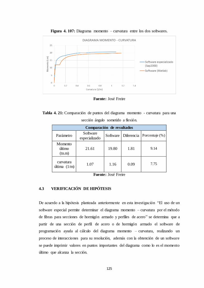
125
Figura 4. 107: Diagrama momento – curvatura entre los dos softwares.
Fuente: José Freire
Tabla 4. 21: Comparación de puntos del diagrama momento - curvatura para una
sección ángulo sometido a flexión.
Comparación de resultados
Parámetro Software
especializado Software Diferencia Porcentaje (%)
Momento último (tn.m)
21.61 19.80 1.81 9.14
curvatura última (1/m)
1.07 1.16 0.09 7.75
Fuente: José Freire
4.3 VERIFICACIÓN DE HIPÓTESIS
De acuerdo a la hipótesis planteada anteriormente en esta investigación “El uso de un
software especial permite determinar el diagrama momento – curvatura por el método
de fibras para secciones de hormigón armado y perfiles de acero” se determina que a
partir de una sección de perfil de acero o de hormigón armado el software de
programación ayuda al cálculo del diagrama momento – curvatura, realizando un
proceso de interacciones para su resolución, además con la obtención de un software
se puede imprimir valores en puntos importantes del diagrama como lo es el momento
último que alcanza la sección.

126
CAPÍTULO V
CONCLUSIONES Y RECOMENDACIONES
5.1 CONCLUSIONES
En el cálculo de diagrama momento curvatura el modelo de Mander para el
hormigón armado y el modelo de Park y Paulay para el acero que ayuda a la
consecución del software planteado debido a que son modelos que se acercan
de mejor manera al comportamiento del material.
Se realizó una comparación entre el diagrama momento – curvatura establecido
por un software especializado y el software desarrollado en la presente
investigación, que permitió determinar una variación porcentual en el anális is
de secciones de hormigón armado y perfiles de acero, lo cual valida la
aplicación del programa propuesto.
Se determinó a través de las gráficas momento – curvatura que el
comportamiento de una sección sometida a flexión y flexocompresión varía en
función a la carga que se aplica al elemento debido a que a mayor carga el
momento obtenido del cálculo disminuye de forma considerable al igual que la
ductilidad.
El software computacional permitió el análisis minucioso de cada una de las
secciones de hormigón armado y perfiles de acero obteniendo graficas con
resultados que reflejan el verdadero comportamiento de dichas secciones
sometidas a flexión y flexocompresión.
El método de fibras permite discretizar de mejor manera el análisis de una
sección de hormigón armado ya que se trabaja fraccionando al elemento en
varias dovelas obteniendo resultados más precisos que reflejan de manera real
el comportamiento estudiado.
127
5.2 RECOMENDACIONES
Implementar el uso del software desarrollado en la presente investigac ión
permite analizar de manera específica el comportamiento de materiales tales
como hormigón armado o perfiles de acero.
Se recomienda la utilización de investigaciones preliminares que permitan
establecer un punto de partida y a su vez fomente el análisis de materia les
estructurales con la ayuda de softwares computacionales.
Se recomienda un previo análisis del tipo de valores y unidades empleadas en
el programa computacional desarrollado en esta investigación, previniendo
errores o fallas en la gráfica arrojada por el software.

128
C.- MATERIALES DE REFERENCIA
1. BIBLIOGRAFÍA
[1] C. M. Guzmán Pillajo, Comportamiento de elementos de hormigón armado
reforzados con fibras, Quito: Universidad Central del Ecuador, 2015, pp. 123-
135.
[2] O. Vargas González, Simulación numérica inelástica de pórticos de concreto
simple y reforzado, mediante el método de elementos finitos y el método del
empuje lateral, Bogotá: Universidad Nacional de Colombia, 2014.
[3] R. Aguiar Falconí, Análisis sísmico por desempeño, Quito: Centro de
Investigaciones Científicas Escuela Politécnica del Ejército, 2003.
[4] C. D. Medina Robalino, Estudio de la relación momento - curvatura como
herramienta para entender el comportamiento de secciones de hormigón armado,
Ambato: Universidad Técnica de Ambato, 2012.
[5] C. Culver, The moment curvature relations for composite beams, Bethlehem:
Lehigh University, 1960.
[6] S. R. Pérez Mejía, Análisis sísmico elástico e inelástico de una edificación de
concreto armado, Xalapa: Universidad Veracruzana, 2013.
[7] D. Toro Castillo, Elaboración y análisis de curvas: “momento flector vs.
curvatura” para secciones transversales de columnas de concreto reforzado
diseñadas según el código aci 318-2002, Guayaquil: Escuela Politécnica del
Litoral, 2006.
[8] C. C. Choo, Investigation of rectangular concrete columns reinforced o
prestressed with fiber reinforced polymer (FRP) bars or tendons, Fresno:
University of Kentucky, 2005.
[9] L. A. Díaz López y D. J. Santos Cavalho, Desempeño sísmico de un edific io
aporticado de cuatro pisos diseñado con el reglamento nacional de edificaciones
y aceptando una deriva máxima de 1%, Lima: Pontificia Universidad Católica
del Perú, 2013.
129
[10] H. Méndez Romero, Efecto de las deformaciones por cortante en los diagramas
momento-curvatura M-φ de secciones de concreto reforzado y sus implicaciones
en la evaluación y diseño sísmico de estructuras, México: Universidad Nacional
Autónoma de México, 2011.
[11] M. Romo Proaño, Temas de Hormigón Armado, Quito: Escuela Politécnica del
Ejercito, 2007.
[12] L. Y. Allauca Sanchez, Desempeño sísmico de un edificio aporticado de cinco
pisos diseñado con las normas peruanas de edificaciones, Lima: Pontific ia
Universidad Católica del Perú, 2006.
[13] V. A. Pinoargote Rovello, Verificación del factor de reducción sísmico R, para
el análisis inelástico de estruccturas de hormigón armado de acuerdo al NEC-11,
Guayaquil: Universidad Católica de Santiago de Guayaquil, 2014.
[14] G. Ottazzi Pasino, Material de Apoyo para la Enseñanza de los Cursos de Diseño
y Comportamiento del Concreto Armado, Lima: Pontificia Universidad Católica
del Perú, 2004.
[15] M. Reyes Casimiro, Análisis sísmico por desempeño, México: Instituto
Politécnico Nacional, 2014.
[16] E. D. Mora Martínez, Comportamiento de estructuras de acero con y sin
disipadores de energía tipo TADAS, ubicadas en la ciudad de Quito, por el
método del espectro de capacidad, Quito: Escuela Politécnica Nacional, 2015.
[17] J. M. Carapaz Caranqui, La utilización del software matlab como herramienta
didáctica en el aprendizaje de matemáticas, de los estudiantes de quinto semestre
de la carrera de física y matemática de la FECYT, Universisdad Técnica del
Norte durante el año lectivo 2013-2014, Ibarra: Universidad Técnica del Norte,
2014.
[18] L. Rodríguez Ojeda, Análisis numérico básico. Un enfoque algorítmico con el
soporte de Matlab, Guayaquil: Escuela Superior Politécnica del Litoral, 2011.

130
2. ANEXOS
Programa para determinar el diagrama momento curvatura de un sección rectangular
de hormigón armado sometido a flexocompresión.
function varargout = hor_arm_sec_rec_flexocompresion(varargin)
% HOR_ARM_SEC_REC_FLEXOCOMPRESION MATLAB code for
hor_arm_sec_rec_flexocompresion.fig
% HOR_ARM_SEC_REC_FLEXOCOMPRESION, by itself, creates a
new HOR_ARM_SEC_REC_FLEXOCOMPRESION or raises the existing
% singleton*.
%
% H = HOR_ARM_SEC_REC_FLEXOCOMPRESION returns the handle
to a new HOR_ARM_SEC_REC_FLEXOCOMPRESION or the handle to
% the existing singleton*.
%
%
HOR_ARM_SEC_REC_FLEXOCOMPRESION('CALLBACK',hObject,eventData,h
andles,...) calls the local
% function named CALLBACK in
HOR_ARM_SEC_REC_FLEXOCOMPRESION.M with the given input
arguments.
%
% HOR_ARM_SEC_REC_FLEXOCOMPRESION('Property','Value',...)
creates a new HOR_ARM_SEC_REC_FLEXOCOMPRESION or raises the
% existing singleton*. Starting from the left, property
value pairs are
% applied to the GUI before
hor_arm_sec_rec_flexocompresion_OpeningFcn gets called. An
% unrecognized property name or invalid value makes
property application
% stop. All inputs are passed to
hor_arm_sec_rec_flexocompresion_OpeningFcn via varargin.
%
% *See GUI Options on GUIDE's Tools menu. Choose "GUI
allows only one
% instance to run (singleton)".
%
% See also: GUIDE, GUIDATA, GUIHANDLES
% Edit the above text to modify the response to help
hor_arm_sec_rec_flexocompresion
% Last Modified by GUIDE v2.5 07-Dec-2016 07:30:46
% Begin initialization code - DO NOT EDIT
gui_Singleton = 1;
gui_State = struct('gui_Name', mfilename, ...
'gui_Singleton', gui_Singleton, ...
'gui_OpeningFcn',
@hor_arm_sec_rec_flexocompresion_OpeningFcn, ...
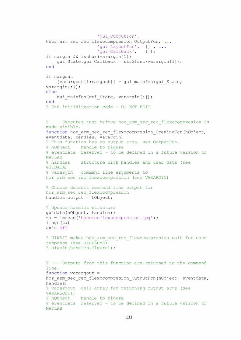
131
'gui_OutputFcn',
@hor_arm_sec_rec_flexocompresion_OutputFcn, ...
'gui_LayoutFcn', [] , ...
'gui_Callback', []);
if nargin && ischar(varargin{1})
gui_State.gui_Callback = str2func(varargin{1});
end
if nargout
[varargout{1:nargout}] = gui_mainfcn(gui_State,
varargin{:});
else
gui_mainfcn(gui_State, varargin{:});
end
% End initialization code - DO NOT EDIT
% --- Executes just before hor_arm_sec_rec_flexocompresion is
made visible.
function hor_arm_sec_rec_flexocompresion_OpeningFcn(hObject,
eventdata, handles, varargin)
% This function has no output args, see OutputFcn.
% hObject handle to figure
% eventdata reserved - to be defined in a future version of
MATLAB
% handles structure with handles and user data (see
GUIDATA)
% varargin command line arguments to
hor_arm_sec_rec_flexocompresion (see VARARGIN)
% Choose default command line output for
hor_arm_sec_rec_flexocompresion
handles.output = hObject;
% Update handles structure
guidata(hObject, handles);
za = imread('hsecrecflexocompresion.jpg');
image(za)
axis off
% UIWAIT makes hor_arm_sec_rec_flexocompresion wait for user
response (see UIRESUME)
% uiwait(handles.figure1);
% --- Outputs from this function are returned to the command
line.
function varargout =
hor_arm_sec_rec_flexocompresion_OutputFcn(hObject, eventdata,
handles)
% varargout cell array for returning output args (see
VARARGOUT);
% hObject handle to figure
% eventdata reserved - to be defined in a future version of
MATLAB
132
% handles structure with handles and user data (see
GUIDATA)
% Get default command line output from handles structure
varargout{1} = handles.output;
function edit1_Callback(hObject, eventdata, handles)
% hObject handle to edit1 (see GCBO)
% eventdata reserved - to be defined in a future version of
MATLAB
% handles structure with handles and user data (see
GUIDATA)
global b;
b=str2double(get(hObject,'String'));
% Hints: get(hObject,'String') returns contents of edit1 as
text
% str2double(get(hObject,'String')) returns contents of
edit1 as a double
% --- Executes during object creation, after setting all
properties.
function edit1_CreateFcn(hObject, eventdata, handles)
% hObject handle to edit1 (see GCBO)
% eventdata reserved - to be defined in a future version of
MATLAB
% handles empty - handles not created until after all
CreateFcns called
% Hint: edit controls usually have a white background on
Windows.
% See ISPC and COMPUTER.
if ispc && isequal(get(hObject,'BackgroundColor'),
get(0,'defaultUicontrolBackgroundColor'))
set(hObject,'BackgroundColor','white');
end
function edit2_Callback(hObject, eventdata, handles)
% hObject handle to edit2 (see GCBO)
% eventdata reserved - to be defined in a future version of
MATLAB
% handles structure with handles and user data (see
GUIDATA)
global h;
h=str2double(get(hObject,'String'));
% Hints: get(hObject,'String') returns contents of edit2 as
text
% str2double(get(hObject,'String')) returns contents of
edit2 as a double

133
% --- Executes during object creation, after setting all
properties.
function edit2_CreateFcn(hObject, eventdata, handles)
% hObject handle to edit2 (see GCBO)
% eventdata reserved - to be defined in a future version of
MATLAB
% handles empty - handles not created until after all
CreateFcns called
% Hint: edit controls usually have a white background on
Windows.
% See ISPC and COMPUTER.
if ispc && isequal(get(hObject,'BackgroundColor'),
get(0,'defaultUicontrolBackgroundColor'))
set(hObject,'BackgroundColor','white');
end
function edit3_Callback(hObject, eventdata, handles)
% hObject handle to edit3 (see GCBO)
% eventdata reserved - to be defined in a future version of
MATLAB
% handles structure with handles and user data (see
GUIDATA)
global r1;
r1=str2double(get(hObject,'String'));
% Hints: get(hObject,'String') returns contents of edit3 as
text
% str2double(get(hObject,'String')) returns contents of
edit3 as a double
% --- Executes during object creation, after setting all
properties.
function edit3_CreateFcn(hObject, eventdata, handles)
% hObject handle to edit3 (see GCBO)
% eventdata reserved - to be defined in a future version of
MATLAB
% handles empty - handles not created until after all
CreateFcns called
% Hint: edit controls usually have a white background on
Windows.
% See ISPC and COMPUTER.
if ispc && isequal(get(hObject,'BackgroundColor'),
get(0,'defaultUicontrolBackgroundColor'))
set(hObject,'BackgroundColor','white');
end
function edit4_Callback(hObject, eventdata, handles)
% hObject handle to edit4 (see GCBO)

134
% eventdata reserved - to be defined in a future version of
MATLAB
% handles structure with handles and user data (see
GUIDATA)
global a1;
a1=str2double(get(hObject,'String'));
% Hints: get(hObject,'String') returns contents of edit4 as
text
% str2double(get(hObject,'String')) returns contents of
edit4 as a double
% --- Executes during object creation, after setting all
properties.
function edit4_CreateFcn(hObject, eventdata, handles)
% hObject handle to edit4 (see GCBO)
% eventdata reserved - to be defined in a future version of
MATLAB
% handles empty - handles not created until after all
CreateFcns called
% Hint: edit controls usually have a white background on
Windows.
% See ISPC and COMPUTER.
if ispc && isequal(get(hObject,'BackgroundColor'),
get(0,'defaultUicontrolBackgroundColor'))
set(hObject,'BackgroundColor','white');
end
function edit5_Callback(hObject, eventdata, handles)
% hObject handle to edit5 (see GCBO)
% eventdata reserved - to be defined in a future version of
MATLAB
% handles structure with handles and user data (see
GUIDATA)
global a2;
a2=str2double(get(hObject,'String'));
% Hints: get(hObject,'String') returns contents of edit5 as
text
% str2double(get(hObject,'String')) returns contents of
edit5 as a double
% --- Executes during object creation, after setting all
properties.
function edit5_CreateFcn(hObject, eventdata, handles)
% hObject handle to edit5 (see GCBO)
% eventdata reserved - to be defined in a future version of
MATLAB
% handles empty - handles not created until after all
CreateFcns called

135
% Hint: edit controls usually have a white background on
Windows.
% See ISPC and COMPUTER.
if ispc && isequal(get(hObject,'BackgroundColor'),
get(0,'defaultUicontrolBackgroundColor'))
set(hObject,'BackgroundColor','white');
end
function edit6_Callback(hObject, eventdata, handles)
% hObject handle to edit6 (see GCBO)
% eventdata reserved - to be defined in a future version of
MATLAB
% handles structure with handles and user data (see
GUIDATA)
global a4;
a4=str2double(get(hObject,'String'));
% Hints: get(hObject,'String') returns contents of edit6 as
text
% str2double(get(hObject,'String')) returns contents of
edit6 as a double
% --- Executes during object creation, after setting all
properties.
function edit6_CreateFcn(hObject, eventdata, handles)
% hObject handle to edit6 (see GCBO)
% eventdata reserved - to be defined in a future version of
MATLAB
% handles empty - handles not created until after all
CreateFcns called
% Hint: edit controls usually have a white background on
Windows.
% See ISPC and COMPUTER.
if ispc && isequal(get(hObject,'BackgroundColor'),
get(0,'defaultUicontrolBackgroundColor'))
set(hObject,'BackgroundColor','white');
end
function edit7_Callback(hObject, eventdata, handles)
% hObject handle to edit7 (see GCBO)
% eventdata reserved - to be defined in a future version of
MATLAB
% handles structure with handles and user data (see
GUIDATA)
global e1;
e1=str2double(get(hObject,'String'));
% Hints: get(hObject,'String') returns contents of edit7 as
text
% str2double(get(hObject,'String')) returns contents of
edit7 as a double

136
% --- Executes during object creation, after setting all
properties.
function edit7_CreateFcn(hObject, eventdata, handles)
% hObject handle to edit7 (see GCBO)
% eventdata reserved - to be defined in a future version of
MATLAB
% handles empty - handles not created until after all
CreateFcns called
% Hint: edit controls usually have a white background on
Windows.
% See ISPC and COMPUTER.
if ispc && isequal(get(hObject,'BackgroundColor'),
get(0,'defaultUicontrolBackgroundColor'))
set(hObject,'BackgroundColor','white');
end
function edit8_Callback(hObject, eventdata, handles)
% hObject handle to edit8 (see GCBO)
% eventdata reserved - to be defined in a future version of
MATLAB
% handles structure with handles and user data (see
GUIDATA)
global fc;
fc=str2double(get(hObject,'String'));
% Hints: get(hObject,'String') returns contents of edit8 as
text
% str2double(get(hObject,'String')) returns contents of
edit8 as a double
% --- Executes during object creation, after setting all
properties.
function edit8_CreateFcn(hObject, eventdata, handles)
% hObject handle to edit8 (see GCBO)
% eventdata reserved - to be defined in a future version of
MATLAB
% handles empty - handles not created until after all
CreateFcns called
% Hint: edit controls usually have a white background on
Windows.
% See ISPC and COMPUTER.
if ispc && isequal(get(hObject,'BackgroundColor'),
get(0,'defaultUicontrolBackgroundColor'))
set(hObject,'BackgroundColor','white');
end
function edit9_Callback(hObject, eventdata, handles)
137
% hObject handle to edit9 (see GCBO)
% eventdata reserved - to be defined in a future version of
MATLAB
% handles structure with handles and user data (see
GUIDATA)
global fy;
fy=str2double(get(hObject,'String'));
% Hints: get(hObject,'String') returns contents of edit9 as
text
% str2double(get(hObject,'String')) returns contents of
edit9 as a double
% --- Executes during object creation, after setting all
properties.
function edit9_CreateFcn(hObject, eventdata, handles)
% hObject handle to edit9 (see GCBO)
% eventdata reserved - to be defined in a future version of
MATLAB
% handles empty - handles not created until after all
CreateFcns called
% Hint: edit controls usually have a white background on
Windows.
% See ISPC and COMPUTER.
if ispc && isequal(get(hObject,'BackgroundColor'),
get(0,'defaultUicontrolBackgroundColor'))
set(hObject,'BackgroundColor','white');
end
function edit10_Callback(hObject, eventdata, handles)
% hObject handle to edit10 (see GCBO)
% eventdata reserved - to be defined in a future version of
MATLAB
% handles structure with handles and user data (see
GUIDATA)
global nc;
nc=str2double(get(hObject,'String'));
% Hints: get(hObject,'String') returns contents of edit10 as
text
% str2double(get(hObject,'String')) returns contents of
edit10 as a double
% --- Executes during object creation, after setting all
properties.
function edit10_CreateFcn(hObject, eventdata, handles)
% hObject handle to edit10 (see GCBO)
% eventdata reserved - to be defined in a future version of
MATLAB
% handles empty - handles not created until after all
CreateFcns called
138
% Hint: edit controls usually have a white background on
Windows.
% See ISPC and COMPUTER.
if ispc && isequal(get(hObject,'BackgroundColor'),
get(0,'defaultUicontrolBackgroundColor'))
set(hObject,'BackgroundColor','white');
end
function edit11_Callback(hObject, eventdata, handles)
% hObject handle to edit11 (see GCBO)
% eventdata reserved - to be defined in a future version of
MATLAB
% handles structure with handles and user data (see
GUIDATA)
global nt;
nt=str2double(get(hObject,'String'));
% Hints: get(hObject,'String') returns contents of edit11 as
text
% str2double(get(hObject,'String')) returns contents of
edit11 as a double
% --- Executes during object creation, after setting all
properties.
function edit11_CreateFcn(hObject, eventdata, handles)
% hObject handle to edit11 (see GCBO)
% eventdata reserved - to be defined in a future version of
MATLAB
% handles empty - handles not created until after all
CreateFcns called
% Hint: edit controls usually have a white background on
Windows.
% See ISPC and COMPUTER.
if ispc && isequal(get(hObject,'BackgroundColor'),
get(0,'defaultUicontrolBackgroundColor'))
set(hObject,'BackgroundColor','white');
end
function edit12_Callback(hObject, eventdata, handles)
% hObject handle to edit12 (see GCBO)
% eventdata reserved - to be defined in a future version of
MATLAB
% handles structure with handles and user data (see
GUIDATA)
global p;
p=str2double(get(hObject,'String'));
% Hints: get(hObject,'String') returns contents of edit12 as
text
% str2double(get(hObject,'String')) returns contents of
edit12 as a double

139
% --- Executes during object creation, after setting all
properties.
function edit12_CreateFcn(hObject, eventdata, handles)
% hObject handle to edit12 (see GCBO)
% eventdata reserved - to be defined in a future version of
MATLAB
% handles empty - handles not created until after all
CreateFcns called
% Hint: edit controls usually have a white background on
Windows.
% See ISPC and COMPUTER.
if ispc && isequal(get(hObject,'BackgroundColor'),
get(0,'defaultUicontrolBackgroundColor'))
set(hObject,'BackgroundColor','white');
end
function edit13_Callback(hObject, eventdata, handles)
% hObject handle to edit13 (see GCBO)
% eventdata reserved - to be defined in a future version of
MATLAB
% handles structure with handles and user data (see
GUIDATA)
global a3;
a3=str2double(get(hObject,'String'));
% Hints: get(hObject,'String') returns contents of edit13 as
text
% str2double(get(hObject,'String')) returns contents of
edit13 as a double
% --- Executes during object creation, after setting all
properties.
function edit13_CreateFcn(hObject, eventdata, handles)
% hObject handle to edit13 (see GCBO)
% eventdata reserved - to be defined in a future version of
MATLAB
% handles empty - handles not created until after all
CreateFcns called
% Hint: edit controls usually have a white background on
Windows.
% See ISPC and COMPUTER.
if ispc && isequal(get(hObject,'BackgroundColor'),
get(0,'defaultUicontrolBackgroundColor'))
set(hObject,'BackgroundColor','white');
end
% --- Executes on button press in pushbutton2.
function pushbutton2_Callback(hObject, eventdata, handles)
% hObject handle to pushbutton2 (see GCBO)

140
% eventdata reserved - to be defined in a future version of
MATLAB
% handles structure with handles and user data (see
GUIDATA)
global b;
global h;
global p;
global r1;
global a1;
global a2;
global a3;
global a4;
global e1;
global fc;
global fy;
global nc;
global nt;
ec = 0.0005;
c = 0;
ek = 2038800;
ey = 0.002;
esh = 0.008;
esu = 0.11;
fuy = 1.5;
m = 100;
fprintf('%6s %10s %8s %12s\n','ec','c','phi','momento')
fprintf('%6s %10s %8s %9s\n','','cm','1/m','t.m')
for i=1:m;
ec = (esu-0.06)/(m+1-i);
sumafc1 = 2000;
sumafc2 = 1000;
raiz = 1000;
for c=(h/2):-0.0001:0
if (raiz<=100);
break
else
d = h-r1;
eec = (4.7*sqrt(fc*0.0981))/0.0000981;
eey = fy/2038800;
ees1 = ((r1-c)*ec)/c;
if (ees1<=ey);
fs1 = ees1*ek;
elseif (ees1>ey)&&(ees1<=esh);
fs1 = fy;
141
elseif (ees1>esh)&&(ees1<=esu);
re = esu-esh;
me = (fuy*(((30*re)+1)*((30*re)+1))-(60*re)-1)/(15*re*re);
fs1 = fy*(((((me*(ees1-esh))+2)/((60*(ees1-
esh))+2)))+((((ees1-esh)*(60-
me)))/(2*(((30*re)+1))*((30*re)+1))));
else
fs1 = 0;
end
f1 = fs1*a1;
ees2 = (((h/2)-c)*ec)/c;
if (ees2<=ey);
fs2 = ees2*ek;
elseif (ees2>ey)&&(ees2<=esh);
fs2 = fy;
elseif (ees2>esh)&&(ees2<=esu);
re = esu-esh;
me = (fuy*(((30*re)+1)*((30*re)+1))-(60*re)-1)/(15*re*re);
fs2 = fy*(((((me*(ees2-esh))+2)/((60*(ees2-
esh))+2)))+((((ees2-esh)*(60-
me)))/(2*(((30*re)+1))*((30*re)+1))));
else
fs2 = 0;
end
f2 = fs2*a2;
ees3 = ((d-c)*ec)/c;
if (ees3<=ey);
fs3 = ees3*ek;
elseif (ees3>ey)&&(ees3<=esh);
fs3 = fy;
elseif (ees3>esh)&&(ees3<=esu);
re = esu-esh;
me = (fuy*(((30*re)+1)*((30*re)+1))-(60*re)-1)/(15*re*re);
fs3 = fy*(((((me*(ees3-esh))+2)/((60*(ees3-
esh))+2)))+((((ees3-esh)*(60-
me)))/(2*(((30*re)+1))*((30*re)+1))));
else
fs3 = 0;
end
f3 = fs3*a3;
pn = 2*a4/(e1*(b-(2*r1)));
fl = 0.5*0.85*pn*fy*0.0981;
fpcc = fc*0.0981*((2.254*sqrt(1+((7.94*fl)/(fc*0.0981))))-
(2*fl/(fc*0.0981))-1.254);
fpcc1 = fpcc/0.0981;
eecc = 0.002*(1+(5*((fpcc/(fc*0.0981))-1)));
x = ec/eecc;
emc = 5000*sqrt(fc*0.0981);
emsec = fpcc/eecc;
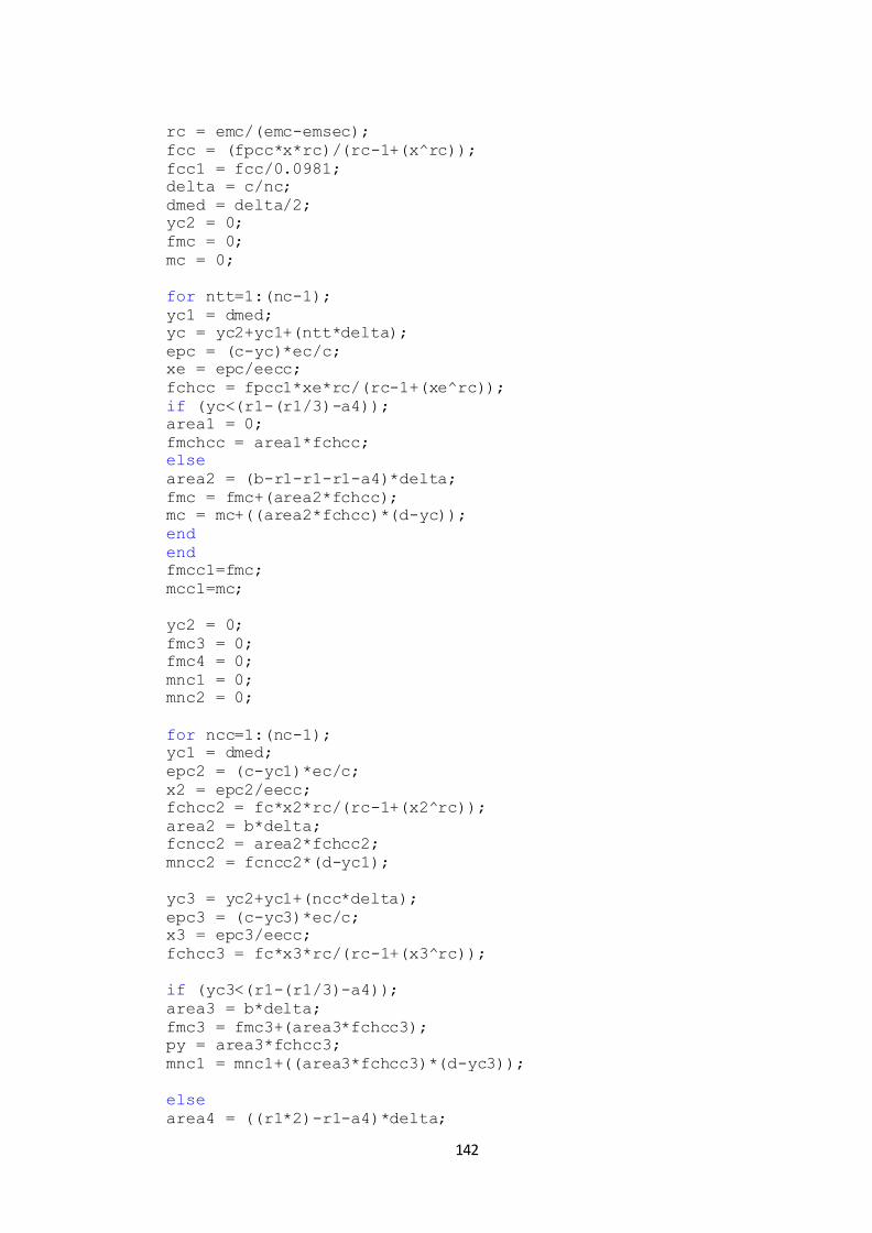
142
rc = emc/(emc-emsec);
fcc = (fpcc*x*rc)/(rc-1+(x^rc));
fcc1 = fcc/0.0981;
delta = c/nc;
dmed = delta/2;
yc2 = 0;
fmc = 0;
mc = 0;
for ntt=1:(nc-1);
yc1 = dmed;
yc = yc2+yc1+(ntt*delta);
epc = (c-yc)*ec/c;
xe = epc/eecc;
fchcc = fpcc1*xe*rc/(rc-1+(xe^rc));
if (yc<(r1-(r1/3)-a4));
area1 = 0;
fmchcc = area1*fchcc;
else
area2 = (b-r1-r1-r1-a4)*delta;
fmc = fmc+(area2*fchcc);
mc = mc+((area2*fchcc)*(d-yc));
end
end
fmcc1=fmc;
mcc1=mc;
yc2 = 0;
fmc3 = 0;
fmc4 = 0;
mnc1 = 0;
mnc2 = 0;
for ncc=1:(nc-1);
yc1 = dmed;
epc2 = (c-yc1)*ec/c;
x2 = epc2/eecc;
fchcc2 = fc*x2*rc/(rc-1+(x2^rc));
area2 = b*delta;
fcncc2 = area2*fchcc2;
mncc2 = fcncc2*(d-yc1);
yc3 = yc2+yc1+(ncc*delta);
epc3 = (c-yc3)*ec/c;
x3 = epc3/eecc;
fchcc3 = fc*x3*rc/(rc-1+(x3^rc));
if (yc3<(r1-(r1/3)-a4));
area3 = b*delta;
fmc3 = fmc3+(area3*fchcc3);
py = area3*fchcc3;
mnc1 = mnc1+((area3*fchcc3)*(d-yc3));
else
area4 = ((r1*2)-r1-a4)*delta;
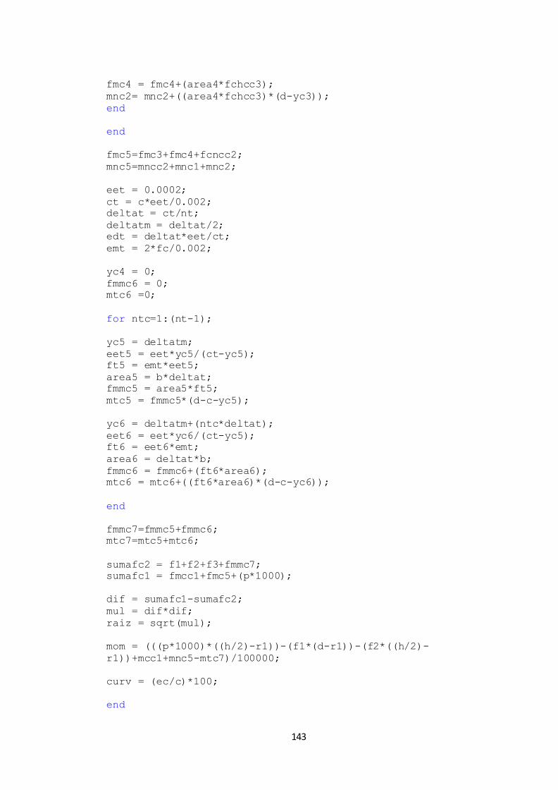
143
fmc4 = fmc4+(area4*fchcc3);
mnc2= mnc2+((area4*fchcc3)*(d-yc3));
end
end
fmc5=fmc3+fmc4+fcncc2;
mnc5=mncc2+mnc1+mnc2;
eet = 0.0002;
ct = c*eet/0.002;
deltat = ct/nt;
deltatm = deltat/2;
edt = deltat*eet/ct;
emt = 2*fc/0.002;
yc4 = 0;
fmmc6 = 0;
mtc6 =0;
for ntc=1:(nt-1);
yc5 = deltatm;
eet5 = eet*yc5/(ct-yc5);
ft5 = emt*eet5;
area5 = b*deltat;
fmmc5 = area5*ft5;
mtc5 = fmmc5*(d-c-yc5);
yc6 = deltatm+(ntc*deltat);
eet6 = eet*yc6/(ct-yc5);
ft6 = eet6*emt;
area6 = deltat*b;
fmmc6 = fmmc6+(ft6*area6);
mtc6 = mtc6+((ft6*area6)*(d-c-yc6));
end
fmmc7=fmmc5+fmmc6;
mtc7=mtc5+mtc6;
sumafc2 = f1+f2+f3+fmmc7;
sumafc1 = fmcc1+fmc5+(p*1000);
dif = sumafc1-sumafc2;
mul = dif*dif;
raiz = sqrt(mul);
mom = (((p*1000)*((h/2)-r1))-(f1*(d-r1))-(f2*((h/2)-
r1))+mcc1+mnc5-mtc7)/100000;
curv = (ec/c)*100;
end

144
end
if mom>=0;
phi(i)=curv;
MOM(i)=mom;
matriz=[ec,c,phi(i),MOM(i)];
disp(matriz)
else
end
end
figure (1)
title ('DIAGRAMA MOMENTO - CURVATURA')
plot(phi,MOM)
xlabel('CURVATURA (1/m)')
ylabel('MOMENTO T-m')
grid on
hold on
Programa para determinar el diagrama momento curvatura de un sección
rectangular de hormigón armado sometido a flexión.
function varargout = hor_arm_sec_rec_flexion(varargin)
% HOR_ARM_SEC_REC_FLEXION MATLAB code for
hor_arm_sec_rec_flexion.fig
% HOR_ARM_SEC_REC_FLEXION, by itself, creates a new
HOR_ARM_SEC_REC_FLEXION or raises the existing
% singleton*.
%
% H = HOR_ARM_SEC_REC_FLEXION returns the handle to a new
HOR_ARM_SEC_REC_FLEXION or the handle to
% the existing singleton*.
%
%
HOR_ARM_SEC_REC_FLEXION('CALLBACK',hObject,eventData,handles,.
..) calls the local
% function named CALLBACK in HOR_ARM_SEC_REC_FLEXION.M
with the given input arguments.
%
% HOR_ARM_SEC_REC_FLEXION('Property','Value',...) creates
a new HOR_ARM_SEC_REC_FLEXION or raises the
% existing singleton*. Starting from the left, property
value pairs are
% applied to the GUI before
hor_arm_sec_rec_flexion_OpeningFcn gets called. An

145
% unrecognized property name or invalid value makes
property application
% stop. All inputs are passed to
hor_arm_sec_rec_flexion_OpeningFcn via varargin.
%
% *See GUI Options on GUIDE's Tools menu. Choose "GUI
allows only one
% instance to run (singleton)".
%
% See also: GUIDE, GUIDATA, GUIHANDLES
% Edit the above text to modify the response to help
hor_arm_sec_rec_flexion
% Last Modified by GUIDE v2.5 05-Dec-2016 20:58:14
% Begin initialization code - DO NOT EDIT
gui_Singleton = 1;
gui_State = struct('gui_Name', mfilename, ...
'gui_Singleton', gui_Singleton, ...
'gui_OpeningFcn',
@hor_arm_sec_rec_flexion_OpeningFcn, ...
'gui_OutputFcn',
@hor_arm_sec_rec_flexion_OutputFcn, ...
'gui_LayoutFcn', [] , ...
'gui_Callback', []);
if nargin && ischar(varargin{1})
gui_State.gui_Callback = str2func(varargin{1});
end
if nargout
[varargout{1:nargout}] = gui_mainfcn(gui_State,
varargin{:});
else
gui_mainfcn(gui_State, varargin{:});
end
% End initialization code - DO NOT EDIT
% --- Executes just before hor_arm_sec_rec_flexion is made
visible.
function hor_arm_sec_rec_flexion_OpeningFcn(hObject,
eventdata, handles, varargin)
% This function has no output args, see OutputFcn.
% hObject handle to figure
% eventdata reserved - to be defined in a future version of
MATLAB
% handles structure with handles and user data (see
GUIDATA)
% varargin command line arguments to hor_arm_sec_rec_flexion
(see VARARGIN)
% Choose default command line output for
hor_arm_sec_rec_flexion
handles.output = hObject;

146
% Update handles structure
guidata(hObject, handles);
za = imread('hsecrecflexion.jpg');
image(za)
axis off
% UIWAIT makes hor_arm_sec_rec_flexion wait for user response
(see UIRESUME)
% uiwait(handles.figure1);
% --- Outputs from this function are returned to the command
line.
function varargout =
hor_arm_sec_rec_flexion_OutputFcn(hObject, eventdata, handles)
% varargout cell array for returning output args (see
VARARGOUT);
% hObject handle to figure
% eventdata reserved - to be defined in a future version of
MATLAB
% handles structure with handles and user data (see
GUIDATA)
% Get default command line output from handles structure
varargout{1} = handles.output;
function edit1_Callback(hObject, eventdata, handles)
% hObject handle to edit1 (see GCBO)
% eventdata reserved - to be defined in a future version of
MATLAB
% handles structure with handles and user data (see
GUIDATA)
global b;
b=str2double(get(hObject,'String'));
% Hints: get(hObject,'String') returns contents of edit1 as
text
% str2double(get(hObject,'String')) returns contents of
edit1 as a double
% --- Executes during object creation, after setting all
properties.
function edit1_CreateFcn(hObject, eventdata, handles)
% hObject handle to edit1 (see GCBO)
% eventdata reserved - to be defined in a future version of
MATLAB
% handles empty - handles not created until after all
CreateFcns called
% Hint: edit controls usually have a white background on
Windows.
% See ISPC and COMPUTER.

147
if ispc && isequal(get(hObject,'BackgroundColor'),
get(0,'defaultUicontrolBackgroundColor'))
set(hObject,'BackgroundColor','white');
end
function edit2_Callback(hObject, eventdata, handles)
% hObject handle to edit2 (see GCBO)
% eventdata reserved - to be defined in a future version of
MATLAB
% handles structure with handles and user data (see
GUIDATA)
global h;
h=str2double(get(hObject,'String'));
% Hints: get(hObject,'String') returns contents of edit2 as
text
% str2double(get(hObject,'String')) returns contents of
edit2 as a double
% --- Executes during object creation, after setting all
properties.
function edit2_CreateFcn(hObject, eventdata, handles)
% hObject handle to edit2 (see GCBO)
% eventdata reserved - to be defined in a future version of
MATLAB
% handles empty - handles not created until after all
CreateFcns called
% Hint: edit controls usually have a white background on
Windows.
% See ISPC and COMPUTER.
if ispc && isequal(get(hObject,'BackgroundColor'),
get(0,'defaultUicontrolBackgroundColor'))
set(hObject,'BackgroundColor','white');
end
function edit3_Callback(hObject, eventdata, handles)
% hObject handle to edit3 (see GCBO)
% eventdata reserved - to be defined in a future version of
MATLAB
% handles structure with handles and user data (see
GUIDATA)
global r1;
r1=str2double(get(hObject,'String'));
% Hints: get(hObject,'String') returns contents of edit3 as
text
% str2double(get(hObject,'String')) returns contents of
edit3 as a double

148
% --- Executes during object creation, after setting all
properties.
function edit3_CreateFcn(hObject, eventdata, handles)
% hObject handle to edit3 (see GCBO)
% eventdata reserved - to be defined in a future version of
MATLAB
% handles empty - handles not created until after all
CreateFcns called
% Hint: edit controls usually have a white background on
Windows.
% See ISPC and COMPUTER.
if ispc && isequal(get(hObject,'BackgroundColor'),
get(0,'defaultUicontrolBackgroundColor'))
set(hObject,'BackgroundColor','white');
end
function edit4_Callback(hObject, eventdata, handles)
% hObject handle to edit4 (see GCBO)
% eventdata reserved - to be defined in a future version of
MATLAB
% handles structure with handles and user data (see
GUIDATA)
global a1;
a1=str2double(get(hObject,'String'));
% Hints: get(hObject,'String') returns contents of edit4 as
text
% str2double(get(hObject,'String')) returns contents of
edit4 as a double
% --- Executes during object creation, after setting all
properties.
function edit4_CreateFcn(hObject, eventdata, handles)
% hObject handle to edit4 (see GCBO)
% eventdata reserved - to be defined in a future version of
MATLAB
% handles empty - handles not created until after all
CreateFcns called
% Hint: edit controls usually have a white background on
Windows.
% See ISPC and COMPUTER.
if ispc && isequal(get(hObject,'BackgroundColor'),
get(0,'defaultUicontrolBackgroundColor'))
set(hObject,'BackgroundColor','white');
end
function edit5_Callback(hObject, eventdata, handles)
% hObject handle to edit5 (see GCBO)

149
% eventdata reserved - to be defined in a future version of
MATLAB
% handles structure with handles and user data (see
GUIDATA)
global a2;
a2=str2double(get(hObject,'String'));
% Hints: get(hObject,'String') returns contents of edit5 as
text
% str2double(get(hObject,'String')) returns contents of
edit5 as a double
% --- Executes during object creation, after setting all
properties.
function edit5_CreateFcn(hObject, eventdata, handles)
% hObject handle to edit5 (see GCBO)
% eventdata reserved - to be defined in a future version of
MATLAB
% handles empty - handles not created until after all
CreateFcns called
% Hint: edit controls usually have a white background on
Windows.
% See ISPC and COMPUTER.
if ispc && isequal(get(hObject,'BackgroundColor'),
get(0,'defaultUicontrolBackgroundColor'))
set(hObject,'BackgroundColor','white');
end
function edit6_Callback(hObject, eventdata, handles)
% hObject handle to edit6 (see GCBO)
% eventdata reserved - to be defined in a future version of
MATLAB
% handles structure with handles and user data (see
GUIDATA)
global a3;
a3=str2double(get(hObject,'String'));
% Hints: get(hObject,'String') returns contents of edit6 as
text
% str2double(get(hObject,'String')) returns contents of
edit6 as a double
% --- Executes during object creation, after setting all
properties.
function edit6_CreateFcn(hObject, eventdata, handles)
% hObject handle to edit6 (see GCBO)
% eventdata reserved - to be defined in a future version of
MATLAB
% handles empty - handles not created until after all
CreateFcns called

150
% Hint: edit controls usually have a white background on
Windows.
% See ISPC and COMPUTER.
if ispc && isequal(get(hObject,'BackgroundColor'),
get(0,'defaultUicontrolBackgroundColor'))
set(hObject,'BackgroundColor','white');
end
function edit7_Callback(hObject, eventdata, handles)
% hObject handle to edit7 (see GCBO)
% eventdata reserved - to be defined in a future version of
MATLAB
% handles structure with handles and user data (see
GUIDATA)
global e1;
e1=str2double(get(hObject,'String'));
% Hints: get(hObject,'String') returns contents of edit7 as
text
% str2double(get(hObject,'String')) returns contents of
edit7 as a double
% --- Executes during object creation, after setting all
properties.
function edit7_CreateFcn(hObject, eventdata, handles)
% hObject handle to edit7 (see GCBO)
% eventdata reserved - to be defined in a future version of
MATLAB
% handles empty - handles not created until after all
CreateFcns called
% Hint: edit controls usually have a white background on
Windows.
% See ISPC and COMPUTER.
if ispc && isequal(get(hObject,'BackgroundColor'),
get(0,'defaultUicontrolBackgroundColor'))
set(hObject,'BackgroundColor','white');
end
function edit8_Callback(hObject, eventdata, handles)
% hObject handle to edit8 (see GCBO)
% eventdata reserved - to be defined in a future version of
MATLAB
% handles structure with handles and user data (see
GUIDATA)
global fc;
fc=str2double(get(hObject,'String'));
% Hints: get(hObject,'String') returns contents of edit8 as
text
% str2double(get(hObject,'String')) returns contents of
edit8 as a double

151
% --- Executes during object creation, after setting all
properties.
function edit8_CreateFcn(hObject, eventdata, handles)
% hObject handle to edit8 (see GCBO)
% eventdata reserved - to be defined in a future version of
MATLAB
% handles empty - handles not created until after all
CreateFcns called
% Hint: edit controls usually have a white background on
Windows.
% See ISPC and COMPUTER.
if ispc && isequal(get(hObject,'BackgroundColor'),
get(0,'defaultUicontrolBackgroundColor'))
set(hObject,'BackgroundColor','white');
end
function edit9_Callback(hObject, eventdata, handles)
% hObject handle to edit9 (see GCBO)
% eventdata reserved - to be defined in a future version of
MATLAB
% handles structure with handles and user data (see
GUIDATA)
global fy;
fy=str2double(get(hObject,'String'));
% Hints: get(hObject,'String') returns contents of edit9 as
text
% str2double(get(hObject,'String')) returns contents of
edit9 as a double
% --- Executes during object creation, after setting all
properties.
function edit9_CreateFcn(hObject, eventdata, handles)
% hObject handle to edit9 (see GCBO)
% eventdata reserved - to be defined in a future version of
MATLAB
% handles empty - handles not created until after all
CreateFcns called
% Hint: edit controls usually have a white background on
Windows.
% See ISPC and COMPUTER.
if ispc && isequal(get(hObject,'BackgroundColor'),
get(0,'defaultUicontrolBackgroundColor'))
set(hObject,'BackgroundColor','white');
end
function edit10_Callback(hObject, eventdata, handles)

152
% hObject handle to edit10 (see GCBO)
% eventdata reserved - to be defined in a future version of
MATLAB
% handles structure with handles and user data (see
GUIDATA)
global nc;
nc=str2double(get(hObject,'String'));
% Hints: get(hObject,'String') returns contents of edit10 as
text
% str2double(get(hObject,'String')) returns contents of
edit10 as a double
% --- Executes during object creation, after setting all
properties.
function edit10_CreateFcn(hObject, eventdata, handles)
% hObject handle to edit10 (see GCBO)
% eventdata reserved - to be defined in a future version of
MATLAB
% handles empty - handles not created until after all
CreateFcns called
% Hint: edit controls usually have a white background on
Windows.
% See ISPC and COMPUTER.
if ispc && isequal(get(hObject,'BackgroundColor'),
get(0,'defaultUicontrolBackgroundColor'))
set(hObject,'BackgroundColor','white');
end
function edit11_Callback(hObject, eventdata, handles)
% hObject handle to edit11 (see GCBO)
% eventdata reserved - to be defined in a future version of
MATLAB
% handles structure with handles and user data (see
GUIDATA)
global nt;
nt=str2double(get(hObject,'String'));
% Hints: get(hObject,'String') returns contents of edit11 as
text
% str2double(get(hObject,'String')) returns contents of
edit11 as a double
% --- Executes during object creation, after setting all
properties.
function edit11_CreateFcn(hObject, eventdata, handles)
% hObject handle to edit11 (see GCBO)
% eventdata reserved - to be defined in a future version of
MATLAB
% handles empty - handles not created until after all
CreateFcns called
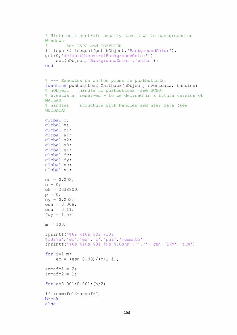
153
% Hint: edit controls usually have a white background on
Windows.
% See ISPC and COMPUTER.
if ispc && isequal(get(hObject,'BackgroundColor'),
get(0,'defaultUicontrolBackgroundColor'))
set(hObject,'BackgroundColor','white');
end
% --- Executes on button press in pushbutton2.
function pushbutton2_Callback(hObject, eventdata, handles)
% hObject handle to pushbutton2 (see GCBO)
% eventdata reserved - to be defined in a future version of
MATLAB
% handles structure with handles and user data (see
GUIDATA)
global b;
global h;
global r1;
global a1;
global a2;
global a3;
global e1;
global fc;
global fy;
global nc;
global nt;
ec = 0.002;
c = 0;
ek = 2038800;
p = 0;
ey = 0.002;
esh = 0.008;
esu = 0.11;
fuy = 1.5;
m = 100;
fprintf('%6s %10s %8s %10s
%13s\n','ec','es','c','phi','momento')
fprintf('%6s %10s %9s %9s %10s\n','','','cm','1/m','t.m')
for i=1:m;
ec = (esu-0.08)/(m+1-i);
sumafc1 = 2;
sumafc2 = 1;
for c=0.001:0.001:(h/2)
if (sumafc1<=sumafc2)
break
else

154
d = h-r1;
eec = (4.7*sqrt(fc*0.0981))/0.0000981;
eey = fy/2038800;
ees = (((d)-c)*ec)/c;
eeps= ((c-r1)*ec)/c;
if (ees<=ey);
fs = ees*ek;
elseif (ees>ey)&&(ees<=esh);
fs = fy;
elseif (ees>esh)&&(ees<=esu);
re = esu-esh;
me = (fuy*(((30*re)+1)*((30*re)+1))-(60*re)-1)/(15*re*re);
fs = fy*(((((me*(ees-esh))+2)/((60*(ees-
esh))+2)))+((((ees-esh)*(60-
me)))/(2*(((30*re)+1))*((30*re)+1))));
else
fs = 0;
end
fps = eeps*ek;
ts = fs*a2;
cps = fps*a1;
pn = 2*a3/(e1*(b-(2*r1)));
fl = 0.5*0.85*pn*fy*0.0981;
fpcc = fc*0.0981*((2.254*sqrt(1+((7.94*fl)/(fc*0.0981))))-
(2*fl/(fc*0.0981))-1.254);
fpcc1 = fpcc/0.0981;
eecc = 0.002*(1+(5*((fpcc/(fc*0.0981))-1)));
x = ec/eecc;
emc = 5000*sqrt(fc*0.0981);
emsec = fpcc/eecc;
rc = emc/(emc-emsec);
fcc = (fpcc*x*rc)/(rc-1+(x^rc));
fcc1 = fcc/0.0981;
delta = c/nc;
dmed = delta/2;
yc2 = 0;
fmc = 0;
mc = 0;
for ntt=1:(nc-1);
yc1 = dmed;
yc = yc2+yc1+(ntt*delta);
epc = (c-yc)*ec/c;
xe = epc/eecc;
fchcc = fpcc1*xe*rc/(rc-1+(xe^rc));
if (yc<(r1-(r1/3)-a3));
area1 = 0;
fmchcc = area1*fchcc;
else
area2 = (b-r1-r1-r1-a3)*delta;
fmc = fmc+(area2*fchcc);

155
mc = mc+((area2*fchcc)*(d-yc));
end
end
fmcc1=fmc;
mcc1=mc;
yc2 = 0;
fmc3 = 0;
fmc4 = 0;
mnc1 = 0;
mnc2 = 0;
for ncc=1:(nc-1);
yc1 = dmed;
epc2 = (c-yc1)*ec/c;
x2 = epc2/eecc;
fchcc2 = fc*x2*rc/(rc-1+(x2^rc));
area2 = b*delta;
fcncc2 = area2*fchcc2;
mncc2 = fcncc2*(d-yc1);
yc3 = yc2+yc1+(ncc*delta);
epc3 = (c-yc3)*ec/c;
x3 = epc3/eecc;
fchcc3 = fc*x3*rc/(rc-1+(x3^rc));
if (yc3<(r1-(r1/3)-a3));
area3 = b*delta;
fmc3 = fmc3+(area3*fchcc3);
py = area3*fchcc3;
mnc1 = mnc1+((area3*fchcc3)*(d-yc3));
else
area4 = ((r1*2)-r1-a3)*delta;
fmc4 = fmc4+(area4*fchcc3);
mnc2= mnc2+((area4*fchcc3)*(d-yc3));
end
end
fmc5=fmc3+fmc4+fcncc2;
mnc5=mncc2+mnc1+mnc2;
eet = 0.0002;
ct = c*eet/0.002;
deltat = ct/nt;
deltatm = deltat/2;
edt = deltat*eet/ct;
emt = 2*fc/0.002;
yc4 = 0;
fmmc6 = 0;
mtc6 =0;
for ntc=1:(nt-1);
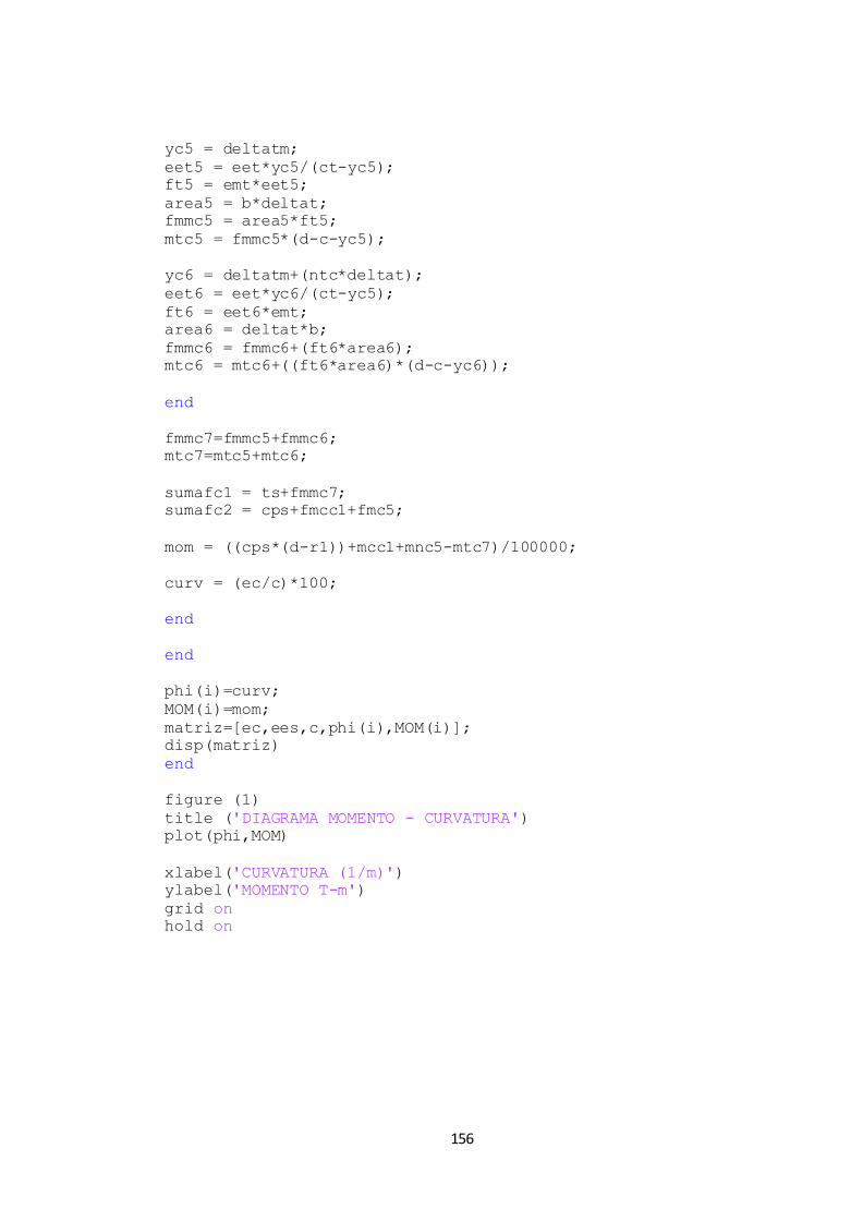
156
yc5 = deltatm;
eet5 = eet*yc5/(ct-yc5);
ft5 = emt*eet5;
area5 = b*deltat;
fmmc5 = area5*ft5;
mtc5 = fmmc5*(d-c-yc5);
yc6 = deltatm+(ntc*deltat);
eet6 = eet*yc6/(ct-yc5);
ft6 = eet6*emt;
area6 = deltat*b;
fmmc6 = fmmc6+(ft6*area6);
mtc6 = mtc6+((ft6*area6)*(d-c-yc6));
end
fmmc7=fmmc5+fmmc6;
mtc7=mtc5+mtc6;
sumafc1 = ts+fmmc7;
sumafc2 = cps+fmcc1+fmc5;
mom = ((cps*(d-r1))+mcc1+mnc5-mtc7)/100000;
curv = (ec/c)*100;
end
end
phi(i)=curv;
MOM(i)=mom;
matriz=[ec,ees,c,phi(i),MOM(i)];
disp(matriz)
end
figure (1)
title ('DIAGRAMA MOMENTO - CURVATURA')
plot(phi,MOM)
xlabel('CURVATURA (1/m)')
ylabel('MOMENTO T-m')
grid on
hold on

157
Programa para determinar el diagrama momento curvatura de un sección
circular de hormigón armado sometido a flexocompresión.
function varargout = hor_arm_sec_cir_flexocompresion(varargin)
% HOR_ARM_SEC_CIR_FLEXOCOMPRESION MATLAB code for
hor_arm_sec_cir_flexocompresion.fig
% HOR_ARM_SEC_CIR_FLEXOCOMPRESION, by itself, creates a
new HOR_ARM_SEC_CIR_FLEXOCOMPRESION or raises the existing
% singleton*.
%
% H = HOR_ARM_SEC_CIR_FLEXOCOMPRESION returns the handle
to a new HOR_ARM_SEC_CIR_FLEXOCOMPRESION or the handle to
% the existing singleton*.
%
%
HOR_ARM_SEC_CIR_FLEXOCOMPRESION('CALLBACK',hObject,eventData,h
andles,...) calls the local
% function named CALLBACK in
HOR_ARM_SEC_CIR_FLEXOCOMPRESION.M with the given input
arguments.
%
% HOR_ARM_SEC_CIR_FLEXOCOMPRESION('Property','Value',...)
creates a new HOR_ARM_SEC_CIR_FLEXOCOMPRESION or raises the
% existing singleton*. Starting from the left, property
value pairs are
% applied to the GUI before
hor_arm_sec_cir_flexocompresion_OpeningFcn gets called. An
% unrecognized property name or invalid value makes
property application
% stop. All inputs are passed to
hor_arm_sec_cir_flexocompresion_OpeningFcn via varargin.
%
% *See GUI Options on GUIDE's Tools menu. Choose "GUI
allows only one
% instance to run (singleton)".
%
% See also: GUIDE, GUIDATA, GUIHANDLES
% Edit the above text to modify the response to help
hor_arm_sec_cir_flexocompresion
% Last Modified by GUIDE v2.5 07-Dec-2016 04:23:58
% Begin initialization code - DO NOT EDIT
gui_Singleton = 1;
gui_State = struct('gui_Name', mfilename, ...
'gui_Singleton', gui_Singleton, ...
'gui_OpeningFcn',
@hor_arm_sec_cir_flexocompresion_OpeningFcn, ...
'gui_OutputFcn',
@hor_arm_sec_cir_flexocompresion_OutputFcn, ...
'gui_LayoutFcn', [] , ...
'gui_Callback', []);

158
if nargin && ischar(varargin{1})
gui_State.gui_Callback = str2func(varargin{1});
end
if nargout
[varargout{1:nargout}] = gui_mainfcn(gui_State,
varargin{:});
else
gui_mainfcn(gui_State, varargin{:});
end
% End initialization code - DO NOT EDIT
% --- Executes just before hor_arm_sec_cir_flexocompresion is
made visible.
function hor_arm_sec_cir_flexocompresion_OpeningFcn(hObject,
eventdata, handles, varargin)
% This function has no output args, see OutputFcn.
% hObject handle to figure
% eventdata reserved - to be defined in a future version of
MATLAB
% handles structure with handles and user data (see
GUIDATA)
% varargin command line arguments to
hor_arm_sec_cir_flexocompresion (see VARARGIN)
% Choose default command line output for
hor_arm_sec_cir_flexocompresion
handles.output = hObject;
% Update handles structure
guidata(hObject, handles);
za = imread('hseccirflexocompresion.jpg');
image(za)
axis off
% UIWAIT makes hor_arm_sec_cir_flexocompresion wait for user
response (see UIRESUME)
% uiwait(handles.figure1);
% --- Outputs from this function are returned to the command
line.
function varargout =
hor_arm_sec_cir_flexocompresion_OutputFcn(hObject, eventdata,
handles)
% varargout cell array for returning output args (see
VARARGOUT);
% hObject handle to figure
% eventdata reserved - to be defined in a future version of
MATLAB
% handles structure with handles and user data (see
GUIDATA)
% Get default command line output from handles structure

159
varargout{1} = handles.output;
function edit1_Callback(hObject, eventdata, handles)
% hObject handle to edit1 (see GCBO)
% eventdata reserved - to be defined in a future version of
MATLAB
% handles structure with handles and user data (see
GUIDATA)
global di;
di=str2double(get(hObject,'String'));
% Hints: get(hObject,'String') returns contents of edit1 as
text
% str2double(get(hObject,'String')) returns contents of
edit1 as a double
% --- Executes during object creation, after setting all
properties.
function edit1_CreateFcn(hObject, eventdata, handles)
% hObject handle to edit1 (see GCBO)
% eventdata reserved - to be defined in a future version of
MATLAB
% handles empty - handles not created until after all
CreateFcns called
% Hint: edit controls usually have a white background on
Windows.
% See ISPC and COMPUTER.
if ispc && isequal(get(hObject,'BackgroundColor'),
get(0,'defaultUicontrolBackgroundColor'))
set(hObject,'BackgroundColor','white');
end
function edit3_Callback(hObject, eventdata, handles)
% hObject handle to edit3 (see GCBO)
% eventdata reserved - to be defined in a future version of
MATLAB
% handles structure with handles and user data (see
GUIDATA)
global r;
r=str2double(get(hObject,'String'));
% Hints: get(hObject,'String') returns contents of edit3 as
text
% str2double(get(hObject,'String')) returns contents of
edit3 as a double
% --- Executes during object creation, after setting all
properties.
function edit3_CreateFcn(hObject, eventdata, handles)
% hObject handle to edit3 (see GCBO)
% eventdata reserved - to be defined in a future version of
MATLAB
160
% handles empty - handles not created until after all
CreateFcns called
% Hint: edit controls usually have a white background on
Windows.
% See ISPC and COMPUTER.
if ispc && isequal(get(hObject,'BackgroundColor'),
get(0,'defaultUicontrolBackgroundColor'))
set(hObject,'BackgroundColor','white');
end
function edit4_Callback(hObject, eventdata, handles)
% hObject handle to edit4 (see GCBO)
% eventdata reserved - to be defined in a future version of
MATLAB
% handles structure with handles and user data (see
GUIDATA)
global a1;
a1=str2double(get(hObject,'String'));
% Hints: get(hObject,'String') returns contents of edit4 as
text
% str2double(get(hObject,'String')) returns contents of
edit4 as a double
% --- Executes during object creation, after setting all
properties.
function edit4_CreateFcn(hObject, eventdata, handles)
% hObject handle to edit4 (see GCBO)
% eventdata reserved - to be defined in a future version of
MATLAB
% handles empty - handles not created until after all
CreateFcns called
% Hint: edit controls usually have a white background on
Windows.
% See ISPC and COMPUTER.
if ispc && isequal(get(hObject,'BackgroundColor'),
get(0,'defaultUicontrolBackgroundColor'))
set(hObject,'BackgroundColor','white');
end
function edit5_Callback(hObject, eventdata, handles)
% hObject handle to edit5 (see GCBO)
% eventdata reserved - to be defined in a future version of
MATLAB
% handles structure with handles and user data (see
GUIDATA)
global nv;
nv=str2double(get(hObject,'String'));

161
% Hints: get(hObject,'String') returns contents of edit5 as
text
% str2double(get(hObject,'String')) returns contents of
edit5 as a double
% --- Executes during object creation, after setting all
properties.
function edit5_CreateFcn(hObject, eventdata, handles)
% hObject handle to edit5 (see GCBO)
% eventdata reserved - to be defined in a future version of
MATLAB
% handles empty - handles not created until after all
CreateFcns called
% Hint: edit controls usually have a white background on
Windows.
% See ISPC and COMPUTER.
if ispc && isequal(get(hObject,'BackgroundColor'),
get(0,'defaultUicontrolBackgroundColor'))
set(hObject,'BackgroundColor','white');
end
function edit6_Callback(hObject, eventdata, handles)
% hObject handle to edit6 (see GCBO)
% eventdata reserved - to be defined in a future version of
MATLAB
% handles structure with handles and user data (see
GUIDATA)
global a2;
a2=str2double(get(hObject,'String'));
% Hints: get(hObject,'String') returns contents of edit6 as
text
% str2double(get(hObject,'String')) returns contents of
edit6 as a double
% --- Executes during object creation, after setting all
properties.
function edit6_CreateFcn(hObject, eventdata, handles)
% hObject handle to edit6 (see GCBO)
% eventdata reserved - to be defined in a future version of
MATLAB
% handles empty - handles not created until after all
CreateFcns called
% Hint: edit controls usually have a white background on
Windows.
% See ISPC and COMPUTER.
if ispc && isequal(get(hObject,'BackgroundColor'),
get(0,'defaultUicontrolBackgroundColor'))
set(hObject,'BackgroundColor','white');
end
162
function edit7_Callback(hObject, eventdata, handles)
% hObject handle to edit7 (see GCBO)
% eventdata reserved - to be defined in a future version of
MATLAB
% handles structure with handles and user data (see
GUIDATA)
global es;
es=str2double(get(hObject,'String'));
% Hints: get(hObject,'String') returns contents of edit7 as
text
% str2double(get(hObject,'String')) returns contents of
edit7 as a double
% --- Executes during object creation, after setting all
properties.
function edit7_CreateFcn(hObject, eventdata, handles)
% hObject handle to edit7 (see GCBO)
% eventdata reserved - to be defined in a future version of
MATLAB
% handles empty - handles not created until after all
CreateFcns called
% Hint: edit controls usually have a white background on
Windows.
% See ISPC and COMPUTER.
if ispc && isequal(get(hObject,'BackgroundColor'),
get(0,'defaultUicontrolBackgroundColor'))
set(hObject,'BackgroundColor','white');
end
function edit8_Callback(hObject, eventdata, handles)
% hObject handle to edit8 (see GCBO)
% eventdata reserved - to be defined in a future version of
MATLAB
% handles structure with handles and user data (see
GUIDATA)
global fc;
fc=str2double(get(hObject,'String'));
% Hints: get(hObject,'String') returns contents of edit8 as
text
% str2double(get(hObject,'String')) returns contents of
edit8 as a double
% --- Executes during object creation, after setting all
properties.
function edit8_CreateFcn(hObject, eventdata, handles)
% hObject handle to edit8 (see GCBO)

163
% eventdata reserved - to be defined in a future version of
MATLAB
% handles empty - handles not created until after all
CreateFcns called
% Hint: edit controls usually have a white background on
Windows.
% See ISPC and COMPUTER.
if ispc && isequal(get(hObject,'BackgroundColor'),
get(0,'defaultUicontrolBackgroundColor'))
set(hObject,'BackgroundColor','white');
end
function edit9_Callback(hObject, eventdata, handles)
% hObject handle to edit9 (see GCBO)
% eventdata reserved - to be defined in a future version of
MATLAB
% handles structure with handles and user data (see
GUIDATA)
global fy;
fy=str2double(get(hObject,'String'));
% Hints: get(hObject,'String') returns contents of edit9 as
text
% str2double(get(hObject,'String')) returns contents of
edit9 as a double
% --- Executes during object creation, after setting all
properties.
function edit9_CreateFcn(hObject, eventdata, handles)
% hObject handle to edit9 (see GCBO)
% eventdata reserved - to be defined in a future version of
MATLAB
% handles empty - handles not created until after all
CreateFcns called
% Hint: edit controls usually have a white background on
Windows.
% See ISPC and COMPUTER.
if ispc && isequal(get(hObject,'BackgroundColor'),
get(0,'defaultUicontrolBackgroundColor'))
set(hObject,'BackgroundColor','white');
end
function edit10_Callback(hObject, eventdata, handles)
% hObject handle to edit10 (see GCBO)
% eventdata reserved - to be defined in a future version of
MATLAB
% handles structure with handles and user data (see
GUIDATA)
global nc;

164
nc=str2double(get(hObject,'String'));
% Hints: get(hObject,'String') returns contents of edit10 as
text
% str2double(get(hObject,'String')) returns contents of
edit10 as a double
% --- Executes during object creation, after setting all
properties.
function edit10_CreateFcn(hObject, eventdata, handles)
% hObject handle to edit10 (see GCBO)
% eventdata reserved - to be defined in a future version of
MATLAB
% handles empty - handles not created until after all
CreateFcns called
% Hint: edit controls usually have a white background on
Windows.
% See ISPC and COMPUTER.
if ispc && isequal(get(hObject,'BackgroundColor'),
get(0,'defaultUicontrolBackgroundColor'))
set(hObject,'BackgroundColor','white');
end
function edit11_Callback(hObject, eventdata, handles)
% hObject handle to edit11 (see GCBO)
% eventdata reserved - to be defined in a future version of
MATLAB
% handles structure with handles and user data (see
GUIDATA)
global nt;
nt=str2double(get(hObject,'String'));
% Hints: get(hObject,'String') returns contents of edit11 as
text
% str2double(get(hObject,'String')) returns contents of
edit11 as a double
% --- Executes during object creation, after setting all
properties.
function edit11_CreateFcn(hObject, eventdata, handles)
% hObject handle to edit11 (see GCBO)
% eventdata reserved - to be defined in a future version of
MATLAB
% handles empty - handles not created until after all
CreateFcns called
% Hint: edit controls usually have a white background on
Windows.
% See ISPC and COMPUTER.
if ispc && isequal(get(hObject,'BackgroundColor'),
get(0,'defaultUicontrolBackgroundColor'))
set(hObject,'BackgroundColor','white');
165
end
function edit12_Callback(hObject, eventdata, handles)
% hObject handle to edit12 (see GCBO)
% eventdata reserved - to be defined in a future version of
MATLAB
% handles structure with handles and user data (see
GUIDATA)
global pu;
pu=str2double(get(hObject,'String'));
% Hints: get(hObject,'String') returns contents of edit12 as
text
% str2double(get(hObject,'String')) returns contents of
edit12 as a double
% --- Executes during object creation, after setting all
properties.
function edit12_CreateFcn(hObject, eventdata, handles)
% hObject handle to edit12 (see GCBO)
% eventdata reserved - to be defined in a future version of
MATLAB
% handles empty - handles not created until after all
CreateFcns called
% Hint: edit controls usually have a white background on
Windows.
% See ISPC and COMPUTER.
if ispc && isequal(get(hObject,'BackgroundColor'),
get(0,'defaultUicontrolBackgroundColor'))
set(hObject,'BackgroundColor','white');
end
% --- Executes on button press in pushbutton2.
function pushbutton2_Callback(hObject, eventdata, handles)
% hObject handle to pushbutton2 (see GCBO)
% eventdata reserved - to be defined in a future version of
MATLAB
% handles structure with handles and user data (see
GUIDATA)
global di;
global r;
global pu;
global a1;
global nv;
global a2;
global es;
global fc;
global fy;
global nc;

166
global nt;
ec = 0.0005;
c = 0;
ek = 2038800;
ey = 0.002;
esh = 0.008;
esu = 0.11;
fuy = 1.5;
fprintf('%6s %9s %10s %13s\n','ec','c','phi','momento')
fprintf('%6s %10s %9s %10s\n','','cm','1/m','t.m')
cont = 100;
for i=1:cont;
ec = (esu-0.08)/(cont+1-i);
sumafc1 = 2000;
sumafc2 = 1000;
raiz = 1000;
for c=(di/2):-0.001:0
if (raiz<=100);
break
else
d=di-r-a2-(a1/2);
rec=di-d;
c2 = di-r-r-a2-a2-a1;
p=2*pi*(c2/2);
ltc=p/nv;
z=0;
ey = 0.002;
esh = 0.008;
esu = 0.11;
fuy = 1.5;
sumafu1 = 0;
mom1 = 0;
for la=ltc:ltc:p
ang = (360*la)/(2*pi*(c2/2));
ra=ang*pi/180;
x=cos(ra);
dist = (c2/2)*x;
ees = ((((di/2)-dist)-c)*ec)/c;
coc = (((di/2)-dist)-c);
if (ees<=ey);
fs = ees*ek;
elseif (ees>ey)&&(ees<=esh);
fs = fy;
elseif (ees>esh)&&(ees<=esu);

167
re = esu-esh;
me = (fuy*(((30*re)+1)*((30*re)+1))-(60*re)-1)/(15*re*re);
fs = fy*(((((me*(ees-esh))+2)/((60*(ees-
esh))+2)))+((((ees-esh)*(60-
me)))/(2*(((30*re)+1))*((30*re)+1))));
else
fs = 0;
end
f = fs*a1;
sumafu1= sumafu1+f;
m = ((c2/2)+dist)*f;
mom1 = mom1+m;
end
ds = di-(2*rec)-a2;
sp = es-a2;
ae = (pi/4)*((ds-(sp/2))^2);
rocc = nv*a1*a1/(ds^2);
acc = (pi/4)*ds*ds*(1-rocc);
ke = ae/acc;
kes = ((1+(-sp/(2*ds)))^2)/(1-rocc);
ros = (pi*a2*a2)/(ds*es);
fl = 0.5*kes*ros*fy;
fpcc = fc*((2.254*sqrt(1+((7.94*fl)/fc)))-(2*fl/(fc))-1.254);
eecc = 0.002*(1+(5*((fpcc/(fc))-1)));
x = ec/eecc;
emc = 5000*sqrt(fc*0.0981);
emsec = fpcc*0.0981/eecc;
rc = emc/(emc-emsec);
delta = c/nc;
dmed = delta/2;
yc2 = 0;
fmc = 0;
mc = 0;
for ntt=1:(nc-1);
yc1 = dmed;
yc = yc2+yc1+(ntt*delta);
epc = (c-yc)*ec/c;
xe = epc/eecc;
fchcc = fpcc*xe*rc/(rc-1+(xe^rc));
dab = (2*sqrt(((di/2)^2)-((di/2)-yc)^2));
if (yc<(rec-(a1/2)-a2));
area1 = 0;
fmchcc = area1*fchcc;
else
area2 = (dab-rec-rec-a2-a2-a1-a1)*delta;
fmc = fmc+(area2*fchcc);
mc = mc+((area2*fchcc)*(d-yc));
end
end

168
fmcc1=fmc;
mcc1=mc;
yc2 = 0;
fmc3 = 0;
fmc4 = 0;
mnc1 = 0;
mnc2 = 0;
for ncc=1:(nc-1);
yc1 = dmed;
epc2 = (c-yc1)*ec/c;
x2 = epc2/eecc;
fchcc2 = fc*x2*rc/(rc-1+(x2^rc));
dab2 = (2*sqrt(((di/2)^2)-((di/2)-yc1)^2));
area2 = dab2*dmed;
fcncc2 = area2*fchcc2;
mncc2 = fcncc2*(d-yc1);
yc3 = yc2+yc1+(ncc*delta);
epc3 = (c-yc3)*ec/c;
x3 = epc3/eecc;
fchcc3 = fc*x3*rc/(rc-1+(x3^rc));
dab3 = (2*sqrt(((di/2)^2)-((di/2)-yc3)^2));
if (yc3<(rec-(a1/2)-a2));
area3 = dab3*delta;
fmc3 = fmc3+(area3*fchcc3);
py = area3*fchcc3;
mnc1 = mnc1+((area3*fchcc3)*(d-yc3));
else
area4 = (rec+rec+a1+a1+a2)*delta;
fmc4 = fmc4+(area4*fchcc3);
mnc2= mnc2+((area4*fchcc3)*(d-yc3));
end
end
fmc5=fmc3+fmc4+fcncc2;
mnc5=mncc2+mnc1+mnc2;
eet = 0.0002;
ct = c*eet/0.002;
deltat = ct/nt;
deltatm = deltat/2;
edt = deltat*eet/ct;
emt = 2*fc/0.002;
yc4 = 0;
fmmc6 = 0;
mtc6 =0;
for ntc=1:(nt-1);
169
yc5 = deltatm;
eet5 = eet*yc5/(ct-yc5);
ft5 = emt*eet5;
dab5 = (2*sqrt(((di/2)^2)-((di/2)-yc5)^2));
area5 = dab5*deltat;
fmmc5 = area5*ft5;
mtc5 = fmmc5*(d-c-yc5);
yc6 = deltatm+(ntc*deltat);
eet6 = eet*yc6/(ct-yc5);
ft6 = eet6*emt;
dab6 = (2*sqrt(((di/2)^2)-((di/2)-yc6)^2));
area6 = deltat*dab6;
fmmc6 = fmmc6+(ft6*area6);
mtc6 = mtc6+((ft6*area6)*(d-c-yc6));
end
fmmc7=fmmc5+fmmc6;
mtc7=mtc5+mtc6;
sumafc2 = sumafu1+fmmc7;
sumafc1 = fmcc1+fmc5+(pu*1000);
dif = sumafc1-sumafc2;
mul = dif*dif;
raiz = sqrt(mul);
mom = (((pu*1000)*((di/2)-rec))-mom1-mtc7+mcc1+mnc5)/100000;
curv = (ec/c)*100;
end
end
if mom>=0
phi(i)=curv;
MOM(i)=mom;
matriz=[ec,c,phi(i),MOM(i)];
disp(matriz)
else
end
end
figure (1)
title ('DIAGRAMA MOMENTO - CURVATURA')
plot(phi,MOM)
xlabel('CURVATURA (1/m)')
ylabel('MOMENTO T-m')
grid on
hold on

170
Programa para determinar el diagrama momento curvatura de un sección W de
perfil de acero sometido a flexocompresión.
function varargout = per_ace_sec_w_flexocompresion(varargin)
% PER_ACE_SEC_W_FLEXOCOMPRESION MATLAB code for
per_ace_sec_w_flexocompresion.fig
% PER_ACE_SEC_W_FLEXOCOMPRESION, by itself, creates a new
PER_ACE_SEC_W_FLEXOCOMPRESION or raises the existing
% singleton*.
%
% H = PER_ACE_SEC_W_FLEXOCOMPRESION returns the handle to
a new PER_ACE_SEC_W_FLEXOCOMPRESION or the handle to
% the existing singleton*.
%
%
PER_ACE_SEC_W_FLEXOCOMPRESION('CALLBACK',hObject,eventData,han
dles,...) calls the local
% function named CALLBACK in
PER_ACE_SEC_W_FLEXOCOMPRESION.M with the given input
arguments.
%
% PER_ACE_SEC_W_FLEXOCOMPRESION('Property','Value',...)
creates a new PER_ACE_SEC_W_FLEXOCOMPRESION or raises the
% existing singleton*. Starting from the left, property
value pairs are
% applied to the GUI before
per_ace_sec_w_flexocompresion_OpeningFcn gets called. An
% unrecognized property name or invalid value makes
property application
% stop. All inputs are passed to
per_ace_sec_w_flexocompresion_OpeningFcn via varargin.
%
% *See GUI Options on GUIDE's Tools menu. Choose "GUI
allows only one
% instance to run (singleton)".
%
% See also: GUIDE, GUIDATA, GUIHANDLES
% Edit the above text to modify the response to help
per_ace_sec_w_flexocompresion
% Last Modified by GUIDE v2.5 07-Dec-2016 08:16:50
% Begin initialization code - DO NOT EDIT
gui_Singleton = 1;
gui_State = struct('gui_Name', mfilename, ...
'gui_Singleton', gui_Singleton, ...
'gui_OpeningFcn',
@per_ace_sec_w_flexocompresion_OpeningFcn, ...
'gui_OutputFcn',
@per_ace_sec_w_flexocompresion_OutputFcn, ...
'gui_LayoutFcn', [] , ...
'gui_Callback', []);
171
if nargin && ischar(varargin{1})
gui_State.gui_Callback = str2func(varargin{1});
end
if nargout
[varargout{1:nargout}] = gui_mainfcn(gui_State,
varargin{:});
else
gui_mainfcn(gui_State, varargin{:});
end
% End initialization code - DO NOT EDIT
% --- Executes just before per_ace_sec_w_flexocompresion is
made visible.
function per_ace_sec_w_flexocompresion_OpeningFcn(hObject,
eventdata, handles, varargin)
% This function has no output args, see OutputFcn.
% hObject handle to figure
% eventdata reserved - to be defined in a future version of
MATLAB
% handles structure with handles and user data (see
GUIDATA)
% varargin command line arguments to
per_ace_sec_w_flexocompresion (see VARARGIN)
% Choose default command line output for
per_ace_sec_w_flexocompresion
handles.output = hObject;
% Update handles structure
guidata(hObject, handles);
za = imread('pasecwflexocompresion.jpg');
image(za)
axis off
% UIWAIT makes per_ace_sec_w_flexocompresion wait for user
response (see UIRESUME)
% uiwait(handles.figure1);
% --- Outputs from this function are returned to the command
line.
function varargout =
per_ace_sec_w_flexocompresion_OutputFcn(hObject, eventdata,
handles)
% varargout cell array for returning output args (see
VARARGOUT);
% hObject handle to figure
% eventdata reserved - to be defined in a future version of
MATLAB
% handles structure with handles and user data (see
GUIDATA)
% Get default command line output from handles structure

172
varargout{1} = handles.output;
function edit1_Callback(hObject, eventdata, handles)
% hObject handle to edit1 (see GCBO)
% eventdata reserved - to be defined in a future version of
MATLAB
% handles structure with handles and user data (see
GUIDATA)
global d;
d=str2double(get(hObject,'String'));
% Hints: get(hObject,'String') returns contents of edit1 as
text
% str2double(get(hObject,'String')) returns contents of
edit1 as a double
% --- Executes during object creation, after setting all
properties.
function edit1_CreateFcn(hObject, eventdata, handles)
% hObject handle to edit1 (see GCBO)
% eventdata reserved - to be defined in a future version of
MATLAB
% handles empty - handles not created until after all
CreateFcns called
% Hint: edit controls usually have a white background on
Windows.
% See ISPC and COMPUTER.
if ispc && isequal(get(hObject,'BackgroundColor'),
get(0,'defaultUicontrolBackgroundColor'))
set(hObject,'BackgroundColor','white');
end
function edit2_Callback(hObject, eventdata, handles)
% hObject handle to edit2 (see GCBO)
% eventdata reserved - to be defined in a future version of
MATLAB
% handles structure with handles and user data (see
GUIDATA)
global b1;
b1=str2double(get(hObject,'String'));
% Hints: get(hObject,'String') returns contents of edit2 as
text
% str2double(get(hObject,'String')) returns contents of
edit2 as a double
% --- Executes during object creation, after setting all
properties.
function edit2_CreateFcn(hObject, eventdata, handles)
% hObject handle to edit2 (see GCBO)
173
% eventdata reserved - to be defined in a future version of
MATLAB
% handles empty - handles not created until after all
CreateFcns called
% Hint: edit controls usually have a white background on
Windows.
% See ISPC and COMPUTER.
if ispc && isequal(get(hObject,'BackgroundColor'),
get(0,'defaultUicontrolBackgroundColor'))
set(hObject,'BackgroundColor','white');
end
function edit3_Callback(hObject, eventdata, handles)
% hObject handle to edit3 (see GCBO)
% eventdata reserved - to be defined in a future version of
MATLAB
% handles structure with handles and user data (see
GUIDATA)
global tf1;
tf1=str2double(get(hObject,'String'));
% Hints: get(hObject,'String') returns contents of edit3 as
text
% str2double(get(hObject,'String')) returns contents of
edit3 as a double
% --- Executes during object creation, after setting all
properties.
function edit3_CreateFcn(hObject, eventdata, handles)
% hObject handle to edit3 (see GCBO)
% eventdata reserved - to be defined in a future version of
MATLAB
% handles empty - handles not created until after all
CreateFcns called
% Hint: edit controls usually have a white background on
Windows.
% See ISPC and COMPUTER.
if ispc && isequal(get(hObject,'BackgroundColor'),
get(0,'defaultUicontrolBackgroundColor'))
set(hObject,'BackgroundColor','white');
end
function edit4_Callback(hObject, eventdata, handles)
% hObject handle to edit4 (see GCBO)
% eventdata reserved - to be defined in a future version of
MATLAB
% handles structure with handles and user data (see
GUIDATA)
global tw;

174
tw=str2double(get(hObject,'String'));
% Hints: get(hObject,'String') returns contents of edit4 as
text
% str2double(get(hObject,'String')) returns contents of
edit4 as a double
% --- Executes during object creation, after setting all
properties.
function edit4_CreateFcn(hObject, eventdata, handles)
% hObject handle to edit4 (see GCBO)
% eventdata reserved - to be defined in a future version of
MATLAB
% handles empty - handles not created until after all
CreateFcns called
% Hint: edit controls usually have a white background on
Windows.
% See ISPC and COMPUTER.
if ispc && isequal(get(hObject,'BackgroundColor'),
get(0,'defaultUicontrolBackgroundColor'))
set(hObject,'BackgroundColor','white');
end
function edit5_Callback(hObject, eventdata, handles)
% hObject handle to edit5 (see GCBO)
% eventdata reserved - to be defined in a future version of
MATLAB
% handles structure with handles and user data (see
GUIDATA)
global b2;
b2=str2double(get(hObject,'String'));
% Hints: get(hObject,'String') returns contents of edit5 as
text
% str2double(get(hObject,'String')) returns contents of
edit5 as a double
% --- Executes during object creation, after setting all
properties.
function edit5_CreateFcn(hObject, eventdata, handles)
% hObject handle to edit5 (see GCBO)
% eventdata reserved - to be defined in a future version of
MATLAB
% handles empty - handles not created until after all
CreateFcns called
% Hint: edit controls usually have a white background on
Windows.
% See ISPC and COMPUTER.
if ispc && isequal(get(hObject,'BackgroundColor'),
get(0,'defaultUicontrolBackgroundColor'))
set(hObject,'BackgroundColor','white');

175
end
function edit6_Callback(hObject, eventdata, handles)
% hObject handle to edit6 (see GCBO)
% eventdata reserved - to be defined in a future version of
MATLAB
% handles structure with handles and user data (see
GUIDATA)
global tf2;
tf2=str2double(get(hObject,'String'));
% Hints: get(hObject,'String') returns contents of edit6 as
text
% str2double(get(hObject,'String')) returns contents of
edit6 as a double
% --- Executes during object creation, after setting all
properties.
function edit6_CreateFcn(hObject, eventdata, handles)
% hObject handle to edit6 (see GCBO)
% eventdata reserved - to be defined in a future version of
MATLAB
% handles empty - handles not created until after all
CreateFcns called
% Hint: edit controls usually have a white background on
Windows.
% See ISPC and COMPUTER.
if ispc && isequal(get(hObject,'BackgroundColor'),
get(0,'defaultUicontrolBackgroundColor'))
set(hObject,'BackgroundColor','white');
end
function edit12_Callback(hObject, eventdata, handles)
% hObject handle to edit12 (see GCBO)
% eventdata reserved - to be defined in a future version of
MATLAB
% handles structure with handles and user data (see
GUIDATA)
global pa;
pa=str2double(get(hObject,'String'));
% Hints: get(hObject,'String') returns contents of edit12 as
text
% str2double(get(hObject,'String')) returns contents of
edit12 as a double
% --- Executes during object creation, after setting all
properties.
function edit12_CreateFcn(hObject, eventdata, handles)
% hObject handle to edit12 (see GCBO)
% eventdata reserved - to be defined in a future version of
MATLAB

176
% handles empty - handles not created until after all
CreateFcns called
% Hint: edit controls usually have a white background on
Windows.
% See ISPC and COMPUTER.
if ispc && isequal(get(hObject,'BackgroundColor'),
get(0,'defaultUicontrolBackgroundColor'))
set(hObject,'BackgroundColor','white');
end
% --- Executes on selection change in selector.
function selector_Callback(hObject, eventdata, handles)
% hObject handle to selector (see GCBO)
% eventdata reserved - to be defined in a future version of
MATLAB
% handles structure with handles and user data (see
GUIDATA)
% Hints: contents = cellstr(get(hObject,'String')) returns
selector contents as cell array
% contents{get(hObject,'Value')} returns selected item
from selector
global fy;
global ey;
global esh;
global esu;
global fuy;
a=get(handles.selector,'Value')
switch a
case 1
fy = 2530;
ey = 0.0012;
esh = 0.020;
esu = 0.2;
fuy = 1.6;
case 2
fy = 3515;
ey = 0.0017;
esh = 0.015;
esu = 0.17;
fuy = 1.2;
case 3
fy = 3515;
ey = 0.0017;
esh = 0.015;
esu = 0.17;
fuy = 1.2;
case 4
fy = 3515;

177
ey = 0.0017;
esh = 0.015;
esu = 0.17;
fuy = 1.2;
case 5
fy = 3515;
ey = 0.0017;
esh = 0.015;
esu = 0.17;
fuy = 1.2;
case 6
fy = 4921;
ey = 0.0024;
esh = 0.015;
esu = 0.17;
fuy = 1.2;
end
% --- Executes during object creation, after setting all
properties.
function selector_CreateFcn(hObject, eventdata, handles)
% hObject handle to selector (see GCBO)
% eventdata reserved - to be defined in a future version of
MATLAB
% handles empty - handles not created until after all
CreateFcns called
% Hint: popupmenu controls usually have a white background on
Windows.
% See ISPC and COMPUTER.
if ispc && isequal(get(hObject,'BackgroundColor'),
get(0,'defaultUicontrolBackgroundColor'))
set(hObject,'BackgroundColor','white');
end
% --- Executes on button press in pushbutton2.
function pushbutton2_Callback(hObject, eventdata, handles)
% hObject handle to pushbutton2 (see GCBO)
% eventdata reserved - to be defined in a future version of
MATLAB
% handles structure with handles and user data (see
GUIDATA)
global d;
global b1;
global tf1;
global tw;
global b2;
global tf2;
178
global pa;
global fy;
global ey;
global esh;
global esu;
global fuy;
ek = 2043000;
ycg = (((b2*tf2)*(tf2/2))+(((d-tf1-tf2)*tw)*(tf2+((d-tf1-
tf2)/2)))+...
((b1*tf1)*((tf1/2)+tf2+(d-tf1-tf2))))/...
((b2*tf2)+((d-tf1-tf2)*tw)+(b1*tf1));
fprintf('%6s %10s %12s\n','es','phi','momento')
fprintf('%6s %10s %8s\n','','1/m','t.m')
area = (b1*tf1)+(b2*tf2)+((d-tf1-tf2)*tw);
py = area*fy;
dp = (pa*1000)/py;
disi = ycg*(1+dp);
diss = d-disi;
ek = 2043000;
z = ((pa*1000)*ycg/area);
m=1000;
if dp<=1;
for i=1:m;
ees=esu/(m+1-i);
ees2=ees*diss/disi;
if (ees<=ey);
fs = ees*ek;
fs2 = ees2*ek;
ff1 = (((fs2*(d-disi-tf1)/(d-disi))*tf1)+((fs2-(fs2*(d-
disi-tf1)/(d-disi)))*(tf1/2)))*b1;
brf1 = d-(tf1/2);
fw1 = ((d-disi)-tf1)*((fs2*(d-disi-tf1)/(d-disi)))*tw/2;
brw1 = ((2/3)*(d-disi-tf1))+disi;
fw2 = (disi-tf2)*((fs*(disi-tf2)/(disi)))*tw/2;
brw2 = ((1/3)*(disi-tf2))+tf2;
ff2 = (((fs*(disi-tf2)/(disi))*tf2)+((fs-(fs*(disi-
tf2)/(disi)))*(tf2/2)))*b2;

179
brf2 = tf2/2;
mom = ((ff1*brf1)+(fw1*brw1)-(ff2*brf2)-
(fw2*brw2))/100000;
cur = (ees/(disi))*100;
elseif (ees>ey)&&(ees<=esh);
fs = fy;
if (ees2<ey)&&(ees2<=esh)
fs2 = ees2*ek;
ff1 = (((fs2*(d-disi-tf1)/(d-disi))*tf1)+((fs2-(fs2*(d-
disi-tf1)/(d-disi)))*(tf1/2)))*b1;
brf1 = d-(tf1/2);
fw1 = ((d-disi)-tf1)*((fs2*(d-disi-tf1)/(d-disi)))*tw/2;
brw1 = ((2/3)*(d-disi-tf1))+disi;
fw2 = (disi-tf2)*((fs*(disi-tf2)/(disi)))*tw/2;
brw2 = ((1/3)*(disi-tf2))+tf2;
ff2 = (((fs*(disi-tf2)/(disi))*tf2)+((fs-(fs*(disi-
tf2)/(disi)))*(tf2/2)))*b2;
brf2 = tf2/2;
mom = ((ff1*brf1)+(fw1*brw1)-(ff2*brf2)-
(fw2*brw2))/100000;
cur = (ees/(disi))*100;
else
fs2 = fy;
ff1 = (((fs2*(d-disi-tf1)/(d-disi))*tf1)+((fs2-(fs2*(d-
disi-tf1)/(d-disi)))*(tf1/2)))*b1;
brf1 = d-(tf1/2);
fw1 = ((d-disi)-tf1)*((fs2*(d-disi-tf1)/(d-disi)))*tw/2;
brw1 = ((2/3)*(d-disi-tf1))+disi;
fw2 = (disi-tf2)*((fs*(disi-tf2)/(disi)))*tw/2;
brw2 = ((1/3)*(disi-tf2))+tf2;
ff2 = (((fs*(disi-tf2)/(disi))*tf2)+((fs-(fs*(disi-
tf2)/(disi)))*(tf2/2)))*b2;
brf2 = tf2/2;
mom = ((ff1*brf1)+(fw1*brw1)-(ff2*brf2)-
(fw2*brw2))/100000;

180
cur = (ees/(disi))*100;
end
elseif (ees>esh)&&(ees<=esu);
re = esu-esh;
me = (fuy*(((30*re)+1)*((30*re)+1))-(60*re)-1)/(15*re*re);
fs = fy*(((((me*(ees-esh))+2)/((60*(ees-esh))+2)))+...
((((ees-esh)*(60-
me)))/(2*(((30*re)+1))*((30*re)+1))));
ees3 = ees*(disi-tf2)/(disi);
fs3 = fy*(((((me*(ees3-esh))+2)/((60*(ees3-esh))+2)))+...
((((ees3-esh)*(60-
me)))/(2*(((30*re)+1))*((30*re)+1))));
if (ees2<=esh)
fs2 = fy;
dis5 = esh*(disi)/ees;
dis6 = disi-tf2;
if fs3<=fy
ff1 = (((fs2*(d-disi-tf1)/(d-disi))*tf1)+((fs2-(fs2*(d-
disi-tf1)/(d-disi)))*(tf1/2)))*b1;
brf1 = d-(tf1/2);
fw12 = ((d-disi)-tf1)*((fs2*(d-disi-tf1)/(d-disi)))*tw/2;
brw12 = ((2/3)*(d-disi-tf1))+disi;
fw21 = (fy*(dis6-dis5))*tw;
brw21 = ((dis6-dis5)/2)+tf2;
fw22 = (fy*dis5)/2*tw;
brw22 = ((1/3)*dis5)+tf2;
ff2 = ((fs+fs3)*tf2/2)*b2;
brf2 = tf2/2;
mom = ((ff1*brf1)+(fw12*brw12)-(fw21*brw21)-...
(fw22*brw22)-(ff2*brf2))/100000;
cur = (ees/(diss))*100;
else
ff1 = (((fs2*(d-disi-tf1)/(d-disi))*tf1)+((fs2-(fs2*(d-
disi-tf1)/(d-disi)))*(tf1/2)))*b1;
brf1 = d-(tf1/2);
181
fw12 = ((d-disi)-tf1)*((fs2*(d-disi-tf1)/(d-disi)))*tw/2;
brw12 = ((2/3)*(d-disi-tf1))+disi;
fw22 = (fy*dis5)/2*tw;
brw22 = ((1/3)*dis5)+tf2;
ff2 = ((fs+fs3)*tf2/2)*b2;
brf2 = tf2/2;
mom = ((ff1*brf1)+(fw12*brw12)-(fw22*brw22)-
(ff2*brf2))/100000;
cur = (ees/(disi))*100;
end
else
re = esu-esh;
me = (fuy*(((30*re)+1)*((30*re)+1))-(60*re)-1)/(15*re*re);
fs2 = fy*(((((me*(ees2-esh))+2)/((60*(ees2-esh))+2)))+...
((((ees2-esh)*(60-
me)))/(2*(((30*re)+1))*((30*re)+1))));
ees4 = ees2*(diss-tf1)/(diss);
fs4 = fy*(((((me*(ees4-esh))+2)/((60*(ees4-esh))+2)))+...
((((ees4-esh)*(60-
me)))/(2*(((30*re)+1))*((30*re)+1))));
dis1 = d-disi-tf1;
dis2 = esh*(d-disi)/ees;
dis3 = ey*(d-disi)/ees;
dis4 = ey*(disi)/ees;
dis5 = esh*(disi)/ees;
dis6 = disi-tf2;
if fs3<=fy
ff1 = ((fs2+fs4)*tf1/2)*b1;
brf1 = d-(tf1/2);
fw11 = (fs4*(dis1-dis2))*tw;
brw11 = ((dis1-dis2)/2)+dis2+disi;
fw12 = (fs4*dis2)/2*tw;
brw12 = ((2/3)*dis2)+disi;
fw21 = (fy*(dis6-dis5))*tw;

182
brw21 = ((dis6-dis5)/2)+tf2;
fw22 = (fy*dis5)/2*tw;
brw22 = ((1/3)*dis5)+tf2;
ff2 = ((fs+fs3)*tf2/2)*b2;
brf2 = tf2/2;
mom = ((ff1*brf1)+(fw11*brw11)+(fw12*brw12)-(fw21*brw21)-
...
(fw22*brw22)-(ff2*brf2))/100000;
cur = (ees/(diss))*100;
else
ff1 = ((fs2+fs4)*tf1/2)*b1;
brf1 = d-(tf1/2);
fw11 = (fs4*(dis1-dis2))*tw;
brw11 = ((dis1-dis2)/2)+dis2+disi;
fw12 = (fs2-fs4)*(dis1-dis2)*tw/2;
brw12 = ((2/3)*(dis1-dis2))+ dis2+disi;
fw14 = (fy*dis2)/2*tw;
brw14 = ((2/3)*dis2)+disi;
fw21 = (fy*(dis6-dis5))*tw;
brw21 = ((dis6-dis5)/2)+tf2;
fw22 = (fs3-fs)*(dis6-dis5)*tw/2;
brw22 = ((1/3)*(dis6-dis5))+tf2;
fw24 = (fy*dis5)/2*tw;
brw24 = ((1/3)*dis5)+tf2+(dis6-dis5);
ff2 = ((fs+fs3)*tf2/2)*b2;
brf2 = tf2/2;
mom = ((ff1*brf1)+(fw11*brw11)+(fw12*brw12)+...
(fw14*brw14)-(fw21*brw21)-(fw22*brw22)+...
(fw24*brw24)-(ff2*brf2))/100000;
cur = (ees/(disi))*100;
end
end
else
fs = 0;
end
phi(i)=cur;
183
MOM(i)=mom;
matriz=[ees,phi(i),MOM(i)];
disp(matriz)
end
figure (1)
title ('DIAGRAMA MOMENTO - CURVATURA')
plot(phi,MOM)
xlabel('CURVATURA (1/m)')
ylabel('MOMENTO T-m')
grid on
hold on
else
disp('P>Pu no se puede realizar el diagrama momento -
curvatura')
end
Programa para determinar el diagrama momento curvatura de un sección W de
perfil de acero sometido a flexión.
function varargout = per_ace_sec_w_flexion(varargin)
% PER_ACE_SEC_W_FLEXION MATLAB code for
per_ace_sec_w_flexion.fig
% PER_ACE_SEC_W_FLEXION, by itself, creates a new
PER_ACE_SEC_W_FLEXION or raises the existing
% singleton*.
%
% H = PER_ACE_SEC_W_FLEXION returns the handle to a new
PER_ACE_SEC_W_FLEXION or the handle to
% the existing singleton*.
%
%
PER_ACE_SEC_W_FLEXION('CALLBACK',hObject,eventData,handles,...
) calls the local
% function named CALLBACK in PER_ACE_SEC_W_FLEXION.M with
the given input arguments.
%
% PER_ACE_SEC_W_FLEXION('Property','Value',...) creates a
new PER_ACE_SEC_W_FLEXION or raises the
% existing singleton*. Starting from the left, property
value pairs are
% applied to the GUI before
per_ace_sec_w_flexion_OpeningFcn gets called. An
% unrecognized property name or invalid value makes
property application
% stop. All inputs are passed to
per_ace_sec_w_flexion_OpeningFcn via varargin.
%

184
% *See GUI Options on GUIDE's Tools menu. Choose "GUI
allows only one
% instance to run (singleton)".
%
% See also: GUIDE, GUIDATA, GUIHANDLES
% Edit the above text to modify the response to help
per_ace_sec_w_flexion
% Last Modified by GUIDE v2.5 07-Dec-2016 06:39:33
% Begin initialization code - DO NOT EDIT
gui_Singleton = 1;
gui_State = struct('gui_Name', mfilename, ...
'gui_Singleton', gui_Singleton, ...
'gui_OpeningFcn',
@per_ace_sec_w_flexion_OpeningFcn, ...
'gui_OutputFcn',
@per_ace_sec_w_flexion_OutputFcn, ...
'gui_LayoutFcn', [] , ...
'gui_Callback', []);
if nargin && ischar(varargin{1})
gui_State.gui_Callback = str2func(varargin{1});
end
if nargout
[varargout{1:nargout}] = gui_mainfcn(gui_State,
varargin{:});
else
gui_mainfcn(gui_State, varargin{:});
end
% End initialization code - DO NOT EDIT
% --- Executes just before per_ace_sec_w_flexion is made
visible.
function per_ace_sec_w_flexion_OpeningFcn(hObject, eventdata,
handles, varargin)
% This function has no output args, see OutputFcn.
% hObject handle to figure
% eventdata reserved - to be defined in a future version of
MATLAB
% handles structure with handles and user data (see
GUIDATA)
% varargin command line arguments to per_ace_sec_w_flexion
(see VARARGIN)
% Choose default command line output for per_ace_sec_w_flexion
handles.output = hObject;
% Update handles structure
guidata(hObject, handles);
za = imread('pasecwflexion.jpg');
image(za)
axis off

185
% UIWAIT makes per_ace_sec_w_flexion wait for user response
(see UIRESUME)
% uiwait(handles.figure1);
% --- Outputs from this function are returned to the command
line.
function varargout = per_ace_sec_w_flexion_OutputFcn(hObject,
eventdata, handles)
% varargout cell array for returning output args (see
VARARGOUT);
% hObject handle to figure
% eventdata reserved - to be defined in a future version of
MATLAB
% handles structure with handles and user data (see
GUIDATA)
% Get default command line output from handles structure
varargout{1} = handles.output;
function edit1_Callback(hObject, eventdata, handles)
% hObject handle to edit1 (see GCBO)
% eventdata reserved - to be defined in a future version of
MATLAB
% handles structure with handles and user data (see
GUIDATA)
global d;
d=str2double(get(hObject,'String'));
% Hints: get(hObject,'String') returns contents of edit1 as
text
% str2double(get(hObject,'String')) returns contents of
edit1 as a double
% --- Executes during object creation, after setting all
properties.
function edit1_CreateFcn(hObject, eventdata, handles)
% hObject handle to edit1 (see GCBO)
% eventdata reserved - to be defined in a future version of
MATLAB
% handles empty - handles not created until after all
CreateFcns called
% Hint: edit controls usually have a white background on
Windows.
% See ISPC and COMPUTER.
if ispc && isequal(get(hObject,'BackgroundColor'),
get(0,'defaultUicontrolBackgroundColor'))
set(hObject,'BackgroundColor','white');
end
186
function edit2_Callback(hObject, eventdata, handles)
% hObject handle to edit2 (see GCBO)
% eventdata reserved - to be defined in a future version of
MATLAB
% handles structure with handles and user data (see
GUIDATA)
global b1;
b1=str2double(get(hObject,'String'));
% Hints: get(hObject,'String') returns contents of edit2 as
text
% str2double(get(hObject,'String')) returns contents of
edit2 as a double
% --- Executes during object creation, after setting all
properties.
function edit2_CreateFcn(hObject, eventdata, handles)
% hObject handle to edit2 (see GCBO)
% eventdata reserved - to be defined in a future version of
MATLAB
% handles empty - handles not created until after all
CreateFcns called
% Hint: edit controls usually have a white background on
Windows.
% See ISPC and COMPUTER.
if ispc && isequal(get(hObject,'BackgroundColor'),
get(0,'defaultUicontrolBackgroundColor'))
set(hObject,'BackgroundColor','white');
end
function edit3_Callback(hObject, eventdata, handles)
% hObject handle to edit3 (see GCBO)
% eventdata reserved - to be defined in a future version of
MATLAB
% handles structure with handles and user data (see
GUIDATA)
global tf1;
tf1=str2double(get(hObject,'String'));
% Hints: get(hObject,'String') returns contents of edit3 as
text
% str2double(get(hObject,'String')) returns contents of
edit3 as a double
% --- Executes during object creation, after setting all
properties.
function edit3_CreateFcn(hObject, eventdata, handles)
% hObject handle to edit3 (see GCBO)
% eventdata reserved - to be defined in a future version of
MATLAB

187
% handles empty - handles not created until after all
CreateFcns called
% Hint: edit controls usually have a white background on
Windows.
% See ISPC and COMPUTER.
if ispc && isequal(get(hObject,'BackgroundColor'),
get(0,'defaultUicontrolBackgroundColor'))
set(hObject,'BackgroundColor','white');
end
function edit4_Callback(hObject, eventdata, handles)
% hObject handle to edit4 (see GCBO)
% eventdata reserved - to be defined in a future version of
MATLAB
% handles structure with handles and user data (see
GUIDATA)
global tw;
tw=str2double(get(hObject,'String'));
% Hints: get(hObject,'String') returns contents of edit4 as
text
% str2double(get(hObject,'String')) returns contents of
edit4 as a double
% --- Executes during object creation, after setting all
properties.
function edit4_CreateFcn(hObject, eventdata, handles)
% hObject handle to edit4 (see GCBO)
% eventdata reserved - to be defined in a future version of
MATLAB
% handles empty - handles not created until after all
CreateFcns called
% Hint: edit controls usually have a white background on
Windows.
% See ISPC and COMPUTER.
if ispc && isequal(get(hObject,'BackgroundColor'),
get(0,'defaultUicontrolBackgroundColor'))
set(hObject,'BackgroundColor','white');
end
function edit5_Callback(hObject, eventdata, handles)
% hObject handle to edit5 (see GCBO)
% eventdata reserved - to be defined in a future version of
MATLAB
% handles structure with handles and user data (see
GUIDATA)
global b2;
b2=str2double(get(hObject,'String'));

188
% Hints: get(hObject,'String') returns contents of edit5 as
text
% str2double(get(hObject,'String')) returns contents of
edit5 as a double
% --- Executes during object creation, after setting all
properties.
function edit5_CreateFcn(hObject, eventdata, handles)
% hObject handle to edit5 (see GCBO)
% eventdata reserved - to be defined in a future version of
MATLAB
% handles empty - handles not created until after all
CreateFcns called
% Hint: edit controls usually have a white background on
Windows.
% See ISPC and COMPUTER.
if ispc && isequal(get(hObject,'BackgroundColor'),
get(0,'defaultUicontrolBackgroundColor'))
set(hObject,'BackgroundColor','white');
end
function edit6_Callback(hObject, eventdata, handles)
% hObject handle to edit6 (see GCBO)
% eventdata reserved - to be defined in a future version of
MATLAB
% handles structure with handles and user data (see
GUIDATA)
global tf2;
tf2=str2double(get(hObject,'String'));
% Hints: get(hObject,'String') returns contents of edit6 as
text
% str2double(get(hObject,'String')) returns contents of
edit6 as a double
% --- Executes during object creation, after setting all
properties.
function edit6_CreateFcn(hObject, eventdata, handles)
% hObject handle to edit6 (see GCBO)
% eventdata reserved - to be defined in a future version of
MATLAB
% handles empty - handles not created until after all
CreateFcns called
% Hint: edit controls usually have a white background on
Windows.
% See ISPC and COMPUTER.
if ispc && isequal(get(hObject,'BackgroundColor'),
get(0,'defaultUicontrolBackgroundColor'))
set(hObject,'BackgroundColor','white');
end

189
% --- Executes on selection change in selector.
function selector_Callback(hObject, eventdata, handles)
% hObject handle to selector (see GCBO)
% eventdata reserved - to be defined in a future version of
MATLAB
% handles structure with handles and user data (see
GUIDATA)
% Hints: contents = cellstr(get(hObject,'String')) returns
selector contents as cell array
% contents{get(hObject,'Value')} returns selected item
from selector
global fy;
global ey;
global esh;
global esu;
global fuy;
a=get(handles.selector,'Value');
switch a
case 1
fy = 2530;
ey = 0.0012;
esh = 0.020;
esu = 0.2;
fuy = 1.5;
case 2
fy = 3515;
ey = 0.0017;
esh = 0.015;
esu = 0.17;
fuy = 1.1;
case 3
fy = 3515;
ey = 0.0017;
esh = 0.015;
esu = 0.17;
fuy = 1.1;
case 4
fy = 3515;
ey = 0.0017;
esh = 0.015;
esu = 0.17;
fuy = 1.1;
case 5
fy = 3515;
ey = 0.0017;
esh = 0.015;
190
esu = 0.17;
fuy = 1.1;
case 6
fy = 4921;
ey = 0.0024;
esh = 0.015;
esu = 0.17;
fuy = 1.0;
end
% --- Executes during object creation, after setting all
properties.
function selector_CreateFcn(hObject, eventdata, handles)
% hObject handle to selector (see GCBO)
% eventdata reserved - to be defined in a future version of
MATLAB
% handles empty - handles not created until after all
CreateFcns called
% Hint: popupmenu controls usually have a white background on
Windows.
% See ISPC and COMPUTER.
if ispc && isequal(get(hObject,'BackgroundColor'),
get(0,'defaultUicontrolBackgroundColor'))
set(hObject,'BackgroundColor','white');
end
% --- Executes on button press in pushbutton2.
function pushbutton2_Callback(hObject, eventdata, handles)
% hObject handle to pushbutton2 (see GCBO)
% eventdata reserved - to be defined in a future version of
MATLAB
% handles structure with handles and user data (see
GUIDATA)
global d;
global b1;
global tf1;
global tw;
global b2;
global tf2;
global fy;
global ey;
global esh;
global esu;
global fuy;
ek = 2043000;
191
ycg = (((b2*tf2)*(tf2/2))+(((d-tf1-tf2)*tw)*(tf2+((d-tf1-
tf2)/2)))+...
((b1*tf1)*((tf1/2)+tf2+(d-tf1-tf2))))/...
((b2*tf2)+((d-tf1-tf2)*tw)+(b1*tf1));
fprintf('%6s %10s %12s\n','es','phi','momento')
fprintf('%6s %10s %8s\n','','1/m','t.m')
m=1000;
for i=1:m;
ees=esu/(m+1-i);
if (ees<=ey);
fs = ees*ek;
ff1 = (((fs*(d-ycg-tf1)/(d-ycg))*tf1)+((fs-(fs*(d-ycg-
tf1)/(d-ycg)))*(tf1/2)))*b1;
brf1 = d-(tf1/2);
fw1 = ((d-ycg)-tf1)*((fs*(d-ycg-tf1)/(d-ycg)))*tw/2;
brw1 = ((2/3)*(d-ycg-tf1))+ycg;
fw2 = (ycg-tf2)*((fs*(ycg-tf2)/(ycg)))*tw/2;
brw2 = ((1/3)*(ycg-tf2))+tf2;
ff2 = (((fs*(ycg-tf2)/(ycg))*tf2)+((fs-(fs*(ycg-
tf2)/(ycg)))*(tf2/2)))*b2;
brf2 = tf2/2;
mom =
((ff1*brf1)+(fw1*brw1)+(ff2*brf2)+(fw2*brw2))/100000;
cur = (ees/(d-ycg))*100;
elseif (ees>ey)&&(ees<=esh);
fs = fy;
ff1 = (((fs*(d-ycg-tf1)/(d-ycg))*tf1)+((fs-(fs*(d-ycg-
tf1)/(d-ycg)))*(tf1/2)))*b1;
brf1 = d-(tf1/2);
fw1 = ((d-ycg)-tf1)*((fs*(d-ycg-tf1)/(d-ycg)))*tw/2;
brw1 = ((2/3)*(d-ycg-tf1))+ycg;
fw2 = (ycg-tf2)*((fs*(ycg-tf2)/(ycg)))*tw/2;
brw2 = ((1/3)*(ycg-tf2))+tf2;
ff2 = (((fs*(ycg-tf2)/(ycg))*tf2)+((fs-(fs*(ycg-
tf2)/(ycg)))*(tf2/2)))*b2;
brf2 = tf2/2;
mom =
((ff1*brf1)+(fw1*brw1)+(ff2*brf2)+(fw2*brw2))/100000;

192
cur = (ees/(d-ycg))*100;
elseif (ees>esh)&&(ees<=esu);
re = esu-esh;
me = (fuy*(((30*re)+1)*((30*re)+1))-(60*re)-1)/(15*re*re);
fs = fy*(((((me*(ees-esh))+2)/((60*(ees-esh))+2)))+...
((((ees-esh)*(60-
me)))/(2*(((30*re)+1))*((30*re)+1))));
ees2 = ees*(d-ycg-tf1)/(d-ycg);
fs2 = fy*(((((me*(ees2-esh))+2)/((60*(ees2-esh))+2)))+...
((((ees2-esh)*(60-
me)))/(2*(((30*re)+1))*((30*re)+1))));
dis1 = d-ycg-tf1;
dis2 = esh*(d-ycg)/ees;
dis3 = ey*(d-ycg)/ees;
dis4 = ey*(ycg)/ees;
dis5 = esh*(ycg)/ees;
dis6 = ycg-tf2;
if fs2<=fy
ff1 = ((fs+fs2)*tf1/2)*b1;
brf1 = d-(tf1/2);
fw11 = (fy*(dis1-dis2))*tw;
brw11 = ((dis1-dis2)/2)+dis2+ycg;
fw12 = (fy*dis2)/2*tw;
brw12 = ((2/3)*dis2)+ycg;
fw21 = (fy*(dis6-dis5))*tw;
brw21 = ((dis6-dis5)/2)+tf2;
fw22 = (fy*dis5)/2*tw;
brw22 = ((1/3)*dis5)+tf2;
ff2 = ((fs+fs2)*tf2/2)*b2;
brf2 = tf2/2;
mom =
((ff1*brf1)+(fw11*brw11)+(fw12*brw12)+(fw21*brw21)+...
(fw22*brw22)+(ff2*brf2))/100000;
cur = (ees/(d-ycg))*100;
else

193
ff1 = ((fs+fs2)*tf1/2)*b1;
brf1 = d-(tf1/2);
fw11 = (fy*(dis1-dis2))*tw;
brw11 = ((dis1-dis2)/2)+dis2+ycg;
fw12 = (fs2-fs)*(dis1-dis2)*tw/2;
brw12 = ((2/3)*(dis1-dis2))+ dis2+ycg;
fw14 = (fy*dis2)/2*tw;
brw14 = ((2/3)*dis2)+ycg;
fw21 = (fy*(dis6-dis5))*tw;
brw21 = ((dis6-dis5)/2)+tf2;
fw22 = (fs2-fs)*(dis6-dis5)*tw/2;
brw22 = ((1/3)*(dis6-dis5))+tf2;
fw24 = (fy*dis5)/2*tw;
brw24 = ((1/3)*dis5)+tf2+(dis6-dis5);
ff2 = ((fs+fs2)*tf2/2)*b2;
brf2 = tf2/2;
mom = ((ff1*brf1)+(fw11*brw11)+(fw12*brw12)+...
(fw14*brw14)+(fw21*brw21)+(fw22*brw22)+...
(fw24*brw24)+(ff2*brf2))/100000;
cur = (ees/(d-ycg))*100;
end
else
fs = 0;
end
phi(i)=cur;
MOM(i)=mom;
matriz=[ees,phi(i),MOM(i)];
disp(matriz)
end
figure (1)
title ('DIAGRAMA MOMENTO - CURVATURA')
plot(phi,MOM)
xlabel('CURVATURA (1/m)')
ylabel('MOMENTO T-m')
grid on
hold on
194
Programa para determinar el diagrama momento curvatura de un sección C de
perfil de acero sometido a flexocompresión.
function varargout = per_ace_sec_c_flexocompresion(varargin)
% PER_ACE_SEC_C_FLEXOCOMPRESION MATLAB code for
per_ace_sec_c_flexocompresion.fig
% PER_ACE_SEC_C_FLEXOCOMPRESION, by itself, creates a new
PER_ACE_SEC_C_FLEXOCOMPRESION or raises the existing
% singleton*.
%
% H = PER_ACE_SEC_C_FLEXOCOMPRESION returns the handle to
a new PER_ACE_SEC_C_FLEXOCOMPRESION or the handle to
% the existing singleton*.
%
%
PER_ACE_SEC_C_FLEXOCOMPRESION('CALLBACK',hObject,eventData,han
dles,...) calls the local
% function named CALLBACK in
PER_ACE_SEC_C_FLEXOCOMPRESION.M with the given input
arguments.
%
% PER_ACE_SEC_C_FLEXOCOMPRESION('Property','Value',...)
creates a new PER_ACE_SEC_C_FLEXOCOMPRESION or raises the
% existing singleton*. Starting from the left, property
value pairs are
% applied to the GUI before
per_ace_sec_c_flexocompresion_OpeningFcn gets called. An
% unrecognized property name or invalid value makes
property application
% stop. All inputs are passed to
per_ace_sec_c_flexocompresion_OpeningFcn via varargin.
%
% *See GUI Options on GUIDE's Tools menu. Choose "GUI
allows only one
% instance to run (singleton)".
%
% See also: GUIDE, GUIDATA, GUIHANDLES
% Edit the above text to modify the response to help
per_ace_sec_c_flexocompresion
% Last Modified by GUIDE v2.5 07-Dec-2016 10:56:57
% Begin initialization code - DO NOT EDIT
gui_Singleton = 1;
gui_State = struct('gui_Name', mfilename, ...
'gui_Singleton', gui_Singleton, ...
'gui_OpeningFcn',
@per_ace_sec_c_flexocompresion_OpeningFcn, ...
'gui_OutputFcn',
@per_ace_sec_c_flexocompresion_OutputFcn, ...
'gui_LayoutFcn', [] , ...
'gui_Callback', []);
195
if nargin && ischar(varargin{1})
gui_State.gui_Callback = str2func(varargin{1});
end
if nargout
[varargout{1:nargout}] = gui_mainfcn(gui_State,
varargin{:});
else
gui_mainfcn(gui_State, varargin{:});
end
% End initialization code - DO NOT EDIT
% --- Executes just before per_ace_sec_c_flexocompresion is
made visible.
function per_ace_sec_c_flexocompresion_OpeningFcn(hObject,
eventdata, handles, varargin)
% This function has no output args, see OutputFcn.
% hObject handle to figure
% eventdata reserved - to be defined in a future version of
MATLAB
% handles structure with handles and user data (see
GUIDATA)
% varargin command line arguments to
per_ace_sec_c_flexocompresion (see VARARGIN)
% Choose default command line output for
per_ace_sec_c_flexocompresion
handles.output = hObject;
% Update handles structure
guidata(hObject, handles);
za = imread('paseccflexocompresion.jpg');
image(za)
axis off
% UIWAIT makes per_ace_sec_c_flexocompresion wait for user
response (see UIRESUME)
% uiwait(handles.figure1);
% --- Outputs from this function are returned to the command
line.
function varargout =
per_ace_sec_c_flexocompresion_OutputFcn(hObject, eventdata,
handles)
% varargout cell array for returning output args (see
VARARGOUT);
% hObject handle to figure
% eventdata reserved - to be defined in a future version of
MATLAB
% handles structure with handles and user data (see
GUIDATA)
% Get default command line output from handles structure

196
varargout{1} = handles.output;
function edit1_Callback(hObject, eventdata, handles)
% hObject handle to edit1 (see GCBO)
% eventdata reserved - to be defined in a future version of
MATLAB
% handles structure with handles and user data (see
GUIDATA)
global d;
d=str2double(get(hObject,'String'));
% Hints: get(hObject,'String') returns contents of edit1 as
text
% str2double(get(hObject,'String')) returns contents of
edit1 as a double
% --- Executes during object creation, after setting all
properties.
function edit1_CreateFcn(hObject, eventdata, handles)
% hObject handle to edit1 (see GCBO)
% eventdata reserved - to be defined in a future version of
MATLAB
% handles empty - handles not created until after all
CreateFcns called
% Hint: edit controls usually have a white background on
Windows.
% See ISPC and COMPUTER.
if ispc && isequal(get(hObject,'BackgroundColor'),
get(0,'defaultUicontrolBackgroundColor'))
set(hObject,'BackgroundColor','white');
end
function edit2_Callback(hObject, eventdata, handles)
% hObject handle to edit2 (see GCBO)
% eventdata reserved - to be defined in a future version of
MATLAB
% handles structure with handles and user data (see
GUIDATA)
global b;
b=str2double(get(hObject,'String'));
% Hints: get(hObject,'String') returns contents of edit2 as
text
% str2double(get(hObject,'String')) returns contents of
edit2 as a double
% --- Executes during object creation, after setting all
properties.
function edit2_CreateFcn(hObject, eventdata, handles)
% hObject handle to edit2 (see GCBO)

197
% eventdata reserved - to be defined in a future version of
MATLAB
% handles empty - handles not created until after all
CreateFcns called
% Hint: edit controls usually have a white background on
Windows.
% See ISPC and COMPUTER.
if ispc && isequal(get(hObject,'BackgroundColor'),
get(0,'defaultUicontrolBackgroundColor'))
set(hObject,'BackgroundColor','white');
end
function edit3_Callback(hObject, eventdata, handles)
% hObject handle to edit3 (see GCBO)
% eventdata reserved - to be defined in a future version of
MATLAB
% handles structure with handles and user data (see
GUIDATA)
global tf;
tf=str2double(get(hObject,'String'));
% Hints: get(hObject,'String') returns contents of edit3 as
text
% str2double(get(hObject,'String')) returns contents of
edit3 as a double
% --- Executes during object creation, after setting all
properties.
function edit3_CreateFcn(hObject, eventdata, handles)
% hObject handle to edit3 (see GCBO)
% eventdata reserved - to be defined in a future version of
MATLAB
% handles empty - handles not created until after all
CreateFcns called
% Hint: edit controls usually have a white background on
Windows.
% See ISPC and COMPUTER.
if ispc && isequal(get(hObject,'BackgroundColor'),
get(0,'defaultUicontrolBackgroundColor'))
set(hObject,'BackgroundColor','white');
end
function edit4_Callback(hObject, eventdata, handles)
% hObject handle to edit4 (see GCBO)
% eventdata reserved - to be defined in a future version of
MATLAB
% handles structure with handles and user data (see
GUIDATA)
global tw;

198
tw=str2double(get(hObject,'String'));
% Hints: get(hObject,'String') returns contents of edit4 as
text
% str2double(get(hObject,'String')) returns contents of
edit4 as a double
% --- Executes during object creation, after setting all
properties.
function edit4_CreateFcn(hObject, eventdata, handles)
% hObject handle to edit4 (see GCBO)
% eventdata reserved - to be defined in a future version of
MATLAB
% handles empty - handles not created until after all
CreateFcns called
% Hint: edit controls usually have a white background on
Windows.
% See ISPC and COMPUTER.
if ispc && isequal(get(hObject,'BackgroundColor'),
get(0,'defaultUicontrolBackgroundColor'))
set(hObject,'BackgroundColor','white');
end
function edit12_Callback(hObject, eventdata, handles)
% hObject handle to edit12 (see GCBO)
% eventdata reserved - to be defined in a future version of
MATLAB
% handles structure with handles and user data (see
GUIDATA)
global pa;
pa=str2double(get(hObject,'String'));
% Hints: get(hObject,'String') returns contents of edit12 as
text
% str2double(get(hObject,'String')) returns contents of
edit12 as a double
% --- Executes during object creation, after setting all
properties.
function edit12_CreateFcn(hObject, eventdata, handles)
% hObject handle to edit12 (see GCBO)
% eventdata reserved - to be defined in a future version of
MATLAB
% handles empty - handles not created until after all
CreateFcns called
% Hint: edit controls usually have a white background on
Windows.
% See ISPC and COMPUTER.
if ispc && isequal(get(hObject,'BackgroundColor'),
get(0,'defaultUicontrolBackgroundColor'))
set(hObject,'BackgroundColor','white');
end

199
% --- Executes on selection change in selector.
function selector_Callback(hObject, eventdata, handles)
% hObject handle to selector (see GCBO)
% eventdata reserved - to be defined in a future version of
MATLAB
% handles structure with handles and user data (see
GUIDATA)
% Hints: contents = cellstr(get(hObject,'String')) returns
selector contents as cell array
% contents{get(hObject,'Value')} returns selected item
from selector
global fy;
global ey;
global esh;
global esu;
global fuy;
a=get(handles.selector,'Value');
switch a
case 1
fy = 2530;
ey = 0.0012;
esh = 0.020;
esu = 0.2;
fuy = 1.5;
case 2
fy = 3515;
ey = 0.0017;
esh = 0.015;
esu = 0.17;
fuy = 1.2;
case 3
fy = 3515;
ey = 0.0017;
esh = 0.015;
esu = 0.17;
fuy = 1.2;
case 4
fy = 3515;
ey = 0.0017;
esh = 0.015;
esu = 0.17;
fuy = 1.2;
case 5
fy = 3515;
ey = 0.0017;
esh = 0.015;
esu = 0.17;

200
fuy = 1.2;
case 6
fy = 4921;
ey = 0.0024;
esh = 0.015;
esu = 0.17;
fuy = 1.2;
end
% --- Executes during object creation, after setting all
properties.
function selector_CreateFcn(hObject, eventdata, handles)
% hObject handle to selector (see GCBO)
% eventdata reserved - to be defined in a future version of
MATLAB
% handles empty - handles not created until after all
CreateFcns called
% Hint: popupmenu controls usually have a white background on
Windows.
% See ISPC and COMPUTER.
if ispc && isequal(get(hObject,'BackgroundColor'),
get(0,'defaultUicontrolBackgroundColor'))
set(hObject,'BackgroundColor','white');
end
% --- Executes on button press in pushbutton2.
function pushbutton2_Callback(hObject, eventdata, handles)
% hObject handle to pushbutton2 (see GCBO)
% eventdata reserved - to be defined in a future version of
MATLAB
% handles structure with handles and user data (see
GUIDATA)
global d;
global b;
global tf;
global tw;
global pa;
global fy;
global ey;
global esh;
global esu;
global fuy;
ek = 2043000;
ycg = (((b*tf)*(tf/2))+(((d-tf-tf)*tw)*(tf+((d-tf-tf)/2)))+...
((b*tf)*((tf/2)+tf+(d-tf-tf))))/...
((b*tf)+((d-tf-tf)*tw)+(b*tf));

201
fprintf('%6s %10s %12s\n','es','phi','momento')
fprintf('%6s %10s %8s\n','','1/m','t.m')
area = (b*tf)+(b*tf)+((d-tf-tf)*tw);
py = area*fy;
dp = (pa*1000)/py;
disi = ycg*(1+dp);
diss = d-disi;
z = ((pa*1000)*ycg/area);
m=1000;
if dp<=1;
for i=1:m;
ees=esu/(m+1-i);
ees2=ees*diss/disi;
if (ees<=ey);
fs = ees*ek;
fs2 = ees2*ek;
ff1 = (((fs2*(d-disi-tf)/(d-disi))*tf)+((fs2-(fs2*(d-disi-
tf)/(d-disi)))*(tf/2)))*b;
brf1 = d-(tf/2);
fw1 = ((d-disi)-tf)*((fs2*(d-disi-tf)/(d-disi)))*tw/2;
brw1 = ((2/3)*(d-disi-tf))+disi;
fw2 = (disi-tf)*((fs*(disi-tf)/(disi)))*tw/2;
brw2 = ((1/3)*(disi-tf))+tf;
ff2 = (((fs*(disi-tf)/(disi))*tf)+((fs-(fs*(disi-
tf)/(disi)))*(tf/2)))*b;
brf2 = tf/2;
mom = ((ff1*brf1)+(fw1*brw1)-(ff2*brf2)-
(fw2*brw2))/100000;
cur = (ees/(disi))*100;
elseif (ees>ey)&&(ees<=esh);
fs = fy;
if (ees2<ey)&&(ees2<=esh)
fs2 = ees2*ek;

202
ff1 = (((fs2*(d-disi-tf)/(d-disi))*tf)+((fs2-(fs2*(d-disi-
tf)/(d-disi)))*(tf/2)))*b;
brf1 = d-(tf/2);
fw1 = ((d-disi)-tf)*((fs2*(d-disi-tf)/(d-disi)))*tw/2;
brw1 = ((2/3)*(d-disi-tf))+disi;
fw2 = (disi-tf)*((fs*(disi-tf)/(disi)))*tw/2;
brw2 = ((1/3)*(disi-tf))+tf;
ff2 = (((fs*(disi-tf)/(disi))*tf)+((fs-(fs*(disi-
tf)/(disi)))*(tf/2)))*b;
brf2 = tf/2;
mom = ((ff1*brf1)+(fw1*brw1)-(ff2*brf2)-
(fw2*brw2))/100000;
cur = (ees/(disi))*100;
else
fs2 = fy;
ff1 = (((fs2*(d-disi-tf)/(d-disi))*tf)+((fs2-(fs2*(d-disi-
tf)/(d-disi)))*(tf/2)))*b;
brf1 = d-(tf/2);
fw1 = ((d-disi)-tf)*((fs2*(d-disi-tf)/(d-disi)))*tw/2;
brw1 = ((2/3)*(d-disi-tf))+disi;
fw2 = (disi-tf)*((fs*(disi-tf)/(disi)))*tw/2;
brw2 = ((1/3)*(disi-tf))+tf;
ff2 = (((fs*(disi-tf)/(disi))*tf)+((fs-(fs*(disi-
tf)/(disi)))*(tf/2)))*b;
brf2 = tf/2;
mom = ((ff1*brf1)+(fw1*brw1)-(ff2*brf2)-
(fw2*brw2))/100000;
cur = (ees/(disi))*100;
end
elseif (ees>esh)&&(ees<=esu);
re = esu-esh;
me = (fuy*(((30*re)+1)*((30*re)+1))-(60*re)-1)/(15*re*re);
fs = fy*(((((me*(ees-esh))+2)/((60*(ees-esh))+2)))+...
((((ees-esh)*(60-
me)))/(2*(((30*re)+1))*((30*re)+1))));
ees3 = ees*(disi-tf)/(disi);
fs3 = fy*(((((me*(ees3-esh))+2)/((60*(ees3-esh))+2)))+...

203
((((ees3-esh)*(60-
me)))/(2*(((30*re)+1))*((30*re)+1))));
if (ees2<=esh)
fs2 = fy;
dis5 = esh*(disi)/ees;
dis6 = disi-tf;
if fs3<=fy
ff1 = (((fs2*(d-disi-tf)/(d-disi))*tf)+((fs2-(fs2*(d-disi-
tf)/(d-disi)))*(tf/2)))*b;
brf1 = d-(tf/2);
fw12 = ((d-disi)-tf)*((fs2*(d-disi-tf)/(d-disi)))*tw/2;
brw12 = ((2/3)*(d-disi-tf))+disi;
fw21 = (fy*(dis6-dis5))*tw;
brw21 = ((dis6-dis5)/2)+tf;
fw22 = (fy*dis5)/2*tw;
brw22 = ((1/3)*dis5)+tf;
ff2 = ((fs+fs3)*tf/2)*b;
brf2 = tf/2;
mom = ((ff1*brf1)+(fw12*brw12)-(fw21*brw21)-...
(fw22*brw22)-(ff2*brf2))/100000;
cur = (ees/(diss))*100;
else
ff1 = (((fs2*(d-disi-tf)/(d-disi))*tf)+((fs2-(fs2*(d-disi-
tf)/(d-disi)))*(tf/2)))*b;
brf1 = d-(tf/2);
fw12 = ((d-disi)-tf)*((fs2*(d-disi-tf)/(d-disi)))*tw/2;
brw12 = ((2/3)*(d-disi-tf))+disi;
fw22 = (fy*dis5)/2*tw;
brw22 = ((1/3)*dis5)+tf;
ff2 = ((fs+fs3)*tf/2)*b;
brf2 = tf/2;
mom = ((ff1*brf1)+(fw12*brw12)-(fw22*brw22)-
(ff2*brf2))/100000;
cur = (ees/(disi))*100;
end

204
else
re = esu-esh;
me = (fuy*(((30*re)+1)*((30*re)+1))-(60*re)-1)/(15*re*re);
fs2 = fy*(((((me*(ees2-esh))+2)/((60*(ees2-esh))+2)))+...
((((ees2-esh)*(60-
me)))/(2*(((30*re)+1))*((30*re)+1))));
ees4 = ees2*(diss-tf)/(diss);
fs4 = fy*(((((me*(ees4-esh))+2)/((60*(ees4-esh))+2)))+...
((((ees4-esh)*(60-
me)))/(2*(((30*re)+1))*((30*re)+1))));
dis1 = d-disi-tf;
dis2 = esh*(d-disi)/ees;
dis3 = ey*(d-disi)/ees;
dis4 = ey*(disi)/ees;
dis5 = esh*(disi)/ees;
dis6 = disi-tf;
if fs3<=fy
ff1 = ((fs2+fs4)*tf/2)*b;
brf1 = d-(tf/2);
fw11 = (fs4*(dis1-dis2))*tw;
brw11 = ((dis1-dis2)/2)+dis2+disi;
fw12 = (fs4*dis2)/2*tw;
brw12 = ((2/3)*dis2)+disi;
fw21 = (fy*(dis6-dis5))*tw;
brw21 = ((dis6-dis5)/2)+tf;
fw22 = (fy*dis5)/2*tw;
brw22 = ((1/3)*dis5)+tf;
ff2 = ((fs+fs3)*tf/2)*b;
brf2 = tf/2;
mom = ((ff1*brf1)+(fw11*brw11)+(fw12*brw12)-(fw21*brw21)-
...
(fw22*brw22)-(ff2*brf2))/100000;
cur = (ees/(diss))*100;
else
ff1 = ((fs2+fs4)*tf/2)*b;

205
brf1 = d-(tf/2);
fw11 = (fs4*(dis1-dis2))*tw;
brw11 = ((dis1-dis2)/2)+dis2+disi;
fw12 = (fs2-fs4)*(dis1-dis2)*tw/2;
brw12 = ((2/3)*(dis1-dis2))+ dis2+disi;
fw14 = (fy*dis2)/2*tw;
brw14 = ((2/3)*dis2)+disi;
fw21 = (fy*(dis6-dis5))*tw;
brw21 = ((dis6-dis5)/2)+tf;
fw22 = (fs3-fs)*(dis6-dis5)*tw/2;
brw22 = ((1/3)*(dis6-dis5))+tf;
fw24 = (fy*dis5)/2*tw;
brw24 = ((1/3)*dis5)+tf+(dis6-dis5);
ff2 = ((fs+fs3)*tf/2)*b;
brf2 = tf/2;
mom = ((ff1*brf1)+(fw11*brw11)+(fw12*brw12)+...
(fw14*brw14)-(fw21*brw21)-(fw22*brw22)+...
(fw24*brw24)-(ff2*brf2))/100000;
cur = (ees/(disi))*100;
end
end
else
fs = 0;
end
phi(i)=cur;
MOM(i)=mom;
matriz=[ees,phi(i),MOM(i)];
disp(matriz)
end
figure (1)
title ('DIAGRAMA MOMENTO - CURVATURA')
plot(phi,MOM)
xlabel('CURVATURA (1/m)')
ylabel('MOMENTO T-m')
grid on
hold on
else
disp('P>Pu no se puede realizar el diagrama momento -
curvatura')
end
206
Programa para determinar el diagrama momento curvatura de un sección C de
perfil de acero sometido a flexión.
function varargout = per_ace_sec_c_flexion(varargin)
% PER_ACE_SEC_C_FLEXION MATLAB code for
per_ace_sec_c_flexion.fig
% PER_ACE_SEC_C_FLEXION, by itself, creates a new
PER_ACE_SEC_C_FLEXION or raises the existing
% singleton*.
%
% H = PER_ACE_SEC_C_FLEXION returns the handle to a new
PER_ACE_SEC_C_FLEXION or the handle to
% the existing singleton*.
%
%
PER_ACE_SEC_C_FLEXION('CALLBACK',hObject,eventData,handles,...
) calls the local
% function named CALLBACK in PER_ACE_SEC_C_FLEXION.M with
the given input arguments.
%
% PER_ACE_SEC_C_FLEXION('Property','Value',...) creates a
new PER_ACE_SEC_C_FLEXION or raises the
% existing singleton*. Starting from the left, property
value pairs are
% applied to the GUI before
per_ace_sec_c_flexion_OpeningFcn gets called. An
% unrecognized property name or invalid value makes
property application
% stop. All inputs are passed to
per_ace_sec_c_flexion_OpeningFcn via varargin.
%
% *See GUI Options on GUIDE's Tools menu. Choose "GUI
allows only one
% instance to run (singleton)".
%
% See also: GUIDE, GUIDATA, GUIHANDLES
% Edit the above text to modify the response to help
per_ace_sec_c_flexion
% Last Modified by GUIDE v2.5 07-Dec-2016 10:25:13
% Begin initialization code - DO NOT EDIT
gui_Singleton = 1;
gui_State = struct('gui_Name', mfilename, ...
'gui_Singleton', gui_Singleton, ...
'gui_OpeningFcn',
@per_ace_sec_c_flexion_OpeningFcn, ...
'gui_OutputFcn',
@per_ace_sec_c_flexion_OutputFcn, ...
'gui_LayoutFcn', [] , ...
'gui_Callback', []);
if nargin && ischar(varargin{1})

207
gui_State.gui_Callback = str2func(varargin{1});
end
if nargout
[varargout{1:nargout}] = gui_mainfcn(gui_State,
varargin{:});
else
gui_mainfcn(gui_State, varargin{:});
end
% End initialization code - DO NOT EDIT
% --- Executes just before per_ace_sec_c_flexion is made
visible.
function per_ace_sec_c_flexion_OpeningFcn(hObject, eventdata,
handles, varargin)
% This function has no output args, see OutputFcn.
% hObject handle to figure
% eventdata reserved - to be defined in a future version of
MATLAB
% handles structure with handles and user data (see
GUIDATA)
% varargin command line arguments to per_ace_sec_c_flexion
(see VARARGIN)
% Choose default command line output for per_ace_sec_c_flexion
handles.output = hObject;
% Update handles structure
guidata(hObject, handles);
za = imread('paseccflexion.jpg');
image(za)
axis off
% UIWAIT makes per_ace_sec_c_flexion wait for user response
(see UIRESUME)
% uiwait(handles.figure1);
% --- Outputs from this function are returned to the command
line.
function varargout = per_ace_sec_c_flexion_OutputFcn(hObject,
eventdata, handles)
% varargout cell array for returning output args (see
VARARGOUT);
% hObject handle to figure
% eventdata reserved - to be defined in a future version of
MATLAB
% handles structure with handles and user data (see
GUIDATA)
% Get default command line output from handles structure
varargout{1} = handles.output;
208
function edit1_Callback(hObject, eventdata, handles)
% hObject handle to edit1 (see GCBO)
% eventdata reserved - to be defined in a future version of
MATLAB
% handles structure with handles and user data (see
GUIDATA)
global d;
d=str2double(get(hObject,'String'));
% Hints: get(hObject,'String') returns contents of edit1 as
text
% str2double(get(hObject,'String')) returns contents of
edit1 as a double
% --- Executes during object creation, after setting all
properties.
function edit1_CreateFcn(hObject, eventdata, handles)
% hObject handle to edit1 (see GCBO)
% eventdata reserved - to be defined in a future version of
MATLAB
% handles empty - handles not created until after all
CreateFcns called
% Hint: edit controls usually have a white background on
Windows.
% See ISPC and COMPUTER.
if ispc && isequal(get(hObject,'BackgroundColor'),
get(0,'defaultUicontrolBackgroundColor'))
set(hObject,'BackgroundColor','white');
end
function edit2_Callback(hObject, eventdata, handles)
% hObject handle to edit2 (see GCBO)
% eventdata reserved - to be defined in a future version of
MATLAB
% handles structure with handles and user data (see
GUIDATA)
global b;
b=str2double(get(hObject,'String'));
% Hints: get(hObject,'String') returns contents of edit2 as
text
% str2double(get(hObject,'String')) returns contents of
edit2 as a double
% --- Executes during object creation, after setting all
properties.
function edit2_CreateFcn(hObject, eventdata, handles)
% hObject handle to edit2 (see GCBO)
% eventdata reserved - to be defined in a future version of
MATLAB
209
% handles empty - handles not created until after all
CreateFcns called
% Hint: edit controls usually have a white background on
Windows.
% See ISPC and COMPUTER.
if ispc && isequal(get(hObject,'BackgroundColor'),
get(0,'defaultUicontrolBackgroundColor'))
set(hObject,'BackgroundColor','white');
end
function edit3_Callback(hObject, eventdata, handles)
% hObject handle to edit3 (see GCBO)
% eventdata reserved - to be defined in a future version of
MATLAB
% handles structure with handles and user data (see
GUIDATA)
global tf;
tf=str2double(get(hObject,'String'));
% Hints: get(hObject,'String') returns contents of edit3 as
text
% str2double(get(hObject,'String')) returns contents of
edit3 as a double
% --- Executes during object creation, after setting all
properties.
function edit3_CreateFcn(hObject, eventdata, handles)
% hObject handle to edit3 (see GCBO)
% eventdata reserved - to be defined in a future version of
MATLAB
% handles empty - handles not created until after all
CreateFcns called
% Hint: edit controls usually have a white background on
Windows.
% See ISPC and COMPUTER.
if ispc && isequal(get(hObject,'BackgroundColor'),
get(0,'defaultUicontrolBackgroundColor'))
set(hObject,'BackgroundColor','white');
end
function edit4_Callback(hObject, eventdata, handles)
% hObject handle to edit4 (see GCBO)
% eventdata reserved - to be defined in a future version of
MATLAB
% handles structure with handles and user data (see
GUIDATA)
global tw;
tw=str2double(get(hObject,'String'));

210
% Hints: get(hObject,'String') returns contents of edit4 as
text
% str2double(get(hObject,'String')) returns contents of
edit4 as a double
% --- Executes during object creation, after setting all
properties.
function edit4_CreateFcn(hObject, eventdata, handles)
% hObject handle to edit4 (see GCBO)
% eventdata reserved - to be defined in a future version of
MATLAB
% handles empty - handles not created until after all
CreateFcns called
% Hint: edit controls usually have a white background on
Windows.
% See ISPC and COMPUTER.
if ispc && isequal(get(hObject,'BackgroundColor'),
get(0,'defaultUicontrolBackgroundColor'))
set(hObject,'BackgroundColor','white');
end
% --- Executes on selection change in selector.
function selector_Callback(hObject, eventdata, handles)
% hObject handle to selector (see GCBO)
% eventdata reserved - to be defined in a future version of
MATLAB
% handles structure with handles and user data (see
GUIDATA)
% Hints: contents = cellstr(get(hObject,'String')) returns
selector contents as cell array
% contents{get(hObject,'Value')} returns selected item
from selector
global fy;
global ey;
global esh;
global esu;
global fuy;
a=get(handles.selector,'Value');
switch a
case 1
fy = 2530;
ey = 0.0012;
esh = 0.020;
esu = 0.2;
fuy = 1.3;
case 2
fy = 3515;
ey = 0.0017;

211
esh = 0.015;
esu = 0.17;
fuy = 0.8;
case 3
fy = 3515;
ey = 0.0017;
esh = 0.015;
esu = 0.17;
fuy = 0.8;
case 4
fy = 3515;
ey = 0.0017;
esh = 0.015;
esu = 0.17;
fuy = 0.8;
case 5
fy = 3515;
ey = 0.0017;
esh = 0.015;
esu = 0.17;
fuy = 0.8;
case 6
fy = 4921;
ey = 0.0024;
esh = 0.015;
esu = 0.17;
fuy = 0.8;
end
% --- Executes during object creation, after setting all
properties.
function selector_CreateFcn(hObject, eventdata, handles)
% hObject handle to selector (see GCBO)
% eventdata reserved - to be defined in a future version of
MATLAB
% handles empty - handles not created until after all
CreateFcns called
% Hint: popupmenu controls usually have a white background on
Windows.
% See ISPC and COMPUTER.
if ispc && isequal(get(hObject,'BackgroundColor'),
get(0,'defaultUicontrolBackgroundColor'))
set(hObject,'BackgroundColor','white');
end
% --- Executes on button press in pushbutton2.
function pushbutton2_Callback(hObject, eventdata, handles)

212
% hObject handle to pushbutton2 (see GCBO)
% eventdata reserved - to be defined in a future version of
MATLAB
% handles structure with handles and user data (see
GUIDATA)
global d;
global b;
global tf;
global tw;
global fy;
global ey;
global esh;
global esu;
global fuy;
ek = 2043000;
ycg = (((b*tf)*(tf/2))+(((d-tf-tf)*tw)*(tf+((d-tf-tf)/2)))+...
((b*tf)*((tf/2)+tf+(d-tf-tf))))/...
((b*tf)+((d-tf-tf)*tw)+(b*tf));
fprintf('%6s %10s %12s\n','es','phi','momento')
fprintf('%6s %10s %8s\n','','1/m','t.m')
m=1000; %numero de pasos
for i=1:m;
ees=esu/(m+1-i);
if (ees<=ey);
fs = ees*ek;
ff1 = (((fs*(d-ycg-tf)/(d-ycg))*tf)+((fs-(fs*(d-ycg-
tf)/(d-ycg)))*(tf/2)))*b;
brf1 = d-(tf/2);
fw1 = ((d-ycg)-tf)*((fs*(d-ycg-tf)/(d-ycg)))*tw/2;
brw1 = ((2/3)*(d-ycg-tf))+ycg;
fw2 = (ycg-tf)*((fs*(ycg-tf)/(ycg)))*tw/2;
brw2 = ((1/3)*(ycg-tf))+tf;
ff2 = (((fs*(ycg-tf)/(ycg))*tf)+((fs-(fs*(ycg-
tf)/(ycg)))*(tf/2)))*b;
brf2 = tf/2;
mom =
((ff1*brf1)+(fw1*brw1)+(ff2*brf2)+(fw2*brw2))/100000;
cur = (ees/(d-ycg))*100;
elseif (ees>ey)&&(ees<=esh);
fs = fy;
213
ff1 = (((fs*(d-ycg-tf)/(d-ycg))*tf)+((fs-(fs*(d-ycg-
tf)/(d-ycg)))*(tf/2)))*b;
brf1 = d-(tf/2);
fw1 = ((d-ycg)-tf)*((fs*(d-ycg-tf)/(d-ycg)))*tw/2;
brw1 = ((2/3)*(d-ycg-tf))+ycg;
fw2 = (ycg-tf)*((fs*(ycg-tf)/(ycg)))*tw/2;
brw2 = ((1/3)*(ycg-tf))+tf;
ff2 = (((fs*(ycg-tf)/(ycg))*tf)+((fs-(fs*(ycg-
tf)/(ycg)))*(tf/2)))*b;
brf2 = tf/2;
mom =
((ff1*brf1)+(fw1*brw1)+(ff2*brf2)+(fw2*brw2))/100000;
cur = (ees/(d-ycg))*100;
elseif (ees>esh)&&(ees<=esu);
re = esu-esh;
me = (fuy*(((30*re)+1)*((30*re)+1))-(60*re)-1)/(15*re*re);
fs = fy*(((((me*(ees-esh))+2)/((60*(ees-esh))+2)))+...
((((ees-esh)*(60-
me)))/(2*(((30*re)+1))*((30*re)+1))));
ees2 = ees*(d-ycg-tf)/(d-ycg);
fs2 = fy*(((((me*(ees2-esh))+2)/((60*(ees2-esh))+2)))+...
((((ees2-esh)*(60-
me)))/(2*(((30*re)+1))*((30*re)+1))));
dis1 = d-ycg-tf;
dis2 = esh*(d-ycg)/ees;
dis3 = ey*(d-ycg)/ees;
dis4 = ey*(ycg)/ees;
dis5 = esh*(ycg)/ees;
dis6 = ycg-tf;
if fs2<=fy
ff1 = ((fs+fs2)*tf/2)*b;
brf1 = d-(tf/2);
fw11 = (fy*(dis1-dis2))*tw;
brw11 = ((dis1-dis2)/2)+dis2+ycg;
fw12 = (fy*dis2)/2*tw;
brw12 = ((2/3)*dis2)+ycg;

214
fw21 = (fy*(dis6-dis5))*tw;
brw21 = ((dis6-dis5)/2)+tf;
fw22 = (fy*dis5)/2*tw;
brw22 = ((1/3)*dis5)+tf;
ff2 = ((fs+fs2)*tf/2)*b;
brf2 = tf/2;
mom =
((ff1*brf1)+(fw11*brw11)+(fw12*brw12)+(fw21*brw21)+...
(fw22*brw22)+(ff2*brf2))/100000;
cur = (ees/(d-ycg))*100;
else
ff1 = ((fs+fs2)*tf/2)*b;
brf1 = d-(tf/2);
fw11 = (fy*(dis1-dis2))*tw;
brw11 = ((dis1-dis2)/2)+dis2+ycg;
fw12 = (fs2-fs)*(dis1-dis2)*tw/2;
brw12 = ((2/3)*(dis1-dis2))+ dis2+ycg;
fw14 = (fy*dis2)/2*tw;
brw14 = ((2/3)*dis2)+ycg;
fw21 = (fy*(dis6-dis5))*tw;
brw21 = ((dis6-dis5)/2)+tf;
fw22 = (fs2-fs)*(dis6-dis5)*tw/2;
brw22 = ((1/3)*(dis6-dis5))+tf;
fw24 = (fy*dis5)/2*tw;
brw24 = ((1/3)*dis5)+tf+(dis6-dis5);
ff2 = ((fs+fs2)*tf/2)*b;
brf2 = tf/2;
mom = ((ff1*brf1)+(fw11*brw11)+(fw12*brw12)+...
(fw14*brw14)+(fw21*brw21)+(fw22*brw22)+...
(fw24*brw24)+(ff2*brf2))/100000;
cur = (ees/(d-ycg))*100;
end
else
fs = 0;
end
phi(i)=cur;

215
MOM(i)=mom;
matriz=[ees,phi(i),MOM(i)];
disp(matriz)
end
figure (1)
title ('DIAGRAMA MOMENTO - CURVATURA')
plot(phi,MOM)
xlabel('CURVATURA (1/m)')
ylabel('MOMENTO T-m')
grid on
hold on
Programa para determinar el diagrama momento curvatura de un sección tubo
rectangular de perfil de acero sometido a flexocompresión.
function varargout =
per_ace_sec_tub_cir_flexocompresion(varargin)
% PER_ACE_SEC_TUB_CIR_FLEXOCOMPRESION MATLAB code for
per_ace_sec_tub_cir_flexocompresion.fig
% PER_ACE_SEC_TUB_CIR_FLEXOCOMPRESION, by itself, creates
a new PER_ACE_SEC_TUB_CIR_FLEXOCOMPRESION or raises the
existing
% singleton*.
%
% H = PER_ACE_SEC_TUB_CIR_FLEXOCOMPRESION returns the
handle to a new PER_ACE_SEC_TUB_CIR_FLEXOCOMPRESION or the
handle to
% the existing singleton*.
%
%
PER_ACE_SEC_TUB_CIR_FLEXOCOMPRESION('CALLBACK',hObject,eventDa
ta,handles,...) calls the local
% function named CALLBACK in
PER_ACE_SEC_TUB_CIR_FLEXOCOMPRESION.M with the given input
arguments.
%
%
PER_ACE_SEC_TUB_CIR_FLEXOCOMPRESION('Property','Value',...)
creates a new PER_ACE_SEC_TUB_CIR_FLEXOCOMPRESION or raises
the
% existing singleton*. Starting from the left, property
value pairs are
% applied to the GUI before
per_ace_sec_tub_cir_flexocompresion_OpeningFcn gets called.
An
% unrecognized property name or invalid value makes
property application
216
% stop. All inputs are passed to
per_ace_sec_tub_cir_flexocompresion_OpeningFcn via varargin.
%
% *See GUI Options on GUIDE's Tools menu. Choose "GUI
allows only one
% instance to run (singleton)".
%
% See also: GUIDE, GUIDATA, GUIHANDLES
% Edit the above text to modify the response to help
per_ace_sec_tub_cir_flexocompresion
% Last Modified by GUIDE v2.5 07-Dec-2016 08:53:30
% Begin initialization code - DO NOT EDIT
gui_Singleton = 1;
gui_State = struct('gui_Name', mfilename, ...
'gui_Singleton', gui_Singleton, ...
'gui_OpeningFcn',
@per_ace_sec_tub_cir_flexocompresion_OpeningFcn, ...
'gui_OutputFcn',
@per_ace_sec_tub_cir_flexocompresion_OutputFcn, ...
'gui_LayoutFcn', [] , ...
'gui_Callback', []);
if nargin && ischar(varargin{1})
gui_State.gui_Callback = str2func(varargin{1});
end
if nargout
[varargout{1:nargout}] = gui_mainfcn(gui_State,
varargin{:});
else
gui_mainfcn(gui_State, varargin{:});
end
% End initialization code - DO NOT EDIT
% --- Executes just before per_ace_sec_tub_cir_flexocompresion
is made visible.
function
per_ace_sec_tub_cir_flexocompresion_OpeningFcn(hObject,
eventdata, handles, varargin)
% This function has no output args, see OutputFcn.
% hObject handle to figure
% eventdata reserved - to be defined in a future version of
MATLAB
% handles structure with handles and user data (see
GUIDATA)
% varargin command line arguments to
per_ace_sec_tub_cir_flexocompresion (see VARARGIN)
% Choose default command line output for
per_ace_sec_tub_cir_flexocompresion
handles.output = hObject;

217
% Update handles structure
guidata(hObject, handles);
za = imread('pasectrflexocompresion.jpg');
image(za)
axis off
% UIWAIT makes per_ace_sec_tub_cir_flexocompresion wait for
user response (see UIRESUME)
% uiwait(handles.figure1);
% --- Outputs from this function are returned to the command
line.
function varargout =
per_ace_sec_tub_cir_flexocompresion_OutputFcn(hObject,
eventdata, handles)
% varargout cell array for returning output args (see
VARARGOUT);
% hObject handle to figure
% eventdata reserved - to be defined in a future version of
MATLAB
% handles structure with handles and user data (see
GUIDATA)
% Get default command line output from handles structure
varargout{1} = handles.output;
function edit1_Callback(hObject, eventdata, handles)
% hObject handle to edit1 (see GCBO)
% eventdata reserved - to be defined in a future version of
MATLAB
% handles structure with handles and user data (see
GUIDATA)
global d;
d=str2double(get(hObject,'String'));
% Hints: get(hObject,'String') returns contents of edit1 as
text
% str2double(get(hObject,'String')) returns contents of
edit1 as a double
% --- Executes during object creation, after setting all
properties.
function edit1_CreateFcn(hObject, eventdata, handles)
% hObject handle to edit1 (see GCBO)
% eventdata reserved - to be defined in a future version of
MATLAB
% handles empty - handles not created until after all
CreateFcns called
% Hint: edit controls usually have a white background on
Windows.
% See ISPC and COMPUTER.

218
if ispc && isequal(get(hObject,'BackgroundColor'),
get(0,'defaultUicontrolBackgroundColor'))
set(hObject,'BackgroundColor','white');
end
function edit2_Callback(hObject, eventdata, handles)
% hObject handle to edit2 (see GCBO)
% eventdata reserved - to be defined in a future version of
MATLAB
% handles structure with handles and user data (see
GUIDATA)
global b;
b=str2double(get(hObject,'String'));
% Hints: get(hObject,'String') returns contents of edit2 as
text
% str2double(get(hObject,'String')) returns contents of
edit2 as a double
% --- Executes during object creation, after setting all
properties.
function edit2_CreateFcn(hObject, eventdata, handles)
% hObject handle to edit2 (see GCBO)
% eventdata reserved - to be defined in a future version of
MATLAB
% handles empty - handles not created until after all
CreateFcns called
% Hint: edit controls usually have a white background on
Windows.
% See ISPC and COMPUTER.
if ispc && isequal(get(hObject,'BackgroundColor'),
get(0,'defaultUicontrolBackgroundColor'))
set(hObject,'BackgroundColor','white');
end
function edit3_Callback(hObject, eventdata, handles)
% hObject handle to edit3 (see GCBO)
% eventdata reserved - to be defined in a future version of
MATLAB
% handles structure with handles and user data (see
GUIDATA)
global tf;
tf=str2double(get(hObject,'String'));
% Hints: get(hObject,'String') returns contents of edit3 as
text
% str2double(get(hObject,'String')) returns contents of
edit3 as a double

219
% --- Executes during object creation, after setting all
properties.
function edit3_CreateFcn(hObject, eventdata, handles)
% hObject handle to edit3 (see GCBO)
% eventdata reserved - to be defined in a future version of
MATLAB
% handles empty - handles not created until after all
CreateFcns called
% Hint: edit controls usually have a white background on
Windows.
% See ISPC and COMPUTER.
if ispc && isequal(get(hObject,'BackgroundColor'),
get(0,'defaultUicontrolBackgroundColor'))
set(hObject,'BackgroundColor','white');
end
function edit4_Callback(hObject, eventdata, handles)
% hObject handle to edit4 (see GCBO)
% eventdata reserved - to be defined in a future version of
MATLAB
% handles structure with handles and user data (see
GUIDATA)
global tw;
tw=str2double(get(hObject,'String'));
% Hints: get(hObject,'String') returns contents of edit4 as
text
% str2double(get(hObject,'String')) returns contents of
edit4 as a double
% --- Executes during object creation, after setting all
properties.
function edit4_CreateFcn(hObject, eventdata, handles)
% hObject handle to edit4 (see GCBO)
% eventdata reserved - to be defined in a future version of
MATLAB
% handles empty - handles not created until after all
CreateFcns called
% Hint: edit controls usually have a white background on
Windows.
% See ISPC and COMPUTER.
if ispc && isequal(get(hObject,'BackgroundColor'),
get(0,'defaultUicontrolBackgroundColor'))
set(hObject,'BackgroundColor','white');
end
function edit12_Callback(hObject, eventdata, handles)
% hObject handle to edit12 (see GCBO)
% eventdata reserved - to be defined in a future version of
MATLAB

220
% handles structure with handles and user data (see
GUIDATA)
global pa;
pa=str2double(get(hObject,'String'));
% Hints: get(hObject,'String') returns contents of edit12 as
text
% str2double(get(hObject,'String')) returns contents of
edit12 as a double
% --- Executes during object creation, after setting all
properties.
function edit12_CreateFcn(hObject, eventdata, handles)
% hObject handle to edit12 (see GCBO)
% eventdata reserved - to be defined in a future version of
MATLAB
% handles empty - handles not created until after all
CreateFcns called
% Hint: edit controls usually have a white background on
Windows.
% See ISPC and COMPUTER.
if ispc && isequal(get(hObject,'BackgroundColor'),
get(0,'defaultUicontrolBackgroundColor'))
set(hObject,'BackgroundColor','white');
end
% --- Executes on selection change in selector.
function selector_Callback(hObject, eventdata, handles)
% hObject handle to selector (see GCBO)
% eventdata reserved - to be defined in a future version of
MATLAB
% handles structure with handles and user data (see
GUIDATA)
% Hints: contents = cellstr(get(hObject,'String')) returns
selector contents as cell array
% contents{get(hObject,'Value')} returns selected item
from selector
global fy;
global ey;
global esh;
global esu;
global fuy;
a=get(handles.selector,'Value');
switch a
case 1
fy = 2530;
ey = 0.0012;
esh = 0.020;
esu = 0.2;
fuy = 1.6;

221
case 2
fy = 3515;
ey = 0.0017;
esh = 0.015;
esu = 0.17;
fuy = 1.2;
case 3
fy = 3515;
ey = 0.0017;
esh = 0.015;
esu = 0.17;
fuy = 1.2;
case 4
fy = 3515;
ey = 0.0017;
esh = 0.015;
esu = 0.17;
fuy = 1.2;
case 5
fy = 3515;
ey = 0.0017;
esh = 0.015;
esu = 0.17;
fuy = 1.2;
case 6
fy = 4921;
ey = 0.0024;
esh = 0.015;
esu = 0.17;
fuy = 1.2;
end
% --- Executes during object creation, after setting all
properties.
function selector_CreateFcn(hObject, eventdata, handles)
% hObject handle to selector (see GCBO)
% eventdata reserved - to be defined in a future version of
MATLAB
% handles empty - handles not created until after all
CreateFcns called
% Hint: popupmenu controls usually have a white background on
Windows.
% See ISPC and COMPUTER.
if ispc && isequal(get(hObject,'BackgroundColor'),
get(0,'defaultUicontrolBackgroundColor'))
set(hObject,'BackgroundColor','white');
end

222
% --- Executes on button press in pushbutton2.
function pushbutton2_Callback(hObject, eventdata, handles)
% hObject handle to pushbutton2 (see GCBO)
% eventdata reserved - to be defined in a future version of
MATLAB
% handles structure with handles and user data (see
GUIDATA)
global d;
global b;
global tf;
global tw;
global pa;
global fy;
global ey;
global esh;
global esu;
global fuy;
ek = 2043000;
ycg = (((b*tf)*(tf/2))+(((d-tf-tf)*tw)*(tf+((d-tf-tf)/2)))+...
((b*tf)*((tf/2)+tf+(d-tf-tf))))/...
((b*tf)+((d-tf-tf)*tw)+(b*tf));
fprintf('%6s %10s %12s\n','es','phi','momento')
fprintf('%6s %10s %8s\n','','1/m','t.m')
area = (2*b*tf)+((d-tf-tf)*tw*2);
py = area*fy;
dp = (pa*1000)/py;
disi = ycg*(1+dp);
diss = d-disi;
ek = 2043000;
z = ((pa*1000)*ycg/area);
m=1000;
if dp<=1;
for i=1:m;
ees=esu/(m+1-i);
ees2=ees*diss/disi;
if (ees<=ey);
fs = ees*ek;
223
fs2 = ees2*ek;
ff1 = (((fs2*(d-disi-tf)/(d-disi))*tf)+((fs2-(fs2*(d-disi-
tf)/(d-disi)))*(tf/2)))*b;
brf1 = d-(tf/2);
fw1 = ((d-disi)-tf)*((fs2*(d-disi-tf)/(d-disi)))*tw;
brw1 = ((2/3)*(d-disi-tf))+disi;
fw2 = (disi-tf)*((fs*(disi-tf)/(disi)))*tw;
brw2 = ((1/3)*(disi-tf))+tf;
ff2 = (((fs*(disi-tf)/(disi))*tf)+((fs-(fs*(disi-
tf)/(disi)))*(tf/2)))*b;
brf2 = tf/2;
mom = ((ff1*brf1)+(fw1*brw1)-(ff2*brf2)-
(fw2*brw2))/100000;
cur = (ees/(disi))*100;
elseif (ees>ey)&&(ees<=esh);
fs = fy;
if (ees2<ey)&&(ees2<=esh)
fs2 = ees2*ek;
ff1 = (((fs2*(d-disi-tf)/(d-disi))*tf)+((fs2-(fs2*(d-disi-
tf)/(d-disi)))*(tf/2)))*b;
brf1 = d-(tf/2);
fw1 = ((d-disi)-tf)*((fs2*(d-disi-tf)/(d-disi)))*tw;
brw1 = ((2/3)*(d-disi-tf))+disi;
fw2 = (disi-tf)*((fs*(disi-tf)/(disi)))*tw;
brw2 = ((1/3)*(disi-tf))+tf;
ff2 = (((fs*(disi-tf)/(disi))*tf)+((fs-(fs*(disi-
tf)/(disi)))*(tf/2)))*b;
brf2 = tf/2;
mom = ((ff1*brf1)+(fw1*brw1)-(ff2*brf2)-
(fw2*brw2))/100000;
cur = (ees/(disi))*100;
else
fs2 = fy;
ff1 = (((fs2*(d-disi-tf)/(d-disi))*tf)+((fs2-(fs2*(d-disi-
tf)/(d-disi)))*(tf/2)))*b;
brf1 = d-(tf/2);
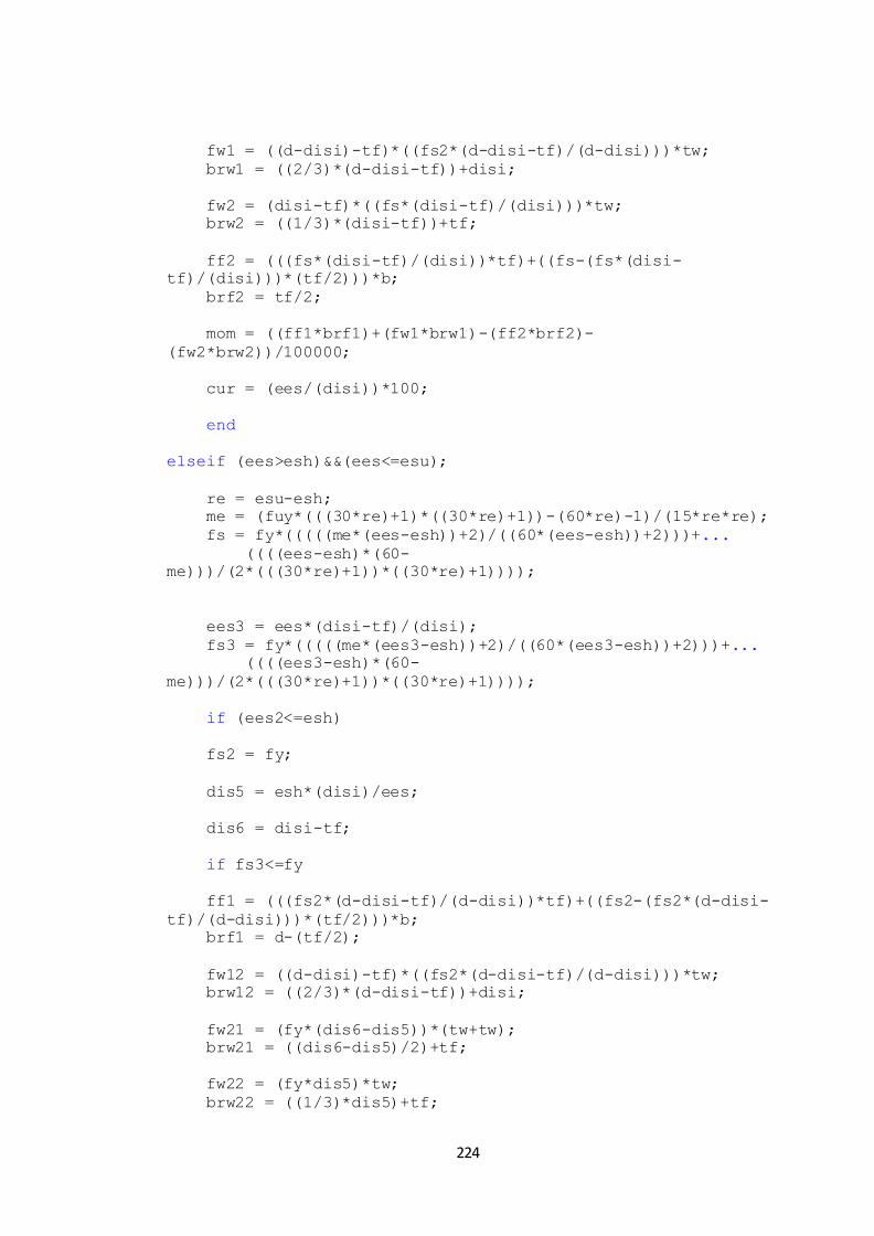
224
fw1 = ((d-disi)-tf)*((fs2*(d-disi-tf)/(d-disi)))*tw;
brw1 = ((2/3)*(d-disi-tf))+disi;
fw2 = (disi-tf)*((fs*(disi-tf)/(disi)))*tw;
brw2 = ((1/3)*(disi-tf))+tf;
ff2 = (((fs*(disi-tf)/(disi))*tf)+((fs-(fs*(disi-
tf)/(disi)))*(tf/2)))*b;
brf2 = tf/2;
mom = ((ff1*brf1)+(fw1*brw1)-(ff2*brf2)-
(fw2*brw2))/100000;
cur = (ees/(disi))*100;
end
elseif (ees>esh)&&(ees<=esu);
re = esu-esh;
me = (fuy*(((30*re)+1)*((30*re)+1))-(60*re)-1)/(15*re*re);
fs = fy*(((((me*(ees-esh))+2)/((60*(ees-esh))+2)))+...
((((ees-esh)*(60-
me)))/(2*(((30*re)+1))*((30*re)+1))));
ees3 = ees*(disi-tf)/(disi);
fs3 = fy*(((((me*(ees3-esh))+2)/((60*(ees3-esh))+2)))+...
((((ees3-esh)*(60-
me)))/(2*(((30*re)+1))*((30*re)+1))));
if (ees2<=esh)
fs2 = fy;
dis5 = esh*(disi)/ees;
dis6 = disi-tf;
if fs3<=fy
ff1 = (((fs2*(d-disi-tf)/(d-disi))*tf)+((fs2-(fs2*(d-disi-
tf)/(d-disi)))*(tf/2)))*b;
brf1 = d-(tf/2);
fw12 = ((d-disi)-tf)*((fs2*(d-disi-tf)/(d-disi)))*tw;
brw12 = ((2/3)*(d-disi-tf))+disi;
fw21 = (fy*(dis6-dis5))*(tw+tw);
brw21 = ((dis6-dis5)/2)+tf;
fw22 = (fy*dis5)*tw;
brw22 = ((1/3)*dis5)+tf;
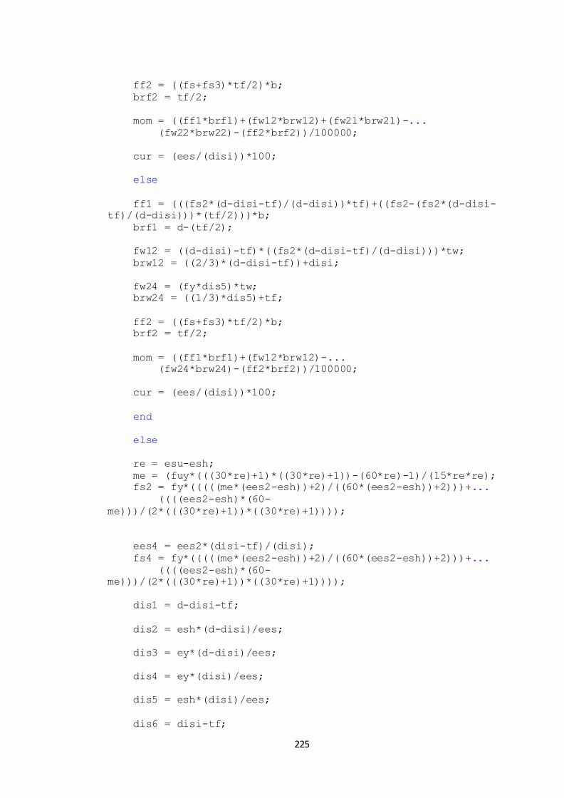
225
ff2 = ((fs+fs3)*tf/2)*b;
brf2 = tf/2;
mom = ((ff1*brf1)+(fw12*brw12)+(fw21*brw21)-...
(fw22*brw22)-(ff2*brf2))/100000;
cur = (ees/(disi))*100;
else
ff1 = (((fs2*(d-disi-tf)/(d-disi))*tf)+((fs2-(fs2*(d-disi-
tf)/(d-disi)))*(tf/2)))*b;
brf1 = d-(tf/2);
fw12 = ((d-disi)-tf)*((fs2*(d-disi-tf)/(d-disi)))*tw;
brw12 = ((2/3)*(d-disi-tf))+disi;
fw24 = (fy*dis5)*tw;
brw24 = ((1/3)*dis5)+tf;
ff2 = ((fs+fs3)*tf/2)*b;
brf2 = tf/2;
mom = ((ff1*brf1)+(fw12*brw12)-...
(fw24*brw24)-(ff2*brf2))/100000;
cur = (ees/(disi))*100;
end
else
re = esu-esh;
me = (fuy*(((30*re)+1)*((30*re)+1))-(60*re)-1)/(15*re*re);
fs2 = fy*(((((me*(ees2-esh))+2)/((60*(ees2-esh))+2)))+...
((((ees2-esh)*(60-
me)))/(2*(((30*re)+1))*((30*re)+1))));
ees4 = ees2*(disi-tf)/(disi);
fs4 = fy*(((((me*(ees2-esh))+2)/((60*(ees2-esh))+2)))+...
((((ees2-esh)*(60-
me)))/(2*(((30*re)+1))*((30*re)+1))));
dis1 = d-disi-tf;
dis2 = esh*(d-disi)/ees;
dis3 = ey*(d-disi)/ees;
dis4 = ey*(disi)/ees;
dis5 = esh*(disi)/ees;
dis6 = disi-tf;

226
if fs3<=fy
ff1 = ((fs2+fs4)*tf/2)*b;
brf1 = d-(tf/2);
fw11 = (fs4*(dis1-dis2))*(tw+tw);
brw11 = ((dis1-dis2)/2)+dis2+disi;
fw12 = (fs4*dis2)*tw;
brw12 = ((2/3)*dis2)+disi;
fw21 = (fy*(dis6-dis5))*(tw+tw);
brw21 = ((dis6-dis5)/2)+tf;
fw22 = (fy*dis5)*tw;
brw22 = ((1/3)*dis5)+tf;
ff2 = ((fs+fs3)*tf/2)*b;
brf2 = tf/2;
mom = ((ff1*brf1)+(fw11*brw11)+(fw12*brw12)-(fw21*brw21)-
...
(fw22*brw22)-(ff2*brf2))/100000;
cur = (ees/(disi))*100;
else
ff1 = ((fs2+fs4)*tf/2)*b;
brf1 = d-(tf/2);
fw11 = (fs4*(dis1-dis2))*(tw+tw);
brw11 = ((dis1-dis2)/2)+dis2+disi;
fw12 = (fs2-fs4)*(dis1-dis2)*2*(tw+tw);
brw12 = ((2/3)*(dis1-dis2))+dis2+disi;
fw14 = (fy*dis2)*tw;
brw14 = ((2/3)*dis2)+disi;
fw21 = (fy*(dis6-dis5))*(tw+tw);
brw21 = ((dis6-dis5)/2)+tf;
fw22 = (fs-fs3)*(dis6-dis5)*2*(tw+tw);
brw22 = ((1/3)*(dis6-dis5))+tf;
fw24 = (fy*dis5)*tw;
brw24 = ((1/3)*dis5)+tf+(dis6-dis5);
ff2 = ((fs+fs3)*tf/2)*b;
brf2 = tf/2;
mom = ((ff1*brf1)+(fw11*brw11)+(fw12*brw12)+...
(fw14*brw14)-(fw21*brw21)-(fw22*brw22)-...
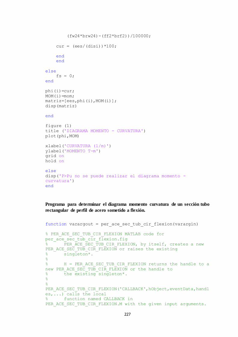
227
(fw24*brw24)-(ff2*brf2))/100000;
cur = (ees/(disi))*100;
end
end
else
fs = 0;
end
phi(i)=cur;
MOM(i)=mom;
matriz=[ees,phi(i),MOM(i)];
disp(matriz)
end
figure (1)
title ('DIAGRAMA MOMENTO - CURVATURA')
plot(phi,MOM)
xlabel('CURVATURA (1/m)')
ylabel('MOMENTO T-m')
grid on
hold on
else
disp('P>Pu no se puede realizar el diagrama momento -
curvatura')
end
Programa para determinar el diagrama momento curvatura de un sección tubo
rectangular de perfil de acero sometido a flexión.
function varargout = per_ace_sec_tub_cir_flexion(varargin)
% PER_ACE_SEC_TUB_CIR_FLEXION MATLAB code for
per_ace_sec_tub_cir_flexion.fig
% PER_ACE_SEC_TUB_CIR_FLEXION, by itself, creates a new
PER_ACE_SEC_TUB_CIR_FLEXION or raises the existing
% singleton*.
%
% H = PER_ACE_SEC_TUB_CIR_FLEXION returns the handle to a
new PER_ACE_SEC_TUB_CIR_FLEXION or the handle to
% the existing singleton*.
%
%
PER_ACE_SEC_TUB_CIR_FLEXION('CALLBACK',hObject,eventData,handl
es,...) calls the local
% function named CALLBACK in
PER_ACE_SEC_TUB_CIR_FLEXION.M with the given input arguments.

228
%
% PER_ACE_SEC_TUB_CIR_FLEXION('Property','Value',...)
creates a new PER_ACE_SEC_TUB_CIR_FLEXION or raises the
% existing singleton*. Starting from the left, property
value pairs are
% applied to the GUI before
per_ace_sec_tub_cir_flexion_OpeningFcn gets called. An
% unrecognized property name or invalid value makes
property application
% stop. All inputs are passed to
per_ace_sec_tub_cir_flexion_OpeningFcn via varargin.
%
% *See GUI Options on GUIDE's Tools menu. Choose "GUI
allows only one
% instance to run (singleton)".
%
% See also: GUIDE, GUIDATA, GUIHANDLES
% Edit the above text to modify the response to help
per_ace_sec_tub_cir_flexion
% Last Modified by GUIDE v2.5 07-Dec-2016 08:20:40
% Begin initialization code - DO NOT EDIT
gui_Singleton = 1;
gui_State = struct('gui_Name', mfilename, ...
'gui_Singleton', gui_Singleton, ...
'gui_OpeningFcn',
@per_ace_sec_tub_cir_flexion_OpeningFcn, ...
'gui_OutputFcn',
@per_ace_sec_tub_cir_flexion_OutputFcn, ...
'gui_LayoutFcn', [] , ...
'gui_Callback', []);
if nargin && ischar(varargin{1})
gui_State.gui_Callback = str2func(varargin{1});
end
if nargout
[varargout{1:nargout}] = gui_mainfcn(gui_State,
varargin{:});
else
gui_mainfcn(gui_State, varargin{:});
end
% End initialization code - DO NOT EDIT
% --- Executes just before per_ace_sec_tub_cir_flexion is made
visible.
function per_ace_sec_tub_cir_flexion_OpeningFcn(hObject,
eventdata, handles, varargin)
% This function has no output args, see OutputFcn.
% hObject handle to figure
% eventdata reserved - to be defined in a future version of
MATLAB

229
% handles structure with handles and user data (see
GUIDATA)
% varargin command line arguments to
per_ace_sec_tub_cir_flexion (see VARARGIN)
% Choose default command line output for
per_ace_sec_tub_cir_flexion
handles.output = hObject;
% Update handles structure
guidata(hObject, handles);
za = imread('pasectrflexion.jpg');
image(za)
axis off
% UIWAIT makes per_ace_sec_tub_cir_flexion wait for user
response (see UIRESUME)
% uiwait(handles.figure1);
% --- Outputs from this function are returned to the command
line.
function varargout =
per_ace_sec_tub_cir_flexion_OutputFcn(hObject, eventdata,
handles)
% varargout cell array for returning output args (see
VARARGOUT);
% hObject handle to figure
% eventdata reserved - to be defined in a future version of
MATLAB
% handles structure with handles and user data (see
GUIDATA)
% Get default command line output from handles structure
varargout{1} = handles.output;
function edit1_Callback(hObject, eventdata, handles)
% hObject handle to edit1 (see GCBO)
% eventdata reserved - to be defined in a future version of
MATLAB
% handles structure with handles and user data (see
GUIDATA)
global d;
d=str2double(get(hObject,'String'));
% Hints: get(hObject,'String') returns contents of edit1 as
text
% str2double(get(hObject,'String')) returns contents of
edit1 as a double
% --- Executes during object creation, after setting all
properties.
function edit1_CreateFcn(hObject, eventdata, handles)
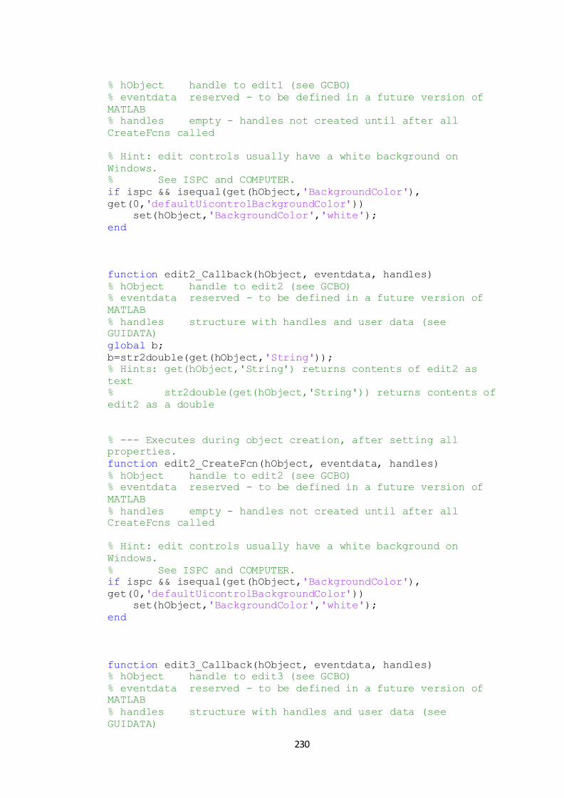
230
% hObject handle to edit1 (see GCBO)
% eventdata reserved - to be defined in a future version of
MATLAB
% handles empty - handles not created until after all
CreateFcns called
% Hint: edit controls usually have a white background on
Windows.
% See ISPC and COMPUTER.
if ispc && isequal(get(hObject,'BackgroundColor'),
get(0,'defaultUicontrolBackgroundColor'))
set(hObject,'BackgroundColor','white');
end
function edit2_Callback(hObject, eventdata, handles)
% hObject handle to edit2 (see GCBO)
% eventdata reserved - to be defined in a future version of
MATLAB
% handles structure with handles and user data (see
GUIDATA)
global b;
b=str2double(get(hObject,'String'));
% Hints: get(hObject,'String') returns contents of edit2 as
text
% str2double(get(hObject,'String')) returns contents of
edit2 as a double
% --- Executes during object creation, after setting all
properties.
function edit2_CreateFcn(hObject, eventdata, handles)
% hObject handle to edit2 (see GCBO)
% eventdata reserved - to be defined in a future version of
MATLAB
% handles empty - handles not created until after all
CreateFcns called
% Hint: edit controls usually have a white background on
Windows.
% See ISPC and COMPUTER.
if ispc && isequal(get(hObject,'BackgroundColor'),
get(0,'defaultUicontrolBackgroundColor'))
set(hObject,'BackgroundColor','white');
end
function edit3_Callback(hObject, eventdata, handles)
% hObject handle to edit3 (see GCBO)
% eventdata reserved - to be defined in a future version of
MATLAB
% handles structure with handles and user data (see
GUIDATA)

231
global tf;
tf=str2double(get(hObject,'String'));
% Hints: get(hObject,'String') returns contents of edit3 as
text
% str2double(get(hObject,'String')) returns contents of
edit3 as a double
% --- Executes during object creation, after setting all
properties.
function edit3_CreateFcn(hObject, eventdata, handles)
% hObject handle to edit3 (see GCBO)
% eventdata reserved - to be defined in a future version of
MATLAB
% handles empty - handles not created until after all
CreateFcns called
% Hint: edit controls usually have a white background on
Windows.
% See ISPC and COMPUTER.
if ispc && isequal(get(hObject,'BackgroundColor'),
get(0,'defaultUicontrolBackgroundColor'))
set(hObject,'BackgroundColor','white');
end
function edit4_Callback(hObject, eventdata, handles)
% hObject handle to edit4 (see GCBO)
% eventdata reserved - to be defined in a future version of
MATLAB
% handles structure with handles and user data (see
GUIDATA)
global tw;
tw=str2double(get(hObject,'String'));
% Hints: get(hObject,'String') returns contents of edit4 as
text
% str2double(get(hObject,'String')) returns contents of
edit4 as a double
% --- Executes during object creation, after setting all
properties.
function edit4_CreateFcn(hObject, eventdata, handles)
% hObject handle to edit4 (see GCBO)
% eventdata reserved - to be defined in a future version of
MATLAB
% handles empty - handles not created until after all
CreateFcns called
% Hint: edit controls usually have a white background on
Windows.
% See ISPC and COMPUTER.
if ispc && isequal(get(hObject,'BackgroundColor'),
get(0,'defaultUicontrolBackgroundColor'))

232
set(hObject,'BackgroundColor','white');
end
% --- Executes on selection change in selector.
function selector_Callback(hObject, eventdata, handles)
% hObject handle to selector (see GCBO)
% eventdata reserved - to be defined in a future version of
MATLAB
% handles structure with handles and user data (see
GUIDATA)
% Hints: contents = cellstr(get(hObject,'String')) returns
selector contents as cell array
% contents{get(hObject,'Value')} returns selected item
from selector
global fy;
global ey;
global esh;
global esu;
global fuy;
a=get(handles.selector,'Value');
switch a
case 1
fy = 2530;
ey = 0.0012;
esh = 0.020;
esu = 0.2;
fuy = 1.2;
case 2
fy = 3515;
ey = 0.0017;
esh = 0.015;
esu = 0.17;
fuy = 0.9;
case 3
fy = 3515;
ey = 0.0017;
esh = 0.015;
esu = 0.17;
fuy = 0.9;
case 4
fy = 3515;
ey = 0.0017;
esh = 0.015;
esu = 0.17;
fuy = 0.9;
case 5
fy = 3515;

233
ey = 0.0017;
esh = 0.015;
esu = 0.17;
fuy = 0.9;
case 6
fy = 4921;
ey = 0.0024;
esh = 0.015;
esu = 0.17;
fuy = 0.7;
end
% --- Executes during object creation, after setting all
properties.
function selector_CreateFcn(hObject, eventdata, handles)
% hObject handle to selector (see GCBO)
% eventdata reserved - to be defined in a future version of
MATLAB
% handles empty - handles not created until after all
CreateFcns called
% Hint: popupmenu controls usually have a white background on
Windows.
% See ISPC and COMPUTER.
if ispc && isequal(get(hObject,'BackgroundColor'),
get(0,'defaultUicontrolBackgroundColor'))
set(hObject,'BackgroundColor','white');
end
% --- Executes on button press in pushbutton2.
function pushbutton2_Callback(hObject, eventdata, handles)
% hObject handle to pushbutton2 (see GCBO)
% eventdata reserved - to be defined in a future version of
MATLAB
% handles structure with handles and user data (see
GUIDATA)
global d;
global b;
global tf;
global tw;
global fy;
global ey;
global esh;
global esu;
global fuy;
ek = 2043000;
ycg = (((b*tf)*(tf/2))+(((d-tf-tf)*tw)*(tf+((d-tf-tf)/2)))+...
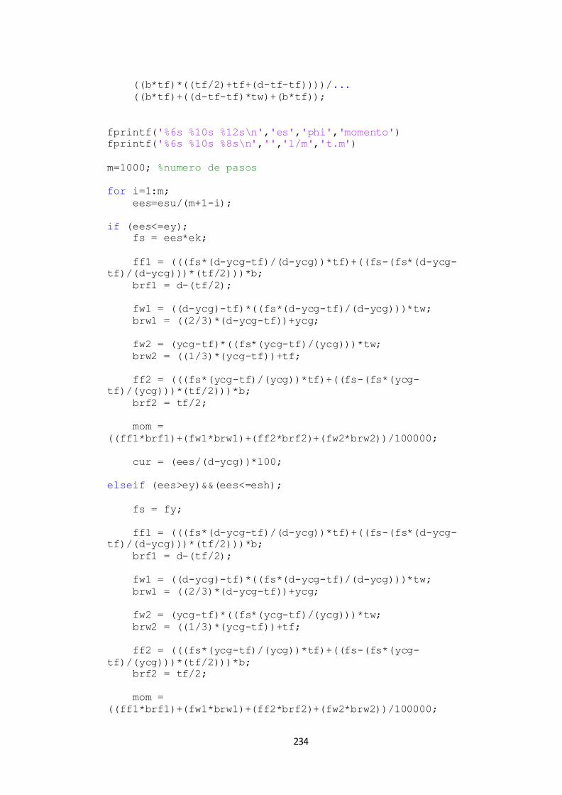
234
((b*tf)*((tf/2)+tf+(d-tf-tf))))/...
((b*tf)+((d-tf-tf)*tw)+(b*tf));
fprintf('%6s %10s %12s\n','es','phi','momento')
fprintf('%6s %10s %8s\n','','1/m','t.m')
m=1000; %numero de pasos
for i=1:m;
ees=esu/(m+1-i);
if (ees<=ey);
fs = ees*ek;
ff1 = (((fs*(d-ycg-tf)/(d-ycg))*tf)+((fs-(fs*(d-ycg-
tf)/(d-ycg)))*(tf/2)))*b;
brf1 = d-(tf/2);
fw1 = ((d-ycg)-tf)*((fs*(d-ycg-tf)/(d-ycg)))*tw;
brw1 = ((2/3)*(d-ycg-tf))+ycg;
fw2 = (ycg-tf)*((fs*(ycg-tf)/(ycg)))*tw;
brw2 = ((1/3)*(ycg-tf))+tf;
ff2 = (((fs*(ycg-tf)/(ycg))*tf)+((fs-(fs*(ycg-
tf)/(ycg)))*(tf/2)))*b;
brf2 = tf/2;
mom =
((ff1*brf1)+(fw1*brw1)+(ff2*brf2)+(fw2*brw2))/100000;
cur = (ees/(d-ycg))*100;
elseif (ees>ey)&&(ees<=esh);
fs = fy;
ff1 = (((fs*(d-ycg-tf)/(d-ycg))*tf)+((fs-(fs*(d-ycg-
tf)/(d-ycg)))*(tf/2)))*b;
brf1 = d-(tf/2);
fw1 = ((d-ycg)-tf)*((fs*(d-ycg-tf)/(d-ycg)))*tw;
brw1 = ((2/3)*(d-ycg-tf))+ycg;
fw2 = (ycg-tf)*((fs*(ycg-tf)/(ycg)))*tw;
brw2 = ((1/3)*(ycg-tf))+tf;
ff2 = (((fs*(ycg-tf)/(ycg))*tf)+((fs-(fs*(ycg-
tf)/(ycg)))*(tf/2)))*b;
brf2 = tf/2;
mom =
((ff1*brf1)+(fw1*brw1)+(ff2*brf2)+(fw2*brw2))/100000;
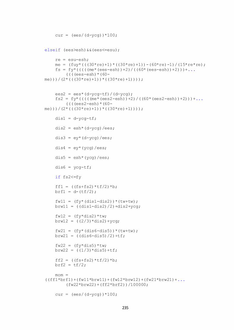
235
cur = (ees/(d-ycg))*100;
elseif (ees>esh)&&(ees<=esu);
re = esu-esh;
me = (fuy*(((30*re)+1)*((30*re)+1))-(60*re)-1)/(15*re*re);
fs = fy*(((((me*(ees-esh))+2)/((60*(ees-esh))+2)))+...
((((ees-esh)*(60-
me)))/(2*(((30*re)+1))*((30*re)+1))));
ees2 = ees*(d-ycg-tf)/(d-ycg);
fs2 = fy*(((((me*(ees2-esh))+2)/((60*(ees2-esh))+2)))+...
((((ees2-esh)*(60-
me)))/(2*(((30*re)+1))*((30*re)+1))));
dis1 = d-ycg-tf;
dis2 = esh*(d-ycg)/ees;
dis3 = ey*(d-ycg)/ees;
dis4 = ey*(ycg)/ees;
dis5 = esh*(ycg)/ees;
dis6 = ycg-tf;
if fs2<=fy
ff1 = ((fs+fs2)*tf/2)*b;
brf1 = d-(tf/2);
fw11 = (fy*(dis1-dis2))*(tw+tw);
brw11 = ((dis1-dis2)/2)+dis2+ycg;
fw12 = (fy*dis2)*tw;
brw12 = ((2/3)*dis2)+ycg;
fw21 = (fy*(dis6-dis5))*(tw+tw);
brw21 = ((dis6-dis5)/2)+tf;
fw22 = (fy*dis5)*tw;
brw22 = ((1/3)*dis5)+tf;
ff2 = ((fs+fs2)*tf/2)*b;
brf2 = tf/2;
mom =
((ff1*brf1)+(fw11*brw11)+(fw12*brw12)+(fw21*brw21)+...
(fw22*brw22)+(ff2*brf2))/100000;
cur = (ees/(d-ycg))*100;
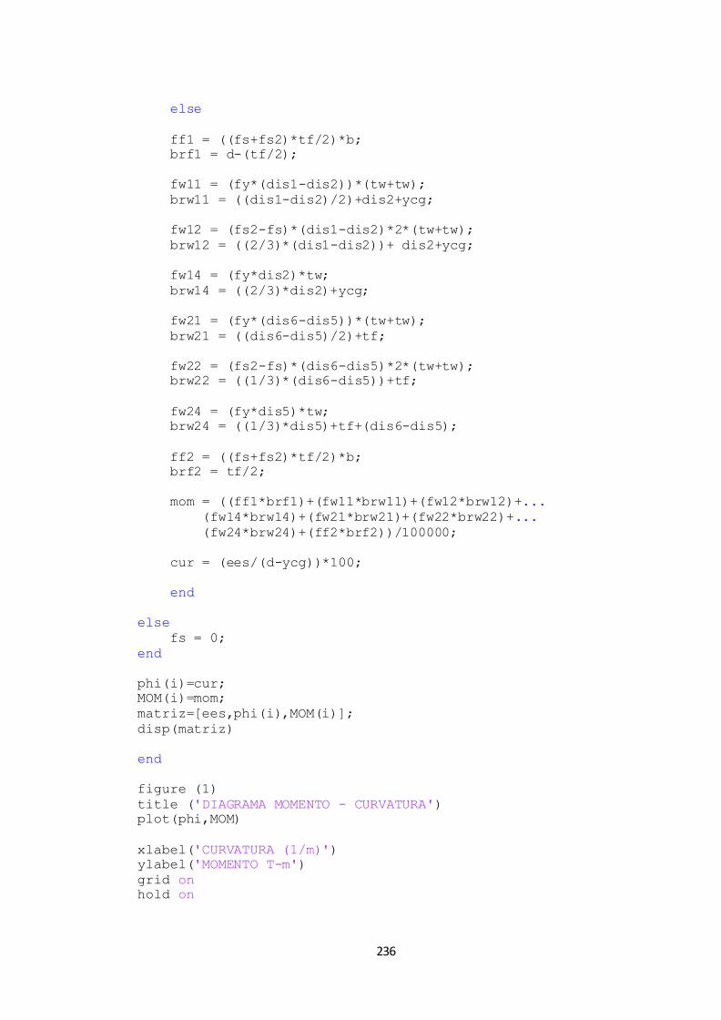
236
else
ff1 = ((fs+fs2)*tf/2)*b;
brf1 = d-(tf/2);
fw11 = (fy*(dis1-dis2))*(tw+tw);
brw11 = ((dis1-dis2)/2)+dis2+ycg;
fw12 = (fs2-fs)*(dis1-dis2)*2*(tw+tw);
brw12 = ((2/3)*(dis1-dis2))+ dis2+ycg;
fw14 = (fy*dis2)*tw;
brw14 = ((2/3)*dis2)+ycg;
fw21 = (fy*(dis6-dis5))*(tw+tw);
brw21 = ((dis6-dis5)/2)+tf;
fw22 = (fs2-fs)*(dis6-dis5)*2*(tw+tw);
brw22 = ((1/3)*(dis6-dis5))+tf;
fw24 = (fy*dis5)*tw;
brw24 = ((1/3)*dis5)+tf+(dis6-dis5);
ff2 = ((fs+fs2)*tf/2)*b;
brf2 = tf/2;
mom = ((ff1*brf1)+(fw11*brw11)+(fw12*brw12)+...
(fw14*brw14)+(fw21*brw21)+(fw22*brw22)+...
(fw24*brw24)+(ff2*brf2))/100000;
cur = (ees/(d-ycg))*100;
end
else
fs = 0;
end
phi(i)=cur;
MOM(i)=mom;
matriz=[ees,phi(i),MOM(i)];
disp(matriz)
end
figure (1)
title ('DIAGRAMA MOMENTO - CURVATURA')
plot(phi,MOM)
xlabel('CURVATURA (1/m)')
ylabel('MOMENTO T-m')
grid on
hold on
237
Programa para determinar el diagrama momento curvatura de un sección tubo
circular de perfil de acero sometido a flexocompresión.
function varargout =
per_ace_sec_tub_cir_flexocompresion(varargin)
% PER_ACE_SEC_TUB_CIR_FLEXOCOMPRESION MATLAB code for
per_ace_sec_tub_cir_flexocompresion.fig
% PER_ACE_SEC_TUB_CIR_FLEXOCOMPRESION, by itself, creates
a new PER_ACE_SEC_TUB_CIR_FLEXOCOMPRESION or raises the
existing
% singleton*.
%
% H = PER_ACE_SEC_TUB_CIR_FLEXOCOMPRESION returns the
handle to a new PER_ACE_SEC_TUB_CIR_FLEXOCOMPRESION or the
handle to
% the existing singleton*.
%
%
PER_ACE_SEC_TUB_CIR_FLEXOCOMPRESION('CALLBACK',hObject,eventDa
ta,handles,...) calls the local
% function named CALLBACK in
PER_ACE_SEC_TUB_CIR_FLEXOCOMPRESION.M with the given input
arguments.
%
%
PER_ACE_SEC_TUB_CIR_FLEXOCOMPRESION('Property','Value',...)
creates a new PER_ACE_SEC_TUB_CIR_FLEXOCOMPRESION or raises
the
% existing singleton*. Starting from the left, property
value pairs are
% applied to the GUI before
per_ace_sec_tub_cir_flexocompresion_OpeningFcn gets called.
An
% unrecognized property name or invalid value makes
property application
% stop. All inputs are passed to
per_ace_sec_tub_cir_flexocompresion_OpeningFcn via varargin.
%
% *See GUI Options on GUIDE's Tools menu. Choose "GUI
allows only one
% instance to run (singleton)".
%
% See also: GUIDE, GUIDATA, GUIHANDLES
% Edit the above text to modify the response to help
per_ace_sec_tub_cir_flexocompresion
% Last Modified by GUIDE v2.5 07-Dec-2016 10:02:29
% Begin initialization code - DO NOT EDIT
gui_Singleton = 1;
gui_State = struct('gui_Name', mfilename, ...
238
'gui_Singleton', gui_Singleton, ...
'gui_OpeningFcn',
@per_ace_sec_tub_cir_flexocompresion_OpeningFcn, ...
'gui_OutputFcn',
@per_ace_sec_tub_cir_flexocompresion_OutputFcn, ...
'gui_LayoutFcn', [] , ...
'gui_Callback', []);
if nargin && ischar(varargin{1})
gui_State.gui_Callback = str2func(varargin{1});
end
if nargout
[varargout{1:nargout}] = gui_mainfcn(gui_State,
varargin{:});
else
gui_mainfcn(gui_State, varargin{:});
end
% End initialization code - DO NOT EDIT
% --- Executes just before per_ace_sec_tub_cir_flexocompresion
is made visible.
function
per_ace_sec_tub_cir_flexocompresion_OpeningFcn(hObject,
eventdata, handles, varargin)
% This function has no output args, see OutputFcn.
% hObject handle to figure
% eventdata reserved - to be defined in a future version of
MATLAB
% handles structure with handles and user data (see
GUIDATA)
% varargin command line arguments to
per_ace_sec_tub_cir_flexocompresion (see VARARGIN)
% Choose default command line output for
per_ace_sec_tub_cir_flexocompresion
handles.output = hObject;
% Update handles structure
guidata(hObject, handles);
za = imread('pasectcflexocompresion.jpg');
image(za)
axis off
% UIWAIT makes per_ace_sec_tub_cir_flexocompresion wait for
user response (see UIRESUME)
% uiwait(handles.figure1);
% --- Outputs from this function are returned to the command
line.
function varargout =
per_ace_sec_tub_cir_flexocompresion_OutputFcn(hObject,
eventdata, handles)
239
% varargout cell array for returning output args (see
VARARGOUT);
% hObject handle to figure
% eventdata reserved - to be defined in a future version of
MATLAB
% handles structure with handles and user data (see
GUIDATA)
% Get default command line output from handles structure
varargout{1} = handles.output;
function edit1_Callback(hObject, eventdata, handles)
% hObject handle to edit1 (see GCBO)
% eventdata reserved - to be defined in a future version of
MATLAB
% handles structure with handles and user data (see
GUIDATA)
global d;
d=str2double(get(hObject,'String'));
% Hints: get(hObject,'String') returns contents of edit1 as
text
% str2double(get(hObject,'String')) returns contents of
edit1 as a double
% --- Executes during object creation, after setting all
properties.
function edit1_CreateFcn(hObject, eventdata, handles)
% hObject handle to edit1 (see GCBO)
% eventdata reserved - to be defined in a future version of
MATLAB
% handles empty - handles not created until after all
CreateFcns called
% Hint: edit controls usually have a white background on
Windows.
% See ISPC and COMPUTER.
if ispc && isequal(get(hObject,'BackgroundColor'),
get(0,'defaultUicontrolBackgroundColor'))
set(hObject,'BackgroundColor','white');
end
function edit2_Callback(hObject, eventdata, handles)
% hObject handle to edit2 (see GCBO)
% eventdata reserved - to be defined in a future version of
MATLAB
% handles structure with handles and user data (see
GUIDATA)
global tw;
tw=str2double(get(hObject,'String'));

240
% Hints: get(hObject,'String') returns contents of edit2 as
text
% str2double(get(hObject,'String')) returns contents of
edit2 as a double
% --- Executes during object creation, after setting all
properties.
function edit2_CreateFcn(hObject, eventdata, handles)
% hObject handle to edit2 (see GCBO)
% eventdata reserved - to be defined in a future version of
MATLAB
% handles empty - handles not created until after all
CreateFcns called
% Hint: edit controls usually have a white background on
Windows.
% See ISPC and COMPUTER.
if ispc && isequal(get(hObject,'BackgroundColor'),
get(0,'defaultUicontrolBackgroundColor'))
set(hObject,'BackgroundColor','white');
end
function edit12_Callback(hObject, eventdata, handles)
% hObject handle to edit12 (see GCBO)
% eventdata reserved - to be defined in a future version of
MATLAB
% handles structure with handles and user data (see
GUIDATA)
global pa;
pa=str2double(get(hObject,'String'));
% Hints: get(hObject,'String') returns contents of edit12 as
text
% str2double(get(hObject,'String')) returns contents of
edit12 as a double
% --- Executes during object creation, after setting all
properties.
function edit12_CreateFcn(hObject, eventdata, handles)
% hObject handle to edit12 (see GCBO)
% eventdata reserved - to be defined in a future version of
MATLAB
% handles empty - handles not created until after all
CreateFcns called
% Hint: edit controls usually have a white background on
Windows.
% See ISPC and COMPUTER.
if ispc && isequal(get(hObject,'BackgroundColor'),
get(0,'defaultUicontrolBackgroundColor'))
set(hObject,'BackgroundColor','white');
end

241
% --- Executes on selection change in selector.
function selector_Callback(hObject, eventdata, handles)
% hObject handle to selector (see GCBO)
% eventdata reserved - to be defined in a future version of
MATLAB
% handles structure with handles and user data (see
GUIDATA)
% Hints: contents = cellstr(get(hObject,'String')) returns
selector contents as cell array
% contents{get(hObject,'Value')} returns selected item
from selector
global fy;
global ey;
global esh;
global esu;
global fuy;
a=get(handles.selector,'Value');
switch a
case 1
fy = 2530;
ey = 0.0012;
esh = 0.020;
esu = 0.2;
fuy = 1.5;
case 2
fy = 3515;
ey = 0.0017;
esh = 0.015;
esu = 0.17;
fuy = 0.9;
case 3
fy = 3515;
ey = 0.0017;
esh = 0.015;
esu = 0.17;
fuy = 0.9;
case 4
fy = 3515;
ey = 0.0017;
esh = 0.015;
esu = 0.17;
fuy = 0.9;
case 5
fy = 3515;
ey = 0.0017;
esh = 0.015;
esu = 0.17;

242
fuy = 0.9;
case 6
fy = 4921;
ey = 0.0024;
esh = 0.015;
esu = 0.17;
fuy = 0.8;
end
% --- Executes during object creation, after setting all
properties.
function selector_CreateFcn(hObject, eventdata, handles)
% hObject handle to selector (see GCBO)
% eventdata reserved - to be defined in a future version of
MATLAB
% handles empty - handles not created until after all
CreateFcns called
% Hint: popupmenu controls usually have a white background on
Windows.
% See ISPC and COMPUTER.
if ispc && isequal(get(hObject,'BackgroundColor'),
get(0,'defaultUicontrolBackgroundColor'))
set(hObject,'BackgroundColor','white');
end
% --- Executes on button press in pushbutton2.
function pushbutton2_Callback(hObject, eventdata, handles)
% hObject handle to pushbutton2 (see GCBO)
% eventdata reserved - to be defined in a future version of
MATLAB
% handles structure with handles and user data (see
GUIDATA)
global d;
global tw;
global pa;
global fy;
global ey;
global esh;
global esu;
global fuy;
ek = 2043000;
b = 2* sqrt(((d/2)^2)-(((d/2)-(tw))^2));
ycg = (((b*tw)*(tw/2))+(((d-tw-tw)*tw)*(tw+((d-tw-tw)/2)))+...
((b*tw)*((tw/2)+tw+(d-tw-tw))))/...
243
((b*tw)+((d-tw-tw)*tw)+(b*tw));
fprintf('%6s %10s %12s\n','es','phi','momento')
fprintf('%6s %10s %8s\n','','1/m','t.m')
area = (pi*(d/2)*(d/2))-(pi*((d-tw-tw)/2)*((d-tw-tw)/2));
py = area*fy;
dp = (pa*1000)/py;
disi = ycg*(1+dp);
diss = d-disi;
ek = 2043000;
z = ((pa*1000)*ycg/area);
m=1000; %numero de pasos
if dp<=1
for i=1:m;
ees=esu/(m+1-i);
ees2=ees*diss/disi;
if (ees<=ey);
fs = ees*ek;
fs2 = ees2*ek;
ff1 = (((fs2*(d-disi-tw)/(d-disi))*tw)+((fs2-(fs2*(d-disi-
tw)/(d-disi)))*(tw/2)))*b;
brf1 = d-(tw/2);
fw1 = ((d-disi)-tw)*((fs2*(d-disi-tw)/(d-disi)))*tw;
brw1 = ((2/3)*(d-disi-tw))+disi;
fw2 = (disi-tw)*((fs*(disi-tw)/(disi)))*tw;
brw2 = ((1/3)*(disi-tw))+tw;
ff2 = (((fs*(disi-tw)/(disi))*tw)+((fs-(fs*(disi-
tw)/(disi)))*(tw/2)))*b;
brf2 = tw/2;
mom =
((ff1*brf1)+(fw1*brw1)+(ff2*brf2)+(fw2*brw2))/100000;
cur = (ees/(disi))*100;
elseif (ees>ey)&&(ees<=esh);
fs = fy;
if (ees2<ey)&&(ees2<=esh)

244
fs2 = ees2*ek;
ff1 = (((fs2*(d-disi-tw)/(d-disi))*tw)+((fs2-(fs2*(d-disi-
tw)/(d-disi)))*(tw/2)))*b;
brf1 = d-(tw/2);
fw1 = ((d-disi)-tw)*((fs2*(d-disi-tw)/(d-disi)))*tw;
brw1 = ((2/3)*(d-disi-tw))+disi;
fw2 = (disi-tw)*((fs*(disi-tw)/(disi)))*tw;
brw2 = ((1/3)*(disi-tw))+tw;
ff2 = (((fs*(disi-tw)/(disi))*tw)+((fs-(fs*(disi-
tw)/(disi)))*(tw/2)))*b;
brf2 = tw/2;
mom =
((ff1*brf1)+(fw1*brw1)+(ff2*brf2)+(fw2*brw2))/100000;
cur = (ees/(disi))*100;
else
fs2 = fy;
ff1 = (((fs2*(d-disi-tw)/(d-disi))*tw)+((fs2-(fs2*(d-disi-
tw)/(d-disi)))*(tw/2)))*b;
brf1 = d-(tw/2);
fw1 = ((d-disi)-tw)*((fs2*(d-disi-tw)/(d-disi)))*tw;
brw1 = ((2/3)*(d-disi-tw))+disi;
fw2 = (disi-tw)*((fs*(disi-tw)/(disi)))*tw;
brw2 = ((1/3)*(disi-tw))+tw;
ff2 = (((fs*(disi-tw)/(disi))*tw)+((fs-(fs*(disi-
tw)/(disi)))*(tw/2)))*b;
brf2 = tw/2;
mom =
((ff1*brf1)+(fw1*brw1)+(ff2*brf2)+(fw2*brw2))/100000;
cur = (ees/(disi))*100;
end
elseif (ees>esh)&&(ees<=esu);
re = esu-esh;
me = (fuy*(((30*re)+1)*((30*re)+1))-(60*re)-1)/(15*re*re);
fs = fy*(((((me*(ees-esh))+2)/((60*(ees-esh))+2)))+...

245
((((ees-esh)*(60-
me)))/(2*(((30*re)+1))*((30*re)+1))));
ees3 = ees*(disi-tw)/(disi);
fs3 = fy*(((((me*(ees3-esh))+2)/((60*(ees3-esh))+2)))+...
((((ees3-esh)*(60-
me)))/(2*(((30*re)+1))*((30*re)+1))));
if (ees2<=esh)
fs2 = fy;
dis1 = d-disi-tw;
dis2 = esh*(d-disi)/ees;
dis3 = ey*(d-disi)/ees;
dis4 = ey*(disi)/ees;
dis5 = esh*(disi)/ees;
dis6 = disi-tw;
if (dis1>(dis2+tw))&&(dis6>(dis5+tw))
if fs3<=fy
ff1 = (((fs2*(d-disi-tw)/(d-disi))*tw)+((fs2-(fs2*(d-disi-
tw)/(d-disi)))*(tw/2)))*b;
brf1 = d-(tw/2);
fw12 = (fs*dis2)*tw;
brw12 = ((2/3)*dis2)+disi;
fw21 = (fy*(dis6-dis5))*(tw+tw);
brw21 = ((dis6-dis5)/2)+tw;
fw22 = (fy*dis5)*tw;
brw22 = ((1/3)*dis5)+tw;
ff2 = ((fs+fs3)*tw/2)*b;
brf2 = tw/2;
mom = ((ff1*brf1)+(fw12*brw12)+(fw21*brw21)+...
(fw22*brw22)+(ff2*brf2))/100000;
cur = (ees/(disi))*100;
else
ff1 = (((fs2*(d-disi-tw)/(d-disi))*tw)+((fs2-(fs2*(d-disi-
tw)/(d-disi)))*(tw/2)))*b;
brf1 = d-(tw/2);

246
fw12 = ((fs2*(d-disi-tw)/(d-disi))*(dis1-dis2))*2*(tw+tw);
brw12 = ((2/3)*(dis1-dis2))+ dis2+disi;
fw22 = (fs3-fs)*(dis6-dis5)*2*(tw+tw);
brw22 = ((1/3)*(dis6-dis5))+tw;
fw24 = (fs3*dis5)*tw;
brw24 = ((1/3)*dis5)+tw+(dis6-dis5);
ff2 = ((fs+fs3)*tw/2)*b;
brf2 = tw/2;
mom = ((ff1*brf1)+(fw12*brw12)+...
(fw24*brw24)+(fw22*brw22)+(ff2*brf2))/100000;
cur = (ees/(disi))*100;
end
end
else
re = esu-esh;
me = (fuy*(((30*re)+1)*((30*re)+1))-(60*re)-1)/(15*re*re);
fs2 = fy*(((((me*(ees2-esh))+2)/((60*(ees2-esh))+2)))+...
((((ees2-esh)*(60-
me)))/(2*(((30*re)+1))*((30*re)+1))));
ees4 = ees2*(d-disi-tw)/(d-disi);
fs4 = fy*(((((me*(ees4-esh))+2)/((60*(ees4-esh))+2)))+...
((((ees4-esh)*(60-
me)))/(2*(((30*re)+1))*((30*re)+1))));
dis1 = d-disi-tw;
dis2 = esh*(d-disi)/ees;
dis3 = ey*(d-disi)/ees;
dis4 = ey*(disi)/ees;
dis5 = esh*(disi)/ees;
dis6 = disi-tw;
if fs3<=fy
ff1 = ((fs2+fs4)*tw/2)*b;
brf1 = d-(tw/2);
fw11 = (fs4*(dis1-dis2))*(tw+tw);
brw11 = ((dis1-dis2)/2)+dis2+disi;
247
fw12 = (fs4*dis2)*tw;
brw12 = ((2/3)*dis2)+disi;
fw21 = (fy*(dis6-dis5))*(tw+tw);
brw21 = ((dis6-dis5)/2)+tw;
fw22 = (fy*dis5)*tw;
brw22 = ((1/3)*dis5)+tw;
ff2 = ((fs+fs3)*tw/2)*b;
brf2 = tw/2;
mom =
((ff1*brf1)+(fw11*brw11)+(fw12*brw12)+(fw21*brw21)+...
(fw22*brw22)+(ff2*brf2))/100000;
cur = (ees/(disi))*100;
else
ff1 = ((fs2+fs4)*tw/2)*b;
brf1 = d-(tw/2);
fw11 = (fy*(dis1-dis2))*(tw+tw);
brw11 = ((dis1-dis2)/2)+dis2+disi;
fw12 = (fs2-fs4)*(dis1-dis2)*2*(tw+tw);
brw12 = ((2/3)*(dis1-dis2))+ dis2+disi;
fw14 = (fy*dis2)*tw;
brw14 = ((2/3)*dis2)+disi;
fw21 = (fy*(dis6-dis5))*(tw+tw);
brw21 = ((dis6-dis5)/2)+tw;
fw22 = (fs3-fs)*(dis6-dis5)*2*(tw+tw);
brw22 = ((1/3)*(dis6-dis5))+tw;
fw24 = (fy*dis5)*tw;
brw24 = ((1/3)*dis5)+tw+(dis6-dis5);
ff2 = ((fs+fs3)*tw/2)*b;
brf2 = tw/2;
mom = ((ff1*brf1)+(fw11*brw11)+(fw12*brw12)+...
(fw14*brw14)+(fw21*brw21)+(fw22*brw22)+...
(fw24*brw24)+(ff2*brf2))/100000;
cur = (ees/(disi))*100;
end
end
else
fs = 0;

248
end
phi(i)=cur;
MOM(i)=mom;
matriz=[ees,phi(i),MOM(i)];
disp(matriz)
end
figure (1)
title ('DIAGRAMA MOMENTO - CURVATURA')
plot(phi,MOM)
xlabel('CURVATURA (1/m)')
ylabel('MOMENTO T-m')
grid on
hold on
else
disp('P>Pu no se puede realizar el diagrama momento -
curvatura')
end
Programa para determinar el diagrama momento curvatura de un sección tubo
circular de perfil de acero sometido a flexión.
function varargout = per_ace_sec_tub_cir_flexion(varargin)
% PER_ACE_SEC_TUB_CIR_FLEXION MATLAB code for
per_ace_sec_tub_cir_flexion.fig
% PER_ACE_SEC_TUB_CIR_FLEXION, by itself, creates a new
PER_ACE_SEC_TUB_CIR_FLEXION or raises the existing
% singleton*.
%
% H = PER_ACE_SEC_TUB_CIR_FLEXION returns the handle to a
new PER_ACE_SEC_TUB_CIR_FLEXION or the handle to
% the existing singleton*.
%
%
PER_ACE_SEC_TUB_CIR_FLEXION('CALLBACK',hObject,eventData,handl
es,...) calls the local
% function named CALLBACK in
PER_ACE_SEC_TUB_CIR_FLEXION.M with the given input arguments.
%
% PER_ACE_SEC_TUB_CIR_FLEXION('Property','Value',...)
creates a new PER_ACE_SEC_TUB_CIR_FLEXION or raises the
% existing singleton*. Starting from the left, property
value pairs are
% applied to the GUI before
per_ace_sec_tub_cir_flexion_OpeningFcn gets called. An
% unrecognized property name or invalid value makes
property application
249
% stop. All inputs are passed to
per_ace_sec_tub_cir_flexion_OpeningFcn via varargin.
%
% *See GUI Options on GUIDE's Tools menu. Choose "GUI
allows only one
% instance to run (singleton)".
%
% See also: GUIDE, GUIDATA, GUIHANDLES
% Edit the above text to modify the response to help
per_ace_sec_tub_cir_flexion
% Last Modified by GUIDE v2.5 07-Dec-2016 09:29:20
% Begin initialization code - DO NOT EDIT
gui_Singleton = 1;
gui_State = struct('gui_Name', mfilename, ...
'gui_Singleton', gui_Singleton, ...
'gui_OpeningFcn',
@per_ace_sec_tub_cir_flexion_OpeningFcn, ...
'gui_OutputFcn',
@per_ace_sec_tub_cir_flexion_OutputFcn, ...
'gui_LayoutFcn', [] , ...
'gui_Callback', []);
if nargin && ischar(varargin{1})
gui_State.gui_Callback = str2func(varargin{1});
end
if nargout
[varargout{1:nargout}] = gui_mainfcn(gui_State,
varargin{:});
else
gui_mainfcn(gui_State, varargin{:});
end
% End initialization code - DO NOT EDIT
% --- Executes just before per_ace_sec_tub_cir_flexion is made
visible.
function per_ace_sec_tub_cir_flexion_OpeningFcn(hObject,
eventdata, handles, varargin)
% This function has no output args, see OutputFcn.
% hObject handle to figure
% eventdata reserved - to be defined in a future version of
MATLAB
% handles structure with handles and user data (see
GUIDATA)
% varargin command line arguments to
per_ace_sec_tub_cir_flexion (see VARARGIN)
% Choose default command line output for
per_ace_sec_tub_cir_flexion
handles.output = hObject;
% Update handles structure

250
guidata(hObject, handles);
za = imread('pasectcflexion.jpg');
image(za)
axis off
% UIWAIT makes per_ace_sec_tub_cir_flexion wait for user
response (see UIRESUME)
% uiwait(handles.figure1);
% --- Outputs from this function are returned to the command
line.
function varargout =
per_ace_sec_tub_cir_flexion_OutputFcn(hObject, eventdata,
handles)
% varargout cell array for returning output args (see
VARARGOUT);
% hObject handle to figure
% eventdata reserved - to be defined in a future version of
MATLAB
% handles structure with handles and user data (see
GUIDATA)
% Get default command line output from handles structure
varargout{1} = handles.output;
function edit1_Callback(hObject, eventdata, handles)
% hObject handle to edit1 (see GCBO)
% eventdata reserved - to be defined in a future version of
MATLAB
% handles structure with handles and user data (see
GUIDATA)
global d;
d=str2double(get(hObject,'String'));
% Hints: get(hObject,'String') returns contents of edit1 as
text
% str2double(get(hObject,'String')) returns contents of
edit1 as a double
% --- Executes during object creation, after setting all
properties.
function edit1_CreateFcn(hObject, eventdata, handles)
% hObject handle to edit1 (see GCBO)
% eventdata reserved - to be defined in a future version of
MATLAB
% handles empty - handles not created until after all
CreateFcns called
% Hint: edit controls usually have a white background on
Windows.
% See ISPC and COMPUTER.

251
if ispc && isequal(get(hObject,'BackgroundColor'),
get(0,'defaultUicontrolBackgroundColor'))
set(hObject,'BackgroundColor','white');
end
function edit2_Callback(hObject, eventdata, handles)
% hObject handle to edit2 (see GCBO)
% eventdata reserved - to be defined in a future version of
MATLAB
% handles structure with handles and user data (see
GUIDATA)
global tw;
tw=str2double(get(hObject,'String'));
% Hints: get(hObject,'String') returns contents of edit2 as
text
% str2double(get(hObject,'String')) returns contents of
edit2 as a double
% --- Executes during object creation, after setting all
properties.
function edit2_CreateFcn(hObject, eventdata, handles)
% hObject handle to edit2 (see GCBO)
% eventdata reserved - to be defined in a future version of
MATLAB
% handles empty - handles not created until after all
CreateFcns called
% Hint: edit controls usually have a white background on
Windows.
% See ISPC and COMPUTER.
if ispc && isequal(get(hObject,'BackgroundColor'),
get(0,'defaultUicontrolBackgroundColor'))
set(hObject,'BackgroundColor','white');
end
% --- Executes on selection change in selector.
function selector_Callback(hObject, eventdata, handles)
% hObject handle to selector (see GCBO)
% eventdata reserved - to be defined in a future version of
MATLAB
% handles structure with handles and user data (see
GUIDATA)
% Hints: contents = cellstr(get(hObject,'String')) returns
selector contents as cell array
% contents{get(hObject,'Value')} returns selected item
from selector
global fy;
global ey;
global esh;

252
global esu;
global fuy;
a=get(handles.selector,'Value');
switch a
case 1
fy = 2530;
ey = 0.0012;
esh = 0.020;
esu = 0.2;
fuy = 1.2;
case 2
fy = 3515;
ey = 0.0017;
esh = 0.015;
esu = 0.17;
fuy = 1.0;
case 3
fy = 3515;
ey = 0.0017;
esh = 0.015;
esu = 0.17;
fuy = 1.0;
case 4
fy = 3515;
ey = 0.0017;
esh = 0.015;
esu = 0.17;
fuy = 1.0;
case 5
fy = 3515;
ey = 0.0017;
esh = 0.015;
esu = 0.17;
fuy = 1.0;
case 6
fy = 4921;
ey = 0.0024;
esh = 0.015;
esu = 0.17;
fuy = 0.8;
end
% --- Executes during object creation, after setting all
properties.
function selector_CreateFcn(hObject, eventdata, handles)
% hObject handle to selector (see GCBO)

253
% eventdata reserved - to be defined in a future version of
MATLAB
% handles empty - handles not created until after all
CreateFcns called
% Hint: popupmenu controls usually have a white background on
Windows.
% See ISPC and COMPUTER.
if ispc && isequal(get(hObject,'BackgroundColor'),
get(0,'defaultUicontrolBackgroundColor'))
set(hObject,'BackgroundColor','white');
end
% --- Executes on button press in pushbutton2.
function pushbutton2_Callback(hObject, eventdata, handles)
% hObject handle to pushbutton2 (see GCBO)
% eventdata reserved - to be defined in a future version of
MATLAB
% handles structure with handles and user data (see
GUIDATA)
global d;
global tw;
global fy;
global ey;
global esh;
global esu;
global fuy;
ek = 2043000;
b = 2* sqrt(((d/2)^2)-(((d/2)-(tw))^2));
ycg = (((b*tw)*(tw/2))+(((d-tw-tw)*tw)*(tw+((d-tw-tw)/2)))+...
((b*tw)*((tw/2)+tw+(d-tw-tw))))/...
((b*tw)+((d-tw-tw)*tw)+(b*tw));
fprintf('%6s %10s %12s\n','es','phi','momento')
fprintf('%6s %10s %8s\n','','1/m','t.m')
m=1000; %numero de pasos
for i=1:m;
ees=esu/(m+1-i);
if (ees<=ey);
fs = ees*ek;
ff1 = (((fs*(d-ycg-tw)/(d-ycg))*tw)+((fs-(fs*(d-ycg-
tw)/(d-ycg)))*(tw/2)))*b;
brf1 = d-(tw/2);
fw1 = ((d-ycg)-tw)*((fs*(d-ycg-tw)/(d-ycg)))*tw;

254
brw1 = ((2/3)*(d-ycg-tw))+ycg;
fw2 = (ycg-tw)*((fs*(ycg-tw)/(ycg)))*tw;
brw2 = ((1/3)*(ycg-tw))+tw;
ff2 = (((fs*(ycg-tw)/(ycg))*tw)+((fs-(fs*(ycg-
tw)/(ycg)))*(tw/2)))*b;
brf2 = tw/2;
mom =
((ff1*brf1)+(fw1*brw1)+(ff2*brf2)+(fw2*brw2))/100000;
cur = (ees/(d-ycg))*100;
elseif (ees>ey)&&(ees<=esh);
fs = fy;
ff1 = (((fs*(d-ycg-tw)/(d-ycg))*tw)+((fs-(fs*(d-ycg-
tw)/(d-ycg)))*(tw/2)))*b;
brf1 = d-(tw/2);
fw1 = ((d-ycg)-tw)*((fs*(d-ycg-tw)/(d-ycg)))*tw;
brw1 = ((2/3)*(d-ycg-tw))+ycg;
fw2 = (ycg-tw)*((fs*(ycg-tw)/(ycg)))*tw;
brw2 = ((1/3)*(ycg-tw))+tw;
ff2 = (((fs*(ycg-tw)/(ycg))*tw)+((fs-(fs*(ycg-
tw)/(ycg)))*(tw/2)))*b;
brf2 = tw/2;
mom =
((ff1*brf1)+(fw1*brw1)+(ff2*brf2)+(fw2*brw2))/100000;
cur = (ees/(d-ycg))*100;
elseif (ees>esh)&&(ees<=esu);
re = esu-esh;
me = (fuy*(((30*re)+1)*((30*re)+1))-(60*re)-1)/(15*re*re);
fs = fy*(((((me*(ees-esh))+2)/((60*(ees-esh))+2)))+...
((((ees-esh)*(60-
me)))/(2*(((30*re)+1))*((30*re)+1))));
ees2 = ees*(d-ycg-tw)/(d-ycg);
fs2 = fy*(((((me*(ees2-esh))+2)/((60*(ees2-esh))+2)))+...
((((ees2-esh)*(60-
me)))/(2*(((30*re)+1))*((30*re)+1))));
dis1 = d-ycg-tw;
dis2 = esh*(d-ycg)/ees;
255
dis3 = ey*(d-ycg)/ees;
dis4 = ey*(ycg)/ees;
dis5 = esh*(ycg)/ees;
dis6 = ycg-tw;
if fs2<=fy
ff1 = ((fs+fs2)*tw/2)*b;
brf1 = d-(tw/2);
fw11 = (fy*(dis1-dis2))*(tw+tw);
brw11 = ((dis1-dis2)/2)+dis2+ycg;
fw12 = (fy*dis2)*tw;
brw12 = ((2/3)*dis2)+ycg;
fw21 = (fy*(dis6-dis5))*(tw+tw);
brw21 = ((dis6-dis5)/2)+tw;
fw22 = (fy*dis5)*tw;
brw22 = ((1/3)*dis5)+tw;
ff2 = ((fs+fs2)*tw/2)*b;
brf2 = tw/2;
mom =
((ff1*brf1)+(fw11*brw11)+(fw12*brw12)+(fw21*brw21)+...
(fw22*brw22)+(ff2*brf2))/100000;
cur = (ees/(d-ycg))*100;
else
ff1 = ((fs+fs2)*tw/2)*b;
brf1 = d-(tw/2);
fw11 = (fy*(dis1-dis2))*(tw+tw);
brw11 = ((dis1-dis2)/2)+dis2+ycg;
fw12 = (fs2-fs)*(dis1-dis2)*2*(tw+tw);
brw12 = ((2/3)*(dis1-dis2))+ dis2+ycg;
fw14 = (fy*dis2)*tw;
brw14 = ((2/3)*dis2)+ycg;
fw21 = (fy*(dis6-dis5))*(tw+tw);
brw21 = ((dis6-dis5)/2)+tw;
fw22 = (fs2-fs)*(dis6-dis5)*2*(tw+tw);
brw22 = ((1/3)*(dis6-dis5))+tw;

256
fw24 = (fy*dis5)*tw;
brw24 = ((1/3)*dis5)+tw+(dis6-dis5);
ff2 = ((fs+fs2)*tw/2)*b;
brf2 = tw/2;
mom = ((ff1*brf1)+(fw11*brw11)+(fw12*brw12)+...
(fw14*brw14)+(fw21*brw21)+(fw22*brw22)+...
(fw24*brw24)+(ff2*brf2))/100000;
cur = (ees/(d-ycg))*100;
end
else
fs = 0;
end
phi(i)=cur;
MOM(i)=mom;
matriz=[ees,phi(i),MOM(i)];
disp(matriz)
end
figure (1)
title ('DIAGRAMA MOMENTO - CURVATURA')
plot(phi,MOM)
xlabel('CURVATURA (1/m)')
ylabel('MOMENTO T-m')
grid on
hold on
Programa para determinar el diagrama momento curvatura de un ángulo de
perfil de acero sometido a flexocompresión.
function varargout = per_ace_sec_l_flexocompresion(varargin)
% PER_ACE_SEC_L_FLEXOCOMPRESION MATLAB code for
per_ace_sec_l_flexocompresion.fig
% PER_ACE_SEC_L_FLEXOCOMPRESION, by itself, creates a new
PER_ACE_SEC_L_FLEXOCOMPRESION or raises the existing
% singleton*.
%
% H = PER_ACE_SEC_L_FLEXOCOMPRESION returns the handle to
a new PER_ACE_SEC_L_FLEXOCOMPRESION or the handle to
% the existing singleton*.
%
%
PER_ACE_SEC_L_FLEXOCOMPRESION('CALLBACK',hObject,eventData,han
dles,...) calls the local

257
% function named CALLBACK in
PER_ACE_SEC_L_FLEXOCOMPRESION.M with the given input
arguments.
%
% PER_ACE_SEC_L_FLEXOCOMPRESION('Property','Value',...)
creates a new PER_ACE_SEC_L_FLEXOCOMPRESION or raises the
% existing singleton*. Starting from the left, property
value pairs are
% applied to the GUI before
per_ace_sec_l_flexocompresion_OpeningFcn gets called. An
% unrecognized property name or invalid value makes
property application
% stop. All inputs are passed to
per_ace_sec_l_flexocompresion_OpeningFcn via varargin.
%
% *See GUI Options on GUIDE's Tools menu. Choose "GUI
allows only one
% instance to run (singleton)".
%
% See also: GUIDE, GUIDATA, GUIHANDLES
% Edit the above text to modify the response to help
per_ace_sec_l_flexocompresion
% Last Modified by GUIDE v2.5 07-Dec-2016 12:22:57
% Begin initialization code - DO NOT EDIT
gui_Singleton = 1;
gui_State = struct('gui_Name', mfilename, ...
'gui_Singleton', gui_Singleton, ...
'gui_OpeningFcn',
@per_ace_sec_l_flexocompresion_OpeningFcn, ...
'gui_OutputFcn',
@per_ace_sec_l_flexocompresion_OutputFcn, ...
'gui_LayoutFcn', [] , ...
'gui_Callback', []);
if nargin && ischar(varargin{1})
gui_State.gui_Callback = str2func(varargin{1});
end
if nargout
[varargout{1:nargout}] = gui_mainfcn(gui_State,
varargin{:});
else
gui_mainfcn(gui_State, varargin{:});
end
% End initialization code - DO NOT EDIT
% --- Executes just before per_ace_sec_l_flexocompresion is
made visible.
function per_ace_sec_l_flexocompresion_OpeningFcn(hObject,
eventdata, handles, varargin)
% This function has no output args, see OutputFcn.
% hObject handle to figure

258
% eventdata reserved - to be defined in a future version of
MATLAB
% handles structure with handles and user data (see
GUIDATA)
% varargin command line arguments to
per_ace_sec_l_flexocompresion (see VARARGIN)
% Choose default command line output for
per_ace_sec_l_flexocompresion
handles.output = hObject;
% Update handles structure
guidata(hObject, handles);
za = imread('paseclflexocompresion.jpg');
image(za)
axis off
% UIWAIT makes per_ace_sec_l_flexocompresion wait for user
response (see UIRESUME)
% uiwait(handles.figure1);
% --- Outputs from this function are returned to the command
line.
function varargout =
per_ace_sec_l_flexocompresion_OutputFcn(hObject, eventdata,
handles)
% varargout cell array for returning output args (see
VARARGOUT);
% hObject handle to figure
% eventdata reserved - to be defined in a future version of
MATLAB
% handles structure with handles and user data (see
GUIDATA)
% Get default command line output from handles structure
varargout{1} = handles.output;
function edit1_Callback(hObject, eventdata, handles)
% hObject handle to edit1 (see GCBO)
% eventdata reserved - to be defined in a future version of
MATLAB
% handles structure with handles and user data (see
GUIDATA)
global d;
d=str2double(get(hObject,'String'));
% Hints: get(hObject,'String') returns contents of edit1 as
text
% str2double(get(hObject,'String')) returns contents of
edit1 as a double

259
% --- Executes during object creation, after setting all
properties.
function edit1_CreateFcn(hObject, eventdata, handles)
% hObject handle to edit1 (see GCBO)
% eventdata reserved - to be defined in a future version of
MATLAB
% handles empty - handles not created until after all
CreateFcns called
% Hint: edit controls usually have a white background on
Windows.
% See ISPC and COMPUTER.
if ispc && isequal(get(hObject,'BackgroundColor'),
get(0,'defaultUicontrolBackgroundColor'))
set(hObject,'BackgroundColor','white');
end
function edit2_Callback(hObject, eventdata, handles)
% hObject handle to edit2 (see GCBO)
% eventdata reserved - to be defined in a future version of
MATLAB
% handles structure with handles and user data (see
GUIDATA)
global b;
b=str2double(get(hObject,'String'));
% Hints: get(hObject,'String') returns contents of edit2 as
text
% str2double(get(hObject,'String')) returns contents of
edit2 as a double
% --- Executes during object creation, after setting all
properties.
function edit2_CreateFcn(hObject, eventdata, handles)
% hObject handle to edit2 (see GCBO)
% eventdata reserved - to be defined in a future version of
MATLAB
% handles empty - handles not created until after all
CreateFcns called
% Hint: edit controls usually have a white background on
Windows.
% See ISPC and COMPUTER.
if ispc && isequal(get(hObject,'BackgroundColor'),
get(0,'defaultUicontrolBackgroundColor'))
set(hObject,'BackgroundColor','white');
end
function edit3_Callback(hObject, eventdata, handles)
% hObject handle to edit3 (see GCBO)

260
% eventdata reserved - to be defined in a future version of
MATLAB
% handles structure with handles and user data (see
GUIDATA)
global tf;
tf=str2double(get(hObject,'String'));
% Hints: get(hObject,'String') returns contents of edit3 as
text
% str2double(get(hObject,'String')) returns contents of
edit3 as a double
% --- Executes during object creation, after setting all
properties.
function edit3_CreateFcn(hObject, eventdata, handles)
% hObject handle to edit3 (see GCBO)
% eventdata reserved - to be defined in a future version of
MATLAB
% handles empty - handles not created until after all
CreateFcns called
% Hint: edit controls usually have a white background on
Windows.
% See ISPC and COMPUTER.
if ispc && isequal(get(hObject,'BackgroundColor'),
get(0,'defaultUicontrolBackgroundColor'))
set(hObject,'BackgroundColor','white');
end
function edit4_Callback(hObject, eventdata, handles)
% hObject handle to edit4 (see GCBO)
% eventdata reserved - to be defined in a future version of
MATLAB
% handles structure with handles and user data (see
GUIDATA)
global tw;
tw=str2double(get(hObject,'String'));
% Hints: get(hObject,'String') returns contents of edit4 as
text
% str2double(get(hObject,'String')) returns contents of
edit4 as a double
% --- Executes during object creation, after setting all
properties.
function edit4_CreateFcn(hObject, eventdata, handles)
% hObject handle to edit4 (see GCBO)
% eventdata reserved - to be defined in a future version of
MATLAB
% handles empty - handles not created until after all
CreateFcns called
261
% Hint: edit controls usually have a white background on
Windows.
% See ISPC and COMPUTER.
if ispc && isequal(get(hObject,'BackgroundColor'),
get(0,'defaultUicontrolBackgroundColor'))
set(hObject,'BackgroundColor','white');
end
function edit12_Callback(hObject, eventdata, handles)
% hObject handle to edit12 (see GCBO)
% eventdata reserved - to be defined in a future version of
MATLAB
% handles structure with handles and user data (see
GUIDATA)
global pa;
pa=str2double(get(hObject,'String'));
% Hints: get(hObject,'String') returns contents of edit12 as
text
% str2double(get(hObject,'String')) returns contents of
edit12 as a double
% --- Executes during object creation, after setting all
properties.
function edit12_CreateFcn(hObject, eventdata, handles)
% hObject handle to edit12 (see GCBO)
% eventdata reserved - to be defined in a future version of
MATLAB
% handles empty - handles not created until after all
CreateFcns called
% Hint: edit controls usually have a white background on
Windows.
% See ISPC and COMPUTER.
if ispc && isequal(get(hObject,'BackgroundColor'),
get(0,'defaultUicontrolBackgroundColor'))
set(hObject,'BackgroundColor','white');
end
% --- Executes on selection change in selector.
function selector_Callback(hObject, eventdata, handles)
% hObject handle to selector (see GCBO)
% eventdata reserved - to be defined in a future version of
MATLAB
% handles structure with handles and user data (see
GUIDATA)
% Hints: contents = cellstr(get(hObject,'String')) returns
selector contents as cell array
% contents{get(hObject,'Value')} returns selected item
from selector
global fy;
global ey;
global esh;

262
global esu;
global fuy;
a=get(handles.selector,'Value');
switch a
case 1
fy = 2530;
ey = 0.0012;
esh = 0.020;
esu = 0.2;
fuy = 1.5;
case 2
fy = 3515;
ey = 0.0017;
esh = 0.015;
esu = 0.17;
fuy = 1.2;
case 3
fy = 3515;
ey = 0.0017;
esh = 0.015;
esu = 0.17;
fuy = 1.2;
case 4
fy = 3515;
ey = 0.0017;
esh = 0.015;
esu = 0.17;
fuy = 1.2;
case 5
fy = 3515;
ey = 0.0017;
esh = 0.015;
esu = 0.17;
fuy = 1.2;
case 6
fy = 4921;
ey = 0.0024;
esh = 0.015;
esu = 0.17;
fuy = 1.1;
end
% --- Executes during object creation, after setting all
properties.
function selector_CreateFcn(hObject, eventdata, handles)
% hObject handle to selector (see GCBO)
263
% eventdata reserved - to be defined in a future version of
MATLAB
% handles empty - handles not created until after all
CreateFcns called
% Hint: popupmenu controls usually have a white background on
Windows.
% See ISPC and COMPUTER.
if ispc && isequal(get(hObject,'BackgroundColor'),
get(0,'defaultUicontrolBackgroundColor'))
set(hObject,'BackgroundColor','white');
end
% --- Executes on button press in pushbutton2.
function pushbutton2_Callback(hObject, eventdata, handles)
% hObject handle to pushbutton2 (see GCBO)
% eventdata reserved - to be defined in a future version of
MATLAB
% handles structure with handles and user data (see
GUIDATA)
global d;
global b;
global tf;
global tw;
global pa;
global fy;
global ey;
global esh;
global esu;
global fuy;
ek = 2043000;
ycg = (((d*tw)*(d/2))+((((b-tw)*tf)*(tf/2))))/((d*tw)+((b-
tw)*tf));
fprintf('%6s %10s %12s\n','es','phi','momento')
fprintf('%6s %10s %8s\n','','1/m','t.m')
area = (d*tw)+((b-tw)*tf);
py = area*fy;
dp = (pa*1000)/py;
disi = ycg*(1+dp);
diss = d-disi;
ek = 2043000;
z = ((pa*1000)*ycg/area);
m=1000; %numero de pasos

264
if dp<=1
if diss>=disi
for i=1:m;
ees=esu/(m+1-i);
if (ees<=ey);
ees2 = (ees*disi)/(d-disi);
fs = ees*ek;
fs2 = ees2*ek;
fw1 = ((d-disi))*((fs*(d-disi)/(d-disi)))*tw/2;
brw1 = ((2/3)*(d-disi))+disi;
fw2 = (disi-tf)*((fs2*(disi-tf)/(disi)))*tw/2;
brw2 = ((1/3)*(disi-tf))+tf;
ff2 = (((fs2*(disi-tf)/(disi))*tf)+((fs2-(fs2*(disi-
tf)/(disi)))*(tf/2)))*b;
brf2 = tf/2;
mom = ((fw1*brw1)+(ff2*brf2)+(fw2*brw2))/100000;
cur = (ees/(d-disi))*100;
elseif (ees>ey)&&(ees<=esh);
fs = fy;
fw1 = ((d-disi))*((fs))*tw/2;
brw1 = ((2/3)*(d-disi))+disi;
fw2 = (disi-tf)*((fs2*(disi-tf)/(disi)))*tw/2;
brw2 = ((1/3)*(disi-tf))+tf;
ff2 = (((fs*(disi-tf)/(disi))*tf)+((fs2-(fs2*(disi-
tf)/(disi)))*(tf/2)))*b;
brf2 = tf/2;
mom = ((fw1*brw1)+(ff2*brf2)+(fw2*brw2))/100000;
cur = (ees/(d-disi))*100;
elseif (ees>esh)&&(ees<=esu);
re = esu-esh;
me = (fuy*(((30*re)+1)*((30*re)+1))-(60*re)-1)/(15*re*re);
fs = fy*(((((me*(ees-esh))+2)/((60*(ees-esh))+2)))+...
((((ees-esh)*(60-
me)))/(2*(((30*re)+1))*((30*re)+1))));

265
ees3 = ees2*(disi-tf)/(disi);
fs3 = fy*(((((me*(ees3-esh))+2)/((60*(ees3-esh))+2)))+...
((((ees3-esh)*(60-
me)))/(2*(((30*re)+1))*((30*re)+1))));
dis1 = d-disi;
dis2 = esh*(d-disi)/ees;
dis3 = ey*(d-disi)/ees;
dis4 = ey*(disi)/ees;
dis5 = esh*(disi)/ees;
dis6 = disi-tf;
if fs2<=fy
fw11 = (fs*(dis1-dis2))*tw;
brw11 = ((dis1-dis2)/2)+dis2+disi;
fw12 = (fs*dis2)/2*tw;
brw12 = ((2/3)*dis2)+disi;
fw21 = (fs*(dis6-dis5))*tw;
brw21 = ((dis6-dis5)/2)+tf;
fw22 = (fs*dis5)/2*tw;
brw22 = ((1/3)*dis5)+tf;
ff2 = ((fs3+fs2)*tf/2)*b;
brf2 = tf/2;
mom = ((fw11*brw11)+(fw12*brw12)+(fw21*brw21)+...
(fw22*brw22)+(ff2*brf2))/100000;
cur = (ees/(d-disi))*100;
else
fw11 = (fs*(dis1-dis2))*tw;
brw11 = ((dis1-dis2)/2)+dis2+disi;
fw12 = (fs)*(dis1-dis2)*tw/2;
brw12 = ((2/3)*(dis1-dis2))+ dis2+disi;
fw14 = (fy*dis2)/2*tw;
brw14 = ((2/3)*dis2)+disi;
fw21 = (fs*(dis6-dis5))*tw;
brw21 = ((dis6-dis5)/2)+tf;

266
fw22 = (fs3-fs2)*(dis6-dis5)*tw/2;
brw22 = ((1/3)*(dis6-dis5))+tf;
fw24 = (fy*dis5)/2*tw;
brw24 = ((1/3)*dis5)+tf+(dis6-dis5);
ff2 = ((fs3+fs2)*tf/2)*b;
brf2 = tf/2;
mom = ((fw11*brw11)+(fw12*brw12)+...
(fw14*brw14)+(fw21*brw21)+(fw22*brw22)+...
(fw24*brw24)+(ff2*brf2))/100000;
cur = (ees/(d-disi))*100;
end
else
fs = 0;
end
phi(i)=cur;
MOM(i)=mom;
matriz=[ees,phi(i),MOM(i)];
disp(matriz)
end
else
for i=1:m;
ees=esu/(m+1-i);
if (ees<=ey);
ees2=ees*diss/disi;
fs = ees*ek;
fs2 = ees2*ek;
fw1 = ((d-disi))*((fs*(d-disi)/(d-disi)))*tw/2;
brw1 = ((2/3)*(d-disi))+disi;
fw2 = (disi-tf)*((fs2*(disi-tf)/(disi)))*tw/2;
brw2 = ((1/3)*(disi-tf))+tf;
ff2 = (((fs2*(disi-tf)/(disi))*tf)+((fs2-(fs2*(disi-
tf)/(disi)))*(tf/2)))*b;
brf2 = tf/2;
mom = ((fw1*brw1)+(ff2*brf2)+(fw2*brw2))/100000;
cur = (ees/(d-disi))*100;
elseif (ees>ey)&&(ees<=esh);

267
fs = fy;
fw1 = ((d-disi))*((fs))*tw/2;
brw1 = ((2/3)*(d-disi))+disi;
fw2 = (disi-tf)*((fs2*(disi-tf)/(disi)))*tw/2;
brw2 = ((1/3)*(disi-tf))+tf;
ff2 = (((fs*(disi-tf)/(disi))*tf)+((fs2-(fs2*(disi-
tf)/(disi)))*(tf/2)))*b;
brf2 = tf/2;
mom = ((fw1*brw1)+(ff2*brf2)+(fw2*brw2))/100000;
cur = (ees/(d-disi))*100;
elseif (ees>esh)&&(ees<=esu);
re = esu-esh;
me = (fuy*(((30*re)+1)*((30*re)+1))-(60*re)-1)/(15*re*re);
fs = fy*(((((me*(ees-esh))+2)/((60*(ees-esh))+2)))+...
((((ees-esh)*(60-
me)))/(2*(((30*re)+1))*((30*re)+1))));
ees3 = ees2*(disi-tf)/(disi);
fs3 = fy*(((((me*(ees3-esh))+2)/((60*(ees3-esh))+2)))+...
((((ees3-esh)*(60-
me)))/(2*(((30*re)+1))*((30*re)+1))));
dis1 = d-disi;
dis2 = esh*(d-disi)/ees;
dis3 = ey*(d-disi)/ees;
dis4 = ey*(disi)/ees;
dis5 = esh*(disi)/ees;
dis6 = disi-tf;
if fs2<=fy
fw11 = (fs*(dis1-dis2))*tw;
brw11 = ((dis1-dis2)/2)+dis2+disi;
fw12 = (fs*dis2)/2*tw;
brw12 = ((2/3)*dis2)+disi;
fw21 = (fs*(dis6-dis5))*tw;
brw21 = ((dis6-dis5)/2)+tf;
fw22 = (fs*dis5)/2*tw;
brw22 = ((1/3)*dis5)+tf;

268
ff2 = ((fs3+fs2)*tf/2)*b;
brf2 = tf/2;
mom = ((fw11*brw11)+(fw12*brw12)+(fw21*brw21)+...
(fw22*brw22)+(ff2*brf2))/100000;
cur = (ees/(d-disi))*100;
else
fw11 = (fs*(dis1-dis2))*tw;
brw11 = ((dis1-dis2)/2)+dis2+disi;
fw12 = (fs)*(dis1-dis2)*tw/2;
brw12 = ((2/3)*(dis1-dis2))+ dis2+disi;
fw14 = (fy*dis2)/2*tw;
brw14 = ((2/3)*dis2)+disi;
fw21 = (fs*(dis6-dis5))*tw;
brw21 = ((dis6-dis5)/2)+tf;
fw22 = (fs3-fs2)*(dis6-dis5)*tw/2;
brw22 = ((1/3)*(dis6-dis5))+tf;
fw24 = (fy*dis5)/2*tw;
brw24 = ((1/3)*dis5)+tf+(dis6-dis5);
ff2 = ((fs3+fs2)*tf/2)*b;
brf2 = tf/2;
mom = ((fw11*brw11)+(fw12*brw12)+...
(fw14*brw14)+(fw21*brw21)+(fw22*brw22)+...
(fw24*brw24)+(ff2*brf2))/100000;
cur = (ees/(d-disi))*100;
end
else
fs = 0;
end
phi(i)=cur;
MOM(i)=mom;
matriz=[ees,phi(i),MOM(i)];
disp(matriz)
end
end
figure (1)
title ('DIAGRAMA MOMENTO - CURVATURA')

269
plot(phi,MOM)
xlabel('CURVATURA (1/m)')
ylabel('MOMENTO T-m')
grid on
hold on
else
disp('P>Pu no se puede realizar el diagrama momento -
curvatura')
end
Programa para determinar el diagrama momento curvatura de un ángulo de
perfil de acero sometido a flexión.
function varargout = per_ace_sec_l_flexion(varargin)
% PER_ACE_SEC_L_FLEXION MATLAB code for
per_ace_sec_l_flexion.fig
% PER_ACE_SEC_L_FLEXION, by itself, creates a new
PER_ACE_SEC_L_FLEXION or raises the existing
% singleton*.
%
% H = PER_ACE_SEC_L_FLEXION returns the handle to a new
PER_ACE_SEC_L_FLEXION or the handle to
% the existing singleton*.
%
%
PER_ACE_SEC_L_FLEXION('CALLBACK',hObject,eventData,handles,...
) calls the local
% function named CALLBACK in PER_ACE_SEC_L_FLEXION.M with
the given input arguments.
%
% PER_ACE_SEC_L_FLEXION('Property','Value',...) creates a
new PER_ACE_SEC_L_FLEXION or raises the
% existing singleton*. Starting from the left, property
value pairs are
% applied to the GUI before
per_ace_sec_l_flexion_OpeningFcn gets called. An
% unrecognized property name or invalid value makes
property application
% stop. All inputs are passed to
per_ace_sec_l_flexion_OpeningFcn via varargin.
%
% *See GUI Options on GUIDE's Tools menu. Choose "GUI
allows only one
% instance to run (singleton)".
%
% See also: GUIDE, GUIDATA, GUIHANDLES
% Edit the above text to modify the response to help
per_ace_sec_l_flexion

270
% Last Modified by GUIDE v2.5 07-Dec-2016 12:08:25
% Begin initialization code - DO NOT EDIT
gui_Singleton = 1;
gui_State = struct('gui_Name', mfilename, ...
'gui_Singleton', gui_Singleton, ...
'gui_OpeningFcn',
@per_ace_sec_l_flexion_OpeningFcn, ...
'gui_OutputFcn',
@per_ace_sec_l_flexion_OutputFcn, ...
'gui_LayoutFcn', [] , ...
'gui_Callback', []);
if nargin && ischar(varargin{1})
gui_State.gui_Callback = str2func(varargin{1});
end
if nargout
[varargout{1:nargout}] = gui_mainfcn(gui_State,
varargin{:});
else
gui_mainfcn(gui_State, varargin{:});
end
% End initialization code - DO NOT EDIT
% --- Executes just before per_ace_sec_l_flexion is made
visible.
function per_ace_sec_l_flexion_OpeningFcn(hObject, eventdata,
handles, varargin)
% This function has no output args, see OutputFcn.
% hObject handle to figure
% eventdata reserved - to be defined in a future version of
MATLAB
% handles structure with handles and user data (see
GUIDATA)
% varargin command line arguments to per_ace_sec_l_flexion
(see VARARGIN)
% Choose default command line output for per_ace_sec_l_flexion
handles.output = hObject;
% Update handles structure
guidata(hObject, handles);
za = imread('paseclflexion.jpg');
image(za)
axis off
% UIWAIT makes per_ace_sec_l_flexion wait for user response
(see UIRESUME)
% uiwait(handles.figure1);
% --- Outputs from this function are returned to the command
line.

271
function varargout = per_ace_sec_l_flexion_OutputFcn(hObject,
eventdata, handles)
% varargout cell array for returning output args (see
VARARGOUT);
% hObject handle to figure
% eventdata reserved - to be defined in a future version of
MATLAB
% handles structure with handles and user data (see
GUIDATA)
% Get default command line output from handles structure
varargout{1} = handles.output;
function edit1_Callback(hObject, eventdata, handles)
% hObject handle to edit1 (see GCBO)
% eventdata reserved - to be defined in a future version of
MATLAB
% handles structure with handles and user data (see
GUIDATA)
global d;
d=str2double(get(hObject,'String'));
% Hints: get(hObject,'String') returns contents of edit1 as
text
% str2double(get(hObject,'String')) returns contents of
edit1 as a double
% --- Executes during object creation, after setting all
properties.
function edit1_CreateFcn(hObject, eventdata, handles)
% hObject handle to edit1 (see GCBO)
% eventdata reserved - to be defined in a future version of
MATLAB
% handles empty - handles not created until after all
CreateFcns called
% Hint: edit controls usually have a white background on
Windows.
% See ISPC and COMPUTER.
if ispc && isequal(get(hObject,'BackgroundColor'),
get(0,'defaultUicontrolBackgroundColor'))
set(hObject,'BackgroundColor','white');
end
function edit2_Callback(hObject, eventdata, handles)
% hObject handle to edit2 (see GCBO)
% eventdata reserved - to be defined in a future version of
MATLAB
% handles structure with handles and user data (see
GUIDATA)
global b;

272
b=str2double(get(hObject,'String'));
% Hints: get(hObject,'String') returns contents of edit2 as
text
% str2double(get(hObject,'String')) returns contents of
edit2 as a double
% --- Executes during object creation, after setting all
properties.
function edit2_CreateFcn(hObject, eventdata, handles)
% hObject handle to edit2 (see GCBO)
% eventdata reserved - to be defined in a future version of
MATLAB
% handles empty - handles not created until after all
CreateFcns called
% Hint: edit controls usually have a white background on
Windows.
% See ISPC and COMPUTER.
if ispc && isequal(get(hObject,'BackgroundColor'),
get(0,'defaultUicontrolBackgroundColor'))
set(hObject,'BackgroundColor','white');
end
function edit3_Callback(hObject, eventdata, handles)
% hObject handle to edit3 (see GCBO)
% eventdata reserved - to be defined in a future version of
MATLAB
% handles structure with handles and user data (see
GUIDATA)
global tf;
tf=str2double(get(hObject,'String'));
% Hints: get(hObject,'String') returns contents of edit3 as
text
% str2double(get(hObject,'String')) returns contents of
edit3 as a double
% --- Executes during object creation, after setting all
properties.
function edit3_CreateFcn(hObject, eventdata, handles)
% hObject handle to edit3 (see GCBO)
% eventdata reserved - to be defined in a future version of
MATLAB
% handles empty - handles not created until after all
CreateFcns called
% Hint: edit controls usually have a white background on
Windows.
% See ISPC and COMPUTER.
if ispc && isequal(get(hObject,'BackgroundColor'),
get(0,'defaultUicontrolBackgroundColor'))
set(hObject,'BackgroundColor','white');

273
end
function edit4_Callback(hObject, eventdata, handles)
% hObject handle to edit4 (see GCBO)
% eventdata reserved - to be defined in a future version of
MATLAB
% handles structure with handles and user data (see
GUIDATA)
global tw;
tw=str2double(get(hObject,'String'));
% Hints: get(hObject,'String') returns contents of edit4 as
text
% str2double(get(hObject,'String')) returns contents of
edit4 as a double
% --- Executes during object creation, after setting all
properties.
function edit4_CreateFcn(hObject, eventdata, handles)
% hObject handle to edit4 (see GCBO)
% eventdata reserved - to be defined in a future version of
MATLAB
% handles empty - handles not created until after all
CreateFcns called
% Hint: edit controls usually have a white background on
Windows.
% See ISPC and COMPUTER.
if ispc && isequal(get(hObject,'BackgroundColor'),
get(0,'defaultUicontrolBackgroundColor'))
set(hObject,'BackgroundColor','white');
end
% --- Executes on selection change in selector.
function selector_Callback(hObject, eventdata, handles)
% hObject handle to selector (see GCBO)
% eventdata reserved - to be defined in a future version of
MATLAB
% handles structure with handles and user data (see
GUIDATA)
% Hints: contents = cellstr(get(hObject,'String')) returns
selector contents as cell array
% contents{get(hObject,'Value')} returns selected item
from selector
global fy;
global ey;
global esh;
global esu;
global fuy;
a=get(handles.selector,'Value');

274
switch a
case 1
fy = 2530;
ey = 0.0012;
esh = 0.020;
esu = 0.2;
fuy = 1.4;
case 2
fy = 3515;
ey = 0.0017;
esh = 0.015;
esu = 0.17;
fuy = 1.0;
case 3
fy = 3515;
ey = 0.0017;
esh = 0.015;
esu = 0.17;
fuy = 1.0;
case 4
fy = 3515;
ey = 0.0017;
esh = 0.015;
esu = 0.17;
fuy = 1.0;
case 5
fy = 3515;
ey = 0.0017;
esh = 0.015;
esu = 0.17;
fuy = 1.0;
case 6
fy = 4921;
ey = 0.0024;
esh = 0.015;
esu = 0.17;
fuy = 1.0;
end
% --- Executes during object creation, after setting all
properties.
function selector_CreateFcn(hObject, eventdata, handles)
% hObject handle to selector (see GCBO)
% eventdata reserved - to be defined in a future version of
MATLAB
% handles empty - handles not created until after all
CreateFcns called
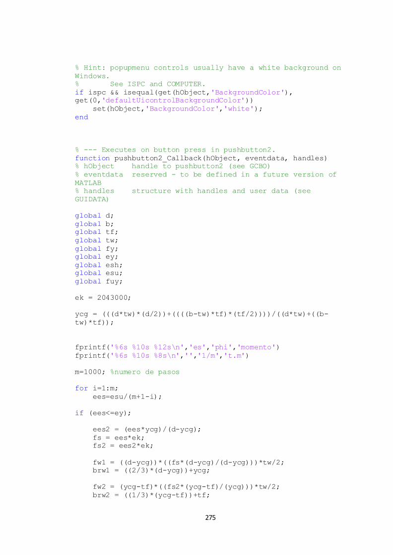
275
% Hint: popupmenu controls usually have a white background on
Windows.
% See ISPC and COMPUTER.
if ispc && isequal(get(hObject,'BackgroundColor'),
get(0,'defaultUicontrolBackgroundColor'))
set(hObject,'BackgroundColor','white');
end
% --- Executes on button press in pushbutton2.
function pushbutton2_Callback(hObject, eventdata, handles)
% hObject handle to pushbutton2 (see GCBO)
% eventdata reserved - to be defined in a future version of
MATLAB
% handles structure with handles and user data (see
GUIDATA)
global d;
global b;
global tf;
global tw;
global fy;
global ey;
global esh;
global esu;
global fuy;
ek = 2043000;
ycg = (((d*tw)*(d/2))+((((b-tw)*tf)*(tf/2))))/((d*tw)+((b-
tw)*tf));
fprintf('%6s %10s %12s\n','es','phi','momento')
fprintf('%6s %10s %8s\n','','1/m','t.m')
m=1000; %numero de pasos
for i=1:m;
ees=esu/(m+1-i);
if (ees<=ey);
ees2 = (ees*ycg)/(d-ycg);
fs = ees*ek;
fs2 = ees2*ek;
fw1 = ((d-ycg))*((fs*(d-ycg)/(d-ycg)))*tw/2;
brw1 = ((2/3)*(d-ycg))+ycg;
fw2 = (ycg-tf)*((fs2*(ycg-tf)/(ycg)))*tw/2;
brw2 = ((1/3)*(ycg-tf))+tf;
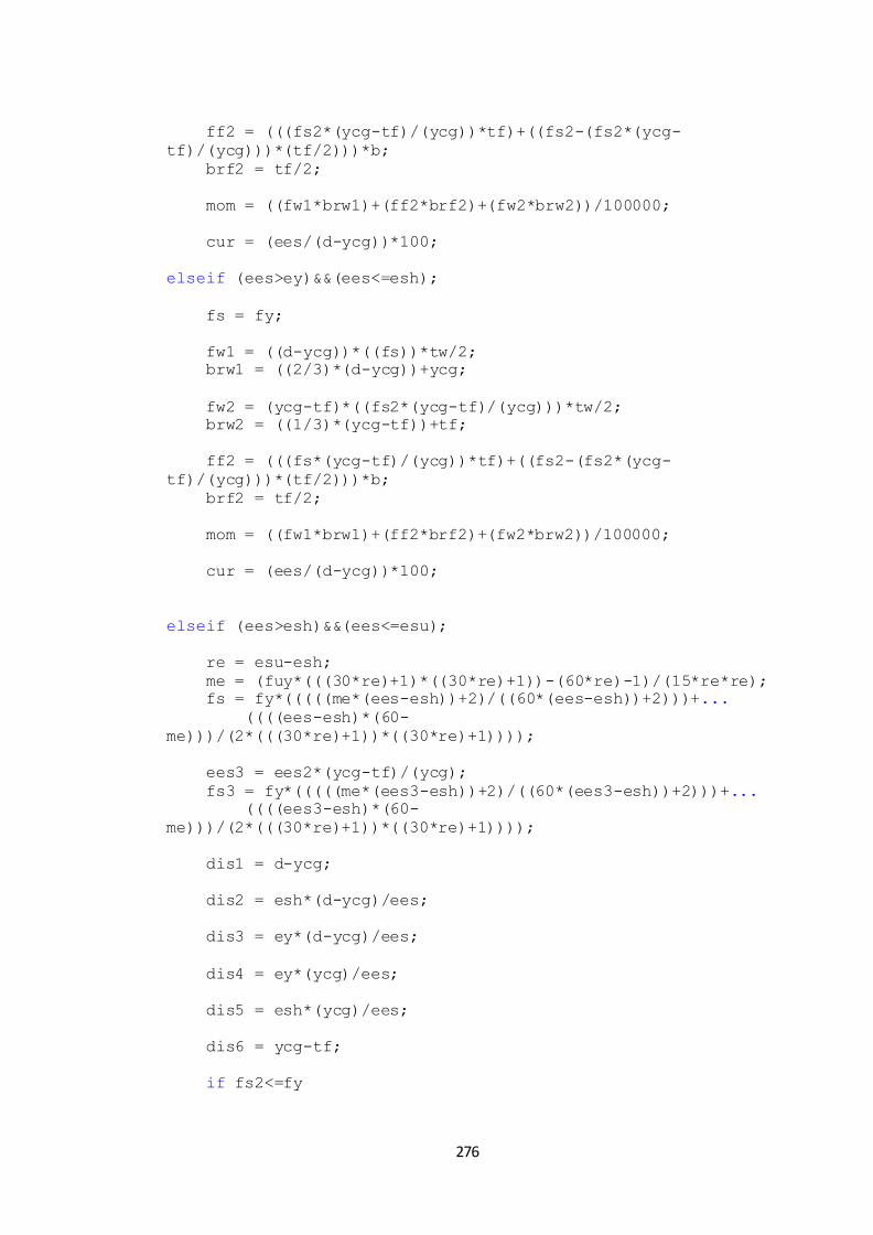
276
ff2 = (((fs2*(ycg-tf)/(ycg))*tf)+((fs2-(fs2*(ycg-
tf)/(ycg)))*(tf/2)))*b;
brf2 = tf/2;
mom = ((fw1*brw1)+(ff2*brf2)+(fw2*brw2))/100000;
cur = (ees/(d-ycg))*100;
elseif (ees>ey)&&(ees<=esh);
fs = fy;
fw1 = ((d-ycg))*((fs))*tw/2;
brw1 = ((2/3)*(d-ycg))+ycg;
fw2 = (ycg-tf)*((fs2*(ycg-tf)/(ycg)))*tw/2;
brw2 = ((1/3)*(ycg-tf))+tf;
ff2 = (((fs*(ycg-tf)/(ycg))*tf)+((fs2-(fs2*(ycg-
tf)/(ycg)))*(tf/2)))*b;
brf2 = tf/2;
mom = ((fw1*brw1)+(ff2*brf2)+(fw2*brw2))/100000;
cur = (ees/(d-ycg))*100;
elseif (ees>esh)&&(ees<=esu);
re = esu-esh;
me = (fuy*(((30*re)+1)*((30*re)+1))-(60*re)-1)/(15*re*re);
fs = fy*(((((me*(ees-esh))+2)/((60*(ees-esh))+2)))+...
((((ees-esh)*(60-
me)))/(2*(((30*re)+1))*((30*re)+1))));
ees3 = ees2*(ycg-tf)/(ycg);
fs3 = fy*(((((me*(ees3-esh))+2)/((60*(ees3-esh))+2)))+...
((((ees3-esh)*(60-
me)))/(2*(((30*re)+1))*((30*re)+1))));
dis1 = d-ycg;
dis2 = esh*(d-ycg)/ees;
dis3 = ey*(d-ycg)/ees;
dis4 = ey*(ycg)/ees;
dis5 = esh*(ycg)/ees;
dis6 = ycg-tf;
if fs2<=fy
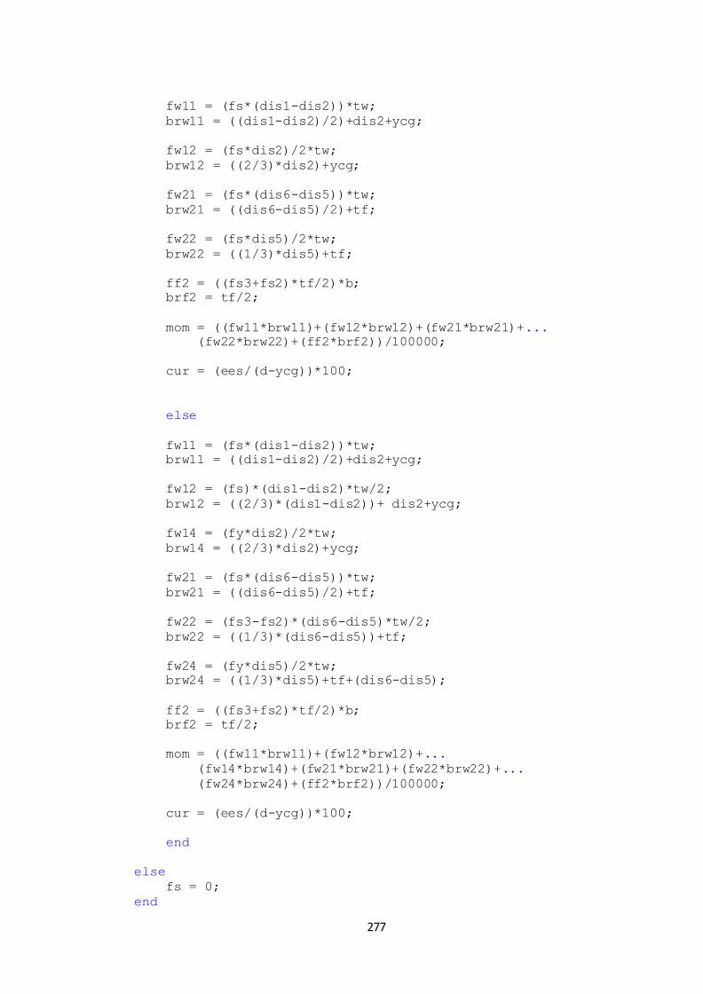
277
fw11 = (fs*(dis1-dis2))*tw;
brw11 = ((dis1-dis2)/2)+dis2+ycg;
fw12 = (fs*dis2)/2*tw;
brw12 = ((2/3)*dis2)+ycg;
fw21 = (fs*(dis6-dis5))*tw;
brw21 = ((dis6-dis5)/2)+tf;
fw22 = (fs*dis5)/2*tw;
brw22 = ((1/3)*dis5)+tf;
ff2 = ((fs3+fs2)*tf/2)*b;
brf2 = tf/2;
mom = ((fw11*brw11)+(fw12*brw12)+(fw21*brw21)+...
(fw22*brw22)+(ff2*brf2))/100000;
cur = (ees/(d-ycg))*100;
else
fw11 = (fs*(dis1-dis2))*tw;
brw11 = ((dis1-dis2)/2)+dis2+ycg;
fw12 = (fs)*(dis1-dis2)*tw/2;
brw12 = ((2/3)*(dis1-dis2))+ dis2+ycg;
fw14 = (fy*dis2)/2*tw;
brw14 = ((2/3)*dis2)+ycg;
fw21 = (fs*(dis6-dis5))*tw;
brw21 = ((dis6-dis5)/2)+tf;
fw22 = (fs3-fs2)*(dis6-dis5)*tw/2;
brw22 = ((1/3)*(dis6-dis5))+tf;
fw24 = (fy*dis5)/2*tw;
brw24 = ((1/3)*dis5)+tf+(dis6-dis5);
ff2 = ((fs3+fs2)*tf/2)*b;
brf2 = tf/2;
mom = ((fw11*brw11)+(fw12*brw12)+...
(fw14*brw14)+(fw21*brw21)+(fw22*brw22)+...
(fw24*brw24)+(ff2*brf2))/100000;
cur = (ees/(d-ycg))*100;
end
else
fs = 0;
end

278
phi(i)=cur;
MOM(i)=mom;
matriz=[ees,phi(i),MOM(i)];
disp(matriz)
end
figure (1)
title ('DIAGRAMA MOMENTO - CURVATURA')
plot(phi,MOM)
xlabel('CURVATURA (1/m)')
ylabel('MOMENTO T-m')
grid on
hold on