Universidad de Granada - decsai.ugr.es · doctores m as j ovenes del grupo, Nacho, Manolo Cobo, Jos...
184
Universidad de Granada Departamento de Ciencias de la Computaci´ on e Inteligencia Artificial Programa de Doctorado en Ciencias de la Computaci´ on y Tecnolog´ ıaInform´atica Sistemas de Clasificaci´ on Basados en Reglas Difusas para Problemas no Balanceados. Aproximaciones y Uso de Nuevas Estrategias para Resolver Problemas Intr´ ınsecos a los Datos no Balanceados Tesis Doctoral Victoria L´opez Morales Granada, marzo de 2014
Transcript of Universidad de Granada - decsai.ugr.es · doctores m as j ovenes del grupo, Nacho, Manolo Cobo, Jos...

Universidad de Granada
Departamento de Ciencias de la Computacione Inteligencia Artificial
Programa de Doctorado en Ciencias de la Computaciony Tecnologıa Informatica
Sistemas de Clasificacion Basados en Reglas Difusas
para Problemas no Balanceados. Aproximaciones y
Uso de Nuevas Estrategias para Resolver Problemas
Intrınsecos a los Datos no Balanceados
Tesis Doctoral
Victoria Lopez Morales
Granada, marzo de 2014


Universidad de Granada
Sistemas de Clasificacion Basados en Reglas Difusas
para Problemas no Balanceados. Aproximaciones y
Uso de Nuevas Estrategias para Resolver Problemas
Intrınsecos a los Datos no Balanceados
MEMORIA QUE PRESENTA
Victoria Lopez Morales
PARA OPTAR AL GRADO DE DOCTOR EN INFORMATICA
Marzo de 2014
DIRECTORES
Francisco Herrera Triguero y Alberto Fernandez Hilario
Departamento de Ciencias de la Computacione Inteligencia Artificial


La memoria titulada “Sistemas de Clasificacion Basados en Reglas Difusas para Problemasno Balanceados. Aproximaciones y Uso de Nuevas Estrategias para Resolver Problemas Intrınsecosa los Datos no Balanceados”, que presenta Da. Victoria Lopez Morales para optar al grado de doctor,ha sido realizada dentro del Programa Oficial de Doctorado en “Ciencias de la Computacion yTecnologıa Informatica”, en el Departamento de Ciencias de la Computacion e Inteligencia Artificialde la Universidad de Granada bajo la direccion de los doctores D. Francisco Herrera Triguero y D.Alberto Fernandez Hilario.
El doctorando y los directores de la tesis garantizamos, al firmar esta tesis doctoral, que eltrabajo ha sido realizado por el doctorando bajo la direccion de los directores de la tesis, y hastadonde nuestro conocimiento alcanza, en la realizacion del trabajo se han respetado los derechos deotros autores a ser citados cuando se han utilizado sus resultados o publicaciones.
Granada, marzo de 2014
El Doctorando Los directores
Fdo: Victoria Lopez Morales Fdo: Francisco Herrera Triguero Fdo: Alberto Fernandez Hilario

Esta tesis doctoral ha sido parcialmente subvencionada por el Ministerio de Ciencia e Innovacionbajo el Proyectos Nacional TIN2011-28488. Tambien ha sido subvencionada bajo el programa debecas de Formacion de Profesorado Universitario del Ministerio de Educacion, en su Resolucion del11 de Octubre de 2010, bajo la referencia AP2009-4889.

Agradecimientos
Como la gratitud en silencio no sirve a nadie, quisiera aprovechar la oportunidad que me brindanestas lıneas para acordarme de las personas que han ido poniendo su granito de arena para ayudarmea superar el reto que supone completar el desarrollo de una tesis doctoral.
En primer lugar, quisiera agradecer a mis directores de tesis Francisco Herrera y AlbertoFernandez todo el tiempo y esfuerzo que han dedicado para introducirme en el mundo de la inves-tigacion. Sin su apoyo decidido, esta tesis no hubiera llegado a ser lo que hoy es. Su guıa y consejohan demostrado ser un aliado valioso para ir avanzando en este recorrido.
Asimismo quisiera acordarme de todos aquellos que me han acompanado en el dıa a dıa de lainvestigacion: de aquellos junto a los que comence la tesis, Isaac, Jose Antonio, Alvaro, y de aquellosque nos ayudan de alguna manera con ella, Salva y Julian. Tambien agradezco la companıa de losdoctores mas jovenes del grupo, Nacho, Manolo Cobo, Jose Garcıa, Christoph, Fran y Michela ode los jovenes doctores “de fuera”, Mikel en Pamplona y Cristobal en Jaen. Tambien se agradecelos consejos de la experiencia de Jesus y Rafa Alcala, Jose Manuel Benıtez o Chris Cornelis.
No puedo olvidarme de los doctorandos mas noveles a los que les queda todavıa un poquitomas de camino por andar: Dani, Sara, Pablo, Sergio, Juanan, Raquel, Rosa y Lala, siempre consu optimismo y alegrıa. Finalmente, tambien incluir en este grupo a los ex-residentes de Orquıdeascon los que comparto muchas mananas un fuzzy coffee, Olmo, Rafa, Edu, Alberto e Irene.
I would also like to express my gratitude in these lines to Vasile Palade, the supervisor for myresearch visit at University of Oxford. Our talks about imbalanced datasets have been very valuable tounderstand some features of the problem and to redirect my focus from uncertain objectives towardsmore sensible paths.
En el plano personal, quisiera acordarme de mis padres Jose y MaVictoria porque gracias a suapoyo y consejos, he podido dıa a dıa, cruzar el camino de la superacion y abordar este desafıo.Vuestra confianza y paciencia, los momentos de nervios y de tension que habeis compartido conmigome han servido de empuje para seguir adelante. Debo mencionar asimismo a mi tıa Encarnacionque tambien me ha acompanado en este camino de aprendizaje y evolucion.
No menos importante ha sido el aliento de mis hermanos, Manuel e Isabel. Sabiendo que jamasencontrare la forma de agradecer su constante apoyo y confianza, solo espero que comprendan quesu presencia en todo momento ha sido uno de los mejores alicientes en seguir avanzando hacia lameta.
Finalmente, dicen que los ultimos seran los primeros, quiero darle las gracias a Joaquın por suinfinita paciencia, carino y comprension. Su mente inquieta me ha permitido ver un camino de luzcuando parecıa que infinitos obstaculos me cerraban el camino. ¡Gracias por ser como eres y estara mi lado!

Table of Contents
Page
I. PhD dissertation 1
1. Introduction . . . . . . . . . . . . . . . . . . . . . . . . . . . . . . . . . . . . . . . . . 1
Introduccion . . . . . . . . . . . . . . . . . . . . . . . . . . . . . . . . . . . . . . . . . . . 3
2. Preliminaries . . . . . . . . . . . . . . . . . . . . . . . . . . . . . . . . . . . . . . . . 5
2.1. Classification problems with imbalanced classes . . . . . . . . . . . . . . . . . 7
2.2. Data Mining and Big Data . . . . . . . . . . . . . . . . . . . . . . . . . . . . 9
2.3. Fuzzy Rule Based Classification Systems . . . . . . . . . . . . . . . . . . . . . 12
3. Justification . . . . . . . . . . . . . . . . . . . . . . . . . . . . . . . . . . . . . . . . . 14
4. Objectives . . . . . . . . . . . . . . . . . . . . . . . . . . . . . . . . . . . . . . . . . . 15
5. Discussion of results . . . . . . . . . . . . . . . . . . . . . . . . . . . . . . . . . . . . 16
5.1. A Study on the Data Intrinsic Characteristics in Classification Problems withImbalanced Datasets and Analysis of the Behavior of the Techniques fromthe State-of-the-art . . . . . . . . . . . . . . . . . . . . . . . . . . . . . . . . . 16
5.2. Addressing the Data Intrinsic Characteristics of Imbalanced Problems usingFRBCSs and Machine Learning Techniques . . . . . . . . . . . . . . . . . . . 19
5.2.1. A Hierarchical Genetic Fuzzy System Based On Genetic Program-ming for Addressing Classification with Highly Imbalanced and Bor-derline Data-sets . . . . . . . . . . . . . . . . . . . . . . . . . . . . . 19
5.2.2. On the Importance of the Validation Technique for Classificationwith Imbalanced Datasets: Addressing Covariate Shift when Datais Skewed . . . . . . . . . . . . . . . . . . . . . . . . . . . . . . . . . 21
5.3. A study on the Scalability of FRBCSs for Imbalanced Datasets in the BigData Scenario . . . . . . . . . . . . . . . . . . . . . . . . . . . . . . . . . . . . 22
6. Concluding Remarks . . . . . . . . . . . . . . . . . . . . . . . . . . . . . . . . . . . . 24
Conclusiones . . . . . . . . . . . . . . . . . . . . . . . . . . . . . . . . . . . . . . . . . . . 26
7. Future Work . . . . . . . . . . . . . . . . . . . . . . . . . . . . . . . . . . . . . . . . 29
II. Publications: Published and Accepted Papers 31
vii

viii TABLE OF CONTENTS
1. A Study on the Data Intrinsic Characteristics in Classification Problems with Imba-lanced Datasets and Analysis of the Behavior of the Techniques from the State-of-the-art . . . . . . . . . . . . . . . . . . . . . . . . . . . . . . . . . . . . . . . . . . . . 31
1.1. Analysis of preprocessing vs. cost-sensitive learning for imbalanced classifi-cation. Open problems on intrinsic data characteristics . . . . . . . . . . . . . 31
1.2. An Insight into Classification with Imbalanced Data: Empirical Results andCurrent Trends on Using Data Intrinsic Characteristics . . . . . . . . . . . . 59
2. Addressing the Data Intrinsic Characteristics of Imbalanced Problems using FRBCSsand Machine Learning Techniques . . . . . . . . . . . . . . . . . . . . . . . . . . . . 91
2.1. A Hierarchical Genetic Fuzzy System Based On Genetic Programming forAddressing Classification with Highly Imbalanced and Borderline Data-sets . 91
2.2. On the Importance of the Validation Technique for Classification with Imba-lanced Datasets: Addressing Covariate Shift when Data is Skewed . . . . . . 115
3. A study on the Scalability of FRBCSs for Imbalanced Datasets in the Big DataScenario . . . . . . . . . . . . . . . . . . . . . . . . . . . . . . . . . . . . . . . . . . . 131
3.1. Cost-Sensitive Linguistic Fuzzy Rule-Based Classification Systems under theMapReduce Framework for Imbalanced Big Data . . . . . . . . . . . . . . . . 131
Bibliography 169
Part I. PhD dissertation
1. Introduction
Classification and prediction tasks are taking place constantly in our daily life. We can findseveral examples carried out by experts in very different fields, such as medical diagnosis, patternrecognition, product rating and so on. From a general point of view, the concept of classificationcovers every context where a decision is made based on the available information. However, thefulfillment of this task may entail many problems such as some inefficiency in the process, or thedifficult of the context in which the problem is been set up. Thereby, the development of automaticsystems makes easier the work as they enable the obtaining of more accurate predictions. Thesesystems are interesting because the data analysis performed by them does not have the subjectivityattached to human beings and because the capacity of analysis of an automatic method (in termsof data volume) is always bigger than a person capacity.
The classification problem is defined on the context of data mining (DM) and it can be catego-rized as a supervised learning task [TSK06]. This concept can be defined as the set of examples wehave available are labeled with the class they belong to. From here on, we have to learn and builda model or decision function that is able to return the class belonging to a new example based onits attribute values. This system is known as a classifier.
When trying to solve a given stage of the classification application, experts and researchersmust know the data structure that they are processing. In accordance with the former, they canachieve the maximum accuracy related to all the concepts included in the problem. For example,there are many work areas where the class distribution is not balanced. Since most of the standardlearning approximations consider a balanced training set, this leads to the obtaining of a suboptimalclassification model, namely a good cover on the examples that belong to the majority class (alsoknown as negative class), whereas the minority examples (known as positive class) are more difficultto be properly identified. This problem is known as classification with imbalanced data [HG09,SWK09].
We must emphasize the importance of this problem, as it is related to real-world domains. Inthese cases, a high cost is involved when examples of the positive class are classified in a wrong wayas the examples that belong to the positive class are the most interesting from the learning pointof view. Some of these real-world applications are medical diagnosis and fraud detection, amongothers. These problems typically present a small number of examples from the positive class asexamples from this class are usually associated with exceptional or significant cases, or because theacquisition of instances is costly.
1

2 Part I. PhD dissertation
In the area of classification in general, and in classification with imbalanced datasets in parti-cular, Computational Intelligence techniques (CI) [Kon05, Pet07] have shown to be a very robusttool to obtain models with a high degree of confidence. Although there is no complete agreementwith respect to a definition on CI, there is a widely accepted vision about areas included under thisparadigm, such as Artificial Neural Networks, Fuzzy Logic and Evolutionary Computation. Amongthe available techniques in this field, linguistic fuzzy rule-based classification systems (FRBCS)[INN04] are a popular tool because of the interpretability of their models based on linguistic va-riables, which are easier to understand to final users or experts while obtaining good results in thearea of imbalanced classification [FGdJH08, FdJH09, FdJH10].
Returning to the specific problem of classification with imbalanced datasets, we must note thatsince the initial studies it has been shown that the loss of efficiency is due to non-uniform distributionon classes. However, recent research suggests that the problem in this scenario is the synergybetween the imbalance and some intrinsic characteristics of data. Among these characteristics wecan find the overlapping between classes [GMS08, DT10], the presence of small-disjuncts [Wei05,Wei10], the treatment of the borderline samples [DKS09, NSW10], the problem of noisy instances[BF99, SKVHF14], and finally, the different distribution on partitions of training and test data,which is known as dataset shift [Shi00, MTH10].
However, the difficulties in the obtaining of good performance models in classification problemsand DM are not only related with the uneven class distribution. A new concept called Big Data hasspread quickly in this framework [ADA11, Mad12]. This new scenario is defined by those problemsthat cannot be addressed effectively and/or efficient through the standard computational resourcescurrently available. This situation does not necessarily imply large volumes of information, but justsimply that the existing methods that are used to address the problem are not able to provide aclassification answer within our requirements.
Our interest in this memory mainly lies in the study of the problem of classification withimbalanced datasets from the perspective of the data intrinsic characteristics that this type ofproblems display. We intend to perform a detailed analysis of the existing solutions to the problemto fully understand their behavior and discern which are more appropriate from a general pointof view. With the information provided by this study, we intend to develop new learning methodswith FRBCSs that will address the data intrinsic characteristics that degrade the performanceof classifiers with imbalanced data. Hence, we aim at improving the behavior of the standardmethodology defined to this area of DM. At last, our intention is to extend the study of classificationwith imbalanced data to the big data field. In particular, our goal is to analyze the scalability ofthe basic solutions of FRBCSs raised on, and propose new parallelization techniques to addressthis problem effectively.
To perform this study, this PhD dissertation is divided into two parts. The first one is devotedto the statement of the problem considered and the discussion of obtained results; whereas thesecond part corresponds to the publications associated with the study.
In Part I of this document we begin with a section devoted to the preliminaries related to theproblem (Section 2), introducing the information about related approaches and other problems.Next, we define the open problems in this framework (Section 3) that justify the development ofthis thesis as well as the proposed objectives (Section 4). Then, we present Section 5, discussionof results, which provides a summary of the developed studies and the most important resultsobtained for the objectives considered in this manuscript. Later, Section 6 summarizes the resultsobtained herein and presents some conclusions about them to, finally (Section 7), discuss someaspects of future work that are open in the present memory.

1 Introduction 3
Finally, to develop the objectives, Part II of the memory is constituted of five publicationsdistributed in three parts:
A Study on the Data Intrinsic Characteristics in Classification Problems with ImbalancedDatasets and Analysis of the Behavior of the Techniques from the State-of-the-art.
Addressing the Data Intrinsic Characteristics of Imbalanced Problems using FRBCSs andMachine Learning Techniques.
A study on the Scalability of FRBCSs for Imbalanced Datasets in the Big Data Scenario.
Introduccion
Las tareas de clasificacion y prediccion estan continuamente presentes en la vida cotidiana. Po-demos encontrar diversos ejemplos realizados por expertos en diferentes ambitos, como por ejemploen diagnostico medico, reconocimiento de patrones, calificacion de productos, y un largo etcetera.Desde un punto de vista general, el concepto de clasificacion cubre cualquier contexto en el que setoma una decision en base a la informacion disponible. Sin embargo, la realizacion de esta tareapuede conllevar distintos problemas como la lentitud al llevarla a cabo o la dificultad del contexto.De este modo, el desarrollo de sistemas automaticos no solo puede ayudar a facilitar esta labor, sinoque ademas puede permitir efectuar mejor las predicciones. Esto es debido a que el analisis de losdatos carece de la subjetividad inherente a los seres humanos y porque la capacidad de analisis deun metodo automatico siempre sera mucho mayor (el volumen de datos con los que puede trabajares mas amplio) que la capacidad de una persona
El problema de clasificacion se enmarca dentro del contexto de la Minerıa de Datos (MDD) ensu vertiente supervisada [TSK06]. Con ello nos referimos a que el conjunto de ejemplos de los quedisponemos para realizar el aprendizaje estan etiquetados con la clase a la que pertenecen. A partirde este punto debemos aprender y construir un modelo o funcion de decision capaz de devolver laclase correspondiente a un nuevo ejemplo en base a los atributos que lo caracterizan. Este sistemase denomina un clasificador.
Cuando se pretende resolver una aplicacion dada en el escenario de la clasificacion, los expertose investigadores deben conocer la estructura de los datos que gestionan para de este modo alcanzarla maxima precision para todos los conceptos incluidos en el problema [DHS01]. Por ejemplo, haymuchas areas de trabajo en los que la distribucion de las clases no es equilibrada. Puesto que lamayorıa de las aproximaciones de aprendizaje estandar consideran un conjunto de entrenamientoequilibrado (o balanceado), esto conlleva la obtencion de un modelo de clasificacion sub-optimo, esdecir, un modelo con una buena cobertura de los ejemplos mayoritarios (tambien conocida comoclase negativa), mientras que los minoritarios (conocidos como clase positiva) son mas difıciles dediscriminar. Este hecho se conoce como la clasificacion con conjuntos de datos no balanceados[HG09, SWK09].
Debemos enfatizar la importancia de este problema, ya que esta relacionado con problemasen dominios del mundo real que implican un alto coste cuando los ejemplos de la clase positivase clasifican de manera erronea. Algunos de estos escenarios son diagnosis medica, sistemas dedeteccion de intrusiones y deteccion de fraudes, entre otros. Los ejemplos de la clase positiva suelen

4 Part I. PhD dissertation
ser poco numerosos en estos problems ya que suelen estar asociados con casos excepcionales osignificativos, o porque la adquisicion de estas instancias es costosa.
En el area de clasificacion en general, y de clasificacion con datos no balanceados en particular,las tecnicas de Inteligencia Computacional (IC) [Kon05, Pet07] han mostrado ser una herramientamuy robusta para la obtencion de modelos con un alto grado de acierto. Aunque no existe un acuerdototal con respecto a una definicion de IC, hay una vision ampliamente aceptada sobre las areasque se enmarcan en este paradigma, como son las Redes Neuronales Artificiales, Logica Difusa, yComputacion Evolutiva. Entre las tecnicas disponibles en este campo, los Sistemas de ClasificacionBasados en Reglas Difusas (SCRBDs) Linguısticas [INN04] son una herramienta popular debido ala interpretabilidad de sus modelos asociados basados en variables linguısticas, que son mas facilesde comprender para los usuarios finales o expertos, ademas de obtener muy buenos resultados enel campo de accion de la clasificacion no balanceada [FGdJH08, FdJH09, FdJH10].
Retomando el problema especıfico de la clasificacion con conjuntos no balanceados, debemosdestacar que desde los estudios iniciales se ha mostrado que la perdida de rendimiento se debea la distribucion no uniforme de las clases. Sin embargo, recientes investigaciones sugieren que elproblema en este escenario es la sinergia entre el desbalanceo y algunas caracterısticas intrınsecas delos datos. Entre estas caracterısticas podemos encontrar el solapamiento entre las clases [GMS08,DT10], la presencia de pequenos datos disjuntos (en ingles small disjuncts) [Wei05, Wei10], eltratamiento de los ejemplos frontera o borderline [DKS09, NSW10], el problema de las instanciascon ruido [BF99, SKVHF14], y finalmente la distinta distribucion en las particiones de datos deentrenamiento y test, conocido como dataset shift [Shi00, MTH10].
Pero la problematica en la resolucion de los problemas de clasificacion y MDD no solo se encuadraen el hecho de los conjuntos de datos no balanceados. Un nuevo concepto denominado Big Data seha extendido rapidamente en este marco de trabajo [ADA11, Mad12]. Este nuevo escenario se definepor medio de aquellos problemas que no pueden ser abordados de manera efectiva y/o eficiente atraves de los recursos computacionales estandar de que disponemos actualmente. Debemos remarcarque big data no implica necesariamente amplios volumenes de informacion, sino basicamente quelos metodos existentes no son capaces de proporcionar una respuesta adecuada en estas situaciones.
Nuestro interes en esta memoria reside principalmente en el estudio de los problemas de clasifi-cacion con conjuntos de datos no balanceados bajo la perspectiva de las caracterısticas internas quepresentan este tipo de problemas. Pretendemos realizar un analisis pormenorizado de las solucionesexistentes para conocer su comportamiento y discernir cuales son las mas apropiadas desde unpunto de vista general, con el objetivo de desarrollar nuevos metodos de aprendizaje con SCBRDsque permitan abordar las caracterısticas intrınsecas de los datos, y por tanto mejorar el compor-tamiento de las metodologıas estandar definidas para este area de la MDD. Por ultimo, nuestraintencion es la de extender el estudio de la clasificacion con datos no balanceados al campo de bigdata. En particular, nuestro objetivo sera analizar la escalabilidad de las soluciones basicas plan-teadas sobre SCBRDs, y proponer nuevas tecnicas de paralelizacion para abordar este problema demanera efectiva.
Para llevar a cabo este estudio, la presente memoria se divide en dos partes, la primera de ellasdedicada al planteamiento del problema y discusion de los resultados y la segunda correspondientea las publicaciones asociadas al estudio.
En la Parte I de la memoria comenzamos con una seccion dedicada al “Planteamiento del Proble-ma” (Seccion 2), introduciendo este con detalle y describiendo las tecnicas utilizadas para resolverlo.Asimismo, definimos los problemas abiertos en este marco de trabajo que justifican la realizacion deesta memoria (Seccion 3) ası como los objetivos propuestos (Seccion 4). Posteriormente, incluimos

2 Preliminaries 5
una seccion de “Discusion de Resultados”, Seccion 5, que proporciona una informacion resumidade las propuestas y los resultados mas interesantes obtenidos en las distintas partes en las quese divide el estudio. La seccion de “Conclusiones” (Seccion 6) resume los resultados obtenidos enesta memoria y presenta algunas conclusiones sobre estos. Finalmente, se comentan en la Seccion7 algunos aspectos sobre trabajos futuros que quedan abiertos en la presente memoria.
Por ultimo, para desarrollar los objetivos planteados, la Parte II de la memoria esta constituidapor cinco publicaciones distribuidas en tres partes:
Estudio de las Caracterısticas Intrınsecas de los Datos en Problemas de Clasificacion conConjuntos de Datos No Balanceados y Analisis del Comportamiento de las Tecnicas delEstado del Arte.
Desarrollo de Aproximaciones para Resolver las Caracterısticas Intrınsecas de los ProblemasNo Balanceados mediante SCBRDs y Tecnicas de Aprendizaje Automatico.
Estudio de la Escalabilidad de los SCBRDs para Conjuntos de Datos No Balanceados en unEscenario de Big Data.
2. Preliminaries
The development of information technologies has enabled an extensive data gathering in thelast years in different knowledge and business areas. The recognition of patterns in data, whichis common in humans, is automated using what is known as Knowledge Discovery in Databases(KDD). KDD was defined in 1996 [FPSS96] as “the nontrivial process of identifying valid, novel,potentially useful and ultimately understandable patterns in data”. Currently, it enforces two mainroles: it has become fundamental in scientific research due to its analysis and knowledge discoverycapabilities from available data; and it gradually expands with success its knowledge from tradi-tional applications like marketing or finances, to other domains like industry, energy, medicine,bioinformatics or web analytics among others. In all of them, the amount of information and theneed to retrieve useful knowledge with a direct benefit, are increased at the same pace.
KDD is composed by a set of interactive and iterative steps such as data preprocessing, a searchfor interesting patterns with a concrete representation and the interpretation for these patterns(Figure 1). Although KDD is the appropriate name for this procedure, the term Data Mining (DM)[TSK06] is frequently used to refer to the complete process. This term represents the knowledgeextraction from computed data [Pyl99] being actually the main task of the whole system. Dependingon the objective, in DM it is possible to distinguish between predictive and descriptive tasks. For thefirst ones, the objective is finding a model which allows the prediction of future behavior, usuallyby means of supervised learning. Within this group of DM tasks, classification, regression andprediction of temporal series can be found. Regarding descriptive DM, the process tries to builda model that describes information about the underlying data problem employing unsupervisedlearning, and includes association rules extraction, clustering and summarization techniques amongothers tasks for DM.
An area with strong similarities with DM, is Machine Learning (ML) [Alp04]. Machine learningis a branch of artificial intelligence that concerns design and development of algorithms that are

6 Part I. PhD dissertation
Figure 1: The KDD process
capable of learning patterns or concepts based in empirical data analysis, like sensor data o data-bases (which is the closest case for ML). In short, it is a tool that extracts knowledge from a set ofexamples that represent the problem that we need to undertake.
In this memory, we will focus on the context of supervised learning and more specifically, inclassification. In this scenario, classification refers to the process -with the previous knowledge ofcertain classes or categories- where we establish a function or rule to pinpoint new predictions insome of the existing classes (supervised learning). A classifier receives as input a set of examples,labeled as training set, which learn the classification rule. Besides, the validation process of aclassifier uses a set of examples which are not known during the learning process, named as testset, and which are used to check the accuracy of the classifier. The classes are from a predictionproblem, where each class corresponds to the possible output of a function to predict from attributesthat describe the elements of a dataset.
When working with real applications in classification, we can see that they frequently present avery different distribution of examples inside their classes. This situation is known as the problemof imbalanced classes [CJK04, HG09, SWK09] and is considered as one of the challenges in DM[YW06]. Specifically, in the context of binary problems, a class is usually represented by very fewexamples, while the other is described by many instances. The minority class is usually the mainobjective from the learning point of view and, for this reason, the cost related to a poor classificationof one example of this class is greater than on the majority class.
An additional factor that affects the development of potential programs for the induction ofknowledge is the massive generation of data in which we currently find ourselves immersed. Thisscenario has occurred for three main reasons [Kra13]:
1. Hundreds of applications like mobile sensors, multi-media social services, and other devicesthat are gathering information continuously.

2 Preliminaries 7
2. The storage capacity has increased so much that data are cheaper than ever, making attractiveto the customer to buy more space than to choose what to delete.
3. ML methods and information retrieval have achieved a significant improvement in the lastyears, allowing the acquisition of a higher level of knowledge from the data.
Specifically, Terabytes of data are written every day resulting in a large Volume; real-timerequirements clearly imply a high Velocity, we can find a great Variety of either structured,semi-structured or even unstructured data; and data must be cleaned prior to integration on thesystem to maintain the Veracity [GGM12]. Those properties of 4V defines what is known as theproblem of Big Data [ADA11, Mad12], having achieved the status of hot topic between academicand industry areas.
In addition to the importance of scalability in construction of models, is the construction of asymbolic structure in order to be useful, not only from a functional point of view, but also from theperspective of interpretability, i.e:, to seek models understandable to humans. A concept relatedto the interpretability of models is CI [Kon05] (also known as Soft Computing). This conceptencompasses those models or techniques that try to seek inexact solutions to computer problemsthat are too complex so we cannot obtain an exact solution in a polynomial time. Logically, giventhe amount of data that we are working in DM, this idea includes most of the methodologies thatcan be applied. Among the most popular of them, we can identify evolutionary computation [Gol89],fuzzy logic [Zad65], neural networks [Gur97], case-based reasoning [AKA91] or any hybridizationon the above.
Within the context of CI, our framework for the development of the thesis is focused on the use oflinguistic FRBCS [INN04]. The main reason is due to the advantage associated with the obtainingof easy interpretable models, based on linguistic variables, which are simpler to understand to thefinal or expert user. Additionally, this type of systems have performed well when applied to theclassification with imbalanced datasets.
The following subsections detail each of these aspects that are directly related herein. In Section2.1, we introduce in detail the problem of classification with imbalanced datasets. Later, in Section2.2, we define the area of work concerning the concept big data. Finally, in Section 2.3, we describethe characteristics of linguistic FRBCS.
2.1. Classification problems with imbalanced classes
Within the real problems of ML in general, and classification in particular, researchers find thatthe example distribution in different classes or concepts that represent the dataset is not uniform.This problem is observable in many examples, such as fraud detection, risks management, textsclassification, medical diagnosis, and many other domains in which this characteristic is implicitlyattached to the problem, because fortunately, there are usually very few anomalous cases in com-parison with normal cases. Another situation which can lead to the appearance of this type of setsoccurs when the data acquisition process is limited (due to economical or private reasons). It isimportant to note that this type of datasets with imbalanced classes differ from standard datasetsnot only in the imbalance between classes, but also into the growing importance of the minorityclass, traditionally identified each as positive class.
Despite showing a fairly common occurrence and a strong impact on day life applications, theproblem of imbalanced classes has not been properly solved by ML algorithms, since they assumebalanced class distributions or equal classification costs for all classes.

8 Part I. PhD dissertation
In fact, most of the learning algorithms aim to obtain a model with a high accuracy on predictionand a good generalization ability. Nevertheless, those algorithms that perform well in the contextof standard classification not necessarily achieve the best performance for imbalanced datasets[FGL+10]. We note therefore that the bias on classification algorithms for examples of the majorityclass [SWK09, HG09] is the most direct consequence derived from the unequal distribution ofclasses. When the search process is guided by the standard accuracy measure, it benefits thecovering of the majority of the examples. Secondly, the classification rules predicting the positiveclass are often highly specialized so their coverage is very low, and therefore, they are discarded infavor of more general rules, for example, those that predict the negative class.
In practical applications, the rate of the minority over the majority class may be drastic whenwe have 1 example versus 10, 1 versus 100 or 1,000. In our work, we have considered the imbalanceratio or IR [OPBM09], defined as the fraction between the number of examples of the majorityclass and the minority class, to organize the different sets of data according to the value of IR.
Unfortunately, the problem of imbalanced classes usually appears in combination with differentdata intrinsic characteristics. This imposes additional constraints during the learning stage. First,we highlight the presence of areas with a high overlapping between classes, whose effect is muchmore negative as when we want to discriminate the examples of the positive class [GMS08, DT10].Additionally there may also be small groups of examples (small-disjuncts) of the minority class thatcan be treated mistakenly as noise, and therefore ignored by the classifier [OPBMG+09, Wei10].The existence of even a few noisy examples can degrade the identification of the minority class,because it has a lower number of examples [SKVHF14]. Finally, we should note the case of datasetshift, based on the different distribution of data partitions between training and test [MTH10].
In this manner, a high difficulty arises to achieve the final goal of developing a classifier thatobtains a high precision, on both the positive and negative classes of the problem. This is whythe area of imbalanced classification datasets has been widely studied through last years [HG09,SWK09]. A large number of solutions has been developed for this task, and can be categorized intothree groups:
Sampling data: in which training instances are modified to achieve a distribution of classclasses more balanced in order to enable the classifiers to work in a similar way as the standardclassification [BPM04].
Algorithmic modification: this procedure is oriented towards the adaptation of learningmodels, so we can tune them to the properly addressed the uneven class distribution[LTY13, ZHC13].
Cost-sensitive learning: such solutions incorporate approximations on the level of data, onalgorithmic level, or even on both levels together. Higher costs are considered due to badclassification of examples of the positive class compared to the negative class and, therefore,tries to minimize the level of associated cost to the overall problem [BP10, ZLA03].
In addition to the previous techniques, recently, ensembles of classifiers have appeared as apossible solution on the problem of class imbalance, awaking a great interest among researchers[KR14, LWZ09, SKVHN10, SKWW07, VHKN09, WY13]. The ensemble based methods are mo-dified or adapted by combination among the ensemble learning algorithm itself and any of thetechniques described above, to namely, either as data level or by algorithmic modifications basedon cost sensitive learning.

2 Preliminaries 9
In the case of adding a data level approach for learning algorithm ensemble, the new hybridmethod usually preprocesses the data before the formation of each classifier. In addition, in costsensitive ensembles type, instead of the modifying the base classifier towards the end of acceptingcosts in the learning process, what they do is guide the minimization of costs through ensemblelearning algorithm. Thus, we avoid the modification on the based learning method, but the maindrawback, which is the definition of costs, will be present.
2.2. Data Mining and Big Data
It is very challenging to present a correct definition of the term Big Data [Kra13]. This termwas coined very recently, when data intensive companies started to face large collections of data,at a petabyte scale. In fact, it is estimated that a 90 % of the data currently available has beencreated within the last two years [WZWD14]. The sources of this huge amount of information arevery sparse: Applications tracking clicks in websites, transaction records, sensors, social networks,scientific applications . . .
Initially, we might argue that the term big data is only related with the size of the data. But thetruth is that this Volume of data is not the only property inherent to the big data realm. BesidesVolume, it is very easy to realize that large collections of data will most likely show a high degreeof variability, heterogeneous structures, and a remarkable Variety regarding the way in whichinformation is represented. For example, different software implementations of data managementsystems will involve the use of different protocols and data schemes [SJ12]. Also, the data formathere plays a fundamental role when determining how it will be processed (as data managementsystems will not deal with images in the same way as they do with, for example, text files).
Velocity is another fundamental property of the topic at hand. Nowadays, users demand foran acceptable response time when working with data processing applications. Obviously, this factorwill be mostly affected by the computational resources available (as we cannot compare a personalcomputer with a data processing center of a large company in terms of processing power).
Finally, big data applications must also maintain the Veracity of information; that is, diminishthe effect of anomalies and noise within the data.
These factors are commonly known as the four V’s of big data, and form the basis of most of thecurrent definitions of the term, such as Gartner’s “Big data is high volume, high velocity, and/orhigh variety information assets that require new forms of processing to enable enhanced decisionmaking, insight discovery and process optimization”.
However, big data challenges are mainly motivated by two issues [LJ12]:
The storage and management of large volumes of data. This problem is closely related withtraditional entity-relation database management systems. Commercial solutions often offergood scalability, being able to manage petabytes-sized databases. However, besides their highcost - regarding both money and computational resources - they also are very restrictivewhen it comes to import data from its original representation. Open source systems, suchas MySQL, are less prone to show this problem, but they often show a much more limitedscalability.
The exploration and analysis of the data, aiming to discover useful knowledge for futureapplications [WZWD14]. Standard analytics are usually based upon entity-relation schemes,and developed through various SQL queries. However, besides the difficulties managing and

10 Part I. PhD dissertation
storing data, the problem here is the lack of statistical support to go beyond mere aggregationsof data. And even if database applications would be able to provide such support, they stillcould not provide it in an efficient way, considering the large amount of data that they mustmanage.
Distributed [RJBF+80] and parallel [DGS+90] databases could be used to address the firstissue, enabling existing systems to deal with a high workload of analytics-related tasks. However,they again face very serious problems when big data comes to the scene, as they require very highhardware requirements. Also, current applications need to manage unstructured or semi-structureddata, which becomes an additional challenge for this kind of systems.
An alternative has been proposed to the traditional databases, according to these facts: A newtechnology for data management, known as Not Only SQL (NoSQL) [HHLD11, CDG+08], whichbasically consists on storing the information as Key-Value keys, providing horizontally distributedscalability. It is important to remark that NoSQL databases provide with a flexible data model,supporting different data representations; thus, big data applications are quickly adopting NoSQLas their main option for storage.
A second point of view is focused on the programming models that are adopted to analyze thedata, most of which are commonly based on parallel computing [SAM96], such as, for example, theMessage Passing Interface (MPI) model [GLDS96]. The challenges here are to provide a proper wayto access to the data and to ease the development of specific software according to the requirementsand limitations of the common programming paradigms.
For example, standard DM algorithms require all data to be loaded in the physical memory. Thisis a challenging problem in big data, because most of the times data is stored throughout differentmachines/networks, and thus gathering it requires a large amount of network-based communicationand input/output operations. And even if this would be feasible, there is still the necessity ofproviding an extremely large amount of physical memory to store all the data needed to run thecomputing programs.
A new generation of systems has been developed in order to provide a proper way of tacklingthe aforementioned issues, with MapReduce [DG08] and Hadoop [The12, Lam11] - its open sourceimplementation - as its most representative members both in industry and academia.
This new paradigm avoids the above limitations regarding the necessities of loading the data,storing it in physical memory, or even the use of SQL. Instead, developers now can code their pro-grams using this new model, which enables them to parallelize the applications automatically. Thisis achieved by the definition of two simple functions - well-known in the functional programmingparadigm - denoted as Map and Reduce. Map can be used to group and split data, whereas Reduceaim is to perform the necessary computations to produce the final output of the program.
Both functions work by dividing the input dataset into independent subsets, which can beprocessed in parallel by Map tasks. Then, Hadoop sorts the outputs of the Map tasks and convertthem to inputs for the Reduce tasks. In more detail, it works as follows [WYLD10]:
Key/Value pairs are the processing primitives. The Map functions are applied to everyinput key/value pair, generating an arbitrary number of intermediate key/value pairs.
These intermediate values are provided to the Reduce function, by using an iterator able tomanage very large lists of pairs (often too large to be stored in the physical memory). TheReduce functions are then applied to all the values associated with the same intermediatekeys, generating an arbitrary number of output key/value pairs.

2 Preliminaries 11
As an optimizing step, MapReduce introduces the use of Combiners, which are able to workdirectly with the output of the Map functions. This allows to save a huge amount of networktraffic, since it does not require the intermediate step of sorting the keys before feeding theminto the Reduce tasks.
The final component of MapReduce is the Partitioner, which is in charge of splitting theintermediate keys and assigning the key/value pairs to the Reduce tasks. The default Par-titioner computes a hash value of the key, and computes the modulus of dividing it by thenumber of Reduce tasks, using it as an index to deliver approximately the same number ofkeys to each task.
We must highlight that, in the four points previously arisen, the last two functions are optionalduring the MapReduce process and its usage is limited to those jobs that need to be intenselyoptimized. In a general case, Hadoop-based programs (Figure 2) are managed by Map functioncalls, which are distributed throughout multiple machines by partitioning automatically the inputdata into M slots (so they can be processed in parallel by different machines); and Reduce functioncalls which are distributed by partitioning the key space into R chunks, with R specified by theuser.
Figure 2: Complete flowchart of an operation in MapReduce
In summary, Hadoop-based systems are oriented towards the distribution of datasets in a clus-ter (which does not necessarily has to be formed by high performance machines) to parallelizecomputations in the nodes. The rationale here is that mapping functions can be defined to createintermediate <key, value> tuples and reducing functions can be used to process the data spatially,avoiding the rather costly alternative of gathering the data in a core machine. In this way, a repre-sentative example could be to count the number of occurrences of every word in a large collectionof documents. Here, Hadoop will proceed to use mapping functions to broadcast every word withthe count of the times that it appear in every single document. Then, reducing functions will sumsthose values along each distinct word, obtaining as a result the final count.
12 Part I. PhD dissertation
2.3. Fuzzy Rule Based Classification Systems
Fuzzy systems are one of the most important areas where the fuzzy set theory is applied. In theclassification scenario, a model structure is used in the form of FRBCSs. FRBCSs constitute anextension of rule-based systems, since they use type rules like IF-THEN, whose antecedent (andin some cases consequent) are composed of fuzzy logic statements, instead of conditionals witha traditional format. Additionally, they have demonstrated their ability to so solve classificationproblems or DM in a large number of applications [Kun00, INN04].
The most common type of FRBCSs are linguistic FRBCSs or Mandani type [Mam74], whichthey have the following format:
Ri : IF Xi1 IS Ai1 AND · · · AND Xin IS Ain THEN Ck WITH PRik
where i = 1 to M , and being Xi1 to Xin input variables and Ck the output class associated tothe rule, being Ai1 to Ain antecedent labels, and PRik the weight of the rule [IY05] (usually thecertainty factor associated with the class).
All FRBCSs are composed of two basic components such as knowledge base (KB) and themodule with the inference system. The KB is formed by two components, a Data Base (BD) anda Rule Base (BR):
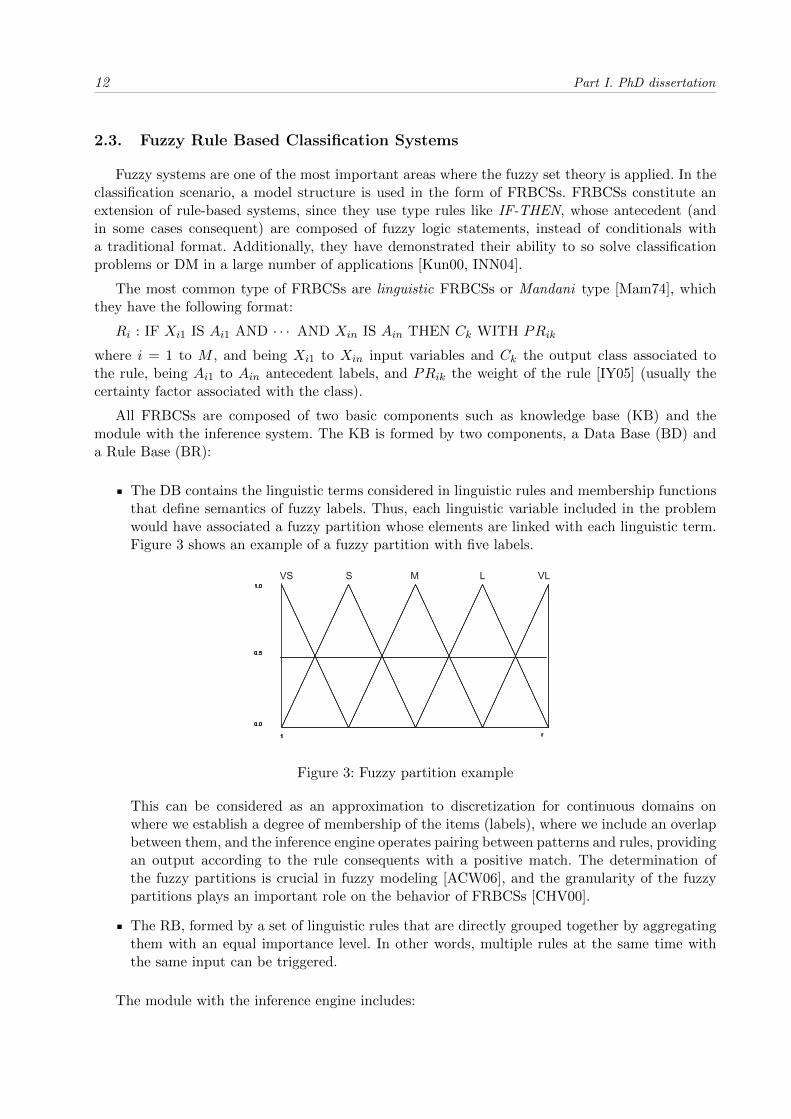
The DB contains the linguistic terms considered in linguistic rules and membership functionsthat define semantics of fuzzy labels. Thus, each linguistic variable included in the problemwould have associated a fuzzy partition whose elements are linked with each linguistic term.Figure 3 shows an example of a fuzzy partition with five labels.
V V
Figure 3: Fuzzy partition example
This can be considered as an approximation to discretization for continuous domains onwhere we establish a degree of membership of the items (labels), where we include an overlapbetween them, and the inference engine operates pairing between patterns and rules, providingan output according to the rule consequents with a positive match. The determination ofthe fuzzy partitions is crucial in fuzzy modeling [ACW06], and the granularity of the fuzzypartitions plays an important role on the behavior of FRBCSs [CHV00].
The RB, formed by a set of linguistic rules that are directly grouped together by aggregatingthem with an equal importance level. In other words, multiple rules at the same time withthe same input can be triggered.
The module with the inference engine includes:

2 Preliminaries 13
A fuzzification interface, which has the effect of transforming crisp data in fuzzy sets.
An inference system, which taking received data from the fuzzification interface, it uses theinformation contained on the KB to do an inference using a fuzzy reasoning method (FRM).
Specifically, if we consider a new pattern on Xp = (Xp1, . . . , Xpn) and a RB formed by Lfuzzy rules, the inference engine steps for classification are as follows [CdJH99]:
1. Matching Degree. It calculates the strength of activation of the IF part using for all therules in the RB with the Xp pattern, using a conjunction operator (usually a T-norm).
µAj (Xp) = T (µAj1(Xp1), . . . , µAjn(Xpn)), j = 1, . . . , L. (I.1)
2. Association degree. We calculate the association degree of the Xp pattern with the Mclasses according to each rule in RB. When considering rules with only a consequent(like the ones presented in this section) this association degree only refers to consequentclass of the rule (k = Cj).
bkj = h(µAj (Xp), RWkj ), k = 1, . . . ,M, j = 1, . . . , L. (I.2)
3. Degree of consistency of the classification pattern for all classes. We use an aggregationfunction that combines the positive degrees of association calculated on the previousstep.
Yk = f(bkj , j = 1, . . . , L y bkj > 0), k = 1, . . . ,M. (I.3)
4. Classification. We apply a decision function F about the consistency degree of the systemfor the pattern classification in all classes. This function will determine the l class labelcorresponding to the maximum value.
F (Y1, . . . , YM ) = l so that Yl = {max(Yk), k = 1, . . . ,M}. (I.4)
Finally, the generic structure of a FRBCS is shown on Figure 4.
VS S M L VL
Figure 4: FRBCS structure

14 Part I. PhD dissertation
3. Justification
After the presentation of all the main concepts related to the topic, we identified some openproblems that were interesting to be further analyzed:
In the scenario of classification with imbalanced datasets, there are some works that reviewthe associated issues to this problem [HG09, SWK09]. These contributions aggregate someof the solutions that have been given to the problem and they discuss some related aspectslike assessment metrics and the relationship between real-world problems and imbalance.However, these texts do not perform an experimental comparison among the diverse proposalsavailable in the state-of-the-art. Furthermore, the different type of solutions that are givento the problem are grouped by families which are categorized with respect to some specificcharacteristic that differentiates them. There is not a comparison that contrasts the behaviorof methods belonging to different families of methods which could be helpful to select anappropriate alternative among all the available approaches.
Furthermore, the existing studies on classification with imbalanced datasets are mainly fo-cused on dealing with the uneven class distribution and trying to find a balance betweengeneralization and proper identification of the underrepresented class. These surveys try toexplore the nature of the problem; however, they do not analyze in depth some data intrin-sic characteristics that may have an excessive negative effect over the classification of thesedatasets. Moreover, some of these characteristics have been sketchily considered without es-tablishing a baseline to compare their impact over imbalanced datasets.
Among the data intrinsic characteristics that degrade the performance of classifiers in theimbalanced scenario, we can identify the presence of small disjuncts, the areas of overlap-ping between the classes or the presence of borderline and/or noisy examples. FRBCSs havedemonstrated their good performance in the imbalanced scenario [FGdJH08, FdJH09] pro-viding an effective tool to achieve good classification results while providing an interpretablemodel to the end user. Furthermore, FRBCSs have also demonstrated their robustness in thepresence of noise [SLH10]. In this manner, it is interesting to design a new FRBCS that isable to be adapted to different data areas to address skewed class distributions together withsome of the data intrinsic characteristics that deteriorate the classification performance.
Another data problem that affects the classification with imbalanced data is the dataset shiftproblem. The issue of dataset shift often appears on real world data mining applications,mostly due to sample selection biases when obtaining the training data. The relationshipbetween the class imbalance problem and dataset shift has been hinted [MTH10], however,this issue has been previously studied only from a data level point of view and has notanalyzed the impact in the classification performance over some well-known machine learningmethods.
The enormous increment of data generation and storage that has taken place in the last yearshas become a challenge to standard ML techniques. In this context, the knowledge extractionprocess is desired to be able to manage and include this new information to the learning stepin a reasonable amount of time. Unfortunately, the more popular approaches to deal withthis situation are based on a parallel divide-and-conquer strategy, where the available data isdistributed among several processing nodes. This way of working has a pernicious effect on

4 Objectives 15
the performance of classifiers in the imbalanced scenario as this division promotes the smallsample size problem and the generation of small disjuncts. Furthermore, as it is a topic thathas emerged in the last years, there are no works that analyze how to tackle imbalanced bigdata problems.
4. Objectives
The aim of this thesis is to perform an in-depth study of classification with imbalanced datasetsfocusing on the performance of available methods and to analyze the issues that degrade theperformance in this scenario, with an especial focus to the usefulness of FRBCSs to address thistype of problems. This thesis is organized in several objectives which gather the open problemsthat were described in the previous section and which summarize the main goal:
To determine the behavior of the available techniques for classification with imbalanced data-sets. Considering the numerous methods available for classification with imbalanced datasets,we aim to perform an study that is experimentally able to determine the performance of thedifferent groups of families of methods that are able to deal with these datasets, namely, pre-processing methods, cost-sensitive learning and ensemble based classifiers. In order to do so,we include methods from different learning paradigms such as decision trees, instance-basedlearning, support vector machines and fuzzy rule-based classification systems. Moreover, wewant to explore how these families of methods work among themselves, and also how theybehave when they are contrasted with other methods that belong to a different family.
To perform a thorough analysis on the data intrinsic characteristics that hinder the learningin the presence of imbalanced datasets. We want to evaluate the impact of the data intrinsiccharacteristics that have been said to strongly influence the performance of classifiers whendealing with imbalanced datasets. We think that it is interesting to bring together all the dataproblems that have been brought up by other authors. Furthermore, it is also interesting toperform an experimental analysis that compares the influence and the degradation that thesedata intrinsic characteristics inflict over the classifiers and the correct identification of samplesthat belong to each class.
To improve the effectiveness in the classification of imbalanced datasets considering the da-ta intrinsic characteristics using FRBCSs. Among the methods available for classification,FRBCSs have been considered effective tools for classification as they provide a good trade-offbetween the precision achieved by the model and the accuracy obtained. This type of met-hods have demonstrated its good performance with imbalanced datasets [FGdJH08, FdJH09].They also enable the obtaining of new methodologies that are able to consider the data in-trinsic characteristics previously studied to improve the effectiveness in classification in thisscenario. The nature of fuzzy methods is able to improve the performance when noise is in-volved. Furthermore, the use of a hierarchical method allows the management of differentgranularity levels. These different granularity levels are able to better divide the regions withoverlapping between the classes, to better distinguish the borderline instances that belong toeach class and to reduce the number of small disjuncts that are created when the fuzzy rulesare generated.

16 Part I. PhD dissertation
To examine the impact of dataset shift as a data intrinsic characteristic when imbalanceddatasets are considered. Dataset shift is another of the data intrinsic characteristics that hasan impact on the performance that classifiers may obtain when confronted with an unevenclass distribution. Dataset shift often appears on real world data mining applications, however,it can also be introduced when a cross validation procedure is used. In this manner, it seemsinteresting to study how several classifiers that come from different ML approaches behavewhen they are applied in a situation where dataset shift is alleviated in contrast with asituation where dataset shift is more tangible.
To evaluate the suitability of FRBCSs for imbalanced big data problems. As real-world pro-blems usually present a skewed class distribution, it is natural to assume that in the big datascenario, where massive amounts of data are collected trying to represent reality as close aspossible, this distribution is also noticeable. Furthermore, big data introduces a certain degreeof uncertainty and ambiguity as the data collected comes from different sources, is incompleteand sometimes it cannot be trusted. Therefore, FRBCSs seem to provide a suitable solutionto this type of problem as they are inherently able to deal with this type of information. It isnecessary to check if the current FRBCSs algorithms are able to directly provide an answerin this situation or if it is needed to somehow modify the current approaches and adapt themso that they can provide a suitable resolution to imbalanced big data in a reasonable responsetime.
5. Discussion of results
In this section, a brief summary of the different proposals that have been included in this Ph.D.dissertation are presented, describing their main contents, a brief discussion about the obtainedresults and the associated journal publications.
5.1. A Study on the Data Intrinsic Characteristics in Classification Problems
with Imbalanced Datasets and Analysis of the Behavior of the Techniques
from the State-of-the-art
The problem of classification with imbalanced datasets has attracted the attention of researchersin the last decade as it is present in many real-world applications. Numerous proposals to deal withimbalanced datasets have been presented to help to overcome the problem and obtain a correctidentification of samples that belong to each class, focusing specially on the minority class.
In order to fully understand the problem of classification with imbalanced datasets we need toexhaustively analyze the performance of several techniques that have been introduced to deal withthis problem in the state-of-the-art. In this way, our aim is to test which of these techniques aremore suitable in a certain scenario and how techniques that belong to different families interactamong them and with other proposals that belong to other families. In a second step, our goal isto study the characteristics that emerge in data and that influence the performance of classifiers inthe presence of imbalanced datasets.
Starting from the groups of methods proposed in [HG09, SWK09], we establish a comparisonamong the most popular approaches presented in the state-of-the-art. Specifically, we first com-pare the SMOTE algorithm [CBHK02], one of the most important methods in classification with

5 Discussion of results 17
imbalanced datasets; the SMOTE algorithm combined with the ENN cleaning technique [BPM04],an enhancement to the original SMOTE algorithm; several cost-sensitive approaches that dependon the base classifier used [Tin02, VCC99, LFH10, HV03]; and a wrapper procedure [CCHJ08]that combines two sampling steps which automatically determine the degree of balance needed toobtain a good performance (first an undersampling step and then, an oversampling step) with acost-sensitive method.
In order not to bias the comparison, we select several algorithms from diverse classificationparadigms, namely the C4.5 decision tree [Qui93], support vector machines [CV95], the fuzzy hybridgenetic based machine learning rule generation FRBCS [IYN05] and the 3-nearest neighbor classifier[AKA91].
The experiments performed demonstrate the usefulness of addressing specifically classificationwith imbalanced datasets, as the techniques included outperform the standard learning algorithm.The results achieved show that there is not an imbalanced approach that clearly outperforms theothers for all the algorithms considered and that there are not clear differences between prepro-cessing and cost-sensitive learning. The SMOTE and SMOTE+ENN approaches show a similarperformance; the cost-sensitive version usually obtains a competitive performance with respect topreprocessing; and the wrapper procedure is able to improve the results when the nearest neighborclassifier is used.
As these results are not able to provide us with a complete insight of the approaches used todeal with imbalance, we decided to develop a thorough study that would help to fully understandthe problem. In order to expand the previous study, we selected more preprocessing methodsfor the comparison, contrasting some oversampling and hybrid resampling techniques. We alsoselected additional cost-sensitive learning methods based on meta-learning in addition to the directapproaches previously studied previously.
In this case, we also select several algorithms from different learning paradigms so that theconclusions extracted are not only relevant to one method. Specifically, for this study we havechosen the C4.5 decision tree [Qui93], the SMO support vector machine [CV95] and the nearestneighbor classifier [AKA91].
Moreover, to perform this new study, instead of comparing all the methods all together in onecomparison, we divide the comparison in two steps, performing first an “intra-family” comparison,and then, an “inter-family” comparison. The “intra-family” comparison analyzes preprocessingapproaches, cost-sensitive learning methods and ensembles for class imbalance separately in orderto determine which method or methods excel among the others within the same family. When wehave selected the best performing methods from each “intra-family” comparison, we then performthe an “inter-family” comparison considering only the methods that showed a better performancein the previous analysis in order to identify the best performing approach without considering itsfoundations and features.
The results obtained show diverse results for the different methods considered. For the prepro-cessing methods, the SMOTE and SMOTE+ENN approaches demonstrate once again that theyare the more robust methods obtaining in general a better performance. In cost-sensitive learning,we have varying behaviors. The direct cost-sensitive approaches usually obtain a good performan-ce, while the meta-learning methods behave as well as the direct approaches for some algorithms,and in other cases, they are not competitive enough. In the ensembles family, we can highlightthe performance of the SMOTE-Bagging and the RUS-Boost approaches, as they provide robustresults for all the learning methods.
The ‘intra-family” comparison yielded divergent results according to the base classifier used. For

18 Part I. PhD dissertation
instance, the C4.5 algorithm provides a better performance for the ensembles of classifiers. Thisbehavior is somehow expected as many ensembles are designed considering decision trees as baseclassifiers. On the contrary case, we find the SMO algorithm, whose results for ensembles are lesscompetitive than preprocessing and cost-sensitive learning, which obtain an equivalent performance.Furthermore, the nearest-neighbor classifier is the most stable one and where the differences aremore difficult to be appreciated.
The study of the state-of-the-art has not only provided an insight about the approaches thatcan be used to tackle the problem of imbalanced classification but also it has provided informationabout what we have called the data intrinsic characteristics. The data intrinsic characteristics aresome features that can be appear in the data and that negatively affect the performance of methodsin imbalanced datasets. These characteristics can also emerge in balanced datasets, however, theirinfluence in the performance of classifiers in the imbalanced scenario is much more disastrous thanin the general case.
The impact of the data intrinsic characteristics is observed first when the performance of themethods is contrasted against the IR and the F1 measure [HB02], a metric that tries to measurethe existing overlapping between the classes. Using the C4.5 classifier we are able to identify areasof good and bad behavior when the datasets are organized according to the F1 measure, while weare not able to extract any information when those datasets are organized according to the IR.In this manner, we first review the impact of the overlap with respect to imbalance, and also theinfluence of the dataset shift.
However, this revision did not cover the whole set of data characteristics that degrade theperformance of classifiers in imbalanced datasets. In this manner, we performed an in-depth studyabout the data intrinsic characteristics. These include the presence of small disjuncts [OPBMG+09,Wei10], the lack of density and information in the training data [RJ91, JS02], the problem ofoverlapping between the classes [GMS08, DT10], the impact of noisy data in imbalanced domains[SKVHF14], the significance of the borderline instances [NSW] to perform a correct identificationof samples that belong to each class and the differences between the training and test data, alsoknown as dataset shift [MTH10].
For each one of this problems, we first revise the previous studies available in the state-of-the-artconcerning the specific data intrinsic characteristic analyzed. Then, we perform some experimentsover some synthetic datasets that were created to clearly display the problem at hand. The ex-periment demonstrates the impact and influence of the characteristic over the performance of thelearning method, in this case, the C4.5 decision tree. Finally, and if they are available, we presentthe methods that have been proposed to alleviate the problems and we test again over the syntheticdatasets how these methods are able to alleviate the damaging impact of these characteristics overthe imbalanced datasets. In this way, we are able to discuss how the data intrinsic characteristicsaffect the classification performance in imbalanced data trying to establish a baseline between theimpact of each one of this data intrinsic characteristics.
The journal articles associated to this part are:
V. Lopez, A. Fernandez, J. G. Moreno-Torres, F. Herrera, Analysis of preproces-sing vs. cost-sensitive learning for imbalanced classification. Open problems on intrin-sic data characteristics. Expert Systems with Applications 39:7 (2012) 6585–6608, doi:10.1016/j.eswa.2011.12.043
V. Lopez, A. Fernandez, S. Garcıa, V. Palade, F. Herrera, An Insight into Classification withImbalanced Data: Empirical Results and Current Trends on Using Data Intrinsic Characte-

5 Discussion of results 19
ristics. Information Sciences 250 (2013) 113–141, doi: 10.1016/j.ins.2013.07.007
5.2. Addressing the Data Intrinsic Characteristics of Imbalanced Problems
using FRBCSs and Machine Learning Techniques
In the previous section, we introduced the data intrinsic characteristics that have an impacton the classification performance of the learners. This knowledge has enabled the identificationof issues that need to be addressed to improve the performance of existing classifiers. Among theclassifiers that provide a robust model in the presence of noise (one of the problems that negativelyinfluence the presence of the imbalance), FRBCSs provide an interpretable model while maintaininga reasonable predictive capacity. Therefore, in Section 5.2.1 we present a proposal that describesa FRBCS that is designed to adapt its behavior considering the data intrinsic characteristics thatmay affect the specific data case that is managed. Furthermore, some other intrinsic characteristicsmay also influence the classifiers, like the dataset shift. In this manner, we present a study inSection 5.2.2 that analyzes the performance of several approaches to machine learning over datathat is less affected by dataset shift in contrast with data which is more influenced by the datasetshift problem.
5.2.1. A Hierarchical Genetic Fuzzy System Based On Genetic Programming for
Addressing Classification with Highly Imbalanced and Borderline Data-sets
In this work, we propose GP-COACH-H (Genetic Programming-based learning of COmpactand ACcurate fuzzy rule-based classification systems for High-dimensional problems Hierarchical).This methodology consists of a hierarchical environment to improve the performance of linguisticFRBCS, preserving the original descriptive power of fuzzy models and augmenting its precisionimproving the performance in areas of the data that are especially difficult to properly identifyknown as .
The hierarchical environment that allows the usage of different granularity levels alleviates someof the data intrinsic characteristics that aggravate the performance of classifiers in the imbalancedscenario. The idea is to establish two types of rules, specific rules that posses a high granularitylevel, and more general rules with a low granularity level. In this manner, the number of generatedsmall disjuncts is reduced, and therefore, the damaging impact is alleviated. Furthermore, it isalso able to address the overlapping between the classes, as this method increments its granularitywhen samples from both classes are mixed to some extent, and thus improving the identificationof minority class instances in this situation. Moreover, this method is also able detect borderlineexamples, as it modifies its granularity level to properly identify and differentiate the class frontiers.
GP-COACH-H follows a genetic programming-based algorithm for the learning of fuzzy rulebases using a genetic cooperative-competitive learning approach that generates DNF fuzzy rules. Itis based on the GP-COACH algorithm [BRdJH10] and follows a hierarchical fuzzy scheme similarto HFRBCS(Chi) [FdJH09].
This method is divided in three different steps. First, a preprocessing stage is applied usingthe SMOTE algorithm [CBHK02] to balance the class distribution. Then, a hierarchical data baseis created over the balanced dataset. The generation of the hierarchical data base is done by thegeneration of triangular equally distributed membership functions that are built in two levels andthe generation of the hierarchical rule base is performed by a genetic programming procedure thatbuilds rules with two granularity levels that try to cover as many samples as possible while being

20 Part I. PhD dissertation
simple and compact. Finally, a step to refine the hierarchical knowledge base is applied. Figure 5depicts a flowchart of the GP-COACH-H algorithm.
Preprocessed
DatabaseSMOTE
GP-COACH +
Internal Hierarchical
Procedure
Fuzzy HRB
GenerationFuzzy Rules
(HRB)Layer t & Layer t+1
HDB
DB Layer t+1
DB Layer t
Preprocessed
Database
Genetic
Selection &
Tuning
Preprocessed
Database
Fuzzy Rules
(HRB)Layer t & Layer t+1
HDB
DB Layer t+1
DB Layer t
Final Fuzzy Rules
(Final HRB)Layer t & Layer t+1
Final HKB
Final DB Layer t
Final DB Layer t+1
Final HDB
1st
2nd
3rd
Figure 5: Flowchart of GP-COACH-H
To demonstrate the effectiveness of the proposal we considered forty-four highly imbalanceddatasets (datasets with an IR higher than 9) in our experimental study and we compare the resultswith the baseline algorithms, namely, the original GP-COACH algorithm over a dataset preproces-sed with SMOTE, C4.5 preprocessed with SMOTE+ENN and the previous hierarchical proposalHFRBCS(Chi) that served as inspiration for GP-COACH-H. The comparisons performed demons-trate the necessity of using the preprocessing step for highly imbalanced datasets. Furthermore,GP-COACH-H displays a good performance in this scenario, where the data intrinsic characte-ristics seem to deteriorate the classifiers performance. This good behavior is supported by thecorresponding non-parametric statistical tests.
On the other hand, we have also tested the model over thirty borderline datasets which intro-duce different disturbance levels that allow the study of the performance over samples that areclearly more borderline than others. In this context, the obtained results are even more definitiveas there is a huge gap between the performance of the proposal and the comparison methods.This demonstrates that the proposal is even more effective when confronted with the data intrinsiccharacteristic themselves.

5 Discussion of results 21
5.2.2. On the Importance of the Validation Technique for Classification with Imba-
lanced Datasets: Addressing Covariate Shift when Data is Skewed
The data intrinsic characteristics discernible in the data degrade the performance of classifiersover imbalanced datasets to a further extent than if they were applied to more or less balanceddatasets. One of this data intrinsic characteristics is what is known as the dataset shift problem.This issue is defined as the case where training and test data follow different distributions. One ofthe types of dataset shift is known as covariate shift, where the input attribute values have differentdistributions between the training and test sets.
Cross-validation is a technique used for assessing how a classifier will perform when classifyingnew instances of the task at hand. When a k-fold cross-validation procedure is used, the originalsample is randomly partitioned into k subsamples; one of this subsamples is used as test set andthe other k − 1 subsamples will build the training set. However, when a dataset is partitionedin training and test sets, it may induce dataset shift if the partitioning scheme does not try tomaintain the same data distributions in the created sets. The DOB-SCV algorithm [MTSH12] isa cross-validation procedure that tries to limit the impact of partition-induced covariate shift andprior-probability shift.
We compared the performance of different ML methodologies using a standard stratified cross-validation scheme against the cross-validation datasets obtained with the DOB-SCV algorithm.In this way, we contrast how the algorithms behave in a more hostile environment, that is, whenmore dataset shift is appreciable, and in a more favorable environment when the dataset shift isreduced by a more appropriate partitioning method. This methodology enables us to compare thedegree of influence of the dataset shift problem over imbalanced datasets using diverse classificationparadigms.
The developed experimental study uses sixty-six imbalanced datasets that range from low im-balanced datasets to highly imbalanced datasets. The methods compared are the C4.5 decisiontree [Qui93], the Chi et al’s FRBCS [CYP96], the nearest neighbor classifier [AKA91], the SMOsupport vector machine [CV95] and a hybrid classifier based on fuzzy sets and support vector ma-chines called PDFC [CW03]. These algorithms have been run over the datasets preprocessed withthe SMOTE algorithm [CBHK02] so that their results are not biased because of the uneven classdistribution.
The results obtained showed that there are statistical differences between the usage of the twoselected different partitioning methods with only one single run of the partitioning scheme. Thisindicates the damaging impact that the covariate shift has on imbalanced data, as these differencesare not always observed when balanced datasets are compared [MTSH12].
However, these differences are more noticeable in some methods than others. For instance, theC4.5 decision tree is the method that is more affected by the presence of dataset shift which isclosely followed by the Chi et al’s classifier. In the opposite case, we can find the SMO and PDFCmethods as the ones that are less affected by the differences in the distribution between the trainingand test sets.
Furthermore, the experimental study also shows that dataset shift has a damaging effect pro-portional to the imbalance ratio associated to the corresponding dataset. When the performanceof the low imbalanced datasets is contrasted with the performance of the methods for the highlyimbalanced datasets, we can observe that the detected differences are greater for this second groupof data, and also, that these differences are more stable for the low imbalanced datasets. Theseresults corroborate the initial hypothesis that dataset shift had a pernicious effect over the skewed

22 Part I. PhD dissertation
class distributions and they encourage the usage of appropriate partitioning methods especially inthe imbalanced scenario to avoid undesirable data intrinsic characteristic problems.
The journal articles associated to this part are:
V. Lopez, A. Fernandez, M. J. del Jesus, F. Herrera, A Hierarchical Genetic FuzzySystem Based On Genetic Programming for Addressing Classification with Highly Im-balanced and Borderline Data-sets. Knowledge-Based Systems 38 (2013) 85–104, doi:10.1016/j.knosys.2012.08.025
V. Lopez, A. Fernandez, F. Herrera, On the Importance of the Validation Technique forClassification with Imbalanced Datasets: Addressing Covariate Shift when Data is Skewed.Information Sciences 257 (2014) 1–13, doi: 10.1016/j.ins.2013.09.038
5.3. A study on the Scalability of FRBCSs for Imbalanced Datasets in the Big
Data Scenario
One of the most highlighted trends in the recent years by the information technology industryis what is known as big data. Learning from big data implies the treatment and analysis of datasetswith a considerable size. These data collections have some specific features that added up to theenormous amount of information and the need to provide an effective immediate answer, pose achallenge to the performance of standard classifier algorithms.
The information available in big data usually comes from heterogeneous sources which additio-nally introduce some degree of variety to data. Furthermore, this data also has a lot of volatility andvariability, is often incomplete and the veracity of the information is questionable. In this situationFRBCSs are able to provide a model that is able to manage all the uncertainty and ambiguity thatis inherent to big data while providing a good trade-off between precision and interpretability.
However, a standard FRBCS that is not adapted to consider the uneven class distribution isnot able to provide good classification results for imbalanced datasets. Among the techniques thatare able to tackle the imbalanced problem, cost-sensitive learning seems like a sensible choice asit incorporates the misclassification costs into the algorithm design without highly increasing thecomplexity of the model.
In this work, we proposed the usage of a linguistic FRBCS which we have called Chi-FRBCS-BigDataCS. This method is based on the MapReduce framework [DG08], one of the most popularapproaches towards big data nowadays. The MapReduce model distributes the computation intoseveral independent processing units following two key operations: a Map-function and a Reduce-function.
The Chi-FRBCS-BigDataCS method is based on the original Chi et al’s algorithm [CYP96].The original Chi et al’s algorithm is modified to include the misclassification costs of the instancesbelonging to each class. In order to do so, we modify the computation of the rule weight modifyingthe original penalized certainty factor so that it consider the misclassification costs.
The classification process for Chi-FRBCS-BigDataCS algorithm is divided in two different Ma-pReduce steps: the building of the model, which describes how the KB is created; and the estimationof the classes for a dataset, which predicts the class for the samples that belong to a big dataset.
The MapReduce procedure associated to the building of the model is performed in three differentsteps:
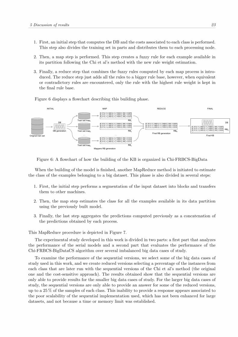
5 Discussion of results 23
1. First, an initial step that computes the DB and the costs associated to each class is performed.This step also divides the training set in parts and distributes them to each processing node.
2. Then, a map step is performed. This step creates a fuzzy rule for each example available inits partition following the Chi et al’s method with the new rule weight estimation.
3. Finally, a reduce step that combines the fuzzy rules computed by each map process is intro-duced. The reduce step just adds all the rules to a bigger rule base, however, when equivalentor contradictory rules are encountered, only the rule with the highest rule weight is kept inthe final rule base.
Figure 6 displays a flowchart describing this building phase.
Train set map1
Train set mapn
…
Train set map2
R1: IF A1 = L1 AND A2 = L1 THEN C1; RW1 = 0.9875
R2: IF A1 = L1 AND A2 = L2 THEN C2; RW2 = 0.9142
R3: IF A1 = L2 AND A2 = L1 THEN C1; RW3 = 0.4215
...
RB1
R1: IF A1 = L1 AND A2 = L1 THEN C1; RW1 = 0.9654
R2: IF A1 = L1 AND A2 = L2 THEN C2; RW2 = 0.8842
R3: IF A1 = L2 AND A2 = L1 THEN C2; RW3 = 0.6534
…
RB2
R1: IF A1 = L1 AND A2 = L1 THEN C1; RW1 = 0.7415
R2: IF A1 = L1 AND A2 = L2 THEN C1; RW2 = 0.2419
R3: IF A1 = L2 AND A2 = L1 THEN C2; RW3 = 0.4715
…
RBn
…
Mappers RB generation
Original train set
DB generation
R1: IF A1 = L1 AND A2 = L1 THEN C1; RW1 = 0.9875
R2: IF A1 = L1 AND A2 = L2 THEN C2; RW2 = 0.9142
R3: IF A1 = L2 AND A2 = L1 THEN C2; RW3 = 0.6534
…
RBR
Final RB generation
DB
R1: IF A1 = L1 AND A2 = L1 THEN C1; RW1 = 0.9875
R2: IF A1 = L1 AND A2 = L2 THEN C2; RW2 = 0.9142
R3: IF A1 = L2 AND A2 = L1 THEN C2; RW3 = 0.6534
…
RBR
DB
Final KB
INITIAL MAP REDUCE FINAL
Figure 6: A flowchart of how the building of the KB is organized in Chi-FRBCS-BigData
When the building of the model is finished, another MapReduce method is initiated to estimatethe class of the examples belonging to a big dataset. This phase is also divided in several steps:
1. First, the initial step performs a segmentation of the input dataset into blocks and transfersthem to other machines.
2. Then, the map step estimates the class for all the examples available in its data partitionusing the previously built model.
3. Finally, the last step aggregates the predictions computed previously as a concatenation ofthe predictions obtained by each process.
This MapReduce procedure is depicted in Figure 7.
The experimental study developed in this work is divided in two parts: a first part that analyzesthe performance of the serial models and a second part that evaluates the performance of theChi-FRBCS-BigDataCS algorithm over several imbalanced big data cases of study.
To examine the performance of the sequential versions, we select some of the big data cases ofstudy used in this work, and we create reduced versions selecting a percentage of the instances fromeach class that are later run with the sequential versions of the Chi et al’s method (the originalone and the cost-sensitive approach). The results obtained show that the sequential versions areonly able to provide results for the smaller big data cases of study. For the larger big data cases ofstudy, the sequential versions are only able to provide an answer for some of the reduced versions,up to a 25 % of the samples of each class. This inability to provide a response appears associated tothe poor scalability of the sequential implementation used, which has not been enhanced for largedatasets, and not because a time or memory limit was established.

24 Part I. PhD dissertation
Classification set map1
Classification set mapn
…
Classification set map2
Sample11: Actual class C1; Predicted class C1
Sample12: Actual class C2; Predicted class C2
Sample13: Actual class C1; Predicted class C2
...
Predictions set1
Sample21: Actual class C1; Predicted class C1
Sample22: Actual class C2; Predicted class C2
Sample23: Actual class C2; Predicted class C2
...
Predictions set2
Samplen1: Actual class C2; Predicted class C1
Samplen2: Actual class C2; Predicted class C2
Samplen3: Actual class C1; Predicted class C2
...
Predictions setn
…
Mappers classification sets prediction
Original classification setFinal predictions file
INITIAL MAP FINAL
Sample11: Actual class C1; Predicted class C1
Sample12: Actual class C2; Predicted class C2
Sample13: Actual class C1; Predicted class C2
...
Sample21: Actual class C1; Predicted class C1
Sample22: Actual class C2; Predicted class C2
Sample23: Actual class C2; Predicted class C2
...
Samplen1: Actual class C2; Predicted class C1
Samplen2: Actual class C2; Predicted class C2
Samplen3: Actual class C1; Predicted class C2
...
Figure 7: A flowchart of how the classification of a big data classification set is organized in Chi-
FRBCS-BigData
The results obtained for the Chi-FRBCS-BigDataCS approach demonstrate that the MapRe-duce framework is able to deal with big data for FRBCSs. According to the precision of the model(calculated with the AUC measure), the Chi-FRBCS-BigDataCS approach obtains competitive re-sults with respect to its sequential counterpart. This behavior is clearly noticed when the numberof mappers (divisions for parallelization) is increased as the available data to build each rule issmaller and, therefore, it is more difficult to properly describe the original dataset.
When the runtime of the model is examined, a speed gain is observed for the higher values ofthe number of mappers. Nevertheless, this speed gain is not lineal: the speed gain observed for thesmaller values of the number of mappers is higher than the speed gain observed for larger valuesof the number of mappers. In this manner, it is necessary to further analyze an optimal value forthe number of mappers to find a trade-off between a value small enough to preserve the predictivecapacity of the model and a large value that obtains the minimum runtimes.
The journal article associated to this part is:
V. Lopez, S. del Rıo, J. M. Benıtez, F. Herrera, Cost-Sensitive Linguistic Fuzzy Rule BasedClassification Systems under the MapReduce Framework for Imbalanced Big Data. FuzzySets and Systems, doi: 10.1016/j.fss.2014.01.015, in press (2014)
6. Concluding Remarks
The main focus of this PhD dissertation has been to get an insight about classification withimbalanced datasets and its related challenges. Our focus of interest has been the performance ofdiverse proposals on the topic and the analysis of the data intrinsic characteristics which affectthe learning of imbalanced datasets. To analyze these issues, we have focused on FRBCSs aslearners because they are effective tools that provide a good trade-off between the precision andinterpretability of the models.
In a first step, our aim was to gain a deep understanding about classification with imbalanceddatasets and the issues that need to be addressed to improve the performance of methods that

6 Concluding Remarks 25
are able to address this problem. To complete both objectives, we needed to thoroughly revise thestate-of-the-art related to classification with imbalanced data. In doing so, we appreciated that evenwhen numerous proposals had been given to address the problem, they had not been experimentallycompared difficulting the selection of a solution from a practitioner point of view.
In accordance with the former, we decided to perform an extensive analysis of diverse solutionsrecommended for skewed class distributions. We started performing a comparison between prepro-cessing techniques and cost-sensitive learning. To do so, we selected several algorithms from diverseclassification paradigms, namely, decision trees, support vector machines, FRBCSs and instance-based learning. The results were not able to find a superiority of one approach over another evenwhen slight differences were found for certain baseline classifiers.
As this first study was not conclusive enough, we decided to extend the previous comparisonadding some more preprocessing and cost-sensitive approaches, in order to have a more robustanalysis. Moreover, we also included in the analysis ensembles of classifiers for class imbalance, asthey are considered effective and powerful tools that are able to address this problem.
Furthermore, instead of comparing all the methods alltogether, we decided to compare the diver-se methodologies in families comparisons, and only the methods that showed a better performancewere selected to evaluate their performance with respect to methods belonging to other families.In general, the proposals showed a more or less similar behavior, where the ensembles of classifiersobtained better results when the base classifier is a weak learner.
The study of the state-of-the-art has not only provided an insight about the approaches thatcan be used to tackle the problem of imbalanced classification but also it has provided informationabout what we have called the data intrinsic characteristics. The data intrinsic characteristics aresome features that can be appear in the data and that negatively affect the performance of methodsin imbalanced datasets. These characteristics can also emerge in balanced datasets, however, theirinfluence in the performance of classifiers in the imbalanced scenario is much more disastrous thanin the general case.
This data intrinsic characteristics include the presence of small disjuncts, the lack of densityand information in the training data, the problem of overlapping between the classes, the impactof noisy data in imbalanced domains, the significance of the borderline instances to perform acorrect identification of samples that belong to each class and the differences between the trainingand test data, also known as dataset shift. We have thoroughly discussed how they affect theclassification performance in imbalanced data and we have included some experimental results thattry to establish a baseline between the impact of each one of this data intrinsic characteristics.
In a second step, we developed some studies that focus on the identified data intrinsic charac-teristics to improve the performance of classifiers when there is an uneven class distribution.
In the first of this studies, a new hierarchical fuzzy rule-based classification system was proposedto deal with imbalanced problems which we have called GP-COACH-H. This method features twodifferent granularities that are used to better represent each class. In this way, low granularityrules cover the more general concepts while high granularity rules cover the most specific concepts,traditionally related to the minority class.
These different granularities also allow the model to confront some of the data intrinsic charac-teristics. The number of generated small disjuncts is lower with this methodology, as it is able tocover small data areas. Furthermore, the overlapping between the classes is better addressed, as themethod adapts its behavior in the class frontiers and therefore, it obtains a better class separation.In addition, the borderline samples are better covered because rules with higher granularity are

26 Part I. PhD dissertation
used to properly identify those examples.
The second study devoted to the improvement of methods using the data intrinsic characte-ristics analyzes the impact of dataset shift over classification with imbalanced datasets. In thiscase, we observe the dataset shift, and more specifically covariate shift, that is induced by the datapartitioning scheme that is traditionally used to validate a new proposal. We compare the perfor-mance results obtained using a standard stratified cross-validation procedure with the ones achievedby DOB-SCV, a novel partitioning algorithm which has been proposed precisely to alleviate theaddition of covariate shift.
The experimental study associated demonstrated that the partitioning scheme has a strongimpact on the performance of classifiers. This effect is observed in the several algorithms comparedwhich were selected to represent diverse machine learning paradigms. Furthermore, this influencevaries depending on the type of learners which is used. Dataset shift has also a dissimilar behaviorwhen different degrees of imbalance are considered: for the low imbalanced datasets, the impact ofdataset shift is more limited than in the highly imbalanced datasets, where we also observed anelevated variability of results.
In a third step, we decided to explore how skewed class distributions are influenced by oneof the latest trends in the information technology industry: Big Data. Big data applications areincreasingly becoming the main focus of attention because of the enormous increment of datageneration and storage that has taken place in the last years. This situation becomes a challengewhen huge amounts of data are processed to extract knowledge because the data mining techniquesare not adapted to the new space and time requirements. Furthermore, big data tends to introducesome degree of uncertainty and ambiguity because their data comes from various sources, withdifferent levels of validity and with incomplete information.
To deal with this type of problem, we have proposed the Chi-FRBCS-BigDataCS algorithm,a FRBC method that is able to deal with imbalanced big data. It is based on the MapReduceframework, one of the most popular approaches nowadays to approach big data problems. As afuzzy rule-method, it is able to effectively address the vagueness in the data while providing a goodperformance. Our proposal is based in cost-sensitive learning, which enables it to deal with theuneven class distribution.
The results associated to this study show that it is necessary to specifically address big dataproblems, as the sequential counterparts are not able to provide results even in some reducedversions of the cases of study considered. However, the developed model performance depends onthe number of mappers considered for the experiments. When a high number of mappers is used,the model obtain slow runtimes, however, the performance of the classifier is also affected. If asmall number of mappers is considered, then, the classification performance is notably improved,but it comes at the expense of a rise in the runtime spent by the model.
Conclusiones
El principal objetivo de esta Tesis Doctoral ha sido el de profundizar en la clasificacion de datosno balanceados y los retos que representa. Nuestro interes se ha centrado en la caracterizacion delrendimiento de diferentes propuestas acerca del tema y el analisis de las caracterısticas intrınsecasde los datos que inflyen en el aprendizaje con datos no balanceados. Para analizar estas cuestiones,nos hemos centrado en la utilizacion de SCBRDs debido a que son herramientas efectivas que

6 Concluding Remarks 27
proporcionan un buen equilibrio entre la precision y la interpetabilidad de los modelos.
En primera aproximacion, nuestro objetivo fue conseguir un conocimiento profundo de la clasifi-cacion con datos no balanceados y los problemas que deberıan resolverse para mejorar el rendimientode los metodos que consiguen resolver el problema. Para completar ambos objetivos, necesitaba-mos repasar por completo el estado del arte de la clasificacion con datos no balanceados. En elproceso, pudimos apreciar que a pesar de que se habıan planteado muchas soluciones para abordarel problema, dichas propuestas no se habıan comparado experimentalmente, lo que dificultaba laseleccion de una solucion desde un punto de vista practico.
En este sentido, decidimos realizar un analisis completo de diferentes soluciones recomendadaspara distribuciones sesgadas. Comenzamos realizando una comparacion entre tecnicas de prepro-cesamiento y aprendizaje sensible al coste. Para ello, seleccionamos varios algoritmos de diferentesparadigmas de clasificacion, como son arboles de decision, maquinas de soporte vectorial, SCBRDsası como aprendizaje basado en instancias. Considerando los resultados obtenidos, no era posibledeterminar la superioridad de un enfoque frente a otro incluso cuando aparecieron ligeras diferenciaspara ciertos clasificadores basicos.
Dado que este primer analisis no resulto suficientemente esclarecedor, decidimos extender lacomparativa anterior anadiendo algunas tecnicas de preprocesamiento y aproximaciones sensiblesal coste adicionales para conseguir unos resultados mas robustos. Asimismo, tambien incluımos enel analisis tecnicas basadas en ensembles para abordar la clasificacion con datos no balanceados,ya que son consideradas unas herramientas potentes y efectivas para enfrentarse a este problema.
Ademas, en lugar de comparar todos los metodos al mismo tiempo, decidimos agruparlos enfamilias de comparacion, de forma que solo los metodos que demostraron mejor rendimiento seevaluaron con respecto a metodos de otras familias. En general, las propuestas mostraron un com-portamiento similar, donde los grupos de clasificadores obtenıan mejores resultados al trabajar conclasificadores debiles.
Esta revision del estado del arte no solo ha proporcionado una vision mas profunda de comolas propuestas pueden usarse para afrontar el problema de clasificacion no balanceada sino quetambien ha proporcionado informacion acerca de lo que hemos llamado caracterısticas intrınsecasde los datos. Las caracterısticas intrınsecas de los datos son algunas caracterısticas que puedenestar presentes en los datos y que afectan negativamente el rendimiento de los metodos en datosno balanceados. Estas caracterısticas pueden aparecer tambien en datos balanceados, sin embargosu influencia en el rendimiento de los clasificadores en el caso no balanceado es muchısimo masdesastroso que en el caso general.
Las caracterısticas intrınsecas de los datos incluyen la presencia de pequenos grupos disjuntos,falta de densidad e informacion en los datos de entrenamiento, el problema del solapamiento entrelas clases, el impacto de datos ruidosos en dominios no balanceados, la importancia de las instanciasde borde para realizar una correcta identificacion de las muestras que pertenecen a cada clase, y lasdiferencias entre los datos de entrenamiento y de test, tambien conocido como dataset shift. Hemosanalizado en profundidad como afectan el rendimiento de la clasificacion en datos no balanceadosy hemos incluido algunos resultados experimentales que intentan determinar los fundamentos delimpacto de cada una de estas caracterısticas intrınsecas.
En segunda instancia, hemos desarrollado algunos estudios que se centran en las caracterısticasintrınsecas de los datos para mejorar el rendimiento de clasificadores cuando hay una clase condistribucion no uniforme.
Para el primero de estos analisis, se ha propuesto un nuevo sistema de clasificacion jerarqui-

28 Part I. PhD dissertation
co basado en reglas difusas para trabajar con problemas no balanceados, que hemos denominadoGP-COACH-H. Este metodo dispone de dos diferentes granularidades que se pueden usar pararepresentar de la manera mas fiel posible cada clase. De este modo, las reglas de baja granulari-dad cubren los conceptos mas generales, mientras que las reglas de gran granularidad cubren losconceptos mas especıficos, relacionados tradicionalmente con las clases minoritarias.
Esta diferenciacion de granularidades tambien permite afrontar algunas de las caracterısticasintrınsecas de los datos. El numero de conjuntos disjuntos generados es menor con esta metodologıa,ya que es capaz de cubrir pequenas areas de datos. Ademas, el solapamiento entre las clases semaneja mejor, ya que el metodo adapta su comportamiento en las clases frontera y por lo tanto,consigue una mejor separacion de clases. Ademas, las muestras del borde se interpretan mejor yaque las reglas con granularidad alta se utilizan para identificar adecuadamente esos ejemplos.
El segundo estudio se ha centrado en la mejora de los metodos que utilizan las caracterısticasintrınsecas de los datos y analiza el impacto del dataset shift en conjunto de datos para la clasifi-cacion con datos no balanceados. En este caso, observamos el dataset shift, y mas especıficamenteel covariate shift, que se induce mediante el esquema de particionado que tradicionalmente se usapara validar una nueva propuesta. Comparamos el rendimiento asociado resultante utilizando unprocedimiento estratificado estandar de validacion cruzada con los resultados alcanzados por DOB-SCV, un nuevo algoritmo de particionamiento que se ha propuesto precisamente para aliviar lapresencia del covariate shift.
El estudio experimental asociado demostro que el esquema de particionado tiene un importanteimpacto en el rendimiento de los clasificadores. Este efecto se observa en los varios algoritmoscomparados que se seleccionaron para representar diferentes paradigmas de aprendizaje automatico.Ademas, esta influencia varıa dependiendo del esquema de aprendizaje que se este utilizando. Elcambio en conjunto de datos tambien posee un comportamiento diferenciado cuando se considerandistintos grados de desbalanceo: para los datos con bajo desbalanceo, el impacto del cambio esmas limitado que en los datos no balanceados, donde tambien se ha podido constatar una elevadavariabilidad de resultados.
Para el tercer paso, decidimos explorar cual es la repercusion en las distribuciones de clases concambio en conjunto de datos de una de las ultimas tendencias de la industria de las tecnologıas de lainformacion: Big data. Las aplicaciones de big data se estan convirtiendo cada vez mas en el foco deatencion principal debido el enorme incremento en la generacion y almacenamiento de informacionque ha tenido lugar en los ultimos anos. Esta situacion se convierte en un reto cuando cantidadesingentes de datos se procesan para la extraccion de conocimiento debido a que las tecnicas deminerıa de datos no estan adaptadas a los nuevos requerimientos de tiempo y espacio. Ademas, enbig data, se tiende a introducir un cierto grado de incertidumbre y ambiguedad ya que los datosproceden de diferentes fuentes, con ciertos niveles de validez y con informacion incompleta.
Para tratar con este tipo de problemas, hemos propuesto el algoritmo Chi-FRBCS-BigDataCS,un SCBRDs que es capaz de procesar big data no balanceado. Se basa en el entorno MapReduce,uno de los enfoques mas populares de la actualidad para el tratamiento de los problemas de bigdata. Como metodo basado en reglas difusas, es capaz de resolver de forma efectiva la imprecisionen los datos a la vez que mantiene buen rendimiento. Nuestra propuesta esta basada en aprendizajesensible al coste, que permite manejar las clases con distribuciones no uniformes.
Los resultados asociados a este estudio demuestran que es necesario tratar especıficamente losproblemas de big data, al igual que los correspondientes componentes secuenciales no son capacesde proporcionar los resultados incluso en algunas versiones simplificadas de los casos de estudioconsiderados. Sin embargo, el rendimiento del modelo desarrollado depende del numero de mapea-

7 Future Work 29
dores considerados para los experimentos. Cuando se utiliza un numero elevado de mapeadores, elmodelo produce tiempos de ejecucion bajos, pero el rendimiento del clasificador se ve afectado. Sise considera un numero pequeno de mapeadores, entonces el rendimiento de la clasificacion mejoranotablemente, pero con un mayor coste en tiempo de ejecucion por parte del modelo.
7. Future Work
Thorough the development of the studies developed in this thesis, numerous issues have arisenas interesting paths of research to be further explored.
Extending the modifications based on the data intrinsic characteristics to multi-classimbalanced problems: In the literature, there has been little work done in the framework ofdatasets with multiple imbalanced classes compared to the extensive collection of works availablefor binary imbalanced classification sets. This opens a wide horizon of possibilities for solving suchproblems not only with FRBCSs, but with any type of learning paradigms.
In our case, we are mainly interested in the implementation of various proposals that can helpincrease the accuracy obtained by the state-of-the-art methods. Introducing operations to deal withthe data intrinsic characteristics with problems with more than two classes can end up with modelsthat have better performance values. Moreover, these methods must consider the possibility ofbuilding a model that can combine the outputs of small classifiers that are able to better identifyminority class instances with respect to larger classes.
Instance and feature selection using multiobjective methods in imbalanced datasets:An approach for improving current classification models in the framework of imbalanced datasetscould be the application of a multiobjective feature and instance selection procedure. The multiob-jective methodology will allow the search by means of the optimization of several measures whichcould be able to improve the quality of the learned system [BJZY13].
Multiobjective methods can feature diverse objectives related to the improvement of the model.In this way, the search could be guided towards the reduction of the number of features, theimprovement of a certain imbalanced performance measure, the diminution of the number of samples(belonging to the minority class or both classes), the improvement related to complexity measures,and so on. Therefore, we suggest to analyze the impact of the diverse targets in the multiobjectiveoptimization process and how they affect the performance of methods in the presence of imbalanceddatasets.
Advanced ensembles methods for imbalanced problems: In the field of imbalanced data-sets, ensembles of classifiers which have been developed in the state-of-the-art have followed theclassical ensemble approaches (Boosting and Bagging). These approaches have been combined withpreprocessing methods achieving very good results.
However, in the literature the newest methods do not only focus on the traditional ensemblemethods but also on some advanced ensemble methods. Therefore, we considered its applicationto the problem of imbalanced classes. In this manner, we have to find a way suitable for input-ting the pre-processing methods and techniques to address the problem of imbalanced classes in

30 Part I. PhD dissertation
each construction method. To this end, we propose the use of ensembles combined with advancedpreprocessing methods like DBSMOTE [BSL12] or MWMOTE [BIYM14].
Analyze the interaction of active learning with imbalanced datasets: The performanceof a predictive model is tightly coupled with the data used during training. In active learning,the model itself plays a hands-on role in the selection of examples for labeling from a large poolof unlabeled examples. It is quite interesting to explore the interaction between active learningand class imbalance, discussing active learning techniques designed specifically for dealing withimbalanced settings, strategies that leverage active learning to overcome the deleterious effects ofclass imbalance, how extreme class imbalance can prevent active learning systems from selectinguseful examples, and alternatives to active learning in these cases.
The design of voting models for ensemble learning algorithms in the context of bigdata: Ensemble learning is one of the most promising areas in machine learning, which is usedsatisfactorily in many real-world applications. These approaches build a set of classifiers and thenclassify new data by taking a vote of their predictions. Two of the most representative ensemblelearning approaches are bagging and boosting. An important issue in ensemble learning is thetechnique to combining predictions (or voting scheme) of ensemble classifiers for big data, since itmay give different results depending upon different factors. The MapReduce approaches developedin this dissertation have used just a majority voting approach in the Reduce phase to combine theoutput of the classifiers built in each data partition used by each Map proccess. Therefore, we needto develop the appropriate combination approaches for partial models extracted in a MapReduceframework.

Part II. Publications: Published and
Accepted Papers
1. A Study on the Data Intrinsic Characteristics in Classification
Problems with Imbalanced Datasets and Analysis of the Beha-
vior of the Techniques from the State-of-the-art
The journal papers associated to this part are:
1.1. Analysis of preprocessing vs. cost-sensitive learning for imbalanced classi-
fication. Open problems on intrinsic data characteristics
V. Lopez, A. Fernandez, J. G. Moreno-Torres, F. Herrera, Analysis of preproces-sing vs. cost-sensitive learning for imbalanced classification. Open problems on intrin-sic data characteristics. Expert Systems with Applications 39:7 (2012) 6585–6608, doi:10.1016/j.eswa.2011.12.043
• Status: Published.
• Impact Factor (JCR 2012): 1.854.
• Subject Category: Computer Science, Artificial Intelligence. Ranking 31 / 115 (Q2).
• Subject Category: Engineering, Electrical & Electronic. Ranking 56 / 243 (Q1).
• Subject Category: Operations Research & Management Science. Ranking 13 / 79 (Q1).
• Citations (Web of Science): 14.
• Citations (Google Scholar): 31.
31


Analysis of preprocessing vs. cost-sensitive learning for imbalancedclassification. Open problems on intrinsic data characteristics
Victoria López a,⇑, Alberto Fernández b, Jose G. Moreno-Torres a, Francisco Herrera a
aDept. of Computer Science and Artificial Intelligence, CITIC-UGR (Research Center on Information and Communications Technology), University of Granada, 18071 Granada, SpainbDept. of Computer Science, University of Jaén, 23071 Jaén, Spain
a r t i c l e i n f o
Keywords:ClassificationImbalanced datasetsPreprocessingCost-sensitive learningClass overlapDataset shift
a b s t r a c t
Class imbalance is among the most persistent complications which may confront the traditional super-vised learning task in real-world applications. The problem occurs, in the binary case, when the numberof instances in one class significantly outnumbers the number of instances in the other class. This situa-tion is a handicap when trying to identify the minority class, as the learning algorithms are not usuallyadapted to such characteristics.The approaches to deal with the problem of imbalanced datasets fall into two major categories: data
sampling and algorithmic modification. Cost-sensitive learning solutions incorporating both the dataand algorithm level approaches assume higher misclassification costs with samples in the minority classand seek to minimize high cost errors. Nevertheless, there is not a full exhaustive comparison betweenthose models which can help us to determine the most appropriate one under different scenarios.The main objective of this work is to analyze the performance of data level proposals against algorithm
level proposals focusing in cost-sensitive models and versus a hybrid procedure that combines those twoapproaches. We will show, by means of a statistical comparative analysis, that we cannot highlight anunique approach among the rest. This will lead to a discussion about the data intrinsic characteristicsof the imbalanced classification problem which will help to follow new paths that can lead to theimprovement of current models mainly focusing on class overlap and dataset shift in imbalancedclassification.
� 2011 Elsevier Ltd. All rights reserved.
1. Introduction
One major problem facing data mining is the class imbalanceproblem (He & Garcia, 2009; Sun, Wong, & Kamel, 2009). It appearsin many applications, and is defined as the case where there existsa significant difference between the class prior rates, that is, theprobability a particular example belongs to a particular class. Theclass imbalance is dominant in a high number of real problemsincluding, but not limited to, telecommunications, WWW, fi-nances, ecology, biology, medicine and so on. It must also bestressed that the positive or minority class is usually the one thathas the highest interest from the learning point of view and it alsoimplies a great cost when it is not well classified (Elkan, 2001).
A wide number of approaches have been proposed to the imbal-anced learning problem that fall largely into two major categories.The first one is data sampling in which the training instances aremodified in such a way as to produce a balanced data distribution
that allow classifiers to perform in a similar manner to standardclassification (Batista, Prati, & Monard, 2004; Chawla, Bowyer, Hall,& Kegelmeyer, 2002). The second one is through algorithmic mod-ification to make base learning methods more attuned to classimbalance issues (Zadrozny & Elkan, 2001). Cost-sensitive learningsolutions incorporating both the data and algorithm level ap-proaches assume higher misclassification costs with samples inthe rare class and seek to minimize the high cost errors (Ling, Yang,Wang, & Zhang, 2004; Zadrozny, Langford, & Abe, 2003).
Works in imbalanced classification usually focus on the devel-opment of new algorithms along one of the categories previouslymentioned. However, there is not a study that exhaustively com-pares solutions from one category to another making difficult theselection of one kind of algorithm when classifying. The aim of thispaper is to develop a thorough experimental study to analyze thepossible differences between preprocessing techniques and cost-sensitive learning for addressing classification with imbalanceddata. In addition, we also present in the comparison a hybrid pro-cedure that combines those two approaches to check whetherthere is a synergy between them.
In order to analyze the oversampling and undersampling meth-odologies against cost-sensitive learning approaches, we will use
0957-4174/$ - see front matter � 2011 Elsevier Ltd. All rights reserved.doi:10.1016/j.eswa.2011.12.043
⇑ Corresponding author. Tel.: +34 958 240598; fax: +34 958 243317.E-mail addresses: [email protected] (V. López), [email protected]
(A. Fernández), [email protected] (J.G. Moreno-Torres), [email protected] (F. Herrera).
Expert Systems with Applications 39 (2012) 6585–6608
Contents lists available at SciVerse ScienceDirect
Expert Systems with Applications
journal homepage: www.elsevier .com/locate /eswa

the ‘‘Synthetic Minority Over-sampling Technique’’ (SMOTE)(Chawla et al., 2002) and its variant with the Wilson’s EditedNearest Neighbor (ENN) rule (Wilson, 1972) as they have shownto obtain a very robust behaviour among many different situations(Batista et al., 2004; Fernández, García, del Jesus, & Herrera, 2008).As cost-sensitive methods we study several modifications towell-known classification methods such as C4.5 (Quinlan, 1993),Support Vector Machines (SVMs) (Vapnik, 1998), k-NearestNeighbor classifier (k-NN) (Cover & Hart, 1967) or Fuzzy HybridGenetics-Based Machine Learning (FH-GBML) rule generationalgorithm (Ishibuchi & Yamamoto, 2005). The combination of theseapproaches is carried out through a wrapper classifier (Chawla,Cieslak, Hall, & Joshi, 2008) that uses the aforementioned cost-sensitive techniques with the preprocessing technique obtainingthe adequate parameters to perform altogether.
In this work, we focus on imbalanced binary classification prob-lems, having selected a benchmark of 66 problems from KEELdataset repository1 (Alcalá-Fdez et al., 2011). We perform ourexperimental study focusing on the precision of the models usingthe Area Under the ROC curve (AUC) (Huang & Ling, 2005). Thisstudy is carried out using nonparametric tests to check whetherthere exist significant differences among the obtained results(Demšar, 2006; García & Herrera, 2008).
On the other hand, after comparing these techniques we alsowant to find what is the source where the difficulties for imbal-anced classification emerge. Many other studies on the behaviorof several standard classifiers in imbalance domains have shownthat significant loss of performance is mainly due to skew of classdistributions. However, several investigations also suggest thatthere are other factors that contribute to such performance deg-radation, for example, size of the dataset, class imbalance level,small disjuncts, density, and overlap complexity (Japkowicz &Stephen, 2002; Prati & Batista, 2004; Weiss & Provost, 2003). Thiswork focuses on the analysis of two of the most pressing openproblems related to data intrinsic characteristics: overlap anddataset shift.
This paper is organized as follows: first, Section 2 presents theproblem of imbalanced datasets and the metric we have employedin this context whereas Section 3 describes some ways to tacklethe problem: the preprocessing methods used, cost-sensitive clas-sification and a wrapper approach to combine both. Next, Section 4describes the algorithms we have used in this study, selectedbenchmark datasets and the configuration of the methods. In Sec-tion 5 an analysis of preprocessing techniques versus cost-sensitivelearning approaches can be found. Section 6 is devoted to discussthe imbalanced classification problem characteristics that makethat problem difficult, analysing the open problems related to dataintrinsic characteristics, class overlap and dataset shift. The conclu-sions of this work can be found in Section 7. Additionally, we in-clude an appendix with the complete tables of results from theexperimental study.
2. Imbalanced datasets in classification
In this section, we first introduce the problem of imbalanceddatasets and then we present the evaluation metrics for this typeof classification problem which differ from usual measures inclassification.
2.1. The problem of imbalanced datasets
In some classification problems, the number of instances ofevery class can be very different. Specifically when facing a dataset
with only two classes, the imbalance problem occurs when oneclass is represented by a large number of examples, while the otheris represented by only a few (Chawla, Japkowicz, & Kotcz, 2004).
The problem of imbalanced datasets is extremely significant(Yang & Wu, 2006) because it is implicit in most real world appli-cations, such as very high resolution airborne imagery (Chen, Fang,Huo, & Li, 2011), e-mail foldering (Bermejo, Gámez, & Puerta, 2011)or micro seismic hazards in coal mines (Sikora, 2011), just citingsome of them. It is important to point out that the minority classusually represents the concept of interest, for example patientswith illnesses in a medical diagnosis problem; whereas the otherclass represents the counterpart of that concept (healthy patients).
Usually, standard classifier algorithms have a bias towards themajority class, since the rules that predict the higher number ofexamples are positively weighted during the learning process in fa-vour of the accuracy metric. Consequently, the instances that be-long to the minority class are misclassified more often than thosebelonging to the majority class. Another important issue relatedto this type of problem is the presence of small disjuncts in thedataset (Weiss & Provost, 2003) and the difficulty most learningalgorithms have in detecting those regions. Furthermore, the mainhandicap in imbalanced datasets is the overlapping between theexamples of the positive and the negative class (García, Mollineda,& Sánchez, 2008). These facts are depicted in Fig. 1(a) and (b)respectively.
2.2. Evaluation in imbalanced domains
The measures of the quality of classification are built from aconfusion matrix (shown in Table 1) which records correctly andincorrectly recognized examples for each class.
The most commonly used empirical measure, accuracy (1), doesnot distinguish between the number of correct labels of differentclasses, which in the framework of imbalanced problems may leadto erroneous conclusions. For example a classifier that obtains anaccuracy of 90% in a dataset with a degree of imbalance 9:1, mightnot be accurate if it does not cover correctly any minority classinstance.
Acc ¼ TP þ TNTP þ FN þ FP þ TN
ð1Þ
Because of this, instead of using accuracy, more correct metrics areconsidered. Specifically, from Table 1 it is possible to obtain fourmetrics of performance that measure the classification quality forthe positive and negative classes independently:
� True positive rate TPrate ¼ TPTPþFN is the percentage of positive
cases correctly classified as belonging to the positive class.� True negative rate TNrate ¼ TN
FPþTN is the percentage of negativecases correctly classified as belonging to the negative class.
� False positive rate FPrate ¼ FPFPþTN is the percentage of negative
cases misclassified as belonging to the positive class.� False negative rate FNrate ¼ FN
TPþFN is the percentage of positivecases misclassified as belonging to the negative class.
One appropriate metric that could be used to measure the per-formance of classification over imbalanced datasets is the ReceiverOperating Characteristic (ROC) curve (Bradley, 1997). In this curve,the tradeoff between the benefits (TPrate) and costs (FPrate) can bevisualized, and acknowledges the fact that the capacity of any clas-sifier cannot increase the number of true positives without alsoincreasing the false positives. The Area Under the ROC Curve(AUC) (Huang & Ling, 2005) corresponds to the probability of cor-rectly identifying which of the two stimuli is noise and which is sig-nal plus noise. AUC provides a single-number summary for theperformance of learning algorithms.1 http://www.keel.es/datasets.php.
6586 V. López et al. / Expert Systems with Applications 39 (2012) 6585–6608
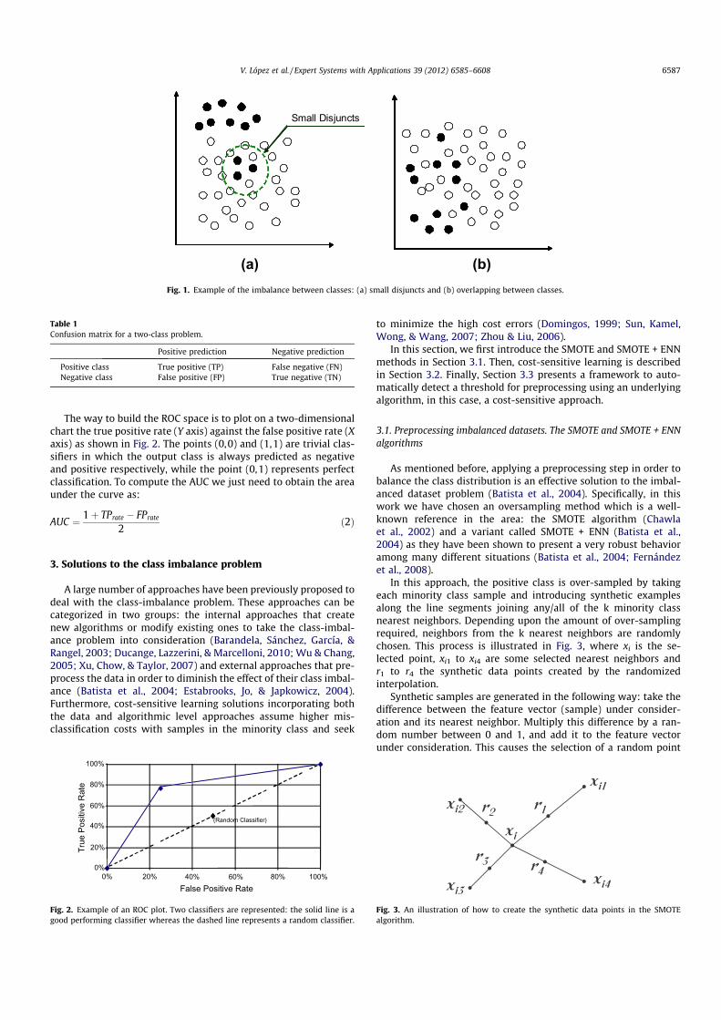
The way to build the ROC space is to plot on a two-dimensionalchart the true positive rate (Y axis) against the false positive rate (Xaxis) as shown in Fig. 2. The points (0,0) and (1,1) are trivial clas-sifiers in which the output class is always predicted as negativeand positive respectively, while the point (0,1) represents perfectclassification. To compute the AUC we just need to obtain the areaunder the curve as:
AUC ¼ 1þ TPrate � FPrate
2ð2Þ
3. Solutions to the class imbalance problem
A large number of approaches have been previously proposed todeal with the class-imbalance problem. These approaches can becategorized in two groups: the internal approaches that createnew algorithms or modify existing ones to take the class-imbal-ance problem into consideration (Barandela, Sánchez, García, &Rangel, 2003; Ducange, Lazzerini, & Marcelloni, 2010; Wu & Chang,2005; Xu, Chow, & Taylor, 2007) and external approaches that pre-process the data in order to diminish the effect of their class imbal-ance (Batista et al., 2004; Estabrooks, Jo, & Japkowicz, 2004).Furthermore, cost-sensitive learning solutions incorporating boththe data and algorithmic level approaches assume higher mis-classification costs with samples in the minority class and seek
to minimize the high cost errors (Domingos, 1999; Sun, Kamel,Wong, & Wang, 2007; Zhou & Liu, 2006).
In this section, we first introduce the SMOTE and SMOTE + ENNmethods in Section 3.1. Then, cost-sensitive learning is describedin Section 3.2. Finally, Section 3.3 presents a framework to auto-matically detect a threshold for preprocessing using an underlyingalgorithm, in this case, a cost-sensitive approach.
3.1. Preprocessing imbalanced datasets. The SMOTE and SMOTE + ENNalgorithms
As mentioned before, applying a preprocessing step in order tobalance the class distribution is an effective solution to the imbal-anced dataset problem (Batista et al., 2004). Specifically, in thiswork we have chosen an oversampling method which is a well-known reference in the area: the SMOTE algorithm (Chawlaet al., 2002) and a variant called SMOTE + ENN (Batista et al.,2004) as they have been shown to present a very robust behavioramong many different situations (Batista et al., 2004; Fernándezet al., 2008).
In this approach, the positive class is over-sampled by takingeach minority class sample and introducing synthetic examplesalong the line segments joining any/all of the k minority classnearest neighbors. Depending upon the amount of over-samplingrequired, neighbors from the k nearest neighbors are randomlychosen. This process is illustrated in Fig. 3, where xi is the se-lected point, xi1 to xi4 are some selected nearest neighbors andr1 to r4 the synthetic data points created by the randomizedinterpolation.
Synthetic samples are generated in the following way: take thedifference between the feature vector (sample) under consider-ation and its nearest neighbor. Multiply this difference by a ran-dom number between 0 and 1, and add it to the feature vectorunder consideration. This causes the selection of a random point
Small Disjuncts
(a) (b)Fig. 1. Example of the imbalance between classes: (a) small disjuncts and (b) overlapping between classes.
Table 1Confusion matrix for a two-class problem.
Positive prediction Negative prediction
Positive class True positive (TP) False negative (FN)Negative class False positive (FP) True negative (TN)
0% 20% 40% 60% 80% 100%False Positive Rate
0%
20%
40%
60%
80%
100%
True
Pos
itive
Rat
e
(Random Classifier)♦
Fig. 2. Example of an ROC plot. Two classifiers are represented: the solid line is agood performing classifier whereas the dashed line represents a random classifier.
Fig. 3. An illustration of how to create the synthetic data points in the SMOTEalgorithm.
V. López et al. / Expert Systems with Applications 39 (2012) 6585–6608 6587
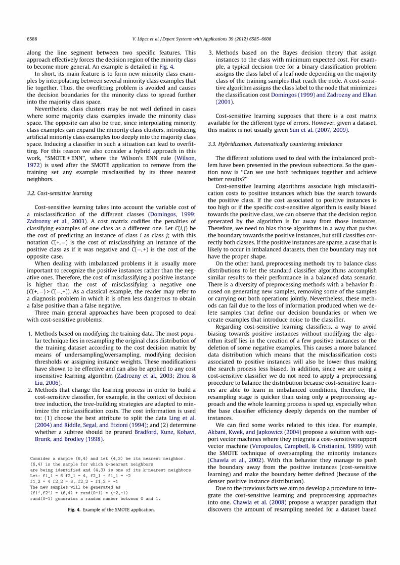
along the line segment between two specific features. Thisapproach effectively forces the decision region of the minority classto become more general. An example is detailed in Fig. 4.
In short, its main feature is to form new minority class exam-ples by interpolating between several minority class examples thatlie together. Thus, the overfitting problem is avoided and causesthe decision boundaries for the minority class to spread furtherinto the majority class space.
Nevertheless, class clusters may be not well defined in caseswhere some majority class examples invade the minority classspace. The opposite can also be true, since interpolating minorityclass examples can expand the minority class clusters, introducingartificial minority class examples too deeply into the majority classspace. Inducing a classifier in such a situation can lead to overfit-ting. For this reason we also consider a hybrid approach in thiswork, ‘‘SMOTE + ENN’’, where the Wilson’s ENN rule (Wilson,1972) is used after the SMOTE application to remove from thetraining set any example misclassified by its three nearestneighbors.
3.2. Cost-sensitive learning
Cost-sensitive learning takes into account the variable cost ofa misclassification of the different classes (Domingos, 1999;Zadrozny et al., 2003). A cost matrix codifies the penalties ofclassifying examples of one class as a different one. Let C(i, j) bethe cost of predicting an instance of class i as class j; with thisnotation C(+,�) is the cost of misclassifying an instance of thepositive class as if it was negative and C(�, +) is the cost of theopposite case.
When dealing with imbalanced problems it is usually moreimportant to recognize the positive instances rather than the neg-ative ones. Therefore, the cost of misclassifying a positive instanceis higher than the cost of misclassifying a negative one(C(+,�) > C(�, +)). As a classical example, the reader may refer toa diagnosis problem in which it is often less dangerous to obtaina false positive than a false negative.
Three main general approaches have been proposed to dealwith cost-sensitive problems:
1. Methods based on modifying the training data. The most popu-lar technique lies in resampling the original class distribution ofthe training dataset according to the cost decision matrix bymeans of undersampling/oversampling, modifying decisionthresholds or assigning instance weights. These modificationshave shown to be effective and can also be applied to any costinsensitive learning algorithm (Zadrozny et al., 2003; Zhou &Liu, 2006).
2. Methods that change the learning process in order to build acost-sensitive classifier, for example, in the context of decisiontree induction, the tree-building strategies are adapted to min-imize the misclassification costs. The cost information is usedto: (1) choose the best attribute to split the data Ling et al.(2004) and Riddle, Segal, and Etzioni (1994); and (2) determinewhether a subtree should be pruned Bradford, Kunz, Kohavi,Brunk, and Brodley (1998).
3. Methods based on the Bayes decision theory that assigninstances to the class with minimum expected cost. For exam-ple, a typical decision tree for a binary classification problemassigns the class label of a leaf node depending on the majorityclass of the training samples that reach the node. A cost-sensi-tive algorithm assigns the class label to the node that minimizesthe classification cost Domingos (1999) and Zadrozny and Elkan(2001).
Cost-sensitive learning supposes that there is a cost matrixavailable for the different type of errors. However, given a dataset,this matrix is not usually given Sun et al. (2007, 2009).
3.3. Hybridization. Automatically countering imbalance
The different solutions used to deal with the imbalanced prob-lem have been presented in the previous subsections. So the ques-tion now is ‘‘Can we use both techniques together and achievebetter results?’’
Cost-sensitive learning algorithms associate high misclassifi-cation costs to positive instances which bias the search towardsthe positive class. If the cost associated to positive instances istoo high or if the specific cost-sensitive algorithm is easily biasedtowards the positive class, we can observe that the decision regiongenerated by the algorithm is far away from those instances.Therefore, we need to bias those algorithms in a way that pushesthe boundary towards the positive instances, but still classifies cor-rectly both classes. If the positive instances are sparse, a case that islikely to occur in imbalanced datasets, then the boundary may nothave the proper shape.
On the other hand, preprocessing methods try to balance classdistributions to let the standard classifier algorithms accomplishsimilar results to their performance in a balanced data scenario.There is a diversity of preprocessing methods with a behavior fo-cused on generating new samples, removing some of the samplesor carrying out both operations jointly. Nevertheless, these meth-ods can fail due to the loss of information produced when we de-lete samples that define our decision boundaries or when wecreate examples that introduce noise to the classifier.
Regarding cost-sensitive learning classifiers, a way to avoidbiasing towards positive instances without modifying the algo-rithm itself lies in the creation of a few positive instances or thedeletion of some negative examples. This causes a more balanceddata distribution which means that the misclassification costsassociated to positive instances will also be lower thus makingthe search process less biased. In addition, since we are using acost-sensitive classifier we do not need to apply a preprocessingprocedure to balance the distribution because cost-sensitive learn-ers are able to learn in imbalanced conditions, therefore, theresampling stage is quicker than using only a preprocessing ap-proach and the whole learning process is sped up, especially whenthe base classifier efficiency deeply depends on the number ofinstances.
We can find some works related to this idea. For example,Akbani, Kwek, and Japkowicz (2004) propose a solution with sup-port vector machines where they integrate a cost-sensitive supportvector machine (Veropoulos, Campbell, & Cristianini, 1999) withthe SMOTE technique of oversampling the minority instances(Chawla et al., 2002). With this behavior they manage to pushthe boundary away from the positive instances (cost-sensitivelearning) and make the boundary better defined (because of thedenser positive instance distribution).
Due to the previous facts we aim to develop a procedure to inte-grate the cost-sensitive learning and preprocessing approachesinto one. Chawla et al. (2008) propose a wrapper paradigm thatdiscovers the amount of resampling needed for a dataset basedFig. 4. Example of the SMOTE application.
6588 V. López et al. / Expert Systems with Applications 39 (2012) 6585–6608

on optimizing evaluation functions which can include the costassociated to the classification. This wrapper infrastructure appliescross-validation to first discover the best amounts of undersam-pling and oversampling, applies the preprocessing algorithms withthe amounts estimated and finally runs the algorithm used overthe preprocessed dataset.
Obviously, searching the entire space of undersampling andSMOTE combinations can quickly become intractable, so the searchprocedure must be fine-tuned. This strategy removes the ‘‘excess’’examples of the majority classes, which reduces the size of thetraining dataset. This also makes learning time more manageable.SMOTE is used to add synthetic examples of the minority classesand increase the generalization performance of the classifier overthe minority classes. Fig. 5 shows the algorithm procedure.
The estimation is done over a training and a test set. The train-ing data is split into five partitions for an internal five-fold cross-validation. The wrapper applies this independent validation stageto each fold to discover the appropriate percentages of samplingfor a given method and classifier combination. Once these percent-ages are discovered, the classifier is re-learned on the originaltraining fold using the discovered percentages and tested on thecorresponding testing fold.
The undersampling estimation starts with no undersamplingfor all majority classes and obtains baseline results on the trainingdata. Then it traverses through the search space of undersamplingpercentages in decrements of Sample Decrement, in a greedy itera-tive fashion, to increase performance over the minority classeswithout sacrificing performance on the majority class.
The oversampling algorithm evaluates different amounts ofSMOTE at steps of Sample Increment (percentage of the numberof examples from the minority class that will be generated in eachstep). This is a greedy search, and at each step the new perfor-mance estimates become the new baseline. That is, the initial base-line is the performance obtained via the Wrapper Undersample. IfSMOTE = Sample Increment improves the performance over thatbaseline by some margin Increment Min, then the performanceachieved at SMOTE = Sample Increment becomes the new baseline.The amount of SMOTE is then incremented by Sample Increment,and another evaluation is performed to check if the performance
increase at new SMOTE amount is at least greater than IncrementMin. This process repeats, greedily, until no performance gainsare observed.
However, there is an important caveat to the search to avoidbeing trapped in a local maximum. If the average does not improveby Increment Min we have to verify that we have not settled on alocal maximum. In order to do so, we look ahead some more stepsat increasing amounts of SMOTE. If the look-ahead does not resultin an improvement in performance, then the amount of SMOTE isreset to the value discovered prior to the look-ahead. This is doneto allow SMOTE to introduce additional examples with the aim ofimproving performance. However, if the addition of examples doesnot help, then we go back to using the lesser amount of SMOTE dis-covered prior to the look-ahead.
We can use different measures to evaluate the performance ofthe classifier to estimate the sampling parameters. Since we areusing cost-sensitive learning algorithms as base classifiers a logicalevaluation criteria is the cost itself. Cost is calculated as shown inEq. (3) when we assume C(+j+) = C(�j�) = 0 (as it is usual in imbal-anced classification).
cost ¼ FNrate � Cð�jþÞ þ FPrate � Cðþj�Þ ð3Þ
4. Experimental framework
In this section, we first introduce the algorithms which are in-cluded in the study (Section 4.1). Next, we provide details of theimbalanced problems chosen for the experimentation and the con-figuration parameters of the methods (Sections 4.2 and 4.3). Final-ly, we present the statistical tests applied to compare the resultsobtained with the different classifiers (Section 4.4).
4.1. Algorithms selected for the study
This section presents the description of the state of the art algo-rithms of four different classification paradigms selected for ourstudy. For each paradigm we outline the base classifier commonlyused in general classification problems and the cost-sensitivelearning version associated to that classifier.
Fig. 5. Illustration on the wrapper undersample SMOTE algorithm. Dashed lines means resampling actions, black boxes represent the parameters estimation and the finalresult is in grey.
V. López et al. / Expert Systems with Applications 39 (2012) 6585–6608 6589

4.1.1. Decision treesDecision trees use simple knowledge representation to classify
examples into a finite number of classes. In a typical setting, thetree nodes represent the attributes, the edges represent the possi-ble values for a particular attribute, and the leaves are assignedwith class labels. Classifying a test sample is straightforward oncea decision tree has been constructed. An object is classified by fol-lowing paths from the root node through the tree to a leaf, takingthe edges corresponding to the values of attributes.
C4.5 decision tree. C4.5 (Quinlan, 1993) is a decision tree gener-ating algorithm. It induces classification rules in the form of deci-sion trees from a set of given examples. The decision tree isconstructed top-down using the normalized information gain(difference in entropy) that results from choosing an attribute forsplitting the data. The attribute with the highest normalized infor-mation gain is chosen to make the decision. The C4.5 algorithmthen recurs on the smaller sublists.
Cost-sensitive C4.5 decision tree. The cost-sensitive C4.5 deci-sion tree (C4.5CS) (Ting, 2002) is a method to induce cost-sensitivetrees that seeks to minimize the number of high cost errors and, asa consequence of that, leads to minimization of the total misclassi-fication costs in most cases.
The method changes the class distribution such that the tree in-duced is in favor of the class with high weight/cost and is less likelyto commit errors with high cost. Specifically, the computation ofthe split criteria for C4.5 (normalized information gain) is modifiedto take into account the a priori probabilities according to the num-ber of samples for each class.
C4.5CS modifies the weight of an instance proportional to thecost of misclassifying the class to which the instance belonged,leaving the sum of all training instance weights still equal to N.Let C(j) be the cost of misclassifying a class j instance; the weightof a class j instance can be computed as
wðjÞ ¼ CðjÞ NPiCðiÞNi
ð4Þ
such that the sum of all instance weights isP
jwðjÞNj ¼ N.The standard greedy divide-and-conquer procedure for induc-
ing minimum error trees can then be used without modification,except that Wj(t) is used instead of Nj(t) in the computation ofthe test selection criterion in the tree growing process and the er-ror estimation in the pruning process. That Wj(t) is the result ofweighting the initial number of instances from a class with theweight computed in Eq. (4):Wj(t) = w(j) � Nj(t) Thus, both processesare affected due to this change.
This modification effectively converts the standard tree induc-tion procedure that seeks to minimize the number of errors, regard-less of cost, to a procedure that seeks to minimize the number oferrorswith highweight or cost. To classify a new instance, C4.5CS pre-dicts the class which has the maximumweight at a leaf, as in C4.5.
C4.5CS also introduces another optional modification that altersthe usual classification process after creating the decision tree. In-stead of classifying using the minimum error criteria, it is advisableto classify using the expected misclassification cost in the last partof the classification procedure. The expected misclassification costfor predicting class i with respect to the instance x is given by
ECiðxÞ /Xj
WjðtðxÞÞcostði; jÞ ð5Þ
where t(x) is the leaf of the tree that instance x falls into andWj(t) isthe total weight of class j training instances in node t.
To classify a new instance x using a minimum error tree withthe minimum expected cost criterion, ECi(x) is computed for everyclass. The instance x is assigned to class i with the smallest valuefor ECi(x); that is, ECiðxÞ < ECi0 ðxÞ for all i0 – i.
4.1.2. Support vector machinesSVMs are one of the binary classifiers based on maximum mar-
gin strategy introduced by Vapnik and Lerner (1963). Originally,SVMs were designed for linear two-class classification with mar-gin, where margin means the minimal distance from the separat-ing hyperplane to the closest data points. SVMs seek an optimalseparating hyperplane, where the margin is maximal. The solutionis based only on those data points at the margin. These points arecalled as support vectors. The linear SVMs have been extended tononlinear examples when the nonlinear separated problem istransformed into a high dimensional feature space using a set ofnonlinear basis functions. However, the SVMs are not necessaryto implement this transformation to determine the separatinghyperplane in the possibly high dimensional feature space. Instead,a kernel representation can be used, where the solution is writtenas a weighted sum of the values of a certain kernel function eval-uated at the support vectors.
Soft margin SVM. In 1995, Cortes and Vapnik suggested a mod-ified maximum margin idea that allows for mislabeled examples(Cortes & Vapnik, 1995; Vapnik, 1998). If there exists no hyper-plane that can split the ‘‘yes’’ and ‘‘no’’ examples, the Soft Marginmethod will choose a hyperplane that splits the examples ascleanly as possible, while still maximizing the distance to the near-est cleanly split examples. The method introduces slack variables,ni, which measure the degree of misclassification of the datum xi.
Cost-sensitive SVM. The cost-sensitive SVM (SVMCS)(Veropoulos et al., 1999) is a modification of the soft-marginsupport vector machine. We need to bias SVM in a way that willpush the boundary away from the positive instances using differ-ent error costs for the positive (C+) and negative (C�) classes.Specifically, the change implies a new optimization function
minw;n;b
maxa;b
12kwk2þCþ Xnþ
fijyi¼þ1gniþC� Xn�
fjjyj¼�1gnj�
Xni¼1
ai½yiðw �xi�bÞ8<:
�1þni��Xni¼1
bini
)ð6Þ
The constraints on ai then become:
0 6 ai 6 Cþ if yi ¼ þ1 ð7Þand
0 6 ai 6 C� if yi ¼ �1 ð8ÞFurthermore, ni > 0 only when ai = C. Therefore non-zero errors onpositive support vectors will have larger ai while non-zero errorson negative support vectors will have smaller ai. The net effect isthat the boundary is pushed more towards the negative instances.
4.1.3. Fuzzy rule based classification system learning methodsA fuzzy rule based classification system (FRBCS) has two main
components: the inference system and the knowledge base. In alinguistic FRBCS, the knowledge base is composed of a rule base,constituted by a set of fuzzy rules, and the data base that storesthe membership functions of the fuzzy partitions associated tothe input variables.
In this work we use fuzzy rules of the following form for ourFRBCSs:
Rule Rj : If x1 is Aj1 and . . . and xn is Ajn
then Class ¼ Cj with RWjð9Þ
where Rj is the label of the jth rule, x = (x1, . . . ,xn) is an n-dimen-sional pattern vector, Aji is an antecedent fuzzy set, Cj is a class label,and RWj is the rule weight (Ishibuchi & Nakashima, 2001). We usetriangular membership functions as fuzzy partitions associated tothe input variables. To compute the rule weight, many alternatives
6590 V. López et al. / Expert Systems with Applications 39 (2012) 6585–6608

have been proposed, although we have considered as a good choicethe use of the heuristic method known as the Penalized CertaintyFactor (PCF) Ishibuchi and Yamamoto (2005):
PCFj ¼P
xp2CjlAj
ðxpÞ �P
xpRCjlAj
ðxpÞPmp¼1lAj
ðxpÞð10Þ
where xp is the pth example of the training set, Cj is the consequentclass of rule j and lAj
ðxpÞ is the membership degree of the examplewith the antecedents of the rule.
Fuzzy hybrid genetic based machine learning rule generationalgorithm. In order to build the rule base, we have chosen theFH-GBML algorithm (Ishibuchi, Yamamoto, & Nakashima, 2005),a proposal that presents a good behaviour in both standard andimbalanced classification (Fernández, del Jesús, & Herrera, 2010;Luengo, Fernández, García, & Herrera, 2011).
The FH-GBML method consists of a Pittsburgh approach whereeach rule set is handled as an individual. It also contains a GeneticCooperative-Competitive Learning (GCCL) approach (an individualrepresents a unique rule), which is used as a kind of heuristic muta-tion for partiallymodifying each rule set. Thismethod uses standardfuzzy rules with rule weights (Ishibuchi & Yamamoto, 2005) whereeach input variable xi is represented by a linguistic termor label. Thesystemdefines 14 possible linguistic terms for each attribute aswellas a special ‘‘do not care’’ as an additional linguistic term.
In the learning process, Npop rule sets are created by randomlyselecting Nrule training patterns. Then, a fuzzy rule from each ofthe selected training patterns is generated by probabilisticallychoosing an antecedent fuzzy set from the 14 candidates
Pdonot careðBkÞ ¼lBk
ðxpiÞP14
j¼1lBj
ðxpiÞ
!and each antecedent fuzzy set of the
generated fuzzy rule is replaced with don’t care using a pre-speci-fied probability Pdo not care.
Npop �1 rule sets are generated by selection, crossover andmutation in the same manner as the Pittsburgh-style algorithm.Next, with a pre-specified probability, a single iteration of the Ge-netic Cooperative–Competitive-style algorithm is applied to eachof the generated rule sets.
Finally, the best rule set is added to the current population inthe newly generated (Npop � 1) rule sets to form the next popula-tion and, if the stopping condition is not satisfied, the genetic pro-cess is repeated again. Classification is performed following thefuzzy reasoning method of the winning rule.
Cost-sensitive fuzzy hybrid genetic based machine learningrule generation algorithm. The FH-GBML-CS (Fuzzy Hybrid Genet-ics-Based Machine Learning Cost-Sensitive) algorithm (López,Fernández, & Herrera, 2010) is a modification of the FH-GBMLoriginal algorithm. The main goal of FH-GBML-CS is to obtain aFRBCS that is able to consider the different costs associated to mis-classification of some of its samples during the building process ofthe RB. To achieve that purpose an algorithmic level solution isused, modifying the original behaviour of the FH-GBML algorithmin some of its steps:
� Adaptation of the fitness function of the Pittsburgh approach.Instead of using the number of correctly classified trainingexamples FH-GBML-CS tries to minimize the misclassificationcost: FNrate � C(�, +) + FPrate � C(+,�).
� Modifications in the computation of the rule weight. The PCF heu-ristic has been adapted to cost-sensitive learning building theCost-Sensitive Penalized Certainty Factor (CS-PCF) which isused in FH-GBML-CS to compute the rule weight:
CS� PCFj ¼P
xp2CjlAj
ðxpÞ � CspPmp¼1lAj
ðxpÞ � Csp�P
xpRCjlAj
ðxpÞ � CspPmp¼1lAj
ðxpÞ � Cspð11Þ
where Csp is the misclassification cost of an example from class p.� Different class label choice for the rule. Instead of selecting theclass considering only the highest compatibility the class withthe highest compatibility � cost is chosen.
4.1.4. Lazy learningLazy learning is a set of methods in which generalization be-
yond the training data is delayed until a query is made to the sys-tem, as opposed to in eager learning, where the system tries togeneralize the training data before receiving queries.
The main advantage gained in employing a lazy learning meth-od is that the target function will be approximated locally, such asin the k-NN algorithm. Because the target function is approximatedlocally for each query to the system, lazy learning systems cansimultaneously solve multiple problems and deal successfully withchanges in the problem domain.
K-nearest neighbor algorithm. k-NN (Cover&Hart, 1967) finds agroupof k instances in the training set that are closest to the test pat-tern. Given a test sample, the algorithm computes the distance (orsimilarity) between the test sample and all of the training samplesto determine its k-nearest neighbors. The class of the test sampleis decided by themost abundant classwithin the k-nearest samples.
Cost-sensitive k-nearest neighbor algorithm. Cost-sensitivek-NN algorithm (Hand & Vinciotti, 2003) is a cost-sensitivelearning version of k-NN based on Bayes risk theory to assign eachsample to its lowest risk class.
Let the cost ofmisclassifying a class i case be ci. Now, if points at xare assigned to class 1, the loss at x is c0p(0jx). Similarly, if points at xare assigned to class 0, the loss at x is c1p(1jx). Theminimum loss at xis thus achieved by assigning points at x to class 1 ifc0p(0jx) < c1p(1jx) and to class 0 otherwise. This is equivalent tothe condition
pð1jxÞ > c0=ðc0 þ c1Þ ð12ÞWithout loss of generality we will rescale the costs so that
(c0 + c1) = 1, so that the classification rule becomes ‘‘Assign pointsat x to class 1 when p(1jx) > c0 and to class 0 otherwise’’.
Nearest neighbor methods estimate the p(ijx) by the proportionof class i points amongst the k nearest neighbors to the point x tobe classified. This requires a choice of a distance metric and achoice of the parameter k.
To sum up, the cost-sensitive k-NN classification rule assigns apoint with measurement vector x to class 1 if k1/k > c0, and other-wise to class 0, where k1 is the number of class 1 points amongstthe k design set points closest to x.
4.1.5. Summary of the different schemes selected for the experimentalstudy
In this work, we test several combinations of preprocessing andcost-sensitive learning with the classification algorithms from eachparadigm described in this section. Specifically, the schemes usedcan be arranged into three categories:
1. Oversampling approaches to balance the data distribution beforeapplying the algorithm which were described in Section 3.1.
2. Cost-sensitive learning methods which take into considerationcosts. The methods used are specific versions that come fromthe original non-balanced algorithms. These algorithm versionshave been described in this section.
3. Application of the hybrid methodology that combines cost-sen-sitive learning and preprocessing: a methodology to automati-cally countering imbalance using cost was described inSection 3.3. We use different combinations of algorithms toevaluate the performance of the methodology.
V. López et al. / Expert Systems with Applications 39 (2012) 6585–6608 6591

For the sake of clarity, Table 2 indicates a list of acronyms usedto identify the different algorithm versions for each paradigm and abrief description of each one of them.
4.2. Datasets and data partitions
In order to analyze the preprocessing approach against the cost-sensitive learning strategy, we have selected 66 datasets from theKEEL dataset repository2 (Alcalá-Fdez et al., 2011).
In the specialized literature, researchers usually manage allimbalanced datasets as a whole (Barandela et al., 2003; Batistaet al., 2004; Chen, Chen, Hsu, & Zeng, 2008). In this work we sortthe different datasets according to their degree of imbalance usingthe imbalance ratio (IR) (Orriols-Puig & Bernadó-Mansilla, 2009),which is defined as the ratio of the number of instances of themajority class and the minority class.
The datasets are summarized in Table 3, where we denote thenumber of examples (#Ex.), number of attributes (#Atts.), classname of each class (positive and negative), class distribution andIR.
To develop the different experiments we consider a 5-foldercross-validation model, i.e., five random partitions of data with a20% and the combination of 4 of them (80%) as training and theremaining one as test. For each dataset we consider the average re-sults of the five partitions. The datasets used in this study use thepartitions provided by the repository in the imbalanced classifica-tion dataset section.3
4.3. Parameters
The configuration parameters for the base classifiers are shownin Table 4. The selected values are common for all the versions ofthe algorithm in the same family to maintain an experimental sce-nario on equal terms. On the other hand, the parameters for thepreprocessing methods used in this study are presented in Table 5.Finally, Table 6 points out the parameters for the implementationof the wrapper routine. All these values were selected accordingto the recommendation of the corresponding authors of each algo-rithm, which is the default parameters’ setting included in theKEEL software (Alcalá-Fdez et al., 2008).
The only ad-hoc parameter value is the k parameter of nearestneighbors. We have set that value to k = 3 instead of k = 1 whichis the usual approach because the cost-sensitive k-NN used in thisstudy achieves an identical performance for 1-NN and 1-NNCS.
Furthermore, we have to identify the misclassification costsassociated to the positive and negative class for the cost-sensitivelearning versions. If we misclassify a positive sample as a negativeone the associated misclassification cost is the IR of the dataset(C(+,�) = IR) whereas if we misclassify a negative sample as a
positive one the associated cost is 1 (C(�,+) = 1). The cost of classi-fying correctly is 0 (C(+,+) = C(�,�) = 0) because guessing the cor-rect class should not penalize the built model.
Although we acknowledge that the tuning of the parameters foreach method on each particular problem could lead to better re-sults, we chose to maintain a baseline performance of each methodas the basis for comparison. Since the experimental study is focusedin the performance of methods from the same family, our hypoth-esis is that methods that win on average on all problemswould alsowin if a better settingwas used. Furthermore, in a frameworkwhereno method is tuned, winner methods tend to correspond to themost robust learners, which is also a desirable characteristic.
4.4. Statistical tests for performance comparison
Statistical analysis needs to be carried out in order to find sig-nificant differences among the results obtained by the studiedmethods (García, Fernández, Luengo, & Herrera, 2009). We con-sider the use of non-parametric tests, according to the recommen-dations made in Demšar (2006), García and Herrera (2008), Garcíaet al. (2009), García, Fernández, Luengo, and Herrera (2010) wherea set of simple, safe and robust non-parametric tests for statisticalcomparisons of classifiers is presented. These tests are used due tothe fact that the initial conditions that guarantee the reliability ofthe parametric tests may not be satisfied, causing the statisticalanalysis to lose credibility (Demšar, 2006).
Since the study is split in parts comparing a group of algorithms,we use statistical tests for multiple comparisons. Specifically, weuse the Iman–Davenport test (Sheskin, 2006) to detect statisticaldifferences among a group of results and the Shaffer post-hoc test(Shaffer, 1986) in order to find out which algorithms are distinctiveamong an n � n comparison.
The post-hoc procedure allows us to know whether a hypothe-sis of comparison of means could be rejected at a specified level ofsignificance a, which we set to 95% in our study. However, it is veryinteresting to compute the p-value associated with each compari-son, which represents the lowest level of significance of a hypoth-esis that results in a rejection. In this manner, we can knowwhether two algorithms perform significantly differently and towhat degree.
Furthermore, we consider the average ranking of the algorithmsin order to show graphically how good a method is with respect toits partners. This ranking is obtained by assigning a position toeach algorithm depending on its performance for each dataset.The algorithm which achieves the best accuracy in a specificdataset will have the first ranking (value 1); then, the algorithmwith the second best accuracy is assigned rank 2, and so forth. Thistask is carried out for all datasets and finally an average ranking iscomputed as the mean value of all rankings.
These tests are suggested in the studies presented by Demšar(2006), García and Herrera (2008), and García et al. (2009), wheretheir use in the field of machine learning is strongly recommended.
Table 2Acronyms used to designate the different algorithm variations used in the experimental study.
Acronym Version description
None The original classifier that names the algorithm familySMOTE The original classifier that names the algorithm family applied to a dataset preprocessed with the SMOTE algorithmSENN The original classifier that names the algorithm family applied to a dataset preprocessed with the SMOTE + ENN algorithmCS The cost-sensitive version of the original classifier from the corresponding algorithm family which was explained in the previous sectionWr_SMOTE Version of the Wrapper routine described in the previous section that uses as main algorithm the cost-sensitive version of the algorithm family and only
performs the oversampling step with the SMOTE algorithmWr_US Version of the Wrapper routine described in the previous section that uses as main algorithm the cost-sensitive version of the algorithm family, performs
the undersampling step with a random undersampling algorithm and the oversampling step with the SMOTE algorithmWr_SENN Version of the Wrapper routine described in the previous section that uses as main algorithm the cost-sensitive version of the algorithm family and only
performs the oversampling step with the SMOTE + ENN algorithm
2 http://www.keel.es/datasets.php.3 http://www.keel.es/imbalanced.php.
6592 V. López et al. / Expert Systems with Applications 39 (2012) 6585–6608

5. Experimental study
In this section, we will perform an analysis to determine theperformance of the different alternatives used for imbalancedclassification. Our aim is to analyze three different issues:
1. The improvement obtained by preprocessing datasets andcost-sensitive learning over the original algorithm.
2. The possible differences between the rebalancing tech-niques versus cost-sensitive learning and in whichcases.
Table 3Summary of imbalanced datasets.
Datasets # Ex. # Atts. Class (�, +) %Class (�;+) IR
Glass1 214 9 (build-win-non_float-proc;remainder) (35.51,64.49) 1.82Ecoli0vs1 220 7 (im;cp) (35.00,65.00) 1.86Wisconsin 683 9 (malignant;benign) (35.00,65.00) 1.86Pima 768 8 (tested-positive; tested-negative) (34.84,66.16) 1.90Iris0 150 4 (Iris-Setosa; remainder) (33.33,66.67) 2.00Glass0 214 9 (build-win-float-proc;remainder) (32.71,67.29) 2.06Yeast1 1484 8 (nuc;remainder) (28.91,71.09) 2.46Vehicle1 846 18 (Saab;remainder) (28.37,71.63) 2.52Vehicle2 846 18 (Bus;remainder) (28.37,71.63) 2.52Vehicle3 846 18 (Opel; remainder) (28.37,71.63) 2.52Haberman 306 3 (Die;Survive) (27.42,73.58) 2.68Glass0123vs456 214 9 (non-window glass;remainder) (23.83,76.17) 3.19Vehicle0 846 18 (Van;remainder) (23.64,76.36) 3.23Ecoli1 336 7 (im;remainder) (22.92,77.08) 3.36New-thyroid2 215 5 (hypo;remainder) (16.89,83.11) 4.92New-thyroid1 215 5 (hyper;remainder) (16.28,83.72) 5.14Ecoli2 336 7 (pp;remainder) (15.48,84.52) 5.46Segment0 2308 19 (brickface;remainder) (14.26,85.74) 6.01Glass6 214 9 (headlamps;remainder) (13.55,86.45) 6.38Yeast3 1484 8 (me3;remainder) (10.98,89.02) 8.11Ecoli3 336 7 (imU;remainder) (10.88,89.12) 8.19Page-blocks0 5472 10 (remainder;text) (10.23,89.77) 8.77Ecoli034vs5 200 7 (p, imL, imU;om) (10.00,90.00) 9.00Yeast2vs4 514 8 (cyt;me2) (9.92,90.08) 9.08Ecoli067vs35 222 7 (cp,omL,pp; imL,om) (9.91,90.09) 9.09Ecoli0234vs5 202 7 (cp, imS, imL, imU;om) (9.90,90.10) 9.10Glass015vs2 172 9 (build-win-non_float-proc, tableware,build-win-float-proc; ve-win-float-proc) (9.88,90.12) 9.12Yeast0359vs78 506 8 (mit,me1,me3,erl;vac,pox) (9.88,90.12) 9.12Yeast02579vs368 1004 8 (mit,cyt,me3,vac,erl;me1,exc,pox) (9.86,90.14) 9.14Yeast0256vs3789 1004 8 (mit,cyt,me3,exc;me1,vac,pox,erl) (9.86,90.14) 9.14Ecoli046vs5 203 6 (cp, imU,omL;om) (9.85,90.15) 9.15Ecoli01vs235 244 7 (cp, im; imS, imL,om) (9.83,90.17) 9.17Ecoli0267vs35 224 7 (cp, imS,omL,pp; imL,om) (9.82,90.18) 9.18Glass04vs5 92 9 (build-win-float-proc,containers; tableware) (9.78,90.22) 9.22Ecoli0346vs5 205 7 (cp, imL, imU,omL;om) (9.76,90.24) 9.25Ecoli0347vs56 257 7 (cp, imL, imU,pp;om,omL) (9.73,90.27) 9.28Yeast05679vs4 528 8 (me2;mit,me3,exc,vac,erl) (9.66,90.34) 9.35Ecoli067vs5 220 6 (cp,omL,pp;om) (9.09,90.91) 10.00Vowel0 988 13 (hid;remainder) (9.01,90.99) 10.10Glass016vs2 192 9 (ve-win-float-proc;build-win-float-proc,build-win-non_float-proc,headlamps) (8.89,91.11) 10.29Glass2 214 9 (Ve-win-float-proc;remainder) (8.78,91.22) 10.39Ecoli0147vs2356 336 7 (cp, im, imU,pp; imS, imL,om,omL) (8.63,91.37) 10.59Led7digit02456789vs1 443 7 (0,2,4,5,6,7,8,9;1) (8.35,91.65) 10.97Glass06vs5 108 9 (build-win-float-proc,headlamps; tableware) (8.33,91.67) 11.00Ecoli01vs5 240 6 (cp, im;om) (8.33,91.67) 11.00Glass0146vs2 205 9 (build-win-float-proc,containers,headlamps,build-win-non_float-proc;ve-win-float-proc) (8.29,91.71) 11.06Ecoli0147vs56 332 6 (cp, im, imU,pp;om,omL) (7.53,92.47) 12.28Cleveland0vs4 177 13 (0;4) (7.34,92.66) 12.62Ecoli0146vs5 280 6 (cp, im, imU,omL;om) (7.14,92.86) 13.00Ecoli4 336 7 (om;remainder) (6.74,93.26) 13.84Yeast1vs7 459 8 (nuc;vac) (6.72,93.28) 13.87Shuttle0vs4 1829 9 (Rad Flow;Bypass) (6.72,93.28) 13.87Glass4 214 9 (containers; remainder) (6.07,93.93) 15.47Page-blocks13vs2 472 10 (graphic;horiz.line,picture) (5.93,94.07) 15.85Abalone9vs18 731 8 (18;9) (5.65,94.25) 16.68Glass016vs5 184 9 (tableware;build-win-float-proc,build-win-non_float-proc,headlamps) (4.89,95.11) 19.44Shuttle2vs4 129 9 (Fpv Open;Bypass) (4.65,95.35) 20.5Yeast1458vs7 693 8 (vac;nuc,me2,me3,pox) (4.33,95.67) 22.10Glass5 214 9 (tableware; remainder) (4.20,95.80) 22.81Yeast2vs8 482 8 (pox;cyt) (4.15,95.85) 23.10Yeast4 1484 8 (me2;remainder) (3.43,96.57) 28.41Yeast1289vs7 947 8 (vac;nuc,cyt,pox,erl) (3.17,96.83) 30.56Yeast5 1484 8 (me1;remainder) (2.96,97.04) 32.78Ecoli0137vs26 281 7 (pp, imL;cp, im,imU, imS) (2.49,97.51) 39.15Yeast6 1484 8 (exc;remainder) (2.49,97.51) 39.15Abalone19 4174 8 (19;remainder) (0.77,99.23) 128.87
V. López et al. / Expert Systems with Applications 39 (2012) 6585–6608 6593

3. Whether a hybrid methodology that combines a preprocessingapproach and a cost-sensitive learning algorithm supposes apositive synergy and enables the achievement of more accurateresults.
The study is divided into different paradigms to check whetherthe conclusions achieved for one paradigm can be extrapolated tothe others.
5.1. Study of decision trees versions: C4.5
Table 7 shows the average results in training and test togetherwith the corresponding standard deviation for the seven versionsof the C4.5 algorithm used in the study: the base classifier, the baseclassifier used over the preprocessed datasets, the cost-sensitive
version of the algorithm and the hybrid versions of it. We stressin boldface the best results achieved for the prediction ability ofthe different techniques. The complete table of results for alldatasets is shown in the appendix of this work.
From this table of results it can be observed that the highestaverage value corresponds to preprocessing approaches closely fol-lowed by the cost-sensitive learning approach and one version ofthe wrapper routine. This suggests the goodness of the preprocess-ing and cost-sensitive learning approaches.
In order to compare the results, a multiple comparison test isused to find the performance relationship between the differentversions studied. The results of the statistical analysis of the C4.5family are as follows. For the sake of a visual comparison, Fig. 6shows the average ranking obtained through Friedman’s test(Friedman, 1937) for these approaches. Under the AUC measure,the Iman–Davenport test detects significant differences amongthe algorithms, since the p-value returned (1.88673E�10) is lowerthan our a-value (0.05). The differences found are analyzed with aShaffer test, shown in Table 8. In this table, a ‘‘+’’ symbol impliesthat the algorithm in the row is statistically better than the onein the column, whereas ‘‘�’’ implies the contrary; ‘‘=’’ means thatthe two algorithms compared have no significant differences. Inbrackets, the adjusted p-value associated to each comparison isshown.
Observing the results from Tables 7 and 8, we conclude that thestandard C4.5 approach is outperformed by most of the methodol-ogies that deal with imbalanced data. The base version is differentfrom every other version except the hybrid version that uses onlyan oversampling step with SMOTE + ENN. Thus, we can state thatthe imbalanced classification approaches (preprocessing andcost-sensitive learning) improve the base classifier.
Comparing the results when applying preprocessing we can seethat the performance of these methods is not statistically differentfor any of its versions. In addition, the performance of thosepreprocessing methods is also not different to the cost-sensitive
Table 4Parameter specification for the algorithms family employed in the experimentation.
Algorithmfamily
Parameters
C4.5 Pruned = trueConfidence = 0.25Minimum number of item-sets per leaf = 2
SVM Kernel type = polynomialC = 100.0Tolerance of termination criterion = 0.001Degree (for kernel function) = 1Gamma (for kernel function) = 0.01coef0 (for kernel function) = 0.0Use the shrinking heuristics = true
FH-GBML Conjunction operator = product t-normRule weight = PCF (FH-GBML and FH-GBML + preprocessing)and PCF-SC (FH-GBML-CS)Fuzzy reasoning method = winning ruleNumber of fuzzy rules = 5 � d (max. 50 rules)Number of rule sets = 200Crossover probability = 0.9Mutation probability = 1/dNumber of replaced rules = all rules except the best-one(Pittsburgh-part,elitist approach)Number of rules/5 (GCCL-part)Total number of generations = 1.000Do not care probability = 0.5Probability of the application of the GCCL iteration = 0.5
k-NN k = 3Distance = Heterogeneous value difference metric (HVDM)
Table 5Parameter specification for the preprocessing algorithms used in this study.
Preprocessing Algorithm Parameters
SMOTE kSMOTE = 5Balancing = 1:1distanceFunction = HVDM
SMOTE_ENN kSMOTE = 5kENN = 3Balancing = 1:1distanceFunction = HVDM
Table 6Parameter specification for the wrapper routine.
Parameter Value
Sample decrement 10%Sample increment 100%Increment min 5%Look-ahead steps 2
Table 7Average table of results using the AUC measure for the C4.5 variety of algorithms.
Algorithm AUCtr AUCtst
C4.5 0.8774 ± 0.0392 0.7902 ± 0.0804C4.5 SMOTE 0.9606 ± 0.0142 0.8324 ± 0.0728C4.5 SENN 0.9471 ± 0.0154 0.8390 ± 0.0772C4.5CS 0.9679 ± 0.0103 0.8294 ± 0.0758C4.5 Wr_SMOTE 0.9679 ± 0.0103 0.8296 ± 0.0763C4.5 Wr_US 0.9635 ± 0.0139 0.8245 ± 0.0760C4.5 Wr_SENN 0.9083 ± 0.0377 0.8145 ± 0.0712
Fig. 6. Average rankings using the AUC measure for the C4.5 variety of algorithms.
6594 V. López et al. / Expert Systems with Applications 39 (2012) 6585–6608

learning version of C4.5. This means that in decision trees both pre-processing and cost-sensitive learning are good approaches to dealwith the problem.
Focusing on the hybridization of cost-sensitive learning andpreprocessing by using a wrapper routine, it can be seen that thereare significant differences both between the different hybrid ver-sions and with the other alternatives. The hybrid version that usesonly an oversampling step with SMOTE + ENN is outperformed byall the other versions except the base version. The rest of the hy-brid versions are not statistically different from the performanceof usual approaches for imbalanced classification. Therefore, wecannot state that the hybridization in decision trees produces a po-sitive synergy between the two techniques.
5.2. Study of support vector machines versions
In this part of the study, we follow the same scheme that waspreviously carried out. The average results are shown in Table 9and, as in the former case, the complete table of results can befound in Appendix A of this work.
According to the results presented in Table 9, we may concludethat the preprocessing approaches perform better than the remain-ing proposals. We first check for significant differences using anIman–Davenport test, which obtains a p-value (5.25259E�36)below our level of significance and near to zero. The associated sta-tistical study is developed in Table 10, where we show the p-valuescomputed by a Shaffer test with which we compare every SVM ver-sion using the AUC measure. In Fig. 7 the average ranking obtainedthrough Friedman’s test for these versions displayed, in which wecan observe that the best rankings correspond to preprocessing
approaches whereas worst rankings coincide with the hybridapproaches.
Table 10 shows that the original SVM is outperformed by thetwo preprocessing versions whereas there are not significant dif-ferences to the rest of versions. This means that the preprocessingapproach improves the base classifier, however, the cost-sensitivelearning proposal for SVMs is not competitive enough to be able tostate that there are statistical differences. The hybridizations alsocannot exceed the base classifier.
Comparing the results of preprocessing datasets we can see thatthe performance of these methods is not statistically different for
Table 8Shaffer test for the C4.5 variety of algorithms using the AUC measure.
C4.5 None SMOTE SENN CS Wr_SMOTE Wr_US Wr_SENN
None � �(6.404E�6) �(4.058E�8) �(6.404E�6) �(7.904E�6) �(.00341) =(.37846)SMOTE +(6.404E�6) � =(1.0) =(1.0) =(1.0) =(1.0) +(.04903)SENN +(4.058E�8) =(1.0) � =(1.0) =(1.0) =(.22569) +(.00152)CS +(6.404E�6) =(1.0) =(1.0) � =(1.0) =(1.0) +(.04903)Wr_SMOTE +(7.904E�6) =(1.0) =(1.0) =(1.0) � =(1.0) +(.04903)Wr_US +(.00341) =(1.0) =(.22569) =(1.0) =(1.0) � =(1.0)Wr_SENN =(.37846) �(.04903) �(.00152) �(.04903) �(.04903) =(1.0) �
Table 9Average table of results using the AUC measure for the SVM variety of algorithms.
Algorithm AUCtr AUCtst
SVM 0.7563 ± 0.0198 0.7341 ± 0.0530SVM SMOTE 0.8806 ± 0.0140 0.8514 ± 0.0568SVM SENN 0.8826 ± 0.0146 0.8517 ± 0.0557SVMCS 0.7869 ± 0.0281 0.7651 ± 0.0621SVM Wr_SMOTE 0.6981 ± 0.0283 0.6820 ± 0.0521SVM Wr_US 0.7077 ± 0.0315 0.6895 ± 0.0619SVM Wr_SENN 0.7656 ± 0.0303 0.7461 ± 0.0662
Table 10Shaffer test for the SVM variety of algorithms using the AUC measure.
SVM None SMOTE SENN CS Wr_SMOTE Wr_US Wr_SENN
None � �(1.364E�8) �(4.749E�7) =(1.0) =(.05819) =(.11667) =(1.0)SMOTE +(1.364E�8) � =(1.0) +(2.409E�7) +(3.329E�17) +(4.454E�16) +(4.042E�7)SENN +(4.749E�7) =(1.0) � +(6.167E�6) +(6.421E�15) +(7.094E�14) +(9.585E�6)CS =(1.0) �(2.409E�7) �(6.167E�6) � +(.01792) +(.03837) =(1.0)Wr_SMOTE =(.05819) �(3.329E�17) �(6.421E�15) �(.01792) � =(1.0) �(.01394)Wr_US =(.11667) �(4.454E�16) �(7.094E�14) �(.03837) =(1.0) � �(.03139)Wr_SENN =(1.0) �(4.042E�7) �(9.585E�6) =(1.0) +(.01394) +(.03139) �
Fig. 7. Average rankings using the AUC measure for the SVM variety of algorithms.
Table 11Average table of results using the AUC measure for the FH-GBML variety ofalgorithms.
Algorithm AUCtr AUCtst
FH-GBML 0.8352 ± 0.0226 0.7692 ± 0.0756FH-GBML SMOTE 0.9181 ± 0.0130 0.8364 ± 0.0733FH-GBML SENN 0.9127 ± 0.0131 0.8350 ± 0.0736FH-GBMLCS 0.9328 ± 0.0076 0.8373 ± 0.0773FH-GBML Wr_SMOTE 0.9330 ± 0.0075 0.8244 ± 0.0830FH-GBML Wr_US 0.9304 ± 0.0095 0.8322 ± 0.0834FH-GBML Wr_SENN 0.8866 ± 0.0306 0.8168 ± 0.0901
V. López et al. / Expert Systems with Applications 39 (2012) 6585–6608 6595

any of its versions. Nevertheless, there are significant differencesbetween the preprocessing versions and the cost-sensitive learningversion for SVMs. Furthermore, the preprocessing versions outper-form statistically any other version.
If we just look at the hybridization of cost-sensitive learningand preprocessing by using a wrapper routine to check if thehybridization contributes to improve the cost-sensitive learningperformance we find that there are significative differences be-tween the different hybrid versions and between the other alterna-tives. The hybrid version that uses only an oversampling step withSMOTE + ENN outperforms the other hybrid versions whereas ithas no significant differences with the cost-sensitive learning ver-sion. The rest of hybrids versions are not statistically different,however, they are also outperformed by the cost-sensitive version.In this paradigm, we cannot say that the hybridization produces apositive synergy between the two techniques because some of thehybrid versions are even outperformed by the cost-sensitive learn-ing proposal.
5.3. Study of fuzzy rule based systems versions: FH-GBML
Table 11 shows the average results in training and test togetherwith the corresponding standard deviation for the seven versionsof the FH-GBML algorithm. The complete table of results for alldatasets is also shown in Appendix A of this work together withthe results of the previous experiments.
According to the average values shown in this table the bestmethods in this case are the preprocessing approaches and thecost-sensitive learning. To carry out the statistical study we firstcheck for significant differences among the algorithms using anIman–Davenport test. The p-value (8.20497E�12) is lower thanour level of confidence a = 0.05 and near to zero. Thus, we canconclude that significant differences do exist, proceeding with aShaffer test. The ranks of the algorithms are presented in Fig. 8,
and the results of the multiple comparison test performed on allalgorithms are shown in Table 12.
At first glance we can check the tendency that we have seen inthe previous studies: the base classifier is significantly differentfrom other versions in the experimental study. Particularly, thebase FH-GBML classifier is outperformed by the other versions,which means that the techniques used in imbalanced classificationare useful and achieve better results than not performing specialstrategies to improve the results.
If we focus now on the performance of preprocessing methodswe can observe that the oversampling versions are not statisticallydifferent. If we examine the preprocessing versions versus thecost-sensitive learning proposal we can see that they also do notdiffer statistically. With this information we can state that prepro-cessing and cost-sensitive learning are a good option to deal withthe imbalanced classification problem.
Finally, we look at the hybridization versions from cost-sensi-tive learning and preprocessing. We find that between the differenthybrid versions there are not statistical differences. If we comparethe hybrid versions against the other versions of the study we canappreciate a difference between one of the hybrid versions and thecost-sensitive learning algorithm. Specifically, the cost-sensitiveversion surpasses the hybrid version that uses only an oversam-pling step with SMOTE + ENN. From this study, we cannot find asynergy in the hybridization.
5.4. Study of lazy learning versions: k-NN
Similar to the studies of other paradigms, we show in Table 13the average results in training and test for the different versions ofthe study. We also refer the reader to the appendix for the com-plete table of results.
According to the average values shown in this table the bestmethods in this case seem to be the hybridizations of the prepro-cessing approaches with cost-sensitive learning. To carry out thestatistical study we first check for significant differences amongthe algorithms using an Iman–Davenport test. The p-value(2.71648E�22) is lower than our level of confidence a = 0.05 andnear to zero. Thus, we can conclude that significant differencesdo exist, proceeding with a Shaffer test. The ranks of the algorithmsare presented in Fig. 9, and the results of the multiple comparisontest performed on all algorithms are shown in Table 14.
Fig. 8. Average rankings using the AUC measure for the FH-GBML variety ofalgorithms.
Table 12Shaffer test for the FH-GBML variety of algorithms using the AUC measure.
FH-GBML None SMOTE SENN CS Wr_SMOTE Wr_US Wr_SENN
None � �(5.439E�10) �(1.078E�6) �(2.379E�7) �(4.128E�5) �(2.379E�7) �(.00676)SMOTE +(5.439E�10) � =(.64093) =(1.0) =(.41406) =(1.0) =(1.0)SENN +(1.078E�6) =(.64093) � =(1.0) =(1.0) =(1.0) =(.60824)CS +(2.379E�7) =(1.0) =(1.0) � =(1.0) =(1.0) +(.02511)Wr_SMOTE +(4.128E�5) =(.41406) =(1.0) =(1.0) � =(1.0) =(1.0)Wr_US +(2.379E�7) =(1.0) =(1.0) =(1.0) =(1.0) � =(.41406)Wr_SENN +(.00676) =(1.0) =(.60824) �(.02511) =(1.0) =(.41406) �
Table 13Average table of results using the AUC measure for the k-NN variety of algorithms.
Algorithm AUCtr AUCtst
3-NN 0.7697 ± 0.0555 0.7752 ± 0.09163-NN SMOTE 0.8880 ± 0.0495 0.8212 ± 0.08363-NN SENN 0.8743 ± 0.0434 0.8166 ± 0.07333-NNCS 0.8229 ± 0.0567 0.8295 ± 0.08543-NN Wr_SMOTE 0.8594 ± 0.0253 0.8596 ± 0.06263-NN Wr_US 0.8564 ± 0.0283 0.8561 ± 0.06553-NN Wr_SENN 0.8849 ± 0.0316 0.8509 ± 0.0664
6596 V. López et al. / Expert Systems with Applications 39 (2012) 6585–6608

In this last part of experiments we confirm the tendency wepointed out after the previous statistical procedures: the base clas-sifier is statistically different from the other versions used in thestudy. Using 3-NN the base classifier is outperformed by all theother algorithms in the analysis. This fact proves again that the ap-proaches used in imbalanced classification are a need to solvethese problems.
Moving to the comparison between preprocessing methods wecan see that they do not differ statistically. If we broadened thecomparison and we include the cost-sensitive learning proposalwe still can see that there are no statistical differences. With thesefacts we can say that preprocessing and cost-sensitive learning arestrong alternatives to solve the imbalanced classification problem.
The hybridization of cost-sensitive learning and preprocessingfor 3-NN seems promising according to the average values. How-ever, the Shaffer test does not indicate us the presence of statisticaldifferences between the different hybrid versions. When we ex-tend the comparison to the preprocessing and cost-sensitive learn-ing versions we can find a difference between the base classifiercombined with the SMOTE dataset and the hybrid version that usesonly an oversampling step with SMOTE + ENN. Surprisingly, thedifference in this case is in favor of the hybrid version. Due to thesefacts, for 3-NNwe cannot say that there is no synergy between pre-processing and cost-sensitive learning; however, this improvementis so small that gets outshined by its bad results in the otherparadigms.
5.5. General analysis on the suitability of preprocessing vs. cost-sensitive learning
As summary of the experimental study, and to unify the differ-ent conclusions extracted through the analysis of the results fromthe different selected paradigms, in this subsection we discuss theresults we can discern attending to the three different issues wewanted to deal with: the first one devoted to demonstrate thegoodness of both approaches for enhancing the performance ofstandard learning algorithms on this scenario, the second one for
contrasting the behaviour of both preprocessing and cost-sensitivebetween them and the third part where a hybrid approach combin-ing the two approaches is studied.
Before addressing the general conclusions we want to empha-size an idea about the generalization of these experiments: we can-not extrapolate the behaviour of a version from one paradigm toanother. This fact has been critical in the hybrids models where ahybrid version was put at the same level of the base classifier ina paradigm whereas the same hybrid version outperformed a pre-processing approach in another paradigm.
Focusing now on the questions of the study, regarding the firstissue, it is straightforward that classification performance is de-graded in an imbalance scenario having a bias towards the major-ity class examples and that the use of the aforementionedtechniques allow us to obtain a better discrimination of the exam-ples of both classes resulting in an overall good classification for allconcepts of the problem (positive and negative classes).
The second part of the study has reflected that the two employedsolutions are quite similar between them and it was not possible tohighlight one of themas themost adequate one for no one of the dif-ferent type of algorithms (paradigms) selected for this study. There-fore, the question on which approach is preferable for addressingclassification with imbalanced datasets is still unresolved.
Finally, the last approach differs from our expectations on a po-sitive synergy. In most cases, the preliminary versions of hybridiza-tion techniques do not show a good behaviour in contrast tostandard preprocessing and cost-sensitive learning. Nevertheless,some work on the combination of preprocessing and cost-sensitivelearning can still be addressed with more specific methods that en-hance the behaviour of these approaches.
6. Analyzing the limitations of both preprocessing and cost-sensitive learning in imbalanced classification. Open problemsrelated to data intrinsic characteristics
According to the conclusions extracted in the previous section,we should focus on the nature of the problem itself in order to de-tect why both type of techniques obtain a comparable quality ofsolutions and how to address the imbalance problem in a morereasonable way. In this section we look at two data intrinsic char-acteristics issues, class overlapping and dataset shift, and theirinfluence on imbalanced classification.
In Section 6.1 we will discuss some results about the influenceof the imbalance ratio over the classification process and its rela-tionship with the class overlap regions. Then, in Section 6.2 we willtalk about the class overlapping problem and how it increases thedifficulty to solve imbalanced classification problems. Finally, Sec-tion 6.3 will present the dataset shift problem and its relationshipto imbalanced datasets classification.
6.1. On the influence of the imbalance ratio and its relationship withthe class overlap regions
As we have stated previously, in real world machine learningapplications, it has often been reported that the class imbalance
Fig. 9. Average rankings using the AUC measure for the k-NN variety of algorithms.
Table 14Shaffer test for the k-NN variety of algorithms using the AUC measure.
3-NN None SMOTE SENN CS Wr_SMOTE Wr_US Wr_SENN
None � �(2.142E�7) �(2.260E�8) �(5.690E�11) �(3.981E�17) �(3.679E�12) �(5.711E�14)SMOTE +(2.142E�7) � =(1.0) =(1.0) �(.03081) =(.80278) =(.34698)SENN +(2.260E�8) =(1.0) � =(1.0) =(.09722) =(1.0) =(.80119)CS +(5.690E�11) =(1.0) =(1.0) � =(.94508) =(1.0) =(1.0)Wr_SMOTE +(3.981E�17) +(.03081) =(.09722) =(.94508) � =(1.0) =(1.0)Wr_US +(3.679E�12) =(.80278) =(1.0) =(1.0) =(1.0) � =(1.0)Wr_SENN +(5.711E�14) =(.34698) =(.80119) =(1.0) =(1.0) =(1.0) �
V. López et al. / Expert Systems with Applications 39 (2012) 6585–6608 6597

hinders the performance of some standard classifiers. However, therelationship between class imbalance and learning algorithms isnot clear yet, and a good understanding of how each one affectsthe other is lacking. Japkowicz and Stephen (2002) state that‘‘Linearly separable domains are not sensitive to any amount ofimbalance. As a matter of fact, as the degree of concept complexity
increases, so does the system’s sensitivity to imbalance’’. Thus, itdoes not seem fair to directly correlate class imbalance to the lossof performance of learning algorithms. Rather, it is quite possiblethat beyond class imbalances yield certain conditions that hamperclassifiers induction.
As a direct result, there is a need to check whether class imbal-ances are truly to blame for the loss of performance of learning sys-tems or whether the class imbalances are not a problem bythemselves. Prati and Batista (2004) develop a study where theytry to find an explanation for this performance decrease. Theirexperiments suggest that the problem is not solely caused by classimbalanced, but it is also related to the degree of data overlappingamong the classes. They propose several experiments with syn-thetic datasets varying the IR and the overlap existing betweenthe two classes. From them, it is deduced that it is not the classprobabilities the main responsible for the hinder in the classifica-tion performance, but instead the degree of overlapping betweenthe classes. This class overlapping may have a role even moreimportant to concept induction than class imbalance. Thus, dealingwith class imbalances will not always help classifiers performanceimprovement.
García et al. (2008) also develop a study focusing on the rela-tionship between the IR and the overlap class regions. They studiedthe performance of several algorithms in different situations ofimbalance and overlap focusing in the k-NN algorithm. For theirstudy, they also use a set of synthetic datasets to check the rela-tionship of these problems in several different situations. On theone hand, they try to find the relation when the IR in the overlapregion is similar to the overall IR whereas on the other hand, theysearch for the relation when the IR in the overlap region is inverseto the overall one (the positive class is locally denser than the neg-ative class in the overlap region). This first situation concludes thatthe increase in overlapping of a homogeneous imbalance affectsmore the (overall) minority class. Furthermore, the more localschemes tend to be better at classifying the minority class whereasmodels based on a more global learning are more robust at classi-fying the majority class. The second situation produces resultswhere the accuracy on positive class is improved whereas negativeclass produces almost-stable accuracy curves. This example revealsthat when the overlapped data is not balanced, the IR in overlap-ping can be more important than the overlapping size. In addition,classifiers based on more global learning attain greater TP rateswhereas more local learning models obtain better TN rates thanthe former. This complementarity between global and local classi-fiers suggest a direction for future works on learning from imbal-ance data which will be discussed in Section 6.2.
Fig. 10. F1 = 0.6994.
Fig. 11. F1 = 9.69.
Fig. 12. F1 = 26.16.
Fig. 13. F1 = 48.65.
6598 V. López et al. / Expert Systems with Applications 39 (2012) 6585–6608

Similarly, Denil and Trappenberg (2010) examine the effects ofoverlap and imbalance on the complexity of the learned model anddemonstrate that overlap is a far more serious factor than imbal-ance in this respect. They demonstrate that these two problemsacting in concert cause difficulties that are more severe than onewould expect by examining their effects in isolation. In order todo so, they also use synthetic datasets for classifying with a SVMwhere they vary the IR, the overlap between classes and the IRand overlap jointly. Their results show that when the training setsize is small, high levels of imbalance cause a dramatic drop inclassifier performance, explained by the presence of small dis-juncts. Overlapping classes cause a consistent drop in performanceregardless of the size of the training set. However, with overlap andimbalance combined the classifier performance is degraded signif-icantly beyond what the model predicts.
On the other hand, there exist recent works which have shownempirically with real world datasets that the quality of the resultshas not a clear relationship with the IR. Specifically, in Luengo et al.(2011) the authors try to characterize this datasets using complex-ity measures, which capture different aspects or sources ofcomplexity which are considered complicated to the classificationtask. Specifically, they use the so called metric F1 or maximum
Fisher’s discriminant ratio (Ho & Basu, 2002) which measures theoverlap of individual feature values. This data complexity metric,for one feature dimension, is defined as:
f ¼ ðl1 � l2Þ2r2
1 þ r22
ð13Þ
where l1, l2, r1 y r2 are the means and variances of the two classes,respectively, in that feature dimension. We compute f for each fea-ture and take the maximum as measure F1. For a multidimensionalproblem, not all features have to contribute to class discrimination.The problem is easy as long as there exists one discriminating fea-ture. Therefore, we can just take the maximum f over all featuredimensions in discussing class separability. Small values indicatethat the classes have a high overlapping degree. Figs. 10–13 showillustrative examples of artificially generated data with two vari-ables in the range [0.0;1.0] and two classes as example, similar tothose used in the studies from García et al. (2008) or Denil andTrappenberg (2010).
In Luengo et al. (2011) the authors depicted the performance ofthe different datasets ordered according to the imbalanced ratioand the F1 measure in order to search for some regions of
Fig. 14. Performance in training and test for the C4.5 decision tree with SMOTE sorted using the IR.
Fig. 15. Performance in training and test for the C4.5 decision tree with SMOTE sorted using the F1 data complexity metric.
V. López et al. / Expert Systems with Applications 39 (2012) 6585–6608 6599

interesting good or bad behaviour. In Fig. 14 we can observe thatthe good and bad results of both learning methods with respectto the preprocessing are not related with the IR value, nor theimprovements achieved with preprocessing steps. However, ifthe datasets are ordered using the F1 measure depicted in Fig. 15both good and bad behavior intervals can be extracted, indicatedby vertical lines. Therefore, the IR is not good enough to predict aclassifier behavior and we need to focus on other problems toachieve better performance.
6.2. Addressing the significance of overlapping for imbalanced datasets
According to the studies previously presented, we observe thenecessity to focus our efforts on the research for solutions in theimbalanced scenario towards the problem of overlapping betweenclasses, without discarding in any case the issue of data distribution.
Our aim, given the current studies on the topic, is to address theoverlapping problem integrating measures to deal with imbalance,opening many ways for future work. Therefore, following theapproaches for imbalanced classification we can find several pathsto improve the performance.
If we look at approaches at the algorithm-level we try to findalgorithms that can show complementarity between global and lo-cal classifiers as suggested by García et al. (2008). A recentlyemerging solution to class imbalance is through the use of ‘‘infor-mation granulation’’. This high level procedure takes a less literalinterpretation of data: instead of viewing a training sample as aset of example points, this type of classification tries to first estab-lish higher level concepts via the construction of information gran-ules. Kaburlasos (2007) propose a method that uses Fuzzy ART(Carpenter, Grossberg, & Rosen, 1991) to select a level of granular-ity. Based on these results, data is represented and a traditionallearner is used. Fuzzy ART at its core is a clustering (unsupervised)system and this approach may be viewed as an additional featuretransformation phase prior to classification. Chen et al. (2008) ap-ply a similar framework, although k-means clustering is used todetermine information granules instead of Fuzzy Art.
Regarding FRBCSs, Fernández, del Jesus, and Herrera (2009) pro-posed to make use of a Hierarchical FRBCS, which consists in theapplication of a thicker granularity in order to generate the initialrule base, and to reinforce those problem subspaces that are spe-cially difficult by means of the application of rules with a highergranularity. Also, in Gama (2004) the author uses a framework ofdecision trees which allows to, for those leaves which have difficul-ties to discriminate between examples of different classes, to applya strong classifier (for example an SVM or any other technique) in
order to obtain a better separability in this specific area of theproblem, rather than just using a standard heuristic.
Therefore, a very positive approach at the algorithm-level couldconsist in working with different granular levels, in a way thatmore general submodels of knowledge could cover the largest partof the problem space, whereas in more difficult areas, that is,boundary zones with a high degree of overlapping, we could usemore specific discrimination functions in different paradigms oflearning algorithms.
If we now turn a look at preprocessing approaches at the data-level we have in mind a double objective: try to find algorithmsthat can balance the data distribution whereas trying to avoidoverlap as much as possible.
In oversampling techniques, and specially for the SMOTE algo-rithm, the problem of over generalization is largely attributed tothe way in which it creates synthetic samples. Specifically, SMOTEgenerates the same number of synthetic data samples for each ori-ginal minority example and does so without consideration toneighboring examples, which increases the occurrence of overlap-ping between classes (Wang & Japkowicz, 2004). To this end, var-ious adaptive sampling methods have been proposed toovercome this limitation; some representative works include theBorderline-SMOTE (Han, Wang, & Mao, 2005), Adaptive SyntheticSampling (He, Bai, Garcia, & Li, 2008) and the Safe-Level-SMOTE(Bunkhumpornpat, Sinapiromsaran, & Lursinsap, 2009) algorithms.In Fig. 16 we can observe the generation of new instances using anover-sampling algorithm. It defines three kind of instances accord-ing to its neighbors: ‘‘Safe’’ instances that can be used to generatesynthetic samples, ‘‘Danger’’ instances that can be used to generatesynthetic samples but can introduce overlap between the two clas-ses and ‘‘Noise’’ instances that should not be used to generate in-stances as they are considered wrongly labelled instances.
Also, some combination of preprocessing of instances with datacleaning techniques could lead to diminish the overlapping that isintroduced from sampling methods. Some representative work inthis area includes the one-sided selection method Kubat and Mat-win (1997), the condensed nearest neighbor rule and Tomek Linksintegration method Batista et al. (2004), the neighborhood cleaningrule Laurikkala (2001) based on the edited nearest neighbor (ENN)rule which removes examples that differ from two of its threenearest neighbors, and the integrations of SMOTE with ENN andSMOTE with Tomek links Batista et al. (2004) (Fig. 17).
In this manner, applying new ways of informed preprocessingtechniques in order to identify and weight significant samplesand discard noisy examples in the boundary areas could be aninteresting topic for future work for both relaxing overlapping
Fig. 16. Data creation based on Borderline instance.
6600 V. López et al. / Expert Systems with Applications 39 (2012) 6585–6608

and rebalancing the data distribution for avoiding the bias towardsthe majority class examples during the learning stage.
Still in the preprocessing approach, Martín-Félez and Mollineda(2010) propose an approach that combines preprocessing and fea-ture selection (specifically in this order), in away that preprocessingdeals with data distribution and small disjuncts (‘‘IR part’’) and fea-ture selection somehow reduces the degree of overlapping (‘‘F1part’’). In amore generalway, the idea behind this approach consistson overcoming different sources of data complexity such as classoverlap, irrelevant and redundant features, noisy samples, classimbalance, low ratios of the sample size to dimensionality and soon using different approaches used to solve each complexity.
Also, Villar, Fernández, Sánchez, and Herrera (2009, 2010) use aFRBCS that performs an a priori learning of the data base to obtainthe optimal number of variables and granularity level for the fuzzypartitions in an imbalance scenario. The authors combine prepro-cessing (SMOTE in this case) with the former technique with verygood results in performance (in contrast with C4.5) with a reduc-tion of about the 65% of the variables for high imbalancedproblems.
In summary, in order to reduce the original overlapping of aproblem, we may apply a feature selection process in order to re-move those instances which do not introduce any relevant infor-mation but makes hard to obtain discrimination functions for agiven dataset.
6.3. Dataset shift in imbalanced classification
The problemof dataset shift (Alaiz-Rodríguez& Japkowicz, 2008;Shimodaira, 2000; Quiñonero Candela, Sugiyama, Schwaighofer, &Lawrence, 2009) is defined as the case where training and test datafollow different distributions. This is a common problem that can
affect all kind of classification problems, and it often appears dueto sample selection bias issues. Amild degree of dataset shift is pres-ent in most real-world problems, but general classifiers are oftencapable of handling it without a severe performance loss.
However, the dataset shift issue is specially relevant when deal-ing with imbalanced classification, because in highly imbalanceddomains, the minority class is particularly sensitive to singularclassification errors, due to the typically low number of examplesit presents (Moreno-Torres & Herrera, 2010). In the most extremecases, a single misclassified example of the minority class can cre-ate a significant drop in performance.
Fig. 18 presents an example of dataset shift in imbalanced clas-sification for clarity. Note how, in the test set, some of the minorityclass examples are in an area where there was none in the trainingset, creating a situation that is likely to produce low classifierperformance.
Since dataset shift is a highly relevant issue in imbalanced clas-sification, it is easy to see why it would be an interesting perspec-tive to focus on in future research regarding the topic.
There are two different potential approaches in the study of theeffect and solution of dataset shift in imbalanced domains. The firstone focuses on intrinsic dataset shift, that is, the data of interest in-cludes some degree of shift that is producing a relevant drop inperformance. In this case, we need to:
� Develop techniques to discover and measure the presence ofdataset shift following the suggestions made in (Cieslak &Chawla, 2009; Wang et al., 2003; Yang, Wu, & Zhu, 2008); butadapting them to focus on the minority class. To do so, eithera partially labeled test set will be needed (in order to properlyidentify the minority class examples in the test set), or a newstrategy will have to be developed.
Fig. 17. (a) Original dataset distribution, (b) post-SMOTE dataset, (c) the identified Tomek links, and (d) the dataset after removing Tomek links.
V. López et al. / Expert Systems with Applications 39 (2012) 6585–6608 6601
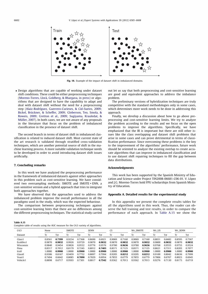
� Design algorithms that are capable of working under datasetshift conditions. These could be either preprocessing techniques(Moreno-Torres, Llorà, Goldberg, & Bhargava, in press) or algo-rithms that are designed to have the capability to adapt anddeal with dataset shift without the need for a preprocessingstep (Alaiz-Rodríguez, Guerrero-Curieses, & Cid-Sueiro, 2009;Bickel, Brückner, & Scheffer, 2009; Globerson, Teo, Smola, &Roweis, 2009; Gretton et al., 2009; Sugiyama, Krauledat, &Müller, 2007). In both cases, we are not aware of any proposalsin the literature that focus on the problem of imbalancedclassification in the presence of dataset shift.
The second branch in terms of dataset shift in imbalanced clas-sification is related to induced dataset shift. Most current state ofthe art research is validated through stratified cross-validationtechniques, which are another potential source of shift in the ma-chine learning process. A more suitable validation technique needsto be developed in order to avoid introducing dataset shift issuesartificially.
7. Concluding remarks
In this work we have analyzed the preprocessing performancein the framework of imbalanced datasets against other approachesin this problem such as cost-sensitive learning. We have consid-ered two oversampling methods: SMOTE and SMOTE + ENN, acost-sensitive version and a hybrid approach that tries to integrateboth approaches together.
We have observed that the approaches used to address theimbalanced problem improve the overall performance in all theparadigms used in the study, which was the expected behaviour.
The comparison between preprocessing techniques againstcost-sensitive learning hints that there are no differences amongthe different preprocessing techniques. The statistical study carried
out let us say that both preprocessing and cost-sensitive learningare good and equivalent approaches to address the imbalanceproblem.
The preliminary versions of hybridization techniques are trulycompetitive with the standard methodologies only in some cases,which determines more work needs to be done in addressing thisapproach.
Finally, we develop a discussion about how to go above pre-processing and cost-sensitive learning limits. We try to analyzethe problem according to the results and we focus on the openproblems to improve the algorithms. Specifically, we haveemphasized that the IR is important but there are still other is-sues like the class overlapping and dataset shift problems thatarise in some cases and can prove detrimental in terms of classi-fication performance. Since overcoming these problems is the keyto the improvement of the algorithms’ performance, future workshould be oriented to analyze the existing overlap to create accu-rate algorithms that can improve in imbalanced classification andto use dataset shift repairing techniques to fill the gap betweendata distributions.
Acknowledgments
This work has been supported by the Spanish Ministry of Edu-cation and Science under Project TIN2008-06681-C06-01. V. Lópezand J.G. Moreno-Torres hold FPU scholarships from Spanish Minis-try of Education.
Appendix A. Detailed results for the experimental study
In this appendix we present the complete results tables forall the algorithms used in this work. Thus, the reader can ob-serve the full training and test results, in order to compare theperformance of each approach. In Table A.15 we show the
Fig. 18. Example of the impact of dataset shift in imbalanced domains.
Table A.15Complete table of results using the AUC measure for the C4.5 variety of algorithms.
C4.5 None SMOTE SENN CS Wr_SMOTE Wr_US Wr_SENN
Dataset Tr Tst Tr Tst Tr Tst Tr Tst Tr Tst Tr Tst Tr Tst
Glass1 0.8561 0.7399 0.9234 0.7368 0.8690 0.6921 0.9069 0.7160 0.9069 0.7160 0.8831 0.6682 0.8595 0.7367Ecoli0vs1 0.9870 0.9832 0.9926 0.9729 0.9870 0.9832 0.9870 0.9832 0.9870 0.9832 0.9800 0.9832 0.9870 0.9832Wisconsin 0.9840 0.9454 0.9826 0.9532 0.9776 0.9576 0.9780 0.9636 0.9780 0.9636 0.9768 0.9555 0.9755 0.9524Pima 0.8317 0.7012 0.8179 0.7245 0.8012 0.7403 0.8571 0.7125 0.8571 0.7125 0.8621 0.7311 0.8203 0.7077Iris0 1.0000 0.9900 1.0000 0.9900 1.0000 0.9900 1.0000 0.9900 1.0000 0.9900 1.0000 0.9900 1.0000 0.9900Glass0 0.9306 0.8167 0.9459 0.7752 0.8897 0.7994 0.9205 0.8212 0.9205 0.8212 0.9100 0.8042 0.8636 0.7999Yeast1 0.7494 0.6642 0.8085 0.7090 0.7829 0.6954 0.7855 0.6779 0.7855 0.6779 0.7806 0.6767 0.8023 0.6945Vehicle1 0.8898 0.6717 0.9503 0.7301 0.8817 0.7542 0.9362 0.7013 0.9362 0.7013 0.9276 0.7130 0.8173 0.6719
6602 V. López et al. / Expert Systems with Applications 39 (2012) 6585–6608

Table A.15 (continued)
C4.5 None SMOTE SENN CS Wr_SMOTE Wr_US Wr_SENN
Dataset Tr Tst Tr Tst Tr Tst Tr Tst Tr Tst Tr Tst Tr Tst
Vehicle2 0.9905 0.9561 0.9905 0.9498 0.9848 0.9419 0.9866 0.9434 0.9866 0.9434 0.9850 0.9450 0.9811 0.9419Vehicle3 0.8588 0.6637 0.9508 0.7282 0.8914 0.7409 0.9221 0.7283 0.9221 0.7283 0.9275 0.7010 0.8569 0.6791Haberman 0.6204 0.5757 0.7124 0.6163 0.7383 0.5884 0.6380 0.5752 0.6380 0.5752 0.5879 0.5476 0.6417 0.5396Glass0123vs456 0.9671 0.9155 0.9868 0.9232 0.9635 0.9240 0.9806 0.8777 0.9806 0.8777 0.9783 0.8931 0.9513 0.9108Vehicle0 0.9863 0.9296 0.9878 0.9188 0.9724 0.9072 0.9861 0.9289 0.9861 0.9289 0.9799 0.9373 0.9752 0.9178Ecoli1 0.9329 0.8586 0.9507 0.9105 0.9335 0.8926 0.9457 0.9114 0.9457 0.9114 0.9394 0.9017 0.9368 0.9065New-thyroid2 0.9679 0.9373 0.9922 0.9659 0.9817 0.9774 0.9903 0.9802 0.9903 0.9802 0.9868 0.9437 0.9744 0.9063New-thyroid1 0.9607 0.9143 0.9879 0.9631 0.9944 0.9889 0.9903 0.9746 0.9903 0.9746 0.9882 0.9746 0.9774 0.9405Ecoli2 0.9297 0.8641 0.9738 0.8811 0.9716 0.8976 0.9594 0.8905 0.9594 0.8905 0.9515 0.8641 0.9473 0.8580Segment0 0.9932 0.9826 0.9986 0.9927 0.9989 0.9916 0.9988 0.9919 0.9988 0.9919 0.9967 0.9894 0.9940 0.9876Glass6 0.9347 0.8132 0.9872 0.8842 0.9851 0.9203 0.9865 0.8896 0.9865 0.8896 0.9878 0.8923 0.9369 0.9365Yeast3 0.9237 0.8597 0.9607 0.8905 0.9617 0.9230 0.9784 0.9117 0.9784 0.9117 0.9796 0.9096 0.9587 0.9176Ecoli3 0.8320 0.7280 0.9671 0.8123 0.9371 0.8705 0.9585 0.8326 0.9585 0.8326 0.9605 0.8452 0.9133 0.8694Page-blocks0 0.9637 0.9221 0.9848 0.9504 0.9797 0.9427 0.9903 0.9458 0.9903 0.9458 0.9894 0.9435 0.9614 0.9284Ecoli034vs5 0.9188 0.8389 0.9854 0.9000 0.9764 0.8806 0.9938 0.9250 0.9938 0.9250 0.9896 0.8972 0.9694 0.9111Yeast2vs4 0.9158 0.8307 0.9814 0.8588 0.9746 0.9042 0.9797 0.8866 0.9797 0.8866 0.9768 0.8955 0.9323 0.8291Ecoli067vs35 0.8789 0.8250 0.9781 0.8500 0.9775 0.8125 0.9875 0.8825 0.9875 0.8825 0.9869 0.8775 0.9201 0.8875Ecoli0234vs5 0.9313 0.8307 0.9897 0.8974 0.9828 0.8947 0.9966 0.8334 0.9966 0.8334 0.9835 0.7946 0.9730 0.8835Glass015vs2 0.8910 0.5011 0.9766 0.6772 0.9083 0.7957 0.9790 0.6003 0.9790 0.6003 0.9758 0.5938 0.8727 0.5508Yeast0359vs78 0.7028 0.5868 0.9490 0.7047 0.9217 0.7024 0.9715 0.6765 0.9715 0.6765 0.9556 0.6721 0.8362 0.6641Yeast02579vs368 0.8809 0.8432 0.9767 0.9143 0.9576 0.9138 0.9874 0.8996 0.9874 0.8996 0.9855 0.8896 0.9533 0.9102Yeast0256vs3789 0.7563 0.6606 0.9330 0.7951 0.9179 0.7817 0.9743 0.7846 0.9743 0.7846 0.9435 0.7403 0.8906 0.7648Ecoli046vs5 0.9368 0.8418 0.9870 0.8701 0.9836 0.8869 0.9911 0.8310 0.9911 0.8310 0.9884 0.8174 0.9543 0.7978Ecoli01vs235 0.9097 0.7136 0.9656 0.8377 0.9650 0.8332 0.9739 0.7641 0.9739 0.7641 0.9727 0.7664 0.9263 0.7532Ecoli0267vs35 0.8788 0.7752 0.9796 0.8155 0.9827 0.8179 0.9889 0.8527 0.9889 0.8527 0.9852 0.8653 0.9067 0.8577Glass04vs5 0.9940 0.9941 0.9910 0.9816 0.9910 0.9754 0.9940 0.9941 0.9940 0.9941 0.9940 0.9941 0.9940 0.9941Ecoli0346vs5 0.9118 0.8615 0.9892 0.8980 0.9885 0.8980 0.9905 0.8507 0.9905 0.8507 0.9905 0.8534 0.9579 0.7730Ecoli0347vs56 0.8600 0.7757 0.9778 0.8568 0.9568 0.8546 0.9892 0.7586 0.9898 0.7764 0.9806 0.7985 0.9384 0.8100Yeast05679vs4 0.8508 0.6802 0.9526 0.7602 0.9199 0.7802 0.9741 0.7243 0.9741 0.7243 0.9691 0.7480 0.9134 0.7804Ecoli067vs5 0.9363 0.7675 0.9875 0.8475 0.9744 0.8450 0.9888 0.8825 0.9888 0.8825 0.9869 0.8775 0.9081 0.8600Vowel0 0.9999 0.9706 0.9971 0.9505 0.9943 0.9455 0.9925 0.9422 0.9925 0.9422 0.9928 0.9311 0.9928 0.9322Glass016vs2 0.8710 0.5938 0.9716 0.6062 0.9375 0.6388 0.9829 0.6155 0.9829 0.6155 0.9807 0.5793 0.8529 0.5788Glass2 0.9350 0.7194 0.9700 0.6390 0.9280 0.7457 0.9734 0.6416 0.9734 0.6416 0.9639 0.6715 0.8669 0.6501Ecoli0147vs2356 0.8578 0.8051 0.9789 0.8277 0.9565 0.8228 0.9882 0.8772 0.9882 0.8772 0.9866 0.8788 0.9112 0.7673Led7digit02456789vs1 0.9022 0.8788 0.9225 0.8908 0.9249 0.8379 0.9203 0.8436 0.9203 0.8436 0.9178 0.8387 0.9042 0.8616Glass06vs5 0.9950 0.9950 0.9912 0.9147 0.9912 0.9647 0.9950 0.9950 0.9950 0.9950 0.9637 0.9579 0.9950 0.9950Ecoli01vs5 0.9114 0.8159 0.9886 0.7977 0.9830 0.8250 0.9778 0.8182 0.9778 0.8182 0.9858 0.8318 0.9392 0.8136Glass0146vs2 0.7879 0.6616 0.9676 0.7842 0.9042 0.7095 0.9847 0.6797 0.9847 0.6797 0.9708 0.6421 0.7930 0.6102Ecoli0147vs56 0.8842 0.8318 0.9798 0.8592 0.9610 0.8424 0.9756 0.8539 0.9756 0.8539 0.9813 0.8371 0.9468 0.7774Cleveland0vs4 0.8648 0.6878 0.9939 0.7908 0.9816 0.7605 0.9886 0.6893 0.9906 0.6823 0.9914 0.6885 0.9086 0.6795Ecoli0146vs5 0.9178 0.7885 0.9870 0.8981 0.9851 0.8981 0.9808 0.8385 0.9808 0.8385 0.9837 0.8135 0.9572 0.8212Ecoli4 0.9430 0.8437 0.9703 0.7794 0.9827 0.9044 0.9680 0.8636 0.9680 0.8636 0.9684 0.8636 0.9505 0.8386Yeast1vs7 0.7608 0.6275 0.9351 0.7003 0.9097 0.7371 0.9741 0.6139 0.9741 0.6139 0.9671 0.6794 0.8530 0.6627Shuttle0vs4 1.0000 0.9997 0.9999 0.9997 0.9999 0.9997 1.0000 0.9997 1.0000 0.9997 1.0000 1.0000 1.0000 1.0000Glass4 0.9403 0.7542 0.9901 0.8867 0.9670 0.8650 0.9104 0.8431 0.9104 0.8431 0.9340 0.8298 0.8861 0.7831Page-blocks13vs2 0.9989 0.9978 0.9975 0.9955 0.9975 0.9910 0.9989 0.9789 0.9989 0.9789 0.9977 0.9978 0.9791 0.9498Abalone9vs18 0.6907 0.5859 0.9142 0.6283 0.9058 0.7193 0.9864 0.6655 0.9864 0.6655 0.9849 0.6369 0.8515 0.7150Glass016vs5 0.9843 0.8943 0.9921 0.8129 0.9864 0.8629 0.9914 0.9886 0.9914 0.9886 0.9914 0.9886 0.9914 0.9886Shuttle2vs4 1.0000 0.9500 0.9990 0.9917 1.0000 1.0000 1.0000 1.0000 1.0000 1.0000 1.0000 1.0000 1.0000 1.0000Yeast1458vs7 0.5000 0.5000 0.9158 0.5367 0.8770 0.5563 0.9640 0.5540 0.9640 0.5540 0.9625 0.5464 0.7788 0.4943Glass5 0.9702 0.8976 0.9921 0.8805 0.9705 0.7756 0.9976 0.9427 0.9976 0.9427 0.9872 0.9854 0.8624 0.8439Yeast2vs8 0.5563 0.5250 0.9071 0.8338 0.8960 0.8197 0.9927 0.8652 0.9927 0.8652 0.9913 0.8359 0.8541 0.7978Yeast4 0.7482 0.6135 0.9071 0.7121 0.9007 0.7257 0.9722 0.7222 0.9722 0.7222 0.9700 0.6999 0.8872 0.7400Yeast1289vs7 0.6290 0.6156 0.9465 0.6832 0.9414 0.6332 0.9752 0.6769 0.9752 0.6769 0.9748 0.6973 0.7073 0.6107Yeast5 0.9453 0.8833 0.9777 0.9337 0.9820 0.9406 0.9929 0.9330 0.9929 0.9330 0.9928 0.9326 0.9743 0.9434Ecoli0137vs26 0.7953 0.7481 0.9678 0.8136 0.9660 0.8136 0.9804 0.8281 0.9804 0.8281 0.9594 0.7954 0.8907 0.8445Yeast6 0.7762 0.7115 0.9326 0.8294 0.9314 0.8270 0.9883 0.8082 0.9883 0.8082 0.9864 0.8099 0.8165 0.7311Abalone19 0.5000 0.5000 0.8550 0.5205 0.8890 0.5166 0.9839 0.5701 0.9839 0.5701 0.9835 0.5543 0.6211 0.5231
Average 0.8774 0.7902 0.9606 0.8324 0.9471 0.8390 0.9679 0.8294 0.9679 0.8296 0.9635 0.8245 0.9083 0.8145
Table A.16Complete table of results using the AUC measure for the SVM variety of algorithms.
SVM None SMOTE SENN CS Wr_SMOTE Wr_US Wr_SENN
Dataset Tr Tst Tr Tst Tr Tst Tr Tst Tr Tst Tr Tst Tr Tst
Glass1 0.5155 0.4963 0.6613 0.6179 0.6780 0.6391 0.6624 0.6264 0.5000 0.5000 0.5097 0.5000 0.6229 0.5682Ecoli0vs1 0.9675 0.9671 0.9844 0.9796 0.9811 0.9770 0.9675 0.9671 0.9844 0.9796 0.9810 0.9731 0.9828 0.9796Wisconsin 0.9728 0.9666 0.9770 0.9727 0.9794 0.9691 0.9724 0.9719 0.9653 0.9552 0.9726 0.9626 0.9777 0.9737Pima 0.7334 0.7194 0.7523 0.7348 0.7520 0.7300 0.7378 0.7289 0.6985 0.6916 0.6960 0.7116 0.7452 0.7449Iris0 1.0000 1.0000 1.0000 1.0000 1.0000 1.0000 1.0000 1.0000 1.0000 1.0000 1.0000 1.0000 1.0000 1.0000
(continued on next page)
V. López et al. / Expert Systems with Applications 39 (2012) 6585–6608 6603

Table A.16 (continued)
SVM None SMOTE SENN CS Wr_SMOTE Wr_US Wr_SENN
Dataset Tr Tst Tr Tst Tr Tst Tr Tst Tr Tst Tr Tst Tr Tst
Glass0 0.7070 0.6914 0.7716 0.7377 0.7755 0.7243 0.5215 0.5074 0.7778 0.7517 0.7778 0.7517 0.7411 0.7520Yeast1 0.5771 0.5732 0.7108 0.7100 0.7096 0.7067 0.6675 0.6749 0.5000 0.5000 0.5012 0.5000 0.6750 0.6897Vehicle1 0.7510 0.7202 0.8001 0.7742 0.8184 0.8055 0.7930 0.7546 0.6401 0.6180 0.6147 0.6076 0.7125 0.6882Vehicle2 0.9693 0.9527 0.9722 0.9601 0.9711 0.9578 0.9734 0.9571 0.9223 0.9068 0.9371 0.9070 0.9023 0.8891Vehicle3 0.7290 0.7134 0.7805 0.7613 0.8101 0.7881 0.8072 0.7904 0.4789 0.4871 0.5612 0.5753 0.6339 0.6306Haberman 0.5223 0.5036 0.6287 0.6344 0.6621 0.6332 0.5225 0.5382 0.5000 0.5000 0.5000 0.5000 0.5217 0.4996Glass0123vs456 0.9151 0.9043 0.9351 0.9050 0.9426 0.8987 0.8572 0.8445 0.8572 0.8445 0.8672 0.8445 0.9425 0.8987Vehicle0 0.9780 0.9490 0.9778 0.9632 0.9778 0.9611 0.9781 0.9493 0.9798 0.9620 0.9805 0.9653 0.9610 0.9470Ecoli1 0.8331 0.8192 0.9082 0.9062 0.9006 0.9024 0.9084 0.9062 0.6430 0.6367 0.6523 0.6535 0.8776 0.8659New-thyroid2 0.9972 0.9829 0.9965 0.9917 0.9917 0.9889 0.9972 0.9829 0.9750 0.9687 0.9802 0.9603 0.9680 0.9659New-thyroid1 0.9972 0.9829 0.9965 0.9944 0.9944 0.9861 0.9943 0.9687 0.9786 0.9516 0.9901 0.9829 0.9701 0.9603Ecoli2 0.7675 0.7351 0.9073 0.9067 0.9065 0.9050 0.5000 0.5000 0.5000 0.5000 0.5000 0.5000 0.8916 0.8805Segment0 0.9954 0.9927 0.9987 0.9955 0.9985 0.9965 0.9990 0.9965 0.9947 0.9932 0.9946 0.9932 0.9944 0.9922Glass6 0.9379 0.9198 0.9497 0.9063 0.9554 0.9009 0.8882 0.8725 0.8882 0.8725 0.8964 0.8919 0.9281 0.9032Yeast3 0.6305 0.6299 0.9056 0.8917 0.9114 0.9061 0.9057 0.8951 0.5000 0.5000 0.5000 0.5000 0.5200 0.5154Ecoli3 0.5000 0.5000 0.9037 0.8984 0.8964 0.8818 0.8222 0.7925 0.5000 0.5000 0.5855 0.5614 0.7267 0.6976Page-blocks0 0.8287 0.8218 0.9251 0.9258 0.9292 0.9273 0.9248 0.9254 0.5001 0.5004 0.4976 0.4769 0.5738 0.5828Ecoli034vs5 0.9153 0.8611 0.9271 0.8889 0.9250 0.8861 0.8750 0.8639 0.8750 0.8639 0.8847 0.8556 0.8972 0.8889Yeast2vs4 0.6691 0.6691 0.9090 0.8896 0.9084 0.8885 0.5000 0.5000 0.5000 0.5000 0.5000 0.5000 0.7408 0.7360Ecoli067vs35 0.8999 0.8525 0.9276 0.8325 0.9239 0.8350 0.8363 0.8025 0.7807 0.7050 0.8468 0.8300 0.8733 0.8275Ecoli0234vs5 0.9229 0.8667 0.9302 0.8892 0.9205 0.8892 0.8813 0.8417 0.8813 0.8417 0.8834 0.8140 0.9292 0.8696Glass015vs2 0.5000 0.5000 0.5943 0.5094 0.5961 0.5191 0.5000 0.5000 0.5000 0.5000 0.5000 0.5000 0.5000 0.5000Yeast0359vs78 0.6067 0.6067 0.7476 0.7451 0.7522 0.7450 0.5000 0.5000 0.5000 0.5000 0.5000 0.5000 0.6067 0.6067Yeast02579vs368 0.8090 0.8006 0.9137 0.9013 0.9143 0.9069 0.5000 0.5000 0.5000 0.5000 0.5000 0.5000 0.8890 0.8981Yeast0256vs3789 0.5524 0.5486 0.8102 0.7940 0.8098 0.8018 0.5000 0.5000 0.5000 0.5000 0.5000 0.5000 0.8034 0.8000Ecoli046vs5 0.9028 0.8696 0.9213 0.8869 0.9130 0.8869 0.8875 0.8696 0.8875 0.8696 0.8806 0.8669 0.8966 0.8642Ecoli01vs235 0.8863 0.8359 0.9393 0.8505 0.9420 0.8550 0.8429 0.7805 0.8429 0.7805 0.8796 0.8582 0.9029 0.7959Ecoli0267vs35 0.8899 0.8526 0.9162 0.8255 0.9156 0.8530 0.8346 0.7851 0.8346 0.7851 0.8288 0.8251 0.8717 0.8079Glass04vs5 0.8893 0.8500 0.9638 0.9566 0.9638 0.9507 0.8893 0.9000 0.8893 0.9000 0.8983 0.9129 0.8893 0.9000Ecoli0346vs5 0.9035 0.8696 0.9191 0.8926 0.9287 0.8926 0.8688 0.8946 0.8688 0.8946 0.8743 0.8973 0.9279 0.8088Ecoli0347vs56 0.9123 0.8935 0.9219 0.9082 0.9224 0.9061 0.8550 0.8135 0.8500 0.8135 0.8545 0.8135 0.9191 0.8848Yeast05679vs4 0.5000 0.5000 0.8016 0.8075 0.7977 0.7875 0.5000 0.5000 0.5000 0.5000 0.5000 0.5000 0.7371 0.7135Ecoli067vs5 0.9094 0.8425 0.9213 0.8475 0.9238 0.8075 0.8500 0.7450 0.8500 0.7450 0.8775 0.8325 0.9013 0.9125Vowel0 0.9096 0.8950 0.9793 0.9622 0.9795 0.9622 0.8655 0.8461 0.9432 0.9244 0.9420 0.9172 0.9477 0.9489Glass016vs2 0.5000 0.5000 0.6462 0.5336 0.6520 0.5267 0.5000 0.5000 0.5000 0.5000 0.5000 0.5000 0.5000 0.5000Glass2 0.5000 0.5000 0.6883 0.6155 0.6852 0.6905 0.7051 0.5953 0.5000 0.5000 0.5000 0.5000 0.5000 0.5000Ecoli0147vs2356 0.8635 0.8434 0.8973 0.8828 0.9060 0.8727 0.7801 0.7267 0.7801 0.7267 0.7882 0.7101 0.8885 0.8568Led7digit02456789vs1 0.9051 0.8901 0.8981 0.8851 0.8850 0.8891 0.5000 0.5000 0.5000 0.5000 0.5000 0.5000 0.9027 0.8272Glass06vs5 0.7071 0.6500 0.9520 0.9437 0.9520 0.9437 0.6929 0.6500 0.6929 0.6500 0.8262 0.6245 0.6929 0.6500Ecoli01vs5 0.9273 0.8364 0.9648 0.8364 0.9608 0.8364 0.8813 0.7909 0.8813 0.7909 0.8864 0.7909 0.9403 0.8864Glass0146vs2 0.5000 0.5000 0.6631 0.6121 0.6729 0.6310 0.5000 0.5000 0.5000 0.5000 0.5000 0.5000 0.5000 0.5000Ecoli0147vs56 0.9080 0.8719 0.9181 0.8612 0.9205 0.8546 0.8400 0.7967 0.8400 0.7967 0.8742 0.8335 0.8984 0.8519Cleveland0vs4 0.9403 0.7483 0.9619 0.8785 0.9627 0.9149 0.9318 0.7483 0.9318 0.7483 0.9503 0.7483 0.8966 0.8014Ecoli0146vs5 0.8798 0.8635 0.9269 0.8904 0.9404 0.8808 0.8438 0.7923 0.8438 0.7923 0.8620 0.8154 0.8865 0.8654Ecoli4 0.5875 0.5750 0.9743 0.9200 0.9739 0.9200 0.9834 0.9529 0.5000 0.5000 0.5000 0.5000 0.6313 0.6000Yeast1vs7 0.5000 0.5000 0.7746 0.7861 0.7664 0.7741 0.5000 0.5000 0.5000 0.5000 0.5000 0.5000 0.5000 0.5000Shuttle0vs4 1.0000 1.0000 1.0000 0.9960 1.0000 1.0000 1.0000 1.0000 1.0000 1.0000 1.0000 0.9960 1.0000 1.0000Glass4 0.6157 0.5592 0.9546 0.9576 0.9621 0.9101 0.9615 0.9126 0.6064 0.5617 0.5964 0.5592 0.7529 0.6733Page-blocks13vs2 0.8896 0.8332 0.9654 0.9561 0.9654 0.9640 0.8513 0.8566 0.6777 0.7757 0.6654 0.6325 0.7104 0.6738Abalone9vs18 0.5029 0.5000 0.8161 0.8127 0.8257 0.8128 0.8352 0.8740 0.5000 0.5000 0.5000 0.5000 0.5000 0.5000Glass016vs5 0.5839 0.4971 0.9536 0.9429 0.9521 0.9457 0.5554 0.5000 0.5554 0.5000 0.6346 0.5886 0.5825 0.5471Shuttle2vs4 1.0000 1.0000 1.0000 1.0000 1.0000 1.0000 1.0000 1.0000 1.0000 1.0000 0.9990 0.9960 1.0000 1.0000Yeast1458vs7 0.5000 0.5000 0.6926 0.6373 0.7032 0.6266 0.5000 0.5000 0.5000 0.5000 0.5000 0.5000 0.5000 0.5000Glass5 0.5554 0.5000 0.9518 0.9512 0.9488 0.9415 0.9713 0.9732 0.5554 0.5000 0.5554 0.5500 0.5143 0.5000Yeast2vs8 0.7739 0.7739 0.8201 0.7663 0.8183 0.7642 0.8223 0.7664 0.5500 0.5739 0.5500 0.5739 0.7739 0.7739Yeast4 0.5000 0.5000 0.8571 0.8241 0.8560 0.8258 0.8604 0.8155 0.5000 0.5000 0.5000 0.5000 0.5000 0.5000Yeast1289vs7 0.5000 0.5000 0.7401 0.7194 0.7455 0.7077 0.5000 0.5000 0.5000 0.5000 0.5000 0.5000 0.5000 0.5000Yeast5 0.5000 0.5000 0.9641 0.9653 0.9642 0.9628 0.9648 0.9656 0.5000 0.5000 0.5000 0.5000 0.5000 0.5000Ecoli0137vs26 0.8733 0.8500 0.9571 0.7990 0.9521 0.8044 0.8733 0.8500 0.8733 0.8500 0.8720 0.8481 0.8553 0.8463Yeast6 0.5000 0.5000 0.8886 0.8730 0.8867 0.8696 0.8807 0.8758 0.5000 0.5000 0.5000 0.5000 0.5000 0.5000Abalone19 0.5000 0.5000 0.8039 0.7930 0.8150 0.7873 0.8170 0.7615 0.5000 0.5000 0.5000 0.5000 0.5000 0.5000
Average 0.7563 0.7341 0.8806 0.8514 0.8826 0.8517 0.7869 0.7651 0.6981 0.6820 0.7077 0.6895 0.7656 0.7461
Table A.17Complete table of results using the AUC measure for the FH-GBML variety of algorithms.
FH-GBML None SMOTE SENN CS Wr_SMOTE Wr_US Wr_SENN
Dataset Tr Tst Tr Tst Tr Tst Tr Tst Tr Tst Tr Tst Tr Tst
Glass1 0.8103 0.7199 0.8194 0.7313 0.8220 0.7331 0.8270 0.7414 0.8263 0.6852 0.8278 0.6964 0.8192 0.7540Ecoli0vs1 0.9958 0.9762 0.9926 0.9627 0.9837 0.9532 0.9942 0.9765 0.9959 0.9729 0.9928 0.9550 0.9878 0.9698isconsin 0.9818 0.9620 0.9811 0.9638 0.9785 0.9720 0.9828 0.9780 0.9841 0.9704 0.9829 0.9704 0.9739 0.9507
6604 V. López et al. / Expert Systems with Applications 39 (2012) 6585–6608
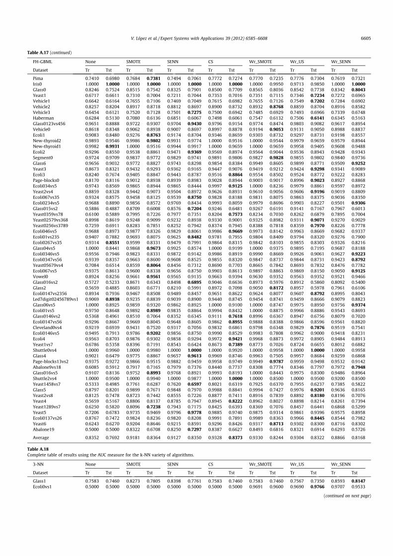
Table A.17 (continued)
FH-GBML None SMOTE SENN CS Wr_SMOTE Wr_US Wr_SENN
Dataset Tr Tst Tr Tst Tr Tst Tr Tst Tr Tst Tr Tst Tr Tst
Pima 0.7410 0.6980 0.7684 0.7381 0.7494 0.7061 0.7772 0.7274 0.7770 0.7235 0.7776 0.7304 0.7619 0.7321Iris0 1.0000 1.0000 1.0000 1.0000 1.0000 1.0000 1.0000 1.0000 1.0000 0.9950 0.9713 0.9850 1.0000 1.0000Glass0 0.8246 0.7524 0.8515 0.7542 0.8325 0.7901 0.8500 0.7709 0.8565 0.8036 0.8542 0.7738 0.8342 0.8043Yeast1 0.6717 0.6611 0.7310 0.7004 0.7211 0.7044 0.7353 0.7016 0.7351 0.7115 0.7346 0.7234 0.7272 0.6965Vehicle1 0.6642 0.6164 0.7655 0.7106 0.7469 0.7049 0.7615 0.6982 0.7655 0.7126 0.7549 0.7202 0.7284 0.6902Vehicle2 0.8257 0.8204 0.8917 0.8718 0.8812 0.8697 0.8900 0.8732 0.8932 0.8768 0.8859 0.8704 0.8916 0.8582Vehicle3 0.6454 0.6121 0.7520 0.7128 0.7501 0.7275 0.7500 0.6942 0.7485 0.6929 0.7493 0.6966 0.7339 0.6748Haberman 0.6284 0.5130 0.7080 0.6136 0.6851 0.6067 0.7498 0.6061 0.7547 0.6132 0.7506 0.6141 0.6345 0.5163Glass0123vs456 0.9651 0.8888 0.9722 0.9307 0.9704 0.9430 0.9796 0.9154 0.9774 0.8474 0.9803 0.9082 0.9617 0.8954Vehicle0 0.8618 0.8348 0.9062 0.8938 0.9007 0.8697 0.8997 0.8878 0.9194 0.9053 0.9131 0.9050 0.8988 0.8837Ecoli1 0.9083 0.8480 0.9276 0.8763 0.9174 0.8704 0.9346 0.8659 0.9303 0.8732 0.9297 0.8731 0.9198 0.8557New-thyroid2 0.9893 0.9546 0.9986 0.9802 0.9931 0.9774 1.0000 0.9516 1.0000 0.9544 0.9979 0.9659 0.9579 0.8944New-thyroid1 0.9982 0.9931 1.0000 0.9516 0.9944 0.9917 1.0000 0.9659 1.0000 0.9659 0.9958 0.9405 0.9608 0.9488Ecoli2 0.9296 0.8550 0.9538 0.8861 0.9471 0.9369 0.9569 0.8974 0.9564 0.9044 0.9536 0.8943 0.9428 0.9343Segment0 0.9724 0.9709 0.9837 0.9772 0.9829 0.9741 0.9891 0.9806 0.9827 0.9828 0.9855 0.9802 0.9840 0.9736Glass6 0.9656 0.9032 0.9772 0.8827 0.9743 0.8298 0.9854 0.8384 0.9949 0.8605 0.9899 0.8771 0.9509 0.9252Yeast3 0.8673 0.8321 0.9432 0.9293 0.9362 0.9165 0.9447 0.9076 0.9419 0.9212 0.9424 0.9298 0.9341 0.9089Ecoli3 0.8240 0.7674 0.9405 0.8847 0.9443 0.8787 0.9516 0.8864 0.9554 0.8502 0.9524 0.8772 0.9222 0.8283Page-blocks0 0.8170 0.8116 0.9012 0.8938 0.8939 0.8983 0.9028 0.8944 0.9003 0.9017 0.8996 0.9023 0.8927 0.8868Ecoli034vs5 0.9743 0.8569 0.9865 0.8944 0.9865 0.8444 0.9997 0.9125 1.0000 0.8236 0.9979 0.8861 0.9597 0.8972Yeast2vs4 0.8859 0.8328 0.9442 0.9073 0.9504 0.8972 0.9626 0.8931 0.9610 0.9056 0.9606 0.9196 0.9019 0.8809Ecoli067vs35 0.9324 0.8575 0.9458 0.8125 0.9539 0.8750 0.9828 0.8188 0.9831 0.8075 0.9863 0.8375 0.9036 0.8350Ecoli0234vs5 0.9688 0.8890 0.9856 0.8572 0.9769 0.8434 0.9993 0.8059 0.9979 0.8696 0.9903 0.8227 0.9501 0.9306Glass015vs2 0.5886 0.4887 0.8709 0.6008 0.8576 0.7204 0.9246 0.6481 0.9267 0.6191 0.9141 0.7167 0.7967 0.6013Yeast0359vs78 0.6100 0.5889 0.7995 0.7226 0.7977 0.7351 0.8204 0.7573 0.8234 0.7030 0.8262 0.6879 0.7895 0.7004Yeast02579vs368 0.8998 0.8619 0.9248 0.9099 0.9232 0.8938 0.9330 0.9001 0.9325 0.8982 0.9311 0.9071 0.9270 0.9029Yeast0256vs3789 0.7259 0.6911 0.8283 0.7851 0.8252 0.7942 0.8374 0.7945 0.8388 0.7818 0.8359 0.7970 0.8226 0.7778Ecoli046vs5 0.9688 0.8973 0.9877 0.8326 0.9829 0.8061 0.9986 0.9669 0.9973 0.8142 0.9963 0.8669 0.9682 0.9337Ecoli01vs235 0.9407 0.7882 0.9693 0.8075 0.9625 0.8482 0.9781 0.7955 0.9804 0.8409 0.9794 0.8320 0.9276 0.7900Ecoli0267vs35 0.9314 0.8551 0.9599 0.8331 0.9479 0.7991 0.9864 0.8315 0.9842 0.8103 0.9855 0.8303 0.9326 0.8216Glass04vs5 1.0000 0.8441 0.9868 0.9673 0.9925 0.8574 1.0000 0.9199 1.0000 0.9375 0.9895 0.7195 0.9687 0.8188Ecoli0346vs5 0.9556 0.7946 0.9823 0.8331 0.9872 0.9142 0.9986 0.8919 0.9990 0.8669 0.9926 0.9061 0.9627 0.9223Ecoli0347vs56 0.9339 0.8357 0.9663 0.8600 0.9608 0.8525 0.9855 0.8320 0.9847 0.8737 0.9844 0.8731 0.9423 0.8792Yeast05679vs4 0.7084 0.6514 0.8559 0.8064 0.8456 0.7312 0.8690 0.7703 0.8665 0.7842 0.8693 0.7832 0.8476 0.7782Ecoli067vs5 0.9375 0.8613 0.9600 0.8338 0.9656 0.8750 0.9903 0.8613 0.9897 0.8863 0.9869 0.8150 0.9050 0.9125Vowel0 0.8924 0.8256 0.9661 0.9561 0.9565 0.9135 0.9663 0.9394 0.9630 0.9352 0.9563 0.9352 0.9521 0.9466Glass016vs2 0.5727 0.5233 0.8671 0.6343 0.8498 0.6895 0.9046 0.6636 0.8973 0.5976 0.8912 0.5860 0.8092 0.5400Glass2 0.5659 0.4885 0.8603 0.6771 0.8210 0.5991 0.8972 0.7098 0.9050 0.8172 0.8957 0.5978 0.7961 0.6106Ecoli0147vs2356 0.8934 0.7936 0.9467 0.8508 0.9489 0.8457 0.9651 0.8622 0.9624 0.8077 0.9607 0.8792 0.8995 0.8043Led7digit02456789vs1 0.9069 0.8938 0.9235 0.8839 0.9039 0.8900 0.9440 0.8745 0.9454 0.8741 0.9459 0.8666 0.9079 0.8823Glass06vs5 1.0000 0.8925 0.9859 0.9320 0.9862 0.8925 1.0000 0.9100 1.0000 0.8747 0.9975 0.8950 0.9756 0.9374Ecoli01vs5 0.9750 0.8648 0.9892 0.8989 0.9835 0.8864 0.9994 0.8432 1.0000 0.8875 0.9966 0.8886 0.9543 0.8693Glass0146vs2 0.5368 0.4961 0.8510 0.7064 0.8352 0.6345 0.9111 0.7618 0.8996 0.6367 0.8947 0.6756 0.8079 0.7020Ecoli0147vs56 0.9296 0.8667 0.9669 0.8045 0.9648 0.8605 0.9862 0.8955 0.9888 0.8388 0.9866 0.8596 0.9561 0.8820Cleveland0vs4 0.9219 0.6939 0.9431 0.7520 0.9317 0.7056 0.9832 0.6861 0.9798 0.6348 0.9829 0.7876 0.9519 0.7541Ecoli0146vs5 0.9495 0.7913 0.9786 0.9202 0.9856 0.8750 0.9990 0.8529 0.9983 0.7808 0.9962 0.9000 0.9418 0.8231Ecoli4 0.9563 0.8703 0.9876 0.9302 0.9858 0.9294 0.9972 0.9421 0.9968 0.8873 0.9972 0.8905 0.9484 0.8913Yeast1vs7 0.6786 0.5358 0.8396 0.7191 0.8543 0.6424 0.8673 0.7389 0.8773 0.7026 0.8724 0.6655 0.8012 0.6882Shuttle0vs4 1.0000 0.9960 1.0000 0.9980 1.0000 1.0000 1.0000 0.9920 1.0000 0.9958 1.0000 1.0000 1.0000 0.9958Glass4 0.9021 0.6479 0.9775 0.8867 0.9657 0.9613 0.9969 0.8746 0.9963 0.7505 0.9957 0.8684 0.9259 0.6868Page-blocks13vs2 0.9375 0.9272 0.9866 0.9515 0.9882 0.9459 0.9958 0.9749 0.9949 0.9787 0.9959 0.9498 0.9532 0.9142Abalone9vs18 0.6085 0.5912 0.7917 0.7165 0.7979 0.7376 0.8440 0.7737 0.8308 0.7774 0.8346 0.7797 0.7972 0.7948Glass016vs5 0.9107 0.8136 0.9752 0.8993 0.9768 0.8921 0.9993 0.8193 1.0000 0.8443 0.9975 0.8300 0.9486 0.8964Shuttle2vs4 1.0000 0.9500 1.0000 0.9940 1.0000 0.9877 1.0000 1.0000 1.0000 0.8500 1.0000 0.9500 0.9200 0.8500Yeast1458vs7 0.5333 0.4985 0.7761 0.6287 0.7620 0.6597 0.8021 0.6319 0.7925 0.6370 0.7955 0.6237 0.7385 0.5822Glass5 0.8797 0.8201 0.9899 0.7671 0.9848 0.7970 0.9988 0.8841 0.9994 0.7427 0.9976 0.9201 0.9636 0.8165Yeast2vs8 0.8125 0.7478 0.8723 0.7442 0.8555 0.7226 0.8877 0.7411 0.8916 0.7839 0.8892 0.8180 0.8196 0.7076Yeast4 0.5659 0.5167 0.8806 0.8137 0.8785 0.7947 0.8945 0.8222 0.8962 0.8027 0.8898 0.8214 0.8261 0.7394Yeast1289vs7 0.6250 0.5820 0.8096 0.7238 0.7943 0.7175 0.8425 0.6393 0.8369 0.7076 0.8457 0.6441 0.6868 0.5299Yeast5 0.7206 0.6783 0.9735 0.9469 0.9796 0.9778 0.9885 0.9740 0.9875 0.9314 0.9861 0.9396 0.9575 0.8958Ecoli0137vs26 0.8767 0.7472 0.9824 0.8236 0.9820 0.8208 0.9991 0.7891 0.9989 0.8363 0.9966 0.8445 0.8544 0.7982Yeast6 0.6243 0.6270 0.9204 0.8646 0.9215 0.8591 0.9296 0.8426 0.9317 0.8713 0.9302 0.8300 0.8716 0.8302Abalone19 0.5000 0.5000 0.8322 0.6708 0.8250 0.7297 0.8387 0.6627 0.8493 0.6816 0.8321 0.6914 0.6293 0.5726
Average 0.8352 0.7692 0.9181 0.8364 0.9127 0.8350 0.9328 0.8373 0.9330 0.8244 0.9304 0.8322 0.8866 0.8168
Table A.18Complete table of results using the AUC measure for the k-NN variety of algorithms.
3-NN None SMOTE SENN CS Wr_SMOTE Wr_US Wr_SENN
Dataset Tr Tst Tr Tst Tr Tst Tr Tst Tr Tst Tr Tst Tr Tst
Glass1 0.7583 0.7460 0.8273 0.7805 0.8398 0.7761 0.7583 0.7460 0.7583 0.7460 0.7567 0.7350 0.8593 0.8147Ecoli0vs1 0.5000 0.5000 0.5000 0.5000 0.5000 0.5000 0.5000 0.5000 0.9691 0.9600 0.9690 0.9766 0.9707 0.9533
(continued on next page)
V. López et al. / Expert Systems with Applications 39 (2012) 6585–6608 6605

results for the C4.5 algorithm versions. Next, the results forthe SVM versions used in the study are shown in Table A.16.Later, the results for the FH-GBML algorithm versions arepresented in Table A.17. Finally, Table A.18 show the averageresults for each dataset for the 3-NN algorithm. We stress inboldface the best results achieved by a version.
References
Akbani, R., Kwek, S., & Japkowicz, N. (2004). Applying support vector machines toimbalanced datasets. In ECML (pp. 39–50).
Alaiz-Rodríguez, R., Guerrero-Curieses, A., & Cid-Sueiro, J. (2009).Improving classification under changes in class and within-classdistributions. In IWANN’09: Proceedings of the 10th international work-
Table A.18 (continued)
3-NN None SMOTE SENN CS Wr_SMOTE Wr_US Wr_SENN
Dataset Tr Tst Tr Tst Tr Tst Tr Tst Tr Tst Tr Tst Tr Tst
Wisconsin 0.9636 0.9658 0.0214 0.9698 0.0209 0.9729 0.9636 0.9658 0.9636 0.9658 0.9641 0.9658 0.9647 0.9658Pima 0.6686 0.6703 0.7479 0.6865 0.7682 0.7099 0.6686 0.6703 0.6686 0.6703 0.6696 0.6711 0.7986 0.7297Iris0 1.0000 1.0000 1.0000 1.0000 1.0000 1.0000 1.0000 1.0000 1.0000 1.0000 0.9988 1.0000 1.0000 1.0000Glass0 0.8144 0.8027 0.8184 0.8185 0.8299 0.8361 0.7884 0.7771 0.7884 0.7771 0.7529 0.7670 0.8025 0.7809Yeast1 0.6559 0.6539 0.7864 0.6772 0.7734 0.7071 0.6740 0.6858 0.6740 0.6858 0.6745 0.6841 0.7772 0.7190Vehicle1 0.6741 0.6314 0.8454 0.6985 0.8230 0.7752 0.7665 0.7476 0.7665 0.7476 0.7664 0.7474 0.7781 0.7472Vehicle2 0.9743 0.9736 0.9753 0.9692 0.9690 0.9620 0.9578 0.9541 0.9578 0.9541 0.8942 0.8960 0.9635 0.9519Vehicle3 0.6395 0.6529 0.8539 0.7085 0.8291 0.7636 0.7365 0.7355 0.7365 0.7355 0.7367 0.7355 0.7416 0.7474Haberman 0.5463 0.5310 0.6955 0.5633 0.6906 0.5767 0.6167 0.6510 0.6167 0.6510 0.6100 0.6516 0.6546 0.5729Glass0123vs456 0.8859 0.8888 0.9709 0.9164 0.9620 0.9334 0.9424 0.9331 0.9424 0.9331 0.9338 0.9399 0.9407 0.9199Vehicle0 0.9446 0.9379 0.9548 0.9471 0.9493 0.9415 0.9473 0.9461 0.9473 0.9461 0.9371 0.9363 0.9535 0.9479Ecoli1 0.7693 0.7636 0.8484 0.8085 0.8345 0.8089 0.8019 0.8036 0.8789 0.8749 0.8721 0.8730 0.9165 0.9065New-thyroid2 0.9508 0.9373 0.9889 0.9889 0.9875 0.9861 0.9831 0.9917 0.9831 0.9917 0.9854 0.9833 0.9688 0.9516New-thyroid1 0.9401 0.9659 0.9917 0.9889 0.9889 0.9861 0.9831 0.9917 0.9831 0.9917 0.9818 0.9806 0.9816 0.9631Ecoli2 0.8253 0.8302 0.8674 0.8382 0.8622 0.8276 0.8307 0.8276 0.9102 0.9154 0.9082 0.9066 0.9396 0.9294Segment0 0.5000 0.5000 0.5000 0.5000 0.5000 0.5000 0.5000 0.5000 0.9970 0.9980 0.9941 0.9937 0.9977 0.9962Glass6 0.9147 0.9140 0.9824 0.9419 0.9770 0.9338 0.9366 0.9419 0.9366 0.9419 0.9305 0.9365 0.9286 0.9419Yeast3 0.8231 0.8171 0.9541 0.8681 0.9470 0.8634 0.8827 0.8777 0.8827 0.8777 0.8859 0.8803 0.9300 0.8824Ecoli3 0.6798 0.6598 0.8514 0.7283 0.8443 0.7772 0.7766 0.7502 0.8432 0.8209 0.8428 0.8478 0.8932 0.8863Page-blocks0 0.9040 0.9075 0.9796 0.9326 0.9748 0.9316 0.9409 0.9370 0.9409 0.9370 0.9409 0.9370 0.9530 0.9193Ecoli034vs5 0.8306 0.8222 0.8813 0.8222 0.8813 0.8222 0.8556 0.8361 0.9389 0.9333 0.9389 0.9222 0.9535 0.9167Yeast2vs4 0.7485 0.7368 0.8573 0.8073 0.8554 0.8073 0.7903 0.7938 0.8680 0.8771 0.8677 0.8771 0.9128 0.8803Ecoli067vs35 0.7109 0.7625 0.8531 0.8200 0.8525 0.8150 0.7724 0.8550 0.8563 0.8900 0.8623 0.8800 0.8627 0.8275Ecoli0234vs5 0.8125 0.8500 0.8746 0.8530 0.8746 0.8530 0.8328 0.8612 0.9294 0.9308 0.9329 0.9280 0.9446 0.9336Glass015vs2 0.5943 0.5788 0.8637 0.6750 0.8637 0.6935 0.7036 0.7097 0.7036 0.7097 0.7073 0.6685 0.7225 0.6067Yeast0359vs78 0.6522 0.6468 0.8736 0.7247 0.8733 0.7203 0.6762 0.6923 0.6762 0.6923 0.6852 0.6979 0.8005 0.6977Yeast02579vs368 0.8845 0.8834 0.9507 0.9024 0.9506 0.9013 0.8970 0.8988 0.8970 0.8988 0.8852 0.8922 0.9269 0.9082Yeast0256vs3789 0.7580 0.7658 0.9066 0.7728 0.9066 0.7655 0.8096 0.7916 0.8096 0.7916 0.8087 0.7861 0.8407 0.7836Ecoli046vs5 0.9111 0.9250 0.9781 0.9282 0.9754 0.9282 0.9328 0.9365 0.9328 0.9365 0.9172 0.9450 0.9335 0.9392Ecoli01vs235 0.7733 0.7700 0.8705 0.7936 0.8705 0.7936 0.8099 0.7850 0.8926 0.8827 0.8973 0.8959 0.9181 0.8564Ecoli0267vs35 0.7263 0.7725 0.8629 0.8401 0.8604 0.8327 0.7745 0.8026 0.8516 0.8526 0.8491 0.8677 0.8566 0.8150Glass04vs5 0.8702 0.9441 0.9412 0.9632 0.9397 0.9511 0.9789 0.9941 0.9789 0.9941 0.9517 0.9761 0.9789 0.9941Ecoli0346vs5 0.8368 0.8000 0.8791 0.8169 0.8791 0.8169 0.8434 0.8419 0.9282 0.9419 0.9096 0.9095 0.9329 0.9446Ecoli0347vs56 0.7925 0.7735 0.8623 0.7920 0.5000 0.5000 0.8263 0.8363 0.9109 0.9119 0.9089 0.9212 0.9317 0.9227Yeast05679vs4 0.6288 0.6257 0.8954 0.7440 0.8978 0.7682 0.7443 0.7968 0.7443 0.7968 0.7383 0.7915 0.8557 0.7825Ecoli067vs5 0.8031 0.8225 0.9500 0.8375 0.9456 0.8250 0.8769 0.8675 0.8769 0.8675 0.8750 0.8825 0.8863 0.8600Vowel0 0.9915 0.9939 0.9999 0.9994 0.9999 0.9994 0.9975 0.9994 0.9975 0.9994 0.9808 0.9800 0.9975 0.9994Glass016vs2 0.5629 0.6357 0.8800 0.7169 0.8771 0.6445 0.7477 0.7893 0.7477 0.7893 0.7640 0.7864 0.7982 0.7560Glass2 0.5474 0.5302 0.9150 0.7162 0.8984 0.7717 0.6969 0.6954 0.6969 0.6954 0.7254 0.7334 0.8470 0.6733Ecoli0147vs2356 0.7838 0.7968 0.8605 0.7959 0.8609 0.7959 0.8160 0.8272 0.8969 0.9057 0.8907 0.9041 0.9262 0.9170Led7digit02456789vs1 0.7696 0.7747 0.8618 0.8215 0.8642 0.8465 0.8261 0.8297 0.8261 0.8297 0.8311 0.8223 0.9018 0.8639Glass06vs5 0.8725 0.9500 0.9786 0.9847 0.9786 0.9847 0.9240 1.0000 0.9240 1.0000 0.9205 0.9400 0.9383 1.0000Ecoli01vs5 0.8932 0.9000 0.9739 0.9023 0.9733 0.9023 0.9216 0.9136 0.9216 0.9136 0.9239 0.9068 0.9312 0.9159Glass0146vs2 0.5302 0.5727 0.8903 0.7019 0.8923 0.7018 0.6940 0.7567 0.6940 0.7567 0.7339 0.7458 0.7404 0.6447Ecoli0147vs56 0.8793 0.8551 0.9666 0.9139 0.9601 0.9025 0.9221 0.9189 0.9221 0.9189 0.9238 0.9156 0.9340 0.9254Cleveland0vs4 0.7726 0.7136 0.9320 0.8346 0.9320 0.8346 0.8487 0.8584 0.8487 0.8584 0.8448 0.8553 0.8727 0.8583Ecoli0146vs5 0.9058 0.9231 0.9740 0.9019 0.9745 0.9000 0.9168 0.9135 0.9168 0.9135 0.9159 0.9250 0.9197 0.9192Ecoli4 0.8238 0.7734 0.8865 0.8421 0.8846 0.8108 0.8366 0.8187 0.9163 0.9155 0.9217 0.9107 0.9281 0.9202Yeast1vs7 0.6153 0.6109 0.8802 0.7390 0.8811 0.6998 0.7170 0.7453 0.7170 0.7453 0.7175 0.7406 0.8039 0.6177Shuttle0vs4 0.9959 0.9960 1.0000 0.9960 1.0000 0.9960 0.9959 0.9960 0.9959 0.9960 0.9959 1.0000 0.9959 0.9960Glass4 0.7628 0.8425 0.9689 0.8917 0.9627 0.9151 0.8885 0.8868 0.8885 0.8868 0.8835 0.8868 0.8912 0.8843Page-blocks13vs2 0.9724 0.9433 0.9963 0.9978 0.9963 0.9989 0.9963 0.9977 0.9963 0.9977 0.9859 0.9888 0.9972 0.9977Abalone9vs18 0.5987 0.6332 0.9099 0.7525 0.9023 0.7416 0.6990 0.7637 0.7998 0.7334 0.8097 0.7408 0.7117 0.6482Glass016vs5 0.9121 0.8971 0.9686 0.9271 0.9664 0.9186 0.9871 0.9857 0.9871 0.9857 0.9757 0.9686 0.9850 0.9857Shuttle2vs4 0.8750 0.9500 0.9959 1.0000 0.9959 1.0000 0.9600 0.9500 0.9600 0.9500 0.9078 0.9140 0.9600 0.9500Yeast1458vs7 0.5163 0.5144 0.8852 0.6944 0.8812 0.6929 0.6249 0.6609 0.6249 0.6609 0.6228 0.6654 0.6719 0.5729Glass5 0.8439 0.8976 0.9780 0.9378 0.9689 0.9732 0.9717 0.9329 0.9717 0.9329 0.9799 0.9256 0.9580 0.9280east2vs8 0.7236 0.7239 0.9656 0.7208 0.9608 0.7371 0.7930 0.8012 0.7930 0.8012 0.7846 0.8012 0.8131 0.7631Yeast4 0.5966 0.5947 0.9594 0.7444 0.9520 0.7571 0.7281 0.7489 0.7281 0.7489 0.7279 0.7489 0.8787 0.7708Yeast1289vs7 0.5520 0.5484 0.9185 0.6586 0.9170 0.6764 0.6677 0.6462 0.6677 0.6462 0.6671 0.6629 0.7135 0.6154Yeast5 0.8056 0.8128 0.9836 0.9503 0.9812 0.9566 0.9357 0.9424 0.9357 0.9424 0.9394 0.9389 0.9530 0.9174Ecoli0137vs26 0.7730 0.7982 0.8680 0.7691 0.5000 0.5000 0.7607 0.7800 0.8361 0.8281 0.8293 0.8244 0.8516 0.8445Yeast6 0.7570 0.7527 0.9720 0.8442 0.9676 0.8540 0.8145 0.8368 0.8145 0.8368 0.8198 0.8497 0.8890 0.8678Abalone19 0.4998 0.4998 0.9780 0.5216 0.9737 0.5205 0.5402 0.5184 0.7576 0.5193 0.7573 0.5357 0.6215 0.5114
Average 0.7697 0.7752 0.8880 0.8212 0.8743 0.8166 0.8229 0.8295 0.8594 0.8596 0.8564 0.8561 0.8849 0.8509
6606 V. López et al. / Expert Systems with Applications 39 (2012) 6585–6608

conference on artificial neural networks (pp. 122–130). Berlin,Heidelberg: Springer.
Alaiz-Rodríguez, R., & Japkowicz, N. (2008). Assessing the impact of changingenvironments on classifier performance. In Canadian AI’08: Proceedings of theCanadian society for computational studies of intelligence, 21st conference onadvances in artificial intelligence (pp. 13–24). Berlin, Heidelberg: Springer-Verlag.
Alcalá-Fdez, J., Fernández, A., Luengo, J., Derrac, J., García, S., Sánchez, L., et al.(2011). KEEL data-mining software tool: Data set repository, integration ofalgorithms and experimental analysis framework. Journal of Multi-Valued Logicand Soft Computing, 17, 255–287.
Alcalá-Fdez, J., Sánchez, L., García, S., del Jesus, M. J., Ventura, S., Garrell, J. M., et al.(2008). Keel: A software tool to assess evolutionary algorithms for data miningproblems. Soft Computing, 13, 307–318.
Barandela, R., Sánchez, J. S., García, V., & Rangel, E. (2003). Strategies for learning inclass imbalance problems. Pattern Recognition, 36, 849–851.
Batista, G. E. A. P. A., Prati, R. C., & Monard, M. C. (2004). A study of the behaviour ofseveral methods for balancing machine learning training data. SIGKDDExplorations, 6, 20–29.
Bermejo, P., Gámez, J., & Puerta, J. (2011). Improving the performance of Naive Bayesmultinomial in e-mail foldering by introducing distribution-based balance ofdatasets. Expert Systems with Applications, 38, 2072–2080.
Bickel, S., Brückner, M., & Scheffer, T. (2009). Discriminative learning undercovariate shift. Journal of Machine Learning Research, 10, 2137–2155.
Bradford, J. P., Kunz, C., Kohavi, R., Brunk, C., & Brodley, C. E. (1998). Pruning decisiontrees with misclassification costs. In ECML (pp. 131–136).
Bradley, A. P. (1997). The use of the area under the roc curve in the evaluation ofmachine learning algorithms. Pattern Recognition, 30, 1145–1159.
Bunkhumpornpat, C., Sinapiromsaran, K., & Lursinsap, C. (2009). Safe-level-smote:Safe-level-synthetic minority over-sampling technique for handling the classimbalanced problem. In Proceedings of the 13th Pacific-Asia conference onadvances in knowledge discovery and data mining PAKDD’09 (pp. 475–482).
Quiñonero Candela, J., Sugiyama, M., Schwaighofer, A., & Lawrence, N. D. (2009).Dataset shift in machine learning. The MIT Press.
Carpenter, G. A., Grossberg, S., & Rosen, D. B. (1991). Fuzzy art: Fast stable learningand categorization of analog patterns by an adaptive resonance system. NeuralNetworks, 4, 759–771.
Chawla, N. V., Bowyer, K. W., Hall, L. O., & Kegelmeyer, W. P. (2002). SMOTE:Synthetic minority over-sampling technique. Journal of Artificial IntelligentResearch, 16, 321–357.
Chawla, N. V., Cieslak, D. A., Hall, L. O., & Joshi, A. (2008). Automatically counteringimbalance and its empirical relationship to cost. Data Mining and KnowledgeDiscovery, 17, 225–252.
Chawla, N. V., Japkowicz, N., & Kotcz, A. (2004). Editorial: Special issue on learningfrom imbalanced data sets. SIGKDD Explorations, 6, 1–6.
Chen, M.-C., Chen, L.-S., Hsu, C.-C., & Zeng, W.-R. (2008). An information granulationbased data mining approach for classifying imbalanced data. InformationSciences, 178, 3214–3227.
Chen, X., Fang, T., Huo, H., & Li, D. (2011). Graph-based feature selection for object-oriented classification in vhr airborne imagery. IEEE Transactions on Geoscienceand Remote Sensing, 49, 353–365.
Cieslak, D. A., & Chawla, N. V. (2009). A framework for monitoring classifiersperformance: When and why failure occurs? Knowledge and InformationSystems, 18, 83–108.
Cortes, C., & Vapnik, V. (1995). Support vector networks. Machine Learning, 20,273–297.
Cover, T., & Hart, P. (1967). Nearest neighbor pattern classification. IEEE Transactionson Information Theory, 13, 21–27.
Demšar, J. (2006). Statistical comparisons of classifiers over multiple data sets.Journal of Machine Learning Research, 7, 1–30.
Denil, M., & Trappenberg, T. (2010). Overlap versus imbalance. In Canadian AI 2010,LNAI (Vol. 6085, pp. 220–231).
Domingos, P. (1999). Metacost: A general method for making classifiers cost-sensitive. In Proceedings of the 5th international conference on knowledgediscovery and data mining (KDD’99) (pp. 155–164).
Ducange, P., Lazzerini, B., & Marcelloni, F. (2010). Multi-objective genetic fuzzyclassifiers for imbalanced and cost-sensitive datasets. Soft Computing, 14,713–728.
Elkan, C. (2001). The foundations of cost-sensitive learning. In Proceedings of the17th IEEE international joint conference on artificial intelligence (IJCAI’01) (pp.973–978).
Estabrooks, A., Jo, T., & Japkowicz, N. (2004). A multiple resampling method forlearning from imbalanced data sets. Computational Intelligence, 20, 18–36.
Fernández, A., García, S., del Jesus, M. J., & Herrera, F. (2008). A study of thebehaviour of linguistic fuzzy rule based classification systems in the frameworkof imbalanced data-sets. Fuzzy Sets and Systems, 159, 2378–2398.
Fernández, A., del Jesus, M. J., & Herrera, F. (2009). Hierarchical fuzzy rule basedclassification systems with genetic rule selection for imbalanced data-sets.International Journal of Approximate Reasoning, 50, 561–577.
Fernández, A., del Jesús, M. J., & Herrera, F. (2010). On the 2-tuples based genetictuning performance for fuzzy rule based classification systems in imbalanceddata-sets. Information Sciences, 180, 1268–1291.
Friedman, M. (1937). The use of ranks to avoid the assumption of normality implicitin the analysis of variance. Journal of the American Statistical Association, 32,675–701.
Gama, J. (2004). Functional trees. Machine Learning, 55, 219–250.
García, S., Fernández, A., Luengo, J., & Herrera, F. (2009). A study of statisticaltechniques and performance measures for genetics-based machine learning:Accuracy and interpretability. Soft Computing, 13, 959–977.
García, S., Fernández, A., Luengo, J., & Herrera, F. (2010). Advanced nonparametrictests for multiple comparisons in the design of experiments in computationalintelligence and data mining: Experimental analysis of power. InformationSciences, 180, 2044–2064.
García, S., & Herrera, F. (2008). An extension on ‘‘statistical comparisons ofclassifiers over multiple data sets’’ for all pairwise comparisons. Journal ofMachine Learning Research, 9, 2607–2624.
García, V., Mollineda, R., & Sánchez, J. S. (2008). On the k-NN performance in achallenging scenario of imbalance and overlapping. Pattern Analysis Applications,11, 269–280.
Globerson, A., Teo, C. H., Smola, A., & Roweis, S. (2009). An adversarial view ofcovariate shift and a minimax approach. In J. Quiñonero Candela, M. Sugiyama,A. Schwaighofer, & N. D. Lawrence (Eds.), Dataset shift in machine learning(pp. 179–198). The MIT Press.
Gretton, A., Smola, A., Huang, J., Schmittfull, M., Borgwardt, K., & Schölkopf, B.(2009). Covariate shift by kernel mean matching. In J. Quiñonero Candela, M.Sugiyama, A. Schwaighofer, & N. D. Lawrence (Eds.), Dataset shift in machinelearning (pp. 131–160). The MIT Press.
Han, H., Wang, W., & Mao, B. (2005). Borderline-SMOTE: A new over-samplingmethod in imbalanced data sets learning. In Proceedings of the internationalconference on intelligent computing (pp. 878–887).
Hand, D. J., & Vinciotti, V. (2003). Choosing k for two-class nearest neighbourclassifiers with unbalanced classes. Pattern Recognition Letters, 24,1555–1562.
He, H., Bai, Y., Garcia, E., & Li, S. (2008). ADASYN: Adaptive synthetic samplingapproach for imbalanced learning. In Proceedings of international joint conferenceon neural networks (pp. 1322–1328).
He, H., & Garcia, E. A. (2009). Learning from imbalanced data. IEEE Transactions onKnowledge and Data Engineering, 21, 1263–1284.
Ho, T., & Basu, M. (2002). Complexity measures of supervised classificationproblems. IEEE Transactions on Pattern Analysis and Machine Intelligence, 24,289–300.
Huang, J., & Ling, C. X. (2005). Using auc and accuracy in evaluating learningalgorithms – appendices. IEEE Transactions on Knowledge and Data Engineering,17.
Ishibuchi, H., & Nakashima, T. (2001). Effect of rule weights in fuzzy rule-basedclassification systems. IEEE Transactions on Fuzzy Systems, 9, 506–515.
Ishibuchi, H., & Yamamoto, T. (2005). Rule weight specification in fuzzy rule-based classification systems. IEEE Transactions on Fuzzy Systems, 13,428–435.
Ishibuchi, H., Yamamoto, T., & Nakashima, T. (2005). Hybridization of fuzzy GBMLapproaches for pattern classification problems. IEEE Transactions on System, Manand Cybernetics B, 35, 359–365.
Japkowicz, N., & Stephen, S. (2002). The class imbalance problem: A systematicstudy. Intelligent Data Analysis Journal, 6, 429–450.
Kaburlasos, V. G. (2007). Granular enhancement of fuzzy art/som neural classifiersbased on lattice theory. In Computational intelligence based on lattice theory (pp.3–23).
Kubat, M., & Matwin, S. (1997). Addressing the curse of imbalanced training sets:One-sided selection. In International conference on machine learning (pp. 179–186).
Laurikkala, J. (2001). Improving identification of difficult small classes by balancingclass distribution. In Proceedings of the conference on AI in medicine in Europe:Artificial intelligence medicine (pp. 63–66).
Ling, C. X., Yang, Q., Wang, J., & Zhang, S. (2004). Decision trees with minimal costs.In ICML.
López, V., Fernández, A., & Herrera, F. (2010). A first approach for cost-sensitiveclassification with linguistic genetic fuzzy systems in imbalanced data-sets. In10th International conference on intelligent systems design and applications, ISDA2010 (pp. 676–681).
Luengo, J., Fernández, A., García, S., & Herrera, F. (2011). Addressing data complexityfor imbalanced data sets: Analysis of SMOTE-based oversampling andevolutionary undersampling. Soft Computing, 15, 1909–1936.
Martín-Félez, R., & Mollineda, R. (2010). On the suitability of combining featureselection and resampling to manage data complexity. In CAEPIA 2009, LNAI (Vol.5988, pp. 141–150).
Moreno-Torres, J. G., & Herrera, F. (2010). A preliminary study on overlapping anddata fracture in imbalanced domains by means of genetic programming-basedfeature extraction. In Proceedings of the 10th international conference onintelligent systems design and applications (ISDA 2010) (pp. 501–506).
Moreno-Torres, J. G., Llorà, X., Goldberg, D. E., & Bhargava, R. (in press). Repairingfractures between data using genetic programming-based feature extraction: Acase study in cancer diagnosis. Information Sciences, doi:10.1016/j.ins.2010.09.018.
Orriols-Puig, A., & Bernadó-Mansilla, E. (2009). Evolutionary rule-based systems forimbalanced datasets. Soft Computing, 13, 213–225.
Prati, R. C., & Batista, G. E. A. P. A. (2004). Class imbalances versus class overlapping:An analysis of a learning system behavior. In Proceedings of Mexicaninternational conference on artificial intelligence (MICAI) (pp. 312–321).
Quinlan, J. (1993). C4.5: Programs for machine learning. Morgan Kauffman.Riddle, P., Segal, R., & Etzioni, O. (1994). Representation design and brute-force
induction in a boeing manufacturing domain. Applied Artificial Intelligence, 8,125–147.
V. López et al. / Expert Systems with Applications 39 (2012) 6585–6608 6607

Shaffer, J. (1986). Modified sequentially rejective multiple test procedures. Journalof the American Statistical Association, 81, 826–831.
Sheskin, D. (2006). Handbook of parametric and nonparametric statistical procedures.Chapman & Hall.
Shimodaira, H. (2000). Improving predictive inference under covariate shift byweighting the log-likelihood function. Journal of Statistical Planning andInference, 90, 227–244.
Sikora, M. (2011). Induction and pruning of classification rules for prediction ofmicroseismic hazards in coal mines. Expert Systems with Applications, 38,6748–6758.
Sugiyama, M., Krauledat, M., & Müller, K.-R. (2007). Covariate shift adaptation byimportance weighted cross validation. Journal of Machine Learning Research, 8,985–1005.
Sun, Y., Kamel, M. S., Wong, A. K. C., & Wang, Y. (2007). Cost-sensitive boosting forclassification of imbalanced data. Pattern Recognition, 40, 3358–3378.
Sun, Y., Wong, A. K. C., & Kamel, M. S. (2009). Classification of imbalanced data: Areview. International Journal of Pattern Recognition and Artificial Intelligence, 23,687–719.
Ting, K. M. (2002). An instance-weighting method to induce cost-sensitive trees.IEEE Transactions on Knowledge and Data Engineering, 14, 659–665.
Vapnik, V. (1998). Statistical learning theory. New York, USA: Wiley.Vapnik, V., & Lerner, A. (1963). Pattern recognition using generalized portrait
method. Automation and Remote Control, 24.Veropoulos, K., Campbell, C., & Cristianini, N. (1999). Controlling the sensitivity of
support vector machines. In Proceedings of the international joint conference on AI(pp. 55–60).
Villar, P., Fernández, A., & Herrera, F. (2010). A genetic algorithm for featureselection and granularity learning in fuzzy rule-based classification systems forhighly imbalanced data-sets. In 13th International conference on informationprocessing and management of uncertainty in knowledge-based systems(IPMU2010), CCIS (Vol. 80, pp. 741–750).
Villar, P., Fernández, A., Sánchez, A., & Herrera, F. (2009). Un algoritmo genético paraselección de características en sistemas de clasificación basados en reglas
difusas para conjuntos de datos altamente no balanceados. In Actas de la XIIIConferencia de la Asociación Española para la Inteligencia Artificial (CAEPIA09) (pp.519–528).
Wang, B., & Japkowicz, N. (2004). Imbalanced data set learning with syntheticsamples. In Proceedings of IRIS machine learning workshop.
Wang, K., Zhou, S., Fu, C. A., Yu, J. X., Jeffrey, F., & Yu, X. (2003). Mining changes ofclassification by correspondence tracing. In Proceedings of the 2003 SIAMinternational conference on data mining (SDM 2003).
Weiss, G. M., & Provost, F. J. (2003). Learning when training data are costly: Theeffect of class distribution on tree induction. Journal of Artificial IntelligenceResearch, 19, 315–354.
Wilson, D. L. (1972). Asymptotic properties of nearest neighbor rules using editeddata. IEEE Transactions on Systems, Man and Cybernetics, 2, 408–421.
Wu, G., & Chang, E. Y. (2005). Kba: Kernel boundary alignment consideringimbalanced data distribution. IEEE Transactions on Knowledge and DataEngineering, 17, 786–795.
Xu, L., Chow, M.-Y., & Taylor, L. S. (2007). Power distribution fault causeidentification with imbalanced data using the data mining-based fuzzyclassification e-algorithm. IEEE Transactions on Power Systems, 22, 164–171.
Yang, Q., & Wu, X. (2006). 10 Challenging problems in data mining research.International Journal of Information Technology and Decision Making, 5, 597–604.
Yang, Y., Wu, X., & Zhu, X. (2008). Conceptual equivalence for contrast mining inclassification learning. Data and Knowledge Engineering, 67, 413–429.
Zadrozny, B., & Elkan, C. (2001). Learning and making decisions when costs andprobabilities are both unknown. In Proceedings of the 7th international conferenceon knowledge discovery and data mining (KDD’01) (pp. 204–213).
Zadrozny, B., Langford, J., & Abe, N. (2003). Cost-sensitive learning by cost-proportionate example weighting. In Proceedings of the 3rd IEEE internationalconference on data mining (ICDM’03) (pp. 435–442).
Zhou, Z.-H., & Liu, X.-Y. (2006). Training cost-sensitive neural networks withmethods addressing the class imbalance problem. IEEE Transactions onKnowledge and Data Engineering, 18, 63–77.
6608 V. López et al. / Expert Systems with Applications 39 (2012) 6585–6608


1 A Study on the Data Intrinsic Characteristics in Classification Problems with Imbalanced Datasets andAnalysis of the Behavior of the Techniques from the State-of-the-art 59
1.2. An Insight into Classification with Imbalanced Data: Empirical Results
and Current Trends on Using Data Intrinsic Characteristics
V. Lopez, A. Fernandez, S. Garcıa, V. Palade, F. Herrera, An Insight into Classification withImbalanced Data: Empirical Results and Current Trends on Using Data Intrinsic Characte-ristics. Information Sciences 250 (2013) 113–141, doi: 10.1016/j.ins.2013.07.007
• Status: Published.
• Impact Factor (JCR 2012): 3.643.
• Subject Category: Computer Science, Information Systems. Ranking 6 / 132 (Q1).
• Citations (Web of Science): 1.
• Citations (Google Scholar): 7.


An insight into classification with imbalanced data: Empiricalresults and current trends on using data intrinsic characteristics
Victoria López a,⇑, Alberto Fernández b, Salvador García b, Vasile Palade c, Francisco Herrera a
aDept. of Computer Science and Artificial Intelligence, CITIC-UGR (Research Center on Information and Communications Technology), University ofGranada, Granada, SpainbDept. of Computer Science, University of Jaén, Jaén, SpaincDepartment of Computer Science, University of Oxford, Oxford OX1 3QD, United Kingdom
a r t i c l e i n f o
Article history:Received 2 October 2012Received in revised form 16 April 2013Accepted 5 July 2013Available online 12 July 2013
Keywords:Imbalanced datasetSamplingCost-sensitive learningSmall disjunctsNoisy dataDataset shift
a b s t r a c t
Training classifiers with datasets which suffer of imbalanced class distributions is animportant problem in data mining. This issue occurs when the number of examples repre-senting the class of interest is much lower than the ones of the other classes. Its presence inmany real-world applications has brought along a growth of attention from researchers.We shortly review the many issues in machine learning and applications of this problem,
by introducing the characteristics of the imbalanced dataset scenario in classification, pre-senting the specific metrics for evaluating performance in class imbalanced learning andenumerating the proposed solutions. In particular, we will describe preprocessing, cost-sensitive learning and ensemble techniques, carrying out an experimental study to contrastthese approaches in an intra and inter-family comparison.We will carry out a thorough discussion on the main issues related to using data intrinsic
characteristics in this classification problem. This will help to improve the current modelswith respect to: the presence of small disjuncts, the lack of density in the training data, theoverlapping between classes, the identification of noisy data, the significance of the border-line instances, and the dataset shift between the training and the test distributions. Finally,we introduce several approaches and recommendations to address these problems in con-junction with imbalanced data, and we will show some experimental examples on thebehavior of the learning algorithms on data with such intrinsic characteristics.
� 2013 Elsevier Inc. All rights reserved.
1. Introduction
In many supervised learning applications, there is a significant difference between the prior probabilities of different clas-ses, i.e., between the probabilities with which an example belongs to the different classes of the classification problem. Thissituation is known as the class imbalance problem [29,66,118] and it is common in many real problems from telecommu-nications, web, finance-world, ecology, biology, medicine not only, and which can be considered one of the top problems indata mining today [143]. Furthermore, it is worth to point out that the minority class is usually the one that has the highestinterest from a learning point of view and it also implies a great cost when it is not well classified [42].
The hitch with imbalanced datasets is that standard classification learning algorithms are often biased towards the major-ity class (known as the ‘‘negative’’ class) and therefore there is a higher misclassification rate for the minority class instances
0020-0255/$ - see front matter � 2013 Elsevier Inc. All rights reserved.http://dx.doi.org/10.1016/j.ins.2013.07.007
⇑ Corresponding author. Tel.: +34 953 213016; fax: +34 953 212472.E-mail addresses: [email protected] (V. López), [email protected] (A. Fernández), [email protected] (S. García), [email protected]
(V. Palade), [email protected] (F. Herrera).
Information Sciences 250 (2013) 113–141
Contents lists available at SciVerse ScienceDirect
Information Sciences
journal homepage: www.elsevier .com/locate / ins

(called the ‘‘positive’’ examples). Therefore, throughout the last years, many solutions have been proposed to deal with thisproblem, both for standard learning algorithms and for ensemble techniques [50]. They can be categorized into three majorgroups:
1. Data sampling: In which the training instances are modified in such a way to produce a more or less balanced classdistribution that allow classifiers to perform in a similar manner to standard classification [9,27].
2. Algorithmic modification: This procedure is oriented towards the adaptation of base learning methods to be moreattuned to class imbalance issues [147]
3. Cost-sensitive learning: This type of solutions incorporate approaches at the data level, at the algorithmic level, or atboth levels combined, considering higher costs for the misclassification of examples of the positive class with respectto the negative class, and therefore, trying to minimize higher cost errors [38,148].
In this paper, our first goal is to come up with a review on this type of methodologies, presenting a taxonomy for eachgroup, enumerating and briefly describing the main properties of the most significant approaches that have been tradition-ally applied in this field. Furthermore, we carry out an experimental study in order to highlight the behavior of the differentparadigms that were previously presented.
Most of the studies on the behavior of several standard classifiers in imbalance domains have shown that significant lossof performance is mainly due to the skewed class distribution, given by the imbalance ratio (IR), defined as the ratio of thenumber of instances in the majority class to the number of examples in the minority class [58,98]. However, there are severalinvestigations which also suggest that there are other factors that contribute to such performance degradation [72]. There-fore, as a second goal, we present a discussion about six significant problems related to data intrinsic characteristics and thatmust be taken into account in order to provide better solutions for correctly identifying both classes of the problem:
1. The identification of areas with small disjuncts [136,137].2. The lack of density and information in the training data [133].3. The problem of overlapping between the classes [37,55].4. The impact of noisy data in imbalanced domains [20,111].5. The significance of the borderline instances to carry out a good discrimination between the positive and negative clas-
ses, and its relationship with noisy examples [39,97].6. The possible differences in the data distribution for the training and test data, also known as the dataset shift [95,114].
This thorough study of the problem can guide us about the source where the difficulties for imbalanced classificationemerge, focusing on the analysis of significant data intrinsic characteristics. Specifically, for each established scenario weshow an experimental example on how it affects the behavior of the learning algorithms, in order to stress its significance.
We must point out that some of these topics have recent studies associated, which are described along this paper, exam-ining their main contributions and recommendations. However, we emphasize that they still need to be addressed in moredetail in order to have models of high quality in this classification scenario and, therefore, we have stressed them as futuretrends of research for imbalanced learning. Overcoming these problems can be the key for developing new approaches thatimprove the correct identification of both the minority and majority classes.
In summary, the main contributions of this new review on former works on this topic [66,118] can be highlighted withrespect to two points: (1) the extensive experimental study with a large benchmark of 66 imbalanced datasets for analyzingthe behavior of the solutions proposed to address the problem of imbalanced data; and (2) a detailed analysis and study ofthe data intrinsic characteristics in this scenario and a brief description on how they affect the performance of the classifi-cation algorithms.
With this aim in mind, this paper is organized as follows. First, Section 2 presents the problem of imbalanced datasets,introducing its features and the metrics employed in this context. Section 3 describes the diverse preprocessing, cost-sen-sitive learning and ensemble methodologies that have been proposed to deal with this problem. Next, we develop an exper-imental study for contrasting the behavior of these approaches in Section 4. Section 5 is devoted to analyzing and discussingthe aforementioned problems associated with data intrinsic characteristics. Finally, Section 6 summarizes and concludes thework.
2. Imbalanced datasets in classification
In this section, we first introduce the problem of imbalanced datasets and then we present the evaluation metrics for thistype of classification problem, which differ from usual measures in classification.
2.1. The problem of imbalanced datasets
In the classification problem field, the scenario of imbalanced datasets appears frequently. The main property of this typeof classification problem is that the examples of one class significantly outnumber the examples of the other one [66,118].
114 V. López et al. / Information Sciences 250 (2013) 113–141
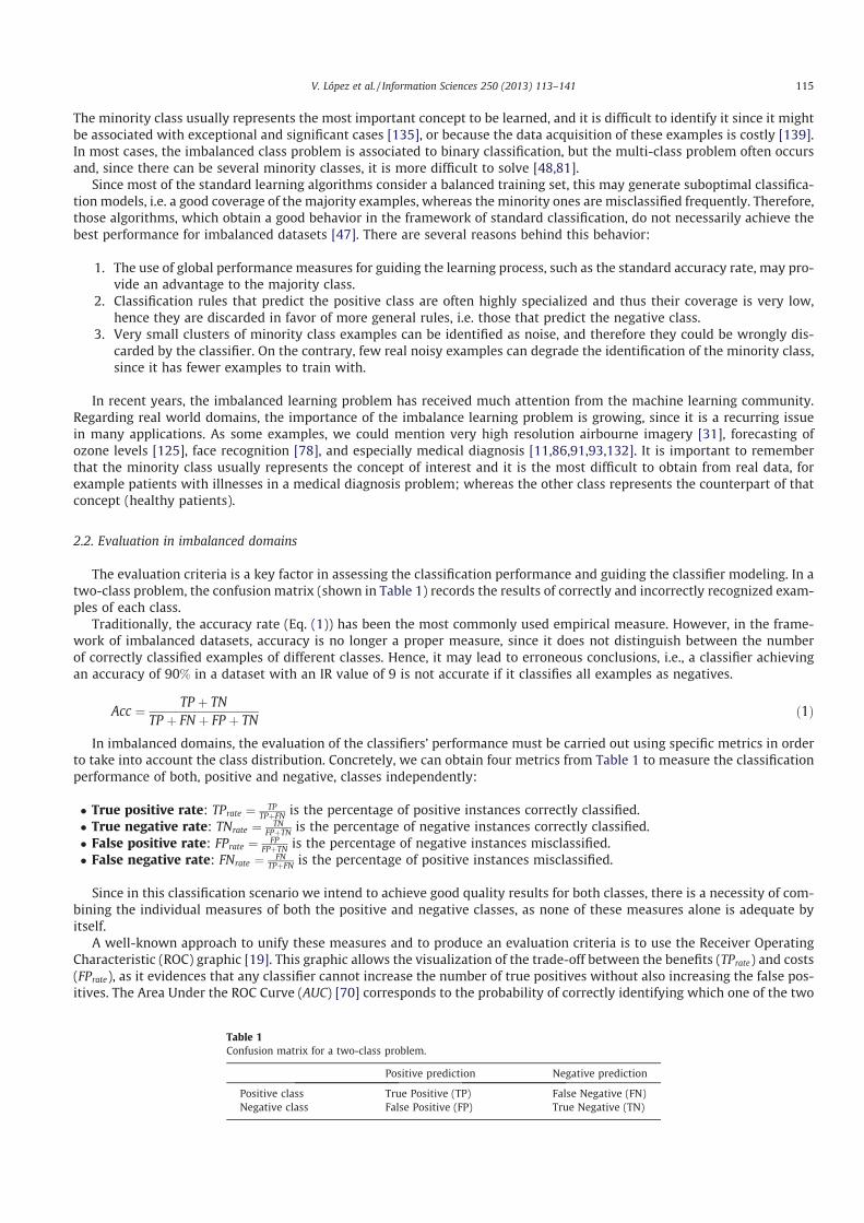
The minority class usually represents the most important concept to be learned, and it is difficult to identify it since it mightbe associated with exceptional and significant cases [135], or because the data acquisition of these examples is costly [139].In most cases, the imbalanced class problem is associated to binary classification, but the multi-class problem often occursand, since there can be several minority classes, it is more difficult to solve [48,81].
Since most of the standard learning algorithms consider a balanced training set, this may generate suboptimal classifica-tion models, i.e. a good coverage of the majority examples, whereas the minority ones are misclassified frequently. Therefore,those algorithms, which obtain a good behavior in the framework of standard classification, do not necessarily achieve thebest performance for imbalanced datasets [47]. There are several reasons behind this behavior:
1. The use of global performance measures for guiding the learning process, such as the standard accuracy rate, may pro-vide an advantage to the majority class.
2. Classification rules that predict the positive class are often highly specialized and thus their coverage is very low,hence they are discarded in favor of more general rules, i.e. those that predict the negative class.
3. Very small clusters of minority class examples can be identified as noise, and therefore they could be wrongly dis-carded by the classifier. On the contrary, few real noisy examples can degrade the identification of the minority class,since it has fewer examples to train with.
In recent years, the imbalanced learning problem has received much attention from the machine learning community.Regarding real world domains, the importance of the imbalance learning problem is growing, since it is a recurring issuein many applications. As some examples, we could mention very high resolution airbourne imagery [31], forecasting ofozone levels [125], face recognition [78], and especially medical diagnosis [11,86,91,93,132]. It is important to rememberthat the minority class usually represents the concept of interest and it is the most difficult to obtain from real data, forexample patients with illnesses in a medical diagnosis problem; whereas the other class represents the counterpart of thatconcept (healthy patients).
2.2. Evaluation in imbalanced domains
The evaluation criteria is a key factor in assessing the classification performance and guiding the classifier modeling. In atwo-class problem, the confusion matrix (shown in Table 1) records the results of correctly and incorrectly recognized exam-ples of each class.
Traditionally, the accuracy rate (Eq. (1)) has been the most commonly used empirical measure. However, in the frame-work of imbalanced datasets, accuracy is no longer a proper measure, since it does not distinguish between the numberof correctly classified examples of different classes. Hence, it may lead to erroneous conclusions, i.e., a classifier achievingan accuracy of 90% in a dataset with an IR value of 9 is not accurate if it classifies all examples as negatives.
Acc ¼ TP þ TNTP þ FN þ FP þ TN
ð1Þ
In imbalanced domains, the evaluation of the classifiers’ performance must be carried out using specific metrics in orderto take into account the class distribution. Concretely, we can obtain four metrics from Table 1 to measure the classificationperformance of both, positive and negative, classes independently:
� True positive rate: TPrate ¼ TPTPþFN is the percentage of positive instances correctly classified.
� True negative rate: TNrate ¼ TNFPþTN is the percentage of negative instances correctly classified.
� False positive rate: FPrate ¼ FPFPþTN is the percentage of negative instances misclassified.
� False negative rate: FNrate ¼ FNTPþFN is the percentage of positive instances misclassified.
Since in this classification scenario we intend to achieve good quality results for both classes, there is a necessity of com-bining the individual measures of both the positive and negative classes, as none of these measures alone is adequate byitself.
A well-known approach to unify these measures and to produce an evaluation criteria is to use the Receiver OperatingCharacteristic (ROC) graphic [19]. This graphic allows the visualization of the trade-off between the benefits (TPrate) and costs(FPrate), as it evidences that any classifier cannot increase the number of true positives without also increasing the false pos-itives. The Area Under the ROC Curve (AUC) [70] corresponds to the probability of correctly identifying which one of the two
Table 1Confusion matrix for a two-class problem.
Positive prediction Negative prediction
Positive class True Positive (TP) False Negative (FN)Negative class False Positive (FP) True Negative (TN)
V. López et al. / Information Sciences 250 (2013) 113–141 115

stimuli is noise and which one is signal plus noise. The AUC provides a single measure of a classifier’s performance for eval-uating which model is better on average. Fig. 1 shows how to build the ROC space plotting on a two-dimensional chart theTPrate (Y-axis) against the FPrate (X-axis). Points in ð0;0Þ and ð1;1Þ are trivial classifiers where the predicted class is always thenegative and positive one, respectively. On the contrary, ð0;1Þ point represents the perfect classifier. TheAUC measure iscomputed just by obtaining the area of the graphic:
AUC ¼ 1þ TPrate � FPrate
2ð2Þ
In [103], the significance of these graphical methods for the classification predictive performance evaluation is stressed.According to the authors, the main advantage of this type of methods resides in their ability to depict the trade-offs betweenevaluation aspects in a multidimensional space rather than reducing these aspects to an arbitrarily chosen (and often biased)single scalar measure. In particular, they present a review of several representation mechanisms emphasizing the best sce-nario for their use; for example, in imbalanced domains, when we are interested in the positive class, it is recommended theuse of precision-recall graphs [36]. Furthermore, the expected cost or profit of each model might be analyzed using costcurves [40], lift and ROI graphs [83].
Other metric of interest to be stressed in this area is the geometric mean of the true rates [7], which can be defined as:
GM ¼ffiffiffiffiffiffiffiffiffiffiffiffiffiffiffiffiffiffiffiffiffiffiffiffiffiffiffiffiffiffiffiffiffiffiffiffiffiffi
TPTP þ FN
� TNFP þ TN
rð3Þ
This metric attempts to maximize the accuracy on each of the two classes with a good balance, being a performance met-ric that correlates both objectives. However, due to this symmetric nature of the distribution of the geometric mean overTPrate (sensitivity) and the TNrate (specificity), it is hard to contrast different models according to their precision on each class.
Another significant performance metric that is commonly used is the F-measure [6]:
Fm ¼ ð1þ b2ÞðPPV � TPrateÞb2PPV þ TPrate
PPV ¼ TPTP þ FP
ð4Þ
A popular choice for b is 1, where equal importance is assigned for both TPrate and the positive predictive value (PPV). Thismeasure would be more sensitive to the changes in the PPV than to the changes in TPrate, which can lead to the selection ofsub-optimal models.
According to the previous comments, some authors try to propose several measures for imbalanced domains in order tobe able to obtain as much information as possible about the contribution of each class to the final performance and to takeinto account the IR of the dataset as an indication of its difficulty. For example, in [10,14] the Adjusted G-mean is proposed.This measure is designed towards obtaining the highest sensitivity (TPrate) without decreasing too much the specificity(TNrate). This fact is measured with respect to the original model, i.e. the original classifier without addressing the class imbal-ance problem. Eq. 5 shows its definition:
False Positive Rate
Tru
e Po
sitiv
e R
ate
0% 20% 40% 60% 80% 100%0%
20%
40%
60%
80%
100%
Random Classifier
Fig. 1. Example of a ROC plot. Two classifiers’ curves are depicted: the dashed line represents a random classifier, whereas the solid line is a classifier whichis better than the random classifier.
116 V. López et al. / Information Sciences 250 (2013) 113–141

AGM ¼ GMþTNrate �ðFPþTNÞ1þFPþTN ; IfTPrate > 0
AGM ¼ 0; IfTPrate ¼ 0ð5Þ
Additionally, in [54] the authors presented a simple performance metric, called Dominance, which is aimed to point outthe dominance or prevalence relationship between the positive class and the negative class, in the range ½�1;þ1� (Eq. 6).Furthermore, it can be used as a visual tool to analyze the behavior of a classifier on a 2-D space from the joint perspectiveof global precision (Y-axis) and dominance (X-axis).
Dom ¼ TPrate � TNrate ð6ÞThe same authors, using the previous concept of dominance, Index of Balanced Accuracy (IBA) [56,57]. IBA weights a per-
formance measure, that aims to make it more sensitive for imbalanced domains. The weighting factor favors those resultswith moderately better classification rates on the minority class. IBA is formulated as follows:
IBAaðMÞ ¼ ð1þ a � DomÞM ð7Þwhere ð1þ a � DomÞ is the weighting factor and M represents a performance metric. The objective is to moderately favor theclassification models with higher prediction rate on the minority class (without underestimating the relevance of the major-ity class) by means of a weighted function of any plain performance evaluation measure.
A comparison regarding these evaluation proposals for imbalanced datasets is out of the scope of this paper. For this rea-son, we refer any interested reader to find a deep experimental study in [57,105].
3. Addressing classification with imbalanced data: preprocessing, cost-sensitive learning and ensemble techniques
A large number of approaches have been proposed to deal with the class imbalance problem. These approaches can becategorized into two groups: the internal approaches that create new algorithms or modify existing ones to take theclass-imbalance problem into consideration [7,41,82,129,152] and external approaches that preprocess the data in orderto diminish the effect of their class imbalance [9,43]. Furthermore, cost-sensitive learning solutions incorporating boththe data (external) and algorithmic level (internal) approaches assume higher misclassification costs for samples in theminority class and seek to minimize the high cost errors [15,38,59,117,150]. Ensemble methods [101,108] are also frequentlyadapted to imbalanced domains, either by modifying the ensemble learning algorithm at the data-level approach to prepro-cess the data before the learning stage of each classifier [17,30,112] or by embedding a cost-sensitive framework in theensemble learning process [44,117,122].
Regarding this, in this section we first introduce the main aspects of the preprocessing techniques. Next, we describe thecost-sensitive learning approach. Finally, we present some relevant ensemble techniques in the framework of imbalanceddatasets.
3.1. Preprocessing imbalanced datasets: resampling techniques
In the specialized literature, we can find some papers about resampling techniques studying the effect of changing theclass distribution in order to deal with imbalanced datasets.
Those works have proved empirically that applying a preprocessing step in order to balance the class distribution is usu-ally an useful solution [9,12,45,46]. Furthermore, the main advantage of these techniques is that they are independent of theunderlying classifier.
Resampling techniques can be categorized into three groups or families:
1. Undersampling methods, which create a subset of the original dataset by eliminating instances (usually majority classinstances).
2. Oversampling methods, which create a superset of the original dataset by replicating some instances or creating newinstances from existing ones.
3. Hybrids methods, which combine both sampling approaches from above.
Within these families of methods, the simplest preprocessing techniques are non-heuristic methods such as randomundersampling and random oversampling. In the first case, the major drawback is that it can discard potentially useful data,that could be important for the learning process. For random oversampling, several authors agree that this method can in-crease the likelihood of occurring overfitting, since it makes exact copies of existing instances.
In order to deal with the mentioned problems, more sophisticated methods have been proposed. Among them, the‘‘Synthetic Minority Oversampling TEchnique’’ (SMOTE) [27] has become one of the most renowned approaches in this area.In brief, its main idea is to create new minority class examples by interpolating several minority class instances that lie to-gether for oversampling the training set.
With this technique, the positive class is over-sampled by taking each minority class sample and introducing syntheticexamples along the line segments joining any/all of the k minority class nearest neighbors. Depending upon the amountof over-sampling required, neighbors from the k nearest neighbors are randomly chosen. This process is illustrated in
V. López et al. / Information Sciences 250 (2013) 113–141 117
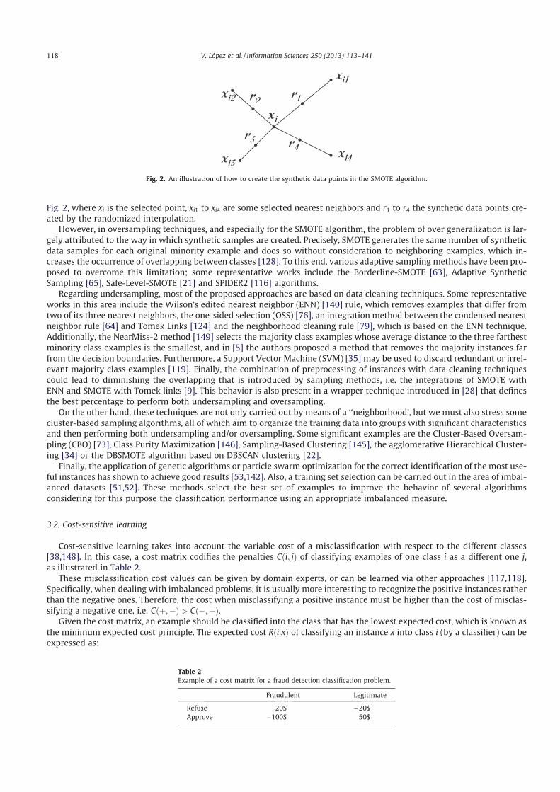
Fig. 2, where xi is the selected point, xi1 to xi4 are some selected nearest neighbors and r1 to r4 the synthetic data points cre-ated by the randomized interpolation.
However, in oversampling techniques, and especially for the SMOTE algorithm, the problem of over generalization is lar-gely attributed to the way in which synthetic samples are created. Precisely, SMOTE generates the same number of syntheticdata samples for each original minority example and does so without consideration to neighboring examples, which in-creases the occurrence of overlapping between classes [128]. To this end, various adaptive sampling methods have been pro-posed to overcome this limitation; some representative works include the Borderline-SMOTE [63], Adaptive SyntheticSampling [65], Safe-Level-SMOTE [21] and SPIDER2 [116] algorithms.
Regarding undersampling, most of the proposed approaches are based on data cleaning techniques. Some representativeworks in this area include the Wilson’s edited nearest neighbor (ENN) [140] rule, which removes examples that differ fromtwo of its three nearest neighbors, the one-sided selection (OSS) [76], an integration method between the condensed nearestneighbor rule [64] and Tomek Links [124] and the neighborhood cleaning rule [79], which is based on the ENN technique.Additionally, the NearMiss-2 method [149] selects the majority class examples whose average distance to the three farthestminority class examples is the smallest, and in [5] the authors proposed a method that removes the majority instances farfrom the decision boundaries. Furthermore, a Support Vector Machine (SVM) [35] may be used to discard redundant or irrel-evant majority class examples [119]. Finally, the combination of preprocessing of instances with data cleaning techniquescould lead to diminishing the overlapping that is introduced by sampling methods, i.e. the integrations of SMOTE withENN and SMOTE with Tomek links [9]. This behavior is also present in a wrapper technique introduced in [28] that definesthe best percentage to perform both undersampling and oversampling.
On the other hand, these techniques are not only carried out by means of a ‘‘neighborhood’, but we must also stress somecluster-based sampling algorithms, all of which aim to organize the training data into groups with significant characteristicsand then performing both undersampling and/or oversampling. Some significant examples are the Cluster-Based Oversam-pling (CBO) [73], Class Purity Maximization [146], Sampling-Based Clustering [145], the agglomerative Hierarchical Cluster-ing [34] or the DBSMOTE algorithm based on DBSCAN clustering [22].
Finally, the application of genetic algorithms or particle swarm optimization for the correct identification of the most use-ful instances has shown to achieve good results [53,142]. Also, a training set selection can be carried out in the area of imbal-anced datasets [51,52]. These methods select the best set of examples to improve the behavior of several algorithmsconsidering for this purpose the classification performance using an appropriate imbalanced measure.
3.2. Cost-sensitive learning
Cost-sensitive learning takes into account the variable cost of a misclassification with respect to the different classes[38,148]. In this case, a cost matrix codifies the penalties Cði; jÞ of classifying examples of one class i as a different one j,as illustrated in Table 2.
These misclassification cost values can be given by domain experts, or can be learned via other approaches [117,118].Specifically, when dealing with imbalanced problems, it is usually more interesting to recognize the positive instances ratherthan the negative ones. Therefore, the cost when misclassifying a positive instance must be higher than the cost of misclas-sifying a negative one, i.e. Cðþ;�Þ > Cð�;þÞ.
Given the cost matrix, an example should be classified into the class that has the lowest expected cost, which is known asthe minimum expected cost principle. The expected cost RðijxÞ of classifying an instance x into class i (by a classifier) can beexpressed as:
Fig. 2. An illustration of how to create the synthetic data points in the SMOTE algorithm.
Table 2Example of a cost matrix for a fraud detection classification problem.
Fraudulent Legitimate
Refuse 20$ �20$Approve �100$ 50$
118 V. López et al. / Information Sciences 250 (2013) 113–141

RðijxÞ ¼Xj
PðjjxÞ � Cði; jÞ ð8Þ
where PðjjxÞ is the probability estimation of classifying an instance into class j. That is, the classifier will classify an instance xinto positive class if and only if:
Pð0jxÞ � Cð1;0Þ þ Pð1jxÞ � Cð1;1Þ 6 Pð0jxÞ � Cð0;0Þ þ Pð1jxÞ � Cð0;1Þor, which is equivalent:
Pð0jxÞ � ðCð1;0Þ � Cð0;0ÞÞ 6 Pð1jxÞðCð0;1Þ � Cð1;1ÞÞTherefore, any given cost-matrix can be converted to one with Cð0;0Þ ¼ Cð1;1Þ ¼ 0. Under this assumption, the classifier
will classify an instance x into positive class if and only if:
Pð0jxÞ � Cð1;0Þ 6 Pð1jxÞ � Cð0;1ÞAs Pð0jxÞ ¼ 1� Pð1jxÞ, we can obtain a threshold p� for the classifier to classify an instance x into positive if Pð1jxÞ P p�,
where
p� ¼ Cð1;0ÞCð1;0Þ � Cð0;1Þ ¼
FPFP þ FN
ð9Þ
Another possibility is to ‘‘rebalance’’ the original training examples the ratio of:
pð1ÞFN : pð0ÞFP ð10Þwhere pð1Þ and pð0Þ are the prior probability of the positive and negative examples in the original training set.
In summary, two main general approaches have been proposed to deal with cost-sensitive problems:
1. Direct methods: The main idea of building a direct cost-sensitive learning algorithm is to directly introduce and uti-lize misclassification costs into the learning algorithms.For example, in the context of decision tree induction, the tree-building strategies are adapted to minimize the mis-classification costs. The cost information is used to: (1) choose the best attribute to split the data [84,107]; and (2)determine whether a subtree should be pruned [18]. On the other hand, other approaches based on genetic algorithmscan incorporate misclassification costs in the fitness function [126].
2. Meta-learning: This methodology implies the integration of a ‘‘preprocessing’’ mechanism for the training data or a‘‘postprocessing’’ of the output, in such a way that the original learning algorithm is not modified. Cost-sensitivemeta-learning can be further classified into two main categories: thresholding and sampling, which are based onexpressions (9) and (10) respectively:� Thresholding is based on the basic decision theory that assigns instances to the class with minimum expected
cost. For example, a typical decision tree for a binary classification problem assigns the class label of a leaf nodedepending on the majority class of the training samples that reach the node. A cost-sensitive algorithm assigns theclass label to the node that minimizes the classification cost [38,147].
� Sampling is based on modifying the training dataset. The most popular technique lies in resampling the originalclass distribution of the training dataset according to the cost decision matrix by means of undersampling/over-sampling [148] or assigning instance weights [123]. These modifications have shown to be effective and can alsobe applied to any cost insensitive learning algorithm [150].
3.3. Ensemble methods
Ensemble-based classifiers, also known as multiple classifier systems [101], try to improve the performance of single clas-sifiers by inducing several classifiers and combining them to obtain a new classifier that outperforms every one of them.Hence, the basic idea is to construct several classifiers from the original data and then aggregate their predictions when un-known instances are presented.
In recent years, ensembles of classifiers have arisen as a possible solution to the class imbalance problem[77,85,112,117,127,131]. Ensemble-based methods are based on a combination between ensemble learning algorithmsand one of the previously discussed techniques, namely data and algorithmic approaches, or cost-sensitive learning solu-tions. In the case of adding a data level approach to the ensemble learning algorithm, the new hybrid method usually pre-process the data before training each classifier. On the other hand, cost-sensitive ensembles, instead of modifying the baseclassifier in order to accept costs in the learning process, guide the cost minimization procedure via the ensemble learningalgorithm. In this way, the modification of the base learner is avoided, but the major drawback, which is the costs definition,is still present.
A complete taxonomy for ensemble methods for learning with imbalanced classes can be found on a recent review [50],which we summarize in Fig. 3. Mainly, the authors distinguish four different families among ensemble approaches for imbal-anced learning. On the one hand, they identified cost-sensitive boosting approaches which are similar to cost-sensitive
V. López et al. / Information Sciences 250 (2013) 113–141 119
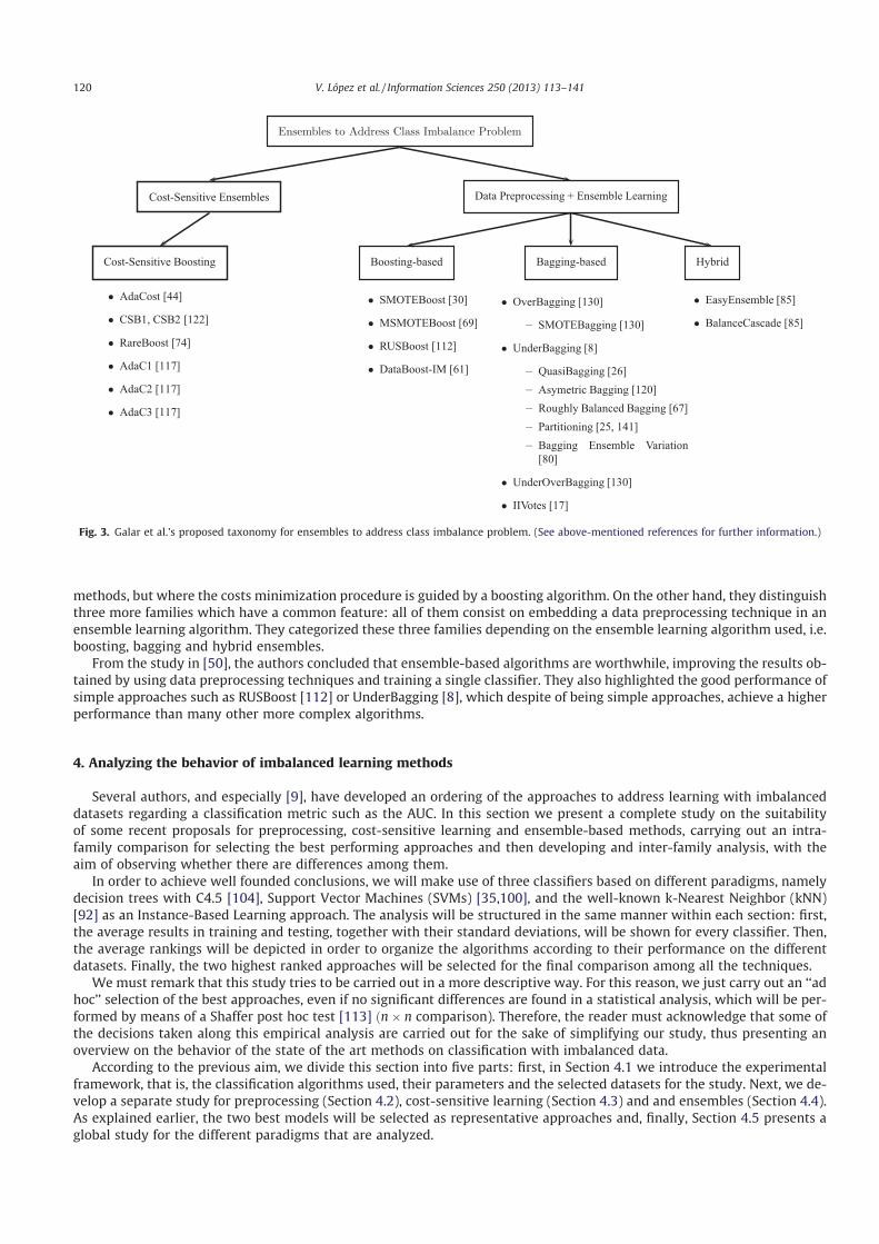
methods, but where the costs minimization procedure is guided by a boosting algorithm. On the other hand, they distinguishthree more families which have a common feature: all of them consist on embedding a data preprocessing technique in anensemble learning algorithm. They categorized these three families depending on the ensemble learning algorithm used, i.e.boosting, bagging and hybrid ensembles.
From the study in [50], the authors concluded that ensemble-based algorithms are worthwhile, improving the results ob-tained by using data preprocessing techniques and training a single classifier. They also highlighted the good performance ofsimple approaches such as RUSBoost [112] or UnderBagging [8], which despite of being simple approaches, achieve a higherperformance than many other more complex algorithms.
4. Analyzing the behavior of imbalanced learning methods
Several authors, and especially [9], have developed an ordering of the approaches to address learning with imbalanceddatasets regarding a classification metric such as the AUC. In this section we present a complete study on the suitabilityof some recent proposals for preprocessing, cost-sensitive learning and ensemble-based methods, carrying out an intra-family comparison for selecting the best performing approaches and then developing and inter-family analysis, with theaim of observing whether there are differences among them.
In order to achieve well founded conclusions, we will make use of three classifiers based on different paradigms, namelydecision trees with C4.5 [104], Support Vector Machines (SVMs) [35,100], and the well-known k-Nearest Neighbor (kNN)[92] as an Instance-Based Learning approach. The analysis will be structured in the same manner within each section: first,the average results in training and testing, together with their standard deviations, will be shown for every classifier. Then,the average rankings will be depicted in order to organize the algorithms according to their performance on the differentdatasets. Finally, the two highest ranked approaches will be selected for the final comparison among all the techniques.
We must remark that this study tries to be carried out in a more descriptive way. For this reason, we just carry out an ‘‘adhoc’’ selection of the best approaches, even if no significant differences are found in a statistical analysis, which will be per-formed by means of a Shaffer post hoc test [113] ðn� n comparison). Therefore, the reader must acknowledge that some ofthe decisions taken along this empirical analysis are carried out for the sake of simplifying our study, thus presenting anoverview on the behavior of the state of the art methods on classification with imbalanced data.
According to the previous aim, we divide this section into five parts: first, in Section 4.1 we introduce the experimentalframework, that is, the classification algorithms used, their parameters and the selected datasets for the study. Next, we de-velop a separate study for preprocessing (Section 4.2), cost-sensitive learning (Section 4.3) and and ensembles (Section 4.4).As explained earlier, the two best models will be selected as representative approaches and, finally, Section 4.5 presents aglobal study for the different paradigms that are analyzed.
Fig. 3. Galar et al.’s proposed taxonomy for ensembles to address class imbalance problem. (See above-mentioned references for further information.)
120 V. López et al. / Information Sciences 250 (2013) 113–141

4.1. Experimental framework
In the first place, we need to define a set of baseline classifiers to be used in all the experiments. Next, we enumerate thesealgorithms and also their parameter values, which have been set considering the recommendation of the correspondingauthors. We must point out that these algorithms are available within the KEEL software tool [4].
1. C4.5 Decision tree [104]: For C4.5, we have set a confidence level of 0.25, the minimum number of item-sets per leafwas set to 2 and pruning was used as well to obtain the final tree.
2. Support vector machines [35]: For the SVM, we have chosen Polykernel reference functions, with an internal param-eter of 1.0 for the exponent of each kernel function and a penalty parameter of the error term of 1.0.
3. Instance based learning (kNN) [92]: In this case, we have selected 1 neighbor for determining the output class, usingthe euclidean distance metric.
We have gathered 66 datasets, whose features are summarized in Table 3, namely the number of examples (#Ex.), num-ber of attributes (#Atts.) and IR. Estimates of the AUC metric were obtained by means of a 5-fold cross-validation. That is, wesplit the dataset into 5 folds, each one containing 20% of the patterns of the dataset. For each fold, the algorithm was trainedwith the examples contained in the remaining folds and then tested with the current fold. This value is set up with the aim ofhaving enough positive class instances in the different folds, hence avoiding additional problems in the data distribution[94,96], especially for highly imbalanced datasets.
We must point out that the dataset partitions employed in this paper are available for download at the KEEL datasetrepository1 [3], so that any interested researcher can use the same data for comparison.
Finally, with respect to the evaluation metric, we use the Area Under the ROC Curve (AUC) [19,70] as evaluation criteria.
4.2. Study on the preprocessing methods
In this section, we analyze the behavior of the preprocessing methods on imbalanced datasets. For this purpose, we com-pare some of the most representative techniques, previously presented in Section 3.1, developing a ranking according to the
Table 3Summary of imbalanced datasets used.
Name #Ex. #Atts. IR Name #Ex. #Atts. IR
Glass1 214 9 1.82 Glass04vs5 92 9 9.22Ecoli0vs1 220 7 1.86 Ecoli0346vs5 205 7 9.25Wisconsin 683 9 1.86 Ecoli0347vs56 257 7 9.28Pima 768 8 1.90 Yeast05679vs4 528 8 9.35Iris0 150 4 2.00 Ecoli067vs5 220 6 10.00Glass0 214 9 2.06 Vowel0 988 13 10.10Yeast1 1484 8 2.46 Glass016vs2 192 9 10.29Vehicle1 846 18 2.52 Glass2 214 9 10.39Vehicle2 846 18 2.52 Ecoli0147vs2356 336 7 10.59Vehicle3 846 18 2.52 Led7digit02456789vs1 443 7 10.97Haberman 306 3 2.68 Glass06vs5 108 9 11.00Glass0123vs456 214 9 3.19 Ecoli01vs5 240 6 11.00Vehicle0 846 18 3.23 Glass0146vs2 205 9 11.06Ecoli1 336 7 3.36 Ecoli0147vs56 332 6 12.28New-thyroid2 215 5 4.92 Cleveland0vs4 177 13 12.62New-thyroid1 215 5 5.14 Ecoli0146vs5 280 6 13.00Ecoli2 336 7 5.46 Ecoli4 336 7 13.84Segment0 2308 19 6.01 Yeast1vs7 459 8 13.87Glass6 214 9 6.38 Shuttle0vs4 1829 9 13.87Yeast3 1484 8 8.11 Glass4 214 9 15.47Ecoli3 336 7 8.19 Page-blocks13vs2 472 10 15.85Page-blocks0 5472 10 8.77 Abalone9vs18 731 8 16.68Ecoli034vs5 200 7 9.00 Glass016vs5 184 9 19.44Yeast2vs4 514 8 9.08 Shuttle2vs4 129 9 20.50Ecoli067vs35 222 7 9.09 Yeast1458vs7 693 8 22.10Ecoli0234vs5 202 7 9.10 Glass5 214 9 22.81Glass015vs2 172 9 9.12 Yeast2vs8 482 8 23.10Yeast0359vs78 506 8 9.12 Yeast4 1484 8 28.41Yeast02579vs368 1004 8 9.14 Yeast1289vs7 947 8 30.56Yeast0256vs3789 1004 8 9.14 Yeast5 1484 8 32.78Ecoli046vs5 203 6 9.15 Ecoli0137vs26 281 7 39.15Ecoli01vs235 244 7 9.17 Yeast6 1484 8 39.15Ecoli0267vs35 224 7 9.18 Abalone19 4174 8 128.87
1 http://www.keel.es/datasets.php.
V. López et al. / Information Sciences 250 (2013) 113–141 121

performance obtained in each case. This representative set of methods is composed by the following techniques: SMOTE[27], SMOTE+ENN [9], Borderline-SMOTE (Border-SMOTE) [63], Adaptive Synthetic Sampling (ADASYN) [65], Safe-Level-SMOTE (SL-SMOTE) [21], SPIDER2 [97] and DBSMOTE [22]. In all cases we try to obtain a level of balance in the training datanear to the 50:50 distribution. Additionally, the interpolations that are computed to generate new synthetic data are madeconsidering the 5-nearest neighbors of minority class instances using the euclidean distance.
In Table 4 we show the average results for all preprocessing methods, also including the performance with the originaldata (None). In bold, we highlight the preprocessing method that obtains the best performing average within each group. Weobserve that, in all cases, the oversampling mechanisms are very good solutions for achieving a higher performance by com-parison to using the original training data.
This behavior is contrasted in Fig. 4, where we have ordered the corresponding methods according to their AUC results intesting for each dataset, considering the average ranking value. We must stress SMOTE+ENN and SMOTE as the top meth-odologies, since they obtain the highest rank for the three classification algorithms used in this study. We can also observethat both Border-SMOTE and ADASYN are quite robust on average, obtaining a fair average ranking for all datasets.
For the sake of finding out which algorithms are distinctive among an n� n comparison, we carry out a Shaffer post hoctest [113], which is shown in Tables 5–7. In these tables, a ‘‘+’’ symbol implies that the algorithm in the row is statisticallybetter than the one in the column, whereas ‘‘�’’ implies the contrary; ‘‘=’’ means that the two algorithms compared show nosignificant differences. In brackets, the adjusted p-value associated to each comparison is shown.
Table 4Average AUC results for the preprocessing techniques.
Preprocessing C4.5 SVM kNN
AUCTr AUCTst AUCTr AUCTst AUCTr AUCTst
None .8790 ±.1226 .7873 ±.1437 .7007 ±.1706 .6891 ±.1681 .8011 ±.1339 .8028 ±.1383SMOTE .9613 ±.0504 .8288 ±.1192 .8631 ±.1045 .8470 ±.1152 .9345 ±.1247 .8341 ±.1194SMOTE+ENN .9482 ±.0525 .8323 ±.1166 .8815 ±.1001 .8461 ±.1162 .9284 ±.1262 .8443 ±.1158Border-SMOTE .9333 ±.0595 .8187 ±.1272 .9082 ±.0941 .8397 ±.1163 .9144 ±.0682 .8177 ±.1314SL-SMOTE .9175 ±.0615 .8285 ±.1112 .8365 ±.1020 .8427 ±.1176 .8024 ±.1331 .8029 ±.1381ADASYN .9589 ±.0469 .8225 ±.1234 .8283 ±.1054 .8323 ±.1148 .9347 ±.0500 .8355 ±.1163SPIDER2 .9684 ±.0378 .8018 ±.1329 .7252 ±.1493 .7371 ±.1542 .8381 ±.1176 .8207 ±.1338DBSMOTE .8908 ±.1006 .7877 ±.1441 .8612 ±.0778 .7546 ±.1368 .8147 ±.1163 .8082 ±.1293
Fig. 4. Average ranking of the preprocessing algorithms for classification with imbalanced datasets.
Table 5Shaffer test for the preprocessing techniques with C4.5 using the AUC measure.
C4.5 None SMOTE SMOTE+ENN Border-SMOTE SL-SMOTE ADASYN SPIDER2 DBSMOTE
None x �(.000002) �(.000000) �(.001104) �(.000096) �(.000124) =(.580860) =(1.00000)SMOTE +(.000002) x =(1.00000) =(1.00000) =(1.00000) =(1.00000) +(.013398) +(.000003)SMOTE+ENN +(.000000) =(1.00000) x =(.769498) =(1.00000) =(1.00000) +(.002466) +(.000000)Border-SMOTE +(.001104) =(1.00000) =(.769498) x =(1.00000) =(1.00000) =(.631767) +(.001379)SL-SMOTE +(.000096) =(1.00000) =(1.00000) =(1.00000) x =(1.00000) =(.159840) +(.000124)ADASYN +(.000124) =(1.00000) =(1.00000) =(1.00000) =(1.00000) x =(.174600) +(.000159)SPIDER2 =(.580860) �(.013398) �(.002466) =(.631767) =(.159840) =(.174600) x =(.631767)DBSMOTE =(1.00000) �(.000003) �(.000000) �(.001379) �(.000124) �(.000159) =(.631767) x
122 V. López et al. / Information Sciences 250 (2013) 113–141

In order to explain why SMOTE+ENN and SMOTE obtain the highest performance, we may emphasize two feasible rea-sons. The first one is related to the addition of significant information within the minority class examples by includingnew synthetic examples. These new examples allow the formation of larger clusters to help the classifiers to separate bothclasses, and the cleaning procedure also adds benefits to the generalization ability during learning. The second reason is thatthe more sophisticated the technique is, the less general it becomes for the high number of benchmark problems selected forour study.
According to these results, we select both SMOTE+ENN and SMOTE as good behaving methodologies for our finalcomparison.
4.3. Study on the cost-sensitive learning algorithms
In this section, we carry out an analysis regarding cost-sensitive classifiers. We use three different approaches, namely‘‘Weighted-Classifier’’ (CS-Weighted) [7,123], MetaCost [38], and the CostSensitive Classifier (CS-Classifier) from the Wekaenvironment [62]. In the first case, the base classifiers are modified usually by weighting the instances of the dataset to takeinto account the a priori probabilities, according to the number of samples in each class. In the two latter cases, we use aninput cost-matrix defining Cðþ;�Þ ¼ IR and Cð�;þÞ ¼ 1.
Table 8 shows the average AUC results where the best average values per algorithm group are highlighted in bold. Fromthis table, we may conclude, as in the previous case for preprocessing, the goodness of the use of this type of solution forimbalanced data, as there is a significant difference with respect to the results obtained with the original data. We may alsoobserve the good behavior of the ‘‘CS-Weighted’’ in contrast with the remaining techniques, and also the good accuracy forthe MetaCost algorithm, for both C4.5 and kNN.
Fig. 5 presents the ranking for the selected methods. We can appreciate that the ‘‘CS-Weighted’’ approach achieves thehighest rank overall, as pointed out before. The MetaCost method obtains also a good average for C4.5 and kNN, but it is out-performed by the CS-Classifier when SVM is used.
As in the latter case, we show a Shaffer post hoc test for detecting significant differences among the results (Tables 9–11).
Table 6Shaffer test for the preprocessing techniques with SVM using the AUC measure.
SVM None SMOTE SMOTE+ENN Border-SMOTE SL-SMOTE ADASYN SPIDER2 DBSMOTE
None x �(.000000) �(.000000) �(.000000) �(.000000) �(.000000) =(.129870) =(1.00000)SMOTE +(.000000) x =(1.00000) =(1.00000) =(1.00000) =(.179175) +(.000000) +(.000000)SMOTE+ENN +(.000000) =(1.00000) x =(1.00000) =(1.00000) =(.199418) +(.000000) +(.000000)Border-SMOTE +(.000000) =(1.00000) =(1.00000) x =(1.00000) =(1.00000) +(.000000) +(.000000)SL-SMOTE +(.000000) =(1.00000) =(1.00000) =(1.00000) x =(1.00000) +(.000000) +(.000000)ADASYN +(.000000) =(.179175) =(.199418) =(1.00000) =(1.00000) x +(.000126) +(.000001)SPIDER2 =(.129870) �(.000000) �(.000000) �(.000000) �(.000000) �(.000126) x =(1.00000)DBSMOTE =(1.00000) �(.000000) �(.000000) �(.000000) �(.000000) �(.000001) =(1.00000) x
Table 7Shaffer test for the preprocessing techniques with kNN using the AUC measure.
kNN None SMOTE SMOTE+ENN Border-SMOTE SL-SMOTE ADASYN SPIDER2 DBSMOTE
None x �(.000757) �(.000000) �(.014934) =(1.00000) �(.000081) �(.004963) =(1.00000)SMOTE +(.000757) x �(.089266) =(1.00000) +(.000701) =(1.00000) =(1.00000) +(.000006)SMOTE+ENN +(.000000) +(.089266) x +(.007968) +(.000000) =(.360402) +(.022513) +(.000000)Border-SMOTE +(.014934) =(1.00000) �(.007968) x +(.014027) =(1.00000) =(1.00000) +(.000253)SL-SMOTE =(1.00000) �(.000701) �(.000000) �(.014027) x �(.000074) �(.004634) =(1.00000)ADASYN +(.000081) =(1.00000) =(.360402) =(1.00000) +(.000074) x =(1.00000) +(.000000)SPIDER2 +(.004963) =(1.00000) �(.022513) =(1.00000) +(.004634) =(1.00000) x +(.000062)DBSMOTE =(1.00000) �(.000006) �(.000000) �(.000253) =(1.00000) �(.000000) �(.000062) x
Table 8Average AUC results for the cost-sensitive learning techniques.
Cost-sensitive C4.5 SVM kNN
AUCTr AUCTst AUCTr AUCTst AUCTr AUCTst
None .8790 ±.1226 .7873 ±.1437 .7007 ±.1706 .6891 ±.1681 .8011 ±.1339 .8028 ±.1383CS-Weighted .9711 ±.0580 .8284 ±.1263 .8751 ±.1068 .8464 ±.1124 .8427 ±.1201 .8463 ±.1177MetaCost .9159 ±.0797 .8370 ±.1287 .6931 ±.1715 .6802 ±.1696 .9849 ±.0118 .8250 ±.1301CS-Classifier .8915 ±.1191 .8116 ±.1387 .8701 ±.1053 .8391 ±.1152 .9993 ±.0046 .8084 ±.1343
V. López et al. / Information Sciences 250 (2013) 113–141 123

The good behavior shown by introducing weights to the training examples can be explained by its simplicity, because thealgorithm procedure is maintained and is adapted to the imbalanced situation. Therefore, it works similarly to an oversam-pling approach but without adding new samples and complexity to the problem itself. On the other hand, the MetaCostmethod follows a similar aim, therefore obtaining high quality results. Regarding these facts, we will select these two meth-ods as the representative ones for this family.
4.4. Study on the ensemble-based techniques
The last family of approaches for dealing with imbalanced datasets that we will analyze is the one based on ensembletechniques. In this case, we have selected five different algorithms which showed a very good behavior on the study carriedout in [50], namely AdaBoost.M1 (AdaB-M1) [110], AdaBoost with costs outside the exponent (AdaC2) [117], RUSBoost(RUSB) [112], SMOTEBagging (SBAG) [130], and EasyEnsemble (EASY) [85]. We must point out that AdaB-M1 was not in-cluded in the taxonomy presented in Section 3.3 since it is not strictly oriented towards imbalanced classification, but wehave decided to study it as a classical ensemble approach and because it has shown a good behavior in [50]. Regardingthe number of internal classifiers used within each approach, AdaB-M1, AdaC2 and SBAG use 40 classifiers, whereas theremaining approaches use only 10. Additionally, EASY considers 4 bags for the learning stage.
Fig. 5. Average ranking of the cost-sensitive learning algorithms for the classification with imbalanced datasets.
Table 9Shaffer test for the cost-sensitive learning techniques with C4.5 using the AUC measure.
C4.5 None CS-Weighted MetaCost CS-Classifier
None x �(.000000) �(.000000) �(.013893)CS-Weighted +(.000000) x =(.787406) +(.020817)MetaCost +(.000000) =(.787406) x +(.013893)CS-Classifier +(.013893) �(.020817) �(.013893) x
Table 10Shaffer test for the cost-sensitive learning techniques with SVM using the AUC measure.
SVM None CS-Weighted MetaCost CS-Classifier
None x �(.000000) =(.449832) �(.000000)CS-Weighted +(.000000) x +(.000000) =(.449832)MetaCost =(.449832) �(.000000) x �(.000000)CS-Classifier +(.000000) =(.449832) +(.000000) x
Table 11Shaffer test for the cost-sensitive learning techniques with kNN using the AUC measure.
kNN None CS-Weighted MetaCost CS-Classifier
None x �(.000000) �(.000075) =(.345231)CS-Weighted +(.000000) x +(.004828) +(.000000)MetaCost +(.000075) �(.004828) x +(.003228)CS-Classifier =(.345231) �(.000000) �(.003228) x
124 V. López et al. / Information Sciences 250 (2013) 113–141

In this case, the average AUC results for training and testing are shown in Table 12. The values highlighted in bold cor-respond to the algorithms that obtain a better performance according to the base classifier. From this table we may concludethe good performance of RUSB, SBAG and EASY. Among them, SBAG stands out for obtaining slightly better results. Anyway,these three algorithms outperform the others considered in this study. The reader might have also noticed that, the greatbehavior of RUSB is attained using only 10 base classifiers.
This can also be seen from Fig. 6, where we can observe that these three algorithms obtain the first rank positions in al-most all cases. It is noticeable that RUSB decreases its results in the case of the SVM algorithm, which can be due to the re-moval of significant samples for determining the support vectors for the margin classifier in each iteration of the learning.
Tables 13–15 present a Shaffer test, where we can observe, in a nutshell, the statistical differences among the ensemblemethodologies selected for this study.
Nevertheless, we must point out that more complex methods do not perform much better than simpler ones. Baggingtechniques are easy to develop, but also powerful when dealing with class imbalance if they are properly combined. Their
Table 12Average AUC results for the ensemble methodologies.
Ensemble C4.5 SVM kNN
AUCTr AUCTst AUCTr AUCTst AUCTr AUCTst
None .8790 ± .1226 .7873 ± .1437 .7007 ± .1706 .6891 ± .1681 .8011 ± .1339 .8028 ± .1383AdaB-M1 .9915 ± .0468 .8072 ± .1334 .7862 ± .1659 .7615 ± .1630 .9983 ± .0101 .8090 ± .1345AdaC2 .9470 ± .0858 .8188 ± .1312 .6366 ± .1497 .6271 ± .1479 .9991 ± .0062 .8080 ± .1344RUSB .9481 ± .0545 .8519 ± .1129 .7667 ± .1652 .7517 ± .1642 .9359 ± .0495 .8465 ± .1118SBAG .9626 ± .0455 .8545 ± .1111 .8662 ± .1050 .8456 ± .1137 .9825 ± .0253 .8485 ± .1164Easy .9076 ± .0626 .8399 ± .1091 .8565 ± .1057 .8370 ± .1150 .9093 ± .0667 .8440 ± .1095
Fig. 6. Average ranking of the ensemble algorithms for the classification with imbalanced datasets.
Table 13Shaffer test for the ensemble methodologies with C4.5 using the AUC measure.
C4.5 None AdaB-M AdaC2 RUSB SBAG Easy
None x =(.214054) �(.000767) �(.000000) �(.000000) �(.000001)AdaB-M =(.214054) x =(.137090) �(.000001) �(.000000) �(.00339)AdaC2 +(.000767) =(.137090) x �(.006691) �(.00115) =(.339838)RUSB +(.000000) +(.000001) +(.006691) x =(.641758) =(.214054)SBAG +(.000000) +(.000000) +(.00115) =(.641758) x +(.099451)Easy +(.000001) +(.003390) =(.339838) =(.214054) �(.099451) x
Table 14Shaffer test for the ensemble methodologies with SVM using the AUC measure.
SVM None AdaB-M AdaC2 RUSB SBAG Easy
None x �(.000721) =(.208828) �(.015681) �(.000000) �(.000000)AdaB-M +(.000721) x +(.000000) =(.401501) �(.000001) �(.000343)AdaC2 =(.208828) �(.000000) x �(.000018) �(.000000) �(.000000)RUSB +(.015681) =(.401501) +(.000018) x �(.000000) �(.000007)SBAG +(.000000) +(.000001) +(.000000) +(.000000) x =(.401501)Easy +(.000000) +(.000343) +(.000000) +(.000007) =(.401501) x
V. López et al. / Information Sciences 250 (2013) 113–141 125

hybridization with data preprocessing techniques has shown competitive results and the key issue of these methods residesin properly exploiting the diversity when each bootstrap replica is formed.
Since we have to select only two methodologies for the global analysis, we will stress SBAG as the best ranked methodand RUSB, because it presents a robust behavior on average and the second best mean performance in two of the threealgorithms.
4.5. Global analysis for the methodologies that address imbalanced classification
In this last section of the experimental analysis on the behavior of the methodologies for addressing classification withimbalanced datasets, we will perform a cross-family comparison for the approaches previously selected as the representa-tives for each case, namely preprocessing (SMOTE and SMOTE+ENN), cost-sensitive learning (CS-Weighted and MetaCost)and ensemble techniques (RUSB and SBAG). The global results are shown in Table 16, whereas the new performance rankingis shown in Fig. 7. As in the previous cases, the bold values in Table 16 correspond to the algorithms that obtain the highestperformance.
Considering these results, we must highlight the dominance of the ensemble approaches versus the remaining models forthe ‘‘weak classifiers’’, i.e. C4.5 and kNN. For SVM, the best results are achieved by preprocessing and CS-weighted, showingthe significance of adjusting the objective function towards the positive instances, for biasing the separating hyperplane.Regarding the comparison between the cost-sensitive classifiers and the oversampling methods, we observe that, on average,SMOTE+ENN, CS-Weighted and SMOTE obtain very good results and, therefore, they have a similar ranking, followed bythe MetaCost method. We must point out that these conclusions regarding the latter techniques are in concordance withthe study done in [88].
Table 15Shaffer test for the ensemble methodologies with kNN using the AUC measure.
kNN None AdaB-M AdaC2 RUSB SBAG Easy
None x =(1.00000) =(1.00000) �(.000000) �(.000000) �(.000118)AdaB-M =(1.00000) x =(1.00000) �(.000017) �(.000000) �(.003106)AdaC2 =(1.00000) =(1.00000) x �(.000006) �(.000000) �(.001517)RUSB +(.000000) +(.000017) +(.000006) x =(.803003) =(.803003)SBAG +(.000000) +(.000000) +(.000000) =(.803003) x +(.063015)Easy +(.000118) +(.003106) +(.001517) =(.803003) �(.063015) x
Table 16Average global results for C4.5 with the representative methodologies for addressing imbalanced classification.
Preprocessing C4.5 SVM kNN
AUCTr AUCTst AUCTr AUCTst AUCTr AUCTst
None .8790 ± .1226 .7873 ± .1437 .7007 ± .1706 .6891 ± .1681 .8011 ± .1339 .8028 ± .1383SMOTE .9613 ± .0504 .8288 ± .1192 .8631 ± .1045 .8470 ± .1152 .9345 ± .1247 .8341 ± .1194SMOTE+ENN .9482 ± .0525 .8323 ± .1166 .8815 ± .1001 .8461 ± .1162 .9284 ± .1262 .8443 ± .1158CS-Weighted .9711 ± .0580 .8284 ± .1263 .8751 ± .1068 .8464 ± .1124 .8427 ± .1201 .8463 ± .1177MetaCost .9159 ± .0797 .8370 ± .1287 .6931 ± .1715 .6802 ± .1696 .9849 ± .0118 .8250 ± .1301RUSB .9481 ± .0545 .8519 ± .1129 .7667 ± .1652 .7517 ± .1642 .9359 ± .0495 .8465 ± .1118SBAG .9626 ± .0455 .8545 ± .1111 .8662 ± .1050 .8456 ± .1137 .9825 ± .0253 .8485 ± .1164
Fig. 7. Average ranking of the representative algorithms for the classification with imbalanced datasets.
126 V. López et al. / Information Sciences 250 (2013) 113–141

In the same way as in the previous sections of this study, we proceed with a Shaffer test (Tables 17–19) that aims to con-trast whether two algorithms are significantly different and how different they are.
As a final remark, we must state that all the solutions analyzed here present different particularities, which make themmore appropriate for a given application. For example, ensemble methodologies have shown to be very accurate, but theirlearning time may be high and the output model can be difficult to comprehend by the final user. Cost-sensitive approacheshave also shown to be very precise, but the necessity of defining an optimal cost-matrix impose hard restrictions to their use.Finally, the preprocessing algorithms have shown their robustness and obtained very good global results, and therefore theycan be viewed as a standard approach for imbalanced datasets.
5. Problems related to data intrinsic characteristics in imbalanced classification
As it was stated in the introduction of this work, skewed class distributions do not hinder the learning task by itself[66,118], but usually a series of difficulties related with this problem turn up. This issue is depicted in Fig. 8, in which weshow the performance of the SBAG with the different datasets used in the previous section, ordered according to the IR,in order to search for some regions of interesting good or bad behavior. As we can observe, there is no pattern of behaviorfor any range of IR, and the results can be poor both for low and high imbalanced data.
Related to this issue, in this section we aim to make a discussion on the nature of the problem itself, emphasizing severaldata intrinsic characteristics that do have a strong influence on imbalanced classification, in order to be able to address thisproblem in a more feasible way.
With this objective in mind, we focus our analysis on using the C4.5 classifier, in order to develop a basic but descriptivestudy by showing a series of patterns of behavior, following a kind of ‘‘educational scheme’’. With respect to the previoussection, which was carried out in an empirical way, this part of the study is devoted to enumerating the scenarios thatcan be found when dealing with classification with imbalanced data, emphasizing their main issues that will allow us to de-sign a better algorithm that can be adapted to different niches of the problem.
Table 17Shaffer test for the representative methodologies with C4.5 using the AUC measure.
C4.5 None SMOTE SMOTE+ENN CS-Weighted MetaCost RUSB SBAG
None x �(.000292) �(.000087) �(.000203) �(.000001) �(.000000) �(.000000)SMOTE +(.000292) x =(1.00000) =(1.00000) =(1.00000) �(.001816) �(.000648)SMOTE+ENN +(.000087) =(1.00000) x =(1.00000) =(1.00000) �(.004560) �(.001423)CS-Weighted +(.000203) =(1.00000) =(1.00000) x =(1.00000) �(.002500) �(.000671)MetaCost +(.000001) =(1.00000) =(1.00000) =(1.00000) x �(.061745) �(.02942)RUSB +(.000000) +(.001816) +(.004560) +(.002500) +(.061745) x =(1.00000)SBAG +(.000000) +(.000648) +(.001423) +(.000671) +(.02942) =(1.00000) x
Table 18Shaffer test for the representative methodologies with SVM using the AUC measure.
SVM None SMOTE SMOTE+ENN CS-Weighted MetaCost RUSB SBAG
None x �(.000000) �(.000000) �(.000000) =(1.00000) �(.097865) �(.000000)SMOTE +(.000000) x =(1.00000) =(1.00000) +(.000000) +(.000000) =(1.00000)SMOTE+ENN +(.000000) =(1.00000) x =(1.00000) +(.000000) +(.000000) =(1.00000)CS-Weighted +(.000000) =(1.00000) =(1.00000) x +(.000000) +(.000000) =(1.00000)MetaCost =(1.00000) �(.000000) �(.000000) �(.000000) x �(.019779) �(.000000)RUSB +(.097865) �(.000000) �(.000000) �(.000000) +(.019779) x �(.000005)SBAG +(.000000) =(1.00000) =(1.00000) =(1.00000) +(.000000) +(.000005) x
Table 19Shaffer test for the representative methodologies with kNN using the AUC measure.
kNN None SMOTE SMOTE+ENN CS-Weighted MetaCost RUSB SBAG
None x �(.002684) �(.000000) �(.000000) �(.038367) �(.000000) �(.000000)SMOTE +(.002684) x �(.058815) �(.049543) =(1.00000) =(.371813) �(.000545)SMOTE+ENN +(.000000) +(.058815) x =(1.00000) +(.004309) =(1.00000) =(.950901)CS-Weighted +(.000000) +(.049543) =(1.00000) x +(.002705) =(1.00000) =(.986440)MetaCost +(.038367) =(1.00000) �(.004309) �(.002705) x �(.057811) �(.000011)RUSB +(.000000) =(.371813) =(1.00000) =(1.00000) +(.057811) x =(.196710)SBAG +(.000000) +(.000545) =(.950901) =(.986440) +(.000011) =(.196710) x
V. López et al. / Information Sciences 250 (2013) 113–141 127

We acknowledge that some of the data intrinsic characteristics described along this section share some features and it isusual that, for a given dataset, several ‘‘sub-problems’’ can be found simultaneously. Nevertheless, we consider a simplifiedview of all these scenarios to serve as a global introduction to the topic.
First, we discuss about the difficulties related to the presence of small disjuncts in the imbalanced data (Section 5.1).Then, we present the issues about the size of the dataset and the lack of density in the training set (Section 5.2). Next,we focus on the class overlap, showing that it is extremely significant on imbalanced domains (Section 5.3). Then, we analyzethe presence of noisy data in this type of problems and how it affects the behavior of both preprocessing techniques andclassification algorithms (Section 5.4). After that, we introduce the concept of borderline instances and its relationship withnoise examples (Section 5.5). Finally, we define the dataset shift problem in the classification with imbalanced datasets(Section 5.6).
5.1. Small disjuncts
The presence of the imbalanced classes is closely related to the problem of small disjuncts. This situation occurs when theconcepts are represented within small clusters, which arise as a direct result of underrepresented subconcepts [99,138].Although those small disjuncts are implicit in most of the problems, the existence of this type of areas highly increasesthe complexity of the problem in the case of class imbalance, because it becomes hard to know whether these examples rep-resent an actual subconcept or are merely attributed to noise [73]. This situation is represented in Fig. 9, where we show anartificially generated dataset with small disjuncts for the minority class and the ‘‘Subclus’’ problem created in [97], where wecan find small disjuncts for both classes: the negative samples are underrepresented with respect to the positive samples inthe central region of positive rectangular areas, while the positive samples only cover a small part of the whole dataset andare placed inside the negative class. We must point out that, in all figures of this section, positive instances are representedwith dark stars whereas negative instances are depicted with light circles.
Fig. 8. Performance in training and testing for the C4.5 decision tree with SBAG as a function of IR.
Fig. 9. Example of small disjuncts on imbalanced data.
128 V. López et al. / Information Sciences 250 (2013) 113–141
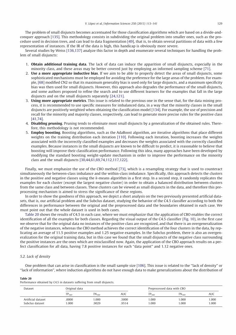
The problem of small disjuncts becomes accentuated for those classification algorithms which are based on a divide-and-conquer approach [135]. This methodology consists in subdividing the original problem into smaller ones, such as the pro-cedure used in decision trees, and can lead to data fragmentation [49], that is, to obtain several partitions of data with a fewrepresentation of instances. If the IR of the data is high, this handicap is obviously more severe.
Several studies by Weiss [136,137] analyze this factor in depth and enumerate several techniques for handling the prob-lem of small disjuncts:
1. Obtain additional training data. The lack of data can induce the apparition of small disjuncts, especially in theminority class, and these areas may be better covered just by employing an informed sampling scheme [71].
2. Use a more appropriate inductive bias. If we aim to be able to properly detect the areas of small disjuncts, somesophisticatedmechanismsmust be employed for avoiding the preference for the large areas of the problem. For exam-ple, [68] modified CN2 so that its maximum generality bias is used only for large disjuncts, and a maximum specificitybias was then used for small disjuncts. However, this approach also degrades the performance of the small disjuncts,and some authors proposed to refine the search and to use different learners for the examples that fall in the largedisjuncts and on the small disjuncts separately [24,121].
3. Using more appropriate metrics. This issue is related to the previous one in the sense that, for the data mining pro-cess, it is recommended to use specific measures for imbalanced data, in a way that the minority classes in the smalldisjuncts are positively weighted when obtaining the classification model [134]. For example, the use of precision andrecall for the minority and majority classes, respectively, can lead to generate more precise rules for the positive class[41,74].
4. Disabling pruning. Pruning tends to eliminate most small disjuncts by a generalization of the obtained rules. There-fore, this methodology is not recommended.
5. Employ boosting. Boosting algorithms, such as the AdaBoost algorithm, are iterative algorithms that place differentweights on the training distribution each iteration [110]. Following each iteration, boosting increases the weightsassociated with the incorrectly classified examples and decreases the weights associated with the correctly classifiedexamples. Because instances in the small disjuncts are known to be difficult to predict, it is reasonable to believe thatboosting will improve their classification performance. Following this idea, many approaches have been developed bymodifying the standard boosting weight-update mechanism in order to improve the performance on the minorityclass and the small disjuncts [30,44,61,69,74,112,117,122].
Finally, we must emphasize the use of the CBO method [73], which is a resampling strategy that is used to counteractsimultaneously the between-class imbalance and the within-class imbalance. Specifically, this approach detects the clustersin the positive and negative classes using the k-means algorithm in a first step. In a second step, it randomly replicates theexamples for each cluster (except the largest negative cluster) in order to obtain a balanced distribution between clustersfrom the same class and between classes. These clusters can be viewed as small disjuncts in the data, and therefore this pre-processing mechanism is aimed to stress the significance of these regions.
In order to show the goodness of this approach, we depict a short analysis on the two previously presented artificial data-sets, that is, our artificial problem and the Subclus dataset, studying the behavior of the C4.5 classifier according to both thedifferences in performance between the original and the preprocessed data and the boundaries obtained in each case. Wemust point out that the whole dataset is used in both cases.
Table 20 shows the results of C4.5 in each case, where we must emphasize that the application of CBO enables the correctidentification of all the examples for both classes. Regarding the visual output of the C4.5 classifier (Fig. 10), in the first casewe observe that for the original data no instances of the positive class are recognized, and that there is an overgeneralizationof the negative instances, whereas the CBO method achieves the correct identification of the four clusters in the data, by rep-licating an average of 11.5 positive examples and 1.25 negative examples. In the Subclus problem, there is also an overgen-eralization for the original training data, but in this case we found that the small disjuncts of the negative class surroundingthe positive instances are the ones which are misclassified now. Again, the application of the CBO approach results on a per-fect classification for all data, having 7.8 positive instances for each ‘‘data point’’ and 1.12 negative ones.
5.2. Lack of density
One problem that can arise in classification is the small sample size [106]. This issue is related to the ‘‘lack of density’’ or‘‘lack of information’’, where induction algorithms do not have enough data to make generalizations about the distribution of
Table 20Performance obtained by C4.5 in datasets suffering from small disjuncts.
Dataset Original data Preprocessed data with CBO
TPrate TNrate AUC TPrate TNrate AUC
Artificial dataset .0000 1.000 .5000 1.000 1.000 1.000Subclus dataset 1.000 .9029 .9514 1.000 1.000 1.000
V. López et al. / Information Sciences 250 (2013) 113–141 129

samples, a situation that becomes more difficult in the presence of high dimensional and imbalanced data. A visual repre-sentation of this problem is depicted in Fig. 11, where we show a scatter plot for the training data of the yeast4 problem(attributes mcg vs. gvh) only with a 10% of the original instances (Fig. 11a) and and with all the data (Fig. 11b). We can appre-ciate that it becomes very hard for the learning algorithm to obtain a model that is able to perform a good generalizationwhen there is not enough data that represents the boundaries of the problem and, what it is also most significant, whenthe concentration of minority examples is so low that they can be simply treated as noise.
Fig. 10. Boundaries obtained by C4.5 with the original and preprocessed data using CBO for addressing the problem of small disjuncts. The new instancesfor (b) and (d) are just replicates of the initial examples.
Fig. 11. Lack of density or small sample size on the yeast4 dataset.
130 V. López et al. / Information Sciences 250 (2013) 113–141

The combination of imbalanced data and the small sample size problem presents a new challenge to the research com-munity [133]. In this scenario, the minority class can be poorly represented and the knowledge model to learn this data spacebecomes too specific, leading to overfitting. Furthermore, as stated in the previous section, the lack of density in the trainingdata may also cause the introduction of small disjuncts. Therefore, two datasets cannot be considered to present the samecomplexity because they have the same IR, as it is also important how the training data represents the minority instances.
In [138], the authors have studied the effect of class distribution and training-set size on the classifier performance usingC4.5 as base learning algorithm. Their analysis consisted in varying both the available training data and the degree of imbal-ance for several datasets and observing the differences for the AUC metric in those cases.
The first finding they extracted is somehow quite trivial, that is, the higher the number of training data, the better theperformance results are, independently of the class distribution. A second important fact that they highlighted is that theIR that yields the best performances occasionally vary from one training-set size to another, giving the support to the notionthat there may be a ‘‘best’’ marginal class distribution for a learning task and suggests that a progressive sampling algorithmmay be useful in locating the class distribution that yields the best, or nearly best, classifier performance.
In order to visualize the effect of the density of examples in the learning process, in Fig. 12 we show the results in AUC forthe C4.5 classifier both for training (black line) and testing (grey line) for the vowel0 problem, varying the percentage oftraining instances from 10% to the original training size. This short experiment is carried out on a 5-fold cross-validation,where the test data is not modified, i.e. in all cases it represents a 20% of the original data; the results shown are the averageof the five partitions.
From this graph, we may distinguish a growth rate directly proportional to the number of training instances that arebeing used. This behavior reflects the findings enumerated previously from [138].
5.3. Overlapping or class separability
The problem of overlapping between classes appears when a region of the data space contains a similar quantity of train-ing data from each class. This situation leads to develop an inference with almost the same a priori probabilities in this over-lapping area, which makes very hard or even impossible the distinction between the two classes. Indeed, any ‘‘linearlyseparable’’ problem can be solved by any simple classifier regardless of the class distribution.
There are several works which aim to study the relationship between overlapping and class imbalance. Particularly, in[102] one can find a study where the authors propose several experiments with synthetic datasets varying the imbalanceratio and the overlap existing between the two classes. Their conclusions stated that the class probabilities are not the mainresponsibles for the hinder in the classification performance, but instead the degree of overlapping between the classes.
To reproduce the example for this scenario, we have created an artificial dataset with 1,000 examples having an IR of 9,i.e. 1 positive instance per 10 instances. Then, we have varied the degree of overlap for individual feature values, from nooverlap to 100% of overlap, and we have used the C4.5 classifier in order to determine the influence of overlapping with re-spect to a fixed IR. First, Table 21 shows the results for the considered cases, where we observe that the performance is highlydegrading with the increase of the overlap. Additionally, Fig. 13 shows this issue, where we can observe that the decision treeis not only unable to obtain a correct discrimination between both classes when they are overlapped, but also that the pre-ferred class is the majority one, leading to low values for the AUC metric.
Additionally, in [55], a similar study with several algorithms in different situations of imbalance and overlap focusing onthe the kNN algorithmwas developed. In this case, the authors proposed two different frameworks: on the one hand, they tryto find the relation when the imbalance ratio in the overlap region is similar to the overall imbalance ratio whereas, on theother hand, they search for the relation when the imbalance ratio in the overlap region is inverse to the overall one (the po-sitive class is locally denser than the negative class in the overlap region). They showed that when the overlapped data is notbalanced, the IR in overlapping can be more important than the overlapping size. In addition, classifiers using a more globallearning procedure attain greater TP rates whereas more local learning models obtain better TN rates than the former.
Fig. 12. AUC performance for the C4.5 classifier with respect to the proportion of examples in the training set for the vowel0 problem.
V. López et al. / Information Sciences 250 (2013) 113–141 131

In [37], the authors examine the effects of overlap and imbalance on the complexity of the learned model and demon-strate that overlapping is a far more serious factor than imbalance in this respect. They demonstrate that these two problemsacting in concert cause difficulties that are more severe than one would expect by examining their effects in isolation. Inorder to do so, they also use synthetic datasets for classifying with a SVM, where they vary the imbalance ratio, the overlapbetween classes and the imbalance ratio and overlap jointly. Their results show that, when the training set size is small, highlevels of imbalance cause a dramatic drop in classifier performance, explained by the presence of small disjuncts. Overlap-ping classes cause a consistent drop in performance regardless of the size of the training set. However, with overlapping andimbalance combined, the classifier performance is degraded significantly beyond what the model predicts.
In one of the latest researches on the topic [89], the authors have empirically extracted some interesting findings on realworld datasets. Specifically, the authors depicted the performance of the different datasets ordered according to differentdata complexity measures (including the IR) in order to search for some regions of interesting good or bad behavior. Theycould not characterize any interesting behavior related to IR, but they do for other metrics that measure the overlap betweenthe classes.
Finally, in [90], an approach that combines preprocessing and feature selection (strictly in this order) is proposed. Thisapproach works in a way where preprocessing deals with class distribution and small disjuncts and feature selection some-how reduces the degree of overlapping. In a more general way, the idea behind this approach tries to overcome differentsources of data complexity such as the class overlap, irrelevant and redundant features, noisy samples, class imbalance,low ratios of the sample size to dimensionality and so on, using different approaches used to solve each complexity.
5.4. Noisy data
Noisy data is known to affect the way any data mining system behaves [20,109,151]. Focusing on the scenario of imbal-anced data, the presence of noise has a greater impact on the minority classes than on usual cases [135]; since the positiveclass has fewer examples to begin with, it will take fewer ‘‘noisy’’ examples to impact the learned subconcept. This issue isdepicted in Fig. 14, in which we can observe the decision boundaries obtained with SMOTE+C4.5 in the Subclus problemwithout noisy data (Fig. 14a) and how the frontiers between the classes are wrongly generated by introducing a 20% gaussiannoise (Fig. 14b).
According to [135], these ‘‘noise-areas’’ can be somehow viewed as ‘‘small disjuncts’’ and in order to avoid the erroneousgeneration of discrimination functions for these examples, some overfitting management techniques must be employed,
Table 21Performance obtained by C4.5 with different degrees of overlapping.
Overlap degree (%) TPrate TNrate AUC
0 1.000 1.000 1.00020 .79.00 1.000 .895040 .4900 1.000 .745050 .4700 1.000 .735060 .4200 1.000 .710080 .2100 .9989 .6044100 .0000 1.000 .5000
Fig. 13. Example of overlapping imbalanced datasets: boundaries detected by C4.5.
132 V. López et al. / Information Sciences 250 (2013) 113–141
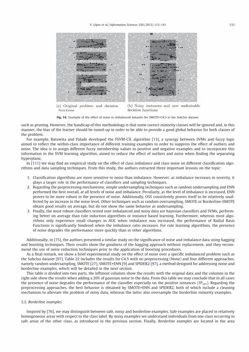
such as pruning. However, the handicap of this methodology is that some correct minority classes will be ignored and, in thismanner, the bias of the learner should be tuned-up in order to be able to provide a good global behavior for both classes ofthe problem.
For example, Batuwita and Palade developed the FSVM-CIL algorithm [13], a synergy between SVMs and fuzzy logicaimed to reflect the within-class importance of different training examples in order to suppress the effect of outliers andnoise. The idea is to assign different fuzzy membership values to positive and negative examples and to incorporate thisinformation in the SVM learning algorithm, aimed to reduce the effect of outliers and noise when finding the separatinghyperplane.
In [111] we may find an empirical study on the effect of class imbalance and class noise on different classification algo-rithms and data sampling techniques. From this study, the authors extracted three important lessons on the topic:
1. Classification algorithms are more sensitive to noise than imbalance. However, as imbalance increases in severity, itplays a larger role in the performance of classifiers and sampling techniques.
2. Regarding the preprocessing mechanisms, simple undersampling techniques such as random undersampling and ENNperformed the best overall, at all levels of noise and imbalance. Peculiarly, as the level of imbalance is increased, ENNproves to be more robust in the presence of noise. Additionally, OSS consistently proves itself to be relatively unaf-fected by an increase in the noise level. Other techniques such as random oversampling, SMOTE or Borderline-SMOTEobtain good results on average, but do not show the same behavior as undersampling.
3. Finally, the most robust classifiers tested over imbalanced and noisy data are bayesian classifiers and SVMs, perform-ing better on average than rule induction algorithms or instance based learning. Furthermore, whereas most algo-rithms only experience small changes in AUC when imbalance was increased, the performance of Radial BasisFunctions is significantly hindered when the imbalance ratio increases. For rule learning algorithms, the presenceof noise degrades the performance more quickly than in other algorithms.
Additionally, in [75], the authors presented a similar study on the significance of noise and imbalance data using baggingand boosting techniques. Their results show the goodness of the bagging approach without replacement, and they recom-mend the use of noise reduction techniques prior to the application of boosting procedures.
As a final remark, we show a brief experimental study on the effect of noise over a specific imbalanced problem such asthe Subclus dataset [97]. Table 22 includes the results for C4.5 with no preprocessing (None) and four different approaches,namely random undersampling, SMOTE [27], SMOTE+ENN [9] and SPIDER2 [97], a method designed for addressing noise andborderline examples, which will be detailed in the next section.
This table is divided into two parts, the leftmost columns show the results with the original data and the columns in theright side show the results when adding a 20% of gaussian noise to the data. From this table wemay conclude that in all casesthe presence of noise degrades the performance of the classifier especially on the positive instances (TPrate). Regarding thepreprocessing approaches, the best behavior is obtained by SMOTE+ENN and SPIDER2, both of which include a cleaningmechanism to alleviate the problem of noisy data, whereas the latter also oversample the borderline minority examples.
5.5. Borderline examples
Inspired by [76], we may distinguish between safe, noisy and borderline examples. Safe examples are placed in relativelyhomogeneous areas with respect to the class label. By noisy examples we understand individuals from one class occurring insafe areas of the other class, as introduced in the previous section. Finally, Borderline examples are located in the area
Fig. 14. Example of the effect of noise in imbalanced datasets for SMOTE+C4.5 in the Subclus dataset.
V. López et al. / Information Sciences 250 (2013) 113–141 133

surrounding class boundaries, where the minority and majority classes overlap. Fig. 15 represents two examples given by[97], named ‘‘Paw’’ and ‘‘Clover’’, respectively. In the former, the minority class is decomposed into 3 elliptic subregions,where two of them are located close to each other, and the remaining smaller sub-region is separated (upper right cluster).The latter also represents a non-linear setting, where the minority class resembles a flower with elliptic petals, which makesdifficult to determine the boundaries examples in order to carry out a correct discrimination of the classes.
The problem of noisy data and the management of borderline examples are closely related, and most of the cleaning tech-niques briefly introduced in Section 3.1 can be used, or are the basis for detecting and emphasizing these borderline in-stances and, what is most important, to distinguish them from noisy instances that can degrade the overall classification.In brief, the better the definition of the borderline areas the more precise the discrimination between the positive and neg-ative classes will be [39].
The family of SPIDER methods were proposed in [115] to ease the problem of the improvement of sensitivity at the cost ofspecificity that appears in the standard cleaning techniques. The SPIDER techniques works by combining a cleaning step ofthe majority examples with a local oversampling of the borderline minority examples [97,115,116].
We may also find other related techniques such as the Borderline-SMOTE [63], which seeks to oversample the minorityclass instances in the borderline areas, by defining a set of ‘‘Danger’’ examples, i.e. those which are most likely to be misclas-sified since they appear in the borderline areas, from which SMOTE generates synthetic minority samples in the neighbor-hood of the boundaries.
Other approaches such as Safe-Level-SMOTE [21] and ADASYN [65] work in a similar way. The former is based on thepremise that previous approaches, such as SMOTE and Borderline-SMOTE, may generate synthetic instances in unsuitablelocations, such as overlapping regions and noise regions; therefore, the authors compute a ‘‘safe-level’’ value for each posi-tive instance before generating synthetic instances and generate them closer to the largest safe level. On the other hand, thekey idea of the ADASYN algorithm is to use a density distribution as a criterion to automatically decide the number of syn-thetic samples that need to be generated for each minority example, by adaptively changing the weights of different minor-ity examples to compensate the skewed distributions.
In [87], the authors use a hierarchical fuzzy rule learning approach, which defines a higher granularity for those problemsubspaces in the borderline areas. The results have shown to be very competitive for highly imbalanced datasets in whichthis problem is accentuated.
Finally, in [97], the authors presented a series of experiments in which it is shown that the degradation in performance ofa classifier is strongly affected by the number of borderline examples. They showed that focused resampling mechanisms(such as the Neighborhood Cleaning Rule [79] or SPIDER2 [97]) work well when the number of borderline examples is largeenough whereas, on the contrary case, oversampling methods allow the improvement of the precision for the minority class.
Table 22Performance obtained by C4.5 in the Subclus dataset with and without noisy instances.
Dataset Original data 20% of Gaussian noise
TPrate TNrate AUC TPrate TNrate AUC
None 1.000 .9029 .9514 .0000 1.000 .5000RandomUnderSampling 1.000 .7800 .8900 .9700 .7400 .8550SMOTE .9614 .9529 .9571 .8914 .8800 .8857SMOTE+ENN .9676 .9623 .9649 .9625 .9573 .9599SPIDER2 1.000 1.000 1.000 .9480 .9033 .9256
Fig. 15. Example of data with difficult borderline examples.
134 V. López et al. / Information Sciences 250 (2013) 113–141
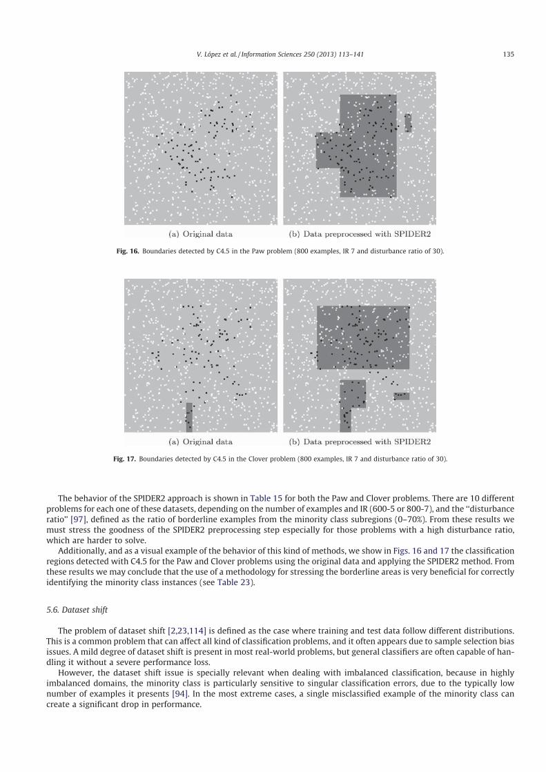
The behavior of the SPIDER2 approach is shown in Table 15 for both the Paw and Clover problems. There are 10 differentproblems for each one of these datasets, depending on the number of examples and IR (600-5 or 800-7), and the ‘‘disturbanceratio’’ [97], defined as the ratio of borderline examples from the minority class subregions (0–70%). From these results wemust stress the goodness of the SPIDER2 preprocessing step especially for those problems with a high disturbance ratio,which are harder to solve.
Additionally, and as a visual example of the behavior of this kind of methods, we show in Figs. 16 and 17 the classificationregions detected with C4.5 for the Paw and Clover problems using the original data and applying the SPIDER2 method. Fromthese results we may conclude that the use of a methodology for stressing the borderline areas is very beneficial for correctlyidentifying the minority class instances (see Table 23).
5.6. Dataset shift
The problem of dataset shift [2,23,114] is defined as the case where training and test data follow different distributions.This is a common problem that can affect all kind of classification problems, and it often appears due to sample selection biasissues. A mild degree of dataset shift is present in most real-world problems, but general classifiers are often capable of han-dling it without a severe performance loss.
However, the dataset shift issue is specially relevant when dealing with imbalanced classification, because in highlyimbalanced domains, the minority class is particularly sensitive to singular classification errors, due to the typically lownumber of examples it presents [94]. In the most extreme cases, a single misclassified example of the minority class cancreate a significant drop in performance.
Fig. 16. Boundaries detected by C4.5 in the Paw problem (800 examples, IR 7 and disturbance ratio of 30).
Fig. 17. Boundaries detected by C4.5 in the Clover problem (800 examples, IR 7 and disturbance ratio of 30).
V. López et al. / Information Sciences 250 (2013) 113–141 135

For clarity, Figs. 18 and 19 present two examples of the influence of the dataset shift in imbalanced classification. In thefirst case (Fig. 18), it is easy to see a separation between classes in the training set that carries over perfectly to the test set.However, in the second case (Fig. 19), it must be noted how some minority class examples in the test set are at the bottomand rightmost areas while they are localized in other areas in the training set, leading to a gap between the training and test-ing performance. These problems are represented in a two-dimensional space by means of a linear transformation of the in-puts variables, following the technique given in [94].
Table 23AUC results in training and testing for the Clover and Paw problems with C4.5 (Original data and data preprocessed with SPIDER2).
Dataset Disturbance 600 examples – IR 5 800 examples – IR 7
None SPIDER2 None SPIDER2
AUCTr AUCTst AUCTr AUCTst AUCTr AUCTst AUCTr AUCTst
Paw 0 .9568 .9100 .9418 .9180 .7095 .6829 .9645 .945730 .7298 .7000 .9150 .8260 .6091 .5671 .9016 .820750 .7252 .6790 .9055 .8580 .5000 .5000 .9114 .840060 .5640 .5410 .9073 .8150 .5477 .5300 .8954 .782970 .6250 .5770 .8855 .8350 .5000 .5000 .8846 .8164
Average .7202 .6814 .9110 .8504 .5732 .5560 .9115 .8411
Clover 0 .7853 .7050 .7950 .7410 .7607 .7071 .8029 .786430 .6153 .5430 .9035 .8290 .5546 .5321 .8948 .797950 .5430 .5160 .8980 .8070 .5000 .5000 .8823 .790760 .5662 .5650 .8798 .8100 .5000 .5000 .8848 .801470 .5000 .5000 .8788 .7690 .5250 .5157 .8787 .7557
Average .6020 .5658 .8710 .7912 .5681 .5510 .8687 .7864
Fig. 18. Example of good behavior (no dataset shift) in imbalanced domains: ecoli4 dataset, 5th partition.
Fig. 19. Example of bad behavior caused by dataset shift in imbalanced domains: ecoli4 dataset, 1st partition.
136 V. López et al. / Information Sciences 250 (2013) 113–141

Since the dataset shift is a highly relevant issue in imbalanced classification, it is easy to see why it would be an inter-esting perspective to focus on in future research regarding this topic. There are two different potential approaches in thestudy of the dataset shift in imbalanced domains:
1. The first one focuses on intrinsic dataset shift, that is, the data of interest includes some degree of shift that is pro-ducing a relevant drop in performance. In this case, we may develop techniques to discover and measure the presenceof dataset shift [32,33,144], but adapting them to focus on the minority class. Furthermore, we may design algorithmsthat are capable of working under dataset shift conditions, either by means of preprocessing techniques [95] or withad hoc algorithms [1,16,60]. In both cases, we are not aware of any proposals in the literature that focus on the prob-lem of imbalanced classification in the presence of dataset shift.
2. The second approach in terms of dataset shift in imbalanced classification is related to induced dataset shift. Mostcurrent state of the art research is validated through stratified cross-validation techniques, which are another poten-tial source of shift in the learning process. A more suitable validation technique needs to be developed in order toavoid introducing dataset shift issues artificially.
6. Concluding remarks
In this paper, we have reviewed the topic of classification with imbalanced datasets, and focused on two main issues: (1)to present the main approaches for dealing with this problem, namely, preprocessing of instances, cost-sensitive learningand ensemble techniques, and (2) to develop a thorough discussion on the effect of data intrinsic characteristics in learningfrom imbalanced datasets.
Mainly, we have pointed out that the imbalanced ratio by itself does not have the most significant effect on the classifiers’performance, but that there are other issues that must be taken into account. We have presented six different cases, which, inconjunction with a skewed data distribution, impose a strong handicap for achieving a high classification performance forboth classes of the problem, i.e., the presence of small disjuncts, the lack of density or small sample size, the class overlap-ping, the noisy data, the correct management of borderline examples, and the dataset shift.
For each one of the mentioned issues, we have described the main features that makes learning algorithms to be wronglybiased and we have presented several solutions proposed along the years in the specialized literature. This review paperemphasizes that there is a current need to study the aforementioned intrinsic characteristics of the data, so that future re-search on classification with imbalanced data should focus on detecting and measuring the most significant data properties,in order to be able to define good solutions as well as alternatives to overcome the problems.
Acknowledgement
This work was partially supported by the Spanish Ministry of Science and Technology under the Project TIN2011-28488and the Andalusian Research Plans P11-TIC-7765 and P10-TIC-6858. V. López holds a FPU scholarship from the Spanish Min-istry of Education.
References
[1] R. Alaiz-Rodríguez, A. Guerrero-Curieses, J. Cid-Sueiro, Improving classification under changes in class and within-class distributions, in: Proceedingsof the 10th International Work-Conference on Artificial Neural Networks (IWANN ’09), Springer-Verlag, Berlin, Heidelberg, 2009, pp. 122–130.
[2] R. Alaiz-Rodríguez, N. Japkowicz, Assessing the impact of changing environments on classifier performance, in: Proceedings of the 21st CanadianConference on Advances in Artificial Intelligence (CCAI’08), Springer-Verlag, Berlin, Heidelberg, 2008, pp. 13–24.
[3] J. Alcalá-Fdez, A. Fernández, J. Luengo, J. Derrac, S. García, L. Sánchez, F. Herrera, KEEL data–mining software tool: data set repository, integration ofalgorithms and experimental analysis framework, Journal of Multi-Valued Logic and Soft Computing 17 (2–3) (2011) 255–287.
[4] J. Alcalá;-Fdez, L. Sánchez, S. García, M.J. del Jesus, S. Ventura, J.M. Garrell, J. Otero, C. Romero, J. Bacardit, V.M. Rivas, J.C. Fernández, F. Herrera, KEEL: asoftware tool to assess evolutionary algorithms for data mining problems, Soft Computing 13 (2009) 307–318.
[5] A. Anand, G. Pugalenthi, G.B. Fogel, P.N. Suganthan, An approach for classification of highly imbalanced data using weighting and undersampling,Amino Acids 39 (5) (2010) 1385–1391.
[6] R. Baeza-Yates, B. Ribeiro-Neto, Modern Information Retrieval, Addison Wesley, 1999.[7] R. Barandela, J.S. Sánchez, V. García, E. Rangel, Strategies for learning in class imbalance problems, Pattern Recognition 36 (3) (2003) 849–851.[8] R. Barandela, R.M. Valdovinos, J.S. Sánchez, New applications of ensembles of classifiers, Pattern Analysis Applications 6 (3) (2003) 245–256.[9] G.E.A.P.A. Batista, R.C. Prati, M.C. Monard, A study of the behaviour of several methods for balancing machine learning training data, SIGKDD
Explorations 6 (1) (2004) 20–29.[10] R. Batuwita, V. Palade, AGm: a new performance measure for class imbalance learning. application to bioinformatics problems, in: Proceedings of the
8th International Conference on Machine Learning and Applications (ICMLA 2009), 2009, pp. 545–550.[11] R. Batuwita, V. Palade, microPred: effective classification of pre-miRNAs for human miRNA gene prediction, Bioinformatics 25 (8) (2009) 989–995.[12] R. Batuwita, V. Palade, Efficient resampling methods for training support vector machines with imbalanced datasets, in: Proceedings of the 2010
International Joint Conference on Neural Networks (IJCNN), 2010.[13] R. Batuwita, V. Palade, FSVM-CIL: fuzzy support vector machines for class imbalance learning, IEEE Transactions on Fuzzy Systems 18 (3) (2010) 558–
571.[14] R. Batuwita, V. Palade, Adjusted geometric-mean: a novel performance measure for imbalanced bioinformatics datasets learning, Journal of
Bioinformatics and Computational Biology 10 (4) (2012).[15] R. Batuwita, V. Palade, Class imbalance learning methods for support vector machines, in: H. He, Y. Ma (Eds.), Imbalanced Learning: Foundations,
Algorithms, and Applications, Wiley, 2013, pp. 83–96.[16] S. Bickel, M. Brückner, T. Scheffer, Discriminative learning under covariate shift, Journal of Machine Learning Research 10 (2009) 2137–2155.
V. López et al. / Information Sciences 250 (2013) 113–141 137

[17] J. Błaszczynski, M. Deckert, J. Stefanowski, S. Wilk, Integrating selective pre-processing of imbalanced data with ivotes ensemble, in: M. Szczuka, M.Kryszkiewicz, S. Ramanna, R. Jensen, Q. Hu (Eds.), Rough Sets and Current Trends in Computing, LNSC, vol. 6086, Springer, Berlin/Heidelberg, 2010,pp. 148–157.
[18] J.P. Bradford, C. Kunz, R. Kohavi, C. Brunk, C.E. Brodley, Pruning decision trees with misclassification costs, in: Proceedings of the 10th EuropeanConference on Machine Learning (ECML’98), 1998, pp. 131–136.
[19] A.P. Bradley, The use of the area under the roc curve in the evaluation of machine learning algorithms, Pattern Recognition 30 (7) (1997) 1145–1159.[20] C.E. Brodley, M.A. Friedl, Identifying mislabeled training data, Journal of Artificial Intelligence Research 11 (1999) 131–167.[21] C. Bunkhumpornpat, K. Sinapiromsaran, C. Lursinsap, Safe–level–SMOTE: Safe–level–synthetic minority over–sampling TEchnique for handling the
class imbalanced problem. In: Proceedings of the 13th Pacific–Asia Conference on Advances in Knowledge Discovery and Data Mining PAKDD’09,2009, pp. 475–482.
[22] C. Bunkhumpornpat, K. Sinapiromsaran, C. Lursinsap, DBSMOTE: density-based synthetic minority over-sampling technique, Applied Intelligence 36(3) (2012) 664–684.
[23] J.Q. Candela, M. Sugiyama, A. Schwaighofer, N.D. Lawrence, Dataset Shift in Machine Learning, The MIT Press, 2009.[24] D.R. Carvalho, A.A. Freitas, A hybrid decision tree/genetic algorithm method for data mining, Information Sciences 163 (1–3) (2004) 13–35.[25] P.K. Chan, S.J. Stolfo, Toward scalable learning with non-uniform class and cost distributions: a case study in credit card fraud detection, in:
Proceedings of the 4th International Conference on Knowledge Discovery and Data Mining (KDD’98). 1998. pp. 164–168.[26] E.Y. Chang, B. Li, G. Wu, K. Goh, Statistical learning for effective visual information retrieval, in: Proceedings of the 2003 International Conference on
Image Processing (ICIP’03), vol. 3, 2003, pp. 609–612.[27] N.V. Chawla, K.W. Bowyer, L.O. Hall, W.P. Kegelmeyer, SMOTE: synthetic minority over-sampling technique, Journal of Artificial Intelligent Research
16 (2002) 321–357.[28] N.V. Chawla, D.A. Cieslak, L.O. Hall, A. Joshi, Automatically countering imbalance and its empirical relationship to cost, Data Mining and Knowledge
Discovery 17 (2) (2008) 225–252.[29] N.V. Chawla, N. Japkowicz, A. Kotcz, Editorial: special issue on learning from imbalanced data sets, SIGKDD Explorations 6 (1) (2004) 1–6.[30] N.V. Chawla, A. Lazarevic, L.O. Hall, K.W. Bowyer, SMOTEBoost: Improving prediction of the minority class in boosting, in: Proceedings of 7th
European Conference on Principles and Practice of Knowledge Discovery in Databases (PKDD’03), 2003, pp. 107–119.[31] X. Chen, T. Fang, H. Huo, D. Li, Graph-based feature selection for object-oriented classification in VHR airborne imagery, IEEE Transactions on
Geoscience and Remote Sensing 49 (1) (2011) 353–365.[32] D.A. Cieslak, N.V. Chawla, Analyzing pets on imbalanced datasets when training and testing class distributions differ, in: Proceedings of the Pacific-
Asia Conference on Knowledge Discovery and Data Mining (PAKDD08). Osaka, Japan, 2008, pp. 519–526.[33] D.A. Cieslak, N.V. Chawla, A framework for monitoring classifiers’ performance: when and why failure occurs?, Knowledge and Information Systems
18 (1) (2009) 83–108[34] G. Cohen, M. Hilario, H. Sax, S. Hugonnet, A. Geissbuhler, Learning from imbalanced data in surveillance of nosocomial infection, Artificial Intelligence
in Medicine 37 (2006) 7–18.[35] C. Cortes, V. Vapnik, Support vector networks, Machine Learning 20 (1995) 273–297.[36] J. Davis, M. Goadrich, The relationship between precisionrecall and ROC curves, in: Proceedings of the 23th International Conference on Machine
Learning (ICML’06), ACM, 2006, pp. 233–240.[37] M. Denil, T. Trappenberg, Overlap versus imbalance, in: Proceedings of the 23rd Canadian Conference on Advances in Artificial Intelligence (CCAI’10),
Lecture Notes on Artificial Intelligence, vol. 6085, 2010, pp. 220–231.[38] P. Domingos, Metacost: a general method for making classifiers cost–sensitive, in: Proceedings of the 5th International Conference on Knowledge
Discovery and Data Mining (KDD’99), 1999, pp. 155–164.[39] D.J. Drown, T.M. Khoshgoftaar, N. Seliya, Evolutionary sampling and software quality modeling of high-assurance systems, IEEE Transactions on
Systems, Man, and Cybernetics, Part A 39 (5) (2009) 1097–1107.[40] C. Drummond, R.C. Holte, Cost curves: an improved method for visualizing classifier performance, Machine Learning 65 (1) (2006) 95–130.[41] P. Ducange, B. Lazzerini, F. Marcelloni, Multi-objective genetic fuzzy classifiers for imbalanced and cost-sensitive datasets, Soft Computing 14 (7)
(2010) 713–728.[42] C. Elkan, The foundations of cost–sensitive learning, in: Proceedings of the 17th IEEE International Joint Conference on Artificial Intelligence (IJCAI’01),
2001, pp. 973–978.[43] A. Estabrooks, T. Jo, N. Japkowicz, A multiple resampling method for learning from imbalanced data sets, Computational Intelligence 20 (1) (2004) 18–
36.[44] W. Fan, S.J. Stolfo, J. Zhang, P.K. Chan, Adacost: misclassification cost-sensitive boosting, in: Proceedings of the 16th International Conference on
Machine Learning (ICML’96), Morgan Kaufmann Publishers Inc., San Francisco, CA, USA, 1999, pp. 97–105.[45] A. Fernández, M.J. del Jesus, F. Herrera, On the 2-tuples based genetic tuning performance for fuzzy rule based classification systems in imbalanced
data-sets, Information Sciences 180 (8) (2010) 1268–1291.[46] A. Fernández, S. García, M.J. del Jesus, F. Herrera, A study of the behaviour of linguistic fuzzy rule based classification systems in the framework of
imbalanced data-sets, Fuzzy Sets and Systems 159 (18) (2008) 2378–2398.[47] A. Fernandez, S. García, J. Luengo, E. Bernadó-Mansilla, F. Herrera, Genetics-based machine learning for rule induction: state of the art, taxonomy and
comparative study, IEEE Transactions on Evolutionary Computation 14 (6) (2010) 913–941.[48] A. Fernández, V. López, M. Galar, M.J. del Jesus, F. Herrera, Analysing the classification of imbalanced data-sets with multiple classes: binarization
techniques and ad-hoc approaches, Knowledge-Based Systems 42 (2013) 97–110.[49] J.H. Friedman, R. Kohavi, Y. Yun, Lazy decision trees, in: Proceedings of the AAAI/IAAI, vol. 1, 1996, pp. 717–724.[50] M. Galar, A. Fernández, E. Barrenechea, H. Bustince, F. Herrera, A review on ensembles for class imbalance problem: bagging, boosting and hybrid
based approaches, IEEE Transactions on Systems, Man, and Cybernetics – part C: Applications and Reviews 42 (4) (2012) 463–484.[51] S. García, J. Derrac, I. Triguero, C.J. Carmona, F. Herrera, Evolutionary-based selection of generalized instances for imbalanced classification,
Knowledge Based Systems 25 (1) (2012) 3–12.[52] S. García, A. Fernández, F. Herrera, Enhancing the effectiveness and interpretability of decision tree and rule induction classifiers with evolutionary
training set selection over imbalanced problems, Applied Soft Computing 9 (2009) 1304–1314.[53] S. García, F. Herrera, Evolutionary under-sampling for classification with imbalanced data sets: proposals and taxonomy, Evolutionary Computation
17 (3) (2009) 275–306.[54] V. García, R.A. Mollineda, J.S. Sánchez, A new performance evaluation method for two-class imbalanced problems, in: Proceedings of the Structural
and Syntactic Pattern Recognition (SSPR’08) and Statistical Techniques in Pattern Recognition (SPR’08), Lecture Notes on Computer Science, vol. 5342,2008, pp. 917–925.
[55] V. García, R.A. Mollineda, J.S. Sánchez, On the k-NN performance in a challenging scenario of imbalance and overlapping, Pattern Analysis Applications11 (3–4) (2008) 269–280.
[56] V. García, R.A. Mollineda, J.S. Sánchez, Theoretical analysis of a performance measure for imbalanced data, in: 20th International Conference onPattern Recognition (ICPR’10), 2010, pp. 617–620.
[57] V. García, R.A. Mollineda, J.S. Sánchez, Classifier performance assessment in two-class imbalanced problems, Internal Communication.(2012).
[58] V. García, J.S. Sánchez, R.A. Mollineda, On the effectiveness of preprocessing methods when dealing with different levels of class imbalance,Knowledge Based Systems 25 (1) (2012) 13–21.
138 V. López et al. / Information Sciences 250 (2013) 113–141
[59] N. García-Pedrajas, J. Pérez-Rodríguez, M. García-Pedrajas, D. Ortiz-Boyer, C. Fyfe, Class imbalance methods for translation initiation site recognitionin DNA sequences, Knowledge Based Systems 25 (1) (2012) 22–34.
[60] A. Globerson, C.H. Teo, A. Smola, S. Roweis, An adversarial view of covariate shift and a minimax approach, in: J. Quiñonero Candela, M. Sugiyama, A.Schwaighofer, N.D. Lawrence (Eds.), Dataset Shift in Machine Learning, The MIT Press, 2009, pp. 179–198.
[61] H. Guo, H.L. Viktor, Learning from imbalanced data sets with boosting and data generation: the DataBoost-IM approach, SIGKDD ExplorationsNewsletter 6 (2004) 30–39.
[62] M. Hall, E. Frank, G. Holmes, B. Pfahringer, P. Reutemann, I.H. Witten, The WEKA data mining software: an update, SIGKDD Explorations 11 (1) (2009)10–18.
[63] H. Han, W.Y. Wang, B.H. Mao, Borderline–SMOTE: a new over–sampling method in imbalanced data sets learning, in: Proceedings of the 2005International Conference on Intelligent Computing (ICIC’05), Lecture Notes in Computer Science, vol. 3644, 2005, pp. 878–887.
[64] P.E. Hart, The condensed nearest neighbor rule, IEEE Transactions on Information Theory 14 (1968) 515–516.[65] H. He, Y. Bai, E.A. Garcia, S. Li, ADASYN: adaptive synthetic sampling approach for imbalanced learning, in: Proceedings of the 2008 IEEE International
Joint Conference on Neural Networks (IJCNN’08), 2008, pp. 1322–1328.[66] H. He, E.A. Garcia, Learning from imbalanced data, IEEE Transactions on Knowledge and Data Engineering 21 (9) (2009) 1263–1284.[67] S. Hido, H. Kashima, Y. Takahashi, Roughly balanced bagging for imbalanced data, Statistical Analysis and Data Mining 2 (2009) 412–426.[68] R.C. Holte, L. Acker, B.W. Porter, Concept learning and the problem of small disjuncts, in: Proceedings of the International Joint Conferences on
Artificial Intelligence, IJCAI’89, 1989, pp. 813–818.[69] S. Hu, Y. Liang, L. Ma, Y. He, MSMOTE: improving classification performance when training data is imbalanced, in: Proceedings of the 2nd
International Workshop on Computer Science and Engineering (WCSE’09), vol. 2, 2009, pp. 13–17.[70] J. Huang, C.X. Ling, Using AUC and accuracy in evaluating learning algorithms, IEEE Transactions on Knowledge and Data Engineering 17 (3) (2005)
299–310.[71] N. Japkowicz, Concept-learning in the presence of between-class and within-class imbalances, in: E. Stroulia, S. Matwin (Eds.), Proceedings of the
14th Canadian Conference on Advances in Artificial Intelligence (CCAI’08), Lecture Notes in Computer Science, vol. 2056, Springer, 2001, pp. 67–77.[72] N. Japkowicz, S. Stephen, The class imbalance problem: a systematic study, Intelligent Data Analysis Journal 6 (5) (2002) 429–450.[73] T. Jo, N. Japkowicz, Class imbalances versus small disjuncts, ACM SIGKDD Explorations Newsletter 6 (1) (2004) 40–49.[74] M.V. Joshi, V. Kumar, R.C. Agarwal, Evaluating boosting algorithms to classify rare classes: comparison and improvements, in: Proceedings of the 2001
IEEE International Conference on Data Mining (ICDM’01), IEEE Computer Society, Washington, DC, USA, 2001, pp. 257–264.[75] T.M. Khoshgoftaar, J. Van Hulse, A. Napolitano, Comparing boosting and bagging techniques with noisy and imbalanced data, IEEE Transactions on
Systems, Man and Cybernetics, Part A: Systems and Humans 41 (3) (2011) 552–568.[76] M. Kubat, S. Matwin, Addressing the curse of imbalanced training sets: one-sided selection, in: Proceedings of the 14th International Conference on
Machine Learning (ICML’97), 1997, pp. 179–186.[77] L.I. Kuncheva, J.J. Rodrguez, A weighted voting framework for classifiers ensembles, Knowledge and Information Systems (2013), http://dx.doi.org/
10.1007/s10115-012-0586-6. in press.[78] N. Kwak, Feature extraction for classification problems and its application to face recognition, Pattern Recognition 41 (5) (2008) 1718–1734.[79] J. Laurikkala, Improving identification of difficult small classes by balancing class distribution, in: Proceedings of the 8th Conference on AI in Medicine
in Europe: Artificial Intelligence Medicine (AIME’01), 2001, pp. 63–66.[80] C. Li, Classifying imbalanced data using a bagging ensemble variation (BEV), Proceedings of the 45th Annual Southeast Regional Conference, vol. 45,
ACM-SE ACM, New York, NY, USA, 2007, pp. 203–208.[81] M. Lin, K. Tang, X. Yao, Dynamic sampling approach to training neural networks for multiclass imbalance classification, IEEE Transactions on Neural
Networks and Learning Systems 24 (4) (2013) 647–660.[82] W. Lin, J.J. Chen, Class-imbalanced classifiers for high-dimensional data, Briefings in Bioinformatics 14 (1) (2013) 13–26.[83] C.X. Ling, C. Li, Data mining for direct marketing: Problems and solutions, in: Proceedings of the 4th International Conference on Knownledge
Discovery and Data Mining (KDD’98), 1998, pp. 73–79.[84] C.X. Ling, Q. Yang, J. Wang, S. Zhang, Decision trees with minimal costs, in: C.E. Brodley (Ed.), Proceedings of the 21st International Conference on
Machine Learning (ICML’04), ACM International Conference Proceeding Series, vol. 69, ACM, 2004, pp. 69–77.[85] X.-Y. Liu, J. Wu, Z.-H. Zhou, Exploratory undersampling for class-imbalance learning, IEEE Transactions on System, Man and Cybernetics B 39 (2)
(2009) 539–550.[86] H.-Y. Lo, C.-M. Chang, T.-H. Chiang, C.-Y. Hsiao, A. Huang, T.-T. Kuo, W.-C. Lai, M.-H. Yang, J.-J. Yeh, C.-C. Yen, S.-D. Lin, Learning to improve area-under-
FROC for imbalanced medical data classification using an ensemble method, SIGKDD Explorations 10 (2) (2008) 43–46.[87] V. López, A. Fernández, M.J. del Jesus, F. Herrera, A hierarchical genetic fuzzy system based on genetic programming for addressing classification with
highly imbalanced and borderline data-sets, Knowledge-Based Systems 38 (2013) 85–104.[88] V. López, A. Fernández, J.G. Moreno-Torres, F. Herrera, Analysis of preprocessing vs. cost-sensitive learning for imbalanced classification. open
problems on intrinsic data characteristics, Expert Systems with Applications 39 (7) (2012) 6585–6608.[89] J. Luengo, A. Fernández, S. García, F. Herrera, Addressing data complexity for imbalanced data sets: analysis of SMOTE-based oversampling and
evolutionary undersampling, Soft Computing 15 (10) (2011) 1909–1936.[90] R. Martín-Félez, R.A., Mollineda, On the suitability of combining feature selection and resampling to manage data complexity, in: Proceedings of the
Conferencia de la Asociacin Espaola de Inteligencia Artificial (CAEPIA’09), Lecture Notes on Artificial Intelligence, vol. 5988, 2010, pp. 141–150.[91] M.A. Mazurowski, P.A. Habas, J.M. Zurada, J.Y. Lo, J.A. Baker, G.D. Tourassi, Training neural network classifiers for medical decision making: the effects
of imbalanced datasets on classification performance, Neural Networks 21 (2–3) (2008).[92] G.J. McLachlan, Discriminant Analysis and Statistical Pattern Recognition, John Wiley and Sons, 2004.[93] L. Mena, J.A. González, Symbolic one-class learning from imbalanced datasets: application in medical diagnosis, International Journal on Artificial
Intelligence Tools 18 (2) (2009) 273–309.[94] J.G. Moreno-Torres, F. Herrera, A preliminary study on overlapping and data fracture in imbalanced domains by means of genetic programming-based
feature extraction, in: Proceedings of the 10th International Conference on Intelligent Systems Design and Applications (ISDA’10), 2010, pp. 501–506.[95] J.G. Moreno-Torres, X. Llorà, D.E. Goldberg, R. Bhargava, Repairing fractures between data using genetic programming-based feature extraction: a case
study in cancer diagnosis, Information Sciences 222 (2013) 805–823.[96] J.G. Moreno-Torres, T. Raeder, R. Aláiz-Rodríguez, N.V. Chawla, F. Herrera, A unifying view on dataset shift in classification, Pattern Recognition 45 (1)
(2012) 521–530.[97] K. Napierala, J. Stefanowski, S. Wilk, Learning from imbalanced data in presence of noisy and borderline examples, in: Proceedings of the 7th
International Conference on Rough Sets and Current Trends in Computing (RSCTC’10), Lecture Notes on Artificial Intelligence, vol. 6086, 2010, pp.158–167.
[98] A. Orriols-Puig, E. Bernadó-Mansilla, Evolutionary rule-based systems for imbalanced datasets, Soft Computing 13 (3) (2009) 213–225.[99] A. Orriols-Puig, E. Bernadó-Mansilla, D.E. Goldberg, K. Sastry, P.L. Lanzi, Facetwise analysis of XCS for problems with class imbalances, IEEE
Transactions on Evolutionary Computation 13 (2009) 260–283.[100] J. Platt, Fast training of support vector machines using sequential minimal optimization, in: Advances in Kernel Methods – Support Vector Learning,
MIT Press, Cambridge, MA, 1998, pp. 42–65.[101] R. Polikar, Ensemble based systems in decision making, IEEE Circuits and Systems Magazine 6 (3) (2006) 21–45.[102] R.C. Prati, G.E.A.P.A., Batista, Class imbalances versus class overlapping: an analysis of a learning system behavior, in: Proceedings of the 2004
Mexican International Conference on Artificial Intelligence (MICAI’04), 2004, pp. 312–321.
V. López et al. / Information Sciences 250 (2013) 113–141 139

[103] R.C. Prati, G.E.A.P.A. Batista, M.C. Monard, A survey on graphical methods for classification predictive performance evaluation, IEEE Transactions onKnowledge and Data Engineering 23 (11) (2011) 1601–1618.
[104] J.R. Quinlan, C4.5: Programs for Machine Learning., Morgan Kauffman, 1993.[105] T. Raeder, G. Forman, N.V. Chawla, Learning from imbalanced data: evaluation matters, in: D.E. Holmes, L.C. Jain (Eds.), Data Mining: Found. and
Intell. Paradigms, vol. ISRL 23, Springer-Verlag, 2012, pp. 315–331.[106] S.J. Raudys, A.K. Jain, Small sample size effects in statistical pattern recognition: recommendations for practitioners, IEEE Transactions on Pattern
Analysis and Machine Intelligence 13 (3) (1991) 252–264.[107] P. Riddle, R. Segal, O. Etzioni, Representation design and brute-force induction in a boeing manufacturing domain, Applied Artificial Intelligence 8
(1994) 125–147.[108] L. Rokach, Ensemble-based classifiers, Artificial Intelligence Review 33 (1) (2010) 1–39.[109] J.A. Sáez, J. Luengo, F. Herrera, A first study on the noise impact in classes for fuzzy rule based classification systems, in: Proceedings of the 2010 IEEE
International Conference on Intelligent Systems and Knowledge Engineering (ISKE’10), IEEE Press, 2010, pp. 153–158.[110] R.E. Schapire, A brief introduction to boosting, in: Proceedings of the International Joint Conference on Artificial Intelligence (IJCAI’99), 1999, pp.
1401–1406.[111] C. Seiffert, T.M. Khoshgoftaar, J. Van Hulse, A. Folleco, An empirical study of the classification performance of learners on imbalanced and noisy
software quality data, Information Sciences (2013), http://dx.doi.org/10.1016/j.ins.2010.12.016. in press.[112] C. Seiffert, T.M. Khoshgoftaar, J. Van Hulse, A. Napolitano, RUSBoost: a hybrid approach to alleviating class imbalance, IEEE Transactions on System,
Man and Cybernetics A 40 (1) (2010) 185–197.[113] J.P. Shaffer, Modified sequentially rejective multiple test procedures, Journal of the American Statistical Association 81 (395) (1986) 826–831.[114] H. Shimodaira, Improving predictive inference under covariate shift by weighting the log-likelihood function, Journal of Statistical Planning and
Inference 90 (2) (2000) 227–244.[115] J. Stefanowski, S. Wilk, Improving rule based classifiers induced by MODLEM by selective pre-processing of imbalanced data, in: Proceedings of the
RSKD Workshop at ECML/PKDD’07, 2007, pp. 54–65.[116] J. Stefanowski, S. Wilk, Selective pre-processing of imbalanced data for improving classification performance, in: Proceedings of the 10th
International Conference on Data Warehousing and Knowledge, Discovery (DaWaK08), 2008, pp. 283–292.[117] Y. Sun, M.S. Kamel, A.K.C. Wong, Y. Wang, Cost-sensitive boosting for classification of imbalanced data, Pattern Recognition 40 (12) (2007) 3358–
3378.[118] Y. Sun, A.K.C. Wong, M.S. Kamel, Classification of imbalanced data: a review, International Journal of Pattern Recognition and Artificial Intelligence 23
(4) (2009) 687–719.[119] Y. Tang, Y.-Q. Zhang, N.V. Chawla, S. Kresser, SVMs modeling for highly imbalanced classification, IEEE Transactions on Systems, Man and Cybernetics,
Part B 9 (1) (2009) 281–288.[120] D. Tao, X. Tang, X. Li, X. Wu, Asymmetric bagging and random subspace for support vector machines-based relevance feedback in image retrieval,
IEEE Transactions on Pattern Analysis and Machine Intelligence 28 (7) (2006) 1088–1099.[121] K.M. Ting, The problem of small disjuncts: its remedy in decision trees, in: Proceedings of the 10th Canadian Conference on Artificial Intelligence
(CCAI’94), 1994, pp. 91–97.[122] K.M. Ting, A comparative study of cost-sensitive boosting algorithms, in: Proceedings of the 17th International Conference on Machine Learning
(ICML’00), Stanford, CA, USA, 2000, pp. 983–990.[123] K.M. Ting, An instance-weighting method to induce cost-sensitive trees, IEEE Transactions on Knowledge and Data Engineering 14 (3) (2002) 659–
665.[124] I. Tomek, Two modifications of CNN, IEEE Transactions on Systems Man and Communications 6 (1976) 769–772.[125] C.-H. Tsai, L.-C. Chang, H.-C. Chiang, Forecasting of ozone episode days by cost-sensitive neural network methods, Science of the Total Environment
407 (6) (2009) 2124–2135.[126] P.D. Turney, Cost-sensitive classification: empirical evaluation of a hybrid genetic decision tree induction algorithm, Journal of Artificial Intelligence
Research 2 (1995) 369–409.[127] J. Van Hulse, T.M. Khoshgoftaar, A. Napolitano, An empirical comparison of repetitive undersampling techniques, in: Proceedings of the 2009 IEEE
International Conference on Information Reuse, Integration (IRI’09), 2009, pp. 29–34.[128] B.X. Wang, N. Japkowicz, Imbalanced data set learning with synthetic samples, in: Proceedings of the IRIS Machine Learning Workshop, 2004.[129] J. Wang, J. You, Q. Li, Y. Xu, Extract minimum positive and maximum negative features for imbalanced binary classification, Pattern Recognition 45 (3)
(2012) 1136–1145.[130] S. Wang, X. Yao, Diversity analysis on imbalanced data sets by using ensemble models, in: Proceedings of the 2009 IEEE Symposium on
Computational Intelligence and Data Mining (CIDM’09), 2009, pp. 324–331.[131] S. Wang, X. Yao, Relationships between diversity of classification ensembles and single-class performance measures, IEEE Transactions on Knowledge
and Data Engineering 25 (1) (2013) 206–219.[132] Z. Wang, V. Palade, Building interpretable fuzzy models for high dimensional data analysis in cancer diagnosis, BMC Genomics 12 ((S2):S5) (2011).[133] M. Wasikowski, X.-W. Chen, Combating the small sample class imbalance problem using feature selection, IEEE Transactions on Knowledge and Data
Engineering 22 (10) (2010) 1388–1400.[134] G.M. Weiss, Timeweaver: a genetic algorithm for identifying pre-dictive patterns in sequences of events, in: W. Banzhaf, J. Daida, A.E. Eiben, M.H.
Garzon, V. Honavar, M. Jakiela, R.E. Smith (Eds.), Proceedings of the Genetic and Evolutionary Computation Conference GECCO’99, vol. 1, MorganKaufmann, Orlando, Florida, USA, 1999, pp. 718–725.
[135] G.M. Weiss, Mining with rarity: a unifying framework, SIGKDD Explorations 6 (1) (2004) 7–19.[136] G.M. Weiss, Mining with rare cases, in: O. Maimon, L. Rokach (Eds.), The Data Mining and Knowledge Discovery Handbook, Springer, 2005, pp. 765–
776.[137] G.M. Weiss, The impact of small disjuncts on classifier learning, in: R. Stahlbock, S.F. Crone, S. Lessmann (Eds.), Data Mining: Annals of Information
Systems, vol. 8, Springer, 2010, pp. 193–226.[138] G.M. Weiss, F.J. Provost, Learning when training data are costly: the effect of class distribution on tree induction, Journal of Artificial Intelligence
Research 19 (2003) 315–354.[139] G.M. Weiss, Y. Tian, Maximizing classifier utility when there are data acquisition and modeling costs, Data Mining and Knowledge Discovery 17 (2)
(2008) 253–282.[140] D.L. Wilson, Asymptotic properties of nearest neighbor rules using edited data, IEEE Transactions on Systems, Man and Cybernetics 2 (3) (1972) 408–
421.[141] R. Yan, Y. Liu, R. Jin, A. Hauptmann, On predicting rare classes with SVM ensembles in scene classification, in: Proceedings of the 2003 IEEE
International Conference on Acoustics, Speech, and Signal Processing (ICASSP’03), vol. 3, 2003, pp. 21–24.[142] P. Yang, L. Xu, B.B. Zhou, Z. Zhang, A.Y. Zomaya, A particle swarm based hybrid system for imbalanced medical data sampling, BMC Genomics 10
(Suppl. 3) (2009). art. no. S34..[143] Q. Yang, X. Wu, 10 challenging problems in data mining research, International Journal of Information Technology and Decision Making 5 (4) (2006)
597–604.[144] Y. Yang, X. Wu, X. Zhu, Conceptual equivalence for contrast mining in classification learning, Data & Knowledge Engineering 67 (3) (2008) 413–429.[145] S. Yen, Y. Lee, Under-sampling approaches for improving prediction of the minority class in an imbalanced dataset, in: Proceedings of the 2006
International Conference on Intelligent, Computing (ICIC06), 2006, pp. 731–740.
140 V. López et al. / Information Sciences 250 (2013) 113–141

[146] K. Yoon, S. Kwek, An unsupervised learning approach to resolving the data imbalanced issue in supervised learning problems in functional genomics,in: Proceedings of the 5th International Conference on Hybrid Intelligent Systems (HIS’05), 2005, pp. 303–308.
[147] B. Zadrozny, C. Elkan, Learning and making decisions when costs and probabilities are both unknown, in: Proceedings of the 7th InternationalConference on Knowledge Discovery and Data Mining (KDD’01), 2001, pp. 204–213.
[148] B. Zadrozny, J. Langford, N. Abe, Cost–sensitive learning by cost–proportionate example weighting, in: Proceedings of the 3rd IEEE InternationalConference on Data Mining (ICDM’03), 2003, pp. 435–442.
[149] J. Zhang, I. Mani, KNN approach to unbalanced data distributions: a case study involving information extraction, in: Proceedings of the 20thInternational Conference on Machine Learning (ICML’03), Workshop Learning from Imbalanced Data Sets, 2003.
[150] Z.-H. Zhou, X.-Y. Liu, Training cost-sensitive neural networks with methods addressing the class imbalance problem, IEEE Transactions on Knowledgeand Data Engineering 18 (1) (2006) 63–77.
[151] X. Zhu, X. Wu, Class noise vs. attribute noise: a quantitative study, Artificial Intelligence Review 22 (3) (2004) 177–210.[152] W. Zong, G.-B. Huang, Y. Chen, Weighted extreme learning machine for imbalance learning, Neurocomputing 101 (2013) 229–242.
V. López et al. / Information Sciences 250 (2013) 113–141 141


2 Addressing the Data Intrinsic Characteristics of Imbalanced Problems using FRBCSs and MachineLearning Techniques 91
2. Addressing the Data Intrinsic Characteristics of Imbalanced
Problems using FRBCSs and Machine Learning Techniques
The journal papers associated to this part are:
2.1. A Hierarchical Genetic Fuzzy System Based On Genetic Programming for
Addressing Classification with Highly Imbalanced and Borderline Data-
sets
V. Lopez, A. Fernandez, M. J. del Jesus, F. Herrera, A Hierarchical Genetic FuzzySystem Based On Genetic Programming for Addressing Classification with Highly Im-balanced and Borderline Data-sets. Knowledge-Based Systems 38 (2013) 85–104, doi:10.1016/j.knosys.2012.08.025
• Status: Published.
• Impact Factor (JCR 2012): 4.104.
• Subject Category: Computer Science, Artificial Intelligence. Ranking 6 / 115 (Q1).
• Citations (Web of Science): 2.
• Citations (Google Scholar): 9.


A hierarchical genetic fuzzy system based on genetic programming foraddressing classification with highly imbalanced and borderline data-sets
Victoria López a,⇑, Alberto Fernández b, María José del Jesus b, Francisco Herrera a
aDept. of Computer Science and Artificial Intelligence, CITIC-UGR, Research Center on Information and Communications Technology, University of Granada, 18071 Granada, SpainbDept. of Computer Science, University of Jaén, 23071 Jaén, Spain
a r t i c l e i n f o
Article history:Received 18 October 2011Received in revised form 3 June 2012Accepted 24 August 2012Available online 3 October 2012
Keywords:Fuzzy rule based classification systemsHierarchical fuzzy partitionsGenetic rule selectionTuningImbalanced data-setsBorderline examples
a b s t r a c t
Lots of real world applications appear to be a matter of classification with imbalanced data-sets. Thisproblem arises when the number of instances from one class is quite different to the number of instancesfrom the other class. Traditionally, classification algorithms are unable to correctly deal with this issue asthey are biased towards the majority class. Therefore, algorithms tend to misclassify the minority classwhich usually is the most interesting one for the application that is being sorted out.Among the available learning approaches, fuzzy rule-based classification systems have obtained a good
behavior in the scenario of imbalanced data-sets. In this work, we focus on some modifications to furtherimprove the performance of these systems considering the usage of information granulation. Specifically,a positive synergy between data sampling methods and algorithmic modifications is proposed, creating agenetic programming approach that uses linguistic variables in a hierarchical way. These linguistic vari-ables are adapted to the context of the problem with a genetic process that combines rule selection withthe adjustment of the lateral position of the labels based on the 2-tuples linguistic model.An experimental study is carried out over highly imbalanced and borderline imbalanced data-sets
which is completed by a statistical comparative analysis. The results obtained show that the proposedmodel outperforms several fuzzy rule based classification systems, including a hierarchical approachand presents a better behavior than the C4.5 decision tree.
� 2012 Elsevier B.V. All rights reserved.
1. Introduction
Learning from imbalanced data-sets is an issue that has at-tracted a lot of attention in machine learning research [29,51]. Thisproblem is characterized by a class distribution where the numberof examples in one class is outnumbered by the number of exam-ples in the other class. The presence of imbalanced data-sets isdominant in a high number of real problems including, but not lim-ited to, medical diagnosis, fraud detection, finances, risk manage-ment, network intrusion and so on. Additionally, the positive orminority class is usually the one that has the highest interest fromthe learning point of view and it also implies a great cost when it isnot well classified [17,57].
A standard classifier that seeks accuracy over a full range of in-stances is frequently not suitable to deal with imbalanced learningtasks, since it tends to be overwhelmed by the majority class thusmisclassifying the minority examples. This situation becomes crit-ical when the minority class is greatly outnumbered by the major-ity class, generating an scenario of highly imbalanced data-sets
where the performance deterioration is amplified. However, somestudies have shown that imbalance for itself is not the only factorthat hinders the classification performance [37]. There are severaldata intrinsic characteristics which lower the learning effective-ness. Some of these handicaps within the data are the presenceof small disjuncts [53], the overlap between the classes [26] orthe existence of noisy [49] and borderline [44] samples. There isno need to say that when the classification data share an skeweddata distribution together with any of the aforementioned situa-tions, the performance degradation is intensified [19,42,53].
A large number of approaches have been proposed to deal withthe class imbalance problem. Those solutions fall largely into twomajor categories. The first is data sampling in which the trainingdata distribution is modified to obtain a set with a balanced distri-bution. Standard classifiers are thus helped to obtain a correctidentification of data [9,6]. The second is through algorithmic mod-ification where the base learning methods are modified to considerthe imbalanced distribution of the data. In this manner, base learn-ing methods change some of its internal operations accordingly[57].
Fuzzy Rule-Based Classification Systems (FRBCSs) [34] areuseful and well-known tools in the machine learning framework.They provide a good trade-off between the empirical precision of
0950-7051/$ - see front matter � 2012 Elsevier B.V. All rights reserved.http://dx.doi.org/10.1016/j.knosys.2012.08.025
⇑ Corresponding author. Tel.: +34 958 240598; fax: +34 958 243317.E-mail addresses: [email protected] (V. López), [email protected]
(A. Fernández), [email protected] (M.J. del Jesus), [email protected] (F. Herrera).
Knowledge-Based Systems 38 (2013) 85–104
Contents lists available at SciVerse ScienceDirect
Knowledge-Based Systems
journal homepage: www.elsevier .com/ locate /knosys

traditional engineering techniques and the interpretabilityachieved through the use of linguistic labels whose semantic isclose to the natural language. Specifically, recent works haveshown that FRBCSs have a good behavior dealing with imbalanceddata-sets by means of the application of instance preprocessingtechniques [20].
The hybridization between fuzzy logic and genetic algorithmsleading to Genetic Fuzzy Systems (GFSs) [12,30] is one of the mostpopular approaches used when different computational intelli-gence techniques are combined. A GFS is basically a fuzzy systemaugmented by a learning process based on evolutionary computa-tion. Among evolutionary algorithms, Genetic Programming (GP)[39] is a development of classical genetic algorithms that evolvetree-shaped solutions using variable length chromosomes. GP hasbeen used in FRBCSs to learn fuzzy rule bases [7] profitting fromits high expressive power and flexibility.
However, the disadvantage of FRBCSs is the inflexibility of theconcept of linguistic variable because it imposes hard restrictionson the fuzzy rule structure [5] which may suppose a loss in accu-racy when dealing with some complex systems, such as highdimensional problems, the presence of noise or overlapped classes.Many different possibilities to enhance the linguistic fuzzy model-ing have been considered in the specialized literature. All of theseapproaches share the common idea of improving the way in whichthe linguistic fuzzy model performs the interpolative reasoning byinducing a better cooperation among the rules in the KnowledgeBase (KB). This rule cooperation may be induced acting on threedifferent model components:
� Approaches acting on the whole KB. This includes the KB deriva-tion [43] and a hierarchical linguistic rule learning [14].
� Approaches acting on the Rule Base (RB). The most commonapproach is rule selection [35] but also multiple rule conse-quent learning [11] could be considered.
� Approaches acting on the Data Base (DB). For example a priorigranularity learning [13] or membership function tuning [1].
In this work, we present a procedure to obtain an HierarchicalFuzzy Rule Based Classification System (HFRBCS) to deal withimbalanced data-sets. In order to do so, this model introducesmodifications both at the data and algorithm level. This procedureis divided into three different steps:
1. A preprocessing technique, the Synthetic Minority Over-sampling Technique (SMOTE) [9], is used to balance thedistribution of training examples in both classes.
2. A hierarchical knowledge base (HKB) [14] is generated, usingthe GP-COACH (Genetic Programming-based learning of COm-pact and ACcurate fuzzy rule-based classification systems forHigh-dimensional problems) algorithm [7] to build the RB.The GP-COACH algorithm has been modified to extend a classi-cal KB into a HKB, integrating a rule expansion process to createhigh granularity rules in each generation of the algorithm. Theusage of a HKB implies an adaptation of the components toallow the interaction of the different granularities in the RBpopulation.
3. A post-processing step involving rule selection and the applica-tion of the 2-tuples based genetic tuning is applied to improvethe overall performance.
The combination of these steps constitutes a convenient ap-proach to solve the problem of classification with imbalanceddata-sets. First of all, the preprocessing technique compensatesthe number of instances for each class easing the learning processfor the consequent procedures. Then, the step to learn the HKB isused to address the imbalanced problem together with some of
the data intrinsic characteristics that difficult the learning. ThisHKB process is appropriate because it increases the accuracy byreinforcing those problem subspaces that are specially difficult inthis environment, such as borderline instances [44], small disjuncts[37] or overlapping regions [26]. Finally, the post-processing steprefines the results achieved by the previous process. The integra-tion of these schemes completes our proposal, which will be de-noted as GP-COACH-H (GP-COACH Hierarchical).
We will focus on two difficult situations in the scenario ofimbalanced data, such as highly imbalanced and borderline imbal-anced classification problems. For that, we have selected a bench-mark of 44 and 30 problems respectively from KEEL data-setrepository1 [2]. We will perform our experimental analysis focusingon the precision of the models using the Geometric Mean of the truerates (GM) [4]. This study will be carried out using non-parametrictests to check whether there are significant differences among theobtained results [25].
This work is structured in the following way. First, Section 2presents an introduction of classification with imbalanced prob-lems, describing its features, the SMOTE algorithm and the metricsthat are used in this framework. Next, Section 3 introduces the pro-posed approach. Sections 4 and 5 describe the experimental frame-work used and the analysis of results, respectively. Next, theconclusions achieved in this work are shown in Section 6. Finally,we include an appendix with the detailed results for the experi-ments performed in the experimental study.
2. Imbalanced data-sets in classification
In this section we delimit the context in which this work is con-tent, briefly introducing the problem of imbalanced classification.Then, we will describe the preprocessing technique that we haveapplied in order to deal with the imbalanced data-sets: the SMOTEalgorithm [9]. We finish this section describing the evaluation met-rics that are used in this specific problem with respect to the mostcommon ones in classification.
2.1. The problem of imbalanced data-sets
In some classification problems, the number of examples thatrepresent the diverse classes is very different. Specifically, theimbalance problem occurs when one class is represented only bya few number of examples, while the others are represented by alarge number of examples [51,29]. In this paper, we focus ontwo-class imbalanced data-sets, where there is a positive (minor-ity) class, with the lowest number of instances, and a negative(majority) class, with the highest number of instances.
This problem is prevalent in many real world applications, suchas medical diagnosis [45,48], anomaly detection [38], image analy-sis [8] or bioinformatics [28], just referencing some of them. Fur-thermore, it is usual that positive classes are the most interestingfrom the application point of view so it is crucial to correctly iden-tify these cases. The importance of this problem in the aforemen-tioned uses has increased the attention towards it, which hasbeen considered one of the 10 challenging problems in data mining[56].
Although these issues occur frequently in data, many data min-ing methods do not naturally perform well under these circum-stances. In fact, many only work optimally when the classes indata are relatively balanced. Furthermore, the performance of algo-rithms is usually more degraded when the imbalance increasesbecause positive examples are more easily forgotten. That situationis critical in highly imbalanced data-sets because the number of
1 http://www.keel.es/datasets.php.
86 V. López et al. / Knowledge-Based Systems 38 (2013) 85–104

positive instances in the data-set is negligible and that situationincreases the difficulty that most learning algorithms have indetecting positive regions. Figs. 1 and 2 depict two data-sets withlow imbalance and high imbalance respectively.
However, the imbalanced data-set is also affected by some cir-cumstances that make the learning more difficult. For example,metrics that have been used traditionally seem inappropriate inthis scenario when they ascribe a high performance to a trivialclassifier that predicts all samples as negative. This behavior iswrapped up in the inner way of building an accurate model, prefer-ring general rules with good coverage for the negative class anddisregarding more specific rules which are the ones associated tothe positive class.
An important issue that appear in imbalanced data-sets is thepresence of borderline examples. Inspired by Kubat and Matwin[40] we may distinguish between safe, noisy and borderline exam-ples. Safe examples are placed in relatively homogeneous areaswith respect to the class label. By noisy examples we understandindividuals from one class occurring in safe areas of the other class.Finally, borderline examples are located in the area surroundingclass boundaries, where the positive and negative classes overlap.These borderline examples make difficult to determine a correctdiscrimination of the classes. For instance, Napierala et al. [44]present in a series of experiments in which it is shown that thedegradation in performance of a classifier in an imbalanced sce-nario is strongly affected by the number of borderline examples.
2.2. Addressing imbalanced data-sets: use of preprocessing and SMOTEalgorithm
A large number of approaches have been proposed to deal withthe class-imbalance problem [51,41,42]. These approaches can becategorized in two groups: the internal approaches that createnew algorithms or modify existing ones to take the class-imbalance problem into consideration [4] and external approachesthat preprocess the data in order to diminish the effect of their
class imbalance [6,23,27]. Furthermore, cost-sensitive learningsolutions incorporating both approaches assume higher misclassi-fication costs with samples in the positive class and seek to mini-mize the high cost errors [17,57]. The great advantage of theexternal approaches is that they are more versatile, since theiruse is independent of the classifier selected. Furthermore, wemay preprocess all data-sets before-hand in order to use them totrain different classifiers. In this manner, the computation timeneeded to prepare the data is only required once. According to this,in this work we have chosen an oversampling method which is areference in this area: the SMOTE algorithm [9] and a variant calledSMOTE + ENN [6].
In this approach, the positive class is over-sampled by takingeach positive class sample and introducing synthetic examplesalong the line segments joining any/all of the k positive class near-est neighbors. Depending upon the amount of over-sampling re-quired, neighbors from the k nearest neighbors are randomlychosen. This process is illustrated in Fig. 3, where xi is the selectedpoint, xi1 to xi4 are some selected nearest neighbors and r1 to r4 thesynthetic data points created by the randomized interpolation.
Synthetic samples are generated in the following way: take thedifference between the feature vector (sample) under consider-ation and its nearest neighbor. Multiply this difference by a ran-dom number between 0 and 1, and add it to the feature vectorunder consideration. This causes the selection of a random pointalong the line segment between two specific features. This ap-proach effectively forces the decision region of the positive classto become more general. An example is detailed in Fig. 4.
In short, its main feature is to form new positive class examplesby interpolating between several positive class examples that lietogether. Thus, the overfitting problem is avoided and causes thedecision boundaries for the positive class to spread further intothe negative class space.
Nevertheless, class clusters may be not well defined in caseswhere some negative class examples might be invading the posi-tive class space. The opposite can also be true, since interpolatingpositive class examples can expand the positive class clusters,introducing artificial positive class examples too deeply into thenegative class space. Inducing a classifier in such a situation canlead to over-fitting. For this reason we will also consider in thiswork a hybrid approach, ‘‘SMOTE+ENN’’, where the Wilson’s EditedNearest Neighbor Rule [54] is used after the SMOTE application toremove any example from the training set misclassified by its threenearest neighbors.
2.3. Evaluation in imbalanced domains
The measures of the quality of classification are built from aconfusion matrix (shown in Table 1) which records correctly andincorrectly recognized examples for each class.
Fig. 1. Data-set with low imbalance (IR = 2.23).
Fig. 2. Data-set with high imbalance (IR = 9.15).Fig. 3. An illustration of how to create the synthetic data points in the SMOTEalgorithm.
V. López et al. / Knowledge-Based Systems 38 (2013) 85–104 87

The most used empirical measure, accuracy (Eq. (1)), does notdistinguish between the number of correct labels of different clas-ses, which in the ambit of imbalanced problems may lead to erro-neous conclusions. For example a classifier that obtains anaccuracy of 90% in a data-set with a 90% of negative instances,might not be accurate if it does not cover correctly any positiveclass instance.
Acc ¼ TP þ TNTP þ FN þ FP þ TN
ð1Þ
Because of this, instead of using accuracy, more appropriatemetrics in this situation are considered. Two common measures,sensitivity and specificity (Eqs. (2) and (3)), approximate the prob-ability of the positive (negative) label being true. In other words,they assess the effectiveness of the algorithm on a single class.
sensitivity ¼ TPTP þ FN
ð2Þ
specificity ¼ TNFP þ TN
ð3Þ
The metric used in this work is the geometric mean of the truerates [4,40], which can be defined as
GM ¼ffiffiffiffiffiffiffiffiffiffiffiffiffiffiffiffiffiffiffiffiffiffiffiffiffiffiffiffiffiffiffiffiffiffiffiffiffiffi
TPTP þ FN
� TNFP þ TN
rð4Þ
This metric attempts to maximize the accuracy of each one ofthe two classes with a good balance. It is a performance metric thatlinks both objectives.
3. The hierarchical genetic programming fuzzy rule basedclassification systemwith rule selection and tuning (GP-COACH-H)
In this section, we will describe our proposal to obtain a hierar-chical FRBCS through the usage of GP and applying rule selectiontogether with 2-tuples lateral tuning, denoted as GP-COACH-H.This proposal is defined through its components in the followingway: Section 3.1 presents a brief introduction of FRBCSs in orderto contextualize the algorithm; next, Section 3.2 describes theGP-COACH algorithm [7] which is the linguistic rule generationmethod based on GP that we have used as base for our proposalof a hierarchical rule base generation method; later, in Section 3.3,the building of the hierarchical fuzzy rule based classification is de-tailed, mentioning the modifications the hierarchical procedureintroduces in the knowledge base generation and in the basicrunning of the GP-COACH algorithm; subsequently, Section 3.4
shows the selection of the best cooperative rules and the tuningof the databases in a genetic process where both objectives collab-orate; and finally, Section 3.5 summarizes the description of theproposal.
3.1. Fuzzy rule based classification systems
FRBCSs are useful and well-known tools in the machine learningframework since they can provide an interpretable model for theend user. A FRBCS has two main components: the Inference Systemand the KB. In a linguistic FRBCS, the KB is composed of a RB, con-stituted by a set of fuzzy rules, and the DB that stores the member-ship functions of the fuzzy partitions associated to the inputvariables. If expert knowledge of the problem is not available, itis necessary to use some Machine Learning process to obtain theKB from examples.
Any classification problem consists of N training patterns xp =(xp1, . . . , xpn), p = 1,2, . . . ,m from M classes where xpi is the ithattribute value (i = 1,2, . . . ,n) of the pth training pattern.
In this work, we use fuzzy rules of the following form to buildour classifier:
Rule Rj : If x1 is bAj1 and . . . and xn is bAj
n then Class
¼ Cj with RWj ð5Þwhere Rj is the label of the jth rule, x = (x1, . . . , xn) is an n-dimensional pattern vector, bAj
i is a set of linguistic labelsfL1i or . . . or Llki g joined by a disjunctive operator, Cj is a class label,and RWj is the rule weight [33]. We use triangular membershipfunctions as linguistic labels whose combination will form an ante-cedent fuzzy set. This kind of rule is called a DNF fuzzy rule.
To compute the rule weight, many heuristics have been pro-posed [36]. In our proposal, we compute the rule weight as the fuz-zy confidence or Certainty Factor (CF) [15], showed in Eq. (6):
RWj ¼ CFj ¼P
xp2ClassCjlbAj
ðxpÞPNp¼1lbAj
ðxpÞð6Þ
where lbAj
ðxpÞ is the matching degree of the pattern xp with theantecedent part of the fuzzy rule Rj.
GP-COACH-H uses the normalized sum fuzzy reasoning method[15] for classifying new patterns by the RB, a general reasoningmodel for combining information provided by different rules,where each rule promotes the classification with its consequentclass according to the matching degree of the pattern with theantecedent part of the fuzzy rule together with its weight. The totalsum for each class is computed as follows:
SumClass hðxpÞ ¼P
Rj2RB;Cj¼hlbAj
ðxpÞ � CFj
maxc¼1;...;M
PRj2RB;Cj¼clbAj
ðxpÞ � CFjð7Þ
ClassðxpÞ ¼ argmaxðSumClass hðxpÞÞ ð8Þ
3.2. The GP-COACH algorithm
The GP-COACH algorithm [7] is a genetic programming-basedalgorithm for the learning of fuzzy rule bases. We will use thismethod as a base for our hierarchical model modifying its behaviorto include the different granularity levels into its inner way ofrunning.
This algorithm is a genetic cooperative-competitive learning ap-proach where the whole population represents the RB obtained.Each individual in the population codifies a rule. These rules areDNF fuzzy rules (Eq. (5)) which allow the absence of some inputfeatures and are generated according to the production rules of acontext-free grammar. As DB we are using linguistic partitions
Fig. 4. Example of the SMOTE application.
Table 1Confusion matrix for a two-class problem.
Positive prediction Negative prediction
Positive class True Positive (TP) False Negative (FN)Negative class False Positive (FP) True Negative (TN)
88 V. López et al. / Knowledge-Based Systems 38 (2013) 85–104

with the same number of linguistic terms for all input variables,composed of symmetrical triangular-shaped and uniformly distrib-uted membership functions.
There are two evaluation functions in the GP-COACH algorithm:a local fitness function, known as raw_fitness, to evaluate the per-formance of each rule and a global fitness function, known asglobal_fitness, to evaluate the behavior of the whole rule popula-tion. The raw_fitness is computed according to Confidence (shownin Eq. (6)) and Support, which measure the accuracy of the ruleand the extent of knowledge of the rule respectively:
SupportðRjÞ ¼P
xp2ClassCjlAj
ðxpÞNCj
ð9Þ
where NCj is the number of examples that belong to the same classthat the one determined in the consequent of the rule. Therefore,the raw_fitness is computed in the following way:
raw fitnessðRjÞ ¼ a � ConfidenceðRjÞ þ ð1� aÞ � SupportðRjÞ ð10ÞFinally, it is important to point out that each time that an individualis evaluated it is also necessary to modify its certainty degree. Onthe other hand, the global_fitness score measure is defined asfollows:
global fitness ¼ w1 � accuracyþw2 � ð1:0� VarNÞ þw3 � ð1:0� CondNÞ þw4 � ð1:0� RulNÞ ð11Þ
where VarN and CondN are the normalized values of the averagenumber of variables and conditions in the rules, and RulN is the nor-malized number of rules in the population respectively.
The GP-COACH algorithm also includes a mechanism for main-taining the diversity in the population: the token competition pro-cedure [55], inspired by the following natural behavior: when anindividual finds a good place to live, it will maintain its positionthere preventing the others to share its position unless they arestronger. Each example in the training set is called a token andthe rules in the population compete to acquire as many tokens aspossible. When a rule matches an example, it tries to seize the to-ken, however, this token will be assigned to the stronger rule thatmatches the example. Stronger individuals exploit their dominantposition by seizing as many tokens as they can. The other onesentering the same position will have their strength decreased be-cause they cannot compete with the stronger ones, by the additionof a penalization in the fitness score of the individual. Therefore, tomodel this behavior, a penalized_function is defined:
penalized fitnessðRjÞ ¼raw fitnessðRjÞ � countðRjÞidealðRjÞ if idealðRjÞ > 0;
0; otherwise
(ð12Þ
where raw_fitness(Rj) is the fitness score obtained from the evalua-tion function (Eq. (10)), count(Rj) is the number of tokens that theindividual actually seized and ideal(Rj) is the total number of tokensthat it can seize, which is equal to the number of examples that theindividual matches.
As a result of the token competition, there can be individualsthat cannot grab any token. These individuals are considered asirrelevant, and they are eliminated from the population becauseall of their examples are covered by other stronger individuals.
Once the token competition mechanism has been applied, it ispossible that some of the examples in the training set are not cov-ered by any of the rules in the population. The generation of newspecific rules covering these examples improves the diversity inthe population, and helps the evolutionary process to easily findstronger and more general rules covering these examples. There-fore, GP-COACH learns rule sets having two different types of fuzzyrules: a core of strong and general rules (primary rules) that cover
most of the examples, and a small set of weaker and more specificrules (secondary rules) that are only used if there are not any pri-mary rule matching the example. These secondary rules are gener-ated by the Chi et al. algorithm [10] over the set of trainingexamples that are left uncovered by the primary rules. This scalyscheme is used in rule based algorithms to cover in a better waythe data space [52]. GP-COACH uses four different genetic opera-tors to generate new individuals during the evolutionary process:
1. Crossover: A part in the first parent is randomly selected andexchanged by another part, randomly selected, in the secondone.
2. Mutation: It is applied to a variable in the rule randomly chosen.The mutation can add a new label to the label set associated tothe variable, remove a label from the label set associated to thevariable or exchange one label in the label set associated to thevariable with another one not included.
3. Insertion: It adds a new variable to the parent rule with at leastone linguistic label.
4. Dropping condition: It selects one variable and removes its con-ditions from the rule.
These operations only generate one offspring each time they areapplied.
Fig. 5 shows the pseudocode associated to the GP-COACH algo-rithm. This method begins creating a random initial populationaccording to the rules in the context-free grammar. Each individualin this population is then evaluated. After that, the initial popula-tion is kept as the best evolved population and its global fitnessscore is computed. Then, the initial population is copied to the cur-rent population and the evolutionary process begins:
1. An offspring population, with the same size than the currentone, is created. Parents are selected by using the tournamentselection mechanism and children are created by using one ofthe four genetic operators. The genetic operator selection isdone in a probabilistic way according to a given probability.
2. Once the offspring population is created, it is joined to the cur-rent population, creating a new population whose size is doublethe current population size. Individuals in this new populationare sorted according to their fitness and the token competitionmechanism is applied. Secondary rules are created if someexamples remain uncovered.
Fig. 5. The GP-COACH algorithm.
V. López et al. / Knowledge-Based Systems 38 (2013) 85–104 89

3. The global fitness score measure is then calculated for this newpopulation. We check whether this new fitness is better thanthe one stored for the best population, updating the best popu-lation and fitness if necessary. In any case, the new populationis copied as the current population in order to be able to applythe evolutionary process again.
The evolutionary process ends when the stop condition is veri-fied, that is when a number of evaluations is reached. Then, thepopulation kept as the best one is returned as the solution to theproblem and GP-COACH finishes.
3.3. Hierarchical fuzzy rule based classification system construction
HFRBCs try to improve the performance of fuzzy rule based sys-tems in data subspaces that are particularly difficult. In order to doso, instead of the classical definition of the KB, we use an extensionknown as HKB [14], which is composed of a set of layers. We willdivide this subsection in two parts: the first part is devoted to thepresentation of the HKB, its components and some general guide-lines about how to build it; the second part is devoted to the inte-gration of the HKB into the inner way of running of the GP-COACHalgorithm which we have used as base for our proposal.
3.3.1. Hierarchical knowledge baseIn order to overcome the inflexibility of the concept of linguistic
variable which degrades the performance of algorithms in complexsearch spaces, we extend the definition of the standard KB into anhierarchical one that preserves the original model descriptivepower and increases its accuracy. This HKB is composed of a setof layers. We define a layer by its components in the followingway:
layerðt;nðtÞÞ ¼ DBðt;nðtÞÞ þ RBðt;nðtÞÞ ð13Þwith n(t) being the number of linguistic terms that compose thepartitions of layer, DB(t,n(t)) (t-linguistic partitions) being the DBwhich contains the linguistic partitions with granularity level n(t)of layer, and RB(t,n(t)) (t-linguistic rules) being the RB formed bythose linguistic rules whose linguistic variables take values in theformer partitions. The number of linguistic terms in the t-linguisticpartitions is defined in the following way:
nðtÞ ¼ ðnð1Þ � 1Þ � 2t�1 þ 1 ð14Þwith n(1) being the granularity of the initial fuzzy partitions.
This set of layers is organized as a hierarchy, where the order isgiven by the granularity level of the linguistic partition defined ineach layer. That is, given two successive layers t and t + 1 then thegranularity level of the linguistic partitions of layer t + 1 is greaterthan the ones of layer t. This causes a refinement of the previouslayer linguistic partitions. As a consequence of the previous defini-tions, we can now define the HKB as the union of every layer t
HKB ¼[t
layerðt;nðtÞÞ ð15Þ
Our proposal considers a two-layer HKB, i.e. starting with an initiallayer t, we produce layer t + 1 in order to extract the final system oflinguistic rules. This fact allows the approach to build a significantlymore accurate modeling of the problem space.
First of all, we need to build the two-layer HDB. The first levellayer is built by the usage of linguistic partitions with the samenumber of linguistic terms for all input variables, composed ofsymmetrical triangular-shaped and uniformly distributed mem-bership functions. The second layer, is built preserving all themembership function modal points, corresponding to each linguis-tic term, through the higher layers of the hierarchy and adding anew linguistic term between each two consecutive terms of the
t-linguistic partition reducing the support of these linguistic termsin order to keep place for the new one, which is located in the mid-dle of them. Fig. 6 shows the linguistic partitions from one level toanother, with n(1) = 3 and n(2) = 5.
The second step affects the generation of the HRB which is com-posed by the RB of layer t and a RB of layer t + 1. Two measures oferror are usually used to build a RB of layer t + 1 from a layer RB oflayer t: a global measure, which is used to evaluate the completeRB, and a local measure, used to determine the goodness of therules. We calculate these measures similarly to other HFRBCSmethodologies focused on classification problems [21]. The globalmeasure used is the accuracy per class, computed as:
AcciðXi;RBÞ ¼ jxp 2 Xi=FRMðxp;RBÞ ¼ ClassðxpÞjjXij ð16Þ
where j j is the number of patterns, Xi is the set of examples of thetraining set that belong to the ith class, FRM(xp,RB) is the class pre-diction of the pattern using the rules in the RB with the FRM used bythe GP-COACH algorithm, and Class(xp) is the class label for examplexp. The local measure utilized is the accuracy for a rule, computedover the whole training set as
AccðX;RjÞ ¼ jXþðRjÞjjXðRjÞj ð17Þ
It is important to remind that since we are using the normalizedsum approach as FRM, X+(Rj) and X(Rj) are defined as
� X(Rj) is the set of examples that have a matching degree withthe rule higher than 0 where this compatibility has contributedto classify the sample as the class label of the rule.
� X+(Rj) is the set of examples that have a matching degree withthe rule higher than 0 where this compatibility has contributedto classify the sample as the class label of the rule and wherethe predicted class corresponds with the class label of theexample.
DB(1,3)
DB(2,5)
31S
32S
33S
51S
53S
55S
52S
54S
Fig. 6. Transition from a partition in DB(1,3) to another one in DB(2,5).
90 V. López et al. / Knowledge-Based Systems 38 (2013) 85–104

For each example in the training set, we obtain a set of rulesthat have contributed to the classification when we compute theglobal measure. Therefore, when we try to compute X+(Rj) andX(Rj) we have for each rule the set of examples where the currentrule has contributed to its classification.
Once we have computed the global measure and the local mea-sure, we characterize the rules as good or bad according to the fol-lowing calculation:
If (Acc(X,Rj) 6 (1 � a) � Acci(Xi,RB)) ThenRj = goodrule
ElseRj = badrule
Good rules are kept in the rule population while bad rules are de-leted from the current population. Then, new high granularity rulesare created using as linguistic rule generator with the DB associ-ated to layer t + 1 and adopting as training set for this task a subsetof the original training set including examples that meets somespecified conditions. If after the generation of these rules we findrepeated rules we only keep one copy of them, or if we find contra-dictory rules (rules with the same antecedent but with differentconsequents) we maintain the rule with a higher rule weight inthe RB while the others are removed.
3.3.2. Integration of a HKB in the GP-COACH algorithmThe usage of a HKB in the inner way of running of the GP-
COACH algorithm induces some changes in its structure. For exam-ple, the existence of the HRB which is composed by the RB of layer tand a RB of layer t + 1 forces the GP-COACH algorithm to provide amechanism to maintain these two RB levels. In our case, these RBsare merged and are evolved together in the different generationscomputed in the GP-COACH algorithm.
The rule population used in the algorithm is now a mixed pop-ulation that combines primary rules and secondary rules where thesecondary rules present different granularities. In this kind of pop-ulation, genetic operators obtain rules according to the type of par-ent rule: primary rules obtain primary rules while secondary rulesobtain secondary rules maintaining the granularity of the originalrule. The only restriction in the application of the genetic opera-tions appears in the usage of the crossover operation where therules selected for the generation of a new rule must have the samegranularity.
The global fitness score is modified to consider the differentgranularities of the rules in the population. The new global fitnessfunction is:
global fitness¼w1 � accuracyþw2 � ð1:0�VarNÞþw3
� 1:0�ðCond LowN �R LowþCond HighN �R HighÞR
� �þw4 � ð1:0�RulNÞ
ð18Þwhere VarN is the normalized average number of variables,Cond_LowN is the normalized average number of conditions in lowgranularity rules, Cond_HighN is the normalized average numberof conditions in high granularity rules, RulN is the normalized num-ber of rules and R_Low,R_High,R are the number of low granularityrules, high granularity rules and total number of rules respectively.
To generate the high granularity rules some additional steps areperformed just after the final step of a GP-COACH generationwhich is the construction of secondary rules for examples thathave not been covered with the current rule base. This process isdone performing the following operations:
1. The rules that compose the rule set are classified as good rules orbad rules as explained in the previous subsection.
2. Good rules are kept in the rule population and bad rules aredirectly deleted.
3. New high granularity rules are created using as linguistic rulegenerator the Chi et al. algorithm [10] with the DB associatedto layer t + 1 and adopting as training set for this task the exam-ples that were classified by the rules that were considered badrules.
4. Repeated and contradictory rules are searched for and only onecopy of the best performing is kept.
Usually, when creating a hierarchical rule base, another step isadded to improve the performance of the final model: a hierarchi-cal rule selection step. In our case, since the hierarchical expansionof rules is embedded into each generation of the GP-COACH algo-rithm, adding a genetic selection process would increase consider-ably the run time of the approach. Therefore, this rule selectionstep is appended after the GP-COACH generations end combinedwith a tuning step to take advantage of the synergy between theserefinements of the KB. Furthermore, GP-COACH tries to obtain acompact rule population with the token competition proceduremaking thus this delay of the rule selection step possible.
3.4. Hierarchical rule base selection and lateral tuning
In this last step, we analyze the use of genetic algorithms to se-lect and tune a compact and cooperative set of fuzzy rules thatobtain a high performance starting from the hierarchical rules gen-erated in the previous step. In order to do so, we consider the ap-proach used by Alcalá et al. [1] that uses the linguistic 2-tuplesrepresentation [32]. This representation allows the lateral dis-placement of the labels considering only one parameter (symbolictranslation parameter), which involves a simplification of the tun-ing search space that aids the obtaining of optimal models. Partic-ularly this happens when it is combined with a rule selectionwithin the same process enabling it to take advantage of the posi-tive synergy that both techniques present. In this way, this processfor contextualizing the membership functions permits them toachieve a better covering degree while maintaining the originalshapes, which results in accuracy improvements without a signif-icant loss in the interpretability of the fuzzy labels. The symbolictranslation parameter of a linguistic term is a number within theinterval [ �0.5,0.5) that expresses the domain of a label when itis moving between its two lateral labels. Let us consider a set of la-bels S representing a fuzzy partition. Formally, we have the pair,(si,ai),si 2 S,ai 2 [�0.5,0.5). An example is illustrated in Fig. 7where we show the symbolic translation of a label representedby the pair (S2, �0.3).
Fig. 7. Lateral displacement of a MF.
V. López et al. / Knowledge-Based Systems 38 (2013) 85–104 91

Alcalá et al. [1] proposed two different rule representationapproaches, a global approach and a local approach. In our algo-rithm, the tuning is applied to the level of linguistic partitions (glo-bal approach). In this way, the pair (Xi, label) takes the same tuningvalue in all the rules where it is considered. For example, X1-is (High,0.3) will present the same value for those rules in whichthe pair ‘‘X1 is High’’ was initially considered. This proposal de-creases the tuning problem complexity, greatly easing the deriva-tion of optimal models.
To accomplish this rule selection and lateral tuning process, weconsider the use of a specific genetic algorithm, the CHC evolution-ary algorithm [18] with the same scheme described in our previousworks [21,22]. In the remainder of this section, we describe thespecific features of our new tuning approach, which involves thecodification of the solutions and initial gene pool, chromosomeevaluation, crossover operator and restarting approach.
1. Codification and Initial Gene Pool: To combine the rule selectionwith the global lateral tuning, a double coding scheme for bothrule selection (CS) and lateral tuning (CT) is used:� For the CS part, each chromosome is a binary vector that
determines when a rule is selected or not (alleles ‘1’ and‘0’ respectively). Considering the M rules contained in thecandidate rule set (rules from the two hierarchical levelsconsidered), the corresponding part CS = {c1, . . . , cM} repre-sents a subset of rules composing the final rule base, so that,If cj = 1 then(Rj 2 RB)else(Rj R RB), with Rj being the corre-sponding jth rule in the candidate rule set and RB beingthe final RB.
� For the CT part, a real coding is considered. This part is thejoint of the a parameters of each fuzzy partition. Let us con-sider the following number of labels per variable: (ml1, ml2,. . . ,mln) for low granularity rules and (mh1, mh2, . . . ,mhn)for high granularity rules, with n being the number of sys-
tem variables. Then, this part has the following form (whereeach gene is associated to the tuning value of the corre-sponding label): CT ¼ ðcl11; . . . ; cl1ml1 ; cl21; . . . ; cl2ml2 ; . . . ; cln1;. . . ; clnmln ; ch11; . . . ; ch1mh1 ; ch21; . . . ; ch2mh2 ;. . . ; chn1; . . . ; chnmhn Þ.
Finally, a chromosome C is coded in the following way: C = CSCT.To make use of the available information, all the candidate rulesare included in the population as an initial solution. To do this,the initial pool is obtained with the first individual having allgenes with value ‘1’ in the CS part and all genes with value‘0.0’ in the CT part. The remaining individuals are generated atrandom.2. Chromosome Evaluation: To evaluate a determined chromosome
we compute its accuracy over the training set. If two individualsobtain the same value, then the individual with the lower num-ber of selected rules is preferred.
3. Crossover Operator: The crossover operator will depend on thechromosome part where it is applied:� In the CS part, the half uniform crossover scheme (HUX) is
employed.� For the CT part, we consider the Parent Centric BLX (PCBLX)
operator [31], which is based on BLX-a.4. Restarting Approach: To get away from local optima, this algo-
rithm uses a restart approach that is performed to improvethe diversity of the population that may be reduced by thestrong elitist pressure of the replacement scheme.
For details about the remainder features of the optimization pro-cess, please refer to Fernández et al. [21] and Fernández et al. [22].
3.5. Summary of the GP-COACH-H algorithm
Once every step of the algorithm has been explained we brieflysum up how the GP-COACH-H algorithm works. Fig. 8 depicts aflowchart of the GP-COACH-H algorithm.
Fig. 8. Flowchart of GP-COACH-H.
92 V. López et al. / Knowledge-Based Systems 38 (2013) 85–104
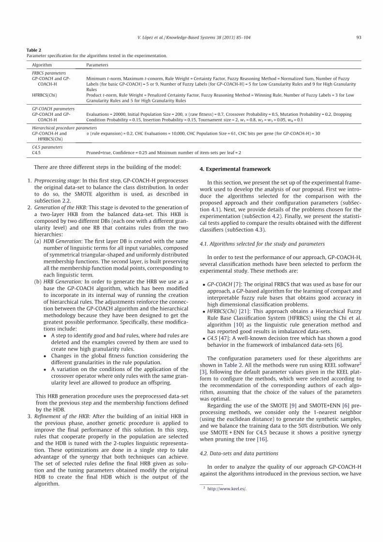
There are three different steps in the building of the model:
1. Preprocessing stage: In this first step, GP-COACH-H preprocessesthe original data-set to balance the class distribution. In orderto do so, the SMOTE algorithm is used, as described insubSection 2.2.
2. Generation of the HKB: This stage is devoted to the generation ofa two-layer HKB from the balanced data-set. This HKB iscomposed by two different DBs (each one with a different gran-ularity level) and one RB that contains rules from the twohierarchies:(a) HDB Generation: The first layer DB is created with the same
number of linguistic terms for all input variables, composedof symmetrical triangular-shaped and uniformly distributedmembership functions. The second layer, is built preservingall the membership function modal points, corresponding toeach linguistic term.
(b) HRB Generation: In order to generate the HRB we use as abase the GP-COACH algorithm, which has been modifiedto incorporate in its internal way of running the creationof hierarchical rules. The adjustments reinforce the connec-tion between the GP-COACH algorithm and the hierarchicalmethodology because they have been designed to get thegreatest possible performance. Specifically, these modifica-tions include:� A step to identify good and bad rules, where bad rules are
deleted and the examples covered by them are used tocreate new high granularity rules.
� Changes in the global fitness function considering thedifferent granularities in the rule population.
� A variation on the conditions of the application of thecrossover operator where only rules with the same gran-ularity level are allowed to produce an offspring.
This HRB generation procedure uses the preprocessed data-setfrom the previous step and the membership functions definedby the HDB.
3. Refinement of the HKB: After the building of an initial HKB inthe previous phase, another genetic procedure is applied toimprove the final performance of this solution. In this step,rules that cooperate properly in the population are selectedand the HDB is tuned with the 2-tuples linguistic representa-tion. These optimizations are done in a single step to takeadvantage of the synergy that both techniques can achieve.The set of selected rules define the final HRB given as solu-tion and the tuning parameters obtained modify the originalHDB to create the final HDB which is the output of thealgorithm.
4. Experimental framework
In this section, we present the set up of the experimental frame-work used to develop the analysis of our proposal. First we intro-duce the algorithms selected for the comparison with theproposed approach and their configuration parameters (subSec-tion 4.1). Next, we provide details of the problems chosen for theexperimentation (subSection 4.2). Finally, we present the statisti-cal tests applied to compare the results obtained with the differentclassifiers (subSection 4.3).
4.1. Algorithms selected for the study and parameters
In order to test the performance of our approach, GP-COACH-H,several classification methods have been selected to perform theexperimental study. These methods are:
� GP-COACH [7]: The original FRBCS that was used as base for ourapproach, a GP-based algorithm for the learning of compact andinterpretable fuzzy rule bases that obtains good accuracy inhigh dimensional classification problems.
� HFRBCS(Chi) [21]: This approach obtains a Hierarchical FuzzyRule Base Classification System (HFRBCS) using the Chi et al.algorithm [10] as the linguistic rule generation method andhas reported good results in imbalanced data-sets.
� C4.5 [47]: A well-known decision tree which has shown a goodbehavior in the framework of imbalanced data-sets [6].
The configuration parameters used for these algorithms areshown in Table 2. All the methods were run using KEEL software2
[3], following the default parameter values given in the KEEL plat-form to configure the methods, which were selected according tothe recommendation of the corresponding authors of each algo-rithm, assuming that the choice of the values of the parameterswas optimal.
Regarding the use of the SMOTE [9] and SMOTE+ENN [6] pre-processing methods, we consider only the 1-nearest neighbor(using the euclidean distance) to generate the synthetic samples,and we balance the training data to the 50% distribution. We onlyuse SMOTE + ENN for C4.5 because it shows a positive synergywhen pruning the tree [16].
4.2. Data-sets and data partitions
In order to analyze the quality of our approach GP-COACH-Hagainst the algorithms introduced in the previous section, we have
Table 2Parameter specification for the algorithms tested in the experimentation.
Algorithm Parameters
FRBCS parametersGP-COACH and GP-
COACH-HMinimum t-norm, Maximum t-conorm, Rule Weight = Certainty Factor, Fuzzy Reasoning Method = Normalized Sum, Number of FuzzyLabels (for basic GP-COACH) = 5 or 9, Number of Fuzzy Labels (for GP-COACH-H) = 5 for Low Granularity Rules and 9 for High GranularityRules
HFRBCS(Chi) Product t-norm, Rule Weight = Penalized Certainty Factor, Fuzzy Reasoning Method = Winning Rule, Number of Fuzzy Labels = 3 for LowGranularity Rules and 5 for High Granularity Rules
GP-COACH parametersGP-COACH and GP-
COACH-HEvaluations = 20000, Initial Population Size = 200, a (raw fitness) = 0.7, Crossover Probability = 0.5, Mutation Probability = 0.2, DroppingCondition Probability = 0.15, Insertion Probability = 0.15, Tournament size = 2, w1 = 0.8, w2 = w3 = 0.05, w4 = 0.1
Hierarchical procedure parametersGP-COACH-H and
HFRBCS(Chi)a (rule expansion) = 0.2, CHC Evaluations = 10,000, CHC Population Size = 61, CHC bits per gene (for GP-COACH-H) = 30
C4.5 parametersC4.5 Pruned=true, Confidence = 0.25 and Minimum number of item-sets per leaf = 2
2 http://www.keel.es/.
V. López et al. / Knowledge-Based Systems 38 (2013) 85–104 93

selected several highly imbalanced and borderline imbalanceddata-sets.
Specifically, as highly imbalanced data-sets, we have selected44 data-sets from KEEL data-set repository3 [2] with an imbalanceratio (IR) [46] greater than 9. The data are summarized in Table 3,where we denote the number of examples (#Ex.), number of attri-butes (#Atts.), class name of each class (positive and negative), classattribute distribution and IR. This table is in ascending order accord-ing to the IR.
Inspired by Kubat and Matwin [40], Napierala et al. [44] createdseveral artificial data-sets that contain borderline examples in animbalanced scenario to address the correct identification of thoseexamples. These data-sets have three different shapes of the posi-tive class: subclus (Fig. 9), clover (Fig. 10) and paw (Fig. 11), all sur-rounded uniformly by the negative class. For each shape, we havedata-sets from two different sizes and IR: data-sets with 600 exam-ples with an IR of 5 and data-sets with 800 examples with an IR of7. Each one of these data-sets is affected by different disturbanceratio levels (0%, 30%, 50%, 60% and 70%). The disturbance ratio issimulated increasing the ratio of borderline examples from the po-sitive class subregions.
To develop the different experiments we consider a 5-fold cross-validation model, i.e., five random partitions of data with a 20% andthe combination of 4 of them (80%) as training and the remainingones as test. For each data-set we consider the average results ofthe five partitions. The data-sets used in this study use the parti-tions provided by the KEEL data-set repository in the imbalancedclassification data-set section.4
4.3. Statistical tests for performance comparison
Statistical analysis needs to be carried out in order to find sig-nificant differences among the results obtained by the studiedmethods [24]. We consider the use of non-parametric tests, accord-ing to the recommendations made in [25,24] where a set of simple,safe and robust non-parametric tests for statistical comparisons ofclassifiers is presented. These tests are used due to the fact that theinitial conditions that guarantee the reliability of the parametrictests may not be satisfied, causing the statistical analysis to losecredibility [50].
TheWilcoxon test [50]will be used as a non-parametric statisticalprocedure in order to conduct pairwise comparisons between twoalgorithms. For multiple comparisons we use the Iman-Davenport
Table 3Summary of imbalanced data-sets.
Data-sets #Ex. #Atts. Class (�;+) %Class (�;+) IR
ecoli034vs5 200 7 (p, imL, imU;om) (10.00,90.00) 9.00yeast2vs4 514 8 (cyt;me2) (9.92,90.08) 9.08ecoli067vs35 222 7 (cp,omL,pp; imL,om) (9.91,90.09) 9.09ecoli0234vs5 202 7 (cp, imS, imL, imU;om) (9.90,90.10) 9.10glass015vs2 172 9 (build-win-non_float-proc, tableware,build-win-float-proc;ve-win-float-proc) (9.88,90.12) 9.12yeast0359vs78 506 8 (mit,me1,me3,erl;vac,pox) (9.88,90.12) 9.12yeast02579vs368 1004 8 (mit,cyt,me3,vac,erl;me1,exc,pox) (9.86,90.14) 9.14yeast0256vs3789 1004 8 (mit,cyt,me3,exc;me1,vac,pox,erl) (9.86,90.14) 9.14ecoli046vs5 203 6 (cp, imU,omL;om) (9.85,90.15) 9.15ecoli01vs235 244 7 (cp, im;imS, imL,om) (9.83,90.17) 9.17ecoli0267vs35 224 7 (cp, imS,omL,pp; imL,om) (9.82,90.18) 9.18glass04vs5 92 9 (build-win-float-proc,containers; tableware) (9.78,90.22) 9.22ecoli0346vs5 205 7 (cp, imL, imU,omL;om) (9.76,90.24) 9.25ecoli0347vs56 257 7 (cp, imL, imU,pp;om,omL) (9.73,90.27) 9.28yeast05679vs4 528 8 (me2;mit,me3,exc,vac,erl) (9.66,90.34) 9.35ecoli067vs5 220 6 (cp,omL,pp;om) (9.09,90.91) 10.00vowel0 988 13 (hid;remainder) (9.01,90.99) 10.10glass016vs2 192 9 (ve-win-float-proc;build-win-float-proc,build-win-non_float-proc,headlamps) (8.89,91.11) 10.29glass2 214 9 (Ve-win-float-proc;remainder) (8.78,91.22) 10.39ecoli0147vs2356 336 7 (cp, im,imU,pp; imS, imL,om,omL) (8.63,91.37) 10.59led7digit02456789vs1 443 7 (0,2,4,5,6,7,8,9;1) (8.35,91.65) 10.97glass06vs5 108 9 (build-win-float-proc,headlamps;tableware) (8.33,91.67) 11.00ecoli01vs5 240 6 (cp, im;om) (8.33,91.67) 11.00glass0146vs2 205 9 (build-win-float-proc,containers,headlamps,build-win-non_float-proc;ve-win-float-proc) (8.29,91.71) 11.06ecoli0147vs56 332 6 (cp, im,imU,pp;om,omL) (7.53,92.47) 12.28cleveland0vs4 177 13 (0;4) (7.34,92.66) 12.62ecoli0146vs5 280 6 (cp, im,imU,omL;om) (7.14,92.86) 13.00ecoli4 336 7 (om;remainder) (6.74,93.26) 13.84yeast1vs7 459 8 (nuc;vac) (6.72,93.28) 13.87shuttle0vs4 1829 9 (Rad Flow;Bypass) (6.72,93.28) 13.87glass4 214 9 (containers; remainder) (6.07,93.93) 15.47page-blocks13vs2 472 10 (graphic;horiz.line,picture) (5.93,94.07) 15.85abalone9vs18 731 8 (18;9) (5.65,94.25) 16.68glass016vs5 184 9 (tableware;build-win-float-proc,build-win-non_float-proc,headlamps) (4.89,95.11) 19.44shuttle2vs4 129 9 (Fpv Open;Bypass) (4.65,95.35) 20.5yeast1458vs7 693 8 (vac;nuc,me2,me3,pox) (4.33,95.67) 22.10glass5 214 9 (tableware; remainder) (4.20,95.80) 22.81yeast2vs8 482 8 (pox;cyt) (4.15,95.85) 23.10yeast4 1484 8 (me2;remainder) (3.43,96.57) 28.41yeast1289vs7 947 8 (vac;nuc,cyt,pox,erl) (3.17,96.83) 30.56yeast5 1484 8 (me1;remainder) (2.96,97.04) 32.78ecoli0137vs26 281 7 (pp, imL;cp, im,imU, imS) (2.49,97.51) 39.15yeast6 1484 8 (exc;remainder) (2.49,97.51) 39.15abalone19 4174 8 (19;remainder) (0.77,99.23) 128.87
3 http://www.keel.es/datasets.php. 4 http://www.keel.es/imbalanced.php.
94 V. López et al. / Knowledge-Based Systems 38 (2013) 85–104

test to detect statistical differences among a group of results, and theHolm post-hoc test in order to find which algorithms are distinctiveamong a 1 � n comparison.
The post-hoc procedure allows us to knowwhether a hypothesisof comparison of means could be rejected at a specified level of sig-nificance a. However, it is very interesting to compute the p-valueassociatedwith each comparison, which represents the lowest levelof significance of a hypothesis that results in a rejection. It is theadjusted p-value. In this manner, we can know whether twoalgorithms are significantly different and how different they are.
Furthermore, we consider the average ranking of the algo-rithms, in order to show how good a method is with respect toits partners. This ranking is obtained by assigning a position toeach algorithm depending on its performance for each data-set.The algorithm which achieves the best accuracy in a specificdata-set will have the first ranking (value 1); then, the algorithmwith the second best accuracy is assigned rank 2, and so forth. Thistask is carried out for all data-sets and finally an average ranking iscomputed as the mean value of all rankings.
These tests are suggested in the studies presented in [25,24],where their use in the field of machine learning is highly recom-mended. For a wider description of the use of these tests, please re-fer to the website on Statistical Inference in ComputationalIntelligence and Data Mining.5
5. Experimental study
In this section, we present a set of experiments to illustrate anddemonstrate the behavior of GP-COACH-H. These experiments aredesigned towards two objectives: to exemplify how the GP-COACH-H algorithm works, and to determine its robustness forhighly and borderline imbalanced data-sets.
We organize those experiments in the following way. First, Sec-tion 5.1 presents a case of study over one one of the highly imbal-anced data-sets presented in the previous section. Next, Section 5.2contains an analysis of the impact of the hierarchical step in thealgorithm. Section 5.3 studies the the importance of the usage ofa preprocessing step when dealing with highly imbalanced data-sets. Later, Section 5.4 performs a global comparison among thefuzzy classification methods and C4.5 over the highly imbalanceddata-sets. Finally, in Section 5.5, this global comparison is also car-ried out over the borderline imbalanced data-sets.
5.1. Sample procedure of the GP-COACH-H algorithm: a case of study
In order to illustrate how GP-COACH-H works we have selectedthe glass0146vs2 data-set. We will follow the algorithm operationsand the results it provides. The glass0146vs2 data-set is a highlyimbalanced data-set from the KEEL data-set repository,6 with 9 in-put attributes, 205 instances and an IR equal to 11.06. We have se-lected this data-set as one with a small size whose results can beeasily interpreted.
For this specific run, we have chosen the 3rd partition from the5-fcv used in all the experiments. This partition uses 164 instancesfor training (14 positive and 150 negative) and 41 for test (3 posi-tive and 38 negative), using the 9 input attributes of the wholedata-set. The first step of the GP-COACH-H algorithm (see Fig. 8)uses the SMOTE algorithm to balance the class distribution. There-fore, we apply the SMOTE algorithm and we obtain a new trainingset that contains 300 instances, 150 instances for each class.
The second step starts using the preprocessed data-set to gener-ate the HKB. In order to generate the HKB, we first generate theHDB from the available data. The HDB is generated (as was ex-plained in the previous sections) with the same number of linguis-tic terms for all input variables, composed of symmetricaltriangular-shaped and uniformly distributed membership func-tions. The second layer, is built preserving all the membershipfunction modal points, corresponding to each linguistic term.Figs. 12 and 13 show the linguistic variables generated for theMg attribute, according to the given instructions.
Once we have generated the HDB, we start the GP procedure togenerate the HRB. This procedure evolves a rule populationthrough several generations, including the usage of genetic opera-tors to generate new individuals, the token competition procedureto delete irrelevant rules and the hierarchical creation of new rulesin each step. At the end of the iterations, a rule base with differentgranularity rules is obtained. In Fig. 14, the rules generated usingthe generated HDB and the preprocessed training set are shown.
At this point, we start the last step of the algorithm which is thegenetic rule selection and lateral tuning of the variables. To obtainthe final solution, we use the preprocessed set from the first stepand the HKB generated previously. The genetic search looks for a
Fig. 9. Subclus.
Fig. 10. Clover.
Fig. 11. Paw.
5 http://sci2s.ugr.es/sicidm/.6 http://www.keel.es/imbalanced.php.
V. López et al. / Knowledge-Based Systems 38 (2013) 85–104 95

new HKB that better represents the data. Figs. 15–17 show the newHDB and HRB obtained, which are the final output of the GP-COACH-H algorithm.
5.2. Analysis of the impact of the hierarchical levels over theimbalanced data-sets
This subsection is devoted to the impact of the usage of the HKBin the GP-COACH-H algorithm in relation to not using a HKB anduse a traditional KB instead. In this manner, we will detect theinfluence of this component of the GP-COACH-H algorithm thusjustifying its use.
We will compare the results of the GP-COACH-H algorithmaccording to the fuzzy HKB generated after the application of the
GP procedure to the results of the basic GP-COACH algorithm with5 and 9 labels, using SMOTE as preprocessing algorithm in bothcases. The performance measures used are sensitivity and specific-ity to observe the impact for each class. Table 4 shows the averageresults for each algorithm over the highly imbalanced data-sets.The complete table of results for all data-sets can be found in theappendix of this work.
Considering the sensitivity measure the best performing aver-age algorithm is the basic GP-COACH with 5 labels, however, ifwe look at the specificity measure then the best performing algo-rithm is the basic GP-COACH with 9 labels. Therefore, we need toconsider the effectiveness for each class separately.
Contemplating the positive class, we can observe that the bestperformance in training is higher for the hierarchical version, being
Fig. 14. Rules generated after the Fuzzy HRB Generation.
Fig. 13. Database Layer 2 with 9 labels, Mg attribute.
Fig. 12. Database Layer 1 with 5 labels, Mg attribute.
96 V. López et al. / Knowledge-Based Systems 38 (2013) 85–104

able to describe the training set more accurately than in the pres-ence of low granularity rules only. Therefore, our initial intuitionwhere the HKB was able to better describe difficult data spaces isconfirmed. Comparing the training results in relation to the testresults we notice a drop in performance for all the algorithmswhere GP-COACH-5 gets the best results, GP-COACH-H obtainssimilar results to GP-COACH-5 and GP-COACH-9 accomplisheslower results than the other two.
Analyzing the results associated to the negative class, we see analmost opposite situation. For training results the GP-COACH-9algorithm is the algorithm that best describes the data, a situationwhere GP-COACH-H is supposed to be found. Nevertheless, GP-COACH-H is designed to specifically deal with imbalanced data-sets concentrating on the positive class so is logical that it doesnot characterize the negative class as well as the previous case.
Confronting the training results with the test results we find a dropin the performance on equal levels for each approaches. Therefore,GP-COACH-9 is the best performing algorithm for the negativeclass, closely followed by GP-COACH-H where GP-COACH-5 perfor-mance falls behind those two approaches.
After checking the performance in each class, we discover thatthe basic GP-COACH is a powerful tool to describe one of our clas-ses depending on the number of labels used. Nevertheless, if wechoose a specific number of labels to focus on one class the finalperformance is degraded in the other one. Consequently, the GP-COACH-H approach that combines low granularity and high gran-ularity rules is able to address the description of both classesaccordingly. Its performance does not exceed the results of the ba-sic algorithm, however, it goes closely after them in each class. Fur-thermore, there is not a high decrease in performance for the class
Fig. 16. Final database Layer 2 with 9 labels, Mg attribute.
Fig. 15. Final database Layer 1 with 5 labels, Mg attribute.
Table 4Average results for GP-COACH-5, GP-COACH-9 and GP-COACH-H for the highly imbalanced data-sets.
Data-set Sensitivitytr Sensitivitytst Specificitytr Specificitytst
GP-COACH-5 .9097 ± .0307 .7809 ± .1212 .8643 ± .0307 .8531 ± .1212GP-COACH-9 .8983 ± .0267 .7319 ± .1334 .9231 ± .0267 .9055 ± .1334GP-COACH-H .9398 ± .0204 .7797 ± .1233 .9025 ± .0204 .8855 ± .1233
Table 5Average results for GP-COACH versions with and without SMOTE preprocessing for the highly imbalanced data-sets.
Data-set No preprocessing SMOTE preprocessing
GMtr GMtst GMtr GMtst
GP-COACH-5 .4789 ± .1017 .3677 ± .1922 .8763 ± .0307 .7897 ± .1212GP-COACH-9 .5074 ± .0871 .3929 ± .1996 .9056 ± .0267 .7845 ± .1334GP-COACH-H .4536 ± .1216 .3439 ± .1697 .9576 ± .0121 .8175 ± .1193
V. López et al. / Knowledge-Based Systems 38 (2013) 85–104 97

as in the basic algorithm. In this manner, GP-COACH-H is able toprofit from the descriptive power of each granularity level obtain-ing a good balance between the performance of both classes.
5.3. Analysis of the suitability of the preprocessing step for imbalancedproblems
In this part of the study, our aim is to show the suitability of thepreprocessing step included in GP-COACH-H as the first step of thealgorithm. We also check the performance of applying this prepro-cessing step to the basic GP-COACH algorithm in order to show thenecessity of this procedure when dealing with imbalanced data-sets, thus justifying the inclusion of this step in our proposal.
According to this objective, we show the average GM results intraining and test in Table 5, together with the corresponding stan-dard deviation, for the basic GP-COACH algorithm and for the hier-archical GP-COACH-H with and without SMOTE preprocessing overthe highly imbalanced data-sets presented in Section 4.2. The com-plete table of results for all data-sets is shown in the appendix ofthis work. We observe that the best result in test (which is stressedin boldface) always corresponds to the one obtained when theSMOTE preprocessing is applied. Furthermore, there is an enor-mous difference between the usage or not usage of preprocessing.Therefore, we conclude that the usage of SMOTE as preprocessingclearly outperforms the usage of the original data-sets makingthe use of this methodology a necessity in the framework of imbal-anced data-sets.
5.4. Analysis of GP-COACH-H on highly imbalanced data-sets
The following part of the study will consider the performance ofthe GP-COACH-H algorithm in contrast with other FRBCS learningproposals and with the C4.5 algorithm. Table 6 shows the averageGM results in training and test together with the correspondingstandard deviation for the highly imbalanced data-sets considered.By rows, we can observe the results for the basic GP-COACH meth-od with 5 and 9 labels (GP-COACH-5 and GP-COACH-9), theHFRBCS(Chi), the proposed GP-COACH-H and the C4.5 decisiontree. The best average case in test is highlighted in bold. The com-plete table of results for all data-sets is also shown in the appendixof this work together with the results of the previous experiments.We remind that SMOTE is used for the FRBCS whereas SMOTE+ENNis applied in conjunction with C4.5 along all the experiments.
According to the average values shown in this table the bestmethod in highly imbalanced data-sets is the GP-COACH-H. To car-ry out the statistical study we first check for significant differencesamong the algorithms using an Iman-Davenport test. The p-value(0.0779) is low enough to reject the null equality hypothesis witha high confidence level. Thus, we can conclude that significant dif-ferences do exist, proceeding by showing in Table 7 the average
Fig. 17. Final rules generated with the GP-COACH-H algorithm.
Table 6Average results for FRBCS methods and C4.5 for the highly imbalanced data-sets.SMOTE preprocessing for FRBCS methods, SMOTE+ENN for C4.5.
Data-set GMtr GMtst
GP-COACH-5 .8763 ± .0307 .7897 ± .1212GP-COACH-9 .9056 ± .0267 .7845 ± .1334HFRBCS(Chi) .9331 ± .0117 .7901 ± .1325GP-COACH-H .9576 ± .0121 .8175 ± .1193C4.5 .9549 ± .0180 .7848 ± .1452
Table 7Average rankings and adjusted p-values using Holm’s post-hoc procedure for FRBCSmethods and C4.5 adopting the GM measure for the highly imbalanced data-sets.
Algorithm Average ranking Adjusted p-value (Holm’s test)
GP-COACH-H 2.4091GP-COACH-9 3.0227 0.0862GP-COACH-5 3.0909 0.0862C4.5 3.2045 0.0549HFRBCS(Chi) 3.2727 0.0416
Table 8Average results for FRBCS methods and C4.5 for the borderline imbalanced data-sets.SMOTE preprocessing for FRBCS methods, SMOTE+ENN for C4.5.
Data-set GMtr GMtst
GP-COACH-5 .7899 ± .0218 .7630 ± .0578GP-COACH-9 .8103 ± .0330 .7628 ± .0705HFRBCS(Chi) .8316 ± .0195 .7992 ± .0461GP-COACH-H .8674 ± .0157 .8234 ± .0428C4.5 .8881 ± .0244 .8208 ± .0462
Table 9Average rankings and adjusted p-values using Holm’s post-hoc procedure for FRBCSmethods and C4.5 adopting the GM measure for the borderline imbalanced data-sets.
Algorithm Average ranking Adjusted p-value (Holm’s test)
GP-COACH-H 1.7333C4.5 1.9000 0.6831HFRBCS(Chi) 3.0667 0.0022GP-COACH-9 3.8667 0.0000GP-COACH-5 4.4333 0.0000
Table 10Wilcoxon test to compare GP-COACH-H against C4.5 in borderline imbalanced data-sets. R+ corresponds to the sum of the ranks for GP-COACH-H and R� to C4.5.
Comparison R+ R� p-Value
GP-COACH-H vs C4.5 261.0 204.0 0.551
98 V. López et al. / Knowledge-Based Systems 38 (2013) 85–104

ranks of the algorithms and the adjusted p-values computed by theHolm test. Looking at this table we can notice that GP-COACH-Hobtains the lower ranking which makes it the control method usedfor the post-hoc computation. As all the adjusted p-values are suf-ficiently low to reject the null-hypothesis in all cases, the assump-tion where GP-COACH-H is the best performing method consideredfor highly imbalanced data-sets is reinforced.
5.5. Analysis of GP-COACH-H on borderline imbalanced data-sets
In the last part of our study, we want to analyze the behavior ofthe GP-COACH-H proposal in the scenario of imbalance borderlinedata-sets. We will take into account the same algorithms consid-ered in the analysis for highly imbalanced data-sets, namely, thebasic GP-COACH method with 5 and 9 labels (GP-COACH-5 andGP-COACH-9), HFRBCS(Chi), GP-COACH-H and the C4.5 decisiontree. Table 8 shows the average results in training and test togetherwith the corresponding standard deviation for the algorithms usedin the study over the borderline imbalanced data-sets. As in previ-ous tables, the best average case in test is highlighted in bold andthe complete table of results for the borderline imbalanced data-sets is also shown in the appendix of this work.
Observing the average results table we detect GP-COACH-H asthe method with the best average results. Similarly to the proce-dure used in the highly imbalanced data-sets comparison we startthe statistical study for borderline imbalanced data-sets comput-ing the Iman-Davenport test to discern if there are significant dif-ferences among the algorithms. The p-value computed is zero,implying that there are differences between the algorithms. There-fore, we perform the Holm test as post-hoc procedure. Table 9 con-tains the ranks of the algorithms and the adjusted p-valuescomputed using the Holm test.
According to Table 9 the lowest ranking corresponds to GP-COACH-H turning it into the control method used in the Holm testas the best performing method for borderline data-sets. In thiscase, the adjusted p-values associated to the basic GP-COACH (with5 and 9 labels) and to HFRBCS(Chi) are low enough to reject thenull-hypothesis with a high confidence level. This means, thatour proposal GP-COACH-H is the best performing FRBCS in border-line imbalanced data-sets. In the remaining case (C4.5), we per-form a Wilcoxon test (Table 10) in order to check if we finddifferences between both algorithms.
In this case, the p-value computed does not reject the nullhypothesis. Nevertheless, GP-COACH-H achieves a higher sum ofranks, which means that GP-COACH-H has obtained a greater per-formance in a superior number of data-sets than C4.5, turning GP-COACH-H into a competitive method. Furthermore, the averageperformance of GP-COACH-H is better than the performance ofC4.5 and the standard deviation is lower which causes GP-COACH-H to be a more robust method in each occasion.
To sum up, our experimental study has shown that GP-COACH-H is an algorithm that presents a good behavior in the frameworkof imbalanced data-sets, specifically, when dealing with highimbalanced data and borderline imbalanced data. The design ofGP-COACH-H integrates different strategies to deal with the prob-lem that help to overcome the difficulties when they appear. Spe-cifically, the preprocessing step is used to counter the imbalanceproblem, the hierarchical procedure is added to the FRBCS usedas base to obtain a better representation of the data-set in difficultareas such as small disjuncts or borderline samples and the ruleselection combined with tuning refines the results obtainedimproving the overall results. These schemes combined togetherdeal with the mentioned problems in conjunction generating goodresults.
6. Concluding remarks
In this paper we have presented a FRBCS with different granu-lation levels that integrates rule selection and the 2-tuples tuningapproach to improve the performance in imbalanced data-sets. Theproposal integrates data sampling together with algorithm modifi-cations to the basic approach and adapts its behavior to the differ-ent granulation levels considered, adding a post-processing stepthat helps the hierarchical fuzzy rule base classification systemto have a better adaptation to the context of each problem andtherefore to enhance its global behavior.
The proposed hierarchical fuzzy rule based classification wascompared to the GP-COACH algorithm, HFRBCS algorithm and theC4.5 decision tree in order to demonstrate its good performance.The experimental study justifies the combination of SMOTE withthe algorithmic modifications such as the usage of a hierarchicalknowledge base in order to increase the performance in the imbal-anced data-set scenario. Moreover, the results obtained when wedealwith this scenario evidence the interest of this proposal. Specif-ically, this proposal outperforms the other approaches in the frame-work of highly imbalanced data-sets, which usually is an scenariowhere most algorithms have lots of difficulties to perform properly.
For borderline imbalanced data-sets our approach shows a bet-ter behavior than other FRBCSs used in the experimental studioand maintains a competitive performance when it is comparedwith C4.5. These results have been contrasted by several non-parametric statistical procedures that reinforce the extractedconclusions.
As future work, we consider several lines of work centered onthe features of GP-COACH-H that can still be enhanced to obtaina better performance. One possibility includes the modification ofthe genetic operations to achieve a multi-objective procedure thatenables a trade-off between interpretability and accuracy. More-over, we want to study in depth the data intrinsic characteristicsthat hinder the performance in imbalanced data-sets and incorpo-rate this knowledge into the model with a specialized strategy foreach case. Another possibility focus on the balance level of the pre-processing step. If an equal balance is not needed and can besubstituted by a lower number of instances then the run time ofthe algorithm will decrease.
Acknowledgments
This work has been supported by the Spanish Ministry of Sci-ence and Technology under Projects TIN2011-28488 andTIN2008-06681-C06-02, and the Andalusian Research Plan P10-TIC-6858 and TIC-3928. V. López holds a FPU scholarship fromSpanish Ministry of Education.
Appendix A. Detailed results for the experimental study
In this appendix we present the complete results tables for allthe algorithms used in this work. Thus, the reader can observethe full training and test results, with their associated standarddeviation, in order to compare the performance of each approach.In Table 11 we show the detailed results for the GP-COACH-5, GP-COACH-9 and GP-COACH-H versions with SMOTE preprocessingfor the GP procedure using the specificity and sensitivity measures.Next, in Table 12 we show the results for the basic GP-COACHmethod and the hierarchical GP-COACH-H with and withoutSMOTE preprocessing. Later, the results for each FRBCS methodwith SMOTE preprocessing and C4.5 with SMOTE+ENN preprocess-ing over the highly imbalanced data-sets are shown in Table 13. Fi-nally, Table 14 presents the results for the same algorithms asTable 13 over the borderline data-sets considered.
V. López et al. / Knowledge-Based Systems 38 (2013) 85–104 99

Table11
Completetableof
resu
ltsforGP-CO
ACH
-5,G
P-CO
ACH
-9an
dGP-CO
ACH
-HaftertheGPproc
edur
eus
ingthesp
ecificity
andsens
itivitymea
sures.
Data-set
GP-COACH-5
GP-COACH-9
GP-COACH-H
Sensitivity
trSe
nsitivity
tst
Specificity
trSp
ecificity
tst
Sensitivity
trSe
nsitivity
tst
Specificity
trSp
ecificity
tst
Sensitivity
trSe
nsitivity
tst
Specificity
trSp
ecificity
tst
ecoli034
vs5
.975
0±.016
5.850
0±.128
2.976
4±.016
5.972
2±.128
2.987
5±.015
8.900
0±.070
9.965
3±.015
8.955
6±.070
9.937
5±.056
7.850
0±.075
9.980
6±.056
7.966
7±.075
9ye
ast2vs4
.931
6±.009
2.881
8±.041
2.919
6±.009
2.917
9±.041
2.926
5±.004
4.881
8±.038
1.931
9±.004
4.928
8±.038
1.936
5±.016
6.863
6±.047
1.935
2±.016
6.930
8±.047
1ecoli067
vs35
.965
4±.019
3.840
0±.209
3.920
0±.019
3.865
0±.209
3.943
8±.021
0.840
0±.226
5.941
2±.021
0.925
0±.226
5.966
0±.029
2.840
0±.224
8.946
3±.029
2.920
0±.224
8ecoli023
4vs5
.962
5±.009
5.750
0±.155
2.979
4±.009
5.933
8±.155
2.962
5±.040
9.800
0±.164
8.967
0±.040
9.917
4±.164
8.987
5±.011
1.850
0±.123
9.982
2±.011
1.939
2±.123
9glass0
15vs2
.742
9±.133
7.483
3±.218
3.477
4±.133
7.496
8±.218
3.807
7±.051
1.183
3±.303
2.858
1±.051
1.767
7±.303
2.897
8±.044
0.600
0±.073
9.774
2±.044
0.767
7±.073
9ye
ast035
9vs7
8.765
0±.084
0.640
0±.124
4.527
3±.084
0.531
2±.124
4.370
0±.025
8.360
0±.083
3.849
9±.025
8.841
8±.083
3.845
0±.019
9.700
0±.082
0.816
4±.019
9.802
6±.082
0ye
ast025
79vs36
8.876
3±.009
3.870
0±.037
6.957
7±.009
3.951
4±.037
6.886
4±.010
9.890
0±.039
5.927
9±.010
9.920
4±.039
5.878
8±.009
3.860
0±.048
8.957
7±.009
3.954
7±.048
8ye
ast025
6vs3
789
.709
6±.013
6.685
8±.067
6.925
1±.013
6.927
1±.067
6.732
2±.014
9.706
3±.056
3.902
2±.014
9.899
4±.056
3.724
7±.015
4.706
3±.059
8.919
1±.015
4.918
2±.059
8ecoli046
vs5
.975
0±.016
8.900
0±.124
8.974
0±.016
8.950
9±.124
8.987
5±.017
4.850
0±.216
6.983
6±.017
4.956
6±.216
61.00
00±.007
3.850
0±.211
7.972
7±.007
3.940
1±.211
7ecoli01v
s235
.968
9±.015
1.860
0±.113
1.912
5±.015
1.895
5±.113
1.968
9±.015
2.910
0±.067
0.939
8±.015
2.922
7±.067
0.947
9±.018
4.770
0±.191
5.944
3±.018
4.936
4±.191
5ecoli026
7vs3
5.921
6±.021
1.800
0±.131
1.920
9±.021
1.915
6±.131
1.977
8±.033
4.800
0±.112
5.922
0±.033
4.891
6±.112
5.944
4±.026
0.800
0±.092
8.907
3±.026
0.870
9±.092
8glass0
4vs5
1.00
00±.020
8.900
0±.127
7.933
8±.020
8.928
7±.127
71.00
00±.024
71.00
00±.013
4.942
6±.024
7.927
9±.013
41.00
00±.036
5.800
0±.402
0.919
0±.036
5.841
2±.402
0ecoli034
6vs5
1.00
00±.002
8.800
0±.113
2.991
9±.002
8.978
4±.113
2.987
5±.015
9.850
0±.063
2.981
1±.015
9.945
9±.063
21.00
00±.010
7.850
0±.060
8.977
0±.010
7.962
2±.060
8ecoli034
7vs5
6.970
0±.010
4.800
0±.103
9.946
1±.010
4.922
4±.103
9.970
0±.016
6.800
0±.145
9.959
0±.016
6.939
7±.145
9.980
0±.006
9.840
0±.092
3.948
3±.006
9.930
9±.092
3ye
ast056
79vs4
.784
3±.019
8.783
6±.075
9.856
9±.019
8.849
0±.075
9.799
0±.015
8.763
6±.085
8.875
3±.015
8.861
6±.085
8.818
4±.011
7.725
5±.065
3.849
6±.011
7.844
9±.065
3ecoli067
vs5
1.00
00±.014
4.800
0±.127
7.911
3±.014
4.885
0±.127
7.962
5±.016
2.850
0±.088
4.948
8±.016
2.940
0±.088
4.962
5±.015
3.850
0±.051
3.946
3±.015
3.935
0±.051
3vo
wel0
.986
1±.011
6.966
7±.015
4.952
7±.011
6.953
2±.015
4.977
8±.007
5.944
4±.009
3.951
0±.007
5.936
5±.009
3.961
1±.016
0.933
3±.023
2.963
0±.016
0.958
8±.023
2glass0
16vs2
.956
0±.055
8.550
0±.122
8.644
3±.055
8.588
6±.122
8.823
1±.035
5.300
0±.238
5.825
7±.035
5.788
6±.238
5.971
4±.017
1.583
3±.174
1.728
6±.017
1.708
6±.174
1glass2
.926
4±.025
6.766
7±.084
1.533
0±.025
6.507
4±.084
1.762
6±.061
5.350
0±.372
5.851
4±.061
5.802
7±.372
5.940
7±.053
3.466
7±.154
4.822
5±.053
3.750
5±.154
4ecoli014
7vs2
356
.922
8±.024
1.720
0±.106
0.926
7±.024
1.899
0±.106
0.880
8±.052
1.713
3±.146
7.921
8±.052
1.905
6±.146
7.922
1±.023
2.833
3±.047
7.912
0±.023
2.915
4±.047
7led7
digit024
5678
9vs1
.858
2±.024
6.860
7±.082
9.942
1±.024
6.948
3±.082
9.858
2±.027
4.832
1±.070
8.943
4±.027
4.950
7±.070
8.864
8±.021
6.860
7±.085
1.940
3±.021
6.945
8±.085
1glass0
6vs5
1.00
00±.007
31.00
00±.011
3.979
8±.007
3.990
0±.011
31.00
00±.006
9.900
0±.133
2.984
9±.006
9.930
0±.133
21.00
00±.014
11.00
00±.021
5.972
2±.014
1.959
5±.021
5ecoli01v
s51.00
00±.013
7.800
0±.124
8.963
6±.013
7.968
2±.124
81.00
00±.007
5.900
0±.090
8.978
4±.007
5.940
9±.090
81.00
00±.004
3.850
0±.086
8.978
4±.004
3.954
5±.086
8glass0
146v
s2.925
3±.048
3.783
3±.045
0.620
8±.048
3.590
9±.045
0.897
8±.066
5.516
7±.319
1.808
5±.066
5.802
7±.319
1.895
6±.027
3.583
3±.074
8.748
6±.027
3.734
3±.074
8ecoli014
7vs5
6.970
0±.022
2.800
0±.038
5.945
5±.022
2.898
7±.038
5.990
0±.015
4.800
0±.066
1.957
7±.015
4.928
2±.066
1.980
0±.019
8.840
0±.089
8.938
1±.019
8.911
8±.089
8clev
elan
d0vs4
.980
0±.019
4.566
7±.171
0.968
7±.019
4.969
7±.171
0.941
8±.026
6.633
3±.211
4.978
1±.026
6.963
4±.211
4.960
0±.037
8.800
0±.163
2.943
9±.037
8.914
6±.163
2ecoli014
6vs5
1.00
00±.017
1.850
0±.113
3.957
7±.017
1.938
5±.113
3.987
5±.016
8.850
0±.115
8.975
0±.016
8.942
3±.115
81.00
00±.011
1.850
0±.116
2.971
2±.011
1.946
2±.116
2ecoli4
.975
0±.015
1.900
0±.071
7.975
5±.015
1.981
1±.071
7.962
5±.020
1.850
0±.080
6.972
3±.020
1.958
8±.080
6.975
0±.014
3.900
0±.072
4.972
3±.014
3.968
4±.072
4ye
ast1vs7
.933
3±.056
8.833
3±.053
9.564
0±.056
8.564
4±.053
9.866
7±.083
2.466
7±.146
5.873
6±.083
2.848
3±.146
5.900
0±.031
4.666
7±.089
9.750
6±.031
4.694
5±.089
9sh
uttle0v
s41.00
00±.000
01.00
00±.002
01.00
00±.000
0.998
2±.002
01.00
00±.000
3.992
0±.010
3.999
0±.000
3.998
8±.010
3.998
0±.002
3.991
7±.009
41.00
00±.002
31.00
00±.009
4glass4
1.00
00±.016
8.733
3±.409
0.961
5±.016
8.920
0±.409
0.980
0±.021
2.833
3±.130
6.973
9±.021
2.950
0±.130
61.00
00±.018
7.666
7±.393
7.947
8±.018
7.920
0±.393
7pa
ge-block
s13v
s4.927
3±.047
7.900
0±.067
9.918
9±.047
7.914
4±.067
9.939
1±.070
3.840
0±.157
4.926
2±.070
3.923
3±.157
4.973
5±.011
6.793
3±.127
3.982
5±.011
6.975
2±.127
3ab
alon
e9-18
.743
9±.035
5.730
6±.099
6.658
9±.035
5.670
5±.099
6.827
5±.014
9.588
9±.110
3.788
5±.014
9.785
1±.110
3.844
6±.019
1.777
8±.091
7.800
4±.019
1.782
3±.091
7glass0
16vs5
1.00
00±.010
61.00
00±.042
2.964
3±.010
6.931
4±.042
21.00
00±.005
8.900
0±.131
2.964
3±.005
8.931
4±.131
21.00
00±.010
8.800
0±.167
2.955
7±.010
8.942
9±.167
2sh
uttle2v
s41.00
00±.049
61.00
00±.066
7.931
0±.049
6.919
0±.066
71.00
00±.004
61.00
00±.009
0.995
9±.004
6.992
0±.009
01.00
00±.004
61.00
00±.000
0.993
9±.004
61.00
00±.000
0ye
ast145
8vs7
.691
7±.110
4.433
3±.208
6.601
2±.110
4.582
9±.208
6.775
0±.049
8.400
0±.111
8.749
2±.049
8.745
1±.111
8.858
3±.031
4.500
0±.128
4.692
3±.031
4.675
6±.128
4glass5
.971
4±.031
7.600
0±.529
7.972
0±.031
7.956
1±.529
7.971
4±.034
0.600
0±.408
5.985
4±.034
0.980
5±.408
51.00
00±.036
8.800
0±.422
5.918
3±.036
8.912
2±.422
5ye
ast2vs8
.575
0±.031
9.550
0±.148
7.991
9±.031
9.995
7±.148
7.650
0±.021
1.600
0±.160
6.997
3±.021
1.997
8±.160
6.962
5±.017
5.550
0±.132
2.925
9±.017
5.911
1±.132
2ye
ast4
.843
4±.009
5.723
6±.052
7.878
9±.009
5.877
2±.052
7.798
8±.014
0.687
3±.046
9.893
9±.014
0.890
5±.046
9.921
6±.013
7.801
8±.043
8.823
8±.013
7.824
8±.043
8ye
ast128
9vs7
.758
3±.155
6.533
3±.125
3.606
5±.155
6.612
2±.125
3.791
7±.067
2.466
7±.163
3.827
7±.067
2.807
9±.163
3.900
0±.049
5.700
0±.090
2.713
2±.049
5.692
5±.090
2ye
ast5
.920
8±.026
2.861
1±.047
8.949
3±.026
2.947
9±.047
8.932
4±.028
9.883
3±.043
4.964
2±.028
9.966
7±.043
4.948
7±.013
1.908
3±.047
7.948
8±.013
1.947
9±.047
7ecoli013
7vs2
6.886
7±.041
8.700
0±.420
2.951
6±.041
8.949
0±.420
2.853
3±.035
4.700
0±.420
0.956
2±.035
4.956
2±.420
01.00
00±.010
6.800
0±.420
1.936
2±.010
6.901
5±.420
1ye
ast6
.878
6±.012
8.857
1±.090
7.920
8±.012
8.924
8±.090
7.857
1±.018
7.800
0±.134
8.936
7±.018
7.939
9±.134
8.885
7±.013
0.828
6±.098
8.929
4±.013
0.931
0±.098
8ab
alon
e19
.850
8±.013
1.695
2±.082
4.616
5±.013
1.620
0±.082
4.929
8±.019
6.471
4±.056
9.740
2±.019
6.735
9±.056
9.858
8±.016
5.466
7±.147
6.723
3±.016
5.721
6±.147
6
Mea
n.909
7±.030
7.780
9±.121
2.864
3±.030
7.853
1±.121
2.898
3±.026
7.731
9±.133
4.923
1±.026
7.905
5±.133
4.939
8±.020
4.779
7±.123
3.902
5±.020
4.885
5±.123
3
100 V. López et al. / Knowledge-Based Systems 38 (2013) 85–104
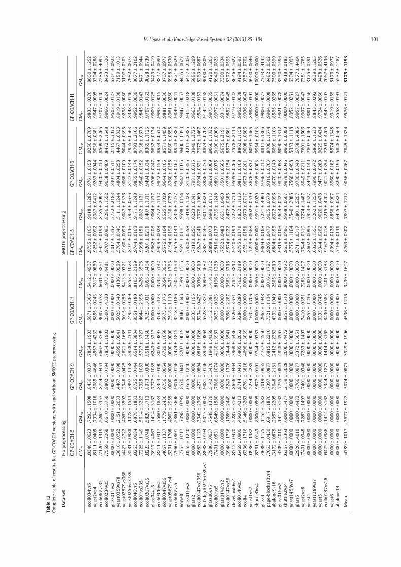
Table
12Co
mpletetableof
resu
ltsforGP-CO
ACH
versions
withan
dwitho
utSM
OTE
prep
rocessing.
Data-set
Noprep
rocessing
SMOTE
prep
rocessing
GP-COACH-5
GP-COACH-9
GP-COACH-H
GP-COACH-5
GP-COACH-9
GP-COACH-H
GM
trGM
tst
GM
trGM
tst
GM
trGM
tst
GM
trGM
tst
GM
trGM
tst
GM
trGM
tst
ecoli034
vs5
.834
8±.062
3.729
3±.150
8.843
6±.033
7.785
4±.190
3.587
1±.536
6.541
2±.496
7.975
5±.016
5.901
8±.128
2.976
1±.015
8.925
0±.070
9.983
3±.027
6.866
0±.125
2ye
ast2vs4
.811
1±.040
5.793
4±.101
8.508
5±.464
6.455
7±.423
2.885
5±.024
3.781
7±.085
0.925
2±.009
2.898
7±.041
2.928
3±.004
4.903
6±.038
1.964
7±.009
5.930
4±.028
8ecoli067
vs35
.712
0±.131
9.526
2±.335
7.872
4±.045
3.666
7±.379
9.908
7±.057
8.663
1±.386
1.942
1±.019
3.818
5±.209
3.942
0±.021
0.850
9±.226
5.970
7±.014
0.728
6±.409
5ecoli023
4vs5
.755
9±.226
9.661
0±.375
9.880
2±.019
4.785
4±.190
3.250
0±.433
0.197
3±.441
1.970
7±.009
5.828
6±.155
2.963
8±.040
9.847
2±.164
8.996
6±.002
4.847
3±.152
6glass0
15vs2
.000
0±.000
0.000
0±.000
0.000
0±.000
0.000
0±.000
0.000
0±.000
0.000
0±.000
0.501
7±.133
7.373
2±.218
3.830
1±.051
1.211
5±.303
2.950
3±.012
7.630
1±.092
2ye
ast035
9vs7
8.381
6±.072
2.215
1±.203
3.446
7±.019
8.459
5±.094
1.502
5±.054
0.413
6±.098
9.576
4±.084
0.511
1±.124
4.480
4±.025
8.446
7±.083
3.891
9±.018
8.718
9±.101
3ye
ast025
79vs36
8.442
3±.272
2.426
3±.359
2.294
8±.042
5.262
1±.168
5.901
5±.025
6.841
3±.032
1.916
0±.009
3.908
7±.037
6.906
8±.010
9.904
4±.039
5.929
8±.008
0.910
7±.030
3ye
ast025
6vs3
789
.358
1±.098
8.107
8±.151
3.399
7±.135
8.292
8±.234
1.749
5±.026
9.635
3±.107
3.810
1±.013
6.795
4±.067
6.812
7±.014
9.795
5±.056
3.834
8±.014
6.798
2±.067
3ecoli046
vs5
.826
3±.068
4.687
8±.183
3.872
5±.014
4.651
4±.383
4.955
1±.018
0.810
5±.212
9.974
4±.016
8.917
1±.124
8.985
5±.017
4.879
3±.216
6.995
2±.003
9.867
7±.210
2ecoli01v
s235
.722
5±.114
9.561
4±.322
2.792
5±.108
3.572
7±.372
7.464
4±.239
5.242
6±.350
8.939
8±.015
1.868
2±.113
1.954
0±.015
2.913
8±.067
0.984
5±.014
3.847
1±.094
4ecoli026
7vs3
5.822
3±.074
8.582
8±.371
3.897
3±.030
0.851
8±.145
8.782
5±.303
1.605
5±.345
4.920
1±.021
1.840
7±.131
1.949
4±.033
4.836
5±.112
5.970
7±.016
3.902
8±.073
9glass0
4vs5
.391
7±.406
7.141
4±.316
2.777
7±.108
5.624
3±.371
3.000
0±.000
0.000
0±.000
0.966
2±.020
8.906
4±.127
7.970
6±.024
7.963
2±.013
4.990
9±.012
5.942
9±.041
9ecoli034
6vs5
.821
1±.031
7.756
0±.188
4.835
3±.039
0.800
5±.089
7.374
2±.512
3.373
2±.513
2.995
9±.002
8.877
2±.113
2.984
2±.015
9.893
4±.063
2.999
3±.001
5.884
7±.069
0ecoli034
7vs5
6.406
7±.133
7.177
9±.243
6.675
6±.066
4.672
9±.165
8.567
3±.187
6.265
4±.395
6.957
6±.010
4.852
5±.103
9.964
4±.016
6.857
1±.145
9.988
1±.003
6.876
7±.097
7ye
ast056
79vs4
.530
1±.170
8.450
2±.295
5.000
0±.000
0.000
0±.000
0.751
8±.111
0.543
3±.176
3.819
4±.019
8.813
6±.075
9.836
0±.015
8.808
0±.085
8.896
1±.028
0.698
8±.053
0ecoli067
vs5
.796
0±.069
1.586
1±.360
6.907
6±.015
6.747
4±.181
5.921
8±.018
6.750
5±.155
4.954
5±.014
4.835
6±.127
7.955
4±.016
2.892
3±.088
4.984
9±.004
1.867
1±.062
9vo
wel0
.776
3±.071
7.709
8±.079
5.852
0±.044
3.820
7±.061
9.804
6±.134
3.759
9±.150
5.969
1±.011
6.959
8±.015
4.964
2±.007
5.940
0±.009
3.994
7±.005
7.946
5±.062
2glass0
16vs2
.055
5±.124
0.000
0±.000
0.055
5±.124
0.000
0±.000
0.000
0±.000
0.000
0±.000
0.782
0±.055
8.541
9±.122
8.812
0±.035
5.421
1±.238
5.941
5±.021
8.646
7±.220
6glass2
.000
0±.000
0.000
0±.000
0.000
0±.000
0.000
0±.000
0.053
5±.119
5.000
0±.000
0.701
9±.025
6.622
3±.084
1.798
1±.061
5.394
9±.372
5.966
3±.018
8.588
6±.129
9ecoli014
7vs2
356
.508
3±.112
3.394
2±.236
0.427
1±.089
4.081
6±.182
6.523
4±.042
7.303
6±.301
9.924
7±.024
1.797
6±.106
0.899
4±.052
1.797
2±.146
7.959
4±.015
3.826
3±.068
7led7
digit024
5678
9vs1
.898
8±.019
4.901
3±.083
0.908
1±.015
6.895
8±.086
4.532
8±.487
2.509
9±.468
2.898
1±.024
6.901
1±.082
9.898
6±.027
4.887
4±.070
8.914
2±.015
8.900
0±.080
9glass0
6vs5
.798
6±.063
7.754
8±.137
9.514
2±.347
0.194
9±.435
9.151
2±.338
1.141
4±.316
2.989
8±.007
3.994
9±.011
3.992
4±.006
9.906
0±.133
2.997
5±.003
5.912
0±.126
3ecoli01v
s5.740
1±.053
1.654
9±.158
0.768
6±.107
4.413
0±.398
7.967
3±.032
3.819
6±.123
8.981
6±.013
7.873
9±.124
8.989
1±.007
5.919
0±.090
8.997
7±.003
1.894
6±.082
3glass0
146v
s2.000
0±.000
0.000
0±.000
0.000
0±.000
0.000
0±.000
0.000
0±.000
0.000
0±.000
0.755
2±.048
3.665
1±.045
0.850
1±.066
5.567
5±.319
1.931
3±.007
4.730
0±.053
4ecoli014
7vs5
6.394
8±.173
6.178
9±.244
9.524
3±.137
6.244
4±.354
1.705
8±.228
7.356
3±.371
5.957
4±.022
2.847
2±.038
5.973
5±.015
4.857
7±.066
1.985
2±.004
5.837
2±.059
5clev
elan
d0vs4
.831
2±.047
0.528
7±.310
0.865
6±.046
4.396
9±.543
6.532
6±.367
1.278
4±.381
2.974
0±.019
4.723
2±.171
0.959
5±.026
6.757
8±.211
4.971
9±.032
2.864
6±.162
7ecoli014
6vs5
.646
9±.090
6.456
0±.421
3.871
4±.046
1.680
5±.206
2.928
4±.028
0.776
2±.211
9.978
5±.017
1.883
2±.113
3.981
1±.016
8.886
2±.115
8.995
2±.003
8.919
4±.059
7ecoli4
.633
6±.171
6.514
6±.326
3.676
1±.381
8.469
6±.303
9.000
0±.000
0.000
0±.000
0.975
1±.015
1.937
3±.071
7.967
3±.020
1.900
8±.080
6.993
6±.004
3.935
7±.070
2ye
ast1vs7
.098
6±.138
2.000
0±.000
0.223
4±.228
5.000
0±.000
0.163
2±.170
6.000
0±.000
0.722
9±.056
8.680
2±.053
9.867
6±.083
2.609
3±.146
5.898
8±.030
1.690
0±.064
6sh
uttle0v
s4.836
1±.014
3.830
0±.059
5.987
7±.010
1.974
4±.038
71.00
00±.000
0.996
0±.009
01.00
00±.000
0.999
1±.002
0.999
5±.000
3.995
4±.010
31.00
00±.000
01.00
00±.000
0glass4
.468
9±.117
5.115
5±.258
2.701
9±.095
5.473
7±.455
0.296
3±.194
8.000
0±.000
0.980
4±.016
8.723
1±.409
0.976
6±.021
2.881
1±.130
6.990
6±.007
7.730
3±.413
2pa
ge-block
s13v
s4.706
3±.043
0.691
7±.187
6.739
7±.087
7.681
5±.221
6.732
1±.113
4.601
6±.172
7.920
5±.047
7.903
5±.067
9.931
6±.070
3.870
6±.157
4.999
4±.000
8.948
2±.050
2ab
alon
e9-18
.317
2±.087
5.235
7±.220
5.364
8±.218
1.241
2±.228
2.439
3±.104
9.256
5±.251
0.688
4±.035
5.692
2±.099
6.807
0±.014
9.669
9±.110
3.859
5±.026
5.750
0±.059
9glass0
16vs5
.430
9±.401
0.141
4±.316
2.775
5±.084
3.482
8±.456
7.000
0±.000
0.000
0±.000
0.981
9±.010
6.964
4±.042
2.982
0±.005
8.909
0±.131
2.992
1±.007
8.855
0±.159
6sh
uttle2v
s4.636
7±.236
3.600
0±.547
7.215
9±.302
8.200
0±.447
2.825
7±.151
0.800
0±.447
2.963
9±.049
6.956
8±.066
7.997
9±.004
6.996
0±.009
01.00
00±.000
0.991
8±.018
3ye
ast145
8vs7
.000
0±.000
0.000
0±.000
0.000
0±.000
0.000
0±.000
0.000
0±.000
0.000
0±.000
0.577
5±.110
4.354
6±.208
6.756
6±.049
8.535
3±.111
8.895
2±.026
1.630
4±.109
5glass5
.292
6±.401
0.200
0±.447
2.776
6±.097
7.537
2±.505
1.000
0±.000
0.000
0±.000
0.971
1±.031
7.580
1±.529
7.978
0±.034
0.675
8±.408
5.995
7±.002
7.787
7±.440
4ye
ast2vs8
.740
1±.034
8.728
3±.149
7.740
1±.034
8.728
3±.149
7.741
0±.035
1.728
3±.149
7.754
4±.031
9.727
4±.148
7.804
9±.021
1.760
1±.160
6.993
7±.004
7.738
1±.176
5ye
ast4
.000
0±.000
0.000
0±.000
0.000
0±.000
0.000
0±.000
0.085
3±.123
6.000
0±.000
0.860
2±.009
5.792
3±.052
7.844
3±.014
0.780
7±.046
9.900
1±.015
6.817
5±.039
1ye
ast128
9vs7
.000
0±.000
0.000
0±.000
0.000
0±.000
0.000
0±.000
0.000
0±.000
0.000
0±.000
0.632
5±.155
6.526
2±.125
3.799
6±.067
2.586
0±.163
3.884
3±.029
2.693
9±.120
5ye
ast5
.000
0±.000
0.000
0±.000
0.000
0±.000
0.000
0±.000
0.033
3±.074
5.000
0±.000
0.934
4±.026
2.902
0±.047
8.947
7±.028
9.922
9±.043
4.972
4±.006
6.942
8±.052
6ecoli013
7vs2
6.647
2±.098
6.141
4±.316
2.334
4±.187
7.141
4±.316
2.843
0±.058
3.140
1±.313
3.916
7±.041
8.721
5±.420
2.902
1±.035
4.720
3±.420
0.984
3±.010
7.706
7±.413
6ye
ast6
.000
0±.000
0.000
0±.000
0.000
0±.000
0.000
0±.000
0.000
0±.000
0.000
0±.000
0.899
4±.012
8.885
6±.090
7.896
0±.018
7.857
4±.134
8.931
9±.015
5.817
0±.097
7ab
alon
e19
.000
0±.000
0.000
0±.000
0.000
0±.000
0.000
0±.000
0.000
0±.000
0.000
0±.000
0.719
6±.013
1.642
5±.082
4.829
0±.019
6.582
8±.056
9.855
8±.019
3.553
2±.148
7
Mea
n.478
9±.101
7.367
7±.192
2.507
4±.087
1.392
9±.199
6.453
6±.121
6.343
9±.169
7.876
3±.030
7.789
7±.121
2.905
6±.026
7.784
5±.133
4.957
6±.012
1.817
5±.119
3
V. López et al. / Knowledge-Based Systems 38 (2013) 85–104 101

Table
13Co
mpletetableof
resu
ltsforFR
BCSmetho
dsan
dC4
.5in
high
lyim
balanc
edda
ta-sets.
SMOTE
prep
rocessingforFR
BCSmetho
ds,S
MOTE
+EN
NforC4
.5.
Data-set
GP-COACH-5
GP-COACH-9
HFR
BCS(Chi)
GP-COACH
-HC4.5
GM
trGM
tst
GM
trGM
tst
GM
trGM
tst
GM
trGM
tst
GM
trGM
tst
ecoli034
vs5
.975
5±.016
5.901
8±.128
2.976
1±.015
8.925
0±.070
9.993
0±.005
0.842
1±.147
1.983
3±.027
6.866
0±.125
2.976
2±.014
9.876
1±.049
2ye
ast2vs4
.925
2±.009
2.898
7±.041
2.928
3±.004
4.903
6±.038
1.952
7±.010
5.893
2±.041
8.964
7±.009
5.930
4±.028
8.974
5±.006
6.902
9±.040
6ecoli067
vs35
.942
1±.019
3.818
5±.209
3.942
0±.021
0.850
9±.226
5.957
4±.016
3.826
7±.141
5.970
7±.014
0.728
6±.409
5.977
1±.020
4.720
6±.407
2ecoli023
4vs5
.970
7±.009
5.828
6±.155
2.963
8±.040
9.847
2±.164
8.991
0±.003
1.842
5±.150
4.996
6±.002
4.847
3±.152
6.982
7±.007
4.886
1±.124
5glass0
15vs2
.501
7±.133
7.373
2±.218
3.830
1±.051
1.211
5±.303
2.696
7±.026
9.559
0±.085
1.950
3±.012
7.630
1±.092
2.906
6±.026
3.778
8±.208
9ye
ast035
9vs7
8.576
4±.084
0.511
1±.124
4.480
4±.025
8.446
7±.083
3.840
1±.004
0.733
0±.040
3.891
9±.018
8.718
9±.101
3.921
3±.021
4.689
4±.088
8ye
ast025
79vs36
8.916
0±.009
3.908
7±.037
6.906
8±.010
9.904
4±.039
5.906
3±.010
3.894
6±.035
5.929
8±.008
0.910
7±.030
3.957
2±.020
6.912
5±.033
6ye
ast025
6vs3
789
.810
1±.013
6.795
4±.067
6.812
7±.014
9.795
5±.056
3.810
6±.016
5.792
7±.067
4.834
8±.014
6.798
2±.067
3.917
3±.018
0.770
7±.036
6ecoli046
vs5
.974
4±.016
8.917
1±.124
8.985
5±.017
4.879
3±.216
6.992
5±.002
9.880
0±.115
6.995
2±.003
9.867
7±.210
2.983
4±.007
9.877
6±.114
8ecoli01v
s235
.939
8±.015
1.868
2±.113
1.954
0±.015
2.913
8±.067
0.984
4±.013
2.870
9±.107
6.984
5±.014
3.847
1±.094
4.964
9±.030
2.827
7±.119
1ecoli026
7vs3
5.920
1±.021
1.840
7±.131
1.949
4±.033
4.836
5±.112
5.960
9±.014
0.824
7±.108
9.970
7±.016
3.902
8±.073
9.982
5±.005
8.806
1±.106
5glass0
4vs5
.966
2±.020
8.906
4±.127
7.970
6±.024
7.963
2±.013
4.945
7±.018
5.709
2±.397
6.990
9±.012
5.942
9±.041
9.990
9±.006
3.974
8±.026
9ecoli034
6vs5
.995
9±.002
8.877
2±.113
2.984
2±.015
9.893
4±.063
2.991
8±.005
7.872
9±.117
5.999
3±.001
5.884
7±.069
0.988
4±.004
6.894
6±.079
3ecoli034
7vs5
6.957
6±.010
4.852
5±.103
9.964
4±.016
6.857
1±.145
9.968
2±.009
9.900
7±.096
2.988
1±.003
6.876
7±.097
7.956
6±.017
6.841
3±.137
7ye
ast056
79vs4
.819
4±.019
8.813
6±.075
9.836
0±.015
8.808
0±.085
8.929
0±.010
3.731
8±.074
7.896
1±.028
0.698
8±.053
0.919
7±.012
8.767
8±.102
9ecoli067
vs5
.954
5±.014
4.835
6±.127
7.955
4±.016
2.892
3±.088
4.953
1±.021
1.855
9±.054
2.984
9±.004
1.867
1±.062
9.974
0±.010
3.837
6±.116
7vo
wel0
.969
1±.011
6.959
8±.015
4.964
2±.007
5.940
0±.009
3.999
9±.000
3.988
2±.016
2.994
7±.005
7.946
5±.062
2.994
3±.004
7.941
7±.081
5glass0
16vs2
.782
0±.055
8.541
9±.122
8.812
0±.035
5.421
1±.238
5.872
6±.023
0.583
7±.200
4.941
5±.021
8.646
7±.220
6.936
5±.032
3.606
3±.117
3glass2
.701
9±.025
6.622
3±.084
1.798
1±.061
5.394
9±.372
5.829
9±.017
4.548
4±.205
7.966
3±.018
8.588
6±.129
9.926
1±.034
2.737
7±.163
3ecoli014
7vs2
356
.924
7±.024
1.797
6±.106
0.899
4±.052
1.797
2±.146
7.951
7±.010
9.847
7±.065
5.959
4±.015
3.826
3±.068
7.956
3±.031
8.811
9±.045
9led7
digit024
5678
9vs1
.898
1±.024
6.901
1±.082
9.898
6±.027
4.887
4±.070
8.938
0±.021
2.827
6±.077
8.914
2±.015
8.900
0±.080
9.921
7±.019
2.837
0±.047
5glass0
6vs5
.989
8±.007
3.994
9±.011
3.992
4±.006
9.906
0±.133
2.974
4±.004
6.890
7±.117
8.997
5±.003
5.912
0±.126
3.991
1±.003
5.962
8±.055
6ecoli01v
s5.981
6±.013
7.873
9±.124
8.989
1±.007
5.919
0±.090
8.993
2±.004
3.868
9±.116
6.997
7±.003
1.894
6±.082
3.982
8±.006
8.808
1±.121
3glass0
146v
s2.755
2±.048
3.665
1±.045
0.850
1±.066
5.567
5±.319
1.700
5±.007
7.511
7±.102
6.931
3±.007
4.730
0±.053
4.901
0±.059
6.615
7±.346
5ecoli014
7vs5
6.957
4±.022
2.847
2±.038
5.973
5±.015
4.857
7±.066
1.979
0±.005
9.888
6±.091
8.985
2±.004
5.837
2±.059
5.960
8±.017
3.825
0±.138
0clev
elan
d0vs4
.974
0±.019
4.723
2±.171
0.959
5±.026
6.757
8±.211
4.999
2±.001
8.396
1±.382
7.971
9±.032
2.864
6±.162
7.981
9±.018
7.730
7±.151
7ecoli014
6vs5
.978
5±.017
1.883
2±.113
3.981
1±.016
8.886
2±.115
8.991
3±.004
7.867
4±.106
9.995
2±.003
8.919
4±.059
7.985
0±.006
1.888
0±.114
8ecoli4
.975
1±.015
1.937
3±.071
7.967
3±.020
1.900
8±.080
6.986
9±.014
1.930
2±.081
7.993
6±.004
3.935
7±.070
2.982
6±.017
0.894
7±.120
2ye
ast1vs7
.722
9±.056
8.680
2±.053
9.867
6±.083
2.609
3±.146
5.916
3±.022
5.707
4±.124
0.898
8±.030
1.690
0±.064
6.909
3±.033
2.722
2±.053
2sh
uttle0v
s41.00
00±.000
0.999
1±.002
0.999
5±.000
3.995
4±.010
31.00
00±.000
0.991
2±.011
51.00
00±.000
01.00
00±.000
0.999
9±.000
2.999
7±.000
7glass4
.980
4±.016
8.723
1±.409
0.976
6±.021
2.881
1±.130
6.998
1±.001
7.703
9±.404
9.990
6±.007
7.730
3±.413
2.966
5±.014
9.763
9±.427
9pa
ge-block
s13v
s4.920
5±.047
7.903
5±.067
9.931
6±.070
3.870
6±.157
4.998
9±.001
2.986
4±.006
5.999
4±.000
8.948
2±.050
2.997
5±.001
8.990
9±.006
5ab
alon
e9-18
.688
4±.035
5.692
2±.099
6.807
0±.014
9.669
9±.110
3.839
6±.030
3.675
6±.140
1.859
5±.026
5.750
0±.059
9.927
3±.007
4.688
4±.118
1glass0
16vs5
.981
9±.010
6.964
4±.042
2.982
0±.005
8.909
0±.131
2.997
1±.003
0.779
6±.436
1.992
1±.007
8.855
0±.159
6.986
3±.004
7.773
8±.432
8sh
uttle2v
s4.963
9±.049
6.956
8±.066
7.997
9±.004
6.996
0±.009
0.999
0±.002
3.974
9±.027
11.00
00±.000
0.991
8±.018
31.00
00±.000
01.00
00±.000
0ye
ast145
8vs7
.577
5±.110
4.354
6±.208
6.756
6±.049
8.535
3±.111
8.903
7±.013
3.624
9±.062
6.895
2±.026
1.630
4±.109
5.871
7±.049
2.334
5±.334
2glass5
.971
1±.031
7.580
1±.529
7.978
0±.034
0.675
8±.408
5.976
4±.022
1.687
3±.395
6.995
7±.002
7.787
7±.440
4.969
8±.029
6.585
1±.534
3ye
ast2vs8
.754
4±.031
9.727
4±.148
7.804
9±.021
1.760
1±.160
6.833
4±.016
4.724
7±.151
0.993
7±.004
7.738
1±.176
5.892
3±.044
7.803
3±.116
7ye
ast4
.860
2±.009
5.792
3±.052
7.844
3±.014
0.780
7±.046
9.900
1±.019
4.826
4±.022
9.900
1±.015
6.817
5±.039
1.898
4±.012
3.689
7±.076
9ye
ast128
9vs7
.632
5±.155
6.526
2±.125
3.799
6±.067
2.586
0±.163
3.869
9±.022
4.693
7±.043
7.884
3±.029
2.693
9±.120
5.940
8±.025
9.552
2±.166
2ye
ast5
.934
4±.026
2.902
0±.047
8.947
7±.028
9.922
9±.043
4.978
2±.003
3.942
0±.025
9.972
4±.006
6.942
8±.052
6.981
9±.007
7.939
0±.047
4ecoli013
7vs2
6.916
7±.041
8.721
5±.420
2.902
1±.035
4.720
3±.420
0.986
7±.007
9.714
8±.418
0.984
3±.010
7.706
7±.413
6.965
0±.032
0.706
2±.409
3ye
ast6
.899
4±.012
8.885
6±.090
7.896
0±.018
7.857
4±.134
8.934
1±.017
7.849
2±.128
8.931
9±.015
5.817
0±.097
7.930
1±.015
7.802
9±.154
1ab
alon
e19
.719
6±.013
1.642
5±.082
4.829
0±.019
6.582
8±.056
9.834
3±.028
0.701
9±.085
6.855
8±.019
3.553
2±.148
7.883
8±.030
0.155
0±.212
5
Mea
n.876
3±.030
7.789
7±.121
2.905
6±.026
7.784
5±.133
4.933
1±.011
7.790
1±.132
5.957
6±.012
1.817
5±.119
3.954
9±.018
0.784
8±.145
2
102 V. López et al. / Knowledge-Based Systems 38 (2013) 85–104
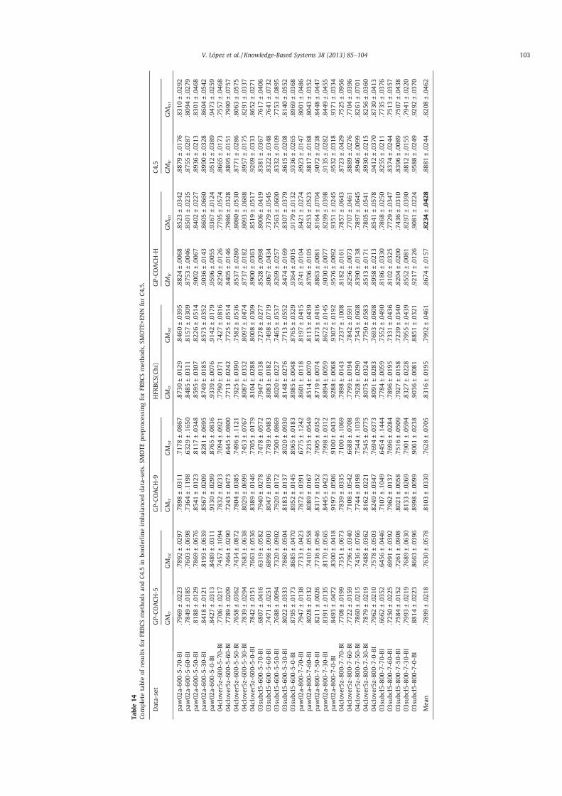
Table
14Co
mpletetableof
resu
ltsforFR
BCSmetho
dsan
dC4
.5in
borderlin
eim
balanc
edda
ta-sets.
SMOTE
prep
rocessingforFR
BCSmetho
ds,S
MOTE
+ENN
forC4
.5.
Data-set
GP-COACH-5
GP-COACH-9
HFR
BCS(Chi)
GP-COACH-H
C4.5
GM
trGM
tst
GM
trGM
tst
GM
trGM
tst
GM
trGM
tst
GM
trGM
tst
paw02
a-60
0-5-70
-BI
.796
9±.022
3.789
2±.029
7.789
8±.031
1.717
8±.086
7.873
0±.012
9.846
0±.039
5.882
4±.006
8.852
3±.034
2.887
9±.017
6.831
0±.029
2pa
w02
a-60
0-5-60
-BI
.784
9±.018
5.760
3±.069
8.736
4±.119
8.632
9±.165
0.848
5±.031
1.815
7±.030
9.875
3±.004
6.850
1±.023
5.875
5±.028
7.809
4±.027
9pa
w02
a-60
0-5-50
-BI
.818
8±.012
9.786
9±.067
6.854
1±.012
3.811
7±.034
8.859
5±.030
7.822
6±.051
4.900
2±.006
7.840
2±.022
7.893
6±.021
3.830
1±.046
8pa
w02
a-60
0-5-30
-BI
.841
8±.012
1.819
3±.063
9.856
7±.020
9.828
1±.069
5.874
9±.018
5.857
3±.035
2.903
6±.014
3.860
5±.066
0.899
0±.032
8.860
4±.054
2pa
w02
a-60
0-5-0-BI
.842
7±.031
3.848
9±.031
1.913
0±.029
9.876
5±.083
6.933
9±.007
6.914
2±.017
9.959
6±.005
5.936
7±.012
4.951
2±.038
9.947
3±.025
904
clov
er5z
-600
-5-70-BI
.770
6±.021
7.745
7±.109
4.783
2±.023
3.709
4±.092
1.779
0±.037
1.742
7±.081
6.825
0±.012
6.779
5±.057
4.866
5±.017
3.755
7±.046
804
clov
er5z
-600
-5-60-BI
.778
9±.020
9.746
4±.029
0.724
3±.047
3.644
5±.080
0.771
3±.024
2.772
5±.051
4.840
5±.014
6.798
6±.032
8.889
5±.015
1.799
0±.075
704
clov
er5z
-600
-5-50-BI
.765
8±.036
2.743
4±.087
2.780
4±.038
5.749
6±.112
1.792
5±.039
0.758
2±.053
6.853
7±.028
0.808
0±.053
0.877
1±.028
6.806
3±.057
504
clov
er5z
-600
-5-30-BI
.783
9±.029
4.768
3±.063
8.802
9±.069
9.745
3±.076
7.808
7±.033
2.809
7±.047
4.873
7±.018
2.809
3±.068
8.895
7±.017
5.829
1±.033
704
clov
er5z
-600
-5-0-B
I.784
2±.015
1.766
3±.053
6.838
9±.014
6.770
5±.017
9.810
4±.028
8.800
8±.030
9.890
0±.036
3.851
9±.051
7.926
9±.033
3.865
2±.027
103
subc
l5-600
-5-70-BI
.680
7±.041
6.631
9±.058
2.794
0±.027
8.747
8±.057
2.794
7±.013
8.727
8±.027
7.852
8±.009
8.800
6±.041
9.838
1±.036
7.761
7±.040
603
subc
l5-600
-5-60-BI
.747
1±.025
1.689
8±.090
3.804
7±.019
6.778
9±.048
3.808
3±.018
2.749
8±.071
9.806
7±.043
4.737
9±.054
5.832
2±.034
8.764
1±.073
203
subc
l5-600
-5-50-BI
.768
8±.009
4.732
0±.090
2.792
0±.017
2.750
0±.086
9.802
0±.022
7.746
5±.053
7.826
9±.025
7.756
3±.060
0.833
2±.010
9.775
3±.089
503
subc
l5-600
-5-30-BI
.802
2±.033
3.786
0±.050
4.818
3±.013
7.802
0±.093
0.814
8±.027
6.771
3±.055
2.847
4±.016
9.830
7±.037
9.861
5±.020
8.814
0±.055
203
subc
l5-600
-5-0-B
I.879
5±.017
3.868
5±.047
0.895
2±.014
5.896
5±.018
3.898
5±.004
8.876
5±.032
9.936
4±.001
5.917
9±.013
2.933
6±.026
5.896
9±.036
8pa
w02
a-80
0-7-70
-BI
.794
7±.013
8.773
3±.042
3.787
2±.039
1.677
5±.124
2.860
1±.011
8.819
7±.041
5.874
1±.010
4.842
1±.027
4.892
3±.014
7.800
1±.048
6pa
w02
a-80
0-7-60
-BI
.802
8±.013
2.741
0±.055
8.808
9±.016
7.723
5±.054
9.851
4±.007
0.811
3±.043
9.870
6±.010
5.825
3±.052
3.881
7±.018
8.804
3±.035
2pa
w02
a-80
0-7-50
-BI
.821
1±.002
6.773
6±.054
6.831
7±.015
2.790
5±.035
2.871
9±.007
4.837
3±.041
6.886
3±.008
1.816
4±.070
4.907
2±.023
8.844
8±.044
7pa
w02
a-80
0-7-30
-BI
.839
1±.013
5.817
0±.056
5.844
5±.042
3.799
8±.031
2.889
4±.005
9.867
2±.014
5.903
0±.007
7.829
9±.039
8.913
5±.028
2.844
9±.045
5pa
w02
a-80
0-7-0-BI
.849
3±.047
2.830
0±.041
8.919
7±.050
6.910
0±.043
3.928
8±.006
8.930
7±.019
2.957
6±.009
2.935
1±.024
5.953
2±.031
8.937
1±.033
404
clov
er5z
-800
-7-70-BI
.770
8±.019
9.735
1±.067
3.783
9±.033
5.710
0±.106
9.789
8±.014
3.723
7±.100
8.818
2±.016
1.785
7±.064
3.872
3±.042
9.752
5±.095
604
clov
er5z
-800
-7-60-BI
.772
2±.015
9.779
6±.034
0.710
8±.054
2.668
8±.070
8.779
9±.019
4.784
2±.059
1.825
6±.007
3.770
7±.046
1.888
9±.027
6.770
4±.039
604
clov
er5z
-800
-7-50-BI
.786
0±.021
5.743
6±.076
6.774
4±.019
8.754
4±.103
9.792
8±.029
0.754
3±.060
8.839
0±.013
8.789
7±.064
5.894
6±.009
9.826
1±.070
104
clov
er5z
-800
-7-30-BI
.787
9±.021
9.748
8±.036
2.816
2±.022
1.754
5±.077
5.807
5±.032
4.775
0±.058
3.851
3±.017
1.780
5±.054
1.893
0±.021
5.825
6±.036
004
clov
er5z
-800
-7-0-B
I.796
2±.021
0.757
8±.050
3.824
9±.034
7.769
4±.037
3.809
1±.028
3.769
3±.060
8.895
8±.021
3.854
1±.057
8.941
2±.037
0.873
0±.041
303
subc
l5-800
-7-70-BI
.666
2±.035
2.645
6±.044
6.710
7±.104
9.645
4±.144
4.778
4±.005
9.755
2±.049
0.818
6±.033
0.786
8±.025
0.825
5±.021
1.773
5±.037
603
subc
l5-800
-7-60-BI
.725
0±.022
5.699
1±.039
2.796
2±.013
7.769
6±.028
4.789
6±.019
5.733
1±.043
6.810
2±.032
5.772
9±.034
7.837
4±.024
4.751
3±.035
703
subc
l5-800
-7-50-BI
.758
4±.015
2.726
1±.090
8.802
1±.005
8.751
6±.050
9.792
7±.015
8.723
9±.034
0.820
4±.020
0.743
6±.031
0.839
6±.008
9.750
7±.043
803
subc
l5-800
-7-30-BI
.799
3±.021
9.768
9±.063
0.813
3±.026
9.790
1±.059
4.832
7±.022
8.795
5±.043
9.855
2±.008
1.829
7±.039
0.881
2±.015
5.794
1±.022
003
subc
l5-800
-7-0-B
I.881
4±.022
3.866
3±.039
6.899
8±.009
9.906
1±.023
8.903
6±.008
1.885
1±.032
1.921
7±.012
6.908
1±.022
4.958
8±.024
9.929
2±.037
0
Mea
n.789
9±.021
8.763
0±.057
8.810
3±.033
0.762
8±.070
5.831
6±.019
5.799
2±.046
1.867
4±.015
7.823
4±.042
8.888
1±.024
4.820
8±.046
2
V. López et al. / Knowledge-Based Systems 38 (2013) 85–104 103
References
[1] R. Alcalá, J. Alcalá-Fdez, F. Herrera, A proposal for the genetic lateral tuning oflinguistic fuzzy systems and its interaction with rule selection, IEEETransactions on Fuzzy Systems 15 (2007) 616–635.
[2] J. Alcalá-Fdez, A. Fernández, J. Luengo, J. Derrac, S. García, L. Sánchez, F. Herrera,KEEL data-mining software tool: data set repository, integration of algorithmsand experimental analysis framework, Journal of Multi-Valued Logic and SoftComputing 17 (2011) 255–287.
[3] J. Alcalá-Fdez, L. Sánchez, S. García, M.J. del Jesus, S. Ventura, J.M. Garrell, J.Otero, C. Romero, J. Bacardit, V.M. Rivas, J.C. Fernández, F. Herrera, KEEL: asoftware tool to assess evolutionary algorithms for data mining problems, SoftComputing 13 (2009) 307–318.
[4] R. Barandela, J.S. Sánchez, V. García, E. Rangel, Strategies for learning in classimbalance problems, Pattern Recognition 36 (2003) 849–851.
[5] A. Bastian, How to handle the flexibility of linguistic variables withapplications, International Journal of Uncertainty, Fuzziness and Knowledge-Based Systems 2 (1994) 463–484.
[6] G.E.A.P.A. Batista, R.C. Prati, M.C. Monard, A study of the behaviour of severalmethods for balancing machine learning training data, SIGKDD Explorations 6(2004) 20–29.
[7] F.J. Berlanga, A.J. Rivera, M.J. del Jesus, F. Herrera, GP-COACH: geneticprogramming-based learning of compact and accurate fuzzy rule-basedclassification systems for high-dimensional problems, Information Sciences180 (2010) 1183–1200.
[8] J. Charles, Automatic recognition of complete palynomorphs in digital images,Machine Vision and Applications 22 (2011) 53–60.
[9] N.V. Chawla, K.W. Bowyer, L.O. Hall, W.P. Kegelmeyer, SMOTE: syntheticminority over-sampling technique, Journal of Artificial Intelligent Research 16(2002) 321–357.
[10] Z. Chi, H. Yan, T. Pham, Fuzzy Algorithms with Applications to ImageProcessing and Pattern Recognition, World Scientific, 1996.
[11] O. Cordón, F. Herrera, A proposal for improving the accuracy of linguisticmodeling, IEEE Transactions on Fuzzy Systems 8 (2000) 335–344.
[12] O. Cordón, F. Herrera, F. Hoffmann, L. Magdalena, Genetic fuzzy systems:evolutionary tuning and learning of fuzzy knowledge bases, Advances in FuzzySystems – Applications and Theory, vol. 19, World Scientific, 2001.
[13] O. Cordón, F. Herrera, P. Villar, Generating the knowledge base of a fuzzy rule-based system by the genetic learning of the data base, IEEE Transactions onFuzzy Systems 9 (2001) 667–674.
[14] O. Cordon, F. Herrera, I. Zwir, Linguistic modeling by hierarchical systems oflinguistic rules, IEEE Transactions on Fuzzy Systems 10 (2002) 2–20.
[15] O. Cordón, M. del Jesus, F. Herrera, A proposal on reasoning methods in fuzzyrule-based classification systems, International Journal of Approximate 20(1999) 21–45.
[16] C. Drummond, R.C. Holte, C4.5, class imbalance, and cost sensitivity: whyunder-sampling beats over-sampling, in: Proceedings of the InternationalConference on Machine Learning (ICML 2003) Workshop on Learning fromImbalanced Data Sets II, 2003, pp. 1–8.
[17] C. Elkan, The foundations of cost-sensitive learning, in: Proceedings of the 17thIEEE International Joint Conference on Artificial Intelligence (IJCAI’01), 2001,pp. 973–978.
[18] L.J. Eshelman, The CHC adaptive search algorithm: How to have safe searchwhen engaging in nontraditional genetic recombination, in: Foudations ofGenetic Algorithms, Morgan Kaufmann, 1990, pp. 265–283.
[19] A. Fernández, S. García, F. Herrera, Addressing the classification withimbalanced data: open problems and new challenges on class distribution,in: Proceedings of the 6th International Conference on Hybrid ArtificialIntelligence Systems (HAIS’11), 2011, pp. 1–10.
[20] A. Fernández, S. García, M.J. del Jesus, F. Herrera, A study of the behaviour oflinguistic fuzzy rule based classification systems in the framework ofimbalanced data-sets, Fuzzy Sets and Systems 159 (2008) 2378–2398.
[21] A. Fernández, M.J. del Jesus, F. Herrera, Hierarchical fuzzy rule basedclassification systems with genetic rule selection for imbalanced data-sets,International Journal of Approximate Reasoning 50 (2009) 561–577.
[22] A. Fernández, M.J. del Jesus, F. Herrera, On the 2-tuples based genetic tuningperformance for fuzzy rule based classification systems in imbalanced data-sets, Information Sciences 180 (2010) 1268–1291.
[23] S. García, J. Derrac, I. Triguero, C.J. Carmona, F. Herrera, Evolutionary-basedselection of generalized instances for imbalanced classification, Knowledge-Based Systems 25 (2012) 3–12.
[24] S. García, A. Fernández, J. Luengo, F. Herrera, A study of statistical techniquesand performance measures for genetics-based machine learning: accuracy andinterpretability, Soft Computing 13 (2009) 959–977.
[25] S. García, F. Herrera, An extension on ‘‘statistical comparisons of classifiersover multiple data sets’’ for all pairwise comparisons, Journal of MachineLearning Research 9 (2008) 2607–2624.
[26] V. García, R. Mollineda, J.S. Sánchez, On the k-NN performance in a challengingscenario of imbalance and overlapping, Pattern Analysis Applications 11(2008) 269–280.
[27] V. García, J. Sánchez, R. Mollineda, On the effectiveness of preprocessingmethods when dealing with different levels of class imbalance, Knowledge-Based Systems 25 (2012) 13–21.
[28] N. García-Pedrajas, J. Pérez-Rodríguez, M. García-Pedrajas, D. Ortiz-Boyer, C.Fyfe, Class imbalance methods for translation initiation site recognition inDNA sequences, Knowledge-Based Systems 25 (2012) 22–34.
[29] H. He, E.A. Garcia, Learning from imbalanced data, IEEE Transactions onKnowledge and Data Engineering 21 (2009) 1263–1284.
[30] F. Herrera, Genetic fuzzy systems: taxonomy, current research trends andprospects, Evolutionary Intelligence 1 (2008) 27–46.
[31] F. Herrera, M. Lozano, A.M. Sánchez, A taxonomy for the crossover operator forreal-coded genetic algorithms: an experimental study, International Journal ofIntelligent Systems 18 (2003) 309–338.
[32] F. Herrera, L. Martínez, A 2-tuple fuzzy linguistic representation model forcomputing with words, IEEE Transactions on Fuzzy Systems 8 (2000) 746–752.
[33] H. Ishibuchi, T. Nakashima, Effect of rule weights in fuzzy rule-basedclassification systems, IEEE Transactions on Fuzzy Systems 9 (2001) 506–515.
[34] H. Ishibuchi, T. Nakashima, M. Nii, Classification and Modeling with LinguisticInformation Granules: Advanced Approaches to Linguistic Data Mining,Springer-Verlag, 2004.
[35] H. Ishibuchi, K. Nozaki, N. Yamamoto, H. Tanaka, Selecting fuzzy if–then rulesfrom classification problems using genetic algorithms, IEEE Transactions onFuzzy Systems 9 (1995) 260–270.
[36] H. Ishibuchi, T. Yamamoto, Rule weight specification in fuzzy rule-basedclassification systems, IEEE Transactions on Fuzzy Systems 13 (2005) 428–435.
[37] N. Japkowicz, S. Stephen, The class imbalance problem: a systematic study,Intelligent Data Analysis Journal 6 (2002) 429–450.
[38] W. Khreich, E. Granger, A. Miri, R. Sabourin, Iterative boolean combination ofclassifiers in the ROC space: an application to anomaly detection with HMMs,Pattern Recognition 43 (2010) 2732–2752.
[39] J.R. Koza, Genetic Programming: On the Programming of Computers by Meansof Natural Selection, The MIT Press, 1992.
[40] M. Kubat, S. Matwin, Addressing the curse of imbalanced training sets: one-sided selection, in: 14th International Conference on MachineLearning(ICML97), 1997, pp. 179–186.
[41] J. Liu, Q. Hu, D. Yu, A comparative study on rough set based class imbalancelearning, Knowledge-Based Systems 21 (2008) 753–763.
[42] V. López, A. Fernández, J.G. Moreno-Torres, F. Herrera, Analysis ofpreprocessing vs. cost-sensitive learning for imbalanced classification. Openproblems on intrinsic data characteristics, Expert Systems with Applications39 (2012) 6585–6608.
[43] L. Magdalena, F. Monasterio-Huelin, A fuzzy logic controller with learningthrough the evolution of its knowledge base, International Journal ofApproximate Reasoning 16 (1997) 335–358.
[44] K. Napierala, J. Stefanowski, S. Wilk, Learning from imbalanced data inpresence of noisy and borderline examples, in: 7th International Conferenceon Rough Sets and Current Trends in Computing (RSCTC2010), 2010, pp. 158–167.
[45] S. Oh, M. Lee, B.T. Zhang, Ensemble learning with active example selection forimbalanced biomedical data classification, IEEE/ACM Transactions onComputational Biology and Bioinformatics 8 (2011) 316–325.
[46] A. Orriols-Puig, E. Bernadó-Mansilla, Evolutionary rule-based systems forimbalanced datasets, Soft Computing 13 (2009) 213–225.
[47] J. Quinlan, C4.5: Programs for Machine Learning., Morgan Kauffman, 1993.[48] J. Ren, ANN vs. SVM: which one performs better in classification of MCCs in
mammogram imaging, Knowledge-Based Systems 26 (2012) 144–153.[49] C. Seiffert, T.M. Khoshgoftaar, J.V. Hulse, A. Folleco, An empirical study of the
classification performance of learners on imbalanced and noisy softwarequality data, Information Sciences, in press. http://dx.doi.org/10.1016/j.ins.2010.12.016.
[50] D. Sheskin, Handbook of Parametric and Nonparametric Statistical Procedures,Chapman & Hall/CRC, 2011.
[51] Y. Sun, A.K.C. Wong, M.S. Kamel, Classification of imbalanced data: a review,International Journal of Pattern Recognition and Artificial Intelligence 23(2009) 687–719.
[52] D. Wang, T.S. Dillon, Extraction of classification rules characterized byellipsoidal regions using soft-computing techniques, International Journal ofSystems Science 37 (2006) 969–980.
[53] G.M. Weiss, Mining with rarity: a unifying framework, SIGKDD Explorations 6(2004) 7–19.
[54] D.L. Wilson, Asymptotic properties of nearest neighbor rules using edited data,IEEE Transactions on Systems, Man and Cybernetics 2 (1972) 408–421.
[55] M.L. Wong, K.S. Leung, Data Mining Using Grammar-Based GeneticProgramming and Applications, Kluwer Academic Publishers, 2000.
[56] Q. Yang, X. Wu, 10 challenging problems in data mining research, InternationalJournal of Information Technology & Decision Making 5 (2006) 597–604.
[57] B. Zadrozny, C. Elkan, Learning and making decisions when costs andprobabilities are both unknown, in: Proceedings of the 7th InternationalConference on Knowledge Discovery and Data Mining (KDD’01), 2001, pp.204–213.
104 V. López et al. / Knowledge-Based Systems 38 (2013) 85–104


2 Addressing the Data Intrinsic Characteristics of Imbalanced Problems using FRBCSs and MachineLearning Techniques 115
2.2. On the Importance of the Validation Technique for Classification with
Imbalanced Datasets: Addressing Covariate Shift when Data is Skewed
V. Lopez, A. Fernandez, F. Herrera, On the Importance of the Validation Technique forClassification with Imbalanced Datasets: Addressing Covariate Shift when Data is Skewed.Information Sciences 257 (2014) 1–13, doi: 10.1016/j.ins.2013.09.038
• Status: Published.
• Impact Factor (JCR 2012): 3.643.
• Subject Category: Computer Science, Information Systems. Ranking 6 / 132 (Q1).


On the importance of the validation technique for classificationwith imbalanced datasets: Addressing covariate shift when datais skewed
Victoria López a,⇑, Alberto Fernández b, Francisco Herrera a
aDepartment of Computer Science and Artificial Intelligence, CITIC-UGR (Research Center on Information and Communications Technology), University ofGranada, Granada, SpainbDepartment of Computer Science, University of Jaén, Jaén, Spain
a r t i c l e i n f o
Article history:Received 13 August 2012Received in revised form 14 June 2013Accepted 15 September 2013Available online 21 September 2013
Keywords:ClassificationImbalanced datasetCovariate shiftDataset shiftValidation techniquePartitioning
a b s t r a c t
In the field of Data Mining, the estimation of the quality of the learned models is a key stepin order to select the most appropriate tool for the problem to be solved. Traditionally, a k-fold validation technique has been carried out so that there is a certain degree of indepen-dency among the results for the different partitions. In this way, the highest average per-formance will be obtained by the most robust approach. However, applying a ‘‘random’’division of the instances over the folds may result in a problem known as dataset shift,which consists in having a different data distribution between the training and test folds.In classification with imbalanced datasets, in which the number of instances of one class
is much lower than the other class, this problem is more severe. The misclassification ofminority class instances due to an incorrect learning of the real boundaries caused by anot well fitted data distribution, truly affects the measures of performance in this scenario.Regarding this fact, we propose the use of a specific validation technique for the partition-ing of the data, known as ‘‘Distribution optimally balanced stratified cross-validation’’ toavoid this harmful situation in the presence of imbalance. This methodology makes thedecision of placing close-by samples on different folds, so that each partition will end upwith enough representatives of every region.We have selected a wide number of imbalanced datasets from KEEL dataset repository
for our study, using several learning techniques from different paradigms, thus makingthe conclusions extracted to be independent of the underlying classifier. The analysis ofthe results has been carried out by means of the proper statistical study, which showsthe goodness of this approach for dealing with imbalanced data.
� 2013 Elsevier Inc. All rights reserved.
1. Introduction
Standard learning algorithms are designed under the premise of a balanced class distribution. When dealing with skewedclass distributions, the classification problem becomes more difficult, specifically for correctly identifying the minority con-cepts within the data [11]. This issue is known as the class imbalance problem [21,38], in which there is an under-repre-sented class (positive) and a majority class (negative). This problem is present in many real-world classification tasks andhas been considered as a challenge within the Data Mining community [48].
0020-0255/$ - see front matter � 2013 Elsevier Inc. All rights reserved.http://dx.doi.org/10.1016/j.ins.2013.09.038
⇑ Corresponding author. Tel.: +34 958 240598; fax: +34 958 243317.E-mail addresses: [email protected] (V. López), [email protected] (A. Fernández), [email protected] (F. Herrera).
Information Sciences 257 (2014) 1–13
Contents lists available at ScienceDirect
Information Sciences
journal homepage: www.elsevier .com/locate / ins

In order to validate the performance of a classifier, both in standard and imbalanced classification, stratified cross-vali-dation (SCV) is the most commonly employed method in the literature. It places an equal number of samples of each classon each partition to maintain class distributions similar in all partitions [9]. However, when this process is carried out in arandom way, it may introduce a different data distribution between the training and test partitions, thus leading to inaccu-rate conclusions when learning a model from the training data. This issue is known as dataset shift [8], or more specificallycovariate shift [30].
In the presence of imbalance, this problem is even more critic according to the metrics of performance applied in thisscenario. Since misclassifications for the positive class instances severely hinder the average precision, we must try to avoidthose errors in test which are due to a ‘‘random clustering’’ of the classes, i.e. generating outliers.
A more suitable validation technique needs to be employed in order to avoid introducing dataset shift issues artificially. Inthis paper, we suggest the use of a novel methodology called ‘‘Distribution optimally balanced SCV’’ (DOB–SCV) [31] whendealing with imbalanced datasets. This method attempts to minimize covariate shift by keeping data distribution as similaras possible between training and test folds by maximizing diversity on each fold and trying to keep all folds as resembling aspossible to each other. The mechanism of this approach consists in selecting the k closest neighbours for a given instance andplace them in different folds (with k being the number of total partitions), so that the data distribution between the trainingand test partitions remains as close as possible.
We must point out that neither SCV nor DOB–SCV can undoubtedly estimate the true classification error of a given model.In particular, there are several factors which may affect the output for unseen samples, and make some problems more dif-ficult than others. Among others, we may stress uneven class distribution (as studied in this paper), the dimensionality of theproblem and its relationship with the overlapping between the classes, and the presence of noise and/or outliers. However,we suggest that, by making the training and test partitions more similar between them, the use of DOB–SCV can guarantee abetter average validation of the results. As pointed out previously, in this way we may avoid those classification errors whichare due to dataset shift, especially those regarded to the minority class instances.
In order to evaluate the goodness and validity of the use of this new partitioning mechanism for imbalanced datasets, wedevelop a thorough empirical study by setting up an experimental framework which includes a set of sixty-six real-worldproblems from the KEEL dataset repository [3,4] (http://www.keel.es/dataset.php). We measure the performance of the clas-sifiers based on its Area Under the Curve (AUC) metric [23] as suggested in imbalanced domains. Additionally, we study thesignificance of the results by the proper statistical tests as suggested in the literature [17,20]. Finally, we check the robust-ness of the DOB–SCV strategy using several well-known classifiers from different Machine Learning paradigms: decisiontrees [34], fuzzy rule based classification systems (FRBCS) [24], instance-based learning [1], and Support Vector Machines(SVMs) [12,15].
This study provides three significant contributions to the research community on classification with imbalanced data,namely:
1. We establish the motivation for the use of a new validation technique for avoiding dataset shift, which highly affects theperformance in this scenario.
2. The goodness of this novel methodology is confirmed by means of a thorough experimental analysis. In this study, severalalgorithms from different paradigms were selected, showing better average performance estimates when using DOB–SCV.
3. Finally, we have concluded that the optimistic/pessimistic estimation of the performance also depends on the problem tobe classified. In this way, the intrinsic data characteristics may have some degree of influence on the final results obtainedby the classifier.
In order to carry out the study, this manuscript is organized as follows. First, Section 2 introduces the problem of imbal-anced data. Next, Section 3 contains the main concepts that are developed in this work, i.e. the basis on validation techniquesand the problem of covariate/dataset shift. Then, the experimental framework is presented in Section 4, whereas all the anal-ysis of the results is shown along Section 5. Finally, Section 6 summarises and concludes the work.
2. Imbalanced datasets in classification
In this section, we will first introduce the problem of imbalanced datasets, describing its features and why is so difficult tolearn in this classification scenario. Then, we will present how to address this problem, enumerating diverse approaches thatcan be applied to ease the discrimination of the minority (positive) and majority (negative) classes. Finally, we will discusshow to evaluate the performance of the results in this situation.
2.1. The problem of imbalanced datasets
The main property of this type of classification problem (in a binary context) is that the examples of one class outnumberthe examples of the other one [11,38]. The minority classes are usually the most important concepts to be learnt, since theymight be associated with exceptional and significant cases [42] or because the data acquisition of these examples is costly
2 V. López et al. / Information Sciences 257 (2014) 1–13

[44]. Since most of the standard learning algorithms consider a balanced training set, this situation may cause the obtentionof suboptimal classification models, i.e. a good coverage of the majority examples whereas the minority ones are misclassi-fied more frequently [21,38].
Traditionally, the Imbalance Ratio (IR), i.e. the ratio between the majority and minority class examples [32], is the mainhint to identify a set of problems which need to be addressed in a special way. Additionally, other data intrinsic character-istics that are related to this concept may include the overlapping between classes [26], lack of representative data [41],small disjuncts [33,43], dataset shift [29] and other issues which have interdependent effects with data distribution(imbalance).
The hitch here is that most learning algorithms aim to obtain a model with a high prediction accuracy and a goodgeneralization capability. However, this inductive bias towards such a model poses a serious challenge to the classificationof imbalanced data [38]. First, if the search process is guided by the standard accuracy rate, it benefits the covering of themajority examples; second, classification rules that predict the positive class are often highly specialized and thus theircoverage is very low, hence they are discarded in favour of more general rules, i.e. those that predict the negative class.Furthermore, it is not easy to distinguish between noisy examples and positive class examples and they can be completelyignored by the classifier.
2.2. Addressing the imbalanced problem: preprocessing and cost-sensitive learning
A large number of approaches have been proposed to deal with the class imbalance problem [28], which can be catego-rized in three groups:
1. Data level solutions: the objective consists in rebalancing the class distribution by sampling the data space to diminishthe effect caused by class imbalance, acting as an external approach [6,10,39].
2. Algorithmic level solutions: these solutions try to adapt several classification algorithms to reinforce the learning towardsthe positive class. Therefore, they can be defined as internal approaches that create new algorithms or modify existingones to take the class imbalance problem into consideration [5,49].
3. Cost-sensitive solutions: this type of solutions incorporate approaches at the data level, at the algorithmic level, or at bothlevels jointly, considering higher costs for the misclassification of examples of the positive class with respect to the neg-ative class, and therefore, trying to minimize higher cost errors [18,40,50].
The advantage of the data level solutions is that they are more versatile, since their use is independent of the classifierselected. Furthermore, we may preprocess all datasets before-hand in order to use them to train different classifiers. In thismanner, we only need to prepare the data once. Furthermore, previous analysis on preprocessing methods with several clas-sifiers have shown the goodness of the oversampling techniques [6].
The simplest approach, random oversampling, makes exact copies of existing instances, and therefore several authorsagree that this method can increase the likelihood of occurring overfitting [6]. According to the previous fact, more sophis-ticated methods have been proposed based on the generation of synthetic samples. Among them, the ‘‘Synthetic MinorityOver-sampling TEchnique’’ (SMOTE) [10] algorithm, whose main idea is to form new positive class examples by interpolatingbetween several positive class examples that lie together, has become one of the most significant approaches in this area.
The positive class is over-sampled by taking each minority class sample and introducing synthetic examples along theline segments joining any/all of the k minority class nearest neighbours. Depending upon the amount of over-sampling re-quired, neighbours from the k nearest neighbours are randomly chosen. This process is illustrated in Fig. 1, where xi is theselected point, xi1 to xi4 are some selected nearest neighbours and r1 to r4 the synthetic data points created by the random-ised interpolation.
Synthetic samples are generated in the following way: take the difference between the feature vector (sample) under con-sideration and its nearest neighbour. Multiply this difference by a random number between 0 and 1, and add it to the featurevector under consideration. This causes the selection of a random point along the line segment between two specific fea-tures. This approach effectively forces the decision region of the positive class to become more general.
Fig. 1. An illustration of how to create the synthetic data points in the SMOTE algorithm.
V. López et al. / Information Sciences 257 (2014) 1–13 3

2.3. Evaluation in imbalanced domains
The evaluation criteria is a key factor in both assessing the classification performance and guiding the classifier modelling.In a two-class problem, the confusion matrix (shown in Table 1) records the results of correctly and incorrectly recognizedexamples of each class.
Traditionally, accuracy rate (Eq. (1)) has been the most commonly used empirical measure. However, in the framework ofimbalanced datasets, accuracy is no longer a proper measure, since it does not distinguish between the number of correctlyclassified examples of different classes. Hence, it may lead to erroneous conclusions, i.e., a classifier achieving an accuracy of90% in a dataset with an IR value of 9, is not accurate if it classifies all examples as negatives.
Acc ¼ TP þ TNTP þ FN þ FP þ TN
ð1Þ
In imbalanced domains, the evaluation of the classifiers’ performance must be carried out using specific metrics to take intoaccount the class distribution. Specifically, a well-known approach to produce an evaluation criteria in an imbalanced sce-nario is to use the Receiver Operating Characteristic (ROC) graphic [7]. This graphic allows to visualize the trade-off betweenthe benefits (TPrate) and costs (FPrate), thus it evidences that any classifier cannot increase the number of true positives with-out also increasing the false positives. The Area Under the ROC Curve (AUC) [22] corresponds to the probability of correctlyidentifying which one of the two stimuli is noise and which one is signal plus noise. AUC provides a single measure of a clas-sifier’s performance for evaluating which model is better on average. Fig. 2 shows how to build the ROC space plotting on atwo-dimensional chart the TPrate (Y-axis) against the FPrate (X-axis). Points in (0,0) and (1,1) are trivial classifiers where thepredicted class is always the negative and positive respectively. On the contrary, (0,1) point represents the perfect classifi-cation. The AUC measure is computed just by obtaining the area of the graphic:
AUC ¼ 1þ TPrate � FPrate
2ð2Þ
3. Classifier evaluation techniques and the issue of dataset shift
As stated in the introduction of this work, the estimation of the performance of a classifier, via partitioning in training andtest folds, is a necessary procedure in order to validate the results for a given experiment. However, the way this task isdeveloped has a direct influence in the analysis of the obtained models. Specifically, the issue of dataset shift can occur whenthe distribution of the samples in training and test is quite different between them, leading to ‘‘overfitting’’.
Table 1Confusion matrix for a two-class problem.
Positive prediction Negative prediction
Positive class True Positive (TP) False Negative (FN)Negative class False Positive (FP) True Negative (TN)
False Positive Rate
Tru
e Po
sitiv
e R
ate
0% 20% 40% 60% 80% 100%0%
20%
40%
60%
80%
100%
Random Classifier
Fig. 2. Example of an ROC plot. Two classifiers’ curves are depicted: the dashed line represents a random classifier, whereas the solid line is a classifierwhich is better than the random classifier.
4 V. López et al. / Information Sciences 257 (2014) 1–13
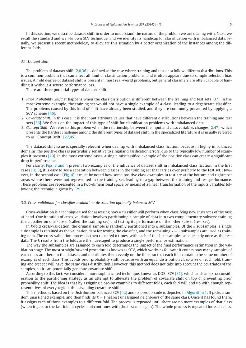
In this section, we describe dataset shift in order to understand the nature of the problem we are dealing with. Next, werecall the standard and well-known SCV technique, and we identify its handicap for classification with imbalanced data. Fi-nally, we present a recent methodology to alleviate this situation by a better organization of the instances among the dif-ferent folds.
3.1. Dataset shift
The problem of dataset shift [2,8,36] is defined as the case where training and test data follow different distributions. Thisis a common problem that can affect all kind of classification problems, and it often appears due to sample selection biasissues. A mild degree of dataset shift is present in most real-world problems, but general classifiers are often capable of han-dling it without a severe performance loss.
There are three potential types of dataset shift:
1. Prior Probability Shift: It happens when the class distribution is different between the training and test sets [37]. In themost extreme example, the training set would not have a single example of a class, leading to a degenerate classifier.The problems caused by this kind of shift have already been studied, and they are commonly prevented by applying aSCV scheme [46].
2. Covariate Shift: In this case, it is the input attribute values that have different distributions between the training and testsets [36]. We focus on the impact of this type of shift for classification problems with imbalanced data.
3. Concept Shift:We refer to this problem when the relationship between the input and class variables changes [2,47], whichpresents the hardest challenge among the different types of dataset shift. In the specialized literature it is usually referredto as ‘‘Concept Drift’’ [27,45].
The dataset shift issue is specially relevant when dealing with imbalanced classification, because in highly imbalanceddomains, the positive class is particularly sensitive to singular classification errors, due to the typically low number of exam-ples it presents [29]. In the most extreme cases, a single misclassified example of the positive class can create a significantdrop in performance.
For clarity, Figs. 3 and 4 present two examples of the influence of dataset shift in imbalanced classification. In the firstcase (Fig. 3), it is easy to see a separation between classes in the training set that carries over perfectly to the test set. How-ever, in the second case (Fig. 4) it must be noted how some positive class examples in test are at the bottom and rightmostareas where there were not represented in the training set, leading to a gap between the training and test performance.These problems are represented in a two-dimensional space by means of a linear transformation of the inputs variables fol-lowing the technique given by [29].
3.2. Cross-validation for classifier evaluation: distribution optimally balanced SCV
Cross-validation is a technique used for assessing how a classifier will perform when classifying new instances of the taskat hand. One iteration of cross-validation involves partitioning a sample of data into two complementary subsets: trainingthe classifier on one subset (called the training set) and testing its performance on the other subset (test set).
In k-fold cross-validation, the original sample is randomly partitioned into k subsamples. Of the k subsamples, a singlesubsample is retained as the validation data for testing the classifier, and the remaining k � 1 subsamples are used as train-ing data. The cross-validation process is then repeated k times, with each of the k subsamples used exactly once as the testdata. The k results from the folds are then averaged to produce a single performance estimation.
The way the subsamples are assigned to each fold determines the impact of the final performance estimation in the val-idation stage. The most straightforward procedure is known as SCV, which works as follows: it counts how many samples ofeach class are there in the dataset, and distributes them evenly on the folds, so that each fold contains the same number ofexamples of each class. This avoids prior probability shift, because with an equal distribution class-wise on each fold, train-ing and test set will have the same class distribution. However, this method does not take into account the covariates of thesamples, so it can potentially generate covariate shift.
According to this fact, we consider a more sophisticated technique, known as DOB–SCV [31], which adds an extra consid-eration to the partitioning strategy as an attempt to alleviate the problem of covariate shift on top of preventing priorprobability shift. The idea is that by assigning close-by examples to different folds, each fold will end up with enough rep-resentatives of every region, thus avoiding covariate shift.
This method is based on the Distribution-balanced SCV [52] and its pseudo-code is depicted in Algorithm 1. It picks a ran-dom unassigned example, and then finds its k � 1 nearest unassigned neighbours of the same class. Once it has found them,it assigns each of those examples to a different fold. The process is repeated until there are no more examples of that class(when it gets to the last fold, it cycles and continues with the first one again). The whole process is repeated for each class.
V. López et al. / Information Sciences 257 (2014) 1–13 5

Algorithm 1. DOB–SCV partitioning method
for each class cj 2 C dowhile count (cj) > 0 doe0 randomly select an example of class cj from Dei ith closest example to e0 of class cj from D (i = 1, . . . , k � 1)Fi Fi
Sei(i = 0, . . . , k � 1)
D Dnei(i = 0, . . . , k � 1)end while
end for
4. Experimental framework
In this section we first provide details of the real-world binary-class imbalanced problems chosen for the experiments(Section 4.1). Then, we will describe the learning algorithms selected for this study and their configuration parameters (Sec-tion 4.2). Finally, we present the statistical tests applied to compare the results obtained with the different classifiers(Section 4.3).
4.1. Benchmark data
There is no consensus in the research community on what threshold must be set up for a given dataset to suffer from theimbalance problem. In this paper, we consider a dataset to be imbalanced when the positive class has a distribution of exam-ples below 40% of the number of instances that belong to the majority class, that is, if the ratio between the examples of the
(a) Training data. AUC = .9043 (b) Test data. AUC = 1.000
Fig. 3. Example of good behaviour (no dataset shift) in imbalanced domains: ecoli4 dataset, 5th partition.
(a) Training data. AUC = 1.000 (b) Test data. AUC = .8750
Fig. 4. Example of bad behaviour caused by dataset shift in imbalanced domains: ecoli4 dataset, 1st partition.
6 V. López et al. / Information Sciences 257 (2014) 1–13

majority and minority class is higher than 1.5. The data used in the study are summarized in Table 2, where we denote thenumber of examples (#Ex.), number of attributes (#Atts.) and IR. This table is in ascending order according to the IR.
As pointed out along this paper, the estimates of the AUC measure are obtained by means of a standard SCV and the DOB–SCV. The number of folds selected in both cases is 5. This value is set up with the aim of having enough positive class in-stances in the different folds, hence avoiding additional problems in the data distribution, especially for highly imbalanceddatasets. Furthermore, we must point out that the original dataset partitions with 5-fold-cross-validation employed in thispaper are available for download at the KEEL dataset repository [3] so that any interested researcher can use the same datafor comparison.
4.2. Algorithms and parameters
In order to check the robustness of the DOB–SCV strategy, we have make use of several well-known classifiers from dif-ferent Machine Learning paradigms: the C4.5 Decision Tree [34], the Chi et al. algorithm [13] as FRBCS [24], the well knownk-NN algorithm [16] as instance-based learning method [1], and SVMs with both the Support Vector Machines with SMOoptimization [15] and the Positive Definite Fuzzy Classifier (PDFC) [12]. Specifically, we have selected the following ap-proaches as they are considered to be baseline algorithms in the field of Data Mining and they cover the widest used par-adigms in classification. In this way, we can study the validity of our proposal within different types of classifiers, thusbeing able to generalize our extracted conclusions.
Next, we detail the parameter values for the different learning algorithms selected in this study, which have been set con-sidering the recommendation of the corresponding authors:
1. C4.5For C4.5 we have set a confidence level of 0.25, the minimum number of item-sets per leaf was set to 2 and the applicationof pruning was used to obtain the final tree.
2. Chi et al.We will apply a configuration consisting in product T-norm as conjunction operator, together with the Penalized Cer-tainty Factor approach [25] for the rule weight, and winning rule as Fuzzy Reasoning Method [14]. Furthermore, we haveselected the use of 5 labels per variable.
Table 2Summary of imbalanced datasets used.
Name #Ex. #Atts. IR Name #Ex. #Atts. IR
Glass1 214 9 1.82 Glass04vs5 92 9 9.22Ecoli0vs1 220 7 1.86 Ecoli0346vs5 205 7 9.25Wisconsin 683 9 1.86 Ecoli0347vs56 257 7 9.28Pima 768 8 1.90 Yeast05679vs4 528 8 9.35Iris0 150 4 2.00 Ecoli067vs5 220 6 10.00Glass0 214 9 2.06 Vowel0 988 13 10.10Yeast1 1484 8 2.46 Glass016vs2 192 9 10.29Vehicle1 846 18 2.52 Glass2 214 9 10.39Vehicle2 846 18 2.52 Ecoli0147vs2356 336 7 10.59Vehicle3 846 18 2.52 Led7digit02456789vs1 443 7 10.97Haberman 306 3 2.68 Glass06vs5 108 9 11.00Glass0123vs456 214 9 3.19 Ecoli01vs5 240 6 11.00Vehicle0 846 18 3.23 Glass0146vs2 205 9 11.06Ecoli1 336 7 3.36 Ecoli0147vs56 332 6 12.28New-thyroid2 215 5 4.92 Cleveland0vs4 177 13 12.62New-thyroid1 215 5 5.14 Ecoli0146vs5 280 6 13.00Ecoli2 336 7 5.46 Ecoli4 336 7 13.84Segment0 2308 19 6.01 Yeast1vs7 459 8 13.87Glass6 214 9 6.38 Shuttle0vs4 1829 9 13.87Yeast3 1484 8 8.11 Glass4 214 9 15.47Ecoli3 336 7 8.19 Page-blocks13vs2 472 10 15.85Page-blocks0 5472 10 8.77 Abalone9vs18 731 8 16.68Ecoli034vs5 200 7 9.00 Glass016vs5 184 9 19.44Yeast2vs4 514 8 9.08 Shuttle2vs4 129 9 20.50Ecoli067vs35 222 7 9.09 Yeast1458vs7 693 8 22.10Ecoli0234vs5 202 7 9.10 Glass5 214 9 22.81Glass015vs2 172 9 9.12 Yeast2vs8 482 8 23.10Yeast0359vs78 506 8 9.12 Yeast4 1484 8 28.41Yeast02579vs368 1004 8 9.14 Yeast1289vs7 947 8 30.56Yeast0256vs3789 1004 8 9.14 Yeast5 1484 8 32.78Ecoli046vs5 203 6 9.15 Ecoli0137vs26 281 7 39.15Ecoli01vs235 244 7 9.17 Yeast6 1484 8 39.15Ecoli0267vs35 224 7 9.18 Abalone19 4174 8 128.87
V. López et al. / Information Sciences 257 (2014) 1–13 7
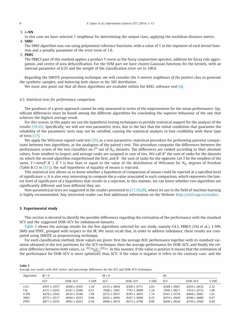
3. k-NNIn this case we have selected 1 neighbour for determining the output class, applying the euclidean distance metric.
4. SMOThe SMO algorithm was run using polynomial reference functions, with a value of 1 in the exponent of each kernel func-tion and a penalty parameter of the error term of 1.0.
5. PDFCThe FRBCS part of this method applies a product T-norm as the fuzzy conjunction operator, addition for fuzzy rule aggre-gation, and centre of area defuzzification. For the SVM part we have chosen Gaussian functions for the kernels, with aninternal parameter of 0.25 and the weight of the classification error set to 100.0.
Regarding the SMOTE preprocessing technique, we will consider the 5-nearest neighbours of the positive class to generatethe synthetic samples, and balancing both classes to the 50% distribution.
We must also point out that all these algorithms are available within the KEEL software tool [4].
4.3. Statistical tests for performance comparison
The goodness of a given approach cannot be only measured in terms of the improvement for the mean performance. Sig-nificant differences must be found among the different algorithms for concluding the superior behaviour of the one thatachieves the highest average result.
For this reason, in this paper we use the hypothesis testing techniques to provide statistical support for the analysis of theresults [19,35]. Specifically, we will use non-parametric tests, due to the fact that the initial conditions that guarantee thereliability of the parametric tests may not be satisfied, causing the statistical analysis to lose credibility with these typeof tests [17].
We apply the Wilcoxon signed-rank test [35] as a non-parametric statistical procedure for performing pairwise compar-isons between two algorithms, as the analogous of the paired t-test. This procedure computes the differences between theperformance scores of the two classifiers on ith out of Nds datasets. The differences are ranked according to their absolutevalues, from smallest to largest, and average ranks are assigned in case of ties. We call R+ the sum of ranks for the datasetson which the second algorithm outperformed the first, and R� the sum of ranks for the opposite. Let T be the smallest of thesums, T =min(R+,R�). If T is less than or equal to the value of the distribution of Wilcoxon for Nds degrees of freedom(Table B.12 in [51]), the null hypothesis of equality of means is rejected.
This statistical test allows us to know whether a hypothesis of comparison of means could be rejected at a specified levelof significance a. It is also very interesting to compute the p-value associated to each comparison, which represents the low-est level of significance of a hypothesis that results in a rejection. In this manner, we can know whether two algorithms aresignificantly different and how different they are.
Non-parametrical tests are suggested in the studies presented in [17,19,20], where its use in the field of machine learningis highly recommended. Any interested reader can find additional information on the Website http://sci2s.ugr.es/sicidm/.
5. Experimental study
This section is devoted to identify the possible differences regarding the estimation of the performance with the standardSCV and the suggested DOB–SCV for imbalanced datasets.
Table 3 shows the average results for the five algorithms selected for our study, namely C4.5, FRBCS (Chi et al.), 1-NN,SMO and PDFC, grouped with respect to the IR. We must recall that, in order to address imbalance, these results are com-puted using SMOTE as preprocessing technique.
For each classification method, three values are given: first the average AUC performance together with its standard var-iation obtained in the test partitions for the SCV technique, then the average performance for DOB–SCV, and finally the rel-ative difference between both values, i.e. AUCDOB�SCV�AUCSCV
AUCSCV. In this manner, if the value is positive it means that the estimation of
the performance for DOB–SCV is more optimistic than SCV; if the value is negative it refers to the contrary case; and the
Table 3Average test results with AUC metric and percentage differences for the SCV and DOB–SCV techniques.
Algorithm IR < 9 IR > 9 All
SCV DOB–SCV % Diff. SCV DOB–SCV % Diff. SCV DOB–SCV % Diff.
C4.5 .8597 ± .0357 .8698 ± .0393 1.28 .8133 ± .0844 .8309 ± .0751 2.83 .8288 ± .0681 .8439 ± .0632 2.32Chi .8151 ± .0352 .8187 ± .0380 0.51 .7698 ± .1041 .7781 ± .0909 1.24 .7849 ± .0811 .7916 ± .0733 1.00k-NN .8478 ± .0342 .8616 ± .0340 1.96 .8272 ± .0937 .8395 ± .0855 1.74 .8341 ± .0739 .8468 ± .0683 1.81SMO .8573 ± .0317 .8644 ± .0253 0.96 .8425 ± .0695 .8427 ± .0606 0.23 .8474 ± .0569 .8500 ± .0488 0.47PDFC .8877 ± .0293 .8901 ± .0263 0.34 .8608 ± .0819 .8672 ± .0708 0.86 .8698 ± .0644 .8749 ± .0560 0.69
8 V. López et al. / Information Sciences 257 (2014) 1–13

Table4
Detailedtest
resu
ltswithAUCmetrican
dpe
rcen
tage
differen
cesfortheSC
Van
dDOB–
SCV
tech
niqu
es.V
alue
saregrou
pedby
classification
algo
rithm.
Dataset
IRC4.5
Chi
k-NN
SMO
PDFC
SCV
DOB–S
CV
%Diff.
SCV
DOB–S
CV
%Diff.
SCV
DOB–S
CV
%Diff.
SCV
DOB–S
CV
%Diff.
SCV
DOB–S
CV
%Diff.
Glass1
1.82
.757
7±.037
9.741
6±.041
3�2
.12
.678
8±.066
3.656
7±.067
0�3
.26
.773
8±.056
1.800
0±.045
43.38
.569
2±.067
6.609
1±.013
37.01
.707
2±.025
9.730
3±.021
53.26
Ecoli0vs1
1.86
.976
1±.019
0.980
6±.017
80.46
.957
0±.049
8.951
6±.032
0�0
.57
.962
6±.030
2.970
4±.012
90.80
.979
6±.021
9.980
8±.017
50.12
.983
1±.016
7.984
1±.015
60.10
Wisco
nsin
1.86
.954
5±.019
9.958
5±.011
60.42
.573
4±.021
5.569
9±.028
4�0
.62
.962
4±.017
7.965
5±.011
80.33
.970
6±.010
3.972
8±.006
10.23
.956
8±.005
1.956
6±.014
6�0
.01
Pima
1.90
.714
5±.038
8.745
1±.036
64.27
.671
4±.025
1.701
0±.054
54.41
.680
8±.050
5.694
0±.043
21.93
.741
2±.039
7.742
4±.024
00.16
.750
8±.035
1.748
2±.051
5�0
.35
Iris0
2.00
.990
0±.022
4.990
0±.022
40.00
1.00
00±.000
01.00
00±.000
00.00
1.00
00±.000
01.00
00±.000
00.00
1.00
00±.000
01.00
00±.000
00.00
1.00
00±.000
01.00
00±.000
00.00
Glass0
2.06
.785
6±.023
4.770
9±.118
9�1
.87
.682
6±.022
3.686
5±.033
30.56
.859
5±.059
8.817
1±.076
8�4
.93
.711
7±.029
8.718
3±.012
30.93
.757
6±.082
1.772
2±.065
01.92
Yea
st1
2.46
.711
3±.029
5.711
7±.042
40.05
.699
4±.014
2.697
4±.037
4�0
.28
.653
3±.031
8.659
6±.012
10.97
.703
8±.027
3.714
6±.037
21.54
.715
2±.034
7.717
6±.017
90.34
Veh
icle1
2.52
.746
8±.012
5.722
2±.045
1�3
.30
.634
8±.018
5.685
8±.032
48.04
.632
3±.020
4.686
2±.039
58.52
.747
0±.025
4.758
8±.024
51.59
.873
2±.019
3.859
8±.018
0�1
.53
Veh
icle2
2.52
.947
6±.016
0.954
7±.017
40.76
.873
5±.031
2.864
8±.016
6�1
.00
.953
9±.020
2.929
9±.014
9�2
.52
.928
7±.010
3.924
7±.020
2�0
.42
.981
1±.007
4.980
6±.009
7�0
.06
Veh
icle3
2.52
.701
5±.028
1.729
0±.046
03.92
.721
2±.012
3.694
6±.022
5�3
.69
.683
5±.023
5.656
2±.064
2�3
.99
.728
2±.037
6.737
6±.037
01.30
.840
1±.015
2.832
9±.023
7�0
.85
Hab
erman
2.68
.630
9±.040
7.652
1±.022
73.37
.618
5±.026
6.612
3±.093
5�0
.99
.539
4±.052
5.609
6±.086
913
.01
.616
1±.061
2.619
9±.046
00.61
.612
0±.058
7.625
6±.058
82.23
Glass01
23vs45
63.19
.883
2±.060
5.925
6±.036
34.80
.864
0±.014
0.866
2±.065
50.25
.922
4±.015
4.939
5±.039
31.85
.881
9±.071
4.917
3±.033
14.02
.929
2±.051
2.937
4±.038
60.88
Veh
icle0
3.23
.914
3±.023
7.946
5±.007
33.52
.849
5±.016
0.869
7±.020
92.38
.910
6±.019
1.930
1±.024
52.14
.956
2±.015
9.958
7±.012
80.26
.976
4±.009
5.981
3±.006
50.50
Ecoli1
3.36
.916
2±.048
5.866
1±.035
8�5
.47
.879
1±.048
7.879
3±.019
00.02
.829
8±.078
3.893
4±.028
57.66
.893
3±.045
2.893
1±.013
3�0
.03
.896
7±.054
6.885
4±.015
3�1
.26
New
-thyroid2
4.92
.963
1±.045
6.983
3±.018
12.10
.965
9±.061
2.974
6±.027
50.90
.977
4±.027
9.969
0±.032
5�0
.85
.977
4±.029
6.994
4±.007
61.75
.991
7±.007
6.991
7±.012
40.00
New
-thyroid1
5.14
.980
2±.037
1.969
0±.047
3�1
.13
.954
8±.085
9.960
3±.066
40.58
.977
4±.027
9.980
6±.012
40.32
.986
1±.017
0.988
9±.015
20.28
.994
4±.007
6.991
7±.012
4�0
.28
Ecoli2
5.46
.892
1±.071
5.883
4±.050
0�0
.97
.917
0±.049
0.906
1±.040
0�1
.19
.934
3±.050
5.927
2±.041
4�0
.77
.908
5±.046
9.904
6±.042
7�0
.43
.938
1±.041
9.931
1±.040
5�0
.75
Segm
ent0
6.01
.992
7±.006
0.991
2±.007
6�0
.15
.959
0±.012
1.964
9±.006
60.61
.994
9±.006
6.993
4±.003
8�0
.15
.991
7±.009
0.991
7±.005
40.00
.996
0±.003
3.999
0±.001
70.30
Glass6
6.38
.845
0±.075
0.889
6±.083
95.28
.796
9±.067
9.839
6±.083
45.36
.868
6±.086
7.936
5±.066
47.82
.905
7±.055
2.936
5±.071
93.40
.893
8±.081
3.917
6±.071
42.66
Yea
st3
8.11
.886
9±.034
4.908
6±.036
32.45
.894
2±.033
7.888
1±.028
1�0
.68
.860
7±.013
4.869
3±.029
71.00
.904
0±.012
8.900
3±.031
4�0
.41
.922
4±.021
3.930
1±.024
60.83
Ecoli3
8.19
.775
5±.078
7.867
7±.106
711
.90
.866
5±.080
1.868
1±.042
30.19
.777
7±.048
2.813
9±.046
94.65
.887
4±.041
8.875
8±.067
8�1
.31
.879
8±.055
4.879
7±.046
2�0
.01
Page
-block
s08.77
.948
4±.015
3.947
2±.014
0�0
.12
.874
4±.018
5.875
2±.018
90.09
.895
3±.015
5.913
5±.014
72.03
.872
9±.021
5.877
4±.016
90.52
.933
5±.010
1.930
0±.012
2�0
.37
Ecoli034
vs5
9.00
.858
3±.080
6.869
4±.111
81.29
.819
4±.134
3.822
2±.105
50.34
.847
2±.136
1.863
9±.132
31.97
.894
4±.103
7.900
0±.066
90.62
.883
3±.113
9.888
9±.108
00.63
Yea
st2v
s49.08
.862
0±.058
9.871
6±.035
81.11
.860
7±.049
2.872
7±.028
21.39
.880
7±.065
5.890
5±.050
41.11
.886
3±.028
7.896
3±.024
41.13
.915
4±.060
8.920
1±.034
40.51
Ecoli067
vs35
9.09
.812
5±.209
7.822
5±.094
51.23
.792
5±.166
0.785
0±.108
4�0
.95
.862
5±.149
5.867
5±.103
70.58
.855
0±.150
9.850
0±.082
4�0
.58
.865
0±.168
7.880
0±.087
31.73
Ecoli023
4vs5
9.10
.897
4±.105
1.852
8±.087
1�4
.97
.811
4±.157
7.872
5±.104
37.53
.853
0±.126
1.880
8±.110
23.26
.894
6±.110
9.902
9±.097
20.92
.905
6±.113
5.886
2±.096
4�2
.15
Glass01
5vs2
9.12
.744
4±.115
2.641
1±.069
4�1
3.87
.558
3±.084
8.512
6±.175
2�8
.18
.657
3±.128
7.629
0±.101
8�4
.29
.534
4±.040
0.573
7±.096
87.34
.804
3±.118
2.779
3±.102
1�3
.11
Yea
st03
59vs78
9.12
.722
2±.053
7.702
2±.087
4�2
.77
.704
0±.063
1.706
3±.052
70.32
.754
3±.038
4.718
8±.085
6�4
.72
.742
8±.041
5.749
5±.063
50.90
.717
0±.037
7.702
8±.078
6�1
.99
Yea
st02
579v
s368
9.14
.917
1±.016
4.904
4±.032
5�1
.39
.887
1±.038
0.881
3±.042
1�0
.65
.904
4±.028
2.892
7±.049
3�1
.28
.903
5±.036
6.902
7±.033
6�0
.09
.902
1±.031
9.903
7±.039
50.19
Yea
st02
56vs37
899.14
.754
3±.024
2.777
1±.058
53.02
.779
8±.076
3.783
7±.023
30.49
.780
7±.055
6.806
8±.047
53.33
.794
0±.051
0.809
5±.037
61.96
.818
9±.052
8.814
2±.027
4�0
.58
Ecoli046
vs5
9.15
.872
9±.099
3.834
2±.109
4�4
.44
.839
4±.143
4.853
3±.164
51.65
.864
2±.142
7.891
8±.107
33.20
.897
9±.108
6.897
8±.109
2�0
.01
.850
7±.092
6.908
6±.106
16.81
Ecoli01v
s235
9.17
.804
1±.166
0.837
7±.135
94.18
.744
1±.080
5.820
9±.069
11.32
.828
6±.150
7.885
0±.106
96.80
.857
7±.092
3.876
4±.083
82.17
.886
8±.151
2.921
4±.072
03.90
Ecoli026
7vs3
59.18
.770
4±.108
2.860
6±.086
911
.71
.775
3±.075
2.788
1±.139
81.65
.897
6±.098
5.892
8±.091
8�0
.53
.873
1±.077
6.873
0±.084
0�0
.01
.842
6±.108
5.880
4±.053
34.49
Glass04
vs5
9.22
.981
6±.016
8.970
6±.029
4�1
.12
.721
0±.198
9.722
4±.142
20.20
.969
1±.038
3.920
6±.115
6�5
.01
.962
9±.040
8.958
1±.015
5�0
.50
.963
6±.025
4.970
6±.041
60.72
Ecoli034
6vs5
9.25
.870
3±.051
7.878
4±.119
60.93
.856
8±.098
6.817
6±.115
6�4
.57
.883
8±.098
6.856
1±.093
3�3
.13
.895
3±.058
7.895
3±.058
90.00
.916
9±.070
7.911
5±.062
7�0
.59
Ecoli034
7vs5
69.28
.836
8±.151
4.899
2±.044
37.45
.819
6±.110
7.830
6±.112
41.34
.883
4±.121
5.876
4±.093
0�0
.79
.919
1±.088
8.890
5±.081
3�3
.11
.905
5±.083
8.918
5±.080
91.44
Yea
st05
679v
s49.35
.768
2±.100
9.795
4±.082
73.55
.798
9±.062
5.801
1±.048
10.28
.775
3±.059
9.800
3±.059
73.23
.788
5±.084
9.800
5±.018
21.51
.790
0±.093
0.801
4±.039
21.45
Ecoli067
vs5
1.00
.825
0±.086
2.887
5±.069
07.58
.827
5±.095
8.787
5±.063
1�4
.83
.867
5±.057
7.880
0±.067
71.44
.867
5±.085
5.845
0±.084
1�2
.59
.870
0±.047
3.865
0±.108
8�0
.57
Vow
el0
1.10
.943
3±.048
3.975
0±.015
53.36
.978
9±.018
3.993
3±.001
51.47
1.00
00±.000
0.998
9±.001
5�0
.11
.956
6±.011
7.959
9±.009
20.35
.998
9±.001
5.999
4±.001
20.06
Glass01
6vs2
1.29
.636
7±.125
5.675
2±.147
86.06
.600
2±.084
1.514
0±.117
1�1
4.36
.681
4±.179
3.697
6±.167
42.38
.537
9±.112
0.581
9±.077
18.19
.760
5±.120
8.776
9±.131
62.16
Glass2
1.39
.542
4±.140
1.749
8±.115
538
.25
.520
6±.112
0.624
1±.098
219
.89
.644
7±.098
7.733
1±.131
613
.72
.598
5±.157
0.598
9±.084
10.07
.768
8±.148
6.778
9±.108
11.31
Ecoli014
7vs2
356
1.59
.846
1±.045
3.842
6±.066
9�0
.41
.789
4±.060
6.804
3±.072
81.89
.850
7±.030
9.885
7±.100
84.11
.884
4±.076
7.886
2±.046
10.20
.902
5±.054
2.882
3±.015
8�2
.23
Led7
digit024
5678
9vs1
1.97
.883
2±.096
2.820
7±.099
5�7
.08
.830
2±.074
9.798
3±.081
0�3
.84
.810
8±.033
3.865
2±.043
26.70
.887
5±.053
1.824
8±.054
9�7
.07
.885
2±.092
3.861
1±.095
4�2
.73
Glass06
vs5
11.00
.914
7±.118
6.960
0±.028
54.95
.750
0±.221
5.785
0±.187
64.67
.940
0±.120
7.920
0±.124
2�2
.13
.943
9±.034
4.949
2±.026
00.56
.974
5±.035
8.959
7±.013
3�1
.51
Ecoli01v
s511
.00
.822
7±.107
4.852
3±.011
43.59
.838
6±.144
7.850
0±.144
51.36
.854
5±.152
5.890
9±.097
34.26
.893
2±.075
6.897
7±.066
30.51
.879
5±.101
8.911
4±.066
03.62
Glass01
46vs2
11.06
.756
4±.108
9.736
1±.150
9�2
.68
.514
6±.105
4.552
7±.119
77.39
.645
3±.088
4.744
5±.130
115
.37
.615
7±.073
2.618
5±.049
60.45
.802
9±.135
9.783
8±.065
0�2
.38
Ecoli014
7vs5
612
.28
.864
1±.056
5.847
4±.042
5�1
.93
.844
1±.112
9.845
8±.053
50.19
.875
6±.062
2.874
0±.071
7�0
.19
.909
3±.035
3.892
8±.076
0�1
.82
.890
7±.075
5.912
4±.083
12.44
(con
tinu
edon
next
page)
V. López et al. / Information Sciences 257 (2014) 1–13 9
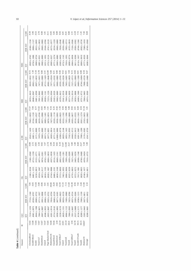
Table4(con
tinu
ed)
Dataset
IRC4.5
Chi
k-NN
SMO
PDFC
SCV
DOB–S
CV
%Diff.
SCV
DOB–S
CV
%Diff.
SCV
DOB–S
CV
%Diff.
SCV
DOB–S
CV
%Diff.
SCV
DOB–S
CV
%Diff.
Cleve
land0
vs4
12.62
.721
0±.125
9.771
9±.118
07.05
.118
8±.053
8.118
8±.058
0�0
.08
.854
3±.143
0.704
2±.065
2�1
7.57
.907
6±.061
9.901
0±.093
2�0
.72
.892
9±.076
5.818
8±.153
8�8
.30
Ecoli014
6vs5
13.00
.898
1±.097
5.853
8±.079
7�4
.93
.848
1±.121
5.871
2±.133
02.72
.848
1±.117
1.915
4±.112
07.94
.884
6±.094
7.896
2±.110
11.30
.875
0±.108
8.909
6±.112
73.96
Ecoli4
13.84
.804
4±.138
8.898
0±.073
211
.64
.923
0±.081
3.915
2±.077
1�0
.85
.917
1±.068
9.960
8±.052
74.77
.948
1±.059
0.899
7±.063
2�5
.10
.906
0±.072
4.901
2±.069
5�0
.53
Yea
st1v
s713
.87
.706
4±.067
1.671
1±.102
7�5
.00
.652
4±.104
7.667
1±.091
32.26
.747
9±.127
9.661
0±.074
6�1
1.62
.769
1±.064
2.747
7±.043
1�2
.78
.688
1±.052
1.707
1±.083
22.76
Shuttle0v
s413
.87
.999
7±.000
7.999
1±.000
8�0
.06
.987
2±.011
7.987
4±.028
10.02
.996
0±.008
9.995
7±.008
8�0
.03
.996
0±.008
9.996
0±.008
90.00
.996
0±.008
9.996
0±.008
90.00
Glass4
15.47
.850
8±.093
5.898
6±.137
65.61
.861
8±.110
5.876
2±.145
91.67
.891
7±.116
2.908
5±.149
11.88
.892
8±.116
1.871
3±.142
9�2
.41
.925
1±.105
2.934
4±.078
61.01
Page
-block
s13v
s415
.85
.995
5±.004
7.956
5±.075
2�3
.91
.892
8±.106
7.868
4±.081
0�2
.74
.997
7±.005
1.987
6±.007
4�1
.01
.722
3±.122
6.809
6±.064
812
.09
.975
2±.012
4.974
1±.012
9�0
.11
Aba
lone9
vs18
16.68
.620
1±.051
4.785
4±.079
426
.66
.674
4±.098
8.693
7±.093
82.86
.682
0±.081
4.745
7±.066
99.34
.845
8±.056
4.797
7±.052
4�5
.68
.896
9±.022
7.837
3±.057
7�6
.65
Glass01
6vs5
19.44
.971
4±.014
3.968
6±.012
0�0
.29
.848
6±.219
1.851
4±.143
50.34
.877
1±.219
1.932
9±.111
86.35
.934
3±.032
9.937
1±.019
20.31
.877
1±.227
4.921
4±.122
95.05
Shuttle2v
s42.50
.995
8±.009
3.987
7±.018
5�0
.82
.883
8±.216
0.884
0±.216
10.02
1.00
00±.000
0.995
8±.009
3�0
.42
.996
0±.008
9.996
0±.008
90.00
.996
0±.008
9.996
0±.008
90.00
Yea
st14
58vs7
22.10
.523
0±.017
0.588
9±.062
312
.59
.571
3±.083
0.606
1±.039
06.10
.639
0±.077
8.629
0±.062
5�1
.56
.657
0±.061
2.653
9±.074
5�0
.46
.656
9±.043
9.702
4±.054
86.92
Glass5
22.81
.882
9±.133
1.982
9±.013
911
.33
.746
3±.205
2.843
9±.128
113
.07
.882
9±.214
8.923
2±.118
24.56
.934
1±.031
8.939
0±.022
80.52
.873
2±.114
5.925
6±.098
46.01
Yea
st2v
s823
.10
.806
6±.112
2.749
0±.098
0�7
.13
.806
6±.069
4.709
9±.056
6�1
2.00
.805
5±.142
5.750
1±.109
6�6
.88
.766
4±.096
0.766
3±.049
5�0
.01
.792
4±.105
5.789
2±.071
3�0
.41
Yea
st4
28.41
.700
4±.056
5.782
3±.078
611
.69
.832
5±.023
9.830
3±.020
9�0
.27
.724
2±.059
3.766
8±.089
95.88
.821
7±.043
0.835
2±.062
91.64
.809
0±.077
4.815
5±.081
90.80
Yea
st12
89vs7
3.56
.705
1±.069
7.603
7±.072
4�1
4.38
.677
0±.085
3.702
7±.066
53.80
.644
4±.071
3.650
3±.087
70.92
.721
6±.051
4.722
7±.071
30.15
.696
4±.093
8.712
6±.050
62.31
Yea
st5
32.78
.933
7±.040
0.938
9±.026
60.56
.937
2±.027
2.946
5±.025
61.00
.932
6±.041
3.951
4±.033
32.01
.965
6±.006
8.965
3±.006
9�0
.04
.961
1±.029
0.939
6±.030
2�2
.24
Ecoli013
7vs2
639
.15
.813
6±.217
1.878
0±.121
57.92
.791
7±.198
1.859
8±.134
08.60
.828
1±.208
7.883
6±.126
36.69
.849
0±.196
9.848
9±.120
9�0
.01
.811
8±.195
7.874
4±.126
67.72
Yea
st6
39.15
.828
0±.127
7.799
6±.119
9�3
.44
.882
0±.085
5.879
6±.048
8�0
.27
.799
8±.120
0.836
1±.127
44.54
.875
1±.071
2.874
4±.049
4�0
.08
.868
4±.061
0.856
2±.073
0�1
.41
Aba
lone1
912
8.87
.520
3±.044
3.582
7±.081
111
.99
.674
8±.107
7.697
6±.042
43.38
.517
6±.038
5.576
3±.065
311
.34
.789
4±.046
3.790
8±.072
90.18
.677
7±.052
9.728
0±.101
97.42
Ave
rage
.828
8±.068
1.843
9±.063
22.32
.784
9±.081
1.791
6±.073
31.00
.834
1±.073
9.846
8±.068
31.81
.847
4±.056
9.850
0±.048
80.47
.869
8±.064
4.874
9±.056
00.69
10 V. López et al. / Information Sciences 257 (2014) 1–13

higher the obtained number, the most significant the selection of the validation approach is. Additionally, we show the de-tailed test results for all datasets in Table 4.
From these tables of results we may observe that for all five algorithms, the DOB–SCV validation technique achieves ahigher estimation of the performance for most datasets, therefore being more robust for analyzing the quality of the modelslearned in imbalanced data.
Furthermore, we must point out that the degree of imbalance of the dataset has a direct impact on the diverse results overthe different folds in the obtained results, i.e. the higher the IR is, the greater the differences between the standard SCV andthe DOB–SCV are. In addition to the former, the standard deviation computation supports this perception: these values forboth partitioning techniques are similar when the degree of imbalance is low; however, when the IR is higher we may ob-serve that the standard deviation is much higher in contrast with low imbalanced datasets. Additionally, DOB–SCV has lowerstandard deviation values than SCV, therefore sustaining the reduction of the gap between training and test partitions.
This issue may arise due to the fact that, the lower the number of positive instances we have in a dataset with respect tothe negative ones, the more significant is to maintain the data distribution to avoid the differences in performance betweentraining and test.
The characteristics of specific datasets do not pose a source of knowledge when trying to observe if there is a group ofthem where DOB–SCV performs better than SCV. In general, DOB–SCV obtains a better performance for most of the algo-rithms for each dataset, however, only few of the datasets considered are able to provide a clear trend for all the algorithms:the cases where DOB–SCV obtains a better estimation than SCV (for instance, Abalone19 or Glass2) are more numerous thanthe contrary case (Ecoli2 or Yeast2vs8) and the improvement is much greater than the loss.
When trying to find a group of data with the highest differences between DOB–SCV and SCV, it is not possible to do sowithout also considering the algorithm underneath. For instance, if we try to observe where the greatest improvements orlosses are obtained for each algorithm, we realize that the datasets obtained for one algorithm are completely different fromthe datasets obtained for the rest.
In order to give statistical support to the findings previously extracted, we will carry out a Wilcoxon test to compare bothvalidation techniques with the five classification algorithms. This analysis is shown in Table 5 where the algorithms are com-pared by rows.
The conclusions from this test are clear, from which significant differences are found between DOB–SCV and SCV in allcases with a low p-value. Furthermore, the higher sums of the ranks for DOB–SCV tell us about the goodness of this approach.
To summarize, we must stress that DOB–SCV is a suitable methodology for contrasting the performance of the classifi-cation algorithms in imbalanced data. When the distribution of the classes is skewed, using standard estimation modelsmay lead to misleading conclusions on the quality of the prediction. The proposed use of this model addresses the handicapof losing the generalization ability because of the way data is distributed among the different folds.
6. Concluding remarks
In this work we have proposed the use of a novel partition-based methodology, named as DOB–SCV, which aims atobtaining a better estimation of a classifier’s performance by carrying out an heterogeneous organization of the instancesof the classes among the different folds.
We have identified this validation technique as a very suitable procedure in the framework of imbalanced datasets. It isstraightforward to realize that, in the case that one of the classes of the problem contains a fewer number of examples, andregarding to the evaluation metrics used in this scenario, introducing covariate shift between training and test will unequiv-ocally lead to high differences in performance in the learning and validation stages.
The stable performance estimation of DOB–SCV has been contrasted versus the classical k-fold SCV, detecting significantdifferences between both techniques for several classifiers often used in imbalanced tasks such as C4.5, FRBCSs, k-NN andSVMs. Wemust highlight that avoiding different data distribution inside each fold will allow researchers on imbalanced datato concentrate their efforts on designing new learning models based only on the skewed data, rather than seeking for com-plex solutions when trying to overcome the gaps between training and test results. Nevertheless, neither SCV nor DOB–SCVcan unequivocally guarantee to obtain the best estimate of the true error for a given problem. This can only be achieved byhaving infinite data or, at least, that the input data covers the whole problem space, which is not usually the case.
Table 5Wilcoxon’s tests to compare the results with the DOB–SCV versus the standard SCV. R+ corresponds to the sum of the ranks for the DOB–SCV partitioningapproach and and R� to the original SCV partitioning.
Comparison R+ R� p-value
C4.5[DOB–SCV] vs C4.5[SCV] 1391 754 0.0371Chi[DOB–SCV] vs Chi[SCV] 1411 734 0.0267k-NN[DOB–SCV] vs k-NN[SCV] 1536 609 0.0024SMO[DOB–SCV] vs SMO[SCV] 1395 816 0.0639PDFC[DOB–SCV] vs PDFC[SCV] 1366 845 0.0955
V. López et al. / Information Sciences 257 (2014) 1–13 11

Acknowledgments
This work was partially supported by the Spanish Ministry of Science and Technology under Project TIN2011-28488 andthe Andalusian Research Plans P11-TIC-7765 and P10-TIC-6858. V. López holds a FPU scholarship from Spanish Ministry ofEducation.
References
[1] D.W. Aha, D. Kibler, M.K. Albert, Instance-based learning algorithms, Machine Learning 6 (1991) 37–66.[2] R. Alaiz-Rodríguez, N. Japkowicz, Assessing the impact of changing environments on classifier performance, in: Proceedings of the 21st Canadian
Conference on Advances in Artificial Intelligence (CCAI’08), Springer-Verlag, Berlin, Heidelberg, 2008.[3] J. Alcalá-Fdez, A. Fernández, J. Luengo, J. Derrac, S. García, L. Sánchez, F. Herrera, KEEL data-mining software tool: data set repository, integration of
algorithms and experimental analysis framework, Journal of Multi-Valued Logic and Soft Computing 17 (2–3) (2011) 255–287.[4] J. Alcalá;-Fdez, L. Sánchez, S. García, M.J. del Jesus, S. Ventura, J.M. Garrell, J. Otero, C. Romero, J. Bacardit, V.M. Rivas, J.C. Fernández, F. Herrera, KEEL: a
software tool to assess evolutionary algorithms for data mining problems, Soft Computing 13 (2009) 307–318.[5] R. Barandela, J.S. Sánchez, V. García, E. Rangel, Strategies for learning in class imbalance problems, Pattern Recognition 36 (3) (2003) 849–851.[6] G.E.A.P.A. Batista, R.C. Prati, M.C. Monard, A study of the behaviour of several methods for balancing machine learning training data, SIGKDD
Explorations 6 (1) (2004) 20–29.[7] A.P. Bradley, The use of the area under the ROC curve in the evaluation of machine learning algorithms, Pattern Recognition 30 (7) (1997) 1145–1159.[8] J.Q. Candela, M. Sugiyama, A. Schwaighofer, N.D. Lawrence, Dataset Shift in Machine Learning, The MIT Press, 2009.[9] J.R. Cano, F. Herrera, M. Lozano, Evolutionary stratified training set selection for extracting classification rules with trade off precision-interpretability,
Data and Knowledge Engineering 60 (2007) 90–108.[10] N.V. Chawla, K.W. Bowyer, L.O. Hall, W.P. Kegelmeyer, SMOTE: synthetic minority over-sampling technique, Journal of Artificial Intelligent Research 16
(2002) 321–357.[11] N.V. Chawla, N. Japkowicz, A. Kotcz, Editorial: special issue on learning from imbalanced data sets, SIGKDD Explorations 6 (1) (2004) 1–6.[12] Y. Chen, J. Wang, Support vector learning for fuzzy rule-based classification systems, IEEE Transactions on Fuzzy Systems 11 (6) (2003) 716–728.[13] Z. Chi, H. Yan, T. Pham, Fuzzy Algorithms with Applications to Image Processing and Pattern Recognition, World Scientific, 1996.[14] O. Cordón, M.J. del Jesus, F. Herrera, A proposal on reasoning methods in fuzzy rule-based classification systems, International Journal of Approximate
Reasoning 20 (1) (1999) 21–45.[15] C. Cortes, V. Vapnik, Support vector networks, Machine Learning 20 (1995) 273–297.[16] T. Cover, P. Hart, Nearest neighbor pattern classification, IEEE Transactions on Information Theory 13 (1967) 21–27.[17] J. Demšar, Statistical comparisons of classifiers over multiple data sets, Journal of Machine Learning Research 7 (2006) 1–30.[18] P. Domingos, Metacost: a general method for making classifiers cost-sensitive, in: Proceedings of the 5th International Conference on Knowledge
Discovery and Data Mining (KDD’99), 1999.[19] S. García, A. Fernández, J. Luengo, F. Herrera, A study of statistical techniques and performance measures for genetics-based machine learning:
accuracy and interpretability, Soft Computing 13 (10) (2009) 959–977.[20] S. García, F. Herrera, An extension on ‘‘statistical comparisons of classifiers over multiple data sets’’ for all pairwise comparisons, Journal of Machine
Learning Research 9 (2008) 2607–2624.[21] H. He, E.A. Garcia, Learning from imbalanced data, IEEE Transactions on Knowledge and Data Engineering 21 (9) (2009) 1263–1284.[22] J. Huang, C.X. Ling, Using AUC and accuracy in evaluating learning algorithms, IEEE Transactions on Knowledge and Data Engineering 17 (3) (2005)
299–310.[23] Y.-M. Huang, C.-M. Hung, H.C. Jiau, Evaluation of neural networks and data mining methods on a credit assessment task for class imbalance problem,
Nonlinear Analysis: Real World Applications 7 (4) (2006) 720–747.[24] H. Ishibuchi, T. Nakashima, M. Nii, Classification and Modeling with Linguistic Information Granules: Advanced Approaches to Linguistic Data Mining,
Springer-Verlag, 2004.[25] H. Ishibuchi, T. Yamamoto, Rule weight specification in fuzzy rule-based classification systems, IEEE Transactions on Fuzzy Systems 13 (2005) 428–
435.[26] N. Japkowicz, S. Stephen, The class imbalance problem: a systematic study, Intelligent Data Analysis Journal 6 (5) (2002) 429–450.[27] T. Lane, C.E. Brodley, Approaches to online learning and concept drift for user identification in computer security, in: KDD, 1998.[28] V. López, A. Fernández, J.G. Moreno-Torres, F. Herrera, Analysis of preprocessing vs. cost-sensitive learning for imbalanced classification. Open
problems on intrinsic data characteristics, Expert Systems with Applications 39 (7) (2012) 6585–6608.[29] J.G. Moreno-Torres, F. Herrera, A preliminary study on overlapping and data fracture in imbalanced domains by means of genetic programming-based
feature extraction, in: Proceedings of the 10th International Conference on Intelligent Systems Design and Applications (ISDA’10), 2010.[30] J.G. Moreno-Torres, T. Raeder, R. Aláiz-Rodríguez, N.V. Chawla, F. Herrera, A unifying view on dataset shift in classification, Pattern Recognition 45 (1)
(2012) 521–530.[31] J.G. Moreno-Torres, J.A. Sáez, F. Herrera, Study on the impact of partition-induced dataset shift on k-fold cross-validation, IEEE Transactions on Neural
Networks and Learning Systems 23 (8) (2012) 1304–1313.[32] A. Orriols-Puig, E. Bernadó-Mansilla, Evolutionary rule-based systems for imbalanced datasets, Soft Computing 13 (3) (2009) 213–225.[33] A. Orriols-Puig, E. Bernadó-Mansilla, D.E. Goldberg, K. Sastry, P.L. Lanzi, Facetwise analysis of XCS for problems with class imbalances, IEEE
Transactions on Evolutionary Computation 13 (2009) 260–283.[34] J. Quinlan, C4.5: Programs for Machine Learning, Morgan Kauffman, 1993.[35] D. Sheskin, Handbook of Parametric and Nonparametric Statistical Procedures, Chapman & Hall/CRC, 2006.[36] H. Shimodaira, Improving predictive inference under covariate shift by weighting the log-likelihood function, Journal of Statistical Planning and
Inference 90 (2) (2000) 227–244.[37] A. Storkey, When training and test sets are different: characterizing learning transfer, in: J.Q. Candela, M. Sugiyama, A. Schwaighofer, N.D. Lawrence
(Eds.), Dataset Shift in Machine Learning, MIT Press, 2009, pp. 3–28.[38] Y. Sun, A.K.C. Wong, M.S. Kamel, Classification of imbalanced data: a review, International Journal of Pattern Recognition and Artificial Intelligence 23
(4) (2009) 687–719.[39] Y. Tang, Y.-Q. Zhang, N.V. Chawla, S. Kresser, SVMs modeling for highly imbalanced classification, IEEE Transactions on Systems, Man and Cybernetics,
Part B 39 (1) (2009) 281–288.[40] K.M. Ting, An instance-weighting method to induce cost-sensitive trees, IEEE Transactions on Knowledge and Data Engineering 14 (3) (2002) 659–665.[41] M. Wasikowski, X.-W. Chen, Combating the small sample class imbalance problem using feature selection, IEEE Transactions on Knowledge and Data
Engineering 22 (10) (2010) 1388–1400.[42] G.M. Weiss, Mining with rarity: a unifying framework, SIGKDD Explorations 6 (1) (2004) 7–19.[43] G.M. Weiss, F.J. Provost, Learning when training data are costly: the effect of class distribution on tree induction, Journal of Artificial Intelligence
Research 19 (2003) 315–354.
12 V. López et al. / Information Sciences 257 (2014) 1–13

[44] G.M. Weiss, Y. Tian, Maximizing classifier utility when there are data acquisition and modeling costs, Data Mining and Knowledge Discovery 17 (2)(2008) 253–282.
[45] G. Widmer, M. Kubat, Learning in the presence of concept drift and hidden contexts, Machine Learning 23 (1) (1996) 69–101.[46] I.H. Witten, E. Frank, Data Mining: Practical Machine Learning Tools and Techniques, second ed., Morgan Kaufmann, San Mateo, CA, 2005.[47] K. Yamazaki, M. Kawanabe, S. Watanabe, M. Sugiyama, K.-R. Müller, Asymptotic bayesian generalization error when training and test distributions are
different, in: Z. Ghahramani (Ed.), ICML, ACM International Conference Proceeding Series, vol. 227, ACM, 2007.[48] Q. Yang, X. Wu, 10 Challenging problems in data mining research, International Journal of Information Technology and Decision Making 5 (4) (2006)
597–604.[49] B. Zadrozny, C. Elkan, Learning and making decisions when costs and probabilities are both unknown, in: Proceedings of the 7th International
Conference on Knowledge Discovery and Data Mining (KDD’01), 2001.[50] B. Zadrozny, J. Langford, N. Abe, Cost-sensitive learning by cost-proportionate example weighting, in: Proceedings of the 3rd IEEE International
Conference on Data Mining (ICDM’03), 2003.[51] J.H. Zar, Biostatistical Analysis, Prentice Hall, Upper Saddle River, New Jersey, 1999.[52] X. Zeng, T.R. Martinez, Distribution-balanced stratified cross validation for accuracy estimation, Journal of Experimental and Theoretical Artificial
Intelligence 12 (1) (2000) 1–12.
V. López et al. / Information Sciences 257 (2014) 1–13 13


3 A study on the Scalability of FRBCSs for Imbalanced Datasets in the Big Data Scenario 131
3. A study on the Scalability of FRBCSs for Imbalanced Datasets
in the Big Data Scenario
The journal paper associated to this part is:
3.1. Cost-Sensitive Linguistic Fuzzy Rule-Based Classification Systems under
the MapReduce Framework for Imbalanced Big Data
V. Lopez, S. del Rıo, J. M. Benıtez, F. Herrera, Cost-Sensitive Linguistic Fuzzy Rule BasedClassification Systems under the MapReduce Framework for Imbalanced Big Data. FuzzySets and Systems, doi: 10.1016/j.fss.2014.01.015, in press (2014)
• Status: Published (in press).
• Impact Factor (JCR 2012): 1.749.
• Subject Category: Computer Science, Theory & Methods. Ranking 17 / 100 (Q1).
• Subject Category: Mathematics, Applied. Ranking 21 / 247 (Q1).
• Subject Category: Statistics & Probability. Ranking 17 / 117 (Q1).


JID:FSS AID:6482 /FLA [m3SC+; v 1.188; Prn:4/03/2014; 14:35] P.1 (1-34)
Available online at www.sciencedirect.com
ScienceDirect
Fuzzy Sets and Systems ••• (••••) •••–•••www.elsevier.com/locate/fss
Cost-sensitive linguistic fuzzy rule based classification systemsunder the MapReduce framework for imbalanced big data
Victoria López ∗, Sara del Río, José Manuel Benítez, Francisco Herrera
Dept. of Computer Science and Artificial Intelligence, CITIC-UGR (Research Center on Information and Communications Technology),University of Granada, Granada, Spain
Abstract
Classification with big data has become one of the latest trends when talking about learning from the available information.The data growth in the last years has rocketed the interest in effectively acquiring knowledge to analyze and predict trends. Thevariety and veracity that are related to big data introduce a degree of uncertainty that has to be handled in addition to the vol-ume and velocity requirements. This data usually also presents what is known as the problem of classification with imbalanceddatasets, a class distribution where the most important concepts to be learned are presented by a negligible number of examples inrelation to the number of examples from the other classes. In order to adequately deal with imbalanced big data we propose theChi-FRBCS-BigDataCS algorithm, a fuzzy rule based classification system that is able to deal with the uncertainly that is intro-duced in large volumes of data without disregarding the learning in the underrepresented class. The method uses the MapReduceframework to distribute the computational operations of the fuzzy model while it includes cost-sensitive learning techniques in itsdesign to address the imbalance that is present in the data. The good performance of this approach is supported by the experimentalanalysis that is carried out over twenty-four imbalanced big data cases of study. The results obtained show that the proposal is ableto handle these problems obtaining competitive results both in the classification performance of the model and the time needed forthe computation.© 2014 Elsevier B.V. All rights reserved.
Keywords: Fuzzy rule based classification systems; Big data; MapReduce; Hadoop; Imbalanced datasets; Cost-sensitive learning
1. Introduction
The development and maturity of the information technologies has enabled an exponential growth on the datathat is produced, processed, stored, shared, analyzed and visualized. According to IBM [1], in 2012, every day 1.5quintillion bytes of data are created, which means that the 90% of the data created in the world has been producedin the last two years. Big data [2] encompass a collection of datasets whose size and complexity challenges thestandard database management systems and defies the application of knowledge extraction techniques. This data
* Corresponding author. Tel.: +34 958 240598; fax: +34 958 243317.E-mail addresses: [email protected] (V. López), [email protected] (S. del Río), [email protected] (J.M. Benítez),
[email protected] (F. Herrera).
http://dx.doi.org/10.1016/j.fss.2014.01.0150165-0114/© 2014 Elsevier B.V. All rights reserved.

JID:FSS AID:6482 /FLA [m3SC+; v 1.188; Prn:4/03/2014; 14:35] P.2 (1-34)
2 V. López et al. / Fuzzy Sets and Systems ••• (••••) •••–•••
comes from a wide range of sources such as sensors, digital pictures and videos, purchase transactions, social mediaposts, everywhere [3].
This generation and collection of large datasets has further encouraged the analysis and knowledge extractionprocess with the belief that with more data available, the information that could be derived from it will be moreprecise. However, the standard algorithms that are used in data mining are not usually able to deal with these hugedatasets [4]. In this manner, classification algorithms must be redesigned and adapted considering the solutions thatare being used in big data so that they are able to be used under these premises maintaining its predictive capacity.
One of the complications that make difficult the extraction of useful information from datasets is the problem ofclassification with imbalanced data [5,6]. This problem occurs when the number of instances of one class (positiveor minority class) is substantially smaller than the number of instances that belong to the other classes (negative ormajority classes). The importance of this problem resides on its prevalence in numerous real-world applications suchas telecommunications, finances, medical diagnosis and so on. In this situation, the interest of the learning is focusedtowards the minority class as it is the class that needs to be correctly identified in these problems [7]. Big data is alsoaffected by this uneven class distribution.
Standard classification algorithms do not usually work appropriately when dealing with imbalanced datasets. Theusage of global performance measures for the construction of the model and the search for the maximum general-ization capacity induce in algorithms a mechanism that tends to neglect the rules associated with instances of theminority class.
Fuzzy Rule Based Classification Systems (FRBCSs) [8] are effective and accepted tools for pattern recognitionand classification. They are able to obtain a good precision while supplying an interpretable model for the end userthrough the usage of linguistic labels. Furthermore, the FRBCSs can manage uncertainty, ambiguity or vaguenessin a very effective way. This trait is especially interesting when dealing with big data, as uncertainty is inherent tothis situation. However, when dealing with big data, the information at disposal usually contains a high number ofinstances and/or features. In this scenario the inductive learning capacity of FRBCSs is affected by the exponentialgrowth of the search space. This growth complicates the learning process and it can lead to scalability problems orcomplexity problems generating a rule set that is not interpretable [9].
To overcome this situation there have been several approaches that aim to build parallel fuzzy systems [10]. Theseapproaches can distribute the creation of the rule base [11] or the post-processing of the built model, using a par-allelization to perform a rule selection [12] or a lateral tuning of the fuzzy labels [13]. Moreover, a fuzzy learningmodel can be completely redesigned to obtain a parallel approach that decreases the computation time needed [14].However, these models aim to reduce the wait for a final classification without damaging the performance and are notdesigned to handle huge volumes of data. In this manner, it is necessary to redesign the FRBCSs accordingly to beable to provide an accurate classification in a small lapse of time from big data.
Numerous solutions have been proposed to deal with imbalanced datasets [7,15]. These solutions are typicallyorganized in two groups: data-level solutions [16,17], which modify the original training set to obtain a more orless balanced class distribution that can be used with any classifier, and algorithm-level solutions, which alter theoperations of an algorithm so that the minority class instances have more relevance and are correctly classified. Cost-sensitive solutions [18,19] integrate both approaches as they are focused in reducing the misclassification costs, higherfor the instances of the minority class.
The approaches used to tackle big data usually involve some kind of parallelization to efficiently process andanalyze all the available data. One of the most popular frameworks for big data, MapReduce [20], organizes theprocessing in two key operations: a map process that is responsible for dividing the original dataset and processingeach chunk of information, and a reduce process that collects the results provided in the previous step and combinesthose results accordingly including new treatment if necessary. This approach that divides the original dataset in partscan have a strong pernicious effect when dealing with imbalanced datasets as the data intrinsic characteristics impactis amplified. Specifically, the small sample size [21] is induced when the original dataset is shared out and the datasetshift problem [22] may also be encouraged in the process. The addition of these problems reinforce the necessity ofproperly dealing with imbalanced datasets, not only for the original imbalance that is present in the data but also forthe occasioned problems that arise when the partitions are created.
In this paper, we present a FRBCS that is capable of classifying imbalanced big data which has been denoted asChi-FRBCS-BigDataCS. The method is based on the Chi et al.’s approach [23], a classical FRBCS learning method,which has been modified to deal with imbalanced datasets and big data at the same time. The usage of a FRBCS

JID:FSS AID:6482 /FLA [m3SC+; v 1.188; Prn:4/03/2014; 14:35] P.3 (1-34)
V. López et al. / Fuzzy Sets and Systems ••• (••••) •••–••• 3
enables the treatment of the uncertainty that is inherent to real-world problems and especially, in big data problems,as the variety and veracity of the collected information pose a serious source of uncertainty and vagueness in the data.Fuzzy rules have demonstrated to adequately manage the uncertainty in a reasonable manner and therefore, FRBCSsseem to be a sensible choice to overcome this situation. Furthermore, FRBCSs [24,25], and specifically the Chi etal.’s method [26,27], have also been successfully applied to imbalanced domains where they do not only combat theproblem of an uneven class distribution but they also face up to the challenge of the uncertainty in the class frontierswhich comes up because of the borderline samples [28], the noise in the data [29] and the small disjuncts [30] amongothers.
Furthermore, using the Chi et al.’s method helps the classification in big data as it is a model that shows somecharacteristics that make it especially suitable to build a parallel approach instead of using a more state-of-the-artFRBCS method. The Chi et al.’s method is a simple approach that does not have complex operations and stronginteractions between parts of the algorithm. This behavior allows a division of the processing operations withoutdeeply degrading the performance of the algorithm. Moreover, all the rules generated by the Chi et al.’s methodhave the same structure: rules with as many antecedents as attributes in the dataset that only use one fuzzy label.Maintaining a common structure for the rules enormously benefits the combination and aggregation of rules that werecreated in different parallel operations and it greatly reduces the processing time. Other state-of-the-art methods maycreate more accurate rule bases, however, the associated rules do not have a common design and then, grouping themtogether substantially complicates the learning.
To deal with imbalanced big data, the proposed Chi-FRBCS-BigDataCS algorithm modifies the basic FRBCSapproach combining two approaches:
• To deal with big data, the FRBCS method has been adapted following the MapReduce principles that direct adistribution of the work on several processing units.
• To address the imbalance that is present in the data, some modifications induced by cost-sensitive learning havebeen applied to the model. The use of a cost-sensitive approach is appropriate in this case as it does not introduceintensive computation operations and not adding thus extra runtime to the final model. For this, we propose anew rule weight computation, the Penalized Cost-Sensitive Certainty Factor (PCF-CS), an approach based on theoriginal Penalized Certainty Factor that takes into consideration the misclassification costs.
In order to assess the performance of the suggested approach, we have used twenty-four imbalanced big data casesof study that provide information about how the proposal works, its strengths and its limitations. The experimentalstudy is organized to analyze the performance related to two types of measures: an evaluation on the classificationperformance, which is measured by a well-known metric in imbalanced classification, the Area Under the ROC Curve[31], and an examination on the runtime of the approaches tested.
This paper is arranged as follows. In Section 2 some background information about classification with big data andimbalanced datasets is given. Next, Section 3 introduces some basic concepts about FRBCSs, describes the Chi et al.’salgorithm, and presents a scalability study to show the unfeasibility of this algorithm for big data. Section 4 shows howthe basic Chi et al.’s algorithm is modified to address imbalanced datasets including the information about the new ruleweight computation, and replays the scalability study to demonstrate that big data needs to be specifically addressed.Then, Section 5 characterizes the Chi-FRBCS-BigDataCS approach to deal with big data. Section 6 indicates theconfiguration of the experimental study, the results obtained and a discussion about them. Finally, the conclusionsachieved in this work are shown in Section 7.
2. Classification with big data and imbalanced datasets
In this section we present some background information about the specific related data problems that we are tryingto clarify. In Section 2.1 we provide information about big data, its characteristics and some solutions that have beenproposed to overcome this challenge. Then, in Section 2.2, an overview about classification with imbalanced datasetsis supplied featuring a description of its traits, given solutions, which are the main threats to properly solve thisproblem and how the performance of algorithms is measured in this scenario.

JID:FSS AID:6482 /FLA [m3SC+; v 1.188; Prn:4/03/2014; 14:35] P.4 (1-34)
4 V. López et al. / Fuzzy Sets and Systems ••• (••••) •••–•••
Fig. 1. The 4Vs of big data.
2.1. The difficulties of classification with big data
With the development of information technologies, organizations have had to face new challenges to analyze vastamounts of information. For this reason, the concept of “Big Data” is formulated, which is applied to all the informa-tion that cannot be processed or analyzed using traditional techniques or tools [32]. According to the definition givenby the Gartner analyst Doug Laney in a 2001 MetaGroup research publication [33], we may describe big data as a3Vs model (Volume, Velocity and Variety) [34,35]:
• Volume: It refers to the huge amount of data that needs to be processed, stored and analyzed.• Velocity: It is an indication of how quickly the data needs to be analyzed so that it can provide an informed
response.• Variety: It is related to the different types of structured and unstructured data that organizations can accumulate
such as tabular data (databases), hierarchical data, documents and e-mail, among others.
More recently, an additional V has been proposed by some organizations to describe the big data model [1] (Fig. 1):Veracity, which is an indication of data integrity and the trust on this information to make decisions. In this workwe focus on effectively addressing the volume challenge, while trying to achieve reasonable results concerning thevelocity model and also attempting to manage the uncertainty introduced by the variety and veracity.
These data volumes that we call big data are coming from different sources. For example, Facebook hosts approx-imately 10 billion photos, taking up one Petabyte of storage. The New York Stock Exchange generates about oneTerabyte of new trade data per day, or the Internet Archive stores around 2 Petabytes of data, and is growing at a rateof 20 Terabytes per month [32].
Among the proposed solutions to the problem, one of the most popular approaches was proposed by Dean andGhemawat, who worked at Google. They presented a parallel programming model, MapReduce, which is a frame-work for processing large volumes of data over a cluster of machines [20,36,37]. Generally, a MapReduce programcontains two main phases: a map-function and a reduce-function. In the first phase, the input data is processed by themap-function, generating some intermediate results as the input of the reduce function in the second phase, whichprocess the generated intermediate results to produce a final output.
Specifically, the MapReduce model is based on basic data structure which is the key-value pair, and all data pro-cessed in MapReduce is used in those key-value pair terms. In this manner, the map and reduce functions work asfollows:
• Map-function: the master node performs a segmentation of the input dataset into independent blocks and dis-tributes them to the worker nodes. Next, the worker node processes the smaller problem, and passes the answerback to its master node. In terms of key-value pairs, the map-function receives a key-value pair as input and emitsa set of intermediate key-value pairs as output. Before the execution of a reduce function, the MapReduce library

JID:FSS AID:6482 /FLA [m3SC+; v 1.188; Prn:4/03/2014; 14:35] P.5 (1-34)
V. López et al. / Fuzzy Sets and Systems ••• (••••) •••–••• 5
Fig. 2. The MapReduce programming model.
groups all intermediate values associated with the same intermediate key and transforms them to speed up thecomputation in the reduce function.
• Reduce-function: the master node collects the answers to all the sub-problems and combines them in some way toform the final output. Considering the key-value pairs, the reduce-function accepts the intermediate key providedby the MapReduce library and generates as final results the corresponding pair of key and value.
Fig. 2 depicts a typical MapReduce program with its map step and its reduce step. The terms k and v refer to thekey and value pair respectively; k′ and v′ to the intermediate model and v′′ to the output generated.
Apache Hadoop is the most popular implementation of the MapReduce programming model [32,38]. It is an open-source framework written in Java that supports the processing of large datasets in a distributed computing environment.Hadoop has a distributed file system, HDFS, that facilitates rapid data transfer rates among nodes and allows the sys-tem to continue operating uninterrupted in case of a node failure. The Apache Mahout project [39] is one of the mostrelevant tools that integrate machine learning algorithms in a Hadoop system.
However, following a MapReduce design is not always the best solution when dealing with big data [40]. Specifi-cally, iterative algorithms are not able to obtain a good performance as they need to launch a MapReduce job for eachiteration notably increasing the computation time due to the overhead. Therefore, there are some other open-sourceprojects that are emerging to address big data as alternatives to MapReduce and Hadoop:
• Spark [41]: It is a cluster computing system that was developed in the UC Berkeley AMPLab and it is used torun large-scale applications such as spam filtering and traffic prediction. Spark provides primitives for in-memorycluster computing and APIs in Scala, Java and Python.
• Apache Drill [42]: It is a framework that supports data-intensive distributed applications for interactive analysisof large-scale datasets. Drill is a version of Google’s Dremel system, which is a scalable, interactive ad-hoc querysystem for analysis of read-only nested data. Furthermore, its goal is to be able to scale to 10,000 servers or moreand to be able to process Petabytes of data and trillions of records in seconds.
Some other incipient software projects are Twister [43], Ricardo [44], D3.js [45], HCatalog [46], Storm [47] orImpala [48], among others.
2.2. Classification with imbalanced datasets
Real-world classification problems typically present a class distribution where one or more classes have an insignif-icant number of examples in contrast with the number of examples from the other classes. This circumstance is knownas the problem of classification with imbalanced datasets [5,6] and has been recognized as a challenge from the datamining community [49]. The main concern in this problem resides in the importance of the correct identification ofthe minority classes as they are the major focus of interest and their incorrect identification may entail high costs [18].Imbalanced classification problems are found in diverse domains such as software defect prediction [50,51], finances[52], bioinformatics [53–55] and medical applications [56,57], just to mention some of them.

JID:FSS AID:6482 /FLA [m3SC+; v 1.188; Prn:4/03/2014; 14:35] P.6 (1-34)
6 V. López et al. / Fuzzy Sets and Systems ••• (••••) •••–•••
Table 1Confusion matrix for a two-class problem.
Positive prediction Negative prediction
Positive class True Positive (TP) False Negative (FN)Negative class False Positive (FP) True Negative (TN)
Standard classification algorithms are usually unable to correctly deal with imbalanced datasets because they arebuilt under the premise of obtaining the maximum generalization ability. In this manner, these algorithms try to obtaingeneral rules that cover as many examples as possible, benefiting the majority class, while more specific rules thatcover the minority class are discarded because of its small presence in the whole dataset. In this way, the minorityclass examples are treated like noise and therefore, these samples are finally neglected in the classification.
The imbalance ratio (IR) [58], which is the ratio of the number of instances in the majority class to the numberof examples in the minority class IR = #maj_class_samples
#min_class_samples , is usually a clue to determine how difficult an imbalancedproblem is. However, classification with imbalanced datasets is not only complicated by the dissimilar class distri-bution but also by some data intrinsic characteristics that interact with this issue aggravating the problem to a majorextent than those difficulties in isolation [7]. Some of these data intrinsic characteristics include the presence of smalldisjuncts in the data [30], the small sample size for imbalanced classes [21], the overlapping between the classes [59],the presence of noisy [60] and borderline [61] examples and the dataset shift [22], which unites all the differences inthe data distribution for the training and testing sets.
Big data techniques usually work in a parallel way dividing the original training set in subsets and distributing themalong the processing units. This way of working is especially pernicious if the big data available is also imbalancedas it induces some of the aforementioned data problems: the small sample size problem and the dataset shift problem.In the first case, it is needed to establish a processing scheme that does not dramatically decrease the size of the newprocessed subsets. In the second case, a new subdivision of the dataset must be carefully done so that the subsetsthat are created for the training in each processing unit are as close as possible to the original training set. In thismanner, we should avoid the prior probability shift [62], not changing the class distribution in the subsets, as well asthe covariate shift [63], not changing the input attribute values distribution when the data portions are created.
Various approaches have been proposed to deal with imbalanced datasets [5–7,15]. These approaches are usu-ally organized in two groups: data-level approaches and algorithm-level approaches. The data-level approaches [16,17] modify the original training set to obtain a more or less balanced distribution that is properly addressed bystandard classification algorithms. This balancing process can be done adding examples to the minority class extend-ing the dataset (over-sampling) or deleting examples from the majority class reducing the dataset (under-sampling).Algorithm-level approaches [25,64] adapt classification algorithms to guide the learning process towards the minorityclass. This adaptation can modify the inner way of working of an algorithm in favor of the minority class or it caneven evidence the creation of new algorithms with this goal.
Additionally, cost-sensitive learning solutions include strategies at the data-level and the algorithm-level by consid-ering variable misclassification costs for each class [19,65]. When dealing with imbalanced datasets it is more relevantto correctly classify minority instances than majority ones, and therefore, the cost associated to the misclassification ofa minority instance should be higher than the cost associated to the contrary case: Cost(min,maj) > Cost(maj,min). Inthis manner, cost-sensitive learning is either used as a direct approach that modifies how the algorithm works or is usedas a meta-learning technique that modifies how the input or output information is processed [65,66]. Finally, anotherfamily of algorithms that has demonstrated a good behavior for imbalanced datasets is the ensembles of classifiers[67].
Selecting an appropriate performance measure is a vital decision when dealing with imbalanced datasets, not onlyto guide the construction of the model, but also to evaluate its achievement in comparison with other algorithms. Themost used performance measure in classification, the overall classification accuracy, is not recommended when thereis an uneven class distribution as it is biased towards the majority class: a classifier over a dataset with an IR of 9that obtains a 90% of accuracy may not be a proper classifier as it may classify all the instances as belonging to themajority class, completely neglecting the minority class which is our interest in the problem.
In the imbalanced scenario, the evaluation of the classifiers performance should be computed considering specificmetrics that observe the current class distribution. The confusion matrix (Table 1), which reports the results of correctly

JID:FSS AID:6482 /FLA [m3SC+; v 1.188; Prn:4/03/2014; 14:35] P.7 (1-34)
V. López et al. / Fuzzy Sets and Systems ••• (••••) •••–••• 7
or incorrectly classifying the examples of each class, leads to the obtaining of four metrics that describe both classesindependently:
• True positive rate TPrate = TPTP+FN is the percentage of positive instances correctly classified.
• True negative rate TNrate = TNFP+TN is the percentage of negative instances correctly classified.
• False positive rate FPrate = FPFP+TN is the percentage of negative instances misclassified.
• False negative rate FNrate = FNTP+FN is the percentage of positive instances misclassified.
However, these measures are not satisfactory by themselves as we are seeking a good classification accuracy inboth classes, and therefore, an approach to combine these measures is needed.
A graphical method that could be used to measure the performance of classification with imbalanced datasets isthe Receiver Operating Characteristic (ROC) curve [68]. The ROC curve depicts the variation of the TPrate againstthe FPrate taking into account different decision threshold values. The Area Under the ROC Curve (AUC) metric [31]is able to provide a numerical performance measure that can be used to analyze the behavior of different learningalgorithms. The AUC measure is computed obtaining the area of the ROC graphic. Specifically, we approximate thisarea following the next formula:
AUC = 1 + TPrate − FPrate
2(1)
3. Classification with fuzzy rule based classification systems: The Chi et al.’s algorithm and the scalabilityproblem
This section purpose is to provide the information needed to explain the necessity of modifying traditional methodswhen building FRBCSs in imbalanced big data. As a basis for the approach, we will recall some elementary definitionsabout FRBCSs in Section 3.1. Then, we will present the FRBCS that has been used to construct our approach, theChi et al.’s algorithm in Section 3.2. Finally, we will show a scalability study in Section 3.3 that demonstrates therequirement of effectively addressing big data.
3.1. Fuzzy rule based classification systems
Among the diverse techniques that are used to deal with classification problems in data mining, FRBCSs are widelyused because they produce an interpretable model with a reasonable prediction rate.
A FRBCS is formed of two main components: the knowledge base (KB) and the inference system. In a linguisticFRBCS, the KB is built from the rule base (RB) and the data base (DB). The RB contains all the rules that composethe model and the DB encodes the membership functions associated to the fuzzy data partitions that are related tothe input attribute values. The inference system directs the way in which new examples are classified considering theinformation stored in the KB. The most advantageous situation arises when expert information is available, however,this is very unusual and automatic learning methods to build the KB are needed.
Let m be the number of training patterns xp = (xp1, . . . , xpn) from C classes that form a classification problem,being xpi is the ith attribute value (i = 1,2, . . . , n) of the p-th training pattern.
In this work, we use fuzzy rules of the following form to build our classifier:
Rule Rj : If x1 is A1j and . . . and xn is An
j then Class = Cj with RWj (2)
where Rj is the label of the j th rule, x = (x1, . . . , xn) is an n-dimensional pattern vector, Aij is an antecedent fuzzy
set, Cj is a class label, and RWj is the rule weight [69]. We use triangular membership functions as linguistic labels.Numerous heuristics have been proposed to compute the rule weight [69]. A good choice for the computation of
the rule weight is the Penalized Certainty Factor (PCF) [70], showed in Eq. (3):
RWj = PCFj =∑
xp∈ClassCjμAj
(xp) − ∑xp /∈ClassCj
μAj(xp)
∑mp=1 μAj
(xp)(3)

JID:FSS AID:6482 /FLA [m3SC+; v 1.188; Prn:4/03/2014; 14:35] P.8 (1-34)
8 V. López et al. / Fuzzy Sets and Systems ••• (••••) •••–•••
where μAj(xp) is the matching degree of the pattern xp with the antecedent part of the fuzzy rule Rj . We use the
fuzzy reasoning method (FRM) of the wining rule [71], a classical approach, for the classification of new patternsby the RB. When a new pattern xp = (xp1, . . . , xpn) needs to be classified, the winner rule Rw is decided as the ruleverifying:
μw(xp) · RWw = max{μj (xp) · RWj ; j = 1 . . .L
}(4)
The pattern xp is classified as class Cw which is the class indicated in the consequent of the winner rule Rw . In thecase where several rules obtain the same maximum value in Eq. (4) for the example xp but with different classes onthe consequent, the classification of the pattern xp is rejected and therefore, no class is assigned to it. Similarly, if theexample xp does not match any rule in the RB, the classification is also rejected and no class is given to the example.
3.2. The Chi et al.’s algorithm for classification
As a base for our FRBCS for imbalanced big data, we have used a simple learning procedure to generate theKB. Specifically, we have considered the method described in [23], that we have called the Chi et al.’s rule genera-tion method or Chi-FRBCS, which is an extension for classification problems of the well-known Wang and Mendelalgorithm [72].
To build the KB, this FRBCS method tries to find the relationship between the variables of the problem andconstitute an association between the domain of features and the domain of classes following the next steps:
1. Establishment of the linguistic partitions: Using the range of values for each attribute Ai , the linguistic fuzzy par-titions that form the DB are computed with the same number of linguistic terms for all input variables, composedof symmetrical triangular-shaped and uniformly distributed membership functions.
2. Generation of a fuzzy rule for each example xp = (xp1, . . . , xpn,Cp): From each example present in the trainingset, a new fuzzy rule is created following the subsequent steps:(a) To compute the matching degree μ(xp) of the example with the different linguistic fuzzy labels for each
attribute using a conjunction operator (represented with a T-norm operator).(b) To assign the example xp to the different linguistic fuzzy labels that obtain the largest membership degree.(c) To generate a rule for the example xp . This rule will have as antecedent the linguistic fuzzy labels computed
in the previous step and as consequent the class associated to the example Cp .(d) To compute the rule weight.
This procedure can generate several rules with the same antecedent. If the consequent of those rules belongs to thesame class then, the replicated rules are deleted. However, if the consequent of those rules belongs to different classesthen, only the rule with the highest weight is maintained in the RB.
3.3. Testing the scalability of the Chi-FRBCS algorithm
At this point, we want to test how the Chi-FRBCS algorithm is able to deal with huge amounts of data runninga scalability test over the KDD Cup 1999 dataset from the UCI dataset repository [73]. The KDD Cup 1999 datasetfeatures multiple classes while in our imbalanced scenario we are interested in problems with two classes. To testthe Chi-FRBCS algorithm we have created several two-class big data cases of study derived from the KDD Cup1999 dataset: specifically, the generated versions of the dataset use the normal and DOS connections as majorityclasses and the rest of attacks have been considered as minority classes. From these two-class datasets, we havecreated several imbalanced big data cases of study derived from it that differ in their size. From all the KDD Cup1999 combinations we have selected three imbalanced big data cases of study that will be compared selecting only apercentage of samples from the original set maintaining the a priori probability between the classes. The percentageof the instances considered are the 10%, 25%, 40%, 50%, 60% and 75% and the experiments were run following a5-fold stratified cross validation partitioning scheme. Further information about how the two-class sets are built canbe found in Section 6.1.
Table 2 shows the information about the cases of study considered together with the average results in training andtest for them. This table is divided by columns in four parts: the first three columns correspond to, for each case of

JID:FSS AID:6482 /FLA [m3SC+; v 1.188; Prn:4/03/2014; 14:35] P.9 (1-34)
V. López et al. / Fuzzy Sets and Systems ••• (••••) •••–••• 9
Tabl
e2
Ave
rage
resu
ltsfo
rth
eC
hi-F
RB
CS
algo
rith
mfo
rth
eim
bala
nced
big
data
case
sof
stud
yus
ing
the
AU
Cm
easu
re,n
umbe
rof
rule
san
dtim
eel
apse
d.
Dat
aset
s#A
tts.
#Ex.
#Cla
ss(m
aj;m
in)
Chi
-FR
BC
S
AU
Ctr
AU
Cts
tnu
mR
ules
Run
time
(s)
Run
time
(hh:
mm
:ss.
SSS)
kddc
up_1
0_no
rmal
_ver
sus_
R2L
4197
390
(97
278;
112)
0.50
000.
5000
131.
615
78.9
9100
:26:
18.9
91kd
dcup
_25_
norm
al_v
ersu
s_R
2L41
243
476
(243
195;
281)
0.50
360.
5000
178.
410
327.
567
02:5
2:07
.567
kddc
up_4
0_no
rmal
_ver
sus_
R2L
4138
956
2(3
8911
2;45
0)0.
5047
0.50
0020
0.2
2832
9.68
107
:52:
09.6
81kd
dcup
_50_
norm
al_v
ersu
s_R
2L41
486
953
(486
390;
563)
0.50
620.
5044
213.
440
170.
131
11:0
9:30
.131
kddc
up_6
0_no
rmal
_ver
sus_
R2L
4158
434
3(5
8366
8;67
5)0.
5046
0.50
0722
6.4
5706
0.82
815
:51:
00.8
28kd
dcup
_75_
norm
al_v
ersu
s_R
2L41
730
429
(729
585;
844)
0.50
670.
5047
240.
085
336.
009
23:4
2:16
.009
kddc
up_f
ull_
norm
al_v
ersu
s_R
2L41
973
907
(972
781;
1126
)0.
5083
0.50
3021
9.2
174
285.
276
48:2
4:45
.276
kddc
up_1
0_D
OS_
vers
us_R
2L41
388
449
(388
337;
112)
1.00
000.
9897
70.0
2549
8.72
707
:04:
58.7
27kd
dcup
_25_
DO
S_ve
rsus
_R2L
4197
112
3(9
7084
2;28
1)0.
9697
0.96
4579
.014
128
0.70
439
:14:
40.7
04kd
dcup
_40_
DO
S_ve
rsus
_R2L
411
553
798
(155
334
8;45
0)N
DN
DN
DN
DN
Dkd
dcup
_50_
DO
S_ve
rsus
_R2L
411
942
248
(194
168
5;56
3)N
DN
DN
DN
DN
Dkd
dcup
_60_
DO
S_ve
rsus
_R2L
412
330
697
(233
002
2;67
5)N
DN
DN
DN
DN
Dkd
dcup
_75_
DO
S_ve
rsus
_R2L
412
913
371
(291
252
7;84
4)N
DN
DN
DN
DN
Dkd
dcup
_ful
l_D
OS_
vers
us_R
2L41
388
449
6(3
883
370;
1126
)N
DN
DN
DN
DN
D
kddc
up_1
0_D
OS_
vers
us_n
orm
al41
485
615
(388
337;
9727
8)0.
9973
0.99
7216
2.2
3289
2.93
609
:08:
12.9
36kd
dcup
_25_
DO
S_ve
rsus
_nor
mal
411
214
037
(970
842;
243
195)
0.99
730.
9973
218.
826
749
6.36
374
:18:
16.3
63kd
dcup
_40_
DO
S_ve
rsus
_nor
mal
411
942
460
(155
334
8;38
911
2)N
DN
DN
DN
DN
Dkd
dcup
_50_
DO
S_ve
rsus
_nor
mal
412
428
075
(194
168
5;48
639
0)N
DN
DN
DN
DN
Dkd
dcup
_60_
DO
S_ve
rsus
_nor
mal
412
913
690
(233
002
2;58
366
8)N
DN
DN
DN
DN
Dkd
dcup
_75_
DO
S_ve
rsus
_nor
mal
413
642
112
(291
252
7;72
958
5)N
DN
DN
DN
DN
Dkd
dcup
_ful
l_D
OS_
vers
us_n
orm
al41
485
615
1(3
883
370;
972
781)
ND
ND
ND
ND
ND

JID:FSS AID:6482 /FLA [m3SC+; v 1.188; Prn:4/03/2014; 14:35] P.10 (1-34)
10 V. López et al. / Fuzzy Sets and Systems ••• (••••) •••–•••
study, the number of attributes (#Atts.), number of examples (#Ex.) and number of instances for each class (minorityand majority). The fourth column is devoted to the results of the Chi-FRBCS algorithm. The results for that algorithmare organized in the following way: the first two columns correspond to the AUC average results in training and test,the third column shows the average number of rules created by the FRBCS and the fourth and fifth columns presentthe average response times in seconds and in the hh:mm:ss.SSS format. Please note, that the hh:mm:ss.SSS formatstands for the hours, minutes, seconds and milliseconds spent in the computation. For each dataset we consider theaverage results of the partitions.
Analyzing the results we can observe the ND (Not Determinable) symbol, which indicates that the algorithm wasnot able to complete the experiment. The implementation tested has not been especially prepared for huge datasetsand the appearance of the ND symbol means that the current algorithm cannot be scaled for big data, as it is not ableto deal with datasets this size.
For example, for the dataset kddcup_normal_versus_R2L, the smallest one considered in this test, we can see thatthe algorithm was able to provide results for all the versions of the problem. The results in training and test do notprovide huge differences between the different reduced versions while we are able to observe an increment in thenumber of rules and in the processing time as more data is available.
For the larger datasets, kddcup_DOS_versus_R2L and kddcup_DOS_versus_normal, we can observe that the re-duced versions of the datasets which were not able to finish have considerably increased from the previous case astheir size is more than four times the size of the kddcup_normal_versus_R2L dataset. Specifically, the Chi-FRBCSalgorithm was not able to complete the experiment starting from the 40% reduced version of the kddcup_DOS_ver-sus_R2L and the kddcup_DOS_versus_normal cases of study, and for the 25% versions, the elapsed time is huge inrelation with the elapsed time for the 10% versions.
Furthermore, we could be tempted to address big data just reducing the size of the original training set so that thecurrent model is able to provide a result; moreover, when the results obtained by the 10% reduced version provide areasonable performance. However, the reduction in the dataset is not only performed in the training set but also in thetest set which alters the conclusions we can extract. In [74], we can observe a set of experiments that are related tothe training of a FRBCS with different versions of the same dataset reducing its size. Their findings showed that theperformance in test (which was maintained) was truly affected by the usage of different training sets.
In this manner, we can conclude that the basic Chi-FRBCS is not an appropriate approach to address imbalancedbig data and it is necessary to specifically address those problems to provide a FRBCS that is able to provide properclassification results in a sensible time.
4. The Chi et al.’s algorithm for classification with imbalanced datasets and the scalability problem
In this section we provide some knowledge about how the basic Chi-FRBCS model can be modified to be ableto address imbalanced problems. First, in Section 4.1, we will present a proposal to improve the classification inthis arduous scenario presenting an approach that uses a new rule weight computation based on the PCF. Then, inSection 4.2, we perform again a scalability study to show that the modifications introduced are adequate to deal withimbalanced data but they are not enough to effectively address imbalanced big data.
4.1. The Chi et al.’s algorithm for classification with imbalanced datasets: using the penalized cost-sensitivecertainty factor
As stated in the previous section, we have selected as basis for our FRBCS for imbalanced big data the Chi-FRBCSmethod [23]. This procedure creates a KB that is able to perform reasonably well in a more or less balanced situation;however, the Chi-FRBCS does not perform properly when classifying imbalanced datasets [26]. To accurately dealwith imbalanced datasets we need to modify the previous proposal using cost-sensitive learning so that it consid-ers during the building of the model the different misclassification costs associated to the various examples. In thismanner, the learning will be biased to better identify the instances of the minority class. This proposal will be calledChi-FRBCS-CS.
Chi-FRBCS-CS follows the same set of steps as Chi-FRBCS changing how the rule weights are computed. Specifi-cally, using the PCF heuristic, we have included the misclassification costs in the rule weight developing the PenalizedCost-Sensitive Certainty Factor (PCF-CS). In this way, the PCF-CS is computed as:

JID:FSS AID:6482 /FLA [m3SC+; v 1.188; Prn:4/03/2014; 14:35] P.11 (1-34)
V. López et al. / Fuzzy Sets and Systems ••• (••••) •••–••• 11
RWj = PCF-CSj =∑
xp∈ClassCjμAj
(xp) · Cs(Cp) − ∑xp /∈ClassCj
μAj(xp) · Cs(Cp)
∑mp=1 μAj
(xp) · Cs(Cp)(5)
where Cs(Cp) is the misclassification cost associated to class Cp , the class of the example xp .The misclassification costs associated to any class should be given by the experts if knowledgeable information
about the problem is available. Unfortunately, this situation is very rare and therefore, we need to establish a procedureto estimate these costs. In our approach we have selected the costs in the following way: Cs(min,maj) = IR andCs(maj,min) = 1. As requested in imbalanced datasets, the misclassification cost for the minority class is muchhigher than the misclassification cost associated to the majority class. Additionally, as the cost is dependent on theproportion between the majority and minority instances, this estimation is valid for datasets that range from a lowimbalance level to extremely imbalanced datasets.
4.2. Testing the scalability of the Chi-FRBCS-CS algorithm
At this point, we want to reproduce the scalability test performed for the Chi-FRBCS-CS algorithm in order totest how the proposal works in imbalanced big data problems considering their size. In this manner, we use the samecases of study as in Section 3.3, the two-class variants of the KDD Cup 1999 dataset that were sampled at the 10%,25%, 40%, 50%, 60% and 75% of its size. Table 3 shows the average results in training and test for the three selectedimbalanced datasets for the Chi-FRBCS and Chi-FRBCS-CS algorithms. We include both algorithms to check thedifferences in behavior between them.
When comparing both approaches we can see that there are not many differences between both Chi-FRBCS ver-sions and that the conclusions extracted for Chi-FRBCS can also be applied to Chi-FRBCS-CS. Specifically, we canrecognize the presence of the ND symbol also for the Chi-FRBCS-CS algorithm and that it appears for the same casesof study where Chi-FRBCS has it. For instance, the kddcup_normal_versus_R2L dataset is processed in all caseswhile the larger datasets, kddcup_DOS_versus_R2L and kddcup_DOS_versus_normal, are only able to produce re-sults when the smallest versions of the datasets are considered. In this manner, it can be inferred that the new approachfor imbalanced datasets does not improve its behavior with respect to the dataset size.
When considering the AUC results in training and test, it can be detected a much better performance for theChi-FRBCS-CS algorithm. This better results can be examined in the kddcup_normal_versus_R2L dataset wherethe AUC values experiment a greater improvement, going from a situation where the minority class is not properlyidentified to a situation where this minority instances are generally considered. This behavior can be seen in thedifferent cases of study considered and does not depend on the data size. In the case of the kddcup_DOS_versus_R2Land kddcup_DOS_versus_normal datasets, the improvement is not as noticeable, however, the tendency to slightlyimprove the results is clear.
Viewing the number of rules generated by both approaches, the Chi-FRBCS-CS is the one that creates a modelwith the lesser number of rules. Regarding the time elapsed to complete the experiments, we can see that there is nota clear tendency between the two Chi-FRBCS versions. Even when they are able to provide results in the same cases,the time needed to finish the computation does not always benefit one algorithm over the other, which means that thecalculation of the PCF-CS does not clearly increase the computation time needed while benefiting the classificationperformance.
Finally, we can conclude that the Chi-FRBCS-CS method is a step forward to deal with imbalanced datasetshowever, it is necessary to specifically address big data using techniques that have been designed to manage hugedatasets, as standard learning algorithms have not been adapted to learn in this arduous situation.
5. The Chi-FRBCS algorithm for imbalanced big data: A MapReduce design
In this section, we will describe our proposal of a FRBCS for imbalanced big data, denoted as Chi-FRBCS-BigDataCS. This proposal is introduced in the following way: Section 5.1 presents a general overview of how theChi-FRBCS algorithm is adapted for big data. Next, in Section 5.2, the building of the model is detailed. Later, Sec-tion 5.3 describes how the instances of a big dataset are classified considering the learned model. Finally, Section 5.4presents a case of study over one of the imbalanced big data problems considered.
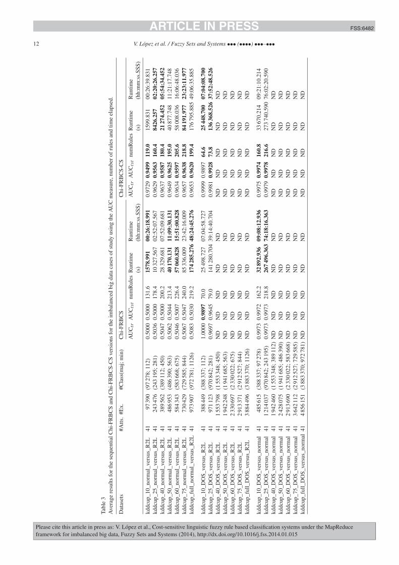
JID:FSS AID:6482 /FLA [m3SC+; v 1.188; Prn:4/03/2014; 14:35] P.12 (1-34)
12 V. López et al. / Fuzzy Sets and Systems ••• (••••) •••–•••
Tabl
e3
Ave
rage
resu
ltsfo
rth
ese
quen
tialC
hi-F
RB
CS
and
Chi
-FR
BC
S-C
Sve
rsio
nsfo
rth
eim
bala
nced
big
data
case
sof
stud
yus
ing
the
AU
Cm
easu
re,n
umbe
rof
rule
san
dtim
eel
apse
d.
Dat
aset
s#A
tts.
#Ex.
#Cla
ss(m
aj;m
in)
Chi
-FR
BC
SC
hi-F
RB
CS-
CS
AU
Ctr
AU
Cts
tnu
mR
ules
Run
time
(s)
Run
time
(hh:
mm
:ss.
SSS)
AU
Ctr
AU
Cts
tnu
mR
ules
Run
time
(s)
Run
time
(hh:
mm
:ss.
SSS)
kddc
up_1
0_no
rmal
_ver
sus_
R2L
4197
390
(97
278;
112)
0.50
000.
5000
131.
615
78.9
9100
:26:
18.9
910.
9729
0.94
9911
9.0
1599
.831
00:2
6:39
.831
kddc
up_2
5_no
rmal
_ver
sus_
R2L
4124
347
6(2
4319
5;28
1)0.
5036
0.50
0017
8.4
1032
7.56
702
:52:
07.5
670.
9629
0.95
6316
0.4
8426
.257
02:2
0:26
.257
kddc
up_4
0_no
rmal
_ver
sus_
R2L
4138
956
2(3
8911
2;45
0)0.
5047
0.50
0020
0.2
2832
9.68
107
:52:
09.6
810.
9637
0.95
8718
0.4
2127
4.45
205
:54:
34.4
52kd
dcup
_50_
norm
al_v
ersu
s_R
2L41
486
953
(486
390;
563)
0.50
620.
5044
213.
440
170.
131
11:0
9:30
.131
0.96
490.
9625
195.
040
877.
748
11:2
1:17
.748
kddc
up_6
0_no
rmal
_ver
sus_
R2L
4158
434
3(5
8366
8;67
5)0.
5046
0.50
0722
6.4
5706
0.82
815
:51:
00.8
280.
9634
0.95
9720
5.6
5800
8.03
616
:06:
48.0
36kd
dcup
_75_
norm
al_v
ersu
s_R
2L41
730
429
(729
585;
844)
0.50
670.
5047
240.
085
336.
009
23:4
2:16
.009
0.96
570.
9638
218.
884
191.
977
23:2
3:11
.977
kddc
up_f
ull_
norm
al_v
ersu
s_R
2L41
973
907
(972
781;
1126
)0.
5083
0.50
3021
9.2
174
285.
276
48:2
4:45
.276
0.96
530.
9620
199.
417
679
5.88
549
:06:
35.8
85
kddc
up_1
0_D
OS_
vers
us_R
2L41
388
449
(388
337;
112)
1.00
000.
9897
70.0
2549
8.72
707
:04:
58.7
270.
9999
0.98
9764
.625
448.
700
07:0
4:08
.700
kddc
up_2
5_D
OS_
vers
us_R
2L41
971
123
(970
842;
281)
0.96
970.
9645
79.0
141
280.
704
39:1
4:40
.704
0.99
810.
9928
73.8
136
368.
526
37:5
2:48
.526
kddc
up_4
0_D
OS_
vers
us_R
2L41
155
379
8(1
553
348;
450)
ND
ND
ND
ND
ND
ND
ND
ND
ND
ND
kddc
up_5
0_D
OS_
vers
us_R
2L41
194
224
8(1
941
685;
563)
ND
ND
ND
ND
ND
ND
ND
ND
ND
ND
kddc
up_6
0_D
OS_
vers
us_R
2L41
233
069
7(2
330
022;
675)
ND
ND
ND
ND
ND
ND
ND
ND
ND
ND
kddc
up_7
5_D
OS_
vers
us_R
2L41
291
337
1(2
912
527;
844)
ND
ND
ND
ND
ND
ND
ND
ND
ND
ND
kddc
up_f
ull_
DO
S_ve
rsus
_R2L
413
884
496
(388
337
0;11
26)
ND
ND
ND
ND
ND
ND
ND
ND
ND
ND
kddc
up_1
0_D
OS_
vers
us_n
orm
al41
485
615
(388
337;
9727
8)0.
9973
0.99
7216
2.2
3289
2.93
609
:08:
12.9
360.
9975
0.99
7416
0.8
3367
0.21
409
:21:
10.2
14kd
dcup
_25_
DO
S_ve
rsus
_nor
mal
411
214
037
(970
842;
243
195)
0.99
730.
9973
218.
826
749
6.36
374
:18:
16.3
630.
9979
0.99
7821
6.6
273
740.
590
76:0
2:20
.590
kddc
up_4
0_D
OS_
vers
us_n
orm
al41
194
246
0(1
553
348;
389
112)
ND
ND
ND
ND
ND
ND
ND
ND
ND
ND
kddc
up_5
0_D
OS_
vers
us_n
orm
al41
242
807
5(1
941
685;
486
390)
ND
ND
ND
ND
ND
ND
ND
ND
ND
ND
kddc
up_6
0_D
OS_
vers
us_n
orm
al41
291
369
0(2
330
022;
583
668)
ND
ND
ND
ND
ND
ND
ND
ND
ND
ND
kddc
up_7
5_D
OS_
vers
us_n
orm
al41
364
211
2(2
912
527;
729
585)
ND
ND
ND
ND
ND
ND
ND
ND
ND
ND
kddc
up_f
ull_
DO
S_ve
rsus
_nor
mal
414
856
151
(388
337
0;97
278
1)N
DN
DN
DN
DN
DN
DN
DN
DN
DN
D

JID:FSS AID:6482 /FLA [m3SC+; v 1.188; Prn:4/03/2014; 14:35] P.13 (1-34)
V. López et al. / Fuzzy Sets and Systems ••• (••••) •••–••• 13
5.1. General overview of the Chi-FRBCS algorithm for big data
The Chi-FRBCS-BigDataCS algorithm is an approach that can be used to classify imbalanced big data. It is aMapReduce design where each map process is responsible for building a RB using only the data included in itsportion and where the reduce process is responsible for collecting and combining the RB generated by each mapperto form the final RB.
We will divide the description of the proposal in two parts: the first part is devoted to the description of the creationof the model, shown in Section 5.2, and the second part is dedicated to the explanation on how new instances areclassified using the previous learned model, in Section 5.3. Both parts follow the MapReduce structure distributing allthe computations needed along several processing units that manage different chunks of information, aggregating theresults obtained in an appropriate manner.
In this description, we do not make a distinction between the steps that need to be followed to create a “normal”model that is able to process big data based on the Chi-FRBCS algorithm, Chi-FRBCS-BigData, and the steps neededto transform this model into our proposal, Chi-FRBCS-BigDataCS, based on the Chi-FRBCS-CS model. The differ-ences in the computation of both models are related to the computation of the rule weight, as stated in Section 4.1,sharing most of the algorithm structure. In this manner, the transition to a big data model follows similar steps andonly the variances associated to the cost-sensitive model will be stated when applicable.
The model presented is a FRBCS built on MapReduce using cost-sensitive learning for the following reasons:
• A FRBCS is able to deal with the uncertainty and imprecise information that emanates from big data, as thosehuge information sources become available from diverse sources that include a high variety while trying to copewith the veracity and trust on the data.
• The MapReduce framework is one of the most currently known alternatives to handle big data and has demon-strated that is capable to perform reasonably well in data mining problems producing even libraries like Mahoutthat include machine learning and data mining algorithms.
• In cost-sensitive learning, the addition of costs into the algorithm way of working does not heavily increase thetime complexity while properly managing the imbalanced problem.
Finally, we have preferred the use of cost-sensitive learning instead of data preprocessing techniques to avoid anextra step in the building of the model following a MapReduce design. Over-sampling techniques would increasethe size of the data to process, therefore increasing the computational needs, while under-sampling may disregardpotentially useful examples which could be underestimated because of the subdivision induced by the MapReducestructure.
5.2. Building the knowledge base for the Chi-FRBCS-BigDataCS using a MapReduce design
In this section, we will describe how the KB is built from the original training set provided following a MapReduceprocedure. This process is illustrated in Fig. 3 and consists of the following steps:
• Initial: In the CS version, the first step needs to estimate the costs for each class giving the minority class agreater cost than the majority class. This cost is estimated in the same way as described in Section 4.1, givinga misclassification cost of 1 for instances belonging to the majority class and a misclassification cost of IR forinstances of the minority class.Next, in both versions of the algorithm, the domain of variation of each feature in the dataset is determined. Then,the different fuzzy membership labels that compose the DB are computed using these domains according to thenumber of labels considered.Finally, in order to comply with Hadoop way of working, the algorithm performs a segmentation of the trainingdataset into independent HDFS blocks. These blocks are then automatically replicated and transferred betweenthe different cluster nodes thanks to the Hadoop environment that implements the MapReduce structure.
• Map: In this step each map task builds a RB with the data blocks of its data portion and generates a file containingthe RB (called RBi , see Fig. 3). More specifically, for each instance belonging to the mapper, a fuzzy rule iscreated in a similar way as described in Section 3.2: we first search for the linguistic fuzzy labels that match

JID:FSS AID:6482 /FLA [m3SC+; v 1.188; Prn:4/03/2014; 14:35] P.14 (1-34)
14 V. López et al. / Fuzzy Sets and Systems ••• (••••) •••–•••
Fig. 3. A flowchart of how the building of the KB is organized in Chi-FRBCS-BigDataCS.
the attribute values of the current example, we select the among the matching fuzzy labels the ones that obtainthe largest matching degree for each attribute, we build the rule using as antecedent the fuzzy labels previouslyselected and as consequent the class associated to the example and finally we compute the rule weight.Please note that for computing the rule weight we use the PCF or PCF-CS for the Chi-FRBCS-BigData or Chi-FRBCS-BigDataCS methods, and that the set of examples used for the rule weight is the set of examples thatbelong to the current map process. In this manner, rules with the same antecedents and consequent can be gener-ated by different mappers but they can have different rule weight values. Moreover, when a new rule is created ina mapper we check, as in the original Chi-FRBCS algorithm, if there is a rule with the same antecedents alreadyin the mapper RB. In that case, if the consequent of the rule is also the same as the rule in the mapper RB, thisrule is discarded while if the consequent of the new rule is different from the consequent of the previously createdrule, then only the rule with the maximum weight is preserved.In this manner, the Map step applies the original Chi-FRBCS classifier or the Chi-FRBCS-CS approach describedin Section 4.1 to the data available in the data partition.
• Reduce: In this next step, the reduce process combines the RBs generated by each mapper (RBi ) to form thefinal RB (called RBR , see Fig. 3). Specifically, the final RB is built from the RBs built from each mapperRB1,RB2, . . . ,RBn in a similar way as in the creation of new rules in each mapper (Fig. 3): we browse therules that belong to the RB generated by each mapper, RBi ; if there is a rule in the final RB, RBR , with the sameantecedent as the rule we are trying to add we only maintain in the final RB, RBR , the rule with the highest ruleweight. In this case it is not necessary to check if the consequent is the same or not as we are maintaining the mostpowerful rules. Equivalent rules (rules with the same antecedent and consequent) can present different weights asthey are computed in different mappers over different training sets.Please note that it is not needed to recompute the rules weights as we are selecting the most confident rulesprovided by each mapper. An alternative that would involve a new weight computation would have been the casewhere equivalent rules are combined to produce a new rule, for instance, computing an average weight betweenthem. However, the direct selection of rules was preferred because of its simplicity which enables to speed up thealgorithm in its reduce step.
• Final: In this last step, the RB that is generated in the reduce process (RBR) and the DB that was calculated in theinitial phase conform the KB that is provided as the output of the computation process. This output will be theentry data for the mechanism that classifies new examples.
Algorithms 1 and 2 show the pseudo-code of the Map function of the MapReduce job for the creation of the modelphase. Algorithm 1 is devoted to obtaining all instances in a mapper’s partition and the Hadoop framework calls it foreach <key/value> pair in this partition. When the previous process is finished, Algorithm 2 is called for each mapperto build a RB with the data blocks of its data portion. Furthermore, Algorithm 3 gives the pseudo-code of the Reduce

JID:FSS AID:6482 /FLA [m3SC+; v 1.188; Prn:4/03/2014; 14:35] P.15 (1-34)
V. López et al. / Fuzzy Sets and Systems ••• (••••) •••–••• 15
function and is called when all mappers have finished, to combine the RBs generated by each mapper to form the finalRB.
Algorithm 1 Map phase for the Chi-FRBCS-BigDataCS algorithm for the building of the model phase MAP(key,value):Input: <key,value> pair, where key is the offset in bytes and value is the content of an instance.Output: <key′ ,value′ > pair, where key′ is any Long value and value′ contains a RB.1: instance ← INSTANCE_REPRESENTATION(value) {instances will contain all instances in this mapper’s split}2: instances ← instances.add(instance)
Algorithm 2 Map phase for the Chi-FRBCS-BigDataCS algorithm for the building of the model phase CLEANUP():1: fuzzy_ChiBuilder.build(instances,posClass,posclassCost,negClassCost)2: ruleBase ← fuzzy_ChiBuilder.getRuleBase()3: EMIT (key, ruleBase)
Algorithm 3 Reduce phase for the Chi-FRBCS-BigDataCS algorithm REDUCE(key, values):Input: <key,values> pair, where key is any Long value and values are the RBs generated by each mapper.Output: <key′ ,value′ > pair, where key′ is a null value and value′ is the final RB.1: while values.hasNext() do2: ruleBase ← values.getValue()3: for i = 0 to ruleBase.size() − 1 do4: if finalRuleBase.size() == 0 then5: finalRuleBase ← finalRuleBase.add(ruleBase.get(i));6: else7: if !finalRuleBase.duplicated(ruleBase.get(i)) then8: finalRuleBase ← finalRuleBase.add(ruleBase.get(i));9: else
10: if The consequent of those rules belongs to different classes then11: rule ← finalRuleBase.getRuleWithHighestRuleWeight(ruleBase.get(i))12: finalRuleBase ← finalRuleBase.add(rule);13: end if14: end if15: end if16: end for17: end while18: EMIT (null, finalRuleBase)
5.3. Classification of new patterns
In this section, we will describe how new instances belonging to a dataset are classified considering the KB builtpreviously. When the MapReduce process devoted to the building of the KB has finished, a new MapReduce processis initiated to estimate the class associated to a dataset. Specifically, this phase is also based on a MapReduce designwhere each map process is responsible for estimating the class for the examples included in its data segment using thefinal KB previously generated. The process follows the next steps:
• Initial: In the same way as in the first step of the building of the model, this step performs a segmentation ofthe input dataset into independent HDFS blocks; replicates and transfers them to other machines to be finallyprocessed independently by each map task at the same time. This step is automatically performed by the Hadoopsystem, the MapReduce implementation we are using.
• Map: In this next step, each map task estimates the class for the examples included in the data block availablefor the mapper using the FRM of the winner rule. In particular, for each example, we compute for all the rulesin the RB the product of the rule weight with the compatibility degree between the linguistic fuzzy labels that
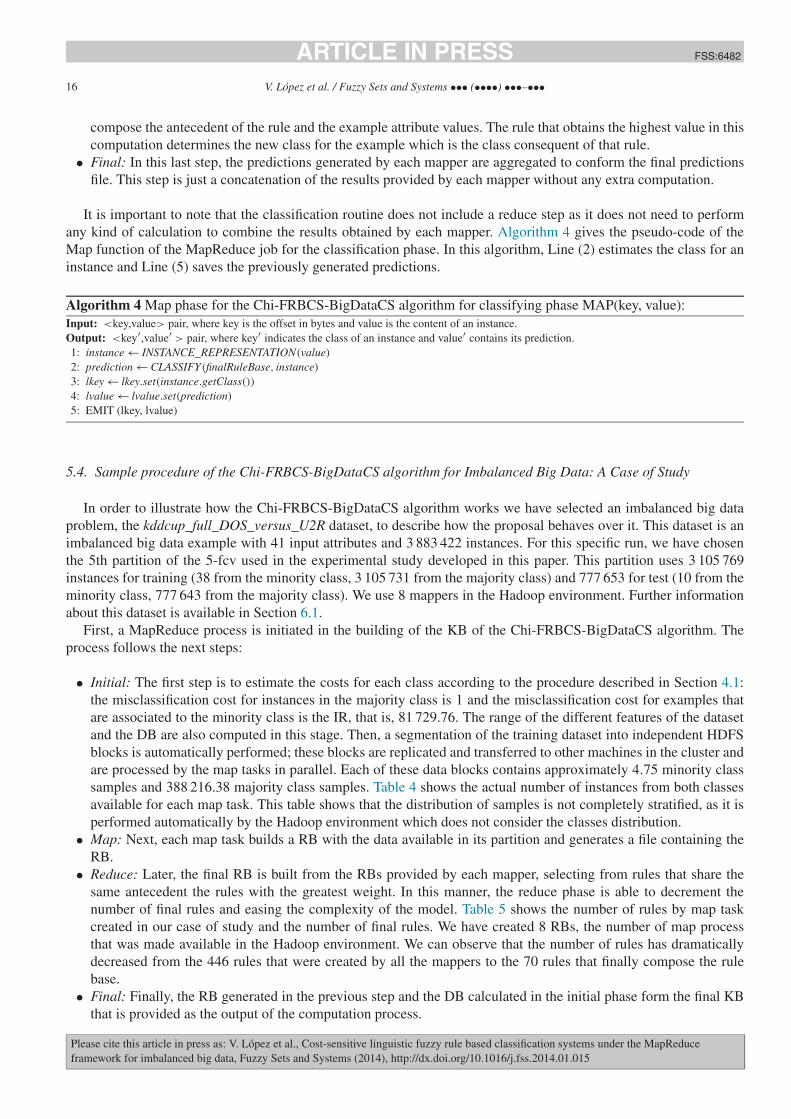
JID:FSS AID:6482 /FLA [m3SC+; v 1.188; Prn:4/03/2014; 14:35] P.16 (1-34)
16 V. López et al. / Fuzzy Sets and Systems ••• (••••) •••–•••
compose the antecedent of the rule and the example attribute values. The rule that obtains the highest value in thiscomputation determines the new class for the example which is the class consequent of that rule.
• Final: In this last step, the predictions generated by each mapper are aggregated to conform the final predictionsfile. This step is just a concatenation of the results provided by each mapper without any extra computation.
It is important to note that the classification routine does not include a reduce step as it does not need to performany kind of calculation to combine the results obtained by each mapper. Algorithm 4 gives the pseudo-code of theMap function of the MapReduce job for the classification phase. In this algorithm, Line (2) estimates the class for aninstance and Line (5) saves the previously generated predictions.
Algorithm 4 Map phase for the Chi-FRBCS-BigDataCS algorithm for classifying phase MAP(key, value):Input: <key,value> pair, where key is the offset in bytes and value is the content of an instance.Output: <key′,value′ > pair, where key′ indicates the class of an instance and value′ contains its prediction.1: instance ← INSTANCE_REPRESENTATION(value)2: prediction ← CLASSIFY(finalRuleBase, instance)3: lkey ← lkey.set(instance.getClass())4: lvalue ← lvalue.set(prediction)
5: EMIT (lkey, lvalue)
5.4. Sample procedure of the Chi-FRBCS-BigDataCS algorithm for Imbalanced Big Data: A Case of Study
In order to illustrate how the Chi-FRBCS-BigDataCS algorithm works we have selected an imbalanced big dataproblem, the kddcup_full_DOS_versus_U2R dataset, to describe how the proposal behaves over it. This dataset is animbalanced big data example with 41 input attributes and 3 883 422 instances. For this specific run, we have chosenthe 5th partition of the 5-fcv used in the experimental study developed in this paper. This partition uses 3 105 769instances for training (38 from the minority class, 3 105 731 from the majority class) and 777 653 for test (10 from theminority class, 777 643 from the majority class). We use 8 mappers in the Hadoop environment. Further informationabout this dataset is available in Section 6.1.
First, a MapReduce process is initiated in the building of the KB of the Chi-FRBCS-BigDataCS algorithm. Theprocess follows the next steps:
• Initial: The first step is to estimate the costs for each class according to the procedure described in Section 4.1:the misclassification cost for instances in the majority class is 1 and the misclassification cost for examples thatare associated to the minority class is the IR, that is, 81 729.76. The range of the different features of the datasetand the DB are also computed in this stage. Then, a segmentation of the training dataset into independent HDFSblocks is automatically performed; these blocks are replicated and transferred to other machines in the cluster andare processed by the map tasks in parallel. Each of these data blocks contains approximately 4.75 minority classsamples and 388 216.38 majority class samples. Table 4 shows the actual number of instances from both classesavailable for each map task. This table shows that the distribution of samples is not completely stratified, as it isperformed automatically by the Hadoop environment which does not consider the classes distribution.
• Map: Next, each map task builds a RB with the data available in its partition and generates a file containing theRB.
• Reduce: Later, the final RB is built from the RBs provided by each mapper, selecting from rules that share thesame antecedent the rules with the greatest weight. In this manner, the reduce phase is able to decrement thenumber of final rules and easing the complexity of the model. Table 5 shows the number of rules by map taskcreated in our case of study and the number of final rules. We have created 8 RBs, the number of map processthat was made available in the Hadoop environment. We can observe that the number of rules has dramaticallydecreased from the 446 rules that were created by all the mappers to the 70 rules that finally compose the rulebase.
• Final: Finally, the RB generated in the previous step and the DB calculated in the initial phase form the final KBthat is provided as the output of the computation process.
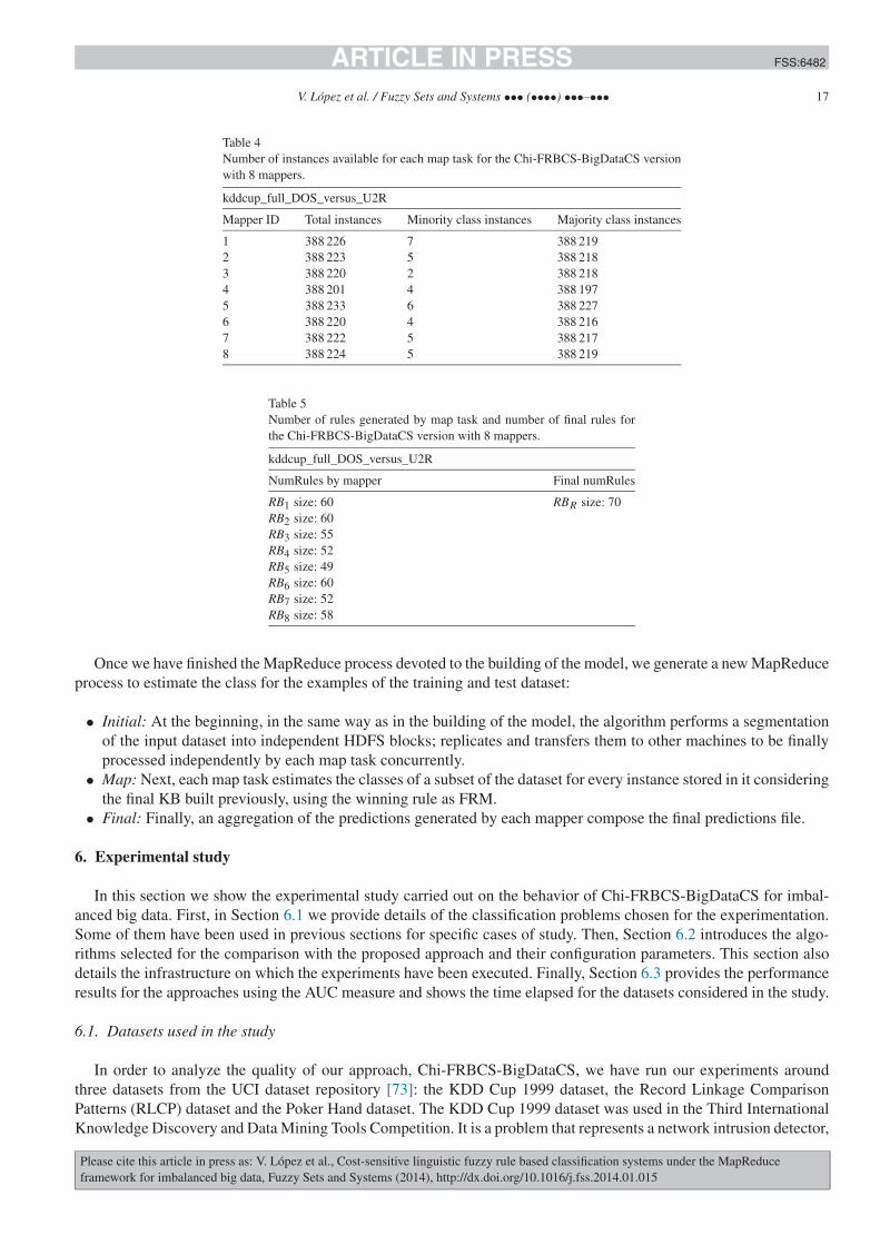
JID:FSS AID:6482 /FLA [m3SC+; v 1.188; Prn:4/03/2014; 14:35] P.17 (1-34)
V. López et al. / Fuzzy Sets and Systems ••• (••••) •••–••• 17
Table 4Number of instances available for each map task for the Chi-FRBCS-BigDataCS versionwith 8 mappers.
kddcup_full_DOS_versus_U2R
Mapper ID Total instances Minority class instances Majority class instances
1 388 226 7 388 2192 388 223 5 388 2183 388 220 2 388 2184 388 201 4 388 1975 388 233 6 388 2276 388 220 4 388 2167 388 222 5 388 2178 388 224 5 388 219
Table 5Number of rules generated by map task and number of final rules forthe Chi-FRBCS-BigDataCS version with 8 mappers.
kddcup_full_DOS_versus_U2R
NumRules by mapper Final numRules
RB1 size: 60 RBR size: 70RB2 size: 60RB3 size: 55RB4 size: 52RB5 size: 49RB6 size: 60RB7 size: 52RB8 size: 58
Once we have finished the MapReduce process devoted to the building of the model, we generate a new MapReduceprocess to estimate the class for the examples of the training and test dataset:
• Initial: At the beginning, in the same way as in the building of the model, the algorithm performs a segmentationof the input dataset into independent HDFS blocks; replicates and transfers them to other machines to be finallyprocessed independently by each map task concurrently.
• Map: Next, each map task estimates the classes of a subset of the dataset for every instance stored in it consideringthe final KB built previously, using the winning rule as FRM.
• Final: Finally, an aggregation of the predictions generated by each mapper compose the final predictions file.
6. Experimental study
In this section we show the experimental study carried out on the behavior of Chi-FRBCS-BigDataCS for imbal-anced big data. First, in Section 6.1 we provide details of the classification problems chosen for the experimentation.Some of them have been used in previous sections for specific cases of study. Then, Section 6.2 introduces the algo-rithms selected for the comparison with the proposed approach and their configuration parameters. This section alsodetails the infrastructure on which the experiments have been executed. Finally, Section 6.3 provides the performanceresults for the approaches using the AUC measure and shows the time elapsed for the datasets considered in the study.
6.1. Datasets used in the study
In order to analyze the quality of our approach, Chi-FRBCS-BigDataCS, we have run our experiments aroundthree datasets from the UCI dataset repository [73]: the KDD Cup 1999 dataset, the Record Linkage ComparisonPatterns (RLCP) dataset and the Poker Hand dataset. The KDD Cup 1999 dataset was used in the Third InternationalKnowledge Discovery and Data Mining Tools Competition. It is a problem that represents a network intrusion detector,
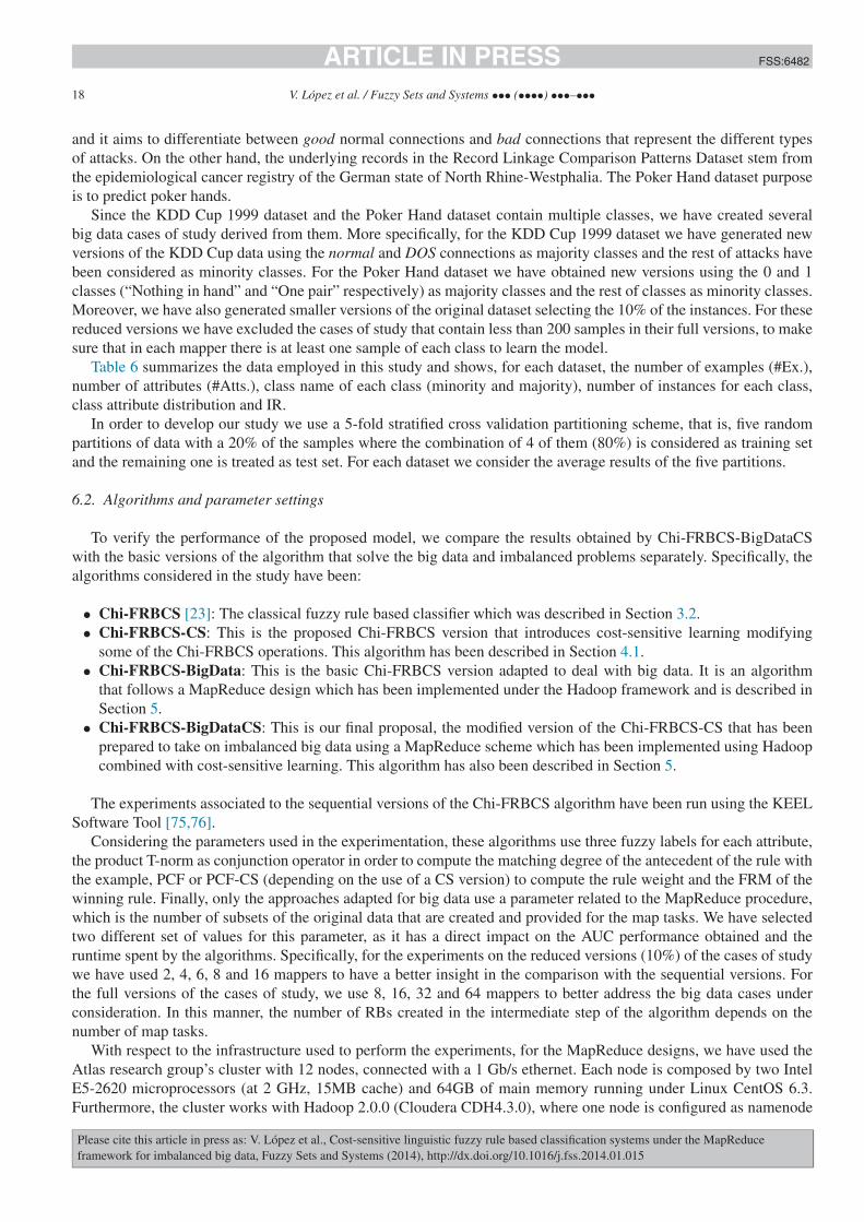
JID:FSS AID:6482 /FLA [m3SC+; v 1.188; Prn:4/03/2014; 14:35] P.18 (1-34)
18 V. López et al. / Fuzzy Sets and Systems ••• (••••) •••–•••
and it aims to differentiate between good normal connections and bad connections that represent the different typesof attacks. On the other hand, the underlying records in the Record Linkage Comparison Patterns Dataset stem fromthe epidemiological cancer registry of the German state of North Rhine-Westphalia. The Poker Hand dataset purposeis to predict poker hands.
Since the KDD Cup 1999 dataset and the Poker Hand dataset contain multiple classes, we have created severalbig data cases of study derived from them. More specifically, for the KDD Cup 1999 dataset we have generated newversions of the KDD Cup data using the normal and DOS connections as majority classes and the rest of attacks havebeen considered as minority classes. For the Poker Hand dataset we have obtained new versions using the 0 and 1classes (“Nothing in hand” and “One pair” respectively) as majority classes and the rest of classes as minority classes.Moreover, we have also generated smaller versions of the original dataset selecting the 10% of the instances. For thesereduced versions we have excluded the cases of study that contain less than 200 samples in their full versions, to makesure that in each mapper there is at least one sample of each class to learn the model.
Table 6 summarizes the data employed in this study and shows, for each dataset, the number of examples (#Ex.),number of attributes (#Atts.), class name of each class (minority and majority), number of instances for each class,class attribute distribution and IR.
In order to develop our study we use a 5-fold stratified cross validation partitioning scheme, that is, five randompartitions of data with a 20% of the samples where the combination of 4 of them (80%) is considered as training setand the remaining one is treated as test set. For each dataset we consider the average results of the five partitions.
6.2. Algorithms and parameter settings
To verify the performance of the proposed model, we compare the results obtained by Chi-FRBCS-BigDataCSwith the basic versions of the algorithm that solve the big data and imbalanced problems separately. Specifically, thealgorithms considered in the study have been:
• Chi-FRBCS [23]: The classical fuzzy rule based classifier which was described in Section 3.2.• Chi-FRBCS-CS: This is the proposed Chi-FRBCS version that introduces cost-sensitive learning modifying
some of the Chi-FRBCS operations. This algorithm has been described in Section 4.1.• Chi-FRBCS-BigData: This is the basic Chi-FRBCS version adapted to deal with big data. It is an algorithm
that follows a MapReduce design which has been implemented under the Hadoop framework and is described inSection 5.
• Chi-FRBCS-BigDataCS: This is our final proposal, the modified version of the Chi-FRBCS-CS that has beenprepared to take on imbalanced big data using a MapReduce scheme which has been implemented using Hadoopcombined with cost-sensitive learning. This algorithm has also been described in Section 5.
The experiments associated to the sequential versions of the Chi-FRBCS algorithm have been run using the KEELSoftware Tool [75,76].
Considering the parameters used in the experimentation, these algorithms use three fuzzy labels for each attribute,the product T-norm as conjunction operator in order to compute the matching degree of the antecedent of the rule withthe example, PCF or PCF-CS (depending on the use of a CS version) to compute the rule weight and the FRM of thewinning rule. Finally, only the approaches adapted for big data use a parameter related to the MapReduce procedure,which is the number of subsets of the original data that are created and provided for the map tasks. We have selectedtwo different set of values for this parameter, as it has a direct impact on the AUC performance obtained and theruntime spent by the algorithms. Specifically, for the experiments on the reduced versions (10%) of the cases of studywe have used 2, 4, 6, 8 and 16 mappers to have a better insight in the comparison with the sequential versions. Forthe full versions of the cases of study, we use 8, 16, 32 and 64 mappers to better address the big data cases underconsideration. In this manner, the number of RBs created in the intermediate step of the algorithm depends on thenumber of map tasks.
With respect to the infrastructure used to perform the experiments, for the MapReduce designs, we have used theAtlas research group’s cluster with 12 nodes, connected with a 1 Gb/s ethernet. Each node is composed by two IntelE5-2620 microprocessors (at 2 GHz, 15MB cache) and 64GB of main memory running under Linux CentOS 6.3.Furthermore, the cluster works with Hadoop 2.0.0 (Cloudera CDH4.3.0), where one node is configured as namenode

JID:FSS AID:6482 /FLA [m3SC+; v 1.188; Prn:4/03/2014; 14:35] P.19 (1-34)
V. López et al. / Fuzzy Sets and Systems ••• (••••) •••–••• 19
Table 6Summary of imbalanced datasets.
Datasets #Ex. #Atts. Class (maj; min) #Class(maj; min) %Class(maj; min) IR
kddcup_10_DOS_versus_normal 485 615 41 (DOS; normal) (388 337; 97 278) (79.968; 20.032) 3.99kddcup_10_DOS_versus_PRB 392 447 41 (DOS; PRB) (388 337; 4110) (98.953; 1.047) 94.49kddcup_10_DOS_versus_R2L 388 449 41 (DOS; R2L) (388 337; 112) (99.971; 0.029) 3467.29kddcup_10_normal_versus_PRB 101 388 41 (normal; PRB) (97 278; 4110) (95.946; 4.054) 23.67kddcup_10_normal_versus_R2L 97 390 41 (normal; R2L) (97 278; 112) (99.885; 0.115) 868.55poker_10_0_vs_2 56 252 10 (0; 2) (51 370; 4882) (91.321; 8.679) 10.52poker_10_0_vs_3 53 533 10 (0; 3) (51 370; 2163) (95.96; 4.04) 23.75poker_10_0_vs_4 51 767 10 (0; 4) (51 370; 397) (99.233; 0.767) 129.40poker_10_0_vs_5 51 575 10 (0; 5) (51 370; 205) (99.603; 0.397) 250.59poker_10_0_vs_6 51 516 10 (0; 6) (51 370; 146) (99.717; 0.283) 351.85poker_10_0_vs_7 51 393 10 (0; 7) (51 370; 23) (99.955; 0.045) 2233.48poker_10_1_vs_2 48 191 10 (1; 2) (43 309; 4882) (89.869; 10.131) 8.87poker_10_1_vs_3 45 472 10 (1; 3) (43 309; 2163) (95.243; 4.757) 20.02poker_10_1_vs_4 43 706 10 (1; 4) (43 309; 397) (99.092; 0.908) 109.09poker_10_1_vs_5 43 514 10 (1; 5) (43 309; 205) (99.529; 0.471) 211.26poker_10_1_vs_6 43 455 10 (1; 6) (43 309; 146) (99.664; 0.336) 296.64poker_10_1_vs_7 43 332 10 (1; 7) (43 309; 23) (99.947; 0.053) 1883.00RLCP_10 574 913 2 (FALSE; TRUE) (572 820; 2093) (99.636; 0.364) 273.68
kddcup_DOS_versus_normal 4 856 151 41 (DOS; normal) (3 883 370; 972 781) (79.968; 20.032) 3.99kddcup_DOS_versus_PRB 3 924 472 41 (DOS; PRB) (3 883 370; 41 102) (98.953; 1.047) 94.48kddcup_DOS_versus_R2L 3 884 496 41 (DOS; R2L) (3 883 370; 1126) (99.971; 0.029) 3448.82kddcup_DOS_versus_U2R 3 883 422 41 (DOS; U2R) (3 883 370; 52) (99.999; 0.001) 74 680.19kddcup_normal_versus_PRB 1 013 883 41 (normal; PRB) (972 781; 41 102) (95.946; 4.054) 23.67kddcup_normal_versus_R2L 973 907 41 (normal; R2L) (972 781; 1126) (99.884; 0.116) 863.93kddcup_normal_versus_U2R 972 833 41 (normal; U2R) (972 781; 52) (99.995; 0.005) 18 707.33poker_0_vs_2 562 530 10 (0; 2) (513 702; 48 828) (91.32; 8.68) 10.52poker_0_vs_3 535 336 10 (0; 3) (513 702; 21 634) (95.959; 4.041) 23.75poker_0_vs_4 517 680 10 (0; 4) (513 702; 3978) (99.232; 0.768) 129.14poker_0_vs_5 515 752 10 (0; 5) (513 702; 2050) (99.603; 0.397) 250.59poker_0_vs_6 515 162 10 (0; 6) (513 702; 1460) (99.717; 0.283) 351.85poker_0_vs_7 513 938 10 (0; 7) (513 702; 236) (99.954; 0.046) 2176.70poker_0_vs_8 513 719 10 (0; 8) (513 702; 17) (99.997; 0.003) 30 217.76poker_0_vs_9 513 710 10 (0; 9) (513 702; 8) (99.998; 0.002) 64 212.75poker_1_vs_2 481 925 10 (1; 2) (433 097; 48 828) (89.868; 10.132) 8.87poker_1_vs_3 454 731 10 (1; 3) (433 097; 21 634) (95.242; 4.758) 20.02poker_1_vs_4 437 075 10 (1; 4) (433 097; 3978) (99.09; 0.91) 108.87poker_1_vs_5 435 147 10 (1; 5) (433 097; 2050) (99.529; 0.471) 211.27poker_1_vs_6 434 557 10 (1; 6) (433 097; 1460) (99.664; 0.336) 296.64poker_1_vs_7 433 333 10 (1; 7) (433 097; 236) (99.946; 0.054) 1835.16poker_1_vs_8 433 114 10 (1; 8) (433 097; 17) (99.996; 0.004) 25 476.29poker_1_vs_9 433 105 10 (1; 9) (433 097; 8) (99.998; 0.002) 54 137.13RLCP 5 749 132 2 (FALSE; TRUE) (5 728 201; 20 931) (99.636; 0.364) 273.67
and jobtracker, and the rest are datanodes and task-trackers. For the sequential experiments we have used a clusterwith Intel Core i7 930 microprocessors (at 2.8 GHz, 15MB cache) and 24GB of main memory connected with a 1 Gb/sethernet. We acknowledge that the runtime comparisons between the sequential versions and the MapReduce designsare not performed in identical machines, however, the time advantage is obtained for the sequential versions whichare, even in this case, notably slower than the Hadoop implementations.
6.3. Analysis of the Chi-FRBCS-BigDataCS behavior
In this part of the study, we want to analyze the behavior of the Chi-FRBCS-BigDataCS proposal in the scenario ofimbalanced big data in contrast with the other learning proposals. This section is divided into two parts: the first part

JID:FSS AID:6482 /FLA [m3SC+; v 1.188; Prn:4/03/2014; 14:35] P.20 (1-34)
20 V. López et al. / Fuzzy Sets and Systems ••• (••••) •••–•••
(Section 6.3.1) is devoted to the presentation of the precision of our approach in terms of classification performanceusing the AUC measure; the second part (Section 6.3.2) is devoted to the analysis on the runtime of the model.
6.3.1. Analysis on the precision of the modelIn this section, we present a set of experiments to illustrate and demonstrate the behavior of Chi-FRBCS-
BigDataCS. These experiments are organized in two phases: the first one compares the behavior of the differentalternatives using the cases of study that contain the 10% of the instances of the original datasets while the secondone compares the behavior of the approaches over the full datasets considered in the study. The experiments whereorganized in this way to be able to contrast the results of the big data versions in relation with the serial versions of thealgorithm for the smaller datasets. Additionally, this organization also permits to check how the results change wheninstead of using a reduced version of the dataset the whole dataset is utilized.
In Tables 7 and 8 we present the average results in training and test for the reduced versions (10%) of the imbalancedbig data cases of study for the Chi-FRBCS and Chi-FRBCS-CS versions respectively. These tables are divided bycolumns in two parts: the first part corresponds to the results of the sequential variant while the second part is relatedto the big data variants of the Chi-FRBCS and Chi-FRBCS-CS algorithms respectively. Furthermore, the results forthe big data alternatives are divided by columns in five parts, which correspond to the number of mappers used: 2, 4,6, 8 and 16 mappers for each case.
Looking at the results we can observe that the performance obtained, both in training and test, is higher in mostof the cases of study for the Chi-FRBCS-CS alternatives, the sequential approach and the big data adaptation for anynumber of mappers configuration. This situation demonstrates the positive influence of the usage of cost-sensitivelearning when dealing with imbalanced data as the classifier is able to provide appropriate solutions in an arduousenvironment. Additionally, we can observe that the model does not present a strong overfitting on the training set inrelation with the test set, as we cannot find huge differences between the results provided for both sets. For instance,for the kddcup_10_normal_versus_PRB dataset using the Chi-FRBCS-BigDataCS with 8 mappers, an AUC of 0.9728in training is obtained which is closely followed by an AUC in test of 0.9723. There are even cases where the test setobtains a better performance than the training set such as kddcup_10_normal_versus_R2L for Chi-FRBCS-BigDataCSusing 8 mappers with an AUC in training of 0.8747 and an AUC in test of 0.8784. This situation is caused by theusage of the PCF or PCF-CS to compute the rule weight as these measures try to make rules as general as possibleconsidering the current dataset.
Next, we compare the results considering the cases of study derived from all original training sets in relationwith the number of mappers considered. For the KDD Cup 1999 cases of study we find that the behavior of theChi-FRBCS and Chi-FRBCS-CS approaches is not steady in relation to the number of mappers considered in theexperiments. For instance, for the Chi-FRBCS sequential version, the test results achieved are worse than the resultsfor the Chi-FRBCS-BigData approach. In this case, increasing the number of mappers may also increase the AUCmetric, however, when the number of mappers is too high this performance is decreased. The Chi-FRBCS-CS se-quential variant, is able to provide better test results than the Chi-FRBCS-BigDataCS proposal. However, there isnot a clear optimal configuration for the number of mappers used, as the results are not stable when increasing thatnumber of mappers. Furthermore, the worse results are obtained for the highest number of mappers considered in theexperiment. In contrast, the training results provide more sensible results, decreasing the performance in a reasonablemanner when the number of mappers is enlarged.
In the case of the Poker Hand cases of study we first discover that the results obtained for this set of data area bit poor, as the AUC measure is usually ranging from 0.5 to 0.6. Similarly to the KDD Cup 1999 dataset, theChi-FRBCS approaches are presenting erratic results where the sequential version provides worse AUC values thanthe Chi-FRBCS-BigData alternative, which is also improving when larger values for the number of mappers are used.In the case of the Chi-FRBCS-CS variants, the performance obtained is clearly related both in training and test withthe number of mappers considered: the best performance is achieved by the sequential Chi-FRBCS-CS algorithmwhile the performance drops when bigger number of mappers are used.
The RLCP dataset is not able to properly identify instances from both classes in the Chi-FRBCS approaches,as the results obtained for all the variants and the number of mappers considered is 0.5. When the Chi-FRBCS-CSalternatives are tested, the RLCP provides reasonable AUC results with almost no variance when the sequential versionis contrasted with smaller values for the number of mappers. Larger values for the number of mappers need to becompared to find a slight drop in accuracy.

JID:FSS AID:6482 /FLA [m3SC+; v 1.188; Prn:4/03/2014; 14:35] P.21 (1-34)
V. López et al. / Fuzzy Sets and Systems ••• (••••) •••–••• 21
Tabl
e7
Ave
rage
resu
ltsfo
rth
eC
hi-F
RB
CS
vers
ions
for
the
imba
lanc
edbi
gda
taca
ses
ofst
udy
usin
gth
eA
UC
mea
sure
.
Dat
aset
sC
hi-F
RB
CS
Chi
-FR
BC
S-B
igD
ata
2m
appe
rs4
map
pers
6m
appe
rs8
map
pers
16m
appe
rs
AU
Ctr
AU
Cts
tA
UC
trA
UC
tst
AU
Ctr
AU
Cts
tA
UC
trA
UC
tst
AU
Ctr
AU
Cts
tA
UC
trA
UC
tst
kddc
up_1
0_D
OS_
vers
us_n
orm
al0.
9973
0.99
720.
9993
0.99
930.
9993
0.99
930.
9993
0.99
930.
9993
0.99
930.
9992
0.99
93kd
dcup
_10_
DO
S_ve
rsus
_PR
B0.
8440
0.84
300.
9055
0.90
550.
9052
0.90
590.
9112
0.91
160.
9029
0.90
090.
9088
0.91
05kd
dcup
_10_
DO
S_ve
rsus
_R2L
1.00
000.
9897
0.99
510.
9954
0.99
880.
9954
0.99
871.
0000
0.99
881.
0000
0.90
130.
8651
kddc
up_1
0_no
rmal
_ver
sus_
PRB
0.86
080.
8589
0.93
640.
9376
0.92
860.
9284
0.93
040.
9311
0.93
370.
9332
0.93
760.
9381
kddc
up_1
0_no
rmal
_ver
sus_
R2L
0.50
000.
5000
0.50
000.
5000
0.51
200.
5032
0.55
600.
5234
0.54
190.
5359
0.51
950.
5111
Ave
rage
(kdd
cup)
0.84
040.
8377
0.86
730.
8676
0.86
880.
8664
0.87
910.
8731
0.87
530.
8739
0.85
330.
8448
poke
r_10
_0_v
s_2
0.57
530.
5052
0.59
170.
5108
0.61
430.
5146
0.63
430.
5182
0.64
930.
5195
0.67
910.
5244
poke
r_10
_0_v
s_3
0.59
550.
5082
0.62
040.
5180
0.64
430.
5222
0.66
000.
5291
0.67
250.
5310
0.70
180.
5381
poke
r_10
_0_v
s_4
0.51
140.
4956
0.51
850.
4999
0.53
360.
4998
0.55
750.
4998
0.57
040.
4997
0.61
120.
5020
poke
r_10
_0_v
s_5
0.76
620.
7039
0.80
530.
7857
0.81
100.
7992
0.81
380.
8002
0.81
430.
8002
0.82
580.
8001
poke
r_10
_0_v
s_6
0.59
280.
4963
0.61
280.
4999
0.63
210.
5044
0.64
540.
5044
0.66
590.
5044
0.69
720.
5043
poke
r_10
_0_v
s_7
0.57
480.
4960
0.59
020.
5000
0.58
910.
5000
0.60
440.
5000
0.60
440.
5000
0.65
950.
5000
poke
r_10
_1_v
s_2
0.55
580.
4933
0.57
490.
5045
0.60
270.
5066
0.61
830.
5086
0.63
300.
5087
0.66
670.
5111
poke
r_10
_1_v
s_3
0.55
030.
4924
0.57
560.
5028
0.59
910.
5048
0.61
340.
5047
0.62
880.
5065
0.65
020.
5082
poke
r_10
_1_v
s_4
0.50
220.
4901
0.52
050.
4999
0.53
980.
4997
0.54
190.
4996
0.55
500.
4994
0.58
620.
4990
poke
r_10
_1_v
s_5
0.70
400.
6222
0.71
710.
6816
0.73
310.
7049
0.73
650.
6977
0.73
320.
7047
0.74
340.
7045
poke
r_10
_1_v
s_6
0.55
450.
4891
0.57
500.
4999
0.59
860.
4997
0.60
370.
4997
0.61
070.
4997
0.63
880.
4994
poke
r_10
_1_v
s_7
0.58
310.
4891
0.58
310.
5000
0.57
920.
5000
0.59
920.
5000
0.57
500.
5000
0.59
500.
5000
Ave
rage
(pok
er)
0.58
880.
5235
0.60
710.
5419
0.62
310.
5463
0.63
570.
5468
0.64
270.
5478
0.67
120.
5493
RL
CP_
100.
5000
0.50
000.
5000
0.50
000.
5000
0.50
000.
5000
0.50
000.
5000
0.50
000.
5000
0.50
00
Tota
lave
rage
0.65
380.
6095
0.67
340.
6300
0.68
450.
6327
0.69
580.
6349
0.69
940.
6357
0.71
230.
6286

JID:FSS AID:6482 /FLA [m3SC+; v 1.188; Prn:4/03/2014; 14:35] P.22 (1-34)
22 V. López et al. / Fuzzy Sets and Systems ••• (••••) •••–•••
Tabl
e8
Ave
rage
resu
ltsfo
rth
eC
hi-F
RB
CS
cost
-sen
sitiv
eve
rsio
nsfo
rth
eim
bala
nced
big
data
case
sof
stud
yus
ing
the
AU
Cm
easu
re.
Dat
aset
sC
hi-F
RB
CS-
CS
Chi
-FR
BC
S-B
igD
ataC
S
2m
appe
rs4
map
pers
6m
appe
rs8
map
pers
16m
appe
rs
AU
Ctr
AU
Cts
tA
UC
trA
UC
tst
AU
Ctr
AU
Cts
tA
UC
trA
UC
tst
AU
Ctr
AU
Cts
tA
UC
trA
UC
tst
kddc
up_1
0_D
OS_
vers
us_n
orm
al0.
9975
0.99
740.
9994
0.99
950.
9995
0.99
950.
9995
0.99
950.
9995
0.99
950.
9994
0.99
93kd
dcup
_10_
DO
S_ve
rsus
_PR
B0.
9849
0.98
310.
9588
0.95
780.
9588
0.95
750.
9584
0.95
730.
9582
0.95
690.
9571
0.95
69kd
dcup
_10_
DO
S_ve
rsus
_R2L
0.99
990.
9897
0.99
990.
9999
0.99
990.
9999
0.99
990.
9999
0.99
990.
9999
0.95
240.
9318
kddc
up_1
0_no
rmal
_ver
sus_
PRB
0.97
070.
9697
0.97
330.
9730
0.97
280.
9729
0.97
330.
9729
0.97
280.
9723
0.96
870.
9688
kddc
up_1
0_no
rmal
_ver
sus_
R2L
0.97
290.
9499
0.96
380.
9161
0.96
400.
9216
0.89
830.
8909
0.87
470.
8784
0.74
430.
7428
Ave
rage
(kdd
cup)
0.98
520.
9780
0.97
900.
9693
0.97
900.
9703
0.96
590.
9641
0.96
100.
9614
0.92
440.
9199
poke
r_10
_0_v
s_2
0.90
750.
5905
0.88
470.
5911
0.84
760.
5737
0.83
150.
5689
0.81
640.
5623
0.78
650.
5500
poke
r_10
_0_v
s_3
0.95
360.
6173
0.91
190.
6213
0.86
520.
5960
0.83
580.
5824
0.81
480.
5727
0.78
450.
5587
poke
r_10
_0_v
s_4
0.98
990.
5787
0.95
230.
5633
0.85
040.
5324
0.78
000.
5287
0.76
420.
5185
0.72
240.
5190
poke
r_10
_0_v
s_5
0.99
210.
8756
0.97
930.
8706
0.92
380.
8399
0.86
850.
8120
0.85
540.
8097
0.83
110.
7997
poke
r_10
_0_v
s_6
0.99
770.
5082
0.93
090.
5148
0.83
440.
5116
0.81
650.
5117
0.81
280.
5115
0.79
550.
5115
poke
r_10
_0_v
s_7
0.99
900.
4947
0.86
660.
4999
0.85
060.
4999
0.82
450.
4999
0.80
840.
4999
0.79
360.
5000
poke
r_10
_1_v
s_2
0.88
180.
5306
0.85
800.
5481
0.81
980.
5380
0.80
160.
5394
0.78
480.
5313
0.75
630.
5261
poke
r_10
_1_v
s_3
0.93
380.
5368
0.88
740.
5423
0.82
060.
5337
0.78
850.
5279
0.76
640.
5203
0.72
180.
5104
poke
r_10
_1_v
s_4
0.98
000.
5359
0.91
350.
5402
0.77
870.
5193
0.72
190.
5086
0.68
480.
5101
0.64
590.
5073
poke
r_10
_1_v
s_5
0.99
180.
8782
0.96
490.
8250
0.91
010.
7881
0.83
940.
7369
0.81
440.
7299
0.76
080.
7105
poke
r_10
_1_v
s_6
0.99
390.
4923
0.85
180.
4974
0.74
880.
4986
0.69
510.
4989
0.69
400.
4989
0.68
190.
4991
poke
r_10
_1_v
s_7
0.99
810.
4868
0.88
670.
4996
0.70
850.
4999
0.68
800.
4999
0.61
110.
4999
0.61
110.
4999
Ave
rage
(pok
er)
0.96
830.
5938
0.90
730.
5928
0.82
990.
5776
0.79
090.
5679
0.76
900.
5638
0.74
100.
5577
RL
CP_
100.
9135
0.91
350.
9135
0.91
350.
9135
0.91
350.
9135
0.91
350.
9110
0.91
040.
9070
0.90
69
Tota
lave
rage
0.96
990.
7183
0.92
760.
7152
0.87
590.
7053
0.84
630.
6972
0.83
020.
6935
0.80
110.
6777

JID:FSS AID:6482 /FLA [m3SC+; v 1.188; Prn:4/03/2014; 14:35] P.23 (1-34)
V. López et al. / Fuzzy Sets and Systems ••• (••••) •••–••• 23
In all these cases of study we can say that there is not a strong degradation in the performance when using theMapReduce versions. Specifically, the Chi-FRBCS-BigDataCS is more affected by the increasing number of mappersthan Chi-FRBCS-BigData, however, this behavior is expected because increasing the number of portions induces thedataset shift problem and the small sample size, situations that have a pernicious effect when dealing with imbalanceddatasets. To test the influence of the small sample size problem when different number of mappers are considered, weshow in Table 9 the diverse number of minority and majority class instances by mapper for the Chi-FRBCS-BigDataversions. Please note that the number of instances per mapper for Chi-FRBCS-BigData and Chi-FRBCS-BigDataCSis the same, because the initial stage in both algorithms is identical: the framework automatically divides the data indifferent information portions that are then copied and distributed to all the mapper processes considered.
As it is expected, the number of instances per mapper from each class is drastically reduced when higher valuesfor the number of mappers are obtained. This decrement on the available number of instances is observed in bothclasses, however, it has a greater impact on the minority class. The minimum average number of samples per mapperin the most adverse situation for the majority class is 2164.75 for all the reduced versions considered, which isa reasonable number of samples to learn the associated fuzzy rules. However, when the number of minority classsamples is observed for the maximum number of mappers considered, we find several cases of study that do not haveat least 7 minority class samples per mapper. In these cases we encounter the small sample size problem which isresponsible for the poor results achieved. The small sample size problem also influences the increasing drop in theperformance of the algorithms when larger values for the number of mappers are utilized. For instance, the cases ofstudy with the lesser number of minority class instances, like poker_10_0_vs_7 and poker_10_1_vs_7, obtain verypoor results being unable to properly identify instances from both classes. In the kddcup_10_normal_versus_R2L caseof study we can also observe the dramatical drop in the performance, going from an AUC value of 0.9693 when 2mappers are used to 0.7428 for 16 mappers, as we range from 45.60 minority class instances by mapper to 5.70.
Table 10 shows the average results in training and test for the full imbalanced big data cases of study. This tableis divided by columns in two parts: the first column is related to the Chi-FRBCS-BigData algorithm while the secondcolumn is related with the cost-sensitive alternative, the Chi-FRBCS-BigDataCS algorithm. As in the preceding case,these algorithms organize their results by columns in four parts according to the number of mappers: 8, 16, 32 and 64respectively. Please note that the sequential versions were not included in this table since these approaches were notable to complete an experiment with data this size as it was shown in the scalability studies (Sections 3.3 and 4.2).
On the first hand, we can observe a similar behavior between the reduced datasets in relation with the full datasets.Specifically, Chi-FRBCS-BigDataCS is able to provide a much better performance than Chi-FRBCS-BigData for allthe diverse number of mappers tested. The differences between the training and test results are observed only for thePoker Hand cases of study which means that overfitting appears when the size of the training set is smaller.
On the other hand, the results related to the number of mappers used also resemble the results obtained for thesequential versions. For instance, when examining the number of mappers used for the big data developments, we cansee that as the number of mappers increases and therefore the data available for each mapper is reduced, our proposalChi-FRBCS-BigDataCS maintains a slight decrease in performance whereas the Chi-FRBCS-BigData alternative isnot able to show a clear tendency.
When we take a closer look grouping together the cases of study that are derived from the same datasets we can ob-serve that the general conclusions extracted can also be applied to these groups. Specifically, the KDD Cup 1999 casesof study follow this different behavior for Chi-FRBCS-BigData and Chi-FRBCS-BigDataCS. Chi-FRBCS-BigDatadoes not show a clear trend for diverse values of the number of mappers, while the Chi-FRBCS-BigDataCS methoddecrements its performance when larger number of mappers are utilized.
The Poker Hand cases of study also closely follow this disposition, not having a shift according to the number ofmappers for the Chi-FRBCS-BigData method but degrading the performance of the Chi-FRBCS-BigDataCS methodfor high values of the number of mappers considered. In addition, we also observe that the values obtained for theAUC measure are still poor for these cases of study, however, they are better than the results obtained for the reduced10% cases of study previously analyzed.
The RLCP dataset shows a similar behavior to the one previously analyzed. The Chi-FRBCS-BigData approachdoes not show a correct classification of the samples considered as it obtains an AUC value of 0.5. For the Chi-FRBCS-BigDataCS, the results achieved, while being better, do not vary much with respect to the number of mappers. For thesmaller values of the number of mappers the AUC results are the same, while they are slightly diminished when largervalues are considered.

JID:FSS AID:6482 /FLA [m3SC+; v 1.188; Prn:4/03/2014; 14:35] P.24 (1-34)
24 V. López et al. / Fuzzy Sets and Systems ••• (••••) •••–•••
Tabl
e9
Ave
rage
num
ber
ofm
inor
ityan
dm
ajor
itycl
ass
inst
ance
sby
map
per
for
the
Chi
-FR
BC
S-B
igD
ata
and
Chi
-FR
BC
S-B
igD
ataC
Sve
rsio
ns.
Dat
aset
sC
hi-F
RB
CS-
Big
Dat
aan
dC
hi-F
RB
CS-
Big
Dat
aCS
2m
appe
rs4
map
pers
6m
appe
rs8
map
pers
16m
appe
rs
#min
clas
s#m
ajcl
ass
#min
clas
s#m
ajcl
ass
#min
clas
s#m
ajcl
ass
#min
clas
s#m
ajcl
ass
#min
clas
s#m
ajcl
ass
kddc
up_1
0_D
OS_
vers
us_n
orm
al39
014.
4015
523
1.60
1950
7.20
7761
5.80
1300
4.80
5174
3.87
9753
.60
3880
7.90
4876
.80
1940
3.95
kddc
up_1
0_D
OS_
vers
us_P
RB
1612
.00
155
366.
8080
6.00
7768
3.40
537.
3351
788.
9340
3.00
3884
1.70
201.
5019
420.
85kd
dcup
_10_
DO
S_ve
rsus
_R2L
40.8
015
533
8.80
20.4
077
669.
4013
.60
5177
9.60
10.2
038
834.
705.
1019
417.
35kd
dcup
_10_
norm
al_v
ersu
s_PR
B16
39.2
038
916.
0081
9.60
1945
8.00
546.
4012
972.
0040
9.80
9729
.00
204.
9048
64.5
0kd
dcup
_10_
norm
al_v
ersu
s_R
2L45
.60
3891
0.40
22.8
019
455.
2015
.20
1297
0.13
11.4
097
27.6
05.
7048
63.8
0po
ker_
10_0
_vs_
219
52.0
020
548.
8097
6.00
1027
4.40
650.
6768
49.6
048
8.00
5137
.20
244.
0025
68.6
0po
ker_
10_0
_vs_
390
6.40
2050
6.80
453.
2010
253.
4030
2.13
6835
.60
226.
6051
26.7
011
3.30
2563
.35
poke
r_10
_0_v
s_4
162.
0020
544.
8081
.00
1027
2.40
54.0
068
48.2
640
.50
5136
.20
20.2
525
68.1
0po
ker_
10_0
_vs_
588
.00
2054
2.00
44.0
010
271.
0029
.33
6847
.33
22.0
051
35.5
011
.00
2567
.75
poke
r_10
_0_v
s_6
52.4
020
554.
0026
.20
1027
7.00
17.4
668
51. 3
313
.10
5138
.50
6.55
2569
.25
poke
r_10
_0_v
s_7
6.80
2055
0.40
3.40
1027
5.20
2.26
6850
.13
1.70
5137
.60
0.85
2568
.80
poke
r_10
_1_v
s_2
1927
.60
1734
8.80
963.
8086
74.4
064
2.53
5782
.93
481.
9043
37.2
024
0.95
2168
.60
poke
r_10
_1_v
s_3
856.
8017
332.
0042
8.40
8666
.00
285.
6057
77.3
321
4.20
4333
.00
107.
1021
66.5
0po
ker_
10_1
_vs_
415
6.00
1732
6.40
78.0
086
63.2
052
.00
5775
.46
39.0
043
31.6
019
.50
2165
.80
poke
r_10
_1_v
s_5
87.6
017
318.
0043
.80
8659
.00
29.2
057
72.6
621
.90
4329
.50
10.9
521
64.7
5po
ker_
10_1
_vs_
656
.80
1732
5.20
28.4
086
62.6
018
.93
5775
.06
14.2
043
31.3
07.
1021
65.6
5po
ker_
10_1
_vs_
78.
8017
324.
004.
4086
62.0
02.
9357
74.6
62.
2043
31.0
01.
1021
65.5
0R
LC
P_10
827.
6022
913
7.60
413.
8011
456
8.80
275.
8776
379.
2020
6.90
5728
4.40
103.
4528
642.
20

JID:FSS AID:6482 /FLA [m3SC+; v 1.188; Prn:4/03/2014; 14:35] P.25 (1-34)
V. López et al. / Fuzzy Sets and Systems ••• (••••) •••–••• 25
Tabl
e10
Ave
rage
resu
ltsfo
rth
ebi
gda
taC
hi-F
RB
CS
vers
ions
for
the
full
imba
lanc
edbi
gda
taca
ses
ofst
udy
usin
gth
eA
UC
mea
sure
.
Dat
aset
sC
hi-F
RB
CS-
Big
Dat
aC
hi-F
RB
CS-
Big
Dat
aCS
8m
appe
rs16
map
pers
32m
appe
rs64
map
pers
8m
appe
rs16
map
pers
32m
appe
rs64
map
pers
AU
Ctr
AU
Cts
tA
UC
trA
UC
tst
AU
Ctr
AU
Cts
tA
UC
trA
UC
tst
AU
Ctr
AU
Cts
tA
UC
trA
UC
tst
AU
Ctr
AU
Cts
tA
UC
trA
UC
tst
kddc
up_D
OS_
vers
us_n
orm
al0.
9992
0.99
920.
9992
0.99
920.
9993
0.99
930.
9992
0.99
920.
9993
0.99
930.
9993
0.99
930.
9993
0.99
930.
9993
0.99
93kd
dcup
_DO
S_ve
rsus
_PR
B0.
8639
0.86
360.
8636
0.86
330.
8639
0.86
390.
8634
0.86
330.
9558
0.95
570.
9556
0.95
560.
9553
0.95
530.
9546
0.95
45kd
dcup
_DO
S_ve
rsus
_R2L
0.99
410.
9913
0.98
810.
9886
0.97
790.
9769
0.99
420.
9918
0.99
990.
9999
0.99
990.
9999
0.99
990.
9999
0.99
990.
9999
kddc
up_D
OS_
vers
us_U
2R0.
8544
0.84
640.
8544
0.84
640.
8544
0.84
640.
8544
0.84
640.
9387
0.93
660.
8960
0.88
800.
8960
0.88
800.
8960
0.88
80kd
dcup
_nor
mal
_ver
sus_
PRB
0.89
360.
8932
0.87
010.
8693
0.87
840.
8788
0.86
930.
8690
0.96
810.
9681
0.96
700.
9671
0.96
830.
9679
0.96
630.
9659
kddc
up_n
orm
al_v
ersu
s_R
2L0.
5086
0.50
500.
5089
0.50
550.
5197
0.51
780.
5246
0.52
230.
9626
0.96
160.
9460
0.94
460.
9101
0.91
190.
8298
0.82
29kd
dcup
_nor
mal
_ver
sus_
U2R
0.53
970.
5000
0.54
540.
5000
0.54
540.
5000
0.54
540.
5000
0.55
180.
5000
0.55
750.
5000
0.55
750.
5000
0.55
750.
5000
Ave
rage
(kdd
cup)
0.80
760.
7998
0.80
420.
7960
0.80
560.
7976
0.80
720.
7989
0.91
090.
9030
0.90
300.
8935
0.89
810.
8889
0.88
620.
8758
poke
r_0_
vs_2
0.52
400.
5146
0.53
100.
5188
0.54
000.
5237
0.54
800.
5271
0.73
710.
6689
0.70
480.
6420
0.65
970.
6054
0.61
260.
5700
poke
r_0_
vs_3
0.53
380.
5189
0.54
770.
5271
0.56
260.
5367
0.57
510.
5432
0.79
500.
7132
0.74
220.
6686
0.67
440.
6163
0.62
500.
5769
poke
r_0_
vs_4
0.50
050.
5000
0.50
120.
5000
0.50
650.
5005
0.51
400.
5009
0.82
620.
6755
0.67
520.
5961
0.58
840.
5345
0.55
260.
5132
poke
r_0_
vs_5
0.73
410.
7298
0.74
830.
7479
0.74
880.
7486
0.74
890.
7486
0.96
860.
9588
0.89
770.
8859
0.77
070.
7673
0.74
900.
7485
poke
r_0_
vs_6
0.54
450.
5194
0.55
530.
5218
0.56
450.
5264
0.57
190.
5280
0.65
590.
5611
0.61
310.
5410
0.59
690.
5371
0.59
430.
5355
poke
r_0_
vs_7
0.59
350.
5115
0.62
200.
5139
0.65
620.
5228
0.67
040.
5299
0.69
350.
5294
0.67
760.
5318
0.68
250.
5318
0.68
250.
5318
poke
r_0_
vs_8
0.50
000.
5000
0.62
620.
5000
0.74
220.
5000
0.83
330.
6750
0.83
960.
7750
0.83
960.
7750
0.83
960.
7750
0.83
960.
7750
poke
r_0_
vs_9
0.75
000.
5000
0.77
080.
5000
0.77
080.
5000
0.77
080.
5000
0.77
080.
5000
0.77
080.
5000
0.77
080.
5000
0.77
080.
5000
poke
r_1_
vs_2
0.50
320.
5004
0.50
710.
5015
0.51
250.
5027
0.51
850.
5045
0.66
810.
5761
0.63
540.
5589
0.59
420.
5363
0.55
750.
5208
poke
r_1_
vs_3
0.50
210.
5002
0.50
560.
5010
0.51
140.
5032
0.51
800.
5054
0.70
040.
6088
0.63
830.
5649
0.57
600.
5326
0.53
930.
5139
poke
r_1_
vs_4
0.50
100.
5000
0.50
160.
5000
0.50
350.
5000
0.50
570.
4999
0.75
110.
6191
0.60
540.
5593
0.52
830.
5062
0.51
540.
5005
poke
r_1_
vs_5
0.74
830.
7481
0.74
840.
7483
0.74
860.
7483
0.74
980.
7490
0.97
450.
9617
0.90
170.
8911
0.78
140.
7769
0.74
880.
7486
poke
r_1_
vs_6
0.50
470.
5000
0.51
460.
5010
0.52
440.
5023
0.53
130.
5034
0.58
260.
5163
0.54
570.
5053
0.53
870.
5043
0.53
880.
5044
poke
r_1_
vs_7
0.50
770.
5016
0.50
890.
5000
0.51
800.
5000
0.52
780.
5000
0.55
170.
5000
0.54
920.
5000
0.54
570.
5000
0.54
380.
5000
poke
r_1_
vs_8
0.51
250.
5000
0.65
830.
5000
0.71
400.
5000
0.76
930.
5000
0.77
450.
5000
0.77
450.
5000
0.77
450.
5000
0.77
450.
5000
poke
r_1_
vs_9
0.83
830.
6000
0.83
830.
6000
0.83
830.
6000
0.83
830.
6000
0.83
830.
6000
0.83
830.
6000
0.83
830.
6000
0.83
830.
6000
Ave
rage
(pok
er)
0.58
110.
5403
0.60
530.
5426
0.62
260.
5447
0.63
690.
5572
0.75
800.
6415
0.71
310.
6137
0.67
250.
5827
0.65
520.
5712
RL
CP
0.50
000.
5000
0.50
000.
5000
0.50
000.
5000
0.50
000.
5000
0.91
340.
9134
0.91
340.
9134
0.91
340.
9134
0.90
930.
9092
Tota
lave
rage
0.64
380.
6143
0.65
900.
6147
0.67
090.
6166
0.68
090.
6253
0.80
910.
7291
0.77
680.
7078
0.74
830.
6858
0.73
310.
6741

JID:FSS AID:6482 /FLA [m3SC+; v 1.188; Prn:4/03/2014; 14:35] P.26 (1-34)
26 V. López et al. / Fuzzy Sets and Systems ••• (••••) •••–•••
The general tendency that incurs in a drop in the performance for good performing algorithms appears usually whena more parallel solution is compared with a less parallel solution or sequential solution, as only partial information isavailable for the computation in contrast with larger portions of information that can even cover the whole informationavailable. However, this undesirable effect is not only related to the less quantity of data available but also to theinduction of the small sample size problem that further hinders the classification performance in imbalanced situations,which is noticeable in Chi-FRBCS-BigDataCS. To measure the effect of this problem, we present in Table 11 thenumber of minority and majority class instances by mapper for the Chi-FRBCS-BigData versions. We would like toremind the reader that the number of instances per mapper for Chi-FRBCS-BigData and Chi-FRBCS-BigDataCS isthe same, because the initial stage in both algorithms is identical.
This table displays the enormous reduction in the number of samples from each class when larger values for thenumber of mappers are utilized. In this case, as in the reduced versions, the decrement of the available samples fromeach class is noticeable, but the influence of the minority class is greater than the influence of the majority class. Forthe full datasets, in the most difficult scenario, the average number of majority class instances per mapper is 5413.60,which is clearly a fair amount of instances to build a model. However, when we turn to the minority class instances,in the worst case scenario we can find several cases of study that are not even able to provide 1 minority class permapper, which are usually cases that are not able to properly identify both classes in the test set. Furthermore, whenwe look at not so dramatic cases of study, we can also find problems with 15 to 20 minority class samples. In thesecases, even when there are more instances, the quantity of them is risible with respect to the number of majorityclass samples, which means that these cases also suffer from the small sample size problem. Furthermore, the smallsample size problem aggravates the decrement in the performance for the larger values of the number of mappers. Forinstance, the kddcup_normal_versus_R2L dataset shows an AUC metric of 0.9616 when 8 mappers are used, whilethis value lowers to 0.8229 when the number of mappers is set to 64.
We acknowledge that this decrement in precision is inevitable when a division of the input data is needed to speedup the classification process; however, these results show that it is of the utmost importance to select an appropriatethreshold to perform the data division for the processing, especially in the presence of imbalanced datasets. When agood threshold is established, the downfall in precision is admissible but when that threshold does not fit the problemconsidered, we can see a lethal reduction in the performance invalidating all the learning process followed due to thesmall sample size problem.
6.3.2. Analysis on the runtime of the modelTables 12 and 13 show the time elapsed in seconds and in the hh:mm:ss.SSS format (hours, minutes, seconds,
milliseconds) for the reduced versions (10%) of the imbalanced big data cases of study for the Chi-FRBCS andthe Chi-FRBCS-BigData alternatives, and for the Chi-FRBCS-CS and Chi-FRBCS-BigDataCS methods respectively.These tables are divided by columns in two parts: the first part corresponds to the results of the sequential variantwhile the second part is related to the big data variants of the Chi-FRBCS and Chi-FRBCS-CS algorithms respectively.Moreover, the results for the big data versions are divided by columns in five parts which correspond to the number ofmappers used: 2, 4, 6, 8 and 16 mappers for each case.
Looking at these tables we can see that, in general, the runtimes obtained by the Chi-FRBCS approaches areslightly lower than the ones obtained by the Chi-FRBCS-CS methods. This behavior is expected as the Chi-FRBCS-CSmethods need to perform additional operations with respect to Chi-FRBCS as they include the misclassification costsin their inner way of running. Moreover, the results obtained show that the sequential versions are notably slower thanthe big data alternatives, even when they are compared with the performance of the big data versions on 2 mappers,as the speed gain is not linearly related to the number of mappers considered. Furthermore, this trend can also be seenamong the different number of mappers considered, as the decrement in the running time is reduced meaningfullywhen the number of mappers is increased. This reduction in the processing time is again not lineal, as this decrementin time is more tangible at the beginning with a lower number of mappers than with a larger number of mappers.
When analyzing the behavior of the groups of cases of study derived from the original datasets we can find differentgroups of behavior for the cases under consideration. A first group corresponds to the bigger cases of study, the onesderived from the KDD Cup 1999 dataset and the RLCP dataset. In this case, we can see that the general trend perfectlyapplies to this data: the sequential versions provide runtimes that greatly exceed the results obtained by the MapReducedesigns. Furthermore, the usage of higher number of mappers is able to improve the execution times, however, that

JID:FSS AID:6482 /FLA [m3SC+; v 1.188; Prn:4/03/2014; 14:35] P.27 (1-34)
V. López et al. / Fuzzy Sets and Systems ••• (••••) •••–••• 27
Tabl
e11
Ave
rage
num
ber
ofm
inor
ityan
dm
ajor
itycl
ass
inst
ance
sby
map
per
for
the
Chi
-FR
BC
S-B
igD
ata
and
Chi
-FR
BC
S-B
igD
ataC
Sve
rsio
ns.
Dat
aset
sC
hi-F
RB
CS-
Big
Dat
aan
dC
hi-F
RB
CS-
Big
Dat
aCS
8m
appe
rs16
map
pers
32m
appe
rs64
map
pers
#min
clas
s#m
ajcl
ass
#min
clas
s#m
ajcl
ass
#min
clas
s#m
ajcl
ass
#min
clas
s#m
ajcl
ass
kddc
up_D
OS_
vers
us_n
orm
al97
254.
6038
836
0.50
4862
7.30
194
180.
2524
313.
6597
090.
1312
156.
8348
545.
06kd
dcup
_DO
S_ve
rsus
_PR
B41
20.4
038
832
6.80
2060
.20
194
163.
4010
30.1
097
081.
7051
5.05
4854
0.85
kddc
up_D
OS_
vers
us_R
2L11
2.20
388
337.
4056
.10
194
168.
7028
.05
9708
4.35
14.0
348
542.
18kd
dcup
_DO
S_ve
rsus
_U2R
4.80
388
337.
402.
4019
416
8.70
1.20
9708
4.35
0.60
4854
2.18
kddc
up_n
orm
al_v
ersu
s_PR
B40
76.2
097
312.
1020
38.1
048
656.
0510
19.0
524
328.
0350
9.53
1216
4.02
kddc
up_n
orm
al_v
ersu
s_R
2L11
7.20
9727
3.50
58.6
048
636.
7529
.30
2431
8.38
14.6
512
159.
19kd
dcup
_nor
mal
_ver
sus_
U2R
4.10
9727
9.20
2.05
4863
9.60
1.03
2431
9.80
0.51
1215
9.90
poke
r_0_
vs_2
4933
.30
5131
9.70
2466
.65
2565
9.85
1233
.32
1282
9.93
616.
6664
14.9
6po
ker_
0_vs
_321
51.6
051
382.
0010
75.8
025
691.
0053
7.90
1284
5.50
268.
9564
22.7
5po
ker_
0_vs
_439
8.30
5136
9.70
199.
1525
684.
8599
.57
1284
2.43
49.7
964
21.2
1po
ker_
0_vs
_521
0.40
5136
4.80
105.
2025
682.
4052
.60
1284
1.20
26.3
064
20.6
0po
ker_
0_vs
_615
2.00
5136
4.20
76.0
025
682.
1038
.00
1284
1.05
19. 0
064
20.5
2po
k er_
0_vs
_722
.60
5137
1.20
11.3
025
685.
605.
6512
842.
802.
8364
21.4
0po
ker_
0_vs
_81.
9051
370.
000.
9525
685.
000.
4812
842.
500.
2464
21.2
5po
ker_
0_vs
_90.
8051
370.
200.
4025
685.
100.
2012
842.
550.
1064
21.2
7po
ker_
1_vs
_248
63.2
043
329.
3024
31.6
021
664.
6512
15.8
010
832.
3260
7.90
5416
.16
poke
r_1_
vs_3
2162
.80
4331
0.30
1081
.40
2165
5.15
540.
7010
827.
5727
0.35
5413
.79
poke
r_1_
vs_4
394.
1043
313.
4019
7.05
2165
6.70
98.5
210
828.
3549
.26
5414
.17
pok e
r_1_
vs_5
197.
9043
316.
8098
.95
2165
8.40
49.4
710
829.
2024
.74
5414
.60
poke
r_1_
vs_6
142.
4043
313.
3071
.20
2165
6.65
35.6
010
828.
3217
.80
5414
.16
poke
r_1_
vs_7
24.5
043
308.
8012
.25
2165
4.40
6.12
1082
7.20
3.06
5413
.60
poke
r_1_
vs_8
2.00
4330
9.40
1.00
2165
4.70
0.50
1082
7.35
0.25
5413
.67
poke
r_1_
vs_9
1.20
4330
9.30
0.60
2165
4.65
0.30
1082
7.32
0.15
5413
.66
RL
CP
2097
.60
572
815.
6010
48.8
028
640
7.80
524.
4014
320
3.90
262.
2071
601.
95
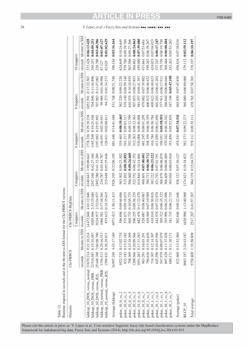
JID:FSS AID:6482 /FLA [m3SC+; v 1.188; Prn:4/03/2014; 14:35] P.28 (1-34)
28 V. López et al. / Fuzzy Sets and Systems ••• (••••) •••–•••
Tabl
e12
Run
time
elap
sed
inse
cond
san
din
the
hh:m
m:s
s.SS
Sfo
rmat
for
the
Chi
-FR
BC
Sve
rsio
ns.
Dat
aset
sC
hi-F
RB
CS
Chi
-FR
BC
S-B
igD
ata
2m
appe
rs4
map
pers
6m
appe
rs8
map
pers
16m
appe
rs
seco
nds
hh:m
m:s
s.SS
Sse
cond
shh
:mm
:ss.
SSS
seco
nds
hh:m
m:s
s.SS
Sse
cond
shh
:mm
:ss.
SSS
seco
nds
hh:m
m:s
s.SS
Sse
cond
shh
:mm
:ss.
SSS
kddc
up_1
0_D
OS_
vers
us_n
orm
al33
670.
214
9:21
:10.
214
1447
2.84
64:
01:1
2.84
641
40.6
431:
09:0
0.64
317
78.2
380:
29:3
8.23
810
52.5
010:
17:3
2.50
137
3.42
80:
06:1
3.42
8kd
dcup
_10_
DO
S_ve
rsus
_PR
B22
510.
587
6:15
:10.
587
9205
.046
2:33
:25.
046
2547
.166
0:42
:27.
166
1165
.548
0:19
:25.
548
704.
896
0:11
:44.
896
249.
251
0:04
:09.
251
kddc
up_1
0_D
OS_
vers
us_R
2L25
448.
700
7:04
:08.
700
9234
.977
2:33
:54.
977
2492
.280
0:41
:32.
280
1197
.892
0:19
:57.
892
707.
083
0:11
:47.
083
228.
386
0:03
:48.
386
kddc
up_1
0_no
rmal
_ver
sus_
PRB
1756
.513
0:29
:16.
513
1068
.581
0:17
:48.
581
234.
787
0:03
:54.
787
136.
951
0:02
:16.
951
99.9
860:
01:3
9.98
667
.127
0:01
:07.
127
kddc
up_1
0_no
rmal
_ver
sus_
R2L
1599
.831
0:26
:39.
831
875.
615
0:14
:35.
615
215.
648
0:03
:35.
648
128.
611
0:02
:08.
611
94.2
730:
01:3
4.27
362
.629
0:01
:02.
629
Ave
rage
(kdd
cup)
1699
7.16
94:
43:1
7.16
969
71.4
131:
56:1
1.41
319
26.1
050:
32:0
6.10
588
1.44
80:
14:4
1.44
853
1.74
80:
08:5
1.74
819
6.16
40:
03:1
6.16
4
poke
r_10
_0_v
s_2
1022
.735
0:17
:02.
735
586.
696
0:09
:46.
696
563.
302
0:09
:23.
302
519.
465
0:08
:39.
465
562.
220
0:09
:22.
220
624.
649
0:10
:24.
649
poke
r_10
_0_v
s_3
832.
182
0:13
:52.
182
575.
673
0:09
:35.
673
515.
892
0:08
:35.
892
543.
217
0:09
:03.
217
539.
140
0:08
:59.
140
579.
760
0:09
:39.
760
poke
r_10
_0_v
s_4
798.
369
0:13
:18.
369
605.
735
0:10
:05.
735
504.
460
0:08
:24.
460
552.
799
0:09
:12.
799
610.
555
0:10
:10.
555
567.
566
0:09
:27.
566
poke
r_10
_0_v
s_5
1209
.566
0:20
:09.
566
596.
255
0:09
:56.
255
522.
352
0:08
:42.
352
512.
363
0:08
:32.
363
507.
853
0:08
:27.
853
504.
863
0:08
:24.
863
poke
r_10
_0_v
s_6
1051
.263
0:17
:31.
263
682.
470
0:11
:22.
470
614.
844
0:10
:14.
844
536.
008
0:08
:56.
008
581.
397
0:09
:41.
397
459.
080
0:07
:39.
080
poke
r_10
_0_v
s_7
963.
291
0:16
:03.
291
520.
087
0:08
:40.
087
460.
601
0:07
:40.
601
481.
295
0:08
:01.
295
479.
882
0:07
:59.
882
473.
661
0:07
:53.
661
poke
r_10
_1_v
s_2
796.
636
0:13
:16.
636
439.
989
0:07
:19.
989
390.
712
0:06
:30.
712
398.
359
0:06
:38.
359
406.
932
0:06
:46.
932
399.
267
0:06
:39.
267
poke
r_10
_1_v
s_3
734.
307
0:12
:14.
307
410.
816
0:06
:50.
816
383.
222
0:06
:23.
222
416.
784
0:06
:56.
784
409.
623
0:06
:49.
623
424.
023
0:07
:04.
023
poke
r_10
_1_v
s_4
645.
596
0:10
:45.
596
442.
978
0:07
:22.
978
421.
791
0:07
:01.
791
411.
050
0:06
:51.
050
401.
203
0:06
:41.
203
377.
247
0:06
:17.
247
poke
r_10
_1_v
s_5
547.
979
0:09
:07.
979
395.
322
0:06
:35.
322
366.
879
0:06
:06.
879
358.
951
0:05
:58.
951
377.
911
0:06
:17.
911
379.
750
0:06
:19.
750
poke
r_10
_1_v
s_6
697.
428
0:11
:37.
428
393 .
996
0:06
:33.
996
366.
409
0:06
:06.
409
370.
342
0:06
:10.
342
366.
044
0:06
:06.
044
360.
484
0:06
:00.
484
poke
r_10
_1_v
s_7
690.
171
0:11
:30.
171
381.
735
0:06
:21.
735
363.
016
0:06
:03.
016
353.
859
0:05
:53.
859
347.
198
0:05
:47.
198
353.
263
0:05
:53.
263
Ave
rage
(pok
er)
832.
460
0:13
:52.
460
502.
646
0:08
:22.
646
456.
123
0:07
:36.
123
454.
541
0:07
:34.
541
465.
830
0:07
:45.
830
458.
634
0:07
:38.
634
RL
CP_
1086
83.1
872:
24:4
3.18
744
20.9
001:
13:4
0.90
011
74.8
230:
19:3
4.82
356
2.27
30:
09:2
2.27
336
9.08
00:
06:0
9.08
017
9.11
20:
02:5
9.11
2
Tota
lave
rage
5758
.809
1:35
:58.
809
2517
.207
0:41
:57.
207
904.
379
0:15
:04.
379
579.
111
0:09
:39.
111
478.
765
0:07
:58.
765
370.
197
0:06
:10.
197
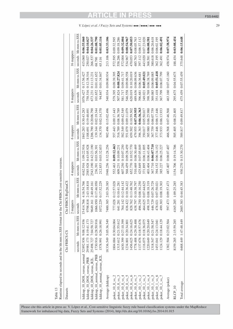
JID:FSS AID:6482 /FLA [m3SC+; v 1.188; Prn:4/03/2014; 14:35] P.29 (1-34)
V. López et al. / Fuzzy Sets and Systems ••• (••••) •••–••• 29
Tabl
e13
Run
time
elap
sed
inse
cond
san
din
the
hh:m
m:s
s.SS
Sfo
rmat
for
the
Chi
-FR
BC
Sco
st-s
ensi
tive
vers
ions
.
Dat
aset
sC
hi-F
RB
CS-
CS
Chi
-FR
BC
S-B
igD
ataC
S
2m
appe
rs4
map
pers
6m
appe
rs8
map
pers
16m
appe
rs
seco
nds
hh:m
m:s
s.SS
Sse
cond
shh
:mm
:ss.
SSS
seco
nds
hh:m
m:s
s.SS
Sse
cond
shh
:mm
:ss.
SSS
seco
nds
hh:m
m:s
s.SS
Sse
cond
shh
:mm
:ss.
SSS
kddc
up_1
0_D
OS_
vers
us_n
orm
al32
892.
936
9:08
:12.
936
1541
4.76
64:
16:5
4.76
641
62.9
161:
09:2
2.91
618
43.2
830:
30:4
3.28
310
76.4
270:
17:5
6.42
741
5.06
00:
06:5
5.06
0kd
dcup
_10_
DO
S_ve
rsus
_PR
B29
981.
173
8:19
:41.
173
9798
.818
2:43
:18.
818
2585
.928
0:43
:05.
928
1188
.691
0:19
:48.
691
758.
516
0:12
:38.
516
250.
027
0:04
:10.
027
kddc
up_1
0_D
OS_
vers
us_R
2L25
498.
727
7:04
:58.
727
9649
.161
2:40
:49.
161
2543
.190
0:42
:23.
190
1206
.790
0:20
:06.
790
673.
231
0:11
:13.
231
266.
537
0:04
:26.
537
kddc
up_1
0_no
rmal
_ver
sus_
PRB
1730
.916
0:28
:50.
916
1066
.950
0:17
:46.
950
236.
391
0:03
:56.
391
139.
344
0:02
:19.
344
101.
652
0:01
:41.
652
68.7
900:
01:0
8.79
0kd
dcup
_10_
norm
al_v
ersu
s_R
2L15
78.9
910:
26:1
8.99
110
72.2
290:
17:5
2.22
921
2.85
30:
03:3
2.85
313
4.37
00:
02:1
4.37
094
.847
0:01
:34.
847
65.1
160:
01:0
5.11
6
Ave
rage
(kdd
cup)
1833
6.54
95:
05:3
6.54
974
00.3
852:
03:2
0.38
519
48.2
560:
32:2
8.25
690
2.49
60:
15:0
2.49
654
0.93
40:
09:0
0.93
421
3.10
60:
03:3
3.10
6
poke
r_10
_0_v
s_2
1804
.004
0:30
:04.
004
777.
028
0:12
:57.
028
552.
463
0:09
:12.
463
557.
443
0:09
:17.
443
579.
395
0:09
:39.
395
572.
595
0:09
:32.
595
poke
r_10
_0_v
s_3
1315
.612
0:21
:55.
612
641.
281
0:10
:41.
281
609.
231
0:10
:09.
231
516.
789
0:08
:36.
789
507.
824
0:08
:27.
824
558.
286
0:09
:18.
286
poke
r_10
_0_v
s_4
1630
.399
0:27
:10.
399
764.
142
0:12
:44.
142
607.
250
0:10
:07.
250
582.
549
0:09
:42.
549
581.
717
0:09
:41.
717
572.
004
0:09
:32.
004
poke
r_10
_0_v
s_5
1234
.801
0:20
:34.
801
636.
422
0:10
:36.
422
568.
459
0:09
:28.
459
551.
079
0:09
:11.
079
546.
558
0:09
:06.
558
534.
967
0:08
:54.
967
poke
r_10
_0_v
s_6
1456
.625
0:24
:16.
625
828.
762
0:13
:48.
762
652.
770
0:10
:52.
770
659.
502
0:10
:59.
502
620.
019
0:10
:20.
019
470.
053
0:07
:50.
053
poke
r_10
_0_v
s_7
1778
.488
0:29
:38.
488
638.
797
0:10
:38.
797
510.
469
0:08
:30.
469
479.
955
0:07
:59.
955
489.
636
0:08
:09.
636
485.
763
0:08
:05.
763
poke
r_10
_1_v
s_2
1137
.676
0:18
:57.
676
496.
250
0:08
:16.
250
425.
849
0:07
:05.
849
396.
363
0:06
:36.
363
396.
681
0:06
:36.
681
397.
112
0:06
:37.
112
poke
r_10
_1_v
s_3
1116
.075
0:18
:36.
075
464.
625
0:07
:44.
625
371.
895
0:06
:11.
895
350.
017
0:05
:50.
017
349.
021
0:05
:49.
021
443.
020
0:07
:23.
020
poke
r_10
_1_v
s_4
1220
.649
0:20
:20.
649
498.
319
0:08
:18.
319
403.
404
0:06
:43.
404
385.
980
0:06
:25.
980
398.
769
0:06
:38.
769
368.
581
0:06
:08.
581
poke
r_10
_1_v
s_5
1318
.547
0:21
:58.
547
446.
729
0:07
:26.
729
367.
710
0:06
:07.
710
367.
759
0:06
:07.
759
369.
085
0:06
:09.
085
380.
618
0:06
:20.
618
poke
r_10
_1_v
s_6
1453
.041
0:24
:13.
041
478.
021
0:07
:58.
021
394.
152
0:06
:34.
152
377.
446
0:06
:17.
446
351.
418
0:05
:51.
418
362.
195
0:06
:02.
195
poke
r_10
_1_v
s_7
1124
.129
0:18
:44.
129
499.
303
0:08
:19.
303
385.
227
0:06
:25.
227
373.
933
0:06
:13.
933
367.
799
0:06
:07.
799
362.
491
0:06
:02.
491
Ave
rage
(pok
er)
1382
.504
0:23
:02.
504
597.
473
0:09
:57.
473
487.
407
0:08
:07.
407
466.
568
0:07
:46.
568
463.
160
0:07
:43.
160
458.
974
0:07
:38.
974
RL
CP_
1081
59.2
852:
15:5
9.28
541
65.2
851:
09:2
5.28
511
54.7
060:
19:1
4.70
650
5.40
50:
08:2
5.40
529
5.67
50:
04:5
5.67
518
8.45
40:
03:0
8.45
4
Tota
lave
rage
6468
.449
1:47
:48.
449
2685
.383
0:44
:45.
383
930.
270
0:15
:30.
270
589.
817
0:09
:49.
817
475.
459
0:07
:55.
459
375.
648
0:06
:15.
648

JID:FSS AID:6482 /FLA [m3SC+; v 1.188; Prn:4/03/2014; 14:35] P.30 (1-34)
30 V. López et al. / Fuzzy Sets and Systems ••• (••••) •••–•••
Fig. 4. Execution times for the kddcup_full_DOS_versus_U2R dataset.
advance is better observed when the number of mappers is smaller than in the larger cases, that is, when the dataavailable per mapper is considerable.
The second group is related to the Poker Hand cases of study, where the processing time gain is not as clear as inthe previous cases. Without a doubt, we can state there are huge differences between the sequential versions and theHadoop implementations. When the big data versions are compared, the runtime improvement can only be detectedfor the smaller values of the number of mappers. The Chi-FRBCS-BigData and Chi-FRBCS-BigDataCS algorithmsseem to no further improve their behavior starting from 16 mappers.
Table 14 shows the average runtime spent in seconds and in the hh:mm:ss.SSS format for the full cases of studyby the Chi-FRBCS-BigData and Chi-FRBCS-BigDataCS algorithms. This table is organized in two big parts: the firstpart is related to the results obtained by the Chi-FRBCS-BigData algorithm while the second part is related to theChi-FRBCS-BigDataCS method. Similarly to the preceding tables, these algorithms present their information in fourcolumns related to the number of mappers considered: 8, 16, 32 and 64 respectively. The sequential versions are notincluded in this table as they are not able to provide a result, as it was shown in the scalability studies (Sections 3.3and 4.2).
In this table, we can observe that the Chi-FRBCS-BigData approach shows a trend that slightly benefits its runtime,however, it does not always surpass the runtime achieved by the Chi-FRBCS-BigDataCS algorithm for any numberof mappers. These results can be understood in the following manner: the Chi-FRBCS-BigData approach is a lesscomplex approach than the Chi-FRBCS-BigDataCS method and therefore, the second algorithm is bound to spendmore processing time due to its additional operations. The usage of cost-sensitive learning is thus a good alternativeas this time addition is insignificant compared to the performance improvement gained in imbalanced datasets. InFig. 4, we can see the difference between the performance of the big data alternatives for the kddcup_full_DOS_ver-sus_U2R dataset, where the Chi-FRBCS-BigDataCS version consumes a bit more of time. However, the Chi-FRBCS-BigDataCS tends to produce a lesser number of rules (scalability studies in Sections 3.3 and 4.2), and therefore thesearch for identical rules may also be less computationally demanding.
In general, when larger values for the number of mappers are used, better runtime results are obtained for both theChi-FRBCS-BigData and the Chi-FRBCS-BigDataCS algorithms. However, the improvement in the processing timesis not linearly related to the number of mappers, as smaller number of mappers show a greater performance gain thanlarger values of mappers.
If we analyze the behavior of the groups of cases of study derived from the original datasets we can also observethe same groups of behavior as in the reduced cases of study previously considered. Again, a first group correspondsto the bigger cases of study, the ones derived from the KDD Cup 1999 dataset and the RLCP dataset. This groupdisplays the general trend extracted from all the data: the usage of higher number of mappers can get faster executiontimes, however, the runtime improvement is better appreciated with a reduced number of mappers instead of withlarger values, that means, when the data available per mapper is abundant. Fig. 4 also presents the trend in the usageof different mappers.
The second group is related to the Poker Hand cases of study, where it is not possible to discern an improvement inthe processing times. For the smaller values of the number of mappers, the results obtained show equivalent results,

JID:FSS AID:6482 /FLA [m3SC+; v 1.188; Prn:4/03/2014; 14:35] P.31 (1-34)
V. López et al. / Fuzzy Sets and Systems ••• (••••) •••–••• 31
Tabl
e14
Run
time
elap
sed
inse
cond
san
din
the
hh:m
m:s
s.SS
Sfo
rmat
for
the
big
data
Chi
-FR
BC
Sve
rsio
ns.
Dat
aset
sC
hi-F
RB
CS-
Big
Dat
aC
hi-F
RB
CS-
Big
Dat
aCS
8m
appe
rs16
map
pers
32m
appe
rs64
map
pers
8m
appe
rs16
map
pers
32m
appe
rs64
map
pers
seco
nds
hh:m
m:s
s.SS
Sse
cond
shh
:mm
:ss.
SSS
seco
nds
hh:m
m:s
s.SS
Sse
cond
shh
:mm
:ss.
SSS
seco
nds
hh:m
m:s
s.SS
Sse
cond
shh
:mm
:ss.
SSS
seco
nds
hh:m
m:s
s.SS
Sse
cond
shh
:mm
:ss.
SSS
kddc
up_D
OS_
vers
us_n
orm
al95
135.
040
26:2
5:35
.040
2642
2.54
67:
20:2
2.54
696
78.6
972:
41:1
8.69
740
60.9
081:
07:4
0.90
896
833.
551
26:5
3:53
.551
2582
4.46
97:
10:2
4.46
976
92.1
552:
08:1
2.15
534
07.8
010:
56:4
7.80
1kd
dcup
_DO
S_ve
rsus
_PR
B62
034.
217
17:1
3:54
.217
1720
6.96
14:
46:4
6.96
153
36.0
431:
28:5
6.04
353
10.4
061:
28:3
0.40
664
827.
368
18:0
0:27
.368
1800
3.64
95:
00:0
3.64
960
94.7
511:
41:3
4.75
151
34.6
971:
25:3
4.69
7kd
dcup
_DO
S_ve
rsus
_R2L
6090
8.73
816
:55:
08.7
3815
615.
652
4:20
:15.
652
6315
.864
1:45
:15.
864
1789
.012
0:29
:49.
012
6205
9.36
517
:14:
19.3
6516
897.
451
4:41
:37.
451
6122
.615
1:42
:02.
615
2047
.410
0:34
:07.
410
kddc
up_D
OS_
vers
us_U
2R60
942.
589
16:5
5:42
.589
1511
4.41
54:
11:5
4.41
542
88.9
561:
11:2
8.95
612
66.3
690:
21:0
6.36
963
665.
339
17:4
1:05
.339
1587
0.63
84:
24:3
0.63
843
02.0
371:
11:4
2.03
712
81.8
010:
21:2
1.80
1kd
dcup
_nor
mal
_ver
sus_
PRB
6059
.310
1:40
:59.
310
1765
.673
0:29
:25.
673
548.
857
0:09
:08.
857
262.
545
0:04
:22.
545
6155
.110
1:42
:35.
110
1523
.940
0:25
:23.
940
753.
089
0:12
:33.
089
301.
214
0:05
:01.
214
kddc
up_n
orm
al_v
ersu
s_R
2L43
62.3
391:
12:4
2.33
918
07.4
350:
30:0
7.43
545
1.02
70:
07:3
1.02
727
9.08
00:
04:3
9.08
045
02.8
561:
15:0
2.85
612
74.3
200:
21:1
4.32
050
3.81
40:
08:2
3.81
432
9.66
20:
05:2
9.66
2kd
dcup
_nor
mal
_ver
sus_
U2R
4279
.778
1:11
:19.
778
1899
.410
0:31
:39.
410
597.
729
0:09
:57.
729
350.
514
0:05
:50.
514
5064
.459
1:24
:24.
459
1290
.801
0:21
:30.
801
730.
109
0:12
:10.
109
327.
904
0:05
:27.
904
Ave
rage
(kdd
cup)
4196
0.28
711
:39:
20.2
8711
404.
584
3:10
:04.
584
3888
.167
1:04
:48.
167
1902
.691
0:31
:42.
691
4330
1.15
012
:01:
41.1
5011
526.
467
3:12
:06.
467
3742
.653
1:02
:22.
653
1832
.927
0:30
:32.
927
poke
r_0_
vs_2
1232
0.90
13:
25:2
0.90
112
325.
506
3:25
:25.
506
1283
9.60
83:
33:5
9.60
813
612.
564
3:46
:52.
564
1250
6.99
63:
28:2
6.99
612
083.
205
3:21
:23.
205
1285
1.93
63:
34:1
1.93
613
292.
345
3:41
:32.
345
poke
r_0_
vs_3
1140
1.85
53:
10:0
1.85
511
659.
858
3:14
:19.
858
1244
8.82
73:
27:2
8.82
713
212.
002
3:40
:12.
002
1148
4.09
83:
11:2
4.09
811
393.
884
3:09
:53.
884
1205
9.24
53:
20:5
9.24
512
349.
548
3:25
:49.
548
poke
r_0_
vs_4
1109
3.36
63:
04:5
3.36
611
244.
520
3:07
:24.
520
1215
5.16
23:
22:3
5.16
212
350.
617
3:25
:50.
617
1116
1.64
53:
06:0
1.64
511
380.
513
3:09
:40.
513
1209
6.64
53:
21:3
6.64
512
087.
170
3:21
:27.
170
poke
r_0_
vs_5
1094
7.36
33:
02:2
7.36
310
870.
675
3:01
:10.
675
1192
6.16
83:
18:4
6.16
812
341.
788
3:25
:41.
788
1137
0.87
03:
09:3
0.87
010
810.
724
3:00
:10.
724
1194
4.13
13:
19:0
4.13
112
262.
003
3:24
:22.
003
poke
r_0_
vs_6
1097
7.25
33:
02:5
7.25
311
041.
819
3:04
:01.
819
1167
4.87
73:
14:3
4.87
712
194.
412
3:23
:14.
412
1134
4.60
63:
09:0
4.60
611
260.
872
3:07
:40.
872
1191
5.54
33:
18:3
5.54
311
807.
885
3:16
:47.
885
poke
r_0_
vs_7
1097
1.63
13:
02:5
1.63
111
158.
933
3:05
:58.
933
1177
8.57
43:
16:1
8.57
412
228.
561
3:23
:48.
561
1185
1.59
53:
17:3
1.59
511
624.
443
3:13
:44.
443
1196
3.44
23:
19:2
3.44
211
887.
682
3:18
:07.
682
poke
r_0_
vs_8
1104
0.80
43:
04:0
0.80
411
088.
482
3:04
:48.
482
1161
5.55
73:
13:3
5.55
712
280.
418
3:24
:40.
418
1179
0.83
63:
16:3
0.83
611
227.
721
3:07
:07.
721
1167
9.05
93:
14:3
9.05
911
809.
133
3:16
:49.
133
poke
r_0_
vs_9
1105
9.62
93:
04:1
9.62
911
130.
037
3:05
:30.
037
1203
9.40
03:
20:3
9.40
011
956.
152
3:19
:16.
152
1138
6.51
13:
09:4
6.51
111
681.
637
3:14
:41.
637
1197
7.67
33:
19:3
7.67
312
152.
204
3:22
:32.
204
poke
r_1_
vs_2
1050
2 .98
52:
55:0
2.98
510
592.
520
2:56
:32.
520
1082
3.18
83:
00:2
3.18
811
550.
568
3:12
:30.
568
1025
6.90
82:
50:5
6.90
810
395.
012
2:53
:15.
012
1076
9.72
92:
59:2
9.72
911
198.
647
3:06
:38.
647
poke
r_1_
vs_3
9734
.080
2:42
:14.
080
1023
2.69
52:
50:3
2.69
510
770.
971
2:59
:30.
971
1064
3.13
42:
57:2
3.13
496
61.5
902:
41:0
1.59
097
69.4
422:
42:4
9.44
210
434.
828
2:53
:54.
828
1058
4.72
62:
56:2
4.72
6po
ker_
1_vs
_493
62.1
642:
36:0
2.16
495
99.1
782:
39:5
9.17
899
81.4
432:
46:2
1.44
310
553.
633
2:55
:53.
633
9443
.253
2:37
:23.
253
9752
.424
2:42
:32.
424
9765
.667
2:42
:45.
667
9806
.559
2:43
:26.
559
poke
r_1_
vs_5
9298
.083
2:34
:58.
083
9637
.974
2:40
:37.
974
1042
8.01
42:
53:4
8.01
410
399.
248
2:53
:19.
248
9412
.589
2:36
:52.
589
9506
.839
2:38
:26.
839
9942
.829
2:45
:42.
829
1026
2.90
22:
51:0
2.90
2po
ker_
1_vs
_690
09.7
792:
30:0
9.77
995
91.3
692:
39:5
1.36
910
112.
862
2:48
:32.
862
1040
7.75
22:
53:2
7.75
297
39.6
232:
42:1
9.62
398
54.6
072:
44:1
4.60
799
63.3
492:
46:0
3.34
910
095.
291
2:48
:15.
291
poke
r_1_
vs_7
9285
.360
2:34
:45.
360
9250
.462
2:34
:10.
462
9962
.175
2:46
:02.
175
1033
3.89
82:
52:1
3.89
895
80.9
272:
39:4
0.92
796
70.8
062:
41:1
0.80
610
300.
841
2:51
:40.
841
1027
6.78
62:
51:1
6.78
6po
ker_
1_vs
_895
45.0
552:
39:0
5.05
593
80.5
642:
36:2
0.56
498
72.0
842:
44:3
2.08
410
226.
082
2:50
:26.
082
9830
.342
2:43
:50.
342
9422
.569
2:37
:02.
569
9912
.194
2:45
:12.
194
1030
0.64
62:
51:4
0.64
6po
ker_
1_vs
_991
79.4
362:
32:5
9.43
694
38.3
472:
37:1
8.34
798
93.5
322:
44:5
3.53
210
335.
326
2:52
:15.
326
9776
.855
2:42
:56.
855
9844
.250
2:44
:04.
250
1019
5.10
82:
49:5
5.10
810
476.
054
2:54
:36.
054
Ave
rage
(pok
er)
1035
8.10
92:
52:3
8.10
910
515.
184
2:55
:15.
184
1114
5.15
33:
05:4
5.15
311
539.
135
3:12
:19.
135
1066
2.45
32:
57:4
2.45
310
604.
934
2:56
:44.
934
1111
0.76
43:
05:1
0.76
411
290.
599
3:08
:10.
599
RL
CP
2655
1.16
27:
22:3
1.16
270
89.9
991:
58:0
9.99
919
22.6
700:
32:0
2.67
060
6.83
10:
10:0
6.83
127
547.
418
7:39
:07.
418
7270
.635
2:01
:10.
635
1830
.273
0:30
:30.
273
721.
305
0:12
:01.
305
Fina
lave
rage
2025
0.12
25:
37:3
0.12
210
631.
876
2:57
:11.
876
8644
.262
2:24
:04.
262
8272
.992
2:17
:52.
992
2088
5.61
35:
48:0
5.61
310
734 .
785
2:58
:54.
785
8575
.044
2:22
:55.
044
8091
.724
2:14
:51.
724

JID:FSS AID:6482 /FLA [m3SC+; v 1.188; Prn:4/03/2014; 14:35] P.32 (1-34)
32 V. López et al. / Fuzzy Sets and Systems ••• (••••) •••–•••
however, when larger values of mappers are considered, the runtime does not improve and it can even become worse.This situation arises due to the smaller size of the Poker Hand cases of study.
Finally, it is necessary to recall that even when a larger number of mappers tend to provide better response times itmay not be wise to try to expand that number as much as possible. As we observed in Section 6.3.1, a large numberof mappers may cause a dramatically drop in the performance, an unwanted case when trying to extract informationfrom data. Therefore, it is needed to analyze the case under consideration to select an appropriate number of mappersfor the experiment. This number of mappers needs to provide a reasonable number of samples for each class to avoidthe small sample size problem and also enough data so that the experiments obtain lesser response times.
To sum up, our experimental study shows that cost-sensitive learning allows us to obtain better classification resultsfor the Chi-FRBCS algorithm. We have also observed that, in the big data versions, increasing the number of mappersdecreases the accuracy of the model, not only because the full information is not available but also because of theinduction of data intrinsic problems that difficult the classification with imbalanced datasets, such as the small samplesize problem. Finally, big data versions allow us to deal with huge amounts of data and obtain better response timeswhich are generally significantly decremented when the number of mappers of the original dataset is increased.
7. Concluding remarks
In this paper, we have introduced a linguistic cost-sensitive fuzzy rule-based classification method for imbalancedbig data called Chi-FRBCS-BigDataCS. Our aim was to obtain a model that is able to handle imbalanced big dataobtaining a good precision without incrementing the processing times. To do so, we use one of the most popularapproaches nowadays to deal with big data: the MapReduce framework, distributing the algorithm computing alongdifferent processing units using the map and reduce operations that have been adapted to the calculations of the fuzzyrule based classification system. We have also used cost-sensitive learning operations which have also modified thealgorithm to consider the misclassification costs, proposing a new approach, PCF-CS, to compute the rule weight thatconsider these costs in its operations.
The experiments conducted in this work demonstrate that the MapReduce framework is able of dealing with bigdata for fuzzy rule based classification systems. The use of a simple but effective fuzzy rule based classification systemsuch as the Chi et al.’s method as base of the approach has enabled the development of a proposal that can profit fromthis simplicity to create an efficient approach. The proposal, Chi-FRBCS-BigDataCS, can obtain classification resultswhen its sequential counterpart was not able to provide results. Furthermore, the runtime needed by the proposal isadmissible according to the results presented. The inclusion of cost-sensitive learning in its way of working, using thenew rule weight procedure PCF-CS, has demonstrated to be a powerful collaborator when dealing with imbalanceddatasets providing effective classification results without largely increasing the processing times.
The performance of our model, Chi-FRBCS-BigDataCS, has been tested in an experimental study includingtwenty-four imbalanced big data cases of study. These results corroborate the goodness of the integration of theapproaches that are used to solve the imbalanced problem and big data separately, namely the usage of the MapRe-duce framework and cost-sensitive learning. Furthermore, the synergy between both strategies alleviates some dataintrinsic problems, like the small sample size problem, that are induced because of the way the learning is done.
Acknowledgements
This work was partially supported by the Spanish Ministry of Science and Technology under project TIN2011-28488 and the Andalusian Research Plans P11-TIC-7765 and P10-TIC-6858. V. López holds a FPU scholarship fromSpanish Ministry of Education.
References
[1] IBM, What is big data? Bringing big data to the enterprise, [Online; accessed December 2013], http://www-01.ibm.com/software/data/bigdata/, 2012.
[2] P. Zikopoulos, C. Eaton, D. DeRoos, T. Deutsch, G. Lapis, Understanding Big Data: Analytics for Enterprise Class Hadoop and StreamingData, McGraw-Hill, 2011.
[3] S. Madden, From databases to big data, IEEE Internet Comput. 16 (3) (2012) 4–6.[4] A. Sathi, Big Data Analytics: Disruptive Technologies for Changing the Game, MC Press, 2012.

JID:FSS AID:6482 /FLA [m3SC+; v 1.188; Prn:4/03/2014; 14:35] P.33 (1-34)
V. López et al. / Fuzzy Sets and Systems ••• (••••) •••–••• 33
[5] H. He, E.A. Garcia, Learning from imbalanced data, IEEE Trans. Knowl. Data Eng. 21 (9) (2009) 1263–1284.[6] Y. Sun, A.K.C. Wong, M.S. Kamel, Classification of imbalanced data: A review, Int. J. Pattern Recognit. Artif. Intell. 23 (4) (2009) 687–719.[7] V. López, A. Fernández, S. García, V. Palade, F. Herrera, An insight into classification with imbalanced data: Empirical results and current
trends on using data intrinsic characteristics, Inf. Sci. 250 (2013) 113–141.[8] H. Ishibuchi, T. Nakashima, M. Nii, Classification and Modeling with Linguistic Information Granules: Advanced Approaches to Linguistic
Data Mining, Springer-Verlag, 2004.[9] Y. Jin, Fuzzy modeling of high-dimensional systems: complexity reduction and interpretability improvement, IEEE Trans. Fuzzy Syst. 8 (2)
(2000) 212–221.[10] T.-P. Hong, Y.-C. Lee, M.-T. Wu, An effective parallel approach for genetic-fuzzy data mining, Expert Syst. Appl. 41 (2) (2014) 655–662.[11] M. Rodríguez, D. Escalante, A. Peregrín, Efficient distributed genetic algorithm for rule extraction, Appl. Soft Comput. 11 (1) (2011) 733–743.[12] Y. Nojima, H. Ishibuchi, I. Kuwajima, Parallel distributed genetic fuzzy rule selection, Soft Comput. 13 (5) (2009) 511–519.[13] I. Robles, R. Alcalá, J. Benítez, F. Herrera, Evolutionary parallel and gradually distributed lateral tuning of fuzzy rule-based systems, Evol.
Intel. 2 (1–2) (2009) 5–19.[14] H. Ishibuchi, S. Mihara, Y. Nojima, Parallel distributed hybrid fuzzy GBML models with rule set migration and training data rotation, IEEE
Trans. Fuzzy Syst. 21 (2) (2013) 355–368.[15] V. López, A. Fernández, J.G. Moreno-Torres, F. Herrera, Analysis of preprocessing vs. cost-sensitive learning for imbalanced classification.
Open problems on intrinsic data characteristics, Expert Syst. Appl. 39 (7) (2012) 6585–6608.[16] N.V. Chawla, K.W. Bowyer, L.O. Hall, W.P. Kegelmeyer SMOTE, Synthetic minority over-sampling technique, J. Artif. Intell. Res. 16 (2002)
321–357.[17] G.E.A.P.A. Batista, R.C. Prati, M.C. Monard, A study of the behaviour of several methods for balancing machine learning training data,
SIGKDD Explor. 6 (1) (2004) 20–29.[18] C. Elkan, The foundations of cost–sensitive learning, in: Proceedings of the 17th IEEE International Joint Conference on Artificial Intelligence
(IJCAI’01), 2001, pp. 973–978.[19] B. Zadrozny, C. Elkan, Learning and making decisions when costs and probabilities are both unknown, in: Proceedings of the 7th International
Conference on Knowledge Discovery and Data Mining (KDD’01), 2001, pp. 204–213.[20] J. Dean, S. Ghemawat, MapReduce: Simplified data processing on large clusters, Commun. ACM 51 (1) (2008) 107–113.[21] M. Wasikowski, X.-W. Chen, Combating the small sample class imbalance problem using feature selection, IEEE Trans. Knowl. Data Eng.
22 (10) (2010) 1388–1400.[22] J.G. Moreno-Torres, T. Raeder, R. Aláiz-Rodríguez, N.V. Chawla, F. Herrera, A unifying view on dataset shift in classification, Pattern
Recognit. 45 (1) (2012) 521–530.[23] Z. Chi, H. Yan, T. Pham, Fuzzy Algorithms with Applications to Image Processing and Pattern Recognition, World Scientific, 1996.[24] T. Nakashima, G. Schaefer, Y. Yokota, H. Ishibuchi, Weighted fuzzy classifier and its application to image processing tasks, Fuzzy Sets Syst.
158 (2007) 284–294.[25] V. López, A. Fernández, M.J. del Jesus, F. Herrera, A hierarchical genetic fuzzy system based on genetic programming for addressing classi-
fication with highly imbalanced and borderline data-sets, Knowl.-Based Syst. 38 (2013) 85–104.[26] A. Fernández, S. García, M.J. del Jesus, F. Herrera, A study of the behaviour of linguistic fuzzy rule based classification systems in the
framework of imbalanced data-sets, Fuzzy Sets Syst. 159 (18) (2008) 2378–2398.[27] A. Fernández, M.J. del Jesus, F. Herrera, Hierarchical fuzzy rule based classification systems with genetic rule selection for imbalanced
data-sets, Int. J. Approx. Reason. 50 (3) (2009) 561–577.[28] K. Napierala, J. Stefanowski, S. Wilk, Learning from imbalanced data in presence of noisy and borderline examples, in: Proceedings of the 7th
International Conference on Rough Sets and Current Trends in Computing, RSCTC’10, in: Lecture Notes on Artificial Intelligence, vol. 6086,2010, pp. 158–167.
[29] J.A. Sáez, J. Luengo, F. Herrera, A first study on the noise impact in classes for fuzzy rule based classification systems, in: Proceedings of the2010 IEEE International Conference on Intelligent Systems and Knowledge Engineering, ISKE’10, IEEE Press, 2010, pp. 153–158.
[30] G.M. Weiss, The impact of small disjuncts on classifier learning, in: R. Stahlbock, S.F. Crone, S. Lessmann (Eds.), Data Mining, in: Annalsof Information Systems, vol. 8, Springer, 2010, pp. 193–226.
[31] J. Huang, C.X. Ling, Using AUC and accuracy in evaluating learning algorithms, IEEE Trans. Knowl. Data Eng. 17 (3) (2005) 299–310.[32] T. White, Hadoop, The Definitive Guide, O’Reilly Media, Inc., 2012.[33] D. Laney, 3D data management: Controlling data volume, velocity, and variety, META Group, 2001, Tech. rep., [Online; accessed December
2013], http://blogs.gartner.com/doug-laney/files/2012/01/ad949-3D-Data-Management-Controlling-Data-Volume-Velocity-and-Variety.pdf.[34] M. Beyer, Gartner says solving big data challenge involves more than just managing volumes of data, [Online; accessed December 2013],
2011, http://www.gartner.com/newsroom/id/1731916.[35] M. Beyer, D. Laney, The importance of big data: A definition, ID: G00235055, Retrieved from Gartner database [Online; accessed December
2013], 2012, http://www.gartner.com/id=2057415.[36] J. Dean, S. Ghemawat, MapReduce: Simplified data processing on large clusters, in: Proceedings of the 6th Symposium on Operating System
Design and Implementation, OSDI 2004, 2004, pp. 137–150.[37] J. Dean, S. Ghemawat, MapReduce: A flexible data processing tool, Commun. ACM 53 (1) (2010) 72–77.[38] C. Lam, Hadoop in Action, Manning Publications Co., 2010.[39] S. Owen, R. Anil, T. Dunning, E. Friedman, Mahout in Action, Manning Publications Co., 2011.[40] J. Lin, MapReduce is good enough? If all you have is a hammer, throw away everything that’s not a nail!, Big Data 1 (1) (2013) 28–37.[41] M. Zaharia, M. Chowdhury, T. Das, A. Dave, J. Ma, M. McCauley, M. Franklin, S. Shenker, I. Stoica, Resilient distributed datasets: A
fault-tolerant abstraction for in-memory cluster computing, in: Proceedings of the 9th USENIX Symposium on Networked Systems Designand Implementation, NSDI 2012, 2012.

JID:FSS AID:6482 /FLA [m3SC+; v 1.188; Prn:4/03/2014; 14:35] P.34 (1-34)
34 V. López et al. / Fuzzy Sets and Systems ••• (••••) •••–•••
[42] Apache Drill Project, Apache Drill, 2013, [Online; December 2013, accessed], http://incubator.apache.org/drill/.[43] J. Ekanayake, H. Li, B. Zhang, T. Gunarathne, S.-H. Bae, J. Qiu, G. Fox, Twister: a runtime for iterative MapReduce, in: Proceedings of the
19th ACM International Symposium on High Performance Distributed Computing (HPDC 2010), 2010, pp. 810–818.[44] S. Das, Y. Sismanis, K.S. Beyer, R. Gemulla, P.J. Haas, J. McPherson, Ricardo: integrating R and Hadoop, in: Proceedings of the ACM
SIGMOD International Conference on Management of Data (SIGMOD 2010), 2010, pp. 987–998.[45] M. Bostock, O.V., J. Heer, D3 data-driven documents, IEEE Trans. Vis. Comput. Graph. 17 (12) (2011) 2301–2309.[46] HCatalog, Hcatalog, [Online; accessed December 2013, accessed] http://hive.apache.org/hcatalog/ (2013).[47] J. Leibiusky, G. Eisbruch, D. Simonassi, Getting Started with Storm, O’Reilly Media, Inc., 2012.[48] Cloudera, Cloudera Impala, [Online; accessed December 2013] (2013). http://www.cloudera.com/content/cloudera/en/products/cdh/
impala.html.[49] Q. Yang, X. Wu, 10 challenging problems in data mining research, Int. J. Inf. Technol. Decis. Mak. 5 (4) (2006) 597–604.[50] T. Khoshgoftaar, K. Gao, A. Napolitano, R. Wald, A comparative study of iterative and non-iterative feature selection techniques for software
defect prediction, Inf. Syst. Front., in press, http://dx.doi.org/10.1007/s10796-013-9430-0.[51] S. Wang, X. Yao, Using class imbalance learning for software defect prediction, IEEE Trans. Reliab. 62 (2) (2013) 434–443.[52] L. Zhou, Performance of corporate bankruptcy prediction models on imbalanced dataset: The effect of sampling methods, Knowl.-Based Syst.
41 (2013) 16–25.[53] A. Gudys, M. Szczesniak, M. Sikora, I. Makalowska, HuntMi: An efficient and taxon-specific approach in pre-miRNA identification, BMC
Bioinform. 14 (2013) 1–10, Article number 83.[54] Q. Wei, R. Dunbrack Jr., The role of balanced training and testing data sets for binary classifiers in bioinformatics, PLoS ONE 8 (7) (2013)
1–12, Article number e67863.[55] H. Yu, J. Ni, J. Zhao, ACOSampling: An ant colony optimization-based undersampling method for classifying imbalanced DNA microarray
data, Neurocomputing 101 (2013) 309–318.[56] Y.-H. Lee, P. Hu, T.-H. Cheng, T.-C. Huang, W.-Y. Chuang, A preclustering-based ensemble learning technique for acute appendicitis diag-
noses, Artif. Intell. Med. 58 (2) (2013) 115–124.[57] J. Nahar, T. Imam, K. Tickle, Y.-P. Chen, Computational intelligence for heart disease diagnosis: A medical knowledge driven approach,
Expert Syst. Appl. 40 (1) (2013) 96–104.[58] A. Orriols-Puig, E. Bernadó-Mansilla, Evolutionary rule-based systems for imbalanced datasets, Soft Comput. 13 (3) (2009) 213–225.[59] V. García, R.A. Mollineda, J.S. Sánchez, On the k-NN performance in a challenging scenario of imbalance and overlapping, Pattern Anal.
Appl. 11 (3–4) (2008) 269–280.[60] C. Seiffert, T.M. Khoshgoftaar, J. Van Hulse, A. Folleco, An empirical study of the classification performance of learners on imbalanced and
noisy software quality data, Inf. Sci. 259 (2014) 571–595.[61] J. Stefanowski, Overlapping, rare examples and class decomposition in learning classifiers from imbalanced data, in: Smart Innovation,
Systems and Technologies, vol. 13, 2013, pp. 277–306.[62] A. Storkey, When training and test sets are different: Characterizing learning transfer, in: J. Quiñonero-Candela, M. Sugiyama, A.
Schwaighofer, N.D. Lawrence (Eds.), Dataset Shift in Machine Learning, MIT Press, 2009, pp. 3–28.[63] H. Shimodaira, Improving predictive inference under covariate shift by weighting the log-likelihood function, J. Stat. Plan. Inference 90 (2)
(2000) 227–244.[64] V. López, I. Triguero, C. Carmona, S. García, F. Herrera, Addressing imbalanced classification with instance generation techniques: IPADE-ID,
Neurocomputing 126 (2014) 15–28.[65] P. Domingos, MetaCost: A general method for making classifiers cost-sensitive, in: Proceedings of the 5th International Conference on
Knowledge Discovery and Data Mining (KDD’99), 1999, pp. 155–164.[66] B. Zadrozny, J. Langford, N. Abe, Cost-sensitive learning by cost-proportionate example weighting, in: Proceedings of the 3rd IEEE Interna-
tional Conference on Data Mining (ICDM’03), 2003, pp. 435–442.[67] M. Galar, A. Fernández, E. Barrenechea, H. Bustince, F. Herrera, A review on ensembles for class imbalance problem: Bagging, boosting and
hybrid based approaches, IEEE Trans. Syst. Man Cybern., Part C, Appl. Rev. 42 (4) (2012) 463–484.[68] A.P. Bradley, The use of the area under the ROC curve in the evaluation of machine learning algorithms, Pattern Recognit. 30 (7) (1997)
1145–1159.[69] H. Ishibuchi, T. Nakashima, Effect of rule weights in fuzzy rule-based classification systems, IEEE Trans. Fuzzy Syst. 9 (4) (2001) 506–515.[70] H. Ishibuchi, T. Yamamoto, Rule weight specification in fuzzy rule-based classification systems, IEEE Trans. Fuzzy Syst. 13 (2005) 428–435.[71] O. Cordón, M.J. del Jesus, F. Herrera, A proposal on reasoning methods in fuzzy rule-based classification systems, Int. J. Approx. Reason.
20 (1) (1999) 21–45.[72] L.X. Wang, J.M. Mendel, Generating fuzzy rules by learning from examples, IEEE Trans. Syst. Man Cybern. 22 (6) (1992) 1414–1427.[73] K. Bache, M. Lichman, UCI machine learning repository, [Online; accessed December 2013], 2013, http://archive.ics.uci.edu/ml.[74] M. Fazzolari, B. Giglio, R. Alcalá, F. Marcelloni, F. Herrera, A study on the application of instance selection techniques in genetic fuzzy
rule-based classification systems: Accuracy-complexity trade-off, Knowl.-Based Syst. 54 (2014) 32–41.[75] J. Alcalá-Fdez, L. Sánchez, S. García, M.J. del Jesus, S. Ventura, J.M. Garrell, J. Otero, C. Romero, J. Bacardit, V.M. Rivas, J.C. Fernández,
F. Herrera, KEEL: a software tool to assess evolutionary algorithms for data mining problems, Soft Comput. 13 (2009) 307–318.[76] J. Alcalá-Fdez, A. Fernández, J. Luengo, J. Derrac, S. García, L. Sánchez, F. Herrera, KEEL data-mining software tool: Data set repository,
integration of algorithms and experimental analysis framework, J. Mult.-Valued Log. Soft Comput. 17 (2–3) (2011) 255–287.


Bibliography
[ACW06] Au W. H., Chan K. C. C., and Wong A. K. C. (2006) A fuzzy approach to partitio-ning continuous attributes for classification. IEEE Transactions on Knowledge andData Engineering 18(5): 715–719.
[ADA11] Agrawal D., Das S., and Abbadi A. E. (2011) Big data and cloud computing: currentstate and future opportunities. In Proceedings of the 14th International Conferenceon Extending Database Technology (EDBT 2011), pp. 530–533.
[AKA91] Aha D., Kibler D., and Albert M. (1991) Instance-based learning algorithms. Ma-chine Learning 6(1): 37–66.
[Alp04] Alpaydin E. (2004) Introduction to Machine Learning. The MIT Press.
[BF99] Brodley C. E. and Friedl M. A. (1999) Identifying mislabeled training data. Journalof Artificial Intelligence Research 11: 131–167.
[BIYM14] Barua S., Islam M., Yao X., and Murase K. (2014) MWMOTE-Majority WeightedMinority Oversampling Technique for imbalanced data set learning. IEEE Transac-tions on Knowledge and Data Engineering 26(2): 405–425.
[BJZY13] Bhowan U., Johnston M., Zhang M., and Yao X. (2013) Evolving diverse ensemblesusing genetic programming for classification with unbalanced data. IEEE Transac-tions on Evolutionary Computation 17(3): 368–386.
[BP10] Batuwita R. and Palade V. (2010) FSVM-CIL: Fuzzy support vector machines forclass imbalance learning. IEEE Transactions on Fuzzy Systems 18(3): 558–571.
[BPM04] Batista G. E. A. P. A., Prati R. C., and Monard M. C. (2004) A study of thebehavior of several methods for balancing machine learning training data. SIGKDDExplorations Newsletter 6(1): 20–29.
[BRdJH10] Berlanga F., Rivera A., del Jesus M., and Herrera F. (2010) GP-COACH: Geneticprogramming-based learning of compact and accurate fuzzy rule-based classificationsystems for high-dimensional problems. Information Sciences 180(8): 1183 – 1200.
[BSL12] Bunkhumpornpat C., Sinapiromsaran K., and Lursinsap C. (2012) DBSMOTE:Density-Based Synthetic Minority Over-sampling TEchnique. Applied Intelligen-ce 36(3): 664–684.
[CBHK02] Chawla N. V., Bowyer K. W., Hall L. O., and Kegelmeyer W. P. (2002) SMO-TE: Synthetic minority over-sampling technique. Journal of Artificial IntelligenceResearch 16: 321–357.
169

170 BIBLIOGRAPHY
[CCHJ08] Chawla N. V., Cieslak D. A., Hall L. O., and Joshi A. (2008) Automatically counte-ring imbalance and its empirical relationship to cost. Data Mining and KnowledgeDiscovery 17(2): 225–252.
[CDG+08] Chang F., Dean J., Ghemawat S., Hsieh W. C., Wallach D. A., Burrows M., ChandraT., Fikes A., and Gruber R. E. (2008) Bigtable: A distributed storage system forstructured data. ACM Transactions on Computer Systems 26(2).
[CdJH99] Cordon O., del Jesus M., and Herrera F. (1999) A proposal on reasoning methodsin fuzzy rule-based classification systems. International Journal of ApproximateReasoning 20(1): 21–45.
[CHV00] Cordon O., Herrera F., and Villar P. (2000) Analysis and guidelines to obtain a gooduniform fuzzy partition granularity for fuzzy rule-based systems using simulatedannealing. International Journal on Approximate Reasoning 25(3): 187–215.
[CJK04] Chawla N. V., Japkowicz N., and Kolcz A. (2004) Special issue on learning fromimbalanced datasets. SIGKDD Explorations Newsletter 6(1): 1–6.
[CV95] Cortes C. and Vapnik V. (1995) Support vector networks. Machine Learning 20:273–297.
[CW03] Chen Y. and Wang J. Z. (2003) Support vector learning for fuzzy rule-based classi-fication systems. IEEE Transactions on Fuzzy Systems 11(6): 716–728.
[CYP96] Chi Z., Yan H., and Pham T. (1996) Fuzzy algorithms with applications to imageprocessing and pattern recognition. World Scientific.
[DG08] Dean J. and Ghemawat S. (2008) MapReduce: simplified data processing on largeclusters. Commununications of the ACM 51(1): 107–113.
[DGS+90] DeWitt D. J., Ghandeharizadeh S., Schneider D. A., Bricker A., Hsiao H. I., andRasmussen R. (1990) The gamma database machine project. IEEE Transactions onKnowledge and Data Engineering 2(1): 44–62.
[DHS01] Duda R. O., Hart P. E., and Stork D. G. (2001) Pattern Classification. Wiley-Interscience.
[DKS09] Drown D. J., Khoshgoftaar T. M., and Seliya N. (2009) Evolutionary samplingand software quality modeling of high-assurance systems. IEEE Transactions onSystems, Man, and Cybernetics, Part A 39(5): 1097–1107.
[DT10] Denil M. and Trappenberg T. (2010) Overlap versus imbalance. In Proceedings ofthe 23rd Canadian Conference on advances in Artificial Intelligence (CCAI’10), pp.220–231.
[FdJH09] Fernandez A., del Jesus M. J., and Herrera F. (2009) Hierarchical fuzzy rule basedclassification systems with genetic rule selection for imbalanced data-sets. Interna-tional Journal of Approximate Reasoning 50(3): 561–577.
[FdJH10] Fernandez A., del Jesus M. J., and Herrera F. (2010) On the 2–tuples based genetictuning performance for fuzzy rule based classification systems in imbalanced data–sets. Information Sciences 180(8): 1268–1291.

BIBLIOGRAPHY 171
[FGdJH08] Fernandez A., Garcıa S., del Jesus M. J., and Herrera F. (2008) A study of thebehaviour of linguistic fuzzy rule based classification systems in the framework ofimbalanced data–sets. Fuzzy Sets and Systems 159(18): 2378–2398.
[FGL+10] Fernandez A., Garcıa S., Luengo J., Bernado-Mansilla E., and Herrera F. (2010)Genetics-based machine learning for rule induction: State of the art, taxonomy andcomparative study. IEEE Transactions on Evolutionary Computation 14(6): 913–941.
[FPSS96] Fayyad U., Piatetsky-Shapiro G., and Smyth P. (1996) From data mining to know-ledge discovery in databases. AI Magazine 17(3): 37–54.
[GGM12] Gupta R., Gupta H., and Mohania M. (2012) Cloud computing and big data analy-tics: What is new from databases perspective? In Proceedings of the First Interna-tional Conference on Big Data Analytics (BDA 2012), pp. 42–61.
[GLDS96] Gropp W., Lusk E. L., Doss N. E., and Skjellum A. (1996) A high-performance,portable implementation of the mpi message passing interface standard. ParallelComputing 22(6): 789–828.
[GMS08] Garcıa V., Mollineda R. A., and Sanchez J. S. (2008) On the k–NN performance ina challenging scenario of imbalance and overlapping. Pattern Analysis Applications11(3–4): 269–280.
[Gol89] Goldberg D. E. (1989) Genetic Algorithms in Search, Optimization and MachineLearning. Addison-Wesley.
[Gur97] Gurney K. N. (1997) An introduction to neural networks. Morgan Kaufmann.
[HB02] Ho T. K. and Basu M. (2002) Complexity measures of supervised classificationproblems. IEEE Transactions on Pattern Analysis and Machine Intelligence 24(3):289–300.
[HG09] He H. and Garcia E. A. (2009) Learning from imbalanced data. IEEE Transactionson Knowledge and Data Engineering 21(9): 1263–1284.
[HHLD11] Han J., Haihong E., Le G., and Du J. (2011) Survey on NoSQL database. InProceedings of the 2011 6th International Conference on Pervasive Computing andApplications (ICPCA 2011), pp. 363–366.
[HV03] Hand D. J. and Vinciotti V. (2003) Choosing k for two–class nearest neighbourclassifiers with unbalanced classes. Pattern Recognition Letters 24: 1555–1562.
[INN04] Ishibuchi H., Nakashima T., and Nii M. (2004) Classification and modeling withlinguistic information granules: Advanced approaches to linguistic Data Mining.Springer–Verlag.
[IY05] Ishibuchi H. and Yamamoto T. (2005) Rule weight specification in fuzzy rule-basedclassification systems. IEEE Transactions on Fuzzy Systems 13: 428–435.
[IYN05] Ishibuchi H., Yamamoto T., and Nakashima T. (2005) Hybridization of fuzzy GBMLapproaches for pattern classification problems. IEEE Transactions on System, Manand Cybernetics B 35(2): 359–365.
172 BIBLIOGRAPHY
[JS02] Japkowicz N. and Stephen S. (2002) The class imbalance problem: a systematicstudy. Intelligent Data Analysis Journal 6(5): 429–450.
[Kon05] Konar A. (2005) Computational Intelligence: Principles, Techniques and Applica-tions. Springer-Verlag.
[KR14] Kuncheva L. I. and Rodrıguez J. J. (2014) A weighted voting framework for classifiersensembles. Knowledge and Information Systems 38(2): 259–275.
[Kra13] Kraska T. (2013) Finding the needle in the big data systems haystack. IEEE InternetComputing 17(1): 84–86.
[Kun00] Kuncheva L. (2000) Fuzzy classifier design. Springer.
[Lam11] Lam C. (2011) Hadoop in action. Manning.
[LFH10] Lopez V., Fernandez A., and Herrera F. (2010) A first approach for cost–sensitiveclassification with linguistic genetic fuzzy systems in imbalanced data–sets. In Pro-ceedings of the 10th International Conference on Intelligent Systems Design andApplications (ISDA’10), pp. 676–681.
[LJ12] Labrinidis A. and Jagadish H. V. (2012) Challenges and opportunities with big data.Proceedings of the VLDB Endowment 5(12): 2032–2033.
[LTY13] Lin M., Tang K., and Yao X. (2013) Dynamic sampling approach to training neu-ral networks for multiclass imbalance classification. IEEE Transactions on NeuralNetworks and Learning Systems 24(4): 647–660.
[LWZ09] Liu X. Y., Wu J., and Zhou Z. H. (2009) Exploratory undersampling for class-imbalance learning. IEEE Transactions on System, Man and Cybernetics, Part B39(2): 539–550.
[Mad12] Madden S. (2012) From databases to big data. IEEE Internet Computing 16(3):4–6.
[Mam74] Mamdani E. (1974) Applications of fuzzy algorithm for control a simple dynamicplant. Proceedings of the Institution of Electrical Engineers 121(12): 1585–1588.
[MTH10] Moreno-Torres J. G. and Herrera F. (2010) A preliminary study on overlappingand data fracture in imbalanced domains by means of genetic programming-basedfeature extraction. In Proceedings of the 10th International Conference on IntelligentSystems Design and Applications (ISDA’10), pp. 501–506.
[MTSH12] Moreno-Torres J., Saez J., and Herrera F. (2012) Study on the impact of partition-induced dataset shift on k-fold cross-validation. IEEE Transactions on Neural Net-works and Learning Systems 23(8): 1304–1312.
[NSW] Napierala K., Stefanowski J., and Wilk S.Learning from imbalanced data in presenceof noisy and borderline examples.
[NSW10] Napierala K., Stefanowski J., and Wilk S. (2010) Learning from imbalanced data inpresence of noisy and borderline examples. In Proceedings of the 7th InternationalConference on Rough Sets and Current Trends in Computing (RSCTC’10), pp. 158–167.

BIBLIOGRAPHY 173
[OPBM09] Orriols-Puig A. and Bernado-Mansilla E. (2009) Evolutionary rule–based systemsfor imbalanced datasets. Soft Computing 13(3): 213–225.
[OPBMG+09] Orriols-Puig A., Bernado-Mansilla E., Goldberg D. E., Sastry K., and Lanzi P. L.(2009) Facetwise analysis of XCS for problems with class imbalances. IEEE Tran-sactions on Evolutionary Computation 13: 260–283.
[Pet07] Peters J. (2007) Book review: Computational intelligence: Principles, techniques andapplications by Amit Konar. The Computer Journal 50(6): 758.
[Pyl99] Pyle D. (1999) Data Preparation for Data Mining. Morgan Kaufmann.
[Qui93] Quinlan J. R. (1993) C4.5: Programs for Machine Learning. Morgan Kaufmann.
[RJ91] Raudys S. J. and Jain A. K. (1991) Small sample size effects in statistical patternrecognition: Recommendations for practitioners. IEEE Transactions on PatternAnalysis and Machine Intelligence 13(3): 252–264.
[RJBF+80] Rothnie Jr. J. B., Bernstein P. A., Fox S., Goodman N., Hammer M., LandersT. A., Reeve C. L., Shipman D. W., and Wong E. (1980) Introduction to a systemfor distributed databases (SDD-1). ACM Transactions on Database Systems 5(1):1–17.
[SAM96] Shafer J., Agrawal R., and Mehta M. (1996) Sprint: A scalable parallel classifier fordata mining. In Proceedings of the 22th International Conference on Very LargeData Bases (VLDB’96), pp. 544–555.
[Shi00] Shimodaira H. (2000) Improving predictive inference under Covariate Shift byWeighting the Log-likelihood Function. Journal of Statistical Planning and Infe-rence 90(2): 227–244.
[SJ12] Schlieski T. and Johnson B. D. (2012) Entertainment in the age of big data. Pro-ceedings of the IEEE 100(Special Centennial Issue): 1404–1408.
[SKVHF14] Seiffert C., Khoshgoftaar T. M., Van Hulse J., and Folleco A. (2014) An empiricalstudy of the classification performance of learners on imbalanced and noisy softwarequality data. Information Sciences 259: 571–595.
[SKVHN10] Seiffert C., Khoshgoftaar T. M., Van Hulse J., and Napolitano A. (2010) RUSBoost:A hybrid approach to alleviating class imbalance. IEEE Transactions on System,Man and Cybernetics, Part A 40(1): 185–197.
[SKWW07] Sun Y., Kamel M. S., Wong A. K. C., and Wang Y. (2007) Cost–sensitive boostingfor classification of imbalanced data. Pattern Recognition 40(12): 3358–3378.
[SLH10] Saez J., Luengo J., and Herrera F. (2010) A first study on the noise impact inclasses for fuzzy rule based classification systems. In 2010 International Conferenceon Intelligent Systems and Knowledge Engineering (ISKE2010), pp. 153–158.
[SWK09] Sun Y., Wong A. K. C., and Kamel M. S. (2009) Classification of imbalanced data:A review. International Journal of Pattern Recognition and Artificial Intelligence23(4): 687–719.

174 BIBLIOGRAPHY
[The12] The Apache Software Foundation (2012) Hadoop, an open source implementationof MapReduce and GFS.
[Tin02] Ting K. M. (2002) An instance–weighting method to induce cost–sensitive trees.IEEE Transactions on Knowledge and Data Engineering 14(3): 659–665.
[TSK06] Tan P. N., Steinbach M., and Kumar V. (2006) Introduction to Data Mining.Addison-Wesley.
[VCC99] Veropoulos K., Campbell C., and Cristianini N. (1999) Controlling the sensitivityof support vector machines. In Proceedings of the International Joint Conferenceon Artificial Intelligence (IJCAI’99), pp. 55–60.
[VHKN09] Van Hulse J., Khoshgoftaar T. M., and Napolitano A. (2009) An empirical com-parison of repetitive undersampling techniques. In Proceedings of the 2009 IEEEInternational Conference on Information Reuse Integration (IRI’09), pp. 29–34.
[Wei05] Weiss G. M. (2005) Mining with rare cases. In Maimon O. and Rokach L. (Eds.)The Data Mining and Knowledge Discovery Handbook, pp. 765–776. Springer.
[Wei10] Weiss G. M. (2010) The impact of small disjuncts on classifier learning. In StahlbockR., Crone S. F., and Lessmann S. (Eds.) Data Mining, volumen 8 of Annals ofInformation Systems, pp. 193–226. Springer.
[WY13] Wang S. and Yao X. (2013) Relationships between diversity of classification ensem-bles and single-class performance measures. IEEE Transactions on Knowledge andData Engineering 25(1): 206–219.
[WYLD10] White B., Yeh T., Lin J., and Davis L. (2010) Web-scale computer vision usingMapReduce for multimedia data mining. In Proceedings of the Tenth InternationalWorkshop on Multimedia Data Mining (MDMKDD’10), pp. 9:1–9:10.
[WZWD14] Wu X., Zhu X., Wu G. Q., and Ding W. (2014) Data mining with big data. IEEETransactions On Knowledge And Data Engineering 26(1): 97–107.
[YW06] Yang Q. and Wu X. (2006) 10 challenging problems in data mining research. Inter-national Journal of Information Technology and Decision Making 5(4): 597–604.
[Zad65] Zadeh L. A. (1965) Fuzzy sets. Information and Control 8: 338–353.
[ZHC13] Zong W., Huang G. B., and Chen Y. (2013) Weighted extreme learning machine forimbalance learning. Neurocomputing 101: 229–242.
[ZLA03] Zadrozny B., Langford J., and Abe N. (2003) Cost–sensitive learning by cost–proportionate example weighting. In Proceedings of the 3rd IEEE InternationalConference on Data Mining (ICDM’03), pp. 435–442.