CENTRO DE INVESTIGACIÓN Y DE ESTUDIOSAVANZADOS DEL INSTITUtO POLITÉCNICO

NACIONAL

UNIDAD ZACATENCO

DEPARTAMENTO DEMATEMÁTICAS

Una Aplicación de Control Estocástico a Negociación deAlta Frecuencia

TESIS

Que presenta

JULIO CÉSAR RODRÍGUEZ BURGOS

Para obtener el grado de

MAESTRO EN CIENCIAS

EN LA ESPECIALIDAD DE

MATEMÁTICAS

Directores de la Tesis:

Dr. Héctor Jasso Fuentes

Dr. Gerardo Hernández del Valle

México, D.F. Febrero, 2014

A Stochastic Control Application to High

Frequency Trading

Julio Cesar

Abstract

From the perspective of optimal control theory, this thesis addresses the problemof establishing optimal strategies to submit limit and market orders to buyingand selling on a Limit Order Book. To do this:

• We establish the problem of High Frequency Trading.

• We provide a brief introduction to optimal stochastic control problems inthree dierent versions: regular, impulsive and mixed control.

• Both issues are related by a system of quasi-integro-variational inequal-ities arising from the equation of Hamilton-Jacobi-Bellman of dynamicprogramming and we provide a solution to the problem.

• The solution obtained is compared with other strategies by simulatingvarious scenarios of Limit Order Book and it is compared to observe itsperformance.

i

Resumen

Desde una perspectiva de la teoria de control optimo, esta tesis aborda el prob-lema de establecer estrategias optimas para colocar ordenes limite y de mercadode compra y venta en un Libro de Ordenes Limite. Para esto:

• Se establece el problema de la Negociación de Alta Frecuencia.

• Se proporciona una breve introducción a los problemas de control estocás-tico óptimo en sus tres diferentes versiones: control regular, impulsivo ymixto.

• Ambos temas son relacionados mediante un sistema de desigualdadescuasi-integro-variacionales surgidas a partir de la ecuación de Hamilton-Jacobi-Bellman de programación dinámica y se proporciona una soluciónal problema.

• La solución obtenida se compara con otras estrategias mediante la simu-lación de varios escenarios de un Libro de Ordenes Límite y se comparapara observar su desempeño.

ii

Contents

1 Introduction 1

2 High Frequency Trading 42.1 The Order Book . . . . . . . . . . . . . . . . . . . . . . . . . . . 4

2.1.1 The Spread . . . . . . . . . . . . . . . . . . . . . . . . . . 62.2 Trading . . . . . . . . . . . . . . . . . . . . . . . . . . . . . . . . 62.3 Traders . . . . . . . . . . . . . . . . . . . . . . . . . . . . . . . . 7

2.3.1 The Investor . . . . . . . . . . . . . . . . . . . . . . . . . 72.3.2 The Market Maker . . . . . . . . . . . . . . . . . . . . . . 72.3.3 The Arbitrageur . . . . . . . . . . . . . . . . . . . . . . . 82.3.4 The Predictor . . . . . . . . . . . . . . . . . . . . . . . . . 82.3.5 The High Frequency Trader . . . . . . . . . . . . . . . . . 9

2.4 Two winner strategies. . . . . . . . . . . . . . . . . . . . . . . . 9

3 Elements of Markov and Controlled Markov Processes 133.1 Main denitions and some properties . . . . . . . . . . . . . . . . 133.2 Some Special Cases . . . . . . . . . . . . . . . . . . . . . . . . . . 16

3.2.1 Jump Processes and Continuous-time Markov Chains . . 163.2.2 Brownian Motion and Diusion Processes . . . . . . . . . 203.2.3 Combinations . . . . . . . . . . . . . . . . . . . . . . . . . 22

3.3 Controlled Markov Processes . . . . . . . . . . . . . . . . . . . . 253.3.1 The control space Π . . . . . . . . . . . . . . . . . . . . . 263.3.2 Controlled jump diusion processes and its associated Hamilton-

Jacobi Bellman Equation . . . . . . . . . . . . . . . . . . 273.4 Impulse Control . . . . . . . . . . . . . . . . . . . . . . . . . . . . 29

3.4.1 Dynamic Programming . . . . . . . . . . . . . . . . . . . 313.5 Mixed Regular Stochastic and Impulse Control . . . . . . . . . . 33

3.5.1 Dynamic Programming . . . . . . . . . . . . . . . . . . . 34

4 Optimal Control applied to High Frequency Trading 364.1 The Market Making model . . . . . . . . . . . . . . . . . . . . . 364.2 Optimal Limit/Market Order Strategies . . . . . . . . . . . . . . 40

4.2.1 Dynamic Programming Equation . . . . . . . . . . . . . . 414.3 One special case: Mean criterion with penalty on inventory . . . 42

iii

5 Simulation 455.1 Simulation of the Processes Involved . . . . . . . . . . . . . . . . 45

5.1.1 Price Process . . . . . . . . . . . . . . . . . . . . . . . . . 455.1.2 Spread Process . . . . . . . . . . . . . . . . . . . . . . . . 465.1.3 Incoming Market Orders Processes . . . . . . . . . . . . . 475.1.4 Inventory and Cash holdings processes . . . . . . . . . . . 48

5.2 Strategies . . . . . . . . . . . . . . . . . . . . . . . . . . . . . . . 485.3 Computational Results . . . . . . . . . . . . . . . . . . . . . . . . 515.4 Conclusions of Simulation . . . . . . . . . . . . . . . . . . . . . . 53

6 Conclusions 54

A Algorithms for Simulation 55

iv

v

List of Symbols

S Polish state space. p. 13S Product space of [0, T ]× S, with 0 < T ≤ ∞,. p. 13B(Ω) Borel σ-algebra of Ω. p. 13B(Ω) Class of real-valued measurable and bounded functions on Ω. p.

13H(·) Markov (Feller) semigroup. p. 13L Innitesimal generator of semigroup H(·). p. 15D(L) Domain of L. p. 15C(Ω) Class of real-valued continuous functions on Ω.Cb(Ω) Class of real-valued continuous bounded functions on Ω. p.14Ck(Ω) Class of real-valued functions on Ω whose `-th partial derivatives,

0 ≤ ` ≤ k, with respect to x ∈ A are continuous. p. 21Cm,k(A×B) Class of real-valued functions on A×B whose `-th partial deriva-

tive, 0 ≤ ` ≤ m, with respect to x ∈ A and r-th derivative,0 ≤ r ≤ k, with respect to y ∈ B are continuous. p.21

P (·, ·, ·, ·) Markovian kernel. p. 14Es,x[·] Conditional expectation given the inital state Xs = x. p.16λ(·, ·) Intensity function or jump rate. p. 17Q(·, ·) Relative transition function. p. 18qxy(·) Transition intensity functions. p. 19Q(·) Generator matrix of a jump process. p. 19N (·) Poisson process. p. 19W (·) Brownian motion or Wiener process. p. 20A Action space. p. 26A(x) Feasible action space when the system is in state x ∈ S. p. 26c Cost (prot) rate function. p. 26Π Space of time-instantaneous (also known as regular) Markov con-

trol policies. p. 26g Terminal cost (or bequest) function. p. 27G Solvency region. p. 27τG Bankruptcy time. p. 27J(·, ·, ·) Performance index or cost function. p. 27Φ(·, ·) Value function. p. 27V Set of admissible impulse controls. p. 29Z Set of admissible impulse values. p. 29K(·, ·) Intervention cost (or benet) function. p. 30

vi

M Intervention operator. p. 31ΦM Subset of C1(·) ∩ C(·) such that φ ≥Mφ. p. 31T Set of stopping times τ with 0 ≤ τ ≤ τG . p. 32W Set of available mixed controls w = (π, ν) with π ∈ Π and ν ∈ V.

p. 33P• Midprice process. p. 37S• Spread process. p. 37X• Cash holding process. p. 39Y• Inventory process. p. 39Nα• Cox process of arrivals of buy (sell) market orders when α = a

(α = b). p. 38αmake• Continuous time predictable control process of the limit order

strategies. p. 38αtake• Impulse control process of the market order strategies. p. 39Bb (Ba) Best bid (ask) quote. p. 38Bb+ (Ba−) Best bid (ask) quote plus (minus) a tick. p. 38

vii

Chapter 1

Introduction

Suppose we are in a bank and see the following US dollar vs Mx peso exchangeprices.

$12.30 at purchase,$12.80 at sale.

Assume now that we have certain information about possible future movesof the prices; in particular, the information about a decision of the governmentmakes the price goes up. Then, we may decide to apply the following strategyin order to make a prot:

1. Buy dollars right now at 12.80,

2. Wait until the price at purchase exceed 12.80, and hence sell the quantitythat we have bought.

As we have noticed, we are expecting the dollar price to rise and then gettingthe prot by selling this quantity of dollars for a greater price; in other words,the higher the rise, the more the prot. In some situations the dierence inexchange prices of US dollar vs Mx peso might be quite large, so it is possiblethat we can accomplish the above strategy for a long period of time. Thus, thisstrategy might not be so convenient.

Let us assume a more attractive situation where now the prices become:

$12.30 at purchase,$12.40 at sale.

Under this new situation, since we have now a lower dierence betweenprices, the waiting must be less than the rst scenario, so it should be moreconvenient to apply the strategy of buying now and selling latter. The advantage

1

of the second situation against the rst lies in the fact that if we are able towait until a surplus of $0.05, and hence sell dollars, in the rst scenario we needthat the price rises $0.55 in order to apply the action of selling, whereas in thesecond situation, we only need a rise of $0.15 in the price.

However, we are far from being the unique investor in this market. Thereis a big quantity of people deciding (with the same or other information) ifthey will follow the same strategy as ours, an opposite strategy (if they thinkthe price will fall) or many others. The considerable growth of the number ofmarket traders willing to selling or buying is what makes a market more liquid,i.e., traders in the market have more possibilities of make a trade.

Another agent that also participates in this trade is the bank. Even whenapparently it is not doing so much, the bank is acting as a market maker. Themarket making is a type of strategy under which the agent (the bank in thiscase) simultaneously oers to buy and sell nancial assets, providing in this waya counterparty to agents who wants to sell or buy such assets. The key ideais that while investors are more interested in the price of the asset, the marketmaker is more interested in the trading by itself. In a certain way, the marketmaking gives a chance to both a seller and a buyer not to trade at the sametime. The market maker serves as buyer (seller) for a seller (buyer) at a timet1, and then, at a time t2 > t1, it acts as the corresponding counterpart.

The incentive that the market maker gets of doing this strategy is that itcan set the prices more convenient for it. In general, a trading depends onthe agent's (the bank's) prices. The revenue for the bank (market maker) isthe dierence between the purchase price and the sale price. This dierence isknown as the market maker spread or simply spread.

We have explained so far how the market maker acts, acquiring a prot in aunique trade. But, how many times does this kind of trading take place? Due tothe modernization of the nancial markets, the answer is hundreds (an perhapsthousands) of times per second. Computers and trading algorithms have becomemore important during the last decade. In particular, High Frequency Tradingis a type of nancial market where fast computers and algorithms of optimalstrategies for submitting prices are vital for the survival of the market maker.

Going back to the bank case, one of the risks it might face, is the situationwhere many investors want to sell. Reasons for this phenomenon might be astructural change in a macroeconomic politic. If the situation does not revert,the bank may have a big loss because it might holding an increasing amountof an asset which value is decreasing. This kind of risk is known as adverseselection risk.

Inventory risk is another risk that happens when we have a considerableamount of inventory and we are not capable of closing the cycle, this means thatwe have not found buyers of the asset. As the spread and not the quantity ofasset is our objective, we are getting a loss.

2

Summary

This works begins, in Chapter 2, by briey describing High Frequency Tradingwhich is a relatively new type of trading in nancial markets. Namely, highfrequency trading is based on supplying liquidity to the market in order toobtain both the spread and the rebate in each transaction. However, as westress within this document, there are several risks which can turn gains intolarge losses if the strategy is not executed properly.

The main objective of this thesis is to use optimal control tools in order tocome up with a properly executed high frequency trading strategy. With thisgoal in mind, in Chapter 3, we collect the main tools used for this analysis.Furthermore, a brief discussion on how to analyse continuous time Markov pro-cesses by means of their innitesimal generator is given as well. In turn, thelatter are used to establish the corresponding Hamilton-Jacobi-Bellman Quasi-Integro-Variational Inequalities (HJBQIVI) of this problem. In particular, theseHJBQIVI are used to solve a mixed problem (regular/impulsive).

Next, in Chapter 4, we present the connection between HBJQIVI and HFT,which in fact is achieved by allowing the dynamics of the state variable to bea jump-diusion process. Furthermore in this chapter it is also proposed thatan optimal HFT strategy is achieved through a mixed, regular and impulsecontrol. The continuous part of this control is handled through limit orders,while the impulsive part is managed by market orders. Finally we discuss asolution provided in [4] which uses the mean as their optimal criterion.

In Chapter 5, using an approximation of the solution described in [4] wecarry out the validation of their model through Monte Carlo simulation. Inother words, dierent strategies are compared among each other making use ofhypothesis testing technique. We do so in order to corroborate the optimalityof the strategy.

3

Chapter 2

High Frequency Trading

Algorithm trading, which consists in the implementation of actions that followcertain prescribed rules by means of high-speed computers, has changed thephilosophy of nancial markets; specically, the equity market. According to[2], around 70% of US stocks trading volume is the responsibility of this kindof trading. Some changes under which these algorithms have inuenced themarkets are, among others, the decrease (in average speed) of execution forsmall immediately executable orders from 10.1 to 0.7 seconds, the decrease inconsolidated average trade size from 724 to 268 shares, and the increase of 662%in the consolidated average daily trades. We can infer from this data that, whilethe execution of trades has become faster and faster, the amount of shares tradedhas become fewer and fewer. Nevertheless, this phenomenon has increased theamount of consolidated trades. A particular case of algorithmic trading is HighFrequency Trading (HTF), which is the topic of this work.

HF Traders use computers to trade with other agents, with the purpose ofcollecting tiny revenues called rebates. Moreover, HFT rms usually, are notholders of a given stock they are dealing with; in contrast, they immediatelyturn around to other investors and sell it, sometimes buying and selling thesame stock hundreds or thousands of times per day.

For further details on this type of trading, see [3].

2.1 The Order Book

At modern securities markets, where buyers and sellers trade a given securitypredominantly by high-speed electronic means, the haggling is stipulated at aplace known as the order book. There is one order book per security at anexchange. For example, consider the next scenario in Table 2.1. The pricesin the middle of Table 2.1 are the quoted bid and ask prices of a given stock,whereas the numbers in the extremes are, respectively, the quantities of thisstock available at those prices. The bid price is the price established in theorder book at which some trader is willing to buy a stock while ask/oer price

4

is the one established in the order book at which he is willing to sell. If a traderwants to buy, then, he considers the ask price, in contrast, if he wants to sell,he looks at the bid.

BID ASK/OFFER700 $50.00 $50.50 600

Table 2.1: Order Book.

These four numbers, visible at all times to anyone with an interest in trad-ing on the exchange, are collectively known as Best Bid and Oer (BBO).Eventhough these are the most important numbers in the order book, there ex-ist more quantities of interest. Following our example, the new quantities maybecome:

BID ASK/OFFER550 $49.10 700 $50.00 $50.50 600 $50.60 650

Table 2.2: Order Book.

Here we see part of what is known as depth of the book . To the left at theBBO there are bid prices lower than the best bid of $50.00, and to the rightthere are oer prices greater than the best oer of $50.50. These market quoteswait on the book until they get reached.

Most of order books follow a price-time priority, i.e., the rst orders that aretraded are those in BBO. If these orders are executed, the new BBO becomesthe next level which was waiting and so on. This also means that if two (ormore) traders are in the bid (ask) part of BBO then the rst one who is goingto buy (sell) is the one that arrive earlier to the book.

In our example, let us suppose that our order book has the BBO as in Table2.2, and we set a buy order of 100 securities at best bid. In this case we get:

BID ASK/OFFER550 $49.90 800 $50.00 $50.50 600 $50.60 650

Table 2.3: Order Book with new 100 buy orders at best bid.

If a given market seller were interested to sell 700 securities to the $50.00-bidder, then we would have to wait a new market seller in order to buy the100 securities. The dierence at this moment is that now we would acquire thepriority to buy.

On the other hand, what if the seller wants to sell 1000 securities instead of700? In this case, not only the 800 securities at best bid would be bought butalso part of the 550 securities at $49.10 would also be bought. This would makethat the new order book becomes

5

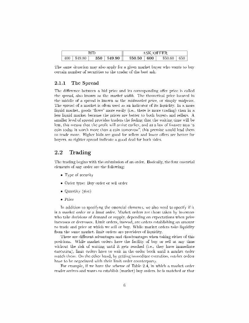
BID ASK/OFFER400 $49.80 350 $49.90 $50.50 600 $50.60 650

The same situation may also apply for a given market buyer who wants to buycertain number of securities to the trader of the best ask.

2.1.1 The Spread

The dierence between a bid price and its corresponding oer price is calledthe spread, also known as the market width. The theoretical price located inthe middle of a spread is known as the midmarket price, or simply midprice.The spread of a market is often used as an indicator of its liquidity. In a moreliquid market, goods ows more easily (i.e., there is more trading) than in aless liquid market because the prices are better to both buyers and sellers. Asmaller level of spread provides traders the feeling that the waiting time will beless, this means that the prot will arrive earlier, and as a law of nance says acoin today is worth more than a coin tomorrow, this premise would lead themto trade more. Higher bids are good for sellers and lower oers are better forbuyers, so tighter spread indicate a good deal for both sides.

2.2 Trading

The trading begins with the submission of an order. Basically, the four essentialelements of any order are the following:

• Type of security

• Order type: Buy order or sell order

• Quantity (size)

• Price

In addition to specifyng the essential elements, we also need to specify if itis a market order or a limit order. Market orders are those taken by investorswho take decisions of demand or supply, depending on expectations when priceincreases or decreases. Limit orders, instead, are orders establishing an amountto trade and price at which we sell or buy. While market orders take liquidityfrom the same market, limit orders are providers of liquidity.

There are dierent advantages and disadvantages when taking either of thispositions. While market orders have the facility of buy or sell at any timewithout the risk of waiting until it gets reached (i.e., they have immediateexecution), limit orders have to wait in the order book until a market ordermatch them. On the other hand, by getting immediate execution, market ordershave to be negociated with their limit order counterparty.

For example, if we have the scheme of Table 2.4, in which a market ordertrader arrives and wants to establish (market) buy orders, he is matched at that

6

instant with the best ask order and has to pay $50.50 for each order. While, ifhe is a limit order trader, he might set a (limit) buy order at best bid and waituntil a trader arrives with a market order of sell. When this happens he willbuy at $50.00 each order. We note that in the rst case, the market order traderpays the spread of $0.50 to the limit order trader. This spread is, sometimes,joined by a rebate.

BID ASK/OFFER550 $49.10 700 $50.00 $50.50 600 $50.60 650

,

Table 2.4: Order Book with depth.

2.3 Traders

There are four basic types of traders: (1) the investor, (2) the market maker, (3)the arbitrageur, and (4) the predictor. Such a classication does not mean thata trader can just take only one of these positions. In fact, most of rms takemore than one position. We shall dene now each category of this classicationand hence we will describe the role played by the High Frequency Trader, whichturns out to be a combination of the basic ones.

2.3.1 The Investor

Investors generally trade because they want to either grow their position in asecurity or reduce it; in other words, they want to increase or decrease theirposition in a security for inherent benet of doing so. The key argument comesfrom the idea to buy a stock because it is believed that it will appreciate invalue; or short it (i.e., to sell a security not owned and hence borrow it) withthe opposite point of view. When investors do hold a security, they intend todo so for relatively long periods of time. Furthermore, when investors trade,they want to do so at the best available price (the highest bid if they are sellingand the lower oer if they are buying). Tighter markets are better than widermarkets for the investor.

2.3.2 The Market Maker

In an ideal market, investor always trade with other investors. Someone whowishes to buy some quantity of stock for his portfolio, wants to nd someonewishing to remove the same quantity from his, and viceversa. However, the mostpart of securities markets have insucient natural liquidity to always matchinvestors with other investors. Here is where market maker ts.

These traders (sometimes called specialists) are willing at all times to eitherbuy or sell a security at quoted bid and oers. Their existence ensures that

7

any investor will always nd a counterparty when he wish to buy or sell a givenstock.

The pure market maker has no inherent interest in holding securities. Theyare said to be in the moving business, not storage. The interest of a marketmaker is quite simple: they want to buy (sell) at one price and sell (buy) atsome higher (lower) price, completing the round-trip, as it were, to earn thedierence as a prot. So market makers work to earn the spread, and the widerthe spread the greater the prot made. This is, of course, the exact opposite ofinvestors as we explained before.

Market makers traders face the so-called inventory risk, which is the possi-bility that an adverse change in price deteriorate their prot by changing thevalue of the inventory. For example, if a market maker has been accumulatingstocks and the price decreases, this will cause that the prot of selling the in-ventory declines. Also, if he has borrowed a lot of stocks by short sales and thestock price increases, the cost of fullling his obligations of return the stockswill result in a loss.

2.3.3 The Arbitrageur

In nance and international economics there is an important rule to follow, thewell-known law of one price, which states that eventhough the prices changeover time, the price of a simply commodity is the same in all places at shortintervals of time. Of course, this require that there are no costs of transaction,or if there are, they are negligible. These costs refers to the buying, selling, ormoving expenses associated to any business transaction. It also includes taxes,fees or commissions.

If this is not the case, there will be people, known as arbitrageurs, tryingto get a riskless benet by buying a stock in the market at lower price and,immediately, selling it in another market at higher price. The arbitrageurs willcontinue with this action until the eect of such trading leads prices in bothmarkets to the same unique price.

As one can suspect, speed is important for two reasons: (1) there is a bigquantity of arbitrageurs constantly looking for mispricings; the arbitrageur withthe fastest order-entry mechanism wins; (2) if the orders are not transmittedand processed at precisely the same time, it is entirely possible that one marketor others will move before both parts of the arbitrage are done, erasing themispricing and leaving the arbitrageur with a position to get out of.

As the security market is so complex and vast, ensuring that there is onlyone price for any security in all the places at the same time is almost impossible.Nevertheless, arbitrageurs make the law of one price to be reached, although itis not their target.

2.3.4 The Predictor

Some types of arbitrage involve mispricings among two or more securities wherethe mispricing is apparent when the two securities are evaluated at the same

8

point in time. In this case, there is another type of trader, called the predictor,looking for pricing discrepancies across time. Because nothing is absolutelypredictable over time, exploiting these discrepancies is much less of a sure thingwhen compared to simple arbitrage.

The predictor, known also as quantitative trader, practices not what we callstatic arbitrage but statistical arbitrage. The latter analyses data over time inorder to make predictions about the future direction of prices. Such predictionsare basically based on mathematics, statistics and probability theory. If hispredictions come true more often than not, they will make a prot.

2.3.5 The High Frequency Trader

A High Frequency (HF) Trader is a hybrid market maker and predictor withadvanced technological capabilities. The essential goal of this sell-side trader isthe same as market makers before that high-speed computer were introducedin nancial markets; that is, to buy on the bid and sell on the oer, buyinglow and selling high, in order to earn the spread. Due to things like decimal-ization, advancements in computing technology, and increased competition, thehigh frequency trader usually uses more innovative, aggressive, and predatorystrategies than those given by traditional market makers.

High frequency traders design trading platform programs that use powerfulcomputers to transact a large number of orders at very fast speeds (they usuallycan send thousands of orders per minute to one market and cancel them atthe same speed). They use complex algorithms to analyze multiple marketsand execute orders based on market conditions. Typically, the traders withthe fastest execution speeds will be more protable than traders with slowerexecution speeds.

2.4 Two winner strategies.

Let us briey explain how a high frequency trader might get a prot. For thispurpose, we shall dene what is a tick. The tick is simply the minimum upwardor downward movement in the price of a security. In this example, we willconsider the tick of $0.05, i.e., ve cents.

Let us assume that each order has only one type of share to be traded. Westart the trading day and look the version of an order book showed in Table 2.5.We observe at the top row three dierent periods of time, and below it threecolumns referring to, respectively, the number of traders (which are betweenparenthesis), the quantity of orders for each trading, and the quote of theseorders. For example, at time t1, we have three traders that together trade 150ask limit orders at the quote $50.30. It is possible that each trader submits 50orders or that one submit 40, another 80, and the last one 30; what matters isthat there are 150 limit orders at that level.

When we arrive as a HF trader at the LOB at time t1, we can apply thefollowing strategy:

9

Time t1 t2 t3(3) 150 $50.30 (3) 150 $50.30 (3) 150 $50.30

ASK (2) 130 $50.25 (2) 130 $50.25 (2) 130 $50.25(1) 70 $50.20 (2) 120 $50.20 (1) 20 $50.20

(1) 120 $50.05 (1) 120 $50.05 (1) 120 $50.05BID (3) 130 $50.00 (3) 130 $50.00 (3) 130 $50.00

(4) 110 $49.95 (4) 110 $49.95 (4) 110 $49.95

Table 2.5: Limit Order Book at times t1, t2, t3

Step 1 At time t2, we submit 50 ask limit orders at the limit quote of $50.20.And we observe that the best ask price has now two traders and 120orders.

Step 2 Suppose that at time t3, a market investor displays 100 buy marketorders, which are sold at the best ask price (in this case $50.20). Sincethere is a price/time priority, 70 orders are sold to the market investorfrom another agent (the one that arrives before us), and hence 30 of our50 orders are then sold.

Step 3 For the next trade, our 20 orders have priority to be sold

Suppose that we sell at short these 30 shares. Then, our cash holdings rightat t3 are 30($50.20) = $1506. In order to get back these 30 shares, we act asfollows.

Case 1This strategy, which can be seen at Table 2.6, is based in the reduction of thespread in order to have priority in execution.

Step 4 At t4, we cancel the 20 ask limit orders and hence we submit 30 buylimit orders at best bid price plus a tick. This means that the new bestbid price is $50.10.

Step 5 Suppose that at time t5, a market investor displays 140 sell marketorders. Again, for the price/time priority, this agent sell us 30 ordersand then he sell the remaining 110 orders to the next level of $50.05of the LOB. This action changes the LOB as observed in the last threecolumns of Table 2.6.

We have already buy all our orders at 30($50.10) = $1503, however, we havereduced the spread by increasing the best bid price by a tick. In this way, wecan liquidate our debt, ending with a total prot of $1506− $1503 = $3 of cashholdings.

Case 2In this case we submit the 30 orders at the current best bid price of the LOB,

10

t3 t4 t5(3) 150 50.30 (3) 100 50.35 (3) 100 50.35

ASK (2) 130 50.25 (3) 150 50.30 (3) 150 50.30(1) 20 50.20 (2) 130 50.25 (2) 130 50.25

(1) 120 50.05 (1) 30 50.10 (1) 10 50.05BID (3) 130 50.00 (1) 120 50.05 (3) 130 50.00

(4) 110 49.95 (3) 130 50.00 (4) 110 49.95

Table 2.6: Strategy 1: Limit Order Book at times t3, t4, t5

as observed in Table 2.7. This movement will not be enough in order to get the30 shares of our debt, so we will use market orders. The steps of this strategyare:

Step 4 At t4, we do two actions. Firstly, we cancel the 20 ask limit orders, andsecondly, we submit 30 buy limit orders at best bid price. This meansthat the new number of orders at best bid price of $50.05 is 150.

Step 5 Suppose that at time t5, an agent displays 140 sell market orders as before.For the price/time priority, this agent will sell 120 orders to the trader whosubmits before us, and then sell 20 orders to us at $50.05.

This strategy leaves the three columns below t5 the same as in the previouscase, which we could observe in the Table 2.7. The principal dierence is there-fore the structure of our inventory and cash holdings. If the trading session isabout to end, we must liquidate our inventory by means of market orders, then:

Step 6 We cancel the 10 buy limit orders and display 10 buy market orders, whichare sold to us at the best ask price of the LOB at time t6

In this way, we might liquidate partially the debt of orders with a cost of20($50.05) = $1001, and the remaining part at 10($50.25) = $502.5. Finally,the prot of this strategy is $1506− ($1001 + $502.5) = $2.5.

t3 t4 t5 t6(3) 150 50.30 (3) 100 50.35 (3) 100 50.35 (3) 100 50.35

ASK (2) 130 50.25 (3) 150 50.30 (3) 150 50.30 (4) 150 50.30(1) 20 50.20 (2) 130 50.25 (2) 130 50.25 (2) 120 50.25

(1) 120 50.05 (2) 150 50.05 (1) 10 50.05 (3) 130 50.00BUY (3) 130 50.00 (3) 130 50.00 (3) 130 50.00 (4) 110 49.95

(4) 110 49.95 (4) 110 49.95 (4) 110 49.95 (3) 80 49.90

Table 2.7: Strategy 2: Limit Order Book for t3, t4, t5, t6

11

When comparing both strategies, we observe that there is a prot dierenceof $0.5. During all the trading session these strategies could be executed thou-sands of times, so, even though at rst sight it seems negligible, this dierencecould increase drastically. In the context of algorithmic trading, these kind ofactions are executed at every second or even faster. Along an hour a dierenceof $0.5× (3600 seconds) = $1800 is, of course, not negligible.

In the particular case of HFT, trades are performed at almost every thou-sandth of a second, so it turns to be a relevant issue to determine an optimalstrategy for the posting of limit and market orders for the hole trading session.The objective of this work is to present, by means of sophisticated (controlled)stochastic models, the obtention of optimal strategies that maximize a certainutility function of a high-frequency trader. Our results are based on the work[4].

12

Chapter 3

Elements of Markov and

Controlled Markov Processes

This chapter shows further results on (uncontrolled and controlled) Markov pro-cesses to be used throughout this thesis. We based ourselves on the followingresources [5, 6, 7, 8, 10] and [11]. The content of this chapter is organized asfollows. In Section 3.1 we introduce the concept of Markov process, related semi-groups and generators, as well as some special cases of Markov processes suchas jump processes and as a particular case continuous-time Markov chains,diusion processes, switching diusions, Levy processes, among others. On theother hand, Section 3.3 is devoted to the study of controlled Markov processes,in particular, we analyse controlled jump diusions on two scenarios:

1. The instantaneous feedback (or regular) control case, and

2. The impulsive control case.

To give a guide on how to solve these two classes of control problems, we in-clude a subsection related to the well-known dynamic programming methodthat introduces the concept of the so-named dynamic programming equationsalso known in this context as Hamilton-Jacobi-Bellman equations.

3.1 Main denitions and some properties

Denition 3.1.1. Let S be a Polish space; that is a complete separable metricspace, and consider S := [0, T ] × S, where T ∈ R+ ∪ +∞. We denote byB(S) (resp. B(S)) the Borel σ-algebra of S (resp. S). Furthermore, let B(S)(resp. B(S)) be the set of Borel measurable and bounded functions from S intoR (resp. S into R), endowed with the supremum norm denoted by ‖ · ‖.

1. A one-parameter family H(t) : t ≥ 0 of bounded linear operators fromthe Banach space B(S) into itself is called a Markov semigroup with

13

Markovian kernels P (s, x, t, A) : t ≥ s ≥ 0, x ∈ S, A ∈ B(S) givenby

H(t)f(s, x) =

∫Sf(s+ t, y)P (s, x, s+ t, dy), ∀f ∈ B(S),

if it satises

(a) H(t+ r) = H(t)H(r), for every t, r ≥ 0,

(b) H(t)f(s, x) ≥ 0, if f(s, x) ≥ 0, for all t ≥ 0, (s, x) ∈ S,(c) H(t)IS(s, x) ≤ 1, for every t ≥ 0, (s, x) ∈ S.

or equivalently

(a') for each 0 ≤ s ≤ t ≤ r, x ∈ S and A ∈ B(S) we have

P (s, x, r, A) =

∫SP (s, x, t, dy)P (t, y, r, A),

which is referred to as the Chapman-Kolmogorov identity,

(b') for each t, s and x the function A 7→ P (s, x, t, A) is a probabilitymeasure on B(S) with P (s, x, t,S) ≤ 1 and P (s, x, s, x) = 1,

(c') for each t, s and A in B(S) the function x 7→ P (s, x, t, A) is Borelmeasurable,

2. The above kernels are called a family of transition functions if for everyxed s ≥ 0 and A in B(S) the mapping (t, x) 7→ P (s, x, t, A) is jointlyBorel measurable in x ∈ S and t ≥ s..

3. The semigroup is called stochastically continuous if

limt→0

P (s, x, s+ t, V ) = 1

for every x ∈ S, s ≥ 0 and any open neighborhood V of x.

4. The semigroup satises the pointwise Feller property (respectively, strongFeller property) if for every t > s ≥ 0 the function x 7→ H(t)f(s, x) iscontinuous at each point of continuity of the function f(s, ·) (respectively,at each point x).

Remark 3.1.2. 1. A time-invariant function f(x) on S is said to belong toB(S) if the function f ′(s, x) := f(x) on S belongs to B(S).

2. A transition probability is said to be time homogeneous if

P (s, x, s+ t, B) = P (0, x, t, B) =: P (t, x,B)

for all s, t ≥ 0, x ∈ S and B ∈ B(S).

Denition 3.1.3. Let Cb(S) (resp. Cb(S)) be the set of real-valued continuousfunctions that belong to B(S) (resp. B(S)).

14

Denition 3.1.4. A Markov semigroup H(t); t ≥ 0 is said to be a (strong)Feller semigroup if the following extra condition is satised

limt→0‖H(t)f − f‖ = 0

for all f ∈ Cb(S).

Remark 3.1.5. Given a semigroup H(t), t ≥ 0, we dene its (right) derivativeat t0 by follows

dH+

dt(t0) =

dH+

dt

∣∣∣t0

:= limt↓t0

H(t)−H(t0)

t− t0,

where the last limit is given in the sense of the supremum norm ‖ · ‖ of B(S).

Denition 3.1.6. The innitesimal generator of a Feller semigroup H(t); t ≥0 is dened as the linear (possibly unbounded) operator

Lf := limt↓0

H(t)f − ft

,

whose domain D(L) is a subset of f ∈ B(S) under which the above limit exists(in the norm of the space B(S)).

Proposition 3.1.7. Given a Feller semigroup H(t), t ≥ 0 with innitesimalgenerator L, the following holds:

1. If f ∈ D(L) and t ≥ 0, then H(t)f ∈ D(L) and

d+(H(t)f)

dt= LH(t)f = H(t)Lf. (3.1)

In particular we get that

H(t)f − f =

∫ t

0

LH(s)fds =

∫ t

0

H(s)Lfds. (3.2)

2. If f ∈ D(L) and t ≥ 0, then∫ t

0

H(s)fds ∈ D(L) (3.3)

and

H(t)f − f = L∫ t

0

H(s)fds. (3.4)

Remark 3.1.8. Using the previous proposition, it can be shown that the domainD(L) is a dense vector subspace of B(S) an that the innitesimal generator Lis a closed operator. The idea of the above assertion is that for every f ∈ B(S)

limt↓0

1

t

∫ t

0

H(s)fds = f, and∫ t

0

H(s)fds ∈ D(L).

15

Let X (·) = X(t)t≥0 be an S-valued Markov process with transition prob-abilities P (s, x, t, B) , i.e.

P (X(t) ∈ B | X(r), 0 ≤ r ≤ s) = P (s,X(s), t, B)

for all t ≥ s ≥ 0 and B ∈ B(S). Denoting by Es,x[·] := E[·|X(s) = x] theconditional expectation given the initial state X(s) = x and Ex[·] := E0,x[·], wecan relate these transition probabilities with the concept of semigroup by meansof

H(t)f(s, x) = Es,x[f(s+ t,X(s+ t))] (3.5)

Conversely, Kolmogorov consistency theorem arms that there exists a uniqueS−valued stochastic processes Y(·) = Y (t)t≥0, with nite dimensional distri-butions given by

P(yt1 ∈ B1, . . . , ytn ∈ Bn) =

∫y∈S

∫y1∈B1

. . .

∫yk∈Bk

Ptk−1,tk (yk−1, dyk)Ptk−2,tk−1(yk−2, dyk−1) . . . Pt0,t1(y, dy1)µ(dy),

where t0 := 0 and µ is the distribution of Y (0) (i.e. the initial distribution).It can be proved that the previous process admits a cádlàg modication

X (·) = X(t)t≥0. We will call to as Markov process this cádlàg modication.Using (3.5), we can rewrite (3.4) as

Es,x[f(s+ t,X(s+ t)

)]− f(s, x) = Es,x

[∫ t

0

Lf(s+ r,X(s+ r)

)dr

],

if f ∈ D(L). Furthermore, in the context of stopping times, we have the follow-ing important theorem, for the time-homogeneous case.

Theorem 3.1.9 (Dynkin's Formula). Let X(t); t ≥ 0 be a Markov processwith innitesimal generator L and let τ be a stopping time such that Ex[τ ] <∞for all x ∈ S. Then, for all f ∈ D(L) and x ∈ S,

Ex[f(X(τ)

)]− f(x) = Ex

[∫ τ

0

Lf(X(t)

)dt

]

3.2 Some Special Cases

3.2.1 Jump Processes and Continuous-time Markov Chains

Let us suppose that we are observing a queue of a bank where there is only onecashier and three people in the queue. At a given initial instant t0, we see thatthe rst person in the queue is attended immediately. Assume that at a randomtime t1 > t0, another costumer arrives. Next, at a random time t2 the cashierhas nished with the rst person. At t3, the cashier has also nished his second

16

tTtT−1tT−2t4 t6t5 t7

1

2

3

4

Costumers

Timet3t1t0 t2

Figure 3.1: One path of a jump-process.

service. Let us consider that this process continues along certain time. If weplot the behaviour of the queue we observe the possible scenario illustrated inFigure 3.1.

The process described above is a special case of a class of process called jumpprocess, which in general behaves as follows: let X(·) be a process that starts ina given point X(s) = x0 at some time s ≥ 0. It stays there for a random time τ1and then it jumps to a new state x1, and it remains at x1 for a random lengthof time τ2. In the case of Markov processes we also have that given that theprocess remains at x1, the next jump to x2 6= x1 is conditionally independentof (x0, τ1), and so on. In general, it is not possible to predict the exact instantof a jump, but it is possible to give information about the rate of occurrence ofthese jumps.

As was illustrated before, jump process are great for modelling queues. Otherprocesses that can be modelled through these processes are inventory problems.

In general, let S be a Polish space and let X(·) = Xtt≥0 be a S-valuedMarkov process with transition probabilities P (s, x, t, B), where t ≥ s ≥ 0,x ∈ S, and B ∈ B(S). Assume that for every s, x, and B, there exists the limit

limh↓0

P (s, x, s+ t, B)− IB(x)

h=: q(s, x,B) (3.6)

where q(s, x,B) is a function continuous in s, jointly measurable in s and x,and σ-additive in B ∈ B(S), and IB(x) is the indicator function of the set B.We have two special cases: (1) if B = S we have q(s, x,S) = 0, i.e., the processcannot jump outside the state space; (2) if B = x, we get the nonnegativefunction

λ(s, x) := −q(s, x, x) = q(s, x,S r x) (3.7)

also known as intensity function and it will be assumed to be nite valued. Iffor x ∈ S, λ(s, x) = 0 we say that x is an absorbent state. On the other hand,

17

if λ(s, x) =∞, we say that x is an instantaneous state. The function λ(s, x) isbetter known as the jump rate because if we dene

τ(s, x) := infr > s | X(r) 6= x

as the time of the rst jump, then it can be veried that

P(τ(s, x) > t | X(s) = x) = exp

[−∫ t

s

λ(r, x)dr

]We now dene the relative transition function as

Q(s, x,B) :=q(s, x,B r x)

λ(s, x)=q(s, x,B r x)q(s, x,S r x)

if λ(s, x) > 0, (3.8)

:= IB(x) if λ(s, x) = 0

Since IB\x(x) = 0, from (3.6) we have that for λ(s, x) > 0

Q(s, x,B) =q(s, x,B r x)q(s, x,S r x)

= limh↓0

P (s, x, s+ h,B r x)P (s, x, s+ h,S r x)

.

Notice that Q(s, x,B) represents the conditional probability that the processtakes a value in B at time s+ h (for h > 0), given that X(s) = x and that theprocess has been submitted to change in (s, s+ h).

The following theorem has been borrowed form [6].

Theorem 3.2.1. For s ≥ 0, x ∈ S and B ∈ B(S), let q(s, x,B) be a functiondened by

q(s, x,B) := −λ(s, x)[IB(x)−Q(s, x,B), ] (3.9)

where:

1. λ(s, x) is a nonnegative measurable function, continuous in s, and boundedon I × S for every nite time interval I.

2. Q(s, x,B) is a probability measure on S for every (s, x); jointly measurablein (s, x) for every B; with Q(s, x, x) = 0, and moreover,

3. For xed x ∈ S and B ∈ B(S), Q(s, x,B) is continuous in s, and for everynite interval I ⊂ [0,∞), Q(s, x,B) is continuous in s ∈ I uniformly withrespect to B.

Then there exists a right-continuous Markov process X (·) with transition prob-abilities P (s, x, t, B) that satisfy equation (3.6) uniformly in s ∈ I for anybounded interval I and xed x and B. Such transition probabilities also satisfythe Kolmogorov backward equation

∂P (s, x, t, B)

∂s= −

∫Sq(s, x, dy)P (s, y, t, B)

= λ(s, x)

[P (s, x, t, B)−

∫Q(s, x, dy)P (s, y, t, B)

](3.10)

18

Continuous-time Markov chains

Consider α(·) to be a jump process with a countable (numerable or nite) statespace S (with the discrete topology). The transition probabilities associated toα(·) will be denoted as follows

P (s, x, t, y) =: pxy(s, t)

Similarly, the functions q and λ in (3.6) and (3.7) turn to, respectively,

qxy(s) := limh↓0

[pxy(s, s+ h)− δxy]

h,

where δxy is the Kronecker delta, and

λx(s) := −qxx(s) =∑y 6=x

qxy(s). (3.11)

The qxy(s) are so-called the transition intensities from the states x to y. Thematrix Q(s) = [qxy(s)] is well known as the generator matrix of α(·). Theinnitesimal generator L is dened for any real-valued function f on S by meansof

Lf(s, x) =∂f(s, x)

∂s+∑y∈S

qxy(s)f(s, y) =∂f(s, x)

∂s+ qxx(s)f(s, x) +

∑y 6=x

qxy(s)f(s, y)

(3.11)=

∂f(s, x)

∂s−∑y 6=x

qxy(s)f(s, x) +∑y 6=x

qxy(s)f(s, y)

=∂f(s, x)

∂s+∑y 6=x

qxy(s)(f(s, y)− f(s, x)

)(3.9)=

∂f(s, x)

∂s+∑y 6=x

λ(s, x)Q(s, x, y)(f(s, y)− f(s, x)

)=

∂f(s, x)

∂s+ λ(s, x)

∑y∈S

Q(s, x, y)(f(s, y)− f(s, x)

)=

∂f(s, x)

∂s+ λ(s, x)

∫SQ(s, x, dy)

(f(s, y)− f(s, x)

)In addition, the backward equation (3.10) becomes

∂pxy(s, t)

∂s= λx(s)pxy(s, t)−

∑z 6=x

qxz(s)pzy(s, t).

Poisson Processes

Consider the particular case S = N endowed with its σ-algebra 2N. For a givenpositive constant λ, we dene the Poisson process N (·) = N(t), t ≥ 0, as ajump process with parameter λ satisfying the following conditions

19

1. N (·) has independent increments

2. N (·) has stationary increments such that N(t + h) − N(t) has Poissondistribution with parameter λh; i.e.

P(N(t+ h)−N(t) = k

)= e−λk

(λh)k

k!

for all k = 0, 1, . . ..

The associated homogeneous transition probability for the Poisson process N(·)is

P (t, x,B) := e−λt∞∑k=0

(λt)k

k!IB(x+ k),

for any t > 0, x in N and B ∈ 2N. The associated semigroup for N(·) in Cb(N)is given by

H(t)f(x) :=

∫Nf(y)p(t, x, dy) = e−λt

∞∑k=0

(λt)k

k!f(x+ k),

for every t > 0 and x ∈ N. Furthermore, its innitesimal generator is

D(L) := Cb(N), Lf(x) := λ[f(x+ 1)− f(x)], for all x ∈ N.

3.2.2 Brownian Motion and Diusion Processes

Brownian Motion

An Rd-valued random process W (t), t ≥ 0, is called a Brownian motion, if

1. W (0) = 0 w.p. 1,

2. W (·) is a process with independent increments,

3. W (·) has continuous sample paths with probability one,

4. the increments W (t)−W (s) have Gaussian distribution with E[W (t)] = 0and Cov(W (t)) = σt for some nonnegative denite d× d matrix σ; whereCov(ζ) denotes the covariance of ζ.

When σ = I, the identity matrix, W (·) is a standard Brownian motion.The typical one-dimensional Brownian motion or Wiener process is dened

on the state space S = R with its Borel σ-algebra B(R). Its transition proba-bilities are given by

p(t, x,B) :=1√2πt

∫B

exp

− (y − x)2

2t

dy,

20

for any t > 0, x in R and B in B(R). The associated semigroup in Cb(R) isgiven by

H(t)f(x) :=

∫Rf(y)p(t, x, dy) =

1√2π

∫ ∞−∞

f(x+√tz) exp

(−z

2

2

)dz,

for every t > 0 and x ∈ R. Its innitesimal generator L is the dierentialoperator L given by

D(L) := f ∈ Cb(R) ∩ C2(R) : f ′′ ∈ Cb(R), Lf :=1

2f ′′.

where C2(R) denotes the class of real-valued functions on R whose partial deriva-tive with respect to the variable x up to the second order are continuous.

Diusion Processes

For a Rd-valued Brownian motionW (t) dened in a probability space (Ω,F ,P),let Ft = σW (s) : s ≤ t. Consider now the process σ(t); t ≥ 0 as a Ft-measurable process taking values in Rn×d, such that∫ t

0

|σ(s)|2ds <∞

for all t ≥ 0, where |σ| := [Tr(σ′σ)]12 =

(n∑i=1

d∑j=1

(σ′σ)2ij

) 12

, with σ′ being

the transpose of σ. Using W (·) and σ(·), we dene the stochastic integral∫ t0σ(s)dW (s) in the usual sense satisfying the martingale property with mean

0 and quadratic variation∫ t

0σ(s)σ′(s)ds.

Given Ft-measurable processes b(·) and σ(·), with∫ t

0|b(s)|ds < ∞, and σ

satisfying the above condition, a process X(·) dened as

X(t) := X(0) +

∫ t

0

b(s)ds+

∫ t

0

σ(s)dW (s) (3.12)

is called an Itô process, or that X(·) has a stochastic dierential equation (SDE )representation. In a compact representation we usually write (3.12) as

dX(t) = b(t)dt+ σ(t)dW (t). (3.13)

Let C1,2([0,∞) × Rn) denote the class of real-valued functions on [0,∞) × Rnwhose second-order mixed partial derivatives with respect to x and rst-orderpartial derivatives with respect to t are continuous. Dene the operator L onC1,2([0,∞)× Rn) by

Lf(t, x) :=∂f(t, x)

∂t+(∇f(x)

)′b(x) +

1

2Tr(∇2f(x)a(x))

=∂f(t, x)

∂t+

n∑i=1

bi(t)∂f(t, x)

∂xi+

1

2

n∑i,j=1

aij(t)∂2f(t, x)

∂xi∂xj,

21

where a(t) = (aij(t)) = σ(t)σ′(t) and ∇f , ∇2f represent the gradient an theHessian matrix of f , respectively. Then for all f ∈ C1,2([0,∞)×Rn), the process

f(t,X(t))− f(0, X(0))−∫ t

0

Lf(s,X(s))ds

is a local martingale. Moreover, X(·) is a Markov process (provided σ(·) andb(·)) are suitable non-random Borel function) in the sense that

P (X(t) ∈ A|Fs) = P (X(t) ∈ A|X(s))

for all 0 ≤ s ≤ t and for any Borel set A. The operator L becomes the generatorof the diusion X(·).

Notice that in the right side of (3.12) or (3.13) the functions b and σ do notdepend on X(·). In many situations we will have the dynamic of the process tobe dependent on X(·), i.e.

dX(t) = b(t,X(t))dt+ σ(t,X(t))dW (t) (3.14)

with a initial condition X(0) = x. The process in (3.14) is also called a (Itô)stochastic dierential equation (SDE ) and, as a particular case when b and σare continuous functions on the variable t, we can verify that X(·) belongs to animportant family of stochastic processes so-named diusion processes. Finally,a process X(·) is known as a (strong) solution of the SDE (3.14), if it satisescertain conditions ensuring the existence and uniqueness of this equation; suchconditions are also known as Itô's conditions, listed below:

• Lipschitz continuity

|b(t, x)− f(t, y)|+ |σ(t, x)− σ(t, y)| ≤ K|x− y|,

for all t ∈ [0, T ], x, y ∈ Rn

• At most linear growth

|b(t, x)|+ |σ(t, x)| ≤ K(1 + |x|),

for all t ∈ [0, T ], x ∈ Rn.

.

3.2.3 Combinations

Switching diusions

Let E = 1, . . . ,m, and let W (·) be an Rd-valued standard Brownian motiondened in the ltered probability space (Ω,F , Ft, P ). Assume that b(·, ·) :Rn × E 7→ Rn and that σ(·, ·) : Rn × E → Rn × Rd satisfy the usual Ito's

22

conditions. A switching diusion, also known as Markov-modulated diusion,is a two-component process (X(·), β(·)) composed by the SDE

dX(t) = b(X(t), β(t))dt+ σ(X(t), β(t))dW (t), with (X(0), β(0)) = (x, β)(3.15)

and by a continuous-time Markov chain β(·) satisfying for i 6= j,

P(β(t+ h) = j | β(t) = i,X(s), β(s), s ≤ t

)= qij(X(t))h+ o(h). (3.16)

It is usual to call X(t) the continuous component and β(t) the discrete compo-nent. The two-component process (X(t), β(t)) is jointly a Markov process. Insome special cases, the switching process β(t) is independent of the Brownianmotion W (t).

Given the process (X(t), β(t)), there is an associated operator representingthe innitesimal generator of such a process, which is dened as follows. Foreach i ∈ E and each f(·, i) ∈ C2(Rn), we have

Lf(x, i) =(∇f(x, i)

)′b(x, i) +

1

2Tr(∇2f(x, i)a(x, i)) + (Qf)(x, i)

=

n∑j=1

bj(x, i)∂f(x, i)

∂xj+

1

2

n∑k,j=1

akj(x, i)∂2f(x, i)

∂xk∂xj

(Qf)(x, i), (3.17)

where

(Qf)(x, i) =∑j∈S

qijf(x, j).

The discrete evolution of the component β(·) can be represented by means ofa stochastic integral with respect to a Poisson random measure. In fact, forx ∈ Rn and i, j ∈ E with j 6= i, let ∆ij(x) be the consecutive (with respect tothe lexicographic ordering on E × E), left-closed, right-open intervals of the realline, each one having length equal to qij(x). Dene a function h : Rn×S×R→ Rby

h(x, i, z) =∑j∈S

(j − i)Iz∈∆ij(x) (3.18)

Then (3.16) is equivalent to

dβ(t) =

∫Rh(x(t), β(t−), z)ν(dt, dz), (3.19)

where ν(dt, dz) is a Poisson random measure with intensity dt×m(dz), and mis the Lebesgue measure on R. In this case, the Poisson random measure ν(·, ·)is independent of the Brownian motion W (·).

23

Levy Processes

Denition 3.2.2. Let (Ω,F , Ftt≥0, P ) be a ltered probability space. AnFt-adapted process X (·) = X(t), t ≥ 0 with X(0) = 0 a.s. is called a Lévyprocess if X(t) is stochastically continuous and has stationary and independentincrements.

It can be assumed that the Lévy processes is cádlàg.Lévy processes are determined by the triple (Σ, α, ν), where Σ describes the

covariance structure of the Brownian motion component, α is the drift compo-nent, and ν describes the rate at which jumps occur. This triplet is given in theLévy-Khintchine formula below.

Theorem 3.2.3 (The Lévy-Khintchine formula). LetX(t) be a n-dimensionalLévy process. Then, there is a unique function ψ : Rn → C such that

E[ei〈u,X(t)〉] = etψ(u), u ∈ Rn, t ≥ 0 (3.20)

Also, ψ(u) can be written as

ψ(u) = i〈b, u〉 − 1

2〈u, au〉+

∫Rnr0

ei〈u,z〉 − 1− i〈u, z〉I|z|<1ν(dz) (3.21)

where a, b and the measure ν are uniquely determined and satisfy the fol-lowing,

• a ∈ Rn×n is a positive semidenite matrix

• b ∈ Rn

• ν is a Borel measure on Rn with ν(0) = 0 and,∫Rn

min1, z2ν(dz) <∞,

Furthermore, (a, b, ν) uniquely determine all nite distributions of the processX(·).

Conversely, if (a, b, ν) is any triple satisfying the three above conditions, thenthere exists a Lévy process satisfying (3.20)-(3.21).

Using the Lévy-Khintchine formula together with the inverse of Fouriertransform we can see that for f ∈ C2(Rn) ∩ Cb(Rn) the innitesimal gener-ator is given by

Lf(x) =

n∑i=1

bi∂f

∂xi(x) +

1

2

n∑i,j=1

aij(x)∂2f

∂xi∂xj(x)

+

∫Rnr0

f(x+ y)− f(x)− i〈∇f(x), y〉I|y|<1ν(dy)

24

Theorem 3.2.4 (Levy-Ito Decomposition). If X(·) is a Lévy process, thenthere exists b ∈ Rn, a Brownian motion WA(·) with covariance matrix A in Rn,and an independent Poisson random measureN on [0,∞)×Rn, withN(t, 0) =0 for each t ≥ 0

X(t) = bt+WA(t) +

∫|z|<1

zN(t, dz) +

∫|z|≥1

zN(t, dz) (3.22)

where N(dt, dz) = N(dt, dz) − ν(dz)dt is the compensated Poisson randommeasure of X(·) (ν is the Lévy measure of X(·)). The process

∫|z|<1

zN(t, dz)

is the compensated sum of small jumps.

In view of the previous decomposition, it is natural to consider more generalstochastic integrals of the form

X(t) = X(0) +

∫ t

0

b(s, ω)ds+

∫ t

0

σ(t, ω)dW (s) +

∫ t

0

∫Rγ(s, z, ω)N(ds, dz)

(3.23)where the integrands satisfy the appropiate conditions for the integrals to existsand we for simplicity have put

N(ds, dz) =

N(ds, dz)− ν(dz)ds if |z| < 1N(ds, dz) if |z| ≥ 1,

and we will also use the short hand dierential notation

dX(t) = b(t)dt+ σ(t)dW (t) +

∫Rγ(t, z)N(dt, dz)

which is called a Itô-Lévy process.We can also have solutions of stochastic dierential equations, when the

coecients b and σ depends explicitly of X(·); in this case we have

dX(t) = b(t,X(t))dt+ σ(t,X(t))dW (t) +

∫Rn

γ(t,X(t−), z)N(dt, dz) (3.24)

where b : [0, T ]×Rn → Rn, σ : [0, T ]×Rn → Rn×m, and γ : [0, T ]×Rn×Rn →Rn×` are given functions that satisfy Itô conditions.

3.3 Controlled Markov Processes

In this section we present a brief description of a general class of continuous-time Markov control processes and a special class of so-named controlled jumpdiusion processes.

Denition 3.3.1. A Continuous-time Markov Control Process (CTMCP) is ave-tuple (

S,A, A(x), x ∈ S, Lu, u ∈ A, c)

where each element is dened as follows:

25

(i) S and A are two Polish spaces called, respectively, the state space and theaction space. These spaces are endowed with their Borel σ-algebras B(S)and B(A), respectively.

(ii) The family A(x), x ∈ S represents the restriction of A to those actionsor decisions available to the controller in the state x ∈ S.

(iii) For each u ∈ A the transition law in S is given by the linear operatorL(u) = Lu, which is the innitesimal generator of an S-valued Markovprocess with transition probability Pu(s, x, t, B).

(iv) Finally, the function c(t, x, u) is a real-valued measurable function denedon S × A called the cost or prot rate function. We assume that c isbounded.

Along with the above denition, we need to dene other elements calledpolicies that can be interpreted as a family π = a(t) ∈ A| 0 ≤ t ≤ T. We aregoing to be interested in a special subset Π, dened in the next subsection.

3.3.1 The control space Π

There are dierent ways to choose the set Π. In this thesis, we will consider onlyMarkov control policies, which consist of all measurable functions π : S → A,such that π(t, x) denotes the control action prescribed by π when the state x ∈ Sis observed at time t, and it is independent on the past information. A Markovcontrol is said to be stationary if it is independent of time, i.e., π(s, x) = π(x)for all (s, x) ∈ S.

Recall that a process X(·) is conservative if its associated semigroup H(t)and its innitesimal generator L satisfy

• H(t)IS = 1 for all t ≥ 0, and

• LIS = 0.

We now can dene the concept of admissible policy.

Denition 3.3.2. We say that a (Markov) policy π ∈ Π is admissible if thereexists a conservative strong Markov process Xπ(t) = X(t), t ≥ 0 such thatits sample paths are càdlàg with only nitely many discontinuities in any niteinterval of time with probability one. Moreover, Xπ(·) has transition probabilitydenoted by Pπ(s, x, t, B) and its associated semigroup Hπ(t) has innitesimalgenerator Lπ satisfying that

Lπ = Lu if π(s, x) = u;

Notice that, when using a policy π ∈ Π, expectations as in (3.5) become

Hπ(t) = Eπs,x[f(s+ t,X(s+ t)

)]=

∫Sf(s+ t, y)Pπ(s, x, t, dy)

26

Finite horizon problems.

In addition to the cost/reward rate function c, dened above, we may con-sider the continuous function g : S → R. Furthermore, we x a domain G inS := [0,∞) × S and dene τG ≥ s as the rst exit time from G of the processXs,x(r); r ≥ s, i.e.

τG = τG,s,x(ω) = infr > s | (r,Xs,x(r, ω)) /∈ G ≤ ∞ (3.25)

As for the notation Xs,x(·) we mean that the Markov process X(·) starts attime s, with the value x.

The function g is well known as the terminal cost or bequest function, whereasthe set G is called solvency region. Finally, τG is sometimes called the bankruptcytime.

Let c(s, x, π) := c(s, x, π(s, x)), and suppose that

Eπs,x[∫ τG

s

|c(r,X(r), π

)|dr + |g

(τG , X(τG)

)|IτG<∞

]<∞

for all (s, x) ∈ S, and π ∈ Π admissible. With this in mind, we dene theperformance index or cost function J(s, x, π) as the functional

J(s, x, π) = Eπs,x[∫ τG

s

c(r,X(r), π)dr + g(τG , X(τG))IτG<∞]. (3.26)

With the previous elements, we are in conditions to formulate the optimal con-trol problem of a CTMCP.

Denition 3.3.3. For each (t, y) ∈ G, the control problem is to nd a functionΦ(t, y) and a control policy π∗ ∈ Π such that

Φ(t, y) := supπ∈Π

J(t, y, π) = J(t, y, π∗) , (3.27)

where the supremum is taken over a given family Π of admissible control policies.If such a control π∗ exists, it is called optimal control policy and Φ is called theoptimal performance or the value function.

3.3.2 Controlled jump diusion processes and its associ-ated Hamilton-Jacobi Bellman Equation

Suppose that the state of a system at time t is described by a stochastic processX(t) ∈ S ⊂ Rn of the form

dX(t) = dXπ(t) = b(t,X(t), π(t,X(t)))dt+ σ(t,X(t), π(t,X(t)))dW (t)

+

∫Rnr0

γ(t,X(t−), π(t−, X(t−)), z)N(dt, dz), (3.28)

27

where b : [0,∞)×S×A → S, σ : [0,∞)×S×A → S×Rm, γ : [0,∞)×S×A×S →S×R`,W (t) is am-dimensional Brownian motion and N(t, z) is a `-dimensionalvector of independent Poisson random measures. The equation (3.28) can beseen as a Markov process whose dynamic changes according to the control policyπ ∈ Π. For notation purposes, we will simply write b(t,X(t), π) instead ofb(t,X(t), π(t,X(t))

), analogously for σ and for γ. Hence equation (3.28) turns

to

dXπ(t) = b(t,X(t), π)dt+ σ(t,X(t), π)dW (t) +

∫Sγ(t,X(t−), π, z)N(dt, dz).

(3.29)For π ∈ Π and φ ∈ C1,2

b ([0,∞)× S), dene

Lπφ(t, x) =∂φ

∂s(t, x) +

n∑i=1

bi(t, x, π)∂φ

∂xi(t, x) +

1

2

n∑i,j=1

aij(t, x, π)∂2φ

∂xi∂xj(t, x)

(3.30)

+

∫Rnr0

φ(t, x+ w)− φ(t, x)− 〈∇φ(t, x), w〉I|w|<1ν(dw)

where aij = (σσ′)ij , x = (x1, . . . , xn) and w := (w1, . . . , wn). It is well knownthat for each choice of the function π, the solution X(t) = Xπ(t) is a jumpdiusion with generator Lπ as in (3.30), and transition probability functionPπ = Pπ(t,x). For this reason, the process X(·) is called a controlled jumpdiusion process.

The next result, which is part of group of results named verication theo-rems, relates the value function Φ in (3.27) with a solution of a certain integro-dierential partial equation (IDPE). (For more details, see [6],[7] or [8]).

Theorem 3.3.4. Given the solvency region G, we denote by G its closure. Letφ be a function in C2(G) ∩ C(G) such that, for all π ∈ Π,

c(t, x, π) + Lπφ(t, x) ≤ 0 (t, x) ∈ G

with boundary values

limt→τG

φ(X(t)

)= g(X(τG)) · IτG<∞ Pπ − a.s.

and such that φ−(X(τ)); τ stopping time, τ ≤ τG is uniformly Pπ-integrablefor all Markov controls π, where φ−(x) := max(−φ(x), 0) denotes the negativepart of φ(x). Then

φ(t, x) ≥ Φ(t, x) for all (t, x) ∈ G

Furthermore, assume that for each (t, x) ∈ G we have a function π∗(t, x)such that

c(t, x, π∗(t, x)) + Lπ∗(t,x)φ(t, x) = 0

28

and φ(t,Xπ∗(t)); τ stopping time, τ ≤ τG is uniformly Pπ-integrable. Thenπ∗ = π∗(t, x) is a Markov control satisfying

φ(t, x) = J(t, x, π∗) = Φ(t, x) for all (t, x) ∈ G;

in other words, π∗ is optimal.

3.4 Impulse Control

In this section, we will summarize some key results concerning to optimal im-pulse control. In these type of problems, the control produces jumps in thecontinuous evolution at random times, all under the controller's decisions. Formore details on these type of controllability, we refer [8].

Throughout this section we will consider a time-homogeneous jump diusionprocess of the form

dX(t) = b(X(t))dt+ σ(X(t))dW (t) +

∫Sγ(X(t−), z)N(dt, dz) (3.31)

where S ⊂ Rn, b : S → S, σ : S → S × Rm and γ : S × S → S × R` are givenfunctions satisfying the conditions for the existence and uniqueness of a solutionX(t).

In this case, the generator L of X(t) becomes

Lφ(x) =

n∑i=1

bi(x)∂φ

∂xi(x) +

1

2

n∑i,j=1

(σσ′)ij(x)∂2φ

∂xi∂xj(x) +

+∑j=1

∫Rnr0

φ(x+ γ(j)(x, zj))− φ(x)−∇φ(x) · γ(j)(x, zj)νj(dzj).

Let ζ ∈ Z ⊂ Rp be some elements called admissible impulse values. Inthis case, at some random times called intervention times τi i = 1, 2, ..., thecontroller can modify X(τi−) to a new state X(τi), according to the transitionΓ : S × Z → S, dened as X(τi) := Γ(X(τi−), ζi). We can observe that ζicould be an arbitrary value or it could depend on the time t when the transitiontakes place. In other words, we can establish an impulse value function asζi : R+ → Z.

Denition 3.4.1. An impulse control ν is the collection of pairs of randomtimes and impulse values of the form

ν = ((τi, ζi))i≤M ; M ≤ ∞

We suppose that the intervention times are not arbitrary random variables.The controller intervenes due to observations he does on the state variable, inparticular, when such state reaches certain critic values or sets. In order to

29

include this situation, we suppose that τi, i ≤ M are Ft-stopping times, i.e.that

τ ≤ t ∈ Ft for all t.

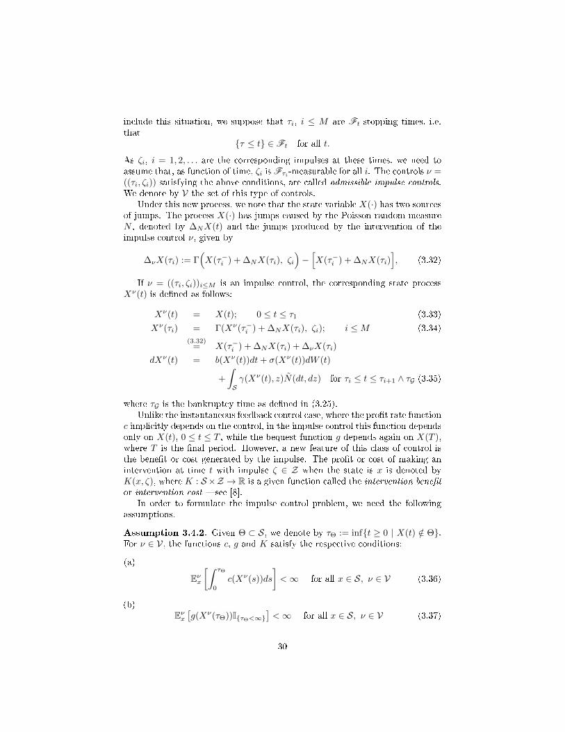
As ζi, i = 1, 2, . . . are the corresponding impulses at these times, we need toassume that, as function of time, ζi is Fτi -measurable for all i. The controls ν =((τi, ζi)) satisfying the above conditions, are called admissible impulse controls.We denote by V the set of this type of controls.

Under this new process, we note that the state variable X(·) has two sourcesof jumps. The process X(·) has jumps caused by the Poisson random measureN , denoted by ∆NX(t) and the jumps produced by the intervention of theimpulse control ν, given by

∆νX(τi) := Γ(X(τ−i ) + ∆NX(τi), ζi

)−[X(τ−i ) + ∆NX(τi)

], (3.32)

If ν = ((τi, ζi))i≤M is an impulse control, the corresponding state processXν(t) is dened as follows:

Xν(t) = X(t); 0 ≤ t ≤ τ1 (3.33)

Xν(τi) = Γ(Xν(τ−i ) + ∆NX(τi), ζi); i ≤M (3.34)(3.32)

= X(τ−i ) + ∆NX(τi) + ∆νX(τi)

dXν(t) = b(Xν(t))dt+ σ(Xν(t))dW (t)

+

∫Sγ(Xν(t), z)N(dt, dz) for τi ≤ t ≤ τi+1 ∧ τG (3.35)

where τG is the bankruptcy time as dened in (3.25).Unlike the instantaneous feedback control case, where the prot rate function

c implicitly depends on the control, in the impulse control this function dependsonly on X(t), 0 ≤ t ≤ T , while the bequest function g depends again on X(T ),where T is the nal period. However, a new feature of this class of control isthe benet or cost generated by the impulse. The prot or cost of making anintervention at time t with impulse ζ ∈ Z when the state is x is denoted byK(x, ζ), where K : S×Z → R is a given function called the intervention benetor intervention cost see [8].

In order to formulate the impulse control problem, we need the followingassumptions.

Assumption 3.4.2. Given Θ ⊂ S, we denote by τΘ := inft ≥ 0 | X(t) /∈ Θ.For ν ∈ V, the functions c, g and K satisfy the respective conditions:

(a)

Eνx[∫ τΘ

0

c(Xν(s))ds

]<∞ for all x ∈ S, ν ∈ V (3.36)

(b)Eνx[g(Xν(τΘ))IτΘ<∞

]<∞ for all x ∈ S, ν ∈ V (3.37)

30

(c)

Eνx

∑τi≤τΘ

K(X(τ−i ) + ∆NX(τi), ζi)

<∞ for all x ∈ S, ν ∈ V (3.38)

Now, in the context of impulse control we dene the performance (cost)criterion as the functional

J(x, ν) = Eνx

∫ τΘ

0c(Xν(s))ds+ g(, Xν(τΘ))IτΘ<∞ +

∑τi≤τΘ

K(X(τ−i ) + ∆NX(τi), ζi)

.Denition 3.4.3. The impulse control problem consists in nding Φ(x) andν∗ ∈ V such that

Φ(x) = supJ(x, ν); ν ∈ V = J(x, ν∗). (3.39)

The intervention should be applied if the benet of doing so is greater thanthe benet of leaving the state moves by its dynamic. The dynamic of theintervention should consider if at any time is worth to interfere with the process.

Denition 3.4.4. Let H be the space of all measurable functions h : Θ → R.The intervention operator M : H → H is dened by

Mh(x) = supζ∈Zh(Γ(x, ζ)) +K(x, ζ) | Γ(x, ζ) ∈ Θ ⊂ S. (3.40)

3.4.1 Dynamic Programming

Let Θ be the closure of Θ, and let ΦM be the set of functions φ : Θ → R suchthat

1. φ ∈ C1 (Θ) ∩ C(Θ),

2. φ ≥Mφ on Θ.

For the rest of this section we assume that ΦM is non-empty.We set a region where it is just not worth to intervene. Let us dene the

continuation region as

D = x ∈ Θ; φ(x) >Mφ(x).

This region specify the set where we just leave the process to continue withoutinterventions.

We need the following groups of assumptions in order to establish the mainresult of impulse controls problems. These assumptions will be also used inmixed control problems established in the next section. Recall that τΘ is therst time the state variable is outside the solvency region Θ.

Assumption 3.4.5. Let φ ∈ ΦM.

31

1. The state variable Xν(t) spends zero time on ∂D a.s., that is

Ex[∫ τΘ

0

I∂D(Xν(s))ds

]= 0

for all x ∈ Θ, ν ∈ V

2. Assume ∂D is a Lipschitz surface, i.e., a surface that locally is the graphof a Lipschitz continuous function.

3. φ ∈ C2(Θ r ∂D) with locally bounded derivatives near ∂D,

4. Lφ+ c ≤ 0 on Θ r ∂D,

LetT = τ ; τ stopping time, 0 ≤ τ ≤ τΘ a.s..

Assumption 3.4.6. For φ ∈ ΦM

1. φ(Xν(t))→ g(Xν(τΘ)) · IτΘ<∞ as t→ τ−Θ a.s. for every initial conditionx ∈ Θ and for all ν ∈ V,

2. φ(Xν(τ)); τ ∈ T is uniformly integrable, for every initial conditionx ∈ Θ and for all ν ∈ V,

3.

Eνx[|φ(Xν(τ))|+

∫ τΘ

0

∣∣Lφ(Xν(s))∣∣+ |σ′(Xν(s))∇φ(Xν(s))|2

+∑j=1

∫R|φ(Xν(s) + γ(j)(Xν(s), zj))− φ(Xν(s))|2νj(dzj)

ds

<∞for all τ ∈ T , ν ∈ V, x ∈ S.

Finally, the last group of assumptions is:

Assumption 3.4.7. If φ ∈ ΦM

1. Lφ+ c = 0 in D,

2. ζ(x) ∈ Argmaxφ(Γ(x, ·)) + K(x, ·) ∈ Z exists for all x ∈ Θ and ζ(·) isa Borel measurable selection.

3. Set the following algorithm

(a) Put τ0 = 0 and X(τ0) = X

(b) Setτi+1 = inft > τi; X

νi(t) /∈ D ∧ τΘand

ζi+1 = ζ(X νi(τ−i+1))

32

(c) If τi+1 < τΘ

i. Apply νi+1 := (τ1, . . . , τi+1; ζ1, . . . , ζi+1) to X to obtain X νi+1

ii. Set i := i+ 1

iii. Return to 2

else, dene ν = (τ1, τ2, . . . ; ζ1, ζ2, . . .)

4. ν ∈ V and φ(X(ν)(τ)); τ ∈ T is uniformly integrable.

We can now state the main result of impulse control problems established inTheorem 6.2 in [8].

Theorem 3.4.8 (Quasi-Integro-Variational Inequalities for Impulse Con-trol.). If φ ∈ ΦM and Assumptions 3.4.5, 3.4.6 hold, we have the following

φ(x) ≥ Φ(x) for all x ∈ Θ. (3.41)

Furthermore, if we have that Assumption 3.4.7 holds, then ν ∈ V, as describedin part 3 of Assumption 3.4.7, is an optimal impulse control such that

φ(x) = Φ(x) for all x ∈ Θ. (3.42)

3.5 Mixed Regular Stochastic and Impulse Con-trol

Consider the situation of Section 3.4, except that now we assume that at anystate x ∈ S we are free to continuously choose a stochastic control t 7→ π(X(t)) ∈A, where A is the action space, and π ∈ Π is a given set of admissible stochasticcontrols. As before, ν = (τ1, τ2, . . . ; ζ1, ζ2, . . .) ∈ V denotes a given impulsecontrol. A mixed control will consist of a pair w := (π, ν). If w = (π, ν) isapplied, we assume that the corresponding state X(t) = Xw(t) at time t isgiven by

dX(t) = b(X(t), π(t))dt+ σ(X(t), π(t))dW (t)

+

∫Sγ(X(t−), π(X(t−)), z)N(dt, dz); τi < t < τi+1 (3.43)

X(τi+1) = Γ(X(τ−i+1) + ∆NX(τi+1), ζi+1); i = 0, 1, 2, . . . (3.44)

where π(t) = π(X(t)) and b : S ×A → S, σ : S ×A → S × Rd andγ : S ×A× S → S × R` are given continuous functions, τ0 = 0.

The admissible mixed controls are the pairs w = (π, ν) ∈ W ⊂ Π × V suchthat a unique strong solution of Xw(t) of (3.43)-(3.44) exists and

τΘ =∞ and limj→∞

τj = τΘ a.s.

33

Dene the performance or total expected prot (cost) of w = (π, ν) ∈ W by

J(x,w) = Ewx[∫ τΘ

0

c(Xw(s), π(s))ds+ g(Xw(τΘ))IτΘ<∞

+∑τi≤τΘ

K(X(τ−i ) + ∆NX(τi), ζi)

(3.45)

where c : Θ × A → R, g : Θ → R and K : Θ × Z → R are given functionssatisfying Assumption 3.4.2.

Denition 3.5.1. The mixed stochastic control problem, or simply mixed con-trol problem, is the following:

Find the value function Φ(x) and an optimal mixed control w∗ = (π∗, ν∗) ∈W such that

Φ(x) = supJ(x,w); w ∈ W = J(x,w∗). (3.46)

The verication theorem for this problem is a combination of the HJB equa-tion associated to the regular (or instantaneous) controllability and the quasi-integro-variational inequalities (QIVI) associated to the impulse controllability.

For each twice dierentiable function h, dene:

Lαh(x) =

n∑i=1

bi(x, α)∂h

∂xi+

1

2

n∑i,j=1

(σσ′)ij(x, α)∂2

∂xi∂xj

+

∫R

∑j=1

h(x+ γ(j)(x, α, z))− h(x)−∇h(x) · γ(j)(x, α, z)νj(dzj) (3.47)

for each α ∈ A. In this case Lα is the generator ofXw(t) if we apply the constantcontrol π(x) = α for all x ∈ S and we do not apply any impulse interventionsto the process.

3.5.1 Dynamic Programming

As in previous section we let

Mh(x) = supζ∈Zh(Γ(x, ζ)) +K(x, ζ) | Γ(x, ζ) ∈ Θ

be the intervention operator.

Remark 3.5.2. In order to establish optimality results for this class of controlproblems (see Theorem 3.5.3 below), we will consider again Assumptions 3.4.5-3.4.7 with the following adjustments:

1. The innitesimal generator L changes now to the innitesimal generatorLα described in (3.47).

34

2. Part (4) of Assumption 3.4.5 changes to:Lαφ(x) + c(x, α) ≤ 0 for all α ∈ A, x ∈ Θ \D, where Θ is the interiorof Θ.

3. For Assumption 3.4.6, it is required that X(τΘ) ∈ ∂Θ a.s. on τΘ <∞.

4. Part (1) of Assumption 3.4.7 changes to:There exists a Markov control π ∈ Π such that

Lπ(x)φ(x) + c(x, π(x)) = 0 for all x ∈ D

5. The algorithm in the part (3) of Assumption 3.4.7, is modifying by thefollowing version:Together with the control π above, we set the following algorithm

(a) Put τ0 = 0 and X(τ0) = X π

(b) Setτi+1 = inft > τi; X

wi(t) /∈ D ∧ τΘand

ζi+1 = ζ(Xwi(τ−i+1))

(c) If τi+1 < τΘ

i. Apply wi+1 :=(π, (τ1, . . . , τi+1; ζ1, . . . , ζi+1)

)to X to obtain

Xwi+1

ii. Set i := i+ 1

iii. Return to 2

else, dene w =(π, (τ1, τ2, . . . ; ζ1, ζ2, . . .)

).

6. Finally, we assume that w ∈ W andφ(Xw(τ)

); τ ∈ T

is uniformly

integrable for all x ∈ Θ.

The following result can be seen in Theorem 8.1 in [8].

Theorem 3.5.3 (Quasi-Integro-Variational Inequalities for Mixed Stochas-tic-Impulse Control.). If φ ∈ ΦM and Assumptions 3.4.5-3.4.6 with the mod-ications of Remark 3.5.2 hold, we have

φ(x) ≥ Φ(x) for all x ∈ Θ. (3.48)

If in addition, with the respective modications of Remark 3.5.2, Assumption3.4.7 holds, the control w ∈ W is an optimal mixed control and, furthermore

φ(x) = Φ(x) for all x ∈ Θ. (3.49)

35

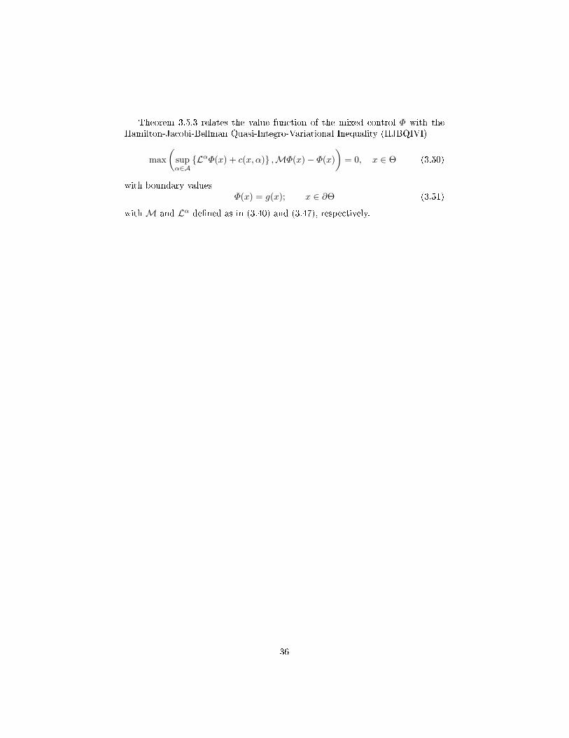
Theorem 3.5.3 relates the value function of the mixed control Φ with theHamilton-Jacobi-Bellman Quasi-Integro-Variational Inequality (HJBQIVI)

max

(supα∈ALαΦ(x) + c(x, α) ,MΦ(x)− Φ(x)

)= 0, x ∈ Θ (3.50)

with boundary valuesΦ(x) = g(x); x ∈ ∂Θ (3.51)

withM and Lα dened as in (3.40) and (3.47), respectively.

36

Chapter 4

Optimal Control applied to

High Frequency Trading

We now establish the connection between High Frequency Trading (Chapter 2)and Markov control processes (Chapter 3). To do this, we follow the recent work[4]. The main idea is to establish a control model in order to obtain optimalstrategies of limit and market orders so that the trader can get the spread in acontext of high frequency trading. The order book considered has a price/timepriority scheme. Thus, when setting a limit order, the agent can choose basicallybetween posting his quote equal to best bid (or ask) and wait the match of thisorder by a market order counterpart, or, in order to get the execution orderpriority, he may set his quote at best bid (or ask) plus (minus) a tick. In thislast option, the market maker will wait less than in the rst option but at aless favourable price. It is assumed that the agent is small, in the sense that hecannot modify the price of the stock.

We shall assume that there are at least three sources of risk by taking alimit order position. The adverse selection risk is the risk that market priceunfavourably deviates, from the limit order trader point of view, after theirorder was taken. The execution risk that comes up when the limit order can notnd its counterpart in market orders. Finally, the risk inventory dealing withthe amount of inventory that is owned which can lead to large losses originatedby prices rises or declines in a unfavourable way. The use of market ordersavoids these risks.

4.1 The Market Making model

Let x a probability space (Ω,F ,P) equipped with a ltration F = (Ft)t≥0

satisfying the usual conditions. This probability space will be the stochasticbasis of all the random variables and stochastic processes in this thesis.

The rst set of processes are considered in the sequel:

37

1. The Midprice process: this process is modelled as an exogenous Markovprocess P(·) with innitesimal generator P and state space R+.

2. The Bid-Ask Spread process: this process takes nite discrete values,multiple of the tick size δ > 0; and jumping at random times. Morespecically, the spread is modelled as a continuous-time (inhomogeneous)Markov chain composed by

(a) A Poisson process N (·) =(N(t)

)t≥0

with deterministic intensity rateλ(t) that represents the tick time clock, i.e., the random times atwhich bid-ask spread change by means of buying and selling ordersof participants in the market

(b) A discrete-time stationary Markov chain S• = (Sn)n∈N, valued in thenite state space S = δIm, where Im := 1, . . . ,m, m ∈ N\0, withprobability transition matrix (ρij)1≤i,j≤M , i.e.,

P [Sn+1 = jδ|Sn = iδ] = ρij ,

such that ρii = 0 and independent of N (·). This Markov chainrepresents the level of spread in tick time.

Thus, we dene the spread process S(·) =(S(t)

)t≥0

as the time-change of

S• by N (·), i.e.S(t) = SN(t), t ≥ 0,

the generator of S(·) becomes R(t) =(rij(t)

)1≤i,j≤m, where

rij(t) = λ(t)ρij

for i 6= j, and rii(t) = −∑j 6=i

rij(t).

These processes are independent of each other.

The objective of the HF trader is to get the spread by means of limit orderswhile controlling his inventory position. Let us explain now what is understoodby limit order strategies.

Limit order strategies

When an agent sets a limit order in the LOB (see Chapter 2), he can wait untilthis order is matched by a market order. The objective is to establish a strategyto get the spread. Because the agent acts as a market maker and his objectiveis only to get the spread, the quote is established at best bid/ask prices or atat best bid/ask prices plus a tick. The problem of choosing between these twooptions depends on both the expected execution time and the size of the spread.There is tradeo between get a faster execution and get a bigger spread. Theagent may submit at any time limit buy/sell orders at the current best bid/ask

38

prices, but he also can establish buy (sell) orders at marginal higher (lower)prices. This latter alternative is used to get priority in the order execution.

The limit order strategies are modelled by a continuous time predictablecontrol process:

αmake(t) = (Qb(t), Qa(t), Lb(t), La(t)), t ≥ 0

where L = (Lb, La) is valued in the admissible set [0, ¯]2, ¯> 0, and it repre-sents the size of the limit buy and sell orders, respectively, and Q = (Qb, Qa)represents the possible choices of the bid and ask quotes either at best prices,denoted by Bb and Ba, respectively, or at marginally improved prices, denotedby Bb+ and Ba− (best-bid plus a tick and best-ask minus a tick prices, respec-tively). These last quotes will strongly depend on the level of spread: if thespread is of just one tick, i.e. s = 1 · δ, then the quote equal to best bid (ask)price plus (minus) a tick becomes a market buy (sell) order and hence we cannotquote our shares plus or minus a tick. This is summarized as follows:

(Qb, Qa) = Q(s), where

Q(s) =

Qb ×Qa := Bb,Bb+ × Ba,Ba− if s > δ(Bb,Ba) if s = δ

For a xed price-spread vector (p, s) ∈ R+ × S, and qa ∈ Qa (resp. qb ∈ Qb),the market maker can establish the bid and ask quotes, respectively, as

πb(qb, p, s) =

p− s

2 for qb = Bbp− s

2 + δ for qb = Bb+

πa(qap, s) =

p+ s

2 for qa = Bap+ s

2 − δ for qa = Ba−.

Exogenous Markets Orders

In order to be executed, limit orders need to be matched by incomming marketorders from other traders in the market. The arrivals of this orders are modelledby independent Cox processes: N a(·) :=

(Na(t)

)t≥0

, for buying market orders,

and N b(·) :=(N b(t)

)t≥0

, for selling market orders. The intensity rate of Na(t)

is given by λa(Qa(t), S(t)) where λa is a deterministic function of the limit quoteselling order, and of the spread. Likewise, the intensity rate of N b(t) is givenby λb(Qb(t), S(t)) where λb is also a deterministic function of the limit quotebuying order and the spread. Both λa and λb are supposed to be non-increasingwith respect to the spread. This means that the larger the spread, the lessoften the arrivals of the market buy and sell orders. These assumptions are inaccordance with the idea that with a small spread the market has more liquidity.It is also assume that

λa(Ba, s) < λa(Ba−, s) and λb(Bb, s) < λb(Bb+, s)

for all s ∈ Im, which is consistent with the price priority condition.

39

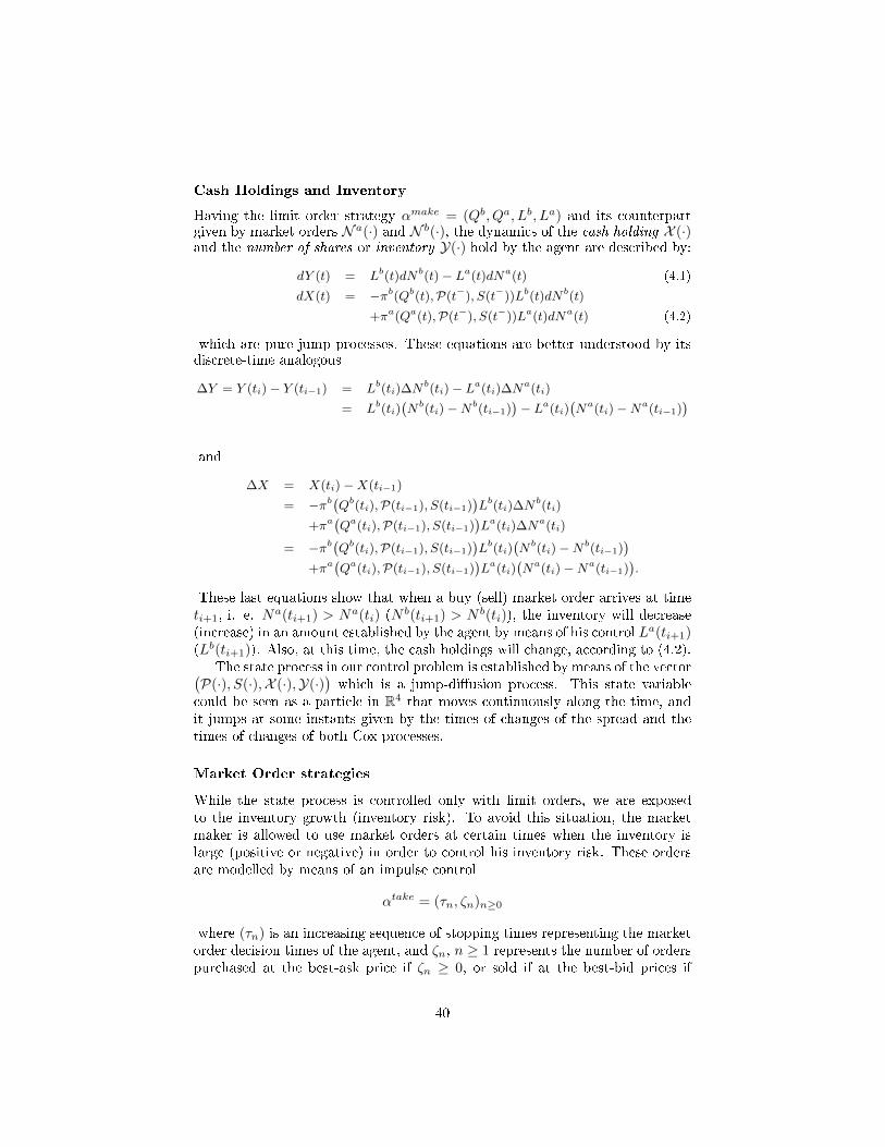
Cash Holdings and Inventory

Having the limit order strategy αmake = (Qb, Qa, Lb, La) and its counterpartgiven by market orders N a(·) and N b(·), the dynamics of the cash holding X (·)and the number of shares or inventory Y(·) hold by the agent are described by:

dY (t) = Lb(t)dNb(t)− La(t)dNa(t) (4.1)

dX(t) = −πb(Qb(t),P(t−), S(t−))Lb(t)dNb(t)

+πa(Qa(t),P(t−), S(t−))La(t)dNa(t) (4.2)

which are pure jump processes. These equations are better understood by itsdiscrete-time analogous

∆Y = Y (ti)− Y (ti−1) = Lb(ti)∆Nb(ti)− La(ti)∆N

a(ti)

= Lb(ti)(Nb(ti)−Nb(ti−1)

)− La(ti)

(Na(ti)−Na(ti−1)

)and

∆X = X(ti)−X(ti−1)

= −πb(Qb(ti),P(ti−1), S(ti−1)

)Lb(ti)∆N

b(ti)

+πa(Qa(ti),P(ti−1), S(ti−1)

)La(ti)∆N

a(ti)

= −πb(Qb(ti),P(ti−1), S(ti−1)

)Lb(ti)

(Nb(ti)−Nb(ti−1)

)+πa

(Qa(ti),P(ti−1), S(ti−1)

)La(ti)

(Na(ti)−Na(ti−1)

).

These last equations show that when a buy (sell) market order arrives at timeti+1, i. e. Na(ti+1) > Na(ti) (N b(ti+1) > N b(ti)), the inventory will decrease(increase) in an amount established by the agent by means of his control La(ti+1)(Lb(ti+1)). Also, at this time, the cash holdings will change, according to (4.2).

The state process in our control problem is established by means of the vector(P(·), S(·),X (·),Y(·)

)which is a jump-diusion process. This state variable

could be seen as a particle in R4 that moves continuously along the time, andit jumps at some instants given by the times of changes of the spread and thetimes of changes of both Cox processes.

Market Order strategies

While the state process is controlled only with limit orders, we are exposedto the inventory growth (inventory risk). To avoid this situation, the marketmaker is allowed to use market orders at certain times when the inventory islarge (positive or negative) in order to control his inventory risk. These ordersare modelled by means of an impulse control

αtake = (τn, ζn)n≥0

where (τn) is an increasing sequence of stopping times representing the marketorder decision times of the agent, and ζn, n ≥ 1 represents the number of orderspurchased at the best-ask price if ζn ≥ 0, or sold if at the best-bid prices if

40

ζn < 0 at these times. When submitting a market order strategy, the cashholdings and the inventory switch at times τn by the following dynamics:

Y (τn) = Y (τ−n ) + ζn, (4.3)

X(τn) = X(τ−n )− c(ζn,P(τn), S(τn)

)(4.4)

wherec(e, p, s) = ep+ |e|s

2+ ε

represents a cost function indicating the amount to be paid immediately whenposting a market order of size e, given the mid price p, a spread s, and a xedfee ε > 0. The fees is established because a market order removes liquidity tothe market.

Finally, we denote as A the set of all limit/market order trading strategiesα = (αmake, αtake)

.

4.2 Optimal Limit/Market Order Strategies

The market model of the LOB is completely determined by the state variables(X ,Y,P, S) which in turn they are controlled by the limit and market orderstrading strategies α ∈ A. The objective of the market maker is to maximizeover a nite-time horizon T the prot from his transactions in the limit orderbook, while keeping under control his inventory, and getting rid of his inventoryat the terminal date, this is establish by the following optimization objective:

maxα∈A

E

[U(Xα(T ))− γ

∫ T

0

g(Y α(t)

)dt

], (4.5)

where we are maximizing over all limit and market order trading strategiesα = (αmake, αtake) in A with the extra condition that Y (T ) = 0, where U is anincreasing reward function, γ is a nonnegative constant, and g is a nonnegativeconvex function, such that the integral term in (4.5) penalizes the variations ofthe inventory.

The terminal condition Y (T ) = 0 on the inventory can be removed by intro-ducing a liquidation function L(x, y, p, s) dened on R2 × R+ × S by:

L(x, y, p, s) = x− c(−y, p, s) = x+ yp− |y|s2− ε. (4.6)

which represents the value that an investor would obtain by liquidating imme-diately his inventory y through a market order, given that the levels of cashholdings, mid-price, and spread are x, p and s, respectively. In this way, wereformulate the problem (4.5) as:

maxα∈A

E

[U(L(Xα(T ), Y α(T ),P(T ), S(T )

))− γ

∫ T

0

g(Y α(T )

)dt

]. (4.7)

41

By dening Zα(t) =(Xα(t), Y α(t), P (t)

)∈ R2 × P, we can dene the value

function associated to (4.7) as:

v(t, z, s) = supα∈A

Et,z,s

[U(L(Zα(T ), S(T )

))− γ

∫ T

t

g(Y α(u)

)du

](4.8)

for t ∈ [0, T ], z = (x, y, p) ∈ R2 × P, s ∈ S. This problem is a mixed stochas-tic/impulse control problem in under the context of a switching jump-diusionmodel.

As we saw in Chapter 3, this kind of problems can be solved from the useof the dynamic programming technique. This is accomplished in the followingsubsection.

4.2.1 Dynamic Programming Equation

Let us x αmake(t) = (qb, qa, `b, `a) =: (q, `), and consider the second-ordernonlocal operator on [0, T ]× R2 × P× S by:

L(q,`)ϕ(t, x, y, p, s) = Pϕ(t, x, y, p, s) +R(t)ϕ(t, x, p, s) (4.9)

+λb(qb, s)[ϕ(t,Γb(x, y, p, s, qb, `b), p, s)− ϕ(t, x, y, p, s)

]+λa(qa, s) [ϕ(t,Γa(x, y, p, s, qa, `a), p, s)− ϕ(t, x, y, p, s)]

for (t, x, y, p, s) ∈ [0, T ]× R2 × P× S, where

R(t)ϕ(t, x, y, p, s) =

m∑j=1

rij(t)[ϕ(t, x, y, p, jδ)− ϕ(t, x, y, p, iδ)], for s = iδ, i ∈ Im

and Γb (resp. Γa) is dened from R2×P×S×Qb×R+ (resp. R2×P×S×Qa×R+)into R2 by

Γb(x, y, p, s, qb, `b) = (x− πb(qb, p, s)`b, y + `b)

Γa(x, y, p, s, qa, `a) = (x+ πa(qa, p, s)`a, y − `a)

The terms in L(q,`) correspond to:

• P is the innitesimal generator of the diusion mid-price process P

• R represents the generator of the continuous-time Markov chain of thespread S.

• The two last terms correspond to the nonlocal operator induced by thejumps of the cash holdings process X (·) and inventory process Y(·) whenapplying an instantaneous limit order strategy action

(Q(t), L(t)

)= (q, `).

The previous operator gives us the dynamic of the time-state variable (t,X ,Y,P, S)when there are no other intervention. For the impulse control strategy, we con-sider the impulse operator associated to market order control dened by:

Mϕ(t, x, y, p, s) = supe∈[−e,e]

ϕ(t,Γtake(x, y, p, s, e), p, s),

42

where e ∈ R+ and Γtake is the impulse transaction function dened from R2 ×P× S× R into R2 by:

Γtake(x, y, p, s, e) = (x− c(e, p, s), y + e) ,

which give us, at any time t under xed (x, y, p, s), the best amount of ordersthat the trader can oer in his market buy or sell orders. However, this actioncould not be taken because it may not be worth to submit a market order whena limit order can make a better prot.

For the control problem (4.8), the Hamilton-Jacobi-Bellman equation is rep-resented by the quasi-integro-variational inequality (QIVI)

min

[−∂v∂t− sup

(q,`)∈Q(s)×[0,¯]2Lq,`v + γg, v −Mv

]= 0, on [0, T )× R2 × P× S

(4.10)

together with the terminal condition:

v(T, x, y, p, s) = U(L(x, y, p, s)), ∀(x, y, p) ∈ R2 × P× S (4.11)

4.3 One special case: Mean criterion with penaltyon inventory

One framework to study (4.5) is the mean criterion, this is expressed as:

U(x) = x, γ > 0 and g(y) = y2,

for x, y ∈ R. Let us assume the case where P(·) =(P(t)

)t≥0

is a martingale.This assumption arises naturally when one considers that there is no informationabout future price movements. This reects the idea that the market makeractions (at least in this work) are not directional; that is, the trader is notconcerned about the price going up or down but the prot made by getting thespread.

The function v might be analysed in each level of spread s = iδ, wherei ∈ Im, as functions vi dened in [0, T )×R2 × P. The martingale property giveus a zero drift term, that is, Pp = 0, so the solution v = (vi)i∈Im to the dynamicprogramming system (4.10)-(4.11) is reduced into the form:

vi(t, x, y, p) = x+ yp+ φi(t, y), (4.12)

where φ = (φi)i∈Im is solution to the system of integro-dierential equations

43

(IDE):

min

−∂φi∂t−

m∑j=1

rij(t)[φj(t, y)− φi(t, y)]

− sup(qb,`b)∈Qb

i×[0,¯]

λbi (qb)

[φi(t, y + `b)− φi(t, y) +

(iδ

2− δ1qb=Bb+

)`b]

− sup(qa,`a)∈Qa

i×[0,¯]

λai (qa)

[φi(t, y − `a)− φi(t, y) +

(iδ

2− δ1qa=Ba−

)`a]

+ γg(y);

φi(t, y)− supe∈[−e,e]

[φi(t, y + e)− iδ

2|e| − ε

]]= 0,

together with the terminal condition:

φi(T, y) = −|y| iδ2− ε,

These one-dimensional IDEs can be solved numerically by a standard nite-dierence methods. An important fact to note is that by using the mean crite-rion, the reduced equation (4.12) shows that the optimal market making strate-gies are price independent, and depend only on the level of inventory and of thespread. Henceforth, α? can be represented as operator from R+ × R× S into Awith α? = (α?,make, α?,take). The control α? divides the space R+ × R× S intwo zones

• M , where just the limit order strategies are activated, and,

• T , where just the market orders strategies act.

The following graphic shows the zones divided by the optimal strategy.Plot 1 Plot 2

Figure 4.1: Stylized shape of the optimal policy sliced in YS

44

In Figure 4.1, which was taken from [4], it is shown the optimal strategiesin two dierent times. Plot 1 shows the optimal policy near date 0 and Plot2 near terminal date T . If we choose a point in a shadow zone of one of thesegraphics, we will be in the limit order strategies zone, and the optimal decisionwill use limit order with La = Lb = 100 and quotes Qa and Qb depending onthe zone where they fall. For example if we are in a point in the middle andtop of the rst plot, we will be in the (Qa, Qb) = (Ba−, Bb+) zone and theoptimal strategy will be α = (αmake, 0) =

((Bb+, Ba−, 100, 100), 0

); whereas

if at time t1, we fall in the non-shadow zone T , the optimal strategy will beα = (0, αtake) =

(0, (t1, 100)

).

This analysis will be the basis for our simulations in the next chapter.

45

Chapter 5

Simulation

The aim of this Chapter is to use simulation to compare, by approximation,the dierent trading strategies used by the authors. That is, the LOB wassimulated and at each step the agent used the policy corresponding to eachparticular strategy.

In other words, we simulated the market of a limit order book where theagent enters at a certain initial date, makes transactions following a certain ruleestablished by the strategy, and gets out at a nal date.

The chapter is divided as follows. In section 5.1 we briey explain theprocedure used to simulate each stochastic process. Section 5.2 species thevarious strategies that the agent will follow. Later, in section 5.3, we comparethe dierent strategies through standard hypothesis testing techniques. Weconclude, in Section 5.4, by discussing our results. The algorithms used hereare based in those given in [1] and [9].

5.1 Simulation of the Processes Involved

5.1.1 Price Process

Within this chapter, the price process P is modelled as a standard Brownianmotion started at P0 = 45. In particular, a realization of this process was car-ried out as follows:

(i) Set P0 = 45.

(ii) Simulate Xi ∼ N(0, 1

60

), 1 ≤ i ≤ n.

(iii) Establish

Pn = P0 +

n∑j=1

Xj , n ≥ .1

(iv) Dene the vector Pn = (P0, . . . , Pn).

46

Hence, the vector Pn contains a discrete approximation of a simulated path ofa Wiener process.

In order to simulate a trajectory of the continous path processes of price andspread, we discretized the time interval per second. For instance, to simulatea trajectory of 300 seconds in length of the price process P we generated 300independent realizations of the random variable Xi dened above. In betweenthese points the process is considered constant.

5.1.2 Spread Process

The spread process is composed of two underlying processes. The rst is adiscrete-time Markov chain (DTMC) taking values in:

δI6 = 0.005 · I6 = 0.005, 0.010, 0.015, 0.020, 0.025.

In particular, we used the transition matrix obtained by the authors. To thisend, let us recall that the entries of the matrix are formed by the probabilities

pij = P[Sn = j|Sn−1 = i].

The simulation of a N -step path of a realizations of a DTMC was carried outas follows:

(i) Choose an initial value of the spread s0 = δi with δ = 0.005, i ∈ 1, 2, 3, 4, 5, 6,and set n = 1

(ii) Simulate an uniform random variable U ∼ Unif[0, 1].

(iii) Set j∗ = min

j∣∣ U ≤ j∑

k=1

pik

and let sn = δ · j∗

(iv) If n < N , set i = j∗ and n = n+ 1 and go to step (ii). Otherwise, stop

That is, the vector of size N + 1, SN = (s0, s1, . . . , sN ) is the realization of aN -step DTMC started at S0 = s0.

The second underlying process is a non-homogeneous Poisson process withintensity rate function λ(·). We can simulate a path of this process in an interval[0, T ] through the following scheme:

(i) Fix λmax = maxλ(t), t ∈ [0, T ]

(ii) Set t = 0, k = 0

(iii) Simulate an exponential random variable Yk ∼ Exp(λmax) and set t =t+ Yk

(iv) If t < T , simulate an uniform random variable U ∼ Unif[0, 1], otherwise,stop.

(v) If u ≤ λ(t)λmax

, set k = k + 1, S(k) = t, and go to step (iii).

47

With the previous algorithm, if K represents the number of jumps in [0, T ], thevector S = (S(1), . . . , S(K)) represents the times of jump of a Poisson process.

In order to simulate the continuous-time Markov chain (CTMC) in the inter-val [0, T ], we proceed as follows: First, simulate the non-homogeneous Poissonprocess and then establish the number N in the DTMC as the number K of thenon-homogeneous Poisson process. In this way, for each entry of S we have thestate at which the process is. We can summarize the information in a vector Sof size 2(K + 1) where the rst entry is the number of jumps. Next, there areK entries with the times of jump, and nally K+ 1 entries with states at whichthe CTMC is each time it jumps.

5.1.3 Incoming Market Orders Processes

Given that both the buy and sell market orders are modelled as Cox processes,it is sucient to explain one of them. We choose to explain ask incoming marketorders. In this case, the spread is the source of stochastic behaviour that aectsthe intensity rate.

These orders also depends on the limit order price established by the tradingstrategy that is followed. For some of the strategies explained in the followingsection, the choice of the limit order price does not depend on these incomingorders, as it will be the case for both the random and passive strategy. However,for the other two strategies, with or without market orders, the dependencearises indirectly through the inventory, which alternatively is contingent on thearrival of these orders.

The time interval where we developed the simulation is the rst ve minutesof the trading day, in other words, the rst three hundred seconds. Given thatwe discretize the interval per seconds, the partition we take is

P = t0 = 0, t1, . . . , t300.

For a given path of the spread and an initial limit ask order price, qai , along theinterval [ti−1, ti], for 1 ≤ i ≤ 300, we use the states of the spread and the timesof change that fall within this interval. Using the previous data, we simulate theCox process as a non-homogeneous Poisson process with intensity rate functionλi(s, q

ai ), which takes values according on the rule on Table 5.1. By giving the

subindex i to the intensity rate function, we highlight the fact that there arethree hundred of these functions, each one depending on the path of the spreadwithin the corresponding interval.

A sell market order is determined by the time it is submitted and the quantityof orders that the agent wishes to sell. With the algorithm described in theprevious paragraph, we obtain a Cox process modelling the arriving time ofthe exogenous market sell orders. Once we have the arrival process, we x thequantity of orders to be one hundred for every sell market order. In this way, wecomplete the model for sell market orders. As we have previously mentioned,the same procedure is carried out for the buy market orders.

48

Ba Ba− Bb Bb+0.005 0.0539 0.1485 0.0718 0.17630.010 0.0435 0.0979 0.0520 0.11440.015 0.0401 0.0846 0.0419 0.09150.020 0.0360 0.0856 0.0409 0.08960.025 0.0435 0.1009 0.0452 0.09300.030 0.0554 0.1202 0.0614 0.1255

Table 5.1:

5.1.4 Inventory and Cash holdings processes

Both of these processes are modelled as stochastic dierential equations (SDE)which depend on the Cox processes of incoming market orders described in theprevious chapter. For convenience of the reader, we recall those equations

dYt = LbtdNbt − Lat dNa

t , (5.1)

dXt = −πb(Qbt , Pt− , St−)LbtdNbt + πa(Qat , Pt− , St−)Lat dN

at . (5.2)

The time discretization used in subsection 5.1.3 yields the following stochasticdierence equations

∆Y = Yti − Yti−1 = Lbti∆Nbti − L

ati∆N

ati

= Lbti(Nbti −N

bti−1

)− Lati(Nati −N

ati−1

)

for the inventory process Y , and

∆X = Xti −Xti−1

= −πb(Qbti , Pti−1 , Sti−1)Lbti∆Nbti + πa(Qati , Pti−1 , Sti−1)Lati∆N

ati

= −πb(Qbti , Pti−1 , Sti−1)Lbti(Nbti −N

bti−1

)

+πa(Qati , Pti−1 , Sti−1)Lati(Nati −N

ati−1

).

for the cash holdings process X.For these processes we observe that both Pti−1 and Sti−1 are given exoge-

nously, while the dierences Nati − N

ati−1

and N bti − N

bti−1

are provided by theCox process described above. As before, we x the size of the order to beLati = Lbti = 100 for all 1 ≤ i ≤ 300. In the next section we describe the way inwhich Qati and Q

bti are selected.

5.2 Strategies

Even though the strategies are a set of actions to be taken in any time t, thedecision of setting a limit order or a market order will be taken only when theCox process has a change, i.e., when Na

t− 6= Nat or N b

t− 6= N bt . We will refer to

49

these times as decision times. We will compare four types of strategies, whichare described below:

1. Passive. This is the most simple strategy. The action to be taken atany decision time is to submit a limit order at the current best bid or askprice. The opposite would be an aggresive strategy which would narrowthe spread by submitting best bid price plus a tick, or best ask minus atick. It is agressive because it decreases the expected time of execution.

2. Random. At any decision time, this strategy submits a limit order witha quote based on a mechanism similar to a fair ip of a coin. That is,contingent on the side coin, we decide if we submit a buy limit order atbest buy price or at best buy price plus a tick. A similar action is takenin the case of sell limit orders.

3. Without Market Orders. This strategy is based on the Figure 3. Thatis, at time t, an action is taken depending on the region in which theinventory and spread (y, s) fall in. The regions are the following:

A An aggressive action both in buy and sell limit orders will be submit-ted. That is, we will establish the quote Bb+ for buy limit orders,and Ba− for sell limit orders.

B In this case, the value of the spread cannot compensate the greatamount of negative inventory we have. This follows from the fact thatwe have accumulated a large amount of shares since we have beenborrowing shares several times. In order to palliate this situation, weset an aggressive action by establishing buy limit orders at a higherprice than the best bid price. At the same time, we submit our quotefor sell limit orders at best ask price. This mean that our quotes willbe (Ba,Bb+).

C In this region, we follow the opposite action than the previous case.We have a large inventory and we want to sell it. The action to betaken in this case is to set the quote of sell limit orders at the level ofthe best ask price minus a tick. On the other hand, the quote for thebuy limit orders remain the same. That is, (Qa, Qb) = (Ba−, Bb)

D Even though in this region the inventory is small, the spread is solittle that it is not worth reducing it more in order to get executionpriority. In this case, we take a passive action in both sell and buylimit orders, that is (Qa, Qb) = (Ba,Bb).

These regions are determined by the sections limited by the lines

γt1 : s = (−0.000125− t+ 1)y + 0.017

andγt2 : s = (0.000125 + t− 1)y + 0.0175.

50

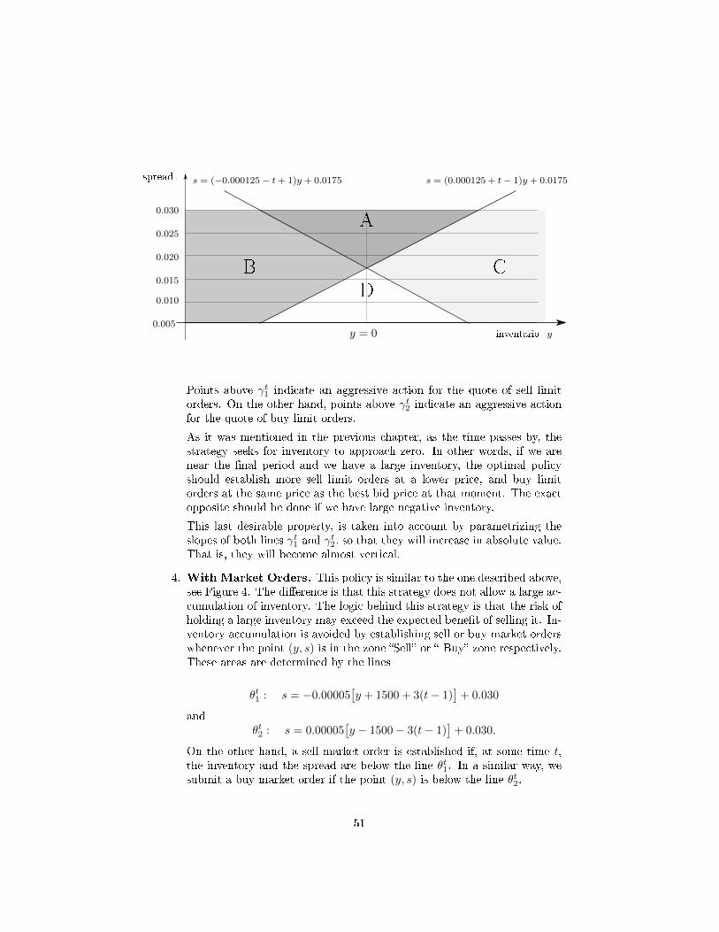
spread

inventario=y

s = (−0.000125 − t+ 1)y + 0.0175 s = (0.000125 + t− 1)y + 0.0175

B C

0.030

0.025

0.020

0.015

0.010

0.005

A

y = 0

D

Points above γt1 indicate an aggressive action for the quote of sell limitorders. On the other hand, points above γt2 indicate an aggressive actionfor the quote of buy limit orders.

As it was mentioned in the previous chapter, as the time passes by, thestrategy seeks for inventory to approach zero. In other words, if we arenear the nal period and we have a large inventory, the optimal policyshould establish more sell limit orders at a lower price, and buy limitorders at the same price as the best bid price at that moment. The exactopposite should be done if we have large negative inventory.

This last desirable property, is taken into account by parametrizing theslopes of both lines γt1 and γt2, so that they will increase in absolute value.That is, they will become almost vertical.

4. With Market Orders. This policy is similar to the one described above,see Figure 4. The dierence is that this strategy does not allow a large ac-cumulation of inventory. The logic behind this strategy is that the risk ofholding a large inventory may exceed the expected benet of selling it. In-ventory accumulation is avoided by establishing sell or buy market orderswhenever the point (y, s) is in the zone Sell or Buy zone respectively.These areas are determined by the lines

θt1 : s = −0.00005[y + 1500 + 3(t− 1)

]+ 0.030

andθt2 : s = 0.00005

[y − 1500− 3(t− 1)

]+ 0.030.

On the other hand, a sell market order is established if, at some time t,the inventory and the spread are below the line θt1. In a similar way, wesubmit a buy market order if the point (y, s) is below the line θt2.

51

spread

inventario=y

s = 0.00005[y − 1500 − 3(t− 1)

]+ 0.030 s = −0.00005

[y + 1500 + 3(t− 1)

]+ 0.030

s = (−0.000125 − t+ 1)y + 0.0175 s = (0.000125 + t− 1)y + 0.0175

B C

0.030

0.025

0.020

0.015

0.010

0.005

A

y = 0

DBuy Sell

In this strategy, both slopes of the lines γt1, γt2, and θ

t1, θ

t2 are parametrized.

To understand the way in which this strategy works, recall that as we ap-proach the nal period, we have to decrease our inventory in an aggressiveway. This is achieved by prioritizing the market over the limit orders. Inthis case, the lines θt1 and θt2 approach the line y = 0 (zero inventory), aswe are near the nal period.

5.3 Computational Results

We carry out n = 30, 000 simulations of each strategy and obtained the followingresults:

Simulation Times Num. Sim. x svector_with_orders 300 30000 74.17757 1522.526

vector_without_orders 300 30000 62.86596 974.5092

vector_random 300 30000 50.11336 1012.785

vector_passive 300 30000 48.45765 822.6015

We also performed hypothesis testing for the dierences in means among thestrategies. Since our goal is to determine which strategy is best, we set the nullto be that the means are the same, and the alternative that one is greater than

52

the other, that is

H0 := µ1 = µ2 v.s. H1 := µ1 6= µ2

To this end, we use the Z- statistic

Z =X1 − X2√s21n1

+s22n2

We present our results in the following table, where the p-value is given byP(Z > z) due to the one-sided alternative.

Vectors to compare z p-valuevector_without_orders vs vector_random 1.57156326 0.05802594

vector_with_orders vs vector_random 2.27935060 0.01132312

vector_without_orders vs vector_without_orders 1.0838286 0.1392204

vector_with_orders vs vector_passive 2.574242294 0.005022995

vector_without_orders vs vector_passive 1.95689577 0.02517986

vector_random vs vector_passive 0.2197919 0.4130166

Table 5.2: Hypothesis Testing of Dierences in Mean

In order to clarify the previous ndings, we also present a table and a gurewith 95% condence intervals, see Table 5.3 and Figure 5.1.

Simulation x s√n

Intervals

vector_with_orders 74.17757 8.790305 (56.94857, 91.40657)

vector_without_orders 62.86596 5.626332 (51.83835, 73.89357)

vector_random 50.11336 5.847314 (38.65262, 61.57409)

vector_passive 48.45765 4.749292 (39.14904, 57.76627)

Table 5.3: 95% Condence Intervals

53

Strategy

mean30 80

56.948 91.40674.177

73.893

39.149

50.11338.652

51.838 62.865

61.5749

57.7662748.457

40 50 60 70

With MarketOrders

Without MarketOrders

Random

passive

90

Figure 5.1: 95% Condence Intervals

5.4 Conclusions of Simulation

Several things should be noted.

• The condence interval of the With Market Orders vector is larger be-cause the sample standard deviation is quite big.

• There is sucient statistical evidence, (p-value=0.005022995) to supportthe hypothesis that the use of our approximated strategy With MarketOrders, yields a greater expected value of prot than the Passive strat-egy.

• Given that for the test of dierence of means between Without MarketOrders and Random, the p-value> 0.05, we cannot reject the hypothesisthat the means are equal. However, it is still such a small value that itis possible that with a larger sample we could nd statistical evidence toreject the null.

• There is sucient statistical evidence that supports the rejection of equal-ity in means between With Market Orders and Random.

• There is not sucient statistical evidence that would allow us to claimthat a Random strategy has a greater expected prot than the Passivestrategy.

54

Chapter 6

Conclusions

There are several theoretical and computational research possibilities regardingHigh Frequency Trading. On the theoretical side many of the models used canbe extended (or better understood) after a deeper study of the market micros-tucture. Furthermore, assumptions like the small agent can be relaxed in orderto allow for interference in the price or spread through individual actions. Onthe computational side, extending the models leads to more complex computa-tional tools, which in turn are used to obtain numerical solutions. Finally, atthis point it is still uncertain if allowing for these extensions will lead to well-behaved solutions. That is, solutions which involve HJBQIVI which in turncould be dealt with using a nite dierence scheme.

The routines developed for this work were done with the statistical packageR. The functions were dened by the author of this work and they are based onalgorithms which appear in [1] and [9].

55

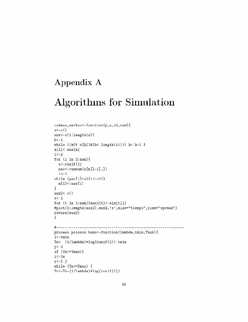
Appendix A

Algorithms for Simulation

cadena_markov<-function(p,s,x0,num)

m<-c()

aux<-c(1:length(s))

h<-1

while ((x0!=s[h])&(h<=length(s))) h<-h+1

m[1]<-aux[h]

l<-2

for (l in 2:num)

u<-runif(1)

pac<-cumsum(p[m[l-1],])

i<-1

while (pac[i]<u)i<-i+1

m[l]<-aux[i]

aux2<-c()

t<-1

for (t in 1:num)aux2[t]<-s[m[t]]

#plot(1:length(aux2),aux2,'s',xlab="tiempo",ylab="spread")

return(aux2)

#------------------------------------------------------------

proceso_poisson_homo<-function(lambda,tmin,Tmax)

l<-tmin

Tn<--(1/lambda)*log(runif(1))+tmin

y<-0

if (Tn<=Tmax)

l<-Tn

y<-1

while (Tn<=Tmax)

Tn<-Tn-(1/lambda)*log(runif(1))

56

y<-y+1

l<-c(l,Tn)

#plot(l,1:y,'s')

return(c(y,l))

#------------------------------------------------------------

lambda_escal_u<-function(t)

if (t<=3600) y<-1.654

else if( (3600<t)&(t<=7200) )y<-0.799

else if ((7200<t)&(t<=10800)) y<-0.516

else if( (10800<t)&(t<=14400) ) y<-0.377

else if( (14400<t)&(t<=18000) ) y<-0.632

else if( (18000<t)&(t<=21600) ) y<-1.305

else if (t<=25200)y<-2.113

return(y)

#--------------------------------------------------------------

evaluacion<-function(f,x)

n<-length(x)

y<-c(1:n)*0

i<-1

for (i in 1:n)

y[i]<-f(x[i])

return(y)

#------------------------------------------------------------

NHPP<-function(f,tmin,Tmax,grid) #genera un Pro Poisson NHomo

t<-seq(tmin,Tmax,grid) #entre [tmin, tmax]

lambda<-evaluacion(f,t)

lambda_max<-max(lambda)

Tn<--(1/lambda_max)*log(runif(1))+tmin

l<-tmin

y<-0

if ((tmin<Tn)&(Tn<=Tmax)) u<-runif(1)

if (u<=(f(Tn)/lambda_max))

l<-Tn

y<-1

while (Tn<=Tmax) Tn<-Tn-(1/lambda_max)*log(runif(1))

u<-runif(1)

if (u<=(f(Tn)/lambda_max))

y<-y+1

l<-c(l,Tn)

#par(mfcol=c(1,1))

#plot(l,1:y,'s')

return(c(y,l))

57

#___________________________________________________________

CTMC<-function(p,s,x0,lambda,tmin,Tmax)

X<-proceso_poisson_homo(lambda,tmin,Tmax)

Y<-cadena_markov(p,s,x0,X[1])

#plot(X[2:length(X)],Y,'s',xlab="segundos",ylab="spread")

return(c(X,Y))

#_______________________________________________________

CTMCNHPP<-function(p,s,x0,f,tmin,tmax,grid)

X<-NHPP(f,tmin,tmax,grid)

Y<-cadena_markov(p,s,x0,X[1])

#plot(X[2:length(X)],Y,'s',xlab="Tiempo en segundos",ylab="Spread")

return(c(X,Y))

#_________________________________________________________

lambdaA<-function(q,s)

S<-c(0.005,0.01,0.015,0.02,0.025,0.03)

Q<-c(1,2)

M<-match(s,S,1)

N<-match(q,Q,5)

y<-0

if ((M==1)&(N==5))y<-0

else if (q==Q[1])if (s==S[1]) y<-0.0539

else if (s==S[2]) y<-0.0435

else if (s==S[3]) y<-0.0401

else if (s==S[4]) y<-0.0360

else if (s==S[5]) y<-0.0435

else y<-0.0554

else if (s==S[1]) y<-0.1485

else if (s==S[2]) y<-0.0979

else if (s==S[3]) y<-0.0846

else if (s==S[4]) y<-0.0856

else if (s==S[5]) y<-0.1009

else y<-0.1202

return(y)

#_______________________________________________________

lambdaB<-function(q,s)

S<-seq(0.005,0.03,len=6)

Q<-c(3,4)

M<-match(s,S,1)

58

N<-match(q,Q,5)

y<-0

if ((M==1)&(N==5))y<-0

else if (q==Q[1])if (s==S[1]) y<-0.0718

else if (s==S[2]) y<-0.0520

else if (s==S[3]) y<-0.0419

else if (s==S[4]) y<-0.0409

else if (s==S[5]) y<-0.0452

else y<-0.0614

else if (s==S[1]) y<-0.1763

else if (s==S[2]) y<-0.1144

else if (s==S[3]) y<-0.0915

else if (s==S[4]) y<-0.0896

else if (s==S[5]) y<-0.0930

else y<-0.1255

return(y)

#---------------------------------------------------------------

fun_lambda<-function(v,t)

y<-stepfun(t,c(v[1],v),f=0)

return(y)

#_________________________________________________________

proc_lambdaA<-function(q,spread)

n<-spread[1]

Tspre<-c(spread[2:(n+1)]) #contiene los tiempos de saltos

Sspre<-c(spread[(n+2):length(spread)]) #contine el estado en

n2<-length(Sspre) #cada salto

lam<-c()

l<-1

for (l in 1:n2) lam[l]<-lambdaA(q,Sspre[l]) #lam contiene los

#par(mfcol=c(2,1)) #movimientos de lambdaA

#plot(Tspre,Sspre,'s',xlab="tiempo",ylab="spread")

#plot(Tspre,lam,'s',xlab="tiempo",ylab="lambda de proceso Cox ask")

return(lam)

#_________________________________________________________

proc_lambdaB<-function(q,spread)

n<-spread[1]

Tspre<-c(spread[2:(n+1)]) #contine los tiempos de saltos

Sspre<-c(spread[(n+2):length(spread)]) #contine el estado en cada salto

n2<-length(Sspre)

lam<-c()

59

l<-1

for (l in 1:n2) lam[l]<-lambdaB(q,Sspre[l]) #lam contiene los

#par(mfcol=c(2,1)) #movimientos de lambdaB

#plot(Tspre,Sspre,'s',xlab="tiempo",ylab="spread")

#plot(Tspre,lam,'s',xlab="tiempo",ylab="lambda de proceso Cox bid")

return(lam)

#_____________________________________________________________

proc_coxA<-function(q,spread,tmin,Tmax)

lambdasA<-proc_lambdaA(q,spread) #lambda es la de la cadena

nsaltos<-spread[1] #markov tiempo continuo del spread

tiempos<-spread[2:(nsaltos+1)]

lambdat<-fun_lambda(lambdasA,tiempos) #vuelve al vector en funcion lambda(t)

NHPP(lambdat,tmin,Tmax,.1) #regresa vector con numero de saltos

#y momento de cada salto

#____________________________________________________________

proc_coxB<-function(q,spread,tmin,Tmax)

lambdasB<-proc_lambdaB(q,spread)

nsaltos<-spread[1]

tiempos<-spread[2:(nsaltos+1)]

lambdat<-fun_lambda(lambdasB,tiempos) #vuelve al vector en funcion lambda(t)

NHPP(lambdat,tmin,Tmax,.1)

#___________________________________________________________

inventario<-function(la,lb,qa,qb,spread,tmin,Tmax,grid)

coxa<-proc_coxA(qa,spread,tmin,Tmax)

coxb<-proc_coxB(qb,spread,tmin,Tmax)

CoxA<-stepfun(coxa[2:length(coxa)],c(0:coxa[1]),f=0)

CoxB<-stepfun(coxb[2:length(coxb)],c(0:coxb[1]),f=0)

n<-(Tmax-tmin)/grid

t<-c(0:n)*grid+tmin

j<-1

y<-c()

y[1]<-0

for (j in 1:n)

y[j+1]<-y[j]+lb*(CoxB(t[j+1])-CoxB(t[j]))-la*(CoxA(t[j+1])-CoxA(t[j]))

return(y)

#_________________________________________________________

midprice<-function(p0,difusion,tmin,Tmax,grid,modelo)

time<-seq(tmin,Tmax,grid)

n<-length(time)

60

if (modelo==1)

mid<-c()

i<-1

mid[i]<-p0

wiemid<-cumsum(rnorm(n,0,difusion))

for (i in 1:(n-1))

mid[i+1]<-mid[i]+difusion*(wiemid[i+1]-wiemid[i])

else

mid<-cumsum(rnorm(n,0,difusion))+p0

return(mid)

#___________________________________________________________

quoteA<-function(qa,spread,precio,tmin,Tmax,grid,tick)

time<-seq(tmin,Tmax,grid)

n<-length(precio)

ns<-spread[1]

dife<-stepfun(spread[2:(ns+1)],c(spread[ns+2],spread[(ns+2):(2*ns+1)]),f=0)

y<-c()

j<-1

for (j in 1:n) y[j]<-precio[j]+dife(time[j])/2-tick*(qa-1)

return(y)

#_____________________________________________________________

quoteB<-function(qb,spread,precio,tmin,Tmax,grid,tick)

time<-seq(tmin,Tmax,grid)

n<-length(precio)

ns<-spread[1]

dife<-stepfun(spread[2:(ns+1)],c(spread[ns+2],spread[(ns+2):(2*ns+1)]),f=0)

y<-c()

j<-1

for (j in 1:n) y[j]<-precio[j]-dife(time[j])/2+tick*(qb-3)

return(y)

#_______________________________________________________________

cash<-function(la,lb,qa,qb,spread,precio,tmin,Tmax,grid,tick)

coxa<-proc_coxA(qa,spread,tmin,Tmax)

coxb<-proc_coxB(qb,spread,tmin,Tmax)

CoxA<-stepfun(coxa[2:length(coxa)],c(0:coxa[1]),f=0)

CoxB<-stepfun(coxb[2:length(coxb)],c(0:coxb[1]),f=0)

t<-seq(tmin,Tmax,grid)

precioA<-quoteA(qa,spread,precio,tmin,Tmax,grid,tick)

precioB<-quoteB(qb,spread,precio,tmin,Tmax,grid,tick)

61

n<-length(precioA)

X<-c()

i<-1

X[i]<-0

for (i in 1:n)

X[i+1]=X[i]-precioB[i]*lb*(CoxB(t[i+1])-CoxB(t[i]))

+precioA[i]*la*(CoxA(t[i+1])-CoxA(t[i]))

return(X)

#______________________________________________________

sim<-function(p,s,x0,funlambda,tmin,Tmax,nsim)

i<-1

x<-c()

y<-c()

ut<-c()

for (i in 1:nsim)

spread<-CTMCNHPP(p,s,x0,funlambda,tmin,Tmax,.1)

precio<-midprice(45,1/60,tmin,Tmax,.1,2)

aux<-optimo(spread,precio,tmin,Tmax,100,100)

y[i]<-aux[Tmax-tmin]

x[i]<-aux[length(aux)]

ut[i]<-x[i]+y[i]*precio[length(precio)]-abs(y[i])*(spread[length(spread)]/2)-.00001

if((i%%100)==0)print (i)

return(ut)

optimo<-function(spread,precio,tmin,Tmax,La,Lb)

S<-stepfun(spread[2:(spread[1]+1)],c(spread[spread[1]+2],

spread[(spread[1]+2):(2*spread[1]+1)]),f=0)

np<-length(precio)

timep<-seq(tmin,Tmax,length.out=np)

P<-stepfun(timep,c(precio[1],precio),f=0)

n<-Tmax-tmin

time<-seq(tmin,Tmax,1)

Y<-c()

X<-c()

Y[1]<-0

X[1]<-0

j<-1

Na<-c()

Na[1]<-0

Nb<-c()

Nb[1]<-0

for (j in 1:(n-1))

62

Bbfun<-function(y)

Bb<-(.000125+j-1)*y+.0175

return(Bb)

Bafun<-function(y)

Ba<-(-.000125-j+1)*y+.0175

return(Ba)

if (Bafun(Y[j])<S(time[j]))

if (Bbfun(Y[j])<S(time[j]))

qa<-2

qb<-4

else qa<-2

qb<-3

else if (Bbfun(Y[j])<S(time[j]))

qa<-1

qb<-4

else qa<-1

qb<-3

# Simulo

CoxA<-proc_coxA(qa,spread,time[j],time[j+1])

CoxB<-proc_coxB(qb,spread,time[j],time[j+1])

Na[j+1]<-CoxA[1]+Na[j]

Nb[j+1]<-CoxB[1]+Nb[j]

# Evaluo

Y[j+1]<-Y[j]+Lb*(Nb[j+1]-Nb[j])-La*(Na[j+1]-Na[j])

X[j+1]<-X[j]-(P(time[j])-S(time[j])/2+0.005*(qb-3))*Lb*(Nb[j+1]-Nb[j])

+(P(time[j])+S(time[j])/2-0.005*(qa-1))*La*(Na[j+1]-Na[j])

return(c(Y,X))

#______________________________________________________

sim_market<-function(p,s,x0,funlambda,tmin,Tmax,nsim)

i<-1

x<-c()

y<-c()

ut<-c()

for (i in 1:nsim)

spread<-CTMCNHPP(p,s,x0,funlambda,tmin,Tmax,.1)

precio<-midprice(45,1/60,tmin,Tmax,.1,2)

aux<-optimo_market(spread,precio,tmin,Tmax,100,100,100)

y[i]<-aux[Tmax-tmin]

x[i]<-aux[length(aux)]

ut[i]<-x[i]+y[i]*precio[length(precio)]

-abs(y[i])*(spread[length(spread)]/2)-.00001

if((i%%100)==0)print (i)

63

return(ut)

optimo_market<-function(spread,precio,tmin,Tmax,La,Lb,E0)

S<-stepfun(spread[2:(spread[1]+1)],c(spread[spread[1]+2],

spread[(spread[1]+2):(2*spread[1]+1)]),f=0)

np<-length(precio)

timep<-seq(tmin,Tmax,length.out=np)

P<-stepfun(timep,c(precio[1],precio),f=0)

ava<-trunc((Lb*9)/(Tmax-tmin))

n<-Tmax-tmin

time<-seq(tmin,Tmax,1)

Y<-c()

X<-c()

Y[1]<-0

X[1]<-0

j<-1

Na<-c()

Na[1]<-0

Nb<-c()

Nb[1]<-0

for (j in 1:(n-1))

Bbfun<-function(y)

Bb<-(.000125+j-1)*y+.0175

return(Bb)

Bafun<-function(y)

Ba<-(-.000125-j+1)*y+.0175

return(Ba)

if (Bafun(Y[j])<S(time[j]))

if (Bbfun(Y[j])<S(time[j]))

qa<-2

qb<-4

else qa<-2

qb<-3

else if (Bbfun(Y[j])<S(time[j]))

qa<-1

qb<-4

else qa<-1

qb<-3

# Simulo

CoxA<-proc_coxA(qa,spread,time[j],time[j+1])

CoxB<-proc_coxB(qb,spread,time[j],time[j+1])

Na[j+1]<-CoxA[1]+Na[j]

Nb[j+1]<-CoxB[1]+Nb[j]

64

# Evaluo

Y[j+1]<-Y[j]+Lb*(Nb[j+1]-Nb[j])-La*(Na[j+1]-Na[j])

X[j+1]<-X[j]-(P(time[j])-S(time[j])/2+0.005*(qb-3))*Lb*(Nb[j+1]

-Nb[j])+(P(time[j])+S(time[j])/2-0.005*(qa-1))*La*(Na[j+1]-Na[j])

# Considero si se efectua orden de mercado

buy<-function(y)

bu<-.00005*(y-1500-(j-1)*ava)+.030

return(bu)

sell<-function(y)

se<--.00005*(y+1500+(j-1)*ava)+.030

return(se)

if (S(time[j])<buy(Y[j+1]))

Y[j+1]<-Y[j+1]+E0

X[j+1]<-X[j+1]-E0*P(time[j])-E0*(S(time[j])/2)-.000001

else if (S(time[j])<sell(Y[j+1]))

Y[j+1]<-Y[j+1]-E0

X[j+1]<-X[j+1]+E0*P(time[j])+E0*(S(time[j])/2)-.000001

return(c(Y,X))

#_______________________________________________________________

sim_pasiv<-function(p,s,x0,funlambda,tmin,Tmax,nsim)

i<-1

x<-c()

y<-c()

ut<-c()

for (i in 1:nsim)

spread<-CTMCNHPP(p,s,x0,funlambda,tmin,Tmax,.1)

precio<-midprice(45,1/60,tmin,Tmax,.1,2)

aux<-optimo_pasiv(spread,precio,tmin,Tmax,100,100,100)

y[i]<-aux[Tmax-tmin]

x[i]<-aux[length(aux)]

ut[i]<-x[i]+y[i]*precio[length(precio)]

-abs(y[i])*(spread[length(spread)]/2)-.00001

if((i%%100)==0)print (i)

return(ut)

optimo_pasiv<-function(spread,precio,tmin,Tmax,La,Lb)

S<-stepfun(spread[2:(spread[1]+1)],c(spread[spread[1]+2],

spread[(spread[1]+2):(2*spread[1]+1)]),f=0)

np<-length(precio)

timep<-seq(tmin,Tmax,length.out=np)

P<-stepfun(timep,c(precio[1],precio),f=0)

65

n<-Tmax-tmin

time<-seq(tmin,Tmax,1)

Y<-c()

X<-c()

Y[1]<-0

X[1]<-0

j<-1

Na<-c()

Na[1]<-0

Nb<-c()

Nb[1]<-0

for (j in 1:(n-1))

qa<-1

qb<-3

# Simulo

CoxA<-proc_coxA(qa,spread,time[j],time[j+1])

CoxB<-proc_coxB(qb,spread,time[j],time[j+1])

Na[j+1]<-CoxA[1]+Na[j]

Nb[j+1]<-CoxB[1]+Nb[j]

# Evaluo

Y[j+1]<-Y[j]+Lb*(Nb[j+1]-Nb[j])-La*(Na[j+1]-Na[j])

X[j+1]<-X[j]-(P(time[j])-S(time[j])/2+0.005*(qb-3))*Lb*(Nb[j+1]-Nb[j])

+(P(time[j])+S(time[j])/2-0.005*(qa-1))*La*(Na[j+1]-Na[j])

return(c(Y,X))

#________________________________________________________

sim_aleat<-function(p,s,x0,funlambda,tmin,Tmax,nsim)

i<-1

x<-c()

y<-c()

ut<-c()

for (i in 1:nsim)

spread<-CTMCNHPP(p,s,x0,funlambda,tmin,Tmax,.1)

precio<-midprice(45,1/60,tmin,Tmax,.1,2)

aux<-optimo_aleat(spread,precio,tmin,Tmax,100,100,100)

y[i]<-aux[Tmax-tmin]

x[i]<-aux[length(aux)]

ut[i]<-x[i]+y[i]*precio[length(precio)]-abs(y[i])*(spread[length(spread)]/2)-.00001

if((i%%100)==0)print (i)

return(ut)

66

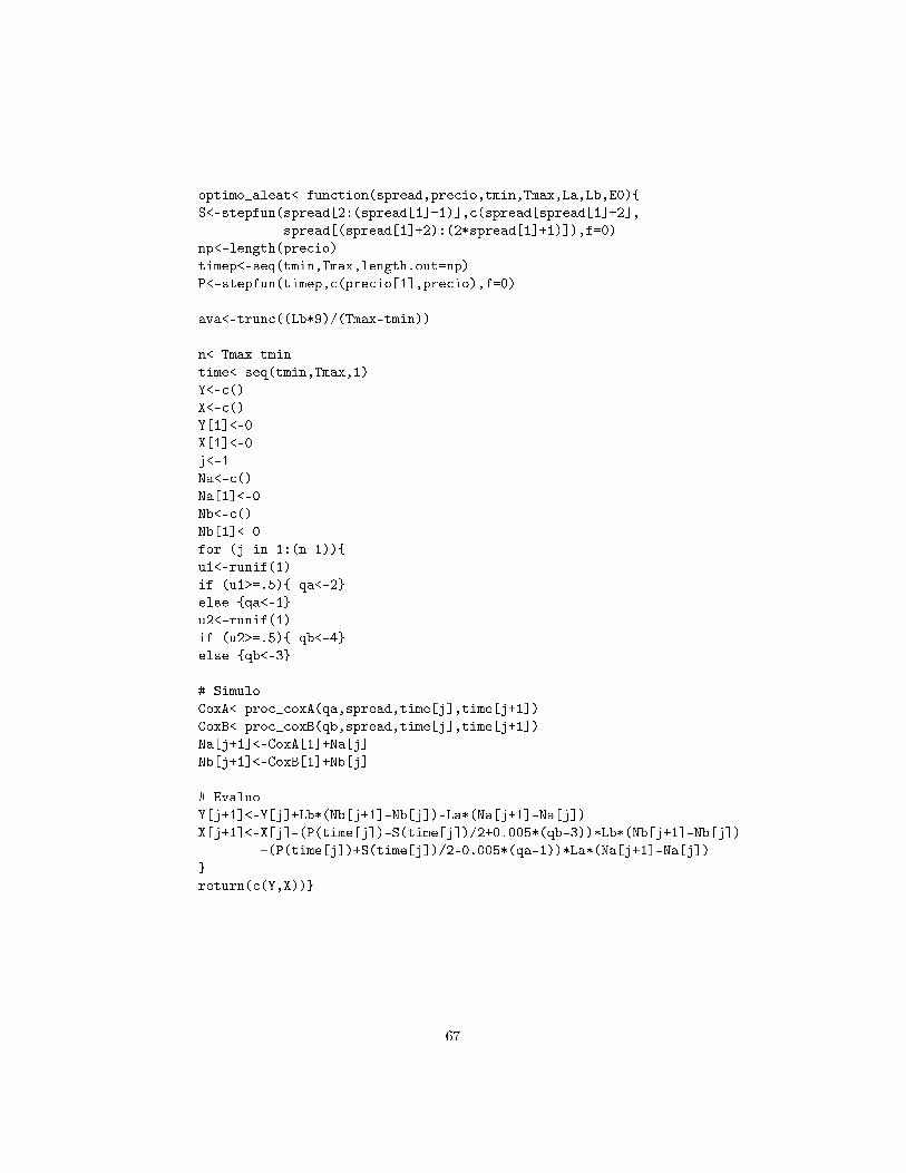
optimo_aleat<-function(spread,precio,tmin,Tmax,La,Lb,E0)

S<-stepfun(spread[2:(spread[1]+1)],c(spread[spread[1]+2],

spread[(spread[1]+2):(2*spread[1]+1)]),f=0)

np<-length(precio)

timep<-seq(tmin,Tmax,length.out=np)

P<-stepfun(timep,c(precio[1],precio),f=0)

ava<-trunc((Lb*9)/(Tmax-tmin))

n<-Tmax-tmin

time<-seq(tmin,Tmax,1)

Y<-c()

X<-c()

Y[1]<-0

X[1]<-0

j<-1

Na<-c()

Na[1]<-0

Nb<-c()

Nb[1]<-0

for (j in 1:(n-1))

u1<-runif(1)

if (u1>=.5) qa<-2

else qa<-1

u2<-runif(1)

if (u2>=.5) qb<-4

else qb<-3

# Simulo

CoxA<-proc_coxA(qa,spread,time[j],time[j+1])

CoxB<-proc_coxB(qb,spread,time[j],time[j+1])

Na[j+1]<-CoxA[1]+Na[j]

Nb[j+1]<-CoxB[1]+Nb[j]

# Evaluo

Y[j+1]<-Y[j]+Lb*(Nb[j+1]-Nb[j])-La*(Na[j+1]-Na[j])

X[j+1]<-X[j]-(P(time[j])-S(time[j])/2+0.005*(qb-3))*Lb*(Nb[j+1]-Nb[j])

+(P(time[j])+S(time[j])/2-0.005*(qa-1))*La*(Na[j+1]-Na[j])

return(c(Y,X))

67

Bibliography

[1] Bratley, P., Fox, B., Schroge, L. (1987) A Guide to Simulation, Springer,New York.

[2] Cartea, A., Jaimungal, S. (2013) Modelling Asset Prices for Algorithmicand High-Frequency Trading. Applied Mathematical Finance, 20, pp. 512-547.

[3] Durbin, M. (2010) All About High-Frequency Trading, McGraw-Hill.

[4] Guilbaud, F., Pham, H. (2013) Optimal high frequency trading with limitand market orders, Quantitative Finance, 13, pp. 79-94.

[5] Menaldi, J. L. (2008) Stochastic Dierential Equations with Jumps.Preprint.

[6] Hernández-Lerma, O. (1994) Lectures on Continuous-Time Markov ControlProcesses, Aportaciones Matemáticas, SMM, México D. F.

[7] Øksendal, B. (2003) Stochastic Dierential Equations. An Introduction withApplications, Springer, New York.

[8] Øksendal, B., Sulem, A. (2005) Applied Stochastic Control of Jump Diu-sions, Springer, New York.

[9] Ross, S. (2006) Simulation Elsevier Academic Press, Oxford.

[10] Tudor, C. (2002) Procesos Estocásticos, Aportaciones Matemáticas, SMM,México D. F.

[11] Yin, G., Zhang, Q. (2013) Continuous-Time Markov Chains and Applica-tions: A Two-Time-Scale Approach, Springer, New York.

68