Modal Logics for Timed Control⋆

Patricia Bouyer1, Franck Cassez2, Francois Laroussinie1

1 LSV, UMR 8643, CNRS & ENS de Cachan, FranceEmail: bouyer,fl@lsv.ens-cachan.fr

2 IRCCyN, UMR 6597, CNRS, FranceEmail: Franck.Cassez@irccyn.ec-nantes.fr

Patricia Bouyer, Franck Cassez, Francois Laroussinie. Modal Logics for Timed Control.Research report RI-2005-3, IRCCyN/CNRS, Nantes, April 2005. 23 pages. Available athttp://www.irccyn.ec-nantes.fr/~cassez

Abstract. In this paper we use the timed modal logic Lν to specifycontrol objectives for timed plants. We show that the control problemfor a large class of objectives can be reduced to a model-checking problemfor an extension (Lcont

ν ) of the logic Lnu with a new modality.More precisely we define a fragment of Lν , namely Ldet

ν , such that anycontrol objective of Ldet

ν can be translated into a Lcontν formula that

holds for the plant if and only if there is a controller that can enforcethe control objective.We also show that the new modality of Lcont

ν strictly increases the ex-pressive power of Lν while model-checking of Lc remains EXPTIME-complete.

1 Introduction

Control problem. The control problem (CP) for discrete event systems was firststudied by Ramadge & Wonham in [RW89]. The CP is the following: “Given afinite-state model of a plant P (open system) with controllable and uncontrol-lable discrete actions, a control objective Φ, does there exist a controller f suchthat the plant supervised by f (closed system) satisfies Φ?”The dense-time ver-sion of the CP with an untimed control objective has been investigated andsolved in [MPS95]. In this seminal paper, Maler et al. consider a plant P givenby a timed game automaton which is a standard timed automaton [AD94] withits set of discrete actions partitioned into controllable and uncontrollable ac-tions. They give an algorithm to decide whether a controller exists or not, andshow that if one such controller exists a witness can be effectively computed.In [WT97] a semi-algorithm has been proposed to solve the CP when the plantis defined by a hybrid (game) automaton.

Specification of control properties. In the aforementioned papers the con-trol objective is either a safety or reachability property (or some simple Buchiconditions). In [dAHM01] the authors give an algorithm to deal with generalω-regular control objectives. It is to be noticed that those control objectives are

⋆ Work supported by ACI Cortos, a program of the French government.

often called internal in the sense that they refer to the state properties (andclocks) of the system to be controlled. In the case of timed systems they onlyrefer to the untimed sequences of states of the system and thus have a restrictiveexpressiveness: it is possible to specify a property like “after p has been reachedq will be reached” but nothing like “after p has been reached, q will be reachedwithin less than d time units” (bounded liveness). Moreover, in the verificationmethodology for closed systems, one usually models (and thinks of) the plant Pand the controller f as a closed system f(P ), and specifies a property ϕ with asuitable timed temporal logic and check whether the closed system f(P ) satisfiesϕ. It is then very natural to have similar logics in the game framework to specifytimed control objectives for open systems.

Our contribution. The logic Lν [LL95] is a subset of the timed µ-calculusthat can be used for specifying timed safety properties of closed timed systems.Modalities of Lν seem to be appropriate to specify timed control objectives aswell because we can use existential and universal quantifications over discreteactions (as it is used in the untimed framework of [AVW03,RP03]), and also overtime delays. The control problem CP for a plant (specified as a timed automaton)and a control objective in Lν expresses as folloes:

Given a timed automaton P , the plant, and a Lν formula ϕ, thesafety control objective, is there a controller f s.t. f(P ) |= ϕ?

(CP)

So far there is no constraint neither on the structure nor on the power of thecontroller f we are looking for: it may even require unbounded memory or arbi-trary small delays between two consecutive controllable actions. In this paper wefocus on controllability (CP) and not on the controller synthesis problem (i.e.exhibit a witness controller).

The main result of the paper is that we can reduce CP for a plant P and anLν control objective ϕ, to a standard model-checking problem on the plant Pand a formula ϕc of a more expressive logic Lcont

ν , that extends Lν with a newmodality. More precisely we exhibit a deterministic fragment of Lν , namely Ldet

ν ,s.t. for all ϕ ∈ Ldet

ν , the following reduction (RED) holds:(

There exists a controller f s.t. f(P ) |= ϕ

)

⇐⇒ P |= ϕc (RED)

where ϕc is a formula of Lcontν . We also give an effective procedure to obtain ϕc

from ϕ.Further on we study the logic Lcont

ν and prove that it is strictly more expressivethan Lν , which is a technically involved result on its own. We also show that thenew modality of Lcont

ν is not necessary when we restrict our attention to samplingcontrol (the controller can do an action every ∆ time units) or to Known SwitchConditions Dense-Time control (where time elapsing is uncontrollable [CHR02]).A natural question following the reduction of equation (RED) above is to studythe model-checking problem for timed automata against Lcont

ν specifications. Inthe paper we prove that i) the model-checking of Lcont

ν over timed automata isEXPTIME-complete; ii) Lcont

ν inherits the compositionality property of Lν .

2

Related work. In the discrete (untimed) case many logics used to specify cor-rectness properties of closed systems have been extended to specify control ob-jectives of open systems. ATL [AHK02] (resp. ATL

∗) is the control versionof CTL (resp. CTL∗). More recently [AVW03,RP03] have considered a moregeneral framework in which properties of the controlled system are specified invarious extensions of the µ-calculus: loop µ-calculus for [AVW03] and quanti-fied µ-calculus for [RP03]. In both cases the control problem is reduced to amodel-checking (or satisfiability) problem as in equation (RED). In the timedframework, external specifications have been studied in [DM02]: properties ofthe controlled system are specified with timed automata, and in [FLTM02], thecontrol objective is given as a formula of the logic TCTL.

Outline of the paper. In section 2 we define basic notions used in the pa-per: timed systems, logic Lν and variants and the control problem. In section 3we prove that (RED) holds and also that ϕc is in Lν for two simpler controlproblems. Section 4 is devoted to the study of the logic Lcont

ν (expressiveness,decidability, and compositionality).

The proofs are given in appendices.

2 Timed Automata and the Timed Modal Logic Lν

We consider as time domain the set R≥0 of non-negative reals. Act is a finiteset of actions.1 We consider a finite set X of variables, called clocks. A clockvaluation over X is a mapping v : X → R≥0 that assigns to each clock a timevalue. The set of all clock valuations over X is denoted R

X≥0. Let t ∈ R≥0, the

valuation v + t is defined by (v + t)(x) = v(x) + t for all x ∈ X . For Y ⊆ X , wedenote by v[Y ← 0] the valuation assigning 0 (resp. v(x)) for any x ∈ Y (resp.x ∈ X \ Y ).We denote C(X) the set of clock constraints defined as the conjunctions of atomicconstraints of the form x ⊲⊳ c with x ∈ X , c ∈ Q≥0 and ⊲⊳∈ <,≤,=,≥, >. Forg ∈ C(X) and v ∈ R

X≥0, we write v |= g if v satisfies g and JgK denotes the set

v ∈ RX≥0 | v |= g.

2.1 Timed Transition Systems & Timed Automata

Timed transition systems. A timed transition system (TTS) is a tuple S =(Q, q0,Act, −→S) where Q is a set of states, q0 ∈ Q is the initial state, and−→S⊆ Q × (Act ∪ R≥0) × Q is a set of transitions. If (q, e, q′) ∈−→S , we also

write qe−−→S q′. The transitions labeled by a ∈ Act (resp. t ∈ R≥0) are called

action (resp. delay) transitions. We make the following common assumptionsabout TTSs [Yi90]:

– 0-delay: q0−−→S q

′ if and only if q = q′,

1 We assume that Act and R≥0 are disjoint.

3

– Additivity: if qd−−→S q

′ and q′d′

−−→S q′′ with d, d′ ∈ R≥0, then q

d+d′

−−−−→S q′′,

– Continuity: if qd−−→S q

′, then for every d′ and d′′ in R≥0 such that d = d′+d′′,

there exists q′′ such that qd′

−−→S q′′ d′′

−−−→S q′,

– Time-determinism: if qe−−→S q

′ and qe−−→S q

′′ with e ∈ R≥0, then q′ = q′′.

A run is a finite or infinite sequence ρ = s0e1−−→S s1

e2−−→S · · ·en−−−→ sn · · ·

We denote by first(ρ) = s0. If ρ is finite, last(ρ) denotes the last state of ρ.Runs(q, S) is the set of runs in S starting from q and Runs(S) = Runs(q0, S). We

use qe−−→S as a shorthand for “∃q′ s.t. q

e−−→S q

′” and extends this notation tofinite runs ρ

e−−→S whenever last(ρ)

e−−→S .

Timed automata. A timed automaton (TA) [AD94] is a tuple A = (L, ℓ0,Act,X, inv, T ) where L is a finite set of locations, ℓ0 ∈ L is the initial location, X isa finite set of clocks, inv : L → C(X) is a mapping that assigns an invariant toeach location, and T ⊆ L× [C(X)×Act× 2X ]× L is a finite set of transitions2.The semantics of a TAA = (L, ℓ0,Act, X, inv, T ) is a TTS SA = (L×RX

≥0, (ℓ0, v0),Act,−→SA

) where v0(x) = 0 for all x ∈ X and −→SAconsists of: i) action tran-

sition: (ℓ, v)a−−→SA

(ℓ′, v′) if there exists a transition ℓg,a,Y−−−−−→ ℓ′ in T s.t. v |= g,

v′ = v[Y ← 0] and v′ |= inv(ℓ′); ii) delay transitions: (ℓ, v)t−−→SA

(ℓ, v′) ift ∈ R≥0, v

′ = v + t and v, v′ ∈ inv(ℓ).

2.2 The Modal Logics Lν , Ldet

νand L

cont

ν

The modal logic Lν [LL95,LL98]. The logic Lν over the finite set of clocksK, the set of identifiers Id, and the set of actions Act is defined as the set offormulae generated by the following grammar:

ϕ ::= tt | ff | ϕ ∧ ϕ | ϕ ∨ ϕ | x in ϕ | x ⊲⊳ c | [a] ϕ | 〈a〉 ϕ |

[δ] ϕ | 〈δ〉 ϕ | Z

where a ∈ Act, x ∈ K, ⊲⊳∈ <,≤,=,≥, >, c ∈ Q≥0, Z ∈ Id.The meaning of the identifiers is specified by a declaration D assigning a Lν

formula to each identifier. When D is understood we write Z =ν ΨZ if D(Z) =

ΨZ . We define the following shorthands in Lν: r in ϕdef= x1 in x2 in · · · in xn in ϕ

if r = x1, · · · , xn ⊆ K.Let S = (Q, q0,Act,−→S) be a TTS. Lν formulae are interpreted over extendedstates (q, v) where for q ∈ Q and v ∈ R

K≥0. We write “S, (q, v) |= ϕ” when an

extended state (q, v) satisfies ϕ in the TTS S. This satisfaction relation is definedas the largest relation satisfying the implications in Table 1. The modalities 〈e〉with e ∈ Act ∪ δ correspond to existential quantification over action or delaytransitions, and [e] is the counterpart for universal quantification. An extendedstate satisfies an identifier Z (denoted S, (q, v) |= Z) if it belongs to the maximal

2 We often write ℓg,a,Y−−−−−→ ℓ′ instead of simply the tuple (ℓ, g, a, Y, ℓ′).

4

fixedpoint of the equation Z =ν ΨZ . Finally the formula clocks are used tomeasure time elapsing in properties. We define JϕKS = (q, v) | S, (q, v) |= ϕ.We write S |= ϕ for S, (q0, v0) |= ϕ where v0(x) = 0 for all x ∈ K. The logic Lν

allows us to express many behavioural properties of timed systems [LL98]. Forexample the formula Z defined by ΨZ = (

∧

a∈Act[a]Z ∧ [δ]Z ∧ϕ) holds when all

reachable states satisfy ϕ. Other examples of formulae will be given later on inthe paper.

S, (q, v) |= α =⇒ α with α ∈ tt, ffS, (q, v) |= x ⊲⊳ c =⇒ v(x) ⊲⊳ c

S, (q, v) |= Z =⇒ S, (q, v) |= ΨZ

S, (q, v) |= ϕ1 op ϕ2, =⇒ S, (q, v) |= ϕ1 op S, (q, v) |= ϕ2 with op ∈ ∧,∨S, (q, v) |= x in ϕ =⇒ S, (q, v[x← 0]) |= ϕ

S, (q, v) |= [a] ϕ =⇒ for all qa−−→S q′, S, (q′, v) |= ϕ

S, (q, v) |= 〈a〉 ϕ =⇒ there is some qa−−→S q′, S, (q′, v) |= ϕ

S, (q, v) |= [δ] ϕ =⇒ for all t ∈ R≥0 s.t. qt−−→S q′, S, (q′, v + d) |= ϕ

S, (q, v) |= 〈δ〉 ϕ =⇒ there is some t ∈ R≥0 s.t. qt−−→S q′, S, (q′, v + d) |= ϕ

Table 1. Satisfaction implications for Lν

The modal logic Lcontν . As we will see later in the paper, the modal operators

of Lν are not sufficient to express dense-time control. Indeed we need to expressthe persistence (w.r.t. time elapsing) of a property until a controllable actionis performed: we thus need to express that some property is true only for asubset of the states of the plant which are reachable by time elapsing beforea controllable action leading to good states is possible. This kind of propertycannot be expressed using the [δ] and 〈δ〉 operators. This is why we define the newmodality [δ〉 , the semantics of which is defined over an extended configuration(q, v) of a TTS S as follows:

S, (q, v) |= ϕ [δ〉 ψ ⇔ either ∀t ∈ R≥0, qt−−→S q

′ ⇒ S, (q′, v + t) |= ϕ

or ∃t ∈ R≥0 s.t. qt−−→S q

′ and S, (q′, v + t) |= ψ and

∀0 ≤ t′ < t, qt′

−−→S q′′ we have S, (q′′, v + t′) |= ϕ

(1)

Let Lcontν be the timed modal logic which extends Lν by adding the modality

[δ〉 . This operator is some kind of “Until” modality over delays. In [HNSY94]the timed µ-calculus which is studied contains a modality the semantics ofwhich is close to the semantics of [δ〉 (the main difference between and [δ〉is that may include an action transition after the delay).

A deterministic fragment of Lν, Ldetν . In the following we will restrict the

possible control objectives to properties expressed in a subset Ldet

ν of Lν . Indeed,

5

we want to define a transformation such that equation (RED) given in the in-troduction holds, the restriction is then motivated by the following remark: acontrol objective of Lν like ϕ1 ∧ ϕ2 intuitively requires to find a controller thatboth ensures ϕ1 and ϕ2. In an inductive construction, this amounts to build acontroller that ensures ϕ1 ∧ ϕ2 from two controllers: one that ensures ϕ1 andan other that ensures ϕ2. This means that we must be able to merge controllersin a suitable manner. The definition of Ldet

ν will syntactically ensure that theconjunctions of Ldet

ν formulae can be merged safely, i.e. that they are in somesense deterministic.

Indeed, any (first-level) subformula of a conjunction in Ldet

ν will be prefixed bya modal operator with a particular action, and then the existence of a controllerfor ϕ1 and another one for ϕ2 entails the existence of a controller for ϕ1 ∧ ϕ2.

In the untimed case, some kind of “deterministic” form is also used (the so-called disjunctive normal form), but this is not a restriction as all formulae ofthe µ-calculus can be rewritten in a disjunctive normal form [JW95]. One hopecould be to be able to transform any formula of Lν into an equivalent formulaof Ldet

ν , but we do not know yet if this is possible. Note that in the untimedframework, transforming formulae of the µ-calculus into formulae in disjunctivenormal form is strongly related to the satisfiability problem, and in the timedcase, the satisfiability problem for Lν is still an open problem [LLW95].

We first define basic terms Bν by the following grammar:

α ::= tt | ff | x ⊲⊳ c | r in 〈a〉 ϕ | r in [a] ϕ

with x ∈ K, r ⊆ K, c ∈ Q and a ∈ Act ∪ δ and ϕ ∈ Ldet

ν (Ldet

ν is definedhereafter).

A set of basic terms A = α1, α2, · · · , αn is deterministic if for all σ ∈ Act∪δthere is at most one i s.t. αi = r in 〈σ〉 ϕ or αi = r in [σ] ϕ.

We then define Ldet

ν as the deterministic fragment of Lν inductively defined asfollows:

Ldet

ν ∋ ϕ, ψ ::= X | ϕ ∨ ψ |∧

α∈A

α

with X ∈ Id and A a (finite) deterministic set of basic terms.

Note that already many properties can be expressed in the fragment Ldet

ν , forexample safety and bounded liveness properties:

X1 = [Bad] ff ∧∧

a 6=Problem,Bad

[a] X1 ∧ [Pb] (z in X2) ∧ [δ] X1

X2 = z < dmax ∧ [Bad] ff ∧ [Alarm] X1 ∧∧

a 6=Alarm,Bad

[a] X2 ∧ [δ] X2

The above formula expresses that the system is always safe (represented byproperty [Bad] ff), and that every Problem is followed in less than dmax timeunits by the Alarm.

6

2.3 The Control Problem

Definition 1 (Fair Plant). A fair plant (plant in the sequel) P is a TA whereAct is partitionned into Actu and Actc and s.t. 1) it is deterministic w.r.t. ev-ery a ∈ Actc; 2) in every state (ℓ, v) the TA P can let time elapse or do anuncontrollable action.

A controller [MPS95] for a plant, is a function that during the evolution ofthe system constantly gives information as to what should be done in order toensure a control objective Φ. In a given state the controller can either i) “enablesome particular controllable action” or ii) “do nothing at this point in time,just wait” which will be denoted by the special symbol λ. Of course a controllercannot prevent uncontrollable actions from occurring. Nevertheless, we assumethat the controller can disable a controllable action at any time, and this willnot block the plant because the plant is fair.

Definition 2 (Controller). Let P = (L, ℓ0,Act, X, inv, T ) be a plant. A con-troller f3 over P is a partial function from Runs(SP ) to Actc ∪ λ s.t. for any

finite run ρ ∈ Runs(SP ), if f(ρ) is defined 4 then f(ρ) ∈ e | ρe−→SP

.

The purpose of a controller f for a plant P is to restrict the set of behavioursin SP in order to ensure that some property holds. Closing the plant P with fproduces a TTS (set of runs) corresponding to the controlled plant:

Definition 3 (Controlled plant). Let P = (L, ℓ0,Act, X, inv, T ) be a plant,q ∈ SP and f a controller over P . The controlled plant f(SP , q) is the TTS(Q, q,Act, −→f ) defined inductively by:

– q ∈ Q,– if ρ ∈ Runs(f(SP , q)), then last(ρ)

e−−→f q

′ and q′ ∈ Q, if last(ρ)e−−→SP

q′

and one of the following three conditions hold:1. e ∈ Actu,2. e ∈ Actc and e ∈ f(ρ),

3. e ∈ R≥0 and ∀0 ≤ e′ < e, ∃last(ρ)e′

−−→SPq′′ s.t. λ ∈ f(ρ

e′

−−→SPq′′).

We note f(P ) the controlled plant P by controller f from initial state of P .

The ∆-dense-time control problem amounts to finding a controller for a systems.t. at least ∆ ≥ 0 time units elapse between two consecutive control actions.Such a controller is called a ∆-controller and can prevent time elapsing and forcea controllable action to happen at any point in time if the time elapsed since thelast controllable move is more than ∆. If ∆ = 0 we admit controllers that cando two consecutive actions separated by arbitrary small delays (even 0-delay),i.e. controllers that have infinite speed. If ∆ > 0, the ∆-controllers are forced tobe strongly non-zeno. We note Contr∆(P ) the set of ∆-controllers for plant P .

3 The notation f comes from the fact that a controller is specified as a function, asstrategies in game theory.

4 ρλ−→SP

stands here for ∃t > 0 s.t. last(ρ)t−→SP

s′.

7

Definition 4 (∆-Dense-Time Control Problem). Let P = (L, ℓ0,Act, X,inv, T ) be a plant, ϕ ∈ Ldet

ν , a (deterministic) safety control objective, and ∆ ∈Q≥0. The ∆-Dense-Time Control Problem (∆-CP for short) asks the following:

Is there a controller f ∈ Contr∆(P ) such that f(P ) |= ϕ? (∆-CP)

Remark 1. In the above ∆-CP, we look for controllers which can do a control-lable action only if the time elapsed since the last controllable action is at least∆. We could specify many other classes of controllers: for example we couldimpose the controller doing controllable actions exactly every ∆ units of time(this is called sampling control — see later), or to alternate controllable actions.Notice that this fits very well in our framework as we will see in section 4 thatLdet

ν is compositional : any reasonable constraint on the controller can be givenas an extra (timed) automaton and taken into account simply by synchronizingit with the plant P . For example the ∆-controllers can be specified by an extraself-loop automaton where the loop is constrained by a guard x ≥ ∆, any con-trollable action can be done, and clock x is reset. In the following we note P∆

the synchronized product of P with this self-loop automaton (see [AD94] for thedefinition of the classical synchronisation product).

3 From Control to Model Checking

In this section, we prove that for any control objective defined as a Ldet

ν formulaϕ, we can build an Lcont

ν formula ϕc that holds for P∆ iff there exists a ∆-controller which supervises plant P in order to satisfy ϕ. This corresponds toequation (RED) we have settled in the introduction.

3.1 Dense-Time Control Problem

Let ϕ be a Ldet

ν formula and σ ∈ Actc ∪ λ, we define the formula ϕ σ by theinductive translation of Fig. 1. Intuitively, formula ϕ ac will hold when there isa controller which ensures ϕ and which starts by enforcing controllable actionac whereas formula ϕ λ will hold when there is a controller which ensures ϕand which starts by delaying. We use the shortcut ϕ to express that nothing isrequired for the strategy, which will correspond to

∨

σ∈Actc∪λ ϕσ.We also use

〈λ〉 tt as a shortcut for∧

ac∈Actc[ac] ff. Note that the new operator [δ〉 is used

in the formula [δ] ϕσ. This translation rule introduces the superscript ac in the

disjunctive right argument of [δ〉 . This just means that we can actually preventtime from elapsing at some point, if we perform a controllable action.We can now state our main theorem about controllability:

Theorem 1. Given P a plant, ϕ ∈ Ldet

ν a control objective, ∆ ∈ Q≥0, we thenhave:

(

∃f ∈ Contr∆(P ) s.t. f(P ) |= ϕ

)

⇐⇒ P∆ |= ϕ (2)

8

^

α∈A

ασ

def=

^

α∈A

ασ

_

α∈A

ασ

def=

_

α∈A

ασ

〈a〉 ϕσ def

=

8

<

:

ff if σ, a ∈ Actc ∧ σ 6= a

〈a〉 ϕ ∧ 〈σ〉 tt if a ∈ Actu

〈a〉 ϕ otherwisex ∼ c

σ def= x ∼ c ∧ 〈σ〉 tt

〈δ〉 ϕσ def

=

〈δ〉 ϕ if σ = λ

ϕ σ if σ ∈ Actcr in ϕ

σ def= r in ϕ

σ

[ac] ϕσ def

=

〈σ〉 tt if ac 6= σ

〈ac〉 ϕ if ac = σ[au] ϕ

σ def= [au] ϕ ∧ 〈σ〉 tt

[δ] ϕσ def

=

8

<

:

ϕ σ if σ ∈ Actc

ϕλ [δ〉

“

_

ac∈Actc

ϕac

”

otherwise Xσ def

= Xσ ∧ 〈σ〉 tt

Fig. 1. Definition of ϕ σ, ϕ ∈ Ldet

ν and σ ∈ Actc ∪ λ

The proof of Theorem 1 can be done by induction on the structure of the formulaand is given in appendix A.

This theorem reduces the controllability problem for properties expressed in Ldet

ν

to some model-checking problem for properties expressed in Lcontν . Note however

that this theorem does not provide a method to synthesize controllers: indeed Lν

and Lcontν are compositional logics (see in the next section), controller synthesis

is thus equivalent to model synthesis. But, as already said, the satisfiabilityproblem (or model synthesis) for Lν is still an open problem [LLW95]. Note alsothat as Lcont

ν is compositional (see next section), verifying P∆ |= ϕ reduces tochecking P |= ϕ /S∆ where S∆ is the self-loop automaton mentioned before.

3.2 Known-Switch Condition Dense-Time Control

Known-switch condition (KSC) dense-time control [CHR02] corresponds to thecontrol of the time-abstract model of a game: intuitively this assumes that timeelapsing is not controllable. A controller can thus choose to do a controllableaction a ∈ Actc or to do nothing (λ), but in the latter case the controller doesnot control the duration of the next continuous move.To see that Lν is sufficient to express KSC dense-time control, we just need tofocus on formula of the type [δ] ϕ as this is the only formula that may need theuse of the [δ〉 operator when translated into a model-checking formula. More

precisely we only need to focus on the translation of [δ] ϕλ

as this is the onlycase that can generate a [δ〉 formula. It is then clear that if the controller choosesλ, and as it has no way of controlling time-elapsing in the time-abstract system,

it must ensure ϕ in all possible future positions in S. Thus [δ] ϕλ

simply reducesto [δ] ϕ λ. Thus Lν is sufficient to express KSC dense-time control.

9

3.3 Sampling Control

The sampling control problem is a version of the control problem where thecontroller can perform a controllable action only at dates k.∆ for k ∈ N and∆ ∈ Q. ∆ is the sampling rate of the controller. Let P be a plant. As emphasizedearlier in this section for the ∆-dense-time control, we can build a plant P∆

where all the controllable actions are required to happen at multiple values ofthe sampling rate ∆. This can be done by defining a timed automaton B∆ withone location ℓ0, a fresh clock y, the invariant inv(ℓ0) ≡ y ≤ ∆ and a number ofloops on ℓ0: for each ac ∈ Actc there is a loop (ℓ0, y = ∆, ac, y, ℓ0). Moreoverwe want to leave the controller free to do nothing. To this end we add a newcontrollable action reset and a loop (ℓ0, y = ∆, reset, y, ℓ0). As this action isnot in P , it is harmless to do it and when the controller does not want to do anaction, it can always choose to do reset.Thus we can design an equivalent version of the sampling control where thecontroller is bound to do a controllable action at each date k.∆ with k ∈ N.As in the previous case of KSC dense-time control problem, we just modify the

definition of [δ] ϕλ

with:

[δ] ϕλ def

= [δ](

([reset] ff ∧ ϕ λ) ∨∨

ac∈Actc

ϕ ac

)

which is equivalent to [δ]ϕ . Indeed the formula [reset]ff holds precisely when nocontrollable action can be perfomed by the controller; and when 〈reset〉tt holds,a controllable move has to be performed.

4 The Timed Modal Logic Lcont

ν

In this section we focus on the logic Lcontν and prove several properties of this

logic, namely its expressive power, its decidability and compositionality.

Lcontν is more expressive than Lν. The modality “[δ〉” has been introduced for

expressing control properties of open systems. We now prove that this operatoradds expressive power to Lν , i.e. it can not be expressed with Lν. As usual wesay that two formulae ϕ and ψ are equivalent for a class of systems S (we thenwrite ϕ ≡S ψ) if for all s ∈ S, s |= ϕ iff s |= ψ. A logic L is said to be asexpressive as L′ over S (denoted L S L

′) if for every ϕ ∈ L′, there exists ψ ∈ Ls.t. ϕ ≡S ψ. And L is said to be strictly more expressive than L′ if L S L

′ andL′ 6S L. We have the following result:

Theorem 2. The logic Lcontν is strictly more expressive than Lν over timed

automata.

The full proof is long and technical, we give it in the appendix, page 18. Herewe just give the techniques which we have used. Let ϕ be the Lcont

ν formula([a] ff) [δ〉 (〈b〉 tt) stating that no a-transition can be performed as long as (via

10

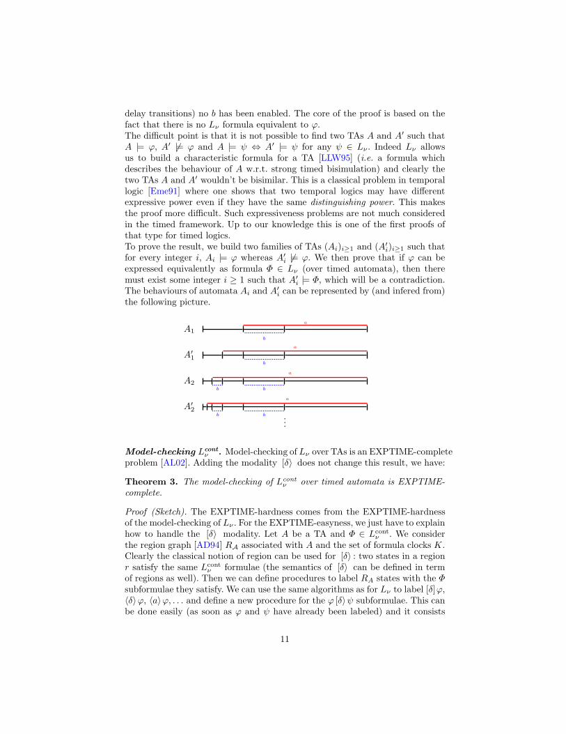
delay transitions) no b has been enabled. The core of the proof is based on thefact that there is no Lν formula equivalent to ϕ.The difficult point is that it is not possible to find two TAs A and A′ such thatA |= ϕ, A′ 6|= ϕ and A |= ψ ⇔ A′ |= ψ for any ψ ∈ Lν . Indeed Lν allowsus to build a characteristic formula for a TA [LLW95] (i.e. a formula whichdescribes the behaviour of A w.r.t. strong timed bisimulation) and clearly thetwo TAs A and A′ wouldn’t be bisimilar. This is a classical problem in temporallogic [Eme91] where one shows that two temporal logics may have differentexpressive power even if they have the same distinguishing power. This makesthe proof more difficult. Such expressiveness problems are not much consideredin the timed framework. Up to our knowledge this is one of the first proofs ofthat type for timed logics.To prove the result, we build two families of TAs (Ai)i≥1 and (A′

i)i≥1 such thatfor every integer i, Ai |= ϕ whereas A′

i 6|= ϕ. We then prove that if ϕ can beexpressed equivalently as formula Φ ∈ Lν (over timed automata), then theremust exist some integer i ≥ 1 such that A′

i |= Φ, which will be a contradiction.The behaviours of automata Ai and A′

i can be represented by (and infered from)the following picture.

A1

a

b

A′1

a

b

A2

a

b b

A′2

a

b b ...

Model-checking Lcontν . Model-checking of Lν over TAs is an EXPTIME-complete

problem [AL02]. Adding the modality [δ〉 does not change this result, we have:

Theorem 3. The model-checking of Lcontν over timed automata is EXPTIME-

complete.

Proof (Sketch). The EXPTIME-hardness comes from the EXPTIME-hardnessof the model-checking of Lν . For the EXPTIME-easyness, we just have to explainhow to handle the [δ〉 modality. Let A be a TA and Φ ∈ Lcont

ν . We considerthe region graph [AD94] RA associated with A and the set of formula clocks K.Clearly the classical notion of region can be used for [δ〉 : two states in a regionr satisfy the same Lcont

ν formulae (the semantics of [δ〉 can be defined in termof regions as well). Then we can define procedures to label RA states with the Φsubformulae they satisfy. We can use the same algorithms as for Lν to label [δ]ϕ,〈δ〉ϕ, 〈a〉ϕ, . . . and define a new procedure for the ϕ [δ〉ψ subformulae. This canbe done easily (as soon as ϕ and ψ have already been labeled) and it consists

11

in a classical “Until” over the delay transitions (see below a way of computingϕ [δ〉 ψ with DBMs). The complexity of the algorithm will remain linear in thesize of RA and Φ, and finally exponential in the size of A and Φ [AL02]. ⊓⊔

Instead of considering region techniques, classical algorithms for timed model-checking use zones (i.e. convex sets of valuations, defined as conjunctions ofx− y ⊲⊳ c constraints and implemented with DBMs [Dil90,Bou04]). This makesverification more efficient in practice. In this approach JϕK is defined as sets ofpairs (q, z) where z is a zone and q is a control state of the TA. This approach isalso possible for Lcont

ν . Indeed we can define Jϕ[δ〉ψK when JϕK and JψK are alreadydefined as sets of symbolic configurations (q, z). We use standard operations onzones:←−z (resp. −→z , zc) denotes the past (resp. future, complement) of z, and z+

represents the set z∪v | ∃t > 0 s.t. v− t ∈ z and ∀0 ≤ t′ < t, v− t′ ∈ z (if z isrepresented by a DBM in normal form, z+ is computed by relaxing constraintsx < c to x ≤ c). It is then easy to prove that:

Jϕ [δ〉 ψK =(←−−JϕKc

)c

∪

[(←−−−−−−−−−(−→JψK ∪ JϕK

)c)c

∩(

JψK ∪(

JϕK ∩(←−−−−−−−JϕK+ ∩ JψK

)))

]

Lcontν is compositional. An important property of Lν is that it is composi-

tional [LL95,LL98] for timed automata. This is also the case for Lcontν .

A logic L is said to be compositional for a class S of models if, given an instance(s1| · · · |sn) |= ϕ with si ∈ S and ϕ ∈ L, it is possible to build a formula ϕ/s1(called a quotient formula) s.t. (s1| · · · |sn) |= ϕ⇔ (s2| · · · |sn) |= ϕ/s1. This canbe viewed as an encoding of the behaviour of s1 into the formula. Of coursethis also depends on the synchronization function, but we will not enter into thedetails here.For ϕ ∈ Lν, A a TA, it is possible to define inductively a quotient formula ϕ/A(we refer to [LL98] for a complete description of this technique). In order toprove that Lcont

ν is compositional it is sufficient to define the quotient formulafor the new modality ϕ [δ〉 ψ. We define the quotient of ϕ1 [δ〉 ϕ2 for a locationℓ of a TA A in the following way:

(

ϕ1 [δ〉 ϕ2

)

/ℓdef=

(

inv(ℓ)⇒ (ϕ1/ℓ))

[δ〉(

inv(ℓ) ∧ (ϕ2/ℓ))

With such a quotient construction we get the following proposition:

Proposition 1. The logic Lcontν is compositional for the class of timed au-

tomata.

We have discussed a little bit in previous sections why the property is very usefuland important. In particular, the new modality of Lcont

ν has been added to themodel-checker CMC [LL98] which implements a compositional model-checking al-gorithm: it first computes a quotient formula of the system and the property andthen check for the satisfiability of the formula. We have added to CMC the quo-tient rule for the operator [δ〉 and thus we can use CMC for checking controllabil-ity properties. We do not provide here our experimental results but better refer tothe web page of the tool: http://www.lsv.ens-cachan.fr/~fl/cmcweb.html.

12

5 Conclusion

In this paper we have used the logic Lν to specify control objectives on timedplants. We have proved that a deterministic fragment of Lν allows us to reducecontrol problems to a model-checking problem for an extension of Lν (denotedLcont

ν ) with a new modality. We have also studied the properties of the extendedlogic Lcont

ν and proved that i) Lcontν is strictly more expressive than Lν; ii) the

model-checking of Lcontν over timed automata is EXPTIME-complete; iii) Lcont

ν

inherits the compositionality property of Lν .

Our current and future work is many-fold:

– extend our work to the synthesis of controllers. An interesting point is that weare not limited to the synthesis of controllers which are timed automata. Notehowever that this problem is strongly related to the satisfiability problemfor Lν which is still open [LLW95].

– use the features of the logic Lν to express more general types of controlobjectives e.g. to take into account dynamic changes of the set of controllableevents as in [AVW03].

References

AD94. Rajeev Alur and David Dill. A theory of timed automata. TheoreticalComputer Science (TCS), 126(2):183–235, 1994.

AHK02. Rajeev Alur, Thomas A. Henzinger, and Orna Kupferman. Alternating-timetemporal logic. Journal of the ACM, 49:672–713, 2002.

AL02. Luca Aceto and Francois Laroussinie. Is your model-checker on time ? onthe complexity of model-checking for timed modal logics. Journal of Logicand Algebraic Programming (JLAP), 52–53:7–51, 2002.

AVW03. Andre Arnold, Aymeric Vincent, and Igor Walukiewicz. Games for synthe-sis of controllers with partial observation. Theoretical Computer Science,1(303):7–34, 2003.

Bou04. Patricia Bouyer. Forward analysis of updatable timed automata. FormalMethods in System Design, 24(3):281–320, 2004.

CHR02. Franck Cassez, Thomas A. Henzinger, and Jean-Francois Raskin. A compar-ison of control problems for timed and hybrid systems. In Proc. 5th Interna-tional Workshop on Hybrid Systems: Computation and Control (HSCC’02),volume 2289 of LNCS, pages 134–148. Springer, 2002.

dAHM01. Luca de Alfaro, Thomas A. Henzinger, and Rupak Majumdar. Symbolicalgorithms for infinite-state games. In Proc. 12th International Conferenceon Concurrency Theory (CONCUR’01), volume 2154 of Lecture Notes inComputer Science, pages 536–550. Springer, 2001.

Dil90. David Dill. Timing assumptions and verification of finite-state concurrentsystems. In Proc. of the Workshop on Automatic Verification Methods forFinite State Systems (1989), volume 407 of Lecture Notes in Computer Sci-ence, pages 197–212. Springer, 1990.

DM02. Deepak D’Souza and P. Madhusudan. Timed control synthesis for externalspecifications. In Proc. 19th International Symposium on Theoretical As-pects of Computer Science (STACS’02), volume 2285 of Lecture Notes inComputer Science, pages 571–582. Springer, 2002.

13

Eme91. E. Allen Emerson. Temporal and Modal Logic, volume B (Formal Modelsand Semantics) of Handbook of Theoretical Computer Science, pages 995–1072. MIT Press Cambridge, 1991.

FLTM02. Marco Faella, Salvatore La Torre, and Aniello Murano. Dense real-timegames. In Proc. 17th IEEE Symposium on Logic in Computer Science(LICS’02), pages 167–176. IEEE Computer Society Press, 2002.

HNSY94. Thomas A. Henzinger, Xavier Nicollin, Joseph Sifakis, and Sergio Yovine.Symbolic model-checking for real-time systems. Information and Computa-tion, 111(2):193–244, 1994.

JW95. David Janin and Igor Walukiewicz. Automata for the modal mu-calculusand related results. In Proc. 20th International Symposium on MathematicalFoundations of Computer Science (MFCS’95), volume 969 of Lecture Notesin Computer Science, pages 552–562. Springer, 1995.

LL95. Francois Laroussinie and Kim G. Larsen. Compositional model-checking ofreal-time systems. In Proc. 6th International Conference on ConcurrencyTheory (CONCUR’95), volume 962 of Lecture Notes in Computer Science,pages 27–41. Springer, 1995.

LL98. Francois Laroussinie and Kim G. Larsen. CMC: A tool for compositionalmodel-checking of real-time systems. In Proc. IFIP Joint International Con-ference on Formal Description Techniques & Protocol Specification, Test-ing, and Verification (FORTE-PSTV’98), pages 439–456. Kluwer Academic,1998.

LLW95. Francois Laroussinie, Kim G. Larsen, and Carsten Weise. From timed au-tomata to logic – and back. In Proc. 20th International Symposium onMathematical Foundations of Computer Science (MFCS’95), volume 969 ofLecture Notes in Computer Science, pages 529–539. Springer, 1995.

MPS95. Oded Maler, Amir Pnueli, and Joseph Sifakis. On the synthesis of discretecontrollers for timed systems. In Proc. 12th Annual Symposium on Theoret-ical Aspects of Computer Science (STACS’95), volume 900 of Lecture Notesin Computer Science, pages 229–242. Springer, 1995.

RP03. Stephane Riedweg and Sophie Pinchinat. Quantified mu-calculus for controlsynthesis. In Proc. 28th International Symposium on Mathematical Foun-dations of Computer Science (MFCS’03), volume 2747 of Lecture Notes inComputer Science, pages 642–651. Springer, 2003.

RW89. P.J.G. Ramadge and W.M. Wonham. The control of discrete event systems.Proc. of the IEEE, 77(1):81–98, 1989.

WT97. Howard Wong-Toi. The synthesis of controllers for linear hybrid automata.In Proc. 36th IEEE Conference on Decision and Control, pages 4607–4612.IEEE Computer Society Press, 1997.

Yi90. Wang Yi. Real-time behaviour of asynchronous agents. In Proc. 1st Inter-national Conference on Theory of Concurrency (CONCUR’90), volume 458of Lecture Notes in Computer Science, pages 502–520. Springer, 1990.

A Proof of Theorem 1

Before proving Theorem 1 we need to take some notations.

Let G = (Q, q0,Act,−→) be a TTS. For s ∈ Q and ∆ ∈ Q≥0 we define:

14

– Gs∆ to be the sub TTS ofG rooted at s such that two consecutive controllable

actions (in Actc) are separated by a time amount t s.t. t ≥ ∆;– G∆ stands for Gq0

∆ ;– for τ ≤ ∆, Gs

∆,τ is the sub TTS of Gs∆ where no controllable action occurs

before τ time units from the root s;– Contr(Gs

∆,τ , s) is the set of controllers for TTSGs∆,τ from state s; Contr(Gq0

∆,0, q0)thus denotes the set of controllers that can let at least ∆ time units betweentwo consecutive controllable actions.

If G is the semantics of a plant P = (L, ℓ0,Act, X, inv, T ) the TTS Gq0

∆ can beeffectively constructed using a parallel composition with a self-loop automaton(with a fresh clock x) enforcing a delay greater than ∆ (e.g. by x ≥ ∆) betweentwo controllable actions. We denote P∆ this synchronized product.

Theorem 1 is a consequence of the following lemma:

Lemma 1. For any σ ∈ Actc ∪ λ, any state s ∈ G and any Ldet

ν formula Φ,we have:

(

∃f ∈ Contr(Gs∆,τ , s) s.t. f(G, s), (s, v) |= Φ ∧ 〈σ〉 tt

)

⇔(

Gs∆,τ , (s, v) |= Φ

σ)

Note how this lemma interprets for formulae Φ :

(

∃f ∈ Contr(Gs∆,τ , s) s.t. f(G, s), (s, v) |= Φ

)

⇔(

Gs∆,τ , (s, v) |= Φ

)

Proof. First we assume that the result holds for the fixpoint variables and we

show the Lemma by structural induction over Ldet

ν formulae. The cases Φdef= x ∼

c or Φdef= r in ϕ are obvious.

– Φdef= [au] ϕ:⇒ Assume there exists f ∈ Contr(Gs

∆,τ , s) s.t. f(G, s), (s, v) |= [au] ϕ ∧

〈σ〉 tt. Then for any f(G, s) : sau−−−→ s′, we have f(G, s), (s′, v) |= ϕ.

Then there exists f ′ ∈ Contr(Gs∆,τ , s

′) s.t. f ′(G, s′), (s′, v) |= ϕ and the

induction hypothesis provides: Gs′

∆,τ , (s′, v) |= ϕ . Since the strategies

cannot block the uncontrollable actions, any action au ∈ Actu that canbe performed from (s, v) in Gs

∆,τ , can also be performed in f(G, s) andthen Gs

∆,τ , (s, v) |= [au]ϕ . Moreover f(G, s), (s, v) |= 〈σ〉tt which implies

that Gs∆,τ , (s, v) |= 〈σ〉 tt, and thus Gs

∆,τ , (s, v) |= [au] ϕσ.

⇐ Assume Gs∆,τ , (s, v) |= [au]ϕ ∧〈σ〉tt. For any transition Gs

∆,τ , sau−−−→ s′,

we have Gs∆,τ , (s

′, v) |= ϕ . By i.h. we know that there exists fau∈

Contr(Gs∆,τ , s

′) s.t. fau(G, s′), (s′, v) |= ϕ. Let f be the strategy defined

by: f(sau−−−→ ρ)

def= fau

(ρ) for any ρ starting in state s′ and f(s) =ac if σ = ac (note that in that case, it is possible to do a σ becauseGs

∆,τ , (s, v) |= 〈σ〉 tt), or f(s) = λ otherwise.

– Φdef= 〈au〉 ϕ:

15

⇒ Assume there exists f ∈ Contr(Gs∆,τ , s) s.t. f(G, s), (s, v) |= 〈au〉ϕ∧〈σ〉tt.

Then there exists f(G, s) : sau−−−→ s′ with f(G, s), (s′, v) |= ϕ. There-

fore there is f ′ ∈ Contr(Gs∆,τ , s

′) s.t. f ′(G, s′), (s′, v) |= ϕ and the i.h.

entails: Gs′

∆,τ , (s′, v) |= ϕ . Gs

∆,τ contains the behaviours of f(G, s),then Gs

∆,τ , (s, v) |= 〈au〉 ϕ . Moreover, f(G, s), (s, v) |= 〈σ〉 tt, thus

Gs∆,τ , (s, v) |= 〈au〉 ϕ ∧ 〈σ〉 tt, and thus Gs

∆,τ , (s, v) |= 〈au〉 ϕσ.

⇐ Assume Gs∆,τ , (s, v) |= 〈au〉ϕ ∧〈σ〉tt. There is a transition Gs

∆,τ , sau−−−→

s′ s.t.Gs∆,τ , (s

′, v) |= ϕ . By i.h. we know that there exists fau∈ Contr(Gs

∆,τ , s′)

s.t. fau(G, s′), (s′, v) |= ϕ. Let f be the strategy defined by: f(s

au−−−→

ρ)def= fau

(ρ) for any ρ starting in state s′ and f(s) = ac if σ = ac, orf(s) = λ otherwise.

– Φdef= 〈ac〉 ϕ:⇒ There exists f ∈ Contr(Gs

∆,τ , s) s.t. f(G, s), (s, v) |= 〈ac〉ϕ∧〈σ〉tt. Thenclearly σ is ac: otherwise this would entail that f is not deterministic andrequires two different controllable actions from the state (s, v). There ex-

ists f(G, s) : sac−−−→ s′ such that f(G, s′), (s′, v) |= ϕ. Moreover defining

f ′ ∈ Contr(Gs∆,∆, s

′) by f ′(ρ)def= f(s

ac−−−→ ρ) for any ρ starting in s′, we

get that f ′(G, s′), (s′, v) |= ϕ. By i.h. we have Gs′

∆,∆, (s′, v) |= ϕ . Gs

∆,τ

contains the behaviours of f(G, s), then Gs∆,τ , (s, v) |= 〈ac〉 ϕ and thus

Gs∆,τ , (s, v) |= 〈ac〉 ϕ

σ.

⇐ The only possible case is σ = ac and Gs∆,τ , (s, v) |= 〈ac〉 ϕ . There is a

transition Gs∆,τ , s

ac−−−→ s′ s.t. Gs′

∆,∆, (s′, v) |= ϕ . By i.h. we know that

there exists f ′ ∈ Contr(Gs∆,∆, s

′) s.t. f ′(G, s′), (s′, v) |= ϕ. Let f be the

strategy defined by: f(sac−−−→ ρ)

def= f ′(ρ) for any ρ run starting in s′ and

f(s) = ac. f is a ∆-strategy and belongs to Contr(Gs∆,τ , s) — note that

in this case τ = 0 —, and f(G, s), (s, v) |= 〈ac〉 ϕ and then 〈ac〉 tt alsoholds for f(G, s), (s, v).

– Φdef= [ac] ϕ:⇒ If ac 6= σ the result is obvious. Now assume ac = σ, then there exists

f ∈ Contr(Gs∆,τ , s) s.t. f(G, s), (s, v) |= [ac] ϕ ∧ 〈ac〉 tt. The same proof

as above (for Φdef= 〈ac〉ϕ) gives Gs

∆,τ , (s, v) |= 〈ac〉 ϕ , i.e. Gs∆,τ , (s, v) |=

[ac] ϕσ.

⇐ First assume σ ∈ Actc\ac or σ = λ. ThenGs∆,τ , (s, v) |= 〈σ〉tt we define

the strategy f to be f(s) = σ. This allows us to have f(G, s), (s, v) |=[ac]ϕ∧〈σ〉tt (as ac is disabled by f). Finally assume σ = ac. Then we have

Gs∆,τ , (s, v) |= 〈ac〉ϕ . There exists Gs

∆,τ , sac−−−→ s′ s.t. Gs′

∆,∆, (s′, v) |= ϕ .

By i.h. there exists f ∈ Contr(Gs∆,∆, s

′) s.t. f ′(G, s′), (s′, v) |= ϕ. Let f

be the strategy defined by f(s) = ac and f(sac−−−→ ρ) = f ′(ρ) for any ρ

run starting in state s′. We have f ∈ Contr(Gs∆,τ , s) and f(G, s), (s, v) |=

[ac] ϕ ∧ 〈σ〉 tt.

– Φdef= 〈δ〉 ϕ:

16

⇒ First assume σ = λ. If there exists f ∈ Contr(Gs∆,τ , s) s.t. f(G, s), (s, v) |=

〈δ〉ϕ, then there is f(G, s), st−−→ st (with t ∈ R) s.t. f(G, s), (st, v+ t) |=

ϕ. By i.h. we have Gs′

∆,τ−t, (s′, v + t) |= ϕ where τ − t stands for

max(τ − t, 0). And then Gs∆,τ , (s, v) |= 〈δ〉 ϕ because Gs

∆,τ is more gen-eral than f(G, s).Now assume σ = ac. There exists f ∈ Contr(Gs

∆,τ , s) s.t. f(G, s), (s, v) |=〈δ〉 ϕ ∧ 〈ac〉 tt. This means that f(s) = ac and then no delay is allowedby the strategy and then it is equivalent to f(G, s), (s, v) |= ϕ ∧ 〈ac〉 tt.By i.h. we have: Gs

∆,τ , (s, v) |= ϕ ac .

⇐ Assume σ = λ. If Gs∆,τ , (s, v) |= 〈δ〉 ϕ , then there exists Gs

∆,τ : st−−→ st

with t ∈ R s.t. Gs∆,τ , (s

t, v + t) |= ϕ . By i.h. we deduce that there

exists f t ∈ Contr(Gs∆,τ−t, s

t) s.t. f t(G, st), (st, v + t) |= ϕ. Let f ∈

Contr(Gs∆,τ , s) be the strategy defined as f(s

t′

−−→ st′) = λ for any

t′ < t, and f(st−−→ ρ) = f t(ρ) for any run ρ starting in state st. Clearly

we have f(G, s), (s, v) |= 〈δ〉 ϕ.

Assume σ ∈ Actc. If Gs∆,τ , (s, v) |= ϕ σ, we have by i.h. that there exists

f ∈ Contr(Gs∆,τ , s) s.t. f(G, s), (s, v) |= ϕ ∧ 〈σ〉 tt. Then we clearly have

f(G, s), (s, v) |= 〈δ〉 ϕ ∧ 〈σ〉 tt.

– Φdef= [δ] ϕ:

⇒ First assume σ ∈ Actc. Assume there exists f ∈ Contr(Gs∆,τ , s) s.t.

f(G, s), (s, v) |= [δ]ϕ∧〈σ〉tt. This implies f(G, s), (s, v) |= ϕ∧〈σ〉tt. Byi.h. we have: Gs

∆,τ , (s, v) |= ϕ σ.Assume σ = λ. Then there exists f ∈ Contr(Gs

∆,τ , s) s.t. f(G, s), (s, v) |=

[δ] ϕ, that is for any transition f(G, s), st−−→ st (with t ∈ R), we have

f(G, s), (st, v + t) |= ϕ. We distinguish two cases:

∗ Every delay transition from Gs∆,τ , s exists also in f(G, s), s. Then the

induction hypothesis entails that for any t, we have 5 Gs∆,τ−t(s

t, v+t) |= ϕ ε and then clearlyGs

∆,τ , (s, v) |= [δ]ϕ ε and thenGs∆,τ , (s, v) |=

ϕ ε [δ〉 ϕ ac for every ac ∈ Actc.∗ There exists some delay transition in Gs

∆,τ from s that does not be-long to f(G, s). This means that the strategy f requires the executionof some controllable action ac from some state st reachable from s

by a delay t: f(st−−→ st) = ac. We then have f(G, s), (st′ , v+ t′) |= ϕ

for any t′ < t and f(G, s), (st, v + t) |= ϕ ∧ 〈ac〉 tt. By i.h. we have

Gst′

∆,τ−t′ , (st′ , v+ t′) |= ϕ λ for any t′ < t and Gs

∆,0, (st, v+ t) |= ϕ ac .

This implies Gs∆,τ , (s, v) |= ϕ λ [δ〉 ϕ ac .

⇐ Assume σ ∈ Actc. Then Gs∆,τ , (s, v) |= ϕ σ entails that there exists some

f ∈ Contr(Gs∆,τ , s) s.t. f(G, s), (s, v) |= ϕ ∧ 〈σ〉 tt. This means that

f(s) = σ and that no delay is indeed allowed by the strategy f . Thenwe clearly have f(G, s), (s, v) |= [δ] ϕ ∧ 〈σ〉 tt.

5 In the following we always assume that τ − t stands for max(0, τ − t).

17

Assume σ = λ and Gs∆,τ , (s, v) |= ϕ λ [δ〉 ϕ ac for some ac ∈ Actc. We

distinguish two cases:

∗ Gs∆,τ , (s, v) |= [δ]ϕ λ. Then for any t ∈ R, we have that Gs

∆,τ : st−−→

st implies Gs∆,τ , (s

t, v + t) |= ϕ λ and then by i.h. there exists ft ∈

Contr(Gs∆,τ−t, s

t) s.t. ft(G, st), (st, v + t) |= ϕ and ft(s

t) = λ. Let f

be the strategy defined by f(st−−→ st) = λ and f(s

t−−→ ρ) = ft(ρ)

for any run ρ starting in state st. Clearly f belongs to Contr(Gs∆,τ , s).

And we have f(G, s), (s, v) |= [δ] ϕ.

∗ There exists t ∈ R s.t. Gs∆,τ : s

t−−→ st and Gs

∆,τ−t, (st, v + t) |=

ϕ ac for some ac ∈ Actc. By i.h. there exists ft ∈ Contr(Gs∆,τ−t, s

t)

s.t. ft(G, st), (st, v + t) |= ϕ ∧ 〈ac〉 tt. Clearly ft(s) = ac and ft

forbids time elapsing from st. Moreover the i.h. applied to statesst′ with t′ < t gives that there exists ft′ ∈ Contr(Gs

∆,τ−t, st′) s.t.

ft′(G, st′), (st′ , v + t′) |= ϕ and ft′(s

t′) = λ. Let f be the strategy

defined by: f(st′

−−→ st′) = λ for any t′ < t, f(st−−→ st) = ac and

f(st′′

−−→ ρst′′) = ft′′(ρ) for t′′ ≤ t. This strategy allows us to deducef(G, s), (s, v) |= [δ] ϕ.

– Φdef=

∨

i ϕi: Direct.

– Φdef=

∧

i ϕi:⇒ Assume there exists f ∈ Contr(Gs

∆,τ , s) s.t. f(G, s), (s, v) |=∧

i αi∧〈σ〉tt.Then we have f(G, s), (s, v) |= αi ∧ 〈σ〉 tt for any i. By h.i. we haveGs

∆,τ , (s, v) |= αiσ for any i, and then Gs

∆,τ , (s, v) |=∧

i αiσ.

⇐ Assume Gs∆,τ , (s, v) |=

∧

i ϕσ. Then by i.h. we have that there exists

some fi ∈ Contr(Gs∆,τ , s) s.t. fi(G, s), (s, v) |= αi ∧ 〈σ〉 tt. It remains to

construct a strategy f by collecting the strategies fi’s. This is possiblebecause ϕ belongs to Ldet

ν , indeed any term αi is prefixed by a modalitywith a different label of Act ∪ δ and then the union of the strategiesfi’s provides a strategy f that belongs to Contr(Gs

∆,τ , s). This gives theresult.

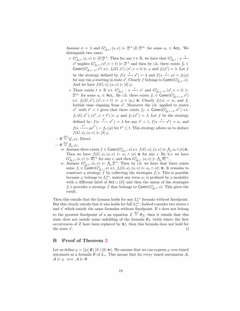
Then this entails that the Lemma holds for any Ldet

ν formula without fixedpoint.But this clearly entails that it also holds for full Ldet

ν . Indeed consider two states sand s′ which satisfy the same formulae without fixedpoint. If s does not belong

to the greatest fixedpoint of a an equation Zdef= ΨZ , then it entails that this

state does not satisfy some unfolding of the formula ΨZ (with where the firstoccurrences of Z have been replaced by tt), then this formula does not hold forthe state s′. ⊓⊔

B Proof of Theorem 2

Let us define ϕ = ([a] ff) [δ〉 (〈b〉 tt). We assume that we can express ϕ over timedautomata as a formula Φ of Lν. This means that for every timed automaton A,A |= ϕ ⇐⇒ A |= Φ.

18

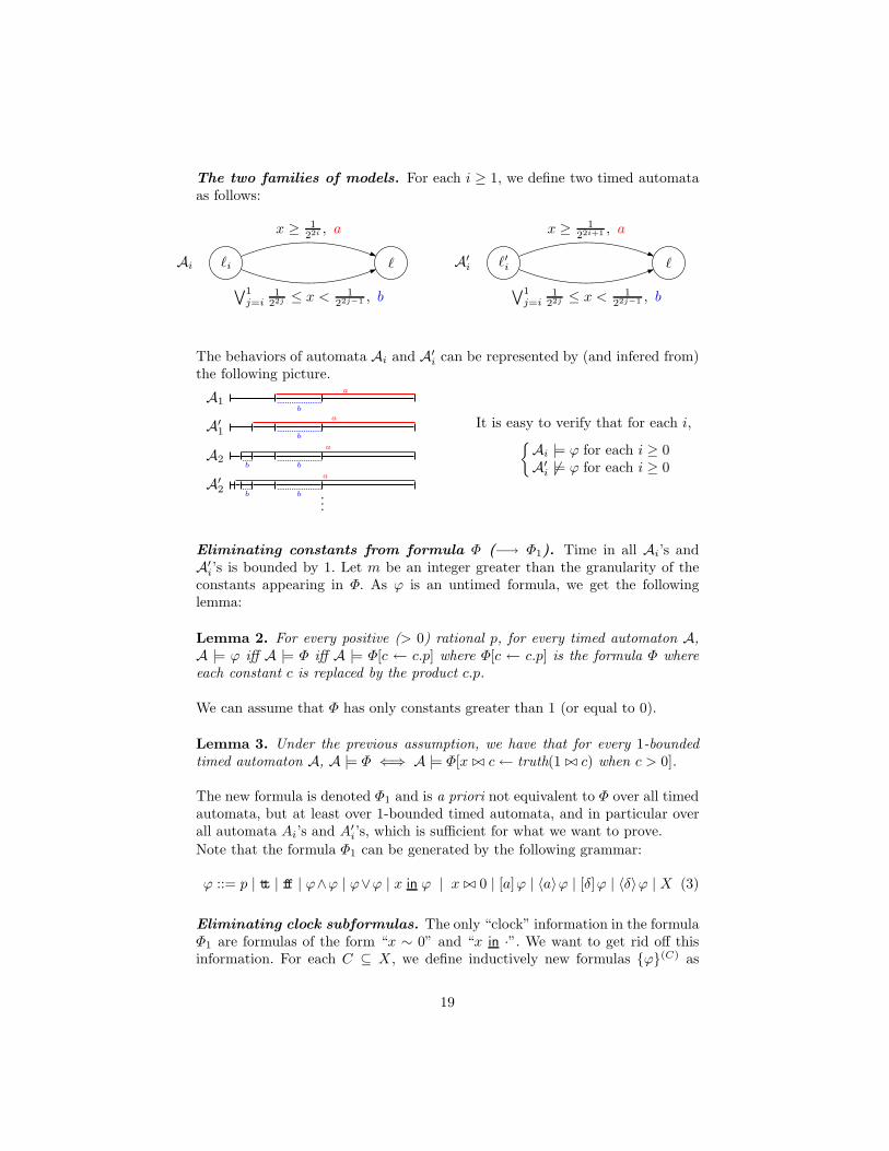
The two families of models. For each i ≥ 1, we define two timed automataas follows:

Ai ℓi ℓ

x ≥ 122i , a

∨1j=i

122j ≤ x <

122j−1 , b

A′i ℓ′i ℓ

x ≥ 122i+1 , a

∨1j=i

122j ≤ x <

122j−1 , b

The behaviors of automata Ai and A′i can be represented by (and infered from)

the following picture.

A1a

b

A′1

a

b

A2

a

b b

A′2

a

b b ...

It is easy to verify that for each i,

Ai |= ϕ for each i ≥ 0A′

i 6|= ϕ for each i ≥ 0

Eliminating constants from formula Φ (−→ Φ1). Time in all Ai’s andA′

i’s is bounded by 1. Let m be an integer greater than the granularity of theconstants appearing in Φ. As ϕ is an untimed formula, we get the followinglemma:

Lemma 2. For every positive (> 0) rational p, for every timed automaton A,A |= ϕ iff A |= Φ iff A |= Φ[c ← c.p] where Φ[c ← c.p] is the formula Φ whereeach constant c is replaced by the product c.p.

We can assume that Φ has only constants greater than 1 (or equal to 0).

Lemma 3. Under the previous assumption, we have that for every 1-boundedtimed automaton A, A |= Φ ⇐⇒ A |= Φ[x ⊲⊳ c← truth(1 ⊲⊳ c) when c > 0].

The new formula is denoted Φ1 and is a priori not equivalent to Φ over all timedautomata, but at least over 1-bounded timed automata, and in particular overall automata Ai’s and A′

i’s, which is sufficient for what we want to prove.

Note that the formula Φ1 can be generated by the following grammar:

ϕ ::= p | tt | ff | ϕ∧ϕ | ϕ∨ϕ | x in ϕ | x ⊲⊳ 0 | [a]ϕ | 〈a〉ϕ | [δ]ϕ | 〈δ〉ϕ | X (3)

Eliminating clock subformulas. The only “clock” information in the formulaΦ1 are formulas of the form “x ∼ 0” and “x in ·”. We want to get rid off thisinformation. For each C ⊆ X , we define inductively new formulas ϕ(C) as

19

follows:

α(C) = α if α ∈ p, tt, ff

ϕ1 op ϕ2(C) = ϕ1

(C) op ϕ2(C) if op ∈ ∧,∨

x in ϕ(C) = x in ϕ(C∪x)

[a]ϕ(C) = [a]ϕ(C)

〈a〉ϕ(C) = 〈a〉ϕ(C)

X(C) = XC

x > 0(C) =

tt if x 6∈ C

ff if x ∈ C

x = 0(C) =

tt if x ∈ C

ff if x 6∈ C

[δ] ϕ(C) = ϕ(C) ∧ [δ] +ϕ(∅)

〈δ〉 ϕ(C) = ϕ(C) ∧ 〈δ〉 +ϕ(∅)

Intuitively the formula ϕ(C) expresses the fact that ϕ holds while the value ofclocks in C is 0 and the value of clocks not in C are strictly greater than 0. Theformula 〈δ〉+ϕ is similar to that of 〈δ〉ϕ but the delay must be positive. Similarly[δ]+ϕ means that for all positive delay, ϕ must hold. We do not redefine formallythese two operators.

Lemma 4. For each timed automaton A, for each formula ϕ generated by thegrammar (3), for each extended configuration (ℓ, u :: v),

(ℓ, u :: v) |= ϕ ⇐⇒ (ℓ, u :: v) |= ϕ(C)

where C = x ∈ X | v(x) = 0. In particular, in the initial configuration (u0 = 0and v0 = 0),

(ℓ0, u0 :: v0) |= ϕ ⇐⇒ (ℓ0, u0 :: v0) |= ϕ(X)

The new formula Φ1(X) has no more clock constraints. We can thus erase alloperators “x in ·” because clocks are no more used. We get a new formula Φ2

(without clocks) which is generated by the grammar

ϕ ::= p | tt | ff | ϕ ∧ ϕ | ϕ ∨ ϕ | [a] ϕ | 〈a〉 ϕ | [δ] + ϕ | 〈δ〉 + ϕ | X (4)

and thus such that for every 1-bounded timed automata A, for every config-uration (ℓ, u) of A, (ℓ, u) |= ϕ ⇐⇒ (ℓ, u) |= Φ2 (Φ2 is equivalent to ϕ over1-bounded timed automata).

Region abstraction. The regions for automatonAi in state ℓi are the intervals:[

0,1

22i

[

,

[

1

22i,

1

22i−1

[

, . . . ,

[

1

2, 1

[

whereas the regions for automaton A′i in state ℓ′i are the intervals:

[

0,1

22i+1

[

,

[

1

22i+1,

1

22i

[

, . . . ,

[

1

2, 1

[

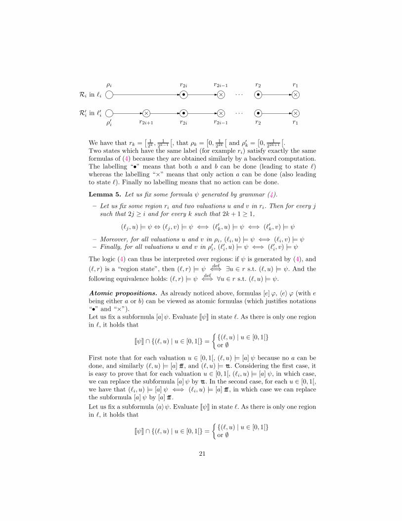
For all automata, only one region is needed in state ℓ, it is the interval [0, 1[. Itis thus only necessary to see what happens in states ℓi and ℓ′i. All regions areright-open. We denote by Ri the region automaton for Ai and R′

i the regionautomaton for A′

i. We can redraw automata Ri and R′i (restricted to states ℓi

and ℓ′i) as follows:

20

Ri in ℓi • × . . . • ×

ρi r2i r2i−1 r2 r1

R′i in ℓ′i × • × . . . • ×

ρ′i r2i+1 r2i r2i−1 r2 r1

We have that rk =[

12k ,

12k−1

[

, that ρk =[

0, 122k

[

and ρ′k =[

0, 122k+1

[

.Two states which have the same label (for example ri) satisfy exactly the sameformulas of (4) because they are obtained similarly by a backward computation.The labelling “•” means that both a and b can be done (leading to state ℓ)whereas the labelling “×” means that only action a can be done (also leadingto state ℓ). Finally no labelling means that no action can be done.

Lemma 5. Let us fix some formula ψ generated by grammar (4).

– Let us fix some region ri and two valuations u and v in ri. Then for every jsuch that 2j ≥ i and for every k such that 2k + 1 ≥ 1,

(ℓj , u) |= ψ ⇔ (ℓj, v) |= ψ ⇐⇒ (ℓ′k, u) |= ψ ⇐⇒ (ℓ′k, v) |= ψ

– Moreover, for all valuations u and v in ρi, (ℓi, u) |= ψ ⇐⇒ (ℓi, v) |= ψ– Finally, for all valuations u and v in ρ′i, (ℓ′i, u) |= ψ ⇐⇒ (ℓ′i, v) |= ψ

The logic (4) can thus be interpreted over regions: if ψ is generated by (4), and

(ℓ, r) is a “region state”, then (ℓ, r) |= ψdef⇐⇒ ∃u ∈ r s.t. (ℓ, u) |= ψ. And the

following equivalence holds: (ℓ, r) |= ψdef⇐⇒ ∀u ∈ r s.t. (ℓ, u) |= ψ.

Atomic propositions. As already noticed above, formulas [e] ϕ, 〈e〉 ϕ (with ebeing either a or b) can be viewed as atomic formulas (which justifies notations“•” and “×”).Let us fix a subformula [a]ψ. Evaluate JψK in state ℓ. As there is only one regionin ℓ, it holds that

JψK ∩ (ℓ, u) | u ∈ [0, 1[ =

(ℓ, u) | u ∈ [0, 1[or ∅

First note that for each valuation u ∈ [0, 1[, (ℓ, u) |= [a] ψ because no a can bedone, and similarly (ℓ, u) |= [a] ff, and (ℓ, u) |= tt. Considering the first case, itis easy to prove that for each valuation u ∈ [0, 1[, (ℓi, u) |= [a] ψ, in which case,we can replace the subformula [a]ψ by tt. In the second case, for each u ∈ [0, 1[,we have that (ℓi, u) |= [a] ψ ⇐⇒ (ℓi, u) |= [a] ff, in which case we can replacethe subformula [a] ψ by [a] ff.

Let us fix a subformula 〈a〉ψ. Evaluate JψK in state ℓ. As there is only one regionin ℓ, it holds that

JψK ∩ (ℓ, u) | u ∈ [0, 1[ =

(ℓ, u) | u ∈ [0, 1[or ∅

21

First note that for each valuation u ∈ [0, 1[, (ℓ, u) 6|= 〈a〉 ψ because no a can bedone. Considering the second case, it is easy to prove that for each valuationu ∈ [0, 1[, (ℓi, u) 6|= 〈a〉 ψ, in which case, we can replace the subformula 〈a〉 ψby ff. In the first case, for each u ∈ [0, 1[, we have that (ℓi, u) |= 〈a〉 ψ ⇐⇒(ℓi, u) |= 〈a〉 tt, in which case we can replace the subformula 〈a〉 ψ by 〈a〉 tt.

With all these remarks we define a new formula Φ4 from Φ3 by rewriting asubformula [a]ψ into [a]ff if ψ does not hold in ℓ and into tt if ψ holds in ℓ, andby rewriting a subformula 〈a〉 ψ by ff if ψ does not hold in ℓ and by 〈a〉 tt if ψholds in ℓ. The new formula Φ4 can be generated by the grammar:

ϕ ::= p | tt | ff | [a] ff | 〈a〉 tt | ϕ ∧ ϕ | ϕ ∨ ϕ | [δ] +ϕ | 〈δ〉 +ϕ | X (5)

For each u ∈ [0, 1[, (ℓi, u) |= ϕ ⇐⇒ (ℓi, u) |= Φ4 and (ℓ′i, u) |= ϕ ⇐⇒ (ℓ′i, u) |=Φ4. We could say that Φ4 is equivalent to ϕ over all automata Ai’s and A′

i’s.

Untiming the formula. We note Ri (resp. R′i) the set of regions in state ℓi

(resp. ℓ′i) for the automatonAi (resp. A′i). We define a new logic by the grammar:

ϕ ::= tt | ff | [a] ff | 〈a〉 tt | ϕ ∧ ϕ | ϕ ∨ ϕ | G+ϕ | F+ϕ | X (6)

This logic is interpreted on the region automata Ri’s and R′i’s. The semantics

(denoted ⊢) is defined inductively by:

(ℓi, ℓ′i, r) ⊢ tt, ff, [a] ff, 〈a〉 tt ⇐⇒ (ℓi, ℓ

′i, r) |= tt, ff, [a] ff, 〈a〉 tt

(ℓi, ℓ′i, r) ⊢ ϕ1 ∧ ϕ2, ϕ1 ∨ ϕ2 ⇐⇒ (ℓi, ℓ

′i, r) ⊢ ϕ1 and, or (ℓi, ℓ

′i, r) ⊢ ϕ2

(ℓi, ℓ′i, r) ⊢ G+ϕ ⇐⇒ ∀r′ ∈ Succ(r), r 6= r′, (ℓi, ℓ

′i, r

′) ⊢ ϕ

(ℓi, ℓ′i, r) ⊢ F+ϕ ⇐⇒ ∃r′ ∈ Succ(r), r 6= r′, (ℓi, ℓ

′i, r

′) ⊢ ϕ

(ℓi, ℓ′i, r) ⊢ X ⇐⇒ (ℓi, ℓ

′i, r) ⊢ def(X)

Operators [δ]+ψ and G+ψ interpreted over regions are not so different: the onlydifference stands in that the current region may not satisfy property ψ. In thesame way, operators 〈δ〉+ψ and F+ψ interpreted over regions are not so different:the only difference stands in that a region different from the current one has tosatisfy ψ.

We rewrite the formula Φ4 into Φ5 by replacing each subformula [δ]+ψ by ψ∧G+ψand each subformula 〈δ〉 +ψ by ψ ∨ F+ψ. It is then easy to prove the followinglemma:

Lemma 6. For each i, for each region r ∈ Ri, (ℓi, r) |= Φ4 ⇐⇒ (ℓi, r) ⊢ Φ5.

Similarly, for each i, for each region r′ ∈ R′i, (ℓ′i, r

′) |= Φ4 ⇐⇒ (ℓ′i, r′) ⊢ Φ5.

The formula Φ5 is now an (fully) untimed formula. Moreover, Φ5 is equivalentto ϕ over the two families of automata (Ai)i≥1 and (A′

i)i≥1. We finally noteΨ = Φ5.

22

Gluing everything. The formula Ψ can be written in normal form as a systemof equations (Xi = fi(X1, ..., Xn))1≤i≤n and Ψ = X1. We assume that each

formula fi(X1, ..., Xn) is a boolean combination of subformulas αji (which can

be either some formula F+βji , or G+βj

i , or some atomic-like formula 〈a〉tt, [a]ff,

tt or ff, or some fix-point variable Xji ):

X1 =ν b1(α11, ..., α

k1

1 )...

Xn =ν bn(α1n, ..., α

knn )

Without loss of generality we assume that no subformula αji is a fix-point variable

Xk. The following lemma justifies this fact:

Lemma 7. We assume that αji = Xk (with i 6= k). Then the new formula

obtained by replacing Xk by its definition formula is equivalent to the previousformula. If αj

i = Xi, then the new formula obtained by replacing this variableXi by tt is equivalent to the initial formula.

Thus, each αji is either an atomic proposition, or its negation, or a formula F+ϕ

or a formula Gϕ.

Lemma 8. The following implications are true.

– Ri ⊢ F+ϕ implies R′i ⊢ F+ϕ — Ri 6⊢ G+ϕ implies R′

i 6⊢ G+ϕ– Ri ⊢ G+ϕ implies R′

i−1 ⊢ G+ϕ — Ri 6⊢ F+ϕ implies R′i−1 6⊢ F+ϕ

– R′i ⊢ F+ϕ implies R′

i+1 ⊢ F+ϕ

There is a sequence (γj)1≤j≤k1∈ tt, ffk1 and an infinite sequence of indexes

I such that b1(α11 ← γ1, ..., α

k1

1 ← γℓ1) is true and for each i ∈ I, for each

1 ≤ j ≤ k1, γj = tt iff Ri |= αj1.

We note αF the set αi1 | γi = tt and αi

1 = F+∗, α¬F the set αi1 | γi =

ff and αi1 = F+∗, αG the set αi

1 | γi = tt and αi1 = G∗, and α¬G the set

αi1 | γi = ff and αi

1 = G∗.From the first line of implications of Lemma 8, for every i ∈ I, R′

i |=∧

αF ∧∧

α¬G. We can even simplify: let’s take some i0 ∈ I, we have that for everyi ≥ i0, R′

i |=∧

αF ∧∧

α¬G. From the second line of implications, for every i ∈ Isuch that i > i0, we have that R′

i−1 |=∧

αG ∧∧

α¬F. Finally we can find somei such that R′

i |=∧

αF ∧∧

α¬G ∧∧

αG ∧∧

α¬F and thus R′i |= Ψ (because for

all possible simple terms, there is no problem). ⊓⊔

23