
Mathematical Models in Food Engineering - Facultad de Ciencias
131
UNIVERSIDAD COMPLUTENSE DE MADRID FACULTAD DE CIENCIAS MATEM ´ ATICAS Departamento de Matem´ atica Aplicada Mathematical Models in Food Engineering Modelos Matem´ aticos en Problemas de la Industria Alimentaria Tesis doctoral realizada por: Nadia Alexandra Sofia Smith Bajo la direcci´on de: ´ Angel Manuel Ramos del Olmo Madrid, 1 de febrero de 2013
Transcript of Mathematical Models in Food Engineering - Facultad de Ciencias
UNIVERSIDAD COMPLUTENSE DE MADRID
FACULTAD DE CIENCIAS MATEMATICAS
Departamento de Matematica Aplicada
Mathematical Models in
Food Engineering
Modelos Matematicos en Problemas
de la Industria Alimentaria
Tesis doctoral realizada por:
Nadia Alexandra Sofia Smith
Bajo la direccion de:
Angel Manuel Ramos del Olmo
Madrid, 1 de febrero de 2013


To my family

Acknowledgements
En primer lugar quiero dar las gracias a mi director de tesis, Angel Manuel Ramos, por toda su ayuda ydedicacion durante estos anos. Gracias por tus sabios consejos, y detalladas correcciones, por tu implicacion yel tiempo que has invertido en los resultados presentados en esta memoria. Gracias por tu paciencia, y, sobretodo, por la confianza que has depositado en mı en los momentos mas difıciles. Gracias por animarme en losprimeros anos, y en los ultimos por apoyarme, a viajar a conferencias y cursos, y hacer estancias en otrasuniversidades. Creo que esto ha sido muy enriquecedor para mı, tanto profesional como personalmente.
Tambien quiero expresar mi agradecimiento a otros profesores e investigadores que han hecho valiosas aporta-ciones a este trabajo: a Benjamin Ivorra por su gran ayuda con COMSOL, sin la cual en muchos casos no habrıasabido avanzar; a Gerardo Oleaga por todo el tiempo que invirtio hace unos anos en ensenarme a resolver unproblema de elementos finitos en Matlab; a Juan-Antonio Infante por su sugerencia acertada de hacer mi tesiscon Angel, por sus acertadas palabras hace anos avisandome de que esto no iba a ser un camino facil, y porsu ayuda (ya fuese academica o personal) en numerosas ocasiones; a nuestros colaboradores del Instituto deCiencia y Tecnologıa de Alimentos y Nutricion del CSIC (Pedro Sanz, Laura Otero, etc.) por las veces en lasque me han atendido allı para ensenarme los experimentos que llevan a cabo, y por los datos experimentalesproporcionados.
I would like to thank all my external collaborators without whom a lot of this work would not have beenpossible: Sarah Mitchell from University of Limerick, Kai Knoerzer from CSIRO, Stephen Peppin and VictorBurlakov from University of Oxford. In particular, a special thanks to Sarah for helping me in a very criticalmoment, making me enjoy some fun Maths and see the end was in sight.
A mis companeros de despacho con los que he pasado tantos anos, gracias por hacer este camino mas llevadero.En especial a Luis, Silvia y Edwin, gracias por tantos buenos ratos tomando cafe, desahogando nuestras penasy compartiendo nuestras buenas experiencias. Tambien a mis companeros de quımicas por hacer las reunionesde altas presiones tan divertidas.
Gracias a mis amigos de la carrera de matematicas que siempre han estado apoyandome desde fuera, y a losque he echado de menos en muchas ocasiones en la facultad desde que terminamos. A mis amigas de toda lavida Bea, Vicky y Marta por siempre estar ahı y todos los buenos ratos juntas. A Irene por su confianza en mıy todas nuestros paseos juntas, que me han servido siempre de desahogo. A mis amigas de la Escolanıa, quepase el tiempo que pase siempre se que todo sigue igual.
I would like to thank my family for making my life so interesting and so much fun: my parents and theirpartners (Sonia and Hampate) for their blind trust in me (special thanks to my Mum for her advice of puttingwork under the pillow and going to sleep); a mi hermana Rosanna tambien por su confianza ciega y apoyo(aunque a veces tenga que ser por Skype desde Australia); a Fran, Nico y Martina, porque me alegran la vida;my Aunt Marianne for all her support and enthusiasm; Granny for giving me that mathematical gene, for allher love and interest towards me; to Ronnie, who I wish could be here to see this work finished. Finally, toMark: thank you for all of your mathematical help (which has been very important in crucial moments), butmainly for making my life so much better. I am very lucky to have you and very happy and excited about ourfuture together.
i


Contents
1 Introduction 11.1 High Pressure Processing of Food . . . . . . . . . . . . . . . . . . . . . . . . . . . . . . . . . . . . 21.2 Mathematical modelling of High-Pressure Processes . . . . . . . . . . . . . . . . . . . . . . . . . 3
2 Motivation 72.1 Case Study . . . . . . . . . . . . . . . . . . . . . . . . . . . . . . . . . . . . . . . . . . . . . . . . 9
2.1.1 Modelling of the population N(t) for a fixed pressure P and temperature T . . . . . . . . 102.1.2 Modelling of the population N(t;P ) for a fixed temperature T . . . . . . . . . . . . . . . 12
2.2 Generalised model . . . . . . . . . . . . . . . . . . . . . . . . . . . . . . . . . . . . . . . . . . . . 18
3 Common heat and mass transfer models 233.1 Solid-type foods . . . . . . . . . . . . . . . . . . . . . . . . . . . . . . . . . . . . . . . . . . . . . . 25
3.1.1 Heat transfer by conduction . . . . . . . . . . . . . . . . . . . . . . . . . . . . . . . . . . . 253.1.2 Heat transfer by conduction and convection . . . . . . . . . . . . . . . . . . . . . . . . . . 26
3.2 Liquid-type foods . . . . . . . . . . . . . . . . . . . . . . . . . . . . . . . . . . . . . . . . . . . . . 283.3 Simplified models . . . . . . . . . . . . . . . . . . . . . . . . . . . . . . . . . . . . . . . . . . . . . 29
3.3.1 For a large solid-type food . . . . . . . . . . . . . . . . . . . . . . . . . . . . . . . . . . . . 293.3.2 For a small solid-type food . . . . . . . . . . . . . . . . . . . . . . . . . . . . . . . . . . . 293.3.3 For a liquid-type food . . . . . . . . . . . . . . . . . . . . . . . . . . . . . . . . . . . . . . 30
4 Dimensional Analysis 314.1 Introduction . . . . . . . . . . . . . . . . . . . . . . . . . . . . . . . . . . . . . . . . . . . . . . . . 324.2 Problem Description . . . . . . . . . . . . . . . . . . . . . . . . . . . . . . . . . . . . . . . . . . . 32
4.2.1 Mathematical Model . . . . . . . . . . . . . . . . . . . . . . . . . . . . . . . . . . . . . . . 334.2.2 Dimensional analysis . . . . . . . . . . . . . . . . . . . . . . . . . . . . . . . . . . . . . . . 34
4.3 Analysis for the pressure up time 0 ≤ t ≤ tp . . . . . . . . . . . . . . . . . . . . . . . . . . . . . . 374.3.1 Exact solution . . . . . . . . . . . . . . . . . . . . . . . . . . . . . . . . . . . . . . . . . . 374.3.2 Approximation ignoring the z-dependence . . . . . . . . . . . . . . . . . . . . . . . . . . . 394.3.3 Approximation including the z-dependence . . . . . . . . . . . . . . . . . . . . . . . . . . 42
4.4 Analysis for the pressure hold time tp < t ≤ tf . . . . . . . . . . . . . . . . . . . . . . . . . . . . . 434.4.1 Exact solution . . . . . . . . . . . . . . . . . . . . . . . . . . . . . . . . . . . . . . . . . . 434.4.2 Approximation ignoring the z-dependence . . . . . . . . . . . . . . . . . . . . . . . . . . . 444.4.3 Approximation including the z-dependence . . . . . . . . . . . . . . . . . . . . . . . . . . 44
4.5 Numerical tests . . . . . . . . . . . . . . . . . . . . . . . . . . . . . . . . . . . . . . . . . . . . . . 454.5.1 Results . . . . . . . . . . . . . . . . . . . . . . . . . . . . . . . . . . . . . . . . . . . . . . 46
4.6 Coupling of Microbial-Enzymatic Inactivation and Heat Transfer Models . . . . . . . . . . . . . . 474.6.1 Resulting activity equation . . . . . . . . . . . . . . . . . . . . . . . . . . . . . . . . . . . 474.6.2 Discretisation of the activity equation . . . . . . . . . . . . . . . . . . . . . . . . . . . . . 484.6.3 Enzymes considered for numerical simulation . . . . . . . . . . . . . . . . . . . . . . . . . 484.6.4 Numerical results . . . . . . . . . . . . . . . . . . . . . . . . . . . . . . . . . . . . . . . . . 48
4.7 Extension to third class boundary conditions . . . . . . . . . . . . . . . . . . . . . . . . . . . . . 504.7.1 Approximation ignoring the z-dependence for pressure up time . . . . . . . . . . . . . . . 514.7.2 Results . . . . . . . . . . . . . . . . . . . . . . . . . . . . . . . . . . . . . . . . . . . . . . 54
iii

iv CONTENTS
4.8 Conclusions . . . . . . . . . . . . . . . . . . . . . . . . . . . . . . . . . . . . . . . . . . . . . . . . 54
5 Horizontal and Vertical Models 555.1 Introduction . . . . . . . . . . . . . . . . . . . . . . . . . . . . . . . . . . . . . . . . . . . . . . . . 565.2 The process models . . . . . . . . . . . . . . . . . . . . . . . . . . . . . . . . . . . . . . . . . . . . 57
5.2.1 Geometries . . . . . . . . . . . . . . . . . . . . . . . . . . . . . . . . . . . . . . . . . . . . 585.2.2 Heat and mass transfer model . . . . . . . . . . . . . . . . . . . . . . . . . . . . . . . . . . 585.2.3 Comparing dimensionless convection effects for vertical and horizontal model . . . . . . . 59
5.3 Numerical tests . . . . . . . . . . . . . . . . . . . . . . . . . . . . . . . . . . . . . . . . . . . . . . 605.3.1 Dimensions of the HP pilot unit . . . . . . . . . . . . . . . . . . . . . . . . . . . . . . . . 605.3.2 Process conditions . . . . . . . . . . . . . . . . . . . . . . . . . . . . . . . . . . . . . . . . 605.3.3 Thermo-physical parameters . . . . . . . . . . . . . . . . . . . . . . . . . . . . . . . . . . 615.3.4 Computational methods . . . . . . . . . . . . . . . . . . . . . . . . . . . . . . . . . . . . . 61
5.4 Numerical results and discussion . . . . . . . . . . . . . . . . . . . . . . . . . . . . . . . . . . . . 625.4.1 Comparison between 2D axis-symmetric and 3D vertical models . . . . . . . . . . . . . . 625.4.2 Comparison between 3D vertical and 3D horizontal models . . . . . . . . . . . . . . . . . 63
5.5 Concluding remarks . . . . . . . . . . . . . . . . . . . . . . . . . . . . . . . . . . . . . . . . . . . 68
6 High-Pressure Shift Freezing Processes 696.1 Introduction . . . . . . . . . . . . . . . . . . . . . . . . . . . . . . . . . . . . . . . . . . . . . . . . 70
6.1.1 Food freezing with HP . . . . . . . . . . . . . . . . . . . . . . . . . . . . . . . . . . . . . . 706.1.2 Main features of a HPSF process . . . . . . . . . . . . . . . . . . . . . . . . . . . . . . . . 716.1.3 Modelling of HPSF processes: state-of-the-art and needs . . . . . . . . . . . . . . . . . . . 72
6.2 Building a new model for a HPSF process . . . . . . . . . . . . . . . . . . . . . . . . . . . . . . . 736.2.1 Modelling heat transfer in a general HP process . . . . . . . . . . . . . . . . . . . . . . . . 736.2.2 Modelling a solidification process using the enthalpy formulation . . . . . . . . . . . . . . 746.2.3 Deriving an expression for the volume fraction gl for a gel food simile . . . . . . . . . . . 766.2.4 Resulting full model for a HPSF process . . . . . . . . . . . . . . . . . . . . . . . . . . . . 78
6.3 Numerical tests . . . . . . . . . . . . . . . . . . . . . . . . . . . . . . . . . . . . . . . . . . . . . . 796.3.1 Results . . . . . . . . . . . . . . . . . . . . . . . . . . . . . . . . . . . . . . . . . . . . . . 81
6.4 Conclusions . . . . . . . . . . . . . . . . . . . . . . . . . . . . . . . . . . . . . . . . . . . . . . . . 84
7 Growth and coarsening of ice crystals 857.1 Motivation for studying growth and coarsening of ice particles . . . . . . . . . . . . . . . . . . . . 857.2 Melting temperature of salty water . . . . . . . . . . . . . . . . . . . . . . . . . . . . . . . . . . . 867.3 Growth and ripening . . . . . . . . . . . . . . . . . . . . . . . . . . . . . . . . . . . . . . . . . . . 89
7.3.1 Ripening . . . . . . . . . . . . . . . . . . . . . . . . . . . . . . . . . . . . . . . . . . . . . 897.3.2 Growth . . . . . . . . . . . . . . . . . . . . . . . . . . . . . . . . . . . . . . . . . . . . . . 907.3.3 Ripening and growth . . . . . . . . . . . . . . . . . . . . . . . . . . . . . . . . . . . . . . . 91
7.4 Numerical simulations . . . . . . . . . . . . . . . . . . . . . . . . . . . . . . . . . . . . . . . . . . 917.4.1 Estimation of some parameters for simulations . . . . . . . . . . . . . . . . . . . . . . . . 917.4.2 Numerical approximation . . . . . . . . . . . . . . . . . . . . . . . . . . . . . . . . . . . . 92
7.5 Numerical experiments . . . . . . . . . . . . . . . . . . . . . . . . . . . . . . . . . . . . . . . . . . 927.5.1 Salty water food model . . . . . . . . . . . . . . . . . . . . . . . . . . . . . . . . . . . . . 937.5.2 Ice-cream food model . . . . . . . . . . . . . . . . . . . . . . . . . . . . . . . . . . . . . . 98
7.6 Conclusions . . . . . . . . . . . . . . . . . . . . . . . . . . . . . . . . . . . . . . . . . . . . . . . . 100
8 Conclusions and future work 101
9 Summary in English 103
10 Resumen en espanol 109

List of Figures
2.1 Reduction of the bacterial population and regression lines corresponding to the different strainsof Listeria monocytogenes from the several trials. T = 25C (fixed). Data source: [33] . . . . . . 12
2.2 Model validation with data for HP inactivation of strain Lm. 17 of Listeria monocytogenes.T = 25C. Source for experimental data: [33]. . . . . . . . . . . . . . . . . . . . . . . . . . . . . 16
2.3 Graph of N(t;P ) (from the first model), for the mean values of the three experiments of strain Lm.17 of
Listeria monocytogenes Lm.17. T = 25C. . . . . . . . . . . . . . . . . . . . . . . . . . . . . . . . . 18
3.1 Pilot-scale HP unit ACB GEC Alstom. Adapted from [69] . . . . . . . . . . . . . . . . . . . . . . 24
3.2 2D axis-symmetric domain . . . . . . . . . . . . . . . . . . . . . . . . . . . . . . . . . . . . . . . . 25
3.3 Different 2D computational domains: (a) large agar sample and (b) small agar sample. Extractedfrom [69] . . . . . . . . . . . . . . . . . . . . . . . . . . . . . . . . . . . . . . . . . . . . . . . . . . 27
4.1 Simplified 2D axis-symmetric computational domain for dimensional analysis . . . . . . . . . . . 33
4.2 Dimensionless temperature profiles calculated with different methods in 1D and 2D for pressureup at t = 0.12 (left) and t = tp = 0.56 (right). . . . . . . . . . . . . . . . . . . . . . . . . . . . . . 46
4.3 Dimensionless temperature profiles calculated with different methods in 1D and 2D for pressurehold at t = 1.50 (left) and t = tf = 2.76 (right). . . . . . . . . . . . . . . . . . . . . . . . . . . . . 47
4.4 Mean enzymatic activity evolution (%) over dimensional time for the considered models . . . . . 49
4.5 Simplified computational domain for third class boundary condition . . . . . . . . . . . . . . . . 50
4.6 Dimensionless temperature profiles calculated with different methods in 1D for the third class(left) and first class (right) boundary conditions. . . . . . . . . . . . . . . . . . . . . . . . . . . . 54
5.1 Example of horizontal, large commercial HPP vessel. Model Hiperbaric 55. Hiperbaric, Burgos,Spain. [42] . . . . . . . . . . . . . . . . . . . . . . . . . . . . . . . . . . . . . . . . . . . . . . . . . 56
5.2 Computational configurations . . . . . . . . . . . . . . . . . . . . . . . . . . . . . . . . . . . . . . 57
5.3 Different plots for 2D and 3D vertical models. Process 1 . . . . . . . . . . . . . . . . . . . . . . 62
5.4 Different plots for 2D and 3D vertical models. Process 2 . . . . . . . . . . . . . . . . . . . . . . 62
5.5 Slice plots 3D vertical model. Process P1 . . . . . . . . . . . . . . . . . . . . . . . . . . . . . . . 64
5.6 Slice plots 3D horizontal model. Process P1 . . . . . . . . . . . . . . . . . . . . . . . . . . . . . . 64
5.7 Averaged temperature evolution for different data sets. Process P1 . . . . . . . . . . . . . . . . . 65
5.8 Averaged temperature over 5 radial slices. Process P1 . . . . . . . . . . . . . . . . . . . . . . . . 66
5.9 Slice plots 3D vertical model. Process P2 . . . . . . . . . . . . . . . . . . . . . . . . . . . . . . . 67
5.10 Slice plots 3D horizontal model. Process P2 . . . . . . . . . . . . . . . . . . . . . . . . . . . . . . 67
5.11 Averaged temperature evolution for different data sets. Process P2 . . . . . . . . . . . . . . . . . 67
5.12 Averaged temperature over 5 radial slices. Process P2 . . . . . . . . . . . . . . . . . . . . . . . . 68
v
vi LIST OF FIGURES
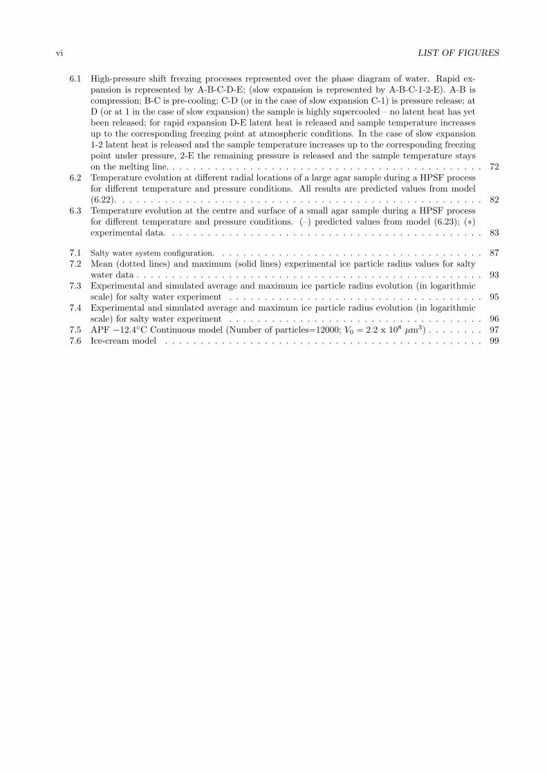
6.1 High-pressure shift freezing processes represented over the phase diagram of water. Rapid ex-pansion is represented by A-B-C-D-E; (slow expansion is represented by A-B-C-1-2-E). A-B iscompression; B-C is pre-cooling; C-D (or in the case of slow expansion C-1) is pressure release; atD (or at 1 in the case of slow expansion) the sample is highly supercooled – no latent heat has yetbeen released; for rapid expansion D-E latent heat is released and sample temperature increasesup to the corresponding freezing point at atmospheric conditions. In the case of slow expansion1-2 latent heat is released and the sample temperature increases up to the corresponding freezingpoint under pressure, 2-E the remaining pressure is released and the sample temperature stayson the melting line. . . . . . . . . . . . . . . . . . . . . . . . . . . . . . . . . . . . . . . . . . . . . 72
6.2 Temperature evolution at different radial locations of a large agar sample during a HPSF processfor different temperature and pressure conditions. All results are predicted values from model(6.22). . . . . . . . . . . . . . . . . . . . . . . . . . . . . . . . . . . . . . . . . . . . . . . . . . . . 82
6.3 Temperature evolution at the centre and surface of a small agar sample during a HPSF processfor different temperature and pressure conditions. (–) predicted values from model (6.23); (∗)experimental data. . . . . . . . . . . . . . . . . . . . . . . . . . . . . . . . . . . . . . . . . . . . . 83
7.1 Salty water system configuration. . . . . . . . . . . . . . . . . . . . . . . . . . . . . . . . . . . . . . 877.2 Mean (dotted lines) and maximum (solid lines) experimental ice particle radius values for salty
water data . . . . . . . . . . . . . . . . . . . . . . . . . . . . . . . . . . . . . . . . . . . . . . . . . 937.3 Experimental and simulated average and maximum ice particle radius evolution (in logarithmic
scale) for salty water experiment . . . . . . . . . . . . . . . . . . . . . . . . . . . . . . . . . . . . 957.4 Experimental and simulated average and maximum ice particle radius evolution (in logarithmic
scale) for salty water experiment . . . . . . . . . . . . . . . . . . . . . . . . . . . . . . . . . . . . 967.5 APF −12.4C Continuous model (Number of particles=12000; V0 = 2.2 x 108 µm3) . . . . . . . . 977.6 Ice-cream model . . . . . . . . . . . . . . . . . . . . . . . . . . . . . . . . . . . . . . . . . . . . . 99
List of Tables
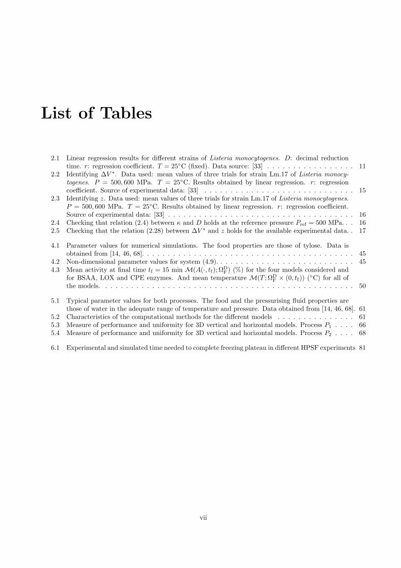
2.1 Linear regression results for different strains of Listeria monocytogenes. D: decimal reductiontime. r: regression coefficient. T = 25C (fixed). Data source: [33] . . . . . . . . . . . . . . . . . 11
2.2 Identifying ∆V ∗. Data used: mean values of three trials for strain Lm.17 of Listeria monocy-
togenes. P = 500, 600 MPa. T = 25C. Results obtained by linear regression. r: regressioncoefficient. Source of experimental data: [33] . . . . . . . . . . . . . . . . . . . . . . . . . . . . . 15
2.3 Identifying z. Data used: mean values of three trials for strain Lm.17 of Listeria monocytogenes.P = 500, 600 MPa. T = 25C. Results obtained by linear regression. r: regression coefficient.Source of experimental data: [33] . . . . . . . . . . . . . . . . . . . . . . . . . . . . . . . . . . . . 16
2.4 Checking that relation (2.4) between κ and D holds at the reference pressure Pref = 500 MPa. . . 162.5 Checking that the relation (2.28) between ∆V ∗ and z holds for the available experimental data. . 17
4.1 Parameter values for numerical simulations. The food properties are those of tylose. Data isobtained from [14, 46, 68]. . . . . . . . . . . . . . . . . . . . . . . . . . . . . . . . . . . . . . . . . 45
4.2 Non-dimensional parameter values for system (4.9). . . . . . . . . . . . . . . . . . . . . . . . . . . 454.3 Mean activity at final time tf = 15 min M(A(·, tf); ΩD
F ) (%) for the four models considered andfor BSAA, LOX and CPE enzymes. And mean temperature M(T ; ΩD
F × (0, tf)) (C) for all ofthe models. . . . . . . . . . . . . . . . . . . . . . . . . . . . . . . . . . . . . . . . . . . . . . . . . 50
5.1 Typical parameter values for both processes. The food and the pressurising fluid properties arethose of water in the adequate range of temperature and pressure. Data obtained from [14, 46, 68]. 61
5.2 Characteristics of the computational methods for the different models . . . . . . . . . . . . . . . 615.3 Measure of performance and uniformity for 3D vertical and horizontal models. Process P1 . . . . 665.4 Measure of performance and uniformity for 3D vertical and horizontal models. Process P2 . . . . 68
6.1 Experimental and simulated time needed to complete freezing plateau in different HPSF experiments 81
vii

Chapter 1
Introduction
There has been significant interest in the study of food engineering from the mid-twentieth century onwards[12, 13, 31, 43, 53, 63, 71, 74, 80, 82, 92]. Humans have been interested in food conservation since ancienttimes, using traditional techniques such as desiccation, conservation in oil, salting, smoking, cooling, etc. Dueto the massive movement of populations to cities, a great supply of food in adequate conditions was necessary.Therefore, the food industry was developed in order to guarantee large-scale food techniques, to prolong itsshelf life, and to make logistic aspects such as transport, distribution and storage, easier. Nowadays, the foodindustry is an increasingly competitive and dynamic arena, given that consumers are now more aware of whatthey eat. Food quality properties, such as taste, texture, appearance, and nutritional content are stronglydependent on the way the foods are processed [53].
Many classical industrial processes are based on thermal treatments, such as, for example, pasteurisation,sterilisation and freezing. In recent years, with the aim to improve these conventional processing technologies, inorder to deliver higher-quality and better food products for the consumers, a number of innovative technologies,also referred to as “emerging” or “novel” technologies have been proposed, investigated, developed, and in somecases, implemented. These “emerging” technologies take advantage of other physics phenomena such as highhydrostatic pressure, electric and electromagnetic fields, and pressure waves. With these innovative technologiesfood engineers can not only develop new food products, but also improve the safety and quality of conventionallytreated food through milder processing. When dealing with innovative processing technologies, several issuesfrom concept development to implementation need addressing. In particular, proper application, development,and optimisation of suitable equipment and process conditions require a significant amount of further knowledgeand understanding [53].
Innovative technologies provide additional complexity and challenges for modellers because of the interactingmultiphysics phenomena. So no longer is there only the thermo- and fluid-dynamic principles of conventionalprocessing, but these innovative technologies also incorporate additional multiphysics dimensions, for example,pressure, electric and electromagnetic fields, among others. To date, some of them still lack an adequate,complete understanding of the basic principles intervening in product and equipment during processing. Properapplication of these technologies, development and optimisation of suitable equipment and process conditions,still require a significant amount of further knowledge [53].
The goal to achieve uniformity of each treatment is common to all innovative processing technologies. Thisgoal can be already an issue at laboratory scale, and it can become progressively worse when scaling up topilot plants and, subsequently, to commercial equipment. However, non-uniformity of the treatment is verycommonly encountered. In fact, the non-uniformities of the process and the lack of process validation ofinnovative processes are the greatest limitations for industrial uptake [53].
We will see in Section 1.2, and afterwards throughout the thesis, that mathematical modelling is a very usefultool for characterising, improving, and optimising innovative food processing technologies. In particular, in thisthesis we are going to focus only on processes that are based on High Hydrostatic Pressure. In Section 1.1 wedescribe the main features of these type of processes and give a brief overview of their benefits and advantages
1

2 CHAPTER 1. INTRODUCTION
over traditional technologies.
1.1 High Pressure Processing of Food
The appearance of High Pressure Processing (HPP) as a tool in the food industry started in the late 1980s [41].Since then to date, extensive research has been done on possible application of HPP as a preservation method[12, 28], to change the physical and functional properties of food systems [11, 41] and to take advantage of thephase diagram of water: freezing, thawing and sub-zero temperature non-frozen storage under pressure [68, 71].
Nowadays, more than 70 companies are using HPP, producing more than 170,000 tons of products [53]. SeveralHPP-treated food products, including juices, jams, jellies, yogurts, ready-to-eat meat, and oysters, are alreadywidely available in the United States, Europe, Japan, New Zealand, and Australia. These successful applicationshave led to a pronounced increase in commercial-scale HPP units around the world during the past 10 years[53].
Several studies [12, 13, 82] have proved that HPP at refrigeration, ambient or moderate heating tempera-ture allows inactivation1 of enzymes and pathogenic and spoilage microorganisms in food, while leaving smallmolecules intact, and therefore not modifying significantly the organoleptic properties (such as colour, odour,texture and flavour).
Two principles underlie the effect of High Pressure (HP): firstly, the Le Chatelier Principle, according to whichany phenomenon (phase transition, chemical reaction, chemical reactivity, change in molecular configuration)accompanied by a decrease in volume will be enhanced by pressure; secondly, pressure is instantaneously anduniformly transmitted independently of the size and the geometry of the food (isostatic pressure). Unlikethermal processing and other classical conservation methods, HP effects are uniform and nearly instantaneousthroughout the food and thus independent of food geometry and equipment size, which has facilitated theexpansion from laboratory findings to full-scale production [89].
Thermal processing is the prevailing method to achieve microbial stability and safety, and although due tothe isostatic principle, HPP has a great advantage as compared to thermal processing, HPP does not escapethe classical limitations, imposed by heat transfer. Heat transfer characterises every process, accompanied bya period of pressure increase or decrease, which is associated with a proportional temperature change of thevessel’s contents due to adiabatic heating. The magnitude of the adiabatic temperature increase or decreasedepends on a number of factors, such as the food product thermo-physical properties (density, thermal expansioncoefficient, and specific heat capacity) and initial temperature, as will be seen in further chapters. Heat transferis caused by the resulting temperature gradients and can lead to large temperature differences, especially inlarge-volume industrial vessels. For a number of HP applications to food engineering, these limitations shouldbe taken into account, trying to avoid as much as possible, non-uniformity at the end of the process.
According to [53], there are two approaches to achieve HP conditions: a direct approach, where a piston isused, which compresses the content of the HP chamber; and an indirect approach, where pressure-transmittingliquid (e.g., water) is pumped into the HP vessel using a HP pump followed by a “pressure intensifier”. Liquidsat extremely high pressures are compressible, requiring extra fluid to be pumped into the vessel. For all themodels described throughout this thesis, we will assume that the HP has been achieved by the indirect method,as will be seen in Chapters 4, 5 and 6.
In general, a “conventional” batch HP process consists of a period of pressure build-up, followed by a period atconstant pressure (holding time) and a period of pressure release. The holding time of a food product dependson the effectiveness of the treatment and the desired remaining level of the critical safety-, or quality-, relatedfactor. It is agreed that, because of the extreme baroresistance of bacterial spores and some enzymes, HPPwill most likely be accompanied by mild to high heating, or other treatments [21, 53]. In cases where HP iscombined with elevated temperatures to minimise the pressure resistance of that safety-, or quality-, relatedaspect, the non-uniform temperature distribution, resulting from heat transfer generated at pressure build-up,will lead to a non-uniform distribution of the desired effect (inactivation of microorganisms, enzymes, etc.)
1Inactivation may be defined as the reduction of undesired biological activity, such as enzymatic catalysis and microbial con-tamination.

1.2. MATHEMATICAL MODELLING OF HIGH-PRESSURE PROCESSES 3
within the product. Depending on the temperature-pressure degradation kinetics of the component that isunder study, this non-uniformity will be more or less pronounced. Especially in heterogeneous food materials,with the contents exhibiting differences in compression heating, the temperatures may not be equally distributedin the food products. Furthermore, the packaging material, the material of the product carrier, and the steelof the HP vessel are not heated to the same extent as the food; therefore, temperature gradients are developedthroughout the system, leading to heat flux from the products to the cooler areas. These spatial temperatureheterogeneities increase over the process time. Although, theoretically, the preheated product heats up uniformlyduring compression to sterilisation temperatures, during pressure holding time temperatures may decrease incertain areas of the vessel. This can affect enzymatic or spore inactivation, and some spores may survive theprocess if temperature loss is not prevented.
Therefore, an accurate evaluation of the effects of pressure, applied during conventional batch HPP, requiresconsideration of the phenomenon above described. If the non-uniform temperature distribution appearing duringthe process is taken into account, it can be assured that the objective of the process has been accomplishedeverywhere within the food product. With this in mind, equations describing the time-temperature-pressurehistory of a product must be coupled with the parameters describing the reaction kinetics for destruction ofmicroorganisms, enzymes, and other factors. The optimisation of batch HP processes for nutrient retentionshould also be based on this approach.
Multiphysics modelling can help greatly in the characterisation of time-temperature-pressure distribution, sub-sequent microbial distributions, and other quality changes as a result of temperature inhomogeneities. Thesemodels can also be applied to the redesign and optimisation of equipment and determination of adequateprocessing conditions for optimum process/product performance.
1.2 Mathematical modelling of High-Pressure Processes
Mathematical modelling is a very useful tool for studying the effect of different systems and process parameterson the outcome of a process. Normally, it is the fastest and least expensive way, given that it minimises thenumber of experiments that need to be conducted to determine the influence of several parameters on the qualityand safety of the process [24].
As previously discussed, most of HP applications in food are not only pressure dependent but also temperaturedependent. This temperature evolution is very important to assure an uniform distribution of the pursuedpressure effect (microbial and/or enzyme inactivation, etc.); also because some industrial processes must takeplace at a constant temperature or in a maximum-minimum threshold to avoid altering properties of the food(e.g. gelification or crystalline state, protein stability, fat migration, freezing, etc.) [71]. As pointed outin [20], from an engineering point of view, a theoretically based heat transfer model that allows predictingthe temperature history within a product under pressure would be essential to homogenise and optimise HPprocesses (design of industrial processes and equipment as well as the quality of the end product).
Depending on the characteristics of the process, the type of food (liquid or solid), the dimensions of the HPvessel, the process conditions (initial temperature, maximum pressure, etc.), different mathematical models willbe used. For example, for a large (when comparing with the pressurizing volume) solid-type food a heat transfermodel with only conduction effects is sufficient [46, 69], whereas for a liquid-type food, convection effects haveto also be included, and therefore equations that model the fluid flow also have to be coupled with the heattransfer equation. If we are studying HP freezing processes, a model that takes into account solidification alsohas to be considered. In some cases, the expression of the process outcome based on the attributes of theprocessed food, that is, e.g. the remaining microbial load, enzyme activity, and chemical reaction products,is required. Within multiphysics modelling, reaction kinetics (i.e., microbial inactivation, quality degradation,chemical reaction, and structural responses) can be coupled with the specific differential equations to providethe spatial distributions of reaction response.
Securing temperature uniformity in HP processed products is crucial for assuring uniform distribution of thepursued pressure effects (e.g. microbial and enzyme inactivation, as we will see in Chapter 2), and the predictionof thermal history within a product under pressure is essential for optimising and homogenising HP process.For this reason, research has focused on heat transfer models that simulate the combination of HP and thermal
4 CHAPTER 1. INTRODUCTION
treatments on food products [71]. Out of many works we highlight the following (references to more of thesekind of models can be found in [18, 71]): Denys et al. [19, 21] suggest a numerical approach for modellingconductive heat transfer during batch HP processing of solid-type food products. The authors showed exper-imentally that non-uniform temperature distribution during HP processing of foods involved a non-uniformenzymatic inactivation. The proposed numerical model could accurately describe the conductive heat transferduring different, but fluid dynamics phenomena in the pressure medium were not included. In [36, 37] theauthors analysed the thermodynamic and fluid-dynamic effects of HP treatments of liquid-type food systems bynumerical simulation. The authors studied the spatial and temporal evolution of temperature and fluid velocityfields. They proved that the uniformity of a HP effect can be disturbed by convective and conductive heat andmass transport conditions that are affected by parameters such as the compression rate, the size of the pressurechamber or the solvent viscosity. In [69] a mathematical model describing the phenomena of heat and masstransfer taking place during the HP treatment of solid foods is obtained, showing the importance of includingconvection effects in some cases. In [46] the temperature distribution is analysed and used as an input for theinactivation of certain enzymes, for both solid- and liquid-type foods, and the behaviour and stability of theproposed models are checked by various numerical examples. Furthermore, various simplified versions of thesemodels are discussed, showing accurate enough results when compared to the original models. Knoerzer et al.[52] considered a model that predicted flow and temperature fields inside a pilot-scale vessel during the pressureheating, holding and cooling stages. The model agreed well with experimental results in which thermocoupleswere used to measure temperature throughout a metallic composite carrier inserted into the vessel. Smith et al.
[86] presented a generalised enthalpy model for a HP Shift Freezing process based on volume fractions depen-dent on temperature and pressure. The model included the effects of pressure on conservation of enthalpy andincorporates the freezing point depression of non-dilute food samples. In addition the significant heat transfereffects of convection in the pressurizing medium are accounted for by solving the two-dimensional Navier-Stokesequations.
Even though there has already been a significant amount of research in this area, there are still many situationsthat arise in HPP that have not been modelled. Therefore, throughout this thesis we have considered differenttypes of HP processes, trying to cover as many situations as possible when working with HP food processing,presenting innovative models. Namely, models for large and small, solid and liquid type foods, for verticallyand horizontally oriented machines, and also for HP freezing processes are analysed. We have developed thecorresponding model for each case, solving each one accordingly. Because every Chapter deals with a differentkind of process, a brief literature review for each of them is given, when relevant, in their individual Chapters.
In Chapter 2 we first start by presenting a model for bacterial and enzymatic inactivation, hence showing thenecessity for knowing the temperature distribution throughout a HP process. A case study of one particularbacteria, for which experimental data is available, is modelled and validated.
In Chapter 3 we present the general aspects of the heat and mass transfer models for HP processes developedin [46, 69]. The new models we derived in Chapters 4, 5 and 6 are based on this one, and thus we decided toinclude this model-presentation chapter to avoid having to introduce the same model in each of the later ones.
In Chapter 4 we introduce one of the most basic type of model for time-temperature-pressure evolution, con-sidering large samples of solid-type foods in a vertically oriented machine. With these, only conduction effectshave to be included in the heat transfer model, which makes its resolution easier, and in some cases may evenbe possible to solve analytically. For vertically oriented machines, a reduction from three to two dimensions ispossible due to the axis-symmetric geometry. Thus, in Chapter 4 several two dimensional models, with differentkind of boundary conditions, are solved analytically and then compared to simplified versions. Also, some ofthe heat transfer models considered in this Chapter are coupled with an enzymatic inactivation model, showinghow this coupling can be done. To date most of the published heat transfer models for solid-type foods hadbeen solved numerically and not analytically.
In Chapter 5 a more complex problem is discussed. We consider liquid-type foods, for which convection effectsalso have to be included into the heat transfer model. Therefore, the equations for fluid flow (Navier–Stokesequations) have to be also solved. Due to the complexity, analytical solutions are no longer available and themodel has to be solved numerically. An added complication to the problem in this Chapter is that we modelprocesses and liquid-type foods placed in both vertically and horizontally oriented HP vessels. For the verticallyoriented HP vessel we could reduce it to two dimensions, due to the axis-symmetry. However for the horizontally

1.2. MATHEMATICAL MODELLING OF HIGH-PRESSURE PROCESSES 5
oriented, there are no longer axis-symmetric features and a three dimensional model is necessary, adding an extrachallenge to the numerical model. The differences between models have been analysed. Developing a model fora horizontally oriented HP vessel is interesting from an industrial point of view, as most of the industrial-scalevessels are in that position [63]. However, at a pilot-scale, they are vertically oriented and therefore most ofthe published research has been focused on these kind of machines, and the models are usually solved in twodimensions.
In Chapter 6 a freezing process that benefits from HP, namely a High-Pressure Shift Freezing (HPSF) process,is described, modelled and solved numerically. Modelling conventional solidification problems is not an easytask, and a lot of interest and research has been put into this area. HP freezing problems, however, havenot been as studied, and in this Chapter we present a generalised enthalpy model for a HPSF process. Themodel can be used for large (when compared to the pressurising fluid volume) solid-type food (only conductioneffects included) and also for small (when compared to the pressurising fluid volume) solid-type food (wherethe significant heat transfer effects of convection in the pressurizing medium are accounted for by solving theNavier–Stokes equations). The model is run for several numerical tests, and good agreement with experimentaldata from the literature is found.
The analysis in Chapter 6 shows that HPSF is more beneficial for ice crystal size and shape than traditional(at atmospheric pressure) freezing. This motivates the work in Chapter 7, which differs from previous Chaptersas we do not solve a model to find the temperature distribution inside a food sample undergoing a HP process.A model for growth and coarsening of ice crystals inside a frozen food sample is developed and some numericalexperiments are given, with which the model is validated by using experimental data. To the best of ourknowledge this is the first model suited for freezing crystallisation in the context of HP.
In Chapter 8 the final conclusions and possible extensions of the presented work are outlined, and in Chapters9 and 10 brief summary in English and Spanish, respectively, of the thesis is given.

Chapter 2
Motivation: Effects of High-Pressure
on enzymes and microorganisms
related to food conservation
Nomenclature for Chapter 2
A Enzymatic activityB Kinetic parameter (K)C Kinetic parameter (MPa−1)Cp Specific heat capacity (J mol−1 K−1)D Decimal reduction time (min)Ea Activation energy (J mol−1)n Number of log-cycles (constant)N Microbial population (cfu g−1)P Pressure (MPa)r Linear regression coefficient (constant)R Universal gas constant (cm3 MPa mol−1 K−1)S Entropy (J mol−1 K−1)t Time (min)T Temperature (K)V Volume (cm3)x x-component of centre of gravityy y-component of centre of gravityz Pressure resistant coefficient (MPa)
Acronyms
HP High Pressure
Greek symbols
∆ν Compressibility factor (cm3 mol−1)∆ζ Thermal expansibility (cm3 mol−1 K−1)∆V ∗ Volume of activation (cm3 mol−1)κ Inactivation rate (min−1)
Indices
0 Initialref Reference
As explained in Chapter 1, some studies [12, 82] have proven that HP causes inactivation of enzymes andmicroorganisms in food. The efficiency of a HP treatment on inactivation depends on several parameters[13, 82] such as the type of microorganism or enzyme under study, the physiological state of the microorganism(e.g. exponentially growing state, stationary state, frozen, etc.), the pressure applied, the temperature, theprocessing time, the pH of the sample and the composition of the food or the dispersion medium.
Let us review some of the general concepts that we mention in this Chapter, following the Encyclopedia Bri-tannica:
Enzymes: Enzymes are large protein molecules that act as biological catalysts, accelerating chemical reactionswithout being consumed to any appreciable extent themselves. The activity of enzymes is specific for a certainset of chemical substrates, and it is dependent on both pH and temperature.
The living tissues of plants and animals maintain a balance of enzymatic activity. This balance is disruptedupon harvest or slaughter. In some cases, enzymes that play a useful role in living tissues may catalyze
7

8 CHAPTER 2. MOTIVATION
spoilage reactions following harvest or slaughter. For example, the enzyme pepsin is found in the stomach ofall animals and is involved in the breakdown of proteins during the normal digestion process. However, soonafter the slaughter of an animal, pepsin begins to break down the proteins of the organs, weakening the tissuesand making them more susceptible to microbial contamination. After the harvesting of fruits, certain enzymesremain active within the cells of the plant tissues. These enzymes continue to catalyze the biochemical processesof ripening and may eventually lead to rotting, as can be observed in bananas. In addition, oxidative enzymesin fruits continue to carry out cellular respiration (the process of using oxygen to metabolise glucose for energy).This continued respiration decreases the shelf life of fresh fruits and may lead to spoilage. Respiration may becontrolled by refrigerated storage or modified-atmosphere packaging.
Microorganism: Microorganisms are a collection of organisms that share the characteristic of being visibleonly with a microscope. They constitute the subject matter of microbiology. Microorganism is a general termthat becomes more understandable if it is divided into its principal types - bacteria, yeasts, molds, protozoa,algae, and rickettsia-predominantly unicellular microbes. Viruses are also included, although they cannot live orreproduce on their own. They are particles, not cells; they consist of deoxyribonucleic acid (DNA) or ribonucleicacid (RNA), but not both. Viruses invade living cells - bacteria, algae, fungi, protozoa, plants, and animals(including humans) - and use their hosts’ metabolic and genetic machinery to produce thousands of new virusparticles. Some viruses can transform normal cells to cancer cells. Rickettsias and chlamydiae are very smallcells that can grow and multiply only inside other living cells. Although bacteria, actinomycetes, yeasts, andmolds are cells that must be magnified in order to see them, when cultured on solid media that allow theirgrowth and multiplication, they form visible colonies consisting of millions of cells.
Bacteria and fungi (yeasts and molds) are the principal types of microorganisms that cause food spoilage andfood - borne illnesses. Foods may be contaminated by microorganisms at any time during harvest, storage,processing, distribution, handling, or preparation. The primary sources of microbial contamination are soil, air,animal feed, animal hides and intestines, plant surfaces, sewage, and food processing machinery or utensils.
Bacteria: Bacteria are unicellular organisms that have a simple internal structure compared with the cells ofother organisms. The increase in the number of bacteria in a population is commonly referred to as bacterialgrowth by microbiologists. This growth is the result of the division of one bacterial cell into two identicalbacterial cells, a process called binary fission. Under optimal growth conditions, a bacterial cell may divideapproximately every 20 minutes. Thus, a single cell can produce almost 70 billion cells in 12 hours. The factorsthat influence the growth of bacteria include nutrient availability, moisture, pH, oxygen levels, and the presenceor absence of inhibiting substances (e.g., antibiotics).
The nutritional requirements of most bacteria are chemical elements such as carbon, hydrogen, oxygen, nitrogen,phosphorus, sulfur, magnesium, potassium, sodium, calcium, and iron. The bacteria obtain these elements byutilizing gases in the atmosphere and by metabolizing certain food constituents such as carbohydrates andproteins.
Temperature and pH play a significant role in controlling the growth rates of bacteria. Bacteria may beclassified into three groups based on their temperature requirement for optimal growth: thermophiles (55C-75C), mesophiles (20C-45C), or psychrotrophs (10C-20C). In addition, most bacteria grow best in a neutralenvironment (pH equal to 7).
Bacteria also require a certain amount of available water for their growth. The availability of water is expressedas water activity and is defined by the ratio of the vapour pressure of water in the food to the vapour pressureof pure water at a specific temperature. Therefore, the water activity of any food product is always a valuebetween 0 and 1, with 0 representing an absence of water and 1 representing pure water. Most bacteria donot grow in foods with a water activity below 0.91, although some halophilic bacteria (those able to toleratehigh salt concentrations) can grow in foods with a water activity lower than 0.75. Growth may be controlledby lowering the water activity - either by adding solutes such as sugar, glycerol, and salt or by removing waterthrough dehydration.
The oxygen requirements for optimal growth vary considerably for different bacteria. Some bacteria requirethe presence of free oxygen for growth and are called obligate aerobes, whereas other bacteria are poisoned bythe presence of oxygen and are called obligate anaerobes. Facultative anaerobes are bacteria that can grow inboth the presence or absence of oxygen. In addition to oxygen concentration, the oxygen reduction potential
2.1. CASE STUDY 9
of the growth medium influences bacterial growth. The oxygen reduction potential is a relative measure of theoxidizing or reducing capacity of the growth medium.
When bacteria contaminate a food substrate, it takes some time before they start growing. This lag phase is theperiod when the bacteria are adjusting to the environment. Following the lag phase is the log phase, in whichpopulation grows in a logarithmic fashion. As the population grows, the bacteria consume available nutrientsand produce waste products. When the nutrient supply is depleted, the growth rate enters a stationary phase inwhich the number of viable bacteria cells remains the same. During the stationary phase, the rate of bacterialcell growth is equal to the rate of bacterial cell death. When the rate of cell death becomes greater than therate of cell growth, the population enters the decline phase.
When the conditions for bacterial cell growth are unfavourable (e.g., low or high temperatures or low moisturecontent), several species of bacteria can produce resistant cells called endospores. Endospores are highly resistantto heat, chemicals, desiccation (drying out), and ultraviolet light. The endospores may remain dormant for longperiods of time. When conditions become favourable for growth (e.g., thawing of meats), the endosporesgerminate and produce viable cells that can begin exponential growth.
After reviewing the general concepts, in Section 2.1 we study a particular case of inactivation of the bacteriaListeria monocytogenes inoculated in raw minced ham, based on the experimental results described in [33].This work was presented as a technical report (see [76]) to Esteban Espuna, S.A.
The methodology followed in Section 2.1 is valid not only for Listeria monocytogenes, which we use here asa practical real-life application, but for many other microorganisms or enzymes. One just needs to follow asimilar approach to the one explained here, but with data corresponding to the new microorganism or enzyme.In Section 2.2 we present a generalised model for microbial or enzymatic inactivation for a more general processand/or microorganism or enzyme.
2.1 A case study: Inactivation of Listeria monocytogenes inocu-
lated in minced raw ham
Let us start by reviewing what Listeria monocytogenes is:
Listeria monocytogenes: (source: [1, 3, 31]) These are the bacteria that cause the infection listeriosis. Itis a facultative anaerobic bacterium, capable of growing and reproducing inside the host’s cells, and is oneof the most virulent food-borne pathogens, with 20 to 30 percent of clinical infections resulting in death. L.monocytogenes is a Gram-positive bacterium, motile via flagella at 30C and below, but usually not at 37C. L.monocytogenes can instead move within eukaryotic cells by explosive polymerisation of actin filaments (knownas comet tails or actin rockets). It can survive in extreme conditions for long periods of time. It can reproducein refrigerated foods, which increases risk during storage.
The bacterium has been isolated from humans and from more than 50 species of wild and domestic animals,including mammals, birds, fish, crustaceans, and ticks. It has also been isolated from environmental sourcessuch as animal silage, soil, plants, sewage, and stream water. It has been found in milk, cheese, raw meat andsea food.
By using experimental data provided in [33] we want to build a mathematical model that allows us to predictthe value of the microbial population N of a sample after going through a HP process. In [33] the populationof Listeria monocytogenes is measured in cfu g−1.1
The inoculation medium of the bacteria, together with the pressure, temperature and time of the process, aredecisive factors for characterising the inactivation process. Due to data limitation we will not be able to includethe dependence of the inoculation medium, as we only have results from test performed on Listeria strains
1In microbiology, colony-forming unit (CFU) is an estimate of viable bacterial or fungal numbers. Unlike direct microscopiccounts where all cells, dead and living, are counted, CFU estimates viable cells. The appearance of a visible colony requiressignificant growth of the initial cells plated - at the time of counting the colonies it is not possible to determine if the colony arosefrom one cell or 1000 cells. Therefore, the results are given as CFU/mL (colony-forming units per milliliter) for liquids, and CFU/g(colony-forming units per gram) for solids to reflect this uncertainty (rather than cells/mL or cells/g).
10 CHAPTER 2. MOTIVATION
inoculated in raw minced ham. The dependence of the inactivation of Listeria on the medium is discussed in[22, 31].
With these data the temperature dependence could not be included either as all experiments were performedat the same temperature (T = 25C). In [31] this dependence is studied.
We will therefore start by finding a formula for microbial population N(t) as a function of time, and theninclude the pressure dependence, giving the microbial population N(t;P ) as a function of time and pressure.The procedure that we follow is:
1. Experimental observation
2. Mathematical modelling
3. Identify kinetic parameters
4. Validation of model with data
2.1.1 Modelling of the population N(t) for a fixed pressure P and temperature T
Experimental observation
HP processes are run on three different strains of Listeria monocytogenes (Lm. 1, Lm. 2, Lm. 17) isolated fromraw ham and inoculated in minced raw ham (with water activity Aw = 0.90). The results of the tests (dataobtained from [33]) are recorded into a table of values (ti, log(N(ti))) where ti is the time (min) and N(ti) thebacterial population at time ti (cfu g−1).
Mathematical modelling
For a fixed temperature T and pressure P , experimental values (ti, log(N(ti))) decrease in a linear way, hencewe use a first order mathematical model given by (see, e.g., [22, 27, 43, 92])
dN(t)
dt= −κN(t), t ≥ 0,
N(0) = N0,
(2.1)
where t is the elapsed process time (min), N(t), N0 (cfu g−1) are the bacterial population at time t and at thestart, respectively, and κ (min−1) is the kinetic inactivation rate constant or death velocity constant.
The solution to (2.1) is given by
ln
(
N(t)
N0
)
= −κt or, equivalently, N(t) = N0 exp (−κt). (2.2)
In Food Engineering, it is common to use the concept of decimal reduction time (see [22]), D, which is definedas the time required to kill 90% of the microorganisms being studied.
Remark 1. In the literature (see, e.g., [31, 81]) D is also defined as the time required for the microorganismsto reduce by one log-cycle, which is equivalent to reduce them by 90% (i.e. N(t) = N0
10 ). Hence if we need the
population to reduce by n-log-cycles (i.e. N(t) = N0
10n ) the processing time should be at least nD min.
For industrial food processes, it is usual to study 5-log-cycles reductions (see [33, 49, 77]), which is equivalentto having a processing time of at least 5D min.
From (2.2)
log
(
N(t)
N0
)
= log(exp (−κt)) = −κt log(e) = −κtln(e)
ln(10)=
−κt
ln(10). (2.3)

2.1. CASE STUDY 11
As D is the time required for N(t) = N0
10 , it holds that
D =ln(10)
κlog
(
N0
N0
10
)
=ln(10)
κ, (2.4)
leading to the relation between the decimal reduction time, D, and the kinetic inactivation rate constant, κ.
From (2.3) and (2.4), the process elapsed time can be expressed as
t = D log
(
N0
N(t)
)
, or, equivalently, log
(
N(t)
N0
)
= − t
D. (2.5)
Identify kinetic parameters
We are going to work with the solution given by the form of (2.5), and thus the kinetic parameter we need toidentify is the decimal reduction time, D. This will allow us to predict the bacterial population after a processat fixed temperature T and pressure P , at an arbitrary time chosen by the model user.
To identify the value of D we use the experimental values and plot a scatter graph. The model validationcarried out in the next step shows that the scattered points will be very close to a straight line with a negativeslope. In this case, according to (2.5), the value of the slope is −1
D. To identify D we find the linear regression
line by linear regression techniques.
Validation of model with data
We need to validate that the first order model together with the identified D, is good enough. To do so we builda table with the values of D calculated by linear regression, and check that, for each identified value of D (whichdepends on pressure, temperature and the Listeria strain we are analysing) provides a good approximation ofthe experimental results for bacterial population N(t) at certain times t. Figures 2.1a, 2.1b, 2.1c and 2.1d
Trial D(min) r1st 1.2778 0.97702nd 1.3769 0.98183rd 1.4172 0.9469
D(mean) 1.3573
Lm1. P = 600 MPa
Trial D(min) r1st 1.4511 0.98742nd 1.4505 0.97793rd 1.5285 0.9314
D(mean) 1.4767
Lm12. P = 600 MPa
Trial D(min) r1st 1.4799 0.992nd 1.5267 0.98173rd 1.4422 0.9772
D(mean) 1.4829
Lm17. P = 600 MPa
Trial D(min) r1st 4.6558 0.992nd 4.3791 0.97493rd 4.7603 0.9794
D(mean) 4.5984
Lm17. P = 500 MPa
Table 2.1: Linear regression results for different strains of Listeria monocytogenes. D: decimal reduction time.r: regression coefficient. T = 25C (fixed). Data source: [33]
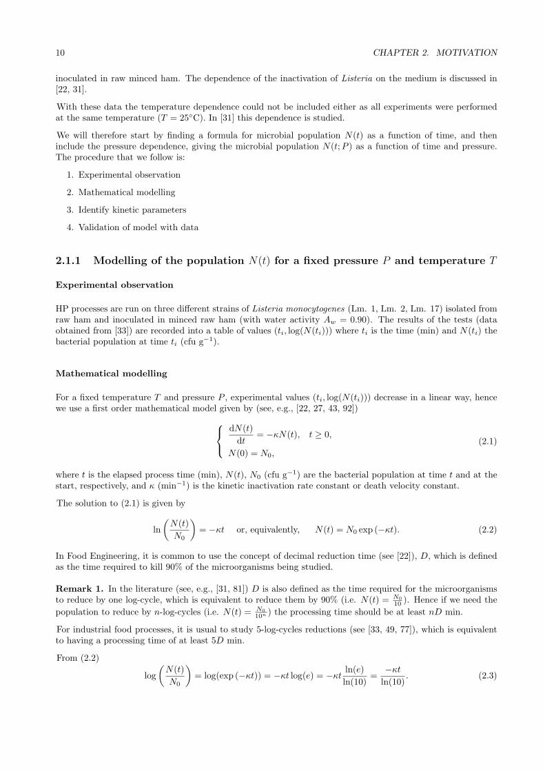
show the experimental bacterial population (∗) as a function of time for different trials, run on different strainsof Listeria, at different pressures and a fixed temperature T = 25C. The straight lines in the figures are thecorrespondent regression lines. Table 2.1 gives the predicted D values and the regression coefficient r, showingthat the regression is good enough for each D calculated.

12 CHAPTER 2. MOTIVATION
0 1 2 3 4 5 6 71
2
3
4
5
6
7
Time (min)
log(
N)
(cfu
/g)
First trial
Second trial
Third trial
(a) Strain Lm.1. P = 600MPa
0 1 2 3 4 5 6 71
2
3
4
5
6
7
Time (min)
log(
N)
(cfu
/g)
First trial
Second trial
Third trial
(b) Strain Lm.12 P = 600MPa
0 1 2 3 4 5 6 71
2
3
4
5
6
7
Time (min)
log(
N)
(cfu
/g)
First trial
Second trial
Third trial
(c) Strain Lm.17 P = 600MPa
0 5 10 15 202
3
4
5
6
7
Time (min)
log(
N)
(cfu
/g)
First trial
Second trial
Third trial
(d) Strain Lm.17 P = 500MPa
Figure 2.1: Reduction of the bacterial population and regression lines corresponding to the different strains ofListeria monocytogenes from the several trials. T = 25C (fixed). Data source: [33]
We have seen that for fixed temperature T and pressure P , with available data of bacterial population atdifferent time steps, we can identify kinetic parameter D by linear regression. This allows us to estimatebacterial population after t minutes of processing at the same temperature and pressure using (2.5). We canalso easily estimate the required time for a n-log-cycle reduction in bacterial population, which is nD as statedin Remark 1.
The following step is to estimate, for a fixed temperature T , the bacterial population N(t;P ) at a given timet and for any pressure P , without having to do experimental measurements for that pressure. For this we willneed to identify some new kinetic parameters, as explained in Section 2.1.2.
2.1.2 Modelling of the population N(t;P ) for a fixed temperature T
Experimental observation
We are going to use the experimental results from [33] of the trials run on strain Lm. 17 of Listeria monocytogenes
at two different pressures, P = 500 MPa and P = 600 MPa. The temperature is fixed at T = 25C.
Mathematical modelling
For fixed pressure P and temperature T we showed that (2.1) (or, equivalently (2.2) or (2.5)) is a valid model. Ifwe now want to extend it for arbitrary pressures, in a suitable range, we need to identify the kinetic parametersthat describe the influence of pressure on microbial population. Not many references to such parameters areavailable (as stated in [31]), however we have found two different models (see [27] and [31]) that focus on theeffects of pressure on microbial population.
2.1. CASE STUDY 13
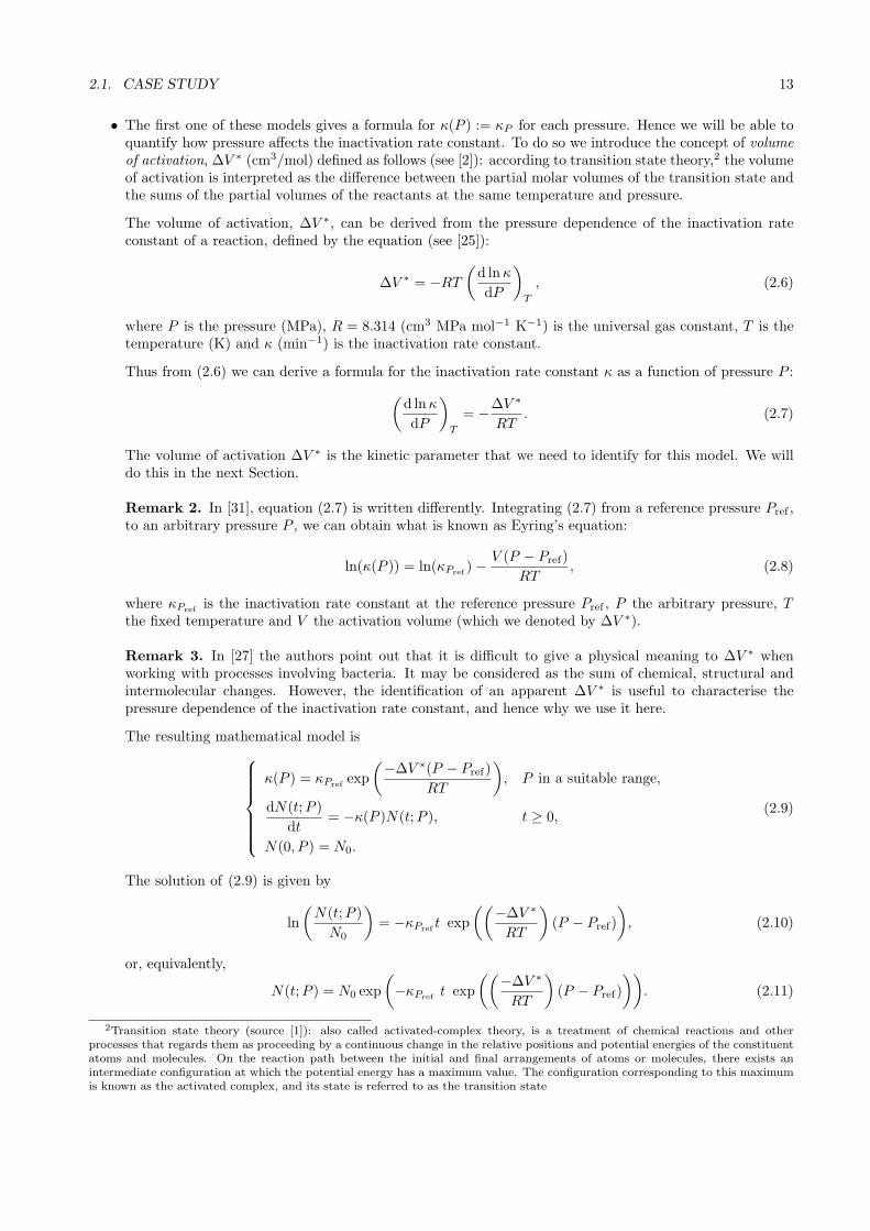
• The first one of these models gives a formula for κ(P ) := κP for each pressure. Hence we will be able toquantify how pressure affects the inactivation rate constant. To do so we introduce the concept of volume
of activation, ∆V ∗ (cm3/mol) defined as follows (see [2]): according to transition state theory,2 the volumeof activation is interpreted as the difference between the partial molar volumes of the transition state andthe sums of the partial volumes of the reactants at the same temperature and pressure.
The volume of activation, ∆V ∗, can be derived from the pressure dependence of the inactivation rateconstant of a reaction, defined by the equation (see [25]):
∆V ∗ = −RT
(
d lnκ
dP
)
T
, (2.6)
where P is the pressure (MPa), R = 8.314 (cm3 MPa mol−1 K−1) is the universal gas constant, T is thetemperature (K) and κ (min−1) is the inactivation rate constant.
Thus from (2.6) we can derive a formula for the inactivation rate constant κ as a function of pressure P :
(
d lnκ
dP
)
T
= −∆V ∗
RT. (2.7)
The volume of activation ∆V ∗ is the kinetic parameter that we need to identify for this model. We willdo this in the next Section.
Remark 2. In [31], equation (2.7) is written differently. Integrating (2.7) from a reference pressure Pref ,to an arbitrary pressure P , we can obtain what is known as Eyring’s equation:
ln(κ(P )) = ln(κPref)− V (P − Pref)
RT, (2.8)
where κPrefis the inactivation rate constant at the reference pressure Pref , P the arbitrary pressure, T
the fixed temperature and V the activation volume (which we denoted by ∆V ∗).
Remark 3. In [27] the authors point out that it is difficult to give a physical meaning to ∆V ∗ whenworking with processes involving bacteria. It may be considered as the sum of chemical, structural andintermolecular changes. However, the identification of an apparent ∆V ∗ is useful to characterise thepressure dependence of the inactivation rate constant, and hence why we use it here.
The resulting mathematical model is
κ(P ) = κPrefexp
(−∆V ∗(P − Pref)
RT
)
, P in a suitable range,
dN(t;P )
dt= −κ(P )N(t;P ), t ≥ 0,
N(0, P ) = N0.
(2.9)
The solution of (2.9) is given by
ln
(
N(t;P )
N0
)
= −κPreft exp
((−∆V ∗
RT
)
(P − Pref)
)
, (2.10)
or, equivalently,
N(t;P ) = N0 exp
(
−κPreft exp
((−∆V ∗
RT
)
(P − Pref)
))
. (2.11)
2Transition state theory (source [1]): also called activated-complex theory, is a treatment of chemical reactions and otherprocesses that regards them as proceeding by a continuous change in the relative positions and potential energies of the constituentatoms and molecules. On the reaction path between the initial and final arrangements of atoms or molecules, there exists anintermediate configuration at which the potential energy has a maximum value. The configuration corresponding to this maximumis known as the activated complex, and its state is referred to as the transition state

14 CHAPTER 2. MOTIVATION
• The second model provides a formula for D(P ) := DP (min) for each pressure. Following [31] we have
log
(
D(P )
DPref
)
= −P − Pref
z, (2.12)
where DPrefis the decimal reduction time at a reference pressure Pref (MPa), P the pressure (MPa), and
z (MPa) is the pressure resistant coefficient or z-pressure-value, which is the kinetic parameter we haveto identify for this model. From (2.12) it is clear that z is the pressure increment from Pref necessary toreduce DPref
by one-log-cycle.
Remark 4. In contrast to what was said in Remark 3 for ∆V ∗, the physical meaning of z is obviouswhen working with bacterias.
The resulting mathematical model in this case is
D(P ) = DPref10
(
−P−Pref
z
)
, P in a suitable range,
dN(t;P )
dt= − ln(10)
D(P )N(t;P ), t ≥ 0,
N(0, P ) = N0.
(2.13)
Remark 5. Note that the second equation of (2.13) is equal to the second equation of (2.9), by takinginto account (2.4).
The solution of (2.13) is given by
log
(
N(t;P )
N0
)
= − t
DPref
10
(
P−Prefz
)
, (2.14)
or, equivalently,
N(t;P ) = N0 10−
tDPref
10(P−Pref
z ). (2.15)
Remark 6. As was said in Remark 1, D(P ) is the time required to reduce the microbial population byone-log-cycle at an arbitrary pressure P . Therefore, by using the formula for D(P ) from the first equationof (2.13), the time t(P, n) required to attain an n-log-cycle reduction is
t(P, n) = n DPref10
(
−P−Pref
z
)
. (2.16)
Identify kinetic parameters
• For the first model the kinetic parameters we need to identify are Pref (MPa) (which could also be chosena priori), κPref
(min−1) and ∆V ∗ (cm3 mol−1). From (2.8) it holds that
ln(κ(P )) = −∆V ∗
RTP +
(
∆V ∗
RTPref + ln(κPref
)
)
. (2.17)
Using identified values of κ(Pi) (we calculate them using the identified mean values D(Pi) from the
previous Section, and the relation κ = ln(10)D
) we plot the scatter graph for (Pi, ln(κ(Pi))). The modelvalidation carried out in the next step shows that the scattered points will be very close to a straight linewith a positive slope. In this case, according to (2.17), the value of the slope is −∆V ∗
RT, from where we can
obtain ∆V ∗. The linear regression line will go through the centre of gravity of the scatter plot, that is
(x, y) =1
m
m∑
i=1
(Pi, ln(κ(Pi))), (2.18)
thus, selecting Pref and κPrefsuch that
(x, y) = (Pref , ln(κPref)), (2.19)
2.1. CASE STUDY 15
we have
Pref = x, and κPref= ey. (2.20)
This allows us to obtain a mathematical model for κ(P ) for any pressure in a suitable range using (2.8).
• For the second model, the kinetic parameters we need to identify are Pref (MPa), DPref(min) and z (MPa).
From (2.12) it holds that
log(D(P )) = −P
z+
(
Pref
z+ log(DPref
)
)
. (2.21)
Using identified values of D(Pi) we plot the scatter graph for (Pi, log(D(Pi))). The model validationcarried out in the next step shows that the scattered points will be very close to a straight line with anegative slope. In this case, according to (2.21), the value of the slope is − 1
z, from where we can obtain
z. The linear regression line will go through the centre of gravity of the scatter plot, that is
(x, y) =1
m
m∑
i=1
(Pi, log(D(Pi))), (2.22)
thus, selecting Pref and DPrefsuch that
(x, y) = (Pref , log(DPref)), (2.23)
we have
Pref = x, and DPref= 10y. (2.24)
This allows us to obtain a mathematical model for D(P ) for any pressure in a suitable range using (2.12).
Validation of model with data
In a similar way to Section 2.1.1, we want to show that (2.9) together with the identified ∆V ∗ value, and (2.13)together with the identified z value, are good enough approximations for a certain range of pressure, whencompared to experimental data. Then we can use (2.11) and (2.15) in order to obtain suitable estimates of themicrobial population of strain Lm.17 of Listeria monocytogenes under those conditions.
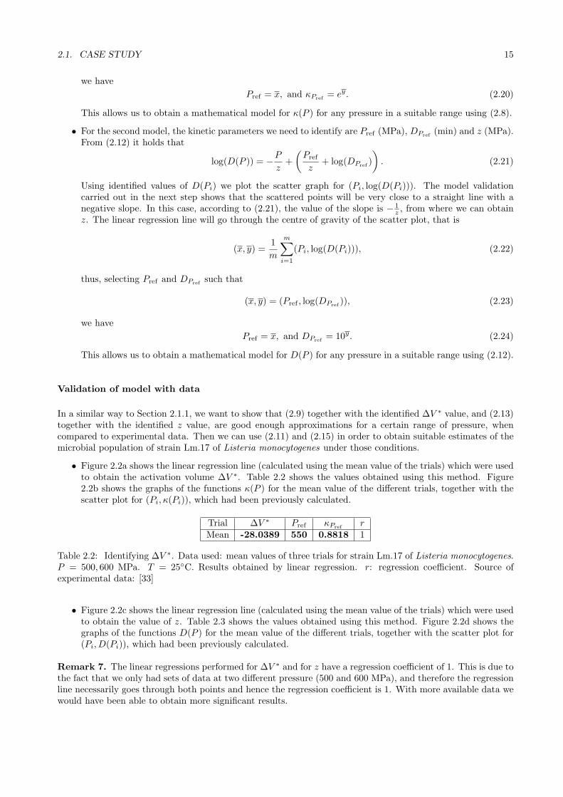
• Figure 2.2a shows the linear regression line (calculated using the mean value of the trials) which were usedto obtain the activation volume ∆V ∗. Table 2.2 shows the values obtained using this method. Figure2.2b shows the graphs of the functions κ(P ) for the mean value of the different trials, together with thescatter plot for (Pi, κ(Pi)), which had been previously calculated.
Trial ∆V ∗ Pref κPrefr
Mean -28.0389 550 0.8818 1
Table 2.2: Identifying ∆V ∗. Data used: mean values of three trials for strain Lm.17 of Listeria monocytogenes.P = 500, 600 MPa. T = 25C. Results obtained by linear regression. r: regression coefficient. Source ofexperimental data: [33]
• Figure 2.2c shows the linear regression line (calculated using the mean value of the trials) which were usedto obtain the value of z. Table 2.3 shows the values obtained using this method. Figure 2.2d shows thegraphs of the functions D(P ) for the mean value of the different trials, together with the scatter plot for(Pi, D(Pi)), which had been previously calculated.
Remark 7. The linear regressions performed for ∆V ∗ and for z have a regression coefficient of 1. This is due tothe fact that we only had sets of data at two different pressure (500 and 600 MPa), and therefore the regressionline necessarily goes through both points and hence the regression coefficient is 1. With more available data wewould have been able to obtain more significant results.
16 CHAPTER 2. MOTIVATION
500 510 520 530 540 550 560 570 580 590 600−0.8
−0.6
−0.4
−0.2
0
0.2
0.4
0.6
P (MPa)
ln(κ
(P))
(m
in−
1 )
Scatter plotRegression lineCentre of gravity
(a) Linear regression lines for obtaining ∆V ∗
500 510 520 530 540 550 560 570 580 590 6000.4
0.6
0.8
1
1.2
1.4
1.6
1.81.8
P (MPa)
κ(P
) (m
in−
1 )
Function κ(P)Scatter plot
(b) Graph of function κ(P )
500 510 520 530 540 550 560 570 580 590 6000.1
0.2
0.3
0.4
0.5
0.6
0.7
0.80.8
P (MPa)
log(
D(P
)) (
min
)
Scatter plotRegression lineCentre of gravity
(c) Linear regression lines for obtaining z
500 510 520 530 540 550 560 570 580 590 6001
1.5
2
2.5
3
3.5
4
4.5
5
P (MPa)
D(P
) (m
in)
Function D(P)Scatter plot
(d) Graph of function D(P )
Figure 2.2: Model validation with data for HP inactivation of strain Lm. 17 of Listeria monocytogenes. T =25C. Source for experimental data: [33].
Trial z (MPa) Pref DPrefr
Mean 203.4609 550 2.6113 1
Table 2.3: Identifying z. Data used: mean values of three trials for strain Lm.17 of Listeria monocytogenes.P = 500, 600 MPa. T = 25C. Results obtained by linear regression. r: regression coefficient. Source ofexperimental data: [33]
Relation between the two models
Let us now see how the two previous models are related. To do so we show that there is a simple mathematicalrelation between ∆V ∗ and z. Let us recall that for fixed pressure P and temperature T , the relation betweenκ and D is given by (2.4). As can be easily seen in Table 2.4 for the reference pressure, Pref = 550 MPa, (2.4)
Trial κPrefln(10) DPref
(calculated by regression) κPref(calculated by regression)
Mean 0.8818 2.6113 2.6113
Table 2.4: Checking that relation (2.4) between κ and D holds at the reference pressure Pref = 500 MPa.
holds, and therefore
DPref=
ln(10)
κPref
(2.25)
For an arbitrary pressure, P ,
D(P ) =ln(10)
κ(P )(2.26)

2.1. CASE STUDY 17
has to hold. Therefore, using the first equation of (2.9) and the first equation of (2.13) it follows
DPref10
(
−P−Pref
z
)
=ln(10)
κPrefexp
(
−∆V ∗(P−Pref)RT
) =⇒ 10
(
−P−Pref
z
)
= exp
(
∆V ∗(P − Pref)
RT
)
,
=⇒ −P − Pref
z= log
(
exp
(
∆V ∗(P − Pref)
RT
))
=ln(
exp(
∆V ∗(P−Pref)RT
))
ln(10)
=⇒ −P − Pref
z=
∆V ∗(P − Pref)
RT ln(10),
(2.27)
from where we can find the relation between ∆V ∗ and z, given by
∆V ∗ = −RT ln(10)
z. (2.28)
Table 2.5 shows that formula (2.28) is correct for our data
Trial z −RT ln(10) ∆V ∗
(calculated by regression) z (calculated by regression)Mean 203.4609 -28.0389 -28.0389
Table 2.5: Checking that the relation (2.28) between ∆V ∗ and z holds for the available experimental data.
Expressions (2.4) and (2.28) allow us to indistinctly use one model or the other, without having to do newregression calculations.
Observations
Kinetic pressure parameters ∆V ∗ and z (together with suitable reference values Pref , κPrefand DPref
) have beenidentified. With these parameters the bacterial population N(t;P ), at any time t and pressure P (within theadequate range), can be calculated.
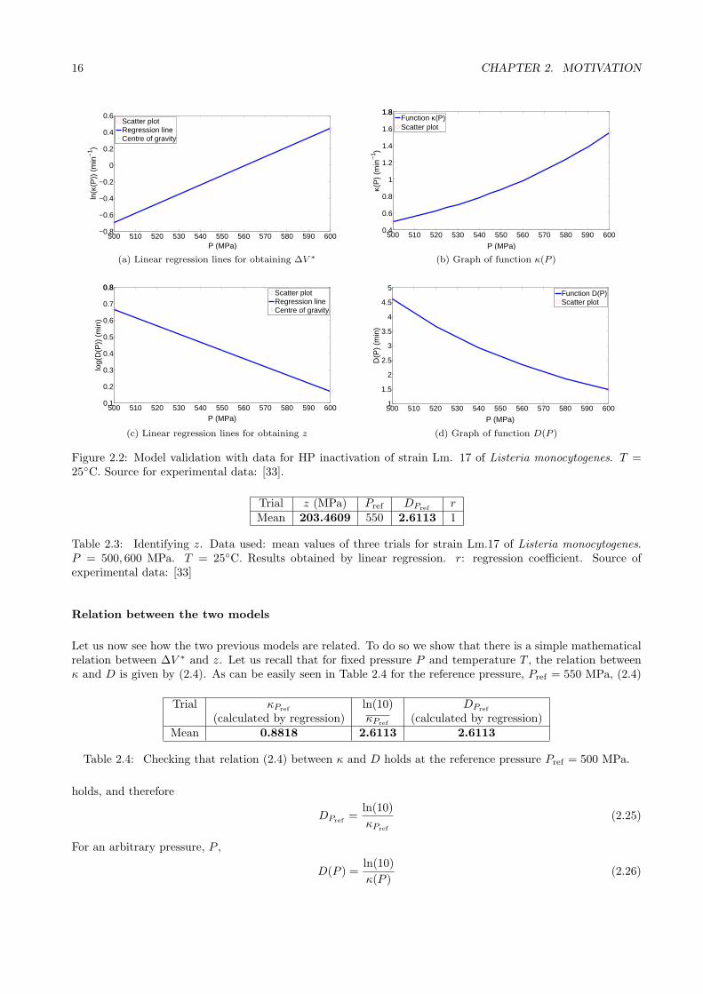
• In particular, for the first model, the bacterial population (of strain Lm.17 of Listeria monocytogenes)after elapsed time t, at any pressure P (preferably in the range 500 - 600 MPa or close to it) and at atemperature of 25C is given by
N(t;P ) = N0 e−κ(P )t, (2.29)
where N0 is the initial bacterial population N0 = 6.3096 · 106 (cfu g−1),
κ(P ) = κPrefexp
(−∆V ∗(P − Pref)
RT
)
, (2.30)
κPref= 0.8818 (min−1), Pref = 550 (MPa), ∆V ∗ = −28.0389 (cm3mol−1), R = 8.314 (Jmol−1K−1), and
T = 298.15 (K). It is easy to see from (2.30) that at a higher pressure, higher is the inactivation rateconstant, κ(P ). In Figure 2.3 a graph of N(t;P ) for t ∈ (0, 7) min and P ∈ (500, 600) MPa can be seen.In the figure it is clear that the lowest values of bacterial population are obtained for higher pressure andtime values.
We point out that the values for ∆V ∗ and κPrefhave been taken as the mean value of the three experiments.
The value for N0 has been taken from [33].
• For the second model, the bacterial population (of strain Lm.17 of Listeria monocytogenes) after elapsedtime t, at any pressure P (preferably in the range 500 - 600 MPa or close to it) and at a temperature of25C is given by
N(t;P ) = N0 10−t
D(P ) , (2.31)

18 CHAPTER 2. MOTIVATION
01
23
45
67
500520
540560
580600
0
1
2
3
4
5
6
7x 10
6
t (min)P (MPa)
N(t
;P)
(cfu
/g)
Figure 2.3: Graph of N(t;P ) (from the first model), for the mean
values of the three experiments of strain Lm.17 of Listeria monocytogenes
Lm.17. T = 25C.
where N0 is the initial bacterial population N0 = 6.3096 · 106 (cfu g−1),
D(P ) = DPref10
(
−P−Pref
z
)
, (2.32)
DPref= 2.6113 (min), Pref = 550 (MPa), and z = 203.4609 (MPa). It is easy to see from (2.32) that at a
higher pressure, lower is the decimal reduction time, D(P ).
Also, according to (2.16), the time required to obtain a n-log-cycle reduction is
t(P, n) = n DPref10−
P−Prefz . (2.33)
We point out that the values for z and DPrefhave been taken as the mean value of the three experiments.
The value for N0 has been taken from [33].
The obvious next step would be to model the population N(t;T, P ) of bacteria for arbitrary pressures andtemperatures, in an adequate range. To follow the same procedure as above we would need experimentalmeasurements at different temperatures. However these were not provided to us in the same study as [33],hence we could not do the entire model validation. However, in Section 2.2 we present a mathematical modelfor microbial and enzymatic inactivation at arbitrary pressures and temperatures, which is a generalisation ofthe models presented above for arbitrary pressure and temperature conditions.
2.2 Generalised mathematical modelling of microbial and enzymatic
inactivation
By analogy to the models derived in Section 2.1, in order to describe changes in the microbial population as afunction of time t, when the food sample is processed at temperature T and pressure P , we can use the following

2.2. GENERALISED MODEL 19
first order model3 (see, e.g., [22, 27, 43, 92]):
dN(t;T, P )
dt= −κ(T, P )N(t;T, P ), t ≥ 0,
N(0;T, P ) = N0,(2.34)
where N0 is the initial microbial population and κ(T, P ) is the inactivation rate (min−1) that now depends ontemperature and pressure. The solution to (2.34) is given by
N(t;T, P ) = N0 exp
(
−∫ t
0
κ(T (s), P (s)) ds
)
, (2.35)
Another equation used very often (see [31]) to calculate changes of microbial population as a function of timeis the following:
dN(t;T, P )
dt= − log 10
D(T, P )N(t;T, P ), t ≥ 0,
N(0;T, P ) = N0,
Solution: N(t;T, P ) = N0 10−∫
t
01
D(T (s),P (s))ds,
(2.36)
where D(T, P ) is the decimal reduction time (min) which also depends on temperature and pressure.
If instead of the microbial population we want to describe changes in enzymatic activity as a function of time,when the food sample is processed at temperature T and pressure P we can use the first-order kinetic model(see, for instance, [62, 87]):
dA(t;T, P )
dt= −κ(T, P )A(t;T, P ), t ≥ 0,
A(0;T, P ) = A0,
Solution: A(t;T, P ) = A0 exp
(
−∫ t
0
κ(T (s), P (s)) ds
)
,
(2.37)
where A(t;T, P ) is the enzymatic activity at time t, when the food sample is processed at temperature Tand pressure P , A0 is the initial enzymatic activity and κ(T, P ) is the inactivation rate (min−1). To measureenzymatic activity several protocols may be used (for example, the unit of enzymatic activity is often used asthe amount of enzyme that catalyses the conversion of 1 µmol of substrate in a minute), taking into accountthe variation of a suitable magnitude per unit of time. According to the chosen magnitude, this activity isexpressed in the corresponding units. However, this is not a relevant issue, what is interesting from a practicalpoint of view is to study the reduction of the non-dimensional value A/A0.
To be able to apply these models we need to identify kinetic parameters κ(T, P ) and D(T, P ) for the microbesor enzymes we are interested in and adequate ranges of temperature and pressure, in a similar way to what wasdone in Section 2.1.
Remark 8. In Section 2.1 we carried out a study case of inactivation of the bacteria Listeria monocytogenes,but exactly the same study could have been done for an enzyme, if data were available.
We have seen above that one can use exactly the same kinetic models are exactly the same for microbial andenzymatic inactivation, and in the following we will show that the identification of kinetic parameters procedurefollows the same approach as above.
For isostatic processes, κ(T ) can be given by Arrhenius’ equation (see, for instance, [59]):
κ(T ) = κTrefexp
((−Ea
R
)(
1
T− 1
Tref
))
, (2.38)
3Higher-order models that describe changes in microbial populations as a function of time can also be found in the literature[92].
20 CHAPTER 2. MOTIVATION
where κ(T ) (min−1) is the inactivation rate for an arbitrary temperature T (K), κTref(min−1) is the inactivation
rate at reference temperature Tref (K), Ea (J mol−1) is the activation energy4 and R = 8.314 (J mol−1 K−1) isthe universal gas constant.
As defined in (2.9), for isothermal processes κ(P ) can be given by (see, for instance, [59]) the following equation(based on Eyring’s equation):
κ(P ) = κPrefexp
(−∆V ∗(P − Pref)
RT
)
, (2.39)
where κ(P ) (min−1) is the inactivation rate for an arbitrary pressure P (MPa), κPref(min−1) is the inactivation
rate at reference pressure Pref (MPa) and ∆V ∗ (cm3 mol−1) is the volume of activation.
For temperature and pressure dependent processes, κ(T, P ) may be calculated by a combination of Arrheniusequation and Eyring equation, as follows (see e.g. [58]):
κ(P, T ) = κref exp
(
−B
(
1
T− 1
Tref
))
exp(−C(P − Pref)), (2.40)
where Tref is a reference temperature (K), Pref is a reference pressure (MPa), κref is the inactivation rate atreference conditions (min−1), B (K) and C (MPa−1) are kinetic parameters that express the dependence of κon temperature and pressure, respectively.
A more complex equation may be used, by considering Eyring’s transition state theory adapted to enzymaticstudy (see e.g. [44, 61]):
κ(P, T )=κref exp
(−∆Vref
RT(P − Pref)
)
exp
(
∆Sref
RT(T − Tref)
)
+ exp
(−∆ν
2RT(P − Pref)
2
)
exp
(−2∆ζ
RT(P − Pref)(T − Tref)
)
+ exp
(
∆Cp
RT
(
T (lnT
Tref− 1) + Tref
)
)
+ high-order terms in P and T ,
(2.41)
where ∆Vref is the volume change at reference conditions (cm3 mol −1), ∆Sref is the entropy change at referenceconditions (J mol−1 K−1), ∆Cp is the heat capacity change (J mol−1 K−1), ∆ζ is the thermal expansibilityfactor (cm3 mol−1 K−1) and ∆ν is the compressibility factor (cm3 J−1 mol−1). Depending on the enzymethat is being studied, higher-order terms can be added to (2.41) in order to refine the approximation of thepressure-temperature dependence of the enzymatic activity.
By construction κ(T, P ) and D(T, P ) are related by κ = ln(10)D
, thereby it is possible to move from one model tothe other. However, we may also calculate D(T, P ) directly by using suitable equations. For D(T ) and D(P ),we have, resp. [31]:
log
(
D(T )
DTref
)
= −T − Tref
zT, (2.42)
log
(
D(P )
DPref
)
= −P − Pref
zP, (2.43)
where zT (K) (resp., zP (MPa)) is the thermal (resp., pressure) resistance constant that can be defined as thetemperature (resp., pressure) increase needed to accomplish a 1-log-cycle reduction in the decimal reductiontime value D (min); DTref
(resp., DPref) (min) is the reference decimal reduction time at reference temperature
Tref (K) (resp., reference pressure Pref (MPa)) within the range of temperatures (resp., pressures) used togenerate experimental data.
Therefore, the problem of identifying function κ(T, P ) is a parameter estimation problem (we have to identifyEa, ∆V ∗, etc...). This parameter identification may be done using regression techniques, like we did in Section2.1 when we had available data.
4Activation energy (chemistry): the minimum amount of energy that is required to activate atoms or molecules to a conditionin which they can undergo chemical transformation or physical transport.
2.2. GENERALISED MODEL 21
Models for enzymatic inactivation have been successfully applied when studying the inactivation of variousenzymes with different conditions of pressure and temperature (see e.g. [44, 59]). However, they can only beused when the temperature and pressure profiles are known. Therefore, these models do not allow to performnumerical simulations in general situations without temperature and pressure evolution data. In practice, fora HP process, the pressure evolution is known as it is imposed by the user and the limits of the equipment.In the case of the temperature evolution it is necessary to consider the adiabatic heating effects due to thework of compression/expansion in the considered HP device. Also the temperature may not be at a suitableinitial temperature, and there may be cooling or heating of the sample to take into account. The temperatureof the processed food may change with time and with space, therefore we need a heat transfer model capableof predicting the temperature for the processed food.
This leads to one of the main goal of this thesis, which has been to propose and analyse several heat andmass transfer models for HP processing of food. Once we have the temperature distribution, we can couple itto the inactivation models to work out the enzymatic or bacterial distribution at any point or time step. Asstated in Chapter 1, throughout the following Chapters we have studied heat transfer models that cover asmany situations as possible when working with HP food processing. In particular, in Chapter 4 several twodimensional models for solid type foods, with different kind of boundary conditions, are solved analytically. Anexample of how a heat transfer model is coupled to a enzymatic inactivation model is given, and some simplifiedversions are discussed. In Chapter 5 a three dimensional model for solid- and liquid-type foods has been solvednumerically for both vertically and horizontally oriented HP vessels. In Chapter 6 a generalised enthalpy modelfor a HP shift freezing is presented and solved numerically. All of the models presented in Chapters 4, 5 and 6are based on one common model that was derived by the authors in [46, 69]. For this reason, before giving thedetails of the heat transfer models studied in the subsequent Chapters, we present and describe this commonmodel in Chapter 3.


Chapter 3
Common features of the heat and mass
transfer models described in this thesis
Nomenclature for Chapter 3
A1, A2 Corner pointsCp Specific heat capacity (J kg−1 K−1)g Gravity vector (m s−2)h Heat transfer coefficient (W m−2 K−1)H Domain height (m)k Thermal conductivity (W m−1 K−1)L Domain width (m)M Mass (kg)n Outward normal unit vector (m)p Mass transfer pressure (Pa)P Equipment Pressure (Pa)r Radial coordinate (m)t Time (s)tf Final time (s)T Temperature (K)T0 Initial temperature (K)Tenv Environment temperature (K)Tr Fixed temperature (K)u Fluid velocity vector (m s−1)V Volume (m3)z Vertical coordinate (m)
Acronyms
HP High Pressure2D Two-dimensional3D Three-dimensional
Greek symbols
β Thermal expansion coefficient (K−1)Γ Whole domain boundaryΓp Boundary of Ω∗
P
Γr Fixed temperature boundaryΓup Heat transfer boundaryη Dynamic viscosity (Pa s)ρ Density (kg m−3)Ω Whole domainΩC Cap of the sample holderΩF Food sample domainΩP Pressurising mediumΩS Steel vessel
Other symbols
∇ Gradient∇· Divergence∇2 Laplacian
Indices
* Rotated domainsF Food domainP Pressurising fluid
All of the models that will be derived in Chapters 4, 5 and 6 have a common feature: the geometry of all ofthem is inspired by the same HP machine (also used in [46, 67, 69]), which is the pilot-scale unit ACB GECAlsthom (Nantes, France) (see Figure 3.1), located at the “Instituto de Ciencia y Tecnologıa de Alimentosy Nutricion” (ICTAN), part of the “Consejo Superior de Investigaciones Cientıficas” (CSIC). Even thoughdifferent mathematical models are used in Chapters 4, 5 and 6, they are all derived from a common heat andmass transfer model [46, 69]. In this Chapter we are going to describe the model that we use throughout theentire thesis as it is the starting point for the rest of our models, and we will distinguish the cases of solid- andliquid-type foods, as we use the former in Chapters 4 and 6, and the latter in Chapter 5.
During a HP process that takes place in the pilot-scale machine previously mentioned, the food sample (orange
23

24 CHAPTER 3. COMMON HEAT AND MASS TRANSFER MODELS
(a) Pilot-scale HP vessel (b) Diagram of its operation
Figure 3.1: Pilot-scale HP unit ACB GEC Alstom. Adapted from [69]
area in Figure 3.1b) is placed inside the steel cylindrical vessel, which is filled with the pressurising fluid (blueare in Figure 3.1b). The user can choose whether to heat or cool the sample during the process throughthe isolated coil which is controlled by the thermo-regulating system (green in Figure 3.1b). A typical HPtreatment consists of a compression step, a holding phase at the target pressure, and a pressure release step.At the beginning, the sample, pressure medium and vessel are usually in equilibrium, all of them at an initialtemperature. During compression, pressure is applied at certain rate up to the target pressure by a hydro-pneumatic pump. The holding phase finishes when expansion takes place. This process usually results in alaminar flow [45, 46], without turbulences appearing neither in the pressurising medium nor in the liquid-typefood. These two conditions (cylindrical geometry and laminar flow) suggest the use of an axis-symmetry model.By using cylindrical coordinates, and eliminating the angular coordinate, the three dimensional model can bereduce to a two dimensional one, allowing the usage of a plane domain, which corresponds to half of an axialsection (i.e. the intersection of the cylinder with a plane containing its axis).
We introduce the notation used in the following Chapters, regarding the planar domains where the problemwill be studied [45, 46]. Firstly, we consider the following four sub-domains (see Figure 3.2):
• ΩF: domain that contains the food sample.
• ΩC: cap of the sample holder (typically rubber).
• ΩP: domain occupied by the pressurising medium.
• ΩS: domain of the steel that surrounds the rest of the domains.
The domain in the cylindrical (r, z)-coordinates is the rectangle Ω = [0, L]× [0, H] and the axis of symmetry isdefined by (0 × (0, H)). The boundary of Ω (this is, the whole domain, defined as Ω = ΩF ∪ ΩC ∪ ΩP ∪ ΩS)is denoted by Γ, where we can distinguish:
• Γr ⊂ L × [0, H], where the temperature is known.
• Γup = [0, L]× H, where heat transfer with the room in which equipment is located may take place.
• Γ \ Γr ∪ Γup, that has zero heat flux, either by axial symmetry or by isolation of the equipment.
Finally, we will use the super index ([ ]∗) to denote the domains generated by rotating all the previously describeddomains (and their corresponding boundaries) along the axis of symmetry (0 × (0, H)) in the 3D version ofthe problem. Namely, Ω∗, Ω∗
F, Ω∗
P, Ω∗
S, Ω∗
C, Γ∗, Γ∗
r and Γ∗
up are the three-dimensional and two-dimensionaldomains generated by rotating, along the axis of symmetry, Ω, ΩF, ΩP, ΩS, ΩC, Γ, Γr and Γup, respectively.
Now we have defined the domain, in the following Sections we are going to describe the equations for the model,distinguishing two significant cases: solid- and liquid-type foods, as in [46].
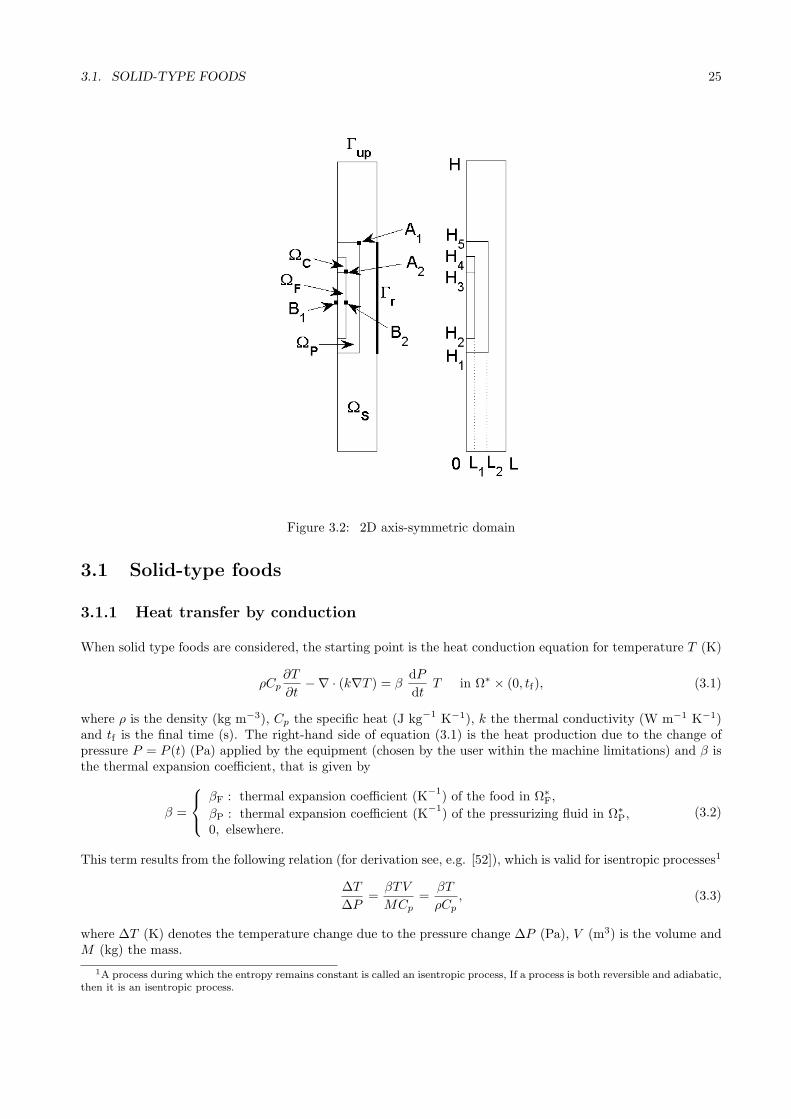
3.1. SOLID-TYPE FOODS 25
Figure 3.2: 2D axis-symmetric domain
3.1 Solid-type foods
3.1.1 Heat transfer by conduction
When solid type foods are considered, the starting point is the heat conduction equation for temperature T (K)
ρCp
∂T
∂t−∇ · (k∇T ) = β
dP
dtT in Ω∗ × (0, tf), (3.1)
where ρ is the density (kg m−3), Cp the specific heat (J kg−1 K−1), k the thermal conductivity (W m−1 K−1)and tf is the final time (s). The right-hand side of equation (3.1) is the heat production due to the change ofpressure P = P (t) (Pa) applied by the equipment (chosen by the user within the machine limitations) and β isthe thermal expansion coefficient, that is given by
β =
βF : thermal expansion coefficient (K−1
) of the food in Ω∗
F,
βP : thermal expansion coefficient (K−1
) of the pressurizing fluid in Ω∗
P,0, elsewhere.
(3.2)
This term results from the following relation (for derivation see, e.g. [52]), which is valid for isentropic processes1
∆T
∆P=
βTV
MCp
=βT
ρCp
, (3.3)
where ∆T (K) denotes the temperature change due to the pressure change ∆P (Pa), V (m3) is the volume andM (kg) the mass.
1A process during which the entropy remains constant is called an isentropic process, If a process is both reversible and adiabatic,then it is an isentropic process.

26 CHAPTER 3. COMMON HEAT AND MASS TRANSFER MODELS
In order to solve equation (3.1), we must specify appropriate boundary and initial conditions depending on theHP machine and the problem under study. We use the same conditions as in [69] for the previously describedpilot-scale unit (ACB GEC Alsthom, Nantes, France)
k∂T
∂n= 0 on Γ∗
0 × (0, tf),
k∂T
∂n= h(Tenv − T ) on Γ∗
up × (0, tf),
T = Tr on Γ∗
r × (0, tf),
T = T0 in Ω∗ × 0,
(3.4)
where n is the outward unit normal vector on the boundary of the domain, T0 (K) is the initial temperature, Tr
(K) is the fixed temperature on Γ∗
r , Tenv (K) is the environment temperature (constant) and h (W m−2 K−1)is the heat transfer coefficient.
By using cylindrical coordinates and taking into account axial symmetry, system (3.1), (3.4) may be rewrittenas the following 2D problem
ρCp
∂T
∂t− 1
r
∂
∂r
(
rk∂T
∂r
)
− ∂
∂z
(
k∂T
∂z
)
= βdP
dtT in Ω× (0, tf),
k∂T
∂n= 0 on Γ0 × (0, tf),
k∂T
∂n= h(Tenv − T ) on Γup × (0, tf),
T = Tr on Γr × (0, tf),
T = T0 in Ω× 0.
(3.5)
This model is suitable for what we will refer to as a “large sample”, i.e. when the filling ratio of the foodsample inside the vessel is much higher than that in the pressurizing medium (see Figure 3.3a), since convectioneffects due to the pressurizing fluid can be neglected. This has been confirmed to be true in [69], by validationwith several comparisons between numerical and experimental results. In [69] the authors show that for “smallsamples”, when the filling ratio of the food inside the vessel is not much higher than in the pressurizing medium(see Figure 3.3b), the solution of this model differs a lot from the experimental results. Therefore they improvethe model by including convection effects in the pressurizing medium. We present this model in Section 3.1.2.
Another case when (3.5) may be used, even if we are dealing with a small sample, is for highly viscous fluids –which could be the case at low temperatures – where convection effects may be negligible. This would reducethe computing time without any significant loss in prediction.
3.1.2 Heat transfer by conduction and convection
The non-homogeneous temperature distribution induces a non-homogeneous density distribution in the pres-surising medium and consequently a buoyancy fluid motion, i.e. free convection. In order to take into accountthe fact that the fluid motion influences the temperature distribution, a non-isothermal flow model is considered.We assume that the fluid velocity, u (m s−1), satisfies the Navier–Stokes equations for compressible Newtonianfluid under Stokes’ assumption (see, e.g., [5]). The resulting system, with appropriate point, boundary and
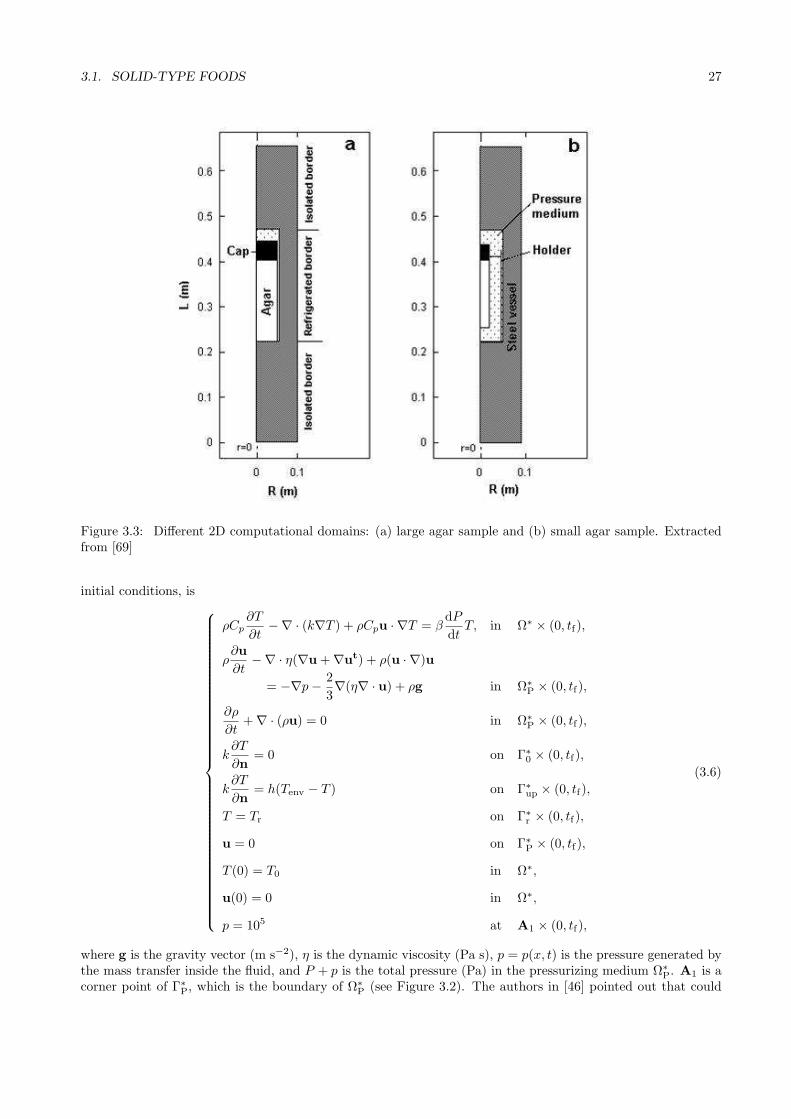
3.1. SOLID-TYPE FOODS 27
Figure 3.3: Different 2D computational domains: (a) large agar sample and (b) small agar sample. Extractedfrom [69]
initial conditions, is
ρCp
∂T
∂t−∇ · (k∇T ) + ρCpu · ∇T = β
dP
dtT, in Ω∗ × (0, tf),
ρ∂u
∂t−∇ · η(∇u+∇ut) + ρ(u · ∇)u
= −∇p− 2
3∇(η∇ · u) + ρg in Ω∗
P × (0, tf),
∂ρ
∂t+∇ · (ρu) = 0 in Ω∗
P × (0, tf),
k∂T
∂n= 0 on Γ∗
0 × (0, tf),
k∂T
∂n= h(Tenv − T ) on Γ∗
up × (0, tf),
T = Tr on Γ∗
r × (0, tf),
u = 0 on Γ∗
P × (0, tf),
T (0) = T0 in Ω∗,
u(0) = 0 in Ω∗,
p = 105 at A1 × (0, tf),
(3.6)
where g is the gravity vector (m s−2), η is the dynamic viscosity (Pa s), p = p(x, t) is the pressure generated bythe mass transfer inside the fluid, and P + p is the total pressure (Pa) in the pressurizing medium Ω∗
P. A1 is acorner point of Γ∗
P, which is the boundary of Ω∗
P (see Figure 3.2). The authors in [46] pointed out that could
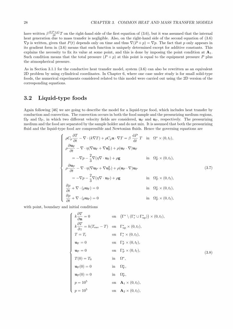
28 CHAPTER 3. COMMON HEAT AND MASS TRANSFER MODELS
have written β d(P+p)dt T on the right-hand side of the first equation of (3.6), but it was assumed that the internal
heat generation due to mass transfer is negligible. Also, on the right-hand side of the second equation of (3.6)∇p is written, given that P (t) depends only on time and thus ∇(P + p) = ∇p. The fact that p only appears inits gradient form in (3.6) means that such function is uniquely determined except for additive constants. Thisexplains the necessity to fix its value at some point, and this is done by imposing the point condition at A1.Such condition means that the total pressure (P + p) at this point is equal to the equipment pressure P plusthe atmospherical pressure.
As in Section 3.1.1 for the conductive heat transfer model, system (3.6) can also be rewritten as an equivalent2D problem by using cylindrical coordinates. In Chapter 6, where one case under study is for small solid-typefoods, the numerical experiments considered related to this model were carried out using the 2D version of thecorresponding equations.
3.2 Liquid-type foods
Again following [46] we are going to describe the model for a liquid-type food, which includes heat transfer byconduction and convection. The convection occurs in both the food sample and the pressurizing medium regions,ΩF and ΩP, in which two different velocity fields are considered, uF and uP, respectively. The pressurizingmedium and the food are separated by the sample holder and do not mix. It is assumed that both the pressurizingfluid and the liquid-type food are compressible and Newtonian fluids. Hence the governing equations are
ρCp
∂T
∂t−∇ · (k∇T ) + ρCpu · ∇T = β
dP
dtT in Ω∗ × (0, tf),
ρ∂uF
∂t−∇ · η(∇uF +∇ut
F) + ρ(uF · ∇)uF
= −∇p− 2
3∇(η∇ · uF) + ρg in Ω∗
F × (0, tf),
ρ∂uP
∂t−∇ · η(∇uP +∇ut
P) + ρ(uP · ∇)uP
= −∇p− 2
3∇(η∇ · uP) + ρg in Ω∗
P × (0, tf),
∂ρ
∂t+∇ · (ρuF) = 0 in Ω∗
F × (0, tf),
∂ρ
∂t+∇ · (ρuP) = 0 in Ω∗
P × (0, tf),
(3.7)
with point, boundary and initial conditions
k∂T
∂n= 0 on
(
Γ∗ \ (Γ∗
r ∪ Γ∗
up))
× (0, tf),
k∂T
∂z= h(Tenv − T ) on Γ∗
up × (0, tf),
T = Tr on Γ∗
r × (0, tf),
uF = 0 on Γ∗
F × (0, tf),
uP = 0 on Γ∗
P × (0, tf),
T (0) = T0 in Ω∗,
uF(0) = 0 in Ω∗
F,
uP(0) = 0 in Ω∗
P,
p = 105 on A1 × (0, tf),
p = 105 on A2 × (0, tf),
(3.8)

3.3. SIMPLIFIED MODELS 29
where Γ∗
F denotes the boundary of Ω∗
F, Γ∗
P denotes the boundary of Ω∗
P and A1, A2 are points of Γ∗
P and Γ∗
F,respectively (see Figure 3.2).
In this case convection plays a very important role, not only in the pressurising fluid, but also in the liquid-typefood. Therefore, to neglect its effect (as in the big solid case), could lead to very different results from the realthermal behaviour, for both large and small samples.
3.3 Simplified models
In [46] the authors proposed several simplified models in order to reduce the computational complexity neededto solve the full models, and checked the validity of such models, showing that compared to the full models, thesimplified ones give similar results and were proved to be faster and easier to implement. Therefore, followingthe work done in [46] we describe some simplified models that will be used in later Chapters, to make theimplementation of freezing models and three-dimensional models, among others, a bit simpler.
3.3.1 For a large solid-type food
For a large solid-type food we consider a simplified version of system (3.5), which has constant coefficients bysetting the thermo-physical parameters Cp, k, β and ρ to their mean value in the range of temperature andpressure considered in the process. This model is denoted by SCC in [46].
3.3.2 For a small solid-type food
For the small solid-type food, where convection effects in the pressurising medium are included, see system(3.6), apart from also considering constant thermo-physical properties, a simplification based on the Boussinesqapproximation is made [46]. More precisely, coefficients Cp, k, β and η are considered to be constant (insteadof temperature and pressure dependent), and are set to their mean value (Cp, k, β and η, respectively) in therange of temperature and pressure considered in the process; ρ is also chosen as a constant value ρ, except forthe gravitational force ρg that appears in the second system (3.6), where ρ remains dependent on temperatureand pressure (in order to keep the effect of the gravitational forces). Furthermore, we assume the pressurisingfluid is incompressible. With the simplifications system (3.6) can be written as
ρCp
∂T
∂t−∇ · (k∇T ) + ρCpu · ∇T = β
dP
dtT, in Ω∗ × (0, tf),
ρ∂u
∂t− η∇2u+ ρ(u · ∇)u = −∇p+ ρg in Ω∗
P × (0, tf),
∇ · (u) = 0 in Ω∗
P × (0, tf),
k∂T
∂n= 0 on Γ∗
0 × (0, tf),
k∂T
∂n= h(Tenv − T ) on Γ∗
up × (0, tf),
T = Tr on Γ∗
r × (0, tf),
u = 0 on Γ∗
P × (0, tf),
T (0) = T0 in Ω∗,
u(0) = 0 in Ω∗,
p = 105 at A1 × (0, tf).
(3.9)
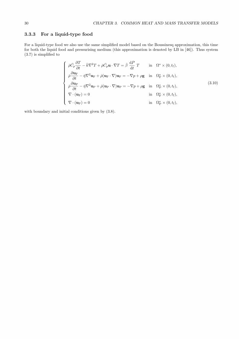
30 CHAPTER 3. COMMON HEAT AND MASS TRANSFER MODELS
3.3.3 For a liquid-type food
For a liquid-type food we also use the same simplified model based on the Boussinesq approximation, this timefor both the liquid food and pressurising medium (this approximation is denoted by LB in [46]). Thus system(3.7) is simplified to
ρCp
∂T
∂t− k∇2T + ρCpu · ∇T = β
dP
dtT in Ω∗ × (0, tf),
ρ∂uF
∂t− η∇2uF + ρ(uF · ∇)uF = −∇p+ ρg in Ω∗
F × (0, tf),
ρ∂uP
∂t− η∇2uP + ρ(uP · ∇)uP = −∇p+ ρg in Ω∗
P × (0, tf),
∇ · (uF) = 0 in Ω∗
F × (0, tf),
∇ · (uP) = 0 in Ω∗
P × (0, tf),
(3.10)
with boundary and initial conditions given by (3.8).
Chapter 4
Dimensional analysis and
simplifications
Nomenclature for Chapter 4
A Enzymatic activitya, b, c, d Dimensionless groups of parametersCp Specific heat capacity (J kg−1 K−1)h Heat transfer coefficient (W m−2 K−1)H Half of the food domain height (m)H2 Half of the complete domain height (m)Jn(·) Bessel function of the first kind of order nk Thermal conductivity (W m−1 K−1)L Food domain width (m)L2 Complete domain width (m)n Outward normal unit vector (m)P Equipment Pressure (Pa)r Radial coordinate (m)R Radial scale (m)t Time (s)tf Final time (s)tp Pressure-up time (s)T Temperature (K)T0 Initial temperature (K)Tr Fixed temperature (K)z Vertical coordinate (m)Z Height scale (m)
Indices
* Rotated domains0 InitialF Food domainin Inner solution for boundary layerout Outer solution for boundary layerS Steel vessel domainup Pressure-up solution
Acronyms
BSAA Bacillus Subtilis α-AmylaseCPE Carrot Pectin Methyl-EsteraseFEM Finite Element MethodHP High-PressureLOX LipoxygenaseODE Ordinary Differential EquationPDE Partial Differential Equation1D One-dimensional2D Two-dimensional2D-all 2D averaged over all domain2D-ave 2D averaged over all domain
excluding top2D-mid 2D at middle height3D Three-dimensional
Greek symbols
β Thermal expansion coefficient (K−1)χ Characteristic function in (0, tp)∆T Temperature scale (K)γ Maximum pressure reached (Pa)ΓD Whole domain boundaryΓDexc Heat transfer boundary
ΓDr Fixed temperature boundary
ΓDsym Axis-symmetric boundary
η Dynamic viscosity (Pa s)κ Inactivation rate (min−1)ρ Density (kg m−3)τ Time scale (s)ΩD Whole domainΩD
F Food sample domainΩD
S Steel vessel
31
32 CHAPTER 4. DIMENSIONAL ANALYSIS
4.1 Introduction
In this Chapter we focus only on solid type foods, with a large filling ratio, where convection effects do notneed to be taken into account as pointed out in Chapter 3. We perform a dimensional analysis which highlightsthe dominant terms in the model, and shows that in some cases the equations can be simplified (in dimension)and yet provide a good approximation. These models for HP processes are much simpler than those found inthe literature [21, 46, 52], but still have the correct qualitative features, and hence would be very importantwhen designing suitable industrial equipments and optimizing the processes. Moreover, using the solutions wepropose, there is no need to have an FEM solver in order to simulate the process. This Chapter is based on theanalysis in [85].
In [54, 55] dimensional analysis of thermo-fluid-dynamic mechanisms taking place during HP treatment of bio-substances is carried out, and both forced and free convection case is described. As the authors point out in[54], dimensional analysis gives the possibility to reduce the large number of internal and external parametersrelated to a HP treatment of a bio-substance, and also to generalise the statement about the process mechanismsand phenomena, showing which have a significant influence and which plays a minor role on the thermo-fluid-dynamics of HP processes. A large value of the dimensionless group, points out an elevated importance of thesemechanisms on the momentum and heat transfer in HP autoclaves. In contrast, if dimensionless parametersbecome very small, it means that these terms can be neglected. In [55] the thermo-fluid-dynamical mechanismsare analysed for three different sizes of a HP chamber, two different pressure generation systems and two model-fluids that differ in viscosity, again discussing the cases of forced and free convection. The results presentedby the authors contain process parameter study based on dimensionless numbers derived from conservationequations of mass, momentum and energy, which as stated in [54], can be very useful for transformation oflaboratory investigations and results into the industrial scale. In both papers, the authors point out that infurther investigations the temporal and spatial distribution of process parameters in the chamber should betaken into consideration.
The dimensional analysis we perform throughout this Chapter is for simpler models than those described in[54, 55] (as we do not consider fluid-dynamics), but nevertheless, we do take into account the temporal andspatial temperature distribution. After identifying the relevant process parameters and neglecting the non-important ones, we proceed to solve the resulting non-dimensional systems. Furthermore, due to the simplicityof the reduced systems, we can find analytical solutions rather than only numerical ones.
In Section 4.2 we describe the problem and present the governing equations to calculate the temperaturedistribution. A dimensional analysis is then performed to simplify the model. Sections 4.3 and 4.4 containa thorough investigation of the complete and simplified models for the pressure up and pressure hold times,respectively, and we are able to find exact and approximate solutions describing the whole process. In Section4.5 we present some numerical results of a particular process, comparing all the models to exact and numericalsolutions. In Section 4.6 we couple the simplified heat transfer models to an enzymatic inactivation model.Section 4.7 briefly considers an extension to third class boundary conditions and, finally, in Section 4.8 we giveconcluding remarks.
4.2 Problem Description
As already stated in Chapter 3, when HP is applied in food technology, it is necessary to take into accountthe thermal effects that are produced by variations of temperature due to the compression/expansion occurringin the food sample and the pressurizing medium. In practice, the pressure evolution, P (t), is known as it isimposed by the user and the limits of the equipment. The temperature of the processed food may change withtime and space, therefore we need a heat transfer model capable of predicting the temperature for the processedfood. From Chapter 3 we know that for solid-type foods with a large filling ratio, a heat transfer model takinginto account only conduction effects is sufficient for correctly predicting the temperature distribution. As themodel is both time and spatially dependent, we also introduce a brief description of the domain describing theHP device considered in our simulations, which is a slight variation of the one presented in Chapter 3.

4.2. PROBLEM DESCRIPTION 33
4.2.1 Mathematical Model
Ω
RotatetoobtainΩ*
F
ΩS
ΓrΓ 0
L
H2
-H2 2L
H
-H
sym
D
D
D
D
D
Figure 4.1: Simplified 2D axis-symmetric computational domain for dimensional analysis
In this Chapter we analyse an axis-symmetric two-dimensional geometry with only the food and the surroundingsteel (see Figure 4.1). This is a simplified version of the geometry presented in Chapter 3 (see Figure 3.2), whichalso included the pressurising fluid and the rubber cap of sample holder. As a matter of fact, other authorshave studied even more complex geometries, which included, e.g. the carrier [52]. However, in this Chapterour focus is on studying a solid-type food with a large filling ratio, where the pressure medium represents a lowproportion of the vessel content, and so we assume that the pressurizing fluid can be ignored (the rubber capis also ignored for the sake of simplicity).
The domain in the cylindrical (r, z)-coordinates is the rectangle ΩD = [0, L2] × [−H2, H2] defined by ΩD =
ΩDF ∪ ΩD
S , where ΩDF = [0, L]× [−H,H] is the food domain, and ΩD
S is the domain of the steel that surroundsthe food. We use ΩD∗ to denote the 3D domain generated by rotating ΩD along the axis of symmetry (0 ×(−H2, H2)). The boundary of ΩD is denoted by ΓD = ΓD
r ∪ ΓDsym, where we can distinguish ΓD
r on which the
temperature is known, and ΓDsym that has zero heat flux by axial symmetry.
We would like to remark that the notation used here is very similar to the one used in Chapter 3, however wehave added the subscript D to denote that we are in the geometry for the dimensional analysis Chapter, whichhas slightly change with respect to the one presented in the previous Chapter.
Since we are only concerned in analysing solid-type foods with a large filling ratio, we only take into accountconduction effects (and neglect convection effects). Thus, when large solid-type foods are considered, as we sawin Section 3.1.1 of Chapter 3, we start with the heat conduction equation for temperature T (K)
ρCp
∂T
∂t−∇ · (k∇T ) = β
dP
dtT in ΩD∗ × (0, tf), (4.1)
where now β is defined as in (3.2), but only has one non-zero component, βF (due to the fact that we are nolonger including the pressurising fluid region). For the sake of simplicity, we are going to use the assumption ofconstant thermo-physical properties described in Section 3.3.1.
34 CHAPTER 4. DIMENSIONAL ANALYSIS
By using cylindrical coordinates and taking into account axial symmetry, equation (4.1) may be re-written in2D as
ρ Cp
∂T
∂t− 1
r
∂
∂r
(
rk∂T
∂r
)
− ∂
∂z
(
k∂T
∂z
)
= βdP
dtT in ΩD × (0, tf). (4.2)
Equation (4.2) must be completed with appropriate boundary and initial conditions. In this Chapter, forsimplicity we assume that the outer walls of the domain are kept at a constant temperature Tr, and that theinitial temperature T0 is constant in each region, therefore giving
∂T
∂r= 0 on ΓD
sym,
T = Tr on ΓDr ,
T = T0 at t = 0.
(4.3)
In Section 4.7 we briefly discuss an extended model with third class boundary conditions. Several authors haveconsidered different boundary conditions to those described above. As we pointed out in Chapter 3, Infante et
al. [46] and Otero et al. [69] assumed a boundary was kept at a refrigerated temperature, as well as a boundaryallowing for heat transfer with the room. Denys et al. [21] considered an overall heat transfer coefficient at thesurface of the cylinder to account for heat transfer through the walls of the HP vessel. Although our conditions(4.3) may seem overly simplistic from a practical consideration, it has been suggested in the literature thatkeeping the walls of machine at a constant temperature may be good for avoiding heat loss [71]. There canbe a problem of heat loss through the wall of the HP vessel, and by anticipating the temperature increase ofthe processed product, resulting from compression, conductive heat transfer and temperature gradients can beavoided [21].
In the following Sections we study exact and approximate solutions for the model with first class boundaryconditions. It is convenient to begin by non-dimensionalising the model to highlight whether any simplificationsare possible.
4.2.2 Dimensional analysis
Given that the pressure function in equation (4.2) only appears in a derivative form, and that the pressureapplied on these processes is typically a piecewise linear function in time (hence such a derivative is usuallypiecewise constant), we do not non-dimensionalise the pressure variable. Instead, we rewrite the pressurederivative dP
dt (t) as
dP
dt(t) =
γ
tp, 0 < t ≤ tp,
0, t > tp,(4.4)
where, for the sake of simplicity, we suppose that dPdt (t) = γ
tp> 0 (P linear) for all t ∈ [0, tp], and γ (Pa)
is the maximum pressure reached (for the sake of simplicity we assume that atmospheric pressure is 0 MPa,instead of 0.1 MPa, which is typically the real value). After time tp the pressure is maintained constant at themaximum value, and therefore the derivative is zero (other cases can be also studied similarly). The releaseof pressure that takes place after tf can be modelled with the same approach. Since it does not introduce anyfurther difficulty we have not considered it here.
Therefore, for 0 < t ≤ tp equation (4.2) can be written as
ρ Cp
∂T
∂t− 1
r
∂
∂r
(
rk∂T
∂r
)
− ∂
∂z
(
k∂T
∂z
)
= βγ
tpT, (4.5)
and for tp < t ≤ tf the same equation holds, except with the right-hand side equal to zero.
The system is now non-dimensionalised by setting
r =r
R, z =
z
Z, t =
t
τ, T =
T − Tr
∆T,
4.2. PROBLEM DESCRIPTION 35
where ∆T , R, Z and τ are suitable temperature, radius, height and time scales, respectively.
Thus, for 0 < t ≤ tpτ, equation (4.5) becomes
ρ Cp ∆T
τ
∂T
∂t− k∆T
R2r
∂
∂r
(
r∂T
∂r
)
− k∆T
Z2
∂2T
∂z2=
βγ∆T
tp(T +
Tr
∆T). (4.6)
For ease of notation we drop the ˆ notation, and so T , z, r and t are now the non-dimensional variables.
We divide equation (4.6) by ρCp∆T/τ , resulting in
∂T
∂t− kτ
R2ρCp
1
r
∂
∂r
(
r∂T
∂r
)
− kτ
Z2ρCp
∂2T
∂z2=
βγτ
ρCptpT +
βγτ
ρCptp
Tr
∆T. (4.7)
The dimensionless groups of parameters in equation (4.7) are
a =kτ
R2ρCp
, b =kτ
Z2ρCp
, c =βγτ
ρCptp, d =
βγτ
ρCptp
Tr
∆T. (4.8)
The radius and height scales that we propose come from the dimensions of the food cylinder, giving R = Land Z = H. Note that we are only considering half of the height of the domain as the z scale for the sake ofsimplicity. For the temperature scale we set ∆T = max |T0 − Tr|, βγT0
ρCp, where ρ and Cp are the density and
specific heat of the food sample, respectively. The quantity βγT0
ρCpis the maximum increase of temperature in
the food sample due to the increase of pressure (according to (3.3)). The time scale τ is chosen from equation(4.7). We wish to investigate what happens when the pressure is increased and therefore balance the pressureterm with the time derivative. This leads to
τ =ρCptpβγ
min
1,∆T
Tr
.
The system in non-dimensional form is therefore given by
∂T
∂t− a
1
r
∂
∂r
(
r∂T
∂r
)
− b∂2T
∂z2= (cT + d)χ(t) in ΩD × (0, tf),
∂T
∂r= 0 on ΓD
sym,
T = 0 on ΓDr,
T = T ∗
0 at t = 0,
(4.9)
where ΩD = (0, L2
L) × (−H2
H, H2
H) is the non-dimensional form of the whole domain ΩD. The function χ(t) is
defined as
χ(t) =
1, if t ∈ (0, tp),
0, elsewhere.
Note that tp/τ and tf/τ have been redefined as tp and tf for convenience. The non-dimensional initial value is
T ∗
0 =T0 − Tr
∆T. (4.10)
It should be pointed out that in (4.8), b = aR2
Z2 and hence with the chosen scales b = a L2
H2 . This will meanthat if the food sample holder is narrow and tall (which is usually the case for the HP pilot scale machines),the conduction parameter in the z direction, b, will be smaller than that in the r direction, a. Thus we wishto investigate whether the heat transfer due to conduction is dominant in the radial direction over the heightdirection, for a thin and tall machine. This will be studied in Sections 4.3.2 and 4.4.2.
System (4.9) is set in ΩD, which involves the two regions to determine the temperature in the food, TF, andin the steel, TS. Taking into account that parameters c and d defined in (4.8) are zero in the steel region, as

36 CHAPTER 4. DIMENSIONAL ANALYSIS
β = 0, (4.9) is defined as
∂TF
∂t− aF
1
r
∂
∂r
(
r∂TF
∂r
)
− bF∂2TF
∂z2= (cFTF + dF)χ(t) in ΩD
F × (0, tf),
∂TS
∂t− aS
1
r
∂
∂r
(
r∂TS
∂r
)
− bS∂2TS
∂z2= 0 in ΩD
S × (0, tf),
∂TF
∂r= 0,
∂TS
∂r= 0 on ΓD
sym,
kF∂TF
∂r= kS
∂TS
∂r, TF = TS on ΓD
FS,
TS = 0 on ΓDr,
TF = T ∗
F0, TS = T ∗
S0at t = 0,
(4.11)
where T ∗
F0and T ∗
S0are the non-dimensional initial temperatures in the food and steel, respectively. ΩD
F =
(0, 1)× (−1, 1) is the non-dimensional food region, and ΩDS = ΩD− ΩD
F the steel one. On the non-dimensional
food-steel boundary, ΓDFS =
[
(0, 1) × 1]
∪[
(0, 1) × −1]
∪[
1 × (−1, 1)]
, continuity of the solution andthe fluxes has been imposed.
We begin by determining an approximate solution for the steel temperature. By assuming that the conductivity
of steel is much larger than that of the food, we can simplify the flux boundary condition on ΓDFS
∂TS
∂r=
kFkS
∂TF
∂r≈ 0, on ΓD
FS. (4.12)
If we also assume that we are working with a narrow and tall machine, i.e. that L << H, and hence bS << aS,the equation for the steel reduces to
∂TS
∂t− aS
1
r
∂
∂r
(
r∂TF
∂r
)
= 0, in ΩDS × (0, tf). (4.13)
Since steel has a high thermal diffusivity, aS, the solution of (4.13) goes to steady state very rapidly, and thesolution to the steady state problem is zero (using the zero flux and zero temperature boundary conditions).
Hence we can conclude that TS ≈ 0. Then the boundary condition for the food at ΓDFS can be approximated
by TF ≈ 0.
Thus, we now only have the temperature in the food problem to solve, and (4.11) reduces to
∂TF
∂t− aF
1
r
∂
∂r
(
r∂TF
∂r
)
− bF∂2TF
∂z2= (cFTF + dF)χ(t) in (0, 1)× (−1, 1)× (0, tf),
∂TF
∂r= 0 on r = 0,
TF = 0 on r = 1,
TF = 0 on z = −1,
TF = 0 on z = 1,
TF = T ∗
F0at t = 0.
(4.14)
One further simplification of system (4.14) can be made, and this is to divide the domain in half at z = 0 andimpose a zero flux boundary condition. Due to symmetry we only need to solve the problem in the upper half

4.3. ANALYSIS FOR THE PRESSURE UP TIME 0 ≤ T ≤ TP 37
of the domain. Finally we have system for TF (that we will simply refer to as T henceforth)
∂T
∂t− a
1
r
∂
∂r
(
r∂T
∂r
)
− b∂2T
∂z2= (cT + d)χ(t) in (0, 1)× (0, 1)× (0, tf),
∂T
∂r= 0 on r = 0,
T = 0 on r = 1,
∂T
∂z= 0 on z = 0,
T = 0 on z = 1,
T = T ∗
0 at t = 0.
(4.15)
4.3 Analysis for the pressure up time 0 ≤ t ≤ tp
4.3.1 Exact solution
An exact solution can be found by solving the 2D system (4.15) using separation of variables. We can create ahomogeneous problem by setting
T (r, z, t) = u(r, z, t) + v(r, z) + w(z). (4.16)
Then the problem to solve for u is
∂u
∂t= a
1
r
∂
∂r
(
r∂u
∂r
)
+ b∂2u
∂z2+ cu in (0, 1)× (0, 1)× (0, tp),
∂u
∂r= 0 on r = 0,
u = 0 on r = 1,
∂u
∂z= 0 on z = 0,
u = 0 on z = 1,
u = T ∗
0 − v(r, z)− w(z) at t = 0,
(4.17)
whilst the problem for v is
0 = a1
r
∂
∂r
(
r∂v
∂r
)
+ b∂2v
∂z2+ cv in (0, 1)× (0, 1)× (0, tp),
∂v
∂r= 0 on r = 0,
v = −w(z) on r = 1,
∂v
∂z= 0 on z = 0,
v = 0 on z = 1,
(4.18)
and the problem for w is
bw′′(z) + cw(z) + d = 0, w′(0) = 0, w(1) = 0. (4.19)
This has solution
w(z) =d
c
(
cos(µz)
cosµ− 1
)
, (4.20)

38 CHAPTER 4. DIMENSIONAL ANALYSIS
where µ =√
c/b.
We use the method of separation of variables and set v(r, z) = R(r)Z(z). Then the boundary conditions implythat R′(0) = Z ′(0) = Z(1) = 0. From (4.18) we deduce that
ar(R′(r) + rR′′(r)) + cR(r)
bR(r)= −Z ′′(z)
Z(z)= ν2, (4.21)
for suitable constants ν ∈ R, where (·)′ denotes differentiation with respect to each variable. Solving the ODEfor Z(z) leads to
Zp(z) = AZp cos(νpz), p = 1, 2, . . . , (4.22)
with AZp ∈ R, and νp = (p− 1/2)π. The ODE for R(r) from (4.21) is
arR′′(r) + aR′(r) + (c− ν2pb)rR(r) = 0, (4.23)
which, after satisfying the boundary condition R′(0) = 0, has solution
Rp(r) = ARpJ0(αpr), (4.24)
where Jn is the Bessel function of the first kind of order n, ARp ∈ R, and
αp =
√
c− ν2pb
a. (4.25)
The combined solution is therefore
v(r, z) =
∞∑
p=1
ApJ0(αpr) cos(νpz). (4.26)
Coefficients Ap are found using the boundary condition v = −w(z) from system (4.18). Thus
−w(z) =
∞∑
p=1
ApJ0(αp) cos(νpz), (4.27)
where w(z) is defined in (4.20). Integrating (4.27) and applying the orthogonality condition it follows that
Ap = − 2
J0(αp)
∫ 1
0
w(z) cos(νpz) dz, (4.28)
We finally turn to the problem for u in (4.17) and separate variables by setting u(r, z, t) = R(r)Z(z)Φ(t). Thenthe boundary conditions imply that R′(0) = R(1) = Z ′(0) = Z(1) = 0. From (4.17) we deduce that now
Φ′(t)
Φ(t)=
ar(R′(r) + rR′′(r))Z(z) + bR(r)Z ′′(z) + cR(r)Z(z)
R(r)Z(z)= −λ2. (4.29)
and so the first equation is solved to give Φ(t) = B exp(−λ2t), for suitable constants λ ∈ R. The solutions of Rand Z are found in an identical manner to that described above, and so
Zm(z) = CZm cos(νmz), m = 1, 2, . . . , Rn(r) = CRnJ0(δnr), n = 1, 2, . . . , (4.30)
where νm = (m− 1/2)π and
δn =
√
c+ λ2mn − ν2mb
a. (4.31)
These are found by solving J0(δn) = 0, in order to satisfy R(0) = 0, and then λmn can be determined from theformula λmn =
√
aδ2n + bν2m − c.
The combined solution for u is therefore
u(r, z, t) =∞∑
n=1
∞∑
m=1
DmnJ0(δnr) cos(νmz) exp(−λ2mnt), (4.32)
4.3. ANALYSIS FOR THE PRESSURE UP TIME 0 ≤ T ≤ TP 39
and coefficients Dmn are found using the initial condition in (4.17). Thus
T ∗
0 − v(r, z)− w(z) =
∞∑
n=1
∞∑
m=1
DmnJ0(δnr) cos(νmz), (4.33)
where w(z) and v(r, z) are defined in (4.20) and (4.26)-(4.28) respectively. Integrating with respect to r and zand using the orthogonality conditions leads to
Dmn =2∫ 1
0
∫ 1
0(T ∗
0 − v(r, z)− w(z)) rJ0(δnr) cos(νmz) dr dz∫ 1
0rJ2
0 (δnr) dr. (4.34)
The solutions for u, v and w are then added together to give the final solution for T in (4.16).
4.3.2 Approximation ignoring the z-dependence
If we assume that we are modelling a narrow and tall machine, and hence b ≪ a, it is reasonable to ignore thez dependence in (4.15) and solve the 1D problem, which is therefore given by
∂T
∂t− a
1
r
∂
∂r
(
r∂T
∂r
)
= (cT + d) in (0, 1)× (0, tp),
∂T
∂r= 0 on r = 0,
T = 0 on r = 1,
T = T ∗
0 at t = 0.
(4.35)
We now consider various exact and approximate solutions to this simplified system.
Separation of variables solution
A separation of variables solution to system (4.35) can be found following the analysis given in Section 4.3.1.To create a homogeneous problem we substitute T (r, t) = u(r, t) + v(r) into (4.35). Then the problem to solvefor u is
∂u
∂t= a
1
r
∂
∂r
(
r∂u
∂r
)
+ cu in (0, 1)× (0, tp),
∂u
∂r= 0 on r = 0,
u = 0 on r = 1,
u = T ∗
0 − v(r) at t = 0,
(4.36)
whilst the problem for v is
0 =a
r
(
v′(r) + rv′′(r))
+ cv + d, (4.37)
with v′(0) = 0 and v(1) = 0. This has solution
v(r) = −d
c+
dJ0(√
car)
cJ0(√
ca). (4.38)
Following the procedure in Section 4.3.1 a straightforward calculation gives the solution for u as
u(r, t) =∞∑
n=1
DnJ0(δnr) exp(−λ2nt), (4.39)

40 CHAPTER 4. DIMENSIONAL ANALYSIS
where δn ∈ R satisfy J0(δn) = 0, λn =√
aδ2n − c, and coefficients Dn are given by
Dn =2∫ 1
0(T ∗
0 − v(r)) rJ0(δnr) dr∫ 1
0rJ2
0 (δnr) dr, (4.40)
with v(r) defined in (4.38). Finally, the solution T is simply the sum of u and v.
Boundary layer solution
Again the starting point is system (4.35). Let us assume that, as is true for some practical cases (an exampleof which will be shown in Section 4.5), d = O(1) and b < a ≪ 1. Then ignoring the terms involving a and b, wefind
∂T
∂t= cT + d (4.41)
T (0) = T ∗
0 , (4.42)
which gives the leading order solution
T (t) = −d
c+
(
T ∗
0 +d
c
)
exp(ct). (4.43)
Note that since solution (4.43) only depends on t it does satisfy the zero flux condition at r = 0, but itobviously cannot satisfy the zero temperature condition at r = 1. Thus we assume that (4.43) is an outer
solution, T ≡ Tout(t), and that there is a boundary layer at r = 1. In this region different terms will form thedominant balance and so to highlight this we re-scale the problem by introducing a boundary-layer coordinateas
r =1− r
δ, (4.44)
where δ ≪ 1 is to be determined. This change of variables has the effect of stretching the region near r = 1 whenδ → 0, which in practice means that the boundary-layer problem (also known as inner problem) is solved on ainfinite domain. If we let Tin(r, t) denote the solution of the problem when using the boundary-layer coordinate,then near r = 1 the PDE in (4.35) becomes
∂Tin
∂t− a
δ21
1− δr
∂
∂r
(
(1− δr)∂Tin
∂r
)
= cTin + d, (4.45)
which is∂Tin
∂t+
a
δ
1
1− δr
∂Tin
∂r− a
δ2∂2Tin
∂r2= cTin + d. (4.46)
To bring out the correct balance in the equation, we take δ =√a, and so coupled with boundary and initial
conditions the leading order problem is
∂Tin
∂t=
∂2Tin
∂r2−√a∂Tin
∂r+ cTin + d in (0,∞)× (0, tp),
Tin = 0 on r = 0,
Tin → Tout(t) as r → ∞,
Tin = T ∗
0 at t = 0,
(4.47)
where Tout(t) is the outer solution given in (4.43). For convenience we subtract off the outer solution to give anew variable which decays to zero as r → ∞. Thus, if we define
Tin(r, t) = Tout(t) + F (r, t), (4.48)
4.3. ANALYSIS FOR THE PRESSURE UP TIME 0 ≤ T ≤ TP 41
the system to solve for F reduces to
∂F
∂t=
∂2F
∂r2−√a∂F
∂r+ cF in (0,∞)× (0, tp),
F = −Tout(t) on r = 0,
F → 0 as r → ∞,
F = 0 at t = 0.
(4.49)
It is first convenient to transform the PDE in (4.49) into a standard heat equation by setting
F (r, t) = exp
(√a r
2+ ct− at
4
)
G(r, t). (4.50)
Then (4.49) becomes
∂G
∂t=
∂2G
∂r2in (0,∞)× (0, tp),
G = −Tout(t) exp(−ct+ at4 ) on r = 0,
G → 0 as r → ∞,
G = 0 at t = 0.
(4.51)
At first glance it appears that this system can be solved using Laplace transforms. However, the resultingtransformed solution is not easy to invert using standard tables and so the solution would have to be given asa complex integral. To avoid this we instead use Fourier sine transforms, which is appropriate because thereis a fixed boundary condition at r = 0. Given a function f(x), 0 ≤ x < ∞, the Fourier sine transform pair isdefined as
f(ω) =2
π
∫
∞
0
f(x) sin(ωx) dx, f(x) =
∫
∞
0
f(ω) sin(ωx) dω. (4.52)
Now if
G(ω, t) =2
π
∫
∞
0
G(r, t) sin(ωr) dr, (4.53)
then the PDE in (4.51) becomes
2
π
∫
∞
0
∂G
∂tsin(ωr) dr =
2
π
∫
∞
0
∂2G
∂r2sin(ωr) dr, (4.54)
or∂G
∂t+ ω2G = −2ωTout(t) exp
(
at4 − ct
)
π. (4.55)
Note that when differentiating G with respect to r twice, we have used the additional condition ∂G∂r
→ 0 asr → ∞, which follows from matching with the outer solution, that only depends on t.
The initial condition in (4.51) implies that G(ω, 0) = 0 and so equation (4.55) has solution
G(ω, t) =2ωd
πc(ω2 + a/4− c)
[
exp(at/4− ct)− exp(−ω2t)]
− 2ω(T ∗
0 + d/c)
π(ω2 + a/4)
[
exp(at/4)− exp(−ω2t)]
, (4.56)
after substituting Tout(t) from (4.43). Finally the solution for G is given by
G(r, t) =
∫
∞
0
G(ω, t) sin(ωr) dω, (4.57)
and so
Tin(r, t) = Tout(t) + exp
(√a r
2− at
4+ ct
)
G(r, t). (4.58)
After adding the inner and outer solutions and subtracting the common part, we can write down the finalsolution in the whole domain as
T (r, t) = −d
c+
(
T ∗
0 +d
c
)
exp(ct) + exp
(
1− r
2+ ct− at
4
)
G
(
1− r√a
, t
)
. (4.59)
42 CHAPTER 4. DIMENSIONAL ANALYSIS
4.3.3 Approximation including the z-dependence
Since the approximate solutions in Section 4.3.2 only depend on r and t it is clear that the boundary conditionat z = 1 is not satisfied (unlike the zero flux boundary condition at z = 0, which is satisfied). We need toconsider a boundary layer analysis near z = 1, and therefore follow a similar analysis to that given in Section4.3.2. Thus we set z = 1 −
√bz and denote Tin(r, z, t) as the inner solution. Then, for leading order terms,
system (4.15) becomes
∂Tin
∂t− a
1
r
∂
∂r
(
r∂Tin
∂r
)
− ∂2Tin
∂z2= (cTin + d) in (0, 1)× (0,∞)× (0, tp),
∂Tin
∂r= 0 on r = 0,
Tin = 0 on r = 1,
Tin → Tout as z → ∞,
Tin = 0 on z = 0,
Tin = T ∗
0 at t = 0,
(4.60)
where Tout is the outer solution of the PDE, i.e. the solution that we solved in Section 4.3.2. We will use theseries solution found in Section 4.3.2, namely
Tout(r, t) = v(r) +∞∑
n=1
DnJ0(δnr) exp(−λ2nt), (4.61)
where v(r) is given in (4.38). Whilst we could use the boundary layer solution (4.59), this form is simpler as itavoids a solution involving several integrals.
Using the same approach as in Section 4.3.2, if we set
Tin(r, z, t) = Tout(r, t) + F (r, z, t), (4.62)
then the PDE in (4.60) becomes
∂F
∂t= a
1
r
∂
∂r
(
r∂F
∂r
)
+∂2F
∂z2+ cF, (4.63)
which follows since Tout(r, t) satisfies the outer PDE. If, as at the start of Section 4.3.2, we assume a ≪ 1 andthen ignore this term here, system (4.60) reduces to the following 1D problem:
∂F
∂t− ∂2F
∂z2= cF in (0,∞)× (0, tp),
F → 0 as z → ∞,
F = h(t) on z = 0,
F = 0 at t = 0,
(4.64)
where for convenience we have defined h(t) = −Tout(r, t) (considering r as a constant value and the solving thesystem for each r). Again using Fourier sine transforms we can find the exact solution to (4.64). This is givenby
F (z, t) =
∫
∞
0
(
2
π
∫ t
0
h(t′) exp((ω2 − c)(t′ − t)) dt′)
sin(ωz) dω, (4.65)
or
F (z, t) =
∫
∞
0
(f1(ω, t) + f2(ω, t)) sin(ωz) dω, (4.66)
4.4. ANALYSIS FOR THE PRESSURE HOLD TIME TP < T ≤ TF 43
where
f1(ω, t) = − 2ωv(r)
π(c− ω2)
[
exp((c− ω2)t)− 1]
, (4.67)
f2(ω, t) =2
π
∞∑
n=0
DnJ0(δnr)
[
exp(−λ2nt)− exp((c− ω2)t)
]
λ2n + c− ω2
. (4.68)
Thus, the inner solution is simply the sum of F and Tout. After adding the inner and outer solutions andsubtracting the common part, we can write down the final solution in the whole domain as
T (r, z, t) = −d
c+
dJ0(√
car)
cJ0(√
ca)
+
∞∑
n=1
DnJ0(δnr) exp(−λ2nt) +
∫
∞
0
(f1(ω, t) + f2(ω, t)) sin
(
1− z√b
ω
)
dω. (4.69)
4.4 Analysis for the pressure hold time tp < t ≤ tf
For t ≥ tp, heating no longer occurs due to the increase in pressure, and hence the right-hand side of the PDEin system (4.15) is zero. Rescaling time as ζ = t− tp, we have
∂T
∂ζ− a
1
r
∂
∂r
(
r∂T
∂r
)
− b∂2T
∂z2= 0 in (0, 1)× (0, 1)× (0, tf − tp),
∂T
∂r= 0 on r = 0,
T = 0 on r = 1,
∂T
∂z= 0 on z = 0,
T = 0 on z = 1,
T = Tup(r, z) at ζ = 0,
(4.70)
where Tup(r, z) is the solution T (r, z, t) of the problem (solved in Section 4.3.1) in the time interval 0 < t < tp,at time t = tp, namely
Tup(r, z) =d
c
(
cos(γz)
cos γ− 1
)
+
∞∑
p=1
ApJ0(αpr) cos(νpz) +
∞∑
n=1
∞∑
m=1
DmnJ0(δnr) cos(νmz) exp(−λ2mntp). (4.71)
We now describe how to extend the analysis given above, for the pressure up time, to the system in the pressurehold time.
4.4.1 Exact solution
The analysis here is similar to that described in Section 4.3.1, but is in fact simpler because the right-hand sideof the PDE is zero and so the problem is already homogeneous. Thus the solution is
T (r, z, t) =
∞∑
j=1
∞∑
k=1
EkjJ0(ηjr) cos(νkz) exp(−ϕ2kj(t− tp)), (4.72)
where ηj ∈ R satisfy J0(ηj) = 0, νk = (k − 1/2)π, and ϕkj =√
aη2j + bν2k . To determine coefficients Ekj we
use the initial condition in (4.70), where Tup is defined in (4.71). Thus, after integrating and applying theorthogonality conditions, we have
Ekj =2∫ 1
0
∫ 1
0Tup(r, z)rJ0(ηjr) cos(νkz) dr dz
∫ 1
0rJ2
0 (ηjr) dr. (4.73)
44 CHAPTER 4. DIMENSIONAL ANALYSIS
4.4.2 Approximation ignoring the z-dependence
Again, assuming b << a, we ignore the z-dependence in (4.70) and solve the 1D problem, which is
∂T
∂ζ− a
1
r
∂
∂r
(
r∂T
∂r
)
= 0 in (0, 1)× (0, tf − tp),
∂T
∂r= 0 on r = 0,
T = 0 on r = 1,
T = Tup(r) at ζ = 0,
(4.74)
where Tup(r) is the 1D pressure up solution given in Section 4.3.2 at t = tp, i.e.
Tup(r) = −d
c+
dJ0(√
car)
cJ0(√
ca)
+∞∑
n=1
DnJ0(δnr) exp(−λ2ntp). (4.75)
A separation of variables solution to system (4.74) can be found using the same analysis as in previous sections.Thus we simply quote the solution as
T (r, t) =
∞∑
j=1
EjJ0(ηjr) exp(−ϕ2j (t− tp)), (4.76)
where ηj ∈ R satisfy J0(ηj) = 0, and ϕj =√a ηj . To determine coefficients Ej we use the initial condition in
(4.74). After integrating and applying the orthogonality condition, we have
Ej =
∫ 1
0Tup(r)J0(ηjr)r dr∫ 1
0rJ2
0 (ηjr) dr, (4.77)
where Tup(r) is defined in (4.75).
A boundary layer solution in 1D, like the one described in Section 4.3.2, was not given here because a boundarylayer near r = 1 is no longer expected. This is due to the fact that the PDE in (4.74) has a right-hand sideequal to zero, so now the a term becomes more important than in the pressure up time, where the c and d termswere dominant.
4.4.3 Approximation including the z-dependence
Following Section 4.3.3 we consider a boundary layer analysis near z = 1 by setting z = 1 −√bz and denote
Tin(r, z, ζ) as the inner solution. Then system (4.70) becomes
∂Tin
∂ζ− a
1
r
∂
∂r
(
r∂Tin
∂r
)
− ∂2Tin
∂z2= 0 in (0, 1)× (0,∞)× (0, tf − tp),
∂Tin
∂r= 0 on r = 0,
Tin = 0 on r = 1,
Tin → Tout(r, t) as z → ∞,
Tin = 0 on z = 0,
T = Tup(r) at ζ = 0,
(4.78)
where Tup(r) is given in (4.75), and Tout(r, t) in (4.76). Following the same setps as in Section 4.3.3 the solutionis found to be
T (r, z, t) = Tout(r, t) +
∞∑
j=1
∫
∞
0
2ω
πEjJ0(ηjr)
[
exp(−ϕ2jζ)− exp(−ω2ζ)
]
ϕ2j − ω2
sin
(
1− z√b
ω
)
. (4.79)
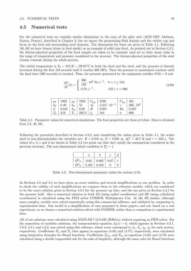
4.5. NUMERICAL TESTS 45
4.5 Numerical tests
For the numerical tests we consider similar dimensions to the ones of the pilot unit (ACB GEC Alsthom,Nantes, France), described in Chapter 3, but we ignore the pressurising fluid domain and the rubber cap andfocus on the food and surrounding steel domains. The dimensions for these are given in Table 4.1. Following[46, 69] we have chosen tylose (a food simile) as an example of solid type food. As pointed out in Section 4.2.1,the thermo-physical properties of the food sample are taken to be constant (and set to their mean value inthe range of temperature and pressure considered in the process). The thermo-physical properties of the steelremain constant during the whole process.
The initial temperature is T0 = 313 K = 39.85C in both the food and the steel, and the pressure is linearlyincreased during the first 183 seconds until it reaches 360 MPa. Then the pressure is maintained constant untilthe final time (900 seconds) is reached. Thus, the pressure generated by the equipment satisfies P (0) = 0 and
dP
dt(t) =
360
183· 106 Pa s−1, 0 < t ≤ 183,
0 Pa s−1, 183 < t < 900.
(4.80)
ρF 1006 ρS 7833 CpF 3780 CpS 465kF 0.49 kS 55 βF 4.217 · 10−4 γ 360 · 106L 0.045 L2 0.09 H 0.091 H2 0.327T0 313 Tr 292.3 tp 183 tf 900
Table 4.1: Parameter values for numerical simulations. The food properties are those of tylose. Data is obtainedfrom [14, 46, 68].
Following the procedure described in Section 4.2.2, and considering the values given in Table 4.1, the scalesused to non-dimensionalise the variables are: R = 0.045 m, Z = 0.091 m, ∆T = 20.7 K and τ = 325 s. Thevalues of a, b, c and d are shown in Table 4.2 (we point out that they satisfy the assumptions considered in theprevious sections). The non-dimensional initial condition is T ∗
0 = 1.
a b c d
ΩDF 0.02 0.005 0.07 1
ΩDS 2.423 0.593 0 0
Table 4.2: Non-dimensional parameter values for system (4.9).
In Sections 4.3 and 4.4 we have given an exact solution and several simplifications to our problem. In orderto check the validity of such simplifications we compare them to the reference models, which are consideredto be the exact solution given in Section 4.3.1 for the pressure up time, and the one given in Section 4.4.1 forthe pressure hold. Also a numerical solution in both 1D (using radial coordinates) and 2D (using cylindricalcoordinates) is calculated using the FEM solver COMSOL Multiphysics 3.5a. In [46, 69] similar, althoughmore complex, models were solved numerically using this commercial software, and validated by comparing toexperimental data. Our model is a simplification of ones proposed in those papers, and not based on a realexperiment, so we choose a numerical solution solved with COMSOL rather than a comparison to experimentaldata.
All of our solutions were calculated using MATLAB 7.12.0.635 (R2011a) without requiring an FEM solver. Forthe separation of variables solutions, the transcendental equation J0(x) = 0, which appears in Sections 4.3.1,4.3.2, 4.4.1 and 4.4.2, was solved using this software, whose roots correspond to δn, δn, ηj , ηj for each section,respectively. Coefficients Dn and Ej that appear in equations (4.40) and (4.77), respectively, were calculatedusing integration formulas for Bessel functions. Coefficients Dmn and Ekj in equations (4.34) and (4.73) werecalculated using a double trapezoidal rule for the sake of simplicity, although the same rules for Bessel functions

46 CHAPTER 4. DIMENSIONAL ANALYSIS
0 0.2 0.4 0.6 0.8 1−0.2
0
0.2
0.4
0.6
0.8
1
1.2
r
T
1D and 2D models − Pressure up at t=0.12
(−) Exact solution 2D (:) Bdy Lyr 2D
(*) Sep Var 1D (o) Bdy Lyr 1D
z=0.97
z=0.96
z=0.98
z=0.99
z=1
z ∈ (0,0.95)
0 0.2 0.4 0.6 0.8 1−0.2
0
0.2
0.4
0.6
0.8
1
1.2
1.4
1.6
1.8
r
T
1D and 2D models − Pressure up at t=tp=0.56
(−) Exact solution 2D (:) Bdy Lyr 2D
(*) Sep Var 1D(o) Bdy Lyr 1D
z ∈ (0,0.95)
z=1
z=0.96
z=0.98
z=0.97
z=0.99
Figure 4.2: Dimensionless temperature profiles calculated with different methods in 1D and 2D for pressure upat t = 0.12 (left) and t = tp = 0.56 (right).
plus some for trigonometric functions could have been used for calculating it directly, or any other quadraturerule could also be used. We truncated each infinite sum and took as many terms as necessary to obtain asolution which did not vary to 16 decimal places from the solution with one term less. Thus, for equations(4.32) and (4.39) we took N = 20 terms, and for (4.72) and (4.75), J = 20 terms. For equations (4.26), P = 35terms, for (4.32), M = 35 terms and for (4.72), K = 35 terms.
For the boundary layer solutions described in Sections 4.3.2 and 4.3.3, in which there are a semi-infinite integrals(namely (4.57) and (4.69)) to calculate, we followed [60], where a method to approximate integrals of the form∫
∞
af(x)φ(x) dx is proposed, with φ(x) being either sin(ωx) or cos(ωx). The integral is approximated by
a numerical integration over a finite domain (a, b), leaving a truncation error equal to the tail integration∫
∞
bf(x)φ(x) dx, plus the discretisation error. Luo and Shevchenko [60] describe a very simple end-point
correction to approximate the tail integration, which reduces significantly the truncation error, and which wehave used in our calculations.
4.5.1 Results
Figure 4.2 shows the dimensionless temperature profiles given by the models presented in Section 4.3 for pressureup time. We have plotted the results of the 2D models at a fixed time (t = 0.12 on the left, t = 0.56 = tp onthe right) for different heights and for all r. As can be seen for all heights z ∈ (0, 0.95) the solution is almostthe same, and also matches perfectly with the 1D results from Sections 4.3.2 and 4.3.2. Then for the rest ofheights up to z = 1, where the boundary layer is, it is clear that the solutions differ from the 1D model for thepoints very close to the top right corner of the 2D domain. There is a slight difference between the boundarylayer solution given in Section 4.3.3 and the exact solution given in Section 4.3.1, especially near r = 1. Thisis because in (4.63) we are ignoring the a term, and therefore no heat conduction in the r direction is takeninto account in this solution. Including this term leads to a problem which is more difficult to solve than theoriginal one, and so the approximation would no longer be a simplification.
Figure 4.3 shows the dimensionless temperature profiles given by the models presented in Section 4.4 for pressurehold time. In this case the plots are at times t = 1.50 on the left and t = 2.76 = tf on the right. For all heightsz ∈ (0, 0.94) the solution is almost the same and again matches perfectly with the 1D results from Section 4.4.2.In this case, however, for the rest of height up until z = 1 which are in the boundary layer, the approximationproposed in Section 4.4.3 differs more from the exact solution given in Section 4.4.1 than in the pressure up timecase. This is because the conduction term in the r direction was ignored again, and, because there is no sourceterm for the pressure hold case, this difference is more noticeable. We remark again that this slight discrepancyis for points that are very close to the top of the 2D domain.
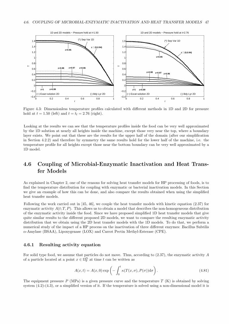
4.6. COUPLING OF MICROBIAL-ENZYMATIC INACTIVATION AND HEAT TRANSFER MODELS 47
0 0.2 0.4 0.6 0.8 1−0.4
−0.2
0
0.2
0.4
0.6
0.8
1
1.2
1.4
1.6
r
T
1D and 2D models − Pressure hold at t=1.50
(−) Exact solution 2D (:) Bdy Lyr 2D
(*) Sep Var 1D
z ∈ (0,0.94)z=0.95
z=1 z=0.99
z=0.98 z=0.96z=0.97
0 0.2 0.4 0.6 0.8 1−0.4
−0.2
0
0.2
0.4
0.6
0.8
1
1.2
1.4
1.6
r
T
1D and 2D models − Pressure hold at t=2.76
(−) Excat solution 2D (:) Bdy Lyr 2D
(*) Sep Var 1D
z=1 z=0.99
z=0.97z=0.98z=0.96
z=0.95
z ∈ (0,0.94)
Figure 4.3: Dimensionless temperature profiles calculated with different methods in 1D and 2D for pressurehold at t = 1.50 (left) and t = tf = 2.76 (right).
Looking at the results we can see that the temperature profiles inside the food can be very well approximatedby the 1D solution at nearly all heights inside the machine, except those very near the top, where a boundarylayer exists. We point out that these are the results for the upper half of the domain (after our simplificationin Section 4.2.2) and therefore by symmetry the same results hold for the lower half of the machine, i.e. thetemperature profile for all heights except those near the bottom boundary can be very well approximated by a1D model.
4.6 Coupling of Microbial-Enzymatic Inactivation and Heat Trans-
fer Models
As explained in Chapter 2, one of the reasons for solving heat transfer models for HP processing of foods, is tofind the temperature distribution for coupling with enzymatic or bacterial inactivation models. In this Sectionwe give an example of how this can be done, and also compare the results obtained when using the simplifiedheat transfer models.
Following the work carried out in [45, 46], we couple the heat transfer models with kinetic equation (2.37) forenzymatic activity A(t;T, P ). This allows us to obtain a model that describes the non-homogeneous distributionof the enzymatic activity inside the food. Since we have proposed simplified 1D heat transfer models that givequite similar results to the different proposed 2D models, we want to compare the resulting enzymatic activitydistribution that we obtain using the 2D heat transfer models with the 1D models. To do that, we perform anumerical study of the impact of a HP process on the inactivation of three different enzymes: Bacillus Subtilisα-Amylase (BSAA), Lipoxygenase (LOX) and Carrot Pectin Methyl-Esterase (CPE).
4.6.1 Resulting activity equation
For solid type food, we assume that particles do not move. Thus, according to (2.37), the enzymatic activity Aof a particle located at a point x ∈ ΩD
F at time t can be written as
A(x, t) = A(x, 0) exp
(
−∫ t
0
κ(T (x, σ), P (σ))dσ
)
. (4.81)
The equipment pressure P (MPa) is a given pressure curve and the temperature T (K) is obtained by solvingsystem (4.2)-(4.3), or a simplified version of it. If the temperature is solved using a non-dimensional model it is
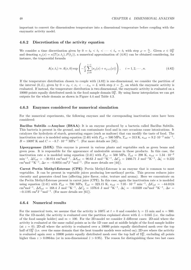
48 CHAPTER 4. DIMENSIONAL ANALYSIS
important to convert the dimensionless temperature into a dimensional temperature before coupling with theenzymatic activity model.
4.6.2 Discretisation of the activity equation
We consider a time discretisation given by 0 = t0 < t1 < · · · < tn = tf with step ϕ = tfn. Given x ∈ ΩD
F
and denoting κj(x) = κ(T (x, tj), P (tj)), a numerical approximation of (4.81) can be obtained considering, forinstance, the trapezoidal formula
A(x, ti) ≈ A(x, 0) exp
−ϕ
2
i−1∑
j=0
(κj(x) + κj+1(x))
, i = 1, 2, · · · , n. (4.82)
If the temperature distribution chosen to couple with (4.82) is one-dimensional, we consider the partition ofthe interval (0, L), given by 0 = x0 < x1 < · · ·xm = L with step x = L
m, on which the enzymatic activity is
evaluated. If instead, the temperature distribution is two-dimensional, the enzymatic activity is evaluated on a10000 points equally distributed mesh in the food sample domain ΩD
F . By using linear interpolation we can getoutputs for the whole domain as shown in Figure 4.4 and Table 4.3.
4.6.3 Enzymes considered for numerical simulation
For the numerical experiments, the following enzymes and the corresponding inactivation rates have beenconsidered:
Bacillus Subtilis α-Amylase (BSAA): It is an enzyme produced by a bacteria called Bacillus Subtilis.This bacteria is present in the ground, and can contaminate food and in rare occasions cause intoxications. Itcatalyzes the hydrolysis of starch, generating sugars (such as maltose) that can modify the taste of food. Theinactivation rate κ is modeled using equation (2.40) with Pref = 500 MPa, Tref = 313 K, κref = 9.2 ·10−2 min−1,B = 10097 K and C = −8.7 · 10−4 MPa−1. (For more details see [58]).
Lipoxygenase (LOX): This enzyme is present in various plants and vegetables such as green beans andgreen peas. It is responsible for the appearance of undesirable aromas in those products. In this case, theinactivation rate κ is modeled using equation (2.41) with Pref = 500 MPa, Tref = 298 K, κref = 1.34 · 10−2
min−1, ∆Vref = −30.814 cm3mol−1, ∆Sref = 90.63 J mol−1K−1, ∆Cp = 2466.71 J mol−1K−1, ∆ζ = 0.222cm3mol−1K−1, ∆ν = −0.0054 cm6J−1mol−1. (For more details see [44]).
Carrot Pectin Methyl-Esterase (CPE): Pectin Methyl-Esterase is an enzyme that is common to mostvegetables. It can be present in vegetable juices producing low-methoxyl pectin. This process reduces juiceviscosity and generates cloud loss (affecting juice flavor, color, texture and aroma). Here we concentrate onthe Pectin Methyl-Esterase present in carrot juice (CPE). In this case, again the inactivation rate κ is modeledusing equation (2.41) with Pref = 700 MPa, Tref = 323.15 K, κref = 7.05 · 10−2 min−1, ∆Vref = −44.0124cm3mol−1, ∆Sref = 168.4 J mol−1K−1, ∆Cp = 1376.6 J mol−1K−1, ∆ζ = −0.0339 cm3mol−1K−1, ∆ν =−0.1195 cm6J−1mol−1. (For more details see [61]).
4.6.4 Numerical results
For the numerical tests, we assume that the activity is 100% at t = 0 and consider tf = 15 min and n = 900.For the 1D-model, the activity is evaluated over the partition explained above with L = 0.045 (i.e. the radiusof the food sample holder) and m = 100. For the 2D-model we consider 3 different cases: 2D-mid where theactivity is evaluated at the same radial points as in the 1D case and at middle height of the food sample holder(at z = 0); 2D-all where the activity is evaluated over a 10000 points equally distributed mesh over the tophalf of ΩD
F (i.e. over the same domain that the heat transfer models were solved on); 2D-ave where the activityis evaluated again over a 10000 points equally distributed mesh over the top half of ΩD
F , excluding all pointshigher than z > 0.0864m (or in non-dimensional z > 0.95). The reason for distinguishing these two last cases

4.6. COUPLING OF MICROBIAL-ENZYMATIC INACTIVATION AND HEAT TRANSFER MODELS 49
is because, as we saw in Figures 4.2 and 4.3, the temperature distributions can be very well approximated bythe 1D solution at nearly all heights inside the machine, except those very near the top. We want to see if thisalso happens for the enzymatic activity.
For the 1D-model, the temperature is calculated using the 1D non-dimensional separation of variables solutiongiven in Section 4.3.2 for Pup, and that of Section 4.4.2 for Phold. Note that due to the similarity of theseparation of variables and the boundary layer solutions calculated in Section 4.3.2, for Pup, the latter couldhave been used instead of the former. For all of the 2D models, the temperature is calculated using the 2Dnon-dimensional exact solution given in Section 4.3.1 for Pup, and that of Section 4.4.1 for Phold.
As we can observe in Figure 4.4 and Table 4.3, the efficiency of the considered HP process for inactivatingenzymes depends on the enzyme under study. For enzyme BSAA, this process is very efficient given that thefinal activity is very low, whilst enzyme CPE seems to be quite resistant to the process, as the final activity isvery high. These results coincide qualitatively with those of [46].
0 100 200 300 400 500 600 700 800 900
20
40
60
80
100
Time(s)
Enz
ymat
ic A
ctiv
ity (
%)
Enzyme BSAA
1D 2D−mid2D−ave2D−all
(a) Enzyme BSAA
0 100 200 300 400 500 600 700 800 90075
80
85
90
95
100
Time(s)
Enz
ymat
ic A
ctiv
ity (
%)
Enzyme LOX
1D 2D−mid2D−ave2D−all
(b) Enzyme LOX
0 100 200 300 400 500 600 700 800 90095
96
97
98
99
100
Time(s)
Enz
ymat
ic A
ctiv
ity (
%)
Enzyme CPE
1D2D−mid2D−ave2D−all
(c) Enzyme CPE
Figure 4.4: Mean enzymatic activity evolution (%) over dimensional time for the considered models
If we compare the results we have obtained to calculate the enzymatic activity, we can see in Figure 4.4 that forthe three enzymes under consideration the 1D, 2D-mid and 2D-ave give very similar results, whilst the 2D-all isslightly different. This is consistent with the results obtained in Section 4.5, where we saw that the temperatureprofiles for the 1D model were very similar to the 2D ones at every point except those near the very top. InTable 4.3 we can observe the differences in the final activity (given by the mean activity in the models at finaltime, i.e. M(A(·, tf); ΩD
F )) for the three enzymes. Table 4.3 also shows the mean temperature M(T (·, tf); ΩDF ))
(C) inside the food domain during the process for the different cases.
Enzyme BSAA shows the largest differences between models. The 1D, 2D-mid and 2D-ave models give similarresults (see Figure 4.4a) with a maximum difference of final mean activity of 2.5%. The 2D-all model howeverdiffers quite a lot, with a maximum difference of 9.5% compared to the other models (see Table 4.3). This isdue to the fact that for the 2D-all case we are considering the points at the very top of the food domain, which,as we saw in Section 4.5, have different temperatures to the rest of the heights. Also enzyme BSAA is sensitive
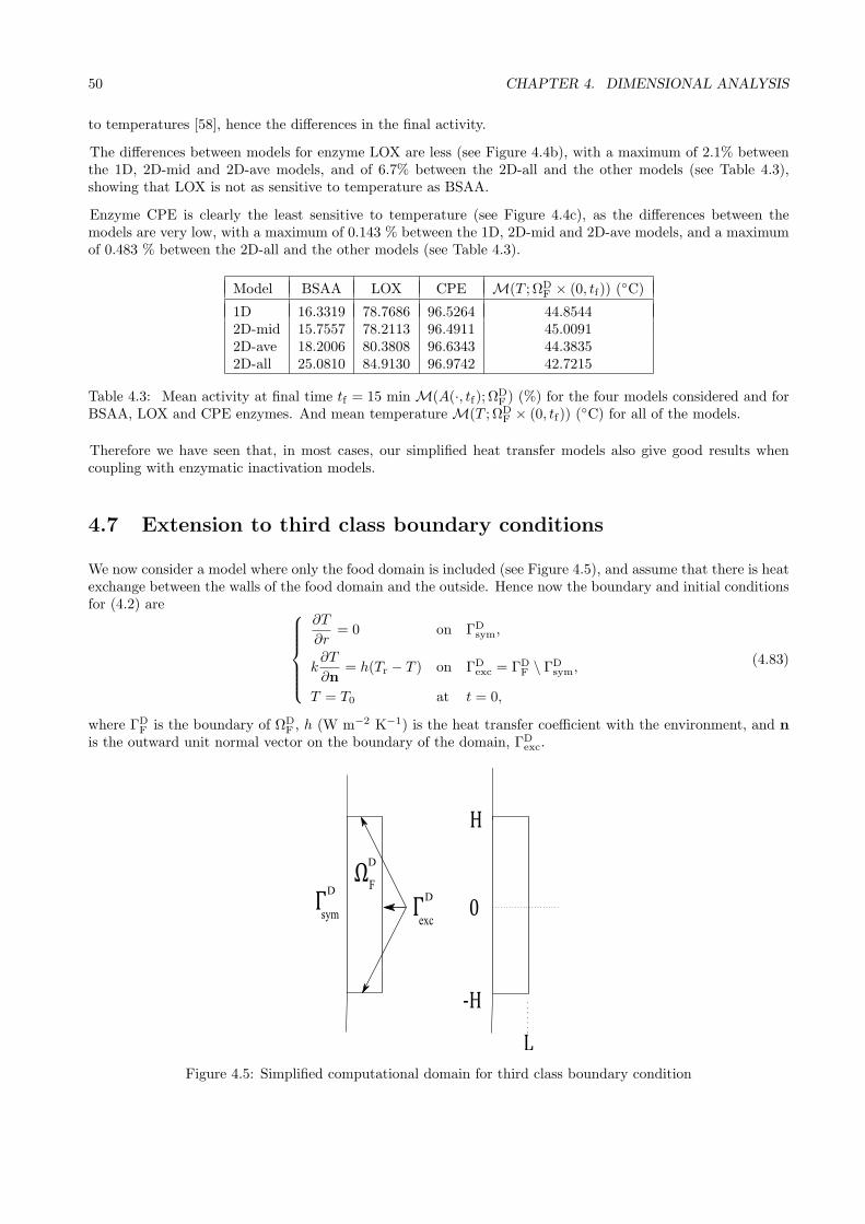
50 CHAPTER 4. DIMENSIONAL ANALYSIS
to temperatures [58], hence the differences in the final activity.
The differences between models for enzyme LOX are less (see Figure 4.4b), with a maximum of 2.1% betweenthe 1D, 2D-mid and 2D-ave models, and of 6.7% between the 2D-all and the other models (see Table 4.3),showing that LOX is not as sensitive to temperature as BSAA.
Enzyme CPE is clearly the least sensitive to temperature (see Figure 4.4c), as the differences between themodels are very low, with a maximum of 0.143 % between the 1D, 2D-mid and 2D-ave models, and a maximumof 0.483 % between the 2D-all and the other models (see Table 4.3).
Model BSAA LOX CPE M(T ; ΩDF × (0, tf)) (
C)
1D 16.3319 78.7686 96.5264 44.85442D-mid 15.7557 78.2113 96.4911 45.00912D-ave 18.2006 80.3808 96.6343 44.38352D-all 25.0810 84.9130 96.9742 42.7215
Table 4.3: Mean activity at final time tf = 15 min M(A(·, tf); ΩDF ) (%) for the four models considered and for
BSAA, LOX and CPE enzymes. And mean temperature M(T ; ΩDF × (0, tf)) (
C) for all of the models.
Therefore we have seen that, in most cases, our simplified heat transfer models also give good results whencoupling with enzymatic inactivation models.
4.7 Extension to third class boundary conditions
We now consider a model where only the food domain is included (see Figure 4.5), and assume that there is heatexchange between the walls of the food domain and the outside. Hence now the boundary and initial conditionsfor (4.2) are
∂T
∂r= 0 on ΓD
sym,
k∂T
∂n= h(Tr − T ) on ΓD
exc = ΓDF \ ΓD
sym,
T = T0 at t = 0,
(4.83)
where ΓDF is the boundary of ΩD
F , h (W m−2 K−1) is the heat transfer coefficient with the environment, and nis the outward unit normal vector on the boundary of the domain, ΓD
exc.
ΩF
Γ 0
L
H
-H
sym Γexc
D
DD
Figure 4.5: Simplified computational domain for third class boundary condition
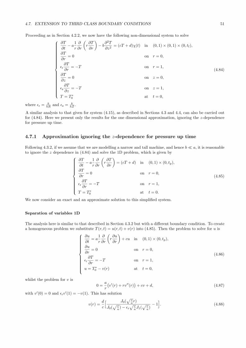
4.7. EXTENSION TO THIRD CLASS BOUNDARY CONDITIONS 51
Proceeding as in Section 4.2.2, we now have the following non-dimensional system to solve
∂T
∂t− a
1
r
∂
∂r
(
r∂T
∂r
)
− b∂2T
∂z2= (cT + d)χ(t) in (0, 1)× (0, 1)× (0, tf),
∂T
∂r= 0 on r = 0,
ǫr∂T
∂r= −T on r = 1,
∂T
∂z= 0 on z = 0,
ǫz∂T
∂z= −T on z = 1,
T = T ∗
0 at t = 0,
(4.84)
where ǫr =khR
and ǫz =khZ
.
A similar analysis to that given for system (4.15), as described in Sections 4.3 and 4.4, can also be carried outfor (4.84). Here we present only the results for the one dimensional approximation, ignoring the z-dependencefor pressure up time.
4.7.1 Approximation ignoring the z-dependence for pressure up time
Following 4.3.2, if we assume that we are modelling a narrow and tall machine, and hence b ≪ a, it is reasonableto ignore the z dependence in (4.84) and solve the 1D problem, which is given by
∂T
∂t− a
1
r
∂
∂r
(
r∂T
∂r
)
= (cT + d) in (0, 1)× (0, tp),
∂T
∂r= 0 on r = 0,
ǫr∂T
∂r= −T on r = 1,
T = T ∗
0 at t = 0.
(4.85)
We now consider an exact and an approximate solution to this simplified system.
Separation of variables 1D
The analysis here is similar to that described in Section 4.3.2 but with a different boundary condition. To createa homogeneous problem we substitute T (r, t) = u(r, t) + v(r) into (4.85). Then the problem to solve for u is
∂u
∂t= a
1
r
∂
∂r
(
r∂u
∂r
)
+ cu in (0, 1)× (0, tp),
∂u
∂r= 0 on r = 0,
ǫr∂T
∂r= −T on r = 1,
u = T ∗
0 − v(r) at t = 0,
(4.86)
whilst the problem for v is
0 =a
r
(
v′(r) + rv′′(r))
+ cv + d, (4.87)
with v′(0) = 0 and ǫrv′(1) = −v(1). This has solution
v(r) =d
c
[ J0(√
car)
J0(√
ca)− ǫr
√
caJ1(√
ca)− 1]
. (4.88)
52 CHAPTER 4. DIMENSIONAL ANALYSIS
A straightforward calculation gives the solution for u as
u(r, t) =
∞∑
n=1
¯DnJ0(¯δnr) exp(−¯λ2
nt), (4.89)
where ¯δn ∈ R satisfy
ǫr¯δJ1(
¯δn) = J0(¯δn), (4.90)
¯λn =
√
a¯δ2n − c and coefficients ¯Dn are given by
¯Dn =2∫ 1
0(T ∗
0 − v(r)) rJ0(¯δnr) dr
∫ 1
0rJ2
0 (¯δnr) dr
, (4.91)
with v(r) defined in (4.88). Finally, the solution T is simply the sum of u and v.
Boundary layer in r
To consider a boundary layer in r we start with system (4.85). Analogously to Section 4.3.2 we assume d = O(1)and b < a ≪ 1. Then ignoring the terms involving a and b, we again have at leading order the outer solutiongiven by (4.43), i.e.
T (t) = −d
c+
(
T ∗
0 +d
c
)
exp(ct). (4.92)
It is clear that since solution (4.92) only depends on t it does satisfy the zero flux condition at r = 0, but itobviously cannot satisfy the third class boundary condition at r = 1. Therefore we consider a boundary layernear r = 1. Following the exact steps as in Section 4.3.2, we introduce the boundary-layer coordinate given by(4.44), take δ =
√a to bring out the correct balance in the equation, which at leading order is
∂Tin
∂t=
∂2Tin
∂r2−√a∂Tin
∂r+ cTin + d in (0,∞)× (0, tp),
∂Tin
∂r=
δ
ǫrTin on r = 0,
Tin → Tout(t) as r → ∞,
Tin = T ∗
0 at t = 0,
(4.93)
where Tout(t) is the outer solution given by (4.92). We define
Tin(r, t) = Tout(t) + exp
(√a r
2+ ct− at
4
)
G(r, t), (4.94)
and so the system for G reduces to
∂G
∂t=
∂2G
∂r2in (0,∞)× (0, tp),
−∂G
∂r+ αG = h(t) on r = 0,
G → 0 as r → ∞,
G = 0 at t = 0,
(4.95)
where
α =
√a
ǫr−
√a
2, h(t) = −
√a
ǫrTout(t) exp (−ct+ at/4). (4.96)

4.7. EXTENSION TO THIRD CLASS BOUNDARY CONDITIONS 53
From [73] we know that (4.95) can be solved by taking the following integral transform
G(ω, t) =
∫
∞
0
G(r, t)K(ω, r) dr, (4.97)
where K(ω, r) is the solution of
d2R(r)
d2r2+ ω2R(r) = 0,
αR(r)− dR(r)
dr= 0 on r = 0,
(4.98)
namely
K(ω, r) =
√
2
π
[ω cos(ωr) + α sin(ωr)√ω2 + α2
]
. (4.99)
Applying the integral transform (4.97) to the PDE in (4.95) gives
∫
∞
0
∂G(r, t)
∂tK(ω, r) dr =
∫
∞
0
∂2G(r, t)
∂r2K(ω, r) dr. (4.100)
Now∫
∞
0
∂2G(r, t)
∂r2K(ω, r) dr = −K
∂G
∂r
∣
∣
∣
∣
r=0
+dK
drG
∣
∣
∣
∣
r=0
− ω2
∫
∞
0
G(r, t)K(ω, r) dr. (4.101)
From (4.95) and (4.98) it follows that at r = 0
−K∂G
∂r+
dK
drG = −K(αG− h(t)) + αKG = h(t)K(ω, 0). (4.102)
Hence∫
∞
0
∂2G(r, t)
∂r2K(ω, r) dr = −ω2G+ h(t)K(ω, 0) = −ω2G+
√
2
πh(t)
ω√ω2 + α2
, (4.103)
and so the PDE in (4.95) becomes
∂G
∂t+ ω2G =
√
2
πh(t)
ω√ω2 + α2
, (4.104)
where h(t) and α are defined in (4.96). The initial condition in (4.95) implies G(ω, 0) = 0, and so equation(4.104) has solution
G(ω, t) =
√
2
π
[ ω√ad
ǫrc√ω2 + α2
exp(at/4− ct)− exp(−ω2t)
ω2 + a/4− c− ω
√a(T ∗
0 + d/c)
ǫr√ω2 + α2
exp(at/4)− exp(−ω2t)
ω2 + a/4
]
, (4.105)
after substituting Tout(t) from (4.92). Finally the solution for G (see [73]) is
G(r, t) =
√
2
π
[
∫
∞
0
G(ω, t)ω√
ω2 + α2cos(ωr) dω +
∫
∞
0
G(ω, t)α√
ω2 + α2sin(ωr) dω
]
, (4.106)
and Tin(r, t) is given by (4.94). After adding the inner and outer solutions ans subtracting the common part,we can write down the final solution in the whole domain as
T (r, t) = −d
c+
(
T ∗
0 +d
c
)
exp(ct) + exp
(
1− r
2+ ct− at
4
)
G
(
1− r√a
, t
)
. (4.107)

54 CHAPTER 4. DIMENSIONAL ANALYSIS
0 0.2 0.4 0.6 0.8 10.7
0.8
0.9
1
1.1
1.2
1.3
1.4
1.5
1.6
r
T
1D models − Pressure up with 3rd class BC
(−) Sep Var 1D (*) Comsol 1D (o) Bdy layer 1D
t=0.01 t=0.12 t=0.23 t=0.34
t=0.45 t=tp=0.56
0 0.2 0.4 0.6 0.8 1−0.2
0
0.2
0.4
0.6
0.8
1
1.2
1.4
1.6
r
T
1D models − Pressure up with 1st class boundary conditions
(−) Sep Var 1D
(*) Comsol 1D
(o) Boundary layer 1D
t=0.34
t=0.45
t=tp=0.56
t=0.01 t=0.12 t=0.23
Figure 4.6: Dimensionless temperature profiles calculated with different methods in 1D for the third class (left)and first class (right) boundary conditions.
4.7.2 Results
We perform numerical tests for the problem with third class boundary conditions, using the same data andparameters as in Section 4.5. The heat transfer coefficient used in the tests is h = 28 W m−2 K−1. Figure 4.6shows the dimensionless temperature profiles that result from solving the pressure up time problem in 1D forboundary conditions of the third and first class (Sections 4.7.1 and 4.3.2, respectively). The temperature hasbeen calculated using separation of variables in 1D (Sections 4.7.1 and 4.3.2, respectively), by a boundary layerin 1D approximation (Sections 4.7.1 and 4.3.2, respectively). Observe that both solutions match perfectly forall times, and also to the 1D COMSOL solution, which has been taken as a reference model. For the first classboundary conditions, an exact solution in 2D was given in Section 4.3.1. However, for the third class boundarycondition we do not give all the possible solutions, as it is analogous to the ones derived throughout Sections4.3 and 4.4, and we just concentrate on the 1D pressure up case. Also, for the first class boundary conditions,the heat transfer model was coupled with an enzymatic inactivation model in Section 4.6. Again, due to theanalogy, we have not gone through the coupling in this case.
4.8 Conclusions
We have presented heat transfer models for predicting temperature profiles inside a solid-type food undergoingHP treatment. Two different kinds of boundary conditions have been considered depending on whether onlythe food holder is taken into account, or whether the surrounding steel is included. We have given a thoroughanalysis describing an exact 2D solution as well as several simplifications in both 2D and 1D. It has beenshown that for the case of a tall and narrow HP machine, the temperature profile inside the food is very wellapproximated by a 1D model, except at points very close to the top and bottom boundaries. For the firstclass boundary conditions, the solutions of the 1D heat transfer models have been used to calculate the finalenzymatic activity, also achieving very similar results to when the temperature of the 2D models are used. Thereduction to 1D is very useful from a computational point of view, since faster simulations can be carried out.This is interesting, for instance, when performing optimisation algorithms, where very often the state equationsneed to be solved many times. In addition, the simplified model can help to calculate thermo-physical propertiesas a function of pressure, via inverse problems, which is an increasing need nowadays for food technologists.From an experimental point of view, results can also be used to determine where to place the thermocouplesinside the food sample in order to measure the temperature experimentally. Finally, we point out that thesolutions given here do not require the use of a “black-box” FEM solver and our approximations allow us toqualitatively describe the physical features involved.

Chapter 5
Modelling High-Pressure Processes in
a Vertical and Horizontal chamber
Nomenclature for Chapter 5
A1, A2 Pressure pointsCp Specific heat capacity (J kg−1 K−1)g Gravity vector (m s−2)h Heat transfer coefficient (W m−2 K−1)H Domain height (m)k Thermal conductivity (W m−1 K−1)L Domain width (m)Lr Radial length scale (m)Lz Vertical length scale (m)M Mass (kg)n Outward normal unit vector (m)p Mass transfer pressure (Pa)P Equipment Pressure (Pa)Pmax Maximum target pressure (Pa)r Radial coordinate (m)t Time (s)tf Final time (s)tup Pressure-up time (s)T Temperature (K)T0 Initial temperature (K)Tenv Environment temperature (K)Tr Fixed temperature (K)u Fluid velocity vector (m s−1)ux, uy, uz Components of the velocity vector uU Velocity scale (m s−1)V Volume (m3)x, y, z Cartesian coordinates (m)
Indices
* Rotated domainsF Food domainhold Pressure-hold solutionP Pressurising fluidup Pressure-up solution
Greek symbols
β Thermal expansion coefficient (K−1)Γ Whole domain boundaryΓp Boundary of Ω∗
P
Γr Fixed temperature boundaryΓup Heat transfer boundaryη Dynamic viscosity (Pa s)θ Cylindrical angular coordinateΘ Temperature scale (K)ρ Density (kg m−3)τ Time scale (s)Ω Whole domainΩC Cap of the sample holderΩF Food sample domainΩP Pressurising mediumΩS Steel vessel
Other symbols
∇ Gradient∇· Divergence∇2 Laplacian
Acronyms
CFD Computational Fluid DynamicsFEM Finite Element MethodHP High PressureHPP High Pressure ProcessingOS Operation systemRAM Random access memory2D Two-dimensional3D Three-dimensional
55
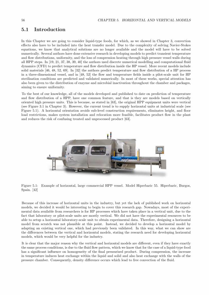
56 CHAPTER 5. HORIZONTAL AND VERTICAL MODELS
5.1 Introduction
In this Chapter we are going to consider liquid-type foods, for which, as we showed in Chapter 3, convectioneffects also have to be included into the heat transfer model. Due to the complexity of solving Navier-Stokesequations, we know that analytical solutions are no longer available and the model will have to be solvednumerically. Several authors have done extensive research in developing models to predict transient temperatureand flow distributions, uniformity, and the loss of compression heating through high pressure vessel walls duringall HPP steps. In [19, 21, 37, 38, 39, 40] the authors used discrete numerical modelling and computational fluiddynamics (CFD) to predict temperature and flow distribution inside the HP vessel. More recent models includesolid materials [46, 48, 52, 69]. In [32] the authors predict temperature and flow distribution of a HP processin a three-dimensional vessel, and in [48, 52] the flow and temperature fields inside a pilot-scale unit for HPsterilisation conditions are predicted and validated numerically. In most of these works, special attention hasalso been given to the distribution of enzyme and microbial inactivation throughout the chamber and packages,aiming to ensure uniformity.
To the best of our knowledge, all of the models developed and published to date on prediction of temperatureand flow distribution of a HPP, have one common feature, and that is they are models based on verticallyoriented high pressure units. This is because, as stated in [63], the original HPP equipment units were vertical(see Figure 3.1 in Chapter 3). However, the current trend is to supply horizontal units at industrial scale (seeFigure 5.1). A horizontal orientation avoids sub-level construction requirements, eliminates height, and floorload restrictions, makes system installation and relocation more feasible, facilitates product flow in the plantand reduces the risk of confusing treated and unprocessed product [63].
Figure 5.1: Example of horizontal, large commercial HPP vessel. Model Hiperbaric 55. Hiperbaric, Burgos,Spain. [42]
Because of this increase of horizontal units in the industry, but yet the lack of published work on horizontalmodels, we decided it would be interesting to begin to cover this research gap. Nowadays, most of the experi-mental data available from researchers is for HP processes which have taken place in a vertical unit, due to thefact that laboratory or pilot-scale units are mostly vertical. We did not have the experimental resources to beable to setup a horizontal laboratory-scale unit to obtain experimental data. Therefore, designing a horizontalmodel from scratch was not plausible at this point. Instead, we decided to develop a horizontal model byadapting an existing vertical one, which had previously been validated. In this way, what we can show arethe differences between the vertical and horizontal models, stating the research need for developing horizontalmodels, which would be very helpful for the industry.
It is clear that the major reason why the vertical and horizontal models are different, even if they have exactlythe same process conditions, is due to the fluid flow pattern, which we know that for the case of a liquid-type foodhas a significant influence on homogeneity of the final pressurised product. During compression, the increasein temperature induces heat exchange within the liquid and solid and also heat exchange with the walls of thepressure chamber. Consequently, density difference occurs which lead to free convection of the fluid.

5.2. THE PROCESS MODELS 57
For upward flow in vertical tubes, the effect of free convection is to accelerate the fluid particles near the wall.This creates steeper velocity and temperature gradients near the wall, and hence higher heat transfer rates.To satisfy continuity considerations, the increased velocity near the wall results in flow retardation at the tubecentre and, in extreme cases, a reversal of flow at the tube centre may even occur (see, e.g., [57, 65]). The flowpattern produced by free convection inside a horizontal tube is quite different than the vertical case; transversefluid movement is more important. When a fluid in a horizontal tube is heated, the buoyancy forces causemovement of the fluid upwards at the sides and downwards at the centre. If combined with forced flow (whichwe do not consider in this work), this effect sets up forward moving spirals and the resulting flow pattern maynot be entirely steady (see, e.g., [65]).
Through the work developed in this Chapter we want to show that the horizontal and vertical flow inside aliquid-type food undergoing a HP process are indeed different, and therefore so is the temperature distribution,which could be problematic for the food industry, if uniformity of pursued effects such as enzymatic or microbialinactivation are required. This work is based on that from [84]. In the following Sections we are going to furtherdevelop a heat transfer model to determine the temperature and flow distribution inside a sample treated withHP in a horizontally oriented vessel, and compare the results to the ones obtained with the heat transfer modelof a HP device placed vertically, with exactly the same process conditions.
5.2 The process models
The starting point is the vertical two-dimensional (2D) axis-symmetric geometry presented in Chapter 3, whichwas modelled and solved numerically in [46]. The selection of an axis-symmetric model is very common inHPP modelling of vertically oriented devices, given that in many cases the system comprises axis-symmetricfeatures, and has been successfully used and validated in several papers (see, e.g. [50, 51, 52, 69]). This modelderived by [46] for liquid-type foods includes conduction and convection effects, and the flow is assumed to belaminar (as we saw in Section 3.2). Other more complex models, which also include turbulence effects (such as,e.g. [50, 51, 52]), could have been chosen as the starting model. However due to the complexity of solving ahorizontal model, we decided to keep it as simple as possible.
For a horizontally oriented HP device, however, there are no longer only axis-symmetric features, and thereforea three-dimensional (3D) model seems necessary. For this reason, in this Chapter we develop both vertical andhorizontal 3D models, in order to compare them. We will first compare the 2D to the 3D vertical model to seehow good the agreement is and to check the efficiency of the 3D model solver that we are going to use. Thenwe will proceed to compare the 3D horizontal to the 3D vertical model, and show how different the results are.
(a) 2D axis-symmetric (b) Full 3D vertical (c) Half 3D horizontal
Figure 5.2: Computational configurations

58 CHAPTER 5. HORIZONTAL AND VERTICAL MODELS
5.2.1 Geometries
Vertically oriented geometries
The computational vertical 2D axis-symmetric geometry consider is the one described in Chapter 3. Thecomputational domain is shown in Figure 5.2a. From this 2D model we generate the 3D vertical model byrotating this geometry along the axis of symmetry; the resulting 3D vertical geometry is depicted in Figure5.2b. We will show in Section 5.4.1 that the solution given by the axis-symmetric 2D vertical model is equal tothe 3D model (ignoring numerical errors).
Horizontally oriented geometry
In the horizontal case there are no longer only axis-symmetric features, and so we obviously cannot reduce themodel to 2D and expect to have the same solution as in the vertical case. However, there is a computationalsimplification that can be made: the model can be solved in only half a cylinder (cutting it longitudinally),hence reducing the number of degrees of freedom. The resulting “half” 3D horizontal geometry is depicted inFigure 5.2c.
5.2.2 Heat and mass transfer model
As stated in Section 5.1, for the purpose of this work we are only going to consider liquid-type foods. If we alsohave convection effects inside the food sample, the differences between the vertical and horizontally orientedchambers will be even more pronounced than if we only considered conduction effects inside the food sample,which is the case for solid-type foods. In this Chapter we are going to solve the full 3D model, to then comparethe results to the 2D-axially symmetric model. Given the difficulties of solving a 3D model we have chosen touse the simplified model proposed in Chapter 3, Section 3.3.3, that is
ρCp
∂T
∂t− k∇2T + ρCpu · ∇T = β
dP
dtT in Ω∗ × (0, tf),
ρ∂uF
∂t− η∇2uF + ρ(uF · ∇)uF = −∇p+ ρg in Ω∗
F × (0, tf),
ρ∂uP
∂t− η∇2uP + ρ(uP · ∇)uP = −∇p+ ρg in Ω∗
P × (0, tf),
∇ · (uF) = 0 in Ω∗
F × (0, tf),
∇ · (uP) = 0 in Ω∗
P × (0, tf),
(5.1)
with the following point, boundary and initial conditions
k∂T
∂n= 0 on
(
Γ∗ \ (Γ∗
r ∪ Γ∗
up))
× (0, tf),
k∂T
∂z= h(Tenv − T ) on Γ∗
up × (0, tf),
T = Tr on Γ∗
r × (0, tf),
uF = 0 on Γ∗
F × (0, tf),
uP = 0 on Γ∗
P × (0, tf),
T (0) = T0 in Ω∗,
uF(0) = 0 in Ω∗
F,
uP(0) = 0 in Ω∗
P,
p = 105 on A1 × (0, tf),
p = 105 on A2 × (0, tf).
(5.2)
5.2. THE PROCESS MODELS 59
System (5.1) together with its boundary and initial conditions (5.2) are valid for all the proposed geometries inSection 5.2.1. For the 2D axis-symmetric model it may be rewritten in cylindrical coordinates [46]. For the 3Dhorizontal “half” model, heat flux and flow symmetric boundary conditions have to be added to (5.2) at the“cutting” boundary.
5.2.3 Comparing dimensionless convection effects for vertical and horizontal model
Before we proceed with our simulations, we want to find a dimensionless quantity for convection effects for boththe vertical and horizontal models, to see which is expected to be more important. For this, we look at the firstequation of (5.1), i.e. the convective heat transfer equation
ρCp
∂T
∂t− k∇2T + ρCpu · ∇T = β
dP
dtT, (5.3)
where ρ, Cp, k, β are considered to be constant (they are set to their mean value in the temperature andpressure range we are working in). We want to non-dimensionalise equation (5.3).
Following Section 4.2.2, we write the pressure derivative that appears in equation (5.3) using (4.4). Becausethe equation to non-dimensionalise now is different to the one in Section 4.2.2 (it includes a convective termand is in Cartesian coordinates instead of cylindrical ones), we choose new scales, and hence equation (5.3) isnon-dimensionalised by setting
x =x
Lr
, y =y
Lr
, z =z
Lz
, t =t
τ, T =
T
Θ, (ux, uy, uz) =
1
U(ux, uy, uz)
where Θ, U , and τ are suitable temperature, velocity, and time scales, respectively. Lr is a radial length scaleand Lz a vertical length scale.
Thus, equation (5.3) becomes
ρCpΘ
τ
∂T
∂t− kΘ
(
1
L2r
(
∂2T
∂x2+
∂2T
∂y2
)
+1
L2z
∂2T
∂z2
)
+ ρCpΘU(ux, uy, uz) ·(
1
Lr
∂T
∂x,1
Lr
∂T
∂y,1
Lz
∂T
∂z
)
=βγΘ
tpT . (5.4)
We divide equation (5.4) by ρCpΘ/τ , resulting in
∂T
∂t− kτ
ρCp
(
1
L2r
(
∂2T
∂x2+
∂2T
∂y2
)
+1
L2z
∂2T
∂z2
)
+ τU
(
ux
Lr
∂T
∂x+
uy
Lr
∂T
∂y+
uz
Lz
∂T
∂z
)
=βγτ
ρCptpT . (5.5)
We want to compare the convection effects between the vertical and horizontal models. If we picture thechamber placed vertically (see Figure 3.2), we can imagine that the fluid in the vertical model is moving upand down the chamber, whilst in the horizontal case it will move from left to right. Therefore, we assume thatthe velocity in the vertical case is mainly moving in the vertical direction, i.e. uz ≫ ux, uy (or equivalently,uz ≫ ux, uy) whilst in the horizontal case it mainly moves in the radial direction, hence uz ≪ ux, uy (orequivalently, uz ≪ ux, uy). We assume, in order to be able to compare the vertical and horizontal convectioneffects, that the velocity field u in both cases is of the same order (even though it has perpendicular directions).
To choose our length scales, we know that the fluid moves between H1 and H5 (see Figure 3.2) in the verticaldirection, and hence Lz = H5 − H1; radially it moves between L1 and L2, and, if the food is of liquid-type,between 0 and L1, and therefore the radial length scale is taken to be the maximum between L1 and L2 − L1
or, for the sake of simplicity, Lr = L2.
Assuming we are in the vertical case, equation (5.5) can be written as
∂T
∂t− kτ
ρCp
(
1
L2r
(
∂2T
∂x2+
∂2T
∂y2
)
+1
L2z
∂2T
∂z2
)
+τU
Lz
uz
∂T
∂z=
βγτ
ρCptpT , (5.6)
60 CHAPTER 5. HORIZONTAL AND VERTICAL MODELS
where the terms with ux and uy have been neglected because of our previous assumption uz ≫ ux, uy. So, inthis case we have a convective coefficient cv = τU
Lz.
If instead we are in the horizontal case, equation (5.5) results in
∂T
∂t− kτ
ρCp
(
1
L2r
(
∂2T
∂x2+
∂2T
∂y2
)
+1
L2z
∂2T
∂z2
)
+τU
Lr
(
ux
∂T
∂x+ uy
∂T
∂y
)
=βγτ
ρCptpT , (5.7)
where now the uz term has been neglected due to our previous assumption uz ≪ ux, uy. So, in this case we
have a convective coefficient ch = τULr
. We can see that the relation between cv and ch is cv = ch
(
Lr
Lz
)
.
From looking at the dimensions of our machine, we have H5 = 0.472 m and H1 = 0.222 m, which gives Lz = 0.25m, and L2 = 0.05 m, which gives Lr = 0.05 m. Using these values we see that cv = ch
5 , so the convection effectsare about 5 times larger in the horizontal case than in the vertical one. We remark that if we had chosen Lr tobe L2 − L1, instead of L2, then this difference would increase from 5 to nearly 10 times.
Also, we would like to point out that in the horizontal case, the convective currents reach the food samplesooner than in the vertical case, as they move mainly in the radial direction (see Figures 5.6a, 5.6b, 5.10a,5.10b), which is smaller than the vertical direction. A fluid particle that is closer to the cold wall (especiallyto the top wall - this is, in the horizontal case) will in general take less time to reach the food sample than thesame particle in the vertical case. This is why the machine placed horizontally cools the sample much fasterthan the vertically oriented one, resulting in lower temperatures throughout the process.
5.3 Numerical tests
5.3.1 Dimensions of the HP pilot unit
For the numerical tests, we have considered a similar size to the pilot unit (ACB GEC Alsthom, Nantes, France)that was used in [69]. The dimensions of the machine are given in Table 5.1. The numerical tests we presentare computed in cylindrical coordinates for the 2D model, assuming cylindrical coordinates and Cartesiancoordinates for the 3D-model. We use the Finite Element Method (FEM) solver COMSOL Multiphysics 3.5ato compute the solutions. More details of the computations will be given in Section 5.4.
5.3.2 Process conditions
Process P1: Moderate temperature and pressure
We consider the following HP processes with different initial temperature and pressure curve (see process P2
in [46]): The initial temperature is T01 = 40C in the whole domain Ω and the pressure is linearly increasedduring the first 183 seconds until it reaches Pmax1 = 360 MPa. Thus, the pressure generated by the equipmentsatisfies P (0) = 0 and
dP1
dt(t) =
360
183· 106 Pa s−1, 0 < t ≤ 183,
0 Pa s−1, t > 183.
(5.8)
Process P2: High temperature and pressure
We also consider a HP process with higher temperature and pressure curve (typical pasteurisation values): Theinitial temperature is T02 = 65C in the whole domain Ω and the pressure is linearly increased during the first200 seconds until it reaches Pmax2
= 600 MPa. Thus, the pressure generated by the equipment satisfies P (0) = 0
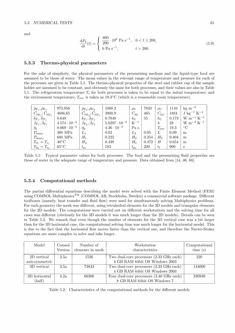
5.3. NUMERICAL TESTS 61
and
dP2
dt(t) =
600
200· 106 Pa s−1, 0 < t ≤ 200,
0 Pa s−1, t > 200.
(5.9)
5.3.3 Thermo-physical parameters
For the sake of simplicity, the physical parameters of the pressurising medium and the liquid-type food areassumed to be those of water. The mean values in the relevant range of temperature and pressure for each ofthe processes are given in Table 5.1. The thermo-physical properties of the steel and rubber cap of the sampleholder are assumed to be constant, and obviously the same for both processes, and their values are also in Table5.1. The refrigeration temperature Tr for both processes is taken to be equal to the initial temperature; andthe environment temperature, Tenv is taken as 19.3C (which is a reasonable room temperature).
ρF1, ρP1
973.856 ρF2, ρP2
1068.2 ρS 7833 ρC 1110 kg m−3
CpF1, CpP1
4686.65 CpF2, CpP2
3900.9 CpS 465 CpC 1884 J kg−1 K−1
kF1, kP1
0.649 kF1, kP2
0.7848 kS 55 kC 0.173 W m−1 K−1
βF1, βP1
4.574 · 10−4 βF2, βP2
5.0297 · 10−4 K−1 h 28 W m−2 K−1
η1 8.069 · 10−4 η2 4.36 · 10−4 Pa s Tenv 19.3 CPmax1
360 MPa L1 0.02 L2 0.05 L 0.09 mPmax2 600 MPa H1 0.222 H2 0.254 H3 0.404 mT01 = Tr1 40C H4 0.439 H5 0.472 H 0.654 mT02 = Tr2 65C tp1
183 tp2200 tf 900 s
Table 5.1: Typical parameter values for both processes. The food and the pressurising fluid properties arethose of water in the adequate range of temperature and pressure. Data obtained from [14, 46, 68].
5.3.4 Computational methods
The partial differential equations describing the model were solved with the Finite Element Method (FEM)using COMSOL MultiphysicsTM (COMSOL AB, Stockholm, Sweden) a commercial software package. Differenttoolboxes (namely, heat transfer and fluid flow) were used for simultaneously solving Multiphysics problems.For each geometry the mesh was different, using tetrahedral elements for the 3D models and triangular elementsfor the 2D models. The computations were carried out on different workstations and the solving time for allcases was different (obviously for the 3D models it was much longer than the 2D models). Details can be seenin Table 5.2. We remark that even though the number of elements for the 3D vertical case was a bit largerthan for the 3D horizontal case, the computational solving time was much longer for the horizontal model. Thisis due to the fact that the horizontal flow moves faster than the vertical one, and therefore the Navier-Stokesequations are more complex to solve and take longer.
Model Comsol Number of Workstation ComputationalVersion elements in mesh characteristics time (s)
2D vertical 3.5a 1526 Two dual-core processors (2.33 GHz each) 220axis-symmetric 4 GB RAM 64bit OS Windows 20033D vertical 3.5a 73843 Two dual-core processors (2.33 GHz each) 144000
4 GB RAM 64bit OS Windows 20033D horizontal 4.2a 66306 Four dual-core processors (3.40 GHz each) 330949
(half) 8 GB RAM 64bit OS Windows 7
Table 5.2: Characteristics of the computational methods for the different models

62 CHAPTER 5. HORIZONTAL AND VERTICAL MODELS
0 100 200 300 400 500 600 700 800 90040
42
44
46
48
50
Time (s)
Ave
rage
T p
rofil
e (°
C)
2D3D
(a) Mean temperature
40 42 44 46 48 50 5240
42
44
46
48
50
52
Temperature−2D (° C)
Tem
pera
ture
−3D
(° C
)
R2 (Pup
)= 0.96381
R2 (Phold
)= 0.98446
bisecting lineEnd PupEnd Phold
(b) Parity plot 2D/3D
38 40 42 44 46 48 50 52 54 5638
40
42
44
46
48
50
52
54
56
T 3D at θ=0
T 3
D a
t res
t θ
bisecting line
Pup (θ=π/2) R2=0.998
Pup (θ=π) R2=0.995
Pup (θ=3π/2) R2=0.996
Phold(θ=π/2) R2=0.999
Phold (θ=π) R2=0.999
Phold (θ=3π/2) R2=0.999
(c) Parity plot 3D
Figure 5.3: Different plots for 2D and 3D vertical models. Process 1
0 100 200 300 400 500 600 700 800 90065
70
75
80
Time (s)
Ave
rage
T p
rofil
e (°
C)
2D3D vertical
(a) Mean temperature
65 70 75 80 8565
70
75
80
85
Temperature−2D (° C)
Tem
pera
ture
−3D
(° C
)
R2 (Pup
)= 0.96751
R2 (Phold
)= 0.91396
bisecting lineEnd PupEnd Phold
(b) Parity plot 2D/3D
60 65 70 75 80 85 9060
65
70
75
80
85
90
T 3D at θ=0T
3D
at r
est θ
bisecting line
Pup (θ=π/2) R2=0.997
Pup (θ=π) R2=0.997
Pup (θ=3π/2) R2=0.997
Phold(θ=π/2) R2=0.998
Phold (θ=π) R2=0.998
Phold (θ=3π/2) R2=0.999
(c) Parity plot 3D
Figure 5.4: Different plots for 2D and 3D vertical models. Process 2
5.4 Numerical results and discussion
5.4.1 Comparison between 2D axis-symmetric and 3D vertical models
Firstly, we compared the results of the 2D axis-symmetric and 3D vertical models, which we expect to benearly identical. The comparison was performed in 45 locations (covering an axis-symmetric plane with a 3 x15 matrix) at three different radial coordinates (symmetry axis, 9 mm distance from symmetry axis and 18mmdistance from symmetry axis) and fifteen different heights (10 mm steps, from 6 mm above the sample holderbottom to 4 mm below the sample holder top) of the food sample region. This comparison with the samepoints was repeated for different planes in the 3D model (at angles θ = 0, π/2, π, 3π/2). The 3D temperaturevariable is taken as the average of the temperature over these different planes. A comparison of the 2D and3D Multiphysics models shows that the model outcome for the temperature was very similar. Figures 5.3a and5.4a show the average temperature over time of the 2D axis-symmetric and 3D vertical model for processes P1
and P2, respectively, with very good agreement. Figures 5.3b and 5.4b show the parity plots for the predictedtemperature from the 2D axis-symmetric and 3D vertical model for processes P1 and P2, respectively. Thecoefficient of determination R2 were greater than 0.9, for both processes, at the end of pressurisation (Pup) andat the end of the process (Phold). Figures 5.3c and 5.4c show the parity plot for the predicted temperatures ofthe 3D model along the different planes (at angles θ = 0, π/2, π, 3π/2), for processes P1 and P2, respectively.The coefficients of determination R2 were greater than 0.99, for both process, at the end of pressurisation (Pup)and at the end of the process (Phold).
We point out that the 2D axis-symmetric solution could be even more similar to the 3D vertical solution if wehad further refined the 3D mesh. However, given that our goal in this paper was to compare the 3D vertical to3D horizontal model, and taking into account the large computational time the 3D models took (see Table 5.2),

5.4. NUMERICAL RESULTS AND DISCUSSION 63
we considered that further refinements to improve the 2D axis-symmetric to 3D vertical solution similarity wasunnecessary, as the results already obtained are good enough.
5.4.2 Comparison between 3D vertical and 3D horizontal models
Let us now compare the 3D vertical and 3D horizontal models. Obviously, the results of these models will nolonger be the same. We expect the temperature to be different, due to the difference in the flow. To comparethe results from the different models, we developed a MATLAB routine to extract temperature data from themodels in COMSOL, in several configurations:
• Over the entire liquid food domain with a 1 mm3 resolution (i.e. we look at the same points for bothcases), which will give us a good idea of the overall difference in temperature performance.
• On the central radial slice of the liquid food domain for both orientations, to help visualise the spatialdifferences radially.
• For further information on spatial differences we select 5 radial slices (and points on them at 1mm2
resolution) along the height in the vertical case (starting from the bottom of the food sample holder andseparated by 0.0375m), and the same slices along the length in the horizontal case. The central radialslice of the previous point coincides with the third slice here. This will give us an idea of the temperaturebehaviour radially but also at different heights.
• Along the central axis of the food sample domain, which will help to illustrate the temperature differenceswith height at the same radial point.
For all of these data sets we plot the averaged temperature over time with standard deviations at ten timesteps for both models, and for both processes P1 and P2. Tables 5.3 and 5.4 show the temperature mean values(measure of performance) and standard deviation values (measure of uniformity) at the end of pressurisation(Pup) and end of the process (Phold), for all of these sets of data, for the 3D vertical and horizontal models, forprocess P1 and P2, respectively
We also look at slice plots of the temperature and velocity field inside the food sample and pressurising mediaat the end of the pressurisation (Pup) and also at the end of the process (Phold), separately for the vertical andhorizontal cases to illustrate the differences in temperature distribution inside the vessel and also the qualitativedifference in the flow distribution.
Process P1: Moderate temperature and pressure
Figures 5.5 and 5.6 show the slice plots for process P1 at the end of Pup and Phold for the vertical and horizontalmodel, respectively. As can be seen, the distribution for the vertical model is homogeneous in the radial directionand changes with height, whereas for the horizontal model the changes in length (equivalent to height for thevertical case) are insignificant, but there are differences in the radial direction. If we focus on a certain lengthfor the horizontal case we can see that the temperature at the top is warmer than at the bottom, which didnot happen in the vertical case (for the vertical case at a given height the temperature distribution inside thesample was more uniform). This can be explained by saying that the cooling is coming from the boundary Γr,which in the horizontal case is at the top and bottom of the sample (as it is depicted in the slice plot), but whenyou put the machine in a vertical position this boundary is at the left and right of the sample. In the verticalcase, because the cooling was coming from the sides, it affected the flow homogeneously, but now it is comingfrom above and below, and because of gravity the lower part is getting cooler faster than the top part.
For both models, at the end of Pup the differences are larger than at the end of Phold due to the fact that thepressurisation induces a heat source, so the overall temperature is larger, and hence so are the differences. At theend of Phold the sample has had enough time to cool down to the boundary temperature Tr almost everywhereand therefore the differences at different locations have reduced. Overall, the temperature of the vertical modelis higher than that of the horizontal one, especially at the end of Pup. This is due to the fact that the flowis faster in the horizontal case, and therefore the sample temperature reaches the boundary temperature at Γr
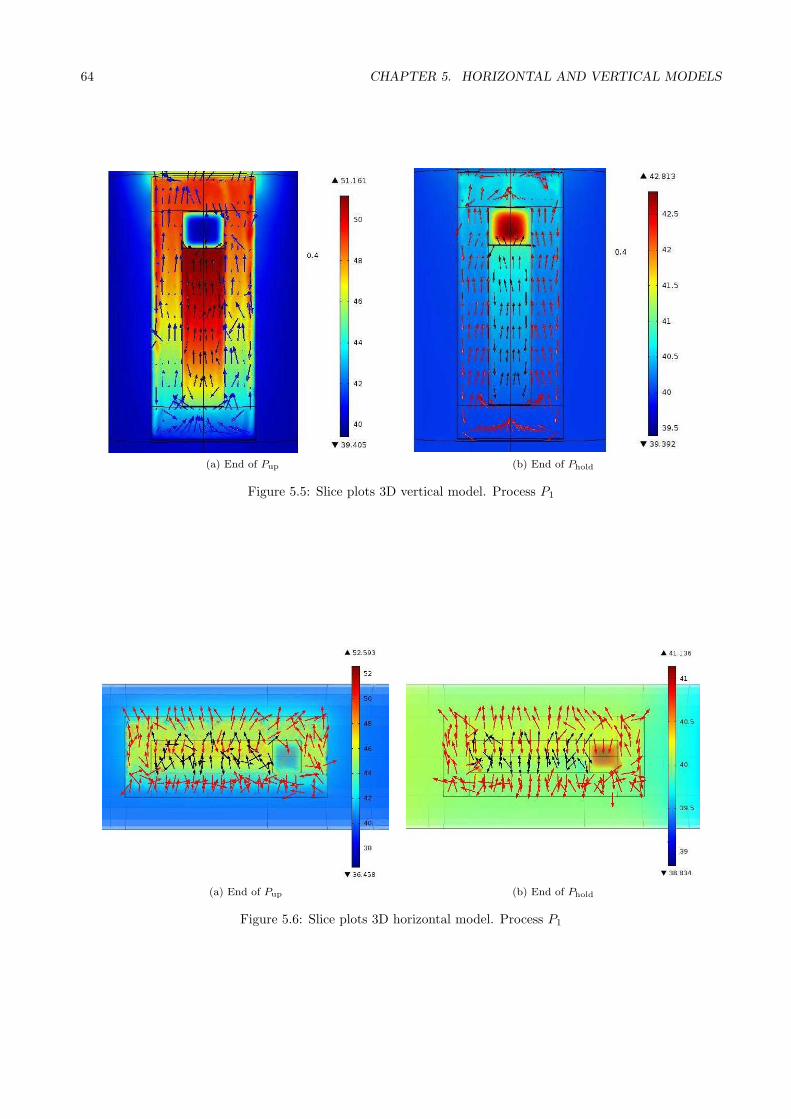
64 CHAPTER 5. HORIZONTAL AND VERTICAL MODELS
(a) End of Pup (b) End of Phold
Figure 5.5: Slice plots 3D vertical model. Process P1
(a) End of Pup (b) End of Phold
Figure 5.6: Slice plots 3D horizontal model. Process P1
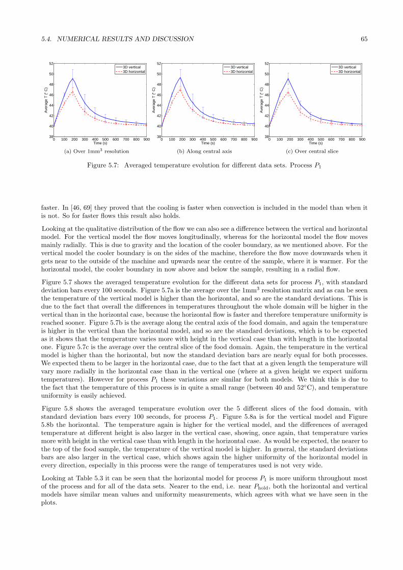
5.4. NUMERICAL RESULTS AND DISCUSSION 65
0 100 200 300 400 500 600 700 800 90038
40
42
44
46
48
50
52
Time (s)
Ave
rage
T (°
C)
3D vertical3D horizontal
(a) Over 1mm3 resolution
0 100 200 300 400 500 600 700 800 90038
40
42
44
46
48
50
52
Time (s)
Ave
rage
T (°
C)
3D vertical3D horizontal
(b) Along central axis
0 100 200 300 400 500 600 700 800 90038
40
42
44
46
48
50
52
Time (s)
Ave
rage
T (°
C)
3D vertical3D horizontal
(c) Over central slice
Figure 5.7: Averaged temperature evolution for different data sets. Process P1
faster. In [46, 69] they proved that the cooling is faster when convection is included in the model than when itis not. So for faster flows this result also holds.
Looking at the qualitative distribution of the flow we can also see a difference between the vertical and horizontalmodel. For the vertical model the flow moves longitudinally, whereas for the horizontal model the flow movesmainly radially. This is due to gravity and the location of the cooler boundary, as we mentioned above. For thevertical model the cooler boundary is on the sides of the machine, therefore the flow move downwards when itgets near to the outside of the machine and upwards near the centre of the sample, where it is warmer. For thehorizontal model, the cooler boundary in now above and below the sample, resulting in a radial flow.
Figure 5.7 shows the averaged temperature evolution for the different data sets for process P1, with standarddeviation bars every 100 seconds. Figure 5.7a is the average over the 1mm3 resolution matrix and as can be seenthe temperature of the vertical model is higher than the horizontal, and so are the standard deviations. This isdue to the fact that overall the differences in temperatures throughout the whole domain will be higher in thevertical than in the horizontal case, because the horizontal flow is faster and therefore temperature uniformity isreached sooner. Figure 5.7b is the average along the central axis of the food domain, and again the temperatureis higher in the vertical than the horizontal model, and so are the standard deviations, which is to be expectedas it shows that the temperature varies more with height in the vertical case than with length in the horizontalone. Figure 5.7c is the average over the central slice of the food domain. Again, the temperature in the verticalmodel is higher than the horizontal, but now the standard deviation bars are nearly equal for both processes.We expected them to be larger in the horizontal case, due to the fact that at a given length the temperature willvary more radially in the horizontal case than in the vertical one (where at a given height we expect uniformtemperatures). However for process P1 these variations are similar for both models. We think this is due tothe fact that the temperature of this process is in quite a small range (between 40 and 52C), and temperatureuniformity is easily achieved.
Figure 5.8 shows the averaged temperature evolution over the 5 different slices of the food domain, withstandard deviation bars every 100 seconds, for process P1. Figure 5.8a is for the vertical model and Figure5.8b the horizontal. The temperature again is higher for the vertical model, and the differences of averagedtemperature at different height is also larger in the vertical case, showing, once again, that temperature variesmore with height in the vertical case than with length in the horizontal case. As would be expected, the nearer tothe top of the food sample, the temperature of the vertical model is higher. In general, the standard deviationsbars are also larger in the vertical case, which shows again the higher uniformity of the horizontal model inevery direction, especially in this process were the range of temperatures used is not very wide.
Looking at Table 5.3 it can be seen that the horizontal model for process P1 is more uniform throughout mostof the process and for all of the data sets. Nearer to the end, i.e. near Phold, both the horizontal and verticalmodels have similar mean values and uniformity measurements, which agrees with what we have seen in theplots.
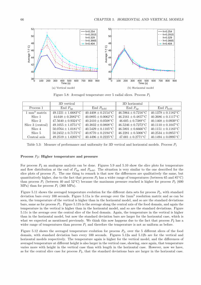
66 CHAPTER 5. HORIZONTAL AND VERTICAL MODELS
0 100 200 300 400 500 600 700 800 90038
40
42
44
46
48
50
52
Time (s)
Ave
rage
T (°
C)
h=0.254h=0.2915h=0.329h=0.3665h=0.404
(a) Vertical model
0 100 200 300 400 500 600 700 800 90038
40
42
44
46
48
50
52
Time (s)
Ave
rage
T (°
C)
h=0.254h=0.2915h=0.329h=0.3665h=0.404
(b) Horizontal model
Figure 5.8: Averaged temperature over 5 radial slices. Process P1
3D vertical 3D horizontalProcess 1 End Pup End Phold End Pup End Phold
1 mm3 matrix 49.1221± 1.6683C 40.4408± 0.2154C 46.5964± 0.7216C 40.1379± 0.1182CSlice 1 44.648± 0.2082C 40.0895± 0.0062C 46.2161± 0.4857C 40.2686± 0.1117CSlice 2 47.5640± 0.9324C 40.2410± 0.0508C 46.605± 0.7389C 40.1468± 0.0939C
Slice 3 (central) 49.1055± 1.0751C 40.3832± 0.0808C 46.5246± 0.7272C 40.1110± 0.1047CSlice 4 50.0764± 1.0181C 40.5429± 0.1105C 46.5801± 0.6666C 40.1151± 0.1183CSlice 5 50.2452± 0.7175C 40.8770± 0.2194C 46.2281± 0.5006C 40.2534± 0.0955C
Central axis 49.2519± 1.6205C 40.4496± 0.2225C 47.001± 0.2771C 40.1494± 0.0995C
Table 5.3: Measure of performance and uniformity for 3D vertical and horizontal models. Process P1
Process P2: Higher temperature and pressure
For process P2 an analogous analysis can be done. Figures 5.9 and 5.10 show the slice plots for temperatureand flow distribution at the end of Pup and Phold. The situation is very similar to the one described for theslice plots of process P1. The one thing to remark is that now the differences are qualitatively the same, butquantitatively higher, due to the fact that process P2 has a wider range of temperatures (between 65 and 85C)than process P1 (between 40 and 52C) because the maximum pressure reached is higher for process P2 (600MPa) than for process P1 (360 MPa).
Figure 5.11 shows the averaged temperature evolution for the different data sets for process P2, with standarddeviation bars every 100 seconds. Figure 5.11a is the average over the 1mm3 resolution matrix and as can beseen, the temperature of the vertical is higher than in the horizontal model, and so are the standard deviationsbars, same as for process P1. Figure 5.11b is the average along the central axis of the food domain, and again thetemperature in the vertical is higher than in the horizontal model, and so are the standard deviations. Figure5.11c is the average over the central slice of the food domain. Again, the temperature in the vertical is higherthan in the horizontal model, but now the standard deviation bars are larger for the horizontal case, which iswhat we expected as mentioned previously. We think this now happens due to the fact that process P2 has awider range of temperatures than process P1 and therefore the temperature is not as uniform as before.
Figure 5.12 shows the averaged temperature evolution for process P2, over the 5 different slices of the fooddomain, with standard deviation bars every 100 seconds. Figures 5.12a and 5.12b are for the vertical andhorizontal models respectively. The temperature again is higher for the vertical model, and the differences ofaveraged temperature at different height is also larger in the vertical case, showing, once again, that temperaturevaries more with height in the vertical case than with length in the horizontal case. However, now we have,as for the central slice case for process P2, that the standard deviations bars are larger in the horizontal case.
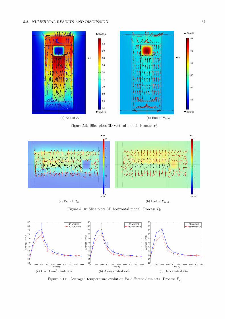
5.4. NUMERICAL RESULTS AND DISCUSSION 67
(a) End of Pup (b) End of Phold
Figure 5.9: Slice plots 3D vertical model. Process P2
(a) End of Pup (b) End of Phold
Figure 5.10: Slice plots 3D horizontal model. Process P2
0 100 200 300 400 500 600 700 800 90062
64
66
68
70
72
74
76
78
80
82
Time (s)
Ave
rage
T (°
C)
3D vertical3D horizontal
(a) Over 1mm3 resolution
0 100 200 300 400 500 600 700 800 90062
64
66
68
70
72
74
76
78
80
82
Time (s)
Ave
rage
T (°
C)
3D vertical3D horizontal
(b) Along central axis
0 100 200 300 400 500 600 700 800 90062
64
66
68
70
72
74
76
78
80
82
Time (s)
Ave
rage
T (°
C)
3D vertical3D horizontal
(c) Over central slice
Figure 5.11: Averaged temperature evolution for different data sets. Process P2
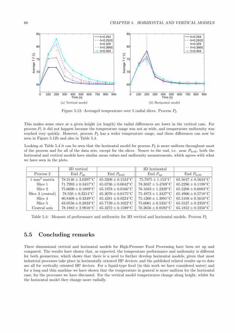
68 CHAPTER 5. HORIZONTAL AND VERTICAL MODELS
0 100 200 300 400 500 600 700 800 900
65
70
75
80
85
Time (s)
Ave
rage
T (°
C)
h=0.254h=0.2915h=0.329h=0.3665h=0.404
(a) Vertical model
0 100 200 300 400 500 600 700 800 900
65
70
75
80
85
Time (s)
Ave
rage
T (°
C)
h=0.254h=0.2915h=0.329h=0.3665h=0.404
(b) Horizontal model
Figure 5.12: Averaged temperature over 5 radial slices. Process P2
This makes sense since at a given height (or length) the radial differences are lower in the vertical case. Forprocess P1 it did not happen because the temperature range was not as wide, and temperature uniformity wasreached very quickly. However, process P2 has a wider temperature range, and these differences can now beseen in Figure 5.12b and also in Table 5.4.
Looking at Table 5.4 it can be seen that the horizontal model for process P2 is more uniform throughout mostof the process and for all of the data sets, except for the slices. Nearer to the end, i.e. near Phold, both thehorizontal and vertical models have similar mean values and uniformity measurements, which agrees with whatwe have seen in the plots.
3D vertical 3D horizontalProcess 2 End Pup End Phold End Pup End Phold
1 mm3 matrix 78.2146± 3.0297C 65.3206± 0.1524C 75.7975± 1.153C 65.5047± 0.5634CSlice 1 71.7993± 0.3457C 65.0736± 0.0042C 78.3037± 5.4769C 65.2296± 0.1198CSlice 2 75.6690± 0.1889C 65.1978± 0.0166C 76.1683± 1.2328C 65.5208± 0.6083C
Slice 3 (central) 78.550± 0.3214C 65.3076± 0.0175C 75.4973± 1.3427C 65.4906± 0.5718CSlice 4 80.8409± 0.3349C 65.4281± 0.0224C 75.1260± 1.3891C 65.5108± 0.5610CSlice 5 83.0556± 0.2833C 65.7739± 0.1022C 75.6061± 0.5331C 65.5527± 0.2359C
Central axis 78.1882± 2.9916C 65.3272± 0.1599C 76.2656± 0.8592C 65.1852± 0.2250C
Table 5.4: Measure of performance and uniformity for 3D vertical and horizontal models. Process P2
5.5 Concluding remarks
Three dimensional vertical and horizontal models for High-Pressure Food Processing have been set up andcompared. The results have shown that, as expected, the temperature performance and uniformity is differentfor both geometries, which shows that there is a need to further develop horizontal models, given that mostindustrial processes take place in horizontally oriented HP devices, and the published related results up to dateare all for vertically oriented HP devices. For a liquid-type food (in this work we have considered water) andfor a long and thin machine we have shown that the temperature in general is more uniform for the horizontalcase, for the processes we have discussed. For the vertical model temperatures change along height, whilst forthe horizontal model they change more radially.
Chapter 6
High-Pressure Shift Freezing Processes
Nomenclature for Chapter 6
B Ratio of unfrozen water to solids (constant)Cp Specific heat capacity (J kg−1 K−1)e Enthalpy (J m−3)E Weight ratio of water and solids (constant)f Mass fraction (constant)fs Mass fraction of ice (constant)g Volume fraction (constant)gb Volume fraction of solids in the food (constant)g Gravity vector (m s−2)h Heat transfer coefficient (W m−2 K−1)H Domain height (m)k Thermal conductivity (W m−1 K−1)L Domain width (m)mi Mass fraction of ice after expansion (constant)M Mass (kg)n Outward normal unit vector (m)p Mass transfer pressure (Pa)P Equipment Pressure (Pa)Patm Atmospheric pressure (Pa)Pmax Pressure before expansion (Pa)PN Nucleation pressure (Pa)r Radial coordinate (m)t Time (s)tp1
Time at which the target pressure is reached (s)tp2
Time at which we start to release pressure (s)tp3
Time at which all the pressure has been released(s)
tf Final time (s)T Temperature (K)Tenv Environment temperature (K)TF Freezing temperature of food (K)Tmin Lowest temperature before nucleation (K)Tprev Temperature before expansion (K)Tr Fixed boundary temperature (K)Tw Freezing point of water (K)u Fluid velocity vector (m s−1)V Volume (m3)x Mass fraction of solids in food (constant)z Vertical coordinate (m)
Greek symbols
αw Molar freezing point of water (kg Kmol−1)
β Thermal expansion coefficient (K−1)δe Liquid/solid enthalpy difference (J m−3)∆Tsc Extent of supercooling (K)ǫ Small time interval over which ice sud-
denly nucleates (s)γw Molecular weight of water (kg mol−1)Γ Whole domain boundaryΓr Fixed temperature boundaryΓup Heat transfer boundaryη Dynamic viscosity (Pa s)λ Latent heat (J kg−1)ρ Density (kg m−3)Ω Whole domainΩC Cap of the sample holderΩF Food sample domainΩP Pressurising mediumΩS Steel vessel
Indices
0 Initial values* Rotated domainsC Rubber capF Food domainl LiquidP Pressurising fluidref Reference values SolidS Steelvol Volumetricw Water
Acronyms
FEM Finite Element MethodHP High-PressureHPSF High-Pressure Shift Freezing2D Two-dimensional3D Three-dimensional
69
70 CHAPTER 6. HIGH-PRESSURE SHIFT FREEZING PROCESSES
6.1 Introduction
In this Chapter we describe, model and solve numerically a High-Pressure Shift Freezing (HPSF) process, basedon the published work [86]. As we will see later further ahead, modelling a general solidification problem isalready a complicated task, mainly because the interface between the solid and liquid phases moves as latent heatis liberated at the interface. All of these problems are non-linear and therefore exact solutions are extremelydifficult. In early years, analytical methods were the only means available to understand mathematically aphysical process involving the moving boundary. Although analytical methods offer an exact solution, theyhave many limitations, and thus analytical solutions are mainly for the one-dimensional cases of an infinite orsemi-infinite region with simple boundary conditions and constant thermal properties. Practical solidificationproblems are rarely one dimensional, initial and boundary conditions are always complex and thermo-physicalproperties can vary with phases, temperature, pressure, etc. For these reasons, nowadays in most engineeringapplications, the moving boundary problem is solved by means of numerical analysis. Due to the amount ofreal-world processes that involve freezing (such as, e.g., ice making, freezing of foods, solidification of metals ina cast process, etc.) and the challenge that modelling them poses, a lot of interest and research has been donein this area [15, 16, 17, 88, 74, 91].
If we focus on the freezing of food, further complications are added. One of the main problems is the highlynon-linearity of the partial differential equations, due to the sudden change of thermo-physical properties suchas specific heat and thermal conductivity around the freezing point. If the food sample has a complex shape,the progress of the freezing front can be highly unpredictable. Also, freezing is associated with large andsudden volume change, mass transfer, stress and cracking, cellular dehydration, supercooling, ice nucleationand propagation [74]. Furthermore, when modelling HP food freezing processes, the effect of pressure onthermal properties (such as latent heat, freezing point, thermal conductivity, specific heat) must also be takeninto account [20, 29, 64, 71].
All of these issues will be considered in the generalised enthalpy model for a HPSF process that we present inthis Chapter.
6.1.1 Food freezing with HP
Freezing is a widespread food preservation technology, as it ensures high food quality with long storage duration,and also because it has an extended implementation area (meat, fish, fruit, vegetables, dairy and egg products,etc.). Despite the benefits, freezing of foods can also cause undesirable changes in their texture and organolepticproperties, and its main drawback is the risk of food damage due to the formation of big ice crystals. Freezingcan be defined as the crystallisation of liquid water into its solid form (ice). Nucleation of ice is a stochasticphenomenon. However, after nucleation, crystallisation always initially occurs under a known temperaturedefined as the initial freezing temperature. Crystal characteristics (size, location) are dependent on the freezingrate (slow freezing produces large crystals, whilst rapid freezing produces small ice crystals). The general purposeof food technologists working on this area has been to develop a freezing process that creates a homogeneousmatrix of small ice crystals [20]. Improvement of known freezing methods and development of new techniques areimportant research goals for the food industry at present. With the recent increasing impact of HP technologyon food processing, there has been a lot of research dealing with the potential applications of HP effects onice-water transitions, given that pressure decreases the freezing and melting point of water to a minimum of−22C at 207.5 MPa [8]. Therefore several HP freezing and thawing processes have been developed [20, 70].
According to the path followed by the process in the phase diagram of water [8], three different types of HPfreezing processes can be distinguished in terms of the way in which the phase transition occurs [29]:
• High-Pressure Assisted Freezing (HPAF): Phase transition occurs under constant pressure, higherthan atmospheric pressure, whilst the temperature is lowered to the corresponding freezing point. Thisprocess is identical to traditional freezing at atmospheric conditions except that it takes place under HP.The process is governed by thermal gradients because the cooling of the sample proceeds from the surfaceto the centre. Ice nucleation only takes place at the outer zone of the sample, which is in direct contactwith the cooling medium. Needle-shaped ice crystals grow radially into the centre. Once the freezingplateau is complete and the sample reaches the final temperature, the pressure is released. As the latent
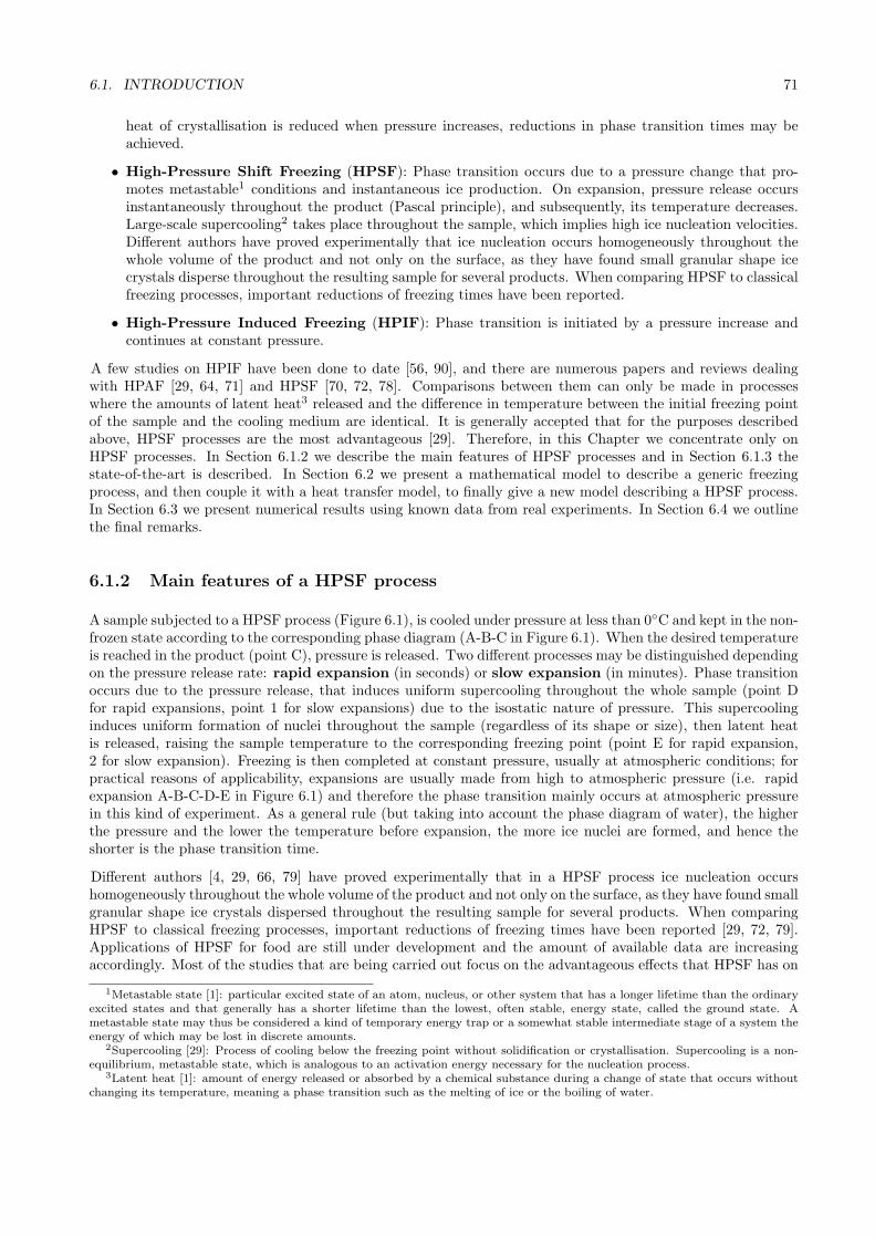
6.1. INTRODUCTION 71
heat of crystallisation is reduced when pressure increases, reductions in phase transition times may beachieved.
• High-Pressure Shift Freezing (HPSF): Phase transition occurs due to a pressure change that pro-motes metastable1 conditions and instantaneous ice production. On expansion, pressure release occursinstantaneously throughout the product (Pascal principle), and subsequently, its temperature decreases.Large-scale supercooling2 takes place throughout the sample, which implies high ice nucleation velocities.Different authors have proved experimentally that ice nucleation occurs homogeneously throughout thewhole volume of the product and not only on the surface, as they have found small granular shape icecrystals disperse throughout the resulting sample for several products. When comparing HPSF to classicalfreezing processes, important reductions of freezing times have been reported.
• High-Pressure Induced Freezing (HPIF): Phase transition is initiated by a pressure increase andcontinues at constant pressure.
A few studies on HPIF have been done to date [56, 90], and there are numerous papers and reviews dealingwith HPAF [29, 64, 71] and HPSF [70, 72, 78]. Comparisons between them can only be made in processeswhere the amounts of latent heat3 released and the difference in temperature between the initial freezing pointof the sample and the cooling medium are identical. It is generally accepted that for the purposes describedabove, HPSF processes are the most advantageous [29]. Therefore, in this Chapter we concentrate only onHPSF processes. In Section 6.1.2 we describe the main features of HPSF processes and in Section 6.1.3 thestate-of-the-art is described. In Section 6.2 we present a mathematical model to describe a generic freezingprocess, and then couple it with a heat transfer model, to finally give a new model describing a HPSF process.In Section 6.3 we present numerical results using known data from real experiments. In Section 6.4 we outlinethe final remarks.
6.1.2 Main features of a HPSF process
A sample subjected to a HPSF process (Figure 6.1), is cooled under pressure at less than 0C and kept in the non-frozen state according to the corresponding phase diagram (A-B-C in Figure 6.1). When the desired temperatureis reached in the product (point C), pressure is released. Two different processes may be distinguished dependingon the pressure release rate: rapid expansion (in seconds) or slow expansion (in minutes). Phase transitionoccurs due to the pressure release, that induces uniform supercooling throughout the whole sample (point Dfor rapid expansions, point 1 for slow expansions) due to the isostatic nature of pressure. This supercoolinginduces uniform formation of nuclei throughout the sample (regardless of its shape or size), then latent heatis released, raising the sample temperature to the corresponding freezing point (point E for rapid expansion,2 for slow expansion). Freezing is then completed at constant pressure, usually at atmospheric conditions; forpractical reasons of applicability, expansions are usually made from high to atmospheric pressure (i.e. rapidexpansion A-B-C-D-E in Figure 6.1) and therefore the phase transition mainly occurs at atmospheric pressurein this kind of experiment. As a general rule (but taking into account the phase diagram of water), the higherthe pressure and the lower the temperature before expansion, the more ice nuclei are formed, and hence theshorter is the phase transition time.
Different authors [4, 29, 66, 79] have proved experimentally that in a HPSF process ice nucleation occurshomogeneously throughout the whole volume of the product and not only on the surface, as they have found smallgranular shape ice crystals dispersed throughout the resulting sample for several products. When comparingHPSF to classical freezing processes, important reductions of freezing times have been reported [29, 72, 79].Applications of HPSF for food are still under development and the amount of available data are increasingaccordingly. Most of the studies that are being carried out focus on the advantageous effects that HPSF has on
1Metastable state [1]: particular excited state of an atom, nucleus, or other system that has a longer lifetime than the ordinaryexcited states and that generally has a shorter lifetime than the lowest, often stable, energy state, called the ground state. Ametastable state may thus be considered a kind of temporary energy trap or a somewhat stable intermediate stage of a system theenergy of which may be lost in discrete amounts.
2Supercooling [29]: Process of cooling below the freezing point without solidification or crystallisation. Supercooling is a non-equilibrium, metastable state, which is analogous to an activation energy necessary for the nucleation process.
3Latent heat [1]: amount of energy released or absorbed by a chemical substance during a change of state that occurs withoutchanging its temperature, meaning a phase transition such as the melting of ice or the boiling of water.
72 CHAPTER 6. HIGH-PRESSURE SHIFT FREEZING PROCESSES
Figure 6.1: High-pressure shift freezing processes represented over the phase diagram of water. Rapid expansionis represented by A-B-C-D-E; (slow expansion is represented by A-B-C-1-2-E). A-B is compression; B-C is pre-cooling; C-D (or in the case of slow expansion C-1) is pressure release; at D (or at 1 in the case of slowexpansion) the sample is highly supercooled – no latent heat has yet been released; for rapid expansion D-Elatent heat is released and sample temperature increases up to the corresponding freezing point at atmosphericconditions. In the case of slow expansion 1-2 latent heat is released and the sample temperature increasesup to the corresponding freezing point under pressure, 2-E the remaining pressure is released and the sampletemperature stays on the melting line.
the texture and structure of various products. In [20] the authors compared the HPSF process to a conventional(at atmospheric pressure) freezing process, and concluded that the nucleation is faster and more uniform in theHPSF processes, producing a homogeneous crystallisation and therefore a better product in terms of texture.In [29] the authors compared the HPAF and HPSF processes on gelatin gel samples and concluded that theHPSF was clearly more advantageous: shorter phase transition times and homogeneous distribution of small icecrystals throughout the sample. HPSF has been successfully applied in the processing of fruits, pork, lobsterand tofu, among other products.
6.1.3 Modelling of HPSF processes: state-of-the-art and needs
Due to the advantages of this method (mainly, its potential to improve the kinetics of the process and thecharacteristics of the ice crystals thus formed) compared to other freezing methods, apart from the publishedresearch focused on the impact of HP on quality aspects of the particular processed food, some modelling studiesconsidering the temperature evolution during treatment of HPSF processes have been published to date. This isimportant in all HP processes, as pointed out by the authors in [71], because some industrial processes have tooccur at a constant temperature or between a minimum-maximum threshold to avoid altering some propertiesof the food (gelification or crystalline state, protein stability, fat migration, freezing...) or to assure a uniformdistribution of the pursued pressure effects (microbial or enzymatic inactivation, uniform nucleation...). Inparticular, when studying HPSF processes, since phase changes are driven by both pressure and temperature,heat transfer effects play a major role in this field. Therefore the research in this area has been focused ontheoretically based heat transfer models that allow to predict the temperature history within a product freezingunder pressure.
Some notable modelling studies are those of [20], where the authors used an explicit two dimensional finitedifference scheme to simulate temperature profiles during HP freezing of a food simile (tylose) and got goodagreement with experimental data, but remarked that an improvement needed is the contribution of convection
6.2. BUILDING A NEW MODEL FOR A HPSF PROCESS 73
heat transfer by the HP fluid. In [78] the authors modelled a HPSF process of a finite cylinder using equationsbased on the crossed product of infinite slabs and infinite cylinders. The time needed to complete the precoolingand change of phase stages is reproduced satisfactorily by the model, however there are misalignments in thetempering phase because experimental and theoretical conditions were not the same, due to the thermal gradi-ents. The authors remark that for this stage a more accurate model (based on finite elements/differences) wouldbe needed. In [54] the authors performed dimensional analysis of the governing equations describing HP pro-cesses with forced and free convection, giving a general overview of thermo-fluid-dynamical mechanisms of thesekind of processes. In [64] a one dimensional finite difference numerical model based on the enthalpy formulationwas developed to simulate HP freezing of tylose, agar gel and potatoes. This model in [64] uses a version of theenthalpy equation derived for constant pressure systems, adapting it to their system by accounting for pressureeffects on the latent heat. In addition their model of freezing point depression of the food samples relies on theSchwartzberg equation [80], which was derived for dilute solutions. At the high ice fractions realised in HPSFsystems, the unfrozen gel between ice crystals is non-dilute and a more general model may be required. In thisChapter we introduce a new enthalpy model by starting from the pressure-dependent conservation of enthalpyequation and determining the non-dilute freezing point depression directly from experimental measurements.
6.2 Building a new model for a HPSF process
We propose a two dimensional axially symmetric mathematical model for a HPSF process, derived from anenthalpy formulation based on volume fractions dependent on temperature and pressure. This model is validfor solid-type foods with a large and small filling sample versus pressurising media ratio. Convection effects inthe pressurising fluid are taken into account when necessary.
In order to simulate a HPSF process, we first present a general heat transfer model in a HP process, and then wemodify it, to take into account the solidification process, by deriving a model based on the enthalpy formulationat non-constant pressure. Also, we present the equations we use to calculate the amount of ice instantaneouslyproduced just after expansion in a HPSF process, the amount of ice formed during the rest of the process, andthe liquid volume fraction. Finally, we give the complete models used to simulate a HPSF process.
6.2.1 Modelling heat transfer in a general HP process
The geometry of the HP device consider for the models derived in this Chapter is the same as the one describedin Chapter 3 (see Figure 3.2). In this Chapter, we are going to deal only with the case of solid-type foods. Firstwe study large solid-type foods, and therefore a model that only takes into account conduction effects like theone presented in Section 3.1.1 will be used. For the small solid-type foods, the model includes the convectioneffects in the pressurising medium, like the one described in Section 3.1.2.
Heat transfer for a large solid-type food
Following Section 3.3.1 the heat transfer for a large solid-type food can be modelled by the following system incylindrical coordinates
ρCp
∂T
∂t− 1
r
∂
∂r
(
rk∂T
∂r
)
− ∂
∂z
(
k∂T
∂z
)
= βdP
dtT in Ω× (0, tf),
k∂T
∂n= 0 on Γ0 × (0, tf),
k∂T
∂n= h(Tenv − T ) on Γup × (0, tf),
T = Tr on Γr × (0, tf),
T = T0 in Ω× 0.
(6.1)
74 CHAPTER 6. HIGH-PRESSURE SHIFT FREEZING PROCESSES
Heat transfer for a small solid-type food
Following Section 3.3.2 the heat transfer for a small solid-type food can be modelled by the following system
ρCp
∂T
∂t−∇ · (k∇T ) + ρCpu · ∇T = β
dP
dtT, in Ω∗ × (0, tf),
ρ∂u
∂t− η∇2u+ ρ(u · ∇)u = −∇p+ ρg in Ω ∗
P × (0, tf),
∇ · (u) = 0 in Ω∗
P × (0, tf),
k∂T
∂n= 0 on Γ∗
0 × (0, tf),
k∂T
∂n= h(Tenv − T ) on Γ∗
up × (0, tf),
T = Tr on Γ∗
r × (0, tf),
u = 0 on Γ∗
P × (0, tf),
T (0) = T0 in Ω∗,
u(0) = 0 in Ω∗,
p = 105 at A1 × (0, tf).
(6.2)
As we know from Chapter 3, system (6.2) can also be rewritten as an equivalent 2D problem by using cylindricalcoordinates (system not shown in this Chapter). The numerical experiments considered in this Chapter werecarried out using the 2D version of the corresponding equations.
In what follows, because we will be using constant thermo-physical properties throughout the rest of the Chapter,we remove the ¯ notation, and will refer to them as per usual, i.e. Cp, k, β, ρ and η.
6.2.2 Modelling a solidification process using the enthalpy formulation
In general, the difficulties of any solidification process are to control the position of the solid/liquid interface andto deal with the release of latent heat, which evolves over a very small temperature range. Crank [17] classifiesthe numerical methods for solving the ‘moving-boundary’ problem into front-tracking methods and fixed-grid
methods. The former methods may be used when there is a distinct phase change and a smooth continuousfront [91]. However, as the solid/liquid interface becomes less distinct (e.g. if it does not move smoothlyor monotonically with time), it may sometimes be difficult or even impossible to track the moving boundarydirectly. It may have sharp peaks, or it may even disappear. Therefore, the possibility of reformulating theproblem in such a way that there is no need to track the position of the solid/liquid interface, but instead it isbound up in a new form of the equations, which applies over the whole of a fixed domain, is an attractive one.These are the so called fixed-grid methods in which the position of the moving boundary appears, a posteriori,as a part of the solution.
The essential feature of the fixed-grid methods is that the latent heat evolution is accounted for in the governingenergy equation by defining either a total enthalpy, an apparent specific heat or a heat source term [91].Consequently, the numerical solution can be carried out on a space grid that remains fixed throughout thecalculations. Another advantage of these methods is that the numerical treatment of the phase change can beachieved through simple modifications of existing heat transfer numerical methods and/or software. To modelHPSF processes we use a combination of such methods, adapted to the case of non-constant pressure.
For a pure non-convecting material obeying Fourier’s law of heat conduction, conservation of enthalpy can bewritten as [7]:
∂e
∂t= ∇ · (k∇T ) +
∂P
∂t, (6.3)
where e is the enthalpy per unit volume (J m−3). If the pressure is constant equation (6.3) reduces to the
6.2. BUILDING A NEW MODEL FOR A HPSF PROCESS 75
enthalpy equation used in [91]. In the enthalpy model of a HPSF process developed in [64] the pressure termon the right-hand side of (6.3) was neglected.
In the general case of non-constant pressure the enthalpy is a function of both temperature and pressure, andfrom thermodynamics we may derive the relation (see, e.g., [26]):
de = ρCpdT + (1− βT )dP. (6.4)
Integrating (6.4) from some reference temperature Tref and reference pressure Pref to the current temperatureand pressure yields an expression for the enthalpy:
e(T, P ) = e(Tref , Pref) +
∫ T
Tref
ρCpdθ +
∫ P
Pref
(1− βT )dΠ. (6.5)
In the case of a mixed-phase region composed of ice crystals (that we will refer to here as the solid part) andthe solid and liquid part of the food that has not frozen yet (that we will refer to here as the liquid part), wemay extend previous enthalpy models based on phase fractions (see [91]) by defining a ‘mixture enthalpy’ as:
e(T, P, gl) = e(Tref , Pref , gl,ref) + (1− gl)
∫ T
Tref
ρsCpsdθ + gl
∫ T
Tref
ρlCpldθ
+(gl − gb)ρlλ+ (1− gl)
∫ P
Pref
(1− βsT )dΠ + gl
∫ P
Pref
(1− βlT )dΠ,
(6.6)
where gl is the volume fraction of the liquid part, gb is the volume fraction of solids in the food (thereforegl − gb is the volume fraction of water in the food) and λ is the latent heat of freezing of water (J kg−1).We consider that gl,ref = gb, that Tref is the temperature (K) at which all the latent heat has been released(typically Tref = −40 C= 233.15 K, see [80]), and that Pref = Patm (Pa), the atmospheric pressure. Similarly,a ‘mixture conductivity’ is defined as:
k = (1− gl)ks + glkl. (6.7)
In the previous equations subscripts [ ]s and [ ]l refer to the solid and liquid phases respectively. Taking thetotal derivative of (6.6) gives:
de = Cvol dT + (1− βvolT ) dP + δe dgl, (6.8)
where Cvol = (1 − gl)ρsCps+ glρlCpl
, δe =∫ T
Tref(ρlCpl
− ρsCps)dθ +
∫ P
PrefT (βs − βl)dΠ + ρlλ and βvol =
(1− gl)βs + glβl. Inserting (6.8) into the enthalpy equation (6.3) leads to:
Cvol∂T
∂t−∇ · (k∇T ) = βvolT
∂P
∂t− δe
∂gl∂t
. (6.9)
For a HPSF process with rapid expansion (see ABCDE in Figure 6.1), typically the pressure profile is as follows:
P (t) =
Pmax − Patm
tp1
t+ Patm t ≤ tp1,
Pmax tp1< t ≤ tp2
,
−Pmax − Patm
tp3− tp2
(t− tp2) + Pmax tp2
< t < tp3,
Patm elsewhere,
(6.10)
where tp1is the time at which the maximum pressure, Pmax, has been reached; tp2
is the time at which we startreleasing pressure; and tp3
is the time at which all the pressure has been released down to atmospheric pressure,Patm ≈ 0.1 MPa.
Experiments suggest (see [72]) that as the pressure is rapidly released (t ∈ (tp2, tp3
)), nucleation is at firstdelayed (leaving the system in a metastable state with respect to the formation of ice) until the pressure nearsatmospheric when ice suddenly nucleates and forms in some small time interval. Therefore we assume there isno ice while the pressure is changing (until t = tp3
), so during this stage equation (6.9) becomes:
ρlCpl
∂T
∂t−∇ · (k∇T ) = βlT
∂P
∂t, t ≤ tp3
. (6.11)

76 CHAPTER 6. HIGH-PRESSURE SHIFT FREEZING PROCESSES
Once the pressure has been released, ice suddenly nucleates and forms in some small time interval (ε), wherewe assume that the change in ice fraction owing to the drop in pressure is some known function of time, hencenow (6.9) becomes:
Cvol∂T
∂t−∇ · (k∇T ) = −δe
∂gl∂t
, t ∈ (tp3, tp3
+ ε), (6.12)
where now δe =∫ T
Tref(ρlCpl
− ρsCps)dθ+ ρlλ, since P = Patm. After this point and until the end of the process,
we assume that the rest of the ice is computed as a function of temperature (an explicit formula for gl is givenin Section 6.2.3), which leads to:
[
Cvol + δe
(
∂gl∂T
)]
∂T
∂t−∇ · (k∇T ) = 0, t ≥ tp3
+ ε. (6.13)
As will be shown in Section 6.3 the model given by (6.9) (equivalent, under the previous assumptions, to (6.11),(6.12) and (6.13)) yields satisfactory agreement between theory and experiment. All the parameters involvedin the model can be easily found in the literature for many food similes, except for the liquid fraction, gl. InSection 6.2.3 we explain different characteristics of a HPSF that will enable us to derive a formula for gl for agel food simile as a function of time and temperature. We note, though, that a more rigorous approach wouldbe to combine with equation (6.9) a stochastic nucleation law for gl(T, P ) quantifying the ice formed at eachinstant as the pressure is released. As no such expression for gl(T, P ) is currently available we leave this tofuture work.
6.2.3 Deriving an expression for the volume fraction gl for a gel food simile
Supercooling reached after expansion
In [72] the authors define the extent of supercooling, ∆Tsc (C), as the difference between the lowest temperature
at the sample centre just before nucleation, Tmin, and the sample freezing temperature, TF, at pressure PN, wherethe nucleation takes place. The extent of supercooling is a crucial factor in the dynamics of a freezing process.In conventional freezing at atmospheric pressure, it is generally admitted that supercooling and nucleation onlyoccurs at the surface of the sample. In [72] the authors show that in HPSF experiments, upon pressure release,a metastable state was reached throughout the sample before nucleation. As can be seen in Figure 6.1, afterexpansion from (Pmax, Tprev), the pressure/temperature coordinates of the sample move to (PN, Tmin), indicatingextensive supercooling. Therefore, the extent of supercooling only depends on the minimum temperature reachedafter expansion and on the pressure at which nucleation occurs. The minimum temperature, Tmin, reached atnucleation pressure, PN, after a rapid pressure release can be estimated according to (3.3), and is accounted forin our heat transfer model. However, the prediction of Tmin using (3.3) implies foreknowledge of the nucleationpressure PN, and this is, in general, very difficult due to the stochastic nature of the nucleation phenomenon.In Section 6.2.3 we explain how to avoid this problem.
Modelling the amount of ice formed instantaneously after expansion
In [72] the authors explain that the pressure release in HPSF processes can be divided, ideally, in two differentphases (see Figure 6.1). In the first phase, expansion takes place under metastable conditions. A percentageof water is instantaneously frozen when PN is reached. The latent heat raises the sample temperature to thecorresponding freezing point. The amount of ice formed at PN can be calculated from the following equation(other equations are given in [72]):
miλ(PN) = (miCpi+ (1−mi)Cpw
)∆Tsc, (6.14)
where mi is the mass fraction of ice (defined as mass of ice divided by initial mass of water) formed afterexpansion, Cpi
(J kg−1 C−1) is the specific heat capacity of ice at the nucleation pressure (taken as the meanvalue of the specific heat capacity at the minimum temperature reached after expansion and the specific heatcapacity at the corresponding melting point), Cpw
(J kg−1 C−1) is the specific heat capacity of water at the
6.2. BUILDING A NEW MODEL FOR A HPSF PROCESS 77
nucleation pressure (taken as the mean value of the specific heat capacity at the minimum temperature reachedafter expansion and the specific heat capacity at the corresponding melting point), ∆Tsc (C) is the extent ofsupercooling, and λ(PN) (J kg−1) is the latent heat at nucleation pressure PN.
Latent heat of freezing of water (J kg−1) as a function of pressure P (MPa) can be estimated by the followingequation (for more details, see [72]):
λ(P ) = 3.114× 10⁻³P 3 − 1.292P 2 − 3.379× 10²P + 3.335× 10⁵. (6.15)
Therefore, we can calculate the percentage of instantaneously frozen water, mi, by using equations (6.14) and(6.15), taking into account the extent of supercooling attained and the latent heat released at nucleation pressure.However, this is just a theoretical evaluation and it is not useful for modelling purposes because experimentaldata of nucleation pressure and temperature during expansion (PN, Tmin) are needed and, as was pointed outin Section 6.2.3, it is in general very difficult to predict the nucleation pressure. To overcome this problem,in [72] the authors proposed a simplified method for HPSF processes with rapid expansions: to assume thatnucleation occurs at atmospheric pressure. On this basis, by using experimental pressure and temperature valuesimmediately prior to expansion (Pmax, Tprev), instead of (PN, Tmin), the amount of ice formed after expansioncan be determined. They do as follows: the minimum temperature after expansion, Tmin, is calculated using(3.3); the corresponding supercooling is attained as ∆Tsc = TF −Tmin; equation (6.15) is used to calculated thelatent heat released at atmospheric pressure, and finally we introduced these values in (6.14) to determine thepercentage of ice instantaneously formed in HPSF experiments with rapid expansions. We use this simplificationin our simulations.
Modelling the mass fraction of ice of the rest of the process
Once we have calculated the amount of ice formed instantaneously after expansion, we need an expression tocalculate how the rest of the ice is formed as a function of temperature. As it occurs at atmospheric pressure,we do not have to worry about taking into account pressure effects this time. After expansion, an amount mi
of ice is instantaneously formed, which can be calculated, as we explained in Section 6.2.3. The temperature israised to the corresponding freezing point at atmospheric pressure due to the release of latent heat.
Remark 9. The mass fraction of ice fs as a function of temperature can be calculated with the followingexpression:
fs(T ) = 1− x0/x(T ), (6.16)
where x0 is the initial mass fraction of solids in the food and x(T ) is the mass fraction of solids in the food(without including the ice generated after the initial reference instant) at temperature T .
This can be easily seen by taking m as the initial mass of solids, mw0the initial mass of water and mw(T ) be
the mass of water in the food at temperature T , then:
x0 =m
m+mw0
, x(T ) =m
m+mw(T )
and therefore:
1− x0/x(T ) = 1− m+mw(T )
m+mw0
=mw0
−mw(T )
m+mw0
=mass of ice
total mass= fs(T )
Next we derive an equation for x(T ). In [75], the following extended Clausius-Clapeyron equation is presentedto calculate the freezing point depression (Tw − T ) of gel, as a function of mass fraction of solids (x):
Tw − T = −αw
γwln
(
1− x−Bx
1− x−Bx+ Ex
)
. (6.17)
In (6.17) Tw is the freezing point of water at atmospheric pressure (i.e. 0C), T is the freezing point of thefood (C), αw is the molar freezing point constant of water (1860 kg K mol−1), γw is the molecular weight ofwater (18 kg mol−1), E is the molecular weight ratio of water and solids (γw/γs) and B is the ratio of unfrozen
78 CHAPTER 6. HIGH-PRESSURE SHIFT FREEZING PROCESSES
water to total solids. E and B are model parameters that the authors of [75] estimate using SAS non-linearregression.
From (6.17) we can calculate the freezing point depression depending on the mass fraction of solids, but wewant to calculate the inverse, i.e., given a certain freezing point temperature T , what is the mass fraction ofsolids at that temperature. From (6.17) it is easy to find an expression for x as a function of T :
x(T ) =exp
γwαw
(T−Tw) −1
expγwαw
(T−Tw)(1 +B − E)− 1−B. (6.18)
Substituting (6.18) into (6.16) we finally get the equation for the mass fraction of ice as a function of temperature:
fs(T ) =exp
γwαw
(T−Tw) −1− x0(expγwαw
(T−Tw)(1 +B − E)− 1−B)
expγwαw
(T−Tw) −1. (6.19)
Expression for the volume fractions
In our model we work with volume fractions instead of mass fractions. The relation between them is given inthe following remark.
Remark 10. In a mixture of two phases the volume fractions (gl, gs) as functions of the mass fractions (fl, fs)are:
gl =flρs
flρs + fsρl, gs =
fsρlfsρl + flρs
. (6.20)
The density of the mixture can be written as ρ = ρlgl+ρsgs and the relationships between the mass and volumefractions in liquid and solid phases are:
fl =ρlglρ
, fs =ρsgsρ
.
As ρ = ρlglfl
and also ρ = ρlgl + ρsgs = gl(ρl − ρs) + ρs, after some straight forward calculations we have that:
gl =flρs
fsρl + flρsand gs = 1− gl = 1− flρs
fsρl + flρs=
fsρlfsρl + flρs
.
As we said in Section 6.2.2, the liquid and solid volume fractions for our model depend on temperature andtime. For a classical freezing process they are considered to be only dependent on temperature, but in a HPSFprocess we have information a priori about when the sample starts to freeze. We know that the sample remainsunfrozen (even at subzero temperatures) until the pressure has been completely released (i.e. at t = tp3
), andat that point there is a percentage of ice instantaneously formed, mi, the mass of which we calculate using(6.14) and (6.15). After this point, the rest of the ice, fs(T ), is computed as a function of temperature following(6.19). We consider that the initial mass of solids in the food is the one before the expansion plus the mass ofice instantaneously formed after releasing pressure. Therefore, we take x0 = fb + (fl − fb)mi, where fb is themass fraction of solids in the food and fl is the mass fraction of liquid in the food. Finally, we have that:
gl(t, T ) =
1 t ≤ tp3,
1−(
miρlmiρl + (1−mi)ρs
)
t− tp3
εtp3
< t < tp3+ ε,
1− fs(T )ρlfs(T )ρl + (1− fs(T ))ρs
t ≥ tp3+ ε,
(6.21)
where ε is the small time interval in which the mass fraction mi of ice is instantaneously formed after thepressure release.
6.2.4 Resulting full model for a HPSF process
We focus on two different situations: HPSF of a large solid-type food and a small solid-type food.
6.3. NUMERICAL TESTS 79
For a large solid-type food
We use system (6.1), but we replace the first equation with (6.9), resulting in:
Cvol∂T
∂t− 1
r
∂
∂r
(
rk∂T
∂r
)
− ∂
∂z
(
k∂T
∂z
)
= βvoldP
dtT − δe
∂gl∂t
in Ω× (0, tf),
k∂T
∂n= 0 on Γ0 × (0, tf),
k∂T
∂n= h(Tenv − T ) on Γup × (0, tf),
T = Tr on Γr × (0, tf),
T = T0 in Ω× 0,
(6.22)
where gl is given by (6.21), P is given by (6.10), and Cvol, δe, k, βvol are defined in Section 6.2.2.
For a small solid-type food
We use system (6.2), but we change the first equation for (6.9) plus the convective term of (6.2), resulting in:
Cvol∂T
∂t−∇ · (k∇T ) + ρCpu · ∇T = βvol
dP
dtT − δe
∂gl∂t
in Ω∗ × (0, tf),
ρ∂u
∂t− η∇2u+ ρ(u · ∇)u = −∇p+ ρg in Ω ∗
P × (0, tf),
∇ · (u) = 0 in Ω∗
P × (0, tf),
k∂T
∂n= 0 on Γ∗
0 × (0, tf),
k∂T
∂n= h(Tenv − T ) on Γ∗
up × (0, tf),
T = Tr on Γ∗
r × (0, tf),
u = 0 on Γ∗
P × (0, tf),
T (0) = T0 in Ω∗,
u(0) = 0 in Ω∗,
p = 105 at A1 × (0, tf).
(6.23)
We point out that in these considered cases (that is, for solid and liquid-type foods) the pressurising medium usedin HPSF processes does not freeze (therefore gl = 1 in ΩP). For both cases, in order to reduce computationalcomplexity, as explained in Chapter 3, we have assumed that the thermo-physical properties of the food sampleare constant, but different in the unfrozen and frozen states. The thermo-physical properties of the steel andthe rubber cap remain constant during the whole process (gl = 1 in those domains). We have also assumedthat the thermo-physical properties of the pressurising fluid are constant for the large sample case, and for thesmall sample case, they are all constant except for ρ which is chosen as a constant value everywhere except inthe gravitational force (i.e. we are using the Boussinesq approximation previously explained).
6.3 Numerical tests
We consider for the numerical tests the size of the pilot unit described in Chapter 3. The dimensions of themachine are L = 0.09 m, H = 0.654 m, L2 = 0.05 m, H1 = 0.222 m and H5 = 0.472 m (see Figure 3.2). Wesimulate in this section the two cases described in Section 6.2.4. The size and location of the sample and the
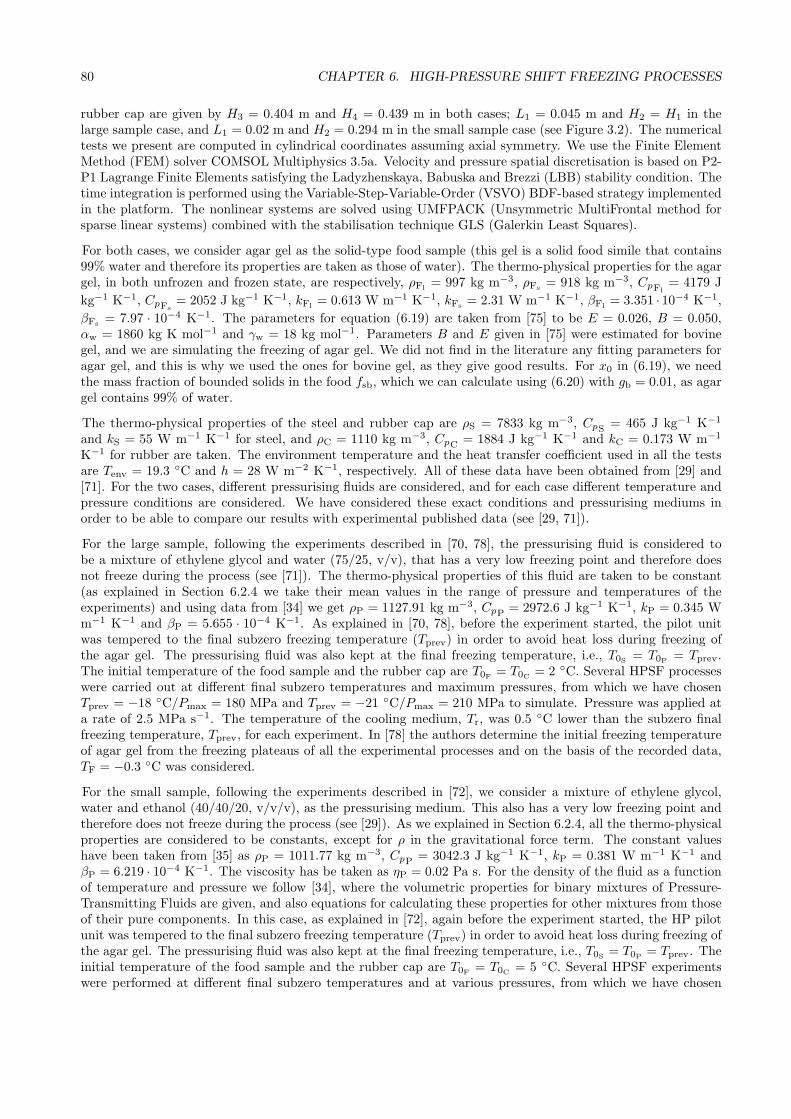
80 CHAPTER 6. HIGH-PRESSURE SHIFT FREEZING PROCESSES
rubber cap are given by H3 = 0.404 m and H4 = 0.439 m in both cases; L1 = 0.045 m and H2 = H1 in thelarge sample case, and L1 = 0.02 m and H2 = 0.294 m in the small sample case (see Figure 3.2). The numericaltests we present are computed in cylindrical coordinates assuming axial symmetry. We use the Finite ElementMethod (FEM) solver COMSOL Multiphysics 3.5a. Velocity and pressure spatial discretisation is based on P2-P1 Lagrange Finite Elements satisfying the Ladyzhenskaya, Babuska and Brezzi (LBB) stability condition. Thetime integration is performed using the Variable-Step-Variable-Order (VSVO) BDF-based strategy implementedin the platform. The nonlinear systems are solved using UMFPACK (Unsymmetric MultiFrontal method forsparse linear systems) combined with the stabilisation technique GLS (Galerkin Least Squares).
For both cases, we consider agar gel as the solid-type food sample (this gel is a solid food simile that contains99% water and therefore its properties are taken as those of water). The thermo-physical properties for the agargel, in both unfrozen and frozen state, are respectively, ρFl
= 997 kg m−3, ρFs= 918 kg m−3, CpFl
= 4179 J
kg−1 K−1, CpFs= 2052 J kg−1 K−1, kFl
= 0.613 W m−1 K−1, kFs= 2.31 W m−1 K−1, βFl
= 3.351 · 10−4 K−1,
βFs= 7.97 · 10−4 K−1. The parameters for equation (6.19) are taken from [75] to be E = 0.026, B = 0.050,
αw = 1860 kg K mol−1 and γw = 18 kg mol−1. Parameters B and E given in [75] were estimated for bovinegel, and we are simulating the freezing of agar gel. We did not find in the literature any fitting parameters foragar gel, and this is why we used the ones for bovine gel, as they give good results. For x0 in (6.19), we needthe mass fraction of bounded solids in the food fsb, which we can calculate using (6.20) with gb = 0.01, as agargel contains 99% of water.
The thermo-physical properties of the steel and rubber cap are ρS = 7833 kg m−3, CpS = 465 J kg−1 K−1
and kS = 55 W m−1 K−1 for steel, and ρC = 1110 kg m−3, CpC = 1884 J kg−1 K−1 and kC = 0.173 W m−1
K−1 for rubber are taken. The environment temperature and the heat transfer coefficient used in all the testsare Tenv = 19.3 C and h = 28 W m−2 K−1, respectively. All of these data have been obtained from [29] and[71]. For the two cases, different pressurising fluids are considered, and for each case different temperature andpressure conditions are considered. We have considered these exact conditions and pressurising mediums inorder to be able to compare our results with experimental published data (see [29, 71]).
For the large sample, following the experiments described in [70, 78], the pressurising fluid is considered tobe a mixture of ethylene glycol and water (75/25, v/v), that has a very low freezing point and therefore doesnot freeze during the process (see [71]). The thermo-physical properties of this fluid are taken to be constant(as explained in Section 6.2.4 we take their mean values in the range of pressure and temperatures of theexperiments) and using data from [34] we get ρP = 1127.91 kg m−3, CpP = 2972.6 J kg−1 K−1, kP = 0.345 Wm−1 K−1 and βP = 5.655 · 10−4 K−1. As explained in [70, 78], before the experiment started, the pilot unitwas tempered to the final subzero freezing temperature (Tprev) in order to avoid heat loss during freezing ofthe agar gel. The pressurising fluid was also kept at the final freezing temperature, i.e., T0S = T0P = Tprev.The initial temperature of the food sample and the rubber cap are T0F = T0C = 2 C. Several HPSF processeswere carried out at different final subzero temperatures and maximum pressures, from which we have chosenTprev = −18 C/Pmax = 180 MPa and Tprev = −21 C/Pmax = 210 MPa to simulate. Pressure was applied ata rate of 2.5 MPa s−1. The temperature of the cooling medium, Tr, was 0.5 C lower than the subzero finalfreezing temperature, Tprev, for each experiment. In [78] the authors determine the initial freezing temperatureof agar gel from the freezing plateaus of all the experimental processes and on the basis of the recorded data,TF = −0.3 C was considered.
For the small sample, following the experiments described in [72], we consider a mixture of ethylene glycol,water and ethanol (40/40/20, v/v/v), as the pressurising medium. This also has a very low freezing point andtherefore does not freeze during the process (see [29]). As we explained in Section 6.2.4, all the thermo-physicalproperties are considered to be constants, except for ρ in the gravitational force term. The constant valueshave been taken from [35] as ρP = 1011.77 kg m−3, CpP = 3042.3 J kg−1 K−1, kP = 0.381 W m−1 K−1 andβP = 6.219 · 10−4 K−1. The viscosity has be taken as ηP = 0.02 Pa s. For the density of the fluid as a functionof temperature and pressure we follow [34], where the volumetric properties for binary mixtures of Pressure-Transmitting Fluids are given, and also equations for calculating these properties for other mixtures from thoseof their pure components. In this case, as explained in [72], again before the experiment started, the HP pilotunit was tempered to the final subzero freezing temperature (Tprev) in order to avoid heat loss during freezing ofthe agar gel. The pressurising fluid was also kept at the final freezing temperature, i.e., T0S = T0P = Tprev. Theinitial temperature of the food sample and the rubber cap are T0F = T0C = 5 C. Several HPSF experimentswere performed at different final subzero temperatures and at various pressures, from which we have chosen
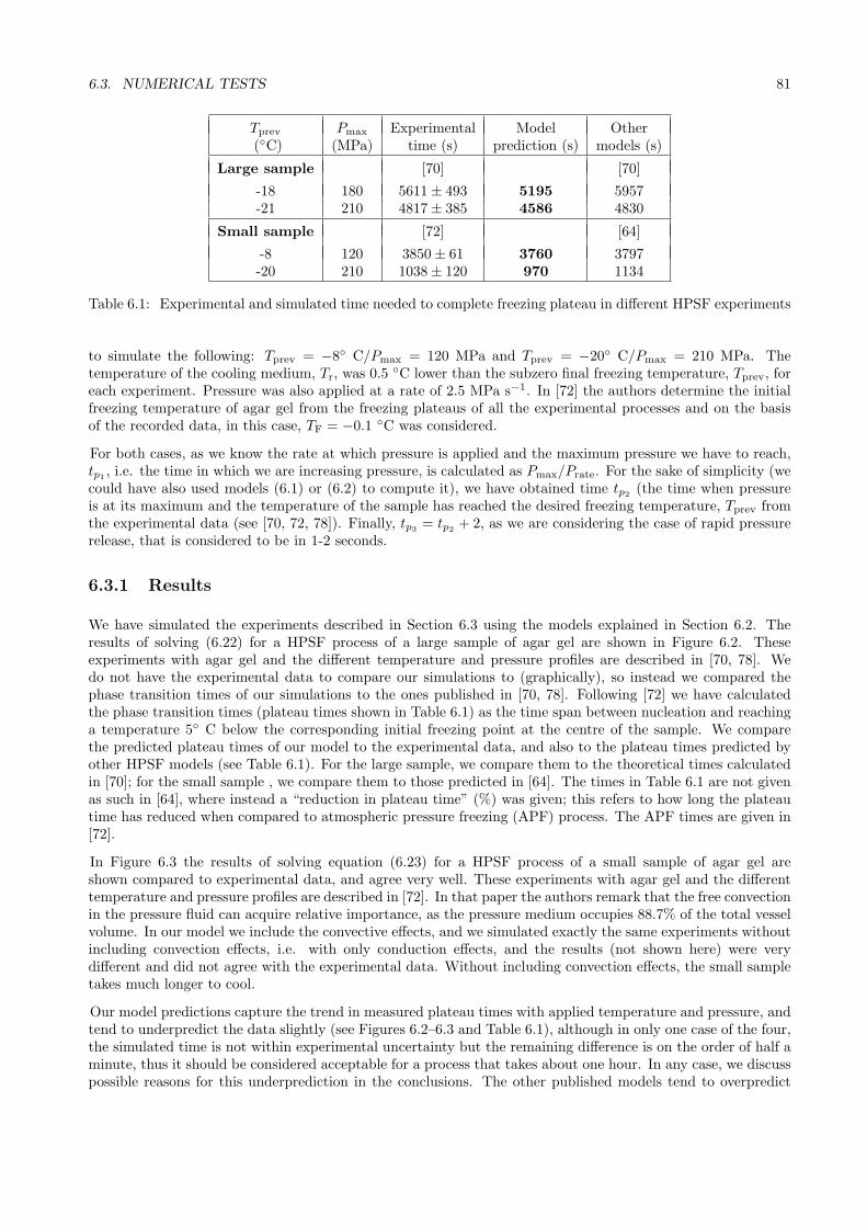
6.3. NUMERICAL TESTS 81
Tprev Pmax Experimental Model Other(C) (MPa) time (s) prediction (s) models (s)
Large sample [70] [70]
-18 180 5611± 493 5195 5957-21 210 4817± 385 4586 4830
Small sample [72] [64]
-8 120 3850± 61 3760 3797-20 210 1038± 120 970 1134
Table 6.1: Experimental and simulated time needed to complete freezing plateau in different HPSF experiments
to simulate the following: Tprev = −8 C/Pmax = 120 MPa and Tprev = −20 C/Pmax = 210 MPa. Thetemperature of the cooling medium, Tr, was 0.5
C lower than the subzero final freezing temperature, Tprev, foreach experiment. Pressure was also applied at a rate of 2.5 MPa s−1. In [72] the authors determine the initialfreezing temperature of agar gel from the freezing plateaus of all the experimental processes and on the basisof the recorded data, in this case, TF = −0.1 C was considered.
For both cases, as we know the rate at which pressure is applied and the maximum pressure we have to reach,tp1
, i.e. the time in which we are increasing pressure, is calculated as Pmax/Prate. For the sake of simplicity (wecould have also used models (6.1) or (6.2) to compute it), we have obtained time tp2
(the time when pressureis at its maximum and the temperature of the sample has reached the desired freezing temperature, Tprev fromthe experimental data (see [70, 72, 78]). Finally, tp3
= tp2+ 2, as we are considering the case of rapid pressure
release, that is considered to be in 1-2 seconds.
6.3.1 Results
We have simulated the experiments described in Section 6.3 using the models explained in Section 6.2. Theresults of solving (6.22) for a HPSF process of a large sample of agar gel are shown in Figure 6.2. Theseexperiments with agar gel and the different temperature and pressure profiles are described in [70, 78]. Wedo not have the experimental data to compare our simulations to (graphically), so instead we compared thephase transition times of our simulations to the ones published in [70, 78]. Following [72] we have calculatedthe phase transition times (plateau times shown in Table 6.1) as the time span between nucleation and reachinga temperature 5 C below the corresponding initial freezing point at the centre of the sample. We comparethe predicted plateau times of our model to the experimental data, and also to the plateau times predicted byother HPSF models (see Table 6.1). For the large sample, we compare them to the theoretical times calculatedin [70]; for the small sample , we compare them to those predicted in [64]. The times in Table 6.1 are not givenas such in [64], where instead a “reduction in plateau time” (%) was given; this refers to how long the plateautime has reduced when compared to atmospheric pressure freezing (APF) process. The APF times are given in[72].
In Figure 6.3 the results of solving equation (6.23) for a HPSF process of a small sample of agar gel areshown compared to experimental data, and agree very well. These experiments with agar gel and the differenttemperature and pressure profiles are described in [72]. In that paper the authors remark that the free convectionin the pressure fluid can acquire relative importance, as the pressure medium occupies 88.7% of the total vesselvolume. In our model we include the convective effects, and we simulated exactly the same experiments withoutincluding convection effects, i.e. with only conduction effects, and the results (not shown here) were verydifferent and did not agree with the experimental data. Without including convection effects, the small sampletakes much longer to cool.
Our model predictions capture the trend in measured plateau times with applied temperature and pressure, andtend to underpredict the data slightly (see Figures 6.2–6.3 and Table 6.1), although in only one case of the four,the simulated time is not within experimental uncertainty but the remaining difference is on the order of half aminute, thus it should be considered acceptable for a process that takes about one hour. In any case, we discusspossible reasons for this underprediction in the conclusions. The other published models tend to overpredict
82 CHAPTER 6. HIGH-PRESSURE SHIFT FREEZING PROCESSES
0 0.25 0.5 0.75 1 1.25 1.5 1.75 2 2.25 2.5x 10
4
−25
−20
−15
−10
−5
0
5
10
Plateau time=5195 s
Time (s)
Tem
pera
ture
(ºC
)
Big sample (Pmax
=180 MPa, Tprev
=−18ºC)
r=0
r=0.01
r=0.02
r=0.035
0 0.25 0.5 0.75 1 1.25 1.5 1.75 2 2.25 2.5 2.75 3x 10
4
−25
−20
−15
−10
−5
0
5
10
Big sample (Pmax
=210 MPa, Tprev
=−21ºC)
Plateau time=4586.5 s
Time (s)
Tem
pera
ture
(ºC
)
r=0
r=0.01
r=0.02
r=0.035
Figure 6.2: Temperature evolution at different radial locations of a large agar sample during a HPSF processfor different temperature and pressure conditions. All results are predicted values from model (6.22).

6.3. NUMERICAL TESTS 83
0 2000 4000 6000 8000 10000
−10
−5
0
5
Surface
Centre Plateau time=3760 s
Small sample (Pmax
=120 MPa, Tprev
=−8ºC)
Time (s)
Tem
pera
ture
(ºC
)
0 2000 4000 6000 8000 10000
−20
−10
0
10
Surface
Centre Plateau time=970 s
Small sample (Pmax
=210 MPa, Tprev
=−20ºC)
Time (s)
Tem
pera
ture
(ºC
)
Figure 6.3: Temperature evolution at the centre and surface of a small agar sample during a HPSF process fordifferent temperature and pressure conditions. (–) predicted values from model (6.23); (∗) experimental data.
84 CHAPTER 6. HIGH-PRESSURE SHIFT FREEZING PROCESSES
the plateau times slightly, but also give quite satisfactory results. However, we remark that the authors in [70]calculated the plateau times taking into account the amount of ice instantaneously produced after expansion,and the time required to freeze the sample at atmospheric pressure, but did not obtain them as a result froma heat transfer model. In [64], for the small sample case, the authors proposed a one dimensional heat transfermodel for the food sample, but they did not model the heat transfer in the pressurising medium. They assumeda boundary condition of the third class at the surface between the food and the pressurising fluid, and had tochoose the surface heat transfer coefficient to best fit the experimental curve, i.e. they had a fitting parameter.Also, they did not validate the precooling stage, so their model is validated only from the temperature at whichthe pressure was released.
6.4 Conclusions
The models described in this Chapter provide a useful tool to simulate the temperature profile at all pointsinside both large and small solid food samples going through a HPSF process. The model for solidificationis based on the enthalpy formulation at non-constant pressure and volume phase fractions. The models aretwo dimensional axis-symmetric, and can therefore predict the temperature distribution at any point inside thefood sample, not just at any radial component, which happens with one dimensional models, but also at anyheight. Convection effects in the pressurising fluid are considered for the small sample case (and shown to beimportant).
For the small sample case, the numerical tests agree with the experimental data very well, especially at thecentre of the sample. We emphasise that no fitting parameters were used in the simulations. At the surfacethere is not an accurate match between the data and the model. However we consider that the modelling effortsare good enough, given the relatively large experimental errors. It is important to point out, that locating athermocouple exactly at the surface is very difficult, and often generates significant measurement errors comingfrom the neighbouring material temperature, which is colder than the food sample. For the large sample case,there is no experimental data to plot against the simulated temperature profile, but the results look verysimilar to the temperature profiles plotted in [78]. When comparing the model plateau times to the publishedexperimental ones, we find that they are in general shorter, but in the range of the latter. In all cases, theprediction errors are on the order of minutes, which is not too bad given that the processing time is on theorder of hours.
Future improvements, in case experimental measurements become more precise, could potentially be obtainedby including temperature and pressure dependence of material properties, anisotropy effects in the frozen region,and extending our 2D convection simulations to 3D.
Chapter 7
Growth and coarsening of ice crystals
Nomenclature for Chapter 7
CRi Coefficients for radii in numerical scheme (µms−1)
Cvice Coefficients for ice volume concentration in nu-merical scheme (s−1)
dt Time step for numerical scheme (s)G System Gibb’s free energy (eV)Iin / Iout Molecule inward / outward flow (µm−2s−1)k Boltzmann constant (eV K−1)K Surface reaction rate (µm s−1)L Latent heat (eV per molecule)M Mass (mg)n Molecular number concentration (µm−3)N Number of molecules in the systemnmax (2νhyd + νoxy)
−1 (µm−3)r minimum ice particle radiusR Ice particle–cluster radius (µm)S Surface (µm2)t Time (s)T Temperature (K)t Time when the melting temperature reaches
the experimental temperature and no more iceprecipitates (s)
v Volume concentration (dimensionless)V Volume (µm3)x Mass concentration (mg µm−3)
Acronyms
APF Atmospheric pressure freezingHPSF High-Pressure Shift freezing
Greek symbols
β Rate of change of µs.water with respectto xs (eV µm3 mg−1 per molecule)
γ Surface energy per unit area (eVµm−2)
µ Chemical potential (eV per molecule)ν Molecular or atomic volume (µm3)ε Cohesive energy (eV per molecule)
Other symbols
〈f〉 mean value of the set fii
Indices
0 Initial modelling timecl Ice particle–clusterexp experimentalGT Gibbs–Thomsonhyd Hydrogeni Ice particles indexice Non precipitated icemelt Meltmf Mean fieldOR Ostwald Ripeningoxy Oxygens Salts.water Salty waterthr Thresholdwater Pure water
7.1 Motivation for studying growth and coarsening of ice particles
After studying High Pressure Shift Freezing (HPSF) processes in Chapter 6 it is clear that HPSF is a goodmethod to produce frozen food with small ice crystal size that are uniformly distributed, and therefore, withreduced tissue damage and higher overall quality [30].
The goal of this Chapter, which is based on the work from [83], is to develop a model to study the growth andcoarsening of ice particles in a frozen food sample, and hence look at the temporal evolution of HPSF frozen ice
85
86 CHAPTER 7. GROWTH AND COARSENING OF ICE CRYSTALS
crystals. This idea came from the work published in [30], where the authors investigated if HPSF frozen systemsfollow the same ice recrystallisation kinetics than those conventionally frozen (at atmospheric conditions). Forthis the authors of [30] designed a system which could hold HPSF frozen samples of suitable size for microscopicobservation without their alteration. Then using direct microscopic examination at different temperatures, theycould follow the evolution of ice crystals with time and study the influence of the freezing method and storagetemperature on recrystallisation. In [30] a 1.86N NaCl solution was used as a food model sample. For thisreason, we model a very simple system consisting of salty water. If we assume that initially the ice particles arehomogeneously distributed and have spherical shape, which occurs with a HPSF frozen sample as explained inChapter 6, our model is valid for any kind of freezing process and not only HPSF. This will allow us to comparethe evolution of HPSF frozen samples to that of samples that have been classically frozen.
In Section 7.2 we describe how to calculate the melting temperature of salty water and show some expressionsregarding the salt mass concentration and the volume concentration of dissolved ice. In Section 7.3 we presenta model that accounts for the growth and ripening of ice crystals in this simple system by developing a theorysomewhat similar to Ostwald ripening [9]. Our model predicts crystal size evolution with time, and also icecrystal size distribution. In Section 7.4 we describe the numerical simulations we have performed and in Section7.5 we present the particular numerical experiments and results for salty water and ice-cream. In Section 7.6we outline the conclusions.
7.2 Melting temperature of salty water
Consider a system consisting of salty water at an experimental temperature Texp. If the temperature is lowenough (below the melting point) the system has a potential to produce a certain amount of ice (which dependson the temperature [6]) via isothermal crystallisation. Let us assume that at time t0 (s) the system hasalready produced part of this ice, which has precipitated in spherical particles of radii Ri (µm). For modellingpurposes it is also convenient to assume that all the ice which can potentially still precipitate, is, at time t0,initially dissolved in salty water, without it having precipitated yet. Such consideration allows developing atheory somewhat similar to Ostwald ripening to account for both growth and coarsening of the pre-existingice particles. During some time there will be two physical processes occuring: growth of ice particles due tothe new ice that is being produced (since the experimental temperature is below the melting temperature) andripening between ice particles.
As we will see below, the salt concentration increases along the process pushing the melting temperature Tmelt
down towards Texp. At some instant t (s), Tmelt(t) (K) reaches the experimental temperature Texp, no more iceis produced and Tmelt(t) = Texp for any t ≥ t. Therefore, for t ≥ t only ripening takes place. Our goal in thisChapter is to study the evolution of the ice particles present in the system for times t ∈ [t0,∞).
Let us suppose that at time t (s) the system is composed of salty water, spherical (for simplicity) precipitatedice particles of radii Ri(t) (µm) larger than a minimum value r (for instance, the minimal radius than ourexperimental equipment is able to measure). Figure 7.1 shows a graphical description of the system.
Let us also assume that the system has a salt mass concentration given by
xs(t) =Ms
Vs.water + Vice(t), (7.1)
where Ms (mg) is the total salt mass dissolved in water and non-precipitated dissolved ice, Vs.water (µm3) isthe volume occupied by salty water that is not part of the non-precipitated ice dissolved in water, and Vice(t)(µm3) is the volume occupied by the non-precipitated ice dissolved in water.
First we illustrate the dependence of the melting temperature upon the salt concentration. Looking at theinteraction between salty water and non–dissolved ice in thermodynamic equilibrium, at melting temperatureTmelt(xs) the chemical potentials of H2O molecules in the non-precipitated ice (µice) and in salty water (µs.water)are equal.
Ice forms very compact structures avoiding H2O molecules to move in void space. Therefore we can neglectentropy and, assuming it does not contain any salt, its chemical potential (measured in eV per molecule) is

7.2. MELTING TEMPERATURE OF SALTY WATER 87
Figure 7.1: Salty water system configuration.
given byµice = −εice (7.2)
which is constant for the range of temperatures and pressures under consideration, where εice (measured in eVper molecule) is the cohesive energy of H2O molecules in ice, i.e. the inter–molecular energy required to breakall the bonds associated with one molecule.
On the other hand, the chemical potential of the liquid salty water depends on xs and then, following Section5 of [47], we have that
µs.water(xs) = µwater − βxs, (7.3)
where −β (eV µm3 mg−1 per molecule) is the rate of change of µs.water with respect to xs.
The chemical potential of liquid substances has a component due to the cohesive energies of its molecules andit also has another component due to the entropy generated by the “voids” appearing in their open structures.This component is specially important for water, since it is a liquid with extraordinary properties, which hasan open structure that is full of voids (see [10]). Therefore, water chemical potential has a component due tothe cohesive energy of H2O molecules and it also has another component due to the entropy generated by the“voids” mentioned above. Thus (see Section 7 of [47]),
µwater(T ) = −εwater + kT ln(nwater
nmax
)
, (7.4)
for any temperature T (K), where εwater is the cohesive energies of H2O molecules in pure water, k is theBoltzmann constant (k ≈ 1.3806488x10⁻²³J K−1 = 8.617332410−5eV K−1), nwater = ν−1
water (molecules perµm3) is the number concentration of H2O molecules in water and nmax is the maximum number concentrationof H2O molecules in water that would be attained in the hypothetical case of water molecules occupying only thevolume occupied by their atoms (i.e. nmax is the inverse of the volume that is occupied by the atoms of a watermolecule or nmax = (2νhyd+νoxy)
−1, where νhyd and νoxy (µm3) are the atomic volumes of hydrogen and oxygen,respectively). According to [10], typical values are νwater = 0.02992 x 10⁻⁹ µm3 and 2νhyd + νoxy = 0.0146 x
10−9 µm3, which gives a ratio nwater
nmax =2νa,hyd+νa,oxy
νwater≈ 0.49, whereas a dense packing of spherical molecules
would yield 0.74. Thus, a large part of the volume of liquid water is actually made of voids.
Then, using that µice = µs.water and (7.2)–(7.4), we obtain that
kTmelt(xs) =Lmelt − βxs
ln(
nmaxnwater
) , (7.5)
with Lmelt = εice − εwater being the latent heat of melting (expressed in eV per molecule). From this equation,

88 CHAPTER 7. GROWTH AND COARSENING OF ICE CRYSTALS
we can obtain a more useful expression for the shift of the melting point:
Tmelt(xs)
Tmelt(0)=
Lmelt − β xs
Lmelt= 1− βxs
Lmelt. (7.6)
This equation illustrates that the higher xs, the lower Tmelt(xs). In reality, once crystallisation/melting starts,xs begins to change. In a crystallisation process it increases pushing Tmelt(xs) down, which eventually stopscrystallisation. It looks like all the ice dissolved has now precipitated.
It is instructive to define xs as a function of the volume concentration of dissolved ice
vice =Vice
Vs.water + Vice. (7.7)
From here we have that
Vice =viceVs.water
1− vice(7.8)
and then
xs(t) =Ms(1− vice(t))
Vs.water= xs(t)(1− vice(t)), (7.9)
where we recall that t (s) is the time when the maximum salt mass concentration is attained, which is achievedwhen all dissolved ice has precipitated. According to Equation (7.6) we have
Tmelt(xs(t))
Tmelt(0)= 1− βxs(t)
Lmelt.
Then, taking into account that Tmelt(xs(t)) = Texp, we obtain
xs(t) =Lmelt
β
(
1− Texp
Tmelt(0)
)
. (7.10)
Let us suppose that, at the initial time t0 the salt concentration is xs(t0) = xs,0 and the volume of water plusdissolved ice is Vs.water + Vice(t0) = V0. Then, we can find the amount of ice crystallised at temperature Texp.From (7.1) we have
xs(t) =xs,0V0
V0 − Vice(t0),
which implies that
Vice(t0) = V0
(
1− xs,0
xs(t)
)
.
Then, from (7.7) we deduce that
vice(t0) =Vice(t0)
V0= 1− xs,0
xs(t). (7.11)
Substituting Equation (7.10) into (7.11) we obtain
vice(t0) = 1− xs,0
Lmelt
β
(
1− Texp
Tmelt(0)
) = 1− βxs,0
Lmelt
Tmelt(0)
(Tmelt(0)− Texp). (7.12)
We can also find the salt mass concentration at any time, as a function of the corresponding volume concentrationof dissolved ice, by using the following expression, deduced from (7.9) and (7.11):
xs(t) = xs(t)(1− vice(t)) =xs,0(1− vice(t))
1− vice(t0). (7.13)
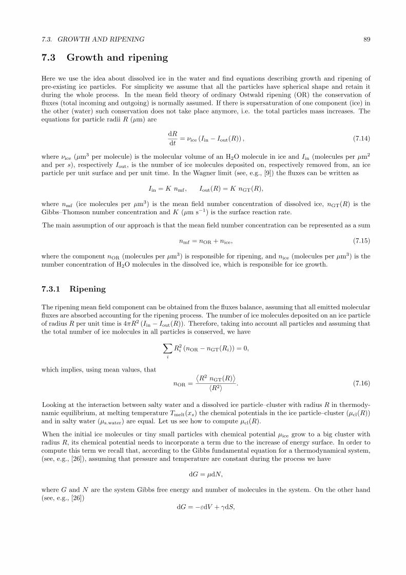
7.3. GROWTH AND RIPENING 89
7.3 Growth and ripening
Here we use the idea about dissolved ice in the water and find equations describing growth and ripening ofpre-existing ice particles. For simplicity we assume that all the particles have spherical shape and retain itduring the whole process. In the mean field theory of ordinary Ostwald ripening (OR) the conservation offluxes (total incoming and outgoing) is normally assumed. If there is supersaturation of one component (ice) inthe other (water) such conservation does not take place anymore, i.e. the total particles mass increases. Theequations for particle radii R (µm) are
dR
dt= νice (Iin − Iout(R)) , (7.14)
where νice (µm3 per molecule) is the molecular volume of an H2O molecule in ice and Iin (molecules per µm2
and per s), respectively Iout, is the number of ice molecules deposited on, respectively removed from, an iceparticle per unit surface and per unit time. In the Wagner limit (see, e.g., [9]) the fluxes can be written as
Iin = K nmf , Iout(R) = K nGT(R),
where nmf (ice molecules per µm3) is the mean field number concentration of dissolved ice, nGT(R) is theGibbs–Thomson number concentration and K (µm s−1) is the surface reaction rate.
The main assumption of our approach is that the mean field number concentration can be represented as a sum
nmf = nOR + nice, (7.15)
where the component nOR (molecules per µm3) is responsible for ripening, and nice (molecules per µm3) is thenumber concentration of H2O molecules in the dissolved ice, which is responsible for ice growth.
7.3.1 Ripening
The ripening mean field component can be obtained from the fluxes balance, assuming that all emitted molecularfluxes are absorbed accounting for the ripening process. The number of ice molecules deposited on an ice particleof radius R per unit time is 4πR2 (Iin − Iout(R)). Therefore, taking into account all particles and assuming thatthe total number of ice molecules in all particles is conserved, we have
∑
i
R2i (nOR − nGT(Ri)) = 0,
which implies, using mean values, that
nOR =
⟨
R2 nGT(R)⟩
〈R2〉 . (7.16)
Looking at the interaction between salty water and a dissolved ice particle–cluster with radius R in thermody-namic equilibrium, at melting temperature Tmelt(xs) the chemical potentials in the ice particle–cluster (µcl(R))and in salty water (µs.water) are equal. Let us see how to compute µcl(R).
When the initial ice molecules or tiny small particles with chemical potential µice grow to a big cluster withradius R, its chemical potential needs to incorporate a term due to the increase of energy surface. In order tocompute this term we recall that, according to the Gibbs fundamental equation for a thermodynamical system,(see, e.g., [26]), assuming that pressure and temperature are constant during the process we have
dG = µdN,
where G and N are the system Gibbs free energy and number of molecules in the system. On the other hand(see, e.g., [26])
dG = −εdV + γdS,
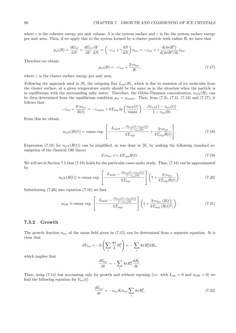
90 CHAPTER 7. GROWTH AND COARSENING OF ICE CRYSTALS
where ε is the cohesive energy per unit volume, S is the system surface and γ is the the system surface energyper unit area. Then, if we apply this to the system formed by a cluster particle with radius R, we have that
µcl(R) =dGcl
dN=
dGcl
dV
dV
dN=
(
−εcl + γdS
dN
)
νice = −εice + γd(4πR2)
d(4πR3/3)νice.
Therefore we obtain
µcl(R) = −εice +2γνiceR
, (7.17)
where γ is the cluster surface energy per unit area.
Following the approach used in [9], the outgoing flux Iout(R), which is due to emission of ice molecules fromthe cluster surface, at a given temperature surely should be the same as in the situation when the particle isin equilibrium with the surrounding salty water. Therefore, the Gibbs-Thomson concentration, nGT(R), canbe then determined from the equilibrium condition µcl = µwater. Then, from (7.3), (7.4), (7.13) and (7.17), itfollows that
−εice +2γνiceR(t)
= −εwater + kTexp ln
(
nGT(t)
nmax
)
− βxs,0(1− vice(t))
1− vice(0).
From this we obtain
nGT(R(t)) = nmax exp
−Lmelt − βxs,0(1−vice(t))
1−vice(0)
kTexp+
2γνicekTexpR(t)
. (7.18)
Expression (7.18) for nGT(R(t)) can be simplified, as was done in [9], by making the following standard as-sumption of the classical OR theory
2γνice << kTexpR(t). (7.19)
We will see in Section 7.5 that (7.19) holds for the particular cases under study. Thus, (7.18) can be approximatedby
nGT(R(t)) ≈ nmax exp
−Lmelt − βxs,0(1−vice(t))
1−vice(0)
kTexp
(
1 +2γνice
kTexpR(t)
)
. (7.20)
Substituting (7.20) into equation (7.16) we find
nOR ≈ nmax exp
−Lmelt − βxs,0(1−vice(t))
1−vice(0)
kTexp
(
1 +2γνice 〈R(t)〉kTexp 〈R(t)2〉
)
. (7.21)
7.3.2 Growth
The growth fraction nice of the mean field given in (7.15) can be determined from a separate equation. It isclear that
dVice = −d
(
∑
i
4π
3R3
i
)
= −∑
i
4πR2i dRi,
which implies thatdVice
dt= −
∑
i
4πR2i
dRi
dt.
Then, using (7.14) but accounting only for growth and without ripening (i.e. with Iout = 0 and nOR = 0) wefind the following equation for Vice(t)
dVice
dt= −νiceKnice
∑
i
4πR2i . (7.22)
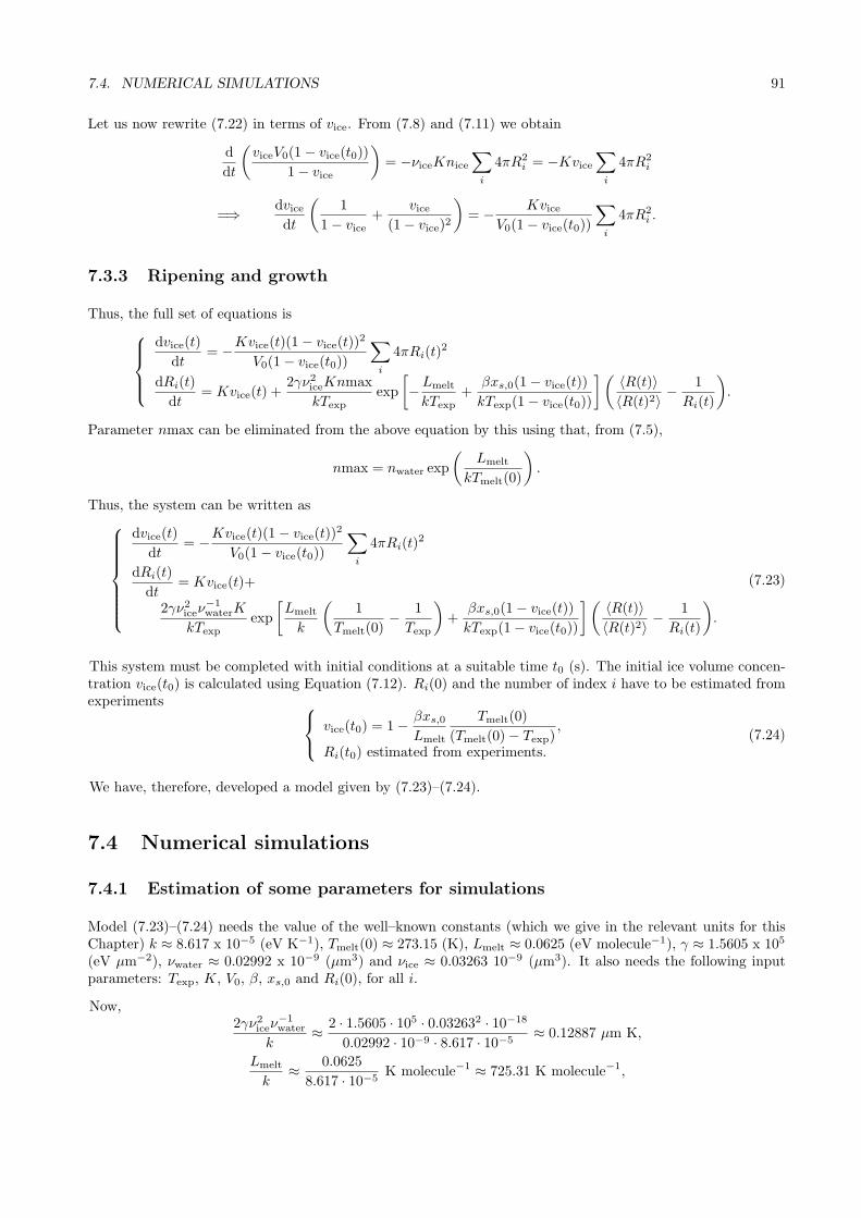
7.4. NUMERICAL SIMULATIONS 91
Let us now rewrite (7.22) in terms of vice. From (7.8) and (7.11) we obtain
d
dt
(
viceV0(1− vice(t0))
1− vice
)
= −νiceKnice
∑
i
4πR2i = −Kvice
∑
i
4πR2i
=⇒ dvicedt
(
1
1− vice+
vice(1− vice)2
)
= − KviceV0(1− vice(t0))
∑
i
4πR2i .
7.3.3 Ripening and growth
Thus, the full set of equations is
dvice(t)
dt= −Kvice(t)(1− vice(t))
2
V0(1− vice(t0))
∑
i
4πRi(t)2
dRi(t)
dt= Kvice(t) +
2γν2iceKnmax
kTexpexp
[
−Lmelt
kTexp+
βxs,0(1− vice(t))
kTexp(1− vice(t0))
]( 〈R(t)〉〈R(t)2〉 −
1
Ri(t)
)
.
Parameter nmax can be eliminated from the above equation by this using that, from (7.5),
nmax = nwater exp
(
Lmelt
kTmelt(0)
)
.
Thus, the system can be written as
dvice(t)
dt= −Kvice(t)(1− vice(t))
2
V0(1− vice(t0))
∑
i
4πRi(t)2
dRi(t)
dt= Kvice(t)+
2γν2iceν−1waterK
kTexpexp
[
Lmelt
k
(
1
Tmelt(0)− 1
Texp
)
+βxs,0(1− vice(t))
kTexp(1− vice(t0))
]( 〈R(t)〉〈R(t)2〉 −
1
Ri(t)
)
.
(7.23)
This system must be completed with initial conditions at a suitable time t0 (s). The initial ice volume concen-tration vice(t0) is calculated using Equation (7.12). Ri(0) and the number of index i have to be estimated fromexperiments
vice(t0) = 1− βxs,0
Lmelt
Tmelt(0)
(Tmelt(0)− Texp),
Ri(t0) estimated from experiments.(7.24)
We have, therefore, developed a model given by (7.23)–(7.24).
7.4 Numerical simulations
7.4.1 Estimation of some parameters for simulations
Model (7.23)–(7.24) needs the value of the well–known constants (which we give in the relevant units for thisChapter) k ≈ 8.617 x 10⁻⁵ (eV K−1), Tmelt(0) ≈ 273.15 (K), Lmelt ≈ 0.0625 (eV molecule−1), γ ≈ 1.5605 x 10⁵
(eV µm−2), νwater ≈ 0.02992 x 10⁻⁹ (µm3) and νice ≈ 0.03263 10−9 (µm3). It also needs the following inputparameters: Texp, K, V0, β, xs,0 and Ri(0), for all i.
Now,2γν2iceν
−1water
k≈ 2 · 1.5605 · 105 · 0.032632 · 10−18
0.02992 · 10−9 · 8.617 · 10−5≈ 0.12887 µm K,
Lmelt
k≈ 0.0625
8.617 · 10−5K molecule−1 ≈ 725.31 K molecule−1,

92 CHAPTER 7. GROWTH AND COARSENING OF ICE CRYSTALS
Lmelt
kTmelt(0)≈ 725.31
273.15molecule−1 ≈ 2.6554 molecule−1,
1
k=
1
8.617 · 10−5K eV−1 ≈ 11604.967 K eV−1,
andTmelt(0)
Lmelt≈ 273.15
0.0625=≈ 4370.4 K eV−1 molecule.
Therefore, system (7.23) can be approximated for the simulations by
dvice(t)
dt= Cvice
(t)
dRi(t)
dt= CRi
(t),
(7.25)
where
Cvice(t) = −Kvice(t)(1− vice(t))
2
V0(1− vice(t0))
∑
i
4πRi(t)2
CRi(t) = Kvice(t)+
0.12887K
Texpexp
[
2.6554− 725.31
Texp+ 11604.967
βxs,0(1− vice(t))
Texp(1− vice(t0))
]( 〈Ri(t)〉〈R(t)2〉 −
1
Ri(t)
)
.
(7.26)
The initial conditions given in (7.24) can be approximated by
vice(t0) = 1− 4370.4βxs,0
(273.15− Texp),
Ri(t0) estimated from experiments.(7.27)
The rest of the input parameters have to be given in the following units: Texp (K), K (µm s−1), V0 (µm3), β(eV µm3 mg−1 per molecule) xs,0 (mg µm−3) and Ri(0) (µm), for all i.
7.4.2 Numerical approximation
The numerical model was implemented in Fortran using a first-order explicit Euler scheme. The estimationof parameters described in Section 7.4.1 was used in the numerical algorithm. Time was discretised from theinitial time, t0, to final time, tf , using a step dt. The numerical scheme was initiated using (7.27) and at a giventime t, if we know vice(t) and Ri(t) we calculate those values at the following time step as
vice(t+ dt) = vice(t) + dt · Cvice(t)
Ri(t+ dt) = Ri(t) + dt · CRi(t),
(7.28)
with Cvice(t) and CRi
(t) given by (7.26).
In an analogous way to [9], when particle radius decreases below a certain threshold, Rthr, the particle isdeclared as evaporated in our model, with its residual content being transferred to other particles in proportionto their surface area. For our simulations we have considered Rthr = 0.01 µm.
7.5 Numerical experiments
We set up two different numerical experiments to validate our model. For the first one we used experimentaldata from [30]. In this work they use a salty water solution as a food model. Because our model was designedspecifically for salty water, we will see that the experimental data fits very well. The second model validationwas done using ice-cream as our food model and was based on the published work [23]. Even though ice cream isa much more complex system that salty water, we tried to adjust our model to this case, and we see reasonableagreement.

7.5. NUMERICAL EXPERIMENTS 93
0 50 100 150 200 25010
20
30
40
50
60
70
80
90
Time (min)
Rad
ius
(µ m
)
HPSF −19.2APF −19.2APF −14.3APF −12.4APF −9.5
Figure 7.2: Mean (dotted lines) and maximum (solid lines) experimental ice particle radius values for saltywater data
7.5.1 Salty water food model
Following [30], a 1.86N NaCl solution is used as a food model solution. The authors selected this concentrationso that at -19.2C, the temperature at which HPSF recrystallisation behavior takes place, the frozen fractionwas approximately 50%. The samples were then introduced into the chamber for HPSF or atmospheric pressureimmersion freezing. The HPSF samples were pressurised to 210 MPa and cooled down to -20 C. Once equi-librium was reached, pressure was quickly released, inducing nucleation. The rest of the freezing process wascompleted at atmospheric pressure. Freezing at atmospheric pressure (APF) was done by immersion in siliconeoil inside the vessel kept at -20C.
Once the samples were frozen they were placed in the chamber for observations to be carried out with amicroscope. Temperature was raised from -19.2C, the lower attained at the chamber, to the target experimentaltemperature and kept constant for a period of 3 h to study recrystallisation phenomena. The authors considerthis time period long enough to represent the more intense phase of the recrystallisation process. These targetexperimental temperatures were -19.2C for comparison of HPSF and APF frozen samples (which we will referto as HPSF-19.2 and APF -19.2) and -14.3C, -12.4C, -9.5C (which will be referred to as APF -14.3, APF-12.4 and APF -9.5, respectively) for system temperature dependence study. The evolution of the ice crystalsduring this period was followed by the micrographs that were automatically taken every 30 minutes. An imageanalysis software was used to detect crystal boundaries from the micrographs, and from this a diameter for eachcrystal was determined.
Discrete experimental data
The data we have available are the diameters of the crystals at each time step. Figure 7.2 shows the maximumand mean radius evolution for each of the experiments. We would like to remark that the maximum radii datais not very reliable, as it should be a monotonic increasing function over time, and as can be seen for somecases it is not. We think this is due to the fact that in the experimental observations a very small sample wasanalyzed (due to the limitations of the equipment, given the complexity of performing these kind of observationswithout alteration of the ice fraction and crystal size distribution, as pointed out in [30]), which meant that onaverage there were 150-200 initial crystals, not enough to get more accurate results. The mean radii evolution,however, looks more reliable.
To simulate these same experiments with our model, we know from Section 7.4.1 that the input parametersneeded are V0, Ri(t0), Texp, K, β and xs,0. From the experimental data we have Ri(t0) (in µm), and Texp
we take as -19.2C=253.95 K, temperature at which we know, from [30], the frozen fraction of the solutionwas approximately 51%. V0 (µm3) is the initial volume of the sample, which we work out for each case in the

94 CHAPTER 7. GROWTH AND COARSENING OF ICE CRYSTALS
following way: we assume that the initial amount of frozen ice is 16% and that the final amount of frozen iceis approximately 51% (i.e. for each experiment there is a total ice fraction of 0.51 and a dissolved ice fractionof 0.35); we can choose the number of particles we want the system to have and then we fit the total volumeso these amounts of ice are obtained (obvioulsy, because we are calculating a volume, this depends also on theinitial radii distribution). For each experiment the number of particles, and hence volumes, were different, andwill be pointed out separately in each graph. The initial salt mass concentration, xs,0, was calculated using thefact that we are working with a 1.86 N NaCl solution. By converting normality to solute mass concentration inthe relevant units, we get xs,0 = 1.0881 · 10−10 mg µm−3. Finally, K and β are model fitting parameters. Forall of the salty water experiments we take K = 1 µm s−1 and β = 2.757 · 107 eV µm4 mg−1 molecule−1.
Let us see, for the case under study, if inequality (7.19) holds. As k ≈ 8.617 x 10⁻⁵ (eV K−1), Texp = 253.95(K), γ ≈ 1.5605 x 10⁵ (eV µm−2) and νice ≈ 0.03263 10−9 (µm3), we have that for (7.19) to hold, necessarily,
Ri >>2γνicekTexp
= 4.6538 x 10⁻⁴ µm, ∀i,
which is true given that all particles in the model have a larger radius than the threshold one (otherwise theydisappear) and Rthr = 0.01 µm.
As mentioned previously, the experimental data was measured for 3 h and we have the radii of the crystalsevery 30 minutes. With our model we can run it for much longer times, which we believe will give a betteridea of the long term behaviour of the ice crystal coarsening. Actually the authors in [30] also point this out,by saying that the ice crystal size distribution attained after much longer storage times would be drasticallydifferent for both models. Our model also predicts crystal size distribution at a given time. To start our modelwe extracted the initial experimental crystal size distribution, which is the input parameter Ri(t0). In whatfollows, for all the above mentioned experiments, we plot the average and maximum radius evolution over timeof the simulation and experimental results to see how well they match. For the salty water model, we do notplot the distributions, given that they do not match well to the experimental ones. This is due to the fact thatthe experimental distributions are discrete (not enough data), and the model predicts continuous distributions,hence the non matching.
Figures 7.3a and 7.3b show the simulated and experimental radius evolution over time for HPSF -19.2 andthe APF -19.2 processes, respectively. For both cases the simulated average radius matches the experimentalaverage radius very well, and as can be seen we let the simulated radius evolve for longer than 3 h. Themaximum radius is not that good at every point, but the experimental data is not that reliable. If we want tocompare the long term behaviour of the sample frozen using HPSF and the one with APF, we can see that theyare very similar, which agrees with what was reported in [30]. We can see that the simulated radii evolutioncurves are not smooth, especially near the end; this again is due to the discreteness of the initial data.
Figures 7.4a, 7.4b and 7.4c show the simulated and experimental radius evolution over time for the APF -14.3, APF -12.4 and the APF -9.5 processes. Again we can see the very good agreement for experimental andsimulated average radii evolution over time.
Continuous experimental data
To test the validity of our model for predicting ice crystal size distributions at a given time, we designed a newset of data from experiment APF -12.4 described in Section 7.5.1. We created a continuous initial distributionfrom the experimental discrete initial one. To do so we calculated the mean value and standard deviation ofthe discrete data, and used these values to create a continuous distributions, assuming it followed a normaldistribution. The initial radii distribution was then extracted from this normal distribution, by taking the sameradii sizes as in the discrete case, but changing the frequency from the discrete ones to the continuous ones.In this way, as we are using a continuous initial distribution as an input for the model, we will be able topredict continuous distributions for different time steps (see Figure 7.5a). Figure 7.5 shows the distributions(7.5a) and the average and maximum simulated and experimental radius evolution over time (7.5b). Again theaverage radii match very well. As can be seen the simulated radii curves are now much smoother than in thediscrete case (see Figure 7.4b). The simulated distributions are now very smooth too. If we had more availableexperimental data, and hence continuous distributions, these simulated distributions could be compared to the

7.5. NUMERICAL EXPERIMENTS 95
10−2
10−1
100
101
102
103
1040
10
20
30
40
50
60
70
80
90
Time (min)
Rad
ius
(µ m
)
Average Radius SimMaximum Radius SimAverage Radius ExpMaximum Radius Exp
(a) HPSF -19.2. (Number of particles=8000; V0 = 1.05 x 108 µm3)
10−2
10−1
100
101
102
103
1040
10
20
30
40
50
60
70
80
90
100
Time (min)
Rad
ius
(µ m
)
Average Radius SimMaximum Radius SimAverage Radius ExpMaximum Radius Exp
(b) APF -19.2 (Number of particles=5000; V0 = 4.8 x 107 µm3)
Figure 7.3: Experimental and simulated average and maximum ice particle radius evolution (in logarithmicscale) for salty water experiment
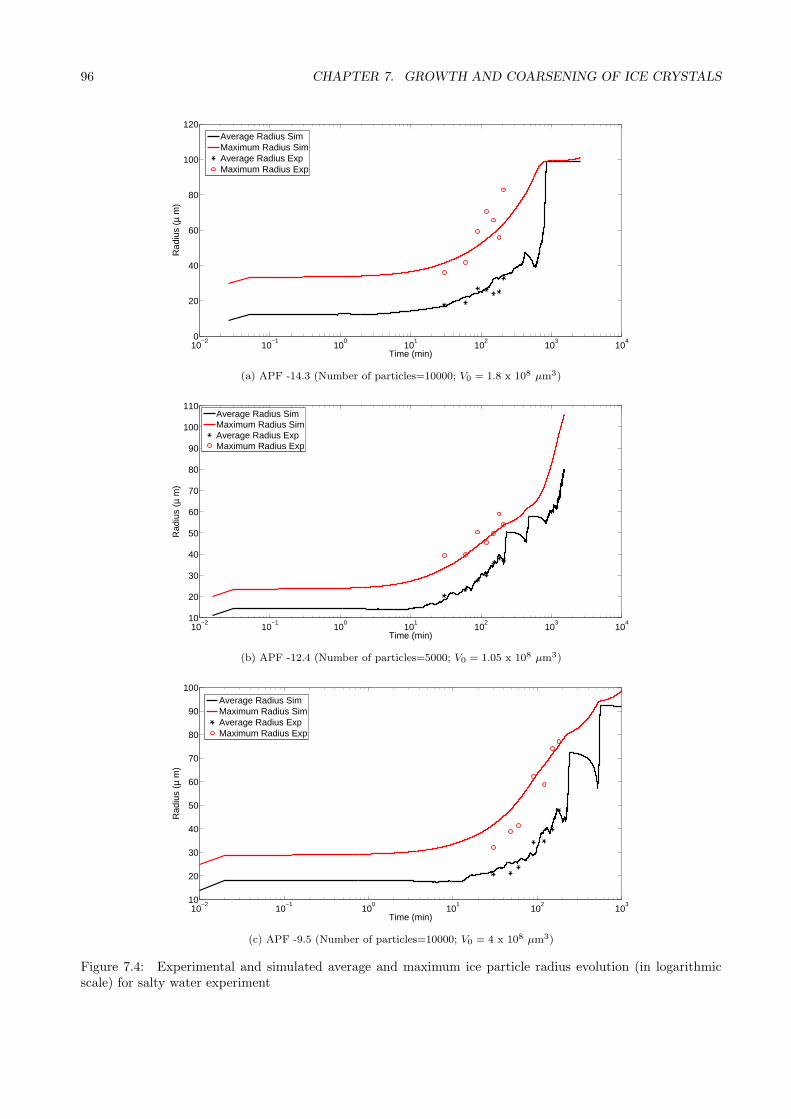
96 CHAPTER 7. GROWTH AND COARSENING OF ICE CRYSTALS
10−2
10−1
100
101
102
103
1040
20
40
60
80
100
120
Time (min)
Rad
ius
(µ m
)
Average Radius SimMaximum Radius SimAverage Radius ExpMaximum Radius Exp
(a) APF -14.3 (Number of particles=10000; V0 = 1.8 x 108 µm3)
10−2
10−1
100
101
102
103
10410
20
30
40
50
60
70
80
90
100
110
Time (min)
Rad
ius
(µ m
)
Average Radius SimMaximum Radius SimAverage Radius ExpMaximum Radius Exp
(b) APF -12.4 (Number of particles=5000; V0 = 1.05 x 108 µm3)
10−2
10−1
100
101
102
10310
20
30
40
50
60
70
80
90
100
Time (min)
Rad
ius
(µ m
)
Average Radius SimMaximum Radius SimAverage Radius ExpMaximum Radius Exp
(c) APF -9.5 (Number of particles=10000; V0 = 4 x 108 µm3)
Figure 7.4: Experimental and simulated average and maximum ice particle radius evolution (in logarithmicscale) for salty water experiment
7.5. NUMERICAL EXPERIMENTS 97
0 5 10 15 20 25 30 35 40 45 500
0.005
0.01
0.015
0.02
0.025
Radius (µ m)
Fre
quen
cy
Initial DistributionAfter 30 minAfter 1 hourAfter 2 hours
(a) Ice particle distributions
10−2
10−1
100
101
102
1030
20
40
60
80
100
120
Time (min)
Rad
ius
(µ m
)
Average Radius SimMaximum Radius SimAverage Radius ExpMaximum Radius Exp
(b) Ice particle radius evolution (in logarithmic scale)
Figure 7.5: APF −12.4C Continuous model (Number of particles=12000; V0 = 2.2 x 108 µm3)
98 CHAPTER 7. GROWTH AND COARSENING OF ICE CRYSTALS
experimental ones.
7.5.2 Ice-cream food model
Following [23] our second numerical experiment uses ice-cream as a food model. As previously stated, ice-creamis a much more complex system than salty water, but we still want to try our model with ice-cream to seeif it can be fitted. In [23] a methodology to characterise the ice crystal size distribution was developed andseveral ice-cream and ice milk formulations were analyzed to test the methodology. A refrigerated glove boxwas constructed to allow temperature control of the sample during preparation and viewing. This glove boxallowed samples to be analyzed at any temperature down to -20C and permitted analysis of samples directlydrawn from an ice-cream freezer. Once the frozen ice-cream samples were ready (at the right temperature) theywere placed in the glove box and left there for enough time to equilibrate to the glove box temperature [23].Afterwards the sample was viewed using conventional brightfield light microscopy, and then size measurementsof the ice crystals were made directly from photomicrographic prints.
Several ice-cream and ice milk formulations varying in total solids level were prepared in [23]. We use the 40%total solids (TS) ice-cream formulation, for no more particular reason than for this formulation a plot of thedistributions at different time steps was given in the cited paper, and we will use it to compare our simulatedresults to. Samples were frozen, then drawn from the freezer and hardened for 24 h, and finally stored in astorage freezer for several weeks. Samples were analyzed for crystal size immediately after drawing from thefreezer (the glove box temperature was set to the draw temperature, −7.3±0.3C); after hardening (at −14C)and after 7 and 14 weeks of storage (also at −14C).
To set up the numerical experimental for our model from this data we make the following assumptions: we takeTexp = −14C=259.15 K, which is the temperature at which all the measurements were done, except for the firstone, immediately after drawing from the freezer. Because of the differences in temperature between the drawingand hardening stages, a significant increase in ice crystal size was observed, as pointed out in [23]. Our modeldoes not account for differences in temperature, so we assume that the temperature is constant throughout thewhole experiment (Texp = −14C), but we will see that our results are still good enough given that the modeldoes account for growth. We take the initial radii distribution, Ri(t0), from Figure 4 in [23] (we extrapolatesome points from the published curve and then create a histogram using those points, which we use as an initialdistribution for our code). We assume that the initial amount of ice formed after drawing is approximately 25%and that the dissolved ice concentration is the same amount, which gives a total ice fraction of 50%. As wewant smooth distributions we consider quite a large number of particles, 4500, and therefore the system volumeis taken as 1.2·109 µm3, to get the correct ice fractions. In this case we do not have a value for the xs,0 from theexperimental data, as we are no longer working with salty water but with ice-cream instead, which has manymore components. This means that we now have three fitting parameters, β, xs,0 and K. However, if we notethat in system (7.25)-(7.27), β and xs,0 always appear as βxs,0 (never separate) we can write the multiplicationof both as one fitting parameter. Thus, we consider βxs,0 = 0.0024 eV molecule−1, which is very close to thevalue used for the salty water βxs,0 = 0.003 eV molecule−1. For K we stick to the same value as for the saltywater experiments, i.e. K = 1 µm s−1.
Again for this case, inequality (7.19) holds. The only parameters that has changed with respect to the salty-water model is Texp which is now 259.15 K, leading to
Ri >> 4.5604 x 10⁻⁴ µm, ∀i,
which is true given Rthr = 0.01 µm.
Figure 7.6 shows the simulated (lines) and experimental (lines with symbols) distributions (7.6a) and the averageand maximum simulated and experimental radius evolution over time (7.6b). The model distribution predictionagrees well with the experimental distributions, except after 14 weeks when the experimental crystals havestopped coarsening (the 7 weeks and 14 weeks distributions are practically the same), whereas the simulatedones continue to coarsen. We think that this is due to the fact that ice-cream contains fat and emulsifierswhich provide a mechanical obstruction to crystal growth (see [23]), something that our model does not takeinto account. For example, the possibility of using temperatures changing with time during the process or the
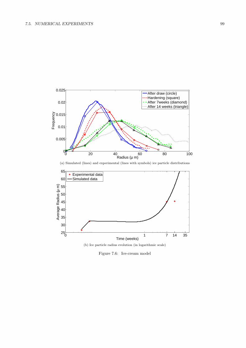
7.5. NUMERICAL EXPERIMENTS 99
0 20 40 60 80 1000
0.005
0.01
0.015
0.02
0.025
Radius (µ m)
Fre
quen
cy
After draw (circle)Hardening (square)After 7weeks (diamond)After 14 weeks (triangle)
(a) Simulated (lines) and experimental (lines with symbols) ice particle distributions
0 1 7 14 3525
30
35
40
45
50
55
60
65
Time (weeks)
Ave
rage
Rad
ius
(µ m
)
Experimental dataSimulated data
(b) Ice particle radius evolution (in logarithmic scale)
Figure 7.6: Ice-cream model
100 CHAPTER 7. GROWTH AND COARSENING OF ICE CRYSTALS
inclusion of mechanisms avoiding crystal growth (such as the fat and emulsifiers mentioned above) are some ofthe new features that could be added to the model.
7.6 Conclusions
We have developed a very simple model that studies growth and coarsening of ice crystals, and validated itfor two different food similes: salty water and ice-cream. The results have shown that the model is accurateenough to predict correctly average radial evolution for all cases, and crystal size distribution, if the initialdata is continuous. Further improvements to the model could be to include more components into the systems,and therefore use it for more complex foods. For example, the possibility of using temperatures that changewith time throughout the process, or the inclusion of mechanisms avoiding crystal growth (such as the fat andemulsifiers mentioned above) are new features that could also be added to the model.

Chapter 8
Conclusions and future work
In this thesis we have described, modelled and analysed several problems related to High-Pressure processesin Food Engineering. There is a very wide range of problems that can be studied in this field, depending onfactors such as the type of food, the size and geometry of the High-Pressure vessel, and the desired effects of theprocess. In particular, in this thesis we have concentrated on problems concerning large and small, solid- andliquid-type foods, vertically and horizontally oriented machines. Also, High-Pressure freezing processes and thegrowth and coarsening of ice crystals inside a frozen food sample have been studied.
One of the main goals of food processing is the inactivation of microorganisms and enzymes, to ensure foodis safe and of good quality for the consumer to eat. In Chapter 2 we presented a bacterial inactivation model(which can also be used for enzymatic inactivation), and gave an example, using experimental data, of how thekinetic parameters can be identified. It was made clear that once these are identified, in order to calculate thefinal bacterial count (or final enzymatic activity) inside a food sample, the temperature and pressure distributionhas to be known, and then both models should be coupled. The pressure profile is known a priori in these typeof processes (it can be chosen by the user), but the temperature distribution changes with time and space, andtherefore heat transfer models for predicting temperature profiles are necessary. Developing such models hasbeen the purpose of this thesis.
Heat transfer models for predicting temperature profiles inside a large solid-type food were presented in Chap-ter 4, and several two- and one-dimensional simplified versions of these models were given, after performingdimensional analysis. These simplified models provide a good approximation of the full model, but are not ascomplex and need less computational time. Also, the solutions given do not require the use of a “black-box”FEM solver and our approximations allow us to qualitatively describe the physical features involved. It hasbeen shown that for the case of a tall and narrow High-Pressure machine, the temperature profile inside thefood is very well approximated by a one-dimensional model, except at points very close to the top and bottomboundaries. Furthermore, the solutions of the one-dimensional heat transfer models have been used to calculatethe final enzymatic activity, also achieving very similar results to those found when the temperature of thetwo-dimensional models are used. This has great advantages for other problems that arise in the High-Pressureprocessing context (which could be possible future work), such as optimisation procedures for equipment designand identification of pressure and temperature dependent thermo-physical parameters of these processes, bymeans of solving inverse problems.
In Chapter 5, we discussed processes that take place in vertically and horizontally oriented High-Pressuremachines for liquid-type foods. To the best of our knowledge, to date, horizontal vessels have not been modelled,but are of great relevance for the food industry, given most industrial-scale machines are horizontal. Thecomputational complexity of these models is very high, as they have to be solved in three dimensions. Wecompared a vertical and horizontal model with exactly the same process conditions, highlighting the importantdifferences arising between the two models. These include modifications to the temperature distribution andflow field of the fluid. In particular, for a liquid-type food (in this work we have considered water), for thevertical model temperatures change with height, whilst for the horizontal model they change more radially.Therefore, for a long and thin machine we have shown that the temperature in general is more uniform for the
101

102 CHAPTER 8. CONCLUSIONS AND FUTURE WORK
horizontal case, for the processes we have discussed. With the work done in this Chapter 5 we are now able topresent an accurate horizontal representation, from which experimentalist can benefit.
Models for a High-Pressure shift freezing process for large and small solid-type foods were given in Chapter 6.The model for solidification is based on the enthalpy formulation at non-constant pressure and volume phasefractions. The model describes the temperature profiles throughout the process and can predict the plateautimes, which are both relevant parameters for food experimentalists. Without using any fitting parameters,the simulated results for the numerical tests we performed agreed very well with the experimental data for thesmall sample case, especially at the centre of the sample. At the surface there is not an accurate match betweenthe data and the model. However, we considered the modelling approach to be sufficient, given the relativelylarge experimental errors. For the large sample case there is no experimental data to plot against the simulatedtemperature profile, but when comparing the model plateau times to the published experimental ones, we findthat they are in general shorter, but in the range of the latter. In all cases, the prediction errors are on theorder of minutes, which is reasonable given that the processing time is on the order of hours.
The development of a model for growth and coarsening of ice crystals, presented in Chapter 7, was motivated bystudies of recrystallisation of frozen food samples. Food engineers want to ensure high quality of products afterlong term storage. The model presented is valid for food samples which have been frozen using High-PressureShift Freezing or conventional freezing, assuming that initially the ice particles are homogeneously distributedand have the same size and shape. The model was solved numerically and validated for two different foodsimiles: salty water and ice-cream. We showed that the model is accurate enough to correctly predict theaverage radial evolution and crystal size distribution. Future work could be to include more components intothe systems, and therefore use it for more complex foods, to introduce non-constant temperatures or to includemechanisms avoiding crystal growth.
Throughout this thesis we have covered a wide range of problems related to Food Engineering, using a largevariety of mathematical techniques in the process. Nevertheless, there is still a large amount of problems thatcan be solved in this area. For example, in Chapters 4, 5 and 6, the models could be further developed so theyare all valid for any type of food sample (i.e. large or small, solid or liquid), and the resulting temperaturedistributions from these models could be coupled with the enzymatic or bacterial inactivation models presentedin Chapter 2, as was briefly highlighted in Chapter 4. Other improvements could potentially be obtained byincluding the temperature and pressure dependence of material properties in all of the heat transfer modelspresented. Also, in Chapter 6, anisotropy effects could be included in the frozen region, and our two-dimensionalconvection simulations extended to three-dimensions. As mentioned above, possible improvements to the modelpresented in Chapter 7 could be to include more components into the systems, and therefore use it for morecomplex foods. The previously listed examples of future work, together with those mentioned in each Chapterindividually, are just some of the possible extensions.

Chapter 9
Summary in English
Introduction and goals of the thesis
There has been significant interest in the study of food engineering from the mid-twentieth century onwards[12, 13, 31, 43, 53, 63, 71, 74, 80, 82, 92]. Humans have been interested in food conservation since ancienttimes, using traditional techniques such as desiccation, conservation in oil, salting, smoking, cooling, etc. Dueto the massive movement of populations to cities, a great supply of food in adequate conditions was necessary.Therefore, the food industry was developed in order to guarantee large-scale food techniques, to prolong itsshelf life, and to make logistic aspects such as transport, distribution and storage, easier. Nowadays, the foodindustry is an increasingly competitive and dynamic arena, given that consumers are now more aware of whatthey eat. Food quality properties, such as taste, texture, appearance, and nutritional content are stronglydependent on the way the foods are processed.
Many classical industrial processes are based on thermal treatments, such as, for example, pasteurisation,sterilisation and freezing. In recent years, with the aim to improve these conventional processing technologies, inorder to deliver higher-quality and better food products for the consumers, a number of innovative technologies,also referred to as “emerging” or “novel” technologies have been proposed, investigated, developed, and in somecases, implemented. These “emerging” technologies take advantage of other physics phenomena such as highhydrostatic pressure, electric and electromagnetic fields, and pressure waves. With these innovative technologiesfood engineers can not only develop new food products, but also improve the safety and quality of conventionallytreated food through milder processing [53].
In particular, in this thesis we have focused on one of these new emerging technologies, High Pressure Processing(HPP) of food. The appearance of HPP as a tool in the food industry started in the late 1980s [41]. Since thento date, extensive research has been done on possible application of HPP as a preservation method [12, 28],to change the physical and functional properties of food systems [11, 41] and to take advantage of the phasediagram of water: freezing, thawing and sub-zero temperature non-frozen storage under pressure [68, 71].
Several studies [12, 13, 82] have proved that HPP allows inactivation of enzymes and pathogenic and spoilagemicroorganisms in food, while leaving small molecules intact, and therefore not modifying significantly theorganoleptic properties (such as colour, odour, texture and flavour).
Two principles underlie the effect of High Pressure (HP): firstly, the Le Chatelier Principle, according to whichany phenomenon (phase transition, chemical reaction, chemical reactivity, change in molecular configuration)accompanied by a decrease in volume will be enhanced by pressure; secondly, pressure is instantaneously anduniformly transmitted independently of the size and the geometry of the food (isostatic pressure).
Therefore, unlike thermal processing, HP effects are uniform and nearly instantaneous throughout the food andthus independent of food geometry and equipment size. However, HPP does not escape the classical limitations,imposed by heat transfer. Heat transfer characterises every process, accompanied by a period of pressureincrease or decrease, which is associated with a proportional temperature change of the vessel’s contents due
103

104 CHAPTER 9. SUMMARY IN ENGLISH
to adiabatic heating. The magnitude of the adiabatic temperature increase or decrease depends on a numberof factors, such as the food product thermo-physical properties (density, thermal expansion coefficient, andspecific heat capacity) and initial temperature. Heat transfer is caused by the resulting temperature gradientsand can lead to large temperature differences, especially in large-volume industrial vessels. For a number ofHP applications to food engineering, these limitations should be taken into account, trying to avoid as much aspossible, non-uniformity at the end of the process.
Therefore, an accurate evaluation of the effects of pressure, applied during conventional batch HPP, requiresthe knowledge of the non-uniform temperature distribution inside the sample. With this in mind, equationsdescribing the time-temperature-pressure history of a product must be coupled with the parameters describingthe reaction kinetics for destruction of microorganisms, enzymes, and other factors. The optimisation of batchHP processes for nutrient retention should also be based on this approach.
Mathematical modelling is a very useful tool for characterising this temperature distribution. Normally, itis the fastest and least expensive way, given that it minimises the number of experiments that need to beconducted to determine the influence of several parameters on the quality and safety of the process. Dependingon the characteristics of the process, the type of food (liquid or solid), the dimensions of the HP vessel, theprocess conditions (initial temperature, maximum pressure, etc.), different mathematical models are used. Forexample, for a large (when comparing with the pressurising volume) solid-type food a heat transfer model withonly conduction effects is sufficient [46, 69], whereas for a liquid-type food, convection effects have to also beincluded, and therefore equations that model the fluid flow also have to be coupled with the heat transferequation. If we are studying HP freezing processes, a model that takes into account solidification also has tobe considered. In some cases, the expression of the process outcome based on the attributes of the processedfood, that is, e.g. the remaining microbial load, enzyme activity, and chemical reaction products, is required.Within multiphysics modelling, reaction kinetics (i.e., microbial inactivation, quality degradation, chemicalreaction, and structural responses) can be coupled with the specific differential equations to provide the spatialdistributions of reaction response.
Even though there has already been a significant amount of research in this area, there are still many situationsthat arise in HPP that have not been modelled. Therefore, throughout this thesis we have considered differenttypes of HP processes, trying to cover as many situations as possible when working with HP food processing,presenting innovative models. Namely, models for large and small, solid and liquid type foods, for verticallyand horizontally oriented machines, and also for HP freezing processes are analysed. We have developed thecorresponding model for each case, solving each one accordingly.
In Chapter 2 we first start by presenting a model for bacterial and enzymatic inactivation, hence showing thenecessity for knowing the temperature distribution throughout a HP process. A case study of one particularbacteria, for which experimental data is available, is modelled and validated.
In Chapter 3 we present the general aspects of the heat and mass transfer models for HP processes developedin [46, 69]. The new models we derived in Chapters 4, 5 and 6 are based on this one, and thus we decided toinclude this model-presentation chapter to avoid having to introduce the same model in each of the later ones.
In Chapter 4 we introduce one of the most basic type of model for time-temperature-pressure evolution, con-sidering large samples of solid-type foods in a vertically oriented machine. With these, only conduction effectshave to be included in the heat transfer model, which makes its resolution easier, and in some cases may evenbe possible to solve analytically. For vertically oriented machines, a reduction from three to two dimensions ispossible due to the axis-symmetric geometry. Thus, in Chapter 4 several two dimensional models, with differentkind of boundary conditions, are solved analytically and then compared to simplified versions. Also, some ofthe heat transfer models considered in this Chapter are coupled with an enzymatic inactivation model, showinghow this coupling can be done. To date most of the published heat transfer models for solid-type foods hadbeen solved numerically and not analytically.
In Chapter 5 a more complex problem is discussed. We consider liquid-type foods, for which convection effectsalso have to be included into the heat transfer model. Therefore, the equations for fluid flow (Navier–Stokesequations) have to be also solved. Due to the complexity, analytical solutions are no longer available and themodel has to be solved numerically. An added complication to the problem in this Chapter is that we modelprocesses and liquid-type foods placed in both vertically and horizontally oriented HP vessels. For the vertically
105
oriented HP vessel we could reduce it to two dimensions, due to the axis-symmetry. However for the horizontallyoriented, there are no longer axis-symmetric features and a three dimensional model is necessary, adding an extrachallenge to the numerical model. The differences between models have been analysed. Developing a model fora horizontally oriented HP vessel is interesting from an industrial point of view, as most of the industrial-scalevessels are in that position [63]. However, at a pilot-scale, they are vertically oriented and therefore most ofthe published research has been focused on these kind of machines, and the models are usually solved in twodimensions.
In Chapter 6 a freezing process that benefits from HP, namely a High-Pressure Shift Freezing (HPSF) process,is described, modelled and solved numerically. Modelling conventional solidification problems is not an easytask, and a lot of interest and research has been put into this area. HP freezing problems, however, havenot been as studied, and in this Chapter we present a generalised enthalpy model for a HPSF process. Themodel can be used for large (when compared to the pressurising fluid volume) solid-type food (only conductioneffects included) and also for small (when compared to the pressurising fluid volume) solid-type food (wherethe significant heat transfer effects of convection in the pressurizing medium are accounted for by solving theNavier–Stokes equations). The model is run for several numerical tests, and good agreement with experimentaldata from the literature is found.
The analysis in Chapter 6 shows that HPSF is more beneficial for ice crystal size and shape than traditional(at atmospheric pressure) freezing. This motivates the work in Chapter 7, which differs from previous Chaptersas we do not solve a model to find the temperature distribution inside a food sample undergoing a HP process.A model for growth and coarsening of ice crystals inside a frozen food sample is developed and some numericalexperiments are given, with which the model is validated by using experimental data. To the best of ourknowledge this is the first model suited for freezing crystallisation in the context of HP.
Main contributions of the thesis
The most important results and contributions of this thesis can be found in Chapters 4, 5, 6 and 7. As saidabove, Chapter 2 is for motivation of the rest of the problems of the thesis, and in Chapter 3 the general heattransfer model used further along on is given.
The heat transfer models presented in Chapter 4 are valid for predicting temperature profiles inside a largesolid-type food undergoing HP treatment. Two different kinds of boundary conditions have been considereddepending on whether only the food holder is taken into account, or whether the surrounding steel is included.We perform a dimensional analysis which highlights the dominant terms in the model, and shows that in somecases the equations can be simplified (in dimension) and yet provide a good approximation. These models forHP processes are much simpler than those found in the literature, but still have the correct qualitative features.Using the solutions we propose, there is no need to have an FEM solver in order to simulate the process. Wehave given a thorough analysis describing an exact 2D solution as well as several simplifications in both 2D and1D. It has been shown that for the case of a tall and narrow HP machine, the temperature profile inside thefood is very well approximated by a 1D model, except at points very close to the top and bottom boundaries.For the first class boundary conditions, the solutions of the 1D heat transfer models have been used to calculatethe final enzymatic activity, also achieving very similar results to when the temperature of the 2D models areused. The reduction to 1D is very useful from a computational point of view, since faster simulations can becarried out. This is interesting, for instance, when performing optimisation algorithms, where very often thestate equations need to be solved many times. In addition, the simplified model can help to calculate thermo-physical properties as a function of pressure, via inverse problems, which is an increasing need nowadays forfood technologists. From an experimental point of view, results can also be used to determine where to placethe thermocouples inside the food sample in order to measure the temperature experimentally.
In Chapter 5 we consider liquid-type foods, for which convection effects also have to be included into the heattransfer model. Due to the complexity of solving Navier-Stokes equations, we know that analytical solutionsare no longer available and the model will have to be solved numerically. Several authors have done extensiveresearch in developing models to predict transient temperature and flow distributions, but to the best of ourknowledge, all of the models developed and published to date on prediction of temperature and flow distribution

106 CHAPTER 9. SUMMARY IN ENGLISH
of a HPP, are based on vertically oriented high pressure units. This is because the original HPP equipmentunits were vertical. However, the current trend is to supply horizontal units at industrial scale. Because ofthis increase of horizontal units in the industry, but yet the lack of published work on horizontal models, wedecided it would be interesting to begin to cover this research gap. Nowadays, most of the experimental dataavailable from researchers is for HP processes which have taken place in a vertical unit, due to the fact thatlaboratory or pilot-scale units are mostly vertical. We did not have the experimental resources to be able tosetup a horizontal laboratory-scale unit to obtain experimental data. Therefore, designing a horizontal modelfrom scratch was not plausible at this point. Instead, we decided to develop a horizontal model by adapting anexisting vertical one, which had previously been validated. In this way, what we can show are the differencesbetween the vertical and horizontal models, stating the research need for developing horizontal models, whichwould be very helpful for the industry. It is clear that the major reason why the vertical and horizontal modelsare different, even if they have exactly the same process conditions, is due to the fluid flow pattern, which weknow that for the case of a liquid-type food has a significant influence on homogeneity of the final pressurisedproduct. The results of the numerical simulations show that, as expected, the temperature performance anduniformity is different for both geometries, mainly due to the differences in the flow. For a liquid-type food(in this work we have considered water) and for a long and thin machine we have shown that the temperaturein general is more uniform for the horizontal case, for the processes we have discussed. For the vertical modeltemperatures change along height, whilst for the horizontal model they change more radially.
In a High-Pressure Shift Freezing (HPSF) process, like the one described in Chapter 6, phase transition occursdue to a pressure change that promotes metastable conditions and instantaneous ice production. On expan-sion, pressure release occurs instantaneously throughout the product (Pascal principle), and subsequently, itstemperature decreases. Large-scale supercooling takes place throughout the sample, which implies high icenucleation velocities. Different authors have proved experimentally that ice nucleation occurs homogeneouslythroughout the whole volume of the product and not only on the surface, as they have found small granularshape ice crystals disperse throughout the resulting sample for several products. Due to the advantages of thismethod (mainly, its potential to improve the kinetics of the process and the characteristics of the ice crystalsthus formed) compared to other freezing methods, some modelling studies considering the temperature evolutionduring treatment of HPSF processes have been published to date. This is important in all HP processes, and inparticular in freezing processes. In Chapter 6 we introduce a new model based on the enthalpy formulation atnon-constant pressure and volume phase fractions. The model is two dimensional axis-symmetric (many of thepublished ones are one dimensional), and is valid both large and small solid food samples. Convection effectsin the pressurising fluid are considered for the small sample case (which is also a novelty when compared topublished models). The numerical results agree with the experimental data very well and no fitting parameterswere used in the simulations.
In Chapter 7 a model to study the growth and coarsening of ice particles in a frozen food sample is developed.We assume that initially the ice particles are homogeneously distributed and have the same spherical shape,which occurs with a HPSF frozen sample, our model is valid for any kind of freezing process and not only HPSF.This will allow us to compare the evolution of HPSF frozen samples to that of samples that have been classicallyfrozen. We present a model that accounts for the growth and ripening of ice crystals in this simple system bydeveloping a theory somewhat similar to “Ostwald ripening”. The model predicts crystal size evolution withtime, and also ice crystal size distribution. We validate it for two different food similes: salty water and ice-cream. The results have shown that the model is accurate enough to predict correctly average radial evolutionfor all cases, and crystal size distribution, if the initial data is continuous.
Conclusions
In this thesis we have described, modelled and analysed several problems related to High-Pressure processesin Food Engineering. There is a very wide range of problems that can be studied in this field, depending onfactors such as the type of food, the size and geometry of the High-Pressure vessel, and the desired effects of theprocess. In particular, in this thesis we have concentrated on problems concerning large and small, solid- andliquid-type foods, vertically and horizontally oriented machines. Also, High-Pressure freezing processes and thegrowth and coarsening of ice crystals inside a frozen food sample have been studied.

107
Throughout this thesis we have covered a wide range of problems related to Food Engineering, using a largevariety of mathematical techniques in the process. Nevertheless, there is still a large amount of problems that canbe solved in this area. For example, in Chapters 4, 5 and 6, the models could be further developed so they are allvalid for any type of food sample (i.e. large or small, solid or liquid), and the resulting temperature distributionsfrom these models could be coupled with the enzymatic or bacterial inactivation models presented in Chapter2, as was briefly highlighted in Chapter 4. Other improvements could potentially be obtained by including thetemperature and pressure dependence of material properties in all of the heat transfer models presented. Also,in Chapter 6, anisotropy effects could be included in the frozen region, and our two-dimensional convectionsimulations extended to three-dimensions. Possible improvements to the model presented in Chapter 7 couldbe to include more components into the system, and therefore use it for more complex foods. The previouslylisted examples of future work, together with those mentioned in each Chapter individually, are just some ofthe possible extensions.


Chapter 10
Resumen en espanol
Introduccion y objetivos de la tesis
Desde mediados del Siglo XX en adelante ha habido un gran interes en problemas relacionados con la industriaalimentaria [12, 13, 31, 43, 53, 63, 71, 74, 80, 82, 92]. La conservacion de alimentos ha sido importante paralos humanos desde la antiguedad, cuando se utilizaban tecnicas tradicionales como la desecacion, el curado, lasalazon, el encurtido, el ahumado, etc. La industria alimentaria se desarrollo cuando se produjo el desplaza-miento masivo de la poblacion al medio urbano, ya que era preciso contar con un suministro masivo de alimentosen condiciones de consumo adecuadas. De esta manera se pudo prolongar la vida util de los alimentos, garantizartratamientos a gran escala y mejorar aspectos logısticos como el transporte, la distribucion y el almacenamiento.
Muchos de los metodos clasicos utilizados para la conservacion de los alimentos consisten en la aplicacion detratamientos termicos, como por ejemplo la pasteurizacion, esterilizacion y congelacion. El problema de estostratamientos es que pueden suponer una reduccion importante de las propiedades organolepticas y nutricionalesdel alimento. Por ello, ya que hoy en dıa no solo importa alargar la vida util de los alimentos, sino que tambiense pretende que sean de buena calidad, se estan desarrollando nuevas tecnicas que se aprovechan de otrosfenomenos fısicos como por ejemplo las altas presiones, los campos electricos y electromagneticos, y las ondasde presion. Con estas tecnologıas novedosas, los ingenieros trabajando en este campo no solo pueden mejorarla calidad de los alimentos tratados, sino que tambien pueden desarrollar nuevos productos [53].
En particular, en esta tesis, nos hemos centrado en estudiar una de estas tecnologıas emergentes, los tratamientosa altas presiones. Estos comenzaron a usarse como herramienta de la industria alimentaria a finales de los anos80 [41]. Desde entonces hasta el dıa de hoy, se han investigado las posibles aplicaciones de las altas presionescomo una tecnica de conservacion [12, 28], el efecto que tienen sobre las propiedades fısicas y funcionales de losalimentos [11, 41], y como se puede aprovechar el diagrama de fases del agua para la congelacion, sublimaciony almacenamiento a temperaturas bajo cero de alimentos no congelados bajo presion [68, 71].
Varios estudios [12, 13, 82] muestran que las altas presiones pueden inactivar enzimas y microorganismos, sinalterar sustancialmente las propiedades organolepticas del alimento, ya que la alta presion no afecta, al menosde forma significativa, a las moleculas pequenas como las que proporcionan el sabor y las vitaminas.
Hay dos principios generales que son de gran interes cuando se habla de la aplicacion de altas presiones: por unaparte, el principio de Le Chatelier, segun el cual el aumento de presion favorece (respectivamente, desfavorece)cualquier fenomeno (cambio de estado, reaccion quımica, cambio en la estructura molecular, etc.) que esteacompanado de un descenso (respectivamente, aumento) de volumen; y por otra, el principio isostatico, segunel cual la presion se transmite de manera uniforme y quasi-instantanea a traves de toda la muestra que estebajo presion.
Por tanto, a diferencia de los procesos termicos, los efectos de las altas presiones son uniformes e instantaneos enel alimento, con independencia de la geometrıa y el tamano de este. Aun ası, los procesos de altas presiones tienenlimitaciones que vienen impuestas por la transferencia de calor. En todo tratamiento con altas presiones, en el
109
110 CHAPTER 10. RESUMEN EN ESPANOL
que hay un incremento o descenso de presion, se genera un cambio proporcional en la temperatura dentro de lavasija de alta presion debido a la generacion de calor adiabatico. La magnitud de este cambio depende de variosfactores, como las propiedades termofısicas del alimento (densidad, calor especıfico, coeficiente de expansiontermica) y la temperatura inicial del proceso. La transferencia de calor se produce debido a los gradientestermicos resultantes y puede provocar grandes diferencias de temperatura dentro del alimento, especialmenteen vasijas grandes de tamano industrial. Para muchas aplicaciones de la ingenierıa alimentaria es importantetener en cuenta estas limitaciones, dado que suele ser conveniente conseguir procesos lo mas uniformes posibles.
Por esto, si se busca entender de manera precisa los efectos de la presion sobre un alimento que es tratado conaltas presiones, hay que tener en cuenta que los procesos con altas presiones son dependientes no solo de lapresion, sino tambien de la temperatura, y conocer la distribucion no uniforme de temperaturas que se generadurante el proceso. Es necesario estudiar las ecuaciones que describen la evolucion de temperaturas y presionen funcion del tiempo, y posteriormente acoplarlas con, por ejemplo, los modelos cineticos de inactivacionde enzimas y microorganismos u otros factores que se quieran estudiar. Tambien es importante conocer ladistribucion de temperaturas si se quiere optimizar los tratamientos de altas presiones.
La modelizacion matematica es una herramienta muy util para hallar esta distribucion de temperaturas, ynormalmente es la manera mas rapida y economica de hacerlo, ya que minimiza el numero de experimentos quehay que llevar a cabo. Dependiendo de las caracterısticas del proceso, el tipo de alimento (solido o lıquido), lasdimensiones de la vasija de alta presion, las condiciones del proceso (temperatura inicial, presion maxima, etc.),el modelos matematico usado sera distinto. Por ejemplo, para un alimento solido grande (en comparacion conla cantidad de lıquido presurizante) un modelo de transferencia de calor por conduccion es suficiente [46, 69],mientras que para un alimento lıquido es necesario incluir tambien los efectos de la conveccion, acoplando portanto la ecuacion de transferencia de calor con las ecuaciones de Navier–Stokes. Si se estudiasen procesos decongelacion por altas presiones, un modelo que tuviese en cuenta el fenomeno de solidificacion serıa necesario.En algunos casos, lo que se busca es un resultado del proceso como la actividad enzimatica resultante o lacantidad final de microorganismos, y la modelizacion matematica tambien es util para esto, ya que se puedenacoplar las ecuaciones de estas reacciones cineticas con las de transferencia de calor, dando lugar a la distribucionespacial de la reaccion buscada.
Hasta la fecha, se ha llevado a cabo mucha investigacion en este campo de modelizacion matematica, pero aunquedan muchos problemas por estudiar. El objetivo de esta tesis doctoral ha sido abordar la mayor cantidadde problemas posibles relacionados con procesos de alimentos tratados a altas presiones. En particular, se handesarrollado y resuelto modelos para alimentos grandes y pequenos, solidos y lıquidos, para maquinas orientadasvertical y horizontalmente, y tambien para procesos de congelacion por altas presiones.
En el capıtulo 2 se presenta un modelo de inactivacion bacteriana, y se resuelve para un caso particular,queriendo hacer hincapie en la necesidad de conocer la distribucion de temperaturas durante el proceso, y portanto motivando el resto de los capıtulos presentados en esta tesis.
El modelo de transferencia de calor y masa presentado en el capıtulo 3, desarrollado por los autores en [46, 69],es la base para los modelos que se describen en los capıtulos 4, 5 y 6, y por ello se presenta en un capıtuloaparte, para poder hacer referencia a el y no tener que repetirlo por separado en cada capıtulo posterior.
En el capıtulo 4 se desarrolla un modelo de evolucion temporal de la temperatura y la presion, para alimentossolidos grandes tratados en una maquina colocada en posicion vertical. Para estos, como se muestra en el capıtulo3 solo hay que incluir los efectos de la conduccion en el modelo de transferencia de calor, lo cual hace mas sencillasu resolucion, y en algunos casos hasta se puede resolver analıticamente. Para maquinas posicionadas en vertical,gracias a la simetrıa axial, se puede reducir el modelo de tres a dos dimensiones. Teniendo esto en cuenta, en elcapıtulo 4 se desarrollan varios modelos bidimensionales, para diferentes tipos de condiciones de contorno, quese resuelven analıticamente y posteriormente se comparan con versiones simplificadas de los mismos. Mostramosque en algunos casos es posible reducir aun mas el modelo de dos dimensiones a una. Ademas, algunos de losmodelos presentados en este capıtulo se acoplan con un modelo de inactivacion enzimatica. Hasta la fecha lagran mayorıa de los modelos publicados de transferencia de calor para alimentos solidos que son tratados conaltas presiones se han resuelto numericamente, pero no analıticamente.
En el capıtulo 5 se estudia un modelo mas complejo. Por una parte se consideran alimentos lıquidos, y portanto los efectos de la conveccion deben incluirse tambien en el modelo de transferencia de calor, por lo que
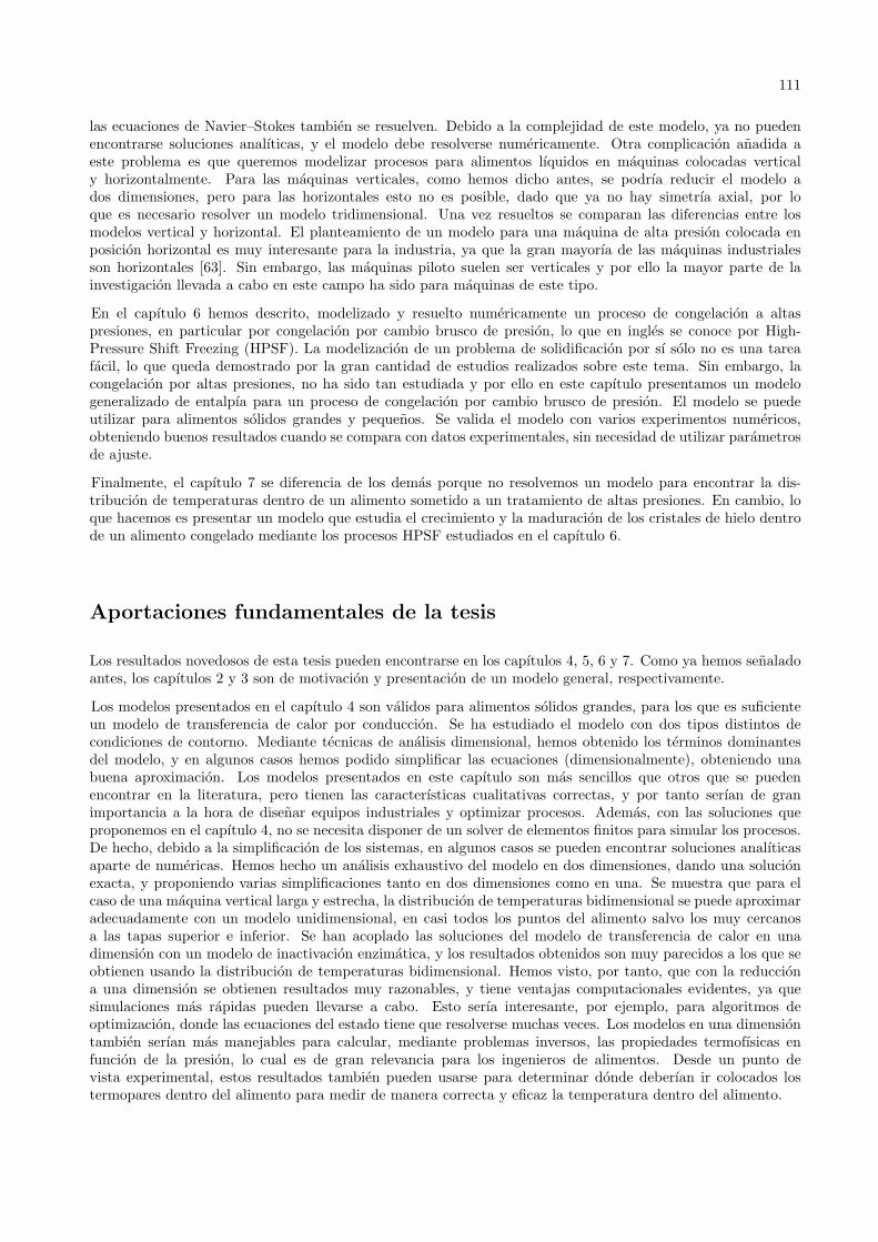
111
las ecuaciones de Navier–Stokes tambien se resuelven. Debido a la complejidad de este modelo, ya no puedenencontrarse soluciones analıticas, y el modelo debe resolverse numericamente. Otra complicacion anadida aeste problema es que queremos modelizar procesos para alimentos lıquidos en maquinas colocadas verticaly horizontalmente. Para las maquinas verticales, como hemos dicho antes, se podrıa reducir el modelo ados dimensiones, pero para las horizontales esto no es posible, dado que ya no hay simetrıa axial, por loque es necesario resolver un modelo tridimensional. Una vez resueltos se comparan las diferencias entre losmodelos vertical y horizontal. El planteamiento de un modelo para una maquina de alta presion colocada enposicion horizontal es muy interesante para la industria, ya que la gran mayorıa de las maquinas industrialesson horizontales [63]. Sin embargo, las maquinas piloto suelen ser verticales y por ello la mayor parte de lainvestigacion llevada a cabo en este campo ha sido para maquinas de este tipo.
En el capıtulo 6 hemos descrito, modelizado y resuelto numericamente un proceso de congelacion a altaspresiones, en particular por congelacion por cambio brusco de presion, lo que en ingles se conoce por High-Pressure Shift Freezing (HPSF). La modelizacion de un problema de solidificacion por sı solo no es una tareafacil, lo que queda demostrado por la gran cantidad de estudios realizados sobre este tema. Sin embargo, lacongelacion por altas presiones, no ha sido tan estudiada y por ello en este capıtulo presentamos un modelogeneralizado de entalpıa para un proceso de congelacion por cambio brusco de presion. El modelo se puedeutilizar para alimentos solidos grandes y pequenos. Se valida el modelo con varios experimentos numericos,obteniendo buenos resultados cuando se compara con datos experimentales, sin necesidad de utilizar parametrosde ajuste.
Finalmente, el capıtulo 7 se diferencia de los demas porque no resolvemos un modelo para encontrar la dis-tribucion de temperaturas dentro de un alimento sometido a un tratamiento de altas presiones. En cambio, loque hacemos es presentar un modelo que estudia el crecimiento y la maduracion de los cristales de hielo dentrode un alimento congelado mediante los procesos HPSF estudiados en el capıtulo 6.
Aportaciones fundamentales de la tesis
Los resultados novedosos de esta tesis pueden encontrarse en los capıtulos 4, 5, 6 y 7. Como ya hemos senaladoantes, los capıtulos 2 y 3 son de motivacion y presentacion de un modelo general, respectivamente.
Los modelos presentados en el capıtulo 4 son validos para alimentos solidos grandes, para los que es suficienteun modelo de transferencia de calor por conduccion. Se ha estudiado el modelo con dos tipos distintos decondiciones de contorno. Mediante tecnicas de analisis dimensional, hemos obtenido los terminos dominantesdel modelo, y en algunos casos hemos podido simplificar las ecuaciones (dimensionalmente), obteniendo unabuena aproximacion. Los modelos presentados en este capıtulo son mas sencillos que otros que se puedenencontrar en la literatura, pero tienen las caracterısticas cualitativas correctas, y por tanto serıan de granimportancia a la hora de disenar equipos industriales y optimizar procesos. Ademas, con las soluciones queproponemos en el capıtulo 4, no se necesita disponer de un solver de elementos finitos para simular los procesos.De hecho, debido a la simplificacion de los sistemas, en algunos casos se pueden encontrar soluciones analıticasaparte de numericas. Hemos hecho un analisis exhaustivo del modelo en dos dimensiones, dando una solucionexacta, y proponiendo varias simplificaciones tanto en dos dimensiones como en una. Se muestra que para elcaso de una maquina vertical larga y estrecha, la distribucion de temperaturas bidimensional se puede aproximaradecuadamente con un modelo unidimensional, en casi todos los puntos del alimento salvo los muy cercanosa las tapas superior e inferior. Se han acoplado las soluciones del modelo de transferencia de calor en unadimension con un modelo de inactivacion enzimatica, y los resultados obtenidos son muy parecidos a los que seobtienen usando la distribucion de temperaturas bidimensional. Hemos visto, por tanto, que con la reducciona una dimension se obtienen resultados muy razonables, y tiene ventajas computacionales evidentes, ya quesimulaciones mas rapidas pueden llevarse a cabo. Esto serıa interesante, por ejemplo, para algoritmos deoptimizacion, donde las ecuaciones del estado tiene que resolverse muchas veces. Los modelos en una dimensiontambien serıan mas manejables para calcular, mediante problemas inversos, las propiedades termofısicas enfuncion de la presion, lo cual es de gran relevancia para los ingenieros de alimentos. Desde un punto devista experimental, estos resultados tambien pueden usarse para determinar donde deberıan ir colocados lostermopares dentro del alimento para medir de manera correcta y eficaz la temperatura dentro del alimento.
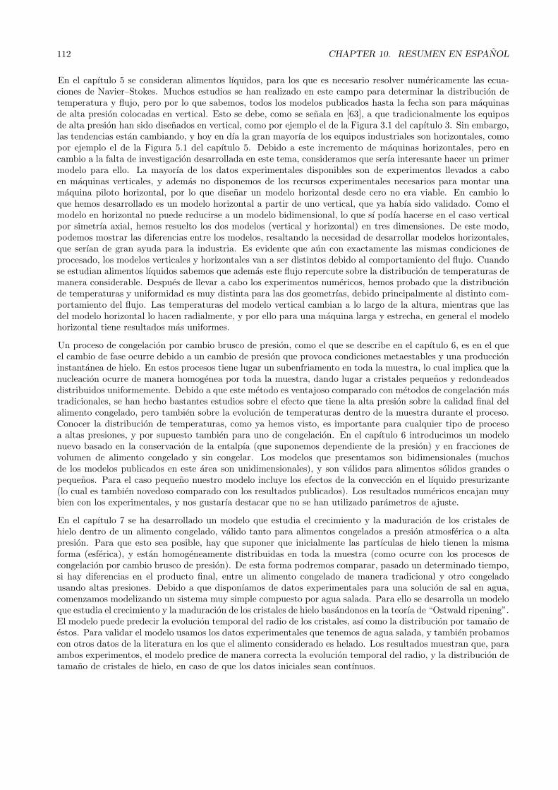
112 CHAPTER 10. RESUMEN EN ESPANOL
En el capıtulo 5 se consideran alimentos lıquidos, para los que es necesario resolver numericamente las ecua-ciones de Navier–Stokes. Muchos estudios se han realizado en este campo para determinar la distribucion detemperatura y flujo, pero por lo que sabemos, todos los modelos publicados hasta la fecha son para maquinasde alta presion colocadas en vertical. Esto se debe, como se senala en [63], a que tradicionalmente los equiposde alta presion han sido disenados en vertical, como por ejemplo el de la Figura 3.1 del capıtulo 3. Sin embargo,las tendencias estan cambiando, y hoy en dıa la gran mayorıa de los equipos industriales son horizontales, comopor ejemplo el de la Figura 5.1 del capıtulo 5. Debido a este incremento de maquinas horizontales, pero encambio a la falta de investigacion desarrollada en este tema, consideramos que serıa interesante hacer un primermodelo para ello. La mayorıa de los datos experimentales disponibles son de experimentos llevados a caboen maquinas verticales, y ademas no disponemos de los recursos experimentales necesarios para montar unamaquina piloto horizontal, por lo que disenar un modelo horizontal desde cero no era viable. En cambio loque hemos desarrollado es un modelo horizontal a partir de uno vertical, que ya habıa sido validado. Como elmodelo en horizontal no puede reducirse a un modelo bidimensional, lo que sı podıa hacerse en el caso verticalpor simetrıa axial, hemos resuelto los dos modelos (vertical y horizontal) en tres dimensiones. De este modo,podemos mostrar las diferencias entre los modelos, resaltando la necesidad de desarrollar modelos horizontales,que serıan de gran ayuda para la industria. Es evidente que aun con exactamente las mismas condiciones deprocesado, los modelos verticales y horizontales van a ser distintos debido al comportamiento del flujo. Cuandose estudian alimentos lıquidos sabemos que ademas este flujo repercute sobre la distribucion de temperaturas demanera considerable. Despues de llevar a cabo los experimentos numericos, hemos probado que la distribucionde temperaturas y uniformidad es muy distinta para las dos geometrıas, debido principalmente al distinto com-portamiento del flujo. Las temperaturas del modelo vertical cambian a lo largo de la altura, mientras que lasdel modelo horizontal lo hacen radialmente, y por ello para una maquina larga y estrecha, en general el modelohorizontal tiene resultados mas uniformes.
Un proceso de congelacion por cambio brusco de presion, como el que se describe en el capıtulo 6, es en el queel cambio de fase ocurre debido a un cambio de presion que provoca condiciones metaestables y una produccioninstantanea de hielo. En estos procesos tiene lugar un subenfriamento en toda la muestra, lo cual implica que lanucleacion ocurre de manera homogenea por toda la muestra, dando lugar a cristales pequenos y redondeadosdistribuidos uniformemente. Debido a que este metodo es ventajoso comparado con metodos de congelacion mastradicionales, se han hecho bastantes estudios sobre el efecto que tiene la alta presion sobre la calidad final delalimento congelado, pero tambien sobre la evolucion de temperaturas dentro de la muestra durante el proceso.Conocer la distribucion de temperaturas, como ya hemos visto, es importante para cualquier tipo de procesoa altas presiones, y por supuesto tambien para uno de congelacion. En el capıtulo 6 introducimos un modelonuevo basado en la conservacion de la entalpıa (que suponemos dependiente de la presion) y en fracciones devolumen de alimento congelado y sin congelar. Los modelos que presentamos son bidimensionales (muchosde los modelos publicados en este area son unidimensionales), y son validos para alimentos solidos grandes opequenos. Para el caso pequeno nuestro modelo incluye los efectos de la conveccion en el lıquido presurizante(lo cual es tambien novedoso comparado con los resultados publicados). Los resultados numericos encajan muybien con los experimentales, y nos gustarıa destacar que no se han utilizado parametros de ajuste.
En el capıtulo 7 se ha desarrollado un modelo que estudia el crecimiento y la maduracion de los cristales dehielo dentro de un alimento congelado, valido tanto para alimentos congelados a presion atmosferica o a altapresion. Para que esto sea posible, hay que suponer que inicialmente las partıculas de hielo tienen la mismaforma (esferica), y estan homogeneamente distribuidas en toda la muestra (como ocurre con los procesos decongelacion por cambio brusco de presion). De esta forma podremos comparar, pasado un determinado tiempo,si hay diferencias en el producto final, entre un alimento congelado de manera tradicional y otro congeladousando altas presiones. Debido a que disponıamos de datos experimentales para una solucion de sal en agua,comenzamos modelizando un sistema muy simple compuesto por agua salada. Para ello se desarrolla un modeloque estudia el crecimiento y la maduracion de los cristales de hielo basandonos en la teorıa de “Ostwald ripening”.El modelo puede predecir la evolucion temporal del radio de los cristales, ası como la distribucion por tamano deestos. Para validar el modelo usamos los datos experimentales que tenemos de agua salada, y tambien probamoscon otros datos de la literatura en los que el alimento considerado es helado. Los resultados muestran que, paraambos experimentos, el modelo predice de manera correcta la evolucion temporal del radio, y la distribucion detamano de cristales de hielo, en caso de que los datos iniciales sean contınuos.
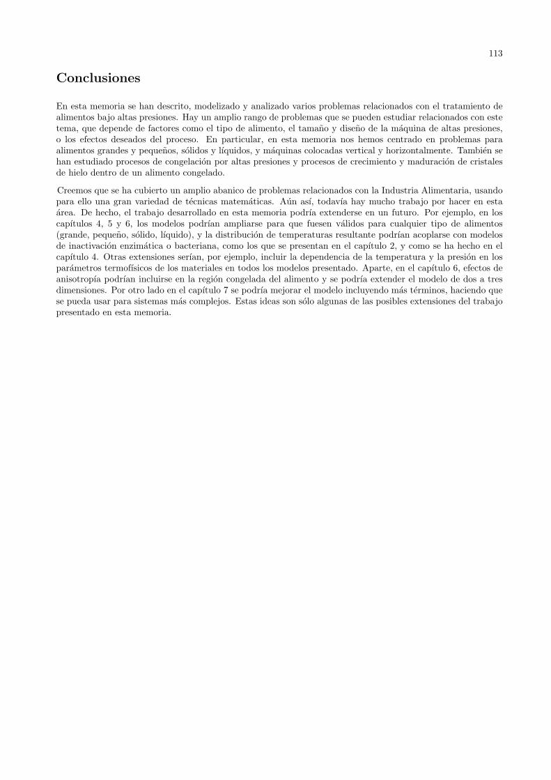
113
Conclusiones
En esta memoria se han descrito, modelizado y analizado varios problemas relacionados con el tratamiento dealimentos bajo altas presiones. Hay un amplio rango de problemas que se pueden estudiar relacionados con estetema, que depende de factores como el tipo de alimento, el tamano y diseno de la maquina de altas presiones,o los efectos deseados del proceso. En particular, en esta memoria nos hemos centrado en problemas paraalimentos grandes y pequenos, solidos y lıquidos, y maquinas colocadas vertical y horizontalmente. Tambien sehan estudiado procesos de congelacion por altas presiones y procesos de crecimiento y maduracion de cristalesde hielo dentro de un alimento congelado.
Creemos que se ha cubierto un amplio abanico de problemas relacionados con la Industria Alimentaria, usandopara ello una gran variedad de tecnicas matematicas. Aun ası, todavıa hay mucho trabajo por hacer en estaarea. De hecho, el trabajo desarrollado en esta memoria podrıa extenderse en un futuro. Por ejemplo, en loscapıtulos 4, 5 y 6, los modelos podrıan ampliarse para que fuesen validos para cualquier tipo de alimentos(grande, pequeno, solido, lıquido), y la distribucion de temperaturas resultante podrıan acoplarse con modelosde inactivacion enzimatica o bacteriana, como los que se presentan en el capıtulo 2, y como se ha hecho en elcapıtulo 4. Otras extensiones serıan, por ejemplo, incluir la dependencia de la temperatura y la presion en losparametros termofısicos de los materiales en todos los modelos presentado. Aparte, en el capıtulo 6, efectos deanisotropıa podrıan incluirse en la region congelada del alimento y se podrıa extender el modelo de dos a tresdimensiones. Por otro lado en el capıtulo 7 se podrıa mejorar el modelo incluyendo mas terminos, haciendo quese pueda usar para sistemas mas complejos. Estas ideas son solo algunas de las posibles extensiones del trabajopresentado en esta memoria.

Bibliography
[1] Encyclopedia Britannica. 15th edition, 1989.
[2] IUPAC: Compendium of Chemical Terminology. 2nd edition, 1997.
[3] Encyclopedia McGraw-Hill. 9th edition, 2002.
[4] E. Alizadeh, N. Chapleau, M. de Lamballeire, and A. Le-Bail. Impact of freezing process on salt diffusivityof seafood: Application to salmon (salmo salar) using conventional and pressure shift freezing. Food
Bioprocess Technol., 2: 257–262, 2009.
[5] R. Aris. Vectors, Tensors, and the Basic Equations of Fluid Mechanics. Dover Publications, Inc. NewYork, 1989.
[6] B. R. Becker and B. A. Fricke. Food thermophysical property models. Int. Comm. Heat Mass Transfer,26(5): 627–636, 1999.
[7] R. E. Bird, W. E. Stewart, and E. N. Lightfoot. Transport Phenomena. Wiley, 1960.
[8] B. W. Bridgman. Water, in the liquid and five solid forms, under pressure. Proc. Am. Acad. Arts Sci.
XLVIII, 13: 439–558, 1912.
[9] V. M. Burlakov and L. Kantorovich. Ostwald ripening of binary alloy particles. The Journal of Chemical
Physics, 134, 2011.
[10] B. Cabane and R. Vuilleumier. The physics of liquid water. C. R. Geoscience, 337: 159–171, 2005.
[11] J. C. Cheftel. Effects of high hydrostatic pressure on food constituents: an overview. In C. Balny, R.
Hayashi, K. Heremans, P. Masson, eds. High Pressure and Biotechnology, 224: 195–209, 1992.
[12] J. C. Cheftel. Review: high-pressure, microbial inactivation and food preservation. Food Sci. Tech. Int.,1(2-3): 75–90, 1995.
[13] J. C. Cheftel and J. Culioli. Effects of high pressure on meat: a review. Meat Science, 46(3): 211–236,1997.
[14] A. C. Cleland and R. L. Earle. Assessment of freezing time prediction methods. J. Food Sci., 49: 1034–1042,1995.
[15] G. Comini, S. Giudice, R. W. Lewis, and 0. C. Zienkiewicz. Finite element solution of non-linear heatconduction problems with special reference to phase change. Int. J. Num. Meth. Engin., 8: 613–624, 1974.
[16] G. Comini, S. Giudice, and O. Saro. A conservative algorithm for multidimensional conduction phasechange. Int. J. Num. Meth. Engin., 30: 697–709, 1990.
[17] J. Crank. Free and Moving Boundary Problems. Oxford Science Publications. New York, 1987.
[18] A. Delgado, C. Rauh, W. Kowalczyk, and A. Baars. Review of modelling and simulation of high pressuretreatment of materials of biological origin. Trends in Food Science and Technology, 19(6): 329–336, 2008.
[19] S. Denys, A. M. Van Loey, and M. E. Hendrickx. A modelling approach for evaluating process uniformity
115
116 BIBLIOGRAPHY
during batch high hydrostatic pressure processing: Combination of a numerical heat transfer model andenzyme inactivation kinetics. Innovative Food Science and Emerging Technologies, 1(1): 5–19, 2000.
[20] S. Denys, A. M. Van Loey, M. E. Hendrickx, and P. Tobback. Modelling heat transfer during high-pressurefreezing and thawing. Biotechol. Prog., 13: 413–423, 1997.
[21] S. Denys, L. R. Ludikhuyze, A. M. Van Loey, and M. E. Hendrickx. Modelling conductive heat transferand process uniformity during batch high-pressure processing of foods. Biotechnol. Prog., 16: 92–101, 2000.
[22] C. Dogan and O. Erkmen. High pressure inactivation kinetics of listeria monocytogenes inactivation inbroth, milk, and peach and orange juices. J. Food Engng., 62: 47–52, 2004.
[23] D .P. Donhowe, R. W. Hartel, and Jr. R. L. Bradley. Determination of ice crystal size distribution in frozendesserts. J. Dairy Sci., 74: 3334–3344, 1991.
[24] J. Irudayaraj (Editor). Food Processing Operations Modeling: Design and Analysis. Marcel Dekker Inc.New York Basel, 2002. ISBN 0824704886.
[25] R. Van Eldik and J. Jonas. High-Pressure Chemistry and Biochemistry. Springer, 1987. ISBN: 9027724571,9789027724571.
[26] J. R. Elliott and C. T. Lira. Introductory Chemical Engineering Thermodynamics. Prentice Hall Interna-tional Series in the Physical and Chemical Engineering Sciences, 2005.
[27] O. Erkmen and C. Dogan. Kinetic analysis of escherichia coli inactivation by high hydrostatic pressure inbroth and foods. Food Microbiol., 21: 181–185, 2004.
[28] D. F. Farkas and D. G. Hoover. High pressure processing. Journal of Food Science Supplement: Kinetics
of microbial inactivation for alternative food processing technologies, pages 47–64, 2001.
[29] P. P. Fernandez, L. Otero, B. Guignon, and P. D. Sanz. High-pressure shift freezing versus high-pressureassisted freezing: Effects on the microstructure of a food model. Food Hydrocolloids, 20: 510–522, 2006.
[30] P. P. Fernandez, L. Otero, M. M. Martino, A. D. Molina-Garcıa, and P. D. Sanz. High-pressure shiftfreezing: recrystallization during storage. European Food Research and Technology, 227(5): 1367–1377,2008.
[31] U. S. Food, Drug Administration, Center for Food Safety, and Applied Nutrition. Kinetics of microbial inac-tivation for alternative food processing technologies, 2000. http://www.fda.gov/Food/ScienceResearch/ResearchAreas/SafePracticesforFoodProcesses/.
[32] A. G. A. Ghani and M. M. Farid. Numerical simulation of solid-liquid food mixture in a high pressureprocessing unit using computational fluid dynamics. Journal of Food Engineering, 80(4): 13031–1042, 2007.
[33] Dr. S. Gola. Microbiological results of tests ordered by Esteban Espuna, S.A, to la Stazione Sperimentale
per l’industria delle conserve alimentari in Parma, 5 Marzo 2004.
[34] B. Guignon, C. Aparicio, and P. D. Sanz. Volumetric properties of pressure-transmitting fluids up to350mpa: Water, ethanol, ehtylene gylcol, propylene glycol, castor oil, silicon oil, and some of their binarymixture. J. Chem. Eng. Data, 55: 3017–3023, 2010.
[35] B. Guignon, A. M. Ramos, J. A. Infante, J. M. Diaz, and P. D. Sanz. Determining thermal parameters inthe cooling of a small-scale high-pressure freezing vessel. Int. J. Refrigeration, 29: 1152–1159, 2006.
[36] C. Hartmann. Numerical simulation of thermodynamic and fluiddynamic processes during the high pressuretreatment of fluid food systems. Innovative Food Science and Emerging Technologies, 3(1): 11–18, 2002.
[37] C. Hartmann and A. Delgado. Numerical simulation of convective and diffusive transport effects on a high- pressure - induced inactivation process. Biotechnology and Bioengineering, 79(1): 94–104, 2002.
[38] C. Hartmann and A. Delgado. Numerical simulation of thermal and fluiddynamical transport effects on ahigh pressure induced inactivation. High Pressure Research, 23: 67–70, 2003.
BIBLIOGRAPHY 117
[39] C. Hartmann, A. Delgado, and J. Szymczyk. Convective and diffusive transport effects in a high pressureinduced inactivation process of packed food. Journal of Food Engineering, 59(1): 33–44, 2003.
[40] C. Hartmann, J-P. Schuhholz, P. Kitsbun, N. Chapleau, A. Le Bail, and A. Delgado. Experimental andnumerical analysis of the thermofluiddynamics in a high-pressure autoclave. Innovative Food Science and
Emerging Technologies, 5: 399–411, 2004.
[41] R. Hayashi. Utilization of pressure in addition to temperature in food science and technology. In High
pressure and biotechnology; Balny, C., Hayashi, R., Heremans, K., Masson, P., Eds.; Colloque INSERM:,224: 185–193, 1992.
[42] Hiperbaric. Hiperbaric: High pressure processing, 2012. http://www.hiperbaric.com/.
[43] A. Ibarz-Ribas and G. V. Barbosa-Canovas. Operaciones unitarias en la ingenierıa de alimentos. Mundi-Prensa Libros, 2005. ISBN 8484761630, 9788484761631.
[44] I. Indrawati, L. R. Ludikhuyze, A. M. van Loey, and M. E. Hendrickx. Lipoxygenase inactivation in greenbeans (phaseolus vulgaris l.) due to high pressure treatment at subzero and elevated temperatures. J.
Agric. Food Chem., 48: 1850–1859, 2000.
[45] J. A. Infante. Analisis numerico de modelos matematicos y problemas inversos en tecnologıa de alimentos.PhD thesis, Universidad Complutense de Madrid, Nov. 2009.
[46] J. A. Infante, B. Ivorra, A. M. Ramos, and J. M. Rey. On the modelling and simulation of high pressureprocesses and inactivation of enzymes in food engineering. Math. Models Methods Appl. Sci., 19(12): 2203–2229, 2009.
[47] G. Job and F. Herrmann. Chemical potential–a quantity in search of recognition. European Journal of
Physics, 27: 353–371, 2006.
[48] P. Juliano, K. Knoerzer, P. Fryer, and C. Versteeg. C. Botulinum inactivation kinetics implemented in acomputational model of a high pressure sterilization process. Biotechnology Process, 25(1): 163–175, 2008.
[49] B. Klotz, D. Leo Pyle, and B. M. Mackey. New mathematical modeling approach for predicting microbialinactivation by high hydrostatic pressure. Applied and Enviromental Microb., 73(8): 2468–2478, 2007.
[50] K. Knoerzer, R. Buckow, P. Juliano, B. Chapman, and C. Versteeg. Carrier optimisation in a pilot-scalehigh pressure sterilisation plant – an iterative cfd approach. Journal of Food Engineering, 97(2): 199–207,2010.
[51] K. Knoerzer and B. Chapman. Effect of material properties and processing conditions on the predictionaccuracy of a cfd model for simulating high pressure thermal (hpt) processing. Journal of Food Engineering,104: 404–413, 2011.
[52] K. Knoerzer, P. Juliano, S. Gladman, C. Versteeg, and P. J. Fryer. A computational model for temper-ature and sterility distributions in a pilot-scale high-pressure high-temperature process. AIChE Journal,53(11): 2996–3010, 2007.
[53] K. Knoerzer, P. Juliano, P. Roupas, and Editors C. Versteeg. Innovative Food Processing Technologies:
Advances in Multiphysics Simulation. Wiley-Blackwell and IFT Press, 2011.
[54] W. Kowalczyk and A. Delgado. Dimensional analysis of thermo-fluid-dynamics of high hydrostatic pressureprocesses with phase transition. Int. J. Heat Mass Transf., 50: 3007–3018, 2007.
[55] W. Kowalczyk and A. Delgado. On convection phenomena during high pressure treatment of liquid media.High Pressure Research, 27(1): 85–92, 2007.
[56] W. Kowalczyk, Chr. Hartmann, and A. Delgado. Modelling and numerical simulation of convection drivenhigh pressure induced phase changes. Int. J. Heat Mass Transf., 47: 1079–1089, 2004.
[57] A. Kupper, E. G. Hauptmann, and M. Iqbal. Combined free and forced convection in a horizontal tubeunder uniform heat flux. Solar Energy, 12: 439–446, 1969.
118 BIBLIOGRAPHY
[58] L. R. Ludikhuyze, I. Van den Broeck, C. A. Weemaes, and M. E. Hendrickx. Kinetic parameters forpressure-temperature inactivation of bacillus subtilis α-amylase under dynamic conditions. Biotechnol.
Prog., 13: 617–623, 1997.
[59] L. R. Ludikhuyze, I. Van den Broeck, C. A. Weemaes, C. Herremans, J. F. Van Impe, M. E. Hendrickx,and P. Tobback. Kinetics for isobaric-isothermal inactivation of bacillus subtilis α-amylase. Biotechnol.
Prog., 13: 523–538, 1997.
[60] X. Luo and P. V. Schevchenko. A short tale of long tail integration. Numerical Algorithms, 56: 577, 2011.
[61] B. Ly-Nguyen, A. M. Loey, C. Smout, S. E. Zcan, D. Fachin, I. Verlent, S. Vu Truong, T. Duvetter, andM. E. Hendrickx. Mild-heat and high-pressure inactivation of carrot pectin methyl-esterase: A kineticstudy. J. Food Sci., 68: 1377–1383, 2003.
[62] K. Miyagawa and K. Suzuki. Studies on taka-amylase a under high pressure: Some kinetic aspects ofpressure inactivation of taka-amylase a. Arch. Biochem. Biophys., 105: 297–302, 1964.
[63] H. Mujica-Paz, A. Valdez-Fragoso, C. Tonello-Samson, J. Welti-Chanes, and J. A. Torres. High-pressureprocessing technologies for the pasteurization and sterilization of foods. Food Bioprocess Technol., 4: 969–985, 2011.
[64] T. Norton, A. Delgado, E. Hogan, P. Grace, and Da-Wen Sun. Simulation of high pressure freezing processesby enthalpy method. J. Food Eng., 91: 260–268, 2009.
[65] D. R. Oliver. The effect of natural convection on viscous-flow heat transfer in horizontal tubes. Chemical
Engineering Science, 17: 335–350, 1962.
[66] L. Otero, M. Martino, N. Zaritzky, M. Solas, and P. D. Sanz. Preservation of microstructure in peach andmango during high-pressure-shift freezing. J. Food Sci., 65: 466–470, 2000.
[67] L. Otero, A. D. Molina-Garcia, A. M. Ramos, and P. D. Sanz. A model for real thermal control inhigh-pressure treatment of foods. Notes. Biotechnol. Prog., 18: 904–908, 2002.
[68] L. Otero, A. Ousegui, B. Guignon, A. Le Bail, and P. D. Sanz. Evaluation of the thermophysical propertiesof tylose gel under pressure in the phase change domain. Food Hydrocolloids, 20: 449–460, 2006.
[69] L. Otero, A. M. Ramos, C. de Elvira, and P. D. Sanz. A model to design high pressure processes towardsa uniform temperature distribution. J. Food Engng, 78: 1463–1470, 2007.
[70] L. Otero and P. D. Sanz. High-pressure shift freezing part 1: Amount of ice instantaneously formed in theprocess. Biotechnol. Prog., 16: 1030–1036, 2000.
[71] L. Otero and P. D. Sanz. Modelling heat transfer in high pressure food processing: a review. Innovative
Food Sci. Emerging Tech., 4: 121–134, 2003.
[72] L. Otero and P. D. Sanz. High-pressure-shift freezing: Main factors implied in the phase transition time.J. Food Engng, 72: 354–363, 2006.
[73] M. Necati Ozisik. Boundary Value Problems of Heat Conduction. Dover Publications Inc. New York, 1968.
[74] Q. Tuan Pham. Modelling heat and mass transfer in frozen foods: a review. Int. J. Refrigeration, 29: 876–888, 2006.
[75] M. S. Rahman, G. Al-Saidi, N. Guizani, and A. Abdullah. Development of state diagram of bovine gel bymeasuring thermal characteristics using differential scanning calorimetry (dsc) and cooling curve method.Thermochim. Acta, 509: 111–119, 2010.
[76] A. M. Ramos and N. A. S. Smith. Efecto de las altas presiones sobre los microorganismos en relacion conla conservacion de alimentos. Caso de la Listeria monocytogenes en jamon crudo picado. Technical report,Universidad Complutense de Madrid, 2009.
[77] C. Rauh, A. Baars, and A. Delgado. Uniformity of enzyme inactivation in a short-time high-pressureprocess. J. Food Engng, 91: 154–163, 2009.
BIBLIOGRAPHY 119
[78] P. D. Sanz and L. Otero. High-pressure shift freezing part 2: Modelling of freezing times for a finitecylindrical model. Biotechnol. Prog., 16: 1037–1043, 2000.
[79] O. Schluter, G. Urrutia Benet, V. Heinz, and D. Knorr. Metastable states of water and ice during pressure-supported freezing of potato tissue. Biotechnol. Prog., 20: 799–810, 2004.
[80] H. R. Schwartzberg. Effective heat capacities for the freezing and thawing of food. J. Food Sci., 41: 152–156,1976.
[81] R. K. Simpson and A. Gilmour. The resistance of Listeria monocytogenes to high hydrostatic pressure infoods. Food Microbiol., 14: 567–573, 1997.
[82] J. P. P. M. Smelt. Recent advances in the microbiology of high pressure processing. Trends Food Sci. Tech.,9: 152–158, 1998.
[83] N. A. S. Smith, V. Burlakov, and A. M. Ramos. Publication in preparation.
[84] N. A. S. Smith, K. Knoerzer, and A. M. Ramos. Publication in preparation.
[85] N. A. S. Smith, S. L. Mitchell, and A. M. Ramos. Analysis and simplification of a mathematical model forhigh-pressure food processes, 2012. Submitted.
[86] N. A. S. Smith, S. S. L. Peppin, and A. M. Ramos. Generalized enthalpy model of a high-pressure shiftfreezing process. Proc. Roy. Soc. A, 468(2145): 2744–2766, 2012.
[87] K. Suzuki and K. Kitamura. Inactivation of enzyme under high pressure: Studies on the kinetics ofinactivation of α–amylase of bacillus subtilis under high pressure. J. Biochem., 54: 214–219, 1963.
[88] C. R. Swaminathan and V. R. Voller. A general enthalpy method for modeling solidification processes.Metallurgical Transactions B, 23(5): 651–664, 1992.
[89] J. A. Torres and G. Velazquez. Commercial opportunities and research challenges in the high pressureprocessing of foods. J. Food Eng., 67: 95–112, 2005.
[90] G. Urrutia, O. Schluter, and D. Knorr. High pressure low temperature processing. suggested definitionsand terminology. Innovative Food Science and Emerging Technologies, 5: 413–427, 2004.
[91] V. R. Voller, C. R. Swaminathan, and B. G. Thomas. Fixed grid techniques for phase change problems: Areview. Int. J. Numer. Methods Eng., 30: 875–898, 1990.
[92] R. Xiong, G. Xie, A. E. Edmondson, and M. A. Sheard. A mathematical model for bacterial inactivation.J. Food Microbiol., 46: 45–55, 1999.