IDENTIFICACIÓN CON REDES NEURONALES PROBABILÍSTICAS DE … · de los tratamientos de deficiencias...

395

Resumen

La sintomatología visual en hojas debida a deficiencias nu-trimentales, como la de hierro (Fe) y manganeso (Mn), son similares en coloración y en tipo de hojas en que se presenta, por lo cual se requiere un método, con base en análisis de imágenes digitales de hojas, que discrimine esas deficien-cias. El objetivo de esta investigación fue analizar imágenes digitales de hojas de frijol (Phaseolus vulgaris L.) var. Caca-huate para identificar, con un clasificador creado con redes neuronales probabilísticas, deficiencias de Fe y Mn en una etapa inicial, cuando todavía es posible revertir los daños con fertilización. Los tratamientos fueron: 1) deficiencia parcial (DP) de Fe (50 %); 2) DP de Mn (50 %); 3) deficien-cia total (DT) de Fe (0 %); 4) DT de Mn (0 %); 5) interac-ción (0 % Fe, 0 % Mn); 6) testigo (100 % Fe, 100 % Mn), con 10 repeticiones; la referencia fue la solución Steiner. Los valores promedio de ocho variables de color y tres de tex-tura, se obtuvieron de seis muestras de imágenes digitales de 100100 píxeles (360 muestras en total), de hojas de frijol obtenidas 74 dds. Estas fueron usadas como variable de entrada para generar clasificadores con redes neuronales probabilísticas con el algoritmo de correlación en cascada de los tratamientos de deficiencias de Fe y Mn. Los clasifica-dores que solo consideraron características texturales, como variables de entrada, tuvieron porcentajes de clasificación correcta global de síntomas menores o iguales a 44 %. En cambio, el porcentaje de clasificación correcta global del

AbstRAct

The visual symptomatology of nutriment deficiencies, like iron (Fe) and manganese (Mn) in plant leafs is similar in their coloration and the kind of leaf they present on. A method based on the analysis of digital images of the leaves, capable to discriminate the differences of such deficiencies is required. The aim of this research was to analyze digital images of common bean (Phaseolus vulgaris L. var. Cacahuate), in order to identify differences in the Fe and Mn lesions in the initial development stage, when it is possible to revert damages with fertilization. To do so, we used a classifier created with probabilistic neuronal networks. The experimental treatments were: 1) partial deficiency (DP) of Fe (50 %); 2) DP of Mn (50 %); 3) total deficiency (DT) of Fe (0 %); 4) DT of Mn (0 %); 5) Fe/Mn interaction (0 % Fe, 0 % Mn); 6) control (100 % Fe, 100 % Mn), with 10 repetitions; Steiner solution was used as reference. The mean values of eight color and three texture variables from digital images of six common bean leaf samples were obtained; these were of 100100 pixels (360 total samples) in 74 dds. These mean values were used as entry variables to generate the classifiers with a cascade correlation algorithm of the Fe and Mn deficiency treatments. The classifiers that only considered textural characteristics had correct global classification of symptoms less or equal to 44 %. In contrast, the highest percentage of correct global classification of the classifiers in the test was of 76.6 % with six variables, which included texture and color characteristics, and six exit classes of difference treatments. The reduction of the number of classes did not increase the percentage of correct classification in the test.

IDENTIFICACIÓN CON REDES NEURONALES PROBABILÍSTICAS DELAS DEFICIENCIAS DE HIERRO Y MANGANESO, USANDO IMÁGENES

DIGITALES DE HOJAS DE FRIJOL (Phaseolus vulgaris L.)

IDENTIFICATION WITH PROBABILISTICAL NEURONAL NETWORKS OFDEFICIENCIES OF IRON AND MANGANESE BY USING DIGITAL IMAGES

FROM BEAN LEAVES (Phaseolus vulgaris L.)

Edgar García-Cruz1, Manuel Sandoval-Villa2, José A. Carrillo-Salazar3*, Jorge M. Valdéz-Carrasco4, Paulina H. González-Fierro5

1Postgrado en Edafología. 2Postgrado en Hidrociencias. 3Postgrado en Recursos Genéticos y Productividad. Fisiología Vegetal. 4Postgrado en Entomología. Colegio de Postgraduados, Campus Montecillo. 56230. Montecillo, Estado de México, México. ([email protected]). 5Centro Internacional de Mejoramiento de Maíz y Trigo (CIMMYT). Texcoco, Estado de México.

*Autor responsable v Author for correspondence.Recibido: noviembre, 2014. Aprobado: abril, 2015.Publicado como ARTÍCULO en Agrociencia 49: 395-409. 2015.

396

AGROCIENCIA, 16 de mayo - 30 de junio, 2015

VOLUMEN 49, NÚMERO 4

mejor clasificador en la prueba fue 76.6 % con seis variables que incluyeron características de textura y color, y seis clases de salida o tratamientos de deficiencias. Un número menor de clases de salida no aumentó el porcentaje de clasificación correcta global en la prueba.

Palabras claves: croma, entropía, espacio de color RGB, homo-geneidad local, matiz, segundo momento angular.

IntRoduccIón

El frijol (Phaseolus vulgaris L.) es una especie susceptible a la deficiencia de hierro (Fe) que puede reducir hasta 100 % el rendimiento

de grano (Clark, 1991; Hansen et al., 2006). Esta deficiencia se manifiesta como clorosis intervenal, mientras que la de manganeso (Mn) se caracteriza en dicotiledóneas como manchas amarillas pequeñas, pero también como clorosis intervenal, lo cual puede confundirse con deficiencia de Fe. El Mn y Fe son nutrimentos relativamente inmóviles en el floema, es decir, no son removilizados hacia los tejidos jóvenes cuando disminuye su suministro vía xilema (Barba-zán, 1998). La deficiencia de ambos elementos pue-de confundirse debido a la similitud de los síntomas de la deficiencia de cada elemento bajo condiciones severas, por lo cual se podría enmascarar además de presentarse en hojas jóvenes (Howeler, 1978). Según Jones et al. (1991), una concentración de Fe y Mn de 15 a 49 mg kg1 es baja y el óptimo es 50 a 300 mg kg1. La toxicidad por Mn distorsiona las ho-jas y produce manchas oscuras; en casos severos hay necrosamiento de los bordes de las hojas que avanza hacia el interior al aumentar la severidad (Schulte y Kelling, 1999). La deficiencia de Fe ocasiona toxici-dad por Mn y viceversa (Somers y Shive, 1942) y una toxicidad leve por Mn es idéntica a la deficiencia de Fe (Twyman, 1950). Según Barbazán (1998), la apreciación visual de las deficiencias de Fe y Mn es aparente después de que la disponibilidad de estos nutrientes es tan baja que la planta no puede completar sus funciones fi-siológicas o ciclo biológico; por lo cual, el cambio de color y textura de la hoja sería una forma práctica para evaluar el estado nutricional, así como la sani-dad requiere determinación visual en una etapa tem-prana de la deficiencia. Sin embargo, en esta etapa, los síntomas no son tan evidentes, lo cual dificulta el diagnóstico.

Key words: chroma, entropy, RGB color space, local homogeneity, hue, second angular momentum.

IntRoductIon

Common bean (Phaseolus vulgaris L.) is a species susceptible to iron (Fe) deficiency, which can reduce up to 100 % of the

grain yield (Clark, 1991; Hansen et al., 2006). This deficiency is manifested as interveinal chlorosis, while that of manganese (Mn) in dicots is characterized by small yellow spots but but can also present interveinal chlorosis, which can therefore be confused with iron deficiency. The Mn and Fe are nutrients relatively immobile in the phloem, i.e. they are not moved back to young tissues when their supply is reduced by the xylem (Barbazan, 1998). Deficiency of both elements can be confused because of the symptoms similarity at severe conditions, which could be masked, as well as present in young leaves (Howeler, 1978). According to Jones et at. (1991), concentrations of Fe and Mn of 15 to 49 mg kg1 are low and their optimum is of 50 to 300 mg kg1. Mn toxicity distort leaves and produces dark spots; in severe cases there is necrosis at the leaves edges which moves inwards as the severity increase (Schulte and Kelling, 1999). Fe deficiency causes toxicity by Mn and vice versa (Somers and Shive, 1942) and a slight Mn toxicity is identical to Fe deficiency (Twyman, 1950). According to Barbazán (1998), the visual appreciation of the Fe and Mn is only apparent when the availability of these nutrients is so low that the plant cannot fulfill its physiological functions or biological cycle; therefore changes in the color and texture of the leafs would be a practical way to assess both, the nutritional status and the overall health of the plants. This requires the visual determination at an early stage of the deficiency. Nevertheless, at this stage, symptoms are not obvious, which makes its diagnosis difficult. Murakami et al. (2005) points out the increase in the research that applies color analysis of digital images to evaluate the foliar nutrition and health in response to environmental stress, mainly because it is a low-cost method. They propose a method to determine the health level of maple leafs based on the bands or the red (R) and green (G) channels of the RGB color space. Textural analysis classifies images ranging from photomicrograph to satellite images,

IDENTIFICACIÓN DE DEFICIENCIAS DE HIERRO Y MANGANESO USANDO IMÁGENES DIGITALES

397GARCÍA-CRUZ et al.

Murakami et al. (2005) señalan el aumento en las investigaciones que aplican el análisis de color de imágenes digitales para evaluar la nutrición foliar y la sanidad en respuesta al estrés ambiental, por ser un método de costo bajo. Ellos proponen un méto-do para determinar el nivel de sanidad de hojas de maple basado en las bandas o canales rojo (R) y ver-de (G) del espacio de color RGB. El análisis textural clasifica imágenes desde microfotografías hasta imá-genes satelitales porque las características texturales contienen información de la distribución espacial de las variaciones de tono de una banda; el tono se basa en la variación de sombras de gris de unidades de resolución en una imagen fotográfica, mientras que la textura está enfocada a la distribución espacial de los tonos de gris (Haralick et al., 1973). Haralick et al. (1973) usaron características de textura con base en matrices de co-ocurrencia en tonos de gris para analizar imágenes obtenidas por sensores remotos; la clasificación de superficies terrestres con base en su uso y la aplicación selectiva de pesticidas se puede hacer mediante esas características. Para distinguir malezas y asperjar selectivamente un pesticida para malezas de hoja ancha o pastos, Meyer et al. (1998) usaron características texturales, las cuales fueron la base para identificar el tipo de cubierta en la super-ficie y el análisis de color fue útil para separar entre plantas y suelo. Hay clasificadores con base en las características texturales y el análisis discriminan-te para identificar tipos de malezas. En un estudio (Burks et al., 2000) se diferenció el suelo y la planta con 100 % de precisión, mientras que la precisión fue 93 % al identificar malezas con el método de co-ocurrencia de color. Kim et al. (2009) usaron el método de co-ocurrencia de color para diferenciar hojas de cítricos con ocho síntomas, incluyendo de-ficiencias de Fe, Mn y Zinc (Zn) y la enfermedad enverdecimiento de los cítricos; mediante un análi-sis discriminante ellos crearon tres clasificadores con base en 14 características texturales como variables, la precisión para diferenciar deficiencias de esos mi-croelementos fue 97.3 %. El análisis textural es la herramienta más precisa para la discriminación de malezas de acuerdo con Meyer et al. (1998), quienes cuestionan si es conveniente combinar característi-cas texturales con las de color para identificar ma-lezas. Según Kim et al. (2009), diversas caracterís-ticas texturales deben considerarse, aunque algunas darán más información que otras, y eliminar las que

because textural features contain information of the spatial distribution of the tone variations of a band; the tone is based on the variation of shades of gray of resolution units in a photographic image, while texture is focused on the spatial distribution of shades of gray (Haralick et al., 1973). Haralick et al. (1973) used texture features based on co-occurrence matrices of gray tones to analyze images obtained by remote sensors; the classification of terrestrial surfaces based on its use and the selective application of pesticides can be done via such features. In order to distinguish weeds and selectively spraying a pesticide for broadleaf weeds or grasses, Meyer et al. (1998) used textural features, which were the basis for identifying the type of cover on the surface and color analysis was useful to discriminate between plants from soil. There are classifiers based on textural features and discriminant analysis to identify weed types. In a study (Burks et al., 2000) soil and plants were differentiated with a 100 % accuracy, whereas the precision was of 93 % when weeds were identified with the co-occurrence of color method. Kim et al. (2009) used the color co-occurrence method to differentiate citrus fruit leaves with eight symptoms, including deficiencies of Fe, Mn and Zinc (Zn) along with the Citrus Greening disease; using a discriminant analysis they created three classifiers based on 14 textural features like variables, with a accuracy in differentiating deficiencies of these micronutrients was 97.3 %. Textural analysis is the most accurate tool for discrimination of weeds according to Meyer et al. (1998), who questioned whether it is suitable to combine textural features with the color ones to identify weeds. According to Kim et al. (2009), various textural characteristics should be considered, although some will yield more information than others, and eliminate those that provide redundant information. To this regard, probabilistic neural networks can be used to create classifiers capable of identifying patterns in data; for this reason, they are a useful tool for the analysis of information (Oide and Ninomiya, 2000). The aim of this research was to identify the symptoms of Fe and Mn deficiency, both separately and in combination, on common beans plants in vegetative stage, via variables of color and texture, using analysis of digital images of leaves and a classifier set by artificial neural networks with the cascade correlation algorithm. The hypothesis was

398



proporcionen información redundante. Al respecto, las redes neuronales probabilísticas pueden usarse para crear clasificadores capaces de identificar patro-nes en datos, por lo cual son una herramienta útil en el análisis de información (Oide y Ninomiya, 2000). El objetivo de la presente investigación fue iden-tificar los síntomas de deficiencia de Fe y Mn, sepa-rados y combinados, de frijol en etapa vegetativa, mediante variables de color y textura, usando aná-lisis de imágenes digitales de hojas y un clasificador con base en redes neuronales artificiales con el al-goritmo de correlación en cascada. La hipótesis fue que las deficiencias de Fe y Mn pueden ser identifi-cadas con características texturales. Las variables de color se calcularon para determinar si éstas tienen nivel mayor de asociación con las deficiencias del cultivo de frijol que las de textura en una etapa tem-prana de desarrollo.

mAteRIAles y métodos

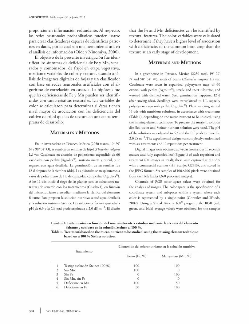
En un invernadero en Texcoco, México (2250 msnm, 19° 29’ N y 98° 54’ O), se sembraron semillas de frijol (Phaseolus vulgaris L.) var. Cacahuate en charolas de poliestireno expandido de 60 cavidades con perlita (Agrolita), sustrato inerte y estéril, y se regaron con agua destilada. La germinación de las semillas fue 12 d después de la siembra (dds). Las plántulas se trasplantaron a vasos de poliestireno de 1 L de capacidad con perlita (Agrolita). A los 19 dds inició el riego de las plantas con las soluciones nu-tritivas de acuerdo con los tratamientos (Cuadro 1), en función del micronutriente a estudiar, mediante la técnica del elemento faltante. Para preparar la solución nutritiva se usó agua destilada y la solución nutritiva Steiner. Las soluciones fueron ajustadas a pH de 6.3 y la CE está predeterminada a 2.0 dS m1. El diseño

that the Fe and Mn deficiencies can be identified by textural features. The color variables were calculated to determine if they have a higher level of association with deficiencies of the common bean crop than the texture at an early stage of development.

mAteRIAls And methods

In a greenhouse in Texcoco, Mexico (2250 masl, 19° 29’ N and 98° 54’ W), seeds of beans (Phaseolus vulgaris L.) var. Cacahuate were sown in expanded polystyrene trays of 60 cavities with perlite (Agrolite), sterile and inert substrate, and watered with distilled water. Seed germination happened 12 d after sowing (das). Seedlings were transplanted to 1 L capacity polystyrene cups with perlite (Agrolite). Plant watering started 19 dds with nutritious solutions, in accordance with treatments (Table 1), depending on the micro-nutrient to be studied, using the missing element technique. To prepare the nutrient solution distilled water and Steiner nutrient solution were used. The pH of the solutions was adjusted to 6.3 and the EC predetermined to 2.0 dS m1. The experimental design was completely randomized with six treatments and 10 repetitions per treatment. Digital images were obtained at 74 das from a fourth, recently mature and fully expanded leaf (Figure 1) of each repetition and treatment (60 images in total); these were captured at 300 dpi with a commercial scanner (HP Scanjet G2410), and stored in the JPEG format. Six samples of 100100 pixels were obtained from each left leaflet (360 processed images). Channels of RGB color space values were obtained for the analysis of images. The color space is the specification of a coordinate system and subspaces within a system where each color is represented by a single point (Gonzalez and Woods, 2002). Using a Visual Basic v. 6.0 program, the RGB (red, green, and blue) average values were obtained for the samples

Cuadro 1. Tratamientos en función del micronutriente a estudiar mediante la técnica del elemento faltante y con base en la solución Steiner al 100 %.

Table 1. Treatments based on the micro-nutrient to be studied, using the missing element technique based on a 100 % Steiner solution.

TratamientoContenido del micronutriente en la solución nutritiva

Hierro (Fe, %) Manganeso (Mn, %)

1 Testigo (solución Steiner 100 %) 100 1002 Sin Mn 100 03 Sin Fe 0 1004 Sin Mn, sin Fe 0 05 Deficiente en Mn 100 506 Deficiente en Fe 50 100



of 100100 pixels for each color category. The RGB values were transformed to the standard sRGB color sorter (linear) defined by the Commission Internationale de L’Éclairage (IEC, IEC61966-2-1, 1999, cited by Mendoza et al., 2006), with which the CIE-Lab color space was calculated. The chroma (C) was

obtained with the equation C a b= +( )2 2 1 2/, and the hue (H)

was calculated from the arctangent of the ratio a/b (McGuire, 1992), where a and b are two channels of the CIE-Lab color space. The constructed program recorded average values per sample of the channels of these color spaces in a spreadsheet. Data were stored in a comma-separated text file, therefore 300 data input/output were obtained for the training and 60 samples for the tests. To calculate the secondary statistics, each pixel of the 100100 pixels sample was transformed to an 8-bit grayscale and the image segments were quantized to 16 shades of gray. The

experimental fue completamente al azar con seis tratamientos y 10 repeticiones por tratamiento. Las imágenes digitales se obtuvieron a los 74 dds de la cuarta hoja recientemente madura (Figura 1) y completamente expan-dida de cada repetición y tratamiento (60 imágenes en total); se capturaron a 300 dpi con un escáner comercial (HP Scanjet G2410), y se almacenaron en el formato JPEG. Seis muestras de 100100 píxeles se obtuvieron de cada foliolo izquierdo (360 imágenes procesadas). Para el análisis de imágenes se obtuvieron los valores de los canales del espacio de color RGB. El espacio de color es la espe-cificación de un sistema de coordenadas y subespacios dentro de un sistema donde cada color es representado por un solo punto (Gonzalez y Woods, 2002). Con un programa en Visual Basic v. 6.0 se obtuvieron los valores RGB (red, green y blue) promedio

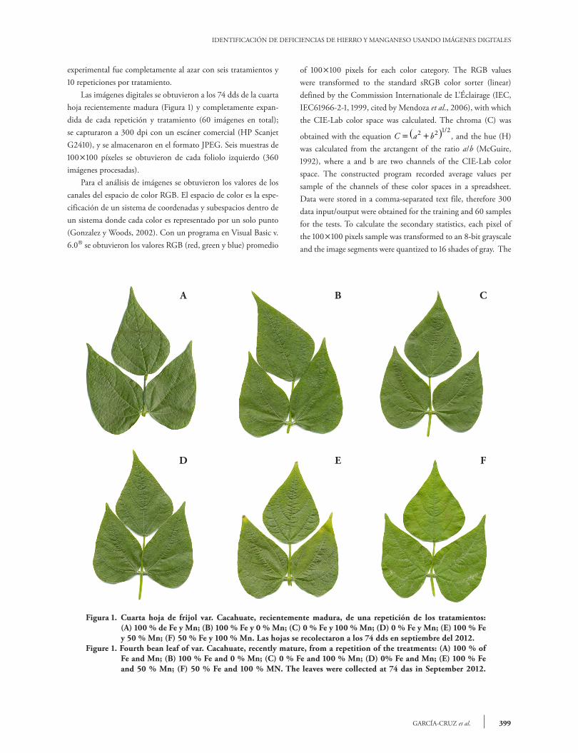
Figura 1. Cuarta hoja de frijol var. Cacahuate, recientemente madura, de una repetición de los tratamientos: (A) 100 % de Fe y Mn; (B) 100 % Fe y 0 % Mn; (C) 0 % Fe y 100 % Mn; (D) 0 % Fe y Mn; (E) 100 % Fe

y 50 % Mn; (F) 50 % Fe y 100 % Mn. Las hojas se recolectaron a los 74 dds en septiembre del 2012.Figure 1. Fourth bean leaf of var. Cacahuate, recently mature, from a repetition of the treatments: (A) 100 % of

Fe and Mn; (B) 100 % Fe and 0 % Mn; (C) 0 % Fe and 100 % Mn; (D) 0% Fe and Mn; (E) 100 % Fe and 50 % Mn; (F) 50 % Fe and 100 % MN. The leaves were collected at 74 das in September 2012.

A B C

D E F

400



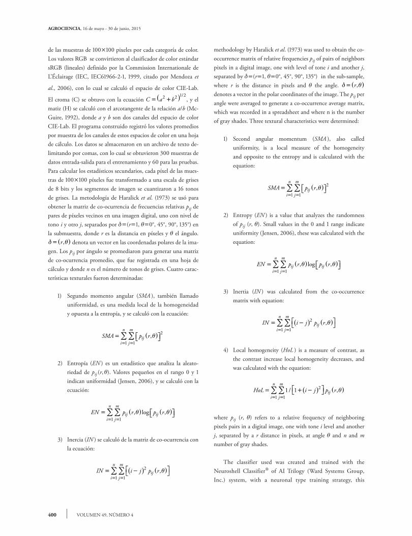
methodology by Haralick et al. (1973) was used to obtain the co-occurrence matrix of relative frequencies pij of pairs of neighbors pixels in a digital image, one with level of tone i and another j, separated by (r1, 0°, 45°, 90°, 135°) in the sub-sample, where r is the distance in pixels and the angle. δ θ=( )r, denotes a vector in the polar coordinates of the image. The pij per angle were averaged to generate a co-occurrence average matrix, which was recorded in a spreadsheet and where n is the number of gray shades. Three textural characteristics were determined:

1) Second angular momentum (SMA ), also called uniformity, is a local measure of the homogeneity and opposite to the entropy and is calculated with the equation:

SMA p rij

j

m

i

n= ( )

==∑∑ ,θ 2

11

2) Entropy (EN ) is a value that analyzes the randomness of pij (r, ). Small values in the 0 and 1 range indicate uniformity (Jensen, 2006), these was calculated with the equation:

EN p r p rij ij

j

m

i

n= ( ) ( )

==∑∑ , log ,θ θ

11

3) Inertia (IN ) was calculated from the co-occurrence matrix with equation:

IN i j p rij

j

m

i

n= −( ) ( )

==∑∑ 2

11,θ

4) Local homogeneity (HoL ) is a measure of contrast, as the contrast increase local homogeneity decreases, and was calculated with the equation:

HoL i j p rij

j

m

i

n= + −( ) ( )

==∑∑ 1 1 2

11/ ,θ

where pij (r, ) refers to a relative frequency of neighboring pixels pairs in a digital image, one with tone i level and another j, separated by a r distance in pixels, at angle and n and m number of gray shades.

The classifier used was created and trained with the Neuroshell Classifier of AI Trilogy (Ward Systems Group, Inc.) system, with a neuronal type training strategy, this

de las muestras de 100100 pixeles por cada categoría de color. Los valores RGB se convirtieron al clasificador de color estándar sRGB (lineales) definido por la Commission Internationale de L’Éclairage (IEC, IEC61966-2-1, 1999, citado por Mendoza et

al., 2006), con lo cual se calculó el espacio de color CIE-Lab.

El croma (C) se obtuvo con la ecuación C a b= +( )2 2 1 2/, y el

matiz (H) se calculó con el arcotangente de la relación a/b (Mc-Guire, 1992), donde a y b son dos canales del espacio de color CIE-Lab. El programa construido registró los valores promedios por muestra de los canales de estos espacios de color en una hoja de cálculo. Los datos se almacenaron en un archivo de texto de-limitando por comas, con lo cual se obtuvieron 300 muestras de datos entrada-salida para el entrenamiento y 60 para las pruebas.Para calcular los estadísticos secundarios, cada píxel de las mues-tras de 100100 píxeles fue transformado a una escala de grises de 8 bits y los segmentos de imagen se cuantizaron a 16 tonos de grises. La metodología de Haralick et al. (1973) se usó para obtener la matriz de co-ocurrencia de frecuencias relativas pij de pares de píxeles vecinos en una imagen digital, uno con nivel de tono i y otro j, separados por (r1, 0°, 45°, 90°, 135°) en la submuestra, donde r es la distancia en píxeles y el ángulo. δ θ=( )r, denota un vector en las coordenadas polares de la ima-gen. Los pij por ángulo se promediaron para generar una matriz de co-ocurrencia promedio, que fue registrada en una hoja de cálculo y donde n es el número de tonos de grises. Cuatro carac-terísticas texturales fueron determinadas:

1) Segundo momento angular (SMA ), también llamado uniformidad, es una medida local de la homogeneidad y opuesta a la entropía, y se calculó con la ecuación:

SMA p rij

j

m

i

n= ( )

==∑∑ ,θ 2

11

2) Entropía (EN ) es un estadístico que analiza la aleato-riedad de pij (r, ). Valores pequeños en el rango 0 y 1 indican uniformidad (Jensen, 2006), y se calculó con la ecuación:

EN p r p rij ij

j

m

i

n= ( ) ( )

==∑∑ , log ,θ θ

11

3) Inercia (IN ) se calculó de la matriz de co-ocurrencia con la ecuación:

IN i j p rij

j

m

i

n= −( ) ( )

==∑∑ 2

11,θ



4) Homogeneidad local (HoL ) es una medida del contras-te, al aumentar el contraste disminuye la homogeneidad local, y se calculó con la ecuación:

HoL i j p rij

j

m

i

n= + −( ) ( )

==∑∑ 1 1 2

11/ ,θ

donde pij (r, ) se refiere a una frecuencia relativa de pares de píxeles vecinos en una imagen digital, uno con nivel de tono i y otro j, separados por una distancia r en pixeles, en el ángulo , y con n y m número de tonos de grises.

El clasificador que se utilizó se creó y entrenó con el sistema Neuroshell Classifier de AI Trilogy (Ward Systems Group, Inc.) con la estrategia de entrenamiento tipo neuronal; este programa permite crear redes neuronales artificiales supervisadas con el al-goritmo de correlación en cascada y fue propuesto por Fahlman y Lebiere (1990). Este algoritmo inicia con una red neuronal artificial mínima que durante el entrenamiento añade, una por una, nuevas unidades en la capa oculta, lo cual genera una estruc-tura multicapa. Una vez que se añade a la estructura una nueva unidad en la capa oculta, los pesos del lado de las entradas se hacen constantes por lo cual esta unidad se vuelve un detector de patrones permanente en la red neuronal, y está disponible para producir valores de salida o para crear otros detectores de patro-nes más complejos. Esta arquitectura se caracteriza por la rapidez para entrenar las redes neuronales artificiales con pocos juegos de datos, y donde un patrón de entrada es clasificado de acuerdo con un número específico de categorías (Ward Systems Group, Inc., 1997-2007). Las redes neuronales artificiales son modelos estadísticos no lineales diferenciables, que pueden aprender de una base de datos donde en ocasiones no se cuenta con todos los escenarios posibles, y no requieren de funciones o reglas bien definidas; producen aproximaciones convenientes e incluyen variaciones que otros sistemas consideran como ruido (Neural Innovations Ltd, 1997). El clasificador tuvo dos a ocho escenarios de variables de en-tradas de color y textura (los canales del espacio de color RGB, el C y H; y cuatro características texturales (SMA, EN, IN y HoL), seis (100 % de Fe y Mn; 100 % Fe, 0 % Mn; 0 % Fe, 100 % Mn; 0 % Fe, 0 % Mn; 100 % Fe, 50 % Mn y 50 % Fe, 100 % Mn) o cuatro clases (100 % de Fe y Mn; 100 % Fe, 0 % Mn; 0 % Fe, 100 % Mn; 0 % Fe, 0 % Mn) tratamientos; y un número máximo de 150 neuronas en la capa oculta. Quince escenarios de entradas se usaron, con 360 datos entrada-salida balanceados, cuando se consideraron seis clases de salida del clasificador, y otros 15 esce-narios de entradas, con 240 datos entrada-salida, cuando fueron cuatro clases de salida del clasificador. Tanto en el clasificador de seis (que corresponde a seis tratamientos), como en el de cuatro

program allows to create artificial neural networks supervised with the cascade correlation algorithm and it was proposed by Fahlman and Lebiere (1990). This algorithm starts with a minimum artificial neural network that, during training, add one by one new units in a hidden layer, which creates a multilayer structure. Once a new unit in the hidden layer is added to the structure, the weights on the entries side of become constant by which this unit becomes a permanent patterns detector in the neural network, and is available to produce output values, or to create other detectors of more complex patterns. This architecture is characterized by the speed to train artificial neural networks using few data sets, and where a pattern of entry is classified according with a specific number of categories (Ward Systems Group, Inc., 1997-2007). Artificial neural networks are differentiable non-linear statistical models, which can learn from a database where sometimes not all the possible scenarios are found, and do not require functions or well defined rules; they produce convenient approaches and include variations that other systems considered noise (Neural Innovations Ltd, 1997). The classifier had two to eight scenarios variables of color and texture inputs (the RGB space color channels, C and H; and four textural characteristics (SMA, EN, IN and HoL)), six (100 % Fe and Mn; 100 % Fe, 0 % Mn; 0 % Fe, 100 % Mn; 0 % Fe, 0 % Mn; 100 % Fe, 50 % Mn and 50 % Fe, 100 % Mn) or four classes (100 % Fe and Mn; 100 % Fe, 0 % Mn; 0 % Fe, 100 % Mn; 0 % Fe, 0 % Mn) or treatments; and a maximum of 150 neurons in the hidden layer. 15 entry scenarios, with 360 balanced input/output data, were used when six kinds of classifier output and other 15 scenarios of entries, with 240 input/output data, were considered when they were four kinds of classifier output. Both in the classifier of six (which corresponds to six treatments) as in the four classes (four treatments), each entry scenario was repeated 10 times with random partitions of data from 90 % for training and 10 % for the test. The experimental design was completely randomized, with the data an ANOVA was performed, to evaluate the performance of the classifier based on the percentage of correct overall classification between entries in the test scenarios the treatment means were compared with the Tukey test (p0.05). These analyses were performed with the SAS statistical program version 8.1 (SAS Institute Inc., 1999-2000). The contingency table of the best-case scenario entries was obtained based on the overall response percentage of classification in the classifier of six and four classes. Sensitivity, referred to as the fraction of observations with the symptom identified correctly, was calculated in this contingency table, and refers to the probability that a model correctly detects a symptom when in fact it is present. Also, the specificity was calculated, referred

402



clases (cuatro tratamientos), cada escenario de entradas se repitió 10 veces con particiones aleatorias de los datos de 90 % para el entrenamiento y 10 % para la prueba. El diseño experimental fue completamente al azar, con los datos se realizó un ANDEVA y las medias de los tratamientos se compararon con la prueba de Tukey (p0.05), para evaluar el desempeño del clasificador con base en el porcentaje de clasifi-cación global correcta entre escenarios de entradas en la prueba. Estos análisis se hicieron con SAS versión 8.1 (SAS Institute Inc., 1999-2000). La tabla de contingencia de los mejores escenarios de entradas se obtuvo con base en la respuesta global del por-centaje de clasificación en el clasificador de seis y en el de cuatro clases. En esta tabla de contingencia se calculó la sensibilidad, referida como la fracción de observaciones con el síntoma iden-tificado correctamente, y se refiere a la probabilidad de que un modelo detecte correctamente un síntoma cuando de hecho está presente. También se calculó la especificidad referida como la fracción de observaciones descartadas correctamente de tener el síntoma, y se refiere a la probabilidad de que un modelo detecte la ausencia de un síntoma.

ResultAdos y dIscusIón

Prueba de escenarios de entradas de seis tratamientos

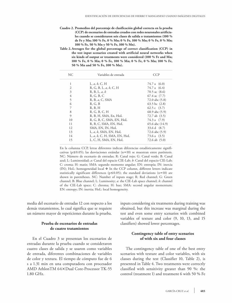
En el Cuadro 2 se presentan los escenarios de en-tradas en la prueba cuando se consideraron seis clases de salida y diferentes combinaciones de variables de color y textura como variables de entrada. Las diferencias entre tratamientos en la prue-ba (Cuadro 2) fueron altamente significativas (p0.001). El escenario de entradas 12 (Cuadro 2), que consideró las características texturales como va-riables de entrada, tuvo el porcentaje menor de cla-sificación correcta global de síntomas de deficiencias de Fe y Mn (33.6 %) durante la prueba. En cambio, se obtuvo 63.5 % de clasificación correcta global en la prueba con el escenario de entradas que incluyó los tres canales del espacio de color RGB (clasificador 6), y este porcentaje aumentó al usar otras combinacio-nes de canales de color. La combinación de caracteres texturales y de color permitió obtener algunos de los escenarios de entradas (10 y 14) con mayores por-centajes de clasificación global correcta en la prueba, pero estos no fueron diferentes (p0.05) con los ob-tenidos con los mejores escenarios de entradas (1 y 2), los cuales consistieron principalmente de variables de color. Durante la prueba, la única diferencia fue la

to as the fraction of observations correctly discarded of with symptom, and refers to the probability that a model detects the absence of a symptom.

Results And dIscussIon

Scenarios test of six treatments entries

The scenarios of entries in the test, that considered six kinds of output and different combinations of variables in color and texture as input variables, are presented in Table 2. The differences between treatments in the test (Table 2) were highly significant (p0.001). The scenario 12 of the entries (Table 2), which considered textural characteristics as input variables, had the lowest percentage (33.6 %) of correct global classification of Fe and Mn deficiencies symptoms during the test. On the other hand, 63.5 % of overall correct classification was obtained in the test with the scenario of entries that included three RGB color space channels (classifier 6), and this percentage increased to use other combinations of color channels. The combination of textural and color characters allowed some of the input scenarios (10 and 14) with higher overall percentages of correct classification in the test, but these were not different (p0.05) to those obtained with the inputs best-case scenario (1 and 2), which mainly consisted color variables. During the test, the only difference was the mean of scenario of entries 12 respect to the other treatments, which indicate that a greater number of repetitions during the test are required.

Test of entire scenarios of four treatments

Table 3 presents scenarios of entries during the test when we considered four kinds of output classes and different combinations of variables in color and texture were used as input variables. The computation time was of 6 s to 1.31 min on a computer with an AMD AthlonTM 64Dual-Core processor TK-55 1.80 GHz. The difference in the test (p0.05) is the average of the percentage of overall correct classification of inputs scenario that considered the variables of texture (classifier 12) from the rest of inputs scenario (Table 3). With the entries scenarios, when considering four treatments, a higher percentage of overall correct classification respect to scenarios of



Cuadro 2. Promedios del porcentaje de clasificación global correcta en la prueba (CCP) de escenarios de entradas creados con redes neuronales artificia-les cuando se consideraron seis clases de salida o tratamientos (100 % de Fe y Mn; 100 % Fe, 0 % Mn; 0 % Fe, 100 % Mn; 0 % Fe, 0 % Mn; 100 % Fe, 50 % Mn y 50 % Fe, 100 % Mn).

Table 2. Averages for the global percentage of correct classification (CCP) in the test input scenarios created with artificial neural networks when six kinds of output or treatments were considered (100 % Fe and Mn; 100 % Fe, 0 % Mn; 0 % Fe, 100 % Mn; 0 % Fe, 0 % Mn; 100 % Fe,

50 % Mn and 50 % Fe, 100 % Mn).

NC Variables de entrada CCP

1 L, a, b, C, H 74.7 a (6.0)2 R, G, B, L, a, b, C, H 74.7 a (6.4)3 R, B, L, a, b 70.5 ac (8.6)4 R, G, B, C 67.4 ac (7.7)5 R, B, a, C, SMA 72.0 abc (5.8)6 R, G, B 63.5 bc (2.8)7 R, B, H 62.5 c (3.7)8 R, G, B, C, H 68.9 abc (5.9)9 R, B, H, SMA, En, HoL 72.7 ab (3.5)10 R, G, B, C, SMA, EN, HoL 74.3 a (7.9)11 R, B, C, SMA, EN, HoL 65.6 abc (14.9)12 SMA, EN, IN, HoL 33.6 d (8.7)13 L, a, b, SMA, EN, HoL 72.6 abc (5.9)14 L, a, b, C, H, SMA, EN, HoL 73.6 a (3.5)15 L, C, H, SMA, EN, HoL 72.6 ab (5.0)

En la columna CCP, letras diferentes indican diferencias estadísticamente signifi-cativas (p0.05); las desviaciones estándar (n10) se muestran entre paréntesis. NC: Número de escenario de entradas; R: Canal rojo; G: Canal verde; B: Canal azul; L: Luminosidad; a: Canal del espacio CIE-Lab; b: Canal del espacio CIE-Lab; C: croma; H: matiz; SMA: segundo momento angular; EN: entropía; IN: inercia (IN); HoL: homogeneidad local v In the CCP column, different letters indicate statistically significant differences (p0.05); the standard deviations (n10) are shown in parentheses. NC: Number of inputs stage; R: Red channel; G: Green channel; B: Blue channel; L: Luminosity; a: the CIE-Lab space channel; b: channel of the CIE-Lab space; C: chroma; H: hue; SMA: second angular momentum; EN: entropy; IN: inertia; HoL: local homogeneity.

media del escenario de entradas 12 con respecto a los demás tratamientos, lo cual significa que se requiere un número mayor de repeticiones durante la prueba.

Prueba de escenarios de entradas de cuatro tratamientos

En el Cuadro 3 se presentan los escenarios de entradas durante la prueba cuando se consideraron cuatro clases de salida y se usaron como variables de entrada, diferentes combinaciones de variables de color y textura. El tiempo de cómputo fue de 6 s a 1.31 min en una computadora con procesador AMD AthlonTM 64Dual Core-Processor TK-55 1.80 GHz.

inputs considering six treatments during training was obtained, but this increase was marginal during the test and even some entry scenarios with combined variables of texture and color (9, 10, 13, and 15 classifiers) showed lower percentages.

Contingency table of entry scenarios of with six and four classes

The contingency table of one of the best entry scenarios with texture and color variables, with six classes during the test (Classifier 10, Table 2), is presented in Table 4. Two treatments were correctly classified with sensitivity greater than 90 %: the control (treatment 1) and treatment 6 with 50 % Fe

404



Cuadro 3. Promedios del porcentaje de clasificación global correcta en la prue-ba (CCP) de escenarios de entradas creados con redes neuronales artificiales cuando se consideraron cuatro clases de salida o trata-mientos (100 % de Fe y Mn; 100 % Fe, 0 % Mn; 0 % Fe, 100 % Mn; 0 % Fe, 0 % Mn).

Table 3. Averages for the percentage of overall correct classification (CPC) in the test of input scenarios created with artificial neural networks when four kinds of output or treatments were considered (100 % Fe and Mn; 100 % Fe, 0 % Mn; 0 % Fe, 100 % Mn; 0 % Fe, 0 % Mn).

NC Variables de entrada CCP

1 L, a, b, C, H 79.7 a (7.5)2 R, G, B, L, a, b, C, H 75.9 a (8.4)3 R, B, L, a, b 74.6 a (8.0)4 R, G, B, C 75.1 a (7.0)5 R, B, a, C, SMA 73.6 a (8.1)6 R, G, B 68.1 a (7.7)7 R, B, H 70.1 a (5.6)8 R, G, B, C, H 76.1 a (5.6)9 R, B, H, SMA, En, HoL 70.0 a (7.4)10 R, G, B, C, SMA, EN, HoL 73.8 a (6.6)11 R, B, C, SMA, EN, HoL 67.0 a (10.8)12 SMA, EN, IN, HoL 44.9 b (9.2)13 L, a, b, SMA, EN, HoL 70.4 a (7.5)14 L, a, b, C, H, SMA, EN, HoL 78.3 a (7.8)15 L, C, H, SMA, EN, HoL 68.7 a (5.6 )

En la columna CCP, letras diferentes indican diferencias estadísticamente signifi-cativas (p0.05); las desviaciones estándar (n10) se muestran entre paréntesis. NC: Número de escenario de entradas; R: Canal rojo; G: Canal verde; B: Canal azul; L: Luminosidad; a: Canal del espacio CIE-Lab; b: Canal del espacio CIE-Lab; C: croma; H: matiz; SMA: segundo momento angular; EN: entropía; IN: inercia (IN); HoL: homogeneidad local v In the CCP column, different letters indicate statistically significant differences (p0.05); the standard deviations (n10) are shown in parentheses. NC: Number of inputs scenarios; R: Red channel; G: Green channel; B: Blue channel; L: Luminosity; a: CIE-Lab space channel; b: Channel of the CIE-Lab space; C: chroma; H: hue; SMA: second angular momentum; EN: entropy; IN: inertia; HoL: local homogeneity.

La diferencia en la prueba (p0.05) es el pro-medio del porcentaje de clasificación correcta global del escenario de entradas que consideró las variables de textura (clasificador 12) del resto de escenarios de entradas (Cuadro 3). Con los escena-rios de entradas al considerar cuatro tratamientos se obtuvo porcentaje mayor de clasificación co-rrecta global respecto a los escenarios de entradas, considerando seis tratamientos durante el entrena-miento, pero este aumento fue marginal durante la prueba e inclusive algunos escenarios de entradas con variables combinadas de textura y color (Cla-sificadores 9, 10, 13, y 15) presentaron porcentajes menores.

and 100 % MN. The other treatments are classified with sensitivities over 60 % except for treatment 2 (100 % Fe and 0 % Mn) with a sensitivity of 40 %,which was mainly confused with class 3; the absence of one of two micronutrient of modified Steiner solution is characteristic of classes 2 and 3. The treatments had specificity than 90 %, where treatments 2 (100 % Fe, 0 % Mn) and 3 (0 % Fe, 100% Mn) had the lower specificities, whereas treatment 6 (50 % Fe, 100 % Mn) had the highest specificity. Regarding the entry scenario with four kinds of output (Table 5), control (100 % Fe and Mn) had sensitivity greater than 90 %, while treatment 2 (100 % Fe, 0 % Mn) had the lower sensitivity



Cuadro 4. Estadísticas promedio (n10) del arreglo matricial o tabla de contingencia en la prueba para el escenario de entradas con las variables de entrada “red” (R), “green” (G), “blue” (B), croma (C), y los caracteres texturales segundo momen-to angular (SMA), entropía (EN), y homogeneidad local (HoL), y seis clases de salida o tratamientos†.

Table 4. Statistical average (n10) of the matrix arrangement or table of contingency in the test for the scenario of inputs with the variables of input “red” (R), “green” (G), “blue” (B), chroma (C), and textural characters second angular momentum (SMA), entropy (EN), and local homogeneity (HoL), and six kinds of output or treatments†.

ClasificadoObservado

Total1 2 3 4 5 6

1 54 5 0 3 8 0 702 1 25 11 8 2 0 473 1 18 38 2 2 1 624 2 5 5 46 2 1 615 1 6 5 1 46 0 596 1 1 1 0 0 58 61

Total 60 60 60 60 60 60 360

Relación V-P 0.9 0.42 0.63 0.77 0.77 0.97Relación F-P 0.05 0.07 0.08 0.05 0.04 0.01Relación V-N 0.95 0.93 0.92 0.95 0.96 0.99Relación F-N 0.10 0.58 0.37 0.23 0.23 0.03Sensibilidad 99 % 42 % 63 % 77 % 77 % 97 %Especificidad 95 % 93 % 92 % 95 % 96 % 99 %

†100 % Fe y Mn, tratamiento 1; 100 % Fe, 0 % Mn, tratamiento 2; 0 % Fe, 100 % Mn, tratamiento 3; 0 % Fe, 0 % Mn. tratamiento 4; 100 % Fe, 50 % Mn, tratamiento 5; 50 % Fe, 100 % Mn, tratamiento 6. V-P: identificados correctamente; F-P: identificados inco-rrectamente; V-N: descartados correctamente; F-N: descartados incorrectamente v †100 % Fe and Mn, treatment 1; 100 % Fe, 0 % Mn, treatment 2; 0 % Fe, 100 % Mn, treatment 3; 0 % Fe, 0 % Mn, treatment 4; 100 % Fe, 50 % Mn, treatment 5; 50 % Fe, 100 % Mn, treatment 6. V-P: identified correctly; F-P: identified incorrectly; V-N: discarded properly; F-N: discarded improperly.

Tabla de contingencia de escenarios de entradas con seis y cuatro clases

La tabla de contingencia de uno de los mejores escenarios de entradas con variables de textura y co-lor, con seis clases durante la prueba (Clasificador 10, Cuadro 2), se presenta en el Cuadro 4. Dos trata-mientos fueron clasificados correctamente con sensi-bilidad mayor a 90 %: e1 testigo (tratamiento 1) y el tratamiento 6 con 50 % de Fe y 100 % de Mn. Los otros tratamientos son clasificados con sensibilidades mayores de 60 % excepto el tratamiento 2 (100 % Fe y 0 % Mn) con sensibilidad de 40 %, el cual fue confundido principalmente con la clase 3; es caracte-rístico de las clases 2 y 3 la ausencia de uno de los dos micronutrientes modificados en la solución Steiner. Los tratamientos presentaron especificidades mayo-res a 90 %, donde los tratamientos 2 (100 % Fe, 0 % Mn) y 3 (0 % Fe, 100 % Mn) tuvieron las especifici-dades menores mientras que el tratamiento 6 (50 % Fe, 100 % Mn) observó la mayor especificidad.

although it presented the highest specificity. The lower specificity was observed with treatment 3 (0 % Fe, 100 % Mn). According with Howeler (1978), severe deficiencies of Fe or Mn can produce similar symptoms, and under these circumstances the plant damage is irreversible. In the present research, the symptoms of these elements deficiency at 74 das in leaves of common bean (Figure 1) were not apparent (55 d after treatment started), making the identification of the cause to the naked eye difficult, even for an expert; however, its detection at this stage is critical to be able to reverse deficiencies with fertilization. Due to the difficulty of identification, artificial neural networks as a tool are used to create a classifier based on color and texture variables from the analysis of digital images. Whit this strategy up to 74.7% of correct classification was obtained of six treatments during the test. Burks et al. (2000) with discriminant analysis and texture characteristics obtained a classifier capable of 93 % of correct identification of weed species; whereas

406



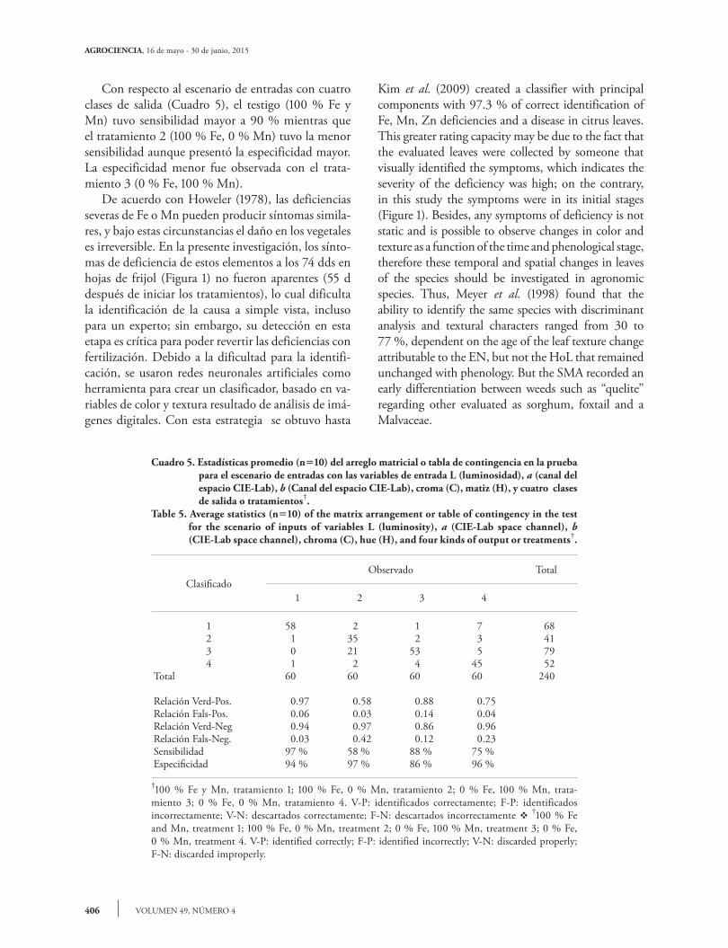
Con respecto al escenario de entradas con cuatro clases de salida (Cuadro 5), el testigo (100 % Fe y Mn) tuvo sensibilidad mayor a 90 % mientras que el tratamiento 2 (100 % Fe, 0 % Mn) tuvo la menor sensibilidad aunque presentó la especificidad mayor. La especificidad menor fue observada con el trata-miento 3 (0 % Fe, 100 % Mn). De acuerdo con Howeler (1978), las deficiencias severas de Fe o Mn pueden producir síntomas simila-res, y bajo estas circunstancias el daño en los vegetales es irreversible. En la presente investigación, los sínto-mas de deficiencia de estos elementos a los 74 dds en hojas de frijol (Figura 1) no fueron aparentes (55 d después de iniciar los tratamientos), lo cual dificulta la identificación de la causa a simple vista, incluso para un experto; sin embargo, su detección en esta etapa es crítica para poder revertir las deficiencias con fertilización. Debido a la dificultad para la identifi-cación, se usaron redes neuronales artificiales como herramienta para crear un clasificador, basado en va-riables de color y textura resultado de análisis de imá-genes digitales. Con esta estrategia se obtuvo hasta

Kim et al. (2009) created a classifier with principal components with 97.3 % of correct identification of Fe, Mn, Zn deficiencies and a disease in citrus leaves. This greater rating capacity may be due to the fact that the evaluated leaves were collected by someone that visually identified the symptoms, which indicates the severity of the deficiency was high; on the contrary, in this study the symptoms were in its initial stages (Figure 1). Besides, any symptoms of deficiency is not static and is possible to observe changes in color and texture as a function of the time and phenological stage, therefore these temporal and spatial changes in leaves of the species should be investigated in agronomic species. Thus, Meyer et al. (1998) found that the ability to identify the same species with discriminant analysis and textural characters ranged from 30 to 77 %, dependent on the age of the leaf texture change attributable to the EN, but not the HoL that remained unchanged with phenology. But the SMA recorded an early differentiation between weeds such as “quelite” regarding other evaluated as sorghum, foxtail and a Malvaceae.

Cuadro 5. Estadísticas promedio (n10) del arreglo matricial o tabla de contingencia en la prueba para el escenario de entradas con las variables de entrada L (luminosidad), a (canal del espacio CIE-Lab), b (Canal del espacio CIE-Lab), croma (C), matiz (H), y cuatro clases de salida o tratamientos†.

Table 5. Average statistics (n10) of the matrix arrangement or table of contingency in the test for the scenario of inputs of variables L (luminosity), a (CIE-Lab space channel), b (CIE-Lab space channel), chroma (C), hue (H), and four kinds of output or treatments†.

ClasificadoObservado Total

1 2 3 4

1 58 2 1 7 682 1 35 2 3 413 0 21 53 5 794 1 2 4 45 52

Total 60 60 60 60 240

Relación Verd-Pos. 0.97 0.58 0.88 0.75Relación Fals-Pos. 0.06 0.03 0.14 0.04Relación Verd-Neg 0.94 0.97 0.86 0.96Relación Fals-Neg. 0.03 0.42 0.12 0.23Sensibilidad 97 % 58 % 88 % 75 %Especificidad 94 % 97 % 86 % 96 %

†100 % Fe y Mn, tratamiento 1; 100 % Fe, 0 % Mn, tratamiento 2; 0 % Fe, 100 % Mn, trata-miento 3; 0 % Fe, 0 % Mn, tratamiento 4. V-P: identificados correctamente; F-P: identificados incorrectamente; V-N: descartados correctamente; F-N: descartados incorrectamente v †100 % Fe and Mn, treatment 1; 100 % Fe, 0 % Mn, treatment 2; 0 % Fe, 100 % Mn, treatment 3; 0 % Fe, 0 % Mn, treatment 4. V-P: identified correctly; F-P: identified incorrectly; V-N: discarded properly; F-N: discarded improperly.



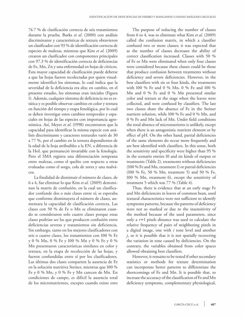
74.7 % de clasificación correcta de seis tratamientos durante la prueba. Burks et al. (2000) con análisis discriminante y características de textura obtuvieron un clasificador con 93 % de identificación correcta de especies de malezas, mientras que Kim et al. (2009) crearon un clasificador con componentes principales con 97.3 % de identificación correcta de deficiencias de Fe, Mn, Zn y una enfermedad en hojas de cítricos. Esta mayor capacidad de clasificación puede deberse a que las hojas fueron recolectadas por quien visual-mente identificó los síntomas, lo cual indica que la severidad de la deficiencia era alta; en cambio, en el presente estudio, los síntomas eran iniciales (Figura 1). Además, cualquier síntoma de deficiencia no es es-tática y es posible observar cambios en color y textura en función del tiempo y etapa fenológica, por lo cual se deben investigar estos cambios temporales y espa-ciales en hojas de las especies con importancia agro-nómica. Así, Meyer et al. (1998) encontraron que la capacidad para identificar la misma especie con aná-lisis discriminante y caracteres texturales varió de 30 a 77 %, por el cambio en la textura dependientes de la edad de la hoja atribuibles a la EN, a diferencia de la HoL que permaneció invariable con la fenología. Pero el SMA registra una diferenciación temprana entre malezas, como el quelite con respecto a otras evaluadas como el sorgo, cola de zorra y una malvá-cea. La finalidad de disminuir el número de clases, de 6 a 4, fue eliminar lo que Kim et al. (2009) denomi-nan la matriz de confusión, en la cual un clasifica-dor confunde dos o más clases entre sí; se esperaba que conforme disminuyera el número de clases, au-mentara la capacidad de clasificación correcta. Las clases con 50 % de Fe o Mn se eliminaron cuan-do se consideraron solo cuatro clases porque estas clases podrían ser las que producen confusión entre deficiencias severas y tratamientos sin deficiencia. Sin embargo, tanto en los mejores clasificadores con seis o cuatro clases, los tratamientos con 100 % Fe y 0 % Mn, 0 % Fe y 100 % Mn y 0 % Fe y 0 % Mn presentaron características similares en color y textura, en la etapa de recolección de las hojas, y fueron confundidas entre sí por los clasificadores. Las últimas dos clases comparten la ausencia de Fe en la solución nutritiva Steiner, mientras que 100 %Fe y 0 % Mn, y 0 % Fe y Mn carecen de Mn. En condiciones de campo, es difícil la ausencia total de los micronutrientes, excepto cuando existe otro

The purpose of reducing the number of classes from 6 to 4, was to eliminate what Kim et al. (2009) called the confusion matrix, in which a classifier confused two or more classes; it was expected that as the number of classes decreases the ability of correct classification increased. Classes with 50 % of Fe or Mn were eliminated when only four classes were considered because these classes could be those that produce confusion between treatments without deficiency and severe deficiencies. However, in the best classifiers with six or four kinds, the treatments with 100 % Fe and 0 % Mn, 0 % Fe and 100 % Mn and 0 % Fe and 0 % Mn presented similar color and texture at the stage when the leaves were collected, and were confused by classifiers. The last two classes share the absence of Fe in the Steiner nutrient solution, while 100 % Fe and 0 % Mn, and 0 % Fe and Mn lack of Mn. Under field conditions the total absence of micronutrients is unlikely, except when there is an antagonistic nutrient element or by effect of pH. On the other hand, partial deficiencies of the same elements do occur more frequently and are best identified with classifiers. In this sense, both the sensitivity and specificity were higher than 95 % in the scenario entries 10 and six kinds of output or treatments (Table 2), treatments without deficiencies (100 % Fe and Mn, treatment 1) or partial deficiencies (100 % Fe, 50 % Mn, treatment 5) and 50 % Fe, 100 % Mn, treatment 6), except the sensitivity of treatment 5 which was 77 % (Table 4). Thus, there is evidence that at an early stage Fe and Mn deficiencies in leaves of common bean, used textural characteristics were not sufficient to identify symptoms patterns, because the patterns of deficiency were not so marked or due to the insensitivity of the method because of the used parameters, since only a r1 pixels distance was used to calculate the relative frequency of pairs of neighboring pixels in a digital image, one with i tone level and another j, so it is possible that it is not spatially recovering the variation in tone caused by deficiencies. On the contrary, the variables obtained from color spaces allowed obtaining best classifiers. However, it remains to be tested if other secondary statistics or methods for texture determination can incorporate better patterns to differentiate the shortcomings of Fe and Mn. It is possible that, to increase the accuracy of the classification of Fe and Mn deficiency symptoms, complementary physiological,

408



elemento nutrimental antagónico o por efecto del pH. En cambio, deficiencias parciales de los mis-mos elementos sí ocurren con mayor frecuencia y son mejor identificados con los clasificadores. En este sentido, tanto la sensibilidad como la especifici-dad fueron mayores a 95 % en el escenario de entra-das 10 y seis clases de salida o tratamientos (Cuadro 2), de los tratamientos sin deficiencias (100 % de Fe y Mn, tratamiento 1) o con deficiencias parciales (100 % Fe, 50 % Mn, tratamiento 5) y 50 % Fe, 100 % Mn, tratamiento 6), excepto la sensibilidad de el tratamiento 5 que fue 77 % (Cuadro 4). Así, hay evidencia de que en una etapa tempra-na de deficiencias de Fe y Mn en hojas de frijol, las características texturales usadas no fueron suficientes para identificar patrones de síntomas, porque los pa-trones de deficiencia no eran tan marcados o debi-do a la insensibilidad del método por los parámetros usados, ya que solo se usó una distancia r1 pixeles para calcular las frecuencia relativa de pares de píxeles vecinos en una imagen digital, uno con nivel de tono i y otro j. Así, es posible que no se esté recuperando espacialmente la variación del tono producido por las deficiencias. En cambio, las variables obtenidas de los espacios de color permitieron obtener mejores clasifi-cadores. Sin embargo, falta probar si otros estadísticos secundarios u métodos para la determinación de tex-tura permiten incorporar mejores patrones para di-ferenciar las deficiencias de Fe y Mn. Es posible que para incrementar la precisión de clasificación de sín-tomas de deficiencia de Fe y Mn se requieran varia-bles fisiológicas, morfológicas o anatómicas comple-mentarias a las evaluaciones visuales propuestas en el presente estudio. Además, Adams et al. (2000) con-sideran que algunos factores pueden interferir para obtener una clasificación de síntomas buena, por ejemplo el estrés hídrico, lumínico o por deficiencias de macronutrientes. En particular, deficiencias seve-ras de nitrógeno (N) o azufre (S) pueden causar sín-tomas similares a los causados por deficiencia de Fe.

conclusIones

Con variables de color y textura fue posible iden-tificar deficiencias iniciales de Fe y Mn en hojas de frijol hasta 75 % de clasificación global correcta, síntomas que difícilmente pueden caracterizarse a simple vista por un experto porque las muestras se

morphological, or anatomical variables have to be added to the visual assessments proposed in this study. In addition, Adams et al. (2000) consider that to obtain a good classification of symptoms other factors can interfere, for example water stress, light stress or macronutrient deficiencies. Particularly, severe deficiencies of nitrogen (N) or sulphur (S) may cause symptoms similar to those caused by Fe deficiency.

conclusIons

It was possible to identify initial shortcomings of Fe and Mn in common bean leaves up to 75 % overall correct classification using color and texture variables, symptoms that can hardly be characterized at a glance by an expert, because the samples were taken at an early stage of deficiency, when it is possible to reverse the damage with fertilization. Never the less, the variables of texture by themselves are not sufficient to obtain a good classifier, and therefore the hypothesis is rejected. The identification of plants without deficiencies and partial deficiencies in both Fe and Mn were higher than 95 %, except the sensitivity of the partial deficiency produced by 100 % Fe and only 50 % of MN.

—End of the English version—

pppvPPP

tomaron en una etapa inicial de deficiencia cuando es posible revertir los daños con fertilización. Pero las variables de textura por sí mismas no son suficientes para obtener un buen clasificador, y la hipótesis se re-chaza. La identificación de plantas sin deficiencias y con deficiencias parciales tanto de Fe y Mn tuvieron especificidad y sensibilidad mayores a 95 %, excepto la sensibilidad de la deficiencia parcial producida por aplicar 100 % de Fe y solo 50 % de Mn.

lIteRAtuRA cItAdA

Adams, M. L., W. A. Norvell, W. D. Philpot, and J. H. Peverly. 2000. Toward the discrimination of manganese, zinc, copper, and iron deficiency in ‘Bragg’ soybean using spectral detection methods. Agron. J. 92: 268-274.

Barbazán, M. 1998. Análisis de Plantas y Síntomas Visuales de Deficiencias. Facultad de Agronomía. Universidad de la República. Montevideo, Uruguay. 27 p.



Burks, T. F., S. A. Shearer, and F. A. Payne. 2000. Classification of weed species using color texture features and discriminant analysis. Amer. Soc. Agric. Eng. 43: 441-448.

Clark, R. B. 1991. Iron: unlocking agronomic potential. Solutions 35: 24-28.

Fahlman, S. E. and C. Lebiere. 1990. The Cascade-Correlation Learning Architecture. Computer Science Department. Carnegie Mellon University. Pittsburgh, PA, USA.

Paper 1938. 13 p. http://repository.cmu.edu/compsci/1938 (Consulta: marzo 2015).Gonzalez, R. C. and R. E. Woods. 2002. Digital Image

Processing. Prentice-Hall. 793 p.Hansen, N. C., B. G. Hopkins, J. W. Ellsworth, and V. D.

Jolley. 2006. Iron nutrition in field crops. In: Iron Nutrition in Plants and Rhizospheric Microorganisms. Springer Netherlands. pp: 23-59.

Haralick, R. M., K. Shanmugan, and I. Dinstein. 1973. Textural features for images classification. IEEE Trans. Systems, Man and Cybernetics 3(6): 610-621.

Howeler, R. H. 1978. The mineral nutrition and fertilization of cassava. In: Cassava Production Course. CIAT. Cali. Colombia. pp. 247-292.

Jensen, J.R. 2006. Introductory Digital Image Processing: A Remote Sensing Perspective. Prentice Hall. Englewood Cliffs, NJ. USA. 608 p.

Jones, J.B., B. Wolf, and H. A. Mills. 1991. Plant Analysis Handbook: A Practical Sampling, Preparation, Analysis, and Interpretation Guide. Micro-Macro Publ., Athens, GA, USA. 213 p.

Kim, D. G., T. F. Burks, A. W. Schumann, M. Zekri, X. Zhao, and J. Quin. 2009. Detection of citrus greening using microscopic imaging. Agric. Eng. Int. the CIGR Ejournal. Manuscript 1194 XI: 1-17.

McGuire, R. G. 1992: Reporting of objective color measurements. HortScience 27: 1254-1255.

Mendoza, F., P. Dejmek, and L. Aguilera. 2006. Calibrated color measurements of agricultural foods using image analysis, Postharvest Biol. Technol. 41 (3): 285-295.

Meyer, G. E., T. Mehta, M. F. Kocher, D. A. Mortensen, and A. Samal. 1998. Textural imaging and discriminant analysis for distinguishing weeds for spot sprying. Trans. ASAE 41(4): 1189-1197.

Murakami, P. F., M. R. Turner, A. K. van den Berg, and P. G. Schaberg. 2005. An instructional guide for leaf color analysis using digital imaging software. United States Department of Agriculture. Washington, DC, USA. 37 p.

Oide, M., and S. Ninomiya. 2000. Discrimination of soybean leaflet shaped by neural networks with image input. Computers Electr. Agric. 29: 59-72.

SAS Institute Inc. 1999-2000. SAS/STAT Guide for Personal Computers. Ver. 8.1 SAS Institute N.C. USA. 890 p.

Schulte, E. E., and K. A. Kelling. 1999. Soil and applied manganese. Publication A2526. Wisconsin County Extension Office. University of Wisconsin, WI, USA. 4 p.

Somers, I. I., and J. W. Shive. 1942. The iron manganese relation in plant metabolism. Plant Physiol. 17: 582-602.

Twyman, E. S. 1950. The iron – manganese balance and its effect on the growth and development of plants. New Phytol. 45: 1469-8137.

IDENTIFICACIÓN CON REDES NEURONALES PROBABILÍSTICAS DE … · de los tratamientos de deficiencias...

Documents

Transcript of IDENTIFICACIÓN CON REDES NEURONALES PROBABILÍSTICAS DE … · de los tratamientos de deficiencias...