Continuous Output Integral Sliding Mode Control forSwitched Linear Systems

R. Galvan-Guerraa, L. Fridmana, J.E. Velazquez-Velazquezb,∗, S. Kamalc, B.Bandyopadhyayc

aFacultad de Ingenierıa–UNAM, Coyoacan CDMX 04510, Mexico.bESIME-Zacatenco IPN, Unidad Profesional Adolfo Lopez Mateos, CDMX 07738, Mexico.

cSystems and Control Engg. IIT Bombay, India.

Abstract

A continuous output integral sliding mode robustification methodology for swit-

ched uncertain linear time invariant systems with state-dependent location tran-

sitions and dwell time is presented. The robustifying methodology is based on

the adjustment of the super-twisting algorithm gains to assure the convergence

time and the attenuation of the chattering. The use of the adjusted STA allows

to reconstruct the states theoretically exactly before half of the dwell time with-

out the usage of filters, via a continuous cascade observer. Moreover, it allows to

generate a continuous control signal that is turn on after the observer has con-

verged, guaranteeing theoretically exact compensation of the matched uncertain-

ties/perturbations before the dwell time.

Keywords: Continuous Output Integral Sliding Mode, Switched System

1. Introduction

State of the Art

Switched systems with state-dependent location transitions arise in applications

where the structure of the system changes when the states fulfill a specific switching

rule [1, 2].

∗Corresponding authorEmail address: jev1_79@hotmail.com (J.E. Velazquez-Velazquez )

Preprint submitted to Nonlinear Analysis: Hybrid Systems April 15, 2016

There are many control architectures for switched systems (see e.g.[3, 4, 5])

that assume the state vector is available, and others that use only output informa-

tion [6, 7, 8]. These strategies provide a nominal controller that makes the closed

loop system to behaves in a nominal way. In the presence of matched uncertain-

ties/perturbations the trajectory of the system could deviate from the nominal

behavior. In this work using only output information we will design a continuous

robustifying methodology that makes the system insensitive to the matched uncer-

tainties/perturbations after the dwell time in every location, i.e. given a nominal

controller we design a new controller that together with the nominal one assure

the location trajectory of the system and the robustification of the nominal behav-

ior before the dwell time in every location.

Methodology

Integral Sliding Modes: Advantages and Disadvantages. The sliding modes me-

thodology has been successfully applied to uncertain systems to compensate theo-

retically exactly 1 the matched uncertainties/perturbations (see e.g. [9, 10, 11, 12]).

The Integral Sliding Mode (ISM) framework [13] allows to robustify a given

nominal controller while it compensates theoretically exactly the matched uncer-

tainties/perturbations just after the initial time. But, the main disadvantages of

this approach are:

• The need of all the states and the initial conditions.

• And the discontinuous control of ISM produces high level chattering.

In the switched framework in [14] an ISM is proposed with the same disadvan-

tages than in the non-switched case.

Output Integral Sliding Modes: Advantages and Disadvantages. The Output In-

tegral Sliding Mode (OISM) method [15, 16] eliminates the need of the states and

1Theoretically exactly means that the algorithm converge exactly in absence of measurement noises,

discretizations and unknown dynamics.

2

the initial conditions. This method robustifies the nominal behavior of the system us-

ing only output information and allows to reconstruct theoretically exactly the system

states just after the initial time by reconstructing step by step the output and its deriva-

tives. Moreover, the controller and the observer work simultaneously and the sliding

motions start just after the initial moment. Since the OISM still uses a discontinuous

control law, it has two weak points:

• Presence of high level chattering.

• To reconstruct the output and its derivatives a first order filter is used. This affects

its ability to reconstruct the state and to compensate the uncertainties/perturbations

right after the initial time.

Chattering Attenuation: Super-Twisting Algorithm. A good option for chattering

attenuation for systems with relative degree one is the Super-Twisting Algorithm

(STA) [17] since:

• It substitutes the discontinuous control law with a continuous one compen-

sating theoretically exactly Lipschitz uncertainties/perturbations [17, 18].

• The sliding variable and its derivatives converge in finite-time to the ori-

gin, allowing to reconstruct the uncertainties/perturbations without filter-

ing. [19, 20].

• The precision is improved with respect to the noises and the discretization

sample step.

For switched systems in [21, 22, 23], different observers capable to reconstruct

theoretically exactly both the states and the location trajectory are proposed using

the STA. The continuous state is reconstructed using classical observation tech-

niques and the location trajectory is identified using residual-based strategies.

However, these results are based on the existence of STA gains that assure con-

vergence before the switching and they do not provide any methodology for the

design of such gains.

3

Continuous Integral Sliding Modes. When the ISM methodology is combined

with the STA a Continuous Integral Sliding Mode (CISM) is obtained. This strat-

egy allows to robustify in a continuous way the nominal behavior of the system.

But, to assure exact compensation of the Lipschitz uncertainties/perturbations

right after the initial time it is necessary to know the initial conditions of the un-

certainties/perturbations, otherwise the methodology has reaching phase.

An output CISM methodology is used in [24] for fault tolerant control of un-

certain linear systems. There, it is assumed that the faults are lipschitz and at the

initial time there are not faults, eliminating the reaching phase of the controller.

The states are reconstructed using a high-order differentiator, that must converge

before the fault occurs. The design of the gains to assure the convergence time is

not provided.

Hence, to apply a continuous output integral sliding mode (COISM) strategy

to switched systems with dwell time when the initial conditions of the uncertain-

ties/perturbations are unknown and can be discontinuous at the switching times, it

is necessary to design an strategy that adjust the STA gains to assure convergence

before the dwell time and the attenuation of the chattering.

Contribution

In this paper a continuous robustifying methodology based on STA and using only

output information for Switched Uncertain Linear Time Invariant Systems (SULTIS)

with state-dependent location transitions and that satisfy the dwell time condition is

proposed.

With this aim, the STA gains are adjusted as a function of the convergence

time, using an estimation of the reaching time. Moreover, the amplitude of the

chattering is attenuated using a switched strategy.

Using the adjusted STA, a cascade structure observer is designed. This observer

has a family of observers that reconstruct the outputs not affected by the un-

certainties/perturbations and their derivatives, allowing to reconstruct the states

without the use of filters. The observers are turn on once the lower derivatives

has been theoretically exactly reconstructed. Sufficient conditions are developed

4

to assure the convergence of the full observer before the half of the dwell time.

After the observer has converged, a COISM controller that uses an OISM sli-

ding variable together with a STA control law is turn on and the gains are designed

to assure its convergence before the dwell time. This ensures exact compensation

of the matched uncertainties/perturbations before the dwell time and using only

output information.

Sufficient restrictions to the state vector at the switching times are developed to

guarantee the absence of switching during the convergence. Under these conditions,

the robustification methodology assures that the location trajectory is preserved.

For the implementation, the STA controller is modified to assure the non-Lipschitz

terms of the observer do not affect the STA behavior of the controller. The integral

structure of the sliding dynamics preserves the continuity of the control law, allowing

to adjust the chattering.

1.1. Paper Organization

This paper is organized as follows. Section 2 presents the problem formulation.

Section 3 adapts the STA gains design for switched systems while Section 4 is devoted

to the robustifying methodology design for the SULTIS. In Section 5 restrictions to the

initial conditions to guarantee the robustification of the SULTIS are given. The special

issues that may arise in the application of the proposed methodology are discussed in

Section 4.2.1. Finally the simulation results are given in Section 7.

1.2. Notations

Throughout this paper we are going to use the following notation

• ⌈s(·)⌋q =

|s1|q sign(s1)

...

|sn|q sign(sn)

, where s ∈ Rn.

• In is the identity matrix of dimension n.

• AT denotes the transpose.

• A+ refers to the pseudo-inverse of the rectangular matrix A, i.e. A+=(AT A)−1AT .

5

• A⊥ is the orthogonal complement of A such that AT A⊥ = 0.

• x(t−j ) = limt→t−j

x(t) and x(t+j ) = limt→t+j

x(t) as the conventional lateral limits.

• ki represents a constant or function in the i-location, while ki denotes the i-

element of the vector k.

• rank (A) is the rank of the matrix A.

• ∥A∥ as the euclidean norm of the matrix or vector A, while |a| is the absolute

value of the scalar a.

• det(A) as usual indicates de determinant of the square matrix A.

• max and min are the maximum and minimum operators respectively.

•∩i

Ai depicts the intersection of the sets Ai

• λ (A) denotes an eigenvalue of the square matrix A, while λmax(A) and λmin(A)

the maximum and minimum eigenvalue respectively.

2. Problem Formulation

Consider a SULTIS with state-dependent location transitions composed by r differ-

ent locations 2.

˙x(t) = Aix(t)+ Bi (u(t)+ϕ(t)) ,

y(t) = Cix(t), x(0) = x0,(1)

where i = σ(x, t) : Rn ×R+ → I = 1,2, . . . ,r denotes the active location,

Ai ∈ Rn×n, Bi ∈ Rn×m and Ci ∈ Rp×n

are known matrices, ϕ : R+ → Rm are uncertainties/perturbations and u(t) is the con-

trol.

2See [25] for a general formal definition.

6

Using a linear transformation x= T1,ix and an output transformation y=Ty,iy, where

T1,i =

B⊥+

i

Cti B⊥+

i + B+i

with Cti = (CiBi)

+Ci(In − BiB+i )B

⊥i , and

Ty,i =

(CiBi)⊥+

(CiBi)+

;

(1) is transformed to

x(t) =

A11,i A12,i

A21,i A22,i

︸ ︷︷ ︸

Ai

x(t)+

0

Im

︸ ︷︷ ︸

Bi

(u(t)+ϕ(t)),

y1(t)

y2(t)

=

C1,i

C2,i

x(t) =

C11,i 0

0 Im

︸ ︷︷ ︸

Ci

x(t), x(0) = x0,

(2)

with i = σ(T−11,i x, t).

A transition between each location is ruled by a set of given switching manifolds

mi,i′ : Rn → R, with i′ ∈ I and i = i′, such that∩i′∈Ii′ =i

x : mi,i′(x) = 0= /0,

When the state x is in location i and mi,i′(x) = 0 it is said that a transition to location i′

occurs. In this paper it is considered that these switching manifolds are known.

Under the assumption that ϕ(t) = 0 a nominal system is defined as

xnom(t) = Aixnom(t)+Biunom(t);

ynom(t) =Cixnom(t), xnom(0) = x0;(3)

where unom(t) =−Kixnom(t), with Ki ∈ Rm×n, is a given stabilizing nominal control.

The switching moments t j, j = 1,2, . . . are not defined a priory but, by using the

given switching manifolds and the nominal trajectory xnom, it is possible to detect these

transitions such that

t j = mini′∈Ii′ =i

t > t j : mi,i′(xnom(t)) = 0

7

Suppose that the switching moments for (3) conform an ordered sequence

0 = t0 < t1 < t2 < · · ·< t j−1 < t j < .. . .

such that t j − t j−1 > δ , i.e. the nominal switched system (3) satisfies the dwell time

condition. To assure the absence of a sliding mode at the switching manifolds, we

assume

limt→t−j

ddt

mi,i′(xnom(t))> ρ and limt→t+j

ddt

mi,i′(xnom(t))> ρ

or

limt→t−j

ddt

mi,i′(xnom(t))<−ρ and limt→t+j

ddt

mi,i′(xnom(t))<−ρ

with ρ > 0. Let σ(xnom(0)) = i0 ∈ I . Then, the location trajectory σ(xnom(t), t) can

be restated as

σ(xnom(t), t) :=

i if σ(xnom(t−), t−) = i and mi,i′(xnom(t)) = 0,

i′ if σ(xnom(t−), t−) = i and mi,i′(xnom(t)) = 0.

By using this information the location trajectory of (3) can be characterized by the

switching sequence

Σ = x0;(i0, t0),(i1, t1), . . . ,(i j, t j), . . . |i j ∈ I , j = 0,1, . . .

For (1), in general, the switching sequence and the state trajectory are affected by the

uncertainties/perturbations ϕ(t).

2.1. General Assumptions

In order to robustify the SULTIS we need to make the following assumptions.

A1. The initial location is known and the initial condition is unknown but bounded,

i.e. there exists µ ∈ R+, such that ∥x(0)∥ ≤ µ .

A2. The SULTIS without any controller satisfies the dwell time condition.

A3. rankBi = rankCiBi = m for all i ∈ I .

8

A4. The uncertainties/disturbances ϕ conform a bounded Lipschitz function:

∥ϕ(t)∥ ≤ Ψimax , ∀t ∈ [t j−1, t j];∥∥ϕ(t)∥∥≤ Φimax , ∀t ∈ [t j−1, t j];

where Φimax ,Ψimax ∈ R+ are given for all i ∈ I .

A5. The switched system (1) has more outputs than inputs, i.e. p > m.

A6. The switched system is controllable in every location [26], i.e. the pair (Ai, Bi) is

controllable for i ∈ I .

A7. The switched system is strongly observable in every location [27], i.e. the triple

(Ai, Bi,Ci) is strongly observable for i ∈ I . More details about this concept are

given in the appendix.

3. STA Adjustment for Switched Systems

It is well known that to assure finite time stability of the sliding variables, the

design of the STA gains is crucial [28, 29, 30, 31]. In these works an estimation of

the upper bound of the convergence time is obtained. But, they do not design the

STA gains for a given convergence time. In this section we design the STA such

that it has useful features for the control and observation of switched systems.

Normally, in multi-variable sliding modes the control injection is designed in a

decoupled form, allowing to apply directly the scalar STA gains design procedure

to the multi-variable case.

Consider a scalar system

χ(t) = u(t)+ζ (t), (4)

where ζ (t) is a bounded lipschitz unknown signal such that∥∥∥ζ (t)

∥∥∥ ≤ ϑ1 and

∥ζ (t)∥ ≤ ϑ2. u(t) is an STA control law [17]

u(t) =−κ1⌈χ(t)⌋12 +w(t),

w(t) =−κ2⌈χ(t)⌋0, w(0) = 0.(5)

9

Then the closed loop system takes the form

χ(t) =−κ1⌈χ(t)⌋12 +Π(t)

Π(t) =−κ2⌈χ(t)⌋0 + ϕ(t).(6)

with Π(t) = ζ (t)+ω(t).

3.1. STA Gains Design with a Desired Convergence Time

To design the STA gains with a desired convergence time an estimation of the

reaching time tR is needed. This estimation can be obtained by using a Lyapunov

analysis.

3.1.1. Lyapunov Function

Consider the following continuous candidate Lyapunov function [29]

V (χ,Π) =

k2

4

(Π(t)⌊χ(t)⌉0

γ + k0em(χ,Π)√

χ(χ,Π))2

, χ(t)Π(t) = 0,2k2Π2(t)

κ1, χ(t) = 0,

|χ(t)|2 , Π(t) = 0.

,

where

γ = κ2 −ϑ1⌊χ(t)Π(t)⌉0,

m(χ,Π) =1√

g−1arctan

(κ1g⌊χ(t)⌉1/2 −2Π(t)

2√

g−1Π(t)

),

χ(χ,Π) = 2γ|χ(t)|−κ1⌊χ(t)⌉1/2Π(t)+Π(t)2,

k =√

γ

∣∣∣∣∣k√g− e−(arctan((g−1)−1/2)+0.5π⌊χ(t)Π(t)⌉0)√

g−1

∣∣∣∣∣ ,k0 =

⌊χ(t)Π(t)⌉0

γ

k√

geπ⌊χ(t)Π(t)⌉0

√g−1 − earctan( −1

g−1 )

,

g =8γκ2

1, k ∈ I(g−)∩ I(g+), g± =

8(κ2 ±ϑ1)

κ21

,

I(g) =

2g+

e(− π

2 −arctan(

1√g−1

))1

g−1

√g

,e(

π2 −arctan

(1√g−1

))1

g−1

√g

.

The next statement provides sufficient conditions for the STA gains to assure finite-time

stability and an estimation of the reaching time.

10

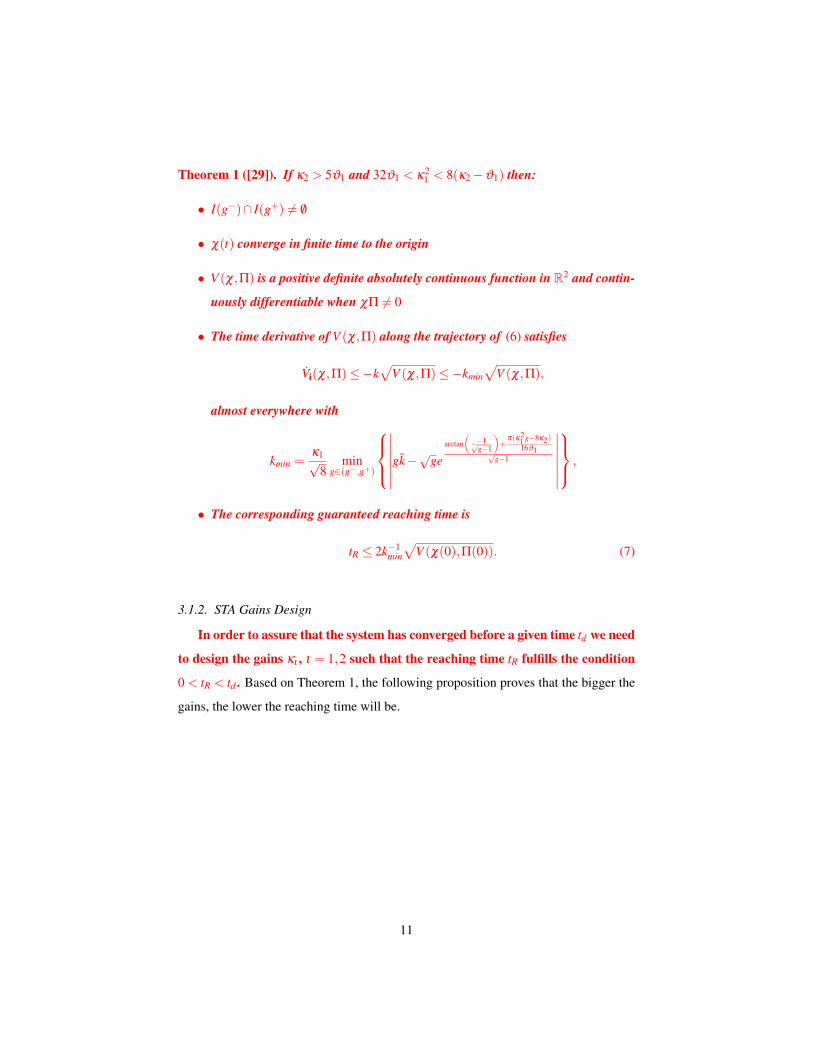
Theorem 1 ([29]). If κ2 > 5ϑ1 and 32ϑ1 < κ21 < 8(κ2 −ϑ1) then:

• I(g−)∩ I(g+) = /0

• χ(t) converge in finite time to the origin

• V (χ,Π) is a positive definite absolutely continuous function in R2 and contin-

uously differentiable when χΠ = 0

• The time derivative of V (χ,Π) along the trajectory of (6) satisfies

Vi(χ,Π)≤−k√

V (χ,Π)≤−kmin√

V (χ,Π),

almost everywhere with

kmin =κ1√

8min

g∈(g−,g+)

∣∣∣∣∣∣∣gk−√

gearctan

(−1√g−1

)+

π(κ21 g−8κ2)16ϑ1√

g−1

∣∣∣∣∣∣∣ ,

• The corresponding guaranteed reaching time is

tR ≤ 2k−1min

√V (χ(0),Π(0)). (7)

3.1.2. STA Gains Design

In order to assure that the system has converged before a given time td we need

to design the gains κι , ι = 1,2 such that the reaching time tR fulfills the condition

0 < tR < td . Based on Theorem 1, the following proposition proves that the bigger the

gains, the lower the reaching time will be.

11

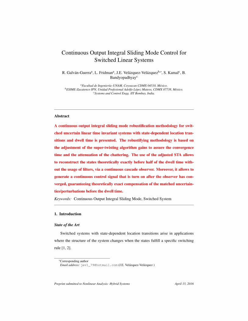
Figure 1: Plot of kmin for a scalar STA with ϑ1 = 1, s(0) = 0 and Π(0)≤ 1

Proposition 1. If (χ(0),Π(0)) is bounded then for κ1 and κ2 large enough it is possi-

ble to make tR arbitrarily small.

PROOF. Note that the maximum of the function kmin is achieved when κ1 reach its

maximum value (see Figure1). So it is easy to prove that

limκ2→∞

limκ1→

√8(κ2−ϑ1)

kmin → ∞.

and

limκ2→∞

limκ1→

√8(κ2−ϑ1)

V (χ(0),Π(0))→

0, χ(0)Π(0) = 0,

0, χ(0) = 0,|χ(0)|

2 , Π(0) = 0.

Hence for any bounded (χ(0),Π(0)), tR can be made arbitrarily small.

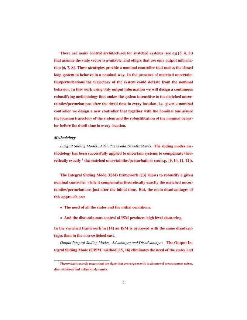
Observe that for a given td there exists a gains set such that tR < td (see Figure 2).

The next lemma gives sufficient conditions to assure a desired reaching time.

12

Figure 2: Behavior of tR for different values of κ1 and κ2 for a scalar STA with ϑ1 = 1, χ(0) = 0 and

Π(0) ≤ 1. The gray horizontal plane at tR = td = 1 shows that for a large enough gains, a reaching time

lower than 1 can be assured.

Lemma 1. If the STA gains are designed such that

(κ1,κ2) ∈ K =

(κ1,κ2)

∣∣∣∣∣∣∣∣∣2√

2kϑ2kminκ1

− td < 0,

κ2 > 5ϑ1,

32ϑ1 < κ21 < 8(κ2 −ϑ1)

,

where td is a given time and χ(0) = 0, then χ has a reaching time tR < td .

PROOF. Since κ2 > 5ϑ1 and 32ϑ1 < κ21 < 8(κ2 −ϑ1), χ(t) converge in finite time

with a reaching time tR. Now, since χ(0) = 0,

V (χ(0),Π(0))≤ 2k2ϑ 22

κ21

and

tR ≤ 2√

2kϑ2

kminκ1

Hence since (κ1,κ2) ∈ K, we can assure tR < td .

Any given reaching time can be achieved if the STA gains satisfies Lemma

1. But the lower the reaching time, the bigger the gains should be, causing an

increment in the chattering. This issue is the subject of the next subsection.

13

3.2. Chattering Attenuation

The amplitude of the chattering Ac for the STA can be estimated using the

describing function method [32] as

Ac =4κ2

πωc

1Im(W−1( jωc))

where

W ( jωc) =Ci( jωcIn − (Ai −BiKi))−1Bi

is the transfer function of the nominal system (3) and the chattering frequency ωc

is a solution of the equation

4κ2

πωc

1Im(W−1( jωc))

−(

1.1128κ1

Re(W−1( jωc))

)= 0.

This estimation can be used in the design of the STA gains. As it was mentioned

in the previous subsection, the bigger the STA gains, the lower the desired td can

be, inducing an increment in the amplitude of the chattering. It is shown in [17]

that the discrete realization of the STA has precision of order 2, i.e. for small

sample step ∆t, Ac ≈ kp(∆t)2 . In Table 1, the value of kp for different values of td

is presented. It can be seen that the lower td , the bigger kp would be.

td κ1 κ2 ∆t = 0.01 ∆t = 0.001 ∆t = 0.0001 kp

1 5.6569 9.1 1.1977e−03 1.2243e−05 1.3281e−07 13

0.1 13.6569 58.1 6.7563e−03 8.0541e−05 8.1274e−07 80

0.01 44.6569 545.1 7.0854e−02 7.7505e−04 7.7982e−06 775

Table 1: Chattering amplitude for different desired reaching times td : (κ1,κ2) ∈ K. W (s) = 1s , ϑ1 = ϑ2 = 1.

The amplitude of the chattering is attenuated by solving the following mini-

mization problem

Optimization Problem 1. (κ∗1 ,κ∗

2 )R = argmin(κ1,κ2)∈K

Ac +κ21 +κ2

2 subject to

max(min(I(g−)),min(I(g+)))< k < min(max(I(g−)),max(I(g+)))

g− > 1 and g+ > 1;(8)

14

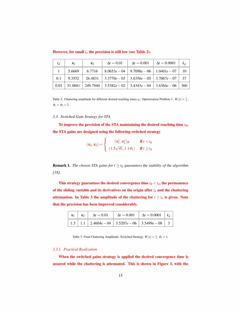
However, for small td the precision is still low (see Table 2).

td κ1 κ2 ∆t = 0.01 ∆t = 0.001 ∆t = 0.0001 kp

1 5.6669 6.7716 8.0653e−04 9.7098e−06 1.0401e−07 10

0.1 9.3552 26.4831 3.3770e−03 3.6356e−05 3.7067e−07 37

0.01 31.0681 249.7940 3.5382e−02 3.4343e−04 3.6364e−06 360

Table 2: Chattering amplitude for different desired reaching times td : Optimization Problem 1. W (s) = 1s ,

ϑ1 = ϑ2 = 1.

3.3. Switched Gain Strategy for STA

To improve the precision of the STA maintaining the desired reaching time tR,

the STA gains are designed using the following switched strategy

(κ1,κ2) =

(κ∗1 ,κ∗

2 )R if t < td

(1.5√

ϑ1,1.1ϑ1) if t ≥ td

Remark 1. The chosen STA gains for t ≥ td guarantees the stability of the algorithm

[18].

This strategy guarantees the desired convergence time tR < td , the permanence

of the sliding variable and its derivatives on the origin after td and the chattering

attenuation. In Table 3 the amplitude of the chattering for t ≥ td is given. Note

that the precision has been improved considerably.

κ1 κ2 ∆t = 0.01 ∆t = 0.001 ∆t = 0.0001 kp

1.5 1.1 2.4604e−04 3.5207e−06 3.5499e−08 3

Table 3: Final Chattering Amplitude: Switched Strategy. W (s) = 1s , ϑ1 = 1.

3.3.1. Practical Realization

When the switched gains strategy is applied the desired convergence time is

assured while the chattering is attenuated. This is shown in Figure 3, with the

15

gains presented in Table 2 and Table 3. Note that the system converges long be-

fore td . When the bound of the uncertainties/perturbations and the discretization

steps are known the convergence of the sliding variable and its derivatives can be

detected according to the criteria given in [33, Theorem 2]. Hence, the STA gains

can be switched to the lower value as soon as the convergence is detected.

0 0.5 1−0.02

0

0.02

χ(t)

, td=

1

0.5 1 1.5 2

−2

0

2x 10

−6

0 0.05 0.1−5

0

5x 10

−3

χ(t)

, t d=

0.1

0.05 0.1 0.15

−2

0

2x 10

−6

0 0.005 0.01−5

0

5x 10

−4

χ(t)

, t d=

0.01

t0.01 0.02

−2

0

2x 10

−6

t

Figure 3: Chattering Behavior under the switched strategy for different desired reaching times td . ∆t =

0.0001.

The smaller the desired convergence time, the greater the STA gains and con-

sequently the chattering should be. In this case, the switching between the gains

may cause a transient (see Figure 3). Theoretically, that is not a reaching phase

since the convergence before td is assured. But, during the practical realization

the STA with the smaller gains reconverge to the smaller neighborhood, with an

overshot of the same order than the chattering level presented in the system before

td .

16

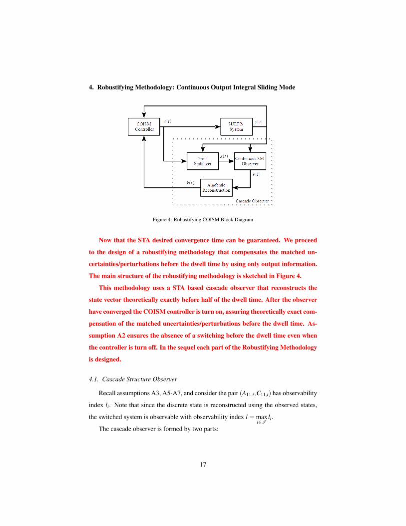
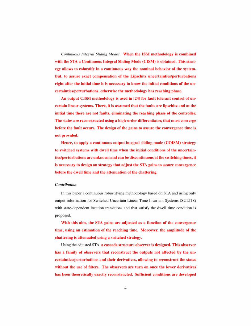
4. Robustifying Methodology: Continuous Output Integral Sliding Mode

Figure 4: Robustifying COISM Block Diagram

Now that the STA desired convergence time can be guaranteed. We proceed

to the design of a robustifying methodology that compensates the matched un-

certainties/perturbations before the dwell time by using only output information.

The main structure of the robustifying methodology is sketched in Figure 4.

This methodology uses a STA based cascade observer that reconstructs the

state vector theoretically exactly before half of the dwell time. After the observer

have converged the COISM controller is turn on, assuring theoretically exact com-

pensation of the matched uncertainties/perturbations before the dwell time. As-

sumption A2 ensures the absence of a switching before the dwell time even when

the controller is turn off. In the sequel each part of the Robustifying Methodology

is designed.

4.1. Cascade Structure Observer

Recall assumptions A3, A5-A7, and consider the pair (A11,i,C11,i) has observability

index li. Note that since the discrete state is reconstructed using the observed states,

the switched system is observable with observability index l = maxi∈I

li.

The cascade observer is formed by two parts:

17

• A Luenberger observer

˙x1(t) = A11,ix1(t)+A12,iy2(t)+Ki (y1(t)−C11,ix1(t)) (9)

that stabilizes the error eLO = x1(t)− x1(t) in a ball around the origin.

• A hierarchical observer composed by:

– A family of super-twisting based observers

xak = A11,ix1(t)+A12,iy2(t)−Lk,i(t)(

C11,iAk−111,i Lk,i

)−1vk(t), (10)

k = 1, . . . , l − 1,, that reconstruct theoretically exactly before half of the

dwell time, step by step, the output uncertainties/perturbations free part

and its derivatives. Lk,i(t) is a design matrix and vk(t) is an output injection

signal based on the STA.

– And an algebraic part

x(t) =

x1(t)

y2(t)

; (11)

where x1(t) = x1(t)−O+1,i,lv(t) with O1,i,l the observability matrix of the

pair (C11,A11) and

v(t) =

C11x1(t)− y1(t)

v1(t)

v2(t)...

vl−1(t)

.

The algebraic part (11) reconstructs theoretically exactly the states of the

system before half of the dwell time.

The existence of the pseudo-inverse of O1,i,l is assured by Lemma 4 given in the

appendix. The next subsections are devoted to the design of each part of the observer.

18

4.1.1. Luenberger Observer: Observation Error Stabilizer

To reconstruct theoretically exactly the states without filtration an STA-based hi-

erarchical observer is used. But, to design the gains of this observer it is necessary

that the first derivative of the state vector is bounded. To assure this bound exists even

when the system is unstable a Luenberger observer is proposed. This observer acts

as an observation error stabilizer and it can be shown that its first derivative remains

bounded.

For the Luenberger observer (9), with initial conditions

C1x1(0) = y1(0), x1(t−j ) = x1(t+j );

the observation error eLO(t) is ruled by

eLO(t) = (A11,i −KiC11,i)eLO(t);

where the matrix Ki is designed by solving the following LMI problem

LMI Problem 1. [34] Find P, S, Yi and λ such that λ is reduced to a minimum and

S = ST > 0, P = PT > 0, λ In−m −P < 0

AT11,iP−CT

11,iYTi +PA11,i −YiC11,i +S < 0, i ∈ I ;

and take the observer gains Ki = P−1Yi.

This problem minimizes the upper bound of a quadratic cost function of the esti-

mation error and stabilizes the observation error.

∥eLO(t)∥ ≤√

ηe−αt(µ +∥x(0)∥)< γ.

where η = λmax(P)λmin(P)

and α = λmin(S)2λmax(P)

. Under these conditions the first derivative of the

observation error remains bounded, i.e.

∥eLO(t)∥< ∥A11,i −KiC11,i∥γ.

Remark 2. We are not assuming that x neither x are bounded. The Luenberger

observer only assures eLO and eLO are bounded.

19

4.1.2. Hierarchical Observer Design

To reconstruct the states x(t) theoretically exactly before half of the dwell time

without the use of filters, it is necessary to recover the vectors C11Ak−111,i x1(t) by us-

ing a family of super-twisting based observers with a convergence time tR < δ2(l−1) .

Each observer is turn on once the lower derivative observers have converged. Assur-

ing theoretically exact reconstruction of the output error and its l − 1-derivatives for

t j−1 +δ2 ≤ t ≤ t j.

The observer design is given by the following theorem.

Theorem 2. Assume

(a) The auxiliary state vectors xak, for all k = 1, . . . , l − 1, i ∈ I and τk = t j−1 +

δ (k−1)2(l−1) ≤ t ≤ t j is designed as in (10), where Lk,i(t)∈Rn−m×p−m is a design matrix

such that det(

C11,iAk−111,i Lk,i

)= 0.

(b) At t = τk the k-th variable xak satisfies

C11,ixa1(t+j−1) = y1(t+j−1),

C11,iAk−111,i xak(τk) =C11,iAk−1

11,i x1(τk)− vk−1(τk);

i = I , j = 1,2, . . . , and k = 2, . . . , l −1.

(c) The sliding variables sk are designed as

sk(y1(t),xak(t))=

y1(t)−C11,ixa1(t), k = 1,

C11,iAk−111,i x1(t)− vk−1(t)−C11,iAk−1

11,i xak(t), k=2, . . . , l −1.

(12)

(d) The output injection vk is designed as an STA of the form

vk(t) =−κk,i1⌈sk(y1(t), t)⌋12 +ϖk(t),

ϖk =−κk,i2⌈sk(y1(t), t)⌋0,

ϖk(t0) = 0, ϖk(τ+k ) = ϖk(τ−k )+ ϖi,k;

(13)

where ϖi,k ∈ Rp.

20

(e) And (κk,i1 ,κk,i2) ∈ KO,k, where

KO,k =

(κ1,κ2)

∣∣∣∣∣∣∣∣∣2√

2kM2,i,kkminκ1

− δ2(l−1) < 0,

κ2 > 5M1,i,k,

32M1,i,k < κ21 < 8(κ2 −M1,i,k)

,

with

M1,i,k ≥∥∥∥C11,iAk

11,i

∥∥∥(∥Ai −KiCi∥γi +∥Bi∥Ψimax) ;

M2,i,k ≥∥∥∥C11,iAk

11,i

∥∥∥γi.

Then,

vk(t) =−C11,iAk11,i (x1(t)− x1(t)) ,

for t j−1+δ2 ≤ t ≤ t j and it is possible to reconstruct theoretically exactly all the vector

functions C11,iAk−111,i x1(t) in the same time interval.

PROOF. Recall that the observers are turn on sequentially whenever the observers that

reconstruct the lowers derivatives have converged. The proof is constructive and can

be obtained iteratively.

Let’s start by recovering the first vector C11,iA11,ix1(t). Let k=1, since the con-

ditions (a)-(c) are fulfilled; it is clear that s1(y1(t j−1),xa1(t j−1)) = 0. Moreover, the

time derivative of the sliding variable along the trajectories of (2) and (10) has the

form

s1(y1(t),xa1(t)) =C11,iA11,i (x1(t)− x1(t))+ v1(t), (14)

and once it has converged, the equivalent control that maintains the trajectory on the

surface has the form

v1eq(t) =−C11,iA11,i (x1(t)− x1(t)) .

Now, we design the output injection (d) assuring the sliding variable s1 and its deriva-

tives converge to the origin before each switching. Substituting the STA output in-

jection (13) on the auxiliary state vector xa1, then (14) can be restated as

s1(y1(t),xa1(t)) =−κ1,i1⌈s1(y1(t), t)⌋12 +Λ1(t),

Λ1 =−κ1,i2⌈s1(y1(t), t)⌋0 +C11,iA11,i(x1(t)− ˙x1(t)

),

Λ1(t jR) =C11,iA11,i (x1(t jR)− x1(t jR)) ;

21

where Λ1(t) = C11,iA11,i (x1(t)− x1(t))+ϖ1(t). Observe that this dynamical system

has the form (6).

Since (κ1,i1 ,κ1,i2) satisfies Lemma 2 (condition (e)) and s1(y1(t j−1),xa1(t j−1) = 0,

s1 converges to the origin with a reaching time t1, jR < τ2. Then, exact convergence of

s1 and its derivatives to the origin for τ2 ≤ t ≤ t j is assured.

Assume the result is true for k = k, and let us prove the result for k = k+ 1.

Once again our aim is to recover the k-vector C11,iAk11,ix(t). Conditions (a)-(c) are

satisfied. Taking the time derivative of the sliding variable along the trajectories of

(2) and (10) for τk ≤ t < t j.

sk(y1(t),xak(t)) =C11,iAk11,i (x1(t)− x1(t))+ vk(t). (15)

Moreover, once the k-th sliding variable and its derivatives have converged,

C11,iAk11,ixak(τk) =C11,iAk

11,ix1(τk).

and the equivalent control is

vkeq(t) =−C11,iAk11,i (x1(t)− x1(t)) .

Designing the output injection (d) the sliding variable dynamics (15) can be rewritten

as

sk(y1(t),xak(t)) =−κk1⌈sk(y1(t), t)⌋12 +Λk(t),

Λk =−κk,i2⌈sk(y1(t), t)⌋0 +C11,iAk11,i(x1(t)− ˙x1(t)

),

Λk(τk) =C11,iAk11,ix1 (τk)− x1(τk)) ,

where Λk(t) =C11,iAk11,i (x1(t)− x1(t))+ϖk(t).

Since condition (e) is satisfied and sk(y1(τk),xak(τk))= 0, once again from Lemma

1, sk converges to the origin with a reaching time tk, jR < τk+1. And the exact conver-

gence of sk and its derivatives to the origin for τk+1 ≤ t ≤ t j is guaranteed.

Note that we proved exact reconstruction of the output error and its (l − 1) time

derivatives for t j−1 +δ2 ≤ t ≤ t j.

22

Remark 3. The precision of the observer is improved if the switched strategy pro-

posed in section 4 is applied with td = t j−1 +δ2 .

4.1.3. State Reconstruction

Using the family of STA observers the output y1 and its l − 1 time-derivatives at

every location have been reconstructed theoretically exactly in the time interval [t j−1+

δ2 , t j]. Using this information we can construct the vector

O1,i,lx1(t) = O1,i,l x1(t)− v(t).

Since the pair (Ai,Bi,Ci) is strongly observable, the pseudo-inverse of O1,i,l is well

defined (see Lemma 4 in the Appendix) and the states can be recovered by means of

the equation

x1(t) = x1(t)−O+1,i,lv(t). (16)

Then, the algebraic observer is suggested as

x1(t) = x1(t)−O+1,i,lv(t); (17)

and we are able to reconstruct theoretically exactly the states for t j−1 +δ2 ≤ t ≤ t j by

using (11).

4.2. Continuous Output Integral Sliding Mode

In the previous section we designed an observer capable to reconstruct theoretically

exactly the states of the SULTIS before half of the dwell time, i.e. x(t) = x(t) for all

t j−1+δ2 ≤ t < t j. Once the states have been reconstructed, at t = t j−1+

δ2 the controllers

are turn on. In this section the integral part of the control law is designed.

Consider the SULTIS (2) and define the output based integral sliding dynamics

s(y, t) = Gi

(y(t)− y

(t j−1 +

δ2

))−

t∫t j−1+

δ2

GiCi(Aix(τ)+Biunom(τ))dτ, (18)

i ∈ I ; where Gi ∈ Gi is a design matrix such that

Gi = G ∈ Rm×n : detDi = 0,

23

with Di = GiCiBi. Observe that s(

y(

t j−1 +δ2

), t j−1 +

δ2

)= 0. Taking the first deriva-

tive of the sliding variable along the trajectory of (2) we obtain

s(y, t) = GiCiAi (x(t)− x(t))+Di (uint(t)+ϕ(t)) . (19)

Since x(t) = x(t), then

s(y, t) = Di (uint(t)+ϕ(t)) ; (20)

the equivalent control [13] that maintains the trajectory on the sliding mode is

uIeq =−D−1i ϕ(t), (21)

and the sliding mode dynamics of the SULTIS takes the form

x(t) = Aix(t)+Biunom(t)

y(t) =Cix(t), x(0) = x0;(22)

Remark 4. In the sequel assume the projection matrix is designed without loss of gen-

erality such that Di = I.

4.2.1. Implementation of STA Controller based on STA Observer

The control law uint depends on the observed state x. So it is necessary to design

this controller in such a way that the observer STA dynamics does not affect the proper-

ties of the controller [35], i.e. the uncertain/perturbations should be Lipschitz without

affecting the continuity of the control law. Let us design the COISM term using the

STA [17]

uint =−κi1⌈s(y(t), t)⌋12 +ω(t),

ω =−κi2⌈s(y(t), t)⌋0, ω(

t j−1 +δ2

)= 0;

(23)

24

where κiι ∈ R+ with i ∈ I and ι = 1,2. Substituting the STA control (23) in (19) and

with a simple change of variable.

s(y, t) =−κi1⌈s(y(t), t)⌋12 +Ω(t)+GiCiAi

O+1,i,lv(t)

0

,Ω(t) =−κi2⌈s(y(t), t)⌋0 +GiCiAi

(x1(t)− ˙x1(t))

0

+ ϕ(t),

s(

y, t j−1 +δ2

)= 0;

(24)

where

Ω(t) = GiCiAi

(x1(t)− x1(t))

0

+ϕ(t)+ω(t).

The term O+1,i,lv(t) is non-Lipschitz, so it is not possible to consider it as uncertainty/perturbation

and to assure the convergence of the STA. If the proposed Super-Twisting controller is

changed to

uint =−GiCiAi

O+1,i,lv(t)

0

−κi1⌈s(y(t), t)⌋12 +ω(t),

ω =−κi2⌈s(y(t), t)⌋0, ω(0) = 0, ω(t+j ) = ω(t−j )+ ωi;

(25)

we compensate the term GiCiAiO+i,lv(t), the sliding dynamics have the typical STA

form

s(y, t) =−κi1⌈s(y(t), t)⌋12 +Ω(t),

Ω(t) =−κi2⌈s(y(t), t)⌋0 +GiCiAi

(x1(t)− ˙x1(t))

0

+ ϕ(t),

s(y, t j−1) = 0;

(26)

Remark 5. Thanks to the integral structure of s(y, t) the non-Lipschitz dynamics of

the observer that affect the controller, only depends on v, the continuous part of the

observer dynamics. Hence, the continuity of uint is preserved.

The following Lemma gives the design of the STA gains (κi1 ,κi2) for the controller.

25

Lemma 2. Suppose assumptions A1-A6 are satisfied and (κi1 ,κi2) ∈ KC

KC =

(κ1,κ2)

∣∣∣∣∣∣∣∣∣2√

2kL2,ikminκ1

− δ2 < 0,

κ2 > 5L1,i,

32L1,i < κ21 < 8(κ2 −L1,i)

,

with

L1,i ≥ Φimax +∥GiCiAi∥(∥Ai −KiCi∥γi +∥Bi∥Ψimax) ;

L2,i ≥ ∥GiCiAi∥γi +Φimax .

Then, the sliding mode dynamics converges to the origin with a reaching time t jR <

t j−1 +δ < t j.

PROOF. This result comes directly from Lemma 1.

With this we assure the robustification of the nominal trajectory before the dwell

time.

Remark 6. The precision of the controller is improved if the switched strategy pro-

posed in section 4 is applied with td = t j−1 +δ .

Remark 7. In comparison with [15], we are not able to reconstruct the states right

after the initial time. Due to the presence of the reaching phase, the controller and the

observer will re-converge after every switching. But, the proposed methodology does

not need the use of filters.

5. Robustifying Conditions: Restrictions to the Initial Conditions

Along the paper, we assume the existence of the dwell time. However we are

considering state dependent location transitions and any deviation of the state

trajectory may provoke an undesirable switching. In this section we analyze under

which condition we can guarantee the existence of the dwell time, and hence the

robustification of the nominal trajectory.

Recall that the controller have been designed such that it converges before t =

t j−1 + δ . But, during the reaching phase the COISM controller cause a transient

26

in the SULTIS that could produce an unexpected switching. To avoid this issue, it

is necessary to restrict the value of the states at the switching times.

Lemma 3. If

∥x(t j−1)∥ ≤ µ j−1 <

ξ j−1,max −

∥∥∥∥∥ t j−1+δ/2∫t j−1

eAi(t j−1+δ2 −τ)dτ

∥∥∥∥∥∥Bi∥Φmax∥∥eAiδ/2∥∥ . (27)

where

ξ j−1,max =∥Ai −BiKi∥e∥Ai−BiKi∥ δ

2Mi,min −∥Bi∥

δ2

umax;

Mi,min = mini′I ,i =i′

∥∥∥∥argminx∈Rn

|Mi,i′(x)|∥∥∥∥ ;

umax = ∥uint(t)+ϕ(t)∥ ≤ κ1m14 s

12max +Ωmax;

Ωmax = Φmax +(κ2 +Ψmax)δ2

;

smax =(

Ωmax +α0κ1m14

) δ2

;

(28)

with α0 the unique positive root of the equation

α −a0 −b0α12 = 0

with

a0 =δ 2Ωmax

8, and b0 =

√2δ 3

2 κ1m14

6.

Then the SULTIS does not switch before the dwell time.

PROOF. The proof of this lemma comes directly from the bound of the state vec-

tor and the sliding variable for all t j−1 < t ≤ t j−1 + δ . Recall that s(y, t) ∈ Rm.

Majoring Ω, we can show that ∥Ω(t)∥ ≤ Ωmax and by applying the Martynyuk-

Kosolapov’s integral inequality [Theorem 4.1][36] to the integral equation of s we

get that ∥s(y, t)∥ ≤ smax. Note that at t = t j−1 +δ2

∥x(t j−1 +δ/2)∥ ≤∥∥∥eAiδ/2

∥∥∥µ j−1 +

∥∥∥∥∥∥∥t j−1+δ/2∫

t j−1

eAi(t j−1+δ/2−τ)dτ

∥∥∥∥∥∥∥∥Bi∥Φmax = ξ j−1.

27

Hence,

∥x(t)∥ ≤ξ j−1 +∥Bi∥ δ

2 umax

∥Ai −BiKi∥e∥Ai−BiKi∥ δ

2

by direct application of the Gronwall-Bellman inequality to the integral equation of

the SULTIS for t j−1 ≤ t < δ . Furthermore, if (27) is satisfied then ξ j−1 < ξ j−1,max

and the state trajectory does not hit any switching manifold for all t j−1 ≤ t < δ .

With this lemma, we can analyze if for a given set of switching manifolds and a

bound of the initial condition, the SULTIS with state dependent location transitions can

be robustified.

6. Discussion

The proposed methodology provides theoretically exact reconstruction of the

states and theoretically exact compensation of the uncertainties/perturbations be-

fore every switching. However, it is necessary to fulfill assumption A.4. In the sce-

nario that the uncertainties/perturbations present discontinuities in specific time

instants between the switching times, the controller will re-converge, making the

SULTIS sensitive to any uncertainty/perturbation during every reaching phase.

The occurrence of these discontinuities must happen before the dwell time, oth-

erwise the location trajectory may change and the robustification of the SULTIS

cannot be guaranteed.

The restriction that the initial states are bounded is just for the first location,

after this we can assure that everything is bounded. To eliminate this restriction

the STA used in the observer can be replaced by its uniform version [37], assuring

fixed time convergence. But we cannot do the same with the controller since the

controller would need actuators with infinite gains and with bounded actuators

this is not feasible.

In the hybrid framework, the state vector can be discontinuous at the switch-

ing time, i.e. x(t−j ) = x(t+j )+∆x. We are not assuming any knowledge about the

continuous state after the initial time, hence ∆x is unknown and the observer needs

to re-converge after every switching. In the case that ∆x is known, it is possible to

28

design the observer such that it does not lose its convergence after the switching.

This can be done by causing a discontinuity in the variable ϖk at the switching

times. Note that sk(y1(t+j ),xak(t+j )) = sk(y1(t−j ),xak(t−j )) = 0 and if

ϖi,k =−ϖ(t−j )−(

C1,i′Aki′

)(x(t−j )+∆(x)− x(t−j )

)=−ϖ(t−j )−

(C1,i′A

ki′

)(O+

1,i,lv(t−j )+∆(x)

);

where i′ ∈ I . Then Λk(t−j ) = Λk(t+j ) = 0 and the hierarchical observer is capable

to reconstruct theoretically exactly the states of the system for t ≥ δ2 .

If the observer does not lose its convergence, it is not necessary to turn off the

controller after the switching. The gains can be designed with a desired reach-

ing time td = δ for t ≥ t1, and the needed STA gains are lower, diminishing the

chattering. Furthermore, the restriction of the state at the switching times is less

restrictive since we eliminate the possible unstable behavior of the system.

Finally, the controller can be designed to eliminate the re-convergence after the

switching. But, it is necessary that the observer does not lose its convergence and

the uncertainties/perturbations should be continuous at the switching times. By

inducing a discontinuity to the variable ω , the continuity of the sliding variables s

and Ω is warranted. As in the observer case, s(y(t+j ), t+j ) = s(y(t−j ), t

−j ) = 0 and if

ω(t+j ) = ω(t−j )+(GiCiAi −Gi′Ci′Ai′)O+1,i,lv(t

−j )−Gi′Ci′Ai′∆x.

Then s(·) = s(·) = Ω(·) = 0 for t ≥ δ . And the robustification of the nominal

controller is achieved in the same time interval. However, this condition is lit-

tle bit restrictive. If the controller is designed in this way, and the uncertain-

ties/perturbations are not continuous, then the controller will re-converge, but it

is necessary to maintain the high STA gains to assure the re-convergence before

the dwell time.

29

7. Simulation Results

To show the applicability of the proposed approach, consider a system of the

form (1) with two locations, where

A1 =

0 1 0 0

0 0 1 0

0 0 0 1

1 2 3 4

, A2 =

0 0 −1 0

−50 −200 −365 −250

0 0 0 −1

0 −1 0 0

B1 =

0

0

0

1

, B2 =

0

2

0

0

, C1 =

0 0 0 1

1 0 0 0

, C2 =

1 0 0 0

0 1 0 0

,

and

σ(xnom, t) =

2 σ(xnom(t−), t−) = 1 and |x4| ≤ 0.5,

1 σ(xnom(t−), t−) = 2 and |x4|> 1,

σ(xnom(t−), t−) otherwise.

It is considered that the system starts in location i0 = 1. The initial conditions

x0 = [0.1;−0.1;0.2;−1.5]T are unknown with a known bound µ = 2 and the un-

certainties/perturbations used in the simulations are

ϕ(t) = 5sin(π cos(3πt))+10.

All the simulations are done in Simulink, using the Euler method with a sample

step ∆t = 1e− 5. Note that the system, is unstable and satisfies the robustifying

conditions with dwell time δ = 0.1.

30

0 1 2 3−0.5

0

0.5

xnom,1,x

1

0 1 2 3−0.2

0

0.2

xnom,2,x

2

0 1 2 3−0.5

0

0.5

xnom,3,x

3

0 1 2 3−2

0

2

xnom,4,x

4

0 1 2 3−0.5

0

0.5

ynom,1,y1

0 1 2 3−2

0

2

ynom,2,y2

0 1 2 3−20

0

20

unom

t0 1 2 3

1

2

t

σ

Figure 5: Nominal Behavior of (3) vs SULTIS (2) with the nominal controller only: Nominal behavior

(continuous line), SULTIS (dashed line)

The system is transformed into the form (2), with

T1,1 =

0 1 0 0

0 0 1 0

−1 0 0 0

0 0 0 1

, T1,2 =

−1 0 0 0

0 0 1 0

0 0 0 1

0 0.5 0 0

,

31

0 1 2 3−0.5

0

0.5

x1,x

1

0 1 2 3−1

−0.5

0

0.5

x2,x

2

0 1 2 3−0.5

0

0.5

x3,x

3

0 1 2 3−2

0

2

x4,x

4

0 1 2 3

1

2

t

σ

0 1 2 3

0

0.1

0.2

‖x−

x‖

t

Figure 6: OISM Cascade Observer Behavior: Real State (continuous line), observed state x (dashed line).

Ty,1 =

0 1

1 0

, and Ty,2 =

−1 0

0 0.5

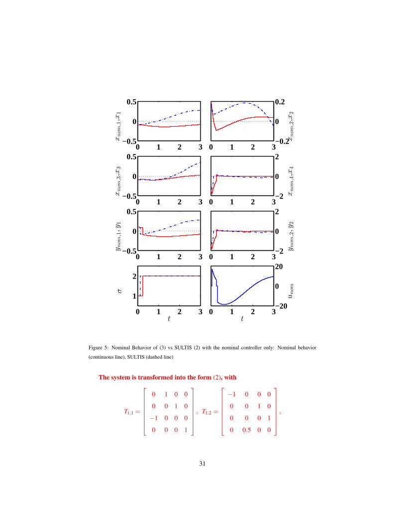
,For the transformed nominal system (3), an LQR nominal controller is proposed

in each location:

K1 =[

2.4142 6.0210 9.0699 9.9279]

and

K2 =[−50.0200 1.2563 0.2688 −251.8423

]This nominal controller guarantees the stability of the nominal system (see Figure

5). When the nominal controller is applied and there are uncertainties/perturbations

in the system, the nominal controller is incapable to take the states to zero, see Fig-

ure 5. This shows the necessity of the robustifying methodology.

32

For comparison purposes, let’s apply an OISM controller [15] to the system.

As it was mentioned in the introduction this controller is based on a first order

sliding mode methodology, and uses filters to reconstruct the states. In Figure 10

the reconstructed state is presented. Note that the filters, affect the state recon-

struction.

The OISM controller compensates theoretically exactly the matched uncer-

tainties/perturbations. But the control signal is discontinuous, generating high

level chattering (see Figure 7)

0 1 2 3−0.5

0

0.5

x1

0 1 2 3−1

−0.5

0

0.5

x2

0 1 2 3−0.5

0

0.5

x3

0 1 2 3−2

0

2

x4

0 1 2 3

1

2

t

σ

0 1 2 3−1000

0

1000u

t

Figure 7: SULTIS with an OISM controller

Now, let’s apply the COISM methodology. First we design the cascade ob-

server. Recall that this observer is composed by two parts: The Luenberger-type

error stabilizer and the hierarchical observer. The Luenberger stabilizer was de-

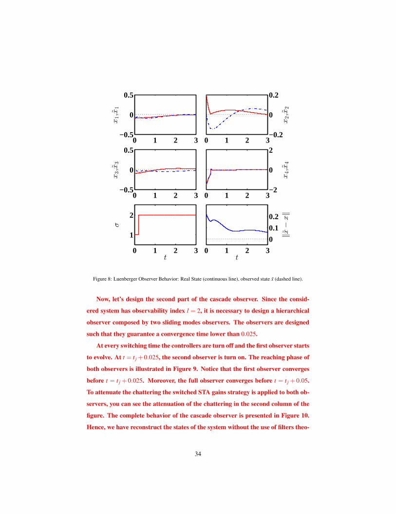
signed using the LMI Problem 1. This stabilizer is shown in Figure 8 and it is

designed for the uncertainties/perturbations free part of the SULTIS assuring the

existence of a bound for the observation error eLO and it’s first derivative.

33

0 1 2 3−0.5

0

0.5

x1,x

1

0 1 2 3−0.2

0

0.2

x2,x

2

0 1 2 3−0.5

0

0.5

x3,x

3

0 1 2 3−2

0

2

x4,x

4

0 1 2 3

1

2

t

σ

0 1 2 3

0

0.1

0.2

‖x−

x‖

t

Figure 8: Luenberger Observer Behavior: Real State (continuous line), observed state x (dashed line).

Now, let’s design the second part of the cascade observer. Since the consid-

ered system has observability index l = 2, it is necessary to design a hierarchical

observer composed by two sliding modes observers. The observers are designed

such that they guarantee a convergence time lower than 0.025.

At every switching time the controllers are turn off and the first observer starts

to evolve. At t = t j +0.025, the second observer is turn on. The reaching phase of

both observers is illustrated in Figure 9. Notice that the first observer converges

before t = t j + 0.025. Moreover, the full observer converges before t = t j + 0.05.

To attenuate the chattering the switched STA gains strategy is applied to both ob-

servers, you can see the attenuation of the chattering in the second column of the

figure. The complete behavior of the cascade observer is presented in Figure 10.

Hence, we have reconstruct the states of the system without the use of filters theo-

34

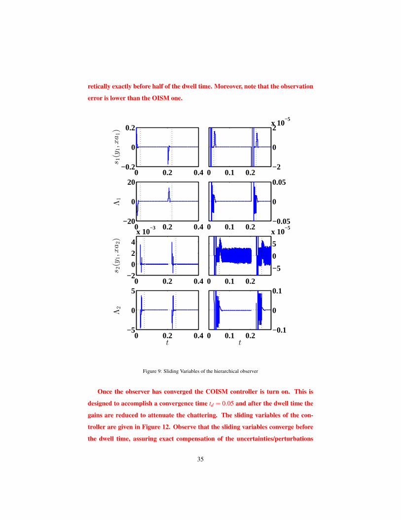
retically exactly before half of the dwell time. Moreover, note that the observation

error is lower than the OISM one.

0 0.2 0.4−0.2

0

0.2

s1(y

1,xa1)

0 0.1 0.2−2

0

2x 10

−5

0 0.2 0.4−20

0

20

Λ1

0 0.1 0.2−0.05

0

0.05

0 0.2 0.4−2

02

4x 10

−3

s2(y

1,xa2)

0 0.1 0.2

−5

0

5

x 10−5

0 0.2 0.4−5

0

5

Λ2

t0 0.1 0.2

−0.1

0

0.1

t

Figure 9: Sliding Variables of the hierarchical observer

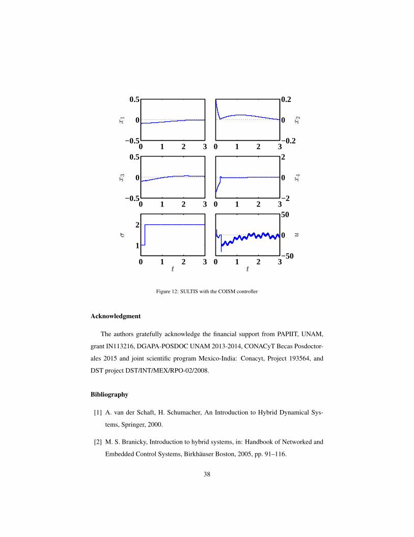
Once the observer has converged the COISM controller is turn on. This is

designed to accomplish a convergence time td = 0.05 and after the dwell time the

gains are reduced to attenuate the chattering. The sliding variables of the con-

troller are given in Figure 12. Observe that the sliding variables converge before

the dwell time, assuring exact compensation of the uncertainties/perturbations

35

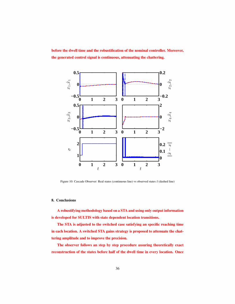
before the dwell time and the robustification of the nominal controller. Moreover,

the generated control signal is continuous, attenuating the chattering.

0 1 2 3−0.5

0

0.5x1,x

1

0 1 2 3−0.2

0

0.2

x2,x

2

0 1 2 3−0.5

0

0.5

x3,x

3

0 1 2 3−2

0

2

x4,x

4

0 1 2 3

1

2

t

σ

0 1 2 3

0

0.1

0.2

‖x−

x‖

t

Figure 10: Cascade Observer: Real states (continuous line) vs observed states x (dashed line)

8. Conclusions

A robustifying methodology based on a STA and using only output information

is developed for SULTIS with state dependent location transitions.

The STA is adjusted to the switched case satisfying an specific reaching time

in each location. A switched STA gains strategy is proposed to attenuate the chat-

tering amplitude and to improve the precision.

The observer follows an step by step procedure assuring theoretically exact

reconstruction of the states before half of the dwell time in every location. Once

36

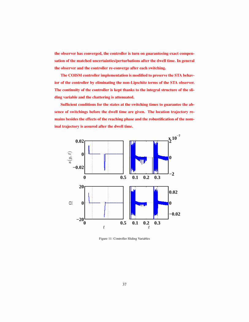
the observer has converged, the controller is turn on guaranteeing exact compen-

sation of the matched uncertainties/perturbations after the dwell time. In general

the observer and the controller re-converge after each switching.

The COISM controller implementation is modified to preserve the STA behav-

ior of the controller by eliminating the non-Lipschitz terms of the STA observer.

The continuity of the controller is kept thanks to the integral structure of the sli-

ding variable and the chattering is attenuated.

Sufficient conditions for the states at the switching times to guarantee the ab-

sence of switchings before the dwell time are given. The location trajectory re-

mains besides the effects of the reaching phase and the robustification of the nom-

inal trajectory is assured after the dwell time.

0 0.5

−0.02

0

0.02

s(y,t)

0.1 0.2 0.3−2

0

2x 10

−7

0 0.5−20

0

20

Ω

t0.1 0.2 0.3

−0.02

0

0.02

t

Figure 11: Controller Sliding Variables

37

0 1 2 3−0.5

0

0.5

x1

0 1 2 3−0.2

0

0.2

x2

0 1 2 3−0.5

0

0.5

x3

0 1 2 3−2

0

2

x4

0 1 2 3

1

2

t

σ

0 1 2 3−50

0

50

u

t

Figure 12: SULTIS with the COISM controller

Acknowledgment

The authors gratefully acknowledge the financial support from PAPIIT, UNAM,

grant IN113216, DGAPA-POSDOC UNAM 2013-2014, CONACyT Becas Posdoctor-

ales 2015 and joint scientific program Mexico-India: Conacyt, Project 193564, and

DST project DST/INT/MEX/RPO-02/2008.

Bibliography

[1] A. van der Schaft, H. Schumacher, An Introduction to Hybrid Dynamical Sys-

tems, Springer, 2000.

[2] M. S. Branicky, Introduction to hybrid systems, in: Handbook of Networked and

Embedded Control Systems, Birkhauser Boston, 2005, pp. 91–116.

38

[3] H. J. Sussmann, A maximum principle for hybrid optimal control problems, in:

38th IEEE Conference on Decision and Control (CDC), Vol. 1, 1999, pp. 425

–430.

[4] M. V. Mohrenschildt, Hybrid systems: solutions, stability, control, in: American

Control Conference (ACC), Vol. 1, 2000, pp. 692 –698 vol.1.

[5] J. P. Hespanha, A. Morse, Switching between stabilizing controllers, Automatica

38 (11) (2002) 1905 – 1917.

[6] Z. Li, C. Wen, Y. Soh, Observer-based stabilization of switching linear systems,

Automatica 39 (3) (2003) 517 – 524.

[7] N. H. El-Farra, P. Mhaskar, P. D. Christofides, Output feedback control of swit-

ched nonlinear systems using multiple lyapunov functions, Systems & Control

Letters 54 (12) (2005) 1163 – 1182.

[8] P. Caravani, E. De Santis, Observer-based stabilization of linear switching sys-

tems, International Journal of Robust and Nonlinear Control 19 (14) (2009) 1541–

1563.

[9] L. Wu, J. Lam, Sliding mode control of switched hybrid systems with time-

varying delay, International Journal of Adaptive Control and Signal Processing

22 (10) (2008) 909–931.

[10] L. Wu, P. Shi, H. Gao, State estimation and sliding-mode control of markovian

jump singular systems, IEEE Transactions on Automatic Control 55 (5) (2010)

1213–1219.

[11] L. Wu, D. W. Ho, C. Li, Sliding mode control of switched hybrid systems with

stochastic perturbation, Systems & Control Letters 60 (8) (2011) 531 – 539.

[12] L. Wu, W. X. Zheng, H. Gao, Dissipativity-based sliding mode control of swit-

ched stochastic systems, IEEE Transactions on Automatic Control 58 (3) (2013)

785–791.

[13] V. I. Utkin, Sliding Modes in Control and Optimization, Springer-Verlag, 1992.

39

[14] J. Lian, J. Zhao, G. M. Dimirovski, Integral sliding mode control for a class of

uncertain switched nonlinear systems, European Journal of Control 16 (1) (2010)

16 – 22.

[15] F. J. Bejarano, L. Fridman, A. S. Poznyak, Output integral sliding mode con-

trol based on algebraic hierarchical observer, International Journal of Control 80

(2007) 443 – 453.

[16] L. Fridman, A. Poznyak, F. J. Bejarano Rodrıguez, Robust Output LQ Optimal

Control via Integral Sliding Modes, Birkhauser, 2014.

[17] A. Levant, Sliding order and sliding accuracy in sliding mode control, Interna-

tional journal of control 58 (6) (1993) 1247–1263.

[18] Y. Shtessel, C. Edwards, L. Fridman, A. Levant, Sliding Mode Control and Ob-

servation, Birkhauser Boston, 2013.

[19] T. Floquet, J. P. Barbot, Super twisting algorithm-based step-by-step sliding mode

observers for nonlinear systems with unknown inputs, International Journal of

Systems Science 38 (10) (2007) 803–815.

[20] F. Bejarano, L. Fridman, A. Poznyak, Exact state estimation for linear systems

with unknown inputs based on hierarchical super-twisting algorithm, Interna-

tional Journal of Robust and Nonlinear Control 17 (18) (2007) 1734–1753.

[21] H. Saadaoui, N. Manamanni, M. Djemaı, J. Barbot, T. Floquet, Exact differen-

tiation and sliding mode observers for switched lagrangian systems, Nonlinear

Analysis: Theory, Methods & Applications 65 (5) (2006) 1050 – 1069.

[22] F. J. Bejarano, L. Fridman, State exact reconstruction for switched linear systems

via a super-twisting algorithm, International Journal of Systems Science 42 (5)

(2011) 717–724.

[23] F. Bejarano, A. Pisano, E. Usai, Finite-time converging jump observer for swit-

ched linear systems with unknown inputs, Nonlinear Analysis: Hybrid Systems

5 (2) (2011) 174 – 188.

40

[24] H. Rıos, S. Kamal, L. M. Fridman, A. Zolghadri, Fault tolerant control allocation

via continuous integral sliding-modes: A hosm-observer approach, Automatica

51 (2015) 318 – 325.

[25] M. S. Shaikh, P. E. Caines, On the hybrid optimal control problem: Theory and

algorithms, IEEE Transactions on Automatic Control 52 (9) (2007) 1587–1603.

[26] W. J. Rugh, Linear System Theory, Prentice Hall, 1993.

[27] M. Hautus, Strong detectability and observers, Linear Algebra and its Applica-

tions 50 (1983) 353 – 368.

[28] Y. Orlov, Finite time stability and robust control synthesis of uncertain switched

systems, SIAM Journal on Control and Optimization 43 (4) (2004) 1253–1271.

[29] A. Polyakov, A. Poznyak, Reaching time estimation for super-twisting second or-

der sliding mode controller via lyapunov function designing, Automatic Control,

IEEE Transactions on 54 (8) (2009) 1951–1955.

[30] V. Utkin, About second order sliding mode control, relative degree, finite-time

convergence and disturbance rejection, in: Variable Structure Systems (VSS),

2010 11th International Workshop on, 2010, pp. 528–533.

[31] J. Moreno, M. Osorio, A lyapunov approach to second-order sliding mode con-

trollers and observers, in: Decision and Control, 2008. CDC 2008. 47th IEEE

Conference on, 2008, pp. 2856–2861.

[32] I. Boiko, L. Fridman, Analysis of chattering in continuous sliding-mode con-

trollers, IEEE Transactions on Automatic Control 50 (9) (2005) 1442–1446.

[33] M. T. Angulo, L. Fridman, A. Levant, Output-feedback finite-time stabilization

of disturbed LTI systems, Automatica 48 (4) (2012) 606 – 611.

[34] A. Alessandri, P. Coletta, Switching observers for continuous-time and discrete-

time linear systems, in: American Control Conference, 2001. Proceedings of the

2001, Vol. 3, IEEE, 2001, pp. 2516–2521.

41

[35] A. Chalanga, S. Kamal, L. Fridman, B. Bandyopadhyay, J. A. Moreno, How to

implement super-twisting controller based on sliding mode observer?, in: Vari-

able Structure Systems (VSS), 2014 13th International Workshop on, 2014, pp.

1–6.

[36] D. Bainov, P. Simeonov, Integral Inequalities and Applications, 1st Edition,

Vol. 57 of Mathematics and its Applications, Springer Netherlands, 1992.

[37] E. Cruz-Zavala, J. Moreno, L. Fridman, Uniform robust exact differentiator, Au-

tomatic Control, IEEE Transactions on 56 (11) (2011) 2727–2733.

[38] W. Kratz, Characterization of strong observability and construction of an ob-

server, Linear Algebra and its Applications 221 (1995) 31 – 40.

[39] R. Vidal, A. Chiuso, S. Soatto, S. Sastry, Observability of linear hybrid systems,

in: O. Maler, A. Pnueli (Eds.), Hybrid Systems: Computation and Control, Vol.

2623 of Lecture Notes in Computer Science, Springer Berlin Heidelberg, 2003,

pp. 526–539.

Appendix A. Strong Observability: Concept and Results

In this section we restate the strong observability concepts used in the design

of the COISM methodology for switched systems.

Definition 1 ([26]). The observability index l is the minimum integer such that

rank(Oi,l) = n

with

Oi,l =

Ci

CiAi

...

CiAl−1i

.

Definition 2 ([27]). The triple (Ai,Bi,Ci) is strongly observable if y(t)≡ 0 on [t j−1, t j]

with a piece-wise continuous function u(t) always implies x(t)≡ 0.

42

Proposition 2 ([38]). Define the matrices

Si,l =[

Oi,l Ti,l

]and S∗i,l =

I 0

Oi,l Ti,l

;

with

Ti,l =

0 · · · 0

CiBi · · · 0...

. . ....

CiAl−2i Bi · · · CiBi

and Oi,l =

Ci

CiAi

...

CiAl−1i

.

The triple (Ai,Bi,Ci) is strongly observable, if and only if the rank condition

rank (Si,l) = rank (S∗i,l)

holds.

Lemma 4. [15] If the pair (Ai,Bi,Ci) is strongly observable and p > m then the pair A11,i A12,i

0 0

,Ci

is observable.

Remark 8. A direct consequence of Lemma 4 is that the observability matrix O1,i,l

has full rank.

Remark 9. The strong observability property assures the state vector x(t) can be

reconstructed besides the presence of matched uncertainties/perturbations. Since

the location transitions depend on x(t) and the initial location is known, we can

assure the SULTIS is strongly observable. If the initial location were unknown, a

distinguishibility condition [39] would be necessary to guarantee the observability of

the SULTIS.

43