Proceedings of the 2013

International Conference on

Computational and Mathematical

Methods in Science and Engineering

Almería, Spain

June 24-27, 2013

CMMSE

VOLUME I

Editors: Ian Hamilton & Jesús Vigo-Aguiar

Associate Editors:

H. Adeli, P. Alonso, M.T. De Bustos, M. Demiralp, J.A. Ferreira, A. Q. M. Khaliq,

J.A. López-Ramos, P. Oliveira, J.C. Reboredo, M. Van Daele,

E. Venturino, J. Whiteman, B. Wade

Proceedings of the 2013 International Conference on

Computational and Mathematical Methods in Science and Engineering

Cabo de Gata, Almería, Spain

June 24-27, 2013

Editors I. P. Hamilton & J. Vigo-Aguiar

Associate Editors H. Adeli, P. Alonso, M.T. De Bustos,

M. Demiralp, J.A. Ferreira, A. Q. M. Khaliq, J.A. López-Ramos, P. Oliveira, J.C. Reboredo,

M. Van Daele, E. Venturino, J. Whiteman, B. Wade

@CMMSE Preface- Page ii

ISBN 978-84-616-2723-3

@Copyright 2013 CMMSE Printed on acid-free paper

@CMMSE Preface- Page iii

Preface

It is our great pleasure to present the proceedings of the 13th International Conference on Computational and Mathematical Methods in Science and Engineering (CMMSE 2013), at Cabo de Gata, Almería (Spain), 24-27 June 2013, comprised of the extended abstracts of the conference presentations.

Since its inception in Milwaukee in 2000, CMMSE has provided a stimulating annual forum for researchers, from a wide range of disciplines, who have found in CMMSE a fruitful arena in which to disseminate their contributions to the research community. Researchers also benefit from being at the crossroads of computational and mathematical methods in a wide variety of research areas. Encouraging the development of the new computational and mathematical methods increasingly demanded by diverse disciplines continues to be the cornerstone of the conference.

Interest in understanding the behaviour of complex systems and phenomena is growing since this essential for the technological development of our society. The resolution of many problems at the theoretical and practical level in science, engineering, economics, and finance requires the intensive development of computational and mathematical methods, which have thus become essential research tools. CMMSE 2013 covers all the computational and mathematical fields, providing specific responses for specific fields and describing up-to-date developments to an expert audience. In addition, mini-symposia and special sessions cover a wide range of specialized topics.

New large-scale problems that arise in fields like bioinformatics, computational chemistry, and astrophysics are considered in a high-performance computing session, whereas mathematical problems related to internet security are considered in another session. Likewise, analytical, numerical and computational aspects of partial differential equations in life and materials science are considered in a specific mini-symposium. The computational finance session covers problems related to asset pricing, trading and risk analysis of financial assets that have no analytic solutions under realistic assumptions and thus require computational methods to be resolved. The symposium on new educational methodologies supported by new technologies offers a forum for discussion of the growing impact of new technologies on teaching, and the development of new tools to increase learning efficiency. Flow-modelling of particles with motivated behaviour in complex networks, applied to traffic flows, pedestrian flows, ecology, etc., are presented in the symposium on mathematical models and information-intelligent transport systems. Recent techniques to solve various types of optimization problems in engineering are presented in the session on computational methods for linear and nonlinear optimization, while numerical methods for solving nonlinear problems are presented in another specific session. Recent theoretical and applied mathematical developments related to cryptography and codes, bio-mathematics, combinatorial optimization algorithms, and algebraic analysis are presented in other specific sessions. Novel methods for the approximation of univariate and multivariate functions, the solution of ordinary and partial differential equations, and the decomposition of multivariate arrays are presented in two mini-symposia. Another mini-symposium covers new computational methods for improving computed tomography reconstruction quality and speed. Finally, special sessions cover topics related to industrial mathematics, ab initio materials and simulation, computational discrete mathematics and the numerical solution of differential equations.

@CMMSE Preface- Page iv

We would like to thank the plenary speakers for their outstanding contributions to research and leadership in their respective fields, including physics, chemistry, engineering, and computational finance. We would also like to thank the special session organizers and scientific committee members, who have played a very important part in setting the direction of CMMSE 2013. Finally, we would like to thank the participants because, without their interest and enthusiasm, the conference would not have been possible.

These proceedings, comprised of the extended abstracts of the conference presentations, are of significant interest and contain original and substantial analyses of computational and mathematical methodologies. The proceedings have five volumes, the first four correspond to the articles typeset in LaTeX and the fifth to articles typeset in Word.

We cordially welcome all participants. We hope you enjoy the conference.

Cabo de Gata, Almería (Spain), 20 June 2013

I. P. Hamilton, J. Vigo-Aguiar, H. Adeli, P. Alonso, M.T. De Bustos, M. Demiralp, J.A. Ferreira, A. Q. M. Khaliq,

J.A. López-Ramos, P. Oliveira, J.C. Reboredo, M. Van Daele, E. Venturino, J. Whiteman, B. Wade

@CMMSE Preface- Page v

CMMSE 2013 Mini-symposia

Session Title Organizers High Performance Computing (HPC) Enrique S. Quintana Ortí & G. Ester

Martín Garzón P.D.E.'S in Life and Material Sciences

Paula Oliveira & J.A. Ferreira

Computational Finance

Abdul Khaliq & Juan C. Reboredo

New Educational Methodologies Supported by New Technologies

José A. Piedra

Mathematical Models and Information-Intelligent Systems on Transport

Valerii V. Kozlov & Andreas Schadschneider & Alexander P. Buslaev

Computational Methods for Linear and Nonlinear Optimization

Maria Teresa Torres Monteiro

Numerical Methods for Solving Nonlinear Problems

Juan R. Torregrosa & A. Cordero

Crypto & Codes Juan Antonio López-Ramos & İrfan Şiap Bio-mathematics Ezio Venturino, Nico Stollenwerk &

Maíra Aguiar Recent Methodological Developments in Function Approximation, Multiway Array Decompositions, ODE and PDE Solutions: Applications From Dynamical Systems to Quantum and Statistical Dynamics

Metin Demiralp & Alper Tunga & Burcu Tunga

CMMSE 2013 Special Sessions

Session Title Organizers Industrial Mathematics Bruce A. Wade Ab initio materials & simulation Ian Hamilton Computational Discrete Mathematics José Carlos Valverde Fajardo Numerical solution of differential equations

J. Vigo Aguiar & Marnix Van Daele

Computational Methods in Tomography J. Román Bilbao Castro, G. Ester Martín Garzón & J. J. Fernández Rodriguez

@CMMSE Preface- Page vi

Acknowledgements We would like to express our gratitude to Universidad de Almeria, ASAC communications & Patronato de la Alhambra y Generalife our sponsors, for its assistance. We also would like to thank all of the local organizers for their efforts devoted to the success of this conference:

o Pedro Alonso - Universidad de Oviedo - Gijón, Spain o José A. Álvarez-Bermejo – Universidad de Almería, Spain o M. Teresa de Bustos - Universidad de Salamanca, Spain

o Antonio Fernández - Universidad de Salamanca, Spain o Pedro Gonzalez Rodelas - Universidad de Granada, Spain o Juan Antonio López Ramos - Universidad de Almería, Spain

o Raquel Cortína Pajarón - Universidad de Oviedo -Gijón, Spain o Antonio Sánchez Martín - Universidad de Salamanca, Spain

CMMSE 2013 Plenary Speakers • Abdul Q. M. Khaliq - Middle Tennessee State University, USA • Ezio Venturino - University of Torino, Italy • José M. Soler - Univ. Autónoma de Madrid , Spain • John Whiteman, - Brunel University, London, UK • Marnix Van Daele - University of Gent, Belgium • Metin Demiralp - Turkish Academy of Sciences, Turkish • Mikel Luján - Manchester University, UK • Nico Stollenwerk - University Lisbon, Portugal

@CMMSE Preface- Page vii

Volume I

Page 1 of 1797

Page 2 of 1797

Contents:

Volume I

Volume I............................................................................................................................. 1 Index ................................................................................................................................... 3 Determinants and inverses of nonsingular pentadiagonal matrices Abderramán Marrero, J. .................................................................................................... 21 A new tool for generating orthogonal polynomial sequences Abderramán Marrero, J.; Tomeo, V.; Torrano, E. ............................................................. 25 ParallDroid: A framework for parallelism in AndroidTM Acosta, A.; Almeida, F. ..................................................................................................... 37 "Kâi lêuat òk" is everything: 26, 27, 66 Aguiar, M.; Stollenwerk, N. ............................................................................................... 40 An improved information rate of perfect secret sharing scheme based on dominating set of vertices Al Saidi, N.M.G.; Rajab, N.A.; Said, M.R.Md.; Kadhim, K.A. ............................................ 50 Testing for a class of bivariate exponential distributions Alba-Fernández, V.; Jiménez-Gamerro, M.D. .................................................................. 61 A matrix algorithm for computing orbits in parallel and sequential dynamical systems Aledo, J.A.; Martínez, S.; Valverde, J.C............................................................................ 67 Accelerating the computation of nonnegative matrix factorization in multi-core and many-core architectures Alonso, P.; García, V.M.; Martínez-Zaldívar, F.J.; Salazar, A.; Vergara, L.; Vidal, A.M. ................................................................................................................................... 71 Almost strictly sign regular matrices Alonso, P; Peña, J.M.; Serrano, M.L. ................................................................................ 80 An ECC based key agreement protocol for mobile access control Alvarez-Bermejo, J.A.; Lodroman, M.A.; Lopez-Ramos, J.A. ........................................... 86

Page 3 of 1797

The conservative method of calculating the Boltzmann collision integral for simple gases, gas mixtures and gases with rotational degrees of freedom Anikin, Y.A.; Dodulad, O.I.; Kloss, Y. Y.; Tcheremissine, F.G. ......................................... 93 Finite-volume discretization of a 1d reaction-diffusion based multiphysics modelling of charge trapping in an insulator submitted to an electron beam irradiation Aoufi, A.; Damamme, G. ................................................................................................. 105 On soft functions Aras, C.G.; Sönmez, A.; Çakalli, H. ................................................................................ 110 Numerical solution of time-dependent Maxwell's equations for modeling scattered electromagnetic wave's propagation Araújo, A.; Barbeiro, S.; Pinto, L.; Caramelo, F.; Correia, A.L.; Morgado, M.; Serranho, P.; Silva, A.S.F.C.; Bernardes, R. .................................................................. 121 Parallel extrapolated algorithms for computing PageRank Arnal, J.; Migallón, H; Migallón, V.; Palomino, J.A.; Penadés, J. ................................... 130 Parallel evolutionary approaches for solving a planar leader-follower facility problem Arrondo, A.G.; Redondo, J.L.; Fernández, J.; Ortigosa, P.M. ........................................ 140 Analysis of the performance of the Google Earth running in a cluster display wall Arroyo, I.; Giné, F.; Roig, C. ............................................................................................ 146 High-order iterative methods by using weight functions technique Artidiello, S.; Cordero, A.; Torregrosa, J.R.; Vassileva, M. ............................................. 157 On Z2Z2[u]−Additive Codes Aydogdu, I.; Abualrub, T.; Siap, I. ................................................................................... 169 Analytical and numerical study of diffusion through biodegradable viscoelastic materials Azhdari, E.; Ferreira, J.A.; de Oliveira, P.; da Silva, P.M................................................ 174 Drug Delivery from an ocular implant into the vitreous chamber of the eye Azhdari, E.; Ferreira, J.A.; de Oliveira, P.; da Silva, P.M................................................ 185 Boolean sum based differential quadrature Barrera, D.; González, P.; Ibáñez, F.; Ibáñez, M.J. ........................................................ 196 A WENO-based method to improve the determination of the threshold voltage and characterize DIBL effects in MOSFET transistors Barrera, D.; González, P.; Ibáñez, M.J.; Roldán, A.M.; Roldán, A.M. ........................... 202 Error estimates for modified Hermite interpolant on the simplex Barrera, D.; Ibáñez, M.J.; Nouisser, O. ........................................................................... 210 Discrete orthogonal polynomial technique for parameter determination in MOSFETs transitors Barrera, D.; Ibáñez, M.J.; Roldán, A.M.; Roldán, J.B.; Yáñez, R. .................................. 213

Page 4 of 1797

Conservation law construction via mathematical fluctuation theory for exponentially anharmonic, symmetric, quantum oscillator Bayat, S.; Demiralp, M. ................................................................................................... 218 Optimal control of a linear and unbranched chemical process with n steps: the quasi-analytical solution Bayón, L.; Grau, J.M.; Ruiz, M.M.; Suárez, P.M. ............................................................ 226 Linear and cyclic codes over a finite non chain ring Bayram, A.; Siap, I. ......................................................................................................... 232 Soft path connectedness on soft topological spaces Bayramov, S.; Gunduz, C.; Erdem, A. ............................................................................ 239 Problem solving environment for gas flow simulation in micro structures on the base of the Boltzmann equation Bazhenov, I.I.; Dodulad, O.I.; Ivanova, I.D.; Kloss, Y.Y.; Rjabchenkov, V.V.; Shuvalov, P.V.; Tcheremissine, F.G. .............................................................................. 246 Solving systems of nonlinear mixed Fredholm-Volterra integro-differential equations using fixed point techniques and biorthogonal systems Berenguer, M.I.; Gámez, D.; López, A.J. ........................................................................ 258 A new use of correlation-immune Boolean functions in cryptography and new results Bhasin, S.; Carlet, C.; Guilley, S. .................................................................................... 262 Product type weights generated by a single nonproduct type weight gunction in high dimensional model representation (HDMR) Bodur, D.; Demiralp, M. .................................................................................................. 265 Computational modelling of meteorological variables on multicores and multi-GPU systems Boratto, M.; Alonso, P.; Gimenéz, D. .............................................................................. 273 Impact of the information exchange policies in load balancing algorithms Bosque, J.L.; Robles, O.D.; Toharia, P.; Pastor, L. ........................................................ 277 Symbolic computation of a canonical form for a class of linear functional systems Boudellioua, M.S. ............................................................................................................ 289 Efficient protocols to control glioma growth Branco, J.R.; Ferreira, J.A.; de Oliveira, P. ..................................................................... 293 Allee effects models in randomly varying environments Braumann, C.A.; Carlos, C. ............................................................................................ 304 Exploiting multi-core platforms for multi-model forest fire spread prediction Brun, C.; Margalef, T.; Cortés, A. .................................................................................... 308 Do niches help in controlling disease spread in ecoepidemic models Bulai, I.M.; Chialva, B.; Duma, D.; Venturino, E. ............................................................ 320

Page 5 of 1797

GPU acceleration of a tool for wind power forecasting Burdiat, M.; Hagopian, J.I.; Silva, J.P.; Dufrechou, E.; Gutiérrez, A.; Pedemonte, M.; Cazes, G.; Ezzatti, P. ................................................................................................ 340 On recovery of state parameters of systems via video-images analysis Buslaev, A.P.; Yashina, M.V. .......................................................................................... 352 A predator-prey model with strong Allee effect on prey and interference among predators Cabrera-Villegas, J.; Córdova-Lepe, F.; González-Olivares, E. ..................................... 359 Homogenization of the Poisson equation with Dirichlet conditions in random perforated domains Calvo-Jurado, C.; Casado-Díaz, J.; Luna-Laynez, M. .................................................... 364

Page 6 of 1797

Contents:

Volume II

Volume II ....................................................................................................................... 369 Index ............................................................................................................................... 371 Analysis and control of the electronic motion with time-dependent density-functional theory: new developments in the octopus code Castro, A. ........................................................................................................................ 389 Reconstruction of separatrix curves and surfaces in squirrels competition models with niche Cavoretto, R.; De Rossi, A.; Perracchione, E.; Venturino, E. ......................................... 400 Abelian subalgebras and ideals of maximal dimension for Leibniz algebras Ceballos, M.; Núñez, J.; Tenorio, A.F. ............................................................................ 412 A technique to design derivative-free iterative methods for nonlinear equations Cordero, A.; Torregrosa, J.R. .......................................................................................... 417 A Mandelbrot set in the antenna of the cat set Cordero, A.; Torregrosa, J.R.; Vindel, P. ........................................................................ 428 A method to extract precise implication from contexts Cordero, P.; Enciso, M.; Mora, A.; Ojeda-Aciego, M. ..................................................... 437 Impulsive hospitalization: Epidemiological control on farms Córdova-Lepe, F.; Del-Valle, R.; Solis, M.E. .................................................................. 444 High-performance process-level migration of MPI applications Cores, I.; Rodríguez, G.; Martín, M.M.; González, P. ..................................................... 456 Multi-adjoint concept lattices reduced by thresholds Cornejo, M.E.; Medina, J.; Ramírez, E. .......................................................................... 467 Averaging technics on the C1-integrability of a Stark-Zeeman problem de Bustos-Muñoz, M.T. ................................................................................................... 477 Sensitivity analysis and variance reduction in a stochastic NDT problem De Staelen, R. H.; Beddek, K. ........................................................................................ 482

Page 7 of 1797

Using population level models to characterize individual behavior with space extension and P.E.A.(probabilistic evolution approach) Demiralp, E.; Hernandez-Garcia, L.; Demiralp, M. ......................................................... 487 Constancy adding space extension (CASE) to get Kronecker power series kernel separability in conical explicit ordinary differential equation solutions Demiralp, M. .................................................................................................................... 496 Kernel separability in Kronecker power solutions for conical explicit ordinary differential equations Demiralp, M. .................................................................................................................... 504 DDMOA2: Improved descent directions-based multiobjective algorithm Denysiuk, R.; Costa, L.; Espírito Santo, I. ...................................................................... 513 Obtaining the set of solutions of a multi-adjoint relation equations from concept lattice theory Díaz, J.C.; Medina, J. ...................................................................................................... 525 Performance analysis of a parallel lattice reduction algorithm on many-core architectures Domene, F.; Józsa, C.M.; Vidal, A.M.; Piñero, G.; Gonzalez, A. .................................... 535 On the pricing and hedging of options for highly volatile periods El-Khatib, Y.; Hatemi-J. A. .............................................................................................. 543 A numerical method based on the polynomial regression for the inverse diffusion problem Erdem, A. ........................................................................................................................ 555 e-Learning supporting formative evaluation Escoriza, J.; Lopez-Ramos, J.A.; Peralta, J. .................................................................. 567 Importance of the fitted straight line for confidence bands in a Normal Q-Q Plot Estudillo-Martínez, M.D.; Castillo-Gutiérrez, S.; Lozano-Aguilera, E. ............................ 576 Expanding the applicability of Steffensen's method for solving nonlinear equations in Banach spaces Ezquerro, J. A.; Hernández-Verón, M. A.; Magreñán, Á.A. ............................................ 580 A mixed difference scheme guaranteeing positive solutions for European option pricing under a tempered stable process Fakharany, M.; Company, R.; Jódar, L. .......................................................................... 584 Power spectral density estimation of ELF signals by averaged of periodograms Fernández Ros, M.; Gázquez Parra, J.A.; Novas Castellano, N.; García Salvador, R. ..................................................................................................................................... 590 Variational and numerical analysis of a mixed kinetic-diffusion surfactant model for the modified Langmuir-Hinshelwood equation Fernández, J.R.; Kalita, P.; Migórski, S.; Muñiz, M.C.; Núñez, C. .................................. 601

Page 8 of 1797

Multiresolution analysis for two-dimensional interpolatory schemes Fernández, L.; Fortes, M.A.; Rodríguez, M.L. ................................................................ 615 On the characterization of markerless CAR systems based on mobile phones Fernández, V.; Orduña, J.M.; Morillo, P.......................................................................... 618 A mathematical model for controlled drug delivery in swelling polymers Ferreira, J.A.; Grassi, Gudiño, E.; de Oliveira, P. ........................................................... 630 Numerical simulation of a coupled cardiovascular drug delivery model Ferreira, J.A.; Naghipoor, J.; de Oliveira, P. ................................................................... 642 SABR/LIBOR market models: pricing and calibration for some interest rate derivatives Ferreiro, A.M.; García, J.A.; López-Salas, J.G.; Vázquez, C. ........................................ 654 Nonpolynomial approximation of solutions to delay fractional differential equations Ford, N.J.; Morgado, M.L.; Rebelo, M............................................................................. 666 Filling holes with shape conditions Fortes, M.A.; González, P.; Palomares, A.; Pasadas, M. ............................................... 676 Performance analysis of SSE instructions in multi-core CPUs and GPU computing on FDTD scheme for solid and fluid vibration problems Francés, J.; Bleda, S.; Márquez, A.; Neipp, C.; Gallego, S.; Otero, B.; Beléndez, A. .... 681 Performance analysis of multi-core CPUs and GPU computing on SF-FDTD scheme for third order nonlinear materials and periodic media Francés, J.; Bleda, S.; Tervo, J.; Neipp, C.; Márquez, A.; Pascual, I.; Beléndez, A. ..... 693 Parallel implementation of pixel purity index for a GPU cluster Franco, J.M.; Sevilla, J.; Plaza, A.J. ............................................................................... 705 Genetic meta-heuristics for batch scheduling in multi-cluster environments Gabaldon, E.; Guirado, F.; Lerida, J.L. ........................................................................... 709 Performance evaluation of convolutional codes over any finite field Galiano, V.; Gandia, R.; Herranz, V. ............................................................................... 721 Accelerating an evolutionary algorithm for global optimization on GPUs García Martínez, J.M.; Garzón, E.M.; Ortigosa, P.M. ..................................................... 732 Radiation induced color centers in Silica: a first-principle investigation. Giacomazzi, L.; Richard, N.; Martin-Samos, L. ............................................................... 738 A volume averaging and overlapping domain decomposition technique to model mass transport in textiles Goessens, T.; Malengier, B.; Constales, D.; De Staelen, R.H. ...................................... 742 Pyramid method for GPU-aided finite difference method Golovashkin, D.; Kochurov, A. ........................................................................................ 746 A predator-prey model with weak Allee effect on prey and ratio-dependent functional response González-Olivares, E.; Flores, J.D. ................................................................................. 757

Page 9 of 1797

Control of vibrations of a string with a tip mass González-Santos, G.; Vargas-Jarillo, C. ......................................................................... 769 Numerical solution of a nonlinear parabolic problem with an unknown Dirichlet boundary condition Grimmonprez, M.; Slodicka, M. ....................................................................................... 781

Page 10 of 1797

Contents:

Volume III

Volume III ..................................................................................................................... 787 Index ............................................................................................................................... 789 Towards a data assimilation method for blood circulation Guerra, T.; Tiago, J.; Sequeira, A. .................................................................................. 807 Mathematical modeling of timed-arc Petri nets as dynamical systems Guirao, J.L.G.; Pelayo, F.L.; Valverde, J.C. .................................................................... 813 Real dynamics for damped Newton's method applied to cubic polynomials Gutiérrez, J.M.; Magreñán, A.A. ..................................................................................... 821 High performance option pricing based on spatially adaptive sparse grids Heinecke, A. .................................................................................................................... 825 New families of iterative methods with fourth and sixth order of convergence and their dynamics Hueso, J.L.; Martínez, E.; Teruel, C. ............................................................................... 828 GPU-accelerated uniform sampling of implicit surfaces Iwasaki, M.; Nakata, S.; Tanaka, S. ................................................................................ 839 GPU accelerated 4D-CT reconstruction using higher order PDE regularization in spatial and temporal domains Kazantsev, D.; Lionheart, W.R.B.; Withers, P.J.; Lee, P.D............................................. 843 Riccati transformation method for solving constrained dynamic stochastic optimal allocation problem Kilianová, S.; Sevcovic, D. .............................................................................................. 852 Computational comparison of various FEM adaptivity approaches Korous, L.; Kus, P.; Karban, P. ....................................................................................... 858 On synergy of totally connected flows on chainmails Kozlov, V.V.; Buslaev, A.P.; Tatashev, A.G. ................................................................... 861

Page 11 of 1797

Efficient implementation of Newton solver for the finite element method Kus, P.; Korous, L.; Karban, P. ....................................................................................... 875 A stabilized finite volume numerical scheme for solving the partial differential equation in the Heston model Kútik, P.; Mikula, K. ......................................................................................................... 879 Population dynamics of a predator-prey system with recruitment and capture on both species Ladino, L.M.; Sabogal, E. I.; Valverde, J.C. .................................................................... 890 Radial basis function methods in computational finance Larsson, E.; Gomes, S.M.; Heryudono, A.; Safdari-Vaighani, A. ................................... 895 An application of generalized centro-invertible matrices Lebtahi, L.; Romero, O.; Thome, N. ................................................................................ 907 Further accuracy analysis of a mesh refinement method using 2D lid-driven cavity ows Li, Z. ................................................................................................................................ 911 High-order energy-conserved splitting FDTD scheme for solving Maxwell's equations Liang, D.; Yuan, Q........................................................................................................... 923 Tracing traintors via elliptic curves Lodroman, M.A.; Lopez-Ramos, J.A. .............................................................................. 927 Analyzing GOP-based parallel strategies with the HEVC encoder López-Granado, O.; Malumbres, M.P.; Migallón, H.; Piñol, P. ....................................... 934 Algorithms to develop semi-analytical planetary theories using Sundman generalized anomalies as temporal variables with aid of a C++ Poisson series processor López-Ortí, J.A.; Agost Gómez, V.; Barreda Rochera, M. .............................................. 946 Computationally eficient algorithm for mesh refinement based on octrees and linked lists López-Portugués, M.; López-Fernández, J.A.; Marful-Díaz, D.; Ayestarán, R.G.; Las-Heras, F. .................................................................................................................. 950 Aircraft noise scattering computation using GPUs López-Portugués, M.; López-Fernández, J.A.; Ranilla, J.; Ayestarán, R.G. .................. 958 DyRM: A dynamic roofline model based o runtime information Lorenzo, O.G.; Pena, T.F.; Cabaleiro, J.C.; Pichel, J.C.; Rivera, F.F. ........................... 965 Two new efficient methods for solving systems of nonlinear equations Lotfi, T.; Mahdiani, K.; Bakhtiari, P.; Cordero, A.; Torregrosa, J.R. ................................ 977 Some three-step iterative methods with memory with highest efficiency index Lotfi, T.; Tavakoli, E.; Mahdiani, K.; Cordero, A.; Torregrosa, J.R. ................................ 984 On generalization based on Bi et al iterative methods with eight-order convergence for solving nonlinear equations Lotfi, T.; Zadeh, M.M.; Abadi, M.A. ................................................................................. 990

Page 12 of 1797

Geodesic regression on spheres: a numerical optimization approach Machado, L.; Monteiro, T. ............................................................................................... 994 Stochastic amplification and childhood diseases in large geographical areas Marguta, R.; Parisi, A. ................................................................................................... 1001 A model to generate process logs with equi-probable runs Marinaro, P.; Diaz, I.; Troiano, L. .................................................................................. 1006 Modelling the effect of MDR-TB on Tuberculosis epidemic Martorano, S.; Yang, H.M.; Venturino, E. ..................................................................... 1013 Modelling pack hunting and prey herd behavior Melchionda, D.; Pastacaldi, E.; Perri, C.; Venturino, E. ................................................ 1017 Numerical optimization experiments using the hyperbolic smoothing strategy to solve MPCC Melo, T.M.M.; Matias, J.L.H.; Monteiro, M.T.T. ............................................................ 1029 A batched Cholesky solver for local RX anomaly detection on GPUs Molero, J.M.; Garzón, E.M.; García, I.; Quintana-Ortí, E.S.; Plaza, A. ......................... 1037 Designs and binary codes constructed from the simple group Ru of Rudvalis Moori, J.; Rodrigues, B. ................................................................................................ 1042 Relaxing the role of adjoint pairs in multi-adjoint logic programming Moreno, G.; Penabad, J.; Vázquez, C. ......................................................................... 1056

Page 13 of 1797

Contents:

Volume IV

Volume IV .................................................................................................................... 1069 Index ............................................................................................................................. 1071 A mathematical model for electromagnetic energy harvesters Morgado, L.F.; Morgado, M.L.; Silva, N.; Morais, R. .................................................... 1089 A two-dimensional convergence and error study for the time dependent convection-diffusion equation Nut, G. ........................................................................................................................... 1097 Exploration of a HPC approach for coherent tomography Ortega, G.; Lobera, J.; García, I.; Arroyo, M.P.; Garzón, E.M. ..................................... 1109 A tuned, concurrent-kernel approach to speed up the APSP problem Ortega-Arranz, H.; Torres, Y.; Llanos, D.R.; Gonzalez-Escribano, A. .......................... 1114 MacWilliams identity for linear codes over Mnxs(Z3k) with respect to Rosenbloom-Tsfasman metric Ozen, M.; Özzaim, T. .................................................................................................... 1126 A special class of reversible codes over GF(256) and DNA constructions Oztas, E.S.; Siap, I. ....................................................................................................... 1133 The ASTRA tomography toolbox Palenstijn, W.J.; Batenburg, K.J.; Sijbers, J. ................................................................ 1139 Lattice thermal conductivity from first principles via the 2n+1 theorem and Boltzmann transport equation Paulatto, L.; Fugallo, G.; Lazzeri, M.; Mauri, F. ............................................................ 1146 An adaptive Padé algorithm for the solution of time-invariant differential matrix Riccati equations Peinado, J.; Alonso, P.; Ibáñez, J.; Hernández, V.; Boratto, M. ................................... 1150 Application of ant colony optimization in an hybrid coarse-grained and all-atom based protein structure prediction strategy Peña, J.; Cecilia, J.M.; Pérez-Sánchez, H. ................................................................... 1154

Page 14 of 1797

A GPU based volunteer computing platform for the discovery of bioactive compounds Pérez-Sánchez, H.; Guerrero, G.D.; Sanz, F.; Cecilia, J.M. ......................................... 1157 Pure project-based learning in computer vision Piedra-Fernandez, J.A.; Fernandez-Martinez, A.; Peralta Lopez, M. ........................... 1161 Protection of privacy in microdata Quirós, P.; Alonso, P.; Díaz, I.; Montes, S. ................................................................... 1170 Solving systems of nonlinear equations by harmony search Ramadas, G.C.V.; Fernandes, E.M.G.P. ...................................................................... 1176 Wavelet-based evidence on gold and exchange rates dependence. Implications for risk management Reboredo, J.C.; Rivera-Castro, M.A. ............................................................................ 1187 Undestanding dengue fever dynamics: study of seasonality in the models Rocha, F.; Skwara, U.; Aguiar, M.; Stollenwerk, N. ...................................................... 1197 Unmixing-based retrieval system for remotely sensed hyperspectral imagery on GPUs Sevilla, J.; Bernabe, S.; Plaza, A. ................................................................................. 1210 A numerical analysis of MHD flow, heat and mass transfer for the UCM fluid over a stretching surface with thermal radiation Shateyi, S.; Marewo, G. ................................................................................................ 1214 Universal range reduction algorithm for generating random variables with a rational probability-generating function Shmerling, E. ................................................................................................................. 1225 Complete and byte m-spotty poset level weight enumerators of linear codes over finite fields Siap, V.; Akbiyik, S.; Siap, I. ......................................................................................... 1228 A MacWilliams type identity for m-spotty Rosenbloom-Tsfasman weight enumerators over Frobenius rings Siap, V.; Özen, M. ......................................................................................................... 1236 A parallel iterative MIMO receiver with variable complexity detectors Simarro, M.; Ramiro, C.; Martínez-Zaldívar, F.J.; Vidal, A.M.; Gonzalez, A. ................ 1242 Superdiffusion in epidemiological models Skwara, U.; Rocha, F.; Aguiar, M.; Stollenwerk, N. ...................................................... 1250 Testing particle filters for dengue fever studies via simple reinfection models Stollenwerk, N.; Aguiar, M.; Rocha, F.; Skwara, U. ...................................................... 1262 Semiclassical approximations of stochastic epidemiological processes towards parameter estimation Stollenwerk, N.; Masoero, D.; Skwara, U.; Rocha, F.; Ghaffari, P.; Aguiar, M. ............ 1278 A PDE method for American options pricing under stochastic interest rates Tangman, D.Y.; Coonjobeharry, R.K.; Bhuruth, M. ...................................................... 1290

Page 15 of 1797

Comparing algorithms for approximation of a nonlinear mixed type functional differential equation Teodoro, M.F. ................................................................................................................ 1301 Preliminary study of contact modelling the interface between user skin and wearable equipment Teodoro, F.; Silva, P.; Figueiredo-Pina, C. ................................................................... 1306 A class of Leslie-Gower type predator-prey model with sigmoid funcional response Tintinago-Ruiz, P.C.; González-Olivares, E. ................................................................. 1310 Node optimization through enhanced multivariance product representation (EMPR) Tuna, S.; Tunga, B. ....................................................................................................... 1322 Multivariate data modelling through factorized HDMR with optimized weight factors Tunga, B. ....................................................................................................................... 1331 Multivariate data modelling through EMPR in orthogonal geometry Tunga, M.A. ................................................................................................................... 1342 An approach to an efficient scheduling scheme for delivering queries to heterogenous clusters in the similarity search problem Uribe-Paredes, R.; Cazorla, D.; Arias, E.; Sánchez, J.L. .............................................. 1350 Error estimates for the full discretization of a nonlocal model for type-I superconductors Van Bockstal, K.; Slodicka, M. ...................................................................................... 1364 Deferred correction based on exponentially fitted mono-implicit Runge-Kutta methods Van Daele, M.; Hollevoet, D. ......................................................................................... 1369 The choice of the frequency in Trigonometrically-fitted methods. The use of the first integrals in case of periodic solutions Vigo-Aguiar, J.; Ramos, H. ........................................................................................... 1381 A case study of oversubscription on multi-CPU & multi-GPU heterogeneous systems Vilches, A.; Navarro, A.; Corbera, F.; Asenjo, R. .......................................................... 1401 Beam Propagation Method vectorization by means of CUDA technology Vorotnikova, D.G.; Golovashkin, D.L. ........................................................................... 1413 On new concepts of equilibria in games with incomplete information and ambiguity about future, with applications in economics and ecology Wiszniewska-Matyszkiel, A. .......................................................................................... 1423 Valuation of CMS-Linked TARNs Xu, Y.; Liang, J. ............................................................................................................. 1428 Simulation models of monotone random walks on graphs Yaroshenko, A. .............................................................................................................. 1438

Page 16 of 1797

Contents:

Volume V

Volume V ..................................................................................................................... 1451 Index ............................................................................................................................. 1453 A trajectory data warehouse for patients of Bell’s Palsy disease recovery surveillance Akaichi, J.; Manaa, M. ................................................................................................... 1471 Computer simulation of the storage of hydrogen in porous carbons Alonso, J. A.; Cabria, I.; López, M. J. ............................................................................ 1481 Determination of ground thermal diffusivity from subsurface temperatures. First results of experimental study of geothermal borehole Q-THERMIE-UNIOVI Arias-Penas, D.; Castro-García, M.P.; Rey-Ronco, M.A.; Alonso-Sánchez, T............. 1484 Genetic algorithm applied for a resources system selection problem for distributed/agile/virtual enterprises integration Avila, P.; Mota, A.; Putnik, G.; Costa, L. ....................................................................... 1490 Modelling of tunneling effect in ultra thin oxide of double gate (DG) MOSFET Bella, M.; Smaani, B.; Labiod, S.; Latreche, S. ............................................................. 1499 Automatic Routine Tuning to Represent Landform Attributes on Multicore and Multi-GPU Systems Boratto M., Alonso P., Gimenéz D. and Barreto M ....................................................... 1506 R algorithms to calculate VUS and plot ROC surface. An application from three-ordered categories of eating disorders. Caballero-Díaz, F.F.; Rivas-Moya, T. ........................................................................... 1519 Proposal of active learning with TIC’s in Mathematics subjects for engineers. Campillo, P.; Perea, C. ................................................................................................. 1527 Linearization technique and its application to numerical solution of bidimensional nonlinear convection diffusion equation Campos, M.D.; Romao, E.C.; Moura, L.F.M. ................................................................ 1535 Improvement of virtual screening predictions using support vector machines Cano, G.; Botía-Blaya, J.; Palma, J.; García-Rodríguez, J.; Pérez-Sánchez, H. ......... 1544

Page 17 of 1797

Dimensionless parameters in natural convection in porous media, isolated spaces, heated from below Cánovas, M.; Alhama, I. ................................................................................................ 1553 Non-physical finite element method: multiple material discontinuities Darvizeh, R.; Davey, K. ................................................................................................. 1562 A scalable self-balanced model for unified cloud storage based on a multi-layer architecture Díaz, A.F.; Anguita, M.; Ortega, J.; Ortiz, A. ................................................................. 1574 On the impact of mobile technology on students learning of Mathematics- A United Arab Emirates University case study El-Khatib, Y.; Diene, A.; Abubakar, A.; Anwar, M.N. .................................................... 1586 Atanassov's intuitionistic fuzzy Γ−hyperideals of Γ−semihypergroups Ersoy, B.A.; Davvaz, B. ................................................................................................. 1598 A splitting scheme for solving the advection-diffusion equation Gavete, L.; Molina, P.; Gavete, M.L.; Ureña, F.; Benito, J.J. ........................................ 1607 Fractal analysis to quantify wind direction fluctuations Harrouni, S. ................................................................................................................... 1618 Semiconductor and graphene quantum dots: electron-electron interactions, topology and spin blockade Hawrylak, P. .................................................................................................................. 1625 T-matrix for multiple barriers in monolayer graphene Hdez-Fuentevilla, C.; Lejarreta-Glez, J.D.; Diez, E. ..................................................... 1627 Multi-agent solution of the hydraulic transient equations in pressurized systems Izquierdo, J.; del Montalvo, I.; Pérez-García, R.; Ayala-Cabrera, D. ............................ 1636 Iterative three-sizes filter for colour images Kourgli, A.; Oukil, Y. ...................................................................................................... 1646 Numerical Investigation on number of detonation points in fragmentation warhead Kulsirikasem, W.; Tanapornraweekit, G.; Laksana, C. ................................................. 1657 Gold clusters and nanostructures: Adsorption of, and reactions with, small molecules Liu, X.J.; Hamilton, P..................................................................................................... 1664 Thresholding algorithms for oil slick detection in Radar SAR images Lounis, B.; Belhadj-Aissa, A. ......................................................................................... 1667 Topology optimization of a mid-size horizantal axis wind turbine hub Makaracı, M.; Demir, S. ................................................................................................ 1675

Page 18 of 1797

Process optimisation with the aid of artificial neural networks Mansour, M.; Elli, J.E. ................................................................................................... 1685 A finite volume - finite difference method with stiff ode solver for advection-diffusion-reaction equation Molina, P.; Gavete, L.; Gavete, M.L.; Ureña, F.; Benito, J.J. ........................................ 1697 Comparing point clouds under uncertainty Ordóñez, C.; López, F. de A.; Roca-Pardiñas, J.; García-Castro, S. ........................... 1708 Land use discrimination of full and compact polarimetric data modes Ouarzeddine, M.; Souissi, B.; Belhad-Aissa, A. ............................................................ 1712 Problem-based learning experiment for a real client in engineering Peralta, M.; Fernández, A.; Piedra, J.A.; Torres, J.A. ................................................... 1721 Filtering and optimization the rainfall cells observed in radar images Raaf, O.; Adane, A. ....................................................................................................... 1732 Compact modeling of undoped nanoscale double gate MOSFET transistor: Short channel effects Smaani, B.; Bella, M.; Beghoul, M.R.; Latreche, S. ...................................................... 1741 SVM classification for compact polarimetric data using Stokes parameters Souissi, B.; Ouarzeddine, M.; Belhad-Aissa, A. ............................................................ 1750 Neural network ensemble of RBFs to approximation of large data sample driving problems functions Torres, J.A.; Martinez, F.J.; Peralta, M.; Puertas, S. .................................................... 1759 Conservative finite-difference schemes for 2D problem of femtosecond pulse propagation in semiconductor Trofimov, V.A.; Loginova, M.M.; Egorenkov, V.A. ........................................................ 1767 Mathematical functions used for temperature-dependent tissue characteristics in radiofrequency ablation modeling Trujillo, M.; Berjano, E. .................................................................................................. 1777 Effect of the material properties on the yielding of the two-layered composite cylinder with free ends Yalçin, F.; Ozturk, A.; Gulgec, M. .................................................................................. 1786 .

Page 19 of 1797

Page 20 of 1797

Proceedings of the 13th International Conferenceon Computational and Mathematical Methodsin Science and Engineering, CMMSE 201324–27 June, 2013.

Determinants and inverses of nonsingularpentadiagonal matrices

J. Abderraman Marrero1

1 Department of Mathematics Applied to Information Technologies, TelecommunicationEngineering School, UPM - Technical University of Madrid, Spain.

emails: jc.abderraman@upm.es

Abstract

For nonsingular n× n (n ≥ 6) pentadiagonal matrices P having nonzero entries onits second subdiagonal, we propose a procedure for computing both the determinantdetP in O(n) times, and accurate information for obtaining the inverse P−1 in O(n2)times. In the general nonsingular case, n ≥ 5, a suitable decomposition of P, as aproduct of two nonsingular upper Hessenberg matrices, allows us another procedure forobtaining both detP and P−1 taking advantage of such low rank structured matrices.

Key words: Determinant, inverse, matrix computations, pentadiagonal matrix.

1 Introduction

Nonsingular pentadiagonal matrices of a finite order n, P = pi,j1≤i,j≤n (with pi,j = 0for |i − j| > 2) have a role in current methods of the numerical analysis. They frequentlyarise in ODEs, PDEs, interpolation and spline problems [4], boundary value problems,BVP, involving fourth order derivatives. Also, pentadiagonal matrices appear and in finerapproximations of second order derivatives. Gauss-Jordan methods with partial pivotingare usually handled in the inversion of such matrices. However, these methods can destroythe special structure and sparsity of the pentadiagonal matrices. Hence, computationaltechniques based on the low rank structure of the pentadiagonal matrices are of interest.

Particular algorithms for the inversion of P are known. In the sequential line, a pro-cedure for the inverse of P was provided in [3], with the condition in the entries pi,j 6= 0for i− j = 2, or j − i = 2, in O(n2) times. Another procedure with complexity O(n2) wasproposed for pentadiagonal matrices having an LU (Doolittle) factorization, [7].

c©CMMSE ISBN: 978-84-616-2723-3Page 21 of 1797

Determinants and inverses of nonsingular pentadiagonal matrices

Fast numerical algorithms for the determinant of pentadiagonal matrices P are requiredto test efficiently the existence of unique solutions of the PDEs, and also for inverse construc-tion methods of symmetric pentadiagonal Toeplitz matrices. Some results with complexityO(n) have been obtained for the determinant of nonsingular pentadiagonal matrices P,[2, 5, 6]. As a continuation of this line, we propose a fast and accurate computation, alsowith complexity O(n), for the determinant of a pentadiagonal matrix having nonzero entriesin its second subdiagonal, currently used in numerical analysis. In addition, all the accurateinformation about the inverse P−1 is obtained with complexity O(n2).

The computation of the determinant and the inverse of any nonsingular pentadiagonalmatrix P taking advantage of its special low rank structure, and without conditions onits entries, is an open question. We propose here a simple factorization for the generalnonsingular case, where the pentadiagonal matrix P can be decomposed as a product oftwo suitable upper Hessenberg matrices. It provides us the determinant and the inverse ofP by exploiting the low rank structure of the Hessenberg matrices [1].

2 Pentadiagonal matrices having nonzero entries in its sec-ond subdiagonal.

The 2 × 2 block structure P =

(P11 02U P22

), for a n × n (n ≥ 6) nonsingular pentadi-

agonal matrix is assumed. P11 and P22 are matrices of order 2 × n − 2 and n − 2 × 2,respectively. Matrix 02 is the zero matrix of order 2. The n − 2×n − 2 matrix U is non-singular upper triangular. The transposed partitioning for its inverse is known, P−1 =(−U−1P22M21 U−1 + U−1P22M21P11U

−1

M21 −M21P11U−1

), with M21 = 1

detP

(C1,n−1 C2,n−1

C1,n C2,n

),

and the given Ci,j are cofactors of P. Therefore, P−1 can be seen as:

P−1 =

(−U−1P22

I2

)M21

(I2 −P11U

−1)

+

(0n,2 U−1

02 02,n

), (1)

a rank two perturbation of a strictly upper triangular matrix. Just consider as, given P, theinformation required for the inversion of this class of pentadiagonal matrices is containedin the matrices M21 and U−1. From these matrices, we can obtain the inverse using (1).

2.1 Computing the determinant in O(n) times

Proposition 1 Let P a n × n (n ≥ 6) nonsingular pentadiagonal matrix having nonzeroentries on its second subdiagonal. Then, detP can be computed in O(n) times by

detP =

(n−2∏k=1

pk+2,k

)det

(C∗1,n−1 C∗

2,n−1

C∗1n C∗

2n

), (2)

c©CMMSE ISBN: 978-84-616-2723-3Page 22 of 1797

J. Abderraman Marrero

where the C∗ji are cofactors of the matrix P∗ = P · diag

(1p31

, 1p42

, · · · , 1pn,n−2

, 1, 1).

Proof. It is a consequence of the formula detP =(∏n−2

k=1 pk+2,k

)· X ′n given in [3].

Here, we have chosen the transposed matrix because the determinant is the same. Fromthe recurrences (5) and (6) given in [3] taking the transposes, we observe that X

′n =

det

((−1)nC∗

1,n (−1)n−1C∗1,n−1

(−1)nC∗2n (−1)n−1C∗

2,n−1

)= det

(C∗1,n−1 C∗

2,n−1

C∗1n C∗

2n

), where the given cofactors

of P∗ are involved.

Note also that detP∗ = det

(C∗1,n−1 C∗

2,n−1

C∗1n C∗

2n

), where the cofactors are related with

determinants of sparse upper Hessenberg matrices and with ones on their subdiagonal.Therefore, such determinants can be computed with complexity O(n).

Given P we require as main cost 13n+O(1) quotients and products for obtaining detP;5n operations for computing P∗ and 8n operations for computing the cofactors from (2).

In Table 1 we compare with the built-in routine of Matlabr commercial package det(),and the Sogabe algorithm [5], for a current matrix P with entries pi,j = 1, for |i − j| ≤ 2,and pi,j = 0 otherwise. Sogabe algorithm breaks down because some principal submatricesare singular. Our procedure also works with singular pentadiagonal matrices with non zeroentries in the second subdiagonal.

2.2 Computing the inverse in O(n2) times

The procedure derived from Proposition 1 can be used to obtain the matrices M21 and U−1,containing all the information of the inverse matrix P−1. It is no difficult to observe that

M21 = 1detP

(C1,n−1 C2,n−1

C1n C2n

)= 1

detP∗

(C∗1,n−1 C∗

2,n−1

C∗1n C∗

2n

). Thus we can obtain M21

with complexity O(n). Also U−1 can easily be obtained from the matrix P∗(3 : n, 1 : n−2).By reason of the sparsity and the ones on the main diagonal of such matrix, we can obtainU−1 with reasonable accuracy in O(n2) times. That is, given P∗(3 : n, 1 : n − 2) in O(n)times, the main cost for obtaining U−1 is 2n2 − 10n + 2 products. With M21, U

−1, andthe matrix operations from (1), we supply the inverse in O(n2) times.

3 Nonsingular pentadiagonal matrices: the general setting.

For general n × n (n ≥ 5) nonsingular pentadiagonal matrices, we assume a 2 × 2 block

structure P =

(R 0

H C

). Here R is a 1×n− 1 row, and C a n− 1× 1 column matrix. H

is an n−1×n−1 reduced upper Hessenberg matrix. The unreduced case is also applicable,but it is efficiently handled in Section 2.

c©CMMSE ISBN: 978-84-616-2723-3Page 23 of 1797

Determinants and inverses of nonsingular pentadiagonal matrices

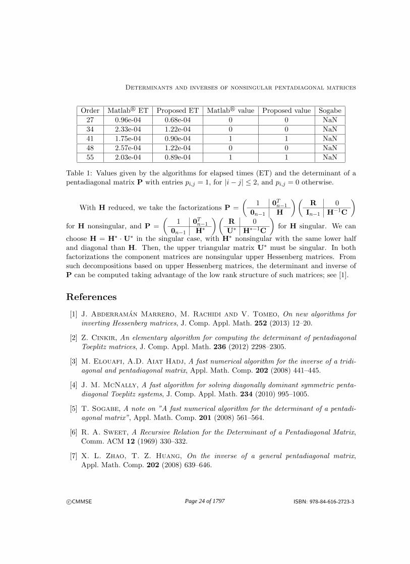
Order Matlabr ET Proposed ET Matlabr value Proposed value Sogabe

27 0.96e-04 0.68e-04 0 0 NaN

34 2.33e-04 1.22e-04 0 0 NaN

41 1.75e-04 0.90e-04 1 1 NaN

48 2.57e-04 1.22e-04 0 0 NaN

55 2.03e-04 0.89e-04 1 1 NaN

Table 1: Values given by the algorithms for elapsed times (ET) and the determinant of apentadiagonal matrix P with entries pi,j = 1, for |i− j| ≤ 2, and pi,j = 0 otherwise.

With H reduced, we take the factorizations P =

(1 0Tn−1

0n−1 H

)(R 0

In−1 H−1C

)for H nonsingular, and P =

(1 0Tn−1

0n−1 H∗

)(R 0

U∗ H∗−1C

)for H singular. We can

choose H = H∗ · U∗ in the singular case, with H∗ nonsingular with the same lower halfand diagonal than H. Then, the upper triangular matrix U∗ must be singular. In bothfactorizations the component matrices are nonsingular upper Hessenberg matrices. Fromsuch decompositions based on upper Hessenberg matrices, the determinant and inverse ofP can be computed taking advantage of the low rank structure of such matrices; see [1].

References

[1] J. Abderraman Marrero, M. Rachidi and V. Tomeo, On new algorithms forinverting Hessenberg matrices, J. Comp. Appl. Math. 252 (2013) 12–20.

[2] Z. Cinkir, An elementary algorithm for computing the determinant of pentadiagonalToeplitz matrices, J. Comp. Appl. Math. 236 (2012) 2298–2305.

[3] M. Elouafi, A.D. Aiat Hadj, A fast numerical algorithm for the inverse of a tridi-agonal and pentadiagonal matrix, Appl. Math. Comp. 202 (2008) 441–445.

[4] J. M. McNally, A fast algorithm for solving diagonally dominant symmetric penta-diagonal Toeplitz systems, J. Comp. Appl. Math. 234 (2010) 995–1005.

[5] T. Sogabe, A note on ”A fast numerical algorithm for the determinant of a pentadi-agonal matrix”, Appl. Math. Comp. 201 (2008) 561–564.

[6] R. A. Sweet, A Recursive Relation for the Determinant of a Pentadiagonal Matrix,Comm. ACM 12 (1969) 330–332.

[7] X. L. Zhao, T. Z. Huang, On the inverse of a general pentadiagonal matrix,Appl. Math. Comp. 202 (2008) 639–646.

c©CMMSE ISBN: 978-84-616-2723-3Page 24 of 1797

Proceedings of the 13th International Conferenceon Computational and Mathematical Methodsin Science and Engineering, CMMSE 201324–27 June, 2013.

A new tool for generating orthogonal polynomial sequences

J. Abderraman Marrero1, Venancio Tomeo2 and Emilio Torrano3

1 Department of Mathematics Applied to Information Technologies, TelecommunicationEngineering School, UPM - Technical University of Madrid, Spain.

2 Department of Algebra, Faculty of Statistical Studies, University Complutense, Spain.

3 Department of Applied Mathematics, Faculty of Informatics, UPM - TechnicalUniversity of Madrid, Spain.

emails: jc.abderraman@upm.es, tomeo@estad.ucm.es, emilio@fi.upm.es

Abstract

Adequate conditions, using a known result on a class of finite Hessenberg matrices,are here proposed to make available finite, and infinite, matrices as a rank one pertur-bation of strictly upper triangular matrices UV + T . Some characterizations on suchmatrices for generating orthogonal polynomial sequences are also considered.

Key words: Hessenberg matrix, inverse matrix, orthogonal polynomials, hermitianmoment problem.

1 Introduction

The orthogonal polynomials, [7] are currently applied in many branches of science andengineering. They have a determinantal representation, involving particular Hessenbergmatrices. A characterization for the nonsingular unreduced Hessenberg matrices in the finitecase is related with the particular structure of its inverse matrix, [5, 6]. Such inverse is arank one perturbation of a triangular matrix UV +T . Matrix T is triangular, U is a columnvector, and V is a row vector. Some conditions on their entries must be accomplished. Inthis work we want to obtain the unreduced Hessenberg matrix D, or the Jacobi matrix inthe symmetric case, and related with sequence of orthogonal polynomials, by inverting anadequate matrix, without invoking the matrix derived from the dot product. The momentproblem is no considered. Hence, we only need two adequate sequences U and V , and

c©CMMSE ISBN: 978-84-616-2723-3Page 25 of 1797

A new tool for generating orthogonal polynomial sequences

an associated upper triangular matrix T , so that the matrix to be inverted is UV + T .From the characteristics of U , V , and T , not only algebraic conditions can be obtained,but some other analytical and topological properties. Therefore, we propose the new toolwith some algebraic results, and some other possible connections remaining as open lines.Nevertheless, the final task could be about the conditions on U, V , and T , so that theinverse of the matrix UV + T be a subnormal operator.

1.1 Unreduced Hessenberg matrices with a finite order

We extend and adapt here to upper Hessenberg matrices H; i.e. hij = 0 for i ≥ j + 2,a well-known lemma, [5]. We also recall that an upper Hessenberg matrix H = (hij)

ni,j=1

having nonzero entries in its subdiagonal, hi+1,i 6= 0, and i = 1, 2, ..., n− 1, is an unreducedupper Hessenberg matrix.

Lemma 1 A nonsingular matrix H = (hij)1≤i,j≤n is unreduced upper Hessenberg if andonly if its inverse matrix has the structure B = UV + T , being U a column matrix withnonzero n-th component, V is a row matrix with nonzero 1-st component, and T is strictlyupper triangular having null entries in the main diagonal and nonzero entries in the super-diagonal, ti,i+1 = 1

hi+1,i6= 0, 1 ≤ i ≤ n− 1.

Proof. First, we assume that H is an unreduced upper Hessenberg matrix. A directcomputation of its inverse H−1 using the cofactor matrix gives, for i ≥ j,

bij =Adj(j, i)

|H|=

(−1)i+j

|H|

∣∣∣∣∣∣Hj−1 D E

0 F G

0 0 H(i)n−i

∣∣∣∣∣∣ =(−1)i+j

|H||Hj−1|[hj+1,j · · ·hi,i−1]|H(i)

n−i| =

=(−1)i−1

|H||H(i)

n−i|1

[hi+1,1 · · ·hn,n−1]· (−1)j−1|Hj−1|[hj+1,j · · ·hn,n−1],

with |Hj−1| the j − 1 left principal minor and |H(i)n−i| the n − i right principal minor from

the matrix H. Matrix F is a triangular one, containing on its diagonal entries from thesubdiagonal of H. If we define

ui =(−1)i−1

|H||H(i)

n−i|1

[hi+1,1 · · ·hn,n−1]and vj = (−1)j−1|Hj−1|[hj+1,j · · ·hn,n−1]

we have bij = uivj , i ≥ j. Taking the conventions |H0| = 1 and |H(n)0 | = 1, we observe that

v1 and un are nonzero entries. This fact about the lower half of B gives us the adequate

c©CMMSE ISBN: 978-84-616-2723-3Page 26 of 1797

J. Abderraman Marrero, Venancio Tomeo and Emilio Torrano

structure of the inverse,

B =

u1u2...un

( v1 v2 · · · vn)

+

0 t12 t13 · · · t1n0 0 t23 · · · t2n0 0 0 · · · t3n...

......

. . ....

0 0 0 · · · 0

= UV + T.

Hence,

B =

u1v1 b12 b13 · · · b1nu2v1 u2v2 b23 · · · b2nu3v1 u3v2 u3v3 · · · b3n

......

.... . .

...unv1 unv2 unv3 · · · unvn

, (1)

with bij = uivj + ti,j , for j > i.

The determinant of B gives, |B| = v1un

∣∣∣∣∣∣∣∣∣∣∣

u1 b12 b13 · · · b1nu2 u2v2 b23 · · · b2nu3 u3v2 u3v3 · · · b3n...

......

. . ....

1 v2 v3 · · · vn

∣∣∣∣∣∣∣∣∣∣∣.

Subtracting, in each row ri of the previous matrix, the last row rn by ui, there results

|B| = v1un

∣∣∣∣∣∣∣∣∣∣∣

0 b12 − u1v2 b13 − u1v3 · · · b1n − u1vn0 0 b23 − u2v3 · · · b2n − u2vn0 0 0 · · · b3n − u3vn...

......

. . ....

1 v2 v3 · · · vn

∣∣∣∣∣∣∣∣∣∣∣.

Therefore,

|B| = (−1)n+1v1un

n−1∏i=1

(bi,i+1 − uivi+1) = v1un

n−1∏i=1

(−ti,i+1) =v1un∏n−1

i=1 (−hi+1,i). (2)

The last equality is obtained from the expression bi,i+1 = uivi+1+ 1hi+1,i

; see [2], Proposition

2. Hence, ti,i+1 = 1hi+1,i

6= 0.

Now we assume that H is the inverse matrix of a nonsingular matrix B = (bij) as givenin (1), with entries bij = uivj , i ≥ j, and bij = uivj + ti,j , i < j, with 1 ≤ i, j ≤ n. Also,ti,i+1 = 1

hi+1,i6= 0, un 6= 0, and v1 6= 0. We note from (2) that |B| is independent of the

entries bij , and j − i ≥ 2. The adjoints of these entries are null values, and the nonsingularmatrix H = B−1 is upper Hessenberg. In addition, as B is nonsingular, its determinant|B| 6= 0, the ti,i+1 = 1

hi+1,i6= 0, and H is unreduced.

An equivalent lemma can be obtained for the lower Hessenberg matrices.

c©CMMSE ISBN: 978-84-616-2723-3Page 27 of 1797

A new tool for generating orthogonal polynomial sequences

1.2 Unreduced tridiagonal matrices with a finite order

We recall that a tridiagonal matrix having nonzero entries in both the subdiagonal and thesuperdiagonal is called unreduced tridiagonal matrix. The following result is known [5].

Lemma 2 A nonsingular matrix T = (tij)1≤i,j≤n is an unreduced tridiagonal matrix if andonly if its inverse matrix B = (bij) has the entries:

bij = uivj for i ≥ j, bij = witj for i ≤ j,

and the entries u1, vn, wn, and t1 are nonzero.

Proof. As a tridiagonal matrix is at the same time lower and upper Hessenberg, this resultis an immediate consequence from Lemma 1.

Trivially, ukvk = wktk. If in addition the matrix is symmetric, ui = ti, and vj = wj .

Example 1 From Lemma 1 on finite matrices, for the real symmetric tridiagonal matrixof an order n:

Jn =

b a 0 0 · · · 0a b a 0 · · · 00 a b a · · · 00 0 a b · · · 0...

......

.... . .

...0 0 0 0 · · · b

,

with a > 0, we obtain the matrix Bn:

Bn =

|Jn−1||J0||Jn|

−a |Jn−2||J0||Jn|

a2|Jn−3||J0||Jn|

· · · (−a)n−1|J0||J0||Jn|

−a |Jn−2||J0||Jn|

|Jn−2||J1||Jn|

−a |Jn−3||J1||Jn|

· · · (−a)n−2|J1||J1||Jn|

a2|Jn−3||J0||Jn|

−a |Jn−3||J1||Jn|

|Jn−3||J2||Jn|

· · · (−a)n−3|J2||J2||Jn|

......

.... . .

...

(−a)n−1|J0||J0||Jn|

(−a)n−2|J1||J1||Jn|

(−a)n−3|J2||J2||Jn|

· · · |J0||Jn−1||Jn|

.

Because for n determined we expand the determinant |Jn| by the first column, the involveddeterminants can easily be computed by the three-term recurrence:

|Jn| = b|Jn−1| − a2|Jn−2|. (3)

c©CMMSE ISBN: 978-84-616-2723-3Page 28 of 1797

J. Abderraman Marrero, Venancio Tomeo and Emilio Torrano

For the conditions of main interest, b2 − 4a2 > 0, we have

|Jn| =

(b+√b2 − 4a2

)n+1−(b−√b2 − 4a2

)n+1

2n+1√b2 − 4a2

,

that can trivially be obtained using induction.

Some methods for inverting finite tridiagonal matrices are available; see e.g. [1, 3].

2 Orthogonal polynomials and Hessenberg matrices

Let µ be a finite and positive Borel measure on a bounded domain of the complex plane.If we define the moments as cij =

∫suppµ z

izjdµ(z), we have an hermitian definite positive(HDP) matrix M = (cij)

∞i,j=0. If the measure lies on a subset of the real numbers, the

moments are Sij =∫suppµ x

i+jdµ(x), and M = (Sij)∞i,j=0 is a Hankel matrix.

From a HDP matrix M , no necessarily a moment matrix, we can obtain a Hessenbergmatrix D associated to M . The finite sections of D are Dn = T−1n M ′nT

−Hn ; see [4]. As

in the matrix sequence of increasing order Dn∞n=1 each Dn is principal submatrix of thefollowing Dn+1, we can associate the infinite matrix D with M . The upper Hessenbergmatrix D gives a large recurrence relation for generating the monic orthogonal sequencePn(z)∞n=0, where:

Pn(z) = |Inz −Dn|. (4)

Hence, we can obtain M , D, and the monic orthogonal polynomial sequence no associatedwith measures. Nevertheless it has uniquely algebraic interest. In the case of the Jacobimatrix, D = J , it allows us the three-term recurrence relation.

2.1 Orthogonal polynomials on the real line

For the orthogonal polynomials sequences on the real line the matrix D = J is the well-known Jacobi matrix,

J =

b0 a1 0 · · ·a1 b1 a2 · · ·0 a2 b2 · · ·...

......

. . .

,

with bi ∈ R y ai > 0. The Jacobi matrices J have associated a well-known three-termrecurrence relation that generates the orthogonal polynomial sequence.

We characterize the matrices U , V , and T so that J = (UV + T )−1. Note that thematrix J is generated by two numerical sequences (a1, a2, · · · , an, · · · ), (b0, b1, · · · , bn, · · · ).Because J is symmetric, the real matrix UV + T must also be symmetric. Then trivially,

tij = ujvi − uivj . (5)

c©CMMSE ISBN: 978-84-616-2723-3Page 29 of 1797

A new tool for generating orthogonal polynomial sequences

Therefore, the orthogonal polynomial sequences on the real line are given by the sequences(u1, u2, u3, ...) and (v1, v2, v3, ...), because the matrix T satisfies (5).

2.2 Relations between the finite sequence from Jn and Bn.

Proposition 1 Let Jn a real symmetric tridiagonal matrix generated by (b0, b1, ...bn−1)and (a1, a2, ..., an−1), with ai > 0. Then its inverse matrix is determined by the vectorsU = (u1, u2, ..., un) and V = (v1, v2, ..., vn) generated by the recurrence relations

v1 = 1, v2 =

1− b0v1a1

,

vj+1 =1− aj−1vj−1 − bj−1vj

aj,

j = 2, 3, ...., n− 1.

un =(−1)n+1[a1a2 · · · an−1]

|Jn|, ,

un−1 =(−1)n[a1a2 · · · an−2]bn−1

|Jn|,

ui−1 =−bi−1ui − aiui+1

ai−1,

i = n− 1, ...., 3, 2.

(6)

and the matrix Tn = (tij) given by (5).

Proof. We take v1 = 1.. The product of the first row of Jn by the first column of Bn gives:

b0u1v1 + a1u1u2 = 1 ⇒ v2 =1− b0v1a1

·

The product of the j-th row of Jn by the j-th column of Bn, with uj 6= 0, and aj 6= 0, gives:

aj−1ujvj−1 + bj−1ujvj + ajujvj+1 = 1 ⇒ vj+1 =1− aj−1vj−1 − bj−1vj

aj,

Hence, the entries vj from V can recursively be computed from v1 and v2.Solving un from (2), and taking into consideration that v1 = 1 and bi,i+1−uivi+1 = ti+1,i,

we have

un =(−1)n+1[a1a2 · · · an−1]

|Jn|·

The product of the first row of Bn by the last column of Jn gives:

un−1an−1 + unbn−1 = 0 ⇒ un−1 =−bn−1unan−1

=(−1)n[a1a2 · · · an−2]bn−1

|Jn|·

The product of the first row of Bn by the i-th column of Jn gives:

ui−1ai−1 + uibi−1 + ui+1ai = 0 ⇒ ui−1 =−bi−1ui − aiui+1

ai−1.

Hence, the entries ui of U are recursively computed from un and un−1. The matrix Tn, withentries given by (5), is required so that Bn be a symmetric matrix.

c©CMMSE ISBN: 978-84-616-2723-3Page 30 of 1797

J. Abderraman Marrero, Venancio Tomeo and Emilio Torrano

Proposition 2 Given Bn = (bij)ni,j=1 with the structure UV +T , and the tij satisfying (5).

Then its inverse matrix, symmetric and tridiagonal, Jn is defined by the sequences bini,j=1

and aini,j=1, ai > 0. Moreover, such sequences satisfy the recursive relations:

ai =1

ui+1vi − uivi+1, bi =

1− aiui+1 − ai+1ui+2vi+1

ui+1vi+1· (7)

Proof. The entries on the subdiagonal from Jn are the reciprocal of the correspondententries on the superdiagonal from the matrix T , and its value is given by (5). Hence:

ai = hi+1,1 =1

ti,i+1=

1

ui+1vi − uivi+1·

Known the ai, we can obtain the bi considering the product of the i-th row of Jn by thei-th column of Bn:

aiui+1 + biui+1vi+1 + ai+1ui+2vi+1 = 1 ⇒ bi =1− aiui+1 − ai+1ui+2vi+1

ui+1vi+1·

3 Consistency of the finite Hessenberg matrices

We consider now finite nonsingular n×n matrices B with the same structure B = UV +T ,i.e. a rank one perturbation of a tridiagonal matrix with null diagonal and full positivesuperdiagonal, with the conditions uk 6= 0, ∀k = 1, 2, ..., n and v1 6= 0. The principalsections B1, B2, ..., Bn of B, have also the same structure UV + T . Then, their inverses arealso unreduced upper Hessenberg matrices with positive subdiagonal.

The natural question about the construction of such sections of the Hessenberg matrixH is related with the consistency, if Hk is a principal submatrix of Hk+1. This is notrue because the last column of Hk is different than the correspondent column in Hk+1.Nevertheless, it is true that

(Hk)k−1 = (Hk+1)k−1.

That is, when deleting the last column and row of Hk, and the two last columns and rowsof Hk+1, the resulting matrices are the same. In the following theorem is shown that thismatrix sequence Hk is consistent. The matrix H can be built by sections.

Theorem 1 Given the n× n matrix B with the structure UV + T , uk 6= 0, ∀k = 1, 2, ..., nand v1 6= 0. When the Hk, principal sections of the matrix B−1, and their inverses areconsidered, the sequence of the inverses Hk is consistent. That is, each matrix containsthe entries of the previous one, with the exception of its last row and column, and satisfying(Hk)k−1 = (Hk+1)k−1, ∀k = 2, 3, ..., n− 1.

c©CMMSE ISBN: 978-84-616-2723-3Page 31 of 1797

A new tool for generating orthogonal polynomial sequences

Proof. Let Bk be the k-th section of B, and Hk the inverse matrix of Bk. In order todemonstrate the consistency of Hk, we assume the following block partition for the Bk,

u1v1 u1v2 + t12 u1v3 + t13 u1v4 + t14 · · · u1vk−1 + t1,k−1 u1vk + t1ku2v1 u2v2 u2v3 + t23 u2v4 + t24 · · · u2vk−1 + t2,k−1 u2vk + t2ku3v1 u3v2 u3v3 u3v4 + t34 · · · u3vk−1 + t3,k−1 u3vk + t3k

......

......

. . ....

...uk−1v1 uk−1v2 uk−1v3 uk−1v4 · · · uk−1vk−1 uk−1vk + tk−1,kukv1 ukv2 ukv3 ukv4 · · · ukvk−1 ukvk

and for

Hk =

h11 h12 h13 h14 · · · h1,k−1 hikh21 h22 h23 h24 · · · h2,k−1 h2k0 h32 h33 h34 · · · h3,k−1 h3k...

......

.... . .

......

0 0 0 0 · · · hk−1,k−1 hk−1,k0 0 0 0 · · · hk,k−1 hkk

.

The product BkHk accomplishes:

BkHk =

(B11 B12

B21 B22

)(H11 H12

H21 H22

)=

(Ik−1 0

0 1

),

and we derive:

B11H11 +B12H21 = B11H11 +

u1vk + t1ku2vk + t2ku3vk + t3k

...uk−1vk + tk−1,k

(

0 0 0 0 · · · hk,k−1)

= B11H11 +

0 0 · · · 0 (u1vk + t1k)hk,k−10 0 · · · 0 (u2vk + t2k)hk,k−10 0 · · · 0 (u3vk + t3k)hk,k−1...

.... . .

......

0 0 · · · 0 (uk−1vk + tk−1,k)hk,k−1

= Ik−1.

Taking the (k−2)-th section from these matrices of order k−1, in order to avoid the nonzerocolumn, we have:

(B11H11 +B12H21)k−2 = (B11H11)k−2 = Ik−2.

Since the matrix H11 is upper Hessenberg:

(B11)k−2(H11)k−2 = (B11H11)k−2 = Ik−2, k = 3, 4, ..., n.

c©CMMSE ISBN: 978-84-616-2723-3Page 32 of 1797

J. Abderraman Marrero, Venancio Tomeo and Emilio Torrano

From this result, we finally obtain, (Hk)k−1 = ((Bk)−1)k−1 = (Hn)k−1.

This result aim us to define a matrix sequence Hknk=1 with an increasing order, whereeach matrix is a principal submatrix of the following matrices in the sequence, i.e. allowsus to define the matrix Hn = (hij)

ni,j=1 associated to the matrix B. This possibility could

be many applications in the case of infinite matrices.

Example 2 Given the upper Hessenberg matrix of order 6:

D =

2 1 0 0 0 11 2 1 0 0 30 1 2 1 −1 00 0 1 2 1 00 0 0 1 2 10 0 0 0 1 2

with inverse matrix:

B =

5/6 −2/3 1/2 −1/3 1/6 1/2−1/2 1 −1/2 0 1/2 −3/22/3 −4/3 2 −5/3 4/3 1−1/2 1 −3/2 2 −3/2 −1/21/3 −2/3 1 −4/3 5/3 0−1/6 1/3 −1/2 2/3 −5/6 1/2

Taking the sections B2, B3, B4 y B5 of the matrix B, and inverting such matrices, we have:

D2 =

(2 4/31 5/3

), D3 =

2 1 −1/41 2 1/40 1 3/4

D4 =

2 1 0 1/31 2 1 10 1 2 5/30 0 1 4/3

, D5 =

2 1 0 0 −1/21 2 1 0 −3/20 1 2 1 −10 0 1 2 10 0 0 1 3/2

.

We can observe that (D3)1 = (D2)1, (D4)2 = (D3)2, (D5)3 = (D4)3. It is the recursive formto generate the matrix D.

4 Matrices U, V and T in terms of orthogonal polynomials

Let M be an infinite HDP matrix and let D be the associated Hessenberg matrix. The

Pn(z) are the monic polynomials, the pn(z) the normalized polynomials, and P (j)n−j(z),

c©CMMSE ISBN: 978-84-616-2723-3Page 33 of 1797

A new tool for generating orthogonal polynomial sequences

n > j, P(j)0 (z) = 1, be the associated monic polynomials, defined by P

(j)n−j(z) = |In−jz −

D(j)n−j |, where D

(j)n−j is the matrix of order n − j. This matrix results when deleting the j

first rows and columns of the matrix Dn. Also, let p(j)n−j(z) be the normalized associatedpolynomials, see [7], where the normalization considered for the monic polynomials is given

by formula p(j)n−j(z) =

P(j)n−j(z)

[dj+2,j+1···dn+1,n], n > j, p

(j)0 = 1. For j = 0, this normaliza-

tion is also adequate for the polynomials pn(z). The n-th resolvent matrix is defined as(Inz −Dn)−1, ∀z ∈ C\z : pn(z) = 0.

Theorem 2 The finite resolvent matrices associated to matrix D are given by

(Inz −Dn)−1[i, j] =

1

di+1,i

pj−1(z)p(i)n−i(z)

pn(z), if j ≤ i,

1

di+1,i

[pj−1(z)p

(i)n−i(z)

pn(z)− p(i)j−i−1(z)

], if j > i.

(8)

Proof. We must multiply Inz − Dn by (Inz − Dn)−1, and we have In. For this task, itis sufficient multiply the i-th row of Inz −Dn by the i-th column of (Inz −Dn)−1. Usingformulas of the large recurrence relation satisfied for the associated polynomials, we obtainthat this product is 1. Also we multiply the i-th row of first matrix by the j-th column,i 6= j, of the second matrix. In a similar way, we obtain that this product is 0.

4.1 A method to compute the inverses of finite Hessenberg matrices

Taking z = 0 in expression (8), with i and j determined, the left side is a number with aminus sign. Multiplying by (−1) in both sides, we have

D−1n [i, j] =

−1

di+1,i

pj−1(0)p(i)n−i(0)

pn(0), if j ≤ i,

−1

di+1,i

pj−1(0)p(i)n−i(0)

pn(0)+

1

di+1,ip(i)j−i−1(0), if j > i.

(9)

As a consequence, if the polynomials are known, we can compute the inverse of the matrixDn with this method. It is an alternative to the method given in Lemma 1. Finally, we givea numerical example of computation of the inverse matrix from the polynomial sequence.

Example 3 Let be the tridiagonal matrix Jn =

2 1 01 2 1

1 2. . .

. . .. . . 11 2

, where, as di+1,i =

1, the norm of monic polynomials is 1 and pn(z) = Pn(z). The determinants |Jn| = n+1 are

c©CMMSE ISBN: 978-84-616-2723-3Page 34 of 1797

J. Abderraman Marrero, Venancio Tomeo and Emilio Torrano

obtained by induction. The polynomials for z = 0 are pn(0) = (−1)n(n+ 1). The associatedpolynomials are the same than the general polynomials because the matrix is Toeplitz. Then,the inverse matrix results as J−1n = UV + T , with

U =

nn+1

−n−1n+1n−2n+1

...(−1)n−1 1

n+1

, V =(

1 −2 3 −4 · · · (−1)n−1n),

and the matrix T =

0 1 −2 3 −4 · · · (−1)n−1(n− 2)0 0 1 −2 3 · · · (−1)n−2(n− 3)0 0 0 1 −2 · · · (−1)n−3(n− 4)

0 0 0 0 1. . .

......

......

......

. . . 10 0 0 0 0 · · · 0

.

Note that, when n tends to ∞, the vector U will be U =(

1 −1 1 −1 1 · · ·)T

,and the inverse matrix obtained, inverse of the infinite matrix J , is

J−1 =

1 −1 1 −1 1 · · ·−1 2 −2 2 −2 · · ·1 −2 3 −3 3 · · ·−1 2 −3 4 −4 · · ·...

......

......

. . .

=((−1)i+j mini, j∞i,j=1

),

as it is easy to verify doing the products BJ = JB = I.

5 Conclusions

A new method to generate Hessenberg matrices with positive subdiagonal has been pro-posed. That is, a method to obtain orthogonal polynomial sequences. We have studiedthe conditions on U , V , and T in order to have an associated symmetric tridiagonal Jacobimatrix D. Basically, T must verify tij = ujvi−uivj . The conditions for matrix D will be anupper Hessenberg matrix, no Jacobi tridiagonal, are tij 6= ujvi−uivj . The determination ofconditions on U , V , and T that allow us know when the associated matrix D be a solutionof a moment problem, i.e. the study of subnormality of matrix D, remains as an openproblem.

c©CMMSE ISBN: 978-84-616-2723-3Page 35 of 1797

A new tool for generating orthogonal polynomial sequences

References

[1] J. Abderraman Marrero, M. Rachidi, V. Tomeo, Non-symbolic algorithms forthe inversion of tridiagonal matrices, J. Comp. Appl. Math. 252 (2013) 3–11.

[2] J. Abderraman Marrero, M. Rachidi, V. Tomeo, On new algorithms for invert-ing Hessenberg matrices, J. Comp. Appl. Math. 252 (2013) 12–20.

[3] B. Bukhberger, G. A. Emel’yanenko, Methods of inverting tridiagonal matrices,Comput. Math. Phys. URSS 13 (1973) 10–20.

[4] C. Escribano, A. Giraldo, M. A. Sastre, E. Torrano, Hessenberg matrix forsums of Hermitian positive definite matrices and weighted shifts, J. Comp. Appl. Math.236 (2011) 98–106.

[5] D. K. Faddeev, Properties of a matrix, inverse of a Hessenberg matrix, Journal ofMathematical Sciences 24 (1984) 118–120.

[6] Y. Ikebe, On inverses of Hessenberg matrices, Linear Algebra Appl. 24 (1979) 93–97.

[7] G. Szego, Orthogonal Polynomials, fourth ed., Colloq. Pub., vol. 23, Amer. Math.Soc., Rhode Island, USA, 1975

c©CMMSE ISBN: 978-84-616-2723-3Page 36 of 1797

Proceedings of the 13th International Conferenceon Computational and Mathematical Methodsin Science and Engineering, CMMSE 201324–27 June, 2013.

ParallDroid: A Framework for Parallelism in AndroidTM

A. Acosta1 and F. Almeida1

1 Dept. Estadıstica, I.O. y Computacion, La Laguna University, Spain

emails: aacostad@ull.es, falmeida@ull.es

Abstract

The advent of emergent SoCs and MPSocs opens a new era on the small mobiledevices (Smartphones, Tablets, ...) in terms of computing capabilities and applicationsto be addressed. The efficient use of such devices, including the parallel power, is still achallenge for general purpose programmers due to the very high learning curve demand-ing very specific knowledge of the devices. While some efforts are currently being made,mainly in the scientific scope, the scenario is still quite far from being the desirablefor non-scientific applications where very few of them take advantage of the parallelcapabilities of the devices. We propose Paralldroid (Framework for Parallelism in An-droid), a parallel development framework oriented to general purpose programmers forstandard mobile devices. Paralldroid presents a programming model that unifies thedifferents programming models of Android. The user just implements a Java appli-cations and introduces a set of Paralldroid annotations in the sections of code to beoptimized. The Paralldroid system automatically generates the native C, OpenCL orRenderscript code for the annotated section. The ParallDroid transformation modelinvolves source-to-source transformations and skeletal programming.

Key words: SoC, android, source to source translator.

1 Introduction

SoCs (Systems on Chip [1]) have been the enabling technology behind the evolution ofmany of todays ubiquitous technologies, such as Internet, mobile wireless technology, andhigh definition television. The information technology age, in turn, has fuelled a globalcommunications revolution. With the rise of communications with mobile devices, morecomputing power has been put in such systems. The technologies available in desktopcomputers are now implemented in embedded and mobile devices. We find new processors

c©CMMSE ISBN: 978-84-616-2723-3Page 37 of 1797

ParalldroidTM

with multicore architectures and GPUs developed for this market like the Nvidia Tegra [2]with two and five ARM cores and a low power GPU, and the OMAPTM5 [3] platform fromTexas Instruments that also goes in the same direction.

On the other hand, software frameworks have been developed to support the building ofsoftware for such devices. The main actors in this software market have their own platforms:Android [4] from Google, iOS [5] from Apple and Windows phone [6] from Microsoft arecontenders in the smartphone market.

Conceptually, from the architectural perspective, the model can be viewed as a tra-ditional heterogeneous CPU/GPU with a unified memory architecture, where memory isshared between the CPU and GPU and acts as a high bandwidth communication channel.In the non-unified memory architectures, it was common to have only a subset of the actualmemory addressable by the GPU.

Under this scenario, we find a strong divorce among traditional mobile software devel-opers and parallel programmers, the first tend to use high level frameworks like Eclipse forthe development of Java programs, without any knowledge of parallel programming (An-droid: Eclipse + Java, Windows: Visual Studio + C#, IOS: XCode + Objective C), andthe latter that use to work on Linux, doing their programs directly in OpenCL closer tothe metal. The former take the advantage of the high level expressiveness while the latterassume the challenge of high performance programming. The work developed in this papertries to bring these to worlds.

We propose the ParallDroid system, a development framework that allows for the au-tomatic development of Renderscript, native C or OpenCL code for mobile devices (Smart-phones, Tablets, ...). The developer fills and annotate the code that wants to execute inparallel. Annotations used are an extension of OpenMP [7]. ParallDroid uses the informa-tion provided in this annotations to generate a new parallel program that incorporates thecode sections to run over mobile device.

The advantages of this approach are well known:

• Increased use of the parallel devices by non-expert users

• Rapid inclusion of emerging technology into their systems

• Delivery of new applications due to the rapid development time

• Unifies the differents programming models of Android

To validate the performance of the code generated by our framework, we consider fivedifferent applications, transform a image to grayscale, convolve 3x3 and 5x5, levels and ageneral convolve implementation. In all cases, we implemented five versions of code, thead-hoc version from a Java developer, ad-hoc native C implementation, ad-hoc Renderscriptimplementation, and the versions generated by paralldroid, generated native C code and

c©CMMSE ISBN: 978-84-616-2723-3Page 38 of 1797

A. Acosta, F. Almeida

generated renderscript code. We execute these problems over two SoCs devices runningAndroid, a Samsung Galaxy SIII and an Asus Transformer Prime TF201.

The computational experience performed on five different problems prove that the re-sults are quite promising. The computational experience proved that ParallDroid offersgood performances with a very low cost of development where the parallelism is hidden tothe sequential developer. As expected, the renderscript versions improve to the Java imple-mentation so, ParallDroid is an useful tool for the automatic generation of the renderscriptcode. ParallDroid also contributes to increase the productivity in the parallel developmentsdue to the low effort required.

Acknowledgements

This work has been supported by the EC (FEDER) and the Spanish MEC with the I+D+Icontract number: TIN2011-24598

References

[1] SoCC: IEEE International System–on–Chip Conference. http://www.ieee-socc.org/(September 2012)

[2] NVIDIA: NVIDIA Tegra mobile processors: Tegra2, Tegra 3 and Tegra 4. http:

//www.nvidia.com/object/tegra-superchip.html

[3] Instruments, T.: OMAPTMMobile Processors : OMAPTM5 platform. http://www.ti.com/omap5

[4] Google: Android mobile platform. http://www.android.com

[5] Apple: iOS: Apple mobile operating system. http://www.apple.com/ios

[6] Microsoft: Windows Phone: Microsoft mobile operating system. http://www.

microsoft.com/windowsphone

[7] OpenMP: Openmp: Api specification for parallel programming. http://openmp.org/

wp/

c©CMMSE ISBN: 978-84-616-2723-3Page 39 of 1797

Proceedings of the 13th International Conferenceon Computational and Mathematical Methodsin Science and Engineering, CMMSE 201324–27 June, 2013.

“kai leuat ok” is everything: 26, 27, 66

Maıra Aguiar1 and Nico Stollenwerk1

1 Centro de Matematica e Aplicacoes Fundamentais, Lisbon University

emails: maira@ptmat.fc.ul.pt, nico@eptmat.fc.ul

Abstract

Dengue fever dynamics are well known to be particularly complex with large fluctuationsof disease incidence. Mathematical models describing the transmission of dengue viruses needto be parametrized on data referring to incidence of disease in order to be used as a predictivetools to evaluate the introduction of intervention strategies like vector control and vaccination.For Thailand, two different sources of the long-term empirical dengue data (1980-2012) areavailable and consists of monthly incidences of hospital admission cases, the hard copy (HC)data from 1980-2005 and the electronic files (EF) from 2003 to present, where the clinicalclassification of the disease are notified using separate files. By gathering, cross-checking andanalyzing the overlapping epidemiological years of the data (2003-2005) we observed a consid-erable underestimation of dengue cases in Thailand during the transition HC-EF, which affectsconsiderably the model development, interpretation and its correct application.

Key words: Dengue fever, data analysis, modeling

1 Introduction

It is estimated that every year there are 70 − 500 million dengue infections, 36 million cases ofdengue fever (DF) and 2.1 million cases of dengue hemorrhagic fever (DHF) and dengue shocksyndrome (DSS), with more than 20.000 deaths per year [2, 1]. In many countries in Asia andSouth America DF and DHF/DSS has become a substantial public health concern leading to serioussocial-economic costs. Over the past 50 years, the number of infected patients (DF/DHF/DSS)has been rising steadily. There is no specific treatment for dengue, and a vaccine which simulatesa protective immune response to all four serotypes is not yet available. Tetravalent vaccines areunder investigation and besides the relatively slow progress in the development of the dengue virusvaccine, a tetravalent live attenuated vaccine and a live chimeric virus vaccine are presently goingthrough Phase III trials [3, 4].

c©CMMSE ISBN: 978-84-616-2723-3Page 40 of 1797

“KAI LEUAT OK” IS EVERYTHING: 26, 27, 66

The Thai word used to describe dengue illness refers to fever with blood leakage (kai leuat ok,the English pronunciation of the Thai language), which was later on possibly written and translatedaccording to each one of the possible clinical manifestation of the disease, as it follows: (I) kai leuatok deeng gee or code 26, to describe DHF, however it is unusual to be found in the Thai documents,where the simplification kai leuat ok is mostly used. The DHF cases may evolve towards a collectionof symptoms with hemorrhagic fever leading to shock or DSS, in Thai (II) glum aa-gaan kai leuat okchok or code 27. The classic dengue or DF, a non-fatal form of illness classically defined as a fevercaused by a dengue virus (which is rarely associated with blood leakage), is traditionally written askai leuat ok but could be eventually written as (III) kai deeng gee or code 66.

Dengue dynamics is well known to be particularly complex with large fluctuations of diseaseincidences. The long-term incidence dengue data in Thailand have been continually used, amongtheoretical epidemiologists and modelers, to describe the dynamics of dengue epidemics. Up tonow, 33 years of dengue illness incidence data are available and have been continually used, as forexample in [5, 6, 18, 8, 9], to parametrize mathematical models as a tool to predict and control thedisease.

From 1980 to 2005 the aggregated data, presented as “DHF-Total”, have been publicly dis-tributed as a hard copy (HC) book format through the Bureau of Epidemiology Annual Epidemio-logical Surveillance Report [21]. Starting in 2003, the disease was notified using separate electronicfiles (EF) for each one of the possible clinical classification. By gathering, cross-checking and an-alyzing the overleaping data (2003-2005) it was observed that the sum of all clinical cases of thedisease (DF+DHF+DSS) gives rise to the DHF-Total incidence data in Thailand. The English trans-lation of the Thai documents still causes confusion when interpreting the data, and for modelingpurposes it leads to a significant underestimation of the real number of dengue cases in Thailand.From 2003 on, only the clinical classification of DHF cases have been counted whereas the DF andDSS cases were neglected. Such data cross-checking was carried out for all Provinces in Thailandshowing the same results.

In Fig. 1A we present the official monthly incidence of dengue illness in Thailand for bothsources of the 2003 overlapping data, the HC [21] and the EF separate files for each disease clin-ical classification. We list the given numbers for DHF-Total, DF, DHF and DSS respectively andobserve that the number of cases classified clinically as DHF differs considerably from the numberspresented as DHF-Total in [21]. When taking into account also the number of cases for DF and DSSwe clearly see that the final numbers matches the original data collection of DHF-Total cases. Forthe epidemiological years of 2004 and 2005, the results were exactly the same (see Fig. 1B-C, andthe underestimation of dengue cases is increasing rapidly as shown in Fig. 1D.

This underestimation is strongly associated with the English translation and misinterpretation ofthe Thai documents, generating an inexact continuous time series to be used for modeling purposes,affecting considerably the model development, interpretation and its correct application.

c©CMMSE ISBN: 978-84-616-2723-3Page 41 of 1797

AGUIAR MAIRA, STOLLENWERK NICO

A)

B)

C)

D)

Figure 1: Thailand DHF-Total data comparison between the HC book and EF for each clinicalclassification DF, DHF and DSS. In A) 2003 epidemiological year, in B) 2004 epidemiological yearand in C) 2005 epidemiologycal year. In D) from 2003 to present, Thailand underestimation ofdengue cases.

c©CMMSE ISBN: 978-84-616-2723-3Page 42 of 1797

“KAI LEUAT OK” IS EVERYTHING: 26, 27, 66

2 Compartmental models applied to dengue fever

Almost all mathematical models for infectious diseases start from the same basic premise: that thepopulation can be subdivided into a set of distinct classes. The most commonly used frameworkfor epidemiological systems, is still the SIR-type model, a good and simple model for many infec-tious diseases. The SIR epidemic model divides the population into three classes: susceptible (S),Infected (I) and Recovered (R). Multi-strain dengue models are modeled with SIR-type modelswhere the SIR classes are labeled for the hosts that have seen the individual strains. Assumingthat the transmission of the disease is contagious from person to person, the susceptibles becomeinfected and infectious with infection rate β, are cured and become recovered with recovery rateγ. Partial or temporary or life long immunity can be assumed, depending on the biology of thepathogen After a waning immunity period α, the recovered individual can become susceptible, to adifferent strain again.

Retrospective dengue data and the possibility to estimate hidden states in dengue models fromsuch data [8, 10] have been discussed, specially, primary versus secondary infection, and symp-tomatic versus asymptomatic cases that can be studied via the first already available models [11,12, 8, 9, 13]. Although the multi-strain interaction leading to deterministic chaos via ADE has beendescribed previously, e.g. [14, 15, 16], the role of temporary cross-immunity has been neglectedleading to unrealistic biological parameter estimation. More recently, despite incorporation of tem-porary cross-immunity in rather complicated models, the possible dynamical structures were notdeeply analyzed [17, 18, 19]. When including temporary cross-immunity into the ADE denguemodels, a rich dynamic structure including chaos in wider and more biologically realistic parameterregions was found [11, 12, 8, 9, 13].

The basic two-strain model shows a rich variety of dynamics through bifurcations up to de-terministically chaotic behavior in wider and more biologically realistic parameter regions thanpreviously anticipated when neglecting temporary cross-immunity. The seasonal two-strain modelwith import of infected have shown a qualitatively good result when comparing empirical denguedata and simulation results, where patterns of the data behavior were similarly found to happen inthe time series simulations (see Fig. 2A).

2.1 The two-strain model

The two-strain model with temporary cross-immunity is a 9 dimensional system where the popula-tion N is divided into ten classes. For two different strains, named strain 1 and strain 2, we label theSIR classes for the hosts that have seen the individual strains, without epidemiological asymmetrybetween strains, i.e. infections with strain one followed by strain two or vice versa contribute in thesame way to the force of infection. The complete system of ordinary differential equations (ODEs)

c©CMMSE ISBN: 978-84-616-2723-3Page 43 of 1797

AGUIAR MAIRA, STOLLENWERK NICO

for the two-strain epidemiological model can be written as follows.

S = µ(N − S)− β(t)

NS(I1 + ρ ·N + φI21)

−β(t)N

S(I2 + ρ ·N + φI12) (1)

I1 =β(t)

NS(I1 + ρ ·N + φI21)− (γ + µ)I1 (2)

I2 =β(t)

NS(I2 + ρ ·N + φI12)− (γ + µ)I2 (3)

R1 = γI1 − (α+ µ)R1 (4)

R2 = γI2 − (α+ µ)R2 (5)

S1 = αR1 −β(t)

NS1(I2 + ρ ·N + φI12)− µS1 (6)

S2 = αR2 −β(t)

NS2(I1 + ρ ·N + φI21)− µS2 (7)

˙I12 =β(t)

NS1(I2 + ρ ·N + φI12)− (γ + µ)I12 (8)

˙I21 =β(t)

NS2(I1 + ρ ·N + φI21)− (γ + µ)I21 (9)

R = γ(I12 + I21)− µR . (10)

2.2 Numerical analysis

Mathematical models describing the transmission of dengue viruses need to be parametrized ondata referring to incidence of disease. We take Chiang Mai Province, North of Thailand, as matchempirical data with model simulations. The birth and death rate, recovery rate, degree of seasonalityand the temporary cross-immunity rate are fixed. The infection rate and ratio of secondary infectionscontributing to force of infection are the parameters that may vary when matching different data sets.

In Figure 2A we match empirical DHF-Total (DF+DHF+DSS) incidence data for the Provinceof Chiang Mai with the two-strain model simulation. A qualitatively good result is obtained, wherepatterns of the irregular data occurs and is predicted by the models. The parameter values used inthe simulation are listed in Table 1.

In Figure 2B we match empirical DHF-Total (DF+DHF+DSS) from 1980 to 2002 and continuewith only clinical DHF incidence data with the two-strain model simulation. With a different pa-rameter set we observe a qualitatively good result from 2003 on, however, the previous HC data cannot be described. The parameter values used in the simulation are listed in Table 2.

c©CMMSE ISBN: 978-84-616-2723-3Page 44 of 1797

“KAI LEUAT OK” IS EVERYTHING: 26, 27, 66

A)

0

500

1000

1500

2000

2500

3000

1980 1984 1988 1992 1996 2000 2004 2008 2012

Chia

ng M

ai D

ata

time (years) B)

0

500

1000

1500

2000

2500

3000

1980 1984 1988 1992 1996 2000 2004 2008 2012

Chia

ng M

ai D

ata

time (years)

C)

0

500

1000

1500

2000

2500

3000

1980 1984 1988 1992 1996 2000 2004 2008 2012

Chia

ng M

ai D

ata

time (years) D)

0

500

1000

1500

2000

2500

3000

2004 2006 2008 2010 2012

Chia

ng M

ai D

ata

time (years)

Figure 2: In A) empirical DHF-Total (DF+DHF+DSS) incidence data (in red) for the Province ofChiang Mai in the North of Thailand, with a population size N = 1.6 × 106, are matched withsimulations (in blue) for the seasonal two-strain model with import of infected. Here, the force ofinfection β = 2γ and the secondary infection contribution to the force of infection ratio φ = 0.9.The other parameter values are given in Table 1. In B) empirical DHF-Total (DF+DHF+DSS)incidence data (in red) for the Province of Chiang Mai in the North of Thailand, with a populationsize N = 1.6× 106, are matched with simulations (in blue) for the seasonal two-strain model withimport of infected. Here, the force of infection β = 2γ and the secondary infection contribution tothe force of infection ratio φ = 0.9. The other parameter values are given in Table 1. In B) we matchthe empirical DHF-Total (DF+DHF+DSS) from 1980 to 2002 (in red), continued with DHF clinicalincidence only (in green) with the seasonal two-strain model with import of infected simulations (inblue). Here, the force of infection is considerably smaller β = 1.5γ as well the secondary infectioncontribution to the force of infection ratio φ = 0.7. The other parameter values are given in Table 2.In C-D) we present the matching of the two data sets, using parameter set ONE, with the modelsimulation (in blue).

c©CMMSE ISBN: 978-84-616-2723-3Page 45 of 1797

AGUIAR MAIRA, STOLLENWERK NICO

Table 1: Parameter set ONE: DHF-Total (DF+DHF+DSS) data set matching

Par. Description Values Ref.N population size 1.6× 106

µ birth and death rate 1/65y [22]γ recovery rate 52y−1 [1]β infection rate 2 · γ [14, 11, 8, 9]η degree of seasonality ∈ [0, 0.35] [8, 9]ρ import parameter ∈ [0, 10−10] [8, 9]α temporary cross-immunity rate 2y−1 [20]φ ratio of secondary infections

contributing to force of infection 0.9 [8, 9]

Table 2: Parameter set TWO: From 2003 on, DHF-only data set matching

Par. Description Values Ref.N population size 1.6× 106

µ birth and death rate 1/65y [22]γ recovery rate 52y−1 [1]β infection rate 1.5 · γ [14, 11, 8, 9]η degree of seasonality ∈ [0, 0.35] [8, 9]ρ import parameter ∈ [0, 10−10] [8, 9]α temporary cross-immunity rate 2y−1 [20]φ ratio of secondary infections

contributing to force of infection 0.7 [8, 9]

Using the simulation obtained with parameter set ONE (see Table 1), Figures 2C-D show thedata matching comparison. As for the non fixed parameters, infection rate and secondary infectioncontribution to the force of infection rate, we observe a considerable difference in parameter val-ues that could lead to non efficient intervention on disease control and to a wrong Public Healthintervention measures decision, depending on which data set we are using.

3 Conclusions

The two-strain model model has the minimal degree of complexity to generate both primary andsecondary infection cases, and it allows to derive dengue hemorrhagic fever cases which constitutethe most widely available data on dengue epidemiology. The simplicity of our model allows rigorousinference of both parameters from empirical time series.

c©CMMSE ISBN: 978-84-616-2723-3Page 46 of 1797

“KAI LEUAT OK” IS EVERYTHING: 26, 27, 66

Much of the dengue data available to theoretical epidemiologists consists of time series trackingthe evolution of a subset of state variables of an underlying dynamical system through a surveillancesystem. For Thailand, two different sources of the long-term empirical dengue data (1980-2012) areavailable and consists of monthly incidences of hospital admission cases, the HC from 1980-2005and the EF from 2003 to present. By gathering, cross-checking and analyzing the overlapping epi-demiological years of the data (2003-2005) we observed a considerable underestimation of denguecases in Thailand during the transition HC-EF files, from 2003 on, where only the clinical clas-sification of DHF cases have been counted. The exact continuous time series is obtained whenconsidering all admission cases, DF+DHF+DSS, however the underestimation of cases are increas-ing, probably a consequence of the English interpretation of the Thai documents.

As for modeling purposes two different parameter sets were obtained depending on the dataset was used. Based on this observation, we conclude that the underestimation of the real numberof dengue cases in Thailand will affect considerably the model development, interpretation and itscorrect application. Being able to describe and predict the future expected outbreaks of dengue in theabsence of human interventions is the major goal if one wants to understand the effects of consideredcontrol measures. This is especially important with the upcoming perspective of a dengue virusvaccine requiring a high quality data and knowledge on how to best implement the vaccinationprogram and use the candidate vaccine at the population-level when it will be accessible. For anyinterpretation based on the the long-term empirical incidence dengue data, the data aggregation isessential to improve model development, interpretation and its correct application.

Acknowledgements

Dengue surveillance data were provided by the Bureau of Epidemiology, Department off DiseaseControl, Ministry of Public Health, Thailand. This work has been supported by the European Unionunder FP7 in the DENFREE project and the Portuguese FCT project PTDC/MAT/115168/2009.

References

[1] WORLD HEALTH ORGANIZATION, Dengue and severe dengue, Fact sheet 117 (2012). Re-trieved from http : //www.who.int/mediacentre/factsheets/fs117/en/

[2] DENGUE VACCINE INITIATIVE (DVI), Dengue Overview (2013). Retrieved from http ://www.denguevaccines.org/dengue− overview − 0

[3] WORLD HEALTH ORGANIZATION, Initiative for Vaccine Research (2011). Retrieved fromhttp : //www.who.int/vaccine research/diseases/dengue/denguevaccines/en/index.html

[4] SCHMITZ, J., ROEHRIG, J., BARRETT, A., HOMBACH, J., Next generation dengue vaccines:A review of candidates in preclinical, Vaccine 29 (2011) 7276–7284.

c©CMMSE ISBN: 978-84-616-2723-3Page 47 of 1797

AGUIAR MAIRA, STOLLENWERK NICO

[5] DEREK A.T. CUMMINGS, RAFAEL A. IRIZARRY, NORDEN E. HUANG, TIMOTHY P. ENDY,ANANDA NISALAK, KUMNUAN UNGCHUSAK & DONALD S. BURKE, Travelling waves inthe occurrence of dengue haemorrhagic fever in Thailand, Nature 427 (2005) 334–347.

[6] CAZELLES B, CHAVEZ M, MCMICHAEL AJ, HALES S., Nonstationary influence of El Ninoon the synchronous dengue epidemics in Thailand, PLoS Med. (2005) 2(4):e106.

[7] Y. NAGAO & K KOELLE, Decreases in dengue transmission may act to increase the incidenceof dengue hemorrhagic fever, Proc. Natl. Acad. Sci. 105 (2008) 2238–2243.

[8] AGUIAR, M., BALLESTEROS, S., KOOI, B.W., & STOLLENWERK, N., The role of season-ality and import in a minimalistic multi-strain dengue model capturing differences betweenprimary and secondary infections: complex dynamics and its implications for data analysis,Jounal of Theoretical Biology 289 (2011) 181–196.

[9] AGUIAR, M., KOOI, W. B., ROCHA, F., GHAFFARI, P. AND STOLLENWERK, N.,How much complexity is needed to describe the fluctuations observed in dengue hemor-rhagic fever incidence data? Ecological Complexity (2012) Published online at: http ://dx.doi.org/10.1016/j.ecocom.2012.09.001

[10] STOLLENWERK, N., AGUIAR, M., BALLESTEROS, S., BOTO, J., KOOI, W. B., & MATEUS,L., Dynamic noise, chaos and parameter estimation in population biology, Interface, Focus 2(2012) 156–169.

[11] AGUIAR, M., KOOI, B., & STOLLENWERK, N., Epidemiology of dengue fever: A model withtemporary cross-immunity and possible secondary infection shows bifurcations and chaoticbehaviour in wide parameter regions, Math. Model. Nat. Phenom. 3 (2008) 48–70.

[12] AGUIAR, M., STOLLENWERK, N., & KOOI, B., Torus bifurcations, isolas and chaotic attrac-tors in a simple dengue fever model with ADE and temporary cross immunity, Intern. Journalof Computer Mathematics 86 (2009) 1867–77.

[13] MAIRA AGUIAR (2012). Rich dynamics in multi-strain models: non-linear dynamics anddeterministic chaos in dengue fever epidemiology, PhD Thesis, ISBN 978-989-20-2882-8,Edited by Maıra Aguiar, Portugal.

[14] FERGUSON, N., ANDERSON, R. AND GUPTA, S., The effect of antibody-dependent enhance-ment on the transmission dynamics and persistence of multiple-strain pathogens, Proc. Natl.Acad. Sci. USA 96 (1999) 790–94.

[15] SCHWARTZ, I. B., ET AL., Chaotic desynchronization of multi-strain diseases, Physical Re-view E 72 (2005) 066201–6.

c©CMMSE ISBN: 978-84-616-2723-3Page 48 of 1797

“KAI LEUAT OK” IS EVERYTHING: 26, 27, 66

[16] BILLINGS, L., ET AL., CInstabilities in multiserotype disease models with antibody-dependent enhancement, Journal of Theoretical Biology 246 (2007) 18–27.

[17] Wearing, H.J. & Rohani, P. (2006). Ecological and immunological determinants of dengueepidemics Proc. Natl. Acad. Sci. USA , 103, 11802–11807.

[18] NAGAO, Y. & KOELLE, K., Decreases in dengue transmission may act to increase the inci-dence of dengue hemorrhagic fever, Proc. Natl. Acad. Sci. USA 105 (2008) 2238–2243.

[19] RECKER, M. ET AL., Immunological serotype interactions and their effect on the epidemio-logical pattern of dengue, Proc. R. Soc. B. 276 (2009) 2541–2548.

[20] S. MATHEUS, X. DEPARIS, B. LABEAU, J. LELARGE, J. MORVAN, P. DUSSART, Discrim-ination between Primary and Secondary Dengue Virus Infection by an Immunoglobulin GAvidity Test Using a Single Acute-Phase Serum Sample. Journal of Clinical Microbiology 45(2005) 2793–97.

[21] BUREAU OF EPIDEMIOLOGY, MINISTRY OF PUBLIC HEALTH OF THAILAND, Annual epi-demiological surveillance report, Thailand (2003, 2004, 2005) ISSN 0857-6521.

[22] WORLD POPULATION PROSPECTS: THE 2008 REVISION, Population Database. Retrievedfrom http : //esa.un.org/unpp/index.asp?panel = 2

c©CMMSE ISBN: 978-84-616-2723-3Page 49 of 1797

Proceedings of the 13th International Conferenceon Computational and Mathematical Methodsin Science and Engineering, CMMSE 201324–27 June, 2013.

An Improved Information Rate of Perfect Secret Sharing

Scheme Based on Dominating set of Vertices

N. M. G. Al-Saidi1, N.A. Rajab1, Mohamad Rushdan Md. Said2 and K.

A. Kadhim1

1 The Branch of Applied Mathematics Applied Sciences Department, University ofTechnology, Baghdad, Iraq

2 Institute for Mathematical Research (INSPEM), Universiti Putra Malaysia, DarulEhsan, 43400 Serdang, Malaysia

emails: nadiamg08@gmail.com, nuha.abd10@gmail.com, rushdan@math.upm.edu.my,kadhum.technology@gmail.com

Abstract

Due to the fast development in data communication systems and computer networksin recent years, the necessity to protect the secret data is of great demands. Severalmethods have been arisen to protect the secret data; one of them is the secret sharingscheme. It is a method of distributing a secret K among a finite set of participants,in such a way that only predefined subset of participant is enabled to reconstruct asecret from their shares. A secret sharing scheme realizing uniform access structure de-scribed by a graph has received a considerable attention, where each vertex representsa participant and each edge represents a minimum authorized subset. In this paper,an independent dominating set of vertices in a graph G is introduced and applied asa novel idea to construct a secret sharing scheme such that the vertices of the graphrepresents the participants and the dominating set of vertices in G represents the min-imal authorized set. This new scheme is based on principle of non-adjacent vertices,whereas, most of the previous works are based on the principle of adjacent vertices. Weprove that the scheme is perfect, and the lower bound of the information rate for thisnew construction is improved as compared to some well-known previous constructions.

Key words: Secret sharing scheme, independent dominating set, information rate,uniform access structure, rank

c©CMMSE ISBN: 978-84-616-2723-3Page 50 of 1797

Information Rate of Perfect Secret Sharing

1 Introduction

Secret sharing scheme is a method of distributing a secret K among a finite set of partici-pants P = p1, · · · , pn, such that, only predefined specific subset belonging to the accessstructure when they pooling their partial information together, can reconstruct the secret,whereas, any other subset not in the access structure can determine nothing about thesecret. The first kind of secret sharing scheme called (t, n)-threshold scheme is introducedindependently by Shamir [1] and Blakley [2] in 1979. A considerable attention was given tothis subject after on. An efficient secret sharing scheme is the one that has high informationrate (small share size) which is considered as a measure for the efficiency of such systems.Hence, an extensive consideration has been given to improve this value. It is defined as theratio of the length of the secret to the average length of the share given to the participant.A special participant D, not in the set P, is called the dealer takes the responsibility todistribute the shares to each participant. The family of all the subset of participant, calledan access structure Γ [3].

In the (t, n)-threshold scheme, all the t-subsets of a set of n-participant capable of re-constructing the secret are called the authorized sets and represented by Γ0, whereas, thosenot belonging to Γ are called unauthorized sets. An authorized set B is called minimalif it satisfies the following relations; for B′ ⊂ B, and B′ ∈ Γ implies B′ = B. If B ∈ Γand B ⊂ B′ implies that B′ ∈ Γ , then the access structure is called monotone. In thiscase, the collection of minimal authorized set could uniquely determine the access structure.Many approaches for construction of secret sharing scheme have been proposed. A specialconstruction class is the threshold scheme. Ito, Saito, and Nishizeki [4] have generalizedthis concept and proposed a method for any monotone access structure, when the size ofeach share is no less than the size of the secret. This scheme is called perfect. It is calledideal, if the size of each share is the same as the size of the secret [5].

The relation between secret sharing scheme and an access structure have considerableinterest by many researchers ( see, for example [6, 7, 8]). Several approaches were devel-oped to obtain an efficient implementation of secret sharing scheme for an arbitrary accessstructure, but there is no general method. An approach based on graph theory that in-vestigates an access structure over a set of two participants are of special interest from thepractical point of view, because such access structure can be represented by a graph, inwhich the vertices represent the participant, and the edges represent an access structure.This approach is called graph access structure and has been studied by many researchers(see, for example [4, 7, 8, 9]).

The general idea behind the B-decomposition of a graph access structure proposed byStinson [8, 10], is to find all subgraphs of G, such that; at least B subgraphs of them have

c©CMMSE ISBN: 978-84-616-2723-3Page 51 of 1797

N. M. G. Al-Saidi, N.A. Rajab, Mohamad Rushdan Md. Said, K. A. Kadhim

to contains each edge of E. This leads to an increase in the number of such subgraphsthat increased exponentially with the number of vertices (participants), and following inan exponential time construction. In this paper, we propose an approach that investigatesthe minimum access structure in a manner differs from the previous construction that wasbased on adjacent principle of vertices. In our approach, the minimum authorized subsetsrepresent the set of all minimum independent dominating set of vertices in the graph G.

The current work is organized as follows: In Section 2, some terminologies related todomination in graph G, and to secret sharing scheme is presented. The main algorithm forthe decomposition and reconstruction of the proposed method is given in Section 3. Theefficiency of the constructed secret sharing scheme is demonstrated and proved through theinformation rate in section 4. Finally, the paper is concluded in section 5.

2 Domination in graph and secret sharing scheme

Many theories and applications for the domination in graph theory as a natural modelfor many location problems have been arisen. As an example; the fire station problem,school bus routing, computer communication networks, social network theory, and codingtheory. Some graph theoretical definitions, and some important terminologies related tosecret sharing scheme are given to fill in some background for the reader. A more detailedreview of the topics in this section, can be found in [11, 12, 13, 14, 15].

A graph G is an ordered pair G = (V ;E) where V is a set of elements which are calledvertices, and the set E = e = u, v ∈ E : u, v ∈ V is called edges. The order of G, |G|equals |V |. A graph H = (W ;F ) is a subgraph of another graph G = (V ;E) if W ⊆ V andF ⊆ E. All graphs used in this work are simple, connected, and undirected.

Definition 2.1: The set of vertices adjesnt to v ∈ V is called an open neighborhoodN(v) such that N(v) = u ∈ V : u, v ∈ E, whereas, the closed neighborhood is the setN [v] = N(v) ∪ v.

Definition 2.2: The degree d(v) of a vertex v is the size of N(v), or equivalently, thenumber of edges incident to v.

Definition 2.3: A graph G is an r-regular if the minimum degree of a graph G equalsits maximum degree and equals r. A 2-regular, 3-regular, and (n − 1)-regular graphs arecalled a cycle, cubic, and complete graphs respectively.

Definition 2.4: A graph G is decomposable into H1,H2, . . . ,Hk if G has subgraphsH1,H2, · · · ,Hk, such that:

c©CMMSE ISBN: 978-84-616-2723-3Page 52 of 1797

Information Rate of Perfect Secret Sharing

1. Each edge of G belongs to one of the Hi ’s for some i = 1, 2, · · · , k.

2. Hi and Hj have no edges in common, when i 6= j.

Definition 2.5: For a graph G = (V ;E), a set of vertices D is called a dominating set ofvertices in G, if N [D] = V , or equivalently, every vertex in V −D is adjacent to at leastone vertex inD. A dominating set D is minimal if no proper subset of D is a dominating set.

Definition 2.6: An independent dominating set of vertices (ID) in a graph G, is thedominating set D that has no two vertices of D connected by an edge of G. The minimumcardinality of an independent dominating set ID is called a minimum independent domi-nating set MID where |MID| is called minimum independent domination number. In thiswork, such type of dominating set is used in the construction for the secret sharing scheme.

The information rat that specifies the efficiency of the secret sharing schemes has in-troduced for the first time by Brickell [16]. He defined it as follows.

Definition 2.7: The information rate ρ of a secret sharing scheme is ρ = log2(|K|)/log2(|S|),where K, and S, represents the secret and the share respectively. The term ideal is usedfor a perfect secret sharing scheme with information rate equals (1).

Definition 2.8: The maximum cardinality of a minimal qualified subset is called therank (m) of an access structure Γ.

3 The proposed algorithm

A novel construction algorithm of a perfect secret sharing scheme with an access structureof rank m is proposed in this section. It is based on the same concepts given by H. Sun[17, 18]. This algorithm consists of three parts as follows.

1. The Initialization Phase

(a) Given G = (V,E), be an r-regular graph, with V = v1, v2, · · · , vn. Let P =p1, p2, · · · , pn be the set of participant corresponding to the set V .

(b) Construct Γ0 by computing all (MID) in G, such that Γ0 = MID : V =∪MID. Hence, |MID| = m the rank (or, the minimum qualified set).

(c) All the computation is done over GF (q), where q is a prime, and q ≥ 2n+ 2.

2. The Decomposition Phase

(a) Decompose the graph G into n-subgraphs Gi, where V (Gi) = V/N [vi] : i =1, 2, · · · , n.

c©CMMSE ISBN: 978-84-616-2723-3Page 53 of 1797

N. M. G. Al-Saidi, N.A. Rajab, Mohamad Rushdan Md. Said, K. A. Kadhim

(b) Decompose Γ0 into n of Γi’s, such that Γi = MID ∈ Γ0 where MID ⊇ pi andΓ0 =

⋃ni=1 Γi.

(c) Define Γ∗i = X : X ∪pi ∈ Γi. The closure of Γ

∗i is a uniform access structure of

rank m−1 or the set of all minimum independent set of vertices in the subgraphGi.

(d) Let K = k1, k2, · · · , km be a secret, such that, ki is taken randomly fromGF (q(m−1)!).

• A polynomial f(x) of degree (m − 1) is selected by the dealer, where itscoefficients are K = k1, k2, · · · , km. Hence, f(x) = (k1x

m−1 + k2xm−2 +

· · ·+ km) mod q(m−1)!.

• Compute yi, such that, yi = f(i)(modq), i = 1, 2, · · · , n. The secret is recon-structed by getting m or more yi’s.

• The dealer select n random numbers r1, r2, · · · , rn over GF (q(m−1)!).

(e) The value ri + yi is distributed to each Γ∗i . Hence the share of the participant pi

is as follows:

Si =< ri, Si(Γ∗1), · · · , Si(Γ

∗i−1), (Γ

∗i+1), . . . , Si(Γ

∗n) >.

The secret can be reconstructed when the participant of the authorizer pool theirshare together. The reconstruction phase could be expressed as follow:

3. The reconstruction phase

The secret can be reconstructed by getting m or more yi. This can be done bycombining their values together, for all X ∈ Γ0 such that X = (p1, p2, · · · , pm). Wecan obtain each yi from Sj(Γ

∗l ), because Γ∗

l elements dominates the subgraph Gl.Hence we can obtain m of yi that recovers f(x) easily.

4 Improved information rate

Keeping the length of a share as small as possible is a desired purpose. This leads to an im-proved information rate that could result in an efficient and practical secret sharing scheme.The characteristics of the graph used in the construction, such as, order, regular, and graphdominating, etc., have affected the information rate values. Applying the proposed algo-rithm in Section 3, the relations between these characteristics are deduced. In this work, theexperimental implementation is summarized in some important relations. These relationsare observed using Table(1). It tabulates the relations between graph order, regularity, andgraph domination. Based on these values an important generalized relation is abstractedin theorem (1). It describes the relation between the main characteristics of a graph with

c©CMMSE ISBN: 978-84-616-2723-3Page 54 of 1797

Information Rate of Perfect Secret Sharing

Table 1: The relation between order, regular, and dominating set

No. V er′s. r = 2 r = 3 r = 4 r = 5 r = 6 r = 7 r = 8 —–

1 4 MID=2 - - - - - - -

2 5 MID=2 - - - - - - -

3 6 MID=2 MID=2 MID=2 - - - - -

4 7 MID=3 - MID=2 - - - - -

5 8 MID=3 MID=2 MID=2 MID=2 MID=2 - - -

6 9 MID=3 - MID=2 - MID=2 - - -

7 10 MID=4 MID=3 MID=2 MID=2 MID=2 MID=2 MID=2 -

8 11 MID=4 - MID=3 - MID=2 - MID=2 -

9 12 MID=4 MID=3 MID=3 MID=2 MID=2 MID=2 MID=2 -

10 13 MID=5 - MID=3 - MID=2 - MID=2 -

11 14 MID=5 MID=4 MID=3 MID=3 MID=2 MID=2 MID=2 -

12 15 MID=5 - MID=3 - MID=3 - MID=2 -

13 16 MID=6 MID=4 MID=4 MID=3 MID=3 MID=2 MID=2 -

14 17 MID=6 - MID=4 - MID=3 - MID=2 -

15 18 MID=6 MID=5 MID=4 MID=3 MID=3 MID=3 MID=2 -

16 19 MID=7 - MID=4 - MID=3 - MID=3 -

17 20 MID=7 MID=5 MID=4 MID=4 MID=3 MID=3 MID=3 -

18 21 MID=7 - MID=5 - MID=3 - MID=3 -

19 22 MID=8 MID=6 MID=5 MID=4 MID=4 MID=3 MID=3 -

20 23 MID=8 - MID=5 - MID=4 - MID=3 -

21 24 MID=8 MID=6 MID=5 MID=4 MID=4 MID=3 MID=3 -

- - - - - - - - - -

rank (m).

Observation 1.Let G = (V,E) be an r-regular simple graph with |V | = n, where n ≥ 4 then |MID| =m = ⌈ n

r+1⌉.

Theorem 1.Let G = (V,E) be an r-regular simple graph with |V | = n, where n ≥ 4 if |MID| = m,then,

m(r + 1) ≥ n ≥

m(r + 1)− r if r is even

m(r + 1)− r + 1 if r is odd

c©CMMSE ISBN: 978-84-616-2723-3Page 55 of 1797

N. M. G. Al-Saidi, N.A. Rajab, Mohamad Rushdan Md. Said, K. A. Kadhim

Proof : Let G be an r-regular simple graph with |V | = n, n ≥ 4 and |MID| = m, letMID = v1, v2, · · · , vm , such that d(vi) = r, that represent the degree of the vertex vi,and N(vi) represents the neighborhood of the vertices vi, i = 1, · · · ,m.

To prove the upper bound, if (N(vi): i = 1, · · · ,m) are disjoint sets, then |V | = mr+m.If u ∈ N(vi)

⋂

N(vj, where i, j ∈ 1, 2, · · · , n, that means, there is at least one vertex incommon in two neighborhood. Therefore, |V | < mr +m.

To prove the lower bound, if r is an even number, and N(vi) are equal for all i =1, · · · ,m, then |V | = r + m, this is true when m = 2. If m > 2 then there existsN(vi) 6= N(vj) i.e. (∃u /∈ N(vi)

⋂

N(vj), for any i, j ∈ 1, 2, · · · ,m). Since the graph isr-regular, then any two different neighborhoods have at most r vertices in common. There-fore, |V | > m(r + 1)− r.If r is an odd number, and at least two sets of neighborhoods common in a vertex v. Hence,the sets of neighborhood have at most (r − 1) vertices in common, because there is nor-regular graph of odd order. Therefore, |V | > rm+m− r + 1.

The general information rat are introduced using the notion of entropy, such that, theinformation rate of a secret sharing scheme that defined in [19], is as follows:

ρ =H(S)

maxi∈1,··· ,nH(Ii)=

log2|S|

maxi∈1,··· ,nlog2(Si). (1)

Theorem 2.Let G = (V,E) be an r-regular simple graph with |V | = n, where n ≥ 4, if |MID| = m, form ≥ 4, then the information rate of the secrete sharing graph of G is

ρ =(m− 1)! log2(q)

maxtΣ(t:pi∈Gt)(|Gt| −N(pi)) + 1log2(q)(2)

Where Gt is the graph decomposition of G, t = 1, 2, · · · , n.

Proof : To prove the information rate; since the share of participant pi isSi =< ri, Si(Γ

∗1), · · · , Si(Γ

∗i−1), (Γ

∗i+1), . . . , Si(Γ

∗n) >, and the length of Si(Γ

∗j ) is equal to

log(p(|Gt|−N(pi)), therefore, if pi ∈ Gt, and N(pi) is the neighborhood of the vertex pi, then,the length of share Si is equal to log(q(t : pi ∈ Gt)

Σ(|Gt|−N(pi))+1). Since the length of thesecret K is equal to log(q(m−1)!), Hence, the information rate of the secret sharing schemeis ρ, such that;

ρ =log2|K|

log2|S|=

(m− 1)!log2(q)

maxtΣ(t:pi∈Gt)(|Gt| −N(pi)) + 1log2(q)(3)

c©CMMSE ISBN: 978-84-616-2723-3Page 56 of 1797

Information Rate of Perfect Secret Sharing

The lower bound is calculated from the worst case when Gt is an r-regular subgraph.Since the number of vertices in Gt is (n− r − 1), then the lower bound is as follows,

ρ ≥(m− 1)!

((n − r)(n− r − 1) + 1), when, (m− 1) <

n

(rMin + 1)≤ m (4)

The upper bound is as follows,

ρ ≤(m− 1)!

((n − r)(n− r − 1) + 1), when, (m− 1) <

n

(rMax + 1)≤ m (5)

The average information rate with two bounds (upper, lower) is compared to the boundsgiven by H. Sun [17] in order to show that the constructed values have improved bounds.The comparison can be shown in Table (2).

Table 2: Comparison between our proposed method and Sun’s [17] Method

No. of vertices n Sun’s method Our method

2r + 2 ≥ n ≥ r + 2 ρ ≥2

(r+1)ρ ≥

2r

3r + 1 ≥ n ≥ 2r + 4 ρ ≥6

((n−1)2+2)ρ ≥

6((n−r)(n−r−1)+2)

m(r + 1) ≥ n ≥

m(r + 1)− r if r is even

m(r + 1)− r + 1 if r is odd.ρ ≥

(n−m+1)

(n

m)

ρ ≥(m−1)!

(n−r)(n−r−1)+1

Example: Let G be a graph with n = 8, r=2, and m=3, then, based on the proposedalgorithm in Section 3, the decomposition of the graph G is shown in Figure(1), whereΓ0 = 1, 4, 7, 2, 5, 8, 3, 6, 1, 2, 4, 7, 2, 5, 7, 3, 5, 8, 4, 6, 1.

The information rate of the present proposed method is calculated using Table (2).This table presents the lengths of the shares. Therefore, by applying equation (2), theinformation rate of the proposed method equals (ρ = 0.1875), whereas, (ρ = 0.1176) usingSun’s method.

Conclusions

A new decomposition construction for perfect secret sharing scheme with graph accessstructure is proposed in this paper. It is based on an independent dominating set of verticesin a graph G. In most of the previous proposed decomposition construction, the minimum

c©CMMSE ISBN: 978-84-616-2723-3Page 57 of 1797

N. M. G. Al-Saidi, N.A. Rajab, Mohamad Rushdan Md. Said, K. A. Kadhim

Figure 1: Decomposition based on dominating set of Vertices in Graph G

Table 3: The length of the shares for example 1j = 1 j = 2 j = 3 j = 4 j = 5 j = 6 j = 7 j = 8

i=1 - - log(q4) log(q3) log(q3) log(q3) log(q4) -

i=2 - - - log(q4) log(q3) log(q3) log(q3) log(q4)

i=3 log(q4) - - - log(q4) log(q3) log(q3) log(q3)

i=4 log(q3) log(q4) - - - log(q4) log(q3) log(q3)

i=5 log(q3) log(q3) log(q4) - - - log(q4) log(q3)

i=6 log(q3) log(q3) log(q3) log(q4) - - - log(q4)

i=7 log(q4) log(q3) log(q3) log(q3) log(q4) - - -

i=8 - log(q4) log(q3) log(q3) log(q3) log(q4) - -

authorized subset is constructed by a set of edges in graph G, which is considered as smallshare in the construction of large schemes, whereas, in our scheme, the minimum authorizedsubset represents the minimum independent dominating set of vertices in the graph G.The information rate that used as a measure of the efficiency for secret sharing scheme is

c©CMMSE ISBN: 978-84-616-2723-3Page 58 of 1797

Information Rate of Perfect Secret Sharing

calculated. We conclude that the proposed scheme is the most efficient.

Acknowledgements

This work has been totally supported by University of Technology -applied sciences department-branch of applied mathematics -Baghdad-Iraq, and partially supported as a short term studyby University Putra Malaysia-Institute for mathematical researches (INSPEM).

References

[1] A. Shamir, How to share a secret, Commun. of the ACM, 22(1979) 612–613.

[2] G. R. Blakley, Safeguarding cryptographic keys, Proc. of the 1979 AFIPS NationalComputer Conference of AFIPS Conference proceedings, AFIPS Press 48 (1979) 313–317.

[3] H. Sun, and B. Chen, On the decomposition constructions for perfect secret sharingschemes, Proceeding of Information and Communication Security, ICICS’97, Beijing,China, (1997) 11–14.

[4] M. Ito, A. Saito and T. Nishizeki, Secret sharing scheme realizing general accessstructure,Proc. IEEE Globecom ’87 (1987) 99–102.

[5] H. Sun, Decomposition Construction for secret sharing schemes with graph accessstructures in polynomial time, SIAM Journal on Discrete Mathematics,24(2) (2010)617–638.

[6] A. Beimel, T. Tassa, and E.Weinreb, Characterizing ideal weighted thresholdsecret sharing, SIAM J. Discrete Math., 22 (2008) 360397.

[7] G. Di Crescenzo and C. Galdi, Hypergraph decomposition and secret sharing,Discrete Appl. Math., 157 (2009) 928946.

[8] C. Blundo, A. De Santis, D. R. Stinson, and U. Vaccaro,Graph decomposi-tion and secret sharing schemes J. of Cryptology, 8(1)(1995) 39-64.

[9] M. Liu, L. Xiao, and Z. Zhang, Multiplicative linear secret sharing schemes basedon connectivity of graphs, IEEE Trans. Inform. Theory, 53 (2007) 39733978.

[10] E. F. Brickell and D. R. Stinson, Some improved bounds on the information rateof perfect secret sharing schemes, J. Cryptology, 5(1992)153-166.

c©CMMSE ISBN: 978-84-616-2723-3Page 59 of 1797

N. M. G. Al-Saidi, N.A. Rajab, Mohamad Rushdan Md. Said, K. A. Kadhim

[11] P. A. Dreyer, Applications and variations of domination in graph, Ph. D. thesis,The State University of New Jersey, 2000.

[12] G. J. Chang, Algorithmic aspects of domination in graphs, Handbook of Combinato-rial Optimization, (D.-Z. Du and P. M. Pardalos eds.), 3(2011) 339-405.

[13] J. M. Tarr, Domination in graphs, Master thesis, University of South Florida, 2010.

[14] C. Blundo, A. De Santis, L. Gargano, and U. Vaccaro, On the informationrate of secret sharing schemes, Theoretical Computer Science, 154(2)(1996) 283-306.

[15] D. R. Stinson, New general lower bounds on the information rate of secret sharingschemes, Lecture Notes in Computer Science, 740(1993) 170-184.

[16] E. F. Brickell, Some ideal secret sharing schemes, Journal of Combin. Math. andCombin. Comput., 6(1989) 105–113.

[17] H. Sun, Recursive constructions for perfect secret sharing schemes, Computers andMathematics with Applications, 37(1999) 87–96.

[18] H. Sun, and S. Shieh, Constructing perfect secret sharing schemes for general anduniform access structures, Journal of information science and engineering, 15(1999)679–689.

[19] S. Iftene, Secret sharing schemes with applications in security protocols, Ph.D. thesis,Al. I. Cuza University of Ia’si, 2007.

c©CMMSE ISBN: 978-84-616-2723-3Page 60 of 1797

Proceedings of the 13th International Conferenceon Computational and Mathematical Methodsin Science and Engineering, CMMSE 201324–27 June, 2013.

Testing for a class of bivariate exponential distributions

V. Alba-Fernandez1 and M.D. Jimenez-Gamero2

1 Department of Statistics and O.R., University of Jaen, Spain

2 Department of Statistics and O.R., University of Sevilla, Spain

emails: mvalba@ujaen.es, dolores@us.es

Abstract

Bivariate and multivariate exponential distributions are widely applied in several ar-eas such as reliability, queueing systems or hydrology. Among this kind of distributions,the Moran-Downton exponential distribution is an appealing choice. Nevertheless, forthe inferences to be sound, it must be checked if it can be reasonably assumed that thismodel provides an adequate description of the available data. Here, a goodness-of-fittest for the Moran-Downton exponential distribution is proposed. The test statisticexploits the analytically convenient formula of the characteristic function of this distri-bution and compares it with the empirical characteristic function of the sample. Largesample properties of the proposed test are studied. The finite sample performance ofthe proposed test is numerically studied. Finally, the test is applied to a real data setdescribing the joint distributions of rainfall events for two rain gauge stations in Spain.

Key words: Empirical characteristic function, goodness-of-fit, Moran-Downton dis-tribution, Bootstrap distribution estimator

MSC 2000: AMS 62F03, 62F40.

1 Introduction

Bivariate exponential distributions refer to bivariate distributions with both marginal dis-tributions being exponential. There is no unique extension of the univariate exponentialdistribution to the bivariate case and several kinds of bivariate exponential distributionshave been proposed (see for example [6, Ch. 10] and [5, Ch. 47]). Besides the applicationsin the area of life testing, reliability or queueing systems, this sort of distributions has proveduseful for modeling hydrological data, which are essentially non-negative and asymmetric([6, 5]).

c©CMMSE ISBN: 978-84-616-2723-3Page 61 of 1797

Testing for a class of bivariate exponential distributions

Among the hydrological data analyses, the study of rainfall characteristics has been anarea of great interest for many researchers studying rainfall patterns in many countries ofthe world. The use of univariate distributions has been a standard approach in such rainfallanalysis. However, the application of bivariate distributions has not been pursued to anygreat extent, despite it being more relevant to these problems. The pair-wise dependencebetween rainfall characteristics has been described in the literature by using some familiesof bivariate distributions. Some of them are derived by means of the copula method andassuming exponential marginals. Applications of these bivariate distributions to study thejoint distributions of different rainfall variables can be found in [10] for modeling rainfallintensity, depth and duration in the Amite River basin in Lousiana, United States; alsoin [2], where Gumbel’s type I bivariate exponential distribution was used to model rainfallintensity and duration in the Po basin, Italy.

However, other bivariate exponential distributions which are not based on copulas havebeen also used. One of these distributions is the Moran-Downton bivariate exponentialdistribution, MD distribution for short. For instance, in [8] the authors claimed that thisdistribution is an appealing choice to be used for pairs of hydrological quantities such asstreamflow at two points of a river, or rainfall at two locations, or in [3] where the authorsapplied this distribution to drought data from the state of Nebraska, United States. How-ever, in the mentioned applications, the adequacy of the model is concluded from the fittedmarginals and from the observed correlation. But this is clearly erroneous because thereexist several bivariate exponential distributions with correlated components and exponen-tial marginals, and some important quantities depending directly on the joint distributionmay have rather different values for different bivariate exponential distributions having thesame correlation coefficient. Thus, a formal procedure to check if one specified model isappropriate to fit a data set is necessary, beyond testing exponentiality of each component.In this sense, the aim of this paper is to develop a goodness-of-fit (gof) test for the MDdistribution.

2 A gof test for the MD distribution

A bivariate random variable X = (X1, X2) is said to have a MD distribution, X ∼MD(λ1, λ2, ρ), if it has the following probability density function (pdf)

f(x;λ1, λ2, ρ) =λ1λ21− ρ

exp

(−λ1x1 + λ2x2

1− ρ

)I0

(2√λ1x1λ2x2ρ

1− ρ

),

for x1, x2 > 0, where λ1, λ2 > 0 and 0 ≤ ρ < 1 are the parameters of the distribution andI0 is the modified Bessel function of the first kind of order zero,

I0(z) =1

π

∫ π

0ez cos(x)dx =

∑k≥0

(14z

2)k

(k!)2.

c©CMMSE ISBN: 978-84-616-2723-3Page 62 of 1797

V. Alba Fernandez, M.D. Jimenez Gamero

Equivalently, we write X ∼ MD(θ), with θ = (λ1, λ2, ρ) ∈ Θ = θ = (λ1, λ2, ρ), λ1, λ2 >0, 0 ≤ ρ < 1, . Clearly, X1 and X2 are independent if and only if ρ = 0. The marginalpdfs of X1 and X2 are exponential with scale parameters λ1 and λ2, respectively, and ρ isthe coefficient of correlation between X1 and X2.

Since the pdf and the cumulative distribution function (cdf) of the MD distribution donot have an easily tractable expression (see [6, pp. 436]), the application of classical goftests based on the cdf may become rather cumbersome. Here, we propose a gof test basedon the characteristic function, which is given by

φ0(t; θ) =λ1λ2

(λ1 − it1)(λ2 − it2) + ρt1t2,

i =√−1. With this aim, we will also make use of the following property: if (X1, X2) ∼

MD(λ1, λ2, ρ), then (Y1, Y2) ∼MD(1, 1, ρ), where Yk = λkXk, k = 1, 2.Therefore, for testing

H0 : X ∼MD(θ), for some θ ∈ Θ0,H1 : X MD(θ), ∀θ ∈ Θ0,

(1)

where Θ0 = θ = (λ1, λ2, ρ), λ1, λ2 > 0, 0 < ρ < 1, ⊂ Θ, a reasonable test function is thefollowing one,

Ψ =

1, if Tn,w(θ) ≥ tn,w,α,0, otherwise,

(2)

where tn,w,α is the 1− α percentile of the null distribution of Tn,w(θ),

Tn,w(θ) = n

∫ ∣∣∣∣ φn(t)

φ(t; 1, 1, ρ)− 1

∣∣∣∣2w(t)dt, (3)

φn(t) is the ecf associated with Y1, . . . , Yn, t = (t1, t2),

φn(t) =1

n

n∑j=1

exp(it1Yj1 + it2Yj2),

θ = (λ1, λ2, ρ) be a consistent estimator of θ, Yj = (λ1Xj1, λ2Xj2), 1 ≤ j ≤ n, and w(t) ≥ 0is a weight function on R2 with finite integral,

∫w(t)dt < ∞, and an unspecified integral

denotes integration over the whole space R2.Note that Tn,w(θ) is invariant with respect to changes of scale in each component of

X. As a consequence, the null distribution of Tn,w(θ) does not depend on the parametersλ1 and λ2. Thus to derive the null distribution we can assume that the data come from aMD(1, 1, ρ) distribution.

The presence of w(t) in the expression of Tn,w(θ) has two main purposes: for adequatechoices of w, it renders the integral (3) finite and it also gives a readily computable closed

c©CMMSE ISBN: 978-84-616-2723-3Page 63 of 1797

Testing for a class of bivariate exponential distributions

form of Tn,w(θ). A problem with the test function Ψ defined in (2) is the calculation of the

critical point tn,w,α. The exact null distribution of the test statistic Tn,w(θ) is unknown.A classical way to overcome this problem consist in approximating the null distribution ofthe test statistic by means of its asymptotic null distribution. When H0 is true, Tn,w(θ)converges in law to a linear combination of independent χ2

1 variates, where the weights inthis linear combination depend in a very complicated way on the unknown true value ofthe parameter θ, and thus they are unknown. Therefore, the asymptotic null distributionof Tn,w(θ) does not provide a useful approximation. Because of this reason, we propose to

approximate the null distribution of Tn,w(θ) through a parametric bootstrap estimator (seefor example Meintanis and Swanepoel [7], Jimenez-Gamero et al. [4], Alba-Fernandez et al.[1]).

We have study some properties of the proposed test and discussed some practical con-siderations related to the w(t) and θ. The properties studied are asymptotic, that is tosay, they are valid for large samples. The finite sample performance of the proposed test isnumerically analyzed by means of a simulation study.

3 Application

As mentioned before, the MD distribution has been used to model rainfall at two locations.Here, we applied the proposed gof test for modeling precipitation data (in mm) from two raingauge stations in the Eastern of Spain. The two rain gauge stations analyzed were Valencia(V) and Reus (R). Monthly total rainfall data from January of 2000 to June of 2012 (n =140observations) were collected from the website of the Spanish State Meteorological Agency(AEMET, www.aemet.es). The left panel of Figure 1 displays the scatterplot of the data.

0 50 100 150 200 250 300 350

050

100

150

200

250

Rainfall (Valencia)

Rai

nfal

l (R

eus)

0.0 0.2 0.4 0.6 0.8

0.0

0.2

0.4

0.6

0.8

Empirical cumulative probability

Cum

ulat

ive

prob

abili

ty o

f fitt

ed M

D

Figure 1: Scatterplot of Spanish data (left panel) and empirical versus theoretical cumulativeprobabilities (right panel).

c©CMMSE ISBN: 978-84-616-2723-3Page 64 of 1797

V. Alba Fernandez, M.D. Jimenez Gamero

Table 1: p-values for testing gof to MD.p-values a = 0.5 a = 1 a = 2(V,R) 0.425 0.440 0.250

The estimations of the parameters are λ1 = 0.0227, λ2 = 0.0234, and ρ = 0.232. Theproposed test was applied to this data set, taking as weight function w(t) = exp(−a‖t‖2), a =0.5, 1, 2, t ∈ R2. The resultant p-values are shown in Table 1. From the obtained p-values,it can be concluded that the MD distribution provides a reasonable model for this data set.A graphical device that help us to see how well the MD distribution fits the data is thatproposed by [9], that compares the joint cumulative relative frequencies to the theoreticalcumulative probabilities. The right panel of Figure 1 displays it. Looking at this figure wesee that the theoretical probabilities fit the empirical ones quite well, in fact, the associatedcorrelation between them is 0.9942.

References

[1] M.V. Alba-Fernandez, D. Barrera-Rosillo, M.J. Ibanez-Perez, M.D.Jimenez-Gamero, A homogeneity test for bivariate random variables, Comput. Stat.24 (2009) 513–531.

[2] B. Bacchi, G. Becciu, N.T. Kottegoda, Bivariate exponential model applied tointensities and durations of extreme rainfall,Journal of Hydrology 155 (1994) 225–236.

[3] A.K. Gupta, S. Nadarajah, Product moments of Downton’s bivariate exponentialdistribution, Water Resources Management 22 (2008) 671–679.

[4] M.D. Jimenez-Gamero, M.V. Alba-Fernandez, J. Munoz-Garcıa, Y.Chalco-Cano, Goodness-of-fit tests based on empirical characteristic functions, Com-put. Stat. Data Anal. 53 (2009) 3957–3971.

[5] S. Kotz, N. Balakrishnan, N.L. Johnson, Continuous Multivariate Distributions.Volume 1: Models and applications, Wiley, 2000.

[6] N. Balakrishnan, C.D. Lai, Continuous bivariate distributions, Springer, 2009.

[7] S.G. Meintanis, J. Swanepoel, Bootstrap goodness-of-fit tests with estimated param-eters based on empirical transformations, Statist. Probab. Lett. 77 (2007) 1004–1013.

[8] M. Nagao, M. Kadoya, Two-variate exponential distribution and its numerical tablefor engineering application, Bulletin of the Disaster Prevention Research Institute,Kyoto University 20 (1971) 183–215.

c©CMMSE ISBN: 978-84-616-2723-3Page 65 of 1797

Testing for a class of bivariate exponential distributions

[9] S. Yue, The bivariate lognormal distribution to model a multivariate flood episode,Hydrological Processes 14 (2000) 2575–2588.

[10] L. Zhang, V.P. Singh, Bivariate rainfall frequency distribution using ArchimedeanCopulas,Journal of Hydrology 332 (2007) 93–109.

c©CMMSE ISBN: 978-84-616-2723-3Page 66 of 1797

Proceedings of the 13th International Conferenceon Computational and Mathematical Methodsin Science and Engineering, CMMSE 201324–27 June, 2013.

A matrix algorithm for computing orbitsin parallel and sequential dynamical systems

Juan A. Aledo1, Silvia Martınez1 and Jose C. Valverde1

1 Department of Mathematics, University of Castilla-La Mancha

emails: juanangel.aledo@uclm.es, silvia.msanahuja@uclm.es,jose.valverde@uclm.es

Abstract

We provide a matrix method in order to compute orbits of parallel and sequentialdynamical systems on maxterm and minterm Boolean functions. To be more precise,we study this problem when the dynamical system is defined over an undirected graphand also over a directed graph. We also extend the results to systems where the localBoolean functions are not dependent restrictions of a global one.

Key words: Discrete dynamical systems, parallel dynamical systems, sequential dy-namical systems, computation of orbits, dependency graphs, Boolean functions.

MSC 2000: 37B99, 37E15, 37N99, 68R10, 94C10.

1 Summary

In the development of the theory of computer simulation, discrete dynamical systems haveplayed an important role. Actually, in the last years, several computer processes have beenmathematically modeled by dynamical systems (see [1, 2, 6, 11, 13, 14, 15]).

Certainly, in computer simulation, there are many entities and each entity has a stateat a given time. Thus, the update of the states of the entities constitutes an evolution intime of the system, i.e., a discrete dynamical system (see [7, 8, 9]).

The update of the states is determined by relations of the entities, which can be repre-sented by a dependency (directed or undirected) graph, and by local rules, which togetherconstitute the (global) evolution operator of the dynamical system (see [12, 16]).

c©CMMSE ISBN: 978-84-616-2723-3Page 67 of 1797

Matrix algorithm for computing orbits

If the states of the entities are updated in a parallel manner, the system is called aparallel dynamical system (PDS) [1, 2, 6], while if they are updated in a sequential order,the system is named a sequential dynamical system (SDS) [6, 14, 15].

In a previous work [2], the authors proved that PDS over directed dependency graphscan present periodic orbits of any period when the evolution operators are general maxtermsor minterms (see also [4]). This situation totally differs from the case of PDS over undirecteddependency graphs, where only (eventually) fixed points or 2-periodic orbits can exist. Thus,depending on the structure of the (directed) dependency graph, the orbit structure of thesystem can turn out very involved due to the coexistence of periodic orbits of differentperiods.

According to [12] and [16], one of the main goals in the study of a dynamical system isto give a complete characterization of its orbit structure. In our particular case, as the statespace of the system is finite, every orbit is periodic or eventually periodic. Nevertheless,taking into account the mentioned results in [2] and [3], determining a priori the differentcoexistent periods of its orbits seems to be impossible for an arbitrary system, since itdepends both on the dependency graph and on the evolution operator.

It claims for a method to compute every orbit of the system, which is the purpose of thiswork. In fact, we develop algorithms in order to compute orbits of parallel and sequentialdynamical systems defined over directed (and undirected) graphs when the evolution oper-ator is a general minterm or maxterm and, likewise, when it is constituted by independentlocal Boolean functions, so providing a new tool for the study of orbits of these dynamicalsystems.

In this work we provide a matrix algorithm in order to compute orbits of parallel andsequential dynamical systems on maxterm and minterm Boolean functions. To be moreprecise, we study this problem when the dynamical system is defined over an undirectedgraph and also over a directed graph. We also extend the results to systems where the localBoolean functions are not dependent restrictions of a global one. All these results appearin our recent paper [5].

Acknowledgements

This work has been partially supported by the grants MTM2011-23221, PEII11-0132-7661and PEII09-0184-7802.

c©CMMSE ISBN: 978-84-616-2723-3Page 68 of 1797

Juan A. Aledo, Silvia Martınez and Jose C. Valverde

References

[1] J.A. Aledo, S. Martinez, F.L. Pelayo and J.C. Valverde, Parallel DynamicalSystems on Maxterms and Minterms Boolean Functions, Math. Comput. Model. 35(2012) 666–671.

[2] J.A. Aledo, S. Martinez and J.C. Valverde, Parallel dynamical systems overdirected dependency graphs, Appl. Math. Comput. 219 (2012) 1114–1119.

[3] J.A. Aledo, S. Martinez and J.C. Valverde, Parallel discrete dynamical systemson independent local functions, J. Comput. Appl. Math. 237 (2013) 335–339.

[4] J.A. Aledo, S. Martinez and J.C. Valverde, Parallel dynamical systems overspecial digraph classes, Int. J. Comput. Math. DOI:10.1080/00207160.2012.742191

[5] J.A. Aledo, S. Martinez and J.C. Valverde, Updating method for the compu-tation of orbits in parallel and sequential dynamical systems, Int. J. Comput. Math.DOI:10.1080/00207160.2013.767894

[6] C.L. Barret, W.Y.C. Chen and M.J. Zheng, iscrete dynamical systems on graphsand Boolean functions, Math. Comput. Simul. 66 (2004) 487–497.

[7] C.L. Barret and C.M. Reidys, Elements of a theory of computer simulation I,Appl. Math. Comput. 98 (1999) 241–259.

[8] C.L. Barret, H.S. Mortveit and C.M. Reidys, Elements of a theory of computersimulation II, Appl. Math. Comput. 107 (2002) 121–136.

[9] C.L. Barret, H.S. Mortveit and C.M. Reidys, Elements of a theory of computersimulation III, Appl. Math. Comput. 122 (2002) 325–340.

[10] E. A. Bender and S. G. Williamson, A Short Course in Discrete Mathematics,Dover Publications, Inc., Mineola, New York, 2005.

[11] O. Coln-Reyes, R. Laubenbacher and B. Pareigis, Boolean monomial dynamicalsystems, Ann. Combin. 8 (2004) 425–439.

[12] Y.A. Kuznetsov, Elements of Applied Bifurcation Theory, Springer, New York, 2004.

[13] R. Laubenbacher and B. Pareigis, Decomposition and simulation of sequentialdynamical systems, Adv. Appl. Math. 30 (2003) 655-678.

[14] H.S. Mortveit and C.M. Reidys, Discrete, sequential dynamical systems, DiscreteMath. 226 (2002) 281–295.

c©CMMSE ISBN: 978-84-616-2723-3Page 69 of 1797

Matrix algorithm for computing orbits

[15] H.S. Mortveit and C.M. Reidys, An Introduction to Sequential Dynamical Systems,Springer, New York, 2007.

[16] S. Wiggins, Introduction to Applied Nonlinear Systems and Chaos, Springer, NewYork, 1990.

c©CMMSE ISBN: 978-84-616-2723-3Page 70 of 1797

Proceedings of the 13th International Conferenceon Computational and Mathematical Methodsin Science and Engineering, CMMSE 201324–27 June, 2013.

Accelerating the Computation of Nonnegative MatrixFactorization in Multi-core and Many-core Architectures

P. Alonso1, V.M. Garcıa2, F.J. Martınez-Zaldıvar3, A. Salazar3, L.Vergara3 and A.M. Vidal2

1 Departamento de Matematicas, Universidad de Oviedo (Spain)

2 Departamento de Sistemas Informaticos y Computacion, Universitat Politecnica deValencia (Spain)

3 Instituto de Telecomunicaciones y Aplicaciones Multimedia, Universitat Politecnica deValencia (Spain)

emails: palonso@uniovi.es, vmgarcia@dsic.upv.es, fjmartin@dcom.upv.es,asalazar@dcom.upv.es, lvergara@dcom.upv.es, avidal@dsic.upv.es

Abstract

In this work, sequential and parallel implementations of the Lee & Seung algorithmfor calculating the Nonnegative Matrix Factorization on parallel computers (with multi-core architecture and Graphics Processing Units) are presented. The algorithm hasbeen reorganized to obtain a quality approach from two points of view: accuracy andexecution time. Moreover, the performance of the proposed algorithms is analyzed.

Key words: NNMF, GPU, multi-core, many-core, parallel algorithm

1 Introduction

Let us consider the problem of approximating a nonnegative matrix A ∈ Rm×n, i.e., allelements must be equal to or greater than zero, by means of a product of two nonnegativematrices W ∈ Rm×k and H ∈ Rk×n, of low rank k ≤ min(m,n) with A ≈WH. Usuallyk is chosen to be smaller than m and n, so that W and H are smaller than the originalmatrix. The problem can be addressed as the computation of two matrices W0 and H0

such that‖A−W0H0‖F = min

W≥0,H≥0‖A−WH‖F , (1)

c©CMMSE ISBN: 978-84-616-2723-3Page 71 of 1797

NNMF in multi/many-core architectures

where ‖·‖F denotes the well know Frobenius norm. (Although it is also possible to useanother kind of distance instead of the Frobenius norm, throughout this paper we focus onthe problem as outlined in Equation (1).)

The importance of this decomposition, known as Nonnegative Matriz Factorization(NNMF), lies in the fact that an approximation of the matrix A can be built from apositive basis W with a small number of columns, as compared with the size of the originalmatrix A. This allows that each column vector of A can be approximated as a linearcombination of vectors of a base W, thus converting the NNMF in a very useful tool inmany applications. In recent years, the NNMF has become an essential tool in fields suchas document clustering, data mining, machine learning, data analysis, image analysis, audiosource separation, bioinformatics, etc., [1], [3], [7], [18], [19].

It is necessary to have efficient algorithms that compute this decomposition in a shorttime, especially for those cases where the sizes of the matrices appearing in the problemsare large enough to require a significant computational effort, or when there exist temporalrestrictions in finding the solution of the problem. The use of new parallel architecturesbased on multi-core processors and/or Graphics Processing Units (GPUs) is a good alterna-tive to reduce the computation time of the NNMF. Many algorithms have been developedfor the calculation of this factorization, see for example [2], [5], [6], [8], [10], [11], [12], [16],[17], [20]. It can be remarked that presented in [12] by its simplicity and its ability to beeffectively used in many applications.

Our principal goal is to develop a parallel algorithm that can be used in solving prob-lems of audio source separation [9]. For this type of applications the use of parallel com-puters based on recent successful architectures (i.e. multi-cores or GPUs) is very adequate.Therefore we have focused on developing efficient parallel algorithms on such architectures.Previous experiences in parallelization of NNMF algorithms can be found in [4], where theauthors developed an algorithm on GPUs. Also it is noteworthy the parallel approach in[14] for distributed memory clusters or the work described in [1] where the authors alsofocussed in an NNMF parallel algorithm for solving some audio signals problems.

In our case we have chosen to focus on the possibility of parallelization of an algorithmbased on the Lee & Seung algorithm [12] on multi-core and GPUs architectures. This se-quential algorithm provides very good performance in terms of simplicity and opportunitiesfor parallelization. In this work we have tried to reorganize the algorithm in order to obtaina quality approach from the point of view of minimizing the error and to parallelize it inorder to obtain a low cost per iteration.

The rest of the paper is organized as follows: Section 2 describes the sequential algorithmto be parallelized and analyzes its theoretical computational cost and some improvements toincrease the accuracy of the algorithm. In Section 3, we discuss the parallelization strategyon multi-core and many-core architectures. Section 4 presents an experimental analysis ofthe performance of the parallel algorithm from two points of view: numerical accuracy and

c©CMMSE ISBN: 978-84-616-2723-3Page 72 of 1797

Alonso, Garcıa, Martınez-Zaldıvar, Salazar, Vergara and Vidal

execution time improvements with regard to the sequential algorithm. Finally, we showsome conclusions and future work in Section 5.

2 Sequential Lee & Seung Algorithm for computing NNMF

The simplest approach for calculating NNMF was provided by Lee & Seung in [12]. The ideais quite simple and only involves matrix-matrix product type operations and componentwisematrix operations. That is the reason why it is an algorithm easy to implement. In [12] it isalso shown the convergence of this algorithm to a solution of Equation (1). The algorithmhas the advantage of its simplicity but also the disadvantages of slow convergence towardsthe solution or the obtention of a high residue if a small number of iterations are carriedout.

Algorithm 1 Lee & Seung Algorithm (LSA)

Inputs:

A ∈ Rm×n,A(i, j) ≥ 0 ∀i, jk ≤ min(m,n)Outputs:

W ∈ Rm×k, H ∈ Rk×n, W (i, j), H(i, j) ≥ 0 ∀i, j1: Choose random W ∈ Rm×k,H ∈ Rk×n, W (i, j), H(i, j) ≥ 02: for cont = 1, 2, ...→ Convergence do3: B = WTWH;C = WTA;4: D = WHHT ;E = AHT ;5: for i = 1, 2, ..., k do6: for j = 1, 2, ..., n do7: H(i, j) = H(i,j)·C(i,j)

B(i,j)8: end for9: end for

10: for i = 1, 2, ...,m do11: for j = 1, 2, ..., k do12: W (i, j) = W (i,j)·E(i,j)

D(i,j)13: end for14: end for15: end for

The main operations involved in the Lee & Seung Algorithm (LSA) are matrix multi-plications (lines 3 and 4) and the elementwise matrix-matrix multiplications/divisions (lines7 and 12, just inside loops 5 and 10 respectively). This results in a computational cost that

c©CMMSE ISBN: 978-84-616-2723-3Page 73 of 1797

NNMF in multi/many-core architectures

can be expressed in flops per iteration as:

TSEQ = (4mnk + 2k(m + n)(k + 1)) (flops/iter) ≈(4mnk + 2k2(m + n)

)(flops/iter).

Other good approaches for calculating the NNMF are the alternating least squaresmethods [5], [7], [10]. One of the advantages of LSA is that the matrix solutions W andH can be used as inputs of a more costly alternating least squares method in order toaccelerate its convergence.

One possibility to accelerate LSA and improve the error bounds for a fixed number ofiterations, is to update matrix H with the newly computed version of the matrix W. Now,the algorithm can be expressed as:

Algorithm 2 Modified Lee & Seung Algorithm (MLSA)

Inputs:

A ∈ Rm×n,A(i, j) ≥ 0 ∀i, jk ≤ min(m,n)Outputs:

W ∈ Rm×k, H ∈ Rk×n, W (i, j), H(i, j) ≥ 0 ∀i, j1: Choose random W ∈ Rm×k,H ∈ Rk×n, W (i, j), H(i, j) ≥ 02: for cont = 1, 2, ...→ Convergence do3: B = WTWH;C = WTA;4: for i = 1, 2, ..., k do5: for j = 1, 2, ..., n do6: H(i, j) = H(i,j)·C(i,j)

B(i,j)7: end for8: end for9: D = WHHT ;E = AHT ;

10: for i = 1, 2, ...,m do11: for j = 1, 2, ..., k do12: W (i, j) = W (i,j)·E(i,j)

D(i,j)13: end for14: end for15: end for

With this strategy, the cost per iteration remains the same but the number of iterationsrequired for convergence is improved.

c©CMMSE ISBN: 978-84-616-2723-3Page 74 of 1797

Alonso, Garcıa, Martınez-Zaldıvar, Salazar, Vergara and Vidal

3 Parallelizing the Lee & Seung Algorithm

Since the highest cost operations in LSA are basically matrix-matrix products, the simplestapproach to parallelize it is to use numerical linear algebra libraries. This option allows,first of all, validation of algorithms and realization of a performance analysis in terms ofaccuracy, number of iterations required for convergence, comparisons with other standardalgorithms, etc. On the other hand, it provides a set of reference implementations, whichallows to analyze other specific implementations, explicitly organized by the programmer,with regard to runtime, speedup or other parameters. The generic parallel algorithm isshown in Algorithm 3.

Algorithm 3 Parallel Modified Lee & Seung Algorithm (PMLSA)

Inputs:

A ∈ Rm×n,A(i, j) ≥ 0 ∀i, jk ≤ min(m,n)Outputs:

W ∈ Rm×k, H ∈ Rk×n, W (i, j), H(i, j) ≥ 0 ∀i, j1: Choose random W ∈ Rm×k,H ∈ Rk×n, W (i, j), H(i, j) ≥ 02: for cont = 1, 2, ...→ Convergence do3: B = WTWH;C = WTA; (using parallel version of gemm)

4: for i = 1, 2, ..., k, (using implemented parallel version ---multithreaded/kernel---) do5: for j = 1, 2, ..., n do6: H(i, j) = H(i,j)·C(i,j)

B(i,j)7: end for8: end for9: D = WHHT ;E = AHT ; (using parallel version of gemm)

10: for i = 1, 2, ...,m (using implemented parallel version ---multithreaded/kernel---) do11: for j = 1, 2, ..., k do12: W (i, j) = W (i,j)·E(i,j)

D(i,j)13: end for14: end for15: end for

In the case of the parallel approach for dense matrices on multi-core processors, athreaded version of BLAS3/LAPACK have been used to design the parallel implementation.This has allowed the efficient use of CPU resources with multiple cores, as well as automaticorganization of blocks of parallel algorithms.

In the case of the implementation on GPUs for dense matrices, we have utilized theCUBLAS library [15]. As in the case of LAPACK, it allows obtaining good referencealgorithms for the SIMD (Single Instruction, Multiple Data) organization of the algorithms

c©CMMSE ISBN: 978-84-616-2723-3Page 75 of 1797

NNMF in multi/many-core architectures

implicit in this library.

In Algorithm 3, gemm denotes cublasDgemm/dgemm for CUBLAS/LAPACK general matrixmultiplications.

4 Experimental analysis

We analyze in this section the performance of the proposed algorithms from two points ofview: accuracy and speedup. The machine where the tests were run has one Intel(R) Corei7-3820 CPU working at a frequency of 3.6 GHz with 10 240 kB of cache memory and 16GB of main memory with hyperthreading capability, running a 64 bits Centos 6.4 Linuxoperating system with a 4.4.7 gcc version.

Besides, this machine incorporates a NVIDIA Kepler K20c GPU with 2496 cores and4.7 GB of global memory. Its compute capability is 3.5 and the installed driver, SDK andtoolkit version is 5.0.

Every result has been obtained with five tests (matrix A is uniformly distributed inthe interval (0,1) and the initial values for W and H are the first k columns and rowsof A respectively), discarding the best and the worst values and averaging the remainingintermediate ones. The double precision matrix multiplications have been computed usingthe Intel MKL Numerical Linear Algebra library release 11.0 threaded version using eitherone thread or the maximum (four —eight with hyperthreading—) number of threads. Inthe case of GPUs, matrix operations have been performed by using the CUDA CUBLASlibrary, version 5.0.

Table 1 summarizes some of the experimental results for algorithms based on the useof the aforementioned libraries using different versions. For several sizes of matrices (m =n =100, 500, 1000, 2000 and 4000, with k = m/2) it is shown: root mean squared residualr (Matlab R2012b [13] implementation of NNMF algorithm using the multiplicative updateversion with the default number of 100 maximum iterations and our proposed MLSA versionwith 100 iterations too), runtime in ms (GPU version and 1 thread and maximum numberof thread versions) and speedup (GPUs version versus 1 thread and maximum number ofthreads versions).

It can be observed that the root mean squared residual r of the proposed MLSA methodis always less than the Matlab residual and it decreases when the problem size increases forboth methods. Besides, the speedup remains approximately constant with the dimension ofthe problem when it becames moderately large with values around 35 and 12 when eitherone thread or four threads respectively are used in the CPU.

c©CMMSE ISBN: 978-84-616-2723-3Page 76 of 1797

Alonso, Garcıa, Martınez-Zaldıvar, Salazar, Vergara and Vidal

m = n 100 500 1000 2000 4000

r = ||A−WH||F√m·n

(Matlab) 0.160 0.206 0.227 0.288 0.288(MLSA) 0.157 0.191 0.199 0.204 0.205

TGPU (ms) 24 117 558 3516 26 231

TCPU (ms)(1 thread) 35 2321 16 201 120 679 935 508

(max. threads) 26 1141 6922 45 172 324 523

Speedup(1 thread) 1.5 19.8 29.0 34.3 35.7

(max. threads) 1.1 9.8 12.0 12.8 12.4

Table 1: Performance

5 Conclusion

Sequential and parallel implementations of (M)LSA have been developed for calculating theNNMF on parallel computers with multicore and GPU architectures. Although there arecurrently more powerful algorithms, this algorithm is still competitive in terms of accuracy,ease of implementation and good performance on parallel computers. It is also possible touse matrices obtained by this algorithm as input matrices to other more powerful algorithmssuch as alternating least squares methods.

The performance obtained by the algorithms developed are promising considering thatthe acceleration in the calculation of the NNMF is not done at the expense of losing precision.In this work we focus on algorithms based on the use of libraries for dense matrices (suchas LAPACK for multi-core architectures or CUBLAS for many-core architectures). Thesparse case, a more detailed description of the performance of dynamic type algorithms onGPUs, or comparisons with other more powerful algorithms are lines of work that will beaddressed shortly.

Acknowledgements

This work has been partially funded by PROMETEO/2009/013 project of Generalitat Va-lenciana, and projects TEC2009-13741 of the Ministerio Espanol de Ciencia e Innovacion,and TEC2012-38142-C04 of the Ministerio Espanol de Economıa y Competitividad.

References

[1] E. Battenberg, A.Freed, D. Wessel, Advances In The Parallelization Of MusicAnd Audio Applications., Ann Arbor, MI: MPublishing, University of Michigan Library2010.

c©CMMSE ISBN: 978-84-616-2723-3Page 77 of 1797

NNMF in multi/many-core architectures

[2] M. Berry, M. Browne, A. Langville, V. Pauca, R. Plemmons, Algorithmsand applications for aproximate nonnegative matrix factorization, Comput. Statist.Data Anal. 52 (2007) 155–173.

[3] A. Bjorck, Numerical Methods for Least Squares Problems, SIAM, North-Holland,Amsterdam, 1996.

[4] J.J. Carabias-Orti, T. Virtanen, P. Vera-Candeas, N. Ruiz-Reyes,F.J. Canadas-Quesada, Musical Instrument Sound Multi-Excitation Model for Non-Negative Spectrogram Factorization, IEEE Journal of Selected Topics in Signal Process-ing 5(6) (2011) 1144–1158.

[5] A. Cichocki, S. Cruces, S.I. Amari, Generalized Alpha-Beta Divergences andTheir Application to Robust Nonnegative Matrix Factorization, Entropy 13(2011) 134–170.

[6] A. Cichocki , A.H. Phan, Fast local algorithms for large scale nonnegative matrixand tensor factorizations, IEICE Trans. Fundamentals Electron. Commun. Comput.Sci. E92- A(2009), 708–721.

[7] A. Cichocki, R. Zdunek, S.I. Amari, Hierarchical ALS algorithms for nonnegativematrix and 3d tensor factorization, Lecture Notes in Comput. Sci. 4666 (2007) 169–176.

[8] N. Guan, D. Tao, Z. Luo, B. Yuan, NeNMF: An Optimal Gradient Methodfor Nonnegative Matrix Factorization, IEES Transactions on Signal Processign 60(6)(2012) 2882–2898.

[9] J. Kim, H. Park, Sparse non-negative matrix factorizations via alternating non-negativity-constrained least squares for microarray data analysis, Bioinform. 23 (2007)1495–1502.

[10] J. Kim, H. Park, Fast Nonnegative Matrix Factorization: An Active-Set-Like Methodand Comparisons, SIAM J. Sci. Comput. 33(6)(2011) 3261–3281.

[11] D.D. Lee, H.S. Seung, Learning the parts of objects by non-negative matrix factor-ization, Nature 401 (1999) 788–791.

[12] D.D. Lee, H.S. Seung, Algorithms for non-negative matrix factorization, MIT Press:Cambridge, MA 13 (2001) 556–562.

[13] MATLAB version 8.0 (R2012b), The MathWorks, Inc., Natick, Massachusetts, UnitedStates.

c©CMMSE ISBN: 978-84-616-2723-3Page 78 of 1797

Alonso, Garcıa, Martınez-Zaldıvar, Salazar, Vergara and Vidal

[14] E. Mejia-Roa, C. Garcia, J.I. Gomez, M. Prieto, C. Tenllado, A.Pascual-Montano, F. Tirado, Parallelism on the Non-negative Matrix Factor-ization, Applications, Tools and Techniques on the Road to Exascale Computing, vol.22, Amsterdam, Netherlands, IOS Press BV, pp. 421–428, 2012.

[15] Nvidia, CUBLAS Library Users Guide, 2013.

[16] P. Paatero, U. Tapper Positive matrix factorization: A non-negative factor modelwith optimal utilization of error estimates of data values, Environmetrics 5 (1994)111–126.

[17] P. Paatero, Least squares formulation of robust non-negative factor analysis, Chemo-metrics Intell. Lab. Syst. 37(1997) 23–35.

[18] F.J. Rodriguez-Serrano, J.J. Carabias-Orti, P. Vera-Candeas, T. Vir-tanen, N. Ruiz-Reyes, Multiple Instrument Mixtures Source Separation EvaluationUsing Instrument-Dependent NMF Models, LNCS 7191 (2012) 380–387.

[19] J. Wnag, W. Zhong, J. Zhang, NNMF-Based Factorization Techniques for High-Accuracy Privacy Protection on Non-negative-valued Datasets, Data Mining Work-shops, 2006. ICDM Workshops 2006. Sixth IEEE International Conference on Com-puting & Processing. pp. 513–517, 2006.

[20] W. Xu, X. Liu, Y. Gong , Document Clustering Based On Non-negative MatrixFactorization, Proceedings of the 26th annual international ACM SIGIR conference onResearch and development in information retrieval. SIGIR 2003, pp. 267–273, 2003.

c©CMMSE ISBN: 978-84-616-2723-3Page 79 of 1797

Proceedings of the 13th International Conferenceon Computational and Mathematical Methodsin Science and Engineering, CMMSE 201324–27 June, 2013.

Almost Strictly Sign Regular matrices

Pedro Alonso1, Juan Manuel Pena2 and Marıa Luisa Serrano1

1 Departamento de Matematicas, Universidad de Oviedo, Spain

2 Departamento de Matematica Aplicada, Universidad de Zaragoza, Spain

emails: palonso@uniovi.es, jmpena@unizar.es, mlserrano@uniovi.es

Abstract

In this work we announce a characterization of almost strictly sign regular matricesusing Neville elimination. Neville elimination is an elimination procedure that consistsof making zeros in a column of a matrix by adding to each row an adequate multiple ofthe previous one.

Key words: Almost Strictly Sign Regular matrices, Neville elimination, characteri-zation

MSC 2000: AMS codes (optional)

1 Introduction

Totally positive (TP) and sign regular (SR) matrices arise naturally in many areas of math-ematics, statistics, economics, etc (see [3], [4], [10] and [11]). On the other hand, in somerecent papers it has been shown that an elimination procedure, called Neville elimination, isvery convenient when working with totally positive and sign regular matrices. Many prop-erties of these matrices and its subclasses have been proved using this elimination procedure(see [6] and [7]).

Roughly speaking, Neville elimination consists of making zeros in a column of a matrixby adding to each row an adequate multiple of the previous one (see [5] for more details),instead of using just a row with a fixed pivot as in Gauss elimination. This process is analternative to Gaussian elimination which has been proved to be very useful with totallypositive matrices, sign regular matrices or other related types of matrices, without increasingthe error bounds (see [2]). Furthermore, we show that using this procedure it is possibleto obtain algorithms with high relative accuracy (HRA) for the computation of eigenvalues

c©CMMSE ISBN: 978-84-616-2723-3Page 80 of 1797

Almost Strictly Sign Regular matrices

and inverses of Pascal matrices (total nonnegative matrices) (see [1]). Other related resultson HRA can be seen in [9].

In the last years different authors have studied the matrices strictly totally positive(STP) matrices, almost strictly totally positive (ASTP) matrices (see [7]), strictly signregular (SSR) matrices or almost strictly sign regular (ASSR) matrices (see [8]).

In this work we announce some results about ASSR matrices. The main result charac-terizes ASSR matrices using Neville elimination.

2 Basic notations and auxiliary results

For k, n ∈ N, with 1 ≤ k ≤ n, Qk,n denotes the set of all increasing sequences of k naturalnumbers not greater than n. For α = (α1, . . . , αk), β = (β1, . . . , βk) ∈ Qk,n and A an n× nreal matrix, we denote A[α|β] the k × k submatrix of A containing rows α1, . . . , αk andcolumns β1, . . . , βk of A. If α = β, we denote by A[α] := A[α|α] the corresponding principalminor. Q0

k,n denotes the set of increasing sequences of k consecutive natural numbers notgreater than n.

First we define the matrices type-I and type-II staircase.

Definiton 1 A matrix A = (aij)1≤i,j≤n is called type-I staircase if it satisfies simultaneouslythe following conditions

• a11 6= 0, a22 6= 0, . . . , ann 6= 0;

• aij = 0, i > j ⇒ akl = 0, ∀l ≤ j, i ≤ k;

• aij = 0, i < j ⇒ akl = 0, ∀k ≤ i, j ≤ l.

Definiton 2 A matrix A = (aij)1≤i,j≤n is called type-II staircase if it satisfies simultane-ously the following conditions

• a1,n 6= 0, a2,n−1 6= 0, . . . , an,1 6= 0;

• aij = 0, j > n− i+ 1 ⇒ akl = 0, ∀i ≤ k, j ≤ l;

• aij = 0, j < n− i+ 1 ⇒ akl = 0, ∀k ≤ i, l ≤ j.

To describe clearly the zero pattern of a nonsingular matrix A type-I staircase (ortype-II staircase, using the n × n backward identity matrix Pn) we must introduce somenotations. For a matrix A = (aij)1≤i,j≤n type-I staircase, we denote

i0 = 1, j0 = 1, (1)

c©CMMSE ISBN: 978-84-616-2723-3Page 81 of 1797

P. Alonso, J. M. Pena, M.L. Serrano

for k = 1, . . . , l:

ik = maxi / aijk−1

6= 0

+ 1 (≤ n+ 1), (2)

jk = max j / aikj = 0+ 1 (≤ n+ 1), (3)

where l is given in this recurrent definition by jl = n+ 1.Analogously we denote

j0 = 1, i0 = 1 (4)

for k = 1, . . . , r:

jk = maxj / aik−1j

6= 0

+ 1 (≤ n+ 1), (5)

ik = maxi / aijk = 0

+ 1 (≤ n+ 1), (6)

where ir = n+ 1.Finally, we denote by I, J , I and J the following sets of indices, thereby defining the

zero pattern in the matrix A:

I = i0, i1, . . . , il , J = j0, j1, . . . , jl ,I =

i0, i1, . . . , ir

, J =

j0, j1, . . . , jr

.

Definiton 3 Given a matrix A = (aij)1≤i,j≤n type-I (type-II) staircase, we say that a sub-matrix A[α|β], with α, β ∈ Qm,n is nontrivial if all its main diagonal (secondary diagonal)elements are non-zero.

The minor associated to a nontrivial submatrix (A[α|β]) is called nontrivial minor(detA[α|β]).

Next, we define the SR, SSR and ASSR matrices, and finally we present the character-ization performed in [8] for ASSR matrices (see Theorem 10, pp 4184).

Definiton 4 Given a vector ε = (ε1, ε2, . . . , εn) ∈ Rn, we say that ε is a signature sequence,or simply, is a signature, if |εi| = | ± 1| = 1, ∀i ∈ N, i ≤ n.

Definiton 5 A real matrix A n× n is said to be SR, with signature ε = (ε1, ε2, . . . , εn), ifall its minors satisfy that

εm detA[α|β] ≥ 0, α, β ∈ Qm,n, m ≤ n. (7)

Definiton 6 A real matrix A n × n is said to be SSR, with signature ε = (ε1, ε2, . . . , εn),if all its minors satisfy that

εm detA[α|β] > 0, α, β ∈ Qm,n, m ≤ n. (8)

c©CMMSE ISBN: 978-84-616-2723-3Page 82 of 1797

Almost Strictly Sign Regular matrices

Definiton 7 A real matrix A n× n is said to be ASSR, with signature ε = (ε1, ε2, . . . , εn),if all its nontrivial minors detA[α|β] satisfy that

εm detA[α|β] > 0, α, β ∈ Qm,n, m ≤ n. (9)

Theorem 1 Let A a real matrix n × n and ε = (ε1, ε2, . . . , εn) be a signature. Then A isnonsingular ASSR with signature ε if and only if A is a type-I or type-II staircase matrix,and all its nontrivial minors with α, β ∈ Q0

m,n, m ≤ n, satisfy

εm detA[α|β] > 0. (10)

3 Main results

Let A = (aij)1≤i,j≤n be a n × n matrix and h = 1, . . . n − 1, we denote by Ah the matrixdefined as

Ah := (ahij)1≤i,j≤n−h+1, ahij := ai+h−1,j+h−1. (11)

Analogously, the transpose of Ah, i.e. ATh , is denoted as

ATh := (aT,hij )1≤i,j≤n−h+1, aT,hij := aj+h−1,i+h−1. (12)

In the following two results, we announce necessary conditions for nonsingular ASSRtype-I and type-II staircase matrices, respectively.

Theorem 2 Let B = (bij)1≤i,j≤n be a nonsingular type-I staircase matrix, with zero pattern

defined by I, J , I, J . If B is ASSR with signature ε = (ε1, ε2, . . . , εn), then the Nevilleelimination of B can be performed without row exchanges and the pivots pij satisfy, for any1 ≤ j ≤ i ≤ n,

pij = 0⇔ bij = 0 (13)

εj−jtεj−jt+1pij > 0⇔ bij 6= 0 (14)

where ε0 = 1,

jt = max js / 0 ≤ s ≤ k − 1, j − js ≤ i− is (15)

and k is the only index satisfying that jk−1 ≤ j < jk.

Theorem 3 Let B = (bij)1≤i,j≤n be a nonsingular type-II staircase matrix, with zero pat-

tern defined by I, J , I, J . If B is ASSR with signature ε = (ε1, ε2, . . . , εn), then the Nevilleelimination of BT can be performed without row exchanges and the pivots qij satisfy, forany 1 ≤ i ≤ j ≤ n,

qij = 0⇔ bij = 0 (16)

c©CMMSE ISBN: 978-84-616-2723-3Page 83 of 1797

P. Alonso, J. M. Pena, M.L. Serrano

εi−itεi−it+1qij > 0⇔ bij 6= 0 (17)

where ε0 = 1,

it = maxis / 0 ≤ s ≤ k − 1, i− is ≤ j − js

(18)

and k is the only index satisfying that ik−1 ≤ i < ik.

Finally, in the following two results we characterize all ASSR matrices through Nevilleelimination.

Theorem 4 A nonsingular matrix A = (aij)1≤i,j≤n is ASSR with signature ε = (ε1, ε2, . . . ,εn), with ε2 = 1 if and only if for every h = 1, . . . , n − 1 the following properties holdsimultaneously:

(i) A is type-I staircase;

(ii) the Neville elimination of the matrices Ah and ATh can be performed without row

exchanges;

(iii) the pivots phij of the Neville elimination of Ah satisfy conditions corresponding to (13),

(14), and the pivots qhij of the Neville elimination ATh satisfy (16) and (17);

(iv) for the positions (ih, jh) of matrix Ah:

• if ih ≥ jh and ih − jh = iht − jht then εjh−jhtεjh−jht +1 = εjh−1εjh,

• if ih < jh and ih − jh = iht − jht then εih−ihtεih−iht +1 = εih−1εih,

where indices iht , jht , i

ht , j

ht are given by conditions corresponding to (15) and (18).

Theorem 5 Let Pn be the n × n backward identity matrix. A nonsingular matrix A =(aij)1≤i,j≤n is ASSR with signature ε = (ε1, ε2, . . . ,εn), with ε2 = −1 if and only if forevery h = 1, . . . , n− 1 the following properties holds simultaneously:

(i) B = PnA is type-I staircase;

(ii) the Neville elimination of the matrices Bh = PnAh and BTh = PnA

Th can be performed

without row exchanges;

(iii) the pivots phij of the Neville elimination of Bh satisfy conditions corresponding to (13),

(14), and the pivots qhij of the Neville elimination of BTh satisfy (16) and (17);

(iv) for the positions (ih, jh) of matrix PnAh:

• if ih ≥ jh and ih − jh = iht − jht then εjh−jhtεjh−jht +1 = εjh−1εjh,

• if ih < jh and ih − jh = iht − jht then εih−ihtεih−iht +1 = εih−1εih,

where indices iht , jht , i

ht , j

ht are given by conditions corresponding to (15) and (18).

c©CMMSE ISBN: 978-84-616-2723-3Page 84 of 1797

Almost Strictly Sign Regular matrices

Acknowledgements

This work has been partially supported by the Spanish Research Grant MTM2012-31544and under MEC and FEDER Grant TEC2012-38142-C04-04.

References

[1] P. Alonso, J. Delgado, R. Gallego, J.M. Pena, Conditioning and accuratecomputations with Pascal matrices, J. Comput. Appl. Math, in press.

[2] P. Alonso, J. Delgado, R. Gallego, J.M. Pena, Growth Factors of PivotingStrategies Associated to Neville Elimination, J. Comput. Appl. Math, 235 (7) (2011)1755–1762 .

[3] T. Ando, Total positive matrices, Linear Algebra Appl. 90 (1987) 165–219.

[4] S.M. Fallat, Ch.R. Johnson, Totally Nonnegative Matrices, Princeton UniversityPress, 2011.

[5] M. Gasca, J.M. Pena, Total positivity and Neville elimination, Linear Algebra Appl.165 (1992) 25–44.

[6] M. Gasca, J.M. Pena, On the characterization of almost strictly totally positivematrices, Adv. Comput. Math. 3(3) (1995) 239–250.

[7] M. Gasca, J.M. Pena, Characterizations and decompositions of almost strictly pos-itive matrices, SIAM J. Matrix Anal. Appl. 28(1) (2006) 1–8.

[8] R. Huang, J. Liu, L. Zhu, Nonsingular almost strictly sign regular matrices, LinearAlgebra Appl. 436 (2012) 4179–4192.

[9] P. Koev, Accurate eigenvalues and SVDs of totally nonnegative matrices, SIAM J.Matrix Anal. Appl. 27 (2005) 1–23.

[10] J.M. Pena, Shape Preserving Representations in Computer Aided-Geometric Design,Nova Science Publishers, New York, 1999.

[11] A. Pinkus, Totally Positive Matrices, Cambridge University Press, Cambridge, UK,2010.

c©CMMSE ISBN: 978-84-616-2723-3Page 85 of 1797

Proceedings of the 13th International Conferenceon Computational and Mathematical Methodsin Science and Engineering, CMMSE 201324–27 June, 2013.

An ECC based key agreement protocol for mobile accesscontrol

J.A. Alvarez-Bermejo1, M.A. Lodroman2 and J.A. Lopez-Ramos2

1 Department of Informatics, University of Almeria

2 Department of Mathematics, University of Almeria

emails: jaberme@ual.es, antonela lodroman@yahoo.com, jlopez@ual.es

Abstract

We introduce a key agreement protocol based on the Diffie-Hellman key exchangeprotocol for elliptic curves that do not need the existence of a PKI infrastructure. Theprotocol is suitable light devices with low computational and storage capabilities wheremobile devices can directly authorize other mobile devices to exchange keys to access aservice of system in a secure an authenitcated manner.

Key words: Elliptic Curves, Diffie-Hellman key exchangeMSC 2000: AMS codes (optional)

1 Introduction

Mobile authentication in an insecure channel is nowadays an important issue due to thehuge growth of applications for mobile devices in our society. Although authentication canbe implemented using traditional public key cryptography ([7], [2]), due to the low com-putational resources of most mobile devices, cryptosystems using modular exponentationare rarely implemented, so this traditional cryptography is being substituted by the socalled Elliptic Curve Cryptosystems (ECC) introduced in [3] and [4], mainly due the newstandards for public key cryptography recommended in [5].

ECC shows significant advantadges concerning key sizes and fast computations, so itshows to be a great alternative due to its higher efficiency and low requirements for keylength. Thus an ECC based authentication protocol shows to be more suitable for mobiledevices.

c©CMMSE ISBN: 978-84-616-2723-3Page 86 of 1797

ECC based key agreement protocol

However ECC also needs a public key infrastructure to maintain certificates and whenthe number of user increases, the store requirements grow and also the number of suchcertificates. Moreover, when implementing an authenticated key agreement protocol, thecorresponding public key of each party should be authenticated. Therefore, since deployinga PKI system is not easy, some alternatives has been considered as identity based keyagreement protocols as those given in [1], [6] or [8].

Most of them have been proven to be unsecure against some kind of attack, but themain problem that we have to face off is efficiency. Our aim in this paper is to introduce anew authenticated key agreement protocol based on the Diffie-Hellman problem for ellipticcurves where users can play different roles and trusting is based on the roles based by theseusers.

2 The protocol

The protocol is divided into four different phases: initialization, key generation, key regis-tration, authentication and key revocation and where participants may play four differentroles: administrator, super user, visitor user and guard.

There exist two basic rules in the protocol: on one hand we have the key owners, thatwill be administrator, super users and the visitor users; on the other hand, the key verifiers,that will be the guards. Among the keys we will have three different grades: those belongingto the administrator and super user will be called master keys and the others will be visitorkeys. Thus the roles played for every participant will determine the attributes of each one,i.e., access to a determined system and/or capability to generate other keys. Concerningthis second issue, those holding a master key will be allowed to generate other master keyor a visitor key and those holding a visitor key will not be allowed to generate any key.

2.1 Initialization

Each guard system G will match at least one administrator A. The initialization phase willbe developed under a secure channel and will consist on the following steps:

1. A chooses an elliptic curve E , P ∈ E and an integer rA and computes QA = rAP .

2. A sends a message to G consisting in QA||P ||E||IDA.

3. G chooses rG , computes QG = rGP and stores KAG = rGQA

4. G sends back a message to A consisting in IDG ||QG .

5. A stores KAG = rAQG

Thus the common key among A and G will be KAG .

c©CMMSE ISBN: 978-84-616-2723-3Page 87 of 1797

J.A. Alvarez-Bermejo, A. Lodroman, J.A. Lopez-Ramos

2.2 Key generation

When a user U wishes access to any system or service whose guard is G then he demmandseither a master key or a visitor key to an administrator A or a super user S. Let us assumethat the request is sent to A, who is sharing KAG . This phase is given by the followingsteps:

1. U chooses an elliptic curve E , P ∈ E and an integer rU and computes QU = rUP .

2. U sends a message to G consisting in KeyGen||QU ||P ||E||IDG ||IDU .

3. A chooses rA and computes QA = rAP , KAS = rAQU ,C = EKAG (QU , IDG, IDA, P, E , V TU ) and HA = EKAS (C), where V TU will determinea valid time to use the demmanded key. A may also store KAS for future securecommunications with U

4. A sends a message to U consisting in C||HA||QA.

5. U computes KAS = rUQA and D = EKAS (C), verfies that D = HA and stores C.

2.3 Key Registration

In this phase the user U will demmand access to the system or service whose guard is Gvia the information C that U received from A and at the end, both G and U will sharea common key to either stablish secure communciations or U (depending on his role), cangenerate new keys for other users to give access to the system given by G. The steps formingthis phase are:

1. U chooses Q ∈ E and an integer sU and computes RU = sUQ.

2. U sends a message to G consisting in KeyReg||C||IDA||IDU ||Q||RU ||E .

3. G gets the information given in C using KAG , verifies its identity IDG , that A isauthenticated with him, validity of V TU and E . He also gets QU and P .

4. G chooses two integers u′G and r′G and computes the following:

• RG = u′GQ.

• SG = u′GRU .

• K = h(SG) for h a hash function.

• R′G = r′GP .

• KUG = r′GWU .

c©CMMSE ISBN: 978-84-616-2723-3Page 88 of 1797

ECC based key agreement protocol

• J = EK(KUG).

5. G sends a message to U consisting in RG ||K||R′G ||J .

6. U computes D = sURG and h(D)

7. U verifies that h(D) = K.

8. U computes F = sUR′G and EK(F ), verifying that EK(F ) = J .

9. U stores F = KUG .

Now KUG will be use either to authenticate U when trying to access the system whoseguard is G as we will show in the next or to generate new master or visitor keys as introducedbefore.

2.4 Authentication

Authentication is the phase that grants access to any system or service supervised by G.The guard G will authenticate any key owner U via their shared key using a typical challengemethod.

1. U sends a message to G consisting in Auth||IDU .

2. G checks validity TU , i.e., time of access to the service for U , chooses an integer rrandomly and sends back the message IDG ||r.

3. U computes and sends the message n = EKAG (r).

4. G grants the access in case n = EKAG (r).

2.5 Key Revocation

Key Revocation could be necesary as in the case of compromosing the master key of anyuser. Thus every key that was created from this user could also be compromised and so,all them should be revoked. The idea is then simple: we just have to represent every keyin a directed graph where parent vertexes correspond to key generators and child vertexesto key requestor. Then if a key should be revoked as well as every key generated from thecorresponding user to the first one, we will revoke this key and all the keys of users in itschild vertexes.

c©CMMSE ISBN: 978-84-616-2723-3Page 89 of 1797

J.A. Alvarez-Bermejo, A. Lodroman, J.A. Lopez-Ramos

3 Implementation aspects

As exposed in the previous sections, the usage of elliptic curves has the main advantage ofbeing suitable for computation in embedded devices and sensor networks (mainly becausethe length of the keys is not as big in bytes- as it is in other cryptographic methods).

Implementing solutions where the higher range of devices is achieved, is a must incurrent developments; this, added to the need of focusing in low power consumption de-vices and mobile devices as they are the mainstream devices in market, such developmentsshould be considered in an efficient and multiplatform language. Java, is a multiplatformprogramming language with strong components devoted to Internet connectivity, wich is adesirable issue- but it is also a definition for an abstract model for a computing platform,this has two direct consequences, the former is that the code written once (unless usingspecial directives or libraries to use accelerators such as GPUs- or using assembler suchas Oolong- to accelerate complex operations that lacks performance during the JIT stage)executes everywhere (including ARM embedded platforms, see [12]). And the latter, is thatno matter what the device the code is ran on, the specification is optimized for it, and thecode is run with warranties of being efficient in a high percentage. An example of such opti-mized virtual machines for embedded devices that enable ECC in them is the Squawk VM,which is a result of efforts to write a J2ME CLDC [10] compliant Java Virtual Machine, inJava, which provides OS level mechanisms for embedded devices, portability and debuggingof the VM. It is primarily written in Java, and is compliant with the Connected LimitedDevice Configuration (CLDC) 1.1 Java Micro Edition (Java ME) configuration [11]. Thefact that it runs without the need for an operating system is commonly known as runningon the bare metal [9]. Nevertheless, when facing the arithmetic underneath the exposedprotocols (namely, scalar and points products, inversions, signatures,) some optimizationsmay be necessary in order to allow embedded processors face the computation required, asin [12] where authors modify existing algorithms to use less storage space for precomputedvalues and to accelerate the execution in an ARM processor. As known, the performance ofthe elliptic curve cryptosystem (ECC) deeply depends on the computation of scalar multi-plication. Thus, how to speed up the computation of the elliptic curve scalar multiplicationis a significant issue. In [12], Lim and Lee, proposed a more flexible precomputation methodused in wireless networks environments for speeding up the computation of exponentiation.This method can be also used for speeding up the scalar multiplication of elliptic curves.Authors, in [12], used the Java language to design the user interface of the ECDSA-likesystem, and their implementation experienced significative improvements. Therefore, anefficient method to secure information through ECC is feasible of being implemented in avery easy and reusable manner via the Java programming language and virtual machine,and being ported to a wide range of computing platforms ranging from supercomputers tomobile devices (ARM), sensor networks, and so on. Added to this, it is worth to cite the

c©CMMSE ISBN: 978-84-616-2723-3Page 90 of 1797

ECC based key agreement protocol

resources (libraries) available to developers to manage concurrence and security (messagedigest, ) in an almost transparent way.

Acknowledgements

First author is supported by TIN2008-01117 grant of Ministerio de Ciencia e Innovacion.Third authord is supported by Junta de Andalucıa grant FQM 0211.

References

[1] Chen, L., Kudla, C., Identity based authenticated key agreement protocols from pair-ings, Computer Security Foundations Workshop, 2003, Proceedings 16th IEEE, 219–233, 2003.

[2] ElGamal, T., A public key cryptosystem and a signature scheme based on discretelogarithms, Information Theory, IEEE Transactions 31(4), 469–472, 1985.

[3] Koblitz, N., Elliptic curve cryptosystems, Mathematics of Computation, 48(177), 203–209, 1987.

[4] Miller, V., Use of elliptic curves in cryptography, CRYPTO: Proceedings of Crypto,417–426, 1985.

[5] NSA suite b cryptography, http://www.nsa.gov/ia/programs/suiteb cryptography/

[6] Okamoto, E., Proposal for identity-based key distribution systems, Electronic Letters,22(24), 1283–1284, 1986.

[7] Rivest, R., Sharmir, A., Adleman, L., A method for obtaining digital signatures andpublic-key cryptography, Communications of the ACM 21(2), 120–128, 1978.

[8] Shim, K., Efficient id-based authenticated key agreement protocol based on weil pair-ing, Electronics Letters, 39(8), 653–654, 2003.

[9] Simon, D., Cifuentes, C., Cleal, D., Daniels, J., White, D., JavaTM on the bare metalof wireless sensor devices: the Squawk virtual machine, Proceedings of the 2nd Interna-tional Conference on Virtual Execution Environments 2006, Ottawa, Ontario, Canada,2006.

[10] Sun Microsystems, Inc., Java ME: Connected Limited Device Configuration (CLDC);JSR 30, JSR 139 (online), available: http://java.sun.com/products/cldc/, 2009 (ac-cessed 19 February 2009).

c©CMMSE ISBN: 978-84-616-2723-3Page 91 of 1797

J.A. Alvarez-Bermejo, A. Lodroman, J.A. Lopez-Ramos

[11] Sun Microsystems, Inc., Java ME Technology APIs and Docs (online), available:http://java.sun.com/javame/reference/apis.jsp, 2009 (accessed 19 February 2009).

[12] Tsaur, W.-J., Chou, C.-H., Efficient algorithms for speeding up the computations ofelliptic curve cryptosystems, Applied Mathematics and Computation, 168(2), 1045–1064, 2005.

c©CMMSE ISBN: 978-84-616-2723-3Page 92 of 1797

Proceedings of the 13th International Conference

on Computational and Mathematical Methods

in Science and Engineering, CMMSE 2013

24–27 June, 2013.

The Conservative Method of Calculating the Boltzmann

Collision Integral for Simple Gases, Gas Mixtures and Gases

with Rotational Degrees of Freedom

Yu. A. Anikin1,2, O. I. Dodulad1,2, Yu. Yu. Kloss1,2 and

F. G. Tcheremissine1,3

1 , Moscow Institute of Physics and Technology

2 , National Research Centre Kurchatov Institute

3 , Dorodnicyn Computing Centre of RAS

emails: , dodulad@list.ru, ,

Abstract

The conservative method of calculating the Boltzmann collision integral for simplegases, gas mixtures and gases with rotational degrees of freedom of molecules is pre-sented. The method is applied to two fundamental rarefied gas problems: the heattransfer problem, and the problem of the shock wave structure.

Key words: Boltzmann equation, conservative method, gas mixture, gas with rota-

tional degrees of freedom, shock wave, heat transfer

1 Introduction

Simulation of gas flows in microdevices and vacuum equipment, calculation of flows overaircraft in the upper atmosphere, analysis of processes in the shock front region and solutionof many other problems, where the characteristic flow size is comparable with the mean freepath of gas molecules, require application of kinetic theory methods and solution of theBoltzmann equation.

Numerical solution of this equation is a complicated task due to its high dimensionalityand difficulties with calculating the multidimensional nonlinear collision integral. Today,the following methods of numerical solution or replacement of the Botzmann equation areknown:

c©CMMSE ISBN: 978-84-616-2723-3Page 93 of 1797

The Conservative Method of Calculating the Boltzmann Collision Integral

• statistical simulation methods [1]. They are characterized by significant statisticalnoise making it difficult to obtain highly accurate solutions.

• numerical analysis method based on expansion of the distribution function in polyno-mials and calculation of the collision integral from the approximation obtained. Thismethod proved to be useful for one-dimensional shock wave structure problems [2], [3]and heat transfer problems [4], but it is very time-consuming and not conservative.The method has not been used for 2D or 3D flows.

• discrete-velocity methods that consider only those molecular collisions which initialand final velocities belong to the selected velocity grid. These methods allow obtainingresults not affected by statistical noise as is the case of statistical simulation methods.The solution convergence to the exact solution of the Boltzmann equation at higherdiscretization of the velocity space has been proved [5], however, the convergenceis slow, which calls for significant computing resources to obtain somewhat reliableresults.

• spectral methods. The basic approaches are described in [7] and [6]. An attemptto resolve the spectral methods conservatism issue is presented in [8]. Earlier worksconsider only spatially uniform problems, but in recent years the spectral method wasalso applied to one-dimensional in the physical space problems.

• projection method [9]. This is a discrete ordinate method which key feature is theconservative projection method of computing the collision integral, which provides forstrict fulfillment of conservation laws, non-negative solution, and zero value of thecollision integral of the Maxwellian distribution function. The method has been usedsuccessfully for calculation of both supersonic flows [10] and slow flows only slightlydeviating from the thermodynamic equilibrium state [11].

The present work is devoted specifically to the conservative projection method of cal-culating the Boltzmann collision integral. The method is described in the following section.It is presented as applied to a single-component monoatomic gas and generalized for a gasmixture. A modification of the conservative projection method, the multipoint projectionmethod, is presented for a mixture of gases differing greatly in molecular masses. For di-atomic molecules, there is described a method of solving the generalized Boltzmann equationthat takes into account the exchange of translational and rotational energy of molecules.The method uses pre-calculated differential cross-sections of collisions of molecules with ro-tational degees of freedom, which makes the calculations more realistic compared to thosepresented in [12], where a two-stage model of inelastic collision and a probabilistic modelof transitions between rotational levels [13] are considered.

Particular attention in the work is given to the use of realistic molecule interactionpotentials, which allowed making a comparison between numerical results and experimental

c©CMMSE ISBN: 978-84-616-2723-3Page 94 of 1797

Yu. A. Anikin, O. I. Dodulad, Yu. Yu. Kloss, F. G. Tchremissine

data. This is discussed in Section 3 that considers two fundamental rarefied gas problems:the heat transfer problem, and the problem of finding the shock wave structure.

2 Conservative projection method of calculating the collision

integral

2.1 The method for a simple gas

The approximation of the collision integral is built for a simple gas as follows:

I(ξ) =

∫

(

f(ξ′1)f(ξ′)− f(ξ1)f(ξ)

)

gσ(θ, g) d2n d3ξ1.

Here ξ, ξ1 are pre-collision velocities of the molecules, g = |g|, g = ξ1 − ξ is the relativevelocity vector, ξ′ = 0.5g − 0.5gn, ξ′1 = 0.5g + 0.5gn are post-collision velocities of themolecules, n is the unit vector of the direction of scattering, σ(θ, g) is the scattering cross-section that in the general case depends on the normal angle cos θ = (n, g)/g and theabsolute value of relative velocity g. For the hard-sphere model the cross-section is aconstant σ(θ, g) = 4πd2, where d is the hard sphere diameter.

When the Boltzmann equation is solved numerically in the velocity space, there isselected domain Ω of volume V where a grid of equally spaced velocity nodes ξγ, γ =1, . . . , N is built. On the generated grid, the distribution function and collision integral arerepresented in the basis of δ-functions in the following form:

f(ξ) =V

N

N∑

γ=1

fγδ(ξ − ξγ), I(ξ) =V

N

N∑

γ=1

Iγδ(ξ − ξγ).

The symmetry property allows rearranging the collision integral into the form

Iγ =

∫

(

δ(ξ − ξγ) + δ(ξ1 − ξγ)− δ(ξ′ − ξγ)− δ(ξ′1 − ξγ))

×

×(

f(ξ′1)f(ξ′)− f(ξ1)f(ξ)

)

gσ(θ, g) d2n d3ξ1.

For calculation of the symmetrized collision integral, there is used a uniform 8-dimensionalcubature Korobov grid [14] of nodes in space ξαν

, ξβν, nν , ν = 1, . . . , Nν which nodes ξαν

,ξβν

coincide with the nodes of the velocity grid.Since post-collision velocities are not in the grid nodes, the last two δ-functions in

the projector are replaced with a combination of projectors into two pairs of nodes (ξλν,

ξλν+sν ) and (ξµν , ξµν−sν ) nearest to ξανand ξβν

, respectively, where sν is the 3D vector ofdisplacement to the neighboring grid node, which components can take values of 0, 1, -1

δ(ξ′ − ξγ) = (1− rν)δ(ξλν− ξγ) + rνδ(ξλν+sν − ξγ),

δ(ξ′1 − ξγ) = (1− rν)δ(ξµν− ξγ) + rνδ(ξµν−sν − ξγ).

(1)

c©CMMSE ISBN: 978-84-616-2723-3Page 95 of 1797

The Conservative Method of Calculating the Boltzmann Collision Integral

Such a replacement means that contributions to the collision integral in non-nodal pointsξ′ and ξ′1 are distributed among pairs of the nearest grid nodes. The coefficient rν is foundin view of the energy conservation law ξ2αν

+ ξ2βν= (1− rν)(ξ

2λν

+ ξ2µν)+ rν(ξ

2λν+sν

+ ξ2µν−sν ).The law of conservation of momentum is automatically fulfilled for the uniform grid

with the symmetric choice of projection nodes as described above. The collision integralcalculation formula takes the form

Iγ =

Nν∑

ν=1

Bν(−(δγ,αν + δγ,βν) + (1− rν)(δγ,λν

+ δγ,µν ) + rν(δγ,λν+sν + δγ,µν−sν ))×

×(f(ξ′1)f(ξ′)− fανfβν

)|ξβν− ξαν

|,

(2)

where δα,β =

1, α = β,0, α 6= β

is the Kronecker symbol, and fαν = f(ξαν), fβν

= f(ξβν) are

values of the grid distribution function.Various interpolation types can be used to calculate f(ξ′1)f(ξ

′), but the preferred oneis polynomial

f(ξ′1)f(ξ′) = (fλν

fµν )1−rν (fλν+sνfµν−sν )

rν , (3)

that provides for zero value of the collison integral of the Maxwellian distribution functionand fulfillment of the Boltzmanns H-theorem for the discretized equation.

At the time step τ the Boltzmann equation is solved using the symmetric scheme ofsplitting into the advection operator T∆t/2 and relaxation collision operator C∆t:

f∆t = T∆t/2(C∆t(T∆t/2(f0))) (4)

The relaxation equation is integrated using a scheme that has correct asymptotics att → ∞. Let us write the equation in the integral form, having introduced intermediate timevalues tν = t0 + τν/N1 and intermediate values of fγ,ν , where fγ,ν |ν=0, . . . , f

γ,ν |ν=N1 aredistribution functions at time t0, . . . , t0 + τ , respectively

fγ,N1 = fγ,0 +

∫ t0+τ

t0

Iγdt = fγ,0 +

N1∑

ν=1

∫ t0+τν/N1

t0+τ(ν−1)/N1

Iγdt, (5)

which is rewritten as the continuous computation scheme

fαν ,ν = fαν ,ν−1 − τBν∆νgν , fβν ,ν = fβν ,ν−1 − τBν∆νgν ,fλν ,ν = fλν ,ν−1 + (1− rν)τBν∆νgν , fµν ,ν = fµν ,ν−1 + (1− rν)τBν∆νgν ,fµν−sν ,ν = fµν−sν ,ν−1 + rντBν∆νgν , fλν+sν ,ν = fλν+sν ,ν−1 + rντBν∆νgν ,

(6)

where ∆ν = (fλνfµν )

1−rν (fλν+sνfµν−sν )rν − fανfβν

, Bν = πσ(θν , gν)V N/N1.In problems where the interaction potential differs from the hard-sphere potential, col-

lision cross-sections σ(θ, g) are calculated in advance by the trajectory method and storedin the form of grid dependence σ(θi, gj). When the Boltzmann equation is being solved,the cross-section for specified θ, g is restored by interpolation of the grid dependence valuesσ(θi, gj).

c©CMMSE ISBN: 978-84-616-2723-3Page 96 of 1797

Yu. A. Anikin, O. I. Dodulad, Yu. Yu. Kloss, F. G. Tchremissine

2.2 The projection method for a gas mixture

For a gas mixture, the Boltzmann equation takes the form:

∂fi∂t

+p

mi

∂fi∂x

=∑

j

∫

(

fj(p′1)fi(p

′)− fj(p1)fi(p))

gijσ(θ, gij) d2n d3p1.

where fi is the function of distribution of molecules of type i, i = 1 . . . N by momenta.The projection method described above can also be used for calculation of the colli-

sion integral for a gas mixture. The only requirement that shall be met for the sake ofconservatism is the change from the velocity distribution function to the momentum distri-bution function, and the grid step in the momentum space ∆pi = ∆p, i = 1 . . . N for eachcomponent in the gas mixture.

Then, as in the case of the simple gas, each momentum after collisions is projected ontwo nodes in the grid, which makes the method conservative in terms of energy. Conserva-tiveness in terms of momentum is achieved by symmetric choice of nodes in the grid.

The method works well at medium ratios of molecular masses of the mixture components(see [16], [15]), however, the equality of steps in momentum grids results in the increasednumber of nodes in the grids for heavy components of the mixture. The number of nodesincreases according to relation Ni ∼ (mi/mmin)

3/2. For example, the calculation for ahelium-argon mixture with the mass ratio mHe/mAr = 1/10 results in a 30-times increaseof the grid, which increases dramatically the intensity of the calculations.

To remove this shortcoming of the method, let us consider momentum grids with uni-form step ∆pi that however differs for each component, and perform projection of thecontributions independently for each component of the mixture.

After presentation of the distribution function and collision integral in the basis of δ-functions, reduction of the collision integral to the symmetrical form, and application of theKorobov cubature grid pαν

,pβν,nν , the expression for calculation of the collision integral

acquires the form

Ii(pγ) =N∑

j

Nν∑

ν=1

Bν

(

δ(p′ − pγ) + δ(p′1 − pγ) + δ(pαν − pγ)− δ(pβν− pγ)

)

×

×(

fj(p′1)fi(p

′)− fi(pαν)fj(pβν

))

∣

∣

∣

∣

pαν

mi−

pβν

mj

∣

∣

∣

∣

(7)

where δ(pαν − pγ) = δαν ,γ , δ(pβν− pγ) = δβν ,γ , Kronecker symbols, and fi(pαν

) = fi,αν ,fj(pβν

) = fj,βνvalues of the grid distribution fucntion. As in the case of simple gas, the

following expressions shall be determined by means of the projection procedure: δ(p′ − pγ),δ(p′1 − pγ), fi(p

′), fj(p′1).

To provide for conservation of mass, three components of momentum and energy, theminimum number of projection nodes equals to five. The projection stencil used Λ5 =

c©CMMSE ISBN: 978-84-616-2723-3Page 97 of 1797

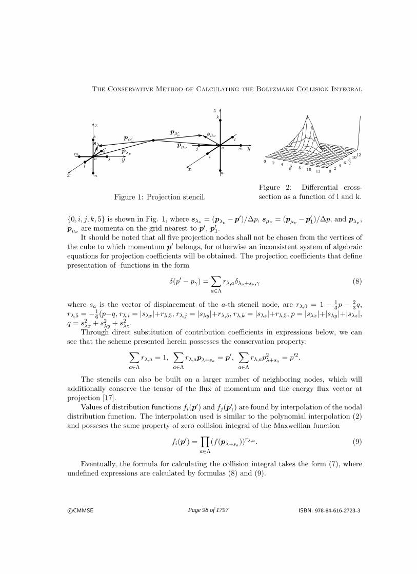
The Conservative Method of Calculating the Boltzmann Collision Integral

Figure 1: Projection stencil.

k

0 2 4 6 8 10 12

l

02

46

81012

Figure 2: Differential cross-section as a function of l and k.

0, i, j, k, 5 is shown in Fig. 1, where sλν= (pλν

− p′)/∆p, sµν = (pµν− p′

1)/∆p, and pλν,

pµνare momenta on the grid nearest to p′, p′

1.It should be noted that all five projection nodes shall not be chosen from the vertices of

the cube to which momentum p′ belongs, for otherwise an inconsistent system of algebraicequations for projection coefficients will be obtained. The projection coefficients that definepresentation of -functions in the form

δ(p′ − pγ) =∑

a∈Λ

rλ,aδλν+sν ,γ (8)

where sa is the vector of displacement of the a-th stencil node, are rλ,0 = 1 − 13p − 2

3q,rλ,5 = −1

6(p−q, rλ,i = |sλx|+rλ,5, rλ,j = |sλy|+rλ,5, rλ,k = |sλz|+rλ,5, p = |sλx|+|sλy|+|sλz|,q = s2λx + s2λy + s2λz.

Through direct substitution of contribution coefficients in expressions below, we cansee that the scheme presented herein possesses the conservation property:

∑

a∈Λ

rλ,a = 1,∑

a∈Λ

rλ,apλ+sa = p′,∑

a∈Λ

rλ,ap2λ+sa = p′2.

The stencils can also be built on a larger number of neighboring nodes, which willadditionally conserve the tensor of the flux of momentum and the energy flux vector atprojection [17].

Values of distribution functions fi(p′) and fj(p

′1) are found by interpolation of the nodal

distribution function. The interpolation used is similar to the polynomial interpolation (2)and posseses the same property of zero collision integral of the Maxwellian function

fi(p′) =

∏

a∈Λ

(f(pλ+sa))rλ,a . (9)

Eventually, the formula for calculating the collision integral takes the form (7), whereundefined expressions are calculated by formulas (8) and (9).

c©CMMSE ISBN: 978-84-616-2723-3Page 98 of 1797

Yu. A. Anikin, O. I. Dodulad, Yu. Yu. Kloss, F. G. Tchremissine

2.3 The projection method for a gas with rotational degrees of freedom

Behavior of a diatomic gas which molecules have rotational degrees of freedom is describedat the kinetic level by the generalized Boltzmann equation [12]:

∂fi∂t

+ ξ∂fi∂x

=∑

j,k,l

∫

(

wklij fl(ξ

′1)fk(ξ

′)− fj(ξ1)fi(ξ))

gijσ(θ, gij) d2n d3ξ1.

The equation is written for the distribution function fi(ξ) of gas molecules at the i-th rotational quantum level. It represents an extension of the Wang Chang Uhlenbecksequation to the case of degeneracy of energy levels which takes place for rotational degreesof freedom in the absence of magnetic field. Factor wkl

ij = qkql/qjqi appears here due to thedegeneracy of levels, with qi being the degeneracy number.

When the equation is solved numerically, the rotational quantum levels are replacedwith the nodes of discretization for angular velocity of rotation. In the general case numer-ical levels will not coincide with quantum levels. As demonstrated in [18], this approachintroduces an error of the order o(∆ω2), where ∆ω is the step in the angular velocity grid.The angular velocity corresponding to the i-th level is equal to ωi = ∆ω(i + 0.5), and thedegeneracy of the numerical level equals qi = ωi, w

klij = ωkωl/ωjωi.

Similarly to the cases of a simple gas and a gas mixture, due to its symmetry properties,the collision integral of the generalized Boltzmann equation can be reduced to the followingsum:

In(ξγ) =

Nν∑

ν=1

Bν

(

δn,kνδ(ξ′ − ξγ) + δn,lνδ(ξ

′1 − ξγ) + δn,iνδ(ξαν − ξγ)− δn,jνδ(ξβν

− ξγ))

×

×(

wklij fl(ξ

′1)fk(ξ

′)− fj(ξβν)fi(ξαν

))

∣

∣ξαν− ξβν

∣

∣

Here, like in (3), δ(ξαν−ξγ) = δαν ,γ , δ(ξβν−ξγ) = δβν ,γ are Kronecker symbols, and fi(ξαν

) =fi,αν , fj(ξβν

) = fj,βνare the values of the grid distribution function. The Kronecker symbols

δn,iν , δn,jν , δn,kν , δn,lν appear here because the sums form (11) are included in the cumulativesum over ν. In this case the integrating grid is 12-dimensional ξαν

, ξβν, nν , iν , jν , kν , lν .

The values of δ(ξ′ − ξγ) and δ(ξ′1 − ξγ) are determined from formulae (1), and those offl(ξ

′1)fk(ξ

′) from the formula (4). The conservation law similar to (2) for determination ofthe coefficient rν is in this case written as ξ2αν

+ Iω2α + ξ2βν

+ Iω2β = (1 − rν)(ξ

2λν

+ ξ2µν) +

rν(ξ2λν+sν

+ ξ2µν−sν ) + Iω2λ + Iω2

µ.

Calculation of differential collision cross-sections σklij (θ, g) involves a considerable diffi-

culty when a gas with rotational degrees of freedom is considered. As with the monatomicgas cross-sections, the cross-sections are pre-calculated, and the grid values are stored indata arrays. Here the scattering cross-sections are a function of 6 variables, and theirstorage calls for a large memory size (typically about 100MB). The cross-sections are cal-culated by the classical trajectory method. The simplest model of interaction between

c©CMMSE ISBN: 978-84-616-2723-3Page 99 of 1797

The Conservative Method of Calculating the Boltzmann Collision Integral

diatomic molecules is the rotator model. Each rotator possesses two centers of massand two centers of forces which interaction is described by the Lennard-Jones potential:

Uij = 4ε[

(σ/rij)12 − (σ/rij)

6]

where rij is the separation distance between the chosen pair

of interacting centers. The rotators moment of inertia is I = mr2a, where ra is the spacingbetween points where the mass resides.

Equations of interaction between two rotators have the form:

dX

dt= G(X), X =

r

r1r2V

ω1

ω2

, G =

V

ω1 × r1ω2 × r2F /µM1/IM2/I

,F = F 11 + F 12 + F 21 + F 22

M1 = r1 × (−F 11 + F 12 − F 21 + F 22)M2 = r2 × (F 11 + F 12 − F 21 − F 22)

(10)Here r is the vector connecting the molecule centers, ±r1,2 are relative mass position vectors,ω1,2 are angular velocities of rotation of molecules, µ is the reduced molecule mass, M1,2 areforce momenta, with values having subscripts 1 or 2 corresponding to the first and secondmolecule, respectively, and F 1,2 is the force of interaction between the i-th center of thefirst molecule and the j-th center of the second molecule (i, j = 1,2).

Equations (10) are solved by Dormand-Prince method representing the 8th-order Runge-Kutta method. The calculations are done in dimensionless variables where σ, ε, µ/2 aretaken as the units of length, energy and mass. Fig. 2 below shows an example of thecross-section σkl

ij (θ, g) at i = 10, j = 5, θ = π/2, g = 5, ∆ω = 3 for molecules of nitrogen(N2) having σ = 3.31A, ε = 37.3K.

3 Examples of calculations

3.1 Heat transfer problem

The study of distribution of gas density, temperature and heat flux between two parallelplates having different temperatures is a fundamental problem of rarefied gas dynamics. Nu-merous works are devoted to this problem. In [4] the problem was solved for the hard-spherepotential by computing the collision integral with the use of a polynomial approximation ofthe distribution function.

Here the problem of heat transfer is studied by the projection method described inSection 2.1 above. The calculations are performed for a single-component monatomic gas.The cross-sections σLJ(θ, g) had been calculated in advance. There was used the Lennard-Jones potential which parameters for argon are εAr = 124K, σAr = 3.418A. The molecularmean free path was found using the omega integral value Ω(2,2) = 1.093 from [19].

c©CMMSE ISBN: 978-84-616-2723-3Page 100 of 1797

Yu. A. Anikin, O. I. Dodulad, Yu. Yu. Kloss, F. G. Tchremissine

−0.50 −0.25 0.00 0.25 0.50

0.90

0.95

1.00

1.05

1.10

1.15

x/λ

Figure 3: Density betweenthe plates for Kn = 0.0658.

−0.50 −0.25 0.00 0.25 0.500.90

0.95

1.00

1.05

1.10

x/λ

Figure 4: Density betweenthe plates for Kn = 0.1395.

−0.50 −0.25 0.00 0.25 0.50

0.95

1.00

1.05

1.10

x/λ

Figure 5: Density betweenthe plates for Kn = 0.1942.

−0.3 0.0 0.3

0.95

1.00

1.05

x/λ

Figure 6: Density betweenthe plates for Kn = 0.2992.

−0.50 −0.25 0.00 0.25 0.50

0.94

0.96

0.98

1.00

1.02

1.04

1.06

x/λ

Figure 7: Density betweenthe plates for Kn = 0.7582.

ξy −4−2024

ξx

12345

Figure 8: Distributionfunction at x = 0 forKn = 0.7582.

Heat transfer between plates with temperatures T± = T (1 ± ∆T ), ∆T = 0.14 isconsidered. Diffuse-reflection boundary conditions with the accommodation coefficientα = 0.826 are set on the plate walls. The problem statement models the experimentsdescribed in [20]. The heat transfer is considered for the following Knudsen numbers(Kn = λ/d, λ is the molecular mean free path, d is a distance between the plates):Kn = 0.0658, 0.1395, 0.1942, 0.2992, 0.7582. Results of the calculations are shown in Figs.3, 4, 5, 6 and 7, respectively. The solid line corresponds to gas density distribution obtainedwith the projection method, the dotted line is plotted for results taken from [4] for the hard-sphere potential, and points show experimental data for argon from [20]. The comparisonshows a good agreement with experimental data except for density in the vicinity of thecold plate for Kn = 0.7582 (see Fig. 7). It is interesting to note that in this case the velocitydistribution function has a high gradient region on the plane ξx = 0 shown in Fig. 8. It isapparent that in this case the distribution is close to that composed by half-Maxwelliansfor temperatures T± = T (1±∆T ) that occurs in the free-molecular flow.

3.2 Shock wave structure

Determination of the shock wave structure is another classical problem of the kinetic theory.This problem was the subject of a number of experimental works and numerical simula-tions. Sufficiently reliable experimental data for monatomic gas Ar and diatomic gas N2 are

c©CMMSE ISBN: 978-84-616-2723-3Page 101 of 1797

The Conservative Method of Calculating the Boltzmann Collision Integral

−6 −3 0 3 60.0

0.2

0.4

0.6

0.8

1.0

M=1.55

M=2.31

x/λ

Figure 9: Density in the shock wave in themonatomic gas, – experimental data [21].

−8 −4 0 4 80.0

0.2

0.4

0.6

0.8

1.0

nu

T

Tβ

x/λ

Figure 10: Structure of the shock wave in gasmixture for M = 3, mα/mβ = 1/2, χβ = 0.1in comparison with data provided in [3].

published in [21]. There are a lot of publications on studies carried out using the statisticalsimulation method (DSMC) [1], [22].

Solution of the Boltzmann equation in case of the hard-sphere potential for a single-component gas and a gas mixture is presented in [2] and [3], respectively. There the collisionintegral is calculated using the same method of polynomial approximation of the distributionfunction as in [4]. By the projection method, the problem was studied, for example in [16].

In the present work the main part of the calculations is done for the realistic Lennard-Jones potential. Fig. 9 shows gas density profiles for shock waves with Mach numbersM = 1.55 and M = 2.31. Points correspond to the experimental data [21]. The solid line isplotted from calculations. Parameters of the Lennard-Jones potential for argon that wereused are listed in the previous section.

Figs. 10 and 11 present results of calculations for the gas mixture. Fig. 10 compares ourdata obtained with the multipoint modification of the projection method (see Section 2.2

−15 0 15 300.0

0.2

0.4

0.6

0.8

1.0

nHe

nXe

x/λ

Figure 11: Density in the shock wave for M =3.89 in the mixture of 97% helium and 3%xenon compared with experimental data [23].

−6 −3 0 3 60.0

0.2

0.4

0.6

0.8

1.0

M=1.53

M=2.4

x/λ

Figure 12: Density in the shock wave inthe diatomic gas compared with experimen-tal data [21].

c©CMMSE ISBN: 978-84-616-2723-3Page 102 of 1797

Yu. A. Anikin, O. I. Dodulad, Yu. Yu. Kloss, F. G. Tchremissine

above) with calculations presented in [3]. The hard-sphere potential was used. A comparisonwith experimental data [23] was also made (see Fig. 11). There was considered the caseof the helium mixture with low molar fraction of xenon. The calculation was done for thefollowing parameters of the Lennard-Jones potential: εHe = 10.2K, εXe = 229K, σHe =2.576A, σXe = 4.055A [19]. Parameters of interaction between different molecules wereobtained on the basis of combination relations: εHe,Xe =

√εHeεXe, σHe,Xe = (σHeσXe)/2.

Fig. 12 shows results of the calculations for the diatomic gas performed through solutionof the generalized Boltzmann equation by the method described in Section 2.3 above. Thecross-sections σkl

ij (θ, g) were obtained with the classical trajectory method. A comparisonwith experimental data for argon taken from [21] is presented.

The comparisons show that for the monatomic gas the application of the Lennard-Jonespotential gives results close to the experimental data. For the gas mixture, there is observeda good agreement in the density profile width (see Fig. 11). The peak in the helium profilemay be associated with the experimental uncertainty. For the diatomic gas the agreementbetween the data is slightly worse. Probably, the model of interaction between diatomicmolecules should be improved by introducing a dipole-dipole interaction and moving apartthe repulsion and attraction centers [24].

Conclusion

The conservative method of calculating the collision integral for simple gases, gas mixturesand gases with rotational degrees of freedom of molecules is presented. It uses the com-mon approach based on the projection method of summing up the contributions in thecollision integral. For inert gases, the method allows calculating the integral for any molec-ular potentials. Gas mixtures can be effciently calculated for any molecular mass ratiosand any concentrations of mixture components. For diatomic gases, there was developedthe methodology of pre-calculating molecular collision cross-sections with translational-rotational energy transitions, which allows calculating the collision integral without theuse of approximate models of inelastic collison. The algorithm of collision integral calcu-lation was optimized, which provided for an essencial increase in the computation speed.Some sample of calculations presented in the paper confirm reliability and high accuracyof the obtained results, thus the efficiency of presented method for solving the Boltzmannequation.

References

[1] Bird, G. A. Oxford University Press, USA, 2nd edition, 1994.

[2] Ohwada, Taku. Physics of Fluids A: Fluid Dynamics 1993, 5(1):217–234.

c©CMMSE ISBN: 978-84-616-2723-3Page 103 of 1797

The Conservative Method of Calculating the Boltzmann Collision Integral

[3] S. Kosuge, K. Aoki, S. Takata. European Journal of Mechanics, B/Fluids 2001,20(1):87–126.

[4] Taku Ohwada. Phys. Fluids 1996; 8:2153.

[5] Palczewski, A., Schneider, J. and Bobylev, A. V. SIAM J. Numer. Anal. 1997;34(5):1865–1883.

[6] Ibragimov, I. and Rjasanow, S. Computing 2002; 69(2):163–186.

[7] Mouhot, C. and Pareschi, L. Math. of Comp. 2006; 75:1833–1852.

[8] Gamba, I. M. and Tharkabhushanam, S. H. J. of Comput. Math. 2010.

[9] Cheremisin, F. G. Physics – Doklady 1997; 42:607–610.

[10] Tcheremissine, F. G. Comp. Math. and Math. Phys. 2006; 46(2):315–329.

[11] Cheremisin, F. G. Doklady Physics 2000; 45(8):401–404.

[12] F. G. Tcheremissine. Comp. Math. and Math. Phys. 2012; 52(2), 252–268.

[13] A.E. Beylich. Aachen: Technisch Hochcshule Report 2000.

[14] N. M. Korobov. Dokl. Akad. Nauk SSSR 1959; 124:1207–1210.

[15] Yu. A. Anikin, O. I. Dodulad, Yu. Yu. Kloss, D. V. Martynov, P. V. Shu-

valov, F. G. Tcheremissine. Vacuum 2012; 86(11):1770–1777.

[16] Raines, A. A. AIP Conf. Proc. 2003; 663(1):67–76.

[17] O. I. Dodulad, F. G. Tcheremissine. In: 28th International Symposium on Rar-efied Gas Dynamics 2012, AIP Conf. Proc. 1501, p. 302–309.

[18] Yu. A. Anikin, O. I. Dodulad. Comp. Math. and Math. Phys. 2013 (to be published)

[19] J. O. Hirschfelder, C. F. Curtiss, R. B. Bird. Wiley: University of Wisconsin,1964.

[20] W. P. Teagan and G. S. Springer. Phys. Fluids 11, 497, 1968.

[21] H. Alsmeyer. J. Fluid. Mech 1976; 74:497–513.

[22] K. Koura. Phys. Fluids 9, 3543, 1997.

[23] A. S. Gmurczyk, M. Tarczynski, Z. A. Walenta. In: 11th International Sympo-sium on Rarefied Gas Dynamics 1978; 1, p. 333–341.

[24] R. M. Berns and A. van der Avoird. J.Chem.Phys. 1980, 72:6107.

c©CMMSE ISBN: 978-84-616-2723-3Page 104 of 1797

Proceedings of the 13th International Conferenceon Computational and Mathematical Methodsin Science and Engineering, CMMSE 201324–27 June, 2013.

Finite-volume discretization of a 1d reaction-diffusion basedmultiphysics modelling of charge trapping in an insulator

submitted to an electron beam irradiation

A. Aoufi1 and G. Damamme2

1 Centre SMS, Laboratoire Georges Friedel, UMR CNRS 5307, Ecole des Mines deSaint-Etienne, 42023 Saint-Etienne Cedex.,

2 CEA Gramat, BP 80200 - 46500 Gramat.,

emails: aoufi@emse.fr, gilles.damamme@cea.fr

Abstract

This paper describes a new one-dimensional reaction-diffusion based modelling forcharge trapping in an insulator submitted to an electron beam irradiation and its fullyimplicit finite-volume discretization.

Key words: reaction-diffusion equations, multiphysics coupling, charge trapping, im-plicit finite-volume scheme.

1 Introduction

Dielectric breakdown in insulating materials is of practical importance since it damageselectronic devices [1]. Secondary electron emission yield (denoted by see) is one of the keyparameters for dielectric materials and is the driving parameter of electric charging whichcan lead to electric breakdown. To study this phenomena, the behaviour of an insulatorsubmitted to electron beam irradiation is considered. Several modelling based upon a two-fluxes method [2] were presented and discussed recently [3],[4],[5],[6],[7]. The purpose ofthis paper is to analyse a new mathematical modelling that is a reformulation in a reaction-diffusion framework of a modelling presented in [3], and is organized as follows. Sectiontwo presents the governing equations of the modelling which couples the trapped chargedensity ρ(z, t), the electric field E(z, t), the number of electron ne(z, t) or holes nh(z, t).Section three describes the fully implicit finite-volume numerical discretization scheme ona staggered refined mesh. A conclusion summarizes the paper.

c©CMMSE ISBN: 978-84-616-2723-3Page 105 of 1797

1d Numerical Study of Charge Trapping in insulator

2 Mathematical modelling

The purpose of the modelling is to analyze by numerical simulation the evolution of theglobal trapped charge per surface unit at time t, Qp(t) defined from the trapped chargeρ(z, t)

Qp(t) =

∫Ωρ(z, t) dz (1)

as a function of the true secondary electronic emission yield see∗(t) defined by

see∗(t) = κje−(0, t)

j0(2)

• The governing equation for the electric field E(z, t) V/m is given by

∇.E(z, t) = Eext −ρ(z, t)

ε0εr(3)

E(0, t) =Qp(t)

ε0εr (1 + εr)(4)

where Eext is the extracting field, ε0 is the vacuum permittivity and εr is the materialpermittivity.

• The governing equation for the number of free charges (nc)c∈e,h depends on thecharge carrier flux jc(z, t) for c ∈ e, h that is given by

jc(z, t) = −Dc(E)∂ne∂z

+ µc(E)vc nc(z, t) (5)

which is the sum of a diffusion term and a convection term. It is worth mentioningthat the convection term can be positive or negative depending on the sign of the”mobility” coefficient µc. The conservation law fulfilled by nc(z, t) is therefore

∂nc∂t

+∂

∂z

(−Dc(E)

∂ne∂z

+ µc(E)vc nc(z, t)

)(6)

= 2Sc(z)−σ+abs,c + σ−abs,c

2nc(z, t) vc + jc(z, t)

σ+abs,c − σ

−abs,c

2

• The governing equation for the trapped charge density ρ(z, t) is given by

∂ρ(z, t)

∂t+∇.jT (z, t) = 0. (7)

The expression of jT (z, t) is given by

jT (z, t) = jh(z, t)− je(z, t)− j0 jprim(z) (8)

c©CMMSE ISBN: 978-84-616-2723-3Page 106 of 1797

A. Aoufi, G. Damamme

• The governing equation for the total trapped charge Qp(t) in C is related to the

trapped charge density ρ(z, t) thanks to the relation Qp(t) =

∫Ωρ(z, t) dz. The inte-

gration of Eq.(7) over Ω leads to the relation

dQp(t)

dt+ jT (L, t)− jT (0, t) = 0. (9)

Taking into account the definition of the true secondary electron emission yield see∗(t)given by

see∗(t) = veκ

2− κne(0, t)

j0. (10)

leads to

dQp(t)

dt= j0 (1− see∗(t)) + vh nh(L, t)− ve ne(L, t). (11)

3 Numerical discretization scheme

The computational domain Ω = [0, L] is split into a set of I control volumes Ωi = [zi, zi+1].The length of control volume Ωi is mi, its center is denoted by ci. di,i+1 is the distancebetween the center of two adjacent control volumes Ωi and Ωi+1. The discrete unknownslocated at the center of each control volume Ωi are ne|k+1

i and nh|k+1i . The discrete un-

knowns located at the edge of each control volume Ωi are ρk+1i , Ek+1

i and jT |k+1i . The

time-discrete unknowns such as Qp|k+1 and see∗|k+1. A backward Euler scheme is used toapproximate the time-derivative and the integration of each governing equation over controlvolume Ωi is given below.

• Discretization of the electric field equation leads to the discrete equation

Ek+1i+1 − E

k+1i =

mi

2

ρk+1i + ρk+1

i+1

ε0εr(12)

where, a trapezoidal rule has been used to discretize the integral of the right handside of Eq.(3). The discrete approximation of boundary condition Eq.(4) is written

Ek+11 = Eext −

1

ε0εr (1 + εr)Qk+1

p (13)

• Discretization of the charge density equation leads to the discrete equation

mi.ρk+1i − ρki

∆t+ jT |k+1

i+1 − jT |k+1i = 0 (14)

c©CMMSE ISBN: 978-84-616-2723-3Page 107 of 1797

1d Numerical Study of Charge Trapping in insulator

• Discretization of the number of free charge carrier’s equation leads to the discreteequation

minc|k+1

i − nc|ki∆t

−Di+ 12

nc|k+1i+1 − nc|k+1

i

di,i+1+Di− 1

2

nc|k+1i − nc|k+1

i−1

di−1,i(15)

= +2mi Sc(ci)−miσ+,k+1abs,c + σ−,k+1

abs,c

2nc|k+1

i vc

+mi µc(E)|k+1i vc nc|k+1

i

σ+,k+1abs,c − σ

−,k+1abs,c

2

Here Di± 12

is computed by the harmonic mean formula given by [8] in order to obtain

the flux continuity across the interface between two adjacent control volumes. Adapteddiscrete equations are also written when the control volume is Ω1 or ΩI in order totake into account the Neuman type boundary conditions. A tridiagonal matrix has tobe inverted by the forward/backward method, i.e. the (α, β)-TDMA algorithm givenby [8] at each step of the nonlinear solver to compute approximation of nc|k+1,p+1 asa function of nc|k+1,p, where p is the nonlinear iteration index. This method is knownto be stable if the matrix is diagonally dominant [8]. This is indeed the case and waseffectively proved formally.

• Discretization of the true secondary electron emission yield see∗(t) leads to the discreteequation

see∗|k+1 = veκ

2− κne|k+1

1

j0. (16)

• Discretization of the trapped charge density equation leads to the discrete equation

Qp|k+1 − Qp|k

∆t= j0

(1− see∗|k+1

)+ vh nh|k+1

I − ve ne|k+1I . (17)

4 Conclusion

In this paper we have presented a new 1D multiphysics modelling charge trapping in aninsulator submitted to an electron beam irradiation. The validation of the fully implicitfinite volume discretization presented in this paper is in progress.

c©CMMSE ISBN: 978-84-616-2723-3Page 108 of 1797

A. Aoufi, G. Damamme

References

[1] G. Damamme, C. Legressus, A.S. De Reggi, IEEE Trans.Dielec.Elect.Insul. 4 (5), 558-584, 1997

[2] S. Chandrasekhar (1960) Radiative transfer, ed New York: Dover, (ISBN 0486-6059-06).

[3] A.Aoufi, G. Damamme, ”Analysis and Numerical Simulation of Secondary ElectronEmission Yield of an Insulator submitted to An Electron Beam”. Proceedings of 23rdInternational Symposium on Discharges and Electrical Insulation in Vacuum, Vols 1and 2, pp.21-24, 2008.

[4] A.Aoufi, G.Damamme, ”Numerical Computation of secondary electron emission yieldby a two fluxes method”, Numerical Analysis and Applied Mathematics, Vols 1-2, AIPConference Proceedings, Vol 1168, pp 212-215, ISBN 978-0-7354-0709-1, InternationalConference on Numerical Analysis and Applied Mathematics, sep 18-22, Rethymno,Greece, 2009, Ed. Simos, TE; Psihoyios, G; Tsitouras, C.

[5] A.Aoufi, G. Damamme, ”Numerical Simulation of Secondary Electron Emission Yieldin the Case of Volume and Surface Trapping Evolution”, Proceedings of 24th Interna-tional Symposium on Discharges and Electrical Insulation in Vacuum, Vols 1 and 2,pp. 11-14, 2010.

[6] A.Aoufi, G.Damamme, ”Two-Fluxes and Reaction-Diffusion Computation of Initialand Transient Secondary Electron Emission Yield by a Finite Volume Method”, pp.89-108, in Numerical Simulations- Applications, Examples and Theory, Edited by Prof.Lutz Angerman, ISBN 978-953-307-440-5, INTECH open Editor, January 2011.

[7] A. Aoufi, G.Damamme, ”1D numerical simulation of charge trapping in an insulatorsubmitted to an electron beam irradiation. Part I: Computation of the initial secondaryelectron emission yield”, Applied Mathematical Modelling, Vol. 35-3,pp 1175-1183.

[8] S.V. Patankar, Numerical Heat Transfer and Fluid Flow”, McGRAW-HILL BOOKCOMPANY, 1980.

c©CMMSE ISBN: 978-84-616-2723-3Page 109 of 1797

Proceedings of the 13th International Conferenceon Computational and Mathematical Methodsin Science and Engineering, CMMSE 201324–27 June, 2013.

On Soft Functions

Cigdem Gunduz Aras1, Ayse Sonmez2 and Huseyin Cakallı3

1 Department of Mathematics, Kocaeli University

2 Department of Mathematics, Gebze Institute of Technology

3 Marmara Egitim Koyu, Maltepe University

emails: carasgunduz@gmail.com, asonmez@gyte.edu.tr, hcakalli@maltepe.edu.tr

Abstract

In this paper, we introduce soft continuous mappings which are defined over an initialuniverse set with a fixed set of parameters. Later we study soft open and soft closedmappings, soft homeomorphism and investigate some properties of these concepts.

Key words: soft sets; soft topology; soft continuity

1 Introduction

Most of the real life problems in social sciences, engineering, medical sciences, economicsetc. the data involved are imprecise in nature. The solutions of such problems involve theuse of mathematical principles based on uncertainty and imprecision. Thus classical settheory, which is based on the crisp and exact case may not be fully suitable for handlingsuch problems of uncertainty. A number of theories have been proposed for dealing withuncertainties efficiently way. Some of these are theory of fuzzy sets [17], theory of intuition-istic fuzzy sets [3], theory of vague sets, theory of interval mathematics [4] ,[7] and theory ofrough sets [14]. However, these theories have their own difficulties. Molodtsov [10] initiateda novel concept of soft sets theory as a new mathematical tool for dealing with uncertaintieswhich is free from the above limitations. A soft set is a collection of approximate descrip-tions of an object. Soft systems provide a very general framework with the involvement ofparameters. Since soft set theory has a rich potential, research on soft set theory and itsapplications in various fields are progressing rapidly. Maji et al. [11], [12] worked on softset theory and presented an application of soft sets in decision making problems.

c⃝CMMSE ISBN: 978-84-616-2723-3Page 110 of 1797

On Soft Functions - the CMMSE proceedings

M.Shabir and M.Naz [16] introduced soft topological spaces. They also defined someconcepts of soft sets on soft topological spaces. Later, researches about soft topologicalspaces were studied in [18]-[20]. In these studies, the concept of soft point is expressed bydifferent approaches. In this paper we refer to the concept of soft point which was given in[22] .

The purpose of this paper is to investigate soft continuity on soft topological spaces.

2 Preliminaries

In this section, we give definitions and some results of soft sets.

Definition 1 ([10]) Let X be an initial universe set and E be a set of parameters. A pair(F,E) is called a soft set over X if only if F is a mapping from E into the set of all subsetsof the set X, i.e., F : E → P (X), where P (X) is the power set of X.

Definition 2 ([11]) A soft set (F,A) over X is said to be a null soft set denoted by Φ iffor all a ∈ A, F (a) = ∅ (null set).

Definition 3 ([11]) A soft set (F,A) over X is said to be an absolute soft set denoted byA if for all a ∈ A, F (a) = X.

Definition 4 [21] Let (F,A) and (G,B) be two soft sets over X . Then (F,A) is called asoft subset of (G,B), denoted by (F,A) ⊂ (G,B), if(i) A ⊂ B,(ii) F (a) ⊂ G(a) for each a ∈ A.

Definition 5 ([11]) The intersection of two soft sets (F,A) and (G,B) over X is the softset (H,C), where C = A ∩ B and ∀c ∈ C, H(c) = F (c) ∩ G(c). This is denoted by(F,A)∩(G,B) = (H,C).

Definition 6 ([11]) The union of two soft sets (F,A) and (G,B) over X is the soft set,where C = A ∪B and ∀c ∈ C,

H(ε) =

F (ε), if ε ∈ A−BG(ε), if ε ∈ B −A

F (ε) ∪G(ε), if ε ∈ A ∩B.

This relationship is denoted by (F,A)∪(G,B) = (H,C).

Definition 7 ([16] ) The complement of a soft set (F,E) is denoted by (F,E)c and isdefined by (F,E)c = (F c, E) where F c : E → P (X) is a mapping given by F c(α) = X−F (α)for all α ∈ E.

c⃝CMMSE ISBN: 978-84-616-2723-3Page 111 of 1797

Cigdem Gunduz Aras, Ayse Sonmez, and Huseyin Cakallı

Definition 8 ([16] ) Let τ be a collection of soft sets over X. Then τ is said to be a softtopology on X if(1) Φ, X belong to τ ,(2) the union of any number of soft sets in τ belongs to τ ,(3) the intersection of any two soft sets in τ belongs to τ .The triplet (X, τ,E) is called a soft topological space over X.

Definition 9 ([16] ) Let (X, τ,E) be a soft topological space over X. A soft set (F,E) overX is said to be a soft closed in X, if its relative complement (F,E)c belongs to τ .

Proposition 1 ([16] ) Let (X, τ,E) be a soft topological space over X. Then the collectionτα = F (α)|(F,E) ∈ τ defines a topology on X for each α ∈ E.

Definition 10 ([16] ) Let (X, τ,E) be a soft topological space over X and (F,E) be a softset over X. Then the soft closure of (F,E), denoted by (F,E) is the intersection of all softclosed super sets of (F,E).

Definition 11 ([16] ) Let (X, τ,E) be a soft topological space over X and (F,E) be a softset over X. Then we associate with (F,E) a soft set over X, denoted by (F,E) and definedas F (α) = F (α), where F (α) is the closure of F (α) in τα for each α ∈ E.

Proposition 2 ([16] ) Let (X, τ,E) be a soft topological space over X and (F,E) be a softset over X. Then (F ,E) ⊂ (F,E) .

Corollary 1 ([16]) Let (X, τ,E) be a soft topological space over X and (F,E) be a soft setover X. Then (F,E) = (F,E) if and only if (F,E)c ∈ τ .

Definition 12 ([23] ) Let (X, τ,E) be a soft topological space over X, (G,E) be a soft setover X and x ∈ X. Then x is said to be a soft interior point of (G,E), if there exists asoft open set (F,E) such that x ∈ (F,E) ⊂ (G,E).

Definition 13 ([23]) Let (X, τ,E) be a soft topological space over X, (G,E) be a soft setover X and x ∈ X. Then (G,E) is said to be a soft neighbourhood of x, if there exists asoft open set (F,E) such that x ∈ (F,E) ⊂ (G,E).

Definition 14 ([23]) Let (X, τ,E) be a soft topological space over X then soft interior ofa soft set (F,E) over X is denoted by (F,E) and is defined as the union of all soft opensets contained in (F,E).

Thus (F,E) is the largest soft open set contained in (F,E).

c⃝CMMSE ISBN: 978-84-616-2723-3Page 112 of 1797

On Soft Functions - the CMMSE proceedings

3 Soft Continuity

Definition 15 ([22] ) Let (F,E) be a soft set over X, and x ∈ X. The soft set (F,E) iscalled a soft point, denoted by (xe, E), if for the element e ∈ E, F (e) = x and F (ec) = ∅for all ec ∈ E − e. In this case, we say that (xe, E) is a point of a soft set (F,E).

Definition 16 Let (X, τ,E) and (Y, τ c, E) be two soft topological spaces, f : (X, τ,E) →(Y, τ c, E) be a mapping. For each soft neighbourhood (H,E) of (f(x)e, E), if there exists asoft neighbourhood (F,E) of (xe, E) such that f((F,E)) ⊂ (H,E), then f is said to be softcontinuous mapping at (xe, E).If f is soft continuous for all (xe, E), then f is called soft continuous on X.

Theorem 1 Let (X, τ,E) and (Y, τ c, E) be two soft topological spaces, f : (X, τ,E) →(Y, τ c, E) be a mapping. Then the following conditions are equivalent:(1) f : (X, τ,E) → (Y, τ c, E) is a soft continuous mapping,(2) For each soft open set (G,E) over Y , f−1((G,E)) is a soft open set over X,(3) For each soft closed set (H,E) over Y , f−1((H,E)) is a soft closed set over X,(4) For each soft set (F,E) over X, f((F,E)) ⊂ (f(F,E)),(5) For each soft set (G,E) over Y , (f−1(G,E)) ⊂ f−1((G,E)),(6) For each soft set (G,E) over Y , f−1((G,E)) ⊂ (f−1(G,E)).

Proof: (1) ⇒ (2) Let (G,E) be a soft open set over Y and (xe, E) ∈ f−1(G,E) bean arbitrary soft point. Then f(xe, E) = (f(x)e, E) ∈ (G,E). Since f is soft continuousmapping, there exists (xe, E) ∈ (F,E) ∈ τ such that f(F,E) ⊂ (G,E). This implies that(xe, E) ∈ (F,E) ⊂ f−1(G,E), f−1((G,E)) is a soft open set over X.

(2) ⇒ (1) Let (xe, E) be a soft point and (f(x)e, E) ∈ (G,E) be an arbitrary soft neigh-bourhood. Then (xe, E) ∈ f−1(G,E) is a soft neighbourhood and f(f−1(G,E)) ⊂ (G,E).

(3) ⇒ (4) Let (F,E) be a soft set over X. Since (F,E) ⊂ f−1(f(F,E)) and f(F,E) ⊂(f(F,E)), we have (F,E) ⊂ f−1(f(F,E)) ⊂ f−1(f(F,E)). By part (3), since f−1(f(F,E))is a soft closed set over X, (F,E) ⊂ f−1(f(F,E)). Thus f((F,E)) ⊂ f(f−1(f(F,E))) ⊂f(F,E) is obtained.

(4) ⇒ (5) Let (G,E) be a soft set over Y and f−1(G,E) = (F,E). By part (4), wehave f((F,E)) = f(f−1(G,E)) ⊂ f(f−1(G,E)) ⊂ (G,E). Then f−1(G,E) = (F,E) ⊂f−1(f(F,E)) ⊂ f−1((G,E)).

(5) ⇒ (6) Let (G,E) be a soft set over Y . Substituting (G,E)c for condition in (5).Then f−1((G,E)c) ⊂ f−1((G,E)c). Since (G,E) = ((G,E)c)c, then we have f−1((G,E)) =

c⃝CMMSE ISBN: 978-84-616-2723-3Page 113 of 1797

Cigdem Gunduz Aras, Ayse Sonmez, and Huseyin Cakallı

f−1(((G,E)c)c) = (f−1((G,E)c))c ⊂ (f−1((G,E)c))c = ((f−1(G,E))c)c = (f−1(G,E)).

(6) ⇒ (2) Let (G,E) be a soft open set over Y . Then since (f−1(G,E)) ⊂ f−1(G,E) =f−1((G,E)) ⊂ (f−1(G,E)), (f−1(G,E)) = f−1(G,E) is obtained. This implies thatf−1(G,E) is a soft open set over X.

Example 1. Let X = h1, h2, h3, E = e1, e2 and τ = Φ, X, (F1, E), (F2, E),τ c = Φ, X, (G1, E), (G2, E) be two soft topologies defined on X, where (F1, E), (F2, E),(G1, E) and (G2, E) are soft sets over X, defined as follows:

F1(e1) = h1, h2, F1(e2) = h3, F2(e1) = X, F2(e2) = h3,

and

G1(e1) = h1, G1(e2) = h3, G2(e1) = h1, h3, G2(e2) = h2, h3,

If we get the mapping f : X → X defined as

f(h1) = f(h2) = h1, f(h3) = h3

then since f−1(G1, E) = (F1, E) and f−1(G2, E) = (F2, E), f is a soft continuous mapping.

Example 2. LetX = h1, h2, h3, E = e1, e2 and τ = Φ, X, (F1, E), (F2, E), (F3, E), (F4, E),τ c = Φ, X, (G1, E), (G2, E), (G3, E), (G4, E) be two soft topologies defined on X where(F1, E), (F2, E), (F3, E), (F4, E), (G1, E), (G2, E), (G3, E) and (G4, E) are soft sets over X,defined as follows:

F1(e1) = h2, F1(e2) = h1, F2(e1) = h2, h3, F2(e2) = h1, h2,

F3(e1) = h3, F3(e2) = h1, h2, F4(e1) = ∅, F4(e2) = h1,

F5(e1) = X, F2(e2) = h1, h2

and

G1(e1) = h2, G1(e2) = h1, G2(e1) = h2, h3, G2(e2) = h1, h2,

G3(e1) = h1, h2, G3(e2) = X, G4(e1) = h2, G4(e2) = h1, h2,

Then (X, τ,E), (X, τ c, E) are two soft topological spaces and f = 1X : X → X is not softcontinuous mapping.

Theorem 2 If f : (X, τ,E) → (Y, τ c, E) is a soft continuous mapping, then for each α ∈ E,fα : (X, τα) → (Y, τ cα) is a continuous mapping.

c⃝CMMSE ISBN: 978-84-616-2723-3Page 114 of 1797

On Soft Functions - the CMMSE proceedings

Proof: Let U ∈ τ cα. Then there exists a soft open set (G,E) over Y such that U = G(α).Since f : (X, τ,E) → (Y, τ c, E) is a soft continuous mapping, f−1(G,E) is a soft open setover X and f−1(G,E)(α) = f−1(G(α)) = f−1(U) is an open set. This implies that fα is acontinuous mapping.

Now we give an example to show that the converse of above theorem does not hold.

Example 3. Let X = x1, x2, x3, Y = y1, y2, y3 and E = e1, e2. Then τ =Φ, X, (F1, E), (F2, E), (F3, E), (F4, E), (F5, E) is a soft topological space over X and τ c =Φ, Y , (G1, E), (G2, E), (G3, E) is a soft topological space over Y . Here (F1, E), (F2, E), (F3, E), (F4, E), (F5, E)are soft sets over X and (G1, E), (G2, E), (G3, E) are soft sets over Y , defined as follows:

F1(e1) = x1, F1(e2) = x1, x3, F2(e1) = x2, F2(e2) = x1,

F3(e1) = x1, x2, F3(e2) = x1, x3, F4(e1) = ∅, F4(e2) = x1, F5(e1) = x1, x2, F5(e2) = X.

and

G1(e1) = Y, G1(e2) = y2, G2(e1) = y1, G2(e2) = y2, G3(e1) = y1, y2, G3(e2) = y2.

If we get the mapping f : X → Y defined as

f(x1) = y2, f(x2) = y1, f(x3) = y3

then f is not a soft continuous mapping, since f−1(G1) /∈ τ , where f−1(G1)(e1) = X,f−1(G1)(e2) = x1. Also, fe1 : (X, τe1) → (Y, τ ce1) and fe2 : (X, τe2) → (Y, τ ce2) arecontinuous mappings. Here

τe1 = ∅, X, x1, x2, x1, x2, τe2 = ∅, X, x1, x1, x3

and

τ ce1 = ∅, Y, y1, y1, y2, τ ce2 = ∅, Y, y2.

Now, let us show that when the above theorem is true.

Theorem 3 If (F ,E)c is a soft open set over X, for each soft set (F,E), then f : (X, τ,E) →(Y, τ c, E) is a soft continuous mapping if and only if fα : (X, τα) → (Y, τ cα) is continuousmapping, for each α ∈ E.

Proof: Let fα : (X, τα) → (Y, τ cα) be a continuous mapping, for each α ∈ E, and let(F,E) be an arbitrary soft set over X. Then fα(F (α)) ⊂ f(F )(α) is satisfied, for eachα ∈ E. Since (F ,E)c ∈ τ , (F ,E) = (F,E) from Corollary 1. Thus f((F,E)) ⊂ f((F,E)) isobtained. This implies that f : (X, τ,E) → (Y, τ c, E) is a soft continuous mapping.

c⃝CMMSE ISBN: 978-84-616-2723-3Page 115 of 1797

Cigdem Gunduz Aras, Ayse Sonmez, and Huseyin Cakallı

Definition 17 Let (X, τ,E) and (Y, τ c, E) be two soft topological spaces, f : X → Y be amapping.a) If the image f((F,E)) of each soft open set (F,E) over X is a soft open set in Y , thenf is said to be a soft open mapping.b) If the image f((H,E)) of each soft closed set (H,E) over X is a soft closed set in Y ,then f is said to be a soft closed mapping.

Proposition 3 If f : (X, τ,E) → (Y, τ c, E) is soft open (closed), then for each α ∈ E,fα : (X, τα) → (Y, τ cα) is an open (closed) mapping.

Proof: The proof of the proposition is straightforward and it is left to the reader. Note that the concepts of soft continuous, soft open and soft closed mappings are all

independent of each other.Example 4. Let (X, τ,E) be soft discrete topological space and (X, τ c, E) be soft

indiscrete topological space. Then 1X : (X, τ,E) → (X, τ c, E) is a soft open and soft closedmapping. But it is not soft continuous mapping.

Example 5. LetX = h1, h2, h3, E = e1, e2 and τ = Φ, X, (F1, E), (F2, E), ..., (F7, E),τ c = Φ, X, (G1, E), (G2, E), (G3, E), (G4, E) be two soft topologies defined on X where(F1, E), (F2, E), (F3, E), ..., (F7, E), (G1, E), (G2, E), (G3, E) and (G4, E) are soft sets overX, defined as follows:

F1(e1) = h2, F1(e2) = h1, F2(e1) = h1, h3, F2(e2) = h2, h3,

F3(e1) = h2, F3(e2) = X, F4(e1) = ∅, F4(e2) = h1,

F5(e1) = h1, h3, F5(e2) = X, F6(e1) = ∅, F6(e2) = h2, h3,

F7(e1) = ∅, F7(e2) = X

andG1(e1) = h2, G1(e2) = h1, G2(e1) = h2, h3, G2(e2) = h1, h2,

G3(e1) = h1, h2, G3(e2) = X, G4(e1) = h2, G4(e2) = h1, h2.

If we get the mapping f : X → X defined as f(hi) = h1, for 1 ≤ i ≤ 3. It is clear that

f−1(G1)(e1) = f−1(G4)(e1) = ∅, f−1(G1)(e2) = f−1(G4)(e2) = X, f−1(G3)(e1) = X, f−1(G3)(e2) = X.

Then f is a soft continuous mapping, but

f(F1)(e1) = h1, f(F1)(e2) = h1, f(F c1 )(e1) = h1, f(F c

1 )(e2) = h1.

Hence it is not both soft open and soft closed mapping.

c⃝CMMSE ISBN: 978-84-616-2723-3Page 116 of 1797

On Soft Functions - the CMMSE proceedings

Example 6. LetX = h1, h2, h3, Y = a, b and E = e1, e2 and τ = Φ, X, (F1, E), (F2, E),τ c = Φ, Y , (G1, E), (G2, E) be two soft topologies defined on X and Y , respectively. Here(F1, E), (F2, E), (G1, E), (G2, E) are soft sets over X and Y , respectively. The soft sets aredefined as follows:

F1(e1) = h1, h2, F1(e2) = h3, F2(e1) = X, F2(e2) = h3,

andG1(e1) = Y, G1(e2) = b, G2(e1) = a, G2(e2) = b,

If we get the mapping f : X → Y defined as

f(h1) = a, f(h2) = f(h3) = b.

It is clear that

f(F1)(e1) = Y, f(F1)(e2) = b, f(F2)(e1) = Y, f(F2)(e2) = b.

Then the mapping f : X → Y is a soft open mapping. Also since f(F c1 )(e1) = b, f(F c

1 )(e2) =Y , it is not soft closed mapping and f−1(G1)(e1) = X, f−1(G1)(e2) = h2, h3. Hence it isnot soft continuous mapping.

Example 7. LetX = h1, h2, h3, Y = a, b, E = e1, e2 and τ = Φ, X, (F1, E), (F2, E), (F3, E),τ c = Φ, Y , (G1, E), (G2, E) be two soft topologies defined on X and Y , respectively. Here(F1, E), (F2, E), (F3, E), (G1, E), (G2, E) are soft sets over X and Y , respectively. The softsets are defined as follows:

F1(e1) = h1, h3, F1(e2) = h2, F2(e1) = X, F2(e2) = h2, h3, F3(e1) = h3, F3(e2) = h2

andG1(e1) = ∅, G1(e2) = a, G2(e1) = a, G2(e2) = Y.

Now we define the mapping f : X → Y as f(h1) = f(h2) = a, f(h3) = b. It is clearthat f(F c

1 (e1)) = f(h2) = a, f(F c1 (e2)) = f(h1, h3) = Y , f(F c

2 (e1)) = ∅, f(F c2 (e2)) =

f(h1) = a, f(F c3 (e1)) = a, f(F c

3 (e2)) = Y . This implies that f is a soft closedmapping. Also f(F1(e1)) = Y, f(F1(e2)) = a, f−1(G1(e1)) = ∅, f−1(G1(e2)) = h1, h2.Then it is not soft open and soft continuous mapping, respectively.

Theorem 4 Let (X, τ,E) and (Y, τ c, E) be two soft topological spaces, f : X → Y be amapping.a) f is a soft open mapping if and only if for each soft set (F,E) over X, f((F,E)) ⊂(f(F,E)) is satisfied.b) f is a soft closed mapping if and only if for each soft set (F,E) over X, (f(F,E)) ⊂f((F,E)) is satisfied.

c⃝CMMSE ISBN: 978-84-616-2723-3Page 117 of 1797

Cigdem Gunduz Aras, Ayse Sonmez, and Huseyin Cakallı

Proof: a) Let f be a soft open mapping and (F,E) be a soft set over X. (F,E) is a softopen set and (F,E) ⊂ (F,E). Since f is a soft open mapping, f((F,E)) is a soft open setin Y and f((F,E)) ⊂ f((F,E)) . Thus f((F,E)) ⊂ f((F,E)) is obtained.Conversely, let (F,E) be any soft open set over X. Then (F,E) = (F,E). From thecondition of theorem, we have f((F,E)) ⊂ (f(F,E)). Then f((F,E)) = f((F,E)) ⊂(f(F,E)) ⊂ f((F,E)). This implies that f((F,E)) = (f(F,E)). This completes theproof.b) Let f be a soft closed mapping and (F,E) be any soft set over X. Since f is a softclosed mapping, f((F,E)) is a soft closed set over Y and f((F,E)) ⊂ f((F,E)). Thusf(F,E) ⊂ f((F,E)) is obtained.Conversely, let (F,E) be any soft closed set over X. From the condition of theorem,(f(F,E)) ⊂ f((F,E)) = f((F,E)) ⊂ (f(F,E)). This means that (f(F,E)) = f((F,E)).This completes the proof.

Definition 18 Let (X, τ,E) and (Y, τ c, E) be two soft topological spaces, f : X → Y be amapping. If f is a bijection, soft continuous and f−1 is a soft continuous mapping, then fis said to be soft homeomorphism from X to Y . When a homeomorphism f exists betweenX and Y , we say that X is soft homeomorphic to Y .

Theorem 5 Let (X, τ,E) and (Y, τ c, E) be two soft topological spaces, f : X → Y be abijective mapping. Then the following conditions are equivalent:(1) f is a soft homeomorphism,(2) f is a soft continuous and soft closed mapping,(3) f is a soft continuous and soft open mapping.

Proof: It is easily obtained.

4 Conclusion

We have introduced soft continuous mappings which are defined over an initial universewith a fixed set of parameters. Later we study soft open and soft closed mappings, softhomeomorphism and investigate some properties of these concepts. In the end, we mustsay that, soft topological spaces are defined over different set of parameters and it does notmake any sense for the results of this paper.

References

[1] M.I.Ali, F.Feng, X.Y.Liu, W.K.Min, M.Shabir, On some new operations in soft settheory, Comput. Math. Appl. 57 (2009) 1547-1553

c⃝CMMSE ISBN: 978-84-616-2723-3Page 118 of 1797

On Soft Functions - the CMMSE proceedings

[2] H.Aktas, N. agman, Soft sets and soft group, Information Science 177 (2007) 2726-2735.

[3] K.Atanassov, Intuitionistic fuzzy sets, Fuzzy Sets and Systems 20 (1986) 87-96.

[4] K.Atanassov, Operators over interval valued intuitionistic fuzzy sets, Fuzzy Sets andSystems 64 (1994) 159-174.

[5] D.Chen, The parametrization reduction of soft sets and its applications, Comput. Math.Appl. 49 (2005) 757-763

[6] F. Feng, Y.B. Jun, X. Zhao, Soft semirings, Comput. Math. Appl.56 (2008) 2621-2628.

[7] M.B.Gorzalzany, A method of inference in approximate reasoning based on interval-valued fuzzy sets, Fuzzy Sets and Systems 21 (1987) 1-17.

[8] Y.B.Jun, C.H.Park, Applications of soft sets in ideal theory of BCK/BCI-Algebras,Inform.Sci. 178 (2008) 2466-2475.

[9] O.Kazanc, .Ylmaz and S.Yamak, Soft sets and soft BCH-Algebras, Hacettepe Journalof Mathematics and Statistics 39(2) (2010) 205-217.

[10] D. Molodtsov, Soft set theory- first results, Comput. Math. Appl.37 (1999) 19-31.

[11] P.K.Maji, R.Bismas, A.R.Roy, Soft set theory, Comput. Math. Appl.45 (2003) 555-562.

[12] P.K.Maji, A.R.Roy, R.Bismas, An Application of soft sets in a decision making prob-lem, Comput. Math. Appl.44 (2002) 1077-1083

[13] Qiu-Mei Sun, Zi-Liong Zhang, Jing Liu, Soft sets and soft modules, Lecture Notes inComput. Sci. 5009 (2008) 403-409.

[14] Z.Pawlak, Rough sets, Int.J.Comput.Sci. 11 (1982) 341-356.

[15] M.Shabir, M.Irfan Ali, Soft ideals and generalized fuzzy ideals in semigroups, NewMath. Nat. Comput. 5 (2009) 599-615.

[16] M.Shabir, M. Naz, On soft topological spaces, Comput. Math. Appl. 61 (2011) 1786-1799.

[17] L.A.Zadeh, Fuzzy sets, Inf. Control 8 (1965) 338-353.

[18] I. Zorlutuna, M. Akdag, W.K. Min, S. Atmaca, Remarks on soft topological spaces,Annals of Fuzzy Mathematics and Informatics, 2012.

[19] N. Cagman, S. Karatas, S. Enginoglu, Soft topology, Comput. Math. Appl. 62 (2011)351-358.

c⃝CMMSE ISBN: 978-84-616-2723-3Page 119 of 1797

Cigdem Gunduz Aras, Ayse Sonmez, and Huseyin Cakallı

[20] W.K. Min, A note on soft topological spaces, Comput. Math. Appl. 62 (2011) 3524-3528.

[21] P. Majumdar, S.K. Samanta, On soft mappings, Comput. Math. Appl., 60 (2010)2666-2672

[22] S. Bayramov, C. Gunduz(Aras), Soft locally compact and soft paracompact spaces,Journal of Mathematics and System Science

[23] S.Hussain, B.Ahmad, Some properties of soft topological spaces, Comput. Math.Appl.62 (2011) 4058-4067

c⃝CMMSE ISBN: 978-84-616-2723-3Page 120 of 1797

Proceedings of the 13th International Conferenceon Computational and Mathematical Methodsin Science and Engineering, CMMSE 201324–27 June, 2013.

Numerical solution of time-dependent Maxwell’s equationsfor modeling scattered electromagnetic wave’s propagation

Aderito Araujo1, Sılvia Barbeiro1, Luıs Pinto1, Francisco Caramelo2,Antonio L. Correia2, Miguel Morgado2,5, Pedro Serranho2,4, Ana Sılvia F.

C. Silva5 and Rui Bernardes2,3

1 CMUC, Department of Mathematics, University of Coimbra, Portugal

2 IBILI, Faculty of Medicine, University of Coimbra, Portugal

3 ABILI, Coimbra, Portugal

4 Mathematics Section, Department of Science and Technology, Open University, Portugal

5 Department of Physics, Faculty of Science and Technology, University of Coimbra,Portugal

emails: alma@mat.uc.pt, silvia@mat.uc.pt, luisp@mat.uc.pt,fcaramelo@fmed.uc.pt, acorreia@aibili.pt, mmorgado@ibili.uc.pt,

Pedro.Serranho@uab.pt, anascsilva@gmail.com, rmbernardes@fmed.uc.pt

Abstract

We present the discontinuous Galerkin method combined with a low-storage Runge-Kutta method as an accurate and efficient way to numerically solve the time-dependentMaxwell’s equations. We investigate the numerical scheme in the context of modelingscattered electromagnetic wave’s propagation through human eye’s structures.

Key words: Maxwell’s equations, discontinuous Galerkin method, low-storage Runge-Kutta method, anisotropic permittivity tensor

1 Introduction

The human retina is a complex structure in the eye that is responsible for the sense ofvision. It is part of the central nervous system, constituted by layers of neurons intercon-nected through synapses [7]. There are ten layers in total; one of them is constituted by

c©CMMSE ISBN: 978-84-616-2723-3Page 121 of 1797

Numerical solution of time-dependent Maxwell’s equations

photosensitive neurons. There are a number of eye-related pathologies that can be identifiedby analysis of these retinal layers in detail [7]. All these pathologies can be diagnosed moreconclusively with the help of the increasingly popular optical imaging technique – opticalcoherence tomography (OCT) [3], [15]. In fact, previous studies have established a linkbetween changes in the blood-retina barrier and in optical properties of the retina [1], [2]which can be identified by this exam.

Physically, OCT it is based in low coherence interferometry. This technique uses anelectromagnetic wave with a low coherence length. In order to better understand the in-formation carried in an optical coherence tomography, it is crucial to study in detail thebehaviour of the electromagnetic wave as it travels through the sample. Several differentmodels have been developed to describe the interactions of the electromagnetic field withbiological structures. The first models were based on single-scattering theory [14], whichis restricted to superficial layers of highly scattering tissue in which only single scatteringoccurs. Simulating the full complexity of the retina, in particular the variation of the sizeand shape of each structure, distance between them and the respective refractive indexes,requires a more rigorous approach that can be achieved by solving Maxwell’s equations.

In this work we discuss the numerical discretization of the time-dependent Maxwell’sequations. We use the discontinuous Galerkin (DG) method for the integration in space anda low-storage Runge-Kutta method for the integration in time. In the model we consideranisotropic permittivity tensors which arise naturally in our application of interest. Weillustrate the performance of the method with some numerical experiments.

2 Maxwell’s Equations

We shall consider the time domain Maxwell’s equations in the two-dimensional transverseelectric (TE) mode. For this case, and assuming no conductivity effects, the equations inthe non-dimensional form are

ε∂Ex

∂t=∂Hz

∂y(1)

ε∂Ey

∂t= −∂H

z

∂x(2)

µ∂Hz

∂t= −∂E

y

∂x+∂Ex

∂y, in Ω× (0, T ], (3)

where E = (Ex, Ey) and Hz represent the electric and magnetic fields, respectively, εrepresents the relative permittivity of the medium and µ is the permeability of the mediumand Ω is a two-dimensional domain. The nondimensionalized variables in (1)-(3) are relatedto the physical variables in the following way

x

L= x,

y

L= y,

ct

L= t, E = Z−1

0 E, Hz = Hz,

c©CMMSE ISBN: 978-84-616-2723-3Page 122 of 1797

A. Araujo, S. Barbeiro, L. Pinto, R. Bernardes et al.

where L is a reference length, c is the speed of light in free space, and Z0 =√µ0/ε0 is

the free-space impedance. The set of equations (1)-(3) must be complemented by properboundary conditions, for instance, the perfect electric boundary condition (PEC) [5]

η × E = 0, on ∂Ω, (4)

or the Silver-Muller absorbing boundary condition [9]

η × E =

õ

εη × (Hz × η), on ∂Ω. (5)

In both cases η denotes the unit outward normal. To complete the model, initial conditions

E0 = E(0) and H0 = H(0), in Ω,

must also be considered.

3 The scattered-field formulation

For the investigation of scattering problems in linear materials, we exploit the linearity ofthe Maxwell’s equations (1)-(3) and separate the fields (E, H) into incident (Ei, H i) andscattered components (Es, Hs), i.e.,

E = Es + Ei and H = Hs +H i. (6)

Assuming that the incident field is also a solution of the Maxwell’s equations we obtain,after some manipulation the scattered field formulation as in [16],

ε∂Ex,s

∂t=∂Hz,s

∂y+ P (7)

ε∂Ey,s

∂t= −∂H

z,s

∂x+Q (8)

µ∂Hz,s

∂t= −∂E

y,s

∂x+∂Ex,s

∂y+R, in Ω× (0, T ] (9)

with the source terms

P (x, y, t) = (εi − ε)∂Ex,i

∂t,

Q(x, y, t) = (εi − ε)∂Ey,i

∂t,

R(x, y, t) = (µi − µ)∂Hz,i

∂t,

where εi and µi represent the relative permittivity and permeability of the medium in whichthe incident field propagates. In our research, for simplicity, we adopt the pure scatteredfield formalism in opposition to the total field/scattered field formalism [16].

c©CMMSE ISBN: 978-84-616-2723-3Page 123 of 1797

Numerical solution of time-dependent Maxwell’s equations

4 Numerical method

The DG method was first introduced in [11]. In particular, the nodal formulation describedin [6] has gained notorious popularity in recent years and it has been extensively used inelectromagnetic problems since the first application of the method to Maxwell’s equationsin 2002 (see [5]). This is the method that we have chosen to use. In opposition to thetraditional finite difference (FD) time domain methods [16] based on the Yee’s scheme [17]the DG method is a high-order accurate method that can easily handle complex geometries.Moreover, local refinement strategies can easily be incorporate due to the ability of themethod to deal with irregular meshes with hanging nodes and local spaces of different orders.When compared to finite element methods [12], the DG method presents the advantages ofavoiding the solution of linear systems when explicit time integrators are employed and thesuitability for parallel implementation on modern multi-graphics processing units (GPUs)[6].

As starting point of our work we use the MatLab codes for the DG method [6]. Thesoftware includes many attributes that we intent to exploit in future work such as three-dimensional routines and nonconforming triangulations. For now, we are concerned withtwo-dimensional problems and we have restricted our attention to conform triangular ele-ments. Our main focus has been on the implementation of additional features needed forthe kind of problems which are in our objectives. For instance, the retinal nerve fiber layerof the retina is a birefringent medium, meaning that tensorial permittivity ε needs to betaken into account. We addressed this issue using the numerical scheme presented in [8].The procedure, based on the so called upwind flux, is fairly simple and can be easily in-corporated in the algorithm. Nevertheless, it seems to be efficient and robust for a widerange of problems, since the two by two matrix that represents the tensor ε only needsto be invertible. In [8] the authors claim that the method, which is an extension of thebasic two-dimensional formulation for isotropic materials to allow anisotropic permittivitytensors, retains the convergence characteristics of the original method. The validation teststhat we present in the next section corroborate those findings.

Another aspect of our study concerns the integration in time. The time integrationscheme used in the original algorithm [6] is a fourth order, five stage low-storage Runge-Kutta (LSRK) method. Such type of schemes are very popular in this context as they retainthe qualities of the original Runge-Kutta schemes while decreasing the memory consumptionsignificatively. However, we recall that explicit methods like the LSRK scheme are subjectto the CFL stability condition. In practice, this means that the time step size is proportionalto the smallest elements of the spatial mesh [6]. For some problems this condition can havea strong impact on the efficiency of the algorithm. In the future we intent to deal with thisissue using local time-stepping strategies [6] or locally implicit time-schemes [4]. For now, wemitigate this restriction implementing the improved fourth order, 14-stage LSRK presentedin [10]. With this scheme the authors report a speed improvement of about 40%− 50% in

c©CMMSE ISBN: 978-84-616-2723-3Page 124 of 1797

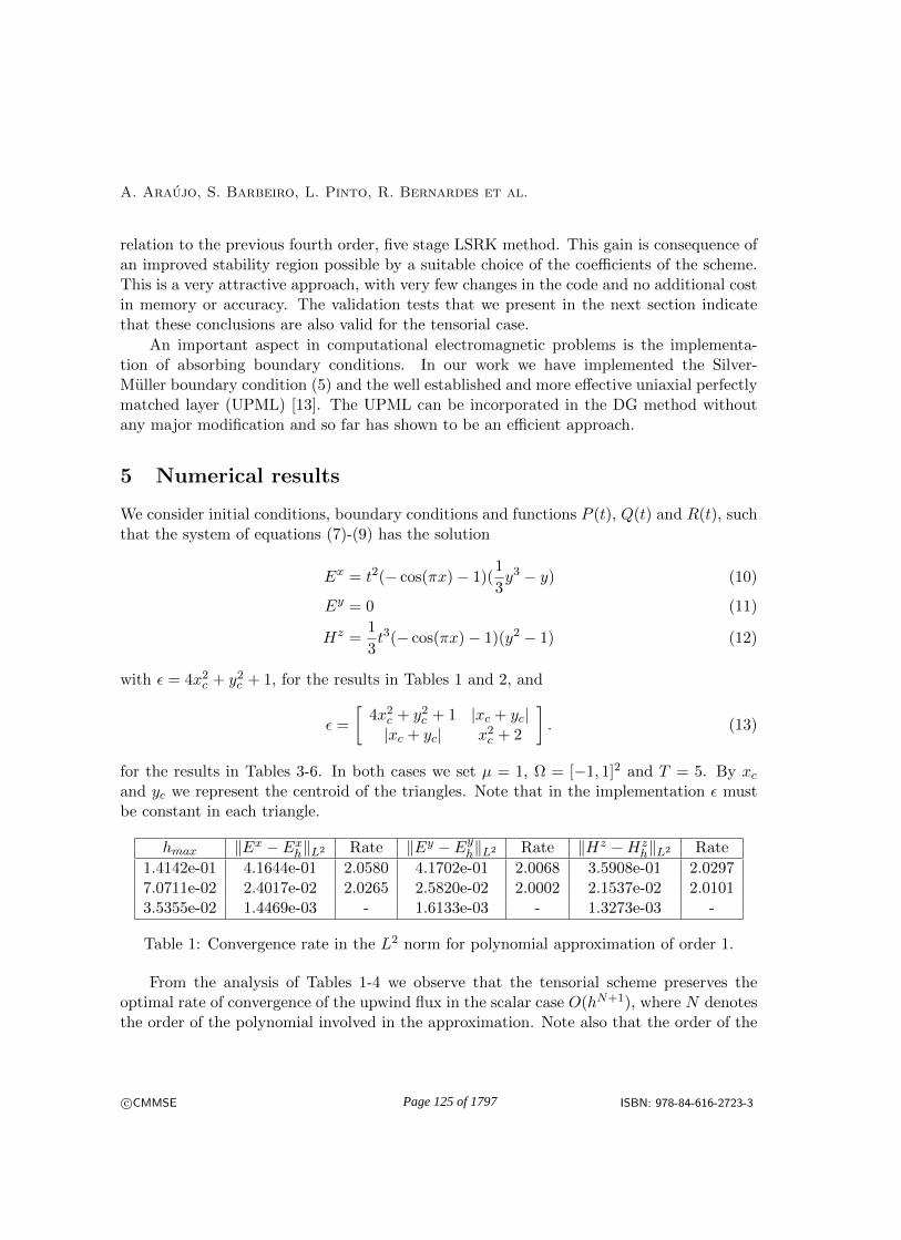
A. Araujo, S. Barbeiro, L. Pinto, R. Bernardes et al.

relation to the previous fourth order, five stage LSRK method. This gain is consequence ofan improved stability region possible by a suitable choice of the coefficients of the scheme.This is a very attractive approach, with very few changes in the code and no additional costin memory or accuracy. The validation tests that we present in the next section indicatethat these conclusions are also valid for the tensorial case.

An important aspect in computational electromagnetic problems is the implementa-tion of absorbing boundary conditions. In our work we have implemented the Silver-Muller boundary condition (5) and the well established and more effective uniaxial perfectlymatched layer (UPML) [13]. The UPML can be incorporated in the DG method withoutany major modification and so far has shown to be an efficient approach.

5 Numerical results

We consider initial conditions, boundary conditions and functions P (t), Q(t) and R(t), suchthat the system of equations (7)-(9) has the solution

Ex = t2(− cos(πx)− 1)(1

3y3 − y) (10)

Ey = 0 (11)

Hz =1

3t3(− cos(πx)− 1)(y2 − 1) (12)

with ε = 4x2c + y2c + 1, for the results in Tables 1 and 2, and

ε =

[4x2c + y2c + 1 |xc + yc||xc + yc| x2c + 2

]. (13)

for the results in Tables 3-6. In both cases we set µ = 1, Ω = [−1, 1]2 and T = 5. By xcand yc we represent the centroid of the triangles. Note that in the implementation ε mustbe constant in each triangle.

hmax ‖Ex − Exh‖L2 Rate ‖Ey − Ey

h‖L2 Rate ‖Hz −Hzh‖L2 Rate

1.4142e-01 4.1644e-01 2.0580 4.1702e-01 2.0068 3.5908e-01 2.02977.0711e-02 2.4017e-02 2.0265 2.5820e-02 2.0002 2.1537e-02 2.01013.5355e-02 1.4469e-03 - 1.6133e-03 - 1.3273e-03 -

Table 1: Convergence rate in the L2 norm for polynomial approximation of order 1.

From the analysis of Tables 1-4 we observe that the tensorial scheme preserves theoptimal rate of convergence of the upwind flux in the scalar case O(hN+1), where N denotesthe order of the polynomial involved in the approximation. Note also that the order of the

c©CMMSE ISBN: 978-84-616-2723-3Page 125 of 1797

Numerical solution of time-dependent Maxwell’s equations

hmax ‖Ex − Exh‖L2 Rate ‖Ey − Ey

h‖L2 Rate ‖Hz −Hzh‖L2 Rate

1.4142e-01 8.6363e-04 3.0268 1.0196e-03 3.0124 1.7076e-03 2.99417.0711e-02 1.3002e-05 3.0120 1.5660e-05 3.0070 2.6901e-05 2.99783.5355e-02 1.9981e-07 - 2.4231e-07 - 4.2159e-07 -

Table 2: Convergence rate in the L2 norm for polynomial approximation of order 2.

hmax ‖Ex − Exh‖L2 Rate ‖Ey − Ey

h‖L2 Rate ‖Hz −Hzh‖L2 Rate

1.4142e-01 5.4515e-01 2.0461 6.2046e-01 1.9949 3.9240e-01 2.02027.0711e-02 3.1963e-02 2.0197 3.9055e-02 1.9964 2.3847e-02 2.00673.5355e-02 1.9438e-03 - 2.4532e-03 - 1.4767e-03 -

Table 3: Convergence rate in the L2 norm for polynomial approximation of order 1.

hmax ‖Ex − Exh‖L2 Rate ‖Ey − Ey

h‖L2 Rate ‖Hz −Hzh‖L2 Rate

1.4142e-01 8.1456e-04 2.9993 9.4071e-04 3.0184 1.7020e-03 2.99407.0711e-02 1.2739e-05 2.9996 1.4328e-05 3.0091 2.6817e-05 2.99793.5355e-02 1.9916e-07 - 2.2106e-07 - 4.2022e-07 -

Table 4: Convergence rate in the L2 norm for polynomial approximation of order 2.

hmax ‖Ex − Ehx‖L2 Time

original fourth order, 5-stage LSRK 7.0711e-02 3.1963e-02 69.25simproved fourth order, 14-stage LSRK 7.0711e-02 3.1963e-02 38.35s (44%)

original fourth order, 5-stage LSRK 3.5355e-02 1.9438e-03 514.26simproved fourth order, 14-stage LSRK 3.5355e-02 1.9438e-03 295.99s (42%)

Table 5: Comparison of the two LSTR methods for polynomial approximation of order 1.

hmax ‖Ex − Ehx‖L2 Time

original fourth order, 5-stage LSRK 7.0711e-02 1.2739e-05 132.43simproved fourth order, 14-stage LSRK 7.0711e-02 1.2739e-05 79.71s (39%)

original fourth order, 5-stage LSRK 3.5355e-02 1.9916e-07 1259.94simproved fourth order, 14-stage LSRK 3.5355e-02 1.9916e-07 745.40s (40%)

Table 6: Comparison of the two LSTR methods for polynomial approximation of order 2.

errors is about the same when we compare the problem with tensorial permittivity and theproblem with scalar permittivity.

In Tables 5 and 6 we compare the two different implementations for the time integration.The error is exactly the same for both methods and the running time decreases about 40%.

c©CMMSE ISBN: 978-84-616-2723-3Page 126 of 1797

A. Araujo, S. Barbeiro, L. Pinto, R. Bernardes et al.

Even though we only show the results for Ex, in our experiments we found that the errorof the other field components, Ey and Hz, present the same type of behaviour.

To illustrate the advantages of the DG method over the FD method we examine thescattering by a dielectric cylinder with a relative permittivity of ε = 5. This scatterer withradius r = 0.5 and centered at the origin is excited by a Gaussian plane wave propagatingalong the y direction. We measured the magnetic filed Hz at the point (x, y) = (−1, 0).In Figure 1 we compare the results obtained with both methods. The DG solution wasobtained using third-order polynomials and a local refined mesh formed by 920 triangles.This means that the number of unknowns is 9.2×103. The FD solution was obtained usinga uniform mesh with h = 1.25× 10−2 implying 4.0× 104 unknowns. Our experiments showthat the DG method is more accurate and efficient. The error, in the Euclidean norm, is1.5827× 10−1 for the DG method and 3.6668× 10−1 for the FD method.

0 1 2 3 4 5 6 7 8 90

0.01

0.02

0.03

0.04

0.05

0.06

0.07

0.08

0.09

Time

Figure 1: Error curves for the DG solution (dash line) and FD solution (solid line).

Acknowledgements

This work has been partially supported by Centro de Matematica da Universidade deCoimbra (CMUC), funded by the European Regional Development Fund through the pro-gram COMPETE and by the Portuguese Government through the FCT - Fundacao para aCiencia e a Tecnologia under the project PEst-C/MAT/UI0324/2011, and by FCT underthe project PTDC/SAU-ENB/119132/2010) and COMPETE (QREN -FCOMP-01-0124-FEDER-021014) program.

c©CMMSE ISBN: 978-84-616-2723-3Page 127 of 1797

Numerical solution of time-dependent Maxwell’s equations

References

[1] R. Bernardes, T. Santos and J. Cunha-Vaz, Evaluation of Blood-Retinal Bar-rier Function from Fourier Domain High-Definition Optical Coherence Tomography, inIFMBE Proceedings 25/XI, 2009, 316–319.

[2] R. Bernardes, T. Santos, P. Serranho, C. Lobo, and J. Cunha-Vaz, Nonin-vasive evaluation of retinal leakage using OCT, Ophtalmologica 226(2) (2011) 29–36.

[3] B. Bouma and G. Tearney, Handbook of optical coherence tomography, MarcelDekker, New York, 2002.

[4] S. Descombes, S. Lanteri and L. Moya, Locally implicit time integration strategiesin a discontinuous Galerkin method for Maxwell’s equations, J. Sci. Comput. 56 (2013)190–218.

[5] J. Hesthaven and T. Warburton, Nodal High-Order Methods on UnstructuredGrids: I. Time-Domain Solution of Maxwell’s Equations, J. Comput. Phys. 181 (2002)186–221.

[6] J. S. Hesthaven and T. Warburton, Nodal Discontinuous Galerkin Methods: Al-gorithms, Analysis, and Applications, Springer Verlag, New York, 2008.

[7] L. Junqueira and J. Carneiro, Basic Histology: Text & Atlas (Junqueira’s BasicHistology), McGraw-Hill Medical, 2005.

[8] M. Konig, K. Busch and J. Niegemann, The Discontinuous Galerkin Time-Domain method for Maxwell’s equations with anisotropic materials, Phot. Nano. Fund.Appl. 8 (2010) 303–309.

[9] C. Muller, Foundations of the Mathematical Theory of Electromagnetic Waves,Springer Verlag, Berlim, 1969.

[10] J. Niegemann, R. Diehl and K. Busch, Efficient low-storage Runge-Kutta schemeswith optimized stability regions, J. Comput. Phys. 231 (2012) 364–372.

[11] W. Reed, T. Hill, Triangular mesh methods for the neutron transport equation, LosAlamos Scientific Laboratory. LA-UR-73-479 (1973).

[12] R. N. Rieben, G. H. Rodrigue and D. A. White, A high order mixed vector finiteelement method for solving the time dependent Maxwell equations on unstructured grids,J. Comput. Phys. 204 (2005) 490–519.

c©CMMSE ISBN: 978-84-616-2723-3Page 128 of 1797

A. Araujo, S. Barbeiro, L. Pinto, R. Bernardes et al.

[13] Z. S. Sacks, D. M. Kingsland, R. Lee and J. -F. Lee, A perfectly matchedanisotropic absorber for use as an absorbing boundary condition, IEEE Trans. An-tennas. Propag. 43 (1995) 1460–1463.

[14] J. M. Schmitt, A. Knuttel, and R. F. Bonner, Measurement of optical propertiesof biological tissues by low-coherence reflectometry, Appl. Opt. 32 (1993) 6032–6042.

[15] P. Serranho, M. Morgado and R. Bernardes Optical Coherence Tomography: aconcept review In: Optical Coherence Tomography: A Clinical and Technical Update.R. Bernardes & J. Cunha-Vaz Eds., Springer-Verlag, 2012, 139–156

[16] A. Taflove and S. C. Hagness, Computational Electrodynamic: The Finite-Difference Time-Domain Method (2nd ed.), Artech House, Norwood, MA, 2000.

[17] K. S. Yee, Numerical solution of initial boundary value problems involving maxwell’sequations in isotropic media, IEEE Trans. Antennas. Propag. 14 (1966) 302–307.

c©CMMSE ISBN: 978-84-616-2723-3Page 129 of 1797

Proceedings of the 13th International Conferenceon Computational and Mathematical Methodsin Science and Engineering, CMMSE 201324–27 June, 2013.

Parallel extrapolated algorithms for computing PageRank

Josep Arnal1, Hector Migallon2, Violeta Migallon1, Juan A. Palomino1

and Jose Penades1

1 Departamento de Ciencia de la Computacion e Inteligencia Artificial, Universidad deAlicante, 03690 San Vicente del Raspeig, Alicante

2 Departamento de Fısica y Arquitectura de Computadores, Universidad MiguelHernandez, 03202 Elche, Alicante

emails: arnal@dccia.ua.es, hmigallon@umh.es, violeta@dccia.ua.es,japb4@alu.ua.es, jpenades@dccia.ua.es

Abstract

The PageRank algorithm for determining the importance of Web pages has becomea central technique in Web search. This algorithm uses the Power method to computesuccessive iterates that converge to the principal eigenvector of the Markov chain repre-senting the Web link graph. In this paper parallel Relaxed and Extrapolated algorithmsbased on the Power method are presented. Different parallel implementations of thePower method and the proposed variants are analyzed using different data distributionstrategies. The reported experiments show the behavior of the designed algorithmsfor realistic test data using an hybrid OpenMP/MPI approach in order to exploit thebenefits of shared memory inside the nodes of current SMP supercomputers.

Key words: PageRank, parallel algorithms, Power method, Relaxed and Extrapolatedmethods

1 Introduction

One of the most difficult problems in Web search is the ranking of the results recalledin response to a user query. Since contemporary Web crawls discover billions of pages,broad topic queries may result in recalling hundreds of thousand of pages containing thequery terms. Only a few dozens of the recalled pages are actually presented to the user.Moreover, these results are presented in order of relevance. A variety of ranking features

c©CMMSE ISBN: 978-84-616-2723-3Page 130 of 1797

Parallel extrapolated algorithms for PageRank

are used by Internet search engines to come up with a good order. Some of the query-independent features are based on page content. Some utilize the hyperlink structure ofthe Web. The PageRank algorithm [11] is one of those that introduces a content neutral-ranking function over Web pages. This ranking is applied to the set of pages returnedby the Google search engine in response to posting a search query. PageRank is basedin part on two simple common sense concepts: A page is important if many importantpages include links to it and a page containing many links has reduced impact on theimportance of the pages it links to. This model has been used by Google as part of itssearch engine technology. PageRank is essentially the stationary distribution vector of aMarkov chain whose transition matrix is a convex combination of the Web link graph anda certain rank 1 matrix. A key parameter in the model is the damping factor, a scalarthat determines the weight given to the Web link graph in the model. Due to the greatsize and sparsity of the matrix, methods based on decomposition are considered infeasible;instead, iterative methods are used, where the computation is dominated by matrix-vectorproducts; see e.g., [1]. Traditionally, PageRank has been computed using the Power method.Many methods to accelerate the Power method have been developed such that extrapolationmethods, block-structure methods or adaptive methods; see e.g., [6], [7], [8], [14] and thereferences cited therein. In recent years opportunities for parallel execution have broadenedtheir scope; see e.g., [3], [4], [12]. In this paper different parallel algorithms based on thePower method for computing PageRank are proposed and analyzed. Concretely, we presentparallel Relaxed and Extrapolated algorithms based on the Power method that accelerateits convergence. The remainder of the paper is structured as follows. In Section 2 we providea brief description of the PageRank problem and we introduce the Power method and someacceleration methods based on the extrapolation technique. In Section 3, parallel algorithmsof the Power method using relaxation and/or extrapolation are introduced. The numericalexperiments performed in Section 4 show the behavior of these algorithms using differentdata distribution strategies on both shared and distributed memory multicore architectures.Finally, in Section 5 we give some conclusions.

2 Computing the PageRank

PageRank [11] is a probability distribution used to represent the likelihood that a personrandomly clicking on links will arrive at any particular page. The PageRank problem canbe seen as a matrix problem. Let G = [gij ]

ni,j=1 be a Web graph adjacency matrix with

elements gij = 1 when there is a link from page j to page i, with i = j, and zero otherwise.Here n is the number of Web pages. From this matrix we can construct a transition matrixP = [pij]

ni,j=1 as follows: pij =

gijcj

if cj = 0 and 0 otherwise, where cj =∑n

i=1 gij, 1 ≤ j ≤ n,

represents the number of out-links from a page j. For pages with a nonzero number of out-links, i.e., cj = 0 for all j, 1 ≤ j ≤ n, the matrix P is column stochastic. Thus each element

c©CMMSE ISBN: 978-84-616-2723-3Page 131 of 1797

J. Arnal, V. Migallon, H. Migallon, J.A. Palomino, J. Penades

of this matrix has values between 0 and 1, and the sum of the components of each columnis 1. In this case the PageRank vector can be obtained by solving Px = x. Since we areinterested in a probability distribution, the sum of the components of x is assumed to beone. Algorithm 1 shows the original Power method [13] for the PageRank computationwhere e = (1, 1, . . . , 1)T . Note that we use the L1 norm ‖x‖1 =

∑ni=1 |xi|.

Algorithm 1 (Power method)

Initialization x0 = en , k = 0

Repeat

xk+1 = Pxk

δ = ‖xk+1 − xk‖1k = k + 1

Until δ < ε

When the matrix P ≥ 0 is irreducible (i.e., its graph is strongly connected) and stochastic,its largest eigenvalue in magnitude is λmax = 1. Thus, Algorithm 1 converges to theeigenvector corresponding to λmax = 1, and when normalized, it is the stationary probabilitydistribution over pages under a random walk on the Web. However, the Web contains manypages without out-links, called dangling nodes. Dangling pages present a problem for themathematical PageRank formulation because in this case the matrix P is non-stochastic andthen Algorithm 1 can not be used. Moreover, the matrix irreducibility is not satisfied for aWeb graph. In order to overcome this difficulty, Page and Brin [11] change the transitionmatrix P to a column stochastic matrix P = α(P + vdT ) + (1 − α)veT , where d ∈ n isthe dangling page indicator defined by di = 1 if and only if ci = 0 and the vector v ∈ n

is some probability distribution over pages. This model means that the random surferjumps from a dangling page according to a distribution v. For this reason v is called ateleportation distribution. Originally uniform teleportation v = e

n was used. Consequently,v is also known as a personalization vector. Then, setting α such that 0 < α < 1 (as a goodcompromise Google uses α = 0.85), the matrix P is column stochastic and irreducible. Onthe other hand, since P is stochastic, then P preserves the L1 norm, that is, ‖P x‖1 = ‖x‖1and therefore we can reformulate Algorithm 1 using the matrix P to solve the PageRankvector. That is, Algorithm 1 is utilized in order to solve the stationary distribution of theergodic Markov chain defined by P , P x = x, obtaining the corresponding algorithm:

Algorithm 2 (Power method for solving P x = x)

Initialization x0 = en , k = 0

Repeat

xk+1 = αPxk

c©CMMSE ISBN: 978-84-616-2723-3Page 132 of 1797

Parallel extrapolated algorithms for PageRank

γ = ‖xk‖1 − ‖xk+1‖1xk+1 = xk+1 + γv

δ = ‖xk+1 − xk‖1k = k + 1

Until δ < ε

Note that although the matrix P is dense, Algorithm 2 has been designed such that it isnot necessary to construct explicitly the matrix P .

On the other hand, the extrapolation algorithms [5] accelerate the convergence ofPageRank by using successive iterates of the Power method to estimate the nonprinci-pal eigenvectors of the hyperlink matrix, and periodically subtracting these estimates fromthe current iterate of the Power method. Concretely, the Extrapolation Power methodstreated here exploit the knowledge of eigenvalues of the hyperlink matrix. Moreover, theextrapolation needs to be applied only once; see e.g., [5].

Algorithm 3 (Extrapolation Power method)

Initialization x0 = en , k = 0

Repeat

xk+1 = αPxk

γ = ‖xk‖1 − ‖xk+1‖1xk+1 = xk+1 + γv

If k + 1 == r + 2

xk+1 = xk+1−αrxk+1−r

1−αr

δ = ‖xk+1 − xk‖1k = k + 1

Until δ < ε

3 Parallel Algorithms

In order to design the parallel algorithms, we consider that P is partitioned into p row blocks.Each block Pi, 1 ≤ i ≤ p, is a matrix of order ni × n, with

∑pi=1 ni = n. Analogously, we

consider the vectors xk and v partitioned according to the block structure of P . Obviously,the Power method for solving P x = x can be executed in parallel. In this case eachprocess actualizes a block of the vector xk+1 and a synchronization of all processes areperformed at each iteration in order to construct the global iterate vector xk+1. Due tothis synchronization, we can use the formulation of Algorithm 2 because the property ofpreserving the L1 norm remains valid.

c©CMMSE ISBN: 978-84-616-2723-3Page 133 of 1797

J. Arnal, V. Migallon, H. Migallon, J.A. Palomino, J. Penades

Algorithm 4 (Parallel Power method)Initialization x0 = e

n , k = 0

Repeat

In process i, i = 1, 2, . . . , p

xk+1i = αPix

k

γ = ‖xk‖1 − ‖xk+1‖1xk+1i = xk+1

i + γvi (1)

xk+1 = [xk+11 , . . . , xk+1

p ]

δ = ‖xk+1 − xk‖1k = k + 1

Until δ < ε

A relaxation parameter β > 0 can be introduced and replace the computation of xk+1i in

(1) with the equation xk+1i = β(xk+1

i + γvi) + (1 − β)xki . Clearly, with β = 1 equation (1)is recovered. In the case of β = 1 we have a Relaxed Power method. In order to acceleratethe convergence of Algorithm 4 we also propose a parallel Relaxed Extrapolated algorithmbased on Algorithm 3 as follows. In Algorithm 5 the relaxation is applied only after theextrapolation is performed.

Algorithm 5 (Parallel Relaxed Extrapolated Power method)Initialization x0 = e

n , k = 0

Repeat

In process i, i = 1, 2, . . . , p

xk+1i = αPix

k

γ = ‖xk‖1 − ‖xk+1‖1xk+1i = xk+1

i + γvi

If k + 1 == r + 2 then xk+1i =

xk+1i −αrxk+1−r

i1−αr

If k + 1 > r + 2 then xk+1i = βxk+1

i + (1− β)xki (2)

xk+1 = [xk+11 , . . . , xk+1

p ]

δ = ‖xk+1 − xk‖1k = k + 1

Until δ < ε

Note that the computation of ‖xk+1‖1 and δ in Algorithms 4 and 5 is also performed inparallel in such a way that each process i computes the portions ‖xk+1

i ‖1 and ‖xk+1i − xki ‖1

followed by a reduction of these values. For the sake of simplicity, we have omitted thesecomputations from the formulation of Algorithms 4 and 5.

c©CMMSE ISBN: 978-84-616-2723-3Page 134 of 1797

Parallel extrapolated algorithms for PageRank

4 Numerical setup

In order to illustrate the behavior of these methods, we have implemented the algorithmsdescribed here on an HPC cluster of 26 nodes HP Proliant SL390s G7 connected througha network of low-latency QDR Infiniband-based. Each node consists of two Intel XEONX5660 hexacore at up to 2.8 GHz and 12MB cache per processor, with 48 GB of RAM.The parallel environment has been managed using both MPI (Message Passing Interface)and OpenMP. That is, an hybrid MPI/OpenMP implementation has been designed bycombining various OpenMP threads for each MPI process. That is, MPI is used for datadistribution, and OpenMP in order to perform the computation inside the cores of eachnode. Concretely, let p be the number of processes performed, p = s ∗ c indicates that snodes of the parallel platform have been used and for each one of these nodes, c OpenMPthreads have been considered. Therefore, we use a philosophy of distributed shared memoryusing p = s × c processes or threads. Particularly, if s = 1 the algorithms are executed inshared memory by using p = c threads on a single node. Conversely, if c = 1, we are workingon distributed memory using p = s nodes. In order to test our parallel implementationsof the algorithms treated here we have used two datasets of different sizes, available fromhttp://law.dsi.unimi.it [9]. These transition matrices have been generated from a web-crawl [2]. Table 1 summarizes, for each graph, the number of nodes (matrix size), thenumber of arcs (nonzero elements of the matrix), the density (arcs/nodes), the percentageof dangling nodes and the needed memory in order to store the matrix. As the dimension

Graph Nodes Arcs Dang. nodes Density Memory

it-2004 41,291,594 1,150,725,436 12.76% 27.87 4.75 GBwebbase-2001 118,142,155 1,019,903,190 23.41% 8.63 5.12 GB

Table 1: Graphs collection.

of the link matrix grows, its relative sparseness increases as well. To compute PageRankfor large domains there is no possible way to work with the matrix in its full format, thememory requirements would be too high. Therefore, a sparse matrix format is needed inorder to store the matrices. Concretely, the Compressed Sparse Row (CSR) format wasused, which is one of the most extensively used storage scheme for general sparse matrices,with minimal storage requirements. We represent the two vectors of indexes of the CSRformat by integers without sign of 32 bits, while the values are represented by using floatingcomma of 32 bits; the iterate vectors are represented by means of double precision of 64 bits.Taking into account that, for each column of the matrix, all nonzero elements are equal toa fixed value, it is stored once in an ordered vector. This modified CSR format (CSR′)[10] has involved a reduction of memory requirements of about 63 − 73% respect to theoriginal CSR format. Implementing the PageRank calculations in a parallel environment

c©CMMSE ISBN: 978-84-616-2723-3Page 135 of 1797

J. Arnal, V. Migallon, H. Migallon, J.A. Palomino, J. Penades

opens several possibilities in partitioning the data (i.e., how the data are divided amongnodes) and load balancing (i.e., to ensure that all nodes perform similar amount of work).The most expensive operation performed in the calculation of the PageRank values is amatrix-vector multiplication. This is a perfectly parallel operation with several possiblemethods for partitioning both the matrix and the vector. We have considered two differentmethods for partitioning the link matrix among nodes. The first method we have chosen isa row-wise distribution (row-wise partitioning) where each node gets the same amount ofrows. However, the number of nonzero elements per row of the link matrix used to calculatePageRank can differ immensely. In order to balance the calculations we consider a secondmatrix distribution strategy where each node has to handle the same amount of nonzeroelements (nonzero elements partitioning).

4.1 Numerical results

Using the datasets of Table 1 we illustrate the performance of the parallel algorithms pro-posed in this work for computing PageRank. Of the algorithms we have discussed herefor accelerating the convergence of PageRank, the combining of relaxation and extrapola-tion performs the best empirically. Figure 1 compares the convergence rates for the Powermethod and the Relaxed (REL) and/or Extrapolated (EXT) methods setting a global con-vergence scheme and varying the stopping criterion for the matrix webbase-2001. As it canbe seen in this figure, the proposed Relaxed Extrapolated (RELEXT) methods reduce thenumber of iterations needed to reach residuals of 10−8, 10−7 and 10−6 by 18%, 20% and21%, respectively. The stopping criterion used in the rest of the paper has been chosensuch that ε = 10−8. For this sttoping criterion the Relaxed Extrapolated methods reducethe number of iterations respect to the Power method by 16% for the matrix it-2004. Notethat the Simple Extrapolation (r = 1) is not effective (see Figure 1(a)) and slows downthe convergence of the Power method. It is due to the fact that the Simple Extrapolationassumes that α is the only eigenvalue of modulus α and this is inaccurate; see e.g., [5]. Byanalyzing the performance of the two strategies of data distribution used, we have obtainedthat, generally, the nonzero elements partitioning is the best distribution strategy for allthe algorithms treated here, more specially as the number of processes increases. Figure2 illustrates this fact for the Power method for different number of processes using sharedmemory, distributed memory, and distributed shared memory. Our experience indicatesthat, for our datasets, a good choice of the values of r in the Extrapolated Power method(EXT) is r = 6, while good choices of β in the Relaxed Power method are between 0.97-0.98. Combining the relaxation and extrapolation such as is indicated in Algorithm 5, thebest times have been obtained for these values of r and β. In order to deal with largerproblems and to use all the available memory in a distributed system, the best strategy ofparallelization need to use at the same time the benefits of shared and distributed memorymultiprocessors. From the performed experiments it follows that usually the best parallel

c©CMMSE ISBN: 978-84-616-2723-3Page 136 of 1797

Parallel extrapolated algorithms for PageRank

40

50

60

70

80

90

100

110

E-08

E-07

E-06Ite

rati

on

s

(a) Number of iterations.

0

5

10

15

20

25

E-06

E-07

E-08

% R

ed

uct

ion

(b) Reduction respect to Power method (%).

Figure 1: Convergence rates for computing PageRank, webbase-2001.

0,0

50,0

100,0

150,0

200,0

250,0

2 4 6 8 12

Number of processes

Row-wise partitioning

Nonzero elements partitioning

Tim

e (

s.)

(a) Shared memory p = 1 ∗ c.

0,0

50,0

100,0

150,0

200,0

250,0

2 4 8 12 20

Number of processes

Row-wise partitioning

Nonzero elements partitioning

Tim

e (

s.)

(b) Distributed memory p = s ∗ 1.

020406080

100120140160

4 8 16 32

Number of processes

Row-wise partitioning

Nonzero elements partitioning

Tim

e (

s.)

(c) Distributed Shared memoryp = s ∗ 4.

Figure 2: Row-wise versus nonzero-elements distribution. Power method, webbase-2001.

results are obtained using 1, 2 or 4 threads in each node. Moreover, it seems inappropriateto use 8 or more cores on a single node. Figure 3 shows the time that the described par-allel algorithms take for computing PageRank varying the number of processes for the twodatasets. The parallel Relaxed Extrapolated algorithms accelerate the convergence signifi-cantly saving 18−20% in the time needed by the parallel Power method to reach a residualof 10−8 for the webbase-2001 and it-2004 matrices. On the other hand, the results show thata considerable speed-up is achieved. Concretely, the global efficiencies achieved respect tothe sequential Power method were about 100−110% for p = 2, 90−98% for p = 4, 63−75%for p = 8 and 45− 55% for p = 16, depending on the density of the matrices.

c©CMMSE ISBN: 978-84-616-2723-3Page 137 of 1797

J. Arnal, V. Migallon, H. Migallon, J.A. Palomino, J. Penades

0,00

50,00

100,00

150,00

200,00

250,00

POWER REL

ß=0.98

EXT r=6 RELEXT

ß=0.98,

r=6

p=2 (1*2)

p=4 (2*2)

p=8 (4*2)

p=16 (4*4)

p=32 (8*4)

Tim

e (

s.)

(a) webbase-2001.

0,00

20,00

40,00

60,00

80,00

100,00

120,00

140,00

POWER REL

ß=0.97

EXT r=6 RELEXT

ß=0.97

r=6

p=2 (1*2)

p=4 (2*2)

p=8 (4*2)

p=16 (4*4)

p=32 (8*4)

Tim

e (

s.)

(b) it-2004.

Figure 3: Parallel Relaxed and/or Extrapolated methods.

5 Conclusions

In this work we have made an analysis of parallel algorithms based on the Power methodand the use of relaxation and/or extrapolation techniques for accelerating the computationof PageRank. Two strategies of data distribution have been used: row-wise partitioning andnonzero elements partitioning. An hybrid implementation has been designed by combiningvarious OpenMP threads for each MPI process. The results show that the proposed parallelRelaxed Extrapolated algorithms can speed up convergence time significantly respect to theparallel Power algorithm.

Acknowledgements

This research was partially supported by the Spanish Ministry of Education, Culture andSport under grant number TIN2011-26254.

References

[1] P. Berkhin, A Survey on PageRank Computing, Internet Mathematics 2(1) (2005)73–120.

[2] P. Boldi, B. Codenotti, M. Santini and S. Vigna, Ubicrawler: A scalable fullydistributed Web crawler, Software: Practice & Experience 34 (2004) 711–726.

[3] D. Gleich, A. Gray, C. Greif and T. Lau, An inner-outer iteration for computingPageRank, SIAM journal of scientific computing 32(1) (2010) 349–371.

c©CMMSE ISBN: 978-84-616-2723-3Page 138 of 1797

Parallel extrapolated algorithms for PageRank

[4] D. Gleich, L. Zhukov and P. Berkhin, Fast Parallel PageRank: A linear systemapproach, In The Fourteenth International World Wide Web Conference New YorkACM Press, 2005.

[5] S.D. Kamvar, Numerical Algorithms for Personalized Search in Self-organizing In-formation Networks, Princeton University Press, 2010.

[6] S.D. Kamvar, T.H. Haveliwala and G.H. Golub, Adaptive Methods for theComputation of PageRank, Linear Algebra and its Applications 386 (2004) 51–65.

[7] S.D. Kamvar, T.H. Haveliwala, C. D. Manning and G.H. Golub, Exploitingthe Block Structure of the Web for Computing PageRank, Stanford University TechnicalReport, SCCM-03-02, 2003.

[8] S. D. Kamvar, T.H. Haveliwala, C. D. Manning and G.H. Golub, Extrapola-tion Methods for Accelerating PageRank Computations, In Twelfth International WorldWide Web Conference (2003) 261–270.

[9] Laboratoy for Web Algorithmics, law.dsi.unimi.it, 2002.

[10] H. Migallon, V. Migallon, J.A. Palomino and J. Penades, ParallelizationStrategies for Computing PageRank, In Proceedings of the Seventh International Con-ference on Engineering Computational Technology, Civil-Comp Press, Stirlingshire,UK, Paper 29, doi:10.4203/ccp.94.29, 2010.

[11] L. Page, S. Brin, R. Motwani and T. Winograd, The PageRank citation ranking:Bringing order to the Web, Technical Report, Stanford Digital Library TechnologiesProject, 1999.

[12] A. Rungsawang and B. Manaskasemsak, Parallel adaptive technique for com-puting PageRank, In Proceedings of the 14th Euromicro International Conference onParallel, Distributed, and Network-Based Processing, PDP’06 (2006) 15–20.

[13] J. H. Wilkinson, The algebraic eigenvalue problem, Oxford: Oxford University Press,1998.

[14] G. Wu, Y. Wei, An Arnoldi-Extrapolation algorithm for computing PageRank, Jour-nal of Computational and Applied Mathematics 234 (2010) 3196-3212.

c©CMMSE ISBN: 978-84-616-2723-3Page 139 of 1797

Proceedings of the 13th International Conferenceon Computational and Mathematical Methodsin Science and Engineering, CMMSE 201324–27 June, 2013.

Parallel evolutionary approaches for solving a planar

leader-follower facility problem

A.G. Arrondo1, J.L. Redondo2, J. Fernandez1 and P.M. Ortigosa3

1 Department of Statistics and Operational Research, University of Murcia, Spain

2 Department of Architecture and Technology, University of Granada, Spain

3 Department of Informatics, ceiA3, University of Almerıa, Spain

emails: agarrondo@um.es, jlredondo@ugr.es, josefdez@um.es, ortigosa@ual.es

Abstract

In the leader-follower facility problem considered in this work, the aim is to maximizethe profit obtained by a chain (the leader) knowing that a competitor (the follower) willreact by locating another single facility after the leader locates its own facility. Thedemand is elastic (it varies depending on the location of the facilities) and is supposedto be concentrated at n demand points. Several heuristic methods were proposed tocope with this hard-to-solve global optimization problem. Through a comprehensivecomputational study, it was shown that the evolutionary algorithm TLUEGO was theheuristic which provides the best solutions. Nevertheless, TLUEGO requires high com-putational effort, even to manage problems with small sizes. This is mainly due to thehigh cost at evaluating the leader’s objective function, which requires the resolutionof another hard-to-solve optimization problem, namely, the follower’s problem. In thiswork, three parallel strategies of TLUEGO for solving this problem, i.e., a distributedmemory programming model, a shared memory programming model and a hybrid ofthe two previous models, which can be executed in different architectures, are proposed.

Key words: Nonlinear bi-level programming problem, centroid (or Stackelberg) prob-lem, evolutionary algorithm, high performance computing approaches

MSC 2000: AMS codes (optional)

1 Introduction

Competitive location deals with the problem of locating facilities to provide a service (orgoods) to the customers (or consumers) of a given geographical area where other competing

c©CMMSE ISBN: 978-84-616-2723-3Page 140 of 1797

Parallel approaches for solving a leader-follower facility problem

facilities offering the same service are already present (or will enter the market in the nearfuture).

The scenario considered in this paper is that of a duopoly. A chain, the leader, wantsto locate a new single facility in a given area of the plane, where there already exist m

facilities offering the same goods or product. The first k of those m facilities belong to thechain (0 ≤ k < m) and the other m-k to a competitor chain, the follower. The leader knowsthat the follower, as a reaction, will subsequently position a new facility too. The demandis supposed to be concentrated at n demand points, whose locations pi are known. Thelocation fj and quality of the existing facilities are also known. The demand points split theirbuying power among the facilities proportionally to the attraction they feel for them. Theattraction for a facility depends on both the location and the quality of the facility. In mostcompetitive location literature it is assumed that the demand is deterministic, i.e., fixedregardless the conditions of the market. However, demand can vary depending on prices,distances to the facilities, etc. Taking variable demand into consideration, as we do here,increases the complexity of the problem and, therefore, the computational effort neededto solve it, but it makes some models more realistic. The aim is to maximize the profitobtained by the leader following the follower’s entry. These types of bilevel programmingproblems were introduced by Hakimi, who introduced the terms medianoid for the followerproblem, and centroid for the leader problem [2]. The interested reader is referred to [5] foran in-detailed description of the model.

For handling the centroid problem, several heuristics were proposed in [5]. The com-putational studies showed that the evolutionary algorithm TLUEGO (Two-Level UniversalEvolutionary Global Optimizer) was more robust than the other strategies. However, thecomputational time employed by TLUEGO for solving small size problems was very high.This clearly suggests that a parallelization of the algorithm is needed, especially if realproblems, with more demand points, are to be solved.

It is important to mention that to solve a single centroid problem, many medianoidproblems have to be solved, since the evaluation of the leader’s objective function at a givenpoint requires the resolution of the corresponding medianoid problem. Recently, in [4], themedianoid problem considered in this work, has been studied and solved using the evo-lutionary algorithm UEGO (Universal Evolutionary Global Optimizer), initially describedin [3]. The computational studies showed that the heuristic algorithm UEGO was a goodalternative to deal with the medianoid problem, and hence it will be considered in thiswork. Nevertheless, solving a medianoid problem is not a negligible task; on the contrary,the medianoid problem is a hard-to-solve global optimization problem (as most competitivelocation problems are).

Traditionally, there have existed two parallel programming models: (i) shared memoryprogramming, where the whole memory is directly accessible to all the processes with an in-tent to provide communication among themselves, and (ii) distributed programming, which

c©CMMSE ISBN: 978-84-616-2723-3Page 141 of 1797

A.G. Arrondo, J.L. Redondo, J. Fernandez and P.M. Ortigosa

is based on the message-passing mechanisms as a method to interchange information amongprocesses. However, nowadays, computer systems are composed by several nodes with di-verse processors which share memory; these nodes communicate to each other by using aninterconnection network. This kind of architecture is called multicomputer. At this level, itmay be possible to parallelize an application by using a hybrid programming model whichcombines both shared memory programming model and distributed programming model.

In this work, we propose three parallel approaches of TLUEGO, which make use ofthree parallel programming paradigms. The aim is to compare parallel versions and analysetheirs efficiency and effectiveness. The rest of the paper is structured as follows: In Section2, the sequential TLUEGO is introduced and the main details of TLUEGO which can affectfor its parallelization are described. Three parallel versions of TLUEGO are depicted inSection 3, and some computational studies are presented in Section 4. The paper ends withsome conclusions in Section 5.

2 The sequential TLUEGO algorithm

TLUEGO is a multimodal evolutionary optimization algorithm based on subpopulations(denominated species). Initially, a random single species is generated considering the wholesearch space. Then, during the optimization process, a list of species is kept by TLUEGO.In fact, TLUEGO can be described as a method for managing this list (i.e. creating, deletingand optimizing species). As the algorithm evolves and applies genetic operators, new speciescan be created. TLUEGO performs a local optimizer operation on each species in the list,which enables the search to focus on the promising regions of the space. At each iterationof the algorithm, a selection procedure is carried out in order to keep only the best speciesin the list.

It is important to mention that there is no relationship among species, which meansthat a single species can create new candidate solutions and evolve without participationof the remaining ones. Therefore, there exists an intrinsic parallelism that can be exploitedby dividing the species list into the processors.

Notice also that computational load of TLUEGO is concentrated in the evaluation of theobjective function after the creation of new candidate solutions and in the local optimizationprocedure. Therefore, both methods are suitable for being run in parallel. The selectionprocedure is a very fast method which requires the knowledge of the whole species list.So, it is necessary that a single processor performs it in order to proceed as the sequentialalgorithm.

3 The parallel TLUEGO approaches

In this section, three parallel strategies of TLUEGO are briefly described.

c©CMMSE ISBN: 978-84-616-2723-3Page 142 of 1797

Parallel approaches for solving a leader-follower facility problem

The first parallel approach of TLUEGO is based on message-passing mechanisms (MPI,[6]) and implements a master-slave technique. Master-slave is a communication model whereone processor (the master) has unidirectional control over one or more processors (theslaves). This technique is called “global parallel model” too, since the management of thepopulation, is global (i.e. all the individuals in the population are considered when theselection procedure is carried out).

The second parallel approach considers a shared memory programming model. In thiscase, OpenMP has been selected [7] and the parallel strategy can be considered a pseudomaster-slave technique, since there does no exist a master processor which distributes thespecies in the list; OpenMP includes mechanisms to manage the whole species list by all theprocessors in parallel, although a single processor is in charge of selecting the best speciesin the list.

The last parallel version of TLUEGO combines both message-passing and shared mem-ory programing models. The result is a hybrid parallel model which exploits parallelismbeyond a single level. A coarse-grain model is considered in an upper level, where the specieslist is distributed, and the pseudo master-slave strategy described above is used to workwith the corresponding species sublists in a lower level. Notice that MPI is need to commu-nicate species in the upper level and OpenMP is used for creating, deleting and optimizingspecies of the sublists.

4 Computational studies

All the computational study are carried out in the supercomputer Ben Arabi of the Super-computing Center of Murcia, Spain. In particular, the executions run in Arabi, which is aBlade Cluster with 816 cores, organized in 32 nodes with 16GB of memory each, and 70nodes with 8GB each (102 nodes altogether). Each node has 8 cores, divided into 2 IntelXeon Quad Core (E5450) to 3.0 GHz. The algorithms have been implemented in C++.

In order to study the performance of the parallel algorithms, different types of problems,varying the number n of demand points, the number m of existing facilities and the numberof k of those facilities belonging to the leader chain were generated. Moreover, severalconfigurations varying the number of nodes, N , of Arabi and the number of cores usedinside each node, Nc, have been considered.

To measure how well-utilized the processors are in solving the problem when the parallelimplementations use P processors, the efficiency metric has been used, Eff(P ) = T (1)

P ·T (P ) .

Notice that T (1) is the time employed by the sequential TLUEGO, and the value of P isgiven by the number N of nodes multiplied by the number Nc of processors used in thenodes.

Our preliminary studies show that all parallel strategies have a good behavior in termsof effectiveness, since they always find the same solution as the sequential algorithm. Notice

c©CMMSE ISBN: 978-84-616-2723-3Page 143 of 1797

A.G. Arrondo, J.L. Redondo, J. Fernandez and P.M. Ortigosa

that, due to the stochastic nature of the algorithms, all the experiments have been run 10times for each instance and average values have been computed.

Concerning the efficiency analysis, both the MPI pure master-slave strategy and theOpenMP pure pseudo master-salve technique reduce the computational time proportionallyto the number of processors, up to 8 processors. However, the efficiency decreases when thenumber of processors P increases. This behaviour also appears in the hybrid parallel version,in which can be observed poor efficiency values as the number of nodes, N , increases.

5 Conclusion

In this study, a leader-follower problem with variable demand presented in literature (see[5]) is considered. In the problem, a chain (the leader) has to decide where to locate a newfacility (and its quality) knowing that a competitor (the follower) will react by locatinganother facility. The demand is assumed to be variable, depending on the distances to andon the quality of the facilities. The model is a hard-to-solve global optimization problem.

Three parallel implementations of TLUEGO, devised to be executed in different archi-tecture platforms, have been proposed. All of them exhibit good performance behaviors,obtaining either optimal or near-optimal efficiency for up to 8 processors. The results arepromising and, in the near future, the scalability of these parallel approaches will be studieddeeper.

Acknowledgements

This work has been funded by grants from the Spanish Ministry of Science and Innovation(TIN2008-01117, ECO2011-24927), Junta de Andalucıa (P10-TIC-6002), Program CEI fromMICINN (PYR-2012-15 CEI BioTIC GENIL, CEB09-0010) and Fundacion Seneca (TheAgency of Science and Technology of the Region of Murcia, 00003/CS/10 and 15254/PI/10),in part financed by the European Regional Development Fund (ERDF).

References

[1] B. Chapman, G. Jost and R. van der Pas. Using OpenMP. Portable shared memoryparallel programming. The MIT Press, Cambridge, Massachusetts, 2008.

[2] S.L. Hakimi. On locating new facilities in a competitive environment. European Journalof Operational Research, 12(1):29–35, 1983.

[3] M. Jelasity, P.M. Ortigosa, and I. Garcıa. UEGO, an abstract clustering technique formultimodal global optimization. Journal of Heuristics, 7(3),215–233, 2001.

c©CMMSE ISBN: 978-84-616-2723-3Page 144 of 1797

Parallel approaches for solving a leader-follower facility problem

[4] J.L. Redondo, J. Fernandez, A.G. Arrondo, I. Garcıa, and P.M. Ortigosa. Deterministicor variable demand? Does it matter when locating a facility? Omega, 40(1): 9–20,2012.

[5] J.L. Redondo, A.G. Arrondo, J. Fernandez, I. Garcıa, and P.M. Ortigosa. A Two-LevelEvolutionary Algorithm for Solving the Facility Location and Design (1|1)-centroidproblem on the Plane with Variable Demand. Submitted

[6] M. Snir, S. Otto, S. Huss-Lederman, D. Walker and J. Dongarra. MPI: The CompleteReference. The MIT Press, Cambridge, Massachusetts. London, England, 1996.

[7] B. Chapman and G. Jost and R. van der Pas. Using OpenMP. Portable shared memoryparallel programming. The MIT Press, Cambridge, Massachusetts. 2008.

c©CMMSE ISBN: 978-84-616-2723-3Page 145 of 1797

Proceedings of the 13th International Conference

on Computational and Mathematical Methods

in Science and Engineering, CMMSE 2013

2427 June, 2013.

Analysis of the Performance of the Google Earth Running in a

Cluster Display Wall

Ismael Arroyo1, Francesc Giné1 and Concepció Roig1

1 Computer Science Department, University of Lleida

emails: ismael.arroyo@udl.cat, sisco, roig@diei.udl.cat

Abstract

Nowadays, clusters of interconnected workstations have become a common solution

for powering large composite displays, or cluster display walls. Our paper is focused

on analyzing a specic cluster display wall developed by Google Technology, named

Liquid Galaxy, made up of homogeneous commodity hardware, running the well-known

Google Earth application. With this in mind, we dened and tested dierent scenarios,

representing the behavior of many kinds of user navigating around dierent places with

variable densities of 3D-buildings. Our results show that the CPU, memory and local

network are good enough to visualize the images properly, while depending on the user

behavior, the external network constitutes the bottleneck of the system.

Key words: Cluster Display Wall, Liquid Galaxy, Google Earth.

1 Introduction

A current method for visualizing large-scale data sets consists of using a display wall basedinfrastructure, in which various screens are distributed in tiles connected to a single computerusing multiple video outputs. The main problem that arises when using display walls is thatthe images are stretched, as resolution of a single screen is resized to t all the screenstogether. To bypass this problem, a cluster-based infrastructure, in which each screen isserved by a computer, is proposed. Some examples are CAVE [1] and GeoWall [2]. Inthis case, visualization of the images accross screens is carried out by using synchronizationbetween computers to pass the data between them. This kind of system is capable of higherresolution and, consequently, it facilitates the analysis of the visualized data.

Nowadays, besides the fact that conventional PCs can be equipped with powerful con-sumer graphics cards with multiple outputs, the availability of software packages for clusters

c©CMMSE ISBN: 978-84-616-2723-3Page 146 of 1797

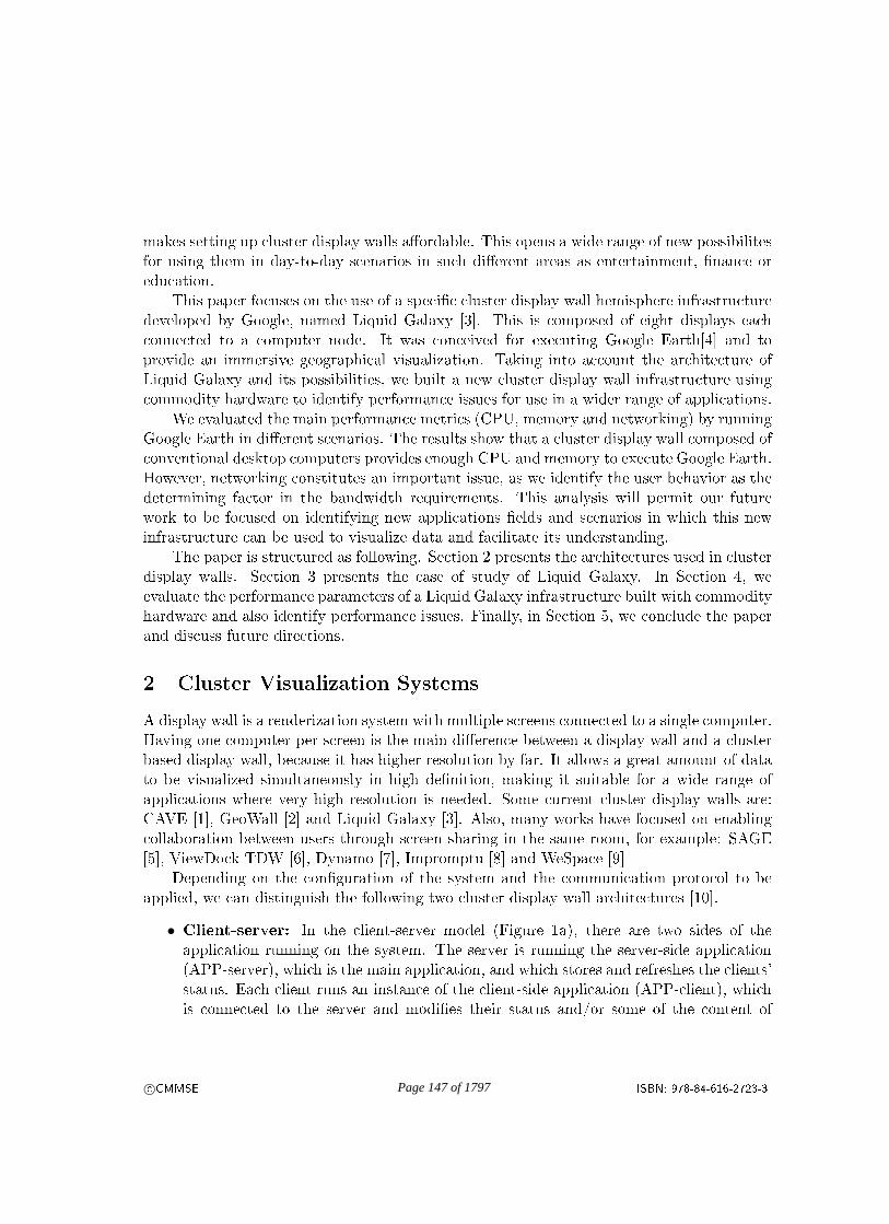
makes setting up cluster display walls aordable. This opens a wide range of new possibilitesfor using them in day-to-day scenarios in such dierent areas as entertainment, nance oreducation.

This paper focuses on the use of a specic cluster display wall hemisphere infrastructuredeveloped by Google, named Liquid Galaxy [3]. This is composed of eight displays eachconnected to a computer node. It was conceived for executing Google Earth[4] and toprovide an immersive geographical visualization. Taking into account the architecture ofLiquid Galaxy and its possibilities, we built a new cluster display wall infrastructure usingcommodity hardware to identify performance issues for use in a wider range of applications.

We evaluated the main performance metrics (CPU, memory and networking) by runningGoogle Earth in dierent scenarios. The results show that a cluster display wall composed ofconventional desktop computers provides enough CPU and memory to execute Google Earth.However, networking constitutes an important issue, as we identify the user behavior as thedetermining factor in the bandwidth requirements. This analysis will permit our futurework to be focused on identifying new applications elds and scenarios in which this newinfrastructure can be used to visualize data and facilitate its understanding.

The paper is structured as following. Section 2 presents the architectures used in clusterdisplay walls. Section 3 presents the case of study of Liquid Galaxy. In Section 4, weevaluate the performance parameters of a Liquid Galaxy infrastructure built with commodityhardware and also identify performance issues. Finally, in Section 5, we conclude the paperand discuss future directions.

2 Cluster Visualization Systems

A display wall is a renderization system with multiple screens connected to a single computer.Having one computer per screen is the main dierence between a display wall and a clusterbased display wall, because it has higher resolution by far. It allows a great amount of datato be visualized simultaneously in high denition, making it suitable for a wide range ofapplications where very high resolution is needed. Some current cluster display walls are:CAVE [1], GeoWall [2] and Liquid Galaxy [3]. Also, many works have focused on enablingcollaboration between users through screen sharing in the same room, for example: SAGE[5], ViewDock TDW [6], Dynamo [7], Impromptu [8] and WeSpace [9]

Depending on the conguration of the system and the communication protocol to beapplied, we can distinguish the following two cluster display wall architectures [10].

• Client-server: In the client-server model (Figure 1a), there are two sides of theapplication running on the system. The server is running the server-side application(APP-server), which is the main application, and which stores and refreshes the clients'status. Each client runs an instance of the client-side application (APP-client), whichis connected to the server and modies their status and/or some of the content of

c©CMMSE ISBN: 978-84-616-2723-3Page 147 of 1797

the APP-server. The user can choose one of the client nodes to interact with. Thisarchitecture can be used to execute both interactive and non-interactive applications.Interactive applications are those that allow a user to access a client node and mod-ify its status. Consequently, it will send the changes to the server making the othersclients fetch these new data and refreshing the stored status for that client node. Opti-Planet [11], Equalizer [12], Chromium [13] and CGLX [14] are examples of interactiveapplications to be executed in a cluster display wall environment. The non-interactiveapplications do not usually allow any changes by the user, although, in the case thatthe user could make some, these would not aect either the server or the other clients.An example of a non-interactive application is Video Streaming [15].

(a) Client-Server (b) Master-Slave

Figure 1: Cluster display wall architectures

• Master-Slave: In the Master-Slave architecture (Figure 1b), each node runs the sameapplication (APP), so the master must manage the synchronization among slaves toensure consistency. The master is the only node that accepts user input and every timethat the master modies its status, it sends the changes to the slaves. Applicationsfor this kind of architecture are usually interactive, such as Google Earth.

In this paper, we focus on the Master-Slave architecture. We study the performancecharacteristics of this kind of system with the specic platform, Liquid Galaxy, which isimplemented in a cluster display wall, developed by Google, to run Google Earth. In thenext section, we present the characteristics of the Liquid Galaxy system.

c©CMMSE ISBN: 978-84-616-2723-3Page 148 of 1797

3 Liquid Galaxy

Liquid Galaxy [3] is a cluster display wall originally built to run Google Earth [4] in orderto create an immersive experience for the user. Liquid Galaxy lets you navigate around theglobe with its 6-axis controller, allowing you instantly zoom in, out, and turn around withcompletely uid motion. You can also search and navigate to specic locations on autopilotusing a touch-screen interface. Figure 2 shows an example of the Google Liquid Galaxyinstalled in the Technological Park in the city of Lleida (Spain) [16].

Figure 2: Lleida Liquid Galaxy

The connection schema of the Liquid Galaxy is depicted in Figure 3, which also indicatesthe dierent running steps.

We can see that each node runs the Google Earth application (GE) and the user onlyinteracts with the master node by means of a 3D mouse. Each movement of the mouse makesthe master node launch a synchronization protocol that consists of the following steps:

1. The master node captures the coordinates (Coords) of the position in Google Earth in-dicated by the user. These coordinates are codied in a UDP packet, named ViewSync,which contains the following information from the view in the application: latitude,longitude, altitude, heading, tilt, roll and planet name.

2. When the master's view is moved, it sends ViewSync packets to broadcast with theobjective of sending it to all the nodes in the network.

3. Every slave node has a conguration le, which holds an oset from the original

c©CMMSE ISBN: 978-84-616-2723-3Page 149 of 1797

Figure 3: Google Earth Architecture

master's view. When the slaves receive a ViewSync packet from the master, theyautomatically calculate and adjust their relative view by adding the local oset.

4. Every node accesses Internet with its own coordinates to download the required data(maps, imagery, 3D layer, etc.) independently from the other nodes.

As we have seen in previous steps, every node executes its own instance of Google Earth,so every node needs an Internet connection to download all the data. For this reason, a web-proxy distributed cache ts very well. Squid [17] is the ocial distributed cache and is alsoincluded in Liquid Galaxy. All nodes will share the same disk cache stored in each node'sSSD. With this solution, the amount of data requests from Internet can be reduced. So, ifthe information is available in the distributed Squid cache, shared by all nodes as peers, itis taken independently by each node.

The Liquid Galaxy system presented in this section was built specically to give serviceto run Google Earth. However, the immersive visualization environment that Liquid Galaxyprovides opens this kind of system for use in a wide range of applications that can benetfrom an immersive visualization environment. Some examples of applications that can berun in this system are WebGL with Aquarium [18], video streaming [15], videogames likeQuake 3 Arena [19], etc.

c©CMMSE ISBN: 978-84-616-2723-3Page 150 of 1797

Taking this possibility into account, we built a new experimental infrastructure that wenamed Liquid Galaxy Code. This new platform is composed of commodity hardware with theaim of enabling it to be built economically thus ensuring extensive use. An experimentationprocess was carried out on this platform to evaluate its viability. This process is reportedin the next section.

4 Experimentation

Figure 4: Liquid Galaxy Code

In this section, an experimentation process is carried out to measure and categorize theoverhead produced by the use of Google Earth in the Liquid Galaxy Code infrastructure inorder to show the resource requirements in usual displacements along the globe. In Figure4, we can see the experimentation platform, which is a cluster display wall of 3 Intel Corei5 3GHz machines, with 2x4GB RAM 1600 MHz, SSD 128GB, NVidia GT620 with three32" screens. One node acts as a master and the other two as slaves. This platform wasbuilt with commodity hardware in order to evaluate the viability of using general-purposeplatforms to visualize high-resolution images in a cluster based way.

For the application under study, the requirements for computing resources vary withthe environment to be visualized. Thus, we measured the three following environments,illustrated in Figure 5, with signicant dierences in the number of high-dened 3D buildingsto be visualized:

• City: A high-density place made up by 3D buildings.

c©CMMSE ISBN: 978-84-616-2723-3Page 151 of 1797

(a) City tour (b) Town tour (c) Desert tour

Figure 5: Images of the three tested environments

• Town: A low to medium-density place that combines zones with few 3D buildings andareas without them.

• Desert: A low-resolution without any 3D buildings to be loaded.

Every environment, or tour, moves throughout eight specic points of interest with apreviously-established time interval between consecutive jumps. We distinguish the twofollowing intervals:

• Long time jumps: the time interval for moving between two consecutive places is 14seconds.

• Short time jumps: the time interval has been set to 7 seconds.

Under the experimentation framework presented above, the key computing resources,CPU, memory and networking were monitored using the Top and Tshark (Command-linebased WireShark) tools. The results are presented below.

4.1 Experimental Results

In our experimentation, both the master and slave nodes were monitored. The resultsobtained showed that there are no dierence between the master node and the slaves. Forthis reason, we only present the results obtained from the master node.

Figure 6 shows the percentage of CPU usage for the three described environments andboth timing jumps. In the short time jumps, there was no dierence between the threeenvironments, and the use of CPU averaged 25% for all of them. This is due to the factthat there was not enough time between jumps to load the needed data. On the otherhand, for the long time jumps, there was a remarkable dierence depending on the kindof environment. The big dierence was in the desert test where there were peaks at eachidle position. This was caused by the low-resolution imagery and the lack of 3D buildings.This made the time interval between jumps long enough to allow the images to be fullyloaded. Referring to the other environments, city and town, similar behavior can be seen

c©CMMSE ISBN: 978-84-616-2723-3Page 152 of 1797

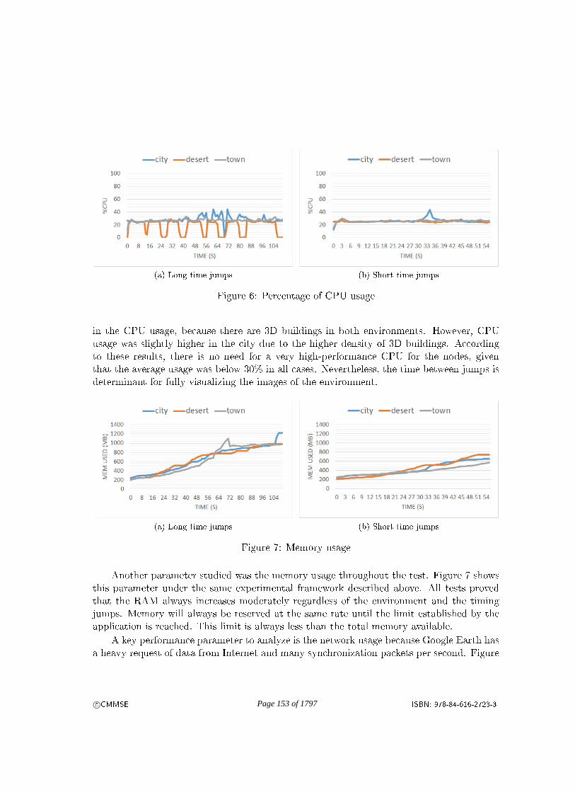
(a) Long time jumps (b) Short time jumps

Figure 6: Percentage of CPU usage

in the CPU usage, because there are 3D buildings in both environments. However, CPUusage was slightly higher in the city due to the higher density of 3D buildings. Accordingto these results, there is no need for a very high-performance CPU for the nodes, giventhat the average usage was below 30% in all cases. Nevertheless, the time between jumps isdeterminant for fully visualizing the images of the environment.

(a) Long time jumps (b) Short time jumps

Figure 7: Memory usage

Another parameter studied was the memory usage throughout the test. Figure 7 showsthis parameter under the same experimental framework described above. All tests provedthat the RAM always increases moderately regardless of the environment and the timingjumps. Memory will always be reserved at the same rate until the limit established by theapplication is reached. This limit is always less than the total memory available.

A key performance parameter to analyze is the network usage because Google Earth hasa heavy request of data from Internet and many synchronization packets per second. Figure

c©CMMSE ISBN: 978-84-616-2723-3Page 153 of 1797

(a) Long time jumps (b) Short time jumps

Figure 8: Networking.

8 presents the network graph measured in kilobytes/s. Despite having the Squid cache [17]activated, we can still perceive peaks whenever a request for data is made. This happensbecause Squid only has an average of 20% cache hits, leading the nodes to download newdata when the next place to visit is far away. There is also a common starting peak in bothtimings and all the tours. This initial peak appears because the tour starts with a generalview of the Earth and has to move to the rst coordinate, having to load all the data untilthe rst position is reached. We can also note that the desert tour has a lower data-requestbecause it has no 3D buildings and low-resolution maps to download. Regarding the graph ofshort time jumps, the time between jumps is so close that the 3D layer has almost no time toload, making it unnecessary to request that heavy-load data. The synchronization betweenslaves is very abundant but it does not have very much weight, making it unnoticeable forthe network. So, the local network does not need a high bandwidth.

5 Conclusions and Future Work

In this paper, we have presented a cluster display wall infrastructure, named Liquid GalaxyCode, which has been built with commodity hardware. We analyzed the performance ofthis system running Google Earth, so that the results may be indicative of the viability ofusing this kind of infrastructure in a wide range of everyday applications. These applicationscan benet from an immersive visualization environment showing the viability of using thetested platform in a more extensive way.

The performance analysis have shown that CPU, memory and local network are enoughto visualize the images. However, the bandwidth of the external network constitutes abottleneck. This causes that the user navigation behaviour in the tested environments,is determinant in order to be able to load all the needed data. Thus, the time intervalbetween consecutive displacements has to be adjusted according to the density of data of

c©CMMSE ISBN: 978-84-616-2723-3Page 154 of 1797

the environment to be visualized.

In the future works, we plan to indentify new scenarios and applications from dierentelds, such as education, nance, chemistry or biology, which can benet from the presentedplatform built with o-the-shelf hardware. Additionally, we will study how to adjust andsynchronize a cluster display wall composed of heterogeneous nodes.

Acknowledgements

We would like to thank to the company Ponent 2002 for facilitating the use of the LleidaLiquid Galaxy and specically to Andreu Ibañez for his collaboration in understanding itsoperation.

References

[1] T. A. DeFanti, D. Acevedo, R. A. Ainsworth, M. D. Brown, S. Cutchin, G. Dawe, K.-U. Doerr, A. Johnson, C. Knox, R. Kooima, et al., The future of the CAVE, CentralEuropean Journal of Engineering, vol. 1, no. 1, pp. 1637, 2011.

[2] A. Johnson, J. Leigh, P. Morin, and P. Van Keken, Geowall: Stereoscopic visualizationfor geoscience research and education, Computer Graphics and Applications, IEEE,vol. 26, no. 6, pp. 1014, 2006.

[3] Google, Liquid Galaxy live demo at TED. Lecture Notes in Computer Science,Springer, 2010.

[4] Google, Google earth, 2013. http://www.google.com/earth/index.html.

[5] L. Renambot, A. Rao, R. Singh, B. Jeong, N. Krishnaprasad, V. Vishwanath, V. Chan-drasekhar, N. Schwarz, A. Spale, C. Zhang, et al., SAGE: the Scalable Adaptive Graph-ics Environment, in Proceedings of WACE, vol. 9, pp. 200409, Citeseer, 2004.

[6] C. D. Lau, M. J. Levesque, S. Chien, S. Date, and J. H. Haga, ViewDock TDW: high-throughput visualization of virtual screening results, Bioinformatics, vol. 26, no. 15,pp. 19151917, 2010.

[7] S. Izadi, H. Brignull, T. Rodden, Y. Rogers, and M. Underwood, Dynamo: a publicinteractive surface supporting the cooperative sharing and exchange of media, in Pro-

ceedings of the 16th annual ACM symposium on User interface software and technology,pp. 159168, ACM, 2003.

c©CMMSE ISBN: 978-84-616-2723-3Page 155 of 1797

[8] J. T. Biehl, W. T. Baker, B. P. Bailey, D. S. Tan, K. M. Inkpen, and M. Czerwinski, Im-promptu: a new interaction framework for supporting collaboration in multiple displayenvironments and its eld evaluation for co-located software development, in Proceed-

ings of the SIGCHI Conference on Human Factors in Computing Systems, pp. 939948,ACM, 2008.

[9] D. Wigdor, H. Jiang, C. Forlines, M. Borkin, and C. Shen, WeSpace: the designdevelopment and deployment of a walk-up and share multi-surface visual collaborationsystem, in Proceedings of the SIGCHI Conference on Human Factors in Computing

Systems, pp. 12371246, ACM, 2009.

[10] C. N. Oliver G. Staadt, Justin Walker and B. Hamann, A survey and performanceanalysis of software platforms for interactive cluster-based multi-screen rendering, Eu-rographics Workshop on Virtual Environments, 2003.

[11] L. Smarr, M. Brown, and C. de Laat, Special section: OptIPlanetthe OptIPuterglobal collaboratory, Future Generation Computer Systems, vol. 25, no. 2, pp. 109113, 2009.

[12] S. Eilemann, M. Makhinya, and R. Pajarola, Equalizer: A scalable parallel renderingframework, Visualization and Computer Graphics, IEEE Transactions on, vol. 15,no. 3, pp. 436452, 2009.

[13] G. Humphreys, M. Houston, R. Ng, R. Frank, S. Ahern, P. D. Kirchner, and J. T.Klosowski, Chromium: a stream-processing framework for interactive rendering onclusters, in ACM Transactions on Graphics (TOG), vol. 21, pp. 693702, ACM, 2002.

[14] K. Doerr and F. Kuester, CGLX: a scalable, high-performance visualization frame-work for networked display environments, Visualization and Computer Graphics, IEEE

Transactions on, vol. 17, no. 3, pp. 320332, 2011.

[15] Panoramic Video Streaming.https://code.google.com/p/liquid-galaxy/wiki/PanoramicVideo.

[16] P. 2002, G-liquid galaxy, 2012. http://www.g-liquidgalaxy.com/.

[17] T. Squid, Squid web proxy cache, 2002.

[18] Greggman and H. Engines, Aquarium WebGL.http://webglsamples.googlecode.com/hg/aquarium/aquarium.html.

[19] OpenArena Team, OpenArena (Quake 3 Arena), 2005. www.openarena.ws.

c©CMMSE ISBN: 978-84-616-2723-3Page 156 of 1797

Proceedings of the 13th International Conferenceon Computational and Mathematical Methodsin Science and Engineering, CMMSE 201324–27 June, 2013.

High-order iterative methods by using weight functionstechnique

Santiago Artidiello1, Alicia Cordero2, Juan R. Torregrosa2 and MariaVassileva1

1 Ciencias Basicas y Ambientales, Instituto Tecnologico de Santo Domingo (INTEC),Dominican Republic

2 Instituto de Matematica Multidisciplinar, Universitat Politecnica de Valencia, Spain

emails: santiago.artidiello@intec.edu.do, acordero@mat.upv.es,jrtorre@mat.upv.es, maria.penkova@intec.edu.do

Abstract

In this work, two families of optimal iterative methods of order eight, for solvingnonlinear equations, are presented. We design them by using the weight function tech-nique, with functions of one, two and three variables. The study of dynamical andnumerical behavior of some elements of these families complete this paper.

Key words: Nonlinear equation, Iterative schemes, optimal methods, weight func-tions technique, efficiency index

MSC 2000: 65H05, 37F10

1 Introduction

Many problems in science and engineering include the search of the solutions of an equationof nonlinear nature. The importance of this type of troubleshooting has showed the needto develop iterative methods for the resolution of these equations.

We consider the problem of finding a zero of a nonlinear function f : I ⊂ R → R, thatis, a solution ξ ∈ I of

f(x) = 0, (1)

restricted to real functions with a unique solution inside an open interval I. Currently thereexist numerous iterative methods for solving the nonlinear equation (1). The majority of

c⃝CMMSE ISBN: 978-84-616-2723-3Page 157 of 1797

High-order iterative methods

the computationally useful techniques to determine roots can be classified into one of thetwo classes: (a) iterative methods that require only functional evaluations of f , and (b)methods whose iterative formula require evaluations of the function and its derivatives.There are two known simple and effective methods that represent these classes: Steffensen’and Newton’s methods, respectively, both with order of convergence two (see, for example[6]). The search of variants of these methods with an accelerated convergence and a reducednumber of operations and functional evaluations has resulted in multistep methods. Theseschemes belong to the class of most powerful methods that overcome the limitations of themethods of a point with respect to the order of convergence and computational efficiency.This type of iterative methods were extensively studied in Traub’s book, [11] and morerecently, in [8].

Newton’s method is among the most used procedures. Many authors have studied andproposed various multistep methods that modify the mentioned scheme to solve nonlinearequations with a high-order of convergence (see [4, 3, 2]). However, these must use deriva-tives, which is a serious disadvantage. Sometimes, the applications of iterative algorithmsthat depend on derivatives are restricted in engineering and science. For these cases, differ-ent authors have developed derivative-free iterative methods in numerous papers, that onlyneed the additional evaluations of the function (see [12, 9, 5, 10]).

In this paper, following the ideas presented in [7] and [1], we present two families ofiterative methods belonging to classes (a) and (b), respectively, both of eighth-order ofconvergence.

2 Design of the families

Let us remember that the iterative expression of Steffensen’s scheme is

xk+1 = xk −f(xk)

2

f(xk + f(xk))− f(xk)(2)

and Newton’s one is

xk+1 = xk −f(xk)

f ′(xk). (3)

If we compose any of these methods with itself, schemes of order 4 with 4 functionalevaluations are obtained in both cases. That makes them non-optimal, according to theconjecture of Kung-Traub [13].

In double Newton scheme, let us consider a frozen derivative in the second step, ob-taining a non-optimal method of order 3 (see [11]), whose iterative expression is:

yk = xk −f(xk)

f ′(xk),

xk+1 = yk −f(yk)

f ′(xk). (4)

c⃝CMMSE ISBN: 978-84-616-2723-3Page 158 of 1797

S. Artidiello, A. Cordero, J.R. Torregrosa, M. Vassileva

The authors in [1], using the technique of weight functions, got to increase to four theorder of convergence of (4) without adding new functional evaluations. The iterative schemeof the obtained method is

yk = xk −f(xk)

f ′(xk),

xk+1 = yk −H(uk)f(yk)

f ′(xk), (5)

where H(uk) represents a real-valued function and uk =f(yk)

b1f(xk) + b2f(yk), being b1 and b2

real parameters.Now, let us consider the double Steffensen scheme, holding the expression of the de-

nominator in the second step

yk = xk −f(xk)

f [zk, xk],

xk+1 = yk −f(yk)

f [zk, xk], (6)

where zk = xk + f(xk) and f [zk, xk] =f(zk)− f(xk)

zk − xk. By using the technique of weight

functions, Petkovic et al. in [7] increase to four the order of convergence of method (6)without adding new functional evaluations. The iterative scheme of the resulting method is

yk = xk −f(xk)

f [zk, xk],

xk+1 = yk −H(uk, vk)f(yk)

f [zk, xk], (7)

where zk = xk +βf(xk), uk =f(yk)

f(xk)and vk =

f(yk)

f(zk). Under some conditions on H and for

nonzero arbitrary values of β, (7) is an optimal method of order four.Following this idea, we design a class of three-steps methods, that satisfies the following

result.

Theorem 1 Let ξ ∈ I be a simple zero of a sufficiently differentiable function f : I ⊂ R →R on the open interval I. Let H and G be sufficiently differentiable real functions and x0be an initial approximation close enough to ξ. If β = 1 and H and G satisfy H(0) = 1,H ′(0) = 2b1, H

′′(0) = 2b1(2b1+ b2), G(0, 0) = Gv(0, 0) = 1, Gu(0, 0) = 2b1, Guv(0, 0) = 4b1and Guu = 2b1(3b1 + b2), then the method

yk = xk − βf(xk)

f ′(xk),

c⃝CMMSE ISBN: 978-84-616-2723-3Page 159 of 1797

High-order iterative methods

zk = yk −H(uk)f(yk)

f ′(xk), (8)

xk+1 = zk −G(uk, vk)f(zk)

f ′(xk),

where uk =f(yk)

b1f(xk) + b2f(yk), being b1 and b2 arbitrary real parameters and vk =

f(zk)

f(yk),

has order of convergence eight for any value b1 different from zero.

From Theorem 1, we see that the most simple functions H and G are

H(u) = 1 + 2b1u+ b1(2b1 + b2)u2,

G(u, v) = 1 + 2b1u+ v + b1(3b1 + b2)u2 + 4b1uv. (9)

If b1 = 1 and b2 = −2 then H = 1 + 2u and the first two steps of (8) correspond to theOstrowski’s method. In this case function G is G = 1 + 2u+ v + u2 + 4uv.

Respect to the class (b) of iterative schemes and from (7), we obtain the followingresult.

Theorem 2 Let ξ ∈ I be a simple zero of a sufficiently differentiable function f : I ⊂ R →R on the open interval I and be x0 one initial approximation close enough to ξ. Let H andG be sufficiently differentiable real functions which satisfy: H(0, 0) = Hu(0, 0) = Hv(0, 0) =1, Huu(0, 0) = Hvv(0, 0) = 2, Huv(0, 0) = 0, G(0, 0, 0) = Gu(0, 0, 0) = Gv(0, 0, 0) =Gw(0, 0, 0) = 1, Guu(0, 0, 0) = Gvv(0, 0, 0) = Guw(0, 0, 0) = Gvw(0, 0, 0) = 2, Guv(0, 0, 0) =1, |Gww(0, 0, 0)| < ∞. Then the method

yk = xk −f(xk)

f [zk, xk],

tk = yk −H(uk, vk)f(yk)

f [zk, xk], (10)

xk+1 = tk −G(uk, vk, wk)f(tk)

f [zk, xk],

where zk = xk+βf(xk), uk =f(yk)

f(xk), vk =

f(yk)

f(zk)and wk =

f(tk)

f(yk), has order of convergence

eight for any value β different from zero.

The most simple functions H and G in this case are

H(u, v) = 1 + u+ v + u2 + v2,

G(u, v, w) = 1 + u+ v + w + u2 + v2 + uv + 2(vw + uw). (11)

c⃝CMMSE ISBN: 978-84-616-2723-3Page 160 of 1797

S. Artidiello, A. Cordero, J.R. Torregrosa, M. Vassileva

Remark 1 The families of three-point methods (8) and (10) require four functional eval-uations and have order of convergence eight. Therefore, these families are optimal in thesense of the Kung-Traub conjecture and have computational efficiency index 81/4 ≈ 1.6818.

In the following sections we are going to use the elements of the families (8) and (10)obtained by choosing the weight functions (9) and (11) and the values of the parametersb1 = 1 and b2 = 0. These elements will be denoted by M1 and M2, respectively.

3 Dynamical aspects

The dynamical properties of the rational function associated to an iterative method actingon a polynomial give us important information about numerical features of the method asits stability and reliability (see [15]).

The dynamical behavior of the orbit of a point on the complex plane can be classifieddepending on its asymptotic behavior. In this way, a point in the Riemann sphere z0 ∈ C isa fixed point of R if R(z0) = z0. A fixed point is attracting, repelling or neutral if |R′(z0)|is less than, greater than or equal to 1, respectively. Moreover, if |R′(z0)| = 0, the fixedpoint is superattracting.

If z∗ is an attracting fixed point of the rational function R, its basin of attraction A(z∗)is defined as the set of pre-images of any order such that

A(z∗f ) =z0 ∈ C : Rn(z0) → z∗, n → ∞

. (12)

The set of points whose orbits tends to an attracting fixed point z∗f is defined as theFatou set, F(R). The complementary set in the Riemann sphere, the Julia set J (R), is theclosure of the set consisting of its repelling fixed points, and establishes the borders betweenthe basins of attraction.

In order to draw the dynamical planes, each point of the complex plane is consideredas a starting point of the iterative scheme and it is painted in different colors dependingon the point which it has converged to. The figures has been generated for values of z0 in[−2, 2]× [−2, 2], with a mesh of 800× 800 points and 80 iterations per point. Depending onthe number of iterations needed to converge, the color of the starting point will be brighter(less iterations) or darker (more iterations). We will represent the dynamical behavior of thementioned elements of the two suggested classes, (8) and (10), for low-degree polynomials,showing their stability and the amplitude of the convergence regions in these cases.

When the element of family (8) M1 is considered, we observe in Figure 1 the basin ofattraction of the different roots of low-degree polynomials. It is possible to observe someregions of slow convergence, in form of ”flowers”, whose petals make narrower while theconvergence is slower. The black point in the center of the flowers correspond to regions

c⃝CMMSE ISBN: 978-84-616-2723-3Page 161 of 1797

High-order iterative methods

IRez−2 −1.5 −1 −0.5 0 0.5 1 1.5 2

(a) x2 − 1

IRez−2 −1.5 −1 −0.5 0 0.5 1 1.5 2

(b) x3 − 1

Figure 1: Dynamical planes for the eighth-order family with derivatives

of no convergence. The observed dynamical planes define wide amplitudes for the differentbasins of the roots.

If we consider now the rational function associated to the element of family (10) andanalyze its dynamical behavior, we find that there exist black regions in the dynamicalplanes (see Figure 2) whose orbits do not tend to any of the roots, but to the infinity. So,the are wide regions of no convergence. Moreover, it can be observed that the amplitude ofthe convergence regions is narrower in some cases. Nevertheless, the convergence improveswhen beta is closer to zero than when it is near one.

In Figure 3, we show the dynamical planes corresponding to function f(x) = 10xe−x2−1in [−2, 2] × [−2, 2], where two simple roots appear. These planes have been obtained byusing Newton, M1 and M2 methods. In all cases, it can be observed that wide regions ofnon convergence appear. Some of them are due to poles of the function f . We observethat the behavior of the proposed methods is not very different from the one of Newton’sscheme.

4 Numerical results

In this section we demonstrate the convergence behavior of the proposed families (8) and(10). In the numerical test made, variable precision arithmetics has been used, with4000 digits of mantissa in Matlab R2010a. In our numerical experiments to comparethe derivative-free iterative methods and the iterative methods that use derivative, we

c⃝CMMSE ISBN: 978-84-616-2723-3Page 162 of 1797

S. Artidiello, A. Cordero, J.R. Torregrosa, M. Vassileva

IRez−2 −1.5 −1 −0.5 0 0.5 1 1.5 2

(a) x2 − 1, β = 0.9

IRez−2 −1.5 −1 −0.5 0 0.5 1 1.5 2

(b) x2 − 1, β = 0.01

Rez−2 −1.5 −1 −0.5 0 0.5 1 1.5 2

(c) x3 − 1, β = 0.9

Rez−2 −1.5 −1 −0.5 0 0.5 1 1.5 2

(d) x3 − 1, β = 0.01

Figure 2: Dynamical planes for the eighth-order family without derivatives

use Newton’s method (NM): xk+1 = xk − f(xk)f ′(xk)

, Steffensen’s method (SM): xk+1 = xk −f(xk)

2

f(xk+f(xk))−f(xk), Ostrowski’s method (OM) [17]: xk+1 = yk − f(yk)

f(xk)−2f(yk)f(xk)f ′(xk)

, where

yk = xk − f(xk)f ′(xk)

, and several iterative methods, quoted below

c⃝CMMSE ISBN: 978-84-616-2723-3Page 163 of 1797

High-order iterative methods

IRez

IImz

−2 −1.5 −1 −0.5 0 0.5 1 1.5 2

−2

−1.5

−1

−0.5

0

0.5

1

1.5

2

(a) NewtonIRez

Imz

−2 −1.5 −1 −0.5 0 0.5 1 1.5 2

−2

−1.5

−1

−0.5

0

0.5

1

1.5

2

(b) M1

Rez

Imz

−2 −1.5 −1 −0.5 0 0.5 1 1.5 2

−2

−1.5

−1

−0.5

0

0.5

1

1.5

2

(c) M2, β = 0.9Rez

Imz

−2 −1.5 −1 −0.5 0 0.5 1 1.5 2

−2

−1.5

−1

−0.5

0

0.5

1

1.5

2

(d) M2, β = 0.01

Figure 3: Dynamical planes for function 10xe−x2 − 1

KWM [4]

yk = xk −f(xk)

f ′(xk)

zk = yk −H1f(yk)

f ′(xk)

xk+1 = zk −[(1 +H1)

2 + (1 + 4H1)H2

] f(zk)

f ′(xk)

where H1 =f(xk)

f(xk)−2f(yk)and H2 =

f(zk)f(yk)−3f(zk)

.

c⃝CMMSE ISBN: 978-84-616-2723-3Page 164 of 1797

S. Artidiello, A. Cordero, J.R. Torregrosa, M. Vassileva

CTVM [2]

yk = xk −f(xk)

f ′(xk)

zk = yk −Hf(yk)

f ′(xk)

xk+1 = uk −(1 +H +

1

2T + L

)f(zk)

f ′(xk)

where H = f(xk)f(xk)−2f(yk)

, T = f(zk)f(yk)−2f(zk)

and L = 3uk−zkyk−xk

.

ZLHM [12]

yk = xk −f(xk)

f [xk, zk]

zk = yk −f(yk)

f [yk, xk] + f [yk, xk, zk](yk − xk)

xk+1 = uk −f(uk)

f [uk, yk] + f [uk, yk, xk](uk − yk) + f [uk, yk, xk, zk](uk − yk)(uk − xk)

SKM [10]

yk = xk −f(xk)

f [xk, zk]

uk = yk −Hf(xk)

f [xk, zk]

xk+1 = uk −Gf(uk)

f [xk, zk]

where H = 1 + w1(xk) + w2(xk), w1(xk) = f(yk)f(xk)

, w2(xk) = f(yk)f(zk)

, G = g1 + g2 + g3,

g1 = 1+(2− f [xk, zk])w1(xk)+ (1− f [xk, zk])w1(xk)2, g2 = (4− f [xk, zk](6+ f [xk, zk](−4+

f [xk, zk])))w1(xk)3, g3 = w3(xk) + w3(xk)

2 + (4 − 2f [xk, zk])w4(xk), w3(xk) = f(uk)f(yk)

and

w4 =f(uk)f(zk)

.

Table 1 shows the expression of the test functions, the roots with sixteen significantdigits and the initial approximation x0 which is the same for all methods. Displayed inTable 2 is the number of iterations (It), the computational order of convergence (COC), theabsolute values of the function |f(xk)| and root obtained at each method ξ.

c⃝CMMSE ISBN: 978-84-616-2723-3Page 165 of 1797

High-order iterative methods

Table 1: Test functions and their roots

Test functions Roots Starting points

f1 =√x4 + 8 sin

(π

x2+2

)+ x3

x4+1−

√6 + 8

17 ξ1 = −2.000000000000000 x0 = −1.8

ξ2 = −1.149212674609088

f2 = x exp(x2)− sin(x2) + 3 cos(x) + 5 ξ = −1.201576112092293 x0 = 2

f3 =√x2 + 2x+ 5− 2 sin(x)− x2 + 3 ξ1 = +2.3319676558839640 x0 = 1

ξ2 = −2.573166514902827

f4 = x4 + sin(

πx2

)− 5 ξ1 = +1.414213562373095 x0 = 2

ξ2 = −1.414213562373095

f5 =(sin(x)− x

2

)2ξ = 0 (double root) x0 = 0.5

5 Conclusions

These results that shown in the Table 1 are in accordance with the efficiency analysis theshow in Theorem 1 and Theorem 2 presented in Section 2. Both the numerical results, suchas the dynamic analysis show that derivative-free methods are more sensitive to the initialapproximation comparing them with those that use derivatives.

Acknowledgements

This research was supported by Ministerio de Ciencia y Tecnologıa MTM2011-28636-C02-02and FONDOCYT 2011-1-B1-33 Republica Dominicana.

References

[1] S. Artidiello, F. Chicharro, A. Cordero and J.R. Torregrosa, Local conver-gence and dynamical analysis of a new family of optimal fourth-order iterative methods,Inter. J. of Comp. Math., DOI: 10.1080/00207160.2012.748900.

[2] A. Cordero, J.R. Torregrosa and M. Vassileva, Tree-step iterative methodwith a optimal eighth order of convergence, J. of Comp. and Appl. Math, 235 (2011)3189–3194.

c⃝CMMSE ISBN: 978-84-616-2723-3Page 166 of 1797

S. Artidiello, A. Cordero, J.R. Torregrosa, M. Vassileva

Tab

le2:

Com

parison

ofvariou

sderivative-free

iterativemethods

NM

SM

OM

KW

MCTVM

M1

ZLHM

SKM

M2

f 1It

99

53

34

34

3COC

2.0000

2.00

004.0000

8.2176

8.3082

8.0000

8.1662

7.9999

8.0000

|f(x

n)|

1.6e-479

2.3e-574

8.8e-752

9.8e-359

1.4e-329

9.6e-2525

6.6e-431

4.2e-1882

9.6e-2522

root

ξ 1ξ

ξ 1ξ 1

ξ 1ξ 1

ξ 1ξ 1

ξ 1f 2

It14

n.c.

53

34

4n.c.

4COC

2.0000

4.0000

7.9547

7.9386

8.0203

8.0038

8.0203

|f(x

n)|

2.6e-553

7.9e-1063

3.5e-517

8.6e-485

5.0e-528

3.7e-1066

5.0e-528

root

ξξ

ξξ

ξξ

ξ

f 3It

88

53

33

314

3COC

2.0000

2.00

003.9998

8.0286

7.9075

7.9753

8.0003

7.6578

7.9753

|f(x

n)|

3.2e-422

1.8e-334

2.7e-1292

5.6e-560

6.7e-622

4.0e-545

9.0e-556

4.4e-080

4.0e-545

root

ξ 1ξ 1

ξ 1ξ 1

ξ 1ξ 1

ξ 1ξ 1

ξ 1f 4

It9

705

43

n.c.

46

n.c.

COC

2.0000

2.00

004.0000

8.0232

7.6465

8.0353

8.0000

|f(x

n)|

8.2e-425

5.1e-306

5.6e-621

1.3e-1714

2.3e-333

1.3e-092

2.7e-1750

root

ξ 1ξ 2

ξ 2ξ 1

ξ 1ξ 1

ξ 1f 5

It536

536

268

n.c.

194

226

179

226

225

COC

1.0000

1.00

001.0000

1.0000

1.0000

1.0000

1.0000

1.0000

|f(x

n)|

7.1e-325

7.9e-325

1.0e-326

3.1e-325

3.5e-325

2.5e-325

2.0e-324

3.5e-325

root

ξξ

ξξ

ξξ

ξξ

ξ

c⃝CMMSE ISBN: 978-84-616-2723-3Page 167 of 1797

High-order iterative methods

[3] Y. Khan, M. Fardi and K. Sayevand, A new general eighth-order family of iterativemethods for solving nonlinear equations, Appl. Math. L. 25 (2012) 2262–2266.

[4] J. Kou and X. Wang, Some improvements of Ostrowski’s method, Appl. Math. L.,23 (2010) 92–96.

[5] Z. Liu, Q. Zheng and P. Zhao, A variant of Steffensen’s method of fourth-orderconvergence and its applications, Appl. Math. and Comput., 216 (2010) 1978–1983.

[6] J.M. Ortega and W.G. Rheinboldt, Iterative solutions of nonlinear equations inseveral variables, Academic Press, New York, 1970.

[7] M.S. Petkovic, S. Ilic and J. Dzunic, Derivative free two-point methods with andwithout memory for solving nonlinear equations, Appl. Math. and Comput., 217 (2010)1887–1895.

[8] M. Petkovic, B. Neta, L. Petkovic and J. Dzunic, Multipoint methods forsolving nonlinear equations, Academic Press, 2012.

[9] H. Ren, Q. Wu and W. Bi, A class of two-step Steffensen type methods with fourth-order convergence, Appl. Math. and Comput., 209 (2009) 206–210.

[10] F. Soleymani and S.K. Khattri, Finding simple roots by seventh- and eighth-orderderivative-free methods, Int. J. Math. Models Meth. Appl. Sci., 1 (2012) 45–52.

[11] J. F. Traub, Iterative methods for the solution of equations, Chelsea Publishing Com-pany, New York, 1977.

[12] Q. Zheng, J. Li and F. Huang, An optimal Steffensen-type family for solving non-linear equations,Appl. Math. and Comput. 217, (2011) 9592–9597.

[13] H.T. Kung and J. F. Traub, Optimal order of one-point and multipoint iteration,J. Assos. Comput. Math. 21 (1974) 643–651.

[14] Q. Zheng, P. Zhao, L. Zhang and W. Ma, Variants of Steffensen-secant methodand applications, Appl. Math. and Comput., 216 (2010) 3486–3496.

[15] P. Blanchard, The Dynamics of Newton’s Method, Proc. of Symposia in AppliedMath. 49 (1994) 139–154.

[16] S. Weerakoon and T.G.I. Fernando, A variant of Newton’s method with acceler-ated third-order convergence, Appl. Math. L., 13 (2000) 87–93.

[17] A.M. Ostrowski, Solution of Equations and System of Equations, Prentice-Hall, Englewood Cliffs, NJ, USA, 1964.

c⃝CMMSE ISBN: 978-84-616-2723-3Page 168 of 1797

Proceedings of the 13th International Conferenceon Computational and Mathematical Methodsin Science and Engineering, CMMSE 201324–27 June, 2013.

On Z2Z2[u]−Additive Codes

Ismail Aydogdu1, Taher Abualrub2 and Irfan Siap1

1 Department of Mathematics, Yildiz Technical University2 Department of Mathematics and Statistics, American University of Sharjah

emails: iaydogdu@yildiz.edu.tr, abualrub@aus.edu, isiap@yildiz.edu.tr

Abstract

In this paper, we introduce a new class of additive codes called Z2Z2[u]−additive codes.This is a generalization towards another direction of recently introduced Z2Z4−additive codes.We determine the generator and parity-check matrices. We introduce a Gray map and give someexamples of optimal codes which are the binary Gray images of Z2Z2[u]−additive codes.

Key words: Z2Z2[u]−Additive Codes, Generator matrix, Parity-check matrixMSC 2000: AMS codes (optional)

1 Introduction

Codes over rings with the remarkable paper by Hammons at el.[4] has been studied intensively forthe last four decades. Z2Z4−additive codes, which are the generalization of binary linear codesand quaternary linear codes, have attracted many researchers in algebraic coding theory recently.The structure of Z2Z4−additive codes and their duals has been determined [2, 3]. Aydogdu andSiap generalize these codes as Z2Zs

2-additive codes [1]. Another important ring of four elements isthe the ring R = Z2 + uZ2 = 0,1,u,1+ u where u2 = 0. A linear code C over R is permutationequivalent to a code with generator matrix,

G =

[Ik1 A B1 +uB20 uIk2 uD

]where A, B1, B2 and D are matrices over Z2.

We know that the ring Z2 is a subring of the ring R. Being inspired by the structure of Z2Z4−additivecodes, we introduce the ring,

Z2Z2[u] = (a,b) | a ∈ Z2 and b ∈ R.

c⃝CMMSE ISBN: 978-84-616-2723-3Page 169 of 1797

Z2 (Z2 +uZ2)−ADDITIVE CODES

The ring Z2Z2[u] is not well-defined with respect to the usual multiplication by u ∈ R. There-fore, the ring is not an R−module. To make it well-defined and enrich with an algebraic structurewe introduce a new multiplication as follows.

We define a map

η : R → Z2

η(a+bq) = a

as η(0) = 0,η(1) = 1,η(u) = 0 and η(u+1) = 1. It is clear that η is a ring homomorphism. Usingthis map, we define a scalar multiplication as follows. For v = (a0,a1, ...,aα−1,b0,b1, ...,bβ−1) ∈Zα

2 × (Z2 +uZ2)β and d ∈ R we have

dv =(η(d)a0,η(d)a1, ...,η(d)aα−1,db0,db1, ...,dbβ−1

). (*)

2 Z2Z2[u]−additive Codes

In this section, we introduce Z2Z2[u]−additive codes. We determine their generators. We alsodefine a dual code and obtain its parity check matrix.

Definition A linear code C is called a Z2Z2[u]−additive code if it is a Z2 + uZ2−submoduleof Zα

2 × (Z2+uZ2)β with respect to the scalar multiplication defined in (*). Then the binary image

Φ(C ) = C is called Z2Z2[u]−linear code of length n = α + 2β where Φ is map from Zα2 × (Z2 +

uZ2)β to Zn

2 defined as;

Φ(a,b) =(a0,a1, ...,aα−1,ϕ(b0),ϕ(b1), ...,ϕ(bβ−1)

)for all a = (a0,a1, ...,aα−1)∈Zα

2 and b = (b0,b1, ...,bβ−1)∈ (Z2 +uZ2)β and ϕ : R →Z2

2 is definedby ϕ(0) = (0,0), ϕ(1) = (0,1),ϕ(u) = (1,1), ϕ(u+1) = (1,0). According to the definition, we cansay that a Z2Z2[u]−additive code is isomorphic to an abelian structure like Zk0

2 ×Z2k12 ×Zk2

2 . Here,the first α coordinates of C are elements from Z2 and remaining β coordinates are from Z2 +uZ2.Let C F

β be the submodule, C Fβ = (a,b) ∈ Zα

2 × (Z2+uZ2)β | b free over (Z2+uZ2)

β and we saydim( C F

β ) = k1. Let D = C \C Fβ = C0 ⊕C1 such that C0 = (a,b) ∈ Zα

2 × (Z2 +uZ2)β | a = 0 ⊆

C \C Fβ and C1 = (a,b) ∈ Zα

2 × (Z2 +uZ2)β | a = 0 ⊆ C \C F

β . Now, denote the dimension of C0as a k0 and denote the dimension of C1 as a k2. Considering all these parameters we say C is of type(α,β ;k0,k1,k2).

2.1 Generator Matrices of Z2Z2[u]−additive Codes

Theorem 2.1.1 Let C be a Z2Z2[u]−additive code of type (α,β ;k0,k1,k2). Then C is permutationequivalent to a Z2Z2[u]−additive code with the standard form matrix,

G =

Ik0 A1 0 0 uT0 S Ik1 A B1 +uB20 0 0 uIk2 uD

(1)

c⃝CMMSE ISBN: 978-84-616-2723-3Page 170 of 1797

ISMAIL AYDOGDU, TAHER ABUALRUB, IRFAN SIAP

where A, A1, B1, B2, D, S and T are matrices over Z2.

Example 2.1.2 Let C be a Z2Z2[u]−additive code of type (2,3;1,2,0) with generator matrix,1 1 u u u0 1 1 0 1+u1 0 1 u u

. (2)

Then C has the standard form matrix as follows,

G =

1 1 0 0 u0 1 1 0 00 0 0 1 0

and C has |C |= 2142 = 32 codewords.

2.2 Duality of Z2Z2[u]−additive Codes

We define an inner product for v,w ∈ Zα2 × (Z2 +uZ2)

β as

⟨v,w⟩= u

(α

∑i=1

viwi

)+

α+β

∑j=α+1

v jw j ∈ (Z2 +uZ2).

Let C be a Z2Z2[u]−additive code. The additive dual of C , denoted by C⊥, is then defined instandard way as

C⊥ =

w ∈ Zα2 × (Z2 +uZ2)

β | ⟨v,w⟩= 0 f or all v ∈ C.

We further define the following auxiliary mappings for constructing an additive dual code of aZ2 (Z2 +uZ2)−additive code. Let χ : Z2 → (Z2 +uZ2) such that χ(0) = 0 and χ(1) = u. And letψ : (Z2 +uZ2)→ Z2 for all x ∈ (Z2 +uZ2) as;

ψ(x) =

0,x = 0 or x = u1,x = 1 or x = u+1

.

Finally, we define also the identity map, ι : Z2 → (Z2 + uZ2) such that ι(0) = 0 and ι(1) = 1.Also, denote the extensions of these functions with the same notations. Therefore, we have; (χ , Id) :Zα

2 × (Z2 + uZ2)β → (Z2 + uZ2)

α × (Z2 + uZ2)β , (ψ, Id) : (Z2 + uZ2)

α × (Z2 + uZ2)β → Zα

2 ×(Z2 + uZ2)

β and (ι , Id) : Zα2 × (Z2 + uZ2)

β → (Z2 + uZ2)α × (Z2 + uZ2)

β . The following lemmapresents an intersection between these maps.

Lemma 2.2.1 Let v ∈ Zα2 × (Z2 +uZ2)

β and w ∈ (Z2 +uZ2)α+β then ⟨χ(v),w⟩u = ⟨v,ψ(w)⟩ ,

where ⟨ , ⟩u denotes the standard inner product of vectors in (Z2 +uZ2).

Corollary 2.2.2 If v,w ∈ Zα2 × (Z2 +uZ2)

β then ⟨χ(v), ι(w)⟩u = ⟨v,w⟩ .

Proposition 2.2.3 Let C be a Z2Z2[u]−additive code of type (α,β ;k0,k1,k2). Then C⊥ =ψ(χ(C )⊥).

c⃝CMMSE ISBN: 978-84-616-2723-3Page 171 of 1797

Z2 (Z2 +uZ2)−ADDITIVE CODES

2.3 Parity-check Matrices of Z2Z2[u]−additive Codes

As in classical case, the generator matrix of the dual code is important. In the following theorem,we give the standard form of the generator matrix of the dual code.

Theorem 2.3.1 Let C be a Z2Z2[u]−additive code of type (α,β ;k0,k1,k2) with standard formmatrix (1). Then the generator matrix for the additive dual code C⊥ is given by

H =

−At1 Iα−k0 −uSt 0 0

−T t 0 −(B1 +uB2)t +DtAt −Dt Iβ−k1−k2

0 0 −uAt uIk2 0

. (3)

Example 2.3.2 Let C be a Z2Z2[u]−additive code of type (2,3;1,1,1) with the generator ma-trix (2). Then we can write the parity-check matrix of C as follows,

H =

[1 1 u 0 01 0 0 1 0

].

It is clear that C is of type (2,3;1,1,0) and has |C |= 2141 = 8 codewords.

3 Examples of Optimal Codes

We present some optimal codes derived from this family of additive codes.

Example 3.1 Let C be a Z2Z2[u]−additive code of type (7,7;3,1,0) with the generator matrix1 0 1 1 0 0 0 1+u 1 1+u 1+u 1 1 11 1 1 0 1 0 0 u u u 0 u 0 00 1 1 1 0 1 0 0 u u u 0 u 00 0 1 1 1 0 1 0 0 u u u 0 u

.Using the gray map which we defined before, we have Φ(C ) =C is a [21,5,10] binary code.

Example 3.2 Consider the Z2Z2[u]−additive code of type (9,9;6,1,0) with the generator ma-trix

1 1 0 1 0 1 1 0 0 1+u 1+u 1+u 1 1 1 1 1 11 0 1 1 1 1 0 1 0 u 0 0 u 0 0 0 0 00 1 0 1 1 1 1 0 1 0 u 0 0 u 0 0 0 01 0 1 0 1 1 1 1 0 0 0 u 0 0 u 0 0 00 1 0 1 0 1 1 1 1 0 0 0 u 0 0 u 0 01 0 1 0 1 0 1 1 1 0 0 0 0 u 0 0 u 01 1 0 1 0 1 0 1 1 0 0 0 0 0 u 0 0 u

.

Then the binary image of this code has parameters [27,8,10].

c⃝CMMSE ISBN: 978-84-616-2723-3Page 172 of 1797

ISMAIL AYDOGDU, TAHER ABUALRUB, IRFAN SIAP

Conclusion

In this work, we introduce linear codes that are special modules and a Gray map that maps thisfamily to linear binary codes. We study their generator matrices and by introducing an inner productwe define their duals and determine their parity-check matrices. We conclude by presenting someoptimal binary codes obtained through this family. Since this is a new definition and a promisingfamily, this topic awaits a deeper exploration.

References

[1] I. Aydogdu and I. Siap, “The Structure of Z2Zs2− Additive Codes: Bounds on the minimum

distance”, Applied Mathematics and Information Sciences(AMIS), accepted (2013).

[2] M. Bilal, J. Borges, S.T. Dougherty, C. Fernandez-Cordoba, “Optimal Codes Over Z2 ×Z4”,VII Jornadas de Matematica Discreta y Algor ıtmica Castro Urdiales, 7-9 de julio de 2010.

[3] J. Borges, C. Fernandez-Cordoba, J. Pujol, J. Rifa and M. Villanueva, “Z2Z4-linearcodes:Generator Matrices and Duality”, Designs, Codes and Cryptography, vol. 54(2), pp. 167-179,2010.

[4] A.R.Hammons, P.V.Kumar, A.R.Calderbank, N.J.A.Sloane, P.Sole, “The Z4-linearity of ker-dock, preparata, goethals and related codes”, IEEE Trans. Inform. Theory 40, 301319 (1994).

c⃝CMMSE ISBN: 978-84-616-2723-3Page 173 of 1797

Proceedings of the 13th International Conference

on Computational and Mathematical Methods

in Science and Engineering, CMMSE 2013

24–27 June, 2013.

Drug Delivery from an ocular implant into the

vitreous chamber of the eye

E. Azhdari1, J.A. Ferreira1, P. de Oliveira1 and P.M. da Silva2

1 Department of Mathematics, University of Coimbra - Portugal

2 Department of Physics and Mathematics, Coimbra Institute of Engineering - Portugal

emails: ebrahim@mat.uc.pt, ferreira@mat.uc.pt, poliveir@mat.uc.pt,pascals@isec.pt

Abstract

A mathematical model which simulates drug delivery from an ocular implant intothe vitreous chamber of the eye is proposed. The model consists of coupled systemsof partial differential equations linked by interface conditions. The chemical structure,the viscoelastic properties and the diffusion phenomena are taken into account to simu-late the evolution of released drug. Numerical simulations that illustrate the interplaybetween these phenomena are included.

Key words: diffusion-reaction equation, drug delivery, biodegradable implant.

1 Introduction

The vitreous humor is the clear gel that fills the space between the lens and the retinaof the eyeball of humans and other vertebrates (Figure 1). It is bounded by the lens, thehyaloid membrane, and the retina. The vitreous is stuck to the retina, but with aging, thevitreous can separate from it. The vitreous humor makes up 80% of the eye to hold itsfairly spherical shape.There are a number of severe diseases that can affect the vitreous and the retina, whichmust be treated over long periods of time and where drugs must be maintained in theirtherapeutic windows. Among these diseases we mention:

• Age-related macular degeneration which is a medical condition that usually affectsolder adults and results in a loss of vision in the center of the visual field because ofdamage to the retina.

c©CMMSE ISBN: 978-84-616-2723-3Page 174 of 1797

Drug Delivery from an ocular implant

• Glaucoma that is an eye disease in which the optic nerve is damaged and that isnormally associated with increased fluid pressure in the anterior chamber of the eye.

• Diabetic retinopathy which is a retinopathy caused by complications of diabetes, thataffect the blood vessels of the retina.

Figure 1: Anatomy of the human eye (http://en.wikipedia.org/wiki/).

Delivering drugs to the vitreous chamber of the eye assumes a crucial role and is achallenging problem due to the presence of various physiological and anatomical barriers.Classical ocular drug delivery systems for posterior segment diseases fall under one of thefollowing categories:

• Systemic delivery: systemic administration of drugs to the blood stream directly, inthe form of injections, or by absorption into the blood stream, in the form of pills.

• Topical delivery: topical delivery in the form of ophthalmic drops which is the mostcommon method used to treat ocular diseases.

None of the these first drug delivery systems is effective. In fact systemic delivery is noteffective because as the eye has a relatively small size the drug concentration carried by theblood stream is not enough which means that it does not reach the therapeutic window ofthe drug; with topical delivery just a small fraction of drug reaches the posterior segment of

c©CMMSE ISBN: 978-84-616-2723-3Page 175 of 1797

E. Azhdari, J.A. Ferreira, P. de Oliveira, P.M. da Silva

the eye due to physiological barriers which difficult the inlet in vitreous of drug in systemiccirculation.

Those classical drug delivery systems are being replaced by direct intravitreal injectionor intravitreal implants of drug. As vitreal injections imply several treatments and cancause side effects as the increase of intraocular pressure and the damage of crystalline lensintravitreal implants have deserved much attention these last years. In this paper we willstudy intravitreal delivery of drug through implants. This delivery system is nowadays themost used method to treat the vitreous chamber of the eye. Intravitreal implants includenonbiodegradable and biodegradable polymers. Controlled release of a therapeutic agentfrom a biodegradable polymeric system presents an alternative to traditional treatmentstrategies that can overcome some of the problems associated with pulsed delivery ([9]).Many drugs have a narrow concentration window of effectiveness and may be toxic at higherconcentration ([9]), so the ability to predict local drug concentrations is necessary for properloading of the delivery system. Mathematical models play a central role in drug releasebecause not only they explain the kinetics of the delivery by describing the interplay of thedifferent phenomena as they quantify the effect of physical parameters in the delivery trend.Several authors have studied mathematical models to describe transport and elimination

Figure 2: Ocular implant (http://www.tanner-eyes.co.uk/patient ozurdex.html andhttp://marcelohosoume.blogspot.pt/2010/10/iluvien-and-future-of-ophthalmic-drug.html).

of drugs in the vitreous ([2, 3, 7, 9]). However at the best of our knowledge the deliveryof drug from a biodegradable implant has not yet been addressed. There are several typeof implants already approved for ophthalmic applications. The model presented in thispaper is a general transport model in a biodegradable viscoelastic material. However inthe numerical simulations some physical data from a FDA 1 approved intravitreal implant,Ozurdex, have been used (Figure 2) .

In Section 2 the geometry of the vitreous chamber of the eye and of the intravitrealimplant are described. In Section 3 the mathematical model is presented. Numerical simu-lations that illustrate the kinetics of the drug release and emphasis the effect of degradationand viscoelasticity are exhibited in Section 4. Finally in Section 5 some conclusions are

1FDA- Food and Drug Administration.

c©CMMSE ISBN: 978-84-616-2723-3Page 176 of 1797

Drug Delivery from an ocular implant

addressed.

2 Geometry

The geometrical model of the human eye adopted in the present study is shown in Figure3 and is based on the physiological dimensions ([7]).

Hyaloid membrane

∂Ω2

Hyaloid membrane

∂Ω3Lens

∂Ω4

Retina∂Ω5

Vitreous chamber

Ω2

Ω1

∂Ω1

Figure 3: Geometry of the vitreous chamber of the human eye (Ω2), hyaloid membrane(∂Ω2, ∂Ω3), lens (∂Ω4), retina (∂Ω5), ocular implant (Ω1) and its boundary (∂Ω1).

The vitreous chamber is mainly composed of vitreous humor and comprises about two-third of the eye. The lens is located behind the iris and is modeled here as an ellipsoid. Thehyaloid membrane and the lens separate the anterior chamber and the posterior chamberof the eye from the vitreous chamber. The retina forms the boundary for the vitreous onthe posterior surface and is modeled as a spherical surface with a radius of 9.1 mm. Theintravitreal implant is placed into the vitreous, as shown in Figure 3, and it is geometricallyrepresented by a cylinder with radius 0.023 mm and height 0.6 mm.

3 Mathematical model

The implant with dispersed drug is placed into the vitreous, near the retina (Figure 3). Thedrug is released in a controlled manner through the vitreous which is a porous media, andits target is the retina, affected by an inflammatory process.

c©CMMSE ISBN: 978-84-616-2723-3Page 177 of 1797

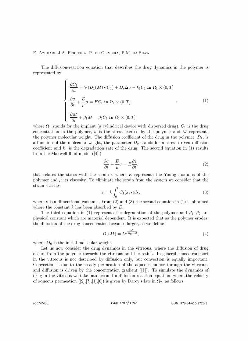
E. Azhdari, J.A. Ferreira, P. de Oliveira, P.M. da Silva

The diffusion-reaction equation that describes the drug dynamics in the polymer isrepresented by

∂C1

∂t= ∇(D1(M)∇C1) +Dv∆σ − k1C1 in Ω1 × (0, T ]

∂σ

∂t+

E

µσ = EC1 in Ω1 × (0, T ]

∂M

∂t+ β1M = β2C1 in Ω1 × (0, T ]

, (1)

where Ω1 stands for the implant (a cylindrical device with dispersed drug), C1 is the drugconcentration in the polymer, σ is the stress exerted by the polymer and M representsthe polymer molecular weight. The diffusion coefficient of the drug in the polymer, D1, isa function of the molecular weight, the parameter Dv stands for a stress driven diffusioncoefficient and k1 is the degradation rate of the drug. The second equation in (1) resultsfrom the Maxwell fluid model ([4],)

∂σ

∂t+

E

µσ = E

∂ε

∂t, (2)

that relates the stress with the strain ε where E represents the Young modulus of thepolymer and µ its viscosity. To eliminate the strain from the system we consider that thestrain satisfies

ε = k

∫

t

0C1(x, s)ds, (3)

where k is a dimensional constant. From (2) and (3) the second equation in (1) is obtainedwhere the constant k has been absorbed by E.

The third equation in (1) represents the degradation of the polymer and β1, β2 arephysical constant which are material dependent. It is expected that as the polymer erodes,the diffusion of the drug concentration becomes larger, so we define

D1(M) = λeM0

M0+M , (4)

where M0 is the initial molecular weight.Let us now consider the drug dynamics in the vitreous, where the diffusion of drug

occurs from the polymer towards the vitreous and the retina. In general, mass transportin the vitreous is not described by diffusion only, but convection is equally important.Convection is due to the steady permeation of the aqueous humor through the vitreous,and diffusion is driven by the concentration gradient ([?]). To simulate the dynamics ofdrug in the vitreous we take into account a diffusion reaction equation, where the velocityof aqueous permeation ([2],[?],[1],[6]) is given by Darcy’s law in Ω2, as follows:

c©CMMSE ISBN: 978-84-616-2723-3Page 178 of 1797

Drug Delivery from an ocular implant

∂C2

∂t+ v.∇C2 −D2∆C2 = 0 in Ω2 × (0, T ], (5)

and

v = −K

µ1∇p in Ω2 × (0, T ]

∇.v = 0 in Ω2 × (0, T ]

. (6)

In equation (5) C2 represents the concentration of the drug in the vitreous, D2 is thediffusion coefficient of the drug in the vitreous and v the velocity of aqueous permeationgiven by (6). In this last system K is the permeability of the vitreous and µ1 is the viscosity

of the permeating aqueous humour ([?]). The termK

µ1is referred to as the hydraulic

conductivity.

Equations (1-6) are completed with initial conditions represented by

C1 = c0, in Ω1, t = 0σ = σ0, in Ω1, t = 0M = M0, in Ω1, t = 0C2 = 0, in Ω2, t = 0v = 0, in Ω2, t = 0p = 2000, in Ω2, t = 0

. (7)

Boundary conditions of different type will be used in the model:

- Boundary conditions for the pressure:

p = 2000, in ∂Ω2, ∪ ∂Ω3 t > 0,

p = 1200, in ∂Ω5, t > 0.

We note that ∂Ω2, ∪ ∂Ω3 represent the hyaloid membrane and ∂Ω5 represents theretina.

- Interface boundary conditions for the flux of drug concentration:

D∇C1.η = A(C1 − C2), in ∂Ω1, t > 0.

- Wall conditions for the velocity: v = 0, in the boundary ∂Ω4, of the vitreous chamberΩ2, and in the boundary of the implant ∂Ω1 (Figure 3).

c©CMMSE ISBN: 978-84-616-2723-3Page 179 of 1797

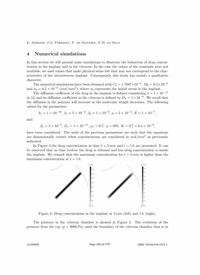
E. Azhdari, J.A. Ferreira, P. de Oliveira, P.M. da Silva

4 Numerical simulations

In this section we will present some simulations to illustrate the behaviour of drug concen-tration in the implant and in the vitreous. In the case the values of the constants were notavailable, we used values that make physical sense but that may not correspond to the char-acteristics of the intravitreous implant. Consequently this study has mainly a qualitativecharacter.

The numerical simulations have been obtained with C0 = 1.7887×10−6 , M0 = 0.5×10−6

and σ0 = 0.5 × 10−6 (mol/mm3), where σ0 represents the initial stress in the implant.The diffusion coefficient of the drug in the implant is defined considering λ = 1× 10−11

in (4) and its diffusion coefficient in the vitreous is defined by D2 = 1×10−8. We recall thatthe diffusion in the polymer will increase as the molecular weight decreases. The followingvalues for the parameters:

k1 = 1× 10−10, β1 = 5× 10−4, β2 = 1× 10−9, µ = 2× 10−4, E = 1× 10−7,

and

Ac = 5× 10−5, Dv = 1× 10−11, µ1 = 0.7, ρ = 970, K = 0.7 × 8.4× 10−8,

have been considered. The units of the previous parameters are such that the equationsare dimensionally correct when concentrations are considered in mol/mm3 as previouslyindicated.

In Figure 4 the drug concentration at time t = 5min and t = 1h are presented. It canbe observed that as time evolves the drug is released and less drug concentration is insidethe implant. We remark that the maximum concentration for t = 5min is higher than themaximum concentration at t = 1h.

Figure 4: Drug concentration in the implant at 5min (left) and 1h (right).

The pressure in the vitreous chamber is showed in Figure 5. The evolution of thepressure from the top (p = 2000Pa) until the boundary of the vitreous chamber that is in

c©CMMSE ISBN: 978-84-616-2723-3Page 180 of 1797

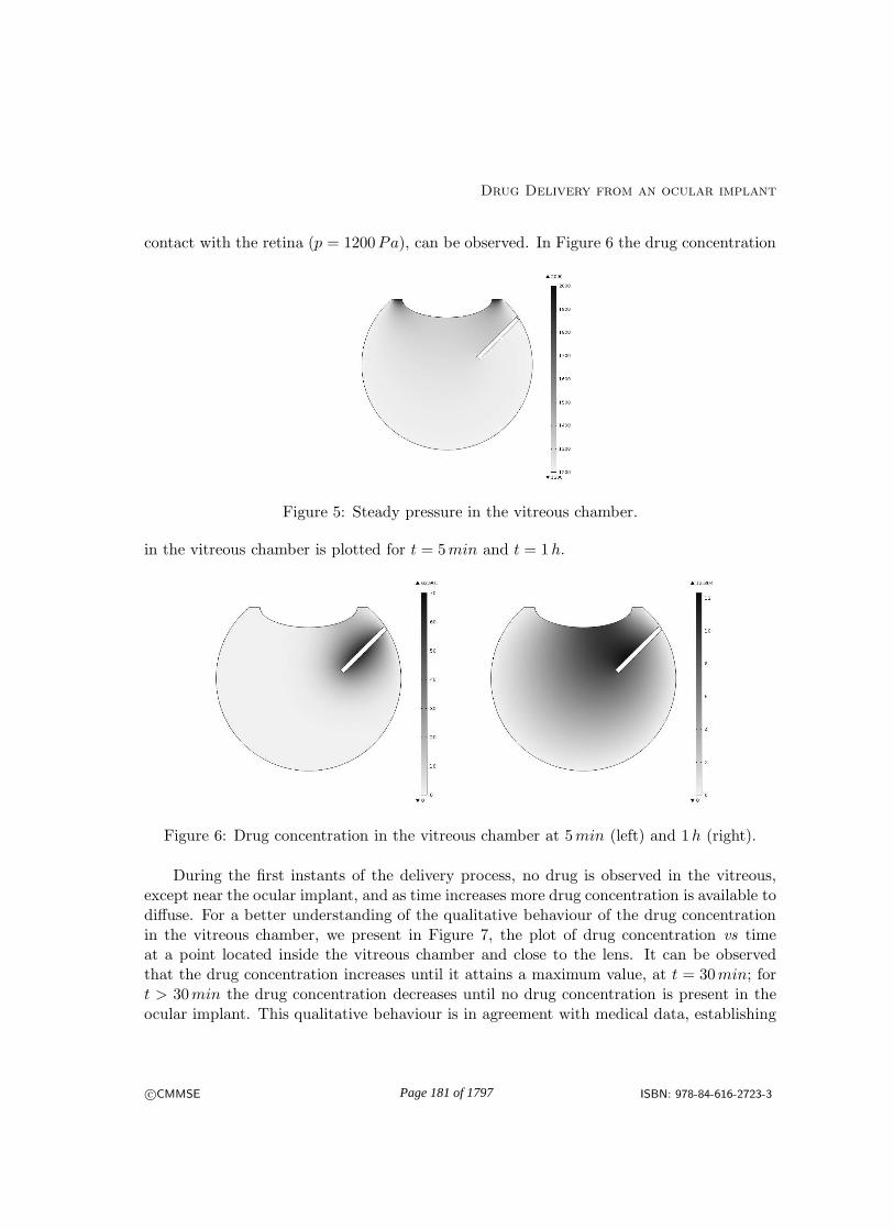
Drug Delivery from an ocular implant

contact with the retina (p = 1200Pa), can be observed. In Figure 6 the drug concentration

Figure 5: Steady pressure in the vitreous chamber.

in the vitreous chamber is plotted for t = 5min and t = 1h.

Figure 6: Drug concentration in the vitreous chamber at 5min (left) and 1h (right).

During the first instants of the delivery process, no drug is observed in the vitreous,except near the ocular implant, and as time increases more drug concentration is available todiffuse. For a better understanding of the qualitative behaviour of the drug concentrationin the vitreous chamber, we present in Figure 7, the plot of drug concentration vs timeat a point located inside the vitreous chamber and close to the lens. It can be observedthat the drug concentration increases until it attains a maximum value, at t = 30min; fort > 30min the drug concentration decreases until no drug concentration is present in theocular implant. This qualitative behaviour is in agreement with medical data, establishing

c©CMMSE ISBN: 978-84-616-2723-3Page 181 of 1797

E. Azhdari, J.A. Ferreira, P. de Oliveira, P.M. da Silva

that for a duration of T units of time the maximum concentration of drug is attained forT , where T

4 < T < T

3 .

Figure 7: Drug concentration in the vitreous chamber along two hours.

Figure 8: Drug concentration in the implant at t = 2h - influence of degradation rateβ1 = 5× 10−4 (left) and β1 = 1× 10−5 (right).

In Figure 8 the influence of the degradation rate is illustrated: a smaller value of β1 leadsto a slower degradation process and consequently more concentration is observed inside thepolymeric implant.

In Figure 9 the influence of Young modulus is illustrated. As expected the increase ofYoung, E, delays the drug release and consequently more drug concentration is observedinside the polymer. In fact as crosslinking density is proportional to E, the large is thisparameter, the more stiff is the material and a more significant barrier difficults the releaseof drug.

c©CMMSE ISBN: 978-84-616-2723-3Page 182 of 1797

Drug Delivery from an ocular implant

Figure 9: Drug concentration at a point of the boundary of the implant around t = 110min- influence of E, E = 1× 10−7 (top line) and E = 1× 10−9 (down line).

5 Conclusion

A coupled model to simulate in vivo drug delivery from an intravitreal viscoelastic biodegrad-able implant has been developed. The whole process is described by a set of partial dif-ferential equations that take into account passive diffusion, convection resulting from thepermeation of aqueous humor, stress driven diffusion and the degradation of the polymer.At the best of our knowledge the dynamics of drug desorption has not been described so farin the literature considering the simultaneous interplay between mechanical, physical andchemical effects. The numerical simulations show qualitative agreement with the physicalexpected behavior. The model clarifies the large influence of the degradation parameterin sustained drug delivery. The viscoelastic properties of the polymeric implant are alsoshown to be an effective control mechanism to delay or to speed up the release of drug.Mathematical modeling is a unique tool to explain transport mechanisms, and to help inimplant design, avoiding expensive and extensive experimentation.

In future work physical values for all the parameters of the model should be retrieved.Also more realistic mechanical models will be considered and the heterogeneous structureof the vitreous, that is characteristic of elderly patients, should be taken into account.

Acknowledgements

This work was partially supported by the Centro de Matematica da Universidade de Coim-bra (CMUC), funded by the European Regional Development Fund through the program

c©CMMSE ISBN: 978-84-616-2723-3Page 183 of 1797

E. Azhdari, J.A. Ferreira, P. de Oliveira, P.M. da Silva

COMPETE and by the Portuguese Government through the FCT - Fundacao para a Cienciae Tecnologia under the projects PEst-C/MAT/UI0324/2011, SFR/BD/33703/2009, and bythe project UTAustin/MAT/0066/2008.

References

[1] R. Avatar, D. Tandon, A mathematical analysis of intravitreal drug transport, Jour-nal of Pharmaceutical Research, 7(1), (2008) 867-877.

[2] R. K. Balachandran and V. H. Barocas, Computer modeling of drug delivery to

the posterior eye: effect of active transport and loss to choroidal blood flow, Pharma-ceutical Research, 25 (2008) 2685-2696.

[3] R. K. Balachandran and V. H. Barocas, Finite element modeling of drug dis-

tribution in the vitreous humor of the rabbit eye, Annals of Biomedical Engineering 25

(1997) 303-314.

[4] C.Hal F. Brinson, L. Catherine Brinson, Polymer Engineering Science and Vis-

coelasticity: An Introduction, Springer, 2008.

[5] D. Cox, R. A. J. Phipps, B. Levine, A. Jacobs and D. Fowler, Distribution of

phencyclidine into vitreous humor, Journal of Analytical Toxicology, 31, (2007) 537-539.

[6] N. Haghjou, M. J. Abdekhodaie, Y. L. Cheng. M. Saadatmand, Computer

modeling of drug distribution after intravitreal administration, W.A.S. Engineering andTecnology, 53, (2011) 706-716.

[7] J. Kathawate and S. Acharya, Computational modeling of intravitreal drug delivery

in the vitreous chamber with different vitreous substitutes,International Journal of Heatand Mass Transfer,51, (2008) 5598-5609.

[8] C.W. Misner, K. S. Thorne and J.A. Wheeler, Computer modeling of drug

delivery to the posterior eye: effect of active transport and loss to choroidal blood flow,Freeman, San Francisco, 1970.

[9] M. S. Stay, J. Xu, T. W. Randolph, and V. H. Barocas, Computer simulation

of convective and diffusive transport of controlled-release drug in the vitreous humor,Pharmaceutical Research, 20(1), (2003) 96-102.

c©CMMSE ISBN: 978-84-616-2723-3Page 184 of 1797

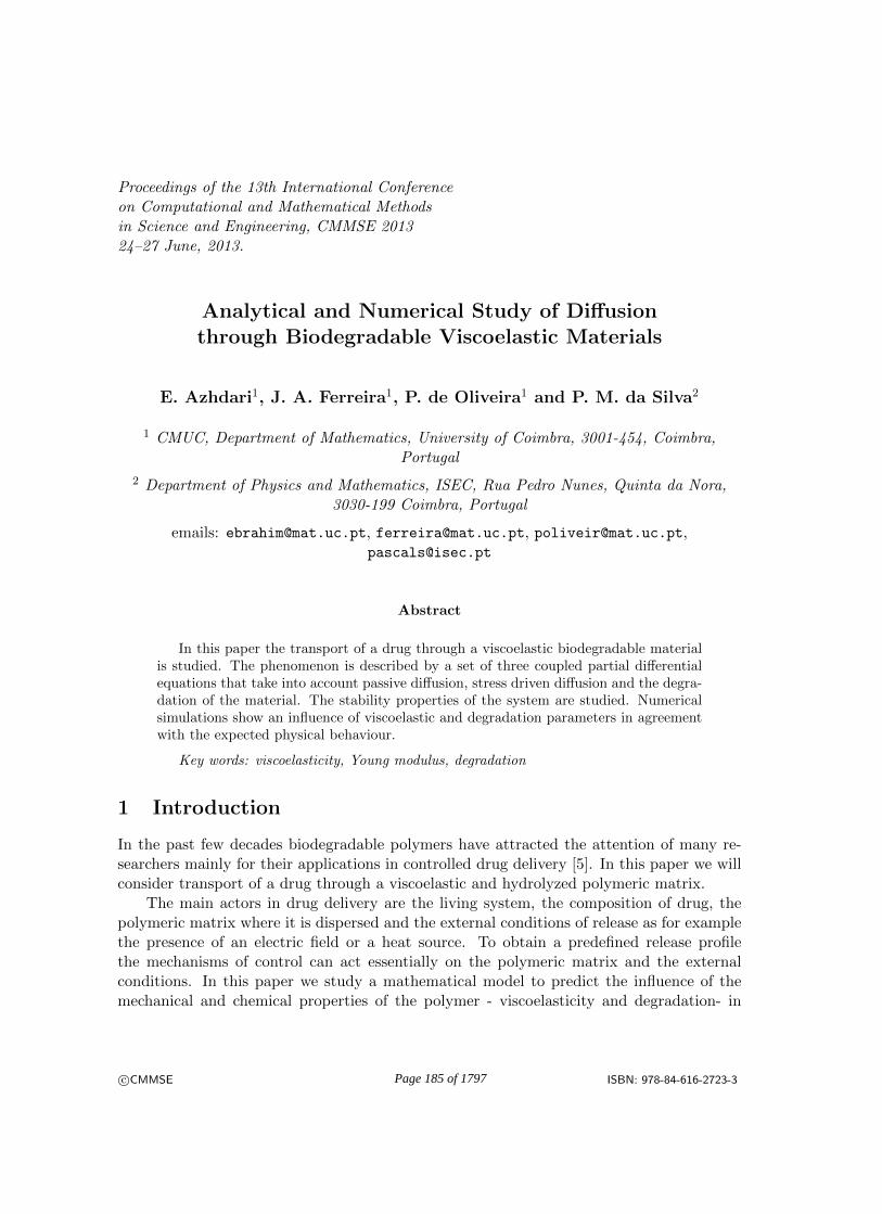
Proceedings of the 13th International Conferenceon Computational and Mathematical Methodsin Science and Engineering, CMMSE 201324–27 June, 2013.

Analytical and Numerical Study of Diffusionthrough Biodegradable Viscoelastic Materials

E. Azhdari1, J. A. Ferreira1, P. de Oliveira1 and P. M. da Silva2

1 CMUC, Department of Mathematics, University of Coimbra, 3001-454, Coimbra,Portugal

2 Department of Physics and Mathematics, ISEC, Rua Pedro Nunes, Quinta da Nora,3030-199 Coimbra, Portugal

emails: ebrahim@mat.uc.pt, ferreira@mat.uc.pt, poliveir@mat.uc.pt,pascals@isec.pt

Abstract

In this paper the transport of a drug through a viscoelastic biodegradable materialis studied. The phenomenon is described by a set of three coupled partial differentialequations that take into account passive diffusion, stress driven diffusion and the degra-dation of the material. The stability properties of the system are studied. Numericalsimulations show an influence of viscoelastic and degradation parameters in agreementwith the expected physical behaviour.

Key words: viscoelasticity, Young modulus, degradation

1 Introduction

In the past few decades biodegradable polymers have attracted the attention of many re-searchers mainly for their applications in controlled drug delivery [5]. In this paper we willconsider transport of a drug through a viscoelastic and hydrolyzed polymeric matrix.

The main actors in drug delivery are the living system, the composition of drug, thepolymeric matrix where it is dispersed and the external conditions of release as for examplethe presence of an electric field or a heat source. To obtain a predefined release profilethe mechanisms of control can act essentially on the polymeric matrix and the externalconditions. In this paper we study a mathematical model to predict the influence of themechanical and chemical properties of the polymer - viscoelasticity and degradation- in

c©CMMSE ISBN: 978-84-616-2723-3Page 185 of 1797

Drug delivery from biodegradable viscoelastic materials

the release rate. As degradation proceeds, the polymer molecular weight decreases anddiffusional paths open through the matrix allowing solved drug molecules to leave the device[6]. Because of the increasing permeability of the system upon polymer degradation, theconstant diffusion coefficient is replaced by a molecular weight dependent diffusion coefficient[7]. The viscoelastic behaviour of the polymeric matrix is described by a Maxwell fluid model[1, 2, 3].

The paper is organised as follows. In Section 2 the mathematical model is presented.In Section 3 the qualitative behaviour of the released mass is studied. A fully discretemethod that mimics the properties of the continuous problem is described in Section 4 andnumerical simulations are exhibited in Section 5. Finally in Section 6 some conclusions areaddressed.

2 The mathematical model

We consider a polymer filling a bounded domain Ω ⊆ Rn with boundary ∂Ω. The diffusion ofdrug from this polymer is described by the following system of partial differential equations:

∂C

∂t= ∇(D(M)∇C) +∇(Dv∇σ) in Ω× (0, T ],

∂σ

∂t+E

µσ = EC in Ω× (0, T ],

∂M

∂t+ β1M = β2C in Ω× (0, T ],

(1)

where C represents the unknown concentration of the drug inside the polymer, σ is theunknown stress, M is the unknown molecular weight of the polymer. The viscoelasticinfluence in the drug transport is represented by the term ∇(Dv∇σ) where Dv is the socalled viscoelastic diffusion coefficient. This term states that the polymer acts as a barrierto the diffusion: as the drug strains the polymer it reacts with a stress of opposite sign.To account for the increasing permeability of the system upon polymer degradation, thediffusion coefficient is defined as

D(M) = D0eM0

M+M0 ,

where D0 is the diffusion coefficient of drug in the non hydrolyzed polymer and M0 is itsinitial molecular weight. The second equation in (1) defines the viscoelastic behaviour ofthe polymer by the Maxwell fluid model [2, 3]

∂σ

∂t+E

µσ = E

∂ε

∂t

c©CMMSE ISBN: 978-84-616-2723-3Page 186 of 1797

E. Azhdari, J. A. Ferreira, P. de Oliveira, P. M. da Silva

where E represents the Young modulus of the material, µ its viscosity and ε is the strainproduced by the drug molecules. If we assume that

ε = k

∫ t

0C(x, s)ds

where k is a positive constant we obtain the second equation in (1) where this constant hasbeen absorbed by E. In the third equation of (1) β1 and β2 are constants that characterizethe degradation properties of the material.

System (1) is completed with initial conditionsC(x, 0) = C0, x ∈ Ω,

σ(x, 0) = σ0, x ∈ Ω,

M(x, 0) = M0, x ∈ Ω,

and boundary conditions C(x, t) = 0 on ∂Ω× (0, T ],

σ(x, t) = 0 on ∂Ω× (0, T ],

M(x, t) = 0 on ∂Ω× (0, T ],

where ∂Ω denotes the boundary of Ω.

3 Qualitative behaviour of a mass related functional

In this section we study the qualitative behaviour of the mass related functional

M(t) =

∫ΩC2(t)dx, t ≥ 0.

From the second equation of (1) we easily get

σ(t) = E

∫ t

0e−Eµ

(t−s)C(s)ds+ σ(0)e

−Eµt, t ≥ 0.

Replacing in the first equation of (1) we obtain for C

∂C

∂t= ∇(D(M)∇C) + E

∫ t

0e−Eµ

(t−s)∇(Dv∇C(s))ds in Ω× (0, T ]. (2)

c©CMMSE ISBN: 978-84-616-2723-3Page 187 of 1797

Drug delivery from biodegradable viscoelastic materials

As 12M

′(t) =∫

ΩC(t)∂C∂t (t)dx we deduce, considering (2)

1

2M ′(t) = −

∥∥∥∥√D(M)∇C(t)

∥∥∥∥2

−(E

∫ t

0e−Eµ

(t−s)Dv∇C(s)ds,∇C(t)

), (3)

where (., .) stands for the scalar product in L2(Ω). From (3) we have

1

2M ′(t) +D0

∥∥∥∥∇C(t)

∥∥∥∥2

≤ D2v

4ε2E2

∥∥∥∥∫ t

0e−Eµ

(t−s)∇C(s)ds

∥∥∥∥2

+ ε2∥∥∥∥∇C(t)

∥∥∥∥2

,

where D0 ≤ D and ε 6= 0. Consequently we deduce

1

2M ′(t) + (D0 − ε2)

∥∥∥∥∇C(t)

∥∥∥∥2

≤ D2v

4ε2E2

∫ t

0e−2E

µ(t−s)

ds

∫ t

0

∥∥∥∥∇C(s)

∥∥∥∥2

ds,

and then

M(t) + 2(D0 − ε2)

∫ t

0

∥∥∥∥∇C(s)

∥∥∥∥2

ds ≤ D2v

2ε2E2

2Eµ

∫ t

0

∫ s

0

∥∥∥∥∇C(µ)

∥∥∥∥2

dµds+M(0).

If ε2 is such thatD0 − ε2 > 0

we obtain

M(t) +

∫ t

0

∥∥∥∥∇C(s)

∥∥∥∥2

ds ≤ D2vE

2

max1, 2(D0 − ε2)4ε2Eµ

∫ t

0

∫ s

0

∥∥∥∥∇C(µ)

∥∥∥∥2

dµds

+1

max1, 2(D0 − ε2)M(0).

Finally Gronwall’s Lemma [4] leads to

M(t) +

∫ t

0

∥∥∥∥∇C(s)

∥∥∥∥2

ds ≤ 1

max1, 2(D0 − ε2)M(0)e

D2vE

2

max1,2(D0−ε2)4ε2Eµ

t. (4)

This last inequality establishes that M(t) and∫ t

0

∥∥∇C(s)∥∥2ds are bounded for bounded

intervals of time. We note that (4) can be improved by eliminating the exponential factorin its right hand side [8]. A stability result of type

M(t) +

∫ t

0e−2γ(t−s)

∥∥∥∥∇C(s)

∥∥∥∥2

ds ≤M(0)

can then be stated for a convenient choice of the parameters of the model.

c©CMMSE ISBN: 978-84-616-2723-3Page 188 of 1797

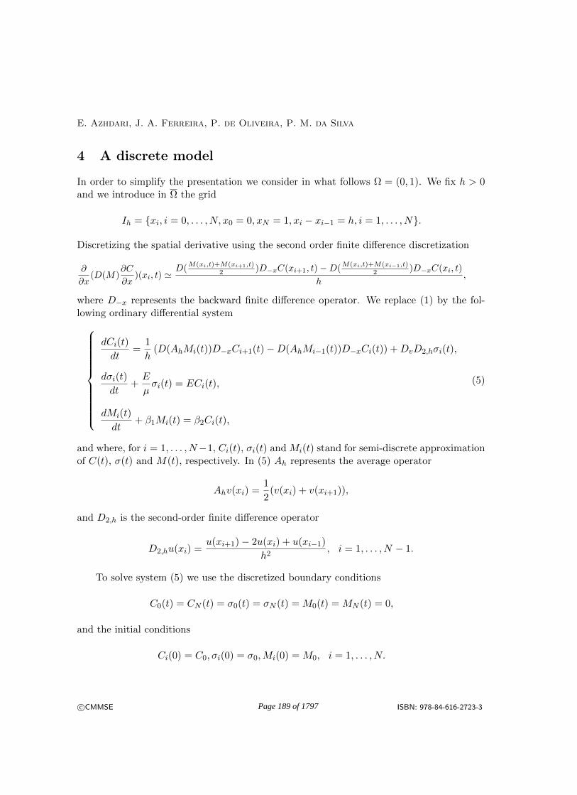
E. Azhdari, J. A. Ferreira, P. de Oliveira, P. M. da Silva

4 A discrete model

In order to simplify the presentation we consider in what follows Ω = (0, 1). We fix h > 0and we introduce in Ω the grid

Ih = xi, i = 0, . . . , N, x0 = 0, xN = 1, xi − xi−1 = h, i = 1, . . . , N.

Discretizing the spatial derivative using the second order finite difference discretization

∂

∂x(D(M)

∂C

∂x)(xi, t) '

D(M(xi,t)+M(xi+1,t)2 )D−xC(xi+1, t)−D(M(xi,t)+M(xi−1,t)

2 )D−xC(xi, t)

h,

where D−x represents the backward finite difference operator. We replace (1) by the fol-lowing ordinary differential system

dCi(t)

dt=

1

h(D(AhMi(t))D−xCi+1(t)−D(AhMi−1(t))D−xCi(t)) +DvD2,hσi(t),

dσi(t)

dt+E

µσi(t) = ECi(t),

dMi(t)

dt+ β1Mi(t) = β2Ci(t),

(5)

and where, for i = 1, . . . , N−1, Ci(t), σi(t) and Mi(t) stand for semi-discrete approximationof C(t), σ(t) and M(t), respectively. In (5) Ah represents the average operator

Ahv(xi) =1

2(v(xi) + v(xi+1)),

and D2,h is the second-order finite difference operator

D2,hu(xi) =u(xi+1)− 2u(xi) + u(xi−1)

h2, i = 1, . . . , N − 1.

To solve system (5) we use the discretized boundary conditions

C0(t) = CN (t) = σ0(t) = σN (t) = M0(t) = MN (t) = 0,

and the initial conditions

Ci(0) = C0, σi(0) = σ0,Mi(0) = M0, i = 1, . . . , N.

c©CMMSE ISBN: 978-84-616-2723-3Page 189 of 1797

Drug delivery from biodegradable viscoelastic materials

The time integration of (5) is performed considering as implicit-explicit approach, definedby

Cn+1i − Cni

∆t=

1

h

(D(AhM

ni )D−xC

n+1i+1 −D(AhM

ni−1)D−xC

n+1i

)+DvD2,hσ

ni ,

σn+1i − σni

∆t+E

µσni = ECn+1

i ,

Mn+1i −Mn

i

∆t+ β1M

ni = β2C

n+1i .

(6)

In (6) Cni , σni , andMn

i for i = 1, ..., N stand for time for approximations of Ci(tn), σi(tn)and Mi(tn) in the time grid defined by

tn, n = 0, . . . ,M, t0 = 0, tM = T, tn − tn−1 = ∆t, n = 1, . . . ,M − 1.

System (6) is completed with the following conditions

Cn0 = CnN = σn0 = σnN = Mn0 = Mn

N = 0, n = 0, . . . ,M.

It can be shown that method (6) is second order consistent in space and first order in time.In the numerical simulations, that we present in Section 5, we consider the drug releasedmass defined by

M(t) =

∫ΩC(x, 0)dx−

∫ΩC(x, t)dx, (7)

for each t ∈ [0, T ].

5 Numerical results

In this section we illustrate the use of the numerical scheme (6). We take C0 = 1,M0 =0.5, σ0 = 0.5, D0 = 0.01, Dv = −1 × 10−4, µ = 1 × 10−2, E = 1 × 10−3, β1 = 0.1, β2 =1 × 10−3, ∆t = 5 × 10−4, h = 1 × 10−2. The units of the concentration are mol/mm3.The units of other variables and parameters are such that the equations are dimensionallycorrect.

In Figure 1 the evolution of C in time is illustrated. As expected the drug concentrationdecreases in time. The evolution of M is plotted in Figure 2, where the decrease in time ofthe molecular weight is consequence of the polymer degradation. In order to see that theevolution inside the polymer is not spatially homogeneous, a plot of the molecular weightat t = 4 is presented in Figure 2(right).

c©CMMSE ISBN: 978-84-616-2723-3Page 190 of 1797

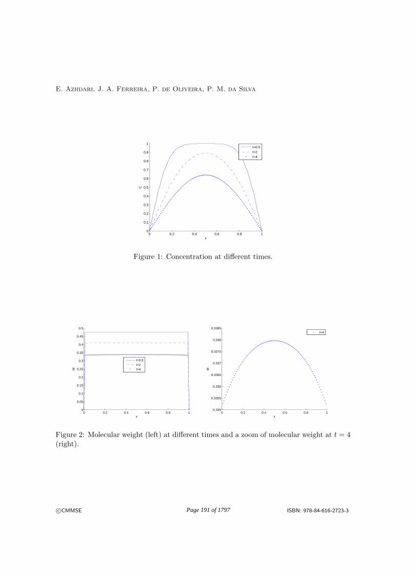
E. Azhdari, J. A. Ferreira, P. de Oliveira, P. M. da Silva

0 0.2 0.4 0.6 0.8 10

0.1

0.2

0.3

0.4

0.5

0.6

0.7

0.8

0.9

1

x

C

t=0.5t=2t=4

Figure 1: Concentration at different times.

0 0.2 0.4 0.6 0.8 10

0.05

0.1

0.15

0.2

0.25

0.3

0.35

0.4

0.45

0.5

x

M

t=0.5t=2t=4

0 0.2 0.4 0.6 0.8 10.335

0.3355

0.336

0.3365

0.337

0.3375

0.338

0.3385

x

M

t=4

Figure 2: Molecular weight (left) at different times and a zoom of molecular weight at t = 4(right).

c©CMMSE ISBN: 978-84-616-2723-3Page 191 of 1797

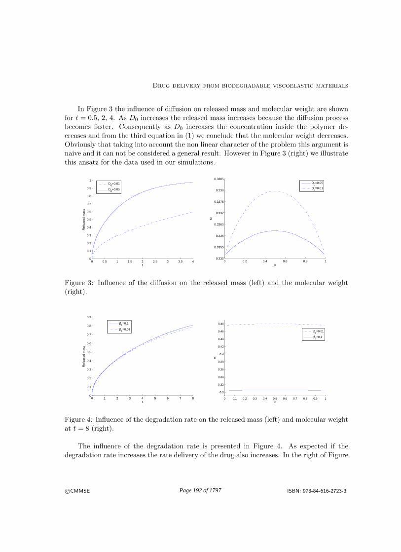
Drug delivery from biodegradable viscoelastic materials

In Figure 3 the influence of diffusion on released mass and molecular weight are shownfor t = 0.5, 2, 4. As D0 increases the released mass increases because the diffusion processbecomes faster. Consequently as D0 increases the concentration inside the polymer de-creases and from the third equation in (1) we conclude that the molecular weight decreases.Obviously that taking into account the non linear character of the problem this argument isnaive and it can not be considered a general result. However in Figure 3 (right) we illustratethis ansatz for the data used in our simulations.

0 0.5 1 1.5 2 2.5 3 3.5 40

0.1

0.2

0.3

0.4

0.5

0.6

0.7

0.8

0.9

1

t

Rel

ease

d m

ass

D

0=0.01

D0=0.05

0 0.2 0.4 0.6 0.8 10.335

0.3355

0.336

0.3365

0.337

0.3375

0.338

0.3385

x

M

D

0=0.05

D0=0.01

Figure 3: Influence of the diffusion on the released mass (left) and the molecular weight(right).

0 1 2 3 4 5 6 7 80

0.1

0.2

0.3

0.4

0.5

0.6

0.7

0.8

0.9

t

Rel

ease

d m

ass

β1=0.1

β1=0.01

0 0.1 0.2 0.3 0.4 0.5 0.6 0.7 0.8 0.9 1

0.3

0.32

0.34

0.36

0.38

0.4

0.42

0.44

0.46

0.48

x

M

β1=0.01

β1=0.1

Figure 4: Influence of the degradation rate on the released mass (left) and molecular weightat t = 8 (right).

The influence of the degradation rate is presented in Figure 4. As expected if thedegradation rate increases the rate delivery of the drug also increases. In the right of Figure

c©CMMSE ISBN: 978-84-616-2723-3Page 192 of 1797

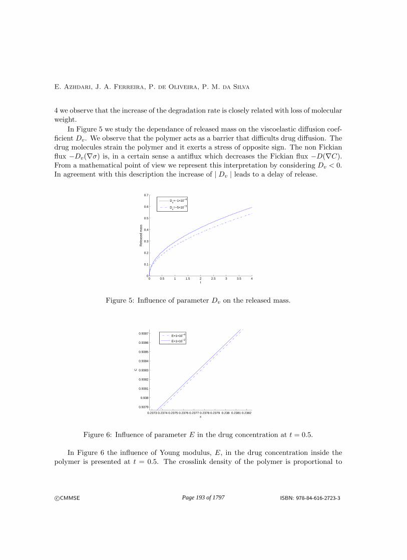
E. Azhdari, J. A. Ferreira, P. de Oliveira, P. M. da Silva

4 we observe that the increase of the degradation rate is closely related with loss of molecularweight.

In Figure 5 we study the dependance of released mass on the viscoelastic diffusion coef-ficient Dv. We observe that the polymer acts as a barrier that difficults drug diffusion. Thedrug molecules strain the polymer and it exerts a stress of opposite sign. The non Fickianflux −Dv(∇σ) is, in a certain sense a antiflux which decreases the Fickian flux −D(∇C).From a mathematical point of view we represent this interpretation by considering Dv < 0.In agreement with this description the increase of | Dv | leads to a delay of release.

0 0.5 1 1.5 2 2.5 3 3.5 40

0.1

0.2

0.3

0.4

0.5

0.6

0.7

t

Rel

ease

d m

ass

Dv=−1×10−4

Dv=−5×10−3

Figure 5: Influence of parameter Dv on the released mass.

0.2373 0.2374 0.2375 0.2376 0.2377 0.2378 0.2379 0.238 0.2381 0.2382

0.9379

0.938

0.9381

0.9382

0.9383

0.9384

0.9385

0.9386

0.9387

x

C

E=1×10−4

E=1×10−2

Figure 6: Influence of parameter E in the drug concentration at t = 0.5.

In Figure 6 the influence of Young modulus, E, in the drug concentration inside thepolymer is presented at t = 0.5. The crosslink density of the polymer is proportional to

c©CMMSE ISBN: 978-84-616-2723-3Page 193 of 1797

Drug delivery from biodegradable viscoelastic materials

Young modulus E and consequently as this constant increases the polymer offers moreresistance to the exit of the drug, which is delayed.

6 Conclusion

A model to simulate transport through a biodegradable viscoelastic material is studied. Theanalytical treatment of the system of partial differential equations lead to the establishmentof stability results. The influence of mechanical and degradation parameters is analysed,showing agreement with physical behaviour. We believe that with future improvements themodel can be used as a tool to design biodegradable polymers with predefined properties.

Acknowledgements

This work was partially supported by the Centro de Matematica da Universidade de Coim-bra (CMUC) and by the Portuguese Government through the FCT - Fundacao para aCiencia e a Tecnologia under the project PEst-C/MAT/UI0324/2011, and Fundacao paraa Ciencia e a Tecnologia, Grant SFRH / BD / 33812 / 2009.

References

[1] H. F. Brinson, L. C. Brinson, Polymer engineering science and viscoelasticity, Anintroduction, Springer, 2008.

[2] D. S. Cohen, A. B. White, JR. t, and T. P. Witelski, Shock Formation in aMultidimensional Viscoelastic Diffusive System, SIAM J. APPL. MATH 55(2) (1995)348–368.

[3] D. S. Cohen, A. B. White, JR, Sharp Fronts due to Diffusion and ViscoelasticRelaxation in Polymers, SIAM J. APPL. MATH 51(2) (1991) 472–483.

[4] T. H. Gronwall, Note on the derivative with respect to a parameter of the solutionsof a system of differential equations, Ann. of Math, 20(4) (1919) 292-296.

[5] L. L. Lao, S. S. Venkatraman, N. A. Peppas, Modeling of drug release frombiodegradable polymer blends, European Journal of Pharmaceutics and Biopharmaceu-tics, 70 (2008) 796–803.

[6] G. Perale, P. Arosio, D. Moscatelli, V. Barri, M. Muller, S. Maccagnanand M. Masi, Anew model of resorbable device degradation and drug release: Transient1-dimension diffusional model, Journal of Controlled Release 136 (2009) 196–205.

c©CMMSE ISBN: 978-84-616-2723-3Page 194 of 1797

E. Azhdari, J. A. Ferreira, P. de Oliveira, P. M. da Silva

[7] J. Siepmann, A. Gopferich, Mathematical modeling of bioerodible, polymeric drugdelivery systems, Advanced Drug Delivery Reviews 48 (2001) 229–247.

[8] V. Thomee and L. B. Wahlbin, Long-Time Numerical Solution of a ParabolicEquation with Memory, Mathematics of Computation 62 (1994) 477–496.

c©CMMSE ISBN: 978-84-616-2723-3Page 195 of 1797

Proceedings of the 13th International Conference

on Computational and Mathematical Methods

in Science and Engineering, CMMSE 2013

24–27 June, 2013.

Boolean sum based differential quadrature

D. Barrera1, P. Gonzalez1, F. Ibanez2 and M. J. Ibanez1

1 Department of Applied Mathematics, University of Granada, 18071-Granada, Spain

2 Grupo Sacyr-Vallehermoso, Paseo de la Castellana, 83, 28046-Madrid, Spain

emails: dbarrera@ugr.es, prodelas@ugr.es, fibanez@gruposyv.com, mibanez@ugr.es

Abstract

A boolean sum differential quadrature method is proposed. It combines an inter-polation operator having a fundamental function with minimal compact support anda quasi-interpolation operator exact on the space of polynomials reproduced by thefirst one. We recall the resulting numerical scheme in the quintic case and derive newschemes from low degree B-splines.

Key words: differential quadrature, B-spline, interpolation, discrete quasi-interpolation

1 Introduction

The Differential Quadrature Method (DQM) is a numerical discretization technique for theapproximation of derivatives by means of weighted sums of function values. It was intro-duced by Bellman and coworkers in the early 1970’s, and it has been extensively employedto approximate spatial partial derivatives (cf. [2], [8] and references quoted therein). Theclassical DQM is polynomial-based, but some spline based DQMs have been proposed thelimitation concerning the number of grid points involved. Given a B-spline (cf. [3], [9]), acardinal lagrangian o hermitian spline with a compactly supported fundamental functionis defined, from which the approximation of the derivatives is derived. The construction ofthese spline interpolants depends strongly on the degree of the B-spline (see for instance [4]and [10]). In this work we present a DQM based on interpolation and quasi-interpolation.Firstly, we consider the construction of compactly supported cardinal functions L based onB-splines such that

L (j) = δj,0, j ∈ Z, (1)

c©CMMSE ISBN: 978-84-616-2723-3Page 196 of 1797

Boolean sum based differential quadrature

δ being the Kronecker sequence. Then, we revise some spline discrete quasi-interpolantsdefined from the same B-splines (cf. e.g. [3], [9] and references quoted therein). Finally,both the interpolants and the quasi-interpolants are used to define new interpolants havingcompactly supported fundamental functions again, and the maximal order of approximation.The quintic case is described and compared with the results obtained in [10].

2 Spline interpolation

Let Mn be the B-spline of order n ≥ 2 centered at the origin. We look for a symmetricalfundamental function L such that

L =∑

j∈J

cjMn (2 · −j) (2)

for some cj ∈ R. Once the structure for L is fixed, we prove that there exist such functionssatisfying the interpolation conditions (1) and we determine one of them.

We will use the following notations. For each r ≥ 0, er (z) := zr is the monomial of

degree r, Pr denotes the space of polynomials of degree at most r, and ˜Mn :=∑

j∈ZMn (j) ejstands for the symbol of Mn.

Lemma 1 The Laurent polynomials

Φ0 :=∑

j∈Z

Mn (2j) e2j and Φ1 :=∑

j∈Z

Mn (2j + 1) e2j+1

have no common zeros on C \ 0.

As a consequence of the previous lemma (see [7]), any finite sequence c satisfying theidentity

Φ0

∑

j∈Z

c2je2j +Φ1

∑

j∈Z

c2j+1e2j+1 = 1

provides such a function L. We use this result in order to obtain a symmetric fundamentalfunction with a small support.

Proposition 2 For each n ≥ 4, let J := −dn, . . . , dn where

dn :=

⌊r⌋ − 2, for n even,

⌊r⌋ − 1, for n odd,

and ⌊r⌋ denotes the integer part of r ∈ R. Then, there are coefficients aj, 0 ≤ j ≤ 2dn such

that the function

L = a0Mn (2 ·+dn) + · · ·+ a2dnMn (2 · −dn)

c©CMMSE ISBN: 978-84-616-2723-3Page 197 of 1797

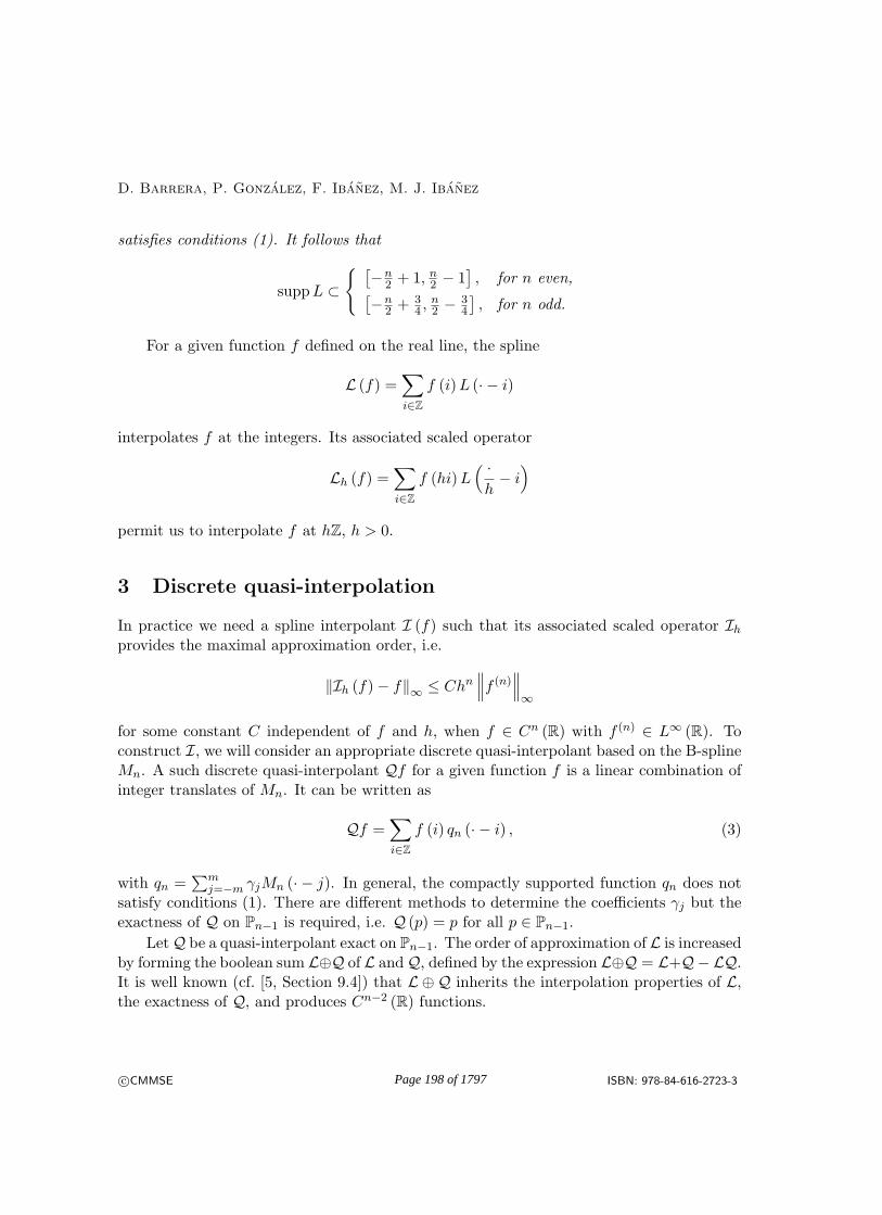
D. Barrera, P. Gonzalez, F. Ibanez, M. J. Ibanez

satisfies conditions (1). It follows that

suppL ⊂

[

−n2 + 1, n2 − 1

]

, for n even,[

−n2 + 3

4 ,n2 − 3

4

]

, for n odd.

For a given function f defined on the real line, the spline

L (f) =∑

i∈Z

f (i)L (· − i)

interpolates f at the integers. Its associated scaled operator

Lh (f) =∑

i∈Z

f (hi)L( ·

h− i

)

permit us to interpolate f at hZ, h > 0.

3 Discrete quasi-interpolation

In practice we need a spline interpolant I (f) such that its associated scaled operator Ihprovides the maximal approximation order, i.e.

‖Ih (f)− f‖∞ ≤ Chn∥

∥

∥f (n)

∥

∥

∥

∞

for some constant C independent of f and h, when f ∈ Cn (R) with f (n) ∈ L∞ (R). Toconstruct I, we will consider an appropriate discrete quasi-interpolant based on the B-splineMn. A such discrete quasi-interpolant Qf for a given function f is a linear combination ofinteger translates of Mn. It can be written as

Qf =∑

i∈Z

f (i) qn (· − i) , (3)

with qn =∑m

j=−m γjMn (· − j). In general, the compactly supported function qn does notsatisfy conditions (1). There are different methods to determine the coefficients γj but theexactness of Q on Pn−1 is required, i.e. Q (p) = p for all p ∈ Pn−1.

LetQ be a quasi-interpolant exact on Pn−1. The order of approximation of L is increasedby forming the boolean sum L⊕Q of L andQ, defined by the expression L⊕Q = L+Q− LQ.It is well known (cf. [5, Section 9.4]) that L ⊕Q inherits the interpolation properties of L,the exactness of Q, and produces Cn−2 (R) functions.

c©CMMSE ISBN: 978-84-616-2723-3Page 198 of 1797

Boolean sum based differential quadrature

4 Boolean sum based differential quadrature

We propose to define the interpolation operator I as the boolean sum of L and a quasi-interpolation operator, Q, i.e. I = L⊕Q. From (2) and (3), we can write

I (f) =∑

i∈Z

f (i)L (· − i) +∑

i∈Z

(Q (f) (i)− f (i)) q (· − i) .

We use this expression to approximate the derivative of a function with respect to a spacevariable.

We recall the quintic case (see [1]) based on a Chebyshev quasi-interpolation operatorand compare this two-stage method with the scheme proposed in [10] for a given functiondefined on the real line. In practice this function is defined on an interval, and standardadditional modifications are required near the boundary.

In [10] the following fundamental function is constructed

ϕ =20523

440M5 −

3483

110

(

M5

(

·+1

3

)

+M5

(

· −1

3

))

+8829

880

(

M5

(

·+2

3

)

+M5

(

· −2

3

))

−131

110(M5 (·+ 1) +M5 (· − 1)) .

It is supported on [−4, 4], and the corresponding quintic interpolation spline

Z (f) =∑

i∈Z

f (i)ϕ (· − i) (4)

is defined on the uniform partition 13Z of R.

It is easy to derive the expression

Z (f)′ (i) = −1

60f (i− 3)+

3

20f (i− 2)−

3

4f (i− 1)+

3

4f (i+ 1)−

3

20f (i+ 2)+

1

60f (i+ 3)

(5)for the derivative of Z (f) at i ∈ Z. Although Z is an operator exact on P5, the obtainedformula is exact on P6.

We give the error of this formula for f ∈ C7 (R).

Proposition 3 Let i ∈ Z. For any f ∈ C7 (R), the error for the scheme given by (5)

satisfies∣

∣f ′ (i)− Z (f)′ (i)∣

∣ ≤1

140

∥

∥

∥f (7)

∥

∥

∥

∞,[i−3,i+3], (6)

where ‖g‖∞,I stands for the uniform norm of g on the interval I.

c©CMMSE ISBN: 978-84-616-2723-3Page 199 of 1797

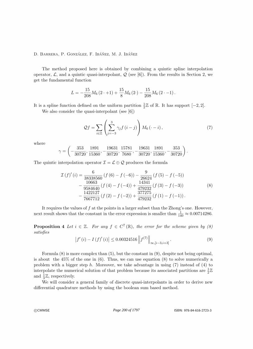
D. Barrera, P. Gonzalez, F. Ibanez, M. J. Ibanez

The method proposed here is obtained by combining a quintic spline interpolationoperator, L, and a quintic quasi-interpolant, Q (see [6]). From the results in Section 2, weget the fundamental function

L = −15

208M6 (2 ·+1) +

15

8M6 (2·)−

15

208M6 (2 · −1) .

It is a spline function defined on the uniform partition 12Z of R. It has support [−2, 2].

We also consider the quasi-interpolant (see [6])

Qf =∑

i∈Z

3∑

j=−3

γjf (i− j)

M6 (· − i) , (7)

where

γ =

(

−353

30720,1891

15360,−

19631

30720,15781

7680,−

19631

30720,1891

15360,−

353

30720

)

.

The quintic interpolation operator I = L ⊕Q produces the formula

I (f)′ (i) =6

38338560(f (6)− f (−6))−

9

26624(f (5)− f (−5))

−10663

9584640(f (4)− f (−4)) +

14341

479232(f (3)− f (−3)) (8)

−1422127

7667712(f (2)− f (−2)) +

377275

479232(f (1)− f (−1)) .

It requires the values of f at the points in a larger subset than the Zhong’s one. However,next result shows that the constant in the error expression is smaller than 1

140 ≈ 0.00714286.

Proposition 4 Let i ∈ Z. For any f ∈ C7 (R), the error for the scheme given by (8)

satisfies∣

∣f ′ (i)− I (f)′ (i)∣

∣ ≤ 0.00324516∥

∥

∥f (7)

∥

∥

∥

∞,[i−3,i+3]. (9)

Formula (8) is more complex than (5), but the constant in (9), despite not being optimal,is about the 45% of the one in (6). Thus, we can use equation (8) to solve numerically aproblem with a bigger step h. Moreover, we take advantage in using (7) instead of (4) tointerpolate the numerical solution of that problem because its associated partitions are 1

2Z

and 13Z, respectively.

We will consider a general family of discrete quasi-interpolants in order to derive newdifferential quadrature methods by using the boolean sum based method.

c©CMMSE ISBN: 978-84-616-2723-3Page 200 of 1797

Boolean sum based differential quadrature

References

[1] D. Barrera and F. Ibanez, Compactly supported fundamental functions for spline-based differential quadrature, in III European Conference on Computational MechanicsSolids, Structures and Coupled Problems in Engineering, C.A. Mota Soares et. al.(eds.), Lisbon, Portugal, 58 June 2006.

[2] C. W. Bert and M. Malik, Differential quadrature method in computational mechanics:a review. Appl. Rev., 49, 1–27, 1996.

[3] C. de Boor, A practical guide to splines. Springer-Verlag, New York, 2001.

[4] Q. Guo, H. Zhong, Non-linear vibration analysis y a spline-based differential quadraturemethod. Journal of Sound and Vibration, 269, 413–420, 2004.

[5] J. Hoshek and D. Lasser, Fundamentals of Computer Aided Geometric Design. A. K.Peters, Wellesley, Massachussets, 1993.

[6] M. J. Ibanez-Perez, Chebyshev-type discrete quasi-interpolants, Mathematics andComputers in Simulation 77 (2008) 218–227.

[7] C. A. Micchelli, Banded matrices with banded inverses. J. Comput. Appl. Math., 41,281–300, 1992.

[8] C. Shu, Differential Quadrature and its applications in Engineering. Springer-Verlag,London, 2000.

[9] L. L. Schumaker, Spline functions. Basic theory. John Wiley & Sons, New York, 1981.

[10] H. Zhong, Spline-based differential quadrature for fourth order differential equationsand its applications to Kirchhoff plates. Applied Mathematical Modelling, 28, 353–366,2004.

c©CMMSE ISBN: 978-84-616-2723-3Page 201 of 1797

Proceedings of the 13th International Conferenceon Computational and Mathematical Methodsin Science and Engineering, CMMSE 201324–27 June, 2013.

A WENO-based method to improve the determination of thethreshold voltage and characterize DIBL effects in MOSFET

transistors

D. Barrera1, P. Gonzalez1, M. J. Ibanez 1, A. M. Roldan 2 and J. B.Roldan 2

1 Department of Applied Mathematics, Campus de Fuentenueva s/n, 18071-Granada,Spain, University of Granada

2 Department of Electronics, Campus de Fuentenueva s/n, 18071-Granada, Spain,University of Granada

emails: dbarrera, prodelas, mibanez, amroldan, jroldan@ugr.es

Abstract

A numerical procedure to obtain the threshold voltage in MOSFETs transistors hasbeen developed by means of a weighted ENO scheme. Making use of this technique, thenumerical noise that comes up in the experimental and simulated data usually employedto characterize these transistors is much reduced. The need of an accurate determina-tion of these parameters motivates the use of this advanced numerical approach, thatsolves many of the issues that affect the conventional parameter extraction procedurescurrently in use in the microelectronics industry. In addition, also the influence of DIBLeffects on the threshold voltage in short channel MOSFETs has been analyzed with thisweighted ENO procedure.

Key words: MOSFETs, Threshold voltage extration, DIBL effects, WENO procedureMSC 2000: AMS codes (65Z05, 65D05, 65D10)

1 Introduction

MOSFETs (Metal Oxide Semiconductor Field Effect Transistors) are the cornerstone in thecurrent semiconductor industry since they are the most used devices for integrated circuitfabrication. Consequently, great efforts have been devoted in the last twenty years to char-acterize, simulate and model these MOSFET transistors. The scaling race, the reduction

c⃝CMMSE ISBN: 978-84-616-2723-3Page 202 of 1797

A WENO-based method to improve the determination of the threshold voltage

of transistor dimensions to improve the integrated circuit performance, has focused the re-search and development efforts in this industry since its very beginning. Because of this,billions of devices can be integrated in state-of-the-art chips [9], [12].

After the fabrication of these transistors, they undergone a characterization process,where the main electrical features: electric currents, capacitances and other magnitudesare measured versus the voltages applied at their terminals, and finally analyzed. Thesecurves are used to determine relevant parameters that characterize the device operation.In particular, these parameters are introduced within compact models to help electronicsengineers incorporate the new devices in the circuits they design.

From the compact modeling viewpoint, both the analytical expressions and the ex-tracted parameters are important. The differences between several transistor technologiesare included in a file of parameters that allow the inclusion of a certain fabrication technol-ogy in the engineers design tools. That is why an exact determination of these parametersis essential to reduce design costs. The extraction process is performed using numericaladjustments and regressions of hundreds of experimentally measured curves. In doing so,the approximation theory and the numerical techniques employed are essential, and in thiscontext we present this paper.

In this work we will use a one-dimensional W.E.N.O. procedure [1], [10] to conve-niently approximate the second derivative of a whole family of curves extracted from atwo-dimensional drain current data set for MOSFET transistors. To do so, we will takeadvantage of the essentially non oscillatory nature of the corresponding polynomial WENOinterpolation to extract the MOSFET transistor threshold voltage (VT ), which is known tobe a key magnitude from the modeling viewpoint [8]. There are many different numericaltechniques to determine the threshold voltage [4, 14] although we will focus in one of themost currently chosen in industry: the Transconductance Change Method (TCM) or SecondDerivative Method (SDM) [3, 4, 5, 7, 13]. In the TCM method, the threshold voltage isrelated to the determination of the gate voltage at which the transistor low drain voltagederivative of the transconductance is maximum (the transconductance is obtained as thedrain current derivative with respect to the gate voltage). Therefore, see Figure 1, thisparameter is calculated by obtaining the maximum of the second derivative of the draincurrent versus gate voltage curve measured at constant low drain voltage (voltages are mea-sured with respect to a grounded terminal: the source; Vds and Vgs are equivalent to Vd andVg respectively):

∂2Id∂V 2

g

∣∣∣∣measured at low Vd,Vg=VT

is a maximum.

Making use of this development, we pretend to study the dependence of the thresholdvoltage on the drain voltage (Vd). This effect is essential in current transistors due to theirreduced size; it is known to be produced by Drain Induce Barrier Lowering (DIBL) effects.In general, the higher the Vd the lower the VT . It is well known in the literature that this

c⃝CMMSE ISBN: 978-84-616-2723-3Page 203 of 1797

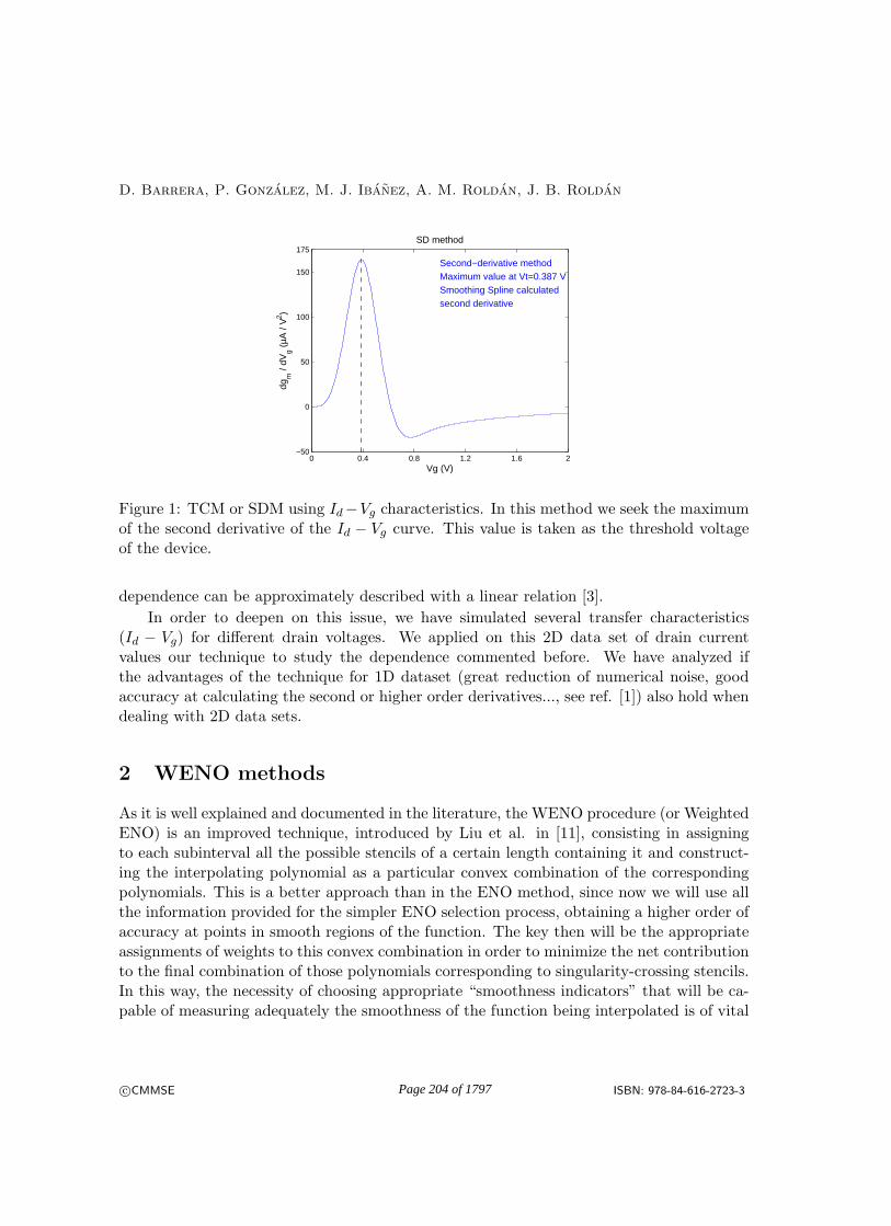
D. Barrera, P. Gonzalez, M. J. Ibanez, A. M. Roldan, J. B. Roldan

0 0.4 0.8 1.2 1.6 2−50

0

50

100

150

175

Second−derivative methodMaximum value at Vt=0.387 VSmoothing Spline calculatedsecond derivative

SD method

Vg (V)

dgm

/ dV

g (µA

/ V

2 )

Figure 1: TCM or SDM using Id−Vg characteristics. In this method we seek the maximumof the second derivative of the Id − Vg curve. This value is taken as the threshold voltageof the device.

dependence can be approximately described with a linear relation [3].

In order to deepen on this issue, we have simulated several transfer characteristics(Id − Vg) for different drain voltages. We applied on this 2D data set of drain currentvalues our technique to study the dependence commented before. We have analyzed ifthe advantages of the technique for 1D dataset (great reduction of numerical noise, goodaccuracy at calculating the second or higher order derivatives..., see ref. [1]) also hold whendealing with 2D data sets.

2 WENO methods

As it is well explained and documented in the literature, the WENO procedure (or WeightedENO) is an improved technique, introduced by Liu et al. in [11], consisting in assigningto each subinterval all the possible stencils of a certain length containing it and construct-ing the interpolating polynomial as a particular convex combination of the correspondingpolynomials. This is a better approach than in the ENO method, since now we will use allthe information provided for the simpler ENO selection process, obtaining a higher order ofaccuracy at points in smooth regions of the function. The key then will be the appropriateassignments of weights to this convex combination in order to minimize the net contributionto the final combination of those polynomials corresponding to singularity-crossing stencils.In this way, the necessity of choosing appropriate “smoothness indicators” that will be ca-pable of measuring adequately the smoothness of the function being interpolated is of vital

c⃝CMMSE ISBN: 978-84-616-2723-3Page 204 of 1797

A WENO-based method to improve the determination of the threshold voltage

0,0

0,5

1,0

1,5

2,0

2,5

3,0

0,0

0,1

0,2

0,3

0,4

0,5

0,6

0,0

0,5

1,0

1,5

2,0

2,5

3,0

I DS (

mA

)

V GS (V)V

DS (V)

Figure 2: Drain current versus gate voltage and drain voltage for the transistor simulated.

importance. Jian and Shu [10] presented some of such indicators, usually more efficientthan that proposed originally by Liu et al.

Another important issue of these techniques is that they were proposed originally fortheir application to the numerical resolution of hyperbolic problems and that they areformulated for the construction of the corresponding ENO or WENO interpolants, basedmainly on cell averages and not just on point values. But some other authors, like thosein [2] have adapted the original procedures to the corresponding point-value interpolationframework, that is what we also use here.

3 Transistor description

In order to analyze the numerical procedures for extracting the threshold voltage reportedat the introduction, we have simulated a conventional silicon MOSFET transistor makinguse of ATLAS (a TCAD tool developed by Silvaco [6] for electronics device simulation,design and characterization). The main technological features of the transistor simulatedare the following: L = 0.3µm channel doping concentration at the oxide surface levelNA = 1017 cm−3, and oxide thickness Tox = 8.7 nm; a N+ poly-silicon gate was used.

4 Results and discussion

The first results obtained with this WENO procedure are being very encouraging, and ingood agreement with the results from the experimental measurements and other model

c⃝CMMSE ISBN: 978-84-616-2723-3Page 205 of 1797

D. Barrera, P. Gonzalez, M. J. Ibanez, A. M. Roldan, J. B. Roldan

0,0 0,5 1,0 1,5 2,0 2,5 3,00,00

0,05

0,10

0,15

0,20

0,25

0,30

I DS (m

A)

VGS (V)

IDS for VDS=0.45V

Figure 3: Drain current Id(A) versus gate voltage, Vg(V ), for a constant drain voltage Vd.

validations using different techniques, so they are making us thinking that they could beappropriate tools for many problems of this type.

In Figure 3, the simulated drain current versus gate voltage of the device under studyis shown. This is one of the curves extracted from the data in Figure 2. The derivative ofthese data is shown in Figure 4. As it is well known, the numerical noise is much greaterwhen calculating derivatives of the simulated and measured data, which is the case here.Nevertheless, the use of the WENO procedure, greatly reduces the oscillations. These effectsare obviously greater for the second derivative; but this time, again, the use of an advancenumerical procedure such as WENO produces a smooth data set (see Figure 5). This outputallowed us to easily calculate the threshold voltage since the maximum is clearly defined andthe typical errors connected with the numerical noise produced in calculating the derivativesare avoided.

The use of the previously described WENO procedure helped us with the analysis ofthe threshold voltage dependence on the drain voltage, due to the well known DIBL effects[3]. As can be seen, a linear trend shows up when the threshold voltage is calculatedversus the drain voltage, as expected (see Figure 6). The use of this method presentspromising possibilities for the automatic determination of the threshold voltage in differentbias conditions using the TCM method. In this respect, the numerical stability linked tothe WENO procedure could permit the inclusion of complex parameter extraction methods,numerically speaking, in conventional industrial tools.

c⃝CMMSE ISBN: 978-84-616-2723-3Page 206 of 1797

A WENO-based method to improve the determination of the threshold voltage

0,0 0,5 1,0 1,5 2,0 2,5 3,00,00

0,02

0,04

0,06

0,08

0,10

0,12

0,14

I' DS (

mA

/V)

VGS (V)

I'DS for VDS= 0.45V

Figure 4: Approximation of the first derivative I ′d(A/V ) versus gate voltage, Vg(V ), usingthe WENO procedure.

0,0 0,5 1,0 1,5 2,0 2,5 3,00,0

0,1

0,2

0,3

0,4

0,5

I''DS for VDS=0.45V

I'' DS (m

A/V

2 )

VGS (V)

Figure 5: Approximation of the maximum of the second derivative I ′′d (A/V 2) versus gatevoltage, Vg(V ).

c⃝CMMSE ISBN: 978-84-616-2723-3Page 207 of 1797

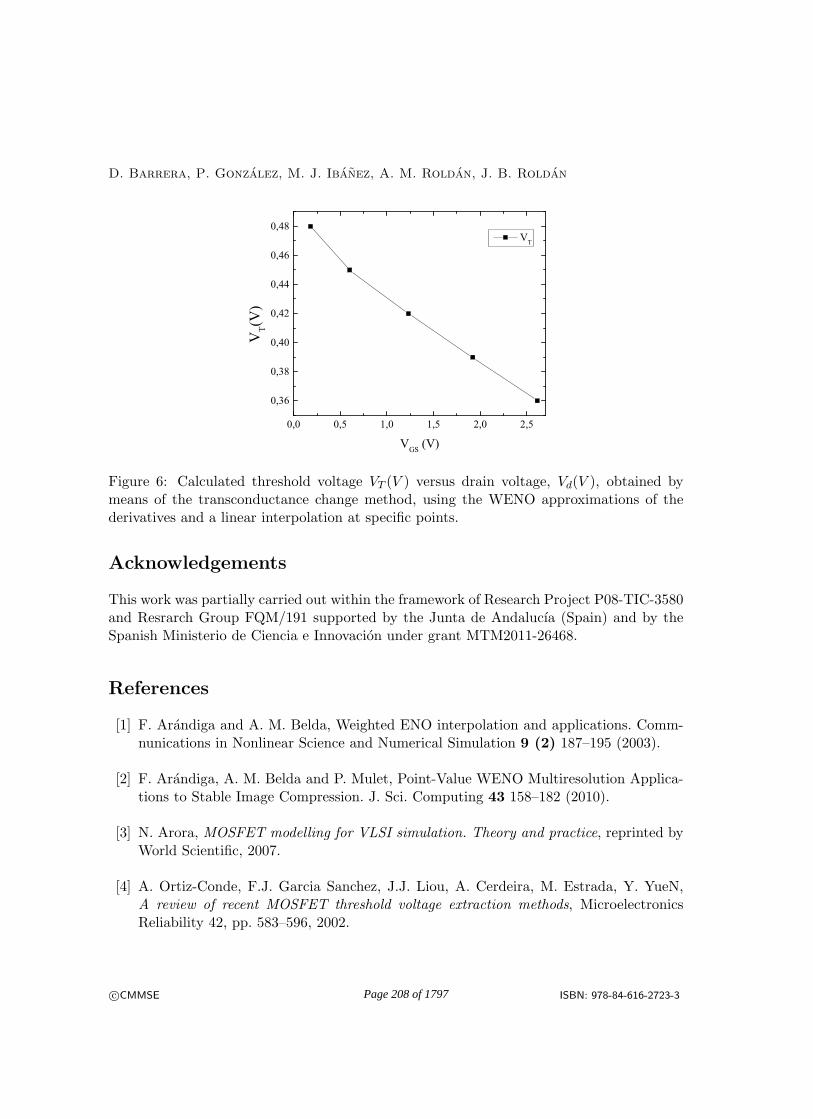
D. Barrera, P. Gonzalez, M. J. Ibanez, A. M. Roldan, J. B. Roldan

0,0 0,5 1,0 1,5 2,0 2,5

0,36

0,38

0,40

0,42

0,44

0,46

0,48

VT(

V)

VGS (V)

VT

Figure 6: Calculated threshold voltage VT (V ) versus drain voltage, Vd(V ), obtained bymeans of the transconductance change method, using the WENO approximations of thederivatives and a linear interpolation at specific points.

Acknowledgements

This work was partially carried out within the framework of Research Project P08-TIC-3580and Resrarch Group FQM/191 supported by the Junta de Andalucıa (Spain) and by theSpanish Ministerio de Ciencia e Innovacion under grant MTM2011-26468.

References

[1] F. Arandiga and A. M. Belda, Weighted ENO interpolation and applications. Comm-nunications in Nonlinear Science and Numerical Simulation 9 (2) 187–195 (2003).

[2] F. Arandiga, A. M. Belda and P. Mulet, Point-Value WENO Multiresolution Applica-tions to Stable Image Compression. J. Sci. Computing 43 158–182 (2010).

[3] N. Arora, MOSFET modelling for VLSI simulation. Theory and practice, reprinted byWorld Scientific, 2007.

[4] A. Ortiz-Conde, F.J. Garcia Sanchez, J.J. Liou, A. Cerdeira, M. Estrada, Y. YueN,A review of recent MOSFET threshold voltage extraction methods, MicroelectronicsReliability 42, pp. 583–596, 2002.

c⃝CMMSE ISBN: 978-84-616-2723-3Page 208 of 1797

A WENO-based method to improve the determination of the threshold voltage

[5] A. Ortiz-Conde, F.J. Garcia Sanchez, J. Muci, A. Teran, J. Liou, C. Ho, RevisitingMOSFET threshold voltage extraction methods, Microelectronics Reliability 53, 90–104,2013.

[6] Atlas manuals. http://www.silvaco.com

[7] D. Flandre, V. Kilchytska and T. Rudenko, gm/Id method for threshold voltage ex-traction applicable in advanced MOSFETs with nonlinear behavior above threshold,IEEE Electron Device Letters 31 (9) (2010) 930–932.

[8] C. Galup-Montoro and Ch. Schneirer Marcio, Mosfet modelling for circuit analysis anddesign, World Scientific, 2007.

[9] The International Technology Roadmap for Semiconductors, ed. 2011 and 2012 update.http://public.itrs.net.

[10] G. Jiang and C.-W. Shu, Efficient implementation of weighted ENO schemes, Journalof Computational Physics 126 202–228 (1996) from an ICASE-NASA Report of 1995.

[11] X-D. Liu, S. Osher and T. Chan, Weighted essentially non-oscillatory schemes, J.Comput. Phys., 115, 200–212 (1994).

[12] G. Moore, Cramming more components onto integrated circuits, Electronics Magazine38 (8) 1965.

[13] H. S. Wong, M. H. White, T. J. Kurttsick and R. V. Booth, Modeling of transconduc-tance degradation and extraction of threshold voltage in thin oxide MOSFETs, SolidState Electronics 20 (1987) 953–968.

[14] M. J. Ibanez, J. B. Roldan, A. M. Roldan, R. Yanez, A comprehensive characterizationof the threshold voltage extraction in MOSFETs transistors based on smoothing splines,Mathematics and Computers in Simulation, accepted for publication, (2013).

c⃝CMMSE ISBN: 978-84-616-2723-3Page 209 of 1797

Proceedings of the 13th International Conferenceon Computational and Mathematical Methodsin Science and Engineering, CMMSE 201324–27 June, 2013.

Error estimates for modified Hermite interpolanton the simplex

D. Barrera1, M. J. Ibanez1 and O. Nouisser2

1 Departamento de matematica aplicada, Universidad de Granada, Spain

2 Departement de mathematiques, Faculte Polydisciplinaire de Safi, Maroc

emails: dbarrera@ugr.es, mibanez@ugr.es, otheman.nouisser@yahoo.fr

Abstract

The objective of this paper, is to study the error estimates of the Hermite inter-polation operator of a multivariate function defined on a given regular simplex usingthe first and the second derivatives of the given function at the vertices of the simplex.The obtained operator is the identity of the cubic polynomials. When the data aregiven inside the simplex, we construct another approximation operator and we give theassociated error estimates.

Key words: Interpolation, Hermite interpolation, Approximation order, error esti-amtes.

1 Introduction

Let S be a simplex in the d-dimensional Eulidean space Rd, with vertices ν0, · · · , νd. Sup-pose we know the values of a function f and those of its partial derivatives up to order twoat the vertices of S. Our aim is to construct an approximation operator that interpolate fand its derivatives from this data.

Thomas F. Sturm [3] considered the Hermite interpolation operator

L[f ](x) =d∑i=0

f(νi)ϕi(λ(x)) +d∑

r=0,r 6=iDνr−νif(νi)φi,r(λ(x))

c©CMMSE ISBN: 978-84-616-2723-3Page 210 of 1797

modified Hermite interpolant on the simplex

that interpolate f and its first derivatives at the vertices of S. He proved that L reproducethe space of quadratic polynomials. The basis functions ϕi and φi 1 ≤ i ≤ d, are the cubicpolynomials given by

ϕi(λ(x)) = λi

(1 + λi −

d∑r=0

λ2r

),

φ(λ(x)) =1

2λiλr (1 + λi − λr)

where λi(x), 0 ≤ i ≤ d, are the barycentric coordinates of x with respect to S that satisfy

x =d∑i=0

λi(x)νi,

λi(x) ≥ 0,∀x ∈ S,

1 =d∑i=0

λi(x),∀x ∈ S.

Her, we denote by Djyf(x) the jth directional derivative of f at x, defined by

Djyf(x) =

[dj

dtjf(x+ ty)

]t=0

In this paper and in order to improve the algebraic precision of the operator L, we considera modified Hermite interpolation operator defined by :

H[f ](x) =d∑i=0

(f(vi) +

1

3Dx−vif(vi)

)+

d∑r=0,r 6=i

(2

3Dvr−vif(vi) +

1

3Dvr−viDx−vif(vi)

)φi,r(x)

.

We establish an integral representation for the error of approximation considered by theoperator H in terms of the one considered by L. In this setting, we establish the errorestimates with respect the infinity norm. Finally, Numerical examples are illustrated toshow the theoretical results.

2 representation of the error of the modified operator

By C(§), we denote the class of all real-valued continuous functions on S, and by Cm(S),where m ∈ N, the subclass of all functions that are m times continuously differentiable inthe following sense. For each x ∈ S and any y ∈ Rd such that x + y ∈ S, the directionalderivatives Dj

yf(x) exist for j = 1, · · · ,m and depend continuously on x.The error of the approximation by H[f ] can be represented as follows.

c©CMMSE ISBN: 978-84-616-2723-3Page 211 of 1797

D. Barrera, M. J. Ibanez, O. Nouisser

Theoreme 2.1 Let f ∈ C4(S). Then

f(x)−H[f ](x) =1

6

d∑i=0

(∫ 1

0D4x−νif(νi + t(x− νi))t2(1− t)dt

)ϕi(x) +

d∑i=0

d∑r=0,r 6=i

(∫ 1

0Dνr−νiD

4x−νif(νi + t(x− νi))dt

)φi,r(λ(x))

when the second derivatives are not involved, the operator H is reduced to the operator L,and the error of the approximation by L[f ] can be reprensented as follows

Theoreme 2.2 Let f ∈ C3(S). Then

f(x)− L[f ](x) =1

2

d∑i=0

(∫ 1

0D3νi−xf(x+ t(νi − x))(1− t)2dt

)ϕi(x) +

d∑i=0

d∑r=0,r 6=i

(∫ 1

0Dνi−νrD

2x−νif(x+ t(νi − x))(1− t)dt

)φi,r(λ(x))

It is interesting to mention that interpolation by L is preserved by H.

Proposition 2.1 For all f ∈ C4(S), we have

1. H[f ](νi) = f(νi),∀i = 0, · · · , d.

2. ∇H(f ](νi) = ∇f(νi),∀i = 0, · · · , d.

3. H[P ] ≡ P , for all cubic polynomial P .

References

[1] A. Guessab, G. Schmeisser, harp error estimates for interpolatory approximationon convex polytopes, SIAM J. Numer. Anal. 43 (2006) 909-923.

[2] A. Guessab, O. Nouisser, G. Schmeisser, A Multivariate approximation by acombination of modified taylor polynomials, J. Comput. Appl. Math. 196 (2006) 162-179.

[3] Thomas F. Sturm, A unique multivariate hermite interpolant on the simplex, J.Math. Anal. Appli.191(1995) 101-117.

c©CMMSE ISBN: 978-84-616-2723-3Page 212 of 1797

Proceedings of the 13th International Conference

on Computational and Mathematical Methods

in Science and Engineering, CMMSE 2013

24–27 June, 2013.

Discrete orthogonal polynomial technique for parameter

determination in MOSFETs transitors

D. Barrera1, M. J. Ibanez1, A. M. Roldan2, J. B. Roldan2 and R. Yanez1

1 Department of Applied Mathematics, University of Granada

2 Department of Electronics, University of Granada

emails: dbarrera, mibanez, amroldan, jroldan, ryanez@ugr.es

Abstract

In this communication, we develop a technique, based on discrete orthogonal poly-nomials, to determine the straight line portions in a data cloud. A practical case todetermine basic parameters of a MOSFET transistor is shown.

Key words: discrete orthogonal polynomials, straight line portion, MOSFET

MSC 2000: 33C45,42C10, 65D10, 82D37

1 Introduction

Transistors, and in particular MOSFETs (Metal Oxide Semiconductor Field Effect Transis-tors), are the most used basic building blocks of integrated circuits (ICs) [1]. The complexityof current chips makes essential their accurate characterization to use them for circuit de-sign purposes. For each generation of transistors the main electrical features have to bemodeled in order to reproduce them as a function of the voltages differences applied be-tween their terminals. The models (usually known as compact models) consist of a set ofanalytical equations and a set of parameters to include in those equations. A different set ofparameters is used for each fabrication technology. These models are used in TCAD circuitsimulation tools and also for hand-calculations used at the first stages of circuit design.

The extraction of the parameters of new technologies is essential since the capacitiesof circuit designers are dependant on the accuracy of model parameters that in many casesare linked to important physical effects.

Each parameter is obtained in a different way. However, few of them share some featuresin common, at least from the numerical viewpoint. In this respect, several parameters are

c©CMMSE ISBN: 978-84-616-2723-3Page 213 of 1797

Discrete orthogonal polynomial technique for parameter determination

obtained by means of extrapolation methods (for example threshold voltage calculation [1]),linear regression (determination of the body factor [1]), slope calculations (extraction of theDIBL parameter[1]), etc. In all these procedures, the determination of portions of curvesthat can be approximated by a straight line is crucial. In this work we just deal with thisissue trying to shed light by means of advanced numerical techniques.

We have developed a method to determine the number of straight line portions containedin a curve in an automatic manner. The algorithm developed, based on discrete orthogonalpolynomials, can be used for parameter extraction purposes. It consist on the isolation ofstraight line portions in experimental or simulated data and the determination of the slopeof those curve sections to calculate one or more parameters of a compact model.

This work is organized as follows: in Section 2 we briefly describe the basic properties ofthe discrete orthogonal Chebyshev polynomials that we will use in this work, in Section 3 wereport and discuss on the numerical procedure employed, and finally, the main conclusionsare drawn in Section 4.

2 Discrete Orthogonal Chebyshev polynomials: basic prop-

erties

In these section we will briefly describe basic properties of discrete orthogonal Chebyshevpolynomials that will be used in this work.

The discrete Chebyshev orthonormal polynomials are defined as the following hyperge-ometric series [2, 3, 4]:

tn(x;L) =1

n!

√

(2n+ 1)(L− n− 1)!

(L+ n)!

n∑

k=0

(−1)kn!

k!(n− k)!(x− k − L+ 1)n(x− k + 1)n, (1)

where L ∈ N is a parameter, x ∈ N, 0 ≤ x ≤ L−1, is the variable, and n ∈ N, 0 ≤ n ≤ L−1,is the degree of the polynomial.

They verify the three term recurrence relation

tn+1(x;L) =dndn+1

(x− βn)tn(x;L)− γndn−1

dn+1tn−1(x;L)

=1

αn(x− βn)tn(x;L)−

αn−1

αntn−1(x;L) (2)

with

αn =n+ 1

2

√

L2 − (n+ 1)2

(2n+ 1)(2n+ 3),

βn =L− 1

2

c©CMMSE ISBN: 978-84-616-2723-3Page 214 of 1797

D. Barrera, M. J. Ibanez, A. M. Roldan, J. B. Roldan, R. Yanez

and they are orthogonal with respect to the scalar product:

〈tn(·, L), tm(·, L)〉 =L−1∑

xi=0

tn(xi;L)tm(xi;L) = δn,m (3)

3 Numerical procedure

In this section we will explain the procedure followed to isolate de straight line portions inthe data (experimental or simulated).

Let’s considered a set of discrete data xi, yi, i = 1, . . . N , with xi equispaced, i.e.xi+1−xi = h (constant). Our purpose is to determine subsets of data xi, yi, i = im, . . . , iMforms a straight line. The procedure can be divided in two parts: i) Given a subset of data,determine if these data forms a straight line and ii) Selection of subsets. Let’s analyze thetwo parts:

3.1 Checking of straight lines

Let’s take a subset of data xi, yi, i = i1, . . . , iM and consider the scalar products

rn = 〈y, tn(·,M)〉 =

M−1∑

i=0

yitn(i,M)

The data can be obtained from a linear combination of the polynomials tn:

yi =∞∑

j=0

cij tj(xi,M)

so the scalar products rn takes the value

rn = cn

where we have used the orthonormality of the polynomials tn. So, if the data yi forms astraight line, we will have that all the scalar products rn will be 0, except r0 and/or r1.In practice, we will consider only the scalar products rn for n = 0, . . . , nmax, with nmax

given. Then, we check if all the coefficients rn, n = 0, . . . , nmax, vanish except r0 and/orr1. Only in this case, we will accept the data as a straight line and n. In practice we willconsider that a coefficient rn vanish if |rn| < ǫ. Of course, it can happens that the data yicomes from a combination of t0, t1 and polynomials with higher degrees than nmax, but,considering that we can choose nmax sufficiently large and that out data are experimentaland, so, affected by measuring errors, this is highly improvable.

c©CMMSE ISBN: 978-84-616-2723-3Page 215 of 1797

Discrete orthogonal polynomial technique for parameter determination

3.2 Determination of straight subsets

We start considering a subset of data with, at least, 4 points, as with 2 points we alwayshave a straight line, but we can choose this initial number of data points arbitrarily from 3.So, we initially begin with i1 = 1 and iM = 4. We then check if it forms a straight line. If itdoes, we begin a binary search for larger subsets of straight line data between iM = 4 andN (the total number of data points), ending when it detects the maximal subset of straightline data points. After that we set ii = iM + 1 (the last point of the previous straight lineplus 1) and iM = i1 + 4 and start the procedure again. If the initial data points (i1 andi1 + 4 doesn’t forms a straight line we increase each by 1 (i1 → i1 + 1 and iM → iM + 1)and start the procedure again. We stop the whole process when there are not enough datato consider a straigh line.

Once we have the subsets of straight line data, we compute the straight lines themselves,as

p(x) = c0t0(x,M) + c1t1(x,M)

This procedure can be straightforwardly generalized to detect substes of data withpolynomial degree higher than 1.

4 Practical case

Here we will use the previously discused techniques to find the stright line subset of datain a MOSFET device with the following characteristics: L = 0.3µm, NA (channel dopingconcentration at the oxide surface level) = 2.8 1016 cm−3, and oxide thickness Tox = 8.7 nm.A N+ polysilicon gate was used

Applying our technique to the simulated data for this MOSFET we find a straight linesubset of data in the range [0.0V, 0.35V ]

0.0 0.5 1.0 1.5 2.0 2.5 3.0Voltage

10-9

10-8

10-7

10-6

10-5

Intensity

This straight line can be easily computed, finding

p(x) = 1011.9384x−10.3234

c©CMMSE ISBN: 978-84-616-2723-3Page 216 of 1797

D. Barrera, M. J. Ibanez, A. M. Roldan, J. B. Roldan, R. Yanez

Aknowledgments

This work was partially carried out within the framework of Research Project P08-TIC-3580supported by the Junta de Andalucıa.

References

[1] N. Arora, MOSFET modelling for VLSI simulation. Theory and practice, reprinted byWorld Scientific, 2007.

[2] A.F. Nikiforov & V.B. Uvarov, Special Functions of Mathematical Physics. BirkhauserVerlag, Basilea, 1988

[3] A.F. Nikiforov, S.K. Suslov & V.B. Uvarov, Classical Orthogonal Polynomials of a Dis-crete Variable. Springer Series in Computational Physics. Springer-Verlag, Berlin, 1991.

[4] R. Alvarez-Nodarse, Polinomios hipergeometricos clasicos y q-polinomios. Monografıasdel Seminario Matematico “Garcıa de Galdeano”.Vol. 26. Prensas Universitarias deZaragoza, Zaragoza, Spain, 2003.

c©CMMSE ISBN: 978-84-616-2723-3Page 217 of 1797

Proceedings of the 13th International Conferenceon Computational and Mathematical Methodsin Science and Engineering, CMMSE 201324–27 June, 2013.

Conservation Law Construction via MathematicalFluctuation Theory for Exponentially Anharmonic,

Symmetric, Quantum Oscillator

Semra Bayat1 and Metin Demiralp1

1 Informatics Institute, Computational Science and Engineering Program, IstanbulTechnical University

emails: bayat@itu.edu.tr, metin.demiralp@gmail.com

Abstract

This work focuses on the point that how conservation laws amongst the expectationvalues can be constructed. We use the expectation value dynamics of quantum systemsand the mathematical fluctuation concept. The fluctuation free equations match theclassical mechanical equations while the introduction of the fluctuations increases thenumber of the ODEs even though the added ODEs are linear in fluctuations. We haveshown that space extension creates space contraction laws while each different orderset of fluctuation creates interfluctuation conservation laws. The familiar laws like theenergy conservation still exist but there is a need to have fluctuation related terms.

Key words: Expectation Values, Quantum Expected Value Dynamics, Fluctuations,Conservation Laws.

1 Introduction

We concern with the conservation law construction for quantum systems by using mathe-matical fluctuation theory in this work. Our focus is taken as the quantum system whosepotential contains a symmetric exponential function which shows the harmonic oscillatorbehaviour at the zero limit of the scaling parameter in its argument. The Schrodingerequation [1] for this system can be explicitly given through the following equalities

i~∂ψ

∂t= Hψ, ψ (x, 0) = ψ0 (x) (1)

c©CMMSE ISBN: 978-84-616-2723-3Page 218 of 1797

Conservation Laws via Fluctuations

H =1

2µp 2 + α

(e

k2q 2 − I

)(2)

pf(x) ≡ −i~∂f(x)

∂x, qf(x) ≡ xf(x) (3)

where I, p, q, and, H denote the identity, momentum, position, and, Hamilton operators ofthe system under consideration. The system has one degree of freedom and describes themotion of a particle which can move on a straight line by definition. µ, α, and, k standfor the mass, potential amplitude, and, anharmonicity constant which are parameters tobe used for system identification. ~ denotes the universal reduced Planck constant whilethe function ψ0 (x) symbolizes the initial form of the wave function. All these enable us torewrite the system’s Schrodinger equation in a single formula explicitly as follows

i~∂ψ(x, t)

∂t= − ~2

2µ

∂2ψ(x, t)

∂x2+ α

(e

k2x 2 − 1

)ψ(x, t), ψ(x, 0) = ψ0 (x0) (4)

which is a parabolic partial differential equation describing the system’s evolution. Thegeneral tendency is to find the wave function by solving this equation and then to evaluatethe expectation values of certain operators corresponding to some observable entities. Hencethe wave function is in fact an intermediate tool and necessitates the solution of a partialdifferential equation (PDE) [2]. This is not an easy task even though the present PDE seemsto be rather easy to be solved, since the increasing degree of freedom in the system at thefocus complicates the problem of solving PDE because of the increasing dimensionality. Thisimportant fact urged us to skip the evaluation of the wave function and construct the ODEsover the expectation values we need to evaluate [3–5]. We call this approach “QuantumExpectation Value Dynamics” because of its nature. We will use this approach for theevaluation of certain expectation values for our target system here. However, our mainpurpose is beyond this. We want to construct certain conservation laws like the energyconservation of the mechanics. We seek the relations amongst the expectation values ofcertain operators such that they do not change functional structure during the evolution ofthe system. We take the first steps in the next section and then we focus on mathematicalfluctuation concept on the continuation of the study [6–9]. Relevant fluctuation equationsare constructed in the following sections.

2 Expectation Value Dynamics on an Extended Space

The exponential function structure in the potential of the target system above complicatesthe formulation since it does not have a finite term representation in powers of its argument.On the other hand, despite its highly complicated singularity at infinity the exponentialfunction has a very specific and pleasant property. Its derivative with respect to its argument

c©CMMSE ISBN: 978-84-616-2723-3Page 219 of 1797

Semra Bayat, Metin Demiralp

is same as itself. Exponential function does not linearly depend on certain finite numberof powers of its argument even though there is a functional dependence amongst them.This brings the idea of considering the exponential function as if an additional independentvariable and therefore to work in an extended space [10, 11]. Hence, we can start with thedefinition

rf(x) ≡(e

k2x 2 − 1

)f(x) (5)

where r is apparently an algebraic multiplication operator. This enables us to write thefollowing Poisson brackets

H, p≡ i

~

[H, p

]= −αkq

(r + I

)(6)

H, q

≡ i

~

[H, q

]=

1

µp (7)

H, r

=

k

2µpq(r + I

)+

k

2µ

(r + I

)qp (8)

These Poisson brackets are in fact the core agents of the temporal derivatives of certainoperator expectation values as the following analysis shows.

The explicit expectation value definition of a given operator o is as follows

〈o〉 (t) ≡∫VdV ψ (x, t)∗ oψ (x, t) (9)

the simple temporal differentiation of this equality produces

d 〈o〉 (t)dt

=⟨H, o

⟩(t) (10)

where H, o

≡ i

~

(Ho− oH

). (11)

These allow us to obtaind 〈p〉dt

= −αk⟨q(r + I

)⟩, 〈p〉 (0) = 〈p〉0 (12)

d 〈q〉dt

=1

µ〈p〉 , 〈q〉 (0) = 〈q〉0 (13)

d 〈r〉dt

=k

2µ

⟨pq(r + I

)⟩+

k

2µ

⟨(r + I

)qp⟩, 〈r〉 (0) = 〈r〉0 (14)

The right hand sides of the latest three equations except the second one are expectationvalues of certain operators which are linearly independent from the left hand side operators.Hence, we can not consider these three equations as a complete set of ODEs. We need toconstruct further equations. We do this in the next section by using fluctuation concept.

c©CMMSE ISBN: 978-84-616-2723-3Page 220 of 1797

Conservation Laws via Fluctuations

3 Conservation Laws at Fluctuationlessness Limit

Let us define the following fluctuation operators somehow describing the deviations fromthe expectation values for p, q and r

φp = p− 〈p〉 I , φq = q − 〈q〉 I , φr = r − 〈r〉 I , (15)

then

p = 〈p〉 I + φp, q = 〈q〉 I + φq, r = 〈r〉 I + φr. (16)

The potential function defined as

V (q) = α(e

k2q 2 − I

)(17)

can be rewritten by using fluctuation operators defined above

V (q) = V(〈q〉 I + φq

)= α

(e

k2 (〈q〉I+φq)

2

− I)

=∞∑j=0

α(e

k2〈q〉2 − I

)(j)

j!φjq

= α(e

k2〈q〉2 − I

)I + αk 〈q〉 e

k2〈q〉2 φq +

∞∑j=2

α(e

k2〈q〉2 − I

)(j)

j!φjq

(18)

The expected value of the potential function V (q) can be evaluated as

〈V (q)〉 = αek2〈q〉2 +

∞∑j=2

(αe

k2〈q〉2)(j)

j!

⟨φjq

⟩

= αek2〈q〉2 +

∞∑j=1

(αe

k2〈q〉2)(j+1)

(j + 1)!

⟨φj+1q

⟩(19)

where we have taken into consideration that the expected value of any one of fluctuationoperators defined above vanishes. Despite this vanishing feature the expectation values ofthe higher degree terms formed by the products of powers of the fluctuation operators donot vanish. We call those entities “Fluctuations”. The jth order fluctuations which can bederived from momentum and position operator expectation values can be defined as follows

ϕj,k =

⟨1

2

(φkpφ

j+1−kq + φj+1−k

q φkp

)⟩j = 1, 2, ... k = 0, 1, ..., j + 1. (20)

c©CMMSE ISBN: 978-84-616-2723-3Page 221 of 1797

Semra Bayat, Metin Demiralp

If we now neglect all fluctuation terms in the potential function expansion and in the righthand side expansion of the expectation value ODE for the operator r then we can write

d 〈p〉dt

= −αk 〈q〉(〈r〉+ I

)(21)

d 〈q〉dt

=1

µ〈p〉 (22)

d 〈r〉dt

=k

µ〈p〉 〈q〉

(〈r〉+ I

). (23)

It is not hard to get the following relation from the second and third equations of this set

k

2〈q〉2 − ln

(I + 〈r〉

)= c1 (24)

where c1 is an arbitrary constant for this moment. This is the reflection of the spaceextension realized by defining r. That equation is in fact an algebraic identification andwe can enforce its validity for the initial expectation value quite naturally. This makes c1vanishing and we can write the following equality at the end

〈r〉 = ek2〈q〉2 − I (25)

This is somehow the reflection of the algebraic relation between r and the position operatorto the relation between these two operators’ expectation values. In other words, this relationtakes us back from the extended space to the original space. Hence we can call this relation“Space Contraction Law“.

The utilization of (25) in the first one of triple equation set in (23) and combining theresulting equation with the second equation of that set takes us to a couple of ODEs inmomentum and position operator. Due to the structure of this couple of ODEs we canintegrate them to the following relation

1

2µ〈p〉2 + α

(e

k2〈q〉2 − I

)= c2 (26)

where c2 is an arbitrary constant for the moment. It in fact corresponds to the total energyof the system under consideration and this relation states that the expectation value of thesystem Hamiltonian is conserved for all time instances. To evaluate the conserved totalenergy value it is sufficient the evaluate the expectation values at the initial moment wherethe wave function is given. So the second law given by (26) is the “Energy ConservationLaw” for the system under consideration.

4 Conservation Laws in First Fluctuation Point of View

In the previous sections we have focused on the expectation value dynamics in an extendedspace to show the role of space extension explicitly. In this section we focus on the case

c©CMMSE ISBN: 978-84-616-2723-3Page 222 of 1797

Conservation Laws via Fluctuations

where no space extension is realized. Hence, the operator r will be undefined and allthe system properties will be described certain entities depending on the momentum andposition operators only. This time we are going to omit again all fluctuations except theones with first order. The approximate form of the system Hamiltonian’s expectation valuecan be given as follows for these cases

〈H〉 =1

2µ〈p〉2 + αe

k2〈q〉2 +

1

2µϕ1,2 +

αk

2

(I + k 〈q〉2

)e

k2〈q〉2ϕ1,0 (27)

This is in fact the first order fluctuation involving approximate form of the overall energyconservation. The expectation value dynamics of the momentum and position operatorswithin the first order fluctuation approximation can be written as follows

d 〈p〉dt

= −αk 〈q〉 ek2〈q〉2 − αk

2

(I + k 〈q〉2

)e

k2〈q〉2ϕ1,0 (28)

d 〈q〉dt

=1

2µ〈p〉 . (29)

These equations are somehow incomplete since they contain unknown fluctuations whichare temporal functions. Hence we need to add certain ODEs to get a complete set of ODEs.To this end we can start with the following definitions

ϕ1,0 =⟨φ2q

⟩, ϕ1,1 =

⟨1

2

(φpφq + φqφp

)⟩, ϕ1,2 =

⟨φ2p

⟩(30)

These definitions can be used to construct ODEs for these entities. For this action we canemploy the Poisson brackets of certain operators and some operator algebra together withstandard algebra. By skipping the intermediate derivation stages we can obtain

dϕ1,0

dt=

2

µϕ1,1 (31)

dϕ1,1

dt= −

(αke

k2〈q〉2 + αk2 〈q〉2 e

k2〈q〉2)ϕ1,0 +

1

µϕ1,2 (32)

dϕ1,2

dt= −2

(αke

k2〈q〉2 + αk2 〈q〉2 e

k2〈q〉2)ϕ1,1 (33)

It is possible to find a conserved entity whose value does not change during the system’sevolution. It can be constructed from the equations of the latest triple set of ODEs above.We can conclude

ϕ21,1 − ϕ1,0ϕ1,2 = c3 (34)

c©CMMSE ISBN: 978-84-616-2723-3Page 223 of 1797

Semra Bayat, Metin Demiralp

where c3 stands for a constant which is arbitrary for this moment. It can be evaluated byusing the initial expectation values via the initial wave form. This relation is conservedfor all time instances of the evolution and we call it “First Order Fluctuation ConservationLaw”. This is somehow the fluctuation reflection of the energy conservation law whichrelates the expectation values of the momentum and position operators.

The other conservation law is again energy conservation law and is based on the invari-ance of the Hamiltonian’s expectation value which depends on the first order fluctuationsas we have mentioned at the beginning of this section. This completes the investigation forthe first order fluctuation preserving case.

5 Concluding Remarks

The purpose of this work has been the construction of conservation laws in the frameworkof the mathematical fluctuation theory. We have used the expectation value dynamics tothis end. We also have shown the role of the space extension in facilitating the analysis.Because of the highly probabilistic nature of the quantum dynamical problems we neededto use the fluctuation concept as the expectation values of the powers of certain deviation(fluctuation) operators. We have reobtained the well known “Energy Conservation Law”for no fluctuation and first order fluctuations. The cases where space extension has beenused certain “Space Contraction Laws” have been obtained. We have interpreted themas going back to the original space from the extended space. The additions fluctuationconcept has arisen the conservation law(s) amongst the fluctuations. We have limited ourinvestigations to the cases where at most first order fluctuations are taken into consideration.All these analyses can be extended to much higher order fluctuation containing cases withoutany remarkable conceptual difficulty even though the volume of the manipulations andintermediate steps increases pretty much.

References

[1] P. A. M. Dirac, The Fundamental Equations of Quantum Mechanics, Proc. R. Soc.Lond. A 109 (1925) 642–653.

[2] H. J. W. Muller-Kirsten, Introduction to Quantum Mechanics: Schrodinger Equa-tion And Path Integral, World Scientific Publishing Company, Singapore, 2006.

[3] M. Demiralp, Determination of the Quantum Motion of the One Dimensional Har-monic Oscillator via Expectation Value Evolutions, Bull. Tech. Univ. Istanbul 47(4)(1994) 357.

c©CMMSE ISBN: 978-84-616-2723-3Page 224 of 1797

Conservation Laws via Fluctuations

[4] M. Demiralp, Quantum Mechanical Matrix Ordinary Differential Equations andTheir Solutions by Characteristic Evolutions, Proceeding of MMACTEE’09, Vouliag-meni, Athens (2009) 657–662.

[5] E. Meral ve M. Demiralp, Determination Of The External Field Amplitude AndDeviation Parameter Through Expectation Value Based Quantum Optimal Control OfMultiharmonic Oscillators Under Linear Control Agents, J. Math. Chem. 46 (2009)834–852.

[6] M. Demiralp, Determination of Quantum Expectation Values Via Fluctuation Expan-sion, Lecture Series on Computer and Computational Sciences, Selected Papers fromInt. Conf. of Comput. Methods in Sci. and Eng. (ICCMSE 2005), Loutraki, Greece,4A (2005) 146–149.

[7] M. Demiralp, A Fluctuation Expansion Method for the Evaluation of a Function’sExpectation Value, Proc. of the Int. Conf. on Numerical Analysis and Applied Mathe-matics (ICNAAM 2005), Rhodes, Greece (2005) 711–714

[8] N. Altay ve M. Demiralp, Numerical Solution of Ordinary Differential Equationsby Fluctuationlessness Theorem, J. Math. Chem. 47(4) (2010) 1323–1344.

[9] M. Ayvaz ve M. Demiralp, A Fluctuation Analysis at the Classical Limit for theExpectation Dynamics of a Single Quartic Quantum Anharmonic Oscillator, AIP Conf.Proc. 1281 (2010) 1950–1953.

[10] S. Uskuplu ve M. Demiralp, Univariate Integration via Space Extension Based NoFluctuation Approximation, AIP Conf. Proc. 1048 566–569.

[11] S. Uskuplu ve M. Demiralp, Conversion of PDEs to Certain Universal and EasilyHandleable Forms Via Space Extension, Proceedings of the 1st WSEAS Int. Conf. onMultivariate Analysis and its Application in Science and Engineering (MAASE’08)(2008) 179–182.

c©CMMSE ISBN: 978-84-616-2723-3Page 225 of 1797

Proceedings of the 13th International Conferenceon Computational and Mathematical Methodsin Science and Engineering, CMMSE 201324–27 June, 2013.

Optimal control of a linear and unbranched chemical processwith n steps: the quasi-analytical solution

L. Bayon1, J.M. Grau1, M.M. Ruiz1 and P.M. Suarez1

1 Department of Mathematics, University of Oviedo, Spain

emails: bayon@uniovi.es, grau@uniovi.es, mruiz@uniovi.es, pedrosr@uniovi.es

Abstract

In this paper we present a method to solve a constrained optimal control problemto calculate the optimal enzyme concentrations in a chemical process by consideringthe minimization of the transition time. The method, based on Pontryagin’s MaximumPrinciple, allows us to obtain, in an almost exclusively analytical way, the generalizedsolution of an n-step system with an unbranched scheme and bilinear kinetic models.

Key words: Optimal Control, Chemical Process, Pontryagin’s PrincipleMSC 2000: 49J30, 49M05, 92E20, 80A30, 92C40

1 Introduction

In this paper we present an optimal control problem that arises when metabolic chemicalprocesses are considered. Within this context, one of the most important problems is thestudy of enzyme concentrations. Our work focuses on dynamic optimization, studying theproblem of minimizing the transition time during which the substrate is converted into theproduct.

Let us consider the following (unbranched) reaction chain of n irreversible reactionssteps converting substrate x1 into product p:

x1u1→ x2

u2→ x3u3→ · · · → xn−1

un−1→ xnun→ p (1)

where x1 is the substrate concentration (starting reagent), p the concentration of the finalproduct, xi (i = 2, . . . , n) the concentration of the intermediate compounds, and ui (i =1, . . . , n) the concentration of the enzyme catalyzing the i-th reaction.

c⃝CMMSE ISBN: 978-84-616-2723-3Page 226 of 1797

Optimal control of a linear and unbranched chemical process with n steps

For the dynamic case, the aim is to solve the problem analytically and numerically. Anexplicit solution for the simplest case, i.e. n = 2, can be found in [1]. For longer pathways,i.e. n > 2, the aforementioned authors solved the optimization problem numerically. Aninteresting study is presented in [2] in which the solution is obtained quasi-analytically,though with the constraint of considering only the case of n = 3 with two intermediatecompounds. An interesting theoretical result is presented in [3] for the general case of nsteps: the optimal enzyme concentration profile is of the “bang-bang” type (a well-knownconcept in the framework of optimal control which implies that the solution switches between0 and the maximal level), except in the last interval. Other qualitative considerations ofthe solution are also presented, but not the analytical solution.

In this paper we shall substantially extend the theoretical analysis of [2] and [3], pre-senting the quasi-analytical solution for the more general case of n steps. The paper isorganized as follows. Section 2 presents the statement of the problem. In Section 3 wecarry out a calculation based on Pontryagin’s Maximum Principle. Finally, we present theconclusions drawn.

2 Statement of the Problem

The optimization of enzyme concentrations in metabolic pathways can be calculated usingthe optimality criterion of minimizing the time period during which an essential productis generated. [1] and [2] assumed bilinear (linear in the metabolite concentrations, xi, andlinear in the enzyme concentrations, ui) and irreversible rate laws. [3] used a more generalmodel: the rate laws are only linear in the ui, and some assumptions are made aboutthe behaviour of xi. In this paper we use a bilinear kinetic model to solve the problemanalytically, likewise assuming that the enzymes can be switched on and off instantaneously.For simplicity’s sake, we employ normalized quantities. Enzyme levels are divided by themaximum total enzyme concentration, and substrate, intermediate and product levels bythe initial substrate concentration.

Our goal is to convert substrate x1 into product p as fast as possible. Several costfunctions may be considered. In [3], combined optimization of the time taken to reach thenew steady state and a measure of enzyme usage is considered. In this paper, we use thetransition time, τ , as defined in [4], which is likewise used in [1] and [2]. Thus, the objectivefunction of the optimization problem may be defined as:

minu1,...un

τ = minu1,...un

∫ ∞

0

1

x1(0)(x1(0)− p(t))dt

Due to normalization, x1(0) = 1, and the conservation relation:

x1(t) + x2(t) + . . .+ xn(t) + p(t) = 1, ∀t ≥ 0

c⃝CMMSE ISBN: 978-84-616-2723-3Page 227 of 1797

L. Bayon, J.M. Grau, M.M. Ruiz and P.M. Suarez

the objective function can be written as:

minu1,...un

τ = minu1,...un

∫ ∞

0(x1(t) + x2(t) + . . .+ xn(t))dt (2)

where the concentrations x1, x2, . . . , xn are the state variables (p is eliminated) and theconcentration of enzymes u1, u2, . . . , un are the control variables.

The model of the reactions in (1) can then be described by the set of differential equa-tions (see [1] and [2]):

x1 = −k1u1x1 x1(0) = 1 x1(t) ≥ 0x2 = k1u1x1 − k2u2x2 x2(0) = 0 x2(t) ≥ 0x3 = k2u2x2 − k3u3x3 x3(0) = 0 x3(t) ≥ 0· · ·xn = kn−1un−1xn−1 − knunxn xn(0) = 0 xn(t) ≥ 0

(3)

where, for the sake of simplicity, we shall assume equal catalytic efficiencies of the enzymes(ki = k = 1). As an initial condition, for t = 0, we shall consider the concentrationsof the intermediate compounds and of the product to be equal to zero. Finally, we shallconsider the concentrations of the compounds, xi, as well as those of the enzymes, ui, to bepositive limited quantities and, after normalization, that the upper bound on the enzymaticconcentration is 1. Hence, (u1(t), ...,un(t)) ∈ Ω, being:

Ω = u = (u1(t), ...,un(t)) ∈ Rn | u1 ≥ 0, . . . un ≥ 0; u1 + . . .+ un ≤ 1 (4)

We have thus stated an optimal control problem.

3 Optimization

In this section we present the solution to the optimal control problem defined in the previoussection using Pontryagin’s Minimum Principle (PMP) [5]. In our case, as regards the controlappearing linearly in the Hamiltonian function H:

H = x1 + x2 + · · ·+ xn + λ1(−u1x1) + λ2(u1x1 − u2x2) + · · ·+ λn(un−1xn−1 − unxn)

when H is minimized w.r.t. the control variables:

minu

H = minu∈Ω

−µ1u1 − µ2u2 − · · · − µnun ;

µ1 = (λ1 − λ2)x1µ2 = (λ2 − λ3)x2...µn−1 = (λn−1 − λn)xn−1

µn = λnxn

(5)

c⃝CMMSE ISBN: 978-84-616-2723-3Page 228 of 1797

Optimal control of a linear and unbranched chemical process with n steps

it is shown that control ui will be activated when the switching function µi reaches itsmaximum value. If ui switches between its upper and lower bounds only at isolated pointsin time, then the optimal control is said to be a bang-bang type control. The times arecalled switching times. We shall obtain the optimal solution constructively by intervals,starting from t = 0 and concatenating the results. The fundamental result to obtain maybe summarized as follows:

Proposition 1. There exists a set of switching times t1, t2, ..., tn−1, (with 0 < ti < tj ,for i < j) which partition the optimization interval as:

[0, t1) ∪ [t1, t2) ∪ ··· ∪ [tn−2, tn−1) ∪ [tn−1,∞)

such that the optimal profile of the i-th enzyme satisfies:

u∗i (t) =

1 for t ∈ [ti−1, ti)0 fot t /∈ [ti−1, ti)

; i = 1, . . . , n− 1

with t0 = 0. In the last interval (t ≥ tn−1), the solution is not of the bang-bang type.

Interval Concentrations τi

[0, t1]x1(t) = e−t

x2(t) = 1− e−t

x3(t) = 0; . . . ;xn(t) = 0t1

[t1, t2]

x1(t) = e−t1

x2(t) =(1− e−t1

)e−(t−t1)

x3(t) =(1− e−t1

) (1− e−(t−t1)

)x4(t) = 0; . . . ;xn(t) = 0

t2 − t1

[t2, t3]

x1(t) = e−t1

x2(t) =(1− e−t1

)e−(t2−t1)

x3(t) =(1− e−t1

) (1− e−(t2−t1)

)e−(t−t2)

x4(t) =(1− e−t1

) (1− e−(t2−t1)

)(1− e−(t−t2))

x5(t) = 0; . . . ;xn(t) = 0

t3 − t2

. . . . . . . . .

[tn−2, tn−1]

x1(t) = e−t1

x2(t) =(1− e−t1

)e−(t2−t1)

x3(t) =(1− e−t1

) (1− e−(t2−t1)

)e−(t3−t2)

...

xn−2(t) =(1− e−t1

)· · · (1− e−(tn−3−tn−4))e−(tn−2−tn−3)

xn−1(t) =(1− e−t1

)· · · (1− e−(tn−2−tn−3))e−(t−tn−2)

xn(t) =(1− e−t1

)· · · (1− e−(tn−2−tn−3))(1− e−(t−tn−2))

tn−1 − tn−2

(6)

c⃝CMMSE ISBN: 978-84-616-2723-3Page 229 of 1797

L. Bayon, J.M. Grau, M.M. Ruiz and P.M. Suarez

The optimal solution is obtained analytically for the intervals [0, t1)∪[t1, t2)∪ ··· ∪[tn−2, tn−1).The value of ui is given by Proposition 1, while the values of the concentrations x1, x2, . . . , xnare given by (6). The transition times τi are defined by:

τi =

∫ ti

ti−1

(x1(t) + x2(t) + x3(t) + · · ·+ xn(t)) dt; i = 1, . . . , n− 1

In the last interval, [tn−1,∞), it is observed that un cannot be activated. Therefore, inorder to calculate the solution in this last interval, we need to determine the minimum totaltransition time, τ . It can be seen that τ(t1, t2, . . . , tn−1, u1, u2, . . . , un) is given by:

τ = tn−1 + x1(tn−1)

(1

u1+ · · ·+ 1

un

)+ x2(tn−1)

(1

u2+ · · ·+ 1

un

)+ · · ·+ xn(tn−1)

(1

un

)where xi(tn−1) are known from (6).

To minimize τ with the condition:

u1 + u2 + . . .+ un = 1

we apply the method of Lagrange multipliers to the augmented functional:

L(t1, t2, . . . , tn−1, u1, u2, . . . , un, β) = τ + β(u1 + u2 + . . .+ un − 1)

In order to do so, we have to solve the non-lineal system:

∂L

∂t1= 0;

∂L

∂t2= 0; . . . ;

∂L

∂tn−1= 0;

∂L

∂u1= 0;

∂L

∂u2= 0; . . . ;

∂L

∂un= 0;

∂L

∂β= 0

which may be done by means of any commonly used program.It is therefore in this last step when we truly determine the switching times: t1, t2, . . . , tn−1,

and the values of u1, u2, . . . , un in the last interval, [tn−1,∞) (in the other intervals ui is givenby Proposition 1). The problem is completely solved by calculating x1(t), x2(t), · · · , xn(t)in [tn−1,∞) by means of the following equations:

x1(t) = x1(tn−1)e−u1(t−tn−1)

x2(t) = x2(tn−1)e−u2(t−tn−1)

+ u1u2−u1

x1(tn−1)(e−u1(t−tn−1) − e−u2(t−tn−1)

)x3(t) = x3(tn−1)e

−u3(t−tn−1) + u2u3−u2

x2(tn−1)e−u2(t−tn−1)

+ u2u1u2−u1

x1(tn−1)(e−u1(t−tn−1)

u3−u1− e−u2(t−tn−1)

u3−u2

)− u2

u3−u2x2(tn−1)e

−u3(t−tn−1)

− u2u1u2−u1

x1(tn−1)(1

u3−u1− 1

u3−u2)e−u3(t−tn−1)

...

We have thus solved the problem quasi-analytically; this last step, the calculation of theswitching times, being the only one that is not carried out analytically or exactly.

c⃝CMMSE ISBN: 978-84-616-2723-3Page 230 of 1797

Optimal control of a linear and unbranched chemical process with n steps

4 Conclusions

Our paper supposes the generalization of the optimal control problem that arises whenconsidering a linear unbranched chemical process with n steps. We provide a quasi-analyticalsolution to the case of n steps by considering the minimization of the transition time.

References

[1] E. Klipp, R. Heinrich, H.G. Holzhutter, Prediction of temporal gene expression.Metabolic optimization by re-distribution of enzyme activities, Eur. J. Biochem. 269(22)(2002) 5406–5413.

[2] M. Bartl, P. Li, S. Schuster, Modelling the optimal timing in metabolic path-way activation-Use of Pontryagin’s Maximum Principle and role of the Golden section,BioSystems 101 (2010) 67–77.

[3] D. Oyarzun, B. Ingalls, R. Middleton, D. Kalamatianos, Sequential activationof metabolic pathways: a dynamic optimization approach, Bull. Math. Biol. 71(8) (2009)1851–1872.

[4] M. Llorens, J.C. Nuno, Y. Rodriguez, E. Melendez-Hevia, F. Montero, Gener-alization of the theory of transition times in metabolic pathways: a geometrical approach,Biophys. J. 77(1) (1999) 23–36.

[5] R. Vinter, Optimal Control, Systems & Control: Foundations & Applications.Birkhauser Boston, Inc., Boston, MA, 2000.

c⃝CMMSE ISBN: 978-84-616-2723-3Page 231 of 1797

Proceedings of the 13th International Conferenceon Computational and Mathematical Methodsin Science and Engineering, CMMSE 201324–27 June, 2013.

Linear and Cyclic Codes over a Finite Non Chain Ring

Aysegul Bayram1 and Irfan Siap1

1 Department of Mathematics, Faculty of Arts and Sciences, Yildiz Technical University

emails: abayram@yildiz.edu.tr, isiap@yildiz.edu.tr

Abstract

In this paper, we study linear and cyclic codes over the non chain ring Zp[v]/〈vp−v〉where p is a prime number. A distance preserving Gray map which induces a relationbetween codes over this ring and Zp codes is introduced. Further, the algebraic structureof cyclic and dual codes over Zp[v]/〈vp − v〉 is also studied.

Key words: Non chain ring, linear codes, cyclic codes,MSC 2000: AMS codes (11T71,94B15,94B05)

1 Introduction

Codes over different special rings have been recently considered. These codes are interestingif they can be related to codes over finite fields via some special maps generally known asGray maps. [8] is the first significant paper that relates codes over the residue ring ofintegers of size 4, i.e. Z4. In [8], some linear codes over Z4 have been mapped to binarycodes which are non linear codes in general via a Gray map and some well known optimalbinary codes, such as Kerdock, Preparata codes, are obtained as images under this map.Then codes over the ring F2+uF2, F2+uF2+u2F2, F2[u]/〈us〉 and their algebraic structuresare studied in [2, 3, 4, 6, 10, 12]. Optimal self dual codes over the ring F2[v]/〈v2 − v〉 hasbeen studied in [5] which motivated us. Lately, some other finite rings which do not posseschain property are also considered. These rings are more difficult to deal with but theyenjoy Gray maps that are interesting. Some examples on this direction are codes over thering Z2[u, v]/〈u, v〉 [13, 14]. Some further study over more generalized rings of this typethat include the ring Z2[u, v]/〈u, v〉 are being carried out pretty recently [7, 13, 14]. Cycliccodes over the ring Z2[v]/〈v2 − v〉 and Z3[v]/〈v3 − v〉 are studied [1, 5, 15].

In this paper, we study codes over the ring R = Zp[v]/〈vp − v〉, where p is a primenumber. This work is a generalization of that in [1]. In the first section we introduce the

c©CMMSE ISBN: 978-84-616-2723-3Page 232 of 1797

Structure of the Ring Zp[v]/〈vp − v〉

ring, its algebraic structure, ideals, units, etc. Next linear codes over R are considered.Then by defining an inner product the dual of a linear code is defined and relation to linearcode and its dual is also presented. Finally, the algebraic structure of cyclic codes and theirduals are presented.

2 Preliminaries

In this section we study the ring Zp[v]/〈vp−v〉 = a0+a1v+...+ap−1vp−1|a0, a1, ..., ap−1 ∈ Zp

and vp = v, its units, ideal structure and its properties. We introduce a Gray map whichis deduced from the Chinese Remainder Theorem and this map relates the ring R with thering Zp ⊕ Zp ⊕ ...⊕ Zp where the number of Zp is p.

Definition 2.1 Let α = a0 + a1v+ ...+ ap−1vp−1 ∈ R and α(i) = a0 + a1i+ ...+ ap−1i

p−1(mod p) then φ(α) = φ(a0 + a1v + ...+ ap−1v

p−1) = (α(0), α(1), ..., α(p− 1)).

The map φ also establishes the first isomorphism since it is a ring isomorphism. Hence, wehave R ∼= Zp[v]/〈v〉 ⊕Zp[v]/〈v− 1〉 ⊕ ...⊕Zp[v]/〈v− (p− 1)〉 ∼= Zpp . Since Zp is a field thenits ideals are trivial ones then the ideals of Zpp consist of the product of the trivial ones.Therefore R is a principal ideal ring.

Lemma 2.2 The number of ideals of R is 2p.

The ideals of R are when ordered by the set inclusion, they do not give a single orderedchain. Such rings are called non chain rings.

If r ∈ R, then, the Hamming weight of a denoted by w(a) is equal to zero if a = 0,and one otherwise. Further, if a = (a1, a2, . . . , an) ∈ Rn, then the Hamming weight ofa is defined by w(a) =

∑ni=1w(ai). Hamming distance (d) between two elements is the

Hamming weight of their difference. It is a well known fact that Hamming distance is ametric on Znp [9].

Lemma 2.3 Let I = 〈α〉 where α = a0 + a1v + ...+ ap−1vp−1 ∈ R.

1. If∑p−1

i=0 w(α(i)) = p, then α is a unit in R.

2. |I| = p∑p−1

i=0 w(α(i)).

Note that by applying the Chinese Remainder Theorem the inverse map of φ exists. Next,we can define a Gray weight wG on R such that: Let α = a0 + a1v + ...+ ap−1v

p−1 ∈ R.

wG(α) = w(φ(α)). (1)

The Gray distance between any two elements α and β of R is defined by dG(α, β) =w(φ(α)− φ(β)) which is a linear distance preserving map from (Rn, dG) to (Zpnp , d).

c©CMMSE ISBN: 978-84-616-2723-3Page 233 of 1797

Aysegul Bayram,Irfan Siap

For instance, let p = 7, if α = 4v+v2 and β = 4v+4v3+5v4+v5, then wG(α) = w(φ(4v+v2)) = w(0, 5, 5, 0, 4, 3, 4) = 5 and wG(β) = w(φ(4v+4v3+5v4+v5)) = w(0, 0, 5, 5, 0, 1, 3) =4 hence dG(α, β) = w(φ(α)−φ(β)) = w((0, 5, 5, 0, 4, 3, 4)−(0, 0, 5, 5, 0, 1, 3)) = w((0, 5, 0, 2, 4, 2, 1)) =5.

Definition 2.4 Let a = (a0, a1, .., ap−1) ∈ Zpp . Then, supp(a) = i|ai 6= 0 ⊆ 1, 2, ..., p.

We can easily check that:

• Let α, β ∈ R. If supp(φ(α)) = supp(φ(β)) then wG(α) = wG(β).

• Let 〈α〉 and 〈β〉 be two ideals in R. supp(φ(α)) = supp(φ(β)) if and only if 〈α〉 = 〈β〉.

Theorem 2.5 Let I = 〈α1, α2, . . . , αs〉 be a finitely generated ideal of R. Then, I = 〈β〉 forsome β ∈ R where supp(φ(β)) =

⋃si=1 supp(φ(αi)).

Lemma 2.6 Let α ∈ R. The followings are true:i) If supp(φ(α)) = 1, ..., p− 1, then α is a unit. Thus, there are (p− 1)p units in R.ii) Let I = 〈α〉 be an ideal of R. If | supp(φ(α))| = p− 1, then I is maximal. Hence, againthere are p maximal ideals in R.

3 Linear Codes over R

Since R is not a chain ring i.e the ideals do not form a single chain with respect to setinclusion, there is no straightforward way of expressing the generating matrix. For instancein [11] and in [14] some special definitions or cases are adapted in order to express linearcodes by generating sets. Here, we make use of the map φ as above and by considering theimage of the code we define its generator matrix and obtain the related results.

Theorem 3.1 Let g1, g2, . . . , gk ⊂ Rn be a generating set of elements of a linear code Cover R of length n where gi = (gi1, gi2, . . . , gin). Then, the matrix

c©CMMSE ISBN: 978-84-616-2723-3Page 234 of 1797

Structure of the Ring Zp[v]/〈vp − v〉

φ(G) =

φ(g11) φ(g12) · · · φ(g1n)φ(vg11) φ(vg12) · · · φ(vg1n)φ(v2g11) φ(v2g12) · · · φ(v2g1n)

......

...φ(vp−1g11) φ(vp−1g12) · · · φ(vp−1g1n

......

...φ(gk1) φ(gk2) · · · φ(gkn)φ(vgk1) φ(vgk2) · · · φ(vgkn)φ(v2gk1) φ(v2gk2) · · · φ(v2gkn)

......

...φ(vp−1gk1) φ(vp−1gk2) · · · φ(vp−1gkn

.

generates φ(C).

Let α = g0 + g1v + ... + gp−1vp−1 ∈ R and α(i) = g0 + g1i + ... + gp−1i

p−1(mod p) for1 ≤ i ≤ p− 1. Then, φ(α) = (g0 + g1i+ ...+ gp−1i

p−1(mod p)) = (α(0), α(1), ..., α(p− 1)).By applying some row operations, the generator matrix becomes row equivalent to a

block matrix whose blocks are (Gij)k×n where

Gij =

α(0) 0

... 0

0 α(1)... 0

......

......

0 0... α(p− 1)

.

R is not a chain ring so minimal independent sets that generate a submodule (linear code)over R can not be defined directly. We adopt a similar approach as in [11] as follows:

Definition 3.2 A set g1, g2, . . . , gk ⊂ Rn is called a minimal independent generating setfor a code C, if

φ(g1), φ(vg1), . . . , φ(vp−1g1), φ(g2), φ(vg2), . . . , φ(vp−1g2), . . . , φ(gk), φ(vgk), . . . , φ(vp−1gk) ⊂ Zpnp

is a Zp-linearly independent set.

Lemma 3.3 If C = 〈g1, g2, . . . , gk〉 where the set g1, g2, . . . , gk ⊂ Rn is a minimalindependent generating set, then |C| = ppk.

Let g = [g1, g2, . . . , gn], h = [h1, h2, . . . , hn] ∈ Rn , gi = gi1 + gi2v + . . . + gipvp−1,hi =

hi1 + hi2v + . . . + hipvp−1 , gi(j) = gi1 + gi2j + . . . + gipj

p−1( mod p) and hi(j) = hi1 +

c©CMMSE ISBN: 978-84-616-2723-3Page 235 of 1797

Aysegul Bayram,Irfan Siap

hi2j + . . . + hipjp−1( mod p) for 1 ≤ j ≤ p. An inner product between the elements of g

and h is defined as follows:

〈g, h〉φ =n∑i=1

p−1∑j=1

(gi(j)hi(j)) .

Let C be a linear code of length n over R. Then the dual code of C is defined by

C⊥ = h ∈ Rn|〈g, h〉φ = 0 for all g ∈ C. (2)

Lemma 3.4 φ(C)⊥ = φ(C⊥).

4 Cyclic Codes over R

The family of cyclic codes is an important class of linear codes and have generated greatinterest in coding theory. Moreover, since they can be described as ideals in same polynomialrings, they have a rich algebraic structure hence they are easy to implement in engineering.In this section we study the algebraic structure of cyclic codes over the ring R. We alsoconclude by presenting the structure of dual codes.

Definition 4.1 A linear code of length n over R is called a cyclic code if every right cyclicshift of a codeword in C also falls in C. In other word a linear code of length n is cyclic ifit is invariant under automorphism σ which is σ(c0, c1, . . . , cn−1) = (cn−1, c0, . . . , cn−2).

As usual if we can identify a codeword c = (c0, c1, . . . , cn−1) in a cyclic code with apolynomial c(x) = c0 + c1x + · · · + cn−1x

n−1, then we obtain a subset of R[x]. The cyclicproperty above means that if c(x) ∈ C so is xc(x) modulo xn − 1. Since a cyclic code oflength n is linear and is closed under multiplication by x modulo xn − 1, it is then clearthat a cyclic code C over R is an ideal in the quotient ring R[x]/〈xn − 1〉.

Let Rn = R[x]/〈xn − 1〉. Since R ∼= Zpp , then

R[x]/〈xn − 1〉 ∼= Zp[x]/〈xn − 1〉 × Zp[x]/〈xn − 1〉 × . . .× Zp[x]/〈xn − 1〉.

LetLn = Zp[x]/〈xn − 1〉 × Zp[x]/〈xn − 1〉 × . . .× Zp[x]/〈xn − 1〉.

Now we can extend the map φ to get an isomorphism between the rings Rn and Ln ina natural way. First, for 1 ≤ i ≤ p, we define a projection map

πi : Zpp → Zp,

such that πi((a1, a2, . . . ap)) = ai.

c©CMMSE ISBN: 978-84-616-2723-3Page 236 of 1797

Structure of the Ring Zp[v]/〈vp − v〉

Next, we define

φ :Rn → Ln

φ(

n∑i=0

aixi) = (

n∑i=0

π1(φ(ai))xi,

n∑i=0

π2(φ(ai))xi, . . . ,

n∑i=0

πp(φ(ai))xi).

For instance, let p = 5 and if f(x) = (1 + v2)x3 + (1 + 3v + v3)x2 + (3v2 + v4)x+ 1 inR4, then, φ(f(x)) = (x3 + x2 + 1, 2x3 + 4x+ 2, 3x+ 1, 2x2 + 3x+ 1, 2x3 + 2x2 + 4x+ 1).

Since we know the structure of Zp[x]/〈xn − 1〉 we can get the structure of Rn =R[x]/〈xn − 1〉. So, Rn is a principal ideal ring. Further, we can determine the genera-tor of ideals as follows: Let I = 〈f1(x), f2(x), . . . , fs(x)〉 be a finitely generated ideal of Rnwhere fi(x) =

∑nj=0 fijx

j and gi = gcd1≤j≤s(πi(φ(fj))), xn − 1) for i = 1, 2, . . . , p. Hence,

I = 〈g(x)〉 where g(x) = φ−1((g1(x), g2(x), . . . , gp(x))).

Lemma 4.2 Let C = 〈g(x)〉 be a cyclic code of length n over R and φ(g(x)) = (g1, g2, . . . , gp)with deg(gcd(gi, x

n − 1)) = n− ki for 1 ≤ i ≤ p, , Then, |C| = p∑p

i=1 ki .

Now we present the structure of the dual of a cyclic code. Suppose C = 〈g(x)〉 is a cycliccode of length n over R and gi = πi(φ(g(x))), then φ(C) = J = 〈(g1(x), g2(x), . . . gp(x))〉.The dual of J is the cyclic code

J⊥ = 〈(h1R(x), h2R(x), . . . , hpR

(x))〉,

where hi(x) = (xn − 1)/(gcd(xn − 1, gi). Let hiR

(x) be the reciprocal polynomial of hi(x).

Hence, C⊥ = 〈φ−1(h1R

(x), h2R

(x), . . . , hpR

(x))〉.

5 Conclusion

We have extended the work done in [1] nd introduced a non chain ring. The structure ofthis ring and codes both linear and cyclic are studied. As a non chain ring some otherproperties of codes defined on this ring can be of interest to the researchers.

References

[1] A.Bayram and I. Siap, Structure of Codes over the Ring Z3[v]/〈v3 − v〉, ApplicableAlgebra in Engineering, Communication and Computing (Accepted 2013.)

[2] T.Abualrub and I. Siap, On the construction of cyclic codes over the ring Z2 +uZ2,WSEAS Trans. on Math. Issue 6, Vol. 5 ( June 2006) 750-756.

c©CMMSE ISBN: 978-84-616-2723-3Page 237 of 1797

Aysegul Bayram,Irfan Siap

[3] M.Al-Ashker and M.Hamoudeh, Cyclic codes over Z2 +uZ2 +u2Z2+... +uk−1Z2,Turk. J. Math. Vol. 35 (2011) 737-749.

[4] T.Abualrub and I. Siap, Cyclic codes over the rings Z2 +uZ2 and Z2 +uZ2 +u2Z2,Des. Codes Crypt. Vol. 42, No. 3 ( March 2007) 273-287.

[5] K.Betsumiya and M.Harada, Optimal self-dual codes over F2×F2, with respect tothe Hamming weight, IEEE Trans. Inf. Theory Vol. 50, No. 2, (2004) 356-358.

[6] A.Bonnecaze and P. Udaya, Cyclic codes and self-dual codes over F2 +uF2, IEEETrans. Inf. Theory. Vol.45, No.4, ( 1999) 1250-1255.

[7] S.T.Dougherty, B.Yildiz and S.Karadeniz, Codes over Rk, Gray maps andtheir binary images, Finite Fields and Their Appl. I Vol. 17 (2011) 205-219.

[8] A.R.Hammons, Jr. P.V.Kumar, J.A.Calderbank, N. J.A.Sloane andP. Sole, The Z-linearity of Kerdock, Preparata, Goethals, and related codes, IEEETrans. Inf. Theory. Vol.40, No.2 (1994) 301-319.

[9] F.J.MacWilliams and N. J.A.Sloane, The theory of error correcting codes, North-Holland, Amsterdam, The Netherlands, 1977.

[10] M.Ozen and I. Siap, Linear codes over Fq[u]/(us) with respect to the Rosenbloom–Tsfasman metric, Des. Codes Crypt. Vol. 38 (2006) 17-29.

[11] Y.H. Park, Modular independence and generator matrices for codes over Zm, Des.Codes Crypt. Vol. 50, No 2 (2009) 147-162.

[12] J.F.Qian, L.N. Zhang and Shi-Xin Zhu, Constacyclic and cyclic codes over F2 +uF2 + u2F2, IEICE Trans. Fundamentals. Vol.E89–A, No.6 (June 2006) 1863-1865.

[13] B.Yildiz and S.Karadeniz, Linear codes over F2 + uF2 + vF2 + uvF2, Des. CodesCrypt. Vol. 54 (2010) 61-81.

[14] B.Yildiz and S.Karadeniz, Cyclic codes over F2 + uF2 + vF2 + uvF2, Des. CodesCrypt. Vol. 58, No.3 (2011) 221-234.

[15] Shi-Xin Zhu, Y. Wang and Min-Jia Shi, Cyclic codes over F2 + vF2, ISIT’09Proceedings of the 2009 IEEE International Conference on Symposium on InformationTheory Vol.3 (2009) 1719-1722.

c©CMMSE ISBN: 978-84-616-2723-3Page 238 of 1797

Proceedings of the 13th International Conferenceon Computational and Mathematical Methodsin Science and Engineering, CMMSE 201324–27 June, 2013.

Soft Path Connectedness on Soft Topological Spaces

S. Bayramov1, C. Gunduz2 and A.Erdem2

1 Department of Mathematics, Kafkas University, Kars, 36100-Turkey

2 Department of Mathematics, Kocaeli University, Kocaeli, 41380-Turkey

emails: baysadi@gmail.com, carasgunduz@gmail.com, erdem.arzu@gmail.com

Abstract

There are some theories as soft topological space and some related concepts such assoft interior, soft closed, soft subspace, soft separation axioms in [8] and soft connected-ness, soft locally connectedness in [7]. In this paper, we define soft path connectednesson soft topological space and continue investigating the properties of soft path connect-edness which is fundamental result for further research on soft topology.

Key words: Soft topological space, soft path connectedness.

1 Introduction

Since there was no mathematical concept to solve complicated problems in the economics,engineering,and environmental areas, a soft set theory was firstly introduced by Molodtsov[6] to deal with the various kinds of uncertainties in these problems. Many researchers havecontributed towards the soft set theory and its applications in various fields, increasingly[1, 2, 5, 9, 10]. Recently the notion of soft topological spaces was studied by Shabir and Naz[8]. They also introduced the concepts of soft open sets, soft closed sets, soft interior, softclosure and soft separation axioms. In [7], soft connectedness, soft locally connectednesswas investigated.

In this paper, we introduce some new concepts in soft topological spaces such as softpath connectedness and examine some properties and relations of this concept.

c©CMMSE ISBN: 978-84-616-2723-3Page 239 of 1797

Soft Path Connectedness

2 Preliminaries

We now recall some definitions.

Definition 2.1. ([6]) Let X be an initial universe and E be a set of parameters. The powerset of X is denoted by P (X) and A is a non-empty subset of E .A pair (F,A) is called asoft set over X, where F is a mapping given by F : A → P (X) . In other words, a softset over X is a parameterized family of subsets of the universe X. For e ∈ A, F (e) can beconsidered as the set of e-approximate elements of the soft set (F,A) . Clearly, a soft set isnot a set.

Definition 2.2. ([6]) The intersection of two soft sets (F,A) and (G,B) over X, is the softset (H,C) , where C = A∩B, and ∀c ∈ C, H (e) = F (e)∩G (e) . We write (F,A)∩(G,B) =(H,C) .

Definition 2.3. ([6]) A soft set (F,A) over X is called a null soft set, denoted by Φ, if∀e ∈ A, F (e) = ∅.

Definition 2.4. ([6]) A soft set (F,A) over X is called an absolute soft set, denoted by A,if ∀e ∈ A, F (e) = X.

Definition 2.5. ([6]) The union of two soft sets (F,A) and (G,B) over X, is the soft set(H,C) , where C = A ∪B, and and ∀c ∈ C

H (e) =

F (e) , if e ∈ A−B,G (e) , if e ∈ B −A,F (e) ∪G (e) , if e ∈ A ∩B.

We write (F,A) ∪ (G,B) = (H,C) .

Definition 2.6. ([5]) Let (F,A) and (G,B) be two soft sets over X. Then (F,A) is a subsetof (G,B) , denoted by (F,A) ⊂ (G,B) if A ⊂ B and for all e ∈ E, F (e) ⊂ G (e) .

Definition 2.7. ([3]) A soft set (F,E) is called a soft point, denoted by (xe, E) , if for eachelement e ∈ E, F (e) = x and F (e′) = ∅ for all element e′ ∈ E − e .

Definition 2.8. ([8]) Let τ be be the collection of soft sets over X, then τ is called a softtopology on X if τ satisfies the following axioms:(i) Φ, X belong to τ.(ii) The union of any number of soft sets in τ belongs to τ.(iii) The intersection of any number of soft sets in τ belongs to τ.The triplet (X, τ,E) is called a soft topological space over X. The members of τ are said tobe soft open in X.

c©CMMSE ISBN: 978-84-616-2723-3Page 240 of 1797

S. Bayramov, C. Gunduz, A.Erdem

Definition 2.9. ([4])A soft set (G,E) in a soft topological space (X, τ,E) is called a softneighborhood of x ∈ X if there exists a soft open set (F,E) such that x ∈ (F,E) ⊂ (G,E) .

Definition 2.10. ([10]) Let (X, τ,E) and (Y, τ ′, E) be two soft topological spaces, f :(X, τ,E) → (Y, τ ′, E) be a mapping. For each neighborhood (H,E) of (f (x)e , E) , if thereexists a soft neighborhood (F,E) of (xe, E) such that f ((F,E)) ⊂ (H,E) , the f is called asoft continuous mapping at (xe, E).

Definition 2.11. ([7]) Let (X, τ,E) be a soft topological space over X.A soft separation ofX is a pair (F,E) and (G,E) of no-null soft open sets over X such that

X = (F,E) ∪ (G,E) ; (F,E) ∩ (G,E) = Φ

Definition 2.12. ([7]) A soft topological space (X, τ,E) is said to be soft connected if theredoes not exist a soft separation of X.

Definition 2.13. ( [7]) Let (Xs, τs, Es)s∈S be a family of soft topological spaces and define

B =

∏s∈S

(Fs, Es) : (Fs, Es) ∈ τs

and τ as the collection of all arbitrary union of elements of B

and τ is a soft topology over∏s∈S

(Xs, τs, Es).

Unless otherwise stated E = N∪0 will be assumed to be a set of parameters and the setof rational numbers on the closed interval I = [0, 1] will be considered as 0, 1, r3, r4, r5, . . ..If e ∈ E, re ∈ Q ∩ I and for all ε > 0 we define the soft set Fε : E → P (I) as Fε (e) =(re − ε, re + ε) . Then the family B = (Fε, E)ε>0 is a soft base of soft toplogy on I. ThenτI is called a soft toplogy generated by B.

Definition 2.14. A soft topological space (I, τI , E) is called a unit soft interval.

Definition 2.15. Let (I, τI , E) be a unit soft interval and (X, τ,E′) be a soft topologicalspace. A soft path is a soft continous map (f, ϕ) : (I, τI , E) → (X, τ,E′) The soft setsf (0)ϕ(e)

e∈E

andf (1)ϕ(e)

e∈E

are said to be the initial and final of the soft path (f, ϕ)

where f : I → X,ϕ : E → E′. It’s clear that for each e ∈ E, the map f : (I, τI) →(X, τϕ(e)

)is a path from f (0)ϕ(e) to f (1)ϕ(e). Hence every soft path can be considered as a

parametrized family on the soft topological space (X, τ,E′).

Definition 2.16. Let (I, τI , E) be a unit soft interval and (X, τ,E′) be a soft topolog-ical space. (X, τ,E′) is said to be a soft path connected space if for each soft points(xe′1 , E

′),(ye′2 , E

′), there exists a soft path (f, ϕ) : (I, τI , E)→ (X, τ,E′) such that

ϕ (e1) = e′1, ϕ (e2) = e′2, f (0) = x, f (1) = y

c©CMMSE ISBN: 978-84-616-2723-3Page 241 of 1797

Soft Path Connectedness

3 The Main Results

The following proposition shows the relation between the soft path connected topologicalspace and path connected topological space.

Proposition 3.1. If (X, τ,E′) is a soft path connected topological space, then (X, τe′) is apath connected topological space for each e′ ∈ E′

Proof. Let x, y ∈ (X, τe′) be arbitrary points; then (xe′ , E′) , (ye′ , E

′) ∈ (X, τ,E′) are softpoints. Since (X, τ,E′) is a soft path connected topological space, there exists a soft path(f, ϕ) : (I, τI , E)→ (X, τ,E′) such that

ϕ (e) = e′, f (0) = x, f (1) = y.

So for each e′ ∈ E′, we now have a path from x to y defined by

fe : (I, (τI)e)→ (X, τe′)

This implies that (X, τe′) , ∀e′ ∈ E′ is a path connected topological space.

Proposition 3.2. The soft unit interval (I, τI , E) is a soft path connected topological space.

Proof. Since (1I , 1E) : (I, τI , E)→ (I, τI , E) is a soft continous map, this is trivial.

The converse of Proposition 3.1 is is not always true, as shown in the next example.

Example 3.3. Let (X, τ1) and (Y, τ2) be two path connected and disjoint topological spaces.Then for E1 = e1, E2 = e2 we can construct the following soft topological spaces

FU : E1 → P (X) : FU (e1) = U,U ∈ τ1FV : E2 → P (Y ) : FV (e2) = V, V ∈ τ2

and consider the soft toplogical space (X ⊕ Y, τ1 ⊕ τ2, E1 ∪ E2) . For any c1 ∈ E1 ∪ E2,(X ⊕ Y, (τ1 ⊕ τ2)e1

)= (X, τ1) and

(X ⊕ Y, (τ1 ⊕ τ2)e2

)= (Y, τ2) are path connected topo-

logical spaces but (X ⊕ Y, τ1 ⊕ τ2, E1 ∪ E2) is not a soft path connected topological space.

Theorem 3.4. The image under a soft continuous map of a soft path connected topologicalspace is soft path connected.

Proof. Suppose (X, τ,E′) is a soft path connected topological space, (Y, τ ′, E′′) is a soft topo-

logical space and (g, ψ) : (X, τ,E′) → (Y, τ ′, E′′) is a soft continuous map. Let(ye′′1 , E

′′)

and(ye′′1 , E

′′)

be soft points of the image (g, ψ) (X, τ,E′) ; then there exist soft points(xe′1 , E

′)

,(xe′1 , E

′)∈ (X, τ,E′) so that

ψ(e′1)

= e′′1, ψ(e′1)

= e′′1, g (x) = y, g (x) = y.

c©CMMSE ISBN: 978-84-616-2723-3Page 242 of 1797

S. Bayramov, C. Gunduz, A.Erdem

Since (X, τ,E′) is a soft path connected topological space, we have a soft path (f, ϕ) :(I, τI , E)→ (X, τ,E′) such that

ϕ (e1) = e′1, ϕ (e1) = e′1, f (0) = x, f (1) = x.

Hence (g, ψ) (f, ϕ) : (I, τI , E)→ (Y, τ ′, E′′) is a soft path from soft point(ye′′1 , E

′′)

to soft

point(ye′′1 , E

′′).

Theorem 3.5. The soft unit interval (I, τI , E) is a soft connected topological space.

Proof. We argue by contradiction. Suppose that the soft unit interval (I, τI , E) is not a softconnected topological space. Then

(F,E) ∪ (G,E) = (I, τI , E)

where (F,E) and (G,E) are nonempty, disjoint soft sets. For each e ∈ E, choose nonemptysets F (e), G (e) ∈ (τI)e and then

F (e) ∪G (e) = I, F (e) ∩G (e) = ∅.

It follows that (I, (τI)e) is not a connected topological space, which is a contradiction.

Theorem 3.6. Any soft path connected topological space is a soft connected topologicalspace.

Proof. Assume for contradiction that (X, τ,E′) is soft path connected topological space butnot a soft connected topological space. Then there exist nonempty, disjoint soft sets (F,E′)and (G,E′) so that (

F,E′)∪(G,E′

)= X.

Since (X, τ,E′) is soft path connected topological space, for each soft points(xe′1 , E

′)∈

(F,E′) ,(ye′2 , E

′)∈ (G,E′) there exists a soft path (f, ϕ) : (I, τI , E)→ (X, τ,E′) such that

ϕ (e1) = e′1, ϕ (e2) = e′2, f (0) = x, f (1) = y.

By Theorem 3.5, (I, τI , E) is a soft connected topological space and Theorem 2.8 in [7]implies that (f, ϕ) (I, τI , E) is a soft connected topological space. Suppose that(

F1, E′) =

(F,E′

)∩ (f, ϕ) (I, τI , E)(

G1, E′) =

(G,E′

)∩ (f, ϕ) (I, τI , E)

are two disjoint soft sets on the soft space (f, ϕ) (I, τI , E) such that

(f, ϕ) (I, τI , E) =(F1, E

′) ∪ (G1, E′) .

This contradicts the fact that (f, ϕ) (I, τI , E) is a soft connected topological space.

c©CMMSE ISBN: 978-84-616-2723-3Page 243 of 1797

Soft Path Connectedness

Theorem 3.7. The topological product of soft topological spaces is a soft path connectedtopological space if and only if each soft topological space is a soft path connected topologicalspace.

Proof. Let (Xs, τs, Es)s∈S be a family of soft topological spaces and∏s∈S

(Xs, τs, Es) be

a soft path connected topological space. Since the projections (ps, qs) :∏s∈S

(Xs, τs, Es) →

(Xs, τs, Es) are soft continuous and surjective, for each s ∈ S, (Xs, τs, Es)s is a soft pathconnected topological space.Conversely, Let (Xs, τs, Es)s∈S be a family of soft path connected topological spaces

and(

(xs)e′s , Es

)s∈S

,(

(ys)e′s , Es

)s∈S

be soft points of∏s∈S

(Xs, τs, Es) . Then for each

s ∈ S,(

(xs)e′s , Es

)and

((ys)e′s , Es

)belong to (Xs, τs, Es) . Since (Xs, τs, Es) is a soft path

connected topological space, we have a soft path (fs, ϕs) : (I, τI , E) → (Xs, τs, Es) suchthat

ϕs (e) = es, ϕs (e) = es, fs (0) = xs, fs (1) = ys.

If we now take ϕ : E →∏s∈S

Es, f : I →∏s∈S

Xs defined by ϕ (e) = ϕs (e)s∈S , f (x) =

fs (x)s∈S , then (f, ϕ) : (I, τI , E)→∏s∈S

(Xs, τs, Es) is a soft path so that

ϕ (e) = ϕs (e)s∈S = ess∈S , ϕ (e) = ϕs (e)s∈S = ess∈S ,f (0) = fs (0)s∈S = xss∈S , f (1) = fs (1)s∈S = yss∈S .

References

[1] Ahmad, B. and Kharal, A., On fuzzy soft sets, Advances in Fuzzy Systems, 2009(2009),6 pages.

[2] Alkhazaleh, S. and Salleh, A.R. and Hassan, N., Possibility fuzzy soft set, Advances inDecision Sciences, 2011(2011), 18 pages.

[3] Bayramov, S. and Gunduz, (Aras) C. , Soft locally compact and soft paracompact spaces,Journal of Mathematics and System Science, (2013), accepted.

[4] Hussain, S. and Ahmad, B. , Some properties of soft topological spaces, Comput. Math.Appl., 62(2011), 4058-4067.

[5] Maji, P. K. and Biswas, R. and Roy, A. R. , Fuzzy soft sets, Journal of Fuzzy Mathe-matics, 9-3(2001), 589-602.

c©CMMSE ISBN: 978-84-616-2723-3Page 244 of 1797

S. Bayramov, C. Gunduz, A.Erdem

[6] Molodtsov, D., Soft set theory-first results, Computers & Mathematics with Applica-tions, 37(1999), 19-31.

[7] Peyghan, E. and Samadi, B. and Tayebi, A., On Soft Connectedness, arXiv:1202.1668v1[math.GN], 8 Feb 2012.

[8] Shabir, M. and Naz, M., On soft topological spaces, Computers and Mathematics withApplications, 61(2011), 1786-1799.

[9] Zhou, X. and Li, Q. and Guo, L. , On generalized interval-valued fuzzy soft sets, Journalof Applied Mathematics, 2012(2012), 18 pages.

[10] Zorlutuna, I. and Akdag, M. and Min, W.K. and Atmaca, S., Remarks on soft topo-logical spaces, Annals of Fuzzy Mathematics and Informatics, 3-2(2012), 171-185.

c©CMMSE ISBN: 978-84-616-2723-3Page 245 of 1797

Proceedings of the 13th International Conference

on Computational and Mathematical Methods

in Science and Engineering, CMMSE 2013

24–27 June, 2013.

Problem Solving Environment for Gas Flow Simulation in

Micro Structures on the Base of the Boltzmann Equation

I. I. Bazhenov1, O. I. Dodulad1,2, I. D. Ivanova1, Yu. Yu. Kloss1,2,

V.V. Rjabchenkov1, P. V. Shuvalov2 and F.G. Tcheremissine2,3

1 , National Research Centre Kurchatov Institute

2 , Moscow Institute of Physics and Technology

3 , Dorodnicyn Computing Centre of RAS

emails: , dodulad@list.ru, , , , ,

Abstract

The paper presents a description of the problem solving environment designed forsimulation of gas flows in micro structures. The computational core of the problem solv-ing environment is based on the direct finite-difference solution of the Boltzmann kineticequation using the conservative projection method of collision integral calculation. Todemonstrate the capabilities of the software and the present stage of its developmentsome results of computing gas flows in the plane and 3D geometry are given. A simplegas, as well as a gas mixture, is considered.

Key words: problem solving environment, gas flow simulation, micro structures,

Boltzmann equation

1 Introduction

At the present time, as technology development allows one to construct different micro andnano devices, the importance of understanding and predicting processes at the micro levelhas been increasing. One of the important areas of research is the study of non-equilibriumgas flows in microstructures. This area is difficult for theoretical study, and experimentalstudy is often too expensive and time-consuming. Therefore, a promising research directionis numerical simulation. The traditional approach of gas flows simulation is based on theNavier-Stokes equations where the gas is treated as a continuous medium. This approach

c©CMMSE ISBN: 978-84-616-2723-3Page 246 of 1797

PSE for Gas Flow Simulation on the Base of the Boltzmann Equation

is applicable only in cases where the Knudsen number, i. e. the ratio of the molecularmean free path to the representative size of the system, is less than the order of 10−2.However, in micro devices under normal conditions the mean free path is often comparableto the characteristic size of the flow, this leads to the inapplicability of the Navier-Stokesequations. For example, at the micro level there is an effect of the thermal transpirationwhere a temperature gradient applied to a surface causes a gas flow along this surface. Sucheffects do not appear at the macro level and not result from the solution of the Navier-Stokesequations.

A kinetic approach is required to describe the rarefied gas flows. The basis of thekinetic theory of gases is the Boltzmann equation. However, the complex structure and thenonlinearity of the Boltzmann equation cause difficulties in the development of not onlyanalytical but also numerical methods for solving the equation.

A few decades ago a reliable method of the direct solution of the Boltzmann equationwas developed [1]. Subsequently, the method has been improved and applied to the problemsof highly non-equilibrium flows [3] as well as to the problems of slightly disturbed flows [2].The method ensures the preservation of mass, momentum and energy conservation laws. Italso turns the collision integral of the Maxwellian distribution function into zero and thuspreserves the thermodynamic equilibrium state. The conservativeness of calculation of thecollision integral is provided by a special projection of molecular velocities after collisionat the nearest nodes of the velocity (or momentum) grid. Because of this procedure themethod is called conservative projection method.

It is on the basis of the conservative projection method that the problem-solving envi-ronment (PSE) designed for simulation of rarefied gas flows was developed. Originally thePSE allowed one to carry out calculations for a one-component gas in areas which could befilled with a structured grid [4].

Then the PSE was improved, it became possible to carry out calculations of deviceswith complex geometries by means of unstructured grids [5]. Then the part of the PSE,which is responsible for the calculation of the collision integral, was improved; it becamepossible to simulate gas mixture flows [6] and gases with internal degrees of freedom on thebasis of the simplified two-level model [7]. Most recently, the method of calculation of thecollision integral for the gas mixture was extended [8], this was improved the efficiency ofcalculations of gas mixtures with disparate molecular masses. At present the integrationinto the PSE of the generalized Boltzmann equation solving method is taking place [7].

At the present time, there are also two other common approaches to modeling of rarefiedgas flows. They are the direct Monte-Carlo simulation (DSMC), and the use of modelequations, in which the complex collision integral is replaced by simpler relaxation forms.The first approach is used for the calculation of supersonic flows and, more recently, formicro-flows. However, for relatively slow subsonic processes, this method requires very time-consuming computation due to considerable statistical errors of O(N−1/2. An example of

c©CMMSE ISBN: 978-84-616-2723-3Page 247 of 1797

O. I. Dodulad, Yu. Yu. Kloss, F. G. Tchremissine et al.

a software environment based on the direct Monte-Carlo simulation is presented in [10].The drawback of the second approach is that the reliability of the results obtained bythe application of simplified models is unknown. A description of another solver designedfor computation of rarefied gas flows which is also based essentially on the conservativeprojection method is given in [11].

2 General structure of problem solving environment

The problem solving environment was developed using open technologies. For parts ofthe PSE related to calculations C++ was chosen as a programming language because itallows one to combine a high performance with object-oriented programming. The last isimportant for the further prospective PSE development. PSE parts responsible for pre-and post-processing of data were written in a high-level programming language Python.The PSE allows one to perform calculations on a personal computer, including the use ofgraphics processors [12]. Complex two- and three-dimensional problems are computed onmulti-processor clusters. The scheme of data flow from the input parameters provided bythe user and the computational grid generation to the results visualization by means ofspecialized packages is presented in Fig. 1. In the center of the picture there is a solver thatis a program that performs all necessary calculations for solving the Boltzmann equation.The calculation is an iterative process of the evolution of the distribution function f(t,x, ξ).The gas macroparameters are obtained by integrating the distribution function multipliedby the corresponding function of the velocity ξ. For a simple gas the Boltzmann equationand the formulae for calculation of the density, velocity and temperature of the gas are thefollowing:

∂f(t,x, ξ)

∂t+ ξ

∂f(t,x, ξ)

∂x=

∫

(

f(ξ′1)f(ξ′)− f(ξ1)f(ξ)

)

gσ(θ, g) d2n d3ξ,

n(t,x) =

∫

f(t,x, ξ)d3ξ, v(t,x) =1

n

∫

f(t,x, ξ)d3ξ, T (t,x) =m

3kn

∫

(ξ−v)2f(t,x, ξ)d3ξ.

Since the method of solving the Boltzmann equation involves the splitting scheme intophysical processes where the transport of molecules and collisions are calculated by turns,the solver itself consists of separate parts responsible for the transport equation and thecalculation of the collision integral.

2.1 Molecular transport: advection equation solvers

The PSE includes two advection equation solvers: solver on structured grid (RectSolv)and solver on unstructured grids. In both solvers first and second order approximationschemes are implemented. The applied second order schemes are monotone and impervious

c©CMMSE ISBN: 978-84-616-2723-3Page 248 of 1797

PSE for Gas Flow Simulation on the Base of the Boltzmann Equation

Figure 1: Scheme of the problem-solving environment.

to the appearance of oscillations. Structured grid solver is much easier and faster, andcan be performed on the GPU, but its applicability is limited to only the problems wheregeometry allows the application of structured grids. Unstructured solver does not have sucha drawback and it is a versatile tool suitable for simulation of complex devices. An open-source software package GMSH [13] is used for generation of unstructured grids. GMSHpackage allows one to fill the computational domain with the mesh satisfying the followingtwo important requirements:

• The mesh should have a high quality. In the case of a tetrahedral mesh it meansthat each cell must be as possible close to a regular tetrahedron. This is due to thefact that the explicit numerical schemes in which the maximum allowable time stepis limited by the Friedrichs – Courant – Lewy condition are used.

• The mesh should be more detailed in areas where the gas flow is of most interestand it should be less detailed where the parameters of gas vary slightly. This ensuresoptimal balance between performance and accuracy.

GMSH also takes into account the specifics of the problem and allows one to select theappropriate type of the unit cells. For example in three-dimensional problems where thecomputational domain can be obtained by extruding of two-dimensional field, unstructuredtetrahedral mesh is not necessary. For such problems prismatic grids constructed by trans-lations of unstructured triangular mesh for two-dimensional area are more suitable. Theapplication of prismatic meshes also makes it easier to perform calculated domain decom-position and to achieve load balancing between processes as it will be discussed below.

Advection equation solvers also allow one to perform parallel calculations on multipro-cessor cluster architectures. For this purpose the whole computational domain is dividedinto sub-areas (domains), each of which is provided by separate computing processor.

c©CMMSE ISBN: 978-84-616-2723-3Page 249 of 1797

O. I. Dodulad, Yu. Yu. Kloss, F. G. Tchremissine et al.

2.2 Collision integral solver

A key part of the PSE is a part of the solver responsible for the calculation of the collisions.According to the inbuilt method the collision integral is calculated by the quadrature formulathat is conservative by mass, momentum, and energy. Due to the multidimensionality of thecollision integral the Korobov grids are used to improve the accuracy of calculations. Overallcalculation of the collision integral and the collision relaxation stage is performed accordingto the scheme of ”continuous computation” [2] in which the distribution function variescontinuously in the process of summation. The collision integral solver includes differentpotentials of intermolecular interaction. For example, the realistic Lennard-Jones potentialcan be applied.

The collision integral solver consists of five sub-parts: the part designed to simulate asimple gas, two parts for a mixture of gases using the two-point or the multi-point projection[8], respectively, and two parts for gas with internal degrees of freedom based on the two-level model and the generalized Boltzmann equation [9] respectively (the latter is currentlyunder development).

The type of the simulated gas does not affect the transport process solvers, i. e., eachof the sub-parts of the collision integral can be used with any of the advection equationsolvers. The collision integral solver demands significant computational resources so itscode has been carefully optimized by using of the processor vector SSE instructions.

2.3 Pre- and post-processing of data

The input parameters for the solver are specified in the configuration xml format file. Themain settings in the configuration file are: the details of the computational grid in thephysical space, the initial conditions specified as macro parameters or the distribution func-tion, the boundary conditions, the type of simulated gas (a simple gas, a mixture of gases,a gas with internal degrees of freedom) and the molecule interaction potential, and thevelocity/momentum grid characteristics in the case of a simple/mixture gas, respectively.

The auxiliary scripts written in Python programming language are used to generate thepart of the configuration file that contains the information about the computational grid.For example, there is a script that converts GMSH file into the appropriate section of theconfiguration file. The remaining sections of the configuration file can be created in a textor xml editor or in a special GUI program. There is also a script used for parametric inves-tigations that generates a large number of configuration files varying one of the parameters.The boundary conditions can be specified as follows: the conditions of specular reflectionof molecules can be applied on the surfaces of symmetry of the problem, the conditionsof diffuse reflection of molecules can be applied on the surface of contact with the solidwalls (full or partial accommodation is possible), the strict conditions, for example, can beapplied to simulate the flow of gas from the outside.

c©CMMSE ISBN: 978-84-616-2723-3Page 250 of 1797

PSE for Gas Flow Simulation on the Base of the Boltzmann Equation

Different post-processors based on open source packages are used for the analysis ofthe results obtained. GnuPlot and Matplotlib library for Python are applied for prepara-tion of camera ready plots and fields. The Paraview environment is convenient to operatewith three-dimensional distributions of macro parameters. There is also our own productBkviewer designed for rapid analysis of the output data.

It should be noted that the initial and boundary conditions input, the calculations andthe results output are performed in dimensionless variables:

x∗ =x

λ, t∗ =

t

τ, ξ∗ =

ξ

v0, n∗ =

n

n0, v∗ =

v∗

v0, T ∗ =

T

T0, f∗ =

f

n0v30,

where λ = 1/√2πσ2

0n0 – the representative molecules mean free path, τ = λ/v0 – themean free path time, v0 – the representative velocity of the gas molecules, n0, T0 – therepresentative density and temperature of the gas. The transition to the dimensionlessvariables, firstly, facilitates the analysis of calculations, secondly, the criterion of similaritycan be applied.

3 Examples of simulation

3.1 Poiseuille flow

Apart from fact that the Poiseuille flow problem is a classical problem of gas dynamicsand can be used as a verification test, study of the Poiseuille flow through micro cavitiesand micro tubes has a practical interest in view of construction of vacuum devices, filtermembranes and gas analyzers. In [14] and [15] the problem is studied by the DSMC methodand solving of model equations, respectively. Here we present the results obtained by thedeveloped PSE.

Let us consider a cylindrical tube with diameter D = 4λ and length L = 16λ (λ is themolecules mean free path), which connects two reservoirs. At the initial time there is apressure difference at the ends of the tube so that the initial pressure ratio at the reservoirsis equal to p1/p2 = 1.1. An unstructured mesh built in the physical space is shown in Fig.2.The condition of the diffuse molecule reflection is set at the reservoirs and tube walls.

The pressure difference at the ends of the tube makes the Poiseuille flow in it. Fig. 3shows the distribution of the gas velocity magnitude v after the flow between the reservoirshas established. In Fig. 4 the longitudinal velocity vx versus the lateral coordinate y isshown. The solid line corresponds to the results of simulation, the dashed line is a quadraticapproximation u(x) = C−∆px2/2µ. The difference between the flow in the rarefied regimeand the one in the continuous regime is primarily that the gas velocity at the walls of thetube is not equal to zero. In Fig. 5 the time evolution of the ratio of pressures in thereservoirs p1(t)/p2(t) is given.

c©CMMSE ISBN: 978-84-616-2723-3Page 251 of 1797

O. I. Dodulad, Yu. Yu. Kloss, F. G. Tchremissine et al.

Figure 2: Unstructured mesh built in physi-cal space.

Figure 3: Distribution of gas velocity magni-tude v.

−1.6 −0.8 0.0 0.8 1.6y/λ

0.006

0.008

0.010

0.012

v x/v

0

Figure 4: Longitudinal velocity vx versus lat-eral coordinatey.

0 2000 4000 60001.00

1.02

1.04

1.06

1.08

1.10

1.12

p1/p2

t/τ

Figure 5: Pressure ratio versus time.

3.2 Shock wave – Boundary Layer Interaction inside a Micro Channel

Study of penetration of a shock wave into a boundary layer and its interaction with achannel wall is one of fundamental problems of gas dynamics. The problem is particularlyimportant for analyses of flows with shock waves in channels of size comparable with themolecular mean free path [16]. Often there are problems related with experimental analysesof supersonic flows in micro channels, so using numerical modeling seems to be a promisingapproach.

For this problem the structured mesh solver of the advection equation is used. Thecalculations are performed in a rectangular channel. The channel has a width H anda length L. At the walls of the channel the diffuse reflection conditions are set. Thetemperature of the walls is constant and equal to the temperature of the gas before theshock wave. Maxwellian distributions with the parameters obtained from Rankin-Hugoniotrelations are set as the boundary conditions at the ends of the channel. At the initial instanta non-disturbed shock wave structure calculated in advance in a one-dimensional problemis placed in the channel. After some period of time, a boundary layer structure is formed.The calculations are performed in the shock wave front coordinate system. The hard sphereintermolecular interaction model is used.

Figs. 6(a) and 6(b) present fields of density and temperature for the shock wave Mach

c©CMMSE ISBN: 978-84-616-2723-3Page 252 of 1797

PSE for Gas Flow Simulation on the Base of the Boltzmann Equation

(a) (b)

Figure 6: Field of (a) density and (b) temperature for Kn = 0.01, M = 2, t = 25

number M = 2 and the Knudsen number Kn = λ/H at the moment of time t = 25. In Figsthe bend of the shock wave front is observed. The hot gas behind the front of the SW isslowing down and cooling near the wall.

3.3 Gas separation in the Knudsen pump

At the present time, there is an increasing interest in the micro devices driven by the effectof thermal transpiration and operating as pumps [17]. In such devices flow of gas mixturecan be even more interesting [18], [19] since the magnitude of flows induced by the thermaltranspiration depends on properties of the gas molecules. Individual mixture componentsmay behave differently inside the micro devices.

Here we present results of gas separation modeling in the Knudsen pump. For thepurpose of reducing of the computational time and increasing the accuracy of the resultsthe problem has been considered in plane geometry. Examples of 3D modeling of gas flowsin the Knudsen pump and its modifications carried out on our PSE can be found in [5] and[20] for a simple gas and a gas mixture, respectively.

The scheme of the Knudsen pump is shown in Fig. 8. The pump consists of tworeservoirs filled with a gas, which are sequentially connected by a narrow and wide channels.The width of channels are h and H, respectively. At the reservoirs walls the temperatureT1 is kept, along the walls of the narrow channel the temperature increases from T1 to T2

at the joint of channels, and then decreases along the wall of the wide channel to the T1.The condition of the diffuse molecule reflection is set at the reservoirs and channels walls.The construction of the pump is symmetric about the channel axis; this allows one to carryout calculations only in a half of the system with the specular boundary condition on thesymmetry line.

A two component mixture of hard sphere molecules having masses mα and mβ is con-sidered. At each point of the device the initial gas temperature are equal to the temperatureof the nearest walls. The initial concentrations of the components are equal, nα = nβ. Theinitial pressure of the mixture in the pump is constant.

c©CMMSE ISBN: 978-84-616-2723-3Page 253 of 1797

O. I. Dodulad, Yu. Yu. Kloss, F. G. Tchremissine et al.

Let us consider the processes of pumping and gas separation in the system with thefollowing parameters: mα/mβ = 1/2, T2/T1 = 4/3, H = 2h, (Kn = 0.5, λ = 1/

√2πσ2(nα+

nβ). Fig. 9 shows time evolutions of the total pressure ratio and partial pressure ratios ofthe components. Under the action of the effect of thermal creep the gas starts flowing inthe near-wall area along the temperature gradient. Then since the thermal creep effect isstronger in the narrow channel than in the wide one, the both gas components are pumpedfrom the left to the right reservoir. At t = 250τ the ratio of the partial pressures of the lightcomponent reaches its maximal value, and the inverse flux of the light component drivenby the increased total pressure in the right reservoir begins.

Fig. 10 shows the steady-state distribution of the gas pressure p(x) = pα(x)+pβ(x) andrelative concentrations of the light gas χα = nα/(nα+nβ) and the heavy gas χβ = nβ/(nα+nβ) along the axis of the pump. The pumping rate reaches the value pA/pB ≈ 1.015, andthe separation in the right reservoir is equal to nα

B/nβB ≈ 0.987.

The gas flow in the pump is shown in Fig. 11. At the area near the channels walls thegas flows in the direction of the temperature gradient, at the middle of channels the reversePoiseuille flow is formed due to the increased pressure at the joint.

3.4 Multistage Knudsen pump

The pumping and the gas separation level can be increased using the multistage Knudsenpump. In the multistage pump the reservoirs are connected by a cascade of sequentiallyconnected narrow and wide channels. The temperature distribution at the channels is thesame as in the single-stage pump: increases at the narrow channel and decreases at thewide one.

Consider the modeling of the multistage device for the Knudsen number Kn = 0.5.The temperatures ratio is equal to T2/T1 = 2, and mα/mβ = 1/2. In Fig. 11 the fieldof the relative concentration χα is shown. In the Fig. 12 the distributions of the totalpressure and the relative concentrations of the components along the pump axis are given.The graphics have a saw-toothed form. The local maxima are located at the joints of thechannels. The total pumping level is much larger compared to the single-stage device andequal to pA/pB = 1.32, and the total gas separation is equal to χα

B/χαA = 0.93.

In addition, consider the gas mixture separation in the Knudsen pump using theLennard-Jones potential of intermolecular interaction U ij = 4εij((σij/r)12 − (σij/r)6). Letthe gas be a mixture of Neon and Argon for which parameters of the Lennard-Jones po-tential are: εNe = 35.7K, εAr = 122.4K, σNe = 2.789A, σAr = 3.482A. The interactionparameters for different atoms are defined by the combinatory relations: εα,β =

√εαεβ ,

σα,β = (σα + σβ)/2. The Knudsen number is defined by the mean free path for Neon,

λ = 1/√2π(σNe)2Ω

(2,2)Ne n0. An omega integral Ω

(2,2)Ne = 0.8135 is used to make equal the

viscosity of the Lennard-Jones gas to the viscosity of the hard sphere gas.

Fig. 13 shows a comparison of the distributions of total pressure and the relative

c©CMMSE ISBN: 978-84-616-2723-3Page 254 of 1797

PSE for Gas Flow Simulation on the Base of the Boltzmann Equation

Figure 7: Scheme of the Knudsen pump.

400 800 1200 16001.000

1.005

1.010

1.015

1.020

1.025

t/τ

pB /pA pαB /pαA p βB /p

βA

Figure 8: Pumping and gas separation versustime.

−6 0 6x/λ

0.492

0.496

0.500

0.504

0.508

χα,β

χα χβ p

0.99

1.00

1.01

1.02

1.03

1.04

p

Figure 9: Pressure and relative concentra-tions along the pump axis.

−10 −5 0 5 100

1

2

3

4

0.0000 0.0003 0.0006 0.0009 0.0012 0.0015

Figure 10: Streamlines of the gas flow

−40 −30 −20 −10 0 10 20 30 400

1

2

3

4

0.46 0.48 0.50 0.52 0.54

Figure 11: Field of the relative concentration χα

−25 0 25x/λ

0.450

0.475

0.500

0.525

0.550

χα,β

χα χβ p

0.8

1.0

1.2

1.4

p

Figure 12: Pressure and relative concentra-tions along the multistage pump axis.

−25 0 25x/λ

0.46

0.48

0.50

0.52

0.54

χNe

χNe p

0.8

1.0

1.2

1.4

p

Figure 13: Pressure and relative concentra-tion of light gas along the pump axis.

c©CMMSE ISBN: 978-84-616-2723-3Page 255 of 1797

O. I. Dodulad, Yu. Yu. Kloss, F. G. Tchremissine et al.

concentrations of the components along the pump axis. The solid line corresponds tothe simulation using the hard-sphere potential, and the dashed line to the Lennard-Jonespotential. The results for the pressure for the both considered potentials are very close, butthe separation levels differ. For the Lennard-Jones potential the separation level is almosttwo times lower, however qualitatively in the both cases the processes evolve in the similarmanner.

Conclusion

The description of the problem solving environment and the examples provided in thispaper show that studies of gas flows in micro channels and micro devices can be efficientlydone by using numerical modeling. The applied approach is based on the direct solutionof the Boltzmann kinetic equation. Thus the accuracy of the results is limited only by theavailable computational resources. As the examples slightly disturbed flows as well as non-steady supersonic flows are presented. Flows of simple gas and gas mixture with realisticintermolecular potential are considered.

References

[1] Cheremisin, F. G. Physics – Doklady 1997; 42:607–610.

[2] Cheremisin, F. G. Doklady Physics 2000; 45(8):401–404.

[3] Tcheremissine, F. G. Comp. Math. and Math. Phys. 2006; 46(2):315–329.

[4] N. I. Khokhlov, Yu. Yu. Kloss, B. A. Shurygin, F. G. Tcheremissine. In:Proceedings of the 26th International Symposium on Rarefied Gas Dynamics. AIPConf. Proc. 1084; 2008, p. 1039–1044.

[5] Anikin Yu.A., Derbakova E.P., Dodulad O.I., Kloss Yu.Yu., Martynov

D.V., Rogozin O.A., Shuvalov P. V., Tcheremissine F.G. Procedia ComputerScience 2010; 1(1):735–744.

[6] Yu. A. Anikin, O. I. Dodulad, Yu. Yu. Kloss, D. V. Martynov, P. V. Shu-

valov, F. G. Tcheremissine. Vacuum 2012; 86(11):1770–1777.

[7] F. G. Tcheremissine. http://www.chemphys.edu.ru/pdf/2007-10-22-001.pdf, 2007(in Russian).

[8] O. I. Dodulad, F. G. Tcheremissine. In: 28th International Symposium on Rar-efied Gas Dynamics 2012, AIP Conf. Proc. 1501, p. 302–309.

c©CMMSE ISBN: 978-84-616-2723-3Page 256 of 1797

PSE for Gas Flow Simulation on the Base of the Boltzmann Equation

[9] F. G. Tcheremissine. Comp. Math. and Math. Phys. 2012; 52(2), 252–268.

[10] Ivanov M.S. et al. In: Proc. of 25th Intern. Symp. on Rarefied Gas Dynamics. 2006,p. 21–28.

[11] V. I. Kolobov, R. R. Arslanbekov, V. V. Aristov, A. A. Frolova, S. A.

Zabelok, F. G. Tcheremissine. Internal Symposium on Rarefied Gas Dynamics,Melville, N.Y; 2005, p. 96–101.

[12] Kloss Yu.Yu., Shuvalov P.V., Tcheremissine F.G. Procedia Computer Science2010; 1(1): 1077–1085.

[13] GMSH. http://geuz.org/gmsh/.

[14] S. Varoutis, D. Valougeorgis, F. Sharipov. In: Proceedings of the 26th In-ternational Symposium on Rarefied Gas Dynamics. AIP Conf. Proc. 1084; 2008, p.1111–1116.

[15] Titarev. Comm. in Comp. Phys. 2012; 52(2): 269–284.

[16] F. Seiler, B. Schmidt. In: Rarefied gas dynamics; International Symposium, 12th,Charlottesville, VA, 1981, p. 1094-1104.

[17] N. K. Gupta, Y. B. Gianchandani. Microporous and Mesoporous Materials 2011;142:535–541.

[18] S. Takata, H. Sugimoto, S. Kosuge. European Journal of Mechanics - B/Fluids2007; 26(2):155–181.

[19] H. Sugimoto, A. Shinotou. In: Proc. of 25th Intern. Symp. on Rarefied GasDynamics. AIP Conf. Proc 1333(1); 2011, p. 784–789.

[20] O. I. Dodulad, I. D. Ivanova, Yu. Yu. Kloss, P. V. Shuvalov, F. G. Tchre-

missine. In: Proc. of the 28th International Symposium on Rarefied Gas Dynamics.AIP Conf. Proc. 1501; 2012, p. 816–823.

c©CMMSE ISBN: 978-84-616-2723-3Page 257 of 1797

Proceedings of the 13th International Conferenceon Computational and Mathematical Methodsin Science and Engineering, CMMSE 201324–27 June, 2013.

Solving systems of nonlinear mixed Fredholm–Volterraintegro–differential equations using fixed point techniques

and biorthogonal systems

M. I. Berenguer1, D. Gamez1 and A. J. Lopez Linares1

1 Department of Applied Mathematics, University of Granada, Spain

emails: maribel@ugr.es, domingo@ugr.es, alopezl@ugr.es

Abstract

Using fixed point techniques and biorthogonal systems in adequate Banach spaces,the problem of approximating the solution of a system of nonlinear mixed Fredholm–Volterra integro–differential equations of the second kind is turned into a new numericalmethod that allows it to be solved numerically.

Key words: Systems of nonlinear mixed Fredholm–Volterra integro–differential equa-tions, biorthogonal systems, fixed point, numerical methods.

MSC 2000: AMS 45J05, 45L05, 45N05, 65R20.

1 Introduction

Some important problems in science and engineering can usually be reduced to a systemsof differential, integral and integro-differential equations. Therefore, the importance ofsuch systems in the study of problems arising from the real world, have made them animportant research topic in Applied Mathematics. Since few of these equations can besolved analytically, it is often necessary to develop numerical techniques that allow us toobtain the approximate solution of such equations. The increasing success with whichthe numerical methods have been used to model concrete situations, have made them animportant research topic in Numerical Analysis (see for example [1], [2], [3], [7], [9], [10],[11], [12], [14] and [15])

c©CMMSE ISBN: 978-84-616-2723-3Page 258 of 1797

Solving systems of nonlinear mixed Fredholm–Volterra integro–differential. . .

2 The problem

Let us consider the system of nonlinear Fredholm–Volterra integro–differential equations ofthe second kind:

X′(t) = F(t,X(t)) +

∫ α+β

αK(t, s,X(s))ds+

∫ t

αH(t, s,X(s))ds, (t, s ∈ [α, α+ β])

X(α) = ρ.(1)

where:

a) α ∈ R and ρ = [ρ1, . . . , ρn]T ∈ Rn,

b) X(t) = [x1(t), . . . , xn(t)]T with X ∈ C([α, α+ β],Rn) is the solution to be calculated,

c) F ∈ C([α, α+ β]× Rn,Rn) with

F(t,X(t)) = [F1(t,X(t)), . . . , Fn(t,X(t))]T ,

d) K,H ∈ C([α, α+ β]2 × Rn,Rn) with

K(t, s,X(s)) = [K1(t, s,X(s)), . . . ,Kn(t, s,X(s))]T and

H(t, s,X(s)) = [H1(t, s,X(s)), . . . ,Hn(t, s,X(s))]T .

In this work we present a numerical method to solve the above mentioned system basedon two classical analytical tools: the fixed point theorem and biorthogonal systems in aBanach space. Such tools have been used also successfully in [4] and [5]. We recall someauxiliary facts from the Fixed Point Theory and the Theory of Schauder Bases, we presentthe method when the Lipschitz condition is assumed on F, G and H in their last variablesand we obtain an explicit control of the error committed. Finally we illustrate the theoreticalresults with some examples.

c©CMMSE ISBN: 978-84-616-2723-3Page 259 of 1797

M. I: Berenguer, D. Gmez, A. J. Linares

References

[1] S. Abbasbandy and A. Taati, Numerical solution of the system of nonlinear Volterraintegro–differential equations with nonlinear differential part by the operational Taumethod and error estimation, J. Comput. Appl. Math. 231 (2009), pp. 106–113.

[2] A. Akyuz–Dascioglu and M. Sezer, Chebyshev polynomial solutions of systems ofhigher–order linear Fredholm–Volterra integro–differential queations, J. Franklin Inst.342 (2005), pp. 688–701.

[3] A. Arikoglu and I. Ozkol, Solution of integral and integro–differential equationsystems by using differential transform method, Comput. Math. Appl. 56 (2008), pp.2411–2417.

[4] M. I. Berenguer, D. Gamez and A. J. Lopez Linares, Fixed–point iterativealgorithm for the linear Fredholm–Volterra integro–differential equation, J. Appl. Math.Vol. 2012 (2012), doi:10.1155/2012/370894. Article ID 370894, 12 pages.

[5] M.I. Berenguer, D. Gamez and A.J. Lopez Linares, Fixed point techniquesand Schauder bases to approximate the solution of the first order nonlinear mixedFredholm-Volterra integro-differential equation, in press, J. Comput. Appl. Math.(2012), doi:10.1016/j.cam.2012.09.020.

[6] B. Gelbaum and J. Gil de Lamadrid, Bases on tensor products of Banach spaces,Pacific J. Math. 11 (1961), pp. 1281–1286.

[7] M. H. Heydari, M. R. Hooshmandasl, F. Mohammadi and C. Cat-tani, Wavelets method for solving systems of nonlinear singular fractionalVolterra integro–differential equations, Commun. Nonlinear Sci. (2013), doi:http://dx.doi.org/101016/j.cnsns.2013.04.026.

[8] G. J. O. Jameson, Topology and Normed Spaces, Chapman & Hall, London, 1974.

[9] K. Maleknejad and M. Tavassoli Kajani, Solving linear integro–differential equa-tion system by Galerkin methods with hybrid functions, Appl. Math. Comput. 159(2004), pp. 603–612.

[10] K. Maleknejad, B. Basirat and E. Hashemizadeh, A Berstein operational matrixapproach for solving a system of high order linear Volterra–Fredholm integro–differentialequations, Math. Comput. Model. 55 (2012), pp. 1363–1372.

[11] J. Pour–Mahmoud, M. Y. Rahimi–Ardabili and S. Shahmorad, Numerical so-lution of the system of Fredholm integro–differential equations by the Tau method, Appl.Math. Comput. 168 (2005), pp. 465–478.

c©CMMSE ISBN: 978-84-616-2723-3Page 260 of 1797

Solving systems of nonlinear mixed Fredholm–Volterra integro–differential. . .

[12] J. Saberi–Nadjafi and M. Tamamgar, The variational method: A highly promisingmethod for solving the system of integro–differential equations, Int. J. Comput. Math.56 (2008), pp. 346–351.

[13] Z. Semadeni, Product Schauder bases and approximation with nodes in spaces of con-tinuous functions, Bull. Acad. Polon. Sci. 11 (1963), pp. 387–391.

[14] E. Yusufoglu, An efficient algorithm for solving integro–differential equations system,Appl. Math. Comput. 192 (2007), pp. 51–55.

[15] S. Yuzbasi, N. Sahin and M. Sezer, Numerical solution of systems of linear Fred-holm integro–differential equations with Bessel polynomial bases, Comput. Math. Appl.61 (2011), pp. 3079–3096.

c©CMMSE ISBN: 978-84-616-2723-3Page 261 of 1797

Proceedings of the 13th International Conferenceon Computational and Mathematical Methodsin Science and Engineering, CMMSE 201324–27 June, 2013.

A new use of correlation-immune Boolean functions incryptography and new results

S. Bhasin1, C. Carlet2 and S. Guilley1

1 Institut Mines-Telecom, Telecom-ParisTech, CNRS LTCI (UMR 5141), 37/39 rueDareau 75 014 Paris, France

2 LAGA, Universities of Paris 8 and Paris 13; CNRS, UMR 7539, Department ofMathematics, 2 rue de la liberte, 93526 Saint-Denis cedex 02, France

emails: shivam.bhasin@TELECOM-ParisTech.fr, claude.carlet@univ-paris8.fr,sylvain.guilley@TELECOM-ParisTech.fr

Abstract

We shall describe how correlation-immune functions and orthogonal arrays can playa new role in cryptography for optimizing the masking counter-measures to side-channelattacks. We shall show why the state of the art on correlation-immune functions doesnot allow addressing the new questions posed by this emerging framework. And weshall give some original results in this sense.Key words: Correlation immune Boolean function, orthogonal array, side channel at-

tack, masking

1 Extended abstract

Correlation-immune Boolean functions (from Fn2 to F2) and their related orthogonal arrays

have well-known applications in symmetric cryptography, since they can be used in thepseudo-random generators of stream ciphers to combine the outputs to several LFSR (inthe so-called combiner model); their correlation immunity allows resisting the Siegenthalerattack.

Definition A Boolean function f is dth-order correlation-immune (d-CI for short) if itsoutput value distribution does not change when at most d coordinates of its input are fixedto arbitrary values.

c©CMMSE ISBN: 978-84-616-2723-3Page 262 of 1797

A new use of correlation-immune Boolean functions in cryptography and new results

The array whose rows are the elements of the support of f is an orthogonal array of strengthd.

A nice characterization exists through the Walsh transform of the function.

Definition The Fourier transform f of a Boolean function (viewed as integer-valued) or of

any integer-valued function f over Fn2 is defined as f :

Fn2 7→ Z

x 7→∑

x∈Fn2f(x)(−1)a·x

where a ·x

is the usual inner product in Fn2 . The Walsh transform Wf of a Boolean function f over Fn

2

is the Fourier transform of its sign function (−1)f .

It has been proved by Xiao and Massey that f is d-CI if and only if Wf (a) is null forevery nonzero vector a of weight at most d. See more in the survey on Boolean functions [1].

In the framework of stream ciphers, the functions must be balanced, that is, have uni-form output distribution. Indeed, if such function is unbalanced, then the plaintext and theciphertext output by the stream cipher have an obvious statistic dependency, which allowsdistinguishing when a pair of texts is a pair (plaintext, ciphertext). Correlation-immunebalanced functions (called resilient functions) have been extensively studied until the inven-tion in 2003 of algebraic attacks on stream ciphers. No construction of functions achievingresistance to the Siegenthaler attack and to algebraic and fast algebraic attacks is knownyet. This makes the recent research in the domain of CI-functions has now more theoreticalinterest than practical.

We will show a new way of having correlation immune functions playing a role incryptography; the functions in this framework will need to have low weight and then to beunbalanced. The implementation of cryptographic algorithms in devices like smart cards,FPGA or ASIC leaks information on the secret data, leading to side channel attacks (SCA).These attacks are very powerful if countermeasures are not included in the implementationof cryptosystems: recall that a cryptanalysis is considered breaking a crypto-system ifit works in less that 280 operations, needing thousands of centuries of computation withcurrent computers and using thousands of pairs of plaintexts-ciphertexts, while SCA canbe efficient, recovering the key with few plaintext-ciphertext pairs in a few seconds.

Counter-measures fortunately exist but are costly in terms of running time and of mem-ory when they need to resist higher order side channel attacks. The most commonly usedcounter-measure is a secret-sharing method called masking. Some implementations of mask-ing counter-measures can be very efficient but cannot afford using all the possible values ofthe mask variable. It can be shown that, for a given level of security, the selection of themask values is optimal when it is chosen in the support of a d-CI Boolean function, where dis as large as possible. The lower the weight of this function, the cheaper the countermeasure.

c©CMMSE ISBN: 978-84-616-2723-3Page 263 of 1797

S. Bhasin, C. Carlet, S. Guilley

This poses new questions on correlation-immune functions. The numerous studiesmade until now dealt with resilient functions and do not work for generating low weightcorrelation-immune functions. We will show why the usual constructions (such as theMaiorana-McFarland construction) and the usual ways of deriving new CI-functions fromknown ones (secondary constructions such as the indirect sum) are not efficient for gener-ating low weight CI functions.

We use Satisfiability Modulo Theory (SMT) tools to study CI functions in at most 10variables. This number is sufficiently large for cryptographic applications to block ciphers(more prone to SCA). We give the minimal weights of d-CI functions in n variables forn ≤ 10 and all d ≤ n. Some of these results were not known previously, such as the minimalweight for (n = 9; d = 4) and (n = 10; d ∈ 4; 5; 6). These results set new bounds for theminimal number of lines of binary orthogonal arrays.

We show that a byte-oriented block cipher such as AES can be protected with only 16mask values against correlation power attacks of orders 1, 2 and 3.

References

[1] C. Carlet, “Boolean Functions for Cryptography and Error Correcting Codes”, Chapterof the monography “Boolean Models and Methods in Mathematics, Computer Science,and Engineering,” Cambridge University Press (Peter Hammer and Yves Crama editors),pages 257-397, 2010.

c©CMMSE ISBN: 978-84-616-2723-3Page 264 of 1797

Proceedings of the 13th International Conferenceon Computational and Mathematical Methodsin Science and Engineering, CMMSE 201324–27 June, 2013.

Product Type Weights Generated by a Single NonproductType Weight Function in High Dimensional Model

Representation (HDMR)

Derya Bodur1 and Metin Demiralp1

1 Informatics Institute, Computational Science and Engineering Program, IstanbulTechnical University

emails: deryabodur1@gmail.com, metin.demiralp@gmail.com

Abstract

This work focuses on the utilization of the nonproduct type weight functions inHDMR. The problem of this type HDMR is the fact that the use of vanishing condi-tions on the components can not be imposed without causing inconsistencies. We haveavoided these impositions in our previous studies in bivariate and trivariate HDMR.What we have obtained there has been the fact that the vanishing conditions can beimposed under not the nonproduct type weight function but under the product of itsunivariate integrals to construct appropriate HDMR. This work extends this result tothe most general multivariance, the HDMR of n variable multivariate functions.

Key words: High Dimensional Model Representation, Weight Functions, WeightFunction Integrals

1 Introduction

Recently we have focused on the impositions to get uniqueness in the construction of HDMRunder orthogonal geometry but nonproduct type weight function. The nonproduct typeweight function destroys the possibility of using vanishing conditions employed in HDMRsunder product type weight functions [1]. This happens because of some inconsistencies inthe equations to determine the HDMR components. This fact has urged us not to imposethe vanishing conditions. The ordinary HDMR under product type weight functions usesthe equations of each possible level of multivariance starting from the constancy [2–15].These equations can be produced by using just the HDMR equation and its univariate,

c©CMMSE ISBN: 978-84-616-2723-3Page 265 of 1797

Nonproduct Type Weight Functions in HDMR

bivariate and higher variate integrals up to and including the highest multiple integrationswhere HDMR is integrated over all independent variables. This procedure produces somenumber equations which are populated same as the HDMR components. Even though thelinearity of the equations in HDMR components facilitate the analysis the integrals overthem appear due to the integrations to construct the equations.

We have started with the simplest nontrivial case, bivariate HDMR for better under-standing the nature of the problem under consideration. After some efforts we have arrivedthe fact that the HDMR components can be uniquely determined by the vanishing con-ditions under not the nonproduct type weight function but the product of its univariateintegrals. We have soon noticed that this very pleasent conclusion was not peculiar to thebivariate HDMR and we have extended our studies to the trivariate HDMR. What we havefound was exactly same conclusion except the number of the factors and the independentvariables was three. We have reported these cases and extended our studies to the HDMRcases where the number of independent variables is four and higher, and, the weight functionis again nonproduct type. The conclusion were what we have expected. However, these con-clusion were incomplete because they could be only the beginning stage of the mathematicalinduction based proof. We now completed the circle and by assuming the validity of theconclusion obtained rather small and fixed number of independent variables for a generalnumber and could be able to show that the conclusion is conserved for the case where thenumber of independent variables is one more than the one in the validity assumed case.The proof is rather comprehensive for a proceeding because of the typographical reasons.However exactly same steps and the logic in the case of bivariate case. Hence we give detailsfor bivariance. Grasping the issue for this case dissolves the induction stage difficulties inmathematical induction based proof.

2 Nonproduct Weighted HDMR for Bivariate Functions

High dimensional model representation of a given bivariate function can be given throughthe following equation

f (x1, x2) = f0 + f1 (x1) + f2 (x2) + f12 (x1, x2) ,

x1 ∈ [ a1, b1 ] , x2 ∈ [ a2, b2 ] (1)

where f symbolizes the given bivariate function while the independent variables are denotedby x1 and x2. Because of the nature of the HDMR, the right hand side of (1) contains fourcomponents: a constant (f0), two univariate functions (f1 and f2), and, a single bivariatefunction (f12). These components can not be uniquely determined unless certain conditionsare imposed on them. To understand how these impositions can be realized we can multiplyboth sides of (1) by a bivariate weight function denoted by Ω (x1, x2) (the weight functioncan only be at most finitely many times vanishing in the region defined as [ a1, b1 ]× [ a2, b2 ]

c©CMMSE ISBN: 978-84-616-2723-3Page 266 of 1797

Derya Bodur, Metin Demiralp

by definition) and then separately integrate with respect to x1 and x2 over their domains.These give∫ b2

a2

dx2Ω (x1, x2) f (x1, x2) =

∫ b2

a2

dx2Ω (x1, x2) f0 +

∫ b2

a2

dx2Ω (x1, x2) f1 (x1)

+

∫ b2

a2

dx2Ω (x1, x2) f2 (x2)

+

∫ b2

a2

dx2Ω (x1, x2) f12 (x1, x2) , x1 ∈ [ a1, b1 ]

(2)∫ b1

a1

dx1Ω (x1, x2) f (x1, x2) =

∫ b1

a1

dx1Ω (x1, x2) f0 +

∫ b1

a1

dx1Ω (x1, x2) f1 (x1)

+

∫ b1

a1

dx1Ω (x1, x2) f2 (x2)

+

∫ b1

a1

dx1Ω (x1, x2) f12 (x1, x2) , x2 ∈ [ a2, b2 ]

(3)

For simplicity we assume that the following unit integral condition is satisfied by the weightfunction. ∫ b1

a1

dx1

∫ b2

a2

dx2Ω (x1, x2) = 1 (4)

The very specific right hand side structures of (2) and (3) urge us to define

Ω1 (x1) ≡∫ b2

a2

dx2Ω (x1, x2) , Ω2 (x2) ≡∫ b1

a1

dx1Ω (x1, x2) (5)

for which the following unit integral conditions remain valid.∫ b1

a1

dx1Ω1 (x1) = 1,

∫ b2

a2

dx2Ω2 (x2) = 1 (6)

Apparently Ω1 and Ω2 are univariate weight functions which convert (2) and (3) to thefollowing concise forms∫ b2

a2

dx2Ω (x1, x2) f (x1, x2) = Ω1 (x1) f0 + Ω1 (x1) f1 (x1) +

∫ b2

a2

dx2Ω (x1, x2) f2 (x2)

+

∫ b2

a2

dx2Ω (x1, x2) f12 (x1, x2) , x1 ∈ [ a1, b1 ]

(7)

c©CMMSE ISBN: 978-84-616-2723-3Page 267 of 1797

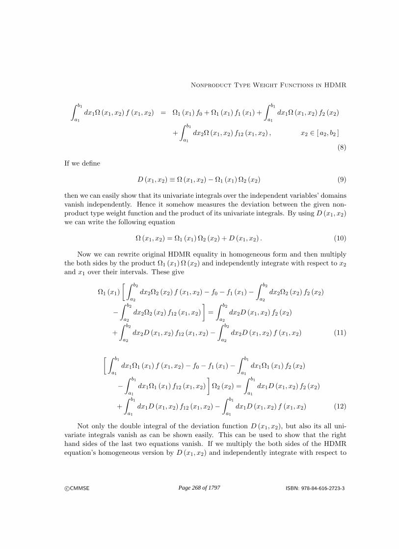
Nonproduct Type Weight Functions in HDMR

∫ b1

a1

dx1Ω (x1, x2) f (x1, x2) = Ω1 (x1) f0 + Ω1 (x1) f1 (x1) +

∫ b1

a1

dx1Ω (x1, x2) f2 (x2)

+

∫ b1

a1

dx2Ω (x1, x2) f12 (x1, x2) , x2 ∈ [ a2, b2 ]

(8)

If we define

D (x1, x2) ≡ Ω (x1, x2)− Ω1 (x1) Ω2 (x2) (9)

then we can easily show that its univariate integrals over the independent variables’ domainsvanish independently. Hence it somehow measures the deviation between the given non-product type weight function and the product of its univariate integrals. By using D (x1, x2)we can write the following equation

Ω (x1, x2) = Ω1 (x1) Ω2 (x2) + D (x1, x2) . (10)

Now we can rewrite original HDMR equality in homogeneous form and then multiplythe both sides by the product Ω1 (x1) Ω (x2) and independently integrate with respect to x2and x1 over their intervals. These give

Ω1 (x1)

[ ∫ b2

a2

dx2Ω2 (x2) f (x1, x2)− f0 − f1 (x1)−∫ b2

a2

dx2Ω2 (x2) f2 (x2)

−∫ b2

a2

dx2Ω2 (x2) f12 (x1, x2)

]=

∫ b2

a2

dx2D (x1, x2) f2 (x2)

+

∫ b2

a2

dx2D (x1, x2) f12 (x1, x2)−∫ b2

a2

dx2D (x1, x2) f (x1, x2) (11)

[ ∫ b1

a1

dx1Ω1 (x1) f (x1, x2)− f0 − f1 (x1)−∫ b1

a1

dx1Ω1 (x1) f2 (x2)

−∫ b1

a1

dx1Ω1 (x1) f12 (x1, x2)

]Ω2 (x2) =

∫ b1

a1

dx1D (x1, x2) f2 (x2)

+

∫ b1

a1

dx1D (x1, x2) f12 (x1, x2)−∫ b1

a1

dx1D (x1, x2) f (x1, x2) (12)

Not only the double integral of the deviation function D (x1, x2), but also its all uni-variate integrals vanish as can be shown easily. This can be used to show that the righthand sides of the last two equations vanish. If we multiply the both sides of the HDMRequation’s homogeneous version by D (x1, x2) and independently integrate with respect to

c©CMMSE ISBN: 978-84-616-2723-3Page 268 of 1797

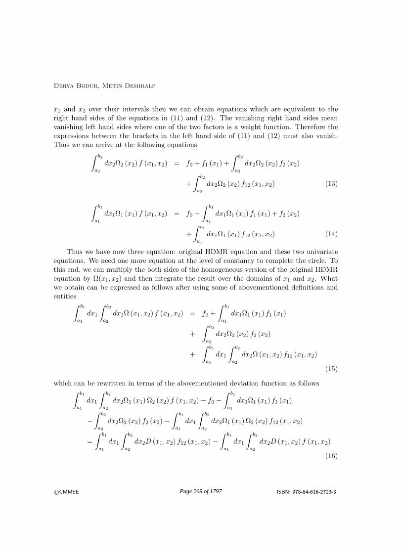
Derya Bodur, Metin Demiralp

x1 and x2 over their intervals then we can obtain equations which are equivalent to theright hand sides of the equations in (11) and (12). The vanishing right hand sides meanvanishing left hand sides where one of the two factors is a weight function. Therefore theexpressions between the brackets in the left hand side of (11) and (12) must also vanish.Thus we can arrive at the following equations∫ b2

a2

dx2Ω2 (x2) f (x1, x2) = f0 + f1 (x1) +

∫ b2

a2

dx2Ω2 (x2) f2 (x2)

+

∫ b2

a2

dx2Ω2 (x2) f12 (x1, x2) (13)

∫ b1

a1

dx1Ω1 (x1) f (x1, x2) = f0 +

∫ b1

a1

dx1Ω1 (x1) f1 (x1) + f2 (x2)

+

∫ b1

a1

dx1Ω1 (x1) f12 (x1, x2) (14)

Thus we have now three equation: original HDMR equation and these two univariateequations. We need one more equation at the level of constancy to complete the circle. Tothis end, we can multiply the both sides of the homogeneous version of the original HDMRequation by Ω(x1, x2) and then integrate the result over the domains of x1 and x2. Whatwe obtain can be expressed as follows after using some of abovementioned definitions andentities∫ b1

a1

dx1

∫ b2

a2

dx2Ω (x1, x2) f (x1, x2) = f0 +

∫ b1

a1

dx1Ω1 (x1) f1 (x1)

+

∫ b2

a2

dx2Ω2 (x2) f2 (x2)

+

∫ b1

a1

dx1

∫ b2

a2

dx2Ω (x1, x2) f12 (x1, x2)

(15)

which can be rewritten in terms of the abovementioned deviation function as follows∫ b1

a1

dx1

∫ b2

a2

dx2Ω1 (x1) Ω2 (x2) f (x1, x2)− f0 −∫ b1

a1

dx1Ω1 (x1) f1 (x1)

−∫ b2

a2

dx2Ω2 (x2) f2 (x2)−∫ b1

a1

dx1

∫ b2

a2

dx2Ω1 (x1) Ω2 (x2) f12 (x1, x2)

=

∫ b1

a1

dx1

∫ b2

a2

dx2D (x1, x2) f12 (x1, x2)−∫ b1

a1

dx1

∫ b2

a2

dx2D (x1, x2) f (x1, x2)

(16)

c©CMMSE ISBN: 978-84-616-2723-3Page 269 of 1797

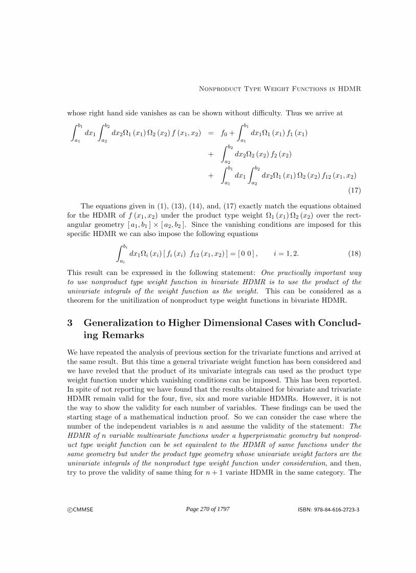
Nonproduct Type Weight Functions in HDMR

whose right hand side vanishes as can be shown without difficulty. Thus we arrive at∫ b1

a1

dx1

∫ b2

a2

dx2Ω1 (x1) Ω2 (x2) f (x1, x2) = f0 +

∫ b1

a1

dx1Ω1 (x1) f1 (x1)

+

∫ b2

a2

dx2Ω2 (x2) f2 (x2)

+

∫ b1

a1

dx1

∫ b2

a2

dx2Ω1 (x1) Ω2 (x2) f12 (x1, x2)

(17)

The equations given in (1), (13), (14), and, (17) exactly match the equations obtainedfor the HDMR of f (x1, x2) under the product type weight Ω1 (x1) Ω2 (x2) over the rect-angular geometry [ a1, b1 ] × [ a2, b2 ]. Since the vanishing conditions are imposed for thisspecific HDMR we can also impose the following equations∫ bi

ai

dx1Ωi (xi) [ fi (xi) f12 (x1, x2) ] = [ 0 0 ] , i = 1, 2. (18)

This result can be expressed in the following statement: One practically important wayto use nonproduct type weight function in bivariate HDMR is to use the product of theunivariate integrals of the weight function as the weight. This can be considered as atheorem for the unitilization of nonproduct type weight functions in bivariate HDMR.

3 Generalization to Higher Dimensional Cases with Conclud-ing Remarks

We have repeated the analysis of previous section for the trivariate functions and arrived atthe same result. But this time a general trivariate weight function has been considered andwe have reveled that the product of its univariate integrals can used as the product typeweight function under which vanishing conditions can be imposed. This has been reported.In spite of not reporting we have found that the results obtained for bivariate and trivariateHDMR remain valid for the four, five, six and more variable HDMRs. However, it is notthe way to show the validity for each number of variables. These findings can be used thestarting stage of a mathematical induction proof. So we can consider the case where thenumber of the independent variables is n and assume the validity of the statement: TheHDMR of n variable multivariate functions under a hyperprismatic geometry but nonprod-uct type weight function can be set equivalent to the HDMR of same functions under thesame geometry but under the product type geometry whose univariate weight factors are theunivariate integrals of the nonproduct type weight function under consideration, and then,try to prove the validity of same thing for n + 1 variate HDMR in the same category. The

c©CMMSE ISBN: 978-84-616-2723-3Page 270 of 1797

Derya Bodur, Metin Demiralp

proof is rather comprehensive in the formulation even though the intermediate steps are nothard to be taken. What we can say is that the proof can be obtained by following certaindeviation functions based on the univariate and multivariate integrals of the nonproducttype weight function. We do not intend to get into details here for typographical reasons.However we are going to report the proof in a coming publication as soon as possible.

References

[1] Derya Bodur, Metin Demiralp, A Perturbative Approach to High DimensionalModel Representation (HDMR) Under Nonproduct Type Weight and Over Orthogo-nal Geometry, AIP Proceedings for the 10th International Conference of NumericalAnalysis and Applied Mathematics (ICNAAM2012), Kos, Greece (2012) 1994–1997.

[2] Sobol, Sensitivity Estimates for Nonlinear Mathematical Models, English Translation:MMCE 1 (1993) 407–414.

[3] Alıs, O. F.; Rabitz, H., General Foundations of High Dimensional Model Represen-tation, Journal of Mathematical Chemistry 25 (1999) 197–233.

[4] Alıs, O. F.; Rabitz, H., Efficient Implementation of HDMR, Journal of Mathemat-ical Chemistry 29 (2001) 127–142.

[5] Li, G.; Rosenthal, C.; Rabitz, H., High Dimensional Model Representation, Jour-nal of Physical Chemistry 105 (2001) 7765–7777.

[6] Li, G.; Schoendorf, J.; Ho, T.; RabitZ, H., Multicut-HDMR with an Applicationto an Ionospheric Model, Journal of Computational Chemistry 25 (2004) 1149–1156.

[7] Tunga, M. A.; Demiralp, M., A Factorized High Dimensional Model Representa-tion on the Nodes of a Finite Hyperprimatic Regular Grid, Applied Mathematics andComputation 164 (2005) 865–883.

[8] Demiralp, M.; Demiralp, E., Reductive Multilinear Array Decomopsition BasedSupport Functions in Enhanced Multivariance Product Representation (EMPR), TheInternational Conference on Applied Computer Science-2010 (WSEAS), Malta (2010)448–454.

[9] Yaman, I.; Demiralp, M., HDMR Approximation of an Evolution Operator witha First Order Partial Differential Operator Argument, App. Num. Anal. and Comp.Math., Wiley CHV (2003) 287–296.

c©CMMSE ISBN: 978-84-616-2723-3Page 271 of 1797

Nonproduct Type Weight Functions in HDMR

[10] Tunga, B.; Demiarlp, M., A Novel Hybrid High Dimensional Model Representation(HHDMR) Based on Combination of Plain and Logarithmic High Dimensional ModelRepresentations, WSEAS 12-th International Conference on Applies Mathematics forScience and Engineering 1 (2007) 157–161.

[11] Demiralp, M., A Gentle Introduction to High Dimensional Model RepresentationUnder Nonproduct Type Weights, in Proceedings of the 2nd International Conferenceon Applied Informatics and Computing Theory, September, 2011 (WSEAS) (2011)113–118.

[12] Li, G.; Artamonov, M.; Rabitz, H.; Wang, S.-W.; Georgopoulos, P. G.;Demiralp, M., High Dimensional Model Representations generated from low orderterms lp-rs-hdmr, Journal of Computational Chemistry 24 (2003) 647–656.

[13] Demiralp, M., Importance and measurement of univariance in high dimensionalmodel representation for multivariate analysis, WSEAS Transactions on Computers5 (2006) 1738–1744.

[14] Tunga, B.; Demiralp, M., Constancy maximization based weight optimization inhigh dimensional model representation, Numer. Algor. 52 (2009) 435–459.

[15] Okan, A.; Baykara, N. A.; Demiralp, M., Weight optimization in enhanced mul-tivariance product representation (empr), In AIP Proceedings for the InternationalConference of Numerical Analysis and Applied Mathematics (ICNAAM 2010) 1281(2010) 1935–1938.

c©CMMSE ISBN: 978-84-616-2723-3Page 272 of 1797

Proceedings of the 13th International Conferenceon Computational and Mathematical Methodsin Science and Engineering, CMMSE 201324–27 June, 2013.

Computational Modelling of Meteorological Variables on Multicoresand Multi-GPU Systems

Murilo Boratto1, Pedro Alonso1 and Domingo Gimenéz2

1 Departamento de Sistemas Informáticos y Computación, Universidad Politécnica de Valencia,Valencia, Spain

2 Departamento de Sistemas Informáticos, Universidad de Murcia, Murcia, Spain

emails: muriloboratto@uneb.br, palonso@dsic.upv.es, domingo@um.es

Abstract

The National Institute of Meteorology (INMET) in Brazil includes a network of meteoro-logical stations which has 24 stations operating in agricultural region of São Francisco RiverValley. There are 11 conventional stations and 13 with automatic systems. The institute gathershigh quality expensive data despite they have been little used. Since there is no possibility ofinstalling meteorological stations everywhere, a cross-validation procedure has been developedin order to evaluate the meteorological data from INMET network using inverse power distanceweighting method. This work aims to present methodologies for meteorological variables repre-sentation through High Performance Computing Models on Multicore and Multi-GPU systems.

Key words: Computational Modelling, Meteorological Variables, Parallel Computing, Per-formance Estimation, Multicore, Multi-GPUs.

1 Introduction

Agricultural region of São Francisco River Valley has a successful public policy for the developmentof semiarid northeast region based on irrigated agriculture. Agriculture has stimulated this regionof the country, bringing socio-economic development to the countryside in a wide area of modernagriculture. This development center is located in the driest area in the Northeast of Brazil, on theSão Francisco River Valley, including a wide area, where natural conditions are exceptional for thedevelopment of irrigated fruit growing.

c©CMMSE ISBN: 978-84-616-2723-3Page 273 of 1797

COMPUTATIONAL MODELLING OF METEOROLOGICAL VARIABLES

Efficiency is demanded in the usage of water for irrigated agriculture so that the process re-mains sustainable in environmental aspects, and the water resources management is the way oneseeks to consider and resolve issues of scarcity. Meteorological variables representation providesdata to quantify the water needs of crops, which is essential for its proper management. The mainmeteorological variables are: temperature, air relative humidity, wind velocity, solar radiation, pre-cipitation and atmospheric pressure. The values of those variables are valid for the points wherethey are measured [1]. The National Institute of Meteorology (INMET) [2] in Brazil includes anetwork of meteorological stations which has 24 stations operating in São Francisco River Valleyagricultural region. There are 11 conventional stations and 13 with automatic systems. These dataare available on the Internet and have been little used. They are high quality data whose acquisitionis considered expensive. Since there is no possibility to install meteorological stations everywhere,this project aims to test and validate, using the Inverse Power Distance Weighting [3], a methodologyfor making a meteorological data representation in INMET stations network.

The problem of this case study is the high computing power required to estimate meteorologi-cal variables that represent the climate of the São Francisco River Valley. The spatial interpolationmethod [4] requires a significant computational power to perform the interpolation on a large setof data, and sequential programming is not practicable in some cases. Currently it is usual to havecomputational systems formed by a multiprocessors with one or more Graphics Processing Units(GPUs). These systems are heterogeneous, due to different types of memory and different speeds ofcomputation between CPU and GPU cores. In order to accelerate the solution of complex problemsit is necessary to use the aggregated computational power of the two subsystems [5]. Heterogeneityintroduces new challenges to algorithm design and system software. Our approach is to fully exploitall the CPU and all GPUs devices on these systems [6] and achieves the objective of maximum effi-ciency by an appropriate balancing of the workload among all the computational resources. Thoseideas introduced methodologies for meteorological variables representation using the Inverse PowerDistance Weighting method on Multicore and Multi-GPU systems.

2 Experimental Results

The computer used in our experiments has two 3.33 GHz Intel Xeon X5680 and 96GB GDDR3main memory. Each one is an hexacore processor with 12 MB of cache memory. It contains twoGPUs NVIDIA Tesla C2070 with 14 stream multiprocessors (SM) and 32 stream processors (SP)each (448 cores in total). In order to validate the presented methodology and derived equations, itwill be applied computing techiques for efficient solution using inverse power distance weightingmethod by using the parallel scheme to represent the computational modeling of meteorologicalvariables of São Francisco river valley region. We have implemented a parallel algorithm usingOpenMP + CUDA. The benchmark was compiled with nvcc. In the experiments, we increased thenumber of stations from 12 to 18 to obtain the number that minimizes time. The execution with the

c©CMMSE ISBN: 978-84-616-2723-3Page 274 of 1797

M. BORATTO ET AL.

original code is denoted by “Sequential”. As can be seen, its behavior is presented in Table 1.

Table 1: Comparative performance analysis of execution time of Sequential (in seconds).Number of Estations Automatic Loop Process

12 988.12 1, 996.19 2, 984.3114 4, 472.69 21, 243.02 25, 715.7116 12, 004.17 63, 424.38 75, 428.5518 81, 498.14 122, 191.27 203, 689.40

12 33.11% 66.89% 100.00%14 17.39% 82.61% 100.00%16 15.91% 84.08% 100.00%18 40.01% 59.99% 100.00%

Where Automatic Time is the time for picks up the access time to the database, LoopTime refers to the internal loop (while (p)), which is the GPU has parallelized, and the ProcessTime includes the time to access the Automatic + Loop. The versions denoted by “Hybrid”represent executions denotes the use of several CPU cores and in two devices simultaneously.

Table 2: Comparative performance analysis of OpenMP + CUDA execution time (in seconds).Number of Estations Automatic Loop Process

12 284.83 157.81 442.5814 912.75 1, 250.66 2, 154.2416 4, 283.81 2, 458.08 6, 742.7518 14, 498.81 7, 723.21 22, 222.84

12 61.23% 34.31% 100.00%14 58.50% 41.50% 100.00%16 66.72% 33.02% 100.00%18 65.36% 34.64% 100.00%

Table 3: Comparative performance analysis of Speedup Rate.Number of Estations Automatic Loop Process

12 3.48 12.65 6.4914 4.90 16.98 11.8216 5.26 15.22 11.1718 6.62 15.82 9.16

In this model, processes are executed by all the elements of the machine, the suitable numberof CPU cores and the two GPU. The results of the experiments show that the parallel CPU + GPUalgorithm reduces the execution time significantly. As can be seen in Table 3 the maximum speedupis around 6 for Automatic Time and 15 for Loop Time, matching the number of cores.

c©CMMSE ISBN: 978-84-616-2723-3Page 275 of 1797

COMPUTATIONAL MODELLING OF METEOROLOGICAL VARIABLES

3 Conclusions and Future Work

From the results obtained, installation of new automatic meteorological stations or redistribution ofalready installed in São Francisco river valley is recommended in order to encourage the use of spaceinterpolation, given its importance for Brazilian agriculture scenario. Furthermore, the performanceresults obtained in this work indicate that the proposed applications are effective, based on the clas-sification task, response time and workload distribution. The applications built also demonstrate theproper measure of computing power that must be combined with intrinsic parallelism, which shouldbe used in algorithm execution. Nevertheless, there are other models of distributed programmingthat can exploit the subject discussed in this article making it more complete. In this sense, newexperiments have been developed to consolidate the mathematical model proposed. Nevertheless,it is still interesting to see the extension of such tuning technique to heterogeneous clusters for thisparticular problem.

References

[1] R. G. Allen, L. S. Pereira, D. Raes, M. Smith, Crop evapotranspiration-guidelines for computingcrop water requirements-fao irrigation and drainage, Irrigation and Drainage 300 (56) (1998)1–15.

[2] F. Oliveira, INMET: 100 Years of Weather in Brazil, INMET, 2009.URL http://books.google.com.br/books?id=VXfxZwEACAAJ

[3] G. Y. Lu, D. W. Wong, An adaptive inverse-distance weighting spatial interpolation technique,Computer Geosciences 34 (9) (2008) 1044–1055.

[4] A. A. E. Jakob, A. F. Young, The use of interpolation methods in the analysis of spatial datasociodemographic, Brazilian Journal Sociodemographic.

[5] M. Boratto, P. Alonso, C. Ramiro, M. Barreto, Heterogeneous computational model for land-form attributes representation on multicore and multi-GPU systems, Procedia CS 9 (2012) 47–56.

[6] F. Song, S. Tomov, J. Dongarra, Efficient support for matrix computations on heterogeneousmulticore and multi-GPU architectures., Tech. Rep. 250, LAPACK Working Note (Jun. 2011).

c©CMMSE ISBN: 978-84-616-2723-3Page 276 of 1797

Proceedings of the 13th International Conferenceon Computational and Mathematical Methodsin Science and Engineering, CMMSE 201324–27 June, 2013.

Impact of the Information Exchange Policies in LoadBalancing Algorithms

Jose Luis Bosque1, Oscar D. Robles2, Pablo Toharia2 and Luis Pastor2

1 Department of Electronica y Computadores, Universidad de Cantabria

2 Department of ATC and CCIA, Universidad Rey Juan Carlos

emails: joseluis.bosque@unican.es, oscardavid.robles@urjc.es,pablo.toharia@urjc.es, luis.pastor@urjc.es

Abstract

This paper presents a detailed study about the information exchange rule of loadbalancing algorithm. It is focused on analyzing how this rule affects the performance aswell as the scalability of these type of algorithms. To do that, different rules widely usedin the bibliography have been implemented, as global rules but also as local rules. Tocompare them, a metric that looks for a compromise between the communications over-head and the speedup of the load balancing algorithm has been used: the InformationEfficiency.

Key words: Heterogeneous computing, load balancing, load index.

1 Introduction

One of the most important challenges that supercomputers which are in the exascale com-puting route face is scalability. Nowadays, supercomputers have hundreds of thousands ofcores, with a tendency for this quantity to grow in the future [1]. Analyzing and solvingall the problems that affect the scalability of these systems will be one of the keys to makethem run real applications with a high degree of efficiency.

One of the key aspects that have a deeper impact on the performance of the applicationsrunning on these supercomputers is the ability to achieve a good load balancing amongall the available nodes. Load balancing algorithms try to assign each node a workloadproportional to its computing capabilities [9]. In order to decide when a load balancingoperation should be done these algorithms need accurate and updated information about

c©CMMSE ISBN: 978-84-616-2723-3Page 277 of 1797

Impact of the Information Exchange Policies in Load Balancing Algorithms

the state of the system’s nodes. The procedure to collect and update this information, calledInformation Exchange Rule [10], can introduce a great overhead in the system, speciallywhen the number of available nodes grows. The scalability of this type of algorithms isgreatly affected by this fact.

In order to completely define the information exchange rule two parameters are needed:a temporal distribution, i. e. when the operations of exchange of information take place,and a spatial distribution, i. e. which nodes are involved in the exchange of information.Regarding the temporal distribution, three types of rules are typically used:

• On-demand. The exchange of information takes place only when a node decides toperform a load balancing operation. At that moment state information from the restof the nodes is requested. This way, the state information is always updated and thenumber of messages in the network is minimized, although the overhead associated toa load balancing operation is increased [8].

• Periodical. Each node periodically reports its state to the others, regardless of whetherit is necessary or not. The selection of the best reporting frequency is critical [6].

• Event-driven. A node only reports its state when an event takes place. In this context,an event will be a node changing its state. This approach reduces the amount ofcommunications and minimizes the risk of network saturation [5].

From an spatial point of view, these information rules can be global rules or local rules.Global rules define information exchanges with all the available nodes in the system. Theinformation they manage is more complete, but they are not quite scalable [7]. Localrules are based on the concept of domain. A domain is a set of nodes among which theinformation is exchanged [2]. Domains can be isolated (one node can not appear in morethan one domain) or overlapped (the domains share some of the nodes).

This paper studies how the information exchange rule affects the scalability of theload balancing algorithms. For that purpose, a basic load balancing algorithm has beenimplemented [4] and different information exchange approaches have been tested: periodical,event-driven and on-demand. Also, separated domains as well as overlapped domains havebeen implemented, and the results achieved in all cases are presented.

In order to do a fair comparison of all the affected parameters, a metric called infor-mation efficiency, proposed in [3] has been used. This metric takes into account a trade-offbetween the use of the network and the workload balancing achieved in the system. Thistrade-off is reflected in a better use of the available resources and therefore in a higherspeedup achieved when the algorithm is used.

This paper is organized as follows. Section 2 presents a the proposed algorithm de-scribing in detail the different information rules implemented. The experimental results arediscussed in section 3. Finally section 4 exposes the conclusions and future work.

c©CMMSE ISBN: 978-84-616-2723-3Page 278 of 1797

J. L. Bosque, O. D. Robles, P. Toharia, L. Pastor

2 Design of the Load Balancing Algorithm

The approach presented in this paper is a dynamic, distributed, and non preemptive loadbalancing algorithm. It is a dynamic algorithm because the assignment of a task to anspecific node is performed in run time. Then the task is completely executed in the assignednode, without any kind of task migration. It is a distributed algorithm since every node inthe cluster takes its own decisions based on local stored information. The algorithm doesnot present any overhead if the nodes are naturally balanced, therefore it can automaticallyturn itself off on global under-loading or over-loading situations.

Depending on whether or not the algorithm uses domains, the decision about doing aload balancing operation can be global or local. When there are not any domains, once anode dedices to perform a load balancing operation the partner is selected among all theavailable nodes. On the other hand, the partner selection will be restricted to the nodes inthe same domain when these are implemented.

2.1 Measuring the state of a node

During this phase the local information needed to determine the workload of the local nodeis collected, to calculate then the load index, which determines the state of the node. Thedecision about the local execution of a new task or launching a new load balancing operationis taken based on this state for each node. The load index is periodically computed and itis discretized in a set of states [4].

Load Index. The load index is calculated based on two static parameters, the numberof cores and the computational power as well as a dynamic parameter, the number of tasksbeing currently executed in the node. A node has two sources of heterogeneity, the numberof cores and their computational power. Thus, it is necessary to specify two differentpossibilities:

• The number of tasks is lower than the number of cores in the node. Therefore, thereare some free cores and this node can accept more tasks, so it will be a recipient node.

• The number of tasks is larger than the number of cores. In this case, the load indexis calculated based on the computational power of the nodes.

States of a Node. The states come from a discretization of the load index in order tominimize the exchange of global information, as well as to simplify load balancing decisions.These states determine the behaviour of a node, and three different ones have been defined:

• Recipient State: The state of a node is recipient when the number of its running tasksis less than the number of cores it has, or when its load index value is bigger than thethreshold neutral-recipient. This means that the node has free cores and then it canassume at least one more task, either local or remote.

c©CMMSE ISBN: 978-84-616-2723-3Page 279 of 1797

Impact of the Information Exchange Policies in Load Balancing Algorithms

• Neutral State: Its load index has a medium value. In this case all the node’s cores areexecuting at least one task. In this state the node can assume new local tasks but itrejects all remote requests.

• Emitter State: A node is Emitter when its load index has a value under the Neutral-Emitter threshold. This means that the node has many more tasks than the numberof cores it has, and so it can not accept any more tasks.

Change of state. A node will change its state whenever a new measurement of theload index crosses a status threshold. Since this parameter is very volatile, it is possiblethat a particular node might be continuously changing its state due to small changes in itsexternal load. To prevent this problem, some degree of hysteresis has been added to eachthreshold. This way, the number of messages due to state changes is reduced.

2.2 Global Information

In order to take decisions about load balancing it is necessary to exchange the state in-formation among the nodes of the cluster. Our approach is a global algorithm, so all thenodes keep updated information about the global system state. Three different policies havebeen implemented for the nodes to broadcast their workload information when they suffera change of state: periodical, event-driven and on-demand:

Periodical. The current state of a node, as well as the previous state of the rest ofthe nodes is sent after a certain period of time. Fixing the most appropriate period of timeis of great importance, since a too short interval would mean sending messages so as tosaturate the network but a too long interval would mean that the information that a nodehas about the others is obsolete. In order to avoid the effect of more than one change ofstate of one node, when a node receives information about another one it checks if the nodethe information is about is already in the recipients list, so the same node is not added orremoved from the list more than once. With this implementation the new state of a node, aswell as its old state, is received. The node will only be added to the list if the node changesfrom recipient to neutral state, and will only be removed from the list if it changes fromneutral to receptor state, not being needed any change in the list in the rest of situations.

Event-driven. The information is sent to the rest of the nodes only when an eventtakes place, being an event a change of state on one node. The information sent is thecurrent state of the node, since every change of state is communicated. As it was alreadymentioned, the algorithm is emitter-initiated so it is only of interest to know which are therecipient nodes. Therefore, an event will take place only when the node becomes recipientor when it leaves the recipient state. On the reception of a message showing a change ofstate, each node updates its receptors list. If the change is about a node that becomesrecipient, that node is added to the list. Otherwise, it will be about a node that leaves therecipient state, so it will be removed from the list.

c©CMMSE ISBN: 978-84-616-2723-3Page 280 of 1797

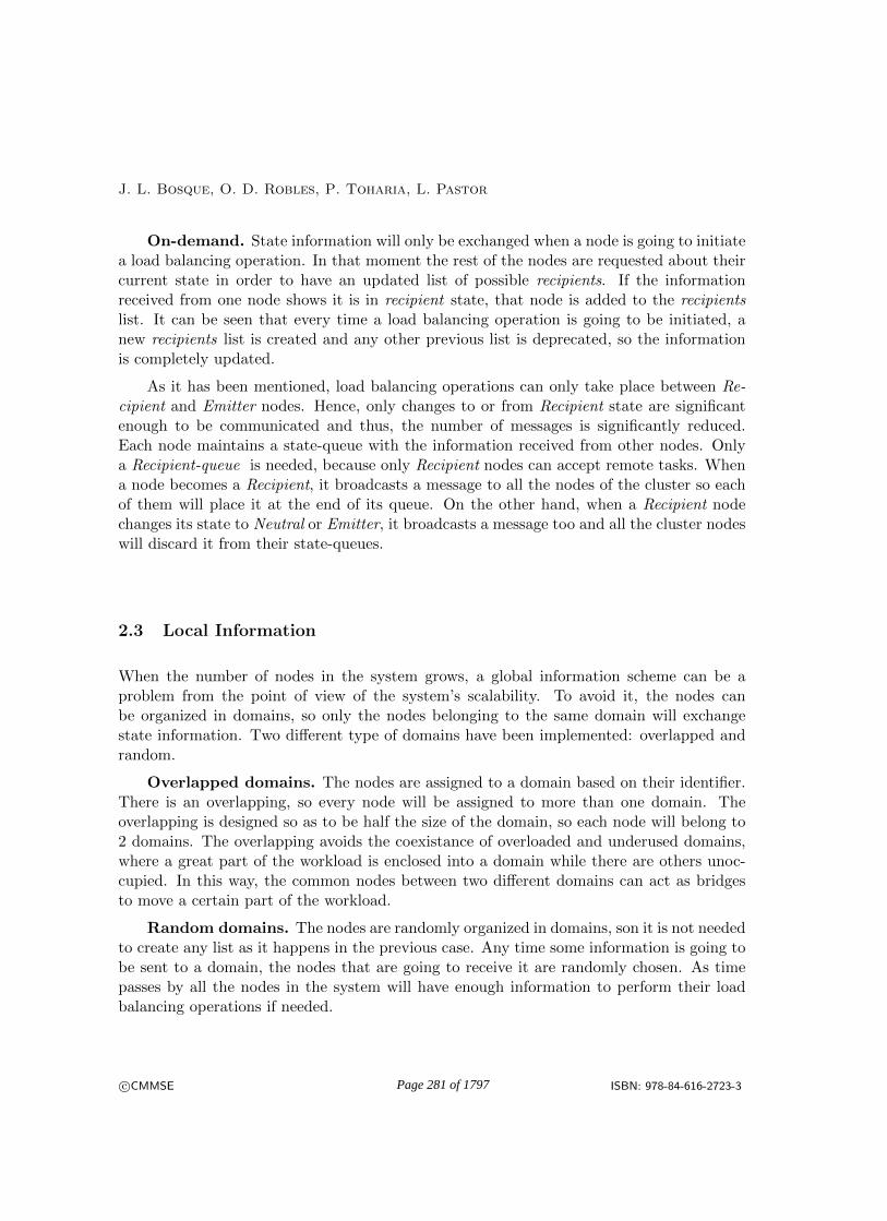
J. L. Bosque, O. D. Robles, P. Toharia, L. Pastor

On-demand. State information will only be exchanged when a node is going to initiatea load balancing operation. In that moment the rest of the nodes are requested about theircurrent state in order to have an updated list of possible recipients. If the informationreceived from one node shows it is in recipient state, that node is added to the recipientslist. It can be seen that every time a load balancing operation is going to be initiated, anew recipients list is created and any other previous list is deprecated, so the informationis completely updated.

As it has been mentioned, load balancing operations can only take place between Re-cipient and Emitter nodes. Hence, only changes to or from Recipient state are significantenough to be communicated and thus, the number of messages is significantly reduced.Each node maintains a state-queue with the information received from other nodes. Onlya Recipient-queue is needed, because only Recipient nodes can accept remote tasks. Whena node becomes a Recipient, it broadcasts a message to all the nodes of the cluster so eachof them will place it at the end of its queue. On the other hand, when a Recipient nodechanges its state to Neutral or Emitter, it broadcasts a message too and all the cluster nodeswill discard it from their state-queues.

2.3 Local Information

When the number of nodes in the system grows, a global information scheme can be aproblem from the point of view of the system’s scalability. To avoid it, the nodes canbe organized in domains, so only the nodes belonging to the same domain will exchangestate information. Two different type of domains have been implemented: overlapped andrandom.

Overlapped domains. The nodes are assigned to a domain based on their identifier.There is an overlapping, so every node will be assigned to more than one domain. Theoverlapping is designed so as to be half the size of the domain, so each node will belong to2 domains. The overlapping avoids the coexistance of overloaded and underused domains,where a great part of the workload is enclosed into a domain while there are others unoc-cupied. In this way, the common nodes between two different domains can act as bridgesto move a certain part of the workload.

Random domains. The nodes are randomly organized in domains, son it is not neededto create any list as it happens in the previous case. Any time some information is going tobe sent to a domain, the nodes that are going to receive it are randomly chosen. As timepasses by all the nodes in the system will have enough information to perform their loadbalancing operations if needed.

c©CMMSE ISBN: 978-84-616-2723-3Page 281 of 1797

Impact of the Information Exchange Policies in Load Balancing Algorithms

2.4 Initiation of Load Balancing Operations

It determines when a new load balancing operation has to begin. Since a load balancingapproach that does not interrupt any execution has been proposed, the decision about whichnode is finally going to execute a task can only be taken in the exact moment of beginningthe execution. Therefore, there must be a emitter-iniciated rule to take this decision, andthe decision about initiating a load balancing operation is completely local to the emitter. Itmust be noticed that on the decision of not doing any load balancing operation, no messageshave to be exchanged, so the communications overhead is reduced. The initiation rule mustbe evaluated every time a new task has to be launched. At this moment, the state of thenode is checked, in order to know if it can accept the local execution of the new task or if thesearch of a better candidate for the execution of the task should be initiated. A node canonly accept the local execution of a new task if it is in recipient or neutral state. Therefore,only if the state of the node is emitter, a load balancing operation is initiated.

2.5 Partner Localization and Load Distribution

Once the decision of doing a load balancing operation is taken, two important steps mustbe performed: to locate a partner to send it the exceeding load and to decide how manytasks should be sent to that partner.

Partner localization. This is a completely local operation, since an emitter nodelooks for a partner in its own recipients queue. The selection of the partner can be done inmany different ways. The approach adopted is to do a first random selection of a few nodes,that are then sorted based on their load index, so the less loaded node is requested. If therequest is rejected, the next node in the list will be requested and so on. This strategy hassome advantages. It reduces the communications overhead since the load indexes do nothave to be constantly updated. Also, it avoids that one candidate is simultaneously chosenby different nodes, because it is in a prominent position in the queue.

Load Distribution. The last step to perform the load balancing operation is to decidehow much workload should be sent to the recipient node. A good distribution is that inwhich each node gets an amount of workload that is proportional to its computationalpower. Therefore, the more similar load indexes are after the load balancing operation, thebetter the load distribution is. In this approach, first of all the recipients are sorted based ontheir load indexes. Then the emitter node sends to the first node in the sorted list as muchworkload as needed to force its load index to change from recipient to neutral state. Then,the second recipient from the list is selected and the same operation is performed. Thisprocess finishes when there is no more workload to send or there are no more recipients.

c©CMMSE ISBN: 978-84-616-2723-3Page 282 of 1797

J. L. Bosque, O. D. Robles, P. Toharia, L. Pastor

3 Experimental Results

The experiments have been run on a cluster composed of 8 nodes AMD single core. A totalof 160 tasks to be delivered are sent to 2 nodes (80 tasks each), in order to test the algorithmbut not to face an excessively large running time. This two nodes begin to execute tasksand as soon as their state changes to emitter they will send tasks to the rest of the availablenodes in the system.

In order to test both global and local information algorithms, the following measureshave been taken:

• tOP is the time to execute the 160 tasks without any load balancing algorithm sending20 of the 160 tasks to each node in the system.

• tDEL is the time passed since the beginning or the test until all the tasks have beendelivered (notice that it is not needed that the execution of the tasks have beencompleted).

• tEXE is the time passed since the execution of the test begins until the execution ofall the tasks launched is finished.

• nSEND is the count of all the comunnications done among the nodes (global process)to inform about their state.

• lbCO is the number of load balancing operations requested that are finally committed.

• lbNCO is the number of load balancing operations that were requested but never werecommitted.

• ε is the information efficiency, measured as ε = lbCOmSEND×numof tasks ×

tOPtEXE

To carry out the experiments two types of static domains have been conformed: the firstone with 4 nodes per domain with an overlapping of 2 nodes; the second one with 2 nodes perdomain with an overlapping of 1 node. To carry out the experiments with random domains,4 setups have been tested from 2 nodes per domain to 7 nodes per domain. Different tableswith all the results achieved have been included, as well as two graphs collecting resultsfrom all the experiments.

Table 1 shows results from the experiments carried out without any domains. It meansthat the node 0 can deliver tasks to any of the available nodes. The other following tablescollect results achieved using the different metrics explained in this paper. From these datafigures 1 and 2 have been produced, and will be analyzed in the following. It must besaid that this paper presents preliminary results, since the number of nodes used in theexperiments is not big enough extract definitive conclusions about the advantages of usingdomains instead of global policies.

c©CMMSE ISBN: 978-84-616-2723-3Page 283 of 1797

Impact of the Information Exchange Policies in Load Balancing Algorithms

Table 1: Experimental results with global policies.tOP nSEND lbCO lbNCO tDEL tEXE top/tEXE ε

Event-driven 396 1960 121 161 395 432 0.917 3.54E-4Periodical 1 396 22981 123 208 414 452 0.876 2.93E-05Periodical 3 396 4648 124 476 419 457 0.867 1.45E-4Periodical 5 396 4704 124 532 424 462 0.857 1.41E-4Periodical 10 396 2576 118 1077 463 501 0.79 2.26E-4On-demand 396 5544 123 500 393 430 0.921 1.28E-4

Global policies It can be seen in Figure 1 that the ratios top/tEXE are quite similarfor the on-demand, event-driven and periodical (with 3 seconds of updating time) policies.However, attending to the information efficiency the event-driven policy has a great ad-vantage with respect to the other ones (see Figure 2). It can be seen that the executiontimes achieved applying this policy are very similar but the number of messages exchangedis much more reduced. This way, table 1 shows that applying this policy means the ex-change of 1960 messages, in front of 4648 messages using the periodical policy and 5544of the on-demand one. Since the number of load balancing operations performed is quitesimilar in all cases, it can be said that the event-driven policy achieves the same results butexchanging less information and therefore reducing the use of the network.

Another important aspect to consider when the different policies are compared is thenumber of load balancing operations that are rejected. The event-driven policy achieves161 rejected operations, while the periodical policy shows 476 and the on-demand one 500.It also means a lower overhead so it can be said that applying the event-driven policy givesa better result.

Table 2: Experimental results with domains of 4 nodes.tOP nSEND lbCO lbNCO tDEL tEXE top/tEXE ε

Event-driven 396 1400 121 97 428 465 0.852 4.6E-4Periodical 1 396 17080 121 99 432 469 0.844 3.74E-05Periodical 3 396 5800 119 356 440 477 0.83 1.07E-4Periodical 5 396 3640 120 436 459 497 0.797 1.64E-4Periodical 10 396 1880 116 941 475 513 0.772 2.98E-4On-demand 396 4225 121 103 428 465 0.852 1.52E-4

Finally, it must be noticed the deep impact that the election of the updating intervalhas on the periodical policy, since it can be seen that it produces a degradation of up to a10%. This parameter is strongly dependent on the system’s dynamism. In this experimentthe tasks have an arriving rate on the nodes of 1 second. With it, policies with largeupdating interval are using obsolete information many times, something that means a highnumber of rejected load balancing operations (reaching 1077 in the case of periodical-10).However, in a less dynamic environment the policies more affected would be the ones thatwere using short updating intervals, since they would cause the exchange of a big amountof information that would never be used.

c©CMMSE ISBN: 978-84-616-2723-3Page 284 of 1797

J. L. Bosque, O. D. Robles, P. Toharia, L. Pastor

Static Domains With respect to the response time shown in Figure 1, once again theevent-driven and on-demand policies achieve the best results, although the periodical-1 pol-icy gives quite similar results. However, Figure 2 shows that attending to the efficiency, itis the event-driven policy the one that achieves much better results than the other ones.Basically the reasons are the same ones already explained in the previous section: it sig-nificantly reduces the number of messages exchanged and therefore the use of the network;provides a lower number of load balancing operations rejected, although in this case thedifference with the other policies is lower, and its response times are very similar to theones provided by the other policies.

Table 3: Experimental results with random domains of 3 Nodes.tOP nSEND lbCO lbNCO tDEL tEXE top/tEXE ε

Event-driven 396 831 111 2362 527 564 0.702 5.86E-4Periodical 1 396 10338 118 329 435 472 0.839 5.99E-05Periodical 3 396 3432 119 596 434 472 0.839 1.82E-05Periodical 5 396 2040 118 949 429 467 0.848 3.07E-4Periodical 10 396 1149 112 1362 484 521 0.760 4.63E-4On-demand 396 2418 123 109 406 444 0.892 2.84E-4

Table 4: Experimental results with random domains of 5 Nodes.tOP nSEND lbCO lbNCO tDEL tEXE top/tEXE ε

Event-driven 396 1325 117 1451 476 513 0.772 4.26E-4Periodical 1 396 16880 122 211 426 464 0.853 3.86E-05Periodical 3 396 5720 122 440 435 471 0.841 1.12E-4Periodical 5 396 3440 121 640 435 472 0.839 1.84E-4Periodical 10 396 1840 116 1153 465 525 0.754 2.97E-4On-demand 396 4050 123 108 415 452 0.876 1.66E-4

Table 5: Experimental results with random domains of 7 nodes.tOP nSEND lbCO lbNCO tDEL tEXE top/tEXE ε

Event-driven 396 1946 123 137 396 433 0.915 3.61E-4Periodical 1 396 23198 127 177 418 456 0.868 2.97E-05Periodical 3 396 7392 124 375 402 439 0.902 9.46E-05Periodical 5 396 5152 123 595 465 503 0.787 1.18E-4Periodical 10 396 2632 116 1054 475 512 0.773 2.13E-4On-demand 396 5523 124 155 396 433 0.915 1.28E-4

Comparing results with the ones achieved with the Global policies, table 2 shows thatthe execution times are worse, but the exchange of information is reduced in a 25% providingthen a better efficiency. This behavior means that the domain-based policies are morescalable. That is, when the number of nodes is increased not only better efficiency resultswill be obtained, but also better response times.

Random Domains Finally, the results achieved by the policies based on random domainsare analyzed. Experiments with domains with 3, 5 and 7 nodes have been done. Regarding

c©CMMSE ISBN: 978-84-616-2723-3Page 285 of 1797

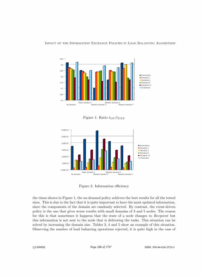
Impact of the Information Exchange Policies in Load Balancing Algorithms

No domainsStatic domains 4

Random domains 3Random domains 5

Random domains 7

0,6

0,65

0,7

0,75

0,8

0,85

0,9

0,95

Event-driven

Periodical 1

Periodical 3

Periodical 5

Periodical 10

On-demand

Figure 1: Ratio tOP /tEXE

No domainsStatic domains 4

Random domains 3Random domains 5

Random domains 7

0,00E+00

1,00E-04

2,00E-04

3,00E-04

4,00E-04

5,00E-04

6,00E-04

Event-driven

Periodical 1

Periodical 3

Periodical 5

Periodical 10

On-demand

Figure 2: Information efficiency

the times shown in Figure 1, the on-demand policy achieves the best results for all the testedsizes. This is due to the fact that it is quite important to have the most updated information,since the components of the domain are randomly selected. By contrast, the event-drivenpolicy is the one that gives worse results with small domains of 3 and 5 nodes. The reasonfor this is that sometimes it happens that the state of a node changes to Recipient butthis information is not sent to the node that is delivering the tasks. This situation can besolved by increasing the domain size. Tables 3, 4 and 5 show an example of this situation.Observing the number of load balancing operations rejected, it is quite high in the case of

c©CMMSE ISBN: 978-84-616-2723-3Page 286 of 1797

J. L. Bosque, O. D. Robles, P. Toharia, L. Pastor

domains with 3 and 5 nodes. But it can be seen this value is lower in the case of domainswith 7 nodes. This value is also significantly reduced in the case of the on-demand policywith respect to the global policies. It can also be seen that the behavior of the periodicalpolicies is similar to the one presented with the global policies.

However, attending to the efficiency values, once again the event-driven policy is theone that achieves the best results, showing better values as smaller is the domain. Thisis due to the lower number of messages exchanged, with a great difference with the otherpolicies.

4 Conclusions and Future Work

The information exchange rule specifies the way the information about the different nodesworkload is collected and maintained, something essential to take the decisions related tothe load balancing. One processor should ideally know every time the real state of the restof the nodes available in the system. However, this is not possible in massively parallelsystems, since it would be considerably prejudicial to the algorithm’s scalability. So a goodinformation exchange rule has to balance the cost of collecting information and keeping anaccurate view of the state of all the nodes in the system.

This paper presents an analysis of the information exchange policies most currentlyused, as the on-demand, the periodical and the event-driven policies are. Each node storesits information state independently, since this is a distributed algorithm. Keeping a globalview of the whole system in massive parallel systems is unfeasible, so local policies mustbe used. These policies group nodes into domains so the exchange of information takesplace only between nodes belonging to the same domain. It preserves the load balancingalgorithm scalability, independently of system’s size.

This work presents preliminary experiments, since the system used has only a few nodes.Anyway some interesting conclusions can be extracted. As a general conclusion it can besaid the event-driven policy is the one that behaves the best on all setups. This is becausethe response times achieved are quite similar to the ones achieved by the other policies, evenbetter in some cases. But also the number of exchanged messages is quite lower than withthe other policies, something that means achieving a better efficiency since the informationexchanged is better used. Another consequence is a minimum number of load balancingoperation requests rejected.

Future works are focused in two main directions. On one hand, to do this study in amassively parallel system, so the policies based on domains can show their power. On theother hand, to deeply analyze the efficiency metrics, to achieve a better correlation betweenthe efficiency and the execution times of the different experiments.

c©CMMSE ISBN: 978-84-616-2723-3Page 287 of 1797

Impact of the Information Exchange Policies in Load Balancing Algorithms

Acknowledgements

This work has been partially supported by the Spanish Ministry of Education and Science(grants TIN2010-21289, TIN2010-21291-C02-02, Consolider CSD2007-00050 and Cajal BlueBrain project) as well as by the HiPEAC European Network of Excellence.

References

[1] The top500 project. November 2012. http://www.top500.org.

[2] Bestoun S. Ahmed, Khairulmizam Samsudin, Abdul Rahman Ramli, and ShahNorBasri. A descriptive performance model of a load balancing single system image. AsiaInternational Conference on Modelling and Simulation, 0:180–184, 2008.

[3] Marta Beltran and Jose Luis Bosque. Information policies for load balancing on het-erogeneous systems. In 5th International Symposium on Cluster Computing and theGrid (CCGrid 2005), 9-12 May, Cardiff, UK, pages 970–976. IEEE Computer Society.

[4] J. L. Bosque, O. D. Robles, P. Toharia, and L. Pastor. Load balancing algorithmfor heterogeneous clusters. In 12th International Conference on Computational andMathematical Methods in Science and Engineering, CMMSE 2012, pp. 207–218.

[5] J. L. Bosque, P. Herrero, M. Salvadores, and M. S. Perez. A collaborative-aware taskbalancing delivery model for clusters. In GPC, pages 146–157, 2007.

[6] N.K. Gondhi and D. Pant. An evolutionary approach for scalable load balancing incluster computing. In Advance Computing Conference, 2009. IACC 2009. IEEE Inter-national, pages 1259 –1264, march 2009.

[7] Wenzheng Li and Hongyan Shi. Dynamic load balancing algorithm based on fcfs. InInnovative Computing, Information and Control (ICICIC), 2009 Fourth InternationalConference on, pages 1528 –1531, dec. 2009.

[8] J. Martnez, F. Almeida, E. Garzn, A. Acosta, and V. Blanco. Adaptive load balanc-ing of iterative computation onheterogeneous nondedicated systems. The Journal ofSupercomputing, 58:385–393, 2011. 10.1007/s11227-011-0595-3.

[9] Xiao Qin, Hong Jiang, Adam Manzanares, Xiaojun Ruan, and Shu Yin.Communication-aware load balancing for parallel applications on clusters. IEEE Trans.Comput., 59(1):42–52, January 2010.

[10] Chengzhong Xu and Francis Lau. Load Balancing in Parallel Computers: Theory andPractice. Kluwer Academic Publishers, Boston, 1997.

c©CMMSE ISBN: 978-84-616-2723-3Page 288 of 1797

Proceedings of the 13th International Conferenceon Computational and Mathematical Methodsin Science and Engineering, CMMSE 201324–27 June, 2013.

Symbolic Computation of a Canonical Formfor a Class of Linear Functional Systems

Mohamed S. Boudellioua1

1 Department of Mathematics and Statistics, Sultan Qaboos University,Muscat, Oman.

emails: boudell@squ.edu.om

Abstract

A matrix pencil is a matrix in the form λE − A where E and A are matrices withelements in a domain D and λ is an indeterminate. If E and A have their elementsin say R, then such pencils may arise in the study of systems of differential algebraicequations. In this paper, we consider a more general class of matrix pencils, arisingfrom linear systems of functional equations, where the entries of E and A belong to apolynomial ring e.g. D = R[α]. A canonical form based on the companion matrix andthe Smith form is presented for a class of such systems. Examples of these systems arelinear neutral delay-differential equations or linear systems of PDEs which are first orderwith respect to one of the unknown functions. Necessary and sufficient conditions arepresented under which a given matrix pencil is equivalent to the canonical form. Theexact form of the equivalence transformation is set out using symbolic computations.Examples are also presented to illustrate the ideas developed in this paper.

Key words: Functional systems, Matrix pencils, Companion form, Smith form, Uni-modular equivalence.

1 Introduction

Canonical forms play an important role in the modern theory of linear systems. Oneparticular form that has proved to be very useful for 1-D linear systems is the so-calledcompanion matrix which is associated with the characteristic polynomial of a given squarematrix. For example, Barnett [1] showed that many of the concepts encountered in 1-Dlinear systems theory can be nicely linked via the companion matrix. In this paper, weconsider a class of multivariate polynomial matrices in the form λE(α)− A(α). This form

c©CMMSE ISBN: 978-84-616-2723-3Page 289 of 1797

Symbolic Computation of a Canonical Form

of matrices arises for example in the study of linear systems of delay-differential equationssuch as suggested by Byrnes et al. [4], where λ = d/dt represents a differential operatorand α a shift operator, i.e., αx(t) = x(t − h). The matrix λE(α) − A(α), referred to asa matrix pencil can be regarded as a generalization of the matrix pencil λE − A oftenencountered in the study of linear systems of differential algebraic equations. A canonicalform associated with the characteristic polynomial of the pair E(α), A(α) is defined for thesepencils. Necessary and sufficient conditions are presented under which a matrix pencil isequivalent to resulting canonical form. The exact form of the transformation connectingthe pencils is established. First we present a few definitions that will be needed later in thepaper.

Definition 1 Let D = K[x1, . . . , xn]. The general linear group GLp(D) is defined by

GLp(D) =M ∈ Dp×p | ∃N ∈ Dp×p : MN = NM = Ip (1)

An element M ∈ GLp(D) is called a unimodular matrix. It follows that M is unimodularif and only if the determinant of M is invertible in D, i.e., is a non-zero element of K.

One of standard tasks carried out in systems theory, is to transform a given systemrepresentation into a simpler form before applying any analytical or numerical method. Thetransformation involved must of course preserve relevant system properties if conclusionsabout the reduced system are to remain valid about the original one. An equivalencetransformation used in the context of linear functional systems is unimodular equivalence.This transformation can be regarded as an extension of Rosenbrock’s equivalence [11] fromthe univariate to the multivariate setting and is defined by the following.

Definition 2 Let T1 and T2 denote two q×p matrices with elements in D then T1 and T2 aresaid to be unimodular equivalent if there exist two matrices M ∈ GLq(D) and N ∈ GLp(D)such that

T2 = MT1N (2)

2 Reduction using Unimodular Equivalence

The reduction of multivariate polynomial matrices arising from linear functional systemswas studied by a number of authors see for example, Frost and Storey [8], Lee and Zak[9]. In particular, Frost and Boudellioua [7] gave necessary and sufficient conditions underwhich a class of bivariate polynomial matrix is unimodular equivalent to a Smith formcorresponding to a simpler system containing only one equation in one unknown. Lin et al.[10] extended this result to the multivariate case. Boudellioua and Quadrat [3] generalizedthis result using a module theoretic approach.

c©CMMSE ISBN: 978-84-616-2723-3Page 290 of 1797

M.S. Boudellioua

Theorem 1 ([7]) Let T ∈ Dn×n, with full row rank, then T is unimodular equivalent tothe Smith form

S =

(In−1 0

0 |T |

)(3)

if and only if there exist a vector U ∈ Dn which admits a left inverse over D such that thematrix

(T U

)has a right inverse over D.

3 Matrix Pencils over D = R[λ, α]

In this section we shall consider a type of matrix in the form λE(α)−A(α). Suppose thatin Theorem 1, D = R[λ, α] and

T = λE(α)−A(α) (4)

where E(α) and A(α) are n × n matrices with elements in R[α] and suppose that thereexists a vector U ∈ Dn which admits a right inverse over D. Then it follows that the matrixT is equivalent to the Smith form:

S =

(In−1 0

0 |λE(α)−A(α)|

)(5)

where |λE(α) − A(α)| is the characteristic polynomial associated with the matrix pair(E(α), A(α)).The following interesting result follows.

Lemma 1 (Canonical form) Consider a matrix T in the form (4) for which the conditionin Theorem 1 holds and let

|T | ≡ |λE(α)−A(α)| =n∑

i=0

ei(α)λn−i, (e0(α) monic)

Then the matrix pencil T is equivalent to the canonical form:

T = λSE(α)− F (α) (6)

where SE(α) is the Smith form:

SE(α) =

(In−1 0

0 e0(α)

)and F (α) is the n× n companion matrix:

F (α) =

0 1 · · · 00 0 · · · 0...

.... . .

...0 0 · · · 1

−en(α) −en−1(α) · · · −e1(α)

c©CMMSE ISBN: 978-84-616-2723-3Page 291 of 1797

Symbolic Computation of a Canonical Form

References

[1] S. Barnett A matrix circle in linear control theory, I.M.A. Bulletin 12 (1976) 173–176.

[2] M.S. Boudellioua Computation of the Smith form for multivariate polynomial ma-trices using Maple, American J. of Computational Mathematics 2 (2012) 21–26.

[3] M.S. Boudellioua and A. Quadrat Serre’s reduction of linear functional systems,Mathematics in Computer Science 4 (2010) 289–312.

[4] C.I Byrnes, M.W. Spong, and T.J. Tarn A several complex variables approach tofeedback stabilization of linear neutral delay-differential systems, Mathematical SystemsTheory 17 (1984) 97–133.

[5] F. Chyzak, A. Quadrat, and D. Robertz OreModules: A sym-bolic package for the study of multidimensional linear systems, In J. Chias-son and J.-J. Loiseau, editors, Applications of Time-Delay Systems, Springer,http://wwwb.math.rwth-aachen.de/OreModules/ LNCIS 352 (2007) 233–264.

[6] A. Fabianska and A. Quadrat Applications of the Quillen-Suslin theorem in multi-dimensional systems theory, In H. Park and G. Regensburger, Editors, Grobner Basesin Control Theory and Signal Processing, Radon Series on Computation and AppliedMathematics, de Gruyter Publisher 3 (2007) 23–106.

[7] M.G. Frost and M.S. Boudellioua Some further results concerning matrices withelements in a polynomial ring, Int. J. Control 43 (1986) 1543–1555.

[8] M.G. Frost and C. Storey Equivalence of a matrix over R[s, z] with its Smith form,Int. J. Control 28 (1979) 665–671.

[9] E.B. Lee and S.H. Zak Smith forms over R[z1, z2], IEEE Trans. Autom. Control 28(1983) 115–118.

[10] Z. Lin, M.S. Boudellioua and L. Xu On the Equivalence and Factorization ofmultivariate polynomial matrices, Proceedings of the 2006 international symposium ofcircuits and systems, Island of Kos (Greece) (2006).

[11] H. H. Rosenbrock, State space and multivariable theory, Nelson-Wiley, London(1970).

c©CMMSE ISBN: 978-84-616-2723-3Page 292 of 1797

Proceedings of the 13th International Conference

on Computational and Mathematical Methods

in Science and Engineering, CMMSE 2013

24–27 June, 2013.

Efficient protocols to control glioma growth

J. R. Branco1, J. A. Ferreira2 and P. de Oliveira2

1 CMUC & Department of Physics and Mathematics, Coimbra Institute of Engineering,

Coimbra, Portugal

2 CMUC & Department of Mathematics, University of Coimbra, Coimbra, Portugal

emails: jrbranco@isec.pt, ferreira@mat.uc.pt, poliveir@mat.uc.pt

Abstract

In this paper we consider a mathematical model to describe glioma evolution. Themodel is established combining the viscoelastic behaviour of the brain tissue with amass conservation law that takes into account the effect of chemotherapy. For the nonFickian model we establish an upper bound for the tumor mass that leads to a sufficientcondition to control tumor growth. Based on the theoretical upper bound, protocol forchemotherapy treatment are proposed. Numerical experiments are included to illustratethe behaviour of the model as well as the efficiency of the presented protocols.

Key words: Viscoelastic behaviour, tumor growth, glioma, chemotherapy.

1 Introduction

Gliomas are the most common type of brain tumors. They begin in the glial cells and thusdiffuse and highly invade the brain tissue, often intermixing with normal brain tissue. Un-fortunately, the prognosis for patients with gliomas is very poor. Median untreated survivaltime for high grade gliomas ranges from 6 months to 1 year and even lower grade gliomascan rarely be cured. Tumor cell transport and proliferation are the main contributors tothe malignant dissemination [21]. Theorists and experimentalists believe that inefficiencyof treatments results of the highly mobility capacity and high proliferation rates presentedby glioma cells.

Research activity in the mathematical modelling of tumor growth has been very fruit-ful specially in solid tumors where the growth primarily comes from cellular proliferation.Glioma’s growth is characterized by proliferation (as solid tumors) but also by invasion of

c©CMMSE ISBN: 978-84-616-2723-3Page 293 of 1797

A sufficient condition to control glioma growth

the surrounding brain tissue. The recognition that tumor cells might spread outside thegrossly visible mass, invading locally and metastasizing distantly, and that some cells dieduring the development process, lead to more complex mathematical concepts than thoseused in the original simple models for solid tumors ([8], [11], [12], [14], [18], [20], [21]).

The most popular model used to measure the glioma growth is characterized by anequation of type

∂c

∂t= ∇(D∇c) + f(c) , in Ω× (0,+∞) . (1)

where Ω ⊂ Rn, n = 1, 2, 3, is the spatial domain of the glioma, c(x, t) denotes the tumor cell

density at location x and time t, f(c) denotes net proliferation of tumor cells, D representsthe diffusion tensor and ∇ defines the spatial gradient operator (see [18]). The proliferationterm f is assumed to be exponential, and so cell growth term is given by f(c) = ρ c, wherethe net proliferation rate ρ is constant. Logistic and gompertzian growths are also possiblechoices for f but found to be unnecessary in the time frames considered for gliomas [14].

Equation (1) is established combining the mass conservation law

∂c

∂t+∇JF = f(c) , in Ω× (0,+∞), (2)

with the classical Fick’s law for the mass flux JF ,

JF = −D∇c . (3)

The partial differential equation (1) is of parabolic type and it is well known that if asudden change on the cell concentration takes place somewhere in the space, it will be feltinstantaneously everywhere. This means that Fickian approach gives rise to infinite speedof propagation which is not a physical property. To avoid this limitation of Fickian modelsan hyperbolic correction has been proposed in different contexts ([1], [2], [6], [7], [13], [16],and the references cited therein).

In this paper we consider a mathematical model to describe glioma growth of nonFickian type that takes into account the viscoelastic behaviour of the brain tissue ([10], [15]and [17]). Following [2], [3], [4], [5] and [19], the viscoelastic behaviour of the brain tissueis included in the definition of the mass flux considering the effect of the stress exerted bythe brain tissue on the tumor cells.

Chemotherapy is one of the most popular treatments used on gliomas. This therapyinvolves the use of drugs to disrupt the cell cycle and to block proliferation. The success ofchemotherapy agents varies widely, depending on cell type and the type of drug being used.The effectiveness of a particular drug is dependent on the concentration of drug reachingthe tumor, the duration of exposure and the sensitivity of the tumor cells to the drug.

Tracqui et al. [22] incorporated chemotherapy by introducing cell death as a loss term.If G(t) defines the time profile of the chemotherapy treatments then, assuming a loss pro-

c©CMMSE ISBN: 978-84-616-2723-3Page 294 of 1797

J. R. Branco, J. A. Ferreira, P. Oliveira

portional to the amount of therapy at a given time, equation (1) is replaced by

∂c

∂t= ∇(D∇c) + f(c)−G(t)c , in Ω× (0,+∞) , (4)

where

G(t) =

k, when chemotherapy is being administered0, otherwise .

(5)

Here k describes the rate of cell death due to exposure to the drug. If f(c) = ρc, for atumor to decrease in size during chemotherapy, k must be larger than the growth rate ρof the cell population. The main question is to define k and the periods of chemotherapyapplications that lead to control the glioma mass.

The mathematical model that we consider is defined in a simple geometry. To applythe modeling approach to specific patients, a more realistic look at the brain geometry andstructure was necessary. In [20] Swanson et al. introduced the complex geometry of thebrain and allowed diffusion to be a function of the spatial variable x to reflect the observationthat glioma cells exhibit higher motility in the white matter than in grey matter ([11]).

The paper is organized as follow. In Section 2 we present a class of non Fickian modelsthat describe the space and time evolution of glioma cells constructed combining the dif-fusion process with the viscoelastic properties of the brain tissue. In Section 3 we studythe behaviour of the glioma mass and we establish sufficient conditions on the parametersof the model that lead to control glioma growth. These sufficient conditions allow us todefine the standard bang-bang chemotherapy protocol. In Section 4 we present numericalexperiments that illustrate the effect of several protocols. Finally, in Section 5 we includesome conclusions.

2 A viscoelastic model

In this section we present the mathematical model that will be considered in this work.Following [2], [3], [4], [5] and [19], if a diffusion process occurs in a medium that has aviscoelastic behaviour then this behaviour should be included in the mass flux. This factmeans that the mass flux J admits the representation

J = JF + JnF , (6)

where the Fickian flux JF is given by (3) and the non Fickian mass flux JnF is defined by

JnF (t) = −Dv∇σ(t), (7)

where σ represents the stress exerted by the brain tissue on the tumor cells.

c©CMMSE ISBN: 978-84-616-2723-3Page 295 of 1797

A sufficient condition to control glioma growth

We will assume that the viscoelastic behaviour of the brain tissue is described by

∂σ

∂t+ βσ = α1ǫ+ α2

∂ǫ

∂t, (8)

where ǫ stands for the strain. Equation (8) is based on a mechanistic model which isrepresented by a spring (restorative force component) and a dashpot (damping component)in parallel connected with a free spring. In (8) the viscoelastic characteristic time β is givenby β = E0+E1

µ1, and α1 = E0E1

µ1, α2 = E0, where E1 is the Young modulus of the spring

element, µ1 represents the viscosity and E0 stands for the Young modulus of the free spring(see for instance [10], [15] and [17]).

Equation (8) leads to the following expression for σ

σ(t) =

∫ t

0e−β(t−s)(α1ǫ(s) + α2

∂ǫ

∂t(s))ds+ e−βtσ(0). (9)

If we assume that the strain ǫ satisfies ǫ = λc where λ is a positive constant (see [2], [3], [4]and [5]) from (9) we obtain

σ(t) = λ

∫ t

0e−β(t−s)(α1c(s) + α2

∂c

∂t(s))ds+ e−βtσ(0). (10)

Mass conservation equation (2) with JF replaced by J , given by (6), leads to the integro-differential equation

∂c

∂t= ∇(D∗∇c) +

∫ t

0ker(t− s)∇(D∗

v∇c(s)) + f(c) , in Ω× (0,+∞) , (11)

where D∗ = D + λα2Dv , D∗v = λ(α1 + α2)Dv and ker(t) = e−βt .

To establish a mathematical model to describe the evolution in time and space of theglioma cells some medical information is needed. According to [8] and [9] the followingassumptions are assumed in our model:

- glioma cells are of two phenotypes: proliferative (state 1) and migratory (state 2);

- in state 1 cells randomly move but there is no cell fission;

- in state 2 cells do not migrate and only proliferation takes place, with rate ρ;

- a cell of type 1 remains in state 1 during a time period and then switches to a cell oftype 2;

- β1 is the switching rate from state 1 to state 2;

- a cell of type 2 remains in state 2 during a time period and then switches to a cell oftype 1;

c©CMMSE ISBN: 978-84-616-2723-3Page 296 of 1797

J. R. Branco, J. A. Ferreira, P. Oliveira

- β2 is the switching rate from state 2 to state 1.

Let u(x, t) and v(x, t) be the densities of migratory and proliferation cells at positionx and time t, respectively. The dynamics of glioma cells in Ω× (0, T ] is then described by(11), where we have dropped the asterisk in D∗ and D∗

v , completed with an equation thatdescribes the dynamic of proliferation cells

∂u

∂t= ∇(D∇u) +

∫ t

0ker(t− s)∇(Dv∇u(s))− β1u+ β2v ,

∂v

∂t= ρv + β1u− β2v ,

(12)

where D and Dv denote square matrices of order n, β1 is the switching rate from migra-tory phenotype to proliferative phenotype and β2 is the switching rate from proliferativephenotype to migratory phenotype.

If chemotherapy is applied and G(t) defines the time profile of the chemotherapy treat-ments then, assuming a loss proportional to the amount of therapy at a given time, system(12) is replaced by

∂u

∂t= ∇(D∇u) +

∫ t

0e−β(t−s)∇(Dv∇u(s))− β1u+ β2v −G(t)u ,

∂v

∂t= ρv + β1u− β2v −G(t)v ,

(13)

where G(t) is defined by (5).System (13) is completed with initial conditions

u(0) = u0, v(0) = v0 in Ω, (14)

and boundary conditionsu(t) = v(t) = 0 on ∂Ω, (15)

where ∂Ω denotes the boundary for Ω. Condition (15) means that glioma is located insidethe brain and cancer cells do not attain pia mater.

3 Control of glioma growth

We will assume that D = [dij ] and Dv = [dv,ij ] are diagonal matrices such that

0 < αe ≤ dii, dv,ii ≤ αb in Ω, i = 1, . . . , n. (16)

Let M1(t) be the natural total mass of tumor cells in Ω,

M1(t) =

∫

Ω(u(t) + v(t)) dΩ (17)

c©CMMSE ISBN: 978-84-616-2723-3Page 297 of 1797

A sufficient condition to control glioma growth

and M2(t) be an artificial mass of tumor cells, defined by the accumulated energy

M2(t) = ‖u(t)‖2 + ‖v(t)‖2 , (18)

where ‖.‖ denotes the usual L2 norm which is induced by the usual L2 inner product (., .).For mathematical reasons we will study the behaviour of the artificial mass of tumor cellsM2(t), hoping to control the natural total mass M1(t).

We have1

2M′

2(t) =

∫

Ω

(

∂u

∂t(t)u(t) +

∂v

∂t(t)v(t)

)

dΩ.

From (13) and taking into account the boundary conditions (15) we deduce

1

2M′

2(t) = −‖√D∇u(t)‖2 −

(

∫ t

0e−β(t−s)Dv∇u(s) ds,∇u(t)

)

+ (− β1 −G(t))‖u(t)‖2

+(ρ− β2 −G(t))‖v(t)‖2 + (β1 + β2)(u(t), v(t)),(19)

where√D = [

√dii ].

As(

∫ t

0e−β(t−s)Dv∇u(s) ds,∇u(t)

)

=1

2

d

dt‖

∫ t

0e−β(t−s)

√

Dv∇u(s) ds‖2

+β ‖

∫ t

0e−β(t−s)

√

Dv ∇u(s) ds‖2,

andαe‖v‖

2 ≤ C2Ω‖

√D∇v‖2, v ∈ H1

0 (Ω), (20)

then from (19) we get

d

dt

(

M2(t) + ‖

∫ t

0e−β(t−s)

√

Dv∇u(s) ds‖2)

≤ −2β‖

∫ t

0e−β(t−s)

√

Dv∇u(s) ds‖2

+2maxβ2 − β1

2−

αe

C2Ω

−G(t),β1 − β2

2+ ρ−G(t)

M2(t).

(21)

Ifβ1 − β2

2+ ρ >

β2 − β12

−αe

C2Ω

(22)

and

β2 − β12

−αe

C2Ω

−G(t) > −β, (23)

then equation (21) leads to

M2(t) ≤ e2((β1−β2

2+ρ)t−

∫ t

0 G(s) ds)M2(0). (24)

c©CMMSE ISBN: 978-84-616-2723-3Page 298 of 1797

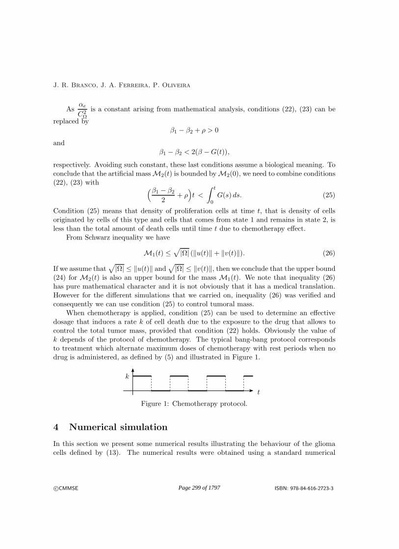
J. R. Branco, J. A. Ferreira, P. Oliveira

Asαe

C2Ω

is a constant arising from mathematical analysis, conditions (22), (23) can be

replaced byβ1 − β2 + ρ > 0

andβ1 − β2 < 2(β −G(t)),

respectively. Avoiding such constant, these last conditions assume a biological meaning. Toconclude that the artificial massM2(t) is bounded byM2(0), we need to combine conditions(22), (23) with

(β1 − β22

+ ρ)

t <

∫ t

0G(s) ds. (25)

Condition (25) means that density of proliferation cells at time t, that is density of cellsoriginated by cells of this type and cells that comes from state 1 and remains in state 2, isless than the total amount of death cells until time t due to chemotherapy effect.

From Schwarz inequality we have

M1(t) ≤√

|Ω| (‖u(t)‖ + ‖v(t)‖). (26)

If we assume that√

|Ω| ≤ ‖u(t)‖ and√

|Ω| ≤ ‖v(t)‖, then we conclude that the upper bound(24) for M2(t) is also an upper bound for the mass M1(t). We note that inequality (26)has pure mathematical character and it is not obviously that it has a medical translation.However for the different simulations that we carried on, inequality (26) was verified andconsequently we can use condition (25) to control tumoral mass.

When chemotherapy is applied, condition (25) can be used to determine an effectivedosage that induces a rate k of cell death due to the exposure to the drug that allows tocontrol the total tumor mass, provided that condition (22) holds. Obviously the value ofk depends of the protocol of chemotherapy. The typical bang-bang protocol correspondsto treatment which alternate maximum doses of chemotherapy with rest periods when nodrug is administered, as defined by (5) and illustrated in Figure 1.

t

k

Figure 1: Chemotherapy protocol.

4 Numerical simulation

In this section we present some numerical results illustrating the behaviour of the gliomacells defined by (13). The numerical results were obtained using a standard numerical

c©CMMSE ISBN: 978-84-616-2723-3Page 299 of 1797

A sufficient condition to control glioma growth

method defined combining the explicit Euler methods with second order centered differenceoperators and a rectangular rule to discretize the spatial derivatives and the time integral,respectively. We consider a homogeneous square domain Ω = [0, 15 cm]×[0, 15 cm] , diffusioncoefficients d11 = d22 = dv,11 = dv,22 = 0.025 cm2/day, growth rate ρ = 0.05 /day, switchingparameters β1 = 10−6/day and β2 = 0.036/day , kernel such that β = 1 and initialcondition defined by 106 proliferation tumor cells at middle square [7, 8] × [7, 8].

In Figure 2 we plot the numerical solutions at day 33 for an virtual untreated patient(G(t) = 0). We observe a decreasing on the highest values of the tumor cells concentrationat initial times followed by an increase and very intense spreading of cells. The contour plotsallow us to observe high gradients on the core of the tumor, defined by the proliferationcells, and that the migration cells are already quite far from the core!

102

103

104

105

0 5 10 150

5

10

15

1

105

106

0 5 10 150

5

10

15migration cells, day 33 proliferation cells, day 33

Figure 2: Numerical results at day 33, obtained with 2D model (13) for k = 0/day.

Let us consider now that the chemotherapy treatment defined by (5) is applied with aprotocol as illustrated in Figure 1. Condition (25) is used to compute an effective drug thatlead to control the total tumor mass. We consider a 24h dosage and different rest periods.In Table 1 we show the minimum value of k allowed by condition (25), for a virtual patientas defined in the beginning os this section. Here αe = 0.025 cm2/day and CΩ = 1√

2.

Protocol kmin [./day]

each 2 days 0.064

each 7 days 0.224

each 14 days 0.448

Table 1: kmin as (25), for a protocol of 24 consecutive hours of chemotherapy .

c©CMMSE ISBN: 978-84-616-2723-3Page 300 of 1797

J. R. Branco, J. A. Ferreira, P. Oliveira

In Figure 3 we plot the cell distribution at day 33, when a protocol of chemotherapyof 24h is administered at days 5, 19 and 33 using k = 0.5/day. We observe that gliomamass at day 33 is less than its mass at day 4 (the day before the first administration of thechemotherapy).

1

102

104

105

0 5 10 150

5

10

15migration cells, day 33

1

105

0 5 10 150

5

10

15proliferation cells, day 33

Figure 3: Numerical results at day 33, obtained with 2D model (13) for k = 0.5/day.

Finally, in Figure 4 we compare glioma masses of the virtual patient when no chemo-therapy is administered and the results of the adminstration of 3 different chemotherapyprotocols. The difference between the protocols is the rest period and the values of k werecomputed using condition (25). We observe that for all protocols glioma masses are lessthan the glioma mass at day 4 (the day before the first administration of the protocol).The results presented in this figure shows the effectiveness of the our approach to definechemotherapy protocols.

12345678

2 4 6 8 10 12 14 16 18 20 22 24 26 28 30 32 34 36 38 40

t [days]

mass [×106]no chemotherapy

2 days protocol G = 0.077 days protocol G = 0.2514 days protocol G = 0.5

Figure 4: Glioma masses M1(t).

c©CMMSE ISBN: 978-84-616-2723-3Page 301 of 1797

A sufficient condition to control glioma growth

5 Conclusions

In this paper we studied a mathematical model to describe the evolution of glioma cellswhen chemotherapy is applied. The model was established combining a mass conservationwith a non Fickian mass flux that takes into account the viscoelastic behaviour of the braintissue described by the Voigt-Kelvin model.

Using the energy method we deduced an estimate for the glioma mass M2(t), definedusing L2 norm. This estimate allowed us to define a sufficient condition on the para-meters of the model that leads to the control of M2(t), more precisely, to guarantee thatM2(t) < M2(0). Such condition was then used to define chemotherapy protocols. Numeri-cal experiments illustrating the behaviour of the glioma mass under the conditions deducedfor the chemotherapy protocols are also included. The results obtained suggest our approachis a promising one. Future work will address the comparison of the model with existingmedical protocols.

Acknowledgements

This work was partially supported by the Centro de Matematica da Universidade de Coim-bra (CMUC), funded by the European Regional Development Fund through the programCOMPETE and by the Portuguese Government through the Fundacao para a Cienciae Tecnologia (FCT) under the projects PEstC/MAT/UI0324/2011 and by the projectUTAustin/MAT/0066/2008.

References

[1] J. R. Branco, J. A. Ferreira, P. de Oliveira, Numerical methods for the ge-

neralized Fisher-Kolmogorov-Petrovskii-Piskunov equation, Applied Numerical Mathe-matics, 57 (2007) 89–102.

[2] D. A. Edwards, D. S. Cohen An unusual moving boundary condition arising in

anomalous diffusion problems, SIAM Journal on Applied Mathematics, 55 (1995) 662–676.

[3] D. A. Edwards, D. S. Cohen A mathematical model for a dissolving polymer, AIChEJournal, 41 (1995) 2345–2355.

[4] D. A. Edwards, Non-Fickian diffusion in thin polymer films, Journal of PolymerScience, Part B: Polymer Physics Edition, 34 (1996) 981–997.

[5] D. A. Edwards, A spatially nonlocal model for polymer-penetrant diffusion, Journalof Applied Mathematics and Physics, 52 (2001) 254–288.

[6] S. Fedotov, Traveling waves in a reaction-diffusion system: diffusion with finite

velocity and Kolmogorov-Petrovskii-Piskunov kinetics, Physical Review E, 58 (1998)4:5143–5145.

c©CMMSE ISBN: 978-84-616-2723-3Page 302 of 1797

J. R. Branco, J. A. Ferreira, P. Oliveira

[7] S. Fedotov, Nonuniform reaction rate distribution for the generalized Fisher equation:

Ignition ahead of the reaction front, Physical Review E, 60 (1999) 4:4958–4961.

[8] S. Fedotov, A. Iomin, Migration and proliferation dichotomy in tumor-cell invasion,Physical Review Letters, 98 (2007) 118110(1)–(4).

[9] S. Fedotov, A. Iomin, Probabilistic approach to a proliferation and migration di-

chotomy in tumor cell invasion, Physical Review E, 77 (2008) 1031911(1)–(10).

[10] G. Franceschini, The mechanics of human brain tissue, PhD thesis, University ofTrento, 2006.

[11] A. Giese, L. Kluwe, B. Laube, H. Meissner, M. Berens, M. Westphal, Mi-

gration of human glioma cells on myelin, Neurosurgery, 38 (1996) 755–764.

[12] S. Habib, C. Molina-Parıs, T. Deisboeck, Complex dynamics of tumors: modeling

an energing brain tumor system with coupled reaction-diffusion equations, Physica A,327 (2003) 501–524.

[13] S. Hassanizadeh, On the transient non-Fickian dispersion theory, Transport inPorous Media, 23 (1996) 107–124.

[14] H. L. Harpold, E. C. Alvord Jr, K. R. Swanson, The evolution of mathemati-

cal modeling of glioma proliferation and invasion, rm Journal of Neuropathology andExperimental Neurology, 66 (2007) 1–9.

[15] J. Humphrey, Continuum biomechanics of soft biological tissues, rm Proceedings ofRoyal Society London, 459 (2003) 3–46.

[16] D. Joseph, L. Preziosi, Heat waves, Review of Modern Physics, 61 (1989) 47–71.

[17] A. Mehrabian, Y. Abousleiman, A general solution to poroviscoelastic model of

hydrocephalic human brain tissue, Journal of Theretical Biology, 29 (2011) 105–118.

[18] J. D. Murray, Mathematical Biology, Springer, 2002.

[19] S. Shaw, J. R. Whiteman Some partial differential Volterra equation problems ari-

sing in viscoelasticity, Proceeding of the Conference on Differential Equations and theirApplications, Brno, (1997) 183–200.

[20] K. R. Swanson, E.C. Alvord Jr, J.D. Murray, A quantitative model for differen-

tial motility of gliomas in grey and white matter, Cell Proliferation, 33 (2000) 317–329.

[21] K. R. Swanson, C. Bridge, J. D. Murray, E. C. Alvord Jr, Virtual and real

brain tumors: using mathematical modelig to quantify glioma growth and invasion,Journal of the Neurological Sciences, 216 (2003) 1–10.

[22] P. Tracqui, G. C. Cruywagen, D. E. Woodward, G. T. Bartoo, J. D. Mur-

ray, E. C. Alvord Jr, A mathematical model of glioma growth: the effect of chemo-

therapy on spatio-temporal growth, Cell Proliferation, 28 (1995) 17–31.

c©CMMSE ISBN: 978-84-616-2723-3Page 303 of 1797

Proceedings of the 13th International Conferenceon Computational and Mathematical Methodsin Science and Engineering, CMMSE 201324–27 June, 2013.

Allee effects models in randomly varying environments

Carlos A. Braumann1 and Clara Carlos2

1 Centro de Investigacao em Matematica e Aplicacoes, Universidade de Evora

2 Escola Superior de Tecnologia do Barreiro, Instituto Politecnico de Setubal

emails: braumann@uevora.pt, clara.carlos@estbarreiro.ips.pt

Abstract

Based on a deterministic model of population growth with Allee effects, we proposea general stochastic model that incorporates environmental random fluctuations in thegrowth process. We study the model properties, existence and uniqueness of solutionand the stationary behavior. We also obtain expressions for the first passage times, inparticular, the mean and standard deviation of extinction times for the population.

Key words: Allee effects, population growth, random environments, extinction times

1 Introduction

Warder Clyde Allee (1885/1955) was an American zoologist and ecologist who taught animalecology. The Allee effects were first described by Allee and colleagues in 1949, as we cansee in [2]. There are two kinds of Allee effects, strong Allee effects and weak Allee effects.When a population has a ”critical size or density” below which the population decreaseson average and above which it increases on average, it is called a strong Allee effect. Onthe other hand, when a population does not exhibit a ”critical size or density” but at lowdensities the population growth rate increases with increasing density, we say there is aweak Allee effect. Allee effects show up in many wildlife populations, particularly whenlow population size hinders the efficacy of collective defensive behavior from predators orresults in individuals being far apart, which makes it difficult to find mating partners.

We introduce a quite general deterministic model of population growth with strongAllee effect, particular cases of which can be seen in [6], [8], [10] or [1]. The stochasticmodel we propose is based on this deterministic model with an added term to accountfor the effect of environmental fluctuations on the growth rate. Other stochastic Allee

c©CMMSE ISBN: 978-84-616-2723-3Page 304 of 1797

Allee effects models in randomly varying environments

effects models have been proposed in [7] and [9] but they consider the effect of demographicstochasticity (stochasticty due to sampling variations in births and deaths in an unchangingenvironment). The model proposed here is important to understand the consequences ofenvironmental variability affecting the growth rate. We study the properties of the proposedstochastic model.

We also characterize the time the population takes to reach a given size for the firsttime. In particular, we study the extinction time for the population.

2 Model

Let X = X(t) be the population size at time t > 0 and L a positive constant. We proposeas a general model with strong Allee effects that the per capita growth rate be of the form

1

X

dX

dt= f(X), (1)

where f(X) is a real C1 function defined for X > 0 such that −∞ < f(0+) < 0 < f(L),f(+∞) < 0 and, strictly, f(X) increases for X < L and decreases for X > L. We assumethat the initial size X(0) = x is known.

In [3] we can find such models with no Allee effects, in particular the classical logisticmodel, corresponding to f(X) = r

(1− X

K

), with intrinsic growth rate r > 0 and carrying

capacity of the environment K > 0. A model of population growth with strong Allee effectssimilar to the logistic models is f(X) = r

(1− X

K

) (XE − 1

), with 0 < E < K (see, for ins-

tance, [6]). An Allee limit E, with 0 < E < L < K such that f(E) = 0, is incorporatedsuch that the per capita population growth is negative below E.

In a randomly fluctuating environment, the per capita growth rate varies randomlyand expression (1) should now be interpreted as describing its average behavior and, sincegrowth is a multiplicative type process, the geometric average is the appropriate one toconsider. We then need to add the effect of environmental fluctuations on the per capitagrowth rate, which we assume to be of the white noise type, of the form σε(t), where ε(t)is a standard continuous-time white noise and σ > 0 is the noise intensity, assumed to beconstant and independent of population size. Therefore, assuming expression (1) representsthe geometric average growth rate, it can be seen in [5] that the appropriate stochasticcalculus to use is the Stratonovich calculus, and so we shall use it here. We obtain thestochastic differential equation (SDE)

1

X

dX

dt= f(X) + σε(t), (2)

with X(0) = x known.

The solution X(t) exists and is unique up to an explosion time. We can show that thereis no explosion and therefore, the solution exists and is unique for all t ≥ 0. The solution

c©CMMSE ISBN: 978-84-616-2723-3Page 305 of 1797

Carlos A. Braumann, Clara Carlos

X(t) is a homogeneous diffusion process with drift coefficient a(x) = x(f(x) + σ2

2

)and

diffusion coefficient b2(x) = σ2x2. Let us define, in the interior of the state space, the scaleand speed measures of X(t). The scale density is

s(y) := exp

(−∫ y

n

2a(θ)

b2(θ)dθ

)=n

yexp

(− 2

σ2

∫ y

n

f(θ)

θdθ

)(3)

and the speed density is

m(y) :=1

b2(y)s(y)=

1

nσ2yexp

(2

σ2

∫ y

n

f(θ)

θdθ

), (4)

where n is an arbitrary (but fixed) point in the interior of the state space and C > 0is a constant. The corresponding ”distribution” functions are S(z) =

∫ zc s(y)dy and

M(z) =∫ zc m(y)dy, the scale function and speed function, respectively, where c is an arbi-

trary (but fixed) point in the interior of the state space. The scale measure is define byS(a, b) = S(b)− S(a) and the speed measure is by M(a, b) = M(b)−M(a).

The state space has boundaries X = 0 and X = +∞. One can see that X = 0 isattracting but unattainable, so there is no t such that X(t) = 0; however, it may happenthat X(t) → 0 when t → +∞ and so ”mathematical” extinction can occur. One can seethat X = +∞ is non-attracting and, therefore, explosions can not occur.

Contrary to the deterministic model (1), the stochastic model (2) does not have anequilibrium point, but it may exist an equilibrium probability distribution for the populationsize, called the stationary distribution, with a probability density function p(y), known asstationary density. The stationary density p(y), when it exists, must satisfy the Kolmogorovforward equation

d(a(y)p(y))

dy− 1

2

d2(b2(y)p(y))

d2y= 0, (5)

We can show that every non-negative solution is not integrable(∫ +∞

0 p(y)dy = +∞)

and,

consequently, contrary to the corresponding stochastic model without Allee effects, there isno stationary density.

In fact, ”mathematical” extinction does occur, since X(t) → 0 when t → +∞, due tothe attractiveness of 0 and non-attractiveness of +∞. But we prefer to use the conceptof ”realistic” extinction, meaning the population dropping below an extinction thresholdq > 0 (for example, q = 1). We are interested in the extinction time, i.e. the timeTq = inft > 0 : X(t) = q required for the population to reach the extinction threshold forthe first time. Assuming 0 < q < x < +∞, we can write (see, for instance, [4]) expressionsfor the n-th order moment of Tq :

M (n)q (x) = E [(Tq)

n|X(0) = x)] = 2

∫ x

qs(ζ)

∫ +∞

ζnM (n−1)

q (θ)m(θ)dθdζ. (6)

Since M(0)q (x) = 1, one can iteratively obtain the moments of any arbitrary order of Tq and,

of course, also the mean and the variance.

c©CMMSE ISBN: 978-84-616-2723-3Page 306 of 1797

Allee effects models in randomly varying environments

Acknowledgements

The authors are members of the Centro de Investigacao em Matematica e Aplicacoes, aresearch center of the Universidade de Evora financed by FCT (Fundacao para a Ciencia eTecnologia, Portugal). Carlos A. Braumann gratefully acknowledges the financial supportfrom the FCT grant PTDC/MAT/115268/2009-Dynamics of epidemiological spreading andthe FAPESP Thematic Project-Assessing control of epidemics using mathematical and com-puter models.

References

[1] P. Amarasekare, Allee effects in metapopulation dynamics, The American Natural-ist, Vol. 152, n.2, 298–302 (1998).

[2] W. C. Allee, A. E. Emerson, O. Park , T. Park and K. P. Schmidt, Principlesof Animal Ecology. Saunders, Philadelphia (1949).

[3] C. A. Braumann, Applications of stochastic differential equations to populationgrowth, Proceedings of the Ninth International Colloquium on Differential Equations(Bainov, D., Ed.), VSP, Utrecht, p. 47–52 (1999).

[4] C. A. Braumann, P. A. Filipe, C. Carlos and C. J. Roquete, Growth of individ-uals in randomly fluctuating environments, Proceedings of the International Conferencein Computational and Mathematical Methods in Science e Engineering, Vigo-Aguiar,J., Alonso, P., Oharu, S., Venturino, E. and Wade, B. (Eds.), Gijon, 201–212 (2009).

[5] C. A. Braumann, Ito versus Stratonovich calculus in random population growth,Mathematical Bioscienses, 206, 81–107 (2007).

[6] F. Courchamp, T. H. Cliutton-Brock and B. Grenffell, Inverse density de-pendence and the Allee effect, Trends in Ecology & Evolution, 14: 405–410 (1999).

[7] B. Dennis, Allee effects in stochastic populations, Oikos, 96: 389–401 (2002).

[8] B. Dennis, Allee effects: population growth, critical density and the change of extinc-tion, Natural Resource Modelling, 3: 481–539 (1989).

[9] S. Engen, R. Lande and B.-E. Sæther, Demographic stochasticity and Allee effectsin populations with two sexes, Ecology, 84(9), 2378-2386 (2003).

[10] M. A. Lewis and P. Kareiva, Allee dynamics and the spread of invading organisms,Theoretical Population Biology 43: 141–158 (1993).

c©CMMSE ISBN: 978-84-616-2723-3Page 307 of 1797

Proceedings of the 13th International Conferenceon Computational and Mathematical Methodsin Science and Engineering, CMMSE 201324–27 June, 2013.

Exploiting Multi-core Platforms for Multi-model Forest FireSpread Prediction

Carlos Brun1, Tomas Margalef1 and Ana Cortes1

1 Computer Architecture and Operating Systems Department, Universitat Autonoma de Barcelona

emails: carlos.brun@caos.uab.es, tomas.margalef@uab.es, ana.cortes@uab.es

Abstract

The Two-Stage forest fire spread prediction methodology was developed to enhanceforest fire evolution forecast by tackling the uncertainty of certain environmental con-ditions. There are parameters, such as wind, that present a variation along terrain andtime. In such cases, it is necessary to develop multi-model prediction schemes thatintegrate forest fire propagation models and complementary models, such as meteoro-logical forecast and wind field models. This multi-model approach should improve theaccuracy of the predictions, but introducing an overhead in the execution time. In thispaper, different multi-model approaches are discussed and the results show that thepropagation prediction is improved. The overhead introduced by the complementarymodels can be overlapped with the data observations so the final prediction time is notincreased significantly.

Key words: HPC, forest fire, prediction, multi-core, efficiency, multi-model.

1 Introduction

Forest fires is a worrisome hazard that every year causes important losses around the world.For that reason, there has been a great research activity in this field during the last decades,in order to develop models which try to represent and predict the behavior of such haz-ard [1][2]. Forest fire spread simulators [3][4] require a set of input parameters describingthe environmental conditions, the initial fire front, the topography of the terrain and thevegetation. However, this input data far from being easy to obtain, it arises as one ofthe main problems to tackle. Topographical data is the most reliable input of a simulator,however, the remaining parameters suffer from different degrees of uncertainty ranging from

c©CMMSE ISBN: 978-84-616-2723-3Page 308 of 1797

Multi-model Forest Fire Spread Prediction

the total ignorance to very low resolution. For that reason, prediction schemes based onexecutions of hundreds or even thousands of fire scenarios (different simulator input config-urations) with the aim of filling the gap of uncertainty have been proposed [5]. Two-StagePrediction strategy [6] is a prediction scheme, which performs a forest fire prediction bypreviously executing a Calibration stage which involves the most sensitive parameters suchas environmental conditions. In this Calibration stage, the actual evolution of the forestfire is observed and a Genetic Algorithm (GA) is carried out to determine the set of pa-rameters that best reproduces the recent evolution of the fire. This set of values is thenused as input parameters in the Prediction stage. As it is well stated, using a GA as atunning strategy will imply a cost in terms of execution time, depending on the time spentfor evaluating each individual. In our case, one individual implies running once FARSITE(the underlying forest fire spread simulator) and, since one single fire spread simulation canlast from seconds to almost one hour, the time incurred in providing a useful predictioncould become prohibitive. Furthermore, the original Two-Stage prediction scheme suffersfrom two main handicaps. This scheme considers an uniform distribution of the parame-ters along the whole terrain and it does not consider prognostic models to enable dynamicparameters changes through time. Both restrictions have a direct impact in the quality ofthe prediction results [4][7]. Thus, the original scheme was modified to be a multi-modelprediction framework where different complementary models were easy to couple, in orderto reduce that negative impact. Therefore, we focus on the meteorological conditions and,in particular, in the wind components, since these are the parameters that most affect firespread [8]. In order to consider the meteorological wind modifications due to the topog-raphy, a wind field model must be introduced to obtain the effective wind at the requiredlevel of detail. On the other hand, to enable the two-stage prediction scheme the capacityof reacting to sudden changes in environmental conditions, it becomes mandatory to fit intothe prediction scheme, environmental data coming from prognostic models such as weatherforecasting models. Both prognostic models and wind field models are computationallyexpensive. So, any approach to couple those models into a system (Two-Stage predictionscheme in our case) will need to carefully analyze the implications in the total executiontime and resources needed. When we deal with natural hazards such as forest fires, anyfire spread prediction must be delivered faster than real time fire evolution to be useful.In this paper, we propose a multi-model prediction framework for forest fire spread pre-diction. This framework involves different models such as forest fire spread model, windfield model and a meteorological model. Due to the computational needs required for thisframework, we rely on High Performance Computing (HPC). Furthermore, since predictingthe evolution of forest fires implies working under very tight real time constraints, we alsoanalyzed how to use the available computing resources in the most efficient way withoutloosing prediction quality.In the next section, the proposed multi-model prediction framework is discussed. In sec-

c©CMMSE ISBN: 978-84-616-2723-3Page 309 of 1797

C.Brun, T.Margalef, A.Cortes

tion 3 the characteristics of the experiment performed and the execution platform used areintroduced. In section 4, a study of the prediction quality provided when different com-plementary models are included into the framework is performed. The execution time andefficiency of each approach is studied in section 5 and, finally the main conclusions of thiswork are reported in section 6.

2 Multi-model forest fire propagation prediction framework

In the above mentioned Two-Stage prediction scheme, the calibrated input parameter setis determined applying a GA. A random population of individuals, each one representinga scenario, is generated. Each individual is simulated and the fire propagation obtainedis compared to the real fire propagation. According to the quality of the prediction, theindividuals are ranked and the genetic operators are applied to generate the new popula-tion. The process is repeated a certain number of iterations and the best individual at theend of the process is selected to run the prediction for the next time interval. The GAfits very well in the Master/Worker paradigm. The Master process generates the initialrandom population. Then, it distributes the individuals to the Worker processes that canbe executed independently on different cores. Each core in the platform can run a Workerprocess. So, the maximum number of Worker processes is limited to the number of avail-able cores in the platform. If the population is larger than the number of cores, then someindividuals must be executed sequentially. Once the Workers have executed the FARSITEsimulation corresponding to its individual, they evaluate the error compared to the actualfire propagation using the symmetric difference among the real and simulated burned area.The error obtained is returned to the Master process that ranks the individuals and appliesthe genetic operators to generate the next population. This process is repeated for a fixednumber of iterations. This scheme has been called Two-Stage basic prediction methodology(2ST-BASIC prediction) and it is shown in figure 1(a). In this scheme, if there are enoughavailable cores, the execution time of each iteration is limited by the execution time of thescenario whose simulation lasts longer. The quality of the calibration depends on the avail-able elapsed time to provide the propagation prediction and the number of individuals oneach iteration, but it must be considered that in these emergency situations, response timeis a critical issue [9]. For the previous studies [10] it was stated that 5 iterations usuallyprovide a successful calibration.

2.1 Coupling Wind Field Model to 2ST-BASIC (2ST-WF)

As it has been mentioned above, some parameters present a spatial and temporal distri-bution which makes the calibration process more difficult since only an average value forthe parameter along map and time can be selected. One of such parameters is wind. The

c©CMMSE ISBN: 978-84-616-2723-3Page 310 of 1797

Multi-model Forest Fire Spread Prediction

wind can be measured by meteorological stations, but the value measured in one meteoro-logical station is a measure in a single point, but in other points of the terrain the value(speed and direction) of the wind can be others due to the orography of the terrain. So,it is necessary to introduce some complementary model that calculates the wind speed anddirection in any point of the terrain given a meteorological wind. The selected wind fieldmodel is WindNinja [7] because it has a direct connection to FARSITE. In this scheme,each worker process receives the parameters representing one particular scenario and then,it is necessary to run the WindNinja wind modeler and afterwards the FARSITE fire prop-agation simulator. This approach is more realistic but the computational time required byWindNinja is quite large. The execution time of the WindNinja modeler depends on themap size and topography, but usually it takes around some minutes on a single core. Thispipelined worker scheme is depicted in figure 1(b).

2.2 Coupling Meteorological Model to 2ST-BASIC (2ST-MM)

It is well known that wind can change suddenly in speed and direction. During the cali-bration stage, it is feasible to receive information from meteorological stations frequently(every 30 minutes or even more frequently). In this case, the wind speed and directiondo not need to be calibrated since they are received from direct measurements. However,during the prediction stage such values are not available beforehand. So, it is necessary tointroduce a meteorological model that can provide the expected values for the meteorolog-ical wind speed and direction. This values can be used during the prediction stage [11]. Inthis work, we assume that meteorological predictions are available from a meteorologicalservice, so, it is not necessary to compute the meteorological forecast on the fire spreadprediction platform. It implies that the computational cost of the 2ST-BASIC forest firepropagation prediction (see figure 1(c)) is not increased.

2.3 Complete Multi-model forest fire propagation scheme (2ST-WF-MM)

Next step is integrating all the mentioned models on a multi-model forest fire propagationframework (figure 1(d)). In this case, the meteorological wind speed and direction are notcalibrated, but they are provided by meteorological model and then introduced to the windfield model to provide the wind field. In this case, the meteorological measures and themeteorological predictions are known before the prediction stage starts and, therefore, thewind field corresponding to each time interval can also be computed beforehand.

3 Experiment design

For the experimental part of this work, we chose a relevant area in Catalonia (north-east ofSpain) as the landscape to be simulated. In particular, we concentrated on the north-east

c©CMMSE ISBN: 978-84-616-2723-3Page 311 of 1797

C.Brun, T.Margalef, A.Cortes

Figure 1: 2ST-BASIC (a), 2ST-WF (b), 2ST-MM (a) and 2ST-WF-MM (b) multi-modelprediction schemes

cape (El Cap de Creus) with an approximate real extension of 900 square kilometers. Inorder to evaluate all proposed schemes, we created a reference fire that lasts 12 hours. Thecomponents of the global meteorological wind (wind speed and wind direction) vary every30 minutes including significant variations between stages. The resulting fire evolution isstored and used as a real fire evolution, and the input settings that were used to generatethis propagation are dismissed. Although this, for this test case, the meteorological datahas been generated in a synthetic way. We have already evaluated the viability to obtainin real time this information from the corresponding local weather forecast service (ServeiMetereologic de Catalunya) [12][13]. This information involves both kind of data needed,real observations provided by meteorological weather stations and forecasted data deliveredby the WRF (Weather Research and Forecasting) model. The time window selected for theCalibration and Prediction stages was chosen taking into account the time period neededto gather useful information from weather forecast services and satellite sensor systems. Inthe former case, the typical time-step of coarse scale weather forecast models ranges from 3to 6 hours, what determines the frequency of delivered data. On the later case, we shouldconsider the time interval required for receiving fire front images that could properly be

c©CMMSE ISBN: 978-84-616-2723-3Page 312 of 1797

Multi-model Forest Fire Spread Prediction

used in that multi-model prediction framework. To obtain such a perimeter information,we rely on sensors systems which are on board both the NASA’s Terra and Aqua satellites.It is necessary for each satellite to complete 3 orbits (approximately 3 hours) to cover thewhole Europe area, so it could be possible to obtain fire perimeters every 3-6 hours [14].Consequently, the time window selected for the Calibration stage and the Prediction stage,in this test case, has been 6 hours each. Therefore, we had 12 hours to execute the wholeprediction scheme independently on the multi-model scheme selected. Since the Calibrationstrategy implements a GA, we perform the experiment for different population sizes such as25, 50 and 100 individuals in order to analyze the influence of this parameter on the resultsin terms of quality, execution time and efficiency. The GA has been iterated 5 times and,for each initial population size, we have performed 5 different experiments with differentinitial population. Thus, the results reported in the following sections are the mean valuesof those 5 experiments.

Finally, the execution platform used for all the results reported in the following sectionsis an IBM cluster x3650 composed of 32 nodes with two Dual-Core Intel(R) Xeon(R) CPU5150 2.66GHz and 12 GB Fully Buffered DIMM 667 MHz each.

4 Quality analysis

The schemes described in section 2 incorporate a GA that iteratively improves the quality ofthe calibration. So, it is necessary to analyze the convergence of the GA and the influence ofother parameters such as the population size in the quality delivered of every multi-modelscheme. Figure 2 summarizes the evolution of the error at each generation for all the 4schemes. It can be observed that the schemes which incorporate the meteorological model(2ST-MM and 2ST-MM-WF) do not require a significant number of generations to achievean almost stable calibration error. The main reason of this behavior is that, in these cases,the wind is not a parameter to be calibrated, but it is a measured or forecasted parameter.Therefore, the calibration process is easier since the wind speed and direction are veryrelevant parameters that must be calibrated carefully. In this cases, the population sizedoes not appear to be a relevant factor since the errors are very similar. The schemes thatdo not incorporate meteorological model (2ST-BASIC and 2ST-WF) must calibrate themeteorological wind value and, therefore, the calibration process requires more iterations.In this schemes, the population size is a relevant factor since larger populations providebetter calibration results. It is also worthy observing that the schemes that incorporate thewind field model (2ST-WF and 2ST-MM-WF)) provide better results than those that usea general value for the whole terrain. It means that the wind field model is an added valueto the prediction process. The calibration process is very significant, but finally the mostrelevant result is the prediction error. Figure 3(a) shows the errors obtained at the end ofthe calibration process and the corresponding prediction errors. The same information is

c©CMMSE ISBN: 978-84-616-2723-3Page 313 of 1797

C.Brun, T.Margalef, A.Cortes

depicted in figures 3(b) where a visualization of the delivered predicted fire front evolutionfor each multi-model scheme is plotted. As we can observe, the multi-model scheme thatprovides better results both in the Calibration stage as in the Prediction stage, is the 2ST-MM-WF as it was expected. Let’s analyze the results scheme by scheme in more detail.The 2ST-BASIC is the scheme that delivers worst results both in prediction and calibrationerrors. This scheme needs to perform all the iterations of the GA to reduce the predictionresults but, even iterating until the preset number of generations, it is not able to adapt tochanges in the meteorological conditions such as wind parameters. The initial populationsize could slightly reduce this penalty but, in general terms, this effect is independent on thenumber of the GA’s individuals. When observing the results provided by the 2ST-WF, wedetected a quality improvement in the Calibration stage. This enhancement is due to, notonly the inclusion of the wind field evaluation for each particular individual, but also to theability of calibrating the general wind components. This ability enables the system to betteradjust the wind parameters to reproduce more precisely the recent past behavior of the fire.However, this enhancement is not extrapolated to the Prediction stage. As we can observe,the prediction error drastically increases despite having a good calibration error. The mainreason of this is that wind values do not keep quite constant from Calibration stage toPrediction stage. Thus, 2ST-WF scheme is not able to adapt to meteorological changes, ifthose changes happens during the Prediction interval. As it is was reported in section 2, toovercame this drawback, a meteorological model was coupled into the multi-model system.The advantages of including such a model are reflected in the prediction errors obtained for2ST-MM and 2ST-MM-WF. Using forecasted data in the Prediction stage helps the systemto dynamically adapts to changes in environmental variables. However, 2ST-MM deliversworse results than 2ST-MM-WF. The reason of this difference is the ability of 2ST-MM-WFto provide high resolution wind flow that better reproduces the wind variations at a fieldlevel. So, if the wind speed varies because of a mountain or a valley the 2ST-MM-WF multi-model scheme captures this effects. Those results keep quite similar for all initial populationsizes, so, a last conclusion in this point could be that, a population size of 25 individualsis enough to obtain a reasonable prediction results. However, these conclusions must becontrasted with the execution time and efficiency results reported in the next section.

5 Execution Time and Efficiency

Prediction quality is a very important issue, but execution time is as critical as accuracy. So,it is necessary to study the execution time of each scheme and the efficiency reached. Theexecution time of each scheme for different population sizes (25, 50 and 100 individuals)have been evaluated and the results are shown in table 1. As it can be observed, theexecution time of the 2ST-WF is by far, the most time consuming multi-model scheme.The need of executing a wind field model for each individual at each iteration results in a

c©CMMSE ISBN: 978-84-616-2723-3Page 314 of 1797

Multi-model Forest Fire Spread Prediction

Figure 2: Prediction error evolution for 2ST-BASIC (a), 2ST-BASIC-WF (b), 2ST-BASIC-MM (c) and 2ST-BASIC-MM-WF (d) using initial populations of 25, 50 and 100 individual

increment of time. So, for the shake of understanding, figure 4, summarizes the executiontime of all schemes except 2ST-WF. The execution time depends on the number of workers,the number of nodes on the system, the architectural features of each node, and morespecifically on the multi-model scheme selected and the particular scenario represented. Asit was described in section 3, for running our test we use 128 cores. Since our populationsare 100 individuals at most, there are enough cores to execute one worker per core, but theinternal architecture of each node has a crucial effect. Each node has 2 processors and 12GBof memory. Internally each processor has 2 cores with a local cache memory of 64KB (32KBfor data and 32KB for instructions) per core and a shared cache of 4MB. The forest firepropagation simulator needs information concerning the features of the terrain where thefire is taking place with a significant resolution. It means that they must usually managearound 3MB of data. Actually, the data size depends on the map size and the resolution,but this is a typical size. Therefore, when we can allocate one worker per node or even perprocessor, each worker has the 4MB of shared cache memory available and this amount ofmemory is enough to store all the required data. However, when the number of workers

c©CMMSE ISBN: 978-84-616-2723-3Page 315 of 1797

C.Brun, T.Margalef, A.Cortes

(a) (b)

Figure 3: Calibration and Prediction errors for all multi-model predictions schemes usinginitial populations of 25, 50 and 100 individuals (a) and the predicted fire front when 25individuals are used (b).

Population size 25 50 100

2ST-BASIC 31.38s 41.16s 70.27s

2ST-WF 829.16s 1083.45s 1609.38s

2ST-MM 34.06s 47.25s 74.07s

2ST-MM-WF 63.71s 73.72s 97.97s

Table 1: Execution time of every scheme and population size.

increases and two workers are allocated in the two cores of the same processor, they mustshare the 4MB of cache memory. This memory is to small to host the data corresponding toboth workers and then they must continuously access to main memory with the significantexecution time degradation. Another factor that affects the execution time when the numberof individuals is increased, is the access to the data files. 100 workers simultaneously readingthe input data files (terrain, vegetation, etc.) and writing the propagation maps in files inNFS, introduce a bottleneck that contributes to increase the execution time. So, largerpopulations (100 individuals) need less generations to converge to a reasonable error, butthe execution time of each generation is significantly larger than the shorter populations (25or 50 individuals). So, the use of more resources does not provide the expected benefit inexecution time. Comparing the execution time obtained by the different schemes, it can beobserved that the 2ST-BASIC is the fastest scheme. It was expected since it is the scheme

c©CMMSE ISBN: 978-84-616-2723-3Page 316 of 1797

Multi-model Forest Fire Spread Prediction

Figure 4: Execution time of 2ST-BASIC, 2ST-MM, 2ST-MM-WF for all population sizes

that involves less models (actually only forest fire simulation is involved) and moreover, allthe parameters are uniform and constant. However, it can be seen that it needs severaliterations of the GA to converge and with the same number of iterations the calibrationand prediction errors are higher than the ones obtained using the other schemes. The 2ST-WF scheme presents an execution time that, in its current state, cannot be assumed. Themain problem incurred by this scheme is that it is necessary to evaluate the wind fieldcorresponding to every individual in any iteration, and this enlarges the duration of a singleiteration. The average execution time of the WindNinja in the tested scenario is around 220seconds. Considering that the number of iterations is 5, then the time incurred by the windfield calculation along the 5 generations is around 1100 seconds. Moreover, the executiontime of FARSITE when a wind field is introduced is larger than the FARSITE execution timewhen a uniform wind is considered. To make this scheme viable, it is necessary to acceleratethe execution of the wind field model. The 2ST-MM scheme assumes that the measurementsof the meteorological stations and the forecasted data provided by meteorological models,are available before the prediction stage is launched. So, this scheme does not introduceany additional computational cost. Instead, since the wind is not introduced as one ofthe parameters to be calibrated, the calibration process is much shorter and the requirednumber of iterations is significantly reduced, with the corresponding reduction in predictiontime. The complete multi-model 2ST-MM-WF scheme does not require to calibrate thewind parameters since they are measured or predicted, and then, the calibration requiresless iterations. So, the computational cost of introducing the Wind field modeler does notsuppose a significant time increase. The only overhead introduced is the one incurred whenevaluating the wind field in the Prediction Stage.

c©CMMSE ISBN: 978-84-616-2723-3Page 317 of 1797

C.Brun, T.Margalef, A.Cortes

6 Conclusions

Fire spreading is a complex phenomena that implies, not only, the execution of a fire spreadmodel, but also complementary models, which enrich the description of the environmentalconditions where the fire takes place. In particular, it is crucial to be able to determinethe wind components at a high resolution for the whole terrain. So, meteorological modelsthat forecast the wind components at a low resolution and wind fields models, which areable to move this low resolution winds to a high resolution wind flows at a field level, arerequired. We have proposed and analyzed three different multi-models fire spread predictionschemes, which are based on the so called Two-Stage prediction method. The inclusion ofthese models have a direct impact in the total execution time of the prediction scheme, aswell as in the number of computing resources needed to run them. So, the performanceof the proposed multi-model schemes has been analyzed in terms of prediction qualityimprovements, execution time incurred to deliver a prediction and their efficiency. Fromthe experimental study outcomes that coupling both models, meteorological and wind fieldmodels, to the forest fire spread model improves the quality of the predictions. However, inorder to use the resources in a more efficient way, the GA implemented in the calibrationstage of the proposed methodology achieves reasonable calibration errors with populationssizes about 25 individuals. That means that it is not necessary to use large populations,instead, the resources released as a consequence of shorten the population, could be directlyapplied to run the commented complementary models.

Acknowledgments

This research has been supported by MICINN-Spain TIN2011-28689-C02-01.

References

[1] D. X. Viegas. Fire line rotation as a mechanism for fire spread on a uniform slope.International Journal of Wildland Fire, 11(1):11–23, 2002.

[2] R.C. Rothermel. How to predict the spread and intensity of forest and range fires. USDepartment of Agriculture, Forest Service, Intermountain Forest and Range Experi-ment Station Ogden, UT, USA, 1983.

[3] M. A. Finney. FARSITE, Fire Area Simulator–model development and evaluation. Res.Pap. RMRS-RP-4, Ogden, UT: U.S. Department of Agriculture, Forest Service, RockyMountain Research Station. 1998.

c©CMMSE ISBN: 978-84-616-2723-3Page 318 of 1797

Multi-model Forest Fire Spread Prediction

[4] A. M. G. Lopes, M. G. Cruz, and D. X. Viegas. Firestation an integrated software sys-tem for the numerical simulation of fire spread on complex topography. EnvironmentalModelling & Software, 17(3):269–285, 2002.

[5] G. Bianchini, M. Denham, A. Cortes, T. Margalef, and E. Luque. Wildland firegrowth prediction method based on multiple overlapping solution. J. Comput. Sci-ence, 1(4):229–237, 2010.

[6] B. Abdalhaq, A. Cortes, T. Margalef, and E. Luque. Enhancing wildland fire pre-diction on cluster systems applying evolutionary optimization techniques. FGCS TheInternational Journal of Grid Computing, 21(1):61 – 67, 2005. Methods Applications.

[7] J. M. Forthofer. Modeling wind in complex terrain for use in fire spread prediction.PhD thesis, Colorado State University, 2007.

[8] B. Abdalhaq, A. Cortes, T. Margalef, and E. Luque. Evolutionary optimization tech-niques on computational grids. In International Conference on Computational Science(1), pages 513–522, 2002.

[9] A. Cencerrado, R. Rodrıguez, A. Cortes, and T. Margalef. Urgency versus accuracy:Dynamic driven application system natural hazard management. International Journalof Numerical analysis and Modeling, (9):432–448, 2012.

[10] M. Denham, K. Wendt, G. Bianchini, A., and T. Margalef. Dynamic data-drivengenetic algorithm for forest fire spread prediction. Journal of Computational Science,3(5):398 – 404, 2012.

[11] C. Brun, T. Artes, T. Margalef, and A. Cortes. Coupling wind dynamics into a dddasforest fire propagation prediction system. Procedia Computer Science, 9(0):1110 – 1118,2012.

[12] METEO.CAT (http://www.meteo.cat). Servei meteorologic de catalunya.

[13] A. Cencerrado, M. A. Senar, and A. Cortes. Support for urgent computing based onresource virtualization. In ICCS (1), pages 227–236, 2009.

[14] D. Rodriguez-Aseretto, D. de Rigoa, M. Di Leoa, A. Cortes, and J. San-Miguel-Ayanza.A data-driven model for large wildfire behaviour prediction in europe. Procedia Com-puter Science (to be published), 2013.

c©CMMSE ISBN: 978-84-616-2723-3Page 319 of 1797

Proceedings of the 13th International Conferenceon Computational and Mathematical Methodsin Science and Engineering, CMMSE 201324–27 June, 2013.

Do niches help in controlling disease spreadin ecoepidemic models?

Iulia Martina Bulai1, Bruna Chialva1, Davide Duma1 and Ezio Venturino1

1 Dipartimento di Matematica “Giuseppe Peano”, Universita di Torino,via Carlo Alberto 10, 10123 Torino, Italy

emails: iuliam@live.it, bruna.chiara@alice.it, davideduma@gmail.com, email:ezio.venturino@unito.it

Abstract

We present three models for refuges in interacting population systems of predator-prey type, with the prey hosting a transmissible disease. The safety niche is assumedto lessen the disease spread, but not to protect prey from predators. This representsa novelty with respect to standard ecosystems where the refuge prevents predators’attacks. The niche is assumed either to protect the healthy individuals, or to hinderthe infected ones to get in contact with the susceptibles, or finally to reduce altogethercontacts that might lead to new cases of the infection. Some counterintuitive resultsare obtained. The effectiveness of the three different strategies are compared. The bestsituation in terms of disease containment appears to be the environment which providesa place where the healthy individuals cannot come in contact with disease carriers.

Key words: refuge, niches, disease transmission, ecoepidemicsMSC 2000: AMS codes 92D30, 92D25, 92D40

1 Introduction

In population models predator-prey and competition systems play a dominant role, sincethe blossoming of this discipline about a century ago. In more recent times, more refinedmodels try to better describe reality. Since prey try to seek protection against attacks oftheir predators in the features of the environment, scientists have tried to incorporate thisbehavior into the interaction models. The introduction of refuges has lead to the observationthat the Lotka-Volterra models gets stabilized [3] even to show global asymptotic stability,[1, 2]. This shows the relevant role that spatial refuges exert in shaping the dynamics of

c©CMMSE ISBN: 978-84-616-2723-3Page 320 of 1797

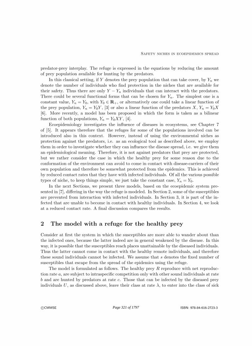
Safety niches in ecoepidemics spread

predator-prey interplay. The refuge is expressed in the equations by reducing the amountof prey population available for hunting by the predators.

In this classical setting, if Y denotes the prey population that can take cover, by Yn wedenote the number of individuals who find protection in the niches that are available fortheir safety. Thus there are only Y − Yn individuals that can interact with the predators.There could be several functional forms that can be chosen for Yn. The simplest one is aconstant value, Yn = Y0, with Y0 ∈ R+, or alternatively one could take a linear function ofthe prey population, Yn = Y0Y , [3] or also a linear function of the predators X, Yn = Y0X[6]. More recently, a model has been proposed in which the form is taken as a bilinearfunction of both populations, Yn = Y0XY , [4].

Ecoepidemiology investigates the influence of diseases in ecosystems, see Chapter 7of [5]. It appears therefore that the refuges for some of the populations involved can beintroduced also in this context. However, instead of using the environmental niches asprotection against the predators, i.e. as an ecological tool as described above, we employthem in order to investigate whether they can influence the disease spread, i.e. we give theman epidemiological meaning. Therefore, it is not against predators that prey are protected,but we rather consider the case in which the healthy prey for some reason due to theconformation of the environment can avoid to come in contact with disease-carriers of theirown population and therefore be somewhat protected from the epidemics. This is achievedby reduced contact rates that they have with infected individuals. Of all the various possibletypes of niche, to keep things simple, we just take the constant case, Yn = Y0.

In the next Sections, we present three models, based on the ecoepidemic system pre-sented in [7], differing in the way the refuge is modeled. In Section 2, some of the susceptiblesare prevented from interaction with infected individuals. In Section 3, it is part of the in-fected that are unable to become in contact with healthy individuals. In Section 4, we lookat a reduced contact rate. A final discussion compares the results.

2 The model with a refuge for the healthy prey

Consider at first the system in which the susceptibles are more able to wander about thanthe infected ones, because the latter indeed are in general weakened by the disease. In thisway, it is possible that the susceptibles reach places unattainable by the diseased individuals.Thus the latter cannot come in contact with the healthy remote individuals, and thereforethese sound individuals cannot be infected. We assume that s denotes the fixed number ofsusceptibles that escape from the spread of the epidemics using the refuge.

The model is formulated as follows. The healthy prey R reproduce with net reproduc-tion rate a, are subject to intraspecific competition only with other sound individuals at rateb and are hunted by predators at rate c. Those that can be infected by the diseased preyindividuals U , as discussed above, leave their class at rate λ, to enter into the class of sick

c©CMMSE ISBN: 978-84-616-2723-3Page 321 of 1797

Iulia Martina Bulai, Bruna Chialva, Davide Duma, Ezio Venturino

inviduals. The latter do not reproduce, are hunted at a rate k 6= c by the predators. Herek > c means that they are weaker than sound ones, and therefore more easy to capture,while k < c instead takes into account the fact that they might be less palatable than thehealthy ones. Finally, they can recover the disease at rate ω and therefore reenter into theS population. As mentioned above, infected are assumed not to contribute to intraspecificpressure, either of sound prey or among themselves; this again is grounded in the fact thattheir disease-related weakness prevents them to compete with the other individuals in thepopulation. The predators are assumed to have also other food sources, for which theyreproduce at rate d, but clearly get a benefit from the interactions with the healthy preyexpressed by the parameter e < c. This constraint expresses the fact that the amount offood they get from the captured prey cannot exceed its mass. So far all the system param-eters are nonnegative. For the predators hunting the infected prey, instead, we could modeltwo different situations. For h > 0, the infected cause a damage to the predators, killingthem. In this paper we concentrate only on this case. In the opposite case we could havethe normal situation in which predators get a reward from capturing the diseased prey, sothat in this situation we would have 0 < −h < k. In summary, the ecoepidemic model withinclusion of a disease-safety niche for the susceptibles reads

dR

dt= R[a− bR− cF ]− λ(R− s)U + ωU (1)

dU

dt= λ(R− s)U − U [kF + ω]

dF

dt= F [d+ eR− fF − hU ]

Note that the above system needs some further qualifications. In fact when R < sthe next to last term in the first equation and the first one in the second equation wouldbecome positive and negative respectively, which makes no sense biologically. Thereforein such situations they should be understood to be identically zero. But in such case theinfected prey in the system are easily seen to vanish, since in the second equation the termon the right hand side is always negative. The system then would settle to one of theequilibria of the classical disease-free predator-prey model, with logistic correction for theprey alternative food supply for the predators, see [7] for its brief analysis. For the benefitof the reader a short summary of its findings is presented also here at the top of Section 5.

The equilibria of (1) are P1 = (0, 0, 0) and

P2 =

(0, 0,

d

f

), P3 =

(ab, 0, 0

), P4 =

(af − cdbf + ce

, 0,ae+ bd

bf + ce

).

The first three points are always feasible, P4 is feasible for

af > cd. (2)

c©CMMSE ISBN: 978-84-616-2723-3Page 322 of 1797

Safety niches in ecoepidemics spread

Then there is coexistence P5 = (R5, U5, F5). Its population values are obtained solving forF and U respectively the second and third equations in (1), thus giving

F5 =1

k[λ(R5 − s)− ω] , U5 =

1

h[d+ eR5 − fF5] .

Substituting into the first one, we obtain the quadratic equation W (R) ≡∑2

k=0 akRk = 0

whose roots give the values of R5. Its coefficients have the following values

a2 =λ

h

(f

kλ− e

)− b− c

kλ, a0 =

1

hk(dk + fsλ+ fω) (sλ+ ω),

a1 = a+c

k(sλ+ ω) +

1

hk[(sλ+ ω)(ek − fλ)− λ(dk + fsλ+ fω)].

Now, since a0 > 0, if the parabola W (R) is concave one positive root will exist. Thus asufficient condition for the existence of P5 is a2 < 0, i.e., explicitly,

fλ2 < h[(b+ e)k + cλ]. (3)

For feasibility, we need also the other population values at a nonnegative level, a fact whichis attained for U5 if ek > fλ, else we must impose it, giving

R5 <dk + fλ+ fω

fλ− ek, (4)

as we do for F5 to obtain

R5 > s+ω

λ. (5)

The Jacobian of (1) is

J =

a− 2bR− λU − cF −λ(R− s) + ω −cRλU λ(R− s)− kF − ω −kUeF −hF d+ eR− hU − 2fF

The eigenvalues for P1 are −λs− ω, d, a, entailing its instability. Those for P2 are −(dk +fλs+ fω)f−1, −d, (af − cd)f−1 giving the stability condition

af < cd. (6)

Comparing this condition with (2), we observe that there is a transcritical bifurcation, forwhich P4 emanates from P2 when the latter becomes unstable. In other words, introducingthe healthy prey invasion number

R(i) ≡ af

cd. (7)

c©CMMSE ISBN: 978-84-616-2723-3Page 323 of 1797

Iulia Martina Bulai, Bruna Chialva, Davide Duma, Ezio Venturino

we have that for R(i) > 1 the healthy prey establish themselves in the environment.

For P3 the eigenvalues are (bd+ ae)b−1, (λa− λsb− bω)b1, −a, giving instability.

At P4 one eigenvalue is easily factored out,

λ(af − cd)− k(bd+ ae)

ce+ bf− λs− ω,

while the remaining ones are roots of the quadratic equation

T (δ) = δ2 + b1δ + b2 = 0, (8)

where letting D = ce+ bf ,

b1 =t1D, b2 =

t3D, t1 = af(b+ e) + bd(f − c),

t3 = (bd+ ae)(af − cd), t2 = t21 − 4t3(bf + ce).

Explicitly,

T1,2 =−b1 ±

√b21 − 4b2

2=−t1 ±

√t2

2(ec+ bf). (9)

0 5 10 15 200

5

R

time

a=21, b=0.3, c=1, d=1, e=0.5, f=0.9,

h=0.1, k=10, λ=10.2, ω=0.8, s=0.9, p=0, q=0

0 5 10 15 200

5

10

U

time

0 5 10 15 200

2

4

F

time

Figure 1: The coexistence equilibrium is attained for the following choice of parameters:a = 21, b = 0.3, c = 1, d = 1, e = 0.5, f = 0.9, h = 0.1, k = 10, λ = 10.2, ω = 0.8, s = 0.9.

c©CMMSE ISBN: 978-84-616-2723-3Page 324 of 1797

Safety niches in ecoepidemics spread

By the feasibility condition (2), t3 > 0 so that t2 < t21. Hence both roots of (9) have negativereal part. Stability hinges then just on the first eigenvalue, i.e. λR4 < kF4 + λs + ω orexplicitly the following condition

λaf − cdbf + ce

< kae+ bd

bf + ce+ λs+ ω. (10)

For the coexistence equilibrium P5, we have run some simulations to show that it canbe attained at a stable level. Figure 1 shows one such instance, for the parameter valuess = 0.9 and

a = 21, b = 0.3, c = 1, d = 1, e = 0.5, f = 0.9, (11)

h = 0.1, k = 10, λ = 10.2, ω = 0.8.

Here the R5 equilibrium value is much higher than the number of individuals s that cantake cover in the safety niche. Observe also that the same inequality holds also for all thehealthy prey population values before attaining the equilibrium level.

3 The case of a cover for the infected

Assume now that part of the infected are somehow confined in an environment in whichhealthy prey cannot enter. In this way the contagion risk is reduced. Let p denote the fixednumber of infected that inhabit the unreacheable territory. With the remaining notationsimilar to model (1), the system in our present case reads

dR

dt= R[a− bR− cF − λ(U − p)] + ωU (12)

dU

dt= λ(U − p)R− U [kF + ω]

dF

dt= F [d+ eR− fF − hU ]

Again, here we have to remark that for U < p the contributions to the infected class isto be understood to drop to zero. In such case, once again, the infected prey in the systemvanish, and the system settles to any equilibrium of the classical disease-free predator-preymodel P4 ≡ P4, [7].

For (12) the equilibria are again the origin P1 ≡ P1 = (0, 0, 0) and the point P2 ≡ P2

but here we find a new predator-free point, while coexistence of healthy prey and predatorsis forbidden. We thus have

P0 =

(a

b,

aλp

aλ− bω, 0

).

c©CMMSE ISBN: 978-84-616-2723-3Page 325 of 1797

Iulia Martina Bulai, Bruna Chialva, Davide Duma, Ezio Venturino

The latter is feasible for aλ > bω, i.e. introducing the disease basic reproduction numberR0, if

R0 ≡aλ

bω> 1. (13)

The presence of the coexistence equilibrium P5 = (R5, U5, F5) can be discussed asfollows. From the last equation of (12) we solve for F

F5 =1

f(d+ eR− hU)

and substitute into the remaining equations to obtain two conic sections

Φ(R,U) ≡ k

fhU2 − ek

fRU + U

(λ− k

fd− ω

)− pλ = 0,

Ψ(R,U) ≡ −(b+

c

fe

)R2 +

(c

fh− λ

)RU +

(pλ− c

fd+ a

)R+ ωU = 0,

of which we seek an intersection (R5, U5) in the first quadrant. We study the each one ofthem separately.

The implicit function Φ = 0 can be solved as a function R = ρ(U),

ρ(U) ≡ 1

fU

[khU2 + (fλ− dk − fω)U − fpλ

].

The numerator is a convex quadratic, which has two real roots with opposite signs, U±. Infact Descartes rule shows that independently of the sign of fλ − dk − fω there is alwaysone variation and one permanence of signs in its coefficients. For U > 0 it is therefore acontinuous function crossing the U axis at U+ > 0, that has a vertical asymptote coincidingwith the R axis and for U > 0 it raises up to infinity, asymptotically approaching thestraight line R = hkf−1U . Its inverse, U = ρ−1(R), has the R axis as horizontal asymptotefor R→ −∞ and goes to infinity for large positive R, crossing the U axis at U+. This curvecorresponds to the level 0 of the surface Φ(R,U). This implicit function is clearly negativeat the origin, since Φ(0, 0) = −pλ < 0, and by continuity retains this sign everywhere belowthe curve U = ρ−1(R), while it is positive above it.

The function Ψ(R,U) instead vanishes at the origin. Studying it on the R axis, we findthat it must cross it also at the point

R(1) =fpλ− c+ af

bf + ce,

which can have either sign. If R(1) < 0, then Ψ(R,U) > 0 in the whole first quadrant.Therefore in this case Φ and Ψ do not meet in the first quadrant and the coexistenceequilibrium P5 does not exist.

c©CMMSE ISBN: 978-84-616-2723-3Page 326 of 1797

Safety niches in ecoepidemics spread

Conversely, if

fpλ+ af > c (14)

since Ψ is a conic section, it must raise up from the origin and then go down to meet the Raxis at R1, thus it defines an arc of a concave function U ≡ A(R) in the first quadrant. Wemust investigate when this arc U = A(R) and the function U = ρ−1(R) meet. We do so bycomparing their respective slopes at R = 0. Evidently, since A(0) = 0 and ρ−1(0) = U+ > 0,if A′(0) < (ρ−1)′(0), no intersection can exist, recalling the concavity of A and the fact thatρ−1 is monotonically increasing, as we can easily verify that [ρ−1(R)]′ = [ρ′(U)]−1 > 0 forU > 0. One can also explicitly find the expression of A(U) as

A(U) = R(bf + ce)R+ cd− fpλ− af

(ch− fλ)R+ fω.

We must impose the converse condition A′(0) > (ρ−1)′(0). Implicit differentiation of Φ andΨ and evaluation at R = 0 yields

(ρ−1)′(0) =ekU+

2hkU+fλ− dk − fω, A′(0) =

1

ω(cd− fpλ− af).

For U = 0 we then need to have the slope of A larger than the one of ρ−1, but this doesnot automatically imply an intersection of the two curves. In fact two intersections existif we additionally require for instance that at the maximum of the arc A, or in general forany suitable value of the abscissa R in [0, R1], the values of A and ρ−1 “interlace”, i.e. thefollowing conditions are met

A′(0) > (ρ−1)′(0), A(R)≥ ρ−1

(R). (15)

The above conditions are then sufficient for the existence of P5. In particular we could hereeasily locate the reference point as R ≡ 1

2R1,The Jacobian of (12) is

J =

a− 2bR− cF − λ(U − p) −λR+ ω −cRλ(U − p) λR− kF − ω −kU

eF −hF d+ eR− hU − 2fF

.P1 is always unstable, since the eigenvalues are d and

−1

2ω +

1

2a+

1

2λ p± 1

2

√ω2 + 2 a ω − 2 λ p ω + a2 + 2 a λ p+ p2 λ2.

For P2 we find the eigenvalue A0 = −d and

A± =1

2f

[af − kd− ωf − cd+ fpλ±

√Y],

Y = 2 kdω f + ω2f2 − 2 kd2c+ 2ω f2a+ 2 kdaf − 2ω fcd+ 2 kdλ pf

−2λ pω f2 − k2d2 + 2 cdλ pf + 2 afcd− 2 af2λ p− a2f2 − c2d2 − p2λ2f2.

c©CMMSE ISBN: 978-84-616-2723-3Page 327 of 1797

Iulia Martina Bulai, Bruna Chialva, Davide Duma, Ezio Venturino

Stability is then ensured if

f(a+ pλ) < kd+ ωf + cd. (16)

0 5 10 15 200

5

10

R

time

a=21, b=0.3, c=1, d=1, e=0.5, f=0.9,

h=0.1, k=10, λ=10.2, ω=0.8, s=0, p=0.1, q=0

0 5 10 15 200

10

20

U

time

0 5 10 15 201.5

2

2.5

F

time

Figure 2: The coexistence equilibrium P5 is achieved when p = 0.1 and the remainingparameters are given by (11) as in Figure 1.

For the point P0 we have the following eigenvalues

B1 =dbaλ− db2ω + ea2λ− eabω − haλ pb

b (aλ− bω)

and the pair

B± =1

2b(aλ− bω)

[a2λ2 − aλ bω − bω aλ+ b2ω2 − ba2λ+ ab2ω − λ pb2ω ±

√X],

X = b2ω2a2λ2 − 2 b3a3λω + λ2p2b4ω2 + a2b4ω2 + b2a4λ2 + b4ω2ω2 + 2 a4bλ3

+a2λ2b2ω2 − 2 a3λ3bω − 2 a3λ3bω − 2 ab4ω ω2 − 2 a3b2ω λ2 + 2 a2b3λω2 + a4λ4

+4 a2λ2b2ω ω − 2 aλ b3ω2ω − 2 b3ω2aλω − 2 ab4ω2λ p− 4 a3b2λ2ω + 4 a2b3ω λω

−2 a2λ3pb2ω + 2 aλ2b3ω2p− 2 b4ω ω2λ p+ 2λ2pb3a2ω + 2 b3ω aλ2pω.

Using feasibility (13), stability in this case is ensured by the following set of conditions

aλ(db+ ea− bhp) > db2ω + eabω, aλ[aλ− 2bω − ab] < bω[bpλ− bω − ab]. (17)

c©CMMSE ISBN: 978-84-616-2723-3Page 328 of 1797

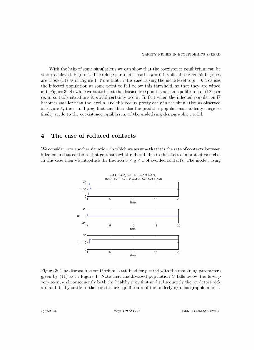
Safety niches in ecoepidemics spread

With the help of some simulations we can show that the coexistence equilibrium can bestably achieved, Figure 2. The refuge parameter used is p = 0.1 while all the remaining onesare those (11) as in Figure 1. Note that in this case raising the niche level to p = 0.4 causesthe infected population at some point to fall below this threshold, so that they are wipedout, Figure 3. So while we stated that the disease-free point is not an equilibrium of (12) perse, in suitable situations it would certainly occur. In fact when the infected population Ubecomes smaller than the level p, and this occurs pretty early in the simulation as observedin Figure 3, the sound prey first and then also the predator populations suddenly surge tofinally settle to the coexistence equilibrium of the underlying demographic model.

4 The case of reduced contacts

We consider now another situation, in which we assume that it is the rate of contacts betweeninfected and susceptibles that gets somewhat reduced, due to the effect of a protective niche.In this case then we introduce the fraction 0 ≤ q ≤ 1 of avoided contacts. The model, using

0 5 10 15 200

20

40

R

time

a=21, b=0.3, c=1, d=1, e=0.5, f=0.9,

h=0.1, k=10, λ=10.2, ω=0.8, s=0, p=0.4, q=0

0 5 10 15 20−20

0

20

U

time

0 5 10 15 200

10

20

F

time

Figure 3: The disease-free equilibrium is attained for p = 0.4 with the remaining parametersgiven by (11) as in Figure 1. Note that the diseased population U falls below the level pvery soon, and consequently both the healthy prey first and subsequently the predators pickup, and finally settle to the coexistence equilibrium of the underlying demographic model.

c©CMMSE ISBN: 978-84-616-2723-3Page 329 of 1797

Iulia Martina Bulai, Bruna Chialva, Davide Duma, Ezio Venturino

again the very same previous notation, now becomes

dR

dt= R[a− bR− cF − (1− q)λU ] + ωU (18)

dU

dt= U [(1− q)λR− kF − ω]

dF

dt= F [d+ eR− fF − hU ]

Clearly, by redefining β = (1 − q)λ for ω = 0 we get the same model studied in [7]. Forthe convenience of the reader we summarize the basic results on the equilibria in whichat least one of the population vanishes and then extend the study for the coexistence, toencompass here the situation ω 6= 0 not considered in [7] for this specific equilibrium. Theequilibria are again all the equilibria of the system (1), namely the origin P1 ≡ P1 ≡ P1,and P2 ≡ P2 ≡ P2, P3 ≡ P3, P4 ≡ P4. For feasibility of P4 clearly we need again (2).

Coexistence P5 = (R5, U5, F5) is obtained by solving the second equation in (18) atequilibrium and substituting into the third equation of (18) to get

F5 =(1− q)λR5 − ω

k, U5 =

(e

h− f

hk(1− q)λ

)R5 +

d

h+

f

hkω,

and finally from the first equation in (18) we get the quadratic∑2

k=0 ckRk, whose roots

determine the value of R5, with c0 = (dkω + fω2)(hk)−1 > 0 and

c2 =( ck− e

h

)(1− q)λ+

f

hk(1− q)2λ2 − b, c1 = a+

c

kω +

e

hω − (1− q)λ

(d

h+ 2

f

hkω

).

Again we can apply Descartes’ rule to have at least a positive root. This occurs for oneroot if we impose either one of the alternative conditions

c2 < 0, c1 < 0; c2 < 0, c1 > 0, (19)

and we get two positive roots if

c2 > 0, c1 < 0. (20)

We do not write explicitly these conditions. For feasibility we must impose

R5 >ω

(1− q)λk(21)

and the condition

R5 >dk + fω

ek − f(1− q)λ, ek > f(1− q)λ, (22)

c©CMMSE ISBN: 978-84-616-2723-3Page 330 of 1797

Safety niches in ecoepidemics spread

since the opposite one ek < f(1− q)λ would give a negative value for R5.

For P1 the eigenvalues are −ω, d, a, showing its instability.

The eigenvalues of P2 are −(dk + fω)f−1, −d, (af − cd)f−1, for which the stabilitycondition is (6). Here again comparing (6) with (2) we observe the existence of a transcriticalbifurcation, for which the same conclusions, using the healthy prey invasion number (7) canbe drawn as for the model with refuge for the healthy prey (1).

The eigenvalues of P3 are (bd+ ae)b−1, [(1− q)λa− bω]b−1, −a, thus it is unstable.

For P4 one eigenvalue can easily be factored out, while the other ones are the roots of thequadratic (8). Thus, as found formerly, by feasibility (2) both its roots have negative realpart, and stability depends only on the first eigenvalue, namely it is given by (1− q)λR4 <kF4 + ω, a condition that can also be explicitly written as

(1− q)λaf − cdbf + ce

< kae+ bd

bf + ce+ ω. (23)

Figure 4 shows the result of a simulation with the same parameter values (11) as forFigure 1, but for q = 0.1, assessing the stability of the coexistence equilibrium P5.

0 5 10 15 200

5

10

R

time

a=21, b=0.3, c=1, d=1, e=0.5, f=0.9,

h=0.1, k=10, λ=10.2, ω=0.8, s=0, p=0, q=0.1

0 5 10 15 200

10

20

U

time

0 5 10 15 201.5

2

2.5

F

time

Figure 4: The coexistence equilibrium is attained P5 for the same parameters (11) as inFigure 1 with q = 0.1.

c©CMMSE ISBN: 978-84-616-2723-3Page 331 of 1797

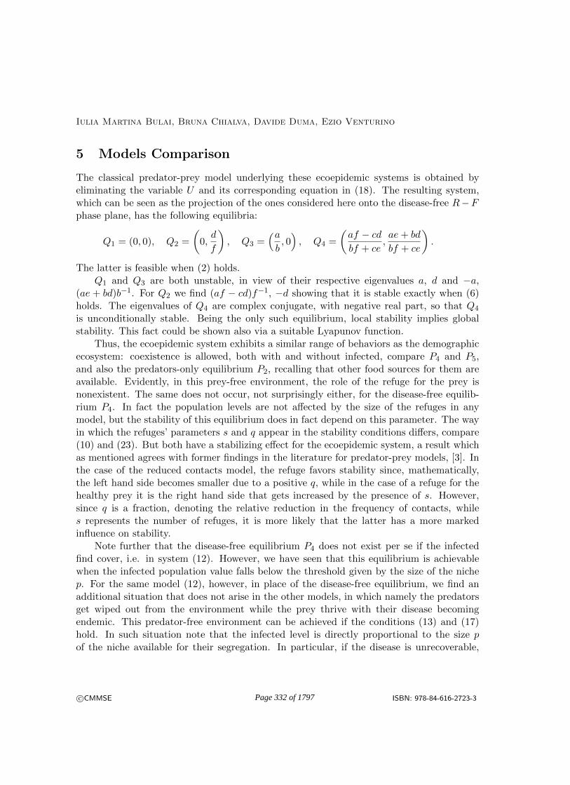
Iulia Martina Bulai, Bruna Chialva, Davide Duma, Ezio Venturino

5 Models Comparison

The classical predator-prey model underlying these ecoepidemic systems is obtained byeliminating the variable U and its corresponding equation in (18). The resulting system,which can be seen as the projection of the ones considered here onto the disease-free R−Fphase plane, has the following equilibria:

Q1 = (0, 0), Q2 =

(0,d

f

), Q3 =

(ab, 0), Q4 =

(af − cdbf + ce

,ae+ bd

bf + ce

).

The latter is feasible when (2) holds.Q1 and Q3 are both unstable, in view of their respective eigenvalues a, d and −a,

(ae + bd)b−1. For Q2 we find (af − cd)f−1, −d showing that it is stable exactly when (6)holds. The eigenvalues of Q4 are complex conjugate, with negative real part, so that Q4

is unconditionally stable. Being the only such equilibrium, local stability implies globalstability. This fact could be shown also via a suitable Lyapunov function.

Thus, the ecoepidemic system exhibits a similar range of behaviors as the demographicecosystem: coexistence is allowed, both with and without infected, compare P4 and P5,and also the predators-only equilibrium P2, recalling that other food sources for them areavailable. Evidently, in this prey-free environment, the role of the refuge for the prey isnonexistent. The same does not occur, not surprisingly either, for the disease-free equilib-rium P4. In fact the population levels are not affected by the size of the refuges in anymodel, but the stability of this equilibrium does in fact depend on this parameter. The wayin which the refuges’ parameters s and q appear in the stability conditions differs, compare(10) and (23). But both have a stabilizing effect for the ecoepidemic system, a result whichas mentioned agrees with former findings in the literature for predator-prey models, [3]. Inthe case of the reduced contacts model, the refuge favors stability since, mathematically,the left hand side becomes smaller due to a positive q, while in the case of a refuge for thehealthy prey it is the right hand side that gets increased by the presence of s. However,since q is a fraction, denoting the relative reduction in the frequency of contacts, whiles represents the number of refuges, it is more likely that the latter has a more markedinfluence on stability.

Note further that the disease-free equilibrium P4 does not exist per se if the infectedfind cover, i.e. in system (12). However, we have seen that this equilibrium is achievablewhen the infected population value falls below the threshold given by the size of the nichep. For the same model (12), however, in place of the disease-free equilibrium, we find anadditional situation that does not arise in the other models, in which namely the predatorsget wiped out from the environment while the prey thrive with their disease becomingendemic. This predator-free environment can be achieved if the conditions (13) and (17)hold. In such situation note that the infected level is directly proportional to the size pof the niche available for their segregation. In particular, if the disease is unrecoverable,

c©CMMSE ISBN: 978-84-616-2723-3Page 332 of 1797

Safety niches in ecoepidemics spread

ω = 0, or if there is no intraspecific competition among the healthy prey, b = 0, the size ofsurviving infected is exactly p. If these situations are not met, then the resulting numberof thriving infected is larger than p. Hence, the higher the refuges, the more endemic thedisease remains, when the predators are wiped out. This is a somewhat counterintuitiveresult. It is true that the niches help the infected not to get in contact with the susceptibles,but then one would expect also an advantage for the healthy individuals. Instead we findthem at the level ab−1 which would be attained at the unstable equilibrium P2. Hence,another way of looking at this situation is to observe that in this case the niche stabilizesthe otherwise unstable predator-free equilibrium, at the price of making the disease endemic.

The numerical experiments with the coexistence equilibria of the three models showthat using the set of demographic parameter values in (11), i.e. those given by the firstrow, the system settles to the demographic disease-free equilibrium (23.2475, 0, 14.0261),whose projection onto the R − F phase plane corresponds of course to the equilibriumof the underlying classical predator-prey system, (23.2475, 14.0261). If we now introducethe disease, with the related parameter values found in the second row of (11), we findthe ecoepidemic equilibrium (2.1133, 1.8658, 2.0819). As we can easily observe, the diseasehas a large impact on the system, reducing both its populations by an order of magnitude.Although the epidemics affects only the prey, its effect is felt also by the predators. This caneasily be interpreted, because a reduced food supply, due to a lower prey population causedby the disease, must reduce also the predator population and, in addition, consumption ofinfected prey is harmful for the predators. In other words, diseases, as stated many timesin ecoepidemiological research, affect the whole ecosystems, and therefore in environmentalstudies they cannot be easily neglected.

Coming back to the effects of our safety refuges, we have run simulations using theprevious parameter values (11), with various sizes for the refuge coefficients s, p and q. Asremarked earlier the proviso holds, that in the models (1) and (12) a check is implemented,for which when U < p and R < s the next to last term in the first equation and the firstone in the second equation are set to zero in both (1) and (12). The results are reported inFigures 5-7.

Comparison of the results indicates that for the healthy refuge, the healthy prey andthe predators at equilibrium increase in a linear fashion their numbers as s grows, whilethe infected appear to reach a plateau. When the infected prey have a cover, there is athreshold value of its size p beyond which the disease disappears and the other populationssuddenly jump to the level of the corresponding demographic, disease-free, classical modeland stay there independently of the value of p. A similar result holds also when it is thecontact rate that gets reduced, i.e. for model (18). In this case the equilibria behaviorbefore the threshold value of q is reached appears to be smoother than in the previous caseof system (12).

c©CMMSE ISBN: 978-84-616-2723-3Page 333 of 1797

Iulia Martina Bulai, Bruna Chialva, Davide Duma, Ezio Venturino

0 0.2 0.4 0.6 0.8 10

0.5

1

1.5

2

2.5

3

3.5

4

4.5

5refuge for healthy prey

s

R

U

F

Figure 5: Equilibrium population values of system (1) as function of the refuge size s.

0 0.2 0.4 0.6 0.8 10

5

10

15

20

25refuge for infected prey

p

R

U

F

Figure 6: Equilibrium population values of system (12) as function of the refuge size p.

We also plot the equilibrium levels of the various populations as function of the diseaseparameters λ and ω versus the refuge parameters s, p and q in Figures 8-13

c©CMMSE ISBN: 978-84-616-2723-3Page 334 of 1797

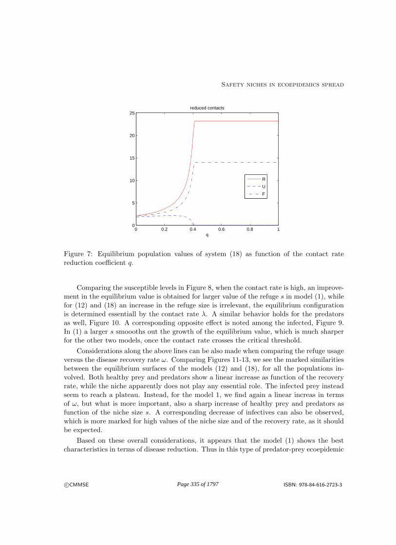
Safety niches in ecoepidemics spread

0 0.2 0.4 0.6 0.8 10

5

10

15

20

25reduced contacts

q

R

U

F

Figure 7: Equilibrium population values of system (18) as function of the contact ratereduction coefficient q.

Comparing the susceptible levels in Figure 8, when the contact rate is high, an improve-ment in the equilibrium value is obtained for larger value of the refuge s in model (1), whilefor (12) and (18) an increase in the refuge size is irrelevant, the equilibrium configurationis determined essentiall by the contact rate λ. A similar behavior holds for the predatorsas well, Figure 10. A corresponding opposite effect is noted among the infected, Figure 9.In (1) a larger s smoooths out the growth of the equilibrium value, which is much sharperfor the other two models, once the contact rate crosses the critical threshold.

Considerations along the above lines can be also made when comparing the refuge usageversus the disease recovery rate ω. Comparing Figures 11-13, we see the marked similaritiesbetween the equilibrium surfaces of the models (12) and (18), for all the populations in-volved. Both healthy prey and predators show a linear increase as function of the recoveryrate, while the niche apparently does not play any essential role. The infected prey insteadseem to reach a plateau. Instead, for the model 1, we find again a linear increas in termsof ω, but what is more important, also a sharp increase of healthy prey and predators asfunction of the niche size s. A corresponding decrease of infectives can also be observed,which is more marked for high values of the niche size and of the recovery rate, as it shouldbe expected.

Based on these overall considerations, it appears that the model (1) shows the bestcharacteristics in terms of disease reduction. Thus in this type of predator-prey ecoepidemic

c©CMMSE ISBN: 978-84-616-2723-3Page 335 of 1797

Iulia Martina Bulai, Bruna Chialva, Davide Duma, Ezio Venturino

system with disease just in the prey, for an endemic disease, the ecosystem with a placewhere some of the healthy individuals can be segregated from coming in contact with diseasecarriers would exhibit the best features to preserve the epidemics to spread. This resultcould possibly give some hints to field ecologists as how to fight diseases in wild populations,in case some artificial refuges, unreachable by the diseased individuals, can be provided inspecific real-life situations.

References

[1] J. B. Collings, Bifurcations and stability analysis of a temperature-dependent mitepredator-prey interaction model incorporating a prey refuge, Bulletin of MathematicalBiology 57 (1995) 63-76.

[2] E. Gonzalez-Olivares, R. Ramos-Jiliberto, Dynamic consequences of preyrefuges in a simple model system: more prey, fewer predators and enhanced stability,Ecological Modelling 166 (2003) 135-146.

[3] E. Gonzalez-Olivares, R. Ramos-Jiliberto, Comments to the effect of prey refugein a simple predator-prey model, Ecological Modelling 232 (2012) 158-160.

[4] E. Gonzalez-Olivares, B. Gonzalez-Yanez, R. Becerra-Klix, Prey refuge useas a function of predator-prey encounters, private communication, submitted to Inter-national Journal of Biomathematics (2012).

[5] H. Malchow, S. Petrovskii, E. Venturino, Spatiotemporal patterns in Ecologyand Epidemiology, CRC, Boca Raton, 2008.

[6] G. D. Ruxton, Short term refuge use and stability of predator-prey models, TheoreticalPopulation Biology 47 (1995) 1-17.

[7] E. Venturino, Epidemics in predator-prey models: disease among the prey, in O.Arino, D. Axelrod, M. Kimmel, M. Langlais: Mathematical Population Dynamics:Analysis of Heterogeneity, Vol. one: Theory of Epidemics, Wuertz Publishing Ltd,Winnipeg, Canada, (1995) 381-393.

c©CMMSE ISBN: 978-84-616-2723-3Page 336 of 1797

Safety niches in ecoepidemics spread

0

5

10

15

20

0

2

4

60

5

10

15

20

25

λ

refuge for healthy prey

s

R

0

5

10

15

20

0

2

4

60

5

10

15

20

25

λ

refuge for infected prey

p

R

0

5

10

15

20

0

2

4

60

5

10

15

20

25

λ

reduced contacts

q

R

Figure 8: Equilibrium population valuefor the healthy prey as function of thedisease contact rate λ and refuge size:top, refuge size s in model (1); middle,refuge size p in model (12); bottom, re-duced contact rate q in model (18). Otherparameter values as in (11).

0

5

10

15

20

0

2

4

6−1

0

1

2

3

λ

refuge for healthy prey

s

U

0

5

10

15

20

0

2

4

60

0.5

1

1.5

2

2.5

λ

refuge for infected prey

p

U

0

5

10

15

20

0

2

4

60

0.5

1

1.5

2

2.5

λ

reduced contacts

q

U

Figure 9: Equilibrium population valuefor the infected prey as function of thedisease contact rate λ and refuge size:top, refuge size s in model (1); middle,refuge size p in model (12); bottom, re-duced contact rate q in model (18). Otherparameter values as in (11).

c©CMMSE ISBN: 978-84-616-2723-3Page 337 of 1797

Iulia Martina Bulai, Bruna Chialva, Davide Duma, Ezio Venturino

0

5

10

15

20

0

2

4

60

5

10

15

λ

refuge for healthy prey

s

F

0

5

10

15

20

0

2

4

60

5

10

15

λ

refuge for infected prey

p

F

0

5

10

15

20

0

2

4

60

5

10

15

λ

reduced contacts

q

F

Figure 10: Equilibrium population valuefor the predators as function of the dis-ease contact rate λ and refuge size: top,refuge size s in model (1); middle, refugesize p in model (12); bottom, reducedcontact rate q in model (18). Other pa-rameter values as in (11).

0

5

10

15

20

0

2

4

60

5

10

15

20

ω

refuge for healthy prey

sR

0

5

10

15

20

0

2

4

60

2

4

6

8

ω

refuge for infected prey

p

R

0

5

10

15

20

0

2

4

60

2

4

6

8

ω

reduced contacts

q

R

Figure 11: Equilibrium population valuefor the healthy prey as function of thedisease contact rate ω and refuge size:top, refuge size s in model (1); middle,refuge size p in model (12); bottom, re-duced contact rate q in model (18). Otherparameter values as in (11).

c©CMMSE ISBN: 978-84-616-2723-3Page 338 of 1797

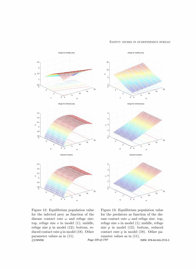
Safety niches in ecoepidemics spread

0

5

10

15

20

0

2

4

60.5

1

1.5

2

2.5

ω

refuge for healthy prey

s

U

0

5

10

15

20

0

2

4

61.8

1.9

2

2.1

2.2

2.3

ω

refuge for infected prey

p

U

0

5

10

15

20

0

2

4

61.8

1.9

2

2.1

2.2

2.3

ω

reduced contacts

q

U

Figure 12: Equilibrium population valuefor the infected prey as function of thedisease contact rate ω and refuge size:top, refuge size s in model (1); middle,refuge size p in model (12); bottom, re-duced contact rate q in model (18). Otherparameter values as in (11).

0

5

10

15

20

0

2

4

60

5

10

15

ω

refuge for healthy prey

s

F

0

5

10

15

20

0

2

4

61

2

3

4

5

ω

refuge for infected prey

p

F

0

5

10

15

20

0

2

4

61

2

3

4

5

ω

reduced contacts

q

F

Figure 13: Equilibrium population valuefor the predators as function of the dis-ease contact rate ω and refuge size: top,refuge size s in model (1); middle, refugesize p in model (12); bottom, reducedcontact rate q in model (18). Other pa-rameter values as in (11).

c©CMMSE ISBN: 978-84-616-2723-3Page 339 of 1797

Proceedings of the 13th International Conferenceon Computational and Mathematical Methodsin Science and Engineering, CMMSE 201324–27 June, 2013.

GPU Acceleration of a Tool for Wind Power Forecasting

Marcel Burdiat1, Jose Ignacio Hagopian1, Juan Pablo Silva1, ErnestoDufrechou1, Alejandro Gutierrez2, Martın Pedemonte1, Gabriel Cazes2

and Pablo Ezzatti1

1 Instituto de Computacion, Facultad de Ingenierıa, Universidad de la Republica, Uruguay

2 Instituto de Mecanica de los Fluidos e Ingenierıa Ambiental, Facultad de Ingenierıa,Universidad de la Republica, Uruguay

emails: mburdiat@gmail.com, jsign.uy@hotmail.com, silvaljp01@hotmail.com,edufrechou@fing.edu.uy, aguti@fing.edu.uy, mpedemon@fing.edu.uy,

agcm@fing.edu.uy, pezzatti@fing.edu.uy

Abstract

Uruguay is currently undergoing a gradual process of inclusion of wind energy inits matrix of electric power generation. In this context, a computational tool for windpower forecasting has been developed in order to predict the electrical power that willbe injected into the electrical grid. The tool is based on the Weather Research andForecasting (WRF) numerical model, which is the computational bottleneck of the ap-plication. For this reason, and in line with several successful efforts of other researchers,this paper presents advances in porting the WRF to GPU. In particular, we presentand study the implementation of sintb and bdy interp1 routines on GPU. The resultsobtained on a Nvidia’s GTX 480 GPU show speedup values of up to 10× when com-pared with the sequential WRF and almost 5× when compared with the four-threadedWRF. This improvement impacts in a 10% reduction in the total runtime of the WRF.Key words: Wind power, WRF, GPU, sintb routine, bdy interp1 routine.

1 Introduction

Although windmills have been used to generate electricity in a domestic scale, mainly in ruralproperties, they have not been considered in Uruguay as an alternative energy source untilrecently. The Wind Power Program (WPP) [3], established in 2007, aims to significantly

c⃝CMMSE ISBN: 978-84-616-2723-3Page 340 of 1797

GPU Acceleration of a Tool for Wind Power Forecasting

increase the generation of electricity from wind energy encouraging the installation of large-scale wind farms in different parts of the country. For this reason, several projects are underdevelopment, and it is estimated that the wind energy penetration factor will be more than20% in 2018 [2]. Under the WPP, UTE, the public utility responsible for the generation andtransfer of electrical energy, installed the wind farm complex Ing. Emanuele Cambilargiu.After three years of continuous operation, it produces an average of 40% of its capacity.

Wind energy has different features compared with other sources of energy.Wind energyis not easy to be stored as potential energy, so the kinetic energy of the air flow is transformedinto rotational mechanical energy which is used for electric power generation that has to beinjected into the electrical grid right away. Moreover, wind energy has a large variabilitydue to the nature of its origin. For this reason, and due to the importance that wind powerwill have for electric power generation in Uruguay, it is necessary to have computationaltools to forecast the generated power. These tools would allow to take decisions in themanagement of the electrical grid in order to meet the energy demand.

With this goal, a computational tool for wind power forecasting of the UTE’s wind farmcomplex was developed. The forecasting process runs four times a day and involves the useof the WRF numerical model [8, 16], which is the computational bottleneck of the wholeprocess. The process generates a low resolution forecast for the whole country and a highresolution forecast where the wind farm complex is located, which are publicly availableon [4]. This process involves a runtime of approximately two hours on a server with eightcores. This runtime is considered high, mainly because it will become necessary could bedesirable to increase the number of wind farms that are predicted.

In recent years, the execution time of several numerical models have been significantlyreduced through porting the numerical model computation, either partially or fully, toGraphics Processing Units (GPUs) [6]. Some of the most relevant numerical models thathave been successfully ported to GPU can be consulted on [17].

In this paper we study the implementation of sintb and bdy interp1 routines on GPUin order to accelerate the tool for wind power forecasting. Our experiments show that justporting these routines to GPU is possible to reduce a 10% the total runtime of the WRF.The rest of the paper is structured as follows. In Section 2, we describe the tool for windpower forecasting and the WRF. Then, in Section 3, we review the related works. In Section4, we introduce the methodology followed for porting routines from CPU to GPU and alsodescribe the implementation of the routines on GPU. In Section 5 we present experimentalresults and, finally, we discuss some conclusions and future work in Section 6.

2 Tool for Wind Power Forecasting

The forecasting process performed by the computational tool involves several steps. Inthe first place, the tool obtains public global meteorological forecasts generated by the

c⃝CMMSE ISBN: 978-84-616-2723-3Page 341 of 1797

Marcel Burdiat et al.

NOAA/National Weather Service using the general circulation model of the atmosphereGlobal Forecast System. These forecasts are generated four times a day, at 00:00, 06:00,12:00 and 18:00 GMT and have a grid resolution of 1×1 (approximately 100km×100km).The WRF is executed locally in our server and uses this data, as well as other parametersas inputs to generate a low resolution forecast for the whole country and one high resolutionforecast for the region of the wind farm complex. A forecast of the wind energy fed intothe grid by each wind turbine is produced using the predictions of the wind speed anddirection at the height of each turbine shaft generated by the WRF, and corrections of thesepredictions through model output statistics. These results are published automatically in6-hour intervals [4], having four daily forecasts that predict the outcome for the next 48hours.

The computationally most expensive step of the whole process corresponds to the WRFexecution, which requires approximately two hours on a server with eight cores. Therefore,the performance of the WRF should be tackled in order to increase the performance of thewhole tool. A description of the WRF is presented below.

2.1 Weather Research and Forecasting Model (WRF)

The WRF is a numerical model for weather prediction and an atmospheric simulationsystem for research and operational applications [8]. The WRF model is Eulerian (usesa fixed coordinate system with respect to the earth), non-hydrostatic (includes explicitequations to calculate the pressure and the gravitational force on the vertical axis) andcompressible (considers density variations suffered by the various fluids involved). TheWRF code is written in Fortran and C, and it currently has about half a million lines ofcode (version 3.4.1). The WRF execution partitions the domain into rectangular patchesthat can be assigned to different processors. These patches are subdivided into tiles thatcan be executed on different threads. Usually, patches need data from other neighboringpatches, so in the border tiles it is necessary to propagate changes between different patches.

The tool for wind power forecasting uses the ARW (“The Advanced Research WRF”)core of the WRF, which was primarily designed for research purposes, but it is also usedfor weather prediction. The WRF generates forecasts of W-E and N-S components that areused to calculate the magnitude of the velocity in m/s and the direction in degrees. To thatend, four nested grid levels (30km×30km, 10km×10km, 3.3km×3.3km and 1.1km×1.1km)are generated, where levels of grid with a higher resolution assimilate the information gen-erated by the model in the levels of grid with a lower resolution. The values predicted bythe tool have been confirmed with real speed and direction data measured by UTE usinganemometers and wind vanes installed in different parts of the country. It is notewor-thy that WRF is executed in parallel in eight cores using the shared memory parallelismconfiguration, which uses the OpenMP API for parallelization.

c⃝CMMSE ISBN: 978-84-616-2723-3Page 342 of 1797

GPU Acceleration of a Tool for Wind Power Forecasting

3 Related work

This section is centered on reviewing previous efforts on porting WRF routines to GPU.The website [10] collects some of the pioneering works on this subject.

In the seminal paper on this subject, Michalakes and Vachharajani [9] address theacceleration of WRF Single Moment 5 Cloud Microphysics (WSM5) module on CUDAC. Although WSM5 only represents 0.4% of the total WRF code, it usually takes up toa quarter of the total processing time on a single core. Each GPU-thread computes thecalculations corresponding to a point of the grid, since the calculations of the verticalcolumn of each grid point are independent of other grid points. The authors evaluatedtheir implementation in a domain with a grid resolution of 71×58 points and 27 verticallevels, using a NVidia GeForce 8800 GTX connected to an Intel Pentium-D at 2.8GHz. Thenumerical results showed slight differences between the GPU and CPU versions, but thevisualization outputs of both versions are indistinguishable. The GPU implementation runs17× faster than the single-threaded CPU version, including the time of the transferencesbetween the host and the device. From this result the authors estimate that it translatesin a 1.25× reduction in the total application runtime.

Later, the same authors [11] ported the WRF Fifth Order Positive Definite TracerAdvection. In this case, it is not possible to make a dimensional division of the problem,as in the previous work. Since the number of floating point operations per memory accessis only 0.76 and a large number of tracers are usually executed, the GPU implementationoverlaps the calculations of a tracer with the asynchronous data transfer required for nexttracer. The authors evaluated their implementation in a domain with a grid resolutionof 134×110 points, 35 vertical levels and 81 tracers, using a Tesla C1060 GPU connectedto a quad-core Intel Xeon E5440. The GPU implementation runs 6.7× faster than thesingle-threaded CPU version.

Finally, Michalakes et al. [7] evaluated the parallelization of Regional Acid DepositionModel version 2 (RADM2) module on a multicore processor (two quad-core Intel Xeon5400), a GPU (Tesla C1060) and a Cell Broadband Engine Architecture (CBEA) [5] device(PowerXCell 8i). RADM2 requires to run the Rosenbrock’s algorithm, which involves con-structing a Jacobian matrix and a LU decomposition, independently for each grid point.In the GPU implementation, some calculations have to be computed on the CPU due tothe large amount of memory required, even though the fundamental steps of the algorithmare executed on the GPU. The parallel implementations were evaluated in a domain witha grid resolution of 40×40 points and 20 vertical levels. The speedup with respect to asingle-threaded CPU version was 7.5× for the multicore processor, 8.5× for the GPU and41× for the CBEA. Despite failing to achieve high speedup values for the GPU implemen-tation, the authors note that the GPU is the cheapest platform of the three used and theyalso highlight the simplicity of its programming compared to CBEA.

In another line of work, Ruetsch et al. [18] ported the Long-Wave Rapid Radiative

c⃝CMMSE ISBN: 978-84-616-2723-3Page 343 of 1797

Marcel Burdiat et al.

Transfer Model (RRTM) module to CUDA Fortran. As in other works, the implementa-tion exploits the independence between the different vertical columns of the domain, evenachieving a higher level of independence in some cases, resulting in a finer grain parallelism.The authors evaluated their implementation in a domain with a grid resolution of 73×60points and 27 vertical levels, using a Tesla C1060 GPU connected to a quad-core Intel XeonE5440 at 2.83 GHz. The speedup of the GPU implementation versus a single-threaded CPUversion is between 8× and 10×. The numerical results showed similar results between theGPU and CPU versions.

Huang et al. developed other relevant works on the subject, in which several moduleswere ported to CUDA C, with the final objective of completely porting WRF to GPU.In one of their works [12], the authors port the Goddard Shortwave Radiation moduleexploiting the independence between the different vertical columns of the domain, as theother authors. The GPU implementation also uses two streams in order to overlap kernelcomputation on the GPU with transferences between the host and the device. The authorsevaluated their implementation in a domain with a grid resolution of 433×308 points and35 vertical levels, using two GeForce GTX 590, i.e. four GPUs, connected to a six-core Inteli7 970. The speedup is 116× for the GPU implementation versus a single-threaded CPUversion, including the time of the transferences between the host and the device.

Following the same idea, the authors ported the Stony Brook University 5-Class CloudMicrophysics module to GPU [13]. In this work, the authors used single precision floatingpoint arithmetic and compiled using the CUDA flag -use fast math that uses faster but lessaccurate computation. Using the same scenario and the same platforms as in the previouswork, the speedup value reported is 352×. Huang et al. also worked on porting the WSM5[14], WDM5 Cloud Microphysics [19], Purdue Lin Cloud Microphysics [20] and KesslerCloud Microphysics [15] modules to GPU using the same ideas, scenario and platforms asin the previous works, reporting speedup values of 357×, 147×, 156× and 70× respectively.

While speedups reported by Huang et al. are impressive, there are some aspects thatshould be taken into account in order to explain these values. In the first place, the scenarioused by Huang et al. is more than 30 times larger than the ones used by other authors,which undoubtedly contributes to the improvement in the speedup. Another aspect thatcertainly impacts on these speedup values reported is the use of the CUDA compile flag-use fast math. Finally, an important issue is that the criterion followed by other authorsto select which routines port to GPU is based on the importance of the routine for theexecution of the WRF, while it is not clear the criterion used by Huang et al.

4 Improving the Performance of the WRF

Our work is focused on improving the runtime of the WRF, and in particular the modulesrequired by the forecasting tool developed for the wind farm complex Ing. Emanuele Cam-

c⃝CMMSE ISBN: 978-84-616-2723-3Page 344 of 1797

GPU Acceleration of a Tool for Wind Power Forecasting

bilargiu. Therefore, an empirical approach is used to determine in which module concentrateour effort. To that end, we follow the guidelines suggested by Michalakes and Vachharajani[9], and Delgado et al. [1] to port applications developed in Fortran to CUDA C.

Four different steps are identified to port an application from Fortran to CUDA C: pro-filing, development, testing and optimization. The profiling stage aims to determine whichare the modules or routines that require longer execution times. Then, in the developmentstage, it is recommended to port first Fortan to C, and then C to CUDA, since directlyporting Fortran to CUDA can incorporate many errors due to the different characteristicsof the languages involved. In the testing stage, it has to be evaluated that the results ob-tained by the GPU are similar to the ones obtained by the CPU, taking into account thatthere might be floating point rounding differences caused by the parallelism. Finally, in theoptimization stage, the CUDA implementation is fine tuned in order to reduce the runtime.

The tools for profiling applications follow two completely different philosophies. On theone hand, there are tools that make changes in the source code at compile time, includingextra code to obtain metrics of the application execution. On the other hand, there aretools that work like a debugger or a virtual machine that obtain the metrics in run-timeusing the original code. Since both approaches are complementary, we decided to profilethe WRF using one tool of a kind. We use gprof, which follows the former approach and itis considered the de-facto profiler in academic environments since it is included in the GNUproject, and valgrind that follows the latter approach. The reports of the single-threadedexecution of WRF generated with both tools showed a great consistency in the results,despite following different philosophies. The routine with longer runtime was sintb thatrequired around the 15% of the total execution time. For this reason, we focus our work inporting this routine to GPU. Even though each invocation of sintb does not take a largeruntime, the routine is invoked more than 10 million times during the WRF execution.

4.1 sintb and bdy interp1 Routines

To begin with, we study the feasibility of porting sintb routine to GPU analyzing therelationship between transference and computation time for a call to sintb. We found thatthis ratio was four to one, so we examined bdy interp1 routine, which is the only routinethat calls sintb. bdy interp1 makes four consecutive calls to sintb with the same inputmatrices, but with different sets of positions. For this reason, a single transference is requiredto make the four invocations to sintb thus compensating the high relative computationalcost of the transference. So, it was considered a better option to also port code from thebdy interp1 routine to the GPU instead of only porting sintb.

After the four sintb calls, the bdy interp1 routine makes assignments to other matricesusing the results from the invocations. Both invocations and assignments are in a loopparallelized using OpenMP in the original code, but the set of positions of each invocationto sintb does not depend on the iteration step. Therefore, we decided to group all calls to

c⃝CMMSE ISBN: 978-84-616-2723-3Page 345 of 1797

Marcel Burdiat et al.

sintb in a single call, postponing all assignments for the end. Following that approach, theFortran code of sintb was ported to C, and it was verified that the results were similar tothose obtained by the original version. Then, the C code of sintb was ported to CUDA.

Now, the main bottlenecks were the transference of the result matrices (25% of thetotal runtime) and the final assignments to other matrices in bdy interp1 (30% of thetotal runtime), since they could not be run concurrently with the kernel. For this reason,we chose to migrate the final assignments in bdy interp1 to a second kernel in CUDA,not only to reduce the computation time of this task, but also taking benefit from the factthat all the inputs of the routine are already on the GPU. This brought a couple of otherimprovements. On the one hand, the final results of bdy interp1 are nearly half of thesize of the intermediate results produced by the invocation to sintb, so the transferencetime from GPU to CPU is significantly reduced. On the other hand, the matrices wherethe final results are updated can be copied from the GPU to the CPU asynchronously andconcurrently with the execution of the first kernel, which hides this transference time. Thepseudocode of the host side of the CUDA implementation outlined above is presented inAlgorithm 1.

Algorithm 1 bdy interp1 Host Side Pseudocode

1: synchronous transferences required by sintb, host to device, stream 12: asynchronous transferences to be updated with final results, host to device, stream 23: invoke sintb kernel through stream 14: synchronize stream 2 Blocks host until all calls in stream 2 are completed5: invoke second kernel through stream 1 Updates the final results6: synchronous transferences of final results, device to host, stream 1

The memory accesses of the GPU implementation are coalesced and the memory spacesallocated on the GPU are reused in order to reduce calls to malloc and free. Finally, weperformed an analysis to find the best balance between the number of registers and sharedmemory used per block. The best configuration consists in using only 24KB of sharedmemory per block, allowing to execute up to two concurrent blocks on each multiprocessor.

5 Experimental Results

This section describes first the scenario used for the experimental study and the executionplatform. Then, the results obtained are presented and analyzed.

5.1 Test Instance

The test instance consists in real information of the 07/15/2012 for a 12 hours climateforecast of the wind farm complex Ing. Emanuele Cambilargiu. The test instance is con-

c⃝CMMSE ISBN: 978-84-616-2723-3Page 346 of 1797

GPU Acceleration of a Tool for Wind Power Forecasting

sidered representative of a normal day of operation of the park. The numerical model usesfour nested grid levels of 30km×30km, 10km×10km, 3.3km×3.3km and 1.1km×1.1km thatassimilate information from the lower resolution to the higher resolution levels of the grid.The 30km×30km domain has a grid resolution of 74×61 points and 54 vertical levels, whilethe others domain has a grid resolution of 40×40 points and 54 vertical levels.

5.2 Test Environment

The execution platform for the CPU runs is a PC with a dual core Intel Core i3-2100processor at 3.10 Ghz with 8 GB using the Fedora 15 Linux operating system. It shouldbe noted that the processor supports hyper-threading. The CPU versions were compiledusing the -O3 flag. The execution platform for the GPU runs is an Nvidia’s GeForce GTX480 (480 CUDA cores, Fermi architecture, Compute Capability 2.0) connected to the CPUplatform. The GPU versions were compiled using the Nvidia’s CUDA compiler 4.1 versionwith the -O3 flag. All the reported total runtime of the GPU executions always include thetransference time of data between CPU and GPU.

5.3 Experimental Analysis

We begin our analysis with the parallelization of the WRF using OpenMP. Table 1 presentsthe experimental results regarding the performance obtained. The table includes the exe-cution time of the single-threaded, two-threaded and four-threaded (using hyper-threading)WRF, as well as the speedup values of the parallel executions. The speedup value obtainedusing two threads is not close to linear; this shows that the parallelization of the WRF isnot a trivial task and that an adequate load balance has to be achieved in order to benefitfrom additional processing units. The execution time with two and four threads allows usto affirm that in this case the use of hyper-threading is justified.

Table 1: OpenMP Parallelization of WRFSingle Thread Two Threads Four ThreadsRuntime (mins) Runtime (mins) Speedup Runtime (mins) Speedup

226.70 126.77 1.79 103.38 2.19

Table 2 presents the execution time of the single-threaded and four-threaded (usinghyper-threading) of bdy interp1 routine, as well as the speedup value of the parallel version.The runtimes reported are the average of all the executions of the routine (the routine isexecuted more than 2.5 million times). The speedup value obtained with four threads isslightly worse than for the entire application which may indicate that the routine has furtherdifficulty to scale with a multithreaded parallelization.

We continue our analysis with the parallelization of the WRF using a GPU. In the firstplace it should be noted that there are no significant differences regarding the numerical

c⃝CMMSE ISBN: 978-84-616-2723-3Page 347 of 1797

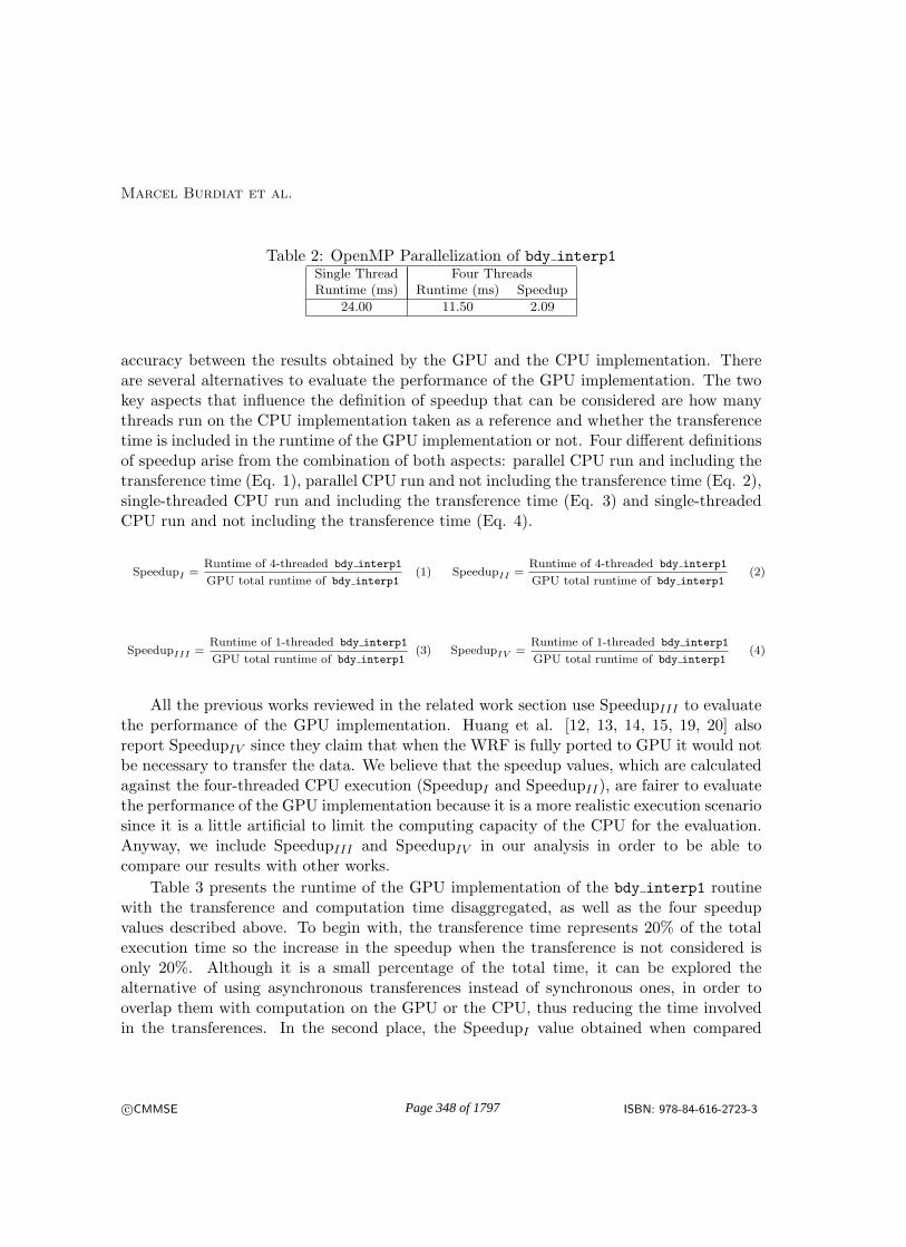
Marcel Burdiat et al.

Table 2: OpenMP Parallelization of bdy interp1Single Thread Four ThreadsRuntime (ms) Runtime (ms) Speedup

24.00 11.50 2.09

accuracy between the results obtained by the GPU and the CPU implementation. Thereare several alternatives to evaluate the performance of the GPU implementation. The twokey aspects that influence the definition of speedup that can be considered are how manythreads run on the CPU implementation taken as a reference and whether the transferencetime is included in the runtime of the GPU implementation or not. Four different definitionsof speedup arise from the combination of both aspects: parallel CPU run and including thetransference time (Eq. 1), parallel CPU run and not including the transference time (Eq. 2),single-threaded CPU run and including the transference time (Eq. 3) and single-threadedCPU run and not including the transference time (Eq. 4).

SpeedupI =Runtime of 4-threaded bdy interp1

GPU total runtime of bdy interp1(1) SpeedupII =

Runtime of 4-threaded bdy interp1

GPU total runtime of bdy interp1(2)

SpeedupIII =Runtime of 1-threaded bdy interp1

GPU total runtime of bdy interp1(3) SpeedupIV =

Runtime of 1-threaded bdy interp1

GPU total runtime of bdy interp1(4)

All the previous works reviewed in the related work section use SpeedupIII to evaluatethe performance of the GPU implementation. Huang et al. [12, 13, 14, 15, 19, 20] alsoreport SpeedupIV since they claim that when the WRF is fully ported to GPU it would notbe necessary to transfer the data. We believe that the speedup values, which are calculatedagainst the four-threaded CPU execution (SpeedupI and SpeedupII), are fairer to evaluatethe performance of the GPU implementation because it is a more realistic execution scenariosince it is a little artificial to limit the computing capacity of the CPU for the evaluation.Anyway, we include SpeedupIII and SpeedupIV in our analysis in order to be able tocompare our results with other works.

Table 3 presents the runtime of the GPU implementation of the bdy interp1 routinewith the transference and computation time disaggregated, as well as the four speedupvalues described above. To begin with, the transference time represents 20% of the totalexecution time so the increase in the speedup when the transference is not considered isonly 20%. Although it is a small percentage of the total time, it can be explored thealternative of using asynchronous transferences instead of synchronous ones, in order tooverlap them with computation on the GPU or the CPU, thus reducing the time involvedin the transferences. In the second place, the SpeedupI value obtained when compared

c⃝CMMSE ISBN: 978-84-616-2723-3Page 348 of 1797

GPU Acceleration of a Tool for Wind Power Forecasting

with the four-threaded execution of the WRF is 4.89. An almost five times reductionin the runtime of the routine can be considered a good result, since the improvement isaccomplished versus an already parallel implementation that was developed by the staff ofdevelopers of the WRF. Finally, the SpeedupIII value obtained is 10.21 that is comparableto the values reported by Michalakes et al. and Ruetsch et al. We could not reach similarvalues to the ones reported by Huang et al., but the scenario we used is significantly smallerand fast math was not used due to the characteristics of the routine that we ported to GPU.

Table 3: GPU Parallelization of bdy interp1Runtime (ms) Speedups

Transference Computation Total SpeedupI SpeedupII SpeedupIII SpeedupIV

0.45 1.90 2.35 4.89 6.05 10.21 12.63

Table 4 presents the runtime of the single-threaded and four-threaded WRF withbdy interp1 routine executing on the GPU, as well as the corresponding speedup val-ues. The implementation of this routine in GPU produces a reduction of more than 10minutes (10.26% of the total runtime) in the runtime of the four-threaded WRF and of 20minutes (8.75% of the total runtime) in the runtime of the single-threaded WRF.

Table 4: GPU Parallelization of WRFSingle Thread + bdy interp1 on GPU Four Threads + bdy interp1 on GPURuntime (mins) Speedup Runtime (mins) Speedup

206.87 1.10 92.77 1.11

6 Conclusions and Future Work

In this paper we have studied the acceleration of a tool for wind power forecasting on a GPU.To this end, we profiled the WRFmodel, which is the main bottleneck of the application, anddetermined that sintb is the routine with longer runtime (around 15% of the total runtimeof WRF). A further analysis showed that it was a better alternative besides porting sintb

to GPU also porting bdy interp1 routine. The implementation of sintb and bdy interp1

routines on Nvidia’s GTX 480 GPU obtained speedup values of up to 10× and almost 5×when compared with the single-threaded and four-threaded execution on CPU, respectively.The acceleration obtained implies a 10% reduction in the total runtime of the WRF.

We identify three lines for future work. The first one is to identify additional routinesto port to GPU in order to accelerate the tool for wind power forecasting. This leads toa second line of interest, which consists in executing the WRF with the two routines onthe GPU for a whole forecast for the next 48 hours. Finally, we aim to use as executionplatform a GPU with Kepler architecture that recently came to market.

c⃝CMMSE ISBN: 978-84-616-2723-3Page 349 of 1797

Marcel Burdiat et al.

Acknowledgements

G. Cazes, E. Dufrechou, P. Ezzatti, A. Gutierrez and M. Pedemonte acknowledge supportfrom Agencia Nacional de Investigacion e Innovacion (ANII), Uruguay and AdministracionNacional de Usinas y Trasmisiones Electricas (UTE), Uruguay. E. Dufrechou, P. Ezzattiand M. Pedemonte also acknowledge support from Programa de Desarrollo de las CienciasBasicas (PEDECIBA), Uruguay.

References

[1] J. Delgado, G. Gazolla, E. Clua and S. Sadjadi, A Case Study on Porting Sci-entific Applications to GPU/CUDA, Journal of Computational Interdisciplinary Sci-ences 2, (2011) 3–11.

[2] Direccion Nacional de Energıa - Ministerio de Industria, Energıa y Minerıa (in Span-ish), http://www.dne.gub.uy/.

[3] Direccion Nacional de Energıa - Ministerio de Industria, Energıa yMinerıa, Programa de Energıa Eolica en Uruguay (in Spanish), http://www.

energiaeolica.gub.uy/.

[4] A. Gutierrez and G. Cazes, Pronosticos Numericos Operativos en Uruguay (inSpanish), http://www.fing.edu.uy/cluster/eolica/.

[5] C. Johns and D. Brokenshire, Introduction to the Cell Broadband Engine Archi-tecture, IBM Journal of Research and Development 51(5), (2007) 503–519.

[6] D. Kirk and W. Hwu, Programming Massively Parallel Processors, Second Edition:A Hands-on Approach, Morgan Kaufmann, 2012.

[7] J. Linford, J. Michalakes, M. Vachharajani and A. Sandu, Multi-core Ac-celeration of Chemical Kinetics for Simulation and Prediction, SC ’09, Proceedings ofthe Conference on High Performance Computing Networking, Storage and Analysis,(2009) 1–11.

[8] J. Michalakes, J. Dudhia, D. Gill, T. Henderson, J. Klemp, W. Skamarockand W. Wang, The Weather Research and Forecast Model: Software architecture andperformance, 11th ECMWF Workshop on HPC in Meteorology, (2004) 156–168.

[9] J. Michalakes and M. Vachharajani, GPU Acceleration of Numerical WeatherPrediction, Parallel Processing Letters 18(4), (2008) 531–548.

c⃝CMMSE ISBN: 978-84-616-2723-3Page 350 of 1797

GPU Acceleration of a Tool for Wind Power Forecasting

[10] J. Michalakes and M. Vachharajani, GPU Acceleration of Numerical WeatherPrediction, http://www.mmm.ucar.edu/wrf/WG2/GPU/.

[11] J. Michalakes and M. Vachharajani, GPU Acceleration of Scalar Advection,Available online: http://www.mmm.ucar.edu/wrf/WG2/GPU/Scalar_Advect.htm.

[12] J. Mielikainen, B. Huang, H.A. Huang and M.D. Goldberg, GPU Acceler-ation of the Updated Goddard Shortwave Radiation Scheme in the Weather Researchand Forecasting (WRF) Model, IEEE Journal of Selected Topics in Applied Earth Ob-servations and Remote Sensing 5(2), (2012) 555–562.

[13] J. Mielikainen, B. Huang, H.A. Huang and M.D. Goldberg, GPU Implementa-tion of Stony Brook University 5-Class Cloud Microphysics Scheme in the WRF, IEEEJournal of Selected Topics in Applied Earth Observations and Remote Sensing 5(2),(2012) 625–633.

[14] J. Mielikainen, B. Huang, H.A. Huang and M.D. Goldberg, ImprovedGPU/CUDA Based Parallel Weather and Research Forecast (WRF) Single Moment5-Class (WSM5) Cloud Microphysics, IEEE Journal of Selected Topics in AppliedEarth Observations and Remote Sensing 5(4), (2012) 1256–1265.

[15] J. Mielikainen, B. Huang, H.A. Huang and M.D. Goldberg, Compute UnifiedDevice architecture (CUDA)-based Parallelization of WRF Kessler Cloud MicrophysicsScheme, Computers & Geosciences 52, (2013) 292–299.

[16] National Center for Atmospheric Research, Weather Research and ForecastingModel, http://www.wrf-model.org/index.php.

[17] Nvidia, CUDA Community Showcase, http://www.nvidia.com/object/cuda_

showcase_html.html.

[18] G. Ruetsch, E. Phillips and M. Fatica, GPU acceleration of the Long-wave RapidRadiative Transfer Model in WRF Using CUDA Fortran, Available online: http://

www.pgroup.com/lit/articles/nvidia_paper_rrtm.pdf.

[19] J. Wang, B. Huang, H.A. Huang and M.D. Goldberg, Parallel Computation ofthe Weather Research and Forecast (WRF) WDM5 Cloud Microphysics on a Many-Core GPU, IEEE 17th International Conference on Parallel and Distributed Systems(ICPADS), (2011) 1032–1037.

[20] J. Wang, B. Huang, H.A. Huang and M.D. Goldberg, GPU Acceleration of theWRF Purdue Lin Cloud Microphysics Scheme, Proc. SPIE 8183, High-PerformanceComputing in Remote Sensing, (2011) 81830R.

c⃝CMMSE ISBN: 978-84-616-2723-3Page 351 of 1797

Proceedings of the 13th International Conferenceon Computational and Mathematical Methodsin Science and Engineering, CMMSE 201324–27 June, 2013.

On recovery of state parameters of systems via video-imagesanalysis

Alexander P. Buslaev1 and Marina V. Yashina2

1 Department of Higher Mathematics, Moscow Automobile and Road State TechnicalUniversity

2 Department of Mathematical Cybernetics and Information Technologies, MoscowTechnical University of Communications and Informatics

emails: apal2006@yandex.ru, yash-marina@yandex.ru

Abstract

Problem of development of pattern recognition methods at the processing of videosequences for the creation of real-time monitoring for complex socio-technical systemsis discussed. Qualitative properties of the assumed dynamical systems are stronglydependent on the input data. At the same time, acquisition means of real values ofinputs are the most difficult and requires of costly measuring systems.

Therefore, the search for effective and system solutions for processing video sequencesin order to restore the characteristics of dynamic systems that are models of complexsocio-technical systems are very important.

Key words: Social-technical systems, pattern recognition

1 Introduction

The problem of intellectual monitoring design becomes relevant for research and optimiza-tion of functioning of complex social-technical systems (STS).

STS modeling is connected with taking into account a lot of factors are categorized intotwo classes: basic and secondary.

The parameters, describing a basic unit, are deterministic component of the model.Other parameters are averaged or become stochastic. Thence in general, models of socialand technical systems are mixed, i.e., being deterministic – stochastic models, for example,[1].

c©CMMSE ISBN: 978-84-616-2723-3Page 352 of 1797

Video-analysis of dynamical systems

2 Traffic as STS

Obviously all transport systems of the cities (megalopolises) and regions are examples ofcomplex social – technical systems. Operation of such systems is connected with providingof society safety, then ensure of the equipment, as a rule not cheap equipment, then solutionof the ecological problem, etc.

So, in Russia with the 140-million population there are annually about 35 000 killedpersons and about 200 000 traumatized persons with various degree weights in traffic acci-dents.

As result of non sufficient street-road network, traffic jams are increased and cause hugeeconomic losses.

3 Visualization of the dynamical systems

Forecasting of a condition of street traffic in megalopolises becomes a global problem becausesaturated traffic flows possess instability, because local events influence quickly extends onall network.

One of approaches to modeling consists in video - images processing of traffic flows inmegalopolis that been received “from above”, i.e., from space, aircraft or dirigible balloons.Large number of information, for example, for Moscow from 200000 to 500000 thousandscars it is necessary to recognize, to process and make recommendations for traffic control.

This problem can not be solved in real time without automation, [2], [3]. And apos-teriory processing is not effective. Now “Yandex-probki” system and similar web-servicesof other known companies give us possibility to look the map of traffic flow in some mega-lopolises of Russian Federation by means of selective information on a high-speed mode ofseparate cars. Also even less stable information (as a rule, text mode) about the reasonsof movement difficulties, [4]. According to Russian proverb “A picture is worth a thousandwords ...”, it is represented that information visualization of even the general plan wouldincrease quality of the forecast and regulations very significantly.

4 Street-road network recognition

In the present review of the general plan we will assume that unit of processing is the blackand white image of the megalopolis or its part that is essentially not local. Let us considerthat capture of information happens in a way of rather high point to consider that the imagehas constant depth, and not too remote that objects of recognition, in our case they arecars, occupied a quantity of pixels. Standard procedures of smoothing shot are applied inscales correlated to part of the average car (in pixels). As basic element of sampling of thescreen we chose an rectangle, that is similar to permission in pixels in a half of the average

c©CMMSE ISBN: 978-84-616-2723-3Page 353 of 1797

Buslaev A.P., Yashina M.V.

size of the car,assuming that the main part of components of flow has no more than twocolors.

Automatic recognition of traffic flow is carried out by means of the analysis of a variationof function of difference module of average means of gray intensity on time for everyonesplitting units. Thus the cells, that containing a movement, [5], are detected SRN = aij,(i, j) ∈ IJ.

5 Estimates of flow numerical characteristics

5.1 Recovery of flow intensity

Function of gray intensity for each cells of the selected set of SRNof will allow to determineintensity of movement as number of transitions of qijof from “it is free = 0” to “by timeis occupied = 1” in unit of time T, qij = qij (T )/T. Summation of qij on any subset of IJ ,forming section, it gives a flow intensity, gives classical characteristic, [4].

5.2 Recovery of flow density

Thus, in each timepoint each cage of IJ is in a condition ”0” or ”1”. For any fixed subsetof IJ a share ”1” estimates flow density. This rough characteristic is applicable to allconditions of movement. However in case of so-called “working movement” it is possible tospecify density assessment, counting not quantity of units (”1”), and quantity of clustersfrom units ”1”.

5.3 Recovery of the turbulent areas

We fix some cell from IJ . As the network is connected, the quantity of neighboring cellsis not empty. Let us calculate correlation functions of states of a considered cell with thenext by which it is possible to determine “the movement direction” and secondary flowmigrations. Relative size of these sizes characterizes coefficient of mixed of cars , a factorwhich negatively influences on flow work.

5.4 Detection of velocity and movement mode

After definition of movement direction the movement velocities of a busy particle is esti-mated by means of time, a particle necessary for movement in following cell.

Synchronous movement of a connected chain of cells means that one rigid object isprocessed. The so-called connected flow means that the strong correlation between sched-ules of the next cells (clusters) exits. The free mode of movement is accompanied by lowcorrelation between the next objects.

c©CMMSE ISBN: 978-84-616-2723-3Page 354 of 1797

Video-analysis of dynamical systems

6 Kerner three-phase theory and automated processing ofthe trajectories field

Traffic flow theory received a a significant stimulus into development, caused widespread ofdevices for automatically register of motion characteristics.

Now some sections of highway have been equipped such devices, and therefore a largeamount of factual information has accumulated.

Kerner [6], [7], has deeply processed of available data, and, on the one hand, demon-strated the inadequacy of existing theoretical approaches, and also formulated some funda-mental assumptions about the structure of traffic flows.

In the presented theory a significant place is the visual analysis of trajectories field atcoordinates (t, x) and (t, x, dotx) for individual vehicles.

For example, a connected chain at steady state in a short time ∆t gives the followingapproximate image, Fig.1.

a b t

Dx

Figure 1: Trajectories fragment of steady state chain

Assuming displacement vectors are the same and small, we obtain that the percentageof pixels occupied by trajectories, is inversely proportional to slope, i.e., velocity. Thus, theimage processing of trajectories field allows to separate the areas of movement with givenspeed mode, including congestion, Fig. 2.

7 Cluster and stochastic flow models on regular networks –chainmails and intelligent monitoring for testing and veri-fication of software

The present method of screen processing by detectors field is relevant for checking theadequacy of the software flow for complex networks.

The present method of screen processing by detectors field is relevant for checking theadequacy of the software flow for complex networks.

One of study problems is to identify the qualitative properties of the flows on thechainmails, i.e. networks of rings, [8].

In particular, the model is composed of a planar ring with shape as shown in Fig. 3.Points N, W, S and E are the nodes adjacent to the ring junctions.

c©CMMSE ISBN: 978-84-616-2723-3Page 355 of 1797

Buslaev A.P., Yashina M.V.

Figure 2: trajectories field, [6]

N

W

S

E

Figure 3: Ring of chainmail

Depending on flow model, either cluster approach or random walks, [9], [10], the flowcomponents move on the ring. They need to interact and migrate to neighboring rings inaccordance with the rules strictly.

The software simulates the system status on computer display and intelligent processing

c©CMMSE ISBN: 978-84-616-2723-3Page 356 of 1797

Video-analysis of dynamical systems

allows to find the accordance of the visible system behavior to the given rules.

a11 a12 a14a13

a21 a22 a24a23

a31 a32 a34a33

a41 a42 a44a43

13

4

2

4

2

4

2

4

2

13 3

2 2 2 2

2 2 2 2

4 4 4 4

3

3

3

1

1

1

3

3

3

3

3

3

1

1

1

Figure 4: Chainmail

In addition, once the credibility of the software is confirmed, it is very useful is thedentify the behaviortrends of a complex dynamical system depending on its parameters.

In particular, for the simplest problem of traffic on chain mail, [11] when on each ringin a certain direction the particle moves only (green), waiting (red), competes for a free cell(yellow), it is relevant of identification of stationary waiting areas (red) after a end-time ornon-zero-ergodic area measure.

Acknowledgements

This work has been supported by grants of RFBR No. 12-01-00974-a and No. 11-07-00622-a.

References

[1] Buslaev A.P., Prikhodko V.M., Tatashev A.G., Yashina M.V. Thedeterministic-stochastic flow model. (2005) http://arXiv.org/auth/v.php N 0504139v1

[2] V. Kastrinaki, M. Zervakis, K. Kalaitzakis. A survey of video processing tech-niques for traffic applications. Elsevier. J. Image and Vision Computing 21 (2003) 359– 381.

[3] E. Atkoyciunas, R. Blake, A. Juozapaviycius, M. Kazimianec. Image proc-cesing in Road Traffic Analysis. Nonlinear Analysis: Modelling and Control, 2005, Vol.10, No. 4, 315 – 332.

c©CMMSE ISBN: 978-84-616-2723-3Page 357 of 1797

Buslaev A.P., Yashina M.V.

[4] Bugaev A.S., Buslaev A.P., Yashina M.V. Road traffic in megalopolis: problemsand perspectives of solution. Part 1. General solutions. - M. Tekhnopoligrafcentr., 2009.– 184.

[5] Buslaev A.P., Provorov A.V., Yashina M.V. Mathematical recognition prob-lems of particle flow characteristics by video sequence images. IPCV’13, The 2013World Congress in Computer Science, Computer Engineering, and Applied Comput-ing (WORLDCOMP’09). Las Vegas, Nevada, USA (July 22-25, 2013), in Proc. of the2013 Int.Conf. on Image processing, computer vision and pattern recognition (has beenaccepted)

[6] Kerner B.S. The Phisics of Traffic. Empirical Freeway Pattern Features, EngineeringApplications and Theory. Springer-Verlag Berlin Heidelberg, 2004, – 682.

[7] Kerner B.S. Introduction to Modern Traffic Flow Theory and Control, Springer-Verlag, 2009, – 265.

[8] Kozlov V.V., Buslaev A.P., Tatashev A.G. Monotonic random walks and clustersflows on networks. Models and applications. Lambert Academic Publishing, 2013, – 300.

[9] Buslaev A.P., Tatashev A.G. On exact values of monotonic random walks char-acteristics on lattices. Journal of Concrete and Applicable Mathematics (JCAM) Vol.11, No.1, 2013. 17–22.

[10] Buslaev A.P., Tatashev A.G., Yashina M.V. Cluster flow models and propertiesof appropriate dynamic systems. Journal of Applied Functional Analysis (JAFA), Vol.8, No. 1, 2013. 54–76.

[11] Buslaev A.P., Tatashev A.G., Yaroshenko A.M., Yashina M.V. QualitativeProperties of Dynamical System on Toroidal Chainmail Proc. of the Int. Conf. NAAM13Rhodes Island, Greece (2013)

c©CMMSE ISBN: 978-84-616-2723-3Page 358 of 1797

Proceedings of the 13th International Conferenceon Computational and Mathematical Methodsin Science and Engineering, CMMSE 201324–27 June, 2013.

A predator-prey model with strongAllee effect on prey and interference among predators

Javier Cabrera-Villegas1, Fernando Cordova-Lepe2 and EduardoGonzalez-Olivares3

1 Departamento de Matematica, Universidad Metropolitana de Ciencias de la Educacion

2 Departamento de Matematica, Fısica y Estadıstica, Universidad Catolica del Maule

3 Instituto de Matematicas, Pontificia Universidad Catolica de Valparaıso

emails: biomathjcv@gmail.com, fcordova@ucm.cl, ejgonzal@ucv.cl

Abstract

In this work a Gause type predator-prey model (as extension of Volterra model)is analyzed. It is assumed that a simple Allee effect affects the prey population andthere exists interference among predators. The stability analysis is giving establishingconditions for the existence and local stability of equilibrium points. Results for theextintion and persistence of the species are given.

Key words: Predator-prey model, Allee effect, functional response, stability, inter-ference among predators.

1 Introduction

In this work, a Gause type predator-prey model [8] is analyzed, modifying the well knownVolterra model [14], in which the functional response is linear; we introduce two new factorsassuming the prey growth rate is affected by a strong Allee effect [7] and there existscompetition between predators [1].

The Allee Effect is a positive relationship between any component of individual fitnessand either numbers or density of conspecific [6, 12, 13]. This phenomenon has been alsocalled depensation in Fisheries Sciences, or negative competition effect (positive densitydependence) in Population Dynamics [5, 10].

Populations can exhibit Allee effect dynamics due to a wide range of biological phenom-ena, such as reduced antipredator vigilance, social thermoregulation, genetic drift, mating

c©CMMSE ISBN: 978-84-616-2723-3Page 359 of 1797

A predator-prey model with interference among predator

difficulty, reduced antipredator defense, and deficient feeding at low densities; however,several other causes may lead to this phenomenon (see Table 1 in [2] or Table 2.1 in [7]).

The Allee effect can be divided into two main types called strong Allee effect [15] orcritical depensation [5, 10] and weak Allee effect [13] or noncritical depensation [5, 10].

The strong Allee effect implies the existence of a threshold population level m [1, 4],below which the population becomes extinct. This requires the population growth rate mustto be negative for population sizes minor that m.

Many continuous time equations have been used to model the Allee effect [4], althoughmost of them are topologically equivalent [9], i.e., solutions have the same qualitative be-havior.

On the other hand, different behavior of predator influencing the interrelation amongprey and predators can be assumed, as example: (i) behavior typical of territorial animalswhere individuals “waste time” in direct contests thereby decreasing time each could other-wise devote to foraging (searching for or handling prey); (ii) spatially aggregated predatorsand prey and so on [3].

In particular, we consider interference or competition between predators as elementaffecting the dynamics of the proposed model. Predator interference or simply interferenceis a collective term that embraces a number of specific mechanisms [3].

In this work, we model the interference of predator as presented in the book by Bazykin[1] considering the linear functional response independent of predator density, which meansthat any single predator affects the prey population growth rate independently of its con-specifics. However, to express the action of another predators in the interaction, in ourformulation is considered a self-interference term as in the logistic growth rate.

The model and general settings are presented in Section 2. In Section 3, the local natureof equilibrium points and the possibility of: a) extinction, b) extinction of predators only, orc) the possibility of coexistence, according to regions of the parameter space, are presented.

2 The model

Using the simplest way to describe the Allee effect and considering competition (interfer-ence) between predators, the model to be studied is described by the planar system:

Xµ :

dxdt = r

(1− x

K

)(x−m)x− qxy,

dydt = (px− c− ey) y, (x, y) ∈ Ω,

(1)

where x(t) and y(t) represent the prey and predator populations size, respectively at instantt ≥ 0, the parameters are all positive, i.e., µ = (r,K, q, p, c, e,m) ∈ R6

+×]0,K[ and Ω =(x, y) ∈ R2/0 ≤ x, 0 ≤ y

.

The parameters have the standard ecological meanings. In the first equation of (1):“r” is the intrinsic prey growth rate, “K” is the prey enviromental carrying capacity, “m”

c©CMMSE ISBN: 978-84-616-2723-3Page 360 of 1797

J. Cabrera-Villegas, F. Cordova-Lepe, E. Gonzalez-Olivares

is the strong Allee effect threshold and “q” is the quantity of prey that can be killed bypredators in each time unit. In the second one: “p” is the efficiency with which predatorsconvert consumed prey into new predators, “c” is the natural death rate of predators and“e” denotes the struggle in predators [11].

In order to simplify the calculations were carried out a re-parameterization and timescaling. It is proved that (1) is a topologically equivalent to the system that follows:

Yη :

dudτ = [(1− u)(u−M)− v]u,dvdτ = BE[u−CE − v]v, (u, v) ∈ Ω,

(2)

where M = mK , B = p

r , C = cpK and E = er

pq . The new parameter vector is η =

(M,B,C,E) ∈]0, 1[×R3+. Moreover, Ω =

(u, v) ∈ R2/0 ≤ u, 0 ≤ v

.

3 Results

For any vector of parameters µ ∈ R6+×]0,K[ there exist the equilibria: (0, 0), (M, 0) and

(1, 0). In addition, some positive equilibrium (u, v) at the intersection of the curves of zeroper capita growth (1 − u)(u −M) − v = 0 and u − C − Ev = 0 may appear. Then, thecoordinate u has to satisfies the quadratic equation Eu2+Au+L = 0, with A = 1−ME−Eand L = ME − C. Hence, we have at most two positive equilibria.

By linearization we obtain the following table with the local behavior of the non positiveequilibria:

(0, 0) (M, 0) (1, 0)

M < 1 < C stable saddle-node stableM < C < 1 stable saddle-node saddle-nodeC < M < 1 stable unstable saddle-node

(3)

None, one or two positive equilibria exist according to the conditions that follow:

No Cond. 1 Cond. 2 Cond. 3

0 M < 1 < C1 M < C < 10 C < M < 1 M > 1− E−1

0 C < M < 1 M < 1− E−1 A2 < 4EL2 C < M < 1 M < 1− E−1 A2 > 4EL

(4)

When M < 1 < C or M < C < 1, we can consider the stable manifold Γ of (M, 0),which is a solution that (making the time to back) goes towards the inside of the firstquadrant of the phase plane. Let us denote Γ+ (resp. Γ−) the subset of R+ × R+ aboveand to the left (resp. above and to the rigth ) of the curve Γ.

c©CMMSE ISBN: 978-84-616-2723-3Page 361 of 1797

A predator-prey model with interference among predator

Theorem 1 (Total extintion) Given p ∈ Ω, the omega-limit set ω(p) is (0, 0), if someof the conditions that follow is satified:

• C ≥ 1 and p ∈ Γ+.

• C < 1 , A ≥ 0 and L ≥ 0.

• A2 − 4EL < 0.

• If L > BE−A−12 u− BCE

2 , when A < 0 or L < 0 and A2 − 4EL ≥ 0.

• p ∈ Γ+ and, in addition, L < BE−A−12 u − BCE

2 with C < 1, A < 0 or L < 0, andA2 − 4EL ≥ 0.

Theorem 2 (Predator extintion) A solution (u(·), v(·)) satisfies v(t) → 0 as t → ∞,but lim sup(u) > 0, if only if C ≥ 1 and (u(·), v(·)) is in Γ− at some instant.

Theorem 3 (Coexistence) A solution (u(·), v(·)), (u(0), v(0)) = p ∈ Ω, is such thatlim sup(u), lim sup(v) > 0 if some of the conditions that follow is satified:

• p ∈ Γ− and moreover L < BE−A−12 u − BCE

2 with C < 1, A < 0 or L < 0, andA2 − 4EL ≥ 0.

• If L > −A2 u when A < 0 or L < 0 and A2 − 4EL ≥ 0 and p is over the the stable

manifold of the positive equilibrium point.

Acknowledgment. This work was partially financed by the Fondecyt 1120218 andDIEA-PUCV 124.730/2012 projects.

References

[1] A. D. Bazykin, Nonlinear dynamics of interacting populations, Nonlinear SciencesSeries A Vol. 11 World Scientific Publishing Co. Pte. Ltd.1998.

[2] L. Berec, E. Angulo and F. Courchamp, Multiple Allee effects and populationmanagement, Trends in Ecology and Evolution, 22 (2007) 185–191.

[3] L. Berec, Impacts of foraging facilitation among predators on predator-prey dynamics,Bulletin of Mathematical Biology, 72 (2010) 94–121.

[4] D. S. Boukal and L. Berec, Single-species models and the Allee effect: Extinctionboundaries, sex ratios and mate encounters, Journal of Theoretical Biology, 218 (2002)375–394.

c©CMMSE ISBN: 978-84-616-2723-3Page 362 of 1797

J. Cabrera-Villegas, F. Cordova-Lepe, E. Gonzalez-Olivares

[5] C. W. Clark, Mathematical Bioeconomics. The optimal management of renewableresources, 2nd edition, John Wiley and Sons, 1990.

[6] F. Courchamp, T. Clutton-Brock and B. Grenfell, Inverse dependence andthe Allee effect, Trends in Ecology and Evolution, 14 (1999) 405–410.

[7] F. Courchamp, L. Berec and J. Gascoigne, Allee effects in Ecology and Conser-vation, Oxford University Press, 2008.

[8] H. I. Freedman, Deterministic Mathematical Models in Population Ecology, MarcelDekker, 1980.

[9] E. Gonzalez-Olivares, B. Gonzalez-Yanez, J. Mena-Lorca and R. Ramos-Jiliberto, Modelling the Allee effect: are the different mathematical forms proposedequivalents?, In R. Mondaini (Ed.) Proceedings of International Symposium on Math-ematical and Computational Biology, E-papers Servicos Editoriais Ltda. 53–71, 2007.

[10] M. Liermann and R. Hilborn, Depensation: evidence, models and implications,Fish and Fisheries, 2 (2001) 33–58.

[11] X.-x. Qiu and H.-b. Xiao, Qualitative analysis of Holling type II predator-prey sys-tems with prey refuges and predator restricts, Nonlinear Analysis: Real World Appli-cations, 14 (2013) 1896–1906.

[12] P. A.Stephens and W. J. Sutherland, Consequences of the Allee effect for be-haviour, ecology and conservation, Trends in Ecology and Evolution, 14 (1999) 401–405.

[13] P. A. Stephens, W. J. Sutherland and R. P. Freckleton, What is the Alleeeffect?, Oikos, 87 (1999) 185–190.

[14] P. Turchin, Complex population dynamics. A theoretical/empirical synthesis, Mono-graphs in Population Biology 35, Princeton University Press, 2003.

[15] G. A. K. van Voorn, L. Hemerik, M. P. Boer and B. W. Kooi, Heteroclinicorbits indicate overexploitation in predator–prey systems with a strong Allee, Mathe-matical Biosciences 209 (2007) 451–469.

c©CMMSE ISBN: 978-84-616-2723-3Page 363 of 1797

Proceedings of the 13th International Conferenceon Computational and Mathematical Methodsin Science and Engineering, CMMSE 201324–27 June, 2013.

Homogenization of the Poisson equation with Dirichletconditions in random perforated domains

Carmen Calvo-Jurado1, Juan Casado-Dıaz2 and Manuel Luna-Laynez2

1 Department of Mathematics, University of Extremadura

2 Department of Differential Equations and Numerical Analysis, University of Sevilla

emails: ccalvo@unex.es, jcasadod@us.es, mllaynez@us.es

Abstract

Key words: homogenization, random perforated domainsMSC 2000: 35R60, 35B27

1 Extended abstract

For a bounded open set O ⊂ RN , and a sequence of open sets Oε ⊂ O, we consider thePoisson equation with Dirichlet conditions on ∂Oε. The problem is to study the asymptoticbehavior of the solutions, when ε tends to zero, by finding the equation satisfied by its limit.This allows us to describe the macroscopic behavior of the material corresponding to themixture of the solid part Oε and the holes Kε = O\Oε. The obtention of this limit equationis a classical problem which has been considered since the early 80’s. Usually, the set Kε

is a union of very small connected components distributed in O. It is well known that thehomogenized equation is an elliptic problem in the whole of O which contains in general anew term of order zero depending on the distribution and size of the holes, the Cioranescu-Murat “strange term” ([6]). The most classical result corresponds to the homogenization

of the Poisson equation with holes of size εN

N−2 if N ≥ 3, or ε−1ε2 if N = 2, which are

periodically distributed with period ε. In this case the coefficient corresponding to the newterm of zero order is a positive constant. The case of arbitrary holes and nonlinear equationshas been considered in several papers such as [4], [5], [6], [7], [9], [10], [16].

Our purpose in the present work is to consider the case where the holes are randomlydistributed. To simplify, we assume N ≥ 3, and similarly to the classical periodic setting, we

consider holes of size εN

N−2 such that the distance between two holes is of order ε. Namely:

c©CMMSE ISBN: 978-84-616-2723-3Page 364 of 1797

Homogenization of Dirichlet problems in random perforated domains

We consider a probability space (Ω,F , P ), a subset Ω ⊂ Ω, and a function T (x) : Ω→ Ω,for every x ∈ RN , which defines an ergodic measure preserving dynamical system in RN .Then, for a compact set K ⊂ RN , we define the sequence of random holes as

Kε(ω) =⋃

z∈RN , T (z)ω∈Ω

(εz + ε

NN−2K

), P -a.e. ω ∈ Ω.

Denoting by Oε(ω) the open set obtained from O by removing the random holes, Kε(ω),we want to study the asymptotic behavior of the solutions uε of

−∆xuε(ω, x) = fε(ω, x) in Oε(ω)

uε(ω, x) = 0 on ∂Oε(ω)P -a.e. ω ∈ Ω, (0.1)

where fε converges strongly in L2P (Ω;H−1(O)) to a function f .

The homogenization of random problems has been considered in several papers, see e.g.[2], [3], [8], [11], [12], [14], [15]. In particular, the G. Neguetseng and G. Allaire two-scaleconvergence method ([1], [13]), which is a very useful tool in periodic homogenization, hasbeen extended in [2] to the setting of random homogenization problems. In general, theheterogeneities considered in those papers are given by functions of the form F (T (xε )ω), withω taking values on the probability space, T a dynamical system as above and F a randomvariable. However, in our problem, the homogenization process contains two different sizes

(εN

N−2 and ε) to describe it, and then, it can not be analyzed by the results of [2]. To solvethis difficulty, we introduce in the present paper a new extension of the two-scale method,which is based on some ideas used in [4] for the homogenization of Dirichlet elliptic problemsin (deterministic) periodic domains. We show that the solution uε of (0.1) converges weaklyin L2

P (Ω;H10 (O)) to the unique solution u of the problem

−∆xu(ω, x)) + γκu(ω, x) = f(ω, x) in O

u(ω, x) = 0 on ∂OP -a.e. ω ∈ Ω,

where the new term γκu is the equivalent for our random problem of the Cioranescu-Muratstrange term in the deterministic case ([6]). Similarly to the classical result, it is given bythe capacity κ of the closed set K in RN , multiplied by γ, the mean density of holes in O.Thanks to the ergodic theory we prove that γ does not depend on ω ∈ Ω or x ∈ O. Fromthe physical point of view this means that the limit behavior of the material correspondingto the mixture of the solid part Oε(ω) and the holes Kε(ω) is deterministic. Similar resultsbut assuming different assumptions about the random distribution of the holes and usingdifferent techniques have been obtained in [3] and [14].

c©CMMSE ISBN: 978-84-616-2723-3Page 365 of 1797

C. Calvo-Jurado, J. Casado-Dıaz, M. Luna-Laynez

Acknowledgements

This work has been partially supported by the project MTM 2011-24457 of the “Ministe-rio de Ciencia e Innovacion” of Spain and the research group FQM-309 of the “Junta deAndalucıa”.

References

[1] G. Allaire, Homogenization and two-scale convergence, SIAM J. Math Anal. 23(1992) 1482–151.

[2] A. Bourgeat, A. Mikelic, S. Wright, Stochastic two-scale convergence in themean and applications J. Reine Angew. Math. 456 (1994) 19-51.

[3] L.A. Caffarelli, A. Mellet, Random homogenization of an obstacle problem, Ann.Inst. H. Poincare Anal. Non Lineaire 26 (2009) 2, 375-395.

[4] J. Casado-Dıaz, Two-Scale convergence for nonlinear Dirichlet problems in perfo-rated domains, Proceedings of the Royal Society of Edinburgh A, 130 (2000) 249–276.

[5] J. Casado-Dıaz, A. Garroni, Asymptotic behavior of nonlinear elliptic systems onvarying domains, SIAM J. Math. Anal. 31 (2000) 581–624.

[6] D. Cionarescu, F. Murat, Un terme etrange venu d’ailleurs, in Nonlinear PartialDifferential Equations and Their Applications, College de France Seminar, Vols. II andIII, Research Notes in Math. 60 and 70 Pitman, London, 1982, 98–138 and 154–178.

[7] G. dal Maso, A. Defranceschi, Limits of nonlinear Dirichlet problems in varyingdomains, Manuscr. Math. 61 (1988) 251–278.

[8] G. Dal Maso, L. Modica, Nonlinear stochastic homogenization and ergodic theory,J. Reine Angew, Math. 368 (1986) 28–42.

[9] G. Dal Maso, U. Mosco, Wiener-criterion and Γ-convergence, Appl. Math. Optim.15 (1987) 15–63.

[10] G. Dal Maso, F. Murat, Asymptotic behaviour and correctors for the Dirichletproblems in perforated domains with homogeneous monotone operators, Ann. Sc. Norm.Sup. Pisa 4 (1997) 239–290.

[11] V.V. Jikov, S.M. Kozlov, O.A. Oleinik Homogenization of differential operatorsand integral functionals, Springer-Verlag, Berlin, 1994.

c©CMMSE ISBN: 978-84-616-2723-3Page 366 of 1797

Homogenization of Dirichlet problems in random perforated domains

[12] S.M. Kozlov, Homogenization of random operators, Math. U.S.S.R. Sb.37 (1980)167–180.

[13] G. Nguetseng, A general convergence result for a functional related to the theory ofhomogenization, SIAM J. Math. Anal. 20 (1989) 608–623.

[14] G.C. Papanicolaou, S.R.S. Varadhan, Diffusion in regions with many smallholes, in Stochastic differential systems, Lecture Notes in Control and InformationSci. Springer, Berlin-New York, 25 (1980).

[15] G.C. Papanicolaou, S.R.S. Varadhan, Boundary value problems with rapidly os-cillating random coefficients, Colloq. Math. Soc. J. Bolyai, North-Holland, Amsterdam-New York, 27 (1981) 835-873.

[16] I.V. Skrypnik, Averaging of nonlinear Dirichlet problems in punctured domains ofgeneral structure, Mat. Sb. 187, 8 (1996) 125–157.

c©CMMSE ISBN: 978-84-616-2723-3Page 367 of 1797

Page 368 of 1797