Análisis térmico del instrumento TIRS (MEDA) del Rover de...
37
Análisis térmico del instrumento TIRS (MEDA) del Rover de la misión MARS 2020 Autor: Adrián Chamorro Moreno [email protected] Instituto IDR/UPM Universidad Politécnica de Madrid (Spain)
Transcript of Análisis térmico del instrumento TIRS (MEDA) del Rover de...

Análisis térmico del instrumento TIRS (MEDA) del Rover de la misión MARS
2020Autor:
Adrián Chamorro [email protected]
Instituto IDR/UPMUniversidad Politécnica de Madrid (Spain)

2
Descripción del sistema
• MEDA (Mars Environmental DynamicAnalyzer)
• TIRS (Thermal InfraRed Sensor) es uno de los sensores del instrumento MEDA
• Dimensiones: 57 x 62.4 x 57 mm³; masa: 97 g
2
CarcasaPlaca aislante
Placa trasera
Placa delantera
Placa soporte
Placa de calibración
PCB
Termopilas

Objetivos del instrumento e implicaciones en el diseño térmico
• Objetivos científicos:• Caracterización del intercambio radiativo en la superficie (土5%)• Medición de la radiación solar reflejada (土5%)• Medición de la temperatura de la superficie y de la atmósfera
baja (土5K)
• Implicaciones en el diseño térmico:• Necesidad de alta estabilidad térmica
• Gradiente espacial máximo en las termopilas < 22 mK
• Imposibilidad de comprobar estos requisitos mediante ensayos• Validación mediante análisis • Necesidad de aplicación de métodos de reducción de
incertidumbre• Ensayo• Análisis de incertidumbre
Credit: E.Sebastián et al.

Modelo térmico detalladoModelización del instrumento:• Alta discretización del modelo
– 1281 nodos planos y 5 nodos nogeométricos
• Modelo simplificado del rover– Ambiente radiativo mas representativo– Sombras
Carcasa
Placa aislante
Placa soporte
Rover
Suelo marciano
TIRS
Termopilas
Placa delantera
Modelización del ambiente térmico:• Cargas solares directas y difusas
– Excentricidad de la orbita marciana; dispersión de laradiación solar por la atmosfera
• Convección:– Convección externa: natural y forzada.– Conducción a través del CO2 interno.
• Deposición de polvo sobre las superficieshorizontales y verticales

Test y correlación del modelo• Ensayo térmico para reducir la incertidumbre del modelo
• Montaje del ensayo:
– Cámara de CO2 presurizada
– Se realizaron dos ensayos con distintos perfiles de consumo de potencia
– Estimación del gradiente de las termopilas a partir de la medida de la termopila 3 (filtro paso banda en visible)
5
15.0
20.0
25.0
30.0
35.0
40.0
45.0
50.0
0 20,000 40,000 60,000
Te
mp
era
ture
(°C
)
Time (s)
TIRS Test 1 Temperature measurements
Support plate
Calibrationplate
Chamber
Case

6
• Correlación del estado estacionario (estado cuasiestacionario en los ensayos):• Acoplamientos conductivos (contacto), acoplamientos convectivos (internos),
conductividades térmicas
Model results before
correlation
(temperature (°C))
CaseCalibration
plate
Support
plate
Test 1Measured 31.79 46.98 43.43
Model 31.85 53.8 40.8
Test 2Measured 26.39 28.60 35.64
Model 26.4 27.2 33.8
Results after
steady state
correlation (ºC)
Case
temperature
Calibration
plate
temperature
Support plate
temperature
Test 1Measured 31.79 46.98 43.43
Model 31.85 47.56 43.26
Test 2Measured 26.39 28.60 35.64
Model 26.40 28.21 35.58
Error
Test 1 0.06 0.58 -0.17
Test 2 -0.05 -0.39 0.01• Correlación del ensayo transitorio:• Fuerte dependencia de los gradientes con la capacidad térmica de las termopilas.
-35.00
-25.00
-15.00
-5.00
5.00
15.00
25.00
3500 5500 7500
ΔT
(mk
)
Tiempo (s)
-100.0-75.0-50.0-25.0
0.025.050.075.0
100.0
0 20,000 40,000 60,000
ΔT
(mk
)
Tiempo (s)
TIRS Test 1: Gradiente de la termopila 3

Análisis realizados
• Análisis estacionarios:• Temperaturas máximas/mínimas• Convección natural• Condiciones de iluminación mas
desfavorables• Análisis de incertidumbre sobre
casos estacionarios
• Análisis transitorios:• Análisis mas relevantes desde el
punto de vista de los requisitos• Análisis de varios soles para
alcanzar una solución periódica• Análisis de sensibilidad frente a
ráfagas de viento-70.00
-50.00
-30.00
-10.00
10.00
30.00
0 20000 40000 60000 80000
Te
mp
era
ture
(°C
)
Time (s)
TIRS Case Temperatures (Worst Hot Case)
Y+
Z+
Foot1
Foot2
Ground
External Atm
RSM
Ejemplo de resultados caso estacionario caliente
Ejemplo de resultados caso transitorio caliente

Concepto experimental: control PI de los heaters para mejorar el comportamiento del instrumento
• Primera aproximación: Aplicación de un bucle de control simple con el fin de evaluar la viabilidad de reducir el gradiente de las termopilas
8
0.00
2.00
4.00
6.00
8.00
10.00
60000 62000 64000 66000
Tiempo (s)
TIRS: Temperatura de la placa soporte
MS1
Pt1000
Pt1000 PI
MS1 PI
-65.00
-62.00
-59.00
-56.00
-53.00
-50.00
18000 20000 22000 24000
Te
mp
era
tura
(°C
)
Tiempo (s)
TIRS: Temperatura de la placa soporte
MS1
Pt1000
Pt1000 PI
MS1 PI

Resultados (activación del control al atardecer)
9
• Control activado durante 30 minutos
• Estado estacionario del control alcanzado
• El gradiente espacial de las termopilas no se ve
reducido• Se puede usar la correlación potencia-gradiente para
eliminar esa fuente de error
-0.030
-0.020
-0.010
0.000
0.010
0.020
0.030
0.040
0.050
60000 62000 64000
ΔT
(K
)
Time (s)
TIRS – Gradiente en las termopilas
ΔT S1
ΔT S2
ΔT S3
ΔT S4
ΔT S5
MAX
MIN
-0.05
0.00
0.05
0.10
0.15
0.20
0.25
0.30
60000 61500 63000 64500
Time (s)
PI controller operation
Power (W) Grad TP3 (K)
∆T = -0.08 Qi R² = 1.00E+00
-0.030
-0.015
0.000
0.015
0.030
0.00 0.05 0.10 0.15 0.20 0.25
∆T
(K
)
Qi heaters (W)
Correlation ∆T-Qi
Grad Tp3
Steady State

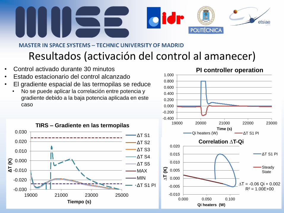
Resultados (activación del control al amanecer)
10
• Control activado durante 30 minutos
• Estado estacionario del control alcanzado
• El gradiente espacial de las termopilas se reduce• No se puede aplicar la correlación entre potencia y
gradiente debido a la baja potencia aplicada en este
caso
-0.030
-0.020
-0.010
0.000
0.010
0.020
0.030
19000 21000 23000 25000
ΔT
(K
)
Tiempo (s)
TIRS – Gradiente en las termopilas
ΔT S1
ΔT S2
ΔT S3
ΔT S4
ΔT S5
MAX
MIN
ΔT S1 PI
-0.400
-0.200
0.000
0.200
0.400
0.600
0.800
1.000
19000 20000 21000 22000 23000
Time (s)
PI controller operation
Qi heaters (W) ΔT S1 PI
-0.350
-0.300
-0.250
-0.200
-0.150
-0.100
-0.050
0.000
0.050
0.000 0.200 0.400 0.600 0.800 1.000
∆T
(K)
Qi heaters (W)
Correlation ∆T-Qi
Resultados (activación del control al amanecer)
11
• Control activado durante 30 minutos
• Estado estacionario del control alcanzado
• El gradiente espacial de las termopilas se reduce• No se puede aplicar la correlación entre potencia y
gradiente debido a la baja potencia aplicada en este
caso
-0.030
-0.020
-0.010
0.000
0.010
0.020
0.030
19000 21000 23000 25000
ΔT
(K
)
Tiempo (s)
TIRS – Gradiente en las termopilas
ΔT S1
ΔT S2
ΔT S3
ΔT S4
ΔT S5
MAX
MIN
ΔT S1 PI
-0.400
-0.200
0.000
0.200
0.400
0.600
0.800
1.000
19000 20000 21000 22000 23000
Time (s)
PI controller operation
Qi heaters (W) ΔT S1 PI
∆T = -0.06 Qi + 0.002R² = 1.00E+00
-0.010
-0.005
0.000
0.005
0.010
0.015
0.020
0.000 0.050 0.100
∆T
(K)
Qi heaters (W)
Correlation ∆T-Qi
ΔT S1 PI
SteadyState

Conclusiones• Se ha mostrado el impacto de los requisitos térmicos en el ciclo de desarrollo del
instrumento, tanto en diseño como en validación y verificación.
• El comportamiento térmico del instrumento TIRS ha sido modelizado y se ha realizado un análisis completo de los escenarios más desfavorables para el instrumento.
• Se ha analizado y mostrado la viabilidad de aplicar un sistema de control para mejorar las prestaciones del instrumento.
12
Trabajos futuros• Los resultados de estos análisis y el modelo térmico desarrollado podrán dar
soporte a las operaciones en vuelo.• Prueba de nuevos modos de operación una vez en Marte.• Prueba del comportamiento térmico ante condiciones degradadas (mitigación
ante posibles incidentes de la misión).

Muchas gracias por su atención, ¿alguna pregunta?
“Two possibilities exist: either we are alone in the Universe or we are not. Both are equally terrifying.” Arthur C. Clarke
Adrián Chamorro [email protected]
Source: NASA/JPL

EXTRA
14

Thermal requirements: drivers of the thermal analysis
•Thermal requirements have guided the thermal analysis process
–Discretization of the model–Transient analyses required (temporal and spatial gradients)
–Needed of performing uncertainty analyses–Dedicated thermal test
15
0.02
0.03
0.04
0.05
0.06
0.07
69000 70000 71000 72000
ΔT
(K
)
Time (s)
Example of sensitivity analysis to wind gust
ΔT S1
ΔT S2
ΔT S3
ΔT S4

-120-100-80-60-40-20
02040
0 25000 50000 75000
Te
mp
era
ture
(°C
)
Time (s)
Environment temperature(Martian summer)
Atmosphere Ground Sky
Thermal environment modelling•Modelling of Martian thermal environment
–Undefined landing site: worst landing site selected (Holden crater)
–Solar loads•Winter and summer (high eccentricity of the Martian orbit)
•Direct and diffuse
•Rover orientation (shadows)
–Boundary temperatures:•Ground, sky, atmosphere and rover temperatures provided as inputs
–Natural and forced convection•External surfaces and atmosphere heat exchange
•Heat exchanged between internal parts because of the presence of the atmosphere
–Dust deposition on surfaces•Effect on the optical finish of the external surfaces 16
0
50
100
150
200
250
300
0 25000 50000 75000
Hea
t fl
ux
(W
/m2)
Time (s)
Direct Ground Solar heat flux(Martian Winter)

Test and model correlation• Dedicated test has been performed to reduce
the uncertatinty of the model.
• Conductive couplings between the componentsof the instrument and the capacitance of thethermopiles have been correlated with themeasurements of the test
• Test setup:
–CO2 pressurized chamber
–Performed in EM of the TIRS (the differences betweenthe EM and FM have been taken into account in theTMM of the test)
–Two test have been performed with different powerconsumption strategy.
17

-200.0
-100.0
0.0
100.0
200.0
0 20,000 40,000 60,000
Th
erm
op
ile
3 g
rad
ien
t (m
K)
Time (s)
TIRS Test 1 Thermopile 3 gradient
15.0
20.0
25.0
30.0
35.0
40.0
45.0
50.0
0 50,000Tem
pera
ture
(°C
)
Time (s)
TIRS Test 1 Temperature measurements
Supportplate
Calibration plate
Chamber
Case
Test and correlation• Two test performed with different power profile
• Gradient in thermopiles estimated from voltage measurements of thermopile 3 during the test
18
15.0
20.0
25.0
30.0
35.0
40.0
0 20,000 40,000 60,000 80,000 100,000Tem
pera
ture
(°C
)
Time (s)
TIRS Test 2 Temperature measurements
-300.0
-200.0
-100.0
0.0
100.0
200.0
0 20,000 40,000 60,000 80,000
Th
erm
op
ile
3
gra
die
nt
(mK
)
Time (s)
TIRS Test 2 Thermopile 3 gradient

Test and correlation
19
• Steady state correlation (quasy-steady state in the tests):
• Conductive couplings (contact), convective couplings ( internal) and thermal
conductivityModel results
before correlation
(temperature (°C))
CaseCalibration
plate
Support
plate
Test 1Measured 31.79 46.98 43.43
Model 31.85 53.8 40.8
Test 2Measured 26.39 28.60 35.64
Model 26.4 27.2 33.8
Results after
steady state
correlation (ºC)
Case
temperature
Calibration
plate
temperature
Support plate
temperature
Test 1Measured 31.79 46.98 43.43
Model 31.85 47.56 43.26
Test 2Measured 26.39 28.60 35.64
Model 26.40 28.21 35.58
Error
Test 1 0.06 0.58 -0.17
Test 2 -0.05 -0.39 0.01
-35.00
-25.00
-15.00
-5.00
5.00
15.00
25.00
3500 5500 7500
ΔT
(mk)
Time (s)
Grad TP3 Model C+40%(mk)
Grad Tp3 Test (mK)
Grad TP3 Model C+20%(mk)
Grad TP3 Model C+30%(mK)
Grad TP3 Model C estimated(mk)
-45.00-30.00-15.00
0.0015.0030.0045.00
3800 8800 13800 18800
Err
or
in t
he
th
erm
op
ile
3 g
rad
ien
t (m
K)
Time (s)
Error in the thermopile 3 gradient for the first and second activation of the heaters
Error Test 1C+20%
Error Test 1C+40%
Error Test 1C+30%
• Transient correlation:
• Strong dependency of the gradients with thermal capacity of the thermopiles

Worst case Analyses in operative environment
•Steady Analyses–To set the thermal envelope of the problem and check the model
–Summer day analysis•14:00 LST and highest summer boundary conditions (BC) temperatures
–Winter night analysis•No Sun and lower winter BC temp.
–Qualification analysis•Hot qualification case has been performed
•Transient Analyses–Nominal operation analyses:
•WHC, no heaters, no wind (natural convection)
•WCC, no heaters, no wind (natural convection)
–Calibration modes•Activation of calibration plate heaters and support plate heaters
–Sensitivity to wind analysis•Change in steady wind
•Gusts 20

Results
•Summer day steady results:–Power: 0 W
Temperature Results (°C)
Part Max Min Average Max ΔT
Case 12.3 10.1 11.7 2.2
Calibration Plate 13.1 13.0 13.1 0.1
Sensors support plate 12.0 12.0 12.0 0.0
Sensors cover plate 12.1 12.0 12.1 0.0
Insulation Plate 14.0 12.2 13.0 1.8
Back Plate 12.9 10.7 11.7 2.2
PCB 12.1 12.3 12.1 -0.2
Thermopiles 12.03 12.02 12.02 0.01
21

Results
•Summer day steady results
22

Transient analysis
•Example of results of a nominal operationcase
23
-0.150
-0.100
-0.050
0.000
0.050
0.100
0.150
0 20000 40000 60000 80000
ΔT
(K
)
Time (s)
TIRS Calibration Plate Gradients (WHC)
ΔT Pt1000-A1
ΔT Pt1000-A1
ΔT Pt1000-A2
ΔT Pt1000-A2
ΔT Pt1000-A2-70.00-60.00-50.00-40.00-30.00-20.00-10.00
0.0010.0020.00
0 50000Te
mp
era
ture
(°C
)
Time (s)
TIRS Calibration Plate Temperatures (WHC)
Pt1000 A2 A2 A1 A1 A2
-0.050
-0.030
-0.010
0.010
0.030
0.050
0.070
0 50000
ΔT
(K
)
Time (s)
TIRS Thermopiles Temperature Gradient (WHC)
ΔT S1ΔT S2ΔT S3ΔT S4ΔT S5 -0.014
-0.010
-0.006
-0.002
0.002
0.006
0.010
0.014
0 20000 40000 60000 80000
dT
/dt
(K/s
)
Time (s)
TIRS Thermopiles Temperature temporal gradient (WHC)
dT/dt S1
dT/dt S2
dT/dt S3
dT/dt S4
dT/dt S5
-70.00
-50.00
-30.00
-10.00
10.00
30.00
0 20000 40000 60000 80000
Te
mp
era
ture
(°C
)
Time (s)
TIRS Case Temperatures (WHC)
Y+
Z+
Foot1
Foot2
Ground
ExternalAtm

Experimental concept: PI heaters control to improve instrument performance
• First approach: Simple control loop in order to assess the
feasibility of the PI control loop to reduce the gradients or
lead to a known gradient in the thermopiles
• Control loop: • PI control loop with Kp = 0.5 and Ki =5/512
• The control loop has been applied where the maximum
gradients were reached on the transient analyses
24

0.00
2.00
4.00
6.00
8.00
10.00
60000 65000
Tem
pera
ture
(°C
)
Time (s)
TIRS Support Plate Temperatures (WCC)
MS1
Pt1000
Pt1000PI
Results (PI activation at 60000 s)
25
• PI controller activated during 30 minutes.
• Steady state of the controller achieved
• The temporal gradient in the thermopiles is
reduced
• The spatial gradient does not achieve a steady
state (variation of the boundary temperatures)
-0.030
-0.020
-0.010
0.000
0.010
0.020
0.030
0.040
0.050
60000 62000 64000
ΔT
(K
)
Time (s)
TIRS Thermopiles Temperature Gradient (WHC)
ΔT S1
ΔT S2
ΔT S3
ΔT S4
ΔT S5
MAX
MIN
-0.015
-0.010
-0.005
0.000
0.005
0.010
0.015
60000 62000 64000
dT
/dt
(K/s
)
Time (s)
TIRS Thermopiles Temperature temporal gradient (WHC)
dT/dt S1
dT/dt S2
dT/dt S3
dT/dt S4

• Linear correlation appears between power in the heaters during control loop and spatial gradient in the thermopiles
• Usable to improve the accuracy under certain circumstances (more effective in the afternoon)
• Deeper analysis needed to calibrate the parameters of the correlation in different situations
26
-0.05
0.00
0.05
0.10
0.15
0.20
0.25
0.30
60000 61000 62000 63000 64000
Time (s)
PI controller operation
Power (W)
∆T = -7.95E-02 Qi R² = 1.00E+00
-0.030
-0.015
0.000
0.015
0.030
0.000 0.100 0.200 0.300
∆T
(K
)
Qi heaters (W)
Correlation ∆T-Qi (t=61000 s) Grad Tp3
Steady State

Conclusions
•Detailed thermal analysis of the TIRS has been performed.
•Thermal behavior of the TIRS has been modeled and worst case scenarios have been analyzed.
•The strict thermal requirements have driven the activities and extra activities to increase the reliability and the accuracy of the results have been performed.
•The control of the heaters of the support plate does not lead to a steady spatial gradient in the thermopiles, but it could be used to improve the accuracy in some circumstances.
27
Future work• Thermal model and analyses could support in flight operations.
• For example new operation modes could be tested in this model
or the thermal performance of the instrument under degraded
conditions could be assessed.

EXTRA 2
28

Test and correlation
29
• The temperature gradient in the thermopiles have been correlated with the estimated temperature in the
test.
TestTest 1
measurement
Test 2
measurement
Gradient in
thermopile 3 (K)0.003 -0.020
Max
gradient
Min
gradient
Average
gradient
Gradient in
Thermopile 3
Test 1 -0.004 -0.002 -0.003 0.003
Test 2-0.026 -0.020 -0.025 -0.020
• The results after the correlation of the gradients in the thermopiles are shown in the following table. Max,
min and average gradient correspond to the five thermopiles in each one of the tests. The values which
has been correlated corresponds to the gradient in the thermopile 3.

Transient analysis•Example of results of a nominal operationcase
30
-120.00
-100.00
-80.00
-60.00
-40.00
-20.00
0.00
20.00
40.00
0 20000 40000 60000 80000
Te
mp
era
ture
(°C
)
Time (s)
TIRS Case Temperatures (WHC)
Y-
Y+
Z+
Z-
Foot1
Foot2
Foot3
Foot4
Sky
Ground
External Atm
RSM

Transient analysis
•Example of results for a non-operational case
31
-1.00
-0.80
-0.60
-0.40
-0.20
0.00
0.20
0 20,000 40,000 60,000 80,000
Po
wer
(W)
Time (s)
Conductive heat transfer
0.00
0.05
0.10
0.15
0.20
0.25
0.30
0.0 50,000.0
Film
Co
eff
icie
nt
h (
W/(
m^2
·K))
Time (s)
Convective heat transfer
hconvnatTopFW
hconvnatBotFW
hconvnatLatFW
hconvnatFcFW

Transient analysis (II)
•Example of results for calibration mode (heaters of the calibration plate ON)
32
-0.06
-0.05
-0.04
-0.03
-0.02
-0.01
0.00
0.01
0.02
19500.00 21500.00 23500.00
ΔT
(K
)
Time (s)
TIRS Thermopiles Temperature Gradient (WHC)
ΔT S1
ΔT S2
ΔT S3
ΔT S4
ΔT S5
-0.002
0.000
0.002
0.004
0.006
0.008
19500 21500 23500
dT
/dt
(K/s
)
Time (s)
TIRS Thermopiles Temperature temporal gradient (WHC)
dT/dt S1
dT/dt S2
dT/dt S3
dT/dt S4
dT/dt S5

Transient Analysis (III)• Example of results for WHC wind sensitivity analysis: steady wind
change
33
-30.00
-25.00
-20.00
-15.00
-10.00
-5.00
68500 69500 70500 71500 72500
Te
mp
era
ture
(°C
)
Time (s)
TIRS Case Temperatures (WHC)
Y-
Z+
Foot1
Foot2
Y- no wind
Foot1 no wind
Z+ no wind

Transient Analysis (III)• Example of results for WHC wind sensitivity analysis: steady wind
change
34
0.02
0.03
0.04
0.05
0.06
0.07
69000 70000 71000 72000
ΔT
(K
)
Time (s)
TIRS Thermopiles Temperature Gradient (WHC)
ΔT S1
ΔT S2
ΔT S3
ΔT S4
ΔT S5
ΔT S5 no wind
-0.014
-0.010
-0.006
-0.002
0.002
0.006
69000 70000 71000 72000 73000
dT
/dt
(K/s
)
Time (s)
TIRS Thermopiles Temperature temporal gradient (WHC)
dT/dt S1
dT/dt S2
dT/dt S3
dT/dt S4
dT/dt S5

Uncertainty analysis
• Uncertainty analysis has been performed taking into account the
guidelines provided in ECSS-E-HB-31-03A
• First, a sensitivity analysis is performed by changing the
parameters of the model taking into account the following table:
• Then, the uncertainty in the different components of the model has
been calculated by quadrature:
𝜙𝑖 = 𝑗=1𝑛 (Δ𝜙𝑟,𝑗)𝑖
2 + (Δ𝜙𝑠)𝑖
where, Δ𝜙𝑖 is the overall uncertainty on model output i, Δ𝜙𝑟,𝑗 is the
uncertainty due to statistical parameters j on model output i, and
(Δ𝜙𝑠)𝑖 is the systematic uncertainty on model output i. 35
Parameter Inaccuracy
Thermal conductivity (homogeneous material) ±10%
Thermal conductivity (composites) ±30%
Contact resistance (by similarity) ±50%
Emissivity ±0.03
Emissivity (<0.2) ±0.02
Absorptance ±0.1
Absorptance (<0.2) ±0.03

-115.00
-105.00
-95.00
-85.00
-75.00
0.6 0.8 1 1.2 1.4Te
mp
era
ture
(°C
)
k FR4 (W m-1 K-1)
Sensitivity Analysis k FR4 (cold case)
Uncertainty analysis• Uncertainty analysis has been performed to
increase the knowledge about the thermal behavior and the sensitivity to the unknowns of the problem.
• First, it is needed to perform a sensitivity analysis:
36
Parameter Inaccuracy
Thermal conductivity
(homogeneous material) ±10%
Thermal conductivity
(composites)±30%
Contact resistance (by
similarity)±50%
Emissivity ±0.03
Emissivity (<0.2) ±0.02
Absorptance ±0.1
Absorptance (<0.2) ±0.03
𝛥𝜙𝑖 =
𝑗=1
𝑛
Δ𝜙𝑟,𝑗 𝑖2+ (Δ𝜙
𝑠 𝑖
-3.00
-2.00
-1.00
0.00
1.00
2.00
3.00
4.00
0.7 1 1.3
ΔTe
mp
era
ture
(°C
)
k FR4 (W m-1 K-1)
Sensitivity Analysis k FR4 (cold case)T Case 1
T Case 2
T Case 3
T Case 4
T CALP
T SP
T IP JCALP
T IP JCASE
T IP Centre
• Once the sensitivity analysis has been performed, the
uncertainty associated to the studied parameters is
computed as:

Uncertainty analysis• The results of all the analyses performed can be found on the
report
• A summary of the results is shown in the following table:
• Taking into account the results of the sensitivity analysis, the results are especially sensitive to
FR4 conductivity and contact resistance. Therefore, it is shown the importance of the dedicated
test that was performed because it has helped to correct the nominal values of the parameters of
the model, what leads to reduce the modelling uncertainty of these parameters.
37
Summary of the results of the sensitivity analysis
Analysis Case Support plateCalibration
plateInsulation plate
Δ𝑘𝐴𝑤6082Max |Δ𝑇| cold case 0.20 0.19 0.21 0.23
Max |Δ𝑇| hot case 0.48 0.45 0.45 0.52
Δ𝑘𝐹𝑅4Max |Δ𝑇| cold case 0.14 0.13 2.54 3.02
Max |Δ𝑇| hot case 0.10 0.26 2.28 2.80
Δ𝑅𝑐Max |Δ𝑇| cold case 0.55 2.09 3.91 2.39
Max |Δ𝑇| hot case 1.57 7.39 5.44 3.76
Δ𝜀Max |Δ𝑇| cold case 0.12 0.02 0.1 0.08
Max |Δ𝑇| hot case 0.16 0.23 0.36 0.40
Δ𝛼 Max |Δ𝑇| cold case - - - -
Max |Δ𝑇| hot case 1.14 0.99 1.34 1.79
Results Δ𝜙𝑟,𝑗
2cold 0.61 2.10 4.67 3.86
hot 2.00 7.48 6.08 5.06