ANÁLISIS DEL COSTE HOSPITALARIO....
136
Departament d’Economia Aplicada. Facultat de Ciències Econòmiques i Empresarials. Universitat Autònoma de Barcelona Programa de tercer cicle del Departament d'Economia Aplicada de la Universitat Autònoma de Barcelona Tesis doctoral Análisis del coste hospitalario. Información e instrumentos para el ajuste de la función de costes hospitalarios. Francesc Cots Reguant Dirección: Dr. Jaume Puig Junoy
Transcript of ANÁLISIS DEL COSTE HOSPITALARIO....

Departament d’Economia Aplicada. Facultat de Ciències Econòmiques i Empresarials. UniversitatAutònoma de Barcelona
Programa de tercer cicle del Departament d'Economia Aplicada de la Universitat Autònoma deBarcelona
Tesis doctoral
Análisis del coste hospitalario.Información e instrumentos para el ajuste de la función de costes
hospitalarios.
Francesc Cots Reguant
Dirección:Dr. Jaume Puig Junoy
Sabadell, a 31 de Enero de 2001


Agradecimientos y justificaciones personales
Esta tesis se ha realizado en el período 1998-2000 y es fruto del trabajo de
investigación realizado a lo largo de los años 1995-2000 por un equipo que ha
posibilitado la consecución de los objetivos que se incluyen. Los investigadores que han
colaborado en aspectos concretos han sido Marta Riu quien ha aportado su
conocimiento en sistemas de case-mix y ha tenido una especial aportación en la
definición de una tabla de equivalencia de los GRDs que se relacionan con
procedimientos quirúrgicos considerados potencialmente ambulatorizables necesaria
para el capítulo 3; Pilar Torre ha asesorado sobre la incorporación de los distintos
sistemas de valoración de la severidad utilizados en los capítulos 4 y 5; el Dr. Marc
Sáez ha colaborado activamente como asesor para aspectos estadísticos para resolver
distintos problemas de esta índole aparecidos en los capítulos 2 i 5; Mercé Comas ha
dado soporte al análisis estadístico del capítulo 5; la Dra. Eulàlia Dalmau trabajó
activamente en la depuración y consolidación de la base de datos con información
económica; David Elvira trabajó activamente en el análisis de la información del
capítulo 2 sobre el cálculo de outliers y, por último, Lluc Mercadé quien en su
colaboración actual con los proyectos de investigación que llevamos a cabo, ha aportado
elementos de discusión sobre los análisis ya realizados, especialmente en lo que se
refiere a la utilización de variables ecológicas y al análisis multinivel.
Quiero hacer explícito mi agradecimiento a la Unitat de Recerca en Serveis Sanitaris
coordinada por el Dr. Jordi Alonso ya que ha sido el ámbito en el que he podido
presentar resultados preliminares y discutir soluciones a problemas planteados.
Por último, agradecer de manera especial al Dr. Xavier Castells que haya posibilitado e
incentivado de manera muy activa la integración del proceso de elaboración de esta tesis
con la dinámica del Servei d’Estudis y haya aportado una visión global sobre la
interacción entre puntos de vista basados en la Economía de la Salud y los relacionados
con la Investigación en Servicios Sanitarios, así como su experiencia y conocimientos
sobre aspectos generales de metodología en investigación y capacidad de reflejarlos
adecuadamente en la redacción final de los resultados.
Quiero agradecer especialmente al Dr. Jaume Puig Junoy que aceptase la dirección de
esta tesis aún dándose múltiples circunstancias negativas como el hecho de ser un

proyecto ya iniciado o bien, existir poca relación entre el objetivo de la tesis y las líneas
habituales de investigación que se desarrollan en el Departamento de Economía
Aplicada de la UAB y, más aún, por no pertenecer al propio departamento. Ha sido un
activo trabajo de dirección que me ha permitido definir los objetivos últimos que
todavía no tenían una orientación clara y me ha aportado un nivel de seguridad
importante en la relevancia y aplicabilidad del proyecto.
Este proyecto ha contado con la financiación del Fondo de Investigaciones Sanitarias
(expedientes 1996/1351 y 1999/0687).
Los trabajos de encuadernación han sido sufragados por el Institut Municipal
d’Investigació Mèdica.
El hecho de realizar esta tesis doctoral responde a razones que normalmente no son las
habituales para justificar su realización. No se trata de una carta de presentación ni una
demostración de suficiencia investigadora, aunque todo ello sin ser el motivo último, se
da por supuesto. Ha sido más bien un proceso de consolidación de un proyecto de
investigación que ahora, con esta tesis, permite marcar un punto y aparte. El proceso
investigador continuará evolucionando pero a un nivel de análisis más micro,
contrastando hipótesis más concretas y mediante procedimientos de recogida de
información prospectivos, más asistenciales y menos administrativos. Este nuevo
planteamiento demandaba un cierre ordenado de la primera etapa.
Debido a esta motivación, el conjunto de los capítulos centrales se ha redactado en
inglés (capítulos 2 a 5) con la intención de conseguir su publicación posterior. El resto
de la tesis (Capítulos 1 y 6) se ha traducido del catalán al castellano obedeciendo a la
voluntad de poder contar con la presencia de personas del resto del estado español en el
tribunal.
A la Valèria i en reconeixement als meus pares.
Sabadell, 31 de Enero de 2001

Capítulo 1 7
Indice.
Capítulo 1. Introducción al estudio de la variabilidad del coste del paciente ingresado.
Justificación. El coste del paciente ingresado. La situación actual en nuestro entorno (desde
Cataluña a la mayor parte de países europeos). Objetivos. Antecedentes concretos: Variabilidad
del coste debida a la existencia de casos extremos; Variabilidad inter-grupo debida a la
utilización de pesos relativos estandarizados provenientes de un entorno económico, social y
organizativo, distinto; Variabilidad intra-grupo debida a errores de medida del propio sistema de
agrupación; El comportamiento de la función de costes por paciente. Las causa de la
variabilidad del coste por paciente. Metodología para el análisis…………….………………….9
Capítulo 2. Relevance of outlier cases in case mix systems and evaluation of trimming
methods for use in Europe.
Introduction: lognormal cost distribution per hospital patient; financial risk; outlier cases;
Determination of outlier cases. Material and methods: Calculation of trimming methods;
Analysis of agreement (Kappa’s coefficient; Sensitivity index; Specificity index; Youden’s
index; ROC curve; MaNemar’s test); Cost associated with outlier cases determined by LOS.
Results. Discussion………………………………………………………..……………………27
Capítulo 3. Medicare's DRG-Weights in a European environment: the Spanish
experience.
Introduction. Material and methods: Identification of unusually expensive cases; Analysis.
Results: Expected deviations; Other systematic deviations; Sensitivity analysis. Discussion:
Global analysis; Diagnosis-related groups causing systematic deviations.
Conclusions………………………..……………………………………………………………45
Capítulo 4. Risk adjustment: beyond patient's classification systems.
Introduction. Material and methods: Variables; Analysis. Results. Discussion.
Conclusions……………………………………………………………………………………..63
Capítulo 5. Constructing an inpatient cost function: from risk adjustment to the
behaviour of variables defining hospital process.
Introduction. Methodology: Cost function; Empirical formulation. Results. Discussion.
Conclusions……………………………………………………………………………………..85

8 Introducción
Capítulo 6. Conclusiones.
Resumen por objetivos. Discusión general. Implicaciones políticas y agenda de información
futura: El futuro de los sistemas de clasificación en España; El conocimiento del coste por
paciente; La mejora de calidad de la información de los informes de alta; La mejora en la
información socioeconómica del paciente………………………… ………………………111
Bibliografía..…………………………………………………………………………………125

Capítulo 1.
Introducción al estudio de la variabilidad del coste del paciente
ingresado.

10 Introducción
Justificación.
Los sistemas sanitarios en el entorno europeo se basan en un predominio de
financiación pública con coberturas que tienden a ser universales y con redes de
provisión más o menos integradas que suministran los servicios sanitarios a la
población. Independientemente de la titularidad de los centros proveedores, la relación
entre la administración sanitaria (financiador-comprador) y los centros proveedores se
establece en un marco de asignación de recursos públicos con la finalidad de cubrir las
necesidades de la población general.
Esta realidad ha significado que el flujo económico entre la administración y los
centros proveedores se ha basado en criterios de subsistencia de la red de provisión para
que cubra el territorio de manera global y permita la prestación de los servicios
demandados por la población. La formulación de los criterios por los cuales un
proveedor recibe ingresos económicos por un nivel de actividad se han basado
históricamente en criterios de reconocimiento retrospectivo del coste incurrido y el
pacto de los niveles de actividad. No ha habido por lo tanto una información subyacente
del valor ni del coste de las actividades realizadas.1
En el contexto de la atención especializada la red de hospitales supone la existencia de
grandes empresas, en ocasiones las mayores empresas del área donde radican. Estos
grandes centros de actividad no han valorado históricamente el coste de su actividad y
no han podido compararse con el resto de hospitales de su entorno. La consecuencia de
esta forma de entender la organización de los sistemas de salud ha provocado un
desconocimiento del nivel de eficiencia del sector en general, una desconexión entre el
volumen de actividad y su composición respecto de los ingresos económicos y, en
definitiva la ausencia de información sobre el coste de la actividad hospitalaria.
Esta situación ha convivido con un largo período de expansión de los sistemas
sanitarios que ha superado al crecimiento real de la economía. En España esta realidad
ha pervivido hasta la mitad de los años 90 y ha significado que los incrementos de
costes en la provisión que se iban produciendo eran absorbidos por el crecimiento del
conjunto del gasto sanitario.2 La necesaria contención de costes del sistema sanitario
español se ha trasladado de forma inmediata a la relación de la administración sanitaria
con los centros proveedores. Desde mitad de los 90 ha aparecido la necesidad de
continuar ofreciendo las misma coberturas, mientras debían ajustarse los recursos

Capítulo 1 11
destinados a la compra de servicios sanitarios y aparecían innovaciones tecnológicas
que multiplicaban la necesidad de recursos, así como la percepción ciudadana de mayor
necesidad de atención sanitaria una vez habían cubierto otras necesidades que
consideraban prioritarias.
La necesidad de conocer los costes de la actividad realizada para conseguir una mayor
eficiencia en el rendimiento de los recursos públicos así como la búsqueda de
mecanismos para hacer más transparente la asignación de recursos a cada centro
proveedor ha propiciado la necesidad de conocer los costes de la actividad realizada.
Les dificultades para obtener información sobre costes de los centros hospitalarios
tienen dos causas principales:
• No existía y no existe actualmente una cultura de análisis del coste por actividad
realizada. La gestión de los centros hospitalarios podía realizarse contando
únicamente con la contabilización general de los gastos que permitiera justificar su
reembolso global por parte de la administración.
• No existe información de precios puesto que la predominancia del sector público
impide que haya un mercado que genere información de precios de los distintos
productos y servicios relacionados con la prestación de servicios sanitarios
• La dificultad de definir producto en la provisión de servicios sanitarios ha
provocado grandes dificultades en los intentos de valoración de la actividad
realizada.
Para avanzar en el conocimiento del coste por actividad provocado por la provisión de
servicios sanitarios es necesario reconocer la naturaleza multiproducto de la función de
producción de un hospital: Hospitalización, Actividad ambulatoria, Urgencias,
Docencia e Investigación. Solamente de esta manera se puede concretar el análisis a
relaciones abordables entre dispositivos asistenciales y su actividad. El conjunto del
estudio que se presenta, se ha concretado en el análisis del coste hospitalario
correspondiente a la actividad de internamiento.
El coste del paciente ingresado.
Para superar las dificultades generales que se acaban de expresar sobre el
desconocimiento del coste unitario observado de las actividades relacionadas con la
atención del paciente ingresado y la dificultad de disponer de una definición de
producto hospitalario, en la investigación aplicada se han realizado una serie de avances
que serán el punto de partida de este estudio.

12 Introducción
• Se han diseñado sistemas de clasificación de pacientes (casemix) que se basan en su
agrupación en un reducido número de categorías de producto bajo criterios de
consumo de recursos, homogeneidad clínica, o factores pronóstico.
Para el análisis de costes los sistemas de agrupación de pacientes basados en
isoconsumo de recursos son claramente los más adecuados. Los distintos sistemas
de salud regionales han optado por distintas versiones de los llamados Grupos
relacionados por el Diagnóstico (GRD). El presente estudio se ha basado en los
GRD de la Heath Care Financing Administration versión 13 utilizados por el Servei
Català de la Salut, aunque se han utilizado también otros sistemas de agrupación
para valorar las diferencias en sus posibilidades en el análisis de costes.
• Proyectos de asignación de costes del tipo coste por paciente ingresado ( a partir de
ahora clinical-cost) basados en técnicas de contabilidad analítica que han permitido
repartir el conjunto del coste de un período al nivel de los pacientes ingresados. Para
este estudio se ha contado con el coste por paciente observado de 35.262 pacientes
pertenecientes a los hospitales públicos del Institut Municipal d’Assistència
Sanitària de Barcelona.
Si bien las técnicas de casemix, básicamente los GRD, se han generalizado, el
conocimiento del coste por paciente observado es todavía un caso excepcional. Esto ha
propiciado que se hayan extendido formas alternativas a la valoración del coste.
Obviando la realidad americana de los sistemas de ratios ‘charge to cost’, en Europa se
han generalizado los sistemas de cálculo definidos como ‘modelling-cost’.3 Estos
sistemas aproximan un coste medio por categoría de producto GRD sobre la base de
distribuir el conjunto del coste de un hospital de forma ponderada a cada paciente según
el GRD al que pertenecen. Para ello se han creado escalas de costes relativos (a partir de
ahora les llamaremos pesos) que ponderan el coste inter-GRD.
En Cataluña, como en toda España y de forma también mayoritaria en Europa, se
utilizan los pesos del sistema Medicare americano. Sobre esta forma de aproximación a
coste por producto se han desarrollado sistemas de comparación benchmarking entre
hospitales y sobre todo, sistemas de pago a hospitales que han comenzado a utilizarse en
años recientes.
El presente estudio pretende valorar los peligros de utilizar estos sistemas de ‘cost-
modelling’ con relación a un estándar como es el coste real observado mediante
‘clinical-cost’, con el fin de ofrecer evidencia empírica sobre las posibilidades del

Capítulo 1 13
primero de los métodos y la necesidad de evolucionar hacia criterios que ajusten mejor
la variabilidad del coste por paciente ingresado.
La justificación definitiva del presente estudio se resume en la necesidad de pasar de
aproximaciones indirectas del coste hospitalario mediante ‘cost-modelling’ al
comportamiento del coste por paciente ingresado, definiendo una especificación
empírica de función de costes del paciente ingresado (FCPI) y valorando las diferencias
que existen entre ambas aproximaciones.

14 Introducción
La situación actual en nuestro entorno (desde Cataluña a la mayor parte de
países europeos)
Quedan muchas preguntas por responder sobre la capacidad de las técnicas de casemix
para el análisis del coste hospitalario. A criterio del autor, se ha producido una
instrumentalización de los GRD para el análisis de costes en España sin una validación
previa de su utilidad:
• No ha habido ningún estudio que haya valorado la capacidad de los GRD para
explicar variabilidad de costes.
• No se ha valorado si los criterios de agrupación de pacientes o bien si los pesos
asociados a cada categoría GRD son adecuados a la realidad del sistema sanitario
en nuestro entorno.
• No se han valorado las diferencias existentes entre los distintos sistemas de
clasificación de pacientes según si incluyen o no valoraciones del nivel de
severidad, así como por los criterios utilizados para determinar comorbilidades y
complicaciones. Dicho de otra forma, no se ha pasado del criterio de análisis del
casemix al de ‘ajuste de riesgos’.
• No se ha realizado ninguna aproximación a la repercusión de los casos
extremadamente costosos sobre el valor medio de la categoría GRD a la que han
sido asignados. Existen tantos criterios para determinar métodos para aislar los
casos extremos como países donde se han implantado estas técnicas con la
intención de financiar los hospitales. En este sentido Cataluña y después otros
servicios regionales como el de Andalucía, han sido los primeros en utilizar
técnicas de casemix para la asignación de recursos sin aislar los casos extremos de
coste.
Gran parte de estas cuestiones no han podido tener respuesta por falta de información
sobre el coste real por paciente ingresado. La oportunidad del presente estudio es
disponer del coste por paciente de una muestra suficiente que podrá ser utilizada como
estándar de comparación.
En consecuencia, prácticamente la totalidad de los análisis de eficiencia hospitalaria
realizados en nuestro entorno, así como los distintos sistemas de pago a hospitales de

Capítulo 1 15
última generación, han utilizado definiciones de producto basadas en técnicas de
casemix sin haber respondido previamente a las cuestiones pendientes expresadas.
También el uso comercial de instrumentos basados en técnicas de casemix ha
sobrevalorado sus posibilidades y capacidad operativa. Se ha extendido la creencia en el
sector sanitario que la relación entre producción y costes se puede resolver con un
simple algoritmo basado en la imputación de los costes totales de un hospital a cada
GRD en función del número de pacientes. Esta creencia supone predeterminar que no
existe variabilidad intra-GRD, amén que el algoritmo de cálculo de los GRD y de los
pesos asociados sean directamente transportable desde los EEUU a cualquier hospital de
nuestro entorno.

16 Introducción
Objetivos
Objetivo principal.
Determinar las causas de la variabilidad del coste por paciente hospitalizado,
considerando el nivel de variabilidad intra-grupo e inter-grupo del coste por paciente
ingresado al utilizar los Grupos Relacionados con el Diagnóstico (GRD) como medida
del producto hospitalario.
Objetivos concretos
1. Analizar la variabilidad del coste generada por la existencia de casos extremos
(outliers). Definir el método de cálculo de outliers de coste más apropiado para ser
utilizado sobre la ‘duración de la estancia’ entendida como variable proxy del coste.
(Capítulo 2)
2. Evaluar las diferencias que existen entre el sistema de pesos asociado a los GRD
utilizados por Medicare ( programa de cobertura pública para personas mayores de
la Health Care Financing Administration- HCFA- en los E.E.U.U.) y los pesos
ajustados a nuestra realidad calculados sobre la base de costes por paciente
observados. (Capítulo 3)
3. Construcción de un sistema de ajuste de riesgos que maximize la capacidad
explicativa de la variabilidad inter e intra GRD, dado el nivel de información
existente en cualquier sistema hospitalario europeo. (Capítulo 4)
4. Estimación empírica de la función de costes por paciente ingresado que permita
explicar el comportamiento del coste por paciente ingresado así como la causa de
este comportamiento. (Capítulo 5)

Capítulo 1 17
Antecedentes concretos
Se presenta en este apartado una breve síntesis de la situación actual del análisis y
discusión sobre los cuatro objetivos concretos a desarrollar en el presente trabajo.
Variabilidad del coste debida a la existencia de casos extremos (Capítulo 2)
Carter4, Söderlund5,6 y Lichtig7 han aportado múltiples evidencias sobre la
importancia de los casos extremos como fuente de variabilidad dentro de cada uno de
los grupos de pacientes considerados a priori homogéneos. Los autores citados han
utilizado la estancia como aproximación del coste cuando han buscado el método de
marcaje de outliers más conveniente a sus necesidades.
Sus soluciones abren un amplio abanico de posibilidades de sistemas de marcaje de
casos extremos que van desde sistemas basados en indicadores de tendencia central
(Carter), hasta sistemas basados en el rango inter-cuartílico (Söderlund), pasando por
sistemas mixtos en los que intervienen las dos propuestas anteriores (Lichtig).
Según Monrad Aas1, casi todos los países que han utilizado los GRD como
instrumento relacionado con la valoración de la actividad realizada en el hospital,
reconocen la existencia de los outliers y los tratan de forma diferente al resto de casos,
ya que significan más coste que el que refleja el valor medio estandarizado aplicado al
GRD correspondiente.
Variabilidad inter-grupo debida a la utilización de pesos relativos estandarizados
provenientes de un entorno económico, social y organizativo, distinto. (Capítulo 3)
Los GRD se han construido y han evolucionado en base a las necesidades del mercado
Medicare. El sistema de medida de pacientes por GRD pretende dar solución al
problema de la definición del producto hospitalario. Los pesos asociados son la
valoración que se da a cada grupo de pacientes en el entorno Medicare.
En consecuencia, los GRD son una medida de producto adaptada a la realidad de una
población concreta y a unos costes relativos fruto de su sistema de prestación de
servicios.

18 Introducción
Muchos países de Europa y también en Australia o Canadá, han importado este sistema
de definición de producto y valoración del mismo. Ante la duda de la capacidad de estos
instrumentos de medida y valoración para adaptarse a la realidad de los sectores de
salud pública europeos (con coberturas de 100% de la población), cabe plantearse hasta
qué punto es recomendable esta importación directa.
Muchos de estos países han adaptado los GRD a su realidad: Gran Bretaña con los
Health-Resource-Groups (HRG)8 , o bien Australia con los AN-GRD9,10. Obviamente,
de la adaptación de los GRD sale una nueva valoración del coste relativo estandarizado
de los mismos3.
Otros países han preferido utilizar directamente los GRD y sus pesos originales. Entre
estos países destacan Noruega,11 Portugal12 y desde 1997, Cataluña.13
Cuando se han introducido cambios, estos han sido motivados por la necesidad
observada de adaptar los criterios de agrupación a las especificidades del sistema
sanitario en cuestión, más que a la constatación de diferencias en las estructuras de
costes relativas. En el caso español, Casas14 validó los GRD como instrumentos de
definición de producto desde un punto de vista clínico. Hoy en día, cuando ya forman
parte de las normativas habituales de diferentes entes regionales (Xunta de Galicia,15
Junta de Andalucía,16) como instrumentos para la asignación de recursos, no se ha
validado si los pesos asociados a los GRD de Medicare se adaptan a la estructura
organizativa, el nivel de eficiencia medio, la práctica clínica, o las características
socioeconómicas de la población.
Variabilidad intra-grupo debida a errores de medida del propio sistema de
agrupación (Capítulo 4)
Existe variabilidad intra-grupo no explicada por los GRD debida al importante número
de factores que intervienen en la formación del coste asociado a la atención de cada uno
de los pacientes.
Los GRD son un compromiso entre la obtención de una clasificación de productos lo
más reducida posible y desagregar la diversidad de los pacientes entre el mayor número
posible de tipologías, con la finalidad de que el coste medio de cada grupo presente la
menor variabilidad posible. Dicho de otra manera, los GRD buscan la máxima
variabilidad inter-grupo y la mínima variabilidad intra-grupo, al mismo tiempo que son
una herramienta fácilmente manejable por incorporar un número reducido de grupos y

Capítulo 1 19
ser útiles para la gestión, para el reembolso, el análisis clínico, el benchmark, o el
análisis de costes por producto final. Otras razones que motivan esta variabilidad hacen
referencia a las variables utilizadas para la construcción de los GRD, las cuales no son
suficientes ni suficientemente buenas17. Recordar que el sistema RUG (Resource
Utilization Groups) análogo a los GRD para pacientes ingresados sociosanitarios, utiliza
un número más elevado de variables para su definición,18 o bien que considera que en el
período inicial de la aplicación de los GRD en EEUU, el incremento de la complejidad
medida por los GRD se debía casi en su totalidad a la mejora de la calidad de las
variables con las que se construyen estos agrupadores.19 Este fenómeno puede estar
dándose ya en Cataluña tras cuatro años de la utilización de los GRD para la valoración
de la actividad hospitalaria pública.20
Iezzoni21 y Elixhauser et al22 han apostado por medidas que mejoren la capacidad de
los GRD para aproximar el coste justificable de los pacientes sobre la base de variables
que explican severidad, complicaciones y comorbilidades. Muchas veces, los GRD no
recogen estas variables que significan causas sistemáticas de variabilidad.
Epstein23 y Beaver et al24 han evidenciado que las diferencias socioeconómicas dan
lugar a incrementos en la variabilidad del consumo de recursos.
El comportamiento de la función de costes por paciente. Las causas de la
variabilidad del coste por paciente (Capítulo 5)
Diversas han sido las aproximaciones a la función de costes hospitalarios, pero todas
ellas tendentes a explicar cómo se comporta el coste total por hospital. A título
meramente ilustrativo pueden citarse los trabajos de Breyer25, Grannemann et al,26
Butler,27 Rosko,28 Söderlund29 y más cercano a nuestra realidad Wagstaff y López-
Casasnovas.30
No hay demasiadas experiencias de estudio del comportamiento de la variabilidad del
coste por paciente y en este campo las aportaciones son más cercanas al ajuste de
riesgos que a una verdadera formulación de función de costes por paciente: Calore y
Iezzoni,31 Thomas y Ashcraft,32 Söderlund et al6 o bien aproximaciones a la variabilidad
de la duración de la estancia.24
La realidad parece ser abrumadora, las aproximaciones al producto hospitalario y a su
coste asociado solamente tienen relevancia en tanto que implican decisiones en el marco
de la macrogestión, en la asignación de recursos. A este nivel de aproximación la

20 Introducción
variabilidad de coste entre pacientes no es relevante y la propia definición de los
agrupadores de pacientes basta para darle solución.
Los conceptos de calidad y de gestión clínica van muy ligados al conocimiento de lo
que se hace y el coste que implica. Teniendo presente que éste es el futuro del análisis
del coste en el hospital, la determinación de la función de costes por paciente ingresado
(FCPI) es el objetivo último a resolver en este trabajo.

Capítulo 1 21
Metodología para el análisis.
Sujeto del estudio.
Los hospitales del Mar y de la Esperança de Barcelona, ambos pertenecientes al
'Institut Municipal d'Assistència Sanitaria'(IMAS). Son hospitales generales de
titularidad pública que prestan la mayor parte de su actividad a pacientes de la
Seguridad Social y que pertenecen a la red de utilización pública de Cataluña, conocida
por XHUP. Se parte de la confección de una base de datos del coste por paciente de
35.262 altas de ambos hospitales correspondientes a los períodos 1995 y 1996. Los
costes por paciente de la base de datos son fruto de la aplicación de un modelo de
contabilidad analítica basada en actividad sobre costes totales históricos.
El IMAS ha desarrollado en el período 1993-1995 un complejo sistema de contabilidad
analítica que permite la asignación a cada paciente del conjunto del coste de
hospitalización. La relación del sistema de contabilidad analítica basado en el sistema de
‘full costing’ aplicado a costes históricos ha demostrado su alta fiabilidad al conseguir
mantener una relación exhaustiva con la contabilidad general, de manera que el reparto
por cada concepto de coste es siempre el reparto del valor global de dicho concepto y
período. Históricamente, el IMAS ha venido generando las herramientas que le permiten
en la actualidad disponer de un contrastado sistema de clasificación de pacientes y de un
consolidado sistema de asignación de costes.
Clasificación de pacientes.
El producto de los hospitales analizados se ha entendido como la desagregación de la
actividad total del hospital entre sus ámbitos de consultas externas, urgencias,
hospitalización, docencia e investigación.
Los hospitales del IMAS vienen clasificando sus altas mediante la clasificación ICD-9-
CM desde 1984. En el período en que se creó la base de datos del estudio se poseía ya de
una serie homogénea agrupada mediante la versión 11 de los Grupos Relacionados por el
Diagnóstico (GRD) de la Health Care Financing Administration (HCFA) que
correspondía al período 1987-1996.

22 Introducción
Sistemas de información y costes.
En el período 1995-1996 las aplicaciones informáticas gestionaban exhaustivamente la
información de Laboratorio, Radiología y Medicina Nuclear, Anatomía patológica,
Farmacia, Dietas y Prótesis por lo que a consumos directos a paciente se refiere.33
La aplicación informática de planificación y control horario de personal permite conocer
el tiempo por persona y el centro de coste donde lo desempeña, así como el tiempo
destinado a guardias y las libranzas de jornada laboral que ello conlleva. Las aplicaciones
de programación de consultas externas, quirófanos, interconsulta y pruebas
complementarias permitían conocer el tiempo de dedicación a estas actividades del
personal médico y residente. Al tratarse de un sistema de contabilidad de costes históricos
totales, el conjunto del tiempo de dedicación registrado se convierte automáticamente en
una proporción relativa del tiempo total contratado; dicho de otra manera, el coste que se
asigna al paciente incorpora la subactividad y/o falta de productividad.
Como pasos previos a la asignación de costes a cada paciente se trabajó en la confección
de parámetros de imputación indirecta (cost-drivers) que son imprescindibles para poder
llegar a la imputación ‘full costing’. Entre los más novedosos reseñamos los que permiten
asignar tiempo destinado a ‘investigación’ mediante la ponderación del ‘factor de
impacto’ de las publicaciones de cada servicio clínico y usando como referencia el Real
decreto 1652/1991 de once de Octubre que en la modificación que hace del RD
1556/1986 de 28 de Junio referente a convenios entre Instituciones Sanitarias y
Universidades, el cual asigna cotas máximas a la dedicación investigadora del personal
médico de hospitales universitarios. De la misma forma y siguiendo las directrices del RD
anterior se imputan los tiempos de dedicación a docencia sobre la base de la aplicación de
control y planificación de personal que incorpora la información de horas destinadas a
docencia. La formación continuada, la gestión y el control de calidad tienen ya parámetros
construidos en base a cálculos de tiempo de dedicación basados en la aplicación de
control horario y en estimaciones realizadas ex-proceso.34
Una parte sustancial del trabajo realizado previamente a la construcción de la base de
datos fue el seguimiento de las aplicaciones informáticas que mantienen los distintos
ámbitos de actividad, de manera que la utilización de la información que generan para un
uso distinto al de una gestión día a día, no representase dificultades o desviaciones de los
valores bajo la perspectiva de la construcción de un sistema de costes exhaustivo.
Capítulo 1 23
El sistema de contabilidad analítica.
El sistema de asignación es un sistema ‘full costing’ de costes históricos que se basa en
el enlace entre los centros de coste de la contabilidad general con centros de coste
analíticos mediante conversión automática. Se asegura así el reparto de la totalidad de
costes referenciados por la contabilidad general a cada paciente como receptor último del
reparto. Se asignan la totalidad de costes incurridos para cada hospital a excepción de los
costes financieros y de la dotaciones a provisiones por insolvencia.35-37
La asignación de costes responde a la imputación del total de costes de los hospitales del
estudio y períodos estudiados, a cada paciente y subsiguientemente a cada GRD. La
forma de asignación se basa en la imputación directa a cada paciente para: laboratorio,
farmacia, radiología, medicina nuclear, anatomía patológica, dietas y prótesis. Los costes
directos o indirectos que necesitan de una imputación indirecta entre distintos centros de
coste analítico antes de llegar al paciente, se imputan iterativamente entre los distintos
centros de coste analíticos hasta llegar al paciente.
El sistema de contabilidad analítica para asignar costes a cada paciente es el enlace de
las aplicaciones mecanizadas que gestionan la actividad de los diferentes servicios
asistenciales, centrales y de soporte de los hospitales objeto de estudio. En ningún caso, se
utilizan fuentes de información que no sean las aportadas por los propios sistemas
mecanizados de información que gestionan el conjunto de la actividad asistencial y
económica de los centros.
Si bien para la mayoría de asignaciones hay variables intermedias que nos permiten
asignar la totalidad del coste de centro de coste analítico indirecto a un centro de coste
analítico final y de este al paciente y consecuentemente a GRD, hay una serie de
parámetros que revisten una especial dificultad y que son crucialmente importantes: la
distribución del tiempo del staff médico de los servicios clínicos que destinan parte de su
tiempo a actividad en régimen ambulatorio, guardias de urgencias, pruebas y procesos
terapéuticos, actividad quirúrgica, hospitalización e interconsulta (éstas con carácter
asistencial) y en lo referente a funciones no asistenciales, docencia, investigación,
gestión y control de calidad.38-40
Para la mayoría de casos, se conocen los tiempos empleados por paciente, como sucede
en la actividad ambulatoria, las pruebas y procesos, la actividad quirúrgica, la
interconsulta y sin relación al paciente, el tiempo destinado a guardias. Es en el resto de

24 Introducción
actividades donde se han construido parámetros de asignación basados en informaciones
totalmente objetivables.
La cantidad de información que se va superponiendo en la confección de un sistema
mecanizado de asignación de costes ha obligado a realizar la validación y el control de
calidad, no tan sólo de la información de base, sino de la traducción y de la adaptación de
ésta a las necesidades de la información con cariz económico en que se traduce
finalmente.
Métodos específicos de cada objetivo concreto.
Variabilidad intra-grupo generada por la existencia de casos extremos.
Se ha determinado la importancia de su existencia sobre la base de diferentes métodos
de marcaje.
Se ha elegido el sistema de marcaje de outliers bajo el criterio de considerar que el
mejor sistema es aquél que, aplicado a coste y a duración de la estancia, manifiesta la
máxima concordancia en el marcaje de casos extremos.
El método de análisis se ha basado en la valoración del nivel de concordancia entre el
hecho de ser o no outlier de coste y estancia al aplicar cada método de marcaje.
Variabilidad inter-grupo debida a la utilización de costes relativos estandarizados
de Medicare.
Se han generado dos estructuras de pesos relativos, la de los pesos Medicare y otra
basada en los costes observados. Se ha analizado si existen diferencias entre las dos
estructuras de pesos y se han contrastado hipótesis sobre diferencias esperadas por
diferencias estructurales de ambos sistemas.
El método de análisis se ha basado en la valoración de la correlación entre las dos
estructuras de pesos y el análisis de las desviaciones individuales y por agrupaciones de
GRD.
Variabilidad intra-grupo debida a error de medida del propio sistema de
agrupación GRD. (ajuste de riesgos)

Capítulo 1 25
Se ha establecido la capacidad de los pesos Medicare para explicar la variabilidad del
coste por paciente. Se ha analizado cómo la utilización de los pesos basados en costes y
la depuración de casos extremos permite mejorar la capacidad explicativa de la
variabilidad de costes por paciente. Se han elegido aquellos indicadores sintéticos que
permiten mejorar aquella parte de la variabilidad intra-grupo no explicada.
El método de análisis se ha basado en estudiar la capacidad de explicación de la
variabilidad del coste del paciente ingresado que aporta cada uno de los sistemas de
ajuste de riesgos planteado, mediante Regresiones Lineales estimadas por Mínimos
Cuadrados Ordinarios.
Propuesta de una función de costes por paciente ingresado (FCPI).
Sobre la base de la información generada en los puntos anteriores, se ha generado una
propuesta de función de costes por paciente ingresado capaz de dar luz a las causas que
explican la variabilidad del coste por paciente ingresado.
El método de análisis se ha basado en estudiar el comportamiento de la función de
costes por paciente ingresado mediante Regresiones Lineales y Modelos Lineales
Mixtos.

26 Introducción

Capítulo 2
Relevance of outlier cases in case mix systems and evaluation of
trimming methods for use in Europe

28 Outlier cases and trimming methods
Introduction
Hospital cost analysis has advanced despite the difficulties of delimiting the product
resulting from hospital activity. The total amount of activity, intermediate products and
ways of approaching different diseases are interrelated in each hospital patient.
Consequently, the associated cost is extremely difficult to evaluate.
At the beginning of the 1980s, systems to define hospital product began to be used
which attempted to contain all activities, products and diagnoses in a limited number of
groups. The central axis of these systems is the inpatient who is assigned to a product
group related to diagnosis and to other criteria concerning severity of illness,
complications, comorbidities, or age. To determine the relationship between total
hospital cost and total hospital product, a simple linear function is used (equation 1).27,41
The main advantage of these patient classification systems is that they eliminate the
imprecision inherent in the multiproduct nature of hospitals where collective action in
any given patient results in infinite possibilities.42 In practical terms, this means that
these systems are able to establish a dialogue between the provider and the purchaser.
The establishment of a purchase-provision relationship for a large number of patients
means that inter-patient cost variation can be approached through patient classification
systems and that a price can be assigned to each category.43 Much of the unexplained
variability that arises when the care a patient receives is more expensive than the
invoice is compensated for by the fact that in another patient the opposite occurs.
Similarly, if the whole diagnosis related group (DRG) is under-financed for a given
hospital, this is compensated for by the over-financing of another DRG.
where Ki is the number of cases and Yi is the value assigned to the product i .
The main limitation of these systems is that they assume that the costs associated with
this group are usually the same and therefore, that the activities associated with patients
in a particular group are also the same.
∑=
∗=n
iiit YkC
1 (1)
Capítulo 2 29
Several analyses have found these systems’ ability to explain cost variation to be
limited.6,29,31,32 The reduction of the cost of one group of patients to the mean cost of
patients belonging to a particular group is a very significant reduction in the complex
framework of hospital product.44
Little more than half of DRGs, the most commonly used patient classification system,
represents more than 90% of the activity of a general hospital.45 Not more than 250
mean values should explain the cost variation related to 20,000 patients in a particular
hospital or to 2,000,000 discharges of a public hospital system.
Another clear limitation of patient classification systems lies in the fragmentation of
patient care. These systems include the field of inpatient hospital care, omitting other
hospital activities (outpatient, emergency and day-hospital care) because of the added
complexity of not having the clear temporal demarcation of patient admission and
discharge.
Lognormal cost distribution per hospital patient
When determining the mean cost associated with each DRG in order to take a decision
about it, the mean value may not be the most appropriate tool with which to value all the
patients in a particular group.
From a mathematical point of view, cost distribution per patient has a minimum value
of 0 and a maximum value tending towards the infinite. Patient cost distribution is
heavily skewed to the right, signifying a form of cost distribution in which the mean
value is subject to tensions which could lead to overvaluation. Consequently, as several
authors have pointed out, cost function distribution is lognormal.7,46
Financial risk
Patient classification systems have been extensively developed due to their use as an
instrument of hospital payment. Obviously, the application of mean values to an entire
national health system supposes financial risk for hospitals whose case mix does not fit
that of the whole system.22,47-49 Thus, if the number of patients with a higher cost than
the value recognised by the corresponding DRG exceeds that of patients with a lower
cost than the standard value, the result will be overall undervaluation of the hospital
product.

30 Outlier cases and trimming methods
Outlier cases
DRG groups incorporate patients far removed from the resource use of most patients
belonging to the same group.50 The consequent valuation according to the mean of the
patients in the group incorporates the tendency of these outlier cases. This effect, known
as masking, leads to the overvaluation of the mean value of this category. On the other
hand, the existence of these cases in resource use (length of hospital stay (LOS) or cost)
means that, when standard external valuations are used to identify them, their cost is
undervalued.
The Medicare system in the United States,4,51,52 the National Health Service in the
United Kingdom5,8,53 and DRG-based clinical analysis systems14,54,55 eliminate these
values to determine standard mean values, which makes robust inter-hospital and inter-
year comparisons possible. Medicare uses a differential payment for these cases.
Determination of outlier cases
To detect outlier cases, several trimming methods can be used which yield different
results.56 57 Of these methods, two stand out. One group is based on the distribution of
the elements which compose the group to be analysed. These methods attempt to make
the arithmetic mean more robust. They use a multiple of the standard deviation of
normal distribution to designate the trimpoint of outlier cases (equation 2):
Trimpoint = mean + a * standard deviation (2)
where 'a' is the parameter that multiplies standard deviation
A second group of trimming methods is based in the inter-quartile range so that a
multiple of the range between the 25th and 75th percentiles is added to the 75th
percentile.
Trimpoint = 75th percentile + a* inter-quartile range (3)
In addition to the difference in conception, parametric or non-parametric, these two
methods also differ in the parameter used. The parameter is the number of times that
either the inter-quartile range is added to the 75th percentile or the standard deviation is
added to the mean. If parametric methods are used, the cost per patient distribution for
each category must be normal, otherwise the parameters used will be skewed. Because
Capítulo 2 31
cost function distribution is lognormal, a logarithmic transformation can be performed
and subsequently applied to the parametric method used. In this case, once the trimpoint
has been found, the transformation obtained reverts to its original value.
In practice, the geometric mean and the standard deviation of the original distribution
are used. The geometric mean equals the arithmetic mean calculated over the
logarithmic transformation. Thus, the parametric methods used by Medicare until 1997
are given by equation (4):
Trimpoint = geometric mean + a* standard deviation (4)
The aim of this study was to determine the most satisfactory outlier trimming method
and to analyse its relevance in the distribution of financial risk among hospitals. The
methodology was based on the hypothesis that the most satisfactory trimming method is
that which shows the greatest agreement when applied to LOS and to costs. This is a
practical hypothesis because resource use in Europe is assimilated by LOS and only
rarely is systematic information on cost per patient available in hospital information
systems.
This study makes use of per discharge cost information from two public hospitals in
Barcelona from 1995 to 1996.

32 Outlier cases and trimming methods
Material and methods
The discharges of patients admitted to the two teaching hospitals during a two-year
period between 1995 and 1996 were analyzed. The MHI’s hospital cost accounting
system based on full costing allocation ensured that the hospitals’ total costs were
distributed among the patients.
Calculation of trimming methods
A database with costs and LOS for 35,262 patients was constructed. For each DRG the
trimpoints for the following equations were calculated both for costs and for LOS:
GM + 2 * SD (referred to hereafter as GM2) (5)
GM + 3 * SD (referred to hereafter as GM3) (6)
75th percentile + 1.5 * IR (referred to hereafter as IQ15) (7)
75th percentile + 2 * IR (referred to hereafter as IQ20) (8)
Where GM is the geometric mean, SD is the standard deviation and IR is the inter-
quartile range.
Analysis of agreement
Contingency tables showing four possibilities were constructed: one representing
agreement between outlier cases in terms of cost and LOS, one representing agreement
between inlier cases and two representing non-agreement (Table 1).
Table 1 2X2 Contingency table
Length of stay(LOS)
inliers outliers Total
costs inliers inliers(a)
false positives(b)
(a) + (b)= c1
outliers false negatives(c)
outliers(d)
(c) + (d)= c2
total (a) + (c)= e1 (b) + (d)= e2 (a)+(b)+(c)+(d)=T

Capítulo 2 33
Several “case by case” agreement tests for each method used were applied to these
contingency tables.50,58 These tests measure the proportion of agreement and the level of
bias in the cells showing non-agreement. We considered cost as the observed variable
and LOS as its estimation.
Kappa’s coefficient
This chance-corrected index was used to determine the degree of agreement between the
results for LOS and for costs.
K = (PO – PC)/(1 – PC) (9)
PO = proportion of observed agreement. In Table 1: PO = (a+d)/T
PC = proportion of chance agreement. In Table 1: PC = (el*cl+e2*c2)/T2
The Kappa coefficient oscillates between negative values and 1. If the agreement
between observation methods A and B is equal to what could be expected by chance,
then K = 0. When PO = 1 (and consequently there is perfect agreement) then K = 1.
Landis and Koch suggest an interpretation of this coefficient, classifying agreement
into: bad (<0), poor (0-0.20), average (0.21-0.40), moderate (0.41-0.60), substantial
(0.60-0.80) and almost perfect (0.81-1). A limitation of the Kappa coefficient is that
unequal symmetrical distributions yield low Kappa coefficients despite higher degrees
of agreement.
Sensitivity index
The sensitivity index is the proportion of LOS outlier cases detected which agreed with
cost outlier cases (standard). The result is expressed in values between 0 and 1
Sensitivity = d /c2 (10)
Specificity index
The specificity index is the proportion of LOS inlier (not outlier) cases which agreed
with cost inlier cases (standard). The result is expressed between 0 and 1:
Specificity = a / cl (11)

34 Outlier cases and trimming methods
Youden’s index
Youden’s index includes the sensitivity and specificity indexes. It is given by equation
(12).59 The result is expressed in values between 0 and 1:
Y = S + E-1 (12)
The sensitivity and specificity indexes and Youden’s index do not correct for the effect
of chance. However, the asymmetry of the contingency table affects the value of the
sensitivity and specificity indexes less than that of Kappa’s coefficient.
Receiver operating characteristic curve
The receiver operating characteristic (ROC) curve is the relationship established
between sensitivity and the complementary specificity.50 Figure 1 shows that the greater
the area below the ROC curve, the greater the agreement on adding higher sensitivity
and lower lack of specificity. The area below the ROC curve can be calculated by
applying equation (13). The maximum value which can be obtained by this index is 100,
equivalent to leaving an area of 100% below the curve:
ROC = 1-U/(cl*c2) (13)
Where U is the value of the Mann-Whitney non-parametric test for the LOS variable
grouped according to the outlier-inlier cost variable and cl and c2 are the number of cost
inlier cases and cost outlier cases respectively.
The Mann-Whitney non-parametric test relates the continuous value of the explanatory
variable with the grouping of the independent variable. The independent variable is
whether or not the case is of extremely high cost and the explanatory variable is LOS.
However, on identifying outlier cases independently for each DRG, the variable of LOS
was reconstructed as the quotient between the LOS of the patient and the average LOS
of the DRG to which the patient belonged. Thus, grouping by DRG was incorporated
into the variable of LOS.

Capítulo 2 35
McNemar’s test
McNemar’s test determines whether there is systematic bias in the cases showing non-
agreement, as shown in cells b (false positives) and c (false negatives) in Table 1.
Systematic bias exists when one type of error predominates. McNemar´s test statistic is
given by:
χ2 = (b - c)/( b + c) (14)
The critical point of this statistic is χ21,α. Above this level, systematic bias at a
significance level of α is believed to exist.
Cost associated with outlier cases determined by LOS
The quality of the trimming method should be analysed according to the volume of
extreme costs identified by the method when applied to the variable of LOS
Independently of the agreement in number of cases, the volume of costs associated with
these cases is the most relevant factor to consider when choosing a trimming method.
Figure 1 ROC curve1.
0
0,1
0,2
0,3
0,4
0,5
0,6
0,7
0,8
0,9
1
0 0,1 0,2 0,3 0,4 0,5 0,6 0,7 0,8 0,9 1
1- specificity (false positives)
sen
siti
vity

36 Outlier cases and trimming methods
The quality indicator created enabled calculation of the percentage of outlier costs
identified when the trimming method was applied to the variable of LOS.
Results
Table 2 shows the percentage of extreme cost and LOS cases for each of the methods
analysed. The percentages of costs and LOS associated with extreme cases are also
shown. Between 2% and 6% of cases were cost outliers with an associated cost of
between 11% and 20%. The percentage of LOS outliers was between 2% and 7% with
associated LOS between 9% and 17% of total LOS. The difference between GM3, used
by Medicare, and the other methods was substantial, GM3 being much more
conservative and identifying far fewer cases than the other methods. In contrast, IQ15
detected many more cases than the other methods.
The overall distribution of the contingency tables for the four methods is summarised in
Tables 3-6. The results of applying the “case by case” agreement tests are presented in
Table 7.
Table 2 Outliers determined by different trimming methods.
cases costs(MM Pta.)
cases Length of stay(LOS)
total 35,262 12,794 35,262 312,073
Percentage of outliers:
by costs by LOS
IQ151 5.90% 20.22% 6.75% 16.29%
IQ202 4.23% 16.50% 4.97% 12.92%
GM23 4.76% 17.91% 4.98% 15.74%
GM34 2.06% 10.56% 2.08% 8.53%
(1) Inter-quartile range with parameter =1.5(2) Inter-quartile range with parameter =2(3) Geometric mean plus two standard deviations(4) Geometric mean plus three standard deviations

Capítulo 2 37
Kappa’s coefficient, Youden’s index and the ROC curve analyse the diagonal of the
contingency tables. When Kappa’s coefficient and Youden’s index were used, GM2
gave the best valuation and was the second best when the ROC curve was used. When
Landis and Koch’s classification of Kappa’s coefficient was used, GM2 and IQ15
showed a substantial degree of agreement. The other methods showed a moderate level
of agreement.
Table 3 Contingency table: Inter-quartile range with parameter = 1.5 (IQ15)
Length of stay(LOS)
inliers Outliers total
costs inliers 32,299 882 33,181
outliers 645 1,436 2,081
total 32,944 2,318 35,262
Table 4 Contingency table: Inter-quartile range with parameter = 2 (IQ20)
Length of stay(LOS)
inliers Outliers total
costs Inliers 33,011 758 33,769
Outliers 498 995 1,493
total 33,509 1,753 35,262

38 Outlier cases and trimming methods
Table 5 Contingency table: Geometric mean plus two standard deviations (GM2)
Length of stay(LOS)
inliers Outliers Total
costs inliers 32,976 609 33,585
outliers 529 1,148 1,677
total 33,505 1,757 35,262
Table 6 Contingency table: Geometric mean plus three standard deviations (GM3)
Length of Stay(LOS)
inliers Outliers Total
costs inliers 34,235 301 34,536
outliers 293 433 726
total 34,528 734 35,262
When the ROC curve was used, GM3 was the method which left the greatest amount
of space below the curve but when other tests were used it gave the lowest values.
McNemar’s test analyses the symmetry of the contingency table. Only GM3 did not
present systematic bias. GM2 presented a value of χ2 = 5.62, very close to the critical
point of this distribution with one degree of freedom and significant at the 5% level
which is 3.481. In contrast, the non-parametric methods (IQ15, IQ20) gave values that
were both very high and far removed from the critical point.

Capítulo 2 39
Table 7 Analysis of agreement by trimming methods
Kappa ROC Curve Youden Sensitivity Specificity McNemar
GM21 0.64 94.5 0.67 0.69 0.98 5.62
GM32 0.58 94.9 0.59 0.60 0.99 0.10
IQ153 0.63 94.4 0.66 0.69 0.97 36.78
IQ204 0.59 94.4 0.64 0.67 0.98 53.82
(1) Geometric mean plus two standard deviations(2) Geometric mean plus three standard deviations(3) Inter-quartile range with parameter = 1.5(4) Inter-quartile range with parameter = 2
The quality of agreement was evaluated by analysis of extreme cost volume associated
with LOS outlier cases. Table 8 shows this analysis for the four methods used. The
parametric method with two standard deviations (GM2) revealed the highest percentage
(68%) of outlier costs when applied to LOS. The remaining methods revealed a lower
percentage of costs, although differences were no higher than 7 points. The value of
extreme cost of the false positives revealed by LOS approximation represented 20% of
total outlier cost according to GM2. Consequently, when GM2 was used the final
overall value detected by the LOS trimpoint was 88%. For the other methods, the final
percentage was 80% or less.
The results of the tests used demonstrate that GM2 was the trimming method showing
the highest level of agreement between cost and LOS variables, both in terms of number
of cases and in terms of the cost revealed.
Unlike the non-parametric methods, the parametric methods did not show systematic
bias where non-agreement was found (false positives and false negatives).

40 Outlier cases and trimming methods
Table 8 Extreme costs revealed by application of trimming methods over length of stay (LOS)
MG21 MG32 IQ153 IQ204
Application to costs
Extreme costs (% total cost) (1) 17.9% 10.6% 20.2% 16.5%
Application to LOS
Associated costs to agreed cases 12.1% 6.2% 13.2% 10.1%
Associated costs to false positives 3.7% 2.3% 3.1% 2.8%
Extreme costs (% total cost) (2) 15.8% 8.5% 16.3% 12.9%
Percentage of revealed cost (2) / (1) 87.9% 80.8% 80.6% 78.3%
(1) Geometric mean plus two standard deviations(2) Geometric mean plus three standard deviations(3) Inter-quartile range with parameter = 1.5(4) Inter-quartile range with parameter = 2

Capítulo 2 41
Discussion
Application of the different trimming methods provides significant information. The
correct identification of a small number of cases (between 2% and 5%) would allow the
management of between 10% and 20% of resource use.
GM2 was the most satisfactory method used both in the analysis of number of cases
and in the analysis of value. When applied to LOS, this method revealed 88% of
extreme costs when false positive were included. This is a high figure, allowing
effective management of outliers, which grouping of patients into DRGs fails to take
into consideration.
GM2 does not reduce the number of extreme cases to the minimum expression and
consequently, it may not be the most appropriate method for the complementary
funding of these cases. Medicare uses the most conservative trimming method to reduce
the percentage of outlier funding to 5% of total expenses for inpatient treatment. Nor is
GM2 the method which detects the greatest number of cases and consequently it does
not comply with the criteria put forward by Söderlund5 for choosing IQ15 for the
National Health Service in the UK. In this case, the argument for choosing the method
which detects the greatest number of cases, costs and LOS is that which makes the
resulting mean value for Health Resources Groups more robust.
Therefore, with the hypothesis used in the present study, the most satisfactory method
is that which shows the greatest agreement between cost outlier cases and their
determination through their application to LOS.
The aim of this type of analysis is to determine cost variability and to identify cases of
extreme cost. Thus, it could be argued that:
1. A small number of cases represent an extremely high percentage of the total
cost of a given hospital.
2. Criteria for choosing the best LOS trimming method can be established
according to its capacity to predict cost outliers.
3. In European environment, the most satisfactory method among those studied
was GM2.
4. Trimming methods and their management are necessary to determine hospital
cost variability once this has been adjusted for case mix.

42 Outlier cases and trimming methods
The relevance of the correct determination of outliers to the aspect of health policy
which concerns cost variation per patient centres on the need of any analysis which
attempts to compare inter-hospital costs to correct for outliers, this need being maximal
if conclusions about relative efficiency are to be drawn.
Although not the objective of our analysis, if we extend the scope of health policy
implications to resource allocation or to hospital services purchasing, our results argue
in favour of the measures applied by Medicare’s payment system. This organisation
allocates part of its budget to fund the extreme cost observed, but constrains the final
amount to a marginal level which does not question its DRG-Prospective Payment
System.
A limitation of our analysis is that it is based on data from two hospitals and therefore,
the results cannot be generalised. Even so, application of the GM2 trimming method to
the total number of discharges from the Catalan Minimum Data Set between 1996 and
1998 revealed that the percentage of LOS outlier cases and their associated LOS was
similar. The cases detected represented 4.49%, very similar to the 4.98% revealed by
our analysis.
In conclusion, a generalised per-patient cost accounting system in Europe is a utopia
which is unlikely to become reality in the short or medium term. Consequently, hospital
cost analyses will probably continue to be based on an analysis of LOS consumption
adjusted by DRG.24 Based on the database analysed in the present study, the correlation
between costs and LOS is 74%.
Outlier cases lead to overvaluation of the estimated mean cost by DRG due to the
lognormal distribution of cost function. For cost analysis, determination of the effect of
this overvaluation is indispensable and consequently, the most appropriate trimming
method should be used. This is essential because each method yields different results.
Thus, criteria for the determination of the most appropriate trimming method have been
elaborated and that their use is necessary in order to be able to compare inter-hospital
costs, once these have been adjusted by case mix techniques.

Capítulo 3.
Medicare's DRG-weights in a European environment:
the Spanish experience.

44 Medicare’s DRG-Weights vs. Cost-based DRG-Weights
Introduction
Following the tendency of other European countries, prospective payment systems (PPS)
capable of defining and valuing hospital output have recently been introduced in Spain.
At the beginning of the 1980s, Catalonia (Spain) began a process of decentralisation
which gave this autonomous region control over its own health system within the general
Spanish context. In the last few years, this system has served as an example for reforms,
mainly regarding hospital care, in other regions of Spain as well as in several South-
American countries. The Catalan public health sector comprises around 70 general
hospitals of which only ten are owned by the regional health service authority, the Catalan
Health Service (CHS). The public health sector hospitals, which serve a population with
public health insurance (100% of the population), are owned by the municipalities, by non-
profit making organisations and by institutions composed of a mixture of these entities and
the CHS.
Until recently, a PPS was used which measured and valued inpatient and outpatient
hospital activity but which did not distinguish among case-mix categories.60 Since 1997,
hospital output measuring systems have been introduced to allocate resources.13 Patients
have been classified according to the Diagnosis-Related-Groups (DRG)-system used by the
US Health Care Financing Administration (HCFA). The HCFA’s DRG-weights have been
used to weight hospital-wide discharges and to determine how much each hospital should
be reimbursed. Unlike a true PPS, the model introduced allocates a fixed budget among
hospital-wide activity which is the total of the forecasted activity detailed by each hospital.
Thus, priority is given to criteria which tend to reduce the providers’ and purchasers’
financial risk, as has been explained by Newhause,47 Magnusen11 and Ellis61.
The usefulness of DRGs and their positive results for clinical analysis in Spain and other
European countries have been partially validated.14,55 They have been used on several
occasions as a patient classification system for hospital cost analysis.33,62
Internationally, this system has been validated and adapted to reimburse hospital output in
several countries,63 such as Portugal,12 Norway,11 United Kingdom,5,6,8,29,64-66 Australia3,9,10
and Ontario in Canada67,68 among others. These countries have modified the patient

Capítulo 3 45
classification system and adjusted the DRG-weights to various degrees. As yet, there has
been no study of the workings of DRGs and their associated weights in Spain.
There are clear differences between European National Health Services and the US
Medicare system. These differences affect the structure of hospital costs and consequently
make the transfer of financial tools between systems difficult. As a primary issue, the
following differences must be considered:
1. Although the information used to create DRG was the widest possible69 and based not
solely on Medicare patients, the recalibration of weights was based on Medicare’s case-
mix52,70 which is very different from the universal health coverage provided by
European National Health Services. Within the US system itself, it is questioned
whether DRG-weights can be applied to such different hospitals and forms of
recalibration.
2. US weights do not incorporate the cost of physicians’ fees for which there is a different
form of payment,71 whereas in Europe, physicians are considered integral to the centres’
staff and no distinctions are made among the financing of operating costs, whether of
staff or of any other type.
3. Because of differences between European systems and the Medicare system, and
because output-based payment methods divide up health care without considering it as a
whole, the moment in which a patient is admitted to hospital or is discharged may also
be different in each system.72 The reasons for this difference may be due to the structure
of the public sector in terms of primary care, long-stay hospitals or nursing homes, to
the financial incentives of the alternatives to inpatient care, or to the incentives of the
hospital payment system.73
4. Ambulatory surgery is performed much more in the US than in Europe;74-76 in Catalonia
it is performed in only a few centres and specialities.77,78 In the US, ambulatory surgery
is financed separately from the general PPS76,79 while the new model implemented in
Catalonia does not distinguish between inpatient and outpatient surgery, reimbursing
both through the weight of the corresponding DRG.13
5. The cost of prostheses forms part of Medicare’s DRG-weights and also of the actual
costs of the hospitals analysed. The price of prostheses is much higher in Spain than in
the US.

46 Medicare’s DRG-Weights vs. Cost-based DRG-Weights
6. Several US health care purchasers who use a DRG-based payment system have decided
to apply different forms of payment to certain case-mix categories. This is because of
the excessive variability in the types of treatment provided by certain specialities,
namely: Rehabilitation, Psychiatry, Drug and Alcohol Abuse, and Transplants.71,80-82
7. The deficient classification of secondary diagnoses leads to the undervaluation of the
DRG to which the patient is assigned.83-85 This most likely leads to actual costs being
underestimated in European health services where until now there has been no financial
incentive to improve the quality of classification.
The aim of this study is to determine whether a positive and sufficient relationship can be
established between Medicare’s DRG-weights (MW)-structure and the cost-based DRG-
weights (CW)-structure determined for the purposes of this study. Our hypothesis is that
the seven above-mentioned differences will invalidate the direct importation of MW to
Spain. A further aim is to quantify the intensity of these differences and to propose possible
adjustments.
The opportunity to carry out this study was provided by exhaustive information on the
cost of 35,262 discharges from the hospitals belonging to the Municipal Institute of Health
(MIH) in Barcelona from 1995 to 1996. Per discharge cost information in Spanish hospitals
is not normally available.
Capítulo 3 47
Material and methods
The discharges of patients admitted to the two teaching hospitals during a two-year period
between 1995 and 1996 were analysed. The MHI’s hospital cost accounting system based
on full costing allocation ensured that the hospitals’ total costs were distributed among the
patients.
Identification of unusually expensive cases
To determine the value of weights based on the average actual cost of each DRG,
unusually expensive cases (outliers) must be eliminated. There are several ways of fixing a
maximum acceptable cost against which outlier costs can be defined. A trimming method
has been chosen which considers the result of adding twice the standard deviation to the
geometric mean of the distribution as the trimming point. Several alternative methods have
been tested such as the geometric mean plus three standard deviations,4 the method of
interquartile space with parameters 1.5 and 2,8 which are those normally used in the
analyses performed in Spain until now,86 and the method described by Lichtig.7 The
method finally chosen is that which shows the best statistical correlation between
application to costs and to hospital length of stay, which is the proxy variable on which the
trimming method is generally applied since it is usually the only variable available.
Determination of a cost-based DRG-structure based on actual average costs
To improve statistical power, DRGs with less than 25 discharges are excluded from our
analysis. The net average cost of each DRG was divided by the total average inpatient cost
to obtain the CW.
Analysis
A paired t test was used to determine whether the CW of each DRG is statistically
different from the MW. The null hypothesis was of equality but, given the economic and
organisational differences between health care systems, as well as the differences
mentioned in the Introduction, it was expected that it would be rejected. The relation

48 Medicare’s DRG-Weights vs. Cost-based DRG-Weights
between the two DRG-weight-scales was estimated by a weighted least squares (WLS)
regression with CW as dependent variable.
The comparison was based on the adjustment of the MW and the CW according to the
number of cases in each DRG; thus the Hospital Production Units (HPU), Medicare's HPU
(MHPU) and cost-based HPU (CHPU), respectively, were determined.
CHPUi = CWi * Ni
CWi = [ AV_DRGi /AV_TOTAL]
where:
CWi is the weight of the DRGi based on actual cost
AV_DRGi is the average cost of DRGi
AV_TOTAL is the average cost of the total number of discharges
Ni is the number of discharges MIH-hospitals belonging to DRGi
MHPUi = MWi * Ni
where:
MWi is the Medicare weight associated with the DRGi
This case-mix adjustment is fundamental because differences in the weight of each DRG
are not all equally relevant, depending on the volume of activity they represent1.
An individual analysis was performed on those DRGs showing deviations predicted by
our original hypothesis as well as on unexpected deviations and both sets of deviations
were evaluated. To do this, groupings of DRGs must be determined which include the
differences mentioned in the Introduction.
1. DRGs with a majority of patients likely to undergo ambulatory surgery were defined
according to the criteria laid out by Espinás.77
2. DRGs in which prostheses are used were grouped together.
3. DRGs involving specialities excluded from the various DRG-based PPSs were grouped
together and were used to analyse the deviation of cost.
1 For instance, the Uniform Hospital Discharge Data Set (UHDDS) of all the hospitals in theCatalan public sector is composed of a total of 567,825 discharges in 1996. Fifty percent ofdischarges are grouped into only 54 DRG (11% of which have cases during this period); and 90%of discharges occur in only 51% of the DRG.

Capítulo 3 49
During the course of the analysis the importance and cause of any unanticipated deviations
which appear were evaluated.
Two sensitivity analyses were performed, one by adjusting the MW of DRGs with
systematic deviations detected between CW- and MW- structures. Another was performed
by applying MW- and CW-structures to the total number of discharges in the Catalan
public sector. The overall deviation between MHPU and CHPU was analysed.

50 Medicare’s DRG-Weights vs. Cost-based DRG-Weights
Results
The total number of discharges, total length of stay, and costs used in the analysis are
shown in Table 1. The exclusion of outlier costs reduces the number of discharges by 4.8%,
the number of hospital stays by 15.4%, and the cost by 17.9%.
The accumulated cost distribution by DRG is practically the same as the accumulated
MHPU distribution, as shown in Fig. 1.Table 1. Description of the data base analysed .
All cases (1)
Without costoutliers cases
(2)
Without costoutliers and DRGswith more than 25
cases (3)Variation (2)
vs. (1)Variation (3)
vs. (1)Number of DRGs 470 470 267 -- 43.2%Discharges 35 262 33 585 30 773 4.8% 12.7%Hospital days 312 073 264 990 242 802 15.1% 22.2%Length of stay 8.85 7.89 7.89 10.8% 10.8%Cost (million pta.) 12 794 10 502 9 428 17.9% 26.3%
The determination of MHPU and of CHPU enables the comparison of the two weight-
structures. Table 2 shows the DRGs with the highest number of HPUs ordered on the basis
of MHPU. The total number of cases analysed, once outlier costs and DRGs with fewer
Figure 1. Accumulated costs and MHPUs by DRG.
0,0%
25,0%
50,0%
75,0%
100,0%
Accumulation of DRGs
Acc
um
ula
tio
m o
f M
HP
Us
and
Co
sts
MHPU
25% 75%50%

Capítulo 3 51
than 25 patients are excluded, is 30,773 (87.3% of the original number), which represents
an average cost per discharge of 306,362 pesetas. The net deviation between the two HPUs-
scales is only 0.06%, thus the agreement between the two DRG-weight scales is almost
perfect.
The correlation between the two DRG-weight-structures, determined by Pearson’s
correlation index is 85%, by Kendall’s correlation is 80%, by Spearman’s correlation is
89% and the adjusted R2 of WLS regression2 is 95%. The paired t-test reveals no
statistically significant deviations between the two DRG-weight structures.
The same results analysed individually for each DRG reveal relevant deviations. Figure 2
shows all the pairs organised in descending order according to their value in terms of
MHPU. Figure 2 and Table 3 show DRG-groupings which were expected to cause
deviation, organised according to the cause of deviation, such as ambulatory surgery,
prostheses, and specialities excluded from existing PPSs. They also show DRGs which led
to unexpected systematic deviations revealed by the analysis, such as gynaecology and
obstetrics, neonates and, those high-technology procedures for which the patient is
temporarily referred to other hospitals. The total deviation for these groupings, which
include 25% of the DRGs, represents 38% of discharges, and 51% of the absolute deviation
between the two DRG-Weight structures.
2 WLS Regression corrected problems of heteroscedasticity between the two DRG-weightstructures.

52 Medicare’s DRG-Weights vs. Cost-based DRG-Weights
Table 2. DRGs with the greatest number of Hospital Production Units based on Medicare-weights (MHPU).
DRG Description Cases Cases without
outliers
Average cost MHPUs CHPUs Deviation
(%)
209 Major joint & lower limb reattachment
procedures
662 638 850 293 1 503.2 1 825.4 21.4%
088 Chronic obstructive pulmonary disease 964 926 249 110 965.7 778.8 -19.4%
489 HIV with major related condition 538 501 474 360 960.7 827.6 -13.8%
014 Specific cerebrovascular disorders except tia 583 559 335 143 703.4 633.6 -9.9%
462 Rehabilitation 476 456 345 787 701.2 533.8 -23.9%
127 Heart failure & shock 626 607 308 978 644.9 627.2 -2.7%
089 Simple pneumonia & pleurisy age >17 w cc 527 500 302 660 590.8 517.3 -12.5%
148 Major small & large bowel procedures w cc 172 163 938 294 572.1 523.4 -8.5%
154 Stomach, esophageal & duodenal procedures
age >17 w cc
115 106 1 256 541 484.2 468.6 -3.2%
082 Respiratory neoplasms 330 317 290 279 434.5 310.6 -28.5%
205 Liver disorders except malig, cirr,alc hepa w
cc
340 329 157 888 417.4 174.1 -58.3%
039 Lens procedures with or without vitrectomy 773 763 197 208 389.3 494.4 27.0%
211 Hip & femur procedures except major joint
age >17 w/o cc
297 283 546 235 382.9 526.1 37.4%
Total for DRGs with more than 25 cases 32 280 30 773 306 362 32 073.3 32 093.1 0.06%

Capítulo 3 53
209
088
014
127
089
154
082
205
174
012
096
079
001
203
316
478
075
202
140
113 24
331
517
246
8 320
122
121
494 18
209
839
5 475
149
144
015
294
120
303
227
197
026
311
290
304
479
416
463
256
191
183 15
5 335
466
005
091 13
814
602
0
193 23
941
5 167 20
704
208
0
064
394
036
403
198
161
258
078 11
4
461
216
128
097
184
236
332
076
173
230
266
143
331
085
145
322
398
397
419 02
442
224
1 449
277 467
278 14
7
189
010
240
334
165
180
179
300
296
493
310
008 47
730
525
403
5
157
095 09
912
324
713
922
3 132
337
274
101 31
801
331
924
541
846
424
934
607
013
3 404
135
019
324
341 26
1
077
244
134
260
056
301
350
443
295
248 40
2
325
141
022 38
327
6 181
011
284
025 05
0
142
047 38
0
102 37
945
3
100
030
033
255
384
451
391
170
399
323
087
378
321
408
388
390
389
489
131
317
433
435
430
434
462
37224
6
370
358
359
371
490
158
364360
267
410 22
9
222
006
232
231
225
234
210
110
219
116
039
211
148
215
118
111
224
214
218
369
159
119
162
160
26213
0
188
381 05
5
206 18
7
270
208
175
326
339
073
163
361
185
343
040
34042
6
060
420
062
373
112
125
090
362
124
356
429
204
302
423
0
100
200
300
400
500
600
700
800
900
1000
209 014 089 082 211 359 389 096 001 219 231 202 113 210 315 371 122 182 302 149 015 303 227 267 290 416 256 183 364 005 138 160 188 415 042 381 206 111 430 394 403 214 258 270 175 326 128 356 339 173 143 073 322 397 422 277 147 010 165 300 310 477 035 361 234 247 132 101 319 464 070 370 185 261 244 056 443 402 433 141 276 378 025 060 047 102 453 030 384
DRG ordered on the basis of MHPU.
MH
PU
an
d C
HP
U
MHPU
CHPU
209
Figure 2. Relationship between MHPUs and CHPUs.
Ambulatory surgery DRGs
DRGs in which prostheses are used
High-technology procedures carried out in other hospitals
DRGs with codification problems
DRGs excluded from PPSs
Obstetrics and gynecology-DRGs

54 Medicare’s DRG-Weights vs. Cost-based DRG-Weights
Table 3. DRG groupings in which deviations between MHPUs and CHPUs are detected.
Groupings presenting systematic deviationnumber ofDRGs (1) Discharges MHPUs CHPUs
Netdeviation
(2)Absolute
deviation (3)
% of totalabsolute
deviation
Ambulatory surgery-DRGs 27 4 396 3 227 2 382 -26% 36% 13%Obstetric and Gynecology-DRGs 8 2 190 1 108 2 206 99% 99% 12%DRGs in which protheses are used 14 2 971 4 063 4 996 23% 24% 11%DRGs excluded from PPSs 9 1 641 2 095 2 137 02% 33% 08%DRGs with codification problems: neonates 3 629 670 222 -67% 67% 05%High-technology procedures carried out in other hospitals 4 502 458 198 -57% 57% 03%Total (groupings presenting systematic deviation) 65 12 329 11 621 12 142 04% 40% 51%
Total 267 32 280 (4) 32 073 32 093 0.06% 28% 100%
(1) DRGs with more than 25 cases.(2) Total deviations between CHPU and MHPU per grouping.(3) Total absolute deviation between CHPU and MHPU per DRG for each grouping.(4) Total discharges (inliers and outliers).
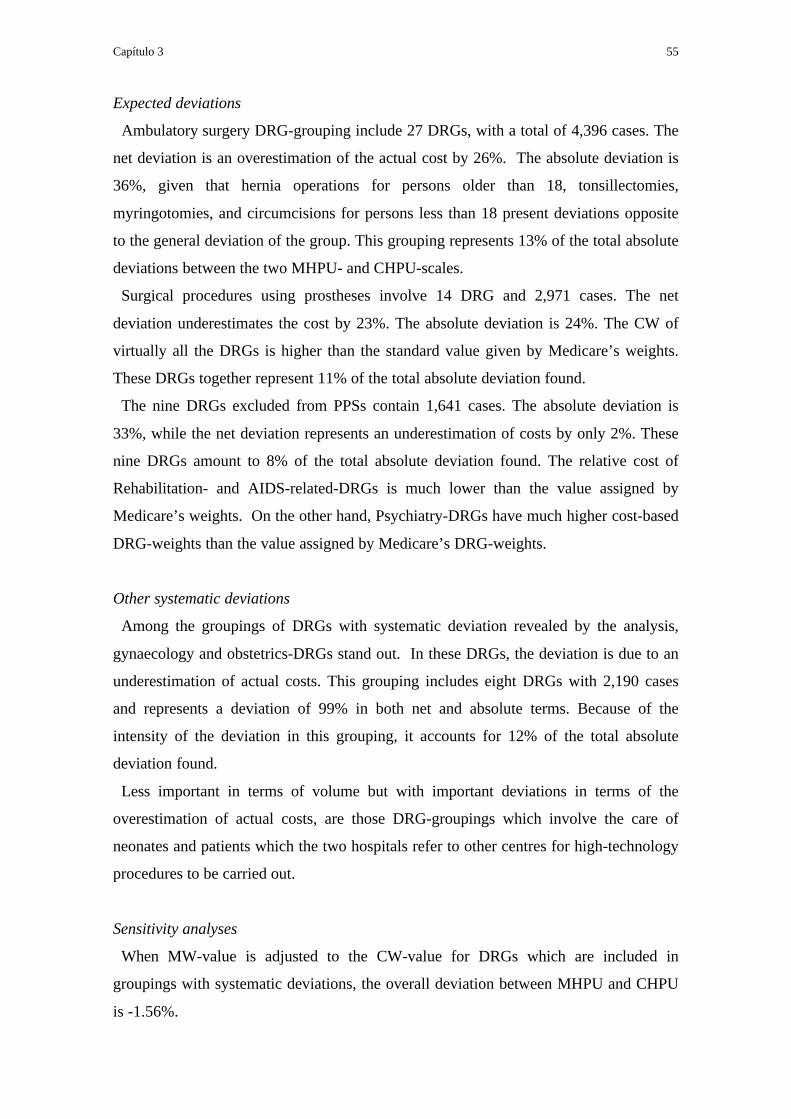
Capítulo 3 55
Expected deviations
Ambulatory surgery DRG-grouping include 27 DRGs, with a total of 4,396 cases. The
net deviation is an overestimation of the actual cost by 26%. The absolute deviation is
36%, given that hernia operations for persons older than 18, tonsillectomies,
myringotomies, and circumcisions for persons less than 18 present deviations opposite
to the general deviation of the group. This grouping represents 13% of the total absolute
deviations between the two MHPU- and CHPU-scales.
Surgical procedures using prostheses involve 14 DRG and 2,971 cases. The net
deviation underestimates the cost by 23%. The absolute deviation is 24%. The CW of
virtually all the DRGs is higher than the standard value given by Medicare’s weights.
These DRGs together represent 11% of the total absolute deviation found.
The nine DRGs excluded from PPSs contain 1,641 cases. The absolute deviation is
33%, while the net deviation represents an underestimation of costs by only 2%. These
nine DRGs amount to 8% of the total absolute deviation found. The relative cost of
Rehabilitation- and AIDS-related-DRGs is much lower than the value assigned by
Medicare’s weights. On the other hand, Psychiatry-DRGs have much higher cost-based
DRG-weights than the value assigned by Medicare’s DRG-weights.
Other systematic deviations
Among the groupings of DRGs with systematic deviation revealed by the analysis,
gynaecology and obstetrics-DRGs stand out. In these DRGs, the deviation is due to an
underestimation of actual costs. This grouping includes eight DRGs with 2,190 cases
and represents a deviation of 99% in both net and absolute terms. Because of the
intensity of the deviation in this grouping, it accounts for 12% of the total absolute
deviation found.
Less important in terms of volume but with important deviations in terms of the
overestimation of actual costs, are those DRG-groupings which involve the care of
neonates and patients which the two hospitals refer to other centres for high-technology
procedures to be carried out.
Sensitivity analyses
When MW-value is adjusted to the CW-value for DRGs which are included in
groupings with systematic deviations, the overall deviation between MHPU and CHPU
is -1.56%.

56 Medicare’s DRG-Weights vs. Cost-based DRG-Weights
Extrapolating MW and CW-structures to the total number of discharges of the Catalan
public sector, the deviation between MHPU and CHPU is 1.6%. The same extrapolation
made to the previous adjustment reveals a overall deviation of -1.2%.

Capítulo 3 57
Discussion
A cost-based DRG-structure has been determined based on information from a hospital
cost accounting system which is clearly suitable for the aim of allocating total costs
incurred to the patients. Because the majority of procedures are highly automated, costs
can be correctly allocated to the patients without any need to use less direct criteria.
In total, 12,700 million pesetas shared among 35,262 discharges have been analysed
which represent approximately 6% of the hospital-wide discharges from the Catalan
public health sector during a one-year period.87 Because the MW of the hospitals of the
MIH with respect to the MW of the whole public system is 1.143, the cost probably
represents a greater percentage. This greater percentage could also be due to other
factors not included in the case-mix and which correspond to the extra cost of teaching
and research,88 to the higher than average level of technology in these hospitals,70,83,89
and to the fact that they serve a low-income population71 and are situated in the most
densely populated metropolitan area in the system.90
Global Analysis
Cost-based weights have been determined and compared with MW. The analysis has
not invalidated the hypothesis of equality between these two structures and the degree
of correlation between them is very high.
The final net deviation between the CHPU-structure and the MHPU-structure is only
0.06%. Thus, MW fit well to the cost-structure analysed.
The sensitivity analyses performed reveal that the overall deviation is very slight. If the
difficulty of extrapolating the results of the two hospitals to the hospital-wide system is
accepted, the deviation is always less than 2%.
Diagnosis-related groups causing systematic deviations
What is undoubtedly of greatest interest is to see how the different DRG-groupings
which could explain differences with respect to Medicare’s weights-structure behave in
the same manner and with the same intensity as our original hypothesis predicted.
3 This information refers to 1996, according to the CHS.

58 Medicare’s DRG-Weights vs. Cost-based DRG-Weights
Thus, adjustments can be made to these weight-structures which could help to reduce
the systematic deviations which have appeared. Firstly, for some Ambulatory Surgery-
DRGs the adjustment should bear in mind that the deviation disappears in those
procedures which are normally carried out on an outpatient basis, such as circumcisions,
tonsillectomies, and myringotomies. For the other Ambulatory Surgery-DRGs,
incentives to perform procedures on an outpatient basis, in preference to inpatient
surgery, should remain until Ambulatory Surgery becomes the norm.
Secondly, the principal negative differences are associated with prostheses. The
adjustment should lead to a progressive decrease in their cost but, in the short term, this
extra cost to the hospitals should be recognised. Thirdly, a simple adjustment to the
weights of those DRG excluded from PPS would not be sufficient to solve the problem.
The example of existing PPSs which exclude these DRG should be followed and other
forms of payment should be sought. The payment system applied in Catalonia makes
these exclusions difficult because it includes these DRGs among "discharges" when
calculating the average DRG-weights.
The determination of CW has served to highlight other differences with respect to
MW. In certain cases it reveals problems of oversupply in relation to the real demand
for certain specialities, as can be seen from the costs of obstetrics and gynaecology-
DRGs. Here, MW serve as a reference point and provide invaluable information as far
as decision-making is concerned.91
In the same way, the cost of DRGs with expensive techniques (angioplasties, cardiac
catheterization, arteriographies) is overestimated by MW. The low relative cost is due to
the fact that the hospitals studied do not perform these procedures, or perform them only
rarely: patients are referred to high-technology centres which perform these procedures
and are then referred back to the original hospital until discharged. The codification
process incorporates these procedures according to CHS regulations, so that MW
recognise them but actual costs do not. These regulations should include a system of
inter-hospital billing within the CHS to avoid billing twice but this was unfortunately
not the case during the period studied. The new hospital payment system incorporated
in Catalonia in 1997 includes an internal billing system which will internalise this
deviation.
The sample is not representative of the different hospitals with their structural
complexities, catchment areas, relative organisational efficiency and case-mix;
consequently, any conclusions which might be drawn cannot be generalised.

Capítulo 3 59
Nevertheless, in an urban area with hospitals accredited as highly productive92 and
which carry additional loads such as teaching and research, MW would reimburse
99.94% of the actual cost according to the case-mix studied.
Another limitation of the study is that some DRGs have insufficient cases to be
analysed. Nevertheless, the DRGs analysed include more than 91% of inlier cases.
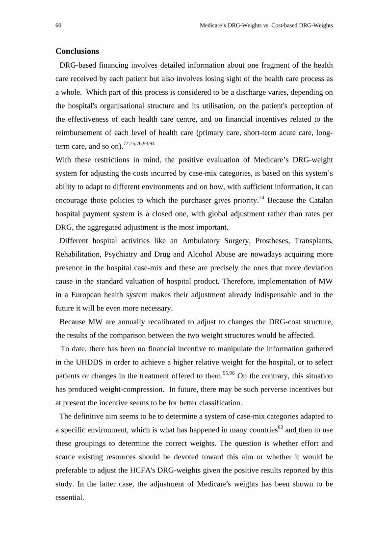
60 Medicare’s DRG-Weights vs. Cost-based DRG-Weights
Conclusions
DRG-based financing involves detailed information about one fragment of the health
care received by each patient but also involves losing sight of the health care process as
a whole. Which part of this process is considered to be a discharge varies, depending on
the hospital's organisational structure and its utilisation, on the patient's perception of
the effectiveness of each health care centre, and on financial incentives related to the
reimbursement of each level of health care (primary care, short-term acute care, long-
term care, and so on).72,75,76,93,94
With these restrictions in mind, the positive evaluation of Medicare’s DRG-weight
system for adjusting the costs incurred by case-mix categories, is based on this system’s
ability to adapt to different environments and on how, with sufficient information, it can
encourage those policies to which the purchaser gives priority.74 Because the Catalan
hospital payment system is a closed one, with global adjustment rather than rates per
DRG, the aggregated adjustment is the most important.
Different hospital activities like an Ambulatory Surgery, Prostheses, Transplants,
Rehabilitation, Psychiatry and Drug and Alcohol Abuse are nowadays acquiring more
presence in the hospital case-mix and these are precisely the ones that more deviation
cause in the standard valuation of hospital product. Therefore, implementation of MW
in a European health system makes their adjustment already indispensable and in the
future it will be even more necessary.
Because MW are annually recalibrated to adjust to changes the DRG-cost structure,
the results of the comparison between the two weight structures would be affected.
To date, there has been no financial incentive to manipulate the information gathered
in the UHDDS in order to achieve a higher relative weight for the hospital, or to select
patients or changes in the treatment offered to them.95,96 On the contrary, this situation
has produced weight-compression. In future, there may be such perverse incentives but
at present the incentive seems to be for better classification.
The definitive aim seems to be to determine a system of case-mix categories adapted to
a specific environment, which is what has happened in many countries63 and then to use
these groupings to determine the correct weights. The question is whether effort and
scarce existing resources should be devoted toward this aim or whether it would be
preferable to adjust the HCFA's DRG-weights given the positive results reported by this
study. In the latter case, the adjustment of Medicare's weights has been shown to be
essential.

Capítulo 4
Risk adjustment: beyond patient classification systems

62 Risk adjustment
Introduction
Considerable information on inpatients is available to those working in hospital
management. This information enables definition of hospital product and observation of
significant attributes that improve the characterisation of patient profile, the health care
process and resource use of the hospital where the patient was treated.21,48,49,97,98
However, analysis of documentation at the individual patient level provides only partial
information, often leading to a superficial description of what has occurred in the health
care process. Aggregated analysis is usually more complete, since it can establish a
resource use profile based on characteristics that define the level of patients’ need for
care.
Diagnosis-related groups (DRGs) have become the most commonly used tools for the
overall analysis of this information, defining products with a similar resource use and
clinical coherence.63 This classification system attempts to establish criteria for patient
grouping based on maximising inter-DRG cost variability and minimising intra-DRG
variability. In contrast, the number of groups must be limited to make the classification
functional for hospital product management.42 This was accomplished through different
DRG versions with the number of groups ranging from 357 to 641. DRGs were
introduced in Spain according to the criteria of Medicare, which uses the Health Care
Financing Administration (HCFA) version with 492 groups.
DRGs are useful in patient classification because they establish an invoicing between
the purchaser and different providers, and consequently they can be used in price
setting. Their capacity, strengths and weakness have been extensively analysed in the
literature.28,61,73,95 However, little in-depth research on the usefulness of DRGs in
hospital cost analysis has been published to date. Studies analysing the isocost capacity
per category presupposed by the DRG systems 5,6,29,66 have shown their limited ability
to reflect resource use variability31,32. The lack of information on real cost per patient
has made validation of DRGs as predictors of cost variability difficult.
At the same time, the ability of other characteristics of the health care process to
explain cost variability has been evaluated. These characteristics include length of stay,24 aspects related to severity17,43 comorbidities and complications22,99-101, characteristics
of provider management (efficiency102 or specialisation103), and the patient’s
socioeconomic status (SES).23,104,105

Capítulo 4 63
The need to understand DRGs as a valuation method of the activity performed and
consequently as a payment system has led to the usefulness of using DRGs as the initial
point of hospital cost analysis to be overlooked. In Europe, where there is universal
public coverage and where the hospitals obtain their incomes mainly from the public
sector, cost and cost variability should be analysed rather than market price.11 In this
setting, competition is not in prices, but in the continued functioning of the hospitals, in
patient access equity, and in the optimum allocation of final and overall resources.1,106
Thus, an analysis of health care activity cost and of the causes of its variability in
Europe is needed. Determination of the characteristics and causes of this cost would
allow improvements to be made to payment systems, which should first reflect cost and
then the standardisation of reasonable cost. This in turn would enable the creation of
adequate incentives to improve allocation of the available economic resources.
In spite of the considerable information available on hospital processes, cost
explanation is usually reduced to length of stay or diagnosis. Authors such as Iezzoni,21
Elixhauser22 or Peiró17 have popularised the concept of ‘risk adjustment’, which refers
to variability in the results of the hospital process as a consequence of variability in the
hospital process itself and in associated resource use. These authors have advanced the
study of the ability of administrative databases to contribute information for use in this
adjustment. Information available on the development of hospital activity has enabled
patient characterisation based on real resources use.
The aim of this study was to a advance the ability of the available hospital
administrative dataset to explain hospital discharge cost variability and specifically, to
analyse the extent to which the various DRG patient classification systems used today
are able to explain cost variability.
A cost database containing information on 35 262 discharges from the two public
teaching hospitals owned by the Municipal Institute of Health (MIH) in Barcelona
enabled evaluation of a range of information from the Minimum Data Set and other
registered data available in their information systems.
The research hypotheses were the following: (i) DRGs provide insufficient
information to explain the variability in observed cost; and (ii) use of the information
added by the Minimum Data Set substantially improves DRGs’ ability to explain cost
variability.

64 Risk adjustment
Methods
The 35 262 admissions from the MIH hospitals, admitted and discharged between
1995 and 1996, were retrospectively analysed (Table 1).
The relationship between total cost per patient and the variables and indexes extracted
from the available information were analysed. The main information sources were the
Minimum Data Set, with a maximum of eleven secondary codified diagnoses, and the
cost accounting system.
Hospital discharge cost is a monetary reflection of a series of activities and resource
uses incurred during the course of the patient’s treatment. These activities and resource
uses differ according to the product, severity of illness, and the patient’s other clinical
variables, SES characteristics, as well as to the management of the health care process.
Table 1. Baseline.H-DRG (1) A-DRG (2) APR-DRG (3)
DRG groups 470 313 319Cases per DRG 71 108 106
Inlierstotal cost 10 501 605 354 10 503 297 026 10 493 333 286
LOS 264 990 265 603 265 140discharges 33 585 33 718 33 713
Outliertotal cost 2 291 919 729 2 290 228 057 2 300 191 797
LOS 47 092 46 478 46 942discharges 1 677 1 544 1 549
Totaltotal cost 12 793 525 083 12 793 525 083 12 793 525 083
LOS 312 081 312 081 312 081discharges 35 262 35 262 35 262
Outlier (%)
Cost 17.9% 17.9% 18.0%LOS 15.1% 14.9% 15.0%
Discharges 4.8% 4.4% 4.4%Average values for inlier cases
Average discharge cost 312 687 311 504 311 255Average LOS 7.89 7.88 7.86
(1) HCFA-DRG(2) Adjacent HCFA-DRG(3) All Patient refined DRG
Variables
A set of variables associated with causes able to explain cost variability was
constructed from the information available. These variables were related to product

Capítulo 4 65
complexity (DRGs and outliers), disease seriousness (severity, complications,
comorbidities), patient characteristics (age, gender, SES characteristics), and
management of the health care process (readmission, circumstances on admission and
discharge, and surgical procedure).
Cost. The MHI’s hospital cost accounting system based on full costing allocation
ensured that the hospitals’ total costs were distributed among the patients.
Consequently, not only is the overall cost per patient known, but also its structure. Thus,
costs related to surgical procedures, intensive care unit treatment, pharmacy, radiology,
laboratory, prosthesis, and pathologic anatomy can be distinguished from costs related
to length of stay (LOS).
Medicare’s DRG-weights (MW). Patient classification systems were used to define
observed hospital product. As a first step, Medicare’s DRG weights were used. This is
the weight system used to value hospital activity in several European hospital payment
systems and is available only for the HCFA’s DRGs.11,13,15,16,20,63,107
Cost-based DRG-weights (CW). As an alternative to using Medicare’s DRG-weights, each
patient was assigned the CW that represents the average cost of all cases within a DRG
with respect to the average total cost of the database analysed.45 The difference in
observed cost-based weights between two discharges belonging to two different DRGs
is the closest possible approximation to inter-DRG variability. Any unexplained
differences must be due to intra-DRG variability not explained by patient classification
system.
Three DRG groupings were used in the analysis:
1. HCFA version 11 DRG grouping (H-DRG) which incorporates comorbidities,
complications and patient age as a splitting variable between product categories.
2. Adjacent-DRG (A-DRG) which are the H-DRG but regrouping categories in which
the difference was due to comorbidities, complications, or age;
3. All Patients Refined (APR)-DRG grouping (version 15)108, which leaves each
patient’s severity of illness to a complementary indicator (severity index).

66 Risk adjustment
Outlier cases. Medicare considers that product definition based on DRGs must correct
for cases of extreme cost compared with the average of cases belonging to a particular
group. These cases, although belonging to a specific DRG, imply a much higher
expenditure than the average of the specific DRG to which they belong.4-6,51 The
geometric mean plus two standard deviations was used to determine cases of
abnormally high cost. This method was applied to each classification system separately,
since each DRG category has a different cut-off point.
Severity. The severity of illness associated with each patient was valued using the
Disease Staging measurement system.31,32,109-111 For the APR-DRG classification
system, the APR-DRG severity indicator was used.
Comorbidities. Several authors have applied the Charlson99 Index to reveal
comorbidities associated with specific secondary diagnoses and the increased
probability of death associated with their presence,100,101,103,112 after transforming and
making it applicable to administrative data (appendix 1). Recently, Elixhauser et al.22
have described a set of 30 groupings of the International Classification of Diseases
(ICD-9-MC) diagnoses that imply comorbidity if they occur as secondary diagnoses.
However, when the secondary diagnosis giving rise to the comorbidity coincides with a
specific DRG they are considered a complication and not a comorbidity (appendix 2).
This method is based on administrative data and incorporates individual variability
parameters for each comorbidity group with respect to costs. A database with 11
possible codified diagnoses enabled use of the algorithm.
Complications. Complications are processes or events arising from hospitalisation that
worsen the patient’s condition. Complications may be general (e.g., urinary infection) or
related to the complaint treated. General complications are shown in appendix 3.
Diagnoses considered as a complication by the method of Elixhauser et al. are included
in this variable. A dummy variable distinguishing cases with complications was used.
Both comorbidity and complications indicators were used to complement the
information added by the A-DRG.
Readmission . Information both on the discharges during the last three months of 1995
and on those during the first three months of 1997 were added to the 1995 and 1996

Capítulo 4 67
databases. This information was then used to calculate the number of readmissions for
each patient. In this analysis, an admission was considered as readmission of a
particular patient within 90 days of the previous admission. The accumulated number of
admissions for each patient gave the value of each patient’s readmission variable. The
first admission of a readmission process is called the Index admission.
Hospital. The installed supply and the organisation of each hospital were considered to
influence cost variability. A dummy variable was used to control for these differences.89
Admission circumstance. Emergency admissions may involve more intensive resource
use than planned ones. Firstly, emergency admissions are often more complex than
planned ones after adjusting for case-mix. Secondly, the cost of the diagnostic tests
carried out in emergency admissions belongs to the episode studied, unlike the cost of
those carried out before planned admissions.
Exitus. The consequences of a patient dying while hospitalised vary. On the one hand,
death may increase cost due to higher treatment intensity, but on the other hand, it may
reduce LOS and, consequently, final cost is reduced when the death occurs before the
normal LOS of patients in a specific DRG category.
Age. It is generally believed that hospital resource use tends to be concentrated during
the last years of a person’s life.113 Therefore, age positively explains part of cost
variability, independently of the clinical characteristics of the disease being treated.
Gender. Gender is a patient-defining variable that may add explanatory power to cost
evolution after variables related to the product, complexity, severity, and age have been
adjusted.
Socioeconomic status (SES). Several studies have supplied information on the effect of
low SES on cost.114 Consequently, the Household Economic Capacity Index (HECI)
was used.115 This index synthesises differences in economic capacity between small
areas in a continuous valuation. Although it is an ecological variable, characteristics of
these small areas provide information on the SES of patients living in the city of

68 Risk adjustment
Barcelona. Among the 35 262 discharges, 26 676 were living in Barcelona City and
consequently information on their SES was available.
Surgical procedure. A dummy variable based on whether patients underwent surgical
procedures or not was determined using DRG type. Although this variable is
incorporated in DRG definition, it is expected that there are characteristics related to
hospital structure and organisation that may be captured through this circumstance.
Analysis
In the present study, real discharge cost variability based on a set of variables
generated by and available in any European hospital is explained. The sign and the
explanatory power of each variable related to discharge cost was evaluated.
Three different approaches to the product were used depending on the DRG grouping
system. On the one hand, we used the H-DRG, which already incorporates the
components of comorbidity and complications. On the other hand, we used the same
DRGs, after eliminating differences in comorbidities, complications, and age (A-DRG).
In these cases, the Elixhauser Index (A-DRGE) and the Charlson Index (A-DRGC)
were applied. Finally we applied the patient classification system based on APR-DRG
where severity definition is determined by the APR-DRG’s grouper severity indicator.
The relationship between discharge cost and the variables constructed was established
with an unadjusted bivariate correlation. The correlation analysis was performed
through Pearson’s lineal correlation for continuous variables and through Spearman’s
lineal correlation for dummy variables.
The multivariate analysis was performed through ordinary least squares by relating
total discharge cost to explanatory variables. A logarithmic transformation of the
variables considered continuous (total cost, SES indicator, comorbidity index and
average cost weight) was applied to reduce the magnitude effect, thus avoiding the
introduction of a fictitious relationship between variables. Similarly, the logarithmic
transformation, which approximates the normal distribution expected for these
variables, was applied. This guaranteed the absence of bias in the statistics used to
validate the estimation.25-27,31,41,46
To obtain more robust cost-based weights, cases belonging to a DRG with less than 37
cases were excluded. A cut-off point was calculated with the aim of including 95% of
cases.

Capítulo 4 69
To answer the initial hypothesis, the multivariate analysis was performed in various
stages:
Equation 1: Analysis of the ability of different DRG patient classification systems
using Medicare’s weights (MW) and cost-based weights (CW).
Equation 2: The set of variables that provides information to risk adjustment. The
variables corresponding to each patient classification system used were introduced. To
simplify the analysis, this completed model was applied only to cases not considered
outliers.

70 Risk adjustment
Results
After exclusion of outliers, the 35 262 discharges were grouped into 313 product
categories for the A-DRG with an average of 108 cases. The results for APR-DRG were
fairly similar: there were 319 DRGs with an average of 106 cases. In contrast, H-DRG
had 470 groups with an average of only 71 patients (Table 1).
Average discharge cost was 362 813 ptas. Average cost, after excluding outliers,
oscillated between 311 255 for APR-DRG and 312 687 ptas. for H-DRG. Outlier cases
accounted for 4.4% of APR-DRG and 4.8% of H-DRG. However, these cases
represented about 15% of stays and 18% of cost, independently of the grouping method.
There was significant gross lineal correlation in all variables except ecological SES.
The sign was positive in all variables except readmissions (Table 2).
Table 2. Crude correlation between patient cost and independent variables
Variable (3)product
Medicare's Weights continuous 0.4762 *HCFA-DRG CW (1) continuous 0.5532 *
Adjacent HCFA-DRG CW (1) continuous 0.5299 *APR-DRG CW (1) continuous 0.5288 *
HCFA-DRG outliers dummy 0.3091 *Adjacent HCFA-DRG outliers dummy 0.3075 *
APR-DRG outliers dummy 0.3145 *Elixhauser's comorbidities continuous 0.1564 *Elixhauser's complications dummy 0.1131 *
Charlson continuous 0.1483 *APR-DRG severity indicator categorical 0.2211 *
Disease Staging categorical 0.1551 *socioeconomic status
Age continuous 0.1369 *Gender dummy 0.0165 *
HECI (2) continuous nshospital process
Readmission index dummy 0.0346 *Readmissions continuous -0.0258 *
Hospital dummy 0.0545 *Emergency admissions dummy 0.0996 *
Exitus dummy 0.1566 *Surgical procedure dummy 0.1521 *
*: significance p<0.01; ns: non significance(1) Cost based DRG-Weights without outlier cases.(2) Household economic capacity index (HECI)(3) Pearson's lineal correlation for continuous variables and through Spearman's lineal correlation for dummy variables.
The ability of MWs to explain cost variability estimated through R2 was 19.3%. CWs
completely representative of the sample studied achieved an explanatory power of
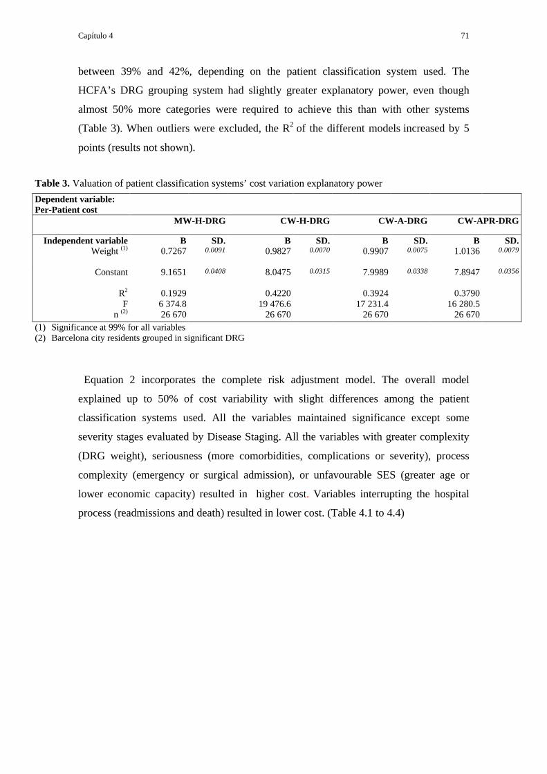
Capítulo 4 71
between 39% and 42%, depending on the patient classification system used. The
HCFA’s DRG grouping system had slightly greater explanatory power, even though
almost 50% more categories were required to achieve this than with other systems
(Table 3). When outliers were excluded, the R2 of the different models increased by 5
points (results not shown).
Table 3. Valuation of patient classification systems’ cost variation explanatory power
Dependent variable:Per-Patient cost
MW-H-DRG CW-H-DRG CW-A-DRG CW-APR-DRG
Independent variable B SD. B SD. B SD. B SD.Weight (1) 0.7267 0.0091 0.9827 0.0070 0.9907 0.0075 1.0136 0.0079
Constant 9.1651 0.0408 8.0475 0.0315 7.9989 0.0338 7.8947 0.0356
R2 0.1929 0.4220 0.3924 0.3790F 6 374.8 19 476.6 17 231.4 16 280.5
n (2) 26 670 26 670 26 670 26 670(1) Significance at 99% for all variables(2) Barcelona city residents grouped in significant DRG
Equation 2 incorporates the complete risk adjustment model. The overall model
explained up to 50% of cost variability with slight differences among the patient
classification systems used. All the variables maintained significance except some
severity stages evaluated by Disease Staging. All the variables with greater complexity
(DRG weight), seriousness (more comorbidities, complications or severity), process
complexity (emergency or surgical admission), or unfavourable SES (greater age or
lower economic capacity) resulted in higher cost. Variables interrupting the hospital
process (readmissions and death) resulted in lower cost. (Table 4.1 to 4.4)

72 Risk adjustment
Table 4.1 Risk adjustment model based on HCFA-DRG (H-DRG)Dependent variable: Per-patient cost B Standard error T Significance
Explanatory variables:Product
CW-H-DRG 0.9228 0.0072 128.5890 *Severity stage 2 0.0182 0.0097 1.8720 ***Severity stage 3 0.0352 0.0115 3.0740 **
Socioeconomic status (SES)Age 0.0158 0.0048 3.2630 *
Gender -0.0205 0.0074 -2.7950 *Household Economic Capacity Index -0.0398 0.0131 -3.0430 *
Hospital processReadmission index 0.1080 0.0244 4.4433 *
Readmissions -0.1356 0.0140 -9.7180 *Hospital -0.1289 0.0107 -12.0890 *
Emergency admission 0.2418 0.0086 28.0030 *Exitus -0.2760 0.0200 -13.7810 *
Surgical procedure 0.1846 0.0092 19.9890 *Constant 0.1846 0.0092 19.9890 *
R2 0.5082
F 2 188.19
n (1) 25 398
(1) Barcelona city residents grouped in significant DRGs
* significance at 99%
** significance at 95%
*** non-significant

Capítulo 4 73
Table 4.2 Risk adjustment model based on A-DRGE:Adjacent HCFA-DRG with Elixhauser's comorbidities and complications index.
Dependent variable : Per-patient cost B Standard error T Significance
Explanatory variables:Product
CW-A-DRGE 0.8961 0.0075 119.8100 *Elixhauser's comorbidities index 0.1418 0.0072 19.6610 *Elixhauser's complications index 0.1063 0.0117 9.0770 *
Severity stage 2 0.0216 0.0099 2.1860 **Severity stage 3 0.0160 0.0119 1.3440 ***
Socioeconomic status (SES)Age 0.0177 0.0050 3.5500 *
Gender -0.0380 0.0075 -5.0710 *Household Economic Capacity Index -0.0393 0.0133 -2.9680 *
Hospital processReadmission index 0.1192 0.0247 4.8200 *
Readmissions -0.1495 0.0142 -10.5250 *Hospital -0.1707 0.0111 -15.4120 *
Emergency admission 0.2499 0.0088 28.4910 *Exitus -0.2941 0.0205 -14.3230 *
Surgical procedure 0.2349 0.0094 24.8660 *Constant 8.3495 0.0725 115.1640 *
R2 0.4893
F 1 747.29
n (1) 25 516
(1) Barcelona city residents grouped in significant DRGs* significance at 99%
** significance at 95%
*** non-significant

74 Risk adjustment
Table 4.3 Risk adjustment model based on A-DRGC:Adjacent HCFA-DRG with Charlson's comorbidities index.Dependent variable : Per-patient cost B Standard error T Significance
Explanatory variables:Product
CW-A-DRGC 0.8987 0.0075 120.0790 *Charlson's comorbidities index 0.1916 0.0096 19.9480 *
Severity stage 2 0.0219 0.0099 2.2140 *Severity stage 3 0.0231 0.0117 1.9710 **
Socioeconomic status (SES)Age 0.0219 0.0050 4.4090 *
Gender -0.0396 0.0075 -5.2660 *Household Economic Capacity Index -0.0399 0.0133 -3.0090 *
Hospital processReadmission index 0.1186 0.0247 4.7910 *
Readmissions -0.1521 0.0142 -10.6930 *Hospital -0.1579 0.0110 -14.3560 *
Emergency admission 0.2570 0.0088 29.3750 *Exitus -0.2984 0.0206 -14.4770 *
Surgical procedure 0.2376 0.0095 25.0100 *Constant 8.3190 0.0725 114.7130 *
R2 0.4880
F 1 871.3
n (1) 25 516
(1) Barcelona city residents grouped in significant DRG
* significance at 99%
** significance at 95%
*** non-significant

Capítulo 4 75
Table 4.4 Risk adjustment model based on All Patient Refined-DRGDependent variable: Per-patient cost B Standard error T Significance
Explanatory variables:Product
CW-APR-DRG 0.9259 0.0077 119.513 *APR-DRG severity index 0.4222 0.0168 25.151 *
Socioeconomic status (SES)Age 0.0139 0.0049 2.8290 *
Gender -0.0357 0.0075 -4.7740 *Household Economic Capacity Index -0.0405 0.0133 -3.0490 *
Hospital processReadmission index 0.2346 0.0247 9.5130 *
Readmissions -0.2881 0.0142 -20.3260 *Hospital -0.1687 0.0109 -15.5170 *
Emergency admission 0.2270 0.0088 25.7570 *Exitus -0.3453 0.0207 -16.6850 *
Surgical procedure 0.2358 0.0094 25.0420 *Constant 7.9475 0.0726 109.4270 *
R2 0.4868
F 2 200.92
n (1) 25 510
(1) Barcelona city residents grouped in significant DRGs
* significance at 99%
** significance at 95%
*** non-significant

76 Risk adjustment
Discussion
This study shows that the ability of different patient classification systems commonly
used in our setting to explain hospital cost variability and to determine resource
allocation can be evaluated by using information from a large number of cases on cost
per patient. The first issue to take into consideration is that using patient classification
systems with imported standardised weights contributes very little to information on
cost variability. Twenty percent of the variability is a low percentage but is similar to
that obtained in other studies.31,32
Normally, the poor ability of DRG-weights to explain cost variability has been
attributed to the weight systems used.45 Using the average value after excluding outliers,
based on the observed costs of the database analysed as weight structure, maximises the
explanatory power of the classification systems used. Certainly, the doubling of
explanatory power after using a completely representative weight structure suggests that
the possibility of improving the utilisation of these systems exist. However, 40% is not
a high percentage. Furthermore, this percentage is the most satisfactory possible since it
was obtained from two hospitals sharing the same management and thus, it does not
show either input price differences or inter-hospital variability.
Another possibility for improvement concerns the effect of outliers in blurring the
explanatory power of these grouping systems, which use the group mean to characterise
all the cases that they incorporate.
Between 4.4% and 4.8% of cases were of extremely high cost. This cost could not be
approximated by the mean of the distribution, since it was too far from its distribution
core. Their effect in terms of cost was 18%, a figure which led to a displacement of the
mean value to higher values, making the mean less representative of all the cases
incorporated. Excluding outliers substantially increased the explanatory power of
DRGs.
After the increase due to exclusion of outliers was discounted, the set of variables
enabling characterisation of patient cost and comparison of resource needs based on
different circumstances linked to the patient, process or supply, did not significantly add
explanatory power. However, signs and stability of parameters of the different
classification systems can add considerable information about the causes of hospital
discharge cost variability:

Capítulo 4 77
1. DRG systems with few product categories can achieve a similar explanatory
power to those that need 50% more categories, when systems to value the
seriousness of the disease treated are used.
2. There are few differences between Elixhauser’s and Charlson’s comorbidities
and complications measures. However, the specificity of the former in
distinguishing complications and comorbidities should be positively valued.
3. The APR-DRG system is the logical synthesis of the points 1 and 2 that seeks to
minimise the number of products and to maximise information about their
seriousness.
4. Differentiating between severity, comorbidities and complications is central to
an analysis of the different causes of cost variability. The Adjacent-HCFA-
DRGs (A-DRG) could provide qualitatively richer information.
5. The simplicity of the Charlson and Elixhauser indexes and their immediate
applicability is an advantage, since the severity indicator algorithm of the APR-
DRG is much more complicated and less intelligible.
In this study, information on the SES characteristics of 26 676 patients, which is not
normally available, was used to evaluate their effect on cost. There was an inverse
relation between SES and cost, as in Medicare’s payment system, in which serving a
population with a lower SES than the average is valued as a justifiable extra cost. This
relationship was not captured in the bivariate analysis, but is clearly relevant after
adjusting for the variables that define product and other circumstances. Because it is
very difficult to collect information on the SES of individual patients in administrative
databases, trust will have to be placed in ecological variables, as is the case with the
HECI when analysing the effect of SES on hospital resource use.
The remaining adjustment variables behaved in accordance with the initial hypothesis:
readmissions resulted in lower average cost per episode while index admissions tended
to result in higher costs. Similarly, death reduced the cost of hospital episodes. This was
observed only in the multivariate analysis since in the bivariate analysis, death was
associated with higher cost.
Even though this study presents the limitation of not representing a sufficiently general
setting to enable extrapolation of the conclusions to an entire health care system, the
results obtained should be valued as highly relevant as they lead to different health
policy implications that should not be ignored:

78 Risk adjustment
1. The ability of administrative databases to define product and value its cost does not
end in DRG grouping. Many aspects could be improved by using information
obtained from administrative databases.
2. The relevance of outliers, because of their intense resource use, should be integrated
into activity valuation based on DRG.
3. Adjustment of DRG-weights to the environment in which they are to be used is
strongly recommended.
4. Aspects associated with patient characteristics and the hospital process, such as
severity, should be valued in order to achieve a good approximation of patient cost.
5. A clear relationship was seen between resource use and the patient SES, which
should be integrated into the valuation of cost considered justifiable.
From these five points it can be concluded that a valuation of different hospital
activities of a health care system that is based only on DRG-weights can be very
inequitable, since these valuation deficiencies may affect some hospitals more deeply
than others.
Because only two hospitals sharing the same type of management and following the
same guidelines were analysed, these five aspects cannot be associated with structural
differences, but must be associated with the activity performed. In other words, they
must be related to casemix and not to structural differences. According to this
reasoning, any payment system based on activity should include these five causes of
cost variability in their method of valuing activity.
This is not the case in the Catalan or Andalusian payment systems mentioned above.
These models consider that beyond Medicare’s DRG-weights, no other reason for
variability apart from structural differences between centres exists.

Capítulo 4 79
Conclusions
Hospital cost can be reasonably well characterised with the available information.
DRGs are not questioned as a tool for hospital activity payment when the purpose is to
give a price to the provider-purchaser relationship. Until now, the crossed subsidies
among cases in the same DRG and across DRGs have been assumed to provide
satisfactory overall application. However, the limitations of DRGs to explain resource
use variability in cost analysis are clear. Nowadays, the available information permits
greater insight into each patient’s cost level and thus, resources can be more efficiently
allocated.
Explanation of what determines per-patient cost should not be confined to DRGs: all
the tools available in hospitals’ current information systems should be used in cost and
risk adjustment.
Measures that complement the information added by DRGs can easily be applied to
administrative databases. Only improvement in the weight system, consideration of
outliers, and valuation of seriousness can make the valuation of justifiable cost for
different hospitals more objective. Among these variables those that potentially offer
greater potential improvement seem to be those that adjust weights to the context in
which they are applied and those that correctly identify outliers.
In conclusion, qualitative improvement of the information in the Minimum Data Set
should be exploited and would permit a much more accurate characterisation of hospital
product and its cost.

80 Risk adjustment
Appendix 1. Scoring the Charlson's comorbidity index from secondary diagnoses.Weights Conditions ICD-9-codes
1 Myocardial infarction 410, 411Congestive heart failure 398, 402, 428
Peripheral vascular disease 440-447Dementia 290, 291, 294
Cerebrovascular disease 430-433, 435Chronic pulmonary disease 491-493
Connective tissue disease 710, 714, 725Ulcer disease 531-534
Mild liver disease 571, 5732 Hemiplegia 342, 434, 436, 437
Moderate or severe renal disease 403, 404, 580-586Diabetes 250
Any tumour 140-195Leukemia 204-208
Lymphoma 200, 202, 2033 Moderate or severe liver disease 070, 570, 5726 Metastatic solid tumor 196-199
Adapted from D'Hoore, 1993.
Appendix 2. Definitions of comorbidities
Comorbidity ICD-9-CM codes DRG screen: case does not have thefollowing disorders (DRG)
1.Congestive heart failure 398.91, 402.11, 402.91, 404.11,404.13, 404.91, 404.93, 428.0-428.9
Cardiac
2. Cardiac arrhythmias 426.10, 426.11, 426.13, 426.2-426.53,426.6-426.89, 427.0, 427.2, 427.31,427.6, 427.9, 785.0, v45.0, v53.3
Cardiac
3. Valvular disease 093.20-093.24, 394.0-397.1, 424.0-424.91, 746.3-746.6, v42.2, v43.3
Cardiac
4. Pulmonary circulation disorders 416.0-416.9, 417.9 Cardiac or COPD(88)
5. Peripheral vascular disorders 440.0-440.9, 441.2, 441.4, 441.7,441.9, 443.1-443.9, 447.1, 557.1,557.9, v43.4
Peripheral vascular (130-131)
6. Hypertension:
uncomplicated 401.1, 401.9 Hypertension (134)
complicated 402.10, 402.9, 404.1, 404.90, 405.11,405.19, 405.91, 405.99
Hypertension (134) or cardiac or renal
7. Paralysis 342.0-342.12, 342.9-344.9 Cerebrovascular (5, 14-17)
8. Other neurological disorders 331.9, 332.0, 333.4, 333.5, 334.0-335.9, 340, 341.1-341.9, 345.00-345.11, 345.40-345.51, 345.80-345.91,348.1, 348.3, 780.3, 784.3
Nervous system (1-35)
9. Chronic pulmonary disease 490-492.8, 493.00-493.91, 494, 495.0-505, 506.4
COPD (88) or asthma (96-98)

Capítulo 4 81
10. Diabetes, uncomplicated (1) 250.00-250.33 Diabetes (294-295)
11. Diabetes, complicated (1) 250.40-250.73, 250.90-250.93 Diabetes (294-295)
12. Hypothyroidism 243-244.2, 244.8, 244.9 Thyroid (290) or endocrine (300-301)
13. Renal failure 403.11, 403.91, 404.12, 404.92, 585,586, v42.0, v45.1, v56.0, v56.8
Kidney transplant (302) or renal failure /dialysis (316-317)
14. Liver disease 070.32, 070.33, 070.54, 456.0, 456.1,456.20, 456.21, 571.0, 571.2, 571.3,571.40-571.49, 571.5, 571.6, 571.8,571.9, 572.3, 572.8, v42.7
Liver
15. Peptic ulcer disease excludingbleeding
531.70, 531.90, 532.70, 532.90,533.70, 533.90, 534.70, 534.90, v12.71
GI hemorhage or ulcer (174-178)
16. AIDS 042-044.9 HIV (488-490)
17. Lymphoma 200.00-202.38, 202.50-203.01, 203.8-203.81, 238.6, 273.3, v10.71, v10.72,v10.79
Leukemia/lymphoma
18. Metastatic cancer(2) 196.0-199.1 Cancer
19. Solid tumour without metastasis(2)
140.0-172.9, 174.0-175.9, 179-195.8,v10.00-v10.9
Cancer
20. Rheumatoid arthritis/collagenvascular diseases
701.0, 710.0-710.9, 714.0-714.9,720.0-720.9, 725
Connective tissue (240-241)
21. Coagulopathy 286.0-286.9, 287.1, 287.3-287.5 Coagulation (397)
22. Obesity 278.0 Obesity procedure (288) or nutrition /metabolic (296-298)
23. Weight loss 260-263.9 Nutrition / metabolic (296-298)
24. Fluid and electrolyte disorders 276.0-276.9 Nutrition / metabolic (296-298)
25. Blood loss anemia 280.0 Anemia (395-396)
26. Deficiency anemias 280.1-281.9, 285.9 Anemia (395-396)
27. Alcohol abuse 291.1, 291.2, 291.5, 291.8, 291.9,303.90-303.93, 305.00-305.03, v113
Alcohol and drug (433-437)
28. Drug abuse 292.0, 292.82-292.89, 292.9, 304.00-304.93, 305.20-305.93
Alcohol and drug (433-437)
29. Psychoses 295.00-298.9, 299.10-299.11 Psychoses (430)
30. Depression 300.4, 301.12, 309.0, 309.1, 311 Depression (426)
Cardiac: 103-108, 110-112, 115-118, 120-127, 129, 132-133, 135-143;Renal: 302-305, 315-333; Liver: 199-202, 205-208; Leukemia/Lymphoma: 400-414, 473, 492;Cancer: 10, 11, 64, 82, 172, 173, 199, 203, 239, 257-260, 274, 275, 303, 318, 319, 338, 344, 346, 347, 354, 355, 357, 363,366, 367, 406-414.(1) If complicated diabetes appears, uncomplicated diabetes is not counted. (2) If metastasis appears cancer is not counted.Adapted from Elixhauser, 1998.
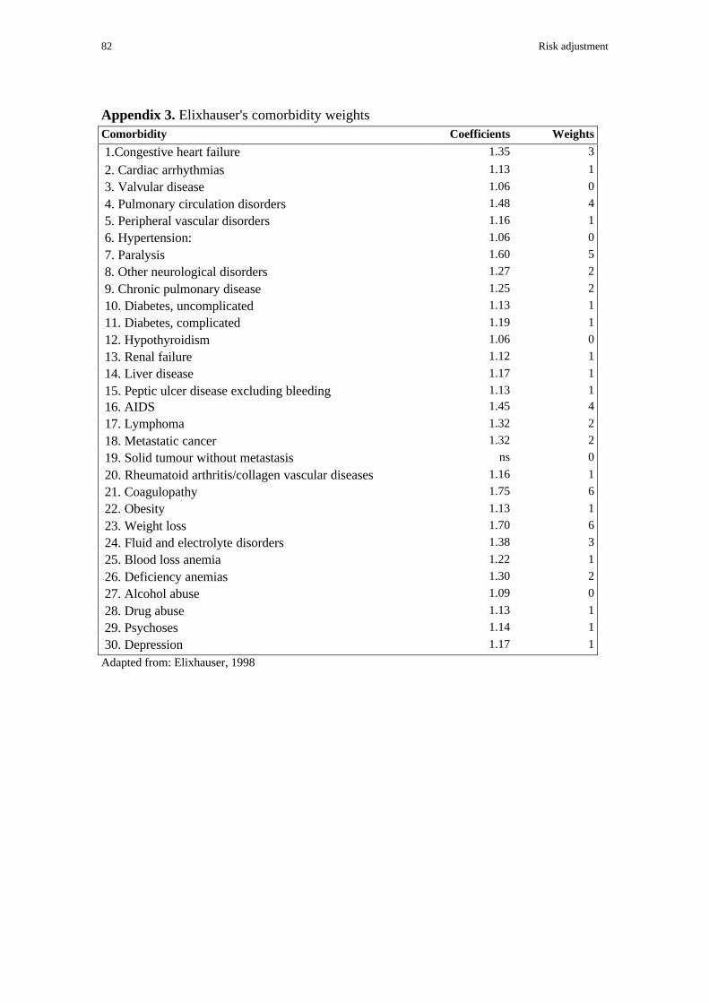
82 Risk adjustment
Appendix 3. Elixhauser's comorbidity weightsComorbidity Coefficients Weights
1.Congestive heart failure 1.35 3
2. Cardiac arrhythmias 1.13 1
3. Valvular disease 1.06 0
4. Pulmonary circulation disorders 1.48 4
5. Peripheral vascular disorders 1.16 1
6. Hypertension: 1.06 0
7. Paralysis 1.60 5
8. Other neurological disorders 1.27 2
9. Chronic pulmonary disease 1.25 2
10. Diabetes, uncomplicated 1.13 1
11. Diabetes, complicated 1.19 1
12. Hypothyroidism 1.06 0
13. Renal failure 1.12 1
14. Liver disease 1.17 1
15. Peptic ulcer disease excluding bleeding 1.13 1
16. AIDS 1.45 4
17. Lymphoma 1.32 2
18. Metastatic cancer 1.32 2
19. Solid tumour without metastasis ns 0
20. Rheumatoid arthritis/collagen vascular diseases 1.16 1
21. Coagulopathy 1.75 6
22. Obesity 1.13 1
23. Weight loss 1.70 6
24. Fluid and electrolyte disorders 1.38 3
25. Blood loss anemia 1.22 1
26. Deficiency anemias 1.30 2
27. Alcohol abuse 1.09 0
28. Drug abuse 1.13 1
29. Psychoses 1.14 1
30. Depression 1.17 1
Adapted from: Elixhauser, 1998

Capítulo 5
Constructing inpatient cost function: from risk adjustment to the
behaviour of variables defining hospital process

84 Inpatient cost function
Introduction
Inpatient cost variability has been described as the most serious problem affecting the
establishment of cost estimations for contracting and hospital efficiency analysis.28
Risk adjustment21,31 aims to establish and isolate the causes of global variability in per-
inpatient cost by constructing instruments that group patients, the most commonly used
being the Diagnosis-Related Groups (DRG). Other instruments adjust the characteristics
of seriousness, such as comorbidities and complications indicators (the Charlson99,101
and Elixhauser indexes,22) or severity in the case of Disease Staging.109 Different ways
of approaching the patient’s socio-economic status have also been studied. These and
other instruments have led to the continued improvement of per-patient cost variability
adjustment.23 Most studies have used one or other of these instruments but only a few
have used all of them together to construct an overall model of cost function.
The main limitations of these approaches concern the difficulty of determining real
per-inpatient cost and consequently of using length of stay (LOS) as a ‘proxy’
variable.24,111 Another limitation is that these cost estimations have been used in the
global cost valuation of the provider or hospital system.26,27 Consequently, the point at
which the set of characteristics defining patient cost variability outlines a per-patient
cost function has not definitively been determined.
Previous analyses have determined the most appropriate tools and the adjustments
necessary in a database of per-patient observed costs. With these premises already
solved, per-patient cost function should be constructed by determining the most
appropriate formulation, taking into account the necessary variables and those that are
available.
The aim of this study was to define an ICF that would incorporate the variables that
best explain inter-DRG and intra-DRG variability. Above all, we wanted to analyse ICF
behaviour and, in particular, the behaviour of the variables that determine intra-GRD
variability.
A database containing information on 35 262 patients with per-patient cost and the
Minimum Data Set (MDS) information of two public and teaching hospitals owned by
Barcelona’s Municipal Institute of Health were used to establish the relationship
between real observed cost and the variables that explain its variability.

Capítulo 5 85
Methodology
Cost function
Hospital cost function (HCF) is a multiproduct function characterised by economies of
scale and scope. However, in the short-term, cost variations among products are
determined by different relative input needs because the hospital supply remains
constant and the spectrum of activities performed by the hospital and its volume does
not vary over short periods.
Within hospitals, product definition has historically been reduced to large divisions
(inpatients, emergencies, ambulatory processes)26 and within the inpatient, the most
widespread definitions are the patient classification systems, mainly DRGs.30 A large
part of the patient’s health care process and consequently of the patient’s final cost is
determined by the physician’s decision. The cost of patients’ belonging to the same
DRG tends to be the same but differs from the average cost of other DRGs due to
differences in care, procedures, diagnostic tests and resource use needs. Thus the HCF is
formulated as following:
HCFi= C(Yi, Wi) + Ui (1)
Where ‘i’ designates the hospital, ‘Y’ is the vector that includes the line of product and
in the case of inpatients differentiates between casemix (through DRG), ‘W’ is the input
price vector that defines the relationship between the physical need of the input vector
and the output cost, and ‘U’ is the randomly distributed error.
Specification of hospital multiproduct cost function.
Hospital multiproduct cost function has been analysed by several authors,25,27 but
almost all of them have analysed how the output typology could define or justify the
cost differences between hospitals. Few of them have analysed the cost variability due
to differences within product category that give rise to this variability.
Concerning inter-hospital cost variability, very rudimentary definitions of output have
been used due to the limitations of the information systems and because the functional
forms permit only a small number of parameters. In 1967 Feldstein was the first to
analyse hospital cost function, using a non-flexible cost function with 8 output groups.

86 Inpatient cost function
116 In 1983 Conrad and Strauss used translog cost function based on structural form
(with only outputs and prices) to analyse three output groups and four input
categories.117 Cowing and Holtmann used the same translog cost function for five
outputs and six input categories.118
In 1986 Grannemann , Brown and Pauly used a ‘hybrid functional form’ in which
inter-hospital cost variability was explained by the structural regressors, output
categories and input prices and by ad-hoc specification variables.26
In 1997 Söderlund et al. postulated the following relationship: average cost per
inpatient = a function of (average casemix, average long stay days per inpatient (the
mean LOS of episodes above the average for their healthcare resource group),
percentage of multiple episodes, outpatient attendances per inpatient, accident and
emergency visits per inpatient, day visits per inpatient, student teaching units per
inpatient, prices of capital items, wage prices, scale of activity, hospital size, degree of
specialisation, trust status, competition from other hospitals, and mix of purchasers).
These authors postulated a simple linear relationship between average costs per
inpatient and the explanatory variables without considering possible interactions
between these variables.119
All these specifications are hospital cost functions, and all of them establish a trade-off
between correct output definition and cost function specification. To answer clinicians’
and managers’ questions concerning the reasons for patient cost variability, a per-patient
cost function in a given hospital with given prices should be constructed that would take
into account other restrictions and other aims. In this situation, product definition is the
most important issue and neither the number of categories nor the number of variables
that define the product for each patient should pose problems.
Only a small number of authors have analysed per-inpatient cost variability more
recently. These analyses have outweighed the optimal valuation of hospital product.
Calore and Iezzoni (1987),31 defined a relationship between inpatient cost and an
additive and separable cost function which is the log-transformation of a Cobb-Douglas
cost function(2):
LnCOST= α0 + α1 lnW + α2 DRG+ α3 SEV +α4 AGE+ α5 COMORB +α6 DIED+ α7 TEACH+ e (2)
Where LnCOST is the natural log of Part-A- inpatient cost in the Medicare system, W
is the Health Care Financing Administration’s (HCFA) hospital wage index, DRG is a

Capítulo 5 87
group of dummy variables for each DRG; SEV is a vector of dummy variables for the
severity index used (patient management categories or Disease Staging); AGE is a
dummy variable for patients over the age of 80 years; COMORB is a dummy variable
for patients with unrelated comorbidity; DIED is a dummy variable for patients who
died and TEACH is a dummy for teaching hospital.
The aim of this specification was to analyse the marginal increase in explanatory
power for the introduction of severity measures over basic product definition based on
DRGs. Estimated cost was used as a proxy of observed cost. Very similar analyses were
performed by Thomas and Ashcraft (1991)32, Averill et al. (1992),120 and Söderlund et
al.(1996) 6, but without complementary independent variables (Table 1).
All these authors have tried to value the part of total cost variability explained by
DRGs or other patient classification systems and the explanatory power using severity
measures that complement the DRG system. Under structural cost function specification
these examples would not be considered cost functions because they do not include
input prices.
These authors’ findings reveal that DRG product classification explains less than 35%
of cost variability using trimmed data when global hospital cost is analysed. If the
analysis is carried out by splitting categories into DRG groupings, the proportions of
cost variability explained tend to be spurious due to the wide range of values.
In 1998 Beaver et al,24 tried to explain intra-DRG cost variability in the Northern
Territory in Australia using an additive and separable functional form that includes ad-
hoc variables which the authors thought were the reason for the per-inpatient resource
use variability. Socio-economic, demographic and process variables were used to
explain unexplained variability after grouping patients by the AN-DRG classification
system. Using a logarithm of LOS as a proxy of inpatient cost, the regression model
explained 45% of its variability.
Restrictions that should be assumed when proposing a per- inpatient cost function
Product/patient classification systems define a number of categories that impose severe
restrictions on the specific definition of cost function. More than 500 groups mean that
any formulation based on translog or generalised Leontief cost functions cannot be
written because these functional forms create at least [m*(m+1)] /2 parameters if prices
are taken; with 500 output groups this would mean 125,250 parameters.27 As Breyer25

88 Inpatient cost function
i
n
ii yaC ∗= ∑
=1
points out, “It is immediately obvious that the increased flexibility is gained at a cost:
the number of parameters to be estimated grows almost proportionately to the square of
the number n of original regressors”. Because of the need for interactions between each
output and other categories to test non-jointness in the production process or the
input/output separability, these specifications are non-viable. At the other extreme,
patient classification systems have usually been implemented through an implicit
functional form that is a simple linear function of the output levels of each product:
(3)
Where ‘ai’ is the relative value of product ‘i’ and ‘yi’ is the quantity of product ‘i’.
However, to reach this conclusion hard restrictions on cost function should be
accepted. The general cost function formulation associated with a multiproduct function
(eq. 4) is based on the assumption that inputs can be used for different products
(jointness), that a combination of outputs can only be obtained with given inputs (non-
input/output separability) and that a proportional increase in inputs can mean an
increase in non-proportional outputs (non-homogeneity returns to scale).
Conventional cost function can be represented as:
C= f(y, w) (4)
where ‘w’ represents the vector of input prices and y is the vector of output.
If non-jointness in the production process is accepted, each product process can be
separated from the others. In a two-product example, cost function can be written as:
C= f(1) (y1,w1) + f(2)(y2,w2) (5)
To impose a new restriction, if input/output separability in the production process is
accepted, this means that there are no specific interactions between individual inputs
and outputs. Costs are now a function of the value of output and of input prices, with
relative marginal costs being independent of input prices. Oil-refinery firms, for
example, present input/output separability because oil (input) can be refined in different

Capítulo 5 89
proportions in final products (lead petrol, unleaded petrol, diesel, paraffin, or others).
When the input/output separability restriction is incorporated, Equation 5 with can be
written as:
C= [g(1) (y1) + g(2) (y2) ] · C (w1,w2) (6)
If prices are accepted as given and equal for all hospitals, then cost function can be
written as in equation 7. Accepting prices are equal for all units is consistent if cost
variability is analysed in the same environment in which there are no differences in
input prices.
C= g(1) (y1) + g(2) (y2) (7)
The difference between (eq. 7) and (eq. 3) now concerns only the relative marginal
cost between each product. If it is supposed that g(1) (y1) = y21 and g(2) (y2) = 3y2
2, then
the marginal cost for each cost function will be ∂g1 / ∂y1 = 2y1 and ∂g2 / ∂y2 = 6y2 and
the relative marginal cost will be y1/3y2. This relative marginal cost is independent of
prices, and thus the final formulation (eq. 3) can be obtained if it is considered that
y1/3y2=a1/a2.
However, these restrictions involve denying that common costs exist in a hospital
multiproduct cost function. The final product based on the discharge that is defined is
the sum of intermediate products. These intermediate products are not related to a single
final product and consequently, the imposition of non-jointness is too restrictive to be
accepted. If the other restrictions are accepted but if it is also accepted that part of
hospital costs are common, then the cost function can be written as follows:
C= C(y1,y2) + g(1) (y1) + g(2) (y2) (8)
Common cost subfunction is the relationship between output and LOS consumed in
the process. In the absence of precise cost information, LOS is sometimes used as a
proxy of total cost per patient. However LOS is, in fact, part of final per-patient cost and
represents the common costs of hospital production function that reverts to each patient
through the hospital days consumed. It should be assumed that cost per day of stay is
equal for all outputs and for all patients. It should also be assumed that cost per day is

90 Inpatient cost function
equal irrespective of the day in which the stay takes place. These last two restrictions
are consistent because common costs for all products are clearly common for each day
of stay. However, due to observed intra-DRG variability days of stay can be supposed
to vary between patients in the same DRG.
At the same time an equal number of subfunctions and number of products are defined.
These specific product cost functions include the costs directly related to the type of
product. It should also be assumed that these costs incorporate variability into each
product, directly related to treatment and indirectly to LOS.
TT
TT
DDaayy ccoosstt
LLOOSS11 22 33 44 55 66 77 88
FFiigguurree 11.. DDaayy ccoosstt vvss.. ttoottaall ddiisscchhaarrggee ccoosstt..
TTrreeaattmmeenntt HHootteell ccoossttssHHTT
TTTT
TT
TT
TT
TT
HH HH HH HH HH HH HHHH

Capítulo 5 91
Table 1. Summary of inpatient cost variability studies.Authors Calore, K.A. and Iezzoni,
M.D.Thomas, J.W. and
Ashcraft, M.L.Averill, R.F. et al. Söderlund, N. et al. Beaver et al.
Year 1987 1991 1992 1996 1998Subject n = 300 122; total cost
and DRG/PMC groupingn = 2 719 cases in
selected 11adjacent-DRGs
n = 76 798 n = 40 000 n = 34 383
Output definition DRG/PMC clusters andseverity scores
A-DRG and severityscores
DRG andComputerisedSeverity Index
DRG; HRGv1;HRGv2
AN-DRG
Dependent variable part A estimated inpatientcost
estimated inpatientcost
Estimated inpatientcost
Cost accounting fortwo hospitals
LOS
Variables output (dummies for allDRGs), severity of illness,
ad-hoc patient andhospital variables and
wages withoutinteractions
severity scores Severity scores Patient classificationsystems
output (dummies for allDRGs), ad-hoc patientand hospital variablesand socio-economic
status withoutinteractions
Specificationassumptions
I/O separability, non-jointness, returns of scale
regression for eachA-DRG grouping
Analysis of variance Analysis of variance(RIV)
I/O separability, non-jointness, returns of
scale and given pricesResults (DRG-basedand trimmed data)
R2 = 30% R2 = 21% with CSI-maximum
Reduction of intra-DRG variability by
ComputerisedSeverity Index of
17.4%
RIV = 23.5% R2 = 30%
Inpatient cost function
The formulation of total hospital cost function (HCF) is largely based on product
definition and consequently, on the variability derived from inter-product differences.
However, as mentioned above, the differences within product categories remain
unexplained. We have defined these categories as isocost, but in fact they present a high
degree of internal variability.6,31,32
Inpatient cost function is also based on product definition by DRGs. This grouping of
patients into DRGs explains inter-DRG variability. However, from the standardised
valuation of the DRGs to observed patient cost, certain factors determine greater more
variability, the intra-DRG variability (eq. 9):
ICFi=C(Yi,Wi, Xi) + Ui (9)
Where ‘i’ identifies each inpatient, ‘Y’ is the product (DRG) vector, ‘W’ the input price,
‘X’ the variables that determine the intra-DRG variability vector and ‘U’ is the
randomly distributed error.

92 Inpatient cost function
Hospital discharge cost is determined by a series of health care processes received by
the patient in specialised centres with a highly technological component. According to
Butler,27 discharge cost is determined by the workload and resource use related to the
inpatient’s stay, the different treatments given to the patient and the fixed costs of
admission and discharge. Each day of stay implies a similar patient care cost. Thus,
these costs, which include a large part of the nursing costs, hotel and general building
infrastructure, should be called fixed. Within a given hospital, cost differences per day
of stay will always be insignificant.121
Apart from LOS, the different intermediate products received by the patient in relation
to the diagnosis and subsequent treatment are what determine variability. Surgical
procedures, intensive care unit treatment, radiological and laboratory tests, pathologic
anatomy, prosthesis and drugs, as well as other techniques and processes, can be easily
recognised. These intermediate products are variable costs in the inpatient hospital
process.
Figure 1. shows how the total cost caused by a hospital discharge in relation to LOS is
distributed. Its shape is determined by the diagnosis, treatment and recuperation period,
which produce the characteristic lognormal distribution.7 Determination of how each
cost component behaves in relation to LOS and discharge enables characterisation of the
cost function of the final hospital product.
Using this vision of the composition of hospital discharge cost, the ICF can be
redefined by separating two aspects: fixed cost with respect to LOS and the variable
cost of treatment (eq.10):
ICFi= Fix C (LOSi, Wi, Xi) + Var C (Yi, Wi, Xi) + Ui (10)
This equation is almost identical to (eq. 8) with the difference that product definition is
not reduced to a single unambiguous label but is composed by several characteristics
that explain the different product dimensions.
As can be seen, the most important difference between equations (10) and (8) lies in
the consideration that fixed cost depends on LOS and not directly on the product. LOS,
however, also depends on the type of product and on the other variables that affect the
patient (eq. 11):
LOSi = LOS (Yi, Xi) + Ui (11)

Capítulo 5 93
Empirical formulation
Data
The 35 262 discharges from the hospitals of the Municipal Institute of Health in
Barcelona, admitted and discharged during 1995 and 1996, were retrospectively
analysed (table 2).
Hospital discharge cost is a monetary reflection of a series of activities and resource
uses incurred during the patient’s stay. These activities and uses differ according to the
product, the severity and the patient’s other clinical variables, socio-economic status
and the management of the health care process.
The main source of information was the Minimum Data Set with eleven codified
secondary diagnoses and the cost accounting system of the hospitals studied.
Table 2. Summary of databaseAll patients Barcelona city residents
Value SD. Value SD.
All cases 35 262 27 355Length of stay 8.9 9.8 9.1 9.9
Inpatient average cost 362 813 501 658 363 446 495 285
% Variable cost 38% 37%Without outliers 33 718 26 170
Length of stay 7.9 7.3 8.1 7.3
Inpatient average cost 311 504 314 368 312 707 305 886
% Variable cost 36% 35%% outliers 4.4% 4.3%
% extreme hospital days 14.9% 14.6%% extreme cost 17.9% 17.7%
Model variables
We differentiated among the variables that shape ICF: those defining product,
environmental variables and control variables (table 3). Environmental variables affect
the hospital process in terms of the variables defining both LOS and treatment intensity,
and also affect the final outcome. The control variables were taken to be those providing
indirect information that could not be provided directly. Products were those that were
diagnosed and performed during the period of inpatient stay. This group of variables
was constructed with the information provided by the International Classification of

94 Inpatient cost function
Diseases (ICD-9-CM) codes. A-DRG, a synthetic and weighted measure of the
comorbidity level, a measure concerning the presence of complications, and a measure
related to the severity of the principal diagnosis were obtained from the database.
The environmental variables were those that describe the patient’s socio-economic
status: age, gender and economic capacity.
Finally, the control variables were focused on the circumstances of admission (whether
planned or through the emergency department) and of discharge (whether the patient
was discharged from hospital or died). Information on the number of readmissions
during the period analysed was also included to incorporate information pertaining to
the whole process and not just that provided by admission and discharge.

Capítulo 5 95
Table 3. Description of the variables1
Variables
Dependent variables:
Per-inpatient total cost Log of per-inpatient cost
Per-inpatient day-hospital cost Log of per-inpatient day-hospital cost
Per-inpatient quasi-fixed cost Log of per-inpatient quasi-fixed cost
Per-inpatient variable cost Log of per-inpatient variable cost
Independent variables:
Comorbidities according to Elixhauser et al.’s criteria Log of comorbidity index
Complications according to Elixhauser et al.’s Criteria 1 if complications; 0 for the rest
Average severity of main diagnosis 1 if Disease Staging = 2; 0 for the rest
High severity of main diagnosis 2 if Disease Staging = 3; 0 for the rest
Age Log of age in years
Sex 1 if female; 0 if male
Family economic capacity Log of family economic capacity index
Readmission index 1 if the discharge is the first of readmission process; 0 for the remaining
Number of readmissions 0 if no readmissions; 1 for one or two readmissions; 2 for the remaining
Hospital 1 if hospital A; 0 if hospital B
Urgent admission 1 if urgent admission; 0 for the remaining
Exitus 1 if exitus; 0 for the rest
(1) Dummy variables of each DRG are not described.
Cost. The MHI’s hospital cost accounting system based on full costing allocation
ensured that the hospitals’ total costs were distributed among the patients.
Consequently, not only is the overall cost per patient known but also its structure.
Total inpatient cost was separated into variable cost and quasi-fixed cost. Variable cost
was the total cost of drugs, radiology, laboratory, pathology, prosthesis, operating room
and intensive care unit. The remaining cost was considered as a quasi-fixed cost related
to LOS.

96 Inpatient cost function
Table 4. Summary of statistics for variables(1) in the inpatient cost function models (n=24 302)Variables Mean sample Standard
deviationMinimum Maximum
Dependent variables:
Per-inpatient total cost 305 771 266 088 10 859 4 559 969
Per-inpatient day-hospital cost 47 159 35 749 10 859 2 078 723
Per-inpatient quasi-fixed cost 201 376 170 525 10 859 2 379 234
Per-inpatient variable cost 104 395 166 997 0 3 665 549
Independent variables:
Comorbidities according to Elixhauser et al.’s criteria 0.79 1.44 0.00 13.00
Complications according to Elixhauser et al.’s criteria 0.13 0.34 0.00 1.00
Average severity of main diagnosis 0.20 0.40 0.00 1.00
High severity of main diagnosis 0.16 0.36 0.00 1.00
Age 57.47 23.90 0.00 109.00
Sex 0.51 0.50 0.00 1.00
Family economic capacity 125.20 36.68 45.46 463.66
Readmission index 0.04 0.19 0.00 1.00
Number of readmissions 0.13 0.81 0.00 16.00
Hospital 0.82 0.38 0.00 1.00
Urgent admission 0.55 0.50 0.00 1.00
Exitus 0.04 0.19 0.00 1.00
(1) Dummy variables of each DRG are not described.
Product variables. The DRG grouping was carried out through HCFA version 13, but
without differences between categories due to age, complications and comorbidities.
The result was the Adjacent-DRG (ADRG). The indicators of comorbidities and
complications levels were constructed by using the indexes defined by Elixhauser.22,122
Finally, severity was introduced by applying Disease Staging to the whole database.110
Environmental variables. Age and gender incorporate information concerning patients’
sociodemographic characteristics. Information on economic capacity was approximated
through the ecological information at the census section level obtained from the
Household Economic Capacity Index (HECI).115 Use of this variable reduced the size of
the database analysed because some of the patients treated did not belong to the city of
Barcelona.
Control variables. Control variables were those that distinguish the two hospitals
studied, those that described whether the patient died while in hospital, and those that

Capítulo 5 97
determine whether the admission was planned or through the emergency department.
Readmission was also considered a control variable. The first admission in a series was
characterised as a dummy control variable.
The ICF to be estimated
Because the ICF specification was restricted in order to be additive and separable and
because nearly all variables were dummies, the most appropriate formulation was, in
this case, a functional formulation of the Cobb-Douglas type (eq. 12).
(12)
A logarithmic transformation of all the continuous variables was performed (table 4).
‘i’ identifies each patient, while ‘j’ and ‘k’ refer to each variable introduced. ‘IC’ is the
inpatient cost, the vector ‘Y’ represents the different DRGs and the vector ‘X’ the
variables explaining intra-DRG’s cost variability. ‘β’ and ‘χ’ are the estimated
parameters for the different variables.
The model to be estimated does not incorporate any reference to input prices because
the two hospitals studied are in fact a functional unit with the same management and the
period analysed was short enough not to include differences due to price variations.
Because outliers are too far from the core of the distribution where they are grouped,
they were excluded from the analysis of the database to reduce the intra-DRG
variability.
Because the incorporation of information on patients’ socio-economic status was of
special interest and because the information was from the 1996 HECI, which refers to
Barcelona City, the estimations were performed using only information on patients from
the database who were residents in Barcelona.
( ) iikk
kj
ijji UXYIC i +++= ∑∑==
12
1
187
10log χββ

98 Inpatient cost function
Table 5. Correlation between inpatient cost and independent variables (1) (n=24 302)Variable Type of variable total cost Variable cost quasi-fixed costProduct
Aggregated-DRG-HCFA outliers dummy 0.308 * 0.216 * 0.280 *Comorbidities (2) continuous 0.156 * 0.067 * 0.226 *Complications (2) dummy 0.113 * -0.022 * 0.176 *
Severity (Disease Staging) categorical 0.155 * -0.087 * 0.259 *Socio-economic status
Age continuous 0.137 * 0.075 * 0.174 *Sex dummy -0.033 * -0.048 * ns
Family economic capacity Continuous ns ns nsProcess management
Readmission index dummy 0.043 * ns 0.050 *Readmission Continuous -0.026 * -0.021 * -0.024 *
Hospital dummy -0.013 ** -0.084 * 0.091 *Urgent admission dummy 0.179 * -0.144 * 0.360 *
Exitus dummy 0.055 * 0.021 * 0.069 *Length of stay continuous 0.748 * 0.4 * 0.967 **: significant p<0.01; **: significant p<0.05; ns: non-significant(1) Pearson’s lineal correlation for continuous variables and Spearman’s correlation for dummy and categorical variables.(2) Variables based on Elixhauser et al.’s criteria.
Model 1. Cost function was estimated through Ordinary Least Squares (OLS) to
observe the degree of adjustment and the signs of the various variables incorporated.
Cost variable followed normal distribution due to logarithmic transformation. However,
because of problems of heteroscedasticity, cost function was modelled through a
Poisson distribution and estimated through Generalised Lineal Models (GLM). The
consistency of the results obtained through OLS did not vary after the new formulation;
for this reason and because OLS outputs are more easily interpreted, the results are
presented through this method. No significant problems of multicollinearity between the
independent variables were observed.
Apart from heteroscedasticity, estimation of the empirical formulation of ICF though
OLS poses serious problems of consistency of the parameters due to the incidental
parameter, defined by Neyman123 and recently updated by Lancaster.124 This effect is
produced when there is a finite number of groups with an unusually high number of
cases – as was the case in our formulation. The variance of the different variables for
each group may vary, thus affecting the stability of the overall estimation of the
parameters. This problem may be overcome either by introducing interactions or by
using a mixed model. Because of the number of variables and because they were
dummies, the first option was not viable. Instead, a mixed model was used in which

Capítulo 5 99
level 1 refers to intra-DRG variability which represents all the variables apart from
DRGs; while level 2 refers to inter-DRG variability incorporated into the DRG itself. A
mixed lineal model (MLM) was estimated assuming that the response variable was
normal.125,126 The mixed model was estimated through Maximum Likelihood and the
results were compared with those of the model estimated by OLS. The consistency of
the estimators was nearly total and consequently the results are presented according to
two methods (OLS and MLM) since the value and tendency of the parameters is almost
identical.127
Model 2. The same function was estimated to explain inpatient day cost. Thus, the
behaviour of the incorporated variables could be observed more in relation to the LOS
than in relation to the whole discharge, which provided an approximation of the
structure of per day cost of stay.
Models 3 and 4. The cost functions were estimated by distinguishing between quasi-
fixed cost, and variable cost.
To perform the multivariate analysis, DRGs with less than 37 cases were excluded by
using a cut-off point that incorporated 95% of the cases in the database. These cases
were eliminated, since the introduction of the DRGs as a dummy adjustment variable
would have incorporate too much significance due to an excessive identification with
the dependent variable. A total of 187 DRG groups remained.

100 Inpatient cost function
Results
The 35 262 cases had an average cost of 362 813 pesetas. After excluding outliers, the
average cost was 311 504. The percentage of outliers was 4.4%. LOS associated with
these cases accounted for 14.9% and associated costs accounted for 17.9%. These
relative figures remained almost the same when analysing only Barcelona City residents
(table 2). 24 032 cases were analysed when non-significant DRG were excluded.
All the variables showed a significant bivariant relationship with cost except the
ecological socio-economic variable (table 5). Concerning total cost, all significant
variables showed a gross positive relationship except readmission and the dummy
variables that corresponded to hospital and gender. When analysing fixed cost, we
obtained a pattern almost identical to that of total cost. The sign variations for variable
cost were significant; thus variables such as principal diagnostic severity or admission
through the emergency department showed a negative relationship with respect to
variable cost.
Inpatient cost function
Estimation of cost function through a multivariate OLS model explained up to 51% of
the total cost variation. The residuals of the MLM estimation rose to 0.53. Tables 6.1
and 6.2 show how the different variables considered for OLS and MLM respectively,
were related in the expected way to total cost. The dummy variables representing each
DRG are not shown, since they only served the function of adjusting the resulting
product in each discharge. In the Cobb-Douglas inpatient cost function parameters
represent cost elasticities. It is important to note the significance and the positive signs
of all the variables defining product, such as comorbidities (+0.16), complications
(+0.14) and age (+0.09); as well as that of those controlling aspects related to the
complexity of the health care process, such as admissions to the emergency department
(+0.36) or the index admission in a series of later readmission (+0.15). Readmission (-
0.16) and death (-0.30) showed high negative sings. Variables that defining socio-
economic status as economic status showed the expected sign, negatively relating level
of wealth to the cost of hospitalisation (-0.04).

Capítulo 5 101
Table 6.1Inpatient cost function. Total cost. OLS linear regression
Dependent variable: Inpatient total cost B Standarderror
ββ t-ratio
Dependent variablesProduct
Comorbidities 0.1582 0.0076 0.1118 20.904 *Complications 0.1400 0.0144 0.0580 9.7410 *
Severity: average stage 0.0938 0.0120 0.0462 7.7880 *Severity: high stage 0.0836 0.0158 0.0372 5.3060 *
Socio-economic statusAge 0.0845 0.0070 0.0853 12.070 *Sex -0.0064 0.0084 -0.0039 -0.7600 ns
Family economic capacity -0.0323 0.0134 -0.0112 -2.4130 **Process management
Readmission index 0.1451 0.0256 0.0332 5.6690 *Readmissions -0.1607 0.0157 -0.0646 -10.221 *
Hospital -0.1244 0.0146 -0.0587 -8.540 *Emergency admission 0.3581 0.0110 0.2188 32.467 *
Exitus -0.2975 0.0212 -0.0677 -14.057 *Constant 11 7096 0.0768 152.509 *
R2 0.5066
F 127.03
n (1) 24 302
(1) Inlier cases living in Barcelona grouped in significant DRG.
* significant at 99%
** significant at 95%
ns non-significant
Inpatient day cost analysis
When the multivariate OLS model was analysed with respect to average inpatient day
cost (table 6.3), the variability explained increased to R2 of 69%. The set of variables
determining intra-DRG variability did not behave in the same way as when used to
explain total cost per patient. Some explanatory variables changed the sign, making it
negative in relation with patient day cost. These variables belonged to those
approximating the seriousness of patient status (comorbidity (-0.02), complexity (-0.02)
and age (-0.12)), and to the seriousness of the health care process (emergency admission
(-0.03)). Death (+0.14) and socio-economic status (+0.03) also changed the sign,
making it positive in relation to day cost.

102 Inpatient cost function
Table 6.2Inpatient cost function. Total cost. Mixed linear model
Fixed effects
Dependent variable: inpatient total cost B Standarderror
t-ratio
Dependent variablesProduct
Comorbidities 0.1566 0.0128 12.2231 *
Complications 0.1864 0.0286 6.3512 *
Severity: average stage 0.0887 0.0122 7.2936 *
Severity: high stage 0.0883 0.0163 5.3936 *
Socio-economic statusAge 0.1183 0.0204 5.4338 *
Sex -0.0054 0.0084 -0.6427 ns
Family economic capacity -0.0329 0.0132 -2.4916 **
Process managementReadmission index 0.0728 0.0126 5.7747 *
Readmissions -0.1656 0.0155 -10.6777 *
Hospital -0.0567 0.0074 -7.6592 *
Emergency admission 0.3542 0.0111 32.0239 *
Exitus -0.3057 0.0211 -14.5206 *
Constant 11.8888 0.1148 103.5366 *
AIC 42 226.95
BIC 41 421.30
Number of observations (1) 24 302
Number of groups 187
Random effects
Standard error
Comorbidities 0.1147954
Complications 0.2178874
Age 0.2137135
(1) Inlier cases living in Barcelona with significant DRG.
* significant at 99%
** significant at 95%
ns non-significant
Differentiation between variable cost and quasi-fixed cost
The partial cost analysis of the variable costs (table 6.4) showed the same signs of the
main explanatory variables as did the general model for whole costs. However, some
variables lost significance. The power (R2) of the estimation to explain variable cost
variability was 48%, only three points below the estimation for total cost.
Fixed costs were explained in a very similar way to the total cost per patient, with no
significant differences (table 6.5).

Capítulo 5 103
Table 6.3Inpatient cost function. Total day-cost. OLS linear regression
Dependent variable: Inpatient total day cost B Standarderror
ββ t-ratio
Dependent variablesProduct
Comorbidities -0.0208 0.0038 -0.0234 -5.520 *Complications -0.0160 0.0072 -0.0105 -2.2330 **
Severity: average stage 0.0143 0.0060 0.0112 2.3870 **Severity: high stage 0.0040 0.0079 0.0029 0.5150 ns
Socio-economic statusAge -0.1236 0.0035 -0.1980 -35.388 *Sex 0.0280 0.0042 0.0273 6.6670 *
Family economic capacity 0.0278 0.0067 0.0153 4.1660 *Process management
Readmission index 0.0057 0.0128 0.0021 0.4470 nsReadmissions -0.0299 0.0078 -0.0190 -3.810 *
Hospital -0.0189 0.0073 -0.0142 -2.606 *Emergency admission -0.1136 0.0055 -0.1102 -20.660 *
Exitus 0.1415 0.0106 0.0511 13.402 *Constant 10.6725 0.0383 278.671 *
R2 0.6936
F 275.50
n (1) 24 302
(1) Inlier cases living in Barcelona grouped in significant DRG.
* significant at 99%
** significant at 95%
ns non-significant

104 Inpatient cost function
Table 6.4Inpatient cost function. Variable cost. OLS linear regression
Dependent variable: variable cost B Standarderror
ββ t-ratio
Dependent variablesProduct
Comorbidities 0.2788 0.0254 0.0602 10.985 *Complications 0.2053 0.0482 0.0260 4.2580 *
Severity: average stage 0.0212 0.0404 0.0032 0.5240 nsSeverity: high stage -0.0161 0.0528 -0.0022 -0.3050 ns
Socio-economic statusAge 5.8688 0.0235 0.1812 24.997 *Sex 0.0506 0.0282 0.0095 1.7930 ns
Family economic capacity 0.0535 0.0448 0.0057 1.1930 nsProcess management
Readmission index 0.3742 0.0858 0.0262 4.3590 *Readmissions -0.4610 0.0527 -0.0566 -8.742 *
Hospital 0.0103 0.0488 0.0015 0.211 nsEmergency admission 0.5739 0.0370 0.1072 15.517 *
Exitus -0.4843 0.0710 -0.0337 -6.822 *Constant 6.2454 0.2575 24.252 *
R2 0.4814
F 114.94
n (1) 24 302
(1) Inlier cases living in Barcelona grouped in significant DRGs.
* significant at 99%
** significant at 95%
ns non-significant

Capítulo 5 105
Table 6.5Inpatient cost function. Quasi-fixed cost. OLS linear regression
Dependent variable: quasi-fixed cost B Standarderror
ββ t-ratio
Dependent variablesProduct
Comorbidities 0.1792 0.0079 0.1211 22.809 *Complications 0.1676 0.0149 0.0663 11.233 *
Severity: average stage 0.0698 0.0125 0.0328 5.577 *Severity: high stage 0.0626 0.0164 0.0268 3.829 *
Socio-economic statusAge 0.0755 0.0073 0.0730 10.395 *Sex -0.0413 0.0087 -0.0243 -4.725 *
Family economic capacity -0.0550 0.0139 -0.0183 -3.962 *Process management
Readmission index -0.1381 0.0266 0.0302 5.196 *Readmissions -0.1406 0.0163 -0.0540 -8.611 *
Hospital -0.1706 0.0151 -0.0770 -11.285 *Emergency admission 0.4644 0.0114 0.2712 40.562 *
Exitus -0.4173 0.0220 -0.0907 -18.990 *Constant 11.7253 0.0797 147.089 *
R2 0.5141
F 130.86
n (1) 24 302
(1) Inlier cases living in Barcelona grouped insignificant DRG.
* significant at 99%
** significant at 95%
ns non-significant

106 Inpatient cost function
Discussion
Analysis of ICF was based on a database containing information on real observed
costs per-patient and a series of characteristics that defines the patient, the disease, the
circumstances related to admission and discharge and other related hospital episodes.
The model used differentiates between two groups of variables. Firstly, the DRGs used
to adjust the inter-DRG variability were employed. Because 187 groups were
introduced as a dummy variable in the OLS model or as a group label in MLM, their
parameters were not systematically analysed. On the other hand, 187 DRG groups is a
relatively small number with which to define the entire activity of two general hospitals
with a total of 24 302 discharges. Reducing DRG groups to adjacent-DRGs by not
distinguishing between complications, comorbidities and age produced an advantageous
definition of product line especially because the reduction in groups did not lead to a
reduction in explanatory power. The second group of variables explained intra-DRG
variability.
The behaviour of these variables can only be given a more in-depth analysis when
different aspects of patient cost such as total cost, patient day cost, quasi-fixed cost and
variable cost have been explained. The following three points should be emphasised:
a) Patient seriousness signifies positive intra-DRG cost variability that is lower
than LOS variability.
The relationship established between variables related to seriousness when these
variables explain total inpatient cost compared with when they explain inpatient day
cost is highly significant. The circumstances defining the patient and the complexity of
the hospital process are clearly associated with a higher total cost per patient22,31,32 but
are also clearly related to a lower cost per stay. Turning back to figure 1 and considering
that adjustment is through product (by DRG), the comparison between the two
estimations shows that higher seriousness during hospital stay signifies a prolongation
that follows the pattern outlined, in which the variable day cost decreases and fixed cost
remains constant, which implies that the marginal cost of an increase in LOS is lower
than the average inpatient day cost. This demonstrates that, even though the greater the
seriousness the higher the resource use, the higher cost is still lower than the average
inpatient day cost4,25,27,51 and tends to coincide with the fixed cost.

Capítulo 5 107
b) Death during hospital stay implies a lower final cost per patient, but also
greater therapeutic intensity during the days of stay
Another important consideration is what happens when the patient dies in hospital. The
different estimations serve to confirm the hypothesis that although death implies a lower
total cost because it truncates the health care process, resource use intensity during the
admission period is higher compared with that of patients who are discharged. These
two results are not incompatible and confirm the hypothesis previous to the analysis.
c) Lower socio-economic status measured ecologically explains positive intra-
DRG variability
The information added through the community variable of the socio-economic status
must be mentioned. Lower socio-economic status is related to higher cost,23,105 but the
analysis also clearly reveals that the inpatient day cost of patients with a higher socio-
economic status is also higher. The absolute relationship between socio-economic status
and overall cost when adjusting by casemix is not surprising and it seems that it is due
to a higher LOS because of a slower recovery. On the other hand, the behaviour of
resource use per day is more difficult to explain. No hypotheses on the influence of
socio-economic status on inpatient day cost can be formed until direct information on
the socio-economic status per patient is available. The results obtained from using
aggregate variables as a proxy of individual variables must be interpreted carefully as
Robinson128 pointed out with the called ecological fallacy, the effect found at the
aggregate level may not occur at the individual level.
Because this study analyses only two hospitals, the results cannot be generalised.
However, our objective was to develop an ICF and to observe the main tendencies in
the behaviour of the variables considered. Another limitation of the study is that the
type of cost accounting system used does not allow fixed costs to be clearly
differentiated from variable costs, since this was not an aim when the system was
designed.

108 Inpatient cost function
Conclusions
A definition of hospital cost function can be formulated using current information
systems. The multiproduct nature of production function, as well as the difficulties of
characterising the resulting product of the health care process, can be overcome by
optimising all the instruments that have been perfected during the last few years.
Determination of the behaviour of inpatient cost is essential to establish an accurate
results measure, payment system or cost analysis. Consequently, we emphasise that:
• Higher hospital resource use can be explained using the explanatory variables that
complement product complexity described per DRG. Consequently, they should be
considered when defining justifiable hospital cost.
• Among the variables that can lead to a better definition of justifiable cost, some,
such as circumstance of admission or age, are purely administrative and others, such
as comorbidities and complications indicators, can be easily constructed.
• Patient seriousness contributes to an increase in total cost, but the marginal increase
is lower than the average inpatient day cost.
• Inpatient cost increases when the patient’s socio-economic status is lower because
LOS increases, but higher socio-economic status led to increased treatment
intensity.
This analysis leaves certain questions unresolved. A more detailed determination of
personal socio-economic status information and a knowledge of its importance than that
allowed by the outline obtained through the ecological approach is needed.
In conclusion, by considering product definition such as that performed in this study
and by observing the results obtained, a solid basis for hospital efficiency analysis can
be obtained.

Capítulo 6.
Conclusiones.

110 Conclusiones
Resumen por objetivos
Objetivo 1.
Analizar la variabilidad del coste generada por la existencia de casos extremos
(outliers). Definir el método de cálculo de outliers de coste más apropiado para ser
utilizado sobre la ‘duración de la estancia’ entendida como variable proxy del
coste.
Inherente a la definición de un sistema de agrupación de pacientes que agrupa a todos
los casos en un número limitado de categorías es la existencia de casos que difieren en
gran medida en el consumo de recursos ya sean costes o duración de la estancia.
Se han analizado dos tipologías de criterios para la determinación de casos extremos.
Los métodos paramétricos basados en robustecer los estimadores de tendencia central
de la distribución y aquellos métodos no paramétricos basados en eliminar la cola de la
distribución mediante distancias intercuartílicas.
Todos los métodos analizados han aportado un resultado muy importante: los casos
considerados extremos (outliers) incorporan un nivel de coste o duración de la estancia
cuatro veces superior a la media de los casos.
El método que mejor concordancia ha demostrado entre la determinación de outliers
por estancia y coste ha sido el que se basa en marcar el punto de corte como resultado
de sumar dos desviaciones estándar a la media geométrica. Este método consigue la
mayor concordancia en número de casos considerados outliers según el criterio del
coeficiente de Kappa, mejor relación entre especificidad y sensibilidad y sobretodo,
mayor capacidad para aproximar costes extremos mediante su aplicación a estancias. En
general, los métodos paramétricos presentan también menor sesgo en los errores
cometidos, es decir, entre falsos positivos y falsos negativos.
Mediante este método de determinación de casos extremos se consideran outliers el
4,76% de los casos y el 19,91% de los costes. No debe considerarse solamente un
criterio para la depuración de las bases de datos para tener unos estimadores de la
tendencia central más robustos, sino que también debe considerarse un resultado
importante en sí mismo. No hay ninguna categoría de producto en la base de datos
utilizada ni en la del SCS que concentre tantos casos y sobretodo, tanto consumo de
recursos. Esta es sin duda una de las limitaciones que deben ser tenidas en cuenta

Capítulo 6 111
cuando se utilizan los GRD como método de clasificación y/o de financiación de
producto hospitalario.
Objetivo 2.
Evaluar las diferencias que existen entre el sistema de pesos asociado a los GRD
utilizados por Medicare (programa de cobertura pública para personas mayores
de la Health Care Financing Administration- H.C.F.A.- en los E.E.U.U.) y los pesos
ajustados a nuestra realidad calculados sobre la base de costes por paciente
observados.
La estructura de pesos utilizada por Medicare consigue una buena correlación con la
estructura de pesos relativos generada a partir de los costes por paciente de los
hospitales del Institut Municipal d’Assistència Sanitària de Barcelona. Concretamente,
la correlación basada en Mínimos Cuadrados Ponderados alcanza el 95%. Otras
valoraciones del nivel de acuerdo entre las dos estructuras de pesos basadas en medidas
de correlación no paramétrica de variables ordinales como Tau B de Kendall
proporcionan niveles de acuerdo muy elevados (80%), mientras que la correlación de
Pearson es del 85%.
Sin embargo, las diferencias entre GRDs concretos pueden ser muy elevadas. Las
hipótesis de partida sostenían que las dos estructuras debían presentar desviaciones
sistemáticas debidas a diferencias de tipo organizativo (pago de los médicos), de
práctica clínica y de estructura de los hospitales del estudio, de población sobre la base
de la cual se recalibraban anualmente (población Medicare frente a población general),
de incentivos por sistemas de financiación distintos (CMA y patologías que presentan
gran variabilidad de intensidad terapéutica), por diferencias entre la relación de los
niveles asistenciales o bien por imperfección de los mecanismos de mercado (precio de
las prótesis).
Todas estas hipótesis resultaron claramente refrendadas por los resultados, de manera
que en los GRD que utilizaban prótesis existía una desviación positiva del 23%, los
procedimientos susceptibles de ser realizados en CMA presentaban una desviación
negativa del 26%, también aquellas patologías excluidas de diversos sistemas de pago
prospectivo en E.E.U.U. como abuso de drogas y alcohol, transplantes y problemas
psiquiátricos, presentan desviaciones muy importantes de signo diverso. También se

112 Conclusiones
pudieron establecer grupos de desviación sistemática debidas a problemas de oferta de
los hospitales de estudio y a los sistemas de pago vigentes en el momento del estudio.
En total, 65 grupos GRD de los 267 analizados, explicaban el 51% de la variabilidad
total.
Como se ha estudiado ampliamente en la literatura, las desviaciones entre diferentes
grupos tienden a compensarse, pero ello no es obstáculo para poder establecer causas
objetivas que provocan desviaciones claras que se deben a diferencias del contexto
europeo respecto al de origen de los pesos Medicare. La utilización de estructuras de
pesos estandarizadas para otros contextos organizativos, culturales y socioeconómicos
debe estar precedida de un proceso de reajuste que reduzca las desviaciones más
evidentes, con lo que se reduciría sustancialmente el volumen de la desviación entre las
dos estructuras de pesos.
Objetivo 3.
Construcción de un sistema de ajuste de riesgos que maximize la capacidad
explicativa de la variabilidad inter e intra-GRD, dado el nivel de información
existente en cualquier sistema hospitalario europeo.
La información generada en los hospitales del estudio permite construir las variables
suficientes para alcanzar la misma o superior capacidad explicativa de la variabilidad
del coste por paciente que la que se pueda conseguir en cualquier sistema hospitalario
avanzado. Con la información del Conjunto Mínimo Básico de Datos, una contabilidad
analítica estándar basada en buenos sistemas de información e información ecológica -
comunitaria- del nivel socioeconómico de la población atendida se puede conseguir un
modelo de Ajuste de Riesgo que supera el 50% de capacidad explicativa de la
variabilidad del coste de paciente ingresado.
La conceptualización del coste del producto hospitalario como una realidad poliédrica
permite construir las variables que explican de forma específica cada una de las aristas
que componen el coste de la atención del paciente hospitalizado. La complejidad de la
patología la representa el GRD mediante los pesos basados en coste real observado una
vez excluidos los casos extremos, la comorbilidad y complicaciones son explicadas por
índices basados en los diagnósticos secundarios, la severidad del diagnóstico principal
la explica el Disease Staging, las características socioeconómicas las explica la edad y el
Capítulo 6 113
sexo y, finalmente, las características del proceso asistencial se explican por variables
de control como los reingresos o bien la admisión urgente.
Segmentar la explicación del coste entre distintas variables ajustadas a cada una de las
causas que lo explican, permite reducir el número de grupos GRD substancialmente sin
reducir la capacidad explicativa global.
Lejos de la tendencia de aumentar el número de categorías para reducir así la
variabilidad intra-grupo, se pueden utilizar adaptaciones reducidas que sean mucho más
manejables y que cumplan a la perfección la función de explicar la complejidad de la
patología, dejando en manos de distintas variables asociadas otras facetas del coste del
producto hospitalario.
Los GRD de la HCFA con sus pesos originales no explican más del 19% de la
variabilidad total y ante esta modesta aportación, existe la posibilidad de llegar al 50%
utilizando la información que es requerida por cualquier servicio de salud a sus
hospitales desde hace más de una década. La diferenciación de las causas de la
variabilidad del coste del paciente entre distintas variables específicas con bajos niveles
de correlación entre ellas, permite conocer las causa reales de la variabilidad del coste y
su importancia real. Las potencialidades de este nivel de ajuste del riesgo financiero
pueden ser utilizadas para mejorar los actuales mecanismos de pago de la actividad
hospitalaria, así como para justificar las diferencias del coste incurrido entre distintos
hospitales, ahora reducidas a causas estructurales.
Objetivo 4.
Formulación de la Función de Costes por Paciente Ingresado que permita explicar
el comportamiento del coste del paciente ingresado así como la causa de este
comportamiento.
Este es el cuarto objetivo concreto final que incorpora información de los demás
objetivos alcanzados y los internaliza para poder llegar a la construcción de una función
que explique el comportamiento del coste de paciente hospitalario ingresado. Partiendo
de una información de coste basada en modelos de contabilidad analítica que se centran
en actividad, alimentados por conductores de coste sustentados en sistemas de
información mecanizados, se han podido asumir los distintos objetivos previos. Una vez
114 Conclusiones
determinados los casos considerados extremos bajo un criterio operativo (objetivo 1),
analizada la capacidad de los sistemas de clasificación de pacientes y de los pesos
asociados que se están utilizando ampliamente en nuestro país para el ajuste del
producto hospitalario (objetivo 2) y creadas las variables que permiten el ajuste del
riesgo generado por la variabilidad del coste por paciente (objetivo 3), es posible
afrontar la formulación de una función empírica que explique el comportamiento de los
costes por paciente ingresado.
La función de costes hospitalarios por paciente ingresado FCPI propuesta tiene dos
características principales:
1ª. El coste de la atención al paciente hospitalizado es la suma de un coste fijo por día
de estancia más un coste variable de tratamiento respecto del alta (del producto).
Aunque no son independientes entre ellos se pueden separar conceptualmente pues
responden a generadores de coste bastante distintos. El coste fijo por día de estancia se
relaciona con las cargas habituales de enfermería en planta y aspectos hoteleros que son
los que definen el concepto de ingreso hospitalario. Por su parte el coste variable de
diagnóstico y tratamiento se relaciona con una determinada patología o proceso, es decir
con el conjunto del alta.
2ª. La utilización de técnicas de casemix absorbe una parte relevante de la variabilidad
de coste que existe entre los distintos grupos o categorías de producto: la variabilidad
inter-producto (inter-GRD), si se usan los valores relativos adecuados (objetivo 2). La
gran variabilidad intraGRD que subyace al utilizar estas técnicas de agrupación de
productos, demostrada al analizar los objetivos anteriores por la existencia de outliers
(objetivo 1) y causas relacionadas con características del paciente (objetivo 3), queda
sin resolver mediante el vector de variables que definen producto.
Sobre la base de ello se define una función de coste por paciente ingresado en la que se
supone separabilidad entre los aspectos de coste fijo por estancia y coste variable por
producto.
FCPIi = C fix(Ei, Wi, Xi) + C var ( Yi, Wi, Xi )+ Ui
Donde i es el paciente, E es la duración de la estancia, Y el producto definido por
GRD, X el vector de variables que explican características diferenciadoras entre
pacientes y U es el error aleatoriamente repartido. W representa el vector de precios no

Capítulo 6 115
relevante en este caso porque la base de datos utilizada obedece a un único conjunto de
gestión y temporal.
La formulación empírica internaliza los conceptos de variabilidad inter-GRD e intra-
GRD con dos grupos de variables claramente diferenciados, mientras que las diferencias
entre coste fijo y coste variable, así como el comportamiento del coste en relación con
la duración de la estancia se han analizado mediante la transformación de la variable
dependiente. La especificación funcional de la función de costes se basa en una función
de tipo Cobb-Douglas:
( ) iikk
kj
ijji UXYCP i +++= ∑∑==
12
1
187
10log χββ
El conjunto de variables dicotómicas que explican variabilidad inter-GRD se reduce a
187 gracias a la transformación de los GRD HCFA v13 originales, y las variables que
explican las características del paciente se elevan hasta 12 teniendo la mayor parte de
ellas la función de explicar alguna de las aristas de la compleja formación del coste por
paciente.
Es destacable que cada una de las variables utilizadas para explicar comorbilidades,
complicaciones, severidad, situación socioeconómica y de proceso asistencial, toman un
signo y significatividad que concuerda con lo esperado con relación al coste final por
paciente.
También es muy destacable que las variables que explican circunstancias agravantes
del estado del paciente (comorbilidades, complicaciones, edad y admisión urgente)
comportan un coste marginal inferior al coste medio por estancia una vez ajustado el
producto. Esto nos permite concluir que el agravamiento de las circunstancias del
paciente se corresponde con un incremento de los días de estancia (coste fijo por
estancia) pero con un coste variable por alta muy inelástico al incremento de días de
estancia. Estos argumentos son claramente compatibles con la independencia del coste
de quirófano para los pacientes quirúrgicos o del coste diagnóstico en el conjunto de
pacientes, respecto de la duración de la estancia para la recuperación completa del
enfermo.

116 Conclusiones
Limitaciones generales a los resultados obtenidos para obtención de los objetivos
planteados.
El uso de una base de datos que se refiere solamente a dos hospitales se debe
considerar una limitación para la extrapolación de las conclusiones obtenidas. Sin
embargo las características de los dos hospitales responden a las de hospitales generales,
urbanos, completamente homogéneos entre ellos puesto que pertenecen a una misma
organización pública y atienden a una diversidad muy elevada de clases sociales de
población. Sus niveles de productividad son de los más elevados del conjunto de la red
pública catalana y los informes de benchmark sobre la calidad de la información
generada para la obtención de una buena clasificación GRD han sido siempre muy
favorables a estos hospitales, así como su tradición en el manejo de técnicas de casemix
los ha convertido en pioneros en este ámbito.
Con relación a la información sobre costes, cabe citar que la dificultad extrema en la
comparabilidad de información de esta índole entre distintos hospitales es también un
argumento para pensar que ampliar la información a otros hospitales hubiera
introducido también un gran número de limitaciones a los resultados. Este último
extremo sólo se hubiera podido dar en el caso que hubiera existido información de coste
por paciente en otros hospitales.

Capítulo 6 117
Discusión general.
El conjunto de capítulos que componen la tesis mantienen una relación entre ellos y
con el objetivo final que quisiera resaltar especialmente en este apartado de discusión
general, puesto que las discusiones de cada capítulo y el resumen por objetivos ya
recogen el conjunto de los resultados obtenidos.
El hilo común que relaciona el conjunto de este trabajo es el análisis de todos aquellos
factores que determinan variabilidad del coste por paciente ingresado sobre la base de la
aproximación a producto hospitalario existente más utilizada en nuestro país y en
general en todos, que son los Grupos Relacionados por el Diagnóstico (GRD).
Los GRD, en su formulación en los E.E.U.U. y con sus valoraciones relativas
correspondientes (pesos), se han incorporado a nuestro entorno sin una evaluación
previa de su capacidad operativa real para explicar la variabilidad de costes entre
pacientes. De la revisión de la literatura se desprenden diversas razones para poner en
duda que la valoración del coste justificable de un hospital sea una formulación lineal
aditiva del estilo:
donde un peso K estandarizado para otro entorno organizativo, cultural y poblacional,
multiplica al número de casos incluidos en cada grupo de pacientes Y.
En primer lugar encontramos la existencia de outliers que debe ser tenida en cuenta
puesto que la construcción de los valores medios por grupo viene sobrevalorada por la
existencia de casos extremadamente más costosos que la mayoría de los pacientes
agrupados en un GRD. La casuística de los métodos utilizados para robustecer los
valores medios de cada grupo sobre la base de neutralizar el impacto de los casos
extremos ha sido tan diversa como países lo han intentado. Por este motivo no se trataba
solamente de introducir un método cualquiera de marcaje de casos extremos sino de
establecer un criterio que permitiera elegir uno entre los más empleados. Este criterio
venía impuesto por la realidad del entorno europeo donde no existe información de
costes generados bajo modelos de coste por paciente. Por este motivo el criterio ha sido
el de seleccionar un método que aplicado a la variable proxy duración de la estancia,
∑=
∗=n
iiit YkC
1

118 Conclusiones
fuera el que seleccionaría los mismos casos que cuando se aplica al coste. En definitiva
se trataba de eliminar variabilidad intra-grupo (intra-GRD).
En segundo lugar, existía evidencia de los problemas que generaba la propia
construcción de los pesos asociados a los GRD de Medicare (los únicos realmente
operativos y utilizados para la contratación de servicios). Debía ponerse en duda su
validez para el entorno europeo en general y en partícular para el caso catalán, puesto
que la mayoría de países que han utilizado estas técnicas de casemix para valorar su
actividad, han recalibrado los pesos según diversidad de técnicas que pretendían que los
pesos utilizados fueran reflejo de su realidad. En este caso la reducción de la
variabilidad inter-GRD que se puede explicar es máxima puesto que se han construido
pesos basados en costes observados por paciente. Al analizar solamente dos hospitales
la aproximación al valor medio real era muy elevada, máxime habiendo eliminado los
casos extremos para la elaboración de este valor medio. Ante este resultado, la reflexión
que tiene una aplicación clara en política sanitaria es que las desviaciones globales
respecto de los pesos Medicare han sido realmente pequeñas pero que para agrupaciones
de GRD con características concretas, estas desviaciones se han manifestado muy
elevadas y por ello deben ser recalibradas y adaptadas a nuestro entorno.
En tercer lugar, desde el inicio de la implantación de los GRD en 1983 en Medicare, se
han destacado las limitaciones de estos sistemas para absorber la variabilidad intra-
GRD. Las técnicas englobadas bajo el concepto de ajuste de riesgos han ido
conceptualizando causas que determinan esta variabilidad intra-grupo. Esta variabilidad
se ha demostrado que puede ser reducida empleando diversos indicadores sintéticos que
utilizan la información administrativa existente. Basándonos en diversos intentos
descritos en al literatura, se ha hecho una selección de aquellos indicadores que mejor
podían explicar cada una de las dimensiones de la variabilidad intra-grupo con la
característica de que fueran lo más estancas posible entre ellas. Este criterio ha servido
para reducir el solapamiento en lo que explicaba cada variable y poderlas considerar
complementarias, rompiendo la tendencia de la literatura de contraponer elementos para
elegir entre diversos uno único que fuera complemento de los GRD o incluso
substitutivo. El resultado de la suma de los tres análisis anteriores es la aplicación de un
modelo de ajuste de riesgos que es capaz de explicar el 51% de la variabilidad del coste
por paciente y contraponerlo con el 19% que la utilización de los GRD permite en
nuestro entorno.

Capítulo 6 119
En cuarto y último lugar, se ha pretendido superar la tendencia a la reducción de la
utilización de los GRD para determinar el coste justificable global de un hospital
básicamente por razones estratégicas de asignación de recursos, sin atender a la
necesidad de conocer el coste real por paciente y las distorsiones que ello crea en la
valoración global. La justificación expresada ampliamente de que las diferencias dentro
de cada grupo se compensan de la misma forma que las diferencias entre grupos para
acabar dando una valoración final correcta por hospital, solo es válida para asignar
recursos a grandes hospitales que presentan gran variedad de casos por GRD y la
mayor parte de los GRD. No es así para la gestión clínica, ni para el análisis de
eficiencia.
Los diversos argumentos analizados que ponen en duda la forma en que se están
utilizando los GRD en nuestro país son los que se han tratado de resolver con los
distintos capítulos de este trabajo. Por este motivo consideraba que una forma de
resumir la información analizada era mediante la construcción de una Función de Coste
por Paciente Ingresado (FCPI) que permitiera el análisis del comportamiento de la
variabilidad de dicho coste.
Una función de costes que incorpora la agrupación GRD, que explica más variabilidad
con menos categorías para explicar variabilidad inter-GRD, que reduce la variabilidad
intra-GRD mediante la eliminación de casos extremos y mediante la utilización de los
índices construidos para explicar comorbilidades, complicaciones, severidad,
características socioeconómicas y sociodemográficas, así como características del
proceso asistencial. En definitiva una función que incorpora todas las causas medibles
de variabilidad de coste por paciente dentro de un hospital.

120 Conclusiones
Implicaciones políticas y agenda de investigación futura.
El futuro de los sistemas de clasificación en España.
Ajustar los Grupos Relacionados por el Diagnóstico a nuestra realidad como lo han
hecho canadienses, australianos e ingleses entre otros, es un objetivo que debería
plantearse en un futuro no muy lejano puesto que de ello depende en gran medida la
credibilidad de este tipo de agrupación por parte de los clínicos, los cuales serán los
grandes destinatarios de estos instrumentos para poder implementar estrategias de
gestión clínica. Por otra parte esta política evitaría la atomización de versiones de GRD
utilizadas por los distintos entes regionales. La decisión del INSALUD de utilizar la
versión All Patient GRD ha llevado a que muchas comunidades con transferencias en
sanidad hayan hecho la misma migración. La filosofía AP GRD es totalmente contraria
a los resultados establecidos en nuestro estudio, según los cuales se ha podido establecer
que con un número muy reducido de categorías se puede mantener la capacidad
explicativa de la variabilidad del coste y a la vez se hace mucho más operativa su
utilización como herramienta de dialogo entre comprador y proveedor o bien, clínico y
gerente. La relación del número de categorías es de ‘dos a uno’ entre el método AP
GRD y los GRD agrupados utilizados en nuestro estudio. Además, los pesos asociados
a Medicare se utilizan para pagar y son de conocimiento público, mientras que los AP
GRD no se han experimentado en la práctica de la contratación y además tienen un
coste elevado que el sistema público de salud debe satisfacer para poder utilizarlos.
El ajuste de los pesos correspondientes a cada grupo debe realizarse tanto si se redefine
la clasificación de productos como si se renuncia a esta opción.
El conocimiento del coste por paciente.
Los últimos años se ha puesto sobre la mesa la necesidad de valorar la actividad que
realizan los hospitales con relación al coste justificable en que incurren. Diversas
acciones como el proyecto SIGNO a nivel INSALUD, el COHAN en el ámbito de la
Junta de Andalucía, el SIE en el Comunidad Valenciana, y también la Central de
Balanços han pretendido conocer el coste de la actividad de los hospitales españoles.
Las experiencias en el ámbito de un hospital concreto también han existido basándose
en muchas ocasiones en refinamientos de los proyectos al nivel de servicios de salud
antes mencionados. De todas formas no son suficientes las experiencias de

Capítulo 6 121
contabilidades de costes por paciente para poder utilizarlas como base para el
recalibrado de los pesos GRD al estilo del Estado de Victoria en Australia, por ejemplo.
Se ha confundido en demasiadas ocasiones el cost-modelling con el coste por paciente
(clinical-cost) y se ha llegado a considerar que con un algoritmo GRD, sus pesos y una
contabilidad general o incluso pública, ya se podía obtener un coste por paciente que
permitiera la gestión clínica, el benchmark, la contratación, la planificación estratégica y
los análisis de eficiencia del sector hospitalario. No es así de ninguna forma y es del
todo necesario conseguir más ejemplos como el de la contabilidad analítica del IMAS
basado en el sistema de información económica y asistencial IMASIS para poder
extrapolar sus resultados a la categoría de estándares que permitan disponer de una
verdadera estructura de pesos estandarizada del coste justificable para los hospitales
catalanes, los españoles e incluso que pueda existir una generalización en el ámbito
europeo.
Este reto de conseguir una red de hospitales con sistemas de coste por paciente basados
en actividad y sistemas de información que alimenten los conductores de coste, topará
con otro problema que deberá resolverse en su momento y que no es otro que la
variabilidad de coste interhospitalaria no explicable por ninguna de las causas
estudiadas en el presente proyecto. La importancia de desmitificar el supuesto coste
justificable con relación al coste de la docencia, la investigación, la super-
especialización como explicación de cualquier coste diferencial es también esencial para
poder conocer el coste justificable de la atención hospitalaria.
La mejora de calidad de la información de los informes de alta.
La información contenida en los informes de alta que realizan los clínicos es la base
del conjunto de la información relacionada con el producto hospitalario en que se ha
basado el proyecto realizado. La mejora de la información que contiene es
absolutamente necesaria para que la información sintética resultante sea cada vez mejor.
Hay diversas causas que la pueden mejorar: Una de ellas es su utilización como
información que valora la actividad del hospital que ya es una realidad en la Xarxa
d’Hospitals d’Utilització Pública de Catalunya (XHUPC). La segunda es la mejora en el
número de diagnósticos codificados. La tercera es el aumento del peso medio global del
sistema que debe apuntarse en buena medida, a las consecuencias reales que esta
información tiene sobre la contratación de servicios. Pero esta mejora debe buscarse en
el trabajo de los expertos en codificación que responden a los estímulos de la dirección

122 Conclusiones
en este sentido, mientras que el papel en la mejora de la información aportada por los
clínicos es muy reducida puesto que su marginación de la capacidad de gestión les hace
refractarios a esta nueva situación. La mejora de la información tendrá un salto
cualitativo espectacular cuando la cultura de la gestión clínica se introduzca de forma
efectiva, puesto que la información sobre el producto hospitalario conseguirá ser en ese
momento el nexo de unión entre toda la cadena de gestión: de la micro gestión (gestión
clínica) a la meso-gestión (gestión de centros) y por último llegando a la macro-gestión
(de los servicios nacionales de salud).
La mejora en la información socioeconómica del paciente.
La información socioeconómica es una parte fundamental de la variabilidad de coste
por paciente y es sin duda la que menos disponible se encuentra en las bases de datos
administrativas que se manejan para la construcción de una buena función de costes por
paciente. Teniendo en cuenta los problemas debidos a la confidencialidad de algunas de
estas informaciones, su uso para la determinación del coste por paciente es del todo
posible gracias a los actuales sistemas de información existentes. Solamente la
existencia de un código identificador único por habitante que estuviera en todas y cada
una de las bases de datos que se manejan en el ámbito público, mejoraría la capacidad
de conocer el impacto del factor socioeconómico en el coste justificable del paciente
atendido.

Bibliografía

124
Bibliografía
1. Monrad Aas IH. Incentives and financing methods. Health Policy 1995;
34:205-220.
2. López Casasnovas, G. Financiación y gasto sanitario público en España:
evolución reciente. Departament d'Economia de la Universitat Pompeu Fabra,
1997.Working paper. UPF, Barcelona.
3. Jackson T. Using computerised patient-level costing data for setting DRG
weights: the Victorian (Australia) cost weight studies. Health Policy; In press.
4. Carter GM, Rumpel JD. Payment rates for unusual Medicare hospital cases.
RAND, 1992.
5. Söderlund N, Gray A, Milne R, Raftery J. The Construction of resource-weights
for healthcare resource groups: a comparison of alternative data sources and
methodological approaches. London: National Casemix Office, 1996.
6. Söderlund N, Gray A, Milne R, Raftery J. Case mix measurement in english
hospitals: an evaluation of five methods for predicting resource use. Journal of
Health Services Research and Policy 1996; 1:10-19.
7. Lichtig LK. Hospital information systems for casemix management. New
York: John Wiley and Sons, 1986.
8. Sanderson HF, Anthony P, Mountney LM. Healthcare resource groups. Version
2. Journal of Public Health Medicine 1995; 17:349-354.
9. Duckett SJ. Hospital payment arrangements to encourage efficiency: the case of
Victoria, Australia. Health Policy 1995; 34:113-134.
10. Duckett SJ. Casemix funding for acute hospital inpatient services in Australia.
The Medical Journal of Australia 1998; 169:S17-S21
11. Magnussen J, Solstad K. Case-based hospital financing: the case of Norway.
Health Policy 1994; 28:23-36.

Bibliografía 125
12. Bentes M, Gonsalves M, Pina E, Santos M. Instituto de Gestäo Informatica e
Financeira, editor. A utilidade da informaçäo de rotina na avaliaçäo da
qualidade: o contributo dos GDHs. 1994. Mimeo.
13. Generalitat de Catalunya. Departament de Sanitat i Seguretat Social. Modalitat
de pagament que regeixen la contractació de serveis sanitaris en l'àmbit del
Servei Català de la Salut. DOGC: decret 179/1997: pp. 8720-8721.1997;
14. Casas M. Sistemes d'informació hospitalària basats en la casuística: grups
relacionats amb el diagnòstic. Impacte en la gestió hospitalària. 1990. Tesi
Doctoral; Barcelona: Universitat Autònoma de Barcelona.
15. López FJ, Mateo R, Gómez JR, Ramón C, Pererias M. Criterios metodológicos
para la elaboración de un contarto-programa o concierto singular sectorizado de
atención especializada a partir de la UPH. 1996.
16. Servicio andaluz de salud. Modelo marco para la financiación de los hospitales
1999. Servicio andaluz de la salud ed. Sevilla: 1999.
17. Peiró S. Comparación de resultados en la asistencia sanitaria. In: Lázaro P,
Marín I, editores. Evaluación de la calidad de la asistencia sanitaria. Madrid:
SmithKline Beecham, 1998:119-138.
18. Portella E, Carrillo E. El finançament de l'atenció sociosanitària: enfocaments
innovadors per a un sector emergent. Bioètica & Debat 1998; 1-12.
19. Carter GM, Newhouse JP, Relles DA. How much change in the case mix index
is DRG creep? Journal of Health Economics 1990; 9:411-428.
20. Gutiérrez R, Cots F, Castells X, Varela J. Consideraciones al nuevo sistema de
financiación de los hospitales de la red pública en Cataluña. Libro de actas de
Congreso de la Asociación Latina para el Análisis de los Servicios de Salud.
Luxemburgo, 1999.
21. Iezzoni LI. The risks of risk adjustment. JAMA 1997; 278:1600-1607.
22. Elixhauser A, Steiner C, Harris R, Coffey RM. Comorbidity measures for use
with administrative data. Medical Care 1998; 36:8-27.

126
23. Epstein AM, Stern RS, Tognetti J, Begg CB, Hartley RM, Cumella E, et al.
The Association of Patients' Socioeconomic Characteristics with the Length of
Hospital Stay and Hospital Charges Within Diagnosis-Related Groups. The
New England Journal of Medicine 1988; 318:1579-1585.
24. Beaver C, Zhao Y, McDermid S, Hindle D. Casemix-based funding of northern
territory public hospitals: adjusting for severity and socio-economic variations.
Health Economics 1998; 7:53-61.
25. Breyer F. The specification of a hospital cost function. A comment on the
recent literature. Journal of Health Economics 1987; 6:147-157.
26. Grannemann TW, Brown RS, Pauly MV. Estimating hospital costs. A
multiple.output analysis. Journal of Health Economics 1986; 5:107-127.
27. Butler JRG. Hospital cost analysis. The Netherlands: Kluwer Academic
Publishers, 1995.
28. Rosko MD. Understanding variations in hospital costs: an economic
perspective. Annals of Operations Research 1996; 67:1-21.
29. Söderlund N. Product definition for healthcare contracting: an overview of
approaches to measuring hospital output with reference to the UK internal
market. Journal of Epidemiology Community Health 1994; 48:224-231.
30. Wagstaff A, López Casasnovas G. Hospital costs in Catalonia: a stochastic
frontier analysis. Applied Economics Letters 1996; 3:471-474.
31. Calore KA, Iezzoni L. Disease staging and PMCs. Can they improve DRGs?
Medical Care 1987; 25:724-737.
32. Thomas JW, Ashcraft MLF. Measuring severity of illness: six severity systems
and their ability to explain cost variations. Inquiry 1991; 28:39-55.
33. Cots F, Castells X, Garcia A, Saez M. Relación de los costes directos de
hospitalización con la duración de la estancia. Gaceta Sanitaria 1997; 11:287-
295.

Bibliografía 127
34. Cots F, Carasusan MG, Castells X .Asignación de tiempo médico a tareas no
asistenciales. X Jornadas de Salud Pública y Administración Sanitaria. Escuela
Anadaluza de Salud Pública. Granada, 1995
35. Chandler IR, Fetter RB, Newbold RC. Cost accounting and budgeting. In:
Fetter RB, Brand DA, Gamache D, editors. DRGs. Their design and
development. Michigan: Ann Arbor, 1991:91-121.
36. Guadalajara N. Analisis de costes en los hospitales. Valencia: MCQ Ediciones,
1994.
37. Temes JL, Díaz JL, Parra B. El coste por proceso hospitalario. Madrid:
Editorial interamericana McGraw-Hill, 1994.
38. Udpa S. Activity-based costing for hospitals. Health Care Management Review
1996; 21:83-96.
39. Young DW, Pearlman LK. Managing the stages of hospital cost accounting.
Healthcare Financial Management 1993; 47:58-80.
40. Finkler SA, Ward DM. Essentials of cost accounting for health care
organizations. second edition ed. Gaithersbourg: An aspen publication, 1999.
41. Butler JRG, Furnival CM, Hart RFG. Estimating treatment cost functions for
progressive disease: a multiproduct approach with an application to breast
cancer. Journal of Health Economics 1995; 14:361-385.
42. Fetter RB, Freeman JL. Grupos relacionados con el diagnóstico: gestión por
líneas de productos en los hospitales. In: Casas M, editor. Los grupos
relacionados por el diagnóstico: experiencia y perspectivas de utilización.
Barcelona: Masson y S.G. Editores, 1991:
43. Peiró S. Limitaciones en la medición de los resultados de la atención
hospitalaria: implicaciones para la gestión. In: AES, editor. Instrumentos para la
gestión en sanidad. Barcelona: SG-Editores S.A., 1995:57-101.
44. López Casasnovas G, Wagstaff A. La financiación hospitalaria basada en la
actividad en sistemas sanitarios públicos, regulación de tarifas y eficiencia: el

128
caso de la concentración hospitalaria en Cataluña. In: López Casasnovas G,
Rodríguez D, editors. La regulación de los servicios sanitarios en España.
Madrid: Editorial Civitas, 1997:213-242.
45. Cots F, Elvira D, Castells X, Dalmau E. Medicare's DRG-Weights in a
European environment: the Spanish experience. Health Policy 2000; 51:31-47.
46. Briggs A, Gray A. The distribution of health care costs and their statistical
analysis for economic evaluation. Journal of Health Services Research and
Policy 1998; 3:233-245.
47. Newhouse JP. Reimbursing health plans and health providers: efficiency in
production versus selection. Journal of Economic Literature 1996; 34:1236-
1263.
48. Iezzoni LI, Ash AS, Shwartz M, Landon BE, Mackiernan YD. Predicting in-
hospital deaths from coronary artery bypass graft surgery. Do different severity
measures give different predictions? Medical Care 1998; 36:28-39.
49. Iezzoni L, Ash AS, Shwartz M, Daley J, Hugues JS, Mackiernan YD. Judging
hospitals by severity-adjusted mortality rates: the influence of the severity-
adjustment method. American Journal of Public Health 1996; 86:1379-1387.
50. Armitage P, Berry G. Statistical methods in medical research. 3rd ed.
Blackwell science Ltd., 1994.
51. Keeler EB, Carter GM, Trude S. Insurance aspects of DRG outlier payments.
Journal of Health Economics 1988; 7:193-214.
52. Carter GM, Jacobson PD, Kominski GF, Perry MJ. Use of diagnosis-related
groups by non-Medicare payers. Health Care Financing Review 1994; 16:127-
158.
53. Smith T, Archer D, Butler F. Heathcare resources groups and general
pactitioner purchasing. In: Sanderson H, Anthony P, Mountney L, editors.
Casemix for all. Oxon: Radcliffe medical press, 1998:49-59.

Bibliografía 129
54. Casas M, Tomas R. Producing DRG statistics at the European level: lessons
from the EURODRG Project. In: Casas M, Wiley M, editors. Diagnosis related
groups in Europe. Uses and perspectives. Berlin: Springer-Verlag, 1993:63-80.
55. Rhodes G, Wiley M, Tomas R, Casas M, Leidl R. Comparing EU hospital
efficiency using diagnosis-related groups. European Journal of Public Health
1997; 7:42-50.
56. Lee H. Outliers in business surveys. In: Cox BG, Binder DA, Chinnappa BN,
Christianson A, Colledge MJ, Kott PS, editors. Business survey methods. New
York: John Wiley & Sons, inc., 1995:
57. Kenny DA. Statistics for the social and behavioral sciences. Boston: Little,
Brown and Company, 1987.
58. Sackett DL, Haynes RB, Guyatt GH, Tugwell P. Epidemiología clínica. Ciencia
básica para la medicina clínica. Buenos Aires: Panamericana, 1994.
59. Feinstein AR. Clinical epidemiology. The architecture of clinical research.
Sounders Company, 1985.
60. Pellisé Urquiza L. Financiación de proveedores sanitarios e intermediarios
financieros: una taxonomía. Hacienda Pública Española 1993; 1:33-44.
61. Ellis RP, McGuire TG. Provider behavior under prospective reimbursement.
Journal of Health Economics 1986; 5:129-151.
62. Ibern P, Bisbel J, Casas M. The development of cost information by DRG -
Experience ina a Barcelona hospital. Health Policy 1991; 17:179-194.
63. Wiley MM. Hospital financing reform and casemix measurement: an
international review. Health Care Financing Review 1992; 14:119-133.
64. Sanderson H, Mountney L. The development of patient groupings for more
effective management of health care. European Journal of Public Health 1997;
7:210-214.

130
65. Sanderson HF. The use of Healthcare Resource Groups in managing clinical
resources. Britisch Journal of Health Care Management 1996; 2:174-176.
66. Söderlund N, Gray A, Milne R, Raftery J. Differences in hospital casemix, and
the relationship between casemix and hospital costs. Journal of Public Health
Medicine 1995; 17:25-32.
67. Pink GH, Bolley HB. Physicians in health care management: 4. Case mix
groups and resource intensity weights: physicians and hospital funding.
Canadian Medical Association Journal 1994; 8:1255-1261.
68. Pink GH, Bolley HB. Physicians in health care management: 3. Case Mix
Groups and Resource Intensity Weights: an overview for physicians. Canadian
Medical Association Journal 1994; 150:889-894.
69. Fetter RB, Brand DA, Gamache D. DRG: their desing and developement.
Michigan: Health Administration Press, 1991.
70. Pope GC. Using hospital specific costs to improve the fairness of prospective
reimbursement. Journal of Health Economics 1990; 9:237-251.
71. Goody B, Friedman MA, Sobaski W. New Directions for Medicare Payment
Systems. Health Care Financing Review 1994; 16:1-11.
72. Shwartz M, Mendelson DN. Hospital cost containment in the 1980s. Hard
lessons learned and prospectsfor 1990s. New Englan 1991; 234:1037-1042.
73. Ellis RP. Creaming, skimping and dumping: provider competition on the
intensive and extensive margins. Journal of Health Economics 1998; 17:537-
555.
74. Altman SH. Measuring Real Case Mix Change Under Medicare's Prospective
Payment System (editorial). Journal of Health Economics 1990; 9:504
75. Lion J, Vertrees J, Malbon A, Collard A, Mowschenson P. Toward a
prospective payment system for ambulatory surgery. Health Care Financing
Review 1990; 11:79-86.

Bibliografía 131
76. Sulvetta MB. Achieving cost control in the hospital outpatient department.
Health Care Financing Review 1991; Annual suplement:95-106.
77. Espinàs JA, Borrás JM, Colomer J, Ramon C, Varela J. Estimation of potential
impact of ambulatory surgery in Catalonia. Medicina Clínica 1997; 109:81-84.
78. Esteva MT. Programa de cirugía mayor ambulatoria: consolidación y
resultados. Gestión Hospitalaria 1995; 1:49-52.
79. Miller ME, Sulvetta MB. Growth in Medicare's Hospital Outpatient Care:
Implications for Prospective Payment. Inquiry 1995; 32:155-163.
80. Chan L, Koepsell TD, Deyo RA, Esselman PC. The effect of medicare's
payment system for rehabilitation hospitals on length of stay, charges, and total
payments. The New England Journal of Medicine 1997; 337:978-985.
81. Schlenker RE, Kramer AM, Hrincevich CA, Eilertsen TB. Rehabilitation Costs:
Implications for prospective payment. Health Services Research 1997; 32:651-
668.
82. Zwanzinger J, Davis L, Bamezai A, Hosek SD. Using DRGs to Pay for
Inpatient Substance Abuse Services: An Assessment of the CHAMPUS
Reimbursement System. Medical Care 1991; 29:565-577.
83. Carter GM, Rogowski JA. How recalibration method, pricing, and coding affect
DRG weights. Health Care Financing Review 1992; 14:83-96.
84. Thorpe KE, Cretin S, Keeler EB. Are the diagnosis-related group case weights
compressed? Health Care Financing Review 1988; 10:37-46.
85. Westphalen JB. Diagnosis related groups: The effect of input error. Australian
Clinical Review 1993; 13:127-131.
86. Casas M. GRD. Una guía práctica para médicos. Cuadernos de gestión clínica.
Barcelona: Iasist, 1995.
87. Servei Català de la Salut. Memòria d'activitat 1996. Barcelona: Servei Català
de la Salut, 1997.

132
88. Morey RC, Ozcan YA, Retzlaff-Roberts DL, Fine DJ. Estimating the hospital-
wide cost differentials warranted for teaching hospitals. Medical Care 1995;
33:531-552.
89. Ibern P, Vertrees JC, Manton KG, Woodbury MA. Hospital Groups and Case-
Mix Measurement for Resource Allocation and Payment. In: Springer-Verlag,
editor. Diagnosis Related Groups in Europe. 1993:193-207.
90. O'Dougherty SM, Cotterill PG, Phillips S, Richter E, De Lew N, Wynn B, et al.
Medicare prospective payment without separate urban and rural rates. Health
Care Financing Review 1992; 14:31-47.
91. Farley DE, Hogan C. Case-Mix Specialization in the Market for Hospital
Services. Health Services Research 1990; 25:757-783.
92. Institut Municipal d'Assistència Sanitària. Memòria 1997. Barcelona: IMAS,
1998.
93. Goldfield N. Ambulatory encounter systems: Implications for payment and
quality. Journal of Ambulatory Care Management 1993; 16:33-49.
94. Miller ME, Sulvetta MB, Englert E. Service Mix in the Hospital Outpatient
Department: Implications for Medicare Payment Reform. Health Services
Research 1995; 30:60-78.
95. Ellis RP, McGuire TG. Hospital response to prospective payment: Moral
Hazard, selection, and practice-style effects. Journal of Health Economics 1996;
15:257-277.
96. McClellan M. Hospital reimbursement incentives: An empirical analysis.
Journal of economics and Management strategy 1997; 6:91-128.
97. Hadley J, Zuckerman S, Iezzoni L. Financial Pressure and Competition.
Changes in Hospital Efficiency and Cost-Shifting Behavior. Medical Care
1996; 34:205-219.

Bibliografía 133
98. Iezzoni L, Foley SM, Daley J, Hughes J, Fisher ES, Heeren T. Comorbidities,
complications and coding bias. Does the number of diagnosis codes matter in
predicting in-hospital mortality? JAMA 1992; 267:2197-2203.
99. Charlson ME, Pompei P, Ales KL, MacKenzie CR. A new method of
classifying prognostic comorbidity in longitudinal studies: development and
validation. J Chron Dis 1987; 40:373-383.
100. D'Hoore W, Sicotte C, Tilquin C. Risk adjustment in outcome assessment: the
Charlson comorbidity index. Meth Inform Med 1993; 32:382-387.
101. Deyo RA, Cherkin DC, Ciol MA. Adapting a clinical comorbidity index for use
with icd-9-cn administrative databases. J Clin Epidemiol 1992; 45:613-619.
102. Söderlund N. Do managers pay their way? The impcat of management input on
hospital productivity in the NHS internal market. J Health Serv Res Policy
1999; 4:6-15.
103. Gutiérrez B, Culler SD, Freund DA. Does Hospital Procedure-Specific Volume
Affect Treatment Costs? A National Study of Knee Replacement Surgery.
Health Services Research 1998; 33:489-513.
104. Epstein AM, Stern RS, Weissman JS. Do the Poor Cost More? A Multihospital
study of Patients' Socioeconomic Status and Use of Hospital Resources. The
New England Journal of Medicine 1990; 322:1122-1128.
105. Weissman JS, Stern RS, Epstein AM. The impact of patient socioeconomic
status and other social factors on readmission: a prospective study in four
massachusetts hospitals. Inquiry 1994; 31:163-172.
106. Ibern P. Competencia entre hospitales. Los hospitales compiten para atraer más
pacientes en lugar de competir en precios. Economía y Salud 1998; 8-8.
107. Raftery J. Benchmarking costs in health services. J Health Serv Res Policy
1999; 4:63-64.
108. All patient refined diagnosis related groups (APR-DRGs). Definitions manual.
Version 15.0. 3M health information systems. 1999;

134
109. Gonnella JS, Hornbrook MC, Louis DZ. Staiging of disease. A case-mix
measurement. JAMA 1984; 251:637-644.
110. Gonnella JS, Louis DZ, Gozum ME. Disease staging clinical criteria. Version
17. 1999; Medstat group.
111. Wiley MM, Tomas R, Casas M. A cross-national, casemix analysis of hospital
length of stay for selected pathologies. European Journal of Public Health 1999;
9:86-92.
112. Librero J, Peiró S AES, 1995; Efectividad hospitalaria: exploración de los
factores asociados al reingreso hospitalario urgente.
113. Flamer HE, Chirstophidis N, Margetts C, Ugoni A, McLean AJ. Extended
hospital stays with increasing age: the impact of an acute geriatric unit. MJA
1996; 164:10-13.
114. Hofer TP, Wolfe RA, Tedeschi PJ, McMahon LF, Griffith JR. Use of
Community Versus Individual Socioeconomic Data in Predicting Variation in
Hospital Use. Health Services Research 1998; 33:243-259.
115. Departament d'estadística.Ajuntament de Barcelona. Índex de capacitat
econòmica familiar a la ciutat de Barcelona II. Barcelona: 1999.
116. Feldstein MS, Pauly MV. Hospital costs in Masachusetts: A methodological
study. Inquiry 1967; 14:22-31.
117. Conrad RF, Strauss RP. A multiple-output multiple-input model of the hospital
industry in Noth Carolina. Applied Economics 1983; 15:341-352.
118. Crowing TG, Holtmann TG. Multiproduct short-run hospital cost funtions:
Empirical evidence and and policy implicatios from cross-section data.
Southern Economic Journal 1983; 49:637-653.
119. Söderlund N, Csaba I, Gray A, Milne R, Raftery J. Impact of the NHS reforms
on english hospital productivity: an analysis of the first three years. BMJ 1997;
315:1126-1129.

Bibliografía 135
120. Averill RF, Bender JA, Dickson PS, Coye MI, Fowler DA, Horn SD, et al. A
study of the relationship between severity of illness and hospital cost in New
Jersey hospitals. Health Services Research 1992; 27:587
121. Riu M, Villares MJ, Castells X, Gili P. Producto enfermero. Medida de tiempo
por proceso. ROL 1996; 23-27.
122. Cots F, Elvira D, Riu M, Torre P. Función de los costes hospitalarios. Causas de
su variabilidad y ajuste de riesgos.XIX Jornadas AES. Zaragoza, 1999
123. Neyman J, Scott EL. Consistent estimation from partially consistent
observations. Econometrica 1948; 16:1-32.
124. Lancaster T. The incidental parameter problem since 1948. Journal of
Econometrics 2000; 95:391-413.
125. Diggle PJ, Liang KY, Zeger SL. Analysis of longitudinal data. London:
Oxford University Press, 1994.
126. Goldstein H. Multilevel estatistical models. 2nd. edition ed. Arnold, 1995.
127. Sánchez-Cantalejo E, Ocaña-Riola R. Los modelos multinivel o la importancia
de la jerarquía. Gaceta Sanitaria 1999; 13:391-398.
128. Robinson WS. Ecological correlations and behaviour of individuals. American
sociological review 1950; 15:351-357.

136