ambp.centre-mersenne.org · ANNALESMATHÉMATIQUES BLAISEPASCAL P. Marios Petropoulos & Pierre...

ANNALES MATHÉMATIQUES

BLAISE PASCALP. Marios Petropoulos & Pierre VanhoveGravity, strings, modular and quasimodular forms

Volume 19, no 2 (2012), p. 379-430.

<http://ambp.cedram.org/item?id=AMBP_2012__19_2_379_0>

© Annales mathématiques Blaise Pascal, 2012, tous droits réservés.L’accès aux articles de la revue « Annales mathématiques Blaise Pas-cal » (http://ambp.cedram.org/), implique l’accord avec les condi-tions générales d’utilisation (http://ambp.cedram.org/legal/). Touteutilisation commerciale ou impression systématique est constitutived’une infraction pénale. Toute copie ou impression de ce fichier doitcontenir la présente mention de copyright.

Publication éditée par le laboratoire de mathématiquesde l’université Blaise-Pascal, UMR 6620 du CNRS

Clermont-Ferrand — France

cedramArticle mis en ligne dans le cadre du

Centre de diffusion des revues académiques de mathématiqueshttp://www.cedram.org/

http://ambp.cedram.org/item?id=AMBP_2012__19_2_379_0

http://ambp.cedram.org/

http://ambp.cedram.org/legal/

http://www.cedram.org/

http://www.cedram.org/

Annales mathématiques Blaise Pascal 19, 379-430 (2012)

Gravity, strings, modular andquasimodular forms

P. Marios PetropoulosPierre Vanhove

Abstract

Modular and quasimodular forms have played an important role in gravity andstring theory. Eisenstein series have appeared systematically in the determinationof spectrums and partition functions, in the description of non-perturbative ef-fects, in higher-order corrections of scalar-field spaces, . . . The latter often appearas gravitational instantons i.e. as special solutions of Einstein’s equations. In thepresent lecture notes we present a class of such solutions in four dimensions, ob-tained by requiring (conformal) self-duality and Bianchi IX homogeneity. In thiscase, a vast range of configurations exist, which exhibit interesting modular prop-erties. Examples of other Einstein spaces, without Bianchi IX symmetry, but withsimilar features are also given. Finally we discuss the emergence and the role ofEisenstein series in the framework of field and string theory perturbative expan-sions, and motivate the need for unravelling novel modular structures.

Gravité, cordes, formes modulaires et quasimodulairesRésumé

Les formes modulaires et quasimodulaires ont joué un rôle important dans lathéorie de la gravité et la théorie des cordes. Les séries d’Eisenstein sont appa-rues de façon systématique dans la détermination des spectres. Les fonctions departitions sont apparues de façon systématique dans la description des effets nonperturbatifs, dans les corrections d’ordre supérieur des espaces de champs sca-laires,... Ces dernières apparaissent souvent comme des instantons gravitationnels,c’est-à-dire des solutions particulières des équations d’Einstein. Dans ces notes decours, nous présentons une classe de telles solutions en dimension quatre, obtenuesen exigeant l’autodualité (conforme) et l’homogénéité Bianchi IX. Dans ce cas, unlarge ensemble de configurations existe qui exhibent d’intéressantes propriétés mo-dulaires. Nous donnons d’autres exemples d’espaces d’Einstein qui bien que n’ayantpas de symétrie Bianchi IX possèdent des caractéristiques similaires. Enfin, nousdiscutons de l’émergence et du rôle des séries d’Eisenstein dans le cadre des déve-loppements perturbatifs de la théorie des champs et des cordes. Nous motivons lebesoin d’étudier dans ce cadre de nouvelles structures modulaires.

379

P.M. Petropoulos & P. Vanhove

1. Introduction

Modular forms often appear in physics as a consequence of duality prop-erties. This comes either as an invariance of a theory or as a relationshipamong two different theories, under some discrete transformation of theparameters. The latter transformation can be a simple Z2 involution oran element of some larger group like SL(2,Z). The examples are numer-ous and have led to important developments in statistical mechanics, fieldtheory, gravity or strings.

One of the very first examples, encountered in the 19th century, is theelectrtic–magnetic duality in vacuum Maxwell’s equations (see e.g. [65]),which are invariant under interchanging electric and magnetic fields. Thiswas revived in the more general framework of Abelian gauge theories byMontonen and Olive in 1977 [79] and culminated in the Seiberg–Wittenduality in supersymmetric non-Abelian gauge theories [94]. There the du-ality group SL(2,Z) acts on a complex parameter τ = θ

2π + 4πig2 , where θ

is the vacuum angle and g is the coupling constant. The modular trans-formations give thus access to the non-perturbative regime of the fieldtheory.

In statistical mechanics, the Kramers–Wannier duality [69] predictedin 1941 the existence of a critical temperature Tc separating the ferro-magnetic (T < Tc) and the paramagnetic (T > Tc) phases in the two-dimensional Ising model. The canonical partition function of the model,computed a few years later by Lars Onsager [81], is indeed expressed interms of modular forms.

Over the last 30 years, modular and quasimodular forms have mostlyemerged in the framework of gravity and string theory. At the first place,one finds (see e.g. [55, 56]) the canonical partition function of a string offundamental frequency ω at temperature T :

Z = 1η(q) , (1.1)

where q = exp 2iπz = exp−~ω/kT and η(q) the Dedekind function (werefer to the appendix for definitions and conventions on theta functions,(A.1)–(A.5)). The average energy stored in a string at temperature T isthus

〈E〉 = −∂ lnZ∂1/kT

= ~ω24E2(z), (1.2)

380

Gravity, strings and (quasi)modular forms

where E2(z) the weight-two quasimodular form. Again, the modular prop-erties of these functions translate into a low-temperature/high-tempera-ture duality, which exhibits a critical temperature, signature of the Hage-dorn transition.

In the above examples the modular group acts on a modular parameterrelated to the temperature. There is a plethora of examples in gravityand string theory of more geometrical nature, related to gravitationalconfigurations and in particular to instantons.

An instanton is a solution of non-linear field equations resulting froman imaginary-time i.e. Euclidean action S[φ] as

δS

δφ= 0. (1.3)

It should not to be confused with a soliton. The latter is a finite-energysolution of non-linear real-time equations of motion and appear in a largepalette of phenomena such as the propagation of solitary waves in liquidmedia (as e.g. tsunamis1) or black holes in gravitational set ups.

Instantons have finite action and enter the description of quantum-mechanical processes, which are not captured by perturbative expansions,as their magnitude is controlled by exp−1/g at small coupling g (in elec-trodynamics g = e2/~c). These phenomena include quantum-mechanicaltunneling and, more generally, decay and creation of bound states. Theiramplitude is weighted by exp(−S/~), where S is the action of the instantonsolution interpolating between initial and final configurations (see [33] fora pedagogical presentation of these methods).

All interacting (i.e. non-linear) field theories exhibit instantons. Theseemerged originally in Yang–Mills theories [17, 62] as well as in generalrelativity [80, 41, 40]. In the latter case, their usefulness for the descriptionof quantum transitions is tempered by quantum inconsistencies of generalrelativity. Such configurations turn out nevertheless to be instrumentalin modern theories of gravity, supergravity and strings for at least tworeasons.

At the first place, some gravitational instantons falling in the class ofasymptotically locally Euclidean (ALE) spaces have the required proper-ties to serve as compactification set ups for superstring models usuallydefined in space–time of dimensions 10. This is the case, for example, ofthe Eguchi–Hanson gravitational instanton [41, 40], which appears as a

1A valuable account of these properties can be found in [82].

381


blow-up of the C2/Z2 A1-type singularity, or of more general Gibbons–Hawking multi-instantons [51].

The second reason is that supergravity and string theories contain manyscalar fields called moduli. Their dynamics is often encapsulated in non-linear sigma models, which happen to have as a target space certain gravi-tational instantons such as the Taub-NUT, Atiyah–Hitchin, Fubini–Study,Pedersen or Calderbank–Pedersen spaces [80, 12, 49, 83, 84, 85, 28, 29].Due to some remarkable underlying duality properties, most of the spacesat hand are expressed in terms of (quasi) modular forms, and this makesthem relevant in the present context.

It should be finally stressed that in the framework of string and su-pergravity theories, quasimodular forms do not appear exclusively viacompactification or moduli spaces. Recent developments on the perturba-tive expansions in quantum field theory reveal how relevant the spaces ofquasimodular forms are for understanding the ultraviolet behaviour andits connections with string theory acting as a ultraviolet regulator[54].They also call for introducing new objects, which stand beyond the realmof Eisenstein series [53].

Acknowledgments. The content of these notes was presented in 2010at the Besse summer school on quasimodular forms by P.M. Petropoulos,who is grateful to the organizers and acknowledges financial support by theANR programme MODUNOMBRES and the Université Blaise Pascal.

He would like to thank also the University of Patras for kind hospitalityat various stages of preparation of the present work. The authors bene-fited from discussions with G. Bossard, J.–P. Derendinger, A. Hanany, H.Nicolai, N. Prezas, K. Sfetsos and P. Tripathy.

The material is based, among others, on works made in collaborationwith I. Bakas, F. Bourliot, J. Estes, M.B. Green, D. Lüst, S.D. Miller, D.Orlando, V. Pozzoli, J.G. Russo, K. Siampos, Ph. Spindel and D. Zagier.This research was supported by the LABEX P2IO, the ANR contract05-BLAN NT09-573739, the PEPS-2010 contract BFC-68788, the ERCAdvanced Grant 226371, the ITN programme PITN-GA-2009-237920 andthe IFCPAR CEFIPRA programme 4104-2.

382


2. Solving Einstein’s equations

It is a hard task in general to solve Einstein’s equations. In four dimen-sions with Euclidean signature, following the paradigm of Yang–Mills,the requirement of self-duality (or of a conformal variation of it) oftenleads to integrable equations. Those are in most cases related to self-dualYang–Mills reductions, and possess remarkable solutions (see. e.g. [105]).It should be mentioned for completeness that self-duality can also serveas a tool in more than four dimensions. In seven or eight dimensions, itcan be implemented using G2 or quaternionic algebras [3, 43, 14, 22]. Itis not clear, at present, whether in those cases some interesting and non-trivial relationship with quasimodular forms emerge. We will therefore notpursue this direction here.

2.1. Curvature decomposition in four dimensionsThe Cahen–Debever–Defrise decomposition, more commonly known asAtiyah–Hitchin–Singer [27, 11], is a convenient taming of the 20 indepen-dent components of the Riemann tensor. In Cartan’s formalism, these arecaptured by a set of curvature two-forms (a, b, . . . = 1, . . . , 4)

Rab = dωab + ωac ∧ ωcb = 12R

abcdθ

c ∧ θd, (2.1)

where θa are a basis of the cotangent space and ωab = Γabcθc the set ofconnection one-forms obeying the requirement of vanishing torsion

T a = dθa + ωab ∧ θb = 12T

abcθ

b ∧ θc = 0. (2.2)

The cyclic and Bianchi identities (d ∧ dθa = d ∧ dωab = 0), assuming atorsionless connection, read:

Rab ∧ θb = 0, (2.3)dRab + ωac ∧Rcb −Rac ∧ ωcb = 0. (2.4)

We will assume the basis θa to be orthonormal with respect to themetric g

g = δabθaθb, (2.5)

and the connection to be metric (∇g = 0), which is equivalent to

ωab = −ωba. (2.6)

383


The latter together with (2.2) determine the connection.The general holonomy group in four dimensions is SO(4), and g is

invariant under local transfromations Λ(x) such that

θa′ = Λ−1 abθb, (2.7)

under which the connection and curvature forms transform as

ωa′b = Λ−1 acω

cdΛdb + Λ−1 a

cdΛcb, (2.8)Ra′b = Λ−1 a

cRcdΛdb. (2.9)

Both ωab and Rab are antisymmetric-matrix-valued one-forms, belongingto the representation 6 of SO(4).

Four dimensions is a special case as SO(4) is factorized into SO(3) ×SO(3). Both connection and curvature forms are therefore reduced withrespect to each SO(3) factor as 3×1+1×3, where 3 and 1 are respectivelythe vector and singlet representations (i, j, . . . = 1, 2, 3):

Σi = 12

(ω0i + 1

2εijkωjk), Ai = 1

2

(ω0i −

12εijkω

jk), (2.10)

Si = 12

(R0i + 1

2εijkRjk), Ai = 1

2

(R0i −

12εijkR

jk), (2.11)

while (2.1) reads:

Si = dΣi − εijkΣj ∧ Σk, Ai = dAi + εijkAj ∧Ak. (2.12)

Usually (Σi,Si) and (Ai,Ai) are referred to as self-dual and anti-self-dual components of the connection and Riemann curvature. This followsfrom the definition of the dual forms (supported by the fully antisymmetricsymbol εabcd2)

ωab = 12ε

a dbc ω

cd, (2.13)

Rab = 12ε

a dbc Rcd, (2.14)

2A remark is in order here for D = 7 and 8. The octonionic structure constantsψαβγ α, β, γ ∈ 1, . . . , 7 and the dual G2-invariant antisymmetric symbol ψαβγδ allowto define a duality relation in 7 and 8 dimensions with respect to an SO(7) ⊃ G2,and an SO(8) ⊃ Spin7 respectively. Note, however, that neither SO(7) nor SO(8) isfactorized, as opposed to SO(4).

384


borrowed from the Yang–Mills3. Under this involutive operation, (Σi,Si)remain unaltered whereas (Ai,Ai) change sign.

Following the previous reduction pattern, the basis of 6 independenttwo-forms can be decomposed in terms of two sets of singlets/vectors withrespect to the two SO(3) factors:

φi = θ0 ∧ θi + 12ε

ijkθ

j ∧ θk, (2.15)

χi = θ0 ∧ θi − 12ε

ijkθ

j ∧ θk. (2.16)

In this basis, the 6 curvature two-forms Si and Ai are decomposed as(SA

)= r

2

(φχ

), (2.17)

where the 6× 6 matrix r reads:

r =(A C+

C− B

)=(W+ C+

C− W−

)+ s

6 I6. (2.18)

The 20 independent components of the Riemann tensor are stored insidethe symmetric matrix r as follows:

• s = Tr r = 2TrA = 2TrB = R/2 is the scalar curvature.

• The 9 components of the traceless part of the Ricci tensor Sab =Rab − R

4 gab (Rab = Rcacb) are given in C+ = (C−)t as

S00 = TrC+, S0i = ε jki C−jk, Sij = C+ij + C−ij − TrC+δij . (2.19)

• The 5 entries of the symmetric and traceless W+ are the compo-nents of the self-dual Weyl tensor, while W− provides the corre-sponding 5 anti-self-dual ones.

3Note the action of the duality on the components, as ωab = Γabcθc, Rab = 12 R

abcdθ

c∧θd:

Γabc = 12 εa fbe Γefc,

Rabcd = 12 εa fbe R

efcd,

and similarly for the Weyl part or the Riemann.

385


In summary,

Si = W+i + 1

12sφi + 12C

+ijχ

j , (2.20)

Ai = W−i + 112sχi + 1

2C−ijφ

j , (2.21)

whereW+i = 1

2W+ij φ

j , W−i = 12W

−ij χ

j (2.22)

are the self-dual and anti-self-dual Weyl two-forms respectively.Given the above decomposition, some remarkable geometries emerge

(see e.g. [39] for details):

Einstein: C± = 0 (⇔ Rab = R4 gab)

Ricci flat: C± = 0, s = 0

Self-dual: Ai = 0⇔ W− = 0, C± = 0, s = 0

Anti-self-dual: Si = 0⇔ W+ = 0, C± = 0, s = 0

Conformally self-dual: W− = 0

Conformally anti-self-dual: W+ = 0

Conformally flat: W+ = W− = 0

Note that self-dual and anti-self-dual geometries are called half-flat in themathematical literature, whereas self-dual and anti-self-dual is meant tobe conformally self-dual and anti-self-dual.

2.2. Einstein spacesThe self-dual and anti-self-dual geometries have a special status as theyare automatically Ricci flat:

Ai = 0 or Si = 0⇒ C± = 0, s = 0. (2.23)They provide therefore special solutions of vacuum Einstein’s equations,which include gravitational instantons already quoted in the introduc-tion such as Eguchi–Hanson, Taub–NUT or Atiyah–Hitchin. More general

386


solutions are obtained by demanding conformal self-duality on Einsteinspaces

W+ = 0 or W− = 0 and C± = 0 (2.24)with non-vanishing scalar curvature4

s = 2Λ. (2.25)Those are the quaternionic spaces and include other remarkable instantonssuch as Fubini–Study, Pedersen or Calderbank–Pedersen.

Conditions (2.24) and (2.25) can be elegantly implemented by intro-ducing the on-shell Weyl tensor

Wab = Rab − Λ3 θ

a ∧ θb. (2.26)

These 6 two-forms can be decomposed into self-dual and anti-self-dualparts:

W+i = Si −

Λ6 φi =W+

i + 112(s− 2Λ)φi + 1

2C+ijχ

j , (2.27)

W−i = Ai −Λ6 χi =W−i + 1

12(s− 2Λ)χi + 12C−ijφ

j . (2.28)

Quaternionic spaces are therefore obtained by demandingW+i = 0 or W−i = 0. (2.29)

Furthermore, using the on-shell Weyl tensor (2.26), the Einstein–Hilbertaction reads:

SEH = 132πG

∫M4

εabcd

(Wab + Λ

6 θa ∧ θb

)∧ θc ∧ θd. (2.30)

3. Self-dual gravitational instantons in Bianchi IX

Inspired by applications to homogeneous cosmology (see e.g. [91]), spacesM4 topologically equivalent to R×M3 have been investigated extensivelyin the cases whereM3 are homogeneous of Bianchi type. These foliationsadmit a three-dimensional group of motions acting transitively on theleavesM3.

The study of all Bianchi classes (I–IX) has been performed (for van-ishing cosmological constant) in [67, 72, 73] and more completed recently

4Requiring vanishing C± amounts to demanding the space to be Einstein (Rab =R4 gab), which implies that its scalar curvature is constant.

387


in [20]. It turns out that only Bianchi IX exhibits a relationship withquasimodular forms.

3.1. Bianchi IX foliationsUnder the above assumptions, a metric on M4 can always be chosen as(see e.g. [98])

ds2 = dt2 + gij(t)σiσj , (3.1)where σi, i = 1, 2, 3 are the left-invariant Maurer–Cartan forms of theBianchi group, satisfying

dσi = 12c

ijkσ

j ∧ σk. (3.2)

This geometry admits three independent Killing vectors ξi, tangent toM3and such that

[ξi, ξj ] = cijkξk. (3.3)In the case of Bianchi IX, the group is SU(2). Using Euler angles, the

Maurer–Cartan forms read:σ1 = sinϑ sinψ dϕ+ cosψ dϑσ2 = sinϑ cosψ dϕ− sinψ dϑσ3 = cosϑ dϕ+ dψ

(3.4)

with 0 ≤ ϑ ≤ π, 0 ≤ ϕ ≤ 2π, 0 ≤ ψ ≤ 4π. The structure constants arecijk = −εijk = −δi`ε`jk with ε123 = 1. Similarly the Killing vectors are

ξ1 = − sinϕ cotϑ∂ϕ + cosϕ∂ϑ + sinϕsinϑ ∂ψ

ξ2 = cosϕ cotϑ∂ϕ + sinϕ∂ϑ − cosϕsinϑ ∂ψ

ξ3 = ∂ϕ.

(3.5)

Although for some Bianchi groups it is necessary to keep gij in (3.1)general, for Bianchi IX it is always possible to bring it into a diagonal form,without loosing generality (for a systematic analysis of this, see [20]). Wewill make this assumption here, introduce three arbitrary functions oftime Ωi as well as a new time coordinate defined as dt =

√Ω1Ω2Ω3dT ,

and write the most general metric (3.1) on a Bianchi IX foliation as

ds2 = δab θa θb = Ω1Ω2Ω3 dT 2 + Ω2Ω3

Ω1

(σ1)2

+ Ω3Ω1

Ω2

(σ2)2

+ Ω1Ω2

Ω3

(σ3)2.

(3.6)

388


For this metric, the two-form basis (2.15) and (2.16) reads:

φi = ΩjΩkdT ∧ σi + Ωiσj ∧ σk, (3.7)χi = ΩjΩkdT ∧ σi − Ωiσj ∧ σk, (3.8)

where i, j, k are a cyclic permutation of 1, 2, 3 without over i. Using Eqs.(2.2), (2.6) and (2.10), one finds for the corresponding Levi–Civita con-nection

Σi = 14√

Ω1Ω2Ω3

(Ωi + ΩjΩk

Ωi− Ωj + ΩkΩi

Ωj− Ωk + ΩiΩj

Ωk

)θi,(3.9)

Ai = 14√

Ω1Ω2Ω3

(Ωi − ΩjΩk

Ωi− Ωj − ΩkΩi

Ωj− Ωk − ΩiΩj

Ωk

)θi,(3.10)

where f stands for df/dT (as previously, i, j, k are a cyclic permutation of1, 2, 3 and no sum over i is assumed) .

3.2. First-order self-duality equations

From now on, will focus on self-dual solutions of Einstein vacuum equa-tions (anti-self-dual solutions are related to the latter e.g. by time rever-sal). Following (2.10), self-duality equations (2.23) read:

dAi + εijkAj ∧Ak = 0. (3.11)

Equations (3.11) are second-order. They admit a first integral, algebraicin the anti-self-dual connection Ai:

Ai = λij2 σj with λij = 0 or δij . (3.12)

Put differently, vanishing anti-self-dual Levi–Civita curvature can be re-alized either with a vanishing anti-self-dual connection, or with a spe-cific non-vanishing one that can be set to zero upon appropriate localSO(3) ⊂ SO(4) frame transformation (see [39] for a general discussion,[50] for Bianchi IX, or [20] for a more recent general Bianchi analysis).These two possibilities lead to two distinct sets of first-order equations. Inthe present case, using (3.10) one obtains:

Ai = 0⇔

Ω1 = Ω2Ω3, Ω2 = Ω3Ω1, Ω3 = Ω1Ω2, (3.13)

389


and

Ai = δijσj

2 ⇔

Ω1 = Ω2Ω3 − Ω1 (Ω2 + Ω3)Ω2 = Ω3Ω1 − Ω2 (Ω3 + Ω1)Ω3 = Ω1Ω2 − Ω3 (Ω1 + Ω2) . (3.14)

Historically, both systems were studied in the 19th century in the searchof integrals lines of vector fields. The first is the Lagrange system, appear-ing as an extension of the rigid-body equations of motion. It is algebraicallyintegrable and was solved à la Jacobi. The second set is called Darboux–Halphen and appeared in Darboux’s work on triply orthogonal surfaces[36]. Generically, it does not possess any polynomial first integral, and wassolved by Halphen in full generality using Jacobi theta functions [59, 58].

In the late seventies, integrable systems of equations such as Lagrangeor Darboux–Halphen emerged in a systematic manner in self-dual Yang–Mills reductions [105]. This has led many authors to investigate theseequations in great detail and, in particular, to unravel their rich integra-bility properties (see e.g. [99, 74, 1] as a sample of the dedicated literature).It took a long time, however, to realize that these systems were actuallyrelated with gravitational instantons, foliated by squashed spheres.

When all three Ωis are identical, the leaves of the foliation are isotropicthree-spheres with SU(2) × SU(2) isometry generated by the above leftKilling vectors ξi, i = 1, 2, 3 (3.5), as well as by three right Killing vectors

e1 = − sinψ cotϑ∂ψ + cosψ ∂ϑ + sinψsinϑ ∂ϕ

e2 = − cosψ cotϑ∂ψ − sinψ ∂ϑ + cosψsinϑ ∂ϕ

e3 = ∂ψ.

(3.15)

Lagrange and Darboux–Halphen systems are equivalent in this case (ac-tually related by time reversal), Ω = ±Ω2, and the solutions lead to flatEuclidean four-dimensional space.

More interesting is the case where Ω1 = Ω2 6= Ω3. Here, the leaves areaxisymmetric squashed three-spheres, invariant under an SU(2) × U(1)isometry group generated by ξi, i = 1, 2, 3 and e3. On the one hand, theLagrange system leads to two distinct gravitational instantons known asEguchi–Hanson I and II [41, 40], out of which the first has a naked singu-larity and is usually discarded. On the other hand, the Darboux–Halphenequations deliver the celebrated Taub–NUT instanton [80].

Thanks to the algebraic integrability properties of Lagrange system, ittook only a few months to Belinski et al. to generalize the Eguchi–Hanson

390


solution to the case where Ω1 6= Ω2 6= Ω3 [18] – the symmetry is strictlySU(2) but the solution is plagued with naked singularities. A similar gen-eralization of the Taub–NUT solution turned out much more intricate,and after some fruitless attempts [50], Atiyah and Hitchin reached a reg-ular solution, eligible as a gravitational instanton and expressed in termsof elliptic functions [12]. It was only realized in 1992 by Takhtajan [99]that first-order self-duality equations for Bianchi IX gravitational instan-tons were in fact Lagrange and Darboux–Halphen systems, and that theAtiyah–Hitchin instanton was a particular case of the general solutionfound by Halphen in 1881 [59, 58].

It is finally worth mentioning that the above systems of ordinary dif-ferential equations also appear in the framework of geometric flows inthree-dimensional Bianchi IX homogeneous spaces. The original mentionon that matter can be found in [34]; later and independently it was alsoquoted in [97]. At that original stage, this relationship was limited to thecase of Bianchi IX with diagonal metric. It was proven recently to hold infull generality in all Bianchi classes [21, 90].

4. The Darboux–Halphen system

The Darboux–Halphen branch of the self-duality first-order equations ofBianchi IX foliations in vacuum is the most interesting for our presentpurpose as it is the one related with quasimodular forms.

4.1. Solutions and action of SL(2,C)Consider the system in the complex plane: ωi(z), z ∈ C satisfying

dω1

dz = ω2ω3 − ω1 (ω2 + ω3)dω2

dz = ω3ω1 − ω2 (ω3 + ω1)dω3

dz = ω1ω2 − ω3 (ω1 + ω2) . (4.1)

The general solutions of this system have the following properties [59, 58,99]:

• The ωs are regular, univalued and holomorphic in a region withmovable boundary (i.e. a dense set of essential singularities). Thelocation of this boundary accurately determines the solution.

391


• If ωi(z) is a solution, thus

ωi(z) = 1(cz + d)2ω

i(az + b

cz + d

)+ c

cz + d,

(a bc d

)∈ SL(2,C) (4.2)

is another solution5 with singularity boundary moved according toz → az+b

cz+d .

The resolution of the equations and the nature of the solutions stronglydepend on whether the ωs are different or not. In the case where ω1 =ω2 = ω3, the solution is simply

ω1,2,3 = 1z − z0

(4.3)

with z0 an arbitrary constant. Under SL(2,C), the new solution ωi(z) isof the form (4.3) with the pole displaced according to

z0 = −dz0 − bcz0 − a

. (4.4)

If ω1 = ω2 6= ω3 the solutions are still algebraic:

ω1,2 = 1z − z0

, ω3 = z − z∗(z − z0)2 (4.5)

with two arbitrary constants: z0, z∗. A simple pole for ω1,2, and double forω3 appears at z0, whereas z∗ is a root for ω3. Acting with SL(2,C) keepsthe structure (4.5) with new parameters:

z0 = −dz0 − bcz0 − a

, z0 − z∗ = z0 − z∗(cz0 − a)2 . (4.6)

The fully anisotropic case is our main motivation here. In this case noalgebraic first integrals exist and the general solution (see [59, 58, 99, 74])is expressed in terms of quasimodular forms, ωi ∈ QM1

2 (Γ(2)), where Γ(2)is the level-2 congruence subgroup of SL(2,Z) (the subset of elements ofthe form

(a bc d

)= ( 1 0

0 1 ) mod 2) . Concretely

ωi(z) = −12

ddz log E i(z) (4.7)

5The same property holds for the Lagrange system (3.13), limited to the subgroupof transformations of the form

(a b0 1/a

). This solution-generating pattern based on the

SL(2,R) is closely related to the Geroch method [46, 19].

392


with E i(z) triplet6 of holomorphic weight-2 modular forms of Γ(2). Again,the SL(2,C) action (4.2) generates new solutions

ωi→

ωiwith a

displaced set of singularities in C, whereas the SL(2,Z) ⊂ SL(2,C) actsas a permutation on ωs.

Note for completeness that real solutions of the real coordinate T areobtained from the general solutions as

Ω`(T ) = iω`(iT ) = −12

ddT log E`(iT ). (4.8)

According to (4.2), new real solutions are generated as

Ωi(T ) = 1(CT +D)2 Ωi

(AT +B

CT +D

)+ C

CT +D,

(A BC D

)∈ SL(2,R).

(4.9)

4.2. Relationship with Schwartz’s and Chazy’s equationsAnisotropic solutions of the Darboux–Halphen system (ω1 6= ω2 6= ω3)exhibit relationships with other remarkable equations. Define

λ = ω1 − ω3

ω1 − ω2 . (4.10)

For ωi solving Darboux–Halphen equations, λ is a solution of of Schwartz’sequation

λ′′′

λ′− 3

2

(λ′′

λ′

)2= −1

2

( 1λ2 + 1

(λ− 1)2 −1

λ(λ− 1)

) (λ′)2. (4.11)

Conversely, any solution of the latter equation provides a solution for theDarboux–Halphen system as the following triplet:

E1 =dλ/dz

λ, E2 =

dλ/dz

λ− 1 , E3 =dλ/dz

λ(λ− 1) , (4.12)

from which it is straightforward to show thatE1 − E2 + E3 = 0. (4.13)

6Notice their general transformations as generated by z → −1/z and z + 1 :

z → −1/z :(E1 E2 E3

)→ z2 (E2 E1 −E3

)z → z + 1 :

(E1 E2 E3

)→ −

(E3 E2 E1

).

393


We also quote for completeness

11− λ = ω1 − ω2

ω3 − ω2 ,1− λλ

= ω3 − ω2

ω1 − ω3 . (4.14)

Define nowy = −2

(ω1 + ω2 + ω3

). (4.15)

Again, for solutions of Darboux–Halphen equations ωi, y a solution ofChazy’s equation [30, 31]

y′′′ = 2yy′′ − 3(y′)2. (4.16)

The first and second derivatives of y provide the remaining symmetricproducts

y′ = 2(ω1ω2 + ω2ω3 + ω3ω1

), (4.17)

y′′ = −12ω1ω2ω3. (4.18)

The Jacobian relating ω1, ω2, ω3 to y, y′, y′′,

J = (ω1 − ω2)(ω2 − ω3)(ω3 − ω1) (4.19)

is regular for ω1 6= ω2 6= ω3. The latter are alternatively obtained bysolving the cubic equation

ω3 + 12yω

2 + 12y′ω + 1

12y′′ = 0, (4.20)

for any solution y of Chazy’s equation.

4.3. The original Halphen solution

A particular solution of the Darboux system (3.14) is the original Halphensolution [59, 58]. In this language, it corresponds to λH = ϑ4

2/ϑ43:

E1H = iπϑ4

4E2

H = −iπϑ42

E3H = −iπϑ4

3

⇔

ω1

H = π6i(E2 − ϑ4

2 − ϑ43)

ω2H = π

6i(E2 + ϑ4

3 + ϑ44)

ω3H = π

6i(E2 + ϑ4

2 − ϑ44).

(4.21)

This is also the solution found by Atiyah and Hitchin [12] as the Bianchi IXgravitational instanton solution relevant for describing the configurationspace of two slowly moving BPS SU(2) Yang–Mills–Higgs monopoles [75,

394


48]. The corresponding Chazy’s solution and derivatives are combinationsof (holomorphic) Eisenstein series (see appendix, Eqs. (A.6)):

yH = iπE2

y′H = iπ6(E2

2 − E4)

y′′H = − iπ3

18(E3

2 − 3E2E4 + 2E6).

(4.22)

Starting from (4.21) all solutions are obtained by SL(2,C) action (4.2).

5. Back to Bianchi IX self-dual solutions

Any real solution Ωi(T ) of the Darboux–Halphen system provides afour-dimensional self-dual solution of Einstein vacuum equations in theform (3.6). Not all these solutions are however bona fide gravitationalinstantons as some regularity requirements must be fulfilled.

5.1. Some general properties

An elementary consistency requirement is that the metric (3.6) should notchange sign along T . In particular, a simple root of a single Ωi turns outto be a genuine curvature singularity. Assuming e.g. linearly vanishing Ω1

and introducing as time coordinate the proper time τ around the root,the metric locally reads:

ds2 ≈ dτ2 + Ξτ 2/3

(σ1)2

+ Υτ 2/3((σ2)2

+(σ3)2)

(5.1)

with Ξ,Υ constants. This metric has a curvature singularity at τ = 0.Other pathologies can appear, which do not necessarily affect the consis-

tency of the solution. Poles of some Ωs or multiple roots are potential nat-ural boundaries or (non-)removable coordinate singularities such as boltsor nuts. The latter are fixed points of some Killing vectors ξ (∇(νξµ) = 0),for which the matrix ∇[νξµ] is respectively of rank 2 and 4. A general, com-plete and detailed presentation of these properties is beyond the scope ofthese notes and is available in the original paper [47]. For our purposehere, we recall two generic situations, where again we present the metricin local proper time τ around a fixed point at τ = 0:

395


Rank 2 – bolt: This singularity is removable if the metric behavesas

ds2 ≈ dτ2 + ζ2((σ1)2 +

(σ2)2)+ n2τ2

4(σ3)2

= dτ2 + n2τ2

4 (dψ + cosϑdϕ)2 + ζ2 (dϑ2 + sin2 ϑdϕ2) , (5.2)

and provided nψ/2 ∈ [0, 2π[. Locally the geometry is thus R2 × S2.

Rank 4 – nut: This singularity is removable if the metric behavesas

ds2 ≈ dτ2 + τ2

4

((σ1)2 +

(σ2)2 +

(σ3)2)

= dτ2 + τ2

4

(dϑ2 + sin2 ϑdϕ2 + (dψ + cosϑdϕ)2

).

(5.3)

For a nut, the local geometry is R4 (here in polar coordinates).

5.2. Behaviour of Darboux–Halphen solutionsAs already pointed out, there are thee distinct cases to consider: Ωi allequal, Ω1 = Ω2 6= Ω3 or Ω1 6= Ω2 6= Ω3. In the first case,

Ωi = 1T − T0

∀i, (5.4)

and the four-dimensional solution corresponds to flat space. When onlytwo Ωs are equal, the isometry group is extended to SU(2) × U(1) andreal solutions read:

Ω1,2 = 1T − T0

, Ω3 = T − T∗(T − T0)2 . (5.5)

There are 3 special points: T = T∗, T0 and T →∞. One can analyze theirnature by zooming around them, using proper time:

• At T → ∞ one recovers the behaviour (5.3) and this point is anut.

• Around T = T0 one finds

ds2 ≈ dτ2 + τ2(dϑ2 + sin2 ϑdϕ2

)+ 1T0 − T∗

(dψ + cosϑdϕ)2 . (5.6)

This is an S1 fibration over R3, the fiber being dψ + cosϑdϕ.It is called Taubian infinity (see [47]) and appears as a natural“boundary”.

396


• At T = T∗ there is a curvature singularity as the metric behaveslike (5.1) with Ξ =

(2

3(T0−T∗)2

)2/3, Υ =

(3

2(T0−T∗)

)2/3.

One therefore concludes that in order to avoid the presence of naked sin-gularities, the singular point T = T∗ should be hidden behind the Taubianinfinity i.e. T∗ < T0 (see Fig. 5.1). Under this assumption, the self-dual so-lution at hand is well behaved and provides the Taub–NUT gravitationalinstanton [80, 39]. It is most commonly written as:

ds2 = r +m

r −mdr2

4 + 14(r2 −m2

)((σ1)2

+(σ2)2)

+m2 r −mr +m

(σ3)2,

(5.7)where m2 = 1

T0−T∗ > 0 and m(r −m) = 2T−T0

.

2 1 1 2

4

2

2

4

6

nut

boundary

singularity

Figure 5.1. Generic solution Ω1 = Ω2 < Ω3.

The case where Ω1 6= Ω2 6= Ω3 is the most interesting in the presentcontext since it involves quasimodular forms. The real Halphen solution

397


(see Eq. (4.21) with z = iT or q = exp−2πT )) reads:Ω1

H(T ) = π6(E2 − ϑ4

2 − ϑ43)< 0

Ω2H(T ) = π

6(E2 + ϑ4

3 + ϑ44)

Ω3H(T ) = π

6(E2 + ϑ4

2 − ϑ44)< Ω2

H.

(5.8)

It is defined for T > 0 with a pole at T = 0:

Ω1H ≈ −

π

2T 2 , Ω2,3H ≈ 1

T. (5.9)

Around this pole, the behaviour of the metric is

ds2 ≈ −(

dτ2 + τ2((σ3)2

+(σ2)2)

+ 2π

(σ1)2), (5.10)

and we recover a Taubian infinity (S1 fiber over R3). The large-T be-haviour is exponential towards a constant

Ω1,3H ≈ ∓4π exp−πT , Ω2

H ≈ π/2 + 4π exp−2πT (5.11)with

ds2 ≈ −(

dτ2 + π

2

((σ1)2

+(σ3)2)

+ 4τ2(σ2)2). (5.12)

This is precisely a bolt as in Eq. (5.2) with n = 4, ζ =√π/2 and per-

mutation of principal directions 2 and 3. All this is depicted in Fig. 5.2.

As already quoted, the self-dual vacuum geometry corresponding toHalphen’s original solution is the Atiyah–Hitchin gravitational instanton[12]. Using modular transformations (4.9), one constructs all other realsolutions with strict SU(2) isometry (i.e. with all Ωi different):

Ωi(T ) = 1(CT +D)2 Ωi

H

(AT +B

CT +D

)+ C

CT +D. (5.13)

Are those well behaved?The answer is no because a root of one Ω always appears between the

Taubian infinity and the bolt. This root is a curvature singularity, whichspoils the regularity of the solution. In order to elaborate on that, we firstobserve that in Eq. (5.13), AT+B

CT+D must be positive, as real ΩiH are only

defined for positive argument. Assume for concreteness that

limT→∞

AT +B

CT +D= A

C> 0. (5.14)

398


Taubian infinity

bolt

1.0 1.5 2.0 2.5 3.0

2

1

1

2

3

4

Figure 5.2. Halphen original solution (Ω1H < 0 < Ω3

H < Ω2H).

On the one hand, at large T

Ωi = 1T

+ O (1/T 2) , (5.15)

and trading T for the local proper time one finds a nut (see (5.3)). On theother hand, the values T∞ = −D/C < T0 = −B/A correspond to two poles,and Ωi(T ) are defined for T < T∞ or T0 < T with reflected behaviour.For T0 / T

Ω1 ≈ − π

2A21

(T − T0)2 , Ω2,3 ≈ 1T − T0

(5.16)

(note the sign flip in Ω1) and

− ds2 ≈ dτ2 + τ2((σ2)2

+(σ3)2)

+ 2A2

π

(σ1)2. (5.17)

Therefore T = T0 is a Taubian infinity (S1 fiber over R3), and as Tmoves from T = T0 to T → +∞ one moves from the Taubian infinity

399


(“boundary”) to a nut. A similar conclusion is reached when scanning Tfrom T∞ to −∞.

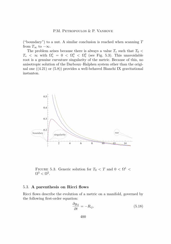
The problem arises because there is always a value T∗ such that T0 <T∗ < ∞ with Ω1

∗ = 0 < Ω3∗ < Ω2

∗ (see Fig. 5.3). This unavoidableroot is a genuine curvature singularity of the metric. Because of this, noanisotropic solution of the Darboux–Halphen system other than the origi-nal one ((4.21) or (5.8)) provides a well-behaved Bianchi IX gravitationalinstanton.

2 4 6 8 10 12 14

0.2

0.3

0.4

0.5

singularitynutboundary

Figure 5.3. Generic solution for T0 < T and 0 < Ω1 <Ω3 < Ω2.

5.3. A parenthesis on Ricci flowsRicci flows describe the evolution of a metric on a manifold, governed bythe following first-order equation:

∂gij∂t

= −Rij , (5.18)

400


where Rij stands for the Ricci tensor of the Levi–Civita connection asso-ciated with gij (see e.g. [32]). It was introduced by Hamilton in 1981 [60]in order to gain insight into the geometrization conjecture of Thurston(see e.g. [101]), a generalization of Poincaré’s 1904 conjecture for three-manifolds, finally demonstrated by Perel’man in 2003 [87, 89, 88]. Ricciflows are also important in modern physics as they describe the renormal-ization group evolution in two-dimensional sigma-models [44].

The case of homogeneous three-manifolds is important as it appears inthe final stage of Thurston’s geometrization. Homogeneous three-manifoldsinclude all 9 Bianchi groups plus 3 coset spaces, which are H3, H2 × S1,S2 × S1 (Sn and Hn are spheres and hyperbolic spaces respectively)[77, 93]. The general asymptotic behaviour was studied in detail in [63].A remarkable and already quoted result [34, 97, 21, 90] is the relationshipbetween the parametric evolution of a metric

ds2 =

√Ω2Ω3

Ω1

(σ1)2

+

√Ω3Ω1

Ω2

(σ2)2

+

√Ω1Ω2

Ω3

(σ3)2

(5.19)

on M3 of Bianchi type7, and the time evolution inside a self-dual grav-itational instanton on M4 = R × M3 as given in (3.6): the equationsare the same (t in (5.18) and T in (3.6) are related as dt =

√Ω1Ω2Ω3dT ).

Ricci flow on three-spheres is therefore governed by the Darboux–Halphenequations (3.14).

Solutions of the Darboux–Halphen system describe Ricci-flow evolutionif ∀i Ωi(T ) > 0, assuming that this holds at some initial time T0. It isstraightforward to see that this is always guaranteed. Indeed, it is truewhen at least two Ωs are equal, as one can see directly from the algebraicsolutions (5.4) and (5.5). More generally, suppose that 0 < Ω1

0 < Ω20 < Ω3

0(the subscript refers to the initial time T0) and that Ω1 has reached attime T1 the value Ω1

1 = 0, while Ω21,Ω3

1 > 0. From Eqs. (3.14) we concludethat at time T1, Ω1

2 = Ω13 = −Ω1

2 Ω13 < 0 and Ω1

1 = Ω12 Ω1

3 > 0. Thislatter inequality implies that Ω1 vanishes at T1 while it is increasing,passing therefore from negative to positive values. This could only happenif Ω1

0 were negative, which contradicts the original assumption. However,if indeed Ω1

0 < 0 and Ω20,Ω3

0 > 0, there is a time T1 where Ω1 becomes

7The precise statement is actually formulated for more general, non-diagonal metrics,as explained in detail in [90], and is valid in all Bianchi classes. For Bianchi IX, thediagonal ansatz exhausts, however, all possibilities.

401


positive and remains positive together with Ω2 and Ω3 until they reachthe asymptotic region.

Solutions (5.4) and (5.5) show that the asymptotic behaviour of Ωs isclearly 1/T , when at least two Ωs are equal. In the more general case, thelarge-T behaviour is readily obtained thanks to the quasimodular proper-ties of the solutions (see footnote 6):

Ω1,2,3(T ) = − 1T 2 Ω2,1,3

( 1T

)+ 1T. (5.20)

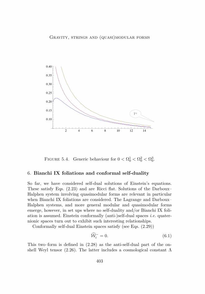
Therefore, for finite and positive Ωi0 ≡ Ωi(0),

Ωi = 1T

+ subleading at large T, (5.21)

as one observes in Fig. 5.4. Note that this does not hold for the solution(5.8) because for the latter T = 0 is a pole and Ωi

0 ≡ Ωi(0) is neither finite,nor positive for all i. The behaviour at large T is not 1/T , but exponential(see Eq. (5.11) and Fig. 5.2).

As a consequence of the generic behaviour (5.21) of Ωs for positive andfinite initial conditions, the late-time geometry on the S3 under the Ricciflow is

ds2 ≈ 1√T

((σ1)2

+(σ2)2

+(σ3)2). (5.22)

This is an isotropic (round) three-sphere of shrinking radius8. It is worthstressing that this universal behaviour is specifically due to the quasimod-ular properties of the solution, reflected in the non-covariant 1/T term of(5.20).

8At large times, the original SU(2) or SU(2) × U(1) isometry group gets enhancedto SU(2)×SU(2), while the volume shrinks to zero. These are generic properties alongthe Ricci flow: the isometry groups may grow in limiting situations, whereas the volumeis never preserved, but shrinks for positive-curvature geometries:

dVdt = 1

2

∫dDx

√det ggij ∂gij

∂t= −1

2

∫dDx

√det gR.

402


T-1

2 4 6 8 10 12 14

0.10

0.15

0.20

0.25

0.30

0.35

0.40

Figure 5.4. Generic behaviour for 0 < Ω10 < Ω2

0 < Ω30.

6. Bianchi IX foliations and conformal self-duality

So far, we have considered self-dual solutions of Einstein’s equations.These satisfy Eqs. (2.23) and are Ricci flat. Solutions of the Darboux–Halphen system involving quasimodular forms are relevant in particularwhen Bianchi IX foliations are considered. The Lagrange and Darboux–Halphen systems, and more general modular and quasimodular formsemerge, however, in set ups where no self-duality and/or Bianchi IX foli-ation is assumed. Einstein conformally (anti-)self-dual spaces i.e. quater-nionic spaces turn out to exhibit such interesting relationships.

Conformally self-dual Einstein spaces satisfy (see Eqs. (2.29))

W−i = 0. (6.1)

This two–form is defined in (2.28) as the anti-self-dual part of the on-shell Weyl tensor (2.26). The latter includes a cosmological constant Λ

403


and (6.1) implies that this space is Einstein (Rab = Λgab) on top of beingconformally self-dual (W− = 0).

6.1. Conformally self-dual Bianchi IX foliations

Assuming the four-dimensional space be a foliation M4 = R ×M3 withM3 a general homogeneous three-sphere invariant under SU(2) isometry,we can in general endow it with a metric (3.6). The Levi–Civita connectionone–forms of the latter are given in (3.9) and (3.10)). Conformal self-duality condition (6.1) does not require the flatness of the anti-self-dualcomponent of the connection Ai as in (3.11). Hence, no first integral like(3.12) is available.

In order to take advantage of the conformal self-duality condition (6.1)and reach first-order differential equations as in the case of pure self-duality, we can parameterize the connection Ai and Σi and demand that(6.1) be satisfied. This is usually done by setting both Ai and Σi propor-tional to σi, as in (3.12), with a T -dependent coefficient though (see e.g.[64]):

Σi = − Bi2Ωi

σi, (6.2)

Ai = ∆i

2Ωiσi. (6.3)

Using Eqs. (3.9) and (3.10), one obtains a relationship between

Ωiand

Bi,∆i:

Ωi = ΩjΩk − Ωi (∆j + ∆k) = −ΩjΩk + Ωi (Bj +Bk) . (6.4)

404


Furthermore, Eqs. (2.27) and (2.28) lead to the following expressions forthe on-shell Weyl tensor:

W+i = −

14Ω1Ω2Ω3

(Bi +BjBk −Bi (Bj +Bk)

)+ Λ

6

φi

−

14Ω1Ω2Ω3

(Bi −BjBk −Bi (Bj +Bk)

)+ Bi

2 (Ωi)2

χi,(6.5)

W−i =

14Ω1Ω2Ω3

(∆i + ∆j∆k + ∆i (∆j + ∆k)

)− ∆i

2 (Ωi)2

φi

+ 1

4Ω1Ω2Ω3

(∆i −∆j∆k + ∆i (∆j + ∆k)

)− Λ

6

χi. (6.6)

The additional (with respect to (6.4)) first-order equations for Bi or∆i are obtained by imposing on-shell conformal self-duality. The canon-ical method for that is to demand that both coefficients of φi and χi in(6.6) vanish. This guarantees (see (2.27)) a conformally self-dual, Einsteinmanifold with scalar curvature R = 4Λ, in other words a quaternionicspace.

Solving the system of equations obtained for conformally self-dual, Ein-stein manifolds depends drastically on whether or not the isometry isstrictly SU(2), i.e. the leaves of the Bianchi IX foliation are anisotropic,triaxial spheres. When the isometry is extended to SU(2)×U(1) (two equalΩs), the equations are algebraically integrable (as in the Darboux–Halphensystem (3.14)) and no relationship appears with modular or quasimodu-lar forms. This leads to a variety of well known biaxial solutions (see[49, 83, 64] as well as [35] for a detailed presentation of the resolution) suchas (anti-)de Sitter–Taub–NUT, (anti-)de Sitter–Eguchi–Hanson, (pseudo-)Fubini–Study – CP2, Pedersen (the parentheses correspond to negativeΛ) . . .When all Ωs are equal, the leaves are round, uniaxial three-spheres,and the only four-geometries are the symmetric S4 orH4 (depending againon the sign of Λ).

Although straightforward, the above approach leads for the triaxial caseto equations which are not known to be integrable. Hence, their resolutionis not systematic and general. An alternative strategy has been proposedby Tod and Hitchin [103, 61], based on twistor spaces and isomonodromicdeformations (see also [104, 71]). In a first step, one sets Λ to zero in (6.6)and demands the coefficient of χi to vanish. This is equivalent to demand-ing conformal self-duality and zero scalar curvature (W− = s = 0) without

405


setting C−ij to zero. Thus, the space is not Einstein and has zero scalarcurvature. The final step is to perform a conformal transformation, whichallows to restore a non-vanishing scalar curvature, while simultaneouslysetting C−ij = 0. One thus obtains a quaternionic space.

Explaining the details of this procedure is beyond our present scope,and we will therefore limit our presentation to the issues involving modularforms, which stem out of conditions W− = s = 0. These are imposed bydemanding that the coefficient of χi vanishes in (6.6) and setting Λ = 0:

I

∆1 = ∆2∆3 −∆1 (∆2 + ∆3)∆2 = ∆3∆1 −∆2 (∆3 + ∆1)∆3 = ∆1∆2 −∆3 (∆1 + ∆2) .

(6.7)

They are supplemented with Eqs. (6.4), which read for ∆i:

II

Ω1 = Ω2Ω3 − Ω1 (∆2 + ∆3)Ω2 = Ω3Ω1 − Ω2 (∆3 + ∆1)Ω3 = Ω1Ω2 − Ω3 (∆1 + ∆2) .

(6.8)

Before pursuing the present investigation any further, it is worth mak-ing contact with the results of Sec. 3.2 on genuine self-duality equations.Assuming the system I and II satisfied i.e. W− = s = 0, Ai (Eq. (2.21))reads:

Ai = 12C−ijφ

j = 12Ωi

(∆j∆k

ΩjΩk− ∆i

Ωi

)φi. (6.9)

Purely self-dual Einstein vacuum spaces are obtained by demanding C−ij =0 (i.e. Rab = 0 since the scalar curvature vanishes). This leads to the twoknown possibilities for Bianchi IX vacuum self-dual Einstein geometriesmet in Sec. 3.2, and satisfying either one of the following systems:

• Lagrange (3.13) for ∆i = 0,

• Darboux–Halphen (3.14) for ∆i = Ωi.

6.2. Solving I & II with Painlevé VISystems I and II (Eqs. (6.7) and (6.8)) describing general conformally self-dual Bianchi IX foliations with vanishing scalar curvature (W− = s = 0)were studied e.g. in [86, 102] prior to their uplift to quaternionic spaces.

406


Further developments in relation with modular properties can be found in[76, 13].

As usual it is convenient to move to the complex plane, introduce ω`(z)and δ`(z) and trade the dot for a prime as derivative with respect to zin (6.7) and (6.8). Real solutions are recovered as previously: Ω`(T ) =iω`(iT ) and ∆`(T ) = iδ`(iT ).

The system I is that of Darboux–Halphen for δi(z) (see (3.14)). Givena solution δi(z) one can solve the system II for ωi(z). Furthermore, theSL(2,C) solution-generating technique described in (4.2) can be general-ized in the present case: given a solution δi(z) and ωi(z),

δi(z) = 1(cz + d)2 δi

(az + b

cz + d

)+ c

cz + d(6.10)

andωi(z) = 1

(cz + d)2ωi(az + b

cz + d

)(6.11)

provide another solution if(a bc d

)∈ SL(2,C).

Assuming δ1 6= δ2 6= δ3 i.e. the triaxial situation (implying automat-ically ω1 6= ω2 6= ω3), we can readily obtain the general solution of thesystem I as in (4.7),

δi(z) = −12

ddz log E i(z), (6.12)

with E i(z) a triplet of weight-two modular forms of Γ(2) ⊂ SL(2,Z). Thesecan be expressed as in (4.12), where λ is a solution of Schwartz’s equation(4.11). Define now a new set of functions wi(z) as

wi = ωi√EjEk

(6.13)

(i, j, k cyclic permutation of 1, 2, 3), and insert the solutions (6.12) in sys-tem II (6.8). The latter becomes

dw1dλ = w2w3

λ,

dw2dλ = w3w1

λ− 1 ,dw3dλ = w1w2

λ(λ− 1) . (6.14)

Notice the first integral w21−w2

2+w23. Even though the value of this integral

is arbitrary, the uplift of the corresponding conformally self-dual geometrywith zero scalar curvature to an Einstein manifold is possble only if theconstant is 1/4 (see [103, 61]).

407


The system of equations (6.14) can be solved in full generality with wiexpressed in terms of solutions y(λ) of Painlevé VI equation [66] (see also[2] for a more general overview):

w21 = (y − λ)y2(y − 1)

λ

(v − 1

2(y − 1)

)(v − 1

2(y − λ)

), (6.15)

w22 = (y − λ)y(y − 1)2

λ− 1 ,

(v − 1

2y

)(v − 1

2(y − λ)

)(6.16)

w23 = (y − λ)2y(y − 1)

λ(λ− 1)

(v − 1

2y

)(v − 1

2(y − 1)

). (6.17)

Here,

v = λ(λ− 1)y′

2y(y − 1)(y − λ) + 14y + 1

4(y − 1) −1

4(y − λ) (6.18)

and y is a solution of Painlevé VI equation (f ′ = df/dλ):

y′′ = 12

(1y

+ 1y − 1 + 1

y − λ

)(y′)2 −

( 1λ

+ 1λ− 1 + 1

y − λ

)y′

+(y − λ)y(y − 1)2

8λ2(λ− 1)2

(1− λ

y2 + λ− 1(y − 1)1 −

3λ(λ− 1)(y − λ)2

). (6.19)

6.3. Back to quasimodular forms

We will for concreteness concentrate on the original solution of systemI, the Halphen solution corresponding to λH = ϑ4

2/ϑ43. This is sufficient as

any other can be generated by SL(2,C) transformations. Equations (6.14)(system II) read now

w′1 = iπϑ44w2w3, w′2 = −iπϑ4

2w3w1, w′1 = −iπϑ43w2w3. (6.20)

In this form, the system can be solved in terms of Jacobi theta functionswith characteristics [13], as an alternative to the solution (6.15)–(6.17).This makes it relevant in the present framework.

408


The solution with w21 − w2

2 + w23 = 1/4 – required for the subsequent

promotion to quaternionic geometries – read:

w1(z) = 12πϑ2(0|z)ϑ3(0|z)

∂vϑ[a+1b

](0|z)

ϑ[ab

](0|z) , (6.21)

w2(z) = e−iπa/2

2πϑ3(0|z)ϑ4(0|z)∂vϑ

[ ab+1](0|z)

ϑ[ab

](0|z) , (6.22)

w3(z) = −e−iπa/2

2πϑ2(0|z)ϑ4(0|z)∂vϑ

[a+1b+1](0|z)

ϑ[ab

](0|z) . (6.23)

Here a, b ∈ C are moduli, mapped under the SL(2,C) transformations(6.10) and (6.11) to other complex numbers. If a, b are integers and thetransformation is in SL(2,Z), the solution is left invariant, up to permu-tation of the three components.

It would be interesting to present the geometrical structure of the con-formally self-dual zero-curvature spaces obtained with the solutions athand, following the general procedure used in Sec. 5.2. This would defi-nitely bring us far from the original goal. The interested reader can finduseful information in the already quoted literature, both for these spacesand for their quaternionic uplift. Note in that respect that even thoughmany families of solutions exist (here in the triaxial case, or more gener-ally for biaxial three-sphere foliations), very few are singularity-free amongwhich, the Fubini–Study or the Pedersen instanton (SU(2) × U(1) isom-etry), or the Hitchin–Tod solution (strict SU(2) symmetry).

As a final remark, let us mention that (6.21), (6.22), (6.23) also capturethe self-dual Ricci flat solutions discussed in Sec. 3 and given in Eqs. (4.21)i.e. the Atiyah–Hitchin gravitational instanton. They correspond to thechoice a = b = 1 mod 2, that must be implemented with care: considera = 1 + 2ε, b = 1 + 2z0ε and take the limit ε → 0. One finds (a usefulidentity for this computation is given in (A.5):

w1 = − 1πϑ2

2ϑ23

(i

z + z0− π

6(E2 − ϑ4

2 − ϑ43

)), (6.24)

w2 = − i

πϑ23ϑ

24

(i

z + z0− π

6(E2 + ϑ4

3 + ϑ44

)), (6.25)

w3 = − i

πϑ22ϑ

24

(i

z + z0− π

6(E2 + ϑ4

2 − ϑ44

)). (6.26)

409


A modulus z0 is left in the solution; under SL(2,Z) it transforms as

z0 →dz0 + b

cz0 + a. (6.27)

For finite z0 the corresponding metric is Weyl-self-dual with zero scalarcurvature The z0 → i∞ limit corresponds to the Ricci-flat, Atiyah–Hitchininstanton (Riemann-self-dual).

6.4. Beyond Bianchi IX foliations

We would like to close our overview on conformally self-dual geometrieswith another family of quaternionic solutions, related to modular formsbut not of the type M4 = R ×M3 with homogeneous M3. Indeed, self-duality (Eq. (2.23)) or conformal self-duality (Eqs. (2.24) and (2.25)) canbe demanded outside ot the framework of foliations.

On can indeed assume an ansatz for the metric of the Gibbons–Hawkingtype [51]:

ds2 = Φ−1(dτ +$idxi

)2+ Φδijdxidxj . (6.28)

Here Φ and $i depend on x only, and thus ∂τ is Killing. With this ansatzmore general self-dual solutions are obtained with U(1), U(1) × U(1) orU(1)×Bianchi isometry. Determining quaternionic spaces, i.e. conformallyself-dual and Einstein, is however far more difficult. It is a real tour de forceto find the most general quaternionic solution with U(1)×U(1) isometryand this was achieved by Calderbank and Pedersen in [29], following theoriginal method of Lebrun [71]. This will be our last example, where anew kind of modular forms emerge.

In coordinates ρ, η, θ, ψ with frame

α = √ρdρ, β = dψ + ηdθ√ρ

, γ = dρ, δ = dη, (6.29)

The metric reads:

ds2 =4ρ2

(F 2ρ + F 2

η

)− F 2

4F 2ρ2

(γ2 + δ2

)+ [(F − 2ρFρ)α− 2ρFηβ]2 + [(F + 2ρFρ)β − 2ρFηα]2

F 2[4ρ2

(F 2ρ + F 2

η

)− F 2

] . (6.30)

410


Here Fρ = ∂ρF and Fη = ∂ηF , where F (ρ, η) is a solution of

ρ2(∂2ρ + ∂2

η

)F = 3

4F. (6.31)

The metric (6.30) has generically two Killing vectors, ∂θ, ∂ψ and F (ρ, η)is a harmonic function on H2 with eigenvalue 3/4. Indeed, the metric onthe hyperbolic plane is

ds2H2 = dρ2 + dη2

ρ2 (6.32)

and Eq. (6.31) can be recast as4H2F = 3

4F. (6.33)Solving (6.33) leads inevitably to modular forms of τ = η+iρ, even thoughalgebraic solutions are also available.

Let us mention for example

F =√ρ+ η2

ρ, (6.34)

which leads to a metric on CP2 with U(1)× SU(2) isometry [84], or

F = ρ2 − ρ20

2√ρ (6.35)

with U(1) × Heisenberg9 symmetry [9]. Solutions for F (ρ, η) with strictU(1)×U(1) isometry open Pandora’s box for non-holomorphic Eisensteinseries such as (see (A.9))

F = E3/2(τ, τ), (6.36)which has a further discrete residual symmetry SL(2,Z) ⊂ SL(2,R).These will be discussed in Sec. 7 and we refer to the appendix for someprecise definitions. Very little is known at present on the geometrical prop-erties of the corresponding quaternionic spaces, or on the fields of appli-cation these spaces could find in physics. In string theory, they are knownto describe the moduli space of hypermultiplets in compactifications onCalabi–Yau threefolds [42]. The relevance of the Calderbank and Peder-sen metrics in this context was recognized in [10]. For further considera-tions on the role of modular and quasimodular foms as string instantoniccontributions to the moduli spaces of these compactifications, we referto [6, 7, 15, 16, 5, 8] and in particular to the recent review [4].

9Heisenberg algebra is Bianchi II.

411


7. Beyond the world of Eisenstein series

To end up this review we would like to elaborate on some connectionsbetween quantum field theory and modular forms. This originates fromthe specific structure of the perturbative expansions in string and fieldtheory, and calls for develping more general modular functions than thenon-holomorphic Eisenstein series discussed earlier in these notes.

7.1. The starting point: perturbation theory

Perturbative expansions in quantum field theory are expressed as sums ofmultidimensional integrals, obtained by applying Feynman rules or uni-tarity constraints. These integrals are plagued by various divergences thatneed to be regulated. It was remarked in [23, 24] that the coefficients ofthese divergences are given by multiple zeta values in four dimensions.Since this original work, it has become more and more important to fur-ther investigate the relationship between quantum field theory and thestructure of multiple zeta values. This connection has fostered importantmathematical results as in instance [25, 26], which have been reviewed inthe recent Séminaire Bourbaki by Pierre Deligne [37].

The next observation is that the above mentioned field-theory Feynmanintegrals arise as certain limits of string-theory integrals defined on higher-genus Riemann surfaces. They are actually obtained from the boundaryof the moduli of higher-genus punctured Riemann surfaces. This bridge tostring theory sets a handle to the world of modular functions.

There are indeed two motivations for embedding the analysis into astring theory framework. The first is of physical nature: perturbative stringtheory is free of ultraviolet divergences, so it provides a well-defined pre-scription for regularizing field-theory divergences. In other words, stringtheory acts as a specific regularization from which we expect to learn moreon the fundamental structure of the quantum field theories. The secondmotivation is directly related to the topic of this text: string theory is theideal arena for exploring the number theoretic considerations of quantumfield theory and their close connection with modular forms.

In the present notes we will focus on the case of the tree level and genusone, following the string analysis in [57, 54] and the mathematical analysisin [52]. We will explain in particular that (non-holomorphic) Eisensteinseries are not enough for capturing all available information carried by the

412


integrals under consideration. The presentation will be schematic, aimingat conveying a message rather that providing all technical details. For thelatter, the interested reader is referred to the quoted literature.

Let us consider the following integral defined on the moduli space ofthe genus-g Riemann surface with four marked points:

A(g)(s, t, u) =∫Mg

dµ∫

Σg

4∏i=1

d2zi exp

∑1≤i<j≤4

2α′ki · kjP (zi, zj)

,(7.1)

whereMg is the moduli space of the closed Riemann surface Σg of genusg. There are four punctures whose positions zi are integrated over. Wehave introduced k1 + k2 + k3 + k4 = 0 with ki · ki = 0 representing ex-ternal massless momenta flowing into each puncture. We will also set theMandelstam variables s = 2k1 · k2 = 2k3 · k4, t = 2k1 · k4 = 2k2 · k3 andu = 2k1 · k3 = 2k2 · k4, obeying s + t + u = 0 for the massless states athand. The physical scale is the inverse tension of the string α′.

The propagator or Green’s function P (z, w) is defined on this Riemannsurface by

0 =∫

Σgd2z√−g P (z, w), (7.2)

∂z∂zP (z, w) = 2πδ(2)(z)− 2πgzz∫Σg d2z

√−g

, (7.3)

∂z∂wP (z, w) = −2πδ(2)(z) + πg∑I=1

ωI(z)(=mΩ)−1IJ ωJ(w), (7.4)

where the ds2 = gzzdzdz is the metric on the Riemann, Ω the periodmatrix, and ωI with 1 ≤ I ≤ g the first Abelian differentials.

7.2. Genus zero: the Eisenstein series

At genus 0, i.e. for the Riemann sphere, the propagator is simply givenby

P (0)(z, w) = log |z − w|2, (7.5)

413


and the integral in (7.1) can be evaluated to give

A(0)(s, t, u) = 1α′3stu

Γ (1 + α′s) Γ (1 + α′t) Γ (1 + α′u)Γ (1− α′s) Γ (1− α′t) Γ (1− α′u)

= 1α′3stu

exp(−∞∑n=1

2ζ(2n+ 1)2n+ 1

[(α′s)n + (α′t)n + (α′u)n

]). (7.6)

The masses of string theory excitations are integer, quantized in units of1/α′. It is therefore expected that the α′ expansion of the string amplitudein (7.6) is given by multiple sums over the integers, but it is remarkablethat this expansion involves only odd zeta values of depth one. For α′ 1a series expansion representation reads:

A(0)(s, t, u) =∑

q≥−1,p≥0c(p,q) σ

p2σ

q3, (7.7)

where we have introduced σ2 = (α′s)2 + (α′t)2 + (α′u)2 and σ3 = 3α′3stu.Since σ1 = (α′s) + (α′t) + (α′u) = 0, we immediately see that all σn =(α′s)n + (α′t)n + (α′u)n with n ≥ 2 are given by [57]

σnn

=∑

2p+3q=n

(p+ q − 1)!p!q!

(σ22

)p (σ33

)q. (7.8)

The coefficients c(p,q) are polynomial in odd zeta values of weight 2p +3q − 3. It is notable that at a given order n = 2p + 3q − 3, the spaceof these coefficients has dimension dn = b(n+ 2)/2c − b(n+ 2)/3c, whichcoincides with the dimension of the space of the holomorphic Eisensteinseries of weight n (see appendix). This hint calls for further investigation,and we would like to mention the recent work connecting the α′ expansionin (7.7) and the motivic multiplet zeta values [92].

One can expand the integrand of (7.7) and obtain each coefficientc(p,q) as a linear combination of the multiple integrals of the propagatorP (0)(zi, zj) (given in (7.5)):

cn12,n13,n14,n23,n24,n34 =∫S2

∏1≤i<j≤4

d2zi∏

1≤i<j≤4P (0)(zi, zj)nij . (7.9)

The integrand of this expression is the product of the propagators con-necting the punctures with multiplicities nij , 1 ≤ i < j ≤ 4, as depicted onFig. 7.1. The contributions in (7.7) are the lowest-order to the full string-

414


1

2

3

4

n12

n13

n14

n23

n24

n34

Figure 7.1. Graph of a vacuum Feynman diagram onthe Riemann surface Σg. The punctures are connected bynij ≥ 0 links representing the number of two-dimensionalpropagators.

theory amplitude of the four-point (four punctures) processes describedhere.

In Eqs. (7.6)–(7.7), we encountered the zeta values

ζ(s) =∑n≥1

1ns. (7.10)

Extending the sum over the integers n to a lattice like p = m + τn ∈Λ(1) = Z + τZ, where10 τ ∈ h = z ∈ C,=m(z) ≥ 0, one gets the(non-holomorphic) Eisenstein series

Es(τ, τ) =∑

p∈Z+τZ

1|p|2s , (7.11)

10The modular parameter τ is expressed in alternative ways throughout these notes:τ = <e(τ) + i=m(τ) = τ1 + iτ2 = η + iρ.

415


where |p|2 = (m + nτ)(m + nτ) is the natural Euclidean norm on thelattice Λ(1). This expression can be made modular-invariant in a trivialway by multiplying by =m(τ)s,

Es(τ, τ) =∑

p∈Z+τZ

=m(τ)s

|p|2s . (7.12)

This Eisenstein series is an eigenfunction of the hyperbolic Laplacian(6.31) with eigenvalue s(s− 1):

4H2Es(τ, τ) = s(s− 1)Es(τ, τ). (7.13)

The case s = 3/2 was discussed in Sec. 6.4, Eqs. (6.34)–(6.36), from adifferent physical perspective.

7.3. Genus one: beyond

At this stage of the exposition the reader may wonder how the abovegeneralization of the zeta values (7.10) into modular forms (7.12) arises instring theory. We will sketch how this goes and show that new automorphicforms are actually needed, standing beyond the well known Eisensteinseries. This requires going beyond the sphere (7.5)–(7.7).

At genus one, the Green’s function is given by

P (1)(z, 0) = −14 log

∣∣∣∣ϑ1(z|τ)ϑ′1(0|τ)

∣∣∣∣2 + π=m(z)2

2τ2. (7.14)

The amplitude in (7.1) reads:

A(1)(s, t, u) =∫F

d2τ

τ22

∫T

∏1≤i<j≤4

d2ziτ2W(1) e−

∑1≤i<j≤4 2α′ki·kj P (1)(zi−zj),

(7.15)where F =

τ ; |<e(τ)| ≤ 1

2 ,=m(τ) > 0,<e(τ)2 + =m(τ)2 ≥ 1

is a fun-damental domain for SL(2,Z), and

T =z; |<e(z)| ≤ 1

2 , 0 ≤ =m(z) ≤ =m(τ).

No closed form for the integral in (7.15) is known, in particular becauseof the presence of non-analytic contributions in the complex (s, t)-plane.

416


For a rigorous definition of this integral we refer to [38]. The expressionfor the genus-one propagator in (7.14) has an alternative representation:

P (1)(z, 0) = 12π

∑p∈Z+τZ

τ2|p|2 e−π

=m(zp)τ2 + C(τ, τ), (7.16)

where C(τ, τ) = log |√

2πη(τ)| is a modular anomaly. Since the latter isz-independent, it drops out of the sum in (7.15) because of the momentum-conservation condition

∑4i=1 ki = 0. The integrand of (7.15) is there-

fore modular-invariant. From now on we will only consider the modular-invariant part of the propagator

P (1)(z, 0) = 12π

∑p∈Z+τZ

τ2|p|2 e−π

=m(zp)τ2 . (7.17)

Following the developments on the sphere, we can analyze the expansionof the amplitude (7.15) for α′ 1. In this regime one gets integrals of thetype (7.9), but this time with the genus-one propagator

Dn12,n13,n14,n23,n24,n34(τ, τ) =∫T

∏1≤i<j≤4

d2z1τ2

∏1≤i<j≤4

P (1)(zi, zj)nij .

(7.18)The product runs over the entire set of links with multiplicities nij , 1 ≤i < j ≤ 4, of the graph Γ depicted in Fig 7.1. By construction theseintegrals are modular functions for SL(2,Z). Performing the integrationover the position of the punctures one gets an alternative form for themodular function Dn12,...,n34(τ, τ) given by

Dn12,...,n34(τ, τ) =∑pi∈Γ

4∏i=1

δ

∑j→vi

pj

∏prop∈Γ

=m(τ)|pi|2

, (7.19)

where the sum is over all the propagators pi of the graph Γ. If there aren12 propagators connecting the vertices 1 and 2, we have n12 differentelements of the lattice pi = mi + τni ∈ Z + τZ, 1 ≤ i ≤ n12. At eachvertex vi of the graph we impose momentum conservation by demandingthat the sum of the incoming momenta pj flowing to this vertex (j → vi)be zero. This is represented by the delta function constraint δ(

∑j→vi pj)

with δ(m+ τn) ≡ δ(m)δ(n).

417


The above sums Dn12,...,n34(τ, τ), introduced in [54], are generalizationsof the Eisenstein series, that we will call Kronecker–Eisenstein follow-ing [52]. With each modular functionDn12,...,n34(τ, τ) we associate a weightgiven by the sum of the integer-valued indices nij . Let us focus for con-creteness on the particular case of n propagators between two punctures,and refer to [54] for the general case. We define

Dn(τ, τ) :=∑

pi∈Z+τZδ

(n∑i=1

pi

)n∏i=1

=m(τ)4π|pi|

. (7.20)

The special cases n = 2 and 3 are given11 in [54, appendix B]

D2(τ, τ) = E2(τ, τ)(4π)2 , (7.21)

D3(τ, τ) = E3(τ, τ)(4π)3 + ζ(3)

64 . (7.22)

However, in general these modular functions do not reduce to Eisensteinseries, as it can easily be seen by evaluating the constant terms. For n ≥ 2it is always possible to decompose the modular form Dn(τ, τ) as [54]

Dn(τ, τ) = Pn(Es(τ, τ)) + δn(τ, τ) (7.23)with Pn(Es(τ, τ)) a polynomial in the Eisenstein series Es(τ, τ) (see Equa-tions. (7.12) and (A.9)) of the form

Pn(Es(τ, τ)) = pn(ζ(2n+ 1))

+ b1(4π)n En(τ, τ) +

∑r+s=n

cr,s(4π)nEr(τ, τ)Es(τ, τ), (7.24)

where pn(ζ(2n+ 1)) is polynomial of degree two in the odd zeta values oftotal weight n. The remainder δn(τ, τ) in (7.23) is a modular form whoseconstant Fourier coefficient does not vanish but tends to zero for τ2 →∞.

Although the definition of the modular functions Dn12,...,n34(τ, τ) givenin (7.20) looks similar to the double-Eisenstein series introduced in [45],one finds that, as opposed to the latter, their constant term involves depth-one zeta values [54] only. Hence, they provide a natural modular-invariantgeneralization of the polynomials in the odd zeta values met in (7.9). Oneway to obtain multiple zeta values is to insert in (7.20) the generalized

11The case n = 3 has been worked out by Don Zagier.

418


propagator used by Goncharov in [52]. Whether the generalization intro-duced by Goncharov does appear in string theory is an open question.From the original physical perspective, this question is relevant becauseit translates into the (im)possibility of appearance of multiple zeta valuesas counter-terms to ultraviolet divergences in quantum field theory. Thismight have important consequences in supergravity.

As a final comment, let us mention that although our discussion wasconfined to the case of modular functions for SL(2,Z), most of the abovecan be generalized to the framework of automorphic functions for higher-rank group [53].

8. Concluding remarks

In the present lecture notes we have given a partial – in all possible senses– review of the emergence of (quasi)modular forms in the context of grav-itational instantons and string theory. These forms often appear as theconsequence of remarkable, explicit or hidden symmetries, and turn outto be valuable tools for unravelling a great deal of properties in a variety ofphysical set ups. The latter include monopole scattering, Ricci flows, non-perturbative (instantonic) corrections to string moduli spaces (via theirFourier coefficients), or perturbative expansions in quantum field theory(via string amplitudes).

We have described how the classical holomorphic Eisenstein series,whose theory is nicely presented in [96, 68], occurs in the context of grav-itational instantons or in studying non-perturbative effects. We have alsoencountered the non-holomorphic Eisenstein series, the analytic propertiesof which are described in [70, 78]. This whole analysis has led us to ar-gue that one needs novel types of modular functions, standing beyond theusual Eisenstein series. Although the analytic properties of these series arestill poorly understood, they seem to be a corner stone for understandingthe challenging nature of interactions in string theory and its consequencesin quantum field theory.

419


Appendix A. Theta functions and Eisenstein series

We collect here some conventions for the modular forms and theta func-tions used in the main text. General results and properties of these objectscan be found in [96, 68].

Introducing q = exp 2iπz, we first define

η(z) = q1/24

∞∏n=1

(1− qn) , (A.1)

E2(z) = 12iπ

ddz log η, (A.2)

as the Dedekind function and the weight-two quasimodular form, whereas

ϑ2(z) =∑p∈Z

q1/2(p+1/2)2

, ϑ3(z) =∑p∈Z

qp2/2, ϑ4(z) =

∑p∈Z

(−1)p qp2/2

(A.3)are the Jacobi theta functions. More generally, one introduces

ϑ

[a

b

](v|z) =

∑m∈Z

exp(iπz(m+ a/2)2 + 2iπ(v + b/2)(m+ a/2)

)(A.4)

with ϑ[11]

= ϑ1, ϑ[10]

= ϑ2, ϑ[00]

= ϑ3, ϑ[01]

= ϑ4. Let us also mention thefollowing relation

ϑ

[α+ 2wβ + 2v

](0|z) = ϑ

[α+ 2wβ

](v|z) = eiπw(w+1+2v)ϑ

[α

β

](v+wz|z). (A.5)

The first holomorphic Eisenstein series areE2(z) = 1− 24

∑∞m=1

mqm

1−qm

E4(z) = 1 + 240∑∞m=1

m3qm

1−qm

E6(z) = 1− 504∑∞m=1

m5qm

1−qm .

(A.6)

Notice that E4(z) and E6(z) are modular forms of weight 4 and 6, whereasE2(z) is the already quoted weight-two quasimodular form. The modular-invariant of weight two is the non-holomorphic combination E2(z)− 3

π=m(z) .It is a classical result that the space of modular forms of weight k isspanned by Ea4E

b6 with 2a + 3b = k. The dimension of this space is

dk = b(k + 2)/2c − b(k + 2)/3c.In the main text we also consider non-holomorphic Eisenstein series

Es(z, z) with z = x + iy, y > 0 and x ∈ R. These are defined as

420


modular-invariant eigenfunctions of the hyperbolic Laplacian (see Eqs.(6.31), (7.12) and (7.13))

y2(∂2x + ∂2

y)Es(z, z) = s(s− 1)Es(z, z), (A.7)with polynomial growth at the cusps (y →∞):

Es(z, z) =∑

(m,n)6=(0,0)

ys

|mz + n|2s, (A.8)

for s ∈ C with large enough real part for convergence. One can extend thedefinition by analytic continuation [70] for all s 6= 1 using the functionalequation Γ(s)π−sEs(z, z) = Γ(1/2 − s)π1/2−sE1−s(z, z). These series havethe following Fourier expansion:

2ξ(2s)Es(z, z) = 2ξ(2s) ys + 2ξ(2s− 1) y1−s

+ 4y1/2∑n 6=0

σ2s−1(|n|)|n|s−1/2

Ks−1/2(2π|n|y) e2πinx (A.9)

where ξ(s) = ζ(s)Γ(s/2)π−s/2 is the completed zeta function, Ks−1/2 is theK-Bessel function and σα(n) =

∑d|n d

α (see e.g. [100] for details).Finally, let us mention how the non-holomorphic series are connected to

the holomorphic ones. For that, one considers the following generalizationof the non-holomorphic Eisenstein functions:

E(w,w)s (z, z) =

∑(m,n)6=(0,0)

ys+w+w

(mz + n)s+w(mz + n)s+w . (A.10)

These series transform under a modular transformation γ =(a bc d

)∈

SL(2,Z) as

E(w,w)s (γ · z, γ · z) = (cz + d)w(cz + d)w E(w,w)

s (z, z). (A.11)Chosing s = n ∈ N and w = −n, we recover the holomorphic Eisensteinseries E(0,−n)

n (z, z) = En(z).

References

[1] M. J. Ablowitz, S. Chakravarty & R. G. Halburd – “In-tegrable systems and reductions of the self-dual Yang-Mills equa-tions”, J. Math. Phys. 44 (2003), no. 8, p. 3147–3173, Integrability,topological solitons and beyond.

421


[2] M. J. Ablowitz & P. A. Clarkson – Solitons, nonlinear evolu-tion equations and inverse scattering, London Mathematical SocietyLecture Note Series, vol. 149, Cambridge University Press, Cam-bridge, 1991.

[3] B. S. Acharya & M. O’Loughlin – “Self-duality in (D ≤ 8)-dimensional Euclidean gravity”, Phys. Rev. D (3) 55 (1997), no. 8,p. R4521–R4524.

[4] S. Alexandrov – “Twistor Approach to String Compactifications:a Review”, arXiv:1111.2892v2 [hep-th], 2011.

[5] S. Alexandrov, D. Persson & B. Pioline – “On the topologyof the hypermultiplet moduli space in type II/CY string vacua”,Phys.Rev. D83 (2011), p. 026001.

[6] S. Alexandrov, B. Pioline, F. Saueressig & S. Vandoren– “Linear perturbations of hyperkähler metrics”, Lett. Math. Phys.87 (2009), no. 3, p. 225–265.

[7] , “Linear perturbations of quaternionic metrics”, Comm.Math. Phys. 296 (2010), no. 2, p. 353–403.

[8] S. Alexandrov, B. Pioline & S. Vandoren – “Self-dual Ein-stein spaces, heavenly metrics, and twistors”, J. Math. Phys. 51(2010), no. 7, p. 073510, 31.

[9] N. Ambrosetti, I. Antoniadis, J.-P. Derendinger &P. Tziveloglou – “The Hypermultiplet with Heisenberg Isome-try in N=2 Global and Local Supersymmetry”, JHEP 1106 (2011),p. 139.

[10] I. Antoniadis, R. Minasian, S. Theisen & P. Vanhove –“String loop corrections to the universal hypermultiplet”, ClassicalQuantum Gravity 20 (2003), no. 23, p. 5079–5102.

[11] M. F. Atiyah, N. J. Hitchin & I. M. Singer – “Self-duality infour-dimensional Riemannian geometry”, Proc. Roy. Soc. LondonSer. A 362 (1978), no. 1711, p. 425–461.

[12] M. Atiyah & N. Hitchin – “Low energy scattering of non-Abelianmonopoles”, Physics Letters A 107 (1985), no. 1, p. 21 – 25.

422


[13] M. V. Babich & D. A. Korotkin – “Self-dual SU(2)-invariantEinstein metrics and modular dependence of theta functions”, Lett.Math. Phys. 46 (1998), no. 4, p. 323–337.

[14] I. Bakas, E. G. Floratos & A. Kehagias – “Octonionic gravi-tational instantons”, Phys. Lett. B 445 (1998), no. 1-2, p. 69–76.

[15] L. Bao, A. Kleinschmidt, B. E. W. Nilsson, D. Persson &B. Pioline – “Instanton corrections to the universal hypermulti-plet and automorphic forms on SU(2, 1)”, Commun. Number TheoryPhys. 4 (2010), no. 1, p. 187–266.

[16] L. Bao, A. Kleinschmidt, B. E. Nilsson, D. Persson & B. Pi-oline – “Rigid Calabi-Yau threefolds, Picard Eisenstein series andinstantons”, arXiv:1005.4848v1 [hep-th], 2010.

[17] A. A. Belavin, A. M. Polyakov, A. S. Schwartz & Y. S.Tyupkin – “Pseudoparticle solutions of the Yang-Mills equations”,Phys. Lett. B 59 (1975), no. 1, p. 85–87.

[18] V. Belinskii, G. Gibbons, D. Page & C. Pope – “Asymptot-ically Euclidean Bianchi IX metrics in quantum gravity”, PhysicsLetters B 76 (1978), no. 4, p. 433 – 435.

[19] G. Bossard, P. Petropoulos & P. Tripathy – “Darboux–Halphen system and the action of Geroch group”, Unpublished,2012.

[20] F. Bourliot, J. Estes, P. M. Petropoulos & P. Spindel– “G3-homogeneous gravitational instantons”, Classical QuantumGravity 27 (2010), no. 10, p. 105007, 17.

[21] F. Bourliot, J. Estes, P. M. Petropoulos & P. Spindel –“Gravitational instantons, self-duality, and geometric flows”, Phys.Rev. D 81 (2010), no. 10, p. 104001, 5.

[22] D. Brecher & M. J. Perry – “Ricci-flat branes”, Nuclear Phys.B 566 (2000), no. 1-2, p. 151–172.

[23] D. J. Broadhurst & D. Kreimer – “Association of multiple zetavalues with positive knots via Feynman diagrams up to 9 loops”,Phys. Lett. B 393 (1997), no. 3-4, p. 403–412.

[24] , “Feynman diagrams as a weight system: four-loop test of afour-term relation”, Phys. Lett. B 426 (1998), no. 3-4, p. 339–346.

423


[25] F. Brown – “On the decomposition of motivic multiple zeta val-ues”, arXiv:1102.1310v2 [math.NT], 2011.

[26] F. C. Brown – “On the periods of some Feynman integrals”,arXiv:0910.0114v2 [math.AG], 2010.

[27] M. Cahen, R. Debever & L. Defrise – “A complex vectorialformalism in general relativity”, J. Math. Mech. 16 (1967), p. 761–785.

[28] D. M. J. Calderbank & H. Pedersen – “Selfdual spaces withcomplex structures, Einstein-Weyl geometry and geodesics”, Ann.Inst. Fourier (Grenoble) 50 (2000), no. 3, p. 921–963.

[29] D. M. J. Calderbank & H. Pedersen – “Selfdual Einstein met-rics with torus symmetry”, J. Differential Geom. 60 (2002), no. 3,p. 485–521.

[30] J. Chazy – “Sur les équations différentielles dont l’intégrale généralepossède une coupure essentielle mobile.”, C.R. Acad. Sc. Paris 150(1910), p. 456–458.

[31] , “Sur les équations différentielles du troisième ordre etd’ordre supérieur dont líntégrale générale a ses points critiquesfixes.”, Acta Math. 34 (1911), p. 317–385 (French).

[32] B. Chow & D. Knopf – The Ricci flow: an introduction, Mathe-matical Surveys and Monographs, vol. 110, American MathematicalSociety, Providence, RI, 2004.

[33] S. Coleman – Aspects of Symmetry, Cambridge University Press,1985.

[34] M. Cvetič, G. W. Gibbons, H. Lü & C. N. Pope – “Cohomo-geneity one manifolds of Spin(7) and G2 holonomy”, Phys. Rev. D(3) 65 (2002), no. 10, p. 106004, 29.

[35] M. Cvetic, G. Gibbons, H. Lu & C. Pope – “Bianchi IX selfdualEinstein metrics and singular G(2) manifolds”, Class.Quant.Grav.20 (2003), p. 4239–4268.

[36] G. Darboux – “Mémoire sur la théorie des coordonnées curvilignes,et des systèmes orthogonaux”, Ann. Sci. École Norm. Sup. (2) 7(1878), p. 101–150, 227–260, 275–348.

424


[37] P. Deligne – “Multizêtas [d’après Francis Brown]”, SéminaireBourbaki, Janvier 2012.

[38] E. D’Hoker & D. H. Phong – “The box graph in superstringtheory”, Nuclear Phys. B 440 (1995), no. 1-2, p. 24–94.

[39] T. Eguchi, P. B. Gilkey & A. J. Hanson – “Gravitation, gaugetheories and differential geometry”, Phys. Rep. 66 (1980), no. 6,p. 213–393.

[40] T. Eguchi & A. J. Hanson – “Gravitational instantons”, Gen.Relativity Gravitation 11 (1979), no. 5, p. 315–320.

[41] , “Selfdual Solutions to Euclidean Gravity”, Annals Phys.120 (1979), p. 82–106.

[42] S. Ferrara & S. Sabharwal – “Quaternionic Manifolds forType II Superstring Vacua of Calabi-Yau Spaces”, Nucl.Phys. B332(1990), p. 317.

[43] E. G. Floratos & A. Kehagias – “Eight-dimensional self-dualspaces”, Phys. Lett. B 427 (1998), no. 3-4, p. 283–290.

[44] D. H. Friedan – “Nonlinear Models in Two + Epsilon Dimensions”,Annals Phys. 163 (1985), p. 318.

[45] H. Gangl, M. Kaneko & D. Zagier – “Double zeta values andmodular forms”, in Automorphic forms and zeta functions, WorldSci. Publ., Hackensack, NJ, 2006, p. 71–106.

[46] R. Geroch – “A method for generating solutions of Einstein’s equa-tions”, J. Mathematical Phys. 12 (1971), p. 918–924.

[47] G. W. Gibbons & S. W. Hawking – “Classification of gravita-tional instanton symmetries”, Comm. Math. Phys. 66 (1979), no. 3,p. 291–310.

[48] G. W. Gibbons & N. S. Manton – “Classical and quantum dy-namics of BPS monopoles”, Nuclear Phys. B 274 (1986), no. 1,p. 183–224.

[49] G. W. Gibbons & C. N. Pope – “CP 2 as a gravitational instan-ton”, Comm. Math. Phys. 61 (1978), no. 3, p. 239–248.

[50] , “The positive action conjecture and asymptotically Eu-clidean metrics in quantum gravity”, Comm. Math. Phys. 66 (1979),no. 3, p. 267–290.

425


[51] G. Gibbons & S. Hawking – “Gravitational multi-instantons”,Physics Letters B 78 (1978), no. 4, p. 430 – 432.

[52] A. Goncharov – “Hodge correlators”, arXiv:0803.0297v2[math.AG], 2010.

[53] M. B. Green, S. D. Miller, J. G. Russo & P. Vanhove –“Eisenstein series for higher-rank groups and string theory ampli-tudes”, Commun.Num.Theor.Phys. 4 (2010), p. 551–596.

[54] M. B. Green, J. G. Russo & P. Vanhove – “Low energy expan-sion of the four-particle genus-one amplitude in type II superstringtheory”, J. High Energy Phys. (2008), no. 2, p. 020, 56.

[55] M. B. Green, J. H. Schwarz & E. Witten – Superstring the-ory. Vol. 1, Cambridge Monographs on Mathematical Physics, Cam-bridge University Press, Cambridge, 1987, Introduction.

[56] , Superstring theory. vol. 2., Cambridge Monographs onMathematical Physics, Cambridge University Press, Cambridge,1987, Loop amplitudes, anomalies and phenomenology.

[57] M. B. Green & P. Vanhove – “The Low-energy expansion ofthe one loop type II superstring amplitude”, Phys.Rev. D61 (2000),p. 104011.

[58] G. H. Halphen – “Sur certains systéme d’équations différetielles”,C. R. Acad. Sci Paris 92 (1881), p. 1404–1407.

[59] , “Sur une systéme d’équations différetielles”, C. R. Acad.Sci Paris 92 (1881), p. 1101–1103.

[60] R. S. Hamilton – “Three-manifolds with positive Ricci curvature”,J. Differential Geom. 17 (1982), no. 2, p. 255–306.

[61] N. J. Hitchin – “Twistor spaces, Einstein metrics and isomon-odromic deformations”, J. Differential Geom. 42 (1995), no. 1,p. 30–112.

[62] G. ’t Hooft – “Symmetry Breaking through Bell-Jackiw Anom-alies”, Phys. Rev. Lett. 37 (1976), p. 8–11.

[63] J. Isenberg & M. Jackson – “Ricci flow of locally homogeneousgeometries on closed manifolds”, J. Differential Geom. 35 (1992),no. 3, p. 723–741.

426


[64] E. Ivanov & G. Valent – “Harmonic space construction of thequaternionic Taub-NUT metric”, Classical Quantum Gravity 16(1999), no. 3, p. 1039–1056.

[65] J. D. Jackson – Classical electrodynamics, second éd., John Wiley& Sons Inc., New York, 1975.

[66] M. Jimbo & T. Miwa – “Monodromy preserving deformation oflinear ordinary differential equations with rational coefficients. II”,Phys. D 2 (1981), no. 3, p. 407–448.

[67] E. Kasner – “Geometrical Theorems on Einstein’s CosmologicalEquations”, Amer. J. Math. 43 (1921), no. 4, p. 217–221.

[68] N. Koblitz – Introduction to elliptic curves and modular forms,second éd., Graduate Texts in Mathematics, vol. 97, Springer-Verlag,New York, 1993.

[69] H. A. Kramers & G. H. Wannier – “Statistics of the two-dimensional ferromagnet. I”, Phys. Rev. (2) 60 (1941), p. 252–262.

[70] R. P. Langlands – On the functional equations satisfied by Eisen-stein series, Lecture Notes in Mathematics, Vol. 544, Springer-Verlag, Berlin, 1976.

[71] C. R. LeBrun – “H-space with a cosmological constant”, Proc.Roy. Soc. London Ser. A 380 (1982), no. 1778, p. 171–185.

[72] D. Lorenz – “Gravitational instanton solutions for Bianchi typesI–IX”, Acta Phys.Polon. B14 (1983), p. 791–805.

[73] D. Lorenz-Petzold – “Gravitational instanton solutions”, Progr.Theoret. Phys. 81 (1989), no. 1, p. 17–22.

[74] A. J. Maciejewski & J.-M. Strelcyn – “On the algebraic non-integrability of the Halphen system”, Phys. Lett. A 201 (1995),no. 2-3, p. 161–166.

[75] N. S. Manton – “A remark on the scattering of BPS monopoles”,Phys. Lett. B 110 (1982), no. 1, p. 54–56.

[76] R. Maszczyk, L. J. Mason & N. M. J. Woodhouse – “Self-dualBianchi metrics and the Painlevé transcendents”, Classical QuantumGravity 11 (1994), no. 1, p. 65–71.

427


[77] J. Milnor – “Curvatures of left invariant metrics on Lie groups”,Advances in Math. 21 (1976), no. 3, p. 293–329.

[78] C. Mœglin & J.-L. Waldspurger – Spectral decompositionand Eisenstein series, Cambridge Tracts in Mathematics, vol. 113,Cambridge University Press, Cambridge, 1995, Une paraphrase del’Écriture [A paraphrase of Scripture].

[79] C. Montonen & D. Olive – “Magnetic monopoles as gauge par-ticles?”, Physics Letters B 72 (1977), no. 1, p. 117 – 120.

[80] E. Newman, L. Tamburino & T. Unti – “Empty-space gen-eralization of the Schwarzschild metric”, J. Mathematical Phys. 4(1963), p. 915–923.

[81] L. Onsager – “Crystal Statistics. I. A Two-Dimensional Modelwith an Order-Disorder Transition”, Phys. Rev. 65 (1944), p. 117–149.

[82] A. Osborne & T. Burch – “Internal Solitons in the AndamanSea”, Science 208 (1980), p. 451–460.

[83] H. Pedersen – “Eguchi-Hanson metrics with cosmological con-stant”, Classical Quantum Gravity 2 (1985), no. 4, p. 579–587.

[84] , “Einstein metrics, spinning top motions and monopoles”,Math. Ann. 274 (1986), no. 1, p. 35–59.

[85] H. Pedersen & Y. S. Poon – “Hyper-Kähler metrics and a gen-eralization of the Bogomolny equations”, Comm. Math. Phys. 117(1988), no. 4, p. 569–580.

[86] , “Kähler surfaces with zero scalar curvature”, ClassicalQuantum Gravity 7 (1990), no. 10, p. 1707–1719.

[87] G. Perelman – “The Entropy formula for the Ricci flow and itsgeometric applications”, arXiv:math/0211159v1 [math.DG], 2002.

[88] , “Finite extinction time for the solutions to the Ricci flow oncertain three-manifolds”, arXiv:math/0307245v1 [math.DG], 2003.

[89] , “Ricci flow with surgery on three-manifolds”,arXiv:math/0303109v1 [math.DG], 2003.

[90] P. Petropoulos, V. Pozzoli & K. Siampos – “Self-dual grav-itational instantons and geometric flows of all Bianchi types”,arXiv:1108.0003v2 [hep-th], 2011.

428


[91] M. P. Ryan, Jr. & L. C. Shepley – Homogeneous relativistic cos-mologies, Princeton University Press, Princeton, N.J., 1975, Prince-ton Series in Physics.

[92] O. Schlotterer & S. Stieberger – “Motivic Multiple Zeta Val-ues and Superstring Amplitudes”, arXiv:1205.1516v1 [hep-th], 2012.

[93] P. Scott – “The geometries of 3-manifolds”, Bull. London Math.Soc. 15 (1983), no. 5, p. 401–487.

[94] N. Seiberg & E. Witten – “Electric-magnetic duality, monopolecondensation, and confinement in N = 2 supersymmetric Yang-Mills theory”, Nuclear Physics B 426 (1994), no. 1, p. 19 – 52,Erratum [95].

[95] , “Erratum”, Nuclear Physics B 430 (1994), no. 2, p. 485 –486.

[96] J.-P. Serre – Cours d’arithmétique, Presses Universitaires deFrance, Paris, 1977, Deuxième édition revue et corrigée, Le Mathé-maticien, No. 2.

[97] K. Sfetsos – “T-duality and RG-flows”, ERG2006, Lefkada,Greece, unpublished., 18-22 September 2006.

[98] P. Spindel – “Gravity before supergravity”, in Supersymmetry(Bonn, 1984), NATO Adv. Sci. Inst. Ser. B Phys., vol. 125, Plenum,New York, 1985, p. 455–533.

[99] L. A. Takhtajan – “A simple example of modular forms as tau-functions for integrable equations”, Teoret. Mat. Fiz. 93 (1992),no. 2, p. 330–341.

[100] A. Terras – Harmonic analysis on symmetric spaces and applica-tions. I, Springer-Verlag, New York, 1985.

[101] W. Thurston – “The Geometry and Topology of Three-Manifolds”, Princeton lecture notes, 1978 – 1981.

[102] K. P. Tod – “A comment on: “Kähler surfaces with zero scalarcurvature” [Classical Quantum Gravity 7 (1990), no. 10, 1707–1719;MR1075860 (91i:53057)] by H. Pedersen and Y. S. Poon”, ClassicalQuantum Gravity 8 (1991), no. 5, p. 1049–1051.

[103] , “Self-dual Einstein metrics from the Painlevé VI equation”,Phys. Lett. A 190 (1994), no. 3-4, p. 221–224.

429


[104] R. S. Ward – “Self-dual space-times with cosmological constant”,Comm. Math. Phys. 78 (1980/81), no. 1, p. 1–17.

[105] , “Integrable and solvable systems, and relations amongthem”, Philos. Trans. Roy. Soc. London Ser. A 315 (1985), no. 1533,p. 451–457, With discussion, New developments in the theory andapplication of solitons.

P. Marios PetropoulosCentre de Physique ThéoriqueÉcole Polytechnique, CNRS UMR 764491128 Palaiseau [email protected]

Pierre VanhoveIHÉSLe Bois-Marie91440 Bures-sur-Yvette, FranceandInstitut de Physique ThéoriqueCEA, CNRS URA 230691191 [email protected]

430

mailto:[email protected]

mailto:[email protected]

ambp.centre-mersenne.org · ANNALESMATHÉMATIQUES BLAISEPASCAL P. Marios Petropoulos & Pierre...

Documents

Transcript of ambp.centre-mersenne.org · ANNALESMATHÉMATIQUES BLAISEPASCAL P. Marios Petropoulos & Pierre...