AIoT: a Kendryte K210 proof of concept

Lucio Giordano

MÁSTER EN INTERNET DE LAS COSASFACULTAD DE INFORMÁTICA

UNIVERSIDAD COMPLUTENSE DE MADRID

Trabajo Fin Máster en Internet de las Cosas

Curso académico 2019-2020Convocatoria: Junio-Julio de 2020

Calificación: 8 (Notable)

Directores:

Luis Piñuel MorenoFrancisco D. Igual-Peña

Autorización de difusión

Giordano Lucio

02/02/2020

El/la abajo firmante, matriculado/a en el Máster en Investigación en Informática dela Facultad de Informática, autoriza a la Universidad Complutense de Madrid (UCM) adifundir y utilizar con fines académicos, no comerciales y mencionando expresamente asu autor el presente Trabajo Fin de Máster: AIoT: A Kendryte K210 Proof of Concept,realizado durante el curso académico 2019-2020 bajo la dirección de Luis Piñuel Moreno yFrancisco Igual Peña en el Departamento de Arquitectura de Computadores y Automática,y a la Biblioteca de la UCM a depositarlo en el Archivo Institucional E-Prints Complutensecon el objeto de incrementar la difusión, uso e impacto del trabajo en Internet y garantizarsu preservación y acceso a largo plazo.

Resumen en castellano

Internet de las Cosas ha dejado de ser una fuente de datos: en los últimos tiempos, estávirando hacia el despliegue de infraestructuras inteligentes gracias a la Inteligencia Artificial.Con la creación de nuevos sistemas en chip que permiten de utilizar el aprendizaje profundoen el edge, se ha dejado de hablar de IoT, para pasar a referimos a AIoT: InteligenciaArtificial de las Cosas.

Uno de estos nuevos sistemas en chip, que permite el aprendizaje profundo en el edge,es el procesador Kendryte K210. El Kendryte K210 está producido por Canaan y contieneun KPU, un acelerador hardware de propósito específico para redes neuronales, que permitela inferencia de redes neuronales profundas en placas pequeñas y baratas en las que estáintegrado.

En este trabajo se aborda el estudio y la implementación de una red neuronal parala detección de personas que se implementará en un Kendryte K210. La detección depersonas es interesante por su versatilidad de uso: puede usarse integrada en una cámarade seguridad o para contar a las personas que se encuentran en un entorno. Además, es útilpoder implementar una detección de personas de bajo costo sin la necesidad de un hardwarepotente y sin la necesidad de realizar comunicaciones constantes con la nube.

Para ello, en primer lugar se analizan las técnicas más avanzadas para la detección deobjetos, hablando de las que logran mejores resultados y que son más adecuadas para el usoen un coprocesador de bajo consumo. A continuación, discutimos las capacidades del K210,con una descripción general de su hardware y su soporte de software, especificando cómose debe modelar una red neuronal para que se ejecute en el K210. Concluimos afirmandoque un posible enfoque para la detección de personas en el K210 es desarrollar una redYolo V2 utilizando MobileNet como feature extractor, y discutimos cómo se ha realizado elentrenamiento de la red neuronal, qué problemas se han encontrado durante el proceso ycómo han sido resueltos.

Palabras clave

IoT, AIoT, Deep Learning, K210, Artificial Intelligence, Person detection, Yolo.

Abstract

The Internet of Things is no longer a data source: in recent times, it is moving towardsthe deployment of Intelligent infrastructures thanks to the Artificial Intelligence. With thecreation of new Systems-on-a-chip that able the Deep Learning on the edge, this technologyhas stopped being called IoT and it is being referred as AIoT: Artificial Intelligence ofThings.

One of these new Systems-on-a-chip that enable the Deep Learning on the edge, is theprocessor Kendryte K210. The Kendryte K210 is produced by Canaan and it containsa KPU, a neural network hardware accelerator, that allows the inference of deep neuralnetworks on small and cheap commodity devices on which it is integrated.

This work deals with the study and implementation of a neural network for persondetection to be implemented on a Kendryte K210. Person detection is interesting becauseof its versatility of use: it may be used integrated on a security camera or to count thepersons met in an environment. Also, it is useful being able to deploy a low-cost persondetector without the need for powerful hardware or constant communications with the cloud.

For that reason, the most advanced techniques techniques for object detection areanalyzed, talking about the ones that achieve better results and are more suitable for theusage in a low-consumption co-processor. Then, we discuss the K210 capabilities, withan overview of its hardware and its software support, specifying how a network should bemodelled to be run on the K210. We conclude stating that one possible approach for persondetection on the K210, is to develop a Yolo V2 network using MobileNet as feature extractorand we discuss how the training has been done, what problems have been met during theprocess and how they have been solved.

Keywords

IoT, AIoT, Deep Learning, K210, Artificial Intelligence, Person detection, Yolo.

Table of Contents

Index i

Acknowledgements iii

1 Introduction 11.1 Artificial Intelligence . . . . . . . . . . . . . . . . . . . . . . . . . . . . . . . 11.2 Internet of Things . . . . . . . . . . . . . . . . . . . . . . . . . . . . . . . . . 3

1.2.1 IoT Computing paradigms . . . . . . . . . . . . . . . . . . . . . . . . 41.3 AIoT . . . . . . . . . . . . . . . . . . . . . . . . . . . . . . . . . . . . . . . . 61.4 Objectives . . . . . . . . . . . . . . . . . . . . . . . . . . . . . . . . . . . . . 71.5 Document structure . . . . . . . . . . . . . . . . . . . . . . . . . . . . . . . . 8

2 A use case: Person detection 102.1 State of the art models for object detection . . . . . . . . . . . . . . . . . . . 10

2.1.1 Haar-like features . . . . . . . . . . . . . . . . . . . . . . . . . . . . . 112.1.2 Histograms of Oriented Gradients . . . . . . . . . . . . . . . . . . . . 122.1.3 Deformable Part Model . . . . . . . . . . . . . . . . . . . . . . . . . . 132.1.4 Deep Learning for image classification . . . . . . . . . . . . . . . . . . 132.1.5 Deep Learning for object detection . . . . . . . . . . . . . . . . . . . 182.1.6 Yolo V2 . . . . . . . . . . . . . . . . . . . . . . . . . . . . . . . . . . 222.1.7 Object detection on MaixPy . . . . . . . . . . . . . . . . . . . . . . . 25

2.2 Modelling the network for person detection . . . . . . . . . . . . . . . . . . . 252.2.1 MobileNet . . . . . . . . . . . . . . . . . . . . . . . . . . . . . . . . . 26

3 Hardware components 313.1 Kendryte K210 . . . . . . . . . . . . . . . . . . . . . . . . . . . . . . . . . . 31

3.1.1 KPU . . . . . . . . . . . . . . . . . . . . . . . . . . . . . . . . . . . . 313.1.2 Risc-V . . . . . . . . . . . . . . . . . . . . . . . . . . . . . . . . . . . 343.1.3 Boards . . . . . . . . . . . . . . . . . . . . . . . . . . . . . . . . . . . 373.1.4 Tools . . . . . . . . . . . . . . . . . . . . . . . . . . . . . . . . . . . . 373.1.5 Programming environments . . . . . . . . . . . . . . . . . . . . . . . 38

4 Training the network 414.1 Objectives and overview . . . . . . . . . . . . . . . . . . . . . . . . . . . . . 41

4.1.1 Structure of the chapter . . . . . . . . . . . . . . . . . . . . . . . . . 434.2 Building the Yolo v2 detector . . . . . . . . . . . . . . . . . . . . . . . . . . 434.3 Dataset and training . . . . . . . . . . . . . . . . . . . . . . . . . . . . . . . 51

4.3.1 Preparing the dataset . . . . . . . . . . . . . . . . . . . . . . . . . . . 53

i

4.4 Results and performances . . . . . . . . . . . . . . . . . . . . . . . . . . . . 554.4.1 Testing the model . . . . . . . . . . . . . . . . . . . . . . . . . . . . . 564.4.2 Inference time on the board . . . . . . . . . . . . . . . . . . . . . . . 58

5 The application 605.1 Monitoring from remote . . . . . . . . . . . . . . . . . . . . . . . . . . . . . 62

6 Conclusions and future work 676.1 Future work . . . . . . . . . . . . . . . . . . . . . . . . . . . . . . . . . . . . 68

Bibliography 69

ii

Acknowledgements

I would like to express my gratitude to my supervisors, Professor Francisco D. Igual-Peña

and Professor Luis Piñuel Moreno for providing me all the materials needed and for their

kind guidance during this project. I also feel the need to thank the Universidad Complutense

de Madrid and in particular, the ArTeCS group, for taking me in as an Erasmus student and

allowing me to have a wonderful and very instructive experience even though the Coronavirus

outbreak made it very hard.

iii

Chapter 1

Introduction

Technologies are evolving very rapidly and those on which people have posed most expectations

in the last few years are those related with the Internet of Things (IoT), the Artificial

Intelligence (AI) and the already consolidated cloud computing [1]. Cloud computing has

been one of the main factors that has pushed the growth and diffusion of the Internet

of Things, offering the possibility of building IoT applications without concerns regarding

building ad-hoc data centers to support it. As of today, AI is being introduced on the edge

of the Internet of Things architecture as a way to improve the resource consumption and

the data management process, reducing unnecessary latencies in data transmissions prior to

processing.

The intersection between Internet of Things and Artificial Intelligence has led to the

Artificial Intelligence of Things and, to better understand the motivation behind this event,

it is necessary to introduce these two technologies separately.

1.1 Artificial Intelligence

Artificial Intelligence is defined as the ability of a computer program or a machine to think,

learn, or take decisions autonomously [42]. AI is a growing field, with many practical

applications and associated research [42]. The first artificial intelligence algorithms resulted

very effective in solving problems that were hard for people and, instead, they struggled

in solving problems that were easy for people. An example, could be the fact that AI

1

algorithms resulted very convenient in extracting insights from large amounts of data, but

found difficulties in recognizing a face or an image, for example. To solve those kind of tasks,

computers must learn their own representation of the problem, and this representation can

be learned as a hierarchy of concepts, with each concept defined in term of its relation to

simpler ones [42]. This kind of relationships and hierarchy of concepts usually yields complex

and deep graphs, so that approach to Artificial Intelligence is called Deep Learning.

Figure 1.1 shows the relationships between the layers on which AI can be divided. As

can be observed, the smallest subset of the AI is the Deep Learning with an example of it,

the Multi-layer-Perceptron, a class of feed-forward neural network. The Deep Learning is

a subset of the Representation learning which is in turn a subset of machine learning and

then of the AI itself.

Figure 1.1: Artificial Intelligence. General overview [42].

The majority of AI algorithms require a huge amount of data to be effective. A good

source of data for the Artificial Intelligence algorithms can be the Internet of Things, whose

2

main characteristic is the massive production of data.

Up to few years ago, it was needed a lot of computational power to run an artificial

Intelligence algorithm and, the whole process, was very hard to do. Nowadays, the Artificial

Intelligence algorithms are getting lighter and, many of them, can be run also on small

devices specifically built for that task. These improvements are also opening the path for the

Artificial Intelligence of Things, which arises by bringing Artificial Intelligence algorithms

on the edge devices of the Internet of Things [37].

1.2 Internet of Things

The term Internet of Things was first coined from Kevin Ashton in 1999 in his presentation

about the RFID technology. From that moment onwards, it has kept a growing interest

from the IT companies, which have invested a lot to improve either the connectivity and

the hardware. Those two elements are the basis on which the IoT is grounded and, in 2008,

the number of IoT devices has exceeded the world’s population.

What differentiates a Thing of the Internet of Things from a simple sensor, is the ability

to communicate. In fact, while a sensor just senses, a Thing is able to sense and communicate

its data to the external world. Furthermore, the Internet of Things is not just a network of

devices able to sense and communicate. A typical IoT architecture can be resolved in four

different layers:

• Hardware Layer: The Things are at the hardware layer. Any object able to sense

and communicate can be considered a Thing, being it a small sensor that just senses

and communicates, or either a car or an airplane, which are embedded of sensors;

• Communication Layer: The communication layer is on top of the hardware layer

and enables the hardware objects to be connected through wireless or wired technologies;

• Data Analytics Layer: The data analytics layer is on top of the communication

layer. This is the layer where the data collected from the two previous layers are

3

analyzed to extract useful information;

• Service Layer: The service layer is on top of the stack. In this layer, the IoT

application can react to the information extracted from the previous layer. The actions

can be taken autonomously by the system or from a human, creating a human-in-

the-loop system. This is the layer where the actions are taken and where the most

significant business value of the IoT systems is produced.

The Internet of Things ecosystem exploits the usage of different communication protocols

to send data either to a base station or to the cloud, where the data are either stored to

be later analyzed or are analyzed on the fly. In IoT applications, many different wireless

communication technologies and protocols can be used to connect the smart devices according

to the need of long or short range communication. Between short range standard network

protocols, the most used are: IPv6 over Low power wireless Personal Area Networks (6LoWPAN),

ZigBee, Bluetooth Low Energy (BLE), Z-Wave and Near Field Communication (NFC).

While SigFox, LoRa or Cellular are Low Power Wide Area Network (LPWAN).

1.2.1 IoT Computing paradigms

Cloud Computing

Up to few years ago, the majority of IoT systems used to have a cloud-centric architecture in

which all the data produced were sent to the cloud. Cloud computing could be defined as the

on-demand availability of computer system resources, especially data storage and computing

power, without a direct active management by the user. The main characteristics of cloud

computing, useful for the Internet of Things, are the possibility to instant scaling and instant

provisioning. The IoT ecosystem has based its growth on the usage of the cloud computing

as a way to store its data and extract knowledge from them, given that cloud providers

offer unlimited storage and computing power with a pay-as-you-go manner. Although the

cloud-centric architecture was considered the standard approach, now it is facing a lot of

challenges that can be summed up with an acronym: BLURS [36]. BLURS stands for:

4

• Bandwidth: The data produced are increasing rapidly, so the bandwidth may become

a bottleneck;

• Latency: The communication between a distant cloud-device implies a latency which

not always is possible to accept;

• Uninterrupted: The communication between cloud and things can be interrupted

by network problems;

• Resource-Constrained: Streaming all the data produced to the cloud may not be

feasible for a very simple thing which may not even have the energy needed for it;

• Security: End devices may be attacked by a malicious user who could take control

of the thing and modify its data.

Another problem is the cost of streaming all the data to the cloud because, in some

cases, not all the data produced by the things are important. It may be ideal to analyze

them on the edge and, according to the application, only send the important insights on the

cloud or take actions directly. For these reasons, the Internet of Things is moving towards a

decentralization of the computation, moving it more near the edge, thus lowering the load

on the cloud.

Edge computing

Edge computing is a distributed computing paradigm, which brings the computation closer

to the location where it is needed. With respect to the cloud computing, which is a

centralized computing paradigm, edge computing improves the latency and saves bandwidth

by reducing the costs related to the communication.

In the last few years, part of the computation has been moved from the cloud to the edge,

closer to the things that produce data. This happened thanks to the hardware available for

the things that is getting always better and now, some decisions can be taken directly by

them, without first sending data either to a base station or to the cloud.

5

Nowadays, artificial Intelligence algorithms can be applied on the edge of the Internet

of Things architecture to either pre-process the data or to take decisions directly. Cloud

computing and edge computing are not to be seen as alternatives but as complementary. In

fact, processing the data on the edge is needed when the application requires low latency

in the response and when saving all the data is not important. Instead, a cloud-centric

architecture may be needed when latency is not a major problem and when all the data

produced need to be stored. When the Artificial Intelligence algorithms are applied directly

on the edge, we talk about a new technology called the Artificial Intelligence of Things.

1.3 AIoT

The Artificial Intelligence of Things was born when the Artificial Intelligence was applied to

the Internet of Things edge devices, to enable real-time intelligence on the edge. This shift

of the computation is needed because, as the Internet of Things is growing, also the costs

for its maintenance are improving drastically and removing part of the computation from

the cloud is a good way to reduce them. In fact, the cost of performing AI algorithms on the

edge, is orders of magnitude lower than cloud-based solution, with bandwidth costs being

the most important factor. One of the leading factor of the shift of part of the computation

from the cloud to the edge is, of course, the improved hardware available for the Internet

of Things end-devices. Apart from the costs, there are some applications in which having

to communicate the data from the edge to the cloud and wait for a response is not feasible

like, for example, in a self driving car, which must avoid obstacles in real time. In that case,

it is not possible to stream the video to a cloud where the detection of obstacles algorithm

is hosted and wait for the response.

The objective of the AIoT is to exploit the two worlds of AI and IoT to enable more efficient

IoT operations, improving how data is managed and how decisions are taken. Thanks to

the improvement of the edge devices hardware, that nowadays can run Artificial Intelligence

algorithms, we can take decisions on the edge and lower the amount of data exchanged with

6

the external, saving up energy and money. Many companies are investing in the development

of hardware accelerator to be used on the edge for machine learning inference. In the last

few years several edge hardware accelerators have been developed, and according to their

processing power, they may be more or less expensive. Some of the most famous are:

• Intel Movidius Neural Compute Stick (NCS) [2].

• Nvidia Jetson series [3].

• Google Coral [4].

At the core of those devices, there are new AI-optimized chips. Those chips, are used for

accelerating vision computing, through the optimization of the inference of convolutional

neural networks. One of the newest AI Chip, which is still not known by many, is the

Kendryte K210, that has been used for this work of Master Thesis.

1.4 Objectives

The objective of this work is to present the capabilities of the Kendryte K210 in a real-

world scenario and, for this purpose, a person detection application has been designed and

developed. For the development of the neural network for person detection, there has been

a deep study of the state-of-the-art to understand what are the techniques that can be

used on the Kendryte K210 which requires specifically built neural networks. Several neural

networks have been trained and converted to be used on the K210, with the objective

of finding the actual best among the alternatives and a report on their performances and

accuracy is presented in section 4.4. The Kendryte K210 is a low cost system-on-chip (SoC)

which is able to infer deep convolutional neural network with real-time performances. The

Kendryte K210 has been used in this work to create a smart security camera which is able

to detect how many persons there are in an environment and also detect if they are too close

to each other. Moreover, the architecture comprehends a remote monitoring of those data,

7

through an online broker that also grants the possibility to observe graphically the data sent

by the board and warn the person in charge of monitoring, when a certain condition is met.

This work belongs to the field of Artificial Intelligence of Things because it exploits the

usage of the AI, in the form of Deep Learning, to improve an Internet of Things application,

that is the security system. The Deep Learning is applied on the edge to detect the persons

directly on the board, by avoiding the computation to be done on the cloud. That choice

has been taken because, streaming the video continuously and process that data on the

cloud, is way more expensive than processing the video stream directly on the board.

1.5 Document structure

The document has been organized in chapters:

• The first chapter has been a chapter of introduction in which the scenario of the AIoT

with its main components has been presented.

• Chapter 2 contains an introduction of computer vision algorithms used to detect

objects in real-time, starting from the pre Machine Learning algorithms and arriving

to the latest deep learning techniques.

• Chapter 3 is about the hardware used for this project, the Kendryte K210. We define

its main features and its capabilities together with a description of the main tools

required to program it.

• In chapter 4, a discussion on how the neural network for person detection has been

modeled and trained to be run on the Kendryte K210 is presented. The software

components of the projects are analyzed, starting to talk about the neural network,

how it has been modelled, trained and what results have been obtained.

• Chapter 5 introduces the architecture of the application, together with the broker that

is used to gather and visualize the data sent from the different nodes.

8

• Chapters 6 contains the conclusions and proposals for future work.

9

Chapter 2

A use case: Person detection

Object detection in real-time video has been historically a challenging task, typically limited

by the required computational power. As of today, with the advent of optimized deep

learning techniques, and the release of new Systems-on-a-Chip specifically designed for

embedded devices and deep neural network acceleration, it is possible to achieve real-time

performance on small and cheap commodity devices. One of those chips enabling deep-

learning model inference on the edge, is the Kendryte K210. Kendryte K210 is equipped

with a KPU[5], a general-purpose neural network hardware accelerator which allows the

inference of convolutional neural networks, offering the possibility of obtaining competitive

performances at the exchange of reasonable power consumption. The goal of this chapter

is to first make an analysis of the state-of-the-art, in order to find the actual best model to

detect people in real time, and then, understand how to leverage the potential performance

of the K210 in order to attain real-time detection on the device.

2.1 State of the art models for object detection

What is object detection? Departing from an image, the objective is to draw boxes on the

objects observed in the image and determine which class they belong to.

The human brain performs this task optimally, but computers techniques struggle to

attain a similar result in terms of accuracy and response time. The first techniques for

object detection were born around the 2000s and they did not use deep learning; instead,

10

they were based on handcrafted features. One example is the sliding windows classifier [67],

which checks if the feature response is strong enough to output a positive detection.

Some of the most famous methods based on the sliding window are:

• Haar-like features.

• Histograms of oriented gradients.

• Deformable part models.

2.1.1 Haar-like features

Owe their name to their similarity with Haar wavelets, the first wavelet to be proposed

in 1909 by Alfred Haar. In discrete form, Haar wavelets are related to a mathematical

operation called the Haar transform. The Haar transform serves as a prototype for all other

wavelet transforms. At the beginning of the image detection, the whole color scale of the

images was used, making the task of feature calculation computationally expensive. Then

in a publication by Papageorgiou et al. [56] it was introduced an alternative way of working

with the images, in which, instead of using the RGB scale, it was proposed to work with a

feature set based on Haar wavelets instead of the usual image intensities. Some years later,

in 2001, Paul Viola and Michael Jones [63] adapted the idea of using Haar wavelets and

developed the Haar-like features. This method considers adjacent rectangular regions at a

specific location in a detection window, sums up the pixel intensities in each region and

calculates the differences between these sums. These differences are then used to classify

subsection of the image.

Figure 2.1 shows how a face is recognized using this technique. A face is defined as a

region containing several areas darker than its adiacent, like for example we expect the eyes

area to be darker than the cheecks and the forehead and the central part of the nose to be

lighter than its sides.

The key advantage of Haar-like feature over the others is its calculation speed because of

11

Figure 2.1: Example of Haar-like features to detect a face [52].

its usage of integral images, a technique used to rapidly calculate the sum of a rectangular

subset of a grid of pixels intensity.

2.1.2 Histograms of Oriented Gradients

Histograms of Oriented Gradients is based on the counting of the occurrences of gradient

orientation in localized portions of an image. The concepts behind this technique were

described for the first time in a patent application in 1986 [54] and used for the first time

in an application in 1994 [64]. Its diffusion only started in 2005 when this technique was

presented in a conference for computer vision. During the conference, it was shown how much

the Histogram of Oriented Gradients was effective for pedestrian detection [55]. The idea

behind the histogram of oriented gradients descriptor is that local object can be described

by the distribution of intensity gradients or edge directions. The image gets divided into

small connected regions called cells and for the pixels within each cell, a histogram of

gradient directions is compiled. The descriptor is the concatenation of these histograms.

An important feature of this technique is that it is invariant to image illumination changes

and to geometric transformation, except for object orientation, because it does its calculation

for cells. Figure 2.2 shows how an image changes when an hog filter is applied on it.

12

Figure 2.2: Example of histogram of oriented gradients applied to an image [6].

2.1.3 Deformable Part Model

Before the deep learning era, the deformable part model was the best-performing method for

object detection. A deformable part model, models an object as a set of parts constrained

in the spatial arrangement they can take. For example a face, can be described as two eyes,

a mouth and a nose but constrained to keep a configuration where the nose is between the

eyes and the mouth. Deformable part models are implemented as a series of discriminative

models that detect each part of the object that must be found, for example, in a face detector

there should be a model for the eyes, one for the nose and one for the mouth. Once the

detection models have been run over the whole image, the results are encoded using a model,

the most famous is the spring model, in which a penalization is added for the deviation from

an expected geometric arrangement [7]. An expected geometric arrangement can be, in the

case of the face detector, the nose being above the mouth.

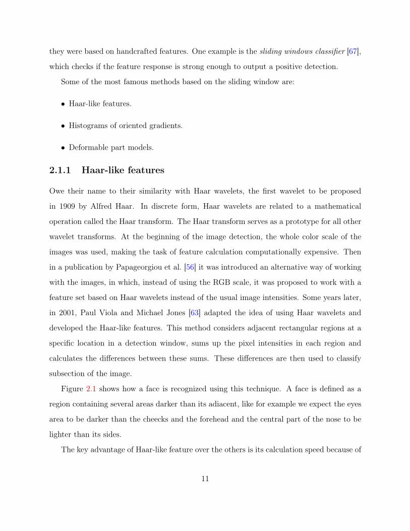
Detecting a person with this technique is possible with the usage of a root filter, plus

deformable parts, as shown in Figure 2.3.

2.1.4 Deep Learning for image classification

A remarkable upgrade to the object detection and classification fields has been brought by

the introduction of the deep learning [35, 57].

13

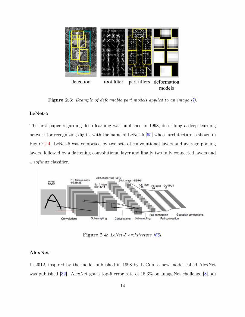
Figure 2.3: Example of deformable part models applied to an image [7].

LeNet-5

The first paper regarding deep learning was published in 1998, describing a deep learning

network for recognizing digits, with the name of LeNet-5 [65] whose architecture is shown in

Figure 2.4. LeNet-5 was composed by two sets of convolutional layers and average pooling

layers, followed by a flattening convolutional layer and finally two fully connected layers and

a softmax classifier.

Figure 2.4: LeNet-5 architecture [65].

AlexNet

In 2012, inspired by the model published in 1998 by LeCun, a new model called AlexNet

was published [32]. AlexNet got a top-5 error rate of 15.3% on ImageNet challenge [8], an

14

important milestone considering that up to that moment, the best top-5 error rate was of

26.2% obtained using a scale-invariant feature transform (SIFT) model. The first AlexNet

contained five consecutive convolutional filters, max-pooling layers and three fully-connected

layers, as shown in Figure 2.5.

Figure 2.5: First AlexNet architecture [32].

VGG16

After the results obtained by the first deep learning models, researchers have tried to create

always deeper convolutional neural network as a way to improve the performances. In

2015 the VGG16 model was published [61]. VGG16 was composed of sixteen convolutional

layers, multiple max-pooling layers and three fully-connected layers, as can be seen in 2.6.

This model introduced the stacking of multiple convolutional layers with ReLU activation

functions for creating nonlinear transformations, which allows models to learn more complex

patterns. In VGG16 were also introduced 3 × 3 filters for each convolution, instead of the

11×11 filters of the AlexNet, which even though were much lighter to compute, did not lower

the performances, yet improving the speed of the training because of the reduced number of

parameters to train. VGG16 obtained 7.3% top-5 error rate on the 2014 ImageNet challenge.

GoogLeNet

In the same year (2014) the concept of “inception modules” was also developed [62]. Instead

of using the original convolutional layer, that uses linear transformations with a nonlinear

15

Figure 2.6: VGG16 Architecture [61].

activation function, it was thought that training multiple convolutional layers simultaneously

and stacking their feature maps linked with a multi-layer perceptron, also produced a

nonlinear transformation. This idea was exploited to produce GoogLeNet, also called

Inception V1, for the usage of the inception modules [62]. GoogLeNet is much deeper than

the VGG16, having 22 layers using the inception modules, for a total of over 50 convolutional

layers. In Figure 2.7 is shown the structure of an inception module, which is composed by

convolutional layers of 1x1, 3x3 and 5x5 and a 3x3 max-pooling layer to increase the sparsity

in the model. The inception module makes it possible to obtain different types of patterns

which, then, are concatenated and given as input to the next inception module. GoogLeNet

obtained a 6.7% error rate in the 2014 ImageNet challenge and also, was incredibly smaller

in size compared with VGG16, being 55MB vs 490MB of the latter.

16

Figure 2.7: Inception Module [62].

Residual Learning

In 2015 another important improvement in the deep learning for image recognition, was

introduced when it was noticed that increasing the depth of the network, also involves an

increasing error rate and not due to over-fitting but due to the difficulties to train and

optimize those extremely deep models. As a way to solve those problems, a new way

of modelling neural networks, called “Residual Learning” [45] was introduced. In those

network, were added some connections between the output of one or multiple convolutional

layers and their original input. Residual neural networks do this by utilizing skip connections

to jump over some layers like shown in Figure 2.8. The neural network introducing those

connections was called ResNet, composed of 152 convolutional layers with 3x3 filters using

residual learning by block of two layers. The ResNet model won the 2015 challenge with a

top-5 error rate of 3.57%

17

Figure 2.8: Architecture example of Residual Block [45].

2.1.5 Deep Learning for object detection

Apart from image classification, deep learning brought important upgrades also for what

concerns the object detection field, in which the objective is to identify and localize the

different objects in an image. The study and comparison of the performance of the different

models are based on various famous datasets:

• The PASCAL Visual Object Classification, containing 20 categories of objects [9].

• The ImageNet dataset published in 2013, containing 200 categories [8].

• The COCO dataset (Common Objects in Context) developed by Microsoft [10], containing

80 categories.

Taking in exam the PASCAL dataset 2007, at the beginning, the best performing

model was the Deformable Part Model V5 (DPM V5) which obtained a mean average

precision (mAP) of 33.7% and performed at 0.07 fps. With the Deep Learning have been

achieved much better results and the first important upgrade came with the Region based

Convolutional Neural Networks (R-CNN).

Region-based Convolutional Neural Networks

Figure 2.9 shows the main idea behind the R-CNN, which is composed of two steps:

• In the first phase, using selective search, it identifies a manageable number of bounding-

box object region candidates, also called, region of interest

18

• In the second phase, it extracts convolutional neural network features from each region

independently for classification.

Figure 2.9: Region with CNN features [41].

With R-CNN [35, 41] it was achieved a mAP of 66.0% and it performed at 0.05 fps. After

several upgrades, R-CNN evolved into Faster R-CNN, which is the third official version of

the Region based CNN that got 73.2% mAP and performed at 7 fps. Great results but still

not enough speed for realtime applications, like for example, in a self-driving car. After

those results, the models have become still more accurate and now the attention has shifted

to the inference speed of the model.

YOLO: You Only Look Once

During the 2016 CVPR [11], the premier annual computer vision event, it was presented

a work called Yolo, (’You Only Look Once’) [60, 58, 59] that proposed a new approach to

object detection.

YOLO uses an alternative approach for object detection, a single neural network predicts

bounding boxes and class probabilities directly from full images in one evaluation. The

basic YOLO model processes images in real-time at 45 frames per second but there are

also other versions, which lower the precision to improve the performance. An example of

Yolo version which is faster but less precise than the standard YOLO is “fast YOLO”, that

processes at 155 frames per second while still achieving double the mAP of other real-time

19

detectors. The main difference is that other object detection systems exploit the usage of

classifiers to perform detection. To detect an object, they take a classifier for that object

and evaluate it at various locations and scales in a test image, while with YOLO, object

detection is reshaped as a single regression problem, directly from image pixels to bounding

box coordinates and class probabilities. Compared to other methods, like DPM and R-CNN,

YOLO is much simpler, having a single convolutional network that simultaneously predicts

multiple bounding boxes and class probabilities for those boxes.

Figure 2.10: Architecture of Yolo v1 [60].

Figure 2.10 presents the architecture of Yolo, with 24 convolutional layers followed by 2

fully connected layers. It also alternates 1 × 1 convolutional layers to reduce the features

space from preceding layers. Yolo divides the image into an S × S grid and for each grid

cell predicts B bounding boxes, confidence for those boxes, and C class probabilities. These

predictions are encoded as an S × S × (B × 5 + C) tensor, where:

• S × S is the shape of the grid cells,

• B × 5, B is the number of boxes and 5 represents the 4 values needed to define a box

plus 1 confidence value,

20

• C represents the different class probabilities.

The input image is divided into an S×S grid. Each grid cell predicts B bounding boxes

and C class probabilities. The bounding box prediction has 5 components: (x, y, w, h,

confidence). The (x, y) coordinates represent the center of the box, relative to the grid cell

location, while (w,h) represent the object dimensions.

The aim of this procedure is that, if no object exists in a cell, the confidence score should

be zero, otherwise, the confidence score should be equal to the intersection over union (IOU)

between the predicted box and the ground truth. Figure 2.11 shows how the Yolo procedure

works.

Figure 2.11: Yolo applied to an image with results [60].

A Yolo v1 network for the Pascal-voc dataset has an output tensor of 7×7× (2×5+20)

that is equal to a 7× 7× 30 tensor.

These methods, such as YOLO and R-CNN have successfully achieved great results in

detecting objects but, their low FPS on non-GPU computers, render them useless for real

time application. For that reason, further upgrade done to Yolo have made it even lighter

than the first version and nowadays, there are also light versions called Tiny Yolo, which

can be run in real time on devices using specifically built AI-chips, like the Kendryte K210.

21

2.1.6 Yolo V2

Yolo V2 introduces the concept of anchor boxes, which are a set of predefined bounding

boxes of a certain height and width [48]. The Anchor Boxes measures are calculated by doing

clustering on the size of the bounding boxes of the objects present in the dataset. Therefore,

instead of predicting a bounding box directly, YOLO V2 predicts which predefined box, the

anchor box, is closer to the object detected and resizes that.

With the introduction of the anchor boxes the output tensor changes in S × S × (k(1 +

4 + 20)) because, instead of trying to predict one single element for each square, Yolo v2

tries to detect one element for each anchor box in each square.

Figure 2.12: Yolo v2 applied to an image to detect man and tie [49].

A practical example to show the difference between Yolo and Yolo v2, can be seen in

Figure 2.12. A Yolo v1 model that can detect man and tie, would try to assign the object

to the grid cell that contains the middle of the object. With this method, the red cell

in Figure 2.12 should detect both the man and his tie, but since any grid cell can only

detect one object, it represents a problem. Adding the anchor boxes solved this problem,

by allowing the grid cell to detect more than one object, using k bounding boxes [49].

22

Figure 2.13: Concept of anchors boxes used by Yolo v2 [49].

Figure 2.13 shows how the concept of anchor boxes is applied on a single grid cell. As

previously said, Yolo v2 uses five anchor boxes. The number of anchor boxes (five) has been

chosen after applying k-means clustering on the training set bounding boxes for different

values of K and plotting the average IOU [12] with closest centroid, using IOU between

the bounding box and the centroid, as distance [48]. Five resulted to be the ideal number,

because it returned the best trade off between model complexity and recall.

Yolo V2 is based on Darknet-19, shown in Figure 2.14, a backbone net composed of 19

convolutional layers and 5 max-pooling layers. Darknet-19 is a network trained as a classifier

on the ImageNet challenge. After that the classifier had been trained, its last layers, that

outputs the classification, were removed and substituted by the Yolo detection layers [59].

23

Figure 2.14: Darknet-19 [48].

It is also possible to use lighter models as feature extractor instead of Darknet-19, for

Yolo v2-based detection. One of the possible alternatives, as back-end networks, are the

MobileNets [13, 46] which come in very different format and size and are also the ones on

which are based some of the person-detection model developed in this work.

24

2.1.7 Object detection on MaixPy

On the boards equipped with the Kendryte K210, it is possible to run models based on

Yolo V2 and, in the official forum of the Maix boards, there are some pre-trained models

for object detection based on it. One of the interesting models based on Tiny Yolo V2 is

called 20Classes_yolo [66]. It is based on the Pascal-voc dataset, so is able to detect 20

classes of objects. The model works pretty well and runs at about 18 FPS but unluckily

no documentation is provided on how the model has been trained. For this reason, several

models have been trained to detect person in real time with the objective of improving it

and to understand what are the different alternatives when it is needed to create a model

for some purpose.

2.2 Modelling the network for person detection

While the most precise models for object detection are those that run a detector with

different shapes in different parts of the image, as explained in 2.1.5 –page 19–, the fastest

models for object detection are those who pose the detection as a regression problem. Two

of the most popular ones are YOLO and SSD, also called single shot detectors [51].

For the creation of the model for person detection, after a study of the state-of-the-art,

instead of using a Yolo v2 network with Darknet-19 as a backbone which would be too

heavy for the K210, it has been decided to take some standard MobileNets which are offered

already trained on the ILSVRC-2012-CLS [8] image classification dataset and use them as

feature extractor for a Yolo V2 network. MobileNet is a class of efficient models for mobile

and embedded vision applications, based on a streamlined architecture that uses Depthwise

separable convolutions to build light weight deep neural networks [46]. This choice has been

taken because Darknet-19 uses convolutional layer which are much harder to compute with

respect to the depth-wise separable convolutions used by MobileNet. Figure 2.15 shows how

the standard convolutional and the Depthwise separable convolution differ, when applied

on the image.

25

Figure 2.15: standard convolution and depthwise convolution [43].

2.2.1 MobileNet

MobileNet is a general architecture and can be used for multiple use cases [13]. Depending

on the use case, it is possible to use different input layer size and different width factors.

This allows different width models, to reduce the number of multiply-adds and thereby

reduce inference cost on mobile devices [46].

MobileNets support any input size greater than 32× 32, with larger image sizes offering

better performance. The number of parameters and number of multiply-adds can be

modified by using the alpha parameter, which increases/decreases the number of filters

in each layer.

As previously said, the choice of using MobileNets instead of Darknet-19 was purely

given by the reduced computational cost brought by the substitution of the convolutional

layers with depthwise separable filters.

Depthwise separable convolution is a form of factorized convolution which divides the

convolution process into two parts: first a depthwise convolution and then a 1×1 convolution,

called pointwise convolution.

The difference between a depthwise separable convolution and a standard convolution is

that a standard convolution both filters and combines inputs into a new set of outputs in

one step, while the depthwise separable convolution splits this process into two steps, the

first layer just filters the input channels and the second layer combines them to create new

26

features.

Depthwise convolution is used to apply a single filter per each input channel (input

depth) and then the pointwise convolution is used to create a linear combination of the

output of the depthwise layer [46]. After each convolution, both batch normalization and

ReLu are applied to assure non linearity.

Images 2.16, 2.17, 2.18 show the difference between a standard convolutional filter and

the depthwise and pointwise filters.

Figure 2.16: Standard Convolutional Filters [46].

Standard convolutions have the computational cost of: DK ×DK ×M ×N ×DF ×DF

• DK ×DK is the kernel size.

• M is the number of input channels.

• N is the number of output channels.

• DF ×DF is the feature map size.

Figure 2.17: Depthwise Filters [46].

Depthwise convolution has a computational cost of: DK ×DK ×M ×DF ×DF

27

• DK ×DK is the kernel size.

• M is the number of input channels.

• DF ×DF is the feature map size.

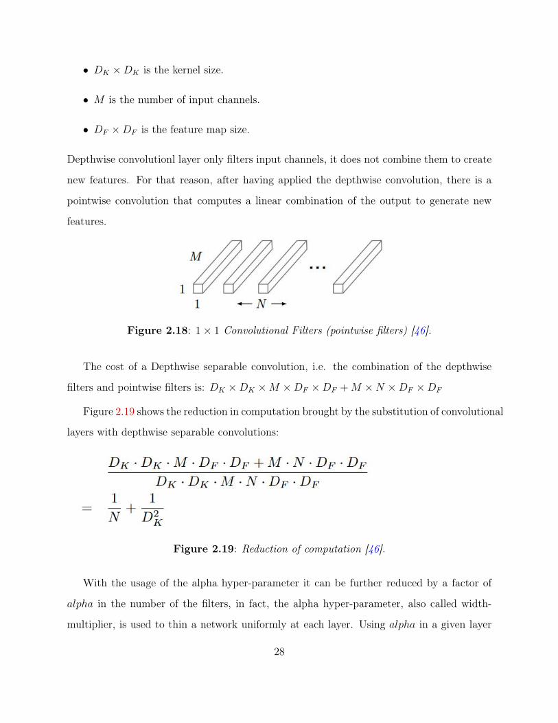
Depthwise convolutionl layer only filters input channels, it does not combine them to create

new features. For that reason, after having applied the depthwise convolution, there is a

pointwise convolution that computes a linear combination of the output to generate new

features.

Figure 2.18: 1× 1 Convolutional Filters (pointwise filters) [46].

The cost of a Depthwise separable convolution, i.e. the combination of the depthwise

filters and pointwise filters is: DK ×DK ×M ×DF ×DF +M ×N ×DF ×DF

Figure 2.19 shows the reduction in computation brought by the substitution of convolutional

layers with depthwise separable convolutions:

Figure 2.19: Reduction of computation [46].

With the usage of the alpha hyper-parameter it can be further reduced by a factor of

alpha in the number of the filters, in fact, the alpha hyper-parameter, also called width-

multiplier, is used to thin a network uniformly at each layer. Using alpha in a given layer

28

with M input channels and N output channels, they will become αM input channels and

αN output channels.

Hence, using the α hyper-parameter the computational cost of a depthwise separable

convolution is: DK ×DK × αM ×DF ×DF + αM × αN ×DF ×DF

MobileNets are mainly used with alpha of values 1.0, which corresponds to the full

MobileNet, 0.75, 0.50 and 0.25. Table 2.2.1 shows how much the network changes according

to the value of the alpha hyper-parameter.

Width Multiplier ImageNet Accuracy Million Mult-adds Million Parameters1.0 MobileNet-224 70.6% 569 4.20.75 MobileNet-224 68.4% 325 2.60.5 MobileNet-224 63.7% 149 1.30.25 MobileNet-224 50.6% 41 0.5

Table 2.1: MobileNet width multiplier [46].

Figure 2.20 shows the standard MobileNet architecture with alpha = 1. Modifying the α

parameter changes the number of filters on each layer by multiplying it for the alpha value.

For example, in the second layer, which Input Size is 112×112×32 in the normal MobileNet,

it becomes 112× 112× 16 in the MobileNet0_50 and 112× 112× 8 in the MobileNet0_25

which use respectively alpha=0.50 and alpha=0.25.

The full architecture of MobileNet V1 consists of a regular 3 × 3 convolution as the very

first layer, followed by 13 times the “depthwise separable convolution block”, represented

in Figure 2.21, for a total of 28 layer, counting the depthwise and pointwise as different

layers, plus the layers used to output the classification, which are substituted when using

the network for detection.

Considering the capabilities of the selected hardware (Kendryte K210) we decided to use

as backend for Yolo V2 either the MobileNets 0.25, 0.5 and 0.75 which were small enough

to fit the K210 and be run with real time performances.

29

Figure 2.20: MobileNet standard Architecture [46].

Figure 2.21: Depthwise Separable convolutions [46].

30

Chapter 3

Hardware components

3.1 Kendryte K210

Kendryte in Chinese means researching intelligence. Kendryte K210 is an AI capable dual

core 64-bit RISC-V processor, designed for machine vision and “machine hearing” [5]. The

Kendryte K210 is a chip accurately developed to bring the Artificial Intelligence on the edge,

i.e. for the Artificial Intelligence of things(AIoT).

Kendryte K210 is equipped with a powerful dual core 64 bit RISC-V processor, a KPU

which is a high performance Convolutional Neural Network (CNN) hardware accelerator

that allows to run small optimized CNN with up to Real Time performance and an APU

for processing microphone array inputs. The SRAM is split into two parts, 6MiB of on-

chip general-purpose SRAM memory and 2MiB of on-chip AI SRAM memory, for a total

of 8MiB. The AI SRAM memory is memory allocated for the KPU. The model’s input and

output feature maps are stored at 2MB KPU RAM while the weights and other parameters

are stored at 6MB RAM [28].

3.1.1 KPU

The KPU is what makes it possible to detect objects in real time. The convolutional neural

networks must be small and optimized according to the chip architecture and support. KPU

has built-in neural network operations such as convolution, batch normalization, activation,

31

Figure 3.1: Kendryte K210 with internal components [28]

and pooling operations. It supports the fixed-point model that can be trained using the

classic training frameworks such as Keras and Tensorflow but trained with specific restriction

rules. It supports 1x1 and 3x3 convolution kernels. This is important because the 1x1

convolutional filters can be used to reduce dimensionality in the filter dimension and make

the model computation lighter. According to the model size, the KPU can run in real-time

or not, as shown in Table 3.1.1:

mode maximum fixed pointmodel size

maximum pre-quantisationfloating point model size

Realtime (>30 fps) 5.9 MiB 11.8 MibNon-realtime(<10 fps) Flash Capacity Flash Capacity

Table 3.1: KPU real time requirements.

The KPU requires a specific neural network model format called Kmodel. The Kmodel

can be obtained converting a Tensorflow Lite model using an open source tool called

32

nncase [29]. It is also possible to convert models created with Keras, but it must be

considered that the K210 uses different standard padding method with respect to Keras’

default padding method, so the network must be adjusted. More in detail, the K210 pads

zeros all around (left, up, right, down), but Keras default pads just right and down. The

nncase tool allows to convert models from various formats. Figure 3.2 shows the different

input formats available and Figure 3.3 shows what are the different output format available.

Figure 3.2: nncase input format [29].

Figure 3.3: nncase output format [29].

The nncase tool also contains a field called inference-type which can be float or, as the

standard version already does, uint8.

The float inference type cannot be used if there are Conv2d layers in the network so

33

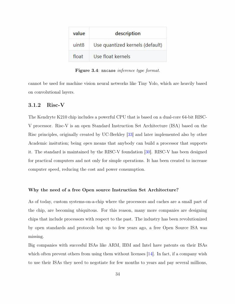
Figure 3.4: nncase inference type format.

cannot be used for machine vision neural networks like Tiny Yolo, which are heavily based

on convolutional layers.

3.1.2 Risc-V

The Kendryte K210 chip includes a powerful CPU that is based on a dual-core 64-bit RISC-

V processor. Risc-V is an open Standard Instruction Set Architecture (ISA) based on the

Risc principles, originally created by UC-Berkley [33] and later implemented also by other

Academic insitution; being open means that anybody can build a processor that supports

it. The standard is maintained by the RISC-V foundation [30]. RISC-V has been designed

for practical computers and not only for simple operations. It has been created to increase

computer speed, reducing the cost and power consumption.

Why the need of a free Open source Instruction Set Architecture?

As of today, custom systems-on-a-chip where the processors and caches are a small part of

the chip, are becoming ubiquitous. For this reason, many more companies are designing

chips that include processors with respect to the past. The industry has been revolutionized

by open standards and protocols but up to few years ago, a free Open Source ISA was

missing.

Big companies with succesful ISAs like ARM, IBM and Intel have patents on their ISAs

which often prevent others from using them without licenses [14]. In fact, if a company wish

to use their ISAs they need to negotiate for few months to years and pay several millions,

34

which rules out academia and small companies [15].

Even though a company decides to pay one of these ISAs providers to create an own

CPU using their ISAs, like paying for an ARM license for example, it does not mean they

can design an ARM core but instead they are allowed to use the design they offer. So, not

only the negotiations require a lot of time and cost, but also buying an ARM licence does

not let the company build its own CPU using the ARM ISA. Important to note that an

Instruction Set Architecture is an interface specification and not an implementation. There

are three types of implementation of an ISA [50]:

• Private closed source, like Appple iOS.

• Licensed open source, like Wind River VxWorks.

• Free, open source that users can change and share, like Linux.

Having a free open source ISA, where companies can add their own needs and collaborate

to its improvement, enables a real free open market of processor designs, which the patents

on ISA quirks prevent [50]. The most important improvements that have been introduced

by having a free open source ISA are:

• Greater innovation via free-market competition.

• Shared open core designs which mean shorter time to market, lower cost from reuse

and less errors considering that more people look at it.

• Processor cost decreases, becoming affordable for more devices, so great for the Internet

of Things.

Risc-V also has the advantage that, having been created after many years from Risc

and Cisc born and development, its own development can be based on the previous ones

and many errors can be avoided. Risc-V development started in 2010, by Patterson and his

students that predicted that in few years, the market of the processor would have changed

and it would have been dominated by:

35

• Small embedded devices requiring Ip address and internet access.

• Personal mobile devices such as smart phones.

• Warehouse-scale computers..

They thought that while it was possible to have distinct ISAs for each platform, life

would be simpler if they could use a single ISA design everywhere [50] and, with that idea

in their minds, they created Risc-V, a Risc based open Instruction set Architecture which

has a small core set of instructions, that can be extended with custom application-specific

accelerators.

Risc-V is based on a Load-store architecture. The instructions into a load-store architecture

are divided into two categories: memory access and ALU operation. Memory access instructions

occur between memory and registers, while ALU operations occur between registers. For

example, in a load-store architecture both the operands of an ADD must be in a register

while in a register-memory architecture one of the operands can also be in memory.

Intel x86 is an example of Register memory architecture and, as said before, Risc-V is

an example of load-store architecture. Risc-V was born with the goal of making a practical

ISA that was open-source, usable academically and in any hardware or software design

without royalties and to go against all the agreements that ARM Holdings [39] and MIPS

technologies require before releasing documents that describe their designs’ advantages [38].

In June 2018 another almost open ISA was published with a project called Mips Open.

Mips Open was started by Wave computing but unlike Risc-V, it was not fully open source

and it was provided under an open use licence. Unluckily, after less then an year, the project

has been closed and the people who were working with it, had to contract a new agreement

with the company [44].

To build a large community of users and to accumulate design and software, the RISC-

V ISA designers decided to do not over-architect for a particular micro-architecture, but

instead planned to support a wide variety of uses: small, fast and low-power real-word

36

implementations and also the rationale for every decision about the architectural choices

are described [30].

The instruction set is the main interface in a computer because it lies between the

hardware and the software. A good instruction set that is open and available for use by

all, reduces the cost of software by permitting far more reuse. It also increases competition

among hardware providers, who can use more resources for design and less for software

support [50].

3.1.3 Boards

During this work of master thesis, several boards equipped with the Kendryte K210 have

been used:

• Maix Go, shown in Figure 3.5.

• M5StickV, shown in Figure 3.6.

The MaixGo is produced by a Chinese company called Sipeed, while the M5StickV is

produced by M5Stack, another Chinese company. The main differences among the Maix

board and the M5StickV are the camera sensors and the absence of the WiFi antenna in the

M5StickV. The Maix board is modular and comes with an ov2640 camera sensor that can

be easily changed, while the M5StickV comes with an OmniVision OV7740 which provides

a best-in-class low light sensitivity making it ideal for machine vision [16]. Unfortunately,

the M5StickV does not have a WiFi antenna, so it has not been possible to use it in the

application. Another difference is that they both have a built-in microphone but the one

in the M5StickV does not work in the current version and the fix is waited for the next

versions.

3.1.4 Tools

There are several tools that are very useful for the developing on the K210.

37

Figure 3.5: Sipeed Maix Go board.

Nncase

Deep Learning models need to be converted into the Kmodel format, as explained in

Section 3.1.1. The conversion from TFlite, or other formats, to Kmodel, is performed

using the nncase tool [29].

Kflash

Kflash is a tool used to load the models and the firmware on the board. There is either a

GUI version or a simpler command-line version.

MaixPy IDE

MaixPy comes with its own IDE (Integrated Development Environment) that makes it easy

to program and setup the board. The MaixPy IDE also provides a framebuffer for viewing

video from the camera, which is useful if the used board does not have the LCD.

3.1.5 Programming environments

The K210 supports several programming environments which adapt to the user needs and

preferences without any substantial difference in terms of performances [17].

38

Figure 3.6: M5StickV board.

• Cmake command line development environment

K210’s official SDK supports two development modes: FreeRTOS and Standalone [28].

• IDE development environment

There is an official IDE for programming the K210, which is based on Visual Studio

Code [18].

• MicroPython development environment

MaixPy ported Micropython to K210. Micropython is a lean version of the Python 3

programming language, that includes a small subset of the Python standard library

and is optimized to run on micro-controllers. The documentation is available either in

English and in Chinese, which usually is a bit more updated [31]. In this environment,

it is needed to flash the firmware only once, then it is possible to upload the script

on the sd card or just use the serial port to interact with Python. There are several

firmware available, which bring more or less functionalities and change in size accordingly

39

and according to the firmware used, the board can also be compatible with the MaixPy

IDE.

40

Chapter 4

Training the network

4.1 Objectives and overview

One of the objectives of this work of master thesis, is the development of a person detection

system and the objective of this chapter is to explain how the neural network for person

detection has been modelled, optimized and trained, to be run on the Kendryte K210. The

official documentation of MaixPy offers an object detector for the 20 classes of the Pascal-

voc dataset, based on a convolutional neural network as feature extractor for Yolo v2 but,

according to the state of the art in 2.2.1 -page 26-, it has been proved that convolutional

layers are much harder to compute of the Depthwise separable convolution, so it has been

decided to substitute the convolutional neural network to be used as feature extractor, with

a MobileNet network. To cover every aspect, some proofs have been done also using Tiny

Yolo as feature extractor, as shown in section 4.4.

Neural Network is a type of machine learning algorithm, so its development follows the

usual workflow of data pre-processing, model building and model evaluation and this chapter

follows the three phases. The greatest time has been spent on the first phase because there

were no state of the art dataset for person detection that returned good results.

As explained in 2.1.5 -page 19-, the fastest models for object detection are those who pose

the task of object detection as a regression problem and considering that the Kendryte K210

is optimized for running Yolo v2 based detectors, all the models are based on it. Moreover,

41

the Kendryte K210 models must respect some characteristics, as explained in 3.1.1 -page

31-, so the choice of the network to be used as feature extractor has been driven by those

requisites.

For the data pre-processing part, a work on the dataset has been carried out, ranging

from the choose of a good dataset for the task of person detection, to the preparation of

its labels for the training of a Yolo v2- based network. Unfortunately, some of the standard

datasets for person detection, “Inria person” [19] and “Pascal Voc” [20] did not yield good

results as they are. Hence, new datasets have been created, extracting images from both

the dataset and adding other external images. All of them have been labelled according to

the Pascal-voc labels using the LabelImg tool [40].

For the model building part, after the study of the state-of-the-art for object detection,

it resulted clear that modelling a network from scratch was not ideal, considering that today,

a lot of work has been done for the field of object detection. In fact, today the majority

of the computer vision field applications are based on Transfer Learning and Fine Tuning.

These techniques permit to train a model for a task using a much smaller dataset and

significantly less computational power. It has also been tried to train the networks from

scratch, but they did not return the same results and also, training a network from scratch

required much more time compared to the time and computational power required when

using pre-trained backend weights. During the training it also has been tried to freeze the

weights of the pre-trained weights in order to just train the detection layer but it did not

return good results.

According to the K210 KPU requirements, it is possible to use few models as backend

network for Yolo v2 for the person detection task:

• Tiny Yolo

• MobileNet with alpha between 0.25 and 0.75

Tiny Yolo is composed of 9 convolutional layers, which should be harder to compute

with respect to the Depthwise separable convolutions of the MobileNets but, while the

42

convolutional layers are harder to compute, on the K210 the Depthwise separable convolutions

are still not implemented completely on the KPU, so the convolutional neural network,

results a bit faster, as shown in 4.4.2. MobileNets have been chosen also for the fact that they

are available with pre-trained weights on the ImageNet dataset, which made the network

converge better and faster.

4.1.1 Structure of the chapter

In the next sections the three phases of the implementation of the neural network are

explained in a more detailed manner. Section 4.2 shows how the neural network has been

modelled using MobileNet with different values for alpha and Tiny Yolo [21], as backend.

Section 4.3 shows which dataset have been used for the training of the network, how they

have been modified and how they have been prepared for the training. Section 4.4 shows

what are the results obtained and what are the final models that have been used on the

board for detecting persons in real time.

4.2 Building the Yolo v2 detector

MobileNet has been chosen as feature extractor for Yolo v2 because of the possibility of

taking already pre-trained weights on the ImageNet dataset, which made it possible to train

it using much less images and much less computational power with respect to training it

without pre-trained weights.

To use MobileNet as the Yolo backend, it is necessary to remove the last layers, which

are used to output the classification in MobileNet, and add the detection layers for Yolo v2.

Either MobileNet with alpha of values 0,75, 0,50 and 0,25 have been used in this work, also

to make a comparison among them. The full MobileNet has not been used, because it does

not fit the k210. As explained in 2.2.1 -page 26-, the different versions of MobileNet do not

differ in the depth of the net but only in the width.

43

Model details

According to the neural network used as feature extractor, the number of parameters and

the weight of the network change:

• The models built using MobileNet with alpha=0.25 as feature extractor weight 246

Kb and contain 226,254 parameters.

• The models built using MobileNet with alpha=0.50 as feature extractor weight 862

Kb and contain 844,926 parameters.

• The models built using MobileNet with alpha=0.75 as feature extractor weight 1.859

Kb and contain 1,856,046 parameters.

• The models built using Tiny Yolo as feature extractor weight 2.231 KB and contain

2,273,342 parameters.

Figures 4.2, 4.3, 4.4, and 4.5 show the structure of the network trained with MobileNet

0.25 as feature extractor. In each layer there are the 25% of filters with respect to the full

MobileNet version.

Figure 4.5 shows the last layers of the network with the layers related to the detection of

Yolo v2, placed instead of the layers related to the classification in MobileNet. In particular,

have been removed the final average pooling that is used to reduce the spatial resolution to

1, before the fully connected layer and the softmax layer that is used to output one of the

one thousand classes, and have been added the layers for the Yolo detection.

With this network, it is possible to use the pre-trained weights to recognize features in

the images and build the block used to exploit those features, in order to detect objects in

the images using the Yolo v2 technique.

For the detection part, after the last Depthwise Convolutions, there has been added a

convolutional layer that is used to generate predictions with a shape of 7x7x30 and then

a reshape layer that converts it in 7x7x5x6. Figure 4.1 shows the Yolo v2 network and its

44

outputs of 7x7x5x6 that, as explained in 2.1.6 -page 22- where Yolo v2 has been discussed,

can be so explained:

• 7 × 7 is the number of blocks in which the image is divided. Each block should be

32× 32 pixels so, changing the image size, implies a change in this layer.

• 5 represents number of anchor boxes used by Yolo v2.

• 6 is equal to numberofclasses + 5, where 5 is the number of components required

to describe each box (4 values to describe its position, width and height plus the

confidence score) and 1 is the number of classes that the network can detect (in the

image there are 20 class probabilities, which belong to the pascal-voc case).

Figure 4.1: Yolo v2 output [47].

45

Figure 4.2: Neural network with MobileNet-0.25 as backend1.

46

Figure 4.3: Neural network with MobileNet-0.25 as backend2.

47

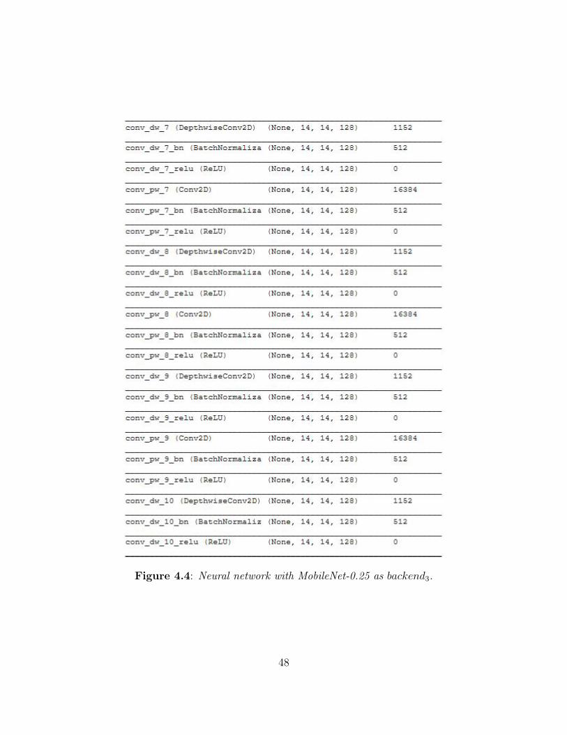
Figure 4.4: Neural network with MobileNet-0.25 as backend3.

48

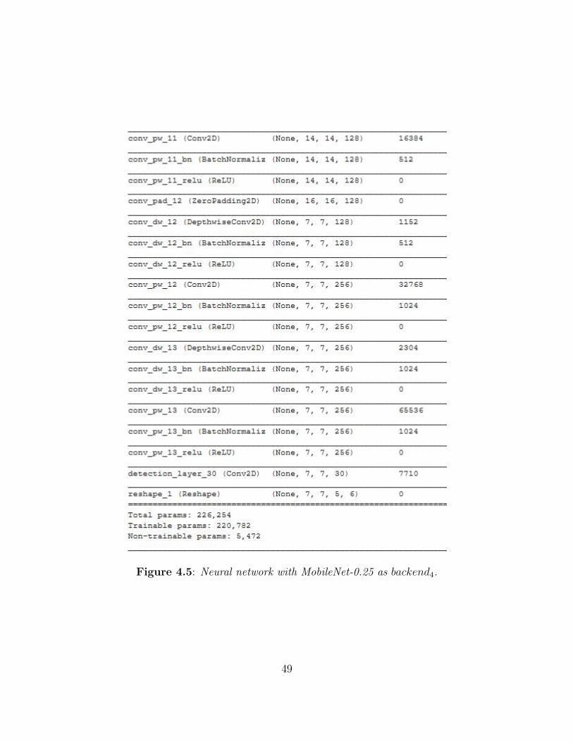
Figure 4.5: Neural network with MobileNet-0.25 as backend4.

49

Figure 4.6 and Figure 4.7 show the structure of the network built using Tiny Yolo as

feature extractor. In Figure 4.7 it is possible to observe the detection layers which are the

same of the network based on MobileNet as feature extractor and also, it is possible to

observe the number of total parameters that is higher than those of the MobileNet-based,

network.

Figure 4.6: Tiny Yolo1.

50

Figure 4.7: Tiny Yolo2.

4.3 Dataset and training

As explained in 2.1.6, considering that the objective is to detect persons, which is a class

present also in the ImageNet dataset on which the MobileNet has been already trained,

it has been possible to perform transfer learning. Transfer learning is a useful technique

which allows to avoid retraining a whole model from scratch, which would require a very

large dataset, by using pre-trained feature extractor model to train new "head" of model.

Training Yolo is a very hard task, so the whole process of creating a Yolo v2 network has

51

not been created from scratch, but some already existing works have been exploited, that

are: experiencor’s keras-yolo2 [40] and Dmitry Maslov’s aXeleRate framework [53].

After having built the neural network using MobileNet as backend, a dataset for the

training must be chosen. Several datasets have been used in this study, the Inria Pedestrian

dataset [19], the pascal-voc [20] and the Fudan pedestrian dataset [34], explained more in

detail in 4.3.1 -page 53-.

Figure 4.8: An example of a Pascal Voc image.

Figure 4.8 shows an example of an image belonging to the pascal voc dataset. Each image

of the dataset is described by an xml file, as in Figure 4.9, which contains the coordinates

of the bounding boxes of the objects.

Figure 4.9: An example of a Pascal Voc object in xml.

52

4.3.1 Preparing the dataset

Before starting the training with a dataset, it is possible to recalculate the anchors that will

be used by the Yolo V2 algorithm. As explained in 2.1.6, where Yolo v2 has been introduced,

the anchors are predefined bounding boxes that the network resizes to adapt to the actual

prediction. The anchors are given to the network for the detection part so that it does not

have to recalculate the bounding boxes for the objects but just resize the ones it already

has, to find the most-similar one to the actual bounding box of the object.

Each dataset has its own set of anchors that are calculated by using k-means clustering on

the dimensions of the ground truth boxes from the original training dataset to find the most

common shapes but, even though it is suggested to recalculate the anchors, no substantial

differences have been noticed when training with recalculated anchors or with the standard

anchors of Yolo v2 tiny [22]. There are several tools that can help recalculating the anchors,

the one that has been used to calculate the anchors of the datasets used for the training

and for the testing, is called gen_anchors.py [40]. To generate the labels for the images,

the tool labelImg [23] has been used, which offers a GUI to trace the bounding box on the

objects and assign them a label which can be saved either with pascal voc format or Yolo

format, as shown in Figure 4.10.

It is useful to have a whole pipeline defined so that if it is needed to detect other objects, it

is possible to create the labels for the new dataset to be used. In this work several datasets

for person detection have been used but none of them worked well as it is, so a work of

filtering and relabelling has been done.

Pascal-voc dataset[20]

The Pascal voc dataset has 5011 images labelled with the 20 voc classes. For this work,

a parser of the labels has been built in order to extract only those containing at least one

person, and have been obtained 2095 images. After that, all the labels of the other objects

of those 2095 images have been removed, making it an only person dataset.

53

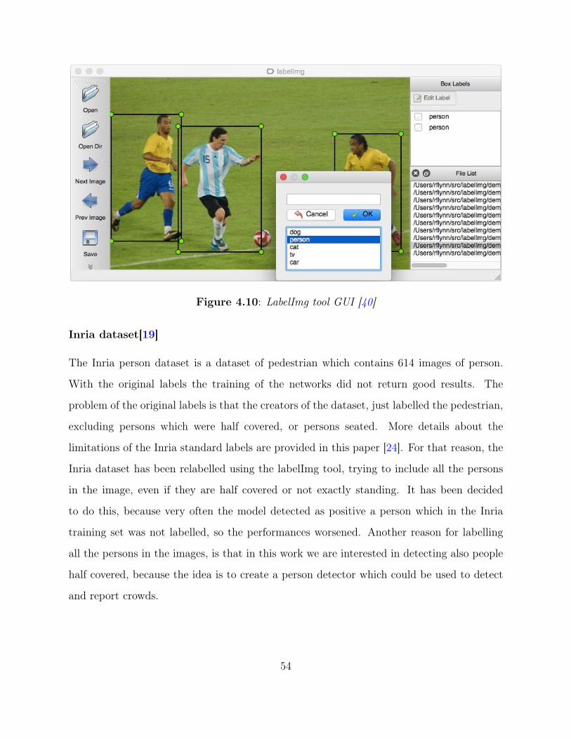
Figure 4.10: LabelImg tool GUI [40]

Inria dataset[19]

The Inria person dataset is a dataset of pedestrian which contains 614 images of person.

With the original labels the training of the networks did not return good results. The

problem of the original labels is that the creators of the dataset, just labelled the pedestrian,

excluding persons which were half covered, or persons seated. More details about the

limitations of the Inria standard labels are provided in this paper [24]. For that reason, the

Inria dataset has been relabelled using the labelImg tool, trying to include all the persons

in the image, even if they are half covered or not exactly standing. It has been decided

to do this, because very often the model detected as positive a person which in the Inria

training set was not labelled, so the performances worsened. Another reason for labelling

all the persons in the images, is that in this work we are interested in detecting also people

half covered, because the idea is to create a person detector which could be used to detect

and report crowds.

54

Fudan dataset [34]

The Fudan dataset is a dataset containing images that are used for pedestrian detection and

its images are taken from scenes around campus and urban streets. It contains 170 images

and 345 persons labelled.

InriaFudan dataset

It has been tried to merge the Inria dataset and the Fudan dataset because they both have

pedestrian images which are very similar among them and because the Fudan only contains

170 images which are not enough for training the network.

Merged dataset

The three different datasets did not bring very good results, so, it has been decided to

try merging them in a single dataset and, as explained in section 4.4, it returned the best

performances.

4.4 Results and performances

Several models have been trained either using pre-trained weights for the MobileNet backend

and without using the pre-trained weights. When using pre-trained weights the network can

actually adapt very good to the new task and is able to detect the persons, while, when

trying to train the network without pre-trained weights, it struggles to improve. For this

reason, the results are only reported for the training done using pre-trained weights.

For Tiny Yolo, there were no pre-trained weights, so the results are reported even if it was

a training from scratch.

Table 4.1 contains the results of the training of the different networks with the different

datasets used. The performance measures used are fscore, precision and recall and are

calculated on the validation dataset, while in table 4.2 they are calculated on a testing

dataset.

55

Model Backend Dataset Epochs mAp Fscore Precision RecallMobileNet alpha=0.75 mergedDataset 300 0.35 0.66 0.76 0.59MobileNet alpha=0.75 PascalVoc 300 0.17 0.098 0.375 0.056MobileNet alpha=0.75 Inria 300 0.22 0.25 0.314 0.207MobileNet alpha=0.75 InriaFudan 300 0.22 0.222 0.218 0.226MobileNet alpha=0.50 mergedDataset 300 0.35 0.66 0.74 0.60MobileNet alpha=0.25 mergedDataset 300 0.22 0.67 0.775 0.584Tiny Yolo mergedDataset 300 0.23 0.559 0.65 0.490

Table 4.1: Training results.

It has been noticed that the dataset returning best results is the one created merging

images from the Inria, Pascal and Fudan datasets. As a consequence, only the results

of the training done using that dataset are presented for the MobileNet with alpha=0.25,

alpha=0.50 and Tiny Yolo. The best performing models in terms of precision and recall in

validation, are the ones built with MobileNet with alpha = 0.75 and alpha = 0.50 as feature

extractor, trained for 300 epochs on the dataset built by us.

4.4.1 Testing the model

For testing purposes, a dataset of images taken with the camera module ov2640 equipped

by the Maix Board, has been created. It contains 130 images with at least 1 person inside.

It has been noticed that, while in validation, with images resized at the size of the network,

it works very good, as can be observed in the results in Table 4.1; results in testing are

poorer, as the images taken with the camera were of low quality, with respect to the ones

used for validation.

Figure 4.11, Figure 4.12 and Figure 4.13 show images with positive detections. In these

cases, the persons are close to the camera so they result easy to be detected.

Figure 4.14 shows an image with a negative detection. In this case, the person is not

very clear because of the low resolution of the image.

Table 4.2 shows the results of the testing done on the testing dataset created by taking

photos with the ov2640. Considering that the detector is based on Yolo v2, it is possible

56

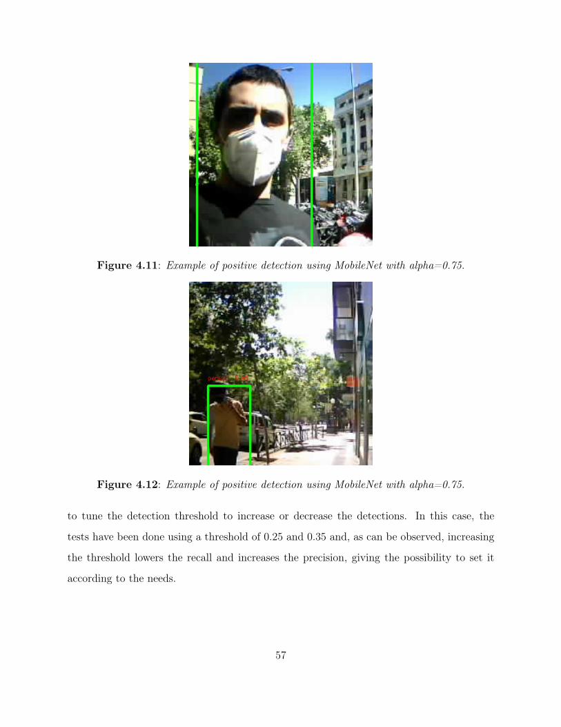
Figure 4.11: Example of positive detection using MobileNet with alpha=0.75.

Figure 4.12: Example of positive detection using MobileNet with alpha=0.75.

to tune the detection threshold to increase or decrease the detections. In this case, the

tests have been done using a threshold of 0.25 and 0.35 and, as can be observed, increasing

the threshold lowers the recall and increases the precision, giving the possibility to set it

according to the needs.

57

Figure 4.13: Example of positive detection using MobileNet with alpha=0.75.

Figure 4.14: Example of negative detection using MobileNet with alpha=0.75.

4.4.2 Inference time on the board

On the board, the different networks run at a very similar speed even though they are

very different in size. Table 4.3 shows at how many FPS the network can infer on the

board. Although the networks are different in size and as studied in the state-of-the-art in

2.2.1 -page 26-, the Depthwise Convolutions should be faster to compute with respect to

the convolutional layers of Tiny Yolo, the nncase [29] tool still does not fully support the

58

Model Backend Fscore Precision Recall thresholdMobileNet alpha=0.75 0.364 0.585 0.264 0.25MobileNet alpha=0.75 0.318 0.750 0.201 0.35MobileNet alpha=0.50 0.390 0.678 0.274 0.25MobileNet alpha=0.50 0.374 0.742 0.250 0.35MobileNet alpha=0.25 0.284 0.590 0.187 0.25MobileNet alpha=0.25 0.204 0.694 0.120 0.35Tiny Yolo 0.213 0.378 0.149 0.25Tiny Yolo 0.184 0.560 0.110 0.35

Table 4.2: Results of testing the networks on the testing dataset.

Depthwise Convolution. As a consequence, some of the operation of the MobileNet backend

are still done in CPU and not in KPU. Very soon, they will be ported on the KPU and

the MobileNet based networks, should become much faster [25]. However, it is possible to

almost double the FPS by using the dual-buff parameter of the sensor, at the exchange of a

higher usage of RAM of about 384 KB [26] and obtain around 30 FPS with all the networks

except the MobileNet with alpha=0.75.

Model Backend FPS Weight FPS dual-buffMobileNet alpha=0.75 12 1.859 KB 20MobileNet alpha=0.50 15 862 KB 29MobileNet alpha=0.25 16 246 KB 32Tiny Yolo 16 2.231 KB 32

Table 4.3: Networks weight (size) and FPS on the board.

In conclusion, according to the available RAMmemory for the network and the requirements

of the application, it is possible to take a faster model or a more precise one, but in

general, the model which performs better in terms of precision and speed is MobileNet

with alpha=0.50, even though the Depthwise Convolution is still not fully supported by the

KPU [25].

59

Chapter 5

The application

Armed with the deep neural network for detecting persons and converted it to Kmodel,

it is possible to upload it to the boards equipped with the K210 and use it. The idea of

the application, is to use this neural network on one or more of these boards to create

low-cost security cameras. The board communicates the extracted data to an online broker,

ThingSpeak, in which there is some logic which warns the user with a message when certain

conditions are met.

The main components of the architecture are:

• The board equipped with the K210: Maix Go.

• The Broker: ThingSpeak.

• IFTTT to communicate with the user.

The neural network is used for two main functions:

• The first one is to detect persons in the video stream, take an average of their number

in n minutes and send that value on the broker.

• The second usage is to detect when two or more persons are too close, take a photo

when this happen and send the number of times this happens in n minutes, on the

broker.

60

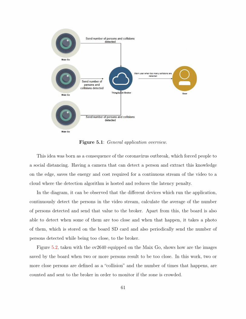
Figure 5.1: General application overview.

This idea was born as a consequence of the coronavirus outbreak, which forced people to

a social distancing. Having a camera that can detect a person and extract this knowledge

on the edge, saves the energy and cost required for a continuous stream of the video to a

cloud where the detection algorithm is hosted and reduces the latency penalty.

In the diagram, it can be observed that the different devices which run the application,

continuously detect the persons in the video stream, calculate the average of the number

of persons detected and send that value to the broker. Apart from this, the board is also

able to detect when some of them are too close and when that happen, it takes a photo

of them, which is stored on the board SD card and also periodically send the number of

persons detected while being too close, to the broker.

Figure 5.2, taken with the ov2640 equipped on the Maix Go, shows how are the images

saved by the board when two or more persons result to be too close. In this work, two or

more close persons are defined as a “collision” and the number of times that happens, are

counted and sent to the broker in order to monitor if the zone is crowded.

61

Figure 5.2: Collision detected.

5.1 Monitoring from remote

To monitor the number of persons in the environment from remote, it has been decided to

use the ThingSpeak broker. The ThingSpeak platform is divided into channels and each

channel contains up to eight fields in which it is possible to publish values. The publish

on the ThingSpeak channels can be performed using the REST API or MQTT. It has

been decided to assign two fields to each one of the board used to monitor the different

environments.

In this way, each board will send in its first assigned field the medium value of person

detected in the last n minutes and in the second field assigned, it will send the number of

collisions detected in the last n minutes. The channel can be monitored in real time from the

platform and it is also possible to add some intelligence directly there, which comprehends

MatLab code that is used to filter the data or to carry out checks on the arriving data in

62

order to trigger some actions.

This architecture, results in a very scalable solution which allows us to monitor different

places with different boards but one single broker which receives the values published from

the devices and work with it.

Figures 5.3 and 5.4 show how the data sent to the broker can be seen from the platform.

The graphs in Figure 5.3 are the ones assigned to the first device and the ones in Figure 5.4

are the ones assigned to the second device. The left images contain the first fields assigned

to the devices on which they publish the medium number of person detected and in the

right images there are the second fields assigned to the devices, which contain the number

of collisions detected.

Figure 5.3: ThingSpeak device 1 data.

Figure 5.4: ThingSpeak device 2 data.

63

With this architectural choice, we can monitor up to four environments with each

channel, by sharing the channel between four devices. ThingSpeak has been chosen because

it provides instant visualizations of data posted by the devices and data can be published

either by REST APIs or MQTT. Also, the ThingSpeak platform offers the possibility to

trigger a React when a condition is met. It is an important feature which is used to warn

the person in charge of monitoring with an SMS, when the number of collisions goes over a

certain number.

With this choices, it is possible to monitor the ThingSpeak channel and if one of the

boards sends a too high value of collisions, that is defined in the react options, it will be

triggered and a message will be sent to the user. To do so, it is needed to create an applet

called Web Hook in the IFTTT platform which can be done through the web or also through

the android application, like in Figure 5.5.

Once that the Web Hook has been created, it is possible to configure a thingHTTP on

the ThingSpeak platform, that triggers the IFTTT applet created. Figure 5.6 shows how

appears the thingHTTP on the IFTTT platform.

The thingHTTP is called when the condition defined in the React is met and in this

case, it was decided to set the React to trigger the process when more than 2 collisions are

detected in the first environments monitored.

64

Figure 5.5: IFTTT WebHook applet on Android phone.

65

Figure 5.6: ThingHTTP on ThingSpeak platform.

66

Chapter 6

Conclusions and future work

The idea of this work was to understand how the K210 AI chip works and what are its

features regarding the computer vision field and see how it can be used in a real application

belonging to the field of the Artificial Intelligence of Things.

Creating a person detector which does all the computation on the edge looked like a very

interesting idea because, while it may look a simple task as of today, it resulted a very hard

one, for the lack of a good dataset and for the reduced size of the network.

After a deep study of the state of the art for the task of person detection, it has been

possible to train a neural network based on the Yolo v2 detection, using MobileNet and

Tiny Yolo as feature extractor and we concluded that MobileNet with alpha=0.50 is the one

performing better, in 4.4.

Several famous datasets have been tried for the training of the network but none of them

worked well as it is and to solve that problem, a merge between them has been done and a

work of relabelling has improved the performances but it could still be improved by defining

better which objects in the image should be detected or not.

In particular, for the person detection problem, should a half-covered person be labelled

or not, in the dataset used for the training? According to the answer, the network may

perform better or worse and also in the literature, this is a debated question.

In conclusion, the K210 resulted to be a very powerful, yet very cheap, System-on-a-chip

and while a person detector is a hard task even for very powerful hardware, and also if we

67

got satisfactory results, there are many, easier, computer vision task that can be solved by

this kind of SoC.

For example, during the coronavirus outbreak, Canaan, the company who owns the

K210, improved their face recognition algorithm including the detection of faces covered by

a mask [27].

The K210 fully satisfied the expectations and even though its support and documentation

are still not complete, and not all the Neural Network operations are supported by the KPU,

they are improving very rapidly thanks to a very active community of users who continuously

talk and share ideas.

6.1 Future work

As possible future works, we propose the creation of a dataset for person detection using

the ov2640 of the MaixGo board, in order to train the neural network using images with the

same quality of those it will meet during the application execution. During the creation of

the dataset, it would also be possible to decide to detect other objects and not only persons.

Detecting more objects would not add much complexity over the network, because the only

change would be in the output layer changing from 7×7×5(5×1) to 7×7×5(5×n) where

n is the number of classes, so the performances in terms of computational cost, should be

approximately the same. Training the network for detecting more classes could be interesting

also to see if the performances over the single class would be lowered in case the network

must detect more classes.

68

Bibliography

[1] https://www.gartner.com/en/newsroom/press-releases/2015-08-18-gartners-2015-

hype-cycle-for-emerging-technologies-identifies-the-computing-innovations-that-

organizations-should-monitor.

[2] https://software.intel.com/content/www/us/en/develop/articles/intel-movidius-

neural-compute-stick.html.

[3] https://www.nvidia.com/en-us/autonomous-machines/embedded-systems/.

[4] https://coral.ai/.

[5] https://s3.cn-north-1.amazonaws.com.cn/dl.kendryte.com/documents/

kendryte_datasheet_20181011163248_en.pdf.

[6] https://www.vlfeat.org/overview/hog.html.

[7] http://www.cse.psu.edu/~rtc12/CSE586/lectures/dpmlecture.pdf.

[8] http://www.image-net.org/.

[9] https://www.tensorflow.org/datasets/catalog/voc.

[10] https://www.tensorflow.org/datasets/catalog/coco.

[11] http://cvpr2016.thecvf.com/.

[12] https://www.pyimagesearch.com/2016/11/07/intersection-over-union-iou-for-object-

detection/.

[13] https://github.com/keras-team/keras-applications/blob/master/keras_

applications/mobilenet.py.

69

[14] https://brej.org/yellow_star/letter.pdf.

[15] https://research.cs.wisc.edu/multifacet/papers/ieeemicro16_card_isa.pdf.

[16] https://www.adafruit.com/product/4321.

[17] https://www.seeedstudio.com/blog/2019/09/12/get-started-with-k210-hardware-and-programming-environment/.

[18] http://kendryte-ide.s3-website.cn-northwest-1.amazonaws.com.cn/.

[19] https://dbcollection.readthedocs.io/en/latest/datasets/inria_ped.html.

[20] http://host.robots.ox.ac.uk/pascal/VOC/.

[21] https://github.com/sipeed/Maix-Keras-workspace.

[22] https://github.com/pjreddie/darknet/blob/master/cfg/yolov2-tiny.cfg.

[23] https://github.com/tzutalin/labelImg.

[24] http://vislab.isr.ist.utl.pt/wp-content/uploads/2012/12/onPurity.pdf.

[25] https://en.bbs.sipeed.com/t/topic/1790/19.

[26] https://maixpy.sipeed.com/en/libs/machine_vision/sensor.html.

[27] https://canaan.io/733.html.

[28] Kendryte homepage. https://kendryte.com/.

[29] nncase converter. https://github.com/kendryte/nncase.

[30] Risc-v specifications. https://riscv.org/specifications/.

[31] sipeed maixpy site. https://maixpy.sipeed.com/en/.

[32] G. E. Hinton A. Krizhevsky, I. Sutskever. Imagenet classification with deep

convolutionalneural networks. 2012.

70

[33] Krste Asanović and David A. Patterson. Instruction sets should be free: The case

for risc-v. Technical Report UCB/EECS-2014-146, EECS Department, University of

California, Berkeley, Aug 2014.

[34] Liang Wang Ben Tan, Junping Zhang. Semi-supervised elastic net for pedestrian

counting. Pattern Recognition, 44:2297–2304, 2011.

[35] J. Brownlee. A gentle introduction to object recognition with deep learning. https://

machinelearningmastery.com/object-recognition-with-deep-learning//, 2019.

[36] R. Buyya C. Chang, S. N. Srirama. Internet of Things (IoT) and New Computing

Paradigms.

[37] L. Claeys. https://verhaert.com/the-intersection-of-ai-and-iot/.

[38] C. Demerijan. How arm licenses it’s ip for production. https://semiaccurate.com/

2013/08/08/how-arm-licenses-its-ip-for-production/, 2013.

[39] C. Demerijan. A long look at how arm licenses chips. https://semiaccurate.com/

2013/08/07/a-long-look-at-how-arm-licenses-chips/, 2013.

[40] experiencor. https://github.com/experiencor/keras-yolo2.

[41] R. Gandhi. R-cnn, fast r-cnn, faster r-cnn, yolo —

object detection algorithms. https://towardsdatascience.com/

r-cnn-fast-r-cnn-faster-r-cnn-yolo-object-detection-algorithms-36d53571365e/,

2019.

[42] Ian Goodfellow, Yoshua Bengio, and Aaron Courville. Deep Learning. MIT Press, 2016.

http://www.deeplearningbook.org.

[43] Yunhui Guo, Yandong Li, Rogerio Feris, Liqiang Wang, and Tajana Rosing. Depthwise

Convolution is All You Need for Learning Multiple Visual Domains. arXiv e-prints,

page arXiv:1902.00927, February 2019.

71

[44] G. Halfacree. Wave computing closes its mips open initiative with

immediate effect, zero warning. https://www.hackster.io/news/

wave-computing-closes-its-mips-open-initiative-with-immediate-effect-zero-warning-e88b0df9acd0,

2019.

[45] Kaiming He, Xiangyu Zhang, Shaoqing Ren, and Jian Sun. Deep Residual Learning

for Image Recognition. arXiv e-prints, page arXiv:1512.03385, December 2015.

[46] Andrew G. Howard, Menglong Zhu, Bo Chen, Dmitry Kalenichenko, Weijun Wang,

Tobias Weyand, Marco Andreetto, and Hartwig Adam. MobileNets: Efficient

Convolutional Neural Networks for Mobile Vision Applications. arXiv e-prints, page

arXiv:1704.04861, April 2017.

[47] Jonathan Hui. https://medium.com/@jonathan_hui/

real-time-object-detection-with-yolo-yolov2-28b1b93e2088.

[48] A. Farhadi J. Redmon. Yolo9000:better, faster, stronger. 2017.

[49] A. Kamal. Yolo, yolov2 and yolov3: All you

want to know. https://medium.com/@amrokamal_47691/

yolo-yolov2-and-yolov3-all-you-want-to-know-7e3e92dc4899/, 2019.

[50] David A. Patterson Krste Asanović. Instruction sets should be free: The case for risc-v.

2014.

[51] Wei Liu, Dragomir Anguelov, Dumitru Erhan, Christian Szegedy, Scott Reed, Cheng-

Yang Fu, and Alexander C. Berg. SSD: Single Shot MultiBox Detector. arXiv e-prints,

page arXiv:1512.02325, December 2015.

[52] A. Maheshwari. https://iq.opengenus.org/face-detection-using-viola-jones-algorithm/.

[53] Dmitry Maslov. https://github.com/AIWintermuteAI/aXeleRate.

72

[54] Robert K. McConnell. Method of and apparatus for pattern recognition. 1986.

[55] B. Triggs N. Dalal. Histogram of oriented gradients for human detection, 2005.

[56] C. P. Papageorgiou, M. Oren, and T. Poggio. A general framework for object detection.

In Sixth International Conference on Computer Vision (IEEE Cat. No.98CH36271),

pages 555–562, 1998.

[57] A. Quaknine. Review of deep learning algorithms

for object detection. https://medium.com/zylapp/

review-of-deep-learning-algorithms-for-object-detection-c1f3d437b852/,

2018.

[58] J. Redmon, S. Divvala, R. Girshick, and A. Farhadi. You only look once:unified, real-

time object detection. 2016.

[59] Joseph Redmon. Darknet: Open source neural networks in c. http://pjreddie.com/

darknet/, 2013–2016.

[60] Joseph Redmon, Santosh Divvala, Ross Girshick, and Ali Farhadi. You Only Look

Once: Unified, Real-Time Object Detection. arXiv e-prints, page arXiv:1506.02640,

June 2015.

[61] Karen Simonyan and Andrew Zisserman. Very Deep Convolutional Networks for Large-

Scale Image Recognition. arXiv e-prints, page arXiv:1409.1556, September 2014.

[62] Christian Szegedy, Wei Liu, Yangqing Jia, Pierre Sermanet, Scott Reed, Dragomir

Anguelov, Dumitru Erhan, Vincent Vanhoucke, and Andrew Rabinovich. Going Deeper

with Convolutions. arXiv e-prints, page arXiv:1409.4842, September 2014.

[63] P. Viola and M. Jones. Rapid object detection using a boosted cascade of simple

features. In Proceedings of the 2001 IEEE Computer Society Conference on Computer

Vision and Pattern Recognition. CVPR 2001, volume 1, pages I–I, 2001.

73

[64] M. Roth W. T. Freeman. Orientation histograms for hand gesture recognition. 1994.

[65] Y. Bengio P. Haffner Y. LeCun, L. Bottou. Gradient-based learning applied to

document recognition. 1998.

[66] Zepan. https://blog.sipeed.com/p/677.html.

[67] Zhengxia Zou, Zhenwei Shi, Yuhong Guo, and Jieping Ye. Object Detection in 20

Years: A Survey. arXiv e-prints, page arXiv:1905.05055, May 2019.

74