Use of Ozone in Water Reclamation for Contaminant Oxidation...Use of Ozone in Water Reclamation for...
494
Use of Ozone in Water Reclamation for Contaminant Oxidation WateReuse Research Foundation
Transcript of Use of Ozone in Water Reclamation for Contaminant Oxidation...Use of Ozone in Water Reclamation for...

UUssee ooff OOzzoonnee iinn WWaatteerr RReeccllaammaattiioonn ffoorr
CCoonnttaammiinnaanntt OOxxiiddaattiioonn
WWaatteeRReeuussee RReesseeaarrcchh FFoouunnddaattiioonn


Use of Ozone in Water Reclamation for
Contaminant Oxidation

About the WateReuse Research Foundation
The mission of the WateReuse Research Foundation is to conduct and promote applied research on the reclamation, recycling, reuse, and desalination of water. The Foundation’s research advances the science of water reuse and supports communities across the United States and abroad in their efforts to create new sources of high quality water for various uses through reclamation, recycling, reuse, and desalination while protecting public health and the environment. The Foundation sponsors research on all aspects of water reuse, including emerging chemical contaminants, microbiological agents, treatment technologies, reduction of energy requirements, concentrate management and desalination, public perception and acceptance, economics, and marketing. The Foundation’s research informs the public of the safety of reclaimed water and provides water professionals with the tools and knowledge to meet their commitment of providing a reliable, safe product for its intended use. The Foundation’s funding partners include the Bureau of Reclamation, the California State Water Resources Control Board, the California Energy Commission, and the California Department of Water Resources. Funding is also provided by the Foundation’s subscribers, water and wastewater agencies, and other interested organizations.

Use of Ozone in Water
Reclamation for Contaminant
Oxidation Shane A. Snyder, Ph.D. University of Arizona Southern Nevada Water Authority Urs von Gunten, Ph.D. Eawag: Swiss Federal Institute of Aquatic Science and Technology Ecole Polytechnique Federale de Lausanne Gary Amy, Ph.D. King Abdullah University of Science and Technology Jean Debroux, Ph.D. Kennedy/Jenks Consultants Daniel Gerrity, Ph.D. University of Nevada, Las Vegas Trussell Technologies, Inc. Southern Nevada Water Authority Cosponsors
Bureau of Reclamation California State Water Resources Control Board Air Products and Chemicals, Inc. APTwater, Inc. City of Chicago Gwinnett County Metawater Seqwater
WateReuse Research Foundation Alexandria, VA

Disclaimer This report was sponsored by the WateReuse Research Foundation and cosponsored by the Bureau of Reclamation and California Water Resources Control Board. The Foundation and its Board Members assume no responsibility for the content reported in this publication or for the opinions or statements of facts expressed in the report. The mention of trade names of commercial products does not represent or imply the approval or endorsement of the WateReuse Research Foundation. This report is published solely for informational purposes. For more information, contact: WateReuse Research Foundation 1199 North Fairfax Street, Suite 410 Alexandria, VA 22314 703-548-0880 703-548-5085 (fax) www.WateReuse.org/Foundation © Copyright 2014 by the WateReuse Research Foundation. All rights reserved. Permission to copy must be obtained from the WateReuse Research Foundation. WateReuse Research Foundation Project Number: WRRF-08-05 WateReuse Research Foundation Product Number: 08-05-1 ISBN: 978-1-941242-11-7

WateReuse Research Foundation v
Contents List of Figures ...................................................................................................................... xi
List of Tables .................................................................................................................... xvii
List of Acronyms ............................................................................................................... xxi
Foreword ........................................................................................................................... xxv
Acknowledgments ........................................................................................................... xxvi
Executive Summary ......................................................................................................... xxix
Chapter 1. Literature Review ............................................................................................ 1
1.1 Introduction .............................................................................................................. 1
1.1.1 Toxicological Implications for Aquatic Environments and Human Health ............................................................................................. 3
1.1.2 Current Water Reuse Guidelines and Regulations ...................................... 7
1.2 Assessment of Oxidation Processes ....................................................................... 11
1.2.1 Ozone ........................................................................................................ 11
1.2.2 Ozone/H2O2 .............................................................................................. 13
1.2.3 UV/H2O2 ................................................................................................... 13
1.3 Prediction of Trace Organic Contaminant Elimination: Kinetics .......................... 14
1.3.1 Second-Order Rate Constants ................................................................... 14
1.3.2 Quantitative Structure–Activity Relationships ......................................... 29
1.3.3 Ozone and ·OH Exposure ......................................................................... 31
1.3.4 Indicator Compounds ................................................................................ 32
1.3.5 Surrogate Parameters ................................................................................ 33
1.4 Efficacy of Ozone for Wastewater Disinfection .................................................... 34
1.5 Transformation Products and Biological Activity ................................................. 37
1.5.1 Ozone Transformation Products ............................................................... 37
1.5.2 ·OH Transformation Products .................................................................. 39
1.5.3 Biological Activity of Specific Transformation Products ......................... 39
1.5.4 Biological Activity of Effluent Mixtures .................................................. 40
1.6 Ozone Byproduct Formation from Matrix Transformation ................................... 42
1.6.1 Bromate and Bromo-organics ................................................................... 42
1.6.2 N-Nitrosamines ......................................................................................... 45
1.6.3 Assimilable Organic Carbon ..................................................................... 46
1.7 Applicability of Aquifer Recharge and Recovery for Ozonated Effluent .............. 46
1.8 Pilot- and Full-Scale Ozonation for Trace Organic Contaminant Mitigation ........ 47
1.8.1 Pilot-Scale Ozone Applications ................................................................ 47
1.8.2 Full-Scale Ozone Applications for TOrC Oxidation and Removal .......... 49
1.8.3 Full-Scale Ozone Applications and Toxicological Implications .............. 51
1.9 Conclusion ............................................................................................................. 52

vi WateReuse Research Foundation
Chapter 2. Technical Approach and Methods ............................................................... 53
2.1 Bench-Scale Oxidation Experiments ..................................................................... 53
2.1.1 Wastewater Collection and Processing ..................................................... 53
2.1.2 Bench-Scale Ozone Testing ...................................................................... 54
2.1.3 Bench-Scale Ultraviolet Experiments ....................................................... 56
2.1.4 Quenching and Preservation ..................................................................... 57
2.2 Target Compounds ................................................................................................. 58
2.3 Organic Characterization ....................................................................................... 63
2.3.1 Excitation Emission Matrices ................................................................... 63
2.3.2 Size-Exclusion Chromatography .............................................................. 65
2.3.3 Assimilable Organic Carbon ..................................................................... 66
2.4 Target Microbes and Methods of Assessing Disinfection ..................................... 67
2.4.1 Coliform Bacteria ..................................................................................... 68
2.4.2 MS2 Bacteriophage ................................................................................... 68
2.4.3 Bacillus subtilis Spores ............................................................................. 69
2.4.4 Eawag Disinfection Experiments .............................................................. 70
2.5 Characterization of ·OH Exposure ......................................................................... 70
2.5.1 pCBA ........................................................................................................ 70
2.5.2 t-BuOH ..................................................................................................... 71
2.6 Bioassays ............................................................................................................... 72
2.6.1 Yeast Estrogen Screen Assay for Total Estrogenicity .............................. 72
2.6.2 Harvard Bioassays .................................................................................... 73
2.7 NDMA and NDMA Formation Potential Testing.................................................. 73
2.8 1,4-Dioxane ............................................................................................................ 74
Chapter 3. Bench-Scale Evaluation of U.S. Secondary Effluents ................................. 75
3.1 Clark County Water Reclamation District, Las Vegas, Nevada ............................ 75
3.1.1 Ozone Demand/Decay .............................................................................. 77
3.1.2 Bromate Formation ................................................................................... 78
3.1.3 ·OH Exposure ........................................................................................... 79
3.1.4 Title 22 Contaminants ............................................................................... 80
3.1.5 Trace Organic Contaminants .................................................................... 83
3.1.6 Disinfection ............................................................................................... 89
3.1.7 Organic Characterization .......................................................................... 95
3.2 Metropolitan Water Reclamation District of Greater Chicago, Illinois ............... 104
3.2.1 Ozone Demand/Decay ............................................................................ 105
3.2.2 Bromate Formation ................................................................................. 106
3.2.3 ·OH Exposure ......................................................................................... 107
3.2.4 Title 22 Contaminants ............................................................................. 108
3.2.5 Trace Organic Contaminants .................................................................. 110 3.2.6 Disinfection ............................................................................................. 116
3.2.7 Organic Characterization ........................................................................ 122

WateReuse Research Foundation vii
3.3 West Basin Municipal Water District, Los Angeles, California .......................... 133
3.3.1 Ozone Demand/Decay ............................................................................ 135
3.3.2 Bromate Formation ................................................................................. 135
3.3.3 ·OH Exposure ......................................................................................... 136
3.3.4 Title 22 Contaminants ............................................................................. 137
3.3.5 Trace Organic Contaminants .................................................................. 140
3.3.6 Disinfection ............................................................................................. 145
3.3.7 Organic Characterization ........................................................................ 151
3.4 Pinellas County Utilities, Pinellas County, Florida ............................................. 160
3.4.1 Ozone Demand/Decay ............................................................................ 162
3.4.2 Bromate Formation ................................................................................. 162
3.4.3 ·OH Exposure ......................................................................................... 163
3.4.4 Title 22 Contaminants ............................................................................. 164
3.4.5 Trace Organic Contaminants .................................................................. 167
3.4.6 Disinfection ............................................................................................. 172
3.4.7 Organic Characterization ........................................................................ 177
3.5 Gwinnett County, Georgia ................................................................................... 187
3.5.1 Ozone Demand/Decay ............................................................................ 189
3.5.2 Bromate Formation ................................................................................. 189
3.5.3 ·OH Exposure ......................................................................................... 190
3.5.4 Title 22 Contaminants ............................................................................. 191
3.5.5 Trace Organic Contaminants .................................................................. 194
3.5.6 Disinfection ............................................................................................. 198
3.5.7 Organic Characterization ........................................................................ 204
Chapter 4. Bench-Scale Evaluation of International Secondary Effluents ............... 213
4.1 Lausanne Wastewater Treatment Plant, Lausanne, Switzerland ......................... 213
4.1.1 Ozone and H2O2 Decomposition Kinetics .............................................. 214
4.1.2 Bromate Formation ................................................................................. 217
4.1.3 Trace Organic Contaminants .................................................................. 219
4.1.4 Disinfection ............................................................................................. 222
4.1.5 Organic Characterization ........................................................................ 223
4.2 Regensdorf (Wüeri) Wastewater Treatment Plant, Regensdorf, Switzerland ...... 226
4.2.1 Background ............................................................................................. 226
4.2.2 Ozone and H2O2 Decomposition Kinetics .............................................. 227
4.2.3 Bromate and Nitrosamine Formation...................................................... 230
4.2.4 Trace Organic Contaminants .................................................................. 231
4.2.5 Disinfection ............................................................................................. 234
4.2.6 Organic Characterization ........................................................................ 235
4.3 Kloten-Opfikon Wastewater Treatment Plant, Glattbrugg, Switzerland ............. 237
4.3.1 Background ............................................................................................. 238
4.3.2 Ozone and H2O2 Decomposition Kinetics .............................................. 238

viii WateReuse Research Foundation
4.3.3 Bromate and Nitrosamine Formation...................................................... 241
4.3.4 Trace Organic Contaminants .................................................................. 242
4.3.5 Disinfection ............................................................................................. 246
4.3.6 Organic Characterization ........................................................................ 247
4.4 Australian Wastewater Treatment Plant, Perth, Australia ................................... 249
4.4.1 Background ............................................................................................. 250
4.4.2 Ozone and H2O2 Decomposition Kinetics .............................................. 250
4.4.3 Bromate Formation ................................................................................. 252
4.4.4 Trace Organic Contaminants .................................................................. 253
4.4.5 Disinfection ............................................................................................. 255
4.4.6 Organic Characterization ........................................................................ 261
4.5 Lowood Wastewater Treatment Plant, Brisbane, Australia ................................. 265
4.5.1 Ozone and H2O2 Decomposition Kinetics .............................................. 265
4.5.2 Bromate and Nitrosamine Formation...................................................... 267
4.5.3 Trace Organic Contaminants .................................................................. 267
4.5.4 Miscellaneous Data ................................................................................. 270
Chapter 5. Summary of Bench-Scale Experiments ...................................................... 271
5.1 Ozone Versus Ozone/H2O2 .................................................................................. 271
5.2 Comparison of Filtered Secondary Effluents ....................................................... 273
5.2.1 General Water Quality ............................................................................ 273
5.2.2 Ozone CT Values .................................................................................... 274
5.2.3 ·OH Exposure and Scavenging ............................................................... 275
5.2.4 Bromate Formation ................................................................................. 278
5.2.5 NDMA .................................................................................................... 279
5.2.6 1,4-Dioxane ............................................................................................ 281
5.2.7 Trace Organic Contaminants .................................................................. 282
5.2.8 Disinfection ............................................................................................. 289
5.2.9 Organic Characterization ........................................................................ 290
Chapter 6. Pilot-Scale Evaluation of Ozone for Water Reclamation ......................... 293
6.1 Description of Pilot-Scale Experiments ............................................................... 293
6.2 Reno-Stead Water Reclamation Facility, Reno, Nevada ..................................... 293
6.2.1 TOrC Mitigation in the RSWRF Pilot Treatment Train ......................... 296
6.2.2 Microbial Inactivation and Removal at RSWRF .................................... 298
6.2.3 Organic Characterization in the RSWRF Pilot Treatment Train ............ 301
6.3 Green Valley Water Reclamation Facility, Tucson, Arizona .............................. 305
6.3.1 TOrC Mitigation and Disinfection in the Tucson Pilot Treatment Train ........................................................................................................ 306
6.3.2 Bioassays for Evaluation of the Tucson Pilot Treatment Train .............. 311
6.4 City of Las Vegas Water Pollution Control Facility, Las Vegas, Nevada ........... 321

WateReuse Research Foundation ix
Chapter 7. Full-Scale Evaluation of Ozone and Advanced Oxidation ....................... 329
7.1 History of Ozonation in Full-Scale Wastewater Applications ............................. 329
7.2 MF-RO-UV/H2O2 ................................................................................................ 332
7.2.1 OCWD Advanced Water Purification Facility ....................................... 332
7.2.2 West Basin Municipal Water District ..................................................... 337
7.3 Ozone and Ozone-BAC ....................................................................................... 337
7.3.1 City of Springfield, Missouri (Ozone) .................................................... 337
7.3.2 Gwinnett County, Georgia (Ozone-BAC) .............................................. 342
7.4 El Paso Water Utilities (Ozone-BAC) ................................................................. 342
7.5 Conclusion ........................................................................................................... 343
Chapter 8. Transformation Products ............................................................................ 345
8.1 Description of Methods ....................................................................................... 345
8.1.1 Compound List ....................................................................................... 345
8.1.2 Real-Time Analysis by Quadrupole Time-of-Flight Mass Spectrometry ........................................................................................... 345
8.1.3 Liquid Chromatography Quadrupole Time-of-Flight Tandem Mass Spectrometry Approach ................................................................. 346
8.2 Method Troubleshooting ...................................................................................... 346
8.2.1 Real-Time Analysis ................................................................................ 346
8.2.2 Liquid Chromatography Quadrupole Time-of-Flight Tandem Mass Spectrometry Analysis .................................................................. 347
8.3 Transformation Products in Laboratory-Grade Water ......................................... 348
8.3.1 Atenolol .................................................................................................. 348
8.3.2 Diphenhydramine.................................................................................... 349
8.3.3 Gemfibrozil ............................................................................................. 350
8.3.4 Ibuprofen ................................................................................................. 351
8.3.5 Naproxen ................................................................................................. 352
8.3.6 Sulfamethoxazole .................................................................................... 353
8.3.7 Trimethoprim .......................................................................................... 354
8.4 Transformation Products in Wastewater .............................................................. 355
8.4.1 Diphenhydramine in Wastewater ............................................................ 355
8.4.2 Naproxen in Wastewater ......................................................................... 357
8.5 Conclusion ........................................................................................................... 358
Chapter 9. Bench-Scale Soil Column Testing ............................................................... 359
9.1 Introduction .......................................................................................................... 359
9.2 Methods ............................................................................................................... 359
9.2.1 Experimental Setup ................................................................................. 359
9.2.2 Analysis of Bulk Organics ...................................................................... 361
9.2.3 TorC Analysis ......................................................................................... 361
9.3 EfOM Characterization ........................................................................................ 361
9.4 TOrC Mitigation .................................................................................................. 364

x WateReuse Research Foundation
9.5 TOrC Behavior during Abiotic Conditions: Sorption Isotherms ......................... 367
9.6 Disinfection Byproduct Formation During Ozonation and Mitigation with ARR ............................................................................................................. 368
9.7 Conclusion ........................................................................................................... 368
Chapter 10. Conceptual Level Cost Estimates ............................................................. 371
10.1 Introduction .......................................................................................................... 371
10.2 Unit Processes Selected for Cost Estimates ......................................................... 371
10.3 Cost Estimation Approach ................................................................................... 372
10.4 Ozone Cost Estimate ............................................................................................ 373
10.4.1 Ozone Capital Costs ................................................................................ 373
10.4.2 Ozone and Ozone/H2O2 Operations and Maintenance Costs .................. 377
10.5 UV/H2O2 Cost Estimate ....................................................................................... 380
10.5.1 UV/H2O2 Capital Costs ........................................................................... 380
10.5.2 UV/H2O2 Operation and Maintenance Costs .......................................... 383
10.6 Low-Pressure Membrane (Microfiltration/Ultrafiltration) Cost Estimate ........... 386
10.6.1 Low-Pressure Membrane (Microfiltration/Ultrafiltration) Capital Costs ........................................................................................... 386
10.6.2 Low-Pressure Membrane (Microfiltration/Ultrafiltration) Operations and Maintenance Costs ......................................................... 388
10.7 High-Pressure Membrane (Nanofiltration/Reverse Osmosis) Cost Estimate ...... 389
10.7.1 High-Pressure Membrane (Nanofiltration/Reverse Osmosis) Capital Costs ........................................................................................... 389
10.7.2 High-Pressure Membrane (Nanofiltration/Reverse Osmosis) Operations and Maintenance Costs ......................................................... 392
10.8 Biological Activated Carbon Cost Estimate ........................................................ 393
10.8.1 Biological Activated Carbon Capital Costs ............................................ 393
10.8.2 Biological Activated Carbon Operations and Maintenance Costs .......... 398
10.9 Advanced Treatment Train Cost Estimates ......................................................... 402
10.9.1 Calculating Baseline Capital and O&M Costs for Combined Processes ............................................................................... 402
10.9.2 Variable Ozone Dose Modification ........................................................ 404
10.9.3 Relating Ozone Costs to Water Quality Objectives ................................ 406
10.10 Conclusion ........................................................................................................... 407
Chapter 11. Conclusion .................................................................................................. 409
References ......................................................................................................................... 411
Appendix A ....................................................................................................................... 425
Appendix B ....................................................................................................................... 439
WateReuse Research Foundation xi
Figures
1.1 Ozone decomposition and •OH formation during ozonation of wastewater ............... 11 1.2 Ozone exposure (or CT) in secondary and tertiary effluents ...................................... 31 1.3 ·OH exposure in secondary and tertiary effluents ...................................................... 32 1.4 Primary reactions between ozone and organic molecules .......................................... 38
2.1 Wastewater collection and laboratory filtration at SNWA ......................................... 53 2.2 Collimated beam apparatuses for bench-scale UV experiments at SNWA ................ 57 2.3 Excitation emission matrix for secondary effluent ..................................................... 64 2.4 Organic characterization with SEC-OCD ................................................................... 66 2.5 AOC determination ..................................................................................................... 67 2.6 Colilert method for total and fecal coliforms .............................................................. 68 2.7 Double agar layer method for MS2 ............................................................................ 69 2.8 Pour plate and membrane filtration methods for Bacillus spores ............................... 70 2.9 YES model corrections for low-dose and acute-toxicity conditions ........................... 73
3.1 Simplified treatment schematic for CCWRD ............................................................. 76 3.2 Ozone demand/decay curves for the CCWRD secondary effluent ............................. 78 3.3 Bromate formation during ozonation of CCWRD secondary effluent ....................... 79 3.4 Destruction of NDMA in the filtered CCWRD secondary effluent ............................ 81 3.5 Destruction of 1,4-dioxane in the filtered CCWRD secondary effluent ..................... 83 3.6 Reduction in total estrogenicity in the filtered CCWRD secondary effluent .............. 85 3.7 Inactivation of spiked E. coli in the CCWRD secondary effluent .............................. 91 3.8 Inactivation of spiked MS2 in the CCWRD secondary effluent ................................. 92 3.9 Inactivation of spiked Bacillus spores in the CCWRD secondary effluent ................ 93 3.10 Significance of CT for disinfection in the CCWRD secondary effluent .................... 94 3.11 CCWRD absorbance spectra after ozonation.............................................................. 96 3.12 CCWRD absorbance spectra after UV and UV/H2O2 ................................................. 97 3.13 Differential UV254 absorbance in the CCWRD secondary effluent ............................ 98 3.14 3D EEMs for ambient samples from CCWRD ........................................................... 99 3.15 3D EEMs after treatment for the filtered CCWRD secondary effluent ...................... 99 3.16 CCWRD fluorescence profiles (Ex254) after ozonation ............................................. 101 3.17 CCWRD fluorescence profiles (Ex254) after UV/H2O2 ............................................. 101 3.18 CCWRD fluorescence profiles (Ex370) after ozonation ............................................. 102 3.19 Changes in fluorescence intensity after ozonation for CCWRD .............................. 103 3.20 Changes in fluorescence intensity after UV/H2O2 for CCWRD ............................... 103 3.21 Simplified treatment schematic for the MWRDGC facility ..................................... 104 3.22 Ozone demand/decay curves for MWRDGC............................................................ 106 3.23 Bromate formation during ozonation of MWRDGC secondary effluent .................. 107 3.24 Destruction of NDMA in the Filtered MWRDGC Secondary Effluent .................... 109 3.25 Destruction of 1,4-dioxane in the filtered MWRDGC secondary effluent ............... 110 3.26 Reduction in total estrogenicity in the filtered MWRDGC secondary effluent ........ 112 3.27 Inactivation of spiked E. coli in the MWRDGC secondary effluent ........................ 118 3.28 Inactivation of spiked MS2 in the MWRDGC secondary effluent ........................... 119 3.29 Inactivation of spiked Bacillus spores in the MWRDGC secondary effluent .......... 120 3.30 Significance of CT for disinfection in the MWRDGC secondary effluent ............... 121 3.31 MWRDGC absorbance spectra after ozonation (unfiltered) ..................................... 123 3.32 MWRDGC absorbance spectra after ozonation (filtered) ......................................... 124 3.33 MWRDGC absorbance spectra after UV and UV/H2O2 ........................................... 125
xii WateReuse Research Foundation
3.34 Differential UV254 absorbance in the MWRDGC secondary effluent ...................... 126 3.35 3D EEMs for ambient samples from MWRDGC ..................................................... 127 3.36 3D EEMs after treatment for the filtered MWRDGC secondary effluent ................ 127 3.37 MWRDGC fluorescence profiles (Ex254) after ozonation ......................................... 128 3.38 MWRDGC fluorescence profiles (Ex254) after UV/H2O2 ......................................... 128 3.39 MWRDGC fluorescence profiles (Ex370) after ozonation ......................................... 131 3.40 Changes in fluorescence intensity after ozonation for MWRDGC ........................... 132 3.41 Changes in fluorescence intensity after UV/H2O2 for MWRDGC ........................... 133 3.42 Simplified treatment schematic for WBMWD ......................................................... 134 3.43 Ozone demand/decay curves for WBMWD ............................................................. 136 3.44 Bromate formation during ozonation of WBMWD secondary effluent ................... 136 3.45 Destruction of NDMA in the filtered WBMWD secondary effluent ........................ 138 3.46 Destruction of 1,4-dioxane in the filtered WBMWD secondary effluent ................. 139 3.47 Reduction in total estrogenicity in the WBMWD secondary effluent ...................... 142 3.48 Inactivation of spiked E. coli in the WBMWD secondary effluent .......................... 147 3.49 Inactivation of spiked MS2 in the WBMWD secondary effluent ............................. 148 3.50 Inactivation of spiked Bacillus spores in the WBMWD secondary effluent ............ 149 3.51 Significance of CT for disinfection in the WBMWD secondary effluent ................ 150 3.52 WBMWD absorbance spectra after ozonation.......................................................... 152 3.53 WBMWD absorbance spectra after UV and UV/H2O2 ............................................. 153 3.54 Differential UV254 absorbance in the filtered WBMWD secondary effluent ............ 154 3.55 3D EEMs for ambient samples from WBMWD ....................................................... 155 3.56 3D EEMs after treatment for the filtered WBMWD secondary effluent .................. 155 3.57 WBMWD fluorescence profiles (Ex254) after ozonation ........................................... 156 3.58 WBMWD fluorescence profiles (Ex254) after UV/H2O2 ........................................... 156 3.59 WBMWD fluorescence profiles (Ex370) after ozonation ........................................... 158 3.60 Changes in fluorescence intensity after ozonation for WBMWD ............................ 159 3.61 Changes in fluorescence intensity after UV/H2O2 for WBMWD ............................. 160 3.62 Simplified treatment schematic for PCU .................................................................. 161 3.63 Ozone demand/decay curves for PCU ...................................................................... 163 3.64 Bromate formation during ozonation of PCU secondary effluent ............................ 163 3.65 Destruction of NDMA in the filtered PCU secondary effluent................................. 165 3.66 Destruction of 1,4-dioxane in the filtered PCU secondary effluent .......................... 167 3.67 Reduction in total estrogenicity in the filtered PCU secondary effluent .................. 169 3.68 Inactivation of spiked E. coli in the PCU secondary effluent ................................... 173 3.69 Inactivation of spiked MS2 in the PCU secondary effluent ...................................... 174 3.70 Inactivation of spiked Bacillus spores in the PCU secondary effluent ..................... 175 3.71 Significance of CT for disinfection in the PCU secondary effluent ......................... 176 3.72 PCU absorbance spectra after ozonation .................................................................. 178 3.73 PCU absorbance spectra after UV and UV/H2O2 ..................................................... 179 3.74 Differential UV254 absorbance in the PCU secondary effluent ................................. 180 3.75 3D EEMs for ambient samples from PCU ................................................................ 181 3.76 3D EEMs after treatment for the filtered PCU secondary effluent ........................... 182 3.77 PCU fluorescence profiles (Ex254) after ozonation ................................................... 183 3.78 PCU fluorescence profiles (Ex254) after UV/H2O2 .................................................... 183 3.79 PCU fluorescence profiles (Ex370) after ozonation ................................................... 185 3.80 Changes in fluorescence intensity after ozonation for PCU ..................................... 186 3.81 Changes in fluorescence intensity after UV/H2O2 for PCU ...................................... 187 3.82 Simplified treatment schematic for the GCGA facility ............................................ 188 3.83 Ozone demand/decay curves for GCGA ................................................................... 190 3.84 Bromate formation during ozonation of GCGA secondary effluent ......................... 190
WateReuse Research Foundation xiii
3.85 Destruction of NDMA in the filtered GCGA secondary effluent ............................. 192 3.86 Destruction of 1,4-dioxane in the filtered GCGA secondary effluent ...................... 193 3.87 Reduction in total estrogenicity in the filtered GCGA secondary effluent ............... 195 3.88 Inactivation of spiked E. coli in the GCGA secondary effluent ............................... 200 3.89 Inactivation of spiked MS2 in the GCGA secondary effluent .................................. 201 3.90 Inactivation of spiked Bacillus spores in the GCGA secondary effluent .................. 202 3.91 Significance of CT for disinfection in the GCGA secondary effluent ...................... 203 3.92 GCGA absorbance spectra after ozonation ............................................................... 205 3.93 GCGA absorbance spectra after UV and UV/H2O2 .................................................. 206 3.94 Differential UV254 absorbance in the GCGA secondary effluent ............................. 207 3.95 3D EEMs for ambient samples from GCGA ............................................................ 208 3.96 3D EEMs after treatment for the filtered GCGA secondary effluent ....................... 208 3.97 GCGA fluorescence profiles (Ex254) after ozonation ................................................ 209 3.98 GCGA fluorescence profiles (Ex254) after UV/H2O2 ................................................ 209 3.99 GCGA fluorescence profiles (Ex370) after ozonation ................................................ 211 3.100 Changes in fluorescence intensity after ozonation for GCGA .................................. 212 3.101 Changes in fluorescence intensity after UV/H2O2 for GCGA .................................. 212
4.1 Simplified treatment schematic for LaWWTP .......................................................... 213 4.2 Ozone exposures (mg-min/L) as a function of O3:DOC ratio for LaWWTP ............ 215 4.3 Ozone demand/decay curves for LaWWTP.............................................................. 215 4.4 Ozone demand/decay with H2O2 addition for LaWWTP (O3:DOC=1.0) ................. 215 4.5 Use of the quench-flow (QF) method for LaWWTP ................................................ 216 4.6 ·OH exposures for LaWWTP ................................................................................... 216 4.7 Determination of ·OH scavenging rate for LaWWTP .............................................. 217 4.8 ·OH yield based for LaWWTP secondary effluent ................................................... 217 4.9 Bromide and bromate concentrations for LaWWTP ................................................ 218 4.10 Bromate mitigation for LaWWTP with the chlorine–ammonia process .................. 218 4.11 Ozone oxidation of indicator compounds in LaWWTP secondary effluent ............. 220 4.12 TOrC mitigation with ozone for LaWWTP (unfiltered) ........................................... 220 4.13 TOrC mitigation with ozone for LaWWTP (filtered) ............................................... 221 4.14 TOrC mitigation with UV for LaWWTP (unfiltered) ............................................... 221 4.15 TOrC mitigation with UV for LaWWTP (filtered) ................................................... 222 4.16 Disinfection efficacy for LaWWTP based on FCM ................................................. 223 4.17 Disinfection efficacy for LaWWTP based on cell-bound ATP ................................ 223 4.18 Changes in absorption spectra for the LaWWTP secondary effluent ....................... 224 4.19 Impact of ozonation on ATP and BDOC for LaWWTP ........................................... 225 4.20 EfOM transformation during ozonation for LaWWTP ............................................. 225 4.21 Effects of biodegradation (following ozonation) for LaWWTP ............................... 226 4.22 Simplified treatment schematic for RWWTP ........................................................... 226 4.23 Ozone exposures (mg-min/L) as a function of O3:DOC ratio for RWWTP ............. 227 4.24 Ozone demand/decay curves for RWWTP ............................................................... 228 4.25 Ozone demand/decay with H2O2 addition for RWWTP (O3:DOC=1.0) .................. 228 4.26 ·OH exposures for RWWTP ..................................................................................... 229 4.27 Determination of ·OH scavenging rate for RWWTP ................................................ 229 4.28 ·OH yield based for RWWTP secondary effluent .................................................... 230 4.29 Bromate concentrations for RWWTP ....................................................................... 230 4.30 Nitrosamine formation for RWWTP ........................................................................ 231 4.31 Ozone oxidation of indicator compounds for RWWTP ............................................ 232 4.32 TOrC mitigation with ozonation for RWWTP (filtered) .......................................... 232 4.33 Effect of H2O2 addition on atenolol and meprobamate oxidation ............................. 233

xiv WateReuse Research Foundation
4.34 UV-based oxidation of the indicator compounds for RWWTP ................................ 233 4.35 TOrC mitigation with UV and UV/H2O2 for RWWTP ............................................ 234 4.36 Relative contributions of UV and ·OH for RWWTP ................................................ 234 4.37 Disinfection efficacy for RWWTP based on FCM ................................................... 235 4.38 Disinfection efficacy for RWWTP based on cell-bound ATP .................................. 235 4.39 Changes in absorption spectra for the RWWTP secondary effluent ......................... 236 4.40 Formation of assimilable organic carbon during ozonation for RWWTP ................ 236 4.41 EfOM transformation during ozonation for RWWTP .............................................. 237 4.42 Effects of biodegradation (following ozonation) for RWWTP................................. 237 4.43 Simplified treatment schematic for KOWWTP ........................................................ 238 4.44 Ozone exposures (mg-min/L) as a function of O3:DOC ratio for KOWWTP .......... 239 4.45 Ozone demand/decay curves for KOWWTP ............................................................ 239 4.46 Ozone demand/decay with H2O2 addition for KOWWTP (O3:DOC=1.0) ............... 239 4.47 ·OH exposures for KOWWTP .................................................................................. 240 4.48 Determination of ·OH scavenging rate for KOWWTP ............................................ 240 4.49 ·OH yield based for KOWWTP secondary effluent ................................................. 241 4.50 Bromide and bromate concentrations for KOWWTP ............................................... 241 4.51 Nitrosamine formation for KOWWTP ..................................................................... 242 4.52 Ozone oxidation of indicator compounds for KOWWTP ........................................ 243 4.53 TOrC mitigation with ozonation for KOWWTP (unfiltered) ................................... 244 4.54 TOrC mitigation with ozonation for KOWWTP (filtered) ....................................... 244 4.55 Effect of H2O2 addition on atenolol and meprobamate oxidation ............................. 245 4.56 UV-based oxidation of the indicator compounds for KOWWTP ............................. 245 4.57 TOrC mitigation with UV and UV/H2O2 for KOWWTP (filtered) .......................... 245 4.58 Relative contributions of UV and ·OH for KOWWTP ............................................. 246 4.59 Disinfection efficacy for KOWWTP based on FCM ................................................ 246 4.60 Disinfection efficacy for KOWWTP based on cell-bound ATP ............................... 247 4.61 Changes in absorption spectra for the KOWWTP secondary effluent ..................... 248 4.62 Formation of assimilable organic carbon during ozonation for KOWWTP ............. 248 4.63 EfOM transformation during ozonation for KOWWTP ........................................... 249 4.64 Effects of biodegradation (following ozonation) for KOWWTP ............................. 249 4.65 Simplified treatment schematic for AWWTP ........................................................... 250 4.66 Ozone exposures (mg-min/L) as a function of O3:DOC ratio for AWWTP ............. 250 4.67 Ozone demand/decay curves for AWWTP ............................................................... 251 4.68 ·OH exposures for AWWTP ..................................................................................... 251 4.69 Determination of ·OH scavenging rate for AWWTP ............................................... 252 4.70 ·OH yield based for AWWTP secondary effluent .................................................... 252 4.71 Bromide and bromate concentrations for AWWTP .................................................. 253 4.72 Bromate mitigation for AWWTP with the chlorine–ammonia process .................... 253 4.73 TOrC mitigation with ozonation for AWWTP (filtered) .......................................... 255 4.74 TOrC mitigation with UV and UV/H2O2 for AWWTP (filtered) ............................. 255 4.75 Inactivation of spiked E. coli in the AWWTP secondary effluent ............................ 257 4.76 Inactivation of spiked MS2 in the AWWTP secondary effluent .............................. 258 4.77 Inactivation of spiked Bacillus spores in the AWWTP secondary effluent .............. 259 4.78 Significance of CT for disinfection in the AWWTP secondary effluent .................. 260 4.79 Changes in absorption spectra for the AWWTP secondary effluent ........................ 261 4.80 3D EEM for the unfiltered secondary effluent from AWWTP ................................. 262 4.81 3D EEMs after ozonation for the unfiltered AWWTP secondary effluent ............... 262 4.82 AWWTP fluorescence profiles (Ex254) after ozonation ............................................ 263 4.83 AWWTP fluorescence profiles (Ex370) after ozonation ............................................ 264 4.84 Changes in fluorescence intensity after ozonation for AWWTP .............................. 264

WateReuse Research Foundation xv
4.85 Simplified treatment schematic for LoWWTP ......................................................... 265 4.86 ·OH exposures for LoWWTP ................................................................................... 266 4.87 Determination of ·OH Scavenging Rate for LoWWTP ............................................ 266 4.88 ·OH yield based for LoWWTP secondary effluent .................................................. 267 4.89 Bromate concentrations for LoWWTP ..................................................................... 267 4.90 Ozone oxidation of indicator compounds for LoWWTP .......................................... 269 4.91 TOrC mitigation with ozonation for LoWWTP (filtered) ........................................ 269 4.92 TOrC mitigation with UV and UV/H2O2 for LoWWTP ........................................... 270
5.1 Summary of ozone CT values (mg-min/L) ............................................................... 275 5.2 Summary of ·OH exposures (M-s) based on pCBA as the probe compound ........... 276 5.3 Summary of ·OH exposures (M-s) based on meprobamate and atrazine ................. 276 5.4 Summary of ·OH yield as a function of ozone dose ................................................. 277 5.5 Comparison of ·OH scavenging rates (s-1) ................................................................ 277 5.6 ·OH scavenging (mg-C/L)-1s-1 from EfOM .............................................................. 278 5.7 Relative contributions of O3 and ·OH to contaminant oxidation (H2O2:O3=0) ........ 288 5.8 Summary of differential UV254 absorbance (U.S.) .................................................... 291 5.9 Summary of total fluorescence ................................................................................. 292
6.1 Pilot-scale treatment trains at RSWRF ..................................................................... 294 6.2 Ozone demand/decay comparison for RSWRF ........................................................ 295 6.3 Differential UV254 absorbance for RSWRF after ozonation ..................................... 295 6.4 Summary of YES data for RSWRF .......................................................................... 297 6.5 Coliform and spore removal/inactivation ................................................................. 300 6.6 MS2 and coliform inactivation during spiking study ................................................ 301 6.7 Absorbance spectra for Sample Event 1 at RSWRF ................................................. 303 6.8 Excitation-emission matrices for RSWRF ................................................................ 304 6.9 Regional fluorescence intensities for RSWRF.......................................................... 305 6.10 Green Valley Water Reclamation Facility pilot ........................................................ 306 6.11 TOrC concentrations at the Tucson pilot (average of three sample events) ............. 306 6.12 TOrC oxidation with ozone alone (average of three sample events) ........................ 307 6.13 TOrC oxidation with UV alone (average of three sample events) ............................ 307 6.14 TOrC mitigation with UV and UV/H2O2 (average of three sample events) ............. 308 6.15 TOrC mitigation with combined treatment processes ............................................... 309 6.16 Total and fecal coliform inactivation (Sample Event 2) ........................................... 309 6.17 Direct NDMA formation and UV mitigation ............................................................ 311 6.18 Example images for cytotoxicity assay ..................................................................... 313 6.19 Baseline cytotoxicity data ......................................................................................... 314 6.20 Ozone cytotoxicity data (no H2O2 addition) ............................................................. 314 6.21 Comparison of treatment processes based on cytotoxicity ....................................... 315 6.22 Example images for the e-screen assay .................................................................... 316 6.23 Baseline estrogenicity data ....................................................................................... 317 6.24 Ozone estrogenicity data (no H2O2 addition) ............................................................ 317 6.25 Comparison of treatment processes based on estrogenicity ...................................... 318 6.26 Example images for the genotoxicity assay .............................................................. 319 6.27 Baseline genotoxicity data ........................................................................................ 320 6.28 Ozone genotoxicity data (no H2O2 addition) ............................................................ 320 6.29 Comparison of treatment processes based on genotoxicity data ............................... 321 6.30 MBR-O3/H2O2-RO Pilot System .............................................................................. 322 6.31 Online absorbance analyzer (s::can spectro::lyser) ................................................... 323 6.32 Influent UV254 absorbance monitoring with s::can spectro::lyser ............................. 324 6.33 Effluent UV254 absorbance monitoring with s::can spectro::lyser ............................ 325
xvi WateReuse Research Foundation
6.34 UV254 absorbance monitoring with routine grab samples ......................................... 326 6.35 UV254 absorbance monitoring during variable dosing experiment ........................... 327
7.1 Schematic of OCWD’s Advanced Water Purification Facility................................. 333 7.2 3D Fluorescence for the MF-RO-UV/H2O2 train at OCWD’s AWPF ...................... 334 7.3 3D Fluorescence for the RO process at OCWD’s AWPF ........................................ 335 7.4 Springfield study site ................................................................................................ 338 7.5 3D fluorescence for the Springfield study site .......................................................... 338 7.6 Historical TOC (mg/L) data for 2011 ....................................................................... 343
8.1 Target compounds selected for the transformation product analysis ........................ 345 8.2 Real-time analysis of naproxen transformation products ......................................... 347 8.3 Oxidation of diphenhydramine after exposure to a range of ozone doses ................ 348 8.4 Atenolol dose–response curve .................................................................................. 349 8.5 Diphenhydramine dose–response curve ................................................................... 350 8.6 Gemfibrozil dose–response curve ............................................................................. 351 8.7 Ibuprofen dose–response curve ................................................................................. 352 8.8 Naproxen dose–response curve ................................................................................. 353 8.9 Sulfamethoxazole dose–response curve ................................................................... 354 8.10 Trimethoprim dose–response curve .......................................................................... 355 8.11 Diphendramine dose–response curve in wastewater ................................................ 356 8.12 Amine oxide transformation product during ozonation of diphenhydramine. .......... 357 8.13 Naproxen dose–response curve in wastewater .......................................................... 357
9.1 Simplified schematic for experimental ARR scenarios ............................................ 361 9.2 Changes in SUVA as a function of retention time in the soil systems ..................... 363 9.3 EEM comparison of ARR treatment configurations (ARR=12 days) ...................... 364 9.4 TOrC mitigation by ARR alone ................................................................................ 365 9.5 TOrC mitigation by ozone alone ............................................................................... 365 9.6 TOrC removal by ARR (12 days) and/or ozone (O3:DOC=1.0) ............................... 366 9.7 Attenuation of recalcitrant TOrCs under different treatment conditions .................. 367
10.1 Capital costs for ozone systems ................................................................................ 374 10.2 Annual O&M costs for ozone ................................................................................... 378 10.3 Annual O&M costs for ozone/H2O2 .......................................................................... 378 10.4 Capital costs for UV/H2O2 ........................................................................................ 381 10.5 Annual O&M costs for UV/H2O2 ............................................................................. 384 10.6 Capital costs for low-pressure membranes (MF/UF) ................................................ 386 10.7 Annual O&M costs for low-pressure membranes (MF/UF) ..................................... 389 10.8 Capital costs for high-pressure membrane filtration ................................................. 390 10.9 Annual O&M costs for high-pressure membranes (NF/RO) .................................... 392 10.10 Capital costs for BAC filters (1–10 MGD) ............................................................... 397 10.11 Capital costs for BAC filters (≥10 MGD) ................................................................. 397 10.12 O&M costs for BAC filters (1–10 MGD) ................................................................. 401 10.13 O&M costs for BAC filters (≥10 MGD) ................................................................... 401 10.14 Capital and annual O&M costs specific to ozone equipment ................................... 405
WateReuse Research Foundation xvii
Tables 1.1 Summary of Acute and Chronic Toxicity in Aquatic Environments ............................ 4 1.2 Summary of Toxicological Relevance of TorCs in Water Supplies ............................. 6 1.3 Water Reuse Standards for Florida, Washington, and California ................................. 8 1.4 Second-Order Ozone and ·OH Rate Constants ........................................................... 16 1.5 Summary of QSARs for Ozone Reactions with Organic Compounds ....................... 30 1.6 Prevalence of Indicators and Pathogens in Secondary Effluent ................................. 35 1.7 Recommended Applied Ozone Doses for Total Coliform Disinfection ..................... 35 1.8 Summary of Experimental Conditions in Xu et al. (2002) ......................................... 36 1.9 Selected TOrCs and Their Ozone Oxidation Byproducts ........................................... 39 1.10 Evaluations of Mixture Toxicity after Oxidation of Selected TorCs .......................... 40 1.11 Bioassay Results after Ozonation of Secondary Effluent ........................................... 41 1.12 Bromate Mitigation Strategies .................................................................................... 44 1.13 Water Quality Data for Wert et al. (2009a) Pilot Study .............................................. 47 1.14 Ozone Residuals in Reno-Stead Pilot System ............................................................ 48 1.15 Water Quality Data for the Regensdorf Wastewater Treatment Plant ........................ 50
2.1 Evaluation of Organic Leaching (TOC in mg/L) During Laboratory Filtration ......... 54 2.2 Experimental Volumes for the 1-L Filtered CCWRD Samples .................................. 56 2.3 Target Compound List ................................................................................................ 59 2.4 Treatability of Target Compounds .............................................................................. 62 2.5 On-Line SPE-LC-MS/MS Method Reporting Limits ................................................. 63 2.6 FI and FRI Data for Secondary Effluent EEM ........................................................... 65
3.1 Initial Water Quality Data for CCWRD ..................................................................... 76 3.2 Ozone Dosing Conditions for 1-L CCWRD Secondary Effluent Samples ................. 77 3.3 ·OH Exposure in the CCWRD Secondary Effluent .................................................... 80 3.4 NDMA Formation in Filtered CCWRD Secondary Effluent During Ozonation ........ 81 3.5 NDMA Formation Potential in the CCWRD Secondary Effluent (O3) ...................... 82 3.6 NDMA Formation Potential in the CCWRD Secondary Effluent (UV) ..................... 82 3.7 Ambient TOrC Concentrations at CCWRD................................................................ 84 3.8 CCWRD TOrC Mitigation by Ozone (Unfiltered) ..................................................... 86 3.9 CCWRD TOrC Mitigation by Ozone (Filtered) ......................................................... 87 3.10 CCWRD TOrC Mitigation by UV (Filtered) .............................................................. 88 3.11 Ambient Microbial Water Quality Data for CCWRD ................................................ 89 3.12 Microbial Spiking Levels for CCWRD Bench-Scale Experiments ............................ 89 3.13 Summary of E. coli Inactivation in the CCWRD Secondary Effluent ........................ 92 3.14 Summary of MS2 Inactivation in the CCWRD Secondary Effluent .......................... 92 3.15 Summary of Bacillus Spore Inactivation in the CCWRD Secondary Effluent ........... 93 3.16 Summary of UV Inactivation in the CCWRD Secondary Effluent ............................ 95 3.17 FI and TI Values for the CCWRD Secondary Effluent ............................................ 102 3.18 Initial Water Quality Data for MWRDGC ................................................................ 104 3.19 Ozone Dosing Conditions for 1-L MWRDGC Samples ........................................... 105 3.20 ·OH Exposure in the MWRDGC Secondary Effluent .............................................. 108 3.21 Direct NDMA Formation in the Filtered MWRDGC Secondary Effluent ............... 109 3.22 NDMA Formation Potential in the Filtered MWRDGC Secondary Effluent ........... 110 3.23 Ambient TOrC Concentrations at MWRDGC .......................................................... 111 3.24 MWRDGC TOrC Mitigation by Ozone (Unfiltered) ............................................... 113 3.25 MWRDGC TOrC Mitigation by Ozone (Filtered) ................................................... 114
xviii WateReuse Research Foundation
3.26 MWRDGC TOrC Mitigation by UV (Filtered) ........................................................ 115 3.27 Ambient Microbial Water Quality Data for MWRDGC .......................................... 116 3.28 Microbial Spiking Levels for MWRDGC Bench-Scale Experiments ...................... 116 3.29 Summary of E. coli Inactivation in the MWRDGC Secondary Effluent .................. 118 3.30 Summary of MS2 Inactivation in the MWRDGC Secondary Effluent ..................... 119 3.31 Summary of Bacillus Spore Inactivation in the MWRDGC Secondary Effluent ..... 120 3.32 Summary of UV Inactivation in the MWRDGC Secondary Effluent ....................... 122 3.33 FI and TI values for the MWRDGC Secondary Effluent ......................................... 130 3.34 Initial Water Quality Data for WBMWD ................................................................. 134 3.35 Ozone Dosing Conditions for 1-L Filtered WBMWD Samples ............................... 135 3.36 ·OH Exposure in the WBMWD Secondary Effluent ................................................ 137 3.37 Direct NDMA Formation in the Filtered WBMWD Secondary Effluent ................. 138 3.38 NDMA Formation Potential in the Filtered WBMWD Secondary Effluent ............. 139 3.39 Ambient TOrC Concentrations at WBMWD............................................................ 141 3.40 WBMWD TOrC Mitigation by Ozone (Filtered) ..................................................... 143 3.41 WBMWD TOrC Mitigation by UV (Filtered) .......................................................... 144 3.42 Ambient Microbial Water Quality Data for WBMWD ............................................ 145 3.43 Microbial Spiking Levels for WBMWD Bench-Scale Experiments ........................ 145 3.44 Summary of E. coli Inactivation in the WBMWD Secondary Effluent .................... 147 3.45 Summary of MS2 Inactivation in the WBMWD Secondary Effluent ...................... 148 3.46 Summary of Bacillus Spore Inactivation in the WBMWD Secondary Effluent ....... 149 3.47 Summary of UV Inactivation in the WBMWD Secondary Effluent ........................ 151 3.48 FI and TI Values for the WBMWD Secondary Effluent .......................................... 157 3.49 Initial Water Quality Data for PCU .......................................................................... 161 3.50 Ozone Dosing Conditions for 1-L Filtered PCU Samples ........................................ 162 3.51 ·OH Exposure in the PCU Secondary Effluent ........................................................ 164 3.52 Direct NDMA Formation in the PCU Secondary Effluent ....................................... 165 3.53 NDMA Formation Potential in the Filtered PCU Secondary Effluent ..................... 166 3.54 Ambient TOrC Concentrations at PCU .................................................................... 168 3.55 PCU TOrC Mitigation by Ozone (Filtered) .............................................................. 170 3.56 PCU TOrC Mitigation by UV (Filtered) ................................................................... 171 3.57 Ambient Microbial Water Quality Data for PCU ..................................................... 172 3.58 Microbial Spiking Levels for PCU Bench-Scale Experiments ................................. 172 3.59 Summary of E. coli Inactivation in the PCU Secondary Effluent............................. 174 3.60 Summary of MS2 Inactivation in the PCU Secondary Effluent ............................... 174 3.61 Summary of Bacillus Spore Inactivation in the PCU Secondary Effluent ................ 175 3.62 Summary of UV Inactivation in the PCU Secondary Effluent ................................. 177 3.63 FI and TI Values for the PCU Secondary Effluent ................................................... 184 3.64 Initial Water Quality Data for GCGA ....................................................................... 188 3.65 Ozone Dosing Conditions for 1-L Filtered GCGA Samples .................................... 189 3.66 ·OH Exposure in the GCGA Secondary Effluent ..................................................... 191 3.67 Direct NDMA Formation in the Filtered GCGA Secondary Effluent ...................... 192 3.68 NDMA Formation Potential in the Filtered GCGA Secondary Effluent .................. 193 3.69 Ambient TOrC Concentrations at GCGA ................................................................. 194 3.70 GCGA TOrC Mitigation by Ozone (Filtered)........................................................... 196 3.71 GCGA TOrC Mitigation by UV (Filtered) ............................................................... 197 3.72 Ambient Microbial Water Quality Data for GCGA .................................................. 198 3.73 Microbial Spiking Levels for GCGA Bench-Scale Experiments ............................. 198 3.74 Summary of E. coli Inactivation in the GCGA Secondary Effluent ......................... 200 3.75 Summary of MS2 Inactivation in the GCGA Secondary Effluent ............................ 201 3.76 Summary of Bacillus Spore Inactivation in the GCGA Secondary Effluent ............ 202
WateReuse Research Foundation xix
3.77 Summary of UV Inactivation in the GCGA Secondary Effluent .............................. 204 3.78 FI and TI Values for the GCGA Secondary Effluent ................................................ 211
4.1 Water Quality Parameters for Secondary Effluent from the LaWWTP ................... 214 4.2 Ambient TOrC Concentrations for LaWWTP .......................................................... 219 4.3 Water Quality Parameters for Secondary Effluent from the RWWTP ..................... 227 4.4 Ambient TOrC Concentrations for RWWTP............................................................ 231 4.5 Water Quality Parameters for Secondary Effluent from the KOWWTP .................. 238 4.6 Ambient TOrC Concentrations for KOWWTP ........................................................ 242 4.7 Water Quality Parameters for Secondary Effluent from the AWWTP ..................... 250 4.8 Ambient TOrC Concentrations for AWWTP ........................................................... 254 4.9 Ambient Microbial Water Quality Data for AWWTP .............................................. 256 4.10 Microbial Spiking Levels for AWWTP Bench-Scale Experiments .......................... 256 4.11 Summary of E. coli Inactivation in the AWWTP Secondary Effluent ..................... 258 4.12 Summary of MS2 Inactivation in the AWWTP Secondary Effluent ........................ 258 4.13 Summary of Bacillus Spore Inactivation in the AWWTP Secondary Effluent ........ 259 4.14 Summary of UV Inactivation in the AWWTP Secondary Effluent .......................... 260 4.15 FI and TI Values for the AWWTP Secondary Effluent ............................................ 263 4.16 Water Quality Parameters for the LoWWTP Secondary Effluent ............................ 265 4.17 Ambient TOrC Concentrations for LoWWTP .......................................................... 268
5.1 Water Quality Summary for Filtered SNWA Secondary Effluents .......................... 274 5.2 Water Quality Summary for Filtered Eawag Secondary Effluents ........................... 274 5.3 Ozone CT Values (mg-min/L) for Filtered SNWA Secondary Effluents ................. 275 5.4 Ozone CT Values (mg-min/L) for Filtered Eawag Secondary Effluents .................. 275 5.5 Average ·OH Exposures (10-11 M-s) for Filtered U.S. Secondary Effluents ............ 276 5.6 Bromide (μg/L) and Bromate Formation (μg/L) for SNWA Secondary Effluents ... 278 5.7 Bromide (μg/L) and Bromate Formation (μg/L) for Eawag Secondary Effluents .... 279 5.8 UV Dose (mJ/cm2) Required for 1.2-Log NDMA Destruction ................................ 279 5.9 Summary of Direct NDMA Formation (ng/L) during Ozonation (SNWA) ............. 280 5.10 Summary of Direct NDMA Formation (ng/L) during Ozonation (Eawag) .............. 280 5.11 NDMA Formation Potential (ng/L) for U.S. Secondary Effluents ........................... 281 5.12 NDMA Formation Potential (ng/L) for International Secondary Effluents .............. 281 5.13 O3:TOC Ratio Required for 0.5-Log Destruction of 1,4-Dioxane ............................ 282 5.14 Summary of Secondary Effluent TOrC Concentrations (ng/L) (SNWA) ................. 283 5.15 Summary of Secondary Effluent TOrC Concentrations (ng/L) (Eawag) .................. 283 5.16 Summary of Finished Effluent TOrC Concentrations (ng/L) (SNWA) .................... 284 5.17 Summary of Finished Effluent TOrC Concentrations (ng/L) (Eawag) ..................... 285 5.18 Average TOrC Oxidation (%) During Ozonation ..................................................... 286 5.19 Average TOrC Destruction for UV and UV/H2O2 .................................................... 287 5.20 Average Log Inactivation for E. coli During Ozonation (U.S.) ................................ 289 5.21 Average Log Inactivation for MS2 During Ozonation (U.S.) .................................. 289 5.22 Average Log Inactivation for B. subtilis Spores During Ozonation (U.S.) .............. 290 5.23 Average Inactivation During UV and UV/H2O2 ....................................................... 291
6.1 TOrC Summary Data for the Six Sample Events at RSWRF ................................... 297 6.2 Estrogenicity of RSWRF Secondary Effluent .......................................................... 298 6.3 TOC Values (mg/L) for RSWRF .............................................................................. 302 6.4 UV254 Values (cm-1) for RSWRF .............................................................................. 302 6.5 Summary of Treatment and Fluorescence Indices .................................................... 304 6.6 Reduction in Estrogenicity (EEq in ng/L) with Ozone and UV................................ 310 6.7 Ozone Dosing Conditions during Variable Dosing Experiment ............................... 327

xx WateReuse Research Foundation
7.1 U.S. Wastewater or Water Reuse Facilities with Ozone ........................................... 331 7.2 Summary of Full-Scale Sample Event at OCWD’s AWPF ...................................... 336 7.3 Summary of Full-Scale Sample Event at the Springfield Study Site ........................ 339 7.4 WRRF-09-10 Model Validation for Springfield Data .............................................. 341
8.1 Transformation Product Summary for Atenolol ....................................................... 349 8.2 Transformation Product Summary for Diphenhydramine ........................................ 350 8.3 Transformation Product Summary for Gemfibrozil .................................................. 351 8.4 Transformation Product Summary for Ibuprofen ..................................................... 352 8.5 Transformation Product Summary for Naproxen ..................................................... 353 8.6 Transformation Product Summary for Sulfamethoxazole ........................................ 354 8.7 Transformation Product Summary for Trimethoprim ............................................... 355 8.8 Transformation Product Summary for Diphenhydramine in Wastewater ................ 356 8.9 Transformation Product Summary for Naproxen in Wastewater ............................. 357
9.1 ARWWTP Secondary Effluent Water Quality ......................................................... 360 9.2 Percent Reduction in DOC and UV254 Absorbance (ARR=12 days) ........................ 362 9.3 Key Peaks and Percent Reductions in Fluorescence Intensity (ARR=12 days) ....... 364 9.4 Measured Kd Values based on Sorption Isotherms ................................................... 368
10.1 Capital Costs for Ozone Contactors .......................................................................... 374 10.2 Capital Costs Associated with Ozone Generation System Components .................. 375 10.3 Other Capital Costs and Related Services for Ozone System Installations .............. 376 10.4 Annual O&M Costs for Ozone ................................................................................. 379 10.5 Annual O&M Costs for Ozone/H2O2 ........................................................................ 379 10.6 Capital Costs for UV/H2O2 ....................................................................................... 382 10.7 Annual O&M Costs for UV/H2O2 ............................................................................ 385 10.8 Capital Costs for Low-Pressure Membranes (MF/UF) ............................................. 387 10.9 Annual O&M Costs for Low-Pressure Membranes (MF/UF) .................................. 389 10.10 Capital Costs for High-Pressure Membrane Filtration (NF/RO) .............................. 391 10.11 Annual O&M Costs for High-Pressure Membranes (NF/RO) .................................. 393 10.12 Capital Costs for BAC Filters with 10 min EBCT.................................................... 395 10.13 Capital Costs for BAC Filters with 20 min EBCT.................................................... 396 10.14 Annual O&M Costs for BAC with 10 min EBCT .................................................... 400 10.15 Annual O&M Costs for BAC with 20 min EBCT .................................................... 400 10.16 Summary of Cost Curve Regression Equations ........................................................ 402 10.17 Flow-Normalized Capital Costs for the Combined Process Trains .......................... 403 10.18 Flow-Normalized Annual O&M Costs for the Combined Process Trains ............... 403 10.19 Total Capital Costs for the Combined Process Trains .............................................. 404 10.20 Total Annual O&M Costs for the Combined Process Trains ................................... 404 10.21 Cost and Oxidation Efficacy of a 50-MGD O3-BAC Treatment Train .................... 407

WateReuse Research Foundation xxi
List of Acronyms
AACE Association for the Advancement of Cost Engineering
ADI acceptable daily intake
AOC assimilable organic carbon
AOP advanced oxidation process
ARR aquifer recharge and recovery
ARWWTP Al-Ruwais Wastewater Treatment Plant
ATP adenosine triphosphate
AWPF Advanced Water Purification Facility
AWWTP Australian Wastewater Treatment Plant
BAC biological activated carbon
BAF biologically active filtration
BDF buffered demand-free
BDOC biologically degradable organic carbon
BHA butylated hydroxyanisole
BOD biochemical oxygen demand
BQ benchmark quotient
CCI Construction Costs Index
CCL3 Contaminant Candidate List 3
CCWRD Clark County Water Reclamation District
CDOC Chromatographable dissolved organic carbon
CDPH California Department of Public Health
CFU colony-forming unit
CID collision-induced dissociation
CLV City of Las Vegas Water Pollution Control Facility
COD chemical oxygen demand
CT concentration x time (as used for disinfection)
DALY disability-adjusted life year
DBP disinfection byproduct
DEET N,N-diethyl-meta-toluamide
DOC dissolved organic carbon
DOM dissolved organic matter
DWEL drinking water equivalent level
DWG drinking water goal
Eawag Swiss Federal Institute for Aquatic Science and Technology
EBCT empty bed contact time
EDC endocrine-disrupting compound

xxii WateReuse Research Foundation
EEM excitation–emission matrix
EEq estradiol equivalent
EfOM effluent organic matter
ENR Engineering News-Record
EPA Environmental Protection Agency
EQS environmental quality standard
ERM electron-rich moiety
EU European Union
FAT full advanced treatment
FCM flow cytometry
FDA Food and Drug Administration
FELST fish early life stage toxicity
FI fluorescence index
FP formation potential
FRI fluorescence regional integration
GAC granular activated carbon
GCGA Gwinnett County, Georgia
GC-MS/MS gas chromatography tandem mass spectrometry
GCM group contribution method
gpm gallons per minute
GRR groundwater replenishment and reuse
GWRS (Orange County) Groundwater Replenishment System
HOC hydrophobic organic carbon
HPLC high-performance liquid chromatography
HRT hydraulic residence time
IOD instantaneous ozone demand
IPR indirect potable reuse
KOWWTP Kloten-Opfikon Wastewater Treatment Plant
LaWWTP Lausanne Wastewater Treatment Plant
LC-MS/MS liquid chromatography tandem mass spectrometry
LoWWTP Lowood Wastewater Treatment Plant
LOX liquid oxygen
LT2ESWTR Long Term 2 Enhanced Surface Water Treatment Rule
LVWPCF Las Vegas Water Pollution Control Facility
MBR membrane bioreactor
MCL maximum contaminant level
MF microfiltration
MFE microfiltration effluent
MFF microfiltration feed
MGD million gallons per day
MPN most probable number

WateReuse Research Foundation xxiii
MRL method reporting limit
MTBE methyl tert-butyl ether
MWRDGC Metropolitan Water Reclamation District of Greater Chicago
ND non-detect
NDBA N-nitrosodi-n-butylamine
NDEA N-nitrosodiethylamine
NDEP Nevada Department of Environmental Protection
NDMA N-nitrosodimethylamine
NDPA N-nitrosodi-n-propylamine
NF nanofiltration
NIST National Institute of Standards and Technology
NL notification level
NMEA N-nitrosomethylethylamine
NO(A)EL no observed (adverse) effect level
NOM natural organic matter
NPIP N-nitrosopiperidine
NPYR N-nitrosopyrrolidine
NTU nephelometric turbidity units
O&M operations and maintenance
OCD organic carbon detection
OCSD Orange County Sanitation District
OCWD Orange County Water District
OECD Organisation for Economic Co-operation and Development
OH&P Overhead and Profit
OND organic nitrogen detection
PAC powdered activated carbon
pCBA para-chlorobenzoic acid
PCU Pinellas County Utilities
PEG polyethylene glycol
PFU plaque-forming unit
POC particulate organic carbon
PPCPs pharmaceuticals and personal care products
PSA pressure swing adsorption
QA/QC quality assurance/quality control
QSAR quantitative structure–activity relationship
Q-TOF quadrupole time-of-flight
RO reverse osmosis
ROC reverse osmosis concentrate
ROF reverse osmosis feed
ROP reverse osmosis product
RSWRF Reno-Stead Water Reclamation Facility

xxiv WateReuse Research Foundation
RWC recycled water contribution
RWWTP Regensdorf Wastewater Treatment Plant
SAT soil aquifer treatment
SDWA Safe Drinking Water Act
SEC size exclusion chromatography
SNWA Southern Nevada Water Authority
SPE solid-phase extraction
SRT solids retention time
SUVA specific UV absorbance
t-BuOH tert-butanol
TCEP tris-(2-chloroethyl)-phosphate
TCPP tris-(2-chloroisopropyl)-phosphate
TDS total dissolved solids
THM trihalomethane
TI treatment index
TKN total Kjeldahl nitrogen
TN total nitrogen
TOC total organic carbon
TON total organic nitrogen
TOrC trace organic contaminant
TOX total organic halides
TP total phosphorus
TSA tryptic soy agar
TSB tryptic soy broth
TSS total suspended solids
TTHMs total trihalomethanes
UF ultrafiltration
USBR United States Bureau of Reclamation
UV ultraviolet
UVP UV product
VPSA vacuum pressure swing adsorption
WBMWD West Basin Municipal Water District
WHO World Health Organization
YES yeast estrogen screen

WateReuse Research Foundation xxv
Foreword The WateReuse Research Foundation, a nonprofit corporation, sponsors research that advances the science of water reclamation, recycling, reuse, and desalination. The Foundation funds projects that meet the water reuse and desalination research needs of water and wastewater agencies and the public. The goal of the Foundation’s research is to ensure that water reuse and desalination projects provide sustainable sources of high-quality water, protect public health, and improve the environment.
An Operating Plan guides the Foundation’s research program. Under the plan, a research agenda of high-priority topics is maintained. The agenda is developed in cooperation with the water reuse and desalination communities including water professionals, academics, and Foundation subscribers. The Foundation’s research focuses on a broad range of water reuse and desalination research topics including:
Defining and addressing emerging contaminants, including chemicals and pathogens Determining effective and efficient treatment technologies to create ‘fit for purpose’
water Understanding public perceptions and increasing acceptance of water reuse Enhancing management practices related to direct and indirect potable reuse Managing concentrate resulting from desalination and potable reuse operations Demonstrating the feasibility and safety of direct potable reuse
The Operating Plan outlines the role of the Foundation’s Research Advisory Committee (RAC), Project Advisory Committees (PACs), and Foundation staff. The RAC sets priorities, recommends projects for funding, and provides advice and recommendations on the Foundation’s research agenda and other related efforts. PACs are convened for each project to provide technical review and oversight. The Foundation’s RAC and PACs consist of experts in their fields and provide the Foundation with an independent review, which ensures the credibility of the Foundation’s research results. The Foundation’s Project Managers facilitate the efforts of the RAC and PACs and provide overall management of projects. Increased public awareness, potential human health effects, and demonstrated impacts on aquatic ecosystems have stimulated recent interest in pharmaceuticals, personal care products (PPCPs), and endocrine-disrupting compounds (EDCs) in water and wastewater. These trace organic contaminants (TOrCs) are largely unregulated, but their ubiquity has necessitated treatment studies to characterize their removal and/or transformation. Because municipal wastewater is considered the primary source of PPCPs and EDCs in the environment, expansion and optimization of wastewater treatment trains may be the most appropriate strategy to mitigate the potential effects of these TOrCs. Ozone is a unique option because its efficacy is similar to that of high-pressure membranes and advanced oxidation processes (AOPs) but with significantly reduced energy and chemical requirements. Ozone is also an effective disinfectant and is capable of significant transformation of bulk organic matter. Therefore, the goal of this project is to characterize the efficacy of ozone for TOrC oxidation, microbial inactivation, and bulk organic matter transformation, while identifying potential disinfection byproducts and transformation products. This project also highlights the synergism between ozone and other treatment barriers in pilot- and full-scale installations, while also providing conceptual cost estimates for advanced treatment trains.
Richard Nagel Chair WateReuse Research Foundation
Melissa Meeker Executive Director WateReuse Research Foundation
xxvi WateReuse Research Foundation
Acknowledgments
This project was funded by the WateReuse Research Foundation in cooperation with the California State Water Resources Control Board and the United States Bureau of Reclamation. This study would not have been possible without the insights, efforts, and dedication of many individuals and organizations. These include the members of the research team and the Project Advisory Committee (members identified in the following); the WateReuse Research Foundation Project Managers, Julie Minton and Stefani McGregor; and many key individuals at the participating utilities and related organizations.
The research team thanks the WateReuse Research Foundation and the following organizations for their contributions: Air Products, APTwater, California Department of Public Health, City of Chicago, Clark County Water Reclamation District, Eawag Engineering Department, El Paso Water Utilities, Gwinnett County, Harvard University School of Public Health, ITT/Wedeco, Kloten-Opfikon Wastewater Treatment Plant, City of Las Vegas Water Pollution Control Facility, Lausanne Wastewater Treatment Plant, Lowood Wastewater Treatment Plant, Metawater, Metropolitan Water Reclamation District of Greater Chicago, Orange County Water District, Ozonia, Pima County, Pinellas County Utilities, Regensdorf (Wüeri) Wastewater Treatment Plant, City of Reno Public Works Department, Reno-Stead Water Reclamation Facility, Seqwater, City of Springfield, Stantec (formerly ECO:LOGIC Engineering), Trojan Technologies, United Water, West Basin Municipal Water District, and WesTech Engineering. Also, the project team would like to acknowledge the following individuals for their valuable comments throughout the study: Jim Burks, Uzi Daniel, Michael Drinkwater, Douglas Drury, Kenneth Ishida, Gregg Oelker, Marsha Pryor, Kerwin Rakness, LeAnna Risso, Keel Robinson, Irazema Rojas, Bill Shepherd, Stan Shumaker, and Vijay Sundaram.
Principal Investigators Shane A. Snyder, Ph.D., University of Arizona, Southern Nevada Water Authority Urs von Gunten, Ph.D., Eawag: Swiss Federal Institute of Aquatic Science and Technology, Ecole Polytechnique Federale de Lausanne Gary Amy, Ph.D., King Abdullah University of Science and Technology Jean Debroux, Ph.D., Kennedy/Jenks Consultants Daniel Gerrity, Ph.D., University of Nevada, Las Vegas ; Trussell Technologies, Inc. ; Southern Nevada Water Authority
Research Project Team William Becker, Ph.D., Hazen and Sawyer Susanna Blunt, Southern Nevada Water Authority Josephine Chu, Southern Nevada Water Authority Richard Cisterna, P.E., Natural Systems Utilities Glen DeLoid, M.D., Harvard University Joseph Drago, Ph.D., Kennedy/Jenks Consultants Shannon Ferguson, Southern Nevada Water Authority

WateReuse Research Foundation xxvii
Sujanie Gamage, Southern Nevada Water Authority Daniel Gerrity, Ph.D., Southern Nevada Water Authority, Trussell Technologies, Inc., UNLV Janie Holady, Southern Nevada Water Authority Lester Kobzik, M.D., Harvard University Jasmine Koster, Southern Nevada Water Authority Darryl Jones, University of Arizona Yunho Lee, Ph.D., Eawag and Gwangju Institute of Science and Technology Jing Lin, Southern Nevada Water Authority Douglas Mawhinney, Ph.D., Southern Nevada Water Authority Roxanne Phillips, Southern Nevada Water Authority Aleksey Pisarenko, Ph.D., Southern Nevada Water Authority; Trussell Technologies, Inc. Paul Pitt, Ph.D., Hazen and Sawyer Megan Plumlee, Ph.D., Kennedy/Jenks Consultants Oscar Quiñones, Southern Nevada Water Authority Benjamin Stanford, Ph.D., Hazen and Sawyer Craig Thompson, P.E., Kennedy/Jenks Consultants Rebecca Trenholm, Southern Nevada Water Authority Brett Vanderford, Southern Nevada Water Authority Eric Wert, P.E., Southern Nevada Water Authority Dongxu Yan, Southern Nevada Water Authority Min Yoon, Ph.D., King Abdullah University of Science and Technology
Participating Agencies Clark County Water Reclamation District (NV) El Paso Water Utilities (TX) Green Valley Water Reclamation Facility (AZ) Gwinnett County (GA) Kloten-Opfikon Wastewater Treatment Plant (Switzerland) City of Las Vegas Water Pollution Control Facility (NV) Lausanne Wastewater Treatment Plant (Switzerland) Lowood Wastewater Treatment Plant (Australia) Metropolitan Water Reclamation District of Greater Chicago (IL) Orange County Water District (CA) Pinellas County Utilities (FL) Regensdorf (Wüeri) Wastewater Treatment Plant (Switzerland) Reno-Stead Water Reclamation Facility (NV) City of Springfield (MO) West Basin Municipal Water District (CA)
Project Advisory Committee Stephen Mezyk, California State University, Long Beach Rip Rice, Rice International Consulting Enterprises Craig Riley, Washington State Department of Health Robert Talbot, United States Bureau of Reclamation

WateReuse Research Foundation xxix
Executive Summary Although pharmaceuticals and personal care products (PPCPs) and endocrine-disrupting compounds (EDCs) are often considered “emerging contaminants,” researchers have been aware of their ubiquity in water for decades. However, increased public awareness, potential human health effects, and demonstrated impacts on aquatic ecosystems have stimulated recent interest in PPCPs and EDCs in water and wastewater. The development of extremely sensitive analytical methods has also allowed researchers to confidently approach parts-per-quadrillion (sub-ng/L) detection limits for a variety of trace organic contaminants (TOrCs), including PPCPs and EDCs. These factors have increased the number and scope of scientific investigations into the presence, fate, and transport of TOrCs in natural and engineered systems.
There are a number of significant sources of PPCPs and EDCs in the environment, but domestic wastewater is considered the primary source. Wastewater treatment trains are generally not designed for the removal of these contaminants. However, the interrelatedness of wastewater discharge and drinking water sources and demonstrated effects on aquatic ecosystems now justify some consideration of TOrCs in the design process. In fact, expansion and optimization of wastewater treatment processes may be the most efficient strategy to mitigate the potential environmental and public health impacts of these contaminants. Ozone is a unique option because of its efficacy in oxidizing TorCs, coupled with its significantly reduced energy and chemical requirements as compared to other advanced processes (e.g., reverse osmosis). Additionally, ozone is an effective disinfectant for wastewater applications, which is particularly important for regulatory compliance. Despite ozone’s advantages, issues such as the formation of bromate, N-nitrosodimethylamine (NDMA), and other potentially toxic oxidation byproducts must be considered.
Ozonation has been studied extensively in relation to water treatment, but the majority of these applications relate to drinking water matrices. This makes it difficult to extrapolate dose responses to wastewater with higher oxidant demand, turbidity, organic content, UV absorbance, and radical scavenging capacity. The primary objective of this project was to characterize the effects of water quality, particularly related to effluent organic matter (EfOM), on ozonation in water reuse applications. This was accomplished through a series of bench- and pilot-scale experiments on a variety of secondary and tertiary effluents from facilities in the United States and several international locations. Samples from several full-scale facilities were also collected to validate the experimental data sets. The efficacy of ozonation was evaluated based on contaminant oxidation, using a suite of indicator compounds, and disinfection, using a variety of surrogate microorganisms. The project also evaluated disinfection byproduct (DBP) mitigation, the benefits of aquifer recharge and recovery (ARR), the formation of oxidation byproducts in laboratory and natural water matrices, and the costs associated with individual unit processes and hypothetical advanced treatment trains. The major project goals were as follows:
1. Perform a comprehensive literature review detailing the efficacy of ozone-based oxidation technologies for contaminant destruction and disinfection. Supplement that information with a discussion of the toxicological relevance and regulatory implications of TOrCs, UV-based alternatives, formation and mitigation of DBPs, and evaluations of pilot- and full-scale ozone systems.
xxx WateReuse Research Foundation
2. Determine the optimal ozonation conditions (e.g., applied ozone dose, hydrogen peroxide dose, contact time, CT, etc.) for target contaminant oxidation and disinfection in 10 secondary effluents.
3. Quantify ozone and hydroxyl radical exposure with a range of dosing conditions and develop empirical tools to predict these exposures in other wastewaters.
4. Evaluate bromate formation and mitigation using H2O2 addition and the chlorine-ammonia process.
5. Evaluate nitrosamine formation and mitigation, including N-nitrosodimethylamine (NDMA) destruction, using pre- and post-treatment techniques.
6. Develop quantitative and qualitative descriptions of bulk organic matter transformation and potential impacts on downstream treatment processes (e.g., biological activated carbon (BAC) or soil aquifer treatment (SAT)).
7. Extend knowledge gained during bench-scale experiments to pilot-scale oxidation technologies (i.e., HiPOx and a Wedeco/ITT reactor), online monitoring tools (e.g., s::can spectro::lyser), and full-scale oxidation systems.
8. Identify transformation products formed during ozonation using high-resolution mass spectrometry and a suite of bioassays.
9. Evaluate the use of ARR in various configurations (i.e., ARR alone, O3-ARR, and ARR-O3) for the removal of recalcitrant compounds, bulk organic matter, and NDMA.
10. On the basis of the data gathered during the project, perform an Association for the Advancement of Cost Engineering (AACE) Class 4 cost estimate comparing the use of ozone- and UV-based oxidation technologies for advanced wastewater treatment.
Secondary effluent samples from 10 different wastewater treatment facilities in the United States, Switzerland, and Australia were collected for a series of bench-scale experiments comparing the efficacy of ozone, ozone/H2O2, UV, and UV/H2O2. To maintain consistency between matrices with a range of water quality, ozone dosing was based on constant mass-based ozone to total organic carbon (O3:TOC) or dissolved organic carbon (O3:DOC) ratios (0.25, 0.5, 1.0, and 1.5), and UV-based oxidation targeted constant UV doses (50, 250, and 500 mJ/cm2) adjusted for the UV254 absorbance of each matrix. The effects of hydrogen peroxide addition were evaluated with molar H2O2:O3 ratios of 0, 0.5, and 1.0 for the ozone experiments and doses of 0, 5, and 10 mg/L for the UV experiments. Water quality for each of the matrices was evaluated based on common parameters, ozone demand/decay, ·OH exposure, and ·OH scavenging.
TOrC oxidation experiments focused on a suite of 17 target compounds that captured a range of treatability based on ozone and ·OH rate constants. The target compounds were supplemented with separate assessments of para-chlorobenzoic acid (pCBA) and tert-butanol (t-BuOH) to quantify OH exposure. The oxidation of 1,4-dioxane was also studied because of its relevance to groundwater replenishment regulations developed by the California Department of Public Health (CDPH). An O3:TOC ratio of approximately 1.5 was generally sufficient to achieve the 0.5-log benchmark established by the CDPH. Also related to the recent revisions to the CDPH regulations, the TOrC data were presented in a “group” framework to provide a generalized report of contaminant oxidation. For example, the most ozone-susceptible compounds (i.e., Group 1) were easily oxidized by greater than 80% with an O3:TOC ratio of 0.25, whereas the most recalcitrant compounds (i.e., Group 5) experienced minimal oxidation with this dosing condition. The effects of prefiltration and H2O2 addition were also tested and generally proved to be insignificant. In contrast to the UV experiments, H2O2 addition

WateReuse Research Foundation xxxi
had little impact on ·OH exposure, and ultimately treatment efficacy for ozone-based oxidation because of the rapid decomposition of ozone into ·OH from side reactions with EfOM. Although some compounds were highly susceptible to UV photolysis (e.g., diclofenac), UV and UV/H2O2 were less effective than ozone-based oxidation for TOrC mitigation. Despite dramatic differences in water quality, consistent O3:TOC ratios and UV doses resulted in similar levels of oxidation for the two treatment processes, respectively, in the 10 different matrices.
The efficacy of ozone- and UV-based treatment for disinfection was also evaluated with respect to Escherichia coli, the bacteriophage MS2, and Bacillus subtilis spores. Assuming the correct dosing conditions were applied, both ozone- and UV-based treatment were effective for the inactivation of these surrogate microbes. With ozonation, E. coli inactivation was more variable than inactivation of the other microbes, specifically in the presence of H2O2, but significant MS2 inactivation was observed with nearly all dosing conditions. The addition of H2O2 reduced the ozone CT considerably because of the rapid conversion of dissolved ozone to ·OH (i.e., apparent CT of 0 mg-min/L), but significant, albeit lower, levels of inactivation were still achieved for E. coli and MS2. B. subtilis spores proved to be the most resistant microbe, in that extended exposure to dissolved ozone (i.e., O3:TOC>1.0) was required prior to any significant inactivation. There was no inactivation of B. subtilis spores with any of the ozone/H2O2 dosing conditions. On the other hand, UV and UV/H2O2 were extremely effective for all three microbes, particularly with advanced oxidation (i.e., UV dose>100 mJ/cm2). A more conservative approach to quantifying disinfection efficacy was also accomplished with flow cytometry and cell-bound adenosine triphosphate (ATP).
Bulk organic matter transformation was explored by a variety of methods, including absorbance spectra, 3D fluorescence excitation emission matrices (EEMs), assimilable organic carbon (AOC) and biodegradable organic carbon (BDOC), and organic matter fractionation. These methods indicated that there was significant transformation during oxidation, which eliminated the wastewater “identity” at higher doses and converted complex, high-molecular-weight, hydrophobic organic fractions into simpler, low-molecular-weight, hydrophilic organic matter. This is particularly important for biological filtration applications, including BAC and ARR, because this process increases the amount of cosubstrate available to biological communities and improves cometabolism of TOrCs.
Because typical ozone and UV/H2O2 dosing conditions are generally insufficient to achieve mineralization, these treatment processes will often convert target compounds into a variety of “unknown” transformation products. The published literature indicates that these transformation products sometimes increase the toxicity of the treated effluent in relation to the original matrix, which was also supported by the Harvard bioassays performed during this study. This study developed a framework for identifying “unknown” transformation products with high-resolution analytical methods and provided examples for several target compounds. This issue highlights the importance of ARR for targeting recalcitrant compounds, removing bulk organic matter, and eliminating the toxicity associated with transformation products. The ARR experiments were performed with bench-scale soil columns and determined that O3-ARR and ARR-O3 were both effective in targeting bulk organic matter and individual TOrCs. O3-ARR proved to be more effective for overall reductions in TOC and DOC, whereas ARR-O3 proved to be more effective for TOrC mitigation and reductions in absorbance and fluorescence.

xxxii WateReuse Research Foundation
With respect to DBPs, significant bromate formation was observed in all of the secondary effluents, although the concentrations varied depending on the initial bromide level. An empirical bromide incorporation model was developed to estimate bromate formation based on bromide and ozone dose. The addition of H2O2 achieved some degree of bromate mitigation, but more problematic matrices required an optimized chlorine–ammonia strategy. Significant direct NDMA formation during ozonation was also observed for a majority of the secondary effluents, and some even exceeded 100 ng/L with moderate ozone doses. It is unclear exactly why there was so much variability among the secondary effluents, but other WateReuse Research Foundation projects are now exploring this issue. Because of the low ozone and ·OH rate constants for NDMA, ozone is an ineffective alternative for NDMA destruction, although preozonation is very effective in reducing NDMA formation potential associated with chloramination. To remove NDMA, high UV doses (~600-700 mJ/cm2 for 1.2-log destruction) or downstream biological filtration (i.e., BAC or ARR) are both viable strategies.
This study also collected samples from a number of pilot- and full-scale ozone systems to validate the bench-scale results. The Reno pilot evaluated the efficacy of ultrafiltration–ozone–BAC as an alternative to full advanced treatment (FAT), or membrane filtration–reverse osmosis–UV/H2O2, in indirect potable reuse (IPR) applications. The Tucson pilot evaluated a combined ozone–UV system to exploit the synergistic benefits of these treatment processes, and samples were also collected from this pilot and assessed for cytotoxicity, estrogenicity, and genotoxicity. Finally, the Las Vegas pilot evaluated the use of an online absorbance analyzer as a potential tool to monitor process performance during full-scale ozonation. Full-scale facilities in Georgia, Texas, California, and Missouri were then studied to describe their experiences and assess the efficacy of their treatment trains.
The project concluded with an AACE Class 4 cost estimate of a variety of advanced treatment processes and hypothetical treatment trains. Models were developed to assist readers in estimating costs for a range of design conditions, including process selection, flow rate, and applied doses.
This study equips the reader with a substantial database of treatment data and an assortment of tools that can be used to identify the most appropriate treatment train for a particular facility, the optimal dosing conditions, the expected water quality, and the estimated costs. The individual bench-scale discussions provide site-specific data for a wide range of water qualities, but overall conclusions are also available in the bench-scale summary. The issue of scale and pre- and post-treatment considerations are also addressed. Therefore, this study targets a broad audience and facilitates the use of ozone for contaminant oxidation in a variety of water reclamation applications.
WateReuse Research Foundation 1
Chapter 1
1.Literature Review
1.1 Introduction
Although pharmaceuticals and personal care products (PPCPs) and endocrine-disrupting compounds (EDCs) are often considered “emerging contaminants,” researchers have been aware of their ubiquity in water for decades. However, increased public awareness, potential human health effects, and demonstrated impacts on aquatic ecosystems have stimulated recent interest in PPCPs and EDCs in water and wastewater (Snyder et al., 2003b). The development of extremely sensitive analytical methods has also allowed researchers to approach parts-per-quadrillion (sub-ng/L) detection limits for a variety of trace organic contaminants (TOrCs) (Snyder et al., 2003a; Vanderford and Snyder, 2006). The use of online solid-phase extraction (SPE) has reduced the material requirements and time associated with analyses (Trenholm et al., 2009), and state-of-the-art high-resolution equipment (i.e., quadrupole time-of-flight [Q-TOF] mass spectrometry) has even allowed real-time detection and identification of oxidation byproducts (Vanderford et al., 2008a). Each of these factors has increased the number and scope of scientific investigations into the presence, fate, and transport of TOrCs in natural and engineered systems. Although there are a number of significant sources of PPCPs and EDCs in the environment, including industrial manufacturing processes and confined animal feeding operations (Snyder et al., 2008b), municipal wastewater is considered the primary source (Hollender et al., 2009). The occurrence of these compounds, associated byproducts, and transformation products in wastewater results from their release during manufacture, excretion after personal use, and disposal of unused quantities (Daughton and Ternes, 1999). In 1999, Daughton and Ternes highlighted the ubiquity of pharmaceuticals, of which more than 3000 are now available by prescription (Benotti et al., 2009), because of their direct correlation to human presence: pharmaceuticals will be detected in any water supply in proximity to human populations (Daughton and Ternes, 1999). In a 2008 review of TOrC occurrence in municipal wastewater effluent, Snyder et al. (2008b) identified pharmaceutical residues, antibiotics, steroid hormones, and fragrances as the most frequently detected compound classes, and Ternes (1998) provided one of the first comprehensive evaluations of TOrC concentrations in municipal wastewater effluent and receiving waters. Fent et al. (2006) also provided a comprehensive review of TOrC concentrations in wastewater effluent in addition to the modes of action and toxicological implications of those contaminants. With respect to wastewater treatment, compound removal and transformation are strongly dependent on the unit processes (e.g., secondary treatment, filtration, disinfection) and operational variables (e.g., oxidant dose, solids retention time (SRT)) employed at a particular plant (Snyder et al., 2003b; Benotti et al., 2009). Even at a single wastewater treatment plant, effluent concentrations can be highly variable, as they are influenced by fluctuations in influent loadings, temperature, and dry versus wet weather flows (Ternes, 1998). Once these contaminants are discharged, natural attenuation occurs through microbial degradation, dilution, adsorption to solids, photolysis, or other forms of abiotic transformation. However, these natural processes are generally insufficient to reduce TOrC concentrations to the limits of analytical methods. Furthermore, some receiving bodies can be
2 WateReuse Research Foundation
composed of 50 to 90% wastewater effluent under dry weather conditions (Daughton and Ternes, 1999). This ultimately leads to contamination of surface water, groundwater (after aquifer recharge or leaching from landfilled solids), and even food supplies (after plant uptake from reclaimed irrigation water) (Daughton and Ternes, 1999; Boxall et al., 2006). Kolpin et al. (2002) documented the extent of contamination (with respect to 95 TOrCs) of 139 predominantly wastewater-impacted streams in the United States. Although identified as a conservative estimate because of method limitations (i.e., method reporting limits (MRLs)), at least one TOrC was detected in 80% of the sample sites, but the concentrations were generally less than 1 μg/L. To highlight immediate impacts on drinking water supplies, Benotti et al. (2009) monitored 51 TOrCs in the source, finished, and distribution system water of 19 U.S. utilities. Although median concentrations of the target pharmaceuticals rarely exceeded 10 ng/L, some TOrCs were detected at maximum concentrations exceeding 100 ng/L. The herbicide atrazine was even detected in systems with no known agricultural applications. Therefore, recalcitrant compounds certainly have the potential to persist in drinking water supplies and contaminate finished drinking water. Water and wastewater treatment trains are generally not designed for the removal of TOrCs. However, the interrelatedness of wastewater discharge and drinking water sources and potential effects on aquatic ecosystems now justify some consideration of TOrCs in the design process. In fact, expansion and optimization of wastewater treatment processes may be the most efficient strategy to mitigate the potential effects of these contaminants. Countless treatment processes have been evaluated for their ability to remove or destroy a variety of TOrCs. These evaluations span the continua of biological treatment (e.g., activated sludge), physicochemical treatment (e.g., media or membrane filtration), conventional oxidation (e.g., chlorine and ozone), and advanced oxidation processes (AOPs; e.g., UV/H2O2) in drinking water and wastewater (Huber et al., 2003a; Kim et al., 2007; Snyder et al., 2006, 2007; Ternes et al., 2002; Westerhoff et al., 2005). Specifically, high-pressure membranes can be very effective for TOrC removal, but the concentrated brines pose disposal issues, particularly for inland applications. The UV AOP (UV/H2O2) is another viable alternative, but the relatively high consumption of hydrogen peroxide (H2O2) and the general necessity of upstream pretreatment can result in a cost-prohibitive process. Ozone is a unique option because its efficacy is generally similar to that of UV/H2O2, but with significantly reduced energy and chemical requirements (Rosenfeldt et al., 2006). Ozone alone has the ability to generate hydroxyl radicals (·OH) when applied to wastewater, and the AOP can be optimized by the addition of H2O2 (Buffle et al., 2006b). The combination of molecular ozone and the more powerful, nonselective hydroxyl radicals allows degradation of more recalcitrant compounds, acceleration of the overall treatment process, and reduction in structural footprints associated with ozone contactors. In addition, ozone is an effective disinfectant for wastewater applications, which is particularly important for regulatory compliance (e.g., the California Department of Public Health [CDPH] Title 22 requirements for recycled water). Despite the effectiveness of ozone, issues such as the formation of bromate, N-nitrosodimethylamine (NDMA) (Stalter et al., 2010c), and other potentially toxic oxidation byproducts (Wert et al., 2007) must be considered. Although ozonation has been studied extensively, the majority of these applications relate to drinking water matrices. This makes it difficult to extrapolate dose responses to wastewater samples with higher oxidant demand, turbidity, organic content, UV absorbance, and radical scavenging capacity. The following review addresses the state of ozonation with respect to wastewater treatment and water reclamation and provides a brief overview of regulatory considerations and relevant toxicological issues.
WateReuse Research Foundation 3
1.1.1 Toxicological Implications for Aquatic Environments and Human Health
Despite significant evidence of their occurrence, scientists, regulators, and policy makers have not reached consensus regarding the actual toxicological implications of TOrCs in drinking water and aquatic ecosystems. One of the primary questions is whether bioassays can be extrapolated to more complex organisms, populations, and ecosystems (Daughton and Ternes, 1999). Simple and complex organisms sometimes share similar organs and physiological traits, but there are other examples where the pathways are dissimilar, which can lead to erroneous conclusions regarding toxicity (Fent et al., 2006). Despite its limitations, the current toolbox of toxicological assays provides valuable information in predicting health implications from exposure to water-borne TOrCs. In the event of future regulatory determinations, scientists, regulators, and policy makers must first determine whether aquatic species or humans will be the critical population requiring protection from TOrCs in water. Aquatic species and humans may both necessitate separate regulations for wastewater and water. Currently, there is little evidence to justify human-based regulations, as will be discussed later, but there is growing concern related to feminization and toxicity in aquatic species. Despite the low concentrations of EDCs in the environment, some fish prefer to live near wastewater outfalls because of the high availability of food in these nutrient-rich locations, thereby ensuring constant exposure to these compounds (Snyder et al., 2008a). Of particular relevance—and this even applies to humans—is their exposure to trace concentrations of organic compounds during early life stages when they are particularly susceptible to the effects of environmental contamination (Snyder et al., 2008a). Numerous studies have documented the effects of trace (i.e., low ng/L) steroid hormones, specifically estrone, 17β-estradiol, and 17α-ethynylestradiol, on aquatic species. Degradation products of nonionic surfactants (e.g., octylphenol and nonylphenol) have also been shown to have estrogenic effects, albeit at orders of magnitude greater concentrations, and have been shown to accumulate in the tissues of fish (Snyder et al., 2008a). In one study on aquatic impacts, long-term exposure of fish to 17α-ethynylestradiol at 4 ng/L resulted in complete feminization of entire populations within two years (Lange et al., 2009). Another study observed some degree of feminization in all male fish from wastewater-impacted rivers in England (Tyler and Jobling, 2008). The feminized fish had elevated vitellogenin levels, disrupted gonad development, low-quality sperm, and generally altered reproductive behavior. These controlled laboratory-scale fish studies have also been expanded to evaluate wastewater with varying levels of treatment. As will be discussed later, Stalter et al. (2010c) studied the toxicity and estrogenicity of ozonated effluent to rainbow trout. In addition to studies on fish, numerous in vitro bioassays have been developed to evaluate a variety of toxicity and estrogenicity endpoints. As mentioned earlier, these assays (e.g., the yeast estrogen screen (YES) assay) are difficult to extrapolate to more complex organisms, but they provide useful information related to parameters such as baseline toxicity, neurotransmitter inhibition, photosynthesis inhibition, genotoxicity, and overall estrogenicity (Escher et al., 2008b, 2009; Macova et al., 2010a; Reungoat et al., 2010; Stalter et al., 2010a). Escher et al. (2008b) observed significant baseline toxicity, acetylcholinesterase inhibition (associated with insecticides), and estrogenicity in primary effluent, but all of these parameters decreased dramatically following conventional secondary treatment. Only slight decreases were observed after subsequent sand filtration. Macova et al. (2010a) expanded the scope of the bioassay work to evaluate a variety of unit processes, and they identified coagulation/flocculation/dissolved air flotation, ozonation, and biological activated carbon
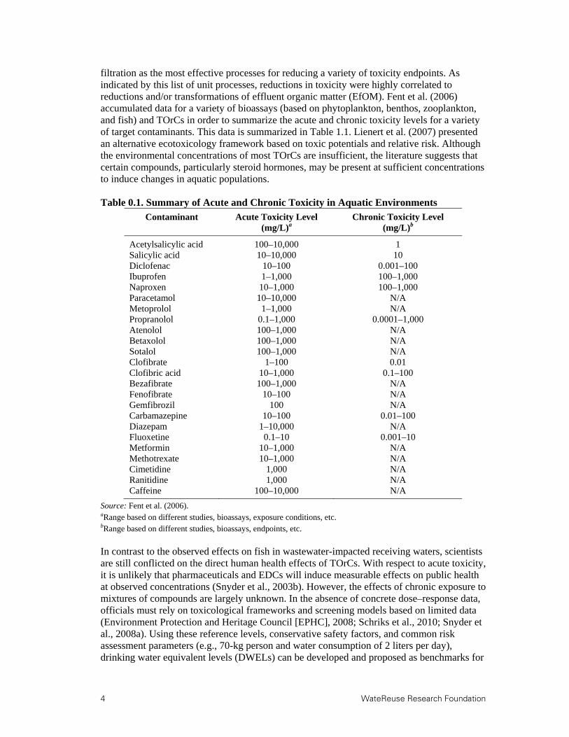
4 WateReuse Research Foundation
filtration as the most effective processes for reducing a variety of toxicity endpoints. As indicated by this list of unit processes, reductions in toxicity were highly correlated to reductions and/or transformations of effluent organic matter (EfOM). Fent et al. (2006) accumulated data for a variety of bioassays (based on phytoplankton, benthos, zooplankton, and fish) and TOrCs in order to summarize the acute and chronic toxicity levels for a variety of target contaminants. This data is summarized in Table 1.1. Lienert et al. (2007) presented an alternative ecotoxicology framework based on toxic potentials and relative risk. Although the environmental concentrations of most TOrCs are insufficient, the literature suggests that certain compounds, particularly steroid hormones, may be present at sufficient concentrations to induce changes in aquatic populations. Table 0.1. Summary of Acute and Chronic Toxicity in Aquatic Environments
Contaminant Acute Toxicity Level
(mg/L)a Chronic Toxicity Level
(mg/L)b
Acetylsalicylic acid 100–10,000 1 Salicylic acid 10–10,000 10 Diclofenac 10–100 0.001–100 Ibuprofen 1–1,000 100–1,000 Naproxen 10–1,000 100–1,000 Paracetamol 10–10,000 N/A Metoprolol 1–1,000 N/A Propranolol 0.1–1,000 0.0001–1,000 Atenolol 100–1,000 N/A Betaxolol 100–1,000 N/A Sotalol 100–1,000 N/A Clofibrate 1–100 0.01 Clofibric acid 10–1,000 0.1–100 Bezafibrate 100–1,000 N/A Fenofibrate 10–100 N/A Gemfibrozil 100 N/A Carbamazepine 10–100 0.01–100 Diazepam 1–10,000 N/A Fluoxetine 0.1–10 0.001–10 Metformin 10–1,000 N/A Methotrexate 10–1,000 N/A Cimetidine 1,000 N/A Ranitidine 1,000 N/A Caffeine 100–10,000 N/A
Source: Fent et al. (2006). aRange based on different studies, bioassays, exposure conditions, etc. bRange based on different studies, bioassays, endpoints, etc. In contrast to the observed effects on fish in wastewater-impacted receiving waters, scientists are still conflicted on the direct human health effects of TOrCs. With respect to acute toxicity, it is unlikely that pharmaceuticals and EDCs will induce measurable effects on public health at observed concentrations (Snyder et al., 2003b). However, the effects of chronic exposure to mixtures of compounds are largely unknown. In the absence of concrete dose–response data, officials must rely on toxicological frameworks and screening models based on limited data (Environment Protection and Heritage Council [EPHC], 2008; Schriks et al., 2010; Snyder et al., 2008a). Using these reference levels, conservative safety factors, and common risk assessment parameters (e.g., 70-kg person and water consumption of 2 liters per day), drinking water equivalent levels (DWELs) can be developed and proposed as benchmarks for
WateReuse Research Foundation 5
water quality. Depending on the study, the DWELs are often compared with observed concentrations in the environment or other exposure routes (e.g., beverages, foods, etc.) (Snyder et al., 2008a) to develop benchmark quotients (BQs) (Schriks et al., 2010), recommended MRLs (Snyder et al., 2008a), or other points of reference. A subset of the DWELs from two human risk assessment studies (Snyder et al., 2008a; Schriks et al., 2010) and the Australian Guidelines for Water Recycling (EPHC, 2008) is provided in Table 1.2. In most cases, these values are only proposed as points of reference to communicate the relevance of TOrCs in water supplies, so they currently have little regulatory significance. In contrast to the ecotoxicological significance of some TOrCs, the observed concentrations of most contaminants are significantly lower than the human toxicological thresholds developed in the referenced studies. This disparity contributes to the ambiguity regarding the need, or lack thereof, for TOrC regulations for drinking water or wastewater effluent intended for indirect potable reuse (IPR).
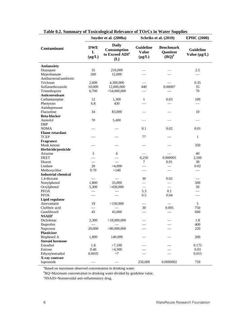
6 WateReuse Research Foundation
Table 0.2. Summary of Toxicological Relevance of TOrCs in Water Supplies
Contaminant
Snyder et al. (2008a) Schriks et al. (2010) EPHC (2008)
DWEL
(μg/L)
Daily Consumption
to Exceed ADIa (L)
Guideline Value (μg/L)
Benchmark Quotient
(BQ)b
Guideline Value (μg/L)
Antianxiety Diazepam 35 210,000 — — 2.5 Meprobamate 260 12,000 — — — Antibacterial/antibiotic Triclosan 2,600 4,300,000 — — 0.35 Sulfamethoxazole 18,000 12,000,000 440 0.00007 35 Trimethoprim 6,700 >54,000,000 — — 70 Anticonvulsant Carbamazepine 12 1,300 1 0.03 100 Phenytoin 6.8 430 — — — Antidepressant Fluoxetine 34 83,000 — — 10 Beta-blocker Atenolol 70 5,400 — — — DBP NDMA — — 0.1 0.02 0.01 Flame retardant TCEP — — 77 — 1 Fragrance Musk ketone — — — — 350 Herbicide/pesticide Atrazine 3 6 — — 40 DEET — — 6,250 0.000005 2,500 Diuron — — 7 0.01 30 Lindane 20 >4,000 — — 0.02 Methoxychlor 0.70 >140 — — — Industrial chemical 1,4-dioxane — — 30 0.02 — Nonylphenol 1,800 33,000 — — 500 Octylphenol 5,300 >430,000 — — 50 PFOA — — 5.3 0.1 — PFOS — — 0.5 0.04 — Lipid regulator Atorvastatin 19 >150,000 — — 5 Clofibric acid — — 30 0.005 750 Gemfibrozil 45 43,000 — — 600 NSAIDc Diclofenac 2,300 >18,000,000 — — 1.8 Ibuprofen — — — — 400 Naproxen 20,000 >80,000,000 — — 220 Plasticizer Bisphenol A 1,800 140,000 — — 200 Steroid hormone Estradiol 1.8 >7,100 — — 0.175 Estrone 0.46 >4,500 — — 0.03 Ethynylestradiol 0.0035 >7 — — 0.015 X-ray contrast Iopromide — — 250,000 0.0000002 750
aBased on maximum observed concentration in drinking water. bBQ=Maximum concentration in drinking water divided by guideline value. cNSAID=Nonsteroidal anti-inflammatory drug.

WateReuse Research Foundation 7
1.1.2 Current Water Reuse Guidelines and Regulations
In contrast to drinking water standards, such as those established by the Safe Drinking Water Act (SDWA) in the United States, and nutrient levels mandated by wastewater discharge permits, there is a paucity of regulation related to TOrCs in wastewater effluents. The U.S. Food and Drug Administration (FDA) requires companies to conduct an environmental impact assessment for any human pharmaceutical expected to be found in the environment at a concentration exceeding 1 μg/L (Fent et al., 2006). However, there is little regulatory guidance beyond that point. Although TOrCs may be the impetus for augmenting treatment trains, it is unclear whether these contaminants will be a significant factor in establishing design criteria for advanced wastewater treatment processes. In many situations, design criteria may actually be based on disinfection requirements or disinfection byproduct (DBP) mitigation. With respect to ozone, one of the primary factors limiting its widespread applicability to water and wastewater treatment is bromate formation. Although a drinking water maximum contaminant level (MCL) of 10 µg/L has been established in the United States, more relaxed targets (e.g., 3 mg/L (Hollender et al., 2009)) have been proposed for environmental discharge, which would increase the applicability of ozone to wastewater treatment. For water reuse in the United States, states can refer to the U.S. Environmental Protection Agency (EPA) Guidelines for Water Reuse (U.S. EPA, 2004), CDPH Title 22 requirements, or local standards for wastewater contaminants. Of course, water reuse regulations vary tremendously depending on the ultimate use of that resource (e.g.., IPR vs. golf course irrigation). For unrestricted urban reuse, states generally specify an acceptable treatment train in addition to turbidity and disinfection requirements. The State of Florida also requires periodic monitoring for Giardia and Cryptosporidium. Reuse requirements for Florida and Washington are provided in Table 1.3, as an example. In 2004, only four states (California, Florida, Hawaii, and Washington) had specific standards for IPR permits, and they generally addressed total suspended solids (TSS), total nitrogen, total organic carbon (TOC), turbidity, total organic halides (TOX), and total coliforms. Wastewater intended for IPR is also expected to comply with primary and secondary drinking water standards. Washington specifically requires water intended for surface percolation or direct recharge to comply with established MCLs, in accordance with the SDWA. For direct recharge applications, California and Washington specify the amount of time the water should be stored in an aquifer before it can be withdrawn for drinking water applications, in addition to offset distances between recharge and withdrawal locations. Washington and California also require reverse osmosis in all direct injection applications (U.S. EPA, 2004). The permitting standards for Florida, Washington, and California are summarized in Table 1.3, and the California requirements are described in the following discussion of Title 22. The CDPH Title 22 requirements address a number of parameters, including total nitrogen, TOC, turbidity, total coliforms, and viruses. In addition to specifying restrictions on proximity of use to municipal water wells and other high-risk areas, Title 22 defines three categories for reuse water: disinfected secondary-23 (e.g., inedible crops and freeway irrigation), disinfected secondary-2.2 (e.g., food crops with no contact between the water and the edible portion of the food), and disinfected tertiary recycled water (e.g., full-contact food crops and unrestricted golf course irrigation). For a “disinfected secondary-23” designation, the median concentration of total coliforms over a 7-day period cannot exceed 23 MPN (most probable number)/100 mL, and no more than one sample can exceed 240 MPN/100 mL over a 30-day period. For a “disinfected secondary-2.2” designation, the median concentration of

8 WateReuse Research Foundation
total coliforms over a 7-day period cannot exceed 2.2 MPN/100 mL, and no more than one sample can exceed 23 MPN/100 mL over a 30-day period. Also, no sample can exceed a total coliform concentration of 240 MPN/100 mL. In addition to complying with the secondary-2.2 requirements, disinfected tertiary recycled water must satisfy specific turbidity requirements related to the mode of filtration. As a conservative guideline, the turbidity should not exceed 2 NTU (nephelometric turbidity units) for media-filtered water or 0.2 NTU for membrane-filtered water. The treatment must also satisfy one of the following disinfection requirements: (1) a free chlorine concentration time (CT) value of at least 450 mg-min/L or (2) an alternative treatment certified by the state of California to achieve at least 5-log inactivation of poliovirus or an acceptable surrogate (e.g., MS2) (CDPH, 2009b). Currently, the HiPOx system produced by APTwater (Pleasant Hill, CA) is the only ozone-based technology certified under Title 22. Table 0.3. Water Reuse Standards for Florida, Washington, and California
Application Parameter FL WA CA
Unrestricted urban reuse
TSS (mg/L) 5 30 N/A Monthly average turbidity (NTU) 2–2.5 2 2 Maximum turbidity (NTU) N/A 5 5 Indicator coliform Fecal Total Total Average (MPN/100 mL) NDa 2.2 2.2 Maximum (MPN/100 mL) 25 23 240c
Indirect potable reuse
TSS (mg/L) 5 5 N/A Monthly average turbidity (NTU) N/A 0.1 2/0.2d Maximum turbidity (NTU) N/A 0.5 10/0.5d Monthly average TOC (mg/L) 3 N/A N/A Maximum TOC (mg/L) 5 1 Calculated Total nitrogen (mg-N/L) 10 10 10 Monthly average TOX (mg/L) 0.2 N/A N/A Indicator coliform Total Total Total Median (MPN/100 mL) N/A 1b 2.2b
Maximum (MPN/100 mL) ND 5b 240c Storage time (months) N/A 12 6 Minimum offset distance (feet) 500 2,000 N/A
Source: U.S. EPA (2004). Note: ND=nondetect and N/A=not applicable. aIn 75% of samples over 30-day period. bOver a 7-day period. cOnly one sample can exceed 23 MPN/100 mL over 30-day period. dMedia filtration/membrane filtration. For IPR in California, applications are now separated into three different categories according to the Draft Groundwater Replenishment Reuse Regulations published in November 2011: (1) groundwater replenishment via surface application without full advanced treatment (FAT), (2) groundwater replenishment via subsurface application with FAT, and (3) groundwater replenishment via surface application with FAT. With the exception of FAT, the requirements are relatively similar between the three categories. All systems are required to demonstrate wastewater source control; satisfy the definition of a “disinfected tertiary effluent”; provide a total of 12-, 10-, and 10-log removal/inactivation for viruses, Giardia cysts, and Cryptosporidium oocysts, respectively; achieve 10 mg-N/L of total nitrogen; and achieve a maximum TOC concentration (TOCmax) equal to 0.5 divided by the proposed recycled water contribution (RWC). For the pathogen reductions, no single treatment process

WateReuse Research Foundation 9
can be credited with more than 6-log removal/inactivation, and each process used to demonstrate compliance must achieve at least 1-log removal/inactivation. Each month of underground storage also provides 1-log viral removal/inactivation, but the agency must calculate the retention time using specified methods. In combination with FAT, which will be described later, 6 months of certified underground storage automatically qualifies for the 10-log parasite removal/inactivation requirements. In addition to satisfying the pathogen reduction requirements, the hydraulic residence time in the subsurface environment must allow sufficient response time to address treatment failures and mitigate public health risks. IPR systems must generally comply with primary and secondary MCLs for drinking water. The CDPH draft regulations specifically address a group of priority toxic pollutants: inorganic chemicals, radionuclide chemicals, organic chemicals, disinfection byproducts, lead, and copper. IPR systems must also achieve established notification levels (NLs) for organic contaminants. Because of its demonstrated carcinogenicity, California has established a public health goal of 3 ng/L, an NL of 10 ng/L, and a response level of 300 ng/L for N-nitrosodimethylamine (NDMA). This is supplemented with NLs of 10 ng/L and response levels of 100 and 500 ng/L for N-nitrosodiethylamine (NDEA) and N-nitrosodi-n-propylamine (NDPA), respectively (CDPH, 2009a). The NL concept differs from the original draft regulations, which mandated 1.2- and 0.5-log removal/destruction of NDMA and 1,4-dioxane, respectively. The previous NDMA and 1,4-dioxane requirements can still be used as a general rule of thumb for treatment train design, as described in the following. The primary distinction between the three IPR categories involves the use of FAT, which is a combination of RO capable of achieving 99.5% sodium chloride rejection and a robust oxidation process. The oxidation process must achieve 0.5-log destruction of at least one indicator compound from each of the following seven compound classes: hydroxy aromatic, amino/acylamino aromatic, nonaromatic with carbon double bonds, deprotonated amine, alkoxy polyaromatic, alkoxy aromatic, and alkyl aromatic. The oxidation process must also achieve 0.3-log destruction of at least one indicator compound from each of the following two compound classes: saturated aliphatic and nitro aromatic. To ensure process integrity, a surrogate parameter (e.g., differential chloramine or UV254 absorbance) must also be correlated with the destruction/removal of the indicator compounds and monitored continuously. These new regulations highlight the importance of compound groupings that have been proposed in this study and surrogate parameters suitable for real-time, online monitoring of process performance, which is the focus of several other WateReuse Research Foundation projects (WRRF-09-10 and WRRF-11-01). Although federal regulations and guidelines pertaining to PPCPs/EDCs and other TOrCs are extremely limited (e.g., atrazine MCL of 3 µg/L), several common PPCPs/EDCs/TOrCs (1,4-dioxane, erythromycin, steroid hormones, nitrosamines, pesticides, etc.) are listed in the most recent version of the U.S. EPA Contaminant Candidate List (CCL3). The CCL3 is a list of unregulated contaminants that are known or have the potential to occur in public water supplies and may pose a threat to human health. Although these contaminants have been identified for priority research, target concentrations have not been identified, and these contaminants may never actually be regulated. Similarly, the European Union recently identified a list of 33 priority substances (atrazine, octylphenols, etc.) for which mitigation measures or environmental quality standards (EQSs) will be developed in the near future (EU, 2000). On the other hand, Australia has specifically identified a number of emerging contaminants, in addition to identifying corresponding drinking water goals (DWGs) for its potable reuse and drinking water systems. In 2008, the Environment Protection Heritage Council, National Health and Medical Research Council, and Natural Resource Management

10 WateReuse Research Foundation
Ministerial Council published the Augmentation of Drinking Water Supplies module of the Australian Guidelines for Water Recycling. The authors emphasize that the information presented in the document is not legally binding and only serves as a summary of scientific evidence pertaining to water reuse paradigms (EPHC, 2008). The Augmentation of Drinking Water Supplies module is primarily based on the Australian Drinking Water Guidelines. Similarly to frameworks used in other countries to establish regulations and goals, the treatment levels identified in the document balance the practicality and costs associated with water and wastewater treatment with the acceptable risk for a particular chemical or microbial contaminant. For microbial contaminants, Australia targets pathogen levels corresponding to 10-6 annual disability-adjusted life years (DALYs) per person, and for most chemical contaminants, the treatment goals are based on no-observed-effect levels (NOELs) supplemented by safety factors or a cancer risk of 10-6. However, the treatment goals are slightly different for emerging contaminants: toxicity equivalents for dioxins and polychlorinated biphenyls, acceptable daily intakes (ADIs) for agricultural and veterinary pharmaceuticals, and therapeutic doses supplemented with safety factors (1,000-10,000) for human pharmaceuticals (EPHC, 2008). A plethora of compounds have been assigned treatment goals in the Australian document, but this review will only discuss several microbes and PPCPs/EDCs/TOrCs that have received considerable attention in recent years because of their ubiquity in wastewater effluent. Based on their anticipated prevalence in wastewater, coupled with the DALY risk framework, required log reductions for Cryptosporidium, enteric viruses, and Campylobacter are 8, 9.5, and 8.1, respectively. The Australian guidelines indicate that the typical IPR system comprised of membrane filtration, RO, and advanced oxidation will be sufficient to achieve these microbial reductions. The document also provides a table of expected treatment efficacies for a variety of wastewater treatment processes, including ozonation: 2- to 6-log inactivation for vegetative bacteria and viruses, 2- to 4-log inactivation for Giardia, 1- to 2-log inactivation of Cryptosporidium, and 0- to 0.5-log inactivation of spore-forming bacteria. A similar table is provided for ozonation of emerging chemical contaminants, including antibiotics (>95% removal), carbamazepine (50–80% removal), ibuprofen (50–80% removal), steroid hormones (>95% removal), and other PPCPs/EDCs/TOrCs (EPHC, 2008). The actual guidelines for a subset of these emerging contaminants were provided earlier in Table 1.2.. Few emerging contaminants exceed the Australian guidelines for augmentation of drinking water supplies—even considering the maximum concentrations observed in secondary effluents (EPHC, 2008). For those compounds with concentrations higher than the recommended guidelines, optimized conventional wastewater treatment (e.g., biotransformation of caffeine) or disinfection processes (e.g., ozonation of steroid hormones) may be sufficient to achieve the specified goals. Implementation of advanced treatment processes would provide even greater safeguards for human and environmental health. Specifically, ozonation is recognized as an effective barrier against organic contaminants and microbes, but its use in wastewater poses interesting scientific and operational complexities, as described in the following sections.

WateReuse Research Foundation 11
1.2 Assessment of Oxidation Processes
1.2.1 Ozone
Ozone decomposition in wastewater effluent (typically secondary effluent) is characterized by two kinetically distinct phases (Buffle et al., 2006c): (1) the “demand phase” where a portion of the dissolved ozone is rapidly consumed over the first 30 s (i.e., instantaneous ozone demand (IOD)) and (2) the “decay phase” where the remaining ozone decays relatively slowly. This biphasic behavior has also been observed in natural waters containing high concentrations of dissolved organic matter (DOM) (Buffle and von Gunten, 2006). During both phases, ozone reacts with organic matter and inorganic scavengers, which causes ozone to decompose naturally into ·OH. These phases are illustrated in Figure 0.1; the numbered steps in Figure 0.1 are described in the following sections.
Figure 0.1. Ozone decomposition and ·OH formation during ozonation of wastewater.
Demand Phase
During the demand phase of wastewater effluent ozonation, ozone is mainly consumed by its direct reaction with EfOM and nitrite. When the applied ozone dose is low compared to the level of EfOM or nitrite, ozone is completely consumed within seconds. Specifically, ozone reacts rapidly with some electron-rich moieties of EfOM, including phenols, anilines, alkoxy- and alkylbenzenes, olefins, and deprotonated amines (Lee and von Gunten, 2010), but little information is currently available on the exact composition of EfOM in terms of the concentration and distribution of these electron-rich moieties. Also, nitrite concentration can be high (e.g., >1 mg-N/L or 71 M) when partial nitrification or denitrification is applied in preceding biological treatment processes. This is critical for ozonation because ozone and nitrite react at a 1:1 mass ratio. Significant ·OH formation occurs during the initial demand phase of ozonation. Mechanistic studies have shown that ·OH can be produced from the reaction of ozone with model organic compounds via intermediates (e.g., O2
-· and O3-·) (Flyunt et al., 2003a). For example, the
reaction of ozone with some phenols and tertiary amines proceeds partly through electron transfer, which generates O3
-· (no. 1) and rapidly decays into ·OH (no. 6). The reaction of
12 WateReuse Research Foundation
ozone with secondary amines produces O2-· (no. 2), which reacts rapidly and selectively with
O3 to form O3-· (no. 5) and ·OH (no. 6). In contrast, the reaction of ozone with olefins and
nitrite does not produce ·OH (no. 3) because the reaction produces negligible O2· and O3
·. The literature quantifies ·OH yields (molar basis) from the reaction of ozone with several classes of organic compounds having electron-rich moieties: 817% for alkoxybenzenes (Mvula et al., 2009), 2443% for phenols (Flyunt et al., 2003b; Mvula and Von Sonntag, 2003), 2830% for anilines (Flyunt et al., 2003a), 15% for tertiary amine (triethylamine) (Flyunt et al., 2003a), and 43% for adenosine (Flyunt et al., 2003a). It should be noted that the experimental conditions in these studies suppressed subsequent ·OH reactions that might otherwise have increased the ·OH yield substantially. Therefore, in addition to the primary ·OH yield, the fate of ·OH should be considered to determine the overall ·OH yield. This aspect will be discussed in greater detail later. Decay Phase
If a dissolved ozone residual persists through the initial demand phase, it is slowly consumed in the secondary decay phase by a series of radical chain reactions. Ozone decomposition can be initiated by OH- (no. 4) or HO2
- (no. 9), which are the anions of H2O (pKa=15.7) and H2O2 (pKa=11.7), respectively. The reaction of OH- with O3 was originally suggested to produce HO2
- by O-transfer: OH- + O3 HO2- + O2 (Staehelln and Hoigné, 1982). Here, the ·OH
radical is generated in the subsequent reaction of HO2- with ozone (i.e., the peroxone
process). However, the O-transfer mechanism was recently challenged and revised into an adduct formation mechanism: OH- + O3 HO4
- HO2· + O2-· (no. 4) (Merényi et al.,
2010b). The adduct HO4- rapidly equilibrates with HO2· + O2
-·. In this case, ·OH is generated in the subsequent reaction of O2
-· with ozone (no. 5). A small fraction of the adduct HO4- can
also transform into HO2- and O2 (not shown in Figure 0.1). Overall, based on the adduct
formation mechanism, 3 moles of ozone are consumed to produce 2 moles of ·OH from the OH--induced initiation step. The reaction of HO2
- with O3 (i.e., the peroxone process) was originally suggested to proceed through electron transfer: HO2
- + O3 HO2• + O3-• (Staehelln and Hoigné, 1982). However,
this reaction was also revised into an adduct formation mechanism: HO2- + O3 HO5
- (Merényi et al., 2010a). The adduct HO5
- has two competing decay pathways. One-half of the HO5
- decays into HO2· + O3-·, which has the same fate as the electron transfer mechanism.
HO2· equilibrates with O2-· and reacts quickly with ozone (no. 5), thereby producing ·OH
(no. 6). O3-· is also rapidly converted into ·OH (no. 6). The other half of the HO5
- decays into 2O2 + OH-. Therefore, during the peroxone process, 3 moles of ozone and 2 moles of hydrogen peroxide are consumed to produce 2 moles of ·OH from the HO2
--induced initiation step. ·OH reacts mainly with EfOM or carbonate/bicarbonate during ozonation of wastewater effluent. The reaction of ·OH with certain moieties in EfOM (promoters such as organic acids and alcohols) leads to carbon-centered radicals. Following O2 addition, these carbon-centered radicals form O2
-· or HO2- (no. 7). As discussed earlier, O2
-· reacts rapidly and selectively with ozone (no. 5), which again produces ·OH. In addition, the reaction of HO2
- with ozone generates ·OH (no. 9). Therefore, the reaction of ·OH with the promoters accelerates the overall ozone decomposition through the chain reaction. It should be noted that ·OH formation via the chain reaction is more efficient for O2
-· than for HO2- as the chain carrier
because of the relative reaction rate difference (Staehelln and Hoigné, 1982):

WateReuse Research Foundation 13
O2-· + O3 O2 + O3
-· k=1.6 109 M-1 s-1 (pH 4.8) HO2
- + O3 HO2· + O3-· k=2.8 106 M-1 s-1.
In the latter reaction, the apparent rate constant for the reaction of H2O2 and O3 at near-neutral pH is (2.8 106) (10pH-11.6). The chain reaction is terminated upon the reaction of ·OH with compounds that do not form O2
-· or HO2- (no. 8, inhibitors such as aliphatic alkyl compounds
and carbonate) (Staehelin and Hoigné, 1985).
·OH Yield during Wastewater Ozonation
The ·OH yield during ozonation of wastewater differs depending on the type of ozone decomposition, which is influenced by ozone dose, pH, concentration and type of EfOM, inorganics, etc. In the initial demand phase, a significant fraction of the applied ozone dose is consumed by the direct reaction of ozone with reactive moieties in EfOM. These direct ozone reactions are expected to produce ·OH yields of 1040%. A recent study calculated an ·OH yield of 13% during ozonation of wastewater effluent (Nöthe et al., 2009b). The ·OH yield from the OH- or HO2
--induced ozone decomposition initiation step is 67% based on the adduct formation mechanisms. The yield can increase if the ·OH radical is involved in the O2
-·-induced chain reaction via promoters. In this scenario, one mole of ·OH is produced from the reaction of O2
-· with ozone, which results in 100% ·OH yield from ozone. The O2-·-
induced chain reaction is only possible when the ozone concentration is high enough to be able to react with O2
-·. Therefore, the ·OH yield will be lower (e.g., 1040%) at lower ozone doses when most of the ozone is consumed by direct reaction with EfOM. The ·OH yield will approach 100% at higher ozone doses when most ozone is consumed by the O2
-·-induced chain reaction.
1.2.2 Ozone/H2O2
Ozone decomposition is typically slow (i.e., several hours for high applied ozone doses) in clean waters containing high carbonate concentrations (e.g., groundwater). To expedite ozone decomposition and the subsequent formation of ·OH, the peroxone process (i.e., the combination of ozone and H2O2) can be implemented (Acero and von Gunten, 2001). As discussed earlier, 3 moles of ozone and 2 moles of H2O2 are consumed to produce 2 moles of ·OH radicals from the HO2
--induced ozone decomposition initiation step. The use of H2O2 in wastewater applications is sometimes questioned (Pocostales et al., 2010) because the higher concentration of EfOM already leads to rapid ozone decomposition into ·OH (e.g., <30 min), particularly for low applied ozone doses. For high applied ozone doses, the addition of H2O2 provides a nearly instantaneous treatment process, which can lead to significant cost savings associated with reduced structural footprints. However, it is important to note that the addition of H2O2 does not necessarily increase ·OH yields and can actually be detrimental to treatment efficacy because of increased ·OH scavenging rates. However, if the peroxone process can accentuate the O2
-·-induced chain reaction during ozone decomposition, the yield of ·OH radical can be increased accordingly.
1.2.3 UV/H2O2
·OH radicals can be produced by the action of UV light ( < 280 nm) on H2O2, according to the following equation: H2O2 + UV 2·OH. During the primary event, 2 moles of ·OH are produced from 1 mole of H2O2. The quantum yield for ·OH from the primary event is 1 because half of the produced ·OH in a solvent cage recombines into H2O2 and only the other
14 WateReuse Research Foundation
half diffuses out of the solvent cage (Legrini et al., 1993). Even though the ·OH yield from H2O2 is high (i.e., 200%), the UV absorption by H2O2 is weak because its molar absorption coefficient at 254 nm is only 18 M-1 cm-1. Moreover, UV-absorbing matrix components (e.g., EfOM) reduce UV transmission, thereby preventing UV photolysis of H2O2. Accordingly, elevated concentrations of H2O2 (e.g., 10 mg/L or 300 M) have to be applied to achieve a reasonable ·OH generation rate during wastewater treatment. After the AOP, any residual H2O2 must often be quenched or catalytically decomposed, which increases the complexity and cost of treatment. This is compounded by the general necessity for pretreatment to increase UV transmissivity and process efficacy. In a typical wastewater effluent matrix, H2O2 is not a significant ·OH scavenger because of its slow reaction with ·OH:
H2O2 + ·OH HO2· + H2O k=2.7107 M-1 s-1.
1.3 Prediction of Trace Organic Contaminant Elimination: Kinetics
Chemical kinetics is useful for describing the elimination of TOrCs during oxidation. In ozonation, TOrC elimination occurs via reactions with ozone and ·OH and therefore can be formulated based on the first equation following. After integration, the second equation provides a means to either calculate unknown rate constants or predict the level of oxidation with specific dosing conditions:
d[TOrC]t/dt= [TOrC][O3] + [TOrC][·OH]
ln([TOrC]t/[TOrC]0)= + .
Based on these equations, it is apparent that TOrC elimination depends on the second-order
rate constants for ozone and ·OH reactions ( and ) and the ozone and ·OH
exposures ( and ). In other words, TOrC elimination can be predicted if
these four parameters are known. Although an immense database of rate constants is already available, ozone and ·OH exposure can vary significantly between matrices.
1.3.1 Second-Order Rate Constants
Second-order rate constants (k) represent the magnitude of reactivity between the oxidant (i.e., ozone and ·OH) and each TOrC. Currently, about 1000 k values are known for ozone reactions, and several thousand k values are known for ·OH reactions (available in a National Institute of Standards and Technology (NIST) database). These k values show that ozone reacts fast only with electron-rich [organic] moieties (ERMs), such as activated aromatic compounds (e.g., phenol, aniline, and polycyclic aromatics), olefins, organosulfurs, and deprotonated amines. In contrast, ·OH reacts very fast with most types of organic moieties, including aliphatic CH bonds (Buxton et al., 1988). Ozone and ·OH k values for many wastewater-derived TOrCs are summarized in Table 1.4.
3Ok OHk
3Ok dtOt
0
3 OHk dtOHt
0
3Ok OHk
dtOt
0
3 dtOHt
0

WateReuse Research Foundation 15
For ionizable organic compounds such as phenols or amines, the k value depends significantly on the ionization state. Typically, deprotonated phenols or amines show several orders of magnitude higher reactivity to ozone than the corresponding protonated ones.
Therefore, the k values at a certain pH (i.e., apparent k values, ) for the reaction of
ozone with phenols or amines increase significantly with increasing pH. The can be
calculated using the following equation, where represents the fraction of each species at a given pH and can be calculated based on the compound’s pKa value. In addition,
and are the species-specific rate constants.
= de-protonated + protonated
Table 1.4 summarizes the second-order rate constants (i.e., species-specific and apparent k values at pH 7 and 8) available in the literature prior to 2010 for the reaction of ozone and ·OH with various TOrCs. Each rate constant was critically examined, particularly with respect to the method applied for rate constant determination, and only those rate constants determined by appropriate kinetic methods (e.g., absolute kinetic or competition kinetic methods) were included in the table. Therefore, ozone or ·OH rate constants are not yet available for some compounds. For these compounds, the unknown rate constant(s) was estimated using quantitative structure–activity relationships (QSARs) for ozone or the group contribution method (GCM) for ·OH (see Section 0 for further details). Table 1.4 indicates that the TOrCs containing phenols and anilines show the highest
reactivity to ozone (i.e., values at pH 7 are typically higher than 106 M1s1). For the
TOrCs containing amines, double bonds, and activated aromatics, the values at pH 7
vary significantly and range from 102 to 106 M1s1. At pH 8, the reactivity pattern was
similar, but for TOrCs containing ionizable moieties such as phenols and amines, the
values increase 10 times compared to those at pH 7. For the TOrCs without electron-rich
moieties, such as ibuprofen, iopromide, diazepam, and NDMA, the values are
typically below 10 M1s1. Most TOrCs show high reactivity toward ·OH, as indicated by high values that
generally vary by less than a factor of two (i.e., 5 109 to 1010 M1s1). Many of these compounds contain aromatic moieties or double bonds that are known to react rapidly with ·OH (Buxton et al., 1988). Low values (e.g., <3 109 M1 s1) were found only for
some contrast media, trialkyl phosphates, and NDMA. These compounds typically contain strong electron-deficient moieties such as halogens or are small, saturated organic molecules (e.g., molecular weight lower than 100 Da).
app,O3k
app,O3k
kO3, deprotonated
protonated,O3k
app,O3k protonatedde,O3
k protonated,O3k
app,O3k
app,O3k
app,O3k
app,O3k
OHk
OHk

16 WateReuse Research Foundation
Table 0.4. Second-Order Ozone and ·OH Rate Constants
Compound/ Usage Class/ Reactive Moiety
pKa
(species of
compound),
M1 s1
at pH 7,
M1 s1
at pH 8,
M1 s1
,
M1 s1
Acebutolol/ -blockers/ 2 amine
9.2 (2 amine)
6.0 101 (cation) (Benner et al., 2008) 2.9 105 (neutral)
(Benner et al., 2008)
1.9 103 1.7 104 4.6 109
(Benner et al., 2008)
N(4)-Acetyl-sulfamethoxazole/ sulfonamide antibiotic/ p-sulfonylaniline or isoxazole
5.5 (sulfonamide N)
2.0 101 (cation) (Dodd et al., 2006a) 2.6 102 (neutral)
(Dodd et al., 2006a)
2.6 102 2.6 102 6.8 109
(Dodd et al., 2006a)
Amikacin/ aminoglycoside antibiotic/ 1 amines
Multiple pKa (1 amine)
1.3 1011.1 104 for pH range 4.18.9 (Dodd et al., 2006a)
4 103 8 103 7.6 109
(Dodd et al., 2006a)
Amoxicillin/ lactam antibiotic/ phenol, thioether, 1 amine
2.7 (carboxyl)/ 7.5 (1 amine)/
9.6 (phenol)
2.2 103 (neutral) (Javier Benitez et al., 2009)
1.0 107 (anion) (Javier Benitez et al., 2009)
2.9 106 7.8 106
6.9 109
(Song et al., 2008a) 8.0 109
(Benitez et al., 2009)
Ampicillin / lactam antibiotic/ thioether, 1 amine
2.5 (carboxyl)/ 7.3 (1 amine)/
5 103 (neutral) (Lee and von Gunten, 2012)
2 104 (anion) (Lee and von Gunten, 2012)
1 104 1.8 104
4.6 109
(Song et al., 2008a)
Atenolol/ -blockers/ 2 amine
9.6 (2 amine)
1.1 102 (cation) (Benner et al., 2008) 6.3 105 (neutral)
(Benner et al., 2008)
1.7 103 1.6 104
8.0 109
(Benner et al., 2008) 7.1 109
(Song et al., 2008b)
3Ok3Ok
3OkOHk

WateReuse Research Foundation 17
Table 1.4—Continued
Compound/ Usage Class/ Reactive Moiety
pKa
(species of
compound),
M1 s1
at pH 7,
M1 s1
at pH 8,
M1 s1
,
M1 s1
Azithromycin/ macrolide antibiotics/ double bond
8.7, 9.5 (3 amine)
6.0 106 (neutral) (Dodd et al., 2006a)
1.2 105 9.9 105 2.9 109
(Dodd et al., 2006a)
Benzotriazole/ complexing agent/ triazole
8.2 (triazole)
36 (neutral) (Karpel Vel Leitner and
Roshani, 2010) 3.5 103 (anion)
(Lutze, 2005)
2.4 102 1.4 103 7.6 109
(Naik and Moorthy, 1995)
Bezafibrate/ lipid regulator/ alkoxy benzene
3.6 (carboxyl) 5.9 102 (anion) (Huber et al., 2003b)
5.9 102 5.9 102
7.4 109
(Huber et al., 2003b) 8.0 109
(Razavi et al., 2009b)
Bisphenol-A/ plasticizer/ phenol
9.6, 10.2 (phenol)
1.7 104 (neutral) (Deborde et al., 2005a) 1.1 109 (mono-anion) (Deborde et al., 2005a)
1.1 109 (di-anion) (Deborde et al., 2005a)
2.7 106 2.7 107 1.0 1010
(Rosenfeldt and Linden, 2004)
Caffeine/ psychoactive stimulant/ double bond
6.5 102
(Broseus et al., 2009) 6.5 106 6.5 107
8.5 109
(Telo and Vieira, 1997)
Carbamazepine/ antiepileptic, analgesic/ double bond
3 105 (neutral)
(Huber et al., 2003b) 3 105 3 105
8.8 109
(Huber et al., 2003b) 5.9 109
(Pereira et al., 2007)
3Ok3Ok
3OkOHk
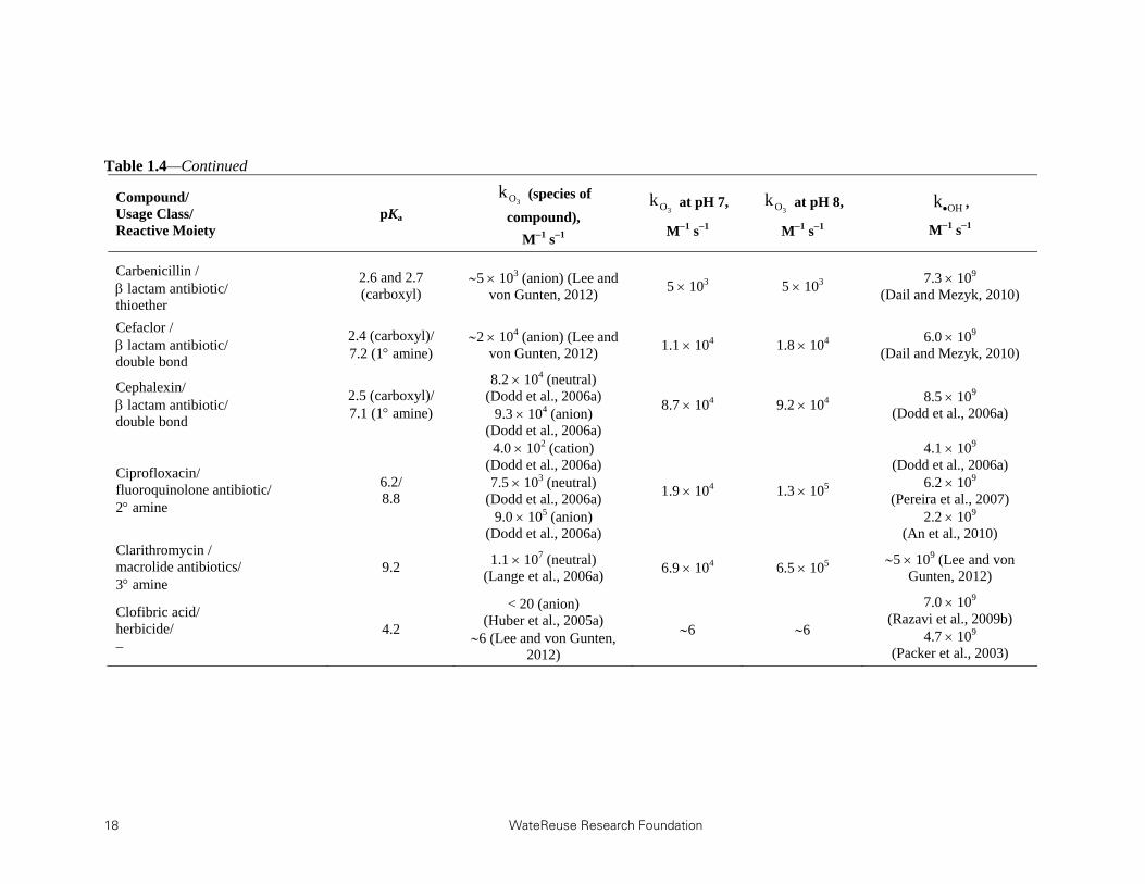
18 WateReuse Research Foundation
Table 1.4—Continued
Compound/ Usage Class/ Reactive Moiety
pKa
(species of
compound),
M1 s1
at pH 7,
M1 s1
at pH 8,
M1 s1
,
M1 s1
Carbenicillin / lactam antibiotic/ thioether
2.6 and 2.7 (carboxyl)
5 103 (anion) (Lee and von Gunten, 2012)
5 103 5 103 7.3 109
(Dail and Mezyk, 2010)
Cefaclor / lactam antibiotic/ double bond
2.4 (carboxyl)/ 7.2 (1 amine)
2 104 (anion) (Lee and von Gunten, 2012)
1.1 104 1.8 104 6.0 109
(Dail and Mezyk, 2010)
Cephalexin/ lactam antibiotic/ double bond
2.5 (carboxyl)/ 7.1 (1 amine)
8.2 104 (neutral) (Dodd et al., 2006a)
9.3 104 (anion) (Dodd et al., 2006a)
8.7 104 9.2 104 8.5 109
(Dodd et al., 2006a)
Ciprofloxacin/ fluoroquinolone antibiotic/ 2 amine
6.2/ 8.8
4.0 102 (cation) (Dodd et al., 2006a) 7.5 103 (neutral)
(Dodd et al., 2006a) 9.0 105 (anion)
(Dodd et al., 2006a)
1.9 104 1.3 105
4.1 109
(Dodd et al., 2006a) 6.2 109
(Pereira et al., 2007) 2.2 109
(An et al., 2010) Clarithromycin / macrolide antibiotics/ 3 amine
9.2 1.1 107 (neutral) (Lange et al., 2006a)
6.9 104 6.5 105 5 109 (Lee and von
Gunten, 2012)
Clofibric acid/ herbicide/
4.2
< 20 (anion) (Huber et al., 2005a)
6 (Lee and von Gunten, 2012)
6 6
7.0 109
(Razavi et al., 2009b) 4.7 109
(Packer et al., 2003)
3Ok3Ok
3OkOHk

WateReuse Research Foundation 19
Table 1.4—Continued
Compound/ Usage Class/ Reactive Moiety
pKa (species of
compound), M1 s1
at pH 7,
M1 s1
at pH 8,
M1 s1
,
M1 s1
Cloxacillin/ lactam antibiotic/ thioether
2.7 (carboxyl)
5 103 (anion) (Lee and von Gunten, 2012)
5 103 5 103 6.3 109
(Dail and Mezyk, 2010)
Danofloxacin/ fluoroquinolone antibiotic/ 3 amine
6.0 (carboxyl)/ 8.8 (3 amine)
5 104 (neutral) (Lee and von Gunten, 2012)
8 105 (anion) (Lee and von Gunten, 2012)
6 104 2 105 6.2 109
(Santoke et al., 2009)
Diatrizoic acid/ contrast media/
3.4 (carboxyl) < 1 (Lee and von Gunten,
2012) < 1 < 1 9.6 108
(Jeong et al., 2010a)
Diazepam/ tranquilizer/
0.75
(Huber et al., 2003b) 0.75 0.75 7.2 109
(Huber et al., 2003b)
Diclofenac/ antiphlogistic/ aniline
4.2 (carboxyl)
1 106 (neutral) (Huber et al., 2003b)
6.8 105 (neutral) (Sein et al., 2008a)
1 106 1 106 7.5 109
(Huber et al., 2003b)
N,N- Diethyl-m-toluamide (DEET)/ insect repellent/ methylbenzene
< 10 (Lee and von Gunten,
2012) < 10 < 10 5.0 109
(Song et al., 2009b)
Diphenhydramine/ antihistamine/ 3 amine
9.0 (3 amine) 8 105 (neutral) (Lee and
von Gunten, 2012) 8 103 7 104
5.4 109
(Yuan et al., 2009)
3Ok3Ok
3OkOHk

20 WateReuse Research Foundation
Table 1.4—Continued
Compound/ Usage Class/ Reactive Moiety
pKa (species of
compound), M1 s1
at pH 7,
M1 s1
at pH 8,
M1 s1
,
M1 s1
Enrofloxacin/ fluoroquinolone antibiotic/ 3 amine
6.1 (carboxyl)/ 7.7 (3 amine)
3.3 102 (cation) (Dodd et al., 2006a) 4.6 104 (neutral)
(Dodd et al., 2006a) 7.8 105 (anion)
(Dodd et al., 2006a)
1.5 105 5.3 105
4.5 109
(Dodd et al., 2006a) 8.0 109
(Santoke et al., 2009)
17-Estradiol (E2)/ natural estrogen/ phenol
10.4 (phenol)
2.2 105 (neutral) (Deborde et al., 2005a)
3.7 109 (anion) (Deborde et al., 2005a)
1.7 106 1.5 107
1.4 1010
(Rosenfeldt and Linden, 2004)
1.6 1010
(Kimura et al., 2004)
Estriol (E3)/ natural estrogen/ phenol
10.4 (phenol)
1.0 105 (neutral) (Deborde et al., 2005a)
3.9 109 (anion) (Deborde et al., 2005a)
1.7 106 1.6 107
1 1010 (Lee and von
Gunten, 2012)
Estrone (E1)/ natural estrogen/ phenol
10.4 (phenol)
1.5 105 (neutral) (Deborde et al., 2005a)
4.2 109 (anion) (Deborde et al., 2005a)
1.8 106 1.7 107
1 1010 (Lee and von
Gunten, 2012)
17-Ethinylestradiol (EE2)/ synthetic estrogen/ phenol
10.4 (phenol)
1.8 105 (neutral) (Deborde et al., 2005a)
3.7 109 (anion) (Deborde et al., 2005a)
7.0 109 (anion) (Huber et al., 2003b)
3.0 106 2.8 107
9.8 109
(Huber et al., 2003b) 1.1 1010
(Rosenfeldt and Linden, 2004)
3Ok3Ok
3OkOHk

WateReuse Research Foundation 21
Table 1.4—Continued
Compound/ Usage Class/ Reactive Moiety
pKa (species of
compound), M1 s1
at pH 7,
M1 s1
at pH 8,
M1 s1
,
M1 s1
Flumequine/ fluoroquinolone antibiotic/ double bond
6.5 (carboxyl)
1.2 (neutral) (Dodd et al., 2006a)
1.8 103 (anion) (Dodd et al., 2006a)
3.0 106 2.8 107 8.3 109
(Santoke et al., 2009)
Galaxolide/ musk fragrance/ alkylbenzene
1.4 102 (Nöthe et al.,
2007) 1.4 102 1.4 102
1010 (Lee and von Gunten, 2012)
Gemfibrozil/ lipid regulator/ alkoxybenzene
4.7 (carboxyl) 2 103 (Lee and von Gunten, 2012)
2 103 2 103 1.0 1010
(Razavi et al., 2009b)
Ibuprofen/ NSAID/ alkylbenzene
4.9 (carboxyl)
7.2 (neutral) (Karpel Vel Leitner and
Roshani, 2010) 9.6 (anion)
(Huber et al., 2003b)
9.6 9.6
7.4 109
(Huber et al., 2003b) 6.5 109
(Yuan et al., 2009) 6.7 109
(Packer et al., 2003) Iohexol/ contrast medium/
< 1 (Lee and von Gunten,
2012) < 1 < 1 3.2 109
(Jeong et al., 2010a)
Iomeprol/ contrast medium/
< 1 (Lee and von Gunten,
2012) < 1 < 1 2.0 109
(Jeong et al., 2010a)
3Ok3Ok
3OkOHk

22 WateReuse Research Foundation
Table 1.4—Continued
Compound/ Usage Class/ Reactive Moiety
pKa (species of
compound), M1 s1
at pH 7,
M1 s1
at pH 8,
M1 s1
,
M1 s1
Iopamidol/ contrast medium/
< 1 (Lee and von Gunten,
2012) < 1 < 1 3.4 109
(Jeong et al., 2010a)
Iopromide/ contrast medium/
< 0.8 (Huber et al., 2003b) < 0.8 < 0.8
3.3 109
(Huber et al., 2003b) 3.3 109
(Huber et al., 2003b) Ketoprofen/ NSAID/ benzene
4.2 (carboxyl) < 10 (Lee and von Gunten,
2012) < 10 < 10 5.4 109
(Pereira et al., 2007)
Levonorgestrel/ synthetic progestogen / double bond
1.4 103
(Broseus et al., 2009) 1.4 103 1.4 103
1 1010 (Lee and von Gunten, 2012)
Lincomycin/ lincosamide antibiotic/ 3 amine, thioether
7.8 (3 amine)
3.3 105 (cation) (Qiang et al., 2004) 2.8 106 (neutral)
(Qiang et al., 2004)
6.7 105 1.8 106
8.5 109
(Dodd et al., 2006a) 4.6 109
(Andreozzi et al., 2006) Medroxyprogesterone/ synthetic progestogen/ double bond
5.6 102
(Broseus et al., 2009) 5.6 102 5.6 102
1 1010 (Lee and von Gunten, 2012)
3Ok3Ok
3OkOHk
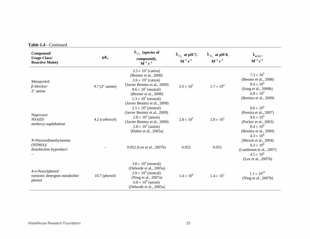
WateReuse Research Foundation 23
Table 1.4—Continued
Compound/ Usage Class/ Reactive Moiety
pKa (species of
compound), M1 s1
at pH 7,
M1 s1
at pH 8,
M1 s1
,
M1 s1
Metoprolol/ -blocker/ 2 amine
9.7 (2 amine)
3.3 102 (cation) (Benner et al., 2008)
2.6 102 (cation) (Javier Benitez et al., 2009)
8.6 105 (neutral) (Benner et al., 2008)
1.3 105 (neutral) (Javier Benitez et al., 2009)
2.0 103 1.7 104
7.3 109
(Benner et al., 2008) 8.4 109
(Song et al., 2008b) 6.8 109
(Benitez et al., 2009)
Naproxen/ NSAID/ methoxy-naphthalene
4.2 (carboxyl)
2.5 104 (neutral) (Javier Benitez et al., 2009)
2.8 105 (anion) (Javier Benitez et al., 2009)
2.8 105 (anion) (Huber et al., 2005a)
2.8 105 2.8 105
8.6 109
(Pereira et al., 2007) 9.6 109
(Packer et al., 2003) 8.4 109
(Benitez et al., 2009)
N-Nitrosodimethylamine (NDMA)/ disinfection byproduct/
0.052 (Lee et al., 2007b) 0.052 0.052
4.3 108
(Mezyk et al., 2004) 4.3 108
(Landsman et al., 2007) 4.5 108
(Lee et al., 2007b)
4-n-Nonylphenol/ nonionic detergent metabolite/ phenol
10.7 (phenol)
3.8 104 (neutral) (Deborde et al., 2005a)
3.9 104 (neutral) (Ning et al., 2007a)
6.8 109 (anion) (Deborde et al., 2005a)
1.4 106 1.4 107 1.1 1010
(Ning et al., 2007b)
3Ok3Ok
3OkOHk

24 WateReuse Research Foundation
Table 1.4. —Continued
Compound/ Usage Class/ Reactive Moiety
pKa (species of
compound), M1 s1
at pH 7,
M1 s1
at pH 8,
M1 s1
,
M1 s1
Norethindrone/ synthetic progestogen/ double bond
2.2 103
(Broseus et al., 2009) 2.2 103 2.2 103
1 1010 (Lee and von Gunten, 2012)
4-n-Octylphenol/ nonionic detergent metabolite/ phenol
10.7 (phenol)
4.3 104 (neutral) (Ning et al., 2007a)
7 109 (anion) (Lee and von Gunten, 2012)
1.4 106 1.4 107 1.1 1010
(Ning et al., 2007b)
Orbifloxacin/ fluoroquinolone antibiotic/ 2 amine
5.6 (carboxyl)/ 8.9 (2 amine)
8 103 (neutral) (Lee and von Gunten, 2012)
9 105 (anion) (Lee and von Gunten, 2012)
1.8 104 1.1 105 6.9 109
(Dodd et al., 2006a)
Paracetamol/ analgesic/ phenol
9.5 (phenol)
1.4 103 (neutral) (Andreozzi et al., 2003)
9.9 108 (anion) (Andreozzi et al., 2003)
3.9 106 3.8 107 5.8 109 (Lee and von
Gunten, 2012)
Penicillin G/ -lactams/ thioether
2.7 4.8 103 (anion) (Dodd et al., 2006a)
4.8 103 4.8 103
7.3 109
(Dodd et al., 2006a) 8.0 109
(Song et al., 2008a) 8.7 109
(Dail and Mezyk, 2010)
Penicillin V/ -lactams/ thioether
2.7 5 103 (anion) (Lee and von Gunten, 2012)
5 103 5 103
8.8 109
(Song et al., 2008a) 8.5 109
(Dail and Mezyk, 2010)
3Ok3Ok
3OkOHk

WateReuse Research Foundation 25
Table 1.4—Continued
Compound/ Usage Class/ Reactive Moiety
pKa (species of
compound), M1 s1
at pH 7,
M1 s1
at pH 8,
M1 s1
,
M1 s1
Phenacetin/ analgesic/ alkoxybenzene
1.6 103
(Javier Benitez et al., 2009) 1.6 103 1.6 103
4.0 109
(Benitez et al., 2009)
Pheyntonin/ antiepileptic/ benzene
< 10 (Lee and von Gunten,
2012) < 10 < 10 6.3 109
(Yuan et al., 2009)
Piperacillin/ -lactams/ 2 amine, thioether
N/A N/A N/A N/A 7.8 109
(Dail and Mezyk, 2010)
Primidone/ anticonvulsant/
< 10 < 10 < 10 6.7 109
(Real et al., 2009)
Progesterone/ natural progestogen / double bond
4.8 102 (Barron et al., 2006)
6.0 102 (Broseus et al., 2009)
4.8 102 4.8 102 1010 (Lee and von
Gunten, 2012)
Propranolol/ -blocker/ methoxy-naphthalene
9.5 1 105 (neutral) (Benner et al., 2008)
1 105 1 105
1.0 1010
(Benner et al., 2008) 1.1 1010
(Song et al., 2008b) Ranitidine/H2 receptor antagonist/3 amine, thioether, double bond
N/A N/A N/A N/A 1.5 1010
(Latch et al., 2003)
3Ok3Ok
3OkOHk

26 WateReuse Research Foundation
Table 1.4—Continued
Compound/ Usage Class/ Reactive Moiety
pKa (species of
compound), M1 s1
at pH 7,
M1 s1
at pH 8,
M1 s1
,
M1 s1
Roxithromycin/ macrolide antibiotics/ 3 amine
9.2 1.0 107 (neutral) (Huber et al., 2003b)
6.3 104 5.9 105 5.4 109
(Dodd et al., 2006a)
Spectinomycin/ antibiotics/ 2 amine
7.1 and 8.9 (2 amine)
3.3 105 (Qiang et al., 2004)
1.3 106 (Qiang et al., 2004)
1.5 105 3.9 105 N/A
Sulfamerazine/ sulfonamide antibiotics/ aniline
7.0 (sulfonamide)
106 (anion) (Lee and von
Gunten, 2012)
6 105 9 105 8.3 109
(Mezyk et al., 2007)
Sulfamethizole/ sulfonamide antibiotics/ aniline
5.3 (sulfonamide)
106 (anion) (Lee and von
Gunten, 2012)
106 106 8.3 109
(Mezyk et al., 2007)
Sulfamethoxazole/ sulfonamide antibiotics/ aniline
5.7 (sulfonamide)
4.7 104 (neutral) (Dodd et al., 2006a)
5.7 105 (anion) (Dodd et al., 2006a)
2.5 106 (anion) (Huber et al., 2003b)
5.5 105 5.7 105
5.5 109
(Huber et al., 2003b) 8.5 109
(Mezyk et al., 2007) 5.8 109
(Boreen et al., 2004)
Sulfamoxole/ sulfonamide antibiotics/ aniline
7.4 (sulfonamide)
106 (anion) (Lee and von
Gunten, 2012)
4 105 8 105 7.1 109
(Boreen et al., 2004)
3Ok3Ok
3Ok OHk

WateReuse Research Foundation 27
Table 1.4—Continued
Compound/ Usage Class/ Reactive Moiety
pKa (species of
compound), M1 s1
at pH 7,
M1 s1
at pH 8,
M1 s1
,
M1 s1
Sulfathiazole/ sulfonamide antibiotics/ aniline
7.2 (sulfonamide)
106 (anion) (Lee and von
Gunten, 2012)
4 105 9 105 7.1 109
(Boreen et al., 2004)
Sulfisoxazole/ sulfonamide antibiotics/ aniline
5.0 (sulfonamide)
106 (anion) (Lee and von
Gunten, 2012)
1 106 1 106 6.6 109
(Boreen et al., 2004)
Tetracycline/ antibiotic/ phenol, double bond, and 3 amine
3.3 (hydroxyl)/ 7.7 (3 amine)/
9.7 (phenol)
9.4 104–4.7 106 for pH range 39
(Dodd et al., 2006a) 3 106 4 106
7.7 109
(Dodd et al., 2006a) 6.3 109
(Jeong et al., 2010b) Tonalide/ musk fragrance/ alkylbenzene
8 (Nöthe et al., 2007) 8 8 1010 (Lee and von Gunten, 2012)
Tributyl phosphate (TBP)/ plasticizer/
< 1 (Lee and von Gunten,
2012) < 1 < 1 6.4 109
(Watts and Linden, 2009)
Tris(2-butoxyethyl) phosphate (TBEP)/ frame retardant/
< 1 (Lee and von Gunten,
2012) < 1 < 1 1.0 1010
(Watts and Linden, 2009)
Tris(2-chloroethyl) phosphate (TCEP)/ frame retardant/
< 1 (Lee and von Gunten,
2012) < 1 < 1 5.6 108
(Watts and Linden, 2009)
3Ok3Ok
3OkOHk

28 WateReuse Research Foundation
Table 1.4—Continued
Compound/ Usage Class/ Reactive Moiety
pKa (species of
compound), M1 s1
at pH 7,
M1 s1
at pH 8,
M1 s1
,
M1 s1
Tris(2-chloroisopropyl) phosphate (TCPP)/ frame retardant/
< 1 (Lee and von Gunten,
2012) < 1 < 1 1.2 108
(Watts and Linden, 2009)
Trimethoprim/ DHFR inhibitor/ diaminopyrimidine
3.2 and 7.1 (pyrimidine)
3.3 104 (di-cation) (Dodd et al., 2006a)
7.4 104 (cation) (Dodd et al., 2006a) 5.2 105 (neutral)
(Dodd et al., 2006a)
2.7 105 4.7 105 6.9 109
(Dodd et al., 2006a)
Triclosan/ antimicrobial agent/ phenol
8.1 (phenol)
1.3 103 (neutral) (Suarez et al., 2007)
5.1 108 (anion) (Suarez et al., 2007)
3.8 107 2.3 108 5.4 109
(Latch et al., 2005)
Tylosin/ macrolide antibiotics/ double bond, 3 amine
7.7 (3 amine)
7.7 104 (cation) (Dodd et al., 2006a) 2.7 106 (neutral)
(Dodd et al., 2006a)
5.1 105 1.8 106 8.2 109
(Dodd et al., 2006a)
Vancomycin/ glycopeptide antibiotic/ double bond, phenol, or 1 amine
multiple pKa
1.1 104–9.1 105 for pH range 38
(Dodd et al., 2006a) 8 105 9 105
8.1 109
(Dodd et al., 2006a)
3Ok3Ok
3OkOHk

WateReuse Research Foundation 29
1.3.2 Quantitative Structure–Activity Relationships
Strong correlations have been found between the logarithms of k values for closely related compounds, such as those possessing a common electron moiety, and substituent descriptor variables, such as Hammett and Taft sigma constants (Canonica and Tratnyek, 2003). These quantitative structure–activity relationships (QSARs) are typically in the form “log(k)==y0 + (descriptor variable),” where y0 and represent the intercept and slope of the linear regression, respectively. These QSARs can be used to predict unknown k values for TOrCs. Especially, when considering the immense numbers and large structural diversity of TOrCs, the QSAR-based prediction method can be a useful screening tool. Table 1.5 summarizes QSARs that are currently available for the reaction of ozone with organic moieties such as benzenes, phenols, phenolates, anilines, double bonds, and amines. Many of these QSARs are based on Hammett-type (,+, and ) or Taft (*) sigma constants except for No. 4, which is based on quantum chemically calculated descriptor variables. Further information on these descriptor variables can be found in the corresponding references. Hoigné and Bader reported the first QSAR for substituted benzenes using p
+ values (No. 1 in Table 1.5). The negative slope (3.1) in No. 1 is consistent with the strong electrophilic nature of ozone. In fact, the negative slope is found for all other QSARs in Table 1.5. Namov and von Sonntag also reported a similar QSAR for substituted benzenes using p
+ values (No. 2). Lee and von Gunten further expanded No. 1 and 2 and developed a QSAR based on 50 k values for various multi-substituted benzenes such as phenols, phenolates, alkylbenzenes, and alkoxybenzenes (No. 3). Naumov and von Sonntag also developed the first QSAR for substituted benzenes using quantum chemically calculated descriptor variables (No. 4). No. 4 incorporates the Gibbs free energies of adduct formation (G0), which are calculated based on density functional theory. The study demonstrated the calculation method as a useful tool to develop new molecular descriptors other than semiempirical Hammett and Taft sigma constants. Suarez et al. were first to show good linear correlations for the reaction of ozone with substituted phenols and phenolates using the +
o,m,p constants (No. 5 and 6, respectively). Lee and von Gunten further developed No. 5 and 6 by including more recently available k values for phenols and phenolates (No. 7 and 8, respectively). Pierpoint et al. showed a linear correlation for the reaction of ozone with substituted anilines using the constants (No. 9). No. 9 was further developed by Lee and von Gunten by including more k values for anilines (No. 10) and using the
o,m,p values instead of constants. Finally, Lee and von Gunten developed QSARs for double bond and amine compounds based on Taft sigma constants (*) (No. 11 and 12, respectively).

30 WateReuse Research Foundation
Table 0.5. Summary of QSARs for Ozone Reactions with Organic Compounds
No. Compound Equation Reference
1 Benzene log( / )=3.1p+ n=8 (Hoigne and Bader, 1983)
2 Benzene log( )=5.3 2.7p+ n=6 (Naumov and von Sonntag,
2010)
3 Benzene log( )=0.04 3.35+p n=50 (Lee and von Gunten, 2012)
4 Benzene log( )=3.03 0.25G0 a n=8 (Naumov and von Sonntag,
2010)
5 Phenol log( )=3.4 3.4+o,m,p n=13 (Suarez et al., 2007)
6 Phenolate log( )=8.9 2.4+o,m,p n=7 (Suarez et al., 2007)
7 Phenol log( )=3.68 2.89+o,m,p n=24 (Lee and von Gunten, 2012)
8 Phenolate log( )=8.80 2.26+o,m,p n=13 (Lee and von Gunten, 2012)
9 Aniline log( / )=1.48 n=9 (Pierpoint et al., 2001)
10 Aniline log( )=7.15 1.54o,m,p
n=14 (Lee and von Gunten, 2012)
11 Double bond log( )=6.25 0.49* n=29 (Lee and von Gunten, 2012)
12 Amine log( )=6.16 1.00* n=53 (Lee and von Gunten, 2012)
Because of the nonselective nature of its reactivity, the QSAR approach for ·OH reactions is different from that of ozone. The group contribution method (GCM) has been applied for the prediction of ·OH reaction rate constants for various organic compounds (Schwarzenbach et al., 2005; Minakata et al., 2009). In this method, the k value for a specific organic compound substructure is determined by the corresponding reaction mechanism and the effect of the neighboring functional group. For the reaction mechanism, GCM considers the following: (1) H-
atom abstraction from C−H bonds [ (H-abstr)]; (2) addition to olefins [ (olefin)]; (3)
addition to aromatic rings [ (Ar)]; and (4) interaction with N-, P-, and S-containing moieties
[ (NPS)]. For each of these reaction mechanisms, there is a “group rate constant,” which
represents the reactivity of a reference reaction, and “substituent factors”, which represent the effect of neighboring functional groups on the reactivity of a reference reaction. Finally, the total
rate constant, (total), can be expressed as the sum of the four rate constants, as follows:
(total)= (H-abstr) + (olefin) + (Ar) + (NPS).
Based on the GCM described in the preceding, the k values of ·OH reactions are generally estimated to be higher than 5 109 M−1s−1 for compounds containing (1) aromatic rings or olefins with electron-donating or even weakly electron-withdrawing substituents, (2) multiple aliphatic C−H bonds (e.g., >4 secondary C−H bonds), or (3) organic sulfur or amine moieties with electron-donating substituents (Schwarzenbach et al., 2005; Minakata et al., 2009). Table 1.5 confirms that most TOrCs fulfilling these criteria above indeed show k values higher than 5 × 10⁹ M−1 s−1.
3Ok kO3, benzene
3Ok
3Ok
3Ok
3Ok
3Ok
3Ok
3Ok
3Ok aniline,O3k
3Ok
3Ok
3Ok
OHk OHk
OHk
OHk
OHk
OHk OHk OHk OHk OHk
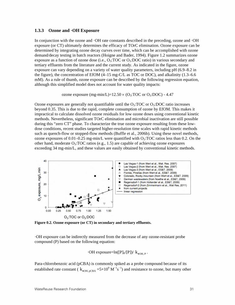
WateReuse Research Foundation 31
1.3.3 Ozone and ·OH Exposure
In conjunction with the ozone and ·OH rate constants described in the preceding, ozone and ·OH exposure (or CT) ultimately determines the efficacy of TOrC elimination. Ozone exposure can be determined by integrating ozone decay curves over time, which can be accomplished with ozone demand/decay testing in batch reactors (Hoigne and Bader, 1994). Figure 1.2 summarizes ozone exposure as a function of ozone dose (i.e., O3:TOC or O3:DOC ratio) in various secondary and tertiary effluents from the literature and the current study. As indicated in the figure, ozone exposure can vary depending on a variety of water quality parameters, including pH (6.9–8.2 in the figure), the concentration of EfOM (4–15 mg-C/L as TOC or DOC), and alkalinity (1.3–6.6 mM). As a rule of thumb, ozone exposure can be described by the following regression equation, although this simplified model does not account for water quality impacts:
ozone exposure (mg-min/L)=12.50 (O3:TOC or O3:DOC) - 4.47 Ozone exposures are generally not quantifiable until the O3:TOC or O3:DOC ratio increases beyond 0.35. This is due to the rapid, complete consumption of ozone by EfOM. This makes it impractical to calculate dissolved ozone residuals for low ozone doses using conventional kinetic methods. Nevertheless, significant TOrC elimination and microbial inactivation are still possible during this “zero CT” phase. To characterize the true ozone exposure resulting from these low-dose conditions, recent studies targeted higher-resolution time scales with rapid kinetic methods such as quench-flow or stopped-flow methods (Buffle et al., 2006b). Using these novel methods, ozone exposures of 0.01–0.25 mg-min/L were quantified with O3:TOC ratios less than 0.2. On the other hand, moderate O3:TOC ratios (e.g., 1.5) are capable of achieving ozone exposures exceeding 34 mg-min/L, and these values are easily obtained by conventional kinetic methods.
Figure 0.2. Ozone exposure (or CT) in secondary and tertiary effluents.
·OH exposure can be indirectly measured from the decrease of any ozone-resistant probe compound (P) based on the following equation:
·OH exposure=ln([P]0/[P])/ .
Para-chlorobenzoic acid (pCBA) is commonly spiked as a probe compound because of its established rate constant ( =5×10⁹ M−1s−1) and resistance to ozone, but many other
P OH,k
pCBA OH,k

32 WateReuse Research Foundation
compounds, including meprobamate, phenytoin, primidone, can also be used. The primary benefit of these alternative probes is that they are generally present at relatively high concentrations in secondary and tertiary effluents, thereby eliminating the need for spiking. Figure 1.3 summarizes the ·OH exposures as a function of ozone dose (i.e., O3:TOC or O3:DOC ratio) in various secondary and tertiary effluents from the literature and the current study. The ·OH exposures can be described by the following regression equation:
·OH exposure=(3.19x10⁻¹⁰) (O3:TOC or O3:DOC) - (3.52 10-11).
Figure 0.3. ·OH exposure in secondary and tertiary effluents.
1.3.4 Indicator Compounds
On the basis of the kinetic concept and rate constants described earlier, TOrC oxidation efficacy can be predicted from the elimination behavior of indicator compounds. The primary difference between probe and indicator compounds is that probe compounds are used to quantify oxidant exposure, whereas indicator compounds are used to evaluate overall process performance. Using indicator compounds is an attractive means of monitoring process efficacy because they narrow the scope of a study, which could otherwise become overwhelming or infeasible due to the countless number of TOrCs and the difficulty and costs associated with their routine analysis. Indicator compounds should be selected based on two primary criteria: (1) they should represent a range of reactivity to ozone and ·OH (i.e., magnitude of k value) and (2) they should occur at relatively high concentrations that are easily measurable. Furthermore, it may be beneficial to choose indicator compounds that have some level of public health or regulatory significance. Based on their established rate constants, indicator compounds can be categorized as follows:
Group 1: This group includes TOrCs with kO3 values higher than 105 M1s1 and k·OH values higher than 5 109 M-1s-1, which generally translates into rapid oxidation (i.e., >90%) at low ozone doses (i.e., O3:TOC ~ 0.25). This group includes phenolic- (e.g., bisphenol A, estrone, nonylphenol, and triclosan), aniline- (e.g., sulfamethoxazole and diclofenac), double-bond- (e.g., carbamazepine), amine- (e.g., ciprofloxacin and roxithromycin), and activated-aromatic-system-containing compounds (e.g., naproxen and propanolol). Kinetic analyses indicate that these TOrCs are mainly eliminated by direct ozone reaction.
WateReuse Research Foundation 33
Group 2: This group includes TOrCs with kO3 values higher than 10 but less than 105 M1s1 and k·OH values higher than 5 109 M-1s-1. These compounds generally require higher ozone doses (i.e., O3:TOC0.5) than the Group 1 compounds to achieve 90% oxidation. TOrCs in this category include compounds containing primary/secondary amines (e.g., amikacin and atenolol) and weakly activated aromatic systems (e.g., benzotriazole and bezafibrate). Kinetic analyses indicate that these TOrCs are eliminated by a combination of ozone and ·OH oxidation.
Group 3: This group includes TOrCs with kO3 values of 10 or below and k·OH values higher than 5x10⁹ M-1s-1. Despite the low kO3 values, these compounds still have relatively high k·OH values because of the presence of benzene rings (e.g., ibuprofen and phenytoin) or long alkyl chains (TCEP). These compounds generally require even higher ozone doses (i.e., O3:TOC ~ 1.0) to achieve 90% oxidation. During wastewater ozonation, ·OH is mainly responsible for the elimination of these TOrCs.
Group 4: This group includes TOrCs with deactivated benzene (e.g., atrazine and iopromide) or short aliphatic carbon chains (e.g., meprobamate), which result in kO3 values <10 M-1s-1 and k·OH values ranging from 1 109 to 5 109 M1s1. These compounds generally require O3:TOC ratios higher than 1.5 to achieve 90% oxidation. Similarly to the Group 3 compounds, ·OH is mainly responsible for the elimination of the Group 4 TOrCs.
Group 5: This group includes TOrCs with short aliphatic carbon chains with electronegative halogens or nitro moieties (e.g., Tris-(2-chloroethyl)-phosphate (TCEP) and NDMA). These compounds have very low kO3 values (i.e., <1) and k·OH values of 1 109 M1s1 or lower. Even at O3:TOC ratios near 1.5, these TOrCs are generally eliminated by less than 50%.
1.3.5 Surrogate Parameters
Nonconjugated aromatic components of EfOM contribute significantly to UV absorption (e.g., 254 nm), whereas conjugated aromatic structures are responsible for visible absorption (e.g., 436 nm). Ozonation is known to be effective in removing color due to the rapid oxidation of these aromatic structures, but the EfOM transformation varies depending on the wavelength of interest. Nöthe et al. noted that relative decreases in absorption at 436 nm (80%) were much more pronounced than those at 254 nm (40%) during wastewater ozonation (Nöthe et al., 2009a). The disparity between these relative changes in absorption is caused by the transformation of conjugated and nonconjugated aromatic structures, which sometimes results in additional compounds that absorb at 254 nm. Although the relative differential absorbance in the visible spectrum may be high, the actual magnitudes of the absorbance values are significantly lower. This may result in analytical limitations in some cases. Furthermore, a recent study from the WateReuse Research Foundation (WRRF-09-10) indicated that it was sometimes difficult to differentiate between varying ozone doses based on changes in visible light absorption (Snyder et al., 2012). In other words, ozonation may result in a higher relative differential in the visible light spectrum, but that differential is sometimes the same regardless of ozone dose. Therefore, differential UV absorbance at 254 nm still appears to be the most appropriate absorbance parameter for evaluating process performance and determining the effective dose. In addition to general process performance, these surrogate parameters, including UV–visible absorption, fluorescence spectra, and oxidation byproduct formation, can be correlated with TOrC elimination during oxidation processes (Wert et al., 2009b; Nanaboina and Korshin, 2010; Rosario-Ortiz et al., 2010). Because these surrogate parameters demonstrate strong correlations
34 WateReuse Research Foundation
and are easily measurable, they provide a valuable tool for monitoring and controlling oxidation processes (Snyder et al., 2012). Many of these parameters can also be monitored with commercially available online analyzers, thereby indicating their potential for full-scale implementation. This is particularly important given the recent revisions to the CDPH regulations for groundwater replenishment, which require the selection of a surrogate parameter that can be monitored continuously and will indicate process efficacy and treatment breakdowns (CDPH, 2011).
1.4 Efficacy of Ozone for Wastewater Disinfection
Ozone inactivates microorganisms by disrupting membrane or protein capsid integrity, destroying vital enzymes, and/or denaturing genetic material (Maier et al., 2000). Although ozone does not provide a stable, long-term residual, which is necessary to prevent microbial regrowth in distribution systems, it is considered to be a stronger disinfectant than chlorine and chloramine. Some microbes (e.g., Giardia cysts and Cryptosporidium oocysts) demonstrate a small degree of resistance to ozone, but there are no significant outliers that limit its applicability to water or wastewater disinfection. In contrast, Cryptosporidium oocysts are considered highly resistant to free chlorine, based on a CT of >7200 mg-min/L for 2-log inactivation (Maier et al., 2000). Because of its propensity for DNA repair after UV disinfection (Yates et al., 2006), 4-log inactivation of adenovirus may require anywhere from 100 to 225 mJ/cm2 (Gerrity et al., 2008). In fact, this resistance is the basis for the viral UV disinfection requirements in the Long Term 2 Enhanced Surface Water Treatment Rule (i.e., 186 mJ/cm2 for 4-log inactivation credit) (Yates et al., 2006). As a basis for comparison, ozone CT values for 2-log inactivation range from 0.006 to 0.02 mg-min/L for E. coli, 0.20 to 0.72 mg-min/L for poliovirus, and 0.53 to 7.0 mg-min/L for Giardia and Cryptosporidium, respectively (Maier et al., 2000). Contrary to these relative values, recent studies suggest that viral inactivation is more rapid than coliform inactivation (Xu et al., 2002; Gehr et al., 2003; Ishida et al., 2008). Historically, water and wastewater utilities have relied upon CT (disinfectant concentration x time) as a means to predict disinfection efficacy. Although the CT concept is adequate for conventional chlorine disinfection, it is not always appropriate for ozone processes, particularly for ozone/H2O2 where the ozone residual is quenched and ·OH chemistry dominates. Similar situations arise with ozone in wastewater because it is short-lived and cannot be easily monitored as it is in drinking water treatment (Buffle et al., 2006d). Recent studies suggest that significant microbial inactivation is possible even when the applied ozone dose is less than the IOD, which corresponds to an apparent CT of 0 ( Gehr et al., 2003; Ishida et al., 2008; Xu et al., 2002). Unfortunately, the current regulatory framework, with its emphasis on CT values, does not recognize these low-dose benefits. Furthermore, significant oxidation of ozone-susceptible TOrCs can be achieved with doses lower than the IOD (Wert et al., 2009a). Therefore, more research is necessary to fully characterize the efficacy and applicability of this low-dose strategy and increase regulatory acceptance. Given the prevalence of pathogenic bacteria, viruses, and parasites in wastewater, effective disinfection is vital to human health, particularly in reclaimed water and IPR applications. In highly contaminated raw wastewater, studies report fecal coliform and Salmonella at levels of 109 MPN/100 mL, Vibrio cholerae at 106 MPN/100 mL, enterococci at 102/100 mL, coliphages at 103 PFU/100 mL, Cryptosporidium at 104 oocysts/L, and a variety of amoebae and helminths (de Velasquez et al., 2008). Although primary, secondary (Table 1.6), and tertiary treatment provide slight reductions in microbial loads, disinfection is always necessary to protect human health because of the low infectious doses for many pathogens.
WateReuse Research Foundation 35
Table 1.6. Prevalence of Indicators and Pathogens in Secondary Effluent
Microbe Number/100 mL
Total coliform 104 to 106 Fecal coliform 104 to 106 Fecal streptococci 103 to 105 Human viruses 10-2 to 103 Salmonella 101 to 102
Source: U.S. EPA (1986). Despite its use in municipal applications since the 1970s (Burns et al., 2007), the available literature related to ozone disinfection for wastewater is somewhat limited. In 1986, the U.S. EPA published its Municipal Wastewater Disinfection design manual describing recommended applied ozone doses for total coliform disinfection, which are provided in Table 1.7 (Burns et al., 2007; U.S. EPA, 1986). During these initial years, ozone was often considered cost-prohibitive and problematic in wastewater applications because of frequent operational issues (Burns et al., 2007; Ishida et al., 2008; Xu et al., 2002). Table 1.7. Recommended Applied Ozone Doses for Total Coliform Disinfection
Water Matrix 2.2 CFU/100 mL 70 CFU/100 mL 200 CFU/100 mL
Tertiary treatment with partial nitrification
35–40 mg/L 15–20 mg/L 12–15 mg/L
Tertiary treatment with full nitrification 15–20 mg/L 5–10 mg/L 3–5 mg/L
Sources: Burns et al. (2007); U.S. EPA (1986).
More recent literature suggests that modern ozone systems are actually viable alternatives for wastewater disinfection. Xu et al. (2002) evaluated two different pilot-scale ozone systems to determine the most important factors affecting ozone efficacy in wastewater. Table 1.8 provides a summary of the experimental conditions for the three wastewaters in their study. Additional tests were performed on Wastewater B after microfiltration (10 µm) to determine the effect of TSS reduction on ozone efficacy.
With a transferred ozone dose of 7.5 mg/L (O3:TOC=0.94), the authors demonstrated consistent fecal coliform levels of <2.2 MPN/100 mL for Wastewater A. With similar ozone-to-TOC ratios in the more challenging wastewaters, the authors could only maintain fecal coliform levels <100 MPN/100 mL. The authors reported 1- to 3-log inactivation of fecal coliforms with transferred ozone doses less than the IOD (i.e., apparent ozone CT of 0). With respect to other pathogens and surrogates in Wastewater C, enterococci and Salmonella were highly susceptible to ozonation; >2.2- and 2.9-log inactivation of F-specific coliphages (e.g., MS2) and enteroviruses was achieved with transferred ozone doses of 8.6 and 4.8 mg/L, respectively; and spore-forming Clostridium experienced less than 2-log inactivation with a transferred ozone dose of 33 mg/L. Finally, to comply with WHO guidelines for irrigation (i.e., fecal coliforms <103 CFU/100 mL), the authors indicated that transferred ozone doses of 2, 4, and 10 mg/L would be required for Wastewaters A, B, and C, respectively. CDPH Title 22 compliance (i.e., <2.2 MPN/100 mL) could only be achieved with practical doses in Wastewater A.

36 WateReuse Research Foundation
Table 1.8. Summary of Experimental Conditions in Xu et al. (2002)
Parameter A B C
Location Indiana, USA Evry, France Washington, UK Flow rate (m3/day) 300,000 48,000 90,000 Matrix Tertiary effluent Secondary effluent Secondary effluent pH 7.0 7.3 7.5 TSS (mg/L) 2.3 5 18 COD (mg/L) 30 36 71 TOC (mg/L) 8 <10 26 UV254 Abs. (cm-1) 0.155 0.222 0.349 Fecal coliforms (log CFU/100 mL)
N/A 3.6–4.5 4.3–6.5
E. coli (log CFU/100 mL)
2.7–4.3 N/A N/A
Clostridium (log CFU/100 mL)
N/A 3.0–4.5 3.6–5.5
Enterococci (log/100 mL)
N/A N/A 4.5–4.9
Enterovirus (PFU/10 L)
N/A N/A 544–775
F-specific coliphage (PFU/mL)
N/A N/A 96–144
Applied O3 dose (mg/L) 1–35 3–16 4–50 Transferred O3 dose (mg/L)
0.5–12 2–13 4–30
IOD (mg/L) 2.5–5.3 3.1–4.2 7.4–9.6 Contact time (min) 3–15 2–10 2–10
As indicated earlier, wastewater quality and level of pretreatment significantly impact ozone efficacy for coliform disinfection. As further evidence, Gehr et al. (2003) performed bench-scale ozone disinfection experiments on a primary effluent from the City of Montreal Wastewater Treatment Plant. The treatment plant, which is designed to handle up to 7.6 million m3/day (343 MGD), utilizes only coarse screening, chemical addition (alum, ferric chloride, and polymer) to improve settling of suspended particles, and primary clarification. There is no disinfection prior to environmental discharge. Because of the limited pretreatment, the wastewater quality was highly variable during the experimental period: TOC of 90 to 110 mg/L (Gagnon et al., 2008), chemical oxygen demand (COD) of 123 to 240 mg/L, TSS of 16 to 45 mg/L, and turbidity of 16 to 31 NTU. Due to substantial reactivity with DOM, the IOD of this wastewater was determined to be 25 mg/L (O3:TOC ≈ 0.25). The authors were able to achieve approximately 3-log inactivation of fecal coliforms with a transferred ozone dose of 70 mg/L (O3:TOC=0.70), but the residual fecal coliform level still exceeded 103 CFU/100 mL. As expected, Clostridium proved to be more resistant and only experienced 1-log inactivation at the same transferred ozone dose. In contrast, the authors achieved 4-log inactivation of MS2, which approached the detection limit of the assay (i.e., 1 PFU/mL), with a transferred ozone dose approximately equal to the IOD (i.e., 25 mg/L). Mezzanotte et al. (2007) evaluated ozone disinfection in a 4.5-m3/h (20-gpm) pilot wastewater treatment plant in Italy. The pilot plant treated secondary effluent with the following average water quality characteristics: pH 7.1, COD <20 mg/L, TOC 5.1 mg/L, TSS 2.3 mg/L, turbidity 1.8 NTU, and UV254 transmittance 75%. The total coliform, fecal coliform, and E. coli levels were 2 105 CFU/100 mL, 4.7 104 CFU/100 mL, and 1.2 104 CFU/100 mL, respectively. The
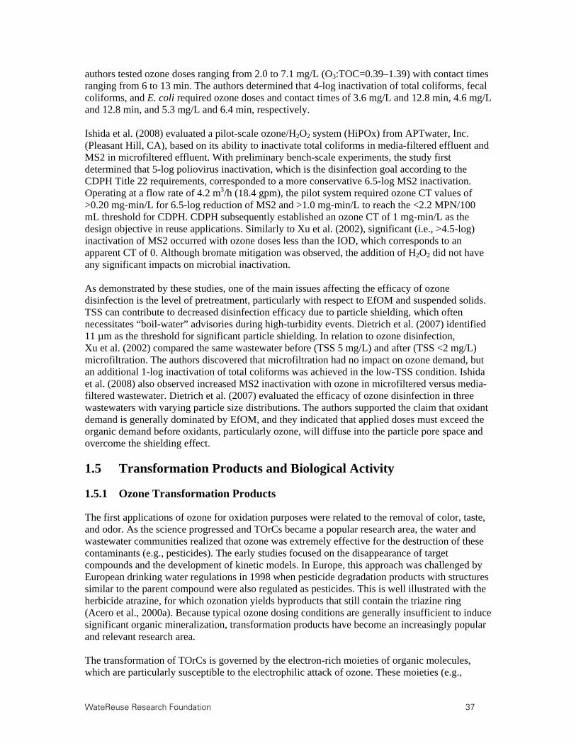
WateReuse Research Foundation 37
authors tested ozone doses ranging from 2.0 to 7.1 mg/L (O3:TOC=0.39–1.39) with contact times ranging from 6 to 13 min. The authors determined that 4-log inactivation of total coliforms, fecal coliforms, and E. coli required ozone doses and contact times of 3.6 mg/L and 12.8 min, 4.6 mg/L and 12.8 min, and 5.3 mg/L and 6.4 min, respectively. Ishida et al. (2008) evaluated a pilot-scale ozone/H2O2 system (HiPOx) from APTwater, Inc. (Pleasant Hill, CA), based on its ability to inactivate total coliforms in media-filtered effluent and MS2 in microfiltered effluent. With preliminary bench-scale experiments, the study first determined that 5-log poliovirus inactivation, which is the disinfection goal according to the CDPH Title 22 requirements, corresponded to a more conservative 6.5-log MS2 inactivation. Operating at a flow rate of 4.2 m3/h (18.4 gpm), the pilot system required ozone CT values of >0.20 mg-min/L for 6.5-log reduction of MS2 and >1.0 mg-min/L to reach the <2.2 MPN/100 mL threshold for CDPH. CDPH subsequently established an ozone CT of 1 mg-min/L as the design objective in reuse applications. Similarly to Xu et al. (2002), significant (i.e., >4.5-log) inactivation of MS2 occurred with ozone doses less than the IOD, which corresponds to an apparent CT of 0. Although bromate mitigation was observed, the addition of H2O2 did not have any significant impacts on microbial inactivation. As demonstrated by these studies, one of the main issues affecting the efficacy of ozone disinfection is the level of pretreatment, particularly with respect to EfOM and suspended solids. TSS can contribute to decreased disinfection efficacy due to particle shielding, which often necessitates “boil-water” advisories during high-turbidity events. Dietrich et al. (2007) identified 11 µm as the threshold for significant particle shielding. In relation to ozone disinfection, Xu et al. (2002) compared the same wastewater before (TSS 5 mg/L) and after (TSS <2 mg/L) microfiltration. The authors discovered that microfiltration had no impact on ozone demand, but an additional 1-log inactivation of total coliforms was achieved in the low-TSS condition. Ishida et al. (2008) also observed increased MS2 inactivation with ozone in microfiltered versus media-filtered wastewater. Dietrich et al. (2007) evaluated the efficacy of ozone disinfection in three wastewaters with varying particle size distributions. The authors supported the claim that oxidant demand is generally dominated by EfOM, and they indicated that applied doses must exceed the organic demand before oxidants, particularly ozone, will diffuse into the particle pore space and overcome the shielding effect.
1.5 Transformation Products and Biological Activity
1.5.1 Ozone Transformation Products
The first applications of ozone for oxidation purposes were related to the removal of color, taste, and odor. As the science progressed and TOrCs became a popular research area, the water and wastewater communities realized that ozone was extremely effective for the destruction of these contaminants (e.g., pesticides). The early studies focused on the disappearance of target compounds and the development of kinetic models. In Europe, this approach was challenged by European drinking water regulations in 1998 when pesticide degradation products with structures similar to the parent compound were also regulated as pesticides. This is well illustrated with the herbicide atrazine, for which ozonation yields byproducts that still contain the triazine ring (Acero et al., 2000a). Because typical ozone dosing conditions are generally insufficient to induce significant organic mineralization, transformation products have become an increasingly popular and relevant research area. The transformation of TOrCs is governed by the electron-rich moieties of organic molecules, which are particularly susceptible to the electrophilic attack of ozone. These moieties (e.g.,

38 WateReuse Research Foundation
olefins, activated aromatic systems, deprotonated amines, and reduced sulfur species) are also responsible for the overall reaction rates with ozone. The general reaction pathways for the primary attack of ozone on an organic molecule are summarized by reactions 1–5 in Figure 0.4 (von Gunten, 2003a).
Figure 0.4. Primary reactions between ozone and organic molecules.
These primary products are typically not stable and undergo further transformation reactions. A detailed discussion of all possible reactions is beyond the scope of this study. Table 1.9 provides an overview of some recent investigations on TOrC transformation during ozonation. Based on these studies and various other studies performed with model compounds, it is possible to make some predictions on transformation product formation during ozonation.
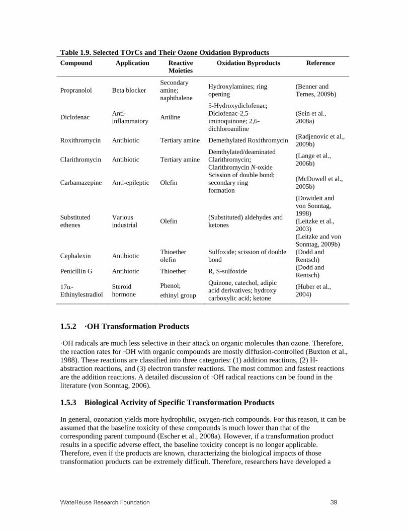
WateReuse Research Foundation 39
Table 1.9. Selected TOrCs and Their Ozone Oxidation Byproducts
Compound Application Reactive Moieties
Oxidation Byproducts Reference
Propranolol Beta blocker Secondary amine; naphthalene
Hydroxylamines; ring opening
(Benner and Ternes, 2009b)
Diclofenac Anti-inflammatory
Aniline
5-Hydroxydiclofenac; Diclofenac-2,5-iminoquinone; 2,6-dichloroaniline
(Sein et al., 2008a)
Roxithromycin Antibiotic Tertiary amine Demethylated Roxithromycin (Radjenovic et al., 2009b)
Clarithromycin Antibiotic Tertiary amine Demthylated/deaminated Clarithromycin; Clarithromycin N-oxide
(Lange et al., 2006b)
Carbamazepine Anti-epileptic Olefin Scission of double bond; secondary ring formation
(McDowell et al., 2005b)
Substituted ethenes
Various industrial
Olefin (Substituted) aldehydes and ketones
(Dowideit and von Sonntag, 1998) (Leitzke et al., 2003) (Leitzke and von Sonntag, 2009b)
Cephalexin Antibiotic Thioether olefin
Sulfoxide; scission of double bond
(Dodd and Rentsch)
Penicillin G Antibiotic Thioether R, S-sulfoxide (Dodd and Rentsch)
17-Ethinylestradiol
Steroid hormone
Phenol;
ethinyl group
Quinone, catechol, adipic acid derivatives; hydroxy carboxylic acid; ketone
(Huber et al., 2004)
1.5.2 ·OH Transformation Products
·OH radicals are much less selective in their attack on organic molecules than ozone. Therefore, the reaction rates for ·OH with organic compounds are mostly diffusion-controlled (Buxton et al., 1988). These reactions are classified into three categories: (1) addition reactions, (2) H-abstraction reactions, and (3) electron transfer reactions. The most common and fastest reactions are the addition reactions. A detailed discussion of ·OH radical reactions can be found in the literature (von Sonntag, 2006).
1.5.3 Biological Activity of Specific Transformation Products
In general, ozonation yields more hydrophilic, oxygen-rich compounds. For this reason, it can be assumed that the baseline toxicity of these compounds is much lower than that of the corresponding parent compound (Escher et al., 2008a). However, if a transformation product results in a specific adverse effect, the baseline toxicity concept is no longer applicable. Therefore, even if the products are known, characterizing the biological impacts of those transformation products can be extremely difficult. Therefore, researchers have developed a

40 WateReuse Research Foundation
battery of bioassays to elucidate the potential consequences of transformation products. Table 1.10 summarizes the relevant results found in the literature. Table 1.10. Evaluations of Mixture Toxicity After Oxidation of Selected TOrCs
Compound Application Bioassay Result Reference
Clarithromycin Antibiotic Growth inhibition of P. putida
Full removal of antibacterial properties
(Lange et al., 2006b)
Roxithromycin; Azithromycin; Tylosin; Ciprofloxacin; Enrofloxacin; Sulfamethoxazole; Trimethoprim; Lincomycin; Tetracycline; Vancomycin; Amikacin
Antibiotic Growth inhibition of E. coli and B. subtilis
Full removal of antibacterial properties
(Dodd et al., 2009)
Penicillin G; Cephalexin
Antibiotic Growth inhibition of E. coli and B. subtilis
Partial removal of antibacterial properties
(Dodd and Rentsch) (Dodd et al., 2009)
Estrone; 17-Estradiol; Estriol; Nonylphenol; Bisphenol A
Endocrine disruptors
Nuclear receptor-ligand assay
Good elimination of estrogenicity
(Zhang et al., 2008)
17-Ethinylestradiol
Synthetic estrogen
Yeast estrogen screen
Good elimination of estrogenicity
(Huber et al., 2004) (Lee et al., 2008)
Triclosan Biocide Growth inhibition of E. coli
Full removal of antibacterial properties
(Suarez et al., 2007)
Dimethylsulfamide Metabolite of the fungicide Tolyfluanide
Not tested; formation of NDMA
Mutagenic compound
(Schmidt and Brauch, 2008) (von Gunten)
1.5.4 Biological Activity of Effluent Mixtures
Bioassays with individual TOrCs demonstrate that in most cases the bioactivity of a particular compound decreases after exposure to ozone or ·OH. However, these assays are generally performed in ultrapure water and do not take into account mixtures of contaminants or the effects of environmental water matrices. Two approaches have been developed to address these issues: (1) in vitro assays after sample concentration and cleanup and (2) in vivo assays with actual organisms. Table 1.11 summarizes the results of the relevant studies available in the literature.

WateReuse Research Foundation 41
Table 1.11 Bioassay Results after Ozonation of Secondary Effluent
Treatment System Test Systems Results Reference
Full-scale ozonation of wastewater
Preconcentration of samples; bioluminescence inhibition; estrogenicity; aryl hydrocarbon receptor response; genotoxicity; neurotoxicity; phytotoxicity
Significant decrease in all endpoints upon ozonation step
(Macova et al., 2010b) (Reungoat et al., 2010)
Full-scale ozonation of secondary effluent
Preconcentration of samples; bioluminescence inhibition; growth inhibition; inhibition of photosynthesis; estrogenicity; inhibition of acetylcholinesterase; genotoxicity
Significant decrease in all endpoints during ozonation; no genotoxicity formation during ozonation
(Escher et al., 2009)
Ozonation of secondary effluent
In vitro tests after pre-concentration; in vivo tests with whole effluent; genotoxicity; retionic acid receptor (RAR) agonist activity; acute ecotoxicity (D. magna); Japanese medaka embryo exposure tests
Significant removal of genotoxicity; RAR agonist activity; acute ecotoxicity; higher ozone doses led to a reduction in hatching success rate
(Cao et al., 2009)
Tertiary treated sewage effluent
In vivo tests with juvenile rainbow trout O. mykiss in liver and kidney tissues glutathione S-transferase (GST), glutathione (GSH), glutathione peroxidase (GPX), lipid peroxidase (LPO), haem peroxidase
Liver: increased haem peroxidase; LPO and GST; total GSH depleted; kidney: increased LPO and GPX; observations show oxidative stress of organism; coagulation after ozonation reduces these effects
(Petala et al., 2009)
Ozonation of secondary effluent
In vivo tests; lemna minor growth inhibition; chironomid toxicity test with the nonbiting midge Chironomus riparius; Lumbriculus variegates toxicity; genotoxicity; estrogenicity
Growth inhibition; removal of estrogenicity; increased genotoxicity; enhanced toxicity for Lumbriculus variegates; effects disappear with post-ozone rapid sand filtration
(Stalter et al., 2010b)
Ozonation of secondary effluent
Fish early life stage toxicity test (rainbow trout, O. mykiss)
Developmental retardation; removal of estrogenicity
(Stalter et al., 2010d)
The results in Table 1.11 indicate that ozonation has quantifiable benefits with respect to toxicity and estrogenicity as determined via in vitro bioassays. However, some in vivo assays indicate that ozonation may increase toxicity in wastewater applications unless posttreatment biological filtration is used. The adverse effects are probably due to oxidation byproducts from the reaction of ozone with EfOM.

42 WateReuse Research Foundation
1.6 Ozone Byproduct Formation from Matrix Transformation
1.6.1 Bromate and Bromo-organics
Chlorate, bromate, and iodate can be formed during ozonation if certain boundary conditions are fulfilled. Whereas chlorate is of some human toxicological concern (WHO drinking water guideline value of 700 μg/L), bromate is considered a potential human carcinogen and is regulated at 10 μg/L by the U.S. EPA . In recent studies, it has been shown that bromate can be reduced in simulated gastric juices (Keith et al., 2006a, 2006b). Even though these processes are quite slow in the presence of hydrochloric acid at concentrations similar to that in gastric juice, they can be accelerated by the presence of reducing species such as H2S (Keith et al., 2006b). However, additional research under more realistic conditions will be necessary to justify an increase in the drinking water standard for bromate. In contrast to bromate, iodate is nontoxic because it is quickly reduced to iodide in the stomach. It is even added to table salt as an iodine supplement (Burgi et al., 2001). Therefore, bromate is the more relevant disinfection byproduct with respect to ozonation. Bromate is formed in bromide-containing waters through a complicated mechanism including both ozone and ·OH reactions and has been studied in great detail in the last two decades (Haag and Hoigné, 1983a; Hofmann and Andrews, 2001; Song et al., 1997; von Gunten and Hoigne, 1994; von Gunten and Hoigné, 1996; von Gunten and Oliveras, 1998b).
Bromate formation begins when ozone converts bromide to hypobromite (OBr-), which is in equilibrium with hypobromous acid (HOBr, pKa=8.8) (Haag and Hoigné, 1983b). After two sequential oxygen-atom-transfer reactions, hypobromite is converted to bromite (BrO2
-) and bromate (BrO3
-). In this reaction sequence, hypobromous acid/hypobromite is a crucial intermediate because its further transformation is relatively slow. Therefore, its lifetime is sufficiently long so that it can undergo various side reactions. In the presence of ammonia, it can form monobromamine, which is only slowly oxidized by ozone to nitrate and bromide. Therefore, the transient monobromamine concentration is significant and allows reductions in the rate of bromate formation. As a matter of fact, ammonia addition is one of the proposed methods for bromate minimization ( Hofmann and Andrews, 2001; Pinkernell and Von Gunten, 2001a; Song et al., 1997). Another important sink for the hypobromous acid intermediate is its reaction with H2O2. This reaction may occur in H2O2-based AOPs: HOBr + HO2
- Br- + O2 + H2Ok=7.6 108 M-1s-1 (von Gunten and Oliveras, 1997). Because of this reaction, bromate formation is sometimes lower in the ozone/H2O2 AOP than in the conventional ozonation process. However, even in the presence of H2O2, bromate cannot be entirely suppressed during ozonation (Von Gunten and Oliveras, 1998a). In contrast, bromate formation is completely suppressed in the UV/H2O2 AOP. -radiolysis experiments indicate that HOBr is indeed a decisive intermediate in the bromate formation pathway even if ·OH radicals are the only oxidants (Von Gunten and Oliveras, 1998a). Because of the relatively high concentration of H2O2 in the UV/H2O2 system, the rate of HOBr reduction to bromide is sufficiently high to avoid further oxidation of HOBr to bromate. Bromate formation in ·OH-based processes proceeds according to the following simplified reaction sequence (for a comprehensive reaction sequence see Von Gunten and Oliveras, 1998a):
Br- + ·OH BrOH- k=1.06 1010 M-1s-1 (Zehavi and Rabani, 1972) BrOH- Br- + ·OH k=3.3 107 s-1 (Zehavi and Rabani, 1972) BrOH- Br. + -OH k=4.2 106 s-1 (Zehavi and Rabani, 1972)

WateReuse Research Foundation 43
Br. + Br- Br2.- + -OH k ≈ 1010 M-1s-1 (Zehavi and Rabani, 1972)
2Br2.- Br3
- + Br- k=2 109 M-1s-1 (Sutton et al., 1965 ) Br3
- Br2 + Br- k=8.3 108 s-1 (Sidgwick, 1952) Br2 + Br- Br3
- k=1010 M-1s-1 (Sidgwick, 1952) Br2 + H2O HOBr + H+ + Br- k=3.5 10-9 M2 (Beckwith et al., 1996) HOBr + ·OH BrO. + H2O k=2 109 M-1s-1 (Buxton and Dainton, 1968) OBr- + ·OH BrO. + -OH k=4.5 109 M-1s-1 ( Buxton and Dainton, 1968) 2BrO. + H2O OBr- + BrO2
- + 2H+ k=4.5 109 M-1s-1 ( Buxton and Dainton, 1968) BrO2
- + ·OH BrO2. + -OH k=2 109 M-1s-1 ( Buxton and Dainton, 1968)
BrO2. + ·OH BrO3
- + H+ k=2 109 M-1s-1 (Field et al., 1982). To explain the fact that bromate formation is not entirely suppressed by ozone/H2O2, a pathway that does not include HOBr as an intermediate must exist. The following reaction has been suggested: Br. + O3 BrO· + O2 k=1.5 108 M-1s-1 (Von Gunten and Oliveras, 1998a). The bromate formation pathway is further complicated by the fact that carbonate radicals may also play a role in the oxidation of hypobromite: CO3
-· + OBr- BrO· + CO32- k=4.3 107 M-1s-1 ( Buxton and Dainton, 1968).
Therefore, alkalinity can have an influence on bromate formation kinetics and the formation pathway. Finally, DOM has an important influence on bromate formation. Its main role is related to its effect on the ozone chemistry and ·OH formation during ozonation (Pinkernell and Von Gunten, 2001b).
Once bromate is formed, it can be removed with a variety of processes: activated carbon filtration, iron(II) addition, UV and photocatalytic processes, and biological processes ( Asami et al., 1999; Bao et al., 1999; Gordon et al., 2002; Kirisits et al., 2000; Kirisits et al., 2001; Mills et al., 1996; Peldszus et al., 2004; Siddiqui et al., 1997; van der Kooij et al., 1989; Van Ginkel et al., 2005). Activated carbon, which is sometimes in place after ozonation, is only efficient when it is fresh. Initially, chemical bromate reduction occurs, but over time, bromate mitigation is limited to bioconversion via anaerobic metabolism. However, such conditions are not easily established in the oxygen-rich environment resulting from ozonation. UV-based processes for bromate removal are typically very energy-intensive, and chemical reduction is highly inefficient. Therefore, no bromate reduction processes have been implemented in full-scale water treatment systems. Instead, bromate mitigation at full-scale treatment plants relies on initial reductions in bromate formation. Based on mechanistic understanding of bromate formation, various minimization methods are available today and are summarized in Table 1.12 ( Buffle et al., 2004a; Galey et al., 2000; Krasner et al., 1993; Kruithof et al., 1993; Neemann et al., 2004; Pinkernell and Von Gunten, 2001; Song et al., 1997; van der Kooij et al., 1989).

44 WateReuse Research Foundation
Table 1.12. Bromate Mitigation Strategies
Method BrO3
- Reduction Compared to Conventional Ozonation
Problems
pH depression ca. factor 2 High-alkalinity waters
Ammonia addition ca. factor 2 Residual ammonia has to be removed in biological filtration; ammonia addition forbidden in many European countries
Chlorine–ammonia process
ca. factor 10 Residual ammonia; ammonia addition forbidden in many European countries; formation of halo-organic compounds in prechlorination
Peroxone process Depends largely on point of
H2O2 addition
Disinfection might be significantly affected; mostly suited for bromate minimization in pure oxidation processes
The chlorine–ammonia process is particularly interesting and is the result of empirical observations that bromate formation can be substantially reduced in systems with prechlorination followed by ammonia addition (Neemann et al., 2004). The mechanism of this process has been explained by the following four reaction steps (Buffle et al., 2004b): 1. HOCl + Br- HOBr + Cl- k=1.55 x 10³ M-1s-1 (Kumar and Margerum, 1987) 2. HOBr + NH3 NH2Br + H2O k=8 x 10⁷ M-1s-1 (Haag et al., 1984) 3. O3 + NH2Br Y k=40 M-1s-1 (Haag et al., 1984) 4. Y + 2O3 2H+ + NO3
- + Br- + 3O2 k >> 40 M-1s-1 (Haag et al., 1984). The advantage of this process is the efficient masking of bromide as monobromamine (NH2Br) prior to ozonation. NH2Br reacts slowly with ozone and releases bromide. Therefore, especially during the initial phase of ozonation, for which the ·OH impact is high, bromide is not available for oxidation to bromate. Reaction 1 is the critical step in this reaction sequence. Due to the acid–base speciation of HOCl, the reaction rate for Reaction 1 is pH-dependent (only HOCl reacts with bromide; pKa of HOCl=7.5). Furthermore, the reaction of HOCl with DOM may lead to chloro-organic compounds. Therefore, the free chlorine contact time has to be optimized for maximum bromide oxidation and acceptable formation of chloro-/bromo-organics.
It has also been shown that the chlorine–ammonia process works if the raw water already contains ammonia. Based on the fact that chlorine reacts quickly with ammonia (kHOCl,NH3 ≈ 3 106 M-1s-1 (Deborde and von Gunten, 2008)) and that the formed NH2Cl only reacts slowly with bromide (kNH2Cl,Br- at pH 7=2.8 10-1 M-1s-1 (Trofe, 1980)), one can expect that bromide will not be oxidized to HOBr under such conditions. Therefore, an additional mechanism has been suggested, namely the reaction of chlorine with organic amines, leading to the corresponding chloramines and a reduction in ·OH yield during postozonation (Buffle and von Gunten, 2006).
Bromate minimization in the peroxone process has been optimized by the HiPOx process (Bowman, 2005), in which ozone is added in small portions throughout a specially designed reactor. This allows the residual ozone concentrations to be kept very low, which suppresses the Br. + O3 reaction. With excess H2O2, HOBr is reduced back to bromide. From a regulatory perspective, this strategy is only applicable for oxidation and not for disinfection because of the low applied ozone doses and, consequently, low CT values. However, the HiPOx process is capable of achieving significant microbial inactivation with appropriate dosing, as indicated by its CDPH Title 22 certification.
WateReuse Research Foundation 45
The formation of halogenated compounds during ozonation is restricted to the formation of brominated compounds (Richardson et al., 1999a; Zhang et al., 2005). Chlorinated compounds cannot be formed during ozonation because chloride is very slowly oxidized by ozone and not by ·OH at circumneutral pH (Klaening and Wolff, 1985; von Gunten, 2003b). Mixed chloro–bromo compounds are only formed if ozonation is combined with pre- or postchlorination/chloramination ( Buffle et al., 2004a; Krasner et al., 2006a); Richardson et al., 1999a). It was also found that ozonation followed by chloramine led to the formation of trihalonitromethanes (Krasner et al., 2006b). However, these findings have to be interpreted with caution, because no biological filtration step was applied after ozonation. This step might have removed the precursors for these compounds (Krasner et al., 2009b). Iodinated compounds are not likely to be formed during ozonation, because the oxidation of iodide to iodate is a very fast process, giving no time for the formation of iodo-organic compounds (Bichsel and von Gunten, 1999; Krasner et al., 2009a).
1.6.2 N-Nitrosamines
NDMA and other nitrosamines have received considerable attention because of their relatively high carcinogenic potential. Nitrosamines generally form when chloramine reacts with secondary and tertiary amines of natural and anthropogenic origin (Choi et al., 2002; Mitch and Sedlak, 2002; Schreiber and Mitch, 2006). Recently, it has been shown that NDMA can also be formed during ozonation of dimethylamine and N,N-dimethylsulfamide (von Gunten et al., 2010), which means that direct NDMA formation is a potential concern during ozonation of secondary and tertiary effluents. The most common NDMA control strategies include UV treatment and microbial degradation when NDMA is present in the source water (Sharpless and Linden, 2003), but the destruction of NDMA with ozone and ozone/H2O2 is also possible. Ozone mitigation is rare, however, because NDMA has a low reactivity with ozone (k=0.052 M-1s-1 (Lee et al., 2007b)) and ·OH (k=4.5 × 10⁸ M-1s-1 (Lee et al., 2007b)). Also, design doses would have to be sufficient to overcome the initial spike in NDMA that is due to direct formation. Nevertheless, it has been demonstrated that NDMA in RO permeate can be greatly reduced (1-log or greater) using ozone/H2O2, because NDMA precursors are greatly reduced in comparison to secondary effluent (i.e., limited direct formation), and ·OH scavenging is minimal. In the past, the CDPH required California utilities to demonstrate 1.2-log removal or destruction of NDMA when applying an AOP after reverse osmosis in groundwater recharge applications. Due to the susceptibility of NDMA to photolysis (Sharpless and Linden, 2003), UV/H2O2 became the standard treatment process in these applications. However, this AOP can be costly because of lamp cleaning and replacement, high energy requirements, and the costs associated with H2O2
addition. Furthermore, the recent revisions to the draft CDPH regulations have replaced the 1.2-log NDMA requirement with a straightforward NL of 10 ng/L for NDMA. Therefore, if NDMA formation can be controlled in the sourcewater, other oxidation alternatives may become more appealing in IPR applications. Ozonation is also known to be effective in destroying NDMA precursors (e.g., secondary or tertiary amine precursors) and reducing NDMA formation potential in subsequent chloramination processes (Lee et al., 2007a). Therefore, ozone implementation may be hindered by direct NDMA formation in some matrices, but ozone is effective in reducing NDMA concentrations in RO permeate and overall formation potential during chloramination.

46 WateReuse Research Foundation
1.6.3 Assimilable Organic Carbon
The vast majority of nonhalogenated byproducts are a result of the oxidation of electron-rich moieties of the DOM (aromatic systems, olefins, etc.) with ozone and ·OH radicals. This leads to the formation of smaller oxygen-rich molecules (e.g., carboxylic acids, aldehydes, and ketones) (Richardson et al., 1999b), which are often highly biodegradable and can be classified as assimilable organic carbon (AOC) or biologically degradable organic carbon (BDOC) (Hammes et al., 2006; Siddiqui et al., 1997; van der Kooij et al., 1989). The mechanisms and formation kinetics of these compounds are typically governed by the reaction of ozone with certain DOM moieties, such as phenols or other activated aromatic systems. Upon ozonation, this leads to various olefins and eventually small organic acids and aldehydes (Leitzke and von Sonntag, 2009a; Ramseier and von Gunten, 2009).
1.7 Applicability of Aquifer Recharge and Recovery for Ozonated Effluent
Treated effluent intended for IPR covers a vast spectrum of water quality, but most IPR applications involve some form of environmental barrier. In addition to creating mental separation between the wastewater origin and the potable end product, the environment provides a natural treatment barrier where additional contaminant attenuation and microbial inactivation are achieved. Surface water discharge is common in some locations, but groundwater replenishment is often the preferred alternative, particularly in California. This type of application is sometimes referred to as groundwater replenishment and reuse (GRR), soil aquifer treatment (SAT), or aquifer recharge and recovery (ARR). For spreading applications, some IPR agencies use conventional tertiary effluent, whereas other systems still employ FAT (i.e., MF-RO-UV/H2O2) prior to aquifer recharge. For direct injection, agencies generally prefer or are required to employ FAT, because RO permeate is typically perceived to be the ideal matrix for potable reuse. This is intuitive, because RO is effective in removing both bulk organic matter, trace organics, and a variety of other contaminants. In fact, RO is able to achieve TOC concentrations lower than 0.5 mg/L, whereas tertiary effluent may be an order of magnitude higher. In the context of the CDPH draft regulations for groundwater replenishment, this correlates to a facility being able to recharge <10% tertiary effluent (with the remaining fraction being composed of diluent water) or 100% RO permeate. Therefore, from a regulatory perspective, RO permeate holds a distinct advantage over tertiary effluent. Despite this regulatory advantage, the issue becomes more complex after the short-term impacts of ARR are considered. According to a recent study, direct injection of 100% RO permeate may actually lead to significant leaching of TOC in basins that have been continually exposed to tertiary effluent in the past (Drewes et al., 2010). In that study, leaching in laboratory-scale columns increased the TOC in the recharge water from 0.57 mg/L to 1.17 mg/L, which would correlate to a change in theoretical RWC from 88% down to 43%. Furthermore, direct injection of 100% RO permeate led to leaching of ammonia from the soil, which was then oxidized to nitrate during transport. In an actual IPR application, this could potentially jeopardize the total nitrogen and nitrate objectives mandated in the CDPH regulations. Other studies indicate that attenuation of persistent TOrCs can be improved by supplying soil microbes with BDOC or AOC (Rauch-Williams et al., 2010), as defined in the previous section. Although RO permeate appears to be at a disadvantage in this scenario, Drewes et al. (2010) indicates that the TOC leached by 100% RO permeate provides sufficient substrate to induce

WateReuse Research Foundation 47
cometabolism of TOrCs. Over time, this type of system will stabilize, and TOC leaching will become insignificant, which may lead to a decrease in TOrC attenuation during long-term operation. Therefore, tertiary/oxidized effluent may hold a long-term advantage over 100% RO permeate in ARR applications. The efficacy of ARR is described later in Chapter 9.
1.8 Pilot- and Full-Scale Ozonation for Trace Organic Contaminant Mitigation
Water and wastewater treatment technologies sometimes encounter significant obstacles as the processes are scaled up from bench-scale experiments to pilot- and full-scale demonstrations. Although bench-scale evaluations provide an invaluable scientific foundation for a particular process, the value of a novel technology cannot be realized until it is implemented in the field. Pilot and full-scale installations often reveal the limitations of a particular technology, but they also provide a wealth of resources and information that cannot always be duplicated in a laboratory setting (large quantity of treated water, integration into a larger treatment train to evaluate synergistic or antagonistic relationships, discharge to the environment, etc.). The following sections describe evaluations of ozone technologies after field deployment and highlight the importance of scale to those particular studies.
1.8.1 Pilot-Scale Ozone Applications
Wert et al. (2009a) evaluated pilot-scale ozonation with three tertiary-treated U.S. wastewaters based on oxidation of a suite of ambient TOrCs and spiked para-chlorobenzoic acid (pCBA). Based on the water quality data in Table 1.13, these experimental matrices offered a wide range of conditions related to competing organic matter and level of pretreatment (i.e., nitrification/denitrification). The pilot-scale ozone system was operated at a flow rate of 1 L/min (0.26 gpm) with targeted O3:TOC ratios of 0.2, 0.6, and 1.0; and provided a contact time of 24 min. Table 1.13. Water Quality Data for Wert et al. (2009a) Pilot Study
Parameter A B C
Location Nevada Florida Colorado pH 8.2 7.6 7.1 Alkalinity (mg/L as CaCO3) 128 269 101 Bromide (mg/L) 0.18 0.17 0.19 TOC (mg/L) 6.6 10.3 10.3 UV254 absorbance (cm-1) 0.140 0.260 0.171 SUVA (L/mg-m) 2.11 2.52 1.66 Total nitrogen (mg-N/L) 14.8 9.38 13.8 NH4 (mg-N/L) <0.2 6.98 1.28 NO3 (mg-N/L) 12 0.074 9.7 NO2 (mg-N/L) <0.05 0.77 0.40 kOH-EfOM (109 M-1s-1) 0.68 2.72 1.12
In all three wastewaters, an O3:TOC ratio of 0.2 was insufficient to generate a measurable ozone residual (i.e., CT ≈ 0 mg-min/L), but the process still demonstrated significant concentration reductions for many ozone-susceptible contaminants, particularly for Wastewater A. An O3:TOC ratio of 0.6 achieved greater than 70% reductions in 15 of the 27 detected contaminants for all three wastewaters, and only TCEP, TCPP, iopromide, atrazine, and meprobamate experienced reductions of less than 80% with an O3:TOC ratio of 1.0. For all three wastewaters, the authors

48 WateReuse Research Foundation
indicated that a CT of less than 1 mg-min/L was sufficient to remove more than 95% of the ozone-susceptible compounds (i.e., carbamazepine, diclofenac, naproxen, sulfamethoxazole, and triclosan), and a CT of approximately 6 mg-min/L was sufficient to remove more than 50% of the ozone-resistant compounds (i.e., atrazine, iopromide, diazepam, ibuprofen, and pCBA). The study also included bench-scale experiments indicating that both the amount and type of EfOM contribute to a wastewater’s ozone reactivity, as indicated by the kOH-EfOM values in Table 1.14. Sundaram et al. (2009) described the efficacy of a pilot-scale HiPOx reactor operated at the Reno-Stead Water Reclamation Facility (Reno, NV). In their study, the HiPOx reactor was part of a 40-L/min (10.7 gpm) pilot-scale treatment train consisting of conventional secondary effluent (SRT of 25 days), ultrafiltration, ozone (Table 1.14), and biological activated carbon (BAC) with a bed depth of 4.5 ft and an empty bed contact time (EBCT) of 30 min. With respect to water quality, the ultrafiltration effluent had a pH of 6.9, DOC of 6.4 mg/L, alkalinity of 92 mg/L as CaCO3, and nitrite less than 0.06 mg-N/L. Table 1.14. Ozone Residuals in Reno-Stead Pilot System
Applied Ozone Dose (mg/L) 3 5 7
O3:DOC ratio (g O3/g DOC) 0.47 0.78 1.09 Time to Depletion (min) 3.6 7.7 13.5
Source: Sundaram et al. (2009). During the initial ozone optimization phase, the initial concentrations of 13 monitored TOrCs were below the reporting limits for the analytical methods, presumably because of the preceding biological process and ultrafiltration. With 3 mg/L of applied ozone, 12 compounds were more than 99% removed, and 5 compounds (DEET, fluoxetine, phenytoin, sulfamethoxazole, and meprobamate) were more than 50% removed. With the exception of meprobamate (75%), all of the detected compounds were more than 95% removed with 5 mg/L of applied ozone, and even meprobamate was more than 90% removed with 7 mg/L of applied ozone. However, even with peroxide addition at a molar ratio (H2O2:O3) of 1.5, bromate formation exceeded 10 µg/L with 7 mg/L of applied ozone. Therefore, continuous ozonation was limited to 3 mg/L of applied ozone or 5 mg/L of applied ozone supplemented with peroxide addition at a molar ratio (H2O2:O3) of 1.0. Because advanced wastewater treatment and source protection are particularly common practices in Europe, there are many examples of ozone field deployment related to European utilities. Huber et al. (2005b) monitored the concentrations of spiked antibiotics, EDCs, and antineoplastics (i.e., chemotherapy drugs) during pilot-scale ozonation. The pilot-scale reactor consisted of two contactors in series with a total hydraulic retention time of 8.4 min. The influent to the reactor consisted of conventional secondary effluent, secondary effluent spiked with 15 mg/L of TSS, and permeate from a pilot-scale membrane bioreactor (MBR). Secondary effluent samples were collected from a full-scale wastewater treatment plant in Kloten-Opfikon, Switzerland that serves a population of 55,000 and performs grit removal, primary clarification, and nitrification/denitrification with an SRT of approximately 11 days. The membrane permeate was fed with the same primary clarified water, but the SRT for the MBR was greater than 70 days. With respect to water quality data, the pH ranged from 7.0 to 7.5, the DOC ranged from 7.7 to 6.6 mg/L, the COD ranged from 41 to 22 mg/L, the TSS ranged from 20 to 0 mg/L, and the alkalinity ranged from 310 to540 mg/L for the secondary effluent and MBR, respectively. Target contaminants were spiked at levels ranging from 0.5 to 5 µg/L to mimic common environmental conditions.
WateReuse Research Foundation 49
In this study, an applied ozone dose of 0.5 mg/L (O3:TOC=0.06–0.08) achieved less than 50% reductions for the ozone-susceptible compound classes (i.e., macrolide antibiotics, sulfonamide antibiotics, and estrogens) and less than 10% for the X-ray contrast media. However, an applied ozone dose of only 2 mg/L (O3:TOC=0.26–0.30) was sufficient to remove more than 90% of the ozone-susceptible compounds. Ozone doses of 2 mg/L and 5 mg/L (O3:TOC=0.65–0.76) achieved 30% and 60% removal of the X-ray contrast media, respectively. In these experiments, an ozone residual was only present in the second contactor when the applied ozone dose exceeded 2 mg/L. With respect to pretreatment, the authors indicated that suspended solids generally had limited effects on ozone efficacy. This was confirmed by a mathematical model suggesting that ozone consumption by sludge particles of diameter greater than 50 µm can be considered insignificant, thereby emphasizing the interactions with DOM and colloidal material. The authors attributed the few exceptions where the MBR permeate actually experienced minor, yet significant, reductions in performance to the effect of elevated pH, which leads to more rapid ozone decomposition and reduced oxidant exposure. Although the oxidation of TOrCs was not significantly affected by pretreatment, disinfection was hindered—by as much as 1 log—by the presence of suspended solids. These studies evaluated pilot-scale ozonation in relatively high-quality wastewater (i.e., secondary effluent or better). In contrast, Gagnon et al. (2008) evaluated pilot-scale ozonation in primary effluent at the City of Montreal Wastewater Treatment Plant, which was described previously in relation to a separate disinfection study. The primary effluent in this study was characterized by a pH of 8.1–8.2, TSS of 5 mg/L, DOC ranging from 90 to 110 mg/L, and residual aluminum and iron concentrations of 0.6–0.9 and 0.3–0.4 mg/L, respectively. The pilot-scale ozone generator was capable of producing 15–30 mg/L of dissolved O3, and the contactor provided approximately 18 min of contact time. The authors monitored a suite of TOrCs (salicylic acid, clofibric acid, ibuprofen, 2-hydroxy-ibuprofen, naproxen, triclosan, carbamazepine, and diclofenac) with ambient concentrations ranging from 23 to 2,556 ng/L for clofibric acid and salicylic acid, respectively. With an applied ozone dose of 15 mg/L (O3:DOC ≈ 0.15), only 2-hydroxy-ibuprofen experienced less than a 50% reduction in concentration. As the ozone dose increased to 20 mg/L (O3:DOC ≈ 0.20), only ibuprofen and 2-hydroxy-ibuprofen experienced less than 70% reduction in concentration. Furthermore, with the exception of 2-hydroxy-ibuprofen, there was little difference in treatment for the various contaminants when the applied ozone dose increased from 20 mg/L (O3:DOC ≈ 0.20) to 30 mg/L (O3:DOC ≈ 0.30). Given the extremely high concentration of competing organic matter, the pilot-scale ozone system was quite effective in oxidizing the trace contaminants, but it is unclear whether this type of application is cost effective due to the extremely high applied ozone dose required.
1.8.2 Full-Scale Ozone Applications for TOrC Oxidation and Removal
From 2003 to 2005, Nakada et al. (2007) analyzed four sets of samples from a full-scale wastewater treatment plant in Tokyo, Japan. Serving a population of approximately 460,000, the wastewater treatment plant treats 0.17 million m3/day (45 MGD) with primary and secondary treatment (SRT not specified). Following the secondary clarifiers, a portion of the flow is diverted for advanced treatment consisting of upflow sand filtration at a velocity of 110 m/day followed by ozonation at an applied dose of 3 mg/L and contact time of 27 min. Additional water quality information (pH, DOC, etc.) was not provided. With respect to sand filtration, the authors reported limited removal for hydrophilic (log KOW < 3) pharmaceuticals and EDCs, but the more hydrophobic compounds (log KOW > 3) experienced high, yet sporadic removal. With respect to the overall treatment process, many of the compounds approached the limits of quantification after activated sludge, filtration, and ozonation. However, there were a few notable exceptions with relatively high effluent concentrations in one or more sample events, including nonylphenol,
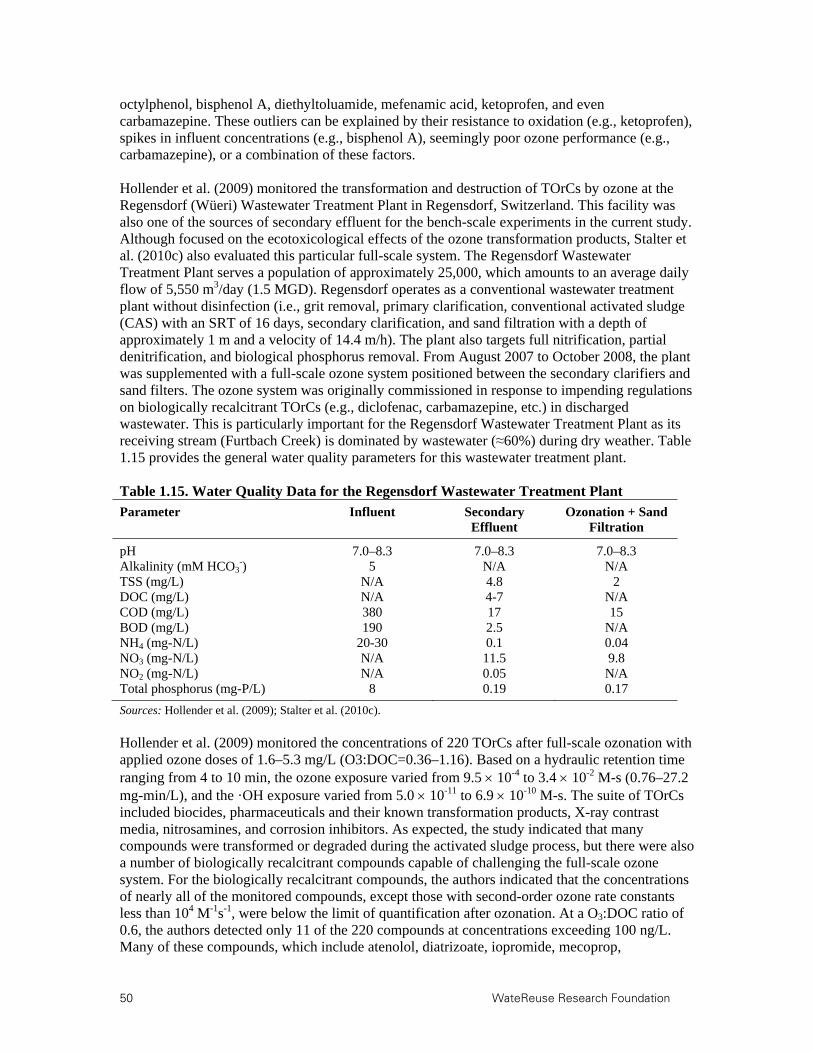
50 WateReuse Research Foundation
octylphenol, bisphenol A, diethyltoluamide, mefenamic acid, ketoprofen, and even carbamazepine. These outliers can be explained by their resistance to oxidation (e.g., ketoprofen), spikes in influent concentrations (e.g., bisphenol A), seemingly poor ozone performance (e.g., carbamazepine), or a combination of these factors. Hollender et al. (2009) monitored the transformation and destruction of TOrCs by ozone at the Regensdorf (Wüeri) Wastewater Treatment Plant in Regensdorf, Switzerland. This facility was also one of the sources of secondary effluent for the bench-scale experiments in the current study. Although focused on the ecotoxicological effects of the ozone transformation products, Stalter et al. (2010c) also evaluated this particular full-scale system. The Regensdorf Wastewater Treatment Plant serves a population of approximately 25,000, which amounts to an average daily flow of 5,550 m3/day (1.5 MGD). Regensdorf operates as a conventional wastewater treatment plant without disinfection (i.e., grit removal, primary clarification, conventional activated sludge (CAS) with an SRT of 16 days, secondary clarification, and sand filtration with a depth of approximately 1 m and a velocity of 14.4 m/h). The plant also targets full nitrification, partial denitrification, and biological phosphorus removal. From August 2007 to October 2008, the plant was supplemented with a full-scale ozone system positioned between the secondary clarifiers and sand filters. The ozone system was originally commissioned in response to impending regulations on biologically recalcitrant TOrCs (e.g., diclofenac, carbamazepine, etc.) in discharged wastewater. This is particularly important for the Regensdorf Wastewater Treatment Plant as its receiving stream (Furtbach Creek) is dominated by wastewater (≈60%) during dry weather. Table 1.15 provides the general water quality parameters for this wastewater treatment plant. Table 1.15. Water Quality Data for the Regensdorf Wastewater Treatment Plant
Parameter Influent Secondary Effluent
Ozonation + Sand Filtration
pH 7.0–8.3 7.0–8.3 7.0–8.3 Alkalinity (mM HCO3
-) 5 N/A N/A TSS (mg/L) N/A 4.8 2 DOC (mg/L) N/A 4-7 N/A COD (mg/L) 380 17 15 BOD (mg/L) 190 2.5 N/A NH4 (mg-N/L) 20-30 0.1 0.04 NO3 (mg-N/L) N/A 11.5 9.8 NO2 (mg-N/L) N/A 0.05 N/A Total phosphorus (mg-P/L) 8 0.19 0.17
Sources: Hollender et al. (2009); Stalter et al. (2010c). Hollender et al. (2009) monitored the concentrations of 220 TOrCs after full-scale ozonation with applied ozone doses of 1.6–5.3 mg/L (O3:DOC=0.36–1.16). Based on a hydraulic retention time ranging from 4 to 10 min, the ozone exposure varied from 9.5 10-4 to 3.4 10-2 M-s (0.76–27.2 mg-min/L), and the ·OH exposure varied from 5.0 10-11 to 6.9 10-10 M-s. The suite of TOrCs included biocides, pharmaceuticals and their known transformation products, X-ray contrast media, nitrosamines, and corrosion inhibitors. As expected, the study indicated that many compounds were transformed or degraded during the activated sludge process, but there were also a number of biologically recalcitrant compounds capable of challenging the full-scale ozone system. For the biologically recalcitrant compounds, the authors indicated that the concentrations of nearly all of the monitored compounds, except those with second-order ozone rate constants less than 104 M-1s-1, were below the limit of quantification after ozonation. At a O3:DOC ratio of 0.6, the authors detected only 11 of the 220 compounds at concentrations exceeding 100 ng/L. Many of these compounds, which include atenolol, diatrizoate, iopromide, mecoprop,

WateReuse Research Foundation 51
benzotriazole, 5-methylbenzotriazole, sucralose, DEET, diazinon, galaxolidone, and benzothiazole, require extended exposure to ·OH to achieve significant concentration reductions. At the highest O3:DOC ratio, only two X-ray contrast media were detected at concentrations exceeding 100 ng/L. The Hollender et al. (2009) study also monitored transformation products, disinfection byproducts, and the costs associated with the operation of the full-scale ozone plant. For example, AOC concentrations increased because of ozonation, but a portion of the AOC was removed during the subsequent sand filtration. The use of ozone, particularly in drinking water treatment applications, is often hindered by the formation of bromate, which is regulated at 10 µg/L by the U.S. EPA. During full-scale ozonation, the bromate concentration never exceeded 7.5 µg/L even at the highest applied ozone dose, primarily because of low influent bromide concentrations (<30 µg/L). However, nitrosamine formation proved to be problematic in that varying influent concentrations of NDMA, although partially removed during the activated sludge process, were compounded by NDMA formation during the ozonation process (up to 14 ng/L). With respect to NDMA formation potential during ozonation, the authors indicated that the variability in the secondary clarifier effluent (i.e., variable concentrations of NDMA and its precursors) was more significant than the ozone dose. NDMA destruction was limited (<25%) even at the highest ozone and ·OH exposure, but the subsequent sand filtration achieved up to 50% reductions in NDMA concentrations by biological activity. Finally, with respect to energy consumption, the full-scale ozone system consumed approximately 12 kWh/kg O3, which amounts to 0.035 kWh/m3 of wastewater at an O3:DOC ratio of 0.6. According to the authors, this is just over 10% of the total energy consumption (≈0.3 kWh/m3) of a typical wastewater treatment plant targeting nutrient removal.
1.8.3 Full-Scale Ozone Applications and Toxicological Implications
In Stalter et al. (2010c), secondary-clarified, ozonated, and post-ozone sand-filtered wastewater were compared with artificial control water to determine their toxicity during an in vivo rainbow trout assay (fish early life stage toxicity (FELST) test). In this study, the O3:DOC ratio ranged from 0.4 to 1.0. Using Organisation for Economic Co-operation and Development (OECD) guideline 210 as an experimental template, three tests were performed on these waters: (1) extended exposure of fertilized eggs to each water without additional treatment, (2) extended exposure of fertilized eggs to each water after 0.4-µm microfiltration, and (3) extended exposure of recently hatched fish to each water without additional treatment. Toxicity was evaluated based on a combination of objective and subjective factors, including egg coagulation, hatching, swim up, mortality, malformation, abnormal behavior, and vitellogenin concentrations in whole-body homogenates. The first experiment was hindered by the development of fungal contamination in all of the wastewater exposures. After elimination of this contamination with microfiltration pretreatment, subsequent testing indicated that all of the wastewaters, and particularly the ozonated sample, showed negatively impacted egg coagulation, hatching, swim up, biomass, and mortality in comparison to the control. Because no ozone residual was detected in any of the samples, the authors hypothesized that oxidation byproducts (e.g., aldehydes, carboxylic acids, ketones, or more specific compounds) were responsible for the increased toxicity of the ozone effluent, but the subsequent sand filtration was able to reduce this toxicity. In contrast, no developmental differences were observed in recently hatched fish that had not been previously exposed to wastewater. However, the secondary effluent was linked to increased feminization of the rainbow trout, but this effect was significantly reduced after ozone and post-ozone sand filtration—even below that of the control sample. Therefore, the authors suggest that ozone is extremely effective in reducing the potential estrogenic effects of

52 WateReuse Research Foundation
wastewater that is discharged to the environment, but post-ozone sand filtration is necessary to reduce the toxicity of oxidation byproducts. Reungoat et al. (2010) evaluated the concentrations and toxicity of ambient TOrCs at a full-scale water reclamation plant with ozonation. Macova et al. (2010a) provided a more in-depth analysis of the toxicity data from this plant. The South Caboolture Water Reclamation Plant in Queensland, Australia serves a population of approximately 40,000 and receives effluent from a nearby wastewater treatment plant operating a conventional activated sludge process at an SRT of 16 days. The influent DOC ranges from 15 to 20 mg/L, and the effluent DOC is less than 8 mg/L. Although the final product is considered nonpotable, the reclamation plant targets drinking water standards using an extensive treatment train that includes biological denitrification with methanol addition, pre-ozonation (0.1 g O3/g DOC, 2 mg/L O3), coagulation/flocculation/dissolved air flotation, sand filtration, main ozonation (0.5 g O3/g DOC, 5 mg/L O3, 15 min of contact time), BAC filtration, and final ozonation (0.1 g O3/g DOC, 2 mg/L O3). During the sampling period, the BAC had only been operating for 4 months since its last replacement, suggesting that both adsorption and biological degradation would contribute significantly to the observed removals. The authors reported that all of the compounds detected in the influent were still present at reportable concentrations following pre-ozonation because of the high concentration of competing organic matter (>20 mg/L). However, only half of the original contaminants were detected at reportable concentrations following the main ozonation phase, and of the remaining contaminants, only the most recalcitrant compounds (e.g., iopromide and gabapentin) were removed by less than 70%. After the subsequent BAC and final ozonation processes, only gabapentin and roxithromycin were confidently detected at reportable concentrations. With few exceptions, each component of the treatment train generally demonstrated reductions in baseline toxicity, estrogenicity, aryl hydrocarbon receptor response, genotoxicity, neurotoxicity, and phytotoxicity, but the most significant reductions were associated with the dissolved air flotation and sand filtration, main ozonation, and BAC processes. Although the Reungoat et al. (2010) study suggests that the final ozonation process provided no significant benefits with respect to TOrCs and toxicity, there may still be significant disinfection benefits, particularly related to pathogen regrowth during the BAC process, thereby justifying its implementation.
1.9 Conclusion
Despite recent research emphasis on pharmaceuticals and other TOrCs in water supplies, there is limited guidance that utilities can rely on when developing, expanding, or optimizing treatment strategies. As municipalities increasingly turn to IPR to augment their water supplies, these systems will likely take a proactive approach to removing TOrCs and oxidation byproducts. Although conventional water and wastewater technologies were not specifically designed to address these concerns, many of these treatment options are quite effective for TOrC mitigation. In the event that recalcitrant compounds are detected, conventional treatment trains can be augmented with advanced treatment technologies, including reverse osmosis, UV/H2O2, and ozone (with or without H2O2). However, wastewater applications for ozone have been limited, so the objective of this study is to better characterize the process to allow process optimization, cost reduction, and, most importantly, improved wastewater quality.

WateReuse Research Foundation 53
Chapter 2
2.Technical Approach and Methods
2.1 Bench-Scale Oxidation Experiments
2.1.1 Wastewater Collection and Processing
Bench-scale experiments were performed at the Southern Nevada Water Authority (SNWA) and the Swiss Federal Institute of Aquatic Science and Technology (Eawag). The study sites were divided between the two laboratories based on geographic location: SNWA was responsible for secondary effluents from the United States, whereas Eawag was responsible for secondary effluents from international locations.
For the U.S. wastewaters, unfiltered secondary effluent was collected from each participating utility in 75-L high-density polyethylene containers (Figure 0.1A). The water was then filtered in series through 10-μm and 0.5-μm polypropylene spiral-wound cartridge filters (MicroSentryT, Shelco Filters, Middletown, CT) in the laboratory (Figure 2.1B). After the first and second sets of bench-scale experiments, organic leaching from the cartridge filters became evident in the unfiltered versus filtered TOC values. In a separate experiment, deionized water was passed through different types of cartridge filters to evaluate organic leaching. For all of the materials, significant leaching was evident with little preconditioning, as indicated in Table 2.1. For the third, fourth, and fifth sets of bench-scale experiments, approximately 200 L of deionized water was passed through the cartridges prior to the filtering of each wastewater. This reduced the amount of organic leaching, but a small level of contamination was still evident, based on the TOC values in some of the bench-scale data sets. This leaching had a slight impact on some of the analyses during the second sample event, but there were no significant effects during any of the other experiments. Separate oxidation experiments were performed for each of the major tests (e.g., ozone demand/decay, TOrCs, NDMA destruction, disinfection, etc.) to provide sufficient sample volume for the analytical methods and to reduce potential interferences caused by spiked contaminants. Samples were collected immediately for TOC and UV254 absorbance to determine proper dosing conditions for the subsequent ozone and UV experiments.
Figure 0.1. Wastewater collection and laboratory filtration at SNWA.
A. B.

54 WateReuse Research Foundation
Table 0.1. Evaluation of Organic Leaching (TOC in mg/L) During Laboratory Filtration
Material Preconditioning: Volume of DI Water (L)
0 25 75 150 225
Polypropylene A 29 0.92 0.73 <0.2 <0.2 Polypropylene B 72 0.84 0.21 <0.2 <0.2 Glass fiber 530 1.6 0.29 <0.2 <0.2 Cotton 44 3.2 1.4 0.64 0.42
For the international wastewaters (i.e., in the Eawag laboratory), the corresponding bench-scale experiments required less sample volume, so the collection containers were smaller, and the secondary effluents were processed with 0.45-μm cellulose acetate filters prior to the experiments. In contrast to the spiral-wound cartridge filters, there was no observable leaching from the cellulose acetate filters. This true laboratory microfiltration resulted in EfOM composed of dissolved organic carbon rather than total organic carbon in the filtered secondary effluents. As a result, the dosing conditions in the filtered Eawag experiments were determined based on O3:DOC ratios rather than O3:TOC ratios.
2.1.2 Bench-Scale Ozone Testing
Bench-scale ozone tests were performed by spiking aliquots of ozone stock from a batch reactor. Nanopure water (Barnstead, Dubuque, IA) was placed inside a water-jacketed flask and cooled to 2 °C. Once it was cooled, 11% gaseous ozone was diffused into the water using an oxygen-fed generator (SNWA: Model CFS-1A, Ozonia North America, Inc., Elmwood Park, NJ; Eawag: Model CMG 3-3, Innovatec, Rheinbach, Germany). Ozone stock solution concentrations and dissolved ozone residuals were measured with the indigo trisulfonate colorimetric method according to Standard Method 4500-O3. The concentration of the stock solution remained relatively constant during each set of experiments, but day-to-day concentrations ranged from 80 to 110 mg/L over the course of the project. For the ozone/H2O2 experiments, H2O2 was added immediately before the addition of the ozone stock solution. To encompass a range of treatment conditions, O3:TOC ratios of 0.25, 0.50, 1.0, and 1.5 and molar H2O2:O3 ratios of 0, 0.5, and 1.0 were selected for evaluation. The final ozone dose also accounted for nitrite at a 1:1 mass ratio. An example dose calculation is provided in the following. The Clark County Water Reclamation District (CCWRD) secondary effluent had the following water quality characteristics (after dilution):
TOC=6.8 mg/L
NO 0.051mg/LasN x /
/ 0.167 mg/L as NO2.
Ozone reacts with nitrite as follows:
O3 + NO2
- O2 + NO3-.
Because NO2=46 g/mole as NO2 and O3=48 g/mole, the reaction requires an approximate 1:1 mass ratio to satisfy the ozone demand caused by nitrite. Therefore, assuming standard mass-based ratios for O3:TOC and O3:NO2, the following equation can be used to calculate the applied ozone dose:
Applied O3 dose (mg/L)=O3:TOC [TOC] (mg/L) + [NO2-] (mg/L as NO2).
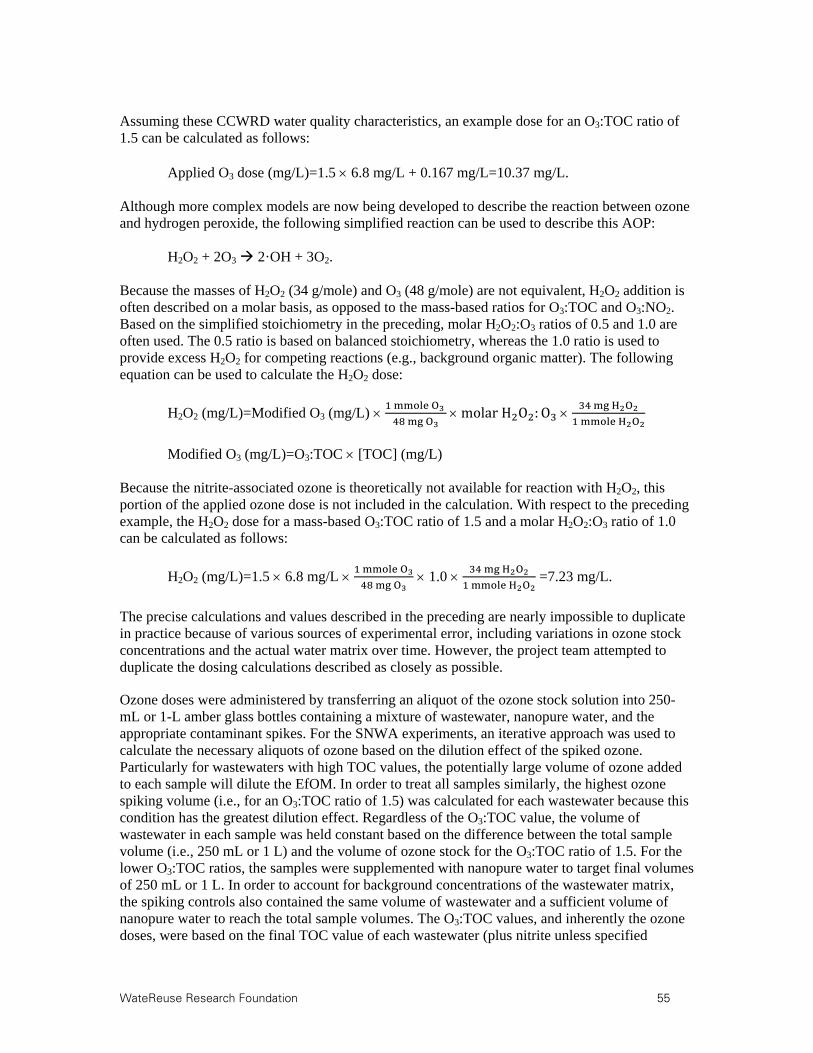
WateReuse Research Foundation 55
Assuming these CCWRD water quality characteristics, an example dose for an O3:TOC ratio of 1.5 can be calculated as follows:
Applied O3 dose (mg/L)=1.5 6.8 mg/L + 0.167 mg/L=10.37 mg/L. Although more complex models are now being developed to describe the reaction between ozone and hydrogen peroxide, the following simplified reaction can be used to describe this AOP: H2O2 + 2O3 2·OH + 3O2. Because the masses of H2O2 (34 g/mole) and O3 (48 g/mole) are not equivalent, H2O2 addition is often described on a molar basis, as opposed to the mass-based ratios for O3:TOC and O3:NO2. Based on the simplified stoichiometry in the preceding, molar H2O2:O3 ratios of 0.5 and 1.0 are often used. The 0.5 ratio is based on balanced stoichiometry, whereas the 1.0 ratio is used to provide excess H2O2 for competing reactions (e.g., background organic matter). The following equation can be used to calculate the H2O2 dose:
H2O2 (mg/L)=Modified O3 (mg/L)
molarH O : O
Modified O3 (mg/L)=O3:TOC [TOC] (mg/L)
Because the nitrite-associated ozone is theoretically not available for reaction with H2O2, this portion of the applied ozone dose is not included in the calculation. With respect to the preceding example, the H2O2 dose for a mass-based O3:TOC ratio of 1.5 and a molar H2O2:O3 ratio of 1.0 can be calculated as follows:
H2O2 (mg/L)=1.5 6.8 mg/L
1.0
=7.23 mg/L.
The precise calculations and values described in the preceding are nearly impossible to duplicate in practice because of various sources of experimental error, including variations in ozone stock concentrations and the actual water matrix over time. However, the project team attempted to duplicate the dosing calculations described as closely as possible.
Ozone doses were administered by transferring an aliquot of the ozone stock solution into 250-mL or 1-L amber glass bottles containing a mixture of wastewater, nanopure water, and the appropriate contaminant spikes. For the SNWA experiments, an iterative approach was used to calculate the necessary aliquots of ozone based on the dilution effect of the spiked ozone. Particularly for wastewaters with high TOC values, the potentially large volume of ozone added to each sample will dilute the EfOM. In order to treat all samples similarly, the highest ozone spiking volume (i.e., for an O3:TOC ratio of 1.5) was calculated for each wastewater because this condition has the greatest dilution effect. Regardless of the O3:TOC value, the volume of wastewater in each sample was held constant based on the difference between the total sample volume (i.e., 250 mL or 1 L) and the volume of ozone stock for the O3:TOC ratio of 1.5. For the lower O3:TOC ratios, the samples were supplemented with nanopure water to target final volumes of 250 mL or 1 L. In order to account for background concentrations of the wastewater matrix, the spiking controls also contained the same volume of wastewater and a sufficient volume of nanopure water to reach the total sample volumes. The O3:TOC values, and inherently the ozone doses, were based on the final TOC value of each wastewater (plus nitrite unless specified

56 WateReuse Research Foundation
otherwise) after the dilution effect was accounted for. The volume for each wastewater is provided in its corresponding section of the report, but an example is provided in Table 0.2. Table 0.2. Experimental Volumes for the 1-L Filtered CCWRD Samples
O3:TOC/ H2O2:O3
Wastewater Volume
(mL)
Nanopure Volume
(mL)
O3 Volume (mL)
O3 Dose (mg/L)
H2O2 Volume
(μL)
H2O2 Dose (mg/L)
Spike 892 108 0 0 0 0 0.25/0 892 90 18 1.7 0 0 0.25/0.5 892 90 18 1.7 61 0.6 0.25/1.0 892 90 18 1.7 122 1.2 0.5/0 892 71 37 3.4 0 0 0.5/0.5 892 71 37 3.4 123 1.2 0.5/1.0 892 71 37 3.4 246 2.5 1.0/0 892 36 72 6.8 0 0 1.0/0.5 892 36 72 6.8 242 2.4 1.0/1.0 892 36 72 6.8 483 4.8 1.5/0 892 0 108 10.2 0 0 1.5/0.5 892 0 108 10.2 363 3.6 1.5/1.0 892 0 108 10.2 725 7.3
Notes: Some values are affected by rounding error and the precision of the ozone spike. Concentration of O3 stock solution=95 mg/L. Concentration of H2O2 stock solution=10 g/L. Before dilution: TOC=7.6 mg/L | NO2=0.057 mg/L as N=0.187 mg/L as NO2.. Dilution ratio=(892/1000)=0.892. After dilution: TOC=6.8 mg/L | NO2=0.051 mg/L as N=0.167 mg/L as NO2. For the Eawag ozone experiments, ozone doses were determined based on O3:DOC ratios of 0.25, 0.5, 1.0, and 1.5. Unlike the SNWA approach, the secondary effluent samples were not diluted with nanopure water prior to spiking ozone, so the dilution factors differed between the various dosing conditions. Nevertheless, the dilution factors were usually kept below 10% even at an O3:TOC ratio of 1.5 using a concentrated ozone stock solution (i.e., > 72 mg/L). The dilution factors at each ozone dose were still considered in evaluating the various water quality parameters and treatment efficacy. Regardless of the ozone dosing strategy, treatment efficacy, including TOrC elimination, was consistent between the SNWA and Eawag experiments. This confirms that the two ozone dosing strategies are valid and comparable.
2.1.3 Bench-Scale Ultraviolet Experiments
Based on the suggested protocols of Bolton and Linden (2003) and Kuo et al. (2003), bench-scale collimated beams containing one (Figure 2.2A) or two (Figure 2.2B) 46-cm, 15-W low-pressure mercury arc bulbs (Model G15T8, Ushio, Cypress, CA) were used for the UV irradiation experiments at SNWA. Two collimated beams were used because of the large number of samples and the long exposure times required for UV doses characteristic of advanced oxidation (i.e., >250 mJ/cm2). The bulbs produced nearly monochromatic germicidal light at a peak wavelength of 254 nm. The collimated beam apparatuses also included adjustable platforms and slow-speed stir plates to ensure proper mixing during the irradiation periods. Following a 5-min warm-up period for the UV lamp, the intensity of the UV light was measured using an IL1700 research radiometer with Sensor SUD240 (International Light, Newburyport, MA). A calibration traceable to NIST standards was performed on each component by the manufacturer prior to the experiments. Prior to the irradiation experiments, the platform was adjusted to ensure that the surface of the radiometer detector and the wastewater sample were at the same level during the calibration and irradiation phases, respectively. The incident UV intensity for the collimated

WateReuse Research Foundation 57
beam in Figure 2.2A was approximately 0.23 mW/cm2, and the incident UV intensity for the collimated beam in Figure 2.2B was approximately 0.58 mW/cm2.
The UV experiments at Eawag were conducted in a DEMA 125 merry-go-round photoreactor (Hans Mangels, Bornheim-Roisdorf, Germany) equipped with a low-pressure mercury lamp (Model TNN 15/32, Heraeus Noblelight, Hanau, Germany), which emits nearly monochromatic light at 254 nm. The lamp was contained in a quartz cooling jacket, and the photoreactor was filled with deionized water kept at a constant temperature of 25 C. Sample solutions, typically 20 mL, were contained in quartz tubes with an internal diameter of 14 mm and an external diameter of 17 mm. Fluence and fluence rate values were determined by chemical actinometry at low optical density using 5 M of aqueous atrazine as an actinometer, which has a quantum yield of 0.046 and a molar absorption coefficient of 3860 M-1cm-1 at a wavelength of 254 nm . The average UV intensity for the merry-go-round photoreactor was approximately 1.4 mW/cm2.
UV doses were calculated as the product of the incident UV intensity (I0), a series of collimated beam correction factors, and the exposure times. The corrections accounted for the reflection factor (RF), Petri factor (PF), water factor (WF), and divergence factor (DF) associated with each collimated beam (Bolton and Linden, 2003; Kuo et al., 2003), which are described in Figure 2.2. The water factor is described as a range because it depends on the UV254 absorbance of the sample matrix and is therefore sample-dependent. The UV and UV/H2O2 experiments were repeated in 100-mL aliquots until a sufficient sample volume had been collected for the various analytical methods. In order to capture disinfection- and contaminant-specific effects related to UV photolysis and oxidation, a wide range of UV doses were evaluated. For the Clark County Water Reclamation District (CCWRD) experiments, UV doses of 23, 45, 225, and 680 mJ/cm2 were used. After further evaluation of full-scale AOP conditions, UV doses of 50, 250, and 500 mJ/cm2 were used for the remaining four sets of experiments. An H2O2 concentration of 10 mg/L was selected for the CCWRD UV AOP experiments, and H2O2 concentrations of 5 and 10 mg/L were selected for the other four sets of experiments.
Figure 0.2. Collimated beam apparatus for bench-scale UV experiments at SNWA.
2.1.4 Quenching and Preservation
Hydrogen peroxide controls (i.e., 10 mg/L of H2O2 with no ozone or UV exposure) were also collected for each experiment. The duration of H2O2 exposure, which generally ranged from 30 min to 1 h, was selected to mimic the longest potential exposure time during each set of experiments. This always corresponded to UV irradiation with 500 or 750 mJ/cm2. At the end of the exposure time, the H2O2 controls were quenched with 10 mg/L of sodium thiosulfate. For the ozone and ozone/H2O2 samples, H2O2 residuals were quenched with 10 mg/L of sodium thiosulfate after at least 30 min of reaction time, which was sufficient for complete ozone decay

58 WateReuse Research Foundation
in all samples. For the UV/H2O2 experiments, samples were quenched with 10 mg/L of sodium thiosulfate at the end of each UV exposure. Finally, TOrC and NDMA samples were preserved with 1 g/L of sodium azide to prevent biodegradation prior to analysis.
Because thiosulfate reacts with chloramine, NDMA formation potential (FP) samples were quenched with 0.05 mg/L of bovine catalase at 30 min of reaction time prior to chloramination (Liu et al., 2003). After the 10-day NDMA FP test, which will be described later in the report, residual chloramine was quenched with 50 mg/L of sodium thiosulfate. The finished NDMA FP samples were then preserved with 1 g/L of sodium azide to prevent biodegradation prior to analysis.
2.2 Target Compounds
Analytical methods for TOrCs are now approaching parts-per-quadrillion detection limits with high degrees of accuracy and precision. Coupled with state-of-the-art equipment, these methods have allowed researchers to detect and quantify a seemingly infinite number of TOrCs in countless matrices (e.g., air, soil, water, wastewater, food). These contaminants include PPCPs, pesticides, household chemicals, industrial chemicals, flame retardants, disinfection byproducts, and steroid hormones (Trenholm et al., 2009). Many of these contaminants are also suspected EDCs.
To focus the scope of the research, a representative subset of the TOrC universe was selected for evaluation. The indicator compounds were selected based on several factors, including structural and chemical properties (e.g., functional groups, polarity, aromaticity, etc.), use classes (e.g., antibiotic, fragrance, anticonvulsant, etc.), high frequency of environmental occurrence ( Benotti et al., 2009; Kolpin et al., 2002; Snyder et al., 2008a), resistance to natural (e.g., biodegradation, photolysis, etc.) and engineered treatment processes (e.g., adsorption, oxidation, etc.) ( Huber et al., 2003a; Ternes et al., 2002; Westerhoff et al., 2005), and amenability to existing analytical methods (Trenholm et al., 2009). The compounds selected for this study and their corresponding structures and guideline concentrations are listed in Table 2.3. Although these compounds have generated considerable interest in the research, treatment, and regulatory arenas, only atrazine is currently regulated by the U.S. EPA at an MCL of 3 µg/L.

WateReuse Research Foundation 59
Table 0.3. Target Compound List
Contaminant Use Class Structure DWEL (μg/L)a
AG (µg/L)b
Meprobamate Anti-anxiety 260 N/A
Sulfamethoxazole Antibiotic 18,000 35
Trimethoprim Antibiotic 81,000 70
Carbamazepine Anticonvulsant 35,000 100
Phenytoin Anticonvulsant 150,000 N/A
Primidone Anticonvulsant N/A N/A
aDWEL=Drinking Water Equivalent Level (Snyder et al., 2008a). bAG=Australian Guidelines (EPHC, 2008). cEPA MCL for Atrazine.

60 WateReuse Research Foundation
Table 2.3—Continued
Contaminant Use Class Structure DWEL (μg/L)a
AG (µg/L)b
Triclosan Anti-microbial N/A 0.35
Atenolol Beta blocker
13,000 N/A
TCEP Tris-(2-
chloroethyl)-phosphate
Flame Retardant N/A 1
Musk ketone Fragrance N/A 350
Atrazine Herbicide 3c 40

WateReuse Research Foundation 61
Table 2.3—Continued
Contaminant Use Class Structure DWEL (μg/L)a
AG (µg/L)b
Gemfibrozil Lipid regulator 600,000 600
Diclofenac NSAID
49,000 1.8
Ibuprofen NSAID N/A 400
Naproxen NSAID 140,000 220
DEET Pesticide N/A 2.5
Bisphenol A Plasticizer 1,800 200
As shown in Table 0.4, the target compounds were also classified based on their relative resistance to oxidation, which will become important in future discussions of the ozone oxidation data. The Group 1 compounds are characterized by relatively high ozone (>105 M-1s-1) and ·OH (>5 109 M-1s-1) rate constants due to their electron-rich moieties, including phenols (triclosan and bisphenol A), anilines (diclofenac and sulfamethoxazole), olefins (carbamazepine), and activated aromatics (trimethoprim and naproxen). The Group 2 compounds are characterized by moderately high ozone (10 < kozone < 105 M-1s-1) and high ·OH rate constants (> 5 109 M-1s-1), the Group 3 compounds are characterized by low ozone (<10 M-1s-1) but high ·OH rate constants (>5 109 M-1s-1), the Group 4 compounds are characterized by low ozone (< 10 M-1s-1) and moderately low ·OH (109 < kOH < 5 109 M-1s-1) rate constants, and the Group 5 compounds are very resistant to both ozone (< 1 M-1s-1) and ·OH (< 109 M-1s-1).
CH3
CH3
OHHO
CH3
CH3
OHHO

62 WateReuse Research Foundation
Table 0.4. Treatability of Target Compounds Compound Ozonea ·OHb Photolysisc Biodeg. Sorption Group 1 Sulfamethoxazole 3 106 6 109 7.2 10-4 Diclofenac 1 106 8 109 1.8 10-3 Bisphenol A 7 105 1 1010 <5.0x10⁻⁵ Carbamazepine 3 105 9 109 <5.0x10⁻⁵ Trimethoprim 3 105 7 109 <5.0x10⁻⁵ Naproxen 2 105 1 1010 1.4 10-4 Triclosan 4 107 1 1010 9.2 10-4 Group 2 Gemfibrozil 2 104 1 1010 <5.0 10-5 Atenolol 2 103 8 109 <5.0 10-5 Group 3 Ibuprofen 10 7 109 <5.0 10-5 Phenytoin <10 6 109 3.5 10-4 DEET <10 5 109 <5.0 10-5 Primidone <10 7 109 <5.0 10-5 Group 4 Atrazine 6 3 109 2.1 10-4 Meprobamate <1 4 109 <5.0 10-5 Group 5 Musk ketone <1 1 109 1.6 10-4 TCEP <1 7 108 <5.0 10-5
Notes: High treatability (e.g., >80% removal) Low treatability (e.g., <20% removal).
Sources: Acero et al. (2000b); Huber et al. (2003a); Deborde et al. (2005b); Huber et al. (2005b); Dodd et al. (2006b); Benner et al. (2008); Deborde and von Gunten (2008); Razavi et al. (2009a); Song et al. (2009a); Pocostales et al. (2010). aValues in this column correspond to kO3 (M
-1 s-1) at pH 7. bValues in this column correspond to kOH (M
-1 s-1). cValues in this column correspond to kUV ((mJ/cm2)-1).
The target compounds were analyzed by online SPE followed by liquid chromatography tandem mass spectrometry (LC-MS/MS) with isotope dilution (Gerrity et al., 2010; Trenholm et al., 2009). This method was selected because of its reduced sample volumes, solvent volumes, and total analysis time per sample (≈20 min) compared to traditional offline SPE-LC-MS/MS methods. Therefore, this method was able to shorten sample turnaround times and increase experimental throughput. Online SPE-LC-MS/MS was accomplished with a Symbiosis Pharma (Spark Holland, Emmen, the Netherlands) system in XLC mode using Analyst 1.4.2 (Applied Biosystems, Foster City, CA). Samples were collected in 40-mL amber glass vials with quenching agents and preservatives as described previously. If analysis was not performed immediately following each experiment, samples were refrigerated at 4°C and extracted within 14 days of collection.
Prior to analysis, 10 mL of sample was measured in a volumetric flask and spiked with isotopically labeled standards at 100 ng/L. This provided sufficient sample volume for replicates, matrix spikes, and dilutions, if necessary. A 1.5-mL aliquot of each sample was transferred into a 2-mL autosampler vial, although only 1.0 mL was used for extractions. Extractions were performed using Waters Oasis HLB Prospekt cartridges (30 mm, 2.5 mg, 10 1 mm, 96 tray)
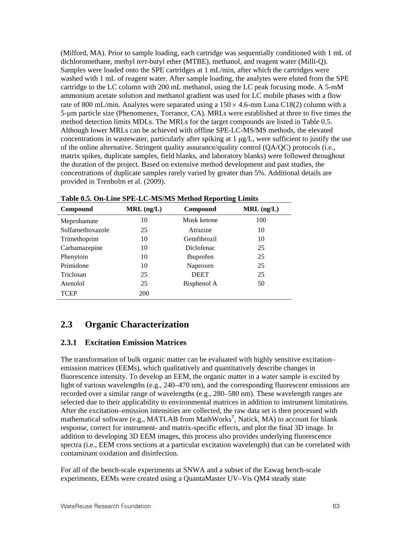
WateReuse Research Foundation 63
(Milford, MA). Prior to sample loading, each cartridge was sequentially conditioned with 1 mL of dichloromethane, methyl tert-butyl ether (MTBE), methanol, and reagent water (Milli-Q). Samples were loaded onto the SPE cartridges at 1 mL/min, after which the cartridges were washed with 1 mL of reagent water. After sample loading, the analytes were eluted from the SPE cartridge to the LC column with 200 mL methanol, using the LC peak focusing mode. A 5-mM ammonium acetate solution and methanol gradient was used for LC mobile phases with a flow rate of 800 mL/min. Analytes were separated using a 150 4.6-mm Luna C18(2) column with a 5-µm particle size (Phenomenex, Torrance, CA). MRLs were established at three to five times the method detection limits MDLs. The MRLs for the target compounds are listed in Table 0.5. Although lower MRLs can be achieved with offline SPE-LC-MS/MS methods, the elevated concentrations in wastewater, particularly after spiking at 1 μg/L, were sufficient to justify the use of the online alternative. Stringent quality assurance/quality control (QA/QC) protocols (i.e., matrix spikes, duplicate samples, field blanks, and laboratory blanks) were followed throughout the duration of the project. Based on extensive method development and past studies, the concentrations of duplicate samples rarely varied by greater than 5%. Additional details are provided in Trenholm et al. (2009). Table 0.5. On-Line SPE-LC-MS/MS Method Reporting Limits
Compound MRL (ng/L) Compound MRL (ng/L)
Meprobamate 10 Musk ketone 100
Sulfamethoxazole 25 Atrazine 10 Trimethoprim 10 Gemfibrozil 10 Carbamazepine 10 Diclofenac 25 Phenytoin 10 Ibuprofen 25 Primidone 10 Naproxen 25 Triclosan 25 DEET 25 Atenolol 25 Bisphenol A 50
TCEP 200
2.3 Organic Characterization
2.3.1 Excitation Emission Matrices
The transformation of bulk organic matter can be evaluated with highly sensitive excitation–emission matrices (EEMs), which qualitatively and quantitatively describe changes in fluorescence intensity. To develop an EEM, the organic matter in a water sample is excited by light of various wavelengths (e.g., 240–470 nm), and the corresponding fluorescent emissions are recorded over a similar range of wavelengths (e.g., 280–580 nm). These wavelength ranges are selected due to their applicability to environmental matrices in addition to instrument limitations. After the excitation–emission intensities are collected, the raw data set is then processed with mathematical software (e.g., MATLAB from MathWorksT, Natick, MA) to account for blank response, correct for instrument- and matrix-specific effects, and plot the final 3D image. In addition to developing 3D EEM images, this process also provides underlying fluorescence spectra (i.e., EEM cross sections at a particular excitation wavelength) that can be correlated with contaminant oxidation and disinfection.
For all of the bench-scale experiments at SNWA and a subset of the Eawag bench-scale experiments, EEMs were created using a QuantaMaster UV–Vis QM4 steady state

64 WateReuse Research Foundation
spectrofluorometer (Photon Technology International, Inc., Birmingham, NJ). The spectrofluorometer included a 75-W short-arc xenon lamp with an effective excitation range of 240–470 nm. Data processing included corrections for the spectral sensitivity of the lamp, and an inner filter correction was also applied, using equations from the literature (MacDonald et al., 1997) and the UV absorbance spectra of the sample matrices. For the inner filter correction, the light was assumed to illuminate a small volume at the center of the cell, and the excitation and emission path lengths were assumed to be 0.5 cm (Westerhoff et al., 2001). The width of the excitation beam was assumed to be 0.1 cm, and the width of the emission was assumed to be 1 cm. These assumptions are incorporated into the modification to Beer’s Law, as described in the literature (MacDonald et al., 1997).
Figure 2.3 is an EEM characteristic of secondary wastewater effluent, because it includes intense fluorescence in all three regions, particularly in the regions associated with soluble microbial products and fulvic acids. As shown in Figure 2.3, EEMs include an upper boundary resulting from “bleeding” when the excitation and emission wavelengths are approximately equal to each other. Molecules cannot emit light at energy levels greater than the excitation source, so emissions at wavelengths less than the excitation wavelength are ignored. Therefore, the region above the upper boundary is always blank. As shown in Figure 2.3, EEMs sometimes include a lower boundary characteristic of second-order light scattering, which occurs at emission wavelengths that are approximately twice the excitation wavelength. In contrast to the upper boundary, fluorescence data can be collected below the second-order scattering boundary. Figure 2.3 also provides delineations for the organic regions first described in Chen et al. (2003). The regions were modified by the project team to account for the limitations (e.g., effective excitation range) of the spectrofluorometer used in this study. The regions also account for 15-nm safety factors near the “bleeding” and second-order scatter boundaries. Fluorescence in each region indicates the presence of specific organic fractions, as follows: (I) aromatic proteins and soluble microbial products, (II) fulvic-like substances, and (III) humic-like substances.
Figure 0.3. Excitation emission matrix for secondary effluent.
EEMs can be analyzed qualitatively by observing changes in fluorescence intensity (i.e., color), but there are also quantitative alternatives such as the fluorescence index (FI) (McKnight et al., 2001). The FI is the ratio of the fluorescence emission at 450 nm to that at 500 nm when excited by a wavelength of 370 nm (i.e., Ex370Em450/Ex370Em500). The FI has been used to differentiate terrestrially derived organic matter (e.g., surface water from a forested watershed) with lower FIs from microbially derived organic matter (e.g., wastewater) with higher FIs (McKnight et al.,
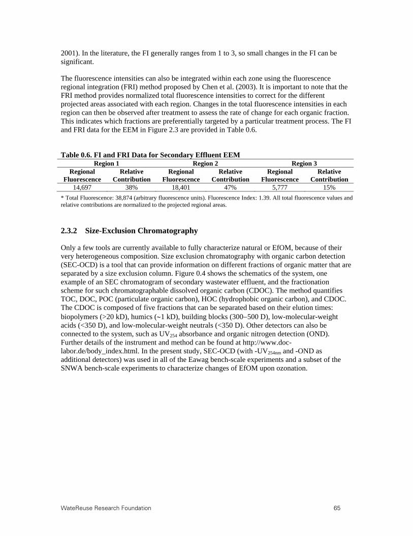
WateReuse Research Foundation 65
2001). In the literature, the FI generally ranges from 1 to 3, so small changes in the FI can be significant.
The fluorescence intensities can also be integrated within each zone using the fluorescence regional integration (FRI) method proposed by Chen et al. (2003). It is important to note that the FRI method provides normalized total fluorescence intensities to correct for the different projected areas associated with each region. Changes in the total fluorescence intensities in each region can then be observed after treatment to assess the rate of change for each organic fraction. This indicates which fractions are preferentially targeted by a particular treatment process. The FI and FRI data for the EEM in Figure 2.3 are provided in Table 0.6.
Table 0.6. FI and FRI Data for Secondary Effluent EEM Region 1 Region 2 Region 3
Regional Fluorescence
Relative Contribution
Regional Fluorescence
Relative Contribution
Regional Fluorescence
Relative Contribution
14,697 38% 18,401 47% 5,777 15%
* Total Fluorescence: 38,874 (arbitrary fluorescence units). Fluorescence Index: 1.39. All total fluorescence values and relative contributions are normalized to the projected regional areas.
2.3.2 Size-Exclusion Chromatography
Only a few tools are currently available to fully characterize natural or EfOM, because of their very heterogeneous composition. Size exclusion chromatography with organic carbon detection (SEC-OCD) is a tool that can provide information on different fractions of organic matter that are separated by a size exclusion column. Figure 0.4 shows the schematics of the system, one example of an SEC chromatogram of secondary wastewater effluent, and the fractionation scheme for such chromatographable dissolved organic carbon (CDOC). The method quantifies TOC, DOC, POC (particulate organic carbon), HOC (hydrophobic organic carbon), and CDOC. The CDOC is composed of five fractions that can be separated based on their elution times: biopolymers (>20 kD), humics (1 kD), building blocks (300500 D), low-molecular-weight acids (<350 D), and low-molecular-weight neutrals (<350 D). Other detectors can also be connected to the system, such as UV254 absorbance and organic nitrogen detection (OND). Further details of the instrument and method can be found at http://www.doc-labor.de/body_index.html. In the present study, SEC-OCD (with -UV254nm and -OND as additional detectors) was used in all of the Eawag bench-scale experiments and a subset of the SNWA bench-scale experiments to characterize changes of EfOM upon ozonation.

66 WateReuse Research Foundation
Figure 0.4. Organic characterization with SEC-OCD.
2.3.3 Assimilable Organic Carbon
During ozonation, organic matter is transformed into compounds with low molecular weight and high oxygen content, some of which support microbiological growth. These oxidation byproducts are commonly summarized as AOC. Biological filtration steps (e.g., slow sand or activated carbon filtration) often follow ozonation to remove AOC. For the Eawag bench-scale experiments, AOC formation during ozonation of wastewater effluent was investigated using three different methods (Figure 2.5) (Hammes et al., 2008, 2010). Ozonated wastewater samples were passed through 0.1-μm filters, and these cell-free samples were inoculated with a microbial community from a wastewater effluent. The samples were incubated at 30C until a stationary phase was reached approximately 72 h later. The cell concentration in the stationary phase was measured by flow cytometry and translated into AOC concentration with a conversion factor and a median size of cells (Method 1, Figure 2.5). Dissolved organic carbon concentration was measured before and after the AOC test to estimate the BDOC (Method 2, Figure 2.5). Finally, the cell growth was also quantified by ATP measurements (Method 3, Figure 2.5).

WateReuse Research Foundation 67
Figure 0.5. AOC determination.
2.4 Target Microbes and Methods of Assessing Disinfection
Because of differences in laboratory capabilities, different disinfection analyses were performed at Eawag and SNWA, although a subset of the secondary effluents were evaluated with both methods. For the Eawag bench-scale experiments, two different methods were used to assess cell integrity: (1) flow cytometry for total cell concentration and (2) adenosine triphosphate (ATP) quantification. Both of these methods are cultivation-independent, so they may actually underestimate the level of inactivation achieved during disinfection. Although the microbial cells may appear intact, which would result in positive detection in the flow cytometer and cell-bound ATP, they may no longer be viable.
For the SNWA bench-scale experiments, disinfection was evaluated using cultivation-dependent analyses for indicator coliform bacteria, f-specific coliphages as a surrogate for human viruses (e.g., poliovirus, coxsackievirus, echovirus), and spore-forming bacteria as a surrogate for protozoan parasites (e.g., Cryptosporidium oocysts and Giardia cysts). Spiking experiments were performed with Escherichia coli 15597, MS2 bacteriophage, and Bacillus subtilis spores to represent the three groups described. In the bench-scale experiments, the wastewaters were spiked with sufficient target microbes to quantify a range of inactivation. A subset of the pilot-scale experiments were performed with spiked microbes, particularly to address the 5-log viral inactivation requirement in Title 22. When possible, pilot-scale experiments were also performed with indigenous microbes to address other reuse guidelines and requirements, particularly the total coliform requirement of <2.2 MPN/100 mL in Title 22. The following sections describe the microbial assays and protocols used to prepare the spiking stocks for the bench- and pilot-scale experiments.

68 WateReuse Research Foundation
2.4.1 Coliform Bacteria
Because of the current focus on total and fecal coliforms for water reuse requirements, E. coli 15597 (ATCC 15597) was used in the spiking studies, and total and fecal coliforms were monitored in certain pilot-scale experiments. E. coli is a gram-negative, rod-shaped bacterium that is often used as an indicator of fecal contamination in water supplies. Total coliforms, fecal coliforms, and spiked E. coli were assayed with the 24-h Colilert method (Idexx, Westbrook, ME) using the Quanti-Tray 2000 quantification protocol. The Colilert method is a U.S. EPA-approved method for total and fecal coliform quantification in wastewater. Coliform bacteria can be assayed with 100 mL of sample as described in Figure 2.6, and total and fecal coliforms can be differentiated based on fluorescence after 24 h of incubation at 35 °C.
Figure 0.6. Colilert method for total and fecal coliforms.
E. coli 15597 spiking stocks were propagated in log phase in tryptic soy broth (TSB). The concentrated stocks were then centrifuged, washed, and resuspended in buffered demand-free (BDF) water (Thurston-Enriquez et al., 2003). The final stocks generally contained ≈1010 CFU/100 mL.
2.4.2 MS2 Bacteriophage
MS2 is a single-stranded RNA bacteriophage (virus that infects bacteria) that is approximately 27 nm in diameter. MS2 is often used as a surrogate for human enteroviruses, such as poliovirus, coxsackievirus, and echovirus. MS2 (ATCC 15597-B1) was prepared and assayed with the double agar layer method (Adams, 1959) using antibiotic-resistant E. coli 700891 (ATCC 700891) as the bacterial host. All MS2 culture media (i.e., TSB, 0.7% tryptic soy agar (TSA) for the soft overlay, and 1.5% TSA as the solid substrate) were spiked with ampicillin and streptomycin at final concentrations of 15 mg/L to prevent growth of indigenous bacteria. Because E. coli 700891 can grow in media supplemented with antibiotics, this host is commonly used for MS2 assays in environmental samples. Plaques were counted after 18 h of incubation at 35 °C. Figure 2.7 illustrates the double agar layer method for MS2.
MS2 stocks were purified with polyethylene glycol (PEG) precipitation and Vertrel extraction before being resuspended in BDF water (Thurston-Enriquez et al., 2003). This purification process was used to monodisperse the bacteriophages and remove a significant portion of the organic matter associated with the culture media, thereby reducing potential scavenging effects during the oxidation experiments (Mesquita et al., 2010). The final stocks generally contained ≈1011 PFU/mL.
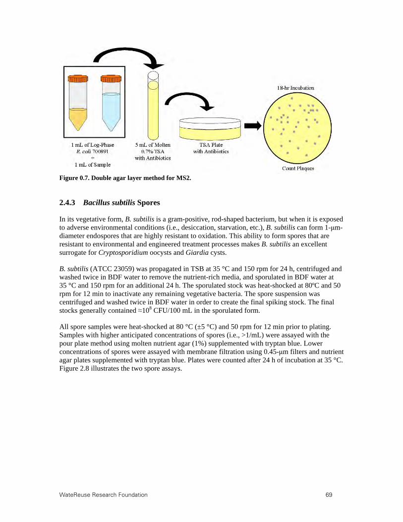
WateReuse Research Foundation 69
Figure 0.7. Double agar layer method for MS2.
2.4.3 Bacillus subtilis Spores
In its vegetative form, B. subtilis is a gram-positive, rod-shaped bacterium, but when it is exposed to adverse environmental conditions (i.e., desiccation, starvation, etc.), B. subtilis can form 1-μm-diameter endospores that are highly resistant to oxidation. This ability to form spores that are resistant to environmental and engineered treatment processes makes B. subtilis an excellent surrogate for Cryptosporidium oocysts and Giardia cysts.
B. subtilis (ATCC 23059) was propagated in TSB at 35 °C and 150 rpm for 24 h, centrifuged and washed twice in BDF water to remove the nutrient-rich media, and sporulated in BDF water at 35 °C and 150 rpm for an additional 24 h. The sporulated stock was heat-shocked at 80ºC and 50 rpm for 12 min to inactivate any remaining vegetative bacteria. The spore suspension was centrifuged and washed twice in BDF water in order to create the final spiking stock. The final stocks generally contained ≈108 CFU/100 mL in the sporulated form.
All spore samples were heat-shocked at 80 °C (±5 °C) and 50 rpm for 12 min prior to plating. Samples with higher anticipated concentrations of spores (i.e., >1/mL) were assayed with the pour plate method using molten nutrient agar (1%) supplemented with tryptan blue. Lower concentrations of spores were assayed with membrane filtration using 0.45-μm filters and nutrient agar plates supplemented with tryptan blue. Plates were counted after 24 h of incubation at 35 °C. Figure 2.8 illustrates the two spore assays.

70 WateReuse Research Foundation
Figure 0.8. Pour plate and membrane filtration methods for Bacillus spores.
2.4.4 Eawag Disinfection Experiments
For the Eawag bench-scale experiments, disinfection efficacy was evaluated by two different methods: (1) total cell concentration by flow cytometry (FCM) and (2) quantification of cell-bound ATP. Because both of these methods are cultivation-independent, they may underestimate the level of inactivation achieved during disinfection. Although the microbial cells may appear intact, which would result in positive detection in the flow cytometer and cell-bound ATP, they may no longer be viable.
2.5 Characterization of ·OH Exposure
Two different approaches were used to characterize ·OH exposure and yield during wastewater ozonation: (1) a pCBA assay and (2) a t-BuOH assay.
2.5.1 pCBA
Because of its selectivity in reacting with ·OH, the chemical para-chlorobenzoic acid (pCBA) is often used to determine the ·OH exposure during AOPs. The rate of pCBA degradation during ·OH exposure can be modeled according to the following second-order reaction, where k·OH,pCBA has been previously determined to be 5 109 M-1s-1:
.
After the rate equation is rearranged and solved, the following equation can be used to determine the overall ·OH exposure during AOPs:
pCBAOHkdt
pCBAd
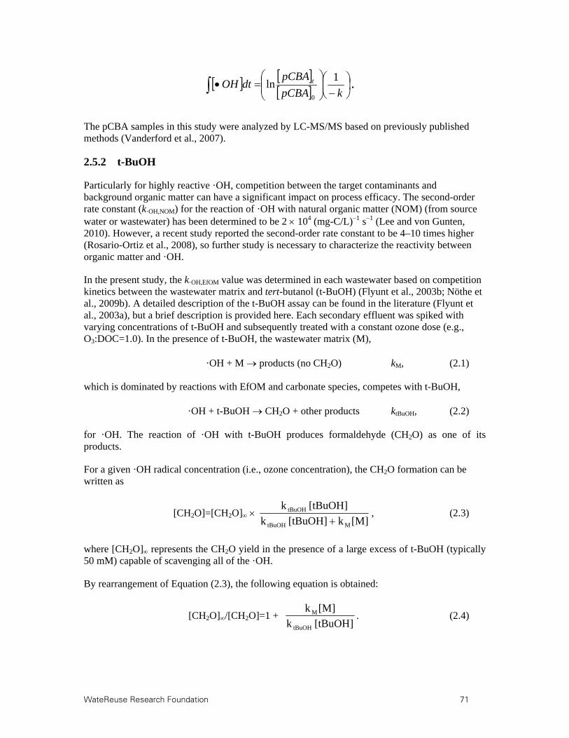
WateReuse Research Foundation 71
.
The pCBA samples in this study were analyzed by LC-MS/MS based on previously published methods (Vanderford et al., 2007).
2.5.2 t-BuOH
Particularly for highly reactive ·OH, competition between the target contaminants and background organic matter can have a significant impact on process efficacy. The second-order rate constant (k·OH,NOM) for the reaction of ·OH with natural organic matter (NOM) (from source water or wastewater) has been determined to be 2 104 (mg-C/L)1 s1 (Lee and von Gunten, 2010). However, a recent study reported the second-order rate constant to be 4–10 times higher (Rosario-Ortiz et al., 2008), so further study is necessary to characterize the reactivity between organic matter and ·OH.
In the present study, the k·OH,EfOM value was determined in each wastewater based on competition kinetics between the wastewater matrix and tert-butanol (t-BuOH) (Flyunt et al., 2003b; Nöthe et al., 2009b). A detailed description of the t-BuOH assay can be found in the literature (Flyunt et al., 2003a), but a brief description is provided here. Each secondary effluent was spiked with varying concentrations of t-BuOH and subsequently treated with a constant ozone dose (e.g., O3:DOC=1.0). In the presence of t-BuOH, the wastewater matrix (M),
·OH + M products (no CH2O) kM, (2.1) which is dominated by reactions with EfOM and carbonate species, competes with t-BuOH, ·OH + t-BuOH CH2O + other products ktBuOH, (2.2) for ·OH. The reaction of ·OH with t-BuOH produces formaldehyde (CH2O) as one of its products.
For a given ·OH radical concentration (i.e., ozone concentration), the CH2O formation can be written as
[CH2O]=[CH2O] , (2.3)
where [CH2O] represents the CH2O yield in the presence of a large excess of t-BuOH (typically 50 mM) capable of scavenging all of the ·OH.
By rearrangement of Equation (2.3), the following equation is obtained:
[CH2O]/[CH2O]=1 + . (2.4)
kpCBA
pCBAdtOH t 1
ln0
[M]k [tBuOH]k
[tBuOH]k
MtBuOH
tBuOH
[tBuOH]k
[M]k
tBuOH
M

72 WateReuse Research Foundation
Based on the slope of [CH2O]/[CH2O] versus [t-BuOH] and the known value of ktBuOH (6 108 M1 s1), the ·OH scavenging rate attributable to the wastewater matrix (i.e., kM[M]) can be determined.
2.6 Bioassays
2.6.1 Yeast Estrogen Screen Assay for Total Estrogenicity
A YES assay (Routledge and Sumpter, 1996) was used to analyze a subset of the samples for total estrogenic activity. A human-estrogen-receptor-transfected yeast strain was supplied by Duke University with the permission of John Sumpter of Brunel University (Middlesex, UK). Assay procedures followed those originally published (Routledge and Sumpter, 1996) with several modifications. Yeast colonies were propagated on sterile plates filled with a Difco Sabouraud dextrose agar (Becton, Dickinson, and Company, Sparks, MD) at 60 mg/L + 3 mL of 2.5 mg/mL chloramphenicol (Alfa Aesar, Ward Hill, MA). A new plate was streaked every 30 to 60 days using a single colony from the previous plate. Stock plates were incubated in the dark for 3 days at 30 ºC and then stored at 4 ºC. Growth and assay media were prepared as originally described but were inoculated with a single colony from the most recent streak plate. All incubation was carried out at 30 ºC in a dark, temperature-controlled incubator.
For sample analysis, microplates (96-well) were inoculated with aliquots of the sample, yeast, and chlorophenol red-β-D-galactopyranoside (CPRG, from EMD Bioscience, La Jolla, CA). The wells were allowed to develop for up to 5 days to reach adequate color development. Color development was measured using a PowerWave 340 Microplate Reader (BioTek, Winooski, VT) at 650 nm for turbidity correction and 570 nm for color change. The corrected absorbance was calculated as A570 – A650, and data were analyzed using the open source software “R” version 2.4.0 (R_Development_Core_Team, 2006) in conjunction with a dose–response curve (DRC) add-on package (Ritz and Streibig, 2005). This software was used to calculate the concentration of estradiol, or the relative concentration of the sample extract, needed to induce 50% of the maximum response, written as the EC50. After comparison with the standard curve, an estradiol equivalent (EEq) concentration was determined for each unknown sample.
A four-parameter logistic model was used to develop the standard and sample dose–response curves. This model allowed the analyst to define the lower limit, upper limit, slope, and EC50 values based on standard and experimental data. The four-parameter logistic model is described by the following:
,
where b=slope, c=lower limit, d=upper limit, and e=EC50. The EC50 values were never forced upon a given model, but lower limit, upper limit, and slope were adjusted to achieve best fit and match the trends observed by the estradiol standards. Best fit was determined by iteratively adjusting model parameters to minimize the standard error associated with deviation of data points from the model fit.
Model adjustments are particularly important for minimizing the errors associated with low-dose response, whereby the EC50 is underestimated due to failure of the sigmoidal dose–response curve to reach a maximum plateau. For example, Figure 2.9A illustrates an estradiol standard curve and
))}log()(log(exp{1)),,,(,(
exb
cdcedcbxf

WateReuse Research Foundation 73
a low-dose condition modeled with two different approaches: (1) using default settings and (2) using the maximum and minimum responses from the estradiol standards while manually shaping the curve to the low-dose sample data. The manual correction yields a more characteristic dose–response curve and, ultimately, a more accurate EEq concentration. The four-parameter logistic model is also able to account for early cell die-off, which is common in extracts that exert outright toxicity on the yeast or in aqueous samples with high biological activity. An example of an acute-toxicity condition is illustrated in Figure 2.9B. Again, manual adjustments to model parameters are necessary to eliminate the effects of toxicity and more accurately describe the dose–response curve.
Figure 0.9. YES model corrections for low-dose and acute-toxicity conditions.
2.6.2 Harvard Bioassays
Researchers from the Harvard School of Public Health analyzed a subset of the samples from WRRF-08-05 using a series of bioassays. The bioassay samples assessed three different endpoints: cytotoxicity, genotoxicity, and estrogenicity. The assays are described in greater detail in conjunction with the Tucson pilot discussion in Section 6.2.
2.7 NDMA and NDMA Formation Potential Testing
NDMA was measured with a modification to EPA Method 521, which included SPE, analysis by GC-MS/MS, and corrections based on isotope dilution. Samples were collected in 1-L amber glass bottles containing 1.0 g of sodium azide and 80 mg of sodium thiosulfate. NDMA quantitation was performed using a GC-MS/MS system and isotope dilution according to published methods (Holady et al., 2012). NDMA standards were purchased from Ultra Scientific (Kingstown, RI, USA) and isotopically labeled NDMA was purchased from Cambridge Isotope Laboratories (Andover, MA, USA).
For evaluating NDMA-formation potential, residual H2O2 was quenched with 0.05 mg/L bovine catalase for 30 min. Samples were then spiked with preformed monochloramine and stored for 10 days at room temperature based on previously published methods (Mitch and Sedlak, 2004). Blank samples of deionized water were always below the MRL for NDMA (2.5 ng/L) and did not yield any measurable NDMA during the 10-day formation potential test. A monochloramine
Concentration Factor
A5
70 -
A65
0
0
1
2
3
4
0 0.01 1 100
Concentration Factor
A5
70 -
A65
0
0
1
2
3
4
0 0.01 1 100
A B
A57
0-A
650
Concentration Factor Concentration Factor
A: Low-Dose Condition B: Acute-Toxicity Condition
Default
Manual
Manual
Default
Concentration Factor
A5
70 -
A65
0
0
1
2
3
4
0 0.01 1 100
Concentration Factor
A5
70 -
A65
0
0
1
2
3
4
0 0.01 1 100
A B
Concentration Factor
A5
70 -
A65
0
0
1
2
3
4
0 0.01 1 100
Concentration Factor
A5
70 -
A65
0
0
1
2
3
4
0 0.01 1 100
Concentration Factor
A5
70 -
A65
0
0
1
2
3
4
0 0.01 1 100
Concentration Factor
A5
70 -
A65
0
0
1
2
3
4
0 0.01 1 100
A BA B
A57
0-A
650
Concentration Factor Concentration Factor
A: Low-Dose Condition B: Acute-Toxicity Condition
Default
Manual
Manual
Default
74 WateReuse Research Foundation
stock solution was prepared by rapidly mixing sodium hypochlorite into ammonium chloride solution based on published methods (Kumar and Margerum, 1987). Sodium hypochlorite (10–14% free available chlorine by weight) was obtained from VWR (Radnor, PA) and standardized using iodometric titration prior to use. Ammonium chloride, 99%, was obtained from Sigma Aldrich (St. Louis, MO, USA).
2.8 1,4-Dioxane
1,4-Dioxane samples were shipped to Weck Laboratories, Inc. (Industry, CA) for analysis. Samples were prepared and analyzed using EPA Methods 3520C and 8270M, respectively.

WateReuse Research Foundation 75
Chapter 3
3.Bench-Scale Evaluation of U.S. Secondary Effluents
3.1 Clark County Water Reclamation District, Las Vegas, NV
Clark County Water Reclamation District (CCWRD, Las Vegas, NV) currently treats an average daily flow of approximately 100 million gallons per day (MGD) and discharges the tertiary-treated UV-disinfected effluent into Lake Mead. Because Lake Mead is the immediate drinking water source for the Las Vegas metropolitan area and an additional 30 million people downstream, CCWRD is a significant contributor to water reuse. Furthermore, past studies have observed increased feminization rates for fish populations in the effluent-dominated Las Vegas Bay, which is the discharge point into Lake Mead. To mitigate the potential environmental impacts of its discharged effluent, CCWRD is currently evaluating a number of treatment options to reduce the concentrations of trace organic contaminants. In addition to process optimization strategies (e.g., increasing SRTs in the activated sludge basins), CCWRD is also considering ultrafiltration and ozonation. The ultrafiltration system is intended as (1) a microbiological barrier, (2) a pretreatment system to reduce the total suspended solids of the secondary effluent and increase ozone disinfection efficacy, and (3) an additional barrier for total phosphorus reductions. The ozone system targets reductions in estrogenicity in addition to disinfection for any microbes that pass through the membrane, particularly viruses.
The influent CCWRD wastewater is primarily municipal, but some industrial contributions are present. The CCWRD effluent is discharged into Lake Mead after treatment with bar screens; grit removal; primary clarification with ferric chloride addition; conventional activated sludge (SRT ≈ 7 days) with full nitrification (NH3,eff < 0.1 mg-N/L), partial denitrification, and biological phosphorus removal; secondary clarification; dual-media filtration with alum addition; and UV disinfection. A separate train treats a portion of the secondary effluent with flocculation, sedimentation, dual-media filtration with alum addition, and chlorine or UV disinfection. This UV-disinfected effluent is also discharged into Lake Mead, and the chlorine-disinfected effluent is pumped into the reclaimed water distribution system for irrigation and power plant cooling. With biological and chemical phosphorus removal, CCWRD is able to target total phosphorus levels of <100 μg/L in the finished effluent. A simplified treatment schematic for CCWRD is provided in Figure 3.1, and additional water quality data are provided hereafter.
Unfiltered secondary effluent from CCWRD was collected in April 2010, and the initial water quality data in Table 3.1 were obtained. Using the initial TOC and nitrite data, the ozone dosing conditions in Table 3.2 were calculated.

76 WateReuse Research Foundation
Figure 3.1. Simplified treatment schematic for CCWRD.
Table 3.1. Initial Water Quality Data for CCWRD
Unfiltered Secondary Effluent
pH 6.9 TOC (mg/L) 7.1 UV254 absorbance cm-1 0.132 TSS (mg/L) <5 Turbidity (NTU) 1.19 Alkalinity (mg/L) 123 TN (mg-N/L) 16.1 TKN (mg-N/L)a 2.04 TON (mg-N/L)b 1.95 NH3 (mg-N/L) 0.09 NO3 (mg-N/L) 14.0 NO2 (mg-N/L) 0.06 Bromide (μg/L) 174 NDMA (ng/L) <2.5
Filtered Secondary Effluent
pH 6.9 TOC (mg/L) 7.6 UV254 absorbance (cm-1) 0.146 TSS (mg/L) <5 Turbidity (NTU) 0.55
Finished Effluent TOC (mg/L) 5.8 UV254 absorbance (cm-1) 0.128 NDMA (ng/L) <2.5
aTotal Kjeldahl nitrogen: Sum of total organic nitrogen and ammonia. bTotal organic nitrogen: Difference between total nitrogen and ammonia, nitrate, and nitrite.
1°
Flocculation
2°CAS
HOCl
UV
Dual-Media
PreliminaryDual-Media Lake
Mead
Central Plant
UV Lake Mead
Advanced Water Treatment Plant
UF
O3
Pilot Facility
3°
1°
FlocculationFlocculation
2°CAS
HOClHOCl
UV
Dual-MediaDual-Media
PreliminaryDual-MediaDual-Media Lake
Mead
Central Plant
UVUV Lake Mead
Advanced Water Treatment Plant
UF
O3
Pilot Facility
3°

WateReuse Research Foundation 77
Table 3.2. Ozone Dosing Conditions for 1-L CCWRD Secondary Effluent Samples
O3:TOC/ H2O2:O3
Wastewater Volume (mL)
Nanopure Volume
(mL)
O3 Volume (mL)
O3
Dose (mg/L)
H2O2 Volume
(μL)
H2O2 Dose (mg/L)
Unfiltered Spike 899 101 0 0 0 0 0.25/0 899 84 17 1.6 0 0 0.25/0.5 899 84 17 1.6 57 0.6 0.25/1.0 899 84 17 1.6 115 1.2 0.5/0 899 67 34 3.2 0 0 0.5/0.5 899 67 34 3.2 115 1.2 0.5/1.0 899 67 34 3.2 230 2.3 1.0/0 899 34 67 6.3 0 0 1.0/0.5 899 34 67 6.3 226 2.3 1.0/1.0 899 34 67 6.3 452 4.5 1.5/0 899 0 101 9.5 0 0 1.5/0.5 899 0 101 9.5 339 3.4 1.5/1.0 899 0 101 9.5 678 6.8
Filtered Spike 892 108 0 0 0 0 0.25/0 892 90 18 1.7 0 0 0.25/0.5 892 90 18 1.7 61 0.6 0.25/1.0 892 90 18 1.7 122 1.2 0.5/0 892 71 37 3.4 0 0 0.5/0.5 892 71 37 3.4 123 1.2 0.5/1.0 892 71 37 3.4 246 2.5 1.0/0 892 36 72 6.8 0 0 1.0/0.5 892 36 72 6.8 242 2.4 1.0/1.0 892 36 72 6.8 483 4.8 1.5/0 892 0 108 10.2 0 0 1.5/0.5 892 0 108 10.2 363 3.6 1.5/1.0 892 0 108 10.2 725 7.3
Notes. Some values are affected by rounding error and the precision of the ozone spike. Concentration of O3 stock solution=95 mg/L; concentration of H2O2 stock solution=10 g/L; unfiltered dilution ratio=(899/1000)=0.899; unfiltered TOC after dilution: 6.4 mg/L; unfiltered NO2 after dilution=0.051 mg-N/L=0.168 mg/L as NO2; filtered dilution ratio=(892/1000)=0.892; filtered TOC after dilution: 6.8 mg/L; filtered NO2 after dilution=0.051 mg-N/L.
3.1.1 Ozone Demand/Decay
Figure 3.2 illustrates the ozone demand/decay curves for filtered and unfiltered CCWRD secondary effluent under various dosing conditions. The graph only includes dosing conditions with a measurable ozone residual after 30 s; corresponding CT values are also provided. For the O3/H2O2 samples, the addition of H2O2 caused a nearly instantaneous reaction with the dissolved ozone, which led to the formation of ·OH but eliminated the dissolved ozone residual. Because of reactions with EfOM, the 0.25 O3:TOC ratio was insufficient to establish a measurable ozone residual after 30 s. For the remaining dosing conditions, the graph illustrates the instantaneous ozone demand (i.e., the precipitous drop between 0 and 30 s) and the decay over time. The graph also indicates that there was no significant difference between filtered and unfiltered secondary effluent with respect to ozone demand and decay. This is consistent with the literature and indicates that the organic leaching from the cartridge filters did not impact the oxidation experiments for the CCWRD experiments.

78 WateReuse Research Foundation
Figure 3.2. Ozone demand/decay curves for the CCWRD secondary effluent.
3.1.2 Bromate Formation
One of the major factors limiting the use of ozone in water and wastewater treatment is bromate formation. Although some studies indicate that more relaxed bromate guidelines should be applied to wastewater treatment, the U.S. EPA MCL of 10 μg/L in drinking water is often used as a point of reference. As illustrated in Figure 3.3, significant bromate formation occurred during ozonation of CCWRD secondary effluent. The bromide values listed in each figure differ from the value in the previous table because of the dilution effect of the ozone stock. There was a noticeable difference in bromate formation for the unfiltered and filtered experiments, but it is unclear why cartridge filtration would affect bromate formation. The difference between the two data sets may be attributable to inherent variability during ozonation. Although the addition of H2O2 provided some degree of bromate mitigation, the O3:TOC ratios of 1.0 and 1.5 both exceeded 10 μg/L in all samples—even exceeding 90 μg/L in the absence of H2O2. To satisfy the 10 μg/L benchmark, O3:TOC ratios of 0.25 and 0.5 would be necessary unless further mitigation measures were implemented.
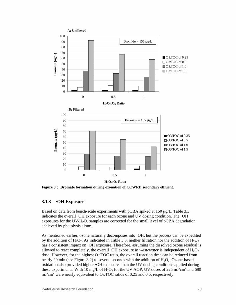
WateReuse Research Foundation 79
Figure 3.3. Bromate formation during ozonation of CCWRD secondary effluent.
3.1.3 ·OH Exposure
Based on data from bench-scale experiments with pCBA spiked at 150 μg/L, Table 3.3 indicates the overall ·OH exposure for each ozone and UV dosing condition. The ·OH exposures for the UV/H2O2 samples are corrected for the small level of pCBA degradation achieved by photolysis alone.
As mentioned earlier, ozone naturally decomposes into ·OH, but the process can be expedited by the addition of H2O2. As indicated in Table 3.3, neither filtration nor the addition of H2O2 has a consistent impact on ·OH exposure. Therefore, assuming the dissolved ozone residual is allowed to react completely, the overall ·OH exposure in wastewater is independent of H2O2 dose. However, for the highest O3:TOC ratio, the overall reaction time can be reduced from nearly 20 min (see Figure 3.2) to several seconds with the addition of H2O2. Ozone-based oxidation also provided higher ·OH exposures than the UV dosing conditions applied during these experiments. With 10 mg/L of H2O2 for the UV AOP, UV doses of 225 mJ/cm2 and 680 mJ/cm2 were nearly equivalent to O3:TOC ratios of 0.25 and 0.5, respectively.
Bro
mat
e (μ
g/L
)
0
10
20
30
40
50
60
70
80
90
100
0 0.5 1
H2O2:O3 Ratio
Bro
mat
e (u
g/L
)O3:TOC of 0.25O3:TOC of 0.5O3:TOC of 1.0O3:TOC of 1.5
Bromide = 156 μg/L
A: Unfiltered
Bro
mat
e (μ
g/L
)
0
10
20
30
40
50
60
70
80
90
100
0 0.5 1
H2O2:O3 Ratio
Bro
mat
e (u
g/L
)O3:TOC of 0.25O3:TOC of 0.5O3:TOC of 1.0O3:TOC of 1.5
Bromide = 156 μg/L
A: Unfiltered
0
10
20
30
40
50
60
70
80
90
100
0 0.5 1
H2O2:O3 Ratio
Bro
mat
e (u
g/L
)O3:TOC of 0.25O3:TOC of 0.5O3:TOC of 1.0O3:TOC of 1.5
Bromide = 156 μg/L
0
10
20
30
40
50
60
70
80
90
100
0 0.5 1
H2O2:O3 Ratio
Bro
mat
e (u
g/L
)O3:TOC of 0.25O3:TOC of 0.5O3:TOC of 1.0O3:TOC of 1.5
Bromide = 156 μg/L
A: Unfiltered
0
10
20
30
40
50
60
70
80
90
100
0 0.5 1
H2O2:O3 Ratio
Bro
mat
e (u
g/ O3:TOC of 0.25O3:TOC of 0.5O3:TOC of 1.0O3:TOC of 1.5
Bromide = 155 μg/L
B: Filtered
Bro
mat
e (μ
g/L
)
0
10
20
30
40
50
60
70
80
90
100
0 0.5 1
H2O2:O3 Ratio
Bro
mat
e (u
g/ O3:TOC of 0.25O3:TOC of 0.5O3:TOC of 1.0O3:TOC of 1.5
Bromide = 155 μg/L
B: Filtered
Bro
mat
e (μ
g/L
)

80 WateReuse Research Foundation
Table 3.3. ·OH Exposure in the CCWRD Secondary Effluent
Ozone:TOC H2O2:O3=0 H2O2:O3=0.5 H2O2:O3=1.0
Unfiltered ozone (10-11 M-s) 0.25 6.7 6.7 7.9 0.5 20 23 25 1.0 39 35 35 1.5 [pCBA]<MRL [pCBA]<MRL 49
Filtered ozone (10-11 M-s) 0.25 8.1 8.1 9.2 0.5 19 22 24 1.0 39 37 37 1.5 [pCBA]<MRL 53 [pCBA]<MRL
UV Dose (mJ/cm2) H2O2=0 mg/L H2O2=5 mg/L H2O2=10 mg/L
Filtered UV (10-11 M-s) 0 N/A N/A 0a 23 N/A N/A 0.41 45 N/A N/A 2.0 225 N/A N/A 4.4 680 N/A N/A 14
aBased on H2O2 control.
3.1.4 Title 22 Contaminants
In the past, the California Department of Public Health Title 22 requirements for water recycling required reuse systems to demonstrate 1.2- and 0.5-log destruction or removal of NDMA and 1,4-dioxane, respectively. To satisfy these requirements, reuse systems often implemented a UV AOP (i.e., UV/H2O2) because NDMA is susceptible to UV photolysis and 1,4-dioxane is susceptible to ·OH oxidation.
Bench-scale experiments were performed with filtered CCWRD wastewater to evaluate the use of ozone and UV for the destruction of spiked NDMA (200 ng/L) and 1,4-dioxane (700 μg/L). Figure 3.4 indicates that UV doses of approximately 500 and 625 mJ/cm2 were required to satisfy the Title 22 requirement with UV and UV/H2O2, respectively. The additional energy required to reach the 1.2-log treatment goal with UV/H2O2 is plausible because the H2O2 will absorb a portion of the incident photons, and NDMA is not susceptible to ·OH oxidation. This was supported by a separate NDMA destruction experiment with ozone and ozone/H2O2. An O3:TOC ratio of 1.5 only achieved 0.05- to 0.14-log destruction of NDMA at H2O2:O3 ratios of 0 and 0.5, respectively. Not only did ozone achieve limited levels of NDMA destruction, but also it led to a small level of NDMA formation. This should not be confused with NDMA formation potential, which incorporates chloramination to intentionally form NDMA. As indicated in Table 3.4, the ozone-induced NDMA formation remained relatively constant regardless of ozone or H2O2 dose.
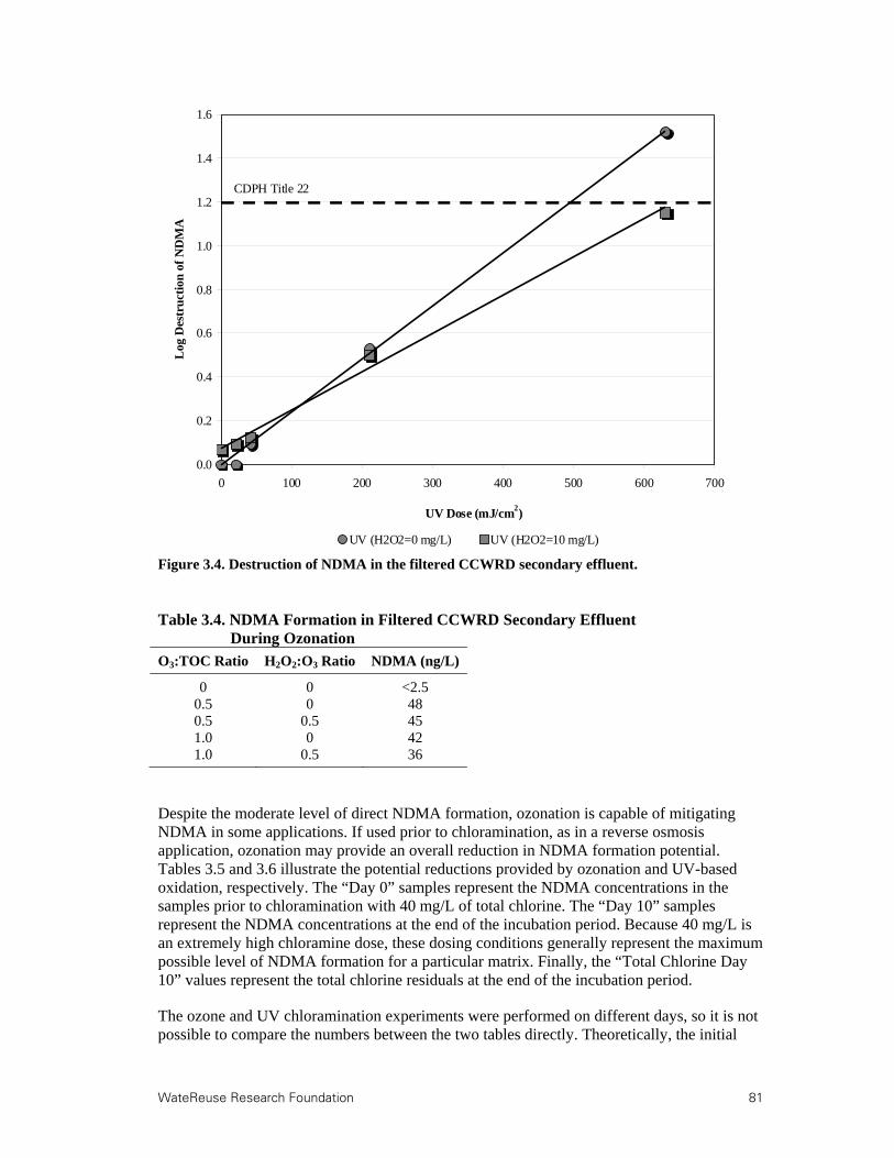
WateReuse Research Foundation 81
Figure 3.4. Destruction of NDMA in the filtered CCWRD secondary effluent.
Table 3.4. NDMA Formation in Filtered CCWRD Secondary Effluent
During Ozonation
O3:TOC Ratio H2O2:O3 Ratio NDMA (ng/L)
0 0 <2.5 0.5 0 48 0.5 0.5 45 1.0 0 42 1.0 0.5 36
Despite the moderate level of direct NDMA formation, ozonation is capable of mitigating NDMA in some applications. If used prior to chloramination, as in a reverse osmosis application, ozonation may provide an overall reduction in NDMA formation potential. Tables 3.5 and 3.6 illustrate the potential reductions provided by ozonation and UV-based oxidation, respectively. The “Day 0” samples represent the NDMA concentrations in the samples prior to chloramination with 40 mg/L of total chlorine. The “Day 10” samples represent the NDMA concentrations at the end of the incubation period. Because 40 mg/L is an extremely high chloramine dose, these dosing conditions generally represent the maximum possible level of NDMA formation for a particular matrix. Finally, the “Total Chlorine Day 10” values represent the total chlorine residuals at the end of the incubation period.
The ozone and UV chloramination experiments were performed on different days, so it is not possible to compare the numbers between the two tables directly. Theoretically, the initial
0.0
0.2
0.4
0.6
0.8
1.0
1.2
1.4
1.6
0 100 200 300 400 500 600 700
UV Dose (mJ/cm2)
Log
Des
truc
tion
UV (H2O2=0 mg/L) UV (H2O2=10 mg/L)
CDPH Title 22L
og D
estr
uct
ion
of
ND
MA
0.0
0.2
0.4
0.6
0.8
1.0
1.2
1.4
1.6
0 100 200 300 400 500 600 700
UV Dose (mJ/cm2)
Log
Des
truc
tion
UV (H2O2=0 mg/L) UV (H2O2=10 mg/L)
CDPH Title 22L
og D
estr
uct
ion
of
ND
MA

82 WateReuse Research Foundation
chloramine dose was the same in both experiments (40 mg/L as Cl2), which should yield relatively similar formation potentials for the secondary and finished effluents. Although the finished effluent received additional treatment compared to the secondary effluent (i.e., sand filtration and a UV dose of 40 mJ/cm2), these processes are insufficient to achieve significant reductions in NDMA formation potential. Therefore, the secondary and finished effluents were essentially replicate samples. The fact that there was a significant difference between the secondary and finished effluents—for both NDMA and total chlorine residual on Day 10—indicates that the chloramination process was slightly different on the two days. To avoid this issue, the NDMA formation potential tests were all performed on the same day in the subsequent bench-scale experiments. Despite the differences between the two tables, it is still possible to compare the numbers within each table to illustrate the relative changes in NDMA formation potential. Based on Table 3.5, ozonation achieved reductions in overall NDMA formation potential ranging from 61% to 75%. Accounting for the Day 0 concentrations, the overall reduction reaches 84%, based on the available data. Therefore, assuming that direct NDMA formation during ozonation can be controlled or limited, ozonation may provide significant NDMA benefits during subsequent chloramination. Based on the data in Table 3.6, low UV doses with or without H2O2 were insufficient to achieve reductions in NDMA formation potential, although higher UV doses with 10 mg/L of H2O2 addition achieved up to a 45% reduction in NDMA formation potential. Furthermore, the bench-scale UV dose of 45 mJ/cm2 yielded an NDMA concentration similar to that of the finished effluent (~40 mJ/cm2). Table 3.5. NDMA Formation Potential in the CCWRD Secondary Effluent (O3)
Testing Condition NDMA Day 0 (before chloramine)
NDMA Day 10 (after chloramine)
Total Chlorine Day 10
Secondary effluent <2.5 ng/L 590 ng/L 2.4 mg/L H2O2 Control Not measured 550 ng/L 1.0 mg/L Ozone 0.25/0 Not measured 230 ng/L 2.2 mg/L Ozone 0.25/0.5 Not measured 230 ng/L 2.5 mg/L Ozone 0.5/0 48 ng/L 150 ng/L 2.5 mg/L Ozone 0.5/0.5 45 ng/L 140 ng/L 2.6 mg/L Ozone 1.0/0 42 ng/L 150 ng/L 2.5 mg/L Ozone 1.0/0.5 36 ng/L 160 ng/L 2.4 mg/L Ozone 1.5/0 Not measured 150 ng/L 2.2 mg/L Ozone 1.5/0.5 Not measured 190 ng/L 2.2 mg/L
Table 3.6. NDMA Formation Potential in the CCWRD Secondary Effluent (UV)
Testing Condition NDMA Day 0 (before chloramine)
NDMA Day 10 (after chloramine)
Total Chlorine
Day 10
UV 23/0 Not measured 1,400 ng/L 13 mg/L UV 23/10 Not measured 1,400 ng/L 12 mg/L UV 45/0 Not measured 1,300 ng/L 12 mg/L UV 45/10 Not measured 1,300 ng/L 13 mg/L UV 225/0 Not measured 1,300 ng/L 13 mg/L UV 225/10 Not measured 1,200 ng/L 14 mg/L UV 680/0 Not measured Not measured 13 mg/L UV 680/10 Not measured 770 ng/L 12 mg/L Finished effluent <2.5 ng/L 1,400 ng/L 12 mg/L
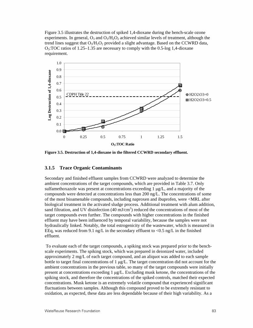
WateReuse Research Foundation 83
Figure 3.5 illustrates the destruction of spiked 1,4-dioxane during the bench-scale ozone experiments. In general, O3 and O3/H2O2 achieved similar levels of treatment, although the trend lines suggest that O3/H2O2 provided a slight advantage. Based on the CCWRD data, O3:TOC ratios of 1.25–1.35 are necessary to comply with the 0.5-log 1,4-dioxane requirement.
Figure 3.5. Destruction of 1,4-dioxane in the filtered CCWRD secondary effluent.
3.1.5 Trace Organic Contaminants
Secondary and finished effluent samples from CCWRD were analyzed to determine the ambient concentrations of the target compounds, which are provided in Table 3.7. Only sulfamethoxazole was present at concentrations exceeding 1 μg/L, and a majority of the compounds were detected at concentrations less than 200 ng/L. The concentrations of some of the most bioamenable compounds, including naproxen and ibuprofen, were <MRL after biological treatment in the activated sludge process. Additional treatment with alum addition, sand filtration, and UV disinfection (40 mJ/cm2) reduced the concentrations of most of the target compounds even further. The compounds with higher concentrations in the finished effluent may have been influenced by temporal variability, because the samples were not hydraulically linked. Notably, the total estrogenicity of the wastewater, which is measured in EEq, was reduced from 9.1 ng/L in the secondary effluent to <0.5 ng/L in the finished effluent.
To evaluate each of the target compounds, a spiking stock was prepared prior to the bench-scale experiments. The spiking stock, which was prepared in deionized water, included approximately 2 mg/L of each target compound, and an aliquot was added to each sample bottle to target final concentrations of 1 μg/L. The target concentration did not account for the ambient concentrations in the previous table, so many of the target compounds were initially present at concentrations exceeding 1 μg/L. Excluding musk ketone, the concentrations of the spiking stock, and therefore the concentrations of the spiked controls, matched their expected concentrations. Musk ketone is an extremely volatile compound that experienced significant fluctuations between samples. Although this compound proved to be extremely resistant to oxidation, as expected, these data are less dependable because of their high variability. As a
0.0
0.1
0.2
0.3
0.4
0.5
0.6
0.7
0.8
0.9
1.0
0 0.25 0.5 0.75 1 1.25 1.5
O3:TOC Ratio
Log
Des
tru
cti
H2O2:O3=0H2O2:O3=0.5
CDPH Title 22
Log
Des
tru
ctio
n o
f 1,
4-d
ioxa
ne

84 WateReuse Research Foundation
result, musk ketone is generally omitted from the data presentation. Finally, H2O2 alone (i.e., 10 mg/L of H2O2 with no ozone or UV exposure) had no noticeable effect on the concentrations of the target compounds.
Table 3.7. Ambient TOrC Concentrations at CCWRD
Parameter Secondary Effluent (ng/L) Finished Effluent (ng/L)
Bisphenol A <50 <50 Diclofenac 131 57 Gemfibrozil 34 12 Ibuprofen <25 <25 Musk ketone <100 <100 Naproxen <25 <25 Triclosan 29 38 Atenolol 421 120 Atrazine <10 <10 Carbamazepine 251 192 DEET 155 232 Meprobamate 629 362 Phenytoin 216 113 Primidone 134 168 Sulfamethoxazole 1,220 1,150 Trimethoprim 256 43 TCEP 525 349 Total estrogenicity (EEq) 9.1 <0.074
Tables 3.8 and 3.9 show the relative oxidation levels of the 16 target compounds (musk ketone omitted) as a function of O3:TOC and H2O2:O3 ratios in the unfiltered and filtered CCWRD secondary effluent, respectively. As described earlier, the target compounds were divided into five categories based on their second-order ozone and ·OH rate constants, and “indicator” compounds were also defined as the average of the values within each group. In general, there were no significant differences between the filtered ands unfiltered samples or the ozone and ozone/H2O2 samples. The compounds within each group experienced highly consistent levels of oxidation, thereby justifying the applicability of the indicator framework. The shading represents the dosing conditions required to achieve at least 80% oxidation of the target compounds, whereas the extreme resistance of TCEP limited its level of oxidation to <30%.
Table 3.10 shows the relative oxidation levels of the 16 target compounds as a function of UV and H2O2 dose. The previously defined groups are not necessarily applicable to UV and UV/H2O2 because of the compounds’ variable susceptibility to UV photolysis. Two compounds (diclofenac and triclosan) experienced 90% removal with a UV dose of 225 mJ/cm2, three compounds (atrazine, phenytoin, and sulfamethoxazole) experienced greater than 50% removal with a UV dose of 680 mJ/cm2, and a majority of the target compounds experienced less than 20% removal at a UV dose of 680 mJ/cm2. As indicated by the light shading in Table 3.10, the high ·OH rate constants for some of the compounds allowed significant oxidation when UV doses were coupled with H2O2 addition. Although UV/H2O2 was more effective than UV photolysis, UV AOP was still inferior to ozone and ozone/H2O2 for a majority of the compounds.
Although it is important to understand the efficacy of various treatment processes in removing or oxidizing individual compounds, TOrCs are always present in complex mixtures

WateReuse Research Foundation 85
for which aquatic impacts and health effects are unknown. Some assays are able to capture the aggregate effects of these mixtures based on a variety of endpoints. For example, the YES assay can be used to quantify the total estrogenicity of a sample. Figure 3.6 illustrates the change in total estrogenicity after (A) ozone- and (B) UV-based treatment processes. As indicated by the dashed lines, O3:TOC ratios of 0.5 and higher achieved the MRL (i.e., <0.074 ng/L) for all H2O2 doses. UV photolysis demonstrated high variability and was unable to achieve the MRL for the UV doses in this experiment, whereas UV/H2O2 was able to reach the MRL with 680 mJ/cm2. The addition of H2O2 alone caused a small reduction in the initial EEq value, which is shown for the UV/H2O2 data point at 0 mJ/cm2.
Figure 3.6. Reduction in total estrogenicity in the filtered CCWRD secondary effluent.
EE
q (
ng/
L)
EE
q (
ng/
L)
A: Ozone-Based Treatment B: UV-Based Treatment
0
2
4
6
8
10
0 0.25 0.5 0.75 1 1.25 1.5
O3:TOC Ratio
H2O2:O3=0 H2O2:O3=0.5 H2O2:O3=1.0
0
2
4
6
8
10
0 100 200 300 400 500 600 700
UV Dose (mJ/cm2)
UV (H2O2 = 0 mg/L) UV (H2O2 = 10 mg/L)
EE
q (
ng/
L)
EE
q (
ng/
L)
A: Ozone-Based Treatment B: UV-Based Treatment
0
2
4
6
8
10
0 0.25 0.5 0.75 1 1.25 1.5
O3:TOC Ratio
H2O2:O3=0 H2O2:O3=0.5 H2O2:O3=1.0
0
2
4
6
8
10
0 100 200 300 400 500 600 700
UV Dose (mJ/cm2)
UV (H2O2 = 0 mg/L) UV (H2O2 = 10 mg/L)
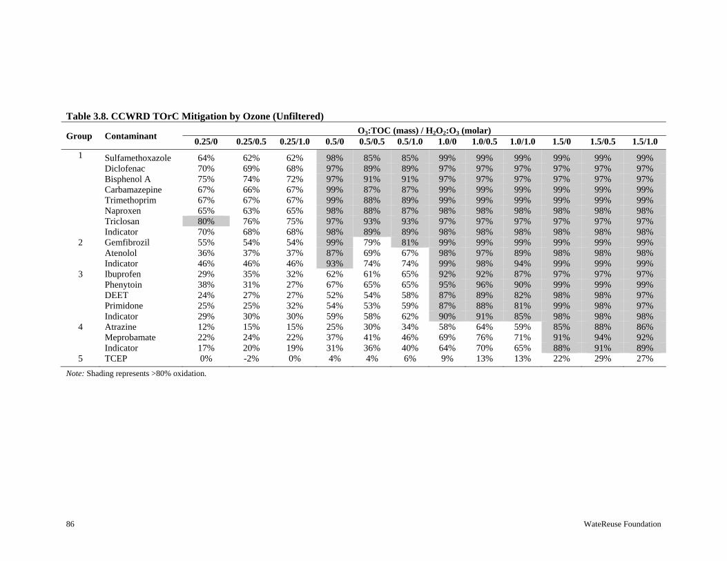
86 WateReuse Foundation
Table 3.8. CCWRD TOrC Mitigation by Ozone (Unfiltered)
Group Contaminant O3:TOC (mass) / H2O2:O3 (molar)
0.25/0 0.25/0.5 0.25/1.0 0.5/0 0.5/0.5 0.5/1.0 1.0/0 1.0/0.5 1.0/1.0 1.5/0 1.5/0.5 1.5/1.0
1 Sulfamethoxazole 64% 62% 62% 98% 85% 85% 99% 99% 99% 99% 99% 99% Diclofenac 70% 69% 68% 97% 89% 89% 97% 97% 97% 97% 97% 97% Bisphenol A 75% 74% 72% 97% 91% 91% 97% 97% 97% 97% 97% 97% Carbamazepine 67% 66% 67% 99% 87% 87% 99% 99% 99% 99% 99% 99% Trimethoprim 67% 67% 67% 99% 88% 89% 99% 99% 99% 99% 99% 99% Naproxen 65% 63% 65% 98% 88% 87% 98% 98% 98% 98% 98% 98% Triclosan 80% 76% 75% 97% 93% 93% 97% 97% 97% 97% 97% 97% Indicator 70% 68% 68% 98% 89% 89% 98% 98% 98% 98% 98% 98%
2 Gemfibrozil 55% 54% 54% 99% 79% 81% 99% 99% 99% 99% 99% 99% Atenolol 36% 37% 37% 87% 69% 67% 98% 97% 89% 98% 98% 98% Indicator 46% 46% 46% 93% 74% 74% 99% 98% 94% 99% 99% 99%
3 Ibuprofen 29% 35% 32% 62% 61% 65% 92% 92% 87% 97% 97% 97% Phenytoin 38% 31% 27% 67% 65% 65% 95% 96% 90% 99% 99% 99% DEET 24% 27% 27% 52% 54% 58% 87% 89% 82% 98% 98% 97% Primidone 25% 25% 32% 54% 53% 59% 87% 88% 81% 99% 98% 97% Indicator 29% 30% 30% 59% 58% 62% 90% 91% 85% 98% 98% 98%
4 Atrazine 12% 15% 15% 25% 30% 34% 58% 64% 59% 85% 88% 86% Meprobamate 22% 24% 22% 37% 41% 46% 69% 76% 71% 91% 94% 92% Indicator 17% 20% 19% 31% 36% 40% 64% 70% 65% 88% 91% 89%
5 TCEP 0% -2% 0% 4% 4% 6% 9% 13% 13% 22% 29% 27%
Note: Shading represents >80% oxidation.

WateReuse Research Foundation 87
Table 3.9. CCWRD TOrC Mitigation by Ozone (Filtered)
Group Contaminant O3:TOC (mass) / H2O2:O3 (molar)
0.25/0 0.25/0.5 0.25/1.0 0.5/0 0.5/0.5 0.5/1.0 1.0/0 1.0/0.5 1.0/1.0 1.5/0 1.5/0.5 1.5/1.0 1 Sulfamethoxazole 64% 63% 74% 98% 98% 97% 99% 99% 99% 99% 99% 99%
Diclofenac 72% 70% 80% 97% 97% 97% 97% 97% 97% 97% 97% 97% Bisphenol A 70% 73% 85% 98% 98% 98% 98% 98% 98% 98% 98% 98% Carbamazepine 69% 67% 71% 99% 99% 99% 99% 99% 99% 99% 99% 99% Trimethoprim 70% 69% 75% 99% 99% 99% 99% 99% 99% 99% 99% 99% Naproxen 67% 67% 72% 98% 98% 97% 98% 98% 97% 98% 98% 97% Triclosan 79% 81% 95% 97% 97% 97% 97% 97% 97% 97% 77% 97% Indicator 70% 70% 79% 98% 98% 98% 98% 98% 98% 98% 95% 98%
2 Gemfibrozil 55% 49% 53% 99% 99% 99% 99% 99% 99% 99% 99% 97% Atenolol 37% 35% 41% 97% 82% 79% 98% 98% 97% 98% 98% 93% Indicator 46% 42% 47% 98% 91% 89% 99% 99% 98% 99% 99% 95%
3 Ibuprofen 32% 33% 37% 70% 71% 72% 97% 97% 96% 97% 97% 92% Phenytoin 40% 38% 43% 78% 77% 76% 98% 99% 98% 99% 99% 95% DEET 27% 29% 32% 63% 66% 66% 94% 96% 94% 99% 99% 90% Primidone 21% 22% 28% 64% 63% 63% 95% 96% 93% 99% 99% 90% Indicator 30% 31% 35% 69% 69% 69% 96% 97% 95% 99% 99% 92%
4 Atrazine 13% 15% 16% 32% 35% 35% 72% 76% 74% 89% 92% 77% Meprobamate 19% 24% 22% 46% 48% 48% 80% 85% 85% 94% 97% 84% Indicator 16% 20% 19% 39% 42% 42% 76% 81% 80% 92% 95% 81%
5 TCEP 2% 0% 2% 2% 5% 6% 14% 19% 21% 26% 30% 29%
Note: Shading represents >80% oxidation.

88 WateReuse Foundation
Table 3.10. CCWRD TOrC Mitigation by UV (Filtered)
Group Contaminant UV Dose (mJ/cm2) / H2O2 Dose (mg/L)
23/0 23/10a 45/0 45/10 225/0 225/10 680/0 680/10
1 Sulfamethoxazole 9% N/A 10% 22% 43% 51% 86% 93% Diclofenac 21% N/A 39% 47% 93% 95% 98% 98% Bisphenol A -5% N/A -3% 23% 13% 48% 4% 84% Carbamazepine -3% N/A -5% 2% 7% 32% 12% 66% Trimethoprim -8% N/A -10% 5% 3% 24% -1% 55% Naproxen -19% N/A -6% -5% 10% 34% 18% 74% Triclosan 22% N/A 13% 38% 88% 89% 97% 97%
2 Gemfibrozil 6% N/A -13% 17% 14% 37% 16% 65% Atenolol 6% N/A 12% 11% 11% 32% 16% 58%
3 Ibuprofen -11% N/A -6% 3% 9% 30% 8% 62% Phenytoin 24% N/A 19% 47% 46% 66% 70% 90% DEET -6% N/A -1% 6% 8% 23% 4% 49% Primidone -8% N/A -12% -2% 5% 14% -5% 36%
4 Atrazine -1% N/A 3% -3% 30% 24% 53% 59% Meprobamate 4% N/A -1% 5% 5% 14% 1% 30%
5 TCEP -6% N/A -4% 24% 10% 26% 1% 25%
aSample not analyzed. Shading represents >80% photolysis or oxidation. Groupings refer to ozone and ·OH rate constants.

WateReuse Foundation 89
3.1.6 Disinfection
Ambient secondary (before and after laboratory filtration) and finished effluent samples from CCWRD were assayed for total and fecal coliforms, MS2, and Bacillus spores. The ambient microbial water quality data are provided in Table 3.11. Based on the microbial prevalence in the filtered secondary effluent, it is apparent that laboratory filtration with a nominal pore size of 0.5 μm was highly ineffective. Table 3.11. Ambient Microbial Water Quality Data for CCWRD
Microbial Surrogate
Unfiltered Secondary Effluent
Filtered Secondary Effluent
Finished Effluent
Total coliforms (MPN/100 mL)
7.3 104 3.3 103 8
Fecal coliforms (MPN/100 mL) 4.4 103 2.9 102 <1
MS2 (PFU/mL)
<1 <1 <1
Bacillus spores (CFU/100 mL) 3.0 103 1.0 103 30
To illustrate a wide range of inactivation, the ozone and UV disinfection samples were spiked with relatively large numbers of the surrogate microbes, as indicated in Table 3.12. The E. coli spiking stocks contained approximately 109–1010 MPN/100 mL (after purification), the MS2 stocks contained approximately 109–1010 PFU/mL (after purification), and the B. subtilis spore stocks contained approximately 108–109 CFU/100 mL (after heat shock and purification). Although the stocks were purified, only 250 L of the appropriate spiking stock was added to 250 mL of sample to target a sufficient microbial load while limiting the artificial organic loading associated with the culture media.
Table 3.12. Microbial Spiking Levels for CCWRD Bench-Scale Experiments
Microbial Surrogate Unfiltered Ozone
Disinfection Filtered Ozone
Disinfection Filtered UV Disinfection
E. coli (MPN/100 mL) 5.4 107 5.4 107 1.6 107 MS2 (PFU/mL) 3.1 107 2.0 107 9.6 107 B. subtilis spores (CFU/100 mL) 2.5 105 2.6 105 2.2 05
Figure 3.7 illustrates the inactivation of spiked E. coli during the bench-scale ozone experiments. The disinfection results are reported based on “log inactivation,” which simplifies order-of-magnitude changes in microbial numbers. This nomenclature replaces percent inactivation (e.g., 90%, 99%, 99.9%) with its “base-10” log equivalent (e.g., 1-log, 2-log, 3-log). The solid and dashed lines near the top of the figure represent the limits of inactivation based on the spiking levels in the filtered and unfiltered samples, respectively. In addition, there were four samples (Unfiltered 0.5/0.5, Unfiltered 0.5/1.0, Filtered 1.0/1.0, and Filtered 1.5/1.0) that could not be quantified because they were not sufficiently diluted during the assay period. The data points for these samples, which are indicated by arrows in the

90 WateReuse Foundation
figure, represent the maximum level of inactivation based on the most diluted sample that was assayed. Therefore, the actual level of inactivation was less than that indicated by the data points.
In general, the filtered versus unfiltered comparison proved to be inconclusive because of the inherent variability in the data sets. On average, the addition of H2O2 alone achieved less than 0.3-log inactivation, but when combined with ozonation, the addition of H2O2 consistently hindered E. coli inactivation. This indicates that the increased reactivity of ·OH combined with the scavenging effects of EfOM was generally detrimental to the disinfection process. Although molecular ozone also decomposes into ·OH over time, the initial ozone exposure was critical for improving disinfection efficacy. The average log-inactivation values for each treatment condition—after the unfiltered and filtered data sets are combined—are provided in Table 3.13.
Figure 3.8 illustrates the inactivation of spiked MS2 during the bench-scale ozone experiments. Similarly to E. coli, there was no noticeable difference between the filtered and unfiltered samples, the addition of H2O2 alone achieved less than 0.3-log inactivation, and when combined with ozonation, the addition of H2O2 consistently hindered MS2 inactivation. With respect to the CDPH Title 22 requirements, an O3:TOC ratio >1.0 appears to be sufficient for 5-log MS2 inactivation, regardless of the H2O2 dose. With no H2O2 addition, an O3:TOC ratio greater than 1.0 is even sufficient for the 6.5-log alternative treatment goal. However, none of the H2O2 treatment conditions satisfied the 6.5-log alternative for this particular set of samples. The average log-inactivation values for each treatment condition (combined unfiltered and filtered data) are provided in Table 3.14.
Figure 3.9 illustrates the inactivation of spiked B. subtilis spores during the bench-scale ozone experiments. B. subtilis proved to be an interesting test microbe because of its unique dose–response relationship for ozone and ·OH. As expected, the spores proved to be extremely resistant to oxidation and only experienced significant inactivation for an O3:TOC ratio of 1.5 with no H2O2 addition. In other words, a sufficient ozone CT had to be administered before ozone and •OH were able to penetrate the spore coat and inactivate the bacteria. This is consistent with the disinfection “lag phase” characteristic of many spore-forming microbes. Although there appears to be a significant difference between the unfiltered and filtered samples at an O3:TOC ratio of 1.5 (no H2O2 addition), this is likely attributable to inherent variability rather than the effect of filtration. Furthermore, oxidation with ·OH alone is extremely ineffective for spore inactivation, presumably because of the highly reactive nature of ·OH and competition with EfOM. The average log-inactivation values for each treatment condition (combined unfiltered and filtered data) are provided in Table 3.15.
Finally, Figure 3.10 provides a summary of the ozone disinfection data for the three surrogate microbes with respect to the CT framework. Figure 3.10A illustrates the dose–response relationships for the filtered and unfiltered samples (combined) with no H2O2 addition. Figure 3.10B illustrates the dose–response relationships for the filtered and unfiltered samples (combined) with H2O2:O3 ratios of 0.5 and 1.0 (also combined). According to theses data, the CT framework is not always appropriate, because substantial levels of inactivation can be achieved when the apparent ozone CT is zero. However, the level of inactivation for vegetative bacteria and viruses is generally less than that observed when an ozone residual is present, and no inactivation of spore-forming bacteria can be achieved without a measurable CT.

WateReuse Foundation 91
Table 3.16 summarizes the efficacy of UV and UV/H2O2 for the inactivation of the three surrogate microbes. The efficacy of UV-based disinfection differs dramatically from that of ozone-based disinfection because UV is highly effective against both vegetative and spore-forming bacteria, whereas some viruses demonstrate resistance. Even 45 mJ/cm2 was sufficient to reach the limits of inactivation for E. coli and Bacillus spores, regardless of H2O2 addition. On the other hand, MS2 inactivation occurred more slowly and only reached the limit of inactivation for UV doses of 225 and 680 mJ/cm2 with 10 mg/L of H2O2. Particularly with respect to advanced oxidation dosing conditions (i.e., 225 or 680 mJ/cm2 with 10 mg/L of H2O2), one can expect substantial inactivation of all microbes present in wastewater. This constitutes a significant advantage of UV-based treatment over the ozone-based alternatives.
Although the addition of H2O2 appeared to be beneficial for the inactivation of the three microbes, the demonstrated resistance of Bacillus spores to oxidation indicates that the slightly higher level of inactivation with UV/H2O2 was likely attributable to experimental variability. Because the incident germicidal light is only marginally impacted by the addition of H2O2, the higher inactivation levels for E. coli and MS2 with UV/H2O2 are likely significant. In contrast to ozone/H2O2, where the H2O2 immediately “quenches” the ozone residual, the effects of germicidal UV and photogenerated ·OH are more synergistic.
Figure 3.7. Inactivation of spiked E. coli in the CCWRD secondary effluent.
0
1
2
3
4
5
6
7
8
9
0.00 0.25 0.50 0.75 1.00 1.25 1.50
O3:TOC Ratio
Log
In
acti
vati
on
Filtered (H2O2:O3=0) Filtered (H2O2:O3=0.5) Filtered (H2O2:O3=1.0)Unfiltered (H2O2:O3=0) Unfiltered (H2O2:O3=0.5) Unfiltered (H2O2:O3=1.0)
E. coli Limits of Inactivation
0
1
2
3
4
5
6
7
8
9
0.00 0.25 0.50 0.75 1.00 1.25 1.50
O3:TOC Ratio
Log
In
acti
vati
on
Filtered (H2O2:O3=0) Filtered (H2O2:O3=0.5) Filtered (H2O2:O3=1.0)Unfiltered (H2O2:O3=0) Unfiltered (H2O2:O3=0.5) Unfiltered (H2O2:O3=1.0)
E. coli Limits of Inactivation
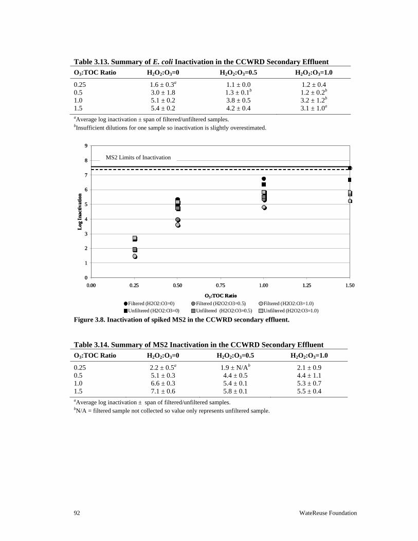
92 WateReuse Foundation
Table 3.13. Summary of E. coli Inactivation in the CCWRD Secondary Effluent
O3:TOC Ratio H2O2:O3=0 H2O2:O3=0.5 H2O2:O3=1.0
0.25 1.6 ± 0.3a 1.1 ± 0.0 1.2 ± 0.4 0.5 3.0 ± 1.8 1.3 ± 0.1b 1.2 ± 0.2b 1.0 5.1 ± 0.2 3.8 ± 0.5 3.2 ± 1.2b 1.5 5.4 ± 0.2 4.2 ± 0.4 3.1 ± 1.0a aAverage log inactivation ± span of filtered/unfiltered samples. bInsufficient dilutions for one sample so inactivation is slightly overestimated.
Figure 3.8. Inactivation of spiked MS2 in the CCWRD secondary effluent.
Table 3.14. Summary of MS2 Inactivation in the CCWRD Secondary Effluent
O3:TOC Ratio H2O2:O3=0 H2O2:O3=0.5 H2O2:O3=1.0
0.25 2.2 ± 0.5a 1.9 ± N/Ab 2.1 ± 0.9 0.5 5.1 ± 0.3 4.4 ± 0.5 4.4 ± 1.1 1.0 6.6 ± 0.3 5.4 ± 0.1 5.3 ± 0.7 1.5 7.1 ± 0.6 5.8 ± 0.1 5.5 ± 0.4 aAverage log inactivation ± span of filtered/unfiltered samples. bN/A = filtered sample not collected so value only represents unfiltered sample.
0
1
2
3
4
5
6
7
8
9
0.00 0.25 0.50 0.75 1.00 1.25 1.50
O3:TOC Ratio
Log
Ina
ctiv
atio
n
Filtered (H2O2:O3=0) Filtered (H2O2:O3=0.5) Filtered (H2O2:O3=1.0)Unfiltered (H2O2:O3=0) Unfiltered (H2O2:O3=0.5) Unfiltered (H2O2:O3=1.0)
MS2 Limits of Inactivation
0
1
2
3
4
5
6
7
8
9
0.00 0.25 0.50 0.75 1.00 1.25 1.50
O3:TOC Ratio
Log
Ina
ctiv
atio
n
Filtered (H2O2:O3=0) Filtered (H2O2:O3=0.5) Filtered (H2O2:O3=1.0)Unfiltered (H2O2:O3=0) Unfiltered (H2O2:O3=0.5) Unfiltered (H2O2:O3=1.0)
MS2 Limits of Inactivation

WateReuse Foundation 93
Figure 3.9. Inactivation of spiked Bacillus spores in the CCWRD secondary effluent.
Table 3.15. Summary of Bacillus Spore Inactivation in the CCWRD Secondary Effluent
O3:TOC Ratio H2O2:O3=0 H2O2:O3=0.5 H2O2:O3=1.0
0.25 0.0 ± 0.0a 0.0 ± 0.0 0.0 ± 0.0 0.5 0.0 ± 0.0 0.0 ± 0.0 0.0 ± 0.0 1.0 0.1 ± 0.0 0.0 ± 0.0 0.0 ± 0.0 1.5 1.2 ± 0.6 0.0 ± 0.0 0.0 ± 0.0
aAverage log inactivation ± span of filtered/unfiltered samples.
0
1
2
3
4
0.00 0.25 0.50 0.75 1.00 1.25 1.50
O3:TOC Ratio
Log
Ina
ctiv
atio
n
Filtered (H2O2:O3=0) Filtered (H2O2:O3=0.5) Filtered (H2O2:O3=1.0)Unfiltered (H2O2:O3=0) Unfiltered (H2O2:O3=0.5) Unfiltered (H2O2:O3=1.0)
Bacillus spore Limits of Inactivation
0
1
2
3
4
0.00 0.25 0.50 0.75 1.00 1.25 1.50
O3:TOC Ratio
Log
Ina
ctiv
atio
n
Filtered (H2O2:O3=0) Filtered (H2O2:O3=0.5) Filtered (H2O2:O3=1.0)Unfiltered (H2O2:O3=0) Unfiltered (H2O2:O3=0.5) Unfiltered (H2O2:O3=1.0)
Bacillus spore Limits of Inactivation

94 WateReuse Foundation
Figure 3.10. Significance of CT for disinfection in the CCWRD secondary effluent.
0
1
2
3
4
5
6
7
8
9
0.25 0.50 1.00 1.50
O3:TOC Ratio
Log
In
acti
vati
on
0
5
10
15
20
25
30
Ozo
ne
CT
(m
g-m
in/L
Bacillus spore E. coli MS2 CT
A: No H2O2 Addition
Log
Ina
ctiv
atio
n
Ozo
ne C
T (
mg-
min
/L)
0
1
2
3
4
5
6
7
8
9
0.25 0.50 1.00 1.50
O3:TOC Ratio
Log
In
acti
vati
on
0
5
10
15
20
25
30
Ozo
ne
CT
(m
g-m
in/L
Bacillus spore E. coli MS2 CT
A: No H2O2 Addition
Log
Ina
ctiv
atio
n
Ozo
ne C
T (
mg-
min
/L)
0
1
2
3
4
5
6
7
8
9
0.25 0.50 1.00 1.50
O3:TOC Ratio
Log
In
acti
vati
on
0
5
10
15
20
25
30
Ozo
ne
CT
(m
g-m
in/L
Bacillus spore E. coli MS2 CT
B: H2O2 Addition
Log
Ina
ctiv
atio
n
Ozo
ne
CT
(m
g-m
in/L
)
0
1
2
3
4
5
6
7
8
9
0.25 0.50 1.00 1.50
O3:TOC Ratio
Log
In
acti
vati
on
0
5
10
15
20
25
30
Ozo
ne
CT
(m
g-m
in/L
Bacillus spore E. coli MS2 CT
B: H2O2 Addition
Log
Ina
ctiv
atio
n
Ozo
ne
CT
(m
g-m
in/L
)
(combination of filtered and unfiltered samples with H2O2:O3=0)
(combination of filtered and unfiltered samples with H2O2:O3=0.5 and 1.0)
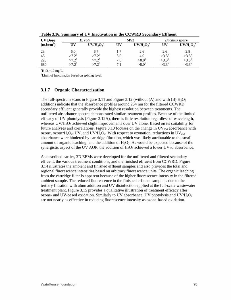
WateReuse Foundation 95
Table 3.16. Summary of UV Inactivation in the CCWRD Secondary Effluent
UV Dose (mJ/cm2)
E. coli MS2 Bacillus spore UV UV/H2O2
a UV UV/H2O2a UV UV/H2O2
a
23 6.0 6.7 1.7 2.6 2.6 2.8 45 >7.2b >7.2b 3.0 4.0 >3.3b >3.3b 225 >7.2b >7.2b 7.0 >8.0b >3.3b >3.3b 680 >7.2b >7.2b 7.1 >8.0b >3.3b >3.3b aH2O2=10 mg/L. bLimit of inactivation based on spiking level.
3.1.7 Organic Characterization
The full-spectrum scans in Figure 3.11 and Figure 3.12 (without (A) and with (B) H2O2 addition) indicate that the absorbance profiles around 254 nm for the filtered CCWRD secondary effluent generally provide the highest resolution between treatments. The unfiltered absorbance spectra demonstrated similar treatment profiles. Because of the limited efficacy of UV photolysis (Figure 3.12A), there is little resolution regardless of wavelength, whereas UV/H2O2 achieved slight improvements over UV alone. Based on its suitability for future analyses and correlations, Figure 3.13 focuses on the change in UV254 absorbance with ozone, ozone/H2O2, UV, and UV/H2O2. With respect to ozonation, reductions in UV254 absorbance were hindered by cartridge filtration, which was likely attributable to the small amount of organic leaching, and the addition of H2O2. As would be expected because of the synergistic aspect of the UV AOP, the addition of H2O2 achieved a lower UV254 absorbance.
As described earlier, 3D EEMs were developed for the unfiltered and filtered secondary effluent, the various treatment conditions, and the finished effluent from CCWRD. Figure 3.14 illustrates the ambient and finished effluent samples and also provides the total and regional fluorescence intensities based on arbitrary fluorescence units. The organic leaching from the cartridge filter is apparent because of the higher fluorescence intensity in the filtered ambient sample. The reduced fluorescence in the finished effluent sample is due to the tertiary filtration with alum addition and UV disinfection applied at the full-scale wastewater treatment plant. Figure 3.15 provides a qualitative illustration of treatment efficacy after ozone- and UV-based oxidation. Similarly to UV absorbance, UV photolysis and UV/H2O2 are not nearly as effective in reducing fluorescence intensity as ozone-based oxidation.

96 WateReuse Foundation
Figure 3.11. CCWRD absorbance spectra after ozonation.
0
0.03
0.06
0.09
0.12
0.15
240 280 320 360 400 440 480 520 560 600
Wavelength (nm)
0
0.03
0.06
0.09
0.12
0.15
240 280 320 360 400 440 480 520 560 600
Wavelength (nm)
Ab
sorb
ance
(cm
-1)
Ab
sorb
ance
(cm
-1)
O3:TOC = 0
O3:TOC = 0.25
O3:TOC = 0.5
O3:TOC = 1.0
O3:TOC = 1.5
Wavelength (nm) Wavelength (nm)
O3:TOC = 0
O3:TOC = 0.25
O3:TOC = 0.5
O3:TOC = 1.0
O3:TOC = 1.5
A: H2O2:O3=0 B: H2O2:O3=0.5
0
0.03
0.06
0.09
0.12
0.15
240 280 320 360 400 440 480 520 560 600
Wavelength (nm)
0
0.03
0.06
0.09
0.12
0.15
240 280 320 360 400 440 480 520 560 600
Wavelength (nm)
Ab
sorb
ance
(cm
-1)
Ab
sorb
ance
(cm
-1)
O3:TOC = 0
O3:TOC = 0.25
O3:TOC = 0.5
O3:TOC = 1.0
O3:TOC = 1.5
Wavelength (nm) Wavelength (nm)
O3:TOC = 0
O3:TOC = 0.25
O3:TOC = 0.5
O3:TOC = 1.0
O3:TOC = 1.5
A: H2O2:O3=0 B: H2O2:O3=0.5

WateReuse Foundation 97
Figure 3.12. CCWRD absorbance spectra after UV and UV/H2O2.
0
0.03
0.06
0.09
0.12
0.15
240 280 320 360 400 440 480 520 560 600
Wavelength (nm)
0
0.03
0.06
0.09
0.12
0.15
240 280 320 360 400 440 480 520 560 600
Wavelength (nm)
Ab
sorb
ance
(cm
-1)
Wavelength (nm)
Ab
sorb
ance
(cm
-1)
Wavelength (nm)
A: H2O2=0 mg/L B: H2O2:O3=10 mg/L
UV = 0 mJ/cm2
UV = 23 mJ/cm2
UV = 45 mJ/cm2
UV = 225 mJ/cm2
UV = 680 mJ/cm2
UV = 0 mJ/cm2
UV = 23 mJ/cm2
UV = 45 mJ/cm2
UV = 225 mJ/cm2
UV = 680 mJ/cm2
0
0.03
0.06
0.09
0.12
0.15
240 280 320 360 400 440 480 520 560 600
Wavelength (nm)
0
0.03
0.06
0.09
0.12
0.15
240 280 320 360 400 440 480 520 560 600
Wavelength (nm)
Ab
sorb
ance
(cm
-1)
Wavelength (nm)
Ab
sorb
ance
(cm
-1)
Wavelength (nm)
A: H2O2=0 mg/L B: H2O2:O3=10 mg/L
UV = 0 mJ/cm2
UV = 23 mJ/cm2
UV = 45 mJ/cm2
UV = 225 mJ/cm2
UV = 680 mJ/cm2
UV = 0 mJ/cm2
UV = 23 mJ/cm2
UV = 45 mJ/cm2
UV = 225 mJ/cm2
UV = 680 mJ/cm2

98 WateReuse Foundation
Figure 3.13. Differential UV254 absorbance in the CCWRD secondary effluent.
0%
10%
20%
30%
40%
50%
60%
70%
0 100 200 300 400 500 600 700
UV Dose (mJ/cm2)
Dif
fere
nti
al U
V25
4 A
bso
rban
ce
UV (H2O2 = 0 mg/L) UV (H2O2 = 10 mg/L)
Dif
fere
ntia
l UV
254
Ab
sorb
ance
Dif
fere
ntia
l UV
254
Ab
sorb
ance
A: Ozone-Based Treatment (Unfiltered and Filtered) B: UV-Based Treatment (Filtered)
O 3:TO C Ratio
Filtered (H2O2:O3 = 0) Filtered (H2O2:O3 = 0.5) Filtered (H2O2:O3 = 1.0)
Unfiltered (H2O2:O3=0) Unfiltered (H2O2:O3=0.5) Unfiltered (H2O2:O3=1.0)
0%
10%
20%
30%
40%
50%
60%
70%
0 0.25 0.5 0.75 1 1.25 1.50%
10%
20%
30%
40%
50%
60%
70%
0 100 200 300 400 500 600 700
UV Dose (mJ/cm2)
Dif
fere
nti
al U
V25
4 A
bso
rban
ce
UV (H2O2 = 0 mg/L) UV (H2O2 = 10 mg/L)
Dif
fere
ntia
l UV
254
Ab
sorb
ance
Dif
fere
ntia
l UV
254
Ab
sorb
ance
A: Ozone-Based Treatment (Unfiltered and Filtered) B: UV-Based Treatment (Filtered)
O 3:TO C Ratio
Filtered (H2O2:O3 = 0) Filtered (H2O2:O3 = 0.5) Filtered (H2O2:O3 = 1.0)
Unfiltered (H2O2:O3=0) Unfiltered (H2O2:O3=0.5) Unfiltered (H2O2:O3=1.0)
0%
10%
20%
30%
40%
50%
60%
70%
0 0.25 0.5 0.75 1 1.25 1.5

WateReuse Research Foundation 99
Figure 3.14. 3D EEMs for ambient samples from CCWRD.
Figure 3.15. 3D EEMs after treatment for the filtered CCWRD secondary effluent.

100 WateReuse Research Foundation
In addition to qualitative comparison between treatment conditions, 3D EEMs can be deconvoluted to identify quantitative changes in fluorescence intensity. These analyses include changes in fluorescence spectra, total fluorescence, the FI (as defined earlier), and the treatment index (TI). Figures 3.16 and 3.17 illustrate the fluorescence profiles at an excitation wavelength of 254 nm after ozonation and UV/H2O2, respectively. Because the addition of H2O2 did not have a significant impact on ozone efficacy and UV photolysis provided limited reductions in fluorescence intensity (see Figure 3.15), these fluorescence profiles are not shown. Fluorescence profiles are similar to absorbance spectra in that they demonstrate relatively consistent changes after oxidation, which is promising for their use as a surrogate for process efficacy. To develop process models, however, the optimal combination of excitation and emission wavelengths must be identified, which will be described later.
As shown in Figures 3.16 and 3.17, the maximum fluorescence intensity in secondary effluent EEMs often occurs near an excitation wavelength of 254 nm and an emission wavelength of 450 nm. Based on this observation, the TI was defined as the change in fluorescence intensity between ambient and treated samples at this particular point (i.e., Ex254Em450,T/Ex254Em450,A). The FI was defined earlier as the ratio of the emissions within a single EEM at 450 and 500 nm when excited by a wavelength of 370 nm (i.e., Ex370Em450/Ex370Em500). These indices are provided in Table 3.17.
With respect to ozonation, the FI values decreased consistently for O3:TOC ratios of 0.25 and 0.5, but started to stabilize with higher ozone doses. In other words, the organic matter associated with emissions at 450 nm experienced more rapid transformation with low ozone doses than the organic matter associated with emissions at 500 nm. Further transformation at higher ozone doses occurred at similar relative rates, thereby stabilizing the FI. These relative changes are illustrated in Figure 3.18, and similar trends are apparent in Figure 3.19, which illustrates the changes in total and regional fluorescence intensities (not to be confused with fluorescence indices (FI)) after ozonation. In Figure 3.19, the regional fluorescence intensities associated with soluble microbial products (Region I) and fulvic acids (Region II) decreased at a higher rate than those of the humic acids (Region III). The TI, which measures the extent of organic transformation, reached as low as 0.06 for the highest O3:TOC ratio, indicating that 94% of the original fluorescence had been eliminated. In general, there was no consistent difference between the unfiltered and filtered wastewater, whereas the addition of H2O2 hindered the ozone process slightly. Because of the limited reduction in fluorescence with UV and UV/H2O2, the corresponding FI and TI values did not change significantly. The corresponding changes in total and regional fluorescence intensities for UV and UV/H2O2 are illustrated in Figure 3.20.

WateReuse Research Foundation 101
Figure 3.16. CCWRD fluorescence profiles (Ex254) after ozonation.
Figure 3.17. CCWRD fluorescence profiles (Ex254) after UV/H2O2.
Excitation Wavelength = 254 nmH2O2:O3 = 0
0.00
0.25
0.50
0.75
1.00
1.25
1.50
1.75
2.00
280 300 320 340 360 380 400 420 440 460 480
Emission Wavelength (nm)
Flu
ores
cen
ce I
nte
nsit
y
O3:TOC = 0
O3:TOC = 0.25O3:TOC = 0.5
O3:TOC = 1.0O3:TOC = 1.5
Flu
ores
cen
ce I
nte
nsit
y
Excitation Wavelength = 254 nmH2O2:O3 = 0
0.00
0.25
0.50
0.75
1.00
1.25
1.50
1.75
2.00
280 300 320 340 360 380 400 420 440 460 480
Emission Wavelength (nm)
Flu
ores
cen
ce I
nte
nsit
y
O3:TOC = 0
O3:TOC = 0.25O3:TOC = 0.5
O3:TOC = 1.0O3:TOC = 1.5
Flu
ores
cen
ce I
nte
nsit
y
Excitation Wavelength = 254 nmH2O2 = 10 mg/L
0.00
0.25
0.50
0.75
1.00
1.25
1.50
1.75
2.00
280 300 320 340 360 380 400 420 440 460 480
Emission Wavelength (nm)
Flu
or
esce
nce
In
ten
UV = 0 mJ/cm2
UV = 23 mJ/cm2
UV = 45 mJ/cm2
UV = 225 mJ/cm2
UV = 680 mJ/cm2
Flu
ores
cen
ce I
nte
nsi
ty
Excitation Wavelength = 254 nmH2O2 = 10 mg/L
0.00
0.25
0.50
0.75
1.00
1.25
1.50
1.75
2.00
280 300 320 340 360 380 400 420 440 460 480
Emission Wavelength (nm)
Flu
or
esce
nce
In
ten
UV = 0 mJ/cm2
UV = 23 mJ/cm2
UV = 45 mJ/cm2
UV = 225 mJ/cm2
UV = 680 mJ/cm2
Flu
ores
cen
ce I
nte
nsi
ty
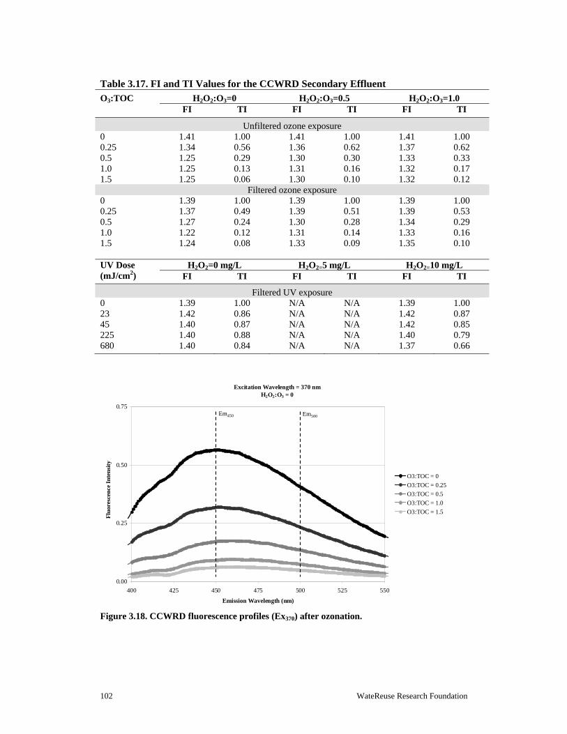
102 WateReuse Research Foundation
Table 3.17. FI and TI Values for the CCWRD Secondary Effluent
O3:TOC H2O2:O3=0 H2O2:O3=0.5 H2O2:O3=1.0 FI TI FI TI FI TI
Unfiltered ozone exposure 0 1.41 1.00 1.41 1.00 1.41 1.00 0.25 1.34 0.56 1.36 0.62 1.37 0.62 0.5 1.25 0.29 1.30 0.30 1.33 0.33 1.0 1.25 0.13 1.31 0.16 1.32 0.17 1.5 1.25 0.06 1.30 0.10 1.32 0.12
Filtered ozone exposure 0 1.39 1.00 1.39 1.00 1.39 1.00 0.25 1.37 0.49 1.39 0.51 1.39 0.53 0.5 1.27 0.24 1.30 0.28 1.34 0.29 1.0 1.22 0.12 1.31 0.14 1.33 0.16 1.5 1.24 0.08 1.33 0.09 1.35 0.10
UV Dose (mJ/cm2)
H2O2=0 mg/L H2O2=5 mg/L H2O2=10 mg/L FI TI FI TI FI TI
Filtered UV exposure 0 1.39 1.00 N/A N/A 1.39 1.00 23 1.42 0.86 N/A N/A 1.42 0.87 45 1.40 0.87 N/A N/A 1.42 0.85 225 1.40 0.88 N/A N/A 1.40 0.79 680 1.40 0.84 N/A N/A 1.37 0.66
Figure 3.18. CCWRD fluorescence profiles (Ex370) after ozonation.
Excitation Wavelength = 370 nmH2O2:O3 = 0
0.00
0.25
0.50
0.75
400 425 450 475 500 525 550
Emission Wavelength (nm)
Flu
ores
cen
ce I
nten
sity
O3:TOC = 0
O3:TOC = 0.25
O3:TOC = 0.5
O3:TOC = 1.0
O3:TOC = 1.5
Flu
ores
cen
ce I
nten
sity
Em450 Em500
Excitation Wavelength = 370 nmH2O2:O3 = 0
0.00
0.25
0.50
0.75
400 425 450 475 500 525 550
Emission Wavelength (nm)
Flu
ores
cen
ce I
nten
sity
O3:TOC = 0
O3:TOC = 0.25
O3:TOC = 0.5
O3:TOC = 1.0
O3:TOC = 1.5
Flu
ores
cen
ce I
nten
sity
Em450 Em500

WateReuse Research Foundation 103
Figure 3.19. Changes in fluorescence intensity after ozonation for CCWRD. H2O2:O3=0.
Figure 3.20. Changes in fluorescence intensity after UV/H2O2 for CCWRD. H2O2=10 mg/L.
0
5,000
10,000
15,000
20,000
25,000
30,000
35,000
40,000
0 0.25 0.5 0.75 1 1.25 1.5
O3:TOC Ratio
Flu
ores
cenc
e In
ten
sity
(un
itle
ss)
Total Fluorescence Fulvic Acids Proteins and Soluble Microbial Products Humic Acids
Flu
ores
cen
ce I
nte
nsi
ty (
un
itle
ss)
0
5,000
10,000
15,000
20,000
25,000
30,000
35,000
40,000
0 0.25 0.5 0.75 1 1.25 1.5
O3:TOC Ratio
Flu
ores
cenc
e In
ten
sity
(un
itle
ss)
Total Fluorescence Fulvic Acids Proteins and Soluble Microbial Products Humic Acids
Flu
ores
cen
ce I
nte
nsi
ty (
un
itle
ss)
0
5,000
10,000
15,000
20,000
25,000
30,000
35,000
40,000
0 100 200 300 400 500 600 700
UV Dose (mJ/cm2)
Flu
ores
cenc
e In
ten
sity
(un
itle
ss)
Total Fluorescence Fulvic Acids Proteins and Soluble Microbial Products Humic Acids
Flu
ores
cen
ce I
nte
nsi
ty (
un
itle
ss)
0
5,000
10,000
15,000
20,000
25,000
30,000
35,000
40,000
0 100 200 300 400 500 600 700
UV Dose (mJ/cm2)
Flu
ores
cenc
e In
ten
sity
(un
itle
ss)
Total Fluorescence Fulvic Acids Proteins and Soluble Microbial Products Humic Acids
Flu
ores
cen
ce I
nte
nsi
ty (
un
itle
ss)

104 WateReuse Research Foundation
3.2 Metropolitan Water Reclamation District of Greater Chicago, Chicago, IL
The Metropolitan Water Reclamation District of Greater Chicago (MWRDGC) operates seven wastewater treatment facilities. The MWRDGC study site treats approximately 240 MGD of wastewater, composed primarily of domestic flows with minor industrial contributions. The liquid treatment train consists of preliminary screening, grit removal, primary clarification, conventional activated sludge, and secondary clarification. The activated sludge process operates with an SRT ranging from 7 to 14 days in the summer and winter, respectively, and achieves full nitrification and incidental partial denitrification. The secondary effluent is discharged to the North Shore Channel without filtration or disinfection. Therefore, this data set does not include evaluations of “finished” effluent. A simplified treatment schematic of the facility is provided in Figure 3.21. Unfiltered secondary effluent from the MWRDGC facility was collected in August 2010, and the initial water quality data in Table 3.18 were obtained. Using the initial TOC and nitrite data, the ozone dosing conditions in Table 3.19 were calculated.
Figure 3.21. Simplified treatment schematic for the MWRDGC facility.
Table 3.18. Initial Water Quality Data for MWRDGC Unfiltered Secondary Effluent
pH 7.6 TOC (mg/L) 5.7 UV254 absorbance cm-1 0.108 TSS (mg/L) <5 Turbidity (NTU) 0.50 Alkalinity (mg/L) 134 TN (mg-N/L) 9.80 TKN (mg-N/L)a 0.70 TON (mg-N/L)b 0.63 NH3 (mg-N/L) 0.07 NO3 (mg-N/L) 9.10 NO2 (mg-N/L) <0.05 Bromide (μg/L) 93 NDMA (ng/L) <2.5
Filtered Secondary Effluent
pH 7.6 TOC (mg/L) 6.9 UV254 absorbance (cm-1) 0.131 TSS (mg/L) <5 Turbidity (NTU) 0.35
aTotal Kjeldahl Nitrogen: sum of total organic nitrogen and ammonia. bTotal organic nitrogen: difference between total nitrogen and ammonia, nitrate, and nitrite.
1° North Shore Channel
2°CASPreliminary 1°1° North Shore Channel
2°CAS 2°CASPreliminary
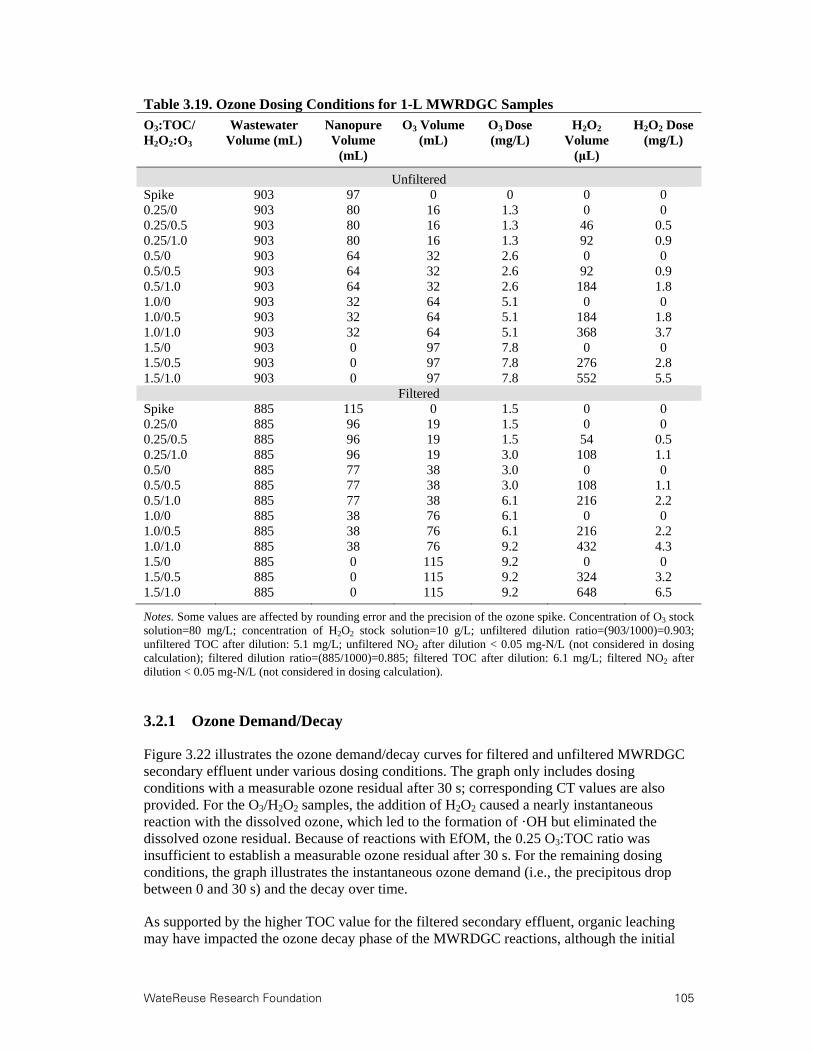
WateReuse Research Foundation 105
Table 3.19. Ozone Dosing Conditions for 1-L MWRDGC Samples
O3:TOC/ H2O2:O3
Wastewater Volume (mL)
Nanopure Volume
(mL)
O3 Volume (mL)
O3 Dose (mg/L)
H2O2 Volume
(μL)
H2O2 Dose (mg/L)
Unfiltered Spike 903 97 0 0 0 0 0.25/0 903 80 16 1.3 0 0 0.25/0.5 903 80 16 1.3 46 0.5 0.25/1.0 903 80 16 1.3 92 0.9 0.5/0 903 64 32 2.6 0 0 0.5/0.5 903 64 32 2.6 92 0.9 0.5/1.0 903 64 32 2.6 184 1.8 1.0/0 903 32 64 5.1 0 0 1.0/0.5 903 32 64 5.1 184 1.8 1.0/1.0 903 32 64 5.1 368 3.7 1.5/0 903 0 97 7.8 0 0 1.5/0.5 903 0 97 7.8 276 2.8 1.5/1.0 903 0 97 7.8 552 5.5
Filtered Spike 885 115 0 1.5 0 0 0.25/0 885 96 19 1.5 0 0 0.25/0.5 885 96 19 1.5 54 0.5 0.25/1.0 885 96 19 3.0 108 1.1 0.5/0 885 77 38 3.0 0 0 0.5/0.5 885 77 38 3.0 108 1.1 0.5/1.0 885 77 38 6.1 216 2.2 1.0/0 885 38 76 6.1 0 0 1.0/0.5 885 38 76 6.1 216 2.2 1.0/1.0 885 38 76 9.2 432 4.3 1.5/0 885 0 115 9.2 0 0 1.5/0.5 885 0 115 9.2 324 3.2 1.5/1.0 885 0 115 9.2 648 6.5
Notes. Some values are affected by rounding error and the precision of the ozone spike. Concentration of O3 stock solution=80 mg/L; concentration of H2O2 stock solution=10 g/L; unfiltered dilution ratio=(903/1000)=0.903; unfiltered TOC after dilution: 5.1 mg/L; unfiltered NO2 after dilution < 0.05 mg-N/L (not considered in dosing calculation); filtered dilution ratio=(885/1000)=0.885; filtered TOC after dilution: 6.1 mg/L; filtered NO2 after dilution < 0.05 mg-N/L (not considered in dosing calculation).
3.2.1 Ozone Demand/Decay
Figure 3.22 illustrates the ozone demand/decay curves for filtered and unfiltered MWRDGC secondary effluent under various dosing conditions. The graph only includes dosing conditions with a measurable ozone residual after 30 s; corresponding CT values are also provided. For the O3/H2O2 samples, the addition of H2O2 caused a nearly instantaneous reaction with the dissolved ozone, which led to the formation of ·OH but eliminated the dissolved ozone residual. Because of reactions with EfOM, the 0.25 O3:TOC ratio was insufficient to establish a measurable ozone residual after 30 s. For the remaining dosing conditions, the graph illustrates the instantaneous ozone demand (i.e., the precipitous drop between 0 and 30 s) and the decay over time.
As supported by the higher TOC value for the filtered secondary effluent, organic leaching may have impacted the ozone decay phase of the MWRDGC reactions, although the initial

106 WateReuse Research Foundation
ozone demand was similar between the filtered and unfiltered samples. Although this affects the overall CT values for the higher applied ozone doses, the effect on oxidation efficacy may be insignificant, as many of the reactions occur rapidly, as demonstrated by the reaction time experiments for the CCWRD secondary effluent.
Figure 3.22. Ozone demand/decay curves for MWRDGC.
3.2.2 Bromate Formation
As illustrated in Figure 3.23, limited bromate formation occurred during ozonation of the MWRDGC secondary effluent. The bromate levels were lower than those observed during the CCWRD experiments, which is likely attributable to the lower bromide concentrations, and the filtered and unfiltered samples also yielded similar bromate formation. With respect to magnitude, the O3:TOC ratio of 0.25 rarely produced bromate levels >MRL, and the O3:TOC ratio of 0.5 was also <MRL or <10 μg/L for all samples. The 1.0 and 1.5 O3:TOC ratios did not yield substantial bromate formation, but the samples did exceed the 10 μg/L benchmark in all samples. Similarly to CCWRD, the addition of H2O2 provided some degree of bromate mitigation. To achieve the 10 μg/L treatment objective, the applied ozone dose would be limited to an O3:TOC ratio <1.0 or the process would have to be supplemented with substantial H2O2 doses (assuming no other mitigation measures are implemented).

WateReuse Research Foundation 107
Figure 3.23. Bromate formation during ozonation of MWRDGC secondary effluent.
3.2.3 ·OH Exposure
Based on data from bench-scale experiments with pCBA spiked at 500 μg/L, Table 3.20 indicates the overall ·OH exposure for each ozone and UV dosing condition. The ·OH exposures for the UV/H2O2 samples are corrected for the low level of pCBA degradation achieved by photolysis alone.
For MWRDGC, filtration had a slight negative impact on ·OH exposure because of organic leaching from the cartridge filters, but similarly to CCWRD, H2O2 addition had no significant impact on ·OH exposure. Therefore, assuming the dissolved ozone residual is allowed to react completely, the overall ·OH exposure in wastewater is independent of the H2O2 dose. However, for the highest O3:TOC ratio, the overall reaction time can be reduced from nearly

108 WateReuse Research Foundation
12 min (see Figure 3.22) to several seconds by addition of H2O2. Ozone-based oxidation also provided higher ·OH exposures than the UV dosing conditions applied during these experiments. With 10 mg/L of H2O2 for the UV AOP, UV doses of 250 mJ/cm2 and 500 mJ/cm2 were nearly equivalent to O3:TOC ratios of 0.25 and 0.5, respectively. Table 3.20. ·OH Exposure in the MWRDGC Secondary Effluent
Ozone:TOC H2O2:O3=0 H2 O2:O3=0.5 H2O2:O3=1.0
Unfiltered ozone exposure (10-11 M-s) 0.25 5.6 5.9 6.1 0.5 14 11 16 1.0 39 41 33 1.5 71 79 61
Filtered ozone exposure (10-11 M-s) 0.25 3.8 4.4 5.0 0.5 10 12 11 1.0 26 28 26 1.5 47 52 48
UV Dose (mJ/cm2) H2O2=0 mg/L H2O2=5 mg/L H2O2=10 mg/L
Filtered UV exposure (10-11 M-s) 0 N/A N/A 0.61a 50 N/A N/A 0.84 250 N/A 4.5 6.5 500 N/A 6.7 12
aBased on H2O2 control.
3.2.4 Title 22 Contaminants
Bench-scale experiments were performed with the filtered MWRDGC wastewater to evaluate the use of ozone and UV for the destruction of spiked NDMA (120 ng/L) and 1,4-dioxane (750 μg/L). Figure 3.24 indicates that UV doses ranging from 600 to 700 mJ/cm2 were necessary to satisfy the Title 22 NDMA requirement. O3:TOC ratios >1.0 achieved net NDMA destruction (data not shown) because of limited direct formation during ozonation (see Table 3.21). However, NDMA is highly resistant to ·OH oxidation so the extent of NDMA mitigation was insignificant (<0.1 log), particularly considering the high ozone doses required.

WateReuse Research Foundation 109
Figure 3.24. Destruction of NDMA in the filtered MWRDGC secondary effluent.
Table 3.21. Direct NDMA Formation in the Filtered MWRDGC Secondary Effluent
O3:TOC Ratio H2O2:O3 Ratio NDMA (ng/L)
0 0 <2.5 0.5 0 9.8 0.5 0.5 11 1.0 0 9.2 1.0 0.5 10
Table 3.22 illustrates the potential reductions in NDMA formation potential provided by ozonation and UV-based oxidation. With respect to the secondary effluent, the overall NDMA formation potential with chloramination was lower than that at CCWRD. Because direct NDMA formation with ozonation was also lower in the MWRDGC secondary effluent, standard chloramine-based formation potential tests may also provide insight for ozone. Similarly to CCWRD, ozonation achieved reductions in overall NDMA formation potential ranging from 85% to 92%, although increased ozone doses did not necessarily lead to greater reductions in formation potential. Accounting for the Day 0 concentrations, the overall reduction reaches 95% based on the available data. Also similarly to CCWRD, UV and UV/H2O2 achieved limited reductions in formation potential, with the maximum reduction of 34% occurring with a UV dose of 500 mJ/cm2 and an H2O2 dose of 10 mg/L.
Figure 3.25 illustrates the destruction of spiked 1,4-dioxane during the bench-scale ozone experiments. In general, O3 and O3/H2O2 achieved similar levels of treatment, although the trend lines suggest that O3/H2O2 provided a slight advantage. For MWRDGC, O3:TOC ratios >1.5 are necessary to comply with the 0.5-log requirement.
0.0
0.2
0.4
0.6
0.8
1.0
1.2
1.4
1.6
0 100 200 300 400 500 600 700
UV Dose (mJ/cm2)
Log
Des
truc
tion
of
ND
MA
CDPH Title 22
Log
Des
tru
ctio
n o
f N
DM
A
UV (H2O2=0 mg/L) UV (H2O2=5 mg/L) UV (H2O2=10 mg/L)
0.0
0.2
0.4
0.6
0.8
1.0
1.2
1.4
1.6
0 100 200 300 400 500 600 700
UV Dose (mJ/cm2)
Log
Des
truc
tion
of
ND
MA
CDPH Title 22
Log
Des
tru
ctio
n o
f N
DM
A
UV (H2O2=0 mg/L) UV (H2O2=5 mg/L) UV (H2O2=10 mg/L)
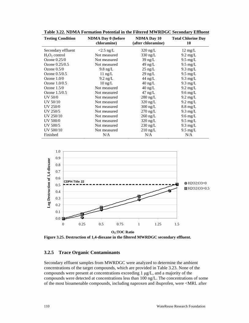
110 WateReuse Research Foundation
Table 3.22. NDMA Formation Potential in the Filtered MWRDGC Secondary Effluent
Testing Condition NDMA Day 0 (before chloramine)
NDMA Day 10 (after chloramine)
Total Chlorine Day 10
Secondary effluent <2.5 ng/L 320 ng/L 12 mg/L H2O2 control Not measured 330 ng/L 9.2 mg/L Ozone 0.25/0 Not measured 39 ng/L 9.5 mg/L Ozone 0.25/0.5 Not measured 49 ng/L 9.5 mg/L Ozone 0.5/0 9.8 ng/L 25 ng/L 9.3 mg/L Ozone 0.5/0.5 11 ng/L 29 ng/L 9.5 mg/L Ozone 1.0/0 9.2 ng/L 44 ng/L 9.3 mg/L Ozone 1.0/0.5 10 ng/L 40 ng/L 9.3 mg/L Ozone 1.5/0 Not measured 40 ng/L 9.2 mg/L Ozone 1.5/0.5 Not measured 47 ng/L 9.6 mg/L UV 50/0 Not measured 280 ng/L 9.2 mg/L UV 50/10 Not measured 320 ng/L 9.2 mg/L UV 250/0 Not measured 300 ng/L 8.8 mg/L UV 250/5 Not measured 270 ng/L 9.3 mg/L UV 250/10 Not measured 260 ng/L 9.6 mg/L UV 500/0 Not measured 320 ng/L 9.5 mg/L UV 500/5 Not measured 230 ng/L 9.3 mg/L UV 500/10 Not measured 210 ng/L 9.5 mg/L Finished N/A N/A N/A
Figure 3.25. Destruction of 1,4-dioxane in the filtered MWRDGC secondary effluent.
3.2.5 Trace Organic Contaminants
Secondary effluent samples from MWRDGC were analyzed to determine the ambient concentrations of the target compounds, which are provided in Table 3.23. None of the compounds were present at concentrations exceeding 1 μg/L, and a majority of the compounds were detected at concentrations less than 100 ng/L. The concentrations of some of the most bioamenable compounds, including naproxen and ibuprofen, were <MRL after
0.0
0.1
0.2
0.3
0.4
0.5
0.6
0.7
0.8
0.9
1.0
0 0.25 0.5 0.75 1 1.25 1.5
O3:TOC Ratio
Log
Des
tru
ctio
n o
f 1,
4-d
ioxa
ne
H2O2:O3=0H2O2:O3=0.5
CDPH Title 22
Log
Des
tru
ctio
n o
f 1,
4-d
ioxa
ne
0.0
0.1
0.2
0.3
0.4
0.5
0.6
0.7
0.8
0.9
1.0
0 0.25 0.5 0.75 1 1.25 1.5
O3:TOC Ratio
Log
Des
tru
ctio
n o
f 1,
4-d
ioxa
ne
H2O2:O3=0H2O2:O3=0.5
CDPH Title 22
Log
Des
tru
ctio
n o
f 1,
4-d
ioxa
ne
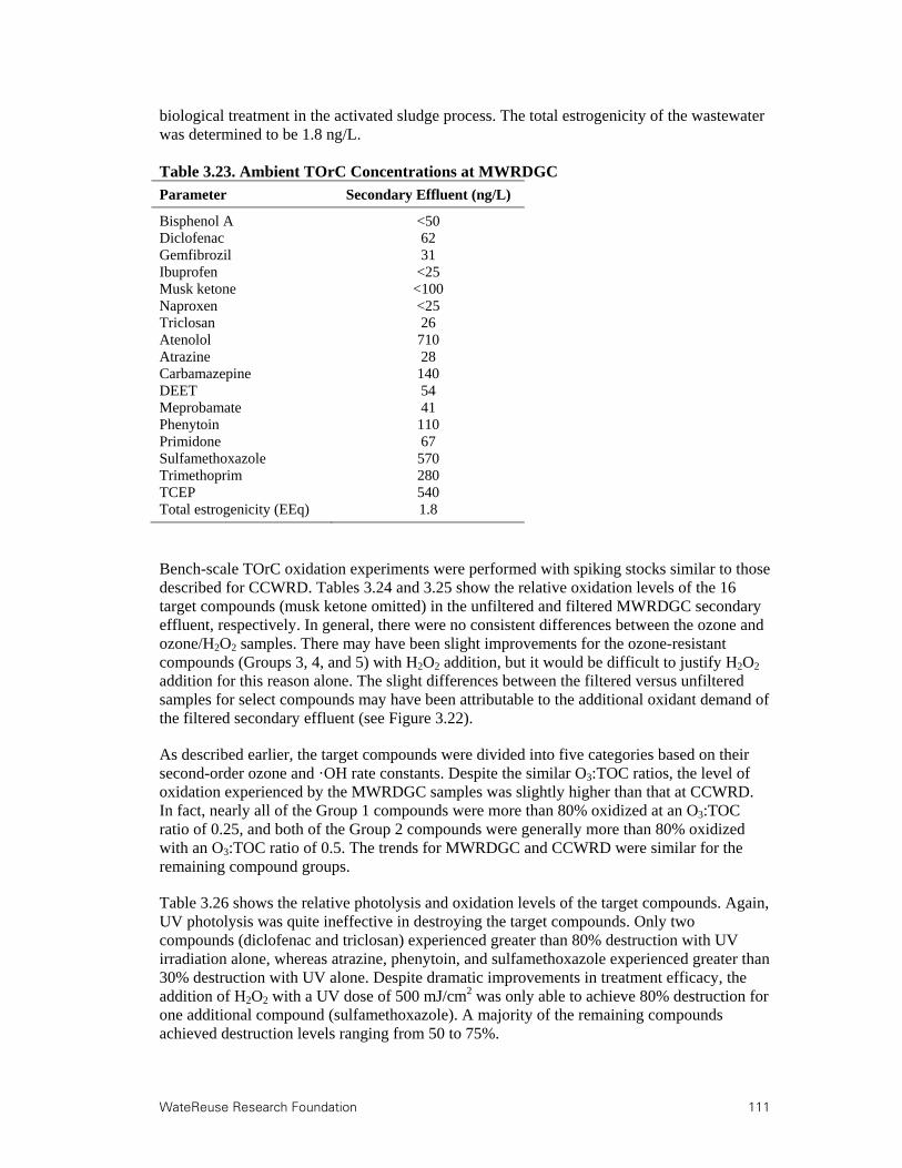
WateReuse Research Foundation 111
biological treatment in the activated sludge process. The total estrogenicity of the wastewater was determined to be 1.8 ng/L. Table 3.23. Ambient TOrC Concentrations at MWRDGC
Parameter Secondary Effluent (ng/L)
Bisphenol A <50 Diclofenac 62 Gemfibrozil 31 Ibuprofen <25 Musk ketone <100 Naproxen <25 Triclosan 26 Atenolol 710 Atrazine 28 Carbamazepine 140 DEET 54 Meprobamate 41 Phenytoin 110 Primidone 67 Sulfamethoxazole 570 Trimethoprim 280 TCEP 540 Total estrogenicity (EEq) 1.8
Bench-scale TOrC oxidation experiments were performed with spiking stocks similar to those described for CCWRD. Tables 3.24 and 3.25 show the relative oxidation levels of the 16 target compounds (musk ketone omitted) in the unfiltered and filtered MWRDGC secondary effluent, respectively. In general, there were no consistent differences between the ozone and ozone/H2O2 samples. There may have been slight improvements for the ozone-resistant compounds (Groups 3, 4, and 5) with H2O2 addition, but it would be difficult to justify H2O2 addition for this reason alone. The slight differences between the filtered versus unfiltered samples for select compounds may have been attributable to the additional oxidant demand of the filtered secondary effluent (see Figure 3.22).
As described earlier, the target compounds were divided into five categories based on their second-order ozone and ·OH rate constants. Despite the similar O3:TOC ratios, the level of oxidation experienced by the MWRDGC samples was slightly higher than that at CCWRD. In fact, nearly all of the Group 1 compounds were more than 80% oxidized at an O3:TOC ratio of 0.25, and both of the Group 2 compounds were generally more than 80% oxidized with an O3:TOC ratio of 0.5. The trends for MWRDGC and CCWRD were similar for the remaining compound groups.
Table 3.26 shows the relative photolysis and oxidation levels of the target compounds. Again, UV photolysis was quite ineffective in destroying the target compounds. Only two compounds (diclofenac and triclosan) experienced greater than 80% destruction with UV irradiation alone, whereas atrazine, phenytoin, and sulfamethoxazole experienced greater than 30% destruction with UV alone. Despite dramatic improvements in treatment efficacy, the addition of H2O2 with a UV dose of 500 mJ/cm2 was only able to achieve 80% destruction for one additional compound (sulfamethoxazole). A majority of the remaining compounds achieved destruction levels ranging from 50 to 75%.

112 WateReuse Research Foundation
Finally, the total estrogenicity of the secondary effluent was oxidized down to the MRL with every ozone and ozone/H2O2 dosing condition. On the other hand, neither UV nor UV/H2O2 was particularly effective in reducing total estrogenicity, but the MRL was eventually achieved with a UV dose of 500 mJ/cm2 and an H2O2 dose of 5 or 10 mg/L. These results are summarized in Figure 3.26.
Figure 3.26. Reduction in total estrogenicity in the filtered MWRDGC secondary effluent.

WateReuse Research Foundation 113
Table 3.24. MWRDGC TOrC Mitigation by Ozone (Unfiltered)
Group Contaminant O3:TOC (mass) / H2O2:O3 (molar)
0.25/0 0.25/0.5 0.25/1.0 0.5/0 0.5/0.5 0.5/1.0 1.0/0 1.0/0.5 1.0/1.0 1.5/0 1.5/0.5 1.5/1.0
1 Sulfamethoxazole 90% 83% 76% 98% 98% 98% 98% 98% 98% 98% 98% 98% Diclofenac 93% 88% 81% 97% 97% 97% 97% 97% 97% 97% 97% 97% Bisphenol A 97% 94% 85% 97% 97% 97% 97% 97% 97% 97% 97% 97% Carbamazepine 92% 88% 82% 99% 99% 99% 99% 99% 99% 99% 99% 99% Trimethoprim 91% 85% 77% 99% 99% 99% 99% 99% 99% 99% 99% 99% Naproxen 91% 85% 79% 98% 98% 98% 98% 98% 98% 98% 98% 98% Triclosan 97% 97% 92% 97% 62% 97% 97% 97% 97% 97% 97% 97% Indicator 93% 89% 82% 98% 93% 98% 98% 98% 98% 98% 98% 98%
2 Gemfibrozil 79% 77% 70% 99% 98% 99% 99% 99% 99% 99% 99% 99% Atenolol 54% 51% 51% 84% 72% 94% 98% 98% 98% 98% 98% 98% Indicator 67% 64% 61% 92% 85% 97% 99% 99% 99% 99% 99% 99%
3 Ibuprofen 34% 36% 34% 46% 55% 79% 97% 97% 96% 97% 97% 97% Phenytoin 31% 38% 28% 46% 51% 80% 97% 97% 96% 99% 99% 99% DEET 29% 35% 29% 46% 49% 74% 94% 95% 94% 99% 99% 99% Primidone 22% 33% 28% 44% 39% 70% 94% 94% 92% 99% 99% 99% Indicator 29% 36% 30% 46% 49% 76% 96% 96% 95% 99% 99% 99%
4 Atrazine 11% 12% 9% 20% 20% 38% 69% 72% 71% 89% 91% 89% Meprobamate 19% 18% 15% 27% 25% 52% 78% 82% 81% 93% 96% 95% Indicator 15% 15% 12% 24% 23% 45% 74% 77% 76% 91% 94% 92%
5 TCEP 4% 5% 2% 2% 5% 7% 14% 19% 21% 23% 32% 30%
Note: Shading represents >80% oxidation.

114 WateReuse Foundation
Table 3.25. MWRDGC TOrC Mitigation by Ozone (Filtered)
Group Contaminant O3:TOC (mass) / H2O2:O3 (molar)
0.25/0 0.25/0.5 0.25/1.0 0.5/0 0.5/0.5 0.5/1.0 1.0/0 1.0/0.5 1.0/1.0 1.5/0 1.5/0.5 1.5/1.0
1 Sulfamethoxazole 95% 94% 91% 98% 98% 98% 98% 98% 98% 98% 98% 98% Diclofenac 97% 97% 97% 97% 97% 97% 97% 97% 97% 97% 97% 97% Bisphenol A 97% 97% 97% 97% 97% 97% 97% 97% 97% 97% 97% 97% Carbamazepine 99% 99% 99% 99% 99% 99% 99% 99% 99% 99% 99% 99% Trimethoprim 99% 99% 98% 99% 99% 99% 99% 99% 99% 99% 99% 99% Naproxen 98% 98% 94% 98% 98% 98% 98% 98% 98% 98% 98% 98% Triclosan 97% 97% 97% 97% 97% 97% 97% 97% 97% 97% 97% 97% Indicator 97% 97% 96% 98% 98% 98% 98% 98% 98% 98% 98% 98%
2 Gemfibrozil 96% 90% 70% 99% 99% 99% 99% 99% 99% 99% 99% 99% Atenolol 57% 53% 49% 98% 98% 94% 98% 98% 98% 98% 98% 98% Indicator 77% 72% 60% 99% 99% 97% 99% 99% 99% 99% 99% 99%
3 Ibuprofen 27% 33% 33% 59% 65% 65% 89% 91% 90% 98% 98% 96% Phenytoin 12% 20% 24% 48% 61% 60% 89% 92% 89% 97% 99% 96% DEET 13% 19% 19% 43% 51% 52% 80% 85% 84% 95% 97% 93% Primidone 24% 29% 33% 48% 58% 59% 84% 86% 86% 96% 96% 93% Indicator 19% 25% 27% 50% 59% 59% 86% 89% 87% 97% 98% 95%
4 Atrazine 9% 11% 11% 24% 29% 29% 53% 53% 56% 74% 76% 73% Meprobamate 10% 13% 15% 29% 36% 38% 62% 65% 67% 81% 86% 83% Indicator 10% 12% 13% 27% 33% 34% 58% 59% 62% 78% 81% 78%
5 TCEP 1% 10% 10% 13% 13% 13% 16% 11% 16% 20% 24% 26%
Note: Shading represents >80% oxidation.

WateReuse Research Foundation 115
Table 3.26. MWRDGC TOrC Mitigation by UV (Filtered)
Group Contaminant UV Dose (mJ/cm2) / H2O2 Dose (mg/L)
50/0 50/10 250/0 250/5 250/10 500/0 500/5 500/10
1 Sulfamethoxazole -4% -4% 37% 51% 58% 65% 71% 80%
Diclofenac 40% 41% 89% 94% 97% 97% 97% 97% Bisphenol A 6% -6% 6% 22% 46% 6% 28% 71% Carbamazepine 9% 9% 0% 21% 43% 0% 22% 62% Trimethoprim 3% 3% 3% 17% 34% -3% 17% 54% Naproxen 8% 17% 8% 31% 53% 18% 38% 73% Triclosan 10% 18% 70% 83% 89% 93% 95% 97%
2 Gemfibrozil 8% 5% 3% 19% 40% 4% 5% 60% Atenolol 10% 10% -3% 16% 29% 3% 10% 55%
3 Ibuprofen 8% 8% 6% 25% 40% 7% 22% 62% Phenytoin 6% 11% 32% 41% 56% 44% 55% 79% DEET 9% 9% 9% 21% 33% 9% 15% 52% Primidone 8% 8% 3% 18% 38% 8% 18% 52%
4 Atrazine 7% 1% 17% 24% 35% 33% 27% 56% Meprobamate 7% 3% 3% 10% 22% 2% 3% 36%
5 TCEP 10% 17% 17% 18% 20% 13% -4% 26%
Notes. Shading represents >80% photolysis or oxidation. Groupings refer to ozone and ·OH rate constants.
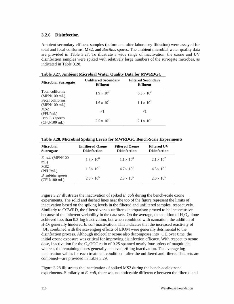
116 WateReuse Foundation
3.2.6 Disinfection
Ambient secondary effluent samples (before and after laboratory filtration) were assayed for total and fecal coliforms, MS2, and Bacillus spores. The ambient microbial water quality data are provided in Table 3.27. To illustrate a wide range of inactivation, the ozone and UV disinfection samples were spiked with relatively large numbers of the surrogate microbes, as indicated in Table 3.28. Table 3.27. Ambient Microbial Water Quality Data for MWRDGC
Microbial Surrogate Unfiltered Secondary
Effluent Filtered Secondary
Effluent
Total coliforms (MPN/100 mL)
1.9 103 6.3 102
Fecal coliforms (MPN/100 mL) 1.6 102 1.1 102
MS2 (PFU/mL)
<1 <1
Bacillus spores (CFU/100 mL) 2.5 103 2.1 103
Table 3.28. Microbial Spiking Levels for MWRDGC Bench-Scale Experiments
Microbial Surrogate
Unfiltered Ozone Disinfection
Filtered Ozone Disinfection
Filtered UV Disinfection
E. coli (MPN/100 mL)
1.3 108 1.1 108 2.1 107
MS2 (PFU/mL) 1.5 107 4.7 107 4.3 107
B. subtilis spores (CFU/100 mL) 2.6 105 2.3 105 2.0 105
Figure 3.27 illustrates the inactivation of spiked E. coli during the bench-scale ozone experiments. The solid and dashed lines near the top of the figure represent the limits of inactivation based on the spiking levels in the filtered and unfiltered samples, respectively. Similarly to CCWRD, the filtered versus unfiltered comparison proved to be inconclusive because of the inherent variability in the data sets. On the average, the addition of H2O2 alone achieved less than 0.3-log inactivation, but when combined with ozonation, the addition of H2O2 generally hindered E. coli inactivation. This indicates that the increased reactivity of ·OH combined with the scavenging effects of EfOM were generally detrimental to the disinfection process. Although molecular ozone also decomposes into ·OH over time, the initial ozone exposure was critical for improving disinfection efficacy. With respect to ozone dose, inactivation for the O3:TOC ratio of 0.25 spanned nearly four orders of magnitude, whereas the remaining doses generally achieved >6-log inactivation. The average log-inactivation values for each treatment condition—after the unfiltered and filtered data sets are combined—are provided in Table 3.29.
Figure 3.28 illustrates the inactivation of spiked MS2 during the bench-scale ozone experiments. Similarly to E. coli, there was no noticeable difference between the filtered and

WateReuse Research Foundation 117
unfiltered samples, and the addition of H2O2 alone achieved less than 0.3-log inactivation. However, the negative impact of H2O2 was not as consistent for MS2 inactivation. With respect to the CDPH Title 22 requirements, an O3:TOC ratio >0.5 was often sufficient for the 5- and 6.5-log inactivation requirements, but there were several samples within this dosing range that did not satisfy this treatment objective. The average log-inactivation values for each treatment condition (combined unfiltered and filtered data) are provided in Table 3.30.
Figure 3.29 illustrates the inactivation of spiked B. subtilis spores during the bench-scale ozone experiments. The spores proved to be extremely resistant to oxidation and only experienced significant inactivation for O3:TOC ratios >1.0 with no H2O2 addition. In other words, a sufficient ozone CT had to be administered before ozone and ·OH were able to penetrate the spore coat and inactivate the bacteria. Similarly to CCWRD, there appears to be a significant difference between the unfiltered and filtered samples at an O3:TOC ratio of 1.0 (no H2O2 addition), but this is likely attributable to inherent variability rather than the effect of filtration. It is important to reiterate that oxidation with ·OH alone (i.e., with H2O2 addition) is extremely ineffective for spore inactivation, presumably because of the highly reactive nature of ·OH and competition with EfOM. The average log-inactivation values for each treatment condition (combined unfiltered and filtered data) are provided in Table 3.31.
Finally, Figure 3.30 provides a summary of the ozone disinfection data for the three surrogate microbes with respect to the CT framework. Figure 3.30A illustrates the dose–response relationships for the filtered and unfiltered samples (combined) with no H2O2 addition. Figure 3.30B illustrates the dose–response relationships for the filtered and unfiltered samples (combined) with H2O2:O3 ratios of 0.5 and 1.0 (also combined). According to these data, the CT framework is not always appropriate because substantial levels of inactivation can be achieved when the apparent ozone CT is zero. However, the level of inactivation for vegetative bacteria and viruses is generally less than that observed when an ozone residual is present, and no inactivation of spore-forming bacteria can be achieved without a measurable CT.
Table 3.32 summarizes the efficacy of UV and UV/H2O2 for the inactivation of the three surrogate microbes. The efficacy of UV-based disinfection differs dramatically from that of ozone-based disinfection because UV is highly effective against both vegetative and spore-forming bacteria, whereas some viruses demonstrate resistance. A dose of 50 mJ/cm2 was sufficient to reach the limits of inactivation for E. coli and Bacillus spores, regardless of H2O2 addition. On the other hand, MS2 inactivation occurred more slowly and only reached the limit of inactivation with a UV dose of 250 mJ/cm2. Although the 500 mJ/cm2 sample did not technically reach the limit of inactivation, the MS2 levels in those samples were extremely low. Particularly with respect to advanced oxidation dosing conditions (i.e., >250 mJ/cm2 with 10 mg/L of H2O2), one can expect substantial inactivation of all microbes present in wastewater. This constitutes a significant advantage for UV-based treatment over the ozone-based alternatives.

118 WateReuse Foundation
Figure 3.27. Inactivation of spiked E. coli in the MWRDGC secondary effluent.
Table 3.29. Summary of E. coli Inactivation in the MWRDGC Secondary Effluent
O3:TOC Ratio H2O2:O3=0 H2O2:O3=0.5 H2O2:O3=1.0
0.25 2.9 ± 2.4a 1.8 ± 1.5 3.2 ± 0.4 0.5 6.9 ± 0.1 6.5 ± 0.5 6.2 ± 0.6 1.0 8.1 ± N/Ab 6.1 ± 1.3 6.3 ± 0.1 1.5 7.5 ± 0.1 6.8 ± 0.2 6.2 ± 0.3 aAverage log inactivation ± span of filtered/unfiltered samples. bN/A: Filtered sample not collected, so value represents only unfiltered sample.
0
1
2
3
4
5
6
7
8
9
0.00 0.25 0.50 0.75 1.00 1.25 1.50
O3:TOC Ratio
Log
Ina
ctiv
atio
n
Filtered (H2O2:O3=0) Filtered (H2O2:O3=0.5) Filtered (H2O2:O3=1.0)Unfiltered (H2O2:O3=0) Unfiltered (H2O2:O3=0.5) Unfiltered (H2O2:O3=1.0)
E. coli Limits of Inactivation
0
1
2
3
4
5
6
7
8
9
0.00 0.25 0.50 0.75 1.00 1.25 1.50
O3:TOC Ratio
Log
Ina
ctiv
atio
n
Filtered (H2O2:O3=0) Filtered (H2O2:O3=0.5) Filtered (H2O2:O3=1.0)Unfiltered (H2O2:O3=0) Unfiltered (H2O2:O3=0.5) Unfiltered (H2O2:O3=1.0)
E. coli Limits of Inactivation

WateReuse Research Foundation 119
Figure 3.28. Inactivation of spiked MS2 in the MWRDGC secondary effluent.
Table 3.30. Summary of MS2 Inactivation in the MWRDGC Secondary Effluent
O3:TOC Ratio H2O2:O3=0 H2O2:O3=0.5 H2O2:O3=1.0
0.25 2.6 ± 1.7 1.2 ± 0.5 1.3 ± 0.6 0.5 5.8 ± 2.7 5.5 ± 1.7 6.2 ± 0.0 1.0 6.1 ± 2.2 6.7 ± 0.4 5.7 ± 1.9 1.5 7.4 ± 0.4 7.3 ± 0.6 6.8 ± 0.3
Note: Average log inactivation ± span of filtered/unfiltered samples.
0
1
2
3
4
5
6
7
8
9
0.00 0.25 0.50 0.75 1.00 1.25 1.50
O3:TOC Ratio
Log
Ina
ctiv
atio
n
Filtered (H2O2:O3=0) Filtered (H2O2:O3=0.5) Filtered (H2O2:O3=1.0)Unfiltered (H2O2:O3=0) Unfiltered (H2O2:O3=0.5) Unfiltered (H2O2:O3=1.0)
MS2 Limits of Inactivation
0
1
2
3
4
5
6
7
8
9
0.00 0.25 0.50 0.75 1.00 1.25 1.50
O3:TOC Ratio
Log
Ina
ctiv
atio
n
Filtered (H2O2:O3=0) Filtered (H2O2:O3=0.5) Filtered (H2O2:O3=1.0)Unfiltered (H2O2:O3=0) Unfiltered (H2O2:O3=0.5) Unfiltered (H2O2:O3=1.0)
MS2 Limits of Inactivation

120 WateReuse Foundation
Figure 3.29. Inactivation of spiked Bacillus spores in the MWRDGC secondary effluent.
Table 3.31. Summary of Bacillus Spore Inactivation in the MWRDGC Secondary Effluent
O3:TOC Ratio H2O2:O3=0 H2O2:O3=0.5 H2O2:O3=1.0
0.25 0.0 ± 0.0a 0.1 ± 0.0 0.0 ± 0.0 0.5 0.1 ± 0.0 0.0 ± 0.0 0.0 ± 0.1 1.0 1.9 ± 0.7 0.0 ± 0.1 0.0 ± 0.0 1.5 >2.4b ± 0.0 0.1 ± 0.1 0.1 ± 0.1 aAverage log inactivation ± span of filtered/unfiltered samples. bLimit of inactivation based on sample dilutions.
0
1
2
3
4
0.00 0.25 0.50 0.75 1.00 1.25 1.50
O3:TOC Ratio
Log
Ina
ctiv
atio
n
Filtered (H2O2:O3=0) Filtered (H2O2:O3=0.5) Filtered (H2O2:O3=1.0)Unfiltered (H2O2:O3=0) Unfiltered (H2O2:O3=0.5) Unfiltered (H2O2:O3=1.0)
Bacillus spore Limits of Inactivation
0
1
2
3
4
0.00 0.25 0.50 0.75 1.00 1.25 1.50
O3:TOC Ratio
Log
Ina
ctiv
atio
n
Filtered (H2O2:O3=0) Filtered (H2O2:O3=0.5) Filtered (H2O2:O3=1.0)Unfiltered (H2O2:O3=0) Unfiltered (H2O2:O3=0.5) Unfiltered (H2O2:O3=1.0)
Bacillus spore Limits of Inactivation

WateReuse Research Foundation 121
Figure 3.30. Significance of CT for disinfection in the MWRDGC secondary effluent.
0
1
2
3
4
5
6
7
8
9
0.25 0.50 1.00 1.50
O3:TOC Ratio
Log
In
acti
vati
on
0
5
10
15
20
25
30
Ozo
ne
CT
(m
g-m
in/L
Bacillus spore E. coli MS2 CT
A: No H2O2 Addition (combination of filtered and unfiltered samples with H2O2:O3 = 0)
Log
Ina
ctiv
atio
n
Ozo
ne
CT
(m
g-m
in/L
)
0
1
2
3
4
5
6
7
8
9
0.25 0.50 1.00 1.50
O3:TOC Ratio
Log
In
acti
vati
on
0
5
10
15
20
25
30
Ozo
ne
CT
(m
g-m
in/L
Bacillus spore E. coli MS2 CT
A: No H2O2 Addition (combination of filtered and unfiltered samples with H2O2:O3 = 0)
Log
Ina
ctiv
atio
n
Ozo
ne
CT
(m
g-m
in/L
)
0
1
2
3
4
5
6
7
8
9
0.25 0.50 1.00 1.50
O3:TOC Ratio
Log
In
acti
vati
on
0
5
10
15
20
25
30
Ozo
ne
CT
(m
g-m
in/L
Bacillus spore E. coli MS2 CT
B: H2O2 Addition (combination of filtered and unfiltered samples with H2O2:O3 = 0.5 and 1.0
Log
In
acti
vati
on
Ozo
ne
CT
(m
g-m
in/L
)
0
1
2
3
4
5
6
7
8
9
0.25 0.50 1.00 1.50
O3:TOC Ratio
Log
In
acti
vati
on
0
5
10
15
20
25
30
Ozo
ne
CT
(m
g-m
in/L
Bacillus spore E. coli MS2 CT
B: H2O2 Addition (combination of filtered and unfiltered samples with H2O2:O3 = 0.5 and 1.0
Log
In
acti
vati
on
Ozo
ne
CT
(m
g-m
in/L
)

122 WateReuse Foundation
Table 3.32. Summary of UV Inactivation in the MWRDGC Secondary Effluent
UV Dose (mJ/cm2)
E. coli MS2 Bacillus spore UV UV/H2O2
a UV UV/H2O2a UV UV/H2O2
a
25 5.3 N/A N/A N/A 2.9 3.2 50 >7.3b >7.3b 2.9 3.8 >3.3b >3.3b 250 >7.3b >7.3b >7.6b >7.6b >3.3b >3.3b 500 >7.3b >7.3b 7.5 7.2 >3.3b >3.3b aH2O2 doses of 5 and 10 mg/L achieved similar levels of inactivation. bLimit of inactivation based on spiking level .
3.2.7 Organic Characterization
The full-spectrum scans in Figures 3.31 through 3.33 (without (A) and with (B) H2O2 addition) indicate that the absorbance profiles around 254 nm generally provide the greatest resolution between treatments. The absorbance spectra for both sets of ozone experiments are shown, because the filtered samples are characterized by discontinuity at 380 nm that may be attributable to organic leaching from the cartridge filters. Because of the limited efficacy of UV photolysis (Figure 3.33A), there is little resolution regardless of wavelength, whereas UV/H2O2 achieved slight improvements over UV alone. Figure 3.34 focuses on the change in UV254 absorbance with ozone, ozone/H2O2, UV, and UV/H2O2. With respect to ozonation, reductions in UV254 absorbance were hindered by cartridge filtration, which was likely attributable to the small amount of organic leaching and the addition of H2O2. As would be expected because of the synergistic aspect of the UV AOP, the addition of H2O2 during UV irradiation achieved a lower UV254 absorbance.
As described earlier, 3D EEMs were developed for the unfiltered secondary effluent, the filtered secondary effluent, and the various treatment conditions. Figure 3.35 illustrates the fluorescence fingerprint of the secondary effluent samples and also provides the total and regional fluorescence intensities based on arbitrary fluorescence units. The organic leaching from the cartridge filter is apparent because of the higher fluorescence intensity in the filtered ambient sample. Figure 3.36 provides a qualitative illustration of treatment efficacy after ozone- and UV-based oxidation. Similarly to UV absorbance, UV photolysis and UV/H2O2 are not nearly as effective in reducing fluorescence intensity as ozone-based oxidation.
Figures 3.37 and 3.38 illustrate the fluorescence profiles at an excitation wavelength of 254 nm after ozonation and UV/H2O2, respectively. Because the addition of H2O2 did not have a significant impact on ozone efficacy, and UV photolysis provided limited reductions in fluorescence intensity (see Figure 3.36), these fluorescence profiles are not shown.

WateReuse Research Foundation 123
Figure 3.31. MWRDGC absorbance spectra after ozonation (unfiltered).
0
0.03
0.06
0.09
0.12
0.15
240 280 320 360 400 440 480 520 560 600
0
0.03
0.06
0.09
0.12
0.15
240 280 320 360 400 440 480 520 560 600
Ab
sorb
ance
(cm
-1)
Ab
sorb
ance
(cm
-1)
O3:TOC = 0
O3:TOC = 0.25
O3:TOC = 0.5
O3:TOC = 1.0
O3:TOC = 1.5
Wavelength (nm) Wavelength (nm)
O3:TOC = 0
O3:TOC = 0.25
O3:TOC = 0.5
O3:TOC = 1.0
O3:TOC = 1.5
A: H2O2:O3=0 B: H2O2:O3=0.5
0
0.03
0.06
0.09
0.12
0.15
240 280 320 360 400 440 480 520 560 600
0
0.03
0.06
0.09
0.12
0.15
240 280 320 360 400 440 480 520 560 600
Ab
sorb
ance
(cm
-1)
Ab
sorb
ance
(cm
-1)
O3:TOC = 0
O3:TOC = 0.25
O3:TOC = 0.5
O3:TOC = 1.0
O3:TOC = 1.5
Wavelength (nm) Wavelength (nm)
O3:TOC = 0
O3:TOC = 0.25
O3:TOC = 0.5
O3:TOC = 1.0
O3:TOC = 1.5
A: H2O2:O3=0 B: H2O2:O3=0.5
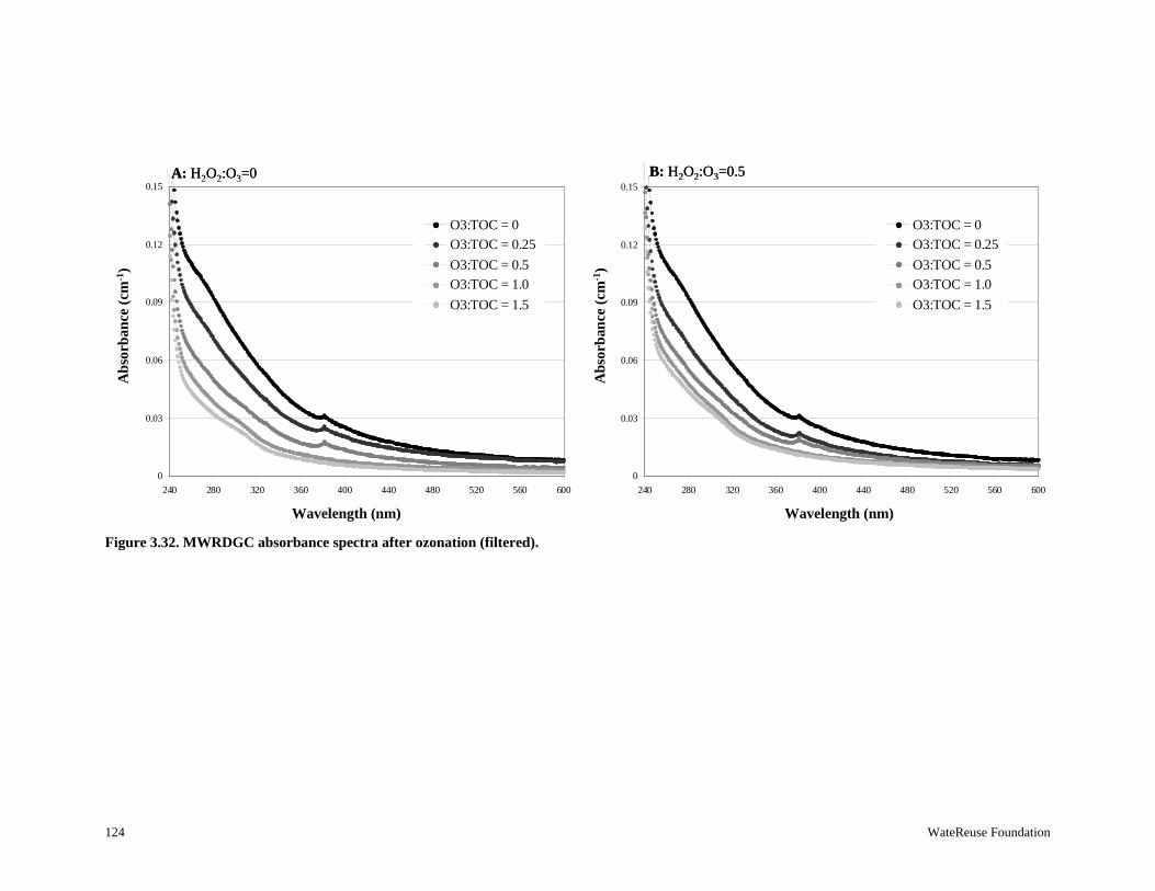
124 WateReuse Foundation
Figure 3.32. MWRDGC absorbance spectra after ozonation (filtered).
0
0.03
0.06
0.09
0.12
0.15
240 280 320 360 400 440 480 520 560 600
0
0.03
0.06
0.09
0.12
0.15
240 280 320 360 400 440 480 520 560 600
Ab
sorb
ance
(cm
-1)
Ab
sorb
ance
(cm
-1)
O3:TOC = 0
O3:TOC = 0.25
O3:TOC = 0.5
O3:TOC = 1.0
O3:TOC = 1.5
Wavelength (nm) Wavelength (nm)
O3:TOC = 0
O3:TOC = 0.25
O3:TOC = 0.5
O3:TOC = 1.0
O3:TOC = 1.5
A: H2O2:O3=0 B: H2O2:O3=0.5
0
0.03
0.06
0.09
0.12
0.15
240 280 320 360 400 440 480 520 560 600
0
0.03
0.06
0.09
0.12
0.15
240 280 320 360 400 440 480 520 560 600
Ab
sorb
ance
(cm
-1)
Ab
sorb
ance
(cm
-1)
O3:TOC = 0
O3:TOC = 0.25
O3:TOC = 0.5
O3:TOC = 1.0
O3:TOC = 1.5
Wavelength (nm) Wavelength (nm)
O3:TOC = 0
O3:TOC = 0.25
O3:TOC = 0.5
O3:TOC = 1.0
O3:TOC = 1.5
A: H2O2:O3=0 B: H2O2:O3=0.5
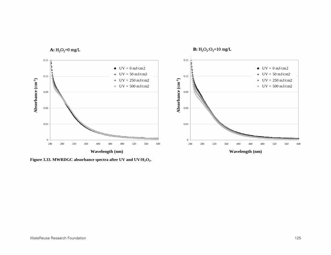
WateReuse Research Foundation 125
Figure 3.33. MWRDGC absorbance spectra after UV and UV/H2O2.
0
0.03
0.06
0.09
0.12
0.15
240 280 320 360 400 440 480 520 560 600
Wavelength (nm)
Ab
sorb
ance
(cm
-1)
0
0.03
0.06
0.09
0.12
0.15
240 280 320 360 400 440 480 520 560 600
Wavelength (nm)
Ab
sorb
ance
(cm
-1)
Ab
sorb
ance
(cm
-1)
Wavelength (nm)
Ab
sorb
ance
(cm
-1)
Wavelength (nm)
A: H2O2=0 mg/L B: H2O2:O3=10 mg/L
UV = 0 mJ/cm2
UV = 50 mJ/cm2
UV = 250 mJ/cm2
UV = 500 mJ/cm2
UV = 0 mJ/cm2
UV = 50 mJ/cm2
UV = 250 mJ/cm2
UV = 500 mJ/cm2
0
0.03
0.06
0.09
0.12
0.15
240 280 320 360 400 440 480 520 560 600
Wavelength (nm)
Ab
sorb
ance
(cm
-1)
0
0.03
0.06
0.09
0.12
0.15
240 280 320 360 400 440 480 520 560 600
Wavelength (nm)
Ab
sorb
ance
(cm
-1)
Ab
sorb
ance
(cm
-1)
Wavelength (nm)
Ab
sorb
ance
(cm
-1)
Wavelength (nm)
A: H2O2=0 mg/L B: H2O2:O3=10 mg/L
UV = 0 mJ/cm2
UV = 50 mJ/cm2
UV = 250 mJ/cm2
UV = 500 mJ/cm2
UV = 0 mJ/cm2
UV = 50 mJ/cm2
UV = 250 mJ/cm2
UV = 500 mJ/cm2
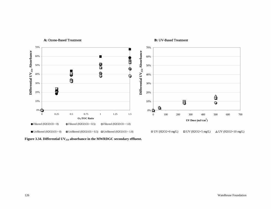
126 WateReuse Foundation
Figure 3.34. Differential UV254 absorbance in the MWRDGC secondary effluent.
0%
10%
20%
30%
40%
50%
60%
70%
0 100 200 300 400 500 600 700
UV Dose (mJ/cm2)
Dif
fere
ntia
l UV2
54 A
bsor
banc
e
0%
10%
20%
30%
40%
50%
60%
70%
0 0.25 0.5 0.75 1 1.25 1.5
O3:TOC Ratio
Dif
fere
nti
al U
V25
4 A
bso
rban
ce
Filtered (H2O2:O3 = 0) Filtered (H2O2:O3 = 0.5) Filtered (H2O2:O3 = 1.0)
Unfiltered (H2O2:O3 = 0) Unfiltered (H2O2:O3 = 0.5) Unfiltered (H2O2:O3 = 1.0)
Dif
fere
nti
al U
V25
4A
bsor
ban
ce
Dif
fere
nti
al U
V25
4A
bsor
ban
ce
A: Ozone-Based Treatment B: UV-Based Treatment
UV (H2O2=0 mg/L) UV (H2O2=5 mg/L) UV (H2O2=10 mg/L)
0%
10%
20%
30%
40%
50%
60%
70%
0 100 200 300 400 500 600 700
UV Dose (mJ/cm2)
Dif
fere
ntia
l UV2
54 A
bsor
banc
e
0%
10%
20%
30%
40%
50%
60%
70%
0 0.25 0.5 0.75 1 1.25 1.5
O3:TOC Ratio
Dif
fere
nti
al U
V25
4 A
bso
rban
ce
Filtered (H2O2:O3 = 0) Filtered (H2O2:O3 = 0.5) Filtered (H2O2:O3 = 1.0)
Unfiltered (H2O2:O3 = 0) Unfiltered (H2O2:O3 = 0.5) Unfiltered (H2O2:O3 = 1.0)
Dif
fere
nti
al U
V25
4A
bsor
ban
ce
Dif
fere
nti
al U
V25
4A
bsor
ban
ce
A: Ozone-Based Treatment B: UV-Based Treatment
UV (H2O2=0 mg/L) UV (H2O2=5 mg/L) UV (H2O2=10 mg/L)

WateReuse Research Foundation 127
Figure 3.35. 3D EEMs for ambient samples from MWRDGC.
Figure 3.36. 3D EEMs after treatment for the filtered MWRDGC secondary effluent.

128 WateReuse Foundation
Figure 3.37. MWRDGC fluorescence profiles (Ex254) after ozonation.
Figure 3.38. MWRDGC fluorescence profiles (Ex254) after UV/H2O2.
Excitation Wavelength = 254 nmH2O2:O3 = 0
0.00
0.25
0.50
0.75
1.00
1.25
1.50
1.75
2.00
280 300 320 340 360 380 400 420 440 460 480
Emission Wavelength (nm)
Flu
ores
cen
ce I
nte
nsit
y
O3:TOC = 0O3:TOC = 0.25O3:TOC = 0.5
O3:TOC = 1.0O3:TOC = 1.5
Flu
ores
cen
ce I
nte
nsit
y
Excitation Wavelength = 254 nmH2O2:O3 = 0
0.00
0.25
0.50
0.75
1.00
1.25
1.50
1.75
2.00
280 300 320 340 360 380 400 420 440 460 480
Emission Wavelength (nm)
Flu
ores
cen
ce I
nte
nsit
y
O3:TOC = 0O3:TOC = 0.25O3:TOC = 0.5
O3:TOC = 1.0O3:TOC = 1.5
Flu
ores
cen
ce I
nte
nsit
y
Excitation Wavelength = 254 nmH2O2 = 10 mg/L
0.00
0.25
0.50
0.75
1.00
1.25
1.50
1.75
2.00
280 300 320 340 360 380 400 420 440 460 480
Emission Wavelength (nm)
Flu
ores
cenc
e In
ten
sity
UV = 0 mJ/cm2
UV = 50 mJ/cm2
UV = 250 mJ/cm2
UV = 500 mJ/cm2
Flu
ores
cen
ce I
nte
nsit
y
Excitation Wavelength = 254 nmH2O2 = 10 mg/L
0.00
0.25
0.50
0.75
1.00
1.25
1.50
1.75
2.00
280 300 320 340 360 380 400 420 440 460 480
Emission Wavelength (nm)
Flu
ores
cenc
e In
ten
sity
UV = 0 mJ/cm2
UV = 50 mJ/cm2
UV = 250 mJ/cm2
UV = 500 mJ/cm2
Flu
ores
cen
ce I
nte
nsit
y

WateReuse Research Foundation 129
Table 3.33 provides the fluorescence (i.e., Ex370Em450/Ex370Em500) and treatment indices (i.e., Ex254Em450,T/Ex254Em450,A) for the MWRDGC experiments. With respect to ozonation, the FI values decreased consistently for O3:TOC ratios of 0.25 and 0.5 but started to stabilize at higher ozone doses. In other words, the organic matter associated with emissions at 450 nm experienced more rapid transformation with low ozone doses than the organic matter associated with emissions at 500 nm. Further transformation at higher ozone doses occurred at similar relative rates, thereby stabilizing the FI. These relative changes are illustrated in Figure 3.39, and similar trends are apparent in Figure 3.40, which illustrates the changes in total and regional fluorescence intensities (not to be confused with fluorescence indices (FI)) after ozonation. In Figure 3.40, the regional fluorescence intensities associated with soluble microbial products (Region I) and fulvic acids (Region II) decreased at a higher rate than those of the humic acids (Region III).
The TI, which measures the extent of organic transformation, was as low as 0.04 for the highest O3:TOC ratio, thereby indicating that 96% of the original fluorescence had been eliminated. In general, ozonation was slightly less effective in the filtered wastewater because of the organic leaching issue, and the addition of H2O2 also hindered the ozonation process slightly. Because of the limited reduction in fluorescence with UV and UV/H2O2, the corresponding FI and TI values did not change significantly. The corresponding changes in total and regional fluorescence intensities for UV and UV/H2O2 are illustrated in Figure 3.41.

130 WateReuse Foundation
Table 3.33. FI and TI values for the MWRDGC Secondary Effluent
O3:TOC H2O2:O3=0 H2O2:O3=0.5 H2O2:O3=1.0 FI TI FI TI FI TI
Unfiltered ozone exposure 0 1.55 1.00 1.55 1.00 1.55 1.00 0.25 1.32 0.45 1.33 0.47 1.40 0.50 0.5 1.26 0.20 1.24 0.22 1.28 0.22 1.0 1.22 0.09 1.26 0.13 1.31 0.14 1.5 1.21 0.04 1.32 0.07 1.32 0.10
Filtered ozone exposure 0 1.53 1.00 1.53 1.00 1.53 1.00 0.25 1.33 0.52 1.24 0.44 1.35 0.52 0.5 1.23 0.25 1.26 0.26 1.27 0.29 1.0 1.24 0.13 1.24 0.17 1.27 0.22 1.5 1.29 0.08 1.25 0.15 1.23 0.19
UV Dose (mJ/cm2)
H2O2=0 mg/L H2O2=5 mg/L H2O2=10 mg/L FI TI FI TI FI TI
Filtered UV exposure 0 1.53 1.00 1.53 1.00 1.53 1.00 50 1.47 0.97 N/A N/A 1.48 0.94 250 1.49 0.95 1.47 0.85 1.45 0.76 500 1.45 0.86 1.42 0.81 1.41 0.68

WateReuse Research Foundation 131
Figure 3.39. MWRDGC fluorescence profiles (Ex370) after ozonation.
Excitation Wavelength = 370 nmH2O2:O3 = 0
0.00
0.25
0.50
0.75
400 425 450 475 500 525 550
Emission Wavelength (nm)
Flu
ores
cen
ce I
nten
sity
O3:TOC = 0
O3:TOC = 0.25
O3:TOC = 0.5
O3:TOC = 1.0
O3:TOC = 1.5
Flu
ores
cen
ce I
nte
nsi
ty
Em450 Em500
Excitation Wavelength = 370 nmH2O2:O3 = 0
0.00
0.25
0.50
0.75
400 425 450 475 500 525 550
Emission Wavelength (nm)
Flu
ores
cen
ce I
nten
sity
O3:TOC = 0
O3:TOC = 0.25
O3:TOC = 0.5
O3:TOC = 1.0
O3:TOC = 1.5
Flu
ores
cen
ce I
nte
nsi
ty
Em450 Em500

132 WateReuse Foundation
Figure 3.40. Changes in fluorescence intensity after ozonation for MWRDGC. H2O2:O3=0.
0
5,000
10,000
15,000
20,000
25,000
30,000
35,000
40,000
0 0.25 0.5 0.75 1 1.25 1.5
O3:TOC Ratio
Flu
ores
cen
ce I
nte
nsi
ty (
uni
tles
s)
Overall Sum Fulvics Proteins and SMPs Humics
Flu
ores
cen
ce I
nte
nsi
ty (
un
itle
ss)
0
5,000
10,000
15,000
20,000
25,000
30,000
35,000
40,000
0 0.25 0.5 0.75 1 1.25 1.5
O3:TOC Ratio
Flu
ores
cen
ce I
nte
nsi
ty (
uni
tles
s)
Overall Sum Fulvics Proteins and SMPs Humics
Flu
ores
cen
ce I
nte
nsi
ty (
un
itle
ss)

WateReuse Research Foundation 133
Figure 3.41. Changes in fluorescence intensity after UV/H2O2 for MWRDGC. H2O2=10 mg/L.
3.3 West Basin Municipal Water District, Los Angeles, CA
The West Basin Municipal Water District (WBMWD) study site is a water recycling facility that receives secondary effluent from a nearby wastewater treatment plant. The wastewater treatment plant serves four million people and treats approximately 250–300 MGD of ~95% municipal wastewater. The liquid treatment train consists of primary clarification with coagulant addition, conventional activated sludge (SRT=1.5 days), and secondary clarification. Approximately 90% of the secondary effluent is discharged to Santa Monica Bay through a 5-mile outfall, and the remaining portion (≈30 MGD) is pumped to the water recycling facility for advanced treatment. The water recycling facility is composed of separate treatment trains serving a variety of final uses. One train includes microfiltration, reverse osmosis, and UV/H2O2, and the final product is used as a saltwater intrusion barrier and for groundwater recharge. The water recycling facility targets a UV dose of 115 mJ/cm2 to achieve the NDMA notification level of 10 ng/L; 3 mg/L of H2O2 addition is necessary to achieve reductions in recalcitrant organic compounds. A similar treatment train with microfiltration and single- or double-pass RO is used for industrial customers. The treatment train with conventional unit processes is described as a “Title 22” product and is used for reclaimed water distribution systems. The sodium hypochlorite process targets a residual of at least 4.09 mg/L and a CT value of 450 mg-min/L, as required by Title 22. Simplified treatment schematics for the wastewater treatment plant and water recycling facility are provided in Figure 3.42.
The WBMWD facility is also piloting an ozone system as pretreatment for it microfiltration process. The wastewater treatment plant sometimes experiences rapid irreversible fouling of its microfiltration membranes, but the ozone pilot has demonstrated success in reducing transmembrane pressures by transforming the organic matter responsible for the fouling.
0
5,000
10,000
15,000
20,000
25,000
30,000
35,000
40,000
0 100 200 300 400 500
UV Dose (mJ/cm2)
Flu
ores
cenc
e In
tens
ity
(un
itle
ss)
Overall Sum Fulvics Proteins and SMPs Humics
Flu
ores
cen
ce I
nte
nsi
ty (
un
itle
ss)
0
5,000
10,000
15,000
20,000
25,000
30,000
35,000
40,000
0 100 200 300 400 500
UV Dose (mJ/cm2)
Flu
ores
cenc
e In
tens
ity
(un
itle
ss)
Overall Sum Fulvics Proteins and SMPs Humics
Flu
ores
cen
ce I
nte
nsi
ty (
un
itle
ss)

134 WateReuse Foundation
Influent from the WBMWD study site (i.e., secondary effluent from the associated wastewater treatment plant) was collected in September of 2010, and the initial water quality data in Table 3.34 were obtained. Effluent samples from the MF-RO-UV/H2O2 treatment train were also analyzed, and these data are reported as “finished effluent.” Using the initial TOC and nitrite data for the filtered secondary effluent, the ozone dosing conditions in Table 3.35 were calculated.
Figure 3.42. Simplified treatment schematic for WBMWD.
Table 3.34. Initial Water Quality Data for WBMWD Unfiltered Secondary Effluent
pH 7.3 TOC (mg/L) 15 TSS (mg/L) 6.3 Turbidity (NTU) 3.38 Alkalinity (mg/L CaCO3) 332 TN (mg-N/L) 47.2 TKN (mg-N/L)a 46.9 TON (mg-N/L)b ~0 NH3 (mg-N/L) 46.9 NO3 (mg-N/L) 0.11 NO2 (mg-N/L) 0.17 Bromide (μg/L) 409 NDMA (ng/L) 20
Filtered Secondary Effluent
pH 7.3 TOC (mg/L) 18 UV254 absorbance (cm-1) 0.268 TSS (mg/L) <5 Turbidity (NTU) 2.65
Finished Effluent TOC (mg/L) 0.21 UV254 absorbance (cm-1) 0.018 NDMA (ng/L) 6.5
aTotal Kjeldahl nitrogen: sum of total organic nitrogen and ammonia. bTotal organic nitrogen: difference between total nitrogen and ammonia, nitrate, and nitrite.
1°
Flocculation Anthracite
MF2°CAS
Santa Monica
Bay
HOCl
Title
22
Distribution
RO
UV AOP
West Basin
Barrier Project
BrineHyperion Wastewater Treatment Plant
1°1°
Flocculation AnthraciteAnthracite
MF2°CAS 2°CAS
Santa Monica
Bay
HOCl
Title
22
Distribution
RO
UV AOP
West Basin
Barrier Project
BrineHyperion Wastewater Treatment PlantWastewater Treatment Plant
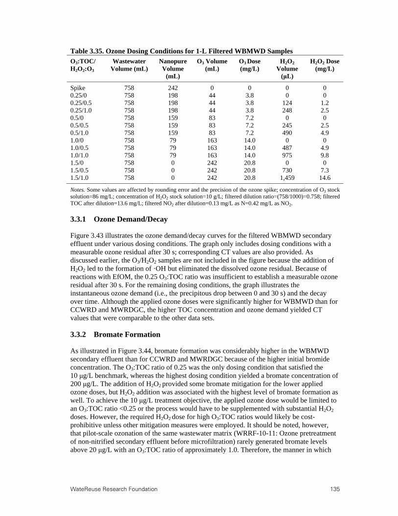
WateReuse Research Foundation 135
Table 3.35. Ozone Dosing Conditions for 1-L Filtered WBMWD Samples
O3:TOC/ H2O2:O3
Wastewater Volume (mL)
Nanopure Volume
(mL)
O3 Volume (mL)
O3 Dose (mg/L)
H2O2 Volume
(μL)
H2O2 Dose (mg/L)
Spike 758 242 0 0 0 0 0.25/0 758 198 44 3.8 0 0 0.25/0.5 758 198 44 3.8 124 1.2 0.25/1.0 758 198 44 3.8 248 2.5 0.5/0 758 159 83 7.2 0 0 0.5/0.5 758 159 83 7.2 245 2.5 0.5/1.0 758 159 83 7.2 490 4.9 1.0/0 758 79 163 14.0 0 0 1.0/0.5 758 79 163 14.0 487 4.9 1.0/1.0 758 79 163 14.0 975 9.8 1.5/0 758 0 242 20.8 0 0 1.5/0.5 758 0 242 20.8 730 7.3 1.5/1.0 758 0 242 20.8 1,459 14.6
Notes. Some values are affected by rounding error and the precision of the ozone spike; concentration of O3 stock solution=86 mg/L; concentration of H2O2 stock solution=10 g/L; filtered dilution ratio=(758/1000)=0.758; filtered TOC after dilution=13.6 mg/L; filtered NO2 after dilution=0.13 mg/L as N=0.42 mg/L as NO2.
3.3.1 Ozone Demand/Decay
Figure 3.43 illustrates the ozone demand/decay curves for the filtered WBMWD secondary effluent under various dosing conditions. The graph only includes dosing conditions with a measurable ozone residual after 30 s; corresponding CT values are also provided. As discussed earlier, the O3/H2O2 samples are not included in the figure because the addition of H2O2 led to the formation of ·OH but eliminated the dissolved ozone residual. Because of reactions with EfOM, the 0.25 O3:TOC ratio was insufficient to establish a measurable ozone residual after 30 s. For the remaining dosing conditions, the graph illustrates the instantaneous ozone demand (i.e., the precipitous drop between 0 and 30 s) and the decay over time. Although the applied ozone doses were significantly higher for WBMWD than for CCWRD and MWRDGC, the higher TOC concentration and ozone demand yielded CT values that were comparable to the other data sets.
3.3.2 Bromate Formation
As illustrated in Figure 3.44, bromate formation was considerably higher in the WBMWD secondary effluent than for CCWRD and MWRDGC because of the higher initial bromide concentration. The O3:TOC ratio of 0.25 was the only dosing condition that satisfied the 10 μg/L benchmark, whereas the highest dosing condition yielded a bromate concentration of 200 μg/L. The addition of H2O2 provided some bromate mitigation for the lower applied ozone doses, but H2O2 addition was associated with the highest level of bromate formation as well. To achieve the 10 μg/L treatment objective, the applied ozone dose would be limited to an O3:TOC ratio <0.25 or the process would have to be supplemented with substantial H2O2 doses. However, the required H2O2 dose for high O3:TOC ratios would likely be cost-prohibitive unless other mitigation measures were employed. It should be noted, however, that pilot-scale ozonation of the same wastewater matrix (WRRF-10-11: Ozone pretreatment of non-nitrified secondary effluent before microfiltration) rarely generated bromate levels above 20 μg/L with an O3:TOC ratio of approximately 1.0. Therefore, the manner in which

136 WateReuse Foundation
ozone is introduced into the water may impact the level of bromate formation in bench- versus large-scale systems.
Figure 3.43. Ozone demand/decay curves for WBMWD.
Figure 3.44. Bromate formation during ozonation of WBMWD secondary effluent.
3.3.3 ·OH Exposure
Based on data from bench-scale experiments with pCBA spiked at approximately 500 μg/L, Table 3.36 indicates the overall ·OH exposure for each ozone and UV dosing condition. The ·OH exposures for the UV/H2O2 samples are corrected for the low level of pCBA degradation achieved by photolysis alone.
In contrast to CCWRD and MWRDGC, H2O2 addition yielded higher overall ·OH exposure at O3:TOC ratios of 1.0 and 1.5. Ozone-based oxidation also provided higher ·OH exposures
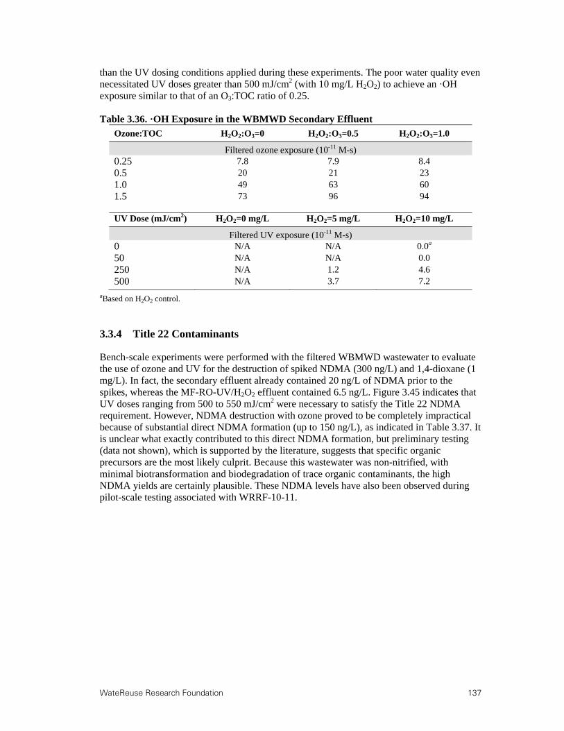
WateReuse Research Foundation 137
than the UV dosing conditions applied during these experiments. The poor water quality even necessitated UV doses greater than 500 mJ/cm2 (with 10 mg/L H2O2) to achieve an ·OH exposure similar to that of an O3:TOC ratio of 0.25. Table 3.36. ·OH Exposure in the WBMWD Secondary Effluent
Ozone:TOC H2O2:O3=0 H2O2:O3=0.5 H2O2:O3=1.0
Filtered ozone exposure (10-11 M-s) 0.25 7.8 7.9 8.4 0.5 20 21 23 1.0 49 63 60 1.5 73 96 94
UV Dose (mJ/cm2) H2O2=0 mg/L H2O2=5 mg/L H2O2=10 mg/L
Filtered UV exposure (10-11 M-s) 0 N/A N/A 0.0a 50 N/A N/A 0.0 250 N/A 1.2 4.6 500 N/A 3.7 7.2
aBased on H2O2 control.
3.3.4 Title 22 Contaminants
Bench-scale experiments were performed with the filtered WBMWD wastewater to evaluate the use of ozone and UV for the destruction of spiked NDMA (300 ng/L) and 1,4-dioxane (1 mg/L). In fact, the secondary effluent already contained 20 ng/L of NDMA prior to the spikes, whereas the MF-RO-UV/H2O2 effluent contained 6.5 ng/L. Figure 3.45 indicates that UV doses ranging from 500 to 550 mJ/cm2 were necessary to satisfy the Title 22 NDMA requirement. However, NDMA destruction with ozone proved to be completely impractical because of substantial direct NDMA formation (up to 150 ng/L), as indicated in Table 3.37. It is unclear what exactly contributed to this direct NDMA formation, but preliminary testing (data not shown), which is supported by the literature, suggests that specific organic precursors are the most likely culprit. Because this wastewater was non-nitrified, with minimal biotransformation and biodegradation of trace organic contaminants, the high NDMA yields are certainly plausible. These NDMA levels have also been observed during pilot-scale testing associated with WRRF-10-11.

138 WateReuse Foundation
Figure 3.45. Destruction of NDMA in the filtered WBMWD secondary effluent.
Table 3.37. Direct NDMA Formation in the Filtered WBMWD Secondary Effluent
O3:TOC Ratio H2O2:O3 Ratio NDMA (ng/L)
0 0 20 0.5 0 170 0.5 0.5 170 1.0 0 160 1.0 0.5 140
Table 3.38 illustrates the potential reductions in NDMA formation potential provided by ozonation and UV-based oxidation. With respect to the secondary effluent, the overall NDMA formation potential with chloramination was extremely high for WBMWD. As mentioned earlier, the fact that direct formation during ozonation also yielded high NDMA concentrations indicates that the precursors are likely similar between the two oxidants. Similar to the previous experiments, ozonation achieved reductions in overall NDMA formation potential ranging from 64% to 89%. Accounting for the Day 0 concentrations, the overall reduction reaches 99% based on the available data. In this case, higher ozone doses yielded lower NDMA formation potentials, whereas H2O2 addition was less effective in reducing NDMA formation potential. UV and UV/H2O2 achieved limited reductions in formation potential, with the maximum reduction of 25% occurring with a UV dose of 500 mJ/cm2 and an H2O2 dose of 10 mg/L.
0.0
0.2
0.4
0.6
0.8
1.0
1.2
1.4
1.6
0 100 200 300 400 500 600 700
UV Dose (mJ/cm2)
Log
Des
truc
tion
of
ND
MA
UV (H2O2=0 mg/L) UV (H2O2=5 mg/L)UV (H2O2 10 /L) Li (UV (H2O2 10 /L))
CDPH Title 22
Log
Des
tru
ctio
n of
ND
MA
UV (H2O2=0 mg/L) UV (H2O2=5 mg/L) UV (H2O2=10 mg/L)
0.0
0.2
0.4
0.6
0.8
1.0
1.2
1.4
1.6
0 100 200 300 400 500 600 700
UV Dose (mJ/cm2)
Log
Des
truc
tion
of
ND
MA
UV (H2O2=0 mg/L) UV (H2O2=5 mg/L)UV (H2O2 10 /L) Li (UV (H2O2 10 /L))
CDPH Title 22
Log
Des
tru
ctio
n of
ND
MA
UV (H2O2=0 mg/L) UV (H2O2=5 mg/L) UV (H2O2=10 mg/L)

WateReuse Research Foundation 139
Table 3.38. NDMA Formation Potential in the Filtered WBMWD Secondary Effluent
Testing Condition NDMA Day 0 (before chloramine)
NDMA Day 10 (after chloramine)
Total Chlorine Day 10
Secondary effluent 20 ng/L 1,600 ng/L 12 mg/L H2O2 control Not measured 1,500 ng/L 13 mg/L Ozone 0.25/0 Not measured 280 ng/L 12 mg/L Ozone 0.25/0.5 Not measured 570 ng/L 12 mg/L Ozone 0.5/0 170 ng/L 210 ng/L 12 mg/L Ozone 0.5/0.5 170 ng/L 360 ng/L 12 mg/L Ozone 1.0/0 160 ng/L 180 ng/L 16 mg/L Ozone 1.0/0.5 140 ng/L 330 ng/L 12 mg/L Ozone 1.5/0 Not measured 170 ng/L 12 mg/L Ozone 1.5/0.5 Not measured 210 ng/L 11 mg/L UV 50/0 Not measured 1,600 ng/L 13 mg/L UV 50/10 Not measured 1,400 ng/L 13 mg/L UV 250/0 Not measured 1,300 ng/L 13 mg/L UV 250/5 Not measured 1,300 ng/L 13 mg/L UV 250/10 Not measured 1,300 ng/L 14 mg/L UV 500/0 Not measured 1,300 ng/L 13 mg/L UV 500/5 Not measured 1,300 ng/L 13 mg/L UV 500/10 Not measured 1,200 ng/L 13 mg/L Finished 6.5 ng/L 22 ng/L 11 mg/L
Figure 3.46 illustrates the destruction of spiked 1,4-dioxane during the bench-scale ozone experiments. The superior performance of the ozone/H2O2 samples supports the previously reported pCBA data, which indicated that H2O2 addition provided a slight benefit for overall ·OH exposure. For WBMWD, O3:TOC ratios between 1.0 and 1.2 are necessary to comply with the 0.5-log requirement.
Figure 3.46. Destruction of 1,4-dioxane in the filtered WBMWD secondary effluent.
0.00
0.25
0.50
0.75
1.00
1.25
0 0.25 0.5 0.75 1 1.25 1.5
O3:TOC Ratio
Lo
g D
estr
uct
ion
of
1,4-
dio
xan
e
H2O2:O3=0
H2O2:O3=0.5CDPH Title 22
Log
Des
tru
ctio
n o
f 1,
4-d
ioxa
ne
0.00
0.25
0.50
0.75
1.00
1.25
0 0.25 0.5 0.75 1 1.25 1.5
O3:TOC Ratio
Lo
g D
estr
uct
ion
of
1,4-
dio
xan
e
H2O2:O3=0
H2O2:O3=0.5CDPH Title 22
Log
Des
tru
ctio
n o
f 1,
4-d
ioxa
ne

140 WateReuse Foundation
3.3.5 Trace Organic Contaminants
Secondary and finished (i.e., MF-RO-UV/H2O2) effluent samples from WBMWD were analyzed to determine the ambient concentrations of the target compounds, which are provided in Table 3.39. The effect of SRT during secondary treatment is quite apparent when the secondary effluent concentrations of WBMWD are compared with those of CCWRD and MWRDGC. The 1.5-day SRT provided minimal biological mitigation of trace organic contaminants, which resulted in relatively high secondary effluent concentrations for all of the target compounds. In fact, even the highly bioamenable compounds (i.e., ibuprofen and naproxen) that were <MRL for CCWRD and MWRDGC were present at reportable concentrations in this water matrix. Furthermore, many of the target compounds were present at concentrations approaching 1 μg/L, and two of the compounds were present at concentrations exceeding 2 μg/L. However, it is important to note that despite high concentrations relative to other secondary effluents, these concentrations likely pose little threat to public health. Atrazine, which is the only regulated contaminant on the target compound list, was even <MRL in the secondary effluent. The total estrogenicity of the secondary effluent was determined to be 0.56 ng/L, but this number should be interpreted with caution, as the highly concentrated secondary effluent may have had cytotoxic effects on the yeast cell line.
Finally, the multibarrier IPR treatment train achieved substantial removal for each of the target compounds, and all but one compound (bisphenol A) was <MRL after MF-RO-UV/H2O2. The exact reason for the breakthrough of bisphenol A is unclear, but it may have been an isolated occurrence captured by a single grab sample. Although bisphenol A is highly susceptible to biological treatment, little biotransformation was expected, based on the low SRT. This compound is also relatively resistant to UV photolysis, but its ·OH rate constant is relatively high, so there should have been significant destruction in the UV/H2O2 process. It is important to note that there was no indication of sample contamination based on the experimental controls. More frequent sampling would be necessary to determine whether bisphenol A breakthrough is a significant problem in this system. Regardless, MF-RO-UV/H2O2 is clearly an effective barrier against TOrC contamination in IPR applications.

WateReuse Research Foundation 141
Table 3.39. Ambient TOrC Concentrations at WBMWD
Parameter Secondary Effluent (ng/L) Finished Effluent (ng/L)
Bisphenol A 280 86 Diclofenac 280 <25 Gemfibrozil 2,500 <10 Ibuprofen 47 <25 Musk ketone <100 <100 Naproxen 320 <25 Triclosan 150 <25 Atenolol 2,100 <25 Atrazine <10 <10 Carbamazepine 260 <10 DEET 640 <25 Meprobamate 290 <10 Phenytoin 160 <10 Primidone 96 <10 Sulfamethoxazole 700 <25 Trimethoprim 700 <10 TCEP 630 <200 Total estrogenicity (EEq) 0.56 <0.074
Bench-scale TOrC oxidation experiments were performed with protocols and spiking stocks similar to those described for the previous wastewater matrices. However, a comparison of filtered versus unfiltered wastewater was not performed. Table 3.40 shows the relative oxidation levels of the 16 target compounds (musk ketone omitted) after ozonation. In contrast to the previous data sets, Table 3.40 supports the conclusion from the pCBA experiment (see Table 3.36) that H2O2 addition increased ·OH exposure at higher O3:TOC ratios. The impact of H2O2 was most apparent for the ozone-resistant compounds (Groups 3, 4, and 5) and O3:TOC ratios of 1.0 and 1.5. However, the benefit was minimal and likely insufficient to warrant H2O2 addition for this reason alone.
As described earlier, the target compounds were divided into five categories based on their second-order ozone and ·OH rate constants. As highlighted by the shaded cells, in particular, the relative levels of oxidation were similar during the MWRDGC and WBMWD experiments. All of the Group 1 compounds were more than 80% oxidized at an O3:TOC ratio of 0.25, and both of the Group 2 compounds were more than 80% oxidized with an O3:TOC ratio of 0.5. Groups 3 and 4 required O3:TOC ratios of 1.0 and 1.5, respectively, to exceed 80% oxidation. Similarly to the previous data sets, TCEP proved to be extremely resistant to ozonation, as the level of oxidation never exceeded 35%.
Table 3.41 shows the relative photolysis and UV/H2O2 oxidation levels of the target compounds. Again, UV photolysis was quite ineffective in destroying the target compounds. Only two compounds (diclofenac and triclosan) experienced more than 80% destruction with UV irradiation alone, whereas atrazine, phenytoin, and sulfamethoxazole experienced at least 25% destruction with UV alone. Photolysis appeared to be quite effective for DEET, meprobamate, and TCEP, but these numbers appear to be erroneous because they do not increase with increasing UV dose. The addition of H2O2 with a UV dose of 500 mJ/cm2 was also able to achieve 70% destruction of sulfamethoxazole, whereas a majority of the remaining compounds achieved destruction levels ranging from 20 to 50%.
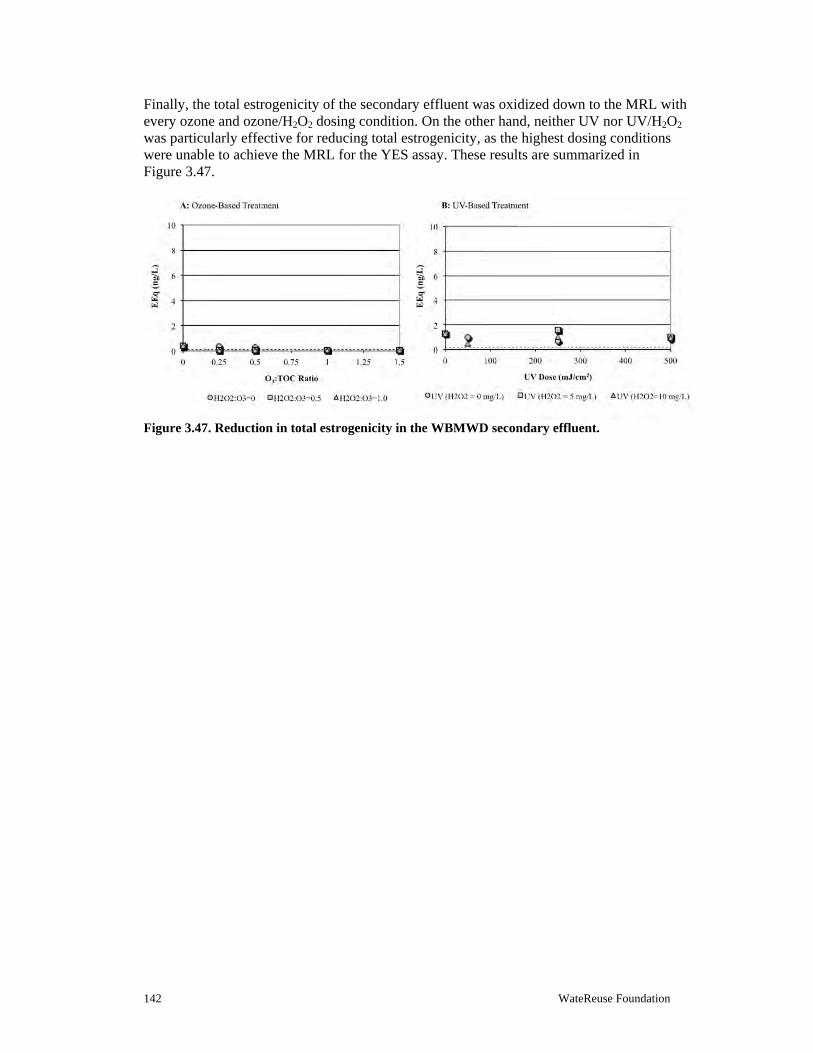
142 WateReuse Foundation
Finally, the total estrogenicity of the secondary effluent was oxidized down to the MRL with every ozone and ozone/H2O2 dosing condition. On the other hand, neither UV nor UV/H2O2 was particularly effective for reducing total estrogenicity, as the highest dosing conditions were unable to achieve the MRL for the YES assay. These results are summarized in Figure 3.47.
Figure 3.47. Reduction in total estrogenicity in the WBMWD secondary effluent.
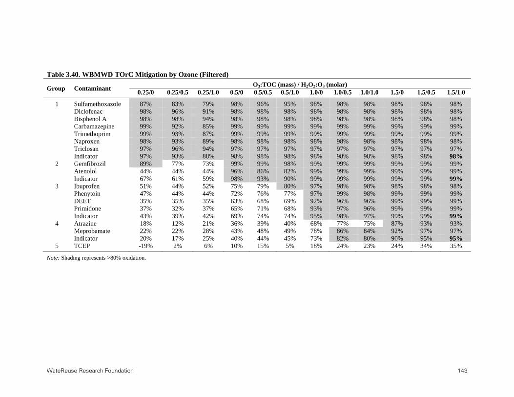
WateReuse Research Foundation 143
Table 3.40. WBMWD TOrC Mitigation by Ozone (Filtered)
Group Contaminant O3:TOC (mass) / H2O2:O3 (molar)
0.25/0 0.25/0.5 0.25/1.0 0.5/0 0.5/0.5 0.5/1.0 1.0/0 1.0/0.5 1.0/1.0 1.5/0 1.5/0.5 1.5/1.0
1 Sulfamethoxazole 87% 83% 79% 98% 96% 95% 98% 98% 98% 98% 98% 98% Diclofenac 98% 96% 91% 98% 98% 98% 98% 98% 98% 98% 98% 98% Bisphenol A 98% 98% 94% 98% 98% 98% 98% 98% 98% 98% 98% 98% Carbamazepine 99% 92% 85% 99% 99% 99% 99% 99% 99% 99% 99% 99% Trimethoprim 99% 93% 87% 99% 99% 99% 99% 99% 99% 99% 99% 99% Naproxen 98% 93% 89% 98% 98% 98% 98% 98% 98% 98% 98% 98% Triclosan 97% 96% 94% 97% 97% 97% 97% 97% 97% 97% 97% 97% Indicator 97% 93% 88% 98% 98% 98% 98% 98% 98% 98% 98% 98%
2 Gemfibrozil 89% 77% 73% 99% 99% 98% 99% 99% 99% 99% 99% 99% Atenolol 44% 44% 44% 96% 86% 82% 99% 99% 99% 99% 99% 99% Indicator 67% 61% 59% 98% 93% 90% 99% 99% 99% 99% 99% 99%
3 Ibuprofen 51% 44% 52% 75% 79% 80% 97% 98% 98% 98% 98% 98% Phenytoin 47% 44% 44% 72% 76% 77% 97% 99% 98% 99% 99% 99% DEET 35% 35% 35% 63% 68% 69% 92% 96% 96% 99% 99% 99% Primidone 37% 32% 37% 65% 71% 68% 93% 97% 96% 99% 99% 99% Indicator 43% 39% 42% 69% 74% 74% 95% 98% 97% 99% 99% 99%
4 Atrazine 18% 12% 21% 36% 39% 40% 68% 77% 75% 87% 93% 93% Meprobamate 22% 22% 28% 43% 48% 49% 78% 86% 84% 92% 97% 97% Indicator 20% 17% 25% 40% 44% 45% 73% 82% 80% 90% 95% 95%
5 TCEP -19% 2% 6% 10% 15% 5% 18% 24% 23% 24% 34% 35%
Note: Shading represents >80% oxidation.

144 WateReuse Foundation
Table 3.41. WBMWD TOrC Mitigation by UV (Filtered)
Group Contaminant UV Dose (mJ/cm2) / H2O2 Dose (mg/L)
50/0 50/10 250/0 250/5 250/10 500/0 500/5 500/10
1 Sulfamethoxazole 7% -15% 49% 36% 42% 67% 68% 70% Diclofenac 39% 4% 92% 85% 89% 98% 97% 97% Bisphenol A 5% 0% 0% 0% 0% 5% 10% 30% Carbamazepine -15% 0% -23% 7% 7% -15% 13% 27% Trimethoprim 5% 0% 0% 5% 5% 0% 5% 21% Naproxen 7% 0% 7% 8% 15% 7% 23% 39% Triclosan 17% 14% 78% 64% 76% 90% 90% 91%
2 Gemfibrozil 3% 6% 0% 12% 15% 6% 18% 23% Atenolol 0% 0% -3% 7% 17% -7% 0% 23%
3 Ibuprofen 9% 0% 9% 7% 10% 9% 19% 29% Phenytoin 16% 5% 35% 23% 30% 55% 48% 51% DEET 17% 0% 17% 5% 10% 4% 5% 20% Primidone 5% -6% 0% 11% 6% 5% -11% 0%
4 Atrazine -9% 0% 11% 17% 18% 27% 36% 39% Meprobamate 29% 3% 31% 6% 6% 32% 3% 14%
5 TCEP 14% 0% 13% -4% -4% 11% 7% 0%
Notes. Groupings based on ozone and OH rate constants. Shading represents >80% photolysis or oxidation.

WateReuse Research Foundation 145
3.3.6 Disinfection
Ambient secondary (before and after laboratory filtration) and finished effluent samples were assayed for total and fecal coliforms, MS2, and Bacillus spores. The ambient microbial water quality data are provided in Table 3.42. In comparison to the previous data sets, the number of indigenous microbes was slightly higher for WBMWD, and MS2 was even detected in the secondary effluent without filter concentration. To illustrate a wide range of inactivation, the ozone and UV disinfection samples were spiked with relatively large numbers of the surrogate microbes, as indicated in Table 3.43.
Table 3.42. Ambient Microbial Water Quality Data for WBMWD
Microbial Surrogate Unfiltered Secondary
Effluent Filtered Secondary
Effluent Finished Effluent
Total coliforms (MPN/100 mL)
3.5 104 3.4 104 <1
Fecal coliforms (MPN/100 mL) 9.4 103 7.7 103 <1
MS2 (PFU/mL)
9 10 <1
Bacillus spores (CFU/100 mL) 1.1 104 7.9 103 <1
Table 3.43. Microbial Spiking Levels for WBMWD Bench-Scale Experiments
Microbial Surrogate Filtered Ozone
Disinfection Filtered UV Disinfection
E. coli (MPN/100 mL) 2.4 107 9.3 106 MS2 (PFU/mL) 6.4 107 9.9 106
B. subtilis spores (CFU/100 mL) 2.2 105 2.8 105
Figure 3.48 illustrates the inactivation of spiked E. coli during the bench-scale ozone experiments. The solid line near the top of the figure represents the limit of inactivation based on the spiking level in the filtered samples. Inactivation by H2O2 alone was generally insignificant, and when combined with ozonation, the addition of H2O2 generally hindered E. coli inactivation. However, the various dosing conditions were more consistent for WBMWD than for CCWRD and MWRDGC with O3:TOC ratios >0.5 generally achieving >6-log inactivation of E. coli. The average log-inactivation values for each treatment condition are provided in Table 3.44.
Figure 3.49 illustrates the inactivation of spiked MS2 during the bench-scale ozone experiments. Again, the inactivation achieved by the addition of H2O2 alone was insignificant, and ozone/H2O2 was slightly less effective than ozone alone. With respect to the CDPH Title 22 requirements, an O3:TOC ratio >0.5 was often sufficient for the 5-log inactivation requirement, and an O3:TOC ratio >1.0 was generally sufficient for the more

146 WateReuse Foundation
stringent 6.5-log inactivation requirement. The average log-inactivation values for each treatment condition are provided in Table 3.45.
Figure 3.50 illustrates the inactivation of spiked B. subtilis spores during the bench-scale ozone experiments. As expected, the spores proved to be extremely resistant to oxidation and only experienced significant inactivation for O3:TOC ratios >1.0 with no H2O2 addition. In other words, a sufficient ozone CT had to be administered before ozone and ·OH were able to penetrate the spore coat and inactivate the bacteria. It is important to reiterate that oxidation with ·OH alone (i.e., with H2O2 addition) is extremely ineffective for spore inactivation, presumably because of the highly reactive nature of ·OH and competition with EfOM. The average log-inactivation values for each treatment condition are provided in Table 3.46. Finally, Figure 3.51 provides a summary of the ozone disinfection data for the three surrogate microbes with respect to the CT framework. Figure 3.51A illustrates the dose–response relationships for the samples with no H2O2 addition, and Figure 3.51B illustrates the dose–response relationships for H2O2:O3 ratios of 0.5 and 1.0 (combined). Similar to the previous data sets, the data indicate that the CT framework is not always appropriate because substantial levels of inactivation can be achieved when the apparent ozone CT is zero. Again, the level of inactivation for vegetative bacteria and viruses is generally less than that observed when an ozone residual is present, and no inactivation of spore-forming bacteria can be achieved without a measurable CT.
Table 3.47 summarizes the efficacy of UV and UV/H2O2 for the inactivation of the three surrogate microbes. The efficacy of UV-based disinfection differs dramatically from that of ozone-based disinfection because UV is highly effective against both vegetative and spore-forming bacteria, whereas some viruses demonstrate resistance. A dose of 50 mJ/cm2 was sufficient to reach the limits of inactivation for E. coli and Bacillus spores, regardless of H2O2 addition. On the other hand, MS2 inactivation occurred more slowly and only reached the limit of inactivation with a UV dose of 250 mJ/cm2. There was no difference in UV/H2O2 performance with H2O2 doses of 5 and 10 mg/L. Particularly with respect to advanced oxidation dosing conditions (i.e., >250 mJ/cm2 with 10 mg/L of H2O2), one can expect substantial inactivation of all microbes present in wastewater. This constitutes a significant advantage for UV-based treatment over the ozone-based alternatives.

WateReuse Research Foundation 147
Figure 3.48. Inactivation of spiked E. coli in the WBMWD secondary effluent.
Table 3.44. Summary of E. coli Inactivation in the WBMWD Secondary Effluent
O3:TOC Ratio H2O2:O3=0 H2O2:O3=0.5 H2O2:O3=1.0
0.25 0.6 0.6 0.5 0.5 6.0 6.1 5.1 1.0 >7.4a 6.1 6.2 1.5 >7.4a 6.2 6.2
aLimit of inactivation based on spiking level.
0
1
2
3
4
5
6
7
8
9
0.00 0.25 0.50 0.75 1.00 1.25 1.50
O3:TOC Ratio
Log
Ina
ctiv
atio
n
Filtered (H2O2:O3=0) Filtered (H2O2:O3=0.5) Filtered (H2O2:O3=1.0)
E. coli Limit of Inactivation
0
1
2
3
4
5
6
7
8
9
0.00 0.25 0.50 0.75 1.00 1.25 1.50
O3:TOC Ratio
Log
Ina
ctiv
atio
n
Filtered (H2O2:O3=0) Filtered (H2O2:O3=0.5) Filtered (H2O2:O3=1.0)
E. coli Limit of Inactivation
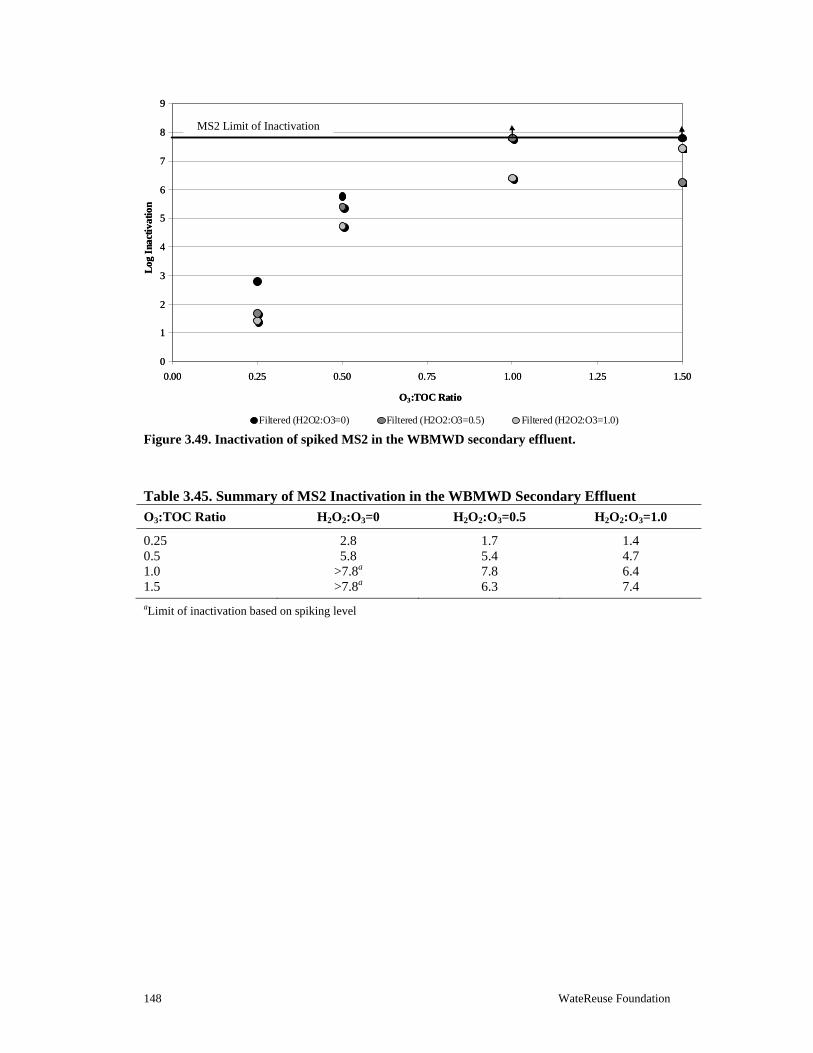
148 WateReuse Foundation
Figure 3.49. Inactivation of spiked MS2 in the WBMWD secondary effluent.
Table 3.45. Summary of MS2 Inactivation in the WBMWD Secondary Effluent
O3:TOC Ratio H2O2:O3=0 H2O2:O3=0.5 H2O2:O3=1.0
0.25 2.8 1.7 1.4 0.5 5.8 5.4 4.7 1.0 >7.8a 7.8 6.4 1.5 >7.8a 6.3 7.4
aLimit of inactivation based on spiking level
0
1
2
3
4
5
6
7
8
9
0.00 0.25 0.50 0.75 1.00 1.25 1.50
O3:TOC Ratio
Log
Ina
ctiv
atio
n
Filtered (H2O2:O3=0) Filtered (H2O2:O3=0.5) Filtered (H2O2:O3=1.0)
MS2 Limit of Inactivation
0
1
2
3
4
5
6
7
8
9
0.00 0.25 0.50 0.75 1.00 1.25 1.50
O3:TOC Ratio
Log
Ina
ctiv
atio
n
Filtered (H2O2:O3=0) Filtered (H2O2:O3=0.5) Filtered (H2O2:O3=1.0)
MS2 Limit of Inactivation

WateReuse Research Foundation 149
Figure 3.50. Inactivation of spiked Bacillus spores in the WBMWD secondary effluent.
Table 3.46. Summary of Bacillus Spore Inactivation in the WBMWD Secondary Effluent
O3:TOC Ratio H2O2:O3=0 H2O2:O3=0.5 H2O2:O3=1.0
0.25 0.0 0.0 0.0 0.5 0.0 0.0 0.0 1.0 2.0 0.0 0.0 1.5 >3.3a 0.0 0.0
aLimit of inactivation based on spiking level
0
1
2
3
4
0.00 0.25 0.50 0.75 1.00 1.25 1.50
O3:TOC Ratio
Log
Ina
ctiv
atio
n
Filtered (H2O2:O3=0) Filtered (H2O2:O3=0.5) Filtered (H2O2:O3=1.0)
Bacillus spore Limit of Inactivation
0
1
2
3
4
0.00 0.25 0.50 0.75 1.00 1.25 1.50
O3:TOC Ratio
Log
Ina
ctiv
atio
n
Filtered (H2O2:O3=0) Filtered (H2O2:O3=0.5) Filtered (H2O2:O3=1.0)
Bacillus spore Limit of Inactivation

150 WateReuse Foundation
Figure 3.51. Significance of CT for disinfection in the WBMWD secondary effluent.
0
1
2
3
4
5
6
7
8
9
0.25 0.50 1.00 1.50
O3:TOC Ratio
Log
In
acti
vati
on
0
5
10
15
20
25
30
Ozo
ne
CT
(m
g-m
in/L
Bacillus spore E. coli MS2 CT
0
1
2
3
4
5
6
7
8
9
0.25 0.50 1.00 1.50
O3:TOC Ratio
Log
In
acti
vati
on
0
5
10
15
20
25
30
Ozo
ne
CT
(m
g-m
in/L
Bacillus spore E. coli MS2 CT
A: No H2O2 Addition
B: H2O2 Addition
Log
Ina
ctiv
atio
nL
og I
nac
tiva
tion
Ozo
ne
CT
(m
g-m
in/L
)O
zon
e C
T (
mg-
min
/L)
0
1
2
3
4
5
6
7
8
9
0.25 0.50 1.00 1.50
O3:TOC Ratio
Log
In
acti
vati
on
0
5
10
15
20
25
30
Ozo
ne
CT
(m
g-m
in/L
Bacillus spore E. coli MS2 CT
0
1
2
3
4
5
6
7
8
9
0.25 0.50 1.00 1.50
O3:TOC Ratio
Log
In
acti
vati
on
0
5
10
15
20
25
30
Ozo
ne
CT
(m
g-m
in/L
Bacillus spore E. coli MS2 CT
A: No H2O2 Addition
B: H2O2 Addition
Log
Ina
ctiv
atio
nL
og I
nac
tiva
tion
Ozo
ne
CT
(m
g-m
in/L
)O
zon
e C
T (
mg-
min
/L)
(combination of H2O2:O3=0.5 and 1.0)

WateReuse Research Foundation 151
Table 3.47. Summary of UV Inactivation in the WBMWD Secondary Effluent
UV Dose (mJ/cm2)
E. coli MS2 Bacillus spores UV UV/H2O2
a UV UV/H2O2a UV UV/H2O2
a
25 >7.0b 5.9 N/A N/A 1.9 1.7 50 7.0 >7.0b 3.1 3.4 >3.5b >3.5b 250 >7.0b >7.0b >7.0b >7.0b >3.5b >3.5b 500 >7.0b >7.0b >7.0b >7.0b >3.5b >3.5b aH2O2 doses of 5 and 10 mg/L achieved similar levels of inactivation. bLimit of inactivation based on spiking level.
3.3.7 Organic Characterization
Similarly to the previous two data sets, the full-spectrum scans in Figures 3.52 and 3.53 (without (A) and with (B) H2O2 addition) indicate that the absorbance profiles around 254 nm generally provide the greatest resolution between treatment. Because of the limited efficacy of UV photolysis (Figure 3.53A), there is little resolution regardless of wavelength, and even UV/H2O2 achieved minimal reductions in absorbance. Figure 3.54 focuses on the change in UV254 absorbance with ozone, ozone/H2O2, UV, and UV/H2O2. With respect to ozonation, reductions in UV254 absorbance were slightly hindered by the addition of H2O2. In contrast to CCWRD and MWRDGC, the synergistic aspect of the UV AOP provided minimal improvements over UV alone.
3D EEMs were developed for the filtered secondary effluent, the MF-RO-UV/H2O2 effluent, and the various treatment conditions. Figure 3.55 illustrates the fluorescence fingerprint of the secondary and finished effluent samples and also provides the total and regional fluorescence intensities, based on arbitrary fluorescence units. The efficacy of the IPR treatment train is apparent based on the dramatic reduction in fluorescence intensity—from the most intense fingerprint of the various data sets to a fingerprint comparable to that of a blank sample. In fact, Regions I and II individually had higher total fluorescence intensities than Regions I, II, and III combined for CCWRD and MWRDGC. In contrast to CCWRD and MWRDGC, Region I (soluble microbial products and biopolymers) composed a larger portion of the total fluorescence than Region II (fulvic acids). Figure 3.56 provides a qualitative illustration of treatment efficacy after ozone- and UV-based oxidation. It is interesting to note that an O3:TOC ratio of 0.25 yields a 3D EEM that is similar to that for the ambient secondary effluents of CCWRD and MWRDGC. Despite the poor water quality, ozone and ozone/H2O2 are capable of achieving substantial reductions in regional and total fluorescence. Despite the corrections for UV absorbance in calculating UV doses, neither UV nor UV/H2O2 are capable of significant reductions in fluorescence.
Figures 3.57 and 3.58 illustrate the fluorescence profiles at an excitation wavelength of 254 nm after ozonation and UV/H2O2, respectively. Because the addition of H2O2 did not have a significant impact on ozone efficacy and UV photolysis provided limited reductions in fluorescence intensity, these fluorescence profiles are not shown. These fluorescence profiles actually provide better resolution for the UV/H2O2 samples than the full 3D EEMs. The fluorescence profiles also illustrate the prominence of Region I fluorescence, because the WBMWD profiles are characterized by two distinct peaks, whereas CCWRD and MWRDGC are characterized by only a single peak associated with Region II.
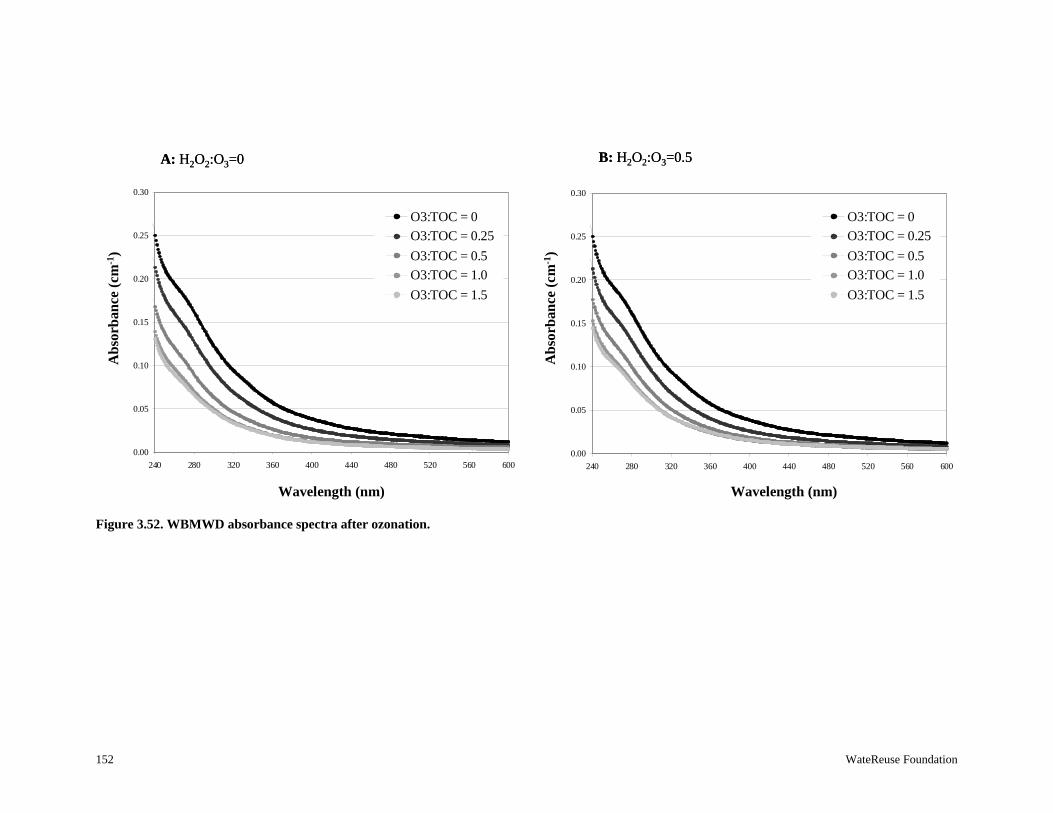
152 WateReuse Foundation
Figure 3.52. WBMWD absorbance spectra after ozonation.
0.00
0.05
0.10
0.15
0.20
0.25
0.30
240 280 320 360 400 440 480 520 560 600
Wavelength (nm)
0.00
0.05
0.10
0.15
0.20
0.25
0.30
240 280 320 360 400 440 480 520 560 600
Ab
sorb
ance
(cm
-1)
Ab
sorb
ance
(cm
-1)
O3:TOC = 0
O3:TOC = 0.25
O3:TOC = 0.5
O3:TOC = 1.0
O3:TOC = 1.5
Wavelength (nm) Wavelength (nm)
O3:TOC = 0
O3:TOC = 0.25
O3:TOC = 0.5
O3:TOC = 1.0
O3:TOC = 1.5
A: H2O2:O3=0 B: H2O2:O3=0.5
0.00
0.05
0.10
0.15
0.20
0.25
0.30
240 280 320 360 400 440 480 520 560 600
Wavelength (nm)
0.00
0.05
0.10
0.15
0.20
0.25
0.30
240 280 320 360 400 440 480 520 560 600
Ab
sorb
ance
(cm
-1)
Ab
sorb
ance
(cm
-1)
O3:TOC = 0
O3:TOC = 0.25
O3:TOC = 0.5
O3:TOC = 1.0
O3:TOC = 1.5
Wavelength (nm) Wavelength (nm)
O3:TOC = 0
O3:TOC = 0.25
O3:TOC = 0.5
O3:TOC = 1.0
O3:TOC = 1.5
A: H2O2:O3=0 B: H2O2:O3=0.5
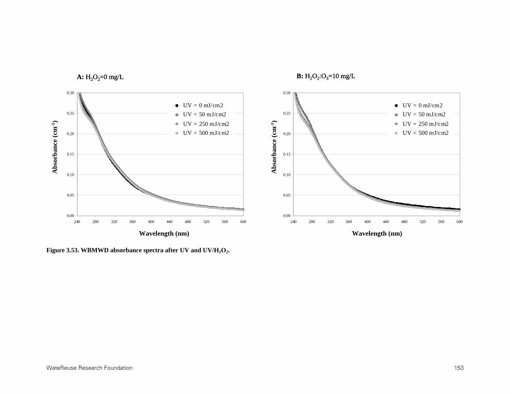
WateReuse Research Foundation 153
Figure 3.53. WBMWD absorbance spectra after UV and UV/H2O2.
0.00
0.05
0.10
0.15
0.20
0.25
0.30
240 280 320 360 400 440 480 520 560 600
Wavelength (nm)
Ab
sorb
ance
(cm
-1)
0.00
0.05
0.10
0.15
0.20
0.25
0.30
240 280 320 360 400 440 480 520 560 600
Wavelength (nm)
Ab
sorb
ance
(cm
-1)
Ab
sorb
ance
(cm
-1)
Wavelength (nm)
Ab
sorb
ance
(cm
-1)
Wavelength (nm)
A: H2O2=0 mg/L B: H2O2:O3=10 mg/L
UV = 0 mJ/cm2
UV = 50 mJ/cm2
UV = 250 mJ/cm2
UV = 500 mJ/cm2
UV = 0 mJ/cm2
UV = 50 mJ/cm2
UV = 250 mJ/cm2
UV = 500 mJ/cm2
0.00
0.05
0.10
0.15
0.20
0.25
0.30
240 280 320 360 400 440 480 520 560 600
Wavelength (nm)
Ab
sorb
ance
(cm
-1)
0.00
0.05
0.10
0.15
0.20
0.25
0.30
240 280 320 360 400 440 480 520 560 600
Wavelength (nm)
Ab
sorb
ance
(cm
-1)
Ab
sorb
ance
(cm
-1)
Wavelength (nm)
Ab
sorb
ance
(cm
-1)
Wavelength (nm)
A: H2O2=0 mg/L B: H2O2:O3=10 mg/L
UV = 0 mJ/cm2
UV = 50 mJ/cm2
UV = 250 mJ/cm2
UV = 500 mJ/cm2
UV = 0 mJ/cm2
UV = 50 mJ/cm2
UV = 250 mJ/cm2
UV = 500 mJ/cm2

154 WateReuse Foundation
Figure 3.54. Differential UV254 absorbance in the filtered WBMWD secondary effluent.
0%
10%
20%
30%
40%
50%
60%
70%
0 0.25 0.5 0.75 1 1.25 1.5
O 3:TO C Ratio
Dif
fere
ntia
l UV
25
4 A
bsor
banc
e
H2O2:O3 = 0 H2O2:O3 = 0.5 H2O2:O3 = 1.0
0%
10%
20%
30%
40%
50%
60%
70%
0 100 200 300 400 500 600 700
UV Dose (mJ/cm2)
Dif
fere
ntia
l UV
25
4 A
bsor
banc
e
UV (H2O2=0 mg/L) UV (H2O2=5 mg/L) UV (H2O2=10 mg/L)
Dif
fere
nti
al U
V25
4A
bsor
ban
ce
Dif
fere
nti
al U
V25
4A
bsor
ban
ce
A: Ozone-Based Treatment B: UV-Based Treatment
0%
10%
20%
30%
40%
50%
60%
70%
0 100 200 300 400 500 600 700
UV Dose (mJ/cm2)
Dif
fere
ntia
l UV
25
4 A
bsor
banc
e
UV (H2O2=0 mg/L) UV (H2O2=5 mg/L) UV (H2O2=10 mg/L)
Dif
fere
nti
al U
V25
4A
bsor
ban
ce
Dif
fere
nti
al U
V25
4A
bsor
ban
ce
A: Ozone-Based Treatment B: UV-Based Treatment

WateReuse Research Foundation 155
Figure 3.55. 3D EEMs for ambient samples from WBMWD.
Figure 3.56. 3D EEMs after treatment for the filtered WBMWD secondary effluent.
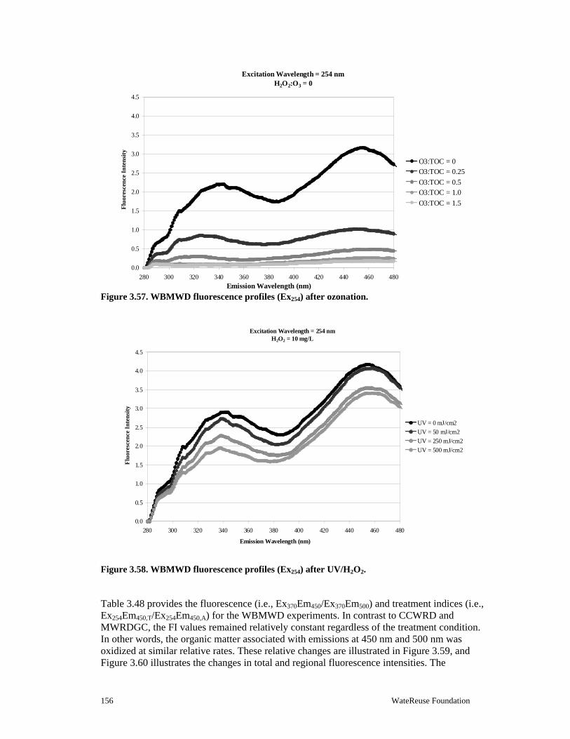
156 WateReuse Foundation
Figure 3.57. WBMWD fluorescence profiles (Ex254) after ozonation.
Figure 3.58. WBMWD fluorescence profiles (Ex254) after UV/H2O2.
Table 3.48 provides the fluorescence (i.e., Ex370Em450/Ex370Em500) and treatment indices (i.e., Ex254Em450,T/Ex254Em450,A) for the WBMWD experiments. In contrast to CCWRD and MWRDGC, the FI values remained relatively constant regardless of the treatment condition. In other words, the organic matter associated with emissions at 450 nm and 500 nm was oxidized at similar relative rates. These relative changes are illustrated in Figure 3.59, and Figure 3.60 illustrates the changes in total and regional fluorescence intensities. The
Excitation Wavelength = 254 nmH2O2:O3 = 0
0.0
0.5
1.0
1.5
2.0
2.5
3.0
3.5
4.0
4.5
280 300 320 340 360 380 400 420 440 460 480
Emission Wavelength (nm)
Flu
ores
cen
ce I
nte
nsit
y
O3:TOC = 0O3:TOC = 0.25
O3:TOC = 0.5O3:TOC = 1.0
O3:TOC = 1.5
Flu
ores
cen
ce I
nte
nsi
ty
Excitation Wavelength = 254 nmH2O2:O3 = 0
0.0
0.5
1.0
1.5
2.0
2.5
3.0
3.5
4.0
4.5
280 300 320 340 360 380 400 420 440 460 480
Emission Wavelength (nm)
Flu
ores
cen
ce I
nte
nsit
y
O3:TOC = 0O3:TOC = 0.25
O3:TOC = 0.5O3:TOC = 1.0
O3:TOC = 1.5
Flu
ores
cen
ce I
nte
nsi
ty
Excitation Wavelength = 254 nmH2O2 = 10 mg/L
0.0
0.5
1.0
1.5
2.0
2.5
3.0
3.5
4.0
4.5
280 300 320 340 360 380 400 420 440 460 480
Emission Wavelength (nm)
Flu
ores
cenc
e In
ten
sity
UV = 0 mJ/cm2
UV = 50 mJ/cm2
UV = 250 mJ/cm2
UV = 500 mJ/cm2
Flu
ores
cen
ce I
nte
nsi
ty
Excitation Wavelength = 254 nmH2O2 = 10 mg/L
0.0
0.5
1.0
1.5
2.0
2.5
3.0
3.5
4.0
4.5
280 300 320 340 360 380 400 420 440 460 480
Emission Wavelength (nm)
Flu
ores
cenc
e In
ten
sity
UV = 0 mJ/cm2
UV = 50 mJ/cm2
UV = 250 mJ/cm2
UV = 500 mJ/cm2
Flu
ores
cen
ce I
nte
nsi
ty
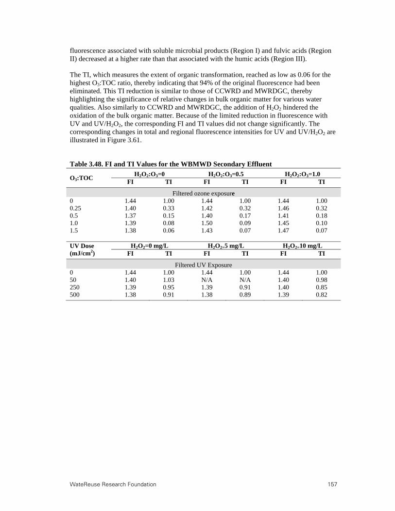
WateReuse Research Foundation 157
fluorescence associated with soluble microbial products (Region I) and fulvic acids (Region II) decreased at a higher rate than that associated with the humic acids (Region III).
The TI, which measures the extent of organic transformation, reached as low as 0.06 for the highest O3:TOC ratio, thereby indicating that 94% of the original fluorescence had been eliminated. This TI reduction is similar to those of CCWRD and MWRDGC, thereby highlighting the significance of relative changes in bulk organic matter for various water qualities. Also similarly to CCWRD and MWRDGC, the addition of H2O2 hindered the oxidation of the bulk organic matter. Because of the limited reduction in fluorescence with UV and UV/H2O2, the corresponding FI and TI values did not change significantly. The corresponding changes in total and regional fluorescence intensities for UV and UV/H2O2 are illustrated in Figure 3.61.
Table 3.48. FI and TI Values for the WBMWD Secondary Effluent
O3:TOC H2O2:O3=0 H2O2:O3=0.5 H2O2:O3=1.0
FI TI FI TI FI TI
Filtered ozone exposure 0 1.44 1.00 1.44 1.00 1.44 1.00 0.25 1.40 0.33 1.42 0.32 1.46 0.32 0.5 1.37 0.15 1.40 0.17 1.41 0.18 1.0 1.39 0.08 1.50 0.09 1.45 0.10 1.5 1.38 0.06 1.43 0.07 1.47 0.07
UV Dose (mJ/cm2)
H2O2=0 mg/L H2O2=5 mg/L H2O2=10 mg/L FI TI FI TI FI TI
Filtered UV Exposure 0 1.44 1.00 1.44 1.00 1.44 1.00 50 1.40 1.03 N/A N/A 1.40 0.98 250 1.39 0.95 1.39 0.91 1.40 0.85 500 1.38 0.91 1.38 0.89 1.39 0.82

158 WateReuse Foundation
Figure 3.59. WBMWD fluorescence profiles (Ex370) after ozonation.
Excitation Wavelength = 370 nmH2O2:O3 = 0
0.00
0.25
0.50
0.75
1.00
400 425 450 475 500 525 550
Emission Wavelength (nm)
Flu
ores
cen
ce I
nten
sity
O3:TOC = 0
O3:TOC = 0.25
O3:TOC = 0.5
O3:TOC = 1.0
O3:TOC = 1.5
Flu
ores
cen
ce I
nte
nsi
tyEm450 Em500
Excitation Wavelength = 370 nmH2O2:O3 = 0
0.00
0.25
0.50
0.75
1.00
400 425 450 475 500 525 550
Emission Wavelength (nm)
Flu
ores
cen
ce I
nten
sity
O3:TOC = 0
O3:TOC = 0.25
O3:TOC = 0.5
O3:TOC = 1.0
O3:TOC = 1.5
Flu
ores
cen
ce I
nte
nsi
tyEm450 Em500

WateReuse Research Foundation 159
Figure 3.60. Changes in fluorescence intensity after ozonation for WBMWD. H2O2:O3=0.
0
10,000
20,000
30,000
40,000
50,000
60,000
70,000
80,000
90,000
100,000
0 0.25 0.5 0.75 1 1.25 1.5
O3:TOC Ratio
Flu
ores
cenc
e In
tens
ity
(un
itle
ss)
Overall Sum Fulvics Proteins and SMPs Humics
Flu
ores
cen
ce I
nte
nsi
ty (
un
itle
ss)
0
10,000
20,000
30,000
40,000
50,000
60,000
70,000
80,000
90,000
100,000
0 0.25 0.5 0.75 1 1.25 1.5
O3:TOC Ratio
Flu
ores
cenc
e In
tens
ity
(un
itle
ss)
Overall Sum Fulvics Proteins and SMPs Humics
Flu
ores
cen
ce I
nte
nsi
ty (
un
itle
ss)

160 WateReuse Foundation
Figure 3.61. Changes in fluorescence intensity after UV/H2O2 for WBMWD. H2O2=10 mg/L.
3.4 Pinellas County Utilities, Pinellas County, FL
The secondary effluent provided by Pinellas County Utilities (PCU) is from a water reclamation facility in the Tampa–St. Petersburg metropolitan area. PCU treats approximately 20 MGD of wastewater composed of >96% domestic and <4% industrial flows. The liquid treatment train consists of preliminary screening and grit removal; primary clarification; conventional activated sludge (SRT=11–13 days) with nitrification, denitrification (TNeff ≈ 1.4 mg/L), and biological phosphorus removal (TPeff ≈ 0.5 mg/L); secondary clarification; deep bed (sand) denitrification filters; shallow bed filters (no longer utilized in their original design capacity); and chlorination. The chlorine disinfection process targets a minimum residual of 1.0 mg/L at the end of the contact basin and a contact time of at least 15 min. The effluent is used in reclaimed water distribution systems for irrigation and as a class 3 surface water discharge, which requires the effluent to comply with recreational water quality standards. The facility is currently being upgraded to include UV disinfection. A simplified treatment schematic of PCU is provided in Figure 3.62.
PCU is particularly interested in ozone technologies as a means to mitigate total trihalomethane (THM) concentrations in the finished effluent. The facility must specifically achieve annual averages of less than 22 μg/L and 34 μg/L for dichlorobromomethane (CHCl2Br) and chlorodibromomethane (CHClBr2), respectively. PCU has also tested for toxicological endpoints in the past but has not reached any definitive conclusions regarding the toxicity of its effluent.
0
10,000
20,000
30,000
40,000
50,000
60,000
70,000
80,000
90,000
100,000
0 100 200 300 400 500
UV Dose (mJ/cm2)
Flu
ores
cenc
e In
tens
ity
(un
itle
ss)
Overall Sum Fulvics Proteins and SMPs Humics
Flu
ores
cen
ce I
nte
nsi
ty (
un
itle
ss)
0
10,000
20,000
30,000
40,000
50,000
60,000
70,000
80,000
90,000
100,000
0 100 200 300 400 500
UV Dose (mJ/cm2)
Flu
ores
cenc
e In
tens
ity
(un
itle
ss)
Overall Sum Fulvics Proteins and SMPs Humics
Flu
ores
cen
ce I
nte
nsi
ty (
un
itle
ss)
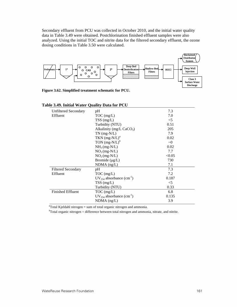
WateReuse Research Foundation 161
Secondary effluent from PCU was collected in October 2010, and the initial water quality data in Table 3.49 were obtained. Postchlorination finished effluent samples were also analyzed. Using the initial TOC and nitrite data for the filtered secondary effluent, the ozone dosing conditions in Table 3.50 were calculated.
Figure 3.62. Simplified treatment schematic for PCU.
Table 3.49. Initial Water Quality Data for PCU
Unfiltered Secondary Effluent
pH 7.3 TOC (mg/L) 7.0 TSS (mg/L) <5 Turbidity (NTU) 0.51 Alkalinity (mg/L CaCO3) 205 TN (mg-N/L) 7.9 TKN (mg-N/L)a 0.02 TON (mg-N/L)b ~0 NH3 (mg-N/L) 0.02 NO3 (mg-N/L) 7.7 NO2 (mg-N/L) <0.05 Bromide (μg/L) 730 NDMA (ng/L) 7.1
Filtered Secondary Effluent
pH 7.3 TOC (mg/L) 7.2 UV254 absorbance (cm-1) 0.187 TSS (mg/L) <5 Turbidity (NTU) 0.33
Finished Effluent TOC (mg/L) 6.8 UV254 absorbance (cm-1) 0.135 NDMA (ng/L) 3.9
aTotal Kjeldahl nitrogen = sum of total organic nitrogen and ammonia. bTotal organic nitrogen = difference between total nitrogen and ammonia, nitrate, and nitrite.
1°Deep Bed
Denitrification Filters
2°CAS
Class 3 Surface Water
Discharge
HOClPreliminary Shallow Bed Filters
Deep Well Injection
Reclaimed Distribution
System
1°1°Deep Bed
Denitrification Filters
2°CAS 2°CAS
Class 3 Surface Water
Discharge
HOClPreliminary Shallow Bed Filters
Deep Well Injection
Reclaimed Distribution
System
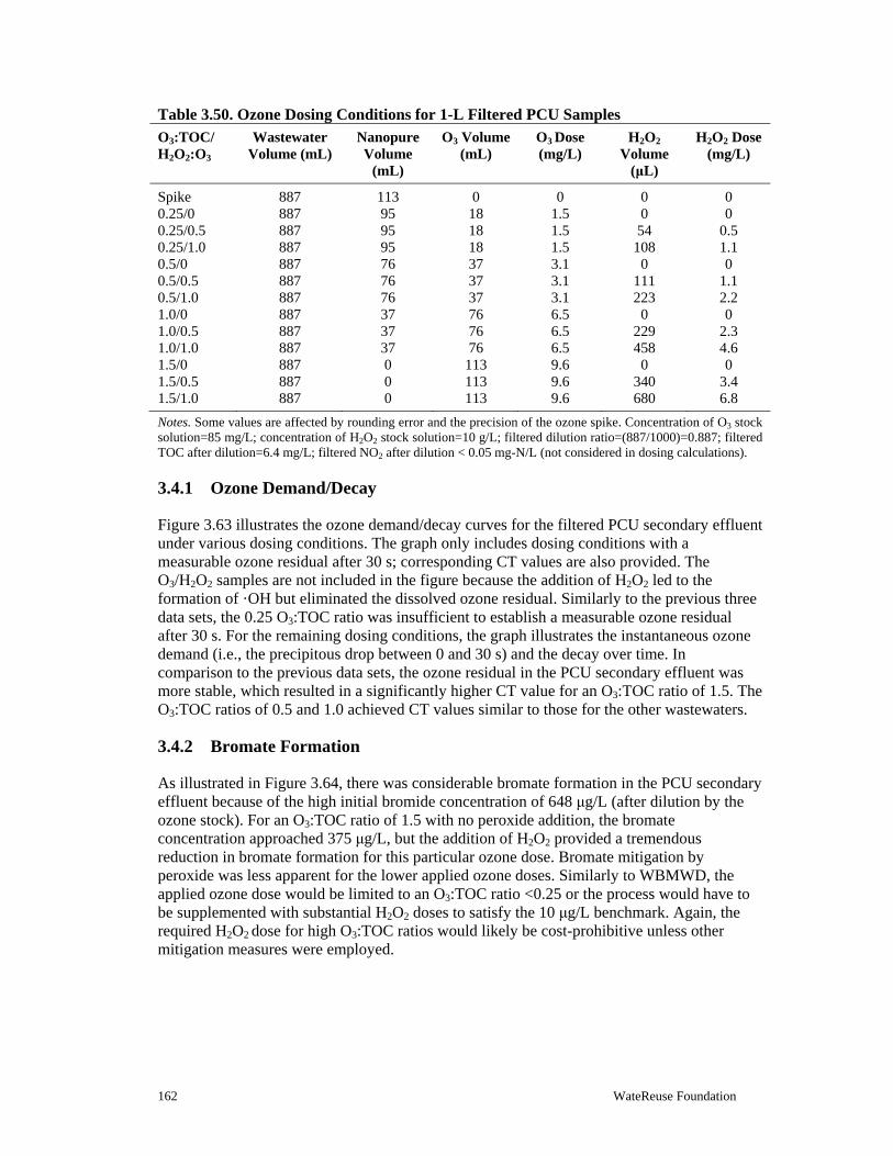
162 WateReuse Foundation
Table 3.50. Ozone Dosing Conditions for 1-L Filtered PCU Samples
O3:TOC/ H2O2:O3
Wastewater Volume (mL)
Nanopure Volume
(mL)
O3 Volume (mL)
O3 Dose (mg/L)
H2O2 Volume
(μL)
H2O2 Dose (mg/L)
Spike 887 113 0 0 0 0 0.25/0 887 95 18 1.5 0 0 0.25/0.5 887 95 18 1.5 54 0.5 0.25/1.0 887 95 18 1.5 108 1.1 0.5/0 887 76 37 3.1 0 0 0.5/0.5 887 76 37 3.1 111 1.1 0.5/1.0 887 76 37 3.1 223 2.2 1.0/0 887 37 76 6.5 0 0 1.0/0.5 887 37 76 6.5 229 2.3 1.0/1.0 887 37 76 6.5 458 4.6 1.5/0 887 0 113 9.6 0 0 1.5/0.5 887 0 113 9.6 340 3.4 1.5/1.0 887 0 113 9.6 680 6.8
Notes. Some values are affected by rounding error and the precision of the ozone spike. Concentration of O3 stock solution=85 mg/L; concentration of H2O2 stock solution=10 g/L; filtered dilution ratio=(887/1000)=0.887; filtered TOC after dilution=6.4 mg/L; filtered NO2 after dilution < 0.05 mg-N/L (not considered in dosing calculations).
3.4.1 Ozone Demand/Decay
Figure 3.63 illustrates the ozone demand/decay curves for the filtered PCU secondary effluent under various dosing conditions. The graph only includes dosing conditions with a measurable ozone residual after 30 s; corresponding CT values are also provided. The O3/H2O2 samples are not included in the figure because the addition of H2O2 led to the formation of ·OH but eliminated the dissolved ozone residual. Similarly to the previous three data sets, the 0.25 O3:TOC ratio was insufficient to establish a measurable ozone residual after 30 s. For the remaining dosing conditions, the graph illustrates the instantaneous ozone demand (i.e., the precipitous drop between 0 and 30 s) and the decay over time. In comparison to the previous data sets, the ozone residual in the PCU secondary effluent was more stable, which resulted in a significantly higher CT value for an O3:TOC ratio of 1.5. The O3:TOC ratios of 0.5 and 1.0 achieved CT values similar to those for the other wastewaters.
3.4.2 Bromate Formation
As illustrated in Figure 3.64, there was considerable bromate formation in the PCU secondary effluent because of the high initial bromide concentration of 648 μg/L (after dilution by the ozone stock). For an O3:TOC ratio of 1.5 with no peroxide addition, the bromate concentration approached 375 μg/L, but the addition of H2O2 provided a tremendous reduction in bromate formation for this particular ozone dose. Bromate mitigation by peroxide was less apparent for the lower applied ozone doses. Similarly to WBMWD, the applied ozone dose would be limited to an O3:TOC ratio <0.25 or the process would have to be supplemented with substantial H2O2 doses to satisfy the 10 μg/L benchmark. Again, the required H2O2 dose for high O3:TOC ratios would likely be cost-prohibitive unless other mitigation measures were employed.

WateReuse Research Foundation 163
Figure 3.63. Ozone demand/decay curves for PCU.
Figure 3.64. Bromate formation during ozonation of PCU secondary effluent.
3.4.3 ·OH Exposure
On the basis of data from bench-scale experiments with pCBA spiked at approximately 2 mg/L for the ozone experiments and 500 μg/L for the UV experiments, Table 3.51 indicates the overall ·OH exposure for each ozone and UV dosing condition. The ·OH exposures for the UV/H2O2 samples are corrected for the small level of pCBA degradation achieved by photolysis alone. Similarly to CCWRD and MWRDGC but contrasting with WBMWD, H2O2 addition did not have a consistent impact on overall ·OH exposure. It is interesting to note that the longer ozone decay period also corresponded to lower overall ·OH exposure than in the previous data sets. This might indicate that the lower reactivity of the bulk organic matter affected the decomposition of ozone into ·OH, but in this scenario, the addition of H2O2 should have
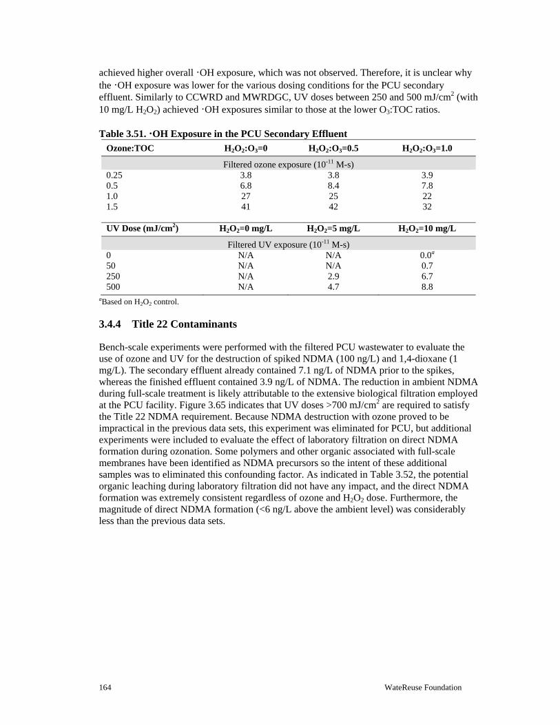
164 WateReuse Foundation
achieved higher overall ·OH exposure, which was not observed. Therefore, it is unclear why the ·OH exposure was lower for the various dosing conditions for the PCU secondary effluent. Similarly to CCWRD and MWRDGC, UV doses between 250 and 500 mJ/cm2 (with 10 mg/L H2O2) achieved ·OH exposures similar to those at the lower O3:TOC ratios. Table 3.51. ·OH Exposure in the PCU Secondary Effluent
Ozone:TOC H2O2:O3=0 H2O2:O3=0.5 H2O2:O3=1.0
Filtered ozone exposure (10-11 M-s) 0.25 3.8 3.8 3.9 0.5 6.8 8.4 7.8 1.0 27 25 22 1.5 41 42 32
UV Dose (mJ/cm2) H2O2=0 mg/L H2O2=5 mg/L H2O2=10 mg/L
Filtered UV exposure (10-11 M-s) 0 N/A N/A 0.0a 50 N/A N/A 0.7 250 N/A 2.9 6.7 500 N/A 4.7 8.8
aBased on H2O2 control.
3.4.4 Title 22 Contaminants
Bench-scale experiments were performed with the filtered PCU wastewater to evaluate the use of ozone and UV for the destruction of spiked NDMA (100 ng/L) and 1,4-dioxane (1 mg/L). The secondary effluent already contained 7.1 ng/L of NDMA prior to the spikes, whereas the finished effluent contained 3.9 ng/L of NDMA. The reduction in ambient NDMA during full-scale treatment is likely attributable to the extensive biological filtration employed at the PCU facility. Figure 3.65 indicates that UV doses >700 mJ/cm2 are required to satisfy the Title 22 NDMA requirement. Because NDMA destruction with ozone proved to be impractical in the previous data sets, this experiment was eliminated for PCU, but additional experiments were included to evaluate the effect of laboratory filtration on direct NDMA formation during ozonation. Some polymers and other organic associated with full-scale membranes have been identified as NDMA precursors so the intent of these additional samples was to eliminated this confounding factor. As indicated in Table 3.52, the potential organic leaching during laboratory filtration did not have any impact, and the direct NDMA formation was extremely consistent regardless of ozone and H2O2 dose. Furthermore, the magnitude of direct NDMA formation (<6 ng/L above the ambient level) was considerably less than the previous data sets.

WateReuse Research Foundation 165
Figure 3.65. Destruction of NDMA in the filtered PCU secondary effluent.
Table 3.52. Direct NDMA Formation in the PCU Secondary Effluent
O3:TOC Ratio H2O2:O3 Ratio Unfiltered NDMA (ng/L) Filtered NDMA (ng/L)
0 0 N/A 7.1 0.25 0 11 10 0.25 0.5 9.6 9.9 0.5 0 13 11 0.5 0.5 11 11 1.0 0 12 11 1.0 0.5 11 11 1.5 0 12 13 1.5 0.5 12 10
Table 3.53 illustrates the potential reductions in NDMA formation potential provided by ozonation and UV-based oxidation. With respect to the secondary effluent, the overall NDMA formation potential with chloramination was relatively low, and the finished effluent was even lower, presumably because of the low level of total nitrogen in the finished effluent. Again, low levels of NDMA after ozonation were linked to low levels of NDMA formation potential after chloramination. Ozonation achieved reductions in overall NDMA formation potential ranging from 91% to 98%. In fact, there was actually a net destruction of NDMA during the chloramination experiments after for the Day 0 concentrations were accounted for. In contrast to previous experiments, ozone/H2O2 led to lower levels of NDMA after chloramination, but higher ozone doses did not necessarily lead to lower NDMA levels. UV and UV/H2O2 were also moderately effective in reducing NDMA formation potential (maximum reduction of 81%), although ozonation was still a more effective option.
0.0
0.2
0.4
0.6
0.8
1.0
1.2
1.4
1.6
0 100 200 300 400 500 600 700
UV Dose (mJ/cm2)
Log
Des
truc
tion
of
ND
MA
UV (H2O2=0 mg/L) UV (H2O2=5 mg/L)UV (H2O2 10 /L) Li (UV (H2O2 10 /L))
CDPH Title 22
Log
Des
tru
ctio
n of
ND
MA
UV (H2O2=0 mg/L) UV (H2O2=5 mg/L) UV (H2O2=10 mg/L)
0.0
0.2
0.4
0.6
0.8
1.0
1.2
1.4
1.6
0 100 200 300 400 500 600 700
UV Dose (mJ/cm2)
Log
Des
truc
tion
of
ND
MA
UV (H2O2=0 mg/L) UV (H2O2=5 mg/L)UV (H2O2 10 /L) Li (UV (H2O2 10 /L))
CDPH Title 22
Log
Des
tru
ctio
n of
ND
MA
UV (H2O2=0 mg/L) UV (H2O2=5 mg/L) UV (H2O2=10 mg/L)

166 WateReuse Foundation
Regardless of the oxidant, the precursors in this matrix appeared to be more susceptible to oxidation than those in the previous bench-scale experiments. Table 3.53. NDMA Formation Potential in the Filtered PCU Secondary Effluent
Testing Condition NDMA Day 0 (before chloramine)
NDMA Day 10 (after chloramine)
Total Chlorine Day 10
Secondary effluent 7.1 ng/L 290 ng/L 1.4 mg/L H2O2 control Not measured 260 ng/L 1.5 mg/L Ozone 0.25/0 10 ng/L 20 ng/L 1.5 mg/L Ozone 0.25/0.5 9.9 ng/L 7.1 ng/L 1.4 mg/L Ozone 0.5/0 11 ng/L 6.4 ng/L 1.2 mg/L Ozone 0.5/0.5 11 ng/L 7.0 ng/L 1.2 mg/L Ozone 1.0/0 11 ng/L 27 ng/L 0.94 mg/L Ozone 1.0/0.5 11 ng/L 10 ng/L 1.2 mg/L Ozone 1.5/0 13 ng/L 23 ng/L 0.96 mg/L Ozone 1.5/0.5 10 ng/L 12 ng/L 1.1 mg/L UV 50/0 Not measured 220 ng/L 1.5 mg/L UV 50/10 Not measured 180 ng/L 1.1 mg/L UV 250/0 Not measured 140 ng/L 1.5 mg/L UV 250/5 Not measured 120 ng/L 1.4 mg/L UV 250/10 Not measured 110 ng/L 1.1 mg/L UV 500/0 Not measured 70 ng/L 1.5 mg/L UV 500/5 Not measured 56 ng/L 1.5 mg/L UV 500/10 Not measured 65 ng/L 1.1 mg/L Finished 3.9 ng/L 91 ng/L 2.4 mg/L
Figure 3.66 illustrates the destruction of spiked 1,4-dioxane during the bench-scale ozone experiments. Although each of the pCBA data sets indicates that H2O2 addition had no impact on overall ·OH exposure, ozone/H2O2 consistently outperformed ozone alone during the 1,4-dioxane experiments. For PCU, O3:TOC ratios between 1.2 and >1.5 are necessary to comply with the 0.5-log requirement for ozone/H2O2 and ozone, respectively.

WateReuse Research Foundation 167
Figure 3.66. Destruction of 1,4-dioxane in the filtered PCU secondary effluent.
3.4.5 Trace Organic Contaminants
Secondary and finished effluent samples from PCU were analyzed to determine the ambient concentrations of the target compounds, which are provided in Table 3.54. None of the target compounds were present at concentrations exceeding 1 μg/L, and a majority of the target compounds were present at <100 ng/L in the secondary effluent. The efficacy of the secondary biological treatment process is evident in the “absence” of the bioamenable compounds (e.g., naproxen and ibuprofen), and the subsequent chlorination process was effective in oxidizing the more susceptible compounds (e.g., diclofenac and gemfibrozil). The total estrogenicity of the secondary and finished effluents was determined to be 0.66 and <0.074 ng/L, respectively.
0.0
0.1
0.2
0.3
0.4
0.5
0.6
0.7
0.8
0.9
1.0
0 0.25 0.5 0.75 1 1.25 1.5
O3:TOC Ratio
Lo
g D
estr
uct
ion
of
1,4-
dio
xan
e
H2O2:O3=0
H2O2:O3=0.5
CDPH Title 22
Log
Des
tru
ctio
n o
f 1,
4-d
ioxa
ne
0.0
0.1
0.2
0.3
0.4
0.5
0.6
0.7
0.8
0.9
1.0
0 0.25 0.5 0.75 1 1.25 1.5
O3:TOC Ratio
Lo
g D
estr
uct
ion
of
1,4-
dio
xan
e
H2O2:O3=0
H2O2:O3=0.5
CDPH Title 22
Log
Des
tru
ctio
n o
f 1,
4-d
ioxa
ne

168 WateReuse Foundation
Table 3.54. Ambient TOrC Concentrations at PCU
Parameter Secondary Effluent (ng/L) Finished Effluent (ng/L)
Bisphenol A <50 <50 Diclofenac 130 <25 Gemfibrozil 120 <10 Ibuprofen <25 <25 Musk Ketone <100 <100 Naproxen <25 <25 Triclosan <25 <25 Atenolol 78 28 Atrazine 42 76 Carbamazepine 310 35 DEET <25 30 Meprobamate 250 360 Phenytoin 260 270 Primidone 240 270 Sulfamethoxazole 990 <25 Trimethoprim 16 <10 TCEP 410 370 Total Estrogenicity (EEq) 0.66 <0.074
Bench-scale TOrC oxidation experiments were performed with spiking stocks and protocols similar to the previous bench-scale experiments. Again, the experiments focused on laboratory-filtered secondary effluent. Table 3.55 shows the relative oxidation levels of the 16 target compounds (musk ketone omitted) after ozonation. Although the pCBA data were inconsistent, the PCU data indicate that H2O2 addition provided a slight benefit for some of the ozone-resistant compounds (Groups 3, 4, and 5) at higher O3:TOC ratios. Similarly to WBMWD, the benefit may not be sufficient to warrant H2O2 addition for this reason alone. With respect to the five rate constant categories, the trends were generally in agreement with the previous bench-scale experiments: an O3:TOC ratio of 0.25 was necessary to achieve greater than 80% oxidation of the Group 1 compounds, an O3:TOC ratio of 0.5 was necessary for the Group 2 compounds, an O3:TOC ratio of 1.0 was necessary for the Group 3 compounds, and an O3:TOC of 1.0 generally achieved 80–90% oxidation for the Group 4 compounds. TCEP proved to be highly resistant to both ozone and ·OH, as this compound barely exceeded 30% oxidation even for the highest dosing conditions.
Table 3.56 shows the relative photolysis and UV/H2O2 oxidation levels of the target compounds. Similarly to the previous data sets, only two compounds (diclofenac and triclosan) experienced greater than 80% destruction with UV irradiation alone, whereas atrazine, phenytoin, and sulfamethoxazole experienced greater than 30% destruction with UV alone. The addition of H2O2 with a UV dose of 500 mJ/cm2 was able to achieve approximately 70% destruction for sulfamethoxazole and phenytoin, whereas the remaining compounds (excluding TCEP) ranged from 20 to 65% destruction.
Finally, the total estrogenicity of the secondary effluent was oxidized down to the MRL with every ozone and H2O2 dosing condition, whereas UV and UV/H2O2 were unable to achieve the MRL with the dosing conditions used in this study. These data are summarized in Figure 3.67. However, the total estrogenicity of the samples was quite low to start, so this might not be a significant concern.
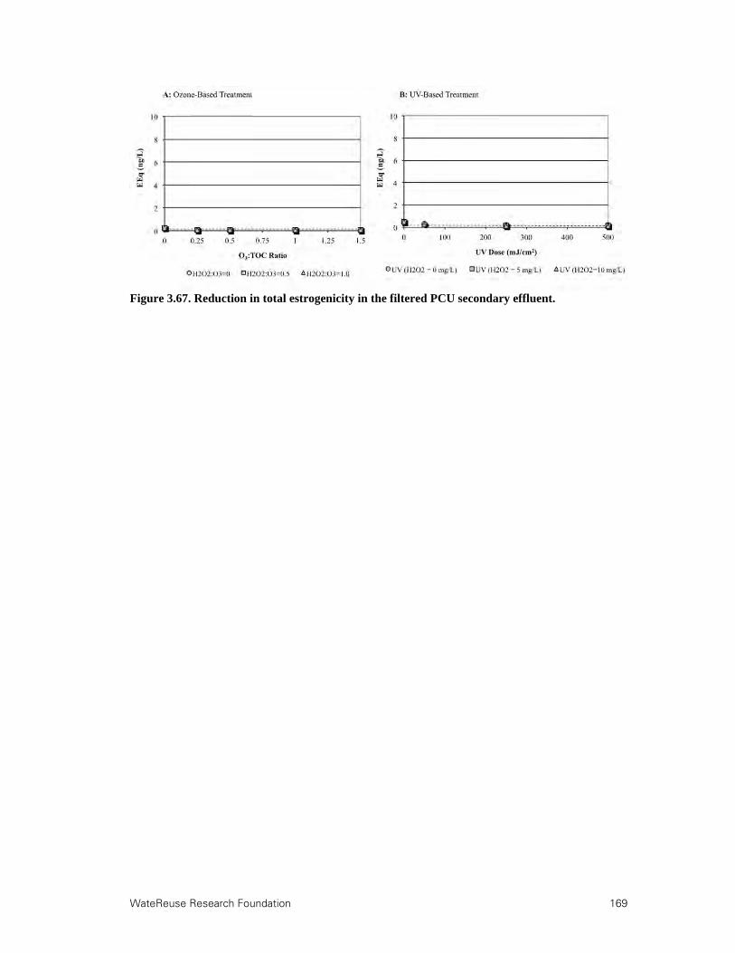
WateReuse Research Foundation 169
Figure 3.67. Reduction in total estrogenicity in the filtered PCU secondary effluent.

170 WateReuse Foundation
Table 3.55. PCU TOrC Mitigation by Ozone (Filtered)
Group Contaminant O3:TOC (mass) / H2O2:O3 (molar)
0.25/0 0.25/0.5 0.25/1.0 0.5/0 0.5/0.5 0.5/1.0 1.0/0 1.0/0.5 1.0/1.0 1.5/0 1.5/0.5 1.5/1.0
1 Sulfamethoxazole 88% 88% 86% 98% 96% 95% 99% 99% 99% 99% 99% 99% Diclofenac 98% 98% 98% 98% 98% 98% 98% 98% 98% 98% 98% 98% Bisphenol A 97% 97% 97% 97% 97% 97% 97% 97% 97% 97% 97% 97% Carbamazepine 99% 99% 93% 99% 99% 99% 99% 99% 99% 99% 99% 99% Trimethoprim 99% 99% 97% 99% 99% 99% 99% 99% 99% 99% 99% 99% Naproxen 98% 98% 94% 98% 98% 98% 98% 98% 98% 98% 98% 98% Triclosan 98% 98% 98% 98% 98% 98% 98% 98% 98% 98% 98% 98% Indicator 97% 97% 95% 98% 98% 98% 98% 98% 98% 98% 98% 98%
2 Gemfibrozil 84% 76% 73% 99% 99% 99% 99% 99% 99% 99% 99% 99% Atenolol 49% 44% 52% 97% 92% 84% 97% 97% 97% 97% 97% 97% Indicator 67% 60% 63% 98% 96% 92% 98% 98% 98% 98% 98% 98%
3 Ibuprofen 40% 42% 45% 70% 73% 75% 92% 97% 95% 98% 98% 98% Phenytoin 36% 42% 32% 70% 73% 77% 93% 97% 96% 97% 99% 99% DEET 29% 29% 35% 57% 62% 65% 85% 94% 92% 93% 99% 97% Primidone 38% 33% 38% 62% 63% 66% 90% 95% 93% 95% 99% 97% Indicator 36% 37% 38% 65% 68% 71% 90% 96% 94% 96% 99% 98%
4 Atrazine 20% 18% 22% 38% 39% 42% 62% 74% 70% 75% 86% 84% Meprobamate 19% 21% 25% 42% 46% 43% 65% 82% 80% 77% 92% 89% Indicator 20% 20% 24% 40% 43% 43% 64% 78% 75% 76% 89% 87%
5 TCEP 11% 7% 14% 12% 14% 12% 12% 25% 21% 21% 32% 32%

WateReuse Research Foundation 171
Table 3.56. PCU TOrC Mitigation by UV (Filtered)
Group Contaminant UV Dose (mJ/cm2) / H2O2 Dose (mg/L)
50/0 50/10 250/0 250/5 250/10 500/0 500/5 500/10
1 Sulfamethoxazole 6% 6% 44% 35% 24% 62% 65% 71% Diclofenac 41% 3% 92% 83% 84% 98% 96% 96% Bisphenol A 20% 0% 20% 6% 13% 25% 31% 54% Carbamazepine 0% 0% 0% 15% 15% 0% 50% 45% Trimethoprim -8% 8% -8% 15% 15% 0% 28% 45% Naproxen 8% 0% 17% 25% 28% 22% 41% 60% Triclosan 37% -9% 89% 76% 74% 97% 95% 95%
2 Gemfibrozil 7% 0% 5% 10% 12% 10% 23% 41% Atenolol 3% -2% 6% 20% 13% 0% 24% 34%
3 Ibuprofen 6% -2% 5% 10% 12% 11% 30% 41% Phenytoin -11% 9% 16% 41% 36% 41% 57% 69% DEET 6% 0% 0% 7% 7% 6% 13% 27% Primidone 0% 9% 5% 18% 14% 9% 27% 36%
4 Atrazine 9% 0% 25% 14% 12% 36% 34% 39% Meprobamate -2% 6% 4% 12% 7% 3% 16% 23%
5 TCEP 3% -4% 2% 4% -2% 5% 2% 0%
Notes. Groupings based on ozone and ·OH rate constants. Shading represents >80% photolysis or oxidation.

172 WateReuse Foundation
3.4.6 Disinfection
Ambient secondary (before and after laboratory filtration) and finished effluent samples were assayed for total and fecal coliforms, MS2, and Bacillus spores. The ambient microbial water quality data are provided in Table 3.57 and appear to be consistent with those for CCWRD and MWRDGC. To illustrate a wide range of inactivation, the ozone and UV disinfection samples were spiked with relatively large numbers of the surrogate microbes, as indicated in Table 3.58.
Table 3.57. Ambient Microbial Water Quality Data for PCU
Microbial Surrogate Unfiltered Secondary
Effluent Filtered Secondary
Effluent Finished Effluent
Total coliforms (MPN/100 mL) 4.3 103 1.3 103 <1
Fecal coliforms (MPN/100 mL) 2.7 102 1.5 102 <1
MS2 (PFU/mL)
<1 <1 <1
Bacillus spores (CFU/100 mL) 5.2 103 4.0 103 73
Table 3.58. Microbial Spiking Levels for PCU Bench-Scale Experiments
Microbial Surrogate Filtered Ozone
Disinfection Filtered UV Disinfection
E. coli (MPN/100 mL) 1.1 108 6.9 106 MS2 (PFU/mL) 1.2 107 9.2 106 B. subtilis spores (CFU/100 mL) 2.2 105 2.4 105
Figure 3.68 illustrates the inactivation of spiked E. coli during the bench-scale ozone experiments. The solid line near the top of the figure represents the limit of inactivation based on the spiking level in the filtered samples. Inactivation with H2O2 alone was generally insignificant, and when combined with ozonation, the addition of H2O2 significantly hindered E. coli inactivation. In fact, the addition of H2O2 reduced the inactivation level by more than 5 logs for an O3:TOC ratio of 1.0. The average log-inactivation values for each treatment condition are provided in Table 3.59.
Figure 3.69 illustrates the inactivation of spiked MS2 during the bench-scale ozone experiments. Again, minimal inactivation was achieved by the addition of H2O2 alone, and in contrast to the E. coli data, ozone and ozone/H2O2 actually achieved similar levels of inactivation. With respect to the CDPH Title 22 requirements, an O3:TOC ratio >0.5 was often sufficient for the 5- and 6.5-log inactivation requirements, but compliance with this benchmark was not entirely consistent. The average log-inactivation values for each treatment condition are provided in Table 3.60.
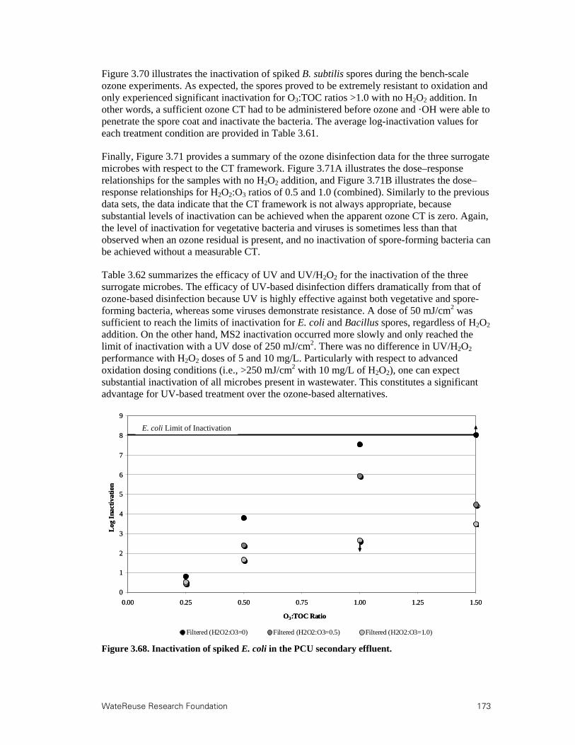
WateReuse Research Foundation 173
Figure 3.70 illustrates the inactivation of spiked B. subtilis spores during the bench-scale ozone experiments. As expected, the spores proved to be extremely resistant to oxidation and only experienced significant inactivation for O3:TOC ratios >1.0 with no H2O2 addition. In other words, a sufficient ozone CT had to be administered before ozone and ·OH were able to penetrate the spore coat and inactivate the bacteria. The average log-inactivation values for each treatment condition are provided in Table 3.61.
Finally, Figure 3.71 provides a summary of the ozone disinfection data for the three surrogate microbes with respect to the CT framework. Figure 3.71A illustrates the dose–response relationships for the samples with no H2O2 addition, and Figure 3.71B illustrates the dose–response relationships for H2O2:O3 ratios of 0.5 and 1.0 (combined). Similarly to the previous data sets, the data indicate that the CT framework is not always appropriate, because substantial levels of inactivation can be achieved when the apparent ozone CT is zero. Again, the level of inactivation for vegetative bacteria and viruses is sometimes less than that observed when an ozone residual is present, and no inactivation of spore-forming bacteria can be achieved without a measurable CT.
Table 3.62 summarizes the efficacy of UV and UV/H2O2 for the inactivation of the three surrogate microbes. The efficacy of UV-based disinfection differs dramatically from that of ozone-based disinfection because UV is highly effective against both vegetative and spore-forming bacteria, whereas some viruses demonstrate resistance. A dose of 50 mJ/cm2 was sufficient to reach the limits of inactivation for E. coli and Bacillus spores, regardless of H2O2 addition. On the other hand, MS2 inactivation occurred more slowly and only reached the limit of inactivation with a UV dose of 250 mJ/cm2. There was no difference in UV/H2O2 performance with H2O2 doses of 5 and 10 mg/L. Particularly with respect to advanced oxidation dosing conditions (i.e., >250 mJ/cm2 with 10 mg/L of H2O2), one can expect substantial inactivation of all microbes present in wastewater. This constitutes a significant advantage for UV-based treatment over the ozone-based alternatives.
Figure 3.68. Inactivation of spiked E. coli in the PCU secondary effluent.
0
1
2
3
4
5
6
7
8
9
0.00 0.25 0.50 0.75 1.00 1.25 1.50
O3:TOC Ratio
Log
Ina
ctiv
atio
n
Filtered (H2O2:O3=0) Filtered (H2O2:O3=0.5) Filtered (H2O2:O3=1.0)
E. coli Limit of Inactivation
0
1
2
3
4
5
6
7
8
9
0.00 0.25 0.50 0.75 1.00 1.25 1.50
O3:TOC Ratio
Log
Ina
ctiv
atio
n
Filtered (H2O2:O3=0) Filtered (H2O2:O3=0.5) Filtered (H2O2:O3=1.0)
E. coli Limit of Inactivation

174 WateReuse Foundation
Table 3.59. Summary of E. coli Inactivation in the PCU Secondary Effluent
O3:TOC Ratio H2O2:O3=0 H2O2:O3=0.5 H2O2:O3=1.0
0.25 0.8 0.5 0.5
0.5 3.8 2.4 1.7
1.0 7.6 6.0 <2.7a
1.5 >8.0b 4.5 3.5
aInsufficient dilutions to accurately quantify sample. bLimit of inactivation based on spiking level.
Figure 3.69. Inactivation of spiked MS2 in the PCU secondary effluent.
Table 3.60. Summary of MS2 Inactivation in the PCU Secondary Effluent
O3:TOC Ratio H2O2:O3=0 H2O2:O3=0.5 H2O2:O3=1.0
0.25 0.8 0.9 1.1 0.5 6.0 >7.1a >7.1 a 1.0 6.4 5.6 5.7 1.5 >7.1 a 6.9 6.9
a Limit of inactivation is based on spiking level.
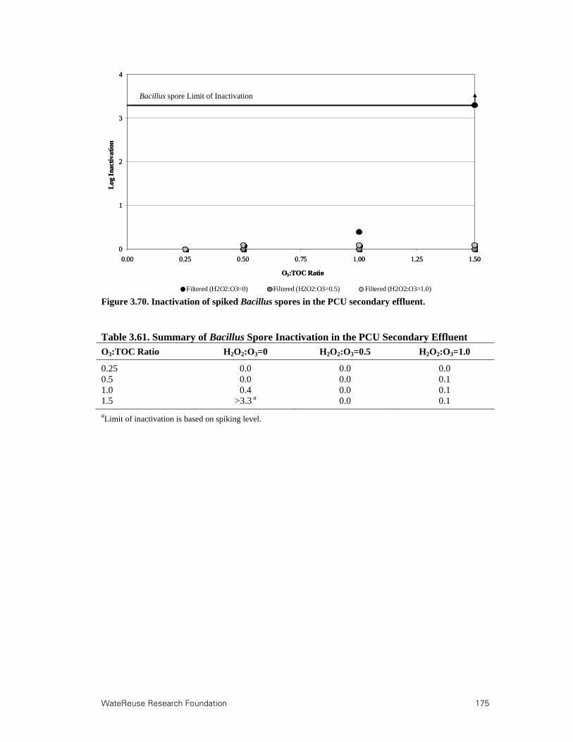
WateReuse Research Foundation 175
Figure 3.70. Inactivation of spiked Bacillus spores in the PCU secondary effluent.
Table 3.61. Summary of Bacillus Spore Inactivation in the PCU Secondary Effluent
O3:TOC Ratio H2O2:O3=0 H2O2:O3=0.5 H2O2:O3=1.0
0.25 0.0 0.0 0.0 0.5 0.0 0.0 0.1 1.0 0.4 0.0 0.1 1.5 >3.3 a 0.0 0.1
aLimit of inactivation is based on spiking level.
0
1
2
3
4
0.00 0.25 0.50 0.75 1.00 1.25 1.50
O3:TOC Ratio
Log
Ina
ctiv
atio
n
Filtered (H2O2:O3=0) Filtered (H2O2:O3=0.5) Filtered (H2O2:O3=1.0)
Bacillus spore Limit of Inactivation
0
1
2
3
4
0.00 0.25 0.50 0.75 1.00 1.25 1.50
O3:TOC Ratio
Log
Ina
ctiv
atio
n
Filtered (H2O2:O3=0) Filtered (H2O2:O3=0.5) Filtered (H2O2:O3=1.0)
Bacillus spore Limit of Inactivation

176 WateReuse Foundation
Figure 3.71. Significance of CT for disinfection in the PCU secondary effluent.

WateReuse Research Foundation 177
Table 3.62. Summary of UV Inactivation in the PCU Secondary Effluent
UV Dose (mJ/cm2)
E. coli MS2 Bacillus spore UV UV/H2O2
a UV UV/H2O2a UV UV/H2O2
a
25 2.5 >6.8b 1.7 1.9 3.3 2.7 50 6.8 >6.8b 2.8 3.1 >3.4b >3.4b 250 >6.8b >6.8b >7.0b >7.0b >3.4b >3.4b 500 >6.8b >6.8b >7.0b >7.0b >3.4b >3.4b aH2O2 doses of 5 and 10 mg/L achieved similar levels of inactivation. bLimit of inactivation is based on spiking level.
3.4.7 Organic Characterization
Similarly to the previous three data sets, the full-spectrum scans in Figures 3.72 and 3.73 (without (A) and with (B) H2O2 addition) indicate that the absorbance profiles around 254 nm generally provide the greatest resolution between treatments. Because of the limited efficacy of UV photolysis (Figure 3.73A), there is little resolution regardless of wavelength, whereas UV/H2O2 (Figure 3.73B) provided slight improvements. Figure 3.74 focuses on the change in UV254 absorbance with ozone, ozone/H2O2, UV, and UV/H2O2. With respect to ozonation, reductions in UV254 absorbance were slightly hindered by the addition of H2O2, whereas the synergistic aspect of the UV AOP provided slight improvements over UV alone.
3D EEMs were developed for the filtered secondary effluent, the finished effluent, and the various treatment conditions. Figure 3.75 illustrates the fluorescence fingerprint of the secondary and finished effluent samples and also provides the total and regional fluorescence intensities based on arbitrary fluorescence units. The fluorescence fingerprint pattern was similar to those for CCWRD and MWRDGC but at a higher intensity. The efficacy of the subsequent full-scale filtration and chlorination processes is apparent, based on the reduction in fluorescence intensity from the secondary effluent to the finished effluent sample.
Figure 3.76 provides a qualitative illustration of treatment efficacy after ozone- and UV-based oxidation. Similarly to the previous data sets, ozone and ozone/H2O2 are capable of achieving substantial reductions in regional and total fluorescence, whereas UV and UV/H2O2 provide minimal reductions. It is interesting to note that the sample associated with an O3:TOC ratio of 1.5 and an H2O2:O3 ratio of 0 was characterized by an unusual fluorescence peak in Region I. This peak is also evident in Figure 3.77, which is described in the following.
Figure 3.77 and Figure 3.78 illustrate the fluorescence profiles at an excitation wavelength of 254 nm after ozonation and UV/H2O2, respectively. Because the addition of H2O2 did not have a significant impact on ozone efficacy and UV photolysis provided limited reductions in fluorescence intensity, these fluorescence profiles are not shown. In contrast to WBMWD, which was characterized by two distinct peaks, PCU was similar to CCWRD and MWRDGC in that only one distinct peak was apparent.

178 WateReuse Foundation
Figure 3.72. PCU absorbance spectra after ozonation.
0.00
0.05
0.10
0.15
0.20
0.25
240 280 320 360 400 440 480 520 560 600
0.00
0.05
0.10
0.15
0.20
0.25
240 280 320 360 400 440 480 520 560 600
Ab
sorb
ance
(cm
-1)
Ab
sorb
ance
(cm
-1)
O3:TOC = 0
O3:TOC = 0.25
O3:TOC = 0.5
O3:TOC = 1.0
O3:TOC = 1.5
Wavelength (nm) Wavelength (nm)
O3:TOC = 0
O3:TOC = 0.25
O3:TOC = 0.5
O3:TOC = 1.0
O3:TOC = 1.5
A: H2O2:O3=0 B: H2O2:O3=0.5
0.00
0.05
0.10
0.15
0.20
0.25
240 280 320 360 400 440 480 520 560 600
0.00
0.05
0.10
0.15
0.20
0.25
240 280 320 360 400 440 480 520 560 600
Ab
sorb
ance
(cm
-1)
Ab
sorb
ance
(cm
-1)
O3:TOC = 0
O3:TOC = 0.25
O3:TOC = 0.5
O3:TOC = 1.0
O3:TOC = 1.5
Wavelength (nm) Wavelength (nm)
O3:TOC = 0
O3:TOC = 0.25
O3:TOC = 0.5
O3:TOC = 1.0
O3:TOC = 1.5
A: H2O2:O3=0 B: H2O2:O3=0.5

WateReuse Research Foundation 179
Figure 3.73. PCU absorbance spectra after UV and UV/H2O2.
0.00
0.05
0.10
0.15
0.20
0.25
240 280 320 360 400 440 480 520 560 600
Wavelength (nm)
Ab
sorb
ance
(cm
-1)
0.00
0.05
0.10
0.15
0.20
0.25
240 280 320 360 400 440 480 520 560 600
Wavelength (nm)
Ab
sorb
ance
(cm
-1)
Ab
sorb
ance
(cm
-1)
Wavelength (nm)
Ab
sorb
ance
(cm
-1)
Wavelength (nm)
A: H2O2=0 mg/L B: H2O2:O3=10 mg/L
UV = 0 mJ/cm2
UV = 50 mJ/cm2
UV = 250 mJ/cm2
UV = 500 mJ/cm2
UV = 0 mJ/cm2
UV = 50 mJ/cm2
UV = 250 mJ/cm2
UV = 500 mJ/cm2
0.00
0.05
0.10
0.15
0.20
0.25
240 280 320 360 400 440 480 520 560 600
Wavelength (nm)
Ab
sorb
ance
(cm
-1)
0.00
0.05
0.10
0.15
0.20
0.25
240 280 320 360 400 440 480 520 560 600
Wavelength (nm)
Ab
sorb
ance
(cm
-1)
Ab
sorb
ance
(cm
-1)
Wavelength (nm)
Ab
sorb
ance
(cm
-1)
Wavelength (nm)
A: H2O2=0 mg/L B: H2O2:O3=10 mg/L
UV = 0 mJ/cm2
UV = 50 mJ/cm2
UV = 250 mJ/cm2
UV = 500 mJ/cm2
UV = 0 mJ/cm2
UV = 50 mJ/cm2
UV = 250 mJ/cm2
UV = 500 mJ/cm2

180 WateReuse Foundation
Figure 3.74. Differential UV254 absorbance in the PCU secondary effluent.
0%
10%
20%
30%
40%
50%
60%
70%
0 0.25 0.5 0.75 1 1.25 1.5
O 3:TO C Ratio
Dif
fere
ntia
l UV
25
4 A
bsor
banc
e
H2O2:O3 = 0 H2O2:O3 = 0.5 H2O2:O3 = 1.0
0%
10%
20%
30%
40%
50%
60%
70%
0 100 200 300 400 500 600 700
UV Dose (mJ/cm2)
Dif
fere
ntia
l UV
25
4 A
bsor
banc
e
UV (H2O2=0 mg/L) UV (H2O2=5 mg/L) UV (H2O2=10 mg/L)
Dif
fere
nti
al U
V25
4A
bsor
ban
ce
Dif
fere
nti
al U
V25
4A
bso
rban
ce
A: Ozone-Based Treatment B: UV-Based Treatment
0%
10%
20%
30%
40%
50%
60%
70%
0 0.25 0.5 0.75 1 1.25 1.5
O 3:TO C Ratio
Dif
fere
ntia
l UV
25
4 A
bsor
banc
e
H2O2:O3 = 0 H2O2:O3 = 0.5 H2O2:O3 = 1.0
0%
10%
20%
30%
40%
50%
60%
70%
0 100 200 300 400 500 600 700
UV Dose (mJ/cm2)
Dif
fere
ntia
l UV
25
4 A
bsor
banc
e
UV (H2O2=0 mg/L) UV (H2O2=5 mg/L) UV (H2O2=10 mg/L)
Dif
fere
nti
al U
V25
4A
bsor
ban
ce
Dif
fere
nti
al U
V25
4A
bso
rban
ce
A: Ozone-Based Treatment B: UV-Based Treatment

WateReuse Research Foundation 181
Figure 3.75. 3D EEMs for ambient samples from PCU.

182 WateReuse Foundation
Figure 3.76. 3D EEMs after treatment for the filtered PCU secondary effluent.

WateReuse Research Foundation 183
Figure 3.77. PCU fluorescence profiles (Ex254) after ozonation.
Figure 3.78. PCU fluorescence profiles (Ex254) after UV/H2O2
Excitation Wavelength = 254 nmH2O2:O3 = 0
0.0
0.5
1.0
1.5
2.0
2.5
3.0
280 300 320 340 360 380 400 420 440 460 480
Emission Wavelength (nm)
Flu
ores
cen
ce I
nte
nsit
y
O3:TOC = 0O3:TOC = 0.25
O3:TOC = 0.5O3:TOC = 1.0O3:TOC = 1.5
Flu
ores
cen
ce I
nte
nsi
ty
Excitation Wavelength = 254 nmH2O2:O3 = 0
0.0
0.5
1.0
1.5
2.0
2.5
3.0
280 300 320 340 360 380 400 420 440 460 480
Emission Wavelength (nm)
Flu
ores
cen
ce I
nte
nsit
y
O3:TOC = 0O3:TOC = 0.25
O3:TOC = 0.5O3:TOC = 1.0O3:TOC = 1.5
Flu
ores
cen
ce I
nte
nsi
ty
Excitation Wavelength = 254 nmH2O2 = 10 mg/L
0.0
0.5
1.0
1.5
2.0
2.5
3.0
280 300 320 340 360 380 400 420 440 460 480
Emission Wavelength (nm)
Flu
ores
cenc
e In
ten
sity
UV = 0 mJ/cm2
UV = 50 mJ/cm2
UV = 250 mJ/cm2UV = 500 mJ/cm2
Flu
ores
cen
ce I
nte
nsi
ty
Excitation Wavelength = 254 nmH2O2 = 10 mg/L
0.0
0.5
1.0
1.5
2.0
2.5
3.0
280 300 320 340 360 380 400 420 440 460 480
Emission Wavelength (nm)
Flu
ores
cenc
e In
ten
sity
UV = 0 mJ/cm2
UV = 50 mJ/cm2
UV = 250 mJ/cm2UV = 500 mJ/cm2
Flu
ores
cen
ce I
nte
nsi
ty

184 WateReuse Foundation
Table 3.63 provides the fluorescence (i.e., Ex370Em450/Ex370Em500) and treatment indices (i.e., Ex254Em450,T/Ex254Em450,A) for the PCU experiments. Similarly to WBMWD, the FI values remained relatively constant regardless of the treatment condition. In other words, the organic matter associated with emissions at 450 nm and 500 nm was oxidized at similar relative rates. These relative changes are illustrated in Figure 3.79, and Figures 3.80 and 3.81 illustrate the changes in total and regional fluorescence intensities for ozone and UV/H2O2, respectively.
The TI, which measures the extent of organic transformation, reached as low as 0.07 for the highest O3:TOC ratio, thereby indicating that 93% of the original fluorescence had been eliminated. This TI reduction is similar to those of the previous three data sets, thereby highlighting the significance of relative changes in bulk organic matter for various water qualities. Also similar to the previous data sets, the addition of H2O2 hindered the oxidation of the bulk organic matter. Because of the limited reduction in fluorescence with UV, the corresponding FI and TI values did not change significantly, although UV/H2O2 provided slight improvements.
Table 3.63. FI and TI Values for the PCU Secondary Effluent
O3:TOC H2O2:O3=0 H2O2:O3=0.5 H2O2:O3=1.0
FI TI FI TI FI TI
Filtered ozone exposure 0 1.30 1.00 1.30 1.00 1.30 1.00 0.25 1.28 0.54 1.26 0.48 1.28 0.50 0.5 1.25 0.26 1.25 0.28 1.27 0.29 1.0 1.24 0.11 1.25 0.14 1.28 0.16 1.5 1.27 0.07 1.28 0.12 1.27 0.12
UV Dose (mJ/cm2)
H2O2=0 mg/L H2O2=5 mg/L H2O2=10 mg/L FI TI FI TI FI TI
Filtered UV exposure 0 1.27 1.00 1.27 1.00 1.27 1.00 50 1.27 1.00 N/A N/A 1.26 0.97 250 1.25 0.98 1.25 0.94 1.24 0.91 500 1.24 0.97 1.23 0.87 1.25 0.80

WateReuse Research Foundation 185
Figure 3.79. PCU fluorescence profiles (Ex370) after ozonation.
Excitation Wavelength = 370 nmH2O2:O3 = 0
0.00
0.25
0.50
0.75
1.00
400 425 450 475 500 525 550
Emission Wavelength (nm)
Flu
ores
cen
ce I
nten
sity
O3:TOC = 0
O3:TOC = 0.25
O3:TOC = 0.5
O3:TOC = 1.0
O3:TOC = 1.5
Flu
ores
cen
ce I
nte
nsi
tyEm450 Em500
Excitation Wavelength = 370 nmH2O2:O3 = 0
0.00
0.25
0.50
0.75
1.00
400 425 450 475 500 525 550
Emission Wavelength (nm)
Flu
ores
cen
ce I
nten
sity
O3:TOC = 0
O3:TOC = 0.25
O3:TOC = 0.5
O3:TOC = 1.0
O3:TOC = 1.5
Flu
ores
cen
ce I
nte
nsi
tyEm450 Em500
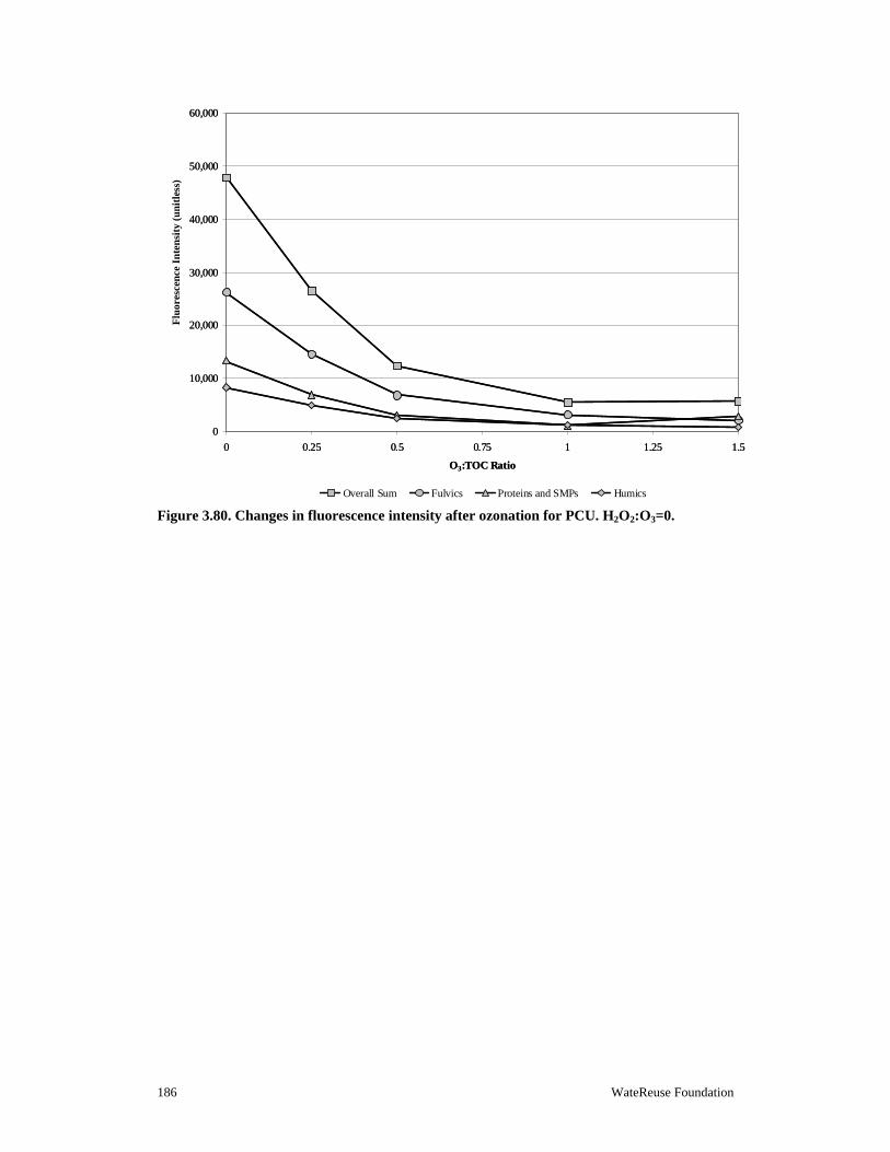
186 WateReuse Foundation
Figure 3.80. Changes in fluorescence intensity after ozonation for PCU. H2O2:O3=0.
0
10,000
20,000
30,000
40,000
50,000
60,000
0 0.25 0.5 0.75 1 1.25 1.5
O3:TOC Ratio
Flu
ores
cenc
e In
tens
ity
(un
itle
ss)
Overall Sum Fulvics Proteins and SMPs Humics
Flu
ores
cenc
e In
ten
sity
(un
itle
ss)
0
10,000
20,000
30,000
40,000
50,000
60,000
0 0.25 0.5 0.75 1 1.25 1.5
O3:TOC Ratio
Flu
ores
cenc
e In
tens
ity
(un
itle
ss)
Overall Sum Fulvics Proteins and SMPs Humics
Flu
ores
cenc
e In
ten
sity
(un
itle
ss)

WateReuse Research Foundation 187
Figure 3.81. Changes in fluorescence intensity after UV/H2O2 for PCU. H2O2=10 mg/L.
3.5 Gwinnett County, GA
The study site in Gwinnett County, GA, hereafter referred to as GCGA, is one of the largest ultrafiltration wastewater treatment plants in the world. The GCGA treats approximately 60 MGD of wastewater composed of >98% domestic flows with minor industrial contributions. Multiple liquid treatment trains include the following processes: preliminary screening and grit removal; primary clarification; conventional activated sludge with full nitrification (NH3 < 0.5 mg/L; SRT=11 days), denitrification, and biological phosphorus removal (TPeff < 0.08 mg/L); secondary clarification; and high-pH lime clarification. One treatment train continues with recarbonation and tri-media filtration (sand, anthracite, and garnet), whereas another treatment train continues with strainers and ultrafiltration. Both trains recombine for preozonation (O3=1.0–1.5 mg/L), biologically active filtration (BAF; EBCT=15 min), and final ozone disinfection (O3=1.0–1.5 mg/L). The BAF process actually contains biological activated carbon, but the media have not been replaced or regenerated, so their adsorption capacity is likely exhausted, thereby isolating the biological component. The effluent is discharged through a 20-mile pipeline to the Chattahoochee River. After years of litigation, Gwinnett County also has a permit to discharge the highly treated effluent directly into Lake Lanier, which is the Atlanta metropolitan area’s primary drinking water source. A simplified treatment schematic of the GCGA facility is provided in Figure 3.82.
Secondary and finished effluent from GCGA was collected in January 2012, and the water quality data in Table 3.64 were obtained. Using the initial TOC and nitrite data for the filtered secondary effluent, the ozone dosing conditions in Table 1.65 were calculated.
0
10,000
20,000
30,000
40,000
50,000
60,000
0 100 200 300 400 500
UV Dose (mJ/cm2)
Flu
ores
cen
ce I
nte
nsi
ty (
unit
less
)
Overall Sum Fulvics Proteins and SMPs Humics
Flu
ores
cenc
e In
ten
sity
(un
itle
ss)
0
10,000
20,000
30,000
40,000
50,000
60,000
0 100 200 300 400 500
UV Dose (mJ/cm2)
Flu
ores
cen
ce I
nte
nsi
ty (
unit
less
)
Overall Sum Fulvics Proteins and SMPs Humics
Flu
ores
cenc
e In
ten
sity
(un
itle
ss)
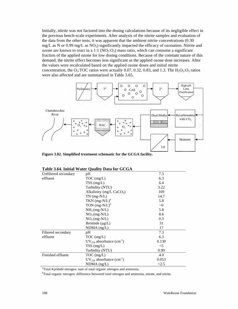
188 WateReuse Foundation
Initially, nitrite was not factored into the dosing calculations because of its negligible effect in the previous bench-scale experiments. After analysis of the nitrite samples and evaluation of the data from the other tests, it was apparent that the ambient nitrite concentrations (0.30 mg/L as N or 0.99 mg/L as NO2) significantly impacted the efficacy of ozonation. Nitrite and ozone are known to react in a 1:1 (NO2:O3) mass ratio, which can consume a significant fraction of the applied ozone for low dosing conditions. Because of the constant nature of this demand, the nitrite effect becomes less significant as the applied ozone dose increases. After the values were recalculated based on the applied ozone doses and initial nitrite concentration, the O3:TOC ratios were actually 0.07, 0.32, 0.83, and 1.3. The H2O2:O3 ratios were also affected and are summarized in Table 3.65.
Figure 3.82. Simplified treatment schematic for the GCGA facility.
Table 3.64. Initial Water Quality Data for GCGA Unfiltered secondary effluent
pH 7.3 TOC (mg/L) 6.3 TSS (mg/L) 6.4 Turbidity (NTU) 3.22 Alkalinity (mg/L CaCO3) 169 TN (mg-N/L) 14.7 TKN (mg-N/L)a 5.8 TON (mg-N/L)b ~0 NH3 (mg-N/L) 5.8 NO3 (mg-N/L) 8.6 NO2 (mg-N/L) 0.3 Bromide (μg/L) 31 NDMA (ng/L) 17
Filtered secondary effluent
pH 7.3 TOC (mg/L) 6.3 UV254 absorbance (cm-1) 0.130 TSS (mg/L) <5 Turbidity (NTU) 0.90
Finished effluent TOC (mg/L) 4.0 UV254 absorbance (cm-1) 0.053 NDMA (ng/L) <2.5
aTotal Kjeldahl nitrogen: sum of total organic nitrogen and ammonia. bTotal organic nitrogen: difference betweenf total nitrogen and ammonia, nitrate, and nitrite.

WateReuse Research Foundation 189
Table 3.65. Ozone Dosing Conditions for 1-L Filtered GCGA Samples
O3:TOC/ H2O2:O3
Wastewater Volume (mL)
Nanopure Volume
(mL)
O3 Volume (mL)
O3 Dose (mg/L)
H2O2 Volume
(μL)
H2O2 Dose (mg/L)
Spike 900 100 0 0 0 0 0.07/0 900 83 17 1.4 0 0 0.07/1.7 900 83 17 1.4 51 0.5 0.07/3.4 900 83 17 1.4 102 1.0 0.32/0 900 67 33 2.8 0 0 0.32/0.8 900 67 33 2.8 99 1.0 0.32/1.6 900 67 33 2.8 199 2.0 0.83/0 900 33 67 5.7 0 0 0.83/0.6 900 33 67 5.7 202 2.0 0.83/1.2 900 33 67 5.7 403 4.0 1.3/0 900 0 100 8.5 0 0 1.3/0.6 900 0 100 8.5 301 3.0 1.3/1.1 900 0 100 8.5 602 6.0
Notes. O3:TOC ratios differ from previous data sets because NO2 was not considered during dosing. Some values are affected by rounding error and the precision of the ozone spike. Concentration of O3 stock solution=85 mg/L; concentration of H2O2 stock solution=10 g/L; filtered dilution ratio=(900/1000)=0.900; filtered TOC after dilution=5.7 mg/L; filtered NO2 after dilution=0.30 mg/L as N=0.99 mg/L as NO2
3.5.1 Ozone Demand/Decay
Figure 3.83 illustrates the ozone demand/decay curves for the filtered GCGA secondary effluent under various dosing conditions. The graph only includes dosing conditions with a measurable ozone residual after 30 s; corresponding CT values are also provided. The O3/H2O2 samples are not included in the figure because the addition of H2O2 led to the formation of ·OH but eliminated the dissolved ozone residual. As expected, the 0.07 O3:TOC ratio was insufficient to establish a measurable ozone residual after 30 s. The low dissolved ozone exposure for an O3:TOC ratio of 0.32 was also expected, considering that O3:TOC ratios of 0.25 were insufficient to establish a residual for the other wastewaters. For the remaining dosing conditions, the graph illustrates the instantaneous ozone demand (i.e., the precipitous drop between 0 and 30 s) and the decay over time. Because of the additional demanded exerted by ambient nitrite levels, the CT values were significantly lower for GCGA than for the other wastewaters.
3.5.2 Bromate Formation
As illustrated in Figure 3.84, there was minimal bromate formation for all of the ozone dosing conditions because of the low initial bromide concentration of 55 μg/L (after dilution by the ozone stock). Even the highest applied ozone doses only formed 10–15 μg/L of bromate, which indicates that this would not be a significant design concern for GCGA. The addition of H2O2 did not have a consistent impact on bromate formation, but dilution after environmental discharge would be more than sufficient to reach the 10 μg/L benchmark without any further mitigation measures.

190 WateReuse Foundation
Figure 3.83. Ozone demand/decay curves for GCGA.
Figure 3.84. Bromate formation during ozonation of GCGA secondary effluent.
See Table 3.65 for H2O2:O3 ratios.
3.5.3 ·OH Exposure
Based on data from bench-scale experiments with pCBA spiked at approximately 500 μg/L, Table 3.66 indicates the overall ·OH exposure for each ozone and UV dosing condition. The ·OH exposures for the UV/H2O2 samples are corrected for the small level of pCBA degradation achieved by photolysis alone.
Similarly to many of the previous experiments, the inconsistencies in the data made it difficult to determine whether H2O2 addition impacted overall ·OH exposures. The overall ·OH exposures were also similar in magnitude to those of CCWRD, MWRDGC, and PCU, whereas WBMWD was characterized by higher ·OH exposure because of its unique

WateReuse Research Foundation 191
background organic matter. For GCGA, UV doses between 250 and 500 mJ/cm2 (with 10 mg/L H2O2) achieved ·OH exposures similar to those of the lower O3:TOC ratios. Table 3.66. ·OH Exposure in the GCGA Secondary Effluent
Ozone:TOC H2O2:O3=Nonea H2O2:O3=Lowa
H2O2:O3=Higha
Filtered ozone exposure (10-11 M-s) 0.07 3.6 4.0 4.4 0.32 9.2 8.9 8.5 0.83 26 32 31 1.3 54 65 53
UV Dose (mJ/cm2) H2O2=0 mg/L H2O2=5 mg/L H2O2=10 mg/L
Filtered UV exposure (10-11 M-s) 0 N/A N/A 0.0b 50 N/A N/A 0.0 250 N/A 1.6 3.6 500 N/A 3.7 7.6
aSee Table 3.65 for H2O2:O3 ratios. bBased on H2O2 control.
3.5.4 Title 22 Contaminants
Bench-scale experiments were performed with the filtered GCGA wastewater to evaluate the use of ozone and UV for the destruction of spiked NDMA (170 ng/L) and 1,4-dioxane (2 mg/L). The secondary effluent contained 17 ng/L of NDMA prior to the spikes, but the full-scale treatment train was able to achieve the analytical MRL (<2.5 ng/L). The reduction in ambient NDMA during full-scale treatment may have been attributable to biodegradation during the BAC process, but the GCGA facility has a relatively complex treatment train. The initial ozonation step likely contributed a small amount of NDMA through a direct formation pathway, as indicated in Table 3.67. However, the initial ozonation step and the subsequent BAC process likely consumed, destroyed, or removed the remaining NDMA precursors. After biodegradation of the NDMA during the BAC process, the final ozonation step did not contribute any additional NDMA through direct formation, which resulted in the <2.5 ng/L value.
For the NDMA spiking experiment, Figure 3.85 indicates that UV doses of approximately 700 mJ/cm2 are required to satisfy the Title 22 NDMA requirement. With respect to the direct formation pathway, ozonation resulted in <10 ng/L of NDMA for all of the dosing conditions, which is quite comparable to that of PCU.
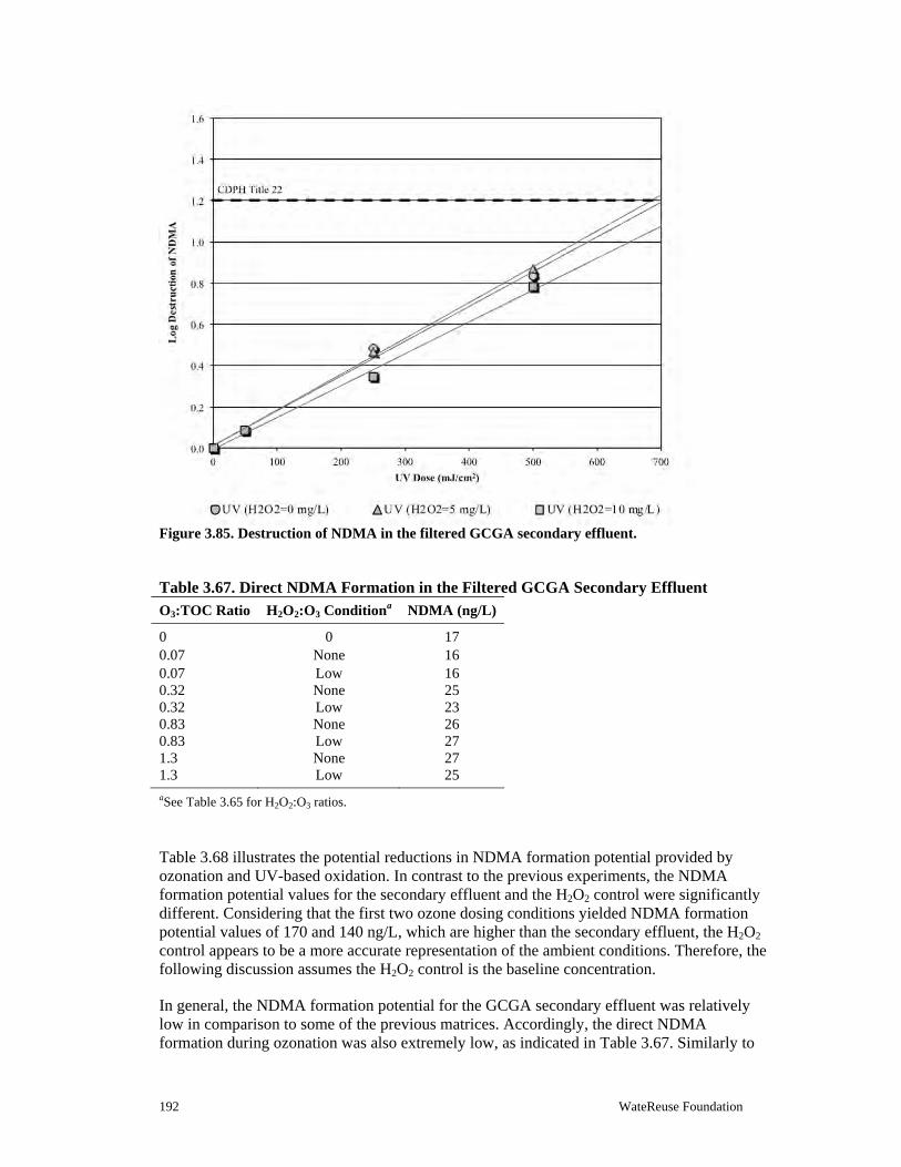
192 WateReuse Foundation
Figure 3.85. Destruction of NDMA in the filtered GCGA secondary effluent.
Table 3.67. Direct NDMA Formation in the Filtered GCGA Secondary Effluent
O3:TOC Ratio H2O2:O3 Conditiona NDMA (ng/L)
0 0 17 0.07 None 16 0.07 Low 16 0.32 None 25 0.32 Low 23 0.83 None 26 0.83 Low 27 1.3 None 27 1.3 Low 25
aSee Table 3.65 for H2O2:O3 ratios.
Table 3.68 illustrates the potential reductions in NDMA formation potential provided by ozonation and UV-based oxidation. In contrast to the previous experiments, the NDMA formation potential values for the secondary effluent and the H2O2 control were significantly different. Considering that the first two ozone dosing conditions yielded NDMA formation potential values of 170 and 140 ng/L, which are higher than the secondary effluent, the H2O2 control appears to be a more accurate representation of the ambient conditions. Therefore, the following discussion assumes the H2O2 control is the baseline concentration.
In general, the NDMA formation potential for the GCGA secondary effluent was relatively low in comparison to some of the previous matrices. Accordingly, the direct NDMA formation during ozonation was also extremely low, as indicated in Table 3.67. Similarly to
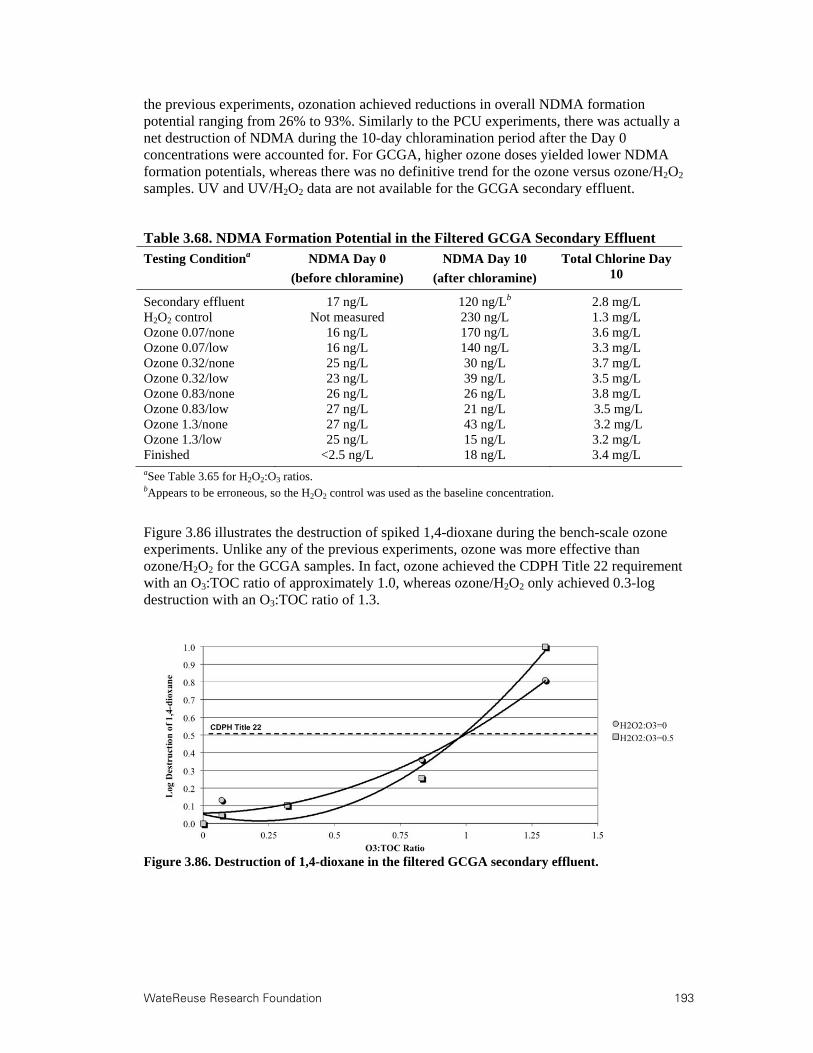
WateReuse Research Foundation 193
the previous experiments, ozonation achieved reductions in overall NDMA formation potential ranging from 26% to 93%. Similarly to the PCU experiments, there was actually a net destruction of NDMA during the 10-day chloramination period after the Day 0 concentrations were accounted for. For GCGA, higher ozone doses yielded lower NDMA formation potentials, whereas there was no definitive trend for the ozone versus ozone/H2O2 samples. UV and UV/H2O2 data are not available for the GCGA secondary effluent.
Table 3.68. NDMA Formation Potential in the Filtered GCGA Secondary Effluent
Testing Conditiona NDMA Day 0
(before chloramine)
NDMA Day 10
(after chloramine)
Total Chlorine Day 10
Secondary effluent 17 ng/L 120 ng/Lb 2.8 mg/L H2O2 control Not measured 230 ng/L 1.3 mg/L Ozone 0.07/none 16 ng/L 170 ng/L 3.6 mg/L Ozone 0.07/low 16 ng/L 140 ng/L 3.3 mg/L Ozone 0.32/none 25 ng/L 30 ng/L 3.7 mg/L Ozone 0.32/low 23 ng/L 39 ng/L 3.5 mg/L Ozone 0.83/none 26 ng/L 26 ng/L 3.8 mg/L Ozone 0.83/low 27 ng/L 21 ng/L 3.5 mg/L Ozone 1.3/none 27 ng/L 43 ng/L 3.2 mg/L Ozone 1.3/low 25 ng/L 15 ng/L 3.2 mg/L Finished <2.5 ng/L 18 ng/L 3.4 mg/L aSee Table 3.65 for H2O2:O3 ratios. bAppears to be erroneous, so the H2O2 control was used as the baseline concentration.
Figure 3.86 illustrates the destruction of spiked 1,4-dioxane during the bench-scale ozone experiments. Unlike any of the previous experiments, ozone was more effective than ozone/H2O2 for the GCGA samples. In fact, ozone achieved the CDPH Title 22 requirement with an O3:TOC ratio of approximately 1.0, whereas ozone/H2O2 only achieved 0.3-log destruction with an O3:TOC ratio of 1.3.
Figure 3.86. Destruction of 1,4-dioxane in the filtered GCGA secondary effluent.

194 WateReuse Foundation
3.5.5 Trace Organic Contaminants
Secondary and finished effluent samples from GCGA were analyzed to determine the ambient concentrations of the target compounds, which are provided in Table 3.69. The secondary effluent samples were generally consistent with other municipal wastewaters with effective activated sludge processes. For example, the most bioamenable compounds (e.g., naproxen and ibuprofen) were <MRL in the secondary effluent, and atenolol and sulfamethoxazole were present at the highest concentrations. However, it is interesting to note that TCEP, which is often present at relatively high concentrations in municipal wastewater, was <MRL. The finished effluent concentrations are also consistent with a treatment train composed of ozone and BAC, as will be discussed in Section 6.1. In other words, only the most biologically and ozone-resistant compounds were detected in the finished effluent. The total estrogenicity of the secondary and finished effluents was determined to be 0.66 and <0.074 ng/L, respectively.
Table 3.69. Ambient TOrC Concentrations at GCGA
Parameter Secondary Effluent (ng/L) Finished Effluent (ng/L)
Bisphenol A <50 <50 Diclofenac 250 <25 Gemfibrozil 150 <10 Ibuprofen <25 <25 Musk ketone <100 <100 Naproxen <25 <25 Triclosan 34 <25 Atenolol 800 <25 Atrazine <10 <10 Carbamazepine 150 <10 DEET 32 <25 Meprobamate 300 190 Phenytoin 110 33 Primidone 91 31 Sulfamethoxazole 1,000 <25 Trimethoprim 400 <10 TCEP <200 <200 Total estrogenicity (EEq) 3.2 <0.074
Table 3.70 shows the relative oxidation levels of the 16 target compounds (musk ketone omitted) in the filtered GCGA secondary effluent. As described earlier, the target compounds were divided into five categories based on their second-order ozone and ·OH rate constants. Similarly to some of the previous data sets, H2O2 addition may have provided a slight advantage for the ozone-resistant compounds (Groups 3, 4, and 5). After the difference in O3:TOC ratios due to the nitrite demand are accounted for, the GCGA oxidation levels were similar to those of previous data sets. Despite the low applied ozone dose, an O3:TOC ratio of 0.07 still achieved significant destruction of all of the target compounds, particularly those in Group 1. However, this dosing condition was unable to achieve 80% destruction of any compound, but an O3:TOC ratio of 0.32 was able to achieve 80% destruction of the Group 1 compounds and one of the Group 2 compounds. The remaining dosing conditions were similar to those in the previous data sets in that the third and fourth O3:TOC ratios achieved at
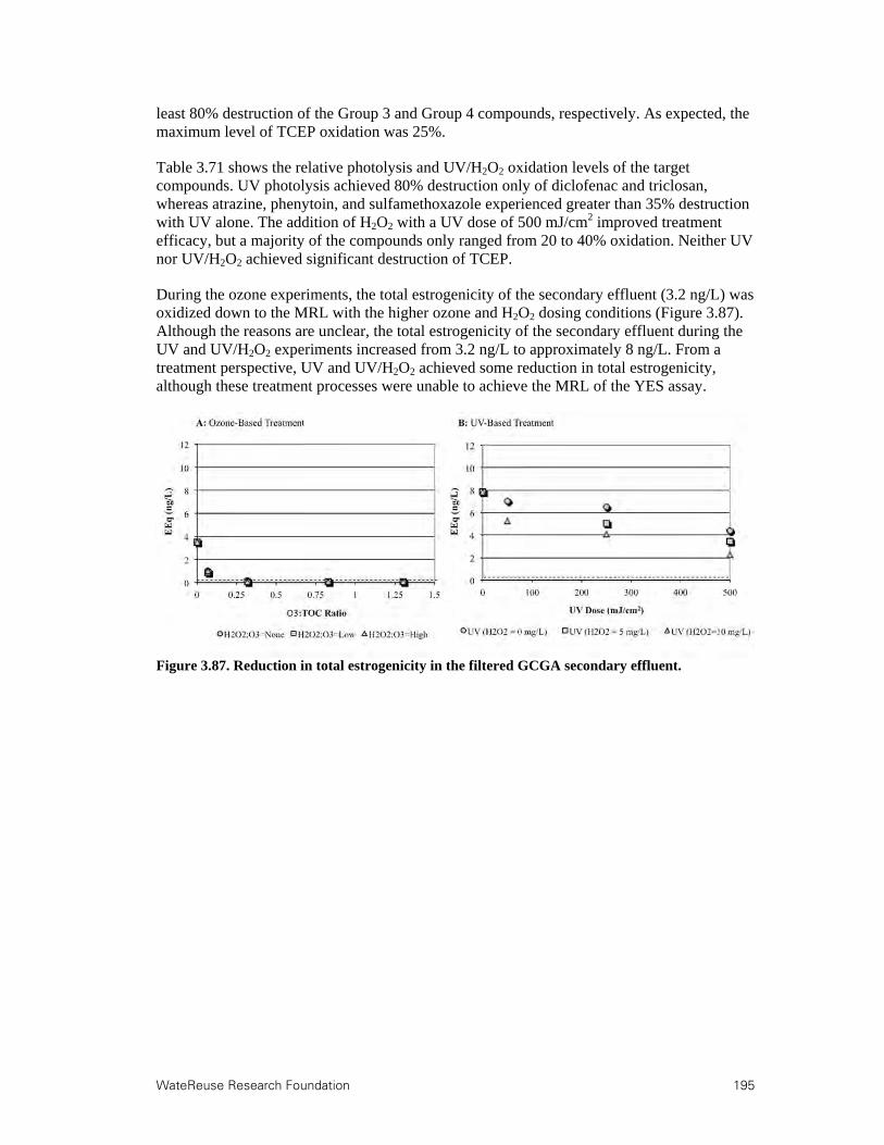
WateReuse Research Foundation 195
least 80% destruction of the Group 3 and Group 4 compounds, respectively. As expected, the maximum level of TCEP oxidation was 25%.
Table 3.71 shows the relative photolysis and UV/H2O2 oxidation levels of the target compounds. UV photolysis achieved 80% destruction only of diclofenac and triclosan, whereas atrazine, phenytoin, and sulfamethoxazole experienced greater than 35% destruction with UV alone. The addition of H2O2 with a UV dose of 500 mJ/cm2 improved treatment efficacy, but a majority of the compounds only ranged from 20 to 40% oxidation. Neither UV nor UV/H2O2 achieved significant destruction of TCEP.
During the ozone experiments, the total estrogenicity of the secondary effluent (3.2 ng/L) was oxidized down to the MRL with the higher ozone and H2O2 dosing conditions (Figure 3.87). Although the reasons are unclear, the total estrogenicity of the secondary effluent during the UV and UV/H2O2 experiments increased from 3.2 ng/L to approximately 8 ng/L. From a treatment perspective, UV and UV/H2O2 achieved some reduction in total estrogenicity, although these treatment processes were unable to achieve the MRL of the YES assay.
Figure 3.87. Reduction in total estrogenicity in the filtered GCGA secondary effluent.
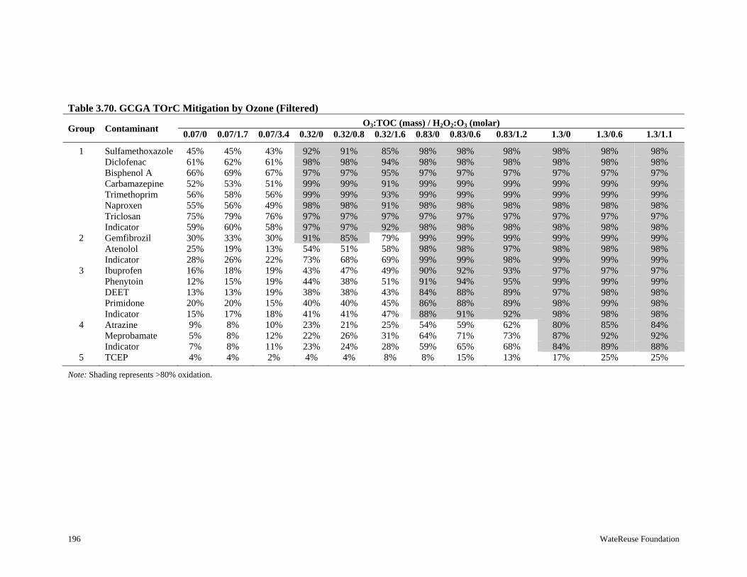
196 WateReuse Foundation
Table 3.70. GCGA TOrC Mitigation by Ozone (Filtered)
Group Contaminant O3:TOC (mass) / H2O2:O3 (molar)
0.07/0 0.07/1.7 0.07/3.4 0.32/0 0.32/0.8 0.32/1.6 0.83/0 0.83/0.6 0.83/1.2 1.3/0 1.3/0.6 1.3/1.1
1 Sulfamethoxazole 45% 45% 43% 92% 91% 85% 98% 98% 98% 98% 98% 98% Diclofenac 61% 62% 61% 98% 98% 94% 98% 98% 98% 98% 98% 98% Bisphenol A 66% 69% 67% 97% 97% 95% 97% 97% 97% 97% 97% 97% Carbamazepine 52% 53% 51% 99% 99% 91% 99% 99% 99% 99% 99% 99% Trimethoprim 56% 58% 56% 99% 99% 93% 99% 99% 99% 99% 99% 99% Naproxen 55% 56% 49% 98% 98% 91% 98% 98% 98% 98% 98% 98% Triclosan 75% 79% 76% 97% 97% 97% 97% 97% 97% 97% 97% 97% Indicator 59% 60% 58% 97% 97% 92% 98% 98% 98% 98% 98% 98%
2 Gemfibrozil 30% 33% 30% 91% 85% 79% 99% 99% 99% 99% 99% 99% Atenolol 25% 19% 13% 54% 51% 58% 98% 98% 97% 98% 98% 98% Indicator 28% 26% 22% 73% 68% 69% 99% 99% 98% 99% 99% 99%
3 Ibuprofen 16% 18% 19% 43% 47% 49% 90% 92% 93% 97% 97% 97% Phenytoin 12% 15% 19% 44% 38% 51% 91% 94% 95% 99% 99% 99% DEET 13% 13% 19% 38% 38% 43% 84% 88% 89% 97% 98% 98% Primidone 20% 20% 15% 40% 40% 45% 86% 88% 89% 98% 99% 98% Indicator 15% 17% 18% 41% 41% 47% 88% 91% 92% 98% 98% 98%
4 Atrazine 9% 8% 10% 23% 21% 25% 54% 59% 62% 80% 85% 84% Meprobamate 5% 8% 12% 22% 26% 31% 64% 71% 73% 87% 92% 92% Indicator 7% 8% 11% 23% 24% 28% 59% 65% 68% 84% 89% 88%
5 TCEP 4% 4% 2% 4% 4% 8% 8% 15% 13% 17% 25% 25%
Note: Shading represents >80% oxidation.
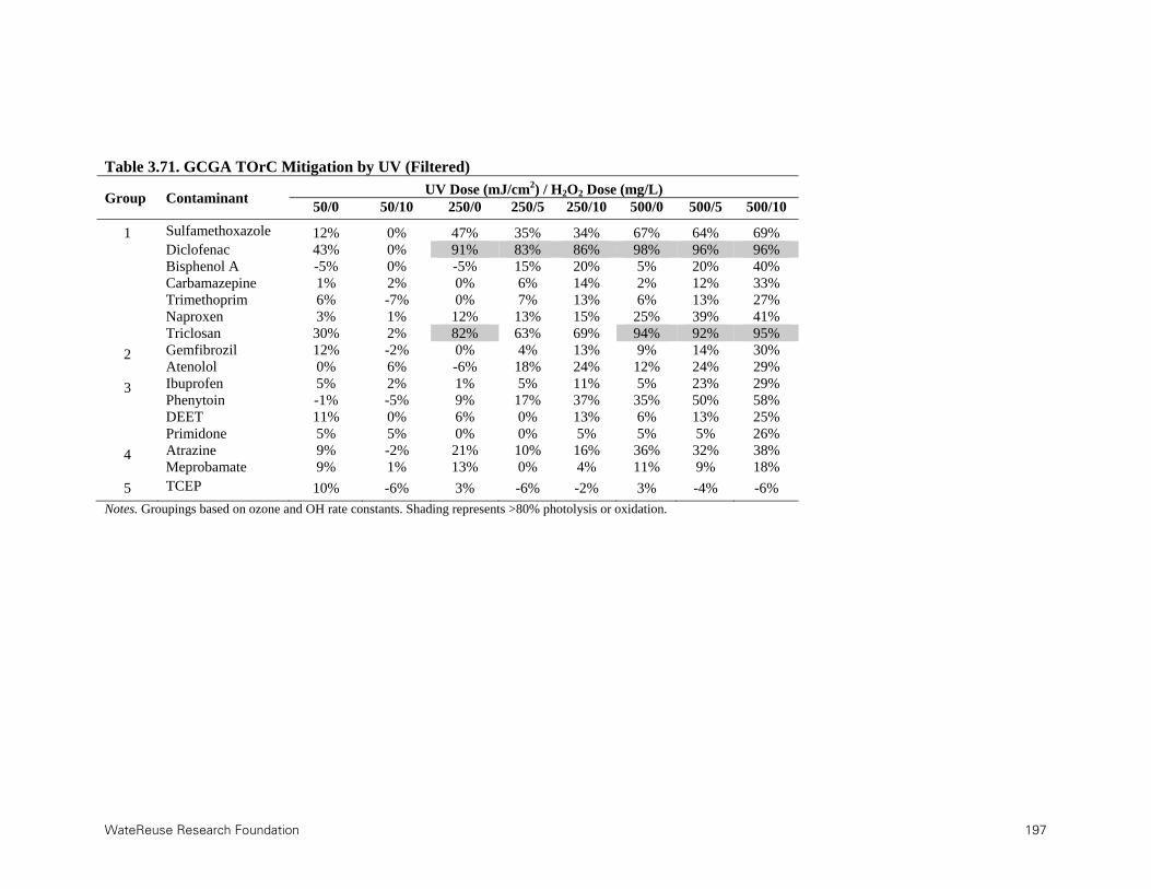
WateReuse Research Foundation 197
Table 3.71. GCGA TOrC Mitigation by UV (Filtered)
Group Contaminant UV Dose (mJ/cm2) / H2O2 Dose (mg/L)
50/0 50/10 250/0 250/5 250/10 500/0 500/5 500/10
1 Sulfamethoxazole 12% 0% 47% 35% 34% 67% 64% 69% Diclofenac 43% 0% 91% 83% 86% 98% 96% 96% Bisphenol A -5% 0% -5% 15% 20% 5% 20% 40% Carbamazepine 1% 2% 0% 6% 14% 2% 12% 33% Trimethoprim 6% -7% 0% 7% 13% 6% 13% 27% Naproxen 3% 1% 12% 13% 15% 25% 39% 41% Triclosan 30% 2% 82% 63% 69% 94% 92% 95%
2 Gemfibrozil 12% -2% 0% 4% 13% 9% 14% 30% Atenolol 0% 6% -6% 18% 24% 12% 24% 29%
3 Ibuprofen 5% 2% 1% 5% 11% 5% 23% 29% Phenytoin -1% -5% 9% 17% 37% 35% 50% 58% DEET 11% 0% 6% 0% 13% 6% 13% 25% Primidone 5% 5% 0% 0% 5% 5% 5% 26%
4 Atrazine 9% -2% 21% 10% 16% 36% 32% 38% Meprobamate 9% 1% 13% 0% 4% 11% 9% 18%
5 TCEP 10% -6% 3% -6% -2% 3% -4% -6%
Notes. Groupings based on ozone and OH rate constants. Shading represents >80% photolysis or oxidation.

198 WateReuse Foundation
3.5.6 Disinfection
Ambient secondary (before and after laboratory filtration) and finished effluent samples were assayed for total and fecal coliforms, MS2, and Bacillus spores. According to the ambient microbial water quality data provided in Table 3.72, the total coliform, fecal coliform, and Bacillus spore values were an order of magnitude higher than those of the previous data sets, whereas MS2 was consistent with the previous wastewaters. To illustrate a wide range of inactivation, the ozone and UV disinfection samples were spiked with relatively large numbers of the surrogate microbes, as indicated in Table 3.73.
Table 3.72. Ambient Microbial Water Quality Data for GCGA
Microbial Surrogate Unfiltered Secondary
Effluent Filtered Secondary
Effluent Finished Effluent
Total Coliforms (MPN/100 mL) 3.5 104 1.6 104 36.3
Fecal Coliforms (MPN/100 mL) 1.1 103 1.0 103 <1
MS2 (PFU/mL)
<1 <1 <1
Bacillus spores (CFU/100 mL) 2.3 104 1.3 104 9.3 103
Table 3.73. Microbial Spiking Levels for GCGA Bench-Scale Experiments
Microbial Surrogate Filtered Ozone
Disinfection Filtered UV Disinfection
E. coli (MPN/100 mL) 1.2 108 1.4 107 MS2 (PFU/mL) 3.4 107 1.3 107 B. subtilis spores (CFU/100 mL) 2.0 105 2.1 105
Figure 3.88 illustrates the inactivation of spiked E. coli during the bench-scale ozone experiments, and the average log-inactivation values for each treatment condition are provided in Table 3.74. The solid line near the top of the figure represents the limit of inactivation based on the spiking level in the filtered samples. Inactivation with H2O2 alone was insignificant, and when combined with ozonation, the addition of H2O2 significantly hindered E. coli inactivation. In fact, the addition of H2O2 reduced the inactivation level by more than 5 logs for an O3:TOC ratio of 1.3. With the exception of one data point, the level of E. coli inactivation for GCGA was very low regardless of O3:TOC ratio, but it is unclear why the level of inactivation was consistently low in this particular wastewater. It is interesting to note that this facility uses ozone as a final disinfectant, and Table 3.72 indicates that the finished effluent still contained 36.3 MPN/100 mL of total coliforms after two stages of ozonation.
Figure 3.89 illustrates the inactivation of spiked MS2 during the bench-scale ozone experiments. Again, minimal inactivation was achieved with the addition of H2O2 alone, and in contrast to the E. coli data, the addition of H2O2 only had a slightly negative impact on MS2 inactivation during ozonation. With respect to the CDPH Title 22 requirements, an

WateReuse Research Foundation 199
O3:TOC ratio between 0.32 and 0.83 was often sufficient for the 5- and 6.5-log inactivation requirements. An O3:TOC ratio of 1.3 achieved the Title 22 benchmarks for all H2O2 conditions. The average log-inactivation values for each treatment condition are provided in Table 3.75.
Figure 3.90 illustrates the inactivation of spiked B. subtilis spores during the bench-scale ozone experiments, and the average log-inactivation values for each treatment condition are provided in Table 3.76. As expected, the spores proved to be extremely resistant to oxidation and only experienced significant inactivation for an O3:TOC ratio of 1.3 with no H2O2 addition. In other words, a sufficient ozone CT had to be administered before ozone and ·OH were able to penetrate the spore coat and inactivate the bacteria. This is consistent with the full-scale data in that limited spore inactivation was achieved despite two stages of ozonation (see Table 3.72).
Figure 3.91 provides a summary of the ozone disinfection data for the three surrogate microbes with respect to the CT framework. Figure 3.91A illustrates the dose–response relationships for the samples with no H2O2 addition, and Figure 3.91B illustrates the dose–response relationships for H2O2:O3 ratios of 0.5 and 1.0 (combined). Similarly to the previous data sets, the data indicate that the CT framework is not always appropriate because substantial levels of inactivation can be achieved when the apparent ozone CT is zero. Again, the level of inactivation for vegetative bacteria and viruses is sometimes less than that observed when an ozone residual is present, and no inactivation of spore-forming bacteria can be achieved without a measurable CT.
Table 3.77 summarizes the efficacy of UV and UV/H2O2 for the inactivation of the three surrogate microbes. The efficacy of UV-based disinfection differs dramatically from ozone-based disinfection because UV is highly effective against both vegetative and spore-forming bacteria, whereas some viruses demonstrate resistance. Approximately 50 mJ/cm2 was sufficient to reach the limits of inactivation for E. coli and Bacillus spores, regardless of H2O2 addition. On the other hand, MS2 inactivation occurred more slowly and only reached the limit of inactivation with a UV dose of 250 mJ/cm2. There was no difference in UV/H2O2 performance with H2O2 doses of 5 and 10 mg/L. Particularly with respect to advanced oxidation dosing conditions (i.e., >250 mJ/cm2 with 10 mg/L of H2O2), one can expect substantial inactivation of all microbes present in wastewater. This constitutes a significant advantage for UV-based treatment over the ozone-based alternatives.

200 WateReuse Foundation
Figure 3.88. Inactivation of spiked E. coli in the GCGA secondary effluent
(see Table 1.65 for H2O2:O3 ratios).
Table 3.74. Summary of E. coli Inactivation in the GCGA Secondary Effluent
O3:TOC Ratio H2O2:O3=Nonea H2O2:O3=Lowa H2O2:O3=Higha
0.07 0.2 0.5 0.2 0.32 0.8 0.7b 0.8 0.83 1.8 1.2 1.0 1.3 7.5 2.0 1.5 aSee Table 1.65 for H2O2:O3 ratios. bInsufficient dilutions to accurately quantify sample.

WateReuse Research Foundation 201
Figure 3.89. Inactivation of spiked MS2 in the GCGA secondary effluent
(see Table 1.65 for H2O2:O3 ratios).
Table 3.75. Summary of MS2 Inactivation in the GCGA Secondary Effluent
O3:TOC Ratio H2O2:O3=Nonea H2O2:O3=Lowa H2O2:O3=Higha
0.07 2.5 ± 0.0 1.4 ± 0.0 1.1 ± 0.0 0.32 5.5 ± 0.0 5.1 ± 0.0 4.5 ± 0.0 0.83 >7.5 ± 0.0b >7.5 ± 0.0b 6.0 ± 0.0 1.3 7.3 ± 0.4 >7.5 ± 0.0b >7.5 ± 0.0b aSee Table 3.65 for H2O2:O3 ratios. bLimit of inactivation based on spiking level.

202 WateReuse Foundation
Figure 3.90. Inactivation of spiked Bacillus spores in the GCGA secondary effluent
(see Table 3.65 for H2O2:O3 ratios).
Table 3.76. Summary of Bacillus Spore Inactivation in the GCGA Secondary Effluent
O3:TOC Ratio H2O2:O3=Nonea H2O2:O3=Lowa H2O2:O3=Higha
0.07 0.0 ± 0.0 0.1 ± 0.0 0.0 ± 0.0 0.32 0.0 ± 0.0 0.0 ± 0.1 0.0 ± 0.1 0.83 0.0 ± 0.1 0.0 ± 0.0 0.0 ± 0.1 1.3 2.1 ± 0.2 0.1 ± 0.1 0.0 ± 0.0
aSee Table 3.65 for H2O2:O3 ratios.
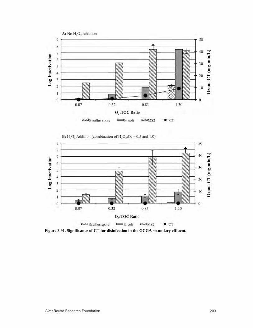
WateReuse Research Foundation 203
Figure 3.91. Significance of CT for disinfection in the GCGA secondary effluent.

204 WateReuse Foundation
Table 3.77. Summary of UV Inactivation in the GCGA Secondary Effluent
UV Dose (mJ/cm2)
E. coli MS2 Bacillus spore UV UV/H2O2
a UV UV/H2O2a UV UV/H2O2
a
25 6.5 6.3 1.8 2.1 2.2 2.6 50 7.1 7.1 3.0 3.2 >3.3b >3.3b 250 >7.1b >7.1b >7.1b >7.1b >3.3b >3.3b 500 >7.1b >7.1b >7.1b >7.1b >3.3b >3.3b aH2O2 doses of 5 and 10 mg/L achieved similar levels of inactivation. bLimit of inactivation based on spiking level.
3.5.7 Organic Characterization
Similarly to the previous data sets, the full-spectrum scans in Figures 3.92 and 3.93 (without (A) and with (B) H2O2 addition) indicate that the absorbance profiles around 254 nm generally provide the greatest resolution between treatment. The addition of H2O2 during ozonation decreased treatment efficacy with respect to absorbance, whereas the addition of H2O2 with UV irradiation provided a slight benefit, although the change in absorbance during both UV processes was much less significant than that of ozonation.
Figure 3.94 focuses on the change in UV254 absorbance with ozone, ozone/H2O2, UV, and UV/H2O2. With respect to ozonation, reductions in UV254 absorbance were slightly hindered by the addition of H2O2. Similar to the absorbance profiles, there was limited reduction in UV254 absorbance with UV or UV/H2O2.
3D EEMs were developed for the filtered secondary effluent, the finished effluent, and the various treatment conditions. Figure 3.95 illustrates the fluorescence fingerprint of the secondary and finished effluent samples and also provides the total and regional fluorescence intensities based on arbitrary fluorescence units. The GCGA secondary effluent had a similar fluorescence fingerprint to those of CCWRD and MWRDGC, whereas the WBMWD and PCU secondary effluents had unique characteristics. However, the GCGA finished effluent is more comparable to WBMWD (MF-RO-UV/H2O2) than CCWRD (UV) or PCU (chlorine).
Figure 3.96 provides a qualitative illustration of treatment efficacy after ozone- and UV-based oxidation. Similarly to the previous data sets, ozone and ozone/H2O2 are capable of achieving substantial reductions in regional and total fluorescence, whereas UV and UV/H2O2 provide minimal reductions. It is interesting to note that the samples associated with an O3:TOC ratio of 0.87 had similar fluorescence characteristics to the GCGA finished effluent.
Figures 3.97 and 3.98 illustrate the fluorescence profiles at an excitation wavelength of 254 nm after ozonation and UV/H2O2, respectively. Because the addition of H2O2 did not have a significant impact on ozone efficacy and UV photolysis provided limited reductions in fluorescence intensity, these fluorescence profiles are not shown. In contrast to WBMWD, which was characterized by two distinct peaks, GCGA was similar to CCWRD, MWRDGC, and PCU in that only one distinct peak was apparent.
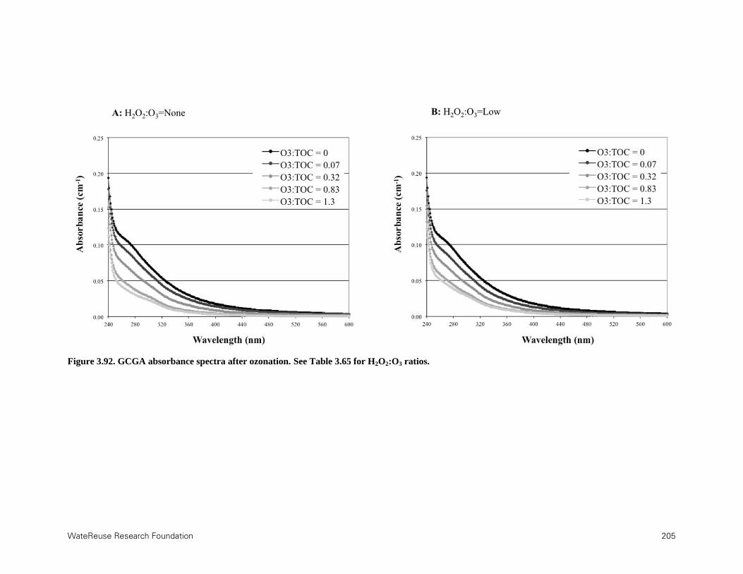
WateReuse Research Foundation 205
Figure 3.92. GCGA absorbance spectra after ozonation. See Table 3.65 for H2O2:O3 ratios.

206 WateReuse Foundation
Figure 3.93. GCGA absorbance spectra after UV and UV/H2O2

WateReuse Research Foundation 207
Figure 3.94. Differential UV254 absorbance in the GCGA secondary effluent (see Table 3.65 for H2O2:O3 ratios).
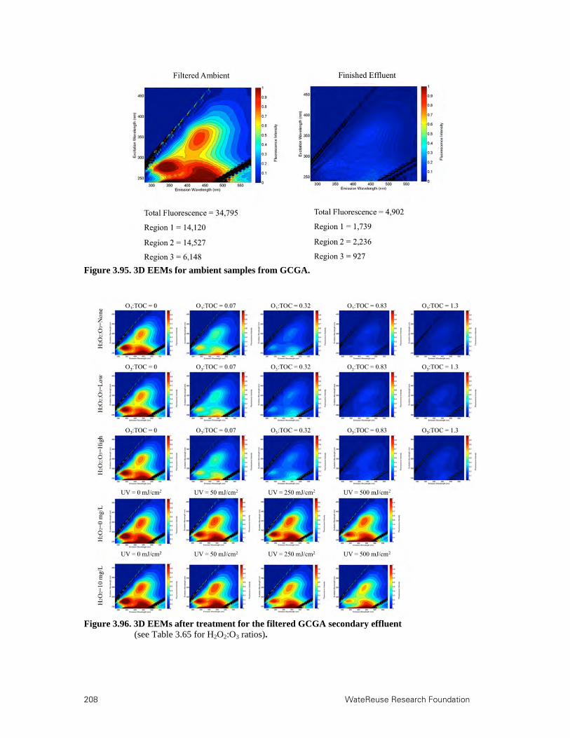
208 WateReuse Research Foundation
Figure 3.95. 3D EEMs for ambient samples from GCGA.
Figure 3.96. 3D EEMs after treatment for the filtered GCGA secondary effluent
(see Table 3.65 for H2O2:O3 ratios).
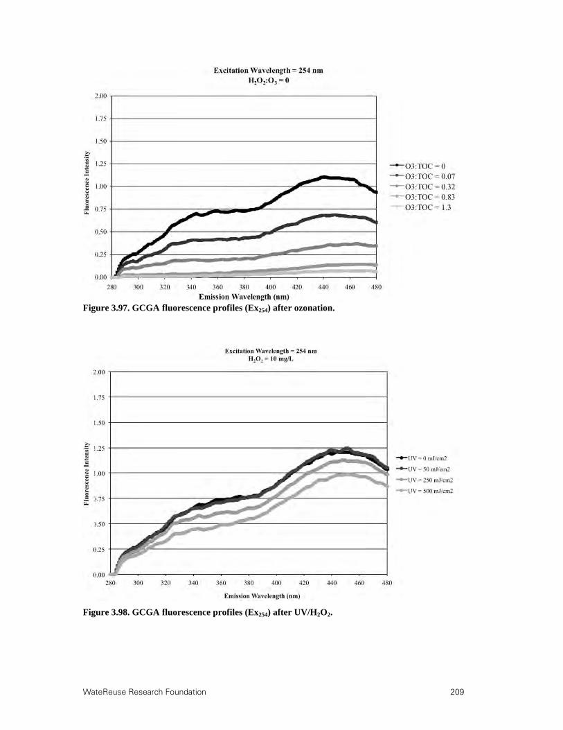
WateReuse Research Foundation 209
Figure 3.97. GCGA fluorescence profiles (Ex254) after ozonation.
Figure 3.98. GCGA fluorescence profiles (Ex254) after UV/H2O2.
210 WateReuse Research Foundation
Table 3.78 provides the fluorescence (i.e., Ex370Em450/Ex370Em500) and treatment indices (i.e., Ex254Em450,T/Ex254Em450,A) for the PCU experiments. The FI values dropped significantly for the ozonated samples, whereas the FI remained relatively constant during the UV and UV/H2O2 processes. In other words, the organic matter associated with emissions at 450 nm was oxidized at a higher rate than that associated with emissions at 500 nm during ozonation. This causes a rapid flattening effect for the fluorescence profile associated with an excitation wavelength of 370 nm (Figure 3.99). The emissions at these particular points were photolyzed and oxidized at similar relative rates during UV and UV/H2O2. Figures 3.100 and 3.101 illustrate the changes in total and regional fluorescence intensities for ozone and UV/H2O2, respectively.
The TI, which measures the extent of organic transformation, reached as low as 0.06 for the highest O3:TOC ratio, indicating that 94% of the original fluorescence had been eliminated. This TI reduction is similar to those of the previous data sets, thereby highlighting the significance of relative changes in bulk organic matter for various water qualities. Also similar to the previous data sets, the addition of H2O2 hindered the oxidation of the bulk organic matter. Because of the limited reduction in fluorescence with UV, the corresponding FI and TI values did not change significantly, although UV/H2O2 provided slight improvements.

WateReuse Research Foundation 211
Table 3.78. FI and TI Values for the GCGA Secondary Effluent
O3:TOC H2O2:O3=Nonea H2O2:O3=Lowa H2O2:O3=Higha FI TI FI TI FI TI
Filtered ozone exposure 0 1.56 1.00 1.56 1.00 1.56 1.00 0.07 1.51 0.63 1.48 0.59 1.50 0.60 0.32 1.33 0.32 1.37 0.33 1.37 0.36 0.83 1.29 0.12 1.35 0.14 1.38 0.16 1.3 1.30 0.06 1.40 0.08 1.40 0.10
UV Dose (mJ/cm2)
H2O2=0 mg/L H2O2=5 mg/L H2O2=10 mg/L FI TI FI TI FI TI
Filtered UV exposure 0 1.57 1.00 1.57 1.00 1.57 1.00 50 1.53 1.01 N/A N/A 1.53 1.03 250 1.50 1.03 1.51 0.97 1.53 0.94 500 1.53 0.96 1.51 0.92 1.53 0.82 aSee Table 3.65 for H2O2:O3 dosing conditions.
Figure 3.99. GCGA fluorescence profiles (Ex370) after ozonation.
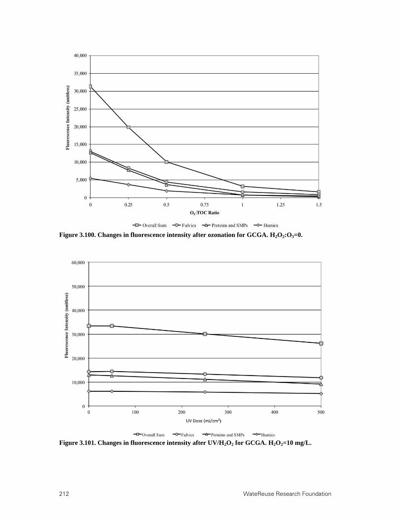
212 WateReuse Research Foundation
Figure 3.100. Changes in fluorescence intensity after ozonation for GCGA. H2O2:O3=0.
Figure 3.101. Changes in fluorescence intensity after UV/H2O2 for GCGA. H2O2=10 mg/L.

WateReuse Research Foundation 213
Chapter 4
4.Bench-Scale Evaluation of International Secondary Effluents
4.1 Lausanne Wastewater Treatment Plant, Lausanne, Switzerland
The international benchmark facility is the Lausanne Wastewater Treatment Plant (LaWWTP) in Lausanne, Switzerland. LaWWTP, which is located in one of the five largest cities in Switzerland, treats approximately 25 MGD from 200,000 people and 70,000 population equivalents from industry. This 25 to 30% industrial fraction is typical of many Swiss municipal wastewater treatment plants. The main treatment train consists of preliminary treatment, primary clarification, conventional activated sludge (SRT=2 to 4 days), and secondary clarification. The biological process is intended primarily for the removal of aggregate organic material (i.e., BOD), as there is no nitrification. However, nitrite is observed with elevated temperatures.
Approximately 10% of the flow is also diverted after primary clarification to a physicochemical treatment process consisting of flocculation, sedimentation, and BAC with limited (i.e., exhausted) adsorption capacity. The plant also feeds ferric chloride to both treatment trains for phosphorus removal. LaWWTP aims for a fecal coliform level of 100 CFU/100 mL to comply with the European Union (EU) water quality directive for bathing, but no disinfection is provided. The finished effluent is discharged into Lake Geneva. A simplified treatment schematic for the LaWWTP is provided in Figure 4.1.
Figure 4.1. Simplified treatment schematic for LaWWTP. Similarly to CCWRD, many Swiss facilities are taking a proactive approach to TOrC mitigation. In response to impending regulations on recalcitrant trace organic contaminants (diclofenac, carbamazepine, etc.) in discharged wastewater, several Swiss utilities have upgraded their treatment trains to evaluate advanced treatment processes. LaWWTP actually
BAC
1°
FlocculationSedimentation
BAC /Sand
PAC UF
O3
2°CAS
2°CASPreliminary Lake Geneva
Pilot Facility
BAC
1°
FlocculationSedimentation
BAC /Sand
PAC UF
O3
2°CAS
2°CASPreliminary Lake Geneva
BAC
1°
FlocculationSedimentation
BAC /Sand
PAC UF
O3
2°CAS
2°CASPreliminary Lake Geneva
Pilot Facility
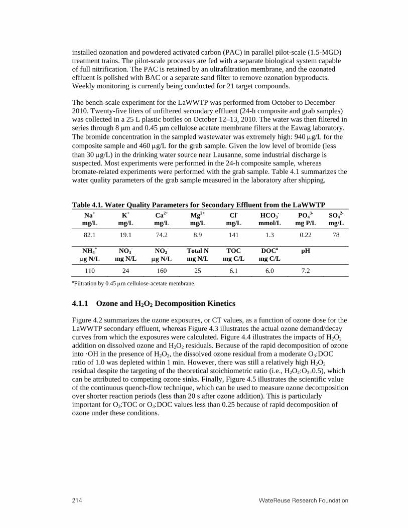
214 WateReuse Research Foundation
installed ozonation and powdered activated carbon (PAC) in parallel pilot-scale (1.5-MGD) treatment trains. The pilot-scale processes are fed with a separate biological system capable of full nitrification. The PAC is retained by an ultrafiltration membrane, and the ozonated effluent is polished with BAC or a separate sand filter to remove ozonation byproducts. Weekly monitoring is currently being conducted for 21 target compounds.
The bench-scale experiment for the LaWWTP was performed from October to December 2010. Twenty-five liters of unfiltered secondary effluent (24-h composite and grab samples) was collected in a 25 L plastic bottles on October 12–13, 2010. The water was then filtered in series through 8 μm and 0.45 μm cellulose acetate membrane filters at the Eawag laboratory. The bromide concentration in the sampled wastewater was extremely high: 940 g/L for the composite sample and 460 g/L for the grab sample. Given the low level of bromide (less than 30 g/L) in the drinking water source near Lausanne, some industrial discharge is suspected. Most experiments were performed in the 24-h composite sample, whereas bromate-related experiments were performed with the grab sample. Table 4.1 summarizes the water quality parameters of the grab sample measured in the laboratory after shipping.
Table 4.1. Water Quality Parameters for Secondary Effluent from the LaWWTP
aFiltration by 0.45 m cellulose-acetate membrane.
4.1.1 Ozone and H2O2 Decomposition Kinetics
Figure 4.2 summarizes the ozone exposures, or CT values, as a function of ozone dose for the LaWWTP secondary effluent, whereas Figure 4.3 illustrates the actual ozone demand/decay curves from which the exposures were calculated. Figure 4.4 illustrates the impacts of H2O2 addition on dissolved ozone and H2O2 residuals. Because of the rapid decomposition of ozone into ·OH in the presence of H2O2, the dissolved ozone residual from a moderate O3:DOC ratio of 1.0 was depleted within 1 min. However, there was still a relatively high H2O2 residual despite the targeting of the theoretical stoichiometric ratio (i.e., H2O2:O3=0.5), which can be attributed to competing ozone sinks. Finally, Figure 4.5 illustrates the scientific value of the continuous quench-flow technique, which can be used to measure ozone decomposition over shorter reaction periods (less than 20 s after ozone addition). This is particularly important for O3:TOC or O3:DOC values less than 0.25 because of rapid decomposition of ozone under these conditions.
Na+ K+ Ca2+ Mg2+ Cl- HCO3- PO4
3- SO42-
mg/L mg/L mg/L mg/L mg/L mmol/L mg P/L mg/L
82.1 19.1 74.2 8.9 141 1.3 0.22 78
NH4+ NO3
- NO2- Total N TOC DOCa pH
g N/L mg N/L g N/L mg N/L mg C/L mg C/L
110 24 160 25 6.1 6.0 7.2
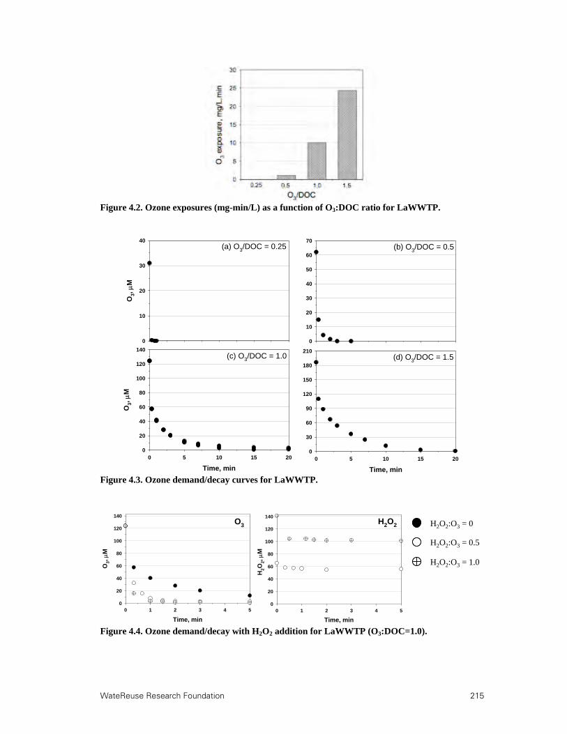
WateReuse Research Foundation 215
Figure 4.2. Ozone exposures (mg-min/L) as a function of O3:DOC ratio for LaWWTP.
Figure 4.3. Ozone demand/decay curves for LaWWTP.
Figure 4.4. Ozone demand/decay with H2O2 addition for LaWWTP (O3:DOC=1.0).
O3,
M
0
10
20
30
40
0
10
20
30
40
50
60
70
Time, min
0 5 10 15 20
O3,
M
0
20
40
60
80
100
120
140
Time, min
0 5 10 15 200
30
60
90
120
150
180
210
(a) O3/DOC = 0.25 (b) O3/DOC = 0.5
(c) O3/DOC = 1.0 (d) O3/DOC = 1.5
Time, min
0 1 2 3 4 5
O3,
M
0
20
40
60
80
100
120
140
0 1 2 3 4 50
20
40
60
80
100
120
140
H2O
2,
M
Time, min
O3 H2O2 H2O2:O3 = 0
H2O2:O3 = 1.0
H2O2:O3 = 0.5
Time, min
0 1 2 3 4 5
O3,
M
0
20
40
60
80
100
120
140
0 1 2 3 4 50
20
40
60
80
100
120
140
H2O
2,
M
Time, min
O3 H2O2 H2O2:O3 = 0
H2O2:O3 = 1.0
H2O2:O3 = 0.5

216 WateReuse Research Foundation
Figure 4.5. Use of the quench-flow (QF) method for LaWWTP.
·OH exposures were also calculated using pCBA (~200 μg/L) and meprobamate (~1 μg/L) as probe compounds during ozonation. Figure 4.6 illustrates the resulting ·OH exposures for the LaWWTP secondary effluent.
Figure 4.6. ·OH exposures for LaWWTP.
The tert-butanol (t-BuOH) competition kinetic method (see Section 2.4.2) was applied to estimate the rate of consumption of ·OH by wastewater constituents such as EfOM, carbonate, bromide, and ammonia (i.e., the ·OH scavenging rate). Using three different ozone doses, the ·OH scavenging rate for LaWWTP was estimated to be ~1.2–1.4 105 s-1, as illustrated in Figure 4.7. Ammonia was insignificant in comparison to EfOM, bicarbonate, and bromide.
O3/DOC
0.00 0.25 0.50 0.75 1.00 1.25 1.50
OH
rad
ical
exp
osur
e, M
.s
0
1e-10
2e-10
3e-10
4e-10
from pCBA datafrom meprobamate data

WateReuse Research Foundation 217
Figure 4.7. Determination of ·OH scavenging rate for LaWWTP.
The t-BuOH assay was also applied to estimate the ·OH yield, which varied from ~10 to 20% with increasing O3:DOC ratios. The ·OH yield is reported as a molar ratio of the ·OH generated to the ozone applied. For the ozone-only experiments, the ·OH yield was based on complete ozone consumption (i.e., no quenching). It should be noted that the O2·
--induced radical chain reactions are significantly suppressed in the t-BuOH assay, so the t-BuOH assay only captures reactions between ozone and EfOM, HO2
, or OH. Based on the data in Figure 4.8, the ·OH yield is slightly dependent on the applied ozone dose. At lower applied ozone doses, direct ozone oxidation is more prevalent than the intermediate conversion to ·OH, presumably because of the instantaneous ozone demand.
Figure 4.8. ·OH yield based for LaWWTP secondary effluent.
4.1.2 Bromate Formation
As mentioned earlier, the bromide level in the secondary effluent grab sample from the LaWWTP was very high, which resulted in bromate levels of up to 61 μg/L at an O3:DOC ratio of 1.5 (Figure 4.9). The figure also illustrates the corresponding decrease in bromide (i.e., bromide incorporation) because of the ozone-induced bromate formation.

218 WateReuse Research Foundation
Figure 4.9 Bromide and bromate concentrations for LaWWTP.
In order to To reduce the formation of bromate, the chlorine–ammonia process was evaluated for the LaWWTP secondary effluent and O3:DOC ratios of 1.0 and 1.5 (see Figure 4.10). With no mitigation efforts, the resulting bromate formation was just over 40 μg/L at an O3:DOC ratio of 1.0. However, as the concentrations of both chlorine and ammonia were increased, bromate formation dropped by more than 50%. There was also a point of diminishing return where further chlorine–ammonia dosing provided little benefit. Although chlorine alone (second bar) and ammonia alone (seventh bar) provided slight reductions in bromate, the greatest stepwise reduction resulted from a chlorine dose of 30 μM together with an ammonia dose of 10 μM (third bar). From that point, small changes in chlorine concentration had a more significant impact than changes in ammonia concentration.
Figure 4.102. Bromate mitigation for LaWWTP with the chlorine–ammonia process.
BrO
3- , g
/L
0
10
20
30
40
50
60
BrO3-Br-
no O
3
O3/DOC =
0.5
500
417
330
250
167
83
0
Br -,
g/LO3/
DOC = 1
.0
O3/DOC =
1.5

WateReuse Research Foundation 219
4.1.3 Trace Organic Contaminants
The ambient LaWWTP TOrC concentrations for the unfiltered secondary effluent and the secondary effluent filtered in the laboratory are provided in Table 4.2. The ambient TOrC data are representative of a municipal treatment facility with a low SRT because of the presence of highly bioamenable compounds such as naproxen. However, the data differ from those for typical U.S. wastewaters in that compounds typically identified as valuable wastewater indicators are either absent (e.g., phenytoin) or present at low concentrations (e.g., meprobamate and primidone).
Table 4.2. Ambient TOrC Concentrations for LaWWTP
Parameter Unfiltered Secondary Effluent (ng/L)
Filtered Secondary Effluent (ng/L)
Bisphenol A <50 <50 Diclofenac 890 840 Gemfibrozil <10 <10 Ibuprofen <25 <25 Musk ketone <100 <100 Naproxen 180 180 Triclosan 53 35 Atenolol 270 250 Atrazine 17 14 Carbamazepine 370 390 DEET 76 73 Meprobamate 23 27 Phenytoin <10 <10 Primidone 87 92 Sulfamethoxazole 520 370 Trimethoprim 90 82 TCEP <200 <200
Compounds with known ozone and ·OH reaction rate constants can be used to predict the elimination of other target contaminants. The compound pCBA has been widely used as an indicator for ·OH because of its limited reactivity with ozone (von Gunten, 2003a). In this study, carbamazepine (kO3=3 105 M1s1; Huber et al., 2003b), bezafibrate (kO3=5.9 102 M1s1; Huber et al., 2003b), and ibuprofen (kO3=10 M1s1; Huber et al., 2003b) were also used as indicator compounds. These compounds were selected because they cover a wide range of ozone reactivity, and their reaction rate constants with ozone do not change as a function of pH. In addition, they are often detected in water supplies impacted by wastewater discharge. These preliminary experiments were performed with high spiking levels (1–1.5 μM; 200–600 μg/L). Figure 4.11 shows the residual concentrations of the indicator compounds as a function of ozone dose in the LaWWTP secondary effluent.
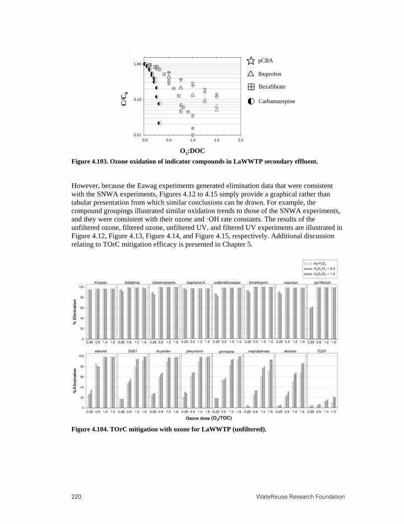
220 WateReuse Research Foundation
Figure 4.103. Ozone oxidation of indicator compounds in LaWWTP secondary effluent.
However, because the Eawag experiments generated elimination data that were consistent with the SNWA experiments, Figures 4.12 to 4.15 simply provide a graphical rather than tabular presentation from which similar conclusions can be drawn. For example, the compound groupings illustrated similar oxidation trends to those of the SNWA experiments, and they were consistent with their ozone and ·OH rate constants. The results of the unfiltered ozone, filtered ozone, unfiltered UV, and filtered UV experiments are illustrated in Figure 4.12, Figure 4.13, Figure 4.14, and Figure 4.15, respectively. Additional discussion relating to TOrC mitigation efficacy is presented in Chapter 5.
Figure 4.104. TOrC mitigation with ozone for LaWWTP (unfiltered).
O3/DOC (g/g)
0.0 0.5 1.0 1.5 2.0Rel
ativ
e r
esid
ual
co
nce
ntr
atio
n, C
/C0
0.01
0.10
1.00
O3:DOC
C/C
0
pCBA
Ibuprofen
Bezafibrate
Carbamazepine
O3/DOC (g/g)
0.0 0.5 1.0 1.5 2.0Rel
ativ
e r
esid
ual
co
nce
ntr
atio
n, C
/C0
0.01
0.10
1.00
O3:DOC
C/C
0
pCBA
Ibuprofen
Bezafibrate
Carbamazepine

WateReuse Research Foundation 221
Figure 4.105. TOrC mitigation with ozone for LaWWTP (filtered).
Figure 4.106. TOrC mitigation with UV for LaWWTP (unfiltered).

222 WateReuse Research Foundation
Figure 4.107. TOrC mitigation with UV for LaWWTP (filtered).
4.1.4 Disinfection
As described in Section 2.3.4, disinfection efficacy during ozonation of the LaWWTP secondary effluent was evaluated by FCM (Figure 4.16) and by quantification of cell-bound ATP (Figure 4.17). Because the assays targeted indigenous bacteria, it was not possible to filter the samples with 0.45 μm membranes, so these ozone doses were based on O3:TOC ratios. In comparison to the SNWA experiments, the FCM data appear to be a very conservative estimate of disinfection efficacy, considering that even the highest ozone dose (O3:TOC=1.5) achieved less than 2-log “removal” of bacteria. There was a limited improvement in bacterial “removal” with prefiltration, and the effects of H2O2 addition were minimal. Based on the ATP analysis, there was a dramatic decrease in cell-bound ATP with moderate ozone doses (O3:TOC>0.5), but the overall concentration of ATP in the sample actually increased at an O3:DOC ratio of 0.5, perhaps because of more efficient release of ATP by ozonation. At O3:TOC ratios greater than 0.5, there was a net decrease in both cell-bound and extracellular ATP. Because the SNWA culture-dependent methods indicated that coliform bacteria were still present at the highest ozone doses, the ATP-based analysis appears to overestimate disinfection efficacy.

WateReuse Research Foundation 223
Figure 4.108. Disinfection efficacy for LaWWTP based on FCM.
Figure 4.109. Disinfection efficacy for LaWWTP based on cell-bound ATP.
4.1.5 Organic Characterization
The differential absorption spectra for LaWWTP were evaluated at four different wavelengths (Figure 4.18). Similarly to the SNWA experiments, the differential absorbance at 254 nm ranged from approximately 20% to 60% for O3:DOC ratios ranging from 0.25 to 1.5. As indicated in the literature review, the absorbance at longer wavelengths (e.g., 436 nm) experienced greater relative decreases, although the changes in the absolute values were not necessarily as significant. Furthermore, the addition of H2O2 had a slight negative impact on treatment efficacy at all wavelengths.

224 WateReuse Research Foundation
Figure 4.110. Changes in absorption spectra for the LaWWTP secondary effluent.
Figure 4.19 illustrates the change in ATP (similar to the disinfection experiments) and the change in biodegradable organic carbon (BDOC) during ozonation. As ozone oxidizes the EfOM, the organic matter is generally transformed into more biodegradable and lower molecular weight building blocks. Figure 4.19 indicates that an O3:TOC ratio of ~1.0 is the optimal dosing condition for maximizing this transformation prior to biodegradation. This concept is also supported by Figure 4.20, which illustrates the conversion of more particulate, hydrophobic, and microbially derived organic matter to simpler organic fractions. Figure 4.21 expands on this transformation by showing the effect of subsequent biodegradation on the ozone-transformed organic matter. In this assay, the simpler organic fractions were more amenable to biodegradation, with moderate ozone doses providing the best treatment efficacy. Therefore, moderate ozone doses (e.g., O3:TOC=0.5 or 1.0) are effective in converting more complex, recalcitrant EfOM to simpler, more bioamenable organic fractions, which results in a net decrease in dissolved organic matter concentrations for most dosing conditions. However, it is unclear why the TOC concentration increased for an O3:TOC ratio of 1.5 with H2O2 addition.
Re
lati
ve
abso
rba
nc
e
0.0
0.2
0.4
0.6
0.8
1.0
O3/DOC (g/g)
0.00 0.25 0.50 0.75 1.00 1.25 1.50 1.75
Re
lati
ve
abso
rba
nc
e
0.0
0.2
0.4
0.6
0.8
1.0
O3/DOC (g/g)
0.00 0.25 0.50 0.75 1.00 1.25 1.50 1.75
(a) 254 nm (b) 280 nm
(c) 350 nm (d) 436 nm
H2O2:O3 = 0
H2O2:O3 = 1.0R
ela
tiv
e ab
sorb
an
ce
0.0
0.2
0.4
0.6
0.8
1.0
O3/DOC (g/g)
0.00 0.25 0.50 0.75 1.00 1.25 1.50 1.75
Re
lati
ve
abso
rba
nc
e
0.0
0.2
0.4
0.6
0.8
1.0
O3/DOC (g/g)
0.00 0.25 0.50 0.75 1.00 1.25 1.50 1.75
(a) 254 nm (b) 280 nm
(c) 350 nm (d) 436 nm
H2O2:O3 = 0
H2O2:O3 = 1.0

WateReuse Research Foundation 225
Figure 4.111. Impact of ozonation on ATP and BDOC for LaWWTP.
Figure 4.20. EfOM transformation during ozonation for LaWWTP.

226 WateReuse Research Foundation
Figure 4.21. Effects of biodegradation (following ozonation) for LaWWTP.
4.2 Regensdorf (Wüeri) Wastewater Treatment Plant, Regensdorf, Switzerland
4.2.1 Background
The Regensdorf Wastewater Treatment Plant (RWWTP) is located near Zurich, Switzerland. The RWWTP, which is sometimes referred to as the Wüeri Wastewater Treatment Plant, was previously described in the literature review (Hollender et al., 2009). The RWWTP primarily serves a residential population of approximately 25,000 people, but some industrial contributions may be present. The liquid treatment train operates at a flow rate of 1.5 MGD and includes bar screens and grit removal; primary clarification; conventional activated sludge (SRT=16 days) with nitrification, limited denitrification, and biological phosphorus removal; secondary clarification; and sand filtration. Similarly to the LaWWTP, the RWWTP targets an effluent fecal coliform level of 100 MPN/100 mL, but no disinfection processes are currently included in the treatment train. From August 2007 to October 2008, the plant was supplemented with a full-scale ozone system positioned between the secondary clarifiers and sand filters. The ozone system was originally commissioned in response to impending regulations on recalcitrant trace organic contaminants (diclofenac, carbamazepine, etc.) in discharged wastewater. This is particularly important for the RWWTP, as its receiving stream (Furtbach Creek) is dominated by wastewater (≈60%) during dry weather conditions. A simplified treatment schematic for the RWWTP is provided in Figure 4.22.
Figure 4.22. Simplified treatment schematic for RWWTP.
1° 2°CASPreliminary SandFurtbach
CreekO3
Not Operating
1°1° 2°CAS 2°CASPreliminary SandSandFurtbach
CreekFurtbach
CreekO3O3
Not Operating

WateReuse Research Foundation 227
The RWWTP bench-scale experiment was performed in July and August 2010. Twenty-five liters of unfiltered secondary effluent (grab sample) were collected in 5-L glass bottles on July 7, 2010. The water was then filtered in series through 8-μm and 0.45-μm cellulose acetate membrane filters at the Eawag laboratory. Table 4.3 summarizes the water quality parameters of the grab samples, which were measured in the laboratory after shipping.
Table 4.3. Water Quality Parameters for Secondary Effluent from the RWWTP
aFiltration by 0.45 m cellulose-acetate membrane.
4.2.2 Ozone and H2O2 Decomposition Kinetics
Figure 4.23 summarizes the ozone exposures, or CT values, for the RWWTP secondary effluent, and Figure 4.24 illustrates the associated demand/decay curves with and without the addition of t-BuOH. In these samples, the t-BuOH suppressed ·OH-induced decomposition of ozone, which allowed a more stable dissolved ozone residual. Finally, Figure 4.25 illustrates the effect of H2O2 addition on dissolved ozone and H2O2 residuals. At an O3:DOC ratio of 1.0, the dissolved ozone residual was completely depleted within 30 s of reaction time at both H2O2 doses, although there was still a significant H2O2 residual in both cases.
Figure 4.23. Ozone exposures (mg-min/L) as a function of O3:DOC ratio for RWWTP.
Na+ K+ Ca2+ Mg2+ Cl- HCO3- PO4
3- SO42-
mg/L mg/L mg/L mg/L mg/L mmol/L mg P/L mg/L
67.5 14.3 74.4 18.1 88.2 4.35 0.21 56.6
NH4+ NO3
- NO2- Total N TOC DOCa pH
g N/L mg N/L g N/L mg N/L mg C/L mg C/L
24.5 12.0 7.5 12.1 5.0 4.7 7.2
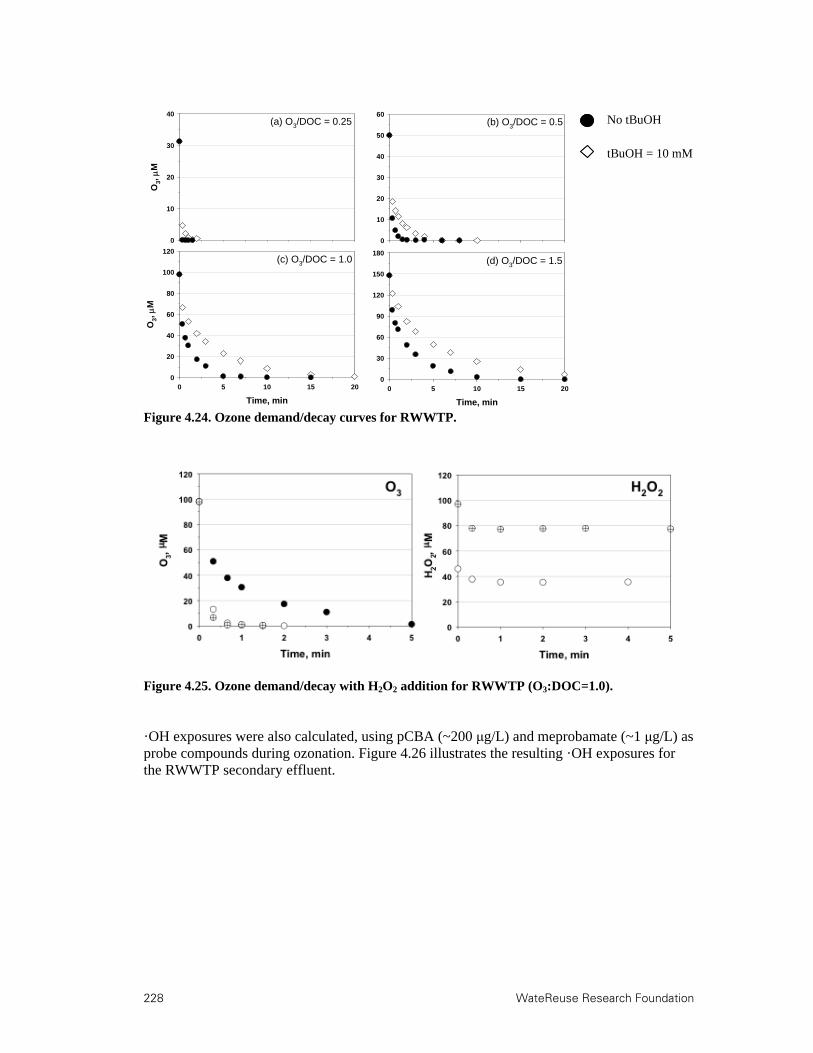
228 WateReuse Research Foundation
Figure 4.24. Ozone demand/decay curves for RWWTP.
Figure 4.25. Ozone demand/decay with H2O2 addition for RWWTP (O3:DOC=1.0).
·OH exposures were also calculated, using pCBA (~200 μg/L) and meprobamate (~1 μg/L) as probe compounds during ozonation. Figure 4.26 illustrates the resulting ·OH exposures for the RWWTP secondary effluent.
O3,
M
0
10
20
30
40
0
10
20
30
40
50
60
Time, min
0 5 10 15 20
O3,
M
0
20
40
60
80
100
120
Time, min
0 5 10 15 200
30
60
90
120
150
180
(a) O3/DOC = 0.25 (b) O3/DOC = 0.5
(c) O3/DOC = 1.0 (d) O3/DOC = 1.5
No tBuOH
tBuOH = 10 mMO
3,
M
0
10
20
30
40
0
10
20
30
40
50
60
Time, min
0 5 10 15 20
O3,
M
0
20
40
60
80
100
120
Time, min
0 5 10 15 200
30
60
90
120
150
180
(a) O3/DOC = 0.25 (b) O3/DOC = 0.5
(c) O3/DOC = 1.0 (d) O3/DOC = 1.5
No tBuOH
tBuOH = 10 mM

WateReuse Research Foundation 229
Figure 4.26. ·OH exposures for RWWTP.
The t-BuOH competition kinetics method was then applied to estimate the rate of ·OH consumption by wastewater constituents such as EfOM, carbonate, bromide, and ammonia (i.e., the ·OH scavenging rate). Using three different ozone doses, the ·OH scavenging rate for RWWTP was estimated to be ~1.0–1.5 105 s-1 (Figure 4.27), which is a slightly larger range than for the LaWWTP but similar in magnitude. Bromide and ammonia were insignificant in comparison to EfOM and bicarbonate.
Figure 4.27. Determination of ·OH scavenging rate for RWWTP.
The t-BuOH assay was also applied to estimate the ·OH yield, which varied from ~10 to 30% with increasing O3:DOC ratios (Figure 4.28). The ·OH yield is reported as a molar ratio of the ·OH generated to the ozone applied.

230 WateReuse Research Foundation
Figure 4.28 ·OH yield based for RWWTP secondary effluent.
4.2.3 Bromate and Nitrosamine Formation
The bromide level in the RWWTP secondary effluent was relatively low, which resulted in bromate levels of less than 20 μg/L even at the highest O3:DOC ratio (Figure 4.29). Figure 4.29 also illustrates the effect of H2O2 addition, which provided slight reductions in bromate formation. Therefore, H2O2 addition may be a viable bromate-mitigation strategy in low-bromide waters, whereas more problematic waters may require the chlorine–ammonia process described in relation to LaWWTP.
Figure 4.29. Bromate concentrations for RWWTP.
In addition to bromate, nitrosamine formation was also monitored as a potential ozone DBP (Figure 4.30). However, in contrast to the U.S. secondary effluents, there was no direct nitrosamine formation during ozonation. Chloramination (1 mM NH2Cl for 10 days) yielded 200 nm of NDMA and 50 nm of N-nitrosopyrrolidine (NPYR), but preozonation was able to reduce this chloramine-induced formation potential significantly. Finally, bromide addition, which has been shown to catalyze nitrosamine formation, had no impact on NDMA or NPRY concentrations in these experiments. Based on all of these observations, the RWWTP secondary effluent is a prime example of a matrix for which ozonation provides clear DBP mitigation benefits—even for nitrosamines.
H2O2:O3 = 0
H2O2:O3 = 1.0
H2O2:O3 = 0.5
O3/DOC
0.0 0.5 1.0 1.5 2.0
BrO
3- , g
/L
0
5
10
15
20
Limit of quantification, 2 g/L
O3:DOC
Bromide = 42 μg/L H2O2:O3 = 0
H2O2:O3 = 1.0
H2O2:O3 = 0.5
O3/DOC
0.0 0.5 1.0 1.5 2.0
BrO
3- , g
/L
0
5
10
15
20
Limit of quantification, 2 g/L
H2O2:O3 = 0
H2O2:O3 = 1.0
H2O2:O3 = 0.5
O3/DOC
0.0 0.5 1.0 1.5 2.0
BrO
3- , g
/L
0
5
10
15
20
Limit of quantification, 2 g/L
O3:DOC
Bromide = 42 μg/L
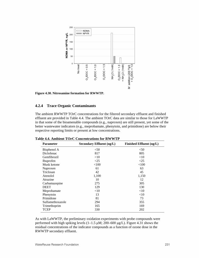
WateReuse Research Foundation 231
Figure 4.30. Nitrosamine formation for RWWTP.
4.2.4 Trace Organic Contaminants
The ambient RWWTP TOrC concentrations for the filtered secondary effluent and finished effluent are provided in Table 4.4. The ambient TOrC data are similar to those for LaWWTP in that some of the bioamenable compounds (e.g., naproxen) are still present, yet some of the better wastewater indicators (e.g., meprobamate, phenytoin, and primidone) are below their respective reporting limits or present at low concentrations. Table 4.4. Ambient TOrC Concentrations for RWWTP
Parameter Secondary Effluent (ng/L) Finished Effluent (ng/L)
Bisphenol A <50 <50 Diclofenac 817 805 Gemfibrozil <10 <10 Ibuprofen <25 <25 Musk ketone <100 <100 Naproxen 61 63 Triclosan 42 45 Atenolol 1,100 1,150 Atrazine 10 12 Carbamazepine 275 305 DEET 129 130 Meprobamate <10 <10 Phenytoin 13 <10 Primidone 81 73 Sulfamethoxazole 294 355 Trimethoprim 165 169 TCEP 330 202
As with LaWWTP, the preliminary oxidation experiments with probe compounds were performed with high spiking levels (1–1.5 μM; 200–600 μg/L). Figure 4.31 shows the residual concentrations of the indicator compounds as a function of ozone dose in the RWWTP secondary effluent.
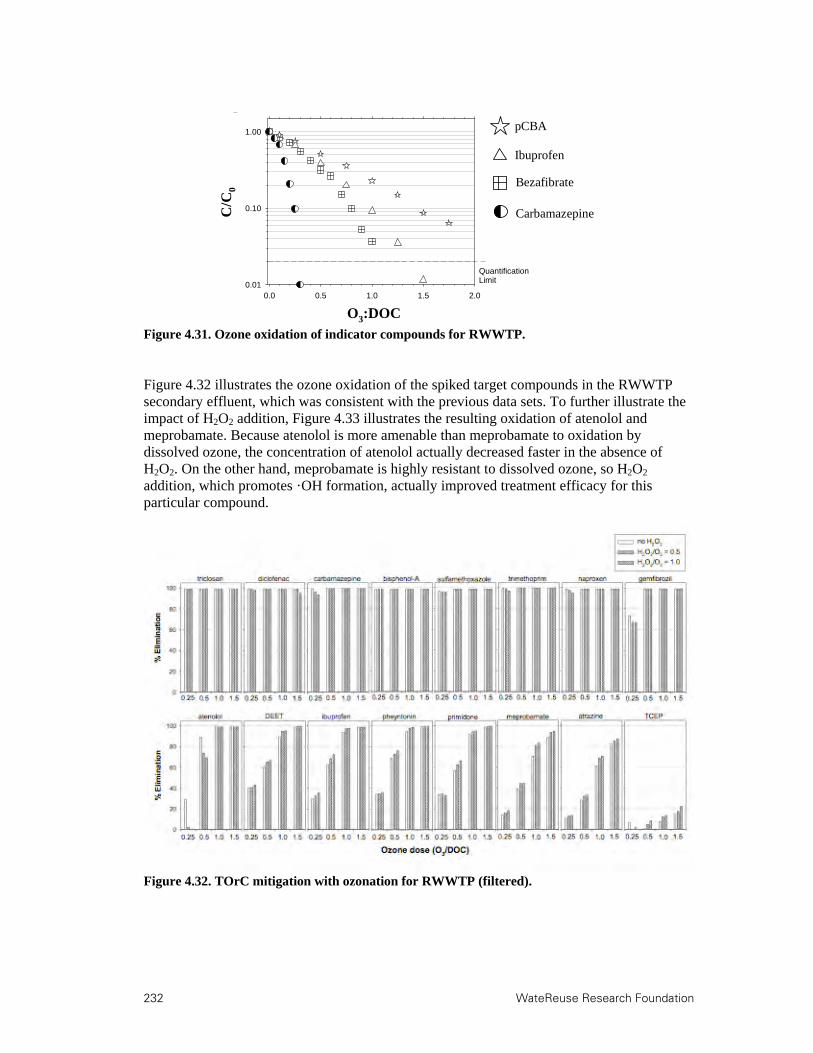
232 WateReuse Research Foundation
Figure 4.31. Ozone oxidation of indicator compounds for RWWTP.
Figure 4.32 illustrates the ozone oxidation of the spiked target compounds in the RWWTP secondary effluent, which was consistent with the previous data sets. To further illustrate the impact of H2O2 addition, Figure 4.33 illustrates the resulting oxidation of atenolol and meprobamate. Because atenolol is more amenable than meprobamate to oxidation by dissolved ozone, the concentration of atenolol actually decreased faster in the absence of H2O2. On the other hand, meprobamate is highly resistant to dissolved ozone, so H2O2 addition, which promotes ·OH formation, actually improved treatment efficacy for this particular compound.
Figure 4.32. TOrC mitigation with ozonation for RWWTP (filtered).
O3/DOC (g/g)
0.0 0.5 1.0 1.5 2.0Rel
ati
ve r
esid
ual
co
nce
ntr
atio
n, C
/C0
0.01
0.10
1.00
QuantificationLimit
O3:DOC
C/C
0
pCBA
Ibuprofen
Bezafibrate
Carbamazepine
O3/DOC (g/g)
0.0 0.5 1.0 1.5 2.0Rel
ati
ve r
esid
ual
co
nce
ntr
atio
n, C
/C0
0.01
0.10
1.00
QuantificationLimit
O3:DOC
C/C
0
pCBA
Ibuprofen
Bezafibrate
Carbamazepine
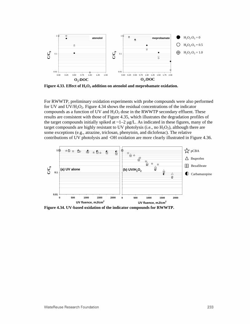
WateReuse Research Foundation 233
Figure 4.33. Effect of H2O2 addition on atenolol and meprobamate oxidation.
For RWWTP, preliminary oxidation experiments with probe compounds were also performed for UV and UV/H2O2. Figure 4.34 shows the residual concentrations of the indicator compounds as a function of UV and H2O2 dose in the RWWTP secondary effluent. These results are consistent with those of Figure 4.35, which illustrates the degradation profiles of the target compounds initially spiked at ~1–2 μg/L. As indicated in these figures, many of the target compounds are highly resistant to UV photolysis (i.e., no H2O2), although there are some exceptions (e.g., atrazine, triclosan, phenytoin, and diclofenac). The relative contributions of UV photolysis and ·OH oxidation are more clearly illustrated in Figure 4.36.
Figure 4.34. UV-based oxidation of the indicator compounds for RWWTP.
0.00 0.25 0.50 0.75 1.00 1.25 1.50 1.75 2.00
0.01
0.1
1
O3/DOC (g/g)
Rel
ativ
e rs
idu
al c
on
cen
trat
ion
, C/C
0
meprobamate
0.00 0.25 0.50 0.75 1.00 1.25 1.50
0.01
0.1
1
O3/DOC (g/g)
Rel
ativ
e rs
idu
al c
on
cen
trat
ion
, C/C
0
atenolol
O3:DOC
C/C
0
O3:DOC
C/C
0
H2O2:O3 = 0
H2O2:O3 = 1.0
H2O2:O3 = 0.5
0 500 1000 1500 2000Rel
ativ
e re
sid
ual
co
nce
ntr
atio
n, C
/C0
0.01
0.1
1
UV fluence, mJ/cm2
0 500 1000 1500 2000
UV fluence, mJ/cm2
(a) UV alone (b) UV/H2O2
C/C
0
pCBA
Ibuprofen
Bezafibrate
Carbamazepine
0 500 1000 1500 2000Rel
ativ
e re
sid
ual
co
nce
ntr
atio
n, C
/C0
0.01
0.1
1
UV fluence, mJ/cm2
0 500 1000 1500 2000
UV fluence, mJ/cm2
(a) UV alone (b) UV/H2O2
C/C
0
pCBA
Ibuprofen
Bezafibrate
Carbamazepine

234 WateReuse Research Foundation
Figure 4.35. TOrC mitigation with UV and UV/H2O2 for RWWTP.
Figure 4.36. Relative contributions of UV and ·OH for RWWTP.
4.2.5 Disinfection
Disinfection efficacy during ozonation was evaluated with FCM and ATP assay. Figure 4.37 shows the changes in total cell concentration by FCM after ozonation of the filtered (8 m) and unfiltered RWWTP secondary effluent. According to total cell counts, ozonation of the RWWTP secondary effluent resulted in greater log reductions than those for the LaWWTP, although they were still less than those reported by the cultivation-dependent assays. There was also little difference between the filtered and unfiltered samples. On the other hand, the ATP assay (Figure 4.38) indicated that there was nearly complete “removal” of the bacteria in
k phot
o, m
J-1 c
m2 (
x10
4 )
0
5
10
15
20
25
% U
V contrib
ution
0
10
20
30
40
50
60
70
80
90
100
kphoto, uv (left)
kphoto, UV/H2O2 (left)
% UV contribution (right)
diclof
enac
triclo
san
sulfa
met
hoxa
zole
phey
tonin
atra
zine
mus
k ket
one
napr
oxen
ibupr
ofen
trim
etop
rim
aten
olol
DEET
carb
amaz
epine
gem
fibro
zil
prim
idone
bisph
enol-
A
mep
roba
mat
e
TCEP
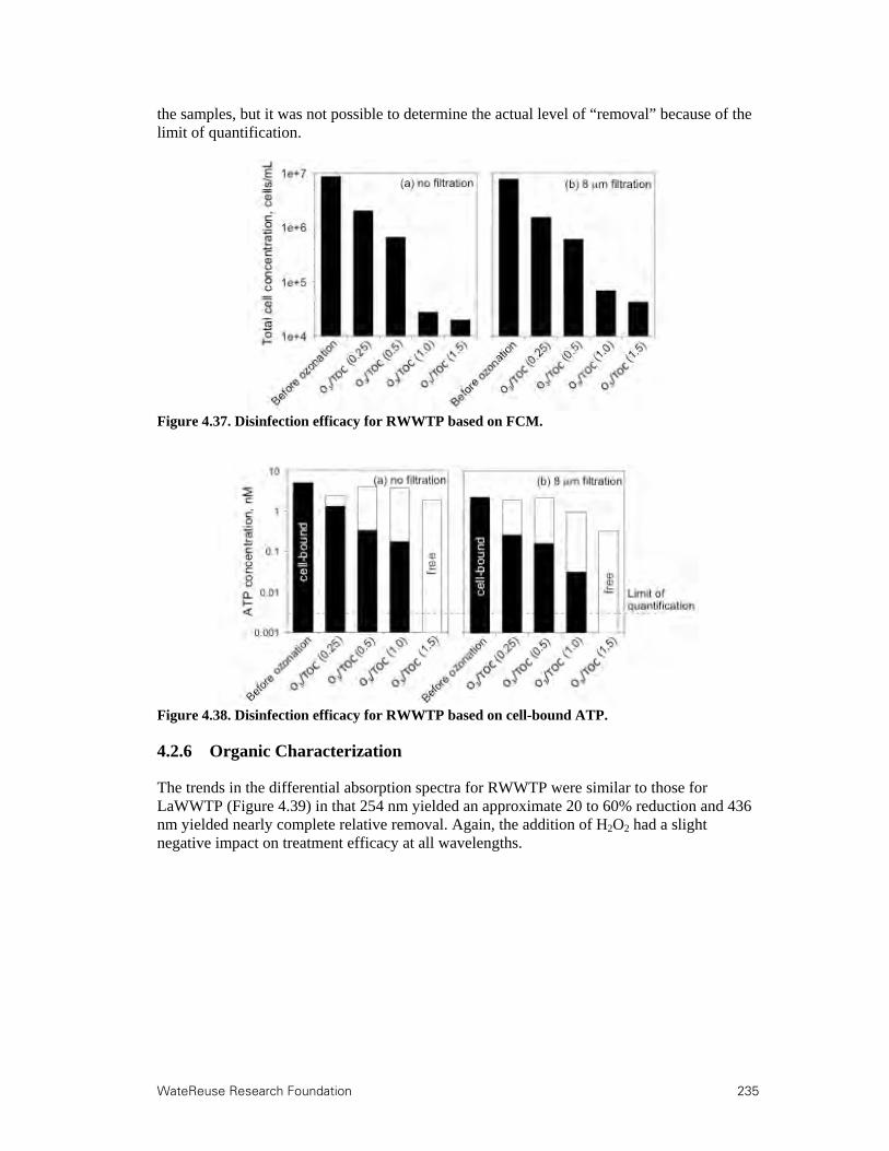
WateReuse Research Foundation 235
the samples, but it was not possible to determine the actual level of “removal” because of the limit of quantification.
Figure 4.37. Disinfection efficacy for RWWTP based on FCM.
Figure 4.38. Disinfection efficacy for RWWTP based on cell-bound ATP.
4.2.6 Organic Characterization
The trends in the differential absorption spectra for RWWTP were similar to those for LaWWTP (Figure 4.39) in that 254 nm yielded an approximate 20 to 60% reduction and 436 nm yielded nearly complete relative removal. Again, the addition of H2O2 had a slight negative impact on treatment efficacy at all wavelengths.
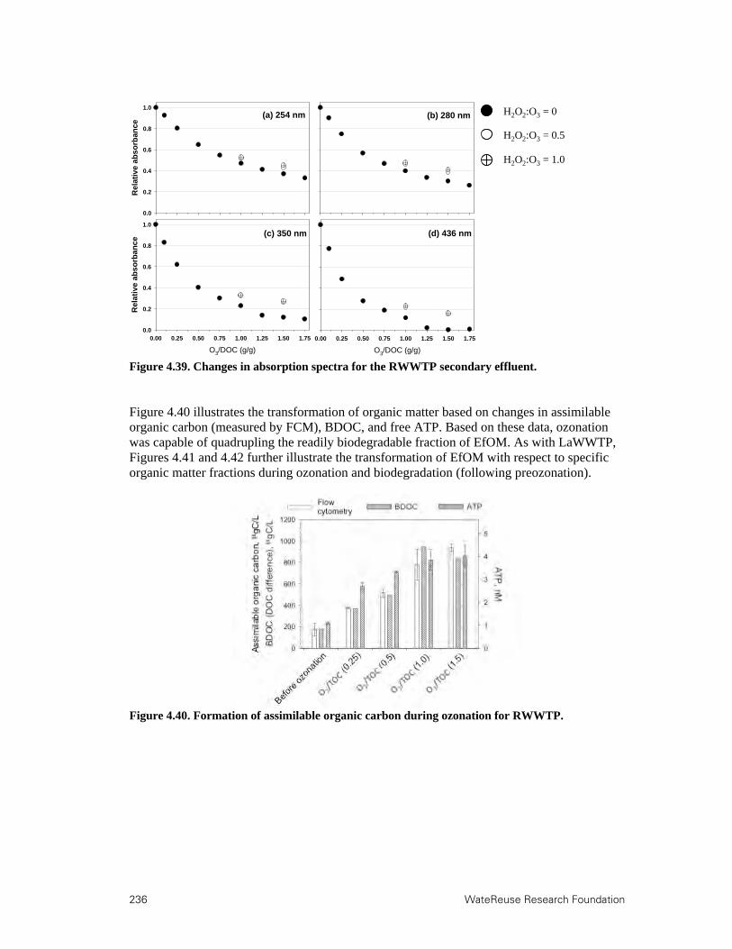
236 WateReuse Research Foundation
Figure 4.39. Changes in absorption spectra for the RWWTP secondary effluent.
Figure 4.40 illustrates the transformation of organic matter based on changes in assimilable organic carbon (measured by FCM), BDOC, and free ATP. Based on these data, ozonation was capable of quadrupling the readily biodegradable fraction of EfOM. As with LaWWTP, Figures 4.41 and 4.42 further illustrate the transformation of EfOM with respect to specific organic matter fractions during ozonation and biodegradation (following preozonation).
Figure 4.40. Formation of assimilable organic carbon during ozonation for RWWTP.
Rel
ativ
e a
bs
orb
ance
0.0
0.2
0.4
0.6
0.8
1.0
O3/DOC (g/g)
0.00 0.25 0.50 0.75 1.00 1.25 1.50 1.75
Rel
ati
ve a
bs
orb
an
ce
0.0
0.2
0.4
0.6
0.8
1.0
O3/DOC (g/g)
0.00 0.25 0.50 0.75 1.00 1.25 1.50 1.75
(a) 254 nm (b) 280 nm
(c) 350 nm (d) 436 nm
H2O2:O3 = 0
H2O2:O3 = 1.0
H2O2:O3 = 0.5R
elat
ive
ab
so
rban
ce
0.0
0.2
0.4
0.6
0.8
1.0
O3/DOC (g/g)
0.00 0.25 0.50 0.75 1.00 1.25 1.50 1.75
Rel
ati
ve a
bs
orb
an
ce
0.0
0.2
0.4
0.6
0.8
1.0
O3/DOC (g/g)
0.00 0.25 0.50 0.75 1.00 1.25 1.50 1.75
(a) 254 nm (b) 280 nm
(c) 350 nm (d) 436 nm
H2O2:O3 = 0
H2O2:O3 = 1.0
H2O2:O3 = 0.5

WateReuse Research Foundation 237
Figure 4.41. EfOM transformation during ozonation for RWWTP.
Figure 4.42. Effects of biodegradation (following ozonation) for RWWTP.
4.3 Kloten-Opfikon Wastewater Treatment Plant, Glattbrugg, Switzerland
The Kloten-Opfikon Wastewater Treatment Plant (KOWWTP) in Glattbrugg, Switzerland, is located near the Zurich International Airport. Despite its small service area of 26,000 residents, the KOWWTP treats primarily domestic flows from 55,000 population equivalents (4.4 MGD), which provides an indication of the high flows originating at the nearby airport. The primary treatment train consists of bar screens and grit removal, primary clarification, conventional activated sludge with nitrification and denitrification, secondary clarification, and sand filtration prior to discharge (without disinfection) to the To Lich River. In the conventional activated sludge process, approximately 40% of the flow is sent directly to an aeration basin with an SRT of 10 to 12 days, but 60% of the flow is sent to a preliminary aeration basin with an SRT of 3 days. Phosphate removal (TPeff ≈ 0.8 mg/L) is provided by ferric sulfate addition during secondary clarification. The KOWWTP also operates a pilot-scale MBR with nitrification, denitrification, and biological phosphorus removal. The MBR has been operated at SRTs of 14 to 18 days, 30 to 36 days, and 60 to 80 days, and the system includes three parallel membrane modules: 0.4 μm microfiltration, 0.1 μm ultrafiltration, and 0.04 μm ultrafiltration. Several peer-reviewed journal articles, including the pilot-scale
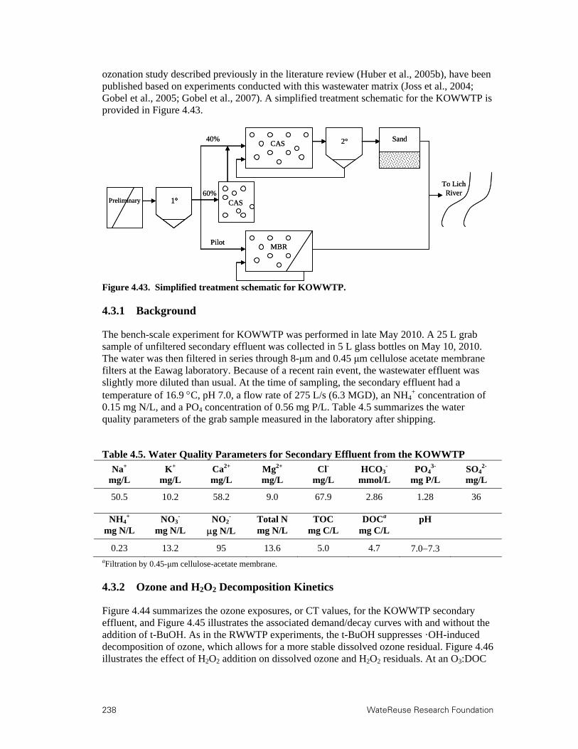
238 WateReuse Research Foundation
ozonation study described previously in the literature review (Huber et al., 2005b), have been published based on experiments conducted with this wastewater matrix (Joss et al., 2004; Gobel et al., 2005; Gobel et al., 2007). A simplified treatment schematic for the KOWWTP is provided in Figure 4.43.
Figure 4.43. Simplified treatment schematic for KOWWTP.
4.3.1 Background
The bench-scale experiment for KOWWTP was performed in late May 2010. A 25 L grab sample of unfiltered secondary effluent was collected in 5 L glass bottles on May 10, 2010. The water was then filtered in series through 8-μm and 0.45 μm cellulose acetate membrane filters at the Eawag laboratory. Because of a recent rain event, the wastewater effluent was slightly more diluted than usual. At the time of sampling, the secondary effluent had a temperature of 16.9 C, pH 7.0, a flow rate of 275 L/s (6.3 MGD), an NH4
+ concentration of 0.15 mg N/L, and a PO4 concentration of 0.56 mg P/L. Table 4.5 summarizes the water quality parameters of the grab sample measured in the laboratory after shipping.
Table 4.5. Water Quality Parameters for Secondary Effluent from the KOWWTP
aFiltration by 0.45-μm cellulose-acetate membrane.
4.3.2 Ozone and H2O2 Decomposition Kinetics
Figure 4.44 summarizes the ozone exposures, or CT values, for the KOWWTP secondary effluent, and Figure 4.45 illustrates the associated demand/decay curves with and without the addition of t-BuOH. As in the RWWTP experiments, the t-BuOH suppresses ·OH-induced decomposition of ozone, which allows for a more stable dissolved ozone residual. Figure 4.46 illustrates the effect of H2O2 addition on dissolved ozone and H2O2 residuals. At an O3:DOC
1°
2°CAS
Preliminary
Sand
MBR
40%
Pilot
CAS60%
To Lich River
1°1°
2°CAS
Preliminary
Sand
MBR
40%
Pilot
CAS60%
To Lich River
Na+ K+ Ca2+ Mg2+ Cl- HCO3- PO4
3- SO42-
mg/L mg/L mg/L mg/L mg/L mmol/L mg P/L mg/L
50.5 10.2 58.2 9.0 67.9 2.86 1.28 36
NH4+ NO3
- NO2- Total N TOC DOCa pH
mg N/L mg N/L g N/L mg N/L mg C/L mg C/L
0.23 13.2 95 13.6 5.0 4.7 7.07.3

WateReuse Research Foundation 239
ratio of 1.0, the dissolved ozone residual was nearly depleted within 30 s of reaction time at both H2O2 doses, although there was still a significant H2O2 residual in both cases.
Figure 4.44. Ozone exposures (mg-min/L) as a function of O3:DOC ratio for KOWWTP.
Figure 4.45. Ozone demand/decay curves for KOWWTP.
Figure 4.46. Ozone demand/decay with H2O2 addition for KOWWTP (O3:DOC=1.0).
No tBuOH
tBuOH = 10 mM
O3,
M
0
10
20
30
40
0
10
20
30
40
50
60
Time, min
0 5 10 15 20
O3,
M
0
20
40
60
80
100
120
Time, min
0 5 10 15 200
30
60
90
120
150
180
(a) O3/DOC = 0.25 (b) O3/DOC = 0.5
(c) O3/DOC = 1.0 (d) O3/DOC = 1.5
No tBuOH
tBuOH = 10 mM
O3,
M
0
10
20
30
40
0
10
20
30
40
50
60
Time, min
0 5 10 15 20
O3,
M
0
20
40
60
80
100
120
Time, min
0 5 10 15 200
30
60
90
120
150
180
(a) O3/DOC = 0.25 (b) O3/DOC = 0.5
(c) O3/DOC = 1.0 (d) O3/DOC = 1.5
H2O2:O3 = 0
H2O2:O3 = 1.0
H2O2:O3 = 0.5
Time, min
0 1 2 3 4 5
O3,
M
0
20
40
60
80
100
120
0 1 2 3 4 50
20
40
60
80
100
120
H2O
2,
M
Time, min
O3 H2O2H2O2:O3 = 0
H2O2:O3 = 1.0
H2O2:O3 = 0.5
Time, min
0 1 2 3 4 5
O3,
M
0
20
40
60
80
100
120
0 1 2 3 4 50
20
40
60
80
100
120
H2O
2,
M
Time, min
O3 H2O2
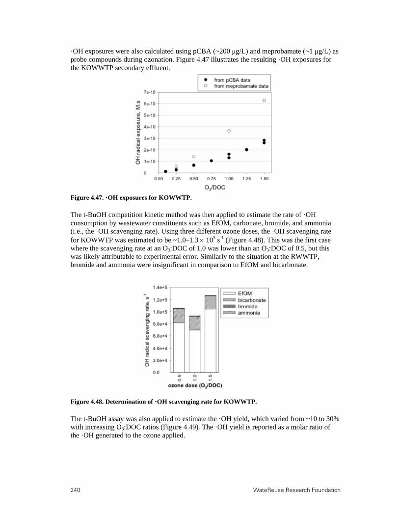
240 WateReuse Research Foundation
·OH exposures were also calculated using pCBA (~200 μg/L) and meprobamate (~1 μg/L) as probe compounds during ozonation. Figure 4.47 illustrates the resulting ·OH exposures for the KOWWTP secondary effluent.
Figure 4.47. ·OH exposures for KOWWTP.
The t-BuOH competition kinetic method was then applied to estimate the rate of ·OH consumption by wastewater constituents such as EfOM, carbonate, bromide, and ammonia (i.e., the ·OH scavenging rate). Using three different ozone doses, the ·OH scavenging rate for KOWWTP was estimated to be ~1.0–1.3 105 s-1 (Figure 4.48). This was the first case where the scavenging rate at an O3:DOC of 1.0 was lower than an O3:DOC of 0.5, but this was likely attributable to experimental error. Similarly to the situation at the RWWTP, bromide and ammonia were insignificant in comparison to EfOM and bicarbonate.
Figure 4.48. Determination of ·OH scavenging rate for KOWWTP.
The t-BuOH assay was also applied to estimate the ·OH yield, which varied from ~10 to 30% with increasing O3:DOC ratios (Figure 4.49). The ·OH yield is reported as a molar ratio of the ·OH generated to the ozone applied.

WateReuse Research Foundation 241
Figure 4.49. ·OH yield based for KOWWTP secondary effluent.
4.3.3 Bromate and Nitrosamine Formation
Figure 4.50 shows the concentration changes for bromide (Br) and bromate (BrO3) during
ozonation of the KOWWTP secondary effluent. Even though the bromide data were scattered, presumably because of some interaction of bromide with EfOM, the trend indicates that the bromide concentration decreased from the initial 37 μg/L to 25 μg/L. The decrease in bromide corresponded to an increase in bromate from 0 to 8.5 μg/L. In the presence of H2O2, bromate formation decreased by up to a factor of 1.8 (e.g., from 8.5 to 4.7 μg/L at an O3:DOC ratio of 1.5 and an H2O2:O3 ratio of 1.0). Because of the relatively low bromide concentration, bromate formation was not a significant issue even at the highest O3:DOC.
Figure 4.50. Bromide and bromate concentrations for KOWWTP.
Nitrosamine formation was also monitored as a potential ozone DBP (Figure 4.51). In contrast with the RWWTP, there was significant direct NDMA formation during ozonation (>100 ng/L), and chloramination also resulted in NDMA concentrations approaching 600 ng/L. These observations indicate that the KOWWTP secondary effluent contained significant nitrosamine precursors. However, preozonation prior to chloramination reduced the NDMA formation potential from nearly 600 ng/L to less than 100 ng/L. Because the ozone-only and ozone–chloramine samples both contained ~100 ng/L of NDMA, preozonation likely destroyed all of the chloramine precursors but still contributed 100 ng/L of direct NDMA formation potential—a net decrease in comparison to chloramine alone, however. Finally, bromide addition resulted in a very slight increase in NDMA at an O3:DOC ratio of 1.0.
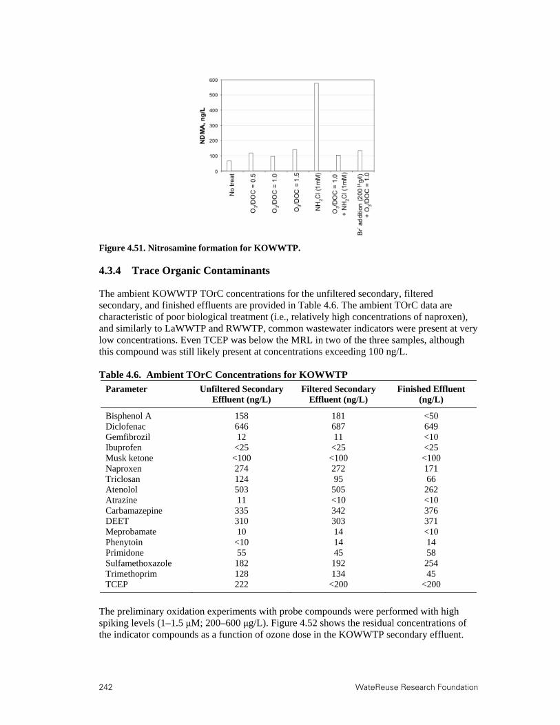
242 WateReuse Research Foundation
Figure 4.51. Nitrosamine formation for KOWWTP.
4.3.4 Trace Organic Contaminants
The ambient KOWWTP TOrC concentrations for the unfiltered secondary, filtered secondary, and finished effluents are provided in Table 4.6. The ambient TOrC data are characteristic of poor biological treatment (i.e., relatively high concentrations of naproxen), and similarly to LaWWTP and RWWTP, common wastewater indicators were present at very low concentrations. Even TCEP was below the MRL in two of the three samples, although this compound was still likely present at concentrations exceeding 100 ng/L. Table 4.6. Ambient TOrC Concentrations for KOWWTP
Parameter Unfiltered Secondary Effluent (ng/L)
Filtered Secondary Effluent (ng/L)
Finished Effluent (ng/L)
Bisphenol A 158 181 <50 Diclofenac 646 687 649 Gemfibrozil 12 11 <10 Ibuprofen <25 <25 <25 Musk ketone <100 <100 <100 Naproxen 274 272 171 Triclosan 124 95 66 Atenolol 503 505 262 Atrazine 11 <10 <10 Carbamazepine 335 342 376 DEET 310 303 371 Meprobamate 10 14 <10 Phenytoin <10 14 14 Primidone 55 45 58 Sulfamethoxazole 182 192 254 Trimethoprim 128 134 45 TCEP 222 <200 <200
The preliminary oxidation experiments with probe compounds were performed with high spiking levels (1–1.5 μM; 200–600 μg/L). Figure 4.52 shows the residual concentrations of the indicator compounds as a function of ozone dose in the KOWWTP secondary effluent.

WateReuse Research Foundation 243
Figure 4.52. Ozone oxidation of indicator compounds for KOWWTP.
Figures 4.53 and 4.54 illustrate the ozone oxidation of the spiked target compounds in the unfiltered and filtered KOWWTP secondary effluents, respectively. These results were also consistent with the previous data sets. Atenolol and meprobamate were used to illustrate the impact of H2O2 addition on different compounds (Figure 4.55), and similarly to RWWTP, atenolol mitigation was negatively impacted by H2O2 addition, whereas meprobamate oxidation increased. Again, this is related to their relative susceptibility to both ozone and ·OH oxidation.
Preliminary oxidation experiments with probe compounds spiked at high concentrations were performed for UV and UV/H2O2. Figure 4.56 shows the residual concentrations of the indicator compounds as a function of UV and H2O2 dose in the KOWWTP secondary effluent. Similarly to the previous data sets, these results are consistent with those of Figure 4.57, which illustrates the degradation profiles of the target compounds initially spiked at environmentally relevant concentrations. Finally, Figure 4.58 shows the calculated photolysis rate constants based on the degradation profiles and the percent contribution of UV photolysis to overall oxidation.
O3/DOC (g/g)
0.0 0.5 1.0 1.5 2.0Re
lati
ve r
esi
du
al c
on
cen
trat
ion
, C/C
0
0.01
0.10
1.00
Qualtification Limit
O3:DOC
C/C
0
pCBA
Ibuprofen
Bezafibrate
Carbamazepine
O3/DOC (g/g)
0.0 0.5 1.0 1.5 2.0Re
lati
ve r
esi
du
al c
on
cen
trat
ion
, C/C
0
0.01
0.10
1.00
Qualtification Limit
O3:DOC
C/C
0
pCBA
Ibuprofen
Bezafibrate
Carbamazepine

244 WateReuse Research Foundation
Figure 4.53. TOrC mitigation with ozonation for KOWWTP (unfiltered).
Figure 4.54. TOrC mitigation with ozonation for KOWWTP (filtered).
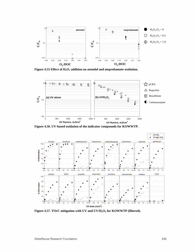
WateReuse Research Foundation 245
Figure 4.55 Effect of H2O2 addition on atenolol and meprobamate oxidation.
Figure 4.56. UV-based oxidation of the indicator compounds for KOWWTP.
Figure 4.57. TOrC mitigation with UV and UV/H2O2 for KOWWTP (filtered).
0.00 0.25 0.50 0.75 1.00 1.25 1.50
0.01
0.1
1
O3/DOC (g/g)
Rel
ativ
e rs
idu
al c
on
cen
tra
tio
n, C
/C0
atenolol
0.00 0.25 0.50 0.75 1.00 1.25 1.50
0.01
0.1
1
O3/DOC (g/g)
Rel
ativ
e rs
idu
al c
on
cen
tra
tio
n, C
/C0
meprobamate
O3:DOC
C/C
0
O3:DOC
C/C
0
H2O2:O3 = 0
H2O2:O3 = 1.0
H2O2:O3 = 0.5
0.00 0.25 0.50 0.75 1.00 1.25 1.50
0.01
0.1
1
O3/DOC (g/g)
Rel
ativ
e rs
idu
al c
on
cen
tra
tio
n, C
/C0
atenolol
0.00 0.25 0.50 0.75 1.00 1.25 1.50
0.01
0.1
1
O3/DOC (g/g)
Rel
ativ
e rs
idu
al c
on
cen
tra
tio
n, C
/C0
meprobamate
O3:DOC
C/C
0
O3:DOC
C/C
0
H2O2:O3 = 0
H2O2:O3 = 1.0
H2O2:O3 = 0.5
0 500 1000 1500 2000Rel
ativ
e re
sid
ual
co
nce
ntr
atio
n,
C/C
0
0.01
0.1
1
UV fluence, mJ/cm2
0 500 1000 1500 2000
(a) UV alone (b) UV/H2O2
UV fluence, mJ/cm2
C/C
0
pCBA
Ibuprofen
Bezafibrate
Carbamazepine
0 500 1000 1500 2000Rel
ativ
e re
sid
ual
co
nce
ntr
atio
n,
C/C
0
0.01
0.1
1
UV fluence, mJ/cm2
0 500 1000 1500 2000
(a) UV alone (b) UV/H2O2
UV fluence, mJ/cm2
C/C
0
pCBA
Ibuprofen
Bezafibrate
Carbamazepine
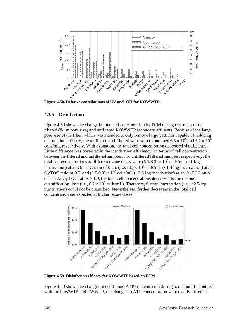
246 WateReuse Research Foundation
Figure 4.58. Relative contributions of UV and ·OH for KOWWTP.
4.3.5 Disinfection
Figure 4.59 shows the change in total cell concentration by FCM during treatment of the filtered (8-μm pore size) and unfiltered KOWWTP secondary effluents. Because of the large pore size of the filter, which was intended to only remove large particles capable of reducing disinfection efficacy, the unfiltered and filtered wastewater contained 6.3 106 and 6.2 106 cells/mL, respectively. With ozonation, the total cell concentration decreased significantly. Little difference was observed in the inactivation efficiency (in terms of cell concentration) between the filtered and unfiltered samples. For unfiltered/filtered samples, respectively, the total cell concentrations at different ozone doses were (6.1/6.0) 105 cells/mL (1-log inactivation) at an O3:TOC ratio of 0.25, (1.2/1.0) 105 cells/mL (1.8-log inactivation) at an O3:TOC ratio of 0.5, and (0.5/0.3) 105 cells/mL (2.3-log inactivation) at an O3:TOC ratio of 1.0. At O3:TOC ratios 1.0, the total cell concentrations decreased to the method quantification limit (i.e., 0.2 105 cells/mL). Therefore, further inactivation (i.e., >2.5-log inactivation) could not be quantified. Nevertheless, further decreases in the total cell concentration are expected at higher ozone doses.
Figure 4.59. Disinfection efficacy for KOWWTP based on FCM.
Figure 4.60 shows the changes in cell-bound ATP concentration during ozonation. In contrast with the LaWWTP and RWWTP, the changes in ATP concentration were clearly different
k phot
o, m
J-1 c
m2 (
x104
)
0
5
10
15
20
25
% U
V contribution
0
10
20
30
40
50
60
70
80
90
100
kphoto, UV (left)
kphoto, UV/H2O2 (left)
% UV contribution (right)
diclof
enac
triclo
san
sulfa
met
hoxa
zole
phey
tonin
atra
zine
mus
k ket
one
napr
oxen
ibupr
ofen
trim
etop
rim
aten
olol
DEET
carb
amaz
epine
gem
fibro
zil
prim
idone
bisph
enol-
A
mep
roba
mat
e
TCEP

WateReuse Research Foundation 247
between the unfiltered and filtered wastewater. The ambient cell-bound ATP concentrations were 2.49 and 1.72 nM in the unfiltered and filtered samples, respectively. In the unfiltered wastewater effluent, the cell-bound ATP concentration decreased gradually from 2.49 to 0.024 nM (2-log inactivation) at an O3:TOC ratio of 1.5 and an H2O2:O3 ratio of 0.5. In contrast, the cell-bound ATP concentration for the filtered samples decreased sharply from 1.72 nM to 0.006 nM (2.5-log inactivation) even at an O3:TOC ratio of 0.5. The slower decrease in the cell-bound ATP concentrations in the unfiltered wastewater effluent can be explained by the presence of large microorganisms, such as protozoa, which may be removed by the 0.8-μm laboratory filtration. These large microorganisms might contain a higher amount of ATP per cell and be more resistant to ozonation. Based on the difference between the unfiltered and filtered samples, large microorganisms are present at concentrations <105 cells/mL, and their contribution to the cell-bound ATP concentration is 0.77 nM.
Figure 4.60. Disinfection efficacy for KOWWTP based on cell-bound ATP.
4.3.6 Organic Characterization
The differential absorption spectra for KOWWTP are provided in Figure 4.61. As expected, ozone oxidation achieved a 20 to 60% reduction in absorbance at 254 nm and even greater reductions in the visible spectrum.
Figure 4.62 illustrates the transformation of organic matter based on changes in assimilable organic carbon (measured by FCM), BDOC, and free ATP. Based on this figure, ozonation achieved a 10-fold increase in AOC with an O3:TOC ratio of 1.5, which is greater than observed with the previous data sets. The BDOC and ATP data also indicated significant transformation of the EfOM in the KOWWTP secondary effluent. Figures 4.63 and 4.64 further illustrate the transformation of EfOM with respect to specific organic matter fractions during ozonation and biodegradation (following preozonation). Similarly to other data sets, Figure 4.63 indicates that large, hydrophobic organic matter is transformed into smaller, hydrophilic components during ozonation. Particulate and hydrophobic organic matter are first transformed into biopolymers (> 20 kD) and humics ( 1 kD), which are then further transformed into building blocks (300500 D) and LMW humics and acids (<350 D). The total decrease in TOC was less than 300 μg-C/L (<6% of the initial concentration) so mineralization of EfOM was minimal. Figure 4.64 indicates that during microbial growth, all organic carbon fractions except biopolymers and LMW humics and acids were consumed to a

248 WateReuse Research Foundation
similar extent. Overall, the decrease in TOC was 1,500 μg-C/L, which amounts to 30% removal of EfOM.
Figure 4.61. Changes in absorption spectra for the KOWWTP secondary effluent.
Figure 4.62. Formation of assimilable organic carbon during ozonation for KOWWTP.
H2O2:O3 = 0
H2O2:O3 = 1.0
H2O2:O3 = 0.5
Rel
ativ
e a
bs
orb
ance
0.0
0.2
0.4
0.6
0.8
1.0
O3/DOC (g/g)
0.0 0.5 1.0 1.5
Rel
ativ
e a
bs
orb
ance
0.0
0.2
0.4
0.6
0.8
1.0
O3/DOC (g/g)
0.0 0.5 1.0 1.5
(a) 254 nm (b) 280 nm
(c) 350 nm (d) 436 nm
H2O2:O3 = 0
H2O2:O3 = 1.0
H2O2:O3 = 0.5
Rel
ativ
e a
bs
orb
ance
0.0
0.2
0.4
0.6
0.8
1.0
O3/DOC (g/g)
0.0 0.5 1.0 1.5
Rel
ativ
e a
bs
orb
ance
0.0
0.2
0.4
0.6
0.8
1.0
O3/DOC (g/g)
0.0 0.5 1.0 1.5
(a) 254 nm (b) 280 nm
(c) 350 nm (d) 436 nm

WateReuse Research Foundation 249
Figure 4.63. EfOM transformation during ozonation for KOWWTP.
Figure 4.64. Effects of biodegradation (following ozonation) for KOWWTP.
4.4 Australian Wastewater Treatment Plant, Perth, Australia
Because of Australia’s commitment to water reuse and proactive approach to addressing TOrCs in water supplies, the project team decided that Australian collaborators would be excellent candidates for inclusion in the study. The first of two Australian utility partners was a wastewater treatment facility located in Perth, Western Australia. The facility requested anonymity, so it is hereafter referred to as AWWTP.
AWWTP began operating in 1970 and is the second largest wastewater treatment plant in Western Australia. The facility treats an average daily flow of 34 MGD, which is composed primarily of municipal wastewater. The main treatment train consists of preliminary treatment, primary clarification, conventional activated sludge with biological nutrient removal (SRT=10–12 days), and secondary clarification. The secondary-treated wastewater flows by gravity to the Indian Ocean via two adjacent outlets—one 1850 m and the other 1650 m offshore and both at a depth of 10 m. Regular monitoring of ocean water quality is
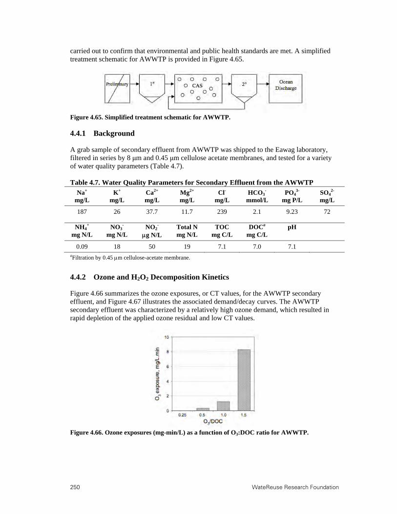
250 WateReuse Research Foundation
carried out to confirm that environmental and public health standards are met. A simplified treatment schematic for AWWTP is provided in Figure 4.65.
Figure 4.65. Simplified treatment schematic for AWWTP.
4.4.1 Background
A grab sample of secondary effluent from AWWTP was shipped to the Eawag laboratory, filtered in series by 8 μm and 0.45 μm cellulose acetate membranes, and tested for a variety of water quality parameters (Table 4.7). Table 4.7. Water Quality Parameters for Secondary Effluent from the AWWTP
aFiltration by 0.45 m cellulose-acetate membrane.
4.4.2 Ozone and H2O2 Decomposition Kinetics
Figure 4.66 summarizes the ozone exposures, or CT values, for the AWWTP secondary effluent, and Figure 4.67 illustrates the associated demand/decay curves. The AWWTP secondary effluent was characterized by a relatively high ozone demand, which resulted in rapid depletion of the applied ozone residual and low CT values.
Figure 4.66. Ozone exposures (mg-min/L) as a function of O3:DOC ratio for AWWTP.
Na+ K+ Ca2+ Mg2+ Cl- HCO3- PO4
3- SO42-
mg/L mg/L mg/L mg/L mg/L mmol/L mg P/L mg/L
187 26 37.7 11.7 239 2.1 9.23 72
NH4+ NO3
- NO2- Total N TOC DOCa pH
mg N/L mg N/L g N/L mg N/L mg C/L mg C/L
0.09 18 50 19 7.1 7.0 7.1
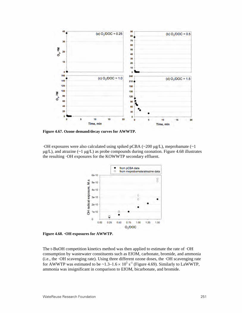
WateReuse Research Foundation 251
Figure 4.67. Ozone demand/decay curves for AWWTP.
·OH exposures were also calculated using spiked pCBA (~200 μg/L), meprobamate (~1 μg/L), and atrazine (~1 μg/L) as probe compounds during ozonation. Figure 4.68 illustrates the resulting ·OH exposures for the KOWWTP secondary effluent.
Figure 4.68. ·OH exposures for AWWTP.
The t-BuOH competition kinetics method was then applied to estimate the rate of ·OH consumption by wastewater constituents such as EfOM, carbonate, bromide, and ammonia (i.e., the ·OH scavenging rate). Using three different ozone doses, the ·OH scavenging rate for AWWTP was estimated to be ~1.3–1.6 105 s-1 (Figure 4.69). Similarly to LaWWTP, ammonia was insignificant in comparison to EfOM, bicarbonate, and bromide.
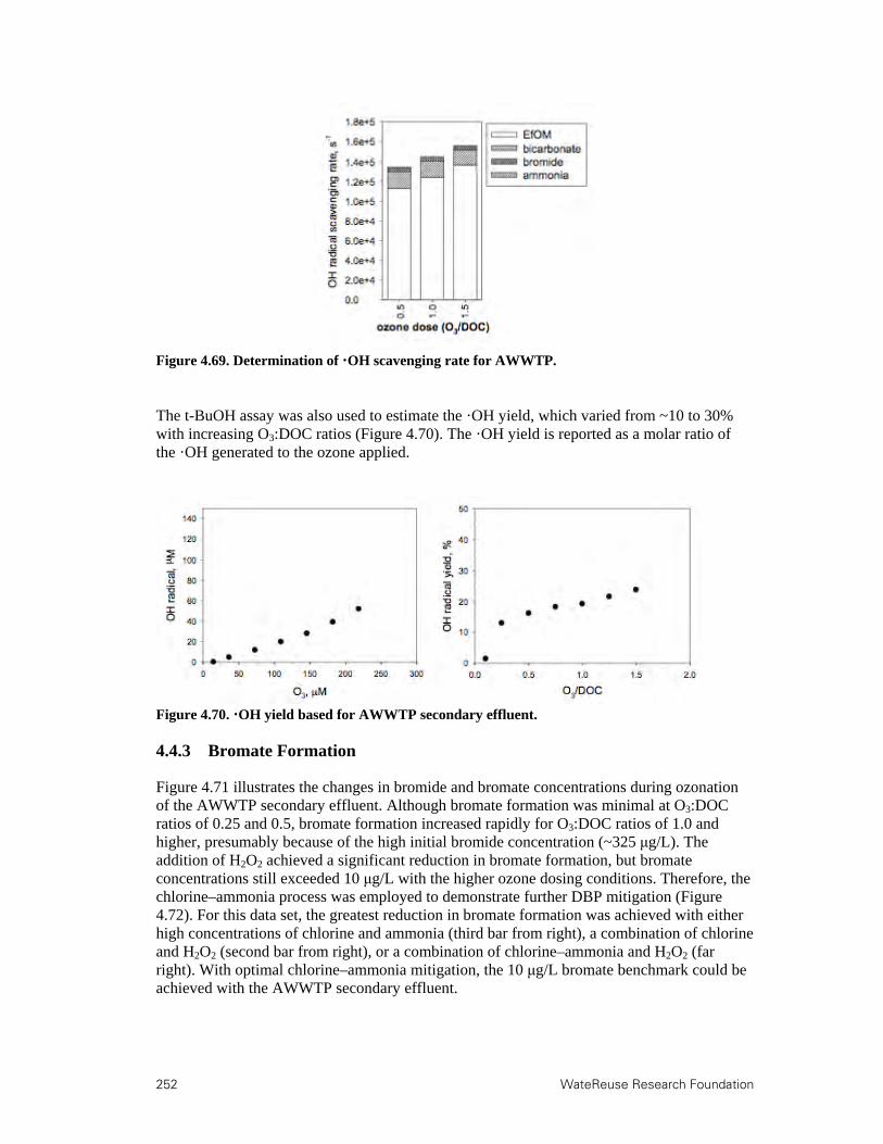
252 WateReuse Research Foundation
Figure 4.69. Determination of ·OH scavenging rate for AWWTP.
The t-BuOH assay was also used to estimate the ·OH yield, which varied from ~10 to 30% with increasing O3:DOC ratios (Figure 4.70). The ·OH yield is reported as a molar ratio of the ·OH generated to the ozone applied.
Figure 4.70. ·OH yield based for AWWTP secondary effluent.
4.4.3 Bromate Formation
Figure 4.71 illustrates the changes in bromide and bromate concentrations during ozonation of the AWWTP secondary effluent. Although bromate formation was minimal at O3:DOC ratios of 0.25 and 0.5, bromate formation increased rapidly for O3:DOC ratios of 1.0 and higher, presumably because of the high initial bromide concentration (~325 μg/L). The addition of H2O2 achieved a significant reduction in bromate formation, but bromate concentrations still exceeded 10 μg/L with the higher ozone dosing conditions. Therefore, the chlorine–ammonia process was employed to demonstrate further DBP mitigation (Figure 4.72). For this data set, the greatest reduction in bromate formation was achieved with either high concentrations of chlorine and ammonia (third bar from right), a combination of chlorine and H2O2 (second bar from right), or a combination of chlorine–ammonia and H2O2 (far right). With optimal chlorine–ammonia mitigation, the 10 μg/L bromate benchmark could be achieved with the AWWTP secondary effluent.

WateReuse Research Foundation 253
Figure 4.71. Bromide and bromate concentrations for AWWTP.
Figure 4.112. Bromate mitigation for AWWTP with the chlorine–ammonia process.
4.4.4 Trace Organic Contaminants
The ambient AWWTP TOrC concentrations for the filtered secondary effluent are provided in Table 4.8. Because there is no treatment downstream of the secondary clarifiers at this

254 WateReuse Research Foundation
facility, a “finished effluent” sample was not collected. The ambient TOrC data are comparable to those for the U.S. wastewaters because of the higher concentrations of the typical wastewater indicators (e.g., primidone, phenytoin, meprobamate, and TCEP). In particular, carbamazepine was also present at a relatively high concentration, and this compound is a prime candidate for ozonation because of its resistance to biodegradation but high ozone and ·OH rate constants.
Figure 4.73 illustrates the ozone oxidation of the spiked target compounds in the filtered AWWTP secondary effluent. Despite the high ozone demand of this matrix, the results were still consistent with the previous data sets based on similar O3:DOC or TOC ratios. Figure 4.74 illustrates the degradation profiles of the target compounds after UV photolysis and UV/H2O2 oxidation.
Table 4.79. Ambient TOrC Concentrations for AWWTP
Parameter Unfiltered Secondary Effluent (ng/L)
Bisphenol A <50 Diclofenac 480 Gemfibrozil <10 Ibuprofen <25 Musk ketone <100 Naproxen 32 Triclosan 42 Atenolol 400 Atrazine <10 Carbamazepine 960 DEET <25 Meprobamate <10 Phenytoin 120 Primidone 170 Sulfamethoxazole 530 Trimethoprim 19 TCEP 550

WateReuse Research Foundation 255
Figure 4.113. TOrC mitigation with ozonation for AWWTP (filtered).
Figure 4.114. TOrC mitigation with UV and UV/H2O2 for AWWTP (filtered).
4.4.5 Disinfection
Rather than disinfectionbeing evaluated with FCM and ATP, ambient secondary (unfiltered) samples from AWWTP were shipped to the SNWA and assayed for total and fecal coliforms, MS2, and Bacillus spores. The ambient microbial water quality data are provided in Table 4.9. Because of the extended shipping time from Australia to Nevada, the reported values likely underestimate the actual numbers of total and fecal coliforms (and possibly MS2) typically found in the AWWTP secondary effluent. The Bacillus spore count was also

256 WateReuse Research Foundation
lower than for some of the U.S. wastewaters, although the difference was not as significant. This may be the result of the microbe’s spore coat, which reduces natural inactivation over time. Similarly to the U.S. bench-scale experiments, the ozone and UV disinfection samples were spiked with relatively large numbers of the surrogate microbes, as indicated in Table 4.10.
Table 4.9. Ambient Microbial Water Quality Data for AWWTP
Microbial Surrogate Unfiltered Secondary
Effluent
Total coliforms (MPN/100 mL) 2.4 102
Fecal coliforms (MPN/100 mL) 4.3 101
MS2 (PFU/mL)
<1
Bacillus spores (CFU/100 mL) 1.0 103
Table 4.10. Microbial Spiking Levels for AWWTP Bench-Scale Experiments
Microbial Surrogate Filtered Ozone
Disinfection Filtered UV Disinfection
E. coli (MPN/100 mL) 1.5 108 4.6 106 MS2 (PFU/mL) 3.2 107 1.2 107 B. subtilis spores (CFU/100 mL) 1.5 105 1.4 105
Figure 4.75 illustrates the inactivation of spiked E. coli during the bench-scale ozone experiments. The solid line near the top of the figure represents the limit of inactivation based on the spiking level. When combined with ozonation, the addition of H2O2 generally hindered E. coli inactivation and also led to a more linear increase in inactivation with higher ozone doses. On the other hand, inactivation with ozone alone followed a more exponential trend, as indicated by the 4-log jump from an O3:TOC of 1.0 to 1.5. Only the O3:TOC of 1.5 with no H2O2 addition achieved greater than 6-log inactivation for AWWTP. The average log-inactivation values for each treatment condition are provided in Table 4.11.
Figure 4.76 illustrates the inactivation of spiked MS2 during the bench-scale ozone experiments (O3:TOC=0.5/H2O2:O3=0 not collected). In contrast to some of the previous data sets, H2O2 addition actually increased the level of inactivation slightly, but the overall inactivation profiles were similar to the previous wastewaters. With respect to the CDPH Title 22 requirements, an O3:TOC ratio >0.5 was often sufficient for the 5-log inactivation requirement, and an O3:TOC ratio >1.0 was generally sufficient for the more stringent 6.5-log inactivation requirement. The average log-inactivation values for each treatment condition are provided in Table 4.12.
Figure 4.77 illustrates the inactivation of spiked B. subtilis spores during the bench-scale ozone experiments. Similarly to the U.S. wastewaters, the spores proved to be extremely resistant to oxidation and only experienced significant inactivation for O3:TOC ratios >1.0 with no H2O2 addition. Furthermore, oxidation with ·OH alone (i.e., with H2O2 addition) was

WateReuse Research Foundation 257
extremely ineffective for spore inactivation. Instead, a high applied ozone dose with extended exposure to dissolved ozone (i.e., high CT) was necessary to achieve significant inactivation. The average log-inactivation values for each treatment condition are provided in Table 4.13.
Figure 4.78 provides a summary of the ozone disinfection data for the three surrogate microbes with respect to the CT framework. Figure 4.78A illustrates the dose–response relationships for the samples with no H2O2 addition, and Figure 4.78B illustrates the dose–response relationships for H2O2:O3 ratios of 0.5 and 1.0 (combined). Similarly to the previous data sets, the data indicate that the CT framework is not always appropriate, because substantial levels of inactivation can be achieved when the apparent ozone CT is zero. Note that the MS2 samples for O3:TOC=0.5/H2O2:O3=0 were not collected. Again, the level of inactivation for vegetative bacteria and viruses is generally lower than that observed when an ozone residual is present, and no inactivation of spore-forming bacteria can be achieved without a measurable CT.
Table 4.14 summarizes the efficacy of UV and UV/H2O2 for the inactivation of the three surrogate microbes. UV disinfection efficacy was slightly lower for AWWTP than with some of the previous data sets. For example, a UV dose of 250 mJ/cm2 only achieved 5.2- and 5.3-log inactivation for UV and UV/H2O2, respectively. This particular dosing condition often achieved the limit of inactivation in previous experiments. However, UV and UV/H2O2 still achieved substantial inactivation for all three microbes under all of the dosing conditions.
Figure 4.115. Inactivation of spiked E. coli in the AWWTP secondary effluent.

258 WateReuse Research Foundation
Table 4.11. Summary of E. coli Inactivation in the AWWTP Secondary Effluent
O3:TOC Ratio H2O2:O3=0 H2O2:O3=0.5 H2O2:O3=1.0
0.25 0.2 0.3 0.4 0.5 0.9 0.9 1.3 1.0 2.6 1.7 1.8 1.5 7.1 3.7 3.2
Figure 4.116. Inactivation of spiked MS2 in the AWWTP secondary effluent.
Table 4.12. Summary of MS2 Inactivation in the AWWTP Secondary Effluent
O3:TOC Ratio H2O2:O3=0 H2O2:O3=0.5 H2O2:O3=1.0
0.25 1.4 1.2 1.1
0.5 N/A 4.1 6.3 1.0 6.5 6.9 7.3 1.5 7.0 >7.5a >7.5a aLimit of inactivation is based on spiking level.
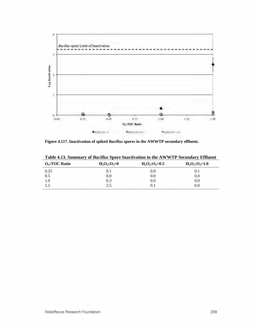
WateReuse Research Foundation 259
Figure 4.117. Inactivation of spiked Bacillus spores in the AWWTP secondary effluent.
Table 4.13. Summary of Bacillus Spore Inactivation in the AWWTP Secondary Effluent
O3:TOC Ratio H2O2:O3=0 H2O2:O3=0.5 H2O2:O3=1.0
0.25 0.1 0.0 0.1 0.5 0.0 0.0 0.0 1.0 0.3 0.0 0.0 1.5 2.5 0.1 0.0
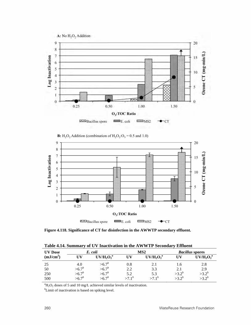
260 WateReuse Research Foundation
Figure 4.118. Significance of CT for disinfection in the AWWTP secondary effluent.
Table 4.14. Summary of UV Inactivation in the AWWTP Secondary Effluent
UV Dose (mJ/cm2)
E. coli MS2 Bacillus spores UV UV/H2O2
a UV UV/H2O2a UV UV/H2O2
a
25 4.0 >6.7b 0.8 2.1 1.6 2.8 50 >6.7b >6.7b 2.2 3.3 2.1 2.9 250 >6.7b >6.7b 5.2 5.3 >3.2b >3.2b 500 >6.7b >6.7b >7.1b >7.1b >3.2b >3.2b aH2O2 doses of 5 and 10 mg/L achieved similar levels of inactivation. bLimit of inactivation is based on spiking level.

WateReuse Research Foundation 261
4.4.6 Organic Characterization
The differential absorption spectra for AWWTP are provided in Figure 4.79. Again, ozone oxidation achieved a 20 to 60% reduction in absorbance at 254 nm and even greater reductions in the visible spectrum.
Figure 4.119. Changes in absorption spectra for the AWWTP secondary effluent.
For AWWTP, the evaluation of EFOM transformation focused on changes in fluorescence spectra, as described previously for the U.S. wastewaters. 3D EEMs were developed for the unfiltered secondary effluent (Figure 4.80) and the various ozone dosing conditions (Figure 4.81). As expected, ozone achieved significant reductions in fluorescence, particularly in the biopolymer region (Region I). This is evident in the fluorescence profile at an excitation wavelength of 254 nm (Figure 4.82) in that there was essentially no fluorescence response at emission wavelengths of 280–380 nm for O3:TOC ratios of 1.0 and 1.5.
Table 4.15 summarizes the fluorescence (i.e., Ex370Em450/Ex370Em500) and treatment indices (i.e., Ex254Em450,T/Ex254Em450,A) for the AWWTP experiments. As with the previous data sets, the FI values decreased with ozonation, although the decrease was not monotonic. Initially, the organic matter associated with emissions at 450 nm experienced more rapid transformation with low ozone doses than the organic matter associated with emissions at 500 nm. Further transformation at higher ozone doses occurred at similar relative rates, thereby stabilizing the FI. These relative changes are illustrated in Figure 4.83. In Figure 4.84, the rapid decrease in fluorescence associated with Region I is highlighted once again. With respect to the TI, ozonation reduced the associated fluorescence by more than 90%, and H2O2 addition had little impact on treatment efficacy.
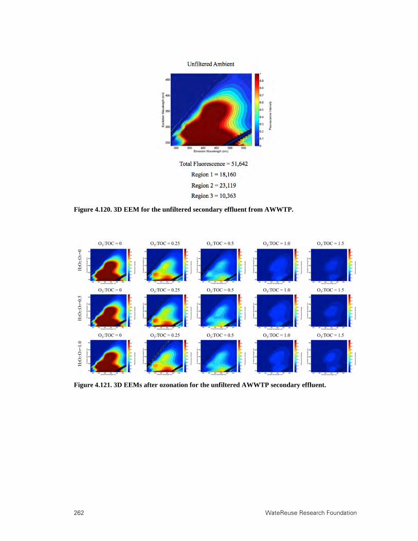
262 WateReuse Research Foundation
Figure 4.120. 3D EEM for the unfiltered secondary effluent from AWWTP.
Figure 4.121. 3D EEMs after ozonation for the unfiltered AWWTP secondary effluent.

WateReuse Research Foundation 263
Figure 4.122. AWWTP fluorescence profiles (Ex254) after ozonation.
Table 4.15. FI and TI Values for the AWWTP Secondary Effluent
O3:TOC H2O2:O3=0 H2O2:O3=0.5 H2O2:O3=1.0 FI TI FI TI FI TI
Unfiltered ozone exposure 0 1.49 1.00 1.49 1.00 1.49 1.00 0.25 1.35 0.49 1.33 0.49 1.35 0.51 0.5 1.27 0.30 1.29 0.31 1.29 0.31 1.0 1.28 0.12 1.30 0.13 1.35 0.12 1.5 1.28 0.07 1.33 0.07 1.39 0.08
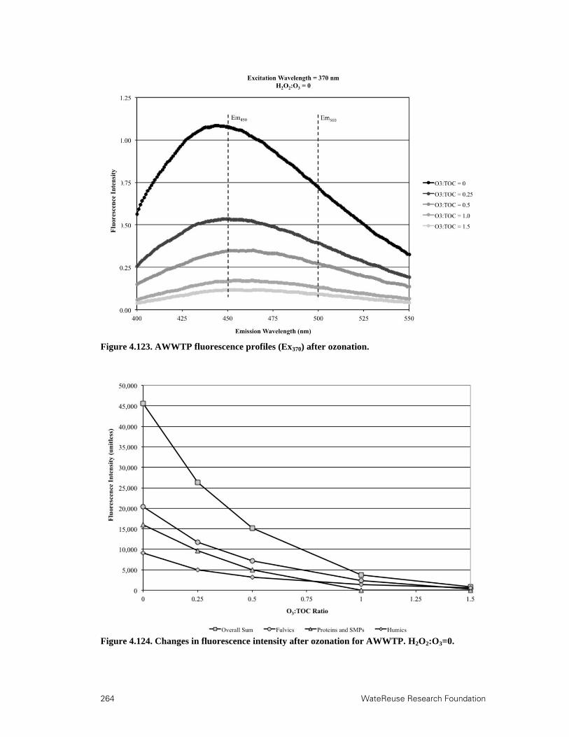
264 WateReuse Research Foundation
Figure 4.123. AWWTP fluorescence profiles (Ex370) after ozonation.
Figure 4.124. Changes in fluorescence intensity after ozonation for AWWTP. H2O2:O3=0.

WateReuse Research Foundation 265
4.5 Lowood Wastewater Treatment Plant, Brisbane, Australia
The second Australian utility partner was the Lowood Wastewater Treatment Plant (LoWWTP), which is located in a small town near Brisbane in Queensland, Australia. The treatment train is designed for low municipal flows and consists of primary clarification, biological trickling filters, secondary clarification, chlorination, and sand filtration prior to discharge to the Brisbane River. The discharge point is located immediately upstream of a major drinking water intake. A simplified treatment schematic for the LoWWTP is provided in Figure 4.85.
Figure 4.125. Simplified treatment schematic for LoWWTP.
The bench-scale experiments for LoWWTP were performed from September to October of 2010. A 20 L grab sample of unfiltered (but chlorinated) secondary effluent was collected in a 25 L plastic bottle on August 18, 2010. Given its high ammonia level (>45 mg/L), the applied chlorine was converted to chloramine at a total chlorine level of 3 mg/L. The sample arrived at the Eawag laboratory on August 23, 2010. The water was then filtered in series by 8- and 0.45-μm cellulose acetate membrane filters in the laboratory. Table 4.16 summarizes the water quality parameters of the Lowood sample. Because of the high DOC content of this matrix, the standard dosing conditions would have required an excessive dilution factor, which would likely distort the results. Instead, these experiments focused on O3:DOC ratios ranging from 0 to 0.6. Table 4.16. Water Quality Parameters for the LoWWTP Secondary Effluent
aFiltration by 0.45 m cellulose-acetate membrane.
4.5.1 Ozone and H2O2 Decomposition Kinetics
The LoWWTP data for ozone and H2O2 decomposition kinetics are described in the following chapter as part of the summarized bench-scale experiments.
·OH exposures were calculated using pCBA (~200 μg/L) and meprobamate (~1 μg/L) as probe compounds during ozonation. Figure 4.86 illustrates the resulting ·OH exposures for the LoWWTP secondary effluent.
1° 2° SandBrisbane
RiverCl2 GasTrickling Filter
1°1° 2° SandSandBrisbane
RiverBrisbane
RiverCl2 GasTrickling Filter
Na+ K+ Ca2+ Mg2+ Cl- HCO3- PO4
3- SO42-
mg/L mg/L mg/L mg/L mg/L mmol/L mg P/L mg/L
66.3 26.7 25.4 10.8 102 5.9 8.8 58
NH4+ NO3
- NO2- total N TOC DOCa pH
mg N/L mg N/L g N/L mg N/L mg C/L mg C/L
>45 <0.25 448 47.2 38.0 26.4 7.3
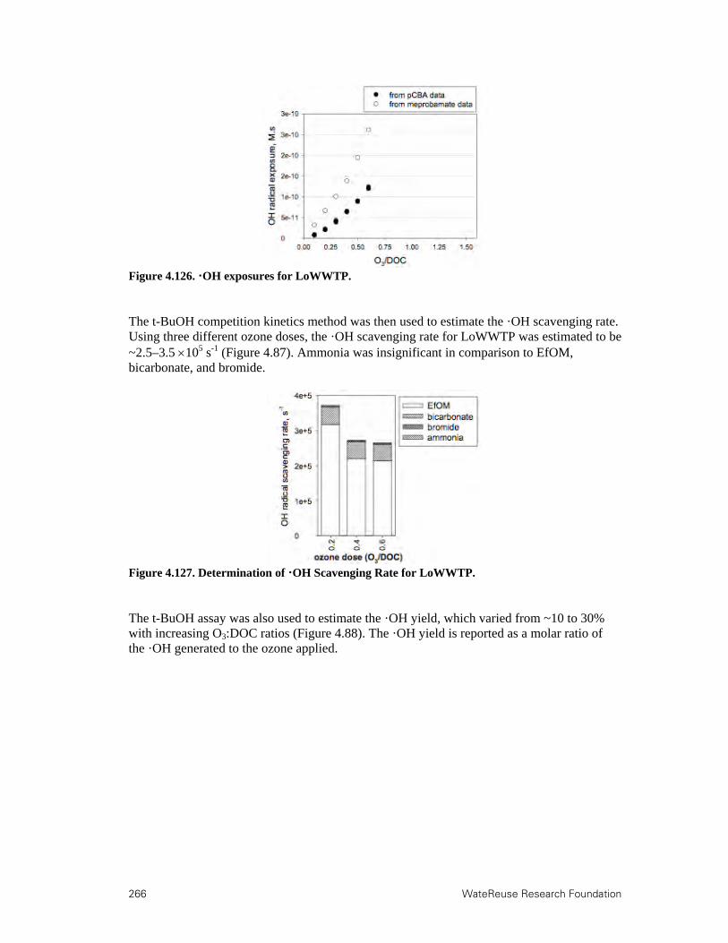
266 WateReuse Research Foundation
Figure 4.126. ·OH exposures for LoWWTP.
The t-BuOH competition kinetics method was then used to estimate the ·OH scavenging rate. Using three different ozone doses, the ·OH scavenging rate for LoWWTP was estimated to be ~2.5–3.5 105 s-1 (Figure 4.87). Ammonia was insignificant in comparison to EfOM, bicarbonate, and bromide.
Figure 4.127. Determination of ·OH Scavenging Rate for LoWWTP.
The t-BuOH assay was also used to estimate the ·OH yield, which varied from ~10 to 30% with increasing O3:DOC ratios (Figure 4.88). The ·OH yield is reported as a molar ratio of the ·OH generated to the ozone applied.

WateReuse Research Foundation 267
Figure 4.128. ·OH yield based for LoWWTP secondary effluent.
4.5.2 Bromate and Nitrosamine Formation
The LoWWTP secondary effluent had a relatively high bromide concentration, but bromate formation during ozonation was only slightly higher than the 10 μg/L benchmark at an O3:DOC ratio of 0.6 (Figure 4.89). The residual chloramine may have provided some in situ bromate mitigation, but the formation could have been reduced even further with optimized chlorine–ammonia conditions or H2O2 addition.
Figure 4.129. Bromate concentrations for LoWWTP.
4.5.3 Trace Organic Contaminants
The ambient TOrC concentrations for the unfiltered, chlorinated secondary effluent from LoWWTP are provided in Table 4.17. The concentrations of some of the more bioamenable compounds (e.g., ibuprofen and naproxen) were extremely high compared to those of some of the other secondary effluents in this study. This indicates that there was limited biological treatment in the upstream trickling filters. Similarly to some of the Swiss samples, several common wastewater indicators (e.g., primidone and meprobamate) were below their respective reporting limits, whereas others (e.g., phenytoin and TCEP) were comparable to typical U.S. secondary effluents. This geographic variability indicates that perceived “universal” indicators are not applicable in all settings. It is uncertain why these particular compounds were below their respective reporting limits, but they may be less prevalent

268 WateReuse Research Foundation
pharmaceuticals—or alternative drugs may be substituted for them—in certain parts of the world.
As mentioned earlier, the high DOC concentration in the LoWWTP secondary effluent limited the applied O3:DOC ratio to 0.6, which corresponded to an initial ozone concentration of 16 mg/L (330 M). At this ozone dose, the wastewater sample was diluted by 22% upon the addition of the concentrated ozone stock solution.
Table 4.17. Ambient TOrC Concentrations for LoWWTP
Parameter Secondary Effluent (ng/L)
Bisphenol A 160 Diclofenac 170 Gemfibrozil 57 Ibuprofen 9,500 Musk ketone <100 Naproxen 2,700 Triclosan 180 Atenolol 1,300 Atrazine <10 Carbamazepine 560 DEET 670 Meprobamate <10 Phenytoin 230 Primidone <10 Sulfamethoxazole 1,400 Trimethoprim 1,500 TCEP 250
The preliminary oxidation data for indicator compounds spiked at high concentrations demonstrated higher treatment efficacy than the previous bench-scale experiments (Figure 4.90). This improved oxidation efficacy may be attributable to either the (1) high EfOM concentration or the (2) synergistic oxidation by residual total chlorine. Figure 4.91 illustrates the ozone oxidation of the target compounds spiked at environmentally relevant concentrations, and Figure 4.92 illustrates the degradation of the target compounds via UV or UV/H2O2. A more comprehensive comparison of these data sets with previous secondary effluents is provided in the next chapter.

WateReuse Research Foundation 269
Figure 4.130. Ozone oxidation of indicator compounds for LoWWTP.
Figure 4.131. TOrC mitigation with ozonation for LoWWTP (filtered).
O3/DOC (g/g)
0.0 0.5 1.0 1.5 2.0Rel
ati
ve r
esid
ual
co
nce
ntr
atio
n, C
/C0
0.01
0.10
1.00
QuantificationLimit
O3:DOC
C/C
0
pCBA
Ibuprofen
Bezafibrate
Carbamazepine
O3/DOC (g/g)
0.0 0.5 1.0 1.5 2.0Rel
ati
ve r
esid
ual
co
nce
ntr
atio
n, C
/C0
0.01
0.10
1.00
QuantificationLimit
O3:DOC
C/C
0
pCBA
Ibuprofen
Bezafibrate
Carbamazepine

270 WateReuse Research Foundation
Figure 4.132. TOrC mitigation with UV and UV/H2O2 for LoWWTP.
4.5.4 Miscellaneous Data
The remaining data will be presented as part of the summarized bench-scale experiments in the next chapter.

WateReuse Research Foundation 271
Chapter 5
5.Summary of Bench-Scale Experiments
The primary goal of this study was to provide a general overview of the use of ozone in wastewater applications, with specific emphasis on TOrC oxidation. The previous discussion of the 10 sets of bench-scale experiments covered a broad range of topics, including oxidant exposure, disinfection byproduct formation, microbial inactivation, TOrC oxidation, and EfOM transformation. The following sections assimilate this enormous database in order to reach general conclusions regarding the design and operation of ozone and UV/H2O2 systems for the treatment of secondary and tertiary effluents.
5.1 Ozone Versus Ozone/H2O2
With respect to ozonation, the addition of H2O2 is intended to drive the formation of ·OH in order to target more recalcitrant compounds. However, ozonation alone is fully capable of generating ·OH in wastewater applications because of side reactions with effluent organic matter. Therefore, the following question can be posed: Why should H2O2 be added to an ozone process? This question will be highlighted in the summaries of the various analyses, but the main points are summarized immediately in the following.
1) Efficacy of ozone versus ·OH. Second-order ozone and ·OH rate constants vary significantly depending on the contaminant of interest. This is the basis for dividing the target compounds in this study into five different groups. Some compounds are susceptible to both ozone and ·OH (e.g., Group 1: naproxen and carbamazepine; Group 2: gemfibrozil and atenolol), some are only susceptible to ·OH (e.g., Group 3: ibuprofen and phenytoin; Group 4: atrazine and meprobamate), and some are resistant to both forms of oxidation (e.g., Group 5: TCEP and musk ketone). In order to oxidize the compounds in all five groups, the oxidation process must achieve excessively high ozone doses or provide moderate ·OH exposure. In matrices with limited background organic matter, including surface water and groundwater, this may require the addition of H2O2.
2) Decomposition of ozone into ·OH. Although the combination of ozone and H2O2 may be more appropriate in low-TOC water matrices, ozone rapidly decomposes into ·OH through reactions with effluent organic matter in wastewater applications. In fact, ozone and ozone/H2O2 generally provide similar overall ·OH exposure in wastewater when sufficient reaction time is provided. Therefore, H2O2 addition is often unnecessary for ozone to qualify as an advanced oxidation process, but other issues may impact the design of the process and warrant H2O2 addition.
3) Bromate control. In previous studies, and to some extent in this study, H2O2 addition has been shown to reduce bromate formation during ozonation. Some studies call for more relaxed bromate guidelines for environmental discharge (e.g., 3 mg/L), but the U.S. EPA maximum contaminant level of 10 μg/L is often used as the benchmark for ozonation processes, particularly for indirect potable reuse applications. Therefore, the combination of high applied ozone doses and high bromide levels may necessitate H2O2 addition to meet the 10 μg/L bromate benchmark. Other forms of bromate mitigation (e.g., the chlorine-ammonia process) are available as well and were discussed previously for the LaWWTP and AWWTP bench-scale experiments.

272 WateReuse Research Foundation
4) Process footprint. The addition of H2O2 allows rapid conversion of dissolved ozone to ·OH, which reduces the reaction time to a matter of seconds. High applied ozone doses without H2O2 (e.g., O3:TOC ratios greater than 1.5) may require large contactors with more than 20 min of residence time. This translates into larger process footprints in full-scale applications. To achieve a combination of ozone residual and small process footprint, H2O2 can be added after a target contact time has been reached to quench the remaining ozone residual while still capturing its oxidation benefits.
5) Trace organic contaminants. As mentioned previously, some target compounds are highly resistant to ozone oxidation but are moderately susceptible to ·OH oxidation. Despite the fact that ozone naturally decomposes into ·OH in wastewater applications, the addition of H2O2 may provide a slight benefit in the oxidation of ozone-resistant compounds (i.e., Groups 3, 4, and 5) when higher applied ozone doses are used (i.e., O3:TOC > 0.5). However, the benefit generally amounts to less than a 10% increase in oxidation. In drinking water applications or groundwater remediation, the addition of H2O2 will likely have a much more significant impact than that of ozone alone.
6) Microbes. In the United States, oxidation-based disinfection is generally governed by the CT framework (i.e., disinfectant concentration exposure time). This is a reasonable strategy for chlorine and chloramine, because they can provide extended exposure times at relatively high oxidant concentrations. Although targeting a residual is possible with ozone, the residual is considerably less stable, so it is more difficult to follow the CT framework. However, dissolved ozone is quite effective against nearly all microbes, including Cryptosporidium and Giardia, so it has become increasingly popular in disinfection applications. The natural decomposition of ozone into ·OH or the forced conversion with H2O2 addition also achieves significant inactivation of certain microbes, including vegetative bacteria (e.g., E. coli) and viruses. However, H2O2 addition generally reduces the level of inactivation achieved by ozone alone at the same O3:TOC ratio, and the level of inactivation is less consistent. The reduced CT or lack of CT also makes it nearly impossible to comply with current guidelines and regulations, which is the basis for this study. Furthermore, the inactivation of spore-forming microbes (e.g., Bacillus spores, Cryptosporidium oocysts, Giardia cysts) with ·OH is extremely inefficient, so H2O2 addition is not recommended in applications targeting these microbes. To exploit the disinfection benefits of dissolved ozone and the smaller footprints associated with ozone/H2O2, it is possible to target a certain CT with dissolved ozone before adding H2O2 to expedite the remaining reactions.
7) Organic matter. Although there are few guidelines and regulations targeting bulk organic matter (other than TOC limits), aesthetic concerns sometimes necessitate reductions in UV absorbance or color, for example. Both dissolved ozone and ozone/H2O2 are particularly effective in improving aesthetic parameters, but the addition of H2O2 will slightly reduce treatment efficacy.
8) Cost. The additional costs and complexities associated with chemical storage, handling, and injection may also limit the attractiveness of ozone/H2O2. Based on the assumptions that follow, which allow for simple process scaling, the chemical cost alone would amount to $658 per year for each mgd of flow rate and mg/L of applied ozone. For a 100-mgd wastewater treatment plant targeting an applied ozone dose of 7 mg/L, the H2O2 addition for the ozone/H2O2 process would cost approximately $460,324 per year.

WateReuse Research Foundation 273
a. 50% H2O2=$0.68/kg b. Process flow rate=1 mgd c. Ozone dose=1 mg/L d. H2O2:O3 ratio=0.5 H2O2=0.35 mg/L
9) UV vs. UV/H2O2. In contrast to ozone-based treatment processes, the addition of H2O2 is generally required for UV-based oxidation. Low-pressure and medium-pressure UV irradiation are extremely effective for microbial inactivation and photolysis of NDMA, but UV light is generally insufficient to oxidize trace organic contaminants. With the exception of certain compounds, including diclofenac and triclosan, significant oxidation often requires a combination of high UV doses (i.e., >250 mJ/cm2) and high concentrations of H2O2 (i.e., >5 mg/L). This is the basis for the “gold standard” in indirect potable reuse: UV photolysis for NDMA mitigation and H2O2 addition for the oxidation of recalcitrant compounds such as 1,4-dioxane.
10) H2O2 quenching. Residual H2O2 is not a significant concern at this point, but there are benefits to optimizing H2O2 dose to prevent chemical waste and alleviate any concerns related to residual discharge. In ozone/H2O2 applications, it may be possible to target appropriate H2O2:O3 ratios so as to achieve complete consumption of H2O2. Based on stoichiometry, a molar H2O2:O3 ratio of 0.5 should lead to complete consumption, but the complex interactions with other scavengers in the target water matrix often complicate the calculation, as illustrated for the LaWWTP, RWWTP, and KOWWTP bench-scale experiments. Therefore, a trial-and-error approach may be required in real-world applications. On the other hand, UV/H2O2 processes will almost always have an H2O2 residual because of the disconnect between the amount of chemical required to achieve a reasonable ·OH exposure and the limited amount of chemical that is actually consumed in the process. If necessary, H2O2 can be quenched by the addition of chemicals, such as calcium thiosulfate, or through catalytic decomposition in activated carbon beds, which are becoming popular in wastewater treatment trains with ozone-based oxidation.
5.2 Comparison of Filtered Secondary Effluents
5.2.1 General Water Quality
Secondary effluent samples were collected from 10 wastewater treatment plants with a range of operational conditions and water quality. The major water quality parameters affecting oxidation are presented for the U.S. and international wastewaters in Table 5.1 and Table 5.2, respectively. Eight of the 10 secondary effluents fell within a TOC range of 5.0–7.6 mg/L, but WBMWD and LoWWTP were clearly the outliers, with TOC concentrations of 18 and 38 mg/L, respectively. The low SRT of WBMWD and the trickling filter at LoWWTP limited the biotransformation of bulk organic matter during the secondary process. For WBMWD, this is also evident based on the high UV254 absorbance and total fluorescence values. The bulk organic matter in the PCU and AWWTP secondary effluents was also unique in that their UV254 and total fluorescence values were relatively high despite the high SRTs at those facilities. As expected, the range of bromide values correlated to significant differences in bromate formation during ozonation. The nitrite values were relatively low and insignificant for most of the facilities. Although nitrite was higher at WBMWD and LoWWTP, their corresponding TOC and DOC concentrations dominated the ozone demand, which rendered the nitrite demand negligible. On the other hand, GCGA had a relatively low TOC, so its high

274 WateReuse Research Foundation
nitrite level had a significant impact on ozone demand and the final O3:TOC and H2O2:O3 ratios, as described earlier. Finally, the 10 secondary effluents covered a wide range of alkalinities, which ultimately impacted oxidant exposure because of ·OH scavenging.
Table 5.1. Water Quality Summary for Filtered SNWA Secondary Effluents
Parameter CCWRD MWRDGC WBMWD PCU GCGA
pH 6.9 7.6 7.3 7.3 7.3 SRT (days) 7 7 1.5 12 11 TOC (mg/L) 7.6 6.9 18 7.2 6.3 NO2 (mg-N/L) 0.06 <0.05 0.17 <0.05 0.30 Bromide (μg/L) 174 93 409 730 31 UV254 (cm-1) 0.15 0.13 0.27 0.19 0.13 Total fluorescence (unitless) 38,874 37,712 94,807 53,996 34,795 Alkalinity (mM HCO3) 2.5 2.7 6.6 4.1 3.4
Table 5.2. Water Quality Summary for Filtered Eawag Secondary Effluents
Parameter LaWWTP RWWTP KOWWTP AWWTP LoWWTP
pH 7.2 7.2 7.0 7.1 7.3 SRT (days) 2–4 16–17 10–12 10–12 N/Aa TOC (mg/L) 6.1 5.0 5.0 7.1 38 DOC (mg/L) 6.0 4.7 4.7 7.0 26 NO2 (mg-N/L) 0.16 <0.05 0.07 0.05 0.45 Bromide (μg/L) 410 40 37 330 140 UV254 (cm-1) 0.10 0.13 0.11 0.20 - Total fluorescence (unitless) - - - 51,642 - Alkalinity (mM HCO3) 1.3 4.4 2.9 2.1 5.9
aN/A = not applicable due to use of trickling filter.
5.2.2 Ozone CT Values
The O3:TOC or O3:DOC ratio is a convenient tool for determining the ozone dose for a particular application. As described in earlier sections, similar O3:TOC and O3:DOC ratios achieve comparable levels of oxidation despite dramatic differences in water quality and dissolved ozone contact time (i.e., CT), which is summarized in Table 5.3 and Table 5.4. All of the ozone exposures and a corresponding regression equation are illustrated in Figure 5.1. With respect to the SNWA experiments, the filtered MWRDGC secondary effluent seemed to be most affected by the cartridge filter contamination that was reported earlier, which is likely the primary reason for its low CT relative to some of the other matrices. Again, PCU was a unique case in that its CT values were similar to those for other matrices for O3:TOC ratios less than 1.5. However, the dissolved ozone residual at an O3:TOC ratio of 1.5 was more stable than for the other wastewaters, which resulted in a much higher CT. The low CT values for GCGA were related to the incorrect applied ozone doses because of the unexpected nitrite demand. With respect to the international secondary effluents, AWWTP was the most notable matrix because it had a significantly higher ozone demand, which reduced its overall CT as well.
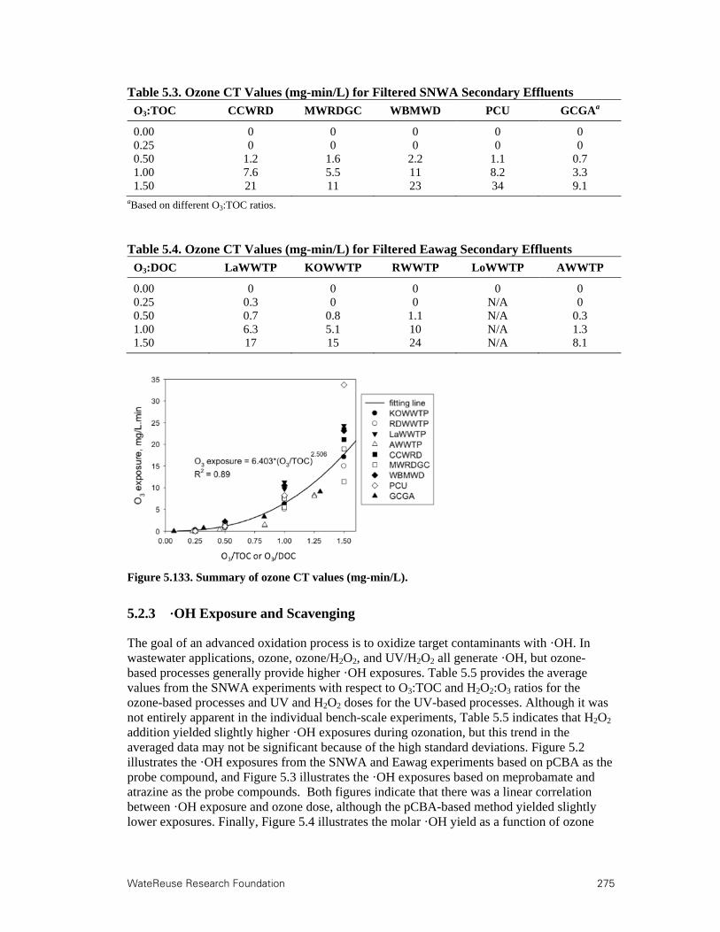
WateReuse Research Foundation 275
Table 5.3. Ozone CT Values (mg-min/L) for Filtered SNWA Secondary Effluents
O3:TOC CCWRD MWRDGC WBMWD PCU GCGAa
0.00 0 0 0 0 0 0.25 0 0 0 0 0 0.50 1.2 1.6 2.2 1.1 0.7 1.00 7.6 5.5 11 8.2 3.3 1.50 21 11 23 34 9.1
aBased on different O3:TOC ratios.
Table 5.4. Ozone CT Values (mg-min/L) for Filtered Eawag Secondary Effluents
O3:DOC LaWWTP KOWWTP RWWTP LoWWTP AWWTP
0.00 0 0 0 0 0 0.25 0.3 0 0 N/A 0 0.50 0.7 0.8 1.1 N/A 0.3 1.00 6.3 5.1 10 N/A 1.3 1.50 17 15 24 N/A 8.1
Figure 5.133. Summary of ozone CT values (mg-min/L).
5.2.3 ·OH Exposure and Scavenging
The goal of an advanced oxidation process is to oxidize target contaminants with ·OH. In wastewater applications, ozone, ozone/H2O2, and UV/H2O2 all generate ·OH, but ozone-based processes generally provide higher ·OH exposures. Table 5.5 provides the average values from the SNWA experiments with respect to O3:TOC and H2O2:O3 ratios for the ozone-based processes and UV and H2O2 doses for the UV-based processes. Although it was not entirely apparent in the individual bench-scale experiments, Table 5.5 indicates that H2O2 addition yielded slightly higher ·OH exposures during ozonation, but this trend in the averaged data may not be significant because of the high standard deviations. Figure 5.2 illustrates the ·OH exposures from the SNWA and Eawag experiments based on pCBA as the probe compound, and Figure 5.3 illustrates the ·OH exposures based on meprobamate and atrazine as the probe compounds. Both figures indicate that there was a linear correlation between ·OH exposure and ozone dose, although the pCBA-based method yielded slightly lower exposures. Finally, Figure 5.4 illustrates the molar ·OH yield as a function of ozone

276 WateReuse Research Foundation
dose for the various secondary effluents. With increased ozone doses, the molar conversion increases from 10% to 30%
Table 5.5. Average ·OH Exposures (10-11 M-s) for Filtered U.S. Secondary Effluents
O3:TOCa H2O2:O3=0 H2O2:O3=0.5 H2O2:O3=1.0 UV Dose (mJ/cm2)b
H2O2=5 mg/L
H2O2=10 mg/L
0.25 7.3 ± 3.8 7.7 ± 4.2 8.4 ± 4.6 0 N/A 0.1 ± 0.3 0.50 14 ± 5.7 16 ± 5.9 16 ± 7.3 50 N/A 0.7 ± 0.8 1.00 35 ± 9.6 38 ± 15 37 ± 15 250 2.6 ± 1.5 5.2 ± 1.4 1.50 56 ± 15 64 ± 22 59 ± 26 500 4.7 ± 1.4 8.9 ± 2.2
aIncludes GCGA data linearly adjusted based on O3:TOC ratio. bIncludes CCWRD data for 45 (50) and 225 (250) mJ/cm2.
Figure 5.2. Summary of ·OH exposures (M-s) based on pCBA as the probe compound.
Figure 5.3. Summary of ·OH exposures (M-s) based on meprobamate and atrazine.

WateReuse Research Foundation 277
Figure 5.4. Summary of ·OH yield as a function of ozone dose.
Figure 5.5 illustrates a comparison of the first-order ·OH scavenging rates for a subset of the bench-scale experiments. These rates account for scavenging from EfOM, bicarbonate, bromide, and ammonia, although EfOM (Figure 5.6) and bicarbonate constituted a majority of the scavenging in all cases. Although the first-order rate constants in Figure 5.5 for WBMWD and LoWWTP were significantly higher than the other matrices because of higher EfOM scavenging, the second-order rate constants were lower in Figure 5.6 because those rates constants are coupled with their higher EfOM concentrations in second-order rate expressions. Excluding WBMWD and LoWWTP, which had significantly higher EfOM concentrations, all of the matrices had relatively similar first- and second-order scavenging rates.
Figure 5.5. Comparison of ·OH scavenging rates (s-1).

278 WateReuse Research Foundation
Figure 5.6. ·OH scavenging (mg-C/L)-1s-1 from EfOM.
5.2.4 Bromate Formation
The initial bromide concentrations for each secondary effluent were directly correlated with bromate formation, as summarized in Tables 5.6 and 5.7. In other words, higher bromide concentrations will lead to higher bromate formation unless some type of mitigation is employed. The bromide incorporation values provide a rough estimate, as indicated by the relatively high standard deviations, of expected bromate formation based on influent bromide concentrations. For an O3:TOC ratio of 1.5, approximately 31% of the initial bromide will be converted to bromate as bromide (Br-=100 μg/L BrO3
-=31 μg/L as Br BrO3-=50 μg/L).
The Eawag experiments yielded slightly lower bromide incorporation factors, which may have been related to the different analysis methods, so the data sets were not combined.
Table 5.6. Bromide (μg/L) and Bromate Formation (μg/L) for SNWA Secondary Effluents
O3:TOC CCWRD MWRDGC WBMWD PCU GCGAa Bromide
Incorporation (%)b
0.25 <1 <1 7.4 7.9 <1 1.2 ± 0.5 0.50 5.7 <1 51 34 1.3 4.6 ± 3.9 1.00 29 18 140 140 6.2 15 ± 8.0 1.50 71 45 190 376 14 31 ± 8.0 Bromide 174 93 409 730 31 --
aBased on different O3:TOC ratios. bIncludes GCGA data linearly adjusted based on O3:TOC ratio.

WateReuse Research Foundation 279
Table 5.7. Bromide (μg/L) and Bromate Formation (μg/L) for Eawag Secondary Effluents
O3:DOC LaWWTP RWWTP KOWWTP AWWTP LoWWTPa Bromide
Incorporation (%)b
0.25 <2 <2 <2 <2 2.2 2.8 ± 2.8 0.50 12 <2 <2 5.0 5.6 3.3 ± 2.2 1.00 38 5.3 4.8 25 9.3 9.5 ± 4.5 1.50 60 9.9 9.4 55 14 18 ± 8.9 Bromide 460 40 37 330 140 --
aBased on different O3:DOC ratios. bExcludes LoWWTP data.
H2O2 addition provided some degree of bromate mitigation during the bench-scale experiments, but the more problematic matrices (e.g., WBMWD and PCU) would require the more effective chlorine–ammonia process (previously described for LaWWTP and AWWTP) or a combination of chlorine–ammonia and H2O2 to achieve the 10-μg/L benchmark. Some researchers question the validity of using this benchmark in environmental discharge applications, but it may be relevant for indirect potable reuse facilities.
5.2.5 NDMA
According to the previous draft California Department of Public Health Title 22 requirements, facilities were required to demonstrate 1.2-log (93.7%) destruction of NDMA prior to groundwater injection. Table 5.8 summarizes the UV doses required for 1.2-log destruction of NDMA during the UV and UV/H2O2 experiments. Except at WBMWD, H2O2 addition negatively impacted NDMA destruction because of the relative efficacy of UV photolysis and NDMA’s low ·OH rate constant. Despite the lamp intensity corrections for UV254 absorbance, the UV dose requirements varied significantly among the various matrices. On average, a UV dose of 600–700 mJ/cm2 for the secondary effluents was required to achieve the CDPH Title 22 benchmark. Although the UV exposures were corrected for UV absorbance, it is unclear whether these doses would also apply for reverse osmosis permeates, which are the common target matrix for UV photolysis of NDMA in indirect potable reuse applications. According to the recent revisions to the draft CDPH regulations, facilities will no longer be required to achieve 1.2-log destruction of NDMA, but they will be required to comply with the 10 ng/L notification level in IPR applications.
Table 5.8. UV Dose (mJ/cm2) Required for 1.2-Log NDMA Destruction
H2O2 Dose (mg/L)
CCWRD MWRDGC WBMWD PCU GCGA Average
0 500 600 571 667 706 609 ± 81 10 662 649 508 717 800 667 ± 107
As described earlier, the magnitude of direct NDMA formation during ozonation was relatively unexpected, particularly for the facilities where formation exceeded 100 ng/L. Direct NDMA formation had previously been reported in the literature, but it was originally thought to be a more localized issue related to specific trace organic compounds (e.g., fungicide metabolite). The data in this study indicate that direct NDMA formation during
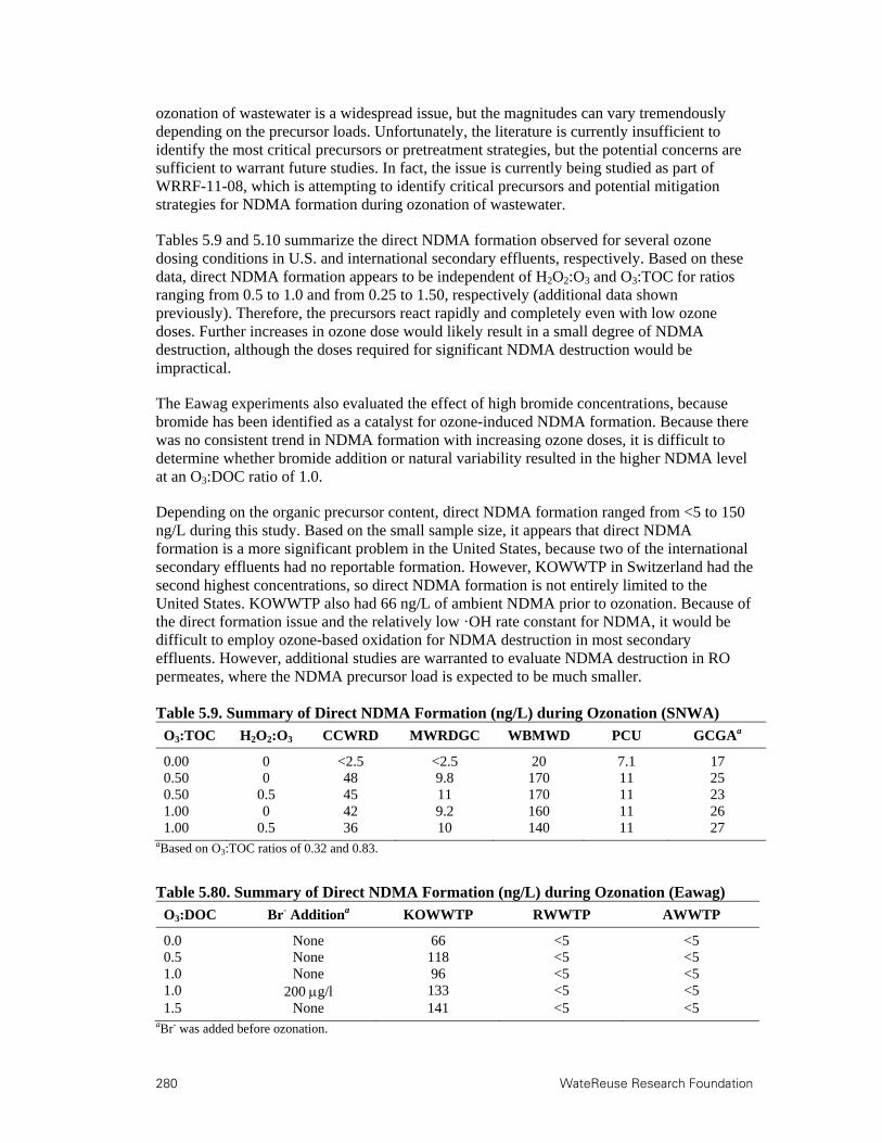
280 WateReuse Research Foundation
ozonation of wastewater is a widespread issue, but the magnitudes can vary tremendously depending on the precursor loads. Unfortunately, the literature is currently insufficient to identify the most critical precursors or pretreatment strategies, but the potential concerns are sufficient to warrant future studies. In fact, the issue is currently being studied as part of WRRF-11-08, which is attempting to identify critical precursors and potential mitigation strategies for NDMA formation during ozonation of wastewater.
Tables 5.9 and 5.10 summarize the direct NDMA formation observed for several ozone dosing conditions in U.S. and international secondary effluents, respectively. Based on these data, direct NDMA formation appears to be independent of H2O2:O3 and O3:TOC for ratios ranging from 0.5 to 1.0 and from 0.25 to 1.50, respectively (additional data shown previously). Therefore, the precursors react rapidly and completely even with low ozone doses. Further increases in ozone dose would likely result in a small degree of NDMA destruction, although the doses required for significant NDMA destruction would be impractical.
The Eawag experiments also evaluated the effect of high bromide concentrations, because bromide has been identified as a catalyst for ozone-induced NDMA formation. Because there was no consistent trend in NDMA formation with increasing ozone doses, it is difficult to determine whether bromide addition or natural variability resulted in the higher NDMA level at an O3:DOC ratio of 1.0.
Depending on the organic precursor content, direct NDMA formation ranged from <5 to 150 ng/L during this study. Based on the small sample size, it appears that direct NDMA formation is a more significant problem in the United States, because two of the international secondary effluents had no reportable formation. However, KOWWTP in Switzerland had the second highest concentrations, so direct NDMA formation is not entirely limited to the United States. KOWWTP also had 66 ng/L of ambient NDMA prior to ozonation. Because of the direct formation issue and the relatively low ·OH rate constant for NDMA, it would be difficult to employ ozone-based oxidation for NDMA destruction in most secondary effluents. However, additional studies are warranted to evaluate NDMA destruction in RO permeates, where the NDMA precursor load is expected to be much smaller. Table 5.9. Summary of Direct NDMA Formation (ng/L) during Ozonation (SNWA)
O3:TOC H2O2:O3 CCWRD MWRDGC WBMWD PCU GCGAa
0.00 0 <2.5 <2.5 20 7.1 17 0.50 0 48 9.8 170 11 25 0.50 0.5 45 11 170 11 23 1.00 0 42 9.2 160 11 26 1.00 0.5 36 10 140 11 27
aBased on O3:TOC ratios of 0.32 and 0.83.
Table 5.80. Summary of Direct NDMA Formation (ng/L) during Ozonation (Eawag)
O3:DOC Br- Additiona KOWWTP RWWTP AWWTP
0.0 None 66 <5 <5 0.5 None 118 <5 <5 1.0 None 96 <5 <5 1.0 200 g/l 133 <5 <5 1.5 None 141 <5 <5
aBr- was added before ozonation.

WateReuse Research Foundation 281
Despite the direct NDMA formation issue, ozonation has also been identified as a potential mitigation strategy for chloramine-induced NDMA formation in reverse osmosis applications. Chloramine is often used to reduce biofouling of RO membranes, but it also leads to significant NDMA concentrations, thereby necessitating downstream UV/H2O2 systems in IPR applications. Tables 5.11 and 5.12 illustrate the NDMA formation potentials in the untreated and treated secondary effluents after 10 days of chloramination.
Table 5.81. NDMA Formation Potential (ng/L) for U.S. Secondary Effluents
O3:TOC H2O2 CCWRD* MWRDGC WBMWD PCU GCGA**
0.0 0 mg/L 590 320 1,600 290 230 0.25 0 mg/L 230 39 280 20 170 0.5 0 mg/L 150 25 210 6.4 30 1.0 0 mg/L 150 44 180 27 26 1.5 0 mg/L 150 40 170 23 43 UV Dose H2O2 CCWRD** MWRDGC WBMWD PCU GCGA
0 mJ/cm2 0 mg/L N/A 320 1,600 290 N/A 50 mJ/cm2 0 mg/L 1,300 280 1,600 220 N/A 50 mJ/cm2 10 mg/L 1,300 320 1,400 180 N/A 250 mJ/cm2 0 mg/L 1,300 300 1,300 140 N/A 250 mJ/cm2 10 mg/L 1,200 260 1,300 110 N/A 500 mJ/cm2 0 mg/L N/A 320 1,300 70 N/A 500 mJ/cm2 10 mg/L 770 210 1,200 65 N/A
*The CCWRD ozone and UV experiments were performed on different samples. **The GCGA ozone data and CCWRD UV data are based on different doses.
Table 5.82. NDMA Formation Potential (ng/L) for International Secondary Effluents
O3:DOC H2O2 KOWWTP RWWTP AWWTP
0.0 0 mg/L 577 210 450 1.0 0 mg/L 104 40 <5
There appeared to be a direct correlation between NDMA formation potential and direct formation during ozonation. In other words, matrices with high direct formation after ozonation (e.g., WBMWD) also had high formation potential after 10 days of chloramine exposure. This observation indicates that NDMA precursors may be similar for ozonation and chloramination. As described previously in the literature, preozonation achieved substantial reductions in chloramine-induced NDMA formation (up to 99%), whereas UV-based treatment was much less effective (up to 78%). Despite these general trends, site-specific water quality (i.e., precursors) still impacted NDMA formation potential, as exemplified in the differences between MWRDGC and AWWTP.
5.2.6 1,4-Dioxane
In addition to the NDMA requirement, the previous draft CDPH regulations also required 0.5 log (68.4%) destruction of 1,4-dioxane. A variation of this requirement is also included in the recent revisions to the draft CDPH regulations for IPR applications. Typically, indirect
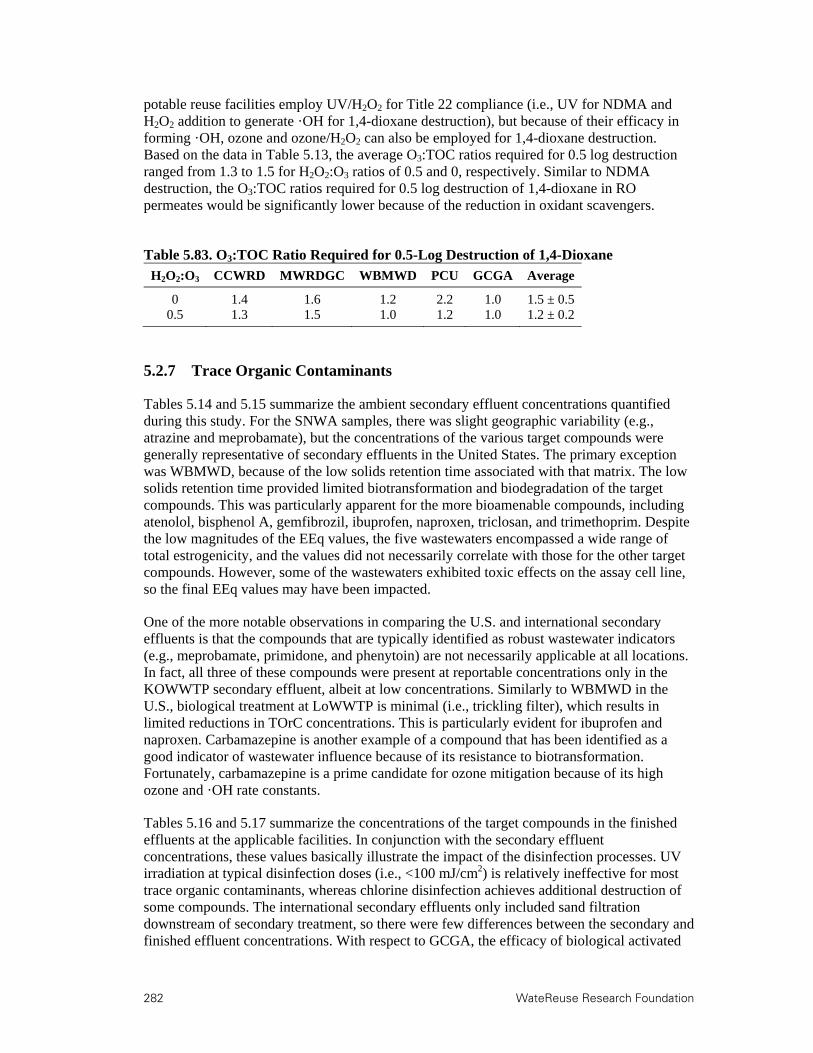
282 WateReuse Research Foundation
potable reuse facilities employ UV/H2O2 for Title 22 compliance (i.e., UV for NDMA and H2O2 addition to generate ·OH for 1,4-dioxane destruction), but because of their efficacy in forming ·OH, ozone and ozone/H2O2 can also be employed for 1,4-dioxane destruction. Based on the data in Table 5.13, the average O3:TOC ratios required for 0.5 log destruction ranged from 1.3 to 1.5 for H2O2:O3 ratios of 0.5 and 0, respectively. Similar to NDMA destruction, the O3:TOC ratios required for 0.5 log destruction of 1,4-dioxane in RO permeates would be significantly lower because of the reduction in oxidant scavengers.
Table 5.83. O3:TOC Ratio Required for 0.5-Log Destruction of 1,4-Dioxane
H2O2:O3 CCWRD MWRDGC WBMWD PCU GCGA Average
0 1.4 1.6 1.2 2.2 1.0 1.5 ± 0.5 0.5 1.3 1.5 1.0 1.2 1.0 1.2 ± 0.2
5.2.7 Trace Organic Contaminants
Tables 5.14 and 5.15 summarize the ambient secondary effluent concentrations quantified during this study. For the SNWA samples, there was slight geographic variability (e.g., atrazine and meprobamate), but the concentrations of the various target compounds were generally representative of secondary effluents in the United States. The primary exception was WBMWD, because of the low solids retention time associated with that matrix. The low solids retention time provided limited biotransformation and biodegradation of the target compounds. This was particularly apparent for the more bioamenable compounds, including atenolol, bisphenol A, gemfibrozil, ibuprofen, naproxen, triclosan, and trimethoprim. Despite the low magnitudes of the EEq values, the five wastewaters encompassed a wide range of total estrogenicity, and the values did not necessarily correlate with those for the other target compounds. However, some of the wastewaters exhibited toxic effects on the assay cell line, so the final EEq values may have been impacted.
One of the more notable observations in comparing the U.S. and international secondary effluents is that the compounds that are typically identified as robust wastewater indicators (e.g., meprobamate, primidone, and phenytoin) are not necessarily applicable at all locations. In fact, all three of these compounds were present at reportable concentrations only in the KOWWTP secondary effluent, albeit at low concentrations. Similarly to WBMWD in the U.S., biological treatment at LoWWTP is minimal (i.e., trickling filter), which results in limited reductions in TOrC concentrations. This is particularly evident for ibuprofen and naproxen. Carbamazepine is another example of a compound that has been identified as a good indicator of wastewater influence because of its resistance to biotransformation. Fortunately, carbamazepine is a prime candidate for ozone mitigation because of its high ozone and ·OH rate constants.
Tables 5.16 and 5.17 summarize the concentrations of the target compounds in the finished effluents at the applicable facilities. In conjunction with the secondary effluent concentrations, these values basically illustrate the impact of the disinfection processes. UV irradiation at typical disinfection doses (i.e., <100 mJ/cm2) is relatively ineffective for most trace organic contaminants, whereas chlorine disinfection achieves additional destruction of some compounds. The international secondary effluents only included sand filtration downstream of secondary treatment, so there were few differences between the secondary and finished effluent concentrations. With respect to GCGA, the efficacy of biological activated
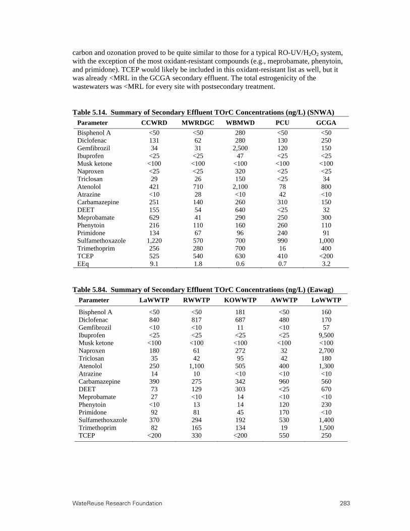
WateReuse Research Foundation 283
carbon and ozonation proved to be quite similar to those for a typical RO-UV/H2O2 system, with the exception of the most oxidant-resistant compounds (e.g., meprobamate, phenytoin, and primidone). TCEP would likely be included in this oxidant-resistant list as well, but it was already <MRL in the GCGA secondary effluent. The total estrogenicity of the wastewaters was <MRL for every site with postsecondary treatment.
Table 5.14. Summary of Secondary Effluent TOrC Concentrations (ng/L) (SNWA)
Parameter CCWRD MWRDGC WBMWD PCU GCGA
Bisphenol A <50 <50 280 <50 <50 Diclofenac 131 62 280 130 250 Gemfibrozil 34 31 2,500 120 150 Ibuprofen <25 <25 47 <25 <25 Musk ketone <100 <100 <100 <100 <100 Naproxen <25 <25 320 <25 <25 Triclosan 29 26 150 <25 34 Atenolol 421 710 2,100 78 800 Atrazine <10 28 <10 42 <10 Carbamazepine 251 140 260 310 150 DEET 155 54 640 <25 32 Meprobamate 629 41 290 250 300 Phenytoin 216 110 160 260 110 Primidone 134 67 96 240 91 Sulfamethoxazole 1,220 570 700 990 1,000 Trimethoprim 256 280 700 16 400 TCEP 525 540 630 410 <200 EEq 9.1 1.8 0.6 0.7 3.2
Table 5.84. Summary of Secondary Effluent TOrC Concentrations (ng/L) (Eawag)
Parameter LaWWTP RWWTP KOWWTP AWWTP LoWWTP
Bisphenol A <50 <50 181 <50 160 Diclofenac 840 817 687 480 170 Gemfibrozil <10 <10 11 <10 57 Ibuprofen <25 <25 <25 <25 9,500 Musk ketone <100 <100 <100 <100 <100 Naproxen 180 61 272 32 2,700 Triclosan 35 42 95 42 180 Atenolol 250 1,100 505 400 1,300 Atrazine 14 10 <10 <10 <10 Carbamazepine 390 275 342 960 560 DEET 73 129 303 <25 670 Meprobamate 27 <10 14 <10 <10 Phenytoin <10 13 14 120 230 Primidone 92 81 45 170 <10 Sulfamethoxazole 370 294 192 530 1,400 Trimethoprim 82 165 134 19 1,500 TCEP <200 330 <200 550 250

284 WateReuse Research Foundation
Table 5.85. Summary of Finished Effluent TOrC Concentrations (ng/L) (SNWA)
Parameter CCWRD MWRDGC WBMWD PCU GCGA (UV) (None) (RO-UV/H2O2) (Cl2) (BAC-O3)
Bisphenol A <50 <50 86 <50 <50 Diclofenac 57 62 <25 <25 <25 Gemfibrozil 12 31 <10 <10 <10 Ibuprofen <25 <25 <25 <25 <25 Musk ketone <100 <100 <100 <100 <100 Naproxen <25 <25 <25 <25 <25 Triclosan 38 26 <25 <25 <25 Atenolol 120 710 <25 28 <25 Atrazine <10 28 <10 76 <10 Carbamazepine 192 140 <10 35 <10 DEET 232 54 <25 30 <25 Meprobamate 362 41 <10 360 190 Phenytoin 113 110 <10 270 33 Primidone 168 67 <10 270 31 Sulfamethoxazole 1,150 570 <25 <25 <25 Trimethoprim 43 280 <10 <10 <10 TCEP 349 540 <200 370 <200 EEq <0.074 1.8 <0.074 <0.074 <0.074
Tables 5.18 and 5.19 provide summaries of ozone- and UV-based destruction of the target compounds, respectively, in the U.S. secondary effluents. Because of the countless trace organic contaminants in the environment, it is impractical to develop oxidation profiles for every known chemical and dosing condition. Grouping contaminants based on their relative resistance/susceptibility to oxidation is a much more reasonable strategy. This strategy is also robust in that compounds with unknown oxidation profiles can often be modeled based on their structural properties—a concept known as QSARs that was described previously in Chapter 1. The groupings used in Table 5.18 can be described as follows:
Group 1: Very susceptible to both ozone and ·OH
Group 2: Moderately susceptible to ozone / highly susceptible to ·OH
Group 3: Very resistant to ozone / highly susceptible to ·OH
Group 4: Very resistant to ozone / moderately susceptible to ·OH
Group 5: Very resistant to both ozone and ·OH A generic indicator also provides an estimate of the expected level of oxidation for an “unknown” compound with similar structural characteristics and rate constants. The indicator was calculated as the average of the target compounds in each group. The grouping and indicator framework proved to be quite useful in that each stepwise increase in O3:TOC ratio led to an additional group of contaminants experiencing greater than 80% oxidation. As described in the literature review, there are few existing guidelines for trace organic contaminant destruction, so relative oxidation (i.e., % destruction) is the most useful descriptor of process performance. Similarly to the pCBA/·OH exposure experiments, H2O2 addition yielded slightly higher destruction of the ozone-resistant compounds (Groups 3, 4, and 5), whereas H2O2 addition was slightly detrimental to the ozone-susceptible compounds. Again, the differences were minimal and insignificant based on the standard deviations across the bench-scale experiments. As described earlier, laboratory filtration had no impact on

WateReuse Research Foundation 285
oxidation efficacy. Finally, because of the rapid destruction of many of the target compounds, it is likely that the compounds in Groups 4 and 5 will control the design of ozone systems for trace organic contaminant mitigation. Table 5.86. Summary of Finished Effluent TOrC Concentrations (ng/L) (Eawag)
Parameter KOWWTP RWWTP
Bisphenol A <50 <50 Diclofenac 649 805 Gemfibrozil <10 <10 Ibuprofen <25 <25 Musk ketone <100 <100 Naproxen 171 63 Triclosan 66 45 Atenolol 262 1,150 Atrazine <10 12 Carbamazepine 376 305 DEET 371 130 Meprobamate <10 <10 Phenytoin 14 <10 Primidone 58 73 Sulfamethoxazole 254 355 Trimethoprim 45 169 TCEP <200 202
The groupings are also presented in Table 5.19 to describe the resistance of the compounds to ·OH, but the utility of the grouping framework is compromised because of the impact of UV photolysis. Although most compounds are highly resistant to UV photolysis alone, some compounds, particularly diclofenac and triclosan, are photolyzed rapidly by UV light. Other compounds that are highly resistant to oxidation, particularly phenytoin and atrazine, also experience moderate levels of photolysis. These UV-susceptible compounds are typically characterized by aromatic ring structures that more effectively absorb UV light. Regardless, ozone oxidation typically achieves higher levels of contaminant mitigation at relevant dosing levels.
Appendices A and B provide individual figures for each TOrC to illustrate relative removal during ozone- and UV-based oxidation, respectively, for all of the U.S. and international secondary effluents. These figures also differentiate the H2O2 and filtration conditions. Except for GCGA and LoWWTP, which were characterized by different O3:TOC or O3:DOC ratios, all of the secondary effluents had similar degradation profiles. Appendices A and B also illustrate the relative contributions of O3 and ·OH during the ozone experiments and UV and ·OH during the UV experiments. An example is provided in Figure 5.7.

286 WateReuse Foundation
Table 5.87. Average TOrC Oxidation (%) During Ozonation
Group Contaminant O3:TOC (mass) / H2O2:O3 (molar)
0.25/0 0.25/0.5 0.25/1.0 0.50/0 0.50/0.5 0.50/1.0 1.0/0 1.0/0.5 1.0/1.0 1.5/0 1.5/0.5 1.5/1.0
1 Sulfamethoxazole 84±13 82±13 83±8 98±0 97±1 96±2 99±1 99±1 99±1 99±1 99±1 99±1 Diclofenac 91±13 90±14 92±8 98±1 98±1 98±1 98±1 98±1 98±1 98±1 98±1 98±1 Bisphenol A 91±14 91±12 93±6 98±1 98±1 98±1 98±1 98±1 98±1 98±1 98±1 98±1 Carbamazepine 92±15 89±15 87±12 99±0 99±0 99±0 99±0 99±0 99±0 99±0 99±0 99±0 Trimethoprim 92±15 90±14 89±11 99±0 99±0 99±0 99±0 99±0 99±0 99±0 99±0 99±0 Naproxen 90±16 89±15 87±10 98±0 98±0 98±1 98±0 98±0 98±1 98±0 98±0 98±1 Triclosan 93±9 93±8 96±2 97±1 97±1 97±1 97±1 97±1 97±1 97±1 92±10 97±1 Indicator 90±14 89±13 90±8 98±0 98±0 98±0 98±0 98±0 98±0 98±0 97±2 98±0
2 Gemfibrozil 81±18 73±17 67±10 99±0 99±0 99±1 99±0 99±0 99±0 99±0 99±0 99±1 Atenolol 47±8 44±7 47±5 97±1 90±7 85±7 98±1 98±1 98±1 98±1 98±1 97±3 Indicator 64±13 59±12 57±7 98±1 95±4 92±4 99±1 99±1 99±1 99±1 99±1 98±2
3 Ibuprofen 38±10 38±6 42±8 69±7 72±6 73±6 94±4 96±3 95±3 98±1 98±1 96±3 Phenytoin 34±15 36±11 36±10 67±13 72±7 73±8 94±4 97±3 95±4 98±1 99±0 97±2 DEET 26±9 28±7 30±8 57±9 62±8 63±8 88±6 93±5 92±5 97±3 99±1 95±4 Primidone 30±9 29±5 34±5 60±8 64±5 64±4 91±5 94±5 92±4 97±2 98±2 95±4 Indicator 32±10 33±6 36±6 63±9 68±6 68±7 92±5 95±4 93±4 98±2 99±1 96±3
4 Atrazine 15±5 14±3 18±5 33±6 36±5 37±6 64±8 70±11 69±9 81±8 87±8 82±9 Meprobamate 18±5 20±5 23±6 40±8 45±6 45±5 71±9 80±10 79±8 86±8 93±5 88±6 Indicator 17±5 17±4 20±5 37±6 41±5 41±5 68±8 75±11 74±9 84±8 90±7 85±8
5 TCEP -1±13 5±5 8±5 9±5 12±5 9±4 15±3 20±6 20±3 23±3 30±4 31±4
Notes. Shading represents >80% oxidation. GCGA omitted because of differences in O3:TOC ratios and the nonlinearity of contaminant oxidation.

WateReuse Research Foundation 287
Table 5.88. Average TOrC Destruction for UV and UV/H2O2
Group Contaminant UV Dose (mJ/cm2) / H2O2 Dose (mg/L)
50/0 50/10 250/0 250/5 250/10 500/0 500/5 500/10
1 Sulfamethoxazole 6±6 2±14 44±5 39±8 42±13 65±2 67±3 73±5 Diclofenac 40±2 19±23 91±2 86±5 90±6 98±1 97±1 97±1 Bisphenol A 5±10 3±11 7±10 11±10 25±21 10±10 22±9 49±18 Carbamazepine -2±9 3±4 -3±11 12±7 22±15 -3±8 24±18 42±15 Trimethoprim -1±8 2±6 0±5 11±6 18±11 1±4 16±10 37±15 Naproxen 4±6 3±8 11±4 19±11 29±16 18±8 35±8 53±16 Triclosan 21±12 13±18 81±8 72±10 79±9 94±3 93±2 95±3
2 Gemfibrozil 3±10 5±7 4±6 11±6 23±14 7±3 15±8 39±16 Atenolol 5±6 5±6 1±7 15±6 23±8 2±8 15±12 35±14
3 Ibuprofen 4±6 2±4 6±3 12±9 21±14 8±3 24±5 40±16 Phenytoin 6±12 13±20 28±15 31±12 45±15 44±8 53±4 64±12 DEET 8±7 3±4 8±6 8±9 17±11 6±2 12±4 31±14 Primidone 1±8 3±7 3±3 12±9 15±13 7±2 10±17 29±22
4 Atrazine 4±8 -1±2 21±7 16±6 21±9 33±4 32±4 43±9 Meprobamate 8±12 4±2 11±12 7±5 11±7 12±14 8±6 23±10
5 TCEP 7±7 6±13 9±6 3±11 8±14 8±5 0±5 5±14
Notes. Groupings based on ozone and OH rate constants. Shading represents >80% oxidation. Includes CCWRD data for 45 (50) and 225 (250) mJ/cm2.

288 WateReuse Research Foundation
Figure 5.7. Relative contributions of O3 and ·OH to contaminant oxidation (H2O2:O3=0).

WateReuse Research Foundation 289
5.2.8 Disinfection
Wastewater contains a great number of bacteria, viruses, and parasites, but only a small fraction of these microbes are actually pathogenic. Pathogenicity even varies between strains of the same species. Ideally, evaluations of disinfection efficacy would focus only on the pathogenic microbes, but the related assays are sometimes impractical because of limited ambient prevalence, complex infectivity assays (e.g., Cryptosporidium oocysts), or the lack or inadequacy of established infectivity assays (e.g., noroviruses). To compile useful databases of disinfection efficacy, researchers often use surrogate microbes that are assumed to have disinfection profiles similar to those for the target pathogens.
Tables 5.20 and 5.21 provide the average levels of inactivation for E. coli and the bacteriophage MS2 with ozone and ozone/H2O2 for the U.S. secondary effluents. E. coli was more resistant than MS2 to ozone-based oxidation, and E. coli inactivation was also more variable between the wastewater matrices. Although dissolved ozone residuals and CTs are often required to demonstrate regulatory compliance, the addition of H2O2, which rapidly quenches any ozone residual, still achieved significant levels of inactivation for E. coli and MS2. However, ozone/H2O2 was generally less effective and slightly more variable than ozone alone for E. coli and MS2 inactivation. In order to achieve the modified CDPH Title 22 benchmark of 6.5-log viral inactivation, O3:TOC ratios of 1.0 to 1.5 were required for ozone and ozone/H2O2, respectively. Although higher dissolved ozone residuals provided greater inactivation, a majority of the microbial inactivation was complete within 15 seconds regardless of H2O2 dose (data not shown). Table 5.20. Average Log Inactivation for E. coli during Ozonation (U.S.)
O3:TOC H2O2:O3=0 H2O2:O3=0.5 H2O2:O3=1.0
0.25 1.5 ± 1.0 1.0 ± 0.6 1.4 ± 1.3 0.50 4.9 ± 1.8 4.1 ± 2.6 3.6 ± 2.5 1.00 7.1 ± 1.3a 5.5 ± 1.1 5.2 ± 1.8 1.50 7.1 ± 1.1a 5.4 ± 1.3 4.8 ± 1.7
Note: GCGA omitted because of differences in O3:TOC ratios. aLimited by spiking level in some samples.
Table 5.21. Average Log Inactivation for MS2 During Ozonation (U.S.)
O3:TOC H2O2:O3=0 H2O2:O3=0.5 H2O2:O3=1.0 0.25 2.1 ± 0.9 1.4 ± 0.5 1.5 ± 0.4 0.50 5.7 ± 0.4 5.6 ± 1.1a 5.6 ± 1.3a 1.00 6.7 ± 0.7a 6.4 ± 1.1 5.8 ± 0.5 1.50 7.4 ± 0.3a 6.6 ± 0.7 6.7 ± 0.8 Note: GCGA omitted because of differences in O3:TOC ratios. aLimited by spiking level in some samples.
Table 5.22 provides the average levels of inactivation for B. subtilis spores, which are generally used as surrogates for pathogenic Cryptosporidium oocysts and Giardia cysts. In comparison to chlorine, ozone achieves higher levels of inactivation of spore-forming microbes, but the spores still provide significant protection against ozone and ·OH. In fact, extended contact with dissolved ozone is required before the oxidant is able to diffuse across the spore coat and inactivate the microbe (data not shown). Therefore, applications targeting spore/oocyst/cyst inactivation should only use O3:TOC ratios >1.0 with no H2O2 addition. The level of inactivation will still be lower than that for vegetative bacteria and viruses.

290 WateReuse Research Foundation
Table 5.22. Average Log Inactivation for B. subtilis Spores During Ozonation (U.S.)
O3:TOC H2O2:O3=0 H2O2:O3=0.5 H2O2:O3=1.0
0.25 0.0 ± 0.0 0.0 ± 0.1 0.0 ± 0.0 0.50 0.0 ± 0.1 0.0 ± 0.0 0.0 ± 0.1 1.00 1.1 ± 1.0 0.0 ± 0.0 0.0 ± 0.1 1.50 2.6 ± 1.0a 0.0 ± 0.1 0.1 ± 0.1
Note: GCGA omitted because of differences in O3:TOC ratios. aLimited by spiking level in some samples.
Table 5.23 provides the average levels of inactivation of all three surrogate microbes with UV and UV/H2O2. UV and UV/H2O2 are extremely effective for the inactivation of both vegetative (e.g., E. coli) and spore-forming microbes (e.g., B. subtilis spores, Cryptosporidium oocysts, and Giardia cysts), which clearly provides an advantage over ozone-based oxidation. In fact, a common disinfection dose of 50 mJ/cm2 achieved the limit of inactivation for E. coli and B. subtilis spores. MS2 was more resistant to UV than the bacterial surrogates, but the modified CDPH Title 22 benchmark of 6.5 log viral inactivation was easily achieved with moderately advanced oxidation dosing conditions (i.e., UV dose >250 mJ/cm2). Viral resistance to germicidal UV light (λ=254 nm) is also reported in the literature and is the basis for the high dose requirements established by the Long Term 2 Enhanced Surface Water Treatment Rule (LT2ESWTR) for drinking water applications. Table 5.23. Average Inactivation during UV and UV/H2O2
UV Dose E. coli MS2 Bacillus spores (mJ/cm2) UV UV/H2O2 UV UV/H2O2 UV UV/H2O2
25 5.5 ± 1.8a 6.4 ± 0.4a 1.7 ± 0.1 2.2 ± 0.4 2.5 ± 0.6 2.5 ± 0.5 50 7.1 ± 0.2a 7.1 ± 0.2a 3.0 ± 0.1 3.5 ± 0.4 3.3 ± 0.2a 3.3 ± 0.1a 250 7.1 ± 0.2a 7.1 ± 0.2a 7.1 ± 0.3a 7.3 ± 0.4a 3.4 ± 0.1a 3.4 ± 0.1a 500 7.1 ± 0.2a 7.1 ± 0.2a 7.2 ± 0.2a 7.1 ± 0.1a 3.4 ± 0.1a 3.4 ± 0.1a
Note: Includes CCWRD data for 23 (25), 45 (50), and 225 (250) mJ/cm2. aLimited by spiking level in some samples.
The Eawag experiments included alternative approaches to quantifying the inactivation of vegetative bacteria, specifically FCM and membrane-bound ATP. These methods provide conservative estimates of bacterial inactivation, because they effectively quantify intact cells rather than viability, which is estimated by culture-dependent methods. Because some cells will be intact but no longer viable (or infectious), FCM and ATP-based methods often underestimate the level of inactivation achieved during treatment. The discrepancy would be even more apparent during UV disinfection, which primarily targets genetic material rather than structural integrity, but the conservative nature of the analyses is also apparent for ozonation.
5.2.9 Organic Characterization
Many of the analyses described in the preceding are time-consuming and costly and require tremendous analytical expertise to ensure high-quality results. In contrast, organic characterization methods such as simple measurements of UV absorbance are quite simple and easy to interpret, which highlights their utility as surrogate measures of oxidation efficacy for contaminant destruction and microbial inactivation. Furthermore, relative changes in bulk organic matter are often quite similar between wastewater matrices despite significant differences in water quality. For example, the UV absorbance profiles for the different wastewater matrices exhibited very similar trends, although the magnitudes varied significantly. A separate project

WateReuse Research Foundation 291
funded by the WateReuse Research Foundation (WRRF-09-10) discusses the relationship between these consistent transformations of bulk organic matter, TOrC oxidation, and microbial inactivation.
With respect to the U.S. secondary effluents, the relative changes in UV254 absorbance for the ozone- and UV-based treatment processes are illustrated in Figure 5.8. These relative changes can also be described by the models that follow. On the other hand, relative changes in UV254 absorbance during the UV/H2O2 process varied significantly between wastewater matrices, which prevented the development of useful models:
H2O2:O3=0: ΔUV254 (%)=100 0.5077 O :TOC . R2=0.92
H2O2:O3=0.5: ΔUV254 (%)=100 0.4343 O :TOC . R2=0.89
H2O2:O3=1.0: ΔUV254 (%)=100 0.4023 O :TOC . R2=0.86
Combined: ΔUV254 (%)=100 0.4460 O :TOC . R2=0.86.
Figure 5.8. Summary of differential UV254 absorbance (U.S.).
Because measurements of total fluorescence (TF) require more complex equipment, this analysis is less common in wastewater treatment operations. However, total fluorescence provides a more sensitive alternative to UV254 absorbance and is capable of differentiating high-quality matrices. This makes total fluorescence a relatively straightforward concept with the potential to act as a surrogate measure of treatment efficacy for contaminant oxidation and microbial inactivation. Similar to absorbance, the magnitude of total fluorescence may vary considerably between different wastewater matrices, but the relative changes are quite consistent. With respect to the U.S. secondary effluents, the relative changes in total fluorescence for the ozone- and UV-based treatment processes are illustrated in Figure 5.9. These relative changes can also be described by the models below.
H2O2:O3=0: ΔTF (%)=100 0.8758 O :TOC . R2=0.86
H2O2:O3=0.5: ΔTF (%)=100 0.8525 O :TOC . R2=0.84
H2O2:O3=1.0: ΔTF (%)=100 0.8345 O :TOC . R2=0.83
Combined: ΔTF (%)=100 0.8541 O :TOC . R2=0.84.
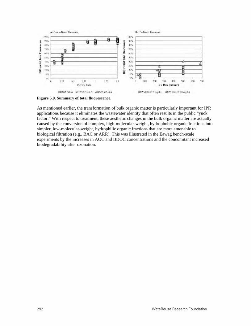
292 WateReuse Research Foundation
Figure 5.9. Summary of total fluorescence.
As mentioned earlier, the transformation of bulk organic matter is particularly important for IPR applications because it eliminates the wastewater identity that often results in the public “yuck factor.” With respect to treatment, these aesthetic changes in the bulk organic matter are actually caused by the conversion of complex, high-molecular-weight, hydrophobic organic fractions into simpler, low-molecular-weight, hydrophilic organic fractions that are more amenable to biological filtration (e.g., BAC or ARR). This was illustrated in the Eawag bench-scale experiments by the increases in AOC and BDOC concentrations and the concomitant increased biodegradability after ozonation.

WateReuse Research Foundation 293
Chapter 6
6.Pilot-Scale Evaluation of Ozone for Water Reclamation
6.1 Description of Pilot-Scale Experiments
The following sections summarize the results from three sets of pilot-scale experiments that were completed as part of this WateReuse Research Foundation study. The first pilot-scale study (Reno, NV) was a long-term evaluation of the principal alternative to FAT for IPR applications: ultrafiltration–ozone/H2O2–BAC. The second pilot-scale study (Tucson, AZ) focused on a combined ozone/UV/H2O2 reactor to evaluate the synergistic capabilities of these treatment processes. A suite of bioassays (cytotoxicity, estrogenicity, and genotoxicity) was also analyzed as part of the Tucson pilot. Finally, the third pilot (Las Vegas, NV) evaluated the potential for continuous monitoring of bulk organic matter transformation to assess process performance and predict TOrC oxidation and microbial inactivation. Additional details related to these pilots are also described in related WateReuse Research Foundation projects, including WRRF-08-08 and WRRF-09-10.
6.2 Reno-Stead Water Reclamation Facility, Reno, NV
In an effort to establish water quality criteria for aquifer injection of reclaimed water, the city of Reno and the Nevada Department of Environmental Protection (NDEP) conducted extensive pilot testing of ultrafiltration, ozone/H2O2 (HiPOx), and BAC at the Reno-Stead Water Reclamation Facility (RSWRF). The “gold standard” treatment train for IPR is generally considered to be membrane filtration (microfiltration or ultrafiltration), reverse osmosis, UV/H2O2, and aquifer injection. The goal of the RSWRF pilot system was to generate a data set to validate membrane filtration, ozone-based oxidation, BAC, and aquifer injection as a viable alternative to the “gold standard,” particularly for inland applications where brine disposal is an issue. This type of treatment train has already demonstrated promise in pilot- and full-scale installations in Europe and Australia, as discussed previously.
The evaluation of the IPR treatment train included extensive monitoring of TOrCs, disinfection byproducts, transformation products, microbial indicators, and microbial characterization in the BAC column. The pilot study, which was performed by the city of Reno, ECO:LOGIC Engineering (now Stantec, Rocklin, CA), and the Southern Nevada Water Authority, included approximately 20 months of continuous operation and was separated into two phases. The first phase (September 2008 to December 2009) evaluated full-scale secondary treatment, pilot-scale ultrafiltration (WesTech Engineering, Salt Lake City, UT), pilot-scale ozone/H2O2 (HiPOx, APTwater, Pleasant Hill, CA), and pilot-scale BAC (WesTech Engineering). The second phase (January 2010 to May 2010) evaluated full-scale secondary treatment, full-scale sand filtration, pilot-scale ozone/H2O2, and pilot-scale BAC. One of the objectives of the different phases was to determine whether ultrafiltration provided significant improvements to the downstream ozone (i.e., increased contaminant destruction and disinfection) and BAC (i.e., reductions in backwash frequency) processes.

294 WateReuse Research Foundation
Secondary effluent (solids retention time 25 days) from the RSWRF was fed into the 40 L/min (10.7 gpm) pilot-scale treatment train (Figure 6.1). During both phases, ozone was dosed at an O3:TOC ratio of approximately 0.8 to 1.0 (5 mg/L), and H2O2 was added at a molar ratio of 1.0 (3.5 mg/L). The H2O2 was added immediately prior to the ozone, and both were added via direct injection through single injection ports. The dosing conditions were selected based on preliminary testing of TOrC oxidation and bromate mitigation (<5 μg/L) during Phase 1. The BAC column was 1 m in diameter and contained approximately 570 kg of Filtrasorb F-400 carbon (Calgon Carbon, Pittsburgh, PA) at a bed depth of 1.4 m. The BAC was operated with an empty bed contact time (EBCT) of 30 min. During the ultrafiltration phase (Phase 1), BAC backwashing was performed once every 14 days, but because of the higher solids loading during the sand filtration phase (Phase 2), backwashing frequency was increased to once every 7 days. The full-scale DynaSand (Parkson Corporation, Fort Lauderdale, FL) media filters were operated in an upflow configuration with continuous backwash and air scour. The conical cells are approximately 2 m (7 ft) in diameter with average bed depth 3 m (10 ft). The filters are operated with an average daily loading rate of 1.6 gpm/ft2 and a peak loading rate of 2.5 gpm/ft2.
Each phase of the project consisted of three separate sampling events to evaluate the consistency in operational performance. For Phase 1, samples were collected in August, November, and December of 2009, and for Phase 2, samples were collected in February, April, and May of 2010. The operational period from September 2008 to August 2009 was used to identify the optimal ozone and H2O2 doses and to establish a stable microbial community in the BAC column.
Figure 6.1. Pilot-scale treatment trains at RSWRF.
In contrast to the previous bench-scale experiments, this part of the project targeted a slightly different set of trace organic contaminants. The more sensitive analytical methods allowed lower method reporting limits and quantification of additional compounds, including steroid hormones. The samples were processed with solid phase extraction and analyzed with liquid chromatography tandem mass spectrometry (LC-MS/MS) with isotope dilution according to previously published methods (Trenholm et al., 2006; Vanderford and Snyder, 2006; Vanderford et al., 2003). Reporting limits for the target compounds ranged from 0.25 to 2000 ng/L. The TOrC analyses were supplemented with organic characterization, quantification of total estrogenicity, and the inactivation and removal of surrogate microbes.
In addition to the samples described above, ultrafiltration (TOC=4.9 mg/L) and sand effluent (TOC=5.6 mg/L) were also evaluated at bench scale to develop ozone demand/decay curves and assess changes in UV254 absorbance. It is important to note that H2O2 was not applied
BAC
1° 2°CASPreliminary
Phase 2
BAC
UF
O3/H2O2
O3/H2O2
Sand
Phase 1
BAC
1° 2°CASPreliminary
Phase 2
BAC
UF
O3/H2O2
O3/H2O2
Sand
Phase 1
Wastewater Treatment Plant
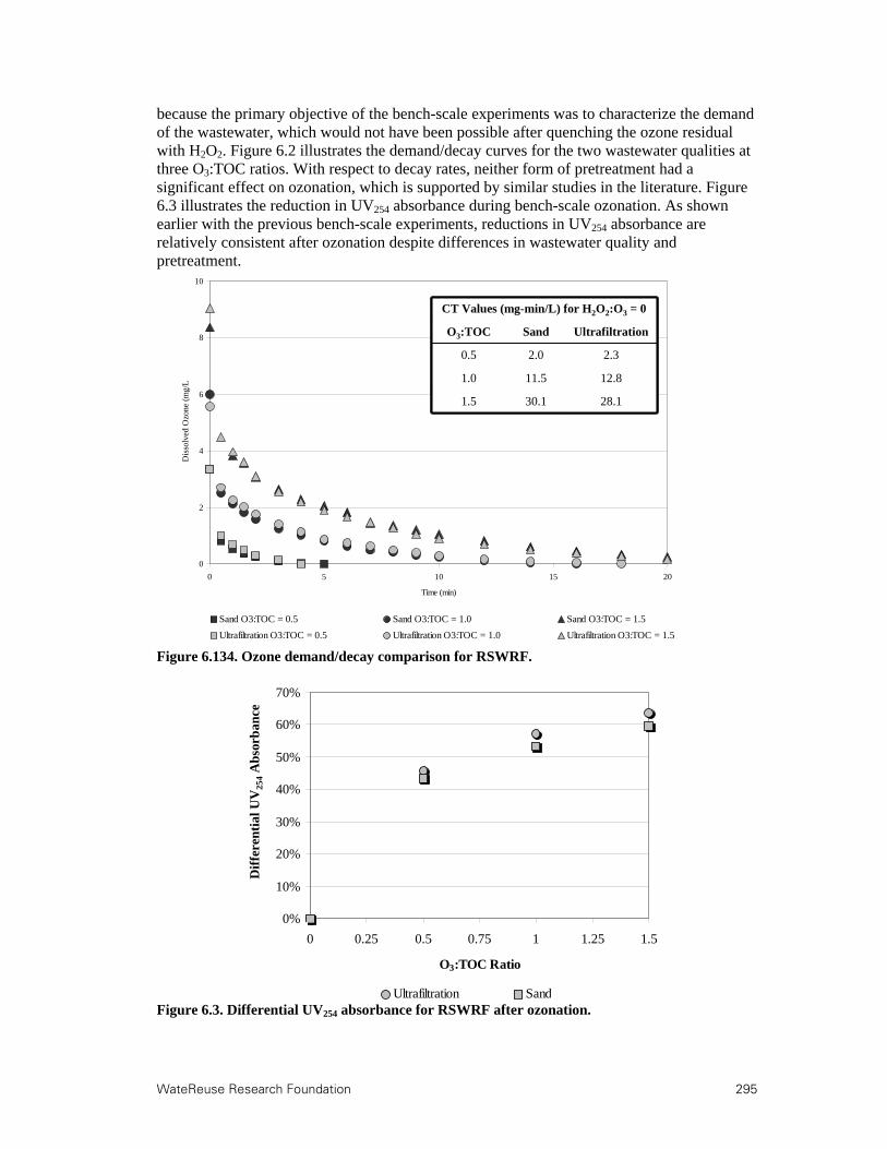
WateReuse Research Foundation 295
because the primary objective of the bench-scale experiments was to characterize the demand of the wastewater, which would not have been possible after quenching the ozone residual with H2O2. Figure 6.2 illustrates the demand/decay curves for the two wastewater qualities at three O3:TOC ratios. With respect to decay rates, neither form of pretreatment had a significant effect on ozonation, which is supported by similar studies in the literature. Figure 6.3 illustrates the reduction in UV254 absorbance during bench-scale ozonation. As shown earlier with the previous bench-scale experiments, reductions in UV254 absorbance are relatively consistent after ozonation despite differences in wastewater quality and pretreatment.
Figure 6.134. Ozone demand/decay comparison for RSWRF.
Figure 6.3. Differential UV254 absorbance for RSWRF after ozonation.
Dis
solv
ed O
zon
e (m
g/L
)
Time (min)
Sand O3:TOC = 0.5 Sand O3:TOC = 1.0 Sand O3:TOC = 1.5
Ultrafiltration O3:TOC = 0.5 Ultrafiltration O3:TOC = 1.0 Ultrafiltration O3:TOC = 1.5
0
2
4
6
8
10
0 5 10 15 20
Time (min)
Dis
solv
ed O
zone
(m
g/L
28.130.11.5
12.811.51.0
2.32.00.5
UltrafiltrationSandO3:TOC
CT Values (mg-min/L) for H2O2:O3 = 0
28.130.11.5
12.811.51.0
2.32.00.5
UltrafiltrationSandO3:TOC
CT Values (mg-min/L) for H2O2:O3 = 0
0%
10%
20%
30%
40%
50%
60%
70%
0 0.25 0.5 0.75 1 1.25 1.5
O3:TOC Ratio
Dif
fere
nti
al U
V25
4 A
bso
rban
ce
Ultrafiltration Sand
Dif
fere
nti
al U
V25
4A
bsor
ban
ce
0%
10%
20%
30%
40%
50%
60%
70%
0 0.25 0.5 0.75 1 1.25 1.5
O3:TOC Ratio
Dif
fere
nti
al U
V25
4 A
bso
rban
ce
Ultrafiltration Sand
Dif
fere
nti
al U
V25
4A
bsor
ban
ce
296 WateReuse Research Foundation
6.2.1 TOrC Mitigation in the RSWRF Pilot Treatment Train
Table 6.1 describes the effects of the various pilot- and full-scale treatment processes on TOrC concentrations. The actual concentrations through the various stages of treatment are provided as an appendix. With respect to the secondary effluent, 27 of the 31 target compounds were detected in at least one sample event, but only the compounds listed in Table 6.1 were detected in all six sample events. Iopromide, ethynylestradiol, testosterone, and progesterone were not detected in any of the sample events. The bold values represent compounds with considerable variability throughout the six sample events. For example, the anticonvulsant phenytoin ranged from 1300 ng/L in February to less than 300 ng/L in April and May. Because phenytoin is dosed throughout the day in most patients, the concentrations should have been relatively stable in each sample event. However, phenytoin is not readily biodegraded in secondary treatment, so its effluent concentration is more susceptible to temporal fluctuations, which are exacerbated by grab sampling as opposed to composite sampling. Despite the variability of some compounds, the concentrations in the secondary effluent were generally similar between the six sample events and ranged from <MRL for iopromide, testosterone, progesterone, and ethynylestradiol to over 1 μg/L for atenolol and TCPP. However, a majority of the target compounds were present at concentrations <100 ng/L in the secondary effluent. In Table 6.1, the percent removals were calculated based on the respective secondary effluent concentrations in each sample event, and then the averages over the sample events were calculated and presented in the table.
In general, ultrafiltration and sand filtration provided limited and sporadic reductions in the concentrations of most TOrCs. Some of the highest removals were experienced by compounds with log KOW values >3 (e.g., gemfibrozil, bisphenol A, and estrone), which would indicate particle-assisted removal by the filtration process. However, several compounds with high log KOW values also experienced low removals during the filtration process (e.g., diclofenac and naproxen). Some of the observed filter removals for the TOrCs were consistent with the literature (e.g., bisphenol A, carbamazepine, DEET, naproxen, TCEP, and trimethoprim), whereas others demonstrated opposite trends (e.g., atenolol, gemfibrozil, ibuprofen, musk ketone, triclosan, and TCPP) (Stevens-Garmon et al., 2011). Furthermore, a small number of compounds experienced different removal profiles after ultrafiltration and after sand filtration. Some of the more bioamenable compounds (e.g., atenolol and gemfibrozil) experienced greater removal during sand filtration because of the likelihood of biofilm formation on the media, whereas the compounds with greater sorption potential (e.g., fluoxetine and triclosan) experienced greater removal during ultrafiltration because of solids rejection. In general, it appears that biophysicochemical properties are not always a reliable indicator of treatment efficacy during filtration.

WateReuse Research Foundation 297
Table 6.1. TOrC Summary Data for the Six Sample Events at RSWRF
Compound Concentration Average % Removal Average % Removal
Secondary Effluent
Ultrafiltration Effluent
Sand Effluent
Ozone/H2O2 Effluent
BAC Effluent
Atenolol 1,110 ng/L 6% 46% 99% >99% Atorvastatin 39 ng/L 44% 6% >98% >98% Atrazine 2.2 ng/L -18% 5% 66% >85% Benzophenone 218 ng/L 11% 16% >64% >64% BHA 69 ng/L 45% 4% >98% >98% Carbamazepine 218 ng/L 4% -4% >99% >99% DEET 224 ng/L -3% -5% 94% >99% Diazepam 2.7 ng/L -8% -9% >90% >90% Estrone 68 ng/L 82% 66% >99% >99% Fluoxetine 51 ng/L 36% -5% >99% >99% Gemfibrozil 484 ng/L 20% 55% >99% >99% Meprobamate 648 ng/L -3% -4% 83% 98% Naproxen 50 ng/L 7% -10% >98% >98% Phenytoin 427 ng/L 35% 33% 98% >99% Primidone 198 ng/L -11% 0% 94% 99% Sulfamethoxazole 688 ng/L 6% -3% 99% >99% TCEP 520 ng/L 1% 2% 16% 96% Triclosan 135 ng/L 98% 3% >99% >99% Trimethoprim 525 ng/L 30% 30% >99% >99%
Figure 6.4. Summary of YES data for RSWRF.
The subsequent ozone/H2O2 process demonstrated significant reductions in nearly all of the target contaminants. Only a small number of compounds (e.g., meprobamate, atrazine, and TCEP) failed to achieve their respective MRLs in at least one sample event. Meprobamate and atrazine still experienced removal of 60–90%, and only TCEP, which is specifically
0
20
40
60
80
100
120
140
Secondary Effluent Filter Effluent Ozone/H2O2 Effluent BAC Effluent
Aug-09 Nov-09 Dec-09 Feb-10 Apr-10 May-10
EE
q (
ng/
L)
<0.5 ng/L <0.5 ng/L
0
20
40
60
80
100
120
140
Secondary Effluent Filter Effluent Ozone/H2O2 Effluent BAC Effluent
Aug-09 Nov-09 Dec-09 Feb-10 Apr-10 May-10
EE
q (
ng/
L)
<0.5 ng/L <0.5 ng/L

298 WateReuse Research Foundation
designed to resist oxidation, experienced less than 30% removal. The remaining target contaminants were removed by more than 90% or to the extent of quantification. Although temporal variability may have affected the secondary effluent and filter effluent concentrations, the ozone/H2O2 process overcame the effects of sampling error with extensive oxidation. In other words, the consistency and effectiveness of the ozone process correlates to a high degree of confidence with the effluent concentrations and calculated removal percentages.
Finally, the BAC process achieved the limit of quantification or at least 95% removal for every target contaminant. Benzophenone (130 and 130 ng/L), meprobamate (11, 17, and 29 ng/L), TCEP (21, 34, and 35 ng/L), and TCPP (100 and 250 ng/L) were the only target contaminants with effluent concentrations exceeding 10 ng/L in some sample events. DEET, ibuprofen, primidone, and sulfamethoxazole were detected at less than 2 ng/L in the BAC effluent.
In addition to concentrations of individual contaminants, the YES assay was used to quantify the total estrogenicity of each sample (Figure 6.4). Similarly to some of the estrogenic target compounds, the secondary effluent EEq values experienced significant variability (7–120 ng/L) because of relatively low values in sample events 2–5 and spikes in sample events 1 and 6. The analytical methods used in this study do not identify all of the individual compounds contributing to estrogenicity. However, the target compound list does include several estrogenic compounds, and these compounds demonstrated trends consistent with the YES assay. This is shown in Table 6.2.
Although filtration was not particularly effective for most TOrCs, both ultrafiltration and sand filtration were effective in removing estrogenic compounds and total estrogenicity. The subsequent ozone/H2O2 process was then capable of oxidizing any residual estrogenic activity, as demonstrated by EEq values <MRL (i.e., 0.5 ng/L) in all sample events. Except for the apparent contamination in sample event 1 and sample event 6, in which estrone was detected at 7.6 ng/L, the individual steroid hormones were also <MRL after secondary clarification or ozone treatment. Table 6.2. Estrogenicity of RSWRF Secondary Effluent
Estrogenic Compound
Sample Event 1 Sample Events 2-5 Sample Event 6
Estrone 113 ng/L 38 ± 17 ng/L 140 ng/L Estradiol 6 ng/L <0.5 ng/L 3 ng/L Bisphenol A <5 ng/L <5 ng/L 72 ng/L Octylphenol 31 ng/L <25 ng/L 31 ng/L EEq (Yes Assay) 35 ng/L 13 ± 6 ng/L 120 ng/L
6.2.2 Microbial Inactivation and Removal at RSWRF
Figure 6.5 illustrates the prevalence of indicator and surrogate bacteria (i.e., total coliforms, fecal coliforms, and Bacillus spores) in the effluent from the various treatment processes. In contrast to ultrafiltration (data not shown), sand filtration provided limited physical removal of bacteria. The subsequent ozone process achieved approximately 2- to 3-log inactivation of total coliforms and 3- to 4-log inactivation of fecal coliforms, but the dosing conditions were insufficient to comply with the most stringent reuse criteria because of the concentration of

WateReuse Research Foundation 299
total (761 ± 419 MPN/100 mL) and fecal coliforms (16 ± 18 MPN/100 mL) in the ozone/H2O2 effluent. Moreover, the number of total (1819 ± 254 MPN/100 mL) and fecal (25 ± 16 MPN/100 mL) coliforms increased slightly in the BAC effluent, presumably because of regrowth on the BAC media. Advanced oxidation has the potential to convert recalcitrant organic matter to more bioavailable forms (e.g., carboxylic acids). This is important for BAC considering that the carbon provides a substrate for vegetative bacteria to attach and develop biofilm communities. Coupled with the continuous supply of biodegradable organic carbon, the contactor provides an ideal environment for bacteria to thrive. This is beneficial for reductions in residual trace organic contaminants and oxidation byproducts, but it provides a regrowth opportunity for indicator bacteria, such as total and fecal coliforms, and even pathogenic bacteria. Despite consistent decreases in each treatment process, the overall treatment train achieved less than 0.7 log reduction in viable Bacillus spores. This is reasonable given Bacillus’s resistance to ozonation, particularly with H2O2 addition.
Based on these bacterial data, a downstream disinfection process (e.g., low-pressure UV irradiation) would certainly be necessary unless membrane filtration or modified dosing conditions were implemented. However, even with more stringent pretreatment, it would still be possible for the subsequent BAC process to trigger coliform violations because of regrowth. Therefore, a final disinfection process may be warranted regardless of whether membrane filtration is implemented. Because of the limited number of indigenous MS2 (<1 PFU/mL), concentrated MS2 was spiked into the ozone/H2O2 influent in order to evaluate the process based on the Title 22 viral inactivation criteria. Five replicate samples were analyzed from two different sample ports on the HiPOx reactor. Sample Port 4 corresponds to approximately 3 s of reaction time, and Sample Port 6 corresponds to approximately 5 s of reaction time. Because of the addition of H2O2 in the HiPOx reactor, these reaction times are sufficient for the oxidation process to reach completion. The MS2 inactivation data, including the simultaneous inactivation of indigenous total and fecal coliforms, is summarized in Figure 6.6. With 5 mg/L of applied ozone and 3.5 mg/L of H2O2, the HiPOx reactor consistently satisfied the 5- and 6.5-log inactivation criteria established by CDPH and Ishida et al. (Ishida et al., 2008), respectively. The simultaneous inactivation of total and fecal coliforms was consistent with the values determined during the full sample events.
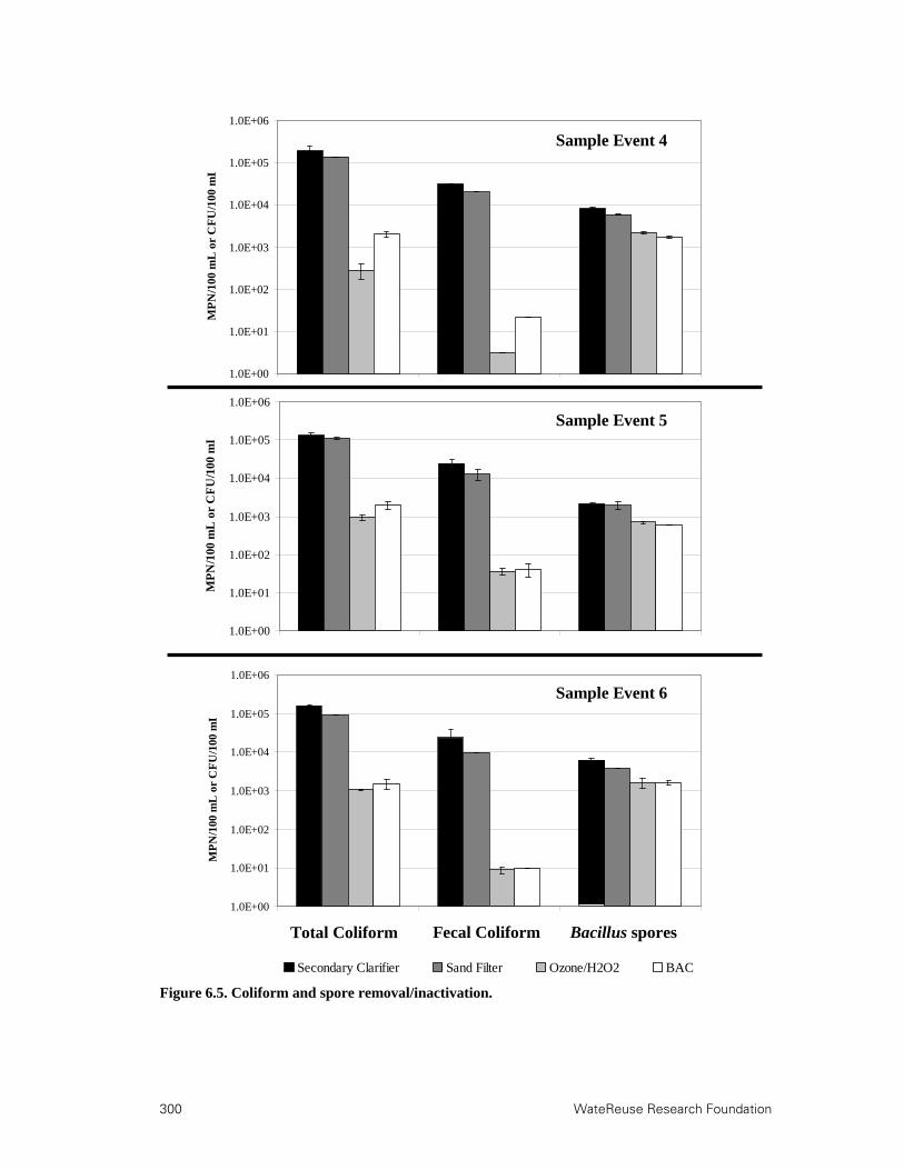
300 WateReuse Research Foundation
Figure 6.5. Coliform and spore removal/inactivation.
Total Coliform Fecal Coliform Bacillus spores
1.0E+00
1.0E+01
1.0E+02
1.0E+03
1.0E+04
1.0E+05
1.0E+06
MP
N/1
00 m
L o
r C
FU
/100
mL
1.0E+00
1.0E+01
1.0E+02
1.0E+03
1.0E+04
1.0E+05
1.0E+06
MP
N/1
00 m
L o
r C
FU
/100
mL
1.0E+00
1.0E+01
1.0E+02
1.0E+03
1.0E+04
1.0E+05
1.0E+06
MP
N/1
00 m
L o
r C
FU
/100
mL
Secondary Clarifier Sand Filter Ozone/H2O2 BAC
Sample Event 6
Sample Event 5
Sample Event 4

WateReuse Research Foundation 301
Figure 6.6. MS2 and coliform inactivation during spiking study.
6.2.3 Organic Characterization in the RSWRF Pilot Treatment Train
During the first phase of the project, the average TOC of the secondary effluent was approximately 6.0 mg/L, but the average TOC increased slightly to approximately 6.8 mg/L during Phase 2. Neither ultrafiltration nor sand filtration had a significant impact on TOC based on effluent values of 5.9 mg/L and 6.6 mg/L, respectively. Because moderate ozone/H2O2 doses are incapable of achieving significant mineralization, the slight decrease in TOC during Phase 1 was reasonable. However, there was a noticeable increase in TOC after ozone/H2O2 treatment during Phase 2. This is likely attributable to biological growth on the walls of the HiPOx reactor. The lack of a dissolved ozone residual, the high bacterial counts in the HiPOx, and the conversion of complex organic matter to assimilable organic carbon created a suitable environment for biofilm growth, which was visually apparent along the walls of the reactor. This biofilm may have been sloughing off periodically, which would explain the increase in TOC. Finally, the BAC process achieved considerable TOC reductions during Phase 1 (51%) because the column still maintained a relatively high adsorption capacity, but Phase 2 only achieved an average TOC reduction of 33%, which could be attributed to the higher TOC loading from the ozone/H2O2 effluent, a reduction in adsorption capacity over time, or a combination of both. This theory was supported by a multidepth analysis of the BAC contactor during Phase 2. This analysis indicated that the first half of the contactor had reached exhaustion (i.e., no reduction in TOC), and the lower depths were approaching exhaustion with each sample event. However, even after 20 months of continuous operation, the BAC contactor still retained some adsorption capacity. The TOC data are summarized in Table 6.3.
As shown in Table 6.4, the UV254 values for the RSWRF were very consistent across the six sample events. Neither ultrafiltration nor sand filtration provided a significant reduction in UV254 absorbance. However, ozone/H2O2 achieved consistent 50% reductions in UV254
absorbance, and the final BAC process provided additional 50% and 29% reductions in Phases 1 and 2, respectively. In addition, Figure 6.7 provides an example (Sample Event 1) of the absorbance spectra for the various unit processes. The secondary effluent and ultrafiltration spectra are nearly identical so it is difficult to distinguish them in the graph.
0
1
2
3
4
5
6
7
8
9
Replicate 1 Replicate 2 Replicate 3 Replicate 4 Replicate 5
Log
Ina
ctiv
atio
n
Sample Port 6
Sample Port 4
Spiked MS2
Total Coliforms
Fecal Coliforms
0
1
2
3
4
5
6
7
8
9
Replicate 1 Replicate 2 Replicate 3 Replicate 4 Replicate 5
Log
Ina
ctiv
atio
n
Sample Port 6
Sample Port 4
Spiked MS2
Total Coliforms
Fecal Coliforms
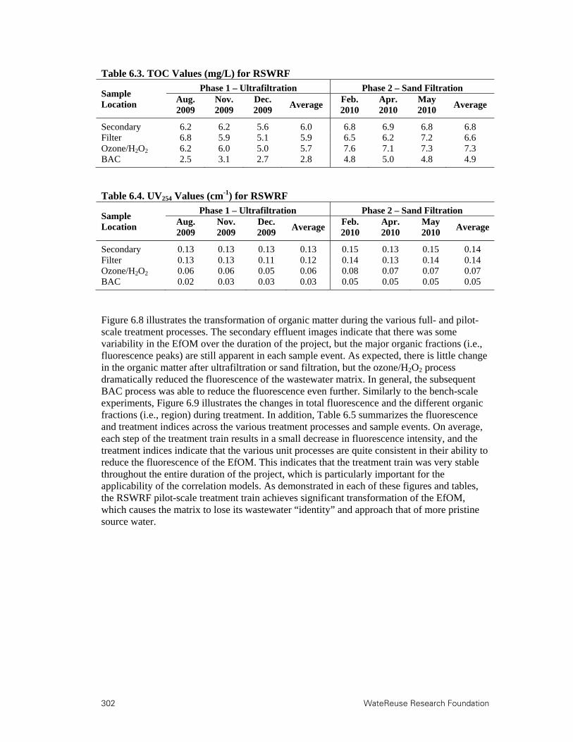
302 WateReuse Research Foundation
Table 6.3. TOC Values (mg/L) for RSWRF
Sample Location
Phase 1 – Ultrafiltration Phase 2 – Sand Filtration Aug. 2009
Nov. 2009
Dec. 2009
Average Feb. 2010
Apr. 2010
May 2010
Average
Secondary 6.2 6.2 5.6 6.0 6.8 6.9 6.8 6.8 Filter 6.8 5.9 5.1 5.9 6.5 6.2 7.2 6.6 Ozone/H2O2 6.2 6.0 5.0 5.7 7.6 7.1 7.3 7.3 BAC 2.5 3.1 2.7 2.8 4.8 5.0 4.8 4.9
Table 6.4. UV254 Values (cm-1) for RSWRF
Sample Location
Phase 1 – Ultrafiltration Phase 2 – Sand Filtration Aug. 2009
Nov. 2009
Dec. 2009
Average Feb. 2010
Apr. 2010
May 2010
Average
Secondary 0.13 0.13 0.13 0.13 0.15 0.13 0.15 0.14 Filter 0.13 0.13 0.11 0.12 0.14 0.13 0.14 0.14 Ozone/H2O2 0.06 0.06 0.05 0.06 0.08 0.07 0.07 0.07 BAC 0.02 0.03 0.03 0.03 0.05 0.05 0.05 0.05
Figure 6.8 illustrates the transformation of organic matter during the various full- and pilot-scale treatment processes. The secondary effluent images indicate that there was some variability in the EfOM over the duration of the project, but the major organic fractions (i.e., fluorescence peaks) are still apparent in each sample event. As expected, there is little change in the organic matter after ultrafiltration or sand filtration, but the ozone/H2O2 process dramatically reduced the fluorescence of the wastewater matrix. In general, the subsequent BAC process was able to reduce the fluorescence even further. Similarly to the bench-scale experiments, Figure 6.9 illustrates the changes in total fluorescence and the different organic fractions (i.e., region) during treatment. In addition, Table 6.5 summarizes the fluorescence and treatment indices across the various treatment processes and sample events. On average, each step of the treatment train results in a small decrease in fluorescence intensity, and the treatment indices indicate that the various unit processes are quite consistent in their ability to reduce the fluorescence of the EfOM. This indicates that the treatment train was very stable throughout the entire duration of the project, which is particularly important for the applicability of the correlation models. As demonstrated in each of these figures and tables, the RSWRF pilot-scale treatment train achieves significant transformation of the EfOM, which causes the matrix to lose its wastewater “identity” and approach that of more pristine source water.

WateReuse Research Foundation 303
Figure 6.7. Absorbance spectra for Sample Event 1 at RSWRF.
0.00
0.02
0.04
0.06
0.08
0.10
0.12
0.14
0.16
0.18
0.20
240 280 320 360 400 440 480 520 560
Wavelength (nm)
Ab
sorb
ance
(cm
-1)
Secondary
Ultrafiltration
Ozone/H2O2
BAC
0.00
0.02
0.04
0.06
0.08
0.10
0.12
0.14
0.16
0.18
0.20
240 280 320 360 400 440 480 520 560
Wavelength (nm)
Ab
sorb
ance
(cm
-1)
Secondary
Ultrafiltration
Ozone/H2O2
BAC

304 WateReuse Research Foundation
Figure 6.8. Excitation-emission matrices for RSWRF.
Table 6.5. Summary of Treatment and Fluorescence Indices
Sample Event
Fluorescence Indices Treatment Indices Sec. Filter Ozone BAC Sec. Filter Ozone BAC
1 1.55 1.49 1.36 1.30 1.00 0.89 0.17 0.05 2 1.31 1.30 1.31 1.27 1.00 1.02 0.15 0.05 3 1.37 1.36 1.34 1.27 1.00 0.91 0.13 0.05 4 1.34 1.33 1.37 1.31 1.00 0.97 0.19 0.08 5 1.42 1.37 1.35 1.30 1.00 0.93 0.17 0.08 6 1.45 1.49 1.39 1.31 1.00 0.90 0.15 0.08 Average 1.41 1.39 1.35 1.29 1.00 0.94 0.16 0.07

WateReuse Research Foundation 305
Figure 6.9. Regional fluorescence intensities for RSWRF.
6.3 Green Valley Water Reclamation Facility, Tucson, AZ
Pilot-scale experiments were also performed at the Green Valley Water Reclamation Facility in Tucson, AZ. Sand-filtered effluent from a conventional wastewater treatment train was fed to a 10-gpm Wedeco/ITT pilot reactor (Herford, Germany). The versatility of the pilot system allowed a variety of treatment configurations, including ozone, ozone/H2O2, UV, UV/H2O2, ozone/UV, and ozone/UV/H2O2. On the basis of a TOC of approximately 6 mg/L, ozone doses of 1.5, 3.0, 6.0, and 9.0 mg/L, which corresponded to O3:TOC ratios of 0.25, 0.50, 1.0, and 1.5, respectively, were applied to the tertiary effluent. For the ozone/H2O2 experiments, peroxide was applied at molar H2O2:O3 ratios of 0 and 1.0. For the UV/H2O2 experiments, UV doses ranged from 250 to 1000 mJ/cm2, and H2O2 was dosed at 10 mg/L. Samples from three separate sample events were analyzed for trace organic contaminants and bulk organic matter. Photos of the pilot skid and reactor are provided in Figure 6.10.
0
5,000
10,000
15,000
20,000
25,000
30,000
35,000
40,000
45,000
Secondary Sand Ozone BAC
Flu
ores
cen
ce I
nte
nsi
ty (
uni
tles
s)
Total Fluorescence Fulvic Acids Proteins and Soluble Microbial Products Humic Acids

306 WateReuse Research Foundation
Figure 6.10. Green Valley Water Reclamation Facility pilot.
6.3.1 TOrC Mitigation and Disinfection in the Tucson Pilot Treatment Train
The tertiary effluent at the Green Valley Water Reclamation Facility contained a suite of TOrCs, as illustrated in Figure 6.11. Except for atenolol, which was significantly lower in the August sample event, the TOrC concentrations remained relatively consistent between February, April, and August. Atenolol has been shown to demonstrate significant intraday temporal variability (Gerrity et al., 2011) so this difference may have been an artifact of the grab samples. Based on this consistency in concentrations, there was not a strong seasonal effect for these target compounds. Sulfamethoxazole was present at a much higher level than any of the other contaminants. Its concentration approached 4000 ng/L, whereas other compounds were generally present at less than 1000 ng/L.
Figure 6.11. TOrC concentrations at the Tucson pilot (average of three sample events).
Figure 6.12 illustrates the oxidation of the target compounds with ozone alone. As expected, only the concentration of TCEP (Group 5) remained relatively constant even at the highest ozone dose. Despite the high ambient sulfamethoxazole concentration, this ozone-susceptible

WateReuse Research Foundation 307
compound (Group 1) experienced dramatic reductions in concentration even at the lowest ozone dose. Many of the compounds were non-detect for an ozone dose of 9.0 mg/L.
Figure 6.12. TOrC oxidation with ozone alone (average of three sample events).
In contrast to ozone, UV alone was significantly less effective for TOrC mitigation. In Figure 6.13, only diclofenac, triclosan, and sulfamethoxazole experienced significant reductions in concentration with UV photolysis. Even with the addition of 10 mg/L of H2O2, a UV dose of 500 mJ/cm2 was ineffective in destroying many of the target compounds (Figure 6.14).
Figure 6.13. TOrC oxidation with UV alone (average of three sample events).
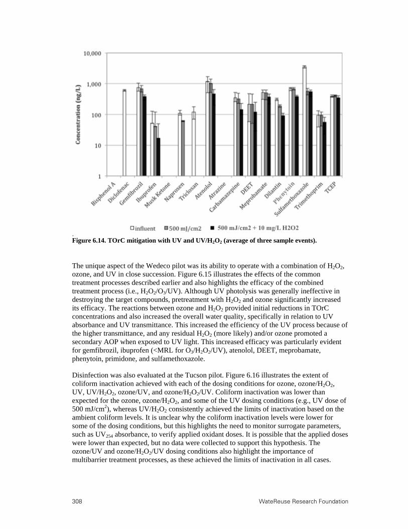
308 WateReuse Research Foundation
Figure 6.14. TOrC mitigation with UV and UV/H2O2 (average of three sample events).
The unique aspect of the Wedeco pilot was its ability to operate with a combination of H2O2, ozone, and UV in close succession. Figure 6.15 illustrates the effects of the common treatment processes described earlier and also highlights the efficacy of the combined treatment process (i.e., H2O2/O3/UV). Although UV photolysis was generally ineffective in destroying the target compounds, pretreatment with H2O2 and ozone significantly increased its efficacy. The reactions between ozone and H2O2 provided initial reductions in TOrC concentrations and also increased the overall water quality, specifically in relation to UV absorbance and UV transmittance. This increased the efficiency of the UV process because of the higher transmittance, and any residual H2O2 (more likely) and/or ozone promoted a secondary AOP when exposed to UV light. This increased efficacy was particularly evident for gemfibrozil, ibuprofen (<MRL for O3/H2O2/UV), atenolol, DEET, meprobamate, phenytoin, primidone, and sulfamethoxazole.
Disinfection was also evaluated at the Tucson pilot. Figure 6.16 illustrates the extent of coliform inactivation achieved with each of the dosing conditions for ozone, ozone/H2O2, UV, UV/H2O2, ozone/UV, and ozone/H2O2/UV. Coliform inactivation was lower than expected for the ozone, ozone/H2O2, and some of the UV dosing conditions (e.g., UV dose of 500 mJ/cm2), whereas UV/H2O2 consistently achieved the limits of inactivation based on the ambient coliform levels. It is unclear why the coliform inactivation levels were lower for some of the dosing conditions, but this highlights the need to monitor surrogate parameters, such as UV254 absorbance, to verify applied oxidant doses. It is possible that the applied doses were lower than expected, but no data were collected to support this hypothesis. The ozone/UV and ozone/H2O2/UV dosing conditions also highlight the importance of multibarrier treatment processes, as these achieved the limits of inactivation in all cases.
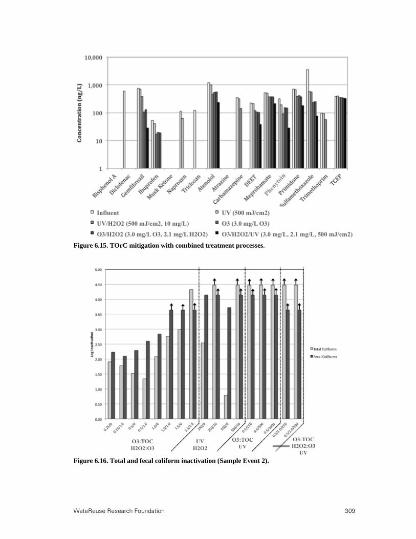
WateReuse Research Foundation 309
Figure 6.15. TOrC mitigation with combined treatment processes.
Figure 6.16. Total and fecal coliform inactivation (Sample Event 2).

310 WateReuse Research Foundation
The change in estrogenicity of the matrix was also evaluated using the YES assay (see Table 6.6). The tertiary effluent at the facility had an EEq value of 2.79 ng/L, but the MRL was rapidly achieved with an O3:TOC ratio of 1.0. UV and UV/H2O2 also achieved reductions in estrogenicity, but there was still a reportable response after a UV dose of 500 mJ/cm2 and an H2O2 dose of 10 mg/L. Estrogenicity and other biological endpoints are evaluated further in Section 3.2.2. Table 6.6. Reduction in Estrogenicity (EEq in ng/L) with Ozone and UV
Ambient O3:TOC | H2O2:O3 UV (mJ/cm2) | H2O2 (mg/L) 0.25 | 0 0.5 | 0 1.0 | 0 500 | 0 500 | 10
2.79 0.46 0.19 <0.07 0.97 0.69
In addition to the synergistic benefits of a combined ozone/UV or ozone/UV/H2O2 process for TOrC mitigation, this tandem treatment train is also effective for NDMA mitigation. As described in the bench-scale sections, direct NDMA formation is one of the major limitations of ozone in wastewater applications. Although ozone is effective for TOrC mitigation, the susceptibility of NDMA to direct photolysis led to the selection of UV/H2O2 as the preferred AOP in IPR applications. However, a combination of ozone and UV capitalizes on the TOrC and NDMA mitigation benefits of ozone and UV, respectively, as illustrated in Figure 6.17. After ozonation, the NDMA concentration increased from ~10 to 23 ng/L at an O3:TOC ratio of 1.0, which would no longer comply with the 10 ng/L notification level mandated by CDPH. Therefore, UV photolysis or some form of downstream biological filtration would be required to achieve the 10 ng/L benchmark in this scenario. On the basis of these data, this objective could be achieved with a UV dose of 250 mJ/cm2.
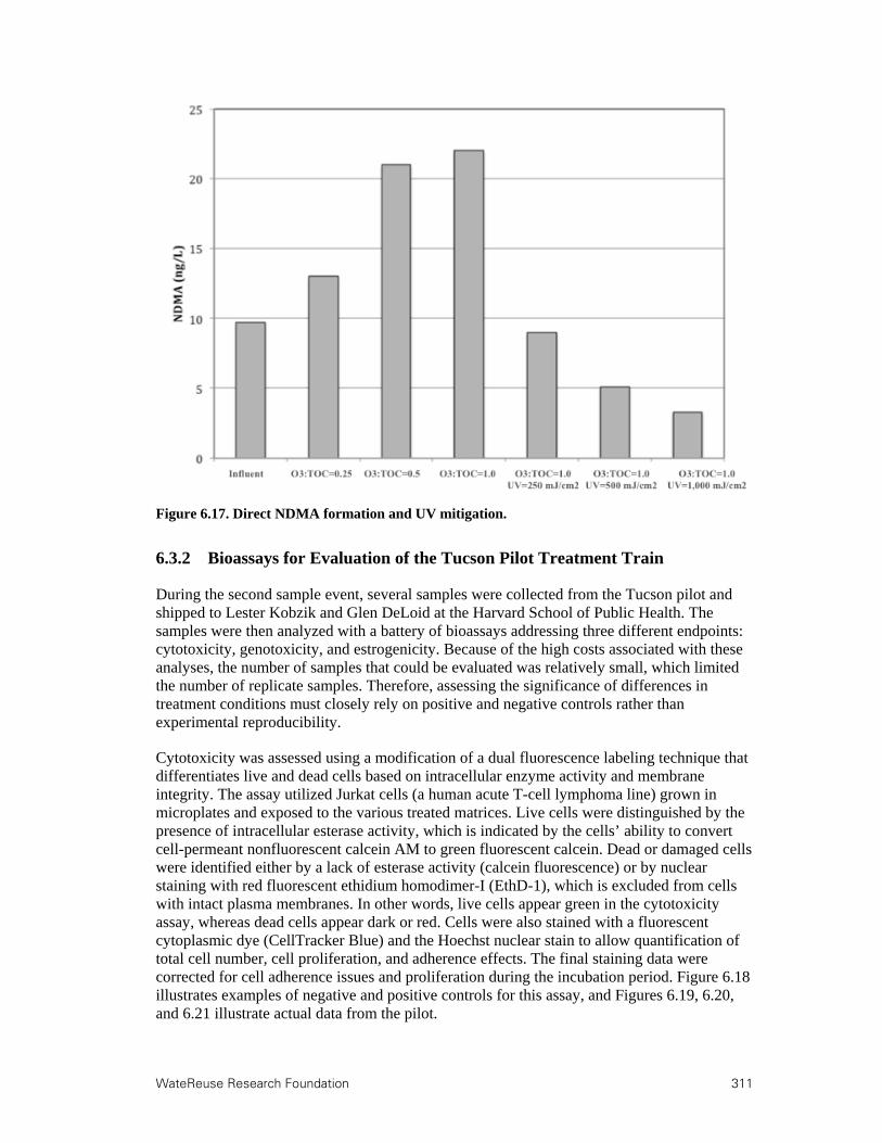
WateReuse Research Foundation 311
Figure 6.17. Direct NDMA formation and UV mitigation.
6.3.2 Bioassays for Evaluation of the Tucson Pilot Treatment Train
During the second sample event, several samples were collected from the Tucson pilot and shipped to Lester Kobzik and Glen DeLoid at the Harvard School of Public Health. The samples were then analyzed with a battery of bioassays addressing three different endpoints: cytotoxicity, genotoxicity, and estrogenicity. Because of the high costs associated with these analyses, the number of samples that could be evaluated was relatively small, which limited the number of replicate samples. Therefore, assessing the significance of differences in treatment conditions must closely rely on positive and negative controls rather than experimental reproducibility.
Cytotoxicity was assessed using a modification of a dual fluorescence labeling technique that differentiates live and dead cells based on intracellular enzyme activity and membrane integrity. The assay utilized Jurkat cells (a human acute T-cell lymphoma line) grown in microplates and exposed to the various treated matrices. Live cells were distinguished by the presence of intracellular esterase activity, which is indicated by the cells’ ability to convert cell-permeant nonfluorescent calcein AM to green fluorescent calcein. Dead or damaged cells were identified either by a lack of esterase activity (calcein fluorescence) or by nuclear staining with red fluorescent ethidium homodimer-I (EthD-1), which is excluded from cells with intact plasma membranes. In other words, live cells appear green in the cytotoxicity assay, whereas dead cells appear dark or red. Cells were also stained with a fluorescent cytoplasmic dye (CellTracker Blue) and the Hoechst nuclear stain to allow quantification of total cell number, cell proliferation, and adherence effects. The final staining data were corrected for cell adherence issues and proliferation during the incubation period. Figure 6.18 illustrates examples of negative and positive controls for this assay, and Figures 6.19, 6.20, and 6.21 illustrate actual data from the pilot.

312 WateReuse Research Foundation
Figures 6.19, 6.20, and 6.21 illustrate the percentage of viable cells remaining after exposure to various matrices and dilutions. Dilutions were required to differentiate between the treatment conditions and overcome the toxicity effects related to the matrix itself. Because the optimal growth conditions for these cell lines are often quite specific and sensitive to nutrient composition, any foreign matrix will exert some level of toxicity. Therefore, the matrix must be diluted to highlight the effects of the experimental treatment conditions.
As shown in Figure 6.19, there was a dramatic difference in cytotoxicity between the laboratory/field blanks, which demonstrated strong reproducibility, and the positive control/secondary effluent. The difference was most apparent at a dilution level of 0.1 (1:10), which indicated that the positive control (50 mM trichloroacetic acid or TCA) and the secondary effluent were more toxic than the blank controls. Figure 6.20 illustrates the effects of several ozone dosing conditions and indicates that low ozone doses may result in moderate levels of cytotoxicity at a dilution level of 0.1. This has also been reported in the literature (Stalter et al., 2010b) and highlights one of the primary benefits of downstream biological filtration—degradation of oxidation byproducts. Despite the toxicity at low O3:TOC ratios, limited cytotoxicity was observed at an O3:TOC ratio of 1.5.
Finally, Figure 6.21 illustrates the differences in cytotoxicity between various treatment processes, including ozonation (O3:TOC=0.5), ozone/H2O2 (O3:TOC=0.5 and H2O2:O3=1.0), UV/H2O2 (UV=500 mJ/cm2 and H2O2=10 mg/L), and ozone/UV (O3:TOC=0.5 and UV=500 mJ/cm2). The secondary effluent, ozonated sample, and UV/H2O2 samples all exhibited the highest levels of cytotoxicity. The cytotoxicity of the ozonated sample was presumably related to oxidation byproducts, whereas the cytotoxicity of the UV/H2O2 sample was presumably a combination of limited oxidation in comparison to ozonated samples and the possible formation of oxidation byproducts. Despite applying the same ozone doses for all of the treatment conditions, the addition of H2O2 or downstream UV irradiation dramatically reduced the level of cytotoxicity during ozonation. At this point, it is unclear what caused this reduction in cytotoxicity, but the duplicate sample indicates that these results are reproducible.
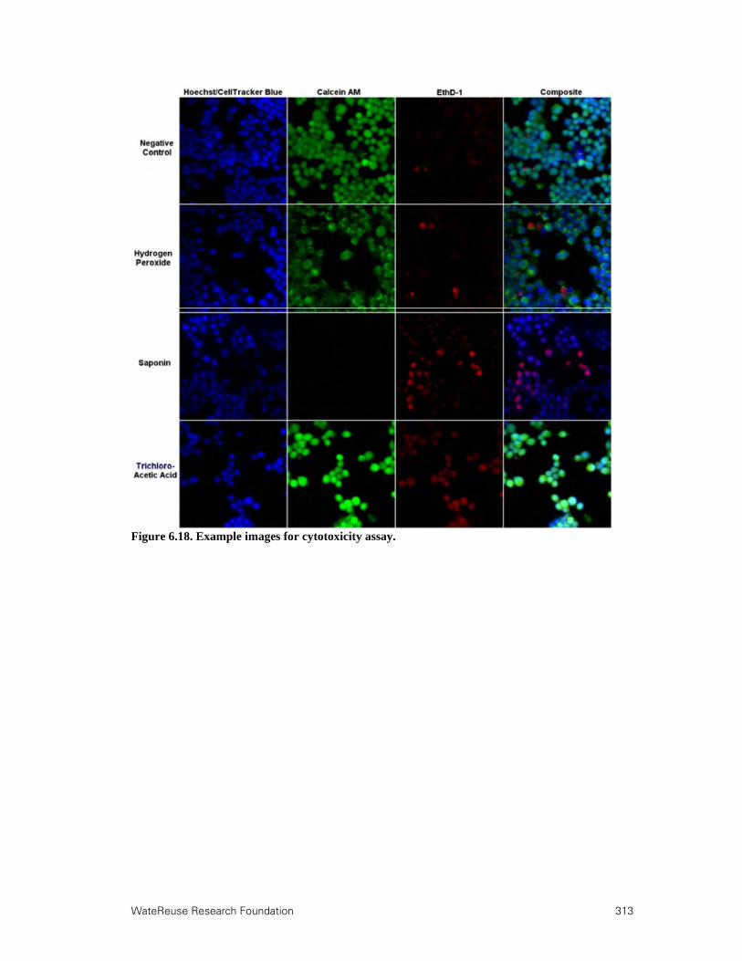
WateReuse Research Foundation 313
Figure 6.18. Example images for cytotoxicity assay.

314 WateReuse Research Foundation
Figure 6.19. Baseline cytotoxicity data.
Figure 6.20. Ozone cytotoxicity data (no H2O2 addition).

WateReuse Research Foundation 315
Figure 6.135. Comparison of treatment processes based on cytotoxicity.
To supplement the YES assay (see Table 6.6), estrogenicity was also quantified using a human breast cancer cell line (MCF-7) and an endometrial carcinoma cell line (Ishikawa). This method is commonly referred to as the e-screen assay. The cell lines were modified to yield a fluorescent signal when exposed to estrogenic (agonistic) matrices and a reduction in fluorescence when exposed to estrogen antagonists. Figure 6.22 illustrates an example of estrogen agonism and antagonism based on a variety of positive and negative controls, and Figures 6.23, 6.24, and 6.25 illustrate the results from the Tucson pilot. The Tucson data are based on the same samples/treatment conditions as the cytotoxicity data presented earlier. The vertical axes represent the relative increase (estrogen agonism) or decrease (estrogen antagonism) in fluorescence after exposure to the test matrices. The same dilution concepts apply to both the cytotoxicity and estrogenicity samples.
Figure 6.23 illustrates the baseline conditions for the estrogenicity testing. Because of effects of dilution at the 1:1000 level (0.001) and background toxicity in the more concentrated samples, the 0.01 dilution (1:100) appears to provide the most relevant data for comparison purposes. As expected, the positive control (2 nM estradiol) and the secondary effluent exhibited stronger fluorescence signals (i.e., higher estrogenicity) than the laboratory and field blanks. However, the blanks exhibited a small degree of variability. The data points in Figure 6.24 were also characterized by experimental variability, but the estrogenicity generally decreased with increasing O3:TOC ratios, as expected. Finally, Figure 6.25 illustrates the effects of different treatment processes and dosing conditions on estrogenicity. The secondary effluent, UV/H2O2, and ozone/H2O2 samples all exhibited relatively high levels of estrogenicity. The UV/H2O2 result is somewhat expected because of the limited efficacy of this treatment process, whereas the efficacy of ozonation appears to have been hindered by peroxide addition. As anticipated, the ozone and ozone/UV samples had the lowest levels of estrogenicity, although the duplicate samples exhibited slight variability. Therefore, the e-screen assay generally supports the results from the YES assay and indicates that ozonation is effective in reducing estrogenicity regardless of the applied ozone dose, whereas UV-based oxidation is less effective at reasonable doses.

316 WateReuse Research Foundation
Figure 6.136. Example images for the e-screen assay.

WateReuse Research Foundation 317
Figure 6.137. Baseline estrogenicity data.
Figure 6.138. Ozone estrogenicity data (no H2O2 addition).

318 WateReuse Research Foundation
Figure 6.139. Comparison of treatment processes based on estrogenicity.
Genotoxicity was quantified using the alkaline single cell gel electrophoresis (“comet”) assay. With the comet assay, DNA damage was visualized by comet-like tails extending from the electrophoresed DNA centers of individual cells. This assay utilized the human lymphoblastoid TK6 cell line, which was exposed to the various treated matrices and appropriate controls. After DNA isolation and gel electrophoresis, the “comet” patterns were visualized with fluorescence and quantified using a custom MATLAB program. Specifically, the “comet” tail size, fraction of DNA contained in the tail, and geometric moment were calculated for each cell, and aggregate means were calculated to identify a representative value for each control and experimental condition. Figure 6.26 illustrates examples of negative controls, positive controls, and arbitrary experimental samples, and Figures 6.27, 6.28, and 6.29 illustrate the results from the Tucson pilot. The Tucson data are based on the same samples/treatment conditions as the cytotoxicity and estrogenicity data presented earlier. The vertical axes represent the geometric moment of the comet tail, which accounts for both the length of the comet tail and the fraction of DNA present in the tail. Increases in any of these parameters indicates an increase in genotoxicity in a particular sample. The same dilution concepts apply to both the cytotoxicity and estrogenicity samples.
Figure 6.27 illustrates the baseline conditions for genotoxicty testing. The 1:10 (0.1) dilution level was the only sample that provided any distinguishable difference between the positive (0.1 mM H2O2 or 3.4 mg/L H2O2) and negative controls, so this dilution level was used as the benchmark in comparing the experimental samples in Figures 6.28 and 6.29. In contrast to the cytotoxicity and estrogenicity testing, the secondary effluent showed no apparent increase in genotoxicity in comparison to the negative controls. Although the geometric moment for the O3:TOC ratio of 1.5 (Figure 6.28) appears to be higher than for the other ozone doses, this is likely because of experimental error and is not actually indicative of genotoxicity. The positive control in Figure 6.27 exhibited a distinct increase at the 0.1 dilution level and nearly reached a geometic moment of 10,000, whereas the O3:TOC ratio of 1.5 exhibited only a slight increase in its geometic moment at the 0.1 dilution level and actually remained relatively flat through the entire dilution series. The other ozone doses were similar to the negative controls.
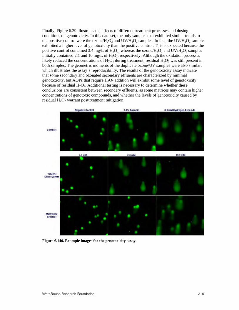
WateReuse Research Foundation 319
Finally, Figure 6.29 illustrates the effects of different treatment processes and dosing conditions on genotoxicity. In this data set, the only samples that exhibited similar trends to the positive control were the ozone/H2O2 and UV/H2O2 samples. In fact, the UV/H2O2 sample exhibited a higher level of genotoxicity than the positive control. This is expected because the positive control contained 3.4 mg/L of H2O2, whereas the ozone/H2O2 and UV/H2O2 samples initially contained 2.1 and 10 mg/L of H2O2, respectively. Although the oxidation processes likely reduced the concentrations of H2O2 during treatment, residual H2O2 was still present in both samples. The geometric moments of the duplicate ozone/UV samples were also similar, which illustrates the assay’s reproducibility. The results of the genotoxicity assay indicate that some secondary and ozonated secondary effluents are characterized by minimal genotoxicity, but AOPs that require H2O2 addition will exhibit some level of genotoxicity because of residual H2O2. Additional testing is necessary to determine whether these conclusions are consistent between secondary effluents, as some matrices may contain higher concentrations of genotoxic compounds, and whether the levels of genotoxicity caused by residual H2O2 warrant posttreatment mitigation.
Figure 6.140. Example images for the genotoxicity assay.

320 WateReuse Research Foundation
Figure 6.141. Baseline genotoxicity data.
Figure 6.142. Ozone genotoxicity data (no H2O2 addition).
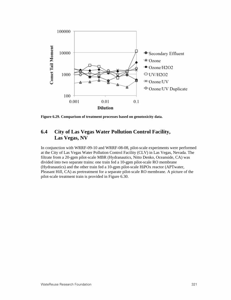
WateReuse Research Foundation 321
Figure 6.29. Comparison of treatment processes based on genotoxicity data.
6.4 City of Las Vegas Water Pollution Control Facility, Las Vegas, NV
In conjunction with WRRF-09-10 and WRRF-08-08, pilot-scale experiments were performed at the City of Las Vegas Water Pollution Control Facility (CLV) in Las Vegas, Nevada. The filtrate from a 20-gpm pilot-scale MBR (Hydranautics, Nitto Denko, Oceanside, CA) was divided into two separate trains: one train fed a 10-gpm pilot-scale RO membrane (Hydranautics) and the other train fed a 10-gpm pilot-scale HiPOx reactor (APTwater, Pleasant Hill, CA) as pretreatment for a separate pilot-scale RO membrane. A picture of the pilot-scale treatment train is provided in Figure 6.30.

322 WateReuse Research Foundation
Figure 6.30. MBR-O3/H2O2-RO pilot system.
The goal of WRRF-08-08 was to validate bench-scale studies demonstrating reductions in RO fouling after preoxidation with ozone and ozone/H2O2. Even at extremely low ozone doses (e.g., 1.5 mg/L or a O3:TOC ratio of approximately 0.25), preoxidation makes EfOM more hydrophilic, as illustrated by the Eawag bench-scale experiments, and less likely to accumulate on membrane surfaces. Ultimately, this leads to improved performance, stable transmembrane pressures, reduced maintenance, and possibly lowered costs. Another goal of WRRF-08-08 was to determine whether the reductions in organic fouling offset the additional capital and O&M costs associated with preoxidation.
For WRRF-09-10, the HiPOx ozone system was evaluated as a stand-alone treatment process for EfOM transformation, TOrC oxidation, and microbial inactivation. MBR filtrate was exposed to applied ozone doses ranging from 0 to 10 mg/L (O3:TOC=0–2.0) and H2O2:O3 ratios of 0 and 0.5. Samples were analyzed for all of the target compounds in the current study, but some compounds were not present in the MBR filtrate because of the efficacy of the biological treatment or their absence in the influent wastewater. Using bench-scale oxidation and disinfection data from WRRF-08-05, correlations were developed between changes in UV254 absorbance and total fluorescence, TOrC oxidation, and the inactivation of E. coli, MS2, and Bacillus spores. In WRRF-09-10, the data from the HiPOx pilot were then compared to these bench-scale data to validate the surrogate correlations. The following discussion will focus on the use of an online analyzer to implement this type of online monitoring strategy to assess treatment efficacy and predict contaminant removal.
The HiPOx unit at CLV was equipped with an online absorbance analyzer from s::can Messtechnik (Vienna, Austria). The s::can spectro::lyser (Figure 6.31) was used to store the entire absorption spectrum of the target water matrix at 5-min time intervals. In addition to automatic absorbance logging for a range of wavelengths (220–720 nm), the analyzer is also
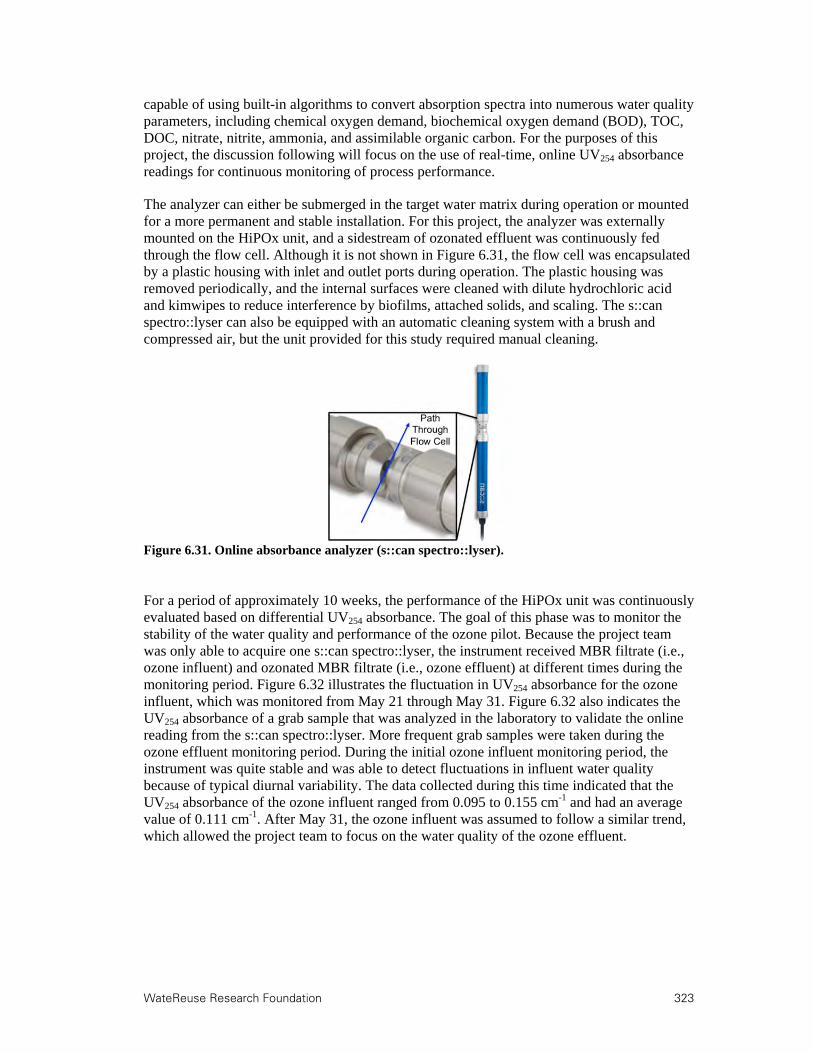
WateReuse Research Foundation 323
capable of using built-in algorithms to convert absorption spectra into numerous water quality parameters, including chemical oxygen demand, biochemical oxygen demand (BOD), TOC, DOC, nitrate, nitrite, ammonia, and assimilable organic carbon. For the purposes of this project, the discussion following will focus on the use of real-time, online UV254 absorbance readings for continuous monitoring of process performance.
The analyzer can either be submerged in the target water matrix during operation or mounted for a more permanent and stable installation. For this project, the analyzer was externally mounted on the HiPOx unit, and a sidestream of ozonated effluent was continuously fed through the flow cell. Although it is not shown in Figure 6.31, the flow cell was encapsulated by a plastic housing with inlet and outlet ports during operation. The plastic housing was removed periodically, and the internal surfaces were cleaned with dilute hydrochloric acid and kimwipes to reduce interference by biofilms, attached solids, and scaling. The s::can spectro::lyser can also be equipped with an automatic cleaning system with a brush and compressed air, but the unit provided for this study required manual cleaning.
Figure 6.31. Online absorbance analyzer (s::can spectro::lyser).
For a period of approximately 10 weeks, the performance of the HiPOx unit was continuously evaluated based on differential UV254 absorbance. The goal of this phase was to monitor the stability of the water quality and performance of the ozone pilot. Because the project team was only able to acquire one s::can spectro::lyser, the instrument received MBR filtrate (i.e., ozone influent) and ozonated MBR filtrate (i.e., ozone effluent) at different times during the monitoring period. Figure 6.32 illustrates the fluctuation in UV254 absorbance for the ozone influent, which was monitored from May 21 through May 31. Figure 6.32 also indicates the UV254 absorbance of a grab sample that was analyzed in the laboratory to validate the online reading from the s::can spectro::lyser. More frequent grab samples were taken during the ozone effluent monitoring period. During the initial ozone influent monitoring period, the instrument was quite stable and was able to detect fluctuations in influent water quality because of typical diurnal variability. The data collected during this time indicated that the UV254 absorbance of the ozone influent ranged from 0.095 to 0.155 cm-1 and had an average value of 0.111 cm-1. After May 31, the ozone influent was assumed to follow a similar trend, which allowed the project team to focus on the water quality of the ozone effluent.

324 WateReuse Research Foundation
Figure 6.32. Influent UV254 absorbance monitoring with s::can spectro::lyser.
Figure 6.33 illustrates the UV254 absorbance of the ozone effluent from May 31 to July 4. In contrast to the relatively stable ozone influent, the ozone effluent experienced dramatic fluctuations in water quality that resulted in numerous UV254 absorbance spikes in the raw data. In order to improve the clarity of the data, any values >0.100 cm-1 were removed from the data set. These points were assumed to be invalid for a variety of possible reasons:
Unexpected or planned shutdowns of the MBR and/or ozone pilots
Scaling or biological fouling of the spectro::lyser
Periodic spikes in turbidity that interrupted the light path in the flow cell
Operational changes to the spectro::lyser (e.g., software, flow modifications)
The gaps in the ozone effluent values indicate data that were removed. During the effluent monitoring period, there were numerous operational problems with the MBR and ozone pilots. For example, the cooling system of the HiPOx unit malfunctioned at one point, which caused periodic overheating and shutdowns of the ozone generator until it was replaced. The spectro::lyser continued to collect absorbance data despite the shut down and lack of flow through the unit. Although this did not benefit the model validation, it indicated that this type of online monitoring system would provide redundancy in alerting plant personnel of operational problems.
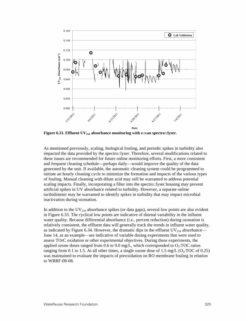
WateReuse Research Foundation 325
Figure 6.33. Effluent UV254 absorbance monitoring with s::can spectro::lyser.
As mentioned previously, scaling, biological fouling, and periodic spikes in turbidity also impacted the data provided by the spectro::lyser. Therefore, several modifications related to these issues are recommended for future online monitoring efforts. First, a more consistent and frequent cleaning schedule—perhaps daily—would improve the quality of the data generated by the unit. If available, the automatic cleaning system could be programmed to initiate an hourly cleaning cycle to minimize the formation and impacts of the various types of fouling. Manual cleaning with dilute acid may still be warranted to address potential scaling impacts. Finally, incorporating a filter into the spectro::lyser housing may prevent artificial spikes in UV absorbance related to turbidity. However, a separate online turibidimeter may be warranted to identify spikes in turbidity that may impact microbial inactivation during ozonation.
In addition to the UV254 absorbance spikes (or data gaps), several low points are also evident in Figure 6.33. The cyclical low points are indicative of diurnal variability in the influent water quality. Because differential absorbance (i.e., percent reduction) during ozonation is relatively consistent, the effluent data will generally track the trends in influent water quality, as indicated by Figure 6.34. However, the dramatic dips in the effluent UV254 absorbance—June 14, as an example—are indicative of variable dosing experiments that were used to assess TOrC oxidation or other experimental objectives. During these experiments, the applied ozone doses ranged from 0.6 to 9.0 mg/L, which corresponded to O3:TOC ratios ranging from 0.1 to 1.5. At all other times, a single ozone dose of 1.5 mg/L (O3:TOC of 0.25) was maintained to evaluate the impacts of preoxidation on RO membrane fouling in relation to WRRF-08-08.

326 WateReuse Research Foundation
Figure 6.34. UV254 absorbance monitoring with routine grab samples.
Most of the operational and data quality issues evident in the data gaps in Figure 6.33 can be mitigated in future applications. After addressing the issues and implementing the recommendations above, the s::can spectro::lyser would certainly provide useful data for operators of water reuse facilities. This is demonstrated by the consistency in the absorbance values detected by the s::can instrument versus the corresponding grab samples. During continuous operation, there are some fluctuations in water quality that would not be captured by periodic grab samples. The s::can spectro::lyser is capable of capturing this temporal variability and ultimately incorporating the online data into a model—whether the TOrC oxidation models developed in WRRF-09-10 or proprietary s::can algorithms—to evaluate a range of water quality parameters.
In order to evaluate the instrument’s ability to track operational modifications, a variable ozone dosing experiment was performed on June 14. The UV254 absorbance data from this experiment, including data for influent grab samples, effluent grab samples, and online monitoring of the ozone effluent, are illustrated in Figure 6.35. During the short timeframe of the dosing experiment, the influent water quality (shaded circles) was relatively stable, considering that the UV254 absorbance only ranged from 0.102 to 0.113 cm3. With respect to the effluent, the numbered boxes indicate different ozone dosing conditions, as described in Table 6.7. The data demonstrate tremendous consistency between the online (empty triangles) and grab sample (black squares) data throughout the testing period.

WateReuse Research Foundation 327
Table 6.7. Ozone Dosing Conditions During Variable Dosing Experiment
Ozone Dosing Condition O3:TOC Ratio Applied Ozone Dose (mg/L)
1 0.1 0.6 2 0.2 1.2 3 0.3 1.8 4 0.4 2.4 5 0.5 3.0 6 0.6 3.6 7 0.7 4.2 8 0.8 4.8 9 0.9 5.4 10 1.0 6.0 11 (Duplicate) 1.0 6.0 12 1.2 7.2 13 1.3 7.8 14 1.4 8.4 15 1.5 9.0
Figure 6.35. UV254 absorbance monitoring during variable dosing experiment.
The most significant question was whether the online absorbance data could be used to predict TOrC oxidation and microbial inactivation. The validation is detailed in WRRF-09-10, but the strategy proved to be an extremely effective tool for predicting process performance and could easily be integrated into full-scale ozone applications.


WateReuse Research Foundation 329
Chapter 7
7.Full-Scale Evaluation of Ozone and Advanced Oxidation
7.1 History of Ozonation in Full-Scale Wastewater Applications
Ozone has been used as a disinfectant for over a century (Loeb et al., 2012), but there has been a distinct dichotomy between drinking water and wastewater applications, particularly related to installation trends throughout the years. After the United States enacted water pollution regulations in the 1970s (the Clean Water Act), ozone became a popular disinfection alternative for wastewater treatment, and the number of U.S. installations eventually peaked at 44 sites by 1985 (Oneby et al., 2010). These were the first ozone installations in North America and some of the first installations for wastewater treatment. During this time, the industry was still refining its approach to the design, installation, and operation of ozone units (Rakness, 2012). Unfortunately, these systems were plagued by O&M problems, and the technology ultimately fell out of favor with the wastewater treatment community (Oneby et al., 2010). In fact, only 5 of the 44 installations were still in operation in 2009. Meanwhile, UV disinfection gained popularity after being identified as a relatively cheap and effective alternative for wastewater applications. On the other hand, the number of ozone installations for drinking water treatment continued to increase rapidly (Oneby et al., 2010) because of ozone’s efficacy in destroying taste and odor compounds, reducing trihalomethane formation, and inactivating bacteria, viruses, and protozoan parasites, particularly Cryptosporidium oocysts and Giardia cysts. The industry also learned from the experiences of the wastewater treatment community (Rakness, 2012).
The increased prevalence of indirect potable reuse and the recent emphasis on trace organic contaminant mitigation has dramatically altered the wastewater treatment landscape. “Planned” IPR covers a broad spectrum of treatment technologies, but MF-RO-UV/H2O2 is currently the preferred treatment train prior to groundwater replenishment and reuse. In fact, CDPH refers to MF-RO-AOP (additional AOP flexibility now allowed) as “full advanced treatment” (FAT) and permits only this train for direct injection applications (CDPH, 2011). The pioneering success of the Orange County Groundwater Replenishment System (GWRS)—a partnership between the Orange County Water District (OCWD) and the Orange County Sanitation District (OCSD)—has greatly advanced the field of IPR by providing a model system, specifically its Advanced Water Purification Facility (AWPF), which has been implemented by numerous agencies. Numerous studies have demonstrated the efficacy of the MF-RO-AOP treatment train in removing nearly all effluent organic matter, trace organic contaminants, and pathogenic microorganisms. Based on published research and historical performance, this treatment train is clearly an effective alternative for IPR. However, this paradigm is not necessarily the most appropriate option in all applications. For example, reverse osmosis generates a concentrated brine stream containing salt, bulk and trace organics, and other undesirable contaminants. Facilities with access to ocean outfalls can take advantage of this convenient disposal option, but this is not possible for many inland locations. Accordingly, this waste stream needs to be treated with additional processes that can greatly increase or even exceed the cost of advanced water treatment (e.g., thermal zero-

330 WateReuse Research Foundation
liquid discharge). This treatment train is also characterized by relatively high energy consumption, chemical use, and capital and O&M costs.
The leading alternative to MF-RO-AOP is some variation of O3-BAC, which has recently been demonstrated in a number of pilot- and full-scale installations in Nevada, New Mexico, Texas, Australia, and Switzerland. A recent study even highlighted the efficacy of three different ozone-BAC facilities in Australia (Reungoat et al., 2011). The data from these studies and installations indicate that that both MF-RO-AOP and O3-BAC are sufficient to ensure a safe and reliable water supply. In fact, the Fred Hervey Water Reclamation Plant (O3-BAC) has been operating for decades with no detrimental effects on public health, and newer ozone facilities, including the F. Wayne Hill Water Resources Center in Georgia, have experienced similar success. Many of these facilities rely on the biological—rather than adsorptive—capacity of the BAC process, so the media may last more than 10 years before replacement is desired. However, these BAC systems may require replenishment rates of several tons of carbon per year to account for media lost in the underdrains and during backwashes. The replacement frequency will be dictated by the water quality objectives, particularly for total organic carbon, but the biological component will address many of the oxidation byproducts regardless of the replacement frequency.
The use of ozone in wastewater applications is not limited to IPR. Ozonation can be integrated into wastewater treatment plants to accomplish a variety of water quality objectives, including general disinfection, sludge conditioning, odor control, preoxidation (prior to biological secondary treatment), and TOrC mitigation (Loeb et al., 2012). Because of a combination of new treatment objectives and improved technology, ozonation is again increasing in popularity in wastewater applications. In fact, wastewater installations in Japan increased from three facilities in the 1980s to over 60 facilities in 2010. In the United States, two ozone facilities recently converted to UV disinfection (Hagerstown, MD and Mahoning County, OH), but there are at least four facilities under design or construction (CCWRD; Scottsdale, AZ; and two facilities in Indianapolis, IN). Another facility—the WBMWD—is currently pilot testing ozone preoxidation to reduce MF fouling, and the full-scale system is expected to be online in the next few years. After these new installations are accounted for, there will be at least 10 wastewater or water reuse facilities in the United States using ozone (summarized in Table 7.1).
Despite the fact that many of the early ozone O&M problems have been addressed over the last few decades, problems are still encountered periodically, as with any technology. One facility recently experienced issues with both of their ozone generators: (1) one generator repeatedly blew high-voltage fuses because of an unknown electrical problem and (2) the other generator developed a leak that allowed coolant to enter the dielectric chamber. At the time of this report, the facility had not identified the cause of the electrical issue, although additional troubleshooting steps were under way. According to industry experts, the electrical issue is not a common problem for ozone systems unless the blown fuses are accompanied by other symptoms, such as cooling water leaks. In the recent past, some systems were affected by bad welds that allowed cooling water to enter the gas side of the generator, but this problem has generally been addressed by the various manufacturers. As a precautionary measure, facilities can ensure that the gas pressure inside the system is always greater than the external cooling water pressure, thereby reducing the potential for costly leaks (Rakness and Muri, 2009). The source of the leak in the second unit was determined to be one of the stainless steel tubes inside the generator, which was subsequently tapped and plugged.
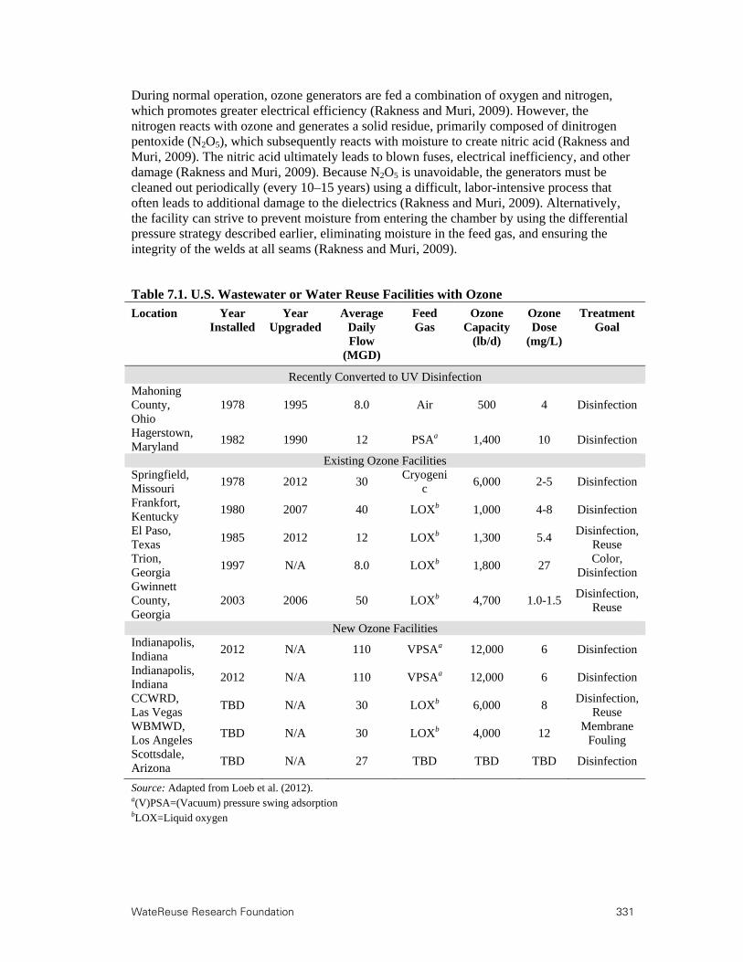
WateReuse Research Foundation 331
During normal operation, ozone generators are fed a combination of oxygen and nitrogen, which promotes greater electrical efficiency (Rakness and Muri, 2009). However, the nitrogen reacts with ozone and generates a solid residue, primarily composed of dinitrogen pentoxide (N2O5), which subsequently reacts with moisture to create nitric acid (Rakness and Muri, 2009). The nitric acid ultimately leads to blown fuses, electrical inefficiency, and other damage (Rakness and Muri, 2009). Because N2O5 is unavoidable, the generators must be cleaned out periodically (every 10–15 years) using a difficult, labor-intensive process that often leads to additional damage to the dielectrics (Rakness and Muri, 2009). Alternatively, the facility can strive to prevent moisture from entering the chamber by using the differential pressure strategy described earlier, eliminating moisture in the feed gas, and ensuring the integrity of the welds at all seams (Rakness and Muri, 2009).
Table 7.1. U.S. Wastewater or Water Reuse Facilities with Ozone
Location Year Installed
Year Upgraded
Average Daily Flow
(MGD)
Feed Gas
Ozone Capacity
(lb/d)
Ozone Dose
(mg/L)
Treatment Goal
Recently Converted to UV Disinfection Mahoning County, Ohio
1978 1995 8.0 Air 500 4 Disinfection
Hagerstown, Maryland
1982 1990 12 PSAa 1,400 10 Disinfection
Existing Ozone Facilities Springfield, Missouri
1978 2012 30 Cryogeni
c 6,000 2-5 Disinfection
Frankfort, Kentucky
1980 2007 40 LOXb 1,000 4-8 Disinfection
El Paso, Texas
1985 2012 12 LOXb 1,300 5.4 Disinfection,
Reuse Trion, Georgia
1997 N/A 8.0 LOXb 1,800 27 Color,
Disinfection Gwinnett County, Georgia
2003 2006 50 LOXb 4,700 1.0-1.5 Disinfection,
Reuse
New Ozone Facilities Indianapolis, Indiana
2012 N/A 110 VPSAa 12,000 6 Disinfection
Indianapolis, Indiana
2012 N/A 110 VPSAa 12,000 6 Disinfection
CCWRD, Las Vegas
TBD N/A 30 LOXb 6,000 8 Disinfection,
Reuse WBMWD, Los Angeles
TBD N/A 30 LOXb 4,000 12 Membrane
Fouling Scottsdale, Arizona
TBD N/A 27 TBD TBD TBD Disinfection
Source: Adapted from Loeb et al. (2012). a(V)PSA=(Vacuum) pressure swing adsorption bLOX=Liquid oxygen
332 WateReuse Research Foundation
The industry has dramatically improved its understanding of ozonation since the early installations, and there is also a wealth of knowledge and experience that did not exist previously, including useful references on the design, installation, and operation of ozone systems (Rakness, 2005). It is important to note that ozone systems in water and wastewater treatment are essentially identical, although the operational control points or treatment goals may differ slightly. Therefore, just as the drinking water industry learned lessons from the early wastewater installations, the wastewater industry can now benefit from recent successes in drinking water treatment (Rakness, 2012).
To assess the accuracy of extrapolating bench-scale data to larger systems, the pilot-scale experiments were supplemented with data from full-scale facilities. The project team collected samples from the following two agencies to evaluate the efficacy of ozone and MF-RO-UV/H2O2 for TOrC mitigation, disinfection, and transformation of bulk organic matter:
OCWD Advanced Water Purification Facility, CA—MF-RO-UV/H2O2
City of Springfield, MO—Ozone
Nine nitrosamines, including NDMA, were also monitored to identify the extent of formation and mitigation provided by the treatment trains.
Additional full-scale MF-RO-UV/H2O2 and ozone-BAC data are provided in Sections 3.2 and 3.4, respectively, which correspond to the WBMWD and GCGA bench-scale experiments. Those sections only highlight the secondary effluents and finished products, but they illustrate the efficacy of the different treatment frameworks. Finally, historical data from the El Paso Water Utilities (El Paso, TX) are also provided to illustrate trends in influent and effluent TOC values at an ozone-BAC facility.
7.2 MF-RO-UV/H2O2
7.2.1 OCWD Advanced Water Purification Facility
On the morning of October 10, 2011, samples were collected from the following locations at OCWD’s 70-MGD MF-RO-UV/H2O2 facility, which is illustrated in Figure 7.1:
Microfiltration feed (MFF)
Reverse osmosis feed (ROF)
Reverse osmosis permeate (ROP)
Reverse osmosis concentrate (ROC)
UV/H2O2 product (UVP)

WateReuse Research Foundation 333
Figure 7.1. Schematic of OCWD’s Advanced Water Purification Facility.
Prior to arriving at the AWPF, the partially nitrified–denitrified secondary effluent from OCSD is dosed with 12.5% sodium hypochlorite, which subsequently reacts with residual ammonia to form chloramines. This feedwater (MFF) is filtered through polypropylene hollow-fiber microfiltration membranes and the effluent (MFE) is stored in a break tank. A chloramine residual is maintained in the MFE, and sulfuric acid and antiscalants are added to form feedwater (ROF) for the three-stage RO process. The RO product/permeate (ROP) is dosed with 3 mg/L of H2O2 prior to the UV AOP, thereby generating the UV product (UVP). A summary of the water quality data associated with these samples is provided in Table 7.2.
The MFF data are characteristic of a conventional secondary/tertiary effluent, and there are no significant outliers to highlight. The nitrosamine concentrations (i.e., NDMA, NPYR, and nitrosomorpholine) were relatively low and presumably formed during exposure to chloramines, which in turn are largely responsible for the small number of coliform bacteria.
As expected, the subsequent microfiltration process (ROF) resulted in small reductions in UV254 absorbance, TOC, some of the target compounds, and coliform bacteria. However, there were several target compounds, including nitrosamines, that increased in concentration across the microfiltration membrane. For many of the target compounds, this increase can likely be attributed to sampling error or matrix interference that may have impacted the analytical methods. For the nitrosamines, the increases in concentration are likely due to longer exposure to chloramine, although sampling error and matrix interference are potential explanations as well.
After reverse osmosis, nearly all of the target compounds were removed to the detection limits of the analytical methods. In fact, only three parameters—UV254 absorbance, total nitrogen, and NDMA—were present at reportable concentrations in the ROP. The UV254 absorbance and total nitrogen values were insignificant, and the NDMA concentration was typical of an RO permeate because of the compound’s low molecular weight, which enables it to pass through the semipermeable membrane and dictates the need for the downstream UV/H2O2 process. On the other hand, the ROC values illustrate one of the major disadvantages of MF-RO treatment trains: reclamation facilities with no access to ocean outfalls must dispose of concentrated brines safely. The ROC samples contained 61 mg/L of

334 WateReuse Research Foundation
total nitrogen and 33 mg/L of TOC, and nearly half of the target compounds were present at the μg/L level in the ROC samples. Furthermore, four of the nitrosamines were present at reportable concentrations, although NDMA was the only nitrosamine above its CDPH notification level.
Just as the ROC sample illustrates the major limitation of MF-RO-AOP, the UVP sample further illustrates why this treatment train is regarded as the preferred alternative in IPR. Specifically, the RO process removes a majority of the target compounds to the detection limits of existing analytical methods, and the downstream UV/H2O2 process provides further polishing to ensure that the final product is essentially ready for human consumption. With respect to the UVP sample, only UV254 absorbance and total nitrogen were present at reportable, albeit exceptionally low, concentrations.
In addition to the parameters listed in Table 7.2, the samples were also characterized based on 3D fluorescence. Despite the different format, the 3D fluorescence data (Figure 7.2) lead to the same conclusion: MF-RO-AOP is extremely effective in removing effluent organic matter and providing multiple barriers against TOrCs and microbial pathogens. This is illustrated by the decrease in fluorescence intensity (color and numeric values) through the treatment train. Again, the efficacy of this treatment train must be considered against the disposal of the concentrated brine stream (Figure 7.3) and the additional costs associated with each treatment process. The cost issue will be described in greater detail later in the report.
Figure 7.2. 3D Fluorescence for the MF-RO-UV/H2O2 train at OCWD’s AWPF.
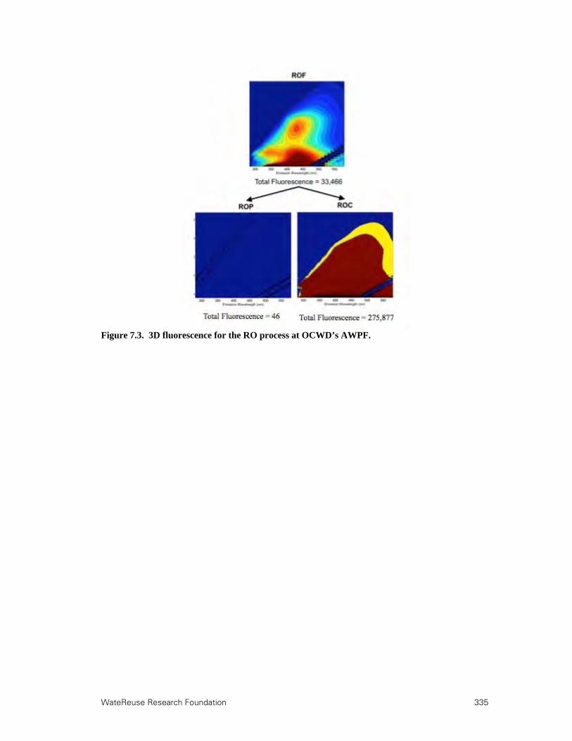
WateReuse Research Foundation 335
Figure 7.3. 3D fluorescence for the RO process at OCWD’s AWPF.

336 WateReuse Research Foundation
Table 7.2. Summary of Full-Scale Sample Event at OCWD’s AWPF
Parameter Units MFF ROF ROP ROC UVP
UV254 absorbance cm-1 0.153 0.125 0.007 0.696 0.004 TN mg-N/L 11 11 1.1 61 1.2 TOC mg/L 6.4 6.0 < 0.20 33 < 0.20 Bisphenol A ng/L < 50 < 50 < 50 < 50 < 50 Diclofenac ng/L < 25 74 < 25 610 < 25 Gemfibrozil ng/L 190 210 < 10 1,300 < 10 Ibuprofen ng/L 80 93 < 25 760 < 25 Musk ketone ng/L < 100 < 100 < 100 180 < 100 Naproxen ng/L 140 200 < 25 1,400 < 25 Triclosan ng/L < 25 < 25 < 25 87 < 25 Atenolol ng/L 590 570 < 25 3,400 < 25 Atrazine ng/L < 10 < 10 < 10 14 < 10 Carbamazepine ng/L 180 210 < 10 1,000 < 10 DEET ng/L 400 410 < 25 2,400 < 25 Meprobamate ng/L 580 540 < 10 3,000 < 10 Phenytoin ng/L 160 150 < 10 840 < 10 Primidone ng/L 110 100 < 10 760 < 10 Sulfamethoxazole ng/L 290 660 < 25 4,500 < 25 Trimethoprim ng/L 31 66 < 10 510 < 10 TCEP ng/L 500 510 < 200 3,000 < 200 Nitrosodimethylamine (NDMA) ng/L 16 42 20 100 < 2.5 Nitrosomethylethylamine (NMEA) ng/L < 5.0 < 5.0 < 5.0 < 5.0 < 5.0 Nitrosodiethylamine (NDEA) ng/L < 5.0 < 5.0 < 5.0 < 5.0 < 5.0 Nitrosodipropylamine (NDPA) ng/L < 10 < 10 < 10 < 10 < 10 Nitrosomorpholine ng/L 6.9 7.5 < 5.0 18 < 5.0 Nitrosopyrrolidine (NPYR) ng/L 23 34 < 10 150 < 10 Nitrosopiperidine (NPIP) ng/L < 5.0 < 5.0 < 5.0 30 < 5.0 Nitrosodibutylamine (NDBA) ng/L < 10 < 10 < 10 < 10 < 10 Nitrosodiphenylamine ng/L < 10 < 10 < 10 < 10 < 10 Total coliform MPN/100 mL 3.1 <1.0 <1.0 <1.0 <1.0 Fecal coliform MPN/100 mL <1.0 <1.0 <1.0 <1.0 <1.0

WateReuse Research Foundation 337
7.2.2 West Basin Municipal Water District
The full-scale data for the MF-RO-UV/H2O2 system operated by the WBMWD were described earlier in the report in Table 3.34 (general water quality), Table 3.39 (TOrC concentrations), Table 3.42 (microbial water quality), and Figure 3.55 (3D fluorescence). In general, the final product water was very similar to that for Orange County, but there were several minor exceptions. For example, the NDMA concentration following the UV/H2O2 process at WBMWD was 6.5 ng/L instead of <2.5 ng/L. Most importantly, however, the concentration was still below the 10 ng/L CDPH notification level. The other significant difference was that bisphenol A was detected at 86 ng/L in the finished product, although all of the other TOrCs were below their respective reporting limits. The field blank (i.e., control sample) was also <MRL for bisphenol A, which indicates that sample contamination is unlikely. The bisphenol A concentration was also relatively high in the secondary effluent in comparison to the other study sites, but additional testing would be needed to verify that this is a consistent problem. Regardless, the WBMWD data support the conclusion that MF-RO-UV/H2O2 is effective against a variety of water-based contaminants and is a suitable treatment train for potable reuse applications.
7.3 Ozone and Ozone-BAC
7.3.1 City of Springfield, MO (Ozone)
On October 10, 2011, samples were collected from the following locations at the 30-MGD facility, which is illustrated in Figure 7.4:
Primary effluent from Plant #2
Secondary effluent from Plant #2
Combined ozone influent
Combined ozone effluent
A summary of the data for the Springfield study site is provided in Table 7.3, and the corresponding 3D fluorescence images are provided in Figure 7.5. The primary and secondary effluent samples were representative of typical wastewater. The primary effluent sample contained high nitrogen and organic carbon concentrations, and many of the trace organic contaminants were present at the μg/L level, particularly the compounds with higher consumption patterns. The compounds with the highest concentrations were the pain relievers and anti-inflammatories (e.g., naproxen and ibuprofen), which is typical of raw wastewater or primary effluent. Nitrosopyrrolidine (NPYR) and nitrosopiperidine (NPIP) were also present at concentrations of 500 ng/L and 380 ng/L, respectively. Further study would be necessary to identify the reason for these high concentrations, but this was outside the scope of the present study. In any case, these compounds were not detected in the secondary effluent, so they appear to be readily amenable to biodegradation.

338 WateReuse Research Foundation
Figure 7.4. Springfield study site.
Figure 7.5. 3D fluorescence for the Springfield study site.
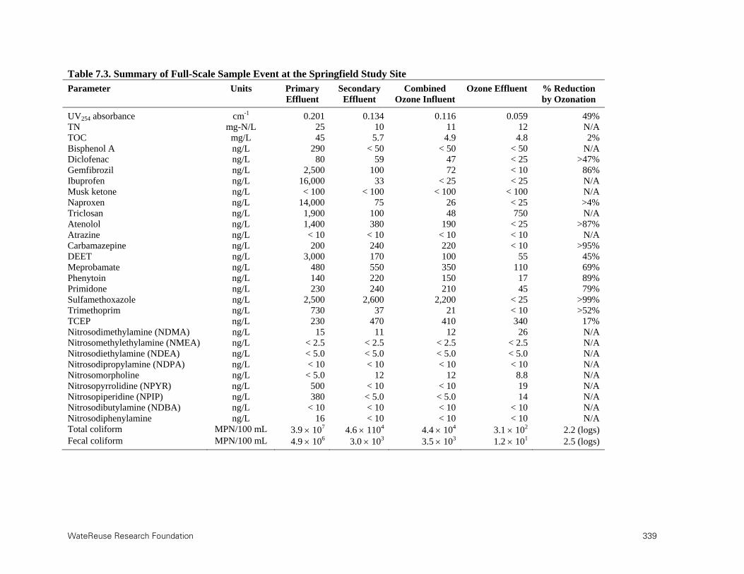
WateReuse Research Foundation 339
Table 7.3. Summary of Full-Scale Sample Event at the Springfield Study Site
Parameter Units Primary Effluent
Secondary Effluent
Combined Ozone Influent
Ozone Effluent % Reduction by Ozonation
UV254 absorbance cm-1 0.201 0.134 0.116 0.059 49% TN mg-N/L 25 10 11 12 N/A TOC mg/L 45 5.7 4.9 4.8 2% Bisphenol A ng/L 290 < 50 < 50 < 50 N/A Diclofenac ng/L 80 59 47 < 25 >47% Gemfibrozil ng/L 2,500 100 72 < 10 86% Ibuprofen ng/L 16,000 33 < 25 < 25 N/A Musk ketone ng/L < 100 < 100 < 100 < 100 N/A Naproxen ng/L 14,000 75 26 < 25 >4% Triclosan ng/L 1,900 100 48 750 N/A Atenolol ng/L 1,400 380 190 < 25 >87% Atrazine ng/L < 10 < 10 < 10 < 10 N/A Carbamazepine ng/L 200 240 220 < 10 >95% DEET ng/L 3,000 170 100 55 45% Meprobamate ng/L 480 550 350 110 69% Phenytoin ng/L 140 220 150 17 89% Primidone ng/L 230 240 210 45 79% Sulfamethoxazole ng/L 2,500 2,600 2,200 < 25 >99% Trimethoprim ng/L 730 37 21 < 10 >52% TCEP ng/L 230 470 410 340 17% Nitrosodimethylamine (NDMA) ng/L 15 11 12 26 N/A Nitrosomethylethylamine (NMEA) ng/L < 2.5 < 2.5 < 2.5 < 2.5 N/A Nitrosodiethylamine (NDEA) ng/L < 5.0 < 5.0 < 5.0 < 5.0 N/A Nitrosodipropylamine (NDPA) ng/L < 10 < 10 < 10 < 10 N/A Nitrosomorpholine ng/L < 5.0 12 12 8.8 N/A Nitrosopyrrolidine (NPYR) ng/L 500 < 10 < 10 19 N/A Nitrosopiperidine (NPIP) ng/L 380 < 5.0 < 5.0 14 N/A Nitrosodibutylamine (NDBA) ng/L < 10 < 10 < 10 < 10 N/A Nitrosodiphenylamine ng/L 16 < 10 < 10 < 10 N/A Total coliform MPN/100 mL 3.9 107 4.6 1104 4.4 104 3.1 102 2.2 (logs) Fecal coliform MPN/100 mL 4.9 106 3.0 103 3.5 103 1.2 101 2.5 (logs)
340 WateReuse Research Foundation
The secondary process is operated in two separate trains, with activated sludge plus biological phosphorus removal in Train #2 (sampling location) and activated sludge with full nitrification and partial denitrification in Train #1. Alum is also added to both trains to provide chemical phosphorus removal. The target mixed liquor suspended solids concentration is approximately 3,000 mg/L. The secondary effluent concentrations from Train #2 were typical of an efficient biological process without nitrification. This is most apparent in the concentrations of the pain relievers and anti-inflammatories, which are degraded extensively during secondary treatment. The concentrations of these target compounds will decrease significantly in all biological processes, but full nitrification generally reduces these compounds to their respective MRLs. The degree of sampling error (i.e., different slugs of water from primary to secondary effluent) is most apparent in the biologically recalcitrant compounds, such as meprobamate, primidone, and phenytoin, which appear to increase through the secondary process.
The combined ozone influent data reflect the mixing of flows from the two different trains. This includes additional sand filtration for Train #2 and more extensive biological treatment and filtration for Train #1. The additional nitrification/denitrification steps in Train #1 are apparent, based on the reduced concentrations of the target compounds. This sample was collected to provide a direct point of comparison for the ozone effluent.
During the sampling event, the Springfield facility was averaging an ozone production rate of approximately 1,200 lb/day. Based on the facility’s average daily flow of 30 MGD, this corresponds to an applied ozone dose of 4.8 mg/L and an O3:TOC ratio of approximately 1.0. The performance of the ozone system was evaluated based on the contaminant groups presented earlier in the report. Based on the summary data in Table 5.18, an O3:TOC ratio of 1.0 should achieve an approximate 50% reduction in UV254 absorbance in addition to the following reductions in the target contaminants:
Group 1=99% (sulfamethoxazole, diclofenac, bisphenol A, carbamazepine, trimethoprim, naproxen, and triclosan)
Group 2=90% (gemfibrozil and atenolol)
Group 3=92% (ibuprofen, phenytoin, DEET, and primidone)
Group 4=68% (atrazine and meprobamate)
Group 5=23% (TCEP)
E. coli=7 logs
The reduction in UV254 absorbance was almost identical to the predicted value, and many of the target compounds were also close to their predicted reductions. Exclusions include compounds that were not detected in the combined ozone influent sample; compounds that reached their respective MRLs during ozonation, which limited the quantifiable range; and three specific outliers (DEET, triclosan, and E. coli). Ozonation only achieved a 45% reduction in the DEET concentration, but it is unclear what caused this deviation from the bench-scale data. The more notable outliers were the Group 1 compound triclosan, which increased in concentration from 48 ng/L to 750 ng/L after ozonation, and E. coli. Although unsubstantiated, because the field blank was <MRL for all of the target contaminants, the elevated triclosan concentration is indicative of some form of contamination during the preparation, collection, or analysis phase. Because triclosan is ubiquitous in hand soaps, this is a plausible explanation, but further testing would be necessary to validate or refute this theory. With respect to E. coli, the potential level of inactivation was limited to only 3.5 logs

WateReuse Research Foundation 341
because the ozone influent sample only contained 3.5 103 MPN/100 mL. In general, it is often easier to achieve several orders of magnitude of inactivation when the initial E. coli level is high, as in the spiked bench-scale experiments. It becomes increasingly difficult to inactivate bacteria as the numbers approach the detection limit of the assay—hence the discrepancy between the maximum level of inactivation (3.5 logs) and the observed level of inactivation (2.5 logs). It is important to note that microbial regrowth during shipping was not a factor, considering that the fecal coliform data measured by the project team were similar to those measured at the facility (data not shown). Also, the total suspended solids concentration in the combined ozone influent was <1 mg/L, so particle shielding was not a significant issue. Therefore, further study is necessary to identify strategies to consistently achieve microbial detection limits with ozonation.
The Springfield data were also analyzed using a model developed for a recent WateReuse Research Foundation project (WRRF-09-10: Use of UV and Fluorescence Spectra as Surrogate Measures for Contaminant Oxidation and Disinfection in the Ozone/H2O2 Advanced Oxidation Process). Using the regression models presented in that report, the contaminant-specific predictions in Table 7.4 were developed for compounds with quantifiable data. Similarly to the group-based comparison previously presented, the contaminant-specific predictions were also consistent with the observed data, excluding the aforementioned outliers. This indicates that the predictive model in WRRF-09-10 can be a powerful tool in monitoring the performance of oxidation processes, particularly ozonation.
Table 7.4. WRRF-09-10 Model Validation for Springfield Data
Parameter Actual % Reduction Predicted % Reduction
UV254 absorbance 49% 50% Total fluorescence 84% 87% Diclofenaca >47% 99% Gemfibrozil 86% 99% Naproxena >4% 99% Atenolola >87% 99% Carbamazepinea >95% 99% DEET 45% 75% Meprobamate 69% 77% Phenytoin 89% 85% Primidone 79% 75% Sulfamethoxazolea >99% 99% Trimethoprima >52% 99% TCEP 17% 18% E. coli 2.5 (logs) 5.3 (logs)
aPercentage reduction limited by MRL.
With respect to the nitrosamines, the ozonated effluent from the Springfield facility was consistent with the bench-scale data in this report. Specifically, ozonation resulted in direct nitrosamine formation, which increased the NDMA concentration from 12 to 26 ng/L. However, this 14 ng/L increase was one of the lowest levels of direct NDMA formation observed in this study, which can likely be attributed to the extensive biological pretreatment (i.e., nitrification/denitrification) provided in Train #1. Although polymer has been implicated as a potential NDMA precursor during ozonation (Padhye et al., 2011), the use of polymer at the Springfield facility did not seem to be a significant factor. Anecdotal evidence suggests
342 WateReuse Research Foundation
that significant polymer use occurs in the biosolids dewatering centrifuges at the Springfield facility, and the resulting centrate, presumably containing residual polymer, is recycled to the head of the treatment plant. Residual polymer is likely degraded during biological secondary treatment, and no further polymer addition occurs downstream of the final clarification process (i.e., immediately upstream of the ozone process).
Similar levels of NPIP and NPYR also formed during ozonation, although there is no basis for comparison in the bench-scale experiments. If CDPH notification levels were a concern in this application, a low level of UV photolysis or downstream biological filtration would be needed to reduce the NDMA concentration to 10 ng/L. NDEA and NDPA were not detected in the sample, so the 10 ng/L notification levels for these compounds would not be an issue. Nitrosomorpholine, which does not have an established notification level, was also detected in the ozonated effluent, but the concentration actually decreased to 8 ng/L from the preceding sample.
After the sample event was completed, the Springfield study site upgraded its ozone system by installing high-efficiency ozone generators and sidestream injection as a replacement for its original diffusion system. With both of the ozone generators operating simulataneously at full capacity, the system is capable of producing 6,000 lbs/day of ozone. However, Springfield’s standard operating procedure is based on a single ozone generator, with the second available for redundancy. It still uses the original cryogenic oxygen supply, but with upgraded control parameters. Since the upgrade, the facility has observed lower fecal coliform counts with lower applied ozone doses. The facility is currently operating at an ozone production rate of 1,000 lbs/day during average flows, but it may reduce that set point to 600–800 lbs/day because of the system’s disinfection efficacy.
7.3.2 Gwinnett County, GA (Ozone-BAC)
The full-scale data for the ozone-BAC process at Gwinnett County were described earlier in the report in Table 3.64 (general water quality), Table 3.69 (TOrC concentrations), Table 3.72 (microbial water quality), and Figure 3.95 (3D fluorescence). In general, the final product waters were similar between Gwinnett County and the Springfield facility, although the coliform and NDMA levels were slightly lower in Georgia. The additional biological filtration process (i.e., BAC) at Gwinnett County was sufficient to remove the ambient NDMA in the secondary effluent (17 ng/L) and any NDMA that may have formed during ozonation (data not collected). It is difficult to provide a more in-depth evaluation of the ozone process at Gwinnett County because the process was not isolated by the original sampling plan during the bench-scale experiments. Samples were only collected for the secondary effluent and the finished product. With the exception of TOC and total dissolved solids, the ozone-BAC treatment train produced a final product of quality similar to that of MF-RO-UV/H2O2.
7.4 El Paso Water Utilities (Ozone-BAC)
The recently upgraded 12-MGD facility operated by the El Paso Water Utilities employs a treatment train comprising a powdered activated carbon biological process (PACT, Siemens, Munich, Germany), lime stabilization, media filtration, ozone disinfection (~5 mg/L), and biological activated carbon prior to aquifer recharge. The ozone system is composed of two Wedeco Effizon ozone generators (ITT Water & Wastewater, Herford, Germany), a nitrogen boost system, and two ozone destruct units. For the BAC process, the carbon has only been replaced twice in 27 years of operation, although two to four tons of carbon are added each

WateReuse Research Foundation 343
year to replenish the amount that is lost in the underdrains and during backwashes. Because one ozone generator is sufficient to meet the facility’s dosing objectives, the second unit is intended only for redundancy. In contrast, some facilities operate multiple units at lower power settings to achieve the same dosing condition as a single unit at a higher power setting.
Figure 7.6 illustrates the historical influent and effluent TOC data sets for 2011, which were provided by the El Paso Water Utilities. During this sampling period, the ozone system was dosing at approximately 5 mg/L, and the BAC empty bed contact time was approximately 10 min. Because the BAC at this facility is not regenerated or replaced very often (every 10–11 years), these data are indicative of a predominantly biological rather than adsorptive process. The minimum, average, and maximum effluent TOC values in 2011 were 1.8, 3.2, and 5.2 mg/L, respectively. Therefore, ozone-BAC facilities are capable of producing product water with minimal organic matter, and these values could likely be reduced even further with more frequent media regeneration or replacement.
Figure 7.6. Historical TOC (mg/L) data for 2011.
7.5 Conclusion The data sets described indicate that the conclusions and removal profiles developed with bench-scale experiments can generally be extrapolated to full-scale systems. Each system will have unique water quality parameters, precursors, and treatment objectives, which will lead to some variability in process performance and final water quality, but the general design principles will be relatively consistent. As demonstrated in previous studies, the MF-RO-UV/H2O2 systems at Orange County and West Basin were extremely effective in eliminating the wastewater identity of the matrices. With the exception of bisphenol A at West Basin, these FAT systems achieved the MRLs for all of the target compounds and the notification levels for the nitrosamines. However, the ROC sample highlighted one of the major limitations of this treatment alternative: because the organic carbon and nitrogen concentrations were extremely high, many of the target compounds were present at the μg/L
0
1
2
3
4
5
6
7
8
9
10
11
12
13
14
15
0
50
100
150
200
250
J F M A M J J A S O N D P
rod
uct
Wat
er T
OC
(m
g/L
)
Raw
Was
tew
ater
TO
C (
mg/
L)
Raw
Product

344 WateReuse Research Foundation
level, and NDMA exceeded its respective notification level. In contrast, the ozone and ozone-BAC treatment trains were not affected by significant residuals management requirements, and the treatment trains were able to achieve the MRLs for a majority of the target compounds. However, this alternative treatment train is generally not capable of achieving the same level of TOC and nitrogen removal without soil aquifer treatment and upstream denitrification, respectively. MF-RO-UV/H2O2 and ozone-based systems have a history of success, so treatment train decisions must be made on a case-by-case basis after accounting for regulatory requirements, salinity objectives, costs, and site feasibility.

WateReuse Research Foundation 345
Chapter 8
8.Transformation Products
8.1 Description of Methods
8.1.1 Compound List
The first step in the transformation product work was to determine which analytes in the target compound list were suitable candidates for evaluation. The compounds were first judged by their susceptibility to ozone oxidation under normal treatment conditions. Compounds with slow reaction rates, such as meprobamate, phenytoin, primidone, TCEP, musk ketone, atrazine, and DEET, were considered poor candidates for the evaluation because of their limited transformation. The second step was to complete a literature survey for the remaining analytes. This revealed that the transformation products resulting from ozone oxidation of atrazine (Acero et al., 2000b), bisphenol A (Deborde et al., 2008), carbamazepine (McDowell et al., 2005a), DEET (Tay et al., 2009), diclofenac (Sein et al., 2008b), sulfamethoxazole (Abellán et al., 2008), and trimethoprim (Radjenovic et al., 2009a) have already been studied and are available in the cited references. To supplement the existing literature and provide points of comparison between studies, the following compounds were selected for analysisWRRF: atenolol, gemfibrozil, ibuprofen, naproxen, sulfamethoxazole, and trimethoprim. Diphenhydramine (allergy medication) was also included in the study, although it was not included in the original target compound list. The structures of these compounds are illustrated in Figure 8.1.
Figure 8.1. Target compounds selected for the transformation product analysis.
8.1.2 Real-Time Analysis by Quadrupole Time-of-Flight Mass Spectrometry
The initial testing was performed using a setup similar to the one reported in the literature (Vanderford et al., 2008b). The solution from a stirred reaction vessel (foil-covered 250 mL

346 WateReuse Research Foundation
glass bottle) was infused into the ionization source of the Agilent 6510 Q-TOF mass spectrometer via a high-performance liquid chromatography pump. The flow rate of the pump was set to 4 mL/min to ensure a rapid transfer from the vessel to the ionization source. However, prior to entering the source, the flow was reduced to ~200 L/min, and methanol was added to aid with the ionization process. Because compounds display different ionization efficiencies, the initial concentration was determined by adding an aqueous stock solution of the target compound to 200 mL of laboratory grade water until a signal of sufficient intensity was reached. Once this concentration was determined, it was applied to the rest of the experiments. Given the limitations of this method in determining structural isomers, other methods of analysis were explored.
8.1.3 Liquid Chromatography Quadrupole Time-of-Flight Tandem Mass Spectrometry Approach
A general chromatographic method was developed in order to have some selectivity of structural isomers. To study the reaction progress, a consistent amount of compound was exposed to a variable amount of ozone. One mL of a 100 mg/L target compound solution was added to amber glass vials containing laboratory grade water. The volume of water varied depending on the volume of ozone solution to be added. A 20 mg/L ozone stock was prepared, and the ozone spiking volume was varied (0, 1, 2.5, 5, 7.5 or 10 mL) depending on the target molar ratio of ozone to compound. After the target volume was reached (11 mL), the glass vial was capped and shaken. The molar ozone-to-compound ratio ranged from ~1.0 to ~10.0. The final solution was held at room temperature for at least 1 h prior to LC Q-TOF MS analysis. It should be noted that similar approaches have been reported by other researchers (Benner and Ternes, 2009a).
The analysis method employed a HALO C18 column (4.6 50 mm, 2.7 m) from MAC-MOD Analytical, Inc. (Chadds Ford, PA, US), gradient elution with 2.5 mM ammonium acetate in H2O (A) and methanol (B), and a 20 L injection volume. Each solution, along with a blank, was analyzed in both positive and negative ionization mode. The resulting data were processed using a molecular feature extraction method on Agilent MassHunter qualitative analysis software. The results of this processing were further analyzed using Agilent Mass Profiler software to help distinguish the transformation products from compounds present in the background.
8.2 Method Troubleshooting
8.2.1 Real-Time Analysis
Real-time analysis was applied to gemfibrozil and naproxen in laboratory-grade water in separate experiments. In each experiment, the analyte was spiked into the reaction vessel at approximately 200 ng/mL. Once a stable signal was obtained at the mass spectrometer, the ozone solution was added until a final concentration of 2 mg/L was reached. The reaction was monitored for a minimum of 20 min prior to the flushing of the system. The resulting transformation products were manually extracted from the total ion chromatogram, and selected ion chromatograms were also extracted. Empirical formulas were calculated from the accurate mass data. The results of the naproxen analysis are illustrated in Figure 8.2.
The real-time analysis provided valuable time resolution of compound decomposition, which can be used to develop reaction mechanisms, but the process was also limited by several
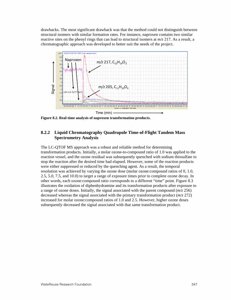
WateReuse Research Foundation 347
drawbacks. The most significant drawback was that the method could not distinguish between structural isomers with similar formation rates. For instance, naproxen contains two similar reactive sites on the phenyl rings that can lead to structural isomers at m/z 217. As a result, a chromatographic approach was developed to better suit the needs of the project.
Figure 8.2. Real-time analysis of naproxen transformation products.
8.2.2 Liquid Chromatography Quadrupole Time-of-Flight Tandem Mass Spectrometry Analysis
The LC-QTOF MS approach was a robust and reliable method for determining transformation products. Initially, a molar ozone-to-compound ratio of 1.0 was applied to the reaction vessel, and the ozone residual was subsequently quenched with sodium thiosulfate to stop the reaction after the desired time had elapsed. However, some of the reaction products were either suppressed or reduced by the quenching agent. As a result, the temporal resolution was achieved by varying the ozone dose (molar ozone:compound ratios of 0, 1.0, 2.5, 5.0, 7.5, and 10.0) to target a range of exposure times prior to complete ozone decay. In other words, each ozone:compound ratio corresponds to a different “time” point. Figure 8.3 illustrates the oxidation of diphenhydramine and its transformation products after exposure to a range of ozone doses. Initially, the signal associated with the parent compound (m/z 256) decreased whereas the signal associated with the primary transformation product (m/z 272) increased for molar ozone:compound ratios of 1.0 and 2.5. However, higher ozone doses subsequently decreased the signal associated with that same transformation product.

348 WateReuse Research Foundation
Figure 8.3. Oxidation of diphenhydramine after exposure to a range of ozone doses.
8.3 Transformation Products in Laboratory-Grade Water
8.3.1 Atenolol
As shown in Figure 8.4, atenolol was oxidized slowly compared to some of the other compounds, which are shown in the following. This is depicted by the change in integrated area, which is an analytical surrogate for compound concentration. In fact, small quantities of atenolol persisted even at the highest ozone doses. Atenolol and its transformation products were most apparent in the positive ion mode, and the associated analytical parameters are summarized in Table 8.1. This table includes the theoretical chemical formula, the number of double bond equivalents, the retention time corresponding to the respective peak, and the dosing conditions for which the transformation products were present. For atenolol, the intensities of the transformation products were significantly lower than that of the parent compound. This was particularly true for product #2, which produced a notably broad chromatographic peak that reached a maximum at an ozone:compound ratio of 7.5. Transformation product #1 reached a maximum at 2.5, whereas product #3 grew more intense with increasing ozone exposure. The reaction appears to proceed via the phenyl ring (#2) and at the ether C–O bond (#3), although the pathway leading to product #1 is not clear at present.

WateReuse Research Foundation 349
Figure 8.4. Atenolol dose–response curve.
Table 8.1. Transformation Product Summary for Atenolol
Species Formula Double Bond Equivalent
Retention Time (min)
Present (ozone:compound)
Parent C14H22N2O3 5 3.80 All #1 C14H20N2O4 6 4.60 1.0, 2.5 #2 C14H22N2O5 5 2.60-2.70 All #3 C6H15NO2 0 1.02 All
8.3.2 Diphenhydramine
The oxidation of diphenhydramine was rapid and complete under the highest dosing condition (Figure 8.5), and the decomposition process yielded several transformation products (Table 8.2). Similar to atenolol, only the positive ionization mode proved to be useful in detecting the compound and its transformation products. Product #1 exhibited a response with similar intensity to that of diphenhydramine, whereas the others were significantly lower. Product #1 achieved a maximum at an ozone exposure of 2.5 and persisted even at the highest exposure of 10.0. This product is likely the amine oxide of diphenhydramine. Products #2 and #3 appear to involve reactions at the aromatic rings, whereas #4 likely involves the complete destruction of the aromatic rings.

350 WateReuse Research Foundation
Figure 8.5. Diphenhydramine dose–response curve.
Table 8.2. Transformation Product Summary for Diphenhydramine
Species Formula Double Bond Equivalent
Retention Time (min)
Present (ozone:compound)
Parent C17H21NO 8 7.36 1.0, 2.5, 5.0 #1 C17H21NO2 8 7.46 All #2 C11H15NO3 5 5.25 All #3 C12H17NO4 5 1.67 All #4 C5H13NO3 0 0.93 All
8.3.3 Gemfibrozil
As expected, gemfibrozil was oxidized rapidly and completely, considering it was only present for the 1.0 and 2.5 dosing ratios (Figure 8.6). The reaction products (Table 8.3) were compoed of different isomers (e.g., #1a and #1b), and they all eluted at shorter retention times than the parent compound. In comparison to the initial gemfibrozil peak, the transformation products displayed a significantly lower response in negative ion mode and a similar response in positive ion mode. The main reaction pathways appeared to proceed through the benzene ring and at the ether C–O bond.
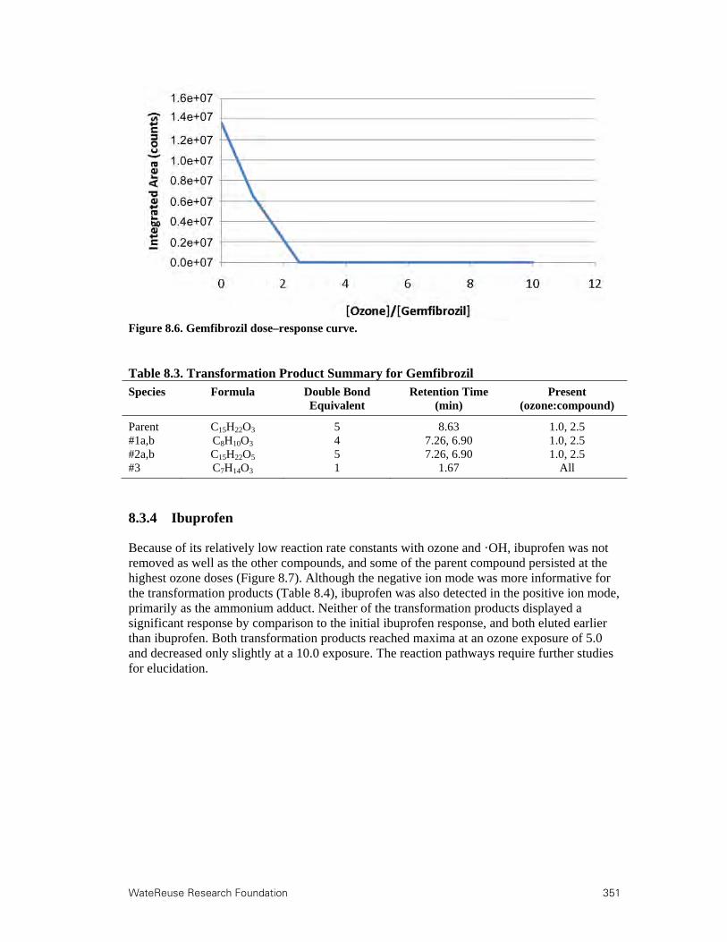
WateReuse Research Foundation 351
Figure 8.6. Gemfibrozil dose–response curve.
Table 8.3. Transformation Product Summary for Gemfibrozil
Species Formula Double Bond Equivalent
Retention Time (min)
Present (ozone:compound)
Parent C15H22O3 5 8.63 1.0, 2.5 #1a,b C8H10O3 4 7.26, 6.90 1.0, 2.5 #2a,b C15H22O5 5 7.26, 6.90 1.0, 2.5 #3 C7H14O3 1 1.67 All
8.3.4 Ibuprofen
Because of its relatively low reaction rate constants with ozone and ·OH, ibuprofen was not removed as well as the other compounds, and some of the parent compound persisted at the highest ozone doses (Figure 8.7). Although the negative ion mode was more informative for the transformation products (Table 8.4), ibuprofen was also detected in the positive ion mode, primarily as the ammonium adduct. Neither of the transformation products displayed a significant response by comparison to the initial ibuprofen response, and both eluted earlier than ibuprofen. Both transformation products reached maxima at an ozone exposure of 5.0 and decreased only slightly at a 10.0 exposure. The reaction pathways require further studies for elucidation.

352 WateReuse Research Foundation
Figure 8.7. Ibuprofen dose–response curve.
Table 8.4. Transformation Product Summary for Ibuprofen
Species Formula Double Bond Equivalent
Retention Time (min)
Present (ozone:compound)
Parent C13H18O2 5 7.80 All #1 C12H16O 5 6.49 All #2 C9H10O 5 4.65 All
8.3.5 Naproxen
Because of its high reaction rate constants, naproxen reacted readily and completely during ozonation and was below detection with an ozone exposure of 2.5 (Figure 8.8). Naproxen was studied only in negative ion mode, and it displayed significant fragmentation—primarily from the loss of CO2—in the ionization process. Based on the data in Table 8.5, all of the transformation products eluted earlier than naproxen. Product #1 displayed significant relative intensity, reached a maximum at an ozone:compound ratio of 2.5, and was mostly degraded with an ozone:compound ratio of 10.0. Product #2 coeluted with #1, followed a similar formation–degradation pattern, but was significantly less intense. The reaction pathways require further study for elucidation, as the mass spectra may be complicated because of fragmentation during the ionization process. It is proposed that Product #1 results from the reaction of ozone at the aromatic rings to form two aldehyde groups, and the ionization process involves the loss of the carboxylic acid group as CO2.

WateReuse Research Foundation 353
Figure 8.8. Naproxen dose–response curve.
Table 8.5. Transformation Product Summary for Naproxen
Species Formula Double Bond Equivalent
Retention Time (min)
Present (ozone:compound)
Parent C14H14O3 9 6.90 1.0 #1 C13H14O3 7 5.55 All #2 C11H10O4 7 5.55 All
8.3.6 Sulfamethoxazole
Also because of its high reaction rate constants, sulfamethoxazole was degraded extensively during ozonation (Figure 8.9) and was barely detected after an exposure of 5.0. Although sulfamethoxazole displayed the highest intensity in the positive ion mode, no transformation products were detected. Based on the data in Table 8.6, one transformation product was observed in he negative ion mode (#1), which was moderate in intensity compared to the (M–H)- ion of sulfamethoxazole.

354 WateReuse Research Foundation
Figure 8.9. Sulfamethoxazole dose–response curve.
Table 8.6. Transformation Product Summary for Sulfamethoxazole
Species Formula Double Bond Equivalent
Retention Time (min)
Present (ozone:compound)
Parent C10H11N3O3S 9 4.20 1.0, 2.5 #1 C7H5N3O4S 7 4.95 All
8.3.7 Trimethoprim
Despite trimethoprim’s high reaction rates with ozone and hydroxyl radicals, the compound was relatively persistent during the transformation product evaluation. In fact, a small amount of trimethoprim persisted even at the highest ozone exposure (Figure 8.10). Trimethoprim and its transformation products (Table 8.7) ionized more efficiently in positive ion mode, although some response was noted in negative ion mode for the (M–H)- and (M+CH3COO)- adducts. Product #2 displayed a moderate intensity compared to trimethoprim, whereas the others exhibited a low response. Products #1, #2, and #4 displayed a maximum intensity at an ozone:compound ratio of 1.0, and they were degraded by a 7.5 ozone exposure. The intensity of Product #3 reached a maximum at an ozone:compound ratio of 7.5.
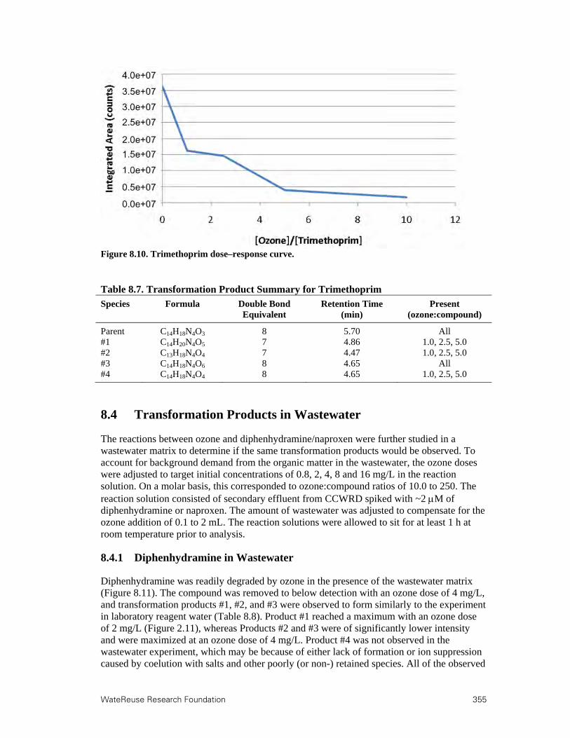
WateReuse Research Foundation 355
Figure 8.10. Trimethoprim dose–response curve.
Table 8.7. Transformation Product Summary for Trimethoprim
Species Formula Double Bond Equivalent
Retention Time (min)
Present (ozone:compound)
Parent C14H18N4O3 8 5.70 All #1 C14H20N4O5 7 4.86 1.0, 2.5, 5.0 #2 C13H18N4O4 7 4.47 1.0, 2.5, 5.0 #3 C14H18N4O6 8 4.65 All #4 C14H18N4O4 8 4.65 1.0, 2.5, 5.0
8.4 Transformation Products in Wastewater
The reactions between ozone and diphenhydramine/naproxen were further studied in a wastewater matrix to determine if the same transformation products would be observed. To account for background demand from the organic matter in the wastewater, the ozone doses were adjusted to target initial concentrations of 0.8, 2, 4, 8 and 16 mg/L in the reaction solution. On a molar basis, this corresponded to ozone:compound ratios of 10.0 to 250. The reaction solution consisted of secondary effluent from CCWRD spiked with ~2 M of diphenhydramine or naproxen. The amount of wastewater was adjusted to compensate for the ozone addition of 0.1 to 2 mL. The reaction solutions were allowed to sit for at least 1 h at room temperature prior to analysis.
8.4.1 Diphenhydramine in Wastewater
Diphenhydramine was readily degraded by ozone in the presence of the wastewater matrix (Figure 8.11). The compound was removed to below detection with an ozone dose of 4 mg/L, and transformation products #1, #2, and #3 were observed to form similarly to the experiment in laboratory reagent water (Table 8.8). Product #1 reached a maximum with an ozone dose of 2 mg/L (Figure 2.11), whereas Products #2 and #3 were of significantly lower intensity and were maximized at an ozone dose of 4 mg/L. Product #4 was not observed in the wastewater experiment, which may be because of either lack of formation or ion suppression caused by coelution with salts and other poorly (or non-) retained species. All of the observed

356 WateReuse Research Foundation
transformation products persisted until the solution was exposed to an ozone dose of 16 mg/L. No new transformation products were detected in these experiments compared to those conducted in laboratory reagent water.
Figure 8.11. Diphendramine dose–response curve in wastewater.
Table 8.8. Transformation Product Summary for Diphenhydramine in Wastewater
Species Formula Double Bond Equivalent
Retention Time (min)
Present (ozone:compound)
Parent C17H21NO 8 7.36 0.8, 2.0 #1 C17H21NO2 8 7.46 0.8, 2.0, 4.0, 8.0 #2 C11H15NO3 5 5.25 0.8, 2.0, 4.0, 8.0 #3 C12H17NO4 5 1.67 2.0, 4.0, 8.0 #4 C5H13NO3 0 0.93 Not observed
Because many of the transformation products were validated in the wastewater matrix, the analysis can be expanded by rationalizing product formation mechanisms based on accepted ozone chemistry, as well as the interpretation of collision-induced dissociation (CID) spectra. For example, diphenhydramine contains a tertiary amine group, which is known to react with ozone to form an amine oxide functionality (Muñoz and von Sonntag, 2000). MS/MS experiments show that the main fragment of this species is C13H11
+, which results from the breaking of the ether C–O bond (illustrated in Figure 8.12). This supports the observation of the oxygen addition at the amine group. This process can be repeated for a variety of parent compounds and their transformation products to develop comprehensive reaction mechanisms and decomposition pathways.
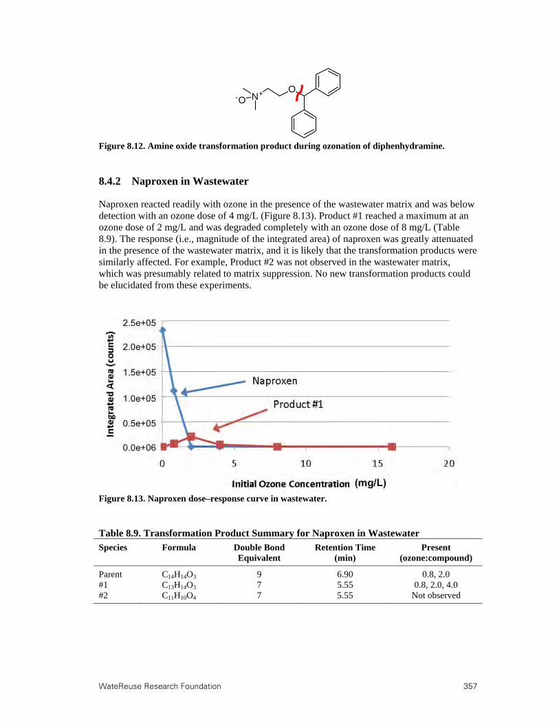
WateReuse Research Foundation 357
Figure 8.12. Amine oxide transformation product during ozonation of diphenhydramine.
8.4.2 Naproxen in Wastewater
Naproxen reacted readily with ozone in the presence of the wastewater matrix and was below detection with an ozone dose of 4 mg/L (Figure 8.13). Product #1 reached a maximum at an ozone dose of 2 mg/L and was degraded completely with an ozone dose of 8 mg/L (Table 8.9). The response (i.e., magnitude of the integrated area) of naproxen was greatly attenuated in the presence of the wastewater matrix, and it is likely that the transformation products were similarly affected. For example, Product #2 was not observed in the wastewater matrix, which was presumably related to matrix suppression. No new transformation products could be elucidated from these experiments.
Figure 8.13. Naproxen dose–response curve in wastewater.
Table 8.9. Transformation Product Summary for Naproxen in Wastewater
Species Formula Double Bond Equivalent
Retention Time (min)
Present (ozone:compound)
Parent C14H14O3 9 6.90 0.8, 2.0 #1 C13H14O3 7 5.55 0.8, 2.0, 4.0 #2 C11H10O4 7 5.55 Not observed
ON+-O

358 WateReuse Research Foundation
8.5 Conclusion
These results support the conclusion that conducting ozone oxidation reactions in laboratory reagent water is a valid first step in the identification of transformation products in environmental matrices. The more intense reaction products appeared to be consistent in both matrices, considering that their formation and disappearance profiles were similar and were relatively unaffected by the background organic matter in the wastewater matrix. However, some transformation products were not observed during the wastewater experiments, presumably because of ion suppression and matrix interference. On the other hand, ozonation of wastewater is known to initiate advanced oxidation processes (Buffle et al., 2006a), which would lead to both ozone and ·OH reactions, but there were no transformation products that were unique to the wastewater experiments. It is possible that matrix interference could suppress compounds unique to the wastewater matrix, but there is no direct evidence to support this theory, so additional testing would be necessary to prove or refute the claim.
LC Q-TOF MS proved to be a powerful technique for qualitatively identifying unknown transformation products, but a quantitative analysis is less easy. In electrospray ionization, the response factors of different compounds can vary markedly based on their chemical properties, and the ionization efficiency can be affected by such things as mobile phase composition (Rt versus gradient) and suppression because of matrix components. Therefore, the concentration of a product cannot be measured reliably without standards. The determination of exact chemical structures will also benefit by analysis of standard compounds, where the combination of matching retention time, accurate mass data, isotopic abundance, and fragmentation is generally considered to be sufficient for compound identification. Because standards for most transformation products are not commercially available, they require custom synthesis, which can be expensive and time-consuming. This makes the identification and quantification of large numbers of transformation products infeasible in many cases. Although comparisons with standards provide more concrete information, structural information can still be deduced by rationalizing product formation mechanisms based on accepted ozone chemistry, as well as the interpretation of CID spectra.
This analysis illustrates how unknown transformation products can be identified to develop standards for quantification and to propose reaction pathways. However, this does not necessarily provide any information on the potential health impacts of the resulting transformation products. Qualitative evaluations of transformation products must be coupled with sensitive bioassays or computer modeling programs to estimate the resulting toxicity. This type of comprehensive analysis is better suited to matrices with demonstrated toxicity, because most oxidation byproducts will have limited toxic effects at relevant concentrations. Alternatively, assuming standards can be developed for individual transformation products, these compounds could also be spiked into water for subsequent bioassay analysis. Because of the tremendous costs (for analysis and synthesis of standards) and required time associated with such comprehensive evaluations, linking transformation products to toxicity was outside the scope of this study. However, this evaluation was effective in characterizing the transformation products of several target compounds, in addition to validating the use of both laboratory-grade water and environmental matrices for transformation product analyses.
WateReuse Research Foundation 359
Chapter 9
9.Bench-Scale Soil Column Testing
9.1 Introduction
During soil transport, oxic biodegradation, anoxic biodegradation, and sorption collectively provide an effective barrier for attenuation of EfOM and TOrCs. Many compounds approach their MRLs during ARR, whereas the more recalcitrant TOrCs require longer residence times or unique redox conditions. Previous TOrC research related to ARR can be summarized as follows: (1) removal of biodegradable TOrCs under aerobic porous infiltration conditions is generally equal to or better than that under anoxic porous infiltration conditions, (2) BDOC acts as a cosubstrate in cometabolic TOrC transformation, (3) the concentration and character of EfOM affect TOrC biodegradation efficiency during recharge operations, and (4) redox conditions and temperature are key factors in influencing performance (Hoppe-Jones et al., 2010; Maeng et al., 2010).
As described earlier, ozonation converts refractory DOC, such as humic and fulvic acids, into more biodegradable fractions. Past studies have shown that this EfOM transformation also increases the biodegradability of recalcitrant TOrCs in ARR systems because of improved cometabolism. Therefore, preozonation (i.e., prior to ARR) can be used to (1) reduce the TOrC loading to the environment with direct oxidation and (2) make the matrix more amenable to biotransformation, thereby achieving further TOrC reductions. In a postozonation strategy, ARR will remove a significant amount of EfOM and reduce the concentrations of contaminant precursors and specific TOrCs. This will reduce the oxidant scavenging potential of the matrix and increase the overall efficiency of the downstream ozone process. In other words, ozonation can be an effective treatment strategy in both locations.
For this phase of the study, ozone oxidation before and after soil passage was tested for TOrC removal. The attenuation of bulk organics and TOrCs in different treatment scenarios (i.e., O3–ARR vs. ARR–O3) was examined to understand parameters and conditions controlling their removal. Both treatment configurations were considered because the O3–ARR approach provides a barrier against transformation products, and the ARR–O3 approach leads to lower costs because of reduced ozone demands. BDOC fractions and their biodegradation rates (slow vs. rapid) were also compared in these experiments using a variety of organic characterization methods.
9.2 Methods
9.2.1 Experimental Setup
In bench-scale tests, Milli-Q water was ozonated in 2-L glass flasks by bubbling ozone generated from a LAB2B ozone generator (Ozonia, Degremont Technologies, Leonia, NJ). The dissolved ozone in the stock solution was measured periodically at a wavelength of 258 nm (E=2950 M-1cm-1) (Rakness et al., 1996) and was confirmed by the indigo trisulfonate method (Bader and Hoigné, 1981). A specific volume of the ozonated water was transferred

360 WateReuse Research Foundation
to batch reactors that contained secondary effluent from the Al-Ruwais Wastewater Treatment Plant (ARWWTP; Jeddah, Saudi Arabia) at room temperature (21°C). O3: DOC ratios of 0.5 and 1.0 were selected to remain consistent with the previous experiments in this study and because of their demonstrated efficacy in oxidizing a wide range of contaminants.
For the soil component, the batch sands were prepared in 1-L glass bottles using 150 g (dry weight) of washed silica sand (grain sizes 0.5–1 mm; bulk density 1.5–1.6 g/cm3; sand porosity 40%). The sands were then bioacclimated for 8 weeks with secondary effluent from ARWWTP. During this period, DOC and UV254 absorbance were monitored until a steady state was achieved. After the acclimation period, the soil batch reactors were fed with secondary effluent or ozonated secondary effluent until a range of retention times had been achieved (3 h, 1, 3, 5, 8, and 12 days). Water samples were then collected for TOrC analysis or for postozonation. This experimental setup allowed evaluations of TOrC mitigation with ARR alone, O3–ARR, and ARR–O3. To differentiate microbial biodegradation and sorption, abiotic batch reactors were also prepared with sodium azide at 20 mM (Maeng, 2010) and monitored over 5 days. Sorption isotherms were generated using a linear regression analysis with TOrC concentrations ranging from 0.5 to 10 μg/L. The typical water quality of the ARWWTP secondary effluent is summarized in Table 9.1, and an overview of the experimental approach is provided in Figure 9.1.
Table 9.1. ARWWTP Secondary Effluent Water Quality
Parameter Value
pH 7.1 TOC (mg-C/L) 5.9 UV254 absorbance (cm-1) 0.148 Turbidity (NTU) 0.47 Fluoride (mg/L) 0.21 Chloride (mg/L) 746 Nitrite (mg-N/L) <MRL Nitrate (mg/L) 28 Bromide (mg/L) 1.44 Sulfate (mg/L) 11 Phosphate (mg/L) 411

WateReuse Research Foundation 361
Figure 9.1. Simplified schematic for experimental ARR scenarios.
9.2.2 Analysis of Bulk Organics
DOC was measured using a Shimadzu TOC analyzer and BDOC was measured weekly during the bioacclimation period (8 weeks). In addition, UV254 and SUVA were monitored as indicators of aromaticity and humic substances using a Shimadzu UV-vis spectrophotometer (UV-2550). LC-OCD-OND-UV254nm based on the Gräntzel thin-film UV reactor (DOC-Labor Dr. Huber, Germany) was used to evaluate major fractions of natural organic matter, such as slowly degrading biopolymers versus rapidly degrading low-molecular-weight acids and neutrals, during treatment processes. Proteins (i.e., soluble microbial product-like), humic-like, and fulvic-like EfOM were characterized using fluorescence excitation–emission matrices using a FlouroMax4 (Horiba, USA). The spectrofluorometer included a 150-W xenon lamp. The slit width for both excitation and emission monochromators was set to 5 nm, and a 5-nm increment was used. Analyses were performed in a 1-cm quartz cuvette at room temperature (21°C). Samples were analyzed in signal/reference mode, where the fluorescence emission intensity is normalized to the intensity of the lamp at the particular excitation wavelength applied.
9.2.3 TOrC Analysis
The TOrC samples were collected in amber glass bottles and were preserved with sodium azide (1 g/L) and ascorbic acid (50 mg/L). The samples were then shipped to the SNWA laboratory, where they were processed and analyzed, as described previously.
9.3 EfOM Characterization
A net reduction in DOC was observed in all systems (ARR alone, O3–ARR, and ARR–O3), as shown in Table 9.2. The most effective treatment was observed in the O3–ARR configuration (29% reduction), followed by the ARR–O3 configuration (24% reduction), with both

362 WateReuse Research Foundation
operating at an O3:DOC ratio of 1.0. At an O3:DOC ratio of 0.5, O3–ARR achieved a 23% reduction in DOC, ARR alone achieved a 17% reduction, and ARR–O3 achieved a 16% reduction. The UV254 absorbance and specific UV254 absorbance (SUVA=UV254 absorbance/DOC) data indicated that the O3–ARR and ARR–O3 were superior to ARR alone. For UV254 absorbance, ARR–O3 achieved 60% and 72% reductions at O3:DOC ratios of 0.5 and 1.0, respectively, and O3–ARR provided 49% and 57%, respectively. However, ARR alone only achieved a 28% reduction in UV254 absorbance. Overall, DOC removal was higher with preozonation because of the increase in BDOC during oxidation, and the reduction in UV254 absorbance was higher with postozonation because of the more efficient destruction of aromatic humic substances.
Table 9.2. Percent Reduction in DOC and UV254 Absorbance (ARR=12 days)
O3:DOC ARRs % DOC Removal % UV254
Removal
0 ARR alone 17 28 0.5 O3-ARR 23 49 0.5 ARR-O
3 16 60
1 O3-ARR 29 57 1 ARR-O
3 24 72
These results indicate that ozonation is effective in transforming the aromaticity and larger humic components of EfOM. Figure 9.2 illustrates the SUVA values for the various ARR configurations after 12 days of residence time. O3–ARR and ARR–O3 consistently achieved lower SUVA values than ARR alone, and ARR–O3 was the more effective configuration among the ozone alternatives. Further reductions were observed after eight days of retention time in the batch soil systems. This may be attributable to the refractory components of humic or fulvic substances taking longer to degrade than overall BDOC and/or a potential transformation of humic substances.
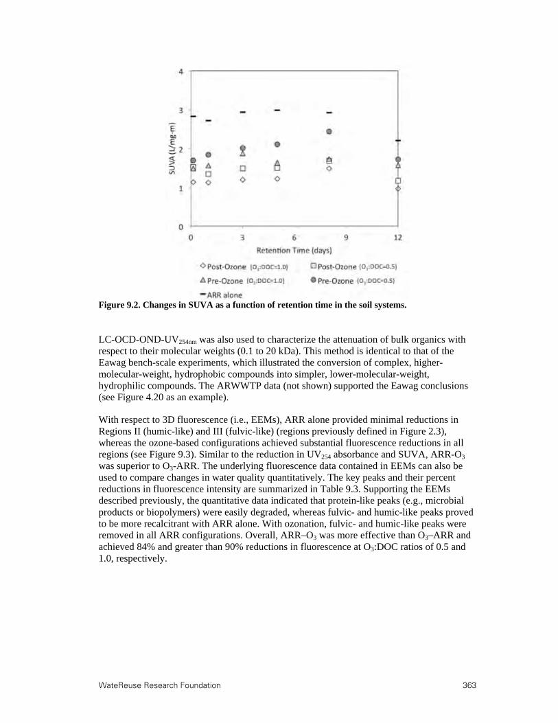
WateReuse Research Foundation 363
Figure 9.2. Changes in SUVA as a function of retention time in the soil systems.
LC-OCD-OND-UV254nm was also used to characterize the attenuation of bulk organics with respect to their molecular weights (0.1 to 20 kDa). This method is identical to that of the Eawag bench-scale experiments, which illustrated the conversion of complex, higher-molecular-weight, hydrophobic compounds into simpler, lower-molecular-weight, hydrophilic compounds. The ARWWTP data (not shown) supported the Eawag conclusions (see Figure 4.20 as an example).
With respect to 3D fluorescence (i.e., EEMs), ARR alone provided minimal reductions in Regions II (humic-like) and III (fulvic-like) (regions previously defined in Figure 2.3), whereas the ozone-based configurations achieved substantial fluorescence reductions in all regions (see Figure 9.3). Similar to the reduction in UV254 absorbance and SUVA, ARR-O3 was superior to O3-ARR. The underlying fluorescence data contained in EEMs can also be used to compare changes in water quality quantitatively. The key peaks and their percent reductions in fluorescence intensity are summarized in Table 9.3. Supporting the EEMs described previously, the quantitative data indicated that protein-like peaks (e.g., microbial products or biopolymers) were easily degraded, whereas fulvic- and humic-like peaks proved to be more recalcitrant with ARR alone. With ozonation, fulvic- and humic-like peaks were removed in all ARR configurations. Overall, ARR–O3 was more effective than O3–ARR and achieved 84% and greater than 90% reductions in fluorescence at O3:DOC ratios of 0.5 and 1.0, respectively.
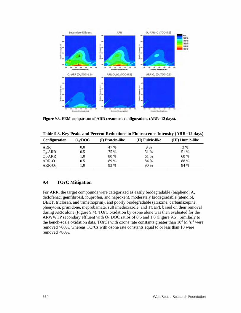
364 WateReuse Research Foundation
Figure 9.3. EEM comparison of ARR treatment configurations (ARR=12 days).
Table 9.3. Key Peaks and Percent Reductions in Fluorescence Intensity (ARR=12 days)
Configuration O3:DOC (I) Protein-like (II) Fulvic-like (III) Humic-like
ARR 0.0 47 % 9 % 3 % O3-ARR 0.5 75 % 51 % 51 % O3-ARR 1.0 80 % 61 % 60 % ARR-O3 0.5 89 % 84 % 88 % ARR-O3 1.0 93 % 90 % 94 %
9.4 TOrC Mitigation
For ARR, the target compounds were categorized as easily biodegradable (bisphenol A, diclofenac, gemfibrozil, ibuprofen, and naproxen), moderately biodegradable (atenolol, DEET, triclosan, and trimethoprim), and poorly biodegradable (atrazine, carbamazepine, phenytoin, primidone, meprobamate, sulfamethoxazole, and TCEP), based on their removal during ARR alone (Figure 9.4). TOrC oxidation by ozone alone was then evaluated for the ARWWTP secondary effluent with O3:DOC ratios of 0.5 and 1.0 (Figure 9.5). Similarly to the bench-scale oxidation data, TOrCs with ozone rate constants greater than 103 M-1s-1 were removed >80%, whereas TOrCs with ozone rate constants equal to or less than 10 were removed <80%.

WateReuse Research Foundation 365
Figure 9.4. TOrC mitigation by ARR alone.
Figure 9.5. TOrC mitigation by ozone alone.
Figure 9.6 illustrates the relative contributions of oxidation and biodegradation/sorption to TOrC removal during O3–ARR and ARR–O3. The data points represent the expected reductions in concentration with 12 days of soil treatment and/or an O3:DOC ratio of 1.0. This summary figure indicates that a majority of the TOrCs can be removed easily by ozone alone or a combination of ozone and ARR. Some of the compounds were resistant to ARR but were susceptible to ozone (carbamazepine, sulfamethoxazole, primidone, and phenytoin), but only DEET proved to be resistant to ozone but moderately susceptible to ARR. Several

366 WateReuse Research Foundation
compounds demonstrated resistance to both ozone and ARR (meprobamate, atrazine, and TCEP). Figure 9.7 further illustrates the impacts of varying ozone dose and treatment process configuration. Although previous literature suggests that preozonation provides greater potential for cometabolism, postozonation (i.e., ARR–O3) achieved lower effluent concentrations for the recalcitrant TOrCs, excluding TCEP. Implementing some form of biological filtration prior to ozonation appears to remove the bioamenable compounds that react rapidly with ozone, thereby reducing oxidant scavenging. This increases the efficacy of downstream ozonation despite similar O3:DOC ratios in both configurations. Although untested in this study, a combination of pre- and postozonation, as is employed at several full-scale facilities (e.g., GCGA), may be the optimal condition. This would increase the ratio of bioamenable organic matter prior to ARR, which would further increase cometabolism of recalcitrant TOrCs and reduce oxidant scavenging for downstream ozonation.
Figure 9.6. TOrC removal by ARR (12 days) and/or ozone (O3:DOC=1.0).
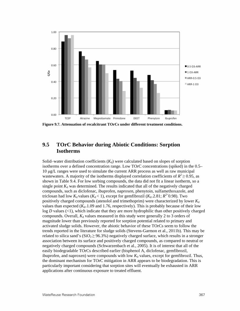
WateReuse Research Foundation 367
Figure 9.7. Attenuation of recalcitrant TOrCs under different treatment conditions.
9.5 TOrC Behavior during Abiotic Conditions: Sorption Isotherms
Solid–water distribution coefficients (Kd) were calculated based on slopes of sorption isotherms over a defined concentration range. Low TOrC concentrations (spiked) in the 0.5–10 μg/L ranges were used to simulate the current ARR process as well as raw municipal wastewaters. A majority of the isotherms displayed correlation coefficients of R2 ≥ 0.95, as shown in Table 9.4. For low sorbing compounds, the data did not fit a linear isotherm, so a single point Kd was determined. The results indicated that all of the negatively charged compounds, such as diclofenac, ibuprofen, naproxen, phenytoin, sulfamethoxazole, and triclosan had low Kd values (Kd < 1), except for gemfibrozil (Kd=2.81; R2=0.98). Two positively charged compounds (atenolol and trimethoprim) were characterized by lower Kd values than expected (Kd=1.09 and 1.76, respectively). This is probably because of their low log D values (<1), which indicate that they are more hydrophilic than other positively charged compounds. Overall, Kd values measured in this study were generally 2 to 3 orders of magnitude lower than previously reported for sorption potential related to primary and activated sludge solids. However, the abiotic behavior of these TOrCs seem to follow the trends reported in the literature for sludge solids (Stevens-Garmon et al., 2011b). This may be related to silica sand’s (SiO2 ≥ 96.3%) negatively charged surface, which results in a stronger association between its surface and positively charged compounds, as compared to neutral or negatively charged compounds (Schwarzenbach et al., 2005). It is of interest that all of the easily biodegradable TOrCs described earlier (bisphenol A, diclofenac, gemfibrozil, ibuprofen, and naproxen) were compounds with low Kd values, except for gemfibrozil. Thus, the dominant mechanism for TOrC mitigation in ARR appears to be biodegradation. This is particularly important considering that sorption sites will eventually be exhausted in ARR applications after continuous exposure to treated effluent.

368 WateReuse Research Foundation
Table 9.4. Measured Kd Values Based on Sorption Isotherms
Compound Kd (L/kg) R2
Atenolol 1.09 1.00 Atrazine 2.57 0.99 BPA 0.67 N/A* Carbamazepine 1.11 1.00 DEET 3.23 0.97 Diclofenac 0.87 N/A Gemfibrozil 2.81 0.98 Ibuprofen 0.66 N/A Musk ketone 0.99 N/A Naproxen 0.71 N/A Phenytoin 0.67 1.00 Primidone 1.11 1.00 Sulfamethoxazole 0.68 0.99 TCPP 2.41 0.99 Triclosan 0.74 0.95 Trimethoprim 1.76 0.99
* Kd values without an R2 value are based on single-point calculations. **Meprobamate was excluded because its analytical standard was unavailable.
9.6 Disinfection Byproduct Formation during Ozonation and Mitigation with ARR
The initial bromide concentration in the ARWWTP secondary effluent was approximately 1.4 mg/L, but the experimental samples contained approximately 899 μg/L because of the dilution effect of the ozone stock. The secondary effluent also included an ambient bromate concentration of 26.1 μg/L, but the source of this bromate is unclear. After ozonation, the bromate level ranged from 36.7 to 120 for O3:TOC ratios ranging from 0.25 to 1.5, respectively.
NDMA is typically present in primary and secondary effluents, with median concentrations of 26 ng/L in the United States (Pehlivanoglu-Mantas and Sedlak, 2006) and 5 ng/L in Switzerland (Krauss et al., 2009). Ozonation of secondary effluent often exacerbates this problem in many matrices, as demonstrated in the bench-scale experiments. For ARWWTP, the secondary effluent contained 7 ng/L of NDMA, and the concentration increased to 12 ng/L after ozonation with an O3:DOC ratio of 1.0. However, the ARR experiments indicated that downstream biological filtration was able to reduce the NDMA concentrations to the reporting limits of the assay (i.e., <5 ng/L) in all samples. The MRL was achieved after 12 days of soil treatment even when NDMA was spiked at ~500 ng/L. This is also consistent with previously published research (Zhou et al., 2009). The data indicate that NDMA precursors were also removed during the ARR process, because there was no reportable NDMA formation during ARR–O3. Therefore, ARR is an effective treatment barrier against NDMA and may eliminate the need for UV photolysis in IPR applications.
9.7 Conclusion
ARR is a robust treatment process capable of achieving substantial removal of many contaminants. The more bioamenable compounds are removed rapidly during soil treatment, but the more recalcitrant compounds may require long residence times or unique redox
WateReuse Research Foundation 369
conditions. Ozone alone is capable of eliminating many TOrCs, but ozone generally achieves incomplete oxidation (i.e., limited mineralization), is unable to destroy some compounds (e.g., TCEP), and only transforms other compounds into simpler oxidation byproducts. Therefore, ARR is an effective secondary barrier to protect human health against these persistent contaminants. The ARR and isotherm experiments in this study indicated that biodegradation was more significant than sorption during soil aquifer treatment, and these collective processes may also be supplemented with dilution in applications that limit recycled water contributions. Therefore, there is a potential for significant reductions in TOrC concentrations during ARR with a variety of mechanisms. With respect to CDPH regulations for spreading applications, at least 90% removal of indicator compounds must be achieved by the biodegradation and sorption pathways. Published research indicates that biodegradation of target contaminants is often more efficient and complete in natural ecosystems comprising diverse microbial communities. There are often complex interactions, feedback, and “communication” between the microbial species that promote degradation pathways. Also, it is often unnecessary to supplement the system with oxygen, organic substrates, or specific microbial species, although exceptions do exist. For example, the reductive dehalogenation of trichloroethene in groundwater is achieved by a specific genus of bacteria (Dehalococcoides), and the process may be improved by adding hydrogen gas to the system (Ernst, 2009). Furthermore, bioremediation of MTBE can be improved by supplementing the “biobarrier” with oxygen (Miller et al., 2001). On the other hand, nonspecific degradation of TOrC mixtures, which is important in IPR applications, can often be achieved under ambient conditions.
In the WRRF-08-05 ARR experiments, both O3–ARR (i.e., preozonation) and ARR–O3 (i.e., postozonation) were more effective than ARR alone in addressing a variety of bulk and trace organics. O3–ARR was superior for overall removal of DOC, whereas ARR–O3 was more effective in reducing UV absorbance, fluorescence, and TOrC concentrations. Finally, ARR proved to be an effective mitigation strategy for ambient NDMA and any NDMA that formed during ozonation. These results also indicate that the reductions in NDMA during soil aquifer treatment may eliminate the need for UV photolysis in typical groundwater replenishment treatment schemes (i.e., FAT). Future research must identify which variables are most critical in terms of TOrC mitigation during ARR or whether travel/storage time alone essentially controls the process. Furthermore, future research should identify strategies to develop engineered soil aquifer treatment to replace natural systems and ultimately eliminate the environmental buffer. This would facilitate the transition from indirect potable reuse to direct potable reuse.

WateReuse Research Foundation 371
Chapter 10
10.Conceptual Level Cost Estimates
10.1 Introduction
Class 4 (i.e., conceptual level) cost estimates (AACE, 2003) were performed to support the data reported earlier in this report and to provide a basis for comparison of various treatment processes evaluated in this study. Conceptual level costs are defined as providing reasonable accuracy to within -30% and +50% of actual costs and can be estimated when ≤1% of design is completed, which is appropriate for this research project. The approach developed by the Project Team is summarized as follows:
Choose unit processes that support the scope of the research project.
Develop capital and operations and maintenance (O&M) cost estimates for key unit processes based on literature, project, and vendor reviews (costs updated to 2011 based on inflation and market changes).
Determine a relative cost estimate for unit processes including microfiltration or ultrafiltration membranes (MF/UF), nanofiltration or reverse osmosis membranes (NF/RO), ozone, ultraviolet light with H2O2 (UV/H2O2), and biological activated carbon (BAC).
Apply cost curves to each unit process, accounting for variability, to determine and evaluate capital and O&M cost on a per-unit-flow capacity basis.
Use ozone bench- and pilot-scale project results (i.e., dosing for desired contaminant oxidation) to estimate O&M costs associated with unit processes.
Develop tables that a user can use to estimate the capital and O&M costs for combinations of specific unit processes at a specific flow capacity.
This approach should allow readers to choose one or more unit processes that would achieve the water quality goals of their preliminary designs and determine the collective capital and O&M Class 4 estimated costs. Through this process, a user could compare the estimated costs associated with different process trains to achieve specific water quality objectives related to TOrCs mitigation.
10.2 Unit Processes Selected for Cost Estimates
Rather than trying to develop cost curves for the entire array of potential water reclamation treatment options (i.e., raw wastewater advanced treatment), the project team assumed that the reader considering water reuse technologies is familiar with the costs associated with conventional wastewater treatment, particularly primary, secondary, and tertiary treatment. Only advanced treatment options were used in the development of the cost curves. The objective here was to provide a toolbox of potential advanced treatment options that could be selected based on the treatment objectives and size/capacity of a given facility. The individual costs would then be summed to obtain an estimated cost for the overall treatment train, which
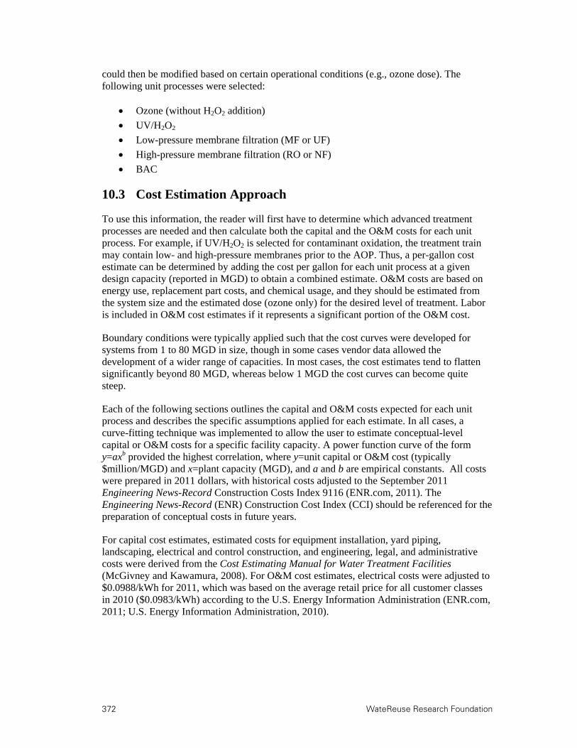
372 WateReuse Research Foundation
could then be modified based on certain operational conditions (e.g., ozone dose). The following unit processes were selected:
Ozone (without H2O2 addition)
UV/H2O2
Low-pressure membrane filtration (MF or UF)
High-pressure membrane filtration (RO or NF)
BAC
10.3 Cost Estimation Approach
To use this information, the reader will first have to determine which advanced treatment processes are needed and then calculate both the capital and the O&M costs for each unit process. For example, if UV/H2O2 is selected for contaminant oxidation, the treatment train may contain low- and high-pressure membranes prior to the AOP. Thus, a per-gallon cost estimate can be determined by adding the cost per gallon for each unit process at a given design capacity (reported in MGD) to obtain a combined estimate. O&M costs are based on energy use, replacement part costs, and chemical usage, and they should be estimated from the system size and the estimated dose (ozone only) for the desired level of treatment. Labor is included in O&M cost estimates if it represents a significant portion of the O&M cost.
Boundary conditions were typically applied such that the cost curves were developed for systems from 1 to 80 MGD in size, though in some cases vendor data allowed the development of a wider range of capacities. In most cases, the cost estimates tend to flatten significantly beyond 80 MGD, whereas below 1 MGD the cost curves can become quite steep.
Each of the following sections outlines the capital and O&M costs expected for each unit process and describes the specific assumptions applied for each estimate. In all cases, a curve-fitting technique was implemented to allow the user to estimate conceptual-level capital or O&M costs for a specific facility capacity. A power function curve of the form y=axb provided the highest correlation, where y=unit capital or O&M cost (typically $million/MGD) and x=plant capacity (MGD), and a and b are empirical constants. All costs were prepared in 2011 dollars, with historical costs adjusted to the September 2011 Engineering News-Record Construction Costs Index 9116 (ENR.com, 2011). The Engineering News-Record (ENR) Construction Cost Index (CCI) should be referenced for the preparation of conceptual costs in future years.
For capital cost estimates, estimated costs for equipment installation, yard piping, landscaping, electrical and control construction, and engineering, legal, and administrative costs were derived from the Cost Estimating Manual for Water Treatment Facilities (McGivney and Kawamura, 2008). For O&M cost estimates, electrical costs were adjusted to $0.0988/kWh for 2011, which was based on the average retail price for all customer classes in 2010 ($0.0983/kWh) according to the U.S. Energy Information Administration (ENR.com, 2011; U.S. Energy Information Administration, 2010).

WateReuse Research Foundation 373
10.4 Ozone Cost Estimate
10.4.1 Ozone Capital Costs
Ozone capital costs were based on data provided by a reputable vendor and were limited to projects designed or built within the past three years. Specifically, the vendor provided costs for facilities ranging from 10 MGD to more than 500 MGD and specified the ozone system size in pounds per day of production. Facility costs for flows less than 10 MGD were not available because of the steep rise in cost for smaller systems.
In developing a baseline ozone dose for the cost estimate, the Project Team assumed a representative TOC of 6 mg/L and a target O3:TOC ratio of 0.5, leading to an applied ozone dose of 3 mg/L. As shown throughout this study, an O3:TOC ratio of 0.5 is quite effective in destroying a wide range of contaminants and achieving significant microbial inactivation. However, some applications will require lower or higher ozone doses, depending on the water quality and treatment objectives. The cost estimation method for ozone doses other than 3 mg/L is described later in this chapter (see Section 10.9.2).
Figure 10.1 provides a graphical representation of the cost curve for ozone systems, including all construction, equipment, and engineering costs along with contractor overhead and profit (OH&P) and contingency. Table 10.1 provides the Project Team’s estimates for the capital costs associated with the physical structures for the contactors. In developing the costs associated with the contactors, it was assumed that the design would provide a hydraulic residence time (HRT) of 5 min. In water reclamation applications, the high level of EfOM imparts a high ozone demand, which results in rapid loss of ozone residual. Typical contactor designs for drinking water applications, which may have contact times of 10 to 20 min, would often be excessive for water reclamation applications. Therefore, the 5-min HRT used for this cost estimate would generally be sufficient to allow complete ozone decay, assuming O3:TOC ratios less than 1.0. Table 10.2 shows the vendor data for the equipment used in the cost curve development, which includes ozone generators, a liquid oxygen (LOX) system (but not LOX consumable costs), a supplemental nitrogen system, ozone injection or diffusers, ozone destruct units, monitors, and the overall control system. Table 10.3 provides the total estimated capital costs including installation (30%); yard piping (10%); landscaping (5%); electrical and control construction (20%); and engineering, legal, and administrative costs (35%). A single redundant ozone generator was included in the cost estimates. Contractor OH&P of 15% and a 30% contingency were also included in the cost estimates.
The Project Team’s estimates required that there be at least one contactor for each ozone generator. The contactors were designed to have a depth of 24 ft with19 ft of submergence and 5 ft of freeboard. Each contactor had between 2 and 10 cells, with a length of 4 ft/cell. The number of contactors for a capacity below 100 MGD was kept at one per generator, whereas the number of cells was adjusted to maintain a reasonable width (assumed to be less than 25 ft). For the larger systems, the number of contactors as well as the number of cells within each contactor was increased to maintain a reasonable contactor volume and width.
Capital costs are presented on a per capacity basis (i.e., $M/MGD). The resulting regression equation for estimating conceptual-level capital costs for a specific ozone facility capacity is as follows:
Ozone Capital Costs (in $M/MGD)=2.26 × (Plant Capacity in MGD)-0.54.
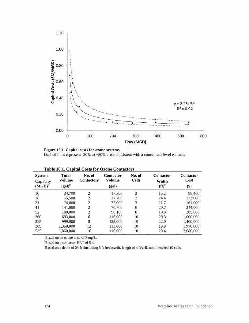
374 WateReuse Research Foundation
Figure 10.1. Capital costs for ozone systems. Dashed lines represent -30% to +50% error consistent with a conceptual-level estimate.
Table 10.1. Capital Costs for Ozone Contactors
System
Capacity
Total Volume
No. of Contactors
Contactor Volume
No. of Cells
Contactor
Width
Contactor Cost
(MGD)a (gal)b (gal) (ft)c ($)
10 34,700 2 17,300 2 15.2 98,400 16 55,500 2 27,700 2 24.4 133,000 21 74,000 2 37,000 3 21.7 161,000 41 141,000 2 70,700 6 20.7 244,000 52 180,000 2 90,100 8 19.8 285,000 200 693,000 6 116,000 10 20.3 1,000,000 288 999,000 8 125,000 10 22.0 1,400,000 389 1,350,000 12 113,000 10 19.8 1,970,000 535 1,860,000 16 116,000 10 20.4 2,680,000
aBased on an ozone dose of 3 mg/L. bBased on a contactor HRT of 5 min. cBased on a depth of 24 ft (including 5 ft freeboard), length of 4 ft/cell, not to exceed 10 cells.

WateReuse Research Foundation 375
Table 10.2. Capital Costs Associated with Ozone Generation System Components
System
Capacity
Ozone System
Operating Size
Ozone
Generators
Ozone Contactor
Capital Cost
Ozone Equipment
Capital Cost
Installation Cost @
30%
Ozone System
Cost
System Capital Unit
Cost
(MGD) (lb/day)a (Units
Capacity) 1.($M)b ($M)c ($M) ($M) ($M/MGD)
10 250 3 125 0.098 1.90 0.57 2.57 0.257 16 400 3 200 0.133 2.07 0.62 2.82 0.177 21 534 3 267 0.161 3.51 1.05 4.72 0.221 41 1,020 2 1020 0.244 2.50 0.75 3.49 0.086 52 1,300 3 650 0.285 4.20 1.26 5.74 0.111
200 5,000 3 2500 1.002 5.25 1.58 7.8 0.039 288 7,200 4 2400 1.404 6.67 2.00 10.1 0.035 389 9,750 4 3250 1.972 10.00 3.00 15.0 0.038 535 13,400 5 3350 2.682 12.5 3.75 18.9 0.035
aBased on an ozone dose of 3 mg/L, listed as lb/day production and operating with one generator in standby bOzone System costs include ozone generators, LOX system, supplemental nitrogen system, ozone injection or diffusers, ozone destruct units, monitors, and overall system control. Ozone system includes one redundant ozone generator cOzone equipment capital costs include one additional generator for redundancy, though the redundancy is not reflected in “Ozone System Operating Size”
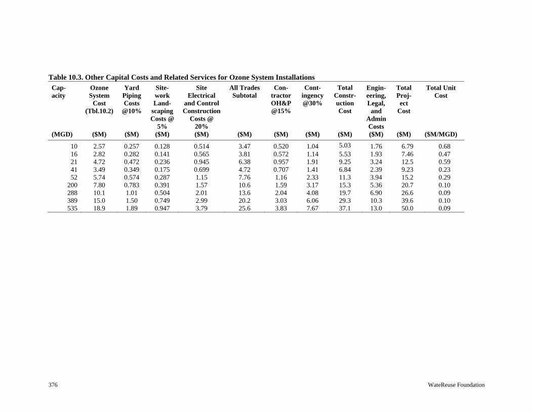
376 WateReuse Foundation
Table 10.3. Other Capital Costs and Related Services for Ozone System Installations
Cap-acity
Ozone System
Cost (Tbl.10.2)
Yard Piping Costs
@10%
Site-work Land-
scaping Costs @
5%
Site Electrical
and Control Construction
Costs @ 20%
All Trades Subtotal
Con-tractor OH&P @15%
Cont-ingency @30%
Total Constr-uction Cost
Engin-eering, Legal,
and Admin Costs
Total Proj-ect
Cost
Total Unit Cost
(MGD) ($M) ($M) ($M) ($M) ($M) ($M) ($M) ($M) ($M) ($M) ($M/MGD)
10 2.57 0.257 0.128 0.514 3.47 0.520 1.04 5.03 1.76 6.79 0.68 16 2.82 0.282 0.141 0.565 3.81 0.572 1.14 5.53 1.93 7.46 0.47 21 4.72 0.472 0.236 0.945 6.38 0.957 1.91 9.25 3.24 12.5 0.59 41 3.49 0.349 0.175 0.699 4.72 0.707 1.41 6.84 2.39 9.23 0.23 52 5.74 0.574 0.287 1.15 7.76 1.16 2.33 11.3 3.94 15.2 0.29
200 7.80 0.783 0.391 1.57 10.6 1.59 3.17 15.3 5.36 20.7 0.10 288 10.1 1.01 0.504 2.01 13.6 2.04 4.08 19.7 6.90 26.6 0.09 389 15.0 1.50 0.749 2.99 20.2 3.03 6.06 29.3 10.3 39.6 0.10 535 18.9 1.89 0.947 3.79 25.6 3.83 7.67 37.1 13.0 50.0 0.09

WateReuse Research Foundation 377
10.4.2 Ozone and Ozone/H2O2 Operations and Maintenance Costs
O&M costs for the ozone systems were limited to energy consumption associated with ozone generation and did not include maintenance or oxygen delivery or production (i.e., LOX, ambient air, or vacuum/pressure swing adsorption (VPSA) systems). Ambient air, LOX, and VPSA will increase the unit energy cost beyond what is described below and should be considered on a system-specific basis. Energy consumption (or energy equivalent consumption) for each type of oxygen delivery system will vary widely based on daily operating conditions, oxygen utilization efficiency, and system capacity. Detailed guidance on the costs associated with VPSA and LOX can be found in Chang et al. (2008). Maintenance costs and additional staff time were assumed to be minimal relative to the total energy costs; thus, they were not included in the calculation. The energy costs associated with ozone destruction, however, were included in the estimates provided in this report.
Therefore, the data shown in Table 10.4 and Figure 10.2 are representative of the vendor-supplied energy costs associated with ozone generation for systems ranging from 10 to 535 MGD. Even without inclusion of the maintenance and oxygen production or delivery costs, the energy costs per pound of ozone and per unit volume of treated water are still within the range reported by Chang et al. (2008). O&M costs are presented on a per-capacity basis (i.e., $M/MGD). The resulting regression equation for estimating conceptual-level O&M costs for a specific capacity is as follows:
Ozone O&M Costs (in $M/MGD)=0.0068 × (Plant Capacity in MGD)-0.051.
In applications where H2O2 addition is warranted (e.g., reductions in contactor size or bromate mitigation), the preceding O&M costs can be adjusted to include chemical addition. The modified estimate assumes that the impact of H2O2 addition on capital costs is insignificant, and the estimate is based on a conservative molar H2O2:O3 ratio of 1.0. Based on an ozone dose of 3 mg/L, this leads to a target H2O2 dose of approximately 2 mg/L. The H2O2 and quenching costs were based on vendor-supplied data for UV/H2O2 systems, which will be described in the next section. The estimates were adjusted in a linear fashion to account for the different doses in the ozone/H2O2 (2 mg/L) and UV/H2O2 (3 mg/L) systems. The annual O&M costs for ozone/H2O2 are summarized in Table 10.5 and illustrated in Figure 10.3. The regression equation for the annual O&M costs for ozone/H2O2 is as follows:
Ozone/H2O2 O&M Costs (in $M/MGD)=0.016 × (Plant Capacity in MGD)-0.020.
378 WateReuse Research Foundation
Figure 10.2. Annual O&M costs for ozone. Based on an ozone dose of 3 mg/L. Dashed lines represent -30% to +50% error consistent with a conceptual-level estimate.
Figure 10.3. Annual O&M costs for ozone/H2O2. Based on an ozone dose of 3 mg/L and an H2O2 dose of 2 mg/L (H2O2:O3=1.0). Dashed lines represent -30% to +50% error consistent with a conceptual-level estimate.

WateReuse Research Foundation 379
Table 10.4. Annual O&M Costs for Ozone
System
Capacity
Ozone System Size
Energy Consumption
Annual
Energy Cost
Unit
O&M Cost (MGD) (lb/day)a (kWh/lb O3) ($M)b ($M/MGD)
10 250 6.75 0.0610 0.0061 16 400 6.65 0.0960 0.0060 21 534 6.65 0.128 0.0060 41 1,020 5.75 0.211 0.0052 52 1,300 6.35 0.298 0.0057 200 5,000 5.65 1.02 0.0051 288 7,200 5.65 1.47 0.0051 389 9,750 5.65 1.99 0.0051 535 13,400 5.55 2.68 0.0050 aBased on an ozone dose of 3 mg/L. bBased on current electrical pricing of $0.0988/kWh.
Table 10.5. Annual O&M Costs for Ozone/H2O2
System Capacity
Ozone System Size
Energy Consumption
Annual Energy Cost
Annual H2O2 Cost
Annual Hypochlorite
Quenching Cost
Total O&M Cost
Unit O&M Cost
(MGD) (lb/day)a (kWh/lb O3) ($M)b ($M)c ($M) ($M/MGD) ($M/MGD)
10 250 6.75 0.0610 0.0340 0.0570 0.152 0.0152 16 400 6.65 0.0960 0.0544 0.0912 0.242 0.0151 21 534 6.65 0.128 0.0714 0.120 0.319 0.0152 41 1,020 5.75 0.211 0.139 0.234 0.584 0.0142 52 1,300 6.35 0.298 0.177 0.296 0.771 0.0148
200 5,000 5.65 1.02 0.680 1.14 2.84 0.0142 288 7,200 5.65 1.47 0.979 1.64 4.09 0.0142 389 9,750 5.65 1.99 1.32 2.22 5.53 0.0142 535 13,400 5.55 2.68 1.82 3.05 7.55 0.0141
aBased on an ozone dose of 3 mg/L. bBased on current electrical pricing of $0.0988/kWh. cBased on an H2O2 dose of 2 mg/L (H2O2:O3=1.0).

380 WateReuse Research Foundation
10.5 UV/H2O2 Cost Estimate
10.5.1 UV/H2O2 Capital Costs
Capital costs for UV/H2O2 were developed from cost curves provided by two major vendors. The cost curves were based on system capacities ranging from approximately 1 to 80 MGD for the first vendor and 10 to 80 MGD for the second vendor. Cost curves from a third, smaller vendor were significantly greater (approximately three times) and were therefore deemed to be unrepresentative of actual costs. The systems were sized based on 1.2-log (94%) removal of NDMA and 0.5-log (68%) removal of 1,4-dioxane per the 2008 CDPH Draft Groundwater Recharge Reuse Regulations. Although the actual system size and water quality objectives will vary from site to site, particularly outside of California, this baseline was chosen to enable comparison.
As mentioned earlier, CDPH recently published revisions to the 2008 draft regulations. Although the water quality objectives for full advanced treatment (i.e., MF-RO-UV/H2O2 or MF-RO-O3/H2O2) changed from 2008 to 2011, the level of treatment required for each set of regulations will still be relatively similar, thereby maintaining the relevance of the NDMA and 1,4-dioxane objectives. On the basis of the revisions, utilities will technically have to meet the notification levels for NDMA (10 ng/L) and 1,4-dioxane (1 μg/L). However, to validate their AOP, utilities will still have to demonstrate specified levels of reduction for a suite of trace organic contaminants, which will be selected based on system monitoring. As an alternative to the broad TOrC objectives, utilities can elect to satisfy the original 0.5-log reduction in 1,4-dioxane.
Figure 10.4 provides a graphical representation of the capital cost curves for the UV/H2O2 systems, including all construction, equipment, and engineering costs. The total costs are summarized in Table 10.6. The vendor estimates only accounted for equipment, therefore total system costs was estimated from the equipment cost plus installation (30%). Total project cost also included yard piping; landscaping; electrical and control construction; contractor OH&P; contingency (30%); and engineering, legal, and administration costs to determine the total estimated capital costs. Based on these estimates, conceptual-level capital costs for UV/H2O2 can be described by the following regression equation:
UV/H2O2 Capital Costs (in $M/MGD)=0.474 × (Plant Capacity, in MGD)-0.056.

WateReuse Research Foundation 381
Figure 10.4. Capital costs for UV/H2O2. Dashed lines represent -30% to +50% error consistent with a conceptual-level estimate.
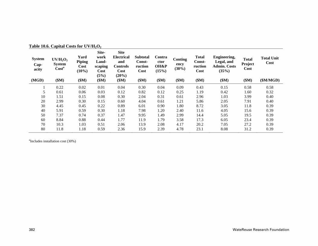
382 WateReuse Research Foundation
Table 10.6. Capital Costs for UV/H2O2
System
Cap-acity
UV/H2O2 System Costa
Yard Piping Cost
(10%)
Site-work Land-
scaping Cost (5%)
Site Electrical
and Controls
Cost (20%)
Subtotal Const-ruction
Cost
Contractor
OH&P (15%)
Contingency
(30%)
Total Const-ruction
Cost
Engineering, Legal, and
Admin. Costs (35%)
Total Project
Cost
Total Unit Cost
(MGD) ($M) ($M) ($M) ($M) ($M) ($M) ($M) ($M) ($M) ($M) ($M/MGD)
1 0.22 0.02 0.01 0.04 0.30 0.04 0.09 0.43 0.15 0.58 0.58 5 0.61 0.06 0.03 0.12 0.82 0.12 0.25 1.19 0.42 1.60 0.32
10 1.51 0.15 0.08 0.30 2.04 0.31 0.61 2.96 1.03 3.99 0.40 20 2.99 0.30 0.15 0.60 4.04 0.61 1.21 5.86 2.05 7.91 0.40 30 4.45 0.45 0.22 0.89 6.01 0.90 1.80 8.72 3.05 11.8 0.39 40 5.91 0.59 0.30 1.18 7.98 1.20 2.40 11.6 4.05 15.6 0.39 50 7.37 0.74 0.37 1.47 9.95 1.49 2.99 14.4 5.05 19.5 0.39 60 8.84 0.88 0.44 1.77 11.9 1.79 3.58 17.3 6.05 23.4 0.39 70 10.3 1.03 0.51 2.06 13.9 2.08 4.17 20.2 7.05 27.2 0.39 80 11.8 1.18 0.59 2.36 15.9 2.39 4.78 23.1 8.08 31.2 0.39
aIncludes installation cost (30%)

WateReuse Research Foundation 383
10.5.2 UV/H2O2 Operation and Maintenance Costs
O&M costs for UV/H2O2, which include equipment replacement, energy consumption, and chemical costs, were developed from cost curves provided by three major vendors. Labor is anticipated to be minimal relative to these other O&M costs and was therefore not included. The cost curves were based on system capacities ranging from approximately 1 to 80 MGD for the first vendor and 10 to 80 MGD for the other two vendors.
The selection of UV and H2O2 doses will influence the O&M costs for energy and chemicals and will vary significantly depending on the treatment application (e.g., disinfection versus chemical oxidation), source water quality, and product water quality criteria. In this case, vendors provided O&M cost estimates assuming chemical oxidation to meet water quality criteria for 1.2-log removal of NDMA and 0.5-log removal of 1,4-dioxane. Although the exact UV dose was not provided by the vendors, the estimated doses were up to 1500 mJ/cm2, and the peroxide doses were in the range of 2.5–3.5 mg/L. The source water was assumed to be RO-treated (earlier in the treatment train), resulting in a high UV transmittance compared to non-RO-treated waters. Here we have conservatively assumed a 95% transmittance for the RO-treated water (Esposito et al., 2007; Swaim et al., 2009). If post-RO water contains atypically high levels of NDMA or 1,4-dioxane, if the hydroxyl radical scavenging capacity is high, or if the UV transmittance is lower than 95%, the estimated cost curves must be recalculated with the assistance of a qualified vendor and engineer.
The annual O&M costs for UV/H2O2 are shown in Figure 10.5 and Table 10.7. The O&M cost curve in Figure 10.5 represents the mean of three vendor estimates over the 1–80 MGD range, which were fairly similar (within 20%). Although total O&M costs were similar across the three vendors, only one vendor provided detailed costs broken down by chemicals, power, and lamp replacement, which are given in Table 10.7). The final column includes the combined data from all three vendors, which can also be estimated based on the following regression equation:
Annual UV/H2O2 O&M Costs (in $M/MGD)=0.038 × (Plant Capacity, in MGD)-0.052.

384 WateReuse Research Foundation
Figure 10.5. Annual O&M costs for UV/H2O2. Dashed lines represent -30% to +50% error consistent with a conceptual-level estimate.

WateReuse Research Foundation 385
Table 10.7. Annual O&M Costs for UV/H2O2
System Capacity
Vendor A, Annual
Operating H2O2 Cost
Vendor A, Annual
Operating Hypochlorite
Quenching Cost
Vendor A, Annual
Operating Energy Cost
Vendor A, Annual
Operating Lamp
Replacement Cost
Vendor A, Total O&M
Cost
Vendor A, Unit O&M
Cost
Mean of Vendors A, B, and C,
Unit O&M Cost
(MGD) ($M) ($M) ($M) ($M) ($M) ($M/MGD) ($M/MGD)a
1 0.005 0.009 0.02 0.004 0.04 0.042 0.042 5 0.03 0.04 0.09 0.01 0.17 0.035 0.031
10 0.05 0.09 0.19 0.02 0.35 0.035 0.031 20 0.10 0.17 0.37 0.05 0.69 0.035 0.031 30 0.16 0.26 0.56 0.07 1.04 0.035 0.031 40 0.21 0.34 0.74 0.09 1.38 0.035 0.031 50 0.26 0.43 0.93 0.11 1.73 0.035 0.031 60 0.31 0.51 1.11 0.14 2.07 0.035 0.031 70 0.36 0.60 1.30 0.16 2.42 0.035 0.031 80 0.41 0.68 1.48 0.18 2.76 0.035 0.031
aData for Vendors B & C are not shown but are included in the mean cost presented here.
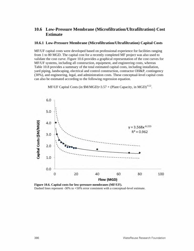
386 WateReuse Research Foundation
10.6 Low-Pressure Membrane (Microfiltration/Ultrafiltration) Cost Estimate
10.6.1 Low-Pressure Membrane (Microfiltration/Ultrafiltration) Capital Costs
MF/UF capital costs were developed based on professional experience for facilities ranging from 1 to 80 MGD. The capital cost for a recently completed MF project was also used to validate the cost curve. Figure 10.6 provides a graphical representation of the cost curves for MF/UF systems, including all construction, equipment, and engineering costs, whereas Table 10.8 provides a summary of the total estimated capital costs, including installation, yard piping, landscaping, electrical and control construction, contractor OH&P, contingency (30%), and engineering, legal, and administration costs. These conceptual-level capital costs can also be estimated according to the following regression equation.
MF/UF Capital Costs (in $M/MGD)=3.57 × (Plant Capacity, in MGD)-0.22.
Figure 10.6. Capital costs for low-pressure membranes (MF/UF). Dashed lines represent -30% to +50% error consistent with a conceptual-level estimate.

WateReuse Research Foundation 387
Table 10.8. Capital Costs for Low-Pressure Membranes (MF/UF)
System
Cap-acity
MF/UF System Costa
Yard Piping Cost
(10%)
Site-work Land-
scaping Cost (5%)
Site Electrical
and Controls
Cost (20%)
Subtotal Const-ruction
Cost
Contractor
OH&P (15%)
Contingency
(30%)
Total Const-ruction
Cost
Engineering, Legal, and
Admin. Costs (35%)
Total Project
Cost
Total Unit Cost
(MGD) ($M) ($M) ($M) ($M) ($M) ($M) ($M) ($M) ($M) ($M) ($M/MGD)
1 1.5 0.15 0.08 0.31 2.1 0.31 0.62 3.0 1.0 4.0 4.04 2 2.3 0.23 0.11 0.46 3.1 0.46 0.93 4.5 1.6 6.1 3.03 4 3.8 0.38 0.19 0.76 5.2 0.77 1.5 7.5 2.6 10.1 2.53 6 5.3 0.53 0.26 1.1 7.1 1.1 2.1 10.3 3.6 13.9 2.32 8 6.7 0.67 0.34 1.3 9.1 1.4 2.7 13.2 4.6 17.8 2.22
10 7.6 0.76 0.38 1.5 10.3 1.5 3.1 15.0 5.2 20.2 2.02 12 8.7 0.87 0.44 1.7 11.8 1.8 3.5 17.1 6.0 23.0 1.92 14 10.2 1.0 0.51 2.0 13.7 2.1 4.1 19.9 7.0 26.9 1.92 16 11.6 1.2 0.58 2.3 15.7 2.4 4.7 22.7 8.0 30.7 1.92 18 12.4 1.2 0.62 2.5 16.7 2.5 5.0 24.2 8.5 32.7 1.82 20 13.8 1.4 0.69 2.8 18.6 2.8 5.6 26.9 9.4 36.4 1.82 40 26.0 2.6 1.3 5.2 35.1 5.3 10.5 50.9 17.8 68.7 1.72 70 37.5 3.7 1.9 7.5 50.6 7.6 15.2 73.3 25.7 99.0 1.41 80 42.8 4.3 2.1 8.6 57.8 8.7 17.3 83.8 29.3 113 1.41
aIncludes installation cost (30%)

388
10.6.2 Low-Pressure Membrane (Microfiltration/Ultrafiltration) Operations and Maintenance Costs
Annual O&M costs for MF/UF treatment are shown in Figure 10.7 and Table 10.9 and include the costs for labor, chemicals, periodic membrane replacement, and energy consumption. These were developed based on the existing cost curves for membrane treatment provided in the United States Bureau of Reclamation (USBR) Desalting Handbook for Planners (USBR, 2003). This handbook provides guidelines for RO treatment of brackish water and is based on data from existing facilities supplemented with performance estimates. For this study, the energy costs from USBR were adapted to reflect the lower energy required for low-pressure membranes (MF/UF) versus high-pressure membranes (NF/RO). Specifically, the USBR costs were reduced by 90% to account for the anticipated reduction in pressure and to generate a more accurate cost estimate for MF/UF. There was no further differentiation between MF and UF feed pressure because this is only a conceptual-level Class 4 cost estimate, but the differences are assumed to be relatively small. For the purposes of this cost estimate, the other O&M costs (labor, chemicals, and membrane replacement) were assumed to be similar in low- and high-pressure membranes. Therefore, the corresponding USBR values were used without modification except for the adjustment to 2011 dollars.
Labor costs were also included in this case because they are anticipated to be significant. However, it should be noted that when O&M costs for combined low- and high-pressure membrane treatment trains (e.g., MF-RO) are summed, labor costs should only be counted once for the overall treatment train. The additional labor associated with the dual membrane system is assumed to be insignificant in comparison to a single membrane process.
The USBR cost curves are available for system capacities ranging from 1.1 to 53 MGD, which is reflected in Figure 10.7 and Table 10.9. The resulting regression equation for estimating conceptual-level O&M costs for a low-pressure membrane system is as follows:
Annual MF/UF O&M Costs (in $M/MGD)=0.30 × (Plant Capacity, in MGD)-0.22. Although the cost curves are based on facilities ranging in size from 1.1 to 53 MGD, the regression equation can also be used for facilities larger than 53 MGD because of the relatively flat nature of the curve.

WateReuse Research Foundation 389
Figure 10.7. Annual O&M costs for low-pressure membranes (MF/UF). Dashed lines represent -30% to +50% error, consistent with a conceptual-level estimate.
Table 10.9. Annual O&M Costs for Low-Pressure Membranes (MF/UF)
System
Capacity
Labor Cost for
Membrane Processes
Chemical Cost for
Membrane Processes
Membrane Replacement
Cost
Energy Cost
Total O&M Cost
Unit O&M Cost
(MGD) ($M) ($M) ($M) ($M) ($M) ($M/MGD)
1.1 0.2 0.1 0.0 0.01 0.40 0.38 2.6 0.2 0.2 0.1 0.04 0.56 0.21 5.3 0.2 0.5 0.2 0.08 0.93 0.18 11 0.3 1.0 0.4 0.16 1.82 0.17 26 0.4 2.3 0.9 0.38 4.01 0.15 53 0.4 4.5 1.8 0.81 7.50 0.14
10.7 High-Pressure Membrane (Nanofiltration/Reverse Osmosis) Cost Estimate
10.7.1 High-Pressure Membrane (Nanofiltration/Reverse Osmosis) Capital Costs
Capital costs for high-pressure membrane filtration, which includes RO and NF, were developed based on professional experience for facilities ranging from 1 to 80 MGD. The capital costs for two recently completed RO projects were also reviewed to validate the cost

390
curve. Figure 10.8 provides a graphical representation of the cost curves for NF/RO systems, including all construction, equipment, and engineering costs. Pretreatment costs, including chemical addition and low-pressure membrane filtration, are not included in the estimate. Table 10.10 summarizes the total estimated capital costs, including equipment installation; yard piping; landscaping, electrical and control construction; contractor OH&P; contingency (30%); and engineering, legal, and administration costs. The resulting regression equation for estimating conceptual-level capital costs for high-pressure membrane (NF/RO) systems is as follows:
NF/RO Capital Costs (in $M/MGD)=7.14 × (Plant Capacity, in MGD)-0.22.
Figure 10.8. Capital costs for high-pressure membrane filtration. Dashed lines represent -30% to +50% error, consistent with a conceptual-level estimate.

WateReuse Research Foundation 391
Table 10.10. Capital Costs for High-Pressure Membrane Filtration (NF/RO)
System
Cap-acity
NF/RO System Costa
Yard Piping Cost
(10%)
Site-work Land-
scaping Cost (5%)
Site Electrical
and Controls
Cost (20%)
Subtotal Const-ruction
Cost
Contractor
OH&P (15%)
Contingency
(30%)
Total Const-ruction
Cost
Engineering, Legal, and
Admin. Costs (35%)
Total Project
Cost
Total Unit Cost
(MGD) ($M) ($M) ($M) ($M) ($M) ($M) ($M) ($M) ($M) ($M) ($M/MGD)
1 3.1 0.31 0.15 0.61 4.1 0.62 1.2 6.0 2.1 8.1 8.08 2 4.6 0.46 0.23 0.92 6.2 0.93 1.9 9.0 3.1 12.1 6.06 4 7.6 0.76 0.38 1.5 10.3 1.5 3.1 15.0 5.2 20.2 5.05 6 10.5 1.1 0.53 2.1 14.2 2.1 4.3 20.7 7.2 27.9 4.65 8 13.5 1.3 0.67 2.7 18.2 2.7 5.4 26.3 9.2 35.6 4.44
10 15.3 1.5 0.76 3.1 20.6 3.1 6.2 29.9 10.5 40.4 4.04 12 17.4 1.7 0.87 3.5 23.5 3.5 7.1 34.1 11.9 46.1 3.84 14 20.3 2.0 1.0 4.1 27.5 4.1 8.2 39.8 13.9 53.7 3.84 16 23.2 2.3 1.2 4.6 31.4 4.7 9.4 45.5 15.9 61.4 3.84 18 24.8 2.5 1.2 5.0 33.4 5.0 10.0 48.5 17.0 65.5 3.64 20 27.5 2.8 1.4 5.5 37.2 5.6 11.1 53.9 18.9 72.7 3.64 40 52.0 5.2 2.6 10.4 70.2 10.5 21.1 102 35.6 137 3.43 70 74.9 7.5 3.7 15.0 101 15.2 30.3 147 51.3 198 2.83 80 85.6 8.6 4.3 17.1 116 17.3 34.7 168 58.7 226 2.83
aIncludes installation cost (30%)
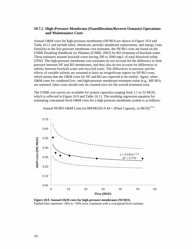
392
10.7.2 High-Pressure Membrane (Nanofiltration/Reverse Osmosis) Operations and Maintenance Costs
Annual O&M costs for high-pressure membranes (NF/RO) are shown in Figure 10.9 and Table 10.11 and include labor, chemicals, periodic membrane replacement, and energy costs. Similarly to the low-pressure membrane cost estimates, the NF/RO costs are based on the USBR Desalting Handbook for Planners (USBR, 2003) for RO treatment of brackish water. These estimates assume brackish water having 500 to 2000 mg/L of total dissolved solids (TDS). The high-pressure membrane cost estimates do not account for the difference in feed pressure between NF and RO membranes, and they also do not account for differences in salinity between brackish water and recycled water. The differences in pressure and the effects of variable salinity are assumed to have an insignificant impact on NF/RO costs, which means that the O&M costs for NF and RO are expected to be similar. Again, when O&M costs for combined low- and high-pressure membrane treatment trains (e.g., MF-RO) are summed, labor costs should only be counted once for the overall treatment train.
The USBR cost curves are available for system capacities ranging from 1.1 to 53 MGD, which is reflected in Figure 10.9 and Table 10.11. The resulting regression equation for estimating conceptual-level O&M costs for a high pressure membrane system is as follows:
Annual NF/RO O&M Costs (in $M/MGD)=0.44 × (Plant Capacity, in MGD)-0.13.
Figure 10.9. Annual O&M costs for high-pressure membranes (NF/RO). Dashed lines represent -30% to +50% error consistent with a conceptual-level estimate.

WateReuse Research Foundation 393
Table 10.11. Annual O&M Costs for High-Pressure Membranes (NF/RO)
System
Capacity
Labor
Cost for Membrane Processes
Chemical Cost for
Membrane Processes
Membrane Replacement
Cost
Energy Cost
Total O&M Cost
Unit O&M Cost
(MGD) ($M) ($M) ($M) ($M) ($M) ($M/MGD)
1.1 0.25 0.10 0.04 0.15 0.53 0.51 2.6 0.20 0.22 0.10 0.39 0.91 0.34 5.3 0.22 0.45 0.18 0.81 1.66 0.31 11 0.29 1.00 0.37 1.63 3.28 0.31 26 0.37 2.34 0.92 3.79 7.42 0.28 53 0.42 4.54 1.76 8.07 14.8 0.28
10.8 Biological Activated Carbon Cost Estimate
10.8.1 Biological Activated Carbon Capital Costs
The capital cost curves for biological activated carbon (BAC) were based on open filter granular activated carbon (GAC) designs in water treatment applications, largely because of the lack of available data and vendor experience with BAC in wastewater applications. However, filter bed volume and standard construction costs were assumed to be equivalent between the two types of installations. Costs were prepared for filter capacities ranging from 1 to 80 MGD.
Capital costs for the construction of a BAC filter include the following major components: filter structure, filter media, backwash pumping, intermediate lift pumping, yard piping, site work, and electrical and control systems. Sources of relevant data and a list of assumptions are as follows:
Filter structure and backwash pumping costs were determined from McGivney and Kawamura (2008)
2010 filter media pricing was provided for the GAC product Filtrasorb 300M from Calgon Carbon Corporation
Intermediate lift pumping costs were determined from Jones and Sanks (2008)
Energy was based on the 2010 national average unit electrical cost (U.S. Energy Information Administration, 2010)
Labor was based on the 2010 mean unit labor cost for water/wastewater treatment operators (U.S. Bureau of Labor Statistics, 2011) and was augmented with a multiplier to account for other overhead costs associated with employment
The time value of money was based on the annual average inflation rate through September 2011 (applied to 2010 filter media, electrical, and labor costs to provide costs in 2011 dollars)
Costs were prepared for EBCTs of 10 and 20 min (Table 10.12 and Table 10.13, respectively) to allow users to select multiple design parameters for their BAC filter application. Separate cost curves were prepared for both small (<10 MGD, Figure 10.10) and large systems
394 WateReuse Research Foundation
(≥10 MGD, Figure 10.11) for ease of estimation on a per capacity basis ($M/MGD). The single-cost-curve (and -cost-equation) approach utilized for the preceding processes did not apply to BAC because the costs were noticeably impacted by economies of scale. Thus, the curve fit and correlation coefficients prepared for the combined data set (i.e., small and large systems) were weaker than those of the separated data sets. Therefore, four different regression equations for BAC capital costs are presented for the various combinations of EBCT and design flow, including contractor OH&P and contingency: Small System (<10 MGD) with 10 min EBCT:
BAC Capital Costs (in $M/MGD)=2.92 × (Plant Capacity, in MGD)-0.52
Small System (<10 MGD) with 20 min EBCT:
BAC Capital Costs (in $M/MGD)=3.03 × (Plant Capacity, in MGD)-0.48
Large System (10-80 MGD) with 10 min EBCT:
BAC Capital Costs (in $M/MGD)=1.43 × (Plant Capacity, in MGD)-0.17
Large System (10-80 MGD) with 20 min EBCT:
BAC Capital Costs (in $M/MGD)=1.52 × (Plant Capacity, in MGD)-0.15.
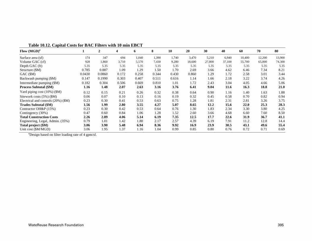
WateReuse Research Foundation 395
Table 10.12. Capital Costs for BAC Filters with 10 min EBCT Flow (MGD)a 1 2 4 6 8 10 20 30 40 60 70 80
Surface area (sf) 174 347 694 1,040 1,390 1,740 3,470 5,210 6,940 10,400 12,200 13,900Volume GAC (cf) 928 1,860 3,710 5,570 7,430 9,280 18,600 27,800 37,100 55,700 65,000 74,300Depth GAC (ft) 5.35 5.35 5.35 5.35 5.35 5.35 5.35 5.35 5.35 5.35 5.35 5.35Structure ($M) 0.785 0.887 1.09 1.29 1.50 1.70 2.69 3.66 4.62 6.46 7.34 8.21GAC ($M) 0.0430 0.0860 0.172 0.258 0.344 0.430 0.860 1.29 1.72 2.58 3.01 3.44Backwash pumping ($M) 0.147 0.1990 0.303 0.407 0.511 0.616 1.14 1.66 2.18 3.22 3.74 4.26Intermediate pumping ($M) 0.182 0.304 0.506 0.669 0.810 1.01 1.72 2.43 3.04 4.05 4.66 5.06Process Subtotal ($M) 1.16 1.48 2.07 2.63 3.16 3.76 6.41 9.04 11.6 16.3 18.8 21.0Yard piping cost (10%) ($M) 0.12 0.15 0.21 0.26 0.32 0.38 0.64 0.90 1.16 1.40 1.63 1.88Sitework costs (5%) ($M) 0.06 0.07 0.10 0.13 0.16 0.19 0.32 0.45 0.58 0.70 0.82 0.94Electrical and controls (20%) ($M) 0.23 0.30 0.41 0.53 0.63 0.75 1.28 1.81 2.31 2.81 3.26 3.75Trades Subtotal ($M) 1.56 1.99 2.80 3.55 4.27 5.07 8.65 12.2 15.6 22.0 25.3 28.3Contractor OH&P (15%) 0.23 0.30 0.42 0.53 0.64 0.76 1.30 1.83 2.34 3.30 3.80 4.25Contingency (30%) 0.47 0.60 0.84 1.06 1.28 1.52 2.60 3.66 4.68 6.60 7.60 8.50Total Construction Costs 2.26 2.89 4.06 5.14 6.19 7.35 12.5 17.7 22.6 31.9 36.7 41.1Engineering, Legal, Admin. (35%) 0.79 1.01 1.42 1.80 2.17 2.57 4.39 6.19 7.91 11.2 12.8 14.4Total project ($M) 3.06 3.90 5.48 6.94 8.36 9.92 16.9 23.9 30.5 43.1 49.6 55.4Unit cost ($M/MGD) 3.06 1.95 1.37 1.16 1.04 0.99 0.85 0.80 0.76 0.72 0.71 0.69
aDesign based on filter loading rate of 4 gpm/sf.

396 WateReuse Research Foundation
Table 10.13. Capital Costs for BAC Filters with 20 min EBCT Flow (MGD)a 1 2 4 6 8 10 20 30 40 60 70 80
Surface area (sf) 174 347 694 1,040 1,390 1,740 3,470 5,210 6,940 10,400 12,153 13,900Volume GAC (cf) 1,860 3,710 7,430 11,100 14,900 18,600 37,100 55,700 74,300 111,000 130,000 149,000Depth GAC (ft) 10.7 10.7 10.7 10.7 10.7 10.7 10.7 10.7 10.7 10.7 10.7 10.7Structure ($M) 0.785 0.887 1.09 1.29 1.50 1.70 2.69 3.66 4.62 6.46 7.34 8.21GAC ($M) 0.0860 0.172 0.344 0.516 0.688 0.860 1.72 2.58 3.44 5.16 6.02 6.88Backwash pumping ($M) 0.147 0.199 0.303 0.407 0.511 0.616 1.14 1.66 2.18 3.22 3.74 4.26Intermediate pumping ($M) 0.182 0.304 0.506 0.669 0.810 1.01 1.72 2.43 3.04 4.05 4.66 5.06Process Subtotal ($M) 1.62 2.11 3.03 3.90 4.73 5.65 9.81 13.9 17.9 25.5 29.4 33.0Yard piping cost (10%) ($M) 0.24 0.32 0.45 0.58 0.71 0.85 1.47 2.09 2.69 3.82 4.41 4.95Sitework costs (5%) ($M) 0.49 0.63 0.91 1.17 1.42 1.70 2.94 4.18 5.38 7.65 8.82 9.89Electrical and controls (20%) ($M) 2.35 3.06 4.39 5.65 6.86 8.19 14.2 20.2 26.0 37.0 42.6 47.8Trades Subtotal ($M) 0.82 1.07 1.54 1.98 2.40 2.87 4.98 7.08 9.09 12.9 14.9 16.7Contractor OH&P (15%) 3.17 4.13 5.93 7.63 9.26 11.1 19.2 27.3 35.1 49.9 57.5 64.5Contingency (30%) 3.17 2.06 1.48 1.27 1.16 1.11 0.96 0.91 0.88 0.83 0.82 0.81Total Construction Costs 1.62 2.11 3.03 3.90 4.73 5.65 9.81 13.9 17.9 25.5 29.4 33.0Engineering, Legal, Admin. (35%) 0.24 0.32 0.45 0.58 0.71 0.85 1.47 2.09 2.69 3.82 4.41 4.95Total project ($M) 0.49 0.63 0.91 1.17 1.42 1.70 2.94 4.18 5.38 7.65 8.82 9.89Unit cost ($M/MGD 2.35 3.06 4.39 5.65 6.86 8.19 14.2 20.2 26.0 37.0 42.6 47.8
aDesign based on filter loading rate of 4 gpm/sf.

WateReuse Research Foundation 397
Figure 10.10. Capital costs for BAC filters (1–10 MGD). Dashed lines represent -30% to +50% error, consistent with a conceptual-level estimate.
Figure 10.11. Capital costs for BAC filters (≥10 MGD). Dashed lines represent -30% to +50% error, consistent with a conceptual-level estimate.

398 WateReuse Research Foundation
10.8.2 Biological Activated Carbon Operations and Maintenance Costs
Annual O&M cost curves for BAC filters were based on GAC data in water treatment applications because of the lack of available data and widespread vendor experience with wastewater BAC. Although construction costs were assumed to be similar, the O&M costs were varied between the water and wastewater by decreasing the replacement interval of the GAC media to once every 8 years. The replacement interval may vary considerably between facilities depending on the specific objectives at each location. Some systems may rely primarily on the biological aspect of BACs, some facilities may seek a combination of biological degradation and adsorption, and others may want to maximize the level of adsorption in the system, all of which have implications for media replacement frequency. The maintenance approach may also differ between facilities as some will purchase virgin replacement media whereas others may install on-site regeneration facilities, such as the Upper Occoquan Service Authority in Fairfax, Virginia. Because of the limited number of wastewater facilities employing BAC or GAC, it was infeasible to evaluate all of these alternatives. Therefore, the costs below utilized an 8-year lifespan for the media. Costs were prepared for design capacities ranging from 1 to 80 MGD, although O&M costs were based on an average flow rate of half of the design capacity.
O&M costs for BAC filters include media replacement, electricity, and labor. Again, curves were developed for two different EBCTs, and the estimates also account for the different amount of media in each configuration. Similarly to the capital costs, cost curves were provided for both small (1–10 MGD) and large systems (>10 MGD) to achieve a better fit (power function curve) for approximating conceptual-level O&M costs. Unlike the capital costs prepared using the rated capacity of the filters, the O&M costs were prepared based on an average treated flow equal to half of the facility’s rated capacity, to account for redundancy and overdesign, which are common in many systems. However, the unit O&M costs are still plotted (Figure 10.12 and Figure 10.13), based on the full design capacity. The estimate also incorporated the following assumptions and parameters:
The physical structure was based on a concrete gravity filter design
The bulk density of GAC was assumed to be 0.45 g/cm3
The unit cost of GAC was assumed to be $1.65/lb
GAC installation costs were assumed to be approximately 30% of the GAC media costs
The filter structure costs were based on Figure 5.5.25b in McGivney and Kawamura (2008)
The backwash pumping costs were based on Figure 5.5.29 in McGivney and Kawamura (2008)
The intermediate pumping costs were based on Figure 29-7 in Sanks et al. (1998)
The GAC replacement frequency was assumed to be 8 years
Unit electrical costs were assumed to be $0.0988/kWh (U.S. Energy Information Administration, 2010)
The average flow was approximated as half of the rated filter capacity
The mean labor rate was assumed to be $20.27 for water/wastewater treatment plant operators (U.S. Bureau of Labor Statistics, 2011) 1.85 for overhead
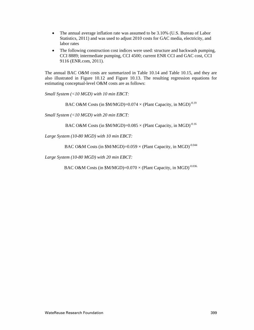
WateReuse Research Foundation 399
The annual average inflation rate was assumed to be 3.10% (U.S. Bureau of Labor Statistics, 2011) and was used to adjust 2010 costs for GAC media, electricity, and labor rates
The following construction cost indices were used: structure and backwash pumping, CCI 8889; intermediate pumping, CCI 4500; current ENR CCI and GAC cost, CCI 9116 (ENR.com, 2011).
The annual BAC O&M costs are summarized in Table 10.14 and Table 10.15, and they are also illustrated in Figure 10.12 and Figure 10.13. The resulting regression equations for estimating conceptual-level O&M costs are as follows: Small System (<10 MGD) with 10 min EBCT:
BAC O&M Costs (in $M/MGD)=0.074 × (Plant Capacity, in MGD)-0.19
Small System (<10 MGD) with 20 min EBCT:
BAC O&M Costs (in $M/MGD)=0.085 × (Plant Capacity, in MGD)-0.16
Large System (10-80 MGD) with 10 min EBCT:
BAC O&M Costs (in $M/MGD)=0.059 × (Plant Capacity, in MGD)-0.044
Large System (10-80 MGD) with 20 min EBCT:
BAC O&M Costs (in $M/MGD)=0.070 × (Plant Capacity, in MGD)-0.036.

400 WateReuse Research Foundation
Table 10.14. Annual O&M Costs for BAC with 10 min EBCT Design capacity (MGD) 1 2 4 6 8 10 20 30 40 50 60 70 80 Average flow (MGD)a 0.5 1 2 3 4 5 10 15 20 25 30 35 40 Labor (hours/day) 1 1 1 1 1 2 2 2 2 2 2 2 2 GAC replacement ($)b $5,550 $11,100 $22,200 $33,300 $44,400 $55,400 $111,000 $166,000 $222,000 $277,000 $333,000 $388,000 $444,000 Energy ($) $18,600 $37,200 $74,400 $112,000 $149,000 $186,000 $372,000 $558,000 $744,000 $929,000 $1,120,000 $1,300,000 $1,490,000 Labor ($) $14,100 $14,100 $14,100 $14,100 $14,100 $28,200 $28,200 $28,200 $28,200 $28,200 $28,200 $28,200 $28,200 Total O&M ($) $38,200 $62,400 $111,000 $159,000 $207,000 $270,000 $511,000 $752,000 $994,000 $1,230,000 $1,480,000 $1,720,000 $1,960,000 Unit O&M ($M/MGD) 0.0765 0.0624 0.0553 0.0530 0.0518 0.0539 0.0511 0.0502 0.0497 0.0494 0.0492 0.0491 0.0490
aO&M costs were calculated assuming 50% of the design flow capacity but plotted based on 100% of the design flow capacity. bFrequency of GAC replacement is 8 years and electrical energy consumption is 1 kWh/1,000 gal.
Table 10.15. Annual O&M Costs for BAC with 20 min EBCT Design capacity (MGD) 1 2 4 6 8 10 20 30 40 50 60 70 80 Average fow (MGD)a 0.5 1 2 3 4 5 10 15 20 25 30 35 40 Labor (hours/day) 1 1 1 1 1 2 2 2 2 2 2 2 2 GAC replacement ($)b $11,100 $22,200 $44,400 $66,500 $88,700 $111,000 $222,000 $333,000 $444,000 $554,000 $665,000 $776,000 $887,000 Energy ($) $18,600 $37,200 $74,400 $112,000 $149,000 $186,000 $372,000 $558,000 $744,000 $929,000 $1,120,000 $1,300,000 $1,490,000 Labor ($) $14,100 $14,100 $14,100 $14,100 $14,100 $28,200 $28,200 $28,200 $28,200 $28,200 $28,200 $28,200 $28,200 Total O&M ($) $43,800 $73,500 $133,000 $192,000 $252,000 $325,000 $622,000 $919,000 $1,220,000 $1,510,000 $1,810,000 $2,110,000 $2,400,000 Unit O&M ($M/MGD) 0.0876 0.0735 0.0664 0.0641 0.0629 0.0650 0.0622 0.0612 0.0608 0.0605 0.0603 0.0602 0.0601
aO&M costs were calculated assuming 50% of the design flow capacity but plotted based on 100% of the design flow capacity. bFrequency of GAC replacement is 8 years and electrical energy consumption is 1 kWh/1,000 gal.
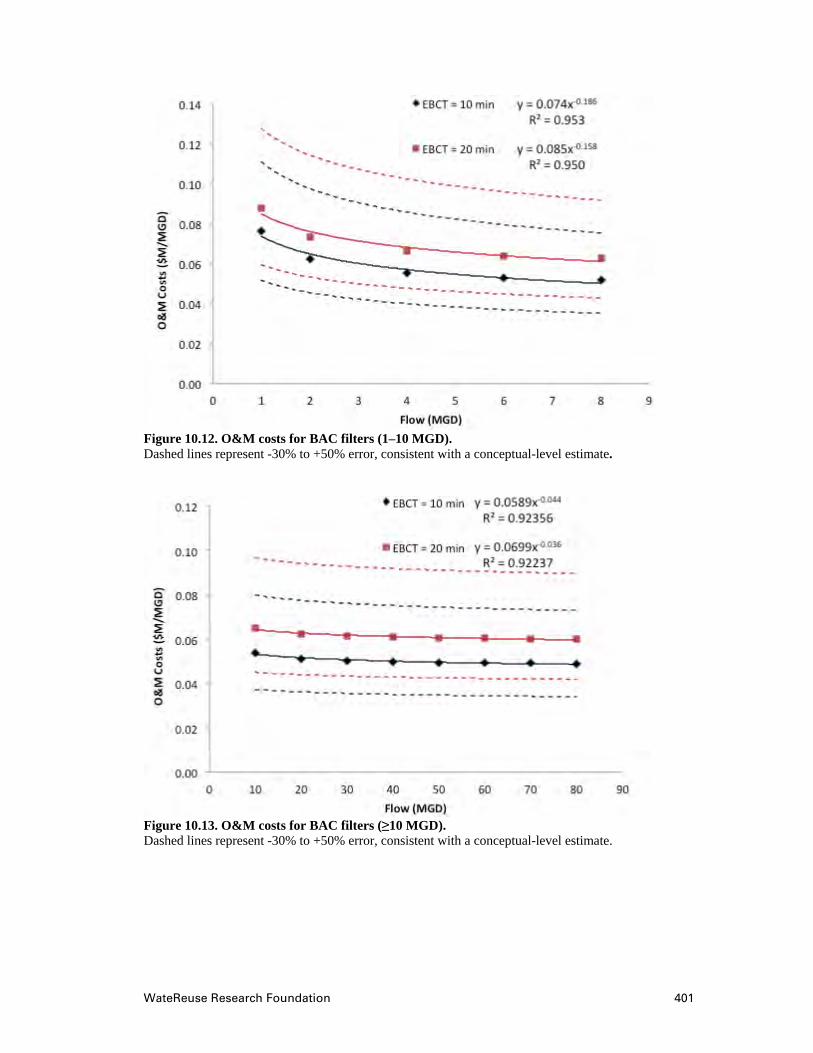
WateReuse Research Foundation 401
Figure 10.12. O&M costs for BAC filters (1–10 MGD). Dashed lines represent -30% to +50% error, consistent with a conceptual-level estimate.
Figure 10.13. O&M costs for BAC filters (≥10 MGD). Dashed lines represent -30% to +50% error, consistent with a conceptual-level estimate.
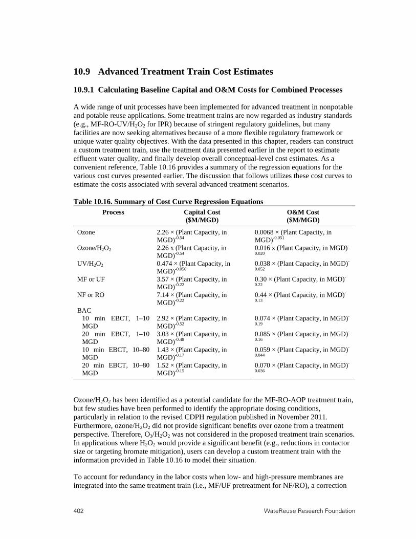
402 WateReuse Research Foundation
10.9 Advanced Treatment Train Cost Estimates
10.9.1 Calculating Baseline Capital and O&M Costs for Combined Processes
A wide range of unit processes have been implemented for advanced treatment in nonpotable and potable reuse applications. Some treatment trains are now regarded as industry standards (e.g., MF-RO-UV/H2O2 for IPR) because of stringent regulatory guidelines, but many facilities are now seeking alternatives because of a more flexible regulatory framework or unique water quality objectives. With the data presented in this chapter, readers can construct a custom treatment train, use the treatment data presented earlier in the report to estimate effluent water quality, and finally develop overall conceptual-level cost estimates. As a convenient reference, Table 10.16 provides a summary of the regression equations for the various cost curves presented earlier. The discussion that follows utilizes these cost curves to estimate the costs associated with several advanced treatment scenarios. Table 10.16. Summary of Cost Curve Regression Equations
Process Capital Cost O&M Cost ($M/MGD) ($M/MGD)
Ozone 2.26 × (Plant Capacity, in MGD)-0.54
0.0068 × (Plant Capacity, in MGD)-0.051
Ozone/H2O2 2.26 x (Plant Capacity, in MGD)-0.54
0.016 x (Plant Capacity, in MGD)-
0.020 UV/H2O2 0.474 × (Plant Capacity, in
MGD)-0.056 0.038 × (Plant Capacity, in MGD)-
0.052 MF or UF 3.57 × (Plant Capacity, in
MGD)-0.22 0.30 × (Plant Capacity, in MGD)-
0.22 NF or RO 7.14 × (Plant Capacity, in
MGD)-0.22 0.44 × (Plant Capacity, in MGD)-
0.13 BAC
10 min EBCT, 1–10 MGD
2.92 × (Plant Capacity, in MGD)-0.52
0.074 × (Plant Capacity, in MGD)-
0.19 20 min EBCT, 1–10 MGD
3.03 × (Plant Capacity, in MGD)-0.48
0.085 × (Plant Capacity, in MGD)-
0.16 10 min EBCT, 10–80 MGD
1.43 × (Plant Capacity, in MGD)-0.17
0.059 × (Plant Capacity, in MGD)-
0.044 20 min EBCT, 10–80 MGD
1.52 × (Plant Capacity, in MGD)-0.15
0.070 × (Plant Capacity, in MGD)-
0.036
Ozone/H2O2 has been identified as a potential candidate for the MF-RO-AOP treatment train, but few studies have been performed to identify the appropriate dosing conditions, particularly in relation to the revised CDPH regulation published in November 2011. Furthermore, ozone/H2O2 did not provide significant benefits over ozone from a treatment perspective. Therefore, O3/H2O2 was not considered in the proposed treatment train scenarios. In applications where H2O2 would provide a significant benefit (e.g., reductions in contactor size or targeting bromate mitigation), users can develop a custom treatment train with the information provided in Table 10.16 to model their situation.
To account for redundancy in the labor costs when low- and high-pressure membranes are integrated into the same treatment train (i.e., MF/UF pretreatment for NF/RO), a correction

WateReuse Research Foundation 403
factor should be applied based on a regression of the labor portion of the cost curve. This correction is described by the following regression equation:
Membrane Labor Correction (in $M/MGD)=0.20 × (Plant Capacity, in MGD)-0.83.
The resulting membrane labor correction should be subtracted from the overall cost estimate for the facility. For example, for a facility with both MF and RO membranes, a 2 MGD facility would subtract $0.1M/MGD from its cost estimate, whereas a 50 MGD facility would subtract $0.008M/MGD from its cost estimate.
To illustrate the use of these cost curve equations in estimating capital and O&M costs for various processes or process combinations, several sets of example calculations are presented in the following tables. The first set of calculations compares the capital and O&M costs of the following combined systems: ozone-BAC, MF-ozone-BAC, MF-RO, MF-RO-UV/H2O2 and MF-Ozone-RO. With respect to the oxidation processes, the ozone system is based on an applied ozone dose of 3 mg/L, and the UV/H2O2 system is designed to achieve 1.2-log removal of NDMA and 0.5-log removal of 1,4-dioxane. The BAC is designed with a 10-min empty bed contact time.
Table 10.17 contains the capital costs for the combined process trains normalized to design flow ($M/MGD). The costs are based on the equations in Table 4.16 modified by the labor correction factor, where necessary. Similarly, Table 10.18 provides the corresponding flow-normalized annual O&M costs for the same treatment trains. Table 10.19 and Table 10.20 present the capital and annual O&M costs ($M), respectively, based on the design capacity of the plants. Table 10.17. Flow-Normalized Capital Costs for the Combined Process Trains
Process Trains and Capital Costs ($M/MGD) Capacity (MGD)
O3-BAC MF-O3-BAC MF-RO MF-RO-UV/H2O2
MF-O3-RO (O3-MF-RO)
1 $5.18 $8.75 $10.71 $11.18 $12.97 5 $2.21 $4.72 $7.52 $7.95 $8.46
10 $1.62 $3.77 $6.45 $6.87 $7.11 25 $1.22 $2.98 $5.28 $5.67 $5.67 50 $1.01 $2.52 $4.53 $4.91 $4.80 80 $0.89 $2.25 $4.08 $4.46 $4.30
Table 10.18. Flow-Normalized Annual O&M Costs for the Combined Process Trains
Process Trains and Annual O&M Costs ($M/MGD) Capacity (MGD)
O3-BAC MF-O3-BAC MF-RO MF-RO-UV/H2O2
MF-O3-RO (O3-MF-RO)
1 $0.08 $0.38 $0.54 $0.58 $0.55 5 $0.06 $0.27 $0.51 $0.55 $0.52
10 $0.06 $0.24 $0.48 $0.51 $0.48 25 $0.06 $0.20 $0.42 $0.46 $0.43 50 $0.06 $0.18 $0.38 $0.41 $0.39 80 $0.05 $0.17 $0.36 $0.39 $0.36

404 WateReuse Research Foundation
Table 10.19. Total Capital Costs for the Combined Process Trains
Process Trains and Capital Costs ($M) Capacity (MGD)
O3-BAC MF-O3-BAC MF-RO MF-RO-UV/H2O2
MF-O3-RO (O3-MF-RO)
1 $5.2 $9.0 $11 $11 $13 5 $11 $24 $38 $40 $42
10 $16 $38 $65 $69 $71 25 $31 $75 $132 $142 $142 50 $50 $126 $226 $245 $240 80 $71 $180 $327 $356 $344
Table 10.20. Total Annual O&M Costs for the Combined Process Trains
Process Trains and Annual O&M Costs ($M) Capacity (MGD)
O3-BAC MF-O3-BAC MF-RO MF-RO-UV/H2O2
MF-O3-RO (O3-MF-RO)
1 $0.1 $0.4 $0.5 $0.6 $0.5 5 $0.3 $1.4 $2.6 $2.7 $2.6
10 $0.6 $2.4 $4.8 $5.1 $4.8 25 $1.4 $5.1 $11 $11 $11 50 $2.8 $9.0 $19 $21 $19 80 $4 $13 $29 $31 $29
10.9.2 Variable Ozone Dose Modification
A second set of calculations is presented to show the relationship between capital and O&M costs for variable ozone doses. The previous cost estimates for the ozone-based treatment trains were developed for an ozone dose of 3 mg/L. In this scenario, however, one must be able to account for potential changes in ozone dose in order to target a range of water quality objectives. As a result, a correction factor was developed based on the following three assumptions/simplifications:
The ozone system costs (generator, wiring, installation, etc.) need to be proportionally increased or decreased to account for changes in planned ozone dose.
The ozone contactor size and other required elements of construction will not be changed as the volume of water being treated remains the same.
The power costs associated with changing the ozone dose can be extrapolated in a linear fashion and used to adjust the annual O&M costs.
On the basis of these assumptions, the capital and annual O&M costs specific to the ozone system were plotted against the design flow (Figure 10.14). These plots, which proved to be linear, can be described by the following regression equations:
Ozone System Capital Costs (in $M)=0.0294 × Capacity (in MGD) + 2.8
Ozone System Annual O&M Costs (in $M)=0.005 × Capacity (in MGD) + 0.02.
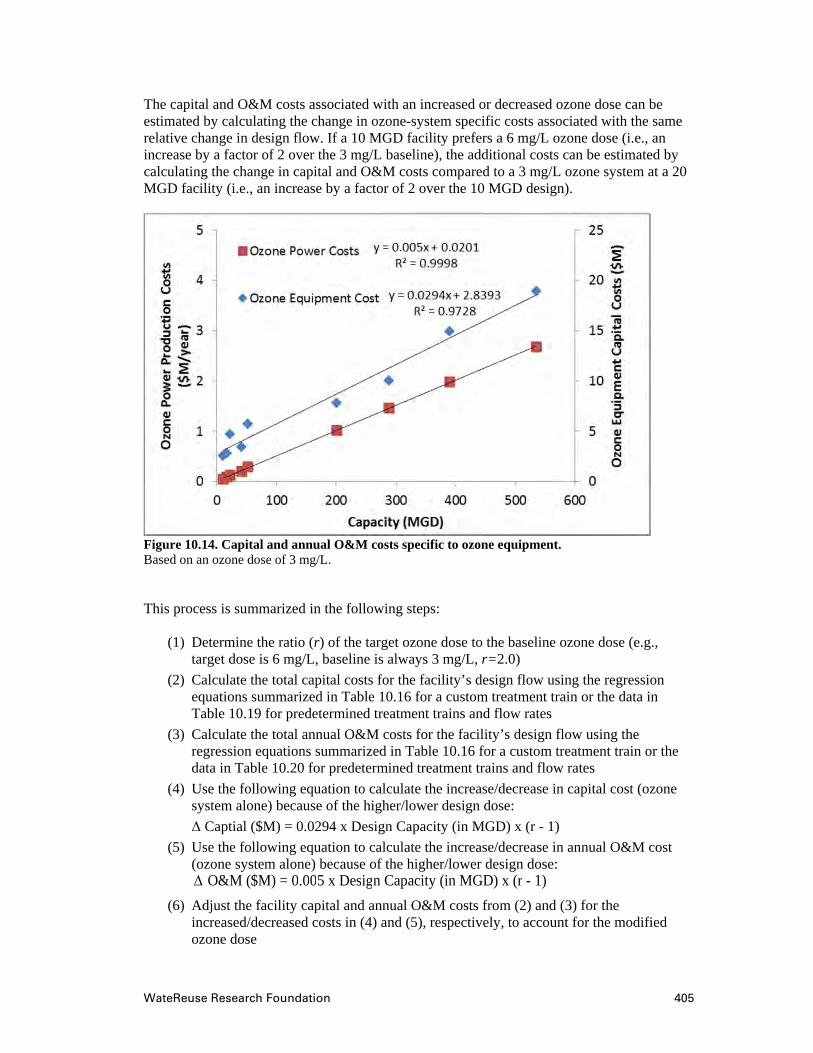
WateReuse Research Foundation 405
The capital and O&M costs associated with an increased or decreased ozone dose can be estimated by calculating the change in ozone-system specific costs associated with the same relative change in design flow. If a 10 MGD facility prefers a 6 mg/L ozone dose (i.e., an increase by a factor of 2 over the 3 mg/L baseline), the additional costs can be estimated by calculating the change in capital and O&M costs compared to a 3 mg/L ozone system at a 20 MGD facility (i.e., an increase by a factor of 2 over the 10 MGD design).
Figure 10.14. Capital and annual O&M costs specific to ozone equipment. Based on an ozone dose of 3 mg/L.
This process is summarized in the following steps:
(1) Determine the ratio (r) of the target ozone dose to the baseline ozone dose (e.g., target dose is 6 mg/L, baseline is always 3 mg/L, r=2.0)
(2) Calculate the total capital costs for the facility’s design flow using the regression equations summarized in Table 10.16 for a custom treatment train or the data in Table 10.19 for predetermined treatment trains and flow rates
(3) Calculate the total annual O&M costs for the facility’s design flow using the regression equations summarized in Table 10.16 for a custom treatment train or the data in Table 10.20 for predetermined treatment trains and flow rates
(4) Use the following equation to calculate the increase/decrease in capital cost (ozone system alone) because of the higher/lower design dose:
Δ Captial ($M) = 0.0294 x Design Capacity (in MGD) x (r - 1)
(5) Use the following equation to calculate the increase/decrease in annual O&M cost (ozone system alone) because of the higher/lower design dose:
(6) Adjust the facility capital and annual O&M costs from (2) and (3) for the increased/decreased costs in (4) and (5), respectively, to account for the modified ozone dose
O&M ($M) = 0.005 x Design Capacity (in MGD) x (r - 1)

406 WateReuse Research Foundation
Using these steps, the adjusted capital costs for a 10 MGD O3-BAC facility operating with a 6 mg/L ozone dose would be $16M + $0.29M=$16.3M, and the adjusted annual O&M costs would be $0.6M + $0.05M=$0.7M.
10.9.3 Relating Ozone Costs to Water Quality Objectives
The costs for ozone-based treatment trains will be highly dependent on the water quality objectives in each application. Some systems will target TOrC mitigation to reduce the potential impacts of their effluent on public and aquatic health, some will determine their dosing conditions based on microbial inactivation goals, and others might design their systems based on aesthetics or odor control. The actual ozone doses in each application may vary significantly, which makes it difficult to capture all possible scenarios, water qualities, and treatment goals. For the purposes of this project, the following discussion will focus on designs targeting TOrC mitigation based on the treatment data described earlier in the report.
The recent regulatory trend emphasizes guidelines based on contaminant groupings rather than individual contaminants. This is evident in recent announcements by the U.S. EPA and revisions published by the CDPH. Specifically, the CDPH is proposing that facilities implementing full advanced treatment (i.e., MF-RO-AOP) must demonstrate specific reductions for nine structural classes. For example, the draft regulations mandate 0.5-log destruction of hydroxy aromatics, amino/acylamino aromatics, and a variety of other classes. The draft regulations also require 0.3-log destruction of saturated aliphatics and nitro aromatics. Although these guidelines only apply to full advanced treatment, a similar approach may be warranted for alternative applications, including spreading of ozone-BAC effluent in recharge basins.
The TOrC data presented earlier in the report incorporated this framework, in that the target compounds were classified into five groups based on their susceptibility to oxidation. The relative removal of these groups also proved to be consistent regardless of secondary effluent water quality. For example, an O3:TOC of 0.25 consistently achieved greater than 80% destruction of the Group 1 contaminants in all of the experimental matrices, whereas an O3:TOC ratio of 1.0 achieved greater than 80% destruction of the target compounds in Groups 1, 2, and 3.
To illustrate the relationship between cost and TOrC oxidation, Table 10.21 describes a theoretical 50 MGD O3-BAC treatment train with respect to capital costs, annual O&M costs, and oxidation efficacy. The facility is also assumed to have a total organic carbon concentration of 6 mg/L at the ozone dosing point and an empty bed contact time of 20 minutes in the BAC system. As demonstrated in the literature and the project data for the City of Reno pilot, downstream BAC provides substantial biodegradation and removal of trace organic contaminants. However, it is still critical to design the upstream ozone process to provide a baseline level of TOrC mitigation because the BAC process is less predictable. As such, Table 10.21 summarizes the data for four different ozone dosing conditions targeting different levels of TOrC oxidation.

WateReuse Research Foundation 407
Table 10.21. Cost and Oxidation Efficacy of a 50-MGD O3-BAC Treatment Train
O3 Dose 1.5 mg/L 3 mg/L 6 mg/L 9 mg/L O3:TOC Ratio 0.25 0.5 1.0 1.5
Conceptual-level cost estimate Capital Costs $49M $50M $52M $53M Annual O&M $2.7M $2.8M $3.1M $3.3M
Average percent destruction of target compounds Group 1 >90% >90% >90% >90% Group 2 >60% >90% >90% >90% Group 3 >30% >60% >90% >90% Group 4 >15% >30% >60% >80% Group 5 <5% >5% >15% >20%
Note: 10-minute EBCT for the BAC process.
As demonstrated in Table 10.21, marginal increases in the capital and annual O&M costs for an O3-BAC process translate to significantly increased levels of contaminant oxidation. Again, these estimated mitigation levels do not account for the additional biodegradation and adsorption in the downstream BAC process, which would lead to final TOrC concentrations that are comparable to those of MF-RO-UV/H2O2. However, the differences in cost between O3-BAC—regardless of ozone dose—and MF-RO-UV/H2O2 are staggering. The highest ozone dose described in Table 10.21 corresponds to capital and annual O&M costs of $53M and $3.3M, respectively. Based on the data in Table 10.19 and Table 10.20, the conceptual-level capital and annual O&M costs for a 50 MGD MF-RO-UV/H2O2 facility are $245M and $21M.
10.10 Conclusion
Treatment costs are impacted by a variety of design variables including flow rate, site constraints, water quality objectives, manufacturer-specific quotes, and other factors. Because of this vast number of variables, the same treatment train may have significantly different costs from one site to another. However, using historical data provided by vendors offers a valuable database from which conceptual-level cost estimates can be developed for a variety of treatment processes and operational conditions. As described by the name, these cost estimates are extremely useful at the conceptual design stage because they allow relatively accurate comparisons of alternative treatment trains.
The tables, unit cost figures, and regression equation in this chapter offer tremendous flexibility in evaluating a wide range of treatment processes, design flows, and dosing conditions. This chapter also describes potential modifications to eliminate labor redundancies in sequential membrane systems and to account for varying ozone dose. Finally, this chapter illustrates common advanced treatment train scenarios for water reuse applications and also describes how users can develop custom treatment trains to suit their specific needs. Therefore, these models are broadly applicable to the water reuse community, particularly for those interested in quantifying the potential cost and water quality benefits associated with ozone-based treatment trains.


WateReuse Research Foundation 409
Chapter 11
11.Conclusion
Trace organic contaminants, particularly pharmaceuticals and endocrine-disrupting compounds, have become an increasingly important research topic and design issue in recent years. Many studies have targeted the occurrence of these compounds and their removal through conventional water and wastewater treatment plants. The overwhelming consensus is that these compounds are incredibly persistent and will inevitably be discharged into the environment from wastewater treatment plants. These discharges have the potential to affect aquatic ecosystems and downstream drinking water intakes. Because of the increasing scarcity of “conventional” water supplies, planned indirect potable reuse is becoming an increasingly important component of municipal water portfolios. Furthermore, water reuse is expanding at an exponential rate, so some variation of direct potable reuse will likely be integrated into many communities in the near future. As this water resource evolution occurs, stakeholders will continue to search for the most effective treatment strategies to address the various issues raised by water reuse, including regulated contaminants, contaminants of emerging concern, pathogens, disinfection byproducts, transformation products, public perception, cost, energy, sustainability, and aquatic and public health effects.
It is theoretically possible to transform raw wastewater into “pure” drinking water, given recent technological advances, but practical issues such as cost and energy limit the extent to which municipalities are able to treat water. Therefore, water quality must be balanced with efficiency and treatment objectives that are consistent with the product’s end use. In some locations, planned IPR has been limited to extremely specific treatment trains (i.e., MF-RO-UV/H2O2) because of a legacy of regulations and historical success. However, recent changes in regulatory frameworks have expanded the treatment toolbox and provided municipalities with cost-effective treatment alternatives. In addition to its historical success in drinking water treatment and some wastewater applications, ozone has the potential to satisfy a wide range of treatment objectives over a broad spectrum of applications.
This study demonstrated that ozone reduces the estrogenicity of secondary effluent, which has direct implications for discharge to environmentally sensitive surface waters. Ozone is also an effective disinfectant, which translates to public health benefits in recycled water applications where direct contact with the water is possible. With respect to MF-RO-UV/H2O2, preozonation converts EfOM into more hydrophilic fractions and reduces organic fouling in downstream membrane processes, thereby increasing performance and reducing energy and costs. This form of preozonation also reduces TOrC loadings to RO membranes, which subsequently reduces the discharge of TOrCs in the RO concentrate. Downstream of RO, ozone can be used as a secondary barrier in the event of RO failure or to target compounds that are capable of passing through an RO membrane. In biological filtration applications, ozone generates AOC or BDOC, which serves as a cosubstrate during cometabolic degradation of recalcitrant TOrCs and unknown transformation products. Finally, ozone can be used simply to oxidize a wide range of contaminants, microbes, and bulk organic matter to increase the chemical, microbiological, and aesthetic quality of the effluent in a conventional wastewater treatment plant.
410 WateReuse Research Foundation
In each of these applications, ozone is often the most effective and cheapest alternative to achieve the specified treatment objectives. Furthermore, ozone is ideal for new installations and retrofits because it is a relatively simple, straightforward, and scalable technology. More importantly, ozone is an established technology that is commercially available and has been implemented at facilities with a wide range of flow conditions.
This study equips the reader with a substantial database of treatment data and an assortment of tools that can be used to identify the most appropriate treatment train for a particular facility, the optimal dosing conditions, the expected water quality, and the estimated costs. The individual bench-scale discussions provide site-specific data for a wide range of water qualities, but overall conclusions are also available in the bench-scale summary. The issue of scale and pre- and post-treatment considerations are also addressed. Thus, this study targets a broad audience and facilitates the use of ozone for contaminant oxidation in a variety of water reclamation applications.
WateReuse Research Foundation 411
References AACE. Cost Estimate Classification System, Recommended Practice 17R-97. Association for the
Advancement of Cost Estimating. http://www.anvari.net/Risk%20Analysis/17r-97.pdf (accessed 30 Mar 2013), 2003.
Abellán, M. N.; Gebhardt, W.; Schröder, H. F. Detection and Identification of Degradation Products of Sulfamethoxazole by Means of LC/MS and -MSn
after Ozone Treatment. Water Sci. Technol. 2008, 58, 1803–1812.
Acero, J. L.; Stemmler, K.; von Gunten, U. Degradation Kinetics of Atrazine and Its Degradation Products with Ozone and OH Radicals: A Predictive Tool for Drinking Water Treatment. Environ. Sci. Technol. 2000a, 34, 591–597.
Acero, J. L.; von Gunten, U. Characterization of Oxidation Processes: Ozonation and the AOP O3/H2O2. J. Am. Water Works Assoc. 2001, 93, 90–100.
Adams, M. Bacteriophages; Interscience Publishers: New York, NY, 1959. An, T.; Yang, H.; Li, G.; Song, W.; Cooper, W. J.; Nie, X. Kinetics and Mechanism of Advanced
Oxidation Processes (AOPs) in Degradation of Ciprofloxacin in Water. Appl. Catal. B Environ. 2010, 94, 288–294.
Andreozzi, R.; Canterino, M.; Giudice, R. L.; Marotta, R.; Pinto, G.; Pollio, A. Lincomycin Solar Photodegradation, Algal Toxicity and Removal from Wastewaters by Means of Ozonation. Water Res. 2006, 40, 630–638.
Andreozzi, R.; Caprio, V.; Marotta, R.; Vogna, D. Paracetamol Oxidation from Aqueous Solutions by Means of Ozonation and H2O2/UV System. Water Res. 2003, 37, 993–1004.
Asami, M.; Aizawa, T.; Morioka, T.; Nishijima, W.; Tabata, A.; Magara, Y. Bromate Removal During Transition from New Granular Activated Carbon (GAC) to Biological Activated Carbon (BAC). Water Res. 1999, 33, 2797–2804.
Bader, H.; Hoigné, J. Determination of Ozone in Water by the Indigo Method. Water Res. 1981, 15, 449–456.
Bao, M. L.; Griffini, O.; Santianni, D.; Barbieri, K.; Burrini, D.; Pantani, F. Removal of Bromate Ion from Water Using Granular Activated Carbon. Water Res. 1999, 33, 2959–2970.
Barron, E.; Deborde, M.; Rabouan, S.; Mazellier, P.; Legube, B. Kinetic and Mechanistic Investigations of Progesterone Reaction with Ozone. Water Res. 2006, 40, 2181–2189.
Beckwith, R. C.; Wang, T. X.; Margerum, D. W. Equilibrium and Kinetics of Bromine Hydrolysis. Inorg. Chem. 1996, 35, 995–1000.
Benitez, F. J.; Real, F. J.; Acero, J. L.; Roldan, G. Removal of Selected Pharmaceuticals in Waters by Photochemical Processes. J. Chem. Technol. Biotechnol. 2009, 84, 1186–1195.
Benner, J.; Salhi, E.; Ternes, T.; von Gunten, U. Ozonation of Reverse Osmosis Concentrate: Kinetics and Efficiency of Beta Blocker Oxidation. Water Res. 2008, 42, 3003–3012.
Benner, J.; Ternes, T. A. Ozonation of Propranolol: Formation of Oxidation Products. Environ. Sci. Technol. 2009a, 43, 5086–5093.
Benotti, M. J.; Trenholm, R. A.; Vanderford, B. J.; Holady, J. C.; Stanford, B. D., Snyder, S. A. Pharmaceuticals and Endocrine Disrupting Compounds in U.S. Drinking Water. Environ. Sci. Technol. 2009, 43, 597–603.
Bichsel, Y.; von Gunten, U. Oxidation of Iodide and Hypoiodous Acid in the Disinfection of Natural Waters. Environ. Sci. Technol. 1999, 33, 4040–4045.
Bolton, J.; Linden, K. Standardization of Methods for Fluence (UV Dose) Determination in Bench-Scale UV Experiments. J. Environ. Eng. 2003, 129, 209–215.
412 WateReuse Research Foundation
Boreen, A. L.; Arnold, W. A.; McNeill, K. Photochemical Fate of Sulfa Drugs in then Aquatic Environment: Sulfa Drugs Containing Five-Membered Heterocyclic Groups. Environ. Sci. Technol. 2004, 38, 3933–3940.
Bowman, R. H. Hipox Advanced Oxidation of TBA and MTBE in Groundwater. In: Contaminated Soils, Sediments and Water: Science in the Real World; Calabrese, E. J., Kostecki, P. T., Dragun, J., Eds.; Springer: New York, 2005; Vol. 9; pp. 299–313.
Boxall, A. B. A.; Johnson, P.; Smith, E. J.; Sinclair, C. J.; Stutt, E.; Levy, L. S. Uptake of Veterinary Medicines from Soils into Plants. J. Agric. Food Chem. 2006, 54, 2288–2297.
Broseus, R.; Vincent, S.; Aboulfadl, K.; Daneshvar, A.; Sauve, S.; Barbeau, B.; Prevost, M. Ozone Oxidation of Pharmaceuticals, Endocrine Disruptors and Pesticides During Drinking Water Treatment. Water Res. 2009, 43, 4707–4717.
Buffle, M. O.; Galli, S.; Von Gunten, U. Enhanced Bromate Control During Ozonation: The Chlorine–Ammonia Process. Environ. Sci. Technol. 2004a, 38, 5187–5195.
Buffle, M. O.; Schumacher, J.; Meylan, S.; Jekel, M.; von Gunten, U. Ozonation and Advanced Oxidation of Wastewater: Effect of O3 Dose, pH, DOM and HO-Scavengers on Ozone Decomposition and HO Generation. Ozone Sci. Eng. 2006a, 28, 247–259.
Buffle, M. O.; von Gunten, U. Phenols and Amine Induced HO Radical Generation During the Initial Phase of Natural Water Ozonation. Environ. Sci. Technol. 2006, 40, 3057–3063.
Burgi, H.; Schaffner, T.; Seiler, J. P. The Toxicology of Iodate: A Review of the Literature. Thyroid 2001, 11, 449–456.
Burns, N.; Hunter, G.; Jackman, A.; Hulsey, B.; Coughenour, J.; Walz, T. The Return of Ozone and the Hydroxyl Radical to Wastewater Disinfection. Ozone Sci. Eng. 2007, 29, 303–306.
Buxton, G. V.; Dainton, F. S. The Radiolysis of Aqueous Solutions of Oxybromine Compounds; The Spectra and Reaction of BrO and BrO2. Proc. R. Soc. London Ser. A 1968, 304, 427–439.
Buxton, G. V.; Greenstock, C .L.; Helman, W. P.; Ross, A. B. Critical-Review of Rate Constants for Reactions of Hydrated Electrons, Hydrogen-Atoms and Hydroxyl Radicals (·OH/·O-) in Aqueous Solution. J. Phys. Chem. Ref. Data 1988a, 17, 513–886.
Canonica, S.; Tratnyek, P. G. Quantitative Structure-Activity Relationships for Oxidation Reactions of Organic Chemicals in Water. Environ. Toxicol. Chem. 2003, 22, 1743–1754.
Cao, N.; Yang, M.; Zhang, Y.; Hu, J.; Ike, M.; Hirotsuji, J.; Matsui, H.; Inoue, D.; Sei, K. Evaluation of Wastewater Reclamation Technologies Based on in vitro and in vivo Bioassays. Sci. Total Environ. 2009, 407, 1588–1597.
CDPH. NDMA and Other Nitrosamines—Drinking Water Issues. http://www.cdph.ca.gov/certlic/drinkingwater/Pages/NDMA.aspx (accessed 30 Mar 2013), 2009a.
CDPH. Regulations Related to Recycled Water; California Code of Regulations, Titles 22 and 17; 2009b.
CDPH. Groundwater Replenishment Reuse; Draft Regulation; 2011. Chang, Y.; Reardon, D. J.; Kwan, P.; Boyd, G.; Brant, J.; Rakness, K. L.; Furukawa, D.
Evaluation of Dynamic Energy Consumption of Advanced Water and Wastewater Treatment Technologies; AwwaRF Project #3056; AWWA Research Foundation: Denver, CO, 2008.
Chen, W.; Westerhoff, P.; Leenheer, J. A.; Booksh, K. Fluorescence Excitation-Emission Matrix Regional Integration to Quantify Spectra for Dissolved Organic Matter. Environ. Sci. Technol. 2003, 37, 5701–5710.
Choi, J.; Valentine, R. L.; Eric, C.; Rosario-Ortiz, F. L.; Snyder, S. A. Formation of N-Nitrosodimethylamine (NDMA) from Reaction of Monochloramine: A New Disinfection By-Product. Water Res. 2002, 36, 817–824.
WateReuse Research Foundation 413
Dail, M. K.; Mezyk, S. P. Hydroxyl-Radical-Induced Degradative Oxidation of -Lactam Antibiotics in Water: Absolute Rate Constant Measurements. J. Phys. Chem. A 2010, 114, 8391–8395.
Daughton, C. G.; Ternes, T. A. Pharmaceuticals and Personal Care Products in the Environment: Agents of Subtle Change? Environ. Health Perspect. 1999, 107, 907–938.
de Velasquez, T. O.; Rojas-Valencia, N.; Ayala, A. Wastewater Disinfection Using Ozone to Remove Free-Living, Highly Pathogenic Bacteria and Amoebae. Ozone Sci. Eng. 2008, 30, 367–375.
Deborde, M.; Rabouan, S.; Duguet, J. P.; Legube, B. Kinetics of Aqueous Ozone-Induced Oxidation of Some Endocrine Disrupters. Environ. Sci. Technol. 2005a, 39, 6086–6092.
Deborde, M.; Rabouan, S.; Mazellier, P.; Duguet, J.-P.; Legube, B. Oxidation of Bisphenol A by Ozone in Aqueous Solution. Water Res. 2008, 42, 4299–4308.
Deborde, M.; von Gunten, U. Reactions of Chlorine with Inorganic and Organic Compounds During Water Treatment—Kinetics and Mechanisms: A Critical Review. Water Res. 2008, 42, 13–51.
Dietrich, J. P.; Loge, F. J.; Ginn, T. R.; Basagaoglu, H. Inactivation of Particle-Associated Microorganisms in Wastewater Disinfection: Modeling of Ozone and Chlorine Reactive Diffusive Transport in Polydispersed Suspensions. Water Res. 2007, 41, 2189–2201.
Dodd, M. C.; Buffle, M. O.; von Gunten, U. Oxidation of Antibacterial Molecules by Aqueous Ozone: Moiety-Specific Reaction Kinetics and Application to Ozone-Based Wastewater Treatment. Environ. Sci. Technol. 2006a, 40, 1969–1977.
Dodd, M. C.; Kohler, H. P. E.; von Gunten, U. Oxidation of Antibacterial Compounds by Ozone and Hydroxyl Radical: Elimination of Biological Activity During Aqueous Ozonation Processes. Environ. Sci. Technol. 2009, 43, 2498–2504.
Dodd, M. C.; Rentsch, D.; Singer, H. P.; Kohler, H.-P. E.; von Gunten, U. Transformation of -Lactam Antibacterial Agents During Aqueous Ozonation: Reaction Pathways and Quantitative Bioassay of Biologically-Active Oxidation Products. Environ. Sci. Technol., 2010, 44, 5940-5948.
Dowideit, P.; von Sonntag, C. Reaction of Ozone with Ethene and Its Methyl- and Chlorine-Substituted Derivatives in Aqueous Solution. Environ. Sci. Technol. 1998, 32, 1112–1119.
Drewes, J. E.; Hoppe, C.; Heil, D.; Dickenson, E. Performance Assessment of Surface Spreading Operations Receiving Different Blends of Tertiary/RO Treated Waters; Final Report to the Water Replenishment District of Southern California: 2010.
ENR.com. 2011. "Construction Cost Indices." http://enr.construction.com/economics/current_costs/ (accessed 12 Dec 2011), 2011.
Environment Protection and Heritage Council. Australian Guidelines for Water Recycling: Augmentation of Drinking Water Supplies; Environment Protection and Heritage Council, National Health and Medical Research Council, National Resource Management Ministerial Council, Australia: Canberra, 2008.
Ernst, T. Use of Dehalococcoides to Bioremediate Groundwater Contaminated with Chlorinated Solvents. Basic Biotechnol. 2009, 5, 72–77.
Escher, B. I.; Bramaz, N.; Mueller, J. F.; Quayle, P.; Rutishauser, S.; Vermeirssen, E. L. M. Toxic Equivalent Concentrations (TEQs) for Baseline Toxicity and Specific Modes of Action as a Tool To Improve Interpretation of Ecotoxicity Testing of Environmental Samples. J. Environ. Monit. 2008a, 10, 612–621.
Escher, B. I.; Bramaz, N.; Ort, C. JEM Spotlight: Monitoring the Treatment Efficiency of a Full Scale Ozonation on a Sewage Treatment Plant with a Mode-of-Action Based Test Battery. J. Environ. Monit. 2009, 11, 1836–1846.
Escher, B. I.; Bramaz, N.; Quayle, P.; Rutishauser, S.; Vermeirssen, E. L. M. Monitoring of the Ecotoxicological Hazard Potential by Polar Organic Micropollutants in Sewage
414 WateReuse Research Foundation
Treatment Plants and Surface Waters Using a Mode-of-Action Based Test Battery. J. Environ. Monit. 2008b, 10, 622–631.
Esposito, K. M.; Phillips, P. J.; Stinson, B. M.; Whalen, G.; Mysore, C. Multiple Barrier Treatment for Indirect Potable Reuse: Considerations for Trace Contaminants of Emerging Concern; Proceedings of the Water Environment Federation: Alexandria, VA, 2007.
EU. Official Journal of the European Communities L 330/32; Council Directive 98/83/EC. http://eur-lex.europa.eu/LexUriServ/LexUriServ.do?uri=OJ:L:1998:330:0032:0054:EN:PDF (accessed March 30, 2013), 1998.
EU. Official Journal of the European Communities L 327/1; Directive 2000/60/EC of the European Parliament and of the Council. http://eur-lex.europa.eu/LexUriServ/LexUriServ.do?uri=OJ:L:2000:327:0001:0072:EN:PDF (accessed March 30, 2013), 2000.
Fent, K.; Weston, A. A.; Caminada, D. Ecotoxicology of Human Pharmaceuticals. Aquat. Toxicol. 2006, 76, 122–159.
Field, R. J.; Raghavan, N. V.; Brummer, J. G. A Pulse Radiolysis Investigation of the Reactions of Bromine Dioxide Radical (BrO2) with Hexacyanoferrate(II), Manganese(II), Phenoxide Ion, and Phenol. J. Phys. Chem. 1982, 86, 2443–2449.
Flyunt, R.; Leitzke, A.; Mark, G.; Mvula, E.; Reisz, E.; Schick, R.; von Sonntag, C. Determination of ·OH, O2·
-, and Hydroperoxide Yields in Ozone Reactions in Aqueous Solution. J. Phys. Chem. B 2003a, 107, 7242–7253.
Gagnon, C.; Lajeunesse, A.; Cejka, P.; Gagnon, F.; Hausler, R. Degradation of Selected Acidic and Neutral Pharmaceutical Products in a Primary-Treated Wastewater by Disinfection Processes. Ozone Sci. Eng. 2008, 30, 387–392.
Galey, C.; Gatel, D.; Amy, G.; Cavard, J. Comparative Assessment of Bromate Control Options. Ozone Sci. Eng. 2000, 22, 267–278.
Gehr, R.; Wagner, M.; Veerasubramanian, P.; Payment, P. Disinfection Efficiency of Peracetic Acid, UV and Ozone after Enhanced Primary Treatment of Municipal Wastewater. Water Res. 2003, 37, 4573–4586.
Gerrity, D.; Ryu, H.; Crittenden, J.; Abbaszadegan, M. UV Inactivation of Adenovirus Type 4 Measured by Integrated Cell Culture qPCR. J. Environ. Sci. Health Part A 2008, 43, 1628–1638.
Gerrity, D.; Stanford, B. D.; Trenholm, R. A.; Snyder, S. A. An Evaluation of a Pilot-Scale Nonthermal Plasma Advanced Oxidation Process for Trace Organic Compound Degradation. Water Res. 2010, 44, 493–504.
Gerrity, D.; Trenholm, R. A.; Snyder, S. A. Temporal Variability of Pharmaceuticals and Illicit Drugs in Wastewater and the Effects of a Major Sporting Event. Water Res. 2011, 45, 5399–5411.
Gobel, A.; McArdell, C. S.; Joss, A.; Siegrist, H.; Giger, W. Fate of Sulfonamides, Macrolides, and Trimethoprim in Different Wastewater Treatment Technologies. Sci. Total Environ. 2007, 372, 361–371.
Gobel, A.; Thomsen, A.; McArdell, C. S.; Joss, A.; Giger, W. Occurrence and Sorption Behavior of Sulfonamides, Macrolides, and Trimethoprim in Activated Sludge Treatment. Environ. Sci. Technol. 2005, 39, 3981–3989.
Gordon, G.; Gauw, R. D.; Emmert, G. L.; Walters, B. D.; Bubnis, B. Chemical Reduction Methods for Bromate Ion Removal. J. Am. Water Works Assoc. 2002, 94, 91–98.
Haag, W. R.; Hoigne, J.; Bader, H. Improved Ammonia Oxidation by Ozone in the Presence of Bromide Ion During Water Treatment. Water Res. 1984, 18, 1125–1128.
Haag, W. R.; Hoigné, J. Ozonation of Bromide-Containing Waters: Kinetics of Formation of Hypobromous Acid and Bromate. Environ. Sci. Technol. 1983a, 17, 261–267.
WateReuse Research Foundation 415
Hammes, F.; Berney, M.; Wang, Y.; Vital, M.; Koster, O.; Egli, T. Flow-Cytometric Total Bacterial Cell Counts as a Descriptive Microbiological Parameter for Drinking Water Treatment Processes. Water Res. 2008, 42, 269–277.
Hammes, F.; Goldschmidt, F.; Vital, M.; Wang, Y.; Egli, T. Measurement and Interpretation of Microbial Adenosine Tri-phosphate (ATP) in Aquatic Environments. Water Res. 2010, 44, 3915–3923.
Hammes, F.; Salhi, E.; Köster, O.; Kaiser, H.-P.; Egli, T.; von Gunten, U. Mechanistic and Kinetic Evaluation of Organic Disinfection By-Product and Assimilable Organic Carbon (AOC) Formation During the Ozonation of Drinking Water. Water Res. 2006, 40, 2275-2286.
Hofmann, R.; Andrews, R. C. Ammoniacal Bromamines: A Review of Their Influence on Bromate Formation During Ozonation. Water Res. 2001, 35, 599–604.
Hoigne, J.; Bader, H. Rate Constants of Reactions of Ozone with Organic and Inorganic Compounds in Water. I. Non-dissociating Organic Compounds. Water Res. 1983, 17, 173-183.
Hoigne, J.; Bader, H. Characterization of Water Quality Criteria for Ozonation Processes. Part II: Lifetime of Added Ozone. Ozone Sci. Eng. 1994, 16, 121–134.
Holady, J. C.; Trenholm, R. A.; Snyder, S. A. Use of Automated Solid-phase Extraction and GC-MS/MS to Evaluate Nitrosamines in Water Matrices. Am. Lab. 2012; http://www.americanlaboratory.com/913-Technical-Articles/38735-Use-of-Automated-Solid-Phase-Extraction-and-GC-MS-MS-to-Evaluate-Nitrosamines-in-Water-Matrices/ (accessed March 30, 2013).
Hollender, J.; Zimmermann, S. G.; Koepke, S.; Krauss, M.; McArdell, C. S.; Ort, C.; Singer, H.; von Gunten, U.; Siegrist, H. Elimination of Organic Micropollutants in a Municipal Wastewater Treatment Plant Upgraded with a Full-Scale Post-ozonation Followed by Sand Filtration. Environ. Sci. Technol. 2009, 43, 7862–7869.
Hoppe-Jones, C.; Oldham, G.; Drewes, J. E. Attenuation of Total Organic Carbon and Unregulated Trace Organic Chemicals in U.S. Riverbank Filtration Systems. Water Res. 2010, 44, 4643–4659.
Huber, M. M.; Canonica, S.; Park, G. Y.; von Gunten, U. Oxidation of Pharmaceuticals During Ozonation and Advanced Oxidation Processes. Environ. Sci. Technol. 2003a, 37, 1016–1024.
Huber, M. M.; Gobel, A.; Joss, A.; Hermann, N.; Loffler, D.; McArdell, C. S.; Ried, A.; Siegrist, H.; Ternes, T. A.; von Gunten, U. Oxidation of Pharmaceuticals During Ozonation of Municipal Wastewater Effluents: A Pilot Study. Environ. Sci. Technol. 2005a, 39, 4290–4299.
Huber, M. M.; Ternes, T. A.; von Gunten, U. Removal of Estrogenic Activity and Formation of Oxidation Products During Ozonation of 17-Ethinylestradiol. Environ. Sci. Technol. 2004, 38, 5177–5186.
Ishida, C.; Salveson, A.; Robinson, K.; Bowman, R.; Snyder, S. Ozone Disinfection with the HiPOx Reactor: Streamlining an "Old Technology" for Wastewater Reuse. Water Sci. Technol. 2008, 58, 1765–1773.
Javier Benitez, F.; Acero, J. L.; Real, F. J.; Roldan, G. Ozonation of Pharmaceutical Compounds: Rate Constants and Elimination in Various Water Matrices. Chemosphere 2009, 77, 53–59.
Jeong, J.; Jung, J.; Cooper, W. J.; Song, W. Degradation Mechanisms and Kinetic Studies for the Treatment of X-ray Contrast Media Compounds by Advanced Oxidation/Reduction Processes. Water Res. 2010a, 44, 4391–4398.
Jeong, J.; Song, W.; Cooper, W. J.; Jung, J.; Greaves, J. Degradation of Tetracycline Antibiotics: Mechanisms and Kinetic Studies for Advanced Oxidation/Reduction Processes. Chemosphere 2010b, 78, 533–540.
416 WateReuse Research Foundation
Jones, G. M.; Sanks, R. L. Pumping Station Design, 3rd ed.; Butterworth–Heinemann: Boston, MA, 2008.
Joss, A.; Andersen, H.; Ternes, T. A.; Richle, P. R.; Siegrist, H. Removal of Estrogens in Municipal Wastewater Treatment under Aerobic and Anaerobic Conditions: Consequences for Plant Optimization. Environ. Sci. Technol. 2004, 38, 3047–3055.
Karpel Vel Leitner, N.; Roshani, B. Kinetic of Benzotriazole Oxidation by Ozone and Hydroxyl Radical. Water Res. 2010, 44, 2058–2066.
Keith, J.; Pacey, G.; Cotruvo, J.; Gordon, G. Preliminary Data on the Fate of Bromate Ion in Simulated Gastric Juices. Ozone: Sci. Eng. 2006a, 28, 165–170.
Keith, J. D.; Pacey, G. E.; Cotruvo, J. A.; Gordon, G. Experimental Results from the Reaction of Bromate Ion with Synthetic and Real Gastric Juices. Toxicology 2006b, 221, 225–228.
Kim, S. D.; Cho, J.; Kim, I. S.; Vanderford, B. J.; Snyder, S. A. Occurrence and Removal of Pharmaceuticals and Endocrine Disruptors in South Korean Surface, Drinking, and Waste Waters. Water Res. 2007, 41, 1013–1021.
Kimura, A.; Taguchi, M.; Arai, H.; Hiratsuka, H.; Namba, H.; Kojima, T. Radiation-Induced Decomposition of Trace Amounts of 17-Estradiol in Water. Radiat. Phys. Chem. 2004, 69, 295–301.
Kirisits, M. J.; Snoeyink, V. L.; Inan, H.; Chee-Sanford, J. C.; Raskin, L.; Brown, J. C. Water Quality Factors Affecting Bromate Reduction in Biologically Active Carbon Filters. Water Res. 2001, 35, 891–900.
Kirisits, M. J.; Snoeyink, V. L.; Kruithof, J. C. The Reduction of Bromate by Granular Activated Carbon. Water Res. 2000, 34, 4250–4260.
Klaening, U. K.; Wolff, T. Laser Flash Photolysis of HClO, ClO-, HBrO, and BrO- in Aqueous Solution. Reaction of Cl- and Br-Atoms. Ber. Bunsenges Phys. Chem. 1985, 89, 243–245.
Kolpin, D. W.; Furlong, E. T.; Meyer, M. T.; Thurman, E. M.; Zaugg, S. D.; Barber, L. B.; Buxton, H. T. Pharmaceuticals, Hormones, and Other Organic Wastewater Contaminants in U.S. Streams, 1999–2000: A National Reconnaissance. Environ. Sci. Technol. 2002, 36, 1202–1211.
Krasner, S. W.; Glaze, W. H.; Weinberg, H. S.; Daniel, P. A.; Najm, I. N. Formation and Control of Bromate During Ozonation of Waters Containing Bromide. J. Am. Water Works Assoc. 1993, 85, 73–81.
Krasner, S. W.; Weinberg, H. S.; Richardson, S. D.; Pastor, S. J.; Chinn, R.; Sclimenti, M. J.; Onstad, G. D.; Thruston, A. D., Jr. Occurrence of a New Generation of Disinfection Byproducts. Environ. Sci. Technol. 2006a, 40, 7175–7185.
Krasner, S. W.; Westerhoff, P.; Chen, B.; Rittmann, B. E.; Nam, S. N.; Amy, G. Impact of Wastewater Treatment Processes on Organic Carbon, Organic Nitrogen, and DBP Precursors in Effluent Organic Matter. Environ. Sci. Technol. 2009a, 43, 2911–2918.
Krauss, M.; Longrée, P.; Dorusch, F.; Ort, C.; Hollender, J. Occurrence and Removal of N-Nitrosamines in Wastewater Treatment Plants. Water Res. 2009, 43, 4381–4391.
Kruithof, J. C.; Meijers, R. T.; Schippers, J. C. Formation, Restriction of Formation and Removal of Bromate. Water Supply 1993, 11, 331–342.
Kumar, K.; Margerum, D. W. Kinetics and Mechanism of General-Acid-Assisted Oxidation of Bromide by Hypochlorite and Hypochlorous Acid. Inorg. Chem. 1987, 26, 2706–2711.
Kuo, J.; Chen, C.; Nellor, M. Standardized Collimated Beam Testing Protocol for Water/Wastewater Ultraviolet Disinfection. J. Environ. Eng. 2003, 129, 774–779.
Landsman, N. A.; Swancutt, K. L.; Bradford, C. N.; Cox, C. R.; Kiddle, J. J.; Mezyk, S. P. Free Radical Chemistry of Advanced Oxidation Process Removal of Nitrosamines in Water. Environ. Sci. Technol. 2007, 41, 5818–5823.
Lange, A.; Paull, G. C.; Coe, T. S.; Katsu, Y.; Urushitani, H.; Iguchi, T.; Tyler, C. R. Sexual Reprogramming and Estrogenic Sensitization in Wild Fish Exposed to Ethinylestradiol. Environ. Sci. Technol. 2009, 43, 1219–1225.
WateReuse Research Foundation 417
Lange, F.; Cornelissen, S.; Kubac, D.; Sein, M. M.; von Sonntag, J.; Hannich, C. B.; Golloch, A.; Heipieper, H. J.; Möder, M.; von Sonntag, C. Degradation of Macrolide Antibiotics by Ozone: A Mechanistic Case Study with Clarithromycin. Chemosphere 2006a, 65, 17–23.
Latch, D. E.; Packer, J. L.; Stender, B. L.; VanOverbeke, J.; Arnold, W. A.; McNeill, K. Aqueous Photochemistry of Triclosan: Formation of 2,4-Dichlorophenol, 2,8-Dichlorodibenzo-p-dioxin, and Oligomerization Products. Environ. Toxicol. Chem. 2005, 24, 517–525.
Latch, D. E.; Stender, B. L.; Packer, J. L.; Arnold, W. A.; McNeill, K. Photochemical Fate of Pharmaceuticals in the Environment: Cimetidine and Ranitidine. Environ. Sci. Technol. 2003, 37, 3342–3350.
Lee, C.; Schmidt, C.; Yoon, J.; von Gunten, U. Oxidation of N-Nitrosodimethylamine (NDMA) Precursors with Ozone and Chlorine Dioxide: Kinetics and Effect on NDMA Formation Potential. Environ. Sci. Technol. 2007a, 41, 2056–2063.
Lee, C.; Yoon, J.; Von Gunten, U. Oxidative Degradation of N-Nitrosodimethylamine by Conventional Ozonation and the Advanced Oxidation Process Ozone/Hydrogen Peroxide. Water Res. 2007b, 41, 581–590.
Lee, Y.; Escher, B. I.; von Gunten, U. Efficient Removal of Estrogenic Activity During Oxidative Treatment of Waters Containing Steroid Estrogens. Environ. Sci. Technol. 2008, 42, 6333–6339.
Lee, Y.; von Gunten, U. 2010. Oxidative Transformation of Micropollutants During Municipal Wastewater Treatment: Comparison of Kinetic Aspects of Selective (Chlorine, Chlorine Dioxide, FerrateVI, and Ozone) and Non-selective Oxidants (Hydroxyl Radical). Water Res. 2010, 44, 555–566.
Lee, Y.; von Gunten, U. Quantitative Structure–Activity Relationships (QSARs) for Transformation of Organic Micropollutants During Oxidative Water Treatment. Water Res. 2012, 46, 6177–6195.
Legrini, O.; Oliveros, E.; Braun, A. M. Photochemical Processes for Water Treatment. Chem. Rev. 1993, 93, 671–698.
Leitzke, A.; Flyunt, R.; Theruvathu, J. A.; Von Sonntag, C. Ozonolysis of Vinyl Compounds, CH2=CH–X, in Aqueous Solution—The Chemistries of the Ensuing Formyl Compounds and Hydroperoxides. Org. Biomol. Chem. 2003, 1, 1012–1019.
Leitzke, A.; von Sonntag, C. Ozonolysis of Unsaturated Acids in Aqueous Solution: Acrylic, Methacrylic, Maleic, Fumaric and Muconic Acids. Ozone Sci. Eng. 2009a, 31, 301–308.
Lienert, J.; Gudel, K.; Escher, B. I. Screening Method for Ecotoxicological Hazard Assessment of 42 Pharmaceuticals Considering Human Metabolism and Excretory Routes. Environ. Sci. Technol. 2007, 41, 4471–4478.
Liu, W.; Andrews, S. A.; Stefan, M. I.; Bolton, J. R. Optimal Methods for Quenching H2O2 Residuals Prior to UFC Testing. Water Res. 2003, 37, 3697–3703.
Loeb, B. L.; Thomson, C. M.; Drago, J.; Takahara, H.; Baig, S. Worldwide Ozone Capacity for Treatment of Drinking Water and Wastewater: A Review. Ozone Sci. Eng. 2012, 34, 64–77.
Lutze, H. Ozonung von Benzotriazolen. Bachelor's Thesis, University Duisburg–Essen, 2005. MacDonald, B. C.; Lvin, S. J.; Patterson, H. Correction of Fluorescence Inner Filter Effects and
the Partitioning of Pyrene to Dissolved Organic Carbon. Anal. Chim. Acta 1997, 338, 155–162.
Macova, M.; Escher, B. I.; Reungoat, J.; Carswell, S.; Chue, K. L.; Keller, J.; Mueller, J. F. Monitoring the Biological Activity of Micropollutants During Advanced Wastewater Treatment with Ozonation and Activated Carbon Filtration. Water Res. 2010a, 44, 477–492.
418 WateReuse Research Foundation
Maeng, S. K. Multiple Objective Treatment Aspects of Bank Filtration. Ph.D. Dissertation, Delft University of Technology and of the Academic Board of the UNESCO-IHE Institute for Water Education, Delft, 2010.
Maeng, S. K.; Ameda, E.; Sharma, S. K.; Grützmacher, G.; Amy, G. L. Organic Micropollutant Removal from Wastewater Effluent-Impacted Drinking Water Sources During Bank Filtration and Artificial Recharge. Water Res. 2010, 44, 4003–4014.
Maier, R. M.; Pepper, I. L.; Gerba, C .P. Environmental Microbiology; Academic Press: San Diego, 2000.
McDowell, D. C.; Huber, M. M.; Wagner, M.; von Gunten, U.; Ternes, T. A. Ozonation of Carbamazepine in Drinking Water: Identification and Kinetic Study of Major Oxidation Products. Environ. Sci. Technol. 2005a, 39, 8014–8022.
McGivney, W.; Kawamura, S. Cost Estimating Manual for Water Treatment Facilities; Wiley & Sons: Hoboken, NJ, 2008.
McKnight, D. M.; Boyer, E. W.; Westerhoff, P. K.; Doran, P. T.; Kulbe, D. T.; Andersen, D. T. Spectrofluorometric Characterization of Dissolved Organic Matter for Indication of Precursor Organic Material and Aromaticity. Limnol. Oceanogr. 2001, 46, 38–48.
Merényi, G.; Lind, J.; Naumov, S.; von Sonntag, C. Reaction of Ozone with Hydrogen Peroxide (Peroxone Process): A Revision of Current Mechanistic Concepts Based on Thermokinetic and Quantum-Chemical Considerations. Environ. Sci. Technol. 2010a, 44, 3505–3507.
Merényi, G.; Lind, J.; Naumov, S.; von Sonntag, C. The Reaction of Ozone with the Hydroxide Ion: Mechanistic Considerations Based on Thermokinetic and Quantum Chemical Calculations and the Role of HO4
- in Superoxide Dismutation. Chem.—Eur. J. 2010b, 16, 1372–1377.
Mesquita, M. M. F.; Stimson, J.; Chae, G.-T.; Tufenkji, N.; Ptzcek, C. J.; Blowes, D. W.; Emelko, M. B. Optimal Preparation and Purification of PRD1-like Bacteriophages for Use in Environmental Fate and Transport Studies. Water Res. 2010, 44, 1114–1125.
Mezyk, S. P.; Cooper, W. J.; Madden, K. P.; Bartels, D. M. Free Radical Destruction of N-Nitrosodimethylamine in Water. Environ. Sci. Technol. 2004, 38, 3161–3167.
Mezyk, S. P.; Neubauer, T. J.; Cooper, W. J.; Peller, J. R. Free-Radical-Induced Oxidative and Reductive Degradation of Sulfa Drugs in Water: Absolute Kinetics and Efficiencies of Hydroxyl Radical and Hydrated Electron Reactions. J. Phys. Chem. A 2007, 111, 9019–9024.
Mezzanotte, V.; Antonelli, M.; Citterio, S.; Nurizzo, C. Wastewater Disinfection Alternatives: Chlorine, Ozone, Peracetic Acid, and UV Light. Water Environ. Res. 2007, 79, 2373–2379.
Miller, K. D.; Johnson, P. C.; Bruce, C. L. Full-Scale in-situ Biobarrier Demonstration for Containment and Treatment of MTBE. Remediation 2001, 12, 25–36.
Mills, A.; Belghazi, A.; Rodman, D.; Hitchins, P. The Removal of Bromate from Potable Water Using Granular Activated Carbon. J. Chartered Inst. Water Environ. Management 1996, 10, 215–217.
Minakata, D.; Li, K.; Westerhoff, P.; Crittenden, J. Development of a Group Contribution Method To Predict Aqueous Phase Hydroxyl Radical (HO) Reaction Rate Constants. Environ. Sci. Technol. 2009, 43, 6220–6227.
Mitch, W. A.; Sedlak, D. L. Formation of N-Nitrosodimethylamine (NDMA) from Dimethylamine During Chlorination. Environ. Sci. Technol. 2002, 36, 588–595.
Mitch, W. A.; Sedlak, D. L. Characterization and Fate of N-Nitrosodimethylamine Precursors in Municipal Wastewater Treatment Plants. Environ. Sci. Technol. 2004, 38, 1445–1454.
Muñoz, F.; von Sonntag, C. The Reactions of Ozone with Tertiary Amines Including the Complexing Agents Nitrilotriacetic acid (NTA) and Ethylenediaminetetraacetic Acid (EDTA) in Aqueous Solution. J. Chem. Soc. Perkin Trans. 2000, 2, 2029–2033.

WateReuse Research Foundation 419
Mvula, E.; Naumov, S.; von Sonntag, C. Ozonolysis of Lignin Models in Aqueous Solution: Anisole, 1,2-Dimethoxybenzene, 1,4-Dimethoxybenzene, and 1,3,5-Trimethoxybenzene. Environ. Sci. Technol. 2009, 43, 6275–6282.
Mvula, E.; Von Sonntag, C. Ozonolysis of Phenols in Aqueous Solution. Org. Biomol. Chem. 2003, 1, 1749–1756.
Naik, D. B.; Moorthy, P. N. Studies on the Transient Species Formed in the Pulse Radiolysis of Benzotriazole. Radiat. Phys. Chem. 1995, 46, 353–357.
Nakada, N.; Shinohara, H.; Murata, A.; Kiri, K.; Managaki, S.; Sato, N.; Takada, H. Removal of Selected Pharmaceuticals and Personal Care Products (PPCPs) and Endocrine-Disrupting Chemicals (EDCs) During Sand Filtration and Ozonation at a Municipal Sewage Treatment Plant. Water Res. 2007, 41, 4373–4382.
Nanaboina, V.; Korshin, G. V. Evolution of Absorbance Spectra of Ozonated Wastewater and Its Relationship with the Degradation of Trace-Level Organic Species. Environ. Sci. Technol. 2010, 44, 6130–6137.
Naumov, S.; von Sonntag, C. Quantum Chemical Studies on the Formation of Ozone Adducts to Aromatic Compounds in Aqueous Solution. Ozone Sci. Eng. 2010, 32, 61–65.
Neemann, J.; Hulsey, R.; Rexing, D.; Wert, E. Controlling Bromate Formation During Ozonation with Chlorine and Ammonia. J. Am. Water Works Assoc. 2004, 96, 26–29.
Ning, B.; Graham, N. J. D.; Zhang, Y. Degradation of Octylphenol and Nonylphenol by Ozone—Part I: Direct Reaction. Chemosphere 2007a, 68, 1163–1172.
Nöthe, T.; Fahlenkamp, H.; von Sonntag, C. Ozonation of Wastewater: Rate of Ozone Consumption and Hydroxyl Radical Yield. Environ. Sci. Technol. 2009a, 43, 5990–5995.
Nöthe, T.; Hartmann, D.; von Sonntag, J.; von Sonntag, C.; Fahlenkamp, H. Elimination of the Musk Fragrances Galaxolide and Tonalide from Wastewater by Ozonation and Concomitant Stripping. Water Sci. Technol. 2007, 55, 287–292.
Oneby, M. A.; Bromley, C. O.; Borchardt, J. H.; Harrison, D. S. Ozone Treatment of Secondary Effluent at U.S. Municipal Wastewater Treatment Plants. Ozone Sci. Eng. 2010, 32, 43–55.
Packer, J. L.; Werner, J. J.; Latch, D. E.; McNeill, K.; Arnold, W. A. Photochemical Fate of Pharmaceuticals in the Environment: Naproxen, Diclofenac, Clofibric Acid, and Ibuprofen. Aquat. Sci. 2003, 65, 342–351.
Padhye, L.; Luzinova, Y.; Cho, M.; Mizaikoff, B.; Kim, J.; Huang, C. PolyDADMAC and Dimethylamine as Precursors of N-Nitrosodimethylamine During Ozonation: Reaction Kinetics and Mechanisms. Environ. Sci. Technol. 2011, 45, 4353–4359.
Pehlivanoglu-Mantas, E.; Sedlak, D. L. The Fate of Wastewater-Derived NDMA Precursors in the Aquatic Environment. Water Res. 2006, 40, 1287–1293.
Peldszus, S.; Andrews, S. A.; Souza, R.; Smith, F.; Douglas, I.; Bolton, J.; Huck, P. M. Effect of Medium-Pressure UV Irradiation on Bromate Concentrations in Drinking Water, a Pilot-Scale Study. Water Res. 2004, 38, 211–217.
Pereira, V. J.; Weinberg, H. S.; Linden, K. G.; Singer, P. C. UV Degradation Kinetics and Modeling of Pharmaceutical Compounds in Laboratory Grade and Surface Water via Direct and Indirect Photolysis at 254 nm. Environ. Sci. Technol. 2007, 41, 1682–1688.
Petala, M.; Kokokiris, L.; Samaras, P.; Papadopoulos, A.; Zouboulis, A. Toxicological and Ecotoxic Impact of Secondary and Tertiary Treated Sewage Effluents. Water Res. 2009, 43, 5063–5074.
Pierpoint, A. C.; Hapeman, C. J.; Torrents, A. Linear Free Energy Study of Ring-Substituted Aniline Ozonation for Developing Treatment of Aniline-Based Pesticide Wastes. J. Agric. Food Chem. 2001, 49, 3827–3832.
Pinkernell, U.; Von Gunten, U. Bromate Minimization During Ozonation: Mechanistic Considerations. Environ. Sci. Technol. 2001a, 35, 2525–2531.

420 WateReuse Research Foundation
Pocostales, J. P.; Sein, M. M.; Knolle, W.; von Sonntag, C.; Schmidt, T. C. Degradation of Ozone-Refractory Organic Phosphates in Wastewater by Ozone and Ozone/Hydrogen Peroxide (Peroxone): The Role of Ozone Consumption by Dissolved Organic Matter. Environ. Sci. Technol. 2010, 44, 8248–8253.
Qiang, Z.; Adams, C.; Surampalli, R. Determination of Ozonation Rate Constants for Lincomycin and Spectinomycin. Ozone Sci. Eng. 2004, 26, 525–537.
R_Development_Core_Team. R: A Language and Environment for Statistical Computing, v. 2.4.0. R Foundation for Statistical Computing: Vienna, 2006.
Radjenovic, J.; Godehardt, M.; Petrovic, M.; Hein, A.; Farre, M.; Jekel, M.; Barcelo, D. Evidencing Generation of Persistent Ozonation Products of Antibiotics Roxithromycin and Trimethoprim. Environ. Sci. Technol. 2009a, 43, 6808–6815.
Rakness, K.; Gordon, G.; Langlais, B.; Masschelein, W.; Matsumoto, N.; Richard, Y.; Robson, C. M.; Somiya, I. Guideline for Measurement of Ozone Concentration in the Process Gas from an Ozone Generator. Ozone Sci. Eng. 1996, 18, 209–229.
Rakness, K. L. Ozone in Drinking Water Treatment: Process Design, Operation, and Optimization; American Water Works Association: Denver, CO, 2005.
Rakness, K. L. Personal communication, 2012. Rakness, K. L.; Muri, J. Keeping Ozone Generators Dry and Cool. IUVA/IOA North American
Conference, Boston, MA, 2009. Ramseier, M. K.; von Gunten, U. Mechanisms of Phenol Ozonation—Kinetics of Formation of
Primary and Secondary Reaction Products. Ozone Sci. Eng. 2009, 31, 201–215. Rauch-Williams, T.; Hoppe-Jones, C.; Drewes, J. E. The Role of Organic Matter in the Removal
of Emerging Trace Organic Chemicals During Managed Aquifer Recharge. Water Res. 2010, 44, 449–460.
Razavi, B.; Song, W.; Cooper, W. J.; Greaves, J.; Jeong, J. Free-Radical-Induced Oxidative and Reductive Degradation of Fibrate Pharmaceuticals: Kinetic Studies and Degradation Mechanisms. J. Phys. Chem. A 2009a, 113, 1287–1294.
Real, F. J.; Javier Benitez, F.; Acero, J. L.; Sagasti, J. J. P.; Casas, F. Kinetics of the Chemical Oxidation of the Pharmaceuticals Primidone, Ketoprofen, and Diatrizoate in Ultrapure and Natural Waters. Ind. Eng. Chem. Res. 2009, 48, 3380–3388.
Reungoat, J.; Escher, B. I.; Macova, M.; Argaud, F. X.; Gernjak, J. K.; Keller, J. Ozonation and Biological Activated Carbon Filtration of Wastewater Treatment Plant Effluents. Water Res. 2011, 46, 863–872.
Reungoat, J.; Macova, M.; Escher, B. I.; Carswell, S.; Mueller, J. F.; Keller, J. Removal of Micropollutants and Reduction of Biological Activity in a Full Scale Reclamation Plant Using Ozonation and Activated Carbon Filtration. Water Res. 2010, 44, 625–637.
Richardson, S. D.; Thruston, A. D., Jr.; Caughran, T. V.; Chen, P. H.; Collette, T. W.; Floyd, T. L.; Schenck, K. M.; Lykins, B. W., Jr.; Sun, G. R.; Majetich, G. Identification of New Drinking Water Disinfection Byproducts Formed in the Presence of Bromide. Environ. Sci. Technol. 1999a, 33, 3378–3383.
Ritz, C.; Streibig, J. C. Bioassay Analysis using R. J. Statist. Software 2005, 12. http://www.jstatsoft.org/v12/i05/paper (accessed March 30, 2013).
Rosario-Ortiz, F. L.; Mezyk, S. P.; Doud, D. F. R.; Snyder, S. A. Quantitative Correlation of Absolute Hydroxyl Radical Rate Constants with Non-isolated Effluent Organic Matter Bulk Properties in Water. Environ. Sci. Technol. 2008, 42, 5924–5930.
Rosario-Ortiz, F. L.; Wert, E. C.; Snyder, S. A. Evaluation of UV/H2O2 Treatment for the Oxidation of Pharmaceuticals in Wastewater. Water Res. 2010, 44, 1440–1448.
Rosenfeldt, E. J.; Linden, K. G. Degradation of Endocrine Disrupting Chemicals Bisphenol A, Ethinyl Estradiol, and Estradiol During UV Photolysis and Advanced Oxidation Processes. Environ. Sci. Technol. 2004, 38, 5476–5483.
WateReuse Research Foundation 421
Rosenfeldt, E. J.; Linden, K. G.; Canonica, S.; von Gunten, U. Comparison of the Efficiency of ·OH Radical Formation During Ozonation and the Advanced Oxidation Processes O3/H2O2 and UV/H2O2. Water Res. 2006, 40, 3695–3704.
Routledge, E. J.; Sumpter, J. P. Estrogenic Activity of Surfactants and Some of Their Degradation Products Assessed Using a Recombinant Yeast Screen. Environ. Toxicol. Chem. 1996, 15, 241–248.
Sanks, R. L.; Tchobanoglous, G.; Bosserman, B. E.; Jones, G. M. Pumping Station Design, 2nd ed.; Butterworth–Heinemann: Boston, 1998.
Santoke, H.; Song, W.; Cooper, W. J.; Greaves, J.; Miller, G. E. Free-Radical-Induced Oxidative and Reductive Degradation of Fluoroquinolone Pharmaceuticals: Kinetic Studies and Degradation Mechanism. J. Phys. Chem. A 2009, 113, 7846–7851.
Schmidt, C. K.; Brauch, H. J. N,N-Dimethylsulfamide as Precursor for N-Nitrosodimethylamine (NDMA) Formation upon Ozonation and Its Fate During Drinking Water Treatment. Environ. Sci. Technol. 2008, 42, 6340–6346.
Schreiber, I. M.; Mitch, W. A. Occurrence and Fate of Nitrosamines and Nitrosamine Precursors in Wastewater-Impacted Surface Water Using Boron as a Conservative Tracer. Environ. Sci. Technol. 2006, 40, 3203–3210.
Schriks, M.; Heringa, M. B.; van der Kooi, M. M. E.; de Voogt, P.; van Wezel, A. P. Toxicological Relevance of Emerging Contaminants for Drinking Water Quality. Water Res. 2010, 44, 461–276.
Schwarzenbach, R. P.; Gschwend, P. M.; Imboden, D. M. Sorption III: Sorption Processes Involving Inorganic Surfaces. In Environmental Organic Chemistry, 2nd ed.; Wiley & Sons: New York, 2005, pp 387–458
Sein, M. M.; Zedda, M.; Tuerk, J.; Schmidt, T. C.; Golloch, A.; von Sonntag, C. Oxidation of Diclofenac with Ozone in Aqueous Solution. Environ. Sci. Technol. 2008a, 42, 6656–6662.
Sharpless, C. M.; Linden, K. G. Experimental and Model Comparisons of Low- and Medium-Pressure Hg Lamps for the Direct and H2O2 Assisted UV Photodegradation of N-Nitrosodimethylamine in Simulated Drinking Water. Environ. Sci. Technol. 2003, 37, 1933–1940.
Siddiqui, M. S.; Amy, G. L.; Murphy, B. D. Ozone Enhanced Removal of Natural Organic Matter from Drinking Water Sources. Water Res. 1997, 31, 3098–3106.
Sidgwick, N. V. The Chemical Elements and Their Compounds, Vol. II; Oxford University Press: Oxford, 1952; p. 1219.
Snyder, S.; Vanderford, B.; Pearson, R.; Quinones, O.; Yoon, Y. Analytical Methods Used To Measure Endocrine Disrupting Compounds in Water. Pract. Periodical Hazard. Toxic Radioact. Waste Manage. 2003a, 7, 224–234.
Snyder, S. A.; Korshin, G.; Gerrity, D.; Wert, E. Use of UV and Fluorescence Spectra as Surrogate Measures for Contaminant Oxidation and Disinfection in the Ozone/H2O2 Advanced Oxidation Process. WateReuse Research Foundation: Alexandria, VA, 2012.
Snyder, S. A.; Trenholm, R. A.; Snyder, E. M.; Bruce, G. M.; Pleus, R. C.; Hemming, J. D. C. Toxicological Relevance of EDCs and Pharmaceuticals in Drinking Water. American Water Works Association Research Foundation, IWA Publishing: Denver, CO, 2008a.
Snyder, S. A.; Vanderford, B. J.; Drewes, J.; Dickenson, E.; Snyder, E. M.; Bruce, G. M.; Pleus, R. C. State of Knowledge of Endocrine Disruptors and Pharmaceuticals in Drinking Water. American Water Works Association Research Foundation, IWA Publishing: Denver, CO, 2008b.
Snyder, S. A.; Wert, E. C.; Lei, H.; Westerhoff, P.; Yoon, Y. Removal of EDCs and Pharmaceuticals in Drinking and Reuse Treatment Processes. American Water Works Association Research Foundation, IWA Publishing: Denver, CO, 2007.

422 WateReuse Research Foundation
Snyder, S. A.; Wert, E. C.; Rexing, D. J.; Zegers, R. E.; Drury, D. D. Ozone Oxidation of Endocrine Disruptors and Pharmaceuticals in Surface Water and Wastewater. Ozone Sci. Eng. 2006, 28, 445–460.
Snyder, S. A.; Westerhoff, P.; Yoon, Y.; Sedlak, D. L. Pharmaceuticals, Personal Care Products, and Endocrine Disruptors in Water: Implications for the Water Industry. Environ. Eng. Sci. 2003b, 20, 449–469.
Song, R.; Westerhoff, P.; Minear, R.; Amy, G. Bromate Minimization During Ozonation. J. Am. Water Works Assoc. 1997, 89, 69–78.
Song, W.; Chen, W.; Cooper, W. J.; Greaves, J.; Miller, G. E. Free-Radical Destruction of -Lactam Antibiotics in Aqueous Solution. J. Phys. Chem. A 2008a, 112, 7411–7417.
Song, W.; Cooper, W. J.; Mezyk, S. P.; Greaves, J.; Peake, B. M. Free Radical Destruction of -Blockers in Aqueous Solution. Environ. Sci. Technol. 2008b, 42, 1256–1261.
Song, W.; Cooper, W. J.; Peake, B. M.; Mezyk, S. P.; Nickelsen, M. G.; O'Shea, K. E. Free-Radical Induced Oxidative and Reductive Degradation of N,N-Diethyl-meta-toluamide (DEET): Kinetic Studies and Degradation Pathways. Water Res. 2009a, 43, 635–642.
Staehelin, J.; Hoigné, J. Decomposition of Ozone in Water: Rate of Initiation by Hydroxide Ions and Hydrogen Peroxide. Environ. Sci. Technol. 1982, 16, 676–681.
Staehelin, J.; Hoigné, J. Decomposition of Ozone in Water in the Presence of Organic Solutes Acting as Promoters and Inhibitors of Radical Chain Reactions. Environ. Sci. Technol. 1985, 19, 1206–1213.
Stalter, D.; Magdeburg, A.; Oehlmann, J. Comparative Toxicity Assessment of Ozone and Activated Carbon Treated Sewage Effluents Using an in vivo Test Battery. Water Res. 2010a, 44, 2610–2620.
Stalter, D.; Magdeburg, A.; Weil, M.; Knacker, T.; Oehlmann, J. Toxication or Detoxication? In vivo Toxicity Assessment of Ozonation as Advanced Wastewater Treatment with the Rainbow Trout. Water Res. 2010c, 44, 439–448.
Stevens-Garmon, J.; Drewes, J. E.; Khan, S. J.; McDonald, J. A.; Dickenson, E. R. Sorption of Emerging Trace Organic Compounds onto Wastewater Sludge Solids. Water Res. 2011a, 45, 3417–3426.
Suarez, S.; Dodd, M. C.; Omil, F.; von Gunten, U. Kinetics of Triclosan Oxidation by Aqueous Ozone and Consequent Loss of Antibacterial Activity: Relevance to Municipal Wastewater Ozonation. Water Res. 2007, 41, 2481–2490.
Sundaram, V.; Emerick, R. W.; Shumaker, S. E. Field Evaluation of MF-Ozone-BAC Process Train for the Removal of Microconstituents from Wastewater Effluent. Presented at the 24th Annual WateReuse Symposium, Seattle, WA, 2009.
Sutton, H. C.; Adams, G. E.; Boag, J. W.; Michael, B. D. Radiolysis Yields and Kinetics in the Pulse Radiolysis of Potassium Bromide Solutions. In Pulse Radiolysis, Ebert, M., Keene, J. P., Swallow, A. J., Baxendale, J. H., Eds.: Academic Press: London, 1965, p. 61.
Swaim, P. D.; Morgan, R.; Mueller, P.; Vorissis, M.; Erdal, U.; Carter, W. Implementing an Effective UV Advanced Oxidation Process. In Proceedings of the Water Environment Federation Disinfection Conference, Alexandria, VA, 2009, pp 678–688.
Tay, K. S.; Rahman, N. A.; Abas, M. R. B. Degradation of DEET by Ozonation in Aqueous Solution. Chemosphere 2009, 76, 1296–1302.
Telo, J. P.; Vieira, A. J. S. C. Mechanism of Free Radical Oxidation of Caffeine in Aqueous Solution. J. Chem. Soc. Perkin Trans. 2 1997, 1755–1757.
Ternes, T. A. Occurrence of Drugs in German Sewage Treatment Plants and Rivers. Water Res. 1998, 32, 3245–3260.
Ternes, T. A.; Meisenheimer, M.; McDowell, D.; Sacher, F.; Brauch, H. J.; Haist-Gulde, B.; Preuss, G.; Wilme, U.; Zulei-Seibert, N. Removal of Pharmaceuticals During Drinking Water Treatment. Environ. Sci. Technol. 2002, 36, 3855–3863.
WateReuse Research Foundation 423
Thurston-Enriquez, J. A.; Haas, C. N.; Jacangelo, J.; Riley, K.; Gerba, C. P. Inactivation of Feline Calicivirus and Adenovirus Type-40 by UV Radiation. Appl. Environ. Microbiol. 2003, 69, 577–582.
Trenholm, R. A.; Vanderford, B. J.; Holady, J. C.; Rexing, D. J.; Snyder, S. A. Broad Range Analysis of Endocrine Disruptors and Pharmaceuticals Using Gas Chromatography and Liquid Chromatography Tandem Mass Spectrometry. Chemosphere 2006, 65, 1990–1998.
Trenholm, R. A.; Vanderford, B. J.; Snyder, S. A. On-Line Solids Phase Extraction LC-MS/MS Analysis of Pharmaceutical Indicators in Water: A Green Alternative to Conventional Methods. Talanta 2009, 79, 1425–1432.
Trofe, T. W. Kinetics of Monochloramine Decomposition in the Presence of Bromide. Environ. Sci. Technol. 1980, 14, 544–549.
Tyler, C. R.; Jobling, S. Roach, Sex, and Gender-Bending Chemicals: The Feminization of Wild Fish in English Rivers. Bioscience 2008, 58, 1051–1059.
USBR. Desalting Handbook for Planners, 3rd ed. Report No. 72. Prepared by RosTek Associates, Inc. for Desalination and Water Purification Research and Development Program, Technical Service Center, United States Department of the Interior, Bureau of Reclamation (USBR), 2003.
U.S. Bureau of Labor Statistics. National Compensation Survey. http://www.bls.gov (accessed 12 Dec 2011), 2011.
U.S. Energy Information Administration. Electric Power Annual 2010. http://www.eia.gov/electricity/annual/ (accessed 12 Dec 2011), 2010.
U.S. EPA. Design Manual: Municipal Wastewater Disinfection. Development, O.o.R.a. Cincinnati. EPA/625/1-86/021, 1986.
U.S. EPA. Guidelines for Water Reuse. Water, O.o. Washington, D.C. EPA/625/R-04/108, 2004. van der Kooij, D.; Hijnen, W. A. M.; Kruithof, J. C. Effects of Ozonation, Biological Filtration
and Distribution on the Concentration of Easily Assimilable Organic Carbon (AOC) in Drinking Water. Ozone Sci. Eng. 1989, 11, 297–311.
Van Ginkel, C. G.; Van Haperen, A. M.; Van Der Togt, B. Reduction of Bromate to Bromide Coupled to Acetate Oxidation by Anaerobic Mixed Microbial Cultures. Water Res. 2005, 39, 59–64.
Vanderford, B. J.; Mawhinney, D. B.; Rosario-Ortiz, F. L.; Snyder, S. A. Real-Time Detection and Identification of Aqueous Chlorine Transformation Products Using QTOF MS. Anal. Chem. 2008a, 80, 4193–4199.
Vanderford, B. J.; Pearson, R. A.; Rexing, D. J.; Snyder, S. A. Analysis of Endocrine Disruptors, Pharmaceuticals, and Personal Care Products in Water Using Liquid Chromatography/Tandem Mass Spectrometry. Anal. Chem. 2003, 75, 6265–6274.
Vanderford, B. J.; Rosario-Ortiz, F. L.; Snyder, S. A. Analysis of p-Chlorobenzoic Acid in Water by Liquid Chromatography–Tandem Mass Spectrometry. J. Chromatogr. 2007, 1164, 219–223.
Vanderford, B. J.; Snyder, S. A. Analysis of Pharmaceuticals in Water by Isotope Dilution Liquid Chromatography/Tandem Mass Spectrometry. Environ. Sci. Technol. 2006, 40, 7312–7320.
von Gunten, U. Ozonation of Drinking Water: Part I. Oxidation Kinetics and Product Formation. Water Res. 2003a, 37, 1443–1467.
von Gunten, U. Ozonation of Drinking Water: Part II. Disinfection and By-Product Formation in Presence of Bromide, Iodide or Chlorine. Water Res. 2003b, 37, 1469–1487.
von Gunten, U.; Hoigne, J. Bromate Formation During Ozonation of Bromide-Containing Waters: Interaction of Ozone and Hydroxyl Radical Reactions. Environ. Sci. Technol. 1994, 28, 1234–1242.

424 WateReuse Research Foundation
von Gunten, U.; Hoigné, J. Ozonation of bromide-containing waters: Bromate formation through ozonation and hydroxyl radicals. In Disinfection By-Products in Water Treatment; Minear, R. A., Amy, G. L., Eds.; CRC Press: Boca Raton, FL, 1996.
von Gunten, U.; Oliveras, Y. Kinetics of the Reaction between Hydrogen Peroxide and Hypobromous Acid: Implication on Water Treatment and Natural Systems. Water Res. 1997, 31, 900–906.
von Gunten, U.; Oliveras, Y. Advanced Oxidation of Bromide-Containig Waters: Bromate Formation Mechanisms. Environ. Sci. Technol. 1998a, 32, 63–70.
von Gunten, U.; Salhi, E.; Schmidt, C. K.; Arnold, W. A. Kinetics and Mechanisms of N-Nitrosodimethylamine (NDMA) Formation During Ozonation of N,N-Dimethylsulfamide-Containing Waters: Bromide Catalysis. Environ. Sci. Technol. 2010, 44, 5762–5768.
von Sonntag, C. Free-Radical-Induced DNA Damage and Its Repair—A Chemical Perspective; Springer-Verlag: Berlin, 2006.
Watts, M. J.; Linden, K. G. Advanced Oxidation Kinetics of Aqueous Trialkyl Phosphate Flame Retardants and Plasticizers. Environ. Sci. Technol. 2009, 43, 2937–2942.
Wert, E. C.; Rosario-Ortiz, F. L.; Drury, D. D.; Snyder, S. A. Formation of Oxidation Byproducts from Ozonation of Wastewater. Water Res. 2007, 41, 1481–1490.
Wert, E. C.; Rosario-Ortiz, F. L.; Snyder, S. A. Effect of Ozone Exposure on the Oxidation of Trace Organic Contaminants in Wastewater. Water Res. 2009a, 43, 1005–1014.
Wert, E. C.; Rosario-Ortiz, F. L.; Snyder, S. A. Using Ultraviolet Absorbance and Color to Assess Pharmaceutical Oxidation During Ozonation of Wastewater. Environ. Sci. Technol. 2009b, 43, 4858–4863.
Westerhoff, P.; Chen, W.; Esparza, M. Fluorescence Analysis of a Standard Fulvic Acid and Tertiary Treated Wastewater. J. Environ. Qual. 2001, 30, 2037–2046.
Westerhoff, P.; Yoon, Y.; Snyder, S.; Wert, E. Fate of Endocrine-Disruptor, Pharmaceutical, and Personal Care Product Chemicals During Simulated Drinking Water Treatment Processes. Environ. Sci. Technol. 2005, 39, 6649–6663.
WHO. Guidelines for Drinking Water Quality; World Health Organization: Geneva, Switzerland, 2004. .
Xu, P.; Janex, M.; Savoye, P.; Cockx, A.; Lazarova, V. Wastewater Disinfection by Ozone: Main Parameters for Process Design. Water Res. 2002, 36, 1043–1055.
Yates, M. V.; Malley, J.; Rochelle, P.; Hoffman, R. Effect of Adenovirus Resistance on UV Disinfection Requirements: A Report on the State of Adenovirus Science. J. Am. Water Works Assoc. 2006, 98, 93–106.
Yuan, F.; Hu, C.; Hu, X.; Qu, J.; Yang, M. Degradation of Selected Pharmaceuticals in Aqueous Solution with UV and UV/H2O2. Water Res. 2009, 43, 1766–1774.
Zehavi, D.; Rabani, J. The Oxidation of Aqueous Bromide Ions by Hydroxyl Radicals. A Pulse Radiolytic Investigation. J. Phys. Chem. 1972, 76, 312–319.
Zhang, H.; Yamada, H.; Tsuno, H. Removal of Endocrine-Disrupting Chemicals During Ozonation of Municipal Sewage with Brominated Byproducts Control. Environ. Sci. Technol. 2008, 42, 3375–3380.
Zhang, X.; Echigo, S.; Lei, H.; Smith, M. E.; Minear, R. A.; Talley, J. W. Effects of Temperature and Chemical Addition on the Formation of Bromoorganic DBPs during Ozonation. Water Res. 2005, 39, 423–435.
Zhou, Q.; McCraven, S.; Garcia, J.; Gasca, M.; Johnson, T. A.; Motzer, W. E. Field Evidence of Biodegradation of N-Nitrosodimethylamine (NDMA) in Groundwater with Incidental and Active Recycled Water Recharge. Water Res. 2009, 43, 793–805.

WateReuse Research Foundation 425
Appendix A
Summary of TOrC Oxidation with Ozonation

426 WateReuse Research Foundation
Car
ba
maz
epin
e
0
20
40
60
80
100
no H2O2
H2O2/O3 = 0.5
H2O2/O3 = 1.0
0.25 0.5 1.0 1.5 0.25 0.5 1.0 1.5 0.25 0.5 1.0 1.5 0.1 0.2 0.3 0.4 0.5 0.6 0.25 0.5 1.0 1.5 0.25 0.5 1.0 1.5 0.25 0.5 1.0 1.5 0.25 0.5 1.0 1.5 0.25 0.5 1.0 1.5
Ozone dose (O3/TOC)
Tri
clo
san
0
20
40
60
80
100
0.25 0.5 1.0 1.5 0.25 0.5 1.0 1.5 0.25 0.5 1.0 1.5 0.1 0.2 0.3 0.4 0.5 0.6 0.25 0.5 1.0 1.5 0.25 0.5 1.0 1.5 0.25 0.5 1.0 1.5 0.25 0.5 1.0 1.5 0.25 0.5 1.0 1.5
KOWWTP RWWTP LaWWTP LoWWTP AWWTP CCWRD MWRDGC WBMWD PCU GCGA
Dic
lofe
na
c
0
20
40
60
80
100
0.25 0.5 1.0 1.5 0.25 0.5 1.0 1.5 0.25 0.5 1.0 1.5 0.1 0.2 0.3 0.4 0.5 0.6 0.25 0.5 1.0 1.5 0.25 0.5 1.0 1.5 0.25 0.5 1.0 1.5 0.25 0.5 1.0 1.5 0.25 0.5 1.0 1.5
Bis
ph
eno
l-A
0
20
40
60
80
100
0.25 0.5 1.0 1.5 0.25 0.5 1.0 1.5 0.25 0.5 1.0 1.5 0.1 0.2 0.3 0.4 0.5 0.6 0.25 0.5 1.0 1.5 0.25 0.5 1.0 1.5 0.25 0.5 1.0 1.5 0.25 0.5 1.0 1.5 0.25 0.5 1.0 1.5
Na
pro
xen
0
20
40
60
80
100
0.25 0.5 1.0 1.5 0.25 0.5 1.0 1.5 0.25 0.5 1.0 1.5 0.1 0.2 0.3 0.4 0.5 0.6 0.25 0.5 1.0 1.5 0.25 0.5 1.0 1.5 0.25 0.5 1.0 1.5 0.25 0.5 1.0 1.5 0.25 0.5 1.0 1.5 0.07 0.32 0.83 1.3
Su
lfam
eth
oxa
zole
0
20
40
60
80
100
0.25 0.5 1.0 1.5 0.25 0.5 1.0 1.5 0.25 0.5 1.0 1.5 0.1 0.2 0.3 0.4 0.5 0.6 0.25 0.5 1.0 1.5 0.25 0.5 1.0 1.5 0.25 0.5 1.0 1.5 0.25 0.5 1.0 1.5 0.25 0.5 1.0 1.5
Tri
me
tho
pri
m
0
20
40
60
80
100
0.25 0.5 1.0 1.5 0.25 0.5 1.0 1.5 0.25 0.5 1.0 1.5 0.1 0.2 0.3 0.4 0.5 0.6 0.25 0.5 1.0 1.5 0.25 0.5 1.0 1.5 0.25 0.5 1.0 1.5 0.25 0.5 1.0 1.5 0.25 0.5 1.0 1.5 0.07 0.32 0.83 1.3
0.07 0.32 0.83 1.3
0.07 0.32 0.83 1.3
0.07 0.32 0.83 1.3
0.07 0.32 0.83 1.3
0.07 0.32 0.83 1.3
Figure A.1. % Elimination of Group 1 TOrCs (triclosan, diclofenac, carbamazepine, bisphenol A, sulfamethoxazole, trimethoprim, and naproxen) as a function of ozone dose in the various secondary effluents.

WateReuse Research Foundation 427
Figure A.2. % Elimination of Group 2 TOrCs (gemfibrozil and atenolol) as a function of ozone dose in the secondary effluents.
Ozone dose (O3/TOC)
0.25 0.5 1.0 1.5 0.25 0.5 1.0 1.5 0.25 0.5 1.0 1.5 0.1 0.2 0.3 0.4 0.5 0.6 0.25 0.5 1.0 1.5 0.25 0.5 1.0 1.5 0.25 0.5 1.0 1.5 0.25 0.5 1.0 1.5 0.25 0.5 1.0 1.5 0.07 0.32 0.83 1.3
Gem
fib
rozi
l
0
20
40
60
80
100
0.25 0.5 1.0 1.5 0.25 0.5 1.0 1.5 0.25 0.5 1.0 1.5 0.1 0.2 0.3 0.4 0.5 0.6 0.25 0.5 1.0 1.5 0.25 0.5 1.0 1.5 0.25 0.5 1.0 1.5 0.25 0.5 1.0 1.5 0.25 0.5 1.0 1.5 0.07 0.32 0.83 1.3
Ate
no
lol
0
20
40
60
80
100
no H2O2
H2O2/O3 = 0.5
H2O2/O3 = 1.0
KOWWTP RWWTP LaWWTP LoWWTP AWWTP CCWRD MWRDGC WBMWD PCU GCGA
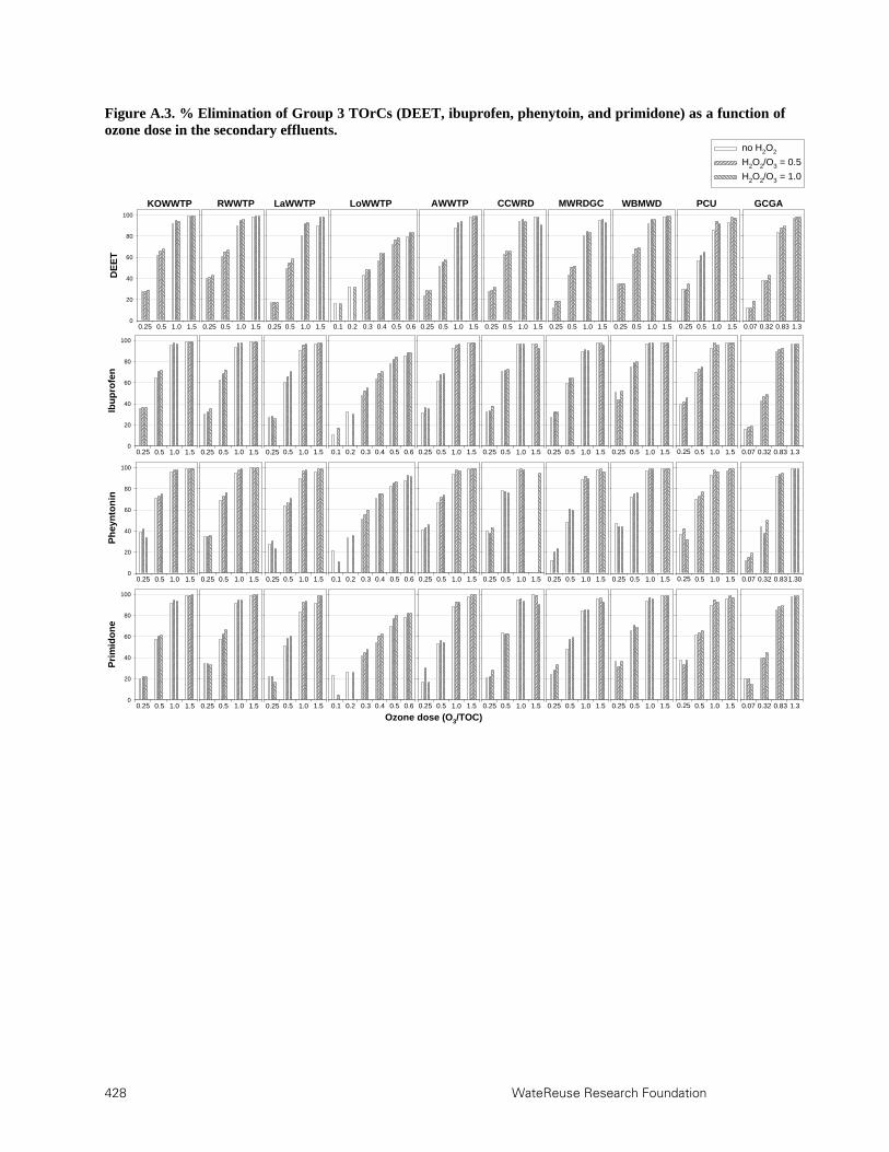
428 WateReuse Research Foundation
Figure A.3. % Elimination of Group 3 TOrCs (DEET, ibuprofen, phenytoin, and primidone) as a function of ozone dose in the secondary effluents.
DE
ET
0
20
40
60
80
100
0.25 0.5 1.0 1.5 0.25 0.5 1.0 1.5 0.25 0.5 1.0 1.5 0.1 0.2 0.3 0.4 0.5 0.6 0.25 0.5 1.0 1.5 0.25 0.5 1.0 1.5 0.25 0.5 1.0 1.5 0.25 0.5 1.0 1.5 0.25 0.5 1.0 1.5 0.07 0.32 0.83 1.3
Ibu
pro
fen
0
20
40
60
80
100
0.25 0.5 1.0 1.5 0.25 0.5 1.0 1.5 0.25 0.5 1.0 1.5 0.1 0.2 0.3 0.4 0.5 0.6 0.25 0.5 1.0 1.5 0.25 0.5 1.0 1.5 0.25 0.5 1.0 1.5 0.25 0.5 1.0 1.5 0.25 0.5 1.0 1.5 0.07 0.32 0.83 1.3
Ph
eyn
ton
in
0
20
40
60
80
100
no H2O2
H2O2/O3 = 0.5
H2O2/O3 = 1.0
0.25 0.5 1.0 1.5 0.25 0.5 1.0 1.5 0.25 0.5 1.0 1.5 0.1 0.2 0.3 0.4 0.5 0.6 0.25 0.5 1.0 1.5 0.25 0.5 1.0 1.5 0.25 0.5 1.0 1.5 0.25 0.5 1.0 1.5 0.25 0.5 1.0 1.5 0.07 0.32 0.831.30
Pri
mid
on
e
0
20
40
60
80
100
0.25 0.5 1.0 1.5 0.25 0.5 1.0 1.5 0.25 0.5 1.0 1.5 0.1 0.2 0.3 0.4 0.5 0.6 0.25 0.5 1.0 1.5 0.25 0.5 1.0 1.5 0.25 0.5 1.0 1.5 0.25 0.5 1.0 1.5 0.25 0.5 1.0 1.5 0.07 0.32 0.83 1.3
Ozone dose (O3/TOC)
KOWWTP RWWTP LaWWTP LoWWTP AWWTP CCWRD MWRDGC WBMWD PCU GCGA

WateReuse Research Foundation 429
Figure A.4. % Elimination of Group 4 TOrCs (meprobamate and atrazine) as a function of ozone dose in the secondary effluents.
Mep
rob
amat
e
0
20
40
60
80
100
0.25 0.5 1.0 1.5 0.25 0.5 1.0 1.5 0.25 0.5 1.0 1.5 0.1 0.2 0.3 0.4 0.5 0.6 0.25 0.5 1.0 1.5 0.25 0.5 1.0 1.5 0.25 0.5 1.0 1.5 0.25 0.5 1.0 1.5 0.25 0.5 1.0 1.5 0.07 0.32 0.83 1.3
Atr
azin
e
0
20
40
60
80
100
no H2O2
H2O2/O3 = 0.5
H2O2/O3 = 1.0
0.25 0.5 1.0 1.5 0.25 0.5 1.0 1.5 0.25 0.5 1.0 1.5 0.1 0.2 0.3 0.4 0.5 0.6 0.25 0.5 1.0 1.5 0.25 0.5 1.0 1.5 0.25 0.5 1.0 1.5 0.25 0.5 1.0 1.5 0.25 0.5 1.0 1.5 0.07 0.32 0.83 1.3
Ozone dose (O3/TOC)
KOWWTP RWWTP LaWWTP LoWWTP AWWTP CCWRD MWRDGC WBMWD PCU GCGA

430 WateReuse Research Foundation
Figure A.5. % Elimination of Group 5 TOrC (TCEP) as a function of ozone dose in the secondary effluents. T
CE
P
0
20
40
60
80
100
0.25 0.5 1.0 1.5 0.25 0.5 1.0 1.5 0.25 0.5 1.0 1.5 0.1 0.2 0.3 0.4 0.5 0.6 0.25 0.5 1.0 1.5 0.25 0.5 1.0 1.5 0.25 0.5 1.0 1.5 0.25 0.5 1.0 1.5 0.25 0.5 1.0 1.5 0.07 0.32 0.83 1.3
Ozone dose (O3/TOC)
no H2O2
H2O2/O3 = 0.5
H2O2/O3 = 1.0
KOWWTP RWWTP LaWWTP LoWWTP AWWTP CCWRD MWRDGC WBMWD PCU GCGA

WateReuse Research Foundation 431
Figure A.6. Relative contribution of ·OH (black bars) and O3 (gray bars) to overall TOrC elimination with O3 alone. The contribution of ·OH to overall elimination was calculated using the equation ·OH contribution = (kOH,M/kOH,P)*(ln([P]/[P]0)*(ln([M]/[M]0)
−1, where M and P represent the target TOrC and OH probe compound, respectively. Meprobamate was used as the OH probe compound (P) in the calculation.
% C
on
trib
uti
on
0
20
40
60
80
100diclofenactriclosan carbamazepine bisphenol-A
0
20
40
60
80
100sulfamethoxazole trimethoprim naproxen gemfibrozil
0
20
40
60
80
100atenolol DEET ibuprofen pheyntonin
0
20
40
60
80
100primidone meprobamate atrazine TCEP
% C
on
trib
uti
on
KO
WW
TP
RW
WT
PLa
WW
TP
LoW
WT
PA
WW
TP
CC
WR
DM
WR
DG
CW
BM
WD
PC
UG
CG
A
KO
WW
TP
RW
WT
PLa
WW
TP
LoW
WT
PA
WW
TP
CC
WR
DM
WR
DG
CW
BM
WD
PC
UG
CG
A
KO
WW
TP
RW
WT
PLa
WW
TP
LoW
WT
PA
WW
TP
CC
WR
DM
WR
DG
CW
BM
WD
PC
UG
CG
A
KO
WW
TP
RW
WT
PLa
WW
TP
LoW
WT
PA
WW
TP
CC
WR
DM
WR
DG
CW
BM
WD
PC
UG
CG
A

432 WateReuse Research Foundation
Figure A.7. Relative contribution of OH (black bars) and O3 (gray bars) to overall TOrC elimination at an H2O2/O3 ratio of 0.5.
% C
on
trib
uti
on
0
20
40
60
80
100diclofenactriclosan carbamazepine bisphenol-A
0
20
40
60
80
100sulfamethoxazole trimethoprim naproxen gemfibrozil
0
20
40
60
80
100atenolol DEET ibuprofen pheyntonin
0
20
40
60
80
100primidone meprobamate atrazine TCEP
% C
on
trib
uti
on
KO
WW
TP
RW
WT
PLa
WW
TP
LoW
WT
PA
WW
TP
CC
WR
DM
WR
DG
CW
BM
WD
PC
UG
CG
AK
OW
WT
PR
WW
TP
LaW
WT
PLo
WW
TP
AW
WT
PC
CW
RD
MW
RD
GC
WB
MW
DP
CU
GC
GA
KO
WW
TP
RW
WT
PLa
WW
TP
LoW
WT
PA
WW
TP
CC
WR
DM
WR
DG
CW
BM
WD
PC
UG
CG
A
KO
WW
TP
RW
WT
PLa
WW
TP
LoW
WT
PA
WW
TP
CC
WR
DM
WR
DG
CW
BM
WD
PC
UG
CG
A

WateReuse Research Foundation 433
Figure A.8. Relative contribution of OH (black bars) and O3 (gray bars) to overall TOrC elimination at an H2O2/O3 ratio of 1.0.
% C
on
trib
uti
on
0
20
40
60
80
100diclofenactriclosan carbamazepine bisphenol-A
0
20
40
60
80
100sulfamethoxazole trimethoprim naproxen gemfibrozil
0
20
40
60
80
100atenolol DEET ibuprofen pheyntonin
0
20
40
60
80
100primidone meprobamate atrazine TCEP
% C
on
trib
uti
on
KO
WW
TP
RW
WT
PLa
WW
TP
LoW
WT
PA
WW
TP
CC
WR
DM
WR
DG
CW
BM
WD
PC
UG
CG
A
KO
WW
TP
RW
WT
PL
aWW
TP
LoW
WT
PA
WW
TP
CC
WR
DM
WR
DG
CW
BM
WD
PC
UG
CG
A
KO
WW
TP
RW
WT
PL
aWW
TP
LoW
WT
PA
WW
TP
CC
WR
DM
WR
DG
CW
BM
WD
PC
UG
CG
AK
OW
WT
PR
WW
TP
LaW
WT
PL
oWW
TP
AW
WT
PC
CW
RD
MW
RD
GC
WB
MW
DP
CU
GC
GA
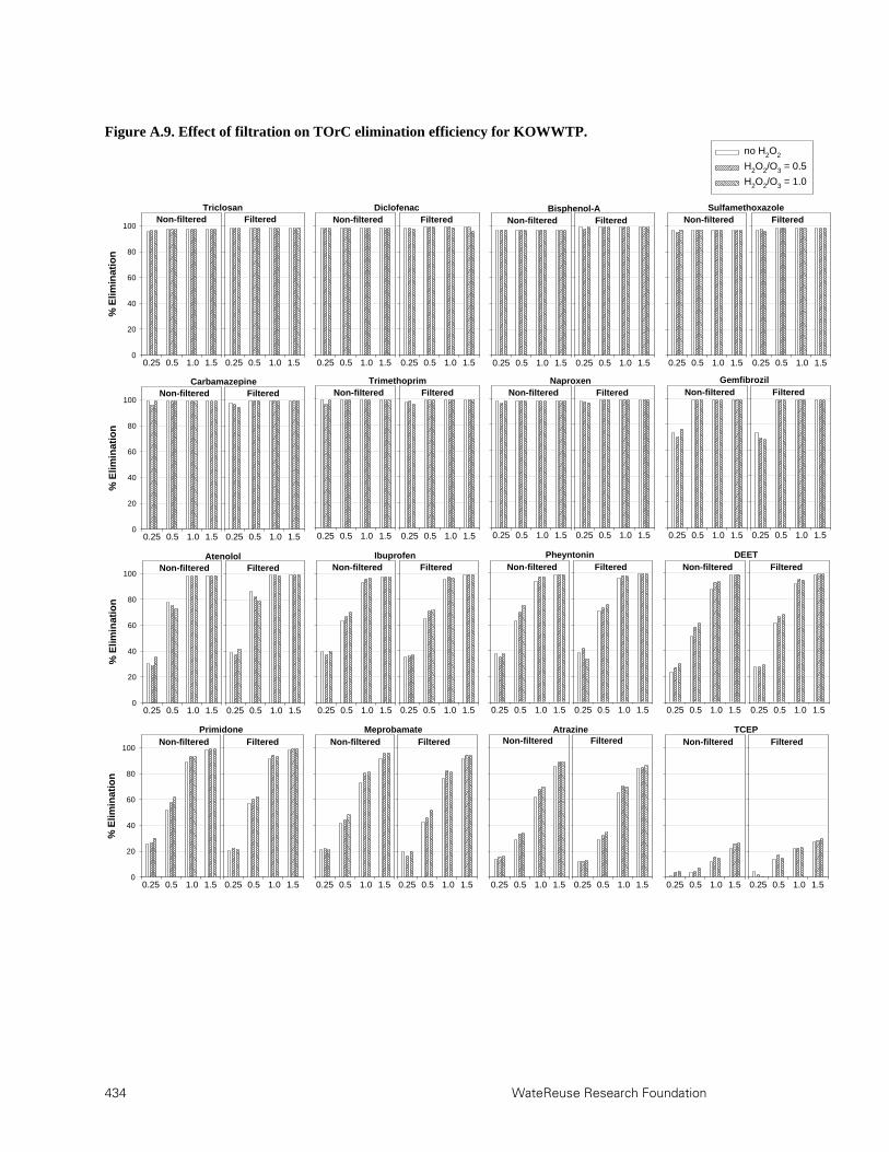
434 WateReuse Research Foundation
Figure A.9. Effect of filtration on TOrC elimination efficiency for KOWWTP.
% E
limin
atio
n
0
20
40
60
80
100
0.25 0.5 1.0 1.5 0.25 0.5 1.0 1.5
TriclosanNon-filtered Filtered
0.25 0.5 1.0 1.5 0.25 0.5 1.0 1.5
DiclofenacNon-filtered Filtered
0.25 0.5 1.0 1.5 0.25 0.5 1.0 1.5
Bisphenol-ANon-filtered Filtered
0.25 0.5 1.0 1.5 0.25 0.5 1.0 1.5
SulfamethoxazoleNon-filtered Filtered
% E
limin
atio
n
0
20
40
60
80
100
0.25 0.5 1.0 1.5 0.25 0.5 1.0 1.5 0.25 0.5 1.0 1.5 0.25 0.5 1.0 1.5 0.25 0.5 1.0 1.5 0.25 0.5 1.0 1.5
CarbamazepineNon-filtered Filtered
TrimethoprimNon-filtered Filtered
NaproxenNon-filtered Filtered
0.25 0.5 1.0 1.5 0.25 0.5 1.0 1.5
GemfibrozilNon-filtered Filtered
% E
limin
atio
n
0
20
40
60
80
100
0.25 0.5 1.0 1.5 0.25 0.5 1.0 1.5 0.25 0.5 1.0 1.5 0.25 0.5 1.0 1.5 0.25 0.5 1.0 1.5 0.25 0.5 1.0 1.5
AtenololNon-filtered Filtered
0.25 0.5 1.0 1.5 0.25 0.5 1.0 1.5
IbuprofenNon-filtered Filtered
PheyntoninNon-filtered Filtered
DEETNon-filtered Filtered
% E
limin
atio
n
0
20
40
60
80
100
0.25 0.5 1.0 1.5 0.25 0.5 1.0 1.5
PrimidoneNon-filtered Filtered
0.25 0.5 1.0 1.5 0.25 0.5 1.0 1.5
MeprobamateNon-filtered Filtered
0.25 0.5 1.0 1.5 0.25 0.5 1.0 1.5
AtrazineNon-filtered Filtered
0.25 0.5 1.0 1.5
no H2O2
H2O2/O3 = 0.5
H2O2/O3 = 1.0
0.25 0.5 1.0 1.5
TCEPNon-filtered Filtered

WateReuse Research Foundation 435
Figure A.10. Effect of filtration on TOrC elimination efficiency for LaWWTP.
% E
limin
atio
n
0
20
40
60
80
100
0.25 0.5 1.0 1.5 0.25 0.5 1.0 1.5
TriclosanNon-filtered Filtered
0.25 0.5 1.0 1.5 0.25 0.5 1.0 1.5
DiclofenacNon-filtered Filtered
0.25 0.5 1.0 1.5 0.25 0.5 1.0 1.5
Bisphenol-ANon-filtered Filtered
0.25 0.5 1.0 1.5 0.25 0.5 1.0 1.5
SulfamethoxazoleNon-filtered Filtered
% E
limin
atio
n
0
20
40
60
80
100
0.25 0.5 1.0 1.5 0.25 0.5 1.0 1.5 0.25 0.5 1.0 1.5 0.25 0.5 1.0 1.5 0.25 0.5 1.0 1.5 0.25 0.5 1.0 1.5
CarbamazepineNon-filtered Filtered
TrimethoprimNon-filtered Filtered
NaproxenNon-filtered Filtered
0.25 0.5 1.0 1.5 0.25 0.5 1.0 1.5
GemfibrozilNon-filtered Filtered
% E
limin
ati
on
0
20
40
60
80
100
0.25 0.5 1.0 1.5 0.25 0.5 1.0 1.5 0.25 0.5 1.0 1.5 0.25 0.5 1.0 1.5 0.25 0.5 1.0 1.5 0.25 0.5 1.0 1.5
AtenololNon-filtered Filtered
0.25 0.5 1.0 1.5 0.25 0.5 1.0 1.5
IbuprofenNon-filtered Filtered
PheyntoninNon-filtered Filtered
DEETNon-filtered Filtered
% E
limin
atio
n
0
20
40
60
80
100
0.25 0.5 1.0 1.5 0.25 0.5 1.0 1.5
PrimidoneNon-filtered Filtered
0.25 0.5 1.0 1.5 0.25 0.5 1.0 1.5
MeprobamateNon-filtered Filtered
0.25 0.5 1.0 1.5 0.25 0.5 1.0 1.5
AtrazineNon-filtered Filtered
0.25 0.5 1.0 1.5
no H2O2
H2O2/O3 = 0.5
H2O2/O3 = 1.0
0.25 0.5 1.0 1.5
TCEPNon-filtered Filtered

436 WateReuse Research Foundation
Figure A.11. Effect of filtration on TOrC elimination efficiency for CCWRD.
% E
limin
atio
n
0
20
40
60
80
100
0.25 0.5 1.0 1.5 0.25 0.5 1.0 1.5
TriclosanNon-filtered Filtered
0.25 0.5 1.0 1.5 0.25 0.5 1.0 1.5
DiclofenacNon-filtered Filtered
0.25 0.5 1.0 1.5 0.25 0.5 1.0 1.5
Bisphenol-ANon-filtered Filtered
0.25 0.5 1.0 1.5 0.25 0.5 1.0 1.5
SulfamethoxazoleNon-filtered Filtered
% E
limin
atio
n
0
20
40
60
80
100
0.25 0.5 1.0 1.5 0.25 0.5 1.0 1.5 0.25 0.5 1.0 1.5 0.25 0.5 1.0 1.5 0.25 0.5 1.0 1.5 0.25 0.5 1.0 1.5
CarbamazepineNon-filtered Filtered
TrimethoprimNon-filtered Filtered
NaproxenNon-filtered Filtered
0.25 0.5 1.0 1.5 0.25 0.5 1.0 1.5
GemfibrozilNon-filtered Filtered
% E
limin
ati
on
0
20
40
60
80
100
0.25 0.5 1.0 1.5 0.25 0.5 1.0 1.5 0.25 0.5 1.0 1.5 0.25 0.5 1.0 1.5 0.25 0.5 1.0 1.5 0.25 0.5 1.0 1.5
AtenololNon-filtered Filtered
0.25 0.5 1.0 1.5 0.25 0.5 1.0 1.5
IbuprofenNon-filtered Filtered
PheyntoninNon-filtered Filtered
DEETNon-filtered Filtered
% E
limin
atio
n
0
20
40
60
80
100
0.25 0.5 1.0 1.5 0.25 0.5 1.0 1.5
PrimidoneNon-filtered Filtered
0.25 0.5 1.0 1.5 0.25 0.5 1.0 1.5
MeprobamateNon-filtered Filtered
0.25 0.5 1.0 1.5 0.25 0.5 1.0 1.5
AtrazineNon-filtered Filtered
0.25 0.5 1.0 1.5
no H2O2
H2O2/O3 = 0.5
H2O2/O3 = 1.0
0.25 0.5 1.0 1.5
TCEPNon-filtered Filtered
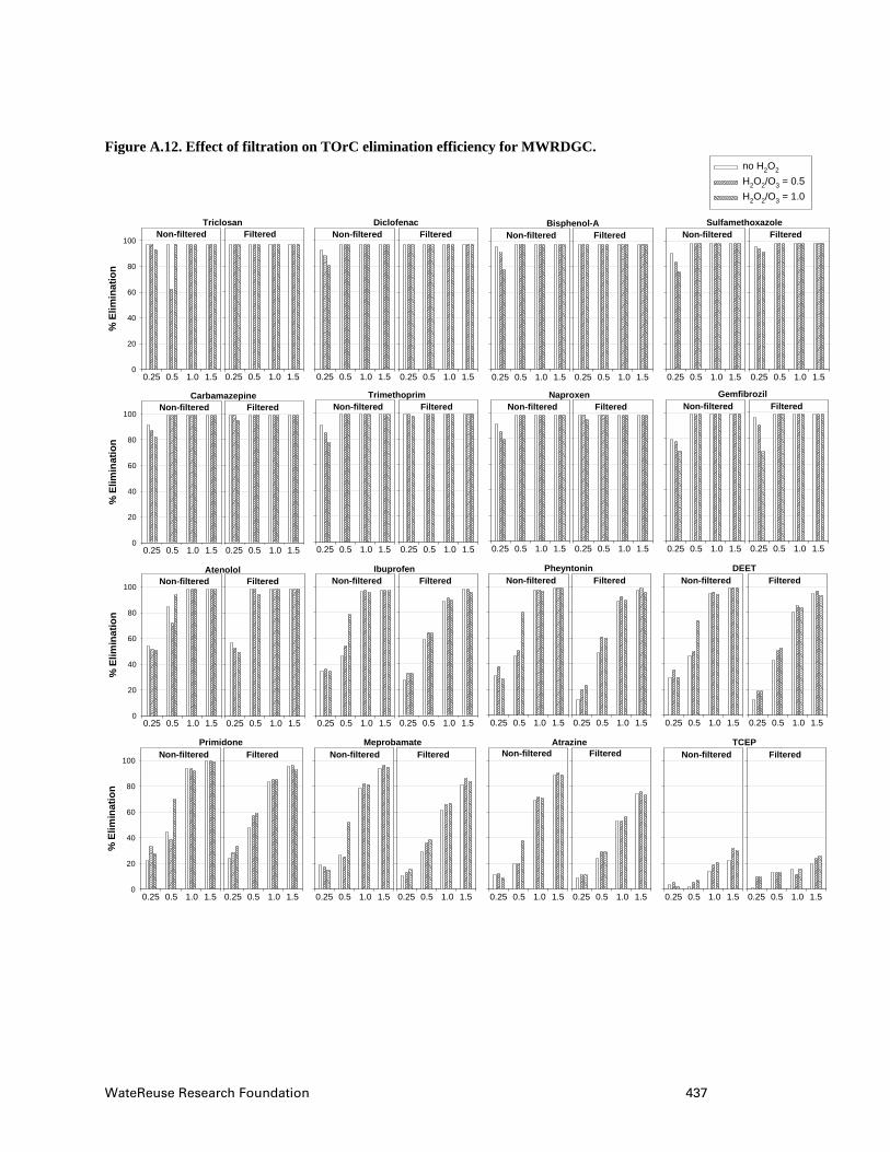
WateReuse Research Foundation 437
Figure A.12. Effect of filtration on TOrC elimination efficiency for MWRDGC.
% E
limin
ati
on
0
20
40
60
80
100
0.25 0.5 1.0 1.5 0.25 0.5 1.0 1.5
TriclosanNon-filtered Filtered
0.25 0.5 1.0 1.5 0.25 0.5 1.0 1.5
DiclofenacNon-filtered Filtered
0.25 0.5 1.0 1.5 0.25 0.5 1.0 1.5
Bisphenol-ANon-filtered Filtered
0.25 0.5 1.0 1.5 0.25 0.5 1.0 1.5
SulfamethoxazoleNon-filtered Filtered
% E
limin
atio
n
0
20
40
60
80
100
0.25 0.5 1.0 1.5 0.25 0.5 1.0 1.5 0.25 0.5 1.0 1.5 0.25 0.5 1.0 1.5 0.25 0.5 1.0 1.5 0.25 0.5 1.0 1.5
CarbamazepineNon-filtered Filtered
TrimethoprimNon-filtered Filtered
NaproxenNon-filtered Filtered
0.25 0.5 1.0 1.5 0.25 0.5 1.0 1.5
GemfibrozilNon-filtered Filtered
% E
limin
ati
on
0
20
40
60
80
100
0.25 0.5 1.0 1.5 0.25 0.5 1.0 1.5 0.25 0.5 1.0 1.5 0.25 0.5 1.0 1.5 0.25 0.5 1.0 1.5 0.25 0.5 1.0 1.5
AtenololNon-filtered Filtered
0.25 0.5 1.0 1.5 0.25 0.5 1.0 1.5
IbuprofenNon-filtered Filtered
PheyntoninNon-filtered Filtered
DEETNon-filtered Filtered
% E
limin
ati
on
0
20
40
60
80
100
0.25 0.5 1.0 1.5 0.25 0.5 1.0 1.5
PrimidoneNon-filtered Filtered
0.25 0.5 1.0 1.5 0.25 0.5 1.0 1.5
MeprobamateNon-filtered Filtered
0.25 0.5 1.0 1.5 0.25 0.5 1.0 1.5
AtrazineNon-filtered Filtered
0.25 0.5 1.0 1.5
no H2O2
H2O2/O3 = 0.5
H2O2/O3 = 1.0
0.25 0.5 1.0 1.5
TCEPNon-filtered Filtered


WateReuse Research Foundation 439
Appendix B
Summary of TOrC Oxidation with UV and UV/H2O2
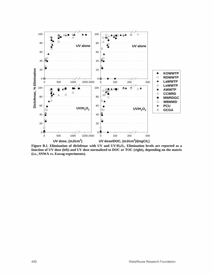
440 WateReuse Research Foundation
0 500 1000 2250 2500
Dic
lofe
nac
, % E
limin
atio
n
0
20
40
60
80
100
UV dose, (mJ/cm2)
0 500 1000 2250 25000
20
40
60
80
100
0 100 200 5000
20
40
60
80
100
UV dose/DOC, (mJ/cm2)/(mgC/L)
0 100 200 5000
20
40
60
80
100
KOWWTPRDWWTPLaWWTPLoWWTPAWWTPCCWRDMWRDGCWBMWDPCUGCGA
UV alone UV alone
UV/H2O2 UV/H2O2
Figure B.1. Elimination of diclofenac with UV and UV/H2O2. Elimination levels are reported as a function of UV dose (left) and UV dose normalized to DOC or TOC (right), depending on the matrix (i.e., SNWA vs. Eawag experiments).
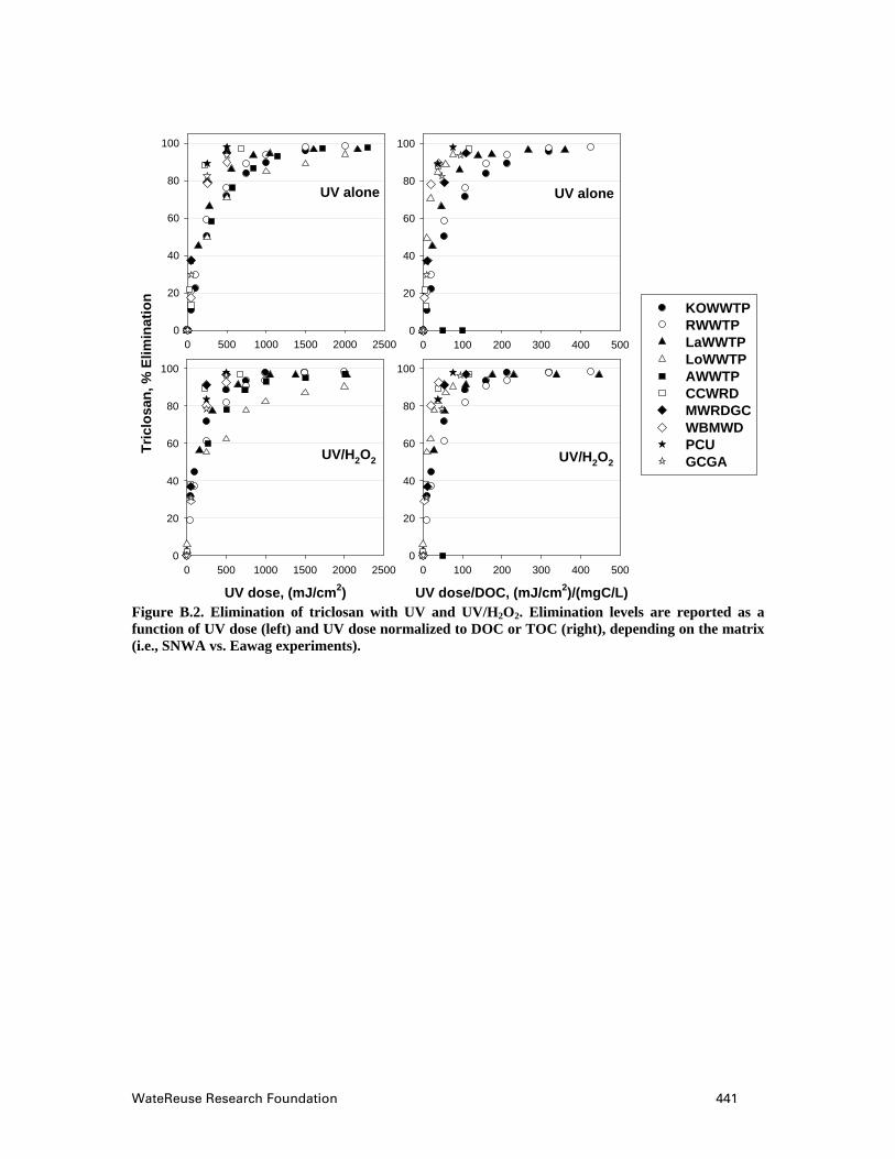
WateReuse Research Foundation 441
0 500 1000 1500 2000 2500
Tri
clo
san
, % E
limin
atio
n
0
20
40
60
80
100
UV dose, (mJ/cm2)
0 500 1000 1500 2000 25000
20
40
60
80
100
0 100 200 300 400 5000
20
40
60
80
100
UV dose/DOC, (mJ/cm2)/(mgC/L)
0 100 200 300 400 5000
20
40
60
80
100
KOWWTPRWWTPLaWWTPLoWWTPAWWTPCCWRDMWRDGCWBMWDPCUGCGA
UV alone UV alone
UV/H2O2 UV/H2O2
Figure B.2. Elimination of triclosan with UV and UV/H2O2. Elimination levels are reported as a function of UV dose (left) and UV dose normalized to DOC or TOC (right), depending on the matrix (i.e., SNWA vs. Eawag experiments).

442 WateReuse Research Foundation
0 500 1000 1500 2000 2500
Su
lfam
eth
oxa
zole
, % E
limin
atio
n
0
20
40
60
80
100
UV dose, (mJ/cm2)
0 500 1000 1500 2000 25000
20
40
60
80
100
0 100 200 300 400 5000
20
40
60
80
100
UV dose/DOC, (mJ/cm2)/(mgC/L)
0 100 200 300 400 5000
20
40
60
80
100
KOWWTPRWWTPLaWWTPLoWWTPAWWTPCCWRDMWRDGCWBMWDPCUGCGA
UV alone UV alone
UV/H2O2 UV/H2O2
Figure B.3. Elimination of sulfamethoxazole with UV and UV/H2O2. Elimination levels are reported as a function of UV dose (left) and UV dose normalized to DOC or TOC (right), depending on the matrix (i.e., SNWA vs. Eawag experiments).

WateReuse Research Foundation 443
0 500 1000 1500 2000 2500
Ph
enyt
oin
, % E
limin
atio
n
0
20
40
60
80
100
UV dose, (mJ/cm2)
0 500 1000 1500 2000 25000
20
40
60
80
100
0 100 200 300 400 5000
20
40
60
80
100
UV dose/DOC, (mJ/cm2)/(mgC/L)
0 100 200 300 400 5000
20
40
60
80
100
KOWWTPRWWTPLaWWTPLoWWTPAWWTPCCWRDMWRDGCWBMWDPCUGCGA
UV alone UV alone
UV/H2O2 UV/H2O2
Figure B.4. Elimination of phenytoin with UV and UV/H2O2. Elimination levels are reported as a function of UV dose (left) and UV dose normalized to DOC or TOC (right), depending on the matrix (i.e., SNWA vs. Eawag experiments).

444 WateReuse Research Foundation
0 500 1000 1500 2000 2500
Atr
azin
e, %
Elim
inat
ion
0
20
40
60
80
100
UV dose, (mJ/cm2)
0 500 1000 1500 2000 25000
20
40
60
80
100
0 100 200 300 400 5000
20
40
60
80
100
UV dose/DOC, (mJ/cm2)/(mgC/L)
0 100 200 300 400 5000
20
40
60
80
100
KOWWTPRWWTPLaWWTPLoWWTPAWWTPCCWRDMWRDGCWBMWDPCUGCGA
UV alone UV alone
UV/H2O2UV/H2O2
Figure B.5. Elimination of atrazine with UV and UV/H2O2. Elimination levels are reported as a function of UV dose (left) and UV dose normalized to DOC or TOC (right), depending on the matrix (i.e., SNWA vs. Eawag experiments).
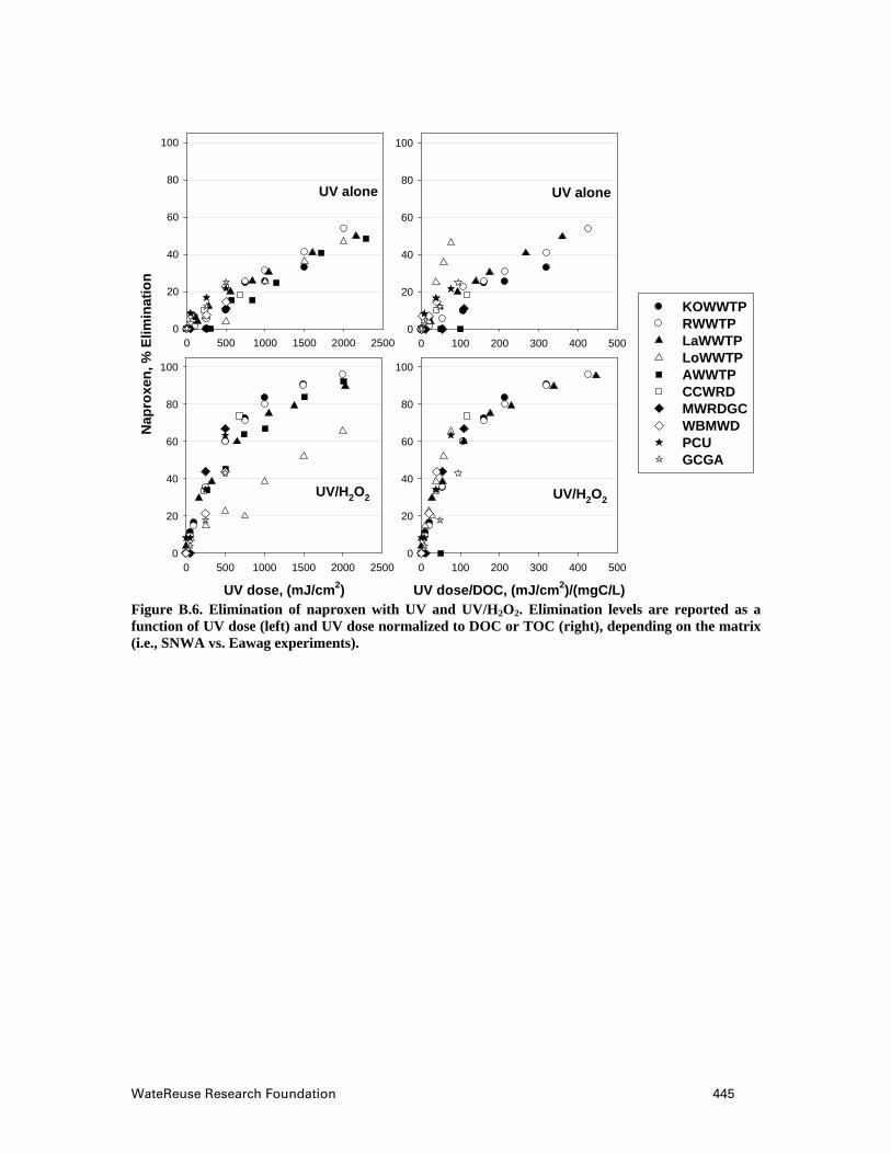
WateReuse Research Foundation 445
0 500 1000 1500 2000 2500
Nap
roxe
n, %
Elim
inat
ion
0
20
40
60
80
100
UV dose, (mJ/cm2)
0 500 1000 1500 2000 25000
20
40
60
80
100
0 100 200 300 400 5000
20
40
60
80
100
UV dose/DOC, (mJ/cm2)/(mgC/L)
0 100 200 300 400 5000
20
40
60
80
100
KOWWTPRWWTPLaWWTPLoWWTPAWWTPCCWRDMWRDGCWBMWDPCUGCGA
UV alone UV alone
UV/H2O2 UV/H2O2
Figure B.6. Elimination of naproxen with UV and UV/H2O2. Elimination levels are reported as a function of UV dose (left) and UV dose normalized to DOC or TOC (right), depending on the matrix (i.e., SNWA vs. Eawag experiments).
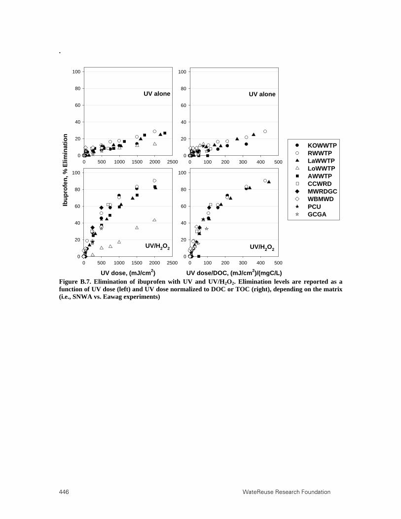
446 WateReuse Research Foundation
.
0 500 1000 1500 2000 2500
Ibu
pro
fen
, % E
limin
atio
n
0
20
40
60
80
100
UV dose, (mJ/cm2)
0 500 1000 1500 2000 25000
20
40
60
80
100
0 100 200 300 400 5000
20
40
60
80
100
UV dose/DOC, (mJ/cm2)/(mgC/L)
0 100 200 300 400 5000
20
40
60
80
100
KOWWTPRWWTPLaWWTPLoWWTPAWWTPCCWRDMWRDGCWBMWDPCUGCGA
UV alone UV alone
UV/H2O2 UV/H2O2
Figure B.7. Elimination of ibuprofen with UV and UV/H2O2. Elimination levels are reported as a function of UV dose (left) and UV dose normalized to DOC or TOC (right), depending on the matrix (i.e., SNWA vs. Eawag experiments)

WateReuse Research Foundation 447
0 500 1000 1500 2000 2500
Tri
met
ho
pri
m, %
Elim
inat
ion
0
20
40
60
80
100
UV dose, (mJ/cm2)
0 500 1000 1500 2000 25000
20
40
60
80
100
0 100 200 300 400 5000
20
40
60
80
100
UV dose/DOC, (mJ/cm2)/(mgC/L)
0 100 200 300 400 5000
20
40
60
80
100
KOWWTPRWWTPLaWWTPLoWWTPAWWTPCCWRDMWRDGCWBMWDPCUGCGA
UV alone UV alone
UV/H2O2 UV/H2O2
Figure B.8. Elimination of trimethoprim with UV and UV/H2O2. Elimination levels are reported as a function of UV dose (left) and UV dose normalized to DOC or TOC (right), depending on the matrix (i.e., SNWA vs. Eawag experiments).

448 WateReuse Research Foundation
0 500 1000 1500 2000 2500
Ate
no
lol,
% E
limin
atio
n
0
20
40
60
80
100
UV dose, (mJ/cm2)
0 500 1000 1500 2000 25000
20
40
60
80
100
0 100 200 300 400 5000
20
40
60
80
100
UV dose/DOC, (mJ/cm2)/(mgC/L)
0 100 200 300 400 5000
20
40
60
80
100
KOWWTPRWWTPLaWWTPLoWWTPAWWTPCCWRDMWRDGCWBMWDPCUGCGA
UV alone UV alone
UV/H2O2 UV/H2O2
Figure B.9. Elimination of atenolol with UV and UV/H2O2. Elimination levels are reported as a function of UV dose (left) and UV dose normalized to DOC or TOC (right), depending on the matrix (i.e., SNWA vs. Eawag experiments).
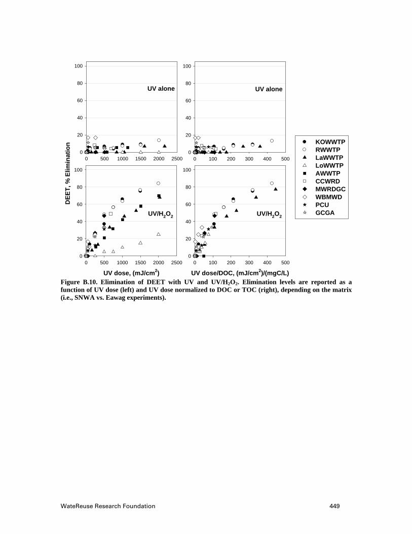
WateReuse Research Foundation 449
0 500 1000 1500 2000 2500
DE
ET
, % E
limin
atio
n
0
20
40
60
80
100
UV dose, (mJ/cm2)
0 500 1000 1500 2000 25000
20
40
60
80
100
0 100 200 300 400 5000
20
40
60
80
100
UV dose/DOC, (mJ/cm2)/(mgC/L)
0 100 200 300 400 5000
20
40
60
80
100
KOWWTPRWWTPLaWWTPLoWWTPAWWTPCCWRDMWRDGCWBMWDPCUGCGA
UV alone UV alone
UV/H2O2 UV/H2O2
Figure B.10. Elimination of DEET with UV and UV/H2O2. Elimination levels are reported as a function of UV dose (left) and UV dose normalized to DOC or TOC (right), depending on the matrix (i.e., SNWA vs. Eawag experiments).

450 WateReuse Research Foundation
0 500 1000 1500 2000 2500
Car
bam
azep
ine,
% E
limin
atio
n
0
20
40
60
80
100
UV dose, (mJ/cm2)
0 500 1000 1500 2000 25000
20
40
60
80
100
0 100 200 300 400 5000
20
40
60
80
100
UV dose/DOC, (mJ/cm2)/(mgC/L)
0 100 200 300 400 5000
20
40
60
80
100
KOWWTPRWWTPLaWWTPLoWWTPAWWTPCCWRDMWRDGCWBMWDPCUGCGA
UV alone UV alone
UV/H2O2 UV/H2O2
Figure B.11. Elimination of carbamazepine with UV and UV/H2O2. Elimination levels are reported as a function of UV dose (left) and UV dose normalized to DOC or TOC (right), depending on the matrix (i.e., SNWA vs. Eawag experiments).

WateReuse Research Foundation 451
0 500 1000 1500 2000 2500
Gem
fib
rozi
l, %
Elim
inat
ion
0
20
40
60
80
100
UV dose, (mJ/cm2)
0 500 1000 1500 2000 25000
20
40
60
80
100
0 100 200 300 400 5000
20
40
60
80
100
UV dose/DOC, (mJ/cm2)/(mgC/L)
0 100 200 300 400 5000
20
40
60
80
100
KOWWTPRWWTPLaWWTPLoWWTPAWWTPCCWRDMWRDGCWBMWDPCUGCGA
UV alone UV alone
UV/H2O2 UV/H2O2
Figure B.12. Elimination of gemfibrozil with UV and UV/H2O2. Elimination levels are reported as a function of UV dose (left) and UV dose normalized to DOC or TOC (right), depending on the matrix (i.e., SNWA vs. Eawag experiments).
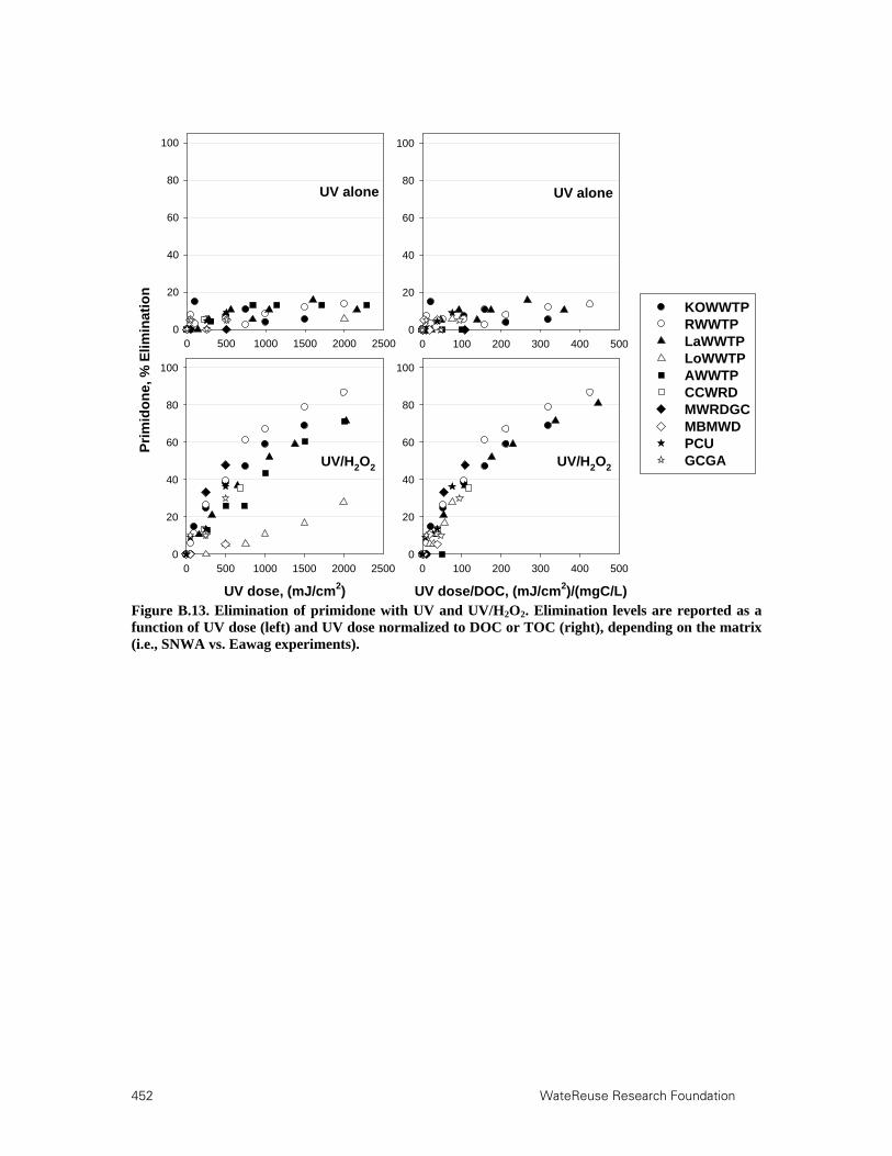
452 WateReuse Research Foundation
0 500 1000 1500 2000 2500
Pri
mid
on
e, %
Elim
inat
ion
0
20
40
60
80
100
UV dose, (mJ/cm2)
0 500 1000 1500 2000 25000
20
40
60
80
100
0 100 200 300 400 5000
20
40
60
80
100
UV dose/DOC, (mJ/cm2)/(mgC/L)
0 100 200 300 400 5000
20
40
60
80
100
KOWWTPRWWTPLaWWTPLoWWTPAWWTPCCWRDMWRDGCMBMWDPCUGCGA
UV alone UV alone
UV/H2O2 UV/H2O2
Figure B.13. Elimination of primidone with UV and UV/H2O2. Elimination levels are reported as a function of UV dose (left) and UV dose normalized to DOC or TOC (right), depending on the matrix (i.e., SNWA vs. Eawag experiments).

WateReuse Research Foundation 453
0 500 1000 1500 2000 2500
Bis
ph
eno
l-A
, % E
limin
atio
n
0
20
40
60
80
100
UV dose, (mJ/cm2)
0 500 1000 1500 2000 25000
20
40
60
80
100
0 100 200 300 400 5000
20
40
60
80
100
UV dose/DOC, (mJ/cm2)/(mgC/L)
0 100 200 300 400 5000
20
40
60
80
100
KOWWTPRWWTPLaWWTPLoWWTPAWWTPCCWRDMWRDGCWBMWDPCUGCGA
UV alone UV alone
UV/H2O2UV/H2O2
Figure B.14. Elimination of bisphenol A with UV and UV/H2O2. Elimination levels are reported as a function of UV dose (left) and UV dose normalized to DOC or TOC (right), depending on the matrix (i.e., SNWA vs. Eawag experiments).

454 WateReuse Research Foundation
0 500 1000 1500 2000 2500
Mep
rob
amat
e, %
Elim
inat
ion
0
20
40
60
80
100
UV dose, (mJ/cm2)
0 500 1000 1500 2000 25000
20
40
60
80
100
0 100 200 300 400 5000
20
40
60
80
100
UV dose/DOC, (mJ/cm2)/(mgC/L)
0 100 200 300 400 5000
20
40
60
80
100
KOWWTPRWWTPLaWWTPLoWWTPAWWTPCCWRDMWRDGCWBMWDPCUGCGA
UV alone UV alone
UV/H2O2 UV/H2O2
Figure B.15. Elimination of meprobamate with UV and UV/H2O2. Elimination levels are reported as a function of UV dose (left) and UV dose normalized to DOC or TOC (right), depending on the matrix (i.e., SNWA vs. Eawag experiments).
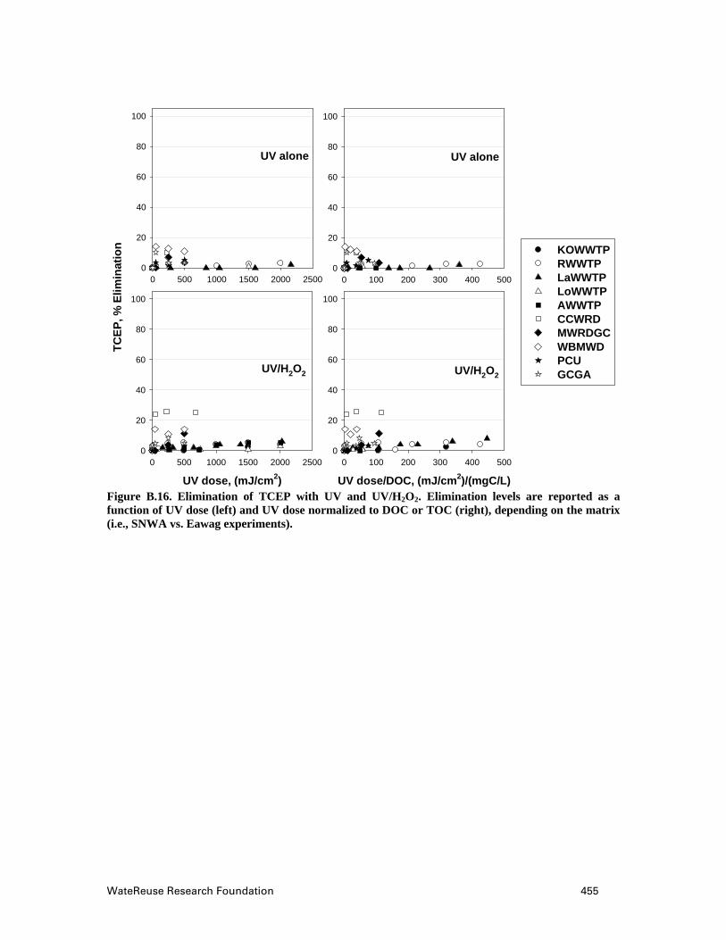
WateReuse Research Foundation 455
0 500 1000 1500 2000 2500
TC
EP
, % E
limin
atio
n
0
20
40
60
80
100
UV dose, (mJ/cm2)
0 500 1000 1500 2000 25000
20
40
60
80
100
0 100 200 300 400 5000
20
40
60
80
100
UV dose/DOC, (mJ/cm2)/(mgC/L)
0 100 200 300 400 5000
20
40
60
80
100
KOWWTPRWWTPLaWWTPLoWWTPAWWTPCCWRDMWRDGCWBMWDPCUGCGA
UV alone UV alone
UV/H2O2 UV/H2O2
Figure B.16. Elimination of TCEP with UV and UV/H2O2. Elimination levels are reported as a function of UV dose (left) and UV dose normalized to DOC or TOC (right), depending on the matrix (i.e., SNWA vs. Eawag experiments).

456 WateReuse Research Foundation
k, (
mJ
/cm
2 )-1 x
10
-4
0
10
20
30
40
50
60
0
5
10
15
20
0
2
4
6
8
10
12
diclofenac triclosan sulfamethoxazole pheyntonin
bisphenol-A naproxen
0
2
4
6
8atrazine ibuprofen
k, (
mJ/
cm2 )-1
x10-4
0
2
4
6
8trimethoprim atenolol
DEET
0
2
4
6
8carbamazepine gemfibrozil
0
1
2
3
4
5
6primidone
0
1
2
3
4meprobamate TCEP
KO
WW
TP
RW
WT
PLW
WT
PLo
WW
TP
AW
WT
PC
CW
RD
MW
RD
GC
WB
MW
DP
CU
GC
GA
WWTPWWTPWWTP
KO
WW
TP
RW
WT
PLW
WT
PLo
WW
TP
AW
WT
PC
CW
RD
MW
RD
GC
WB
MW
DP
CU
GC
GA
KO
WW
TP
RW
WT
PLW
WT
PLo
WW
TP
AW
WT
PC
CW
RD
MW
RD
GC
WB
MW
DP
CU
GC
GA
KO
WW
TP
RW
WT
PLW
WT
PLo
WW
TP
AW
WT
PC
CW
RD
MW
RD
GC
WB
MW
DP
CU
GC
GA
Figure B.17. Pseudo-first-order rate constants (k based on UV dose) for TOrC degradation with UV alone (white bars) and UV/H2O2 (gray bars). Note the different y-axis scales.

WateReuse Research Foundation 457
k[D
OC
], (
mJ
/cm
2)-1
mg
C/L
, x1
0-3
0
10
20
30
40
50
60
0
2
4
6
8
10
12
14
16
0
1
2
3
4
5
6
7
8
diclofenac triclosan sulfamethoxazole pheyntonin
bisphenol-A naproxen
0
1
2
3
4
5
6atrazine ibuprofen
0
1
2
3
4
5trimethoprim atenolol
DEET
0
1
2
3
4
5carbamazepine gemfibrozil
0
1
2
3
4
5primidone
0
1
2
3
4
5meprobamate TCEP
KO
WW
TP
RW
WT
PLW
WT
PLo
WW
TP
AW
WT
PC
CW
RD
MW
RD
GC
WB
MW
DP
CU
GC
GA
KO
WW
TP
RW
WT
PLW
WT
PLo
WW
TP
AW
WT
PC
CW
RD
MW
RD
GC
WB
MW
DP
CU
GC
GA
KO
WW
TP
RW
WT
PLW
WT
PL
oWW
TP
AW
WT
PC
CW
RD
MW
RD
GC
WB
MW
DP
CU
GC
GA
KO
WW
TP
RW
WT
PLW
WT
PLo
WW
TP
AW
WT
PC
CW
RD
MW
RD
GC
WB
MW
DP
CU
GC
GA
Figure B.18. Pseudo-first-order rate constants (k based on UV dose normalized to DOC) for TOrC degradation with UV alone (white bars) and UV/H2O2 (gray bars). Note the different y-axis scales.
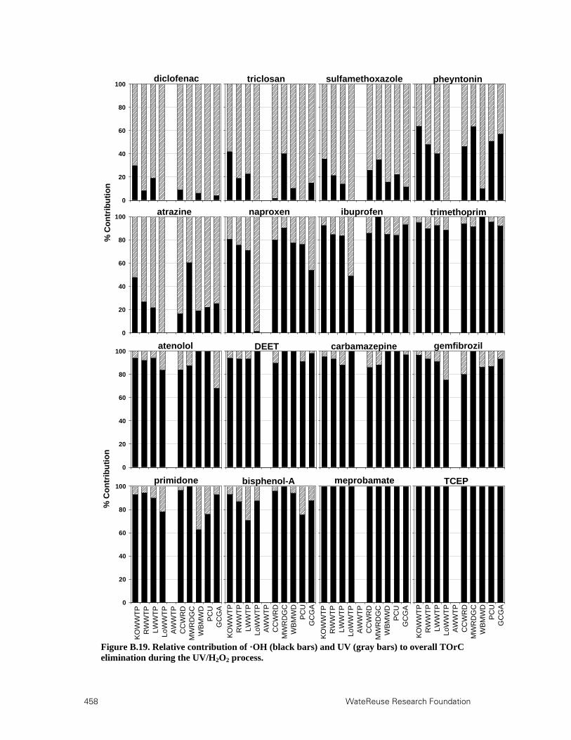
458 WateReuse Research Foundation
% C
on
trib
uti
on
0
20
40
60
80
100diclofenac triclosan sulfamethoxazole pheyntonin
0
20
40
60
80
100atrazine naproxen ibuprofen trimethoprim
0
20
40
60
80
100atenolol DEET carbamazepine gemfibrozil
0
20
40
60
80
100primidone bisphenol-A meprobamate TCEP
% C
on
trib
uti
on
KO
WW
TP
RW
WT
PLW
WT
PLo
WW
TP
AW
WT
PC
CW
RD
MW
RD
GC
WB
MW
DP
CU
GC
GA
KO
WW
TP
RW
WT
PLW
WT
PLo
WW
TP
AW
WT
PC
CW
RD
MW
RD
GC
WB
MW
DP
CU
GC
GA
KO
WW
TP
RW
WT
PLW
WT
PLo
WW
TP
AW
WT
PC
CW
RD
MW
RD
GC
WB
MW
DP
CU
GC
GA
KO
WW
TP
RW
WT
PLW
WT
PLo
WW
TP
AW
WT
PC
CW
RD
MW
RD
GC
WB
MW
DP
CU
GC
GA
Figure B.19. Relative contribution of ·OH (black bars) and UV (gray bars) to overall TOrC elimination during the UV/H2O2 process.


1199 North Fairfax Street, Suite 410
Alexandria, VA 22314 USA
(703) 548-0880
Fax (703) 548-5085
E-mail: [email protected]
wwwwww..WWaatteeRReeuussee..oorrgg//FFoouunnddaattiioonn
Practical Solutions for Water Scarcity