
TRABAJOS DE FÍSICA - FAMAF UNC · FSA Trabajos originales en Física Serie A 1 (2012) 1-16 1...
17
UNIVERSIDAD NACIONAL DE CÓRDOBA FACULTAD DE MATEMÁTICA, ASTRONOMÍA Y FÍSICA ______________________________________________________________________ SERIE “A” TRABAJOS DE FÍSICA Nº 13/2012 Integrated Analysis of Experimental Data C.A. Martín, M.E. Ramia y M.A. Chesta Editores: Miguel A. Chesta–Ricardo C. Zamar ____________________________________________________________ CIUDAD UNIVERSITARIA – 5000 CÓRDOBA REPÚBLICA ARGENTINA
Transcript of TRABAJOS DE FÍSICA - FAMAF UNC · FSA Trabajos originales en Física Serie A 1 (2012) 1-16 1...

UNIVERSIDAD NACIONAL DE CÓRDOBA
FACULTAD DE MATEMÁTICA, ASTRONOMÍA Y FÍSICA ______________________________________________________________________
SERIE “A”
TRABAJOS DE FÍSICA
Nº 13/2012
Integrated Analysis of Experimental Data
C.A. Martín, M.E. Ramia y M.A. Chesta
Editores: Miguel A. Chesta–Ricardo C. Zamar ____________________________________________________________
CIUDAD UNIVERSITARIA – 5000 CÓRDOBA
REPÚBLICA ARGENTINA

FSA Trabajos originales en Física Serie A 1 (2012) 1-16
1
Integrated Analysis of Experimental Data
C.A. Martín, M.E. Ramia and M.A. Chesta
Facultad de Matemática, Astronomía y Física – Universidad Nacional de Córdoba – Ciudad
Universitaria – X5016LAE Córdoba – Argentina
Abstract
A challenging important need is to extract from experimental data the correct values for the
characteristic parameters while, at the same time minimizing their uncertainties. However, when we
have at hand experimental data yielded from different experiments sharing the same characteristic
parameters, it is difficult to find a procedure to take full advantage of the whole data package by
combining the various sets of experimental data into a single fit, and consequently to determine
unique values for such parameters and their uncertainties. In this work we develop a procedure
allowing the integration of the various data sets into a grand set which in turn is analyzed into a
fitting procedure producing unique values for the characteristic parameters in a single shot. This
procedure is successfully applied, employing DataFit, a commercially available software, in two
cases, providing full evidence and support about the reliability of the proposed procedure.
Additionally, a comparison of the values of the uncertainties affecting the characteristic parameters
with those obtained by standard methods is presented.
I – Introduction
In the realm of experimental sciences to carry on experiments and to gather data in order, for
example, to verify a proposed model to describe a system or, by means of a reliable model, to
determine the values for the characteristic parameters of such a system, is a demanding activity
requiring time, supplies, equipment, manpower, etc. For these reasons the analysis of the collected
information must be optimized obtaining the best values for the characteristic parameters and
minimizing the uncertainties affecting them.
In this work we develop a procedure that combines various measurement sets obtained in different
experiments in a unique integrated analysis allowing the determination of the best values for the
characteristic parameters.
These sets of measurements may have been produced in two well differentiated situations. a) The
same experiment is repeated, in the same system and in identical experimental conditions, a number
of times. b) Different experiments sharing characteristic parameters and that may be repeated in
identical experimental conditions a convenient number of times.
It is necessary that the measurements be produced under repeatability conditions, which are: (i) To
employ the same measurement procedure; (ii) The observer/operator is the same; (iii) The same
instruments are used; (iv) The instruments are used in the same conditions; (v) The measurements
are carried out in the same place; and (vi) The measurements are carried out in a short period of
time.

Integrated Analysis of Experimental Data
2
In Section II the procedure is described, and in Section III application examples are given and the
highlights of the procedure are pointed out.
II – Procedure
Let us consider that experiments are performed on a system which may be described by a function
such as that given by the equation
where:
–– x identifies the independent variable in our experiment, for example time, temperature, etc.
–– y is the dependent variable, namely position, specific heat, NQR (Nuclear Quadrupole
Resonance) frequency, magnetization, etc.
–– P1, P2, etc. are characteristic parameters of the system being studied whose values are wanted to
be determined and which may not be obtained by other means.
–– V1, V2, etc. are working parameters which neither depend on nor affect the characteristic
parameters, but instead may be varied in order to produce distinct sets of measurements. These
parameters are known and may be determined by other methods.
Furthermore, in order to simplify let us consider the case where we have two characteristic
parameters P1 and P2 as well as two working parameters V1 and V2 and that x stands for time t.
Generalization is straightforward.
III – A – Repeated Single Experiment
In this case it is analyzed the results of an experiment that may be repeated a number of times n and,
in this way, we end up with n data sets of the form given by
If each set is analyzed on its own we will end up obtaining n pairs of values (P1i, P2i), 1 i n, for
the characteristic parameters. Also, it has been allowed for each set to have different number of data
points (ma, mb, … , mp) as well as spanning different time intervals (T1, T2, … , Tn).
Since the characteristic parameters have a unique value for the particular system, it turns out more
attractive and effective from a physical stand point to ask ourselves: How can we manage the
integration of all of the data from the n sets given in Eqs. 2 in a single analysis producing unique
values for the characteristic parameters P1 and P2?

Martín C A, Ramia M E and Chesta M A
3
To this end what must be done is to construct an array of the n data sets into a grand data set where,
for physical reasons, the characteristic parameters P1 and P2 possess the same value since the
system itself has not been modified and the measurements have been carried out in exactly under
the same experimental conditions. Simultaneously, it is necessary to keep track of each individual
set in order to allow the determination of the other experimental parameters such as, for example,
V1, V2 and the time intervals t under which the different experiments are run.
We propose to build such a grand data set through the ordered union of the n sets appropriately
identifying them by means of the independent variable t.
Among the commercial software, DataFit1 was chosen since it combines simplicity, easiness and is
particularly useful to the objective in this work.
To this end, artificial shifts of the time variables are introduced corresponding to each data set, such
as
where, in general, having performed the ith repetition of the experiment, mi indicates the number of
(tl, yi(tl)) data pairs collected in the ith set while time tl spans the interval [T1+ T2+… +Ti-1 , T1+
T2+… +Ti-1 +Ti).
Therefore, with the proposed union of these n sets a unique grand set is obtained, which consists of
n
i
imM
1
data pairs (yk, tk) with 1 k M and tk [0, T) with
n
i
iTT
1
. The ordering of the (yk,
tk) pairs is the one given in Eqs. 3.
Thus we have prepared the data in an appropriate way to carry on the integrated analysis of the n
measurement sets by means of DataFit, hence determining single values for parameters P1 y P2
optimizing the fitting of the n measurements sets simultaneously.
III – B – Repeated Different Experiments
In this case we consider the analysis of different experiments realized on the same system that may
be repeated. For the sake of clarity, let us consider two different experiments performed on the same
system, sharing characteristic parameters, which may be repeated as in the previous case.
Let the functions g and h describe the two experiments under analysis. Let us also assume that,
following the procedure described in the previous point, the times have been adequately shifted in
order to carry on the proposed analysis

Integrated Analysis of Experimental Data
4
where time t in set 1a takes ku1 values and spans the interval [0, Tu1), in set 2b takes ku2 values and
spans the interval [Tu1, Tu1+Tu2), etc., and kui and kvi indicate the number of (ti, ui) and (tj, yj) data
pairs collected while performing the ith and the jth repetition of the experiments described by g and
h, respectively.
The analysis follows similarly as that developed in the previous point. To proceed it is necessary to
perform the union of these n+m data sets in order to build the grand set, which consists of N+M,
and , data pairs (ui(tc), tc) with Nk1ui ,
and . The order of the ordered pairs is that given in Eqs. 4. It
may be mentioned that there are other equivalent ways of building the grand set and the choice as to
what is the preferred way to build it up to our decision.
In this way the data has been properly prepared to carry on the integrated fit of the n+m sets of
measurements by means of DataFit in a unique analysis thus determining unique values for the
parameters P1 and P2 optimizing the fitting of all of the data simultaneously.
IV – Employing DataFit
In the “Model Editor” screen is where DataFit defines the function Y to be used to fit the data,
allowing this definition to take place through the definition of a series of partial functions Fi with
1 i 9.

Martín C A, Ramia M E and Chesta M A
5
For the sake of simplicity let us consider the case in which the one experiment has been repeated
three times. Generalization is straightforward. This situation is shown in Ec. 5
The way to proceed with DataFit is shown in Appendix A.1 (Section VII).
Running DataFit will allow determining the two shared characteristic parameters P1 and P2 as well
as the six non-shared experimental parameters V11, V21, V12, V22, V13 and V23, with their
corresponding standard deviations.
In the following section examples are given.
V – Examples
Two examples will be developed in detail: (a) The decay of the transverse magnetization in the
Carr-Purcell-Meiboom-Gill (CPMG)2 sequence, Nuclear Magnetic Resonance (NMR) experiment;
and (b) The flywheel experiment, a basic experiment in Mechanics3.
The CPMG corresponds to the repeated single experiment case treated in Section III-A, while the
flywheel corresponds to the repeated different experiments case treated in Section III-B.
NMR-CPMG Decay Signal
The decay of the transversal component of the magnetization in an NMR experiment may be
determined by means of the CPMG pulse sequence. This signal may, in general, be well described
by an exponential decay; its amplitude is related to the amount of substance and to the gain of the
analizer while the characteristic time constant is a property of the compound producing the signal.
In the present case the NMR measurements have been carried out employing a Minispec4
instrument using the 1H in a brine prepared with a concentration of 50 ppm of ClNa. The signals
amplitude obtained are well described by an exponential decay as that given in Eq. 7
The experiment is repeated n times in exactly the same experimental conditions while the time t
sweeps the interval 0 t T, and the data is gathered at times evenly spaced by about 6 ms. In the
present case the experiment has been repeated eight times. Due to the experimental conditions it is
expected that the characteristic parameters Ai and τ2i should have the same value in all eight
measurements. The same situation holds for Si and Oi which are added in order to account for the
presence of base line drifts produced by the NMR spectrometer during the experiments.
Employing T = 12000 ms the DataFit expressions are shown in Appendix A.2 (Section VIII). The
results obtained by means of the integrated fit are given in Table 1 and depicted in Fig. 1.
Table 1: Values of the characteristic parameters in Eqs. a.2
Parameter Value
A (AU*) 15.634 0.004

Integrated Analysis of Experimental Data
6
τ2 (ms) 2444 1
* AU stands for Arbitrary Units.
The uncertainties –standard deviations– in the fitted parameters using DataFit are evaluated
following the Guide ISO/IEC 98-3:2008.5
Sig
na
l A
mp
litu
de
S(t
) (A
U)
t (ms)
0
2
4
6
8
10
12
14
16
0 10000 20000 30000 40000 50000 60000 70000 80000 90000 100000
NMR-CPMG signals
Integrated Fit - Eq. 8
Figure 1: The eight NMR–CPMG brine signal amplitudes (blue) are depicted along the integrated
fit (red) achieved by means of Eq. 6. As may be seen the description of the experimental data is
excellent.
In order to show the improvement achieved by means of the proposed integrated analysis it is
convenient to compare these results with those obtained treating the eight signals individually. The
characteristic parameters obtained for the eight signals are given in Table 2.
Table 2: Values obtained for the characteristic parameters along with their standard deviations are
given for each of the eight signals analyzed with DataFit using the fitting function given in Eq. 6.
Signal A (AU) τ2 (ms)
1 15.6065 0.0095 2440.8 2.5
2 15.6520 0.0091 2447.6 2.4
3 15.6092 0.0089 2435.1 2.4
4 15.7360 0.0092 2460.1 2.4
5 15.6152 0.0089 2450.5 2.4
6 15.6118 0.0090 2434.6 2.4
7 15.5633 0.0087 2434.9 2.3
8 15.6783 0.0091 2448.0 2.4
As may be seen in Table 2 the characteristic parameters, A and τ2, have close but different values.
Two questions arise: (a) How to determine the values to be used? and (b) What are their standard
deviations?
A mean value ( , and ) and its standard deviation ( , and ) may be evaluated in various
ways. Three of them are as follows: (a) applying the basic Gauss theory for random errors6; (b)
applying the procedure defined in the GUM (Guide to the expression of Uncertainty in

Martín C A, Ramia M E and Chesta M A
7
Measurement ISO/IEC 98-3:2008)5; and (c) applying the methodology developed in this integrated
analysis and employing DataFit.
The results of these three ways for τ2 are shown in Eqs. 7.
Results obtained following Gauss theory for random errors
Results obtained following GUM
According to GUM is the uncertainty in the parameter .
Results obtained following this work
Similarly the results obtained for A are shown in Eqs. 10.
Results obtained following Gauss theory for random errors
Results obtained following GUM
According to GUM is the uncertainty in the parameter .

Integrated Analysis of Experimental Data
8
Results obtained following this work
The following conclusions are in order:
1) The mean values and agree with those determined by means the integrated analysis,
thus supporting the reliability of the procedure developed in this work.
2) The GUM standard deviations agree with those determined through the integrated analysis,
thus bringing additional support to the procedure developed in this work.
3) The close agreement in the results given by Eqs. 7b with 7c and 8b with 8c indicates that
the evaluation of uncertainties by DataFit closely follows the GUM.
4) It is generally observed a greater uncertainty in applying the Gauss standard theory, giving
a clear indication of the difficulty of implementing it with a certain type of experimental
data. A more detailed study (e.g. as suggested in the book by P.R. Bevington and D.K.
Robinson8) can lead to decrease the difference between the uncertainties obtained by
different methods.
5) The integrated procedure allows saving time and effort since, in the case under analysis,
the situation was solved with just one fit instead of the eight required by other means.
These savings increase with the number of acquired signals.
6) What has been pointed out for and A is also valid for the other parameters (O and S in
Eq. 6).
7) The integrated analysis procedure provides support to the expectation that the various
measurements have been carried on the same initial experimental conditions, thus
producing repeatability.
8) The integrated analysis methodology allows determining in an elegant form and in just one
attempt unique values for the characteristic parameters (A and ) as well for others that
may not be so relevant (O and S).

Martín C A, Ramia M E and Chesta M A
9
Flywheel
This is a standard experiment carried out in the Mechanics General Physics Laboratory, whose
experimental setup is shown in Fig. 2.
Figure 2: The main parts of the flywheel experimental setup are shown (ring is shown in Fig. 3).
Two main concepts are worked out: (a) The moment of inertia of a rotating flywheel (disk and
ring); and (b) The flywheel kinetic energy losses by friction, mainly at the ball bearings.
The main parts and other considerations are:
The flywheel and the spool, having radius r, are fixed to the axis that is able to rotate.
The axis sits on the supports by low friction ball bearings.
The total moment of inertia I of the system includes the flywheel, the axis, the spool and
the ball bearings.
The moment of inertia of the flywheel may easily be changed.
A mass m hangs from a string which is wound about the spool. The string is no extensible,
and its mass and diameter are negligible compared to corresponding quantities of the
system.
The mass may easily be changed.
The falling of m is what puts the system into motion. Since the string has a limited length,
after a while the mass drops from the spool and the system keeps in motion freely being
acted only by the friction on the ball bearings. This friction will finally bring the system to
rest.
The experiment has two well differentiated stages: (i) The falling of m, starting with the
system initially at rest, puts the system under motion transferring energy until m drops
from the spool; and (ii) The rotating system, due to the friction at the ball bearings,
dissipates its kinetic energy until, eventually, comes to rest.
Disk
Smart Pulley
Hanging
Mass
Center Axis
Pulley
Integrated Analysis of Experimental Data
10
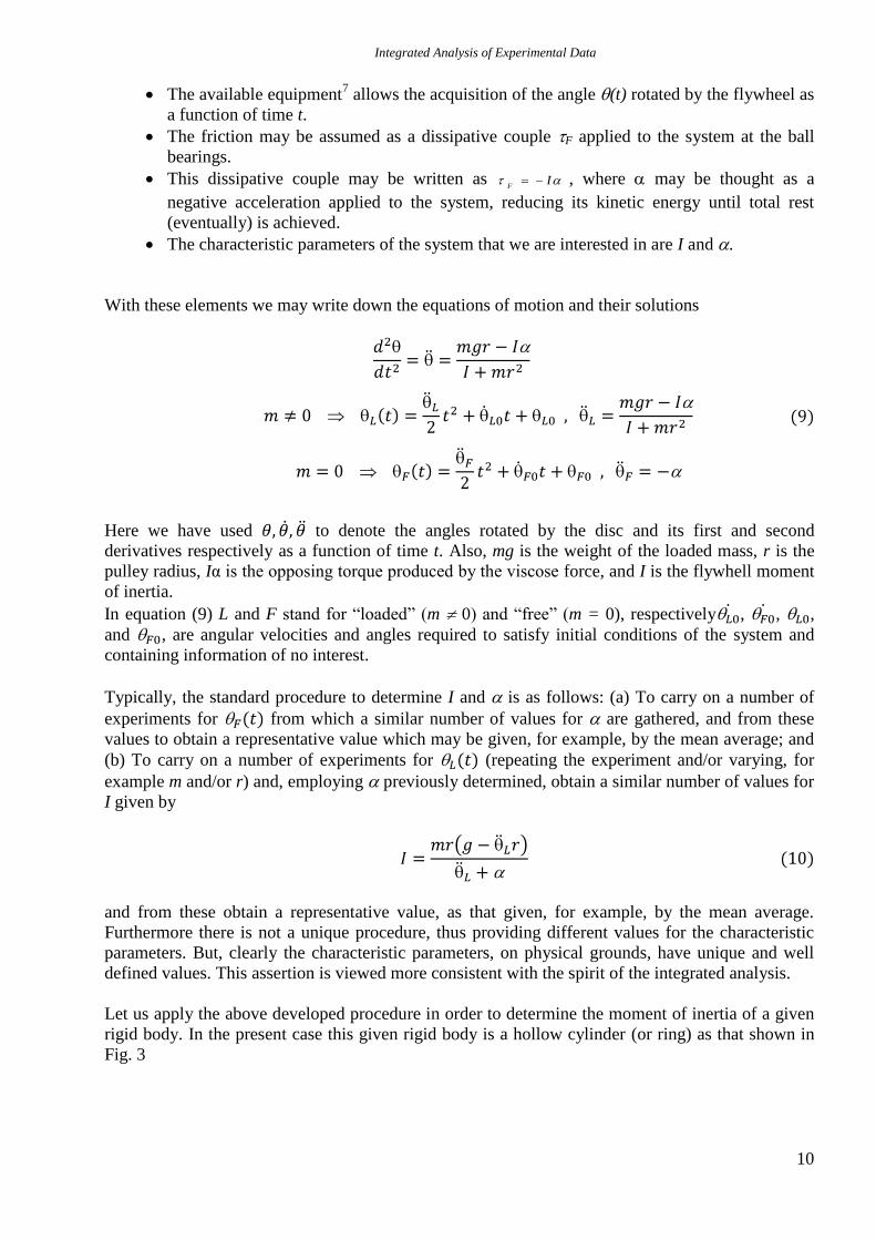
The available equipment7 allows the acquisition of the angle (t) rotated by the flywheel as
a function of time t.
The friction may be assumed as a dissipative couple F applied to the system at the ball
bearings.
This dissipative couple may be written as IF
, where may be thought as a
negative acceleration applied to the system, reducing its kinetic energy until total rest
(eventually) is achieved.
The characteristic parameters of the system that we are interested in are I and .
With these elements we may write down the equations of motion and their solutions
Here we have used to denote the angles rotated by the disc and its first and second
derivatives respectively as a function of time t. Also, mg is the weight of the loaded mass, r is the
pulley radius, Iα is the opposing torque produced by the viscose force, and I is the flywhell moment
of inertia.
In equation (9) L and F stand for “loaded” (m 0) and “free” (m = 0), respectively , , ,
and , are angular velocities and angles required to satisfy initial conditions of the system and
containing information of no interest.
Typically, the standard procedure to determine I and is as follows: (a) To carry on a number of
experiments for from which a similar number of values for are gathered, and from these
values to obtain a representative value which may be given, for example, by the mean average; and
(b) To carry on a number of experiments for (repeating the experiment and/or varying, for
example m and/or r) and, employing previously determined, obtain a similar number of values for
I given by
and from these obtain a representative value, as that given, for example, by the mean average.
Furthermore there is not a unique procedure, thus providing different values for the characteristic
parameters. But, clearly the characteristic parameters, on physical grounds, have unique and well
defined values. This assertion is viewed more consistent with the spirit of the integrated analysis.
Let us apply the above developed procedure in order to determine the moment of inertia of a given
rigid body. In the present case this given rigid body is a hollow cylinder (or ring) as that shown in
Fig. 3

Martín C A, Ramia M E and Chesta M A
11
Figure 3: The geometry of the hollow cylinder is sketched. The material what it is made of is homogenous
throughout its entire volume and its mass is . The geometric moment of inertia
. The uncertainty in has been evaluated following GUM5.
The main objective is to compare the value deduced by means of the present integrated procedure
with that geometrically obtained. Let us call and the moments of inertia of the hollow
cylinder (hc) obtained by means of this integrated procedure (ip) and geometrically determined (g).
This hollow cylinder may be easily mounted on to a disc rigidly attached to the axis and the spool
as shown in Fig. 2. Let be the moment of inertia of the disc, axis, spool and ball bearings.
Thus we have four different experiments: (i) with m falling; (ii) free; (iii)
with m falling; and (iv) free. In the present case each of these four experiments was
repeated three times, therefore the grand set has twelve components. The idea is to apply the
integrated procedure developed in this work in order to determine , , and are
the angular accelerations acting on the free system when the hollow cylinder is attached or not to
the disc, respectively. Furthermore, and are allowed to possess different values in
order to account for the different loads acting on the ball bearings in both cases.
Since the values for m and r were kept constant throughout the experiments, and since g is a
constant, Eqs. 9 may be rewritten as
107.6 ± 0.1 mm
127.6 ± 0.1 mm

Integrated Analysis of Experimental Data
12
Thus the four cases above mentioned may be written as
where the characteristic parameters to be determined are , , and .
A time to separate and identify the twelve sets in the grand set, was found to be
appropriate.
The expressions to be used in DataFit to carry on the fitting are shown in Appendix A.3 (Section
IX).
As mentioned above each of the experiments was repeated three times. The first three runs are those
with while the remaining three are those with . The initial part –the short one- of
each run is that with the falling m, while the final part –the long one– corresponds to the free one.
Thus, the gathered experimental data along with the fit achieved by means of Eqs. 12 are depicted
in Fig. 4.

Martín C A, Ramia M E and Chesta M A
13
Rota
tion A
ngle
(ra
d)
t (s)
0
200
400
600
800
1000
1200
0 500 1000 1500 2000 2500
Data
Integrated Fit - Eq. 15
Figure 4: The twelve runs (blue) are depicted along the integrated fit achieved by means of Eqs. 12.
As may be seen the description of the experimental data is excellent.
The values obtained for the characteristic parameters are those given in Table 3:
Table 3: Values obtained for the characteristic parameters
disc+hc (3.2314 0.0028) 10–2
rad/s2
disc (3.9711 0.0021) 10–2
rad/s2
Idisc (9.286 0.098) 10–3
kg m2
Ihcip (5.110 0.017) 10–3
kg m2
Let us consider particularly , i.e. the moment of inertia of the body we are interested in.
Analyzing each of the six runs –consistent in the loaded and free components- by means of Eqs. 12
we end up with three independent values for and for .
For the sake of being clear the chosen procedure is as follows. Let us consider one of the three runs
with (Eqs. 12-c and 12-d). Fitting the “free” part of the data using Eq. 12-d, is
determined. By introducing this value into Eq. 12-c and fitting the “loaded” part of the data, a value
is determined for .
With these values for and for nine values for are determined
whose mean value and standard deviation are .
Thus, we end up with three values for the moment of inertia of the hollow cylinder
, , and
. These results lead to the following comments:
1) The value determined for agrees with the geometric and run-by-run values,
thus supporting the reliability of the procedure developed in this work.
2) The integrated procedure allows saving time and effort since, in the case under analysis,
the situation was solved with just one fit instead of the twelve required by other means.
This saving increases with the number of acquired signals.

Integrated Analysis of Experimental Data
14
3) The integrated analysis procedure provides support to the expectation that the various
measurements have been carried on in identical conditions, thus producing repeatability as
indicated above in the previous example.
4) The integrated analysis methodology allows determining in an elegant form and in just one
attempt unique values for the characteristic parameters as
well for others that may not be so relevant and related to the initial conditions.
5) What has been pointed out for is also valid for the remaining characteristic
parameters.
VI – Discussion and Conclusions
In this work we have successfully developed a procedure to integrate various related files
and to analyze them in a single fit. The proposed method, if it can be applied, effectively implies a
more realistic analysis of data resulting in a better measurement quality. Briefly, the reason for this
is that for the "integrated analysis" all the experimental points have the same "status". Not so in
other ways in which each data set yields an average value of equal weight, independent of the set to
which it belongs. Which causes small data sets have higher relative weights. The problem could be
overcome including the notion of "statistical weights", which continues to be a patch in an attempt
to get closer to what we have been called the "integrated analysis".
Two examples were analyzed employing DataFit. Various main advantages may be pointed out: (a)
A unique value is determined for the common characteristic parameters –which are the ones we are
most interested in– in a single shot; (b) The uncertainties determined for these characteristic
parameters turn out, as expected, to be generally smaller than those obtained by standard methods;
(c) As a byproduct non characteristic parameters such as baseline drifts, initial conditions, etc., are
also determined; (d) Data handling is easy; (e) Computer time is shortened; and (f) Analysis of
results is shortened and improved.
The method has, perhaps, against the need to know how to program.
VII – Appendix A.1
Let us consider the case in which the one experiment has been repeated three times.
Generalization is straightforward. This situation is shown in Ec. 5. The way to proceed with DataFit
is as follows:
F1=f(P1,P2,V11,V21,x)
F2=f(P1,P2,V12,V22,x-T1)
F3=f(P1,P2,V13,V23,x-(T1+T2)) (a.1)
Y=if(x<T1,F1,if(x<(T1+T2),F2,F3))
Advantage has been taken of the sentence “if” implemented in DataFit. Functions F1, F2, F3 and Y
must be written with the proper syntax. Particularly, DataFit assigns “x” to the independent variable
(that is the reason as to why we have switched t by x).
VIII – Appendix A.2
For the example of NMR-CPMG Decay Signal, the DataFit expressions are:

Martín C A, Ramia M E and Chesta M A
15
F1 = 12000
F2 = A*exp(-(x-0*F1)/τ2)+O+S*(x-0*F1)
F3 = A*exp(-(x-1*F1)/τ2)+O+S*(x-1*F1)
F4 = A*exp(-(x-2*F1)/τ2)+O+S*(x-2*F1)
F5 = A*exp(-(x-3*F1)/τ2)+O+S*(x-3*F1) (a.2)
F6 = A*exp(-(x-4*F1)/τ2)+O+S*(x-4*F1)
F7 = A*exp(-(x-5*F1)/τ2)+O+S*(x-5*F1)
F8 = A*exp(-(x-6*F1)/τ2)+O+S*(x-6*F1)
F9 = A*exp(-(x-7*F1)/τ2)+O+S*(x-7*F1)
Y = if(x<1*F1, F2, if(x<2*F1, F3, if(x<3*F1, F4, if(x<4*F1, F5, if(x<5*F1,
F6,if(x<6*F1, F7, if(x<7*F1, F8, F9)))))))
Each of the eight files has about 2000 data points, thus the grand file contains about 16000 points.
In each of these eight files the independent variable takes evenly spaced values in the
interval.
IX – Appendix A.3
For the case of flywheel the expressions to be used in DataFit to carry on the fitting are:
F1 = 200
F2 = if(x<1*F1, ((6.3166E-3)-(Idisc+Ihc)*Adischc)/(2*((Idisc+Ihc)+
8.1774E-6))*(x-0*F1)^2+VL1*(x-0*F1)+XL1, if(x<2*F1, -Adischc/2*(x-1*F1)^2+
VF1*(x-1*F1)+XF1, 0))
F3 = if(x<3*F1, ((6.3166E-3)-(Idisc+
Ihc)*Adischc)/(2*((Idisc+Ihc)+8.1774E-6))*(x-2*F1)^2+VL2*(x-2*F1)+
XL2, if(x<4*F1, -Adischc/2*(x-3*F1)^2+VF2*(x-3*F1)+XF2, 0))
F4 = if(x<5*F1, ((6.3166E-3)-(Idisc+Ihc)*Adischc)/(2*((Idisc+Ihc)+
8.1774E-6))*(x-4*F1)^2+VL3*(x-4*F1)+XL3, if(x<6*F1, -Adischc/2*(x-5*F1)^2+
VF3*(x-5*F1)+XF3, 0)) (a.3)
F5 = if(x<7*F1, ((6.3166E-3)-Idisc*Adisc)/(2*(Idisc+8.1774E-6))*(x-6*F1)^2+
VL4*(x-6*F1)+XL4, if(x<8*F1, -Adisc/2*(x-7*F1)^2+VF4*(x-7*F1)+XF4, 0))
F6 = if(x<9*F1, ((6.3166E-3)-Idisc*Adisc)/(2*(Idisc+8.1774E-6))*(x-8*F1)^2+
VL5*(x-8*F1)+XL5, if(x<10*F1, -Adisc/2*(x-9*F1)^2+VF5*(x-9*F1)+XF5, 0))
F7 = if(x<11*F1, ((6.3166E-3)-Idisc*Adisc)/(2*(Idisc+8.1774E-6))*(x-10*F1)^2+
VL6*(x-10*F1)+XL6, if(x<12*F1, -Adisc/2*(x-11*F1)^2+VF6*(x-11*F1)+XF6, 0))
Y = if(x<2*F1, F2, if(x<4*F1, F3, if(x<6*F1, F4, if(x<8*F1, F5,
if(x<10*F1, F6, if(x<12*F1, F7, 0))))))
Acknowledgements
Financial support granted by CONICET, SECYT-UNC and MR Technologies S.A. is
gratefully acknowledged.
References
1) Oakdale Engineering – http://www.oakdaleengr.com

Integrated Analysis of Experimental Data
16
2) C.P. Slichter, “Principles of Magnetic Resonance”, Springer (1996).
3) D. Halliday, R. Resnick and J. Walker, “Fundamentals of Physics”, 9th
Edition, Wiley (2010).
4) Minispec Instrument – http://www.brukeroptics.com/minispec.html
5) JCGM-100-2008-E (GUM 1995), “Evaluation of measurement data – Guide to the expression of uncertainty in
measurement”.
6) Roe B.P. “Probability and Statistics in Experimental Physics”, Springer (1992).
7) Pasco Scientific® ME-8953 Rotational Inertia Accessory Kit.
8) P.R. Bevington, D.K. Robinson “Data reduction and error analysis for the physical science”, p. 210, 3° ed. (2003) Mc
Graw Hill.