Estimando la calidad de las “oscilaciones

estocásticas”Guillermo Abramson

Grupo de Física Estadística e Interdisciplinaria (CAB),CONICET e Instituto Balseiro, Bariloche, Argentina

(con Sebastián Risau-Guzmán)

Tandar – Buenos Aires – 2008

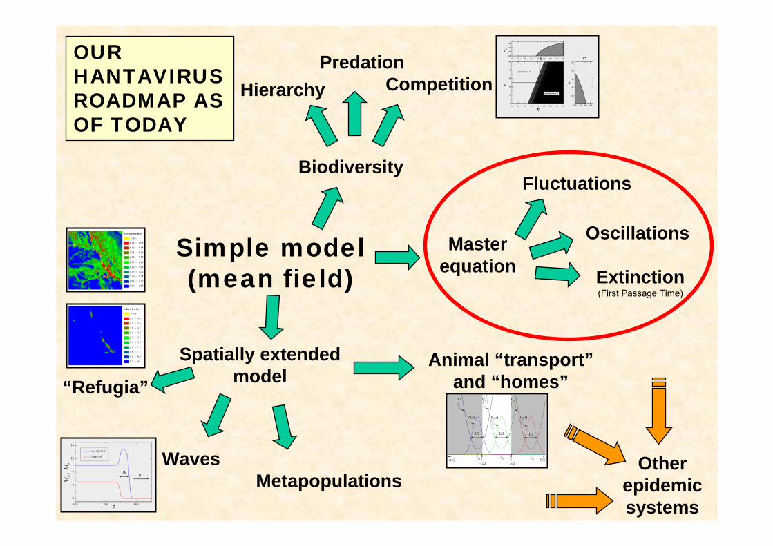
Simple model (mean field)

Spatially extended model

Waves

“Refugia”

Biodiversity

Metapopulations

Fluctuations

Master equation

Oscillations

Extinction (First Passage Time)

CompetitionPredation

Hierarchy

Other epidemic systems

Animal “transport”and “homes”

xc3xc2xc1 xc/2-xc/2 G/2-G/2

L/2

U1U2 U3

P3(x)P2(x)P1(x)

L/2L/2

OUR HANTAVIRUS ROADMAP AS OF TODAY

Fluctuations

Master equation

Oscillations

Extinction (First Passage Time)

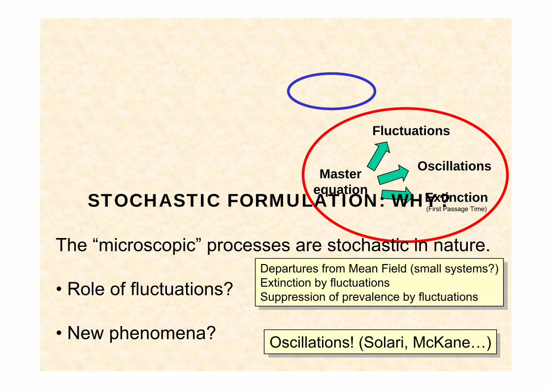
STOCHASTIC FORMULATION: WHY?

The “microscopic” processes are stochastic in nature.

• Role of fluctuations?

• New phenomena?

Departures from Mean Field (small systems?)Extinction by fluctuationsSuppression of prevalence by fluctuations

Departures from Mean Field (small systems?)Extinction by fluctuationsSuppression of prevalence by fluctuations

Oscillations! (Solari, McKane…)Oscillations! (Solari, McKane…)

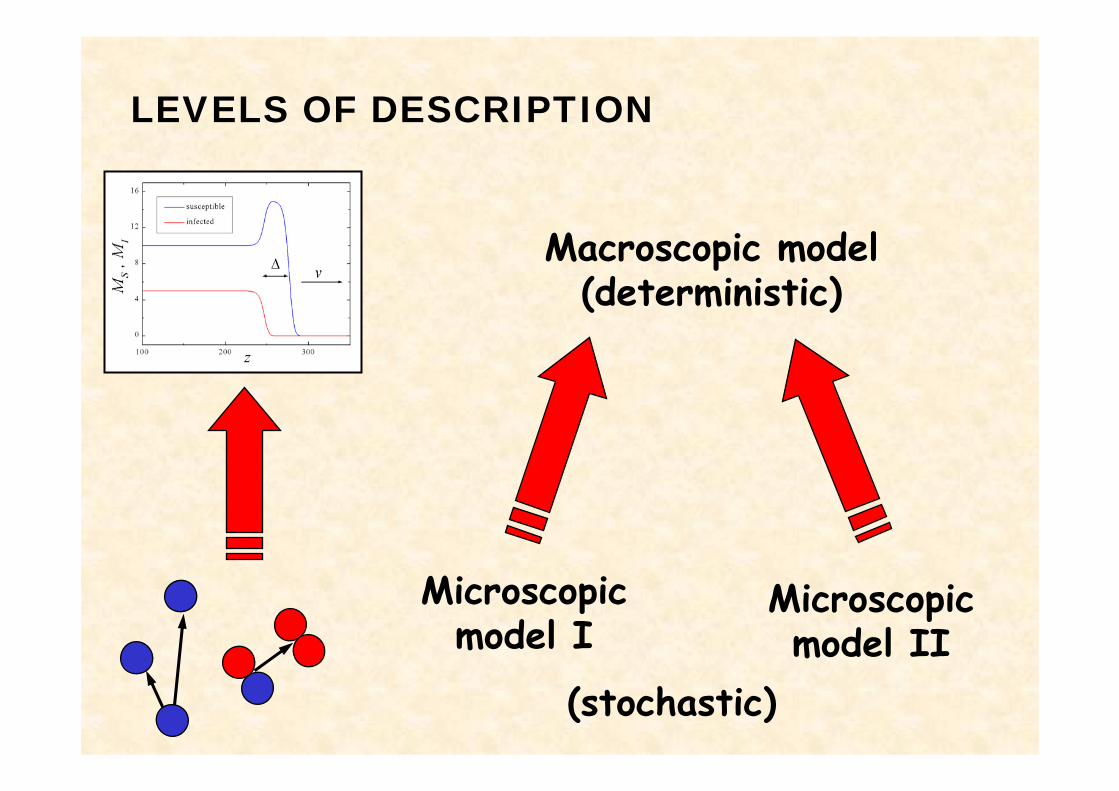
Macroscopic model (deterministic)

Microscopic model II

Microscopic model I

LEVELS OF DESCRIPTION

(stochastic)

OSCILLATIONS IN BIOLOGICAL AND CHEMICAL SYSTEMS

• Predator-prey systems(lynx vs. snow hare, foxes vs. rabbits, etc.)

• Chemical reactions(Belousov-Zhabotinskii, etc.)

• Epidemic systems(measles, pertussis, syphilis, etc.)

measles cases in New York

non-seasonal oscillations!

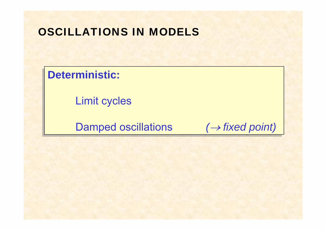
OSCILLATIONS IN MODELS

Deterministic:

Limit cycles

Damped oscillations (→ fixed point)

Deterministic:

Limit cycles

Damped oscillations (→ fixed point)

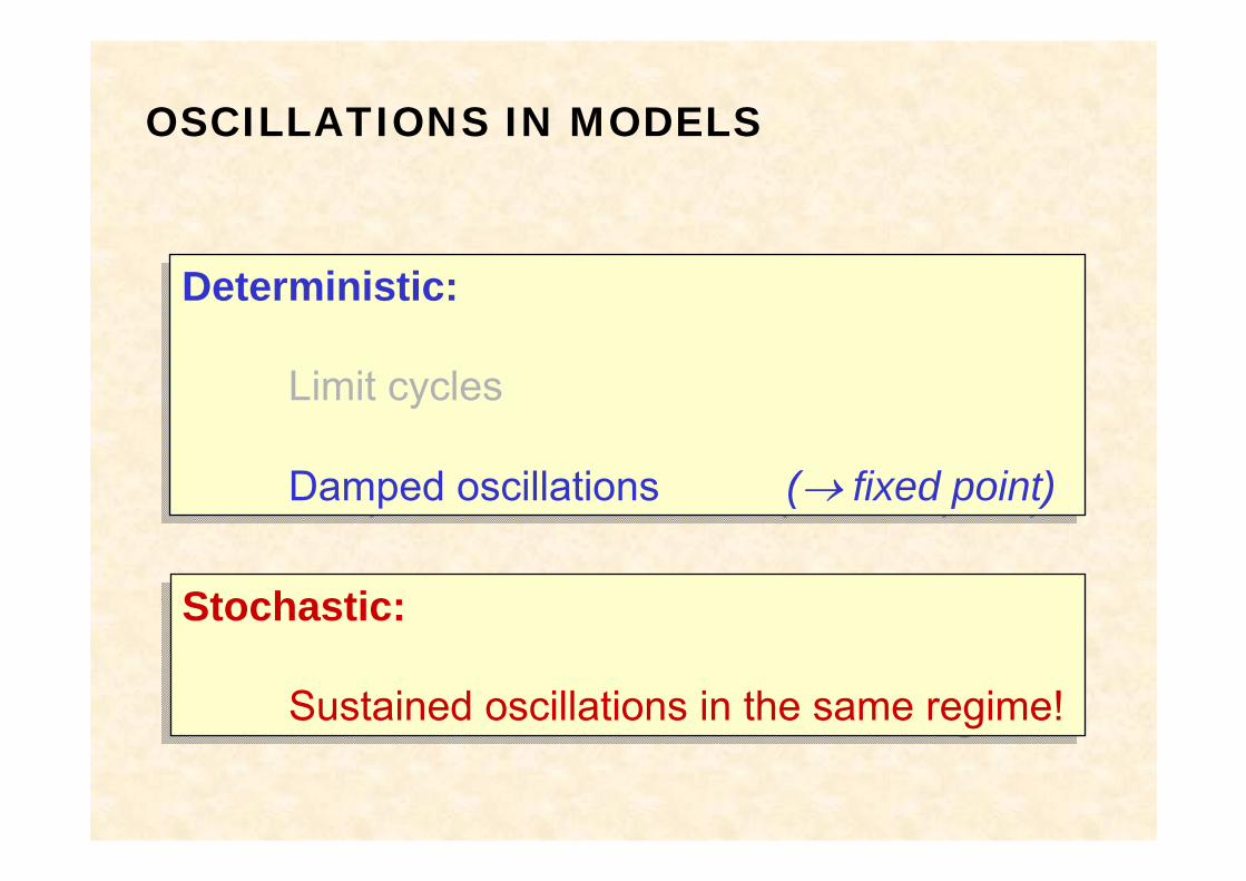
OSCILLATIONS IN MODELS

Deterministic:

Limit cycles

Damped oscillations (→ fixed point)

Deterministic:

Limit cycles

Damped oscillations (→ fixed point)

Stochastic:

Sustained oscillations in the same regime!

Stochastic:

Sustained oscillations in the same regime!

0 100 200

0.3

0.4

0.5

φ(t)

t

macroscopic 10000 realizations

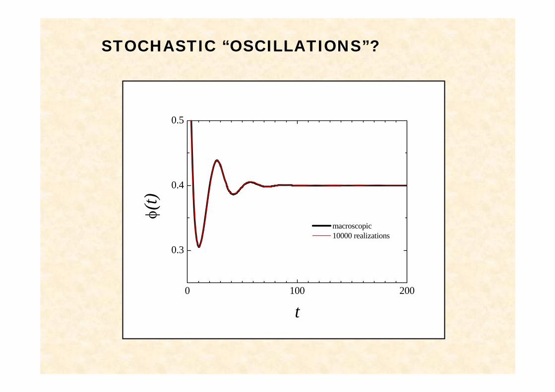
STOCHASTIC “OSCILLATIONS”?

0 100 200

0.3

0.4

0.5

φ(t)

t

macroscopic 10000 realizations 1 realization

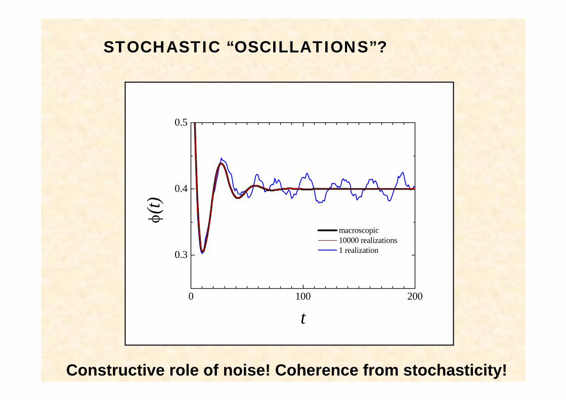
STOCHASTIC “OSCILLATIONS”?

Constructive role of noise! Coherence from stochasticity!

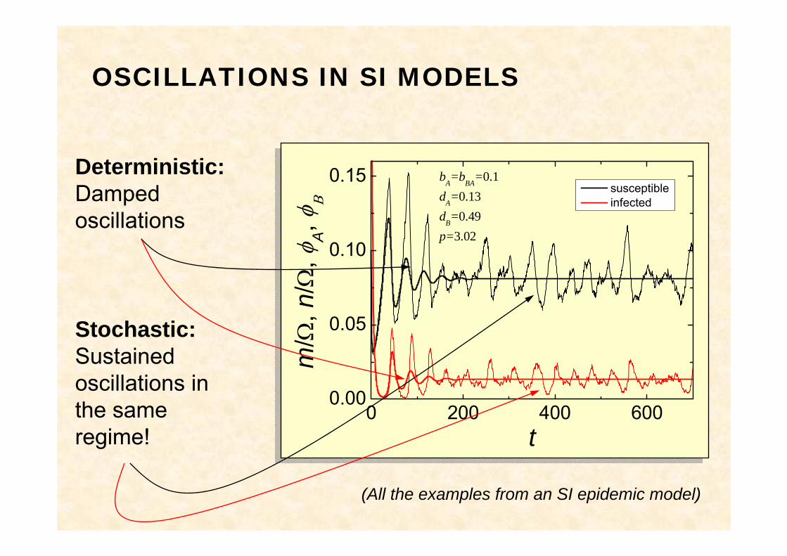
OSCILLATIONS IN SI MODELS

0 200 400 6000.00

0.05

0.10

0.15

m/Ω

, n/Ω

, φA, φ

Β

t

susceptible infected

bA=bBA=0.1dA=0.13dB=0.49p=3.02

(All the examples from an SI epidemic model)

Deterministic:Damped oscillations

Stochastic:Sustained oscillations in the same regime!

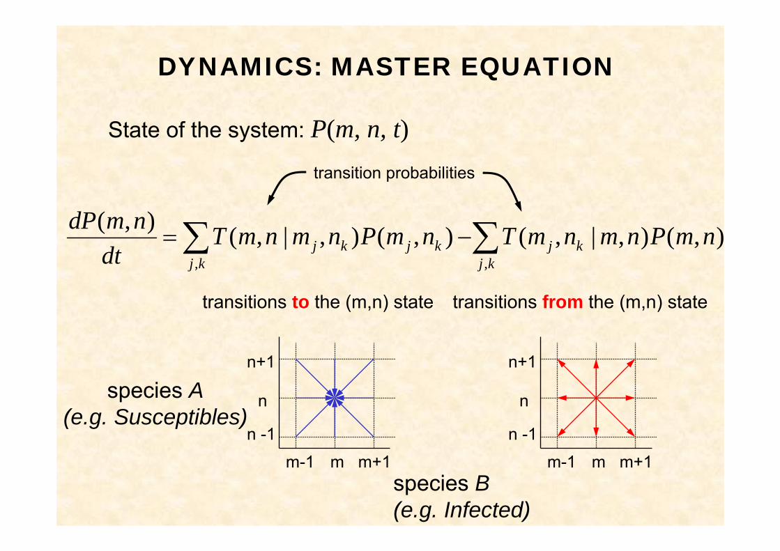
State of the system: P(m, n, t)

DYNAMICS: MASTER EQUATION

∑∑ −=kj

kjkj

kjkj nmPnmnmTnmPnmnmTdt

nmdP,,

),(),|,(),(),|,(),(

transitions from the (m,n) statetransitions to the (m,n) state

transition probabilities

m m+1m-1

n -1

n+1

n

m m+1m-1

n -1

n+1

nspecies A(e.g. Susceptibles)

species B(e.g. Infected)

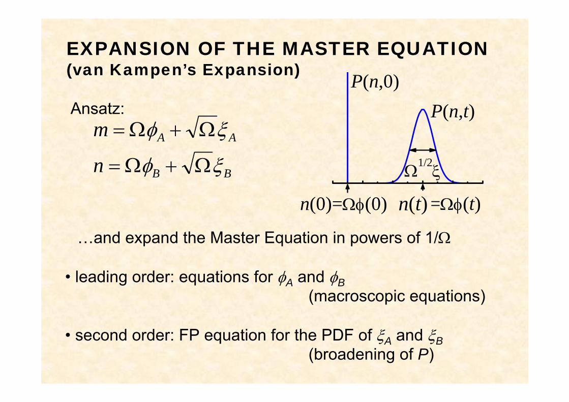
EXPANSION OF THE MASTER EQUATION(van Kampen’s Expansion)

BB

AA

n

m

ξφ

ξφ

Ω+Ω=

Ω+Ω=

…and expand the Master Equation in powers of 1/Ω

• leading order: equations for φA and φB(macroscopic equations)

• second order: FP equation for the PDF of ξA and ξB(broadening of P)

Ansatz:

n(0)=Ωφ(0)

P(n,t)P(n,0)

Ω1/2ξ

S(t)=Ωφ(t)n(t)

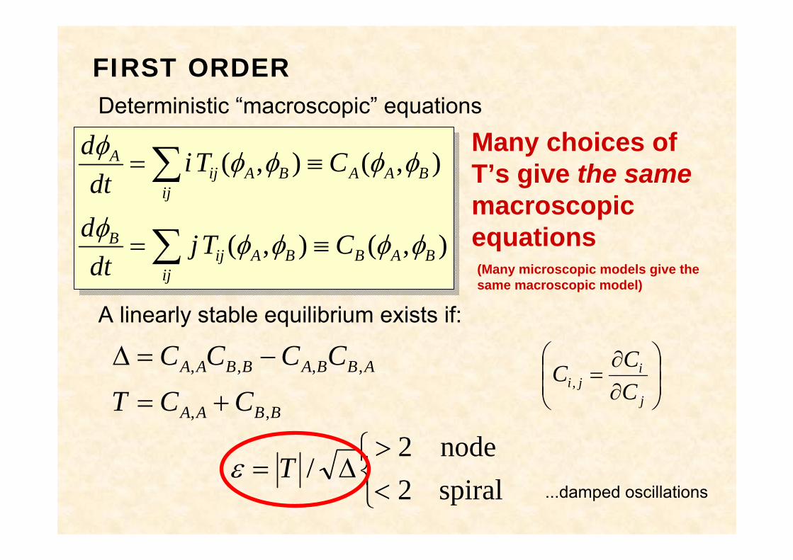
FIRST ORDER

),(),(

),(),(

BABBAij

ijB

BAABAij

ijA

CTjdt

d

CTidt

d

φφφφφ

φφφφφ

≡=

≡=

∑

∑

Deterministic “macroscopic” equations

Many choices of T’s give the samemacroscopic equations

A linearly stable equilibrium exists if:

BBAA

ABBABBAA

CCTCCCC

,,

,,,,

+=

−=Δ⎟⎟⎠

⎞⎜⎜⎝

⎛

∂∂

=j

iji C

CC ,

⎩⎨⎧<>

Δ=spiral2node2

/Tε...damped oscillations

(Many microscopic models give the same macroscopic model)

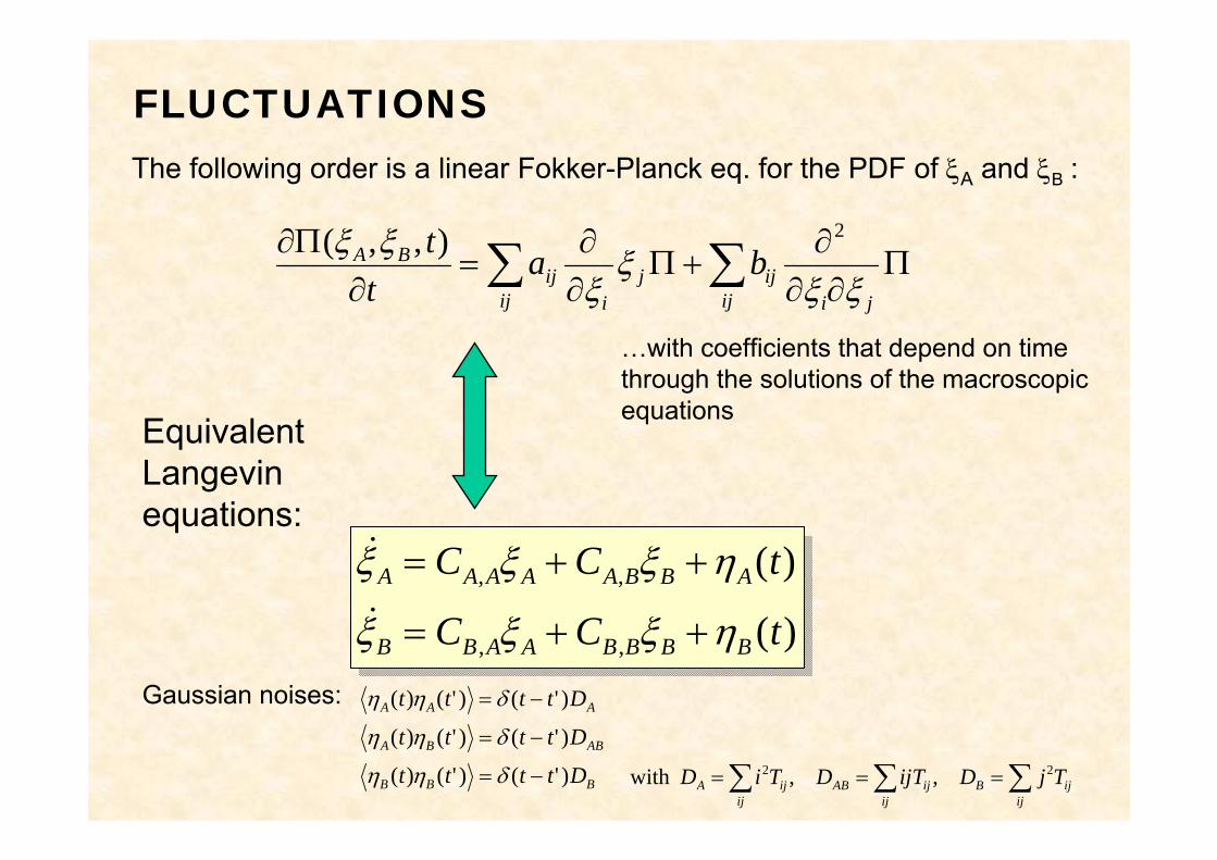
FLUCTUATIONS

∑∑ Π∂∂

∂+Π

∂∂

=∂

Π∂

ij jiij

ijj

iij

BA bat

tξξ

ξξ

ξξ 2),,(

The following order is a linear Fokker-Planck eq. for the PDF of ξA and ξB :

…with coefficients that depend on time through the solutions of the macroscopic equations

)(

)(

,,

,,

tCC

tCC

BBBBAABB

ABBAAAAA

ηξξξ

ηξξξ

++=

++=&

&

BBB

ABBA

AAA

Dtttt

Dtttt

Dtttt

)'()'()(

)'()'()(

)'()'()(

−=

−=

−=

δηη

δηη

δηη

∑∑∑ ===ij

ijBij

ijABij

ijA TjDTijDTiD 22 ,, with

Equivalent Langevin equations:

Gaussian noises:

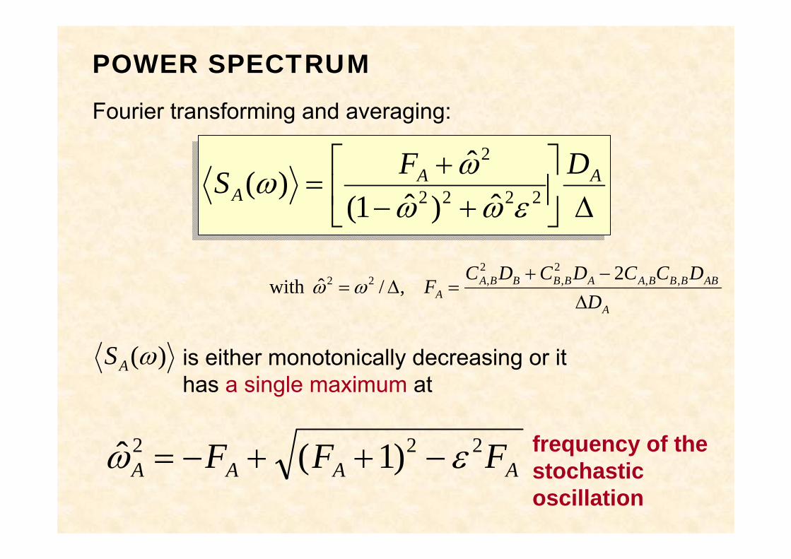
Fourier transforming and averaging:

frequency of thestochasticoscillation

POWER SPECTRUM

Δ⎥⎦

⎤⎢⎣

⎡+−

+= AA

ADFS 2222

2

ˆ)ˆ1(ˆ

)(εωω

ωω

A

ABBBBAABBBBAA D

DCCDCDCF

Δ−+

=Δ= ,,2

,2

,22 2,/ˆ with ωω

is either monotonically decreasing or ithas a single maximum at

)(ωAS

AAAA FFF 222 )1(ˆ εω −++−=

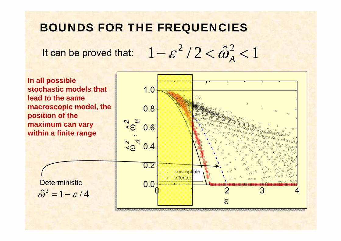
BOUNDS FOR THE FREQUENCIES

1ˆ2/1 22 <<− Aωε

0 1 2 3 40.0

0.2

0.4

0.6

0.8

1.0

^

^ω

2 Α ,

ω2 B

ε

susceptible infected

4/1ˆ 2 εω −=Deterministic

It can be proved that:

In all possible stochastic models that lead to the same macroscopic model, the position of the maximum can vary within a finite range

peak in the power spectrum

“good stochastic oscillation”

?

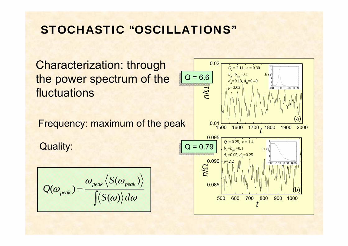
STOCHASTIC “OSCILLATIONS”

Characterization: through the power spectrum of the fluctuations

Frequency: maximum of the peak

Quality:

( )( )

( )peak peak

peak

SQ

S d

ω ωω

ω ω=

∫

1500 1600 1700 1800 1900 20000.01

0.02

(b)

Qi = 2.11, ε = 0.30bA=bBA=0.1dA=0.13, dB=0.49p=3.02

n/Ω

t(a)

0.00 0.03 0.06 0.0902468

10

S( f )

f

500 600 700 800 900 1000

0.085

0.090

0.095Qi = 0.25, ε = 1.4bA=bBA=0.1dA=0.05, dB=0.25p=2.2

n/Ω

t

0.00 0.03 0.06 0.090

1

2

3

4

S( f )

f

Q = 6.6Q = 6.6

Q = 0.79Q = 0.79

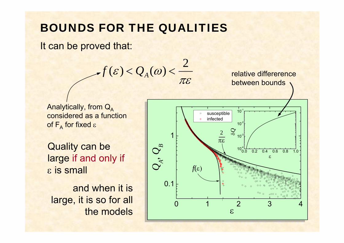
BOUNDS FOR THE QUALITIES

πεωε 2)()( << AQf

It can be proved that:

Quality can belarge if and only ifε is small

0 1 2 3 4

0.1

1πε2

QA, Q

B

ε

susceptible infected

f(ε)

0.0 0.2 0.4 0.6 0.8 1.010-4

10-3

10-2

10-1

δQ

ε

relative differerence between bounds

Analytically, from QAconsidered as a function of FA for fixed ε

and when it is large, it is so for all

the models

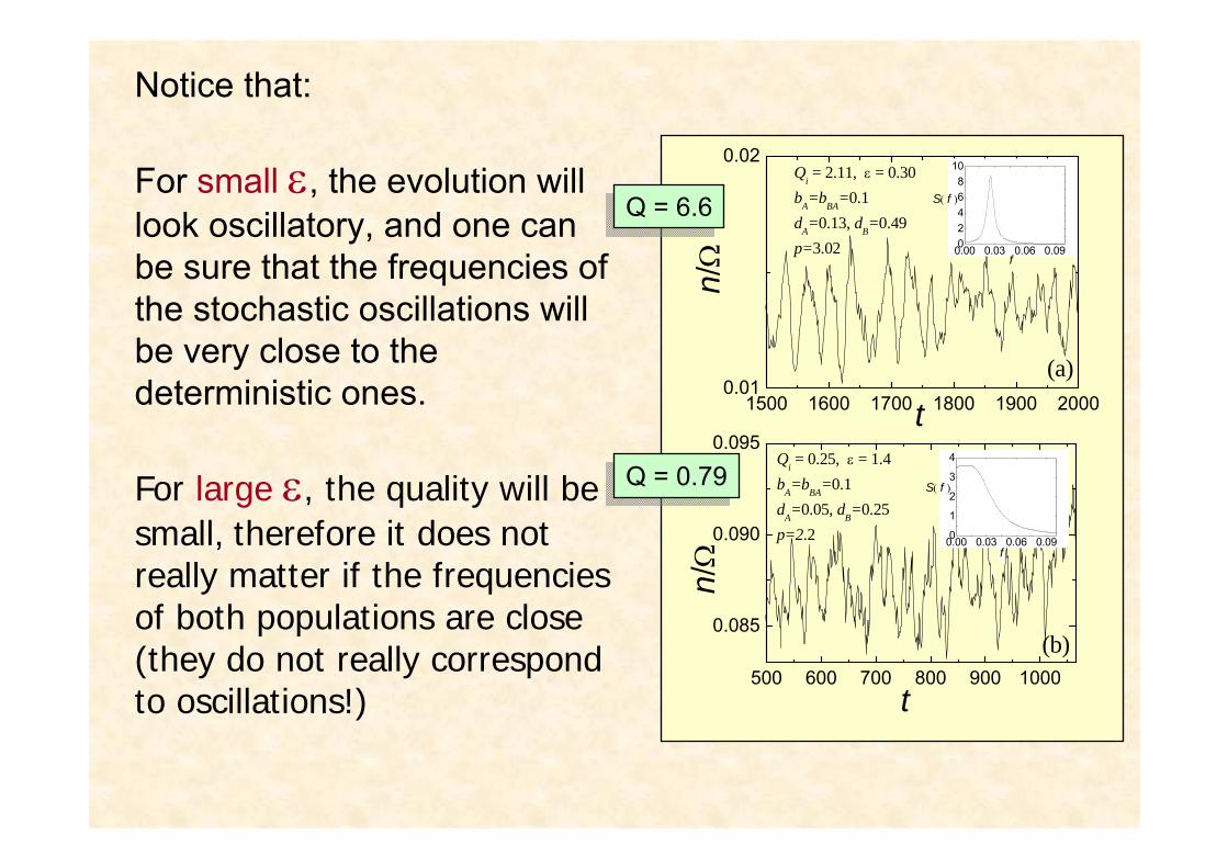
Notice that:

For small ε, the evolution will look oscillatory, and one can be sure that the frequencies of the stochastic oscillations will be very close to the deterministic ones.

For large ε, the quality will be small, therefore it does not really matter if the frequencies of both populations are close (they do not really correspond to oscillations!)

1500 1600 1700 1800 1900 20000.01

0.02

(b)

Qi = 2.11, ε = 0.30bA=bBA=0.1dA=0.13, dB=0.49p=3.02

n/Ω

t(a)

0.00 0.03 0.06 0.0902468

10

S( f )

f

500 600 700 800 900 1000

0.085

0.090

0.095Qi = 0.25, ε = 1.4bA=bBA=0.1dA=0.05, dB=0.25p=2.2

n/Ω

t

0.00 0.03 0.06 0.090

1

2

3

4

S( f )

f

Q = 6.6Q = 6.6

Q = 0.79Q = 0.79

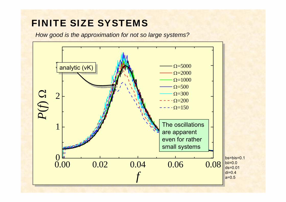
FINITE SIZE SYSTEMS

bs=bis=0.1bii=0.0ds=0.01di=0.4a=0.5

0.00 0.02 0.04 0.06 0.080

1

2

3

P(f)

Ω

f

Ω=5000 Ω=2000 Ω=1000 Ω=500 Ω=300 Ω=200 Ω=150

analytic (vK)analytic (vK)

The oscillations are apparent even for rather small systems

How good is the approximation for not so large systems?

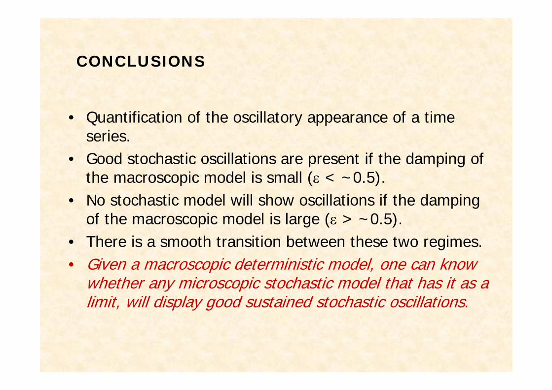
• Quantification of the oscillatory appearance of a time series.

• Good stochastic oscillations are present if the damping of the macroscopic model is small (ε < ~0.5).

• No stochastic model will show oscillations if the damping of the macroscopic model is large (ε > ~0.5).

• There is a smooth transition between these two regimes.• Given a macroscopic deterministic model, one can know

whether any microscopic stochastic model that has it as a limit, will display good sustained stochastic oscillations.

CONCLUSIONS

GRACIAS!

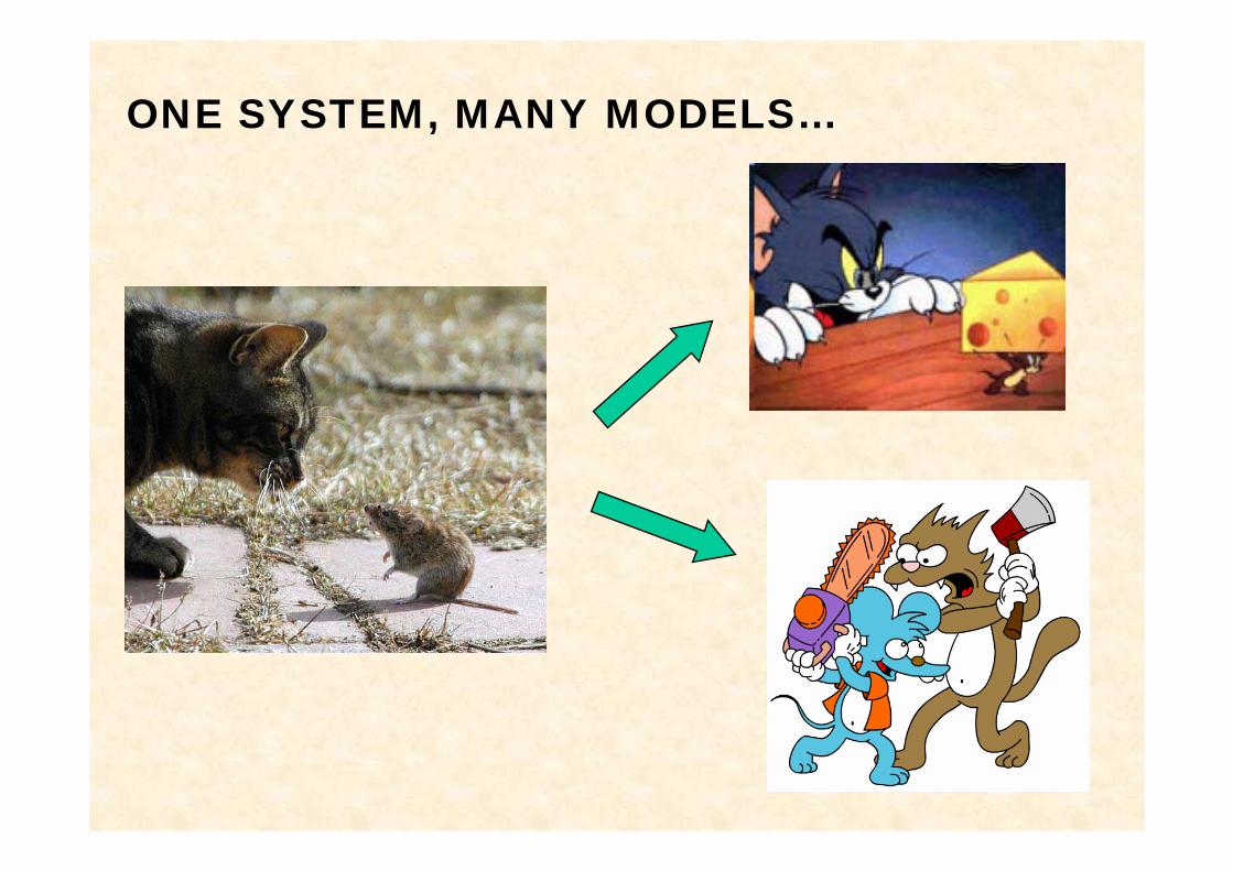
ONE SYSTEM, MANY MODELS…

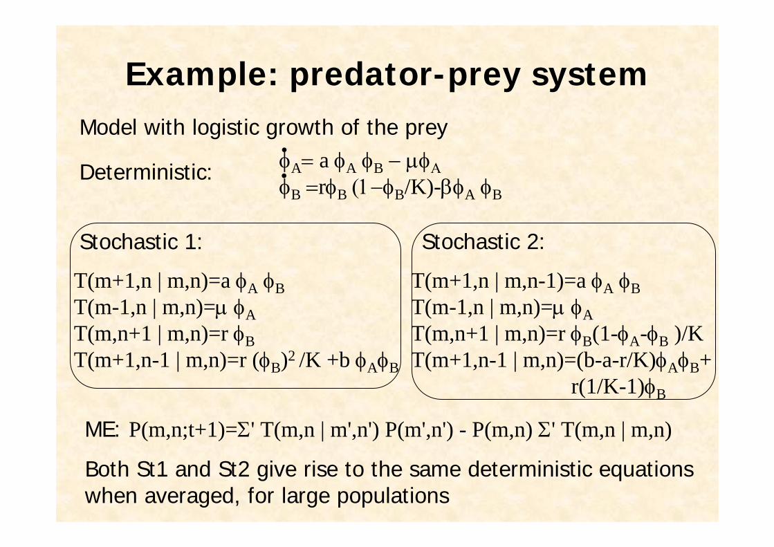
Example: predator-prey systemModel with logistic growth of the prey

Deterministic:

Stochastic 1: Stochastic 2:

Both St1 and St2 give rise to the same deterministic equationswhen averaged, for large populations

φA= a φA φB − μφΑφB =rφB (1−φB/K)-βφA φB

T(m+1,n | m,n)=a φA φBT(m-1,n | m,n)=μ φAT(m,n+1 | m,n)=r φBT(m+1,n-1 | m,n)=r (φB)2 /K +b φAφB

T(m+1,n | m,n-1)=a φA φBT(m-1,n | m,n)=μ φAT(m,n+1 | m,n)=r φB(1-φA-φB )/KT(m+1,n-1 | m,n)=(b-a-r/K)φAφB+

r(1/K-1)φB

ME: P(m,n;t+1)=Σ' T(m,n | m',n') P(m',n') - P(m,n) Σ' T(m,n | m,n)

•

•

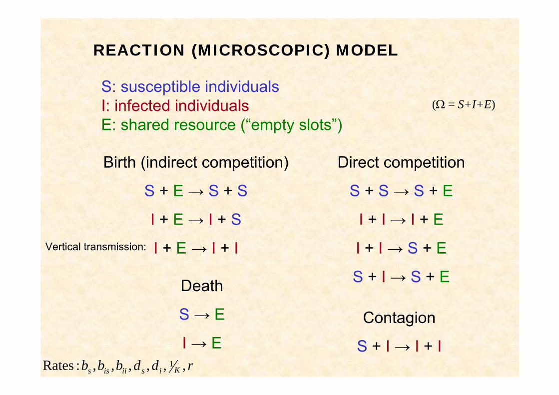
Birth (indirect competition)

S + E → S + S

I + E → I + S

I + E → I + I

Death

S → E

I → EContagion

S + I → I + I

Direct competition

S + S → S + E

I + I → I + E

I + I → S + E

S + I → S + E

S: susceptible individualsI: infected individualsE: shared resource (“empty slots”)

REACTION (MICROSCOPIC) MODEL

Vertical transmission:

rddbbb Kisiiiss ,,,,,, :Rates 1

(Ω = S+I+E)