Revista Mexicana de ngeniería - SciELO · Revista Mexicana de ... de sistemas f´ısicos que ......

Revista Mexicana de Ingeniería Química

CONTENIDO

Volumen 8, número 3, 2009 / Volume 8, number 3, 2009

213 Derivation and application of the Stefan-Maxwell equations

(Desarrollo y aplicación de las ecuaciones de Stefan-Maxwell)

Stephen Whitaker

Biotecnología / Biotechnology

245 Modelado de la biodegradación en biorreactores de lodos de hidrocarburos totales del petróleo

intemperizados en suelos y sedimentos

(Biodegradation modeling of sludge bioreactors of total petroleum hydrocarbons weathering in soil

and sediments)

S.A. Medina-Moreno, S. Huerta-Ochoa, C.A. Lucho-Constantino, L. Aguilera-Vázquez, A. Jiménez-

González y M. Gutiérrez-Rojas

259 Crecimiento, sobrevivencia y adaptación de Bifidobacterium infantis a condiciones ácidas

(Growth, survival and adaptation of Bifidobacterium infantis to acidic conditions)

L. Mayorga-Reyes, P. Bustamante-Camilo, A. Gutiérrez-Nava, E. Barranco-Florido y A. Azaola-

Espinosa

265 Statistical approach to optimization of ethanol fermentation by Saccharomyces cerevisiae in the

presence of Valfor® zeolite NaA

(Optimización estadística de la fermentación etanólica de Saccharomyces cerevisiae en presencia de

zeolita Valfor® zeolite NaA)

G. Inei-Shizukawa, H. A. Velasco-Bedrán, G. F. Gutiérrez-López and H. Hernández-Sánchez

Ingeniería de procesos / Process engineering

271 Localización de una planta industrial: Revisión crítica y adecuación de los criterios empleados en

esta decisión

(Plant site selection: Critical review and adequation criteria used in this decision)

J.R. Medina, R.L. Romero y G.A. Pérez

Revista Mexicanade Ingenierıa Quımica

1

Academia Mexicana de Investigacion y Docencia en Ingenierıa Quımica, A.C.

Volumen 13, Numero 1, Abril 2013

ISSN 1665-2738

1

Vol. 13, No. 1 (2014) 259-277

LOW-RAM ALGORITHM FOR SOLVING 3-D NATURAL CONVECTIONPROBLEMS USING ORTHOGONAL COLLOCATION

ALGORITMO DE BAJO CONSUMO DE RAM PARA RESOLVER PROBLEMAS DECONVECCION NATURAL 3-D, USANDO COLOCACION ORTOGONAL

H. Jimenez-Islas1∗, M. Calderon-Ramırez3, F.I. Molina-Herrera1, G.M. Martınez-Gonzalez2,J.L. Navarrete-Bolanos1, E.O. Castrejon-Gonzalez2

1Departamento de Ingenierıa Bioquımica, 2 Departamento de Ingenierıa Quımica, 3 Departamento de CienciasBasicas. Instituto Tecnologico de Celaya. Av. Tecnologico y Antonio Garcıa Cubas s/n.

Celaya, Guanajuato. C.P.38010. Mexico

Received May 13, 2013; Accepted January 21, 2014

AbstractComputational code IMPLI-C3 is a low-RAM consumption program designed to solve three-dimensional parabolicpartial differential nonlinear equations. The spatial coordinates are discretized using orthogonal collocation withLegendre polynomials while time was discretized via backward finite differences, generating an implicit method thatoriginates a set of algebraic equations, which are solved by nonlinear relaxation for each step of time integration.Nonlinear relaxation is an iterative method that only uses the Jacobian diagonal and voids the RAM storage ofthe entire Jacobian matrix. This allows the simulation of physical systems that require greater number of nodesthat otherwise would use too much RAM when trying to solve by Newton-Raphson. The code was successfullyevaluated using several problems related to natural convection previously reported in literature, observing thatnonlinear relaxation only requires 0.3%-1.5% of the memory required by Newton-Raphson for the same problems.Furthermore, one can be conclude that, in problems with many nodes, the use of multivariate Newton-Raphson isunfeasible due to high consumption of RAM that can even cause it to overflow.

Keywords: nonlinear relaxation, natural convection, orthogonal collocation, parabolic partial differential equations.

ResumenIMPLI-C3 es un codigo computacional que utiliza bajos recursos de memoria RAM, disenado para resolver

ecuaciones diferenciales parciales parabolicas no lineales en tres dimensiones. Los ejes coordenados en el espaciose discretizaron usando colocacion ortogonal con polinomios de Legendre mientras que el tiempo se discretizomediante diferencias finitas hacia atras, generando un esquema implıcito que origina un conjunto de ecuacionesalgebraicas, las cuales se resolvieron mediante relajacion no lineal para cada etapa de integracion en el tiempo.La relajacion no lineal, es un metodo iterativo que emplea solamente la diagonal del Jacobiano para evitar quese almacene toda la matriz Jacobiana en la memoria RAM de la computadora. Lo anterior permite la simulacionde sistemas fısicos que requieren mayor cantidad de nodos que, de otra manera emplearıan demasiada RAM alintentar resolverlos mediante Newton-Raphson. El codigo se evaluo satisfactoriamente usando varios problemasrelacionados con el fenomeno de conveccion natural previamente reportados en la literatura, observando que elmetodo de relajacion no lineal solamente utiliza entre 0.3% a 1.5% de la memoria con respecto al metodo deNewton-Raphson. Ademas se pudo corroborar que, en problemas con muchos nodos, el uso de Newton-Raphsonmultivariable no es factible debido al consumo elevado de memoria RAM que, inclusive puede provocar sudesbordamiento.

Palabras clave: relajacion no lineal, conveccion natural, colocacion ortogonal, ecuaciones diferenciales parcialesparabolicas.

∗Corresponding author. E-mail: [email protected]. +52 (461) 611-75-75

Publicado por la Academia Mexicana de Investigacion y Docencia en Ingenierıa Quımica A.C. 259

Jimenez-Islas et al./ Revista Mexicana de Ingenierıa Quımica Vol. 13, No. 1 (2014) 259-277

1 Introduction

Many problems in the field of Chemical Engineeringare modeled as nonlinear partial parabolic differentialequations (PDE). Most have only numerical solutions.There are several commercial programs uniquelydesigned to solve PDE in specific situations,decreasing the versatility of these software. Theseprograms mainly use finite difference or finite elementmethods, requiring very fine mesh to solve highlynonlinear problems. Therefore, the primary reason todevelop a computer code is to increase versatility,especially for highly nonlinear parabolic PDE 3-Dproblems.

The choice of orthogonal collocation asdiscretization method is based on its greater precisioncompared to other well-known methods, such asfinite difference. Orthogonal collocation gives smallermargins of error in solutions with the same meshthan other methods (Jimenez-Islas and Lopez-Isunza,1996; Ebrahimi et al., 2008). Villadsen and Stewart(1967) reported several problems focused on chemicalengineering, proposing the application of orthogonalcollocation to solve differential equations withboundary values. Subsequently, other authors began toexpand its use (Ebrahimi et al., 2008; Finlayson, 1972;Jimenez-Islas and Lopez-Isunza, 1994; Jimenez-Islas,2001; Barrozo et al., 2006).

The objective of this study is to design an all-purpose computer program that is able to solve in threespatial dimensions any system of nonlinear parabolicPDE 3-D that is presented in dynamic simulation ofprocesses using the orthogonal collocation method forthe discretization of the spatial coordinates (Villadsenand Stewart, 1967; Finlayson, 1980; Jimenez-Islas andLopez-Isunza, 1994) and backward finite differencesof the time variable. With the application of theimplicit method, a set of nonlinear algebraic equationswas obtained. These equations then are solved withnonlinear relaxation (Vemuri and Karplus, 1981) anddo not require a special reordering of the governingequations to solve them, unlike other existing solutionmethods that require specific algebraic arrangementsthat can be difficult to implement in nonlinear cases.Furthermore, the use of nonlinear relaxation does notrequire larger RAM such as Newton-based methods,and it is easy to code in any computer language, sinceoperations between vectors are used, while in Newtonmethods matrix operations are required.

2 MethodologyThe basis of the approximation of differentialoperators via orthogonal collocation requires that thepoints or nodes correspond to roots of orthogonalpolynomials when the residue is zero, Legendre,Jacobi, Hermite, Laguerre, etc. In this work, we usedJacobi polynomials, presented in equation (1). If thecoefficients α = β = 0, equation (1) reduces theorthogonal polynomial to Legendre type.

1∫0

xα(1 − x)βP j(x)PN(x)dx = 0 (1)

In a 2-D domain, the approximation of the solution hasthe following form:

Ti j =

NX+2∑k=1

bik xk−1i j (2)

Developing the first and second derivative, thefollowing equations were obtained:(

dTdx

)i j

=

NX+2∑k=1

bik(k − 1)xk−2i j (3)

(d2Tdx2

)i j

=

NX+2∑k=1

bik(k − 1)(k − 2)xk−3i j

(4)

Where xi j represents the nodes of collocationdefined by the roots of orthogonal polynomials used,that represent the points where approximation ofdifferential operators is performed. Generalizing theabove equations over the entire domain, we obtainedthe following equations in matrix notation (Finlayson,1972, 1980; Jimenez-Islas and Lopez-Isunza, 1994).

T = Qb (5)dTdx

= Cb (6)

d2Tdx2 = Db (7)

Where

Qik = xk−1ii (8)

Cik = (k − 1)xk−2ii (9)

Dik = (k − 1)(k − 2)xk−3ii (10)

Solving for b gives the following:

b = Q−1T (11)

260 www.rmiq.org


Substituting the expression (11) in (6) and (7) yieldsthe following:

dTdx

= CQ−1T = AT (12)

d2Tdx2 = DQ−1T = BT (13)

Where A and B are the collocation matricesthat approximate the first and second derivative,respectively. Expanding these definitions to threespatial coordinates gives the following equations(Jimenez-Islas, 2001):

∂T∂x

=

NX+2∑p=1

AXipTp jk (14)

∂2T∂x2 =

NX+2∑p=1

BXipTp jk (15)

∂T∂y

=

NY+2∑p=1

AY jpTipk (16)

∂2T∂y2 =

NY+2∑p=1

BY jpTipk (17)

∂T∂z

=

NZ+2∑p=1

AZkpTi jp (18)

∂2T∂z2 =

NZ+2∑p=1

BZkpTi jp (19)

The orthogonal collocation method includes all nodespresent in the discretization of partial derivativesand generates greater accuracy with smaller meshesthan finite differences (Jimenez-Islas, 1999; Jimenez-Islas, 2001). By using a finite backward differencein time, which produces a system of nonlinearalgebraic equations that resolves simultaneouslyfor each integration step. The implicit method isunconditionally stable and less dependent on the sizeof stages that occur in explicit methods (Vemuri andKarplus, 1981). The numerical solution of systemsin three dimensions using orthogonal collocationrequires the generation of a large matrix that increasesgeometrically with the number of nodes. It isnecessary to find a method that does not requirethe RAM storage of the Jacobian matrix of Newton-Raphson method. Nonlinear relaxation is one of thealternative methods, which consists of applying aone-dimensional Newton-Raphson to each equationto achieve convergence. Therefore, we only use thediagonal of the Jacobian matrix (Vemuri and Karplus,

1981). Equation (20) shows a relaxation scheme in anonlinear variant, where λ is a relaxation factor thataccelerates and achieves convergence, and determinesthe dimensional displacement of the solution.

xk+1i = xk

i − λfi(xk+1

1 , xk+12 , . . . , xk

i , . . . , xkn

)∂ fi∂xi

∣∣∣∣ (xk+11 , xk+1

2 , . . . , xki , . . . , x

kn

) (20)

The convergence ratio of nonlinear relaxation dependsof the initial value of λ and, in higher nonlinearproblems, requires commonly many iterations toachieve the fixed tolerance. However, the iterationsrun quickly and are easy to code for parallelplatforms. Typically, one can propose an initialvalue of λ = 0.5 for exploring convergence. Takingthe considerations discussed above, we developed aprogram coded in FORTRAN 90 called IMPLI-C3.This computational code can be used interchangeablyon x86 platforms, workstations and supercomputers(using parallel processing). In addition, we developedan easy notation for feeding PDE and their boundariesand initial conditions in an IMPLI-C3 subroutine.For example: T1 is T (1), ∂T1

∂x is TX(1), ∂2T2∂z2 is

TZZ(2), etc. This notation was used successfully inother computer codes (Jimenez-Islas, 1999; Jimenez-Islas, 2001; Carrera-Rodrıguez et al, 2011). Forthe simulations, we used a midrange computer withmicroprocessor Intel CoreT M 2 Duo E4500, 2.20 GHzwith 2 Gb RAM, Windows XPT M and COMPAQT M

Visual FORTRAN compiler v. 6.6c.To assess the reliability of IMPLI-C3 software, the

computer code was validated with four study cases,three of which are related to natural convection. Case Iis a designed system of coupled nonlinear parabolicPDE that has an analytical solution and allows usto analyze the error rate via a mesh independenceanalysis. The remaining cases are associated withnatural convection phenomenon defined as heat ormass transport due buoyancy forces. There exists agreat diversity of buoyancy flows in enclosures that areof interest in science and technology. These buoyancyflows involve challenging physical and mathematicalproblems as the coupling of the flow and transport andof the boundary layer and core flows, the interactionbetween the flow and the driving force, which altersthe regions in which the buoyancy acts, and theoccurrence of multicellular flow. (Ostrach, 1988;Nield and Bejan, 1992, Jimenez-Islas, 1999).

The second case enhances the utility of theincrement of nodes close the boundaries in acylindrical geometry problem with asymmetricbehavior (Ozoe and Toh, 1998). The third case is

www.rmiq.org 261


the classical problem of natural convection in acubical cavity, which is often used as a benchmarkfor assessing new algorithms or codes (De VahlDavis, 1983; Bessonov et al., 1998; Tric et al., 2000;Wakashima and Saitoh, 2004; Ravnik et al., 2008;Brahim and Taieb, 2009). The fourth case, whichis an application of this code to solve the problemof natural convection in grain storage in cylindricalsilos, demonstrates the robustness of IMPLI-C3 insolving complex problems. The convergence criterionis (Carrera-Rodrıguez et al., 2011) as follows:∣∣∣∣ fi (xk+1

1 , xk+12 , . . . , xk

i , . . . , xkn

)∣∣∣∣ ≤ 10−5

for all discretized equations (21)

3 Results and discussion

3.1 Case I: A system of two couplednonlinear PDE with known analyticalsolution

In this study case, we constructed an arbitrary systemof 3-D parabolic PDE with analytical solution, theequations were:

∂T1

∂t=∂2T1

∂X2 +∂2T1

∂Y2 +∂2T1

∂Z2 −∂T1

∂X∂T2

∂Y− ∂T1

∂Y∂T2

∂Z+ T2 + e−t

(4Y3 − Y2 − Z

)+ 24X2YZ − X

(3Z2 + 4

)(22a)

∂T2

∂t=∂2T2

∂X2 +∂2T2

∂Y2 +∂2T2

∂Z2 − T2∂T1

∂X− T1

∂T2

∂Z+ e−t

(6XZ2 + 2Y4 − Y2 − 2

)+ 12X2Y2Z + 6X

(Y2Z2 − 1

)(22b)

With the following boundary and initial conditions:

X = 0, T1 = Ze−t,T2 = Y2e−t (23a)

X = 1,∂T1

∂X= 2Y2,

∂T2

∂X= 3Z2 (23b)

Y = 0, T1 = Ze−t,T2 = 3XZ2 (23c)

Y = 1,∂T1

∂Y= 4X,

∂T2

∂Y= 2e−t (23d)

Z = 0, T1 = 2XY2,T2 = Y2e−t (23e)

Z = 1,∂T1

∂Z= e−t,

∂T2

∂Y= 6X (23f)

t = 0, T1 = 2XY2 + Z,T2 = 3XZ2 + Y2 (23g)

The system was discretized with 7 × 7 × 7, 9 × 9 × 9,13×13×13, 15×15×15, and 21×21×21 orthogonal

Table 1. Analysis of mesh independence in Case I,using the average error of the variables T1 and T2

Mesh Iterations Error T1 Error T2

7×7×7 49143 6.4 % 5.1 %9×9×9 85078 5.1 % 3.6 %

13×13×13 205671 4.1 % 2.2 %15×15×15 289312 3.9 % 1.9 %21×21×21 642630 3.5 % 1.4 %

collocation internal points with Legendre polynomialsand integrated from t = 0 to t = 2 with 200 steps,a relaxation factor λ of 0.7 and a tolerance of 10−5.We also carried out the calculation of the relativeerrors of each variable for t = 2 and verified theerror diminishing and the iterations increasing withincreasing the mesh size. These data, shown in Table1, were compared with the analytic solution of thecoupled parabolic PDE: T1 = 2XY2 + Ze−t and T2 =

3XZ2 + Y2e−t.The simulations were continued with the

integration of the system until steady state was reachedat t = 10 (transient term average value equal to 10−5).Fig. 1 depicts a comparison of isosurfaces of thevariables T1 and T2, including both the numerical andanalytical results, confirming an excellent agreement.

3.2 Case II: Free convection in a cylinder

We have analyzed the 3-D natural convection ina cylinder in which a point of singularity occursalong the axial axis if the problem is modeledusing cylindrical coordinates. Ozoe and Toh (1998)have suggested solving the problem using asymmetricboundary conditions so that the values of nodeslocated in the axial axis are approximated viathe average of adjacent nodes. The Navier-Stokesand energy balance equations were solved usingBoussinesq approximation (Leonardi, 1984) andVector Potential-Vorticity (VP-V) formulation, wherethe pressure and the velocity fields were become toa new expression known as vector potential ψ, whichrepresent a fluid rotational normal vector related to themomentum equations (Roache, 1972) for Pr = 1 andRa = 103 (Ozoe and Toh, 1998).

262 www.rmiq.org


Potential Vector Equations:

ωr = −(∂2ψr

∂ξ2 +1ξ

∂ψr

∂ξ− ψr

ξ2 +1

4π2ξ2

∂2ψr

∂η2 −2

4π2ξ2

∂ψθ∂η

+1

A2

∂2ψr

∂ζ2

)(24a)

ωθ = −(∂2ψθ

∂ξ2 +1ξ

∂ψθ∂ξ− ψθξ2 +

1ξ2

∂2ψθ

4π2∂η2 +2ξ2

∂ψr

∂η+

1A2

∂2ψθ

∂ζ2

)(24b)

ωz = −(∂2ψz

∂ξ2 +1ξ

∂ψz

∂ξ+

1ξ2

∂2ψz

4π2∂η2 +1

A2

∂2ψz

∂ζ2

)(24c)

Vorticity Equations:

∂ωr

∂Fo=

ωr

(1

4π2ξ

∂2ψz

∂ξ∂η− 1

4π2ξ2

∂ψz

∂η− 1

A2

∂2ψθ∂ξ∂ζ

)+ ωθ

1

16π4ξ2

∂2ψz

∂η2 −1

4π2ξA2

∂ψθ∂η∂ζ

+1

4π2ξ

∂ψz

∂ξ− 1

4π2ξA2

∂ψr

∂ζ

+ωz

(1

4π2ξA2

∂2ψz

∂ζ∂η− 1

A4

∂2ψθ

∂ζ2

)

−

(

14π2ξ

∂ψz

∂η− 1

A2

∂ψθ∂ζ

) (∂ωr

∂ξ

)+

(−∂ψz

∂ξ+

1A2

∂ψr

∂ζ

) (1

4π2ξ

∂ωr

∂η− ωθ

4π2ξ

)+

(∂ψθ∂ξ

+ψθξ− 1

4π2ξ

∂ψr

∂η

) (1

A2

∂ωr

∂ζ

)

+ Pr

(∂2ωr

∂ξ2 +1ξ

∂ωr

∂ξ− ωr

ξ2 +1

4π2ξ2

∂2ωr

∂η2 −2

4π2ξ2

∂ωθ∂η

+1A2

∂2ωr

∂ζ2

)+ RaPrA

(1

4π2ξ

∂θ

∂η

)

(24d)

∂ωθ∂Fo

=

ωr

(1A2

∂ψr

∂ξ∂ζ− ∂

2ψz

∂ξ2

)+ ωθ

1

4π2ξA2

∂2ψr

∂η ∂ζ− 1ξA2

∂ψθ∂ζ

− 14π2ξ

∂2ψz

∂η ∂ξ+

14π2ξ2

∂ψz

∂η

+ωz

(1A4

∂2ψr

∂ζ2 −1

A2

∂2ψz

∂ξ ∂ζ

)

−

(

14π2ξ

∂ψz

∂η− 1

A2

∂ψθ∂ζ

) (∂ωθ∂ξ

)+

(−∂ψz

∂ξ+

1A2

∂ψr

∂ζ

) (1

4π2ξ

∂ωθ∂η

+ωr

ξ

)+

(∂ψθ∂ξ

+ψθξ− 1

4π2ξ

∂ψr

∂η

) (1

A2

∂ωθ∂ζ

)

+ Pr

(∂2ωθ

∂ξ2 +1ξ

∂ωθ∂ξ− ωθξ2 +

1ξ2

∂2ωθ

4π2∂η2 +2ξ2

∂ωr

∂η+

1A2

∂2ωθ

∂ζ2

)− RaPrA

(∂θ

∂ξ

)

(24e)

www.rmiq.org 263


∂ωz

∂Fo=

ωr

1ξ


∂2ψθ

∂ξ2

− 14π2ξ

∂2ψr

∂ξ∂η+

14π2ξ2

∂ψr

∂η

+ ωθ

1

4π2ξ2

∂ψθ∂η

+1

4π2ξ

∂2ψθ∂ξ∂η

− 116π4ξ2

∂2ψr

∂η2

+ωz

(1

A2ξ

∂ψθ∂ζ

+1

A2

∂2ψθ∂ξ∂ζ

− 14π2ξA2

∂2ψr

∂η∂ζ

)

−

(

14π2ξ

∂ψz

∂η− 1

A2

∂ψθ∂ζ

) (∂ωz

∂ξ

)+

(−∂ψz

∂ξ+

1A2

∂ψr

∂ζ

) (1

4π2ξ

∂ωz

∂η

)+

(∂ψθ∂ξ

+ψθξ− 1

4π2ξ

∂ψr

∂η

) (1

A2

∂ωz

∂ζ

)

+ Pr

(∂2ωz

∂ξ2 +1ξ

∂ωz

∂ξ+

1ξ2

∂2ωz

4π2∂η2 +1

A2

∂2ωz

∂ζ2

)

(24f)

Energy Equation:

∂θ

∂Fo=

(1

A2

∂ψθ∂ζ− 1

4π2ξ

∂ψz

∂η

)∂θ

∂ξ+

14π2ξ

(∂ψz

∂ξ− 1

A2

∂ψr

∂ζ

)∂θ

∂η+

1A2

(1

4π2ξ

∂ψr

∂η− ∂ψθ

∂ξ− ψθ

ξ

)∂θ

∂ζ

+∂2θ

∂ξ2 +1ξ

∂θ

∂ξ+

14π2ξ2

∂2θ

∂η2 +1

A2

∂2θ

∂ζ2

(25)

8

T1 Numerical

T1 Analytical

T2 Numerical

T2 Analytical

Fig. 1. Comparison of numerical and analytical isosurfaces T1 and T2 at t = 2.0, for Case I. 56

Fig. 1. Comparison of numerical and analytical isosurfaces T1 and T2 at t = 2.0, for Case I.

264 www.rmiq.org


After dimensionless procedure and the VP-Vmethodology, appear terms that relate the systemcharacteristics. Rayleigh number (Ra) indicates therelative magnitude of buoyancy driven flow due todifferences of temperature and density. Prandtl number(Pr) is the rate of momentum and thermal diffusivities,giving a measurement of the transport hydrodynamicand energy efficiency, and the geometric relation (A)is just as the cavity changes in dimensions.

We have used an average of the node values aroundthe center (r = 0) to define the boundary conditionin this point (Ozoe and Toh, 1998). The cylinderwalls shows no-slip condition for the vector potential,

and vorticity is modeled using Wood’s approximation(Roache, 1972) (ξ = 1, ζ = 0, ζ = 1), andequality in field and flux in the azimuthal coordinate (0and 2π, respectively). Temperature remained constantat the bottom, top and halfway around the cylinderwith sinusoidal variation and was proven for the twocases used by Ozoe and Toh (1998) shown in Fig.2. The problem was solved using 9 nodes to radialand axial and 15 azimuthally nodes. This gridding wasemployed to improve the calculation of the azimuthalcoordinate. Fig. 3 shows the coordinate system and themesh grid used in the numerical experiment.

9

57 58

(a) (b)

59

Fig. 2. Temperature boundary conditions used. Top views of the cylinder with thermal 60 boundary conditions for two systems of sample computation: a) model A, b) model B taken 61 from Ozoe and Toh (1998). 62 63

Fig. 2. Temperature boundary conditions used. Top views of the cylinder with thermal boundary conditions for twosystems of sample computation: a) model A, b) model B taken from Ozoe and Toh (1998).

10

64 65 66

Fig. 3. Cylindrical mesh for sample computations in Case II. 67 68

Fig. 3. Cylindrical mesh for sample computations in Case II.

www.rmiq.org 265


11

Fig. 4. Comparative case A, Top views of the isotherms at Fo = 0.35, a) ζ = 0.5, b) ζ= 12.5/13, and side view in the vertical plane c) θ = 0 and θ = π. The black-line plots were taken from Ozoe and Toh (1998) for comparison purposes.

Fig. 4. Comparative case A, Top views of the isotherms at Fo = 0.35, a) ζ= 0.5, b) ζ= 12.5/13, and side view inthe vertical plane c) θ = 0 and θ = π. The black-line plots were taken from Ozoe and Toh (1998) for comparisonpurposes.

266 www.rmiq.org


12

Fig. 5. Comparative case B, Top views of the isotherms at Fo=0.45, a) =0.5/13 ζ b) =12.5/13 ζ and side view in the vertical plane c) 0η = and η π= d) / 6η π= and 7 / 6η π= e) 2 / 6η π= and 8 / 6η π= . The black-lines plots were taken from Ozoe and

Toh (1998) for comparison purposes.

Fig. 5. Comparative case B, Top views of the isotherms at Fo=0.45, a) ζ = 0.5/13 b) ζ = 12.5/13 and side view inthe vertical plane c) η = 0 and d) η = π and e) η = 2π/6 and η = 8π/6. The black-lines plots were taken from Ozoeand Toh (1998) for comparison purposes.

www.rmiq.org 267


Fig. 4 and Fig. 5 show the dynamics of the isothermscompared with the plots reported by Ozoe and Toh(1998) in the equivalent time of the simulationperformed by the authors using another dimensionalrelationship.

IMPLI-C3 code can successfully recreates theproblem using orthogonal collocation with Legendrepolynomials. The central average can circumventthe singularity at the axial axis and demonstratethe advantage of the orthogonal collocation method,which increases the number of nodes in criticalregions, such as near the boundaries.

3.3 Case III: Dynamics of naturalconvection in a differentially heatedcubic cavity

The explanation of buoyancy-driven flow and heattransfer in a cubical cavity is a simple model problemof considerable practical interests as design of air-conditioning systems, storage of fruits and vegetables,food drying equipment, storage of cereal grains atsilos, etc. The problem also provides an excellenttest of numerical methods and computer codes usedfor the calculation of viscous convective flows. (DeVahl Davis, 1983; Bessonov et al., 1998; Tric etal., 2000; Wakashima and Saitoh, 2004; Ravnik etal., 2008; Brahim and Taieb, 2009; Lo et al., 2007).

The problem was analyzed using the Navier-Stokesequations in the form of velocity-vorticity (VV); thismethodology removes the pressure term using curl tothe momentum equation, and reduces expressions withvector properties to obtain a new variable denoted asvorticity.

Natural convection can analyze the transitioneffects between laminar and turbulent flow, with lowviscosity fluids or higher temperature difference, thatoriginate the development of important buoyancyeffect that increases the fluid velocity, this buoyancywas modeled using Boussinesq approximation(Leonardi, 1984; Nield and Bejan, 1992).Velocity-Vorticity Equations (VV):

∂2Ux

∂X2 +1

Ay2

∂2Ux

∂Y2 +1

Az2

∂2Ux

∂Z2 = − 1A2

y

∂ωz

∂Y+

1A2

z

∂ωy

∂Z(26a)

∂2Uy

∂X2 +1

Ay2

∂2Uy

∂Y2 +1

Az2

∂2Uy

∂Z2 =∂ωz

∂X− 1

A2z

∂ωx

∂Z(26b)

∂2Uz

∂X2 +1

Ay2

∂2Uz

∂Y2 +1

Az2

∂2Uz

∂Z2 = − ∂ωy

∂X+

1A2

y

∂ωx

∂Y(26c)

Vorticity equations:

∂ωx

∂Fo= −

Ux∂ωx∂X + Uy

1Ay

2∂ωx∂Y + Uz

1Az

2∂ωx∂Z

−ωx∂Ux∂X − ωy

1Ay

2∂Ux∂Y − ωz

1Az

2∂Ux∂Z

+ Pr∂2ωx

∂X2 +1

Ay2

∂2ωx

∂Y2 +1

Az2

∂2ωx

∂Z2

+ RaPrAz

Ay2

∂θ

∂Y(27a)

∂ωy

∂Fo= −

Ux∂ωy

∂X + Uy1

Ay2∂ωy

∂Y + Uz1

Az2∂ωy

∂Z

−ωx∂Uy

∂X − ωy1

Ay2∂Uy

∂Y − ωz1

Az2∂Uy

∂Z

+ Pr∂2ωy

∂X2 +1

Ay2

∂2ωy

∂Y2 +1

Az2

∂2ωy

∂Z2

− RaPrAz∂θ

∂X(27b)

∂ωz

∂Fo= −

Ux∂ωz∂X + Uy

1Ay

2∂ωz∂Y + Uz

1Az

2∂ωz∂Z

−ωx∂Uz∂X − ωy

1Ay

2∂Uz∂Y − ωz

1Az

2∂Uz∂Z

+ Pr∂2ωz

∂X2 +1

Ay2

∂2ωz

∂Y2 +1

Az2

∂2ωz

∂Z2

(27c)

Energy balance:∂θ

∂Fo= −

Ux∂θ

∂X+

Uy

Ay2

∂θ

∂Y+

Uz

Az2

∂θ

∂Z

+

∂2θ

∂X2 +1

Ay2

∂2θ

∂Y2 +1

Az2

∂2θ

∂Z2

(28)

Boundary conditions:

X = 0, X = 1, U = 0, ωx = 0, ωy = −∂Uz

∂X, ωz =

∂Uy

∂X, θ = −0.5 (29a)

Y = 0,Y = 1, U = 0, ωx =∂Uz

∂Y, ωy = 0, ωz = −∂Ux

∂Y,

∂θ

∂Y= 0 (29b)

Z = 0,Z = 1, U = 0, ωx = −∂Uy

∂Z, ωy =

∂Ux

∂Z, ωz = 0,

∂θ

∂Z= 0 (29c)

268 www.rmiq.org


All initial conditions start at zero.The global Nusselt number represents the

dimensionless rate of change of heat transfer acrossboundary in the hot wall (De Vahl Davis, 1983;Bessonov et al., 1998; Tric et al., 2000; Wakashimaand Saitoh, 2004; Ravnik et al., 2008; Brahim andTaieb, 2009; Lo et al., 2007):

Nu =

∫ 1/2

−1/2

∫ 1/2

−1/2

∂ (Y,Z)∂X

∣∣∣∣∣X=1/2

dYdZ (30)

The simulations were performed for Pr =0.71, Ax=1,Ay=1, Az=1, Ra = 103, 104, and 105 with a mesh of113 and 173 internal nodes within a tolerance of 10−4,

carrying out the time integration to Fo = 0.5 usinga relaxation factor of λ= 0.3 in the solution of thediscretized equations. The results of the iterations andthe Nusselt number are presented in Table 2.

Table 3 shows the comparison of the Nusseltnumber at different values of Ra. Table 4 details themaximum velocity compared to values obtained inprevious experiments conducted by others authors.With a coarse grid, the values are in agreement withthose reported with finer meshes. Also Fig. 6, showsthe dynamics of the isotherms for Ra = 105 obtainingthe well-known behavior of natural convection in thecubical cavity.

Table 2. Computational runs to verify the mesh independence of Case III

Ra Mesh Time increment (∆Fo) Relaxation factor λ Final Time (Fo) Iterations Nu

103 13×13×13 0.005 0.3 0.5 34009 1.0698103 19×19×19 0.005 0.3 0.5 89249 1.0698104 13×13×13 0.005 0.3 0.5 58420 2.0604104 19×19×19 0.005 0.3 0.5 149990 2.0615105 13×13×13 0.005 0.3 0.5 112791 4.4031105 19×19×19 0.005 0.3 0.5 314255 4.3495

Table 3. Comparison of Nusselt number reported for the Case III

Bessonov Tric Wakashima Lo et al. Ravnik Brahim and Thiset al. (1998) et al. (2000) and Saitoh (2004) (2007) et al. (2008) Taieb (2009) work

Mesh 85×65×65 813 1203 413 253 483 173

Nu Ra=103 - 1.0700 - 1.0700 1.0713 1.07124 1.06979Ra=104 2.055 2.0542 2.0624 2.0540 2.0591 2.05604 2.06194Ra=105 4.339 4.3370 4.3665 4.3350 4.3570 4.34320 4.34951

Table 4. Comparison of Nusselt number and maximum velocity reported for Case III.

Brahim and Taieb (2009) Lo et al. (2007) Tric et al. (2000) This work

Mesh 483 413 813 173

Ra=103

Nu 1.07124 1.0710 1.0700 1.06979Umax 3.53509 3.5227 3.54356 3.53007Vmax 0.17137 0.1726 0.17331 0.13516Wmax 3.54163 3.5163 3.54469 3.54415

Ra=104

Nu 2.05604 2.0537 2.0542 2.06194Umax 16.68785 16.5312 16.71986 16.91797Vmax 2.15437 2.1092 2.15657 1.89773Wmax 18.96319 18.6971 18.98359 19.0026

Ra=105

Nu 4.34320 4.3329 4.3370 4.34951Umax 43.84633 43.6877 43.9037 44.84974Vmax 9.63815 9.3720 9.6973 8.64359Wmax 71.02273 70.6267 71.0680 74.51753

www.rmiq.org 269


13

a) b)

c) d)

Fig. 6. Dynamic temperature isosurfaces for values of Ra=10 5 for: a) Fo = 0.005, b) Fo = 0.1, c) Fo = 0.25, and d) Fo = 0.5

69

70

Fig. 6. Dynamic temperature isosurfaces for values of Ra=105 for: a) Fo = 0.005, b) Fo = 0.1, c) Fo = 0.25, and d)Fo = 0.5.

3.4 Case IV: Effect of temperature onnatural convection in grain storage incylindrical silos

Temperature and moisture are the most importantfactors that affect grain quality during storage atsilos or bins. To improve these systems, it isneeded accurate knowledge of the variation intemperature and moisture distribution during largeperiods. Temperature can be modified by bothinternal and external heat sources, changing the grainmoisture equilibrium conditions in the cereal grain.

Internal sources are related with grain respiration,insects and fungi proliferation, highly dependent oftemperature and relative humidity of interstitial air.Instead, external sources are linked to environmentalvariation conditions in the storage period. Temperaturegradients in the cereal grain favoring moisturemigration from warmer to colder regions and thisproduce grain deterioration (Jimenez-Islas et al., 2004;Abalone et al., 2006; Balzi et al., 2008). Giventhe economic importance of cereal grains production,the simulation techniques aid to achieve strategiesto assess a safe storage in unventilated silos. The

270 www.rmiq.org


numerical modeling is a useful tool to predict potentialdamage and provide storage conditions with particularenvironmental characteristics.

In this case, to obtain the mathematical modelthat governs the natural convection of heat and massfor grain storage in cylindrical silos, we considereda silo of radius R and height L that contains aDarcian, isotropic porous medium with interstitialspaces saturated with air. The intergranular air has aninitial absolute humidity Y0 (kg H2O/kg dry air) anda dry-bulb temperature T0. The bottom of the silo isinsulated and the environmental temperature versustime is modeled via a fitted equation on the uppersurface and lateral wall of the silo (Carrera-Rodrıguezet al., 2011). In addition, the silo is impermeable, fluidflow is in laminar regime and ideal gas behavior.

The effect of the water activity of the grain(aw), volumetric heat of respiration as a function oftemperature, buoyancy effects due to temperature andconcentration gradient (double diffusion effect) andlatent heat of vaporization are all taken into account.

The equilibrium of humidity in the grain-airinterface (Yi) is defined as follows:

Yi =18Pv

0aw

29(p − Pv0aw)

(31)

Where:p = Atmospheric pressureaw = Water activity of the grain (calculated from

the sorption isotherm)P0

v = Vapor pressure for water (Jimenez-Islas et al.,2004).

To obtain the thermodynamic properties of cerealgrains, sorghum was used as an example. The valuesin equations (16) to (19) were changed to thosecorresponding to the grain of interest. The data forthe heat of respiration (Q0) of sorghum reported byMohsenin (1980) were adjusted using an exponentialmodel by the least squares method yielding equation(17).

Q0 = 1.837 × 10−9e(−6.5351+0.4604T−0.006526T 2)

e87.804x tanh(0.00269x) (32)

Where:4.4 oC < T < 37.8 oC, 0.12 < x < 0.21, Q0 = J/kg

sorghum · sx = Sorghum moisture in wet basisx = X/(X + 1)To calculate the generation of water (P0) due the

grain metabolism, the stoichiometry of the globalreaction was used in correlation with the heatgeneration (Wilson, 1999). The calculations gave thefollowing equation:

P0 = 3.4118 × 10−8Q0, (33)

where P0 is given in kg H2O / kg sorghum · s.The sorption isotherm for the sorghum is as follows(Brooker et al., 1974):

aw = 1 − exp[− exp (29.18 − 4.086 ln(T + 273.15)

+6.0346 ln x − 0.0105614(T + 273.15) ln x)] (34)

The vapor pressure of water according to the Antoineequation is as follows:

Pv0 = exp

(18.304 − 3816.44

T − 227.02

)(35)

10 oC < T < 150 oC, P0v [=] mm Hg.

Sorghum has a proximate composition on adry basis of 11.82% protein, 80.57% carbohydrates,3.52% lipids, 2.27% fiber, and 1.82 % ash (Woot-Tsuen and Flores, 1970); the sorghum grain has anaverage diameter of 0.003 m. The grain was storedin a small commercial cylindrical bin that was 1.33m in radius and 2.76 m in height with a 15.3 m3

grain capacity. The initial temperature of sorghumwas 30 oC with 16% moisture (dry basis), whilethe environmental temperature was 25 oC with arelative humidity of 50% and an atmospheric pressureof 600 mm Hg. These conditions are typical in theBajio, the agricultural region located in Guanajuatostate, Mexico (Jimenez-Islas et al., 2004). Applyingthe methodology described in Case II, the governingequations are as follows:

Vector potential equations:

ωr = −(∂2ψr

∂ξ2 +1ξ

∂ψr

∂ξ− ψr

ξ2 +1

4π2ξ2

∂2ψr

∂η2 −2

4π2ξ2

∂ψθ∂η

+1

A2

∂2ψr

∂ζ2

)(36a)

ωθ = −(∂2ψθ

∂ξ2 +1ξ


14π2ξ2

∂2ψθ

∂η2 +2ξ2

∂ψr

∂η+

1A2

∂2ψθ

∂ζ2

)(36b)

ωz = −(∂2ψz

∂ξ2 +1ξ

∂ψz

∂ξ+

14π2ξ2

∂2ψz

∂η2 +1

A2

∂2ψz

∂ζ2

)(36c)

www.rmiq.org 271


Vorticity equations:

∂ωr

∂Fo= − Pr

Daωr + Pr

(∂2ωr

∂ξ2 +1ξ

∂ωr

∂ξ− ωr

ξ2 +1

4π2ξ2

∂2ωr

∂η2 −2

4π2ξ2

∂ωθ∂η

+1

A2

∂2ωr

∂ζ2

)+ RaPrA

[1

4π2ξ

∂θ

∂η+

N4π2ξ

∂φ

∂η

](36d)

∂ωθ∂Fo

= − PrDa

ωθ + Pr(∂2ωθ

∂ξ2 +1ξ

∂ωθ∂ξ− ωθξ2 +

14π2ξ2

∂2ωθ

∂η2 +2ξ2

∂ωr

∂η+

1A2

∂2ωθ

∂ζ2

)− RaPrA

[∂θ

∂ξ+ N

∂φ

∂ξ

](36e)

∂ωz

∂Fo= − Pr

Daωz + Pr

(∂2ωz

∂ξ2 +1ξ

∂ωz

∂ξ+

14π2ξ2

∂2ωz

∂η2 +1

A2

∂2ωz

∂ζ2

)(36f)

Energy balance:

∂θ∂Fo = −

[(1

4π2ξ∂ψz∂η− 1

A2∂ψθ∂ζ

)∂θ∂ξ

+ 14π2ξ

(− ∂ψz

∂ξ+ 1

A2∂ψr∂ζ

)∂θ∂η

+ 1A2

(∂ψ

θ

∂ξ+

ψθ

ξ− 1

4π2ξ∂ψr∂η

)∂θ∂ζ

]+ ∂2θ∂ξ2 + 1

ξ∂θ∂ξ

+ 14π2ξ2

∂2θ∂η2 + 1

A2∂2θ∂ζ2 +

Q0ρsR2

(T1−T0)ke f f− λvkyavρa(Yi−[Y0+φa(Y1−Y0)])R2

(T1−T0)ke f f

(36g)

Grain moisture balance:

∂φs

∂Fo=

1Les

(∂2φs

∂ξ2 +1ξ

∂φs

∂ξ+

14π2ξ2

∂2φs

∂η2 +1

A2

∂2φs

∂ζ2

)+

P0ρsR2

ρsα(X1 − X0)− kyavρa(Yi − [

Y0 + φa(Y1 − Y0)])R2

ρsα(X1 − X0)(36h)

Air humidity balance:

∂φa∂Fo = −

[(1

4π2ξ∂ψz∂η− 1

A2∂ψθ∂ζ

)∂φa∂ξ

+ 14π2ξ

(− ∂ψz

∂ξ+ 1

A2∂ψr∂ζ

)∂φa∂η

+ 1A2

(∂ψ

θ

∂ξ+

ψθ

ξ− 1

4π2ξ∂ψr∂η

)∂φa∂ζ

]+ 1

Lea

(∂2φa∂ξ2 + 1

ξ∂φa∂ξ

+ 14π2ξ2

∂2φa∂η2 + 1

A2∂2φa∂ζ2

)+

kyav(Yi−Y)R2

α(Y1−Y0)

(36i)

The Lewis number (Le) represent the ratiobetween thermal and mass diffusivities, is a thicknessmeasurement of thermal and concentration layer,representing the heat ability to be transported bydiffusion. The energy balance has two productionterms, the volumetric heat of respiration in the grainand the loss heat due moisture vaporization. Thegrain moisture balance has a term representing thevolumetric velocity by humidity generation due cerealgrain respiration and the water transferred to the air.The air humidity balance has a term that represents themoisture gain by the water release by the cereal grain.

Temperature boundary conditions for this siloconsist of an insulated base, and the surroundingsare affected by environmental temperature predictedby the following equations reported by Carrera-Rodrıguez et al. (2011).

θ =

[T1+T2

2 + T1 − T1+T22 cos

[(4.516

) (FoR2

3600α

)− 16T2

T1

]]− T0

T f − T0

(37)

Where

T1 =Tmaxexp−[(

Fo R2

86400α

)− 159.823

]2

2(245.07)2 (38a)

T2 =Tmexp−[(

Fo R2

86400α

)− 190.767

]2

2(131.334)2 (38b)

Equations (22a-c) involve both day-night and seasonalcycles, therefore, they have the ability to predictthe ambient temperature over a year (January 1to December 31). The variables required for thecalculation in the year 2009 in the state of Guanajuato,Mexico are presented in Table 5 and equations (22a-c)are adapt easily to predict environmental temperaturein other localities (Carrera-Rodriguez et al., 2011).Mass boundary conditions assumed an impermeablesilo; therefore, the moisture interchanging betweensilo and ambience is negligible. Hence, the boundaryconditions are as follows:

ξ = 0, Average, Average, Average, Average(39a)

272 www.rmiq.org


ξ = 1,∂ψr∂ξ

= 0ψθ = 0ψz = 0

, θ = f (Fo),∂W∂ξ

= 0,∂ϕ

∂ξ= 0

(39b)

η = 0,∂ψ0

∂η=∂ψn

∂η,∂θ0

∂η=∂θn

∂η,

∂W0

∂η=∂Wn

∂η,∂φ0

∂η=∂φn

∂η(39c)

η = 1, ψ0 = ψn, θ0 = θn,W0 = Wn, φ0 = φn (39d)

ζ = 0,ψr = 0ψθ = 0∂ψz∂ζ

= 0,∂θ

∂ζ= 0,

∂W∂ζ

= 0,∂φ

∂ζ= 0 (39e)

ζ = 1,

ψr = 0ψθ = 0∂ψz

∂ζ= 0

, θ = f (Fo),∂W∂ζ

= 0,∂φ

∂ζ= 0(39f)

Wood’s approximation was used for the vorticityboundaries (Leonardi, 1984). The initial conditions areas follows:

Fo = 0, ψ = 0, θ = 0, W = 0, φ = 0 (40)

Fig. 7 shows the geometric system and computationaldomain, including the radial and axial coordinates,with a grid of 9×18×9 collocation points yielding21,780 algebraic equations, and a time-step size of10−4 performing the simulation until one day of realtime (January 1). Due to the stiffness of the governing

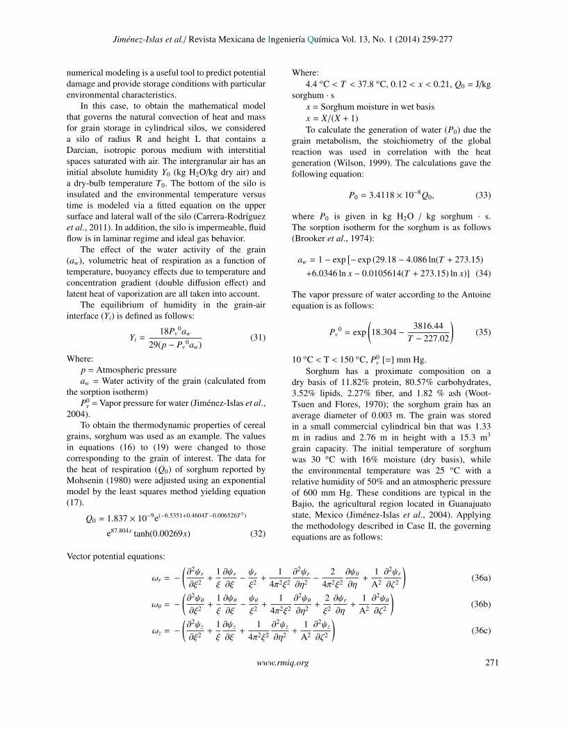
equations, a relaxation factor λ = 0.3 was used. Thesystem reached convergence in 12,424,325 iterationswith a CPU time of 7 days. This CPU time canbe reduced substantially if one uses parallelizationcomputing in workstations or supercomputers. Inaddition, the hardware, the operating systems and theFORTRAN compilers are becoming more efficient.Fig. 8 shows the flow patterns and temperaturecontours, the solid lines in black represent the pathof the air inside the silo and the color contoursrepresented temperatures. At Fo = 0, the dynamictemperature inside the silo is homogenous. There is anincrease in the temperature in the silo (approximately10:00 h). This rise of the surrounding environmentaltemperature accelerates the respiration heat sourceleading to an increase in the temperature insidethe silo. During the warmest hours of the day(approximately 12:00 h to 14:00 h), temperaturegradients concentrate on the sidewall and the surfaceof grains. Similarly, when a cold cycle arrives, thetemperature decreases at the boundary due to the effectof environmental boundary conditions as reported byBalzi et al. (2008). The dynamic central part is theleast sensitive to environmental changes. These resultsare consistent with those reported by Abalone et al.(2006) and Carrera-Rodrıguez et al. (2011). Flowpatterns show a recirculation near the boundaries ofcold air moving down the borders causing the bottomto cool faster. The flow patterns spread across the silo,and when the temperature cycle begins again, coldflow patterns re-form near the borders, validating themodel proposed by Carrera-Rodrıguez et al. (2011).

Jimenez-Islas et al./ Revista Mexicana de Ingenierıa Quımica Vol. 13, No. 1 (2014) xxx-xxx

ξ = 1,∂ψr∂ξ

= 0ψθ = 0ψz = 0

, θ = f (Fo),∂W∂ξ

= 0,∂ϕ

∂ξ= 0

(39b)

η = 0,∂ψ0

∂η=∂ψn

∂η,∂θ0

∂η=∂θn

∂η,

∂W0

∂η=∂Wn

∂η,∂φ0

∂η=∂φn

∂η(39c)

η = 1, ψ0 = ψn, θ0 = θn,W0 = Wn, φ0 = φn (39d)

ζ = 0,ψr = 0ψθ = 0∂ψz∂ζ

= 0,∂θ

∂ζ= 0,

∂W∂ζ

= 0,∂φ

∂ζ= 0 (39e)

ζ = 1,

ψr = 0ψθ = 0∂ψz

∂ζ= 0

, θ = f (Fo),∂W∂ζ

= 0,∂φ

∂ζ= 0(39f)

Wood’s approximation was used for the vorticityboundaries (Leonardi, 1984). The initial conditionsare as follows:

Fo = 0, ψ = 0, θ = 0, W = 0, φ = 0 (40)

Fig. 7 shows the geometric system and computationaldomain, including the radial and axial coordinates,with a grid of 9×18×9 collocation points yielding21,780 algebraic equations, and a time-step size of10−4 performing the simulation until one day of realtime (January 1). Due to the stiffness of the governing

equations, a relaxation factor λ = 0.3 was used. Thesystem reached convergence in 12,424,325 iterationswith a CPU time of 7 days. This CPU time canbe reduced substantially if one uses parallelizationcomputing in workstations or supercomputers. Inaddition, the hardware, the operating systems and theFORTRAN compilers are becoming more efficient.Fig. 8 shows the flow patterns and temperaturecontours, the solid lines in black represent the pathof the air inside the silo and the color contoursrepresented temperatures. At Fo = 0, the dynamictemperature inside the silo is homogenous. There is anincrease in the temperature in the silo (approximately10:00 h). This rise of the surrounding environmentaltemperature accelerates the respiration heat sourceleading to an increase in the temperature insidethe silo. During the warmest hours of the day(approximately 12:00 h to 14:00 h), temperaturegradients concentrate on the sidewall and the surfaceof grains. Similarly, when a cold cycle arrives, thetemperature decreases at the boundary due to the effectof environmental boundary conditions as reported byBalzi et al. (2008). The dynamic central part is theleast sensitive to environmental changes. These resultsare consistent with those reported by Abalone et al.(2006) and Carrera-Rodrıguez et al. (2011). Flowpatterns show a recirculation near the boundaries ofcold air moving down the borders causing the bottomto cool faster. The flow patterns spread across the silo,and when the temperature cycle begins again, coldflow patterns re-form near the borders, validating themodel proposed by Carrera-Rodrıguez et al. (2011).

Table 5. Representative temperature values of the state ofGuanajuato, Mexico for 2009.

Variable ◦C Description

Tmax 30.7 Annual maximum temperatureTmin 4.9 Annual minimum temperatureTm 14.9 Maximum temperature, minimum annualTo 30.0 Initial grain temperatureT f 25.0 Initial temperature of the environment

14

71

72 73 74

Fig. 7. Three-dimensional computational domain for Case IV 75 76

Fig. 7. Three-dimensional computational domain forCase IV.

www.rmiq.org 15

14

71

72 73 74

Fig. 7. Three-dimensional computational domain for Case IV 75 76

Fig. 7. Three-dimensional computational domain for CaseIV.

www.rmiq.org 273


15

(a) (b)

(c) (d)

(e) (f)

Fig. 8. Temperature contours for January 1 for: a) 00:00 h, b) 10:00 h, c) 12:00 h, d) 16:00 h, e) 18:00 h, and f) 20:00 h.

77

X Y

Z

T

2322.52221.52120.5

0.010000

X Y

Z

T

2322.52221.52120.5

0.030000

X Y

Z

T

19.819.619.419.21918.818.6

0.480000

X Y

Z

T

19.919.819.719.619.519.419.319.219.11918.9

0.410000

X Y

Z

T

19.819.619.419.21918.818.618.418.2

0.540000

X Y

Z

T

19.819.619.419.21918.818.6

0.460000

X Y

Z

T

2625.925.825.725.625.525.425.325.225.125

0.010000

X Y

Z

T

2625.925.825.725.625.525.425.325.225.125

0.010000

X Y

Z

T

2625.925.825.725.625.525.425.325.225.125

0.010000

X Y

Z

T

2625.925.825.725.625.525.425.325.225.125

0.010000

X Y

Z

T

2625.925.825.725.625.525.425.325.225.125

0.010000

X Y

Z

T

2625.925.825.725.625.525.425.325.225.125

0.010000

Fig. 8. Temperature contours for January 1 for: a) 00:00 h, b) 10:00 h, c) 12:00 h, d) 16:00 h, e) 18:00 h, and f)20:00 h.

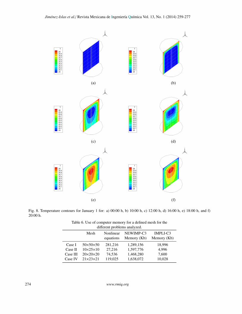
Table 6. Use of computer memory for a defined mesh for thedifferent problems analyzed.

Mesh Nonlinear NEWIMP-C3 IMPLI-C3equations Memory (Kb) Memory (Kb)

Case I 50×50×50 281,216 1,289,156 18,996Case II 10×25×10 27,216 1,597,776 4,996Case III 20×20×20 74,536 1,468,280 7,600Case IV 21×23×21 119,025 1,638,072 10,028

274 www.rmiq.org


3.5 Memory use

We also performed a RAM memory study to illustrateadvantages of nonlinear relaxation versus classicNewton-Raphson multivariate, designing a Newton-Raphson computer code with similar subroutines andoperational characteristics of IMPLI-C3. This codewas named NEWIMP-C3 and his utilization will bereported later. The comparison was performed withthe same type of discretization and an equal amountof free memory, the different cases was carried outwith meshing close to use all free memory available,depending on the problem, comparing the RAMconsumption. Table 6 shows the assigned memoryshowed in the WindowsT M Task Manager, the largedifference between memory consumption illustratesthat nonlinear relaxation has a great advantage tosave memory and allowing address complex problemsthat require large amount of nodes for enhancing theaccuracy of solution. We also observed that memoryconsumption by nonlinear relaxation is only 0.3%-1.5% of the memory required by Newton-Raphson,so the nonlinear relaxation is a robust algorithm thatallows simulating complex problems that require largenumber of nodes.

ConclusionsThe IMPLI-C3 FORTRAN code was suitable to solveproblems involving 3-D parabolic nonlinear PDE,particularly in the natural convection simulations,decreasing substantially the amount of required RAM(approximately 1 % of the memory required ifone uses Newton-Raphson), without any complexalgebraic-rearrangement of governing equations. Thisallows the implementation of finer meshes that arerequired in numerical analysis of complex highlynonlinear problems, where the Newton method isunfeasible due the amount of memory requiredthat often exceed the installed RAM. The use of3-D orthogonal collocation for discretizing spatialcoordinates is an alternative methodology for solvingengineering problems with accuracy.

AcknowledgmentsWe gratefully acknowledge the financial supportof CONACYT, Mexico via grants Basic ScienceSEP-2004-CO1-46230 and CB-2011/167095, andCONCYTEG (Guanajuato State Government) viagrants 07-09-k662-050, 07-09-k119-107, and 09-09-k662-065.

Nomenclature

A ratio height/radius, L/Rav grain-air interfacial area, m2 m−3

aw water activity, dimensionlesse unit vectorC matrix used for the calculation of the

matrix AD matrix used for the calculation of the

matrix BF functionFo Fourier numberNu Nusselt numberNX number of internal nodes in X directionNY number of internal nodes in Y directionNZ number of internal nodes in Z directionP polynomialP pressureP0 volumetric generation of water by

respiration, kg m−3 s−1

Pr Prandtl numberQ matrix used for the calculation of the

matrices A and BQ0 volumetric heat of respiration of the

cereal grain, J −3 s−1

R cylinder radiusRa Rayleigh numberT dependent variable, temperatureT independent variable matrixU dimensionless velocityX, x spatial coordinate in X directionY, y spatial coordinate in Y directionZ, z spatial coordinate in Z directionX grain moisture in dry basis, kg water/kg

dry solidYi absolute humidity in the grain-air

interface, kg water/kg dry airY absolute humidity, kg water/kg dry air

SubscriptsJ local index node XI local node index in Yk, p auxiliary indexesN number of internal nodes0, 1 initial, final condition

Greek symbolsα thermal diffusivity of the porous

medium, ke f f /ρCp

ω vorticity

www.rmiq.org 275


ψ vector potentialθ temperatureλ relaxation factorξ dimensionless radial coordinate, r/Rφs dimensionless moisture grain, (X −

X0)/(X1 − X0)φa dimensionless humidity in the air, (Y −

Y0)/(Y1 − Y0)ζ dimensionless height coordinate, z/Lη dimensionless angular or azimuthal

coordinate, θ/2πρ density, kg/m3

ρa density of dry air, kg/m3

ρs sorghum grain density on dry basis,kg/m3

References

Abalone, R., Gaston, A., Cassinera, A. andLara, M. A. (2006). Modelizacion de laDistribucion de Temperatura y Humedad deGranos Almacenados en Silos. AsociacionArgentina de Mecanica Computacional.Mecanica Computacional; 233-247.

Balzi, U. R., Gaston, A., and Abalone, R.(2008). Efecto de la Conveccion Natural enla Distribucion de Temperatura y Migracionde Humedad en Granos Almacenados enSilos. Asociacion Argentina de MecanicaComputacional. Mecanica Computacional,1471-1485.

Barrozo, M. A. S., Henrique, H. M., Sartori, D.J. M. and Freire, J. T. (2006). The use of theorthogonal collocation method on the study ofthe drying kinetics of soybean seeds. Journal ofStored Products Research 42, 348-356.

Bessonov, O. A., Brailovskaya, V.A., Nikitin, S.A.,and Polezhaev, V. I. (1998). Three-DimensionalNatural Convection in a Cubical Enclosure:A Benchmark Numerical Solution. Advancesin Computational Heat Transfer Procedures ofInternational Symposium Cesme, 1.

Brahim, B. B. and Taieb, L. (2009). Transientnatural convection in 3D tilted enclosureheated from two opposite sides. InternationalCommunications in Heat and Mass Transfer 36,604-613.

Brooker, D. B., Bakker-Arkema, F. W. and Hall C. W.(1974). Drying Cereal Grains. AVI PublishingCompany: Westport, Connecticut. USA.

Carrera-Rodrıguez, M., Martınez-Gonzalez, G. M.,Navarrete-Bolanos, J. L., Botello-Alvarez, J.E., Rico-Martınez, R. and Jimenez-Islas, H.(2011). Transient numerical study of the effectof ambient temperature on 2-D cereal grainstorage in cylindrical silos. Journal of StoredProducts Research 47, 106-122.

De Vahl, Davis, G. (1983). Natural Convection of Airin a Square Cavity: A Benchmark NumericalSolution. International Journal for NumericalMethods in Fluids 3, 249-264.

Ebrahimi, A. A., Ebrahim, H. A. and Jamshidi, E.(2008). Solving partial differential equations ofgas-solid reactions by orthogonal collocation.Computers & Chemical Engineering 32, 1746-1759.

Finlayson, B. A. (1972). The Method of WeightedResiduals and Variational Principles, AcademicPress. USA.

Finlayson, B. A. (1980). Nonlinear Analysis inChemical Engineering. McGraw-Hill College.USA

Jimenez-Islas, H. and Lopez-Isunza, F. (1994).ELI-COL Programa para resolver sistemasde ecuaciones diferenciales parciales elıpticas,por doble colocacion ortogonal. Avances enIngenierıa Quımica 2, 82-86.

Jimenez-Islas H. and Lopez-Isunza F. (1996).PAR-COL2, Programa para resolver EDPparabolicas bidimensionales no lineales, pordoble colocacion ortogonal. Avances enIngenierıa Quımica 4, 168-173.

Jimenez-Islas, H. (1999). Modelamiento Matematicode los Procesos de Transferencia de Momentum,Calor y Masa en Medios Porosos. PhDThesis (in Spanish), Universidad AutonomaMetropolitana Unidad Iztapalapa, Mexico, D.F.

Jimenez-Islas, H., Navarrete-Bolanos, J. L. andBotello-Alvarez, E. (2004). Numerical Study ofthe Natural Convection of Heat and 2-D Mass ofGrain Stored in Cylindrical Silos. Agrociencia38, 325-342

276 www.rmiq.org


Jimenez-Islas, H. (2001). Natural Convectionin a Cubical Porous Cavity: Solution byOrthogonal Collocation. Computational FluidDynamics; Proceedings of the Fourth UNAMSupercomputing Conference. World ScientificPublishing Co. Singapore, 173-180.

Leonardi, E. A. (1984). Numerical Study ofthe Effects of Fluid Properties on NaturalConvection. Ph.D. Thesis. University of NewSouth Wales, Australia.

Lo, D. C., Young, D. L., Murugesan, K., Tsai, C.C., and Gou, M. H. (2007). Velocity-Vorticityformulation for 3D natural convection in aninclined cavity by DQ method. InternationalJournal of Heat and Mass Transfer 50, 479-491.

Mohsenin, N. N. (1980). Thermal Properties ofFoods and Agricultural Materials (2nd ed. pp407). Gordon and Breach Science Publishers:NY. USA.

Nield, D. A. and Bejan, A. (1992). Convection inPorous Media. Springer-Verlag, USA.

Ostrach, S. (1988). Natural Convection inEnclosures. Journal of Heat Transfer 110, 1175-1190

Ozoe, H. and Toh, K. A. (1998). Technique tocircumvent a singularity at a radial center withapplication for a three-dimensional cylindricalsystem. Numerical Heat Transfer, Part B.Fundamentals. An International Journal ofComputation and Methodology 33, 355-365.

Ravnik, J., Skerget, L. and Zunic, Z. (2008).Velocity-Vorticity formulation for 3-D natural

convection in an inclined enclosure by FEM.International Journal of Heat and MassTransfer 51, 4517-4527.

Roache, P.J. (1972). Computational Fluid Dynamics.Hermosa Publisher: Albuquerque, N.M. USA.

Tric, E., Labrose, G. and Betrouni, M. (2000).A first incursion into the 3D structure ofnatural convection of air in a differentiallyheated cubic cavity from accurate numericalsolutions. International Journal of Heat andMass Transfer 43, 4043-4056.

Vemuri, V. R. and Karplus, W. J. (1981). DigitalComputer Treatment of Partial DifferentialEquations. Prentice-Hall Co. USA.

Villadsen, J. V. and Stewart, W. E. (1967). Solutionof Boundary-Value Problems by OrthogonalCollocation. Chemical Engineering Science 22,1483-1501.

Wakashima, S. and Saitoh, T. S. (2004). Benchmarksolutions for natural convection in a cubiccavity using the high-order time-space method.International Journal of Heat and MassTransfer 47, 853-864.

Wilson, M. T. (1999). A Model for Predicting MouldGrowth and Subsequent heat Generation inBulk Stored Grain. Journal of Stored ProductsResearch 35, 1-13.

Woot-Tsuen, W. and Flores, M. (1970). Tabla deComposicion de Alimentos para uso en AmericaLatina (pp 150). Editorial Interamericana, S.A.,Mexico.

www.rmiq.org 277

Revista Mexicana de ngeniería - SciELO · Revista Mexicana de ... de sistemas f´ısicos que ......

Documents

Transcript of Revista Mexicana de ngeniería - SciELO · Revista Mexicana de ... de sistemas f´ısicos que ......