Redactor Prof. dr. ing. Traian Jurc · Redactor şef / Editor in chief Prof.dr.ing. Ioan...
44
Transcript of Redactor Prof. dr. ing. Traian Jurc · Redactor şef / Editor in chief Prof.dr.ing. Ioan...
Redactor şef Editor in chief Profdring Ioan Naforniţă Colegiul de redacţie Editorial Board
Prof dr ing Virgil Tiponuţ Prof dr ing Alexandru Isar Conf dr ing Dorina Isar Prof dr ing Traian Jurcă
Prof dr ing Aldo De Sabata As ing Kovaci Maria - secretar de redacţie Colectivul de recenzare Advisory Board
Prof dr ing Monica Borda UT Cluj-Napoca Prof dr George Mihalas UMF Timişoara Prof dr ing Traian Jurcă UP Timişoara Prof dr ing Virgil Tiponuţ UP Timişoara Prof dr ing Aldo De Sabata UP Timişoara Prof dr ing Alexandru Isar UP Timişoara Prof dr ing Ioan Naforniţă UP Timişoara
Buletinul Ştiinţific
al Universităţii Politehnica din Timişoara
Seria ELECTRONICĂ ŞI TELECOMUNICAŢII
TRANSACTIONS ON ELECTRONICS AND COMMUNICATIONS
Tom 48(62) Fascicola 2 2003
SUMAR
ELECTRONICĂ APLICATĂ
Titu Botoş Virgil Tiponuţ A Mobile Robot Control Method with Artificial Neural Networks (I)hellip 3 Titu Botoş Virgil Tiponuţ A Mobile Robot Control Method with Artificial Neural Networks (II) 7
INSTRUMENTAŢIE
Gabriel Vasiu Liviu Toma Algorithm for Generating Signals Using Table Look-up Methodhelliphelliphelliphelliphelliphelliphelliphellip hellip hellip hellip hellip hellip hellip hellip hellip hellip 11
Robert Pazsitka Liviu Toma Dan Stoiciu Aldo De Sabata New Proof of the Sampling Theorem for Bandpass Signalshelliphelliphelliphelliphelliphelliphelliphellip 14 Robert Pazsitka Sampling Amplitude Modulated Signalshelliphelliphelliphelliphelliphelliphelliphellip 16 Adrian Vacircrtosu The Specific Absorption rate of the Electromagnetic Radiation for Biological Sturctures in the Case of Mobile Telephonyhelliphellip hellip hellip 20
1
TELECOMUNICAŢII
Marius Oltean Miranda Naforniţă The Cyclic Prefix Lenght Influence on OFDM ndash Transmission BERrdquohelliphelliphelliphelliphelliphelliphelliphelliphellip hellip hellip 26 Florin Vancea Codruţa Vancea Methods for JPEG image protection by partial encryptionhellip hellip hellip 30 Maria Simina Moldovan Examination of the signal energy distribution using Wavelet Transformhellip hellip hellip hellip hellip hellip hellip hellip hellip hellip hellip hellip hellip hellip hellip hellip hellip hellip hellip hellip hellip hellip hellip 36
2
Buletinul Ştiinţific al Universităţii Politehnica din Timişoara
Seria ELECTRONICĂ şi TELECOMUNICAŢII TRANSACTIONS on ELECTRONICS and COMMUNICATIONS
Tom 48(62) Fascicola 2 2003
A Mobile Robot Control Method with Artificial Neural Networks (I)
Titu Botoş1 Virgil Tiponuţ
Summary - The present paper is a discussion about a possible artificial neural network implementation of an obstacle avoidance behavior Such a behavior could be the first layer of a mobile robot reactive control system The proposed implementation uses exclusively artificial neural networks and thus takes advantage of their capability to easily adapt to a large variety of situation without even having a (environmental) model The conceived behavior comprises three distinct layers On the first layer a simple forward perceptron provides a position estimation of the environmental reflection points by processing the sensorial data Next a simple competitive network catalogs the encountered scenes On the last level another feed forward network decides the mobile robot azimuth correction Keywords mobile robot reactive control artificial neural network
I INTRODUCTION
One of the most important tasks of a mobile robot control system is the trajectory planning The main goal for such a control algorithm is a collision free trajectory that leads to the desired target point In achieving this goal the quality of the robot - environment interaction especially the environment model accuracy is the key
From a historic perspective the mobile robot control systems started with the hierarchical architecture based on the sense-plan-action control cycle [3] Specialized literature provides several other names for this control paradigm high level control systems coded behavior [6] or analytical method [5]
The most defining characteristic of these systems is the serial style processing cycle First the robot acquires information from the environment and updates the internal environment model Then the robot is reasoning about the necessary steps that should be taken in order to achieve the goal And in the last stage the robot executes one by one the tasks in the list resulted from the second phase
The three steps described above form the sense-plan-action cycle which is repeated indefinitely and is invoked each time the current action set stops matching the reality
Another main characteristic of the hierarchical control system is their global environment model Unfortunately such a model which should represent as
___________________
1 ing T Botoş Universitatea ldquoPolitehnicardquo Timişoara bl Vasile Pacircrvan nr2 1900 Timişoara Email tbotosmaildnttmroT
many environmental details as possible is very hard to conceive and maintain up to date Even if idealy such a global model would be available it is impossible to use an enormous data quantity for real time control
The result of correlating the enormous data quantity of the hierarchical global model that had to be processed with the limited processing power of the rsquo60 processors where quite poor Robots those days were running with a sub-turtle speed around 4mh [3]
These totally disappointing results moved the mobile robot field researchers to other new directions to develop new and faster robot control algorithms Thus in the second half of the rsquo80 the behavioral control theory is born
The one that first proposed the new idea was Brooks (1986) who proposed to assign a specific motor action to a specific stimulus for satisfying the present demand In the new emerged theory the connection between stimulus and its action is called behavior By means of using behaviors the robot is able to respond quickly to the environmental conditions in a reflex manner If multiple behavioral connection coexists an apparent intelligent robot behavior may merge In the new control approach the environment model is avoided by purpose It is advocated the idea that the environment is the best model for itself [3] [4]
The behavioral mobile robot control has gained a lot of interest in the last years Nowadays behavior such desire intention and emotion are studied [6]
The most important features of an efficient mobile robot control system are [7] bull Reliability bull It should be easily adapted or even better to adapt
itself to the environmental and sensorial system performances changes
bull It should be able to learn from it past experiences and even to generalize from its already gained knowledge
bull It should react quickly in order to work in real time If the above qualities are considered for a mobile
robot control system then the artificial neural networks paradigm could be a good approach in order to tackle them [7]
The artificial neural networks paradigm also complies with the behavioral control theory because in their core the environment model is implicit hidden in the network weights Such a model is hard or even impossible for a human being to understand but the
3
robot itself does not need a huge and laborious human understandable model
Further more there is no necessary need for a mathematically precise environment model Indeed for each case there are good and bad robot answers However for mobile robot navigation purpose only rarely there is a single good solution Usually there is a set of trajectories (solutions) which all are about as same as good Here the artificial neural networks generalization power plays an important role in finding viable solutions for not previously encountered situation
The present paper presents and analyzes a possible obstacle avoidance behavior part of a more complex mobile robot reactive control system The proposed approach takes advantage of a pure artificial neural network implementation achieving a pure reactive controller
The previously achieved results presented in [8] are the start point for the present discussion and are therefore presented in the beginning of next section Section II introduces the proposed obstacle avoidance behavior by discussing and motivating the ideas The conclusions are the subject of section III The presentation started within this article is concluded with the simulation results presented as its second part
II THE OBSTACLE AVOIDANCE BEHAVIOR
By following the biological systems example for the pattern analysis and recognition a simple competitive artificial neural network is chosen to cluster the scene encounter by the mobile robot
In the biological world the stimulus self mapping process has an important role in many of the brain functions For instance two different stimulus are (auto) mapped in different regions of the brain However similar stimuli are mapped in close vicinity in a way that preserves the information topological In the same way the simple competitive neural network model creates analogies between the input stimuli and the network outputs
It has been proved in an experimental manner that the cortex activity is directly related to the subject spatial position in respect with the surrounding environmental features Individual neural cells are consistently fired for the same spatial position For every (known) location a brain activity image is obtained and therefore this brain activity patterns could be considered as a map representation [9]
The surrounding environment features are strongly related to the brain activity patterns and a correlation between this two can be created [10] In other words it is possible to cluster the incoming sensorial patterns in classes because there is a univocal relation between the fired class and the spatial position Having in mind this biological example the proposed structure for the obstacle avoidance behavior is distributed on three different levels
The first level processes the ultrasonic sensorial information recorded by a biaural transducer system The first level processor is a simple perceptron It correlates the incoming ultrasonic field levels with known patterns stored as the perceptron weights The
perceptron neurons are spread over the inspected area in front of the mobile robot For each neuron is assigned a possible reflection point position (The dots in Fig2 show also the perceptron neuron position) Therefore the perceptron output reassembles the environmental reflection points spatial position as the neuronal activation levels are proportional with the obstacle detection confidence [8]
As already previously mentioned the second level achieves a clustering job A simple competitive neural network is used to recognize the mobile robot spatial position based on the images generated by the first level
The last level the third decides the mobile robot azimuth correction as a function of the recognized situation and a set of empirical inferred rules
Analogous control systems with similar hierarchical structures are found in [2] [3] [11] and [13]
One can find a similarity between the proposed obstacle avoidance behavior and a fuzzy controller The first layer the one that analyzes the sensorial information is equivalent with the fuzzification stage The second level implements in fact a fuzzy rule database while the last level is similar with the defuzzification process A The clustering layer
As per the above introduction the role of this layer is to cluster the output scenes of the sensorial information processor Every competitive neuron is designed to recognize a particular spatial position [9]
The fundamental idea used as model is the behavior of that part of the human cortex which processes the visual information The process that takes place here transforms the received visual information in patterns which are more and more abstract as the hierarchy of the processing layer increases In the end the last layer is able to fully recognize the incoming visual stimulus Thus the neurons on the first layer receive information only from some parts of the retina being specialized in primary shape recognition like straight and curved lines with certain directions and length On the next layer the cortex neurons are able to combine the lines recognized by the first layer in more complicated geometrical shapes Following this reasoning higher layers of the human cortex add more and more details to the obtained internal image (ie colors and brightness) until finally this image can be clustered [2]
For the obstacle avoidance behavior a similar classification engine is to be created one that can recognize either simple or more complex shapes For this purpose a single competitive neural network is chosen Its output units are formally divided in classes The first class comprises the simple competitive units that become active with one only neuron of the correlation layer active meaning there is only one reflection source present in the investigated environment
The second class of the competitive outputs layer gathers units that become active if two symmetrical (in respect with the median axis of the transducer system) reflection sources are detected in the
4
environment Superior classes become active for scenes with more reflection sources It is possible to recognize shapes like straight and concave walls corners or even combinations of these types of obstacles
It is to be stressed out that the simple competitive layer output indicates that a scene is recognized which could be composed from either one or a combination of several environmental reflection sources Thus the resulting azimuth correction brings the robot closer to a global optimized trajectory because wiser decision may be assumed through consideration of more than just one obstacle
Yet the competitive layer provides a particularity used further by the next level the decision layer The winning neuron of the competitive network does not have its level bounded to the saturation level but instead it preserves the scene recognition confidence level
Here is the reasoning used in order to compute the simple competitive neural network weights for the first two classes
In the first class a competitive neuron is assigned for every output of the correlation layer thus 51 neurons are allocated The weights of the 51 competitive neurons of the first class are set to zero for all the connections but for the one that links the competitive neuron to its correspondent first layer output Therefore a one to one connection is achieved as per Fig1
Fig1 The weights of the first 8 competitive neurons from the first class One can see that there is only one excitatory connection for each neuron while their value decreases for neurons that represent position further to the transducer system
The excitatory weights are set to decreasing values starting from a maximum one set for the neuron that encodes the closest reflection source position This favoures the neurons assigned to closer reflection points However a farther neuron can still win (see Fig2) if it has the highest firing level (recognition confidence level) of its corresponding perceptron output neuron in the correlation layer
For the second class the one that is assigned to represent scenes with two symmetric reflection points the combinations of symmetric points are first to be find There are 21 pairs and a neuron in the second class of the competitive layer is assigned for each pair All the weights of the second class competitive neurons are set to zero excepting the two that connect each neuron with its designed pair The values for these non zero weights are set in a similar fashion as for the neurons in the firs class Equal and decreasing pair values are assigned to each neuron starting with the closest to the transducer system pair
This time the absolute value from which the assignment starts from is lower than in the case of neurons in the first class This choice favors the activation of the first class neurons if only one of the reflection points couple is active However if both neurons of the correlation layer for a symmetric reflection points are active then the net input of the corresponding second class competitive neuron is higher then the individual net input for the first class neurons that encode only one reflection point
Neurons weights for higher classes may be chosen similarly allowing recognition of more complex shapes
In order for the proposed algorithm of choosing the competitive layer weights to be successful two condition have to be met bull The reflection points clustered by one particular
class should outnumber by at least one the number of clustered points for the previous class
bull The competitive neuron weights for a particular output neuron in the correlation layer have to decrease as the competitive neuron belongs to a higher class These two conditions assure that there will always
be an competitive neuron with the highest net input namely the one that belongs to the class with all the excitatory connection activated B The azimuth correction layer
One of the major advantages of the competitive layer is the clear result At any time only one output of the competitive network is active and therefore the task of the last layer the one that decides the robot azimuth correction is greatly simplified Even the decisional layer structure can be thus simplified
100 000 000 000 000 000 000 000 000 000 098 000 000 000 000 000 000 000 000 000 096 000 000 000 000 000 000 000 000 000 094 000 000 000 000 000 000 000 000 000 092 000 000 000 000 000 000 000 000 000 090 000 000 000 000 000 000 000 000 000 088 000 000 000 000 000 000 000 000 000 086 000 000 000 000 000 000 000 000 000 084
Wclass I =
There are multiple choices for the azimuth correction layer implementation style However the simplest one is chosen a simple perceptron Moreover its structure is scaled down to only one neuron connected to all competitive layer outputs
For this defuzzification neuron its weights are set to the appropriate azimuth correction values for each class denoted by the connection with the competitive layer As the output transfer function of this neuron is chosen a linear function (the identity) With this structure for the decisional layer the azimuth correction is directly obtained as the output of the obstacle avoidance controller
The azimuth correction values set as weights for the neuron on the last layer were found by implying human reasoning [8] The values are the same as the one chose by a human being that would be faced with the correspondent scene The final value were found by implying a trial - error process fine tuning the initial chosen values
In Fig2 the azimuth correction for the first class of the competitive network values are shown in a 2D graphical approach The slope of each line segment is proportional with the robot azimuth correction as if the obstacle would be positioned in each neuron place (the robot is positioned at the 00 coordinates point)
5
mthitcfinwcsc
info
imcpn
psbsdidfrfia lanfiprefr
pp
layer contains a simple competitive network In section IIB is presented a possible algorithm to construct the competitive network and to choose its weights The resulting clustering engine is capable to recognize equally well simple and more complicated scenes
On top of the first two layers another neural network is employed which decides the mobile robot azimuth correction based on the case recognized by the second layer Actually the decision network is formed upon a single neuron Since its weights are equal to the azimuth correction values and seen that its output function is linear the provided output can directly drive the mobile robot steering mechanics It was proven by implying several simulations that this last layer provides satisfactory results despite its simplicity
BIBLIOGRAFIE
[1] J Hertz A Krogh Introduction to the theory of the neural
computation 1991 Addison-Wesley Publishing Company [2] M Miclea Psihologie Cognitiva Casa de Editura GLORIA Cluj-
Fig2 The azimuth correction values for the first classcompetitive layer neuron activation The slope of each linesegment is proportional with the robot azimuth correction as ifthe obstacle would be positioned in each neuron (the robot ispositioned at the 00 coordinates point)
It is to be stressed that this figures are the aximum correction values Here is taken advantage of e competitive layer particular behavior to present to s output not some saturated values but the recognition onfidence level of that particular class Therefore the ring level of the winning neuron of the competitive etwork is adjusting the azimuth correction values hich can sweep a range starting from zero (the
orrespondent class element is not present in the current cene) to its maximum value (when the recognition onfidence level of that class element is the highest)
The correction azimuth values for the neurons the higher classes of the competitive network are und in a similar manner
III CONCLUSION
This paper presents a possible approach to plement a obstacle avoidance behavior A
onnectionist approach is chosen because this control aradigm can deal with a large number of cases with no eed for an explicit environmental model
Other studies of the obstacle avoidance roblem based on information provided by ultrasonic ensors can be found in the cited bibliography The ackbone idea is the same based on the ultrasonic ensor reading a repulsive force is computed which rives the robot away from obstacles [10] The new eas described in [8] as well as in this paper differ om the rest in the way that the reflected ultrasonic eld is recorded and processed (using exclusive rtificial neural networks)
The presented behavior is structured on three yers each of them with clear tasks On the first layer a eural network processes the raw recorded ultrasonic eld [8] The first layer output estimates the reflection oint(s) position(s) (together with the confidence cognition level) in the investigated environment in ont of the robot
The job of the second layer is to identify a ossible mobile robot position based on the reflection oints position offered by the first level The second
Napoca 1994 [3] Robin R Murphy ldquoIntroduction to AI Roboticsrdquo MIT Press 2000 [4] A Ram R C Arkin Case-Based Reactive Navigation A Method
for On-Line Selection and Adaptation of Reactive Robotic Control Parameters IEEE Trans Syst MAN Cyber vol27 no3 pp 376-393 Jun 1997
[5] U Nehmzow T Smithers Mapbuilding Using Self-Organizing Networks in Really Useful Robots WWW
[6] P Baroni D Fogli Adding Active Mental Entities to Autonomous Mobile Control Architectures Second ECPD International Conference on Advanced Robots Inteligent Automation and Active Systems Vienna Sept 1996
[7] D Katic Some Recent Issues in Connectionist Robot Control Third ECPD International Conference on Advanced Robots Inteligent Automation and Active Systems Bremen Sept 1997
[8] T Botoş V Tiponuţ ldquo Holografie acustică icircn impuls bidimensională bitraductorrdquo Modern Technologies in the XXI Century Bucureşti 15-16 Nov 2001
[9] G J van Tonder J J Kruger Shape Encoding A Biologically Inspired Method of Transforming Boundary Images into Ensembles of Shape-Related Features IEEE Trans Syst MAN Cyber vol27 no5 pp 749-759 Oct 1997
[10] A Kurz Constructing Maps for Mobile Robot Navigation Based on Ultrasonic Range Data IEEE Trans Syst MAN Cyber vol26 no2 pp 233-242 Apr 1996
[11] S G Tzafestas K C Zikidis A Mobile Robot Guidance System Based On Three Neural Network Modules Second ECPD International Conference on Advanced Robots Inteligent Automation and Active Systems Vienna Sept 1996
[12] L Banta J Moody RNutter Neural Network for Autonomous Robot Navigation WWW
[13] H R Beom H S Cho A Sensor-Based Obstacle Avoidance Controller for a Mobile Robot Using Fuzzy Logic and Neural Network WWW
6
Buletinul Ştiinţific al Universităţii Politehnica din Timişoara
Seria ELECTRONICĂ şi TELECOMUNICAŢII TRANSACTIONS on ELECTRONICS and COMMUNICATIONS
Tom 48(62) Fascicola 2 2003
A Mobile Robot Control Method with Artificial Neural Networks (II)
Titu Botoş1 Virgil Tiponuţ
Summary - The present paper presents the simulation results obtained by controlling a mobile robot with an obstacle avoidance behavior The implied behavior is structured on three distinct layers Fist a simple perceptron is used to process the received sensorial information in order to estimate the reflection points position in the investigated environment On the next layer a competitive network clusters the encountered cases On top of the two networks another one decides the robot azimuth correction The obtained simulations results for few environmental cases are presented and discussed Key words mobile robots reactive control neural networks
I INTRODUCTION
The present paper presents and analyses the simulation results obtained by controlling a mobile robot with an obstacle avoidance behavior (proposed in [6] ) This behavior is meant to form the first layer of a reactive mobile robot controller
The proposed behavior is structured on three distinctive sub-layers each of which has its own well defined role On the first layer an artificial neural network processes the raw captured sensorial information [5] and provides a position estimation (along with the detection confidence) for the reflection points in the investigated environment in front of the mobile robot
Based on the reflection points position estimation the second layer clusters the encountered situations The second level is implemented by involving a simple competitive neural network which is able to classify a wide range of scenes
On top of the first two layers another artificial neural network decides the azimuth correction based on the clustered scene found by the competitive layer In fact this last layer is a single neuron with a linear firing function and its weights set to the desired azimuth correction values
The studied cases presented in this paper attempt to comprise in a few classes the most common scenes that could be encountered by a mobile robot Here are presented single obstacle scenes (with obstacles comparable in dimensions to the mobile robot) as well as wide plane obstacles (walls and corners)
The present paper is structured as follows the second section presents general simulation issues along ___________________________ 1 ing T Botoş Universitatea ldquoPolitehnicardquo Timişoara bl Vasile
Pacircrvan nr2 1900 Timişoara Email tbotosmaildnttmro
with the particular ones for the used environment model the simulations result are presented and discussed in section three and the conclusions are drawn in the final section
II SIMULATION THE USED ENVIRONMENT
MODEL
If one can overlook Takeo Kanades sarcastic remark Simulations are doomed to succeed [9] there are still a number of reasons that make the simulations an attractive solution to prove new ideas
First of all using real mobile robot in experiments imply not only high expenses but also long experimenting time periods In contrast if a sufficiently reliable environment model could be conceived then substantial amount of time and money can be saved with the simulations
Moreover within the simulation the mobile robot evolution can be monitored as a function of a single parameter In order to achieve the same performance a very high controlled environment is in order which of course is hard to achieve
One can use simulation even without real environmental sensorial information A mathematical model could be used to generate such data Performing simulation in such cases could even contribute to a better understanding of the environment
There is of course a possibility that the considered environment model would miss an important environmental parameter andor to consider some with no much relevance [4] To prove however the models validity real experiments have to be involved
The mathematical model considered for the simulation presented in the present paper calculates in an analytical way the ultrasonic pulse time of flight based on the distances between the robot and its surrounding obstacles The ultrasonic waves speed in air is known and considered constant (its variation with temperature humidity and air pressure is disregarded)
For the purpose of the intended simulations the ultrasonic reflections are considered to be of a specular nature The reflection points are found at the base of the orthogonal line to the obstacle surface the normal line that contains the ultrasonic emitter Not all the environment reflection points are considered at a certain moment Only the ones that are found inside of the investigated boundaries are considered at a certain moment [6]
7
The simulated robot has a circular shape with a 150mm radius and it is of the holonomic type The robot speed is considered to be constant with every step equal to 10mm length The investigated environmental space has a section of a corona shape with a 60 degrees opening angle 200mm the small radius and 1400mm the exterior radius [6]
The simulation cycle includes these phases sensorial information processing for the azimuth correction calculation mobile robot orientation update firing a new ultrasonic pulse one step forward displacement and jump back to the cycle beginning
The software involved to develop de simulation is the MATLAB package
III RESULTS A One single cylindrical obstacle
The first studied case is the one that involves one single cylindrical obstacle Its dimension is close to the robot size
The path followed by the robot in such a case is similar to the one presented in Fig1 For any other initial configuration (mobile robot position versus the obstacle position) the mobile robot behavior is alike The mobile robot is always able to avoid the cylindrical obstacle
It has to be stressed out that this kind of obstacle always generates a reflection as long as its central point falls inside the investigated boundaries and that greatly simplify its detection
Upon observation of Fig1 it can be seen that once the robot has changed its azimuth enough and the obstacle does not fall any longer inside the investigated boundaries the robot will preserve its orientation and will continue to travel in the same direction If no obstacles are detected the proposed obstacle avoidance behavior preserves the traveling direction
This observation is further more strengthened upon consideration of Fig2 which presents the mobile robot azimuth history The dashed line in Fig2 presents clearly that after step 123 the mobile robot azimuth remains unmodified
Another issue that can be stressed out from the
Fig2 study is related to the azimuth evolution Although the robot changes the course of direction mainly towards left (the azimuth value is increased) there are small direction oscillation in the obstacle avoidance process
For certain positions distances between the robot and the obstacle the neurons of the first processing layer sense that the obstacle is on the left side of the robot Because of their activation the azimuth correction is toward right hand However their activation levels are small enough and the turns to the right are smaller and eventually disappear
Fig2 The robot azimuth history for a cylindrical obstacle(dashed line) and for a wall (solid line)
These small direction oscillations prove the
pure reactive character of the proposed obstacle avoidance behavior The controller output depends solely on the momentary stimulus input disregarding any previous input values Such a controller that does not consider the action history and does not learn from the past experiences is described in literature as chicken behavior in front of a fence [8]
The direction oscillation presented in Fig2 can be reduced and even completely eliminated if a memory is added to the obstacle avoidance controller If that is the case then the robot avoidance trajectory would be smoother and it will turn later However it is to be questionable if such a memory component is to be attached to a reactive controller Fig1 The path followed by the robot for a single circle type
obstacle scene
B A wall obstacle
For obstacles with wide surfaces the nature of their surfaces should be considered because the reflection type is completely dependent upon them
Therefore for smooth surfaces with roughness dimension smaller then the ultrasonic wave length the reflection is mainly specular They can be detected if the wave incidence angle is less then half of the ultrasonic transducer sensitivity angle Unfortunately the majority of main made surfaces fall under this category
On the other extreme the obstacles with rough surfaces produce rather diffuse reflection This kind of obstacles favor a wide reflection due to the multitude of reflection points on their surface Although the reflection is weaker then for the specular reflection it can be detected on a wider reception angle Almost all the natural surfaces can be clustered here
8
The robot behavior for a wall type obstacle (the obstacle dimensions are much bigger then the robot dimensions) is presented in Fig3 Although the simulation was not allowed to run long enough it is clear that the robot can not avoid the wall The azimuth correction is not strong enough to cause avoidance of the obstacle However this happens not due to the obstacle avoidance behavior but because of the transducers The modeled transducers have a sensitivity angle of only 60 degrees
If one turns back to Fig2 and watches now the solid line it can be easily seen that after the 127-th step the reflection point on the wall falls outside of the inspected boundary the robot does not sense it any more and with no obstacle detected the robot preserves its motion direction Once more because the azimuth correction was not strong enough the robot will eventually collide into the wall
The azimuth value for which the robot fails to sense the wall is 122 degrees Applying the math returns the 32 degree value for the ultrasonic incident angle value higher than half of the modeled transducer sensitivity angle (60 2 degrees) For this value on the specular reflection becomes total with no ultrasonic energy returning to the transducers
The solution for this issue is to use transducers with a much wider sensitivity angle Ideally the transducer sensitivity angle should be wider than 120 degree and for that value the wall could be sensed for much higher ultrasonic incidence angle
To prove the validity of the obstacle avoidance behavior and the lack of the modeled transducers the next simulation considers a rough wall type obstacle In this case because of the walls rough surface there will result a reflected ultrasonic wave for every robot angle
The simulation results are depicted in Fig4 where one can see that the wall is formed out of small cylindrical obstacles This time the obstacle avoidance behavior succeeds to adjust the mobile robot azimuth strong enough to avoid the obstacle
By studying once more Fig2 and taking into account that the initial positions of the robot regarding both the cylindrical obstacle and the wall were the same one more remark results For the wall obstacle the azimuth correction period is longer because the reflection point slides along the wall being visible for longer time As a result the final azimuth correction in the wall case is higher then for the
cylindrical obstacle However the absolute azimuth difference is a function of the robot motion step The difference is bigger for a motion with small steps (less than 5mmstep) but it decrease toward zero for robot steps higher then 10mmstep
Fig4 The mobile robot trajectory for a wall type obstacle withrough surface which is much wider that the robot
Although the difference is not consistent for these two cases this particularity could be usefully used If the azimuth difference for a single scene obstacle is monitored it can be decided if the obstacle is a wall by comparing the final azimuth variance with the value for a cylindrical obstacle Necessary corrections can be correspondingly applied
Fig 3 The mobile robot trajectory for a wall type obstacle withsmooth surface which is much wider that the robot
C Two symmetrical cylindrical obstacles
Another interesting case is the one with two symmetrical obstacles symmetric regarding to the robot transducer system Such a case has a particular importance because the classic ultrasonic systems which use only the time of fly information can not detect it correctly For a scene with two symmetric obstacles a classic range-finder ultrasonic system detects one obstacle placed at a distance equal with half of the transducers - obstacle one - obstacle two triangle perimeter
Fig5 The mobile robot trajectory for a scene with two cylindricaland symmetrical obstacles
Moreover this case proves the clustering ability of the artificial competitive neural network It also validates the algorithm used to build the competitive network Thus if the sensorial information processor (first layer) provides enough information the competitive layer can be conceived in such a way to
9
distinguish even complicated scenes walls with certain orientations corners or even combinations of those
Fig5 presents the configuration of a scene with two symmetric obstacles and the resulting mobile robot trajectory The robot is able to find a way between the two obstacles However along its way through the obstacles most of the time only one obstacle is detected This is the reason why the robot azimuth oscillates around the 90 degrees value (see Fig6)
When both of the obstacles are detected (these situation are depicted in Fig6 with small circles) the azimuth correction is zero opposed to a certain value for avoiding a phantom obstacle in front of the mobile robot
D One corner obstacle
The corner considered for this simulation is a 90 degree one because most of the rooms exhibit a rectangular shape
The way in which the obstacle avoidance behavior controls the robot for a corner obstacle is dependent on the corner surface similar to the case of the wall obstacle Where the corner surfaces are smooth like for most of the man made environments the robot senses only one reflection point Even this point is a hypothetical one because the robots ultrasonic system will pick a multiple reflection (second order - two reflections) on the corner sides The corner sides are not detected because the ultrasonic field incident angle is higher then half of the transducer sensitivity angle and the reflection is therefore complete
The experiments performed proved that the multiple reflection reassembles a virtual point close to the corner tip With only this information available the robot negotiates the corner like a single cylindrical obstacle running eventually into the corner walls
However if the corner sides are rough enough and provide more reflection points then the robot is able to always avoid the corner Such a scenario is presented in Fig7 where again the corner is composed out of a number of cylindrical obstacles
The behavior of the simulated mobile robot controlled solely by the obstacle avoidance behavior in a more complex environment that contains a combination of obstacles is alike to the particular cases previously studied
Fig 7 The mobile robot trajectory in front of a corner
With the obstacle avoidance behavior as the only driving controller a mobile robot will keep moving around without any particular goal but just to wander
II CONCLUSIONS
The obstacle avoidance behavior proposed in [6] is always able to avoid single obstacle with dimensions close to those of the robot Neither are wide obstacles with rough surfaces a problem to avoid However large smooth surfaces that act like perfect mirrors for the ultrasonic wave can not be avoided
This is not because of the proposed obstacle avoidance behavior but because of the transducer incapacity to detect them over certain limits (incident angle values bigger than half of the transducer sensitivity angle) The solution for this issue is to use better transducers with larger sensitivity angle
Fig6 The mobile robot azimuth history for a scene with twosymmetric obstacles
The oscillating shape of the azimuth correction is due to the pure reactive nature of the proposed obstacle avoidance behavior The momentary azimuth correction is a function only of the correspondent sensorial reading If a memory component for the behavior is considered then the small oscillation can be eliminated it is still questionable if such a future is desirable in a reactive mobile robot controller
In a real case some other features could be added to the presented obstacle avoidance behavior in order to obtain a more intelligent control system
BIBLIOGRAFIE [1] J Hertz A Krogh Introduction to the theory of the neural
computation 1991 Addison-Wesley Publishing Company [2] M Miclea Psihologie Cognitivă Casa de Editura GLORIA 1994 [3] Robin R Murphy ldquoIntroduction to AI Roboticsrdquo MIT Press 2000 [4] Ulrich Nehmzow ldquoMobile Robotics A Practical Introductionrdquo
Springer-Verlag London Limited 2000 [5] T Botoş V Tiponuţ ldquo Holografie acustică icircn impuls
bidimensională bitraductorrdquo Modern Technologies in the XXI Century Bucureşti 15-16 Nov 2001rdquo
[6] T Botoş ldquoO metodă de conducere reactivă a roboţilor mobili cu implementare neuronală (I)rdquo
[7] David Lee ldquoThe Map-Building and Exploration Strategies of a Simple Sonar-Equipped Mobile Robot An Experimental Quantitative Evaluationrdquo Cambridge University Press 1996
[8] A Zelinsky Y Kuniyoshi Learning to Coordinate Behaviours for Robot Navigation www
[9] Ulrich Nehmzow Mobile Robotics A Practical Introduction Springer-Verlag 2000 ISBN 1-85233-173-9
[10] MDAdams ldquoSensor Modelling Design and Data Processing for Autonomous Navigationrdquo Word Scientific 1999 ISBN 9-810-23496-1
10
Buletinul Ştiinţific al Universităţii Politehnica din Timişoara
Seria ELECTRONICĂ şi TELECOMUNICAŢII TRANSACTIONS on ELECTRONICS and COMMUNICATIONS
Tom 48(62) Fascicola 2 2003
Algorithm for Generating Signals Using Table Look-up Method
Gabriel Vasiu1 Liviu Toma1
1 Facultatea de Electronică şi Telecomunicaţii Departamentul Măsurări şi Electronică Optică Bd V Pacircrvan Timişoara 300223 e-mail gvasiuetcuttro ltomaetcuttro
Abstract ndash The paper deals with the generation of signals with a TMS320C5402 DSK board using table look-up method The decimation and the interpolation of the samples in the look-up table are used to generate signals with continuously programmable frequency and amplitude The corresponding algorithm and C language program are presented in the paper Index Terms - Generating signals table look-up conti-nuously programmable frequency TMS320C5402 DSK board Code Composer Studio
I INTRODUCTION
The algorithm presented in this paper implements the table look-up method [1] for generating signals with continuously programmable frequency and amplitude
The algorithm is implemented by a C language program designed for a TMS320C5402 DSK board This board includes a TMS320C5402 digital signal processor two TLC320AD50C analog interface cir-cuits (AIC) memory circuits interface circuits (for parallel serial and JTAG ports) expansion memory interface peripheral interface etc The TLC320AD50C AIC provides 16-bit resolution signal conversion from digital-to-analog and from analog-to-digital using oversampling sigma-delta converters [2] The Code Composer Studio (CCS) development environment is used to build and debug programs that run on the DSK board [3]
II THE ALGORITHM
We consider a table in DSK memory that contains
the samples corresponding to one period of the generated signal For signal generation these samples are sent to the digital-to-analog conversion channel of the AIC The transmitted samples are selected from the table through decimation or interpolation (repetition) depending on the required frequency of the generated signal The amplitude of the generated signal depends on the sample values in the table and can be modified by multiplication with a constant
The frequency fg of the generated signal is related to the AICrsquos sampling frequency fs and to the number
of samples n from which a period of the signal is synthesized according to
n
ff s
g = (1)
Therefore to generate a signal of frequency fg
based on a table with N samples xi i=0 1 N-1 we define the displacement δ (difference between the indexes of two samples from the table successively sent to AIC) with
s
g
f
Nf
n
N==δ (2)
Particularly for δ =1 all N samples in the table are
successively and periodically sent to AIC for δ =2 every other sample is sent (the samples with even indexes) and for δ =12 all the samples are sent and every sample is repeated twice
Generally for δ gt1 the samples are selected from the table through decimation and for δ lt1 through interpolation As a rule the indexes of the samples that are successively transmitted from the table are
[ ]50+= δji modulo N j = 0 1 hellip (3)
where we have denoted by [x] the largest integer smaller than x
Using (2) in (3) yields
⎥⎥⎦
⎤
⎢⎢⎣
⎡+= 50
s
g
fNf
ji modulo N j = 0 1 hellip (4)
The TLC320AD50C AIC communicates with the
digital signal processor through a serial interface The digital-to-analog channel of the AIC includes an interpolation filter a 16-bit tworsquos complement delta-sigma DAC a low-pass output filter and a program-mable gain output amplifier The transition frequency
11
of the low-pass filter is about fs2 The output amplifier gain is established through programming and the possible values are 1 12 14 and 0
The output signal of the digital-to-analog con-version channel of the AIC is amplified with a LM386 operational amplifier If the amplifier gain is programmed to 1 a digital input signal with values in the range of minus215 divide 215 minus 1 (samples are represented on 16-bit tworsquos complement) will produce an output voltage in the range minusUemax divide Uemax Uemax = 15V
When generating a signal from the samples stored in a table the amplitude of the generated signal can be modified by multiplying the samples with a constant k The value of this constant depends on the desired output amplitude which is expressed by the maximum absolute value Ugmax which should be less than 15 V To determine this constant the maximum absolute value of the signal described by the samples xi in the table must be calculated as
ixM max= i = 0 1 hellip N-1 (5)
The constant k is
maxmax
152g
eU
MUk = (6)
The sampling frequency of the TLC320AD50C
AIC [1] is
d
mff MCLK
s 92= (7)
where m is a multiplication parameter that can be 1 or 4 d is a division parameter that can take the values 1 2 3 8 and fMCLK is the clock frequency of the AIC The two parameters can be set through programming
In TMS320C5402 DSK board the value for fMCLK is 8192 kHz (213 kHz) so that the possible values for fs are
( )d
mHzf s
34 102 sdot= (8)
The sampling frequency is established by pro-
gramming the parameters m and d and can take discrete values in the 2 divide 64 kHz range
In order to accomplish all necessary operations (decimation or interpolation and multiplication with constant k) for generating the signal in real time two memory buffers are used While the samples are calculated and written to one of the buffers the samples from the other buffer previously calculated are sent to the AIC Then the buffers exchange roles For an accurate operation of this technique the time required to calculate and write the samples in one of the buffers must be smaller than the time necessary to send the samples from the other buffer
III THE SIGNAL GENERATION PROGRAM
A C program for signal generation that implements the algorithm in the previous paragraph is presented This program uses functions from the files boardc and codecc [2] which reside in the programming library of the TMS320C5402 DSK board
The file boardc contains C functions for controlling system operation Therefore for TMS320C5402 DSK board initialization the function brd_init() is used The parameter of this function is the operating frequency of the digital signal processor that can be a multiple of 10 with the lowest being 20 MHz and the highest being 100 MHz
The file codecc contains C functions for controlling the operation of the two AICs of the TMS320C5402 DSK board The functions defined in the codecc module that will be used in the signal generation program are presented in the following
The codec_open() function defines an identifier for the used AIC and establishes its connection with the serial port of the digital signal processor
The codec_sample_rate() function establishes the sampling frequency of the specified AIC through the first parameter of the function at the value prescribed by the second parameter value obtained with (7)
The codec_cont_play() triggers the transmission of the samples to the AIC The samples of each buffer are sent successively with the sampling rate and alternatively from the two buffers This function is defined through the following parameters
- the identifier of the AIC - synchronization mode for sending the samples to
the AIC (this parameter is MODE_INT for sample sending triggered by an interrupt request generated by the AIC or MODE_DMA for sample sending through the direct memory access technique)
- the identifiers of the two buffers - the number of samples for each buffer - a pointer to a function that will be called at the
end of the sample sending from a buffer (the function is defined by the user and can be used for updating the sample values in the corresponding buffer)
- the address of a pointer to a variable that becomes zero at the end of the sample sending from a buffer
Include header files include ltstdiohgt include boardh include codech include semnaleh Defines define fs 16000 define n1 100 Globals int x[2][n1] i=0t=1j=1M float deltair=0fg=250ue_max=15ug_max=10k fg[Hz] ug_max[V] const int tm
12
char t_s=t s - sinusoidal t - triangular l - ramp d - square
Calculate the maximum absolute value of the signal stored in the table
int max(void) int zmx=0 for(z=0zltNz++) mx=(mxltabs((tm+z2))abs((tm+z2))mx) return mx Main void main(void) Locals HANDLE conv=0 int stareq=0tmp Initialize DSK board for use if (brd_init(100)) printf(Eroare brd_initn) Connect AIC to respective serial port if ((conv=codec_open(HANDSET_CODEC))= =0) printf(Eroare codec_open()n) Sets the AIC sample rate codec_sample_rate(convSR_16000) Calculate displacement delta=(fgfs)N Selects signal to be generated switch (t_s) case s tm=ampsine_table[0]break case t tm=amptr_table[0]break case l tm=amplv_table[0]break case d tm=ampdr_table[0] Calculate the amplitude constant M=max() k=((float)32768(Mue_max))ug_max Continuously send data to the AIC codec_cont_play(convMODE_INTx[0]x[1]n10 ampstare) Loop forever while(1) Fill current buffer for(q=0qltn1q++)
Calculate the amplitude of the current sample tmp=(int)((k((tm+i(sizeof(int)))))+05) Write in the current buffer x[t][q]=tmp Calculate the index of the samples in the table ir=ir+delta-((int)(ir+delta+05))N)N i=((int)(ir+05)) Setup for the alternate buffer t^=1 Wait for buffer to be done while(stare= =1) Set the state variable to 1 stare=1
A synthesized sinusoidal signal graph provided by the CCS environment is presented in figure 1
Fig 1 A synthesized sinusoidal signal graph
IV CONCLUSION
An algorithm and a corresponding C program
which use the table look-up method for generating signals with continuously programmable frequency and amplitude are implemented on TMS320C5402 DSK board
REFERENCES [1] Y C Jenq ldquoDigital spectra of nonuniformly sampled signals-Digital look-up tunable sinusoidal oscillatorsrdquo IEEE Trans Instrum Meas vol 37 Sept 1988 [2] Texas Instruments ldquoTLC320AD50CI TLC320AD52C Sigma-Delta Analog Interface Circuits With Master-Slave Functionrdquo Data Manual SLAS131E 2000 [2] Texas Instruments ldquoCode Composer Studio for the C5000 DSP Platform C5402 DSK Development Toolsrdquo CD-ROM 1999
13
Buletinul Ştiinţific al Universităţii Politehnica din Timişoara
Seria ELECTRONICĂ şi TELECOMUNICAŢII TRANSACTIONS on ELECTRONICS and COMMUNICATIONS
Tom 48(62) Fascicola 2 2003
New Proof of the Sampling Theorem for Bandpass Signals
Robert Pazsitka1 Liviu Toma1 Dan Stoiciu1 and Aldo De Sabata1
1 Facultatea de Electronică şi Telecomunicaţii Departamentul Măsurări şi Electronică Optică Bd V Pacircrvan Timişoara 300223 e-mail robietcuttro ltomaetcuttro dstoiciuetcuttro adesabatetcuttro
Abstract ndash In order to avoid aliasing when sampling a signal at a uniform rate it is necessary that all spectral components of the signal have different sample values This condition is used in order to derive the classical sampling theorem for bandpass signals The relation-ships for permissible and minimum sampling rates are derived Keywords Bandpass signals sampling theorem sampling rate aliasing
I INTRODUCTION
Sampling a signal at a uniform rate may produce aliasing In this case it is impossible to recover the original analog signal from the sampled signal To avoid aliasing the spectral representation of the analog signal must not contain sinusoidal components of different frequencies that have the same sample values [1] In order to derive the corresponding condition we use the following two identities
( ) ⎟⎟⎠
⎞⎜⎜⎝
⎛++=⎟⎟
⎠
⎞⎜⎜⎝
⎛+ ϕπϕπ
ee
e fnfkf
fnf 12sin2sin (1)
( ) ⎟⎟⎠
⎞⎜⎜⎝
⎛+minusminus=⎟⎟
⎠
⎞⎜⎜⎝
⎛+ πϕπϕπ
ee
e fnffk
fnf 22sin2sin
(2) where fe is the sampling frequency of the signal sin(2πft+ϕ) and constants k1 k2 are any integers From identities (1) and (2) we obtain the frequencies of the components with the same sample values as the component of frequency f (3) ek fkff 11
+=
(4) ffkf ek minus= 22
To avoid aliasing the sampled signal must contain a single frequency component out of those in (3) and (4) which is obtained for k1=0
II DERIVATION OF THE SAMPLING THEOREM FOR BANDPASS SIGNALS
Consider a bandpass signal s(t) whose spectral
components in the frequency domain satisfy Mm fff lele (5)
where fm and fM are the minimum and maximum frequency in the spectrum respectively The signal bandwidth fB is defined by
mMB fff minus= (6) The frequencies fk1 in (3) and fk2 in (4) correspond to alias components when
Mem ffkff le+le 1 (7)
Mem fffkf leminusle 2 (8)
In order to avoid aliasing a single value should be possible for k1 in (7) namely k1=0 and no solution should be possible for k2 in (8) The inequalities (7) and (8) can be rewritten as
e
M
e
m
fffk
fff minus
leleminus
1 (9)
e
M
e
m
fff
kf
ff +lele
+2 (10)
Since f can take any value between fm and fM the widest allowable ranges for k1 and k2 are
e
mM
e
Mm
fffk
fff minus
leleminus
1 (11)
e
M
e
m
ffk
ff 22
2 lele (12)
14
The inequality (11) holds only for k1=0 iff
11 1 ltminus
leleminus
ltminuse
mM
e
Mm
fff
kf
ff (13)
It follows that
(14) Be ff gt Inequality (12) has no solution for k2 iff
Kff
ffK
e
M
e
m ltltltminus221 (15)
for any integer K larger than unity For satisfying (15) it is necessary that
122ltminus
e
m
e
M
ff
ff
that is
Be ff 2gt (16)
Condition (16) is more restrictive than (14) If no aliasing occurs then the sampling frequency fe satisfies (16)
III RANGES OF SAMPLING RATES
In order to avoid aliasing it is necessary and sufficient for fe to satisfy (15) which can be rewritten in the form
1
22minus
ltltK
ffKf m
eM (17)
(for K=1 the last member should be considered equal to infinity) Inequality (17) admits solutions for fe iff
1
22minus
ltK
fKf mM
which implies
⎥⎦
⎤⎢⎣
⎡lele
B
M
ffK1 (18)
(we have denoted by [x] the largest integer smaller than x) By combining (17) and (18) we get the possible ranges for fe one for every value of K in (18) The
number of ranges is ⎥⎦
⎤⎢⎣
⎡
B
M
ff The range of the smallest
sampling frequencies is
⎟⎟⎟⎟⎟
⎠
⎞
⎜⎜⎜⎜⎜
⎝
⎛
minus⎥⎦
⎤⎢⎣
⎡⎥⎦
⎤⎢⎣
⎡=
1
2
2
B
M
m
B
M
M
ff
f
fff
R (19)
If 1le⎥⎦
⎤⎢⎣
⎡
B
M
ff
then it is not possible to apply a
uniform bandpass sampling procedure In this case (19) reduces to the sampling condition for lowpass signals
IV CONCLUSION In this note a compact and transparent derivation of the sampling theorem for bandpass signals based on the condition that the spectral representation of the analog signal must not contain sinusoidal components of different frequencies with the same sample values has been presented Results known from literature [2] [3] have been obtained in an alternative way
REFERENCES [1] S D Stearns Digital Signal Analysis Hayden Book Company Inc New Jersey 1975 [2] R B Vaughan N L Scott and D R White ldquoThe Theory of Bandpass Samplingrdquo IEEE Transactions on Signal Processing vol 39 pp1973-1984 September 1991 [3] I Naforniţă A Cacircmpeanu A Isar Semnale circuite şi sisteme partea I Universitatea ldquoPolitehnicardquo Timişoara 1995
15
Buletinul Ştiinţific al Universităţii Politehnica din Timişoara
Seria ELECTRONICĂ şi TELECOMUNICAŢII TRANSACTIONS on ELECTRONICS and COMMUNICATIONS
Tom 48(62) Fascicola 2 2003
Sampling Amplitude Modulated Signals
Robert Pazsitka1
Abstract ndash The paper presents the sampling of periodic bandpass signals obtained through amplitude modulation of a sinusoidal carrier with a low-pass periodic signal The relationships for the sampling frequency and the number of samples required for calculating the Fourier coefficients of the modulating signal (or modulating signals in the case of quadrature amplitude modulation) are derived The same relationships are given for calculating the Fourier coefficients of the modulated signal Keywords bandpass signals amplitude modulation quadrature amplitude modulation sampling Fourier coefficients
I INTRODUCTION
An amplitude modulated signal with sinusoidal carrier may be represented as [1]
ttptx 0cos)()( ω= (1) where πω 200 =f is the carrier frequency and is the low-pass modulating signal with the maximum frequency noted The modulated signal is a bandpass signal [1] within the range
)(tp
maxf
max0max0 ffff +divideminus Sampling of bandpass signals and the necessary conditions imposed to the sampling frequency to avoid aliasing are treated in many papers [1] [5] [9] A theorem referring to real bandpass signals is presented in [5] and [6] The spectral components of the bandpass signal
are non-zero only in the frequency range that satisfies
)(txsi fff ltlt where and are the
minimum and maximum frequency in the spectrum respectively The bandwidth is The value of the bandwidth must be less than else the sampling frequency must be greater than
if sf
is ffB minus=
if
sf2 The sampling theorem of bandpass real signals shows that the reconstruction of the signal from its samples is possible if the sampling frequency satisfies the equation [6]
1
22minus
lelen
ff
nf i
es where
Bf
n slele2 (2)
The number from (2) is an integer If n Bf s is also an integer the smallest sampling frequency is
Bfe 2= This paper deals with the particular case of bandpass periodic signals obtained through amplitude modulation of a sinusoidal (periodic) carrier with a low-pass periodic signal containing a sum of sinusoids case not found in literature
II SAMPLING OF AMPLITUDE-MODULATED SIGNALS WITH PERIODIC MODULATING
SIGNAL For calculating the period of the bandpass periodic signal using the periods of the carrier and low-pass periodic signals we make the following statement the product of two periodic signals with frequencies that can be written as ratio of integer numbers is a periodic signal Let us consider two periodic signals with the fundamental frequencies and (the periods 0f 1f
00 1 fT = 11 1 fT = ) If these frequencies are written in the form
0
00 b
af = and
1
11 b
af = (3)
then their ratio is
Qmm
bb
aa
ff
isin=sdot=1
0
0
1
1
0
1
0 (4)
where and 0a 0b 1a 1b 100 bam sdot= 011 bam sdot= are integers Using (4) the above statement can be reformulated as follows the product of two periodic signals with the periods and that can be written 0T 1T
____________________ 1 Facultatea de Electronică şi Telecomunicaţii Departamentul Măsurări şi Electronică Optică Bd V Pacircrvan Timişoara 300223 e-mail robietcuttro
16
as ratio of integer numbers is a periodic signal with the period T where
(5) 1100 TmTmT == where and are integers 0m 1m The integers and must have no common factor for
0m 1mT to be the principal period of the bandpass
periodic signal Else the period calculated with (5) will be a multiple of the principal period We consider that the bandpass periodic signal noted is obtained by amplitude modulation of a sinusoidal carrier with a low-pass periodic signal noted see (1) We note with the period of
with the period of the carrier
)(tx
)(tp 1T)(tp 0T t0cosω and
with the period of the amplitude modulation signal The order of the maximum harmonic in the
spectrum of is noted
xT)(tx
)(tp K The numbers and are chosen so that the period calculated with (5) be the principal period of the signal If is a multiple of then
and else
0m 1m
xT)(tx 0f 1f
11 =m 1ff x = 11 mff x = where 11 gtm For if and we can write sf
(6) ⎩⎨⎧
+==minus==
102
101
KfffMfKfffMf
s
i
From (5) and (6) we can calculate the harmonics
and corresponding to the minimum and maximum frequencies in the spectrum
1M 2M
(7) ⎩⎨⎧
+=minus=
102
101
KmmMKmmM
The bandpass periodic signal has a discrete spectrum in the range
)(tx
xx fMffM 21 lele (8)
The bandwidth of the signal will be
(9) ( ) 11010 2KfKffKffB =minusminus+= The minimum sampling frequency required will be 142 KfBfe =gt The sampling of the amplitude modulated signal
ttptx 0cos)()( ω= can be made so that the samples taken from are samples from the low-pass signal
namely )(tx
)(tp
)()( ee iTpiTx plusmn= (10)
where ee fT 1= From (10) and (1) it follows that 1cos 0 plusmn=eiTω The samples required for
calculating the Fourier coefficients must be taken from one period of or from a multiple of
(uniform sampling) Therefore we can write
N
1T )(tp m
1T
1mTNTe = (11) where is an integer Two cases are possible m Case I πω 20 sTe = ( 1cos 0 =eiTω )
ππ 212 1
11
0 sN
mTTm
m= rArr
smm
mN 1
1
0= (12)
Case II πω sTe =0 ( 1cos 0 plusmn=eiTω )
ππ sN
mTTm
m=1
11
0 12 rArr sm
mmN 12
1
0= (13)
where s is an integer and is the number of samples taken from periods of According to Shannonrsquos theorem should be at least
N1mT )(txN 12 +K
so that and m s have to be chosen accordingly The sampling frequency from (11) will have the value
mNffe 1= The corresponding Fourier coefficients of will be calculated with
)(tp
summinus
=
minus=1
0)(1)(
N
i
iTjkep
eeiTxN
kc ω (14)
for case I ( calculated with (12)) and N
summinus
=
minus minus=1
0)1()(1)(
N
i
iiTjkep
eeiTxN
kc ω (15)
for case II ( calculated with (13)) N III SAMPLING OF QUADRATURE AMPLITUDE
MODULATED SIGNALS In this case the modulated signal is represented as [1] [2]
)(tx
ttqttptx 00 sin)(cos)()( ωω minus= (16)
The low-pass signals and are considered periodic with the same period noted and the maximum harmonic component in the spectrum of these signals is noted with
)(tp )(tq
1T
K If the sampling frequency ee Tf 1= has such a value that the equation
17
2
)12(0πω minus= sTe (17)
be valid where s =1 2 then for i even (18) )()( ee iTpiTx plusmn=
for odd (18rsquo) )()( ee iTqiTx plusmn= i From (18) and (18rsquo) it follows that the sampling interval used for one low-pass signal ( or ) is Similarly with (11) in this case we can write
)(tp )(tq
eT2
and - integers (19) 12 mTTN e = N m In (19) is the number of samples used for calculating the Fourier coefficients of or The total number of samples used for the two low-pass signals is
N)(tp )(tq
N2 From (17) (19) and )(2 1100 Tmmπω = we have
12
2
1
0
minus=
smm
mN (20)
Integers m and s are chosen in order to obtain the smallest greater than or equal to N 12 +K The sampling period can be obtained from (19) The Fourier coefficients for and are calculated with
)(tp )(tq
summinus
=
minus minus=1
0
2 )1()2(1)(N
i
iiTjkep
eeiTxN
kc ω (21)
summinus
=
++minus minus+=1
0
)2( )1()2(1)(N
i
siTiTjkeeq
eeeTiTxN
kc ω (22)
where 12 fπω = and [ ]KKk minusisin The reconstruction of the low-pass signals is made with
(23) sum+
minus=
=K
Kk
tjkpr ekctp ω)()(
(24) sum+
minus=
=K
Kk
tjkqr ekctq ω)()(
The reconstruction of the bandpass (quadrature amplitude-modulated) signal is made with
ttqttptx rrr 00 sin)(cos)()( ωω minus= (25)
IV CALCULATION OF THE FOURIER COEFFICIENTS CORRESPONDING TO THE
BANDPASS PERIODIC SIGNAL For obtaining the Fourier coefficients of the bandpass periodic signal the fundamental frequency must be determined as in chapter II The harmonic components and corresponding to the minimum and maximum frequencies in the spectrum are calculated with (7) The number of samples obtained from one period
of must satisfy the following three conditions [9]
)(tx
xf
1M 2M
NxT )(tx
a) )1(2 12 +minusgt MMN
b) ⎥⎦
⎤⎢⎣
⎡=⎥⎦
⎤⎢⎣
⎡NM
NM 21 22
c) NM12
and NM 22
must be different from
integers where [ ] denotes integer part The sampling period will be NTT xe = As between the Fourier coefficients we have the relationship (the signal is considered real) where denotes complex conjugate we can calculate just one half of the coefficients for example those with positive indices They can be calculated with
kk cc minus= )(tx
summinus
=
minus=1
0)(1 N
i
kiTjek
eeiTxN
c ω (26)
where xfπω 2= and 21 MMk isin If the bandpass signal is an amplitude-modulated signal with sinusoidal carrier as defined by (1) without phase difference between the carrier and the low-pass (periodic) signal we can calculate just one quarter of the Fourier coefficients This is possible because the coefficients corresponding to the frequencies below are the complex conjugates of their respective symmetric coefficients for frequencies greater than To demonstrate this the terms
)(tx
0f
0fttkak 01 coscos ωω and ttkbk 01 cossin ωω
contained by the modulated signal ttptx 0cos)()( ω= can be written as
tka
tkattka
k
kk
)cos(2
)cos(2
coscos
10
1001
ωω
ωωωω
++
+minus= (27)
tkb
tkbttkb
k
kk
)sin(2
)sin(2
cossin
10
1001
ωω
ωωωω
++
+minusminus= (28)
18
This means it is enough to calculate the coefficients with where kc 20 MMk isin ( ) 2210 MMM +=
corresponding to the remaining coefficients being obtained by complex conjugation This property is not valid for quadrature amplitude modulation
0f
Because all of the cases presented above refer to periodic signals the sampling frequency can be lowered by taking the samples from several periods An additional condition must be satisfied [10] namely the number of samples and the number of periods NM should have no common factor
V CONCLUSIONS Signals obtained through amplitude modulation can be sampled such as to obtain directly the samples of the low-pass signal Several relationships are established for calculating (the required number of samples) and the sampling frequency so as to obtain the samples of the low-pass signal if the input signal is a bandpass periodic signal obtained through amplitude modulation If the number results from (12) then the Fourier coefficients are easily calculated with the known formula (14) If the number results from (13) then the Fourier coefficients are calculated with the modified formula (15) The same calculations (number of samples sampling frequency Fourier coefficients corresponding to the low-pass signals) are for the bandpass signal obtained by quadrature amplitude modulation
N
N
N
Chapter 4 presents the condition that must be satisfied by the number of samples obtained from a bandpass signal in order to calculate the Fourier coefficients of this signal If the signal is real (the samples are real number) then and then just half of the coefficients need to be calculated If the bandpass signal is obtained through amplitude-modulation then just one quarter of the coefficients need to be calculated due to the fact that the spectrum is symmetrical with respect to
N
kk cc minus=
0f
REFERENCES [1] Jerry D Gibson The Communications Handbook CRC Press Inc 1997 [2] JL Brown JR First-Order Sampling of Bandpass Signals ndash A New Approach IEEE Trans on Inf Theory Vol IT-26 No 5 Sept 1980 [3] JL Brown JR On Quadrature Sampling of Bandpass Signals IEEE Trans on Aerospace and Electronic Systems Vol AES-15 No 3 May 1979 [4] Marks II J Robert Introduction to Shannon Sampling and Interpolation Theory Springer-Verlag New York Inc 1991 [5] Oran E Brigham The Fast Fourier Transform And Its Application Prentice Hall Inc 1988 [6] Larry Marple Exploding the Nyquist Barrier Misconception IEEE Signal Processing Magazine Vol 13 No5 Sept 1996 [7] Liu J Zhon X Peng Y Spectral Arrangement and other Topics in First-Order Bandpass Sampling Theory IEEE Trans on Sig Proc Vol 49 No 6 June 2001 [8] Vaughan BR Scott LN White RD The Theory of Bandpass Sampling IEEE Trans on Sig Proc Vol 39 No 9 Sept 1991 [9] Robert Pazsitka Sampling of Bandpass Periodical Signals Proceedings of the Symposium on Electronics and Telecommunications Etc 2002 Timisoara Sept 19-20 2002 Vol 1 [10] Robert Pazsitka Eşantionarea semnalelor periodice lucrare de dizertaţie Facultatea de Electronică şi Telecomunicaţii Timişoara iulie 1997
19
Buletinul Ştiinţific al Universităţii Politehnica din Timişoara
Seria ELECTRONICĂ şi TELECOMUNICAŢII TRANSACTIONS on ELECTRONICS and COMMUNICATIONS
Tom 48(62) Fascicola 2 2003
The Specific Absorption Rate of the Electromagnetic Radiation for Biological Structures in the Case of Mobile
Telephony
Adrian Vacircrtosu1
1 Facultatea de Electronică şi Telecomunicaţii Departamentul Măsurări şi Electronică Optică
ABSTRACT Cellular telephony uses a frequency domain ranging between 800 MHz and 2000 MHz with emission powers of 06W to 2W
The frequencies used have wavelengths that can be compared to the physical dimensions of the skull and the power emitted by portable phones is quite high around 06W Because of the proximity of the head (just a few centimeters away) with all the reflections from the surface of the skull and the attenuations that intervene the field intensities that manage to get inside the skull can induce in the cerebral mass currents of the same size with the intensities of normal biological currents
I INTRODUCTION The 5191999 recommendation of the Council
of Europe from the 12th of July 1999 concerning the limitation of public exposure to electromagnetic fields (from 0 Hz to 300 GHz) establishes the limits in values of physical units that characterize electromagnetic radiation at different frequencies The respective norms also called basic restrictions and reference levels establish safety coefficients in the case of electric magnetic and electromagnetic field exposure variable in time based directly on the obvious effects on health and biological considerations Depending on the field frequency the physical units used in order to specify the restrictions are the magnetic induction (B) the density of current (J) the specific absorption rate (SAR) and the power density (S) The SAR unit is used within the 100 kHz ndash 10 GHz frequency range to define the basic restrictions concerning the electromagnetic fields in order to prevent a generalized thermal stress of the body and an excessive localized heating of tissues
According to the 1999519CE 12th of July 1999 Recommendation the reference levels of
radiofrequency fields used in the GSM system are (table 1)
Table 1
Frequency (MHz)
Electric field
E (Vm)
Magnetic field H (Am)
Density of Power (Wmsup2)
900 41 011 45 1800 58 016 9
It is worth noticing that in the case of simultaneous exposure to different frequency fields there is a possibility that the effects of the exposure are cumulative As a convention each effect will be studied using separate calculations and based on the hypotheses separate evaluations of the effects of thermal and electric strain of the organism will be covered
Knowing the electric properties of biological environments is essential to the study of the interaction phenomena between these and the electromagnetic field The electrical properties involve permittivity and electric conduction
The magnetic properties (with some exceptions that do not concern the present paper) are not defined for the biological matter the relative permeability of biological entities is considered to equal a unit (micror= 1) and the losses obtained through the magnetic effect are thought to be negligible
The electric properties that intervene in the study of the biological effects of electromagnetic fields are the electric permittivity ε and the conduction σ defined over the unit of volume of matter Permittivity characterizes the interaction between the environment and the electromagnetic wave that is propagated through it The permittivity of free space is a constant εo and the permitivity of any other environment is a complex
20
measurement ( ) in which ε is an indicator of the property of the environment to store energy while ε indicates the property of the environment to dissipate the energy carried by the electromagnetic field
c jεεε minus=
Relative permittivity measures the net effect of the electric dipoles alignment that characterizes the intimate structure of the matter that is under the influence of an electric field applied from the outside
The energy dissipated per second per unit of volume of homogenous material by an electromagnetic wave incidence is proportionate to the square of the amplitude of the electric field component and is calculated with the help of this formula [1]
P = πf εoεE2 = σ E22 (1)
where σ is the conduction of the environment in which the dissipation of energy takes place The conduction is itself dependent on the frequency
All these parameters (σ ε or tan δ ) characterize the possibility of the environment to absorb the energy from the electromagnetic field
Calculating the values of the dielectric parameters (permittivity conduction wavelength intrinsic impedance penetration depth etc) that characterize the human tissues at the frequencies of 800 MHz and 900 MHz used by the Romanian mobile telephony was done by using a program in EXCEL based on formulas [2] [3] that allows for finding these measurements up to the frequency of 300 GHz
Formulas used in calculation of dielectric properties
complex permittivity
c jεεε minus= (2)
rel complex permittivity
0
εεεεε c
rrcr j =minus= (3)
0
ωεσε =r
ωσε =
permittivity of free space
Fm1085418781768 120
minustimes=ε permeability of free space
Hm104 70
minustimesπ=micro impedance of free space
Ω= 376730313Z 0 wave velocity in free space
ms 10 2997924581c 8
00
times=εmicro
=
angular frequency
f2 π=ω loss tangent of material
r
r
)(tanεε
=ωεσ
=ϑ (4)
propagation constant of material y = α+j β
)j(c
)j(j r
r
2
r2 εminusε⎟
⎠⎞
⎜⎝⎛ ω
microminus=ωε+σωmicro=γ (5)
attenuation constant of material
( ) ⎟⎟⎠
⎞⎜⎜⎝
⎛minusεε+
εmicro⎟⎠⎞
⎜⎝⎛ ω
=α 112c
2r
r
rr (6)
skin depth material
α=δ
1 (7)
phase constant of material
( ) ⎟⎟⎠
⎞⎜⎜⎝
⎛+εprimeε+
εmicro⎟⎠⎞
⎜⎝⎛ ω
=β 112c
2rr
rr (8)
wave velocity in material
βω
=u (9)
wavelength in material βπ
=λ2 (10)
intrinsic impedance of material
r
r
r0
c jZZ
εminusε
micro=
εmicro
= (11)
( ) 2502r
r
r
r0
1ZZ
⎥⎦⎤
⎢⎣⎡ εε+ε
micro= (12)
( ) ( )r
r
1tan21Zphase εε= minus (13) 00lephase(Z)le450
21
II RESULTS OF THE EXPERIMENT
The results of these calculations corresponding to the two bands are presented in the table 2 for f=800 MHz and in the table 3 for f=900 MHz
Table 2a
f=800 MHz micror = 1
TISSUE bone skin blood brain heart
εr 8688429 36212 5882646 464656 6067894
εr 0745467 1234021 2570435 1548868 2253825
σ (Sm) 0033178 0549214 1143998 0689339 1003087
tan(θ) 00858 0340777 0436952 0333337 0371434
α (1m) 2118257 1695389 2747556 1879632 2386113
β (1m) 4946731 1023108 1315008 1158271 1327692u (ms) 102E+08 49130166 38224479 43397013 37859280
λ (m) 0127017 0061413 0047781 0054246 0047324
δ (m) 0472086 0058984 0036396 0053202 0041909
|Ζ| (Ω) 1276914 6175043 4805721 5454375 4758779
Ζ (deg) 2451985 9408961 1180151 9217559 1018837
Table 2b
TISSUE muscle kidney liver lung spleen
εr 5411328 4761208 462569 3323576 5264076
εr 1430979 1890983 1815213 157899 2142521
σ (Sm) 0636871 0841601 0807879 0702745 0953551
tan(θ) 0264441 0397165 039242 0475088 0407008
α (1m) 1616963 2255025 219707 2237002 2427742
β (1m) 1243946 1178704 116132 992159 1240483u (ms) 40408097 42644715 43283050 50662729 40520887
λ (m) 005051 0053306 0054104 0063328 0050651
δ (m) 0061844 0044345 0045515 0044703 0041191
|Ζ| (Ω) 5078194 5360689 5440852 6370586 5093874
Ζ (deg) 7406157 1083061 1071302 1270591 1107336
Table 3a f= 900 MHz micror = 1
TISSUE bone skin blood brain heart
εrrsquo 8634636 3599427 5874271 4636694 6051015
εrrdquo 0818382 1133951 2333097 1421199 2071992
σ (Sm) 0040976 0567761 1168164 0711584 1037431
tan(θ) 0094779 0315037 0397172 0306511 0342421
α (1m) 2623734 1761374 2817931 1946225 2477099
β (1m) 5548936 1145292 1472909 1299078 1488052
TISSUE bone skin blood brain heart
u (ms) 102E+08 49374911 38392510 43529846 38001813
λ (m) 0113232 0054861 0042658 0048366 0042224
δ (m) 0381136 0056774 0035487 0051382 004037
|Ζ| (Ω) 1280628 6205502 4826162 5470811 4776366
Ζ (deg) 2707131 8743167 108308 8520446 9451129
Table 3b
TISSUE muscle kidney liver lung spleen
εr 5406606 4756672 4615513 3306596 5255305
εr 1333614 1714191 1650214 1440076 1950378
σ (Sm) 0667731 0858282 082625 0721035 097654
tan(θ) 0246664 0360376 0357536 0435516 0371126
α (1m) 1697889 2308073 2256177 2310114 2496166
β (1m) 1397314 1321244 1301189 1108984 1390013u (ms) 40469540 42799564 43459223 50991404 40682126
λ (m) 0044966 0047555 0048288 0056657 0045202
δ (m) 0058897 0043326 0044323 0043288 0040061
|Ζ| (Ω) 508583 5379605 5462482 6410789 5113597
Ζ (deg) 6928098 9908974 9836909 1176695 1018059 Formulas used for εr and εrrsquo are [2]
2
2
22
1
13
r
f1000f1
ff1 ⎟⎟
⎠
⎞⎜⎜⎝
⎛sdot
+
ε+
⎟⎟⎠
⎞⎜⎜⎝
⎛+
ε+ε=ε (14)
⎥⎥⎦
⎤
⎢⎢⎣
⎡⎟⎟⎠
⎞⎜⎜⎝
⎛sdot
+sdot
ε+
⎥⎥⎦
⎤
⎢⎢⎣
⎡⎟⎟⎠
⎞⎜⎜⎝
⎛+
ε+
sdotsdotπεσ
=ε2
22
22
11
1
0
0r
f1000f1f1000
f
ff1f
f1000f2
(15) The values of the units used in calculating these dielectric parameters are given in the table 4 [2]
Table 4a
TISSUE bone skin blood brain Heart
ε3 49 33 43 75 43
σo (Sm) 31E-07 0231 0768 0313 063
f1 (MHz) 2360 137 378 433 906
ε1 222 343 136 122 494
f2 (GHz) 204 177 213 165 156
ε2 18 32 543 387 559
22
Table 4b
TISSUE muscle kidney liver lung spleen
ε3 43 43 43 43 43
σo (Sm) 0301 0551 0406 0325 044
f1 (MHz) 83 247 442 818 266
ε1 475 166 136 691 289
f2 (GHz) 152 245 216 151 198
ε2 499 432 416 283 481
The external field incident to the biological structure can be expressed in terms of power density (mWcm2) of amplitude of the electric field component (Vm) or of the magnetic field component (Am) None of these parameters is appropriate for expressing the effects induced by the penetration of the electromagnetic radiation inside the biological domain Considering this situation a specific parameter has to be defined It is called the ldquoSpecific Absorption Rate ndash SARrdquo and it is the variation in time of the elementary energy quantity (dw) absorbed by an element of volume (dv) having a density (ρ) and an elementary mass (dm) [1]
⎟⎟⎠
⎞⎜⎜⎝
⎛=⎟
⎠⎞
⎜⎝⎛=
dVdW
dtd
dmdW
dtdkgWSAR
ρ)(
The Specific Absorption Rate (SAR) is correlated to the penetration depth (δ)in the tissues If the penetration depth (δ) is the distance from the surface of the tissue for which the amplitude of the electric field component reduces with factor e = 271 than the specific absorption rate at this depth reduces to a value equal to 135 of its initial value
Sometimes it is useful to define the depth d (frequently used in hyperthermia cases) at which the power incident to the surface of the irradiated structure is reduced to half (3 dB attenuation) Between (δ) and (d) there is the relation
d = 0345 x δ In order to determine the value of the SAR
parameter the TEMS (Test Mobile System) system was used This system was offered by the ORANGE firm and the measurements were taken at the frequency of 900 MHz
The applications of TEMS for an operational network are
bull it simulates and verifies possible changes in the network
bull it evaluates the quality of the received signal bull it measures the space covered range bull it tests the system (checks new or already
present functions)
- it signals in real time aberrant values of any parameter (for example the large number of interrupted calls)
- it identifies areas with problems of signal coverage or with high levels of interference
bull it presents the data in graphs maps The equipment used for measuring (Fig 1)
contains - special software made by Erricsson-TEMS
(Test Mobile System) - laptop mobile phone special data cable that
insures the PC-mobile phone connection
Fig1 The equipment used for measuring
The TEMS mobile phone is an Erricsson
ordinary phone that uses the TEMS program No supplementary calibrations are necessary for using the TEMS software
This mobile phone has four different operation modes
1 No Service (when it is in an area with no signal coverage)
2 Limited services (only emergency calls) 3 Inactive 4 Dedicate (during a conversation)
The measurements were taken during a
conversation therefore in the dedicate mode Taking the measurements involves - initiating a call - choosing the unit to be measured in this
case the power of the transmitted signal (TxPwr)
- the display of the unit to be measured (Fig2) and information about the distance from the base station (TA ndash Time Advance) the base station code (BSIC ndash Base Station Identity Code) local code (LAC Local Area Code) the channel of the communication (TCH ndash Traffic Channel)
23
In order to calculate the value of SAR the
situation when the telephone is in dedicated mode t0 is used At t0 these units have the following values
TxPwr =18dBm=625mW
TA = 2 d = TAx 500m Therefore the distance (d) to the base station is
1 km BSIC = 23 LAC = 05500
Fig2 The value of the SAR unit for the measured power is determined according to [1]
⎥⎦
⎤⎢⎣
⎡sdot=
=sdot
=ρ
=ρ
σ=
ρε primeprimeωε
=⎥⎦
⎤⎢⎣
⎡
minus
kgW1012550
1000062502P2EE
kgWSAR
3
22r0
where 0ε = permittivity of free space ω = angular frequency ρ = the density of the biologic environment asymp1000 kgm3
E = the intensity of the electric field P = πf εoεE2 = σ E22
Fm10E85418781768 120
minustimes=ε
0
r ωε
σ=ε
It is observed that the specific rate of absorption SAE is under the maximum admitted level of 04 Wkg
The value of SAR can also be determined according to the dielectric parameters ε σ and the electric field generated by the mobile phone In this case the system of measurement contains
bull electric field probe (Wandel amp Goltermann) with the EMR 20 measuring device
bull software for processing the values measured by the probe
bull mobile phone with without the antenna The measurements were done considering the following three positions for the measurement probe
bull positioning the electric field probe in the
speaker area bull positioning the electric field probe in the
inferior keys area bull positioning the electric field probe next to the
inner antenna behind the telephone or next to the extended antenna in the case of telephones with exterior antennas
The results obtained are succinctly presented in the table5 The maximum values of the electric field registered in each area of measurement and expressed in Vm are also presented
Table 5 Telephone type
with internal antenna with external antenna
Area Speaker
Micro-phone back speake
r
antenn
a On 981 668 1126 - 986
Called 2351 755 178 3677 2132
Calling 2142 1966 3398 2994 2418
Speaking
2871 197 3843 3672 282
S T A T E
Off 245 687 1032 -
III CONCLUSIONS
The following observations can be drawn on the
basis of the date from the table bull the internal antenna has directivity by having a
weaker emission in the area of the userrsquos head bull the emission is larger in the superior area of the
internal antenna phone bull the emission is stronger in the states where the
telephone is in contact with the head of the user (when he calls and speaks) the antenna type does not matter
bull the telephone with an external antenna has a stronger emission at the level of the speaker than at the extremity of the antenna
bull the telephone with an external antenna does not have a weaker emission at the level of the speaker in comparison to the internal antenna telephone
24
The difference in values from the experimental data provided by our bibliography and from the theoretical models is due to the various uncertainty factors that are linked to the measurements in a close-range field and the digital character of the signal
bull the size of the detecting field unit that disturbs the measuring field
bull the link between the measuring probe and the emission antenna of the telephone
bull the measuring technique of the digital signal
It was observed that at low levels of power density some effects take place after a longer exposure time They are called ldquolow level power effectsrdquo or ldquoathermic effectsrdquo effects that also appear in the case of using mobile phones It is best to consider the following recommendations even if the SAR value is situated between the limits established by the European Commission
bull to reduce using mobile phones in conditions of low signal
bull to avoid wearing mobile phones close to the sensitive tissues
bull using car kits bull constantly informing the population of the
level of radiation around the base stations by operating frequent measurements that would be accessible to the public
The conclusion is that the general objective should be to reduce the degree of exposure of the population to radiofrequency fields
IV BIBLIOGRAPHY
[1] ZAMFIRESCU MIHAIL SAJIN GH RUSU IONSAJIN MARIA KOVACS EUGENIA ndash Efectele biologice ale radiaţiilor electromagnetice de radiofrecvenţă şi microunde Editura Medicală 2000 [2] GABRIEL C (1996) Compilation of the dielectric properties of body tissues at RF and microwave frequencies Brooks Air Force Base report no ALOE-TR-1996-0037 [3] HURT WD (1996) Radiofrequency radiation dosimetry workshop Brooks Air Force Base report no ALOE-SR-1996-0003 [4] SADIKU MNO (1994) Elements of Electromagnetics Saunders College Publishing New York [5] HOMBACH V Comparison of different human head models XXVth General Assembly of the International Union of Radio Science August 28 - Sept 5 1996 Lille France
25
Buletinul Ştiinţific al Universităţii Politehnica din Timişoara
Seria ELECTRONICĂ şi TELECOMUNICAŢII TRANSACTIONS on ELECTRONICS and COMMUNICATIONS
Tom 48(62) Fascicola 2 2003
The Cyclic Prefix Length Influence on OFDM-Transmission BER
Marius Oltean1 Miranda Naforniţă1
Abstract Orthogonal Frequency Division Multiplexing (OFDM) is one of the recent years equalization approaches used in order to combat the inter-symbol interference introduced by the frequency selectivity of the radio channels The circular extension of the data symbol commonly referred to as cyclic prefix is one of the key elements in an OFDM transmission scheme The influence of the cyclic prefix duration on the BER performance of an OFDM system with in-frame DBPSK modulation is evaluated by means of computer simulation in a multipath fading channel
I INTRODUCTION Mobile radio communication systems are increasingly required to offer a variety of services and qualities for mobile users Unfortunately the radio channel is far from an ideal transmission medium exhibiting both frequency selectivity and time variant character [1] In this context one of the most challenging issues in a radio communication system is to overcome the inter-symbol interference introduced by the multipath propagation of the signal between the transmitter and the receiverrsquos antennas The use of the adaptive equalization to the receiver could be the solution for avoiding this unwanted phenomenon but this complex equalization technique proves oftentimes unsuited for being used in real-time applications at data rates of tens of Mbps in an unfriendly dispersive radio channel environment because of its important computational complexity OFDM is an optimal version of multicarrier modulation techniques which mitigates the effect of the ISI phenomenon keeping a relatively reduced complexity of the equalization process Indeed intuitively one can assume that the frequency selectivity of the channel can be mitigated if instead of transmitting a single high rate serial data stream the transmission is performed simultaneously using several narrow-band subchannels (with a different carrier corresponding to each subchannel) on which the frequency response of the channel looks ldquoflatrdquo
Hence for a given overall data rate increasing the number of carriers reduces the data rate that each individual carrier must convey therefore lengthening the duration of the symbol that modulates each individual subcarrier [2] Slow data rate (and long symbol duration) on each subchannel merely means that the effects of ISI are severely reduced In addition a cyclic prefix is inserted in front of each OFDM symbol This circular extension that is discarded on the receiver side is obtained by copying a number of samples from the end of the OFDM symbol in front of it in order to prevent two consecutive frames to interfere each other as a result of the time dispersion caused by the multipath propagation This way the receiver can independently process each frame in order to estimate the transmitted information Furthermore the equalization process is facilitated by this operation of cyclic prefix insertion and extraction In this chapter we focus on the influence of the cyclic prefix duration on the BER performance of an OFDM system with in-frame DBPSK modulation The performance evaluation in Rice fading conditions is done by means of computer simulation
II THE BLOCK-DIAGRAM OF OFDM
TRANSMISSION SCHEME
In the figure 1 a classical OFDM transmission scheme using FFT (Fast Fourier Transform) is illustrated
The input data sequence is baseband modulated using a digital modulation scheme Various modulation schemes could generally be employed such as BPSK QPSK (also with their differential form) and QAM with several different signal constellations In our system DBPSK method is chosen in order to encode the binary information Data is encoded bdquoin-framerdquo (the baseband signal modulation is performed on the serial data that is inside of what we name a bdquoDFT framerdquo or equivalently an OFDM symbol) The data symbols 1 Univ ldquoPolitehnicardquo Timişoara Facultatea de Electronică şi TelecomunicaţiiDepartamentul Comunicaţii
26
Information symbols
Serial to parallel
converter
Coding amp baseband
modulation
IFFT modulator
Cyclic prefix insertion
Parallel to serial
converterX
ej2πfct
Channel
X
ej2πfct
Serial to parallel
converter
Cyclic prefix extraction
FFT demodulator
Decoding amp demodulation
Parallel to serial
converter
Estimated symbols
Xk k=0hellipN-1
[Xk] k=0hellipN-1
[xk] k=0hellipN-1
[xcpk] k=-LhellipN-1
[ycpk] k=-LhellipN-1
[yk] k=0hellipN-1
[Yk] k=0hellipN-1
Yk k=0hellipN-1
Fig1 The block diagram of an OFDM System
are parallelized in N different substreams Each substream will modulate a separate carrier through the IFFT modulation block which actually generates the OFDM symbol performing the multicarrier modulation A cyclic prefix is inserted in order to eliminate the inter-symbol and inter-block interference (IBI) [3] The data are back-serial converted forming an OFDM symbol that will modulate a high-frequency carrier before its transmission through the channel The radio channel is generally referred to as a linear time-variant system To the receiver the inverse operations are performed in order to estimate the transmitted symbols
III THE CYCLIC PREFIX AND THE EQUALIZATION PROCESS
Since OFDM transmits data in blocks (usually a block is referred to as an bdquoOFDM symbolrdquo) any type of a non-ideal transmission channel (such as a multipath channel in mobile communication systems or a classical dispersive channel as in wired transmissions) will bdquospreadrdquo the OFDM symbol causing the blocks of signal to interfere one another This type of interference is called Inter-Block Interference IBI could lead to inter-symbol interference since two adjacent blocks will overlap causing the distortion of the samples affected by overlapping
In order to combat this interference we could use a cyclic prefix (CP) at the beginning of each symbol If the cyclic prefix spans more than the multipath channel impulse response the interference caused by the time dispersion of the previous transmitted block is entirely absorbed by the prefix samples that are discarded to the receiver The cyclic prefix consists of the last L samples of the OFDM symbol that are copied in front of the data block [4] as we can see in the figure 2 Generally the radio channel exhibits both time variant and frequency selective characteristics If we shall consider however that the channel parameters remain unchanged during the transmission of an OFDM symbol the way that the transmission medium distorts each particular frame is similar to the distortion caused by an
electronic filter [1][5] Under this assumption we can consider the equivalent discrete response of the channel as a linear FIR filter of order L of which the equation is given below
sum=
minussdot=L
n
nznczC0
][)( (1)
The equivalent baseband signal at the channel output can be obtained by the operation of convolution as follows
][][][ ncnxcpnycp = (2)
Discarding the L CP samples from the received sequence the remaining (useful) signal can be expressed as
where ldquo⊛rdquo denotes the circular convolution operator [6] The noticeable thing about the equation 6 is that the circular convolution preserves the temporal support of the signal In our case N transmitted signal samples convolved with L+1 channel impulse response samples will conduce to a received symbol of length N that will be used in the demodulation process Since the circular convolution will not ldquospreadrdquo the signal the receiver can independently process each data block The interference from the
y[n]=x[n] ⊛c[n] (3)
OFDM Symbol
Copy
CP
Transmitted sequence= OFDM symbol+CP
t
Fig2 The cyclic prefix insertion
27
previous transmitted blocks is totally eliminated through this operation of CP insertionextraction Furthermore since x[n]=IDFTX[k] and taking into account the effect of the DFT demodulator the received symbols Y[k] can be expressed as
Y[k]=DFTIDF TX[k] ⊛c[n] k=01hellipN-1 (4)
Since the DFT of a circular convolution of two discrete time signals will conduce to a spectral multiplication
110][][][][][
minus=sdot==sdot=
NkkCkXncDFTkXIDFTDFTkY
(5)
where C[k] represents the sampled frequency response of the equivalent baseband discrete channel corresponding to the frequencies Ωk=k(2πN) The crucial consequence of the relation above is that each modulation symbol X[k] could be recovered to the receiver by a simple pointwise division operation commonly referred to as a ldquoone-tap frequency domain equalizerrdquo as can be seen from the relation (6)
110][][][ 1 minus=sdot= minusandNkkCkYkX (6)
Thus the CP theoretically eliminates both IBI (each block preserves its temporal support) and inter-carrier interference (ICI) (each serial symbol received on the k-th carrier will depend only on the corresponding k-th carrier transmitted symbol not being affected by the adjacent carriers) IV SIMULATION RESULTS AND DISCUSSIONS
1 SIMULATION PARAMETERS
The goal of the simulations was to emphasize the effect of the cyclic prefix duration on the BER performance of an OFDM system with inter-frame DBPSK modulation The radio channel was modeled as a three-ray Rice fading channel with one deterministic line-of-sight (LOS) path and two multipath delayed components The relative delays of the two components are τ1 and τ2 respectively However in most of these simulations it was considered τ1=0 and a normalized delay for τ2 denoted τ2N=τ2LCP LCP represents the cyclic prefix duration expressed as the number of serial samples that compose the cyclic prefix An important parameter for the Rice fading channel is K=PLOSPD which stands for the ratio between the signal power carried by the LOS path (PLOS) and the total power of the two multipath components (PS=P1+P2) Equal power for the two multipath components was considered during the simulations A white gaussian noise is added to the signal at the output of the Rice
fading channel The time interval between the moments in which the first and the last significant component of the multipath signal arrives to the receiver is referred to as maximum excess delay (TM) and it is expressed in number of serial samples (remember that N signal samples generated by the IFFT modulator will compose an OFDM frame) Another parameter of the simulation is the number of subcarriers N that equals the number of serial samples composing an OFDM symbol The time variant character of the radio channel is quantified by the maximum Doppler shift parameter fD The value of this parameter is also expressed in a normalized manner as fDTS TS denoting the OFDM symbol duration A robust differential modulation scheme such as DBPSK was chosen for encoding the binary information No channel estimation techniques are employed and consequently no further equalization is done to the receiver
2 RESULTS AND DISCUSSIONS For the first simulations the relative delay of the second multipath was normalized by the serial symbol duration As can be seen from the figure 3 increasing the cyclic prefix duration improves the BER performance for the OFDM system
Theoretically if the cyclic prefix duration spans more than the maximum delay spread of the channel the errors can be completely eliminated This assumes however a perfect knowledge of the channel impulse response (or equivalently of the channel transfer function) which is a mandatory condition for implementing the equation 6 Since in our implementation no channel estimation techniques are employed the exact form of the channel impulse response doesnrsquot constitute information that can be exploited in the data estimation process The correct
Fig 3 The influence of the cyclic prefix duration on BER performance for DBPSK-OFDM system
Rice fading channel K=3dB SNR=30dB N=64 fDTS=0001
28
detection is entirely based on the robustness and simplicity of the digital modulation scheme that is involved namely DBPSK This explains why the BER is not completely eliminated for a cyclic prefix of theoretically sufficient duration (longer than TM) A noticeable thing resulting from the figure 3 is that while identical for cyclic prefix lengths which cover the channel impulse response the performance degrades for the cases where the cyclic prefix duration becomes insufficient Thus if a cyclic prefix of length LCP=4 is used the transmission offers the best performance between all the considered situations but only starting with a value of the normalized delay that overtakes the length of the circular extension for all the other cases Next we studied the BER performance against the normalized delay of the second multipath which is obtained this time as explained in the previous subsection It can be observed from the figure 4 that increasing the OFDM symbol length improves the performance of the system which confirms [6] In the same time it is proven that the BER is sensitive to the multipath delay spread of the channel
normalized by the cyclic prefix duration Thus as observed in the figure 4a) a two times longer OFDM symbol is needed in order to obtain the same performance when the normalized delay of the second multipath is two times higher (note that for the same value of τ2N on the abscissa τ2 doubles its value when LCP=2) The observation is confirmed by the figure 4b) where the BER curve in the case N=16 LCP=1 is almost identical with the curve plotted for a frame of length N=64 with a cyclic prefix LCP=4 The conclusion that can be drawn from these observations is that at identical ratios between the channel impulse response and the cyclic prefix duration the in-frame OFDM system performance remains sensitive to the effective value of the multipath (or maximum) delay spread parameter (τ2 in our case)
3 CONCLUSIONS
The cyclic prefix duration influences the performances of an OFDM system even if the explicit form of the channel impulse response is unknown and consequently cannot be used in the equalization process The transmission is sensitive to the parameter obtained as the multipath delay of the channel normalized by the cyclic prefix duration The BER performance is in all cases improved by increasing the OFDM symbol length
REFERENCES
[1] B Sklar Rayleigh Fading Channels in Mobile Digital Communication Systems- Part I Characterization IEEE Commun Mag July 1997 [2] Dusan MaticOFDM as a possible modulation technique for multimedia applications in the range of mm waves 10-30-38 TUD-TVS available on-line wwwubicomtudelftnlMMCDocsintroOFDMpdf [3]Werner Henkel Georg Tauboumlck Per Oumllding The cyclic prefix of OFDMDMT ndash an analysis 2002 International Zuumlrich Seminar on Broadband Communications February 19-21 Zuumlrich Switzerland [4]Lu J Tjhung TT Adachi F BER performance of OFDM system in frequency-selective Rician fading with diversity reception available online httpwwwcwcnusedusg~cwcpubzfilesict97_2pdf [5] B Sklar Rayleigh Fading Channels in Mobile Digital Communication Systems- Part II Mitigation IEEE Commun Mag July 1997 [6 ]Chini A Analysis and Simulation of Multicarrier Modulation in Frequency Selective Fading Channels Ph D Thesis 1994 Chapter 3
a)
b)
Fig 4 (ab) The influence of the normalized delay of the second multipath on BER performance for DBPSK-OFDM
system Rice fading channel K=3dB SNR=40dB fDTS=0001
29
Buletinul Ştiinţific al Universităţii Politehnica din Timişoara
Seria ELECTRONICĂ şi TELECOMUNICAŢII TRANSACTIONS on ELECTRONICS and COMMUNICATIONS
Tom 48(62) Fascicola 2 2003
Methods for JPEG image protection by partial encryption Florin Vancea1 Codruţa Vancea2
1 University of Oradea Faculty of Electrotechnics and Informatics Computer Science Department str Armatei Romacircne nr 5 Oradea e-mail fvanceauoradearo 2 University of Oradea Faculty of Electrotechnics and Informatics EMUEE Department str Armatei Romacircne nr 5 Oradea e-mail cvanceauoradearo
Abstract ndash The JPEG format used in static image transfer and storage exhibits some particularities when considered for encryption A commercially useful encryption must degrade the image but keep it within evaluation limits Classical encryption techniques can be applied to a JPEG stream in various phases of its construction and to different segments We evaluate the impact of some alternatives testing on real cases Potential future directions are identified Keywords encryption JPEG DCT
I INTRODUCTION
A significant part of the information transmitted in data networks and stored in computer systems today is represented by images be they static or in motion The need to protect this information against unauthorized access and usage requires no further proof In order to protect text-based information various methods have been devised based on the general theory of encrypting binary information [1] Since images are stored and transported in binary form too we can directly apply known encryption methods to protect them The disadvantage of such approach is that itrsquos too rigid the image becomes unintelligible In copy-protection schemes or in controlled distribution schemes one would like a partial and controlled accessibility to image content Encryption key holders will be able to see and use the image to its normal parameters and potential unauthorized users get access to a degraded version understandable but unusable for any purposes but identification of its value A distribution scheme using such a mechanism can thus publish an electronic catalogue and interested users will only pay for the keys needed to decrypt the images they need The images are transmitted and stored using various formats Generally one is looking to compress the raw information content but this can be achieved in various ways Some methods are using color space reduction by using color tables others are applying compression methods to the raw bitstream resulted from sampling the color information at maximum
capability level Some are using lossless compression techniques others are taking advantage of the particular behavior of the final recipient ndash the human eye The latter use lossy compression where the information cannot be exactly recovered but the resulting quality can be extremely good from the perception point of view and the compression ratio is greatly improved
II THE JPEG STREAM FORMAT
One of the frequently used formats in storing and transmitting still images is the the format proposed by the Joint Photographic Experts Group ndash JPEG standardized in recommendation T81 of ITU-T [2] The recommendation is specifying how to transform the original input image (organized in component planes) to obtain the compressed byte stream Below we will review the JPEG encodingcompression process emphasizing the details that may impact the encryption process Esentially the original information is transformed (if necessary) to an alternative representation space having luminance and chrominance components The chrominance components have lower importance in achieving the perceived quality and can be sampled with a less detailed rate Therefore we will obtain several samples from the luminance component for one sample in a chrominance component Each componentrsquos pack of samples is divided in 8x8 blocks to be transformed with a DCT transformation The DCT process is lossless (except for the rounding errors) but the resulting amount of information is still comparable to the original one obtained after the discriminating sampling In order to achieve compression adapted to human perception the resulting DCT coefficients are quantized differently The coefficients corresponding to higher spatial frequencies can be reproduced with lower precision to obtain a good compromise between the number of bits required in the output stream and
30
the need to reproduce faithfully the image Discrimination between quantization levels is made through quantization tables different for different components These tables must be attached to the transmitted or stored stream and usually have a predictible distribution The output of the quantization step still has considerable redundancy mainly presented as many coefficients being zero The standard specifies a zig-zag ordering scheme that puts the higher-frequency coefficients together and an encoding scheme that skips the zero coefficients and encodes only the non-zero ones using Huffmanrsquos method The resulting Huffman tables are also attached to the data stream and they have a highly predictible structure too Other encoding schemes using arithmetic compression exist but they are limited in extent due to them being subject to licensing issues In the following we will only consider the widespread Huffman-based encoding scheme The binary stream defined by JPEG has a well-defined structure delimited by special sequences named markers These markers can be used to check and eventually recover the synchronization upon decoding From our point of view in order to make reference to the encryption solutions the structure of the JPEG binary stream is represented in Fig 1
Quantization tables
Huffman symbol tables
Structural informationsize component definitions sampling rates
Quantized DCT coefficients Huffman-encoded
MicroheaderByte with zero-count and
it-count Huffman-encoded
Coefficient bits withoutHuffman encoding
Non-image information
Fig 1 Structura of JPEG stream (for encryption)
We can see that the coefficient stream contains only the non-zero coefficients Each non-zero coefficient is introduced by a microheader (Huffman encoded byte) followed by a variable number of unencoded bits (at most 16 bits) representing the actual coefficient The byte contains 4 bits giving the previous skipped zero coefficients and 4 bits giving the coefficientrsquos bitcount When the count of zero coefficient in a span overflow the limit of 16 additional microheaders are attached without any data bits
III ENCRYPTION METHOD
We set our goal to find a suitable encryption method for JPEG-encoded images The method should controllably degrade the image beyond commercial usability but not beyond recognition It should also preserve the image structure so the resulting image will be processable with standard tools especially for
viewing purposes Such a constraint allows the usage of any JPEG-compliant tool in transmission storage and presentation Below we will analyze different candidate methods for solving the above-described problem A Direct encryption of JPEG stream
Encrypting the entire stream goes right out of question because it destroys the logical structure described above and the result is unusable unless decrypted This method violates the initial assumption that the encrypted image is recognizable but unusable B Encrypting the original image
Encrypting the original image means fully extracting the original image from the JPEG stream encrypting its binary form with some method and repacking the result into a new JPEG stream The method is not applicable because - By encrypting the image its statistical structure is
radically changed Any efficient encryption algorithm should produce an output stream without detectable redundancy and the JPEG encoding is making use exactly of some particular kind of redundancy in the input image (photographic image redundancy)
- The process is not perfectly reversible The JPEG compression method is a lossy one At decoding time reconstruction of the original encrypted image will be only an approximation and the decryption is expected to be seriously affected Usual encryptiondecryption algorithms will produce wildly different decryption results for minor changes in ciphertext The algorithms used should be error-tolerant and this commonly means weaker ones
- The JPEG decoding-encoding cycle even without any encryption in-between is lossy The image quality is degraded and non-recoverable Generally each decoding-encoding cycle is impacting the image quality
There is a variation to this method when only part of the bitplanes in the original image are encrypted The method is analyzed in [3] and the conclusion is that in order to avoid attacks one must encrypt at least two of the most significant bitplanes Image degrading after encrypting two significant bitplanes is considerable and the above objections still hold so the method is not suitable for our purpose C Partial encryption of JPEG stream
It is clear that we will have to identify the segments of the stream suitable for encrypting with minimal effort and without adverse impact on compatibility while achieving the desired degrading effect Encrypting the non-image information is not useful to us but the fact that the standard accepts such blocks of information may be useful One can add a non-image information to resulting stream holding any kind of
31
extra information required for decrypting (we are not talking about the key of course) Any processing program on the delivery chain should silently ignore this kind of information We must also note that these blocks might contain reduced versions of the original image (thumbnails) If not protected or eliminated they might be used by an attacker to recover the original image information or might be even used directly as a smaller version of the protected image Encrypting the quantization tables may lead to a significant degradation of the image quality but the quantization tables are highly predictible Some images are using even the original tables recommended by the JPEG committee so encription would be useless Encrypting the Huffman tables is not useful because their structure is also highly predictible Moreover encrypting them would introduce structure inconsistencies because the encrypted text will obviously not represent a valid Huffman table Permutation-like operations controlled by the key are also not useful because the standard specifies a clear order in generating the Huffman symbols and the permutation itself is straightforward reversable Encrypting the structure information is also not acceptable because any modification in this area will produce an incompatible stream Moreover the information here is important for evaluating the image fitness for the purpose and encrypting them will contradict the commercal target adopted initially The only option is to encrypt the Huffman-encoded DCT coefficients Encrypting them directly as a binary stream will be unacceptable again because it destroys the structure outlined in Fig 1 Any decoder will expect microheader-data pairs and the microheader should be Huffman-encoded As Huffman decoding is normally incomplete (meaning that not any bit sequence has a valid symbol attached) it is possible that the directly encrypted stream will produce errors in the decoding proces maybe even ones that are fatal to the decoder Even if we ignore this problem the overall number of coefficients resulting from the decoding process is composed from the number of zero coefficients plus the number of non-zero coefficients and is verifiable against the specified image size and sampling rates Huffman-decoding the encrypted sequence will surely violate this constraint having again potential fatal consequences for the decoder The only remaining options are a) to apply partial manipulation on the bitstream such as to preserve the microheader structure or b) to Huffman decode then encrypt then Huffman recode right back D Selective encryption of coefficient data bits
The most attractive method is to selectively encrypt the bits holding the coefficients values while preserving the microheaders [4] Such a method is keeping the binary stream structure preserving perfect
JPEG compatibility while degrading the quality of the encrypted image version Degradation is perfectly recoverable through decryption with the obvious provision that the encrypted image was not processed in the meantime The method has the additional advantage that it can be performed in a single step as streamed processing The structure of original image is analyzed as it enters the encryption device The elements that should not be modified are passed directly to the output The encryptable elements (coefficient bits) are encrypted with a stream cipher and the result is injected into the output instead of the original bits We should note that the overall size of data is neither increased nor decreased (except minor variations due to standard escaping rules specified in the standard) If we also use an auto-decrypting cipher (eg XOR) the process is identical for both encryption and decryption The process is described in Fig 2
Structure analizer
Streamencryption
Key Fig 2 Selective stream encryption
E Encrypting through idempotent manipulations in
microheader-data pairs
Another possibility identified is to alter the coefficient sequence by applying idempotent (with respect to the structural compliance) manipulations to a span of encoded coefficients As long as we observe the constraint that the overall number of resulting coefficients (both zero and non-zero) is coherent with the number determined from the structural information we can apply key-controlled permutations in a correctly chosen coefficient sequence altering the place where the coefficients are decoded The result is a degraded but structurally correct image The method is harder to apply because it requires storage and many of the potential permutations are idempotent from the image point of view too (think about swapping equal coefficients) We also have to account for interleaving of different components normally encoded with different Huffman tables because we must preserve Huffman decoding coherence Our target must be to change the place of coefficients within the same Huffman decoding space The method has the advantage that it produces deeper changes in image since it traverses the 8x8 block boundaries without changing the statistic distribution thus without requiring a Huffman table regeneration
32
F Encrypting ldquobehind compressionrdquo
A more general version of the above method means Huffman decompression encrypting the coefficients and Huffman recompression The freedom of transformation in this case is improved but the complexity price is higher too A simple approach may use the original Huffman tables so partial stream processing is possible Unfortunately a common encryption procedure applied to coefficient blocks will ruin their zero-rich structure The first consequence is that the original Huffman tables are not statistically correct anymore and recoding with original tables (if possible at all) would introduce an information leak The second consequence is that the compression efficiency may drop drastically even if we regenerate the Huffman tables Finally the strong redundancy induced by the original zero-sequences will significantly affect the overall encryption strength there will be a great risk of known plaintext attacks In order to use this method we should choose encryption algorithms with increased resistance to known plaintext attacks
IV OBSERVATIONS
When applying any of the above-described methods we should take into account the desired and accepted image degradation level Generally encrypting directly the DC coefficients is not recommended because the image degrading is too high Moreover the coefficients are stored using a differential scheme which can be easily saturated when encrypting undiscriminately The simpler path is to focus on AC coefficients Out of those we must keep some in unencrypted form in order to preserve part of original image quality for evaluation purposes The number of unencrypted coefficients to keep depends on the desired and accepted degree of image degradation We can see that some images have right from the start such a compression level that even encrypting all AC coefficients is not providing enough degradation Explanation of this is found in the particular structure of the cofficients resulting from the quantization step For an image with aggresive quantization many of the coefficients have a very limited number of bits Encrypting selectively those bits will preserve the number of bits but will replace with (ideally) 05 probability each bit with its opposite It is clear that for an aggresively quantized image (many 1-bit coefficients) we have a 50 chance that the coefficient is unaffected The selective encryption of coefficient bits exhibits another disadvantage any encryption effect is local to the 8x8 block holding the coefficients This is good for the encrypted image inteligibility but induces a cryptographic weakness Any normal image has lots of correlation between neighbouring blocks and this can be used by a potential attacker
V IMPLEMENTATION
To illustrate the above ideas we implemented the selective encryption of coefficient bits method and a simple version of idempotent manipulation behind compression Encryption itself is not important for these evaluations so we used XOR with a bitstream resulted from a CBC generator having null plaintext Selective encryption led to fairly good results but as expected there are images for which the method is ineffective Fig 3 represents an image with rich detail (ldquoparrotsrdquo) in its original version Fig 4 şi Fig 5 are presenting the same image encrypted while preserving 2 and respectively 5 of the AC coefficients The results are consistent with our expectations The image degradation is controllable and deep enough even when preserving 4 AC coefficients
Fig 3 ldquoparrotsrdquo original
Fig 4 ldquoparrotsrdquo 5 unencrypted AC coefficients
Fig 5 ldquoparrotsrdquo 2 unencrypted AC coefficients
33
Fig 6 ldquomarsrdquo original
Fig 7 ldquomarsrdquo 5 unencrypted AC coefficients
Fig 8 ldquomarsrdquo 2 unencrypted AC coefficients
The original bdquomarsrdquo image in Fig 6 has a lower detail content per 8x8 JPEG block The image is also larger in pixel size Its encrypted versions are represented in Fig 7 şi Fig 8 Even if we preserve only 2 AC coefficients the image is not degraded enough to impact its value We implemented also a simple implementation of keyed idempotent manipulation behind compression Several manipulation schemes were tried - key-controlled permutation of coefficients within
a 8x8 block - key-controlled permutation of coefficients across
blocks within the same JPEG scan preserving the coefficient position in the frequency domain
- key-controlled permutation of coefficients across blocks within the same JPEG scan with intentional breaking of its position in the frequency domain
All the schemes described above were concentrating on reducing to a minimum the impact on the entropy content before compresion in order to achieve a comparable stream size after encryption The tested schemes have produced inconcludent results (low protection degree significantly increased run times) The complexity of the processing software was also significantly higher The above results does not void the eligibility of the encryption behind compression method We assume that these results were obtained due to insufficient study of the method Some approach closer to the perception specifics when considering the encryption process may bring important improvements in this direction
VI CONCLUSIONS
Encrypting image information while preserving the general visual features poses multiple problems but is an interesting domain due to the potential applications We have analyzed some of the methods usable for the wide-spread JPEG format and we have implemented some of the promising ones During the implementation we found out that current methods are not offering consistent results for all types of images Moreover simple treatments like selective encryption of the AC coefficient bits feature potential weaknesses to continuity attacks We must say that achieving the proposed goal (protection of the image content while keeping the evaluation possibility) requires giving up the some advantages like single-step stream processing and size preservation If we drop such requirements there are some methods promising adequate protection adjusted to human perception Future work will analyze how one can exploit the subjective image information content to control the encryption process into obtaining convenient protection
34
REFERENCES
[1] B Schneier ldquoApplied cryptographyrdquo John Wiley amp Sons second edition 1996 [2] The International Telegraph And Telephone Consultative Committee ndash ldquoDigital Compression and Coding of Continuous-Tone Still Images ndash Requirements and Guidelinesrdquo - Recommendation T81 [3] T Maples G Spanos ldquoPerformance study of a selective encryption scheme for the security of networked real-time videordquo Proceedings of the 4th International Conference on Computer Communications and Networks Las Vegas Nevada September 1995 [4] M v Droogenbroeck R Benedett ldquoTechniques for a selective encryption of uncompressed and compressed imagesrdquo ACIVS Advanced Concepts for Intelligent Vision Systems Ghent Belgium pages 90-97 September 2002 [5] H Chang X Li ldquoOn the Application of Image Decomposition to Image Compression and Encryptionrdquo 1996 [6] M Podesser Hans-Peter Schmidt and Andreas Uhl ldquoSelective Bitplane Encryption For Secure Transmission Of Image Data In Mobile Environmentsrdquo Proceedings NORSIG-2002 [7] T Uehara R Safavi-Naini P Ogunbona ldquoSecuring wavelet compression with random permutationsrdquo Proceedings of the 2000 IEEE Pacific Rim Conference on Multimedia pages 332ndash335 Sydney Dec 2000 IEEE Signal Processing Society
35
Buletinul Ştiinţific al Universităţii Politehnica din Timişoara
Seria ELECTRONICĂ şi TELECOMUNICAŢII TRANSACTIONS on ELECTRONICS and COMMUNICATIONS
Tom 48(62) Fascicola 2 2003
Computing Wavelet Transform from Short Time Fourier Transform
i Moldovan Maria Simina1
1 Facultatea de Electronică şi Telecomunicaţii Departamentul Comunicaţii Str Observator Nr 34 Cluj-Napoca e-mail siminamemailro
Wavelet Transform is a relative new analysis technique developed as an alternative for Short Time Fourier Transform which is proved to be superior for several applications Energetic aspects of the two transform ie spectrogram and scalogram are the applications that represents the task of the actual paper An interesting problem is the mapping between the spectrogram and the scalogram To be more specific we are interested to develop an algorithm through which the Wavelet coefficients can be computed directly from STFT coefficients without reconstructing I INTRODUCTION Time-frequency representations may be a useful tool for the visual analysis of signals as they provide information not available from time- or frequency-domain representations alone such as the time variations of the spectrum of the signal or of its power spectrum which translate in distinctive patterns on a time-frequency plot Recently applications of wavelet analysis are widespread and cover many fields of scientific research including medical science (the ECG EEG EMG Echocardiograms clinical sounds-arterial bruits heart sounds breath sounds respiratory patterns blood pressure trends DNA sequences) geophysics engineering image analysis financial analysis There has been developed a code that allow the examination of the signals energy distribution in time-frequency respectively time-scale domains The Fourier spectrogram is a very common tool in signal analysis It gives a description of both time and frequency distribution of the energy in the signal by shifting a window through the signal and taking out the Fourier Transform of the windowed portions The window length determines the time-frequency resolution The scalogram is a more elegant version of time-frequency representation that can be found from the Continuous Wavelet Transform Both the spectrogram and the scalogram produce a more or less easily interpretable visual two-dimensional representation of signals
A lot of spectrograms of the signals are available so we are interesting in a way to construct the scalogram for a given spectrogram To accomplish this goal we need to find out a possible link between Short Time Fourier Transform and Wavelet Transform In order to determine the efficiency of the computing method the obtained coefficients were compared with one resulted from the classical analysis method II SPECTROGRAM AND SCALOGRAM The spectrogram has been the traditional tool for the speech analysis for over 50 years STFT gives a description of both the time and frequency characteristics of the signal The mathematical definitions of the continuous time are given below
dtetgtxSTFTR
tjint Ωminuslowast minus=Ω )()()( ττ (1)
The time-frequency resolution of the STFT is subject of the Heisenberg Uncertainty Principle which states that the product of the standard deviation in time and frequency is limited by
π41
ge∆sdot∆ ft (2)
The discrete STFT is constructed by multiplying a portion of the signal by a window function w[m] of length L Its Fourier Transform is computed and then the window is shifted bdquonrdquo positions along the signal and the process is repeated The Fast Fourier Transform (FFT) is the preferable FT implementation in these computations The Fourier spectrogram is defined as the square modulus of the STFT
2)( )()( ττ Ω=Ω= gx
gxS STFTSPECP (3)
36
The common method of analysis of signals has limited time frequency resolution and therefore limited accuracy If the window length is short the spectrogram will be well localized in time but will have poor frequency resolution If the window is long the frequency resolution will be good but the localization in time will be poor This is the fundamental weakness of the spectrogram demonstrated below
Fig 1 Input signal
Fig 2 Spectrogram with Blackman window of 128 length
Fig 3 Spectrogram with Blackman
Window of 32 length Wavelet analysis is often related to Fourier Transform due to the resemblance between them CWT is similar to the STFT except that instead of a basis of infinite sines and cosines of different frequencies the CWT compares the signal with dilated and time-shifted versions of a single basis function called the mother wavelet The wavelet transform has become a valuable analysis tool due to its ability to elucidate simultaneously both the spectral and the temporal information within the signal The definition of the Continuous Wavelet Transform is
( ) dtttxbaTWC bax )()()( ψψ intinfin
infinminus
sdot= (4)
where x(t) can be any signal with finite energy )(tψ is the mother wavelet bdquoardquo is the dilation (or the scale) of the mother wavelet and bdquobrdquo is the time-shift (or the translation) of the wavelet The scalogram of a signal is the squared magnitude of its wavelet transform
2)()( )( ψψ
xxW TWCbaSCALP == (5) The time and frequency resolutions of the wavelet transform depend on the scale At high frequencies (low scale) the resolution in time is good but the resolution in frequency is poor This is due to the fact that the analyzing wavelet is well localized in time but poorly localized in frequency At low frequencies (high scale) the frequency resolution is good and the time resolution poor This means that for a signal with rapid changes in frequency at high frequencies and slow changes in frequency at low frequencies the scalogram will give a better time frequency representation of the signal than the spectrogram The advantage of the wavelet transform lies not only in its ability to provide a basis whose elements are both spatially and frequency localized but also in the fact that it can be computed by a fast algorithm In this paper we will mainly work with Daubechies (D4) wavelets Both the spectrogram and the scalogram produce a more or less easily interpretable visual two-dimensional representation of signals III COMPARISON OF TIME-FREQUENCY ANALYSIS TECHNIQUES lsquoFig 4rdquo shows our test waveform an exponential chirp with 12 added transients
Fig 4 Chirp signal
In ldquoFig 5rdquo we computed the spectrogram of this waveform It was produced with 64-point Blackman window zero-padded to 256 points We have constructed the test waveform so that the frequency increases exponentially This can be seen from the spectrogram
37
Fig 5 The spectrogram of the test waveform
Now we compare the spectrogram with the corresponding scalograms determinated with Db4 wavelet
Fig 6 The scalogram of the test waveform
The scalogram is a graph with time on the horizontal axis and different octaves (discrete logarithmic frequency scale) on the vertical axis The energy in a certain octave at a given time is represented by the color of the corresponding block It was obtained by using Daubechies Db4 as wavelet function The image offers clearly a better visualization both for the transients and the chirp In the case of the spectrogram the energy distribution region of an impulse located at time stamp t=ti is
limited on the time scale by the time frame t∆ and it expands uniformly overall frequencies On the contrary in the case of the scalogram the energy is only represented for certain frequencies and it is concentrated in the vicinity of the ti on the time scale being not restricted by the time frame It results that from the second representations we can obtain more accurate the frequency content of the impulses and also their time localizations Thereby some undesired signal interferences can be more easily eliminated if we know their time position and frequency content The analytic energy is often used in signal processing It uses the discrete Hilbert transform and returns a smoother scalogram
We select also a biosignal for the comparison between time-frequency and time-scale analysis
Fig 7 Biosignal input
Fig 8 Spectrogram
Fig 9 Scalogram determinated by using Db4 wavelet
Instead of a grayscale used in former times we use a scale from rsquobluersquo (low energy) to lsquoredrsquo (high energy) The features can be determined more precisely in the second case as we expected The scalogram produces a more easily interpretable visual two-dimensional representation of signals As we can see from ldquoFig 10rdquo where the scalogram is computed by using Shannon family function the type of mother wavelet is also important for this kind of analysis
38
Fig 10 Scalogram determinated by using Shannon wavelet
IV COMPUTING WT FROM STFT WITHOUT RECONSTRUCTING
Being given a scaling function )(tφ we have
computed the corresponding mother wavelet )(tψ and then the wavelet transform First of all we have
determinated a direct relation between )(tφ and )(tψ without any intervention of low-pass filtering
operators )(ΩH
In Mallatrsquos Algorithm the function is described as
)(ΩH
Ωminusinfin
minusinfin=sum=Ω jk
kkehH )(
(6) And it must satisfy the conditions
1)0( =H (7)
1)()( 22 =+Ω+Ω πHH (8)
[ ] 220)( ππminusisinΩforallneΩH (9)
The Fourier transform of the function )(tφ satisfies the following equation
)()()2( ΩΦΩ=ΩΦ H (11)
The high-pass filtering operator is given by the condition that
)(ΩG
⎥⎥⎥
⎦
⎤
+Ω
Ω
⎢⎢⎢
⎣
⎡
+Ω
Ω
)(
)(
)(
)(
ππ G
G
H
H
(13)
is a unitary matrix A possible choice for LPF operator is
)()( π+Ω=Ω lowastΩminus HeG j (14) and it gives the Fourier transform
( ) )()(2 ΩΦΩ=ΩΨ G (15) We obtained the following relation
( ) )2
()
2(
2)( 2 ΩΦ
+Ω
Φ
+ΩΦ=ΩΨ
Ωminus
π
πje (16)
Denoting by
( ) ( ) )2
)(( 1 ΩΦΩΦ=ΩΓ minus (17)
it holds the equation
( ) ( ) )2
(22 ΩΦ+ΩΓ=ΩΨ
Ωminus
πj
e (18)
and applying Inverse Fourier Transform results the next expression for mother wavelet
( )12)(2)( 2 minuslowast= minus ttet tj φγψ π (19)
Developing the convolution in the wavelet formulae
( ) ττφτγψ τπ dtet tjintinfin
infinminus
minusminus minusminus= 12)(2)( )(2
(20) and after applying different properties we have that
sdot= intinfin
infinminus
minus)(2)(
22txee
abaTWC a
tjabj
x
ππ
dtda
bte j⎥⎦
⎤⎢⎣
⎡minusminus
minusintinfin
infinminus
ττφτγπτ )12()(2 (21)
This approach is not always possible We can not build a multiresolution approximation from any wavelet orthonormal basis Thus we have chosen B-spline as the family of scaling functions nm(t) and we applied ours results The m-th order of B-spline function nm(t) is defined by
39
)()()( 11 tntntn mm lowast= minus (22) It can be seen that for mgt1 nm(t) is a multiple convolution of n1(t)
44344211
111
11211
minus
minusminus
lowastlowastlowast==lowastlowast=lowast=
p
mmm
nnnnnnnnn
(23) where the first order function is just the Haar scaling function
⎩⎨⎧ isin
=otherwise 0
[01] t1)(1 tn
(24) This convolution can be seen as an integral whose recurrence expression satisfies the relation
)2(2)(0
1 ktnCtn m
m
k
km
mm minus= sum
=
+minus
(25) The corresponding Fourier Transform is
kjm
k
kmmmm eCNN 2
0)
2(
21)(
Ωminus
=sumΩ
=Ω (26)
In this case we obtain
)2
()()( 1 ΩΩ=ΩΓ minus
mm NN (27)
with the Inverse Fourier Transform
sum=
minus minus=m
ok
km
mm
ktCt )2
(2)( δγ (28)
then replacing
)()( tnt m=φ (29)
)((t) tmγγ = (30) the equation (21) can be written as
⎩⎨⎧
sdot= intintinfin
infinminus
minusinfin
infinminus
atjja
bjmx eee
abaTWC
ππτπ 2222)(
ττ
τδ
dn
dttxka
btC
m
m
k
km
m
)12(
)(2
20
minussdot
sdot⎭⎬⎫
⎥⎦
⎤⎢⎣
⎡minus⎟
⎠⎞
⎜⎝⎛ minusminussum
=
minus
(31)
Using the next propriety of the Dirac function
)(1)()(αβ
αβαδ xdttxt =minussdotint
infin
infinminus (32)
for bkat ++rarr )2
(τ we have
τττ dnbkax
CabaTWC
m
km
k
kmm
mx
)12(])2
([
)1(2
)(0
1
minus++
sdotminus=
int
suminfin
infinminus
=minus
(33)
After making some manipulations it holds the relationships
sdot= sum sumsum= ==
+minusm
i
m
iq
iqm
im
m
i
im
mqm CCCtbaY
02 0
2
01
1)1( 2)(
dtitntxq
ss
sqqm
444 3444 211
)22()(1
0
τ
τ sumint=
minusinfin
infinminus
sdotminussdotminus (34)
and Continuous Wavelet Transform became as the following equation
dtitntx
CCC
Ca
baTWC
q
ss
sqqm
m
i
m
iq
iqm
im
m
i
im
km
k
kmqm
mx
444 3444 211
)22()(
)1(2
1)(
10
02 0
2
01
1
0)1)(1(
τ
τ sumint
sum sumsum
sum
=
minusinfin
infinminus
= ==
=+minus
sdotminussdotminus
sdot
sdotminus=
(35) In conclusion it can be seen that the Continuous Wavelet Transform can be computed as a Short Time
Fourier Transform with 0=Ω
)0(
)1(2
1)(
102 0
2
01
1
0)1)(1(
τ=Ω
sdotminus=
sum sumsum
sum
= ==
=+minus
x
m
i
m
iq
iqm
im
m
i
im
km
k
kmqm
mx
STFTCCC
Ca
baTWC(3
6) where we have denoted
sdot==Ω intinfin
infinminus
)()0( 1 txSTFTx τ
40
0
10 )22(
1 =Ω
Ωminus
=
minussum sdotminussdotminus dteitn tjq
ss
sqqm
444 3444 21τ
τ (37)
V COMPARISON OF THE RESULTED COEFFICIENTS In order to determine the efficiency of the computing method the obtained coefficients have been compared to the one resulted from the classical analysis method The resulted coefficients will be presented in the same graphics for both methods using as scaling factor a=16 respectively a=32 and keeping the same signal length In the figure the CWT coefficients computed from STFT have been plotted with continuous blue line and the direct computed ones with red dots The need of great number of computations has a significant effect upon the final result The value of the error is also influenced by the length of the analysis window The larger the window is the bigger the differences from the two sets of coefficients are
Fig 11 Coefficients comparison
VI FINAL REMARKS AND CONCLUSIONS Some consideration of the relation between the mother wavelet and the scaling function has already been exposed Under some conditions a general form of the mother wavelet is retrieved This approach of the transforms can leads to an easy implementation of the STFT and WT and to a better understanding and relationships in DSP software The preceding approaches recommend a potential connection between the energetic representations of these transforms without the reconstruction of the signal The increase numbers of FFT dedicated devices and of previous STFT databases also request this possible link between STFT and WT
REFERENCES [1] C Rusu ldquoComputing WT from STFT without reconstructingrdquo Proc ECSAP-97 pp 251-254 [2] Corneliu Rusu A short way to compute WT from STFT EUSIPCO 96 [3] S Mallat bdquoMultirezolution approximation and wavelet orthonormal of L2(R)rdquo [4]httpgraphicscsucdaviseduCAGDNotesUniform-B-Splines-as-a-Convolutionpdf -ldquoScalogram Modification and Inversionrdquo [5] httpgraphicscsucdaviseduCAGDNotes Uniform-B-Splines-as-a-Convolutionpdf
41
Buletinul Ştiinţific al Universităţii Politehnica din Timişoara
Seria ELECTRONICĂ şi TELECOMUNICAŢII TRANSACTIONS on ELECTRONICS and COMMUNICATIONS
Tom 50(64) Fascicola 1 2005
Instrucţiuni de redactare a articolelor pentru Buletinul ştiinţific al Facultăţii de Electronică şi Telecomunicaţii
Gheorghe I Popescu1
1 Facultatea de Electronică şi Telecomunicaţii Departamentul Comunicaţii Bd V Pacircrvan Timişoara 1900 e-mail geoeeuttro
Rezumat ndash Aceste instrucţiuni sunt concepute să vă prezinte modul de redactare al articolelor pentru Buletinul ştiinţific al Facultăţii de Electronică şi Telecomunicaţii Prezentul material este conceput ca model pentru modul cum trebuie să arate articolele gata de publicare Rezumatul trebuie să conţină descrierea problemei metodele şi soluţiile propuse şi rezultatele experimentale obţinute icircn cel mult 12 racircnduri Nu se admit referinţe bibliografice icircn cadrul rezumatului Cuvinte cheie redactare buletin ştiinţific
I INTRODUCERE
Formatul buletinului va fi A4 Articolele inclusiv tabelele şi figurile nu trebuie să depăşească 6 pagini Numărul de pagini trebuie să fie obligatoriu par
II INSTRUCŢIUNI DE REDACTARE
Articolul trebuie să fie transmis icircn forma standard descrisă icircn acest material Tipărirea se va face cu o imprimantă de bună calitate pe o singură faţă a paginii Textul se va plasa pe două coloane de 8 cm cu spaţiu de 05 cm icircntre ele Pagina A4 orientată pe icircnălţimea paginii are marginile de sus şi jos de 178 cm iar cele din stacircnga şi dreapta de 254 cm Prima pagină a articolului va avea marginea superioară de 5 cm Pentru editarea articolului se recomandă utilizarea procesorului de text Microsoft Word for Windows cu caractere Times New Roman dactilografiate la un racircnd Dimensiunile şi stilul caracterelor sunt Titlul articolului 18 pt icircngroşat autorul 12 pt rezumatul 9 pt icircngroşat cuvintele cheie 9 pt icircngroşat titlu paragraf 10 pt majuscule titlu subparagraf 10 pt italic distanţa de la numărul de ordine la titluri va fi de 025 cm textul normal 10 pt afilierea autorului 8 pt notele de subsol 8 pt legendele figurilor 8 pt şi bibliografia 8 pt
III FIGURI ŞI TABELE Figurile şi tabelele trebuiesc inserate icircn text aliniate la stacircnga Se recomandă evitarea plasării figurilor icircnainte de prima lor menţionare icircn text Se va folosi abrevierea ldquoFig1rdquo chiar şi la icircnceputul propoziţiilor Ecuaţiile
trebuie tipărite cu un racircnd gol deasupra şi dedesubt Numerotarea lor se face simplu icircn paranteze (1) (2) (3) hellip Numerotarea va fi aliniată faţă de marginea dreaptă
IV REFERINŢE BIBLIOGRAFICE Referinţele bibliografice se numerotează consecutiv icircn forma [1] [2] [3]hellip Citările se fac simplu prin plasarea numărului corespunzător [5] Nu sunt permise referinţe bibliografice icircn notele de referinţă icircn subsol Se recomandă scrierea tuturor autorilor şi nu folosirea expresiei ldquoşi alţiirdquo decacirct dacă sunt peste 6 autori
V SFATURI UTILE A Abrevieri şi acronime Explicitaţi abrevierile şi acronimele prima dată cacircnd ele apar icircn text Abrevieri precum IEEE IEE SI MKS CGS ac dc şi rms se consideră cunoscute şi nu mai trebuie explicitate Nu se recomandă utilizarea abrevierilor icircn titluri decacirct icircn cazul cacircnd sunt absolut inevitabile B Alte recomandări Se recomandă utilizarea unităţilor de măsură din sistemul internaţional Utilizarea unităţilor britanice poate fi făcută doar ca unităţi secundare (icircn paranteză) Se va evita combinarea unităţilor SI şi CGS Nu se admit rezultate experimentale preliminare Numerotarea cu cifre romane a titlurilor de paragrafe este opţională Icircn cazul utilizării acestora se vor numerota paragrafelor propriu-zise şi nu ldquoBIBLIOGRAFIArdquo sau ldquoMULŢUMIRIrdquo
BIBLIOGRAFIE [1] A Ignea ldquoPreparation of papers for the International Sympozium Etc rsquo98rdquo Buletinul Universităţii ldquoPolitehnicardquo Tom 43 (57) 1998 Fascicola 1 1998 pp 81
- fascicola2_2003pdf
-
- fascicola2_2003pdf
-
- coperta1pdf
-
- Prof dr ing Monica Borda UT Cluj-Napoca
-
- Prof dr ing Virgil Tiponuţ UP Timişoara
-
- total1_corectatpdf
-
- EApdf
-
- EApdf
-
- lucConIEpdf
-
- Tom 48(62) Fascicola 2 2003
- I INTRODUCTION
-
- A The clustering layer
-
- B The azimuth correction layer
-
- BIBLIOGRAFIE
-
- lucConIIEpdf
-
- Tom 48(62) Fascicola 2 2003
-
- A Mobile Robot Control Method with Artificial
-
- I INTRODUCTION
-
- A One single cylindrical obstacle
-
- B A wall obstacle
-
- C Two symmetrical cylindrical obstacles
-
- D One corner obstacle
-
- BIBLIOGRAFIE
-
- Instrumentatiepdf
-
- tmsJjpdf
-
- Tom 48(62) Fascicola 2 2003
-
- Algorithm for Generating Signals
-
- esantstb21pdf
-
- Tom 48(62) Fascicola 2 2003
-
- art4-b2pdf
-
- Tom 48(62) Fascicola 2 2003
-
- lucr2engl1_corectatapdf
-
- Area
-
- Telecomunicatiipdf
-
- MoldovanArticolpdf
-
- MoldovanArticolpdf
-
- Tom 48(62) Fascicola 2 2003
-
- coperta2pdf
-
- Tom 50(64) Fascicola 1 2005
-

Buletinul Ştiinţific al Universităţii Politehnica din Timişoara
Seria ELECTRONICĂ şi TELECOMUNICAŢII TRANSACTIONS on ELECTRONICS and COMMUNICATIONS
Tom 48(62) Fascicola 2 2003
A Mobile Robot Control Method with Artificial Neural Networks (I)
Titu Botoş1 Virgil Tiponuţ
Summary - The present paper is a discussion about a possible artificial neural network implementation of an obstacle avoidance behavior Such a behavior could be the first layer of a mobile robot reactive control system The proposed implementation uses exclusively artificial neural networks and thus takes advantage of their capability to easily adapt to a large variety of situation without even having a (environmental) model The conceived behavior comprises three distinct layers On the first layer a simple forward perceptron provides a position estimation of the environmental reflection points by processing the sensorial data Next a simple competitive network catalogs the encountered scenes On the last level another feed forward network decides the mobile robot azimuth correction Keywords mobile robot reactive control artificial neural network
I INTRODUCTION
One of the most important tasks of a mobile robot control system is the trajectory planning The main goal for such a control algorithm is a collision free trajectory that leads to the desired target point In achieving this goal the quality of the robot - environment interaction especially the environment model accuracy is the key
From a historic perspective the mobile robot control systems started with the hierarchical architecture based on the sense-plan-action control cycle [3] Specialized literature provides several other names for this control paradigm high level control systems coded behavior [6] or analytical method [5]
The most defining characteristic of these systems is the serial style processing cycle First the robot acquires information from the environment and updates the internal environment model Then the robot is reasoning about the necessary steps that should be taken in order to achieve the goal And in the last stage the robot executes one by one the tasks in the list resulted from the second phase
The three steps described above form the sense-plan-action cycle which is repeated indefinitely and is invoked each time the current action set stops matching the reality
Another main characteristic of the hierarchical control system is their global environment model Unfortunately such a model which should represent as
___________________
1 ing T Botoş Universitatea ldquoPolitehnicardquo Timişoara bl Vasile Pacircrvan nr2 1900 Timişoara Email tbotosmaildnttmroT
many environmental details as possible is very hard to conceive and maintain up to date Even if idealy such a global model would be available it is impossible to use an enormous data quantity for real time control
The result of correlating the enormous data quantity of the hierarchical global model that had to be processed with the limited processing power of the rsquo60 processors where quite poor Robots those days were running with a sub-turtle speed around 4mh [3]
These totally disappointing results moved the mobile robot field researchers to other new directions to develop new and faster robot control algorithms Thus in the second half of the rsquo80 the behavioral control theory is born
The one that first proposed the new idea was Brooks (1986) who proposed to assign a specific motor action to a specific stimulus for satisfying the present demand In the new emerged theory the connection between stimulus and its action is called behavior By means of using behaviors the robot is able to respond quickly to the environmental conditions in a reflex manner If multiple behavioral connection coexists an apparent intelligent robot behavior may merge In the new control approach the environment model is avoided by purpose It is advocated the idea that the environment is the best model for itself [3] [4]
The behavioral mobile robot control has gained a lot of interest in the last years Nowadays behavior such desire intention and emotion are studied [6]
The most important features of an efficient mobile robot control system are [7] bull Reliability bull It should be easily adapted or even better to adapt
itself to the environmental and sensorial system performances changes
bull It should be able to learn from it past experiences and even to generalize from its already gained knowledge
bull It should react quickly in order to work in real time If the above qualities are considered for a mobile
robot control system then the artificial neural networks paradigm could be a good approach in order to tackle them [7]
The artificial neural networks paradigm also complies with the behavioral control theory because in their core the environment model is implicit hidden in the network weights Such a model is hard or even impossible for a human being to understand but the
3
robot itself does not need a huge and laborious human understandable model
Further more there is no necessary need for a mathematically precise environment model Indeed for each case there are good and bad robot answers However for mobile robot navigation purpose only rarely there is a single good solution Usually there is a set of trajectories (solutions) which all are about as same as good Here the artificial neural networks generalization power plays an important role in finding viable solutions for not previously encountered situation
The present paper presents and analyzes a possible obstacle avoidance behavior part of a more complex mobile robot reactive control system The proposed approach takes advantage of a pure artificial neural network implementation achieving a pure reactive controller
The previously achieved results presented in [8] are the start point for the present discussion and are therefore presented in the beginning of next section Section II introduces the proposed obstacle avoidance behavior by discussing and motivating the ideas The conclusions are the subject of section III The presentation started within this article is concluded with the simulation results presented as its second part
II THE OBSTACLE AVOIDANCE BEHAVIOR
By following the biological systems example for the pattern analysis and recognition a simple competitive artificial neural network is chosen to cluster the scene encounter by the mobile robot
In the biological world the stimulus self mapping process has an important role in many of the brain functions For instance two different stimulus are (auto) mapped in different regions of the brain However similar stimuli are mapped in close vicinity in a way that preserves the information topological In the same way the simple competitive neural network model creates analogies between the input stimuli and the network outputs
It has been proved in an experimental manner that the cortex activity is directly related to the subject spatial position in respect with the surrounding environmental features Individual neural cells are consistently fired for the same spatial position For every (known) location a brain activity image is obtained and therefore this brain activity patterns could be considered as a map representation [9]
The surrounding environment features are strongly related to the brain activity patterns and a correlation between this two can be created [10] In other words it is possible to cluster the incoming sensorial patterns in classes because there is a univocal relation between the fired class and the spatial position Having in mind this biological example the proposed structure for the obstacle avoidance behavior is distributed on three different levels
The first level processes the ultrasonic sensorial information recorded by a biaural transducer system The first level processor is a simple perceptron It correlates the incoming ultrasonic field levels with known patterns stored as the perceptron weights The
perceptron neurons are spread over the inspected area in front of the mobile robot For each neuron is assigned a possible reflection point position (The dots in Fig2 show also the perceptron neuron position) Therefore the perceptron output reassembles the environmental reflection points spatial position as the neuronal activation levels are proportional with the obstacle detection confidence [8]
As already previously mentioned the second level achieves a clustering job A simple competitive neural network is used to recognize the mobile robot spatial position based on the images generated by the first level
The last level the third decides the mobile robot azimuth correction as a function of the recognized situation and a set of empirical inferred rules
Analogous control systems with similar hierarchical structures are found in [2] [3] [11] and [13]
One can find a similarity between the proposed obstacle avoidance behavior and a fuzzy controller The first layer the one that analyzes the sensorial information is equivalent with the fuzzification stage The second level implements in fact a fuzzy rule database while the last level is similar with the defuzzification process A The clustering layer
As per the above introduction the role of this layer is to cluster the output scenes of the sensorial information processor Every competitive neuron is designed to recognize a particular spatial position [9]
The fundamental idea used as model is the behavior of that part of the human cortex which processes the visual information The process that takes place here transforms the received visual information in patterns which are more and more abstract as the hierarchy of the processing layer increases In the end the last layer is able to fully recognize the incoming visual stimulus Thus the neurons on the first layer receive information only from some parts of the retina being specialized in primary shape recognition like straight and curved lines with certain directions and length On the next layer the cortex neurons are able to combine the lines recognized by the first layer in more complicated geometrical shapes Following this reasoning higher layers of the human cortex add more and more details to the obtained internal image (ie colors and brightness) until finally this image can be clustered [2]
For the obstacle avoidance behavior a similar classification engine is to be created one that can recognize either simple or more complex shapes For this purpose a single competitive neural network is chosen Its output units are formally divided in classes The first class comprises the simple competitive units that become active with one only neuron of the correlation layer active meaning there is only one reflection source present in the investigated environment
The second class of the competitive outputs layer gathers units that become active if two symmetrical (in respect with the median axis of the transducer system) reflection sources are detected in the
4
environment Superior classes become active for scenes with more reflection sources It is possible to recognize shapes like straight and concave walls corners or even combinations of these types of obstacles
It is to be stressed out that the simple competitive layer output indicates that a scene is recognized which could be composed from either one or a combination of several environmental reflection sources Thus the resulting azimuth correction brings the robot closer to a global optimized trajectory because wiser decision may be assumed through consideration of more than just one obstacle
Yet the competitive layer provides a particularity used further by the next level the decision layer The winning neuron of the competitive network does not have its level bounded to the saturation level but instead it preserves the scene recognition confidence level
Here is the reasoning used in order to compute the simple competitive neural network weights for the first two classes
In the first class a competitive neuron is assigned for every output of the correlation layer thus 51 neurons are allocated The weights of the 51 competitive neurons of the first class are set to zero for all the connections but for the one that links the competitive neuron to its correspondent first layer output Therefore a one to one connection is achieved as per Fig1
Fig1 The weights of the first 8 competitive neurons from the first class One can see that there is only one excitatory connection for each neuron while their value decreases for neurons that represent position further to the transducer system
The excitatory weights are set to decreasing values starting from a maximum one set for the neuron that encodes the closest reflection source position This favoures the neurons assigned to closer reflection points However a farther neuron can still win (see Fig2) if it has the highest firing level (recognition confidence level) of its corresponding perceptron output neuron in the correlation layer
For the second class the one that is assigned to represent scenes with two symmetric reflection points the combinations of symmetric points are first to be find There are 21 pairs and a neuron in the second class of the competitive layer is assigned for each pair All the weights of the second class competitive neurons are set to zero excepting the two that connect each neuron with its designed pair The values for these non zero weights are set in a similar fashion as for the neurons in the firs class Equal and decreasing pair values are assigned to each neuron starting with the closest to the transducer system pair
This time the absolute value from which the assignment starts from is lower than in the case of neurons in the first class This choice favors the activation of the first class neurons if only one of the reflection points couple is active However if both neurons of the correlation layer for a symmetric reflection points are active then the net input of the corresponding second class competitive neuron is higher then the individual net input for the first class neurons that encode only one reflection point
Neurons weights for higher classes may be chosen similarly allowing recognition of more complex shapes
In order for the proposed algorithm of choosing the competitive layer weights to be successful two condition have to be met bull The reflection points clustered by one particular
class should outnumber by at least one the number of clustered points for the previous class
bull The competitive neuron weights for a particular output neuron in the correlation layer have to decrease as the competitive neuron belongs to a higher class These two conditions assure that there will always
be an competitive neuron with the highest net input namely the one that belongs to the class with all the excitatory connection activated B The azimuth correction layer
One of the major advantages of the competitive layer is the clear result At any time only one output of the competitive network is active and therefore the task of the last layer the one that decides the robot azimuth correction is greatly simplified Even the decisional layer structure can be thus simplified
100 000 000 000 000 000 000 000 000 000 098 000 000 000 000 000 000 000 000 000 096 000 000 000 000 000 000 000 000 000 094 000 000 000 000 000 000 000 000 000 092 000 000 000 000 000 000 000 000 000 090 000 000 000 000 000 000 000 000 000 088 000 000 000 000 000 000 000 000 000 086 000 000 000 000 000 000 000 000 000 084
Wclass I =
There are multiple choices for the azimuth correction layer implementation style However the simplest one is chosen a simple perceptron Moreover its structure is scaled down to only one neuron connected to all competitive layer outputs
For this defuzzification neuron its weights are set to the appropriate azimuth correction values for each class denoted by the connection with the competitive layer As the output transfer function of this neuron is chosen a linear function (the identity) With this structure for the decisional layer the azimuth correction is directly obtained as the output of the obstacle avoidance controller
The azimuth correction values set as weights for the neuron on the last layer were found by implying human reasoning [8] The values are the same as the one chose by a human being that would be faced with the correspondent scene The final value were found by implying a trial - error process fine tuning the initial chosen values
In Fig2 the azimuth correction for the first class of the competitive network values are shown in a 2D graphical approach The slope of each line segment is proportional with the robot azimuth correction as if the obstacle would be positioned in each neuron place (the robot is positioned at the 00 coordinates point)
5
mthitcfinwcsc
info
imcpn
psbsdidfrfia lanfiprefr
pp
layer contains a simple competitive network In section IIB is presented a possible algorithm to construct the competitive network and to choose its weights The resulting clustering engine is capable to recognize equally well simple and more complicated scenes
On top of the first two layers another neural network is employed which decides the mobile robot azimuth correction based on the case recognized by the second layer Actually the decision network is formed upon a single neuron Since its weights are equal to the azimuth correction values and seen that its output function is linear the provided output can directly drive the mobile robot steering mechanics It was proven by implying several simulations that this last layer provides satisfactory results despite its simplicity
BIBLIOGRAFIE
[1] J Hertz A Krogh Introduction to the theory of the neural
computation 1991 Addison-Wesley Publishing Company [2] M Miclea Psihologie Cognitiva Casa de Editura GLORIA Cluj-
Fig2 The azimuth correction values for the first classcompetitive layer neuron activation The slope of each linesegment is proportional with the robot azimuth correction as ifthe obstacle would be positioned in each neuron (the robot ispositioned at the 00 coordinates point)
It is to be stressed that this figures are the aximum correction values Here is taken advantage of e competitive layer particular behavior to present to s output not some saturated values but the recognition onfidence level of that particular class Therefore the ring level of the winning neuron of the competitive etwork is adjusting the azimuth correction values hich can sweep a range starting from zero (the
orrespondent class element is not present in the current cene) to its maximum value (when the recognition onfidence level of that class element is the highest)
The correction azimuth values for the neurons the higher classes of the competitive network are und in a similar manner
III CONCLUSION
This paper presents a possible approach to plement a obstacle avoidance behavior A
onnectionist approach is chosen because this control aradigm can deal with a large number of cases with no eed for an explicit environmental model
Other studies of the obstacle avoidance roblem based on information provided by ultrasonic ensors can be found in the cited bibliography The ackbone idea is the same based on the ultrasonic ensor reading a repulsive force is computed which rives the robot away from obstacles [10] The new eas described in [8] as well as in this paper differ om the rest in the way that the reflected ultrasonic eld is recorded and processed (using exclusive rtificial neural networks)
The presented behavior is structured on three yers each of them with clear tasks On the first layer a eural network processes the raw recorded ultrasonic eld [8] The first layer output estimates the reflection oint(s) position(s) (together with the confidence cognition level) in the investigated environment in ont of the robot
The job of the second layer is to identify a ossible mobile robot position based on the reflection oints position offered by the first level The second
Napoca 1994 [3] Robin R Murphy ldquoIntroduction to AI Roboticsrdquo MIT Press 2000 [4] A Ram R C Arkin Case-Based Reactive Navigation A Method
for On-Line Selection and Adaptation of Reactive Robotic Control Parameters IEEE Trans Syst MAN Cyber vol27 no3 pp 376-393 Jun 1997
[5] U Nehmzow T Smithers Mapbuilding Using Self-Organizing Networks in Really Useful Robots WWW
[6] P Baroni D Fogli Adding Active Mental Entities to Autonomous Mobile Control Architectures Second ECPD International Conference on Advanced Robots Inteligent Automation and Active Systems Vienna Sept 1996
[7] D Katic Some Recent Issues in Connectionist Robot Control Third ECPD International Conference on Advanced Robots Inteligent Automation and Active Systems Bremen Sept 1997
[8] T Botoş V Tiponuţ ldquo Holografie acustică icircn impuls bidimensională bitraductorrdquo Modern Technologies in the XXI Century Bucureşti 15-16 Nov 2001
[9] G J van Tonder J J Kruger Shape Encoding A Biologically Inspired Method of Transforming Boundary Images into Ensembles of Shape-Related Features IEEE Trans Syst MAN Cyber vol27 no5 pp 749-759 Oct 1997
[10] A Kurz Constructing Maps for Mobile Robot Navigation Based on Ultrasonic Range Data IEEE Trans Syst MAN Cyber vol26 no2 pp 233-242 Apr 1996
[11] S G Tzafestas K C Zikidis A Mobile Robot Guidance System Based On Three Neural Network Modules Second ECPD International Conference on Advanced Robots Inteligent Automation and Active Systems Vienna Sept 1996
[12] L Banta J Moody RNutter Neural Network for Autonomous Robot Navigation WWW
[13] H R Beom H S Cho A Sensor-Based Obstacle Avoidance Controller for a Mobile Robot Using Fuzzy Logic and Neural Network WWW
6
Buletinul Ştiinţific al Universităţii Politehnica din Timişoara
Seria ELECTRONICĂ şi TELECOMUNICAŢII TRANSACTIONS on ELECTRONICS and COMMUNICATIONS
Tom 48(62) Fascicola 2 2003
A Mobile Robot Control Method with Artificial Neural Networks (II)
Titu Botoş1 Virgil Tiponuţ
Summary - The present paper presents the simulation results obtained by controlling a mobile robot with an obstacle avoidance behavior The implied behavior is structured on three distinct layers Fist a simple perceptron is used to process the received sensorial information in order to estimate the reflection points position in the investigated environment On the next layer a competitive network clusters the encountered cases On top of the two networks another one decides the robot azimuth correction The obtained simulations results for few environmental cases are presented and discussed Key words mobile robots reactive control neural networks
I INTRODUCTION
The present paper presents and analyses the simulation results obtained by controlling a mobile robot with an obstacle avoidance behavior (proposed in [6] ) This behavior is meant to form the first layer of a reactive mobile robot controller
The proposed behavior is structured on three distinctive sub-layers each of which has its own well defined role On the first layer an artificial neural network processes the raw captured sensorial information [5] and provides a position estimation (along with the detection confidence) for the reflection points in the investigated environment in front of the mobile robot
Based on the reflection points position estimation the second layer clusters the encountered situations The second level is implemented by involving a simple competitive neural network which is able to classify a wide range of scenes
On top of the first two layers another artificial neural network decides the azimuth correction based on the clustered scene found by the competitive layer In fact this last layer is a single neuron with a linear firing function and its weights set to the desired azimuth correction values
The studied cases presented in this paper attempt to comprise in a few classes the most common scenes that could be encountered by a mobile robot Here are presented single obstacle scenes (with obstacles comparable in dimensions to the mobile robot) as well as wide plane obstacles (walls and corners)
The present paper is structured as follows the second section presents general simulation issues along ___________________________ 1 ing T Botoş Universitatea ldquoPolitehnicardquo Timişoara bl Vasile
Pacircrvan nr2 1900 Timişoara Email tbotosmaildnttmro
with the particular ones for the used environment model the simulations result are presented and discussed in section three and the conclusions are drawn in the final section
II SIMULATION THE USED ENVIRONMENT
MODEL
If one can overlook Takeo Kanades sarcastic remark Simulations are doomed to succeed [9] there are still a number of reasons that make the simulations an attractive solution to prove new ideas
First of all using real mobile robot in experiments imply not only high expenses but also long experimenting time periods In contrast if a sufficiently reliable environment model could be conceived then substantial amount of time and money can be saved with the simulations
Moreover within the simulation the mobile robot evolution can be monitored as a function of a single parameter In order to achieve the same performance a very high controlled environment is in order which of course is hard to achieve
One can use simulation even without real environmental sensorial information A mathematical model could be used to generate such data Performing simulation in such cases could even contribute to a better understanding of the environment
There is of course a possibility that the considered environment model would miss an important environmental parameter andor to consider some with no much relevance [4] To prove however the models validity real experiments have to be involved
The mathematical model considered for the simulation presented in the present paper calculates in an analytical way the ultrasonic pulse time of flight based on the distances between the robot and its surrounding obstacles The ultrasonic waves speed in air is known and considered constant (its variation with temperature humidity and air pressure is disregarded)
For the purpose of the intended simulations the ultrasonic reflections are considered to be of a specular nature The reflection points are found at the base of the orthogonal line to the obstacle surface the normal line that contains the ultrasonic emitter Not all the environment reflection points are considered at a certain moment Only the ones that are found inside of the investigated boundaries are considered at a certain moment [6]
7
The simulated robot has a circular shape with a 150mm radius and it is of the holonomic type The robot speed is considered to be constant with every step equal to 10mm length The investigated environmental space has a section of a corona shape with a 60 degrees opening angle 200mm the small radius and 1400mm the exterior radius [6]
The simulation cycle includes these phases sensorial information processing for the azimuth correction calculation mobile robot orientation update firing a new ultrasonic pulse one step forward displacement and jump back to the cycle beginning
The software involved to develop de simulation is the MATLAB package
III RESULTS A One single cylindrical obstacle
The first studied case is the one that involves one single cylindrical obstacle Its dimension is close to the robot size
The path followed by the robot in such a case is similar to the one presented in Fig1 For any other initial configuration (mobile robot position versus the obstacle position) the mobile robot behavior is alike The mobile robot is always able to avoid the cylindrical obstacle
It has to be stressed out that this kind of obstacle always generates a reflection as long as its central point falls inside the investigated boundaries and that greatly simplify its detection
Upon observation of Fig1 it can be seen that once the robot has changed its azimuth enough and the obstacle does not fall any longer inside the investigated boundaries the robot will preserve its orientation and will continue to travel in the same direction If no obstacles are detected the proposed obstacle avoidance behavior preserves the traveling direction
This observation is further more strengthened upon consideration of Fig2 which presents the mobile robot azimuth history The dashed line in Fig2 presents clearly that after step 123 the mobile robot azimuth remains unmodified
Another issue that can be stressed out from the
Fig2 study is related to the azimuth evolution Although the robot changes the course of direction mainly towards left (the azimuth value is increased) there are small direction oscillation in the obstacle avoidance process
For certain positions distances between the robot and the obstacle the neurons of the first processing layer sense that the obstacle is on the left side of the robot Because of their activation the azimuth correction is toward right hand However their activation levels are small enough and the turns to the right are smaller and eventually disappear
Fig2 The robot azimuth history for a cylindrical obstacle(dashed line) and for a wall (solid line)
These small direction oscillations prove the
pure reactive character of the proposed obstacle avoidance behavior The controller output depends solely on the momentary stimulus input disregarding any previous input values Such a controller that does not consider the action history and does not learn from the past experiences is described in literature as chicken behavior in front of a fence [8]
The direction oscillation presented in Fig2 can be reduced and even completely eliminated if a memory is added to the obstacle avoidance controller If that is the case then the robot avoidance trajectory would be smoother and it will turn later However it is to be questionable if such a memory component is to be attached to a reactive controller Fig1 The path followed by the robot for a single circle type
obstacle scene
B A wall obstacle
For obstacles with wide surfaces the nature of their surfaces should be considered because the reflection type is completely dependent upon them
Therefore for smooth surfaces with roughness dimension smaller then the ultrasonic wave length the reflection is mainly specular They can be detected if the wave incidence angle is less then half of the ultrasonic transducer sensitivity angle Unfortunately the majority of main made surfaces fall under this category
On the other extreme the obstacles with rough surfaces produce rather diffuse reflection This kind of obstacles favor a wide reflection due to the multitude of reflection points on their surface Although the reflection is weaker then for the specular reflection it can be detected on a wider reception angle Almost all the natural surfaces can be clustered here
8
The robot behavior for a wall type obstacle (the obstacle dimensions are much bigger then the robot dimensions) is presented in Fig3 Although the simulation was not allowed to run long enough it is clear that the robot can not avoid the wall The azimuth correction is not strong enough to cause avoidance of the obstacle However this happens not due to the obstacle avoidance behavior but because of the transducers The modeled transducers have a sensitivity angle of only 60 degrees
If one turns back to Fig2 and watches now the solid line it can be easily seen that after the 127-th step the reflection point on the wall falls outside of the inspected boundary the robot does not sense it any more and with no obstacle detected the robot preserves its motion direction Once more because the azimuth correction was not strong enough the robot will eventually collide into the wall
The azimuth value for which the robot fails to sense the wall is 122 degrees Applying the math returns the 32 degree value for the ultrasonic incident angle value higher than half of the modeled transducer sensitivity angle (60 2 degrees) For this value on the specular reflection becomes total with no ultrasonic energy returning to the transducers
The solution for this issue is to use transducers with a much wider sensitivity angle Ideally the transducer sensitivity angle should be wider than 120 degree and for that value the wall could be sensed for much higher ultrasonic incidence angle
To prove the validity of the obstacle avoidance behavior and the lack of the modeled transducers the next simulation considers a rough wall type obstacle In this case because of the walls rough surface there will result a reflected ultrasonic wave for every robot angle
The simulation results are depicted in Fig4 where one can see that the wall is formed out of small cylindrical obstacles This time the obstacle avoidance behavior succeeds to adjust the mobile robot azimuth strong enough to avoid the obstacle
By studying once more Fig2 and taking into account that the initial positions of the robot regarding both the cylindrical obstacle and the wall were the same one more remark results For the wall obstacle the azimuth correction period is longer because the reflection point slides along the wall being visible for longer time As a result the final azimuth correction in the wall case is higher then for the
cylindrical obstacle However the absolute azimuth difference is a function of the robot motion step The difference is bigger for a motion with small steps (less than 5mmstep) but it decrease toward zero for robot steps higher then 10mmstep
Fig4 The mobile robot trajectory for a wall type obstacle withrough surface which is much wider that the robot
Although the difference is not consistent for these two cases this particularity could be usefully used If the azimuth difference for a single scene obstacle is monitored it can be decided if the obstacle is a wall by comparing the final azimuth variance with the value for a cylindrical obstacle Necessary corrections can be correspondingly applied
Fig 3 The mobile robot trajectory for a wall type obstacle withsmooth surface which is much wider that the robot
C Two symmetrical cylindrical obstacles
Another interesting case is the one with two symmetrical obstacles symmetric regarding to the robot transducer system Such a case has a particular importance because the classic ultrasonic systems which use only the time of fly information can not detect it correctly For a scene with two symmetric obstacles a classic range-finder ultrasonic system detects one obstacle placed at a distance equal with half of the transducers - obstacle one - obstacle two triangle perimeter
Fig5 The mobile robot trajectory for a scene with two cylindricaland symmetrical obstacles
Moreover this case proves the clustering ability of the artificial competitive neural network It also validates the algorithm used to build the competitive network Thus if the sensorial information processor (first layer) provides enough information the competitive layer can be conceived in such a way to
9
distinguish even complicated scenes walls with certain orientations corners or even combinations of those
Fig5 presents the configuration of a scene with two symmetric obstacles and the resulting mobile robot trajectory The robot is able to find a way between the two obstacles However along its way through the obstacles most of the time only one obstacle is detected This is the reason why the robot azimuth oscillates around the 90 degrees value (see Fig6)
When both of the obstacles are detected (these situation are depicted in Fig6 with small circles) the azimuth correction is zero opposed to a certain value for avoiding a phantom obstacle in front of the mobile robot
D One corner obstacle
The corner considered for this simulation is a 90 degree one because most of the rooms exhibit a rectangular shape
The way in which the obstacle avoidance behavior controls the robot for a corner obstacle is dependent on the corner surface similar to the case of the wall obstacle Where the corner surfaces are smooth like for most of the man made environments the robot senses only one reflection point Even this point is a hypothetical one because the robots ultrasonic system will pick a multiple reflection (second order - two reflections) on the corner sides The corner sides are not detected because the ultrasonic field incident angle is higher then half of the transducer sensitivity angle and the reflection is therefore complete
The experiments performed proved that the multiple reflection reassembles a virtual point close to the corner tip With only this information available the robot negotiates the corner like a single cylindrical obstacle running eventually into the corner walls
However if the corner sides are rough enough and provide more reflection points then the robot is able to always avoid the corner Such a scenario is presented in Fig7 where again the corner is composed out of a number of cylindrical obstacles
The behavior of the simulated mobile robot controlled solely by the obstacle avoidance behavior in a more complex environment that contains a combination of obstacles is alike to the particular cases previously studied
Fig 7 The mobile robot trajectory in front of a corner
With the obstacle avoidance behavior as the only driving controller a mobile robot will keep moving around without any particular goal but just to wander
II CONCLUSIONS
The obstacle avoidance behavior proposed in [6] is always able to avoid single obstacle with dimensions close to those of the robot Neither are wide obstacles with rough surfaces a problem to avoid However large smooth surfaces that act like perfect mirrors for the ultrasonic wave can not be avoided
This is not because of the proposed obstacle avoidance behavior but because of the transducer incapacity to detect them over certain limits (incident angle values bigger than half of the transducer sensitivity angle) The solution for this issue is to use better transducers with larger sensitivity angle
Fig6 The mobile robot azimuth history for a scene with twosymmetric obstacles
The oscillating shape of the azimuth correction is due to the pure reactive nature of the proposed obstacle avoidance behavior The momentary azimuth correction is a function only of the correspondent sensorial reading If a memory component for the behavior is considered then the small oscillation can be eliminated it is still questionable if such a future is desirable in a reactive mobile robot controller
In a real case some other features could be added to the presented obstacle avoidance behavior in order to obtain a more intelligent control system
BIBLIOGRAFIE [1] J Hertz A Krogh Introduction to the theory of the neural
computation 1991 Addison-Wesley Publishing Company [2] M Miclea Psihologie Cognitivă Casa de Editura GLORIA 1994 [3] Robin R Murphy ldquoIntroduction to AI Roboticsrdquo MIT Press 2000 [4] Ulrich Nehmzow ldquoMobile Robotics A Practical Introductionrdquo
Springer-Verlag London Limited 2000 [5] T Botoş V Tiponuţ ldquo Holografie acustică icircn impuls
bidimensională bitraductorrdquo Modern Technologies in the XXI Century Bucureşti 15-16 Nov 2001rdquo
[6] T Botoş ldquoO metodă de conducere reactivă a roboţilor mobili cu implementare neuronală (I)rdquo
[7] David Lee ldquoThe Map-Building and Exploration Strategies of a Simple Sonar-Equipped Mobile Robot An Experimental Quantitative Evaluationrdquo Cambridge University Press 1996
[8] A Zelinsky Y Kuniyoshi Learning to Coordinate Behaviours for Robot Navigation www
[9] Ulrich Nehmzow Mobile Robotics A Practical Introduction Springer-Verlag 2000 ISBN 1-85233-173-9
[10] MDAdams ldquoSensor Modelling Design and Data Processing for Autonomous Navigationrdquo Word Scientific 1999 ISBN 9-810-23496-1
10
Buletinul Ştiinţific al Universităţii Politehnica din Timişoara
Seria ELECTRONICĂ şi TELECOMUNICAŢII TRANSACTIONS on ELECTRONICS and COMMUNICATIONS
Tom 48(62) Fascicola 2 2003
Algorithm for Generating Signals Using Table Look-up Method
Gabriel Vasiu1 Liviu Toma1
1 Facultatea de Electronică şi Telecomunicaţii Departamentul Măsurări şi Electronică Optică Bd V Pacircrvan Timişoara 300223 e-mail gvasiuetcuttro ltomaetcuttro
Abstract ndash The paper deals with the generation of signals with a TMS320C5402 DSK board using table look-up method The decimation and the interpolation of the samples in the look-up table are used to generate signals with continuously programmable frequency and amplitude The corresponding algorithm and C language program are presented in the paper Index Terms - Generating signals table look-up conti-nuously programmable frequency TMS320C5402 DSK board Code Composer Studio
I INTRODUCTION
The algorithm presented in this paper implements the table look-up method [1] for generating signals with continuously programmable frequency and amplitude
The algorithm is implemented by a C language program designed for a TMS320C5402 DSK board This board includes a TMS320C5402 digital signal processor two TLC320AD50C analog interface cir-cuits (AIC) memory circuits interface circuits (for parallel serial and JTAG ports) expansion memory interface peripheral interface etc The TLC320AD50C AIC provides 16-bit resolution signal conversion from digital-to-analog and from analog-to-digital using oversampling sigma-delta converters [2] The Code Composer Studio (CCS) development environment is used to build and debug programs that run on the DSK board [3]
II THE ALGORITHM
We consider a table in DSK memory that contains
the samples corresponding to one period of the generated signal For signal generation these samples are sent to the digital-to-analog conversion channel of the AIC The transmitted samples are selected from the table through decimation or interpolation (repetition) depending on the required frequency of the generated signal The amplitude of the generated signal depends on the sample values in the table and can be modified by multiplication with a constant
The frequency fg of the generated signal is related to the AICrsquos sampling frequency fs and to the number
of samples n from which a period of the signal is synthesized according to
n
ff s
g = (1)
Therefore to generate a signal of frequency fg
based on a table with N samples xi i=0 1 N-1 we define the displacement δ (difference between the indexes of two samples from the table successively sent to AIC) with
s
g
f
Nf
n
N==δ (2)
Particularly for δ =1 all N samples in the table are
successively and periodically sent to AIC for δ =2 every other sample is sent (the samples with even indexes) and for δ =12 all the samples are sent and every sample is repeated twice
Generally for δ gt1 the samples are selected from the table through decimation and for δ lt1 through interpolation As a rule the indexes of the samples that are successively transmitted from the table are
[ ]50+= δji modulo N j = 0 1 hellip (3)
where we have denoted by [x] the largest integer smaller than x
Using (2) in (3) yields
⎥⎥⎦
⎤
⎢⎢⎣
⎡+= 50
s
g
fNf
ji modulo N j = 0 1 hellip (4)
The TLC320AD50C AIC communicates with the
digital signal processor through a serial interface The digital-to-analog channel of the AIC includes an interpolation filter a 16-bit tworsquos complement delta-sigma DAC a low-pass output filter and a program-mable gain output amplifier The transition frequency
11
of the low-pass filter is about fs2 The output amplifier gain is established through programming and the possible values are 1 12 14 and 0
The output signal of the digital-to-analog con-version channel of the AIC is amplified with a LM386 operational amplifier If the amplifier gain is programmed to 1 a digital input signal with values in the range of minus215 divide 215 minus 1 (samples are represented on 16-bit tworsquos complement) will produce an output voltage in the range minusUemax divide Uemax Uemax = 15V
When generating a signal from the samples stored in a table the amplitude of the generated signal can be modified by multiplying the samples with a constant k The value of this constant depends on the desired output amplitude which is expressed by the maximum absolute value Ugmax which should be less than 15 V To determine this constant the maximum absolute value of the signal described by the samples xi in the table must be calculated as
ixM max= i = 0 1 hellip N-1 (5)
The constant k is
maxmax
152g
eU
MUk = (6)
The sampling frequency of the TLC320AD50C
AIC [1] is
d
mff MCLK
s 92= (7)
where m is a multiplication parameter that can be 1 or 4 d is a division parameter that can take the values 1 2 3 8 and fMCLK is the clock frequency of the AIC The two parameters can be set through programming
In TMS320C5402 DSK board the value for fMCLK is 8192 kHz (213 kHz) so that the possible values for fs are
( )d
mHzf s
34 102 sdot= (8)
The sampling frequency is established by pro-
gramming the parameters m and d and can take discrete values in the 2 divide 64 kHz range
In order to accomplish all necessary operations (decimation or interpolation and multiplication with constant k) for generating the signal in real time two memory buffers are used While the samples are calculated and written to one of the buffers the samples from the other buffer previously calculated are sent to the AIC Then the buffers exchange roles For an accurate operation of this technique the time required to calculate and write the samples in one of the buffers must be smaller than the time necessary to send the samples from the other buffer
III THE SIGNAL GENERATION PROGRAM
A C program for signal generation that implements the algorithm in the previous paragraph is presented This program uses functions from the files boardc and codecc [2] which reside in the programming library of the TMS320C5402 DSK board
The file boardc contains C functions for controlling system operation Therefore for TMS320C5402 DSK board initialization the function brd_init() is used The parameter of this function is the operating frequency of the digital signal processor that can be a multiple of 10 with the lowest being 20 MHz and the highest being 100 MHz
The file codecc contains C functions for controlling the operation of the two AICs of the TMS320C5402 DSK board The functions defined in the codecc module that will be used in the signal generation program are presented in the following
The codec_open() function defines an identifier for the used AIC and establishes its connection with the serial port of the digital signal processor
The codec_sample_rate() function establishes the sampling frequency of the specified AIC through the first parameter of the function at the value prescribed by the second parameter value obtained with (7)
The codec_cont_play() triggers the transmission of the samples to the AIC The samples of each buffer are sent successively with the sampling rate and alternatively from the two buffers This function is defined through the following parameters
- the identifier of the AIC - synchronization mode for sending the samples to
the AIC (this parameter is MODE_INT for sample sending triggered by an interrupt request generated by the AIC or MODE_DMA for sample sending through the direct memory access technique)
- the identifiers of the two buffers - the number of samples for each buffer - a pointer to a function that will be called at the
end of the sample sending from a buffer (the function is defined by the user and can be used for updating the sample values in the corresponding buffer)
- the address of a pointer to a variable that becomes zero at the end of the sample sending from a buffer
Include header files include ltstdiohgt include boardh include codech include semnaleh Defines define fs 16000 define n1 100 Globals int x[2][n1] i=0t=1j=1M float deltair=0fg=250ue_max=15ug_max=10k fg[Hz] ug_max[V] const int tm
12
char t_s=t s - sinusoidal t - triangular l - ramp d - square
Calculate the maximum absolute value of the signal stored in the table
int max(void) int zmx=0 for(z=0zltNz++) mx=(mxltabs((tm+z2))abs((tm+z2))mx) return mx Main void main(void) Locals HANDLE conv=0 int stareq=0tmp Initialize DSK board for use if (brd_init(100)) printf(Eroare brd_initn) Connect AIC to respective serial port if ((conv=codec_open(HANDSET_CODEC))= =0) printf(Eroare codec_open()n) Sets the AIC sample rate codec_sample_rate(convSR_16000) Calculate displacement delta=(fgfs)N Selects signal to be generated switch (t_s) case s tm=ampsine_table[0]break case t tm=amptr_table[0]break case l tm=amplv_table[0]break case d tm=ampdr_table[0] Calculate the amplitude constant M=max() k=((float)32768(Mue_max))ug_max Continuously send data to the AIC codec_cont_play(convMODE_INTx[0]x[1]n10 ampstare) Loop forever while(1) Fill current buffer for(q=0qltn1q++)
Calculate the amplitude of the current sample tmp=(int)((k((tm+i(sizeof(int)))))+05) Write in the current buffer x[t][q]=tmp Calculate the index of the samples in the table ir=ir+delta-((int)(ir+delta+05))N)N i=((int)(ir+05)) Setup for the alternate buffer t^=1 Wait for buffer to be done while(stare= =1) Set the state variable to 1 stare=1
A synthesized sinusoidal signal graph provided by the CCS environment is presented in figure 1
Fig 1 A synthesized sinusoidal signal graph
IV CONCLUSION
An algorithm and a corresponding C program
which use the table look-up method for generating signals with continuously programmable frequency and amplitude are implemented on TMS320C5402 DSK board
REFERENCES [1] Y C Jenq ldquoDigital spectra of nonuniformly sampled signals-Digital look-up tunable sinusoidal oscillatorsrdquo IEEE Trans Instrum Meas vol 37 Sept 1988 [2] Texas Instruments ldquoTLC320AD50CI TLC320AD52C Sigma-Delta Analog Interface Circuits With Master-Slave Functionrdquo Data Manual SLAS131E 2000 [2] Texas Instruments ldquoCode Composer Studio for the C5000 DSP Platform C5402 DSK Development Toolsrdquo CD-ROM 1999
13
Buletinul Ştiinţific al Universităţii Politehnica din Timişoara
Seria ELECTRONICĂ şi TELECOMUNICAŢII TRANSACTIONS on ELECTRONICS and COMMUNICATIONS
Tom 48(62) Fascicola 2 2003
New Proof of the Sampling Theorem for Bandpass Signals
Robert Pazsitka1 Liviu Toma1 Dan Stoiciu1 and Aldo De Sabata1
1 Facultatea de Electronică şi Telecomunicaţii Departamentul Măsurări şi Electronică Optică Bd V Pacircrvan Timişoara 300223 e-mail robietcuttro ltomaetcuttro dstoiciuetcuttro adesabatetcuttro
Abstract ndash In order to avoid aliasing when sampling a signal at a uniform rate it is necessary that all spectral components of the signal have different sample values This condition is used in order to derive the classical sampling theorem for bandpass signals The relation-ships for permissible and minimum sampling rates are derived Keywords Bandpass signals sampling theorem sampling rate aliasing
I INTRODUCTION
Sampling a signal at a uniform rate may produce aliasing In this case it is impossible to recover the original analog signal from the sampled signal To avoid aliasing the spectral representation of the analog signal must not contain sinusoidal components of different frequencies that have the same sample values [1] In order to derive the corresponding condition we use the following two identities
( ) ⎟⎟⎠
⎞⎜⎜⎝
⎛++=⎟⎟
⎠
⎞⎜⎜⎝
⎛+ ϕπϕπ
ee
e fnfkf
fnf 12sin2sin (1)
( ) ⎟⎟⎠
⎞⎜⎜⎝
⎛+minusminus=⎟⎟
⎠
⎞⎜⎜⎝
⎛+ πϕπϕπ
ee
e fnffk
fnf 22sin2sin
(2) where fe is the sampling frequency of the signal sin(2πft+ϕ) and constants k1 k2 are any integers From identities (1) and (2) we obtain the frequencies of the components with the same sample values as the component of frequency f (3) ek fkff 11
+=
(4) ffkf ek minus= 22
To avoid aliasing the sampled signal must contain a single frequency component out of those in (3) and (4) which is obtained for k1=0
II DERIVATION OF THE SAMPLING THEOREM FOR BANDPASS SIGNALS
Consider a bandpass signal s(t) whose spectral
components in the frequency domain satisfy Mm fff lele (5)
where fm and fM are the minimum and maximum frequency in the spectrum respectively The signal bandwidth fB is defined by
mMB fff minus= (6) The frequencies fk1 in (3) and fk2 in (4) correspond to alias components when
Mem ffkff le+le 1 (7)
Mem fffkf leminusle 2 (8)
In order to avoid aliasing a single value should be possible for k1 in (7) namely k1=0 and no solution should be possible for k2 in (8) The inequalities (7) and (8) can be rewritten as
e
M
e
m
fffk
fff minus
leleminus
1 (9)
e
M
e
m
fff
kf
ff +lele
+2 (10)
Since f can take any value between fm and fM the widest allowable ranges for k1 and k2 are
e
mM
e
Mm
fffk
fff minus
leleminus
1 (11)
e
M
e
m
ffk
ff 22
2 lele (12)
14
The inequality (11) holds only for k1=0 iff
11 1 ltminus
leleminus
ltminuse
mM
e
Mm
fff
kf
ff (13)
It follows that
(14) Be ff gt Inequality (12) has no solution for k2 iff
Kff
ffK
e
M
e
m ltltltminus221 (15)
for any integer K larger than unity For satisfying (15) it is necessary that
122ltminus
e
m
e
M
ff
ff
that is
Be ff 2gt (16)
Condition (16) is more restrictive than (14) If no aliasing occurs then the sampling frequency fe satisfies (16)
III RANGES OF SAMPLING RATES
In order to avoid aliasing it is necessary and sufficient for fe to satisfy (15) which can be rewritten in the form
1
22minus
ltltK
ffKf m
eM (17)
(for K=1 the last member should be considered equal to infinity) Inequality (17) admits solutions for fe iff
1
22minus
ltK
fKf mM
which implies
⎥⎦
⎤⎢⎣
⎡lele
B
M
ffK1 (18)
(we have denoted by [x] the largest integer smaller than x) By combining (17) and (18) we get the possible ranges for fe one for every value of K in (18) The
number of ranges is ⎥⎦
⎤⎢⎣
⎡
B
M
ff The range of the smallest
sampling frequencies is
⎟⎟⎟⎟⎟
⎠
⎞
⎜⎜⎜⎜⎜
⎝
⎛
minus⎥⎦
⎤⎢⎣
⎡⎥⎦
⎤⎢⎣
⎡=
1
2
2
B
M
m
B
M
M
ff
f
fff
R (19)
If 1le⎥⎦
⎤⎢⎣
⎡
B
M
ff
then it is not possible to apply a
uniform bandpass sampling procedure In this case (19) reduces to the sampling condition for lowpass signals
IV CONCLUSION In this note a compact and transparent derivation of the sampling theorem for bandpass signals based on the condition that the spectral representation of the analog signal must not contain sinusoidal components of different frequencies with the same sample values has been presented Results known from literature [2] [3] have been obtained in an alternative way
REFERENCES [1] S D Stearns Digital Signal Analysis Hayden Book Company Inc New Jersey 1975 [2] R B Vaughan N L Scott and D R White ldquoThe Theory of Bandpass Samplingrdquo IEEE Transactions on Signal Processing vol 39 pp1973-1984 September 1991 [3] I Naforniţă A Cacircmpeanu A Isar Semnale circuite şi sisteme partea I Universitatea ldquoPolitehnicardquo Timişoara 1995
15
Buletinul Ştiinţific al Universităţii Politehnica din Timişoara
Seria ELECTRONICĂ şi TELECOMUNICAŢII TRANSACTIONS on ELECTRONICS and COMMUNICATIONS
Tom 48(62) Fascicola 2 2003
Sampling Amplitude Modulated Signals
Robert Pazsitka1
Abstract ndash The paper presents the sampling of periodic bandpass signals obtained through amplitude modulation of a sinusoidal carrier with a low-pass periodic signal The relationships for the sampling frequency and the number of samples required for calculating the Fourier coefficients of the modulating signal (or modulating signals in the case of quadrature amplitude modulation) are derived The same relationships are given for calculating the Fourier coefficients of the modulated signal Keywords bandpass signals amplitude modulation quadrature amplitude modulation sampling Fourier coefficients
I INTRODUCTION
An amplitude modulated signal with sinusoidal carrier may be represented as [1]
ttptx 0cos)()( ω= (1) where πω 200 =f is the carrier frequency and is the low-pass modulating signal with the maximum frequency noted The modulated signal is a bandpass signal [1] within the range
)(tp
maxf
max0max0 ffff +divideminus Sampling of bandpass signals and the necessary conditions imposed to the sampling frequency to avoid aliasing are treated in many papers [1] [5] [9] A theorem referring to real bandpass signals is presented in [5] and [6] The spectral components of the bandpass signal
are non-zero only in the frequency range that satisfies
)(txsi fff ltlt where and are the
minimum and maximum frequency in the spectrum respectively The bandwidth is The value of the bandwidth must be less than else the sampling frequency must be greater than
if sf
is ffB minus=
if
sf2 The sampling theorem of bandpass real signals shows that the reconstruction of the signal from its samples is possible if the sampling frequency satisfies the equation [6]
1
22minus
lelen
ff
nf i
es where
Bf
n slele2 (2)
The number from (2) is an integer If n Bf s is also an integer the smallest sampling frequency is
Bfe 2= This paper deals with the particular case of bandpass periodic signals obtained through amplitude modulation of a sinusoidal (periodic) carrier with a low-pass periodic signal containing a sum of sinusoids case not found in literature
II SAMPLING OF AMPLITUDE-MODULATED SIGNALS WITH PERIODIC MODULATING
SIGNAL For calculating the period of the bandpass periodic signal using the periods of the carrier and low-pass periodic signals we make the following statement the product of two periodic signals with frequencies that can be written as ratio of integer numbers is a periodic signal Let us consider two periodic signals with the fundamental frequencies and (the periods 0f 1f
00 1 fT = 11 1 fT = ) If these frequencies are written in the form
0
00 b
af = and
1
11 b
af = (3)
then their ratio is
Qmm
bb
aa
ff
isin=sdot=1
0
0
1
1
0
1
0 (4)
where and 0a 0b 1a 1b 100 bam sdot= 011 bam sdot= are integers Using (4) the above statement can be reformulated as follows the product of two periodic signals with the periods and that can be written 0T 1T
____________________ 1 Facultatea de Electronică şi Telecomunicaţii Departamentul Măsurări şi Electronică Optică Bd V Pacircrvan Timişoara 300223 e-mail robietcuttro
16
as ratio of integer numbers is a periodic signal with the period T where
(5) 1100 TmTmT == where and are integers 0m 1m The integers and must have no common factor for
0m 1mT to be the principal period of the bandpass
periodic signal Else the period calculated with (5) will be a multiple of the principal period We consider that the bandpass periodic signal noted is obtained by amplitude modulation of a sinusoidal carrier with a low-pass periodic signal noted see (1) We note with the period of
with the period of the carrier
)(tx
)(tp 1T)(tp 0T t0cosω and
with the period of the amplitude modulation signal The order of the maximum harmonic in the
spectrum of is noted
xT)(tx
)(tp K The numbers and are chosen so that the period calculated with (5) be the principal period of the signal If is a multiple of then
and else
0m 1m
xT)(tx 0f 1f
11 =m 1ff x = 11 mff x = where 11 gtm For if and we can write sf
(6) ⎩⎨⎧
+==minus==
102
101
KfffMfKfffMf
s
i
From (5) and (6) we can calculate the harmonics
and corresponding to the minimum and maximum frequencies in the spectrum
1M 2M
(7) ⎩⎨⎧
+=minus=
102
101
KmmMKmmM
The bandpass periodic signal has a discrete spectrum in the range
)(tx
xx fMffM 21 lele (8)
The bandwidth of the signal will be
(9) ( ) 11010 2KfKffKffB =minusminus+= The minimum sampling frequency required will be 142 KfBfe =gt The sampling of the amplitude modulated signal
ttptx 0cos)()( ω= can be made so that the samples taken from are samples from the low-pass signal
namely )(tx
)(tp
)()( ee iTpiTx plusmn= (10)
where ee fT 1= From (10) and (1) it follows that 1cos 0 plusmn=eiTω The samples required for
calculating the Fourier coefficients must be taken from one period of or from a multiple of
(uniform sampling) Therefore we can write
N
1T )(tp m
1T
1mTNTe = (11) where is an integer Two cases are possible m Case I πω 20 sTe = ( 1cos 0 =eiTω )
ππ 212 1
11
0 sN
mTTm
m= rArr
smm
mN 1
1
0= (12)
Case II πω sTe =0 ( 1cos 0 plusmn=eiTω )
ππ sN
mTTm
m=1
11
0 12 rArr sm
mmN 12
1
0= (13)
where s is an integer and is the number of samples taken from periods of According to Shannonrsquos theorem should be at least
N1mT )(txN 12 +K
so that and m s have to be chosen accordingly The sampling frequency from (11) will have the value
mNffe 1= The corresponding Fourier coefficients of will be calculated with
)(tp
summinus
=
minus=1
0)(1)(
N
i
iTjkep
eeiTxN
kc ω (14)
for case I ( calculated with (12)) and N
summinus
=
minus minus=1
0)1()(1)(
N
i
iiTjkep
eeiTxN
kc ω (15)
for case II ( calculated with (13)) N III SAMPLING OF QUADRATURE AMPLITUDE
MODULATED SIGNALS In this case the modulated signal is represented as [1] [2]
)(tx
ttqttptx 00 sin)(cos)()( ωω minus= (16)
The low-pass signals and are considered periodic with the same period noted and the maximum harmonic component in the spectrum of these signals is noted with
)(tp )(tq
1T
K If the sampling frequency ee Tf 1= has such a value that the equation
17
2
)12(0πω minus= sTe (17)
be valid where s =1 2 then for i even (18) )()( ee iTpiTx plusmn=
for odd (18rsquo) )()( ee iTqiTx plusmn= i From (18) and (18rsquo) it follows that the sampling interval used for one low-pass signal ( or ) is Similarly with (11) in this case we can write
)(tp )(tq
eT2
and - integers (19) 12 mTTN e = N m In (19) is the number of samples used for calculating the Fourier coefficients of or The total number of samples used for the two low-pass signals is
N)(tp )(tq
N2 From (17) (19) and )(2 1100 Tmmπω = we have
12
2
1
0
minus=
smm
mN (20)
Integers m and s are chosen in order to obtain the smallest greater than or equal to N 12 +K The sampling period can be obtained from (19) The Fourier coefficients for and are calculated with
)(tp )(tq
summinus
=
minus minus=1
0
2 )1()2(1)(N
i
iiTjkep
eeiTxN
kc ω (21)
summinus
=
++minus minus+=1
0
)2( )1()2(1)(N
i
siTiTjkeeq
eeeTiTxN
kc ω (22)
where 12 fπω = and [ ]KKk minusisin The reconstruction of the low-pass signals is made with
(23) sum+
minus=
=K
Kk
tjkpr ekctp ω)()(
(24) sum+
minus=
=K
Kk
tjkqr ekctq ω)()(
The reconstruction of the bandpass (quadrature amplitude-modulated) signal is made with
ttqttptx rrr 00 sin)(cos)()( ωω minus= (25)
IV CALCULATION OF THE FOURIER COEFFICIENTS CORRESPONDING TO THE
BANDPASS PERIODIC SIGNAL For obtaining the Fourier coefficients of the bandpass periodic signal the fundamental frequency must be determined as in chapter II The harmonic components and corresponding to the minimum and maximum frequencies in the spectrum are calculated with (7) The number of samples obtained from one period
of must satisfy the following three conditions [9]
)(tx
xf
1M 2M
NxT )(tx
a) )1(2 12 +minusgt MMN
b) ⎥⎦
⎤⎢⎣
⎡=⎥⎦
⎤⎢⎣
⎡NM
NM 21 22
c) NM12
and NM 22
must be different from
integers where [ ] denotes integer part The sampling period will be NTT xe = As between the Fourier coefficients we have the relationship (the signal is considered real) where denotes complex conjugate we can calculate just one half of the coefficients for example those with positive indices They can be calculated with
kk cc minus= )(tx
summinus
=
minus=1
0)(1 N
i
kiTjek
eeiTxN
c ω (26)
where xfπω 2= and 21 MMk isin If the bandpass signal is an amplitude-modulated signal with sinusoidal carrier as defined by (1) without phase difference between the carrier and the low-pass (periodic) signal we can calculate just one quarter of the Fourier coefficients This is possible because the coefficients corresponding to the frequencies below are the complex conjugates of their respective symmetric coefficients for frequencies greater than To demonstrate this the terms
)(tx
0f
0fttkak 01 coscos ωω and ttkbk 01 cossin ωω
contained by the modulated signal ttptx 0cos)()( ω= can be written as
tka
tkattka
k
kk
)cos(2
)cos(2
coscos
10
1001
ωω
ωωωω
++
+minus= (27)
tkb
tkbttkb
k
kk
)sin(2
)sin(2
cossin
10
1001
ωω
ωωωω
++
+minusminus= (28)
18
This means it is enough to calculate the coefficients with where kc 20 MMk isin ( ) 2210 MMM +=
corresponding to the remaining coefficients being obtained by complex conjugation This property is not valid for quadrature amplitude modulation
0f
Because all of the cases presented above refer to periodic signals the sampling frequency can be lowered by taking the samples from several periods An additional condition must be satisfied [10] namely the number of samples and the number of periods NM should have no common factor
V CONCLUSIONS Signals obtained through amplitude modulation can be sampled such as to obtain directly the samples of the low-pass signal Several relationships are established for calculating (the required number of samples) and the sampling frequency so as to obtain the samples of the low-pass signal if the input signal is a bandpass periodic signal obtained through amplitude modulation If the number results from (12) then the Fourier coefficients are easily calculated with the known formula (14) If the number results from (13) then the Fourier coefficients are calculated with the modified formula (15) The same calculations (number of samples sampling frequency Fourier coefficients corresponding to the low-pass signals) are for the bandpass signal obtained by quadrature amplitude modulation
N
N
N
Chapter 4 presents the condition that must be satisfied by the number of samples obtained from a bandpass signal in order to calculate the Fourier coefficients of this signal If the signal is real (the samples are real number) then and then just half of the coefficients need to be calculated If the bandpass signal is obtained through amplitude-modulation then just one quarter of the coefficients need to be calculated due to the fact that the spectrum is symmetrical with respect to
N
kk cc minus=
0f
REFERENCES [1] Jerry D Gibson The Communications Handbook CRC Press Inc 1997 [2] JL Brown JR First-Order Sampling of Bandpass Signals ndash A New Approach IEEE Trans on Inf Theory Vol IT-26 No 5 Sept 1980 [3] JL Brown JR On Quadrature Sampling of Bandpass Signals IEEE Trans on Aerospace and Electronic Systems Vol AES-15 No 3 May 1979 [4] Marks II J Robert Introduction to Shannon Sampling and Interpolation Theory Springer-Verlag New York Inc 1991 [5] Oran E Brigham The Fast Fourier Transform And Its Application Prentice Hall Inc 1988 [6] Larry Marple Exploding the Nyquist Barrier Misconception IEEE Signal Processing Magazine Vol 13 No5 Sept 1996 [7] Liu J Zhon X Peng Y Spectral Arrangement and other Topics in First-Order Bandpass Sampling Theory IEEE Trans on Sig Proc Vol 49 No 6 June 2001 [8] Vaughan BR Scott LN White RD The Theory of Bandpass Sampling IEEE Trans on Sig Proc Vol 39 No 9 Sept 1991 [9] Robert Pazsitka Sampling of Bandpass Periodical Signals Proceedings of the Symposium on Electronics and Telecommunications Etc 2002 Timisoara Sept 19-20 2002 Vol 1 [10] Robert Pazsitka Eşantionarea semnalelor periodice lucrare de dizertaţie Facultatea de Electronică şi Telecomunicaţii Timişoara iulie 1997
19
Buletinul Ştiinţific al Universităţii Politehnica din Timişoara
Seria ELECTRONICĂ şi TELECOMUNICAŢII TRANSACTIONS on ELECTRONICS and COMMUNICATIONS
Tom 48(62) Fascicola 2 2003
The Specific Absorption Rate of the Electromagnetic Radiation for Biological Structures in the Case of Mobile
Telephony
Adrian Vacircrtosu1
1 Facultatea de Electronică şi Telecomunicaţii Departamentul Măsurări şi Electronică Optică
ABSTRACT Cellular telephony uses a frequency domain ranging between 800 MHz and 2000 MHz with emission powers of 06W to 2W
The frequencies used have wavelengths that can be compared to the physical dimensions of the skull and the power emitted by portable phones is quite high around 06W Because of the proximity of the head (just a few centimeters away) with all the reflections from the surface of the skull and the attenuations that intervene the field intensities that manage to get inside the skull can induce in the cerebral mass currents of the same size with the intensities of normal biological currents
I INTRODUCTION The 5191999 recommendation of the Council
of Europe from the 12th of July 1999 concerning the limitation of public exposure to electromagnetic fields (from 0 Hz to 300 GHz) establishes the limits in values of physical units that characterize electromagnetic radiation at different frequencies The respective norms also called basic restrictions and reference levels establish safety coefficients in the case of electric magnetic and electromagnetic field exposure variable in time based directly on the obvious effects on health and biological considerations Depending on the field frequency the physical units used in order to specify the restrictions are the magnetic induction (B) the density of current (J) the specific absorption rate (SAR) and the power density (S) The SAR unit is used within the 100 kHz ndash 10 GHz frequency range to define the basic restrictions concerning the electromagnetic fields in order to prevent a generalized thermal stress of the body and an excessive localized heating of tissues
According to the 1999519CE 12th of July 1999 Recommendation the reference levels of
radiofrequency fields used in the GSM system are (table 1)
Table 1
Frequency (MHz)
Electric field
E (Vm)
Magnetic field H (Am)
Density of Power (Wmsup2)
900 41 011 45 1800 58 016 9
It is worth noticing that in the case of simultaneous exposure to different frequency fields there is a possibility that the effects of the exposure are cumulative As a convention each effect will be studied using separate calculations and based on the hypotheses separate evaluations of the effects of thermal and electric strain of the organism will be covered
Knowing the electric properties of biological environments is essential to the study of the interaction phenomena between these and the electromagnetic field The electrical properties involve permittivity and electric conduction
The magnetic properties (with some exceptions that do not concern the present paper) are not defined for the biological matter the relative permeability of biological entities is considered to equal a unit (micror= 1) and the losses obtained through the magnetic effect are thought to be negligible
The electric properties that intervene in the study of the biological effects of electromagnetic fields are the electric permittivity ε and the conduction σ defined over the unit of volume of matter Permittivity characterizes the interaction between the environment and the electromagnetic wave that is propagated through it The permittivity of free space is a constant εo and the permitivity of any other environment is a complex
20
measurement ( ) in which ε is an indicator of the property of the environment to store energy while ε indicates the property of the environment to dissipate the energy carried by the electromagnetic field
c jεεε minus=
Relative permittivity measures the net effect of the electric dipoles alignment that characterizes the intimate structure of the matter that is under the influence of an electric field applied from the outside
The energy dissipated per second per unit of volume of homogenous material by an electromagnetic wave incidence is proportionate to the square of the amplitude of the electric field component and is calculated with the help of this formula [1]
P = πf εoεE2 = σ E22 (1)
where σ is the conduction of the environment in which the dissipation of energy takes place The conduction is itself dependent on the frequency
All these parameters (σ ε or tan δ ) characterize the possibility of the environment to absorb the energy from the electromagnetic field
Calculating the values of the dielectric parameters (permittivity conduction wavelength intrinsic impedance penetration depth etc) that characterize the human tissues at the frequencies of 800 MHz and 900 MHz used by the Romanian mobile telephony was done by using a program in EXCEL based on formulas [2] [3] that allows for finding these measurements up to the frequency of 300 GHz
Formulas used in calculation of dielectric properties
complex permittivity
c jεεε minus= (2)
rel complex permittivity
0
εεεεε c
rrcr j =minus= (3)
0
ωεσε =r
ωσε =
permittivity of free space
Fm1085418781768 120
minustimes=ε permeability of free space
Hm104 70
minustimesπ=micro impedance of free space
Ω= 376730313Z 0 wave velocity in free space
ms 10 2997924581c 8
00
times=εmicro
=
angular frequency
f2 π=ω loss tangent of material
r
r
)(tanεε
=ωεσ
=ϑ (4)
propagation constant of material y = α+j β
)j(c
)j(j r
r
2
r2 εminusε⎟
⎠⎞
⎜⎝⎛ ω
microminus=ωε+σωmicro=γ (5)
attenuation constant of material
( ) ⎟⎟⎠
⎞⎜⎜⎝
⎛minusεε+
εmicro⎟⎠⎞
⎜⎝⎛ ω
=α 112c
2r
r
rr (6)
skin depth material
α=δ
1 (7)
phase constant of material
( ) ⎟⎟⎠
⎞⎜⎜⎝
⎛+εprimeε+
εmicro⎟⎠⎞
⎜⎝⎛ ω
=β 112c
2rr
rr (8)
wave velocity in material
βω
=u (9)
wavelength in material βπ
=λ2 (10)
intrinsic impedance of material
r
r
r0
c jZZ
εminusε
micro=
εmicro
= (11)
( ) 2502r
r
r
r0
1ZZ
⎥⎦⎤
⎢⎣⎡ εε+ε
micro= (12)
( ) ( )r
r
1tan21Zphase εε= minus (13) 00lephase(Z)le450
21
II RESULTS OF THE EXPERIMENT
The results of these calculations corresponding to the two bands are presented in the table 2 for f=800 MHz and in the table 3 for f=900 MHz
Table 2a
f=800 MHz micror = 1
TISSUE bone skin blood brain heart
εr 8688429 36212 5882646 464656 6067894
εr 0745467 1234021 2570435 1548868 2253825
σ (Sm) 0033178 0549214 1143998 0689339 1003087
tan(θ) 00858 0340777 0436952 0333337 0371434
α (1m) 2118257 1695389 2747556 1879632 2386113
β (1m) 4946731 1023108 1315008 1158271 1327692u (ms) 102E+08 49130166 38224479 43397013 37859280
λ (m) 0127017 0061413 0047781 0054246 0047324
δ (m) 0472086 0058984 0036396 0053202 0041909
|Ζ| (Ω) 1276914 6175043 4805721 5454375 4758779
Ζ (deg) 2451985 9408961 1180151 9217559 1018837
Table 2b
TISSUE muscle kidney liver lung spleen
εr 5411328 4761208 462569 3323576 5264076
εr 1430979 1890983 1815213 157899 2142521
σ (Sm) 0636871 0841601 0807879 0702745 0953551
tan(θ) 0264441 0397165 039242 0475088 0407008
α (1m) 1616963 2255025 219707 2237002 2427742
β (1m) 1243946 1178704 116132 992159 1240483u (ms) 40408097 42644715 43283050 50662729 40520887
λ (m) 005051 0053306 0054104 0063328 0050651
δ (m) 0061844 0044345 0045515 0044703 0041191
|Ζ| (Ω) 5078194 5360689 5440852 6370586 5093874
Ζ (deg) 7406157 1083061 1071302 1270591 1107336
Table 3a f= 900 MHz micror = 1
TISSUE bone skin blood brain heart
εrrsquo 8634636 3599427 5874271 4636694 6051015
εrrdquo 0818382 1133951 2333097 1421199 2071992
σ (Sm) 0040976 0567761 1168164 0711584 1037431
tan(θ) 0094779 0315037 0397172 0306511 0342421
α (1m) 2623734 1761374 2817931 1946225 2477099
β (1m) 5548936 1145292 1472909 1299078 1488052
TISSUE bone skin blood brain heart
u (ms) 102E+08 49374911 38392510 43529846 38001813
λ (m) 0113232 0054861 0042658 0048366 0042224
δ (m) 0381136 0056774 0035487 0051382 004037
|Ζ| (Ω) 1280628 6205502 4826162 5470811 4776366
Ζ (deg) 2707131 8743167 108308 8520446 9451129
Table 3b
TISSUE muscle kidney liver lung spleen
εr 5406606 4756672 4615513 3306596 5255305
εr 1333614 1714191 1650214 1440076 1950378
σ (Sm) 0667731 0858282 082625 0721035 097654
tan(θ) 0246664 0360376 0357536 0435516 0371126
α (1m) 1697889 2308073 2256177 2310114 2496166
β (1m) 1397314 1321244 1301189 1108984 1390013u (ms) 40469540 42799564 43459223 50991404 40682126
λ (m) 0044966 0047555 0048288 0056657 0045202
δ (m) 0058897 0043326 0044323 0043288 0040061
|Ζ| (Ω) 508583 5379605 5462482 6410789 5113597
Ζ (deg) 6928098 9908974 9836909 1176695 1018059 Formulas used for εr and εrrsquo are [2]
2
2
22
1
13
r
f1000f1
ff1 ⎟⎟
⎠
⎞⎜⎜⎝
⎛sdot
+
ε+
⎟⎟⎠
⎞⎜⎜⎝
⎛+
ε+ε=ε (14)
⎥⎥⎦
⎤
⎢⎢⎣
⎡⎟⎟⎠
⎞⎜⎜⎝
⎛sdot
+sdot
ε+
⎥⎥⎦
⎤
⎢⎢⎣
⎡⎟⎟⎠
⎞⎜⎜⎝
⎛+
ε+
sdotsdotπεσ
=ε2
22
22
11
1
0
0r
f1000f1f1000
f
ff1f
f1000f2
(15) The values of the units used in calculating these dielectric parameters are given in the table 4 [2]
Table 4a
TISSUE bone skin blood brain Heart
ε3 49 33 43 75 43
σo (Sm) 31E-07 0231 0768 0313 063
f1 (MHz) 2360 137 378 433 906
ε1 222 343 136 122 494
f2 (GHz) 204 177 213 165 156
ε2 18 32 543 387 559
22
Table 4b
TISSUE muscle kidney liver lung spleen
ε3 43 43 43 43 43
σo (Sm) 0301 0551 0406 0325 044
f1 (MHz) 83 247 442 818 266
ε1 475 166 136 691 289
f2 (GHz) 152 245 216 151 198
ε2 499 432 416 283 481
The external field incident to the biological structure can be expressed in terms of power density (mWcm2) of amplitude of the electric field component (Vm) or of the magnetic field component (Am) None of these parameters is appropriate for expressing the effects induced by the penetration of the electromagnetic radiation inside the biological domain Considering this situation a specific parameter has to be defined It is called the ldquoSpecific Absorption Rate ndash SARrdquo and it is the variation in time of the elementary energy quantity (dw) absorbed by an element of volume (dv) having a density (ρ) and an elementary mass (dm) [1]
⎟⎟⎠
⎞⎜⎜⎝
⎛=⎟
⎠⎞
⎜⎝⎛=
dVdW
dtd
dmdW
dtdkgWSAR
ρ)(
The Specific Absorption Rate (SAR) is correlated to the penetration depth (δ)in the tissues If the penetration depth (δ) is the distance from the surface of the tissue for which the amplitude of the electric field component reduces with factor e = 271 than the specific absorption rate at this depth reduces to a value equal to 135 of its initial value
Sometimes it is useful to define the depth d (frequently used in hyperthermia cases) at which the power incident to the surface of the irradiated structure is reduced to half (3 dB attenuation) Between (δ) and (d) there is the relation
d = 0345 x δ In order to determine the value of the SAR
parameter the TEMS (Test Mobile System) system was used This system was offered by the ORANGE firm and the measurements were taken at the frequency of 900 MHz
The applications of TEMS for an operational network are
bull it simulates and verifies possible changes in the network
bull it evaluates the quality of the received signal bull it measures the space covered range bull it tests the system (checks new or already
present functions)
- it signals in real time aberrant values of any parameter (for example the large number of interrupted calls)
- it identifies areas with problems of signal coverage or with high levels of interference
bull it presents the data in graphs maps The equipment used for measuring (Fig 1)
contains - special software made by Erricsson-TEMS
(Test Mobile System) - laptop mobile phone special data cable that
insures the PC-mobile phone connection
Fig1 The equipment used for measuring
The TEMS mobile phone is an Erricsson
ordinary phone that uses the TEMS program No supplementary calibrations are necessary for using the TEMS software
This mobile phone has four different operation modes
1 No Service (when it is in an area with no signal coverage)
2 Limited services (only emergency calls) 3 Inactive 4 Dedicate (during a conversation)
The measurements were taken during a
conversation therefore in the dedicate mode Taking the measurements involves - initiating a call - choosing the unit to be measured in this
case the power of the transmitted signal (TxPwr)
- the display of the unit to be measured (Fig2) and information about the distance from the base station (TA ndash Time Advance) the base station code (BSIC ndash Base Station Identity Code) local code (LAC Local Area Code) the channel of the communication (TCH ndash Traffic Channel)
23
In order to calculate the value of SAR the
situation when the telephone is in dedicated mode t0 is used At t0 these units have the following values
TxPwr =18dBm=625mW
TA = 2 d = TAx 500m Therefore the distance (d) to the base station is
1 km BSIC = 23 LAC = 05500
Fig2 The value of the SAR unit for the measured power is determined according to [1]
⎥⎦
⎤⎢⎣
⎡sdot=
=sdot
=ρ
=ρ
σ=
ρε primeprimeωε
=⎥⎦
⎤⎢⎣
⎡
minus
kgW1012550
1000062502P2EE
kgWSAR
3
22r0
where 0ε = permittivity of free space ω = angular frequency ρ = the density of the biologic environment asymp1000 kgm3
E = the intensity of the electric field P = πf εoεE2 = σ E22
Fm10E85418781768 120
minustimes=ε
0
r ωε
σ=ε
It is observed that the specific rate of absorption SAE is under the maximum admitted level of 04 Wkg
The value of SAR can also be determined according to the dielectric parameters ε σ and the electric field generated by the mobile phone In this case the system of measurement contains
bull electric field probe (Wandel amp Goltermann) with the EMR 20 measuring device
bull software for processing the values measured by the probe
bull mobile phone with without the antenna The measurements were done considering the following three positions for the measurement probe
bull positioning the electric field probe in the
speaker area bull positioning the electric field probe in the
inferior keys area bull positioning the electric field probe next to the
inner antenna behind the telephone or next to the extended antenna in the case of telephones with exterior antennas
The results obtained are succinctly presented in the table5 The maximum values of the electric field registered in each area of measurement and expressed in Vm are also presented
Table 5 Telephone type
with internal antenna with external antenna
Area Speaker
Micro-phone back speake
r
antenn
a On 981 668 1126 - 986
Called 2351 755 178 3677 2132
Calling 2142 1966 3398 2994 2418
Speaking
2871 197 3843 3672 282
S T A T E
Off 245 687 1032 -
III CONCLUSIONS
The following observations can be drawn on the
basis of the date from the table bull the internal antenna has directivity by having a
weaker emission in the area of the userrsquos head bull the emission is larger in the superior area of the
internal antenna phone bull the emission is stronger in the states where the
telephone is in contact with the head of the user (when he calls and speaks) the antenna type does not matter
bull the telephone with an external antenna has a stronger emission at the level of the speaker than at the extremity of the antenna
bull the telephone with an external antenna does not have a weaker emission at the level of the speaker in comparison to the internal antenna telephone
24
The difference in values from the experimental data provided by our bibliography and from the theoretical models is due to the various uncertainty factors that are linked to the measurements in a close-range field and the digital character of the signal
bull the size of the detecting field unit that disturbs the measuring field
bull the link between the measuring probe and the emission antenna of the telephone
bull the measuring technique of the digital signal
It was observed that at low levels of power density some effects take place after a longer exposure time They are called ldquolow level power effectsrdquo or ldquoathermic effectsrdquo effects that also appear in the case of using mobile phones It is best to consider the following recommendations even if the SAR value is situated between the limits established by the European Commission
bull to reduce using mobile phones in conditions of low signal
bull to avoid wearing mobile phones close to the sensitive tissues
bull using car kits bull constantly informing the population of the
level of radiation around the base stations by operating frequent measurements that would be accessible to the public
The conclusion is that the general objective should be to reduce the degree of exposure of the population to radiofrequency fields
IV BIBLIOGRAPHY
[1] ZAMFIRESCU MIHAIL SAJIN GH RUSU IONSAJIN MARIA KOVACS EUGENIA ndash Efectele biologice ale radiaţiilor electromagnetice de radiofrecvenţă şi microunde Editura Medicală 2000 [2] GABRIEL C (1996) Compilation of the dielectric properties of body tissues at RF and microwave frequencies Brooks Air Force Base report no ALOE-TR-1996-0037 [3] HURT WD (1996) Radiofrequency radiation dosimetry workshop Brooks Air Force Base report no ALOE-SR-1996-0003 [4] SADIKU MNO (1994) Elements of Electromagnetics Saunders College Publishing New York [5] HOMBACH V Comparison of different human head models XXVth General Assembly of the International Union of Radio Science August 28 - Sept 5 1996 Lille France
25
Buletinul Ştiinţific al Universităţii Politehnica din Timişoara
Seria ELECTRONICĂ şi TELECOMUNICAŢII TRANSACTIONS on ELECTRONICS and COMMUNICATIONS
Tom 48(62) Fascicola 2 2003
The Cyclic Prefix Length Influence on OFDM-Transmission BER
Marius Oltean1 Miranda Naforniţă1
Abstract Orthogonal Frequency Division Multiplexing (OFDM) is one of the recent years equalization approaches used in order to combat the inter-symbol interference introduced by the frequency selectivity of the radio channels The circular extension of the data symbol commonly referred to as cyclic prefix is one of the key elements in an OFDM transmission scheme The influence of the cyclic prefix duration on the BER performance of an OFDM system with in-frame DBPSK modulation is evaluated by means of computer simulation in a multipath fading channel
I INTRODUCTION Mobile radio communication systems are increasingly required to offer a variety of services and qualities for mobile users Unfortunately the radio channel is far from an ideal transmission medium exhibiting both frequency selectivity and time variant character [1] In this context one of the most challenging issues in a radio communication system is to overcome the inter-symbol interference introduced by the multipath propagation of the signal between the transmitter and the receiverrsquos antennas The use of the adaptive equalization to the receiver could be the solution for avoiding this unwanted phenomenon but this complex equalization technique proves oftentimes unsuited for being used in real-time applications at data rates of tens of Mbps in an unfriendly dispersive radio channel environment because of its important computational complexity OFDM is an optimal version of multicarrier modulation techniques which mitigates the effect of the ISI phenomenon keeping a relatively reduced complexity of the equalization process Indeed intuitively one can assume that the frequency selectivity of the channel can be mitigated if instead of transmitting a single high rate serial data stream the transmission is performed simultaneously using several narrow-band subchannels (with a different carrier corresponding to each subchannel) on which the frequency response of the channel looks ldquoflatrdquo
Hence for a given overall data rate increasing the number of carriers reduces the data rate that each individual carrier must convey therefore lengthening the duration of the symbol that modulates each individual subcarrier [2] Slow data rate (and long symbol duration) on each subchannel merely means that the effects of ISI are severely reduced In addition a cyclic prefix is inserted in front of each OFDM symbol This circular extension that is discarded on the receiver side is obtained by copying a number of samples from the end of the OFDM symbol in front of it in order to prevent two consecutive frames to interfere each other as a result of the time dispersion caused by the multipath propagation This way the receiver can independently process each frame in order to estimate the transmitted information Furthermore the equalization process is facilitated by this operation of cyclic prefix insertion and extraction In this chapter we focus on the influence of the cyclic prefix duration on the BER performance of an OFDM system with in-frame DBPSK modulation The performance evaluation in Rice fading conditions is done by means of computer simulation
II THE BLOCK-DIAGRAM OF OFDM
TRANSMISSION SCHEME
In the figure 1 a classical OFDM transmission scheme using FFT (Fast Fourier Transform) is illustrated
The input data sequence is baseband modulated using a digital modulation scheme Various modulation schemes could generally be employed such as BPSK QPSK (also with their differential form) and QAM with several different signal constellations In our system DBPSK method is chosen in order to encode the binary information Data is encoded bdquoin-framerdquo (the baseband signal modulation is performed on the serial data that is inside of what we name a bdquoDFT framerdquo or equivalently an OFDM symbol) The data symbols 1 Univ ldquoPolitehnicardquo Timişoara Facultatea de Electronică şi TelecomunicaţiiDepartamentul Comunicaţii
26
Information symbols
Serial to parallel
converter
Coding amp baseband
modulation
IFFT modulator
Cyclic prefix insertion
Parallel to serial
converterX
ej2πfct
Channel
X
ej2πfct
Serial to parallel
converter
Cyclic prefix extraction
FFT demodulator
Decoding amp demodulation
Parallel to serial
converter
Estimated symbols
Xk k=0hellipN-1
[Xk] k=0hellipN-1
[xk] k=0hellipN-1
[xcpk] k=-LhellipN-1
[ycpk] k=-LhellipN-1
[yk] k=0hellipN-1
[Yk] k=0hellipN-1
Yk k=0hellipN-1
Fig1 The block diagram of an OFDM System
are parallelized in N different substreams Each substream will modulate a separate carrier through the IFFT modulation block which actually generates the OFDM symbol performing the multicarrier modulation A cyclic prefix is inserted in order to eliminate the inter-symbol and inter-block interference (IBI) [3] The data are back-serial converted forming an OFDM symbol that will modulate a high-frequency carrier before its transmission through the channel The radio channel is generally referred to as a linear time-variant system To the receiver the inverse operations are performed in order to estimate the transmitted symbols
III THE CYCLIC PREFIX AND THE EQUALIZATION PROCESS
Since OFDM transmits data in blocks (usually a block is referred to as an bdquoOFDM symbolrdquo) any type of a non-ideal transmission channel (such as a multipath channel in mobile communication systems or a classical dispersive channel as in wired transmissions) will bdquospreadrdquo the OFDM symbol causing the blocks of signal to interfere one another This type of interference is called Inter-Block Interference IBI could lead to inter-symbol interference since two adjacent blocks will overlap causing the distortion of the samples affected by overlapping
In order to combat this interference we could use a cyclic prefix (CP) at the beginning of each symbol If the cyclic prefix spans more than the multipath channel impulse response the interference caused by the time dispersion of the previous transmitted block is entirely absorbed by the prefix samples that are discarded to the receiver The cyclic prefix consists of the last L samples of the OFDM symbol that are copied in front of the data block [4] as we can see in the figure 2 Generally the radio channel exhibits both time variant and frequency selective characteristics If we shall consider however that the channel parameters remain unchanged during the transmission of an OFDM symbol the way that the transmission medium distorts each particular frame is similar to the distortion caused by an
electronic filter [1][5] Under this assumption we can consider the equivalent discrete response of the channel as a linear FIR filter of order L of which the equation is given below
sum=
minussdot=L
n
nznczC0
][)( (1)
The equivalent baseband signal at the channel output can be obtained by the operation of convolution as follows
][][][ ncnxcpnycp = (2)
Discarding the L CP samples from the received sequence the remaining (useful) signal can be expressed as
where ldquo⊛rdquo denotes the circular convolution operator [6] The noticeable thing about the equation 6 is that the circular convolution preserves the temporal support of the signal In our case N transmitted signal samples convolved with L+1 channel impulse response samples will conduce to a received symbol of length N that will be used in the demodulation process Since the circular convolution will not ldquospreadrdquo the signal the receiver can independently process each data block The interference from the
y[n]=x[n] ⊛c[n] (3)
OFDM Symbol
Copy
CP
Transmitted sequence= OFDM symbol+CP
t
Fig2 The cyclic prefix insertion
27
previous transmitted blocks is totally eliminated through this operation of CP insertionextraction Furthermore since x[n]=IDFTX[k] and taking into account the effect of the DFT demodulator the received symbols Y[k] can be expressed as
Y[k]=DFTIDF TX[k] ⊛c[n] k=01hellipN-1 (4)
Since the DFT of a circular convolution of two discrete time signals will conduce to a spectral multiplication
110][][][][][
minus=sdot==sdot=
NkkCkXncDFTkXIDFTDFTkY
(5)
where C[k] represents the sampled frequency response of the equivalent baseband discrete channel corresponding to the frequencies Ωk=k(2πN) The crucial consequence of the relation above is that each modulation symbol X[k] could be recovered to the receiver by a simple pointwise division operation commonly referred to as a ldquoone-tap frequency domain equalizerrdquo as can be seen from the relation (6)
110][][][ 1 minus=sdot= minusandNkkCkYkX (6)
Thus the CP theoretically eliminates both IBI (each block preserves its temporal support) and inter-carrier interference (ICI) (each serial symbol received on the k-th carrier will depend only on the corresponding k-th carrier transmitted symbol not being affected by the adjacent carriers) IV SIMULATION RESULTS AND DISCUSSIONS
1 SIMULATION PARAMETERS
The goal of the simulations was to emphasize the effect of the cyclic prefix duration on the BER performance of an OFDM system with inter-frame DBPSK modulation The radio channel was modeled as a three-ray Rice fading channel with one deterministic line-of-sight (LOS) path and two multipath delayed components The relative delays of the two components are τ1 and τ2 respectively However in most of these simulations it was considered τ1=0 and a normalized delay for τ2 denoted τ2N=τ2LCP LCP represents the cyclic prefix duration expressed as the number of serial samples that compose the cyclic prefix An important parameter for the Rice fading channel is K=PLOSPD which stands for the ratio between the signal power carried by the LOS path (PLOS) and the total power of the two multipath components (PS=P1+P2) Equal power for the two multipath components was considered during the simulations A white gaussian noise is added to the signal at the output of the Rice
fading channel The time interval between the moments in which the first and the last significant component of the multipath signal arrives to the receiver is referred to as maximum excess delay (TM) and it is expressed in number of serial samples (remember that N signal samples generated by the IFFT modulator will compose an OFDM frame) Another parameter of the simulation is the number of subcarriers N that equals the number of serial samples composing an OFDM symbol The time variant character of the radio channel is quantified by the maximum Doppler shift parameter fD The value of this parameter is also expressed in a normalized manner as fDTS TS denoting the OFDM symbol duration A robust differential modulation scheme such as DBPSK was chosen for encoding the binary information No channel estimation techniques are employed and consequently no further equalization is done to the receiver
2 RESULTS AND DISCUSSIONS For the first simulations the relative delay of the second multipath was normalized by the serial symbol duration As can be seen from the figure 3 increasing the cyclic prefix duration improves the BER performance for the OFDM system
Theoretically if the cyclic prefix duration spans more than the maximum delay spread of the channel the errors can be completely eliminated This assumes however a perfect knowledge of the channel impulse response (or equivalently of the channel transfer function) which is a mandatory condition for implementing the equation 6 Since in our implementation no channel estimation techniques are employed the exact form of the channel impulse response doesnrsquot constitute information that can be exploited in the data estimation process The correct
Fig 3 The influence of the cyclic prefix duration on BER performance for DBPSK-OFDM system
Rice fading channel K=3dB SNR=30dB N=64 fDTS=0001
28
detection is entirely based on the robustness and simplicity of the digital modulation scheme that is involved namely DBPSK This explains why the BER is not completely eliminated for a cyclic prefix of theoretically sufficient duration (longer than TM) A noticeable thing resulting from the figure 3 is that while identical for cyclic prefix lengths which cover the channel impulse response the performance degrades for the cases where the cyclic prefix duration becomes insufficient Thus if a cyclic prefix of length LCP=4 is used the transmission offers the best performance between all the considered situations but only starting with a value of the normalized delay that overtakes the length of the circular extension for all the other cases Next we studied the BER performance against the normalized delay of the second multipath which is obtained this time as explained in the previous subsection It can be observed from the figure 4 that increasing the OFDM symbol length improves the performance of the system which confirms [6] In the same time it is proven that the BER is sensitive to the multipath delay spread of the channel
normalized by the cyclic prefix duration Thus as observed in the figure 4a) a two times longer OFDM symbol is needed in order to obtain the same performance when the normalized delay of the second multipath is two times higher (note that for the same value of τ2N on the abscissa τ2 doubles its value when LCP=2) The observation is confirmed by the figure 4b) where the BER curve in the case N=16 LCP=1 is almost identical with the curve plotted for a frame of length N=64 with a cyclic prefix LCP=4 The conclusion that can be drawn from these observations is that at identical ratios between the channel impulse response and the cyclic prefix duration the in-frame OFDM system performance remains sensitive to the effective value of the multipath (or maximum) delay spread parameter (τ2 in our case)
3 CONCLUSIONS
The cyclic prefix duration influences the performances of an OFDM system even if the explicit form of the channel impulse response is unknown and consequently cannot be used in the equalization process The transmission is sensitive to the parameter obtained as the multipath delay of the channel normalized by the cyclic prefix duration The BER performance is in all cases improved by increasing the OFDM symbol length
REFERENCES
[1] B Sklar Rayleigh Fading Channels in Mobile Digital Communication Systems- Part I Characterization IEEE Commun Mag July 1997 [2] Dusan MaticOFDM as a possible modulation technique for multimedia applications in the range of mm waves 10-30-38 TUD-TVS available on-line wwwubicomtudelftnlMMCDocsintroOFDMpdf [3]Werner Henkel Georg Tauboumlck Per Oumllding The cyclic prefix of OFDMDMT ndash an analysis 2002 International Zuumlrich Seminar on Broadband Communications February 19-21 Zuumlrich Switzerland [4]Lu J Tjhung TT Adachi F BER performance of OFDM system in frequency-selective Rician fading with diversity reception available online httpwwwcwcnusedusg~cwcpubzfilesict97_2pdf [5] B Sklar Rayleigh Fading Channels in Mobile Digital Communication Systems- Part II Mitigation IEEE Commun Mag July 1997 [6 ]Chini A Analysis and Simulation of Multicarrier Modulation in Frequency Selective Fading Channels Ph D Thesis 1994 Chapter 3
a)
b)
Fig 4 (ab) The influence of the normalized delay of the second multipath on BER performance for DBPSK-OFDM
system Rice fading channel K=3dB SNR=40dB fDTS=0001
29
Buletinul Ştiinţific al Universităţii Politehnica din Timişoara
Seria ELECTRONICĂ şi TELECOMUNICAŢII TRANSACTIONS on ELECTRONICS and COMMUNICATIONS
Tom 48(62) Fascicola 2 2003
Methods for JPEG image protection by partial encryption Florin Vancea1 Codruţa Vancea2
1 University of Oradea Faculty of Electrotechnics and Informatics Computer Science Department str Armatei Romacircne nr 5 Oradea e-mail fvanceauoradearo 2 University of Oradea Faculty of Electrotechnics and Informatics EMUEE Department str Armatei Romacircne nr 5 Oradea e-mail cvanceauoradearo
Abstract ndash The JPEG format used in static image transfer and storage exhibits some particularities when considered for encryption A commercially useful encryption must degrade the image but keep it within evaluation limits Classical encryption techniques can be applied to a JPEG stream in various phases of its construction and to different segments We evaluate the impact of some alternatives testing on real cases Potential future directions are identified Keywords encryption JPEG DCT
I INTRODUCTION
A significant part of the information transmitted in data networks and stored in computer systems today is represented by images be they static or in motion The need to protect this information against unauthorized access and usage requires no further proof In order to protect text-based information various methods have been devised based on the general theory of encrypting binary information [1] Since images are stored and transported in binary form too we can directly apply known encryption methods to protect them The disadvantage of such approach is that itrsquos too rigid the image becomes unintelligible In copy-protection schemes or in controlled distribution schemes one would like a partial and controlled accessibility to image content Encryption key holders will be able to see and use the image to its normal parameters and potential unauthorized users get access to a degraded version understandable but unusable for any purposes but identification of its value A distribution scheme using such a mechanism can thus publish an electronic catalogue and interested users will only pay for the keys needed to decrypt the images they need The images are transmitted and stored using various formats Generally one is looking to compress the raw information content but this can be achieved in various ways Some methods are using color space reduction by using color tables others are applying compression methods to the raw bitstream resulted from sampling the color information at maximum
capability level Some are using lossless compression techniques others are taking advantage of the particular behavior of the final recipient ndash the human eye The latter use lossy compression where the information cannot be exactly recovered but the resulting quality can be extremely good from the perception point of view and the compression ratio is greatly improved
II THE JPEG STREAM FORMAT
One of the frequently used formats in storing and transmitting still images is the the format proposed by the Joint Photographic Experts Group ndash JPEG standardized in recommendation T81 of ITU-T [2] The recommendation is specifying how to transform the original input image (organized in component planes) to obtain the compressed byte stream Below we will review the JPEG encodingcompression process emphasizing the details that may impact the encryption process Esentially the original information is transformed (if necessary) to an alternative representation space having luminance and chrominance components The chrominance components have lower importance in achieving the perceived quality and can be sampled with a less detailed rate Therefore we will obtain several samples from the luminance component for one sample in a chrominance component Each componentrsquos pack of samples is divided in 8x8 blocks to be transformed with a DCT transformation The DCT process is lossless (except for the rounding errors) but the resulting amount of information is still comparable to the original one obtained after the discriminating sampling In order to achieve compression adapted to human perception the resulting DCT coefficients are quantized differently The coefficients corresponding to higher spatial frequencies can be reproduced with lower precision to obtain a good compromise between the number of bits required in the output stream and
30
the need to reproduce faithfully the image Discrimination between quantization levels is made through quantization tables different for different components These tables must be attached to the transmitted or stored stream and usually have a predictible distribution The output of the quantization step still has considerable redundancy mainly presented as many coefficients being zero The standard specifies a zig-zag ordering scheme that puts the higher-frequency coefficients together and an encoding scheme that skips the zero coefficients and encodes only the non-zero ones using Huffmanrsquos method The resulting Huffman tables are also attached to the data stream and they have a highly predictible structure too Other encoding schemes using arithmetic compression exist but they are limited in extent due to them being subject to licensing issues In the following we will only consider the widespread Huffman-based encoding scheme The binary stream defined by JPEG has a well-defined structure delimited by special sequences named markers These markers can be used to check and eventually recover the synchronization upon decoding From our point of view in order to make reference to the encryption solutions the structure of the JPEG binary stream is represented in Fig 1
Quantization tables
Huffman symbol tables
Structural informationsize component definitions sampling rates
Quantized DCT coefficients Huffman-encoded
MicroheaderByte with zero-count and
it-count Huffman-encoded
Coefficient bits withoutHuffman encoding
Non-image information
Fig 1 Structura of JPEG stream (for encryption)
We can see that the coefficient stream contains only the non-zero coefficients Each non-zero coefficient is introduced by a microheader (Huffman encoded byte) followed by a variable number of unencoded bits (at most 16 bits) representing the actual coefficient The byte contains 4 bits giving the previous skipped zero coefficients and 4 bits giving the coefficientrsquos bitcount When the count of zero coefficient in a span overflow the limit of 16 additional microheaders are attached without any data bits
III ENCRYPTION METHOD
We set our goal to find a suitable encryption method for JPEG-encoded images The method should controllably degrade the image beyond commercial usability but not beyond recognition It should also preserve the image structure so the resulting image will be processable with standard tools especially for
viewing purposes Such a constraint allows the usage of any JPEG-compliant tool in transmission storage and presentation Below we will analyze different candidate methods for solving the above-described problem A Direct encryption of JPEG stream
Encrypting the entire stream goes right out of question because it destroys the logical structure described above and the result is unusable unless decrypted This method violates the initial assumption that the encrypted image is recognizable but unusable B Encrypting the original image
Encrypting the original image means fully extracting the original image from the JPEG stream encrypting its binary form with some method and repacking the result into a new JPEG stream The method is not applicable because - By encrypting the image its statistical structure is
radically changed Any efficient encryption algorithm should produce an output stream without detectable redundancy and the JPEG encoding is making use exactly of some particular kind of redundancy in the input image (photographic image redundancy)
- The process is not perfectly reversible The JPEG compression method is a lossy one At decoding time reconstruction of the original encrypted image will be only an approximation and the decryption is expected to be seriously affected Usual encryptiondecryption algorithms will produce wildly different decryption results for minor changes in ciphertext The algorithms used should be error-tolerant and this commonly means weaker ones
- The JPEG decoding-encoding cycle even without any encryption in-between is lossy The image quality is degraded and non-recoverable Generally each decoding-encoding cycle is impacting the image quality
There is a variation to this method when only part of the bitplanes in the original image are encrypted The method is analyzed in [3] and the conclusion is that in order to avoid attacks one must encrypt at least two of the most significant bitplanes Image degrading after encrypting two significant bitplanes is considerable and the above objections still hold so the method is not suitable for our purpose C Partial encryption of JPEG stream
It is clear that we will have to identify the segments of the stream suitable for encrypting with minimal effort and without adverse impact on compatibility while achieving the desired degrading effect Encrypting the non-image information is not useful to us but the fact that the standard accepts such blocks of information may be useful One can add a non-image information to resulting stream holding any kind of
31
extra information required for decrypting (we are not talking about the key of course) Any processing program on the delivery chain should silently ignore this kind of information We must also note that these blocks might contain reduced versions of the original image (thumbnails) If not protected or eliminated they might be used by an attacker to recover the original image information or might be even used directly as a smaller version of the protected image Encrypting the quantization tables may lead to a significant degradation of the image quality but the quantization tables are highly predictible Some images are using even the original tables recommended by the JPEG committee so encription would be useless Encrypting the Huffman tables is not useful because their structure is also highly predictible Moreover encrypting them would introduce structure inconsistencies because the encrypted text will obviously not represent a valid Huffman table Permutation-like operations controlled by the key are also not useful because the standard specifies a clear order in generating the Huffman symbols and the permutation itself is straightforward reversable Encrypting the structure information is also not acceptable because any modification in this area will produce an incompatible stream Moreover the information here is important for evaluating the image fitness for the purpose and encrypting them will contradict the commercal target adopted initially The only option is to encrypt the Huffman-encoded DCT coefficients Encrypting them directly as a binary stream will be unacceptable again because it destroys the structure outlined in Fig 1 Any decoder will expect microheader-data pairs and the microheader should be Huffman-encoded As Huffman decoding is normally incomplete (meaning that not any bit sequence has a valid symbol attached) it is possible that the directly encrypted stream will produce errors in the decoding proces maybe even ones that are fatal to the decoder Even if we ignore this problem the overall number of coefficients resulting from the decoding process is composed from the number of zero coefficients plus the number of non-zero coefficients and is verifiable against the specified image size and sampling rates Huffman-decoding the encrypted sequence will surely violate this constraint having again potential fatal consequences for the decoder The only remaining options are a) to apply partial manipulation on the bitstream such as to preserve the microheader structure or b) to Huffman decode then encrypt then Huffman recode right back D Selective encryption of coefficient data bits
The most attractive method is to selectively encrypt the bits holding the coefficients values while preserving the microheaders [4] Such a method is keeping the binary stream structure preserving perfect
JPEG compatibility while degrading the quality of the encrypted image version Degradation is perfectly recoverable through decryption with the obvious provision that the encrypted image was not processed in the meantime The method has the additional advantage that it can be performed in a single step as streamed processing The structure of original image is analyzed as it enters the encryption device The elements that should not be modified are passed directly to the output The encryptable elements (coefficient bits) are encrypted with a stream cipher and the result is injected into the output instead of the original bits We should note that the overall size of data is neither increased nor decreased (except minor variations due to standard escaping rules specified in the standard) If we also use an auto-decrypting cipher (eg XOR) the process is identical for both encryption and decryption The process is described in Fig 2
Structure analizer
Streamencryption
Key Fig 2 Selective stream encryption
E Encrypting through idempotent manipulations in
microheader-data pairs
Another possibility identified is to alter the coefficient sequence by applying idempotent (with respect to the structural compliance) manipulations to a span of encoded coefficients As long as we observe the constraint that the overall number of resulting coefficients (both zero and non-zero) is coherent with the number determined from the structural information we can apply key-controlled permutations in a correctly chosen coefficient sequence altering the place where the coefficients are decoded The result is a degraded but structurally correct image The method is harder to apply because it requires storage and many of the potential permutations are idempotent from the image point of view too (think about swapping equal coefficients) We also have to account for interleaving of different components normally encoded with different Huffman tables because we must preserve Huffman decoding coherence Our target must be to change the place of coefficients within the same Huffman decoding space The method has the advantage that it produces deeper changes in image since it traverses the 8x8 block boundaries without changing the statistic distribution thus without requiring a Huffman table regeneration
32
F Encrypting ldquobehind compressionrdquo
A more general version of the above method means Huffman decompression encrypting the coefficients and Huffman recompression The freedom of transformation in this case is improved but the complexity price is higher too A simple approach may use the original Huffman tables so partial stream processing is possible Unfortunately a common encryption procedure applied to coefficient blocks will ruin their zero-rich structure The first consequence is that the original Huffman tables are not statistically correct anymore and recoding with original tables (if possible at all) would introduce an information leak The second consequence is that the compression efficiency may drop drastically even if we regenerate the Huffman tables Finally the strong redundancy induced by the original zero-sequences will significantly affect the overall encryption strength there will be a great risk of known plaintext attacks In order to use this method we should choose encryption algorithms with increased resistance to known plaintext attacks
IV OBSERVATIONS
When applying any of the above-described methods we should take into account the desired and accepted image degradation level Generally encrypting directly the DC coefficients is not recommended because the image degrading is too high Moreover the coefficients are stored using a differential scheme which can be easily saturated when encrypting undiscriminately The simpler path is to focus on AC coefficients Out of those we must keep some in unencrypted form in order to preserve part of original image quality for evaluation purposes The number of unencrypted coefficients to keep depends on the desired and accepted degree of image degradation We can see that some images have right from the start such a compression level that even encrypting all AC coefficients is not providing enough degradation Explanation of this is found in the particular structure of the cofficients resulting from the quantization step For an image with aggresive quantization many of the coefficients have a very limited number of bits Encrypting selectively those bits will preserve the number of bits but will replace with (ideally) 05 probability each bit with its opposite It is clear that for an aggresively quantized image (many 1-bit coefficients) we have a 50 chance that the coefficient is unaffected The selective encryption of coefficient bits exhibits another disadvantage any encryption effect is local to the 8x8 block holding the coefficients This is good for the encrypted image inteligibility but induces a cryptographic weakness Any normal image has lots of correlation between neighbouring blocks and this can be used by a potential attacker
V IMPLEMENTATION
To illustrate the above ideas we implemented the selective encryption of coefficient bits method and a simple version of idempotent manipulation behind compression Encryption itself is not important for these evaluations so we used XOR with a bitstream resulted from a CBC generator having null plaintext Selective encryption led to fairly good results but as expected there are images for which the method is ineffective Fig 3 represents an image with rich detail (ldquoparrotsrdquo) in its original version Fig 4 şi Fig 5 are presenting the same image encrypted while preserving 2 and respectively 5 of the AC coefficients The results are consistent with our expectations The image degradation is controllable and deep enough even when preserving 4 AC coefficients
Fig 3 ldquoparrotsrdquo original
Fig 4 ldquoparrotsrdquo 5 unencrypted AC coefficients
Fig 5 ldquoparrotsrdquo 2 unencrypted AC coefficients
33
Fig 6 ldquomarsrdquo original
Fig 7 ldquomarsrdquo 5 unencrypted AC coefficients
Fig 8 ldquomarsrdquo 2 unencrypted AC coefficients
The original bdquomarsrdquo image in Fig 6 has a lower detail content per 8x8 JPEG block The image is also larger in pixel size Its encrypted versions are represented in Fig 7 şi Fig 8 Even if we preserve only 2 AC coefficients the image is not degraded enough to impact its value We implemented also a simple implementation of keyed idempotent manipulation behind compression Several manipulation schemes were tried - key-controlled permutation of coefficients within
a 8x8 block - key-controlled permutation of coefficients across
blocks within the same JPEG scan preserving the coefficient position in the frequency domain
- key-controlled permutation of coefficients across blocks within the same JPEG scan with intentional breaking of its position in the frequency domain
All the schemes described above were concentrating on reducing to a minimum the impact on the entropy content before compresion in order to achieve a comparable stream size after encryption The tested schemes have produced inconcludent results (low protection degree significantly increased run times) The complexity of the processing software was also significantly higher The above results does not void the eligibility of the encryption behind compression method We assume that these results were obtained due to insufficient study of the method Some approach closer to the perception specifics when considering the encryption process may bring important improvements in this direction
VI CONCLUSIONS
Encrypting image information while preserving the general visual features poses multiple problems but is an interesting domain due to the potential applications We have analyzed some of the methods usable for the wide-spread JPEG format and we have implemented some of the promising ones During the implementation we found out that current methods are not offering consistent results for all types of images Moreover simple treatments like selective encryption of the AC coefficient bits feature potential weaknesses to continuity attacks We must say that achieving the proposed goal (protection of the image content while keeping the evaluation possibility) requires giving up the some advantages like single-step stream processing and size preservation If we drop such requirements there are some methods promising adequate protection adjusted to human perception Future work will analyze how one can exploit the subjective image information content to control the encryption process into obtaining convenient protection
34
REFERENCES
[1] B Schneier ldquoApplied cryptographyrdquo John Wiley amp Sons second edition 1996 [2] The International Telegraph And Telephone Consultative Committee ndash ldquoDigital Compression and Coding of Continuous-Tone Still Images ndash Requirements and Guidelinesrdquo - Recommendation T81 [3] T Maples G Spanos ldquoPerformance study of a selective encryption scheme for the security of networked real-time videordquo Proceedings of the 4th International Conference on Computer Communications and Networks Las Vegas Nevada September 1995 [4] M v Droogenbroeck R Benedett ldquoTechniques for a selective encryption of uncompressed and compressed imagesrdquo ACIVS Advanced Concepts for Intelligent Vision Systems Ghent Belgium pages 90-97 September 2002 [5] H Chang X Li ldquoOn the Application of Image Decomposition to Image Compression and Encryptionrdquo 1996 [6] M Podesser Hans-Peter Schmidt and Andreas Uhl ldquoSelective Bitplane Encryption For Secure Transmission Of Image Data In Mobile Environmentsrdquo Proceedings NORSIG-2002 [7] T Uehara R Safavi-Naini P Ogunbona ldquoSecuring wavelet compression with random permutationsrdquo Proceedings of the 2000 IEEE Pacific Rim Conference on Multimedia pages 332ndash335 Sydney Dec 2000 IEEE Signal Processing Society
35
Buletinul Ştiinţific al Universităţii Politehnica din Timişoara
Seria ELECTRONICĂ şi TELECOMUNICAŢII TRANSACTIONS on ELECTRONICS and COMMUNICATIONS
Tom 48(62) Fascicola 2 2003
Computing Wavelet Transform from Short Time Fourier Transform
i Moldovan Maria Simina1
1 Facultatea de Electronică şi Telecomunicaţii Departamentul Comunicaţii Str Observator Nr 34 Cluj-Napoca e-mail siminamemailro
Wavelet Transform is a relative new analysis technique developed as an alternative for Short Time Fourier Transform which is proved to be superior for several applications Energetic aspects of the two transform ie spectrogram and scalogram are the applications that represents the task of the actual paper An interesting problem is the mapping between the spectrogram and the scalogram To be more specific we are interested to develop an algorithm through which the Wavelet coefficients can be computed directly from STFT coefficients without reconstructing I INTRODUCTION Time-frequency representations may be a useful tool for the visual analysis of signals as they provide information not available from time- or frequency-domain representations alone such as the time variations of the spectrum of the signal or of its power spectrum which translate in distinctive patterns on a time-frequency plot Recently applications of wavelet analysis are widespread and cover many fields of scientific research including medical science (the ECG EEG EMG Echocardiograms clinical sounds-arterial bruits heart sounds breath sounds respiratory patterns blood pressure trends DNA sequences) geophysics engineering image analysis financial analysis There has been developed a code that allow the examination of the signals energy distribution in time-frequency respectively time-scale domains The Fourier spectrogram is a very common tool in signal analysis It gives a description of both time and frequency distribution of the energy in the signal by shifting a window through the signal and taking out the Fourier Transform of the windowed portions The window length determines the time-frequency resolution The scalogram is a more elegant version of time-frequency representation that can be found from the Continuous Wavelet Transform Both the spectrogram and the scalogram produce a more or less easily interpretable visual two-dimensional representation of signals
A lot of spectrograms of the signals are available so we are interesting in a way to construct the scalogram for a given spectrogram To accomplish this goal we need to find out a possible link between Short Time Fourier Transform and Wavelet Transform In order to determine the efficiency of the computing method the obtained coefficients were compared with one resulted from the classical analysis method II SPECTROGRAM AND SCALOGRAM The spectrogram has been the traditional tool for the speech analysis for over 50 years STFT gives a description of both the time and frequency characteristics of the signal The mathematical definitions of the continuous time are given below
dtetgtxSTFTR
tjint Ωminuslowast minus=Ω )()()( ττ (1)
The time-frequency resolution of the STFT is subject of the Heisenberg Uncertainty Principle which states that the product of the standard deviation in time and frequency is limited by
π41
ge∆sdot∆ ft (2)
The discrete STFT is constructed by multiplying a portion of the signal by a window function w[m] of length L Its Fourier Transform is computed and then the window is shifted bdquonrdquo positions along the signal and the process is repeated The Fast Fourier Transform (FFT) is the preferable FT implementation in these computations The Fourier spectrogram is defined as the square modulus of the STFT
2)( )()( ττ Ω=Ω= gx
gxS STFTSPECP (3)
36
The common method of analysis of signals has limited time frequency resolution and therefore limited accuracy If the window length is short the spectrogram will be well localized in time but will have poor frequency resolution If the window is long the frequency resolution will be good but the localization in time will be poor This is the fundamental weakness of the spectrogram demonstrated below
Fig 1 Input signal
Fig 2 Spectrogram with Blackman window of 128 length
Fig 3 Spectrogram with Blackman
Window of 32 length Wavelet analysis is often related to Fourier Transform due to the resemblance between them CWT is similar to the STFT except that instead of a basis of infinite sines and cosines of different frequencies the CWT compares the signal with dilated and time-shifted versions of a single basis function called the mother wavelet The wavelet transform has become a valuable analysis tool due to its ability to elucidate simultaneously both the spectral and the temporal information within the signal The definition of the Continuous Wavelet Transform is
( ) dtttxbaTWC bax )()()( ψψ intinfin
infinminus
sdot= (4)
where x(t) can be any signal with finite energy )(tψ is the mother wavelet bdquoardquo is the dilation (or the scale) of the mother wavelet and bdquobrdquo is the time-shift (or the translation) of the wavelet The scalogram of a signal is the squared magnitude of its wavelet transform
2)()( )( ψψ
xxW TWCbaSCALP == (5) The time and frequency resolutions of the wavelet transform depend on the scale At high frequencies (low scale) the resolution in time is good but the resolution in frequency is poor This is due to the fact that the analyzing wavelet is well localized in time but poorly localized in frequency At low frequencies (high scale) the frequency resolution is good and the time resolution poor This means that for a signal with rapid changes in frequency at high frequencies and slow changes in frequency at low frequencies the scalogram will give a better time frequency representation of the signal than the spectrogram The advantage of the wavelet transform lies not only in its ability to provide a basis whose elements are both spatially and frequency localized but also in the fact that it can be computed by a fast algorithm In this paper we will mainly work with Daubechies (D4) wavelets Both the spectrogram and the scalogram produce a more or less easily interpretable visual two-dimensional representation of signals III COMPARISON OF TIME-FREQUENCY ANALYSIS TECHNIQUES lsquoFig 4rdquo shows our test waveform an exponential chirp with 12 added transients
Fig 4 Chirp signal
In ldquoFig 5rdquo we computed the spectrogram of this waveform It was produced with 64-point Blackman window zero-padded to 256 points We have constructed the test waveform so that the frequency increases exponentially This can be seen from the spectrogram
37
Fig 5 The spectrogram of the test waveform
Now we compare the spectrogram with the corresponding scalograms determinated with Db4 wavelet
Fig 6 The scalogram of the test waveform
The scalogram is a graph with time on the horizontal axis and different octaves (discrete logarithmic frequency scale) on the vertical axis The energy in a certain octave at a given time is represented by the color of the corresponding block It was obtained by using Daubechies Db4 as wavelet function The image offers clearly a better visualization both for the transients and the chirp In the case of the spectrogram the energy distribution region of an impulse located at time stamp t=ti is
limited on the time scale by the time frame t∆ and it expands uniformly overall frequencies On the contrary in the case of the scalogram the energy is only represented for certain frequencies and it is concentrated in the vicinity of the ti on the time scale being not restricted by the time frame It results that from the second representations we can obtain more accurate the frequency content of the impulses and also their time localizations Thereby some undesired signal interferences can be more easily eliminated if we know their time position and frequency content The analytic energy is often used in signal processing It uses the discrete Hilbert transform and returns a smoother scalogram
We select also a biosignal for the comparison between time-frequency and time-scale analysis
Fig 7 Biosignal input
Fig 8 Spectrogram
Fig 9 Scalogram determinated by using Db4 wavelet
Instead of a grayscale used in former times we use a scale from rsquobluersquo (low energy) to lsquoredrsquo (high energy) The features can be determined more precisely in the second case as we expected The scalogram produces a more easily interpretable visual two-dimensional representation of signals As we can see from ldquoFig 10rdquo where the scalogram is computed by using Shannon family function the type of mother wavelet is also important for this kind of analysis
38
Fig 10 Scalogram determinated by using Shannon wavelet
IV COMPUTING WT FROM STFT WITHOUT RECONSTRUCTING
Being given a scaling function )(tφ we have
computed the corresponding mother wavelet )(tψ and then the wavelet transform First of all we have
determinated a direct relation between )(tφ and )(tψ without any intervention of low-pass filtering
operators )(ΩH
In Mallatrsquos Algorithm the function is described as
)(ΩH
Ωminusinfin
minusinfin=sum=Ω jk
kkehH )(
(6) And it must satisfy the conditions
1)0( =H (7)
1)()( 22 =+Ω+Ω πHH (8)
[ ] 220)( ππminusisinΩforallneΩH (9)
The Fourier transform of the function )(tφ satisfies the following equation
)()()2( ΩΦΩ=ΩΦ H (11)
The high-pass filtering operator is given by the condition that
)(ΩG
⎥⎥⎥
⎦
⎤
+Ω
Ω
⎢⎢⎢
⎣
⎡
+Ω
Ω
)(
)(
)(
)(
ππ G
G
H
H
(13)
is a unitary matrix A possible choice for LPF operator is
)()( π+Ω=Ω lowastΩminus HeG j (14) and it gives the Fourier transform
( ) )()(2 ΩΦΩ=ΩΨ G (15) We obtained the following relation
( ) )2
()
2(
2)( 2 ΩΦ
+Ω
Φ
+ΩΦ=ΩΨ
Ωminus
π
πje (16)
Denoting by
( ) ( ) )2
)(( 1 ΩΦΩΦ=ΩΓ minus (17)
it holds the equation
( ) ( ) )2
(22 ΩΦ+ΩΓ=ΩΨ
Ωminus
πj
e (18)
and applying Inverse Fourier Transform results the next expression for mother wavelet
( )12)(2)( 2 minuslowast= minus ttet tj φγψ π (19)
Developing the convolution in the wavelet formulae
( ) ττφτγψ τπ dtet tjintinfin
infinminus
minusminus minusminus= 12)(2)( )(2
(20) and after applying different properties we have that
sdot= intinfin
infinminus
minus)(2)(
22txee
abaTWC a
tjabj
x
ππ
dtda
bte j⎥⎦
⎤⎢⎣
⎡minusminus
minusintinfin
infinminus
ττφτγπτ )12()(2 (21)
This approach is not always possible We can not build a multiresolution approximation from any wavelet orthonormal basis Thus we have chosen B-spline as the family of scaling functions nm(t) and we applied ours results The m-th order of B-spline function nm(t) is defined by
39
)()()( 11 tntntn mm lowast= minus (22) It can be seen that for mgt1 nm(t) is a multiple convolution of n1(t)
44344211
111
11211
minus
minusminus
lowastlowastlowast==lowastlowast=lowast=
p
mmm
nnnnnnnnn
(23) where the first order function is just the Haar scaling function
⎩⎨⎧ isin
=otherwise 0
[01] t1)(1 tn
(24) This convolution can be seen as an integral whose recurrence expression satisfies the relation
)2(2)(0
1 ktnCtn m
m
k
km
mm minus= sum
=
+minus
(25) The corresponding Fourier Transform is
kjm
k
kmmmm eCNN 2
0)
2(
21)(
Ωminus
=sumΩ
=Ω (26)
In this case we obtain
)2
()()( 1 ΩΩ=ΩΓ minus
mm NN (27)
with the Inverse Fourier Transform
sum=
minus minus=m
ok
km
mm
ktCt )2
(2)( δγ (28)
then replacing
)()( tnt m=φ (29)
)((t) tmγγ = (30) the equation (21) can be written as
⎩⎨⎧
sdot= intintinfin
infinminus
minusinfin
infinminus
atjja
bjmx eee
abaTWC
ππτπ 2222)(
ττ
τδ
dn
dttxka
btC
m
m
k
km
m
)12(
)(2
20
minussdot
sdot⎭⎬⎫
⎥⎦
⎤⎢⎣
⎡minus⎟
⎠⎞
⎜⎝⎛ minusminussum
=
minus
(31)
Using the next propriety of the Dirac function
)(1)()(αβ
αβαδ xdttxt =minussdotint
infin
infinminus (32)
for bkat ++rarr )2
(τ we have
τττ dnbkax
CabaTWC
m
km
k
kmm
mx
)12(])2
([
)1(2
)(0
1
minus++
sdotminus=
int
suminfin
infinminus
=minus
(33)
After making some manipulations it holds the relationships
sdot= sum sumsum= ==
+minusm
i
m
iq
iqm
im
m
i
im
mqm CCCtbaY
02 0
2
01
1)1( 2)(
dtitntxq
ss
sqqm
444 3444 211
)22()(1
0
τ
τ sumint=
minusinfin
infinminus
sdotminussdotminus (34)
and Continuous Wavelet Transform became as the following equation
dtitntx
CCC
Ca
baTWC
q
ss
sqqm
m
i
m
iq
iqm
im
m
i
im
km
k
kmqm
mx
444 3444 211
)22()(
)1(2
1)(
10
02 0
2
01
1
0)1)(1(
τ
τ sumint
sum sumsum
sum
=
minusinfin
infinminus
= ==
=+minus
sdotminussdotminus
sdot
sdotminus=
(35) In conclusion it can be seen that the Continuous Wavelet Transform can be computed as a Short Time
Fourier Transform with 0=Ω
)0(
)1(2
1)(
102 0
2
01
1
0)1)(1(
τ=Ω
sdotminus=
sum sumsum
sum
= ==
=+minus
x
m
i
m
iq
iqm
im
m
i
im
km
k
kmqm
mx
STFTCCC
Ca
baTWC(3
6) where we have denoted
sdot==Ω intinfin
infinminus
)()0( 1 txSTFTx τ
40
0
10 )22(
1 =Ω
Ωminus
=
minussum sdotminussdotminus dteitn tjq
ss
sqqm
444 3444 21τ
τ (37)
V COMPARISON OF THE RESULTED COEFFICIENTS In order to determine the efficiency of the computing method the obtained coefficients have been compared to the one resulted from the classical analysis method The resulted coefficients will be presented in the same graphics for both methods using as scaling factor a=16 respectively a=32 and keeping the same signal length In the figure the CWT coefficients computed from STFT have been plotted with continuous blue line and the direct computed ones with red dots The need of great number of computations has a significant effect upon the final result The value of the error is also influenced by the length of the analysis window The larger the window is the bigger the differences from the two sets of coefficients are
Fig 11 Coefficients comparison
VI FINAL REMARKS AND CONCLUSIONS Some consideration of the relation between the mother wavelet and the scaling function has already been exposed Under some conditions a general form of the mother wavelet is retrieved This approach of the transforms can leads to an easy implementation of the STFT and WT and to a better understanding and relationships in DSP software The preceding approaches recommend a potential connection between the energetic representations of these transforms without the reconstruction of the signal The increase numbers of FFT dedicated devices and of previous STFT databases also request this possible link between STFT and WT
REFERENCES [1] C Rusu ldquoComputing WT from STFT without reconstructingrdquo Proc ECSAP-97 pp 251-254 [2] Corneliu Rusu A short way to compute WT from STFT EUSIPCO 96 [3] S Mallat bdquoMultirezolution approximation and wavelet orthonormal of L2(R)rdquo [4]httpgraphicscsucdaviseduCAGDNotesUniform-B-Splines-as-a-Convolutionpdf -ldquoScalogram Modification and Inversionrdquo [5] httpgraphicscsucdaviseduCAGDNotes Uniform-B-Splines-as-a-Convolutionpdf
41
Buletinul Ştiinţific al Universităţii Politehnica din Timişoara
Seria ELECTRONICĂ şi TELECOMUNICAŢII TRANSACTIONS on ELECTRONICS and COMMUNICATIONS
Tom 50(64) Fascicola 1 2005
Instrucţiuni de redactare a articolelor pentru Buletinul ştiinţific al Facultăţii de Electronică şi Telecomunicaţii
Gheorghe I Popescu1
1 Facultatea de Electronică şi Telecomunicaţii Departamentul Comunicaţii Bd V Pacircrvan Timişoara 1900 e-mail geoeeuttro
Rezumat ndash Aceste instrucţiuni sunt concepute să vă prezinte modul de redactare al articolelor pentru Buletinul ştiinţific al Facultăţii de Electronică şi Telecomunicaţii Prezentul material este conceput ca model pentru modul cum trebuie să arate articolele gata de publicare Rezumatul trebuie să conţină descrierea problemei metodele şi soluţiile propuse şi rezultatele experimentale obţinute icircn cel mult 12 racircnduri Nu se admit referinţe bibliografice icircn cadrul rezumatului Cuvinte cheie redactare buletin ştiinţific
I INTRODUCERE
Formatul buletinului va fi A4 Articolele inclusiv tabelele şi figurile nu trebuie să depăşească 6 pagini Numărul de pagini trebuie să fie obligatoriu par
II INSTRUCŢIUNI DE REDACTARE
Articolul trebuie să fie transmis icircn forma standard descrisă icircn acest material Tipărirea se va face cu o imprimantă de bună calitate pe o singură faţă a paginii Textul se va plasa pe două coloane de 8 cm cu spaţiu de 05 cm icircntre ele Pagina A4 orientată pe icircnălţimea paginii are marginile de sus şi jos de 178 cm iar cele din stacircnga şi dreapta de 254 cm Prima pagină a articolului va avea marginea superioară de 5 cm Pentru editarea articolului se recomandă utilizarea procesorului de text Microsoft Word for Windows cu caractere Times New Roman dactilografiate la un racircnd Dimensiunile şi stilul caracterelor sunt Titlul articolului 18 pt icircngroşat autorul 12 pt rezumatul 9 pt icircngroşat cuvintele cheie 9 pt icircngroşat titlu paragraf 10 pt majuscule titlu subparagraf 10 pt italic distanţa de la numărul de ordine la titluri va fi de 025 cm textul normal 10 pt afilierea autorului 8 pt notele de subsol 8 pt legendele figurilor 8 pt şi bibliografia 8 pt
III FIGURI ŞI TABELE Figurile şi tabelele trebuiesc inserate icircn text aliniate la stacircnga Se recomandă evitarea plasării figurilor icircnainte de prima lor menţionare icircn text Se va folosi abrevierea ldquoFig1rdquo chiar şi la icircnceputul propoziţiilor Ecuaţiile
trebuie tipărite cu un racircnd gol deasupra şi dedesubt Numerotarea lor se face simplu icircn paranteze (1) (2) (3) hellip Numerotarea va fi aliniată faţă de marginea dreaptă
IV REFERINŢE BIBLIOGRAFICE Referinţele bibliografice se numerotează consecutiv icircn forma [1] [2] [3]hellip Citările se fac simplu prin plasarea numărului corespunzător [5] Nu sunt permise referinţe bibliografice icircn notele de referinţă icircn subsol Se recomandă scrierea tuturor autorilor şi nu folosirea expresiei ldquoşi alţiirdquo decacirct dacă sunt peste 6 autori
V SFATURI UTILE A Abrevieri şi acronime Explicitaţi abrevierile şi acronimele prima dată cacircnd ele apar icircn text Abrevieri precum IEEE IEE SI MKS CGS ac dc şi rms se consideră cunoscute şi nu mai trebuie explicitate Nu se recomandă utilizarea abrevierilor icircn titluri decacirct icircn cazul cacircnd sunt absolut inevitabile B Alte recomandări Se recomandă utilizarea unităţilor de măsură din sistemul internaţional Utilizarea unităţilor britanice poate fi făcută doar ca unităţi secundare (icircn paranteză) Se va evita combinarea unităţilor SI şi CGS Nu se admit rezultate experimentale preliminare Numerotarea cu cifre romane a titlurilor de paragrafe este opţională Icircn cazul utilizării acestora se vor numerota paragrafelor propriu-zise şi nu ldquoBIBLIOGRAFIArdquo sau ldquoMULŢUMIRIrdquo
BIBLIOGRAFIE [1] A Ignea ldquoPreparation of papers for the International Sympozium Etc rsquo98rdquo Buletinul Universităţii ldquoPolitehnicardquo Tom 43 (57) 1998 Fascicola 1 1998 pp 81
- fascicola2_2003pdf
-
- fascicola2_2003pdf
-
- coperta1pdf
-
- Prof dr ing Monica Borda UT Cluj-Napoca
-
- Prof dr ing Virgil Tiponuţ UP Timişoara
-
- total1_corectatpdf
-
- EApdf
-
- EApdf
-
- lucConIEpdf
-
- Tom 48(62) Fascicola 2 2003
- I INTRODUCTION
-
- A The clustering layer
-
- B The azimuth correction layer
-
- BIBLIOGRAFIE
-
- lucConIIEpdf
-
- Tom 48(62) Fascicola 2 2003
-
- A Mobile Robot Control Method with Artificial
-
- I INTRODUCTION
-
- A One single cylindrical obstacle
-
- B A wall obstacle
-
- C Two symmetrical cylindrical obstacles
-
- D One corner obstacle
-
- BIBLIOGRAFIE
-
- Instrumentatiepdf
-
- tmsJjpdf
-
- Tom 48(62) Fascicola 2 2003
-
- Algorithm for Generating Signals
-
- esantstb21pdf
-
- Tom 48(62) Fascicola 2 2003
-
- art4-b2pdf
-
- Tom 48(62) Fascicola 2 2003
-
- lucr2engl1_corectatapdf
-
- Area
-
- Telecomunicatiipdf
-
- MoldovanArticolpdf
-
- MoldovanArticolpdf
-
- Tom 48(62) Fascicola 2 2003
-
- coperta2pdf
-
- Tom 50(64) Fascicola 1 2005
-

Buletinul Ştiinţific al Universităţii Politehnica din Timişoara
Seria ELECTRONICĂ şi TELECOMUNICAŢII TRANSACTIONS on ELECTRONICS and COMMUNICATIONS
Tom 48(62) Fascicola 2 2003
A Mobile Robot Control Method with Artificial Neural Networks (II)
Titu Botoş1 Virgil Tiponuţ
Summary - The present paper presents the simulation results obtained by controlling a mobile robot with an obstacle avoidance behavior The implied behavior is structured on three distinct layers Fist a simple perceptron is used to process the received sensorial information in order to estimate the reflection points position in the investigated environment On the next layer a competitive network clusters the encountered cases On top of the two networks another one decides the robot azimuth correction The obtained simulations results for few environmental cases are presented and discussed Key words mobile robots reactive control neural networks
I INTRODUCTION
The present paper presents and analyses the simulation results obtained by controlling a mobile robot with an obstacle avoidance behavior (proposed in [6] ) This behavior is meant to form the first layer of a reactive mobile robot controller
The proposed behavior is structured on three distinctive sub-layers each of which has its own well defined role On the first layer an artificial neural network processes the raw captured sensorial information [5] and provides a position estimation (along with the detection confidence) for the reflection points in the investigated environment in front of the mobile robot
Based on the reflection points position estimation the second layer clusters the encountered situations The second level is implemented by involving a simple competitive neural network which is able to classify a wide range of scenes
On top of the first two layers another artificial neural network decides the azimuth correction based on the clustered scene found by the competitive layer In fact this last layer is a single neuron with a linear firing function and its weights set to the desired azimuth correction values
The studied cases presented in this paper attempt to comprise in a few classes the most common scenes that could be encountered by a mobile robot Here are presented single obstacle scenes (with obstacles comparable in dimensions to the mobile robot) as well as wide plane obstacles (walls and corners)
The present paper is structured as follows the second section presents general simulation issues along ___________________________ 1 ing T Botoş Universitatea ldquoPolitehnicardquo Timişoara bl Vasile
Pacircrvan nr2 1900 Timişoara Email tbotosmaildnttmro
with the particular ones for the used environment model the simulations result are presented and discussed in section three and the conclusions are drawn in the final section
II SIMULATION THE USED ENVIRONMENT
MODEL
If one can overlook Takeo Kanades sarcastic remark Simulations are doomed to succeed [9] there are still a number of reasons that make the simulations an attractive solution to prove new ideas
First of all using real mobile robot in experiments imply not only high expenses but also long experimenting time periods In contrast if a sufficiently reliable environment model could be conceived then substantial amount of time and money can be saved with the simulations
Moreover within the simulation the mobile robot evolution can be monitored as a function of a single parameter In order to achieve the same performance a very high controlled environment is in order which of course is hard to achieve
One can use simulation even without real environmental sensorial information A mathematical model could be used to generate such data Performing simulation in such cases could even contribute to a better understanding of the environment
There is of course a possibility that the considered environment model would miss an important environmental parameter andor to consider some with no much relevance [4] To prove however the models validity real experiments have to be involved
The mathematical model considered for the simulation presented in the present paper calculates in an analytical way the ultrasonic pulse time of flight based on the distances between the robot and its surrounding obstacles The ultrasonic waves speed in air is known and considered constant (its variation with temperature humidity and air pressure is disregarded)
For the purpose of the intended simulations the ultrasonic reflections are considered to be of a specular nature The reflection points are found at the base of the orthogonal line to the obstacle surface the normal line that contains the ultrasonic emitter Not all the environment reflection points are considered at a certain moment Only the ones that are found inside of the investigated boundaries are considered at a certain moment [6]
7
The simulated robot has a circular shape with a 150mm radius and it is of the holonomic type The robot speed is considered to be constant with every step equal to 10mm length The investigated environmental space has a section of a corona shape with a 60 degrees opening angle 200mm the small radius and 1400mm the exterior radius [6]
The simulation cycle includes these phases sensorial information processing for the azimuth correction calculation mobile robot orientation update firing a new ultrasonic pulse one step forward displacement and jump back to the cycle beginning
The software involved to develop de simulation is the MATLAB package
III RESULTS A One single cylindrical obstacle
The first studied case is the one that involves one single cylindrical obstacle Its dimension is close to the robot size
The path followed by the robot in such a case is similar to the one presented in Fig1 For any other initial configuration (mobile robot position versus the obstacle position) the mobile robot behavior is alike The mobile robot is always able to avoid the cylindrical obstacle
It has to be stressed out that this kind of obstacle always generates a reflection as long as its central point falls inside the investigated boundaries and that greatly simplify its detection
Upon observation of Fig1 it can be seen that once the robot has changed its azimuth enough and the obstacle does not fall any longer inside the investigated boundaries the robot will preserve its orientation and will continue to travel in the same direction If no obstacles are detected the proposed obstacle avoidance behavior preserves the traveling direction
This observation is further more strengthened upon consideration of Fig2 which presents the mobile robot azimuth history The dashed line in Fig2 presents clearly that after step 123 the mobile robot azimuth remains unmodified
Another issue that can be stressed out from the
Fig2 study is related to the azimuth evolution Although the robot changes the course of direction mainly towards left (the azimuth value is increased) there are small direction oscillation in the obstacle avoidance process
For certain positions distances between the robot and the obstacle the neurons of the first processing layer sense that the obstacle is on the left side of the robot Because of their activation the azimuth correction is toward right hand However their activation levels are small enough and the turns to the right are smaller and eventually disappear
Fig2 The robot azimuth history for a cylindrical obstacle(dashed line) and for a wall (solid line)
These small direction oscillations prove the
pure reactive character of the proposed obstacle avoidance behavior The controller output depends solely on the momentary stimulus input disregarding any previous input values Such a controller that does not consider the action history and does not learn from the past experiences is described in literature as chicken behavior in front of a fence [8]
The direction oscillation presented in Fig2 can be reduced and even completely eliminated if a memory is added to the obstacle avoidance controller If that is the case then the robot avoidance trajectory would be smoother and it will turn later However it is to be questionable if such a memory component is to be attached to a reactive controller Fig1 The path followed by the robot for a single circle type
obstacle scene
B A wall obstacle
For obstacles with wide surfaces the nature of their surfaces should be considered because the reflection type is completely dependent upon them
Therefore for smooth surfaces with roughness dimension smaller then the ultrasonic wave length the reflection is mainly specular They can be detected if the wave incidence angle is less then half of the ultrasonic transducer sensitivity angle Unfortunately the majority of main made surfaces fall under this category
On the other extreme the obstacles with rough surfaces produce rather diffuse reflection This kind of obstacles favor a wide reflection due to the multitude of reflection points on their surface Although the reflection is weaker then for the specular reflection it can be detected on a wider reception angle Almost all the natural surfaces can be clustered here
8
The robot behavior for a wall type obstacle (the obstacle dimensions are much bigger then the robot dimensions) is presented in Fig3 Although the simulation was not allowed to run long enough it is clear that the robot can not avoid the wall The azimuth correction is not strong enough to cause avoidance of the obstacle However this happens not due to the obstacle avoidance behavior but because of the transducers The modeled transducers have a sensitivity angle of only 60 degrees
If one turns back to Fig2 and watches now the solid line it can be easily seen that after the 127-th step the reflection point on the wall falls outside of the inspected boundary the robot does not sense it any more and with no obstacle detected the robot preserves its motion direction Once more because the azimuth correction was not strong enough the robot will eventually collide into the wall
The azimuth value for which the robot fails to sense the wall is 122 degrees Applying the math returns the 32 degree value for the ultrasonic incident angle value higher than half of the modeled transducer sensitivity angle (60 2 degrees) For this value on the specular reflection becomes total with no ultrasonic energy returning to the transducers
The solution for this issue is to use transducers with a much wider sensitivity angle Ideally the transducer sensitivity angle should be wider than 120 degree and for that value the wall could be sensed for much higher ultrasonic incidence angle
To prove the validity of the obstacle avoidance behavior and the lack of the modeled transducers the next simulation considers a rough wall type obstacle In this case because of the walls rough surface there will result a reflected ultrasonic wave for every robot angle
The simulation results are depicted in Fig4 where one can see that the wall is formed out of small cylindrical obstacles This time the obstacle avoidance behavior succeeds to adjust the mobile robot azimuth strong enough to avoid the obstacle
By studying once more Fig2 and taking into account that the initial positions of the robot regarding both the cylindrical obstacle and the wall were the same one more remark results For the wall obstacle the azimuth correction period is longer because the reflection point slides along the wall being visible for longer time As a result the final azimuth correction in the wall case is higher then for the
cylindrical obstacle However the absolute azimuth difference is a function of the robot motion step The difference is bigger for a motion with small steps (less than 5mmstep) but it decrease toward zero for robot steps higher then 10mmstep
Fig4 The mobile robot trajectory for a wall type obstacle withrough surface which is much wider that the robot
Although the difference is not consistent for these two cases this particularity could be usefully used If the azimuth difference for a single scene obstacle is monitored it can be decided if the obstacle is a wall by comparing the final azimuth variance with the value for a cylindrical obstacle Necessary corrections can be correspondingly applied
Fig 3 The mobile robot trajectory for a wall type obstacle withsmooth surface which is much wider that the robot
C Two symmetrical cylindrical obstacles
Another interesting case is the one with two symmetrical obstacles symmetric regarding to the robot transducer system Such a case has a particular importance because the classic ultrasonic systems which use only the time of fly information can not detect it correctly For a scene with two symmetric obstacles a classic range-finder ultrasonic system detects one obstacle placed at a distance equal with half of the transducers - obstacle one - obstacle two triangle perimeter
Fig5 The mobile robot trajectory for a scene with two cylindricaland symmetrical obstacles
Moreover this case proves the clustering ability of the artificial competitive neural network It also validates the algorithm used to build the competitive network Thus if the sensorial information processor (first layer) provides enough information the competitive layer can be conceived in such a way to
9
distinguish even complicated scenes walls with certain orientations corners or even combinations of those
Fig5 presents the configuration of a scene with two symmetric obstacles and the resulting mobile robot trajectory The robot is able to find a way between the two obstacles However along its way through the obstacles most of the time only one obstacle is detected This is the reason why the robot azimuth oscillates around the 90 degrees value (see Fig6)
When both of the obstacles are detected (these situation are depicted in Fig6 with small circles) the azimuth correction is zero opposed to a certain value for avoiding a phantom obstacle in front of the mobile robot
D One corner obstacle
The corner considered for this simulation is a 90 degree one because most of the rooms exhibit a rectangular shape
The way in which the obstacle avoidance behavior controls the robot for a corner obstacle is dependent on the corner surface similar to the case of the wall obstacle Where the corner surfaces are smooth like for most of the man made environments the robot senses only one reflection point Even this point is a hypothetical one because the robots ultrasonic system will pick a multiple reflection (second order - two reflections) on the corner sides The corner sides are not detected because the ultrasonic field incident angle is higher then half of the transducer sensitivity angle and the reflection is therefore complete
The experiments performed proved that the multiple reflection reassembles a virtual point close to the corner tip With only this information available the robot negotiates the corner like a single cylindrical obstacle running eventually into the corner walls
However if the corner sides are rough enough and provide more reflection points then the robot is able to always avoid the corner Such a scenario is presented in Fig7 where again the corner is composed out of a number of cylindrical obstacles
The behavior of the simulated mobile robot controlled solely by the obstacle avoidance behavior in a more complex environment that contains a combination of obstacles is alike to the particular cases previously studied
Fig 7 The mobile robot trajectory in front of a corner
With the obstacle avoidance behavior as the only driving controller a mobile robot will keep moving around without any particular goal but just to wander
II CONCLUSIONS
The obstacle avoidance behavior proposed in [6] is always able to avoid single obstacle with dimensions close to those of the robot Neither are wide obstacles with rough surfaces a problem to avoid However large smooth surfaces that act like perfect mirrors for the ultrasonic wave can not be avoided
This is not because of the proposed obstacle avoidance behavior but because of the transducer incapacity to detect them over certain limits (incident angle values bigger than half of the transducer sensitivity angle) The solution for this issue is to use better transducers with larger sensitivity angle
Fig6 The mobile robot azimuth history for a scene with twosymmetric obstacles
The oscillating shape of the azimuth correction is due to the pure reactive nature of the proposed obstacle avoidance behavior The momentary azimuth correction is a function only of the correspondent sensorial reading If a memory component for the behavior is considered then the small oscillation can be eliminated it is still questionable if such a future is desirable in a reactive mobile robot controller
In a real case some other features could be added to the presented obstacle avoidance behavior in order to obtain a more intelligent control system
BIBLIOGRAFIE [1] J Hertz A Krogh Introduction to the theory of the neural
computation 1991 Addison-Wesley Publishing Company [2] M Miclea Psihologie Cognitivă Casa de Editura GLORIA 1994 [3] Robin R Murphy ldquoIntroduction to AI Roboticsrdquo MIT Press 2000 [4] Ulrich Nehmzow ldquoMobile Robotics A Practical Introductionrdquo
Springer-Verlag London Limited 2000 [5] T Botoş V Tiponuţ ldquo Holografie acustică icircn impuls
bidimensională bitraductorrdquo Modern Technologies in the XXI Century Bucureşti 15-16 Nov 2001rdquo
[6] T Botoş ldquoO metodă de conducere reactivă a roboţilor mobili cu implementare neuronală (I)rdquo
[7] David Lee ldquoThe Map-Building and Exploration Strategies of a Simple Sonar-Equipped Mobile Robot An Experimental Quantitative Evaluationrdquo Cambridge University Press 1996
[8] A Zelinsky Y Kuniyoshi Learning to Coordinate Behaviours for Robot Navigation www
[9] Ulrich Nehmzow Mobile Robotics A Practical Introduction Springer-Verlag 2000 ISBN 1-85233-173-9
[10] MDAdams ldquoSensor Modelling Design and Data Processing for Autonomous Navigationrdquo Word Scientific 1999 ISBN 9-810-23496-1
10
Buletinul Ştiinţific al Universităţii Politehnica din Timişoara
Seria ELECTRONICĂ şi TELECOMUNICAŢII TRANSACTIONS on ELECTRONICS and COMMUNICATIONS
Tom 48(62) Fascicola 2 2003
Algorithm for Generating Signals Using Table Look-up Method
Gabriel Vasiu1 Liviu Toma1
1 Facultatea de Electronică şi Telecomunicaţii Departamentul Măsurări şi Electronică Optică Bd V Pacircrvan Timişoara 300223 e-mail gvasiuetcuttro ltomaetcuttro
Abstract ndash The paper deals with the generation of signals with a TMS320C5402 DSK board using table look-up method The decimation and the interpolation of the samples in the look-up table are used to generate signals with continuously programmable frequency and amplitude The corresponding algorithm and C language program are presented in the paper Index Terms - Generating signals table look-up conti-nuously programmable frequency TMS320C5402 DSK board Code Composer Studio
I INTRODUCTION
The algorithm presented in this paper implements the table look-up method [1] for generating signals with continuously programmable frequency and amplitude
The algorithm is implemented by a C language program designed for a TMS320C5402 DSK board This board includes a TMS320C5402 digital signal processor two TLC320AD50C analog interface cir-cuits (AIC) memory circuits interface circuits (for parallel serial and JTAG ports) expansion memory interface peripheral interface etc The TLC320AD50C AIC provides 16-bit resolution signal conversion from digital-to-analog and from analog-to-digital using oversampling sigma-delta converters [2] The Code Composer Studio (CCS) development environment is used to build and debug programs that run on the DSK board [3]
II THE ALGORITHM
We consider a table in DSK memory that contains
the samples corresponding to one period of the generated signal For signal generation these samples are sent to the digital-to-analog conversion channel of the AIC The transmitted samples are selected from the table through decimation or interpolation (repetition) depending on the required frequency of the generated signal The amplitude of the generated signal depends on the sample values in the table and can be modified by multiplication with a constant
The frequency fg of the generated signal is related to the AICrsquos sampling frequency fs and to the number
of samples n from which a period of the signal is synthesized according to
n
ff s
g = (1)
Therefore to generate a signal of frequency fg
based on a table with N samples xi i=0 1 N-1 we define the displacement δ (difference between the indexes of two samples from the table successively sent to AIC) with
s
g
f
Nf
n
N==δ (2)
Particularly for δ =1 all N samples in the table are
successively and periodically sent to AIC for δ =2 every other sample is sent (the samples with even indexes) and for δ =12 all the samples are sent and every sample is repeated twice
Generally for δ gt1 the samples are selected from the table through decimation and for δ lt1 through interpolation As a rule the indexes of the samples that are successively transmitted from the table are
[ ]50+= δji modulo N j = 0 1 hellip (3)
where we have denoted by [x] the largest integer smaller than x
Using (2) in (3) yields
⎥⎥⎦
⎤
⎢⎢⎣
⎡+= 50
s
g
fNf
ji modulo N j = 0 1 hellip (4)
The TLC320AD50C AIC communicates with the
digital signal processor through a serial interface The digital-to-analog channel of the AIC includes an interpolation filter a 16-bit tworsquos complement delta-sigma DAC a low-pass output filter and a program-mable gain output amplifier The transition frequency
11
of the low-pass filter is about fs2 The output amplifier gain is established through programming and the possible values are 1 12 14 and 0
The output signal of the digital-to-analog con-version channel of the AIC is amplified with a LM386 operational amplifier If the amplifier gain is programmed to 1 a digital input signal with values in the range of minus215 divide 215 minus 1 (samples are represented on 16-bit tworsquos complement) will produce an output voltage in the range minusUemax divide Uemax Uemax = 15V
When generating a signal from the samples stored in a table the amplitude of the generated signal can be modified by multiplying the samples with a constant k The value of this constant depends on the desired output amplitude which is expressed by the maximum absolute value Ugmax which should be less than 15 V To determine this constant the maximum absolute value of the signal described by the samples xi in the table must be calculated as
ixM max= i = 0 1 hellip N-1 (5)
The constant k is
maxmax
152g
eU
MUk = (6)
The sampling frequency of the TLC320AD50C
AIC [1] is
d
mff MCLK
s 92= (7)
where m is a multiplication parameter that can be 1 or 4 d is a division parameter that can take the values 1 2 3 8 and fMCLK is the clock frequency of the AIC The two parameters can be set through programming
In TMS320C5402 DSK board the value for fMCLK is 8192 kHz (213 kHz) so that the possible values for fs are
( )d
mHzf s
34 102 sdot= (8)
The sampling frequency is established by pro-
gramming the parameters m and d and can take discrete values in the 2 divide 64 kHz range
In order to accomplish all necessary operations (decimation or interpolation and multiplication with constant k) for generating the signal in real time two memory buffers are used While the samples are calculated and written to one of the buffers the samples from the other buffer previously calculated are sent to the AIC Then the buffers exchange roles For an accurate operation of this technique the time required to calculate and write the samples in one of the buffers must be smaller than the time necessary to send the samples from the other buffer
III THE SIGNAL GENERATION PROGRAM
A C program for signal generation that implements the algorithm in the previous paragraph is presented This program uses functions from the files boardc and codecc [2] which reside in the programming library of the TMS320C5402 DSK board
The file boardc contains C functions for controlling system operation Therefore for TMS320C5402 DSK board initialization the function brd_init() is used The parameter of this function is the operating frequency of the digital signal processor that can be a multiple of 10 with the lowest being 20 MHz and the highest being 100 MHz
The file codecc contains C functions for controlling the operation of the two AICs of the TMS320C5402 DSK board The functions defined in the codecc module that will be used in the signal generation program are presented in the following
The codec_open() function defines an identifier for the used AIC and establishes its connection with the serial port of the digital signal processor
The codec_sample_rate() function establishes the sampling frequency of the specified AIC through the first parameter of the function at the value prescribed by the second parameter value obtained with (7)
The codec_cont_play() triggers the transmission of the samples to the AIC The samples of each buffer are sent successively with the sampling rate and alternatively from the two buffers This function is defined through the following parameters
- the identifier of the AIC - synchronization mode for sending the samples to
the AIC (this parameter is MODE_INT for sample sending triggered by an interrupt request generated by the AIC or MODE_DMA for sample sending through the direct memory access technique)
- the identifiers of the two buffers - the number of samples for each buffer - a pointer to a function that will be called at the
end of the sample sending from a buffer (the function is defined by the user and can be used for updating the sample values in the corresponding buffer)
- the address of a pointer to a variable that becomes zero at the end of the sample sending from a buffer
Include header files include ltstdiohgt include boardh include codech include semnaleh Defines define fs 16000 define n1 100 Globals int x[2][n1] i=0t=1j=1M float deltair=0fg=250ue_max=15ug_max=10k fg[Hz] ug_max[V] const int tm
12
char t_s=t s - sinusoidal t - triangular l - ramp d - square
Calculate the maximum absolute value of the signal stored in the table
int max(void) int zmx=0 for(z=0zltNz++) mx=(mxltabs((tm+z2))abs((tm+z2))mx) return mx Main void main(void) Locals HANDLE conv=0 int stareq=0tmp Initialize DSK board for use if (brd_init(100)) printf(Eroare brd_initn) Connect AIC to respective serial port if ((conv=codec_open(HANDSET_CODEC))= =0) printf(Eroare codec_open()n) Sets the AIC sample rate codec_sample_rate(convSR_16000) Calculate displacement delta=(fgfs)N Selects signal to be generated switch (t_s) case s tm=ampsine_table[0]break case t tm=amptr_table[0]break case l tm=amplv_table[0]break case d tm=ampdr_table[0] Calculate the amplitude constant M=max() k=((float)32768(Mue_max))ug_max Continuously send data to the AIC codec_cont_play(convMODE_INTx[0]x[1]n10 ampstare) Loop forever while(1) Fill current buffer for(q=0qltn1q++)
Calculate the amplitude of the current sample tmp=(int)((k((tm+i(sizeof(int)))))+05) Write in the current buffer x[t][q]=tmp Calculate the index of the samples in the table ir=ir+delta-((int)(ir+delta+05))N)N i=((int)(ir+05)) Setup for the alternate buffer t^=1 Wait for buffer to be done while(stare= =1) Set the state variable to 1 stare=1
A synthesized sinusoidal signal graph provided by the CCS environment is presented in figure 1
Fig 1 A synthesized sinusoidal signal graph
IV CONCLUSION
An algorithm and a corresponding C program
which use the table look-up method for generating signals with continuously programmable frequency and amplitude are implemented on TMS320C5402 DSK board
REFERENCES [1] Y C Jenq ldquoDigital spectra of nonuniformly sampled signals-Digital look-up tunable sinusoidal oscillatorsrdquo IEEE Trans Instrum Meas vol 37 Sept 1988 [2] Texas Instruments ldquoTLC320AD50CI TLC320AD52C Sigma-Delta Analog Interface Circuits With Master-Slave Functionrdquo Data Manual SLAS131E 2000 [2] Texas Instruments ldquoCode Composer Studio for the C5000 DSP Platform C5402 DSK Development Toolsrdquo CD-ROM 1999
13
Buletinul Ştiinţific al Universităţii Politehnica din Timişoara
Seria ELECTRONICĂ şi TELECOMUNICAŢII TRANSACTIONS on ELECTRONICS and COMMUNICATIONS
Tom 48(62) Fascicola 2 2003
New Proof of the Sampling Theorem for Bandpass Signals
Robert Pazsitka1 Liviu Toma1 Dan Stoiciu1 and Aldo De Sabata1
1 Facultatea de Electronică şi Telecomunicaţii Departamentul Măsurări şi Electronică Optică Bd V Pacircrvan Timişoara 300223 e-mail robietcuttro ltomaetcuttro dstoiciuetcuttro adesabatetcuttro
Abstract ndash In order to avoid aliasing when sampling a signal at a uniform rate it is necessary that all spectral components of the signal have different sample values This condition is used in order to derive the classical sampling theorem for bandpass signals The relation-ships for permissible and minimum sampling rates are derived Keywords Bandpass signals sampling theorem sampling rate aliasing
I INTRODUCTION
Sampling a signal at a uniform rate may produce aliasing In this case it is impossible to recover the original analog signal from the sampled signal To avoid aliasing the spectral representation of the analog signal must not contain sinusoidal components of different frequencies that have the same sample values [1] In order to derive the corresponding condition we use the following two identities
( ) ⎟⎟⎠
⎞⎜⎜⎝
⎛++=⎟⎟
⎠
⎞⎜⎜⎝
⎛+ ϕπϕπ
ee
e fnfkf
fnf 12sin2sin (1)
( ) ⎟⎟⎠
⎞⎜⎜⎝
⎛+minusminus=⎟⎟
⎠
⎞⎜⎜⎝
⎛+ πϕπϕπ
ee
e fnffk
fnf 22sin2sin
(2) where fe is the sampling frequency of the signal sin(2πft+ϕ) and constants k1 k2 are any integers From identities (1) and (2) we obtain the frequencies of the components with the same sample values as the component of frequency f (3) ek fkff 11
+=
(4) ffkf ek minus= 22
To avoid aliasing the sampled signal must contain a single frequency component out of those in (3) and (4) which is obtained for k1=0
II DERIVATION OF THE SAMPLING THEOREM FOR BANDPASS SIGNALS
Consider a bandpass signal s(t) whose spectral
components in the frequency domain satisfy Mm fff lele (5)
where fm and fM are the minimum and maximum frequency in the spectrum respectively The signal bandwidth fB is defined by
mMB fff minus= (6) The frequencies fk1 in (3) and fk2 in (4) correspond to alias components when
Mem ffkff le+le 1 (7)
Mem fffkf leminusle 2 (8)
In order to avoid aliasing a single value should be possible for k1 in (7) namely k1=0 and no solution should be possible for k2 in (8) The inequalities (7) and (8) can be rewritten as
e
M
e
m
fffk
fff minus
leleminus
1 (9)
e
M
e
m
fff
kf
ff +lele
+2 (10)
Since f can take any value between fm and fM the widest allowable ranges for k1 and k2 are
e
mM
e
Mm
fffk
fff minus
leleminus
1 (11)
e
M
e
m
ffk
ff 22
2 lele (12)
14
The inequality (11) holds only for k1=0 iff
11 1 ltminus
leleminus
ltminuse
mM
e
Mm
fff
kf
ff (13)
It follows that
(14) Be ff gt Inequality (12) has no solution for k2 iff
Kff
ffK
e
M
e
m ltltltminus221 (15)
for any integer K larger than unity For satisfying (15) it is necessary that
122ltminus
e
m
e
M
ff
ff
that is
Be ff 2gt (16)
Condition (16) is more restrictive than (14) If no aliasing occurs then the sampling frequency fe satisfies (16)
III RANGES OF SAMPLING RATES
In order to avoid aliasing it is necessary and sufficient for fe to satisfy (15) which can be rewritten in the form
1
22minus
ltltK
ffKf m
eM (17)
(for K=1 the last member should be considered equal to infinity) Inequality (17) admits solutions for fe iff
1
22minus
ltK
fKf mM
which implies
⎥⎦
⎤⎢⎣
⎡lele
B
M
ffK1 (18)
(we have denoted by [x] the largest integer smaller than x) By combining (17) and (18) we get the possible ranges for fe one for every value of K in (18) The
number of ranges is ⎥⎦
⎤⎢⎣
⎡
B
M
ff The range of the smallest
sampling frequencies is
⎟⎟⎟⎟⎟
⎠
⎞
⎜⎜⎜⎜⎜
⎝
⎛
minus⎥⎦
⎤⎢⎣
⎡⎥⎦
⎤⎢⎣
⎡=
1
2
2
B
M
m
B
M
M
ff
f
fff
R (19)
If 1le⎥⎦
⎤⎢⎣
⎡
B
M
ff
then it is not possible to apply a
uniform bandpass sampling procedure In this case (19) reduces to the sampling condition for lowpass signals
IV CONCLUSION In this note a compact and transparent derivation of the sampling theorem for bandpass signals based on the condition that the spectral representation of the analog signal must not contain sinusoidal components of different frequencies with the same sample values has been presented Results known from literature [2] [3] have been obtained in an alternative way
REFERENCES [1] S D Stearns Digital Signal Analysis Hayden Book Company Inc New Jersey 1975 [2] R B Vaughan N L Scott and D R White ldquoThe Theory of Bandpass Samplingrdquo IEEE Transactions on Signal Processing vol 39 pp1973-1984 September 1991 [3] I Naforniţă A Cacircmpeanu A Isar Semnale circuite şi sisteme partea I Universitatea ldquoPolitehnicardquo Timişoara 1995
15
Buletinul Ştiinţific al Universităţii Politehnica din Timişoara
Seria ELECTRONICĂ şi TELECOMUNICAŢII TRANSACTIONS on ELECTRONICS and COMMUNICATIONS
Tom 48(62) Fascicola 2 2003
Sampling Amplitude Modulated Signals
Robert Pazsitka1
Abstract ndash The paper presents the sampling of periodic bandpass signals obtained through amplitude modulation of a sinusoidal carrier with a low-pass periodic signal The relationships for the sampling frequency and the number of samples required for calculating the Fourier coefficients of the modulating signal (or modulating signals in the case of quadrature amplitude modulation) are derived The same relationships are given for calculating the Fourier coefficients of the modulated signal Keywords bandpass signals amplitude modulation quadrature amplitude modulation sampling Fourier coefficients
I INTRODUCTION
An amplitude modulated signal with sinusoidal carrier may be represented as [1]
ttptx 0cos)()( ω= (1) where πω 200 =f is the carrier frequency and is the low-pass modulating signal with the maximum frequency noted The modulated signal is a bandpass signal [1] within the range
)(tp
maxf
max0max0 ffff +divideminus Sampling of bandpass signals and the necessary conditions imposed to the sampling frequency to avoid aliasing are treated in many papers [1] [5] [9] A theorem referring to real bandpass signals is presented in [5] and [6] The spectral components of the bandpass signal
are non-zero only in the frequency range that satisfies
)(txsi fff ltlt where and are the
minimum and maximum frequency in the spectrum respectively The bandwidth is The value of the bandwidth must be less than else the sampling frequency must be greater than
if sf
is ffB minus=
if
sf2 The sampling theorem of bandpass real signals shows that the reconstruction of the signal from its samples is possible if the sampling frequency satisfies the equation [6]
1
22minus
lelen
ff
nf i
es where
Bf
n slele2 (2)
The number from (2) is an integer If n Bf s is also an integer the smallest sampling frequency is
Bfe 2= This paper deals with the particular case of bandpass periodic signals obtained through amplitude modulation of a sinusoidal (periodic) carrier with a low-pass periodic signal containing a sum of sinusoids case not found in literature
II SAMPLING OF AMPLITUDE-MODULATED SIGNALS WITH PERIODIC MODULATING
SIGNAL For calculating the period of the bandpass periodic signal using the periods of the carrier and low-pass periodic signals we make the following statement the product of two periodic signals with frequencies that can be written as ratio of integer numbers is a periodic signal Let us consider two periodic signals with the fundamental frequencies and (the periods 0f 1f
00 1 fT = 11 1 fT = ) If these frequencies are written in the form
0
00 b
af = and
1
11 b
af = (3)
then their ratio is
Qmm
bb
aa
ff
isin=sdot=1
0
0
1
1
0
1
0 (4)
where and 0a 0b 1a 1b 100 bam sdot= 011 bam sdot= are integers Using (4) the above statement can be reformulated as follows the product of two periodic signals with the periods and that can be written 0T 1T
____________________ 1 Facultatea de Electronică şi Telecomunicaţii Departamentul Măsurări şi Electronică Optică Bd V Pacircrvan Timişoara 300223 e-mail robietcuttro
16
as ratio of integer numbers is a periodic signal with the period T where
(5) 1100 TmTmT == where and are integers 0m 1m The integers and must have no common factor for
0m 1mT to be the principal period of the bandpass
periodic signal Else the period calculated with (5) will be a multiple of the principal period We consider that the bandpass periodic signal noted is obtained by amplitude modulation of a sinusoidal carrier with a low-pass periodic signal noted see (1) We note with the period of
with the period of the carrier
)(tx
)(tp 1T)(tp 0T t0cosω and
with the period of the amplitude modulation signal The order of the maximum harmonic in the
spectrum of is noted
xT)(tx
)(tp K The numbers and are chosen so that the period calculated with (5) be the principal period of the signal If is a multiple of then
and else
0m 1m
xT)(tx 0f 1f
11 =m 1ff x = 11 mff x = where 11 gtm For if and we can write sf
(6) ⎩⎨⎧
+==minus==
102
101
KfffMfKfffMf
s
i
From (5) and (6) we can calculate the harmonics
and corresponding to the minimum and maximum frequencies in the spectrum
1M 2M
(7) ⎩⎨⎧
+=minus=
102
101
KmmMKmmM
The bandpass periodic signal has a discrete spectrum in the range
)(tx
xx fMffM 21 lele (8)
The bandwidth of the signal will be
(9) ( ) 11010 2KfKffKffB =minusminus+= The minimum sampling frequency required will be 142 KfBfe =gt The sampling of the amplitude modulated signal
ttptx 0cos)()( ω= can be made so that the samples taken from are samples from the low-pass signal
namely )(tx
)(tp
)()( ee iTpiTx plusmn= (10)
where ee fT 1= From (10) and (1) it follows that 1cos 0 plusmn=eiTω The samples required for
calculating the Fourier coefficients must be taken from one period of or from a multiple of
(uniform sampling) Therefore we can write
N
1T )(tp m
1T
1mTNTe = (11) where is an integer Two cases are possible m Case I πω 20 sTe = ( 1cos 0 =eiTω )
ππ 212 1
11
0 sN
mTTm
m= rArr
smm
mN 1
1
0= (12)
Case II πω sTe =0 ( 1cos 0 plusmn=eiTω )
ππ sN
mTTm
m=1
11
0 12 rArr sm
mmN 12
1
0= (13)
where s is an integer and is the number of samples taken from periods of According to Shannonrsquos theorem should be at least
N1mT )(txN 12 +K
so that and m s have to be chosen accordingly The sampling frequency from (11) will have the value
mNffe 1= The corresponding Fourier coefficients of will be calculated with
)(tp
summinus
=
minus=1
0)(1)(
N
i
iTjkep
eeiTxN
kc ω (14)
for case I ( calculated with (12)) and N
summinus
=
minus minus=1
0)1()(1)(
N
i
iiTjkep
eeiTxN
kc ω (15)
for case II ( calculated with (13)) N III SAMPLING OF QUADRATURE AMPLITUDE
MODULATED SIGNALS In this case the modulated signal is represented as [1] [2]
)(tx
ttqttptx 00 sin)(cos)()( ωω minus= (16)
The low-pass signals and are considered periodic with the same period noted and the maximum harmonic component in the spectrum of these signals is noted with
)(tp )(tq
1T
K If the sampling frequency ee Tf 1= has such a value that the equation
17
2
)12(0πω minus= sTe (17)
be valid where s =1 2 then for i even (18) )()( ee iTpiTx plusmn=
for odd (18rsquo) )()( ee iTqiTx plusmn= i From (18) and (18rsquo) it follows that the sampling interval used for one low-pass signal ( or ) is Similarly with (11) in this case we can write
)(tp )(tq
eT2
and - integers (19) 12 mTTN e = N m In (19) is the number of samples used for calculating the Fourier coefficients of or The total number of samples used for the two low-pass signals is
N)(tp )(tq
N2 From (17) (19) and )(2 1100 Tmmπω = we have
12
2
1
0
minus=
smm
mN (20)
Integers m and s are chosen in order to obtain the smallest greater than or equal to N 12 +K The sampling period can be obtained from (19) The Fourier coefficients for and are calculated with
)(tp )(tq
summinus
=
minus minus=1
0
2 )1()2(1)(N
i
iiTjkep
eeiTxN
kc ω (21)
summinus
=
++minus minus+=1
0
)2( )1()2(1)(N
i
siTiTjkeeq
eeeTiTxN
kc ω (22)
where 12 fπω = and [ ]KKk minusisin The reconstruction of the low-pass signals is made with
(23) sum+
minus=
=K
Kk
tjkpr ekctp ω)()(
(24) sum+
minus=
=K
Kk
tjkqr ekctq ω)()(
The reconstruction of the bandpass (quadrature amplitude-modulated) signal is made with
ttqttptx rrr 00 sin)(cos)()( ωω minus= (25)
IV CALCULATION OF THE FOURIER COEFFICIENTS CORRESPONDING TO THE
BANDPASS PERIODIC SIGNAL For obtaining the Fourier coefficients of the bandpass periodic signal the fundamental frequency must be determined as in chapter II The harmonic components and corresponding to the minimum and maximum frequencies in the spectrum are calculated with (7) The number of samples obtained from one period
of must satisfy the following three conditions [9]
)(tx
xf
1M 2M
NxT )(tx
a) )1(2 12 +minusgt MMN
b) ⎥⎦
⎤⎢⎣
⎡=⎥⎦
⎤⎢⎣
⎡NM
NM 21 22
c) NM12
and NM 22
must be different from
integers where [ ] denotes integer part The sampling period will be NTT xe = As between the Fourier coefficients we have the relationship (the signal is considered real) where denotes complex conjugate we can calculate just one half of the coefficients for example those with positive indices They can be calculated with
kk cc minus= )(tx
summinus
=
minus=1
0)(1 N
i
kiTjek
eeiTxN
c ω (26)
where xfπω 2= and 21 MMk isin If the bandpass signal is an amplitude-modulated signal with sinusoidal carrier as defined by (1) without phase difference between the carrier and the low-pass (periodic) signal we can calculate just one quarter of the Fourier coefficients This is possible because the coefficients corresponding to the frequencies below are the complex conjugates of their respective symmetric coefficients for frequencies greater than To demonstrate this the terms
)(tx
0f
0fttkak 01 coscos ωω and ttkbk 01 cossin ωω
contained by the modulated signal ttptx 0cos)()( ω= can be written as
tka
tkattka
k
kk
)cos(2
)cos(2
coscos
10
1001
ωω
ωωωω
++
+minus= (27)
tkb
tkbttkb
k
kk
)sin(2
)sin(2
cossin
10
1001
ωω
ωωωω
++
+minusminus= (28)
18
This means it is enough to calculate the coefficients with where kc 20 MMk isin ( ) 2210 MMM +=
corresponding to the remaining coefficients being obtained by complex conjugation This property is not valid for quadrature amplitude modulation
0f
Because all of the cases presented above refer to periodic signals the sampling frequency can be lowered by taking the samples from several periods An additional condition must be satisfied [10] namely the number of samples and the number of periods NM should have no common factor
V CONCLUSIONS Signals obtained through amplitude modulation can be sampled such as to obtain directly the samples of the low-pass signal Several relationships are established for calculating (the required number of samples) and the sampling frequency so as to obtain the samples of the low-pass signal if the input signal is a bandpass periodic signal obtained through amplitude modulation If the number results from (12) then the Fourier coefficients are easily calculated with the known formula (14) If the number results from (13) then the Fourier coefficients are calculated with the modified formula (15) The same calculations (number of samples sampling frequency Fourier coefficients corresponding to the low-pass signals) are for the bandpass signal obtained by quadrature amplitude modulation
N
N
N
Chapter 4 presents the condition that must be satisfied by the number of samples obtained from a bandpass signal in order to calculate the Fourier coefficients of this signal If the signal is real (the samples are real number) then and then just half of the coefficients need to be calculated If the bandpass signal is obtained through amplitude-modulation then just one quarter of the coefficients need to be calculated due to the fact that the spectrum is symmetrical with respect to
N
kk cc minus=
0f
REFERENCES [1] Jerry D Gibson The Communications Handbook CRC Press Inc 1997 [2] JL Brown JR First-Order Sampling of Bandpass Signals ndash A New Approach IEEE Trans on Inf Theory Vol IT-26 No 5 Sept 1980 [3] JL Brown JR On Quadrature Sampling of Bandpass Signals IEEE Trans on Aerospace and Electronic Systems Vol AES-15 No 3 May 1979 [4] Marks II J Robert Introduction to Shannon Sampling and Interpolation Theory Springer-Verlag New York Inc 1991 [5] Oran E Brigham The Fast Fourier Transform And Its Application Prentice Hall Inc 1988 [6] Larry Marple Exploding the Nyquist Barrier Misconception IEEE Signal Processing Magazine Vol 13 No5 Sept 1996 [7] Liu J Zhon X Peng Y Spectral Arrangement and other Topics in First-Order Bandpass Sampling Theory IEEE Trans on Sig Proc Vol 49 No 6 June 2001 [8] Vaughan BR Scott LN White RD The Theory of Bandpass Sampling IEEE Trans on Sig Proc Vol 39 No 9 Sept 1991 [9] Robert Pazsitka Sampling of Bandpass Periodical Signals Proceedings of the Symposium on Electronics and Telecommunications Etc 2002 Timisoara Sept 19-20 2002 Vol 1 [10] Robert Pazsitka Eşantionarea semnalelor periodice lucrare de dizertaţie Facultatea de Electronică şi Telecomunicaţii Timişoara iulie 1997
19
Buletinul Ştiinţific al Universităţii Politehnica din Timişoara
Seria ELECTRONICĂ şi TELECOMUNICAŢII TRANSACTIONS on ELECTRONICS and COMMUNICATIONS
Tom 48(62) Fascicola 2 2003
The Specific Absorption Rate of the Electromagnetic Radiation for Biological Structures in the Case of Mobile
Telephony
Adrian Vacircrtosu1
1 Facultatea de Electronică şi Telecomunicaţii Departamentul Măsurări şi Electronică Optică
ABSTRACT Cellular telephony uses a frequency domain ranging between 800 MHz and 2000 MHz with emission powers of 06W to 2W
The frequencies used have wavelengths that can be compared to the physical dimensions of the skull and the power emitted by portable phones is quite high around 06W Because of the proximity of the head (just a few centimeters away) with all the reflections from the surface of the skull and the attenuations that intervene the field intensities that manage to get inside the skull can induce in the cerebral mass currents of the same size with the intensities of normal biological currents
I INTRODUCTION The 5191999 recommendation of the Council
of Europe from the 12th of July 1999 concerning the limitation of public exposure to electromagnetic fields (from 0 Hz to 300 GHz) establishes the limits in values of physical units that characterize electromagnetic radiation at different frequencies The respective norms also called basic restrictions and reference levels establish safety coefficients in the case of electric magnetic and electromagnetic field exposure variable in time based directly on the obvious effects on health and biological considerations Depending on the field frequency the physical units used in order to specify the restrictions are the magnetic induction (B) the density of current (J) the specific absorption rate (SAR) and the power density (S) The SAR unit is used within the 100 kHz ndash 10 GHz frequency range to define the basic restrictions concerning the electromagnetic fields in order to prevent a generalized thermal stress of the body and an excessive localized heating of tissues
According to the 1999519CE 12th of July 1999 Recommendation the reference levels of
radiofrequency fields used in the GSM system are (table 1)
Table 1
Frequency (MHz)
Electric field
E (Vm)
Magnetic field H (Am)
Density of Power (Wmsup2)
900 41 011 45 1800 58 016 9
It is worth noticing that in the case of simultaneous exposure to different frequency fields there is a possibility that the effects of the exposure are cumulative As a convention each effect will be studied using separate calculations and based on the hypotheses separate evaluations of the effects of thermal and electric strain of the organism will be covered
Knowing the electric properties of biological environments is essential to the study of the interaction phenomena between these and the electromagnetic field The electrical properties involve permittivity and electric conduction
The magnetic properties (with some exceptions that do not concern the present paper) are not defined for the biological matter the relative permeability of biological entities is considered to equal a unit (micror= 1) and the losses obtained through the magnetic effect are thought to be negligible
The electric properties that intervene in the study of the biological effects of electromagnetic fields are the electric permittivity ε and the conduction σ defined over the unit of volume of matter Permittivity characterizes the interaction between the environment and the electromagnetic wave that is propagated through it The permittivity of free space is a constant εo and the permitivity of any other environment is a complex
20
measurement ( ) in which ε is an indicator of the property of the environment to store energy while ε indicates the property of the environment to dissipate the energy carried by the electromagnetic field
c jεεε minus=
Relative permittivity measures the net effect of the electric dipoles alignment that characterizes the intimate structure of the matter that is under the influence of an electric field applied from the outside
The energy dissipated per second per unit of volume of homogenous material by an electromagnetic wave incidence is proportionate to the square of the amplitude of the electric field component and is calculated with the help of this formula [1]
P = πf εoεE2 = σ E22 (1)
where σ is the conduction of the environment in which the dissipation of energy takes place The conduction is itself dependent on the frequency
All these parameters (σ ε or tan δ ) characterize the possibility of the environment to absorb the energy from the electromagnetic field
Calculating the values of the dielectric parameters (permittivity conduction wavelength intrinsic impedance penetration depth etc) that characterize the human tissues at the frequencies of 800 MHz and 900 MHz used by the Romanian mobile telephony was done by using a program in EXCEL based on formulas [2] [3] that allows for finding these measurements up to the frequency of 300 GHz
Formulas used in calculation of dielectric properties
complex permittivity
c jεεε minus= (2)
rel complex permittivity
0
εεεεε c
rrcr j =minus= (3)
0
ωεσε =r
ωσε =
permittivity of free space
Fm1085418781768 120
minustimes=ε permeability of free space
Hm104 70
minustimesπ=micro impedance of free space
Ω= 376730313Z 0 wave velocity in free space
ms 10 2997924581c 8
00
times=εmicro
=
angular frequency
f2 π=ω loss tangent of material
r
r
)(tanεε
=ωεσ
=ϑ (4)
propagation constant of material y = α+j β
)j(c
)j(j r
r
2
r2 εminusε⎟
⎠⎞
⎜⎝⎛ ω
microminus=ωε+σωmicro=γ (5)
attenuation constant of material
( ) ⎟⎟⎠
⎞⎜⎜⎝
⎛minusεε+
εmicro⎟⎠⎞
⎜⎝⎛ ω
=α 112c
2r
r
rr (6)
skin depth material
α=δ
1 (7)
phase constant of material
( ) ⎟⎟⎠
⎞⎜⎜⎝
⎛+εprimeε+
εmicro⎟⎠⎞
⎜⎝⎛ ω
=β 112c
2rr
rr (8)
wave velocity in material
βω
=u (9)
wavelength in material βπ
=λ2 (10)
intrinsic impedance of material
r
r
r0
c jZZ
εminusε
micro=
εmicro
= (11)
( ) 2502r
r
r
r0
1ZZ
⎥⎦⎤
⎢⎣⎡ εε+ε
micro= (12)
( ) ( )r
r
1tan21Zphase εε= minus (13) 00lephase(Z)le450
21
II RESULTS OF THE EXPERIMENT
The results of these calculations corresponding to the two bands are presented in the table 2 for f=800 MHz and in the table 3 for f=900 MHz
Table 2a
f=800 MHz micror = 1
TISSUE bone skin blood brain heart
εr 8688429 36212 5882646 464656 6067894
εr 0745467 1234021 2570435 1548868 2253825
σ (Sm) 0033178 0549214 1143998 0689339 1003087
tan(θ) 00858 0340777 0436952 0333337 0371434
α (1m) 2118257 1695389 2747556 1879632 2386113
β (1m) 4946731 1023108 1315008 1158271 1327692u (ms) 102E+08 49130166 38224479 43397013 37859280
λ (m) 0127017 0061413 0047781 0054246 0047324
δ (m) 0472086 0058984 0036396 0053202 0041909
|Ζ| (Ω) 1276914 6175043 4805721 5454375 4758779
Ζ (deg) 2451985 9408961 1180151 9217559 1018837
Table 2b
TISSUE muscle kidney liver lung spleen
εr 5411328 4761208 462569 3323576 5264076
εr 1430979 1890983 1815213 157899 2142521
σ (Sm) 0636871 0841601 0807879 0702745 0953551
tan(θ) 0264441 0397165 039242 0475088 0407008
α (1m) 1616963 2255025 219707 2237002 2427742
β (1m) 1243946 1178704 116132 992159 1240483u (ms) 40408097 42644715 43283050 50662729 40520887
λ (m) 005051 0053306 0054104 0063328 0050651
δ (m) 0061844 0044345 0045515 0044703 0041191
|Ζ| (Ω) 5078194 5360689 5440852 6370586 5093874
Ζ (deg) 7406157 1083061 1071302 1270591 1107336
Table 3a f= 900 MHz micror = 1
TISSUE bone skin blood brain heart
εrrsquo 8634636 3599427 5874271 4636694 6051015
εrrdquo 0818382 1133951 2333097 1421199 2071992
σ (Sm) 0040976 0567761 1168164 0711584 1037431
tan(θ) 0094779 0315037 0397172 0306511 0342421
α (1m) 2623734 1761374 2817931 1946225 2477099
β (1m) 5548936 1145292 1472909 1299078 1488052
TISSUE bone skin blood brain heart
u (ms) 102E+08 49374911 38392510 43529846 38001813
λ (m) 0113232 0054861 0042658 0048366 0042224
δ (m) 0381136 0056774 0035487 0051382 004037
|Ζ| (Ω) 1280628 6205502 4826162 5470811 4776366
Ζ (deg) 2707131 8743167 108308 8520446 9451129
Table 3b
TISSUE muscle kidney liver lung spleen
εr 5406606 4756672 4615513 3306596 5255305
εr 1333614 1714191 1650214 1440076 1950378
σ (Sm) 0667731 0858282 082625 0721035 097654
tan(θ) 0246664 0360376 0357536 0435516 0371126
α (1m) 1697889 2308073 2256177 2310114 2496166
β (1m) 1397314 1321244 1301189 1108984 1390013u (ms) 40469540 42799564 43459223 50991404 40682126
λ (m) 0044966 0047555 0048288 0056657 0045202
δ (m) 0058897 0043326 0044323 0043288 0040061
|Ζ| (Ω) 508583 5379605 5462482 6410789 5113597
Ζ (deg) 6928098 9908974 9836909 1176695 1018059 Formulas used for εr and εrrsquo are [2]
2
2
22
1
13
r
f1000f1
ff1 ⎟⎟
⎠
⎞⎜⎜⎝
⎛sdot
+
ε+
⎟⎟⎠
⎞⎜⎜⎝
⎛+
ε+ε=ε (14)
⎥⎥⎦
⎤
⎢⎢⎣
⎡⎟⎟⎠
⎞⎜⎜⎝
⎛sdot
+sdot
ε+
⎥⎥⎦
⎤
⎢⎢⎣
⎡⎟⎟⎠
⎞⎜⎜⎝
⎛+
ε+
sdotsdotπεσ
=ε2
22
22
11
1
0
0r
f1000f1f1000
f
ff1f
f1000f2
(15) The values of the units used in calculating these dielectric parameters are given in the table 4 [2]
Table 4a
TISSUE bone skin blood brain Heart
ε3 49 33 43 75 43
σo (Sm) 31E-07 0231 0768 0313 063
f1 (MHz) 2360 137 378 433 906
ε1 222 343 136 122 494
f2 (GHz) 204 177 213 165 156
ε2 18 32 543 387 559
22
Table 4b
TISSUE muscle kidney liver lung spleen
ε3 43 43 43 43 43
σo (Sm) 0301 0551 0406 0325 044
f1 (MHz) 83 247 442 818 266
ε1 475 166 136 691 289
f2 (GHz) 152 245 216 151 198
ε2 499 432 416 283 481
The external field incident to the biological structure can be expressed in terms of power density (mWcm2) of amplitude of the electric field component (Vm) or of the magnetic field component (Am) None of these parameters is appropriate for expressing the effects induced by the penetration of the electromagnetic radiation inside the biological domain Considering this situation a specific parameter has to be defined It is called the ldquoSpecific Absorption Rate ndash SARrdquo and it is the variation in time of the elementary energy quantity (dw) absorbed by an element of volume (dv) having a density (ρ) and an elementary mass (dm) [1]
⎟⎟⎠
⎞⎜⎜⎝
⎛=⎟
⎠⎞
⎜⎝⎛=
dVdW
dtd
dmdW
dtdkgWSAR
ρ)(
The Specific Absorption Rate (SAR) is correlated to the penetration depth (δ)in the tissues If the penetration depth (δ) is the distance from the surface of the tissue for which the amplitude of the electric field component reduces with factor e = 271 than the specific absorption rate at this depth reduces to a value equal to 135 of its initial value
Sometimes it is useful to define the depth d (frequently used in hyperthermia cases) at which the power incident to the surface of the irradiated structure is reduced to half (3 dB attenuation) Between (δ) and (d) there is the relation
d = 0345 x δ In order to determine the value of the SAR
parameter the TEMS (Test Mobile System) system was used This system was offered by the ORANGE firm and the measurements were taken at the frequency of 900 MHz
The applications of TEMS for an operational network are
bull it simulates and verifies possible changes in the network
bull it evaluates the quality of the received signal bull it measures the space covered range bull it tests the system (checks new or already
present functions)
- it signals in real time aberrant values of any parameter (for example the large number of interrupted calls)
- it identifies areas with problems of signal coverage or with high levels of interference
bull it presents the data in graphs maps The equipment used for measuring (Fig 1)
contains - special software made by Erricsson-TEMS
(Test Mobile System) - laptop mobile phone special data cable that
insures the PC-mobile phone connection
Fig1 The equipment used for measuring
The TEMS mobile phone is an Erricsson
ordinary phone that uses the TEMS program No supplementary calibrations are necessary for using the TEMS software
This mobile phone has four different operation modes
1 No Service (when it is in an area with no signal coverage)
2 Limited services (only emergency calls) 3 Inactive 4 Dedicate (during a conversation)
The measurements were taken during a
conversation therefore in the dedicate mode Taking the measurements involves - initiating a call - choosing the unit to be measured in this
case the power of the transmitted signal (TxPwr)
- the display of the unit to be measured (Fig2) and information about the distance from the base station (TA ndash Time Advance) the base station code (BSIC ndash Base Station Identity Code) local code (LAC Local Area Code) the channel of the communication (TCH ndash Traffic Channel)
23
In order to calculate the value of SAR the
situation when the telephone is in dedicated mode t0 is used At t0 these units have the following values
TxPwr =18dBm=625mW
TA = 2 d = TAx 500m Therefore the distance (d) to the base station is
1 km BSIC = 23 LAC = 05500
Fig2 The value of the SAR unit for the measured power is determined according to [1]
⎥⎦
⎤⎢⎣
⎡sdot=
=sdot
=ρ
=ρ
σ=
ρε primeprimeωε
=⎥⎦
⎤⎢⎣
⎡
minus
kgW1012550
1000062502P2EE
kgWSAR
3
22r0
where 0ε = permittivity of free space ω = angular frequency ρ = the density of the biologic environment asymp1000 kgm3
E = the intensity of the electric field P = πf εoεE2 = σ E22
Fm10E85418781768 120
minustimes=ε
0
r ωε
σ=ε
It is observed that the specific rate of absorption SAE is under the maximum admitted level of 04 Wkg
The value of SAR can also be determined according to the dielectric parameters ε σ and the electric field generated by the mobile phone In this case the system of measurement contains
bull electric field probe (Wandel amp Goltermann) with the EMR 20 measuring device
bull software for processing the values measured by the probe
bull mobile phone with without the antenna The measurements were done considering the following three positions for the measurement probe
bull positioning the electric field probe in the
speaker area bull positioning the electric field probe in the
inferior keys area bull positioning the electric field probe next to the
inner antenna behind the telephone or next to the extended antenna in the case of telephones with exterior antennas
The results obtained are succinctly presented in the table5 The maximum values of the electric field registered in each area of measurement and expressed in Vm are also presented
Table 5 Telephone type
with internal antenna with external antenna
Area Speaker
Micro-phone back speake
r
antenn
a On 981 668 1126 - 986
Called 2351 755 178 3677 2132
Calling 2142 1966 3398 2994 2418
Speaking
2871 197 3843 3672 282
S T A T E
Off 245 687 1032 -
III CONCLUSIONS
The following observations can be drawn on the
basis of the date from the table bull the internal antenna has directivity by having a
weaker emission in the area of the userrsquos head bull the emission is larger in the superior area of the
internal antenna phone bull the emission is stronger in the states where the
telephone is in contact with the head of the user (when he calls and speaks) the antenna type does not matter
bull the telephone with an external antenna has a stronger emission at the level of the speaker than at the extremity of the antenna
bull the telephone with an external antenna does not have a weaker emission at the level of the speaker in comparison to the internal antenna telephone
24
The difference in values from the experimental data provided by our bibliography and from the theoretical models is due to the various uncertainty factors that are linked to the measurements in a close-range field and the digital character of the signal
bull the size of the detecting field unit that disturbs the measuring field
bull the link between the measuring probe and the emission antenna of the telephone
bull the measuring technique of the digital signal
It was observed that at low levels of power density some effects take place after a longer exposure time They are called ldquolow level power effectsrdquo or ldquoathermic effectsrdquo effects that also appear in the case of using mobile phones It is best to consider the following recommendations even if the SAR value is situated between the limits established by the European Commission
bull to reduce using mobile phones in conditions of low signal
bull to avoid wearing mobile phones close to the sensitive tissues
bull using car kits bull constantly informing the population of the
level of radiation around the base stations by operating frequent measurements that would be accessible to the public
The conclusion is that the general objective should be to reduce the degree of exposure of the population to radiofrequency fields
IV BIBLIOGRAPHY
[1] ZAMFIRESCU MIHAIL SAJIN GH RUSU IONSAJIN MARIA KOVACS EUGENIA ndash Efectele biologice ale radiaţiilor electromagnetice de radiofrecvenţă şi microunde Editura Medicală 2000 [2] GABRIEL C (1996) Compilation of the dielectric properties of body tissues at RF and microwave frequencies Brooks Air Force Base report no ALOE-TR-1996-0037 [3] HURT WD (1996) Radiofrequency radiation dosimetry workshop Brooks Air Force Base report no ALOE-SR-1996-0003 [4] SADIKU MNO (1994) Elements of Electromagnetics Saunders College Publishing New York [5] HOMBACH V Comparison of different human head models XXVth General Assembly of the International Union of Radio Science August 28 - Sept 5 1996 Lille France
25
Buletinul Ştiinţific al Universităţii Politehnica din Timişoara
Seria ELECTRONICĂ şi TELECOMUNICAŢII TRANSACTIONS on ELECTRONICS and COMMUNICATIONS
Tom 48(62) Fascicola 2 2003
The Cyclic Prefix Length Influence on OFDM-Transmission BER
Marius Oltean1 Miranda Naforniţă1
Abstract Orthogonal Frequency Division Multiplexing (OFDM) is one of the recent years equalization approaches used in order to combat the inter-symbol interference introduced by the frequency selectivity of the radio channels The circular extension of the data symbol commonly referred to as cyclic prefix is one of the key elements in an OFDM transmission scheme The influence of the cyclic prefix duration on the BER performance of an OFDM system with in-frame DBPSK modulation is evaluated by means of computer simulation in a multipath fading channel
I INTRODUCTION Mobile radio communication systems are increasingly required to offer a variety of services and qualities for mobile users Unfortunately the radio channel is far from an ideal transmission medium exhibiting both frequency selectivity and time variant character [1] In this context one of the most challenging issues in a radio communication system is to overcome the inter-symbol interference introduced by the multipath propagation of the signal between the transmitter and the receiverrsquos antennas The use of the adaptive equalization to the receiver could be the solution for avoiding this unwanted phenomenon but this complex equalization technique proves oftentimes unsuited for being used in real-time applications at data rates of tens of Mbps in an unfriendly dispersive radio channel environment because of its important computational complexity OFDM is an optimal version of multicarrier modulation techniques which mitigates the effect of the ISI phenomenon keeping a relatively reduced complexity of the equalization process Indeed intuitively one can assume that the frequency selectivity of the channel can be mitigated if instead of transmitting a single high rate serial data stream the transmission is performed simultaneously using several narrow-band subchannels (with a different carrier corresponding to each subchannel) on which the frequency response of the channel looks ldquoflatrdquo
Hence for a given overall data rate increasing the number of carriers reduces the data rate that each individual carrier must convey therefore lengthening the duration of the symbol that modulates each individual subcarrier [2] Slow data rate (and long symbol duration) on each subchannel merely means that the effects of ISI are severely reduced In addition a cyclic prefix is inserted in front of each OFDM symbol This circular extension that is discarded on the receiver side is obtained by copying a number of samples from the end of the OFDM symbol in front of it in order to prevent two consecutive frames to interfere each other as a result of the time dispersion caused by the multipath propagation This way the receiver can independently process each frame in order to estimate the transmitted information Furthermore the equalization process is facilitated by this operation of cyclic prefix insertion and extraction In this chapter we focus on the influence of the cyclic prefix duration on the BER performance of an OFDM system with in-frame DBPSK modulation The performance evaluation in Rice fading conditions is done by means of computer simulation
II THE BLOCK-DIAGRAM OF OFDM
TRANSMISSION SCHEME
In the figure 1 a classical OFDM transmission scheme using FFT (Fast Fourier Transform) is illustrated
The input data sequence is baseband modulated using a digital modulation scheme Various modulation schemes could generally be employed such as BPSK QPSK (also with their differential form) and QAM with several different signal constellations In our system DBPSK method is chosen in order to encode the binary information Data is encoded bdquoin-framerdquo (the baseband signal modulation is performed on the serial data that is inside of what we name a bdquoDFT framerdquo or equivalently an OFDM symbol) The data symbols 1 Univ ldquoPolitehnicardquo Timişoara Facultatea de Electronică şi TelecomunicaţiiDepartamentul Comunicaţii
26
Information symbols
Serial to parallel
converter
Coding amp baseband
modulation
IFFT modulator
Cyclic prefix insertion
Parallel to serial
converterX
ej2πfct
Channel
X
ej2πfct
Serial to parallel
converter
Cyclic prefix extraction
FFT demodulator
Decoding amp demodulation
Parallel to serial
converter
Estimated symbols
Xk k=0hellipN-1
[Xk] k=0hellipN-1
[xk] k=0hellipN-1
[xcpk] k=-LhellipN-1
[ycpk] k=-LhellipN-1
[yk] k=0hellipN-1
[Yk] k=0hellipN-1
Yk k=0hellipN-1
Fig1 The block diagram of an OFDM System
are parallelized in N different substreams Each substream will modulate a separate carrier through the IFFT modulation block which actually generates the OFDM symbol performing the multicarrier modulation A cyclic prefix is inserted in order to eliminate the inter-symbol and inter-block interference (IBI) [3] The data are back-serial converted forming an OFDM symbol that will modulate a high-frequency carrier before its transmission through the channel The radio channel is generally referred to as a linear time-variant system To the receiver the inverse operations are performed in order to estimate the transmitted symbols
III THE CYCLIC PREFIX AND THE EQUALIZATION PROCESS
Since OFDM transmits data in blocks (usually a block is referred to as an bdquoOFDM symbolrdquo) any type of a non-ideal transmission channel (such as a multipath channel in mobile communication systems or a classical dispersive channel as in wired transmissions) will bdquospreadrdquo the OFDM symbol causing the blocks of signal to interfere one another This type of interference is called Inter-Block Interference IBI could lead to inter-symbol interference since two adjacent blocks will overlap causing the distortion of the samples affected by overlapping
In order to combat this interference we could use a cyclic prefix (CP) at the beginning of each symbol If the cyclic prefix spans more than the multipath channel impulse response the interference caused by the time dispersion of the previous transmitted block is entirely absorbed by the prefix samples that are discarded to the receiver The cyclic prefix consists of the last L samples of the OFDM symbol that are copied in front of the data block [4] as we can see in the figure 2 Generally the radio channel exhibits both time variant and frequency selective characteristics If we shall consider however that the channel parameters remain unchanged during the transmission of an OFDM symbol the way that the transmission medium distorts each particular frame is similar to the distortion caused by an
electronic filter [1][5] Under this assumption we can consider the equivalent discrete response of the channel as a linear FIR filter of order L of which the equation is given below
sum=
minussdot=L
n
nznczC0
][)( (1)
The equivalent baseband signal at the channel output can be obtained by the operation of convolution as follows
][][][ ncnxcpnycp = (2)
Discarding the L CP samples from the received sequence the remaining (useful) signal can be expressed as
where ldquo⊛rdquo denotes the circular convolution operator [6] The noticeable thing about the equation 6 is that the circular convolution preserves the temporal support of the signal In our case N transmitted signal samples convolved with L+1 channel impulse response samples will conduce to a received symbol of length N that will be used in the demodulation process Since the circular convolution will not ldquospreadrdquo the signal the receiver can independently process each data block The interference from the
y[n]=x[n] ⊛c[n] (3)
OFDM Symbol
Copy
CP
Transmitted sequence= OFDM symbol+CP
t
Fig2 The cyclic prefix insertion
27
previous transmitted blocks is totally eliminated through this operation of CP insertionextraction Furthermore since x[n]=IDFTX[k] and taking into account the effect of the DFT demodulator the received symbols Y[k] can be expressed as
Y[k]=DFTIDF TX[k] ⊛c[n] k=01hellipN-1 (4)
Since the DFT of a circular convolution of two discrete time signals will conduce to a spectral multiplication
110][][][][][
minus=sdot==sdot=
NkkCkXncDFTkXIDFTDFTkY
(5)
where C[k] represents the sampled frequency response of the equivalent baseband discrete channel corresponding to the frequencies Ωk=k(2πN) The crucial consequence of the relation above is that each modulation symbol X[k] could be recovered to the receiver by a simple pointwise division operation commonly referred to as a ldquoone-tap frequency domain equalizerrdquo as can be seen from the relation (6)
110][][][ 1 minus=sdot= minusandNkkCkYkX (6)
Thus the CP theoretically eliminates both IBI (each block preserves its temporal support) and inter-carrier interference (ICI) (each serial symbol received on the k-th carrier will depend only on the corresponding k-th carrier transmitted symbol not being affected by the adjacent carriers) IV SIMULATION RESULTS AND DISCUSSIONS
1 SIMULATION PARAMETERS
The goal of the simulations was to emphasize the effect of the cyclic prefix duration on the BER performance of an OFDM system with inter-frame DBPSK modulation The radio channel was modeled as a three-ray Rice fading channel with one deterministic line-of-sight (LOS) path and two multipath delayed components The relative delays of the two components are τ1 and τ2 respectively However in most of these simulations it was considered τ1=0 and a normalized delay for τ2 denoted τ2N=τ2LCP LCP represents the cyclic prefix duration expressed as the number of serial samples that compose the cyclic prefix An important parameter for the Rice fading channel is K=PLOSPD which stands for the ratio between the signal power carried by the LOS path (PLOS) and the total power of the two multipath components (PS=P1+P2) Equal power for the two multipath components was considered during the simulations A white gaussian noise is added to the signal at the output of the Rice
fading channel The time interval between the moments in which the first and the last significant component of the multipath signal arrives to the receiver is referred to as maximum excess delay (TM) and it is expressed in number of serial samples (remember that N signal samples generated by the IFFT modulator will compose an OFDM frame) Another parameter of the simulation is the number of subcarriers N that equals the number of serial samples composing an OFDM symbol The time variant character of the radio channel is quantified by the maximum Doppler shift parameter fD The value of this parameter is also expressed in a normalized manner as fDTS TS denoting the OFDM symbol duration A robust differential modulation scheme such as DBPSK was chosen for encoding the binary information No channel estimation techniques are employed and consequently no further equalization is done to the receiver
2 RESULTS AND DISCUSSIONS For the first simulations the relative delay of the second multipath was normalized by the serial symbol duration As can be seen from the figure 3 increasing the cyclic prefix duration improves the BER performance for the OFDM system
Theoretically if the cyclic prefix duration spans more than the maximum delay spread of the channel the errors can be completely eliminated This assumes however a perfect knowledge of the channel impulse response (or equivalently of the channel transfer function) which is a mandatory condition for implementing the equation 6 Since in our implementation no channel estimation techniques are employed the exact form of the channel impulse response doesnrsquot constitute information that can be exploited in the data estimation process The correct
Fig 3 The influence of the cyclic prefix duration on BER performance for DBPSK-OFDM system
Rice fading channel K=3dB SNR=30dB N=64 fDTS=0001
28
detection is entirely based on the robustness and simplicity of the digital modulation scheme that is involved namely DBPSK This explains why the BER is not completely eliminated for a cyclic prefix of theoretically sufficient duration (longer than TM) A noticeable thing resulting from the figure 3 is that while identical for cyclic prefix lengths which cover the channel impulse response the performance degrades for the cases where the cyclic prefix duration becomes insufficient Thus if a cyclic prefix of length LCP=4 is used the transmission offers the best performance between all the considered situations but only starting with a value of the normalized delay that overtakes the length of the circular extension for all the other cases Next we studied the BER performance against the normalized delay of the second multipath which is obtained this time as explained in the previous subsection It can be observed from the figure 4 that increasing the OFDM symbol length improves the performance of the system which confirms [6] In the same time it is proven that the BER is sensitive to the multipath delay spread of the channel
normalized by the cyclic prefix duration Thus as observed in the figure 4a) a two times longer OFDM symbol is needed in order to obtain the same performance when the normalized delay of the second multipath is two times higher (note that for the same value of τ2N on the abscissa τ2 doubles its value when LCP=2) The observation is confirmed by the figure 4b) where the BER curve in the case N=16 LCP=1 is almost identical with the curve plotted for a frame of length N=64 with a cyclic prefix LCP=4 The conclusion that can be drawn from these observations is that at identical ratios between the channel impulse response and the cyclic prefix duration the in-frame OFDM system performance remains sensitive to the effective value of the multipath (or maximum) delay spread parameter (τ2 in our case)
3 CONCLUSIONS
The cyclic prefix duration influences the performances of an OFDM system even if the explicit form of the channel impulse response is unknown and consequently cannot be used in the equalization process The transmission is sensitive to the parameter obtained as the multipath delay of the channel normalized by the cyclic prefix duration The BER performance is in all cases improved by increasing the OFDM symbol length
REFERENCES
[1] B Sklar Rayleigh Fading Channels in Mobile Digital Communication Systems- Part I Characterization IEEE Commun Mag July 1997 [2] Dusan MaticOFDM as a possible modulation technique for multimedia applications in the range of mm waves 10-30-38 TUD-TVS available on-line wwwubicomtudelftnlMMCDocsintroOFDMpdf [3]Werner Henkel Georg Tauboumlck Per Oumllding The cyclic prefix of OFDMDMT ndash an analysis 2002 International Zuumlrich Seminar on Broadband Communications February 19-21 Zuumlrich Switzerland [4]Lu J Tjhung TT Adachi F BER performance of OFDM system in frequency-selective Rician fading with diversity reception available online httpwwwcwcnusedusg~cwcpubzfilesict97_2pdf [5] B Sklar Rayleigh Fading Channels in Mobile Digital Communication Systems- Part II Mitigation IEEE Commun Mag July 1997 [6 ]Chini A Analysis and Simulation of Multicarrier Modulation in Frequency Selective Fading Channels Ph D Thesis 1994 Chapter 3
a)
b)
Fig 4 (ab) The influence of the normalized delay of the second multipath on BER performance for DBPSK-OFDM
system Rice fading channel K=3dB SNR=40dB fDTS=0001
29
Buletinul Ştiinţific al Universităţii Politehnica din Timişoara
Seria ELECTRONICĂ şi TELECOMUNICAŢII TRANSACTIONS on ELECTRONICS and COMMUNICATIONS
Tom 48(62) Fascicola 2 2003
Methods for JPEG image protection by partial encryption Florin Vancea1 Codruţa Vancea2
1 University of Oradea Faculty of Electrotechnics and Informatics Computer Science Department str Armatei Romacircne nr 5 Oradea e-mail fvanceauoradearo 2 University of Oradea Faculty of Electrotechnics and Informatics EMUEE Department str Armatei Romacircne nr 5 Oradea e-mail cvanceauoradearo
Abstract ndash The JPEG format used in static image transfer and storage exhibits some particularities when considered for encryption A commercially useful encryption must degrade the image but keep it within evaluation limits Classical encryption techniques can be applied to a JPEG stream in various phases of its construction and to different segments We evaluate the impact of some alternatives testing on real cases Potential future directions are identified Keywords encryption JPEG DCT
I INTRODUCTION
A significant part of the information transmitted in data networks and stored in computer systems today is represented by images be they static or in motion The need to protect this information against unauthorized access and usage requires no further proof In order to protect text-based information various methods have been devised based on the general theory of encrypting binary information [1] Since images are stored and transported in binary form too we can directly apply known encryption methods to protect them The disadvantage of such approach is that itrsquos too rigid the image becomes unintelligible In copy-protection schemes or in controlled distribution schemes one would like a partial and controlled accessibility to image content Encryption key holders will be able to see and use the image to its normal parameters and potential unauthorized users get access to a degraded version understandable but unusable for any purposes but identification of its value A distribution scheme using such a mechanism can thus publish an electronic catalogue and interested users will only pay for the keys needed to decrypt the images they need The images are transmitted and stored using various formats Generally one is looking to compress the raw information content but this can be achieved in various ways Some methods are using color space reduction by using color tables others are applying compression methods to the raw bitstream resulted from sampling the color information at maximum
capability level Some are using lossless compression techniques others are taking advantage of the particular behavior of the final recipient ndash the human eye The latter use lossy compression where the information cannot be exactly recovered but the resulting quality can be extremely good from the perception point of view and the compression ratio is greatly improved
II THE JPEG STREAM FORMAT
One of the frequently used formats in storing and transmitting still images is the the format proposed by the Joint Photographic Experts Group ndash JPEG standardized in recommendation T81 of ITU-T [2] The recommendation is specifying how to transform the original input image (organized in component planes) to obtain the compressed byte stream Below we will review the JPEG encodingcompression process emphasizing the details that may impact the encryption process Esentially the original information is transformed (if necessary) to an alternative representation space having luminance and chrominance components The chrominance components have lower importance in achieving the perceived quality and can be sampled with a less detailed rate Therefore we will obtain several samples from the luminance component for one sample in a chrominance component Each componentrsquos pack of samples is divided in 8x8 blocks to be transformed with a DCT transformation The DCT process is lossless (except for the rounding errors) but the resulting amount of information is still comparable to the original one obtained after the discriminating sampling In order to achieve compression adapted to human perception the resulting DCT coefficients are quantized differently The coefficients corresponding to higher spatial frequencies can be reproduced with lower precision to obtain a good compromise between the number of bits required in the output stream and
30
the need to reproduce faithfully the image Discrimination between quantization levels is made through quantization tables different for different components These tables must be attached to the transmitted or stored stream and usually have a predictible distribution The output of the quantization step still has considerable redundancy mainly presented as many coefficients being zero The standard specifies a zig-zag ordering scheme that puts the higher-frequency coefficients together and an encoding scheme that skips the zero coefficients and encodes only the non-zero ones using Huffmanrsquos method The resulting Huffman tables are also attached to the data stream and they have a highly predictible structure too Other encoding schemes using arithmetic compression exist but they are limited in extent due to them being subject to licensing issues In the following we will only consider the widespread Huffman-based encoding scheme The binary stream defined by JPEG has a well-defined structure delimited by special sequences named markers These markers can be used to check and eventually recover the synchronization upon decoding From our point of view in order to make reference to the encryption solutions the structure of the JPEG binary stream is represented in Fig 1
Quantization tables
Huffman symbol tables
Structural informationsize component definitions sampling rates
Quantized DCT coefficients Huffman-encoded
MicroheaderByte with zero-count and
it-count Huffman-encoded
Coefficient bits withoutHuffman encoding
Non-image information
Fig 1 Structura of JPEG stream (for encryption)
We can see that the coefficient stream contains only the non-zero coefficients Each non-zero coefficient is introduced by a microheader (Huffman encoded byte) followed by a variable number of unencoded bits (at most 16 bits) representing the actual coefficient The byte contains 4 bits giving the previous skipped zero coefficients and 4 bits giving the coefficientrsquos bitcount When the count of zero coefficient in a span overflow the limit of 16 additional microheaders are attached without any data bits
III ENCRYPTION METHOD
We set our goal to find a suitable encryption method for JPEG-encoded images The method should controllably degrade the image beyond commercial usability but not beyond recognition It should also preserve the image structure so the resulting image will be processable with standard tools especially for
viewing purposes Such a constraint allows the usage of any JPEG-compliant tool in transmission storage and presentation Below we will analyze different candidate methods for solving the above-described problem A Direct encryption of JPEG stream
Encrypting the entire stream goes right out of question because it destroys the logical structure described above and the result is unusable unless decrypted This method violates the initial assumption that the encrypted image is recognizable but unusable B Encrypting the original image
Encrypting the original image means fully extracting the original image from the JPEG stream encrypting its binary form with some method and repacking the result into a new JPEG stream The method is not applicable because - By encrypting the image its statistical structure is
radically changed Any efficient encryption algorithm should produce an output stream without detectable redundancy and the JPEG encoding is making use exactly of some particular kind of redundancy in the input image (photographic image redundancy)
- The process is not perfectly reversible The JPEG compression method is a lossy one At decoding time reconstruction of the original encrypted image will be only an approximation and the decryption is expected to be seriously affected Usual encryptiondecryption algorithms will produce wildly different decryption results for minor changes in ciphertext The algorithms used should be error-tolerant and this commonly means weaker ones
- The JPEG decoding-encoding cycle even without any encryption in-between is lossy The image quality is degraded and non-recoverable Generally each decoding-encoding cycle is impacting the image quality
There is a variation to this method when only part of the bitplanes in the original image are encrypted The method is analyzed in [3] and the conclusion is that in order to avoid attacks one must encrypt at least two of the most significant bitplanes Image degrading after encrypting two significant bitplanes is considerable and the above objections still hold so the method is not suitable for our purpose C Partial encryption of JPEG stream
It is clear that we will have to identify the segments of the stream suitable for encrypting with minimal effort and without adverse impact on compatibility while achieving the desired degrading effect Encrypting the non-image information is not useful to us but the fact that the standard accepts such blocks of information may be useful One can add a non-image information to resulting stream holding any kind of
31
extra information required for decrypting (we are not talking about the key of course) Any processing program on the delivery chain should silently ignore this kind of information We must also note that these blocks might contain reduced versions of the original image (thumbnails) If not protected or eliminated they might be used by an attacker to recover the original image information or might be even used directly as a smaller version of the protected image Encrypting the quantization tables may lead to a significant degradation of the image quality but the quantization tables are highly predictible Some images are using even the original tables recommended by the JPEG committee so encription would be useless Encrypting the Huffman tables is not useful because their structure is also highly predictible Moreover encrypting them would introduce structure inconsistencies because the encrypted text will obviously not represent a valid Huffman table Permutation-like operations controlled by the key are also not useful because the standard specifies a clear order in generating the Huffman symbols and the permutation itself is straightforward reversable Encrypting the structure information is also not acceptable because any modification in this area will produce an incompatible stream Moreover the information here is important for evaluating the image fitness for the purpose and encrypting them will contradict the commercal target adopted initially The only option is to encrypt the Huffman-encoded DCT coefficients Encrypting them directly as a binary stream will be unacceptable again because it destroys the structure outlined in Fig 1 Any decoder will expect microheader-data pairs and the microheader should be Huffman-encoded As Huffman decoding is normally incomplete (meaning that not any bit sequence has a valid symbol attached) it is possible that the directly encrypted stream will produce errors in the decoding proces maybe even ones that are fatal to the decoder Even if we ignore this problem the overall number of coefficients resulting from the decoding process is composed from the number of zero coefficients plus the number of non-zero coefficients and is verifiable against the specified image size and sampling rates Huffman-decoding the encrypted sequence will surely violate this constraint having again potential fatal consequences for the decoder The only remaining options are a) to apply partial manipulation on the bitstream such as to preserve the microheader structure or b) to Huffman decode then encrypt then Huffman recode right back D Selective encryption of coefficient data bits
The most attractive method is to selectively encrypt the bits holding the coefficients values while preserving the microheaders [4] Such a method is keeping the binary stream structure preserving perfect
JPEG compatibility while degrading the quality of the encrypted image version Degradation is perfectly recoverable through decryption with the obvious provision that the encrypted image was not processed in the meantime The method has the additional advantage that it can be performed in a single step as streamed processing The structure of original image is analyzed as it enters the encryption device The elements that should not be modified are passed directly to the output The encryptable elements (coefficient bits) are encrypted with a stream cipher and the result is injected into the output instead of the original bits We should note that the overall size of data is neither increased nor decreased (except minor variations due to standard escaping rules specified in the standard) If we also use an auto-decrypting cipher (eg XOR) the process is identical for both encryption and decryption The process is described in Fig 2
Structure analizer
Streamencryption
Key Fig 2 Selective stream encryption
E Encrypting through idempotent manipulations in
microheader-data pairs
Another possibility identified is to alter the coefficient sequence by applying idempotent (with respect to the structural compliance) manipulations to a span of encoded coefficients As long as we observe the constraint that the overall number of resulting coefficients (both zero and non-zero) is coherent with the number determined from the structural information we can apply key-controlled permutations in a correctly chosen coefficient sequence altering the place where the coefficients are decoded The result is a degraded but structurally correct image The method is harder to apply because it requires storage and many of the potential permutations are idempotent from the image point of view too (think about swapping equal coefficients) We also have to account for interleaving of different components normally encoded with different Huffman tables because we must preserve Huffman decoding coherence Our target must be to change the place of coefficients within the same Huffman decoding space The method has the advantage that it produces deeper changes in image since it traverses the 8x8 block boundaries without changing the statistic distribution thus without requiring a Huffman table regeneration
32
F Encrypting ldquobehind compressionrdquo
A more general version of the above method means Huffman decompression encrypting the coefficients and Huffman recompression The freedom of transformation in this case is improved but the complexity price is higher too A simple approach may use the original Huffman tables so partial stream processing is possible Unfortunately a common encryption procedure applied to coefficient blocks will ruin their zero-rich structure The first consequence is that the original Huffman tables are not statistically correct anymore and recoding with original tables (if possible at all) would introduce an information leak The second consequence is that the compression efficiency may drop drastically even if we regenerate the Huffman tables Finally the strong redundancy induced by the original zero-sequences will significantly affect the overall encryption strength there will be a great risk of known plaintext attacks In order to use this method we should choose encryption algorithms with increased resistance to known plaintext attacks
IV OBSERVATIONS
When applying any of the above-described methods we should take into account the desired and accepted image degradation level Generally encrypting directly the DC coefficients is not recommended because the image degrading is too high Moreover the coefficients are stored using a differential scheme which can be easily saturated when encrypting undiscriminately The simpler path is to focus on AC coefficients Out of those we must keep some in unencrypted form in order to preserve part of original image quality for evaluation purposes The number of unencrypted coefficients to keep depends on the desired and accepted degree of image degradation We can see that some images have right from the start such a compression level that even encrypting all AC coefficients is not providing enough degradation Explanation of this is found in the particular structure of the cofficients resulting from the quantization step For an image with aggresive quantization many of the coefficients have a very limited number of bits Encrypting selectively those bits will preserve the number of bits but will replace with (ideally) 05 probability each bit with its opposite It is clear that for an aggresively quantized image (many 1-bit coefficients) we have a 50 chance that the coefficient is unaffected The selective encryption of coefficient bits exhibits another disadvantage any encryption effect is local to the 8x8 block holding the coefficients This is good for the encrypted image inteligibility but induces a cryptographic weakness Any normal image has lots of correlation between neighbouring blocks and this can be used by a potential attacker
V IMPLEMENTATION
To illustrate the above ideas we implemented the selective encryption of coefficient bits method and a simple version of idempotent manipulation behind compression Encryption itself is not important for these evaluations so we used XOR with a bitstream resulted from a CBC generator having null plaintext Selective encryption led to fairly good results but as expected there are images for which the method is ineffective Fig 3 represents an image with rich detail (ldquoparrotsrdquo) in its original version Fig 4 şi Fig 5 are presenting the same image encrypted while preserving 2 and respectively 5 of the AC coefficients The results are consistent with our expectations The image degradation is controllable and deep enough even when preserving 4 AC coefficients
Fig 3 ldquoparrotsrdquo original
Fig 4 ldquoparrotsrdquo 5 unencrypted AC coefficients
Fig 5 ldquoparrotsrdquo 2 unencrypted AC coefficients
33
Fig 6 ldquomarsrdquo original
Fig 7 ldquomarsrdquo 5 unencrypted AC coefficients
Fig 8 ldquomarsrdquo 2 unencrypted AC coefficients
The original bdquomarsrdquo image in Fig 6 has a lower detail content per 8x8 JPEG block The image is also larger in pixel size Its encrypted versions are represented in Fig 7 şi Fig 8 Even if we preserve only 2 AC coefficients the image is not degraded enough to impact its value We implemented also a simple implementation of keyed idempotent manipulation behind compression Several manipulation schemes were tried - key-controlled permutation of coefficients within
a 8x8 block - key-controlled permutation of coefficients across
blocks within the same JPEG scan preserving the coefficient position in the frequency domain
- key-controlled permutation of coefficients across blocks within the same JPEG scan with intentional breaking of its position in the frequency domain
All the schemes described above were concentrating on reducing to a minimum the impact on the entropy content before compresion in order to achieve a comparable stream size after encryption The tested schemes have produced inconcludent results (low protection degree significantly increased run times) The complexity of the processing software was also significantly higher The above results does not void the eligibility of the encryption behind compression method We assume that these results were obtained due to insufficient study of the method Some approach closer to the perception specifics when considering the encryption process may bring important improvements in this direction
VI CONCLUSIONS
Encrypting image information while preserving the general visual features poses multiple problems but is an interesting domain due to the potential applications We have analyzed some of the methods usable for the wide-spread JPEG format and we have implemented some of the promising ones During the implementation we found out that current methods are not offering consistent results for all types of images Moreover simple treatments like selective encryption of the AC coefficient bits feature potential weaknesses to continuity attacks We must say that achieving the proposed goal (protection of the image content while keeping the evaluation possibility) requires giving up the some advantages like single-step stream processing and size preservation If we drop such requirements there are some methods promising adequate protection adjusted to human perception Future work will analyze how one can exploit the subjective image information content to control the encryption process into obtaining convenient protection
34
REFERENCES
[1] B Schneier ldquoApplied cryptographyrdquo John Wiley amp Sons second edition 1996 [2] The International Telegraph And Telephone Consultative Committee ndash ldquoDigital Compression and Coding of Continuous-Tone Still Images ndash Requirements and Guidelinesrdquo - Recommendation T81 [3] T Maples G Spanos ldquoPerformance study of a selective encryption scheme for the security of networked real-time videordquo Proceedings of the 4th International Conference on Computer Communications and Networks Las Vegas Nevada September 1995 [4] M v Droogenbroeck R Benedett ldquoTechniques for a selective encryption of uncompressed and compressed imagesrdquo ACIVS Advanced Concepts for Intelligent Vision Systems Ghent Belgium pages 90-97 September 2002 [5] H Chang X Li ldquoOn the Application of Image Decomposition to Image Compression and Encryptionrdquo 1996 [6] M Podesser Hans-Peter Schmidt and Andreas Uhl ldquoSelective Bitplane Encryption For Secure Transmission Of Image Data In Mobile Environmentsrdquo Proceedings NORSIG-2002 [7] T Uehara R Safavi-Naini P Ogunbona ldquoSecuring wavelet compression with random permutationsrdquo Proceedings of the 2000 IEEE Pacific Rim Conference on Multimedia pages 332ndash335 Sydney Dec 2000 IEEE Signal Processing Society
35
Buletinul Ştiinţific al Universităţii Politehnica din Timişoara
Seria ELECTRONICĂ şi TELECOMUNICAŢII TRANSACTIONS on ELECTRONICS and COMMUNICATIONS
Tom 48(62) Fascicola 2 2003
Computing Wavelet Transform from Short Time Fourier Transform
i Moldovan Maria Simina1
1 Facultatea de Electronică şi Telecomunicaţii Departamentul Comunicaţii Str Observator Nr 34 Cluj-Napoca e-mail siminamemailro
Wavelet Transform is a relative new analysis technique developed as an alternative for Short Time Fourier Transform which is proved to be superior for several applications Energetic aspects of the two transform ie spectrogram and scalogram are the applications that represents the task of the actual paper An interesting problem is the mapping between the spectrogram and the scalogram To be more specific we are interested to develop an algorithm through which the Wavelet coefficients can be computed directly from STFT coefficients without reconstructing I INTRODUCTION Time-frequency representations may be a useful tool for the visual analysis of signals as they provide information not available from time- or frequency-domain representations alone such as the time variations of the spectrum of the signal or of its power spectrum which translate in distinctive patterns on a time-frequency plot Recently applications of wavelet analysis are widespread and cover many fields of scientific research including medical science (the ECG EEG EMG Echocardiograms clinical sounds-arterial bruits heart sounds breath sounds respiratory patterns blood pressure trends DNA sequences) geophysics engineering image analysis financial analysis There has been developed a code that allow the examination of the signals energy distribution in time-frequency respectively time-scale domains The Fourier spectrogram is a very common tool in signal analysis It gives a description of both time and frequency distribution of the energy in the signal by shifting a window through the signal and taking out the Fourier Transform of the windowed portions The window length determines the time-frequency resolution The scalogram is a more elegant version of time-frequency representation that can be found from the Continuous Wavelet Transform Both the spectrogram and the scalogram produce a more or less easily interpretable visual two-dimensional representation of signals
A lot of spectrograms of the signals are available so we are interesting in a way to construct the scalogram for a given spectrogram To accomplish this goal we need to find out a possible link between Short Time Fourier Transform and Wavelet Transform In order to determine the efficiency of the computing method the obtained coefficients were compared with one resulted from the classical analysis method II SPECTROGRAM AND SCALOGRAM The spectrogram has been the traditional tool for the speech analysis for over 50 years STFT gives a description of both the time and frequency characteristics of the signal The mathematical definitions of the continuous time are given below
dtetgtxSTFTR
tjint Ωminuslowast minus=Ω )()()( ττ (1)
The time-frequency resolution of the STFT is subject of the Heisenberg Uncertainty Principle which states that the product of the standard deviation in time and frequency is limited by
π41
ge∆sdot∆ ft (2)
The discrete STFT is constructed by multiplying a portion of the signal by a window function w[m] of length L Its Fourier Transform is computed and then the window is shifted bdquonrdquo positions along the signal and the process is repeated The Fast Fourier Transform (FFT) is the preferable FT implementation in these computations The Fourier spectrogram is defined as the square modulus of the STFT
2)( )()( ττ Ω=Ω= gx
gxS STFTSPECP (3)
36
The common method of analysis of signals has limited time frequency resolution and therefore limited accuracy If the window length is short the spectrogram will be well localized in time but will have poor frequency resolution If the window is long the frequency resolution will be good but the localization in time will be poor This is the fundamental weakness of the spectrogram demonstrated below
Fig 1 Input signal
Fig 2 Spectrogram with Blackman window of 128 length
Fig 3 Spectrogram with Blackman
Window of 32 length Wavelet analysis is often related to Fourier Transform due to the resemblance between them CWT is similar to the STFT except that instead of a basis of infinite sines and cosines of different frequencies the CWT compares the signal with dilated and time-shifted versions of a single basis function called the mother wavelet The wavelet transform has become a valuable analysis tool due to its ability to elucidate simultaneously both the spectral and the temporal information within the signal The definition of the Continuous Wavelet Transform is
( ) dtttxbaTWC bax )()()( ψψ intinfin
infinminus
sdot= (4)
where x(t) can be any signal with finite energy )(tψ is the mother wavelet bdquoardquo is the dilation (or the scale) of the mother wavelet and bdquobrdquo is the time-shift (or the translation) of the wavelet The scalogram of a signal is the squared magnitude of its wavelet transform
2)()( )( ψψ
xxW TWCbaSCALP == (5) The time and frequency resolutions of the wavelet transform depend on the scale At high frequencies (low scale) the resolution in time is good but the resolution in frequency is poor This is due to the fact that the analyzing wavelet is well localized in time but poorly localized in frequency At low frequencies (high scale) the frequency resolution is good and the time resolution poor This means that for a signal with rapid changes in frequency at high frequencies and slow changes in frequency at low frequencies the scalogram will give a better time frequency representation of the signal than the spectrogram The advantage of the wavelet transform lies not only in its ability to provide a basis whose elements are both spatially and frequency localized but also in the fact that it can be computed by a fast algorithm In this paper we will mainly work with Daubechies (D4) wavelets Both the spectrogram and the scalogram produce a more or less easily interpretable visual two-dimensional representation of signals III COMPARISON OF TIME-FREQUENCY ANALYSIS TECHNIQUES lsquoFig 4rdquo shows our test waveform an exponential chirp with 12 added transients
Fig 4 Chirp signal
In ldquoFig 5rdquo we computed the spectrogram of this waveform It was produced with 64-point Blackman window zero-padded to 256 points We have constructed the test waveform so that the frequency increases exponentially This can be seen from the spectrogram
37
Fig 5 The spectrogram of the test waveform
Now we compare the spectrogram with the corresponding scalograms determinated with Db4 wavelet
Fig 6 The scalogram of the test waveform
The scalogram is a graph with time on the horizontal axis and different octaves (discrete logarithmic frequency scale) on the vertical axis The energy in a certain octave at a given time is represented by the color of the corresponding block It was obtained by using Daubechies Db4 as wavelet function The image offers clearly a better visualization both for the transients and the chirp In the case of the spectrogram the energy distribution region of an impulse located at time stamp t=ti is
limited on the time scale by the time frame t∆ and it expands uniformly overall frequencies On the contrary in the case of the scalogram the energy is only represented for certain frequencies and it is concentrated in the vicinity of the ti on the time scale being not restricted by the time frame It results that from the second representations we can obtain more accurate the frequency content of the impulses and also their time localizations Thereby some undesired signal interferences can be more easily eliminated if we know their time position and frequency content The analytic energy is often used in signal processing It uses the discrete Hilbert transform and returns a smoother scalogram
We select also a biosignal for the comparison between time-frequency and time-scale analysis
Fig 7 Biosignal input
Fig 8 Spectrogram
Fig 9 Scalogram determinated by using Db4 wavelet
Instead of a grayscale used in former times we use a scale from rsquobluersquo (low energy) to lsquoredrsquo (high energy) The features can be determined more precisely in the second case as we expected The scalogram produces a more easily interpretable visual two-dimensional representation of signals As we can see from ldquoFig 10rdquo where the scalogram is computed by using Shannon family function the type of mother wavelet is also important for this kind of analysis
38
Fig 10 Scalogram determinated by using Shannon wavelet
IV COMPUTING WT FROM STFT WITHOUT RECONSTRUCTING
Being given a scaling function )(tφ we have
computed the corresponding mother wavelet )(tψ and then the wavelet transform First of all we have
determinated a direct relation between )(tφ and )(tψ without any intervention of low-pass filtering
operators )(ΩH
In Mallatrsquos Algorithm the function is described as
)(ΩH
Ωminusinfin
minusinfin=sum=Ω jk
kkehH )(
(6) And it must satisfy the conditions
1)0( =H (7)
1)()( 22 =+Ω+Ω πHH (8)
[ ] 220)( ππminusisinΩforallneΩH (9)
The Fourier transform of the function )(tφ satisfies the following equation
)()()2( ΩΦΩ=ΩΦ H (11)
The high-pass filtering operator is given by the condition that
)(ΩG
⎥⎥⎥
⎦
⎤
+Ω
Ω
⎢⎢⎢
⎣
⎡
+Ω
Ω
)(
)(
)(
)(
ππ G
G
H
H
(13)
is a unitary matrix A possible choice for LPF operator is
)()( π+Ω=Ω lowastΩminus HeG j (14) and it gives the Fourier transform
( ) )()(2 ΩΦΩ=ΩΨ G (15) We obtained the following relation
( ) )2
()
2(
2)( 2 ΩΦ
+Ω
Φ
+ΩΦ=ΩΨ
Ωminus
π
πje (16)
Denoting by
( ) ( ) )2
)(( 1 ΩΦΩΦ=ΩΓ minus (17)
it holds the equation
( ) ( ) )2
(22 ΩΦ+ΩΓ=ΩΨ
Ωminus
πj
e (18)
and applying Inverse Fourier Transform results the next expression for mother wavelet
( )12)(2)( 2 minuslowast= minus ttet tj φγψ π (19)
Developing the convolution in the wavelet formulae
( ) ττφτγψ τπ dtet tjintinfin
infinminus
minusminus minusminus= 12)(2)( )(2
(20) and after applying different properties we have that
sdot= intinfin
infinminus
minus)(2)(
22txee
abaTWC a
tjabj
x
ππ
dtda
bte j⎥⎦
⎤⎢⎣
⎡minusminus
minusintinfin
infinminus
ττφτγπτ )12()(2 (21)
This approach is not always possible We can not build a multiresolution approximation from any wavelet orthonormal basis Thus we have chosen B-spline as the family of scaling functions nm(t) and we applied ours results The m-th order of B-spline function nm(t) is defined by
39
)()()( 11 tntntn mm lowast= minus (22) It can be seen that for mgt1 nm(t) is a multiple convolution of n1(t)
44344211
111
11211
minus
minusminus
lowastlowastlowast==lowastlowast=lowast=
p
mmm
nnnnnnnnn
(23) where the first order function is just the Haar scaling function
⎩⎨⎧ isin
=otherwise 0
[01] t1)(1 tn
(24) This convolution can be seen as an integral whose recurrence expression satisfies the relation
)2(2)(0
1 ktnCtn m
m
k
km
mm minus= sum
=
+minus
(25) The corresponding Fourier Transform is
kjm
k
kmmmm eCNN 2
0)
2(
21)(
Ωminus
=sumΩ
=Ω (26)
In this case we obtain
)2
()()( 1 ΩΩ=ΩΓ minus
mm NN (27)
with the Inverse Fourier Transform
sum=
minus minus=m
ok
km
mm
ktCt )2
(2)( δγ (28)
then replacing
)()( tnt m=φ (29)
)((t) tmγγ = (30) the equation (21) can be written as
⎩⎨⎧
sdot= intintinfin
infinminus
minusinfin
infinminus
atjja
bjmx eee
abaTWC
ππτπ 2222)(
ττ
τδ
dn
dttxka
btC
m
m
k
km
m
)12(
)(2
20
minussdot
sdot⎭⎬⎫
⎥⎦
⎤⎢⎣
⎡minus⎟
⎠⎞
⎜⎝⎛ minusminussum
=
minus
(31)
Using the next propriety of the Dirac function
)(1)()(αβ
αβαδ xdttxt =minussdotint
infin
infinminus (32)
for bkat ++rarr )2
(τ we have
τττ dnbkax
CabaTWC
m
km
k
kmm
mx
)12(])2
([
)1(2
)(0
1
minus++
sdotminus=
int
suminfin
infinminus
=minus
(33)
After making some manipulations it holds the relationships
sdot= sum sumsum= ==
+minusm
i
m
iq
iqm
im
m
i
im
mqm CCCtbaY
02 0
2
01
1)1( 2)(
dtitntxq
ss
sqqm
444 3444 211
)22()(1
0
τ
τ sumint=
minusinfin
infinminus
sdotminussdotminus (34)
and Continuous Wavelet Transform became as the following equation
dtitntx
CCC
Ca
baTWC
q
ss
sqqm
m
i
m
iq
iqm
im
m
i
im
km
k
kmqm
mx
444 3444 211
)22()(
)1(2
1)(
10
02 0
2
01
1
0)1)(1(
τ
τ sumint
sum sumsum
sum
=
minusinfin
infinminus
= ==
=+minus
sdotminussdotminus
sdot
sdotminus=
(35) In conclusion it can be seen that the Continuous Wavelet Transform can be computed as a Short Time
Fourier Transform with 0=Ω
)0(
)1(2
1)(
102 0
2
01
1
0)1)(1(
τ=Ω
sdotminus=
sum sumsum
sum
= ==
=+minus
x
m
i
m
iq
iqm
im
m
i
im
km
k
kmqm
mx
STFTCCC
Ca
baTWC(3
6) where we have denoted
sdot==Ω intinfin
infinminus
)()0( 1 txSTFTx τ
40
0
10 )22(
1 =Ω
Ωminus
=
minussum sdotminussdotminus dteitn tjq
ss
sqqm
444 3444 21τ
τ (37)
V COMPARISON OF THE RESULTED COEFFICIENTS In order to determine the efficiency of the computing method the obtained coefficients have been compared to the one resulted from the classical analysis method The resulted coefficients will be presented in the same graphics for both methods using as scaling factor a=16 respectively a=32 and keeping the same signal length In the figure the CWT coefficients computed from STFT have been plotted with continuous blue line and the direct computed ones with red dots The need of great number of computations has a significant effect upon the final result The value of the error is also influenced by the length of the analysis window The larger the window is the bigger the differences from the two sets of coefficients are
Fig 11 Coefficients comparison
VI FINAL REMARKS AND CONCLUSIONS Some consideration of the relation between the mother wavelet and the scaling function has already been exposed Under some conditions a general form of the mother wavelet is retrieved This approach of the transforms can leads to an easy implementation of the STFT and WT and to a better understanding and relationships in DSP software The preceding approaches recommend a potential connection between the energetic representations of these transforms without the reconstruction of the signal The increase numbers of FFT dedicated devices and of previous STFT databases also request this possible link between STFT and WT
REFERENCES [1] C Rusu ldquoComputing WT from STFT without reconstructingrdquo Proc ECSAP-97 pp 251-254 [2] Corneliu Rusu A short way to compute WT from STFT EUSIPCO 96 [3] S Mallat bdquoMultirezolution approximation and wavelet orthonormal of L2(R)rdquo [4]httpgraphicscsucdaviseduCAGDNotesUniform-B-Splines-as-a-Convolutionpdf -ldquoScalogram Modification and Inversionrdquo [5] httpgraphicscsucdaviseduCAGDNotes Uniform-B-Splines-as-a-Convolutionpdf
41
Buletinul Ştiinţific al Universităţii Politehnica din Timişoara
Seria ELECTRONICĂ şi TELECOMUNICAŢII TRANSACTIONS on ELECTRONICS and COMMUNICATIONS
Tom 50(64) Fascicola 1 2005
Instrucţiuni de redactare a articolelor pentru Buletinul ştiinţific al Facultăţii de Electronică şi Telecomunicaţii
Gheorghe I Popescu1
1 Facultatea de Electronică şi Telecomunicaţii Departamentul Comunicaţii Bd V Pacircrvan Timişoara 1900 e-mail geoeeuttro
Rezumat ndash Aceste instrucţiuni sunt concepute să vă prezinte modul de redactare al articolelor pentru Buletinul ştiinţific al Facultăţii de Electronică şi Telecomunicaţii Prezentul material este conceput ca model pentru modul cum trebuie să arate articolele gata de publicare Rezumatul trebuie să conţină descrierea problemei metodele şi soluţiile propuse şi rezultatele experimentale obţinute icircn cel mult 12 racircnduri Nu se admit referinţe bibliografice icircn cadrul rezumatului Cuvinte cheie redactare buletin ştiinţific
I INTRODUCERE
Formatul buletinului va fi A4 Articolele inclusiv tabelele şi figurile nu trebuie să depăşească 6 pagini Numărul de pagini trebuie să fie obligatoriu par
II INSTRUCŢIUNI DE REDACTARE
Articolul trebuie să fie transmis icircn forma standard descrisă icircn acest material Tipărirea se va face cu o imprimantă de bună calitate pe o singură faţă a paginii Textul se va plasa pe două coloane de 8 cm cu spaţiu de 05 cm icircntre ele Pagina A4 orientată pe icircnălţimea paginii are marginile de sus şi jos de 178 cm iar cele din stacircnga şi dreapta de 254 cm Prima pagină a articolului va avea marginea superioară de 5 cm Pentru editarea articolului se recomandă utilizarea procesorului de text Microsoft Word for Windows cu caractere Times New Roman dactilografiate la un racircnd Dimensiunile şi stilul caracterelor sunt Titlul articolului 18 pt icircngroşat autorul 12 pt rezumatul 9 pt icircngroşat cuvintele cheie 9 pt icircngroşat titlu paragraf 10 pt majuscule titlu subparagraf 10 pt italic distanţa de la numărul de ordine la titluri va fi de 025 cm textul normal 10 pt afilierea autorului 8 pt notele de subsol 8 pt legendele figurilor 8 pt şi bibliografia 8 pt
III FIGURI ŞI TABELE Figurile şi tabelele trebuiesc inserate icircn text aliniate la stacircnga Se recomandă evitarea plasării figurilor icircnainte de prima lor menţionare icircn text Se va folosi abrevierea ldquoFig1rdquo chiar şi la icircnceputul propoziţiilor Ecuaţiile
trebuie tipărite cu un racircnd gol deasupra şi dedesubt Numerotarea lor se face simplu icircn paranteze (1) (2) (3) hellip Numerotarea va fi aliniată faţă de marginea dreaptă
IV REFERINŢE BIBLIOGRAFICE Referinţele bibliografice se numerotează consecutiv icircn forma [1] [2] [3]hellip Citările se fac simplu prin plasarea numărului corespunzător [5] Nu sunt permise referinţe bibliografice icircn notele de referinţă icircn subsol Se recomandă scrierea tuturor autorilor şi nu folosirea expresiei ldquoşi alţiirdquo decacirct dacă sunt peste 6 autori
V SFATURI UTILE A Abrevieri şi acronime Explicitaţi abrevierile şi acronimele prima dată cacircnd ele apar icircn text Abrevieri precum IEEE IEE SI MKS CGS ac dc şi rms se consideră cunoscute şi nu mai trebuie explicitate Nu se recomandă utilizarea abrevierilor icircn titluri decacirct icircn cazul cacircnd sunt absolut inevitabile B Alte recomandări Se recomandă utilizarea unităţilor de măsură din sistemul internaţional Utilizarea unităţilor britanice poate fi făcută doar ca unităţi secundare (icircn paranteză) Se va evita combinarea unităţilor SI şi CGS Nu se admit rezultate experimentale preliminare Numerotarea cu cifre romane a titlurilor de paragrafe este opţională Icircn cazul utilizării acestora se vor numerota paragrafelor propriu-zise şi nu ldquoBIBLIOGRAFIArdquo sau ldquoMULŢUMIRIrdquo
BIBLIOGRAFIE [1] A Ignea ldquoPreparation of papers for the International Sympozium Etc rsquo98rdquo Buletinul Universităţii ldquoPolitehnicardquo Tom 43 (57) 1998 Fascicola 1 1998 pp 81
- fascicola2_2003pdf
-
- fascicola2_2003pdf
-
- coperta1pdf
-
- Prof dr ing Monica Borda UT Cluj-Napoca
-
- Prof dr ing Virgil Tiponuţ UP Timişoara
-
- total1_corectatpdf
-
- EApdf
-
- EApdf
-
- lucConIEpdf
-
- Tom 48(62) Fascicola 2 2003
- I INTRODUCTION
-
- A The clustering layer
-
- B The azimuth correction layer
-
- BIBLIOGRAFIE
-
- lucConIIEpdf
-
- Tom 48(62) Fascicola 2 2003
-
- A Mobile Robot Control Method with Artificial
-
- I INTRODUCTION
-
- A One single cylindrical obstacle
-
- B A wall obstacle
-
- C Two symmetrical cylindrical obstacles
-
- D One corner obstacle
-
- BIBLIOGRAFIE
-
- Instrumentatiepdf
-
- tmsJjpdf
-
- Tom 48(62) Fascicola 2 2003
-
- Algorithm for Generating Signals
-
- esantstb21pdf
-
- Tom 48(62) Fascicola 2 2003
-
- art4-b2pdf
-
- Tom 48(62) Fascicola 2 2003
-
- lucr2engl1_corectatapdf
-
- Area
-
- Telecomunicatiipdf
-
- MoldovanArticolpdf
-
- MoldovanArticolpdf
-
- Tom 48(62) Fascicola 2 2003
-
- coperta2pdf
-
- Tom 50(64) Fascicola 1 2005
-
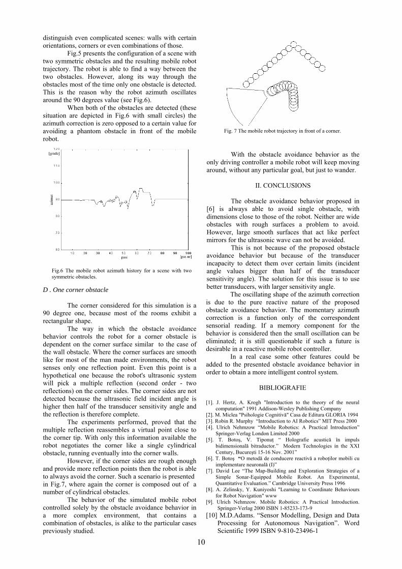
Buletinul Ştiinţific al Universităţii Politehnica din Timişoara
Seria ELECTRONICĂ şi TELECOMUNICAŢII TRANSACTIONS on ELECTRONICS and COMMUNICATIONS
Tom 48(62) Fascicola 2 2003
Algorithm for Generating Signals Using Table Look-up Method
Gabriel Vasiu1 Liviu Toma1
1 Facultatea de Electronică şi Telecomunicaţii Departamentul Măsurări şi Electronică Optică Bd V Pacircrvan Timişoara 300223 e-mail gvasiuetcuttro ltomaetcuttro
Abstract ndash The paper deals with the generation of signals with a TMS320C5402 DSK board using table look-up method The decimation and the interpolation of the samples in the look-up table are used to generate signals with continuously programmable frequency and amplitude The corresponding algorithm and C language program are presented in the paper Index Terms - Generating signals table look-up conti-nuously programmable frequency TMS320C5402 DSK board Code Composer Studio
I INTRODUCTION
The algorithm presented in this paper implements the table look-up method [1] for generating signals with continuously programmable frequency and amplitude
The algorithm is implemented by a C language program designed for a TMS320C5402 DSK board This board includes a TMS320C5402 digital signal processor two TLC320AD50C analog interface cir-cuits (AIC) memory circuits interface circuits (for parallel serial and JTAG ports) expansion memory interface peripheral interface etc The TLC320AD50C AIC provides 16-bit resolution signal conversion from digital-to-analog and from analog-to-digital using oversampling sigma-delta converters [2] The Code Composer Studio (CCS) development environment is used to build and debug programs that run on the DSK board [3]
II THE ALGORITHM
We consider a table in DSK memory that contains
the samples corresponding to one period of the generated signal For signal generation these samples are sent to the digital-to-analog conversion channel of the AIC The transmitted samples are selected from the table through decimation or interpolation (repetition) depending on the required frequency of the generated signal The amplitude of the generated signal depends on the sample values in the table and can be modified by multiplication with a constant
The frequency fg of the generated signal is related to the AICrsquos sampling frequency fs and to the number
of samples n from which a period of the signal is synthesized according to
n
ff s
g = (1)
Therefore to generate a signal of frequency fg
based on a table with N samples xi i=0 1 N-1 we define the displacement δ (difference between the indexes of two samples from the table successively sent to AIC) with
s
g
f
Nf
n
N==δ (2)
Particularly for δ =1 all N samples in the table are
successively and periodically sent to AIC for δ =2 every other sample is sent (the samples with even indexes) and for δ =12 all the samples are sent and every sample is repeated twice
Generally for δ gt1 the samples are selected from the table through decimation and for δ lt1 through interpolation As a rule the indexes of the samples that are successively transmitted from the table are
[ ]50+= δji modulo N j = 0 1 hellip (3)
where we have denoted by [x] the largest integer smaller than x
Using (2) in (3) yields
⎥⎥⎦
⎤
⎢⎢⎣
⎡+= 50
s
g
fNf
ji modulo N j = 0 1 hellip (4)
The TLC320AD50C AIC communicates with the
digital signal processor through a serial interface The digital-to-analog channel of the AIC includes an interpolation filter a 16-bit tworsquos complement delta-sigma DAC a low-pass output filter and a program-mable gain output amplifier The transition frequency
11
of the low-pass filter is about fs2 The output amplifier gain is established through programming and the possible values are 1 12 14 and 0
The output signal of the digital-to-analog con-version channel of the AIC is amplified with a LM386 operational amplifier If the amplifier gain is programmed to 1 a digital input signal with values in the range of minus215 divide 215 minus 1 (samples are represented on 16-bit tworsquos complement) will produce an output voltage in the range minusUemax divide Uemax Uemax = 15V
When generating a signal from the samples stored in a table the amplitude of the generated signal can be modified by multiplying the samples with a constant k The value of this constant depends on the desired output amplitude which is expressed by the maximum absolute value Ugmax which should be less than 15 V To determine this constant the maximum absolute value of the signal described by the samples xi in the table must be calculated as
ixM max= i = 0 1 hellip N-1 (5)
The constant k is
maxmax
152g
eU
MUk = (6)
The sampling frequency of the TLC320AD50C
AIC [1] is
d
mff MCLK
s 92= (7)
where m is a multiplication parameter that can be 1 or 4 d is a division parameter that can take the values 1 2 3 8 and fMCLK is the clock frequency of the AIC The two parameters can be set through programming
In TMS320C5402 DSK board the value for fMCLK is 8192 kHz (213 kHz) so that the possible values for fs are
( )d
mHzf s
34 102 sdot= (8)
The sampling frequency is established by pro-
gramming the parameters m and d and can take discrete values in the 2 divide 64 kHz range
In order to accomplish all necessary operations (decimation or interpolation and multiplication with constant k) for generating the signal in real time two memory buffers are used While the samples are calculated and written to one of the buffers the samples from the other buffer previously calculated are sent to the AIC Then the buffers exchange roles For an accurate operation of this technique the time required to calculate and write the samples in one of the buffers must be smaller than the time necessary to send the samples from the other buffer
III THE SIGNAL GENERATION PROGRAM
A C program for signal generation that implements the algorithm in the previous paragraph is presented This program uses functions from the files boardc and codecc [2] which reside in the programming library of the TMS320C5402 DSK board
The file boardc contains C functions for controlling system operation Therefore for TMS320C5402 DSK board initialization the function brd_init() is used The parameter of this function is the operating frequency of the digital signal processor that can be a multiple of 10 with the lowest being 20 MHz and the highest being 100 MHz
The file codecc contains C functions for controlling the operation of the two AICs of the TMS320C5402 DSK board The functions defined in the codecc module that will be used in the signal generation program are presented in the following
The codec_open() function defines an identifier for the used AIC and establishes its connection with the serial port of the digital signal processor
The codec_sample_rate() function establishes the sampling frequency of the specified AIC through the first parameter of the function at the value prescribed by the second parameter value obtained with (7)
The codec_cont_play() triggers the transmission of the samples to the AIC The samples of each buffer are sent successively with the sampling rate and alternatively from the two buffers This function is defined through the following parameters
- the identifier of the AIC - synchronization mode for sending the samples to
the AIC (this parameter is MODE_INT for sample sending triggered by an interrupt request generated by the AIC or MODE_DMA for sample sending through the direct memory access technique)
- the identifiers of the two buffers - the number of samples for each buffer - a pointer to a function that will be called at the
end of the sample sending from a buffer (the function is defined by the user and can be used for updating the sample values in the corresponding buffer)
- the address of a pointer to a variable that becomes zero at the end of the sample sending from a buffer
Include header files include ltstdiohgt include boardh include codech include semnaleh Defines define fs 16000 define n1 100 Globals int x[2][n1] i=0t=1j=1M float deltair=0fg=250ue_max=15ug_max=10k fg[Hz] ug_max[V] const int tm
12
char t_s=t s - sinusoidal t - triangular l - ramp d - square
Calculate the maximum absolute value of the signal stored in the table
int max(void) int zmx=0 for(z=0zltNz++) mx=(mxltabs((tm+z2))abs((tm+z2))mx) return mx Main void main(void) Locals HANDLE conv=0 int stareq=0tmp Initialize DSK board for use if (brd_init(100)) printf(Eroare brd_initn) Connect AIC to respective serial port if ((conv=codec_open(HANDSET_CODEC))= =0) printf(Eroare codec_open()n) Sets the AIC sample rate codec_sample_rate(convSR_16000) Calculate displacement delta=(fgfs)N Selects signal to be generated switch (t_s) case s tm=ampsine_table[0]break case t tm=amptr_table[0]break case l tm=amplv_table[0]break case d tm=ampdr_table[0] Calculate the amplitude constant M=max() k=((float)32768(Mue_max))ug_max Continuously send data to the AIC codec_cont_play(convMODE_INTx[0]x[1]n10 ampstare) Loop forever while(1) Fill current buffer for(q=0qltn1q++)
Calculate the amplitude of the current sample tmp=(int)((k((tm+i(sizeof(int)))))+05) Write in the current buffer x[t][q]=tmp Calculate the index of the samples in the table ir=ir+delta-((int)(ir+delta+05))N)N i=((int)(ir+05)) Setup for the alternate buffer t^=1 Wait for buffer to be done while(stare= =1) Set the state variable to 1 stare=1
A synthesized sinusoidal signal graph provided by the CCS environment is presented in figure 1
Fig 1 A synthesized sinusoidal signal graph
IV CONCLUSION
An algorithm and a corresponding C program
which use the table look-up method for generating signals with continuously programmable frequency and amplitude are implemented on TMS320C5402 DSK board
REFERENCES [1] Y C Jenq ldquoDigital spectra of nonuniformly sampled signals-Digital look-up tunable sinusoidal oscillatorsrdquo IEEE Trans Instrum Meas vol 37 Sept 1988 [2] Texas Instruments ldquoTLC320AD50CI TLC320AD52C Sigma-Delta Analog Interface Circuits With Master-Slave Functionrdquo Data Manual SLAS131E 2000 [2] Texas Instruments ldquoCode Composer Studio for the C5000 DSP Platform C5402 DSK Development Toolsrdquo CD-ROM 1999
13
Buletinul Ştiinţific al Universităţii Politehnica din Timişoara
Seria ELECTRONICĂ şi TELECOMUNICAŢII TRANSACTIONS on ELECTRONICS and COMMUNICATIONS
Tom 48(62) Fascicola 2 2003
New Proof of the Sampling Theorem for Bandpass Signals
Robert Pazsitka1 Liviu Toma1 Dan Stoiciu1 and Aldo De Sabata1
1 Facultatea de Electronică şi Telecomunicaţii Departamentul Măsurări şi Electronică Optică Bd V Pacircrvan Timişoara 300223 e-mail robietcuttro ltomaetcuttro dstoiciuetcuttro adesabatetcuttro
Abstract ndash In order to avoid aliasing when sampling a signal at a uniform rate it is necessary that all spectral components of the signal have different sample values This condition is used in order to derive the classical sampling theorem for bandpass signals The relation-ships for permissible and minimum sampling rates are derived Keywords Bandpass signals sampling theorem sampling rate aliasing
I INTRODUCTION
Sampling a signal at a uniform rate may produce aliasing In this case it is impossible to recover the original analog signal from the sampled signal To avoid aliasing the spectral representation of the analog signal must not contain sinusoidal components of different frequencies that have the same sample values [1] In order to derive the corresponding condition we use the following two identities
( ) ⎟⎟⎠
⎞⎜⎜⎝
⎛++=⎟⎟
⎠
⎞⎜⎜⎝
⎛+ ϕπϕπ
ee
e fnfkf
fnf 12sin2sin (1)
( ) ⎟⎟⎠
⎞⎜⎜⎝
⎛+minusminus=⎟⎟
⎠
⎞⎜⎜⎝
⎛+ πϕπϕπ
ee
e fnffk
fnf 22sin2sin
(2) where fe is the sampling frequency of the signal sin(2πft+ϕ) and constants k1 k2 are any integers From identities (1) and (2) we obtain the frequencies of the components with the same sample values as the component of frequency f (3) ek fkff 11
+=
(4) ffkf ek minus= 22
To avoid aliasing the sampled signal must contain a single frequency component out of those in (3) and (4) which is obtained for k1=0
II DERIVATION OF THE SAMPLING THEOREM FOR BANDPASS SIGNALS
Consider a bandpass signal s(t) whose spectral
components in the frequency domain satisfy Mm fff lele (5)
where fm and fM are the minimum and maximum frequency in the spectrum respectively The signal bandwidth fB is defined by
mMB fff minus= (6) The frequencies fk1 in (3) and fk2 in (4) correspond to alias components when
Mem ffkff le+le 1 (7)
Mem fffkf leminusle 2 (8)
In order to avoid aliasing a single value should be possible for k1 in (7) namely k1=0 and no solution should be possible for k2 in (8) The inequalities (7) and (8) can be rewritten as
e
M
e
m
fffk
fff minus
leleminus
1 (9)
e
M
e
m
fff
kf
ff +lele
+2 (10)
Since f can take any value between fm and fM the widest allowable ranges for k1 and k2 are
e
mM
e
Mm
fffk
fff minus
leleminus
1 (11)
e
M
e
m
ffk
ff 22
2 lele (12)
14
The inequality (11) holds only for k1=0 iff
11 1 ltminus
leleminus
ltminuse
mM
e
Mm
fff
kf
ff (13)
It follows that
(14) Be ff gt Inequality (12) has no solution for k2 iff
Kff
ffK
e
M
e
m ltltltminus221 (15)
for any integer K larger than unity For satisfying (15) it is necessary that
122ltminus
e
m
e
M
ff
ff
that is
Be ff 2gt (16)
Condition (16) is more restrictive than (14) If no aliasing occurs then the sampling frequency fe satisfies (16)
III RANGES OF SAMPLING RATES
In order to avoid aliasing it is necessary and sufficient for fe to satisfy (15) which can be rewritten in the form
1
22minus
ltltK
ffKf m
eM (17)
(for K=1 the last member should be considered equal to infinity) Inequality (17) admits solutions for fe iff
1
22minus
ltK
fKf mM
which implies
⎥⎦
⎤⎢⎣
⎡lele
B
M
ffK1 (18)
(we have denoted by [x] the largest integer smaller than x) By combining (17) and (18) we get the possible ranges for fe one for every value of K in (18) The
number of ranges is ⎥⎦
⎤⎢⎣
⎡
B
M
ff The range of the smallest
sampling frequencies is
⎟⎟⎟⎟⎟
⎠
⎞
⎜⎜⎜⎜⎜
⎝
⎛
minus⎥⎦
⎤⎢⎣
⎡⎥⎦
⎤⎢⎣
⎡=
1
2
2
B
M
m
B
M
M
ff
f
fff
R (19)
If 1le⎥⎦
⎤⎢⎣
⎡
B
M
ff
then it is not possible to apply a
uniform bandpass sampling procedure In this case (19) reduces to the sampling condition for lowpass signals
IV CONCLUSION In this note a compact and transparent derivation of the sampling theorem for bandpass signals based on the condition that the spectral representation of the analog signal must not contain sinusoidal components of different frequencies with the same sample values has been presented Results known from literature [2] [3] have been obtained in an alternative way
REFERENCES [1] S D Stearns Digital Signal Analysis Hayden Book Company Inc New Jersey 1975 [2] R B Vaughan N L Scott and D R White ldquoThe Theory of Bandpass Samplingrdquo IEEE Transactions on Signal Processing vol 39 pp1973-1984 September 1991 [3] I Naforniţă A Cacircmpeanu A Isar Semnale circuite şi sisteme partea I Universitatea ldquoPolitehnicardquo Timişoara 1995
15
Buletinul Ştiinţific al Universităţii Politehnica din Timişoara
Seria ELECTRONICĂ şi TELECOMUNICAŢII TRANSACTIONS on ELECTRONICS and COMMUNICATIONS
Tom 48(62) Fascicola 2 2003
Sampling Amplitude Modulated Signals
Robert Pazsitka1
Abstract ndash The paper presents the sampling of periodic bandpass signals obtained through amplitude modulation of a sinusoidal carrier with a low-pass periodic signal The relationships for the sampling frequency and the number of samples required for calculating the Fourier coefficients of the modulating signal (or modulating signals in the case of quadrature amplitude modulation) are derived The same relationships are given for calculating the Fourier coefficients of the modulated signal Keywords bandpass signals amplitude modulation quadrature amplitude modulation sampling Fourier coefficients
I INTRODUCTION
An amplitude modulated signal with sinusoidal carrier may be represented as [1]
ttptx 0cos)()( ω= (1) where πω 200 =f is the carrier frequency and is the low-pass modulating signal with the maximum frequency noted The modulated signal is a bandpass signal [1] within the range
)(tp
maxf
max0max0 ffff +divideminus Sampling of bandpass signals and the necessary conditions imposed to the sampling frequency to avoid aliasing are treated in many papers [1] [5] [9] A theorem referring to real bandpass signals is presented in [5] and [6] The spectral components of the bandpass signal
are non-zero only in the frequency range that satisfies
)(txsi fff ltlt where and are the
minimum and maximum frequency in the spectrum respectively The bandwidth is The value of the bandwidth must be less than else the sampling frequency must be greater than
if sf
is ffB minus=
if
sf2 The sampling theorem of bandpass real signals shows that the reconstruction of the signal from its samples is possible if the sampling frequency satisfies the equation [6]
1
22minus
lelen
ff
nf i
es where
Bf
n slele2 (2)
The number from (2) is an integer If n Bf s is also an integer the smallest sampling frequency is
Bfe 2= This paper deals with the particular case of bandpass periodic signals obtained through amplitude modulation of a sinusoidal (periodic) carrier with a low-pass periodic signal containing a sum of sinusoids case not found in literature
II SAMPLING OF AMPLITUDE-MODULATED SIGNALS WITH PERIODIC MODULATING
SIGNAL For calculating the period of the bandpass periodic signal using the periods of the carrier and low-pass periodic signals we make the following statement the product of two periodic signals with frequencies that can be written as ratio of integer numbers is a periodic signal Let us consider two periodic signals with the fundamental frequencies and (the periods 0f 1f
00 1 fT = 11 1 fT = ) If these frequencies are written in the form
0
00 b
af = and
1
11 b
af = (3)
then their ratio is
Qmm
bb
aa
ff
isin=sdot=1
0
0
1
1
0
1
0 (4)
where and 0a 0b 1a 1b 100 bam sdot= 011 bam sdot= are integers Using (4) the above statement can be reformulated as follows the product of two periodic signals with the periods and that can be written 0T 1T
____________________ 1 Facultatea de Electronică şi Telecomunicaţii Departamentul Măsurări şi Electronică Optică Bd V Pacircrvan Timişoara 300223 e-mail robietcuttro
16
as ratio of integer numbers is a periodic signal with the period T where
(5) 1100 TmTmT == where and are integers 0m 1m The integers and must have no common factor for
0m 1mT to be the principal period of the bandpass
periodic signal Else the period calculated with (5) will be a multiple of the principal period We consider that the bandpass periodic signal noted is obtained by amplitude modulation of a sinusoidal carrier with a low-pass periodic signal noted see (1) We note with the period of
with the period of the carrier
)(tx
)(tp 1T)(tp 0T t0cosω and
with the period of the amplitude modulation signal The order of the maximum harmonic in the
spectrum of is noted
xT)(tx
)(tp K The numbers and are chosen so that the period calculated with (5) be the principal period of the signal If is a multiple of then
and else
0m 1m
xT)(tx 0f 1f
11 =m 1ff x = 11 mff x = where 11 gtm For if and we can write sf
(6) ⎩⎨⎧
+==minus==
102
101
KfffMfKfffMf
s
i
From (5) and (6) we can calculate the harmonics
and corresponding to the minimum and maximum frequencies in the spectrum
1M 2M
(7) ⎩⎨⎧
+=minus=
102
101
KmmMKmmM
The bandpass periodic signal has a discrete spectrum in the range
)(tx
xx fMffM 21 lele (8)
The bandwidth of the signal will be
(9) ( ) 11010 2KfKffKffB =minusminus+= The minimum sampling frequency required will be 142 KfBfe =gt The sampling of the amplitude modulated signal
ttptx 0cos)()( ω= can be made so that the samples taken from are samples from the low-pass signal
namely )(tx
)(tp
)()( ee iTpiTx plusmn= (10)
where ee fT 1= From (10) and (1) it follows that 1cos 0 plusmn=eiTω The samples required for
calculating the Fourier coefficients must be taken from one period of or from a multiple of
(uniform sampling) Therefore we can write
N
1T )(tp m
1T
1mTNTe = (11) where is an integer Two cases are possible m Case I πω 20 sTe = ( 1cos 0 =eiTω )
ππ 212 1
11
0 sN
mTTm
m= rArr
smm
mN 1
1
0= (12)
Case II πω sTe =0 ( 1cos 0 plusmn=eiTω )
ππ sN
mTTm
m=1
11
0 12 rArr sm
mmN 12
1
0= (13)
where s is an integer and is the number of samples taken from periods of According to Shannonrsquos theorem should be at least
N1mT )(txN 12 +K
so that and m s have to be chosen accordingly The sampling frequency from (11) will have the value
mNffe 1= The corresponding Fourier coefficients of will be calculated with
)(tp
summinus
=
minus=1
0)(1)(
N
i
iTjkep
eeiTxN
kc ω (14)
for case I ( calculated with (12)) and N
summinus
=
minus minus=1
0)1()(1)(
N
i
iiTjkep
eeiTxN
kc ω (15)
for case II ( calculated with (13)) N III SAMPLING OF QUADRATURE AMPLITUDE
MODULATED SIGNALS In this case the modulated signal is represented as [1] [2]
)(tx
ttqttptx 00 sin)(cos)()( ωω minus= (16)
The low-pass signals and are considered periodic with the same period noted and the maximum harmonic component in the spectrum of these signals is noted with
)(tp )(tq
1T
K If the sampling frequency ee Tf 1= has such a value that the equation
17
2
)12(0πω minus= sTe (17)
be valid where s =1 2 then for i even (18) )()( ee iTpiTx plusmn=
for odd (18rsquo) )()( ee iTqiTx plusmn= i From (18) and (18rsquo) it follows that the sampling interval used for one low-pass signal ( or ) is Similarly with (11) in this case we can write
)(tp )(tq
eT2
and - integers (19) 12 mTTN e = N m In (19) is the number of samples used for calculating the Fourier coefficients of or The total number of samples used for the two low-pass signals is
N)(tp )(tq
N2 From (17) (19) and )(2 1100 Tmmπω = we have
12
2
1
0
minus=
smm
mN (20)
Integers m and s are chosen in order to obtain the smallest greater than or equal to N 12 +K The sampling period can be obtained from (19) The Fourier coefficients for and are calculated with
)(tp )(tq
summinus
=
minus minus=1
0
2 )1()2(1)(N
i
iiTjkep
eeiTxN
kc ω (21)
summinus
=
++minus minus+=1
0
)2( )1()2(1)(N
i
siTiTjkeeq
eeeTiTxN
kc ω (22)
where 12 fπω = and [ ]KKk minusisin The reconstruction of the low-pass signals is made with
(23) sum+
minus=
=K
Kk
tjkpr ekctp ω)()(
(24) sum+
minus=
=K
Kk
tjkqr ekctq ω)()(
The reconstruction of the bandpass (quadrature amplitude-modulated) signal is made with
ttqttptx rrr 00 sin)(cos)()( ωω minus= (25)
IV CALCULATION OF THE FOURIER COEFFICIENTS CORRESPONDING TO THE
BANDPASS PERIODIC SIGNAL For obtaining the Fourier coefficients of the bandpass periodic signal the fundamental frequency must be determined as in chapter II The harmonic components and corresponding to the minimum and maximum frequencies in the spectrum are calculated with (7) The number of samples obtained from one period
of must satisfy the following three conditions [9]
)(tx
xf
1M 2M
NxT )(tx
a) )1(2 12 +minusgt MMN
b) ⎥⎦
⎤⎢⎣
⎡=⎥⎦
⎤⎢⎣
⎡NM
NM 21 22
c) NM12
and NM 22
must be different from
integers where [ ] denotes integer part The sampling period will be NTT xe = As between the Fourier coefficients we have the relationship (the signal is considered real) where denotes complex conjugate we can calculate just one half of the coefficients for example those with positive indices They can be calculated with
kk cc minus= )(tx
summinus
=
minus=1
0)(1 N
i
kiTjek
eeiTxN
c ω (26)
where xfπω 2= and 21 MMk isin If the bandpass signal is an amplitude-modulated signal with sinusoidal carrier as defined by (1) without phase difference between the carrier and the low-pass (periodic) signal we can calculate just one quarter of the Fourier coefficients This is possible because the coefficients corresponding to the frequencies below are the complex conjugates of their respective symmetric coefficients for frequencies greater than To demonstrate this the terms
)(tx
0f
0fttkak 01 coscos ωω and ttkbk 01 cossin ωω
contained by the modulated signal ttptx 0cos)()( ω= can be written as
tka
tkattka
k
kk
)cos(2
)cos(2
coscos
10
1001
ωω
ωωωω
++
+minus= (27)
tkb
tkbttkb
k
kk
)sin(2
)sin(2
cossin
10
1001
ωω
ωωωω
++
+minusminus= (28)
18
This means it is enough to calculate the coefficients with where kc 20 MMk isin ( ) 2210 MMM +=
corresponding to the remaining coefficients being obtained by complex conjugation This property is not valid for quadrature amplitude modulation
0f
Because all of the cases presented above refer to periodic signals the sampling frequency can be lowered by taking the samples from several periods An additional condition must be satisfied [10] namely the number of samples and the number of periods NM should have no common factor
V CONCLUSIONS Signals obtained through amplitude modulation can be sampled such as to obtain directly the samples of the low-pass signal Several relationships are established for calculating (the required number of samples) and the sampling frequency so as to obtain the samples of the low-pass signal if the input signal is a bandpass periodic signal obtained through amplitude modulation If the number results from (12) then the Fourier coefficients are easily calculated with the known formula (14) If the number results from (13) then the Fourier coefficients are calculated with the modified formula (15) The same calculations (number of samples sampling frequency Fourier coefficients corresponding to the low-pass signals) are for the bandpass signal obtained by quadrature amplitude modulation
N
N
N
Chapter 4 presents the condition that must be satisfied by the number of samples obtained from a bandpass signal in order to calculate the Fourier coefficients of this signal If the signal is real (the samples are real number) then and then just half of the coefficients need to be calculated If the bandpass signal is obtained through amplitude-modulation then just one quarter of the coefficients need to be calculated due to the fact that the spectrum is symmetrical with respect to
N
kk cc minus=
0f
REFERENCES [1] Jerry D Gibson The Communications Handbook CRC Press Inc 1997 [2] JL Brown JR First-Order Sampling of Bandpass Signals ndash A New Approach IEEE Trans on Inf Theory Vol IT-26 No 5 Sept 1980 [3] JL Brown JR On Quadrature Sampling of Bandpass Signals IEEE Trans on Aerospace and Electronic Systems Vol AES-15 No 3 May 1979 [4] Marks II J Robert Introduction to Shannon Sampling and Interpolation Theory Springer-Verlag New York Inc 1991 [5] Oran E Brigham The Fast Fourier Transform And Its Application Prentice Hall Inc 1988 [6] Larry Marple Exploding the Nyquist Barrier Misconception IEEE Signal Processing Magazine Vol 13 No5 Sept 1996 [7] Liu J Zhon X Peng Y Spectral Arrangement and other Topics in First-Order Bandpass Sampling Theory IEEE Trans on Sig Proc Vol 49 No 6 June 2001 [8] Vaughan BR Scott LN White RD The Theory of Bandpass Sampling IEEE Trans on Sig Proc Vol 39 No 9 Sept 1991 [9] Robert Pazsitka Sampling of Bandpass Periodical Signals Proceedings of the Symposium on Electronics and Telecommunications Etc 2002 Timisoara Sept 19-20 2002 Vol 1 [10] Robert Pazsitka Eşantionarea semnalelor periodice lucrare de dizertaţie Facultatea de Electronică şi Telecomunicaţii Timişoara iulie 1997
19
Buletinul Ştiinţific al Universităţii Politehnica din Timişoara
Seria ELECTRONICĂ şi TELECOMUNICAŢII TRANSACTIONS on ELECTRONICS and COMMUNICATIONS
Tom 48(62) Fascicola 2 2003
The Specific Absorption Rate of the Electromagnetic Radiation for Biological Structures in the Case of Mobile
Telephony
Adrian Vacircrtosu1
1 Facultatea de Electronică şi Telecomunicaţii Departamentul Măsurări şi Electronică Optică
ABSTRACT Cellular telephony uses a frequency domain ranging between 800 MHz and 2000 MHz with emission powers of 06W to 2W
The frequencies used have wavelengths that can be compared to the physical dimensions of the skull and the power emitted by portable phones is quite high around 06W Because of the proximity of the head (just a few centimeters away) with all the reflections from the surface of the skull and the attenuations that intervene the field intensities that manage to get inside the skull can induce in the cerebral mass currents of the same size with the intensities of normal biological currents
I INTRODUCTION The 5191999 recommendation of the Council
of Europe from the 12th of July 1999 concerning the limitation of public exposure to electromagnetic fields (from 0 Hz to 300 GHz) establishes the limits in values of physical units that characterize electromagnetic radiation at different frequencies The respective norms also called basic restrictions and reference levels establish safety coefficients in the case of electric magnetic and electromagnetic field exposure variable in time based directly on the obvious effects on health and biological considerations Depending on the field frequency the physical units used in order to specify the restrictions are the magnetic induction (B) the density of current (J) the specific absorption rate (SAR) and the power density (S) The SAR unit is used within the 100 kHz ndash 10 GHz frequency range to define the basic restrictions concerning the electromagnetic fields in order to prevent a generalized thermal stress of the body and an excessive localized heating of tissues
According to the 1999519CE 12th of July 1999 Recommendation the reference levels of
radiofrequency fields used in the GSM system are (table 1)
Table 1
Frequency (MHz)
Electric field
E (Vm)
Magnetic field H (Am)
Density of Power (Wmsup2)
900 41 011 45 1800 58 016 9
It is worth noticing that in the case of simultaneous exposure to different frequency fields there is a possibility that the effects of the exposure are cumulative As a convention each effect will be studied using separate calculations and based on the hypotheses separate evaluations of the effects of thermal and electric strain of the organism will be covered
Knowing the electric properties of biological environments is essential to the study of the interaction phenomena between these and the electromagnetic field The electrical properties involve permittivity and electric conduction
The magnetic properties (with some exceptions that do not concern the present paper) are not defined for the biological matter the relative permeability of biological entities is considered to equal a unit (micror= 1) and the losses obtained through the magnetic effect are thought to be negligible
The electric properties that intervene in the study of the biological effects of electromagnetic fields are the electric permittivity ε and the conduction σ defined over the unit of volume of matter Permittivity characterizes the interaction between the environment and the electromagnetic wave that is propagated through it The permittivity of free space is a constant εo and the permitivity of any other environment is a complex
20
measurement ( ) in which ε is an indicator of the property of the environment to store energy while ε indicates the property of the environment to dissipate the energy carried by the electromagnetic field
c jεεε minus=
Relative permittivity measures the net effect of the electric dipoles alignment that characterizes the intimate structure of the matter that is under the influence of an electric field applied from the outside
The energy dissipated per second per unit of volume of homogenous material by an electromagnetic wave incidence is proportionate to the square of the amplitude of the electric field component and is calculated with the help of this formula [1]
P = πf εoεE2 = σ E22 (1)
where σ is the conduction of the environment in which the dissipation of energy takes place The conduction is itself dependent on the frequency
All these parameters (σ ε or tan δ ) characterize the possibility of the environment to absorb the energy from the electromagnetic field
Calculating the values of the dielectric parameters (permittivity conduction wavelength intrinsic impedance penetration depth etc) that characterize the human tissues at the frequencies of 800 MHz and 900 MHz used by the Romanian mobile telephony was done by using a program in EXCEL based on formulas [2] [3] that allows for finding these measurements up to the frequency of 300 GHz
Formulas used in calculation of dielectric properties
complex permittivity
c jεεε minus= (2)
rel complex permittivity
0
εεεεε c
rrcr j =minus= (3)
0
ωεσε =r
ωσε =
permittivity of free space
Fm1085418781768 120
minustimes=ε permeability of free space
Hm104 70
minustimesπ=micro impedance of free space
Ω= 376730313Z 0 wave velocity in free space
ms 10 2997924581c 8
00
times=εmicro
=
angular frequency
f2 π=ω loss tangent of material
r
r
)(tanεε
=ωεσ
=ϑ (4)
propagation constant of material y = α+j β
)j(c
)j(j r
r
2
r2 εminusε⎟
⎠⎞
⎜⎝⎛ ω
microminus=ωε+σωmicro=γ (5)
attenuation constant of material
( ) ⎟⎟⎠
⎞⎜⎜⎝
⎛minusεε+
εmicro⎟⎠⎞
⎜⎝⎛ ω
=α 112c
2r
r
rr (6)
skin depth material
α=δ
1 (7)
phase constant of material
( ) ⎟⎟⎠
⎞⎜⎜⎝
⎛+εprimeε+
εmicro⎟⎠⎞
⎜⎝⎛ ω
=β 112c
2rr
rr (8)
wave velocity in material
βω
=u (9)
wavelength in material βπ
=λ2 (10)
intrinsic impedance of material
r
r
r0
c jZZ
εminusε
micro=
εmicro
= (11)
( ) 2502r
r
r
r0
1ZZ
⎥⎦⎤
⎢⎣⎡ εε+ε
micro= (12)
( ) ( )r
r
1tan21Zphase εε= minus (13) 00lephase(Z)le450
21
II RESULTS OF THE EXPERIMENT
The results of these calculations corresponding to the two bands are presented in the table 2 for f=800 MHz and in the table 3 for f=900 MHz
Table 2a
f=800 MHz micror = 1
TISSUE bone skin blood brain heart
εr 8688429 36212 5882646 464656 6067894
εr 0745467 1234021 2570435 1548868 2253825
σ (Sm) 0033178 0549214 1143998 0689339 1003087
tan(θ) 00858 0340777 0436952 0333337 0371434
α (1m) 2118257 1695389 2747556 1879632 2386113
β (1m) 4946731 1023108 1315008 1158271 1327692u (ms) 102E+08 49130166 38224479 43397013 37859280
λ (m) 0127017 0061413 0047781 0054246 0047324
δ (m) 0472086 0058984 0036396 0053202 0041909
|Ζ| (Ω) 1276914 6175043 4805721 5454375 4758779
Ζ (deg) 2451985 9408961 1180151 9217559 1018837
Table 2b
TISSUE muscle kidney liver lung spleen
εr 5411328 4761208 462569 3323576 5264076
εr 1430979 1890983 1815213 157899 2142521
σ (Sm) 0636871 0841601 0807879 0702745 0953551
tan(θ) 0264441 0397165 039242 0475088 0407008
α (1m) 1616963 2255025 219707 2237002 2427742
β (1m) 1243946 1178704 116132 992159 1240483u (ms) 40408097 42644715 43283050 50662729 40520887
λ (m) 005051 0053306 0054104 0063328 0050651
δ (m) 0061844 0044345 0045515 0044703 0041191
|Ζ| (Ω) 5078194 5360689 5440852 6370586 5093874
Ζ (deg) 7406157 1083061 1071302 1270591 1107336
Table 3a f= 900 MHz micror = 1
TISSUE bone skin blood brain heart
εrrsquo 8634636 3599427 5874271 4636694 6051015
εrrdquo 0818382 1133951 2333097 1421199 2071992
σ (Sm) 0040976 0567761 1168164 0711584 1037431
tan(θ) 0094779 0315037 0397172 0306511 0342421
α (1m) 2623734 1761374 2817931 1946225 2477099
β (1m) 5548936 1145292 1472909 1299078 1488052
TISSUE bone skin blood brain heart
u (ms) 102E+08 49374911 38392510 43529846 38001813
λ (m) 0113232 0054861 0042658 0048366 0042224
δ (m) 0381136 0056774 0035487 0051382 004037
|Ζ| (Ω) 1280628 6205502 4826162 5470811 4776366
Ζ (deg) 2707131 8743167 108308 8520446 9451129
Table 3b
TISSUE muscle kidney liver lung spleen
εr 5406606 4756672 4615513 3306596 5255305
εr 1333614 1714191 1650214 1440076 1950378
σ (Sm) 0667731 0858282 082625 0721035 097654
tan(θ) 0246664 0360376 0357536 0435516 0371126
α (1m) 1697889 2308073 2256177 2310114 2496166
β (1m) 1397314 1321244 1301189 1108984 1390013u (ms) 40469540 42799564 43459223 50991404 40682126
λ (m) 0044966 0047555 0048288 0056657 0045202
δ (m) 0058897 0043326 0044323 0043288 0040061
|Ζ| (Ω) 508583 5379605 5462482 6410789 5113597
Ζ (deg) 6928098 9908974 9836909 1176695 1018059 Formulas used for εr and εrrsquo are [2]
2
2
22
1
13
r
f1000f1
ff1 ⎟⎟
⎠
⎞⎜⎜⎝
⎛sdot
+
ε+
⎟⎟⎠
⎞⎜⎜⎝
⎛+
ε+ε=ε (14)
⎥⎥⎦
⎤
⎢⎢⎣
⎡⎟⎟⎠
⎞⎜⎜⎝
⎛sdot
+sdot
ε+
⎥⎥⎦
⎤
⎢⎢⎣
⎡⎟⎟⎠
⎞⎜⎜⎝
⎛+
ε+
sdotsdotπεσ
=ε2
22
22
11
1
0
0r
f1000f1f1000
f
ff1f
f1000f2
(15) The values of the units used in calculating these dielectric parameters are given in the table 4 [2]
Table 4a
TISSUE bone skin blood brain Heart
ε3 49 33 43 75 43
σo (Sm) 31E-07 0231 0768 0313 063
f1 (MHz) 2360 137 378 433 906
ε1 222 343 136 122 494
f2 (GHz) 204 177 213 165 156
ε2 18 32 543 387 559
22
Table 4b
TISSUE muscle kidney liver lung spleen
ε3 43 43 43 43 43
σo (Sm) 0301 0551 0406 0325 044
f1 (MHz) 83 247 442 818 266
ε1 475 166 136 691 289
f2 (GHz) 152 245 216 151 198
ε2 499 432 416 283 481
The external field incident to the biological structure can be expressed in terms of power density (mWcm2) of amplitude of the electric field component (Vm) or of the magnetic field component (Am) None of these parameters is appropriate for expressing the effects induced by the penetration of the electromagnetic radiation inside the biological domain Considering this situation a specific parameter has to be defined It is called the ldquoSpecific Absorption Rate ndash SARrdquo and it is the variation in time of the elementary energy quantity (dw) absorbed by an element of volume (dv) having a density (ρ) and an elementary mass (dm) [1]
⎟⎟⎠
⎞⎜⎜⎝
⎛=⎟
⎠⎞
⎜⎝⎛=
dVdW
dtd
dmdW
dtdkgWSAR
ρ)(
The Specific Absorption Rate (SAR) is correlated to the penetration depth (δ)in the tissues If the penetration depth (δ) is the distance from the surface of the tissue for which the amplitude of the electric field component reduces with factor e = 271 than the specific absorption rate at this depth reduces to a value equal to 135 of its initial value
Sometimes it is useful to define the depth d (frequently used in hyperthermia cases) at which the power incident to the surface of the irradiated structure is reduced to half (3 dB attenuation) Between (δ) and (d) there is the relation
d = 0345 x δ In order to determine the value of the SAR
parameter the TEMS (Test Mobile System) system was used This system was offered by the ORANGE firm and the measurements were taken at the frequency of 900 MHz
The applications of TEMS for an operational network are
bull it simulates and verifies possible changes in the network
bull it evaluates the quality of the received signal bull it measures the space covered range bull it tests the system (checks new or already
present functions)
- it signals in real time aberrant values of any parameter (for example the large number of interrupted calls)
- it identifies areas with problems of signal coverage or with high levels of interference
bull it presents the data in graphs maps The equipment used for measuring (Fig 1)
contains - special software made by Erricsson-TEMS
(Test Mobile System) - laptop mobile phone special data cable that
insures the PC-mobile phone connection
Fig1 The equipment used for measuring
The TEMS mobile phone is an Erricsson
ordinary phone that uses the TEMS program No supplementary calibrations are necessary for using the TEMS software
This mobile phone has four different operation modes
1 No Service (when it is in an area with no signal coverage)
2 Limited services (only emergency calls) 3 Inactive 4 Dedicate (during a conversation)
The measurements were taken during a
conversation therefore in the dedicate mode Taking the measurements involves - initiating a call - choosing the unit to be measured in this
case the power of the transmitted signal (TxPwr)
- the display of the unit to be measured (Fig2) and information about the distance from the base station (TA ndash Time Advance) the base station code (BSIC ndash Base Station Identity Code) local code (LAC Local Area Code) the channel of the communication (TCH ndash Traffic Channel)
23
In order to calculate the value of SAR the
situation when the telephone is in dedicated mode t0 is used At t0 these units have the following values
TxPwr =18dBm=625mW
TA = 2 d = TAx 500m Therefore the distance (d) to the base station is
1 km BSIC = 23 LAC = 05500
Fig2 The value of the SAR unit for the measured power is determined according to [1]
⎥⎦
⎤⎢⎣
⎡sdot=
=sdot
=ρ
=ρ
σ=
ρε primeprimeωε
=⎥⎦
⎤⎢⎣
⎡
minus
kgW1012550
1000062502P2EE
kgWSAR
3
22r0
where 0ε = permittivity of free space ω = angular frequency ρ = the density of the biologic environment asymp1000 kgm3
E = the intensity of the electric field P = πf εoεE2 = σ E22
Fm10E85418781768 120
minustimes=ε
0
r ωε
σ=ε
It is observed that the specific rate of absorption SAE is under the maximum admitted level of 04 Wkg
The value of SAR can also be determined according to the dielectric parameters ε σ and the electric field generated by the mobile phone In this case the system of measurement contains
bull electric field probe (Wandel amp Goltermann) with the EMR 20 measuring device
bull software for processing the values measured by the probe
bull mobile phone with without the antenna The measurements were done considering the following three positions for the measurement probe
bull positioning the electric field probe in the
speaker area bull positioning the electric field probe in the
inferior keys area bull positioning the electric field probe next to the
inner antenna behind the telephone or next to the extended antenna in the case of telephones with exterior antennas
The results obtained are succinctly presented in the table5 The maximum values of the electric field registered in each area of measurement and expressed in Vm are also presented
Table 5 Telephone type
with internal antenna with external antenna
Area Speaker
Micro-phone back speake
r
antenn
a On 981 668 1126 - 986
Called 2351 755 178 3677 2132
Calling 2142 1966 3398 2994 2418
Speaking
2871 197 3843 3672 282
S T A T E
Off 245 687 1032 -
III CONCLUSIONS
The following observations can be drawn on the
basis of the date from the table bull the internal antenna has directivity by having a
weaker emission in the area of the userrsquos head bull the emission is larger in the superior area of the
internal antenna phone bull the emission is stronger in the states where the
telephone is in contact with the head of the user (when he calls and speaks) the antenna type does not matter
bull the telephone with an external antenna has a stronger emission at the level of the speaker than at the extremity of the antenna
bull the telephone with an external antenna does not have a weaker emission at the level of the speaker in comparison to the internal antenna telephone
24
The difference in values from the experimental data provided by our bibliography and from the theoretical models is due to the various uncertainty factors that are linked to the measurements in a close-range field and the digital character of the signal
bull the size of the detecting field unit that disturbs the measuring field
bull the link between the measuring probe and the emission antenna of the telephone
bull the measuring technique of the digital signal
It was observed that at low levels of power density some effects take place after a longer exposure time They are called ldquolow level power effectsrdquo or ldquoathermic effectsrdquo effects that also appear in the case of using mobile phones It is best to consider the following recommendations even if the SAR value is situated between the limits established by the European Commission
bull to reduce using mobile phones in conditions of low signal
bull to avoid wearing mobile phones close to the sensitive tissues
bull using car kits bull constantly informing the population of the
level of radiation around the base stations by operating frequent measurements that would be accessible to the public
The conclusion is that the general objective should be to reduce the degree of exposure of the population to radiofrequency fields
IV BIBLIOGRAPHY
[1] ZAMFIRESCU MIHAIL SAJIN GH RUSU IONSAJIN MARIA KOVACS EUGENIA ndash Efectele biologice ale radiaţiilor electromagnetice de radiofrecvenţă şi microunde Editura Medicală 2000 [2] GABRIEL C (1996) Compilation of the dielectric properties of body tissues at RF and microwave frequencies Brooks Air Force Base report no ALOE-TR-1996-0037 [3] HURT WD (1996) Radiofrequency radiation dosimetry workshop Brooks Air Force Base report no ALOE-SR-1996-0003 [4] SADIKU MNO (1994) Elements of Electromagnetics Saunders College Publishing New York [5] HOMBACH V Comparison of different human head models XXVth General Assembly of the International Union of Radio Science August 28 - Sept 5 1996 Lille France
25
Buletinul Ştiinţific al Universităţii Politehnica din Timişoara
Seria ELECTRONICĂ şi TELECOMUNICAŢII TRANSACTIONS on ELECTRONICS and COMMUNICATIONS
Tom 48(62) Fascicola 2 2003
The Cyclic Prefix Length Influence on OFDM-Transmission BER
Marius Oltean1 Miranda Naforniţă1
Abstract Orthogonal Frequency Division Multiplexing (OFDM) is one of the recent years equalization approaches used in order to combat the inter-symbol interference introduced by the frequency selectivity of the radio channels The circular extension of the data symbol commonly referred to as cyclic prefix is one of the key elements in an OFDM transmission scheme The influence of the cyclic prefix duration on the BER performance of an OFDM system with in-frame DBPSK modulation is evaluated by means of computer simulation in a multipath fading channel
I INTRODUCTION Mobile radio communication systems are increasingly required to offer a variety of services and qualities for mobile users Unfortunately the radio channel is far from an ideal transmission medium exhibiting both frequency selectivity and time variant character [1] In this context one of the most challenging issues in a radio communication system is to overcome the inter-symbol interference introduced by the multipath propagation of the signal between the transmitter and the receiverrsquos antennas The use of the adaptive equalization to the receiver could be the solution for avoiding this unwanted phenomenon but this complex equalization technique proves oftentimes unsuited for being used in real-time applications at data rates of tens of Mbps in an unfriendly dispersive radio channel environment because of its important computational complexity OFDM is an optimal version of multicarrier modulation techniques which mitigates the effect of the ISI phenomenon keeping a relatively reduced complexity of the equalization process Indeed intuitively one can assume that the frequency selectivity of the channel can be mitigated if instead of transmitting a single high rate serial data stream the transmission is performed simultaneously using several narrow-band subchannels (with a different carrier corresponding to each subchannel) on which the frequency response of the channel looks ldquoflatrdquo
Hence for a given overall data rate increasing the number of carriers reduces the data rate that each individual carrier must convey therefore lengthening the duration of the symbol that modulates each individual subcarrier [2] Slow data rate (and long symbol duration) on each subchannel merely means that the effects of ISI are severely reduced In addition a cyclic prefix is inserted in front of each OFDM symbol This circular extension that is discarded on the receiver side is obtained by copying a number of samples from the end of the OFDM symbol in front of it in order to prevent two consecutive frames to interfere each other as a result of the time dispersion caused by the multipath propagation This way the receiver can independently process each frame in order to estimate the transmitted information Furthermore the equalization process is facilitated by this operation of cyclic prefix insertion and extraction In this chapter we focus on the influence of the cyclic prefix duration on the BER performance of an OFDM system with in-frame DBPSK modulation The performance evaluation in Rice fading conditions is done by means of computer simulation
II THE BLOCK-DIAGRAM OF OFDM
TRANSMISSION SCHEME
In the figure 1 a classical OFDM transmission scheme using FFT (Fast Fourier Transform) is illustrated
The input data sequence is baseband modulated using a digital modulation scheme Various modulation schemes could generally be employed such as BPSK QPSK (also with their differential form) and QAM with several different signal constellations In our system DBPSK method is chosen in order to encode the binary information Data is encoded bdquoin-framerdquo (the baseband signal modulation is performed on the serial data that is inside of what we name a bdquoDFT framerdquo or equivalently an OFDM symbol) The data symbols 1 Univ ldquoPolitehnicardquo Timişoara Facultatea de Electronică şi TelecomunicaţiiDepartamentul Comunicaţii
26
Information symbols
Serial to parallel
converter
Coding amp baseband
modulation
IFFT modulator
Cyclic prefix insertion
Parallel to serial
converterX
ej2πfct
Channel
X
ej2πfct
Serial to parallel
converter
Cyclic prefix extraction
FFT demodulator
Decoding amp demodulation
Parallel to serial
converter
Estimated symbols
Xk k=0hellipN-1
[Xk] k=0hellipN-1
[xk] k=0hellipN-1
[xcpk] k=-LhellipN-1
[ycpk] k=-LhellipN-1
[yk] k=0hellipN-1
[Yk] k=0hellipN-1
Yk k=0hellipN-1
Fig1 The block diagram of an OFDM System
are parallelized in N different substreams Each substream will modulate a separate carrier through the IFFT modulation block which actually generates the OFDM symbol performing the multicarrier modulation A cyclic prefix is inserted in order to eliminate the inter-symbol and inter-block interference (IBI) [3] The data are back-serial converted forming an OFDM symbol that will modulate a high-frequency carrier before its transmission through the channel The radio channel is generally referred to as a linear time-variant system To the receiver the inverse operations are performed in order to estimate the transmitted symbols
III THE CYCLIC PREFIX AND THE EQUALIZATION PROCESS
Since OFDM transmits data in blocks (usually a block is referred to as an bdquoOFDM symbolrdquo) any type of a non-ideal transmission channel (such as a multipath channel in mobile communication systems or a classical dispersive channel as in wired transmissions) will bdquospreadrdquo the OFDM symbol causing the blocks of signal to interfere one another This type of interference is called Inter-Block Interference IBI could lead to inter-symbol interference since two adjacent blocks will overlap causing the distortion of the samples affected by overlapping
In order to combat this interference we could use a cyclic prefix (CP) at the beginning of each symbol If the cyclic prefix spans more than the multipath channel impulse response the interference caused by the time dispersion of the previous transmitted block is entirely absorbed by the prefix samples that are discarded to the receiver The cyclic prefix consists of the last L samples of the OFDM symbol that are copied in front of the data block [4] as we can see in the figure 2 Generally the radio channel exhibits both time variant and frequency selective characteristics If we shall consider however that the channel parameters remain unchanged during the transmission of an OFDM symbol the way that the transmission medium distorts each particular frame is similar to the distortion caused by an
electronic filter [1][5] Under this assumption we can consider the equivalent discrete response of the channel as a linear FIR filter of order L of which the equation is given below
sum=
minussdot=L
n
nznczC0
][)( (1)
The equivalent baseband signal at the channel output can be obtained by the operation of convolution as follows
][][][ ncnxcpnycp = (2)
Discarding the L CP samples from the received sequence the remaining (useful) signal can be expressed as
where ldquo⊛rdquo denotes the circular convolution operator [6] The noticeable thing about the equation 6 is that the circular convolution preserves the temporal support of the signal In our case N transmitted signal samples convolved with L+1 channel impulse response samples will conduce to a received symbol of length N that will be used in the demodulation process Since the circular convolution will not ldquospreadrdquo the signal the receiver can independently process each data block The interference from the
y[n]=x[n] ⊛c[n] (3)
OFDM Symbol
Copy
CP
Transmitted sequence= OFDM symbol+CP
t
Fig2 The cyclic prefix insertion
27
previous transmitted blocks is totally eliminated through this operation of CP insertionextraction Furthermore since x[n]=IDFTX[k] and taking into account the effect of the DFT demodulator the received symbols Y[k] can be expressed as
Y[k]=DFTIDF TX[k] ⊛c[n] k=01hellipN-1 (4)
Since the DFT of a circular convolution of two discrete time signals will conduce to a spectral multiplication
110][][][][][
minus=sdot==sdot=
NkkCkXncDFTkXIDFTDFTkY
(5)
where C[k] represents the sampled frequency response of the equivalent baseband discrete channel corresponding to the frequencies Ωk=k(2πN) The crucial consequence of the relation above is that each modulation symbol X[k] could be recovered to the receiver by a simple pointwise division operation commonly referred to as a ldquoone-tap frequency domain equalizerrdquo as can be seen from the relation (6)
110][][][ 1 minus=sdot= minusandNkkCkYkX (6)
Thus the CP theoretically eliminates both IBI (each block preserves its temporal support) and inter-carrier interference (ICI) (each serial symbol received on the k-th carrier will depend only on the corresponding k-th carrier transmitted symbol not being affected by the adjacent carriers) IV SIMULATION RESULTS AND DISCUSSIONS
1 SIMULATION PARAMETERS
The goal of the simulations was to emphasize the effect of the cyclic prefix duration on the BER performance of an OFDM system with inter-frame DBPSK modulation The radio channel was modeled as a three-ray Rice fading channel with one deterministic line-of-sight (LOS) path and two multipath delayed components The relative delays of the two components are τ1 and τ2 respectively However in most of these simulations it was considered τ1=0 and a normalized delay for τ2 denoted τ2N=τ2LCP LCP represents the cyclic prefix duration expressed as the number of serial samples that compose the cyclic prefix An important parameter for the Rice fading channel is K=PLOSPD which stands for the ratio between the signal power carried by the LOS path (PLOS) and the total power of the two multipath components (PS=P1+P2) Equal power for the two multipath components was considered during the simulations A white gaussian noise is added to the signal at the output of the Rice
fading channel The time interval between the moments in which the first and the last significant component of the multipath signal arrives to the receiver is referred to as maximum excess delay (TM) and it is expressed in number of serial samples (remember that N signal samples generated by the IFFT modulator will compose an OFDM frame) Another parameter of the simulation is the number of subcarriers N that equals the number of serial samples composing an OFDM symbol The time variant character of the radio channel is quantified by the maximum Doppler shift parameter fD The value of this parameter is also expressed in a normalized manner as fDTS TS denoting the OFDM symbol duration A robust differential modulation scheme such as DBPSK was chosen for encoding the binary information No channel estimation techniques are employed and consequently no further equalization is done to the receiver
2 RESULTS AND DISCUSSIONS For the first simulations the relative delay of the second multipath was normalized by the serial symbol duration As can be seen from the figure 3 increasing the cyclic prefix duration improves the BER performance for the OFDM system
Theoretically if the cyclic prefix duration spans more than the maximum delay spread of the channel the errors can be completely eliminated This assumes however a perfect knowledge of the channel impulse response (or equivalently of the channel transfer function) which is a mandatory condition for implementing the equation 6 Since in our implementation no channel estimation techniques are employed the exact form of the channel impulse response doesnrsquot constitute information that can be exploited in the data estimation process The correct
Fig 3 The influence of the cyclic prefix duration on BER performance for DBPSK-OFDM system
Rice fading channel K=3dB SNR=30dB N=64 fDTS=0001
28
detection is entirely based on the robustness and simplicity of the digital modulation scheme that is involved namely DBPSK This explains why the BER is not completely eliminated for a cyclic prefix of theoretically sufficient duration (longer than TM) A noticeable thing resulting from the figure 3 is that while identical for cyclic prefix lengths which cover the channel impulse response the performance degrades for the cases where the cyclic prefix duration becomes insufficient Thus if a cyclic prefix of length LCP=4 is used the transmission offers the best performance between all the considered situations but only starting with a value of the normalized delay that overtakes the length of the circular extension for all the other cases Next we studied the BER performance against the normalized delay of the second multipath which is obtained this time as explained in the previous subsection It can be observed from the figure 4 that increasing the OFDM symbol length improves the performance of the system which confirms [6] In the same time it is proven that the BER is sensitive to the multipath delay spread of the channel
normalized by the cyclic prefix duration Thus as observed in the figure 4a) a two times longer OFDM symbol is needed in order to obtain the same performance when the normalized delay of the second multipath is two times higher (note that for the same value of τ2N on the abscissa τ2 doubles its value when LCP=2) The observation is confirmed by the figure 4b) where the BER curve in the case N=16 LCP=1 is almost identical with the curve plotted for a frame of length N=64 with a cyclic prefix LCP=4 The conclusion that can be drawn from these observations is that at identical ratios between the channel impulse response and the cyclic prefix duration the in-frame OFDM system performance remains sensitive to the effective value of the multipath (or maximum) delay spread parameter (τ2 in our case)
3 CONCLUSIONS
The cyclic prefix duration influences the performances of an OFDM system even if the explicit form of the channel impulse response is unknown and consequently cannot be used in the equalization process The transmission is sensitive to the parameter obtained as the multipath delay of the channel normalized by the cyclic prefix duration The BER performance is in all cases improved by increasing the OFDM symbol length
REFERENCES
[1] B Sklar Rayleigh Fading Channels in Mobile Digital Communication Systems- Part I Characterization IEEE Commun Mag July 1997 [2] Dusan MaticOFDM as a possible modulation technique for multimedia applications in the range of mm waves 10-30-38 TUD-TVS available on-line wwwubicomtudelftnlMMCDocsintroOFDMpdf [3]Werner Henkel Georg Tauboumlck Per Oumllding The cyclic prefix of OFDMDMT ndash an analysis 2002 International Zuumlrich Seminar on Broadband Communications February 19-21 Zuumlrich Switzerland [4]Lu J Tjhung TT Adachi F BER performance of OFDM system in frequency-selective Rician fading with diversity reception available online httpwwwcwcnusedusg~cwcpubzfilesict97_2pdf [5] B Sklar Rayleigh Fading Channels in Mobile Digital Communication Systems- Part II Mitigation IEEE Commun Mag July 1997 [6 ]Chini A Analysis and Simulation of Multicarrier Modulation in Frequency Selective Fading Channels Ph D Thesis 1994 Chapter 3
a)
b)
Fig 4 (ab) The influence of the normalized delay of the second multipath on BER performance for DBPSK-OFDM
system Rice fading channel K=3dB SNR=40dB fDTS=0001
29
Buletinul Ştiinţific al Universităţii Politehnica din Timişoara
Seria ELECTRONICĂ şi TELECOMUNICAŢII TRANSACTIONS on ELECTRONICS and COMMUNICATIONS
Tom 48(62) Fascicola 2 2003
Methods for JPEG image protection by partial encryption Florin Vancea1 Codruţa Vancea2
1 University of Oradea Faculty of Electrotechnics and Informatics Computer Science Department str Armatei Romacircne nr 5 Oradea e-mail fvanceauoradearo 2 University of Oradea Faculty of Electrotechnics and Informatics EMUEE Department str Armatei Romacircne nr 5 Oradea e-mail cvanceauoradearo
Abstract ndash The JPEG format used in static image transfer and storage exhibits some particularities when considered for encryption A commercially useful encryption must degrade the image but keep it within evaluation limits Classical encryption techniques can be applied to a JPEG stream in various phases of its construction and to different segments We evaluate the impact of some alternatives testing on real cases Potential future directions are identified Keywords encryption JPEG DCT
I INTRODUCTION
A significant part of the information transmitted in data networks and stored in computer systems today is represented by images be they static or in motion The need to protect this information against unauthorized access and usage requires no further proof In order to protect text-based information various methods have been devised based on the general theory of encrypting binary information [1] Since images are stored and transported in binary form too we can directly apply known encryption methods to protect them The disadvantage of such approach is that itrsquos too rigid the image becomes unintelligible In copy-protection schemes or in controlled distribution schemes one would like a partial and controlled accessibility to image content Encryption key holders will be able to see and use the image to its normal parameters and potential unauthorized users get access to a degraded version understandable but unusable for any purposes but identification of its value A distribution scheme using such a mechanism can thus publish an electronic catalogue and interested users will only pay for the keys needed to decrypt the images they need The images are transmitted and stored using various formats Generally one is looking to compress the raw information content but this can be achieved in various ways Some methods are using color space reduction by using color tables others are applying compression methods to the raw bitstream resulted from sampling the color information at maximum
capability level Some are using lossless compression techniques others are taking advantage of the particular behavior of the final recipient ndash the human eye The latter use lossy compression where the information cannot be exactly recovered but the resulting quality can be extremely good from the perception point of view and the compression ratio is greatly improved
II THE JPEG STREAM FORMAT
One of the frequently used formats in storing and transmitting still images is the the format proposed by the Joint Photographic Experts Group ndash JPEG standardized in recommendation T81 of ITU-T [2] The recommendation is specifying how to transform the original input image (organized in component planes) to obtain the compressed byte stream Below we will review the JPEG encodingcompression process emphasizing the details that may impact the encryption process Esentially the original information is transformed (if necessary) to an alternative representation space having luminance and chrominance components The chrominance components have lower importance in achieving the perceived quality and can be sampled with a less detailed rate Therefore we will obtain several samples from the luminance component for one sample in a chrominance component Each componentrsquos pack of samples is divided in 8x8 blocks to be transformed with a DCT transformation The DCT process is lossless (except for the rounding errors) but the resulting amount of information is still comparable to the original one obtained after the discriminating sampling In order to achieve compression adapted to human perception the resulting DCT coefficients are quantized differently The coefficients corresponding to higher spatial frequencies can be reproduced with lower precision to obtain a good compromise between the number of bits required in the output stream and
30
the need to reproduce faithfully the image Discrimination between quantization levels is made through quantization tables different for different components These tables must be attached to the transmitted or stored stream and usually have a predictible distribution The output of the quantization step still has considerable redundancy mainly presented as many coefficients being zero The standard specifies a zig-zag ordering scheme that puts the higher-frequency coefficients together and an encoding scheme that skips the zero coefficients and encodes only the non-zero ones using Huffmanrsquos method The resulting Huffman tables are also attached to the data stream and they have a highly predictible structure too Other encoding schemes using arithmetic compression exist but they are limited in extent due to them being subject to licensing issues In the following we will only consider the widespread Huffman-based encoding scheme The binary stream defined by JPEG has a well-defined structure delimited by special sequences named markers These markers can be used to check and eventually recover the synchronization upon decoding From our point of view in order to make reference to the encryption solutions the structure of the JPEG binary stream is represented in Fig 1
Quantization tables
Huffman symbol tables
Structural informationsize component definitions sampling rates
Quantized DCT coefficients Huffman-encoded
MicroheaderByte with zero-count and
it-count Huffman-encoded
Coefficient bits withoutHuffman encoding
Non-image information
Fig 1 Structura of JPEG stream (for encryption)
We can see that the coefficient stream contains only the non-zero coefficients Each non-zero coefficient is introduced by a microheader (Huffman encoded byte) followed by a variable number of unencoded bits (at most 16 bits) representing the actual coefficient The byte contains 4 bits giving the previous skipped zero coefficients and 4 bits giving the coefficientrsquos bitcount When the count of zero coefficient in a span overflow the limit of 16 additional microheaders are attached without any data bits
III ENCRYPTION METHOD
We set our goal to find a suitable encryption method for JPEG-encoded images The method should controllably degrade the image beyond commercial usability but not beyond recognition It should also preserve the image structure so the resulting image will be processable with standard tools especially for
viewing purposes Such a constraint allows the usage of any JPEG-compliant tool in transmission storage and presentation Below we will analyze different candidate methods for solving the above-described problem A Direct encryption of JPEG stream
Encrypting the entire stream goes right out of question because it destroys the logical structure described above and the result is unusable unless decrypted This method violates the initial assumption that the encrypted image is recognizable but unusable B Encrypting the original image
Encrypting the original image means fully extracting the original image from the JPEG stream encrypting its binary form with some method and repacking the result into a new JPEG stream The method is not applicable because - By encrypting the image its statistical structure is
radically changed Any efficient encryption algorithm should produce an output stream without detectable redundancy and the JPEG encoding is making use exactly of some particular kind of redundancy in the input image (photographic image redundancy)
- The process is not perfectly reversible The JPEG compression method is a lossy one At decoding time reconstruction of the original encrypted image will be only an approximation and the decryption is expected to be seriously affected Usual encryptiondecryption algorithms will produce wildly different decryption results for minor changes in ciphertext The algorithms used should be error-tolerant and this commonly means weaker ones
- The JPEG decoding-encoding cycle even without any encryption in-between is lossy The image quality is degraded and non-recoverable Generally each decoding-encoding cycle is impacting the image quality
There is a variation to this method when only part of the bitplanes in the original image are encrypted The method is analyzed in [3] and the conclusion is that in order to avoid attacks one must encrypt at least two of the most significant bitplanes Image degrading after encrypting two significant bitplanes is considerable and the above objections still hold so the method is not suitable for our purpose C Partial encryption of JPEG stream
It is clear that we will have to identify the segments of the stream suitable for encrypting with minimal effort and without adverse impact on compatibility while achieving the desired degrading effect Encrypting the non-image information is not useful to us but the fact that the standard accepts such blocks of information may be useful One can add a non-image information to resulting stream holding any kind of
31
extra information required for decrypting (we are not talking about the key of course) Any processing program on the delivery chain should silently ignore this kind of information We must also note that these blocks might contain reduced versions of the original image (thumbnails) If not protected or eliminated they might be used by an attacker to recover the original image information or might be even used directly as a smaller version of the protected image Encrypting the quantization tables may lead to a significant degradation of the image quality but the quantization tables are highly predictible Some images are using even the original tables recommended by the JPEG committee so encription would be useless Encrypting the Huffman tables is not useful because their structure is also highly predictible Moreover encrypting them would introduce structure inconsistencies because the encrypted text will obviously not represent a valid Huffman table Permutation-like operations controlled by the key are also not useful because the standard specifies a clear order in generating the Huffman symbols and the permutation itself is straightforward reversable Encrypting the structure information is also not acceptable because any modification in this area will produce an incompatible stream Moreover the information here is important for evaluating the image fitness for the purpose and encrypting them will contradict the commercal target adopted initially The only option is to encrypt the Huffman-encoded DCT coefficients Encrypting them directly as a binary stream will be unacceptable again because it destroys the structure outlined in Fig 1 Any decoder will expect microheader-data pairs and the microheader should be Huffman-encoded As Huffman decoding is normally incomplete (meaning that not any bit sequence has a valid symbol attached) it is possible that the directly encrypted stream will produce errors in the decoding proces maybe even ones that are fatal to the decoder Even if we ignore this problem the overall number of coefficients resulting from the decoding process is composed from the number of zero coefficients plus the number of non-zero coefficients and is verifiable against the specified image size and sampling rates Huffman-decoding the encrypted sequence will surely violate this constraint having again potential fatal consequences for the decoder The only remaining options are a) to apply partial manipulation on the bitstream such as to preserve the microheader structure or b) to Huffman decode then encrypt then Huffman recode right back D Selective encryption of coefficient data bits
The most attractive method is to selectively encrypt the bits holding the coefficients values while preserving the microheaders [4] Such a method is keeping the binary stream structure preserving perfect
JPEG compatibility while degrading the quality of the encrypted image version Degradation is perfectly recoverable through decryption with the obvious provision that the encrypted image was not processed in the meantime The method has the additional advantage that it can be performed in a single step as streamed processing The structure of original image is analyzed as it enters the encryption device The elements that should not be modified are passed directly to the output The encryptable elements (coefficient bits) are encrypted with a stream cipher and the result is injected into the output instead of the original bits We should note that the overall size of data is neither increased nor decreased (except minor variations due to standard escaping rules specified in the standard) If we also use an auto-decrypting cipher (eg XOR) the process is identical for both encryption and decryption The process is described in Fig 2
Structure analizer
Streamencryption
Key Fig 2 Selective stream encryption
E Encrypting through idempotent manipulations in
microheader-data pairs
Another possibility identified is to alter the coefficient sequence by applying idempotent (with respect to the structural compliance) manipulations to a span of encoded coefficients As long as we observe the constraint that the overall number of resulting coefficients (both zero and non-zero) is coherent with the number determined from the structural information we can apply key-controlled permutations in a correctly chosen coefficient sequence altering the place where the coefficients are decoded The result is a degraded but structurally correct image The method is harder to apply because it requires storage and many of the potential permutations are idempotent from the image point of view too (think about swapping equal coefficients) We also have to account for interleaving of different components normally encoded with different Huffman tables because we must preserve Huffman decoding coherence Our target must be to change the place of coefficients within the same Huffman decoding space The method has the advantage that it produces deeper changes in image since it traverses the 8x8 block boundaries without changing the statistic distribution thus without requiring a Huffman table regeneration
32
F Encrypting ldquobehind compressionrdquo
A more general version of the above method means Huffman decompression encrypting the coefficients and Huffman recompression The freedom of transformation in this case is improved but the complexity price is higher too A simple approach may use the original Huffman tables so partial stream processing is possible Unfortunately a common encryption procedure applied to coefficient blocks will ruin their zero-rich structure The first consequence is that the original Huffman tables are not statistically correct anymore and recoding with original tables (if possible at all) would introduce an information leak The second consequence is that the compression efficiency may drop drastically even if we regenerate the Huffman tables Finally the strong redundancy induced by the original zero-sequences will significantly affect the overall encryption strength there will be a great risk of known plaintext attacks In order to use this method we should choose encryption algorithms with increased resistance to known plaintext attacks
IV OBSERVATIONS
When applying any of the above-described methods we should take into account the desired and accepted image degradation level Generally encrypting directly the DC coefficients is not recommended because the image degrading is too high Moreover the coefficients are stored using a differential scheme which can be easily saturated when encrypting undiscriminately The simpler path is to focus on AC coefficients Out of those we must keep some in unencrypted form in order to preserve part of original image quality for evaluation purposes The number of unencrypted coefficients to keep depends on the desired and accepted degree of image degradation We can see that some images have right from the start such a compression level that even encrypting all AC coefficients is not providing enough degradation Explanation of this is found in the particular structure of the cofficients resulting from the quantization step For an image with aggresive quantization many of the coefficients have a very limited number of bits Encrypting selectively those bits will preserve the number of bits but will replace with (ideally) 05 probability each bit with its opposite It is clear that for an aggresively quantized image (many 1-bit coefficients) we have a 50 chance that the coefficient is unaffected The selective encryption of coefficient bits exhibits another disadvantage any encryption effect is local to the 8x8 block holding the coefficients This is good for the encrypted image inteligibility but induces a cryptographic weakness Any normal image has lots of correlation between neighbouring blocks and this can be used by a potential attacker
V IMPLEMENTATION
To illustrate the above ideas we implemented the selective encryption of coefficient bits method and a simple version of idempotent manipulation behind compression Encryption itself is not important for these evaluations so we used XOR with a bitstream resulted from a CBC generator having null plaintext Selective encryption led to fairly good results but as expected there are images for which the method is ineffective Fig 3 represents an image with rich detail (ldquoparrotsrdquo) in its original version Fig 4 şi Fig 5 are presenting the same image encrypted while preserving 2 and respectively 5 of the AC coefficients The results are consistent with our expectations The image degradation is controllable and deep enough even when preserving 4 AC coefficients
Fig 3 ldquoparrotsrdquo original
Fig 4 ldquoparrotsrdquo 5 unencrypted AC coefficients
Fig 5 ldquoparrotsrdquo 2 unencrypted AC coefficients
33
Fig 6 ldquomarsrdquo original
Fig 7 ldquomarsrdquo 5 unencrypted AC coefficients
Fig 8 ldquomarsrdquo 2 unencrypted AC coefficients
The original bdquomarsrdquo image in Fig 6 has a lower detail content per 8x8 JPEG block The image is also larger in pixel size Its encrypted versions are represented in Fig 7 şi Fig 8 Even if we preserve only 2 AC coefficients the image is not degraded enough to impact its value We implemented also a simple implementation of keyed idempotent manipulation behind compression Several manipulation schemes were tried - key-controlled permutation of coefficients within
a 8x8 block - key-controlled permutation of coefficients across
blocks within the same JPEG scan preserving the coefficient position in the frequency domain
- key-controlled permutation of coefficients across blocks within the same JPEG scan with intentional breaking of its position in the frequency domain
All the schemes described above were concentrating on reducing to a minimum the impact on the entropy content before compresion in order to achieve a comparable stream size after encryption The tested schemes have produced inconcludent results (low protection degree significantly increased run times) The complexity of the processing software was also significantly higher The above results does not void the eligibility of the encryption behind compression method We assume that these results were obtained due to insufficient study of the method Some approach closer to the perception specifics when considering the encryption process may bring important improvements in this direction
VI CONCLUSIONS
Encrypting image information while preserving the general visual features poses multiple problems but is an interesting domain due to the potential applications We have analyzed some of the methods usable for the wide-spread JPEG format and we have implemented some of the promising ones During the implementation we found out that current methods are not offering consistent results for all types of images Moreover simple treatments like selective encryption of the AC coefficient bits feature potential weaknesses to continuity attacks We must say that achieving the proposed goal (protection of the image content while keeping the evaluation possibility) requires giving up the some advantages like single-step stream processing and size preservation If we drop such requirements there are some methods promising adequate protection adjusted to human perception Future work will analyze how one can exploit the subjective image information content to control the encryption process into obtaining convenient protection
34
REFERENCES
[1] B Schneier ldquoApplied cryptographyrdquo John Wiley amp Sons second edition 1996 [2] The International Telegraph And Telephone Consultative Committee ndash ldquoDigital Compression and Coding of Continuous-Tone Still Images ndash Requirements and Guidelinesrdquo - Recommendation T81 [3] T Maples G Spanos ldquoPerformance study of a selective encryption scheme for the security of networked real-time videordquo Proceedings of the 4th International Conference on Computer Communications and Networks Las Vegas Nevada September 1995 [4] M v Droogenbroeck R Benedett ldquoTechniques for a selective encryption of uncompressed and compressed imagesrdquo ACIVS Advanced Concepts for Intelligent Vision Systems Ghent Belgium pages 90-97 September 2002 [5] H Chang X Li ldquoOn the Application of Image Decomposition to Image Compression and Encryptionrdquo 1996 [6] M Podesser Hans-Peter Schmidt and Andreas Uhl ldquoSelective Bitplane Encryption For Secure Transmission Of Image Data In Mobile Environmentsrdquo Proceedings NORSIG-2002 [7] T Uehara R Safavi-Naini P Ogunbona ldquoSecuring wavelet compression with random permutationsrdquo Proceedings of the 2000 IEEE Pacific Rim Conference on Multimedia pages 332ndash335 Sydney Dec 2000 IEEE Signal Processing Society
35
Buletinul Ştiinţific al Universităţii Politehnica din Timişoara
Seria ELECTRONICĂ şi TELECOMUNICAŢII TRANSACTIONS on ELECTRONICS and COMMUNICATIONS
Tom 48(62) Fascicola 2 2003
Computing Wavelet Transform from Short Time Fourier Transform
i Moldovan Maria Simina1
1 Facultatea de Electronică şi Telecomunicaţii Departamentul Comunicaţii Str Observator Nr 34 Cluj-Napoca e-mail siminamemailro
Wavelet Transform is a relative new analysis technique developed as an alternative for Short Time Fourier Transform which is proved to be superior for several applications Energetic aspects of the two transform ie spectrogram and scalogram are the applications that represents the task of the actual paper An interesting problem is the mapping between the spectrogram and the scalogram To be more specific we are interested to develop an algorithm through which the Wavelet coefficients can be computed directly from STFT coefficients without reconstructing I INTRODUCTION Time-frequency representations may be a useful tool for the visual analysis of signals as they provide information not available from time- or frequency-domain representations alone such as the time variations of the spectrum of the signal or of its power spectrum which translate in distinctive patterns on a time-frequency plot Recently applications of wavelet analysis are widespread and cover many fields of scientific research including medical science (the ECG EEG EMG Echocardiograms clinical sounds-arterial bruits heart sounds breath sounds respiratory patterns blood pressure trends DNA sequences) geophysics engineering image analysis financial analysis There has been developed a code that allow the examination of the signals energy distribution in time-frequency respectively time-scale domains The Fourier spectrogram is a very common tool in signal analysis It gives a description of both time and frequency distribution of the energy in the signal by shifting a window through the signal and taking out the Fourier Transform of the windowed portions The window length determines the time-frequency resolution The scalogram is a more elegant version of time-frequency representation that can be found from the Continuous Wavelet Transform Both the spectrogram and the scalogram produce a more or less easily interpretable visual two-dimensional representation of signals
A lot of spectrograms of the signals are available so we are interesting in a way to construct the scalogram for a given spectrogram To accomplish this goal we need to find out a possible link between Short Time Fourier Transform and Wavelet Transform In order to determine the efficiency of the computing method the obtained coefficients were compared with one resulted from the classical analysis method II SPECTROGRAM AND SCALOGRAM The spectrogram has been the traditional tool for the speech analysis for over 50 years STFT gives a description of both the time and frequency characteristics of the signal The mathematical definitions of the continuous time are given below
dtetgtxSTFTR
tjint Ωminuslowast minus=Ω )()()( ττ (1)
The time-frequency resolution of the STFT is subject of the Heisenberg Uncertainty Principle which states that the product of the standard deviation in time and frequency is limited by
π41
ge∆sdot∆ ft (2)
The discrete STFT is constructed by multiplying a portion of the signal by a window function w[m] of length L Its Fourier Transform is computed and then the window is shifted bdquonrdquo positions along the signal and the process is repeated The Fast Fourier Transform (FFT) is the preferable FT implementation in these computations The Fourier spectrogram is defined as the square modulus of the STFT
2)( )()( ττ Ω=Ω= gx
gxS STFTSPECP (3)
36
The common method of analysis of signals has limited time frequency resolution and therefore limited accuracy If the window length is short the spectrogram will be well localized in time but will have poor frequency resolution If the window is long the frequency resolution will be good but the localization in time will be poor This is the fundamental weakness of the spectrogram demonstrated below
Fig 1 Input signal
Fig 2 Spectrogram with Blackman window of 128 length
Fig 3 Spectrogram with Blackman
Window of 32 length Wavelet analysis is often related to Fourier Transform due to the resemblance between them CWT is similar to the STFT except that instead of a basis of infinite sines and cosines of different frequencies the CWT compares the signal with dilated and time-shifted versions of a single basis function called the mother wavelet The wavelet transform has become a valuable analysis tool due to its ability to elucidate simultaneously both the spectral and the temporal information within the signal The definition of the Continuous Wavelet Transform is
( ) dtttxbaTWC bax )()()( ψψ intinfin
infinminus
sdot= (4)
where x(t) can be any signal with finite energy )(tψ is the mother wavelet bdquoardquo is the dilation (or the scale) of the mother wavelet and bdquobrdquo is the time-shift (or the translation) of the wavelet The scalogram of a signal is the squared magnitude of its wavelet transform
2)()( )( ψψ
xxW TWCbaSCALP == (5) The time and frequency resolutions of the wavelet transform depend on the scale At high frequencies (low scale) the resolution in time is good but the resolution in frequency is poor This is due to the fact that the analyzing wavelet is well localized in time but poorly localized in frequency At low frequencies (high scale) the frequency resolution is good and the time resolution poor This means that for a signal with rapid changes in frequency at high frequencies and slow changes in frequency at low frequencies the scalogram will give a better time frequency representation of the signal than the spectrogram The advantage of the wavelet transform lies not only in its ability to provide a basis whose elements are both spatially and frequency localized but also in the fact that it can be computed by a fast algorithm In this paper we will mainly work with Daubechies (D4) wavelets Both the spectrogram and the scalogram produce a more or less easily interpretable visual two-dimensional representation of signals III COMPARISON OF TIME-FREQUENCY ANALYSIS TECHNIQUES lsquoFig 4rdquo shows our test waveform an exponential chirp with 12 added transients
Fig 4 Chirp signal
In ldquoFig 5rdquo we computed the spectrogram of this waveform It was produced with 64-point Blackman window zero-padded to 256 points We have constructed the test waveform so that the frequency increases exponentially This can be seen from the spectrogram
37
Fig 5 The spectrogram of the test waveform
Now we compare the spectrogram with the corresponding scalograms determinated with Db4 wavelet
Fig 6 The scalogram of the test waveform
The scalogram is a graph with time on the horizontal axis and different octaves (discrete logarithmic frequency scale) on the vertical axis The energy in a certain octave at a given time is represented by the color of the corresponding block It was obtained by using Daubechies Db4 as wavelet function The image offers clearly a better visualization both for the transients and the chirp In the case of the spectrogram the energy distribution region of an impulse located at time stamp t=ti is
limited on the time scale by the time frame t∆ and it expands uniformly overall frequencies On the contrary in the case of the scalogram the energy is only represented for certain frequencies and it is concentrated in the vicinity of the ti on the time scale being not restricted by the time frame It results that from the second representations we can obtain more accurate the frequency content of the impulses and also their time localizations Thereby some undesired signal interferences can be more easily eliminated if we know their time position and frequency content The analytic energy is often used in signal processing It uses the discrete Hilbert transform and returns a smoother scalogram
We select also a biosignal for the comparison between time-frequency and time-scale analysis
Fig 7 Biosignal input
Fig 8 Spectrogram
Fig 9 Scalogram determinated by using Db4 wavelet
Instead of a grayscale used in former times we use a scale from rsquobluersquo (low energy) to lsquoredrsquo (high energy) The features can be determined more precisely in the second case as we expected The scalogram produces a more easily interpretable visual two-dimensional representation of signals As we can see from ldquoFig 10rdquo where the scalogram is computed by using Shannon family function the type of mother wavelet is also important for this kind of analysis
38
Fig 10 Scalogram determinated by using Shannon wavelet
IV COMPUTING WT FROM STFT WITHOUT RECONSTRUCTING
Being given a scaling function )(tφ we have
computed the corresponding mother wavelet )(tψ and then the wavelet transform First of all we have
determinated a direct relation between )(tφ and )(tψ without any intervention of low-pass filtering
operators )(ΩH
In Mallatrsquos Algorithm the function is described as
)(ΩH
Ωminusinfin
minusinfin=sum=Ω jk
kkehH )(
(6) And it must satisfy the conditions
1)0( =H (7)
1)()( 22 =+Ω+Ω πHH (8)
[ ] 220)( ππminusisinΩforallneΩH (9)
The Fourier transform of the function )(tφ satisfies the following equation
)()()2( ΩΦΩ=ΩΦ H (11)
The high-pass filtering operator is given by the condition that
)(ΩG
⎥⎥⎥
⎦
⎤
+Ω
Ω
⎢⎢⎢
⎣
⎡
+Ω
Ω
)(
)(
)(
)(
ππ G
G
H
H
(13)
is a unitary matrix A possible choice for LPF operator is
)()( π+Ω=Ω lowastΩminus HeG j (14) and it gives the Fourier transform
( ) )()(2 ΩΦΩ=ΩΨ G (15) We obtained the following relation
( ) )2
()
2(
2)( 2 ΩΦ
+Ω
Φ
+ΩΦ=ΩΨ
Ωminus
π
πje (16)
Denoting by
( ) ( ) )2
)(( 1 ΩΦΩΦ=ΩΓ minus (17)
it holds the equation
( ) ( ) )2
(22 ΩΦ+ΩΓ=ΩΨ
Ωminus
πj
e (18)
and applying Inverse Fourier Transform results the next expression for mother wavelet
( )12)(2)( 2 minuslowast= minus ttet tj φγψ π (19)
Developing the convolution in the wavelet formulae
( ) ττφτγψ τπ dtet tjintinfin
infinminus
minusminus minusminus= 12)(2)( )(2
(20) and after applying different properties we have that
sdot= intinfin
infinminus
minus)(2)(
22txee
abaTWC a
tjabj
x
ππ
dtda
bte j⎥⎦
⎤⎢⎣
⎡minusminus
minusintinfin
infinminus
ττφτγπτ )12()(2 (21)
This approach is not always possible We can not build a multiresolution approximation from any wavelet orthonormal basis Thus we have chosen B-spline as the family of scaling functions nm(t) and we applied ours results The m-th order of B-spline function nm(t) is defined by
39
)()()( 11 tntntn mm lowast= minus (22) It can be seen that for mgt1 nm(t) is a multiple convolution of n1(t)
44344211
111
11211
minus
minusminus
lowastlowastlowast==lowastlowast=lowast=
p
mmm
nnnnnnnnn
(23) where the first order function is just the Haar scaling function
⎩⎨⎧ isin
=otherwise 0
[01] t1)(1 tn
(24) This convolution can be seen as an integral whose recurrence expression satisfies the relation
)2(2)(0
1 ktnCtn m
m
k
km
mm minus= sum
=
+minus
(25) The corresponding Fourier Transform is
kjm
k
kmmmm eCNN 2
0)
2(
21)(
Ωminus
=sumΩ
=Ω (26)
In this case we obtain
)2
()()( 1 ΩΩ=ΩΓ minus
mm NN (27)
with the Inverse Fourier Transform
sum=
minus minus=m
ok
km
mm
ktCt )2
(2)( δγ (28)
then replacing
)()( tnt m=φ (29)
)((t) tmγγ = (30) the equation (21) can be written as
⎩⎨⎧
sdot= intintinfin
infinminus
minusinfin
infinminus
atjja
bjmx eee
abaTWC
ππτπ 2222)(
ττ
τδ
dn
dttxka
btC
m
m
k
km
m
)12(
)(2
20
minussdot
sdot⎭⎬⎫
⎥⎦
⎤⎢⎣
⎡minus⎟
⎠⎞
⎜⎝⎛ minusminussum
=
minus
(31)
Using the next propriety of the Dirac function
)(1)()(αβ
αβαδ xdttxt =minussdotint
infin
infinminus (32)
for bkat ++rarr )2
(τ we have
τττ dnbkax
CabaTWC
m
km
k
kmm
mx
)12(])2
([
)1(2
)(0
1
minus++
sdotminus=
int
suminfin
infinminus
=minus
(33)
After making some manipulations it holds the relationships
sdot= sum sumsum= ==
+minusm
i
m
iq
iqm
im
m
i
im
mqm CCCtbaY
02 0
2
01
1)1( 2)(
dtitntxq
ss
sqqm
444 3444 211
)22()(1
0
τ
τ sumint=
minusinfin
infinminus
sdotminussdotminus (34)
and Continuous Wavelet Transform became as the following equation
dtitntx
CCC
Ca
baTWC
q
ss
sqqm
m
i
m
iq
iqm
im
m
i
im
km
k
kmqm
mx
444 3444 211
)22()(
)1(2
1)(
10
02 0
2
01
1
0)1)(1(
τ
τ sumint
sum sumsum
sum
=
minusinfin
infinminus
= ==
=+minus
sdotminussdotminus
sdot
sdotminus=
(35) In conclusion it can be seen that the Continuous Wavelet Transform can be computed as a Short Time
Fourier Transform with 0=Ω
)0(
)1(2
1)(
102 0
2
01
1
0)1)(1(
τ=Ω
sdotminus=
sum sumsum
sum
= ==
=+minus
x
m
i
m
iq
iqm
im
m
i
im
km
k
kmqm
mx
STFTCCC
Ca
baTWC(3
6) where we have denoted
sdot==Ω intinfin
infinminus
)()0( 1 txSTFTx τ
40
0
10 )22(
1 =Ω
Ωminus
=
minussum sdotminussdotminus dteitn tjq
ss
sqqm
444 3444 21τ
τ (37)
V COMPARISON OF THE RESULTED COEFFICIENTS In order to determine the efficiency of the computing method the obtained coefficients have been compared to the one resulted from the classical analysis method The resulted coefficients will be presented in the same graphics for both methods using as scaling factor a=16 respectively a=32 and keeping the same signal length In the figure the CWT coefficients computed from STFT have been plotted with continuous blue line and the direct computed ones with red dots The need of great number of computations has a significant effect upon the final result The value of the error is also influenced by the length of the analysis window The larger the window is the bigger the differences from the two sets of coefficients are
Fig 11 Coefficients comparison
VI FINAL REMARKS AND CONCLUSIONS Some consideration of the relation between the mother wavelet and the scaling function has already been exposed Under some conditions a general form of the mother wavelet is retrieved This approach of the transforms can leads to an easy implementation of the STFT and WT and to a better understanding and relationships in DSP software The preceding approaches recommend a potential connection between the energetic representations of these transforms without the reconstruction of the signal The increase numbers of FFT dedicated devices and of previous STFT databases also request this possible link between STFT and WT
REFERENCES [1] C Rusu ldquoComputing WT from STFT without reconstructingrdquo Proc ECSAP-97 pp 251-254 [2] Corneliu Rusu A short way to compute WT from STFT EUSIPCO 96 [3] S Mallat bdquoMultirezolution approximation and wavelet orthonormal of L2(R)rdquo [4]httpgraphicscsucdaviseduCAGDNotesUniform-B-Splines-as-a-Convolutionpdf -ldquoScalogram Modification and Inversionrdquo [5] httpgraphicscsucdaviseduCAGDNotes Uniform-B-Splines-as-a-Convolutionpdf
41
Buletinul Ştiinţific al Universităţii Politehnica din Timişoara
Seria ELECTRONICĂ şi TELECOMUNICAŢII TRANSACTIONS on ELECTRONICS and COMMUNICATIONS
Tom 50(64) Fascicola 1 2005
Instrucţiuni de redactare a articolelor pentru Buletinul ştiinţific al Facultăţii de Electronică şi Telecomunicaţii
Gheorghe I Popescu1
1 Facultatea de Electronică şi Telecomunicaţii Departamentul Comunicaţii Bd V Pacircrvan Timişoara 1900 e-mail geoeeuttro
Rezumat ndash Aceste instrucţiuni sunt concepute să vă prezinte modul de redactare al articolelor pentru Buletinul ştiinţific al Facultăţii de Electronică şi Telecomunicaţii Prezentul material este conceput ca model pentru modul cum trebuie să arate articolele gata de publicare Rezumatul trebuie să conţină descrierea problemei metodele şi soluţiile propuse şi rezultatele experimentale obţinute icircn cel mult 12 racircnduri Nu se admit referinţe bibliografice icircn cadrul rezumatului Cuvinte cheie redactare buletin ştiinţific
I INTRODUCERE
Formatul buletinului va fi A4 Articolele inclusiv tabelele şi figurile nu trebuie să depăşească 6 pagini Numărul de pagini trebuie să fie obligatoriu par
II INSTRUCŢIUNI DE REDACTARE
Articolul trebuie să fie transmis icircn forma standard descrisă icircn acest material Tipărirea se va face cu o imprimantă de bună calitate pe o singură faţă a paginii Textul se va plasa pe două coloane de 8 cm cu spaţiu de 05 cm icircntre ele Pagina A4 orientată pe icircnălţimea paginii are marginile de sus şi jos de 178 cm iar cele din stacircnga şi dreapta de 254 cm Prima pagină a articolului va avea marginea superioară de 5 cm Pentru editarea articolului se recomandă utilizarea procesorului de text Microsoft Word for Windows cu caractere Times New Roman dactilografiate la un racircnd Dimensiunile şi stilul caracterelor sunt Titlul articolului 18 pt icircngroşat autorul 12 pt rezumatul 9 pt icircngroşat cuvintele cheie 9 pt icircngroşat titlu paragraf 10 pt majuscule titlu subparagraf 10 pt italic distanţa de la numărul de ordine la titluri va fi de 025 cm textul normal 10 pt afilierea autorului 8 pt notele de subsol 8 pt legendele figurilor 8 pt şi bibliografia 8 pt
III FIGURI ŞI TABELE Figurile şi tabelele trebuiesc inserate icircn text aliniate la stacircnga Se recomandă evitarea plasării figurilor icircnainte de prima lor menţionare icircn text Se va folosi abrevierea ldquoFig1rdquo chiar şi la icircnceputul propoziţiilor Ecuaţiile
trebuie tipărite cu un racircnd gol deasupra şi dedesubt Numerotarea lor se face simplu icircn paranteze (1) (2) (3) hellip Numerotarea va fi aliniată faţă de marginea dreaptă
IV REFERINŢE BIBLIOGRAFICE Referinţele bibliografice se numerotează consecutiv icircn forma [1] [2] [3]hellip Citările se fac simplu prin plasarea numărului corespunzător [5] Nu sunt permise referinţe bibliografice icircn notele de referinţă icircn subsol Se recomandă scrierea tuturor autorilor şi nu folosirea expresiei ldquoşi alţiirdquo decacirct dacă sunt peste 6 autori
V SFATURI UTILE A Abrevieri şi acronime Explicitaţi abrevierile şi acronimele prima dată cacircnd ele apar icircn text Abrevieri precum IEEE IEE SI MKS CGS ac dc şi rms se consideră cunoscute şi nu mai trebuie explicitate Nu se recomandă utilizarea abrevierilor icircn titluri decacirct icircn cazul cacircnd sunt absolut inevitabile B Alte recomandări Se recomandă utilizarea unităţilor de măsură din sistemul internaţional Utilizarea unităţilor britanice poate fi făcută doar ca unităţi secundare (icircn paranteză) Se va evita combinarea unităţilor SI şi CGS Nu se admit rezultate experimentale preliminare Numerotarea cu cifre romane a titlurilor de paragrafe este opţională Icircn cazul utilizării acestora se vor numerota paragrafelor propriu-zise şi nu ldquoBIBLIOGRAFIArdquo sau ldquoMULŢUMIRIrdquo
BIBLIOGRAFIE [1] A Ignea ldquoPreparation of papers for the International Sympozium Etc rsquo98rdquo Buletinul Universităţii ldquoPolitehnicardquo Tom 43 (57) 1998 Fascicola 1 1998 pp 81
- fascicola2_2003pdf
-
- fascicola2_2003pdf
-
- coperta1pdf
-
- Prof dr ing Monica Borda UT Cluj-Napoca
-
- Prof dr ing Virgil Tiponuţ UP Timişoara
-
- total1_corectatpdf
-
- EApdf
-
- EApdf
-
- lucConIEpdf
-
- Tom 48(62) Fascicola 2 2003
- I INTRODUCTION
-
- A The clustering layer
-
- B The azimuth correction layer
-
- BIBLIOGRAFIE
-
- lucConIIEpdf
-
- Tom 48(62) Fascicola 2 2003
-
- A Mobile Robot Control Method with Artificial
-
- I INTRODUCTION
-
- A One single cylindrical obstacle
-
- B A wall obstacle
-
- C Two symmetrical cylindrical obstacles
-
- D One corner obstacle
-
- BIBLIOGRAFIE
-
- Instrumentatiepdf
-
- tmsJjpdf
-
- Tom 48(62) Fascicola 2 2003
-
- Algorithm for Generating Signals
-
- esantstb21pdf
-
- Tom 48(62) Fascicola 2 2003
-
- art4-b2pdf
-
- Tom 48(62) Fascicola 2 2003
-
- lucr2engl1_corectatapdf
-
- Area
-
- Telecomunicatiipdf
-
- MoldovanArticolpdf
-
- MoldovanArticolpdf
-
- Tom 48(62) Fascicola 2 2003
-
- coperta2pdf
-
- Tom 50(64) Fascicola 1 2005
-
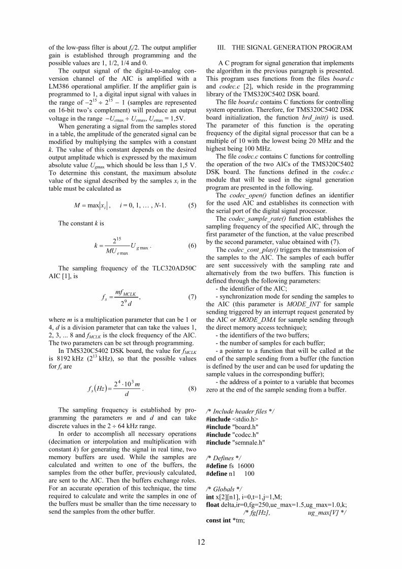
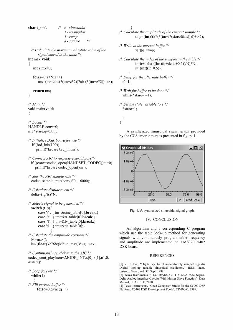
Buletinul Ştiinţific al Universităţii Politehnica din Timişoara
Seria ELECTRONICĂ şi TELECOMUNICAŢII TRANSACTIONS on ELECTRONICS and COMMUNICATIONS
Tom 48(62) Fascicola 2 2003
New Proof of the Sampling Theorem for Bandpass Signals
Robert Pazsitka1 Liviu Toma1 Dan Stoiciu1 and Aldo De Sabata1
1 Facultatea de Electronică şi Telecomunicaţii Departamentul Măsurări şi Electronică Optică Bd V Pacircrvan Timişoara 300223 e-mail robietcuttro ltomaetcuttro dstoiciuetcuttro adesabatetcuttro
Abstract ndash In order to avoid aliasing when sampling a signal at a uniform rate it is necessary that all spectral components of the signal have different sample values This condition is used in order to derive the classical sampling theorem for bandpass signals The relation-ships for permissible and minimum sampling rates are derived Keywords Bandpass signals sampling theorem sampling rate aliasing
I INTRODUCTION
Sampling a signal at a uniform rate may produce aliasing In this case it is impossible to recover the original analog signal from the sampled signal To avoid aliasing the spectral representation of the analog signal must not contain sinusoidal components of different frequencies that have the same sample values [1] In order to derive the corresponding condition we use the following two identities
( ) ⎟⎟⎠
⎞⎜⎜⎝
⎛++=⎟⎟
⎠
⎞⎜⎜⎝
⎛+ ϕπϕπ
ee
e fnfkf
fnf 12sin2sin (1)
( ) ⎟⎟⎠
⎞⎜⎜⎝
⎛+minusminus=⎟⎟
⎠
⎞⎜⎜⎝
⎛+ πϕπϕπ
ee
e fnffk
fnf 22sin2sin
(2) where fe is the sampling frequency of the signal sin(2πft+ϕ) and constants k1 k2 are any integers From identities (1) and (2) we obtain the frequencies of the components with the same sample values as the component of frequency f (3) ek fkff 11
+=
(4) ffkf ek minus= 22
To avoid aliasing the sampled signal must contain a single frequency component out of those in (3) and (4) which is obtained for k1=0
II DERIVATION OF THE SAMPLING THEOREM FOR BANDPASS SIGNALS
Consider a bandpass signal s(t) whose spectral
components in the frequency domain satisfy Mm fff lele (5)
where fm and fM are the minimum and maximum frequency in the spectrum respectively The signal bandwidth fB is defined by
mMB fff minus= (6) The frequencies fk1 in (3) and fk2 in (4) correspond to alias components when
Mem ffkff le+le 1 (7)
Mem fffkf leminusle 2 (8)
In order to avoid aliasing a single value should be possible for k1 in (7) namely k1=0 and no solution should be possible for k2 in (8) The inequalities (7) and (8) can be rewritten as
e
M
e
m
fffk
fff minus
leleminus
1 (9)
e
M
e
m
fff
kf
ff +lele
+2 (10)
Since f can take any value between fm and fM the widest allowable ranges for k1 and k2 are
e
mM
e
Mm
fffk
fff minus
leleminus
1 (11)
e
M
e
m
ffk
ff 22
2 lele (12)
14
The inequality (11) holds only for k1=0 iff
11 1 ltminus
leleminus
ltminuse
mM
e
Mm
fff
kf
ff (13)
It follows that
(14) Be ff gt Inequality (12) has no solution for k2 iff
Kff
ffK
e
M
e
m ltltltminus221 (15)
for any integer K larger than unity For satisfying (15) it is necessary that
122ltminus
e
m
e
M
ff
ff
that is
Be ff 2gt (16)
Condition (16) is more restrictive than (14) If no aliasing occurs then the sampling frequency fe satisfies (16)
III RANGES OF SAMPLING RATES
In order to avoid aliasing it is necessary and sufficient for fe to satisfy (15) which can be rewritten in the form
1
22minus
ltltK
ffKf m
eM (17)
(for K=1 the last member should be considered equal to infinity) Inequality (17) admits solutions for fe iff
1
22minus
ltK
fKf mM
which implies
⎥⎦
⎤⎢⎣
⎡lele
B
M
ffK1 (18)
(we have denoted by [x] the largest integer smaller than x) By combining (17) and (18) we get the possible ranges for fe one for every value of K in (18) The
number of ranges is ⎥⎦
⎤⎢⎣
⎡
B
M
ff The range of the smallest
sampling frequencies is
⎟⎟⎟⎟⎟
⎠
⎞
⎜⎜⎜⎜⎜
⎝
⎛
minus⎥⎦
⎤⎢⎣
⎡⎥⎦
⎤⎢⎣
⎡=
1
2
2
B
M
m
B
M
M
ff
f
fff
R (19)
If 1le⎥⎦
⎤⎢⎣
⎡
B
M
ff
then it is not possible to apply a
uniform bandpass sampling procedure In this case (19) reduces to the sampling condition for lowpass signals
IV CONCLUSION In this note a compact and transparent derivation of the sampling theorem for bandpass signals based on the condition that the spectral representation of the analog signal must not contain sinusoidal components of different frequencies with the same sample values has been presented Results known from literature [2] [3] have been obtained in an alternative way
REFERENCES [1] S D Stearns Digital Signal Analysis Hayden Book Company Inc New Jersey 1975 [2] R B Vaughan N L Scott and D R White ldquoThe Theory of Bandpass Samplingrdquo IEEE Transactions on Signal Processing vol 39 pp1973-1984 September 1991 [3] I Naforniţă A Cacircmpeanu A Isar Semnale circuite şi sisteme partea I Universitatea ldquoPolitehnicardquo Timişoara 1995
15
Buletinul Ştiinţific al Universităţii Politehnica din Timişoara
Seria ELECTRONICĂ şi TELECOMUNICAŢII TRANSACTIONS on ELECTRONICS and COMMUNICATIONS
Tom 48(62) Fascicola 2 2003
Sampling Amplitude Modulated Signals
Robert Pazsitka1
Abstract ndash The paper presents the sampling of periodic bandpass signals obtained through amplitude modulation of a sinusoidal carrier with a low-pass periodic signal The relationships for the sampling frequency and the number of samples required for calculating the Fourier coefficients of the modulating signal (or modulating signals in the case of quadrature amplitude modulation) are derived The same relationships are given for calculating the Fourier coefficients of the modulated signal Keywords bandpass signals amplitude modulation quadrature amplitude modulation sampling Fourier coefficients
I INTRODUCTION
An amplitude modulated signal with sinusoidal carrier may be represented as [1]
ttptx 0cos)()( ω= (1) where πω 200 =f is the carrier frequency and is the low-pass modulating signal with the maximum frequency noted The modulated signal is a bandpass signal [1] within the range
)(tp
maxf
max0max0 ffff +divideminus Sampling of bandpass signals and the necessary conditions imposed to the sampling frequency to avoid aliasing are treated in many papers [1] [5] [9] A theorem referring to real bandpass signals is presented in [5] and [6] The spectral components of the bandpass signal
are non-zero only in the frequency range that satisfies
)(txsi fff ltlt where and are the
minimum and maximum frequency in the spectrum respectively The bandwidth is The value of the bandwidth must be less than else the sampling frequency must be greater than
if sf
is ffB minus=
if
sf2 The sampling theorem of bandpass real signals shows that the reconstruction of the signal from its samples is possible if the sampling frequency satisfies the equation [6]
1
22minus
lelen
ff
nf i
es where
Bf
n slele2 (2)
The number from (2) is an integer If n Bf s is also an integer the smallest sampling frequency is
Bfe 2= This paper deals with the particular case of bandpass periodic signals obtained through amplitude modulation of a sinusoidal (periodic) carrier with a low-pass periodic signal containing a sum of sinusoids case not found in literature
II SAMPLING OF AMPLITUDE-MODULATED SIGNALS WITH PERIODIC MODULATING
SIGNAL For calculating the period of the bandpass periodic signal using the periods of the carrier and low-pass periodic signals we make the following statement the product of two periodic signals with frequencies that can be written as ratio of integer numbers is a periodic signal Let us consider two periodic signals with the fundamental frequencies and (the periods 0f 1f
00 1 fT = 11 1 fT = ) If these frequencies are written in the form
0
00 b
af = and
1
11 b
af = (3)
then their ratio is
Qmm
bb
aa
ff
isin=sdot=1
0
0
1
1
0
1
0 (4)
where and 0a 0b 1a 1b 100 bam sdot= 011 bam sdot= are integers Using (4) the above statement can be reformulated as follows the product of two periodic signals with the periods and that can be written 0T 1T
____________________ 1 Facultatea de Electronică şi Telecomunicaţii Departamentul Măsurări şi Electronică Optică Bd V Pacircrvan Timişoara 300223 e-mail robietcuttro
16
as ratio of integer numbers is a periodic signal with the period T where
(5) 1100 TmTmT == where and are integers 0m 1m The integers and must have no common factor for
0m 1mT to be the principal period of the bandpass
periodic signal Else the period calculated with (5) will be a multiple of the principal period We consider that the bandpass periodic signal noted is obtained by amplitude modulation of a sinusoidal carrier with a low-pass periodic signal noted see (1) We note with the period of
with the period of the carrier
)(tx
)(tp 1T)(tp 0T t0cosω and
with the period of the amplitude modulation signal The order of the maximum harmonic in the
spectrum of is noted
xT)(tx
)(tp K The numbers and are chosen so that the period calculated with (5) be the principal period of the signal If is a multiple of then
and else
0m 1m
xT)(tx 0f 1f
11 =m 1ff x = 11 mff x = where 11 gtm For if and we can write sf
(6) ⎩⎨⎧
+==minus==
102
101
KfffMfKfffMf
s
i
From (5) and (6) we can calculate the harmonics
and corresponding to the minimum and maximum frequencies in the spectrum
1M 2M
(7) ⎩⎨⎧
+=minus=
102
101
KmmMKmmM
The bandpass periodic signal has a discrete spectrum in the range
)(tx
xx fMffM 21 lele (8)
The bandwidth of the signal will be
(9) ( ) 11010 2KfKffKffB =minusminus+= The minimum sampling frequency required will be 142 KfBfe =gt The sampling of the amplitude modulated signal
ttptx 0cos)()( ω= can be made so that the samples taken from are samples from the low-pass signal
namely )(tx
)(tp
)()( ee iTpiTx plusmn= (10)
where ee fT 1= From (10) and (1) it follows that 1cos 0 plusmn=eiTω The samples required for
calculating the Fourier coefficients must be taken from one period of or from a multiple of
(uniform sampling) Therefore we can write
N
1T )(tp m
1T
1mTNTe = (11) where is an integer Two cases are possible m Case I πω 20 sTe = ( 1cos 0 =eiTω )
ππ 212 1
11
0 sN
mTTm
m= rArr
smm
mN 1
1
0= (12)
Case II πω sTe =0 ( 1cos 0 plusmn=eiTω )
ππ sN
mTTm
m=1
11
0 12 rArr sm
mmN 12
1
0= (13)
where s is an integer and is the number of samples taken from periods of According to Shannonrsquos theorem should be at least
N1mT )(txN 12 +K
so that and m s have to be chosen accordingly The sampling frequency from (11) will have the value
mNffe 1= The corresponding Fourier coefficients of will be calculated with
)(tp
summinus
=
minus=1
0)(1)(
N
i
iTjkep
eeiTxN
kc ω (14)
for case I ( calculated with (12)) and N
summinus
=
minus minus=1
0)1()(1)(
N
i
iiTjkep
eeiTxN
kc ω (15)
for case II ( calculated with (13)) N III SAMPLING OF QUADRATURE AMPLITUDE
MODULATED SIGNALS In this case the modulated signal is represented as [1] [2]
)(tx
ttqttptx 00 sin)(cos)()( ωω minus= (16)
The low-pass signals and are considered periodic with the same period noted and the maximum harmonic component in the spectrum of these signals is noted with
)(tp )(tq
1T
K If the sampling frequency ee Tf 1= has such a value that the equation
17
2
)12(0πω minus= sTe (17)
be valid where s =1 2 then for i even (18) )()( ee iTpiTx plusmn=
for odd (18rsquo) )()( ee iTqiTx plusmn= i From (18) and (18rsquo) it follows that the sampling interval used for one low-pass signal ( or ) is Similarly with (11) in this case we can write
)(tp )(tq
eT2
and - integers (19) 12 mTTN e = N m In (19) is the number of samples used for calculating the Fourier coefficients of or The total number of samples used for the two low-pass signals is
N)(tp )(tq
N2 From (17) (19) and )(2 1100 Tmmπω = we have
12
2
1
0
minus=
smm
mN (20)
Integers m and s are chosen in order to obtain the smallest greater than or equal to N 12 +K The sampling period can be obtained from (19) The Fourier coefficients for and are calculated with
)(tp )(tq
summinus
=
minus minus=1
0
2 )1()2(1)(N
i
iiTjkep
eeiTxN
kc ω (21)
summinus
=
++minus minus+=1
0
)2( )1()2(1)(N
i
siTiTjkeeq
eeeTiTxN
kc ω (22)
where 12 fπω = and [ ]KKk minusisin The reconstruction of the low-pass signals is made with
(23) sum+
minus=
=K
Kk
tjkpr ekctp ω)()(
(24) sum+
minus=
=K
Kk
tjkqr ekctq ω)()(
The reconstruction of the bandpass (quadrature amplitude-modulated) signal is made with
ttqttptx rrr 00 sin)(cos)()( ωω minus= (25)
IV CALCULATION OF THE FOURIER COEFFICIENTS CORRESPONDING TO THE
BANDPASS PERIODIC SIGNAL For obtaining the Fourier coefficients of the bandpass periodic signal the fundamental frequency must be determined as in chapter II The harmonic components and corresponding to the minimum and maximum frequencies in the spectrum are calculated with (7) The number of samples obtained from one period
of must satisfy the following three conditions [9]
)(tx
xf
1M 2M
NxT )(tx
a) )1(2 12 +minusgt MMN
b) ⎥⎦
⎤⎢⎣
⎡=⎥⎦
⎤⎢⎣
⎡NM
NM 21 22
c) NM12
and NM 22
must be different from
integers where [ ] denotes integer part The sampling period will be NTT xe = As between the Fourier coefficients we have the relationship (the signal is considered real) where denotes complex conjugate we can calculate just one half of the coefficients for example those with positive indices They can be calculated with
kk cc minus= )(tx
summinus
=
minus=1
0)(1 N
i
kiTjek
eeiTxN
c ω (26)
where xfπω 2= and 21 MMk isin If the bandpass signal is an amplitude-modulated signal with sinusoidal carrier as defined by (1) without phase difference between the carrier and the low-pass (periodic) signal we can calculate just one quarter of the Fourier coefficients This is possible because the coefficients corresponding to the frequencies below are the complex conjugates of their respective symmetric coefficients for frequencies greater than To demonstrate this the terms
)(tx
0f
0fttkak 01 coscos ωω and ttkbk 01 cossin ωω
contained by the modulated signal ttptx 0cos)()( ω= can be written as
tka
tkattka
k
kk
)cos(2
)cos(2
coscos
10
1001
ωω
ωωωω
++
+minus= (27)
tkb
tkbttkb
k
kk
)sin(2
)sin(2
cossin
10
1001
ωω
ωωωω
++
+minusminus= (28)
18
This means it is enough to calculate the coefficients with where kc 20 MMk isin ( ) 2210 MMM +=
corresponding to the remaining coefficients being obtained by complex conjugation This property is not valid for quadrature amplitude modulation
0f
Because all of the cases presented above refer to periodic signals the sampling frequency can be lowered by taking the samples from several periods An additional condition must be satisfied [10] namely the number of samples and the number of periods NM should have no common factor
V CONCLUSIONS Signals obtained through amplitude modulation can be sampled such as to obtain directly the samples of the low-pass signal Several relationships are established for calculating (the required number of samples) and the sampling frequency so as to obtain the samples of the low-pass signal if the input signal is a bandpass periodic signal obtained through amplitude modulation If the number results from (12) then the Fourier coefficients are easily calculated with the known formula (14) If the number results from (13) then the Fourier coefficients are calculated with the modified formula (15) The same calculations (number of samples sampling frequency Fourier coefficients corresponding to the low-pass signals) are for the bandpass signal obtained by quadrature amplitude modulation
N
N
N
Chapter 4 presents the condition that must be satisfied by the number of samples obtained from a bandpass signal in order to calculate the Fourier coefficients of this signal If the signal is real (the samples are real number) then and then just half of the coefficients need to be calculated If the bandpass signal is obtained through amplitude-modulation then just one quarter of the coefficients need to be calculated due to the fact that the spectrum is symmetrical with respect to
N
kk cc minus=
0f
REFERENCES [1] Jerry D Gibson The Communications Handbook CRC Press Inc 1997 [2] JL Brown JR First-Order Sampling of Bandpass Signals ndash A New Approach IEEE Trans on Inf Theory Vol IT-26 No 5 Sept 1980 [3] JL Brown JR On Quadrature Sampling of Bandpass Signals IEEE Trans on Aerospace and Electronic Systems Vol AES-15 No 3 May 1979 [4] Marks II J Robert Introduction to Shannon Sampling and Interpolation Theory Springer-Verlag New York Inc 1991 [5] Oran E Brigham The Fast Fourier Transform And Its Application Prentice Hall Inc 1988 [6] Larry Marple Exploding the Nyquist Barrier Misconception IEEE Signal Processing Magazine Vol 13 No5 Sept 1996 [7] Liu J Zhon X Peng Y Spectral Arrangement and other Topics in First-Order Bandpass Sampling Theory IEEE Trans on Sig Proc Vol 49 No 6 June 2001 [8] Vaughan BR Scott LN White RD The Theory of Bandpass Sampling IEEE Trans on Sig Proc Vol 39 No 9 Sept 1991 [9] Robert Pazsitka Sampling of Bandpass Periodical Signals Proceedings of the Symposium on Electronics and Telecommunications Etc 2002 Timisoara Sept 19-20 2002 Vol 1 [10] Robert Pazsitka Eşantionarea semnalelor periodice lucrare de dizertaţie Facultatea de Electronică şi Telecomunicaţii Timişoara iulie 1997
19
Buletinul Ştiinţific al Universităţii Politehnica din Timişoara
Seria ELECTRONICĂ şi TELECOMUNICAŢII TRANSACTIONS on ELECTRONICS and COMMUNICATIONS
Tom 48(62) Fascicola 2 2003
The Specific Absorption Rate of the Electromagnetic Radiation for Biological Structures in the Case of Mobile
Telephony
Adrian Vacircrtosu1
1 Facultatea de Electronică şi Telecomunicaţii Departamentul Măsurări şi Electronică Optică
ABSTRACT Cellular telephony uses a frequency domain ranging between 800 MHz and 2000 MHz with emission powers of 06W to 2W
The frequencies used have wavelengths that can be compared to the physical dimensions of the skull and the power emitted by portable phones is quite high around 06W Because of the proximity of the head (just a few centimeters away) with all the reflections from the surface of the skull and the attenuations that intervene the field intensities that manage to get inside the skull can induce in the cerebral mass currents of the same size with the intensities of normal biological currents
I INTRODUCTION The 5191999 recommendation of the Council
of Europe from the 12th of July 1999 concerning the limitation of public exposure to electromagnetic fields (from 0 Hz to 300 GHz) establishes the limits in values of physical units that characterize electromagnetic radiation at different frequencies The respective norms also called basic restrictions and reference levels establish safety coefficients in the case of electric magnetic and electromagnetic field exposure variable in time based directly on the obvious effects on health and biological considerations Depending on the field frequency the physical units used in order to specify the restrictions are the magnetic induction (B) the density of current (J) the specific absorption rate (SAR) and the power density (S) The SAR unit is used within the 100 kHz ndash 10 GHz frequency range to define the basic restrictions concerning the electromagnetic fields in order to prevent a generalized thermal stress of the body and an excessive localized heating of tissues
According to the 1999519CE 12th of July 1999 Recommendation the reference levels of
radiofrequency fields used in the GSM system are (table 1)
Table 1
Frequency (MHz)
Electric field
E (Vm)
Magnetic field H (Am)
Density of Power (Wmsup2)
900 41 011 45 1800 58 016 9
It is worth noticing that in the case of simultaneous exposure to different frequency fields there is a possibility that the effects of the exposure are cumulative As a convention each effect will be studied using separate calculations and based on the hypotheses separate evaluations of the effects of thermal and electric strain of the organism will be covered
Knowing the electric properties of biological environments is essential to the study of the interaction phenomena between these and the electromagnetic field The electrical properties involve permittivity and electric conduction
The magnetic properties (with some exceptions that do not concern the present paper) are not defined for the biological matter the relative permeability of biological entities is considered to equal a unit (micror= 1) and the losses obtained through the magnetic effect are thought to be negligible
The electric properties that intervene in the study of the biological effects of electromagnetic fields are the electric permittivity ε and the conduction σ defined over the unit of volume of matter Permittivity characterizes the interaction between the environment and the electromagnetic wave that is propagated through it The permittivity of free space is a constant εo and the permitivity of any other environment is a complex
20
measurement ( ) in which ε is an indicator of the property of the environment to store energy while ε indicates the property of the environment to dissipate the energy carried by the electromagnetic field
c jεεε minus=
Relative permittivity measures the net effect of the electric dipoles alignment that characterizes the intimate structure of the matter that is under the influence of an electric field applied from the outside
The energy dissipated per second per unit of volume of homogenous material by an electromagnetic wave incidence is proportionate to the square of the amplitude of the electric field component and is calculated with the help of this formula [1]
P = πf εoεE2 = σ E22 (1)
where σ is the conduction of the environment in which the dissipation of energy takes place The conduction is itself dependent on the frequency
All these parameters (σ ε or tan δ ) characterize the possibility of the environment to absorb the energy from the electromagnetic field
Calculating the values of the dielectric parameters (permittivity conduction wavelength intrinsic impedance penetration depth etc) that characterize the human tissues at the frequencies of 800 MHz and 900 MHz used by the Romanian mobile telephony was done by using a program in EXCEL based on formulas [2] [3] that allows for finding these measurements up to the frequency of 300 GHz
Formulas used in calculation of dielectric properties
complex permittivity
c jεεε minus= (2)
rel complex permittivity
0
εεεεε c
rrcr j =minus= (3)
0
ωεσε =r
ωσε =
permittivity of free space
Fm1085418781768 120
minustimes=ε permeability of free space
Hm104 70
minustimesπ=micro impedance of free space
Ω= 376730313Z 0 wave velocity in free space
ms 10 2997924581c 8
00
times=εmicro
=
angular frequency
f2 π=ω loss tangent of material
r
r
)(tanεε
=ωεσ
=ϑ (4)
propagation constant of material y = α+j β
)j(c
)j(j r
r
2
r2 εminusε⎟
⎠⎞
⎜⎝⎛ ω
microminus=ωε+σωmicro=γ (5)
attenuation constant of material
( ) ⎟⎟⎠
⎞⎜⎜⎝
⎛minusεε+
εmicro⎟⎠⎞
⎜⎝⎛ ω
=α 112c
2r
r
rr (6)
skin depth material
α=δ
1 (7)
phase constant of material
( ) ⎟⎟⎠
⎞⎜⎜⎝
⎛+εprimeε+
εmicro⎟⎠⎞
⎜⎝⎛ ω
=β 112c
2rr
rr (8)
wave velocity in material
βω
=u (9)
wavelength in material βπ
=λ2 (10)
intrinsic impedance of material
r
r
r0
c jZZ
εminusε
micro=
εmicro
= (11)
( ) 2502r
r
r
r0
1ZZ
⎥⎦⎤
⎢⎣⎡ εε+ε
micro= (12)
( ) ( )r
r
1tan21Zphase εε= minus (13) 00lephase(Z)le450
21
II RESULTS OF THE EXPERIMENT
The results of these calculations corresponding to the two bands are presented in the table 2 for f=800 MHz and in the table 3 for f=900 MHz
Table 2a
f=800 MHz micror = 1
TISSUE bone skin blood brain heart
εr 8688429 36212 5882646 464656 6067894
εr 0745467 1234021 2570435 1548868 2253825
σ (Sm) 0033178 0549214 1143998 0689339 1003087
tan(θ) 00858 0340777 0436952 0333337 0371434
α (1m) 2118257 1695389 2747556 1879632 2386113
β (1m) 4946731 1023108 1315008 1158271 1327692u (ms) 102E+08 49130166 38224479 43397013 37859280
λ (m) 0127017 0061413 0047781 0054246 0047324
δ (m) 0472086 0058984 0036396 0053202 0041909
|Ζ| (Ω) 1276914 6175043 4805721 5454375 4758779
Ζ (deg) 2451985 9408961 1180151 9217559 1018837
Table 2b
TISSUE muscle kidney liver lung spleen
εr 5411328 4761208 462569 3323576 5264076
εr 1430979 1890983 1815213 157899 2142521
σ (Sm) 0636871 0841601 0807879 0702745 0953551
tan(θ) 0264441 0397165 039242 0475088 0407008
α (1m) 1616963 2255025 219707 2237002 2427742
β (1m) 1243946 1178704 116132 992159 1240483u (ms) 40408097 42644715 43283050 50662729 40520887
λ (m) 005051 0053306 0054104 0063328 0050651
δ (m) 0061844 0044345 0045515 0044703 0041191
|Ζ| (Ω) 5078194 5360689 5440852 6370586 5093874
Ζ (deg) 7406157 1083061 1071302 1270591 1107336
Table 3a f= 900 MHz micror = 1
TISSUE bone skin blood brain heart
εrrsquo 8634636 3599427 5874271 4636694 6051015
εrrdquo 0818382 1133951 2333097 1421199 2071992
σ (Sm) 0040976 0567761 1168164 0711584 1037431
tan(θ) 0094779 0315037 0397172 0306511 0342421
α (1m) 2623734 1761374 2817931 1946225 2477099
β (1m) 5548936 1145292 1472909 1299078 1488052
TISSUE bone skin blood brain heart
u (ms) 102E+08 49374911 38392510 43529846 38001813
λ (m) 0113232 0054861 0042658 0048366 0042224
δ (m) 0381136 0056774 0035487 0051382 004037
|Ζ| (Ω) 1280628 6205502 4826162 5470811 4776366
Ζ (deg) 2707131 8743167 108308 8520446 9451129
Table 3b
TISSUE muscle kidney liver lung spleen
εr 5406606 4756672 4615513 3306596 5255305
εr 1333614 1714191 1650214 1440076 1950378
σ (Sm) 0667731 0858282 082625 0721035 097654
tan(θ) 0246664 0360376 0357536 0435516 0371126
α (1m) 1697889 2308073 2256177 2310114 2496166
β (1m) 1397314 1321244 1301189 1108984 1390013u (ms) 40469540 42799564 43459223 50991404 40682126
λ (m) 0044966 0047555 0048288 0056657 0045202
δ (m) 0058897 0043326 0044323 0043288 0040061
|Ζ| (Ω) 508583 5379605 5462482 6410789 5113597
Ζ (deg) 6928098 9908974 9836909 1176695 1018059 Formulas used for εr and εrrsquo are [2]
2
2
22
1
13
r
f1000f1
ff1 ⎟⎟
⎠
⎞⎜⎜⎝
⎛sdot
+
ε+
⎟⎟⎠
⎞⎜⎜⎝
⎛+
ε+ε=ε (14)
⎥⎥⎦
⎤
⎢⎢⎣
⎡⎟⎟⎠
⎞⎜⎜⎝
⎛sdot
+sdot
ε+
⎥⎥⎦
⎤
⎢⎢⎣
⎡⎟⎟⎠
⎞⎜⎜⎝
⎛+
ε+
sdotsdotπεσ
=ε2
22
22
11
1
0
0r
f1000f1f1000
f
ff1f
f1000f2
(15) The values of the units used in calculating these dielectric parameters are given in the table 4 [2]
Table 4a
TISSUE bone skin blood brain Heart
ε3 49 33 43 75 43
σo (Sm) 31E-07 0231 0768 0313 063
f1 (MHz) 2360 137 378 433 906
ε1 222 343 136 122 494
f2 (GHz) 204 177 213 165 156
ε2 18 32 543 387 559
22
Table 4b
TISSUE muscle kidney liver lung spleen
ε3 43 43 43 43 43
σo (Sm) 0301 0551 0406 0325 044
f1 (MHz) 83 247 442 818 266
ε1 475 166 136 691 289
f2 (GHz) 152 245 216 151 198
ε2 499 432 416 283 481
The external field incident to the biological structure can be expressed in terms of power density (mWcm2) of amplitude of the electric field component (Vm) or of the magnetic field component (Am) None of these parameters is appropriate for expressing the effects induced by the penetration of the electromagnetic radiation inside the biological domain Considering this situation a specific parameter has to be defined It is called the ldquoSpecific Absorption Rate ndash SARrdquo and it is the variation in time of the elementary energy quantity (dw) absorbed by an element of volume (dv) having a density (ρ) and an elementary mass (dm) [1]
⎟⎟⎠
⎞⎜⎜⎝
⎛=⎟
⎠⎞
⎜⎝⎛=
dVdW
dtd
dmdW
dtdkgWSAR
ρ)(
The Specific Absorption Rate (SAR) is correlated to the penetration depth (δ)in the tissues If the penetration depth (δ) is the distance from the surface of the tissue for which the amplitude of the electric field component reduces with factor e = 271 than the specific absorption rate at this depth reduces to a value equal to 135 of its initial value
Sometimes it is useful to define the depth d (frequently used in hyperthermia cases) at which the power incident to the surface of the irradiated structure is reduced to half (3 dB attenuation) Between (δ) and (d) there is the relation
d = 0345 x δ In order to determine the value of the SAR
parameter the TEMS (Test Mobile System) system was used This system was offered by the ORANGE firm and the measurements were taken at the frequency of 900 MHz
The applications of TEMS for an operational network are
bull it simulates and verifies possible changes in the network
bull it evaluates the quality of the received signal bull it measures the space covered range bull it tests the system (checks new or already
present functions)
- it signals in real time aberrant values of any parameter (for example the large number of interrupted calls)
- it identifies areas with problems of signal coverage or with high levels of interference
bull it presents the data in graphs maps The equipment used for measuring (Fig 1)
contains - special software made by Erricsson-TEMS
(Test Mobile System) - laptop mobile phone special data cable that
insures the PC-mobile phone connection
Fig1 The equipment used for measuring
The TEMS mobile phone is an Erricsson
ordinary phone that uses the TEMS program No supplementary calibrations are necessary for using the TEMS software
This mobile phone has four different operation modes
1 No Service (when it is in an area with no signal coverage)
2 Limited services (only emergency calls) 3 Inactive 4 Dedicate (during a conversation)
The measurements were taken during a
conversation therefore in the dedicate mode Taking the measurements involves - initiating a call - choosing the unit to be measured in this
case the power of the transmitted signal (TxPwr)
- the display of the unit to be measured (Fig2) and information about the distance from the base station (TA ndash Time Advance) the base station code (BSIC ndash Base Station Identity Code) local code (LAC Local Area Code) the channel of the communication (TCH ndash Traffic Channel)
23
In order to calculate the value of SAR the
situation when the telephone is in dedicated mode t0 is used At t0 these units have the following values
TxPwr =18dBm=625mW
TA = 2 d = TAx 500m Therefore the distance (d) to the base station is
1 km BSIC = 23 LAC = 05500
Fig2 The value of the SAR unit for the measured power is determined according to [1]
⎥⎦
⎤⎢⎣
⎡sdot=
=sdot
=ρ
=ρ
σ=
ρε primeprimeωε
=⎥⎦
⎤⎢⎣
⎡
minus
kgW1012550
1000062502P2EE
kgWSAR
3
22r0
where 0ε = permittivity of free space ω = angular frequency ρ = the density of the biologic environment asymp1000 kgm3
E = the intensity of the electric field P = πf εoεE2 = σ E22
Fm10E85418781768 120
minustimes=ε
0
r ωε
σ=ε
It is observed that the specific rate of absorption SAE is under the maximum admitted level of 04 Wkg
The value of SAR can also be determined according to the dielectric parameters ε σ and the electric field generated by the mobile phone In this case the system of measurement contains
bull electric field probe (Wandel amp Goltermann) with the EMR 20 measuring device
bull software for processing the values measured by the probe
bull mobile phone with without the antenna The measurements were done considering the following three positions for the measurement probe
bull positioning the electric field probe in the
speaker area bull positioning the electric field probe in the
inferior keys area bull positioning the electric field probe next to the
inner antenna behind the telephone or next to the extended antenna in the case of telephones with exterior antennas
The results obtained are succinctly presented in the table5 The maximum values of the electric field registered in each area of measurement and expressed in Vm are also presented
Table 5 Telephone type
with internal antenna with external antenna
Area Speaker
Micro-phone back speake
r
antenn
a On 981 668 1126 - 986
Called 2351 755 178 3677 2132
Calling 2142 1966 3398 2994 2418
Speaking
2871 197 3843 3672 282
S T A T E
Off 245 687 1032 -
III CONCLUSIONS
The following observations can be drawn on the
basis of the date from the table bull the internal antenna has directivity by having a
weaker emission in the area of the userrsquos head bull the emission is larger in the superior area of the
internal antenna phone bull the emission is stronger in the states where the
telephone is in contact with the head of the user (when he calls and speaks) the antenna type does not matter
bull the telephone with an external antenna has a stronger emission at the level of the speaker than at the extremity of the antenna
bull the telephone with an external antenna does not have a weaker emission at the level of the speaker in comparison to the internal antenna telephone
24
The difference in values from the experimental data provided by our bibliography and from the theoretical models is due to the various uncertainty factors that are linked to the measurements in a close-range field and the digital character of the signal
bull the size of the detecting field unit that disturbs the measuring field
bull the link between the measuring probe and the emission antenna of the telephone
bull the measuring technique of the digital signal
It was observed that at low levels of power density some effects take place after a longer exposure time They are called ldquolow level power effectsrdquo or ldquoathermic effectsrdquo effects that also appear in the case of using mobile phones It is best to consider the following recommendations even if the SAR value is situated between the limits established by the European Commission
bull to reduce using mobile phones in conditions of low signal
bull to avoid wearing mobile phones close to the sensitive tissues
bull using car kits bull constantly informing the population of the
level of radiation around the base stations by operating frequent measurements that would be accessible to the public
The conclusion is that the general objective should be to reduce the degree of exposure of the population to radiofrequency fields
IV BIBLIOGRAPHY
[1] ZAMFIRESCU MIHAIL SAJIN GH RUSU IONSAJIN MARIA KOVACS EUGENIA ndash Efectele biologice ale radiaţiilor electromagnetice de radiofrecvenţă şi microunde Editura Medicală 2000 [2] GABRIEL C (1996) Compilation of the dielectric properties of body tissues at RF and microwave frequencies Brooks Air Force Base report no ALOE-TR-1996-0037 [3] HURT WD (1996) Radiofrequency radiation dosimetry workshop Brooks Air Force Base report no ALOE-SR-1996-0003 [4] SADIKU MNO (1994) Elements of Electromagnetics Saunders College Publishing New York [5] HOMBACH V Comparison of different human head models XXVth General Assembly of the International Union of Radio Science August 28 - Sept 5 1996 Lille France
25
Buletinul Ştiinţific al Universităţii Politehnica din Timişoara
Seria ELECTRONICĂ şi TELECOMUNICAŢII TRANSACTIONS on ELECTRONICS and COMMUNICATIONS
Tom 48(62) Fascicola 2 2003
The Cyclic Prefix Length Influence on OFDM-Transmission BER
Marius Oltean1 Miranda Naforniţă1
Abstract Orthogonal Frequency Division Multiplexing (OFDM) is one of the recent years equalization approaches used in order to combat the inter-symbol interference introduced by the frequency selectivity of the radio channels The circular extension of the data symbol commonly referred to as cyclic prefix is one of the key elements in an OFDM transmission scheme The influence of the cyclic prefix duration on the BER performance of an OFDM system with in-frame DBPSK modulation is evaluated by means of computer simulation in a multipath fading channel
I INTRODUCTION Mobile radio communication systems are increasingly required to offer a variety of services and qualities for mobile users Unfortunately the radio channel is far from an ideal transmission medium exhibiting both frequency selectivity and time variant character [1] In this context one of the most challenging issues in a radio communication system is to overcome the inter-symbol interference introduced by the multipath propagation of the signal between the transmitter and the receiverrsquos antennas The use of the adaptive equalization to the receiver could be the solution for avoiding this unwanted phenomenon but this complex equalization technique proves oftentimes unsuited for being used in real-time applications at data rates of tens of Mbps in an unfriendly dispersive radio channel environment because of its important computational complexity OFDM is an optimal version of multicarrier modulation techniques which mitigates the effect of the ISI phenomenon keeping a relatively reduced complexity of the equalization process Indeed intuitively one can assume that the frequency selectivity of the channel can be mitigated if instead of transmitting a single high rate serial data stream the transmission is performed simultaneously using several narrow-band subchannels (with a different carrier corresponding to each subchannel) on which the frequency response of the channel looks ldquoflatrdquo
Hence for a given overall data rate increasing the number of carriers reduces the data rate that each individual carrier must convey therefore lengthening the duration of the symbol that modulates each individual subcarrier [2] Slow data rate (and long symbol duration) on each subchannel merely means that the effects of ISI are severely reduced In addition a cyclic prefix is inserted in front of each OFDM symbol This circular extension that is discarded on the receiver side is obtained by copying a number of samples from the end of the OFDM symbol in front of it in order to prevent two consecutive frames to interfere each other as a result of the time dispersion caused by the multipath propagation This way the receiver can independently process each frame in order to estimate the transmitted information Furthermore the equalization process is facilitated by this operation of cyclic prefix insertion and extraction In this chapter we focus on the influence of the cyclic prefix duration on the BER performance of an OFDM system with in-frame DBPSK modulation The performance evaluation in Rice fading conditions is done by means of computer simulation
II THE BLOCK-DIAGRAM OF OFDM
TRANSMISSION SCHEME
In the figure 1 a classical OFDM transmission scheme using FFT (Fast Fourier Transform) is illustrated
The input data sequence is baseband modulated using a digital modulation scheme Various modulation schemes could generally be employed such as BPSK QPSK (also with their differential form) and QAM with several different signal constellations In our system DBPSK method is chosen in order to encode the binary information Data is encoded bdquoin-framerdquo (the baseband signal modulation is performed on the serial data that is inside of what we name a bdquoDFT framerdquo or equivalently an OFDM symbol) The data symbols 1 Univ ldquoPolitehnicardquo Timişoara Facultatea de Electronică şi TelecomunicaţiiDepartamentul Comunicaţii
26
Information symbols
Serial to parallel
converter
Coding amp baseband
modulation
IFFT modulator
Cyclic prefix insertion
Parallel to serial
converterX
ej2πfct
Channel
X
ej2πfct
Serial to parallel
converter
Cyclic prefix extraction
FFT demodulator
Decoding amp demodulation
Parallel to serial
converter
Estimated symbols
Xk k=0hellipN-1
[Xk] k=0hellipN-1
[xk] k=0hellipN-1
[xcpk] k=-LhellipN-1
[ycpk] k=-LhellipN-1
[yk] k=0hellipN-1
[Yk] k=0hellipN-1
Yk k=0hellipN-1
Fig1 The block diagram of an OFDM System
are parallelized in N different substreams Each substream will modulate a separate carrier through the IFFT modulation block which actually generates the OFDM symbol performing the multicarrier modulation A cyclic prefix is inserted in order to eliminate the inter-symbol and inter-block interference (IBI) [3] The data are back-serial converted forming an OFDM symbol that will modulate a high-frequency carrier before its transmission through the channel The radio channel is generally referred to as a linear time-variant system To the receiver the inverse operations are performed in order to estimate the transmitted symbols
III THE CYCLIC PREFIX AND THE EQUALIZATION PROCESS
Since OFDM transmits data in blocks (usually a block is referred to as an bdquoOFDM symbolrdquo) any type of a non-ideal transmission channel (such as a multipath channel in mobile communication systems or a classical dispersive channel as in wired transmissions) will bdquospreadrdquo the OFDM symbol causing the blocks of signal to interfere one another This type of interference is called Inter-Block Interference IBI could lead to inter-symbol interference since two adjacent blocks will overlap causing the distortion of the samples affected by overlapping
In order to combat this interference we could use a cyclic prefix (CP) at the beginning of each symbol If the cyclic prefix spans more than the multipath channel impulse response the interference caused by the time dispersion of the previous transmitted block is entirely absorbed by the prefix samples that are discarded to the receiver The cyclic prefix consists of the last L samples of the OFDM symbol that are copied in front of the data block [4] as we can see in the figure 2 Generally the radio channel exhibits both time variant and frequency selective characteristics If we shall consider however that the channel parameters remain unchanged during the transmission of an OFDM symbol the way that the transmission medium distorts each particular frame is similar to the distortion caused by an
electronic filter [1][5] Under this assumption we can consider the equivalent discrete response of the channel as a linear FIR filter of order L of which the equation is given below
sum=
minussdot=L
n
nznczC0
][)( (1)
The equivalent baseband signal at the channel output can be obtained by the operation of convolution as follows
][][][ ncnxcpnycp = (2)
Discarding the L CP samples from the received sequence the remaining (useful) signal can be expressed as
where ldquo⊛rdquo denotes the circular convolution operator [6] The noticeable thing about the equation 6 is that the circular convolution preserves the temporal support of the signal In our case N transmitted signal samples convolved with L+1 channel impulse response samples will conduce to a received symbol of length N that will be used in the demodulation process Since the circular convolution will not ldquospreadrdquo the signal the receiver can independently process each data block The interference from the
y[n]=x[n] ⊛c[n] (3)
OFDM Symbol
Copy
CP
Transmitted sequence= OFDM symbol+CP
t
Fig2 The cyclic prefix insertion
27
previous transmitted blocks is totally eliminated through this operation of CP insertionextraction Furthermore since x[n]=IDFTX[k] and taking into account the effect of the DFT demodulator the received symbols Y[k] can be expressed as
Y[k]=DFTIDF TX[k] ⊛c[n] k=01hellipN-1 (4)
Since the DFT of a circular convolution of two discrete time signals will conduce to a spectral multiplication
110][][][][][
minus=sdot==sdot=
NkkCkXncDFTkXIDFTDFTkY
(5)
where C[k] represents the sampled frequency response of the equivalent baseband discrete channel corresponding to the frequencies Ωk=k(2πN) The crucial consequence of the relation above is that each modulation symbol X[k] could be recovered to the receiver by a simple pointwise division operation commonly referred to as a ldquoone-tap frequency domain equalizerrdquo as can be seen from the relation (6)
110][][][ 1 minus=sdot= minusandNkkCkYkX (6)
Thus the CP theoretically eliminates both IBI (each block preserves its temporal support) and inter-carrier interference (ICI) (each serial symbol received on the k-th carrier will depend only on the corresponding k-th carrier transmitted symbol not being affected by the adjacent carriers) IV SIMULATION RESULTS AND DISCUSSIONS
1 SIMULATION PARAMETERS
The goal of the simulations was to emphasize the effect of the cyclic prefix duration on the BER performance of an OFDM system with inter-frame DBPSK modulation The radio channel was modeled as a three-ray Rice fading channel with one deterministic line-of-sight (LOS) path and two multipath delayed components The relative delays of the two components are τ1 and τ2 respectively However in most of these simulations it was considered τ1=0 and a normalized delay for τ2 denoted τ2N=τ2LCP LCP represents the cyclic prefix duration expressed as the number of serial samples that compose the cyclic prefix An important parameter for the Rice fading channel is K=PLOSPD which stands for the ratio between the signal power carried by the LOS path (PLOS) and the total power of the two multipath components (PS=P1+P2) Equal power for the two multipath components was considered during the simulations A white gaussian noise is added to the signal at the output of the Rice
fading channel The time interval between the moments in which the first and the last significant component of the multipath signal arrives to the receiver is referred to as maximum excess delay (TM) and it is expressed in number of serial samples (remember that N signal samples generated by the IFFT modulator will compose an OFDM frame) Another parameter of the simulation is the number of subcarriers N that equals the number of serial samples composing an OFDM symbol The time variant character of the radio channel is quantified by the maximum Doppler shift parameter fD The value of this parameter is also expressed in a normalized manner as fDTS TS denoting the OFDM symbol duration A robust differential modulation scheme such as DBPSK was chosen for encoding the binary information No channel estimation techniques are employed and consequently no further equalization is done to the receiver
2 RESULTS AND DISCUSSIONS For the first simulations the relative delay of the second multipath was normalized by the serial symbol duration As can be seen from the figure 3 increasing the cyclic prefix duration improves the BER performance for the OFDM system
Theoretically if the cyclic prefix duration spans more than the maximum delay spread of the channel the errors can be completely eliminated This assumes however a perfect knowledge of the channel impulse response (or equivalently of the channel transfer function) which is a mandatory condition for implementing the equation 6 Since in our implementation no channel estimation techniques are employed the exact form of the channel impulse response doesnrsquot constitute information that can be exploited in the data estimation process The correct
Fig 3 The influence of the cyclic prefix duration on BER performance for DBPSK-OFDM system
Rice fading channel K=3dB SNR=30dB N=64 fDTS=0001
28
detection is entirely based on the robustness and simplicity of the digital modulation scheme that is involved namely DBPSK This explains why the BER is not completely eliminated for a cyclic prefix of theoretically sufficient duration (longer than TM) A noticeable thing resulting from the figure 3 is that while identical for cyclic prefix lengths which cover the channel impulse response the performance degrades for the cases where the cyclic prefix duration becomes insufficient Thus if a cyclic prefix of length LCP=4 is used the transmission offers the best performance between all the considered situations but only starting with a value of the normalized delay that overtakes the length of the circular extension for all the other cases Next we studied the BER performance against the normalized delay of the second multipath which is obtained this time as explained in the previous subsection It can be observed from the figure 4 that increasing the OFDM symbol length improves the performance of the system which confirms [6] In the same time it is proven that the BER is sensitive to the multipath delay spread of the channel
normalized by the cyclic prefix duration Thus as observed in the figure 4a) a two times longer OFDM symbol is needed in order to obtain the same performance when the normalized delay of the second multipath is two times higher (note that for the same value of τ2N on the abscissa τ2 doubles its value when LCP=2) The observation is confirmed by the figure 4b) where the BER curve in the case N=16 LCP=1 is almost identical with the curve plotted for a frame of length N=64 with a cyclic prefix LCP=4 The conclusion that can be drawn from these observations is that at identical ratios between the channel impulse response and the cyclic prefix duration the in-frame OFDM system performance remains sensitive to the effective value of the multipath (or maximum) delay spread parameter (τ2 in our case)
3 CONCLUSIONS
The cyclic prefix duration influences the performances of an OFDM system even if the explicit form of the channel impulse response is unknown and consequently cannot be used in the equalization process The transmission is sensitive to the parameter obtained as the multipath delay of the channel normalized by the cyclic prefix duration The BER performance is in all cases improved by increasing the OFDM symbol length
REFERENCES
[1] B Sklar Rayleigh Fading Channels in Mobile Digital Communication Systems- Part I Characterization IEEE Commun Mag July 1997 [2] Dusan MaticOFDM as a possible modulation technique for multimedia applications in the range of mm waves 10-30-38 TUD-TVS available on-line wwwubicomtudelftnlMMCDocsintroOFDMpdf [3]Werner Henkel Georg Tauboumlck Per Oumllding The cyclic prefix of OFDMDMT ndash an analysis 2002 International Zuumlrich Seminar on Broadband Communications February 19-21 Zuumlrich Switzerland [4]Lu J Tjhung TT Adachi F BER performance of OFDM system in frequency-selective Rician fading with diversity reception available online httpwwwcwcnusedusg~cwcpubzfilesict97_2pdf [5] B Sklar Rayleigh Fading Channels in Mobile Digital Communication Systems- Part II Mitigation IEEE Commun Mag July 1997 [6 ]Chini A Analysis and Simulation of Multicarrier Modulation in Frequency Selective Fading Channels Ph D Thesis 1994 Chapter 3
a)
b)
Fig 4 (ab) The influence of the normalized delay of the second multipath on BER performance for DBPSK-OFDM
system Rice fading channel K=3dB SNR=40dB fDTS=0001
29
Buletinul Ştiinţific al Universităţii Politehnica din Timişoara
Seria ELECTRONICĂ şi TELECOMUNICAŢII TRANSACTIONS on ELECTRONICS and COMMUNICATIONS
Tom 48(62) Fascicola 2 2003
Methods for JPEG image protection by partial encryption Florin Vancea1 Codruţa Vancea2
1 University of Oradea Faculty of Electrotechnics and Informatics Computer Science Department str Armatei Romacircne nr 5 Oradea e-mail fvanceauoradearo 2 University of Oradea Faculty of Electrotechnics and Informatics EMUEE Department str Armatei Romacircne nr 5 Oradea e-mail cvanceauoradearo
Abstract ndash The JPEG format used in static image transfer and storage exhibits some particularities when considered for encryption A commercially useful encryption must degrade the image but keep it within evaluation limits Classical encryption techniques can be applied to a JPEG stream in various phases of its construction and to different segments We evaluate the impact of some alternatives testing on real cases Potential future directions are identified Keywords encryption JPEG DCT
I INTRODUCTION
A significant part of the information transmitted in data networks and stored in computer systems today is represented by images be they static or in motion The need to protect this information against unauthorized access and usage requires no further proof In order to protect text-based information various methods have been devised based on the general theory of encrypting binary information [1] Since images are stored and transported in binary form too we can directly apply known encryption methods to protect them The disadvantage of such approach is that itrsquos too rigid the image becomes unintelligible In copy-protection schemes or in controlled distribution schemes one would like a partial and controlled accessibility to image content Encryption key holders will be able to see and use the image to its normal parameters and potential unauthorized users get access to a degraded version understandable but unusable for any purposes but identification of its value A distribution scheme using such a mechanism can thus publish an electronic catalogue and interested users will only pay for the keys needed to decrypt the images they need The images are transmitted and stored using various formats Generally one is looking to compress the raw information content but this can be achieved in various ways Some methods are using color space reduction by using color tables others are applying compression methods to the raw bitstream resulted from sampling the color information at maximum
capability level Some are using lossless compression techniques others are taking advantage of the particular behavior of the final recipient ndash the human eye The latter use lossy compression where the information cannot be exactly recovered but the resulting quality can be extremely good from the perception point of view and the compression ratio is greatly improved
II THE JPEG STREAM FORMAT
One of the frequently used formats in storing and transmitting still images is the the format proposed by the Joint Photographic Experts Group ndash JPEG standardized in recommendation T81 of ITU-T [2] The recommendation is specifying how to transform the original input image (organized in component planes) to obtain the compressed byte stream Below we will review the JPEG encodingcompression process emphasizing the details that may impact the encryption process Esentially the original information is transformed (if necessary) to an alternative representation space having luminance and chrominance components The chrominance components have lower importance in achieving the perceived quality and can be sampled with a less detailed rate Therefore we will obtain several samples from the luminance component for one sample in a chrominance component Each componentrsquos pack of samples is divided in 8x8 blocks to be transformed with a DCT transformation The DCT process is lossless (except for the rounding errors) but the resulting amount of information is still comparable to the original one obtained after the discriminating sampling In order to achieve compression adapted to human perception the resulting DCT coefficients are quantized differently The coefficients corresponding to higher spatial frequencies can be reproduced with lower precision to obtain a good compromise between the number of bits required in the output stream and
30
the need to reproduce faithfully the image Discrimination between quantization levels is made through quantization tables different for different components These tables must be attached to the transmitted or stored stream and usually have a predictible distribution The output of the quantization step still has considerable redundancy mainly presented as many coefficients being zero The standard specifies a zig-zag ordering scheme that puts the higher-frequency coefficients together and an encoding scheme that skips the zero coefficients and encodes only the non-zero ones using Huffmanrsquos method The resulting Huffman tables are also attached to the data stream and they have a highly predictible structure too Other encoding schemes using arithmetic compression exist but they are limited in extent due to them being subject to licensing issues In the following we will only consider the widespread Huffman-based encoding scheme The binary stream defined by JPEG has a well-defined structure delimited by special sequences named markers These markers can be used to check and eventually recover the synchronization upon decoding From our point of view in order to make reference to the encryption solutions the structure of the JPEG binary stream is represented in Fig 1
Quantization tables
Huffman symbol tables
Structural informationsize component definitions sampling rates
Quantized DCT coefficients Huffman-encoded
MicroheaderByte with zero-count and
it-count Huffman-encoded
Coefficient bits withoutHuffman encoding
Non-image information
Fig 1 Structura of JPEG stream (for encryption)
We can see that the coefficient stream contains only the non-zero coefficients Each non-zero coefficient is introduced by a microheader (Huffman encoded byte) followed by a variable number of unencoded bits (at most 16 bits) representing the actual coefficient The byte contains 4 bits giving the previous skipped zero coefficients and 4 bits giving the coefficientrsquos bitcount When the count of zero coefficient in a span overflow the limit of 16 additional microheaders are attached without any data bits
III ENCRYPTION METHOD
We set our goal to find a suitable encryption method for JPEG-encoded images The method should controllably degrade the image beyond commercial usability but not beyond recognition It should also preserve the image structure so the resulting image will be processable with standard tools especially for
viewing purposes Such a constraint allows the usage of any JPEG-compliant tool in transmission storage and presentation Below we will analyze different candidate methods for solving the above-described problem A Direct encryption of JPEG stream
Encrypting the entire stream goes right out of question because it destroys the logical structure described above and the result is unusable unless decrypted This method violates the initial assumption that the encrypted image is recognizable but unusable B Encrypting the original image
Encrypting the original image means fully extracting the original image from the JPEG stream encrypting its binary form with some method and repacking the result into a new JPEG stream The method is not applicable because - By encrypting the image its statistical structure is
radically changed Any efficient encryption algorithm should produce an output stream without detectable redundancy and the JPEG encoding is making use exactly of some particular kind of redundancy in the input image (photographic image redundancy)
- The process is not perfectly reversible The JPEG compression method is a lossy one At decoding time reconstruction of the original encrypted image will be only an approximation and the decryption is expected to be seriously affected Usual encryptiondecryption algorithms will produce wildly different decryption results for minor changes in ciphertext The algorithms used should be error-tolerant and this commonly means weaker ones
- The JPEG decoding-encoding cycle even without any encryption in-between is lossy The image quality is degraded and non-recoverable Generally each decoding-encoding cycle is impacting the image quality
There is a variation to this method when only part of the bitplanes in the original image are encrypted The method is analyzed in [3] and the conclusion is that in order to avoid attacks one must encrypt at least two of the most significant bitplanes Image degrading after encrypting two significant bitplanes is considerable and the above objections still hold so the method is not suitable for our purpose C Partial encryption of JPEG stream
It is clear that we will have to identify the segments of the stream suitable for encrypting with minimal effort and without adverse impact on compatibility while achieving the desired degrading effect Encrypting the non-image information is not useful to us but the fact that the standard accepts such blocks of information may be useful One can add a non-image information to resulting stream holding any kind of
31
extra information required for decrypting (we are not talking about the key of course) Any processing program on the delivery chain should silently ignore this kind of information We must also note that these blocks might contain reduced versions of the original image (thumbnails) If not protected or eliminated they might be used by an attacker to recover the original image information or might be even used directly as a smaller version of the protected image Encrypting the quantization tables may lead to a significant degradation of the image quality but the quantization tables are highly predictible Some images are using even the original tables recommended by the JPEG committee so encription would be useless Encrypting the Huffman tables is not useful because their structure is also highly predictible Moreover encrypting them would introduce structure inconsistencies because the encrypted text will obviously not represent a valid Huffman table Permutation-like operations controlled by the key are also not useful because the standard specifies a clear order in generating the Huffman symbols and the permutation itself is straightforward reversable Encrypting the structure information is also not acceptable because any modification in this area will produce an incompatible stream Moreover the information here is important for evaluating the image fitness for the purpose and encrypting them will contradict the commercal target adopted initially The only option is to encrypt the Huffman-encoded DCT coefficients Encrypting them directly as a binary stream will be unacceptable again because it destroys the structure outlined in Fig 1 Any decoder will expect microheader-data pairs and the microheader should be Huffman-encoded As Huffman decoding is normally incomplete (meaning that not any bit sequence has a valid symbol attached) it is possible that the directly encrypted stream will produce errors in the decoding proces maybe even ones that are fatal to the decoder Even if we ignore this problem the overall number of coefficients resulting from the decoding process is composed from the number of zero coefficients plus the number of non-zero coefficients and is verifiable against the specified image size and sampling rates Huffman-decoding the encrypted sequence will surely violate this constraint having again potential fatal consequences for the decoder The only remaining options are a) to apply partial manipulation on the bitstream such as to preserve the microheader structure or b) to Huffman decode then encrypt then Huffman recode right back D Selective encryption of coefficient data bits
The most attractive method is to selectively encrypt the bits holding the coefficients values while preserving the microheaders [4] Such a method is keeping the binary stream structure preserving perfect
JPEG compatibility while degrading the quality of the encrypted image version Degradation is perfectly recoverable through decryption with the obvious provision that the encrypted image was not processed in the meantime The method has the additional advantage that it can be performed in a single step as streamed processing The structure of original image is analyzed as it enters the encryption device The elements that should not be modified are passed directly to the output The encryptable elements (coefficient bits) are encrypted with a stream cipher and the result is injected into the output instead of the original bits We should note that the overall size of data is neither increased nor decreased (except minor variations due to standard escaping rules specified in the standard) If we also use an auto-decrypting cipher (eg XOR) the process is identical for both encryption and decryption The process is described in Fig 2
Structure analizer
Streamencryption
Key Fig 2 Selective stream encryption
E Encrypting through idempotent manipulations in
microheader-data pairs
Another possibility identified is to alter the coefficient sequence by applying idempotent (with respect to the structural compliance) manipulations to a span of encoded coefficients As long as we observe the constraint that the overall number of resulting coefficients (both zero and non-zero) is coherent with the number determined from the structural information we can apply key-controlled permutations in a correctly chosen coefficient sequence altering the place where the coefficients are decoded The result is a degraded but structurally correct image The method is harder to apply because it requires storage and many of the potential permutations are idempotent from the image point of view too (think about swapping equal coefficients) We also have to account for interleaving of different components normally encoded with different Huffman tables because we must preserve Huffman decoding coherence Our target must be to change the place of coefficients within the same Huffman decoding space The method has the advantage that it produces deeper changes in image since it traverses the 8x8 block boundaries without changing the statistic distribution thus without requiring a Huffman table regeneration
32
F Encrypting ldquobehind compressionrdquo
A more general version of the above method means Huffman decompression encrypting the coefficients and Huffman recompression The freedom of transformation in this case is improved but the complexity price is higher too A simple approach may use the original Huffman tables so partial stream processing is possible Unfortunately a common encryption procedure applied to coefficient blocks will ruin their zero-rich structure The first consequence is that the original Huffman tables are not statistically correct anymore and recoding with original tables (if possible at all) would introduce an information leak The second consequence is that the compression efficiency may drop drastically even if we regenerate the Huffman tables Finally the strong redundancy induced by the original zero-sequences will significantly affect the overall encryption strength there will be a great risk of known plaintext attacks In order to use this method we should choose encryption algorithms with increased resistance to known plaintext attacks
IV OBSERVATIONS
When applying any of the above-described methods we should take into account the desired and accepted image degradation level Generally encrypting directly the DC coefficients is not recommended because the image degrading is too high Moreover the coefficients are stored using a differential scheme which can be easily saturated when encrypting undiscriminately The simpler path is to focus on AC coefficients Out of those we must keep some in unencrypted form in order to preserve part of original image quality for evaluation purposes The number of unencrypted coefficients to keep depends on the desired and accepted degree of image degradation We can see that some images have right from the start such a compression level that even encrypting all AC coefficients is not providing enough degradation Explanation of this is found in the particular structure of the cofficients resulting from the quantization step For an image with aggresive quantization many of the coefficients have a very limited number of bits Encrypting selectively those bits will preserve the number of bits but will replace with (ideally) 05 probability each bit with its opposite It is clear that for an aggresively quantized image (many 1-bit coefficients) we have a 50 chance that the coefficient is unaffected The selective encryption of coefficient bits exhibits another disadvantage any encryption effect is local to the 8x8 block holding the coefficients This is good for the encrypted image inteligibility but induces a cryptographic weakness Any normal image has lots of correlation between neighbouring blocks and this can be used by a potential attacker
V IMPLEMENTATION
To illustrate the above ideas we implemented the selective encryption of coefficient bits method and a simple version of idempotent manipulation behind compression Encryption itself is not important for these evaluations so we used XOR with a bitstream resulted from a CBC generator having null plaintext Selective encryption led to fairly good results but as expected there are images for which the method is ineffective Fig 3 represents an image with rich detail (ldquoparrotsrdquo) in its original version Fig 4 şi Fig 5 are presenting the same image encrypted while preserving 2 and respectively 5 of the AC coefficients The results are consistent with our expectations The image degradation is controllable and deep enough even when preserving 4 AC coefficients
Fig 3 ldquoparrotsrdquo original
Fig 4 ldquoparrotsrdquo 5 unencrypted AC coefficients
Fig 5 ldquoparrotsrdquo 2 unencrypted AC coefficients
33
Fig 6 ldquomarsrdquo original
Fig 7 ldquomarsrdquo 5 unencrypted AC coefficients
Fig 8 ldquomarsrdquo 2 unencrypted AC coefficients
The original bdquomarsrdquo image in Fig 6 has a lower detail content per 8x8 JPEG block The image is also larger in pixel size Its encrypted versions are represented in Fig 7 şi Fig 8 Even if we preserve only 2 AC coefficients the image is not degraded enough to impact its value We implemented also a simple implementation of keyed idempotent manipulation behind compression Several manipulation schemes were tried - key-controlled permutation of coefficients within
a 8x8 block - key-controlled permutation of coefficients across
blocks within the same JPEG scan preserving the coefficient position in the frequency domain
- key-controlled permutation of coefficients across blocks within the same JPEG scan with intentional breaking of its position in the frequency domain
All the schemes described above were concentrating on reducing to a minimum the impact on the entropy content before compresion in order to achieve a comparable stream size after encryption The tested schemes have produced inconcludent results (low protection degree significantly increased run times) The complexity of the processing software was also significantly higher The above results does not void the eligibility of the encryption behind compression method We assume that these results were obtained due to insufficient study of the method Some approach closer to the perception specifics when considering the encryption process may bring important improvements in this direction
VI CONCLUSIONS
Encrypting image information while preserving the general visual features poses multiple problems but is an interesting domain due to the potential applications We have analyzed some of the methods usable for the wide-spread JPEG format and we have implemented some of the promising ones During the implementation we found out that current methods are not offering consistent results for all types of images Moreover simple treatments like selective encryption of the AC coefficient bits feature potential weaknesses to continuity attacks We must say that achieving the proposed goal (protection of the image content while keeping the evaluation possibility) requires giving up the some advantages like single-step stream processing and size preservation If we drop such requirements there are some methods promising adequate protection adjusted to human perception Future work will analyze how one can exploit the subjective image information content to control the encryption process into obtaining convenient protection
34
REFERENCES
[1] B Schneier ldquoApplied cryptographyrdquo John Wiley amp Sons second edition 1996 [2] The International Telegraph And Telephone Consultative Committee ndash ldquoDigital Compression and Coding of Continuous-Tone Still Images ndash Requirements and Guidelinesrdquo - Recommendation T81 [3] T Maples G Spanos ldquoPerformance study of a selective encryption scheme for the security of networked real-time videordquo Proceedings of the 4th International Conference on Computer Communications and Networks Las Vegas Nevada September 1995 [4] M v Droogenbroeck R Benedett ldquoTechniques for a selective encryption of uncompressed and compressed imagesrdquo ACIVS Advanced Concepts for Intelligent Vision Systems Ghent Belgium pages 90-97 September 2002 [5] H Chang X Li ldquoOn the Application of Image Decomposition to Image Compression and Encryptionrdquo 1996 [6] M Podesser Hans-Peter Schmidt and Andreas Uhl ldquoSelective Bitplane Encryption For Secure Transmission Of Image Data In Mobile Environmentsrdquo Proceedings NORSIG-2002 [7] T Uehara R Safavi-Naini P Ogunbona ldquoSecuring wavelet compression with random permutationsrdquo Proceedings of the 2000 IEEE Pacific Rim Conference on Multimedia pages 332ndash335 Sydney Dec 2000 IEEE Signal Processing Society
35
Buletinul Ştiinţific al Universităţii Politehnica din Timişoara
Seria ELECTRONICĂ şi TELECOMUNICAŢII TRANSACTIONS on ELECTRONICS and COMMUNICATIONS
Tom 48(62) Fascicola 2 2003
Computing Wavelet Transform from Short Time Fourier Transform
i Moldovan Maria Simina1
1 Facultatea de Electronică şi Telecomunicaţii Departamentul Comunicaţii Str Observator Nr 34 Cluj-Napoca e-mail siminamemailro
Wavelet Transform is a relative new analysis technique developed as an alternative for Short Time Fourier Transform which is proved to be superior for several applications Energetic aspects of the two transform ie spectrogram and scalogram are the applications that represents the task of the actual paper An interesting problem is the mapping between the spectrogram and the scalogram To be more specific we are interested to develop an algorithm through which the Wavelet coefficients can be computed directly from STFT coefficients without reconstructing I INTRODUCTION Time-frequency representations may be a useful tool for the visual analysis of signals as they provide information not available from time- or frequency-domain representations alone such as the time variations of the spectrum of the signal or of its power spectrum which translate in distinctive patterns on a time-frequency plot Recently applications of wavelet analysis are widespread and cover many fields of scientific research including medical science (the ECG EEG EMG Echocardiograms clinical sounds-arterial bruits heart sounds breath sounds respiratory patterns blood pressure trends DNA sequences) geophysics engineering image analysis financial analysis There has been developed a code that allow the examination of the signals energy distribution in time-frequency respectively time-scale domains The Fourier spectrogram is a very common tool in signal analysis It gives a description of both time and frequency distribution of the energy in the signal by shifting a window through the signal and taking out the Fourier Transform of the windowed portions The window length determines the time-frequency resolution The scalogram is a more elegant version of time-frequency representation that can be found from the Continuous Wavelet Transform Both the spectrogram and the scalogram produce a more or less easily interpretable visual two-dimensional representation of signals
A lot of spectrograms of the signals are available so we are interesting in a way to construct the scalogram for a given spectrogram To accomplish this goal we need to find out a possible link between Short Time Fourier Transform and Wavelet Transform In order to determine the efficiency of the computing method the obtained coefficients were compared with one resulted from the classical analysis method II SPECTROGRAM AND SCALOGRAM The spectrogram has been the traditional tool for the speech analysis for over 50 years STFT gives a description of both the time and frequency characteristics of the signal The mathematical definitions of the continuous time are given below
dtetgtxSTFTR
tjint Ωminuslowast minus=Ω )()()( ττ (1)
The time-frequency resolution of the STFT is subject of the Heisenberg Uncertainty Principle which states that the product of the standard deviation in time and frequency is limited by
π41
ge∆sdot∆ ft (2)
The discrete STFT is constructed by multiplying a portion of the signal by a window function w[m] of length L Its Fourier Transform is computed and then the window is shifted bdquonrdquo positions along the signal and the process is repeated The Fast Fourier Transform (FFT) is the preferable FT implementation in these computations The Fourier spectrogram is defined as the square modulus of the STFT
2)( )()( ττ Ω=Ω= gx
gxS STFTSPECP (3)
36
The common method of analysis of signals has limited time frequency resolution and therefore limited accuracy If the window length is short the spectrogram will be well localized in time but will have poor frequency resolution If the window is long the frequency resolution will be good but the localization in time will be poor This is the fundamental weakness of the spectrogram demonstrated below
Fig 1 Input signal
Fig 2 Spectrogram with Blackman window of 128 length
Fig 3 Spectrogram with Blackman
Window of 32 length Wavelet analysis is often related to Fourier Transform due to the resemblance between them CWT is similar to the STFT except that instead of a basis of infinite sines and cosines of different frequencies the CWT compares the signal with dilated and time-shifted versions of a single basis function called the mother wavelet The wavelet transform has become a valuable analysis tool due to its ability to elucidate simultaneously both the spectral and the temporal information within the signal The definition of the Continuous Wavelet Transform is
( ) dtttxbaTWC bax )()()( ψψ intinfin
infinminus
sdot= (4)
where x(t) can be any signal with finite energy )(tψ is the mother wavelet bdquoardquo is the dilation (or the scale) of the mother wavelet and bdquobrdquo is the time-shift (or the translation) of the wavelet The scalogram of a signal is the squared magnitude of its wavelet transform
2)()( )( ψψ
xxW TWCbaSCALP == (5) The time and frequency resolutions of the wavelet transform depend on the scale At high frequencies (low scale) the resolution in time is good but the resolution in frequency is poor This is due to the fact that the analyzing wavelet is well localized in time but poorly localized in frequency At low frequencies (high scale) the frequency resolution is good and the time resolution poor This means that for a signal with rapid changes in frequency at high frequencies and slow changes in frequency at low frequencies the scalogram will give a better time frequency representation of the signal than the spectrogram The advantage of the wavelet transform lies not only in its ability to provide a basis whose elements are both spatially and frequency localized but also in the fact that it can be computed by a fast algorithm In this paper we will mainly work with Daubechies (D4) wavelets Both the spectrogram and the scalogram produce a more or less easily interpretable visual two-dimensional representation of signals III COMPARISON OF TIME-FREQUENCY ANALYSIS TECHNIQUES lsquoFig 4rdquo shows our test waveform an exponential chirp with 12 added transients
Fig 4 Chirp signal
In ldquoFig 5rdquo we computed the spectrogram of this waveform It was produced with 64-point Blackman window zero-padded to 256 points We have constructed the test waveform so that the frequency increases exponentially This can be seen from the spectrogram
37
Fig 5 The spectrogram of the test waveform
Now we compare the spectrogram with the corresponding scalograms determinated with Db4 wavelet
Fig 6 The scalogram of the test waveform
The scalogram is a graph with time on the horizontal axis and different octaves (discrete logarithmic frequency scale) on the vertical axis The energy in a certain octave at a given time is represented by the color of the corresponding block It was obtained by using Daubechies Db4 as wavelet function The image offers clearly a better visualization both for the transients and the chirp In the case of the spectrogram the energy distribution region of an impulse located at time stamp t=ti is
limited on the time scale by the time frame t∆ and it expands uniformly overall frequencies On the contrary in the case of the scalogram the energy is only represented for certain frequencies and it is concentrated in the vicinity of the ti on the time scale being not restricted by the time frame It results that from the second representations we can obtain more accurate the frequency content of the impulses and also their time localizations Thereby some undesired signal interferences can be more easily eliminated if we know their time position and frequency content The analytic energy is often used in signal processing It uses the discrete Hilbert transform and returns a smoother scalogram
We select also a biosignal for the comparison between time-frequency and time-scale analysis
Fig 7 Biosignal input
Fig 8 Spectrogram
Fig 9 Scalogram determinated by using Db4 wavelet
Instead of a grayscale used in former times we use a scale from rsquobluersquo (low energy) to lsquoredrsquo (high energy) The features can be determined more precisely in the second case as we expected The scalogram produces a more easily interpretable visual two-dimensional representation of signals As we can see from ldquoFig 10rdquo where the scalogram is computed by using Shannon family function the type of mother wavelet is also important for this kind of analysis
38
Fig 10 Scalogram determinated by using Shannon wavelet
IV COMPUTING WT FROM STFT WITHOUT RECONSTRUCTING
Being given a scaling function )(tφ we have
computed the corresponding mother wavelet )(tψ and then the wavelet transform First of all we have
determinated a direct relation between )(tφ and )(tψ without any intervention of low-pass filtering
operators )(ΩH
In Mallatrsquos Algorithm the function is described as
)(ΩH
Ωminusinfin
minusinfin=sum=Ω jk
kkehH )(
(6) And it must satisfy the conditions
1)0( =H (7)
1)()( 22 =+Ω+Ω πHH (8)
[ ] 220)( ππminusisinΩforallneΩH (9)
The Fourier transform of the function )(tφ satisfies the following equation
)()()2( ΩΦΩ=ΩΦ H (11)
The high-pass filtering operator is given by the condition that
)(ΩG
⎥⎥⎥
⎦
⎤
+Ω
Ω
⎢⎢⎢
⎣
⎡
+Ω
Ω
)(
)(
)(
)(
ππ G
G
H
H
(13)
is a unitary matrix A possible choice for LPF operator is
)()( π+Ω=Ω lowastΩminus HeG j (14) and it gives the Fourier transform
( ) )()(2 ΩΦΩ=ΩΨ G (15) We obtained the following relation
( ) )2
()
2(
2)( 2 ΩΦ
+Ω
Φ
+ΩΦ=ΩΨ
Ωminus
π
πje (16)
Denoting by
( ) ( ) )2
)(( 1 ΩΦΩΦ=ΩΓ minus (17)
it holds the equation
( ) ( ) )2
(22 ΩΦ+ΩΓ=ΩΨ
Ωminus
πj
e (18)
and applying Inverse Fourier Transform results the next expression for mother wavelet
( )12)(2)( 2 minuslowast= minus ttet tj φγψ π (19)
Developing the convolution in the wavelet formulae
( ) ττφτγψ τπ dtet tjintinfin
infinminus
minusminus minusminus= 12)(2)( )(2
(20) and after applying different properties we have that
sdot= intinfin
infinminus
minus)(2)(
22txee
abaTWC a
tjabj
x
ππ
dtda
bte j⎥⎦
⎤⎢⎣
⎡minusminus
minusintinfin
infinminus
ττφτγπτ )12()(2 (21)
This approach is not always possible We can not build a multiresolution approximation from any wavelet orthonormal basis Thus we have chosen B-spline as the family of scaling functions nm(t) and we applied ours results The m-th order of B-spline function nm(t) is defined by
39
)()()( 11 tntntn mm lowast= minus (22) It can be seen that for mgt1 nm(t) is a multiple convolution of n1(t)
44344211
111
11211
minus
minusminus
lowastlowastlowast==lowastlowast=lowast=
p
mmm
nnnnnnnnn
(23) where the first order function is just the Haar scaling function
⎩⎨⎧ isin
=otherwise 0
[01] t1)(1 tn
(24) This convolution can be seen as an integral whose recurrence expression satisfies the relation
)2(2)(0
1 ktnCtn m
m
k
km
mm minus= sum
=
+minus
(25) The corresponding Fourier Transform is
kjm
k
kmmmm eCNN 2
0)
2(
21)(
Ωminus
=sumΩ
=Ω (26)
In this case we obtain
)2
()()( 1 ΩΩ=ΩΓ minus
mm NN (27)
with the Inverse Fourier Transform
sum=
minus minus=m
ok
km
mm
ktCt )2
(2)( δγ (28)
then replacing
)()( tnt m=φ (29)
)((t) tmγγ = (30) the equation (21) can be written as
⎩⎨⎧
sdot= intintinfin
infinminus
minusinfin
infinminus
atjja
bjmx eee
abaTWC
ππτπ 2222)(
ττ
τδ
dn
dttxka
btC
m
m
k
km
m
)12(
)(2
20
minussdot
sdot⎭⎬⎫
⎥⎦
⎤⎢⎣
⎡minus⎟
⎠⎞
⎜⎝⎛ minusminussum
=
minus
(31)
Using the next propriety of the Dirac function
)(1)()(αβ
αβαδ xdttxt =minussdotint
infin
infinminus (32)
for bkat ++rarr )2
(τ we have
τττ dnbkax
CabaTWC
m
km
k
kmm
mx
)12(])2
([
)1(2
)(0
1
minus++
sdotminus=
int
suminfin
infinminus
=minus
(33)
After making some manipulations it holds the relationships
sdot= sum sumsum= ==
+minusm
i
m
iq
iqm
im
m
i
im
mqm CCCtbaY
02 0
2
01
1)1( 2)(
dtitntxq
ss
sqqm
444 3444 211
)22()(1
0
τ
τ sumint=
minusinfin
infinminus
sdotminussdotminus (34)
and Continuous Wavelet Transform became as the following equation
dtitntx
CCC
Ca
baTWC
q
ss
sqqm
m
i
m
iq
iqm
im
m
i
im
km
k
kmqm
mx
444 3444 211
)22()(
)1(2
1)(
10
02 0
2
01
1
0)1)(1(
τ
τ sumint
sum sumsum
sum
=
minusinfin
infinminus
= ==
=+minus
sdotminussdotminus
sdot
sdotminus=
(35) In conclusion it can be seen that the Continuous Wavelet Transform can be computed as a Short Time
Fourier Transform with 0=Ω
)0(
)1(2
1)(
102 0
2
01
1
0)1)(1(
τ=Ω
sdotminus=
sum sumsum
sum
= ==
=+minus
x
m
i
m
iq
iqm
im
m
i
im
km
k
kmqm
mx
STFTCCC
Ca
baTWC(3
6) where we have denoted
sdot==Ω intinfin
infinminus
)()0( 1 txSTFTx τ
40
0
10 )22(
1 =Ω
Ωminus
=
minussum sdotminussdotminus dteitn tjq
ss
sqqm
444 3444 21τ
τ (37)
V COMPARISON OF THE RESULTED COEFFICIENTS In order to determine the efficiency of the computing method the obtained coefficients have been compared to the one resulted from the classical analysis method The resulted coefficients will be presented in the same graphics for both methods using as scaling factor a=16 respectively a=32 and keeping the same signal length In the figure the CWT coefficients computed from STFT have been plotted with continuous blue line and the direct computed ones with red dots The need of great number of computations has a significant effect upon the final result The value of the error is also influenced by the length of the analysis window The larger the window is the bigger the differences from the two sets of coefficients are
Fig 11 Coefficients comparison
VI FINAL REMARKS AND CONCLUSIONS Some consideration of the relation between the mother wavelet and the scaling function has already been exposed Under some conditions a general form of the mother wavelet is retrieved This approach of the transforms can leads to an easy implementation of the STFT and WT and to a better understanding and relationships in DSP software The preceding approaches recommend a potential connection between the energetic representations of these transforms without the reconstruction of the signal The increase numbers of FFT dedicated devices and of previous STFT databases also request this possible link between STFT and WT
REFERENCES [1] C Rusu ldquoComputing WT from STFT without reconstructingrdquo Proc ECSAP-97 pp 251-254 [2] Corneliu Rusu A short way to compute WT from STFT EUSIPCO 96 [3] S Mallat bdquoMultirezolution approximation and wavelet orthonormal of L2(R)rdquo [4]httpgraphicscsucdaviseduCAGDNotesUniform-B-Splines-as-a-Convolutionpdf -ldquoScalogram Modification and Inversionrdquo [5] httpgraphicscsucdaviseduCAGDNotes Uniform-B-Splines-as-a-Convolutionpdf
41
Buletinul Ştiinţific al Universităţii Politehnica din Timişoara
Seria ELECTRONICĂ şi TELECOMUNICAŢII TRANSACTIONS on ELECTRONICS and COMMUNICATIONS
Tom 50(64) Fascicola 1 2005
Instrucţiuni de redactare a articolelor pentru Buletinul ştiinţific al Facultăţii de Electronică şi Telecomunicaţii
Gheorghe I Popescu1
1 Facultatea de Electronică şi Telecomunicaţii Departamentul Comunicaţii Bd V Pacircrvan Timişoara 1900 e-mail geoeeuttro
Rezumat ndash Aceste instrucţiuni sunt concepute să vă prezinte modul de redactare al articolelor pentru Buletinul ştiinţific al Facultăţii de Electronică şi Telecomunicaţii Prezentul material este conceput ca model pentru modul cum trebuie să arate articolele gata de publicare Rezumatul trebuie să conţină descrierea problemei metodele şi soluţiile propuse şi rezultatele experimentale obţinute icircn cel mult 12 racircnduri Nu se admit referinţe bibliografice icircn cadrul rezumatului Cuvinte cheie redactare buletin ştiinţific
I INTRODUCERE
Formatul buletinului va fi A4 Articolele inclusiv tabelele şi figurile nu trebuie să depăşească 6 pagini Numărul de pagini trebuie să fie obligatoriu par
II INSTRUCŢIUNI DE REDACTARE
Articolul trebuie să fie transmis icircn forma standard descrisă icircn acest material Tipărirea se va face cu o imprimantă de bună calitate pe o singură faţă a paginii Textul se va plasa pe două coloane de 8 cm cu spaţiu de 05 cm icircntre ele Pagina A4 orientată pe icircnălţimea paginii are marginile de sus şi jos de 178 cm iar cele din stacircnga şi dreapta de 254 cm Prima pagină a articolului va avea marginea superioară de 5 cm Pentru editarea articolului se recomandă utilizarea procesorului de text Microsoft Word for Windows cu caractere Times New Roman dactilografiate la un racircnd Dimensiunile şi stilul caracterelor sunt Titlul articolului 18 pt icircngroşat autorul 12 pt rezumatul 9 pt icircngroşat cuvintele cheie 9 pt icircngroşat titlu paragraf 10 pt majuscule titlu subparagraf 10 pt italic distanţa de la numărul de ordine la titluri va fi de 025 cm textul normal 10 pt afilierea autorului 8 pt notele de subsol 8 pt legendele figurilor 8 pt şi bibliografia 8 pt
III FIGURI ŞI TABELE Figurile şi tabelele trebuiesc inserate icircn text aliniate la stacircnga Se recomandă evitarea plasării figurilor icircnainte de prima lor menţionare icircn text Se va folosi abrevierea ldquoFig1rdquo chiar şi la icircnceputul propoziţiilor Ecuaţiile
trebuie tipărite cu un racircnd gol deasupra şi dedesubt Numerotarea lor se face simplu icircn paranteze (1) (2) (3) hellip Numerotarea va fi aliniată faţă de marginea dreaptă
IV REFERINŢE BIBLIOGRAFICE Referinţele bibliografice se numerotează consecutiv icircn forma [1] [2] [3]hellip Citările se fac simplu prin plasarea numărului corespunzător [5] Nu sunt permise referinţe bibliografice icircn notele de referinţă icircn subsol Se recomandă scrierea tuturor autorilor şi nu folosirea expresiei ldquoşi alţiirdquo decacirct dacă sunt peste 6 autori
V SFATURI UTILE A Abrevieri şi acronime Explicitaţi abrevierile şi acronimele prima dată cacircnd ele apar icircn text Abrevieri precum IEEE IEE SI MKS CGS ac dc şi rms se consideră cunoscute şi nu mai trebuie explicitate Nu se recomandă utilizarea abrevierilor icircn titluri decacirct icircn cazul cacircnd sunt absolut inevitabile B Alte recomandări Se recomandă utilizarea unităţilor de măsură din sistemul internaţional Utilizarea unităţilor britanice poate fi făcută doar ca unităţi secundare (icircn paranteză) Se va evita combinarea unităţilor SI şi CGS Nu se admit rezultate experimentale preliminare Numerotarea cu cifre romane a titlurilor de paragrafe este opţională Icircn cazul utilizării acestora se vor numerota paragrafelor propriu-zise şi nu ldquoBIBLIOGRAFIArdquo sau ldquoMULŢUMIRIrdquo
BIBLIOGRAFIE [1] A Ignea ldquoPreparation of papers for the International Sympozium Etc rsquo98rdquo Buletinul Universităţii ldquoPolitehnicardquo Tom 43 (57) 1998 Fascicola 1 1998 pp 81
- fascicola2_2003pdf
-
- fascicola2_2003pdf
-
- coperta1pdf
-
- Prof dr ing Monica Borda UT Cluj-Napoca
-
- Prof dr ing Virgil Tiponuţ UP Timişoara
-
- total1_corectatpdf
-
- EApdf
-
- EApdf
-
- lucConIEpdf
-
- Tom 48(62) Fascicola 2 2003
- I INTRODUCTION
-
- A The clustering layer
-
- B The azimuth correction layer
-
- BIBLIOGRAFIE
-
- lucConIIEpdf
-
- Tom 48(62) Fascicola 2 2003
-
- A Mobile Robot Control Method with Artificial
-
- I INTRODUCTION
-
- A One single cylindrical obstacle
-
- B A wall obstacle
-
- C Two symmetrical cylindrical obstacles
-
- D One corner obstacle
-
- BIBLIOGRAFIE
-
- Instrumentatiepdf
-
- tmsJjpdf
-
- Tom 48(62) Fascicola 2 2003
-
- Algorithm for Generating Signals
-
- esantstb21pdf
-
- Tom 48(62) Fascicola 2 2003
-
- art4-b2pdf
-
- Tom 48(62) Fascicola 2 2003
-
- lucr2engl1_corectatapdf
-
- Area
-
- Telecomunicatiipdf
-
- MoldovanArticolpdf
-
- MoldovanArticolpdf
-
- Tom 48(62) Fascicola 2 2003
-
- coperta2pdf
-
- Tom 50(64) Fascicola 1 2005
-

Buletinul Ştiinţific al Universităţii Politehnica din Timişoara
Seria ELECTRONICĂ şi TELECOMUNICAŢII TRANSACTIONS on ELECTRONICS and COMMUNICATIONS
Tom 48(62) Fascicola 2 2003
Sampling Amplitude Modulated Signals
Robert Pazsitka1
Abstract ndash The paper presents the sampling of periodic bandpass signals obtained through amplitude modulation of a sinusoidal carrier with a low-pass periodic signal The relationships for the sampling frequency and the number of samples required for calculating the Fourier coefficients of the modulating signal (or modulating signals in the case of quadrature amplitude modulation) are derived The same relationships are given for calculating the Fourier coefficients of the modulated signal Keywords bandpass signals amplitude modulation quadrature amplitude modulation sampling Fourier coefficients
I INTRODUCTION
An amplitude modulated signal with sinusoidal carrier may be represented as [1]
ttptx 0cos)()( ω= (1) where πω 200 =f is the carrier frequency and is the low-pass modulating signal with the maximum frequency noted The modulated signal is a bandpass signal [1] within the range
)(tp
maxf
max0max0 ffff +divideminus Sampling of bandpass signals and the necessary conditions imposed to the sampling frequency to avoid aliasing are treated in many papers [1] [5] [9] A theorem referring to real bandpass signals is presented in [5] and [6] The spectral components of the bandpass signal
are non-zero only in the frequency range that satisfies
)(txsi fff ltlt where and are the
minimum and maximum frequency in the spectrum respectively The bandwidth is The value of the bandwidth must be less than else the sampling frequency must be greater than
if sf
is ffB minus=
if
sf2 The sampling theorem of bandpass real signals shows that the reconstruction of the signal from its samples is possible if the sampling frequency satisfies the equation [6]
1
22minus
lelen
ff
nf i
es where
Bf
n slele2 (2)
The number from (2) is an integer If n Bf s is also an integer the smallest sampling frequency is
Bfe 2= This paper deals with the particular case of bandpass periodic signals obtained through amplitude modulation of a sinusoidal (periodic) carrier with a low-pass periodic signal containing a sum of sinusoids case not found in literature
II SAMPLING OF AMPLITUDE-MODULATED SIGNALS WITH PERIODIC MODULATING
SIGNAL For calculating the period of the bandpass periodic signal using the periods of the carrier and low-pass periodic signals we make the following statement the product of two periodic signals with frequencies that can be written as ratio of integer numbers is a periodic signal Let us consider two periodic signals with the fundamental frequencies and (the periods 0f 1f
00 1 fT = 11 1 fT = ) If these frequencies are written in the form
0
00 b
af = and
1
11 b
af = (3)
then their ratio is
Qmm
bb
aa
ff
isin=sdot=1
0
0
1
1
0
1
0 (4)
where and 0a 0b 1a 1b 100 bam sdot= 011 bam sdot= are integers Using (4) the above statement can be reformulated as follows the product of two periodic signals with the periods and that can be written 0T 1T
____________________ 1 Facultatea de Electronică şi Telecomunicaţii Departamentul Măsurări şi Electronică Optică Bd V Pacircrvan Timişoara 300223 e-mail robietcuttro
16
as ratio of integer numbers is a periodic signal with the period T where
(5) 1100 TmTmT == where and are integers 0m 1m The integers and must have no common factor for
0m 1mT to be the principal period of the bandpass
periodic signal Else the period calculated with (5) will be a multiple of the principal period We consider that the bandpass periodic signal noted is obtained by amplitude modulation of a sinusoidal carrier with a low-pass periodic signal noted see (1) We note with the period of
with the period of the carrier
)(tx
)(tp 1T)(tp 0T t0cosω and
with the period of the amplitude modulation signal The order of the maximum harmonic in the
spectrum of is noted
xT)(tx
)(tp K The numbers and are chosen so that the period calculated with (5) be the principal period of the signal If is a multiple of then
and else
0m 1m
xT)(tx 0f 1f
11 =m 1ff x = 11 mff x = where 11 gtm For if and we can write sf
(6) ⎩⎨⎧
+==minus==
102
101
KfffMfKfffMf
s
i
From (5) and (6) we can calculate the harmonics
and corresponding to the minimum and maximum frequencies in the spectrum
1M 2M
(7) ⎩⎨⎧
+=minus=
102
101
KmmMKmmM
The bandpass periodic signal has a discrete spectrum in the range
)(tx
xx fMffM 21 lele (8)
The bandwidth of the signal will be
(9) ( ) 11010 2KfKffKffB =minusminus+= The minimum sampling frequency required will be 142 KfBfe =gt The sampling of the amplitude modulated signal
ttptx 0cos)()( ω= can be made so that the samples taken from are samples from the low-pass signal
namely )(tx
)(tp
)()( ee iTpiTx plusmn= (10)
where ee fT 1= From (10) and (1) it follows that 1cos 0 plusmn=eiTω The samples required for
calculating the Fourier coefficients must be taken from one period of or from a multiple of
(uniform sampling) Therefore we can write
N
1T )(tp m
1T
1mTNTe = (11) where is an integer Two cases are possible m Case I πω 20 sTe = ( 1cos 0 =eiTω )
ππ 212 1
11
0 sN
mTTm
m= rArr
smm
mN 1
1
0= (12)
Case II πω sTe =0 ( 1cos 0 plusmn=eiTω )
ππ sN
mTTm
m=1
11
0 12 rArr sm
mmN 12
1
0= (13)
where s is an integer and is the number of samples taken from periods of According to Shannonrsquos theorem should be at least
N1mT )(txN 12 +K
so that and m s have to be chosen accordingly The sampling frequency from (11) will have the value
mNffe 1= The corresponding Fourier coefficients of will be calculated with
)(tp
summinus
=
minus=1
0)(1)(
N
i
iTjkep
eeiTxN
kc ω (14)
for case I ( calculated with (12)) and N
summinus
=
minus minus=1
0)1()(1)(
N
i
iiTjkep
eeiTxN
kc ω (15)
for case II ( calculated with (13)) N III SAMPLING OF QUADRATURE AMPLITUDE
MODULATED SIGNALS In this case the modulated signal is represented as [1] [2]
)(tx
ttqttptx 00 sin)(cos)()( ωω minus= (16)
The low-pass signals and are considered periodic with the same period noted and the maximum harmonic component in the spectrum of these signals is noted with
)(tp )(tq
1T
K If the sampling frequency ee Tf 1= has such a value that the equation
17
2
)12(0πω minus= sTe (17)
be valid where s =1 2 then for i even (18) )()( ee iTpiTx plusmn=
for odd (18rsquo) )()( ee iTqiTx plusmn= i From (18) and (18rsquo) it follows that the sampling interval used for one low-pass signal ( or ) is Similarly with (11) in this case we can write
)(tp )(tq
eT2
and - integers (19) 12 mTTN e = N m In (19) is the number of samples used for calculating the Fourier coefficients of or The total number of samples used for the two low-pass signals is
N)(tp )(tq
N2 From (17) (19) and )(2 1100 Tmmπω = we have
12
2
1
0
minus=
smm
mN (20)
Integers m and s are chosen in order to obtain the smallest greater than or equal to N 12 +K The sampling period can be obtained from (19) The Fourier coefficients for and are calculated with
)(tp )(tq
summinus
=
minus minus=1
0
2 )1()2(1)(N
i
iiTjkep
eeiTxN
kc ω (21)
summinus
=
++minus minus+=1
0
)2( )1()2(1)(N
i
siTiTjkeeq
eeeTiTxN
kc ω (22)
where 12 fπω = and [ ]KKk minusisin The reconstruction of the low-pass signals is made with
(23) sum+
minus=
=K
Kk
tjkpr ekctp ω)()(
(24) sum+
minus=
=K
Kk
tjkqr ekctq ω)()(
The reconstruction of the bandpass (quadrature amplitude-modulated) signal is made with
ttqttptx rrr 00 sin)(cos)()( ωω minus= (25)
IV CALCULATION OF THE FOURIER COEFFICIENTS CORRESPONDING TO THE
BANDPASS PERIODIC SIGNAL For obtaining the Fourier coefficients of the bandpass periodic signal the fundamental frequency must be determined as in chapter II The harmonic components and corresponding to the minimum and maximum frequencies in the spectrum are calculated with (7) The number of samples obtained from one period
of must satisfy the following three conditions [9]
)(tx
xf
1M 2M
NxT )(tx
a) )1(2 12 +minusgt MMN
b) ⎥⎦
⎤⎢⎣
⎡=⎥⎦
⎤⎢⎣
⎡NM
NM 21 22
c) NM12
and NM 22
must be different from
integers where [ ] denotes integer part The sampling period will be NTT xe = As between the Fourier coefficients we have the relationship (the signal is considered real) where denotes complex conjugate we can calculate just one half of the coefficients for example those with positive indices They can be calculated with
kk cc minus= )(tx
summinus
=
minus=1
0)(1 N
i
kiTjek
eeiTxN
c ω (26)
where xfπω 2= and 21 MMk isin If the bandpass signal is an amplitude-modulated signal with sinusoidal carrier as defined by (1) without phase difference between the carrier and the low-pass (periodic) signal we can calculate just one quarter of the Fourier coefficients This is possible because the coefficients corresponding to the frequencies below are the complex conjugates of their respective symmetric coefficients for frequencies greater than To demonstrate this the terms
)(tx
0f
0fttkak 01 coscos ωω and ttkbk 01 cossin ωω
contained by the modulated signal ttptx 0cos)()( ω= can be written as
tka
tkattka
k
kk
)cos(2
)cos(2
coscos
10
1001
ωω
ωωωω
++
+minus= (27)
tkb
tkbttkb
k
kk
)sin(2
)sin(2
cossin
10
1001
ωω
ωωωω
++
+minusminus= (28)
18
This means it is enough to calculate the coefficients with where kc 20 MMk isin ( ) 2210 MMM +=
corresponding to the remaining coefficients being obtained by complex conjugation This property is not valid for quadrature amplitude modulation
0f
Because all of the cases presented above refer to periodic signals the sampling frequency can be lowered by taking the samples from several periods An additional condition must be satisfied [10] namely the number of samples and the number of periods NM should have no common factor
V CONCLUSIONS Signals obtained through amplitude modulation can be sampled such as to obtain directly the samples of the low-pass signal Several relationships are established for calculating (the required number of samples) and the sampling frequency so as to obtain the samples of the low-pass signal if the input signal is a bandpass periodic signal obtained through amplitude modulation If the number results from (12) then the Fourier coefficients are easily calculated with the known formula (14) If the number results from (13) then the Fourier coefficients are calculated with the modified formula (15) The same calculations (number of samples sampling frequency Fourier coefficients corresponding to the low-pass signals) are for the bandpass signal obtained by quadrature amplitude modulation
N
N
N
Chapter 4 presents the condition that must be satisfied by the number of samples obtained from a bandpass signal in order to calculate the Fourier coefficients of this signal If the signal is real (the samples are real number) then and then just half of the coefficients need to be calculated If the bandpass signal is obtained through amplitude-modulation then just one quarter of the coefficients need to be calculated due to the fact that the spectrum is symmetrical with respect to
N
kk cc minus=
0f
REFERENCES [1] Jerry D Gibson The Communications Handbook CRC Press Inc 1997 [2] JL Brown JR First-Order Sampling of Bandpass Signals ndash A New Approach IEEE Trans on Inf Theory Vol IT-26 No 5 Sept 1980 [3] JL Brown JR On Quadrature Sampling of Bandpass Signals IEEE Trans on Aerospace and Electronic Systems Vol AES-15 No 3 May 1979 [4] Marks II J Robert Introduction to Shannon Sampling and Interpolation Theory Springer-Verlag New York Inc 1991 [5] Oran E Brigham The Fast Fourier Transform And Its Application Prentice Hall Inc 1988 [6] Larry Marple Exploding the Nyquist Barrier Misconception IEEE Signal Processing Magazine Vol 13 No5 Sept 1996 [7] Liu J Zhon X Peng Y Spectral Arrangement and other Topics in First-Order Bandpass Sampling Theory IEEE Trans on Sig Proc Vol 49 No 6 June 2001 [8] Vaughan BR Scott LN White RD The Theory of Bandpass Sampling IEEE Trans on Sig Proc Vol 39 No 9 Sept 1991 [9] Robert Pazsitka Sampling of Bandpass Periodical Signals Proceedings of the Symposium on Electronics and Telecommunications Etc 2002 Timisoara Sept 19-20 2002 Vol 1 [10] Robert Pazsitka Eşantionarea semnalelor periodice lucrare de dizertaţie Facultatea de Electronică şi Telecomunicaţii Timişoara iulie 1997
19
Buletinul Ştiinţific al Universităţii Politehnica din Timişoara
Seria ELECTRONICĂ şi TELECOMUNICAŢII TRANSACTIONS on ELECTRONICS and COMMUNICATIONS
Tom 48(62) Fascicola 2 2003
The Specific Absorption Rate of the Electromagnetic Radiation for Biological Structures in the Case of Mobile
Telephony
Adrian Vacircrtosu1
1 Facultatea de Electronică şi Telecomunicaţii Departamentul Măsurări şi Electronică Optică
ABSTRACT Cellular telephony uses a frequency domain ranging between 800 MHz and 2000 MHz with emission powers of 06W to 2W
The frequencies used have wavelengths that can be compared to the physical dimensions of the skull and the power emitted by portable phones is quite high around 06W Because of the proximity of the head (just a few centimeters away) with all the reflections from the surface of the skull and the attenuations that intervene the field intensities that manage to get inside the skull can induce in the cerebral mass currents of the same size with the intensities of normal biological currents
I INTRODUCTION The 5191999 recommendation of the Council
of Europe from the 12th of July 1999 concerning the limitation of public exposure to electromagnetic fields (from 0 Hz to 300 GHz) establishes the limits in values of physical units that characterize electromagnetic radiation at different frequencies The respective norms also called basic restrictions and reference levels establish safety coefficients in the case of electric magnetic and electromagnetic field exposure variable in time based directly on the obvious effects on health and biological considerations Depending on the field frequency the physical units used in order to specify the restrictions are the magnetic induction (B) the density of current (J) the specific absorption rate (SAR) and the power density (S) The SAR unit is used within the 100 kHz ndash 10 GHz frequency range to define the basic restrictions concerning the electromagnetic fields in order to prevent a generalized thermal stress of the body and an excessive localized heating of tissues
According to the 1999519CE 12th of July 1999 Recommendation the reference levels of
radiofrequency fields used in the GSM system are (table 1)
Table 1
Frequency (MHz)
Electric field
E (Vm)
Magnetic field H (Am)
Density of Power (Wmsup2)
900 41 011 45 1800 58 016 9
It is worth noticing that in the case of simultaneous exposure to different frequency fields there is a possibility that the effects of the exposure are cumulative As a convention each effect will be studied using separate calculations and based on the hypotheses separate evaluations of the effects of thermal and electric strain of the organism will be covered
Knowing the electric properties of biological environments is essential to the study of the interaction phenomena between these and the electromagnetic field The electrical properties involve permittivity and electric conduction
The magnetic properties (with some exceptions that do not concern the present paper) are not defined for the biological matter the relative permeability of biological entities is considered to equal a unit (micror= 1) and the losses obtained through the magnetic effect are thought to be negligible
The electric properties that intervene in the study of the biological effects of electromagnetic fields are the electric permittivity ε and the conduction σ defined over the unit of volume of matter Permittivity characterizes the interaction between the environment and the electromagnetic wave that is propagated through it The permittivity of free space is a constant εo and the permitivity of any other environment is a complex
20
measurement ( ) in which ε is an indicator of the property of the environment to store energy while ε indicates the property of the environment to dissipate the energy carried by the electromagnetic field
c jεεε minus=
Relative permittivity measures the net effect of the electric dipoles alignment that characterizes the intimate structure of the matter that is under the influence of an electric field applied from the outside
The energy dissipated per second per unit of volume of homogenous material by an electromagnetic wave incidence is proportionate to the square of the amplitude of the electric field component and is calculated with the help of this formula [1]
P = πf εoεE2 = σ E22 (1)
where σ is the conduction of the environment in which the dissipation of energy takes place The conduction is itself dependent on the frequency
All these parameters (σ ε or tan δ ) characterize the possibility of the environment to absorb the energy from the electromagnetic field
Calculating the values of the dielectric parameters (permittivity conduction wavelength intrinsic impedance penetration depth etc) that characterize the human tissues at the frequencies of 800 MHz and 900 MHz used by the Romanian mobile telephony was done by using a program in EXCEL based on formulas [2] [3] that allows for finding these measurements up to the frequency of 300 GHz
Formulas used in calculation of dielectric properties
complex permittivity
c jεεε minus= (2)
rel complex permittivity
0
εεεεε c
rrcr j =minus= (3)
0
ωεσε =r
ωσε =
permittivity of free space
Fm1085418781768 120
minustimes=ε permeability of free space
Hm104 70
minustimesπ=micro impedance of free space
Ω= 376730313Z 0 wave velocity in free space
ms 10 2997924581c 8
00
times=εmicro
=
angular frequency
f2 π=ω loss tangent of material
r
r
)(tanεε
=ωεσ
=ϑ (4)
propagation constant of material y = α+j β
)j(c
)j(j r
r
2
r2 εminusε⎟
⎠⎞
⎜⎝⎛ ω
microminus=ωε+σωmicro=γ (5)
attenuation constant of material
( ) ⎟⎟⎠
⎞⎜⎜⎝
⎛minusεε+
εmicro⎟⎠⎞
⎜⎝⎛ ω
=α 112c
2r
r
rr (6)
skin depth material
α=δ
1 (7)
phase constant of material
( ) ⎟⎟⎠
⎞⎜⎜⎝
⎛+εprimeε+
εmicro⎟⎠⎞
⎜⎝⎛ ω
=β 112c
2rr
rr (8)
wave velocity in material
βω
=u (9)
wavelength in material βπ
=λ2 (10)
intrinsic impedance of material
r
r
r0
c jZZ
εminusε
micro=
εmicro
= (11)
( ) 2502r
r
r
r0
1ZZ
⎥⎦⎤
⎢⎣⎡ εε+ε
micro= (12)
( ) ( )r
r
1tan21Zphase εε= minus (13) 00lephase(Z)le450
21
II RESULTS OF THE EXPERIMENT
The results of these calculations corresponding to the two bands are presented in the table 2 for f=800 MHz and in the table 3 for f=900 MHz
Table 2a
f=800 MHz micror = 1
TISSUE bone skin blood brain heart
εr 8688429 36212 5882646 464656 6067894
εr 0745467 1234021 2570435 1548868 2253825
σ (Sm) 0033178 0549214 1143998 0689339 1003087
tan(θ) 00858 0340777 0436952 0333337 0371434
α (1m) 2118257 1695389 2747556 1879632 2386113
β (1m) 4946731 1023108 1315008 1158271 1327692u (ms) 102E+08 49130166 38224479 43397013 37859280
λ (m) 0127017 0061413 0047781 0054246 0047324
δ (m) 0472086 0058984 0036396 0053202 0041909
|Ζ| (Ω) 1276914 6175043 4805721 5454375 4758779
Ζ (deg) 2451985 9408961 1180151 9217559 1018837
Table 2b
TISSUE muscle kidney liver lung spleen
εr 5411328 4761208 462569 3323576 5264076
εr 1430979 1890983 1815213 157899 2142521
σ (Sm) 0636871 0841601 0807879 0702745 0953551
tan(θ) 0264441 0397165 039242 0475088 0407008
α (1m) 1616963 2255025 219707 2237002 2427742
β (1m) 1243946 1178704 116132 992159 1240483u (ms) 40408097 42644715 43283050 50662729 40520887
λ (m) 005051 0053306 0054104 0063328 0050651
δ (m) 0061844 0044345 0045515 0044703 0041191
|Ζ| (Ω) 5078194 5360689 5440852 6370586 5093874
Ζ (deg) 7406157 1083061 1071302 1270591 1107336
Table 3a f= 900 MHz micror = 1
TISSUE bone skin blood brain heart
εrrsquo 8634636 3599427 5874271 4636694 6051015
εrrdquo 0818382 1133951 2333097 1421199 2071992
σ (Sm) 0040976 0567761 1168164 0711584 1037431
tan(θ) 0094779 0315037 0397172 0306511 0342421
α (1m) 2623734 1761374 2817931 1946225 2477099
β (1m) 5548936 1145292 1472909 1299078 1488052
TISSUE bone skin blood brain heart
u (ms) 102E+08 49374911 38392510 43529846 38001813
λ (m) 0113232 0054861 0042658 0048366 0042224
δ (m) 0381136 0056774 0035487 0051382 004037
|Ζ| (Ω) 1280628 6205502 4826162 5470811 4776366
Ζ (deg) 2707131 8743167 108308 8520446 9451129
Table 3b
TISSUE muscle kidney liver lung spleen
εr 5406606 4756672 4615513 3306596 5255305
εr 1333614 1714191 1650214 1440076 1950378
σ (Sm) 0667731 0858282 082625 0721035 097654
tan(θ) 0246664 0360376 0357536 0435516 0371126
α (1m) 1697889 2308073 2256177 2310114 2496166
β (1m) 1397314 1321244 1301189 1108984 1390013u (ms) 40469540 42799564 43459223 50991404 40682126
λ (m) 0044966 0047555 0048288 0056657 0045202
δ (m) 0058897 0043326 0044323 0043288 0040061
|Ζ| (Ω) 508583 5379605 5462482 6410789 5113597
Ζ (deg) 6928098 9908974 9836909 1176695 1018059 Formulas used for εr and εrrsquo are [2]
2
2
22
1
13
r
f1000f1
ff1 ⎟⎟
⎠
⎞⎜⎜⎝
⎛sdot
+
ε+
⎟⎟⎠
⎞⎜⎜⎝
⎛+
ε+ε=ε (14)
⎥⎥⎦
⎤
⎢⎢⎣
⎡⎟⎟⎠
⎞⎜⎜⎝
⎛sdot
+sdot
ε+
⎥⎥⎦
⎤
⎢⎢⎣
⎡⎟⎟⎠
⎞⎜⎜⎝
⎛+
ε+
sdotsdotπεσ
=ε2
22
22
11
1
0
0r
f1000f1f1000
f
ff1f
f1000f2
(15) The values of the units used in calculating these dielectric parameters are given in the table 4 [2]
Table 4a
TISSUE bone skin blood brain Heart
ε3 49 33 43 75 43
σo (Sm) 31E-07 0231 0768 0313 063
f1 (MHz) 2360 137 378 433 906
ε1 222 343 136 122 494
f2 (GHz) 204 177 213 165 156
ε2 18 32 543 387 559
22
Table 4b
TISSUE muscle kidney liver lung spleen
ε3 43 43 43 43 43
σo (Sm) 0301 0551 0406 0325 044
f1 (MHz) 83 247 442 818 266
ε1 475 166 136 691 289
f2 (GHz) 152 245 216 151 198
ε2 499 432 416 283 481
The external field incident to the biological structure can be expressed in terms of power density (mWcm2) of amplitude of the electric field component (Vm) or of the magnetic field component (Am) None of these parameters is appropriate for expressing the effects induced by the penetration of the electromagnetic radiation inside the biological domain Considering this situation a specific parameter has to be defined It is called the ldquoSpecific Absorption Rate ndash SARrdquo and it is the variation in time of the elementary energy quantity (dw) absorbed by an element of volume (dv) having a density (ρ) and an elementary mass (dm) [1]
⎟⎟⎠
⎞⎜⎜⎝
⎛=⎟
⎠⎞
⎜⎝⎛=
dVdW
dtd
dmdW
dtdkgWSAR
ρ)(
The Specific Absorption Rate (SAR) is correlated to the penetration depth (δ)in the tissues If the penetration depth (δ) is the distance from the surface of the tissue for which the amplitude of the electric field component reduces with factor e = 271 than the specific absorption rate at this depth reduces to a value equal to 135 of its initial value
Sometimes it is useful to define the depth d (frequently used in hyperthermia cases) at which the power incident to the surface of the irradiated structure is reduced to half (3 dB attenuation) Between (δ) and (d) there is the relation
d = 0345 x δ In order to determine the value of the SAR
parameter the TEMS (Test Mobile System) system was used This system was offered by the ORANGE firm and the measurements were taken at the frequency of 900 MHz
The applications of TEMS for an operational network are
bull it simulates and verifies possible changes in the network
bull it evaluates the quality of the received signal bull it measures the space covered range bull it tests the system (checks new or already
present functions)
- it signals in real time aberrant values of any parameter (for example the large number of interrupted calls)
- it identifies areas with problems of signal coverage or with high levels of interference
bull it presents the data in graphs maps The equipment used for measuring (Fig 1)
contains - special software made by Erricsson-TEMS
(Test Mobile System) - laptop mobile phone special data cable that
insures the PC-mobile phone connection
Fig1 The equipment used for measuring
The TEMS mobile phone is an Erricsson
ordinary phone that uses the TEMS program No supplementary calibrations are necessary for using the TEMS software
This mobile phone has four different operation modes
1 No Service (when it is in an area with no signal coverage)
2 Limited services (only emergency calls) 3 Inactive 4 Dedicate (during a conversation)
The measurements were taken during a
conversation therefore in the dedicate mode Taking the measurements involves - initiating a call - choosing the unit to be measured in this
case the power of the transmitted signal (TxPwr)
- the display of the unit to be measured (Fig2) and information about the distance from the base station (TA ndash Time Advance) the base station code (BSIC ndash Base Station Identity Code) local code (LAC Local Area Code) the channel of the communication (TCH ndash Traffic Channel)
23
In order to calculate the value of SAR the
situation when the telephone is in dedicated mode t0 is used At t0 these units have the following values
TxPwr =18dBm=625mW
TA = 2 d = TAx 500m Therefore the distance (d) to the base station is
1 km BSIC = 23 LAC = 05500
Fig2 The value of the SAR unit for the measured power is determined according to [1]
⎥⎦
⎤⎢⎣
⎡sdot=
=sdot
=ρ
=ρ
σ=
ρε primeprimeωε
=⎥⎦
⎤⎢⎣
⎡
minus
kgW1012550
1000062502P2EE
kgWSAR
3
22r0
where 0ε = permittivity of free space ω = angular frequency ρ = the density of the biologic environment asymp1000 kgm3
E = the intensity of the electric field P = πf εoεE2 = σ E22
Fm10E85418781768 120
minustimes=ε
0
r ωε
σ=ε
It is observed that the specific rate of absorption SAE is under the maximum admitted level of 04 Wkg
The value of SAR can also be determined according to the dielectric parameters ε σ and the electric field generated by the mobile phone In this case the system of measurement contains
bull electric field probe (Wandel amp Goltermann) with the EMR 20 measuring device
bull software for processing the values measured by the probe
bull mobile phone with without the antenna The measurements were done considering the following three positions for the measurement probe
bull positioning the electric field probe in the
speaker area bull positioning the electric field probe in the
inferior keys area bull positioning the electric field probe next to the
inner antenna behind the telephone or next to the extended antenna in the case of telephones with exterior antennas
The results obtained are succinctly presented in the table5 The maximum values of the electric field registered in each area of measurement and expressed in Vm are also presented
Table 5 Telephone type
with internal antenna with external antenna
Area Speaker
Micro-phone back speake
r
antenn
a On 981 668 1126 - 986
Called 2351 755 178 3677 2132
Calling 2142 1966 3398 2994 2418
Speaking
2871 197 3843 3672 282
S T A T E
Off 245 687 1032 -
III CONCLUSIONS
The following observations can be drawn on the
basis of the date from the table bull the internal antenna has directivity by having a
weaker emission in the area of the userrsquos head bull the emission is larger in the superior area of the
internal antenna phone bull the emission is stronger in the states where the
telephone is in contact with the head of the user (when he calls and speaks) the antenna type does not matter
bull the telephone with an external antenna has a stronger emission at the level of the speaker than at the extremity of the antenna
bull the telephone with an external antenna does not have a weaker emission at the level of the speaker in comparison to the internal antenna telephone
24
The difference in values from the experimental data provided by our bibliography and from the theoretical models is due to the various uncertainty factors that are linked to the measurements in a close-range field and the digital character of the signal
bull the size of the detecting field unit that disturbs the measuring field
bull the link between the measuring probe and the emission antenna of the telephone
bull the measuring technique of the digital signal
It was observed that at low levels of power density some effects take place after a longer exposure time They are called ldquolow level power effectsrdquo or ldquoathermic effectsrdquo effects that also appear in the case of using mobile phones It is best to consider the following recommendations even if the SAR value is situated between the limits established by the European Commission
bull to reduce using mobile phones in conditions of low signal
bull to avoid wearing mobile phones close to the sensitive tissues
bull using car kits bull constantly informing the population of the
level of radiation around the base stations by operating frequent measurements that would be accessible to the public
The conclusion is that the general objective should be to reduce the degree of exposure of the population to radiofrequency fields
IV BIBLIOGRAPHY
[1] ZAMFIRESCU MIHAIL SAJIN GH RUSU IONSAJIN MARIA KOVACS EUGENIA ndash Efectele biologice ale radiaţiilor electromagnetice de radiofrecvenţă şi microunde Editura Medicală 2000 [2] GABRIEL C (1996) Compilation of the dielectric properties of body tissues at RF and microwave frequencies Brooks Air Force Base report no ALOE-TR-1996-0037 [3] HURT WD (1996) Radiofrequency radiation dosimetry workshop Brooks Air Force Base report no ALOE-SR-1996-0003 [4] SADIKU MNO (1994) Elements of Electromagnetics Saunders College Publishing New York [5] HOMBACH V Comparison of different human head models XXVth General Assembly of the International Union of Radio Science August 28 - Sept 5 1996 Lille France
25
Buletinul Ştiinţific al Universităţii Politehnica din Timişoara
Seria ELECTRONICĂ şi TELECOMUNICAŢII TRANSACTIONS on ELECTRONICS and COMMUNICATIONS
Tom 48(62) Fascicola 2 2003
The Cyclic Prefix Length Influence on OFDM-Transmission BER
Marius Oltean1 Miranda Naforniţă1
Abstract Orthogonal Frequency Division Multiplexing (OFDM) is one of the recent years equalization approaches used in order to combat the inter-symbol interference introduced by the frequency selectivity of the radio channels The circular extension of the data symbol commonly referred to as cyclic prefix is one of the key elements in an OFDM transmission scheme The influence of the cyclic prefix duration on the BER performance of an OFDM system with in-frame DBPSK modulation is evaluated by means of computer simulation in a multipath fading channel
I INTRODUCTION Mobile radio communication systems are increasingly required to offer a variety of services and qualities for mobile users Unfortunately the radio channel is far from an ideal transmission medium exhibiting both frequency selectivity and time variant character [1] In this context one of the most challenging issues in a radio communication system is to overcome the inter-symbol interference introduced by the multipath propagation of the signal between the transmitter and the receiverrsquos antennas The use of the adaptive equalization to the receiver could be the solution for avoiding this unwanted phenomenon but this complex equalization technique proves oftentimes unsuited for being used in real-time applications at data rates of tens of Mbps in an unfriendly dispersive radio channel environment because of its important computational complexity OFDM is an optimal version of multicarrier modulation techniques which mitigates the effect of the ISI phenomenon keeping a relatively reduced complexity of the equalization process Indeed intuitively one can assume that the frequency selectivity of the channel can be mitigated if instead of transmitting a single high rate serial data stream the transmission is performed simultaneously using several narrow-band subchannels (with a different carrier corresponding to each subchannel) on which the frequency response of the channel looks ldquoflatrdquo
Hence for a given overall data rate increasing the number of carriers reduces the data rate that each individual carrier must convey therefore lengthening the duration of the symbol that modulates each individual subcarrier [2] Slow data rate (and long symbol duration) on each subchannel merely means that the effects of ISI are severely reduced In addition a cyclic prefix is inserted in front of each OFDM symbol This circular extension that is discarded on the receiver side is obtained by copying a number of samples from the end of the OFDM symbol in front of it in order to prevent two consecutive frames to interfere each other as a result of the time dispersion caused by the multipath propagation This way the receiver can independently process each frame in order to estimate the transmitted information Furthermore the equalization process is facilitated by this operation of cyclic prefix insertion and extraction In this chapter we focus on the influence of the cyclic prefix duration on the BER performance of an OFDM system with in-frame DBPSK modulation The performance evaluation in Rice fading conditions is done by means of computer simulation
II THE BLOCK-DIAGRAM OF OFDM
TRANSMISSION SCHEME
In the figure 1 a classical OFDM transmission scheme using FFT (Fast Fourier Transform) is illustrated
The input data sequence is baseband modulated using a digital modulation scheme Various modulation schemes could generally be employed such as BPSK QPSK (also with their differential form) and QAM with several different signal constellations In our system DBPSK method is chosen in order to encode the binary information Data is encoded bdquoin-framerdquo (the baseband signal modulation is performed on the serial data that is inside of what we name a bdquoDFT framerdquo or equivalently an OFDM symbol) The data symbols 1 Univ ldquoPolitehnicardquo Timişoara Facultatea de Electronică şi TelecomunicaţiiDepartamentul Comunicaţii
26
Information symbols
Serial to parallel
converter
Coding amp baseband
modulation
IFFT modulator
Cyclic prefix insertion
Parallel to serial
converterX
ej2πfct
Channel
X
ej2πfct
Serial to parallel
converter
Cyclic prefix extraction
FFT demodulator
Decoding amp demodulation
Parallel to serial
converter
Estimated symbols
Xk k=0hellipN-1
[Xk] k=0hellipN-1
[xk] k=0hellipN-1
[xcpk] k=-LhellipN-1
[ycpk] k=-LhellipN-1
[yk] k=0hellipN-1
[Yk] k=0hellipN-1
Yk k=0hellipN-1
Fig1 The block diagram of an OFDM System
are parallelized in N different substreams Each substream will modulate a separate carrier through the IFFT modulation block which actually generates the OFDM symbol performing the multicarrier modulation A cyclic prefix is inserted in order to eliminate the inter-symbol and inter-block interference (IBI) [3] The data are back-serial converted forming an OFDM symbol that will modulate a high-frequency carrier before its transmission through the channel The radio channel is generally referred to as a linear time-variant system To the receiver the inverse operations are performed in order to estimate the transmitted symbols
III THE CYCLIC PREFIX AND THE EQUALIZATION PROCESS
Since OFDM transmits data in blocks (usually a block is referred to as an bdquoOFDM symbolrdquo) any type of a non-ideal transmission channel (such as a multipath channel in mobile communication systems or a classical dispersive channel as in wired transmissions) will bdquospreadrdquo the OFDM symbol causing the blocks of signal to interfere one another This type of interference is called Inter-Block Interference IBI could lead to inter-symbol interference since two adjacent blocks will overlap causing the distortion of the samples affected by overlapping
In order to combat this interference we could use a cyclic prefix (CP) at the beginning of each symbol If the cyclic prefix spans more than the multipath channel impulse response the interference caused by the time dispersion of the previous transmitted block is entirely absorbed by the prefix samples that are discarded to the receiver The cyclic prefix consists of the last L samples of the OFDM symbol that are copied in front of the data block [4] as we can see in the figure 2 Generally the radio channel exhibits both time variant and frequency selective characteristics If we shall consider however that the channel parameters remain unchanged during the transmission of an OFDM symbol the way that the transmission medium distorts each particular frame is similar to the distortion caused by an
electronic filter [1][5] Under this assumption we can consider the equivalent discrete response of the channel as a linear FIR filter of order L of which the equation is given below
sum=
minussdot=L
n
nznczC0
][)( (1)
The equivalent baseband signal at the channel output can be obtained by the operation of convolution as follows
][][][ ncnxcpnycp = (2)
Discarding the L CP samples from the received sequence the remaining (useful) signal can be expressed as
where ldquo⊛rdquo denotes the circular convolution operator [6] The noticeable thing about the equation 6 is that the circular convolution preserves the temporal support of the signal In our case N transmitted signal samples convolved with L+1 channel impulse response samples will conduce to a received symbol of length N that will be used in the demodulation process Since the circular convolution will not ldquospreadrdquo the signal the receiver can independently process each data block The interference from the
y[n]=x[n] ⊛c[n] (3)
OFDM Symbol
Copy
CP
Transmitted sequence= OFDM symbol+CP
t
Fig2 The cyclic prefix insertion
27
previous transmitted blocks is totally eliminated through this operation of CP insertionextraction Furthermore since x[n]=IDFTX[k] and taking into account the effect of the DFT demodulator the received symbols Y[k] can be expressed as
Y[k]=DFTIDF TX[k] ⊛c[n] k=01hellipN-1 (4)
Since the DFT of a circular convolution of two discrete time signals will conduce to a spectral multiplication
110][][][][][
minus=sdot==sdot=
NkkCkXncDFTkXIDFTDFTkY
(5)
where C[k] represents the sampled frequency response of the equivalent baseband discrete channel corresponding to the frequencies Ωk=k(2πN) The crucial consequence of the relation above is that each modulation symbol X[k] could be recovered to the receiver by a simple pointwise division operation commonly referred to as a ldquoone-tap frequency domain equalizerrdquo as can be seen from the relation (6)
110][][][ 1 minus=sdot= minusandNkkCkYkX (6)
Thus the CP theoretically eliminates both IBI (each block preserves its temporal support) and inter-carrier interference (ICI) (each serial symbol received on the k-th carrier will depend only on the corresponding k-th carrier transmitted symbol not being affected by the adjacent carriers) IV SIMULATION RESULTS AND DISCUSSIONS
1 SIMULATION PARAMETERS
The goal of the simulations was to emphasize the effect of the cyclic prefix duration on the BER performance of an OFDM system with inter-frame DBPSK modulation The radio channel was modeled as a three-ray Rice fading channel with one deterministic line-of-sight (LOS) path and two multipath delayed components The relative delays of the two components are τ1 and τ2 respectively However in most of these simulations it was considered τ1=0 and a normalized delay for τ2 denoted τ2N=τ2LCP LCP represents the cyclic prefix duration expressed as the number of serial samples that compose the cyclic prefix An important parameter for the Rice fading channel is K=PLOSPD which stands for the ratio between the signal power carried by the LOS path (PLOS) and the total power of the two multipath components (PS=P1+P2) Equal power for the two multipath components was considered during the simulations A white gaussian noise is added to the signal at the output of the Rice
fading channel The time interval between the moments in which the first and the last significant component of the multipath signal arrives to the receiver is referred to as maximum excess delay (TM) and it is expressed in number of serial samples (remember that N signal samples generated by the IFFT modulator will compose an OFDM frame) Another parameter of the simulation is the number of subcarriers N that equals the number of serial samples composing an OFDM symbol The time variant character of the radio channel is quantified by the maximum Doppler shift parameter fD The value of this parameter is also expressed in a normalized manner as fDTS TS denoting the OFDM symbol duration A robust differential modulation scheme such as DBPSK was chosen for encoding the binary information No channel estimation techniques are employed and consequently no further equalization is done to the receiver
2 RESULTS AND DISCUSSIONS For the first simulations the relative delay of the second multipath was normalized by the serial symbol duration As can be seen from the figure 3 increasing the cyclic prefix duration improves the BER performance for the OFDM system
Theoretically if the cyclic prefix duration spans more than the maximum delay spread of the channel the errors can be completely eliminated This assumes however a perfect knowledge of the channel impulse response (or equivalently of the channel transfer function) which is a mandatory condition for implementing the equation 6 Since in our implementation no channel estimation techniques are employed the exact form of the channel impulse response doesnrsquot constitute information that can be exploited in the data estimation process The correct
Fig 3 The influence of the cyclic prefix duration on BER performance for DBPSK-OFDM system
Rice fading channel K=3dB SNR=30dB N=64 fDTS=0001
28
detection is entirely based on the robustness and simplicity of the digital modulation scheme that is involved namely DBPSK This explains why the BER is not completely eliminated for a cyclic prefix of theoretically sufficient duration (longer than TM) A noticeable thing resulting from the figure 3 is that while identical for cyclic prefix lengths which cover the channel impulse response the performance degrades for the cases where the cyclic prefix duration becomes insufficient Thus if a cyclic prefix of length LCP=4 is used the transmission offers the best performance between all the considered situations but only starting with a value of the normalized delay that overtakes the length of the circular extension for all the other cases Next we studied the BER performance against the normalized delay of the second multipath which is obtained this time as explained in the previous subsection It can be observed from the figure 4 that increasing the OFDM symbol length improves the performance of the system which confirms [6] In the same time it is proven that the BER is sensitive to the multipath delay spread of the channel
normalized by the cyclic prefix duration Thus as observed in the figure 4a) a two times longer OFDM symbol is needed in order to obtain the same performance when the normalized delay of the second multipath is two times higher (note that for the same value of τ2N on the abscissa τ2 doubles its value when LCP=2) The observation is confirmed by the figure 4b) where the BER curve in the case N=16 LCP=1 is almost identical with the curve plotted for a frame of length N=64 with a cyclic prefix LCP=4 The conclusion that can be drawn from these observations is that at identical ratios between the channel impulse response and the cyclic prefix duration the in-frame OFDM system performance remains sensitive to the effective value of the multipath (or maximum) delay spread parameter (τ2 in our case)
3 CONCLUSIONS
The cyclic prefix duration influences the performances of an OFDM system even if the explicit form of the channel impulse response is unknown and consequently cannot be used in the equalization process The transmission is sensitive to the parameter obtained as the multipath delay of the channel normalized by the cyclic prefix duration The BER performance is in all cases improved by increasing the OFDM symbol length
REFERENCES
[1] B Sklar Rayleigh Fading Channels in Mobile Digital Communication Systems- Part I Characterization IEEE Commun Mag July 1997 [2] Dusan MaticOFDM as a possible modulation technique for multimedia applications in the range of mm waves 10-30-38 TUD-TVS available on-line wwwubicomtudelftnlMMCDocsintroOFDMpdf [3]Werner Henkel Georg Tauboumlck Per Oumllding The cyclic prefix of OFDMDMT ndash an analysis 2002 International Zuumlrich Seminar on Broadband Communications February 19-21 Zuumlrich Switzerland [4]Lu J Tjhung TT Adachi F BER performance of OFDM system in frequency-selective Rician fading with diversity reception available online httpwwwcwcnusedusg~cwcpubzfilesict97_2pdf [5] B Sklar Rayleigh Fading Channels in Mobile Digital Communication Systems- Part II Mitigation IEEE Commun Mag July 1997 [6 ]Chini A Analysis and Simulation of Multicarrier Modulation in Frequency Selective Fading Channels Ph D Thesis 1994 Chapter 3
a)
b)
Fig 4 (ab) The influence of the normalized delay of the second multipath on BER performance for DBPSK-OFDM
system Rice fading channel K=3dB SNR=40dB fDTS=0001
29
Buletinul Ştiinţific al Universităţii Politehnica din Timişoara
Seria ELECTRONICĂ şi TELECOMUNICAŢII TRANSACTIONS on ELECTRONICS and COMMUNICATIONS
Tom 48(62) Fascicola 2 2003
Methods for JPEG image protection by partial encryption Florin Vancea1 Codruţa Vancea2
1 University of Oradea Faculty of Electrotechnics and Informatics Computer Science Department str Armatei Romacircne nr 5 Oradea e-mail fvanceauoradearo 2 University of Oradea Faculty of Electrotechnics and Informatics EMUEE Department str Armatei Romacircne nr 5 Oradea e-mail cvanceauoradearo
Abstract ndash The JPEG format used in static image transfer and storage exhibits some particularities when considered for encryption A commercially useful encryption must degrade the image but keep it within evaluation limits Classical encryption techniques can be applied to a JPEG stream in various phases of its construction and to different segments We evaluate the impact of some alternatives testing on real cases Potential future directions are identified Keywords encryption JPEG DCT
I INTRODUCTION
A significant part of the information transmitted in data networks and stored in computer systems today is represented by images be they static or in motion The need to protect this information against unauthorized access and usage requires no further proof In order to protect text-based information various methods have been devised based on the general theory of encrypting binary information [1] Since images are stored and transported in binary form too we can directly apply known encryption methods to protect them The disadvantage of such approach is that itrsquos too rigid the image becomes unintelligible In copy-protection schemes or in controlled distribution schemes one would like a partial and controlled accessibility to image content Encryption key holders will be able to see and use the image to its normal parameters and potential unauthorized users get access to a degraded version understandable but unusable for any purposes but identification of its value A distribution scheme using such a mechanism can thus publish an electronic catalogue and interested users will only pay for the keys needed to decrypt the images they need The images are transmitted and stored using various formats Generally one is looking to compress the raw information content but this can be achieved in various ways Some methods are using color space reduction by using color tables others are applying compression methods to the raw bitstream resulted from sampling the color information at maximum
capability level Some are using lossless compression techniques others are taking advantage of the particular behavior of the final recipient ndash the human eye The latter use lossy compression where the information cannot be exactly recovered but the resulting quality can be extremely good from the perception point of view and the compression ratio is greatly improved
II THE JPEG STREAM FORMAT
One of the frequently used formats in storing and transmitting still images is the the format proposed by the Joint Photographic Experts Group ndash JPEG standardized in recommendation T81 of ITU-T [2] The recommendation is specifying how to transform the original input image (organized in component planes) to obtain the compressed byte stream Below we will review the JPEG encodingcompression process emphasizing the details that may impact the encryption process Esentially the original information is transformed (if necessary) to an alternative representation space having luminance and chrominance components The chrominance components have lower importance in achieving the perceived quality and can be sampled with a less detailed rate Therefore we will obtain several samples from the luminance component for one sample in a chrominance component Each componentrsquos pack of samples is divided in 8x8 blocks to be transformed with a DCT transformation The DCT process is lossless (except for the rounding errors) but the resulting amount of information is still comparable to the original one obtained after the discriminating sampling In order to achieve compression adapted to human perception the resulting DCT coefficients are quantized differently The coefficients corresponding to higher spatial frequencies can be reproduced with lower precision to obtain a good compromise between the number of bits required in the output stream and
30
the need to reproduce faithfully the image Discrimination between quantization levels is made through quantization tables different for different components These tables must be attached to the transmitted or stored stream and usually have a predictible distribution The output of the quantization step still has considerable redundancy mainly presented as many coefficients being zero The standard specifies a zig-zag ordering scheme that puts the higher-frequency coefficients together and an encoding scheme that skips the zero coefficients and encodes only the non-zero ones using Huffmanrsquos method The resulting Huffman tables are also attached to the data stream and they have a highly predictible structure too Other encoding schemes using arithmetic compression exist but they are limited in extent due to them being subject to licensing issues In the following we will only consider the widespread Huffman-based encoding scheme The binary stream defined by JPEG has a well-defined structure delimited by special sequences named markers These markers can be used to check and eventually recover the synchronization upon decoding From our point of view in order to make reference to the encryption solutions the structure of the JPEG binary stream is represented in Fig 1
Quantization tables
Huffman symbol tables
Structural informationsize component definitions sampling rates
Quantized DCT coefficients Huffman-encoded
MicroheaderByte with zero-count and
it-count Huffman-encoded
Coefficient bits withoutHuffman encoding
Non-image information
Fig 1 Structura of JPEG stream (for encryption)
We can see that the coefficient stream contains only the non-zero coefficients Each non-zero coefficient is introduced by a microheader (Huffman encoded byte) followed by a variable number of unencoded bits (at most 16 bits) representing the actual coefficient The byte contains 4 bits giving the previous skipped zero coefficients and 4 bits giving the coefficientrsquos bitcount When the count of zero coefficient in a span overflow the limit of 16 additional microheaders are attached without any data bits
III ENCRYPTION METHOD
We set our goal to find a suitable encryption method for JPEG-encoded images The method should controllably degrade the image beyond commercial usability but not beyond recognition It should also preserve the image structure so the resulting image will be processable with standard tools especially for
viewing purposes Such a constraint allows the usage of any JPEG-compliant tool in transmission storage and presentation Below we will analyze different candidate methods for solving the above-described problem A Direct encryption of JPEG stream
Encrypting the entire stream goes right out of question because it destroys the logical structure described above and the result is unusable unless decrypted This method violates the initial assumption that the encrypted image is recognizable but unusable B Encrypting the original image
Encrypting the original image means fully extracting the original image from the JPEG stream encrypting its binary form with some method and repacking the result into a new JPEG stream The method is not applicable because - By encrypting the image its statistical structure is
radically changed Any efficient encryption algorithm should produce an output stream without detectable redundancy and the JPEG encoding is making use exactly of some particular kind of redundancy in the input image (photographic image redundancy)
- The process is not perfectly reversible The JPEG compression method is a lossy one At decoding time reconstruction of the original encrypted image will be only an approximation and the decryption is expected to be seriously affected Usual encryptiondecryption algorithms will produce wildly different decryption results for minor changes in ciphertext The algorithms used should be error-tolerant and this commonly means weaker ones
- The JPEG decoding-encoding cycle even without any encryption in-between is lossy The image quality is degraded and non-recoverable Generally each decoding-encoding cycle is impacting the image quality
There is a variation to this method when only part of the bitplanes in the original image are encrypted The method is analyzed in [3] and the conclusion is that in order to avoid attacks one must encrypt at least two of the most significant bitplanes Image degrading after encrypting two significant bitplanes is considerable and the above objections still hold so the method is not suitable for our purpose C Partial encryption of JPEG stream
It is clear that we will have to identify the segments of the stream suitable for encrypting with minimal effort and without adverse impact on compatibility while achieving the desired degrading effect Encrypting the non-image information is not useful to us but the fact that the standard accepts such blocks of information may be useful One can add a non-image information to resulting stream holding any kind of
31
extra information required for decrypting (we are not talking about the key of course) Any processing program on the delivery chain should silently ignore this kind of information We must also note that these blocks might contain reduced versions of the original image (thumbnails) If not protected or eliminated they might be used by an attacker to recover the original image information or might be even used directly as a smaller version of the protected image Encrypting the quantization tables may lead to a significant degradation of the image quality but the quantization tables are highly predictible Some images are using even the original tables recommended by the JPEG committee so encription would be useless Encrypting the Huffman tables is not useful because their structure is also highly predictible Moreover encrypting them would introduce structure inconsistencies because the encrypted text will obviously not represent a valid Huffman table Permutation-like operations controlled by the key are also not useful because the standard specifies a clear order in generating the Huffman symbols and the permutation itself is straightforward reversable Encrypting the structure information is also not acceptable because any modification in this area will produce an incompatible stream Moreover the information here is important for evaluating the image fitness for the purpose and encrypting them will contradict the commercal target adopted initially The only option is to encrypt the Huffman-encoded DCT coefficients Encrypting them directly as a binary stream will be unacceptable again because it destroys the structure outlined in Fig 1 Any decoder will expect microheader-data pairs and the microheader should be Huffman-encoded As Huffman decoding is normally incomplete (meaning that not any bit sequence has a valid symbol attached) it is possible that the directly encrypted stream will produce errors in the decoding proces maybe even ones that are fatal to the decoder Even if we ignore this problem the overall number of coefficients resulting from the decoding process is composed from the number of zero coefficients plus the number of non-zero coefficients and is verifiable against the specified image size and sampling rates Huffman-decoding the encrypted sequence will surely violate this constraint having again potential fatal consequences for the decoder The only remaining options are a) to apply partial manipulation on the bitstream such as to preserve the microheader structure or b) to Huffman decode then encrypt then Huffman recode right back D Selective encryption of coefficient data bits
The most attractive method is to selectively encrypt the bits holding the coefficients values while preserving the microheaders [4] Such a method is keeping the binary stream structure preserving perfect
JPEG compatibility while degrading the quality of the encrypted image version Degradation is perfectly recoverable through decryption with the obvious provision that the encrypted image was not processed in the meantime The method has the additional advantage that it can be performed in a single step as streamed processing The structure of original image is analyzed as it enters the encryption device The elements that should not be modified are passed directly to the output The encryptable elements (coefficient bits) are encrypted with a stream cipher and the result is injected into the output instead of the original bits We should note that the overall size of data is neither increased nor decreased (except minor variations due to standard escaping rules specified in the standard) If we also use an auto-decrypting cipher (eg XOR) the process is identical for both encryption and decryption The process is described in Fig 2
Structure analizer
Streamencryption
Key Fig 2 Selective stream encryption
E Encrypting through idempotent manipulations in
microheader-data pairs
Another possibility identified is to alter the coefficient sequence by applying idempotent (with respect to the structural compliance) manipulations to a span of encoded coefficients As long as we observe the constraint that the overall number of resulting coefficients (both zero and non-zero) is coherent with the number determined from the structural information we can apply key-controlled permutations in a correctly chosen coefficient sequence altering the place where the coefficients are decoded The result is a degraded but structurally correct image The method is harder to apply because it requires storage and many of the potential permutations are idempotent from the image point of view too (think about swapping equal coefficients) We also have to account for interleaving of different components normally encoded with different Huffman tables because we must preserve Huffman decoding coherence Our target must be to change the place of coefficients within the same Huffman decoding space The method has the advantage that it produces deeper changes in image since it traverses the 8x8 block boundaries without changing the statistic distribution thus without requiring a Huffman table regeneration
32
F Encrypting ldquobehind compressionrdquo
A more general version of the above method means Huffman decompression encrypting the coefficients and Huffman recompression The freedom of transformation in this case is improved but the complexity price is higher too A simple approach may use the original Huffman tables so partial stream processing is possible Unfortunately a common encryption procedure applied to coefficient blocks will ruin their zero-rich structure The first consequence is that the original Huffman tables are not statistically correct anymore and recoding with original tables (if possible at all) would introduce an information leak The second consequence is that the compression efficiency may drop drastically even if we regenerate the Huffman tables Finally the strong redundancy induced by the original zero-sequences will significantly affect the overall encryption strength there will be a great risk of known plaintext attacks In order to use this method we should choose encryption algorithms with increased resistance to known plaintext attacks
IV OBSERVATIONS
When applying any of the above-described methods we should take into account the desired and accepted image degradation level Generally encrypting directly the DC coefficients is not recommended because the image degrading is too high Moreover the coefficients are stored using a differential scheme which can be easily saturated when encrypting undiscriminately The simpler path is to focus on AC coefficients Out of those we must keep some in unencrypted form in order to preserve part of original image quality for evaluation purposes The number of unencrypted coefficients to keep depends on the desired and accepted degree of image degradation We can see that some images have right from the start such a compression level that even encrypting all AC coefficients is not providing enough degradation Explanation of this is found in the particular structure of the cofficients resulting from the quantization step For an image with aggresive quantization many of the coefficients have a very limited number of bits Encrypting selectively those bits will preserve the number of bits but will replace with (ideally) 05 probability each bit with its opposite It is clear that for an aggresively quantized image (many 1-bit coefficients) we have a 50 chance that the coefficient is unaffected The selective encryption of coefficient bits exhibits another disadvantage any encryption effect is local to the 8x8 block holding the coefficients This is good for the encrypted image inteligibility but induces a cryptographic weakness Any normal image has lots of correlation between neighbouring blocks and this can be used by a potential attacker
V IMPLEMENTATION
To illustrate the above ideas we implemented the selective encryption of coefficient bits method and a simple version of idempotent manipulation behind compression Encryption itself is not important for these evaluations so we used XOR with a bitstream resulted from a CBC generator having null plaintext Selective encryption led to fairly good results but as expected there are images for which the method is ineffective Fig 3 represents an image with rich detail (ldquoparrotsrdquo) in its original version Fig 4 şi Fig 5 are presenting the same image encrypted while preserving 2 and respectively 5 of the AC coefficients The results are consistent with our expectations The image degradation is controllable and deep enough even when preserving 4 AC coefficients
Fig 3 ldquoparrotsrdquo original
Fig 4 ldquoparrotsrdquo 5 unencrypted AC coefficients
Fig 5 ldquoparrotsrdquo 2 unencrypted AC coefficients
33
Fig 6 ldquomarsrdquo original
Fig 7 ldquomarsrdquo 5 unencrypted AC coefficients
Fig 8 ldquomarsrdquo 2 unencrypted AC coefficients
The original bdquomarsrdquo image in Fig 6 has a lower detail content per 8x8 JPEG block The image is also larger in pixel size Its encrypted versions are represented in Fig 7 şi Fig 8 Even if we preserve only 2 AC coefficients the image is not degraded enough to impact its value We implemented also a simple implementation of keyed idempotent manipulation behind compression Several manipulation schemes were tried - key-controlled permutation of coefficients within
a 8x8 block - key-controlled permutation of coefficients across
blocks within the same JPEG scan preserving the coefficient position in the frequency domain
- key-controlled permutation of coefficients across blocks within the same JPEG scan with intentional breaking of its position in the frequency domain
All the schemes described above were concentrating on reducing to a minimum the impact on the entropy content before compresion in order to achieve a comparable stream size after encryption The tested schemes have produced inconcludent results (low protection degree significantly increased run times) The complexity of the processing software was also significantly higher The above results does not void the eligibility of the encryption behind compression method We assume that these results were obtained due to insufficient study of the method Some approach closer to the perception specifics when considering the encryption process may bring important improvements in this direction
VI CONCLUSIONS
Encrypting image information while preserving the general visual features poses multiple problems but is an interesting domain due to the potential applications We have analyzed some of the methods usable for the wide-spread JPEG format and we have implemented some of the promising ones During the implementation we found out that current methods are not offering consistent results for all types of images Moreover simple treatments like selective encryption of the AC coefficient bits feature potential weaknesses to continuity attacks We must say that achieving the proposed goal (protection of the image content while keeping the evaluation possibility) requires giving up the some advantages like single-step stream processing and size preservation If we drop such requirements there are some methods promising adequate protection adjusted to human perception Future work will analyze how one can exploit the subjective image information content to control the encryption process into obtaining convenient protection
34
REFERENCES
[1] B Schneier ldquoApplied cryptographyrdquo John Wiley amp Sons second edition 1996 [2] The International Telegraph And Telephone Consultative Committee ndash ldquoDigital Compression and Coding of Continuous-Tone Still Images ndash Requirements and Guidelinesrdquo - Recommendation T81 [3] T Maples G Spanos ldquoPerformance study of a selective encryption scheme for the security of networked real-time videordquo Proceedings of the 4th International Conference on Computer Communications and Networks Las Vegas Nevada September 1995 [4] M v Droogenbroeck R Benedett ldquoTechniques for a selective encryption of uncompressed and compressed imagesrdquo ACIVS Advanced Concepts for Intelligent Vision Systems Ghent Belgium pages 90-97 September 2002 [5] H Chang X Li ldquoOn the Application of Image Decomposition to Image Compression and Encryptionrdquo 1996 [6] M Podesser Hans-Peter Schmidt and Andreas Uhl ldquoSelective Bitplane Encryption For Secure Transmission Of Image Data In Mobile Environmentsrdquo Proceedings NORSIG-2002 [7] T Uehara R Safavi-Naini P Ogunbona ldquoSecuring wavelet compression with random permutationsrdquo Proceedings of the 2000 IEEE Pacific Rim Conference on Multimedia pages 332ndash335 Sydney Dec 2000 IEEE Signal Processing Society
35
Buletinul Ştiinţific al Universităţii Politehnica din Timişoara
Seria ELECTRONICĂ şi TELECOMUNICAŢII TRANSACTIONS on ELECTRONICS and COMMUNICATIONS
Tom 48(62) Fascicola 2 2003
Computing Wavelet Transform from Short Time Fourier Transform
i Moldovan Maria Simina1
1 Facultatea de Electronică şi Telecomunicaţii Departamentul Comunicaţii Str Observator Nr 34 Cluj-Napoca e-mail siminamemailro
Wavelet Transform is a relative new analysis technique developed as an alternative for Short Time Fourier Transform which is proved to be superior for several applications Energetic aspects of the two transform ie spectrogram and scalogram are the applications that represents the task of the actual paper An interesting problem is the mapping between the spectrogram and the scalogram To be more specific we are interested to develop an algorithm through which the Wavelet coefficients can be computed directly from STFT coefficients without reconstructing I INTRODUCTION Time-frequency representations may be a useful tool for the visual analysis of signals as they provide information not available from time- or frequency-domain representations alone such as the time variations of the spectrum of the signal or of its power spectrum which translate in distinctive patterns on a time-frequency plot Recently applications of wavelet analysis are widespread and cover many fields of scientific research including medical science (the ECG EEG EMG Echocardiograms clinical sounds-arterial bruits heart sounds breath sounds respiratory patterns blood pressure trends DNA sequences) geophysics engineering image analysis financial analysis There has been developed a code that allow the examination of the signals energy distribution in time-frequency respectively time-scale domains The Fourier spectrogram is a very common tool in signal analysis It gives a description of both time and frequency distribution of the energy in the signal by shifting a window through the signal and taking out the Fourier Transform of the windowed portions The window length determines the time-frequency resolution The scalogram is a more elegant version of time-frequency representation that can be found from the Continuous Wavelet Transform Both the spectrogram and the scalogram produce a more or less easily interpretable visual two-dimensional representation of signals
A lot of spectrograms of the signals are available so we are interesting in a way to construct the scalogram for a given spectrogram To accomplish this goal we need to find out a possible link between Short Time Fourier Transform and Wavelet Transform In order to determine the efficiency of the computing method the obtained coefficients were compared with one resulted from the classical analysis method II SPECTROGRAM AND SCALOGRAM The spectrogram has been the traditional tool for the speech analysis for over 50 years STFT gives a description of both the time and frequency characteristics of the signal The mathematical definitions of the continuous time are given below
dtetgtxSTFTR
tjint Ωminuslowast minus=Ω )()()( ττ (1)
The time-frequency resolution of the STFT is subject of the Heisenberg Uncertainty Principle which states that the product of the standard deviation in time and frequency is limited by
π41
ge∆sdot∆ ft (2)
The discrete STFT is constructed by multiplying a portion of the signal by a window function w[m] of length L Its Fourier Transform is computed and then the window is shifted bdquonrdquo positions along the signal and the process is repeated The Fast Fourier Transform (FFT) is the preferable FT implementation in these computations The Fourier spectrogram is defined as the square modulus of the STFT
2)( )()( ττ Ω=Ω= gx
gxS STFTSPECP (3)
36
The common method of analysis of signals has limited time frequency resolution and therefore limited accuracy If the window length is short the spectrogram will be well localized in time but will have poor frequency resolution If the window is long the frequency resolution will be good but the localization in time will be poor This is the fundamental weakness of the spectrogram demonstrated below
Fig 1 Input signal
Fig 2 Spectrogram with Blackman window of 128 length
Fig 3 Spectrogram with Blackman
Window of 32 length Wavelet analysis is often related to Fourier Transform due to the resemblance between them CWT is similar to the STFT except that instead of a basis of infinite sines and cosines of different frequencies the CWT compares the signal with dilated and time-shifted versions of a single basis function called the mother wavelet The wavelet transform has become a valuable analysis tool due to its ability to elucidate simultaneously both the spectral and the temporal information within the signal The definition of the Continuous Wavelet Transform is
( ) dtttxbaTWC bax )()()( ψψ intinfin
infinminus
sdot= (4)
where x(t) can be any signal with finite energy )(tψ is the mother wavelet bdquoardquo is the dilation (or the scale) of the mother wavelet and bdquobrdquo is the time-shift (or the translation) of the wavelet The scalogram of a signal is the squared magnitude of its wavelet transform
2)()( )( ψψ
xxW TWCbaSCALP == (5) The time and frequency resolutions of the wavelet transform depend on the scale At high frequencies (low scale) the resolution in time is good but the resolution in frequency is poor This is due to the fact that the analyzing wavelet is well localized in time but poorly localized in frequency At low frequencies (high scale) the frequency resolution is good and the time resolution poor This means that for a signal with rapid changes in frequency at high frequencies and slow changes in frequency at low frequencies the scalogram will give a better time frequency representation of the signal than the spectrogram The advantage of the wavelet transform lies not only in its ability to provide a basis whose elements are both spatially and frequency localized but also in the fact that it can be computed by a fast algorithm In this paper we will mainly work with Daubechies (D4) wavelets Both the spectrogram and the scalogram produce a more or less easily interpretable visual two-dimensional representation of signals III COMPARISON OF TIME-FREQUENCY ANALYSIS TECHNIQUES lsquoFig 4rdquo shows our test waveform an exponential chirp with 12 added transients
Fig 4 Chirp signal
In ldquoFig 5rdquo we computed the spectrogram of this waveform It was produced with 64-point Blackman window zero-padded to 256 points We have constructed the test waveform so that the frequency increases exponentially This can be seen from the spectrogram
37
Fig 5 The spectrogram of the test waveform
Now we compare the spectrogram with the corresponding scalograms determinated with Db4 wavelet
Fig 6 The scalogram of the test waveform
The scalogram is a graph with time on the horizontal axis and different octaves (discrete logarithmic frequency scale) on the vertical axis The energy in a certain octave at a given time is represented by the color of the corresponding block It was obtained by using Daubechies Db4 as wavelet function The image offers clearly a better visualization both for the transients and the chirp In the case of the spectrogram the energy distribution region of an impulse located at time stamp t=ti is
limited on the time scale by the time frame t∆ and it expands uniformly overall frequencies On the contrary in the case of the scalogram the energy is only represented for certain frequencies and it is concentrated in the vicinity of the ti on the time scale being not restricted by the time frame It results that from the second representations we can obtain more accurate the frequency content of the impulses and also their time localizations Thereby some undesired signal interferences can be more easily eliminated if we know their time position and frequency content The analytic energy is often used in signal processing It uses the discrete Hilbert transform and returns a smoother scalogram
We select also a biosignal for the comparison between time-frequency and time-scale analysis
Fig 7 Biosignal input
Fig 8 Spectrogram
Fig 9 Scalogram determinated by using Db4 wavelet
Instead of a grayscale used in former times we use a scale from rsquobluersquo (low energy) to lsquoredrsquo (high energy) The features can be determined more precisely in the second case as we expected The scalogram produces a more easily interpretable visual two-dimensional representation of signals As we can see from ldquoFig 10rdquo where the scalogram is computed by using Shannon family function the type of mother wavelet is also important for this kind of analysis
38
Fig 10 Scalogram determinated by using Shannon wavelet
IV COMPUTING WT FROM STFT WITHOUT RECONSTRUCTING
Being given a scaling function )(tφ we have
computed the corresponding mother wavelet )(tψ and then the wavelet transform First of all we have
determinated a direct relation between )(tφ and )(tψ without any intervention of low-pass filtering
operators )(ΩH
In Mallatrsquos Algorithm the function is described as
)(ΩH
Ωminusinfin
minusinfin=sum=Ω jk
kkehH )(
(6) And it must satisfy the conditions
1)0( =H (7)
1)()( 22 =+Ω+Ω πHH (8)
[ ] 220)( ππminusisinΩforallneΩH (9)
The Fourier transform of the function )(tφ satisfies the following equation
)()()2( ΩΦΩ=ΩΦ H (11)
The high-pass filtering operator is given by the condition that
)(ΩG
⎥⎥⎥
⎦
⎤
+Ω
Ω
⎢⎢⎢
⎣
⎡
+Ω
Ω
)(
)(
)(
)(
ππ G
G
H
H
(13)
is a unitary matrix A possible choice for LPF operator is
)()( π+Ω=Ω lowastΩminus HeG j (14) and it gives the Fourier transform
( ) )()(2 ΩΦΩ=ΩΨ G (15) We obtained the following relation
( ) )2
()
2(
2)( 2 ΩΦ
+Ω
Φ
+ΩΦ=ΩΨ
Ωminus
π
πje (16)
Denoting by
( ) ( ) )2
)(( 1 ΩΦΩΦ=ΩΓ minus (17)
it holds the equation
( ) ( ) )2
(22 ΩΦ+ΩΓ=ΩΨ
Ωminus
πj
e (18)
and applying Inverse Fourier Transform results the next expression for mother wavelet
( )12)(2)( 2 minuslowast= minus ttet tj φγψ π (19)
Developing the convolution in the wavelet formulae
( ) ττφτγψ τπ dtet tjintinfin
infinminus
minusminus minusminus= 12)(2)( )(2
(20) and after applying different properties we have that
sdot= intinfin
infinminus
minus)(2)(
22txee
abaTWC a
tjabj
x
ππ
dtda
bte j⎥⎦
⎤⎢⎣
⎡minusminus
minusintinfin
infinminus
ττφτγπτ )12()(2 (21)
This approach is not always possible We can not build a multiresolution approximation from any wavelet orthonormal basis Thus we have chosen B-spline as the family of scaling functions nm(t) and we applied ours results The m-th order of B-spline function nm(t) is defined by
39
)()()( 11 tntntn mm lowast= minus (22) It can be seen that for mgt1 nm(t) is a multiple convolution of n1(t)
44344211
111
11211
minus
minusminus
lowastlowastlowast==lowastlowast=lowast=
p
mmm
nnnnnnnnn
(23) where the first order function is just the Haar scaling function
⎩⎨⎧ isin
=otherwise 0
[01] t1)(1 tn
(24) This convolution can be seen as an integral whose recurrence expression satisfies the relation
)2(2)(0
1 ktnCtn m
m
k
km
mm minus= sum
=
+minus
(25) The corresponding Fourier Transform is
kjm
k
kmmmm eCNN 2
0)
2(
21)(
Ωminus
=sumΩ
=Ω (26)
In this case we obtain
)2
()()( 1 ΩΩ=ΩΓ minus
mm NN (27)
with the Inverse Fourier Transform
sum=
minus minus=m
ok
km
mm
ktCt )2
(2)( δγ (28)
then replacing
)()( tnt m=φ (29)
)((t) tmγγ = (30) the equation (21) can be written as
⎩⎨⎧
sdot= intintinfin
infinminus
minusinfin
infinminus
atjja
bjmx eee
abaTWC
ππτπ 2222)(
ττ
τδ
dn
dttxka
btC
m
m
k
km
m
)12(
)(2
20
minussdot
sdot⎭⎬⎫
⎥⎦
⎤⎢⎣
⎡minus⎟
⎠⎞
⎜⎝⎛ minusminussum
=
minus
(31)
Using the next propriety of the Dirac function
)(1)()(αβ
αβαδ xdttxt =minussdotint
infin
infinminus (32)
for bkat ++rarr )2
(τ we have
τττ dnbkax
CabaTWC
m
km
k
kmm
mx
)12(])2
([
)1(2
)(0
1
minus++
sdotminus=
int
suminfin
infinminus
=minus
(33)
After making some manipulations it holds the relationships
sdot= sum sumsum= ==
+minusm
i
m
iq
iqm
im
m
i
im
mqm CCCtbaY
02 0
2
01
1)1( 2)(
dtitntxq
ss
sqqm
444 3444 211
)22()(1
0
τ
τ sumint=
minusinfin
infinminus
sdotminussdotminus (34)
and Continuous Wavelet Transform became as the following equation
dtitntx
CCC
Ca
baTWC
q
ss
sqqm
m
i
m
iq
iqm
im
m
i
im
km
k
kmqm
mx
444 3444 211
)22()(
)1(2
1)(
10
02 0
2
01
1
0)1)(1(
τ
τ sumint
sum sumsum
sum
=
minusinfin
infinminus
= ==
=+minus
sdotminussdotminus
sdot
sdotminus=
(35) In conclusion it can be seen that the Continuous Wavelet Transform can be computed as a Short Time
Fourier Transform with 0=Ω
)0(
)1(2
1)(
102 0
2
01
1
0)1)(1(
τ=Ω
sdotminus=
sum sumsum
sum
= ==
=+minus
x
m
i
m
iq
iqm
im
m
i
im
km
k
kmqm
mx
STFTCCC
Ca
baTWC(3
6) where we have denoted
sdot==Ω intinfin
infinminus
)()0( 1 txSTFTx τ
40
0
10 )22(
1 =Ω
Ωminus
=
minussum sdotminussdotminus dteitn tjq
ss
sqqm
444 3444 21τ
τ (37)
V COMPARISON OF THE RESULTED COEFFICIENTS In order to determine the efficiency of the computing method the obtained coefficients have been compared to the one resulted from the classical analysis method The resulted coefficients will be presented in the same graphics for both methods using as scaling factor a=16 respectively a=32 and keeping the same signal length In the figure the CWT coefficients computed from STFT have been plotted with continuous blue line and the direct computed ones with red dots The need of great number of computations has a significant effect upon the final result The value of the error is also influenced by the length of the analysis window The larger the window is the bigger the differences from the two sets of coefficients are
Fig 11 Coefficients comparison
VI FINAL REMARKS AND CONCLUSIONS Some consideration of the relation between the mother wavelet and the scaling function has already been exposed Under some conditions a general form of the mother wavelet is retrieved This approach of the transforms can leads to an easy implementation of the STFT and WT and to a better understanding and relationships in DSP software The preceding approaches recommend a potential connection between the energetic representations of these transforms without the reconstruction of the signal The increase numbers of FFT dedicated devices and of previous STFT databases also request this possible link between STFT and WT
REFERENCES [1] C Rusu ldquoComputing WT from STFT without reconstructingrdquo Proc ECSAP-97 pp 251-254 [2] Corneliu Rusu A short way to compute WT from STFT EUSIPCO 96 [3] S Mallat bdquoMultirezolution approximation and wavelet orthonormal of L2(R)rdquo [4]httpgraphicscsucdaviseduCAGDNotesUniform-B-Splines-as-a-Convolutionpdf -ldquoScalogram Modification and Inversionrdquo [5] httpgraphicscsucdaviseduCAGDNotes Uniform-B-Splines-as-a-Convolutionpdf
41
Buletinul Ştiinţific al Universităţii Politehnica din Timişoara
Seria ELECTRONICĂ şi TELECOMUNICAŢII TRANSACTIONS on ELECTRONICS and COMMUNICATIONS
Tom 50(64) Fascicola 1 2005
Instrucţiuni de redactare a articolelor pentru Buletinul ştiinţific al Facultăţii de Electronică şi Telecomunicaţii
Gheorghe I Popescu1
1 Facultatea de Electronică şi Telecomunicaţii Departamentul Comunicaţii Bd V Pacircrvan Timişoara 1900 e-mail geoeeuttro
Rezumat ndash Aceste instrucţiuni sunt concepute să vă prezinte modul de redactare al articolelor pentru Buletinul ştiinţific al Facultăţii de Electronică şi Telecomunicaţii Prezentul material este conceput ca model pentru modul cum trebuie să arate articolele gata de publicare Rezumatul trebuie să conţină descrierea problemei metodele şi soluţiile propuse şi rezultatele experimentale obţinute icircn cel mult 12 racircnduri Nu se admit referinţe bibliografice icircn cadrul rezumatului Cuvinte cheie redactare buletin ştiinţific
I INTRODUCERE
Formatul buletinului va fi A4 Articolele inclusiv tabelele şi figurile nu trebuie să depăşească 6 pagini Numărul de pagini trebuie să fie obligatoriu par
II INSTRUCŢIUNI DE REDACTARE
Articolul trebuie să fie transmis icircn forma standard descrisă icircn acest material Tipărirea se va face cu o imprimantă de bună calitate pe o singură faţă a paginii Textul se va plasa pe două coloane de 8 cm cu spaţiu de 05 cm icircntre ele Pagina A4 orientată pe icircnălţimea paginii are marginile de sus şi jos de 178 cm iar cele din stacircnga şi dreapta de 254 cm Prima pagină a articolului va avea marginea superioară de 5 cm Pentru editarea articolului se recomandă utilizarea procesorului de text Microsoft Word for Windows cu caractere Times New Roman dactilografiate la un racircnd Dimensiunile şi stilul caracterelor sunt Titlul articolului 18 pt icircngroşat autorul 12 pt rezumatul 9 pt icircngroşat cuvintele cheie 9 pt icircngroşat titlu paragraf 10 pt majuscule titlu subparagraf 10 pt italic distanţa de la numărul de ordine la titluri va fi de 025 cm textul normal 10 pt afilierea autorului 8 pt notele de subsol 8 pt legendele figurilor 8 pt şi bibliografia 8 pt
III FIGURI ŞI TABELE Figurile şi tabelele trebuiesc inserate icircn text aliniate la stacircnga Se recomandă evitarea plasării figurilor icircnainte de prima lor menţionare icircn text Se va folosi abrevierea ldquoFig1rdquo chiar şi la icircnceputul propoziţiilor Ecuaţiile
trebuie tipărite cu un racircnd gol deasupra şi dedesubt Numerotarea lor se face simplu icircn paranteze (1) (2) (3) hellip Numerotarea va fi aliniată faţă de marginea dreaptă
IV REFERINŢE BIBLIOGRAFICE Referinţele bibliografice se numerotează consecutiv icircn forma [1] [2] [3]hellip Citările se fac simplu prin plasarea numărului corespunzător [5] Nu sunt permise referinţe bibliografice icircn notele de referinţă icircn subsol Se recomandă scrierea tuturor autorilor şi nu folosirea expresiei ldquoşi alţiirdquo decacirct dacă sunt peste 6 autori
V SFATURI UTILE A Abrevieri şi acronime Explicitaţi abrevierile şi acronimele prima dată cacircnd ele apar icircn text Abrevieri precum IEEE IEE SI MKS CGS ac dc şi rms se consideră cunoscute şi nu mai trebuie explicitate Nu se recomandă utilizarea abrevierilor icircn titluri decacirct icircn cazul cacircnd sunt absolut inevitabile B Alte recomandări Se recomandă utilizarea unităţilor de măsură din sistemul internaţional Utilizarea unităţilor britanice poate fi făcută doar ca unităţi secundare (icircn paranteză) Se va evita combinarea unităţilor SI şi CGS Nu se admit rezultate experimentale preliminare Numerotarea cu cifre romane a titlurilor de paragrafe este opţională Icircn cazul utilizării acestora se vor numerota paragrafelor propriu-zise şi nu ldquoBIBLIOGRAFIArdquo sau ldquoMULŢUMIRIrdquo
BIBLIOGRAFIE [1] A Ignea ldquoPreparation of papers for the International Sympozium Etc rsquo98rdquo Buletinul Universităţii ldquoPolitehnicardquo Tom 43 (57) 1998 Fascicola 1 1998 pp 81
- fascicola2_2003pdf
-
- fascicola2_2003pdf
-
- coperta1pdf
-
- Prof dr ing Monica Borda UT Cluj-Napoca
-
- Prof dr ing Virgil Tiponuţ UP Timişoara
-
- total1_corectatpdf
-
- EApdf
-
- EApdf
-
- lucConIEpdf
-
- Tom 48(62) Fascicola 2 2003
- I INTRODUCTION
-
- A The clustering layer
-
- B The azimuth correction layer
-
- BIBLIOGRAFIE
-
- lucConIIEpdf
-
- Tom 48(62) Fascicola 2 2003
-
- A Mobile Robot Control Method with Artificial
-
- I INTRODUCTION
-
- A One single cylindrical obstacle
-
- B A wall obstacle
-
- C Two symmetrical cylindrical obstacles
-
- D One corner obstacle
-
- BIBLIOGRAFIE
-
- Instrumentatiepdf
-
- tmsJjpdf
-
- Tom 48(62) Fascicola 2 2003
-
- Algorithm for Generating Signals
-
- esantstb21pdf
-
- Tom 48(62) Fascicola 2 2003
-
- art4-b2pdf
-
- Tom 48(62) Fascicola 2 2003
-
- lucr2engl1_corectatapdf
-
- Area
-
- Telecomunicatiipdf
-
- MoldovanArticolpdf
-
- MoldovanArticolpdf
-
- Tom 48(62) Fascicola 2 2003
-
- coperta2pdf
-
- Tom 50(64) Fascicola 1 2005
-

2
)12(0πω minus= sTe (17)
be valid where s =1 2 then for i even (18) )()( ee iTpiTx plusmn=
for odd (18rsquo) )()( ee iTqiTx plusmn= i From (18) and (18rsquo) it follows that the sampling interval used for one low-pass signal ( or ) is Similarly with (11) in this case we can write
)(tp )(tq
eT2
and - integers (19) 12 mTTN e = N m In (19) is the number of samples used for calculating the Fourier coefficients of or The total number of samples used for the two low-pass signals is
N)(tp )(tq
N2 From (17) (19) and )(2 1100 Tmmπω = we have
12
2
1
0
minus=
smm
mN (20)
Integers m and s are chosen in order to obtain the smallest greater than or equal to N 12 +K The sampling period can be obtained from (19) The Fourier coefficients for and are calculated with
)(tp )(tq
summinus
=
minus minus=1
0
2 )1()2(1)(N
i
iiTjkep
eeiTxN
kc ω (21)
summinus
=
++minus minus+=1
0
)2( )1()2(1)(N
i
siTiTjkeeq
eeeTiTxN
kc ω (22)
where 12 fπω = and [ ]KKk minusisin The reconstruction of the low-pass signals is made with
(23) sum+
minus=
=K
Kk
tjkpr ekctp ω)()(
(24) sum+
minus=
=K
Kk
tjkqr ekctq ω)()(
The reconstruction of the bandpass (quadrature amplitude-modulated) signal is made with
ttqttptx rrr 00 sin)(cos)()( ωω minus= (25)
IV CALCULATION OF THE FOURIER COEFFICIENTS CORRESPONDING TO THE
BANDPASS PERIODIC SIGNAL For obtaining the Fourier coefficients of the bandpass periodic signal the fundamental frequency must be determined as in chapter II The harmonic components and corresponding to the minimum and maximum frequencies in the spectrum are calculated with (7) The number of samples obtained from one period
of must satisfy the following three conditions [9]
)(tx
xf
1M 2M
NxT )(tx
a) )1(2 12 +minusgt MMN
b) ⎥⎦
⎤⎢⎣
⎡=⎥⎦
⎤⎢⎣
⎡NM
NM 21 22
c) NM12
and NM 22
must be different from
integers where [ ] denotes integer part The sampling period will be NTT xe = As between the Fourier coefficients we have the relationship (the signal is considered real) where denotes complex conjugate we can calculate just one half of the coefficients for example those with positive indices They can be calculated with
kk cc minus= )(tx
summinus
=
minus=1
0)(1 N
i
kiTjek
eeiTxN
c ω (26)
where xfπω 2= and 21 MMk isin If the bandpass signal is an amplitude-modulated signal with sinusoidal carrier as defined by (1) without phase difference between the carrier and the low-pass (periodic) signal we can calculate just one quarter of the Fourier coefficients This is possible because the coefficients corresponding to the frequencies below are the complex conjugates of their respective symmetric coefficients for frequencies greater than To demonstrate this the terms
)(tx
0f
0fttkak 01 coscos ωω and ttkbk 01 cossin ωω
contained by the modulated signal ttptx 0cos)()( ω= can be written as
tka
tkattka
k
kk
)cos(2
)cos(2
coscos
10
1001
ωω
ωωωω
++
+minus= (27)
tkb
tkbttkb
k
kk
)sin(2
)sin(2
cossin
10
1001
ωω
ωωωω
++
+minusminus= (28)
18
This means it is enough to calculate the coefficients with where kc 20 MMk isin ( ) 2210 MMM +=
corresponding to the remaining coefficients being obtained by complex conjugation This property is not valid for quadrature amplitude modulation
0f
Because all of the cases presented above refer to periodic signals the sampling frequency can be lowered by taking the samples from several periods An additional condition must be satisfied [10] namely the number of samples and the number of periods NM should have no common factor
V CONCLUSIONS Signals obtained through amplitude modulation can be sampled such as to obtain directly the samples of the low-pass signal Several relationships are established for calculating (the required number of samples) and the sampling frequency so as to obtain the samples of the low-pass signal if the input signal is a bandpass periodic signal obtained through amplitude modulation If the number results from (12) then the Fourier coefficients are easily calculated with the known formula (14) If the number results from (13) then the Fourier coefficients are calculated with the modified formula (15) The same calculations (number of samples sampling frequency Fourier coefficients corresponding to the low-pass signals) are for the bandpass signal obtained by quadrature amplitude modulation
N
N
N
Chapter 4 presents the condition that must be satisfied by the number of samples obtained from a bandpass signal in order to calculate the Fourier coefficients of this signal If the signal is real (the samples are real number) then and then just half of the coefficients need to be calculated If the bandpass signal is obtained through amplitude-modulation then just one quarter of the coefficients need to be calculated due to the fact that the spectrum is symmetrical with respect to
N
kk cc minus=
0f
REFERENCES [1] Jerry D Gibson The Communications Handbook CRC Press Inc 1997 [2] JL Brown JR First-Order Sampling of Bandpass Signals ndash A New Approach IEEE Trans on Inf Theory Vol IT-26 No 5 Sept 1980 [3] JL Brown JR On Quadrature Sampling of Bandpass Signals IEEE Trans on Aerospace and Electronic Systems Vol AES-15 No 3 May 1979 [4] Marks II J Robert Introduction to Shannon Sampling and Interpolation Theory Springer-Verlag New York Inc 1991 [5] Oran E Brigham The Fast Fourier Transform And Its Application Prentice Hall Inc 1988 [6] Larry Marple Exploding the Nyquist Barrier Misconception IEEE Signal Processing Magazine Vol 13 No5 Sept 1996 [7] Liu J Zhon X Peng Y Spectral Arrangement and other Topics in First-Order Bandpass Sampling Theory IEEE Trans on Sig Proc Vol 49 No 6 June 2001 [8] Vaughan BR Scott LN White RD The Theory of Bandpass Sampling IEEE Trans on Sig Proc Vol 39 No 9 Sept 1991 [9] Robert Pazsitka Sampling of Bandpass Periodical Signals Proceedings of the Symposium on Electronics and Telecommunications Etc 2002 Timisoara Sept 19-20 2002 Vol 1 [10] Robert Pazsitka Eşantionarea semnalelor periodice lucrare de dizertaţie Facultatea de Electronică şi Telecomunicaţii Timişoara iulie 1997
19
Buletinul Ştiinţific al Universităţii Politehnica din Timişoara
Seria ELECTRONICĂ şi TELECOMUNICAŢII TRANSACTIONS on ELECTRONICS and COMMUNICATIONS
Tom 48(62) Fascicola 2 2003
The Specific Absorption Rate of the Electromagnetic Radiation for Biological Structures in the Case of Mobile
Telephony
Adrian Vacircrtosu1
1 Facultatea de Electronică şi Telecomunicaţii Departamentul Măsurări şi Electronică Optică
ABSTRACT Cellular telephony uses a frequency domain ranging between 800 MHz and 2000 MHz with emission powers of 06W to 2W
The frequencies used have wavelengths that can be compared to the physical dimensions of the skull and the power emitted by portable phones is quite high around 06W Because of the proximity of the head (just a few centimeters away) with all the reflections from the surface of the skull and the attenuations that intervene the field intensities that manage to get inside the skull can induce in the cerebral mass currents of the same size with the intensities of normal biological currents
I INTRODUCTION The 5191999 recommendation of the Council
of Europe from the 12th of July 1999 concerning the limitation of public exposure to electromagnetic fields (from 0 Hz to 300 GHz) establishes the limits in values of physical units that characterize electromagnetic radiation at different frequencies The respective norms also called basic restrictions and reference levels establish safety coefficients in the case of electric magnetic and electromagnetic field exposure variable in time based directly on the obvious effects on health and biological considerations Depending on the field frequency the physical units used in order to specify the restrictions are the magnetic induction (B) the density of current (J) the specific absorption rate (SAR) and the power density (S) The SAR unit is used within the 100 kHz ndash 10 GHz frequency range to define the basic restrictions concerning the electromagnetic fields in order to prevent a generalized thermal stress of the body and an excessive localized heating of tissues
According to the 1999519CE 12th of July 1999 Recommendation the reference levels of
radiofrequency fields used in the GSM system are (table 1)
Table 1
Frequency (MHz)
Electric field
E (Vm)
Magnetic field H (Am)
Density of Power (Wmsup2)
900 41 011 45 1800 58 016 9
It is worth noticing that in the case of simultaneous exposure to different frequency fields there is a possibility that the effects of the exposure are cumulative As a convention each effect will be studied using separate calculations and based on the hypotheses separate evaluations of the effects of thermal and electric strain of the organism will be covered
Knowing the electric properties of biological environments is essential to the study of the interaction phenomena between these and the electromagnetic field The electrical properties involve permittivity and electric conduction
The magnetic properties (with some exceptions that do not concern the present paper) are not defined for the biological matter the relative permeability of biological entities is considered to equal a unit (micror= 1) and the losses obtained through the magnetic effect are thought to be negligible
The electric properties that intervene in the study of the biological effects of electromagnetic fields are the electric permittivity ε and the conduction σ defined over the unit of volume of matter Permittivity characterizes the interaction between the environment and the electromagnetic wave that is propagated through it The permittivity of free space is a constant εo and the permitivity of any other environment is a complex
20
measurement ( ) in which ε is an indicator of the property of the environment to store energy while ε indicates the property of the environment to dissipate the energy carried by the electromagnetic field
c jεεε minus=
Relative permittivity measures the net effect of the electric dipoles alignment that characterizes the intimate structure of the matter that is under the influence of an electric field applied from the outside
The energy dissipated per second per unit of volume of homogenous material by an electromagnetic wave incidence is proportionate to the square of the amplitude of the electric field component and is calculated with the help of this formula [1]
P = πf εoεE2 = σ E22 (1)
where σ is the conduction of the environment in which the dissipation of energy takes place The conduction is itself dependent on the frequency
All these parameters (σ ε or tan δ ) characterize the possibility of the environment to absorb the energy from the electromagnetic field
Calculating the values of the dielectric parameters (permittivity conduction wavelength intrinsic impedance penetration depth etc) that characterize the human tissues at the frequencies of 800 MHz and 900 MHz used by the Romanian mobile telephony was done by using a program in EXCEL based on formulas [2] [3] that allows for finding these measurements up to the frequency of 300 GHz
Formulas used in calculation of dielectric properties
complex permittivity
c jεεε minus= (2)
rel complex permittivity
0
εεεεε c
rrcr j =minus= (3)
0
ωεσε =r
ωσε =
permittivity of free space
Fm1085418781768 120
minustimes=ε permeability of free space
Hm104 70
minustimesπ=micro impedance of free space
Ω= 376730313Z 0 wave velocity in free space
ms 10 2997924581c 8
00
times=εmicro
=
angular frequency
f2 π=ω loss tangent of material
r
r
)(tanεε
=ωεσ
=ϑ (4)
propagation constant of material y = α+j β
)j(c
)j(j r
r
2
r2 εminusε⎟
⎠⎞
⎜⎝⎛ ω
microminus=ωε+σωmicro=γ (5)
attenuation constant of material
( ) ⎟⎟⎠
⎞⎜⎜⎝
⎛minusεε+
εmicro⎟⎠⎞
⎜⎝⎛ ω
=α 112c
2r
r
rr (6)
skin depth material
α=δ
1 (7)
phase constant of material
( ) ⎟⎟⎠
⎞⎜⎜⎝
⎛+εprimeε+
εmicro⎟⎠⎞
⎜⎝⎛ ω
=β 112c
2rr
rr (8)
wave velocity in material
βω
=u (9)
wavelength in material βπ
=λ2 (10)
intrinsic impedance of material
r
r
r0
c jZZ
εminusε
micro=
εmicro
= (11)
( ) 2502r
r
r
r0
1ZZ
⎥⎦⎤
⎢⎣⎡ εε+ε
micro= (12)
( ) ( )r
r
1tan21Zphase εε= minus (13) 00lephase(Z)le450
21
II RESULTS OF THE EXPERIMENT
The results of these calculations corresponding to the two bands are presented in the table 2 for f=800 MHz and in the table 3 for f=900 MHz
Table 2a
f=800 MHz micror = 1
TISSUE bone skin blood brain heart
εr 8688429 36212 5882646 464656 6067894
εr 0745467 1234021 2570435 1548868 2253825
σ (Sm) 0033178 0549214 1143998 0689339 1003087
tan(θ) 00858 0340777 0436952 0333337 0371434
α (1m) 2118257 1695389 2747556 1879632 2386113
β (1m) 4946731 1023108 1315008 1158271 1327692u (ms) 102E+08 49130166 38224479 43397013 37859280
λ (m) 0127017 0061413 0047781 0054246 0047324
δ (m) 0472086 0058984 0036396 0053202 0041909
|Ζ| (Ω) 1276914 6175043 4805721 5454375 4758779
Ζ (deg) 2451985 9408961 1180151 9217559 1018837
Table 2b
TISSUE muscle kidney liver lung spleen
εr 5411328 4761208 462569 3323576 5264076
εr 1430979 1890983 1815213 157899 2142521
σ (Sm) 0636871 0841601 0807879 0702745 0953551
tan(θ) 0264441 0397165 039242 0475088 0407008
α (1m) 1616963 2255025 219707 2237002 2427742
β (1m) 1243946 1178704 116132 992159 1240483u (ms) 40408097 42644715 43283050 50662729 40520887
λ (m) 005051 0053306 0054104 0063328 0050651
δ (m) 0061844 0044345 0045515 0044703 0041191
|Ζ| (Ω) 5078194 5360689 5440852 6370586 5093874
Ζ (deg) 7406157 1083061 1071302 1270591 1107336
Table 3a f= 900 MHz micror = 1
TISSUE bone skin blood brain heart
εrrsquo 8634636 3599427 5874271 4636694 6051015
εrrdquo 0818382 1133951 2333097 1421199 2071992
σ (Sm) 0040976 0567761 1168164 0711584 1037431
tan(θ) 0094779 0315037 0397172 0306511 0342421
α (1m) 2623734 1761374 2817931 1946225 2477099
β (1m) 5548936 1145292 1472909 1299078 1488052
TISSUE bone skin blood brain heart
u (ms) 102E+08 49374911 38392510 43529846 38001813
λ (m) 0113232 0054861 0042658 0048366 0042224
δ (m) 0381136 0056774 0035487 0051382 004037
|Ζ| (Ω) 1280628 6205502 4826162 5470811 4776366
Ζ (deg) 2707131 8743167 108308 8520446 9451129
Table 3b
TISSUE muscle kidney liver lung spleen
εr 5406606 4756672 4615513 3306596 5255305
εr 1333614 1714191 1650214 1440076 1950378
σ (Sm) 0667731 0858282 082625 0721035 097654
tan(θ) 0246664 0360376 0357536 0435516 0371126
α (1m) 1697889 2308073 2256177 2310114 2496166
β (1m) 1397314 1321244 1301189 1108984 1390013u (ms) 40469540 42799564 43459223 50991404 40682126
λ (m) 0044966 0047555 0048288 0056657 0045202
δ (m) 0058897 0043326 0044323 0043288 0040061
|Ζ| (Ω) 508583 5379605 5462482 6410789 5113597
Ζ (deg) 6928098 9908974 9836909 1176695 1018059 Formulas used for εr and εrrsquo are [2]
2
2
22
1
13
r
f1000f1
ff1 ⎟⎟
⎠
⎞⎜⎜⎝
⎛sdot
+
ε+
⎟⎟⎠
⎞⎜⎜⎝
⎛+
ε+ε=ε (14)
⎥⎥⎦
⎤
⎢⎢⎣
⎡⎟⎟⎠
⎞⎜⎜⎝
⎛sdot
+sdot
ε+
⎥⎥⎦
⎤
⎢⎢⎣
⎡⎟⎟⎠
⎞⎜⎜⎝
⎛+
ε+
sdotsdotπεσ
=ε2
22
22
11
1
0
0r
f1000f1f1000
f
ff1f
f1000f2
(15) The values of the units used in calculating these dielectric parameters are given in the table 4 [2]
Table 4a
TISSUE bone skin blood brain Heart
ε3 49 33 43 75 43
σo (Sm) 31E-07 0231 0768 0313 063
f1 (MHz) 2360 137 378 433 906
ε1 222 343 136 122 494
f2 (GHz) 204 177 213 165 156
ε2 18 32 543 387 559
22
Table 4b
TISSUE muscle kidney liver lung spleen
ε3 43 43 43 43 43
σo (Sm) 0301 0551 0406 0325 044
f1 (MHz) 83 247 442 818 266
ε1 475 166 136 691 289
f2 (GHz) 152 245 216 151 198
ε2 499 432 416 283 481
The external field incident to the biological structure can be expressed in terms of power density (mWcm2) of amplitude of the electric field component (Vm) or of the magnetic field component (Am) None of these parameters is appropriate for expressing the effects induced by the penetration of the electromagnetic radiation inside the biological domain Considering this situation a specific parameter has to be defined It is called the ldquoSpecific Absorption Rate ndash SARrdquo and it is the variation in time of the elementary energy quantity (dw) absorbed by an element of volume (dv) having a density (ρ) and an elementary mass (dm) [1]
⎟⎟⎠
⎞⎜⎜⎝
⎛=⎟
⎠⎞
⎜⎝⎛=
dVdW
dtd
dmdW
dtdkgWSAR
ρ)(
The Specific Absorption Rate (SAR) is correlated to the penetration depth (δ)in the tissues If the penetration depth (δ) is the distance from the surface of the tissue for which the amplitude of the electric field component reduces with factor e = 271 than the specific absorption rate at this depth reduces to a value equal to 135 of its initial value
Sometimes it is useful to define the depth d (frequently used in hyperthermia cases) at which the power incident to the surface of the irradiated structure is reduced to half (3 dB attenuation) Between (δ) and (d) there is the relation
d = 0345 x δ In order to determine the value of the SAR
parameter the TEMS (Test Mobile System) system was used This system was offered by the ORANGE firm and the measurements were taken at the frequency of 900 MHz
The applications of TEMS for an operational network are
bull it simulates and verifies possible changes in the network
bull it evaluates the quality of the received signal bull it measures the space covered range bull it tests the system (checks new or already
present functions)
- it signals in real time aberrant values of any parameter (for example the large number of interrupted calls)
- it identifies areas with problems of signal coverage or with high levels of interference
bull it presents the data in graphs maps The equipment used for measuring (Fig 1)
contains - special software made by Erricsson-TEMS
(Test Mobile System) - laptop mobile phone special data cable that
insures the PC-mobile phone connection
Fig1 The equipment used for measuring
The TEMS mobile phone is an Erricsson
ordinary phone that uses the TEMS program No supplementary calibrations are necessary for using the TEMS software
This mobile phone has four different operation modes
1 No Service (when it is in an area with no signal coverage)
2 Limited services (only emergency calls) 3 Inactive 4 Dedicate (during a conversation)
The measurements were taken during a
conversation therefore in the dedicate mode Taking the measurements involves - initiating a call - choosing the unit to be measured in this
case the power of the transmitted signal (TxPwr)
- the display of the unit to be measured (Fig2) and information about the distance from the base station (TA ndash Time Advance) the base station code (BSIC ndash Base Station Identity Code) local code (LAC Local Area Code) the channel of the communication (TCH ndash Traffic Channel)
23
In order to calculate the value of SAR the
situation when the telephone is in dedicated mode t0 is used At t0 these units have the following values
TxPwr =18dBm=625mW
TA = 2 d = TAx 500m Therefore the distance (d) to the base station is
1 km BSIC = 23 LAC = 05500
Fig2 The value of the SAR unit for the measured power is determined according to [1]
⎥⎦
⎤⎢⎣
⎡sdot=
=sdot
=ρ
=ρ
σ=
ρε primeprimeωε
=⎥⎦
⎤⎢⎣
⎡
minus
kgW1012550
1000062502P2EE
kgWSAR
3
22r0
where 0ε = permittivity of free space ω = angular frequency ρ = the density of the biologic environment asymp1000 kgm3
E = the intensity of the electric field P = πf εoεE2 = σ E22
Fm10E85418781768 120
minustimes=ε
0
r ωε
σ=ε
It is observed that the specific rate of absorption SAE is under the maximum admitted level of 04 Wkg
The value of SAR can also be determined according to the dielectric parameters ε σ and the electric field generated by the mobile phone In this case the system of measurement contains
bull electric field probe (Wandel amp Goltermann) with the EMR 20 measuring device
bull software for processing the values measured by the probe
bull mobile phone with without the antenna The measurements were done considering the following three positions for the measurement probe
bull positioning the electric field probe in the
speaker area bull positioning the electric field probe in the
inferior keys area bull positioning the electric field probe next to the
inner antenna behind the telephone or next to the extended antenna in the case of telephones with exterior antennas
The results obtained are succinctly presented in the table5 The maximum values of the electric field registered in each area of measurement and expressed in Vm are also presented
Table 5 Telephone type
with internal antenna with external antenna
Area Speaker
Micro-phone back speake
r
antenn
a On 981 668 1126 - 986
Called 2351 755 178 3677 2132
Calling 2142 1966 3398 2994 2418
Speaking
2871 197 3843 3672 282
S T A T E
Off 245 687 1032 -
III CONCLUSIONS
The following observations can be drawn on the
basis of the date from the table bull the internal antenna has directivity by having a
weaker emission in the area of the userrsquos head bull the emission is larger in the superior area of the
internal antenna phone bull the emission is stronger in the states where the
telephone is in contact with the head of the user (when he calls and speaks) the antenna type does not matter
bull the telephone with an external antenna has a stronger emission at the level of the speaker than at the extremity of the antenna
bull the telephone with an external antenna does not have a weaker emission at the level of the speaker in comparison to the internal antenna telephone
24
The difference in values from the experimental data provided by our bibliography and from the theoretical models is due to the various uncertainty factors that are linked to the measurements in a close-range field and the digital character of the signal
bull the size of the detecting field unit that disturbs the measuring field
bull the link between the measuring probe and the emission antenna of the telephone
bull the measuring technique of the digital signal
It was observed that at low levels of power density some effects take place after a longer exposure time They are called ldquolow level power effectsrdquo or ldquoathermic effectsrdquo effects that also appear in the case of using mobile phones It is best to consider the following recommendations even if the SAR value is situated between the limits established by the European Commission
bull to reduce using mobile phones in conditions of low signal
bull to avoid wearing mobile phones close to the sensitive tissues
bull using car kits bull constantly informing the population of the
level of radiation around the base stations by operating frequent measurements that would be accessible to the public
The conclusion is that the general objective should be to reduce the degree of exposure of the population to radiofrequency fields
IV BIBLIOGRAPHY
[1] ZAMFIRESCU MIHAIL SAJIN GH RUSU IONSAJIN MARIA KOVACS EUGENIA ndash Efectele biologice ale radiaţiilor electromagnetice de radiofrecvenţă şi microunde Editura Medicală 2000 [2] GABRIEL C (1996) Compilation of the dielectric properties of body tissues at RF and microwave frequencies Brooks Air Force Base report no ALOE-TR-1996-0037 [3] HURT WD (1996) Radiofrequency radiation dosimetry workshop Brooks Air Force Base report no ALOE-SR-1996-0003 [4] SADIKU MNO (1994) Elements of Electromagnetics Saunders College Publishing New York [5] HOMBACH V Comparison of different human head models XXVth General Assembly of the International Union of Radio Science August 28 - Sept 5 1996 Lille France
25
Buletinul Ştiinţific al Universităţii Politehnica din Timişoara
Seria ELECTRONICĂ şi TELECOMUNICAŢII TRANSACTIONS on ELECTRONICS and COMMUNICATIONS
Tom 48(62) Fascicola 2 2003
The Cyclic Prefix Length Influence on OFDM-Transmission BER
Marius Oltean1 Miranda Naforniţă1
Abstract Orthogonal Frequency Division Multiplexing (OFDM) is one of the recent years equalization approaches used in order to combat the inter-symbol interference introduced by the frequency selectivity of the radio channels The circular extension of the data symbol commonly referred to as cyclic prefix is one of the key elements in an OFDM transmission scheme The influence of the cyclic prefix duration on the BER performance of an OFDM system with in-frame DBPSK modulation is evaluated by means of computer simulation in a multipath fading channel
I INTRODUCTION Mobile radio communication systems are increasingly required to offer a variety of services and qualities for mobile users Unfortunately the radio channel is far from an ideal transmission medium exhibiting both frequency selectivity and time variant character [1] In this context one of the most challenging issues in a radio communication system is to overcome the inter-symbol interference introduced by the multipath propagation of the signal between the transmitter and the receiverrsquos antennas The use of the adaptive equalization to the receiver could be the solution for avoiding this unwanted phenomenon but this complex equalization technique proves oftentimes unsuited for being used in real-time applications at data rates of tens of Mbps in an unfriendly dispersive radio channel environment because of its important computational complexity OFDM is an optimal version of multicarrier modulation techniques which mitigates the effect of the ISI phenomenon keeping a relatively reduced complexity of the equalization process Indeed intuitively one can assume that the frequency selectivity of the channel can be mitigated if instead of transmitting a single high rate serial data stream the transmission is performed simultaneously using several narrow-band subchannels (with a different carrier corresponding to each subchannel) on which the frequency response of the channel looks ldquoflatrdquo
Hence for a given overall data rate increasing the number of carriers reduces the data rate that each individual carrier must convey therefore lengthening the duration of the symbol that modulates each individual subcarrier [2] Slow data rate (and long symbol duration) on each subchannel merely means that the effects of ISI are severely reduced In addition a cyclic prefix is inserted in front of each OFDM symbol This circular extension that is discarded on the receiver side is obtained by copying a number of samples from the end of the OFDM symbol in front of it in order to prevent two consecutive frames to interfere each other as a result of the time dispersion caused by the multipath propagation This way the receiver can independently process each frame in order to estimate the transmitted information Furthermore the equalization process is facilitated by this operation of cyclic prefix insertion and extraction In this chapter we focus on the influence of the cyclic prefix duration on the BER performance of an OFDM system with in-frame DBPSK modulation The performance evaluation in Rice fading conditions is done by means of computer simulation
II THE BLOCK-DIAGRAM OF OFDM
TRANSMISSION SCHEME
In the figure 1 a classical OFDM transmission scheme using FFT (Fast Fourier Transform) is illustrated
The input data sequence is baseband modulated using a digital modulation scheme Various modulation schemes could generally be employed such as BPSK QPSK (also with their differential form) and QAM with several different signal constellations In our system DBPSK method is chosen in order to encode the binary information Data is encoded bdquoin-framerdquo (the baseband signal modulation is performed on the serial data that is inside of what we name a bdquoDFT framerdquo or equivalently an OFDM symbol) The data symbols 1 Univ ldquoPolitehnicardquo Timişoara Facultatea de Electronică şi TelecomunicaţiiDepartamentul Comunicaţii
26
Information symbols
Serial to parallel
converter
Coding amp baseband
modulation
IFFT modulator
Cyclic prefix insertion
Parallel to serial
converterX
ej2πfct
Channel
X
ej2πfct
Serial to parallel
converter
Cyclic prefix extraction
FFT demodulator
Decoding amp demodulation
Parallel to serial
converter
Estimated symbols
Xk k=0hellipN-1
[Xk] k=0hellipN-1
[xk] k=0hellipN-1
[xcpk] k=-LhellipN-1
[ycpk] k=-LhellipN-1
[yk] k=0hellipN-1
[Yk] k=0hellipN-1
Yk k=0hellipN-1
Fig1 The block diagram of an OFDM System
are parallelized in N different substreams Each substream will modulate a separate carrier through the IFFT modulation block which actually generates the OFDM symbol performing the multicarrier modulation A cyclic prefix is inserted in order to eliminate the inter-symbol and inter-block interference (IBI) [3] The data are back-serial converted forming an OFDM symbol that will modulate a high-frequency carrier before its transmission through the channel The radio channel is generally referred to as a linear time-variant system To the receiver the inverse operations are performed in order to estimate the transmitted symbols
III THE CYCLIC PREFIX AND THE EQUALIZATION PROCESS
Since OFDM transmits data in blocks (usually a block is referred to as an bdquoOFDM symbolrdquo) any type of a non-ideal transmission channel (such as a multipath channel in mobile communication systems or a classical dispersive channel as in wired transmissions) will bdquospreadrdquo the OFDM symbol causing the blocks of signal to interfere one another This type of interference is called Inter-Block Interference IBI could lead to inter-symbol interference since two adjacent blocks will overlap causing the distortion of the samples affected by overlapping
In order to combat this interference we could use a cyclic prefix (CP) at the beginning of each symbol If the cyclic prefix spans more than the multipath channel impulse response the interference caused by the time dispersion of the previous transmitted block is entirely absorbed by the prefix samples that are discarded to the receiver The cyclic prefix consists of the last L samples of the OFDM symbol that are copied in front of the data block [4] as we can see in the figure 2 Generally the radio channel exhibits both time variant and frequency selective characteristics If we shall consider however that the channel parameters remain unchanged during the transmission of an OFDM symbol the way that the transmission medium distorts each particular frame is similar to the distortion caused by an
electronic filter [1][5] Under this assumption we can consider the equivalent discrete response of the channel as a linear FIR filter of order L of which the equation is given below
sum=
minussdot=L
n
nznczC0
][)( (1)
The equivalent baseband signal at the channel output can be obtained by the operation of convolution as follows
][][][ ncnxcpnycp = (2)
Discarding the L CP samples from the received sequence the remaining (useful) signal can be expressed as
where ldquo⊛rdquo denotes the circular convolution operator [6] The noticeable thing about the equation 6 is that the circular convolution preserves the temporal support of the signal In our case N transmitted signal samples convolved with L+1 channel impulse response samples will conduce to a received symbol of length N that will be used in the demodulation process Since the circular convolution will not ldquospreadrdquo the signal the receiver can independently process each data block The interference from the
y[n]=x[n] ⊛c[n] (3)
OFDM Symbol
Copy
CP
Transmitted sequence= OFDM symbol+CP
t
Fig2 The cyclic prefix insertion
27
previous transmitted blocks is totally eliminated through this operation of CP insertionextraction Furthermore since x[n]=IDFTX[k] and taking into account the effect of the DFT demodulator the received symbols Y[k] can be expressed as
Y[k]=DFTIDF TX[k] ⊛c[n] k=01hellipN-1 (4)
Since the DFT of a circular convolution of two discrete time signals will conduce to a spectral multiplication
110][][][][][
minus=sdot==sdot=
NkkCkXncDFTkXIDFTDFTkY
(5)
where C[k] represents the sampled frequency response of the equivalent baseband discrete channel corresponding to the frequencies Ωk=k(2πN) The crucial consequence of the relation above is that each modulation symbol X[k] could be recovered to the receiver by a simple pointwise division operation commonly referred to as a ldquoone-tap frequency domain equalizerrdquo as can be seen from the relation (6)
110][][][ 1 minus=sdot= minusandNkkCkYkX (6)
Thus the CP theoretically eliminates both IBI (each block preserves its temporal support) and inter-carrier interference (ICI) (each serial symbol received on the k-th carrier will depend only on the corresponding k-th carrier transmitted symbol not being affected by the adjacent carriers) IV SIMULATION RESULTS AND DISCUSSIONS
1 SIMULATION PARAMETERS
The goal of the simulations was to emphasize the effect of the cyclic prefix duration on the BER performance of an OFDM system with inter-frame DBPSK modulation The radio channel was modeled as a three-ray Rice fading channel with one deterministic line-of-sight (LOS) path and two multipath delayed components The relative delays of the two components are τ1 and τ2 respectively However in most of these simulations it was considered τ1=0 and a normalized delay for τ2 denoted τ2N=τ2LCP LCP represents the cyclic prefix duration expressed as the number of serial samples that compose the cyclic prefix An important parameter for the Rice fading channel is K=PLOSPD which stands for the ratio between the signal power carried by the LOS path (PLOS) and the total power of the two multipath components (PS=P1+P2) Equal power for the two multipath components was considered during the simulations A white gaussian noise is added to the signal at the output of the Rice
fading channel The time interval between the moments in which the first and the last significant component of the multipath signal arrives to the receiver is referred to as maximum excess delay (TM) and it is expressed in number of serial samples (remember that N signal samples generated by the IFFT modulator will compose an OFDM frame) Another parameter of the simulation is the number of subcarriers N that equals the number of serial samples composing an OFDM symbol The time variant character of the radio channel is quantified by the maximum Doppler shift parameter fD The value of this parameter is also expressed in a normalized manner as fDTS TS denoting the OFDM symbol duration A robust differential modulation scheme such as DBPSK was chosen for encoding the binary information No channel estimation techniques are employed and consequently no further equalization is done to the receiver
2 RESULTS AND DISCUSSIONS For the first simulations the relative delay of the second multipath was normalized by the serial symbol duration As can be seen from the figure 3 increasing the cyclic prefix duration improves the BER performance for the OFDM system
Theoretically if the cyclic prefix duration spans more than the maximum delay spread of the channel the errors can be completely eliminated This assumes however a perfect knowledge of the channel impulse response (or equivalently of the channel transfer function) which is a mandatory condition for implementing the equation 6 Since in our implementation no channel estimation techniques are employed the exact form of the channel impulse response doesnrsquot constitute information that can be exploited in the data estimation process The correct
Fig 3 The influence of the cyclic prefix duration on BER performance for DBPSK-OFDM system
Rice fading channel K=3dB SNR=30dB N=64 fDTS=0001
28
detection is entirely based on the robustness and simplicity of the digital modulation scheme that is involved namely DBPSK This explains why the BER is not completely eliminated for a cyclic prefix of theoretically sufficient duration (longer than TM) A noticeable thing resulting from the figure 3 is that while identical for cyclic prefix lengths which cover the channel impulse response the performance degrades for the cases where the cyclic prefix duration becomes insufficient Thus if a cyclic prefix of length LCP=4 is used the transmission offers the best performance between all the considered situations but only starting with a value of the normalized delay that overtakes the length of the circular extension for all the other cases Next we studied the BER performance against the normalized delay of the second multipath which is obtained this time as explained in the previous subsection It can be observed from the figure 4 that increasing the OFDM symbol length improves the performance of the system which confirms [6] In the same time it is proven that the BER is sensitive to the multipath delay spread of the channel
normalized by the cyclic prefix duration Thus as observed in the figure 4a) a two times longer OFDM symbol is needed in order to obtain the same performance when the normalized delay of the second multipath is two times higher (note that for the same value of τ2N on the abscissa τ2 doubles its value when LCP=2) The observation is confirmed by the figure 4b) where the BER curve in the case N=16 LCP=1 is almost identical with the curve plotted for a frame of length N=64 with a cyclic prefix LCP=4 The conclusion that can be drawn from these observations is that at identical ratios between the channel impulse response and the cyclic prefix duration the in-frame OFDM system performance remains sensitive to the effective value of the multipath (or maximum) delay spread parameter (τ2 in our case)
3 CONCLUSIONS
The cyclic prefix duration influences the performances of an OFDM system even if the explicit form of the channel impulse response is unknown and consequently cannot be used in the equalization process The transmission is sensitive to the parameter obtained as the multipath delay of the channel normalized by the cyclic prefix duration The BER performance is in all cases improved by increasing the OFDM symbol length
REFERENCES
[1] B Sklar Rayleigh Fading Channels in Mobile Digital Communication Systems- Part I Characterization IEEE Commun Mag July 1997 [2] Dusan MaticOFDM as a possible modulation technique for multimedia applications in the range of mm waves 10-30-38 TUD-TVS available on-line wwwubicomtudelftnlMMCDocsintroOFDMpdf [3]Werner Henkel Georg Tauboumlck Per Oumllding The cyclic prefix of OFDMDMT ndash an analysis 2002 International Zuumlrich Seminar on Broadband Communications February 19-21 Zuumlrich Switzerland [4]Lu J Tjhung TT Adachi F BER performance of OFDM system in frequency-selective Rician fading with diversity reception available online httpwwwcwcnusedusg~cwcpubzfilesict97_2pdf [5] B Sklar Rayleigh Fading Channels in Mobile Digital Communication Systems- Part II Mitigation IEEE Commun Mag July 1997 [6 ]Chini A Analysis and Simulation of Multicarrier Modulation in Frequency Selective Fading Channels Ph D Thesis 1994 Chapter 3
a)
b)
Fig 4 (ab) The influence of the normalized delay of the second multipath on BER performance for DBPSK-OFDM
system Rice fading channel K=3dB SNR=40dB fDTS=0001
29
Buletinul Ştiinţific al Universităţii Politehnica din Timişoara
Seria ELECTRONICĂ şi TELECOMUNICAŢII TRANSACTIONS on ELECTRONICS and COMMUNICATIONS
Tom 48(62) Fascicola 2 2003
Methods for JPEG image protection by partial encryption Florin Vancea1 Codruţa Vancea2
1 University of Oradea Faculty of Electrotechnics and Informatics Computer Science Department str Armatei Romacircne nr 5 Oradea e-mail fvanceauoradearo 2 University of Oradea Faculty of Electrotechnics and Informatics EMUEE Department str Armatei Romacircne nr 5 Oradea e-mail cvanceauoradearo
Abstract ndash The JPEG format used in static image transfer and storage exhibits some particularities when considered for encryption A commercially useful encryption must degrade the image but keep it within evaluation limits Classical encryption techniques can be applied to a JPEG stream in various phases of its construction and to different segments We evaluate the impact of some alternatives testing on real cases Potential future directions are identified Keywords encryption JPEG DCT
I INTRODUCTION
A significant part of the information transmitted in data networks and stored in computer systems today is represented by images be they static or in motion The need to protect this information against unauthorized access and usage requires no further proof In order to protect text-based information various methods have been devised based on the general theory of encrypting binary information [1] Since images are stored and transported in binary form too we can directly apply known encryption methods to protect them The disadvantage of such approach is that itrsquos too rigid the image becomes unintelligible In copy-protection schemes or in controlled distribution schemes one would like a partial and controlled accessibility to image content Encryption key holders will be able to see and use the image to its normal parameters and potential unauthorized users get access to a degraded version understandable but unusable for any purposes but identification of its value A distribution scheme using such a mechanism can thus publish an electronic catalogue and interested users will only pay for the keys needed to decrypt the images they need The images are transmitted and stored using various formats Generally one is looking to compress the raw information content but this can be achieved in various ways Some methods are using color space reduction by using color tables others are applying compression methods to the raw bitstream resulted from sampling the color information at maximum
capability level Some are using lossless compression techniques others are taking advantage of the particular behavior of the final recipient ndash the human eye The latter use lossy compression where the information cannot be exactly recovered but the resulting quality can be extremely good from the perception point of view and the compression ratio is greatly improved
II THE JPEG STREAM FORMAT
One of the frequently used formats in storing and transmitting still images is the the format proposed by the Joint Photographic Experts Group ndash JPEG standardized in recommendation T81 of ITU-T [2] The recommendation is specifying how to transform the original input image (organized in component planes) to obtain the compressed byte stream Below we will review the JPEG encodingcompression process emphasizing the details that may impact the encryption process Esentially the original information is transformed (if necessary) to an alternative representation space having luminance and chrominance components The chrominance components have lower importance in achieving the perceived quality and can be sampled with a less detailed rate Therefore we will obtain several samples from the luminance component for one sample in a chrominance component Each componentrsquos pack of samples is divided in 8x8 blocks to be transformed with a DCT transformation The DCT process is lossless (except for the rounding errors) but the resulting amount of information is still comparable to the original one obtained after the discriminating sampling In order to achieve compression adapted to human perception the resulting DCT coefficients are quantized differently The coefficients corresponding to higher spatial frequencies can be reproduced with lower precision to obtain a good compromise between the number of bits required in the output stream and
30
the need to reproduce faithfully the image Discrimination between quantization levels is made through quantization tables different for different components These tables must be attached to the transmitted or stored stream and usually have a predictible distribution The output of the quantization step still has considerable redundancy mainly presented as many coefficients being zero The standard specifies a zig-zag ordering scheme that puts the higher-frequency coefficients together and an encoding scheme that skips the zero coefficients and encodes only the non-zero ones using Huffmanrsquos method The resulting Huffman tables are also attached to the data stream and they have a highly predictible structure too Other encoding schemes using arithmetic compression exist but they are limited in extent due to them being subject to licensing issues In the following we will only consider the widespread Huffman-based encoding scheme The binary stream defined by JPEG has a well-defined structure delimited by special sequences named markers These markers can be used to check and eventually recover the synchronization upon decoding From our point of view in order to make reference to the encryption solutions the structure of the JPEG binary stream is represented in Fig 1
Quantization tables
Huffman symbol tables
Structural informationsize component definitions sampling rates
Quantized DCT coefficients Huffman-encoded
MicroheaderByte with zero-count and
it-count Huffman-encoded
Coefficient bits withoutHuffman encoding
Non-image information
Fig 1 Structura of JPEG stream (for encryption)
We can see that the coefficient stream contains only the non-zero coefficients Each non-zero coefficient is introduced by a microheader (Huffman encoded byte) followed by a variable number of unencoded bits (at most 16 bits) representing the actual coefficient The byte contains 4 bits giving the previous skipped zero coefficients and 4 bits giving the coefficientrsquos bitcount When the count of zero coefficient in a span overflow the limit of 16 additional microheaders are attached without any data bits
III ENCRYPTION METHOD
We set our goal to find a suitable encryption method for JPEG-encoded images The method should controllably degrade the image beyond commercial usability but not beyond recognition It should also preserve the image structure so the resulting image will be processable with standard tools especially for
viewing purposes Such a constraint allows the usage of any JPEG-compliant tool in transmission storage and presentation Below we will analyze different candidate methods for solving the above-described problem A Direct encryption of JPEG stream
Encrypting the entire stream goes right out of question because it destroys the logical structure described above and the result is unusable unless decrypted This method violates the initial assumption that the encrypted image is recognizable but unusable B Encrypting the original image
Encrypting the original image means fully extracting the original image from the JPEG stream encrypting its binary form with some method and repacking the result into a new JPEG stream The method is not applicable because - By encrypting the image its statistical structure is
radically changed Any efficient encryption algorithm should produce an output stream without detectable redundancy and the JPEG encoding is making use exactly of some particular kind of redundancy in the input image (photographic image redundancy)
- The process is not perfectly reversible The JPEG compression method is a lossy one At decoding time reconstruction of the original encrypted image will be only an approximation and the decryption is expected to be seriously affected Usual encryptiondecryption algorithms will produce wildly different decryption results for minor changes in ciphertext The algorithms used should be error-tolerant and this commonly means weaker ones
- The JPEG decoding-encoding cycle even without any encryption in-between is lossy The image quality is degraded and non-recoverable Generally each decoding-encoding cycle is impacting the image quality
There is a variation to this method when only part of the bitplanes in the original image are encrypted The method is analyzed in [3] and the conclusion is that in order to avoid attacks one must encrypt at least two of the most significant bitplanes Image degrading after encrypting two significant bitplanes is considerable and the above objections still hold so the method is not suitable for our purpose C Partial encryption of JPEG stream
It is clear that we will have to identify the segments of the stream suitable for encrypting with minimal effort and without adverse impact on compatibility while achieving the desired degrading effect Encrypting the non-image information is not useful to us but the fact that the standard accepts such blocks of information may be useful One can add a non-image information to resulting stream holding any kind of
31
extra information required for decrypting (we are not talking about the key of course) Any processing program on the delivery chain should silently ignore this kind of information We must also note that these blocks might contain reduced versions of the original image (thumbnails) If not protected or eliminated they might be used by an attacker to recover the original image information or might be even used directly as a smaller version of the protected image Encrypting the quantization tables may lead to a significant degradation of the image quality but the quantization tables are highly predictible Some images are using even the original tables recommended by the JPEG committee so encription would be useless Encrypting the Huffman tables is not useful because their structure is also highly predictible Moreover encrypting them would introduce structure inconsistencies because the encrypted text will obviously not represent a valid Huffman table Permutation-like operations controlled by the key are also not useful because the standard specifies a clear order in generating the Huffman symbols and the permutation itself is straightforward reversable Encrypting the structure information is also not acceptable because any modification in this area will produce an incompatible stream Moreover the information here is important for evaluating the image fitness for the purpose and encrypting them will contradict the commercal target adopted initially The only option is to encrypt the Huffman-encoded DCT coefficients Encrypting them directly as a binary stream will be unacceptable again because it destroys the structure outlined in Fig 1 Any decoder will expect microheader-data pairs and the microheader should be Huffman-encoded As Huffman decoding is normally incomplete (meaning that not any bit sequence has a valid symbol attached) it is possible that the directly encrypted stream will produce errors in the decoding proces maybe even ones that are fatal to the decoder Even if we ignore this problem the overall number of coefficients resulting from the decoding process is composed from the number of zero coefficients plus the number of non-zero coefficients and is verifiable against the specified image size and sampling rates Huffman-decoding the encrypted sequence will surely violate this constraint having again potential fatal consequences for the decoder The only remaining options are a) to apply partial manipulation on the bitstream such as to preserve the microheader structure or b) to Huffman decode then encrypt then Huffman recode right back D Selective encryption of coefficient data bits
The most attractive method is to selectively encrypt the bits holding the coefficients values while preserving the microheaders [4] Such a method is keeping the binary stream structure preserving perfect
JPEG compatibility while degrading the quality of the encrypted image version Degradation is perfectly recoverable through decryption with the obvious provision that the encrypted image was not processed in the meantime The method has the additional advantage that it can be performed in a single step as streamed processing The structure of original image is analyzed as it enters the encryption device The elements that should not be modified are passed directly to the output The encryptable elements (coefficient bits) are encrypted with a stream cipher and the result is injected into the output instead of the original bits We should note that the overall size of data is neither increased nor decreased (except minor variations due to standard escaping rules specified in the standard) If we also use an auto-decrypting cipher (eg XOR) the process is identical for both encryption and decryption The process is described in Fig 2
Structure analizer
Streamencryption
Key Fig 2 Selective stream encryption
E Encrypting through idempotent manipulations in
microheader-data pairs
Another possibility identified is to alter the coefficient sequence by applying idempotent (with respect to the structural compliance) manipulations to a span of encoded coefficients As long as we observe the constraint that the overall number of resulting coefficients (both zero and non-zero) is coherent with the number determined from the structural information we can apply key-controlled permutations in a correctly chosen coefficient sequence altering the place where the coefficients are decoded The result is a degraded but structurally correct image The method is harder to apply because it requires storage and many of the potential permutations are idempotent from the image point of view too (think about swapping equal coefficients) We also have to account for interleaving of different components normally encoded with different Huffman tables because we must preserve Huffman decoding coherence Our target must be to change the place of coefficients within the same Huffman decoding space The method has the advantage that it produces deeper changes in image since it traverses the 8x8 block boundaries without changing the statistic distribution thus without requiring a Huffman table regeneration
32
F Encrypting ldquobehind compressionrdquo
A more general version of the above method means Huffman decompression encrypting the coefficients and Huffman recompression The freedom of transformation in this case is improved but the complexity price is higher too A simple approach may use the original Huffman tables so partial stream processing is possible Unfortunately a common encryption procedure applied to coefficient blocks will ruin their zero-rich structure The first consequence is that the original Huffman tables are not statistically correct anymore and recoding with original tables (if possible at all) would introduce an information leak The second consequence is that the compression efficiency may drop drastically even if we regenerate the Huffman tables Finally the strong redundancy induced by the original zero-sequences will significantly affect the overall encryption strength there will be a great risk of known plaintext attacks In order to use this method we should choose encryption algorithms with increased resistance to known plaintext attacks
IV OBSERVATIONS
When applying any of the above-described methods we should take into account the desired and accepted image degradation level Generally encrypting directly the DC coefficients is not recommended because the image degrading is too high Moreover the coefficients are stored using a differential scheme which can be easily saturated when encrypting undiscriminately The simpler path is to focus on AC coefficients Out of those we must keep some in unencrypted form in order to preserve part of original image quality for evaluation purposes The number of unencrypted coefficients to keep depends on the desired and accepted degree of image degradation We can see that some images have right from the start such a compression level that even encrypting all AC coefficients is not providing enough degradation Explanation of this is found in the particular structure of the cofficients resulting from the quantization step For an image with aggresive quantization many of the coefficients have a very limited number of bits Encrypting selectively those bits will preserve the number of bits but will replace with (ideally) 05 probability each bit with its opposite It is clear that for an aggresively quantized image (many 1-bit coefficients) we have a 50 chance that the coefficient is unaffected The selective encryption of coefficient bits exhibits another disadvantage any encryption effect is local to the 8x8 block holding the coefficients This is good for the encrypted image inteligibility but induces a cryptographic weakness Any normal image has lots of correlation between neighbouring blocks and this can be used by a potential attacker
V IMPLEMENTATION
To illustrate the above ideas we implemented the selective encryption of coefficient bits method and a simple version of idempotent manipulation behind compression Encryption itself is not important for these evaluations so we used XOR with a bitstream resulted from a CBC generator having null plaintext Selective encryption led to fairly good results but as expected there are images for which the method is ineffective Fig 3 represents an image with rich detail (ldquoparrotsrdquo) in its original version Fig 4 şi Fig 5 are presenting the same image encrypted while preserving 2 and respectively 5 of the AC coefficients The results are consistent with our expectations The image degradation is controllable and deep enough even when preserving 4 AC coefficients
Fig 3 ldquoparrotsrdquo original
Fig 4 ldquoparrotsrdquo 5 unencrypted AC coefficients
Fig 5 ldquoparrotsrdquo 2 unencrypted AC coefficients
33
Fig 6 ldquomarsrdquo original
Fig 7 ldquomarsrdquo 5 unencrypted AC coefficients
Fig 8 ldquomarsrdquo 2 unencrypted AC coefficients
The original bdquomarsrdquo image in Fig 6 has a lower detail content per 8x8 JPEG block The image is also larger in pixel size Its encrypted versions are represented in Fig 7 şi Fig 8 Even if we preserve only 2 AC coefficients the image is not degraded enough to impact its value We implemented also a simple implementation of keyed idempotent manipulation behind compression Several manipulation schemes were tried - key-controlled permutation of coefficients within
a 8x8 block - key-controlled permutation of coefficients across
blocks within the same JPEG scan preserving the coefficient position in the frequency domain
- key-controlled permutation of coefficients across blocks within the same JPEG scan with intentional breaking of its position in the frequency domain
All the schemes described above were concentrating on reducing to a minimum the impact on the entropy content before compresion in order to achieve a comparable stream size after encryption The tested schemes have produced inconcludent results (low protection degree significantly increased run times) The complexity of the processing software was also significantly higher The above results does not void the eligibility of the encryption behind compression method We assume that these results were obtained due to insufficient study of the method Some approach closer to the perception specifics when considering the encryption process may bring important improvements in this direction
VI CONCLUSIONS
Encrypting image information while preserving the general visual features poses multiple problems but is an interesting domain due to the potential applications We have analyzed some of the methods usable for the wide-spread JPEG format and we have implemented some of the promising ones During the implementation we found out that current methods are not offering consistent results for all types of images Moreover simple treatments like selective encryption of the AC coefficient bits feature potential weaknesses to continuity attacks We must say that achieving the proposed goal (protection of the image content while keeping the evaluation possibility) requires giving up the some advantages like single-step stream processing and size preservation If we drop such requirements there are some methods promising adequate protection adjusted to human perception Future work will analyze how one can exploit the subjective image information content to control the encryption process into obtaining convenient protection
34
REFERENCES
[1] B Schneier ldquoApplied cryptographyrdquo John Wiley amp Sons second edition 1996 [2] The International Telegraph And Telephone Consultative Committee ndash ldquoDigital Compression and Coding of Continuous-Tone Still Images ndash Requirements and Guidelinesrdquo - Recommendation T81 [3] T Maples G Spanos ldquoPerformance study of a selective encryption scheme for the security of networked real-time videordquo Proceedings of the 4th International Conference on Computer Communications and Networks Las Vegas Nevada September 1995 [4] M v Droogenbroeck R Benedett ldquoTechniques for a selective encryption of uncompressed and compressed imagesrdquo ACIVS Advanced Concepts for Intelligent Vision Systems Ghent Belgium pages 90-97 September 2002 [5] H Chang X Li ldquoOn the Application of Image Decomposition to Image Compression and Encryptionrdquo 1996 [6] M Podesser Hans-Peter Schmidt and Andreas Uhl ldquoSelective Bitplane Encryption For Secure Transmission Of Image Data In Mobile Environmentsrdquo Proceedings NORSIG-2002 [7] T Uehara R Safavi-Naini P Ogunbona ldquoSecuring wavelet compression with random permutationsrdquo Proceedings of the 2000 IEEE Pacific Rim Conference on Multimedia pages 332ndash335 Sydney Dec 2000 IEEE Signal Processing Society
35
Buletinul Ştiinţific al Universităţii Politehnica din Timişoara
Seria ELECTRONICĂ şi TELECOMUNICAŢII TRANSACTIONS on ELECTRONICS and COMMUNICATIONS
Tom 48(62) Fascicola 2 2003
Computing Wavelet Transform from Short Time Fourier Transform
i Moldovan Maria Simina1
1 Facultatea de Electronică şi Telecomunicaţii Departamentul Comunicaţii Str Observator Nr 34 Cluj-Napoca e-mail siminamemailro
Wavelet Transform is a relative new analysis technique developed as an alternative for Short Time Fourier Transform which is proved to be superior for several applications Energetic aspects of the two transform ie spectrogram and scalogram are the applications that represents the task of the actual paper An interesting problem is the mapping between the spectrogram and the scalogram To be more specific we are interested to develop an algorithm through which the Wavelet coefficients can be computed directly from STFT coefficients without reconstructing I INTRODUCTION Time-frequency representations may be a useful tool for the visual analysis of signals as they provide information not available from time- or frequency-domain representations alone such as the time variations of the spectrum of the signal or of its power spectrum which translate in distinctive patterns on a time-frequency plot Recently applications of wavelet analysis are widespread and cover many fields of scientific research including medical science (the ECG EEG EMG Echocardiograms clinical sounds-arterial bruits heart sounds breath sounds respiratory patterns blood pressure trends DNA sequences) geophysics engineering image analysis financial analysis There has been developed a code that allow the examination of the signals energy distribution in time-frequency respectively time-scale domains The Fourier spectrogram is a very common tool in signal analysis It gives a description of both time and frequency distribution of the energy in the signal by shifting a window through the signal and taking out the Fourier Transform of the windowed portions The window length determines the time-frequency resolution The scalogram is a more elegant version of time-frequency representation that can be found from the Continuous Wavelet Transform Both the spectrogram and the scalogram produce a more or less easily interpretable visual two-dimensional representation of signals
A lot of spectrograms of the signals are available so we are interesting in a way to construct the scalogram for a given spectrogram To accomplish this goal we need to find out a possible link between Short Time Fourier Transform and Wavelet Transform In order to determine the efficiency of the computing method the obtained coefficients were compared with one resulted from the classical analysis method II SPECTROGRAM AND SCALOGRAM The spectrogram has been the traditional tool for the speech analysis for over 50 years STFT gives a description of both the time and frequency characteristics of the signal The mathematical definitions of the continuous time are given below
dtetgtxSTFTR
tjint Ωminuslowast minus=Ω )()()( ττ (1)
The time-frequency resolution of the STFT is subject of the Heisenberg Uncertainty Principle which states that the product of the standard deviation in time and frequency is limited by
π41
ge∆sdot∆ ft (2)
The discrete STFT is constructed by multiplying a portion of the signal by a window function w[m] of length L Its Fourier Transform is computed and then the window is shifted bdquonrdquo positions along the signal and the process is repeated The Fast Fourier Transform (FFT) is the preferable FT implementation in these computations The Fourier spectrogram is defined as the square modulus of the STFT
2)( )()( ττ Ω=Ω= gx
gxS STFTSPECP (3)
36
The common method of analysis of signals has limited time frequency resolution and therefore limited accuracy If the window length is short the spectrogram will be well localized in time but will have poor frequency resolution If the window is long the frequency resolution will be good but the localization in time will be poor This is the fundamental weakness of the spectrogram demonstrated below
Fig 1 Input signal
Fig 2 Spectrogram with Blackman window of 128 length
Fig 3 Spectrogram with Blackman
Window of 32 length Wavelet analysis is often related to Fourier Transform due to the resemblance between them CWT is similar to the STFT except that instead of a basis of infinite sines and cosines of different frequencies the CWT compares the signal with dilated and time-shifted versions of a single basis function called the mother wavelet The wavelet transform has become a valuable analysis tool due to its ability to elucidate simultaneously both the spectral and the temporal information within the signal The definition of the Continuous Wavelet Transform is
( ) dtttxbaTWC bax )()()( ψψ intinfin
infinminus
sdot= (4)
where x(t) can be any signal with finite energy )(tψ is the mother wavelet bdquoardquo is the dilation (or the scale) of the mother wavelet and bdquobrdquo is the time-shift (or the translation) of the wavelet The scalogram of a signal is the squared magnitude of its wavelet transform
2)()( )( ψψ
xxW TWCbaSCALP == (5) The time and frequency resolutions of the wavelet transform depend on the scale At high frequencies (low scale) the resolution in time is good but the resolution in frequency is poor This is due to the fact that the analyzing wavelet is well localized in time but poorly localized in frequency At low frequencies (high scale) the frequency resolution is good and the time resolution poor This means that for a signal with rapid changes in frequency at high frequencies and slow changes in frequency at low frequencies the scalogram will give a better time frequency representation of the signal than the spectrogram The advantage of the wavelet transform lies not only in its ability to provide a basis whose elements are both spatially and frequency localized but also in the fact that it can be computed by a fast algorithm In this paper we will mainly work with Daubechies (D4) wavelets Both the spectrogram and the scalogram produce a more or less easily interpretable visual two-dimensional representation of signals III COMPARISON OF TIME-FREQUENCY ANALYSIS TECHNIQUES lsquoFig 4rdquo shows our test waveform an exponential chirp with 12 added transients
Fig 4 Chirp signal
In ldquoFig 5rdquo we computed the spectrogram of this waveform It was produced with 64-point Blackman window zero-padded to 256 points We have constructed the test waveform so that the frequency increases exponentially This can be seen from the spectrogram
37
Fig 5 The spectrogram of the test waveform
Now we compare the spectrogram with the corresponding scalograms determinated with Db4 wavelet
Fig 6 The scalogram of the test waveform
The scalogram is a graph with time on the horizontal axis and different octaves (discrete logarithmic frequency scale) on the vertical axis The energy in a certain octave at a given time is represented by the color of the corresponding block It was obtained by using Daubechies Db4 as wavelet function The image offers clearly a better visualization both for the transients and the chirp In the case of the spectrogram the energy distribution region of an impulse located at time stamp t=ti is
limited on the time scale by the time frame t∆ and it expands uniformly overall frequencies On the contrary in the case of the scalogram the energy is only represented for certain frequencies and it is concentrated in the vicinity of the ti on the time scale being not restricted by the time frame It results that from the second representations we can obtain more accurate the frequency content of the impulses and also their time localizations Thereby some undesired signal interferences can be more easily eliminated if we know their time position and frequency content The analytic energy is often used in signal processing It uses the discrete Hilbert transform and returns a smoother scalogram
We select also a biosignal for the comparison between time-frequency and time-scale analysis
Fig 7 Biosignal input
Fig 8 Spectrogram
Fig 9 Scalogram determinated by using Db4 wavelet
Instead of a grayscale used in former times we use a scale from rsquobluersquo (low energy) to lsquoredrsquo (high energy) The features can be determined more precisely in the second case as we expected The scalogram produces a more easily interpretable visual two-dimensional representation of signals As we can see from ldquoFig 10rdquo where the scalogram is computed by using Shannon family function the type of mother wavelet is also important for this kind of analysis
38
Fig 10 Scalogram determinated by using Shannon wavelet
IV COMPUTING WT FROM STFT WITHOUT RECONSTRUCTING
Being given a scaling function )(tφ we have
computed the corresponding mother wavelet )(tψ and then the wavelet transform First of all we have
determinated a direct relation between )(tφ and )(tψ without any intervention of low-pass filtering
operators )(ΩH
In Mallatrsquos Algorithm the function is described as
)(ΩH
Ωminusinfin
minusinfin=sum=Ω jk
kkehH )(
(6) And it must satisfy the conditions
1)0( =H (7)
1)()( 22 =+Ω+Ω πHH (8)
[ ] 220)( ππminusisinΩforallneΩH (9)
The Fourier transform of the function )(tφ satisfies the following equation
)()()2( ΩΦΩ=ΩΦ H (11)
The high-pass filtering operator is given by the condition that
)(ΩG
⎥⎥⎥
⎦
⎤
+Ω
Ω
⎢⎢⎢
⎣
⎡
+Ω
Ω
)(
)(
)(
)(
ππ G
G
H
H
(13)
is a unitary matrix A possible choice for LPF operator is
)()( π+Ω=Ω lowastΩminus HeG j (14) and it gives the Fourier transform
( ) )()(2 ΩΦΩ=ΩΨ G (15) We obtained the following relation
( ) )2
()
2(
2)( 2 ΩΦ
+Ω
Φ
+ΩΦ=ΩΨ
Ωminus
π
πje (16)
Denoting by
( ) ( ) )2
)(( 1 ΩΦΩΦ=ΩΓ minus (17)
it holds the equation
( ) ( ) )2
(22 ΩΦ+ΩΓ=ΩΨ
Ωminus
πj
e (18)
and applying Inverse Fourier Transform results the next expression for mother wavelet
( )12)(2)( 2 minuslowast= minus ttet tj φγψ π (19)
Developing the convolution in the wavelet formulae
( ) ττφτγψ τπ dtet tjintinfin
infinminus
minusminus minusminus= 12)(2)( )(2
(20) and after applying different properties we have that
sdot= intinfin
infinminus
minus)(2)(
22txee
abaTWC a
tjabj
x
ππ
dtda
bte j⎥⎦
⎤⎢⎣
⎡minusminus
minusintinfin
infinminus
ττφτγπτ )12()(2 (21)
This approach is not always possible We can not build a multiresolution approximation from any wavelet orthonormal basis Thus we have chosen B-spline as the family of scaling functions nm(t) and we applied ours results The m-th order of B-spline function nm(t) is defined by
39
)()()( 11 tntntn mm lowast= minus (22) It can be seen that for mgt1 nm(t) is a multiple convolution of n1(t)
44344211
111
11211
minus
minusminus
lowastlowastlowast==lowastlowast=lowast=
p
mmm
nnnnnnnnn
(23) where the first order function is just the Haar scaling function
⎩⎨⎧ isin
=otherwise 0
[01] t1)(1 tn
(24) This convolution can be seen as an integral whose recurrence expression satisfies the relation
)2(2)(0
1 ktnCtn m
m
k
km
mm minus= sum
=
+minus
(25) The corresponding Fourier Transform is
kjm
k
kmmmm eCNN 2
0)
2(
21)(
Ωminus
=sumΩ
=Ω (26)
In this case we obtain
)2
()()( 1 ΩΩ=ΩΓ minus
mm NN (27)
with the Inverse Fourier Transform
sum=
minus minus=m
ok
km
mm
ktCt )2
(2)( δγ (28)
then replacing
)()( tnt m=φ (29)
)((t) tmγγ = (30) the equation (21) can be written as
⎩⎨⎧
sdot= intintinfin
infinminus
minusinfin
infinminus
atjja
bjmx eee
abaTWC
ππτπ 2222)(
ττ
τδ
dn
dttxka
btC
m
m
k
km
m
)12(
)(2
20
minussdot
sdot⎭⎬⎫
⎥⎦
⎤⎢⎣
⎡minus⎟
⎠⎞
⎜⎝⎛ minusminussum
=
minus
(31)
Using the next propriety of the Dirac function
)(1)()(αβ
αβαδ xdttxt =minussdotint
infin
infinminus (32)
for bkat ++rarr )2
(τ we have
τττ dnbkax
CabaTWC
m
km
k
kmm
mx
)12(])2
([
)1(2
)(0
1
minus++
sdotminus=
int
suminfin
infinminus
=minus
(33)
After making some manipulations it holds the relationships
sdot= sum sumsum= ==
+minusm
i
m
iq
iqm
im
m
i
im
mqm CCCtbaY
02 0
2
01
1)1( 2)(
dtitntxq
ss
sqqm
444 3444 211
)22()(1
0
τ
τ sumint=
minusinfin
infinminus
sdotminussdotminus (34)
and Continuous Wavelet Transform became as the following equation
dtitntx
CCC
Ca
baTWC
q
ss
sqqm
m
i
m
iq
iqm
im
m
i
im
km
k
kmqm
mx
444 3444 211
)22()(
)1(2
1)(
10
02 0
2
01
1
0)1)(1(
τ
τ sumint
sum sumsum
sum
=
minusinfin
infinminus
= ==
=+minus
sdotminussdotminus
sdot
sdotminus=
(35) In conclusion it can be seen that the Continuous Wavelet Transform can be computed as a Short Time
Fourier Transform with 0=Ω
)0(
)1(2
1)(
102 0
2
01
1
0)1)(1(
τ=Ω
sdotminus=
sum sumsum
sum
= ==
=+minus
x
m
i
m
iq
iqm
im
m
i
im
km
k
kmqm
mx
STFTCCC
Ca
baTWC(3
6) where we have denoted
sdot==Ω intinfin
infinminus
)()0( 1 txSTFTx τ
40
0
10 )22(
1 =Ω
Ωminus
=
minussum sdotminussdotminus dteitn tjq
ss
sqqm
444 3444 21τ
τ (37)
V COMPARISON OF THE RESULTED COEFFICIENTS In order to determine the efficiency of the computing method the obtained coefficients have been compared to the one resulted from the classical analysis method The resulted coefficients will be presented in the same graphics for both methods using as scaling factor a=16 respectively a=32 and keeping the same signal length In the figure the CWT coefficients computed from STFT have been plotted with continuous blue line and the direct computed ones with red dots The need of great number of computations has a significant effect upon the final result The value of the error is also influenced by the length of the analysis window The larger the window is the bigger the differences from the two sets of coefficients are
Fig 11 Coefficients comparison
VI FINAL REMARKS AND CONCLUSIONS Some consideration of the relation between the mother wavelet and the scaling function has already been exposed Under some conditions a general form of the mother wavelet is retrieved This approach of the transforms can leads to an easy implementation of the STFT and WT and to a better understanding and relationships in DSP software The preceding approaches recommend a potential connection between the energetic representations of these transforms without the reconstruction of the signal The increase numbers of FFT dedicated devices and of previous STFT databases also request this possible link between STFT and WT
REFERENCES [1] C Rusu ldquoComputing WT from STFT without reconstructingrdquo Proc ECSAP-97 pp 251-254 [2] Corneliu Rusu A short way to compute WT from STFT EUSIPCO 96 [3] S Mallat bdquoMultirezolution approximation and wavelet orthonormal of L2(R)rdquo [4]httpgraphicscsucdaviseduCAGDNotesUniform-B-Splines-as-a-Convolutionpdf -ldquoScalogram Modification and Inversionrdquo [5] httpgraphicscsucdaviseduCAGDNotes Uniform-B-Splines-as-a-Convolutionpdf
41
Buletinul Ştiinţific al Universităţii Politehnica din Timişoara
Seria ELECTRONICĂ şi TELECOMUNICAŢII TRANSACTIONS on ELECTRONICS and COMMUNICATIONS
Tom 50(64) Fascicola 1 2005
Instrucţiuni de redactare a articolelor pentru Buletinul ştiinţific al Facultăţii de Electronică şi Telecomunicaţii
Gheorghe I Popescu1
1 Facultatea de Electronică şi Telecomunicaţii Departamentul Comunicaţii Bd V Pacircrvan Timişoara 1900 e-mail geoeeuttro
Rezumat ndash Aceste instrucţiuni sunt concepute să vă prezinte modul de redactare al articolelor pentru Buletinul ştiinţific al Facultăţii de Electronică şi Telecomunicaţii Prezentul material este conceput ca model pentru modul cum trebuie să arate articolele gata de publicare Rezumatul trebuie să conţină descrierea problemei metodele şi soluţiile propuse şi rezultatele experimentale obţinute icircn cel mult 12 racircnduri Nu se admit referinţe bibliografice icircn cadrul rezumatului Cuvinte cheie redactare buletin ştiinţific
I INTRODUCERE
Formatul buletinului va fi A4 Articolele inclusiv tabelele şi figurile nu trebuie să depăşească 6 pagini Numărul de pagini trebuie să fie obligatoriu par
II INSTRUCŢIUNI DE REDACTARE
Articolul trebuie să fie transmis icircn forma standard descrisă icircn acest material Tipărirea se va face cu o imprimantă de bună calitate pe o singură faţă a paginii Textul se va plasa pe două coloane de 8 cm cu spaţiu de 05 cm icircntre ele Pagina A4 orientată pe icircnălţimea paginii are marginile de sus şi jos de 178 cm iar cele din stacircnga şi dreapta de 254 cm Prima pagină a articolului va avea marginea superioară de 5 cm Pentru editarea articolului se recomandă utilizarea procesorului de text Microsoft Word for Windows cu caractere Times New Roman dactilografiate la un racircnd Dimensiunile şi stilul caracterelor sunt Titlul articolului 18 pt icircngroşat autorul 12 pt rezumatul 9 pt icircngroşat cuvintele cheie 9 pt icircngroşat titlu paragraf 10 pt majuscule titlu subparagraf 10 pt italic distanţa de la numărul de ordine la titluri va fi de 025 cm textul normal 10 pt afilierea autorului 8 pt notele de subsol 8 pt legendele figurilor 8 pt şi bibliografia 8 pt
III FIGURI ŞI TABELE Figurile şi tabelele trebuiesc inserate icircn text aliniate la stacircnga Se recomandă evitarea plasării figurilor icircnainte de prima lor menţionare icircn text Se va folosi abrevierea ldquoFig1rdquo chiar şi la icircnceputul propoziţiilor Ecuaţiile
trebuie tipărite cu un racircnd gol deasupra şi dedesubt Numerotarea lor se face simplu icircn paranteze (1) (2) (3) hellip Numerotarea va fi aliniată faţă de marginea dreaptă
IV REFERINŢE BIBLIOGRAFICE Referinţele bibliografice se numerotează consecutiv icircn forma [1] [2] [3]hellip Citările se fac simplu prin plasarea numărului corespunzător [5] Nu sunt permise referinţe bibliografice icircn notele de referinţă icircn subsol Se recomandă scrierea tuturor autorilor şi nu folosirea expresiei ldquoşi alţiirdquo decacirct dacă sunt peste 6 autori
V SFATURI UTILE A Abrevieri şi acronime Explicitaţi abrevierile şi acronimele prima dată cacircnd ele apar icircn text Abrevieri precum IEEE IEE SI MKS CGS ac dc şi rms se consideră cunoscute şi nu mai trebuie explicitate Nu se recomandă utilizarea abrevierilor icircn titluri decacirct icircn cazul cacircnd sunt absolut inevitabile B Alte recomandări Se recomandă utilizarea unităţilor de măsură din sistemul internaţional Utilizarea unităţilor britanice poate fi făcută doar ca unităţi secundare (icircn paranteză) Se va evita combinarea unităţilor SI şi CGS Nu se admit rezultate experimentale preliminare Numerotarea cu cifre romane a titlurilor de paragrafe este opţională Icircn cazul utilizării acestora se vor numerota paragrafelor propriu-zise şi nu ldquoBIBLIOGRAFIArdquo sau ldquoMULŢUMIRIrdquo
BIBLIOGRAFIE [1] A Ignea ldquoPreparation of papers for the International Sympozium Etc rsquo98rdquo Buletinul Universităţii ldquoPolitehnicardquo Tom 43 (57) 1998 Fascicola 1 1998 pp 81
- fascicola2_2003pdf
-
- fascicola2_2003pdf
-
- coperta1pdf
-
- Prof dr ing Monica Borda UT Cluj-Napoca
-
- Prof dr ing Virgil Tiponuţ UP Timişoara
-
- total1_corectatpdf
-
- EApdf
-
- EApdf
-
- lucConIEpdf
-
- Tom 48(62) Fascicola 2 2003
- I INTRODUCTION
-
- A The clustering layer
-
- B The azimuth correction layer
-
- BIBLIOGRAFIE
-
- lucConIIEpdf
-
- Tom 48(62) Fascicola 2 2003
-
- A Mobile Robot Control Method with Artificial
-
- I INTRODUCTION
-
- A One single cylindrical obstacle
-
- B A wall obstacle
-
- C Two symmetrical cylindrical obstacles
-
- D One corner obstacle
-
- BIBLIOGRAFIE
-
- Instrumentatiepdf
-
- tmsJjpdf
-
- Tom 48(62) Fascicola 2 2003
-
- Algorithm for Generating Signals
-
- esantstb21pdf
-
- Tom 48(62) Fascicola 2 2003
-
- art4-b2pdf
-
- Tom 48(62) Fascicola 2 2003
-
- lucr2engl1_corectatapdf
-
- Area
-
- Telecomunicatiipdf
-
- MoldovanArticolpdf
-
- MoldovanArticolpdf
-
- Tom 48(62) Fascicola 2 2003
-
- coperta2pdf
-
- Tom 50(64) Fascicola 1 2005
-
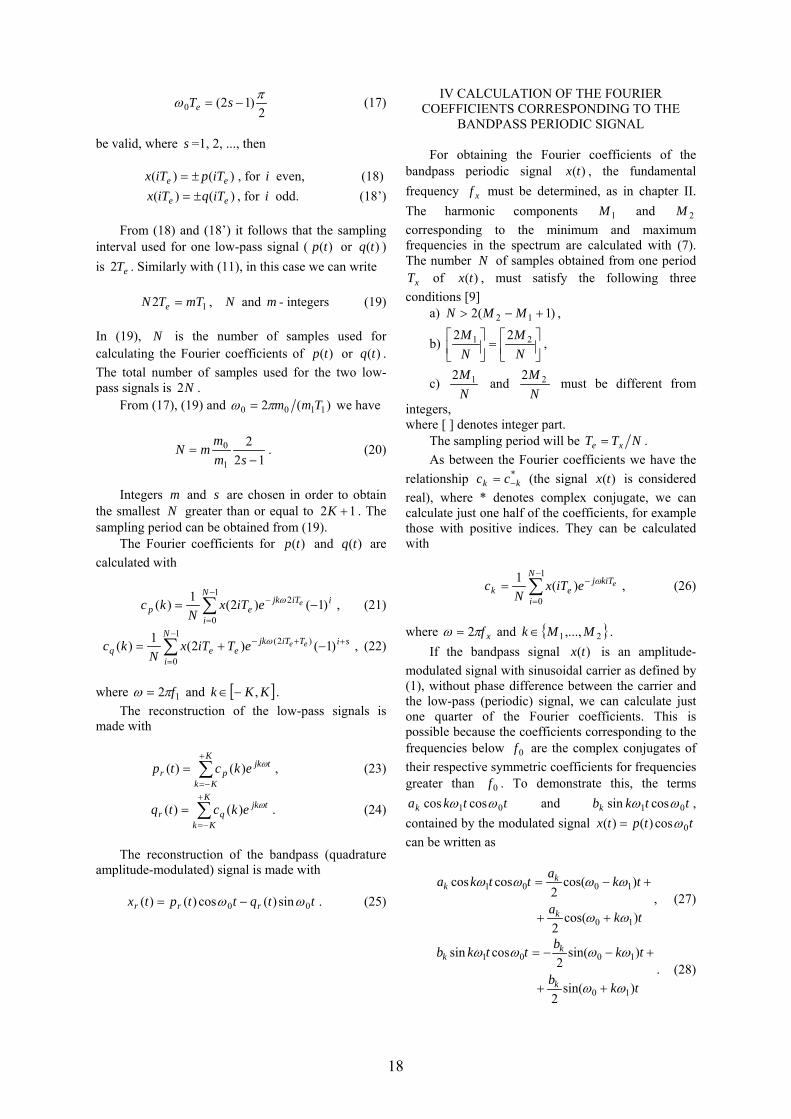

Buletinul Ştiinţific al Universităţii Politehnica din Timişoara
Seria ELECTRONICĂ şi TELECOMUNICAŢII TRANSACTIONS on ELECTRONICS and COMMUNICATIONS
Tom 48(62) Fascicola 2 2003
The Specific Absorption Rate of the Electromagnetic Radiation for Biological Structures in the Case of Mobile
Telephony
Adrian Vacircrtosu1
1 Facultatea de Electronică şi Telecomunicaţii Departamentul Măsurări şi Electronică Optică
ABSTRACT Cellular telephony uses a frequency domain ranging between 800 MHz and 2000 MHz with emission powers of 06W to 2W
The frequencies used have wavelengths that can be compared to the physical dimensions of the skull and the power emitted by portable phones is quite high around 06W Because of the proximity of the head (just a few centimeters away) with all the reflections from the surface of the skull and the attenuations that intervene the field intensities that manage to get inside the skull can induce in the cerebral mass currents of the same size with the intensities of normal biological currents
I INTRODUCTION The 5191999 recommendation of the Council
of Europe from the 12th of July 1999 concerning the limitation of public exposure to electromagnetic fields (from 0 Hz to 300 GHz) establishes the limits in values of physical units that characterize electromagnetic radiation at different frequencies The respective norms also called basic restrictions and reference levels establish safety coefficients in the case of electric magnetic and electromagnetic field exposure variable in time based directly on the obvious effects on health and biological considerations Depending on the field frequency the physical units used in order to specify the restrictions are the magnetic induction (B) the density of current (J) the specific absorption rate (SAR) and the power density (S) The SAR unit is used within the 100 kHz ndash 10 GHz frequency range to define the basic restrictions concerning the electromagnetic fields in order to prevent a generalized thermal stress of the body and an excessive localized heating of tissues
According to the 1999519CE 12th of July 1999 Recommendation the reference levels of
radiofrequency fields used in the GSM system are (table 1)
Table 1
Frequency (MHz)
Electric field
E (Vm)
Magnetic field H (Am)
Density of Power (Wmsup2)
900 41 011 45 1800 58 016 9
It is worth noticing that in the case of simultaneous exposure to different frequency fields there is a possibility that the effects of the exposure are cumulative As a convention each effect will be studied using separate calculations and based on the hypotheses separate evaluations of the effects of thermal and electric strain of the organism will be covered
Knowing the electric properties of biological environments is essential to the study of the interaction phenomena between these and the electromagnetic field The electrical properties involve permittivity and electric conduction
The magnetic properties (with some exceptions that do not concern the present paper) are not defined for the biological matter the relative permeability of biological entities is considered to equal a unit (micror= 1) and the losses obtained through the magnetic effect are thought to be negligible
The electric properties that intervene in the study of the biological effects of electromagnetic fields are the electric permittivity ε and the conduction σ defined over the unit of volume of matter Permittivity characterizes the interaction between the environment and the electromagnetic wave that is propagated through it The permittivity of free space is a constant εo and the permitivity of any other environment is a complex
20
measurement ( ) in which ε is an indicator of the property of the environment to store energy while ε indicates the property of the environment to dissipate the energy carried by the electromagnetic field
c jεεε minus=
Relative permittivity measures the net effect of the electric dipoles alignment that characterizes the intimate structure of the matter that is under the influence of an electric field applied from the outside
The energy dissipated per second per unit of volume of homogenous material by an electromagnetic wave incidence is proportionate to the square of the amplitude of the electric field component and is calculated with the help of this formula [1]
P = πf εoεE2 = σ E22 (1)
where σ is the conduction of the environment in which the dissipation of energy takes place The conduction is itself dependent on the frequency
All these parameters (σ ε or tan δ ) characterize the possibility of the environment to absorb the energy from the electromagnetic field
Calculating the values of the dielectric parameters (permittivity conduction wavelength intrinsic impedance penetration depth etc) that characterize the human tissues at the frequencies of 800 MHz and 900 MHz used by the Romanian mobile telephony was done by using a program in EXCEL based on formulas [2] [3] that allows for finding these measurements up to the frequency of 300 GHz
Formulas used in calculation of dielectric properties
complex permittivity
c jεεε minus= (2)
rel complex permittivity
0
εεεεε c
rrcr j =minus= (3)
0
ωεσε =r
ωσε =
permittivity of free space
Fm1085418781768 120
minustimes=ε permeability of free space
Hm104 70
minustimesπ=micro impedance of free space
Ω= 376730313Z 0 wave velocity in free space
ms 10 2997924581c 8
00
times=εmicro
=
angular frequency
f2 π=ω loss tangent of material
r
r
)(tanεε
=ωεσ
=ϑ (4)
propagation constant of material y = α+j β
)j(c
)j(j r
r
2
r2 εminusε⎟
⎠⎞
⎜⎝⎛ ω
microminus=ωε+σωmicro=γ (5)
attenuation constant of material
( ) ⎟⎟⎠
⎞⎜⎜⎝
⎛minusεε+
εmicro⎟⎠⎞
⎜⎝⎛ ω
=α 112c
2r
r
rr (6)
skin depth material
α=δ
1 (7)
phase constant of material
( ) ⎟⎟⎠
⎞⎜⎜⎝
⎛+εprimeε+
εmicro⎟⎠⎞
⎜⎝⎛ ω
=β 112c
2rr
rr (8)
wave velocity in material
βω
=u (9)
wavelength in material βπ
=λ2 (10)
intrinsic impedance of material
r
r
r0
c jZZ
εminusε
micro=
εmicro
= (11)
( ) 2502r
r
r
r0
1ZZ
⎥⎦⎤
⎢⎣⎡ εε+ε
micro= (12)
( ) ( )r
r
1tan21Zphase εε= minus (13) 00lephase(Z)le450
21
II RESULTS OF THE EXPERIMENT
The results of these calculations corresponding to the two bands are presented in the table 2 for f=800 MHz and in the table 3 for f=900 MHz
Table 2a
f=800 MHz micror = 1
TISSUE bone skin blood brain heart
εr 8688429 36212 5882646 464656 6067894
εr 0745467 1234021 2570435 1548868 2253825
σ (Sm) 0033178 0549214 1143998 0689339 1003087
tan(θ) 00858 0340777 0436952 0333337 0371434
α (1m) 2118257 1695389 2747556 1879632 2386113
β (1m) 4946731 1023108 1315008 1158271 1327692u (ms) 102E+08 49130166 38224479 43397013 37859280
λ (m) 0127017 0061413 0047781 0054246 0047324
δ (m) 0472086 0058984 0036396 0053202 0041909
|Ζ| (Ω) 1276914 6175043 4805721 5454375 4758779
Ζ (deg) 2451985 9408961 1180151 9217559 1018837
Table 2b
TISSUE muscle kidney liver lung spleen
εr 5411328 4761208 462569 3323576 5264076
εr 1430979 1890983 1815213 157899 2142521
σ (Sm) 0636871 0841601 0807879 0702745 0953551
tan(θ) 0264441 0397165 039242 0475088 0407008
α (1m) 1616963 2255025 219707 2237002 2427742
β (1m) 1243946 1178704 116132 992159 1240483u (ms) 40408097 42644715 43283050 50662729 40520887
λ (m) 005051 0053306 0054104 0063328 0050651
δ (m) 0061844 0044345 0045515 0044703 0041191
|Ζ| (Ω) 5078194 5360689 5440852 6370586 5093874
Ζ (deg) 7406157 1083061 1071302 1270591 1107336
Table 3a f= 900 MHz micror = 1
TISSUE bone skin blood brain heart
εrrsquo 8634636 3599427 5874271 4636694 6051015
εrrdquo 0818382 1133951 2333097 1421199 2071992
σ (Sm) 0040976 0567761 1168164 0711584 1037431
tan(θ) 0094779 0315037 0397172 0306511 0342421
α (1m) 2623734 1761374 2817931 1946225 2477099
β (1m) 5548936 1145292 1472909 1299078 1488052
TISSUE bone skin blood brain heart
u (ms) 102E+08 49374911 38392510 43529846 38001813
λ (m) 0113232 0054861 0042658 0048366 0042224
δ (m) 0381136 0056774 0035487 0051382 004037
|Ζ| (Ω) 1280628 6205502 4826162 5470811 4776366
Ζ (deg) 2707131 8743167 108308 8520446 9451129
Table 3b
TISSUE muscle kidney liver lung spleen
εr 5406606 4756672 4615513 3306596 5255305
εr 1333614 1714191 1650214 1440076 1950378
σ (Sm) 0667731 0858282 082625 0721035 097654
tan(θ) 0246664 0360376 0357536 0435516 0371126
α (1m) 1697889 2308073 2256177 2310114 2496166
β (1m) 1397314 1321244 1301189 1108984 1390013u (ms) 40469540 42799564 43459223 50991404 40682126
λ (m) 0044966 0047555 0048288 0056657 0045202
δ (m) 0058897 0043326 0044323 0043288 0040061
|Ζ| (Ω) 508583 5379605 5462482 6410789 5113597
Ζ (deg) 6928098 9908974 9836909 1176695 1018059 Formulas used for εr and εrrsquo are [2]
2
2
22
1
13
r
f1000f1
ff1 ⎟⎟
⎠
⎞⎜⎜⎝
⎛sdot
+
ε+
⎟⎟⎠
⎞⎜⎜⎝
⎛+
ε+ε=ε (14)
⎥⎥⎦
⎤
⎢⎢⎣
⎡⎟⎟⎠
⎞⎜⎜⎝
⎛sdot
+sdot
ε+
⎥⎥⎦
⎤
⎢⎢⎣
⎡⎟⎟⎠
⎞⎜⎜⎝
⎛+
ε+
sdotsdotπεσ
=ε2
22
22
11
1
0
0r
f1000f1f1000
f
ff1f
f1000f2
(15) The values of the units used in calculating these dielectric parameters are given in the table 4 [2]
Table 4a
TISSUE bone skin blood brain Heart
ε3 49 33 43 75 43
σo (Sm) 31E-07 0231 0768 0313 063
f1 (MHz) 2360 137 378 433 906
ε1 222 343 136 122 494
f2 (GHz) 204 177 213 165 156
ε2 18 32 543 387 559
22
Table 4b
TISSUE muscle kidney liver lung spleen
ε3 43 43 43 43 43
σo (Sm) 0301 0551 0406 0325 044
f1 (MHz) 83 247 442 818 266
ε1 475 166 136 691 289
f2 (GHz) 152 245 216 151 198
ε2 499 432 416 283 481
The external field incident to the biological structure can be expressed in terms of power density (mWcm2) of amplitude of the electric field component (Vm) or of the magnetic field component (Am) None of these parameters is appropriate for expressing the effects induced by the penetration of the electromagnetic radiation inside the biological domain Considering this situation a specific parameter has to be defined It is called the ldquoSpecific Absorption Rate ndash SARrdquo and it is the variation in time of the elementary energy quantity (dw) absorbed by an element of volume (dv) having a density (ρ) and an elementary mass (dm) [1]
⎟⎟⎠
⎞⎜⎜⎝
⎛=⎟
⎠⎞
⎜⎝⎛=
dVdW
dtd
dmdW
dtdkgWSAR
ρ)(
The Specific Absorption Rate (SAR) is correlated to the penetration depth (δ)in the tissues If the penetration depth (δ) is the distance from the surface of the tissue for which the amplitude of the electric field component reduces with factor e = 271 than the specific absorption rate at this depth reduces to a value equal to 135 of its initial value
Sometimes it is useful to define the depth d (frequently used in hyperthermia cases) at which the power incident to the surface of the irradiated structure is reduced to half (3 dB attenuation) Between (δ) and (d) there is the relation
d = 0345 x δ In order to determine the value of the SAR
parameter the TEMS (Test Mobile System) system was used This system was offered by the ORANGE firm and the measurements were taken at the frequency of 900 MHz
The applications of TEMS for an operational network are
bull it simulates and verifies possible changes in the network
bull it evaluates the quality of the received signal bull it measures the space covered range bull it tests the system (checks new or already
present functions)
- it signals in real time aberrant values of any parameter (for example the large number of interrupted calls)
- it identifies areas with problems of signal coverage or with high levels of interference
bull it presents the data in graphs maps The equipment used for measuring (Fig 1)
contains - special software made by Erricsson-TEMS
(Test Mobile System) - laptop mobile phone special data cable that
insures the PC-mobile phone connection
Fig1 The equipment used for measuring
The TEMS mobile phone is an Erricsson
ordinary phone that uses the TEMS program No supplementary calibrations are necessary for using the TEMS software
This mobile phone has four different operation modes
1 No Service (when it is in an area with no signal coverage)
2 Limited services (only emergency calls) 3 Inactive 4 Dedicate (during a conversation)
The measurements were taken during a
conversation therefore in the dedicate mode Taking the measurements involves - initiating a call - choosing the unit to be measured in this
case the power of the transmitted signal (TxPwr)
- the display of the unit to be measured (Fig2) and information about the distance from the base station (TA ndash Time Advance) the base station code (BSIC ndash Base Station Identity Code) local code (LAC Local Area Code) the channel of the communication (TCH ndash Traffic Channel)
23
In order to calculate the value of SAR the
situation when the telephone is in dedicated mode t0 is used At t0 these units have the following values
TxPwr =18dBm=625mW
TA = 2 d = TAx 500m Therefore the distance (d) to the base station is
1 km BSIC = 23 LAC = 05500
Fig2 The value of the SAR unit for the measured power is determined according to [1]
⎥⎦
⎤⎢⎣
⎡sdot=
=sdot
=ρ
=ρ
σ=
ρε primeprimeωε
=⎥⎦
⎤⎢⎣
⎡
minus
kgW1012550
1000062502P2EE
kgWSAR
3
22r0
where 0ε = permittivity of free space ω = angular frequency ρ = the density of the biologic environment asymp1000 kgm3
E = the intensity of the electric field P = πf εoεE2 = σ E22
Fm10E85418781768 120
minustimes=ε
0
r ωε
σ=ε
It is observed that the specific rate of absorption SAE is under the maximum admitted level of 04 Wkg
The value of SAR can also be determined according to the dielectric parameters ε σ and the electric field generated by the mobile phone In this case the system of measurement contains
bull electric field probe (Wandel amp Goltermann) with the EMR 20 measuring device
bull software for processing the values measured by the probe
bull mobile phone with without the antenna The measurements were done considering the following three positions for the measurement probe
bull positioning the electric field probe in the
speaker area bull positioning the electric field probe in the
inferior keys area bull positioning the electric field probe next to the
inner antenna behind the telephone or next to the extended antenna in the case of telephones with exterior antennas
The results obtained are succinctly presented in the table5 The maximum values of the electric field registered in each area of measurement and expressed in Vm are also presented
Table 5 Telephone type
with internal antenna with external antenna
Area Speaker
Micro-phone back speake
r
antenn
a On 981 668 1126 - 986
Called 2351 755 178 3677 2132
Calling 2142 1966 3398 2994 2418
Speaking
2871 197 3843 3672 282
S T A T E
Off 245 687 1032 -
III CONCLUSIONS
The following observations can be drawn on the
basis of the date from the table bull the internal antenna has directivity by having a
weaker emission in the area of the userrsquos head bull the emission is larger in the superior area of the
internal antenna phone bull the emission is stronger in the states where the
telephone is in contact with the head of the user (when he calls and speaks) the antenna type does not matter
bull the telephone with an external antenna has a stronger emission at the level of the speaker than at the extremity of the antenna
bull the telephone with an external antenna does not have a weaker emission at the level of the speaker in comparison to the internal antenna telephone
24
The difference in values from the experimental data provided by our bibliography and from the theoretical models is due to the various uncertainty factors that are linked to the measurements in a close-range field and the digital character of the signal
bull the size of the detecting field unit that disturbs the measuring field
bull the link between the measuring probe and the emission antenna of the telephone
bull the measuring technique of the digital signal
It was observed that at low levels of power density some effects take place after a longer exposure time They are called ldquolow level power effectsrdquo or ldquoathermic effectsrdquo effects that also appear in the case of using mobile phones It is best to consider the following recommendations even if the SAR value is situated between the limits established by the European Commission
bull to reduce using mobile phones in conditions of low signal
bull to avoid wearing mobile phones close to the sensitive tissues
bull using car kits bull constantly informing the population of the
level of radiation around the base stations by operating frequent measurements that would be accessible to the public
The conclusion is that the general objective should be to reduce the degree of exposure of the population to radiofrequency fields
IV BIBLIOGRAPHY
[1] ZAMFIRESCU MIHAIL SAJIN GH RUSU IONSAJIN MARIA KOVACS EUGENIA ndash Efectele biologice ale radiaţiilor electromagnetice de radiofrecvenţă şi microunde Editura Medicală 2000 [2] GABRIEL C (1996) Compilation of the dielectric properties of body tissues at RF and microwave frequencies Brooks Air Force Base report no ALOE-TR-1996-0037 [3] HURT WD (1996) Radiofrequency radiation dosimetry workshop Brooks Air Force Base report no ALOE-SR-1996-0003 [4] SADIKU MNO (1994) Elements of Electromagnetics Saunders College Publishing New York [5] HOMBACH V Comparison of different human head models XXVth General Assembly of the International Union of Radio Science August 28 - Sept 5 1996 Lille France
25
Buletinul Ştiinţific al Universităţii Politehnica din Timişoara
Seria ELECTRONICĂ şi TELECOMUNICAŢII TRANSACTIONS on ELECTRONICS and COMMUNICATIONS
Tom 48(62) Fascicola 2 2003
The Cyclic Prefix Length Influence on OFDM-Transmission BER
Marius Oltean1 Miranda Naforniţă1
Abstract Orthogonal Frequency Division Multiplexing (OFDM) is one of the recent years equalization approaches used in order to combat the inter-symbol interference introduced by the frequency selectivity of the radio channels The circular extension of the data symbol commonly referred to as cyclic prefix is one of the key elements in an OFDM transmission scheme The influence of the cyclic prefix duration on the BER performance of an OFDM system with in-frame DBPSK modulation is evaluated by means of computer simulation in a multipath fading channel
I INTRODUCTION Mobile radio communication systems are increasingly required to offer a variety of services and qualities for mobile users Unfortunately the radio channel is far from an ideal transmission medium exhibiting both frequency selectivity and time variant character [1] In this context one of the most challenging issues in a radio communication system is to overcome the inter-symbol interference introduced by the multipath propagation of the signal between the transmitter and the receiverrsquos antennas The use of the adaptive equalization to the receiver could be the solution for avoiding this unwanted phenomenon but this complex equalization technique proves oftentimes unsuited for being used in real-time applications at data rates of tens of Mbps in an unfriendly dispersive radio channel environment because of its important computational complexity OFDM is an optimal version of multicarrier modulation techniques which mitigates the effect of the ISI phenomenon keeping a relatively reduced complexity of the equalization process Indeed intuitively one can assume that the frequency selectivity of the channel can be mitigated if instead of transmitting a single high rate serial data stream the transmission is performed simultaneously using several narrow-band subchannels (with a different carrier corresponding to each subchannel) on which the frequency response of the channel looks ldquoflatrdquo
Hence for a given overall data rate increasing the number of carriers reduces the data rate that each individual carrier must convey therefore lengthening the duration of the symbol that modulates each individual subcarrier [2] Slow data rate (and long symbol duration) on each subchannel merely means that the effects of ISI are severely reduced In addition a cyclic prefix is inserted in front of each OFDM symbol This circular extension that is discarded on the receiver side is obtained by copying a number of samples from the end of the OFDM symbol in front of it in order to prevent two consecutive frames to interfere each other as a result of the time dispersion caused by the multipath propagation This way the receiver can independently process each frame in order to estimate the transmitted information Furthermore the equalization process is facilitated by this operation of cyclic prefix insertion and extraction In this chapter we focus on the influence of the cyclic prefix duration on the BER performance of an OFDM system with in-frame DBPSK modulation The performance evaluation in Rice fading conditions is done by means of computer simulation
II THE BLOCK-DIAGRAM OF OFDM
TRANSMISSION SCHEME
In the figure 1 a classical OFDM transmission scheme using FFT (Fast Fourier Transform) is illustrated
The input data sequence is baseband modulated using a digital modulation scheme Various modulation schemes could generally be employed such as BPSK QPSK (also with their differential form) and QAM with several different signal constellations In our system DBPSK method is chosen in order to encode the binary information Data is encoded bdquoin-framerdquo (the baseband signal modulation is performed on the serial data that is inside of what we name a bdquoDFT framerdquo or equivalently an OFDM symbol) The data symbols 1 Univ ldquoPolitehnicardquo Timişoara Facultatea de Electronică şi TelecomunicaţiiDepartamentul Comunicaţii
26
Information symbols
Serial to parallel
converter
Coding amp baseband
modulation
IFFT modulator
Cyclic prefix insertion
Parallel to serial
converterX
ej2πfct
Channel
X
ej2πfct
Serial to parallel
converter
Cyclic prefix extraction
FFT demodulator
Decoding amp demodulation
Parallel to serial
converter
Estimated symbols
Xk k=0hellipN-1
[Xk] k=0hellipN-1
[xk] k=0hellipN-1
[xcpk] k=-LhellipN-1
[ycpk] k=-LhellipN-1
[yk] k=0hellipN-1
[Yk] k=0hellipN-1
Yk k=0hellipN-1
Fig1 The block diagram of an OFDM System
are parallelized in N different substreams Each substream will modulate a separate carrier through the IFFT modulation block which actually generates the OFDM symbol performing the multicarrier modulation A cyclic prefix is inserted in order to eliminate the inter-symbol and inter-block interference (IBI) [3] The data are back-serial converted forming an OFDM symbol that will modulate a high-frequency carrier before its transmission through the channel The radio channel is generally referred to as a linear time-variant system To the receiver the inverse operations are performed in order to estimate the transmitted symbols
III THE CYCLIC PREFIX AND THE EQUALIZATION PROCESS
Since OFDM transmits data in blocks (usually a block is referred to as an bdquoOFDM symbolrdquo) any type of a non-ideal transmission channel (such as a multipath channel in mobile communication systems or a classical dispersive channel as in wired transmissions) will bdquospreadrdquo the OFDM symbol causing the blocks of signal to interfere one another This type of interference is called Inter-Block Interference IBI could lead to inter-symbol interference since two adjacent blocks will overlap causing the distortion of the samples affected by overlapping
In order to combat this interference we could use a cyclic prefix (CP) at the beginning of each symbol If the cyclic prefix spans more than the multipath channel impulse response the interference caused by the time dispersion of the previous transmitted block is entirely absorbed by the prefix samples that are discarded to the receiver The cyclic prefix consists of the last L samples of the OFDM symbol that are copied in front of the data block [4] as we can see in the figure 2 Generally the radio channel exhibits both time variant and frequency selective characteristics If we shall consider however that the channel parameters remain unchanged during the transmission of an OFDM symbol the way that the transmission medium distorts each particular frame is similar to the distortion caused by an
electronic filter [1][5] Under this assumption we can consider the equivalent discrete response of the channel as a linear FIR filter of order L of which the equation is given below
sum=
minussdot=L
n
nznczC0
][)( (1)
The equivalent baseband signal at the channel output can be obtained by the operation of convolution as follows
][][][ ncnxcpnycp = (2)
Discarding the L CP samples from the received sequence the remaining (useful) signal can be expressed as
where ldquo⊛rdquo denotes the circular convolution operator [6] The noticeable thing about the equation 6 is that the circular convolution preserves the temporal support of the signal In our case N transmitted signal samples convolved with L+1 channel impulse response samples will conduce to a received symbol of length N that will be used in the demodulation process Since the circular convolution will not ldquospreadrdquo the signal the receiver can independently process each data block The interference from the
y[n]=x[n] ⊛c[n] (3)
OFDM Symbol
Copy
CP
Transmitted sequence= OFDM symbol+CP
t
Fig2 The cyclic prefix insertion
27
previous transmitted blocks is totally eliminated through this operation of CP insertionextraction Furthermore since x[n]=IDFTX[k] and taking into account the effect of the DFT demodulator the received symbols Y[k] can be expressed as
Y[k]=DFTIDF TX[k] ⊛c[n] k=01hellipN-1 (4)
Since the DFT of a circular convolution of two discrete time signals will conduce to a spectral multiplication
110][][][][][
minus=sdot==sdot=
NkkCkXncDFTkXIDFTDFTkY
(5)
where C[k] represents the sampled frequency response of the equivalent baseband discrete channel corresponding to the frequencies Ωk=k(2πN) The crucial consequence of the relation above is that each modulation symbol X[k] could be recovered to the receiver by a simple pointwise division operation commonly referred to as a ldquoone-tap frequency domain equalizerrdquo as can be seen from the relation (6)
110][][][ 1 minus=sdot= minusandNkkCkYkX (6)
Thus the CP theoretically eliminates both IBI (each block preserves its temporal support) and inter-carrier interference (ICI) (each serial symbol received on the k-th carrier will depend only on the corresponding k-th carrier transmitted symbol not being affected by the adjacent carriers) IV SIMULATION RESULTS AND DISCUSSIONS
1 SIMULATION PARAMETERS
The goal of the simulations was to emphasize the effect of the cyclic prefix duration on the BER performance of an OFDM system with inter-frame DBPSK modulation The radio channel was modeled as a three-ray Rice fading channel with one deterministic line-of-sight (LOS) path and two multipath delayed components The relative delays of the two components are τ1 and τ2 respectively However in most of these simulations it was considered τ1=0 and a normalized delay for τ2 denoted τ2N=τ2LCP LCP represents the cyclic prefix duration expressed as the number of serial samples that compose the cyclic prefix An important parameter for the Rice fading channel is K=PLOSPD which stands for the ratio between the signal power carried by the LOS path (PLOS) and the total power of the two multipath components (PS=P1+P2) Equal power for the two multipath components was considered during the simulations A white gaussian noise is added to the signal at the output of the Rice
fading channel The time interval between the moments in which the first and the last significant component of the multipath signal arrives to the receiver is referred to as maximum excess delay (TM) and it is expressed in number of serial samples (remember that N signal samples generated by the IFFT modulator will compose an OFDM frame) Another parameter of the simulation is the number of subcarriers N that equals the number of serial samples composing an OFDM symbol The time variant character of the radio channel is quantified by the maximum Doppler shift parameter fD The value of this parameter is also expressed in a normalized manner as fDTS TS denoting the OFDM symbol duration A robust differential modulation scheme such as DBPSK was chosen for encoding the binary information No channel estimation techniques are employed and consequently no further equalization is done to the receiver
2 RESULTS AND DISCUSSIONS For the first simulations the relative delay of the second multipath was normalized by the serial symbol duration As can be seen from the figure 3 increasing the cyclic prefix duration improves the BER performance for the OFDM system
Theoretically if the cyclic prefix duration spans more than the maximum delay spread of the channel the errors can be completely eliminated This assumes however a perfect knowledge of the channel impulse response (or equivalently of the channel transfer function) which is a mandatory condition for implementing the equation 6 Since in our implementation no channel estimation techniques are employed the exact form of the channel impulse response doesnrsquot constitute information that can be exploited in the data estimation process The correct
Fig 3 The influence of the cyclic prefix duration on BER performance for DBPSK-OFDM system
Rice fading channel K=3dB SNR=30dB N=64 fDTS=0001
28
detection is entirely based on the robustness and simplicity of the digital modulation scheme that is involved namely DBPSK This explains why the BER is not completely eliminated for a cyclic prefix of theoretically sufficient duration (longer than TM) A noticeable thing resulting from the figure 3 is that while identical for cyclic prefix lengths which cover the channel impulse response the performance degrades for the cases where the cyclic prefix duration becomes insufficient Thus if a cyclic prefix of length LCP=4 is used the transmission offers the best performance between all the considered situations but only starting with a value of the normalized delay that overtakes the length of the circular extension for all the other cases Next we studied the BER performance against the normalized delay of the second multipath which is obtained this time as explained in the previous subsection It can be observed from the figure 4 that increasing the OFDM symbol length improves the performance of the system which confirms [6] In the same time it is proven that the BER is sensitive to the multipath delay spread of the channel
normalized by the cyclic prefix duration Thus as observed in the figure 4a) a two times longer OFDM symbol is needed in order to obtain the same performance when the normalized delay of the second multipath is two times higher (note that for the same value of τ2N on the abscissa τ2 doubles its value when LCP=2) The observation is confirmed by the figure 4b) where the BER curve in the case N=16 LCP=1 is almost identical with the curve plotted for a frame of length N=64 with a cyclic prefix LCP=4 The conclusion that can be drawn from these observations is that at identical ratios between the channel impulse response and the cyclic prefix duration the in-frame OFDM system performance remains sensitive to the effective value of the multipath (or maximum) delay spread parameter (τ2 in our case)
3 CONCLUSIONS
The cyclic prefix duration influences the performances of an OFDM system even if the explicit form of the channel impulse response is unknown and consequently cannot be used in the equalization process The transmission is sensitive to the parameter obtained as the multipath delay of the channel normalized by the cyclic prefix duration The BER performance is in all cases improved by increasing the OFDM symbol length
REFERENCES
[1] B Sklar Rayleigh Fading Channels in Mobile Digital Communication Systems- Part I Characterization IEEE Commun Mag July 1997 [2] Dusan MaticOFDM as a possible modulation technique for multimedia applications in the range of mm waves 10-30-38 TUD-TVS available on-line wwwubicomtudelftnlMMCDocsintroOFDMpdf [3]Werner Henkel Georg Tauboumlck Per Oumllding The cyclic prefix of OFDMDMT ndash an analysis 2002 International Zuumlrich Seminar on Broadband Communications February 19-21 Zuumlrich Switzerland [4]Lu J Tjhung TT Adachi F BER performance of OFDM system in frequency-selective Rician fading with diversity reception available online httpwwwcwcnusedusg~cwcpubzfilesict97_2pdf [5] B Sklar Rayleigh Fading Channels in Mobile Digital Communication Systems- Part II Mitigation IEEE Commun Mag July 1997 [6 ]Chini A Analysis and Simulation of Multicarrier Modulation in Frequency Selective Fading Channels Ph D Thesis 1994 Chapter 3
a)
b)
Fig 4 (ab) The influence of the normalized delay of the second multipath on BER performance for DBPSK-OFDM
system Rice fading channel K=3dB SNR=40dB fDTS=0001
29
Buletinul Ştiinţific al Universităţii Politehnica din Timişoara
Seria ELECTRONICĂ şi TELECOMUNICAŢII TRANSACTIONS on ELECTRONICS and COMMUNICATIONS
Tom 48(62) Fascicola 2 2003
Methods for JPEG image protection by partial encryption Florin Vancea1 Codruţa Vancea2
1 University of Oradea Faculty of Electrotechnics and Informatics Computer Science Department str Armatei Romacircne nr 5 Oradea e-mail fvanceauoradearo 2 University of Oradea Faculty of Electrotechnics and Informatics EMUEE Department str Armatei Romacircne nr 5 Oradea e-mail cvanceauoradearo
Abstract ndash The JPEG format used in static image transfer and storage exhibits some particularities when considered for encryption A commercially useful encryption must degrade the image but keep it within evaluation limits Classical encryption techniques can be applied to a JPEG stream in various phases of its construction and to different segments We evaluate the impact of some alternatives testing on real cases Potential future directions are identified Keywords encryption JPEG DCT
I INTRODUCTION
A significant part of the information transmitted in data networks and stored in computer systems today is represented by images be they static or in motion The need to protect this information against unauthorized access and usage requires no further proof In order to protect text-based information various methods have been devised based on the general theory of encrypting binary information [1] Since images are stored and transported in binary form too we can directly apply known encryption methods to protect them The disadvantage of such approach is that itrsquos too rigid the image becomes unintelligible In copy-protection schemes or in controlled distribution schemes one would like a partial and controlled accessibility to image content Encryption key holders will be able to see and use the image to its normal parameters and potential unauthorized users get access to a degraded version understandable but unusable for any purposes but identification of its value A distribution scheme using such a mechanism can thus publish an electronic catalogue and interested users will only pay for the keys needed to decrypt the images they need The images are transmitted and stored using various formats Generally one is looking to compress the raw information content but this can be achieved in various ways Some methods are using color space reduction by using color tables others are applying compression methods to the raw bitstream resulted from sampling the color information at maximum
capability level Some are using lossless compression techniques others are taking advantage of the particular behavior of the final recipient ndash the human eye The latter use lossy compression where the information cannot be exactly recovered but the resulting quality can be extremely good from the perception point of view and the compression ratio is greatly improved
II THE JPEG STREAM FORMAT
One of the frequently used formats in storing and transmitting still images is the the format proposed by the Joint Photographic Experts Group ndash JPEG standardized in recommendation T81 of ITU-T [2] The recommendation is specifying how to transform the original input image (organized in component planes) to obtain the compressed byte stream Below we will review the JPEG encodingcompression process emphasizing the details that may impact the encryption process Esentially the original information is transformed (if necessary) to an alternative representation space having luminance and chrominance components The chrominance components have lower importance in achieving the perceived quality and can be sampled with a less detailed rate Therefore we will obtain several samples from the luminance component for one sample in a chrominance component Each componentrsquos pack of samples is divided in 8x8 blocks to be transformed with a DCT transformation The DCT process is lossless (except for the rounding errors) but the resulting amount of information is still comparable to the original one obtained after the discriminating sampling In order to achieve compression adapted to human perception the resulting DCT coefficients are quantized differently The coefficients corresponding to higher spatial frequencies can be reproduced with lower precision to obtain a good compromise between the number of bits required in the output stream and
30
the need to reproduce faithfully the image Discrimination between quantization levels is made through quantization tables different for different components These tables must be attached to the transmitted or stored stream and usually have a predictible distribution The output of the quantization step still has considerable redundancy mainly presented as many coefficients being zero The standard specifies a zig-zag ordering scheme that puts the higher-frequency coefficients together and an encoding scheme that skips the zero coefficients and encodes only the non-zero ones using Huffmanrsquos method The resulting Huffman tables are also attached to the data stream and they have a highly predictible structure too Other encoding schemes using arithmetic compression exist but they are limited in extent due to them being subject to licensing issues In the following we will only consider the widespread Huffman-based encoding scheme The binary stream defined by JPEG has a well-defined structure delimited by special sequences named markers These markers can be used to check and eventually recover the synchronization upon decoding From our point of view in order to make reference to the encryption solutions the structure of the JPEG binary stream is represented in Fig 1
Quantization tables
Huffman symbol tables
Structural informationsize component definitions sampling rates
Quantized DCT coefficients Huffman-encoded
MicroheaderByte with zero-count and
it-count Huffman-encoded
Coefficient bits withoutHuffman encoding
Non-image information
Fig 1 Structura of JPEG stream (for encryption)
We can see that the coefficient stream contains only the non-zero coefficients Each non-zero coefficient is introduced by a microheader (Huffman encoded byte) followed by a variable number of unencoded bits (at most 16 bits) representing the actual coefficient The byte contains 4 bits giving the previous skipped zero coefficients and 4 bits giving the coefficientrsquos bitcount When the count of zero coefficient in a span overflow the limit of 16 additional microheaders are attached without any data bits
III ENCRYPTION METHOD
We set our goal to find a suitable encryption method for JPEG-encoded images The method should controllably degrade the image beyond commercial usability but not beyond recognition It should also preserve the image structure so the resulting image will be processable with standard tools especially for
viewing purposes Such a constraint allows the usage of any JPEG-compliant tool in transmission storage and presentation Below we will analyze different candidate methods for solving the above-described problem A Direct encryption of JPEG stream
Encrypting the entire stream goes right out of question because it destroys the logical structure described above and the result is unusable unless decrypted This method violates the initial assumption that the encrypted image is recognizable but unusable B Encrypting the original image
Encrypting the original image means fully extracting the original image from the JPEG stream encrypting its binary form with some method and repacking the result into a new JPEG stream The method is not applicable because - By encrypting the image its statistical structure is
radically changed Any efficient encryption algorithm should produce an output stream without detectable redundancy and the JPEG encoding is making use exactly of some particular kind of redundancy in the input image (photographic image redundancy)
- The process is not perfectly reversible The JPEG compression method is a lossy one At decoding time reconstruction of the original encrypted image will be only an approximation and the decryption is expected to be seriously affected Usual encryptiondecryption algorithms will produce wildly different decryption results for minor changes in ciphertext The algorithms used should be error-tolerant and this commonly means weaker ones
- The JPEG decoding-encoding cycle even without any encryption in-between is lossy The image quality is degraded and non-recoverable Generally each decoding-encoding cycle is impacting the image quality
There is a variation to this method when only part of the bitplanes in the original image are encrypted The method is analyzed in [3] and the conclusion is that in order to avoid attacks one must encrypt at least two of the most significant bitplanes Image degrading after encrypting two significant bitplanes is considerable and the above objections still hold so the method is not suitable for our purpose C Partial encryption of JPEG stream
It is clear that we will have to identify the segments of the stream suitable for encrypting with minimal effort and without adverse impact on compatibility while achieving the desired degrading effect Encrypting the non-image information is not useful to us but the fact that the standard accepts such blocks of information may be useful One can add a non-image information to resulting stream holding any kind of
31
extra information required for decrypting (we are not talking about the key of course) Any processing program on the delivery chain should silently ignore this kind of information We must also note that these blocks might contain reduced versions of the original image (thumbnails) If not protected or eliminated they might be used by an attacker to recover the original image information or might be even used directly as a smaller version of the protected image Encrypting the quantization tables may lead to a significant degradation of the image quality but the quantization tables are highly predictible Some images are using even the original tables recommended by the JPEG committee so encription would be useless Encrypting the Huffman tables is not useful because their structure is also highly predictible Moreover encrypting them would introduce structure inconsistencies because the encrypted text will obviously not represent a valid Huffman table Permutation-like operations controlled by the key are also not useful because the standard specifies a clear order in generating the Huffman symbols and the permutation itself is straightforward reversable Encrypting the structure information is also not acceptable because any modification in this area will produce an incompatible stream Moreover the information here is important for evaluating the image fitness for the purpose and encrypting them will contradict the commercal target adopted initially The only option is to encrypt the Huffman-encoded DCT coefficients Encrypting them directly as a binary stream will be unacceptable again because it destroys the structure outlined in Fig 1 Any decoder will expect microheader-data pairs and the microheader should be Huffman-encoded As Huffman decoding is normally incomplete (meaning that not any bit sequence has a valid symbol attached) it is possible that the directly encrypted stream will produce errors in the decoding proces maybe even ones that are fatal to the decoder Even if we ignore this problem the overall number of coefficients resulting from the decoding process is composed from the number of zero coefficients plus the number of non-zero coefficients and is verifiable against the specified image size and sampling rates Huffman-decoding the encrypted sequence will surely violate this constraint having again potential fatal consequences for the decoder The only remaining options are a) to apply partial manipulation on the bitstream such as to preserve the microheader structure or b) to Huffman decode then encrypt then Huffman recode right back D Selective encryption of coefficient data bits
The most attractive method is to selectively encrypt the bits holding the coefficients values while preserving the microheaders [4] Such a method is keeping the binary stream structure preserving perfect
JPEG compatibility while degrading the quality of the encrypted image version Degradation is perfectly recoverable through decryption with the obvious provision that the encrypted image was not processed in the meantime The method has the additional advantage that it can be performed in a single step as streamed processing The structure of original image is analyzed as it enters the encryption device The elements that should not be modified are passed directly to the output The encryptable elements (coefficient bits) are encrypted with a stream cipher and the result is injected into the output instead of the original bits We should note that the overall size of data is neither increased nor decreased (except minor variations due to standard escaping rules specified in the standard) If we also use an auto-decrypting cipher (eg XOR) the process is identical for both encryption and decryption The process is described in Fig 2
Structure analizer
Streamencryption
Key Fig 2 Selective stream encryption
E Encrypting through idempotent manipulations in
microheader-data pairs
Another possibility identified is to alter the coefficient sequence by applying idempotent (with respect to the structural compliance) manipulations to a span of encoded coefficients As long as we observe the constraint that the overall number of resulting coefficients (both zero and non-zero) is coherent with the number determined from the structural information we can apply key-controlled permutations in a correctly chosen coefficient sequence altering the place where the coefficients are decoded The result is a degraded but structurally correct image The method is harder to apply because it requires storage and many of the potential permutations are idempotent from the image point of view too (think about swapping equal coefficients) We also have to account for interleaving of different components normally encoded with different Huffman tables because we must preserve Huffman decoding coherence Our target must be to change the place of coefficients within the same Huffman decoding space The method has the advantage that it produces deeper changes in image since it traverses the 8x8 block boundaries without changing the statistic distribution thus without requiring a Huffman table regeneration
32
F Encrypting ldquobehind compressionrdquo
A more general version of the above method means Huffman decompression encrypting the coefficients and Huffman recompression The freedom of transformation in this case is improved but the complexity price is higher too A simple approach may use the original Huffman tables so partial stream processing is possible Unfortunately a common encryption procedure applied to coefficient blocks will ruin their zero-rich structure The first consequence is that the original Huffman tables are not statistically correct anymore and recoding with original tables (if possible at all) would introduce an information leak The second consequence is that the compression efficiency may drop drastically even if we regenerate the Huffman tables Finally the strong redundancy induced by the original zero-sequences will significantly affect the overall encryption strength there will be a great risk of known plaintext attacks In order to use this method we should choose encryption algorithms with increased resistance to known plaintext attacks
IV OBSERVATIONS
When applying any of the above-described methods we should take into account the desired and accepted image degradation level Generally encrypting directly the DC coefficients is not recommended because the image degrading is too high Moreover the coefficients are stored using a differential scheme which can be easily saturated when encrypting undiscriminately The simpler path is to focus on AC coefficients Out of those we must keep some in unencrypted form in order to preserve part of original image quality for evaluation purposes The number of unencrypted coefficients to keep depends on the desired and accepted degree of image degradation We can see that some images have right from the start such a compression level that even encrypting all AC coefficients is not providing enough degradation Explanation of this is found in the particular structure of the cofficients resulting from the quantization step For an image with aggresive quantization many of the coefficients have a very limited number of bits Encrypting selectively those bits will preserve the number of bits but will replace with (ideally) 05 probability each bit with its opposite It is clear that for an aggresively quantized image (many 1-bit coefficients) we have a 50 chance that the coefficient is unaffected The selective encryption of coefficient bits exhibits another disadvantage any encryption effect is local to the 8x8 block holding the coefficients This is good for the encrypted image inteligibility but induces a cryptographic weakness Any normal image has lots of correlation between neighbouring blocks and this can be used by a potential attacker
V IMPLEMENTATION
To illustrate the above ideas we implemented the selective encryption of coefficient bits method and a simple version of idempotent manipulation behind compression Encryption itself is not important for these evaluations so we used XOR with a bitstream resulted from a CBC generator having null plaintext Selective encryption led to fairly good results but as expected there are images for which the method is ineffective Fig 3 represents an image with rich detail (ldquoparrotsrdquo) in its original version Fig 4 şi Fig 5 are presenting the same image encrypted while preserving 2 and respectively 5 of the AC coefficients The results are consistent with our expectations The image degradation is controllable and deep enough even when preserving 4 AC coefficients
Fig 3 ldquoparrotsrdquo original
Fig 4 ldquoparrotsrdquo 5 unencrypted AC coefficients
Fig 5 ldquoparrotsrdquo 2 unencrypted AC coefficients
33
Fig 6 ldquomarsrdquo original
Fig 7 ldquomarsrdquo 5 unencrypted AC coefficients
Fig 8 ldquomarsrdquo 2 unencrypted AC coefficients
The original bdquomarsrdquo image in Fig 6 has a lower detail content per 8x8 JPEG block The image is also larger in pixel size Its encrypted versions are represented in Fig 7 şi Fig 8 Even if we preserve only 2 AC coefficients the image is not degraded enough to impact its value We implemented also a simple implementation of keyed idempotent manipulation behind compression Several manipulation schemes were tried - key-controlled permutation of coefficients within
a 8x8 block - key-controlled permutation of coefficients across
blocks within the same JPEG scan preserving the coefficient position in the frequency domain
- key-controlled permutation of coefficients across blocks within the same JPEG scan with intentional breaking of its position in the frequency domain
All the schemes described above were concentrating on reducing to a minimum the impact on the entropy content before compresion in order to achieve a comparable stream size after encryption The tested schemes have produced inconcludent results (low protection degree significantly increased run times) The complexity of the processing software was also significantly higher The above results does not void the eligibility of the encryption behind compression method We assume that these results were obtained due to insufficient study of the method Some approach closer to the perception specifics when considering the encryption process may bring important improvements in this direction
VI CONCLUSIONS
Encrypting image information while preserving the general visual features poses multiple problems but is an interesting domain due to the potential applications We have analyzed some of the methods usable for the wide-spread JPEG format and we have implemented some of the promising ones During the implementation we found out that current methods are not offering consistent results for all types of images Moreover simple treatments like selective encryption of the AC coefficient bits feature potential weaknesses to continuity attacks We must say that achieving the proposed goal (protection of the image content while keeping the evaluation possibility) requires giving up the some advantages like single-step stream processing and size preservation If we drop such requirements there are some methods promising adequate protection adjusted to human perception Future work will analyze how one can exploit the subjective image information content to control the encryption process into obtaining convenient protection
34
REFERENCES
[1] B Schneier ldquoApplied cryptographyrdquo John Wiley amp Sons second edition 1996 [2] The International Telegraph And Telephone Consultative Committee ndash ldquoDigital Compression and Coding of Continuous-Tone Still Images ndash Requirements and Guidelinesrdquo - Recommendation T81 [3] T Maples G Spanos ldquoPerformance study of a selective encryption scheme for the security of networked real-time videordquo Proceedings of the 4th International Conference on Computer Communications and Networks Las Vegas Nevada September 1995 [4] M v Droogenbroeck R Benedett ldquoTechniques for a selective encryption of uncompressed and compressed imagesrdquo ACIVS Advanced Concepts for Intelligent Vision Systems Ghent Belgium pages 90-97 September 2002 [5] H Chang X Li ldquoOn the Application of Image Decomposition to Image Compression and Encryptionrdquo 1996 [6] M Podesser Hans-Peter Schmidt and Andreas Uhl ldquoSelective Bitplane Encryption For Secure Transmission Of Image Data In Mobile Environmentsrdquo Proceedings NORSIG-2002 [7] T Uehara R Safavi-Naini P Ogunbona ldquoSecuring wavelet compression with random permutationsrdquo Proceedings of the 2000 IEEE Pacific Rim Conference on Multimedia pages 332ndash335 Sydney Dec 2000 IEEE Signal Processing Society
35
Buletinul Ştiinţific al Universităţii Politehnica din Timişoara
Seria ELECTRONICĂ şi TELECOMUNICAŢII TRANSACTIONS on ELECTRONICS and COMMUNICATIONS
Tom 48(62) Fascicola 2 2003
Computing Wavelet Transform from Short Time Fourier Transform
i Moldovan Maria Simina1
1 Facultatea de Electronică şi Telecomunicaţii Departamentul Comunicaţii Str Observator Nr 34 Cluj-Napoca e-mail siminamemailro
Wavelet Transform is a relative new analysis technique developed as an alternative for Short Time Fourier Transform which is proved to be superior for several applications Energetic aspects of the two transform ie spectrogram and scalogram are the applications that represents the task of the actual paper An interesting problem is the mapping between the spectrogram and the scalogram To be more specific we are interested to develop an algorithm through which the Wavelet coefficients can be computed directly from STFT coefficients without reconstructing I INTRODUCTION Time-frequency representations may be a useful tool for the visual analysis of signals as they provide information not available from time- or frequency-domain representations alone such as the time variations of the spectrum of the signal or of its power spectrum which translate in distinctive patterns on a time-frequency plot Recently applications of wavelet analysis are widespread and cover many fields of scientific research including medical science (the ECG EEG EMG Echocardiograms clinical sounds-arterial bruits heart sounds breath sounds respiratory patterns blood pressure trends DNA sequences) geophysics engineering image analysis financial analysis There has been developed a code that allow the examination of the signals energy distribution in time-frequency respectively time-scale domains The Fourier spectrogram is a very common tool in signal analysis It gives a description of both time and frequency distribution of the energy in the signal by shifting a window through the signal and taking out the Fourier Transform of the windowed portions The window length determines the time-frequency resolution The scalogram is a more elegant version of time-frequency representation that can be found from the Continuous Wavelet Transform Both the spectrogram and the scalogram produce a more or less easily interpretable visual two-dimensional representation of signals
A lot of spectrograms of the signals are available so we are interesting in a way to construct the scalogram for a given spectrogram To accomplish this goal we need to find out a possible link between Short Time Fourier Transform and Wavelet Transform In order to determine the efficiency of the computing method the obtained coefficients were compared with one resulted from the classical analysis method II SPECTROGRAM AND SCALOGRAM The spectrogram has been the traditional tool for the speech analysis for over 50 years STFT gives a description of both the time and frequency characteristics of the signal The mathematical definitions of the continuous time are given below
dtetgtxSTFTR
tjint Ωminuslowast minus=Ω )()()( ττ (1)
The time-frequency resolution of the STFT is subject of the Heisenberg Uncertainty Principle which states that the product of the standard deviation in time and frequency is limited by
π41
ge∆sdot∆ ft (2)
The discrete STFT is constructed by multiplying a portion of the signal by a window function w[m] of length L Its Fourier Transform is computed and then the window is shifted bdquonrdquo positions along the signal and the process is repeated The Fast Fourier Transform (FFT) is the preferable FT implementation in these computations The Fourier spectrogram is defined as the square modulus of the STFT
2)( )()( ττ Ω=Ω= gx
gxS STFTSPECP (3)
36
The common method of analysis of signals has limited time frequency resolution and therefore limited accuracy If the window length is short the spectrogram will be well localized in time but will have poor frequency resolution If the window is long the frequency resolution will be good but the localization in time will be poor This is the fundamental weakness of the spectrogram demonstrated below
Fig 1 Input signal
Fig 2 Spectrogram with Blackman window of 128 length
Fig 3 Spectrogram with Blackman
Window of 32 length Wavelet analysis is often related to Fourier Transform due to the resemblance between them CWT is similar to the STFT except that instead of a basis of infinite sines and cosines of different frequencies the CWT compares the signal with dilated and time-shifted versions of a single basis function called the mother wavelet The wavelet transform has become a valuable analysis tool due to its ability to elucidate simultaneously both the spectral and the temporal information within the signal The definition of the Continuous Wavelet Transform is
( ) dtttxbaTWC bax )()()( ψψ intinfin
infinminus
sdot= (4)
where x(t) can be any signal with finite energy )(tψ is the mother wavelet bdquoardquo is the dilation (or the scale) of the mother wavelet and bdquobrdquo is the time-shift (or the translation) of the wavelet The scalogram of a signal is the squared magnitude of its wavelet transform
2)()( )( ψψ
xxW TWCbaSCALP == (5) The time and frequency resolutions of the wavelet transform depend on the scale At high frequencies (low scale) the resolution in time is good but the resolution in frequency is poor This is due to the fact that the analyzing wavelet is well localized in time but poorly localized in frequency At low frequencies (high scale) the frequency resolution is good and the time resolution poor This means that for a signal with rapid changes in frequency at high frequencies and slow changes in frequency at low frequencies the scalogram will give a better time frequency representation of the signal than the spectrogram The advantage of the wavelet transform lies not only in its ability to provide a basis whose elements are both spatially and frequency localized but also in the fact that it can be computed by a fast algorithm In this paper we will mainly work with Daubechies (D4) wavelets Both the spectrogram and the scalogram produce a more or less easily interpretable visual two-dimensional representation of signals III COMPARISON OF TIME-FREQUENCY ANALYSIS TECHNIQUES lsquoFig 4rdquo shows our test waveform an exponential chirp with 12 added transients
Fig 4 Chirp signal
In ldquoFig 5rdquo we computed the spectrogram of this waveform It was produced with 64-point Blackman window zero-padded to 256 points We have constructed the test waveform so that the frequency increases exponentially This can be seen from the spectrogram
37
Fig 5 The spectrogram of the test waveform
Now we compare the spectrogram with the corresponding scalograms determinated with Db4 wavelet
Fig 6 The scalogram of the test waveform
The scalogram is a graph with time on the horizontal axis and different octaves (discrete logarithmic frequency scale) on the vertical axis The energy in a certain octave at a given time is represented by the color of the corresponding block It was obtained by using Daubechies Db4 as wavelet function The image offers clearly a better visualization both for the transients and the chirp In the case of the spectrogram the energy distribution region of an impulse located at time stamp t=ti is
limited on the time scale by the time frame t∆ and it expands uniformly overall frequencies On the contrary in the case of the scalogram the energy is only represented for certain frequencies and it is concentrated in the vicinity of the ti on the time scale being not restricted by the time frame It results that from the second representations we can obtain more accurate the frequency content of the impulses and also their time localizations Thereby some undesired signal interferences can be more easily eliminated if we know their time position and frequency content The analytic energy is often used in signal processing It uses the discrete Hilbert transform and returns a smoother scalogram
We select also a biosignal for the comparison between time-frequency and time-scale analysis
Fig 7 Biosignal input
Fig 8 Spectrogram
Fig 9 Scalogram determinated by using Db4 wavelet
Instead of a grayscale used in former times we use a scale from rsquobluersquo (low energy) to lsquoredrsquo (high energy) The features can be determined more precisely in the second case as we expected The scalogram produces a more easily interpretable visual two-dimensional representation of signals As we can see from ldquoFig 10rdquo where the scalogram is computed by using Shannon family function the type of mother wavelet is also important for this kind of analysis
38
Fig 10 Scalogram determinated by using Shannon wavelet
IV COMPUTING WT FROM STFT WITHOUT RECONSTRUCTING
Being given a scaling function )(tφ we have
computed the corresponding mother wavelet )(tψ and then the wavelet transform First of all we have
determinated a direct relation between )(tφ and )(tψ without any intervention of low-pass filtering
operators )(ΩH
In Mallatrsquos Algorithm the function is described as
)(ΩH
Ωminusinfin
minusinfin=sum=Ω jk
kkehH )(
(6) And it must satisfy the conditions
1)0( =H (7)
1)()( 22 =+Ω+Ω πHH (8)
[ ] 220)( ππminusisinΩforallneΩH (9)
The Fourier transform of the function )(tφ satisfies the following equation
)()()2( ΩΦΩ=ΩΦ H (11)
The high-pass filtering operator is given by the condition that
)(ΩG
⎥⎥⎥
⎦
⎤
+Ω
Ω
⎢⎢⎢
⎣
⎡
+Ω
Ω
)(
)(
)(
)(
ππ G
G
H
H
(13)
is a unitary matrix A possible choice for LPF operator is
)()( π+Ω=Ω lowastΩminus HeG j (14) and it gives the Fourier transform
( ) )()(2 ΩΦΩ=ΩΨ G (15) We obtained the following relation
( ) )2
()
2(
2)( 2 ΩΦ
+Ω
Φ
+ΩΦ=ΩΨ
Ωminus
π
πje (16)
Denoting by
( ) ( ) )2
)(( 1 ΩΦΩΦ=ΩΓ minus (17)
it holds the equation
( ) ( ) )2
(22 ΩΦ+ΩΓ=ΩΨ
Ωminus
πj
e (18)
and applying Inverse Fourier Transform results the next expression for mother wavelet
( )12)(2)( 2 minuslowast= minus ttet tj φγψ π (19)
Developing the convolution in the wavelet formulae
( ) ττφτγψ τπ dtet tjintinfin
infinminus
minusminus minusminus= 12)(2)( )(2
(20) and after applying different properties we have that
sdot= intinfin
infinminus
minus)(2)(
22txee
abaTWC a
tjabj
x
ππ
dtda
bte j⎥⎦
⎤⎢⎣
⎡minusminus
minusintinfin
infinminus
ττφτγπτ )12()(2 (21)
This approach is not always possible We can not build a multiresolution approximation from any wavelet orthonormal basis Thus we have chosen B-spline as the family of scaling functions nm(t) and we applied ours results The m-th order of B-spline function nm(t) is defined by
39
)()()( 11 tntntn mm lowast= minus (22) It can be seen that for mgt1 nm(t) is a multiple convolution of n1(t)
44344211
111
11211
minus
minusminus
lowastlowastlowast==lowastlowast=lowast=
p
mmm
nnnnnnnnn
(23) where the first order function is just the Haar scaling function
⎩⎨⎧ isin
=otherwise 0
[01] t1)(1 tn
(24) This convolution can be seen as an integral whose recurrence expression satisfies the relation
)2(2)(0
1 ktnCtn m
m
k
km
mm minus= sum
=
+minus
(25) The corresponding Fourier Transform is
kjm
k
kmmmm eCNN 2
0)
2(
21)(
Ωminus
=sumΩ
=Ω (26)
In this case we obtain
)2
()()( 1 ΩΩ=ΩΓ minus
mm NN (27)
with the Inverse Fourier Transform
sum=
minus minus=m
ok
km
mm
ktCt )2
(2)( δγ (28)
then replacing
)()( tnt m=φ (29)
)((t) tmγγ = (30) the equation (21) can be written as
⎩⎨⎧
sdot= intintinfin
infinminus
minusinfin
infinminus
atjja
bjmx eee
abaTWC
ππτπ 2222)(
ττ
τδ
dn
dttxka
btC
m
m
k
km
m
)12(
)(2
20
minussdot
sdot⎭⎬⎫
⎥⎦
⎤⎢⎣
⎡minus⎟
⎠⎞
⎜⎝⎛ minusminussum
=
minus
(31)
Using the next propriety of the Dirac function
)(1)()(αβ
αβαδ xdttxt =minussdotint
infin
infinminus (32)
for bkat ++rarr )2
(τ we have
τττ dnbkax
CabaTWC
m
km
k
kmm
mx
)12(])2
([
)1(2
)(0
1
minus++
sdotminus=
int
suminfin
infinminus
=minus
(33)
After making some manipulations it holds the relationships
sdot= sum sumsum= ==
+minusm
i
m
iq
iqm
im
m
i
im
mqm CCCtbaY
02 0
2
01
1)1( 2)(
dtitntxq
ss
sqqm
444 3444 211
)22()(1
0
τ
τ sumint=
minusinfin
infinminus
sdotminussdotminus (34)
and Continuous Wavelet Transform became as the following equation
dtitntx
CCC
Ca
baTWC
q
ss
sqqm
m
i
m
iq
iqm
im
m
i
im
km
k
kmqm
mx
444 3444 211
)22()(
)1(2
1)(
10
02 0
2
01
1
0)1)(1(
τ
τ sumint
sum sumsum
sum
=
minusinfin
infinminus
= ==
=+minus
sdotminussdotminus
sdot
sdotminus=
(35) In conclusion it can be seen that the Continuous Wavelet Transform can be computed as a Short Time
Fourier Transform with 0=Ω
)0(
)1(2
1)(
102 0
2
01
1
0)1)(1(
τ=Ω
sdotminus=
sum sumsum
sum
= ==
=+minus
x
m
i
m
iq
iqm
im
m
i
im
km
k
kmqm
mx
STFTCCC
Ca
baTWC(3
6) where we have denoted
sdot==Ω intinfin
infinminus
)()0( 1 txSTFTx τ
40
0
10 )22(
1 =Ω
Ωminus
=
minussum sdotminussdotminus dteitn tjq
ss
sqqm
444 3444 21τ
τ (37)
V COMPARISON OF THE RESULTED COEFFICIENTS In order to determine the efficiency of the computing method the obtained coefficients have been compared to the one resulted from the classical analysis method The resulted coefficients will be presented in the same graphics for both methods using as scaling factor a=16 respectively a=32 and keeping the same signal length In the figure the CWT coefficients computed from STFT have been plotted with continuous blue line and the direct computed ones with red dots The need of great number of computations has a significant effect upon the final result The value of the error is also influenced by the length of the analysis window The larger the window is the bigger the differences from the two sets of coefficients are
Fig 11 Coefficients comparison
VI FINAL REMARKS AND CONCLUSIONS Some consideration of the relation between the mother wavelet and the scaling function has already been exposed Under some conditions a general form of the mother wavelet is retrieved This approach of the transforms can leads to an easy implementation of the STFT and WT and to a better understanding and relationships in DSP software The preceding approaches recommend a potential connection between the energetic representations of these transforms without the reconstruction of the signal The increase numbers of FFT dedicated devices and of previous STFT databases also request this possible link between STFT and WT
REFERENCES [1] C Rusu ldquoComputing WT from STFT without reconstructingrdquo Proc ECSAP-97 pp 251-254 [2] Corneliu Rusu A short way to compute WT from STFT EUSIPCO 96 [3] S Mallat bdquoMultirezolution approximation and wavelet orthonormal of L2(R)rdquo [4]httpgraphicscsucdaviseduCAGDNotesUniform-B-Splines-as-a-Convolutionpdf -ldquoScalogram Modification and Inversionrdquo [5] httpgraphicscsucdaviseduCAGDNotes Uniform-B-Splines-as-a-Convolutionpdf
41
Buletinul Ştiinţific al Universităţii Politehnica din Timişoara
Seria ELECTRONICĂ şi TELECOMUNICAŢII TRANSACTIONS on ELECTRONICS and COMMUNICATIONS
Tom 50(64) Fascicola 1 2005
Instrucţiuni de redactare a articolelor pentru Buletinul ştiinţific al Facultăţii de Electronică şi Telecomunicaţii
Gheorghe I Popescu1
1 Facultatea de Electronică şi Telecomunicaţii Departamentul Comunicaţii Bd V Pacircrvan Timişoara 1900 e-mail geoeeuttro
Rezumat ndash Aceste instrucţiuni sunt concepute să vă prezinte modul de redactare al articolelor pentru Buletinul ştiinţific al Facultăţii de Electronică şi Telecomunicaţii Prezentul material este conceput ca model pentru modul cum trebuie să arate articolele gata de publicare Rezumatul trebuie să conţină descrierea problemei metodele şi soluţiile propuse şi rezultatele experimentale obţinute icircn cel mult 12 racircnduri Nu se admit referinţe bibliografice icircn cadrul rezumatului Cuvinte cheie redactare buletin ştiinţific
I INTRODUCERE
Formatul buletinului va fi A4 Articolele inclusiv tabelele şi figurile nu trebuie să depăşească 6 pagini Numărul de pagini trebuie să fie obligatoriu par
II INSTRUCŢIUNI DE REDACTARE
Articolul trebuie să fie transmis icircn forma standard descrisă icircn acest material Tipărirea se va face cu o imprimantă de bună calitate pe o singură faţă a paginii Textul se va plasa pe două coloane de 8 cm cu spaţiu de 05 cm icircntre ele Pagina A4 orientată pe icircnălţimea paginii are marginile de sus şi jos de 178 cm iar cele din stacircnga şi dreapta de 254 cm Prima pagină a articolului va avea marginea superioară de 5 cm Pentru editarea articolului se recomandă utilizarea procesorului de text Microsoft Word for Windows cu caractere Times New Roman dactilografiate la un racircnd Dimensiunile şi stilul caracterelor sunt Titlul articolului 18 pt icircngroşat autorul 12 pt rezumatul 9 pt icircngroşat cuvintele cheie 9 pt icircngroşat titlu paragraf 10 pt majuscule titlu subparagraf 10 pt italic distanţa de la numărul de ordine la titluri va fi de 025 cm textul normal 10 pt afilierea autorului 8 pt notele de subsol 8 pt legendele figurilor 8 pt şi bibliografia 8 pt
III FIGURI ŞI TABELE Figurile şi tabelele trebuiesc inserate icircn text aliniate la stacircnga Se recomandă evitarea plasării figurilor icircnainte de prima lor menţionare icircn text Se va folosi abrevierea ldquoFig1rdquo chiar şi la icircnceputul propoziţiilor Ecuaţiile
trebuie tipărite cu un racircnd gol deasupra şi dedesubt Numerotarea lor se face simplu icircn paranteze (1) (2) (3) hellip Numerotarea va fi aliniată faţă de marginea dreaptă
IV REFERINŢE BIBLIOGRAFICE Referinţele bibliografice se numerotează consecutiv icircn forma [1] [2] [3]hellip Citările se fac simplu prin plasarea numărului corespunzător [5] Nu sunt permise referinţe bibliografice icircn notele de referinţă icircn subsol Se recomandă scrierea tuturor autorilor şi nu folosirea expresiei ldquoşi alţiirdquo decacirct dacă sunt peste 6 autori
V SFATURI UTILE A Abrevieri şi acronime Explicitaţi abrevierile şi acronimele prima dată cacircnd ele apar icircn text Abrevieri precum IEEE IEE SI MKS CGS ac dc şi rms se consideră cunoscute şi nu mai trebuie explicitate Nu se recomandă utilizarea abrevierilor icircn titluri decacirct icircn cazul cacircnd sunt absolut inevitabile B Alte recomandări Se recomandă utilizarea unităţilor de măsură din sistemul internaţional Utilizarea unităţilor britanice poate fi făcută doar ca unităţi secundare (icircn paranteză) Se va evita combinarea unităţilor SI şi CGS Nu se admit rezultate experimentale preliminare Numerotarea cu cifre romane a titlurilor de paragrafe este opţională Icircn cazul utilizării acestora se vor numerota paragrafelor propriu-zise şi nu ldquoBIBLIOGRAFIArdquo sau ldquoMULŢUMIRIrdquo
BIBLIOGRAFIE [1] A Ignea ldquoPreparation of papers for the International Sympozium Etc rsquo98rdquo Buletinul Universităţii ldquoPolitehnicardquo Tom 43 (57) 1998 Fascicola 1 1998 pp 81
- fascicola2_2003pdf
-
- fascicola2_2003pdf
-
- coperta1pdf
-
- Prof dr ing Monica Borda UT Cluj-Napoca
-
- Prof dr ing Virgil Tiponuţ UP Timişoara
-
- total1_corectatpdf
-
- EApdf
-
- EApdf
-
- lucConIEpdf
-
- Tom 48(62) Fascicola 2 2003
- I INTRODUCTION
-
- A The clustering layer
-
- B The azimuth correction layer
-
- BIBLIOGRAFIE
-
- lucConIIEpdf
-
- Tom 48(62) Fascicola 2 2003
-
- A Mobile Robot Control Method with Artificial
-
- I INTRODUCTION
-
- A One single cylindrical obstacle
-
- B A wall obstacle
-
- C Two symmetrical cylindrical obstacles
-
- D One corner obstacle
-
- BIBLIOGRAFIE
-
- Instrumentatiepdf
-
- tmsJjpdf
-
- Tom 48(62) Fascicola 2 2003
-
- Algorithm for Generating Signals
-
- esantstb21pdf
-
- Tom 48(62) Fascicola 2 2003
-
- art4-b2pdf
-
- Tom 48(62) Fascicola 2 2003
-
- lucr2engl1_corectatapdf
-
- Area
-
- Telecomunicatiipdf
-
- MoldovanArticolpdf
-
- MoldovanArticolpdf
-
- Tom 48(62) Fascicola 2 2003
-
- coperta2pdf
-
- Tom 50(64) Fascicola 1 2005
-
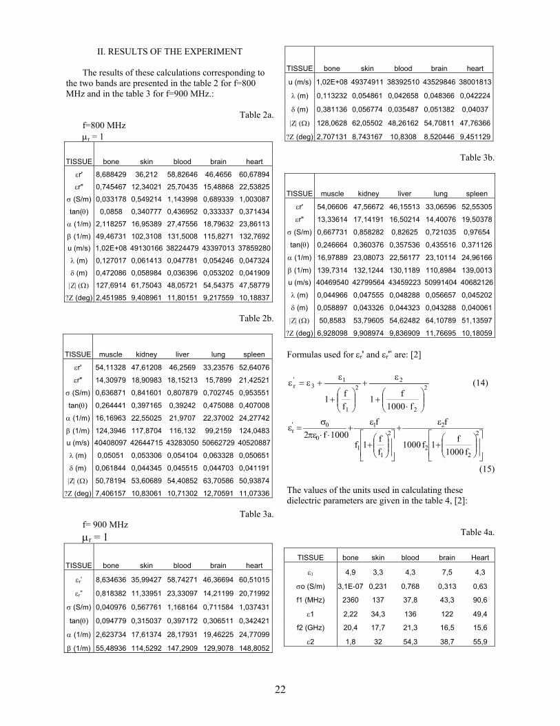

Buletinul Ştiinţific al Universităţii Politehnica din Timişoara
Seria ELECTRONICĂ şi TELECOMUNICAŢII TRANSACTIONS on ELECTRONICS and COMMUNICATIONS
Tom 48(62) Fascicola 2 2003
The Cyclic Prefix Length Influence on OFDM-Transmission BER
Marius Oltean1 Miranda Naforniţă1
Abstract Orthogonal Frequency Division Multiplexing (OFDM) is one of the recent years equalization approaches used in order to combat the inter-symbol interference introduced by the frequency selectivity of the radio channels The circular extension of the data symbol commonly referred to as cyclic prefix is one of the key elements in an OFDM transmission scheme The influence of the cyclic prefix duration on the BER performance of an OFDM system with in-frame DBPSK modulation is evaluated by means of computer simulation in a multipath fading channel
I INTRODUCTION Mobile radio communication systems are increasingly required to offer a variety of services and qualities for mobile users Unfortunately the radio channel is far from an ideal transmission medium exhibiting both frequency selectivity and time variant character [1] In this context one of the most challenging issues in a radio communication system is to overcome the inter-symbol interference introduced by the multipath propagation of the signal between the transmitter and the receiverrsquos antennas The use of the adaptive equalization to the receiver could be the solution for avoiding this unwanted phenomenon but this complex equalization technique proves oftentimes unsuited for being used in real-time applications at data rates of tens of Mbps in an unfriendly dispersive radio channel environment because of its important computational complexity OFDM is an optimal version of multicarrier modulation techniques which mitigates the effect of the ISI phenomenon keeping a relatively reduced complexity of the equalization process Indeed intuitively one can assume that the frequency selectivity of the channel can be mitigated if instead of transmitting a single high rate serial data stream the transmission is performed simultaneously using several narrow-band subchannels (with a different carrier corresponding to each subchannel) on which the frequency response of the channel looks ldquoflatrdquo
Hence for a given overall data rate increasing the number of carriers reduces the data rate that each individual carrier must convey therefore lengthening the duration of the symbol that modulates each individual subcarrier [2] Slow data rate (and long symbol duration) on each subchannel merely means that the effects of ISI are severely reduced In addition a cyclic prefix is inserted in front of each OFDM symbol This circular extension that is discarded on the receiver side is obtained by copying a number of samples from the end of the OFDM symbol in front of it in order to prevent two consecutive frames to interfere each other as a result of the time dispersion caused by the multipath propagation This way the receiver can independently process each frame in order to estimate the transmitted information Furthermore the equalization process is facilitated by this operation of cyclic prefix insertion and extraction In this chapter we focus on the influence of the cyclic prefix duration on the BER performance of an OFDM system with in-frame DBPSK modulation The performance evaluation in Rice fading conditions is done by means of computer simulation
II THE BLOCK-DIAGRAM OF OFDM
TRANSMISSION SCHEME
In the figure 1 a classical OFDM transmission scheme using FFT (Fast Fourier Transform) is illustrated
The input data sequence is baseband modulated using a digital modulation scheme Various modulation schemes could generally be employed such as BPSK QPSK (also with their differential form) and QAM with several different signal constellations In our system DBPSK method is chosen in order to encode the binary information Data is encoded bdquoin-framerdquo (the baseband signal modulation is performed on the serial data that is inside of what we name a bdquoDFT framerdquo or equivalently an OFDM symbol) The data symbols 1 Univ ldquoPolitehnicardquo Timişoara Facultatea de Electronică şi TelecomunicaţiiDepartamentul Comunicaţii
26
Information symbols
Serial to parallel
converter
Coding amp baseband
modulation
IFFT modulator
Cyclic prefix insertion
Parallel to serial
converterX
ej2πfct
Channel
X
ej2πfct
Serial to parallel
converter
Cyclic prefix extraction
FFT demodulator
Decoding amp demodulation
Parallel to serial
converter
Estimated symbols
Xk k=0hellipN-1
[Xk] k=0hellipN-1
[xk] k=0hellipN-1
[xcpk] k=-LhellipN-1
[ycpk] k=-LhellipN-1
[yk] k=0hellipN-1
[Yk] k=0hellipN-1
Yk k=0hellipN-1
Fig1 The block diagram of an OFDM System
are parallelized in N different substreams Each substream will modulate a separate carrier through the IFFT modulation block which actually generates the OFDM symbol performing the multicarrier modulation A cyclic prefix is inserted in order to eliminate the inter-symbol and inter-block interference (IBI) [3] The data are back-serial converted forming an OFDM symbol that will modulate a high-frequency carrier before its transmission through the channel The radio channel is generally referred to as a linear time-variant system To the receiver the inverse operations are performed in order to estimate the transmitted symbols
III THE CYCLIC PREFIX AND THE EQUALIZATION PROCESS
Since OFDM transmits data in blocks (usually a block is referred to as an bdquoOFDM symbolrdquo) any type of a non-ideal transmission channel (such as a multipath channel in mobile communication systems or a classical dispersive channel as in wired transmissions) will bdquospreadrdquo the OFDM symbol causing the blocks of signal to interfere one another This type of interference is called Inter-Block Interference IBI could lead to inter-symbol interference since two adjacent blocks will overlap causing the distortion of the samples affected by overlapping
In order to combat this interference we could use a cyclic prefix (CP) at the beginning of each symbol If the cyclic prefix spans more than the multipath channel impulse response the interference caused by the time dispersion of the previous transmitted block is entirely absorbed by the prefix samples that are discarded to the receiver The cyclic prefix consists of the last L samples of the OFDM symbol that are copied in front of the data block [4] as we can see in the figure 2 Generally the radio channel exhibits both time variant and frequency selective characteristics If we shall consider however that the channel parameters remain unchanged during the transmission of an OFDM symbol the way that the transmission medium distorts each particular frame is similar to the distortion caused by an
electronic filter [1][5] Under this assumption we can consider the equivalent discrete response of the channel as a linear FIR filter of order L of which the equation is given below
sum=
minussdot=L
n
nznczC0
][)( (1)
The equivalent baseband signal at the channel output can be obtained by the operation of convolution as follows
][][][ ncnxcpnycp = (2)
Discarding the L CP samples from the received sequence the remaining (useful) signal can be expressed as
where ldquo⊛rdquo denotes the circular convolution operator [6] The noticeable thing about the equation 6 is that the circular convolution preserves the temporal support of the signal In our case N transmitted signal samples convolved with L+1 channel impulse response samples will conduce to a received symbol of length N that will be used in the demodulation process Since the circular convolution will not ldquospreadrdquo the signal the receiver can independently process each data block The interference from the
y[n]=x[n] ⊛c[n] (3)
OFDM Symbol
Copy
CP
Transmitted sequence= OFDM symbol+CP
t
Fig2 The cyclic prefix insertion
27
previous transmitted blocks is totally eliminated through this operation of CP insertionextraction Furthermore since x[n]=IDFTX[k] and taking into account the effect of the DFT demodulator the received symbols Y[k] can be expressed as
Y[k]=DFTIDF TX[k] ⊛c[n] k=01hellipN-1 (4)
Since the DFT of a circular convolution of two discrete time signals will conduce to a spectral multiplication
110][][][][][
minus=sdot==sdot=
NkkCkXncDFTkXIDFTDFTkY
(5)
where C[k] represents the sampled frequency response of the equivalent baseband discrete channel corresponding to the frequencies Ωk=k(2πN) The crucial consequence of the relation above is that each modulation symbol X[k] could be recovered to the receiver by a simple pointwise division operation commonly referred to as a ldquoone-tap frequency domain equalizerrdquo as can be seen from the relation (6)
110][][][ 1 minus=sdot= minusandNkkCkYkX (6)
Thus the CP theoretically eliminates both IBI (each block preserves its temporal support) and inter-carrier interference (ICI) (each serial symbol received on the k-th carrier will depend only on the corresponding k-th carrier transmitted symbol not being affected by the adjacent carriers) IV SIMULATION RESULTS AND DISCUSSIONS
1 SIMULATION PARAMETERS
The goal of the simulations was to emphasize the effect of the cyclic prefix duration on the BER performance of an OFDM system with inter-frame DBPSK modulation The radio channel was modeled as a three-ray Rice fading channel with one deterministic line-of-sight (LOS) path and two multipath delayed components The relative delays of the two components are τ1 and τ2 respectively However in most of these simulations it was considered τ1=0 and a normalized delay for τ2 denoted τ2N=τ2LCP LCP represents the cyclic prefix duration expressed as the number of serial samples that compose the cyclic prefix An important parameter for the Rice fading channel is K=PLOSPD which stands for the ratio between the signal power carried by the LOS path (PLOS) and the total power of the two multipath components (PS=P1+P2) Equal power for the two multipath components was considered during the simulations A white gaussian noise is added to the signal at the output of the Rice
fading channel The time interval between the moments in which the first and the last significant component of the multipath signal arrives to the receiver is referred to as maximum excess delay (TM) and it is expressed in number of serial samples (remember that N signal samples generated by the IFFT modulator will compose an OFDM frame) Another parameter of the simulation is the number of subcarriers N that equals the number of serial samples composing an OFDM symbol The time variant character of the radio channel is quantified by the maximum Doppler shift parameter fD The value of this parameter is also expressed in a normalized manner as fDTS TS denoting the OFDM symbol duration A robust differential modulation scheme such as DBPSK was chosen for encoding the binary information No channel estimation techniques are employed and consequently no further equalization is done to the receiver
2 RESULTS AND DISCUSSIONS For the first simulations the relative delay of the second multipath was normalized by the serial symbol duration As can be seen from the figure 3 increasing the cyclic prefix duration improves the BER performance for the OFDM system
Theoretically if the cyclic prefix duration spans more than the maximum delay spread of the channel the errors can be completely eliminated This assumes however a perfect knowledge of the channel impulse response (or equivalently of the channel transfer function) which is a mandatory condition for implementing the equation 6 Since in our implementation no channel estimation techniques are employed the exact form of the channel impulse response doesnrsquot constitute information that can be exploited in the data estimation process The correct
Fig 3 The influence of the cyclic prefix duration on BER performance for DBPSK-OFDM system
Rice fading channel K=3dB SNR=30dB N=64 fDTS=0001
28
detection is entirely based on the robustness and simplicity of the digital modulation scheme that is involved namely DBPSK This explains why the BER is not completely eliminated for a cyclic prefix of theoretically sufficient duration (longer than TM) A noticeable thing resulting from the figure 3 is that while identical for cyclic prefix lengths which cover the channel impulse response the performance degrades for the cases where the cyclic prefix duration becomes insufficient Thus if a cyclic prefix of length LCP=4 is used the transmission offers the best performance between all the considered situations but only starting with a value of the normalized delay that overtakes the length of the circular extension for all the other cases Next we studied the BER performance against the normalized delay of the second multipath which is obtained this time as explained in the previous subsection It can be observed from the figure 4 that increasing the OFDM symbol length improves the performance of the system which confirms [6] In the same time it is proven that the BER is sensitive to the multipath delay spread of the channel
normalized by the cyclic prefix duration Thus as observed in the figure 4a) a two times longer OFDM symbol is needed in order to obtain the same performance when the normalized delay of the second multipath is two times higher (note that for the same value of τ2N on the abscissa τ2 doubles its value when LCP=2) The observation is confirmed by the figure 4b) where the BER curve in the case N=16 LCP=1 is almost identical with the curve plotted for a frame of length N=64 with a cyclic prefix LCP=4 The conclusion that can be drawn from these observations is that at identical ratios between the channel impulse response and the cyclic prefix duration the in-frame OFDM system performance remains sensitive to the effective value of the multipath (or maximum) delay spread parameter (τ2 in our case)
3 CONCLUSIONS
The cyclic prefix duration influences the performances of an OFDM system even if the explicit form of the channel impulse response is unknown and consequently cannot be used in the equalization process The transmission is sensitive to the parameter obtained as the multipath delay of the channel normalized by the cyclic prefix duration The BER performance is in all cases improved by increasing the OFDM symbol length
REFERENCES
[1] B Sklar Rayleigh Fading Channels in Mobile Digital Communication Systems- Part I Characterization IEEE Commun Mag July 1997 [2] Dusan MaticOFDM as a possible modulation technique for multimedia applications in the range of mm waves 10-30-38 TUD-TVS available on-line wwwubicomtudelftnlMMCDocsintroOFDMpdf [3]Werner Henkel Georg Tauboumlck Per Oumllding The cyclic prefix of OFDMDMT ndash an analysis 2002 International Zuumlrich Seminar on Broadband Communications February 19-21 Zuumlrich Switzerland [4]Lu J Tjhung TT Adachi F BER performance of OFDM system in frequency-selective Rician fading with diversity reception available online httpwwwcwcnusedusg~cwcpubzfilesict97_2pdf [5] B Sklar Rayleigh Fading Channels in Mobile Digital Communication Systems- Part II Mitigation IEEE Commun Mag July 1997 [6 ]Chini A Analysis and Simulation of Multicarrier Modulation in Frequency Selective Fading Channels Ph D Thesis 1994 Chapter 3
a)
b)
Fig 4 (ab) The influence of the normalized delay of the second multipath on BER performance for DBPSK-OFDM
system Rice fading channel K=3dB SNR=40dB fDTS=0001
29
Buletinul Ştiinţific al Universităţii Politehnica din Timişoara
Seria ELECTRONICĂ şi TELECOMUNICAŢII TRANSACTIONS on ELECTRONICS and COMMUNICATIONS
Tom 48(62) Fascicola 2 2003
Methods for JPEG image protection by partial encryption Florin Vancea1 Codruţa Vancea2
1 University of Oradea Faculty of Electrotechnics and Informatics Computer Science Department str Armatei Romacircne nr 5 Oradea e-mail fvanceauoradearo 2 University of Oradea Faculty of Electrotechnics and Informatics EMUEE Department str Armatei Romacircne nr 5 Oradea e-mail cvanceauoradearo
Abstract ndash The JPEG format used in static image transfer and storage exhibits some particularities when considered for encryption A commercially useful encryption must degrade the image but keep it within evaluation limits Classical encryption techniques can be applied to a JPEG stream in various phases of its construction and to different segments We evaluate the impact of some alternatives testing on real cases Potential future directions are identified Keywords encryption JPEG DCT
I INTRODUCTION
A significant part of the information transmitted in data networks and stored in computer systems today is represented by images be they static or in motion The need to protect this information against unauthorized access and usage requires no further proof In order to protect text-based information various methods have been devised based on the general theory of encrypting binary information [1] Since images are stored and transported in binary form too we can directly apply known encryption methods to protect them The disadvantage of such approach is that itrsquos too rigid the image becomes unintelligible In copy-protection schemes or in controlled distribution schemes one would like a partial and controlled accessibility to image content Encryption key holders will be able to see and use the image to its normal parameters and potential unauthorized users get access to a degraded version understandable but unusable for any purposes but identification of its value A distribution scheme using such a mechanism can thus publish an electronic catalogue and interested users will only pay for the keys needed to decrypt the images they need The images are transmitted and stored using various formats Generally one is looking to compress the raw information content but this can be achieved in various ways Some methods are using color space reduction by using color tables others are applying compression methods to the raw bitstream resulted from sampling the color information at maximum
capability level Some are using lossless compression techniques others are taking advantage of the particular behavior of the final recipient ndash the human eye The latter use lossy compression where the information cannot be exactly recovered but the resulting quality can be extremely good from the perception point of view and the compression ratio is greatly improved
II THE JPEG STREAM FORMAT
One of the frequently used formats in storing and transmitting still images is the the format proposed by the Joint Photographic Experts Group ndash JPEG standardized in recommendation T81 of ITU-T [2] The recommendation is specifying how to transform the original input image (organized in component planes) to obtain the compressed byte stream Below we will review the JPEG encodingcompression process emphasizing the details that may impact the encryption process Esentially the original information is transformed (if necessary) to an alternative representation space having luminance and chrominance components The chrominance components have lower importance in achieving the perceived quality and can be sampled with a less detailed rate Therefore we will obtain several samples from the luminance component for one sample in a chrominance component Each componentrsquos pack of samples is divided in 8x8 blocks to be transformed with a DCT transformation The DCT process is lossless (except for the rounding errors) but the resulting amount of information is still comparable to the original one obtained after the discriminating sampling In order to achieve compression adapted to human perception the resulting DCT coefficients are quantized differently The coefficients corresponding to higher spatial frequencies can be reproduced with lower precision to obtain a good compromise between the number of bits required in the output stream and
30
the need to reproduce faithfully the image Discrimination between quantization levels is made through quantization tables different for different components These tables must be attached to the transmitted or stored stream and usually have a predictible distribution The output of the quantization step still has considerable redundancy mainly presented as many coefficients being zero The standard specifies a zig-zag ordering scheme that puts the higher-frequency coefficients together and an encoding scheme that skips the zero coefficients and encodes only the non-zero ones using Huffmanrsquos method The resulting Huffman tables are also attached to the data stream and they have a highly predictible structure too Other encoding schemes using arithmetic compression exist but they are limited in extent due to them being subject to licensing issues In the following we will only consider the widespread Huffman-based encoding scheme The binary stream defined by JPEG has a well-defined structure delimited by special sequences named markers These markers can be used to check and eventually recover the synchronization upon decoding From our point of view in order to make reference to the encryption solutions the structure of the JPEG binary stream is represented in Fig 1
Quantization tables
Huffman symbol tables
Structural informationsize component definitions sampling rates
Quantized DCT coefficients Huffman-encoded
MicroheaderByte with zero-count and
it-count Huffman-encoded
Coefficient bits withoutHuffman encoding
Non-image information
Fig 1 Structura of JPEG stream (for encryption)
We can see that the coefficient stream contains only the non-zero coefficients Each non-zero coefficient is introduced by a microheader (Huffman encoded byte) followed by a variable number of unencoded bits (at most 16 bits) representing the actual coefficient The byte contains 4 bits giving the previous skipped zero coefficients and 4 bits giving the coefficientrsquos bitcount When the count of zero coefficient in a span overflow the limit of 16 additional microheaders are attached without any data bits
III ENCRYPTION METHOD
We set our goal to find a suitable encryption method for JPEG-encoded images The method should controllably degrade the image beyond commercial usability but not beyond recognition It should also preserve the image structure so the resulting image will be processable with standard tools especially for
viewing purposes Such a constraint allows the usage of any JPEG-compliant tool in transmission storage and presentation Below we will analyze different candidate methods for solving the above-described problem A Direct encryption of JPEG stream
Encrypting the entire stream goes right out of question because it destroys the logical structure described above and the result is unusable unless decrypted This method violates the initial assumption that the encrypted image is recognizable but unusable B Encrypting the original image
Encrypting the original image means fully extracting the original image from the JPEG stream encrypting its binary form with some method and repacking the result into a new JPEG stream The method is not applicable because - By encrypting the image its statistical structure is
radically changed Any efficient encryption algorithm should produce an output stream without detectable redundancy and the JPEG encoding is making use exactly of some particular kind of redundancy in the input image (photographic image redundancy)
- The process is not perfectly reversible The JPEG compression method is a lossy one At decoding time reconstruction of the original encrypted image will be only an approximation and the decryption is expected to be seriously affected Usual encryptiondecryption algorithms will produce wildly different decryption results for minor changes in ciphertext The algorithms used should be error-tolerant and this commonly means weaker ones
- The JPEG decoding-encoding cycle even without any encryption in-between is lossy The image quality is degraded and non-recoverable Generally each decoding-encoding cycle is impacting the image quality
There is a variation to this method when only part of the bitplanes in the original image are encrypted The method is analyzed in [3] and the conclusion is that in order to avoid attacks one must encrypt at least two of the most significant bitplanes Image degrading after encrypting two significant bitplanes is considerable and the above objections still hold so the method is not suitable for our purpose C Partial encryption of JPEG stream
It is clear that we will have to identify the segments of the stream suitable for encrypting with minimal effort and without adverse impact on compatibility while achieving the desired degrading effect Encrypting the non-image information is not useful to us but the fact that the standard accepts such blocks of information may be useful One can add a non-image information to resulting stream holding any kind of
31
extra information required for decrypting (we are not talking about the key of course) Any processing program on the delivery chain should silently ignore this kind of information We must also note that these blocks might contain reduced versions of the original image (thumbnails) If not protected or eliminated they might be used by an attacker to recover the original image information or might be even used directly as a smaller version of the protected image Encrypting the quantization tables may lead to a significant degradation of the image quality but the quantization tables are highly predictible Some images are using even the original tables recommended by the JPEG committee so encription would be useless Encrypting the Huffman tables is not useful because their structure is also highly predictible Moreover encrypting them would introduce structure inconsistencies because the encrypted text will obviously not represent a valid Huffman table Permutation-like operations controlled by the key are also not useful because the standard specifies a clear order in generating the Huffman symbols and the permutation itself is straightforward reversable Encrypting the structure information is also not acceptable because any modification in this area will produce an incompatible stream Moreover the information here is important for evaluating the image fitness for the purpose and encrypting them will contradict the commercal target adopted initially The only option is to encrypt the Huffman-encoded DCT coefficients Encrypting them directly as a binary stream will be unacceptable again because it destroys the structure outlined in Fig 1 Any decoder will expect microheader-data pairs and the microheader should be Huffman-encoded As Huffman decoding is normally incomplete (meaning that not any bit sequence has a valid symbol attached) it is possible that the directly encrypted stream will produce errors in the decoding proces maybe even ones that are fatal to the decoder Even if we ignore this problem the overall number of coefficients resulting from the decoding process is composed from the number of zero coefficients plus the number of non-zero coefficients and is verifiable against the specified image size and sampling rates Huffman-decoding the encrypted sequence will surely violate this constraint having again potential fatal consequences for the decoder The only remaining options are a) to apply partial manipulation on the bitstream such as to preserve the microheader structure or b) to Huffman decode then encrypt then Huffman recode right back D Selective encryption of coefficient data bits
The most attractive method is to selectively encrypt the bits holding the coefficients values while preserving the microheaders [4] Such a method is keeping the binary stream structure preserving perfect
JPEG compatibility while degrading the quality of the encrypted image version Degradation is perfectly recoverable through decryption with the obvious provision that the encrypted image was not processed in the meantime The method has the additional advantage that it can be performed in a single step as streamed processing The structure of original image is analyzed as it enters the encryption device The elements that should not be modified are passed directly to the output The encryptable elements (coefficient bits) are encrypted with a stream cipher and the result is injected into the output instead of the original bits We should note that the overall size of data is neither increased nor decreased (except minor variations due to standard escaping rules specified in the standard) If we also use an auto-decrypting cipher (eg XOR) the process is identical for both encryption and decryption The process is described in Fig 2
Structure analizer
Streamencryption
Key Fig 2 Selective stream encryption
E Encrypting through idempotent manipulations in
microheader-data pairs
Another possibility identified is to alter the coefficient sequence by applying idempotent (with respect to the structural compliance) manipulations to a span of encoded coefficients As long as we observe the constraint that the overall number of resulting coefficients (both zero and non-zero) is coherent with the number determined from the structural information we can apply key-controlled permutations in a correctly chosen coefficient sequence altering the place where the coefficients are decoded The result is a degraded but structurally correct image The method is harder to apply because it requires storage and many of the potential permutations are idempotent from the image point of view too (think about swapping equal coefficients) We also have to account for interleaving of different components normally encoded with different Huffman tables because we must preserve Huffman decoding coherence Our target must be to change the place of coefficients within the same Huffman decoding space The method has the advantage that it produces deeper changes in image since it traverses the 8x8 block boundaries without changing the statistic distribution thus without requiring a Huffman table regeneration
32
F Encrypting ldquobehind compressionrdquo
A more general version of the above method means Huffman decompression encrypting the coefficients and Huffman recompression The freedom of transformation in this case is improved but the complexity price is higher too A simple approach may use the original Huffman tables so partial stream processing is possible Unfortunately a common encryption procedure applied to coefficient blocks will ruin their zero-rich structure The first consequence is that the original Huffman tables are not statistically correct anymore and recoding with original tables (if possible at all) would introduce an information leak The second consequence is that the compression efficiency may drop drastically even if we regenerate the Huffman tables Finally the strong redundancy induced by the original zero-sequences will significantly affect the overall encryption strength there will be a great risk of known plaintext attacks In order to use this method we should choose encryption algorithms with increased resistance to known plaintext attacks
IV OBSERVATIONS
When applying any of the above-described methods we should take into account the desired and accepted image degradation level Generally encrypting directly the DC coefficients is not recommended because the image degrading is too high Moreover the coefficients are stored using a differential scheme which can be easily saturated when encrypting undiscriminately The simpler path is to focus on AC coefficients Out of those we must keep some in unencrypted form in order to preserve part of original image quality for evaluation purposes The number of unencrypted coefficients to keep depends on the desired and accepted degree of image degradation We can see that some images have right from the start such a compression level that even encrypting all AC coefficients is not providing enough degradation Explanation of this is found in the particular structure of the cofficients resulting from the quantization step For an image with aggresive quantization many of the coefficients have a very limited number of bits Encrypting selectively those bits will preserve the number of bits but will replace with (ideally) 05 probability each bit with its opposite It is clear that for an aggresively quantized image (many 1-bit coefficients) we have a 50 chance that the coefficient is unaffected The selective encryption of coefficient bits exhibits another disadvantage any encryption effect is local to the 8x8 block holding the coefficients This is good for the encrypted image inteligibility but induces a cryptographic weakness Any normal image has lots of correlation between neighbouring blocks and this can be used by a potential attacker
V IMPLEMENTATION
To illustrate the above ideas we implemented the selective encryption of coefficient bits method and a simple version of idempotent manipulation behind compression Encryption itself is not important for these evaluations so we used XOR with a bitstream resulted from a CBC generator having null plaintext Selective encryption led to fairly good results but as expected there are images for which the method is ineffective Fig 3 represents an image with rich detail (ldquoparrotsrdquo) in its original version Fig 4 şi Fig 5 are presenting the same image encrypted while preserving 2 and respectively 5 of the AC coefficients The results are consistent with our expectations The image degradation is controllable and deep enough even when preserving 4 AC coefficients
Fig 3 ldquoparrotsrdquo original
Fig 4 ldquoparrotsrdquo 5 unencrypted AC coefficients
Fig 5 ldquoparrotsrdquo 2 unencrypted AC coefficients
33
Fig 6 ldquomarsrdquo original
Fig 7 ldquomarsrdquo 5 unencrypted AC coefficients
Fig 8 ldquomarsrdquo 2 unencrypted AC coefficients
The original bdquomarsrdquo image in Fig 6 has a lower detail content per 8x8 JPEG block The image is also larger in pixel size Its encrypted versions are represented in Fig 7 şi Fig 8 Even if we preserve only 2 AC coefficients the image is not degraded enough to impact its value We implemented also a simple implementation of keyed idempotent manipulation behind compression Several manipulation schemes were tried - key-controlled permutation of coefficients within
a 8x8 block - key-controlled permutation of coefficients across
blocks within the same JPEG scan preserving the coefficient position in the frequency domain
- key-controlled permutation of coefficients across blocks within the same JPEG scan with intentional breaking of its position in the frequency domain
All the schemes described above were concentrating on reducing to a minimum the impact on the entropy content before compresion in order to achieve a comparable stream size after encryption The tested schemes have produced inconcludent results (low protection degree significantly increased run times) The complexity of the processing software was also significantly higher The above results does not void the eligibility of the encryption behind compression method We assume that these results were obtained due to insufficient study of the method Some approach closer to the perception specifics when considering the encryption process may bring important improvements in this direction
VI CONCLUSIONS
Encrypting image information while preserving the general visual features poses multiple problems but is an interesting domain due to the potential applications We have analyzed some of the methods usable for the wide-spread JPEG format and we have implemented some of the promising ones During the implementation we found out that current methods are not offering consistent results for all types of images Moreover simple treatments like selective encryption of the AC coefficient bits feature potential weaknesses to continuity attacks We must say that achieving the proposed goal (protection of the image content while keeping the evaluation possibility) requires giving up the some advantages like single-step stream processing and size preservation If we drop such requirements there are some methods promising adequate protection adjusted to human perception Future work will analyze how one can exploit the subjective image information content to control the encryption process into obtaining convenient protection
34
REFERENCES
[1] B Schneier ldquoApplied cryptographyrdquo John Wiley amp Sons second edition 1996 [2] The International Telegraph And Telephone Consultative Committee ndash ldquoDigital Compression and Coding of Continuous-Tone Still Images ndash Requirements and Guidelinesrdquo - Recommendation T81 [3] T Maples G Spanos ldquoPerformance study of a selective encryption scheme for the security of networked real-time videordquo Proceedings of the 4th International Conference on Computer Communications and Networks Las Vegas Nevada September 1995 [4] M v Droogenbroeck R Benedett ldquoTechniques for a selective encryption of uncompressed and compressed imagesrdquo ACIVS Advanced Concepts for Intelligent Vision Systems Ghent Belgium pages 90-97 September 2002 [5] H Chang X Li ldquoOn the Application of Image Decomposition to Image Compression and Encryptionrdquo 1996 [6] M Podesser Hans-Peter Schmidt and Andreas Uhl ldquoSelective Bitplane Encryption For Secure Transmission Of Image Data In Mobile Environmentsrdquo Proceedings NORSIG-2002 [7] T Uehara R Safavi-Naini P Ogunbona ldquoSecuring wavelet compression with random permutationsrdquo Proceedings of the 2000 IEEE Pacific Rim Conference on Multimedia pages 332ndash335 Sydney Dec 2000 IEEE Signal Processing Society
35
Buletinul Ştiinţific al Universităţii Politehnica din Timişoara
Seria ELECTRONICĂ şi TELECOMUNICAŢII TRANSACTIONS on ELECTRONICS and COMMUNICATIONS
Tom 48(62) Fascicola 2 2003
Computing Wavelet Transform from Short Time Fourier Transform
i Moldovan Maria Simina1
1 Facultatea de Electronică şi Telecomunicaţii Departamentul Comunicaţii Str Observator Nr 34 Cluj-Napoca e-mail siminamemailro
Wavelet Transform is a relative new analysis technique developed as an alternative for Short Time Fourier Transform which is proved to be superior for several applications Energetic aspects of the two transform ie spectrogram and scalogram are the applications that represents the task of the actual paper An interesting problem is the mapping between the spectrogram and the scalogram To be more specific we are interested to develop an algorithm through which the Wavelet coefficients can be computed directly from STFT coefficients without reconstructing I INTRODUCTION Time-frequency representations may be a useful tool for the visual analysis of signals as they provide information not available from time- or frequency-domain representations alone such as the time variations of the spectrum of the signal or of its power spectrum which translate in distinctive patterns on a time-frequency plot Recently applications of wavelet analysis are widespread and cover many fields of scientific research including medical science (the ECG EEG EMG Echocardiograms clinical sounds-arterial bruits heart sounds breath sounds respiratory patterns blood pressure trends DNA sequences) geophysics engineering image analysis financial analysis There has been developed a code that allow the examination of the signals energy distribution in time-frequency respectively time-scale domains The Fourier spectrogram is a very common tool in signal analysis It gives a description of both time and frequency distribution of the energy in the signal by shifting a window through the signal and taking out the Fourier Transform of the windowed portions The window length determines the time-frequency resolution The scalogram is a more elegant version of time-frequency representation that can be found from the Continuous Wavelet Transform Both the spectrogram and the scalogram produce a more or less easily interpretable visual two-dimensional representation of signals
A lot of spectrograms of the signals are available so we are interesting in a way to construct the scalogram for a given spectrogram To accomplish this goal we need to find out a possible link between Short Time Fourier Transform and Wavelet Transform In order to determine the efficiency of the computing method the obtained coefficients were compared with one resulted from the classical analysis method II SPECTROGRAM AND SCALOGRAM The spectrogram has been the traditional tool for the speech analysis for over 50 years STFT gives a description of both the time and frequency characteristics of the signal The mathematical definitions of the continuous time are given below
dtetgtxSTFTR
tjint Ωminuslowast minus=Ω )()()( ττ (1)
The time-frequency resolution of the STFT is subject of the Heisenberg Uncertainty Principle which states that the product of the standard deviation in time and frequency is limited by
π41
ge∆sdot∆ ft (2)
The discrete STFT is constructed by multiplying a portion of the signal by a window function w[m] of length L Its Fourier Transform is computed and then the window is shifted bdquonrdquo positions along the signal and the process is repeated The Fast Fourier Transform (FFT) is the preferable FT implementation in these computations The Fourier spectrogram is defined as the square modulus of the STFT
2)( )()( ττ Ω=Ω= gx
gxS STFTSPECP (3)
36
The common method of analysis of signals has limited time frequency resolution and therefore limited accuracy If the window length is short the spectrogram will be well localized in time but will have poor frequency resolution If the window is long the frequency resolution will be good but the localization in time will be poor This is the fundamental weakness of the spectrogram demonstrated below
Fig 1 Input signal
Fig 2 Spectrogram with Blackman window of 128 length
Fig 3 Spectrogram with Blackman
Window of 32 length Wavelet analysis is often related to Fourier Transform due to the resemblance between them CWT is similar to the STFT except that instead of a basis of infinite sines and cosines of different frequencies the CWT compares the signal with dilated and time-shifted versions of a single basis function called the mother wavelet The wavelet transform has become a valuable analysis tool due to its ability to elucidate simultaneously both the spectral and the temporal information within the signal The definition of the Continuous Wavelet Transform is
( ) dtttxbaTWC bax )()()( ψψ intinfin
infinminus
sdot= (4)
where x(t) can be any signal with finite energy )(tψ is the mother wavelet bdquoardquo is the dilation (or the scale) of the mother wavelet and bdquobrdquo is the time-shift (or the translation) of the wavelet The scalogram of a signal is the squared magnitude of its wavelet transform
2)()( )( ψψ
xxW TWCbaSCALP == (5) The time and frequency resolutions of the wavelet transform depend on the scale At high frequencies (low scale) the resolution in time is good but the resolution in frequency is poor This is due to the fact that the analyzing wavelet is well localized in time but poorly localized in frequency At low frequencies (high scale) the frequency resolution is good and the time resolution poor This means that for a signal with rapid changes in frequency at high frequencies and slow changes in frequency at low frequencies the scalogram will give a better time frequency representation of the signal than the spectrogram The advantage of the wavelet transform lies not only in its ability to provide a basis whose elements are both spatially and frequency localized but also in the fact that it can be computed by a fast algorithm In this paper we will mainly work with Daubechies (D4) wavelets Both the spectrogram and the scalogram produce a more or less easily interpretable visual two-dimensional representation of signals III COMPARISON OF TIME-FREQUENCY ANALYSIS TECHNIQUES lsquoFig 4rdquo shows our test waveform an exponential chirp with 12 added transients
Fig 4 Chirp signal
In ldquoFig 5rdquo we computed the spectrogram of this waveform It was produced with 64-point Blackman window zero-padded to 256 points We have constructed the test waveform so that the frequency increases exponentially This can be seen from the spectrogram
37
Fig 5 The spectrogram of the test waveform
Now we compare the spectrogram with the corresponding scalograms determinated with Db4 wavelet
Fig 6 The scalogram of the test waveform
The scalogram is a graph with time on the horizontal axis and different octaves (discrete logarithmic frequency scale) on the vertical axis The energy in a certain octave at a given time is represented by the color of the corresponding block It was obtained by using Daubechies Db4 as wavelet function The image offers clearly a better visualization both for the transients and the chirp In the case of the spectrogram the energy distribution region of an impulse located at time stamp t=ti is
limited on the time scale by the time frame t∆ and it expands uniformly overall frequencies On the contrary in the case of the scalogram the energy is only represented for certain frequencies and it is concentrated in the vicinity of the ti on the time scale being not restricted by the time frame It results that from the second representations we can obtain more accurate the frequency content of the impulses and also their time localizations Thereby some undesired signal interferences can be more easily eliminated if we know their time position and frequency content The analytic energy is often used in signal processing It uses the discrete Hilbert transform and returns a smoother scalogram
We select also a biosignal for the comparison between time-frequency and time-scale analysis
Fig 7 Biosignal input
Fig 8 Spectrogram
Fig 9 Scalogram determinated by using Db4 wavelet
Instead of a grayscale used in former times we use a scale from rsquobluersquo (low energy) to lsquoredrsquo (high energy) The features can be determined more precisely in the second case as we expected The scalogram produces a more easily interpretable visual two-dimensional representation of signals As we can see from ldquoFig 10rdquo where the scalogram is computed by using Shannon family function the type of mother wavelet is also important for this kind of analysis
38
Fig 10 Scalogram determinated by using Shannon wavelet
IV COMPUTING WT FROM STFT WITHOUT RECONSTRUCTING
Being given a scaling function )(tφ we have
computed the corresponding mother wavelet )(tψ and then the wavelet transform First of all we have
determinated a direct relation between )(tφ and )(tψ without any intervention of low-pass filtering
operators )(ΩH
In Mallatrsquos Algorithm the function is described as
)(ΩH
Ωminusinfin
minusinfin=sum=Ω jk
kkehH )(
(6) And it must satisfy the conditions
1)0( =H (7)
1)()( 22 =+Ω+Ω πHH (8)
[ ] 220)( ππminusisinΩforallneΩH (9)
The Fourier transform of the function )(tφ satisfies the following equation
)()()2( ΩΦΩ=ΩΦ H (11)
The high-pass filtering operator is given by the condition that
)(ΩG
⎥⎥⎥
⎦
⎤
+Ω
Ω
⎢⎢⎢
⎣
⎡
+Ω
Ω
)(
)(
)(
)(
ππ G
G
H
H
(13)
is a unitary matrix A possible choice for LPF operator is
)()( π+Ω=Ω lowastΩminus HeG j (14) and it gives the Fourier transform
( ) )()(2 ΩΦΩ=ΩΨ G (15) We obtained the following relation
( ) )2
()
2(
2)( 2 ΩΦ
+Ω
Φ
+ΩΦ=ΩΨ
Ωminus
π
πje (16)
Denoting by
( ) ( ) )2
)(( 1 ΩΦΩΦ=ΩΓ minus (17)
it holds the equation
( ) ( ) )2
(22 ΩΦ+ΩΓ=ΩΨ
Ωminus
πj
e (18)
and applying Inverse Fourier Transform results the next expression for mother wavelet
( )12)(2)( 2 minuslowast= minus ttet tj φγψ π (19)
Developing the convolution in the wavelet formulae
( ) ττφτγψ τπ dtet tjintinfin
infinminus
minusminus minusminus= 12)(2)( )(2
(20) and after applying different properties we have that
sdot= intinfin
infinminus
minus)(2)(
22txee
abaTWC a
tjabj
x
ππ
dtda
bte j⎥⎦
⎤⎢⎣
⎡minusminus
minusintinfin
infinminus
ττφτγπτ )12()(2 (21)
This approach is not always possible We can not build a multiresolution approximation from any wavelet orthonormal basis Thus we have chosen B-spline as the family of scaling functions nm(t) and we applied ours results The m-th order of B-spline function nm(t) is defined by
39
)()()( 11 tntntn mm lowast= minus (22) It can be seen that for mgt1 nm(t) is a multiple convolution of n1(t)
44344211
111
11211
minus
minusminus
lowastlowastlowast==lowastlowast=lowast=
p
mmm
nnnnnnnnn
(23) where the first order function is just the Haar scaling function
⎩⎨⎧ isin
=otherwise 0
[01] t1)(1 tn
(24) This convolution can be seen as an integral whose recurrence expression satisfies the relation
)2(2)(0
1 ktnCtn m
m
k
km
mm minus= sum
=
+minus
(25) The corresponding Fourier Transform is
kjm
k
kmmmm eCNN 2
0)
2(
21)(
Ωminus
=sumΩ
=Ω (26)
In this case we obtain
)2
()()( 1 ΩΩ=ΩΓ minus
mm NN (27)
with the Inverse Fourier Transform
sum=
minus minus=m
ok
km
mm
ktCt )2
(2)( δγ (28)
then replacing
)()( tnt m=φ (29)
)((t) tmγγ = (30) the equation (21) can be written as
⎩⎨⎧
sdot= intintinfin
infinminus
minusinfin
infinminus
atjja
bjmx eee
abaTWC
ππτπ 2222)(
ττ
τδ
dn
dttxka
btC
m
m
k
km
m
)12(
)(2
20
minussdot
sdot⎭⎬⎫
⎥⎦
⎤⎢⎣
⎡minus⎟
⎠⎞
⎜⎝⎛ minusminussum
=
minus
(31)
Using the next propriety of the Dirac function
)(1)()(αβ
αβαδ xdttxt =minussdotint
infin
infinminus (32)
for bkat ++rarr )2
(τ we have
τττ dnbkax
CabaTWC
m
km
k
kmm
mx
)12(])2
([
)1(2
)(0
1
minus++
sdotminus=
int
suminfin
infinminus
=minus
(33)
After making some manipulations it holds the relationships
sdot= sum sumsum= ==
+minusm
i
m
iq
iqm
im
m
i
im
mqm CCCtbaY
02 0
2
01
1)1( 2)(
dtitntxq
ss
sqqm
444 3444 211
)22()(1
0
τ
τ sumint=
minusinfin
infinminus
sdotminussdotminus (34)
and Continuous Wavelet Transform became as the following equation
dtitntx
CCC
Ca
baTWC
q
ss
sqqm
m
i
m
iq
iqm
im
m
i
im
km
k
kmqm
mx
444 3444 211
)22()(
)1(2
1)(
10
02 0
2
01
1
0)1)(1(
τ
τ sumint
sum sumsum
sum
=
minusinfin
infinminus
= ==
=+minus
sdotminussdotminus
sdot
sdotminus=
(35) In conclusion it can be seen that the Continuous Wavelet Transform can be computed as a Short Time
Fourier Transform with 0=Ω
)0(
)1(2
1)(
102 0
2
01
1
0)1)(1(
τ=Ω
sdotminus=
sum sumsum
sum
= ==
=+minus
x
m
i
m
iq
iqm
im
m
i
im
km
k
kmqm
mx
STFTCCC
Ca
baTWC(3
6) where we have denoted
sdot==Ω intinfin
infinminus
)()0( 1 txSTFTx τ
40
0
10 )22(
1 =Ω
Ωminus
=
minussum sdotminussdotminus dteitn tjq
ss
sqqm
444 3444 21τ
τ (37)
V COMPARISON OF THE RESULTED COEFFICIENTS In order to determine the efficiency of the computing method the obtained coefficients have been compared to the one resulted from the classical analysis method The resulted coefficients will be presented in the same graphics for both methods using as scaling factor a=16 respectively a=32 and keeping the same signal length In the figure the CWT coefficients computed from STFT have been plotted with continuous blue line and the direct computed ones with red dots The need of great number of computations has a significant effect upon the final result The value of the error is also influenced by the length of the analysis window The larger the window is the bigger the differences from the two sets of coefficients are
Fig 11 Coefficients comparison
VI FINAL REMARKS AND CONCLUSIONS Some consideration of the relation between the mother wavelet and the scaling function has already been exposed Under some conditions a general form of the mother wavelet is retrieved This approach of the transforms can leads to an easy implementation of the STFT and WT and to a better understanding and relationships in DSP software The preceding approaches recommend a potential connection between the energetic representations of these transforms without the reconstruction of the signal The increase numbers of FFT dedicated devices and of previous STFT databases also request this possible link between STFT and WT
REFERENCES [1] C Rusu ldquoComputing WT from STFT without reconstructingrdquo Proc ECSAP-97 pp 251-254 [2] Corneliu Rusu A short way to compute WT from STFT EUSIPCO 96 [3] S Mallat bdquoMultirezolution approximation and wavelet orthonormal of L2(R)rdquo [4]httpgraphicscsucdaviseduCAGDNotesUniform-B-Splines-as-a-Convolutionpdf -ldquoScalogram Modification and Inversionrdquo [5] httpgraphicscsucdaviseduCAGDNotes Uniform-B-Splines-as-a-Convolutionpdf
41
Buletinul Ştiinţific al Universităţii Politehnica din Timişoara
Seria ELECTRONICĂ şi TELECOMUNICAŢII TRANSACTIONS on ELECTRONICS and COMMUNICATIONS
Tom 50(64) Fascicola 1 2005
Instrucţiuni de redactare a articolelor pentru Buletinul ştiinţific al Facultăţii de Electronică şi Telecomunicaţii
Gheorghe I Popescu1
1 Facultatea de Electronică şi Telecomunicaţii Departamentul Comunicaţii Bd V Pacircrvan Timişoara 1900 e-mail geoeeuttro
Rezumat ndash Aceste instrucţiuni sunt concepute să vă prezinte modul de redactare al articolelor pentru Buletinul ştiinţific al Facultăţii de Electronică şi Telecomunicaţii Prezentul material este conceput ca model pentru modul cum trebuie să arate articolele gata de publicare Rezumatul trebuie să conţină descrierea problemei metodele şi soluţiile propuse şi rezultatele experimentale obţinute icircn cel mult 12 racircnduri Nu se admit referinţe bibliografice icircn cadrul rezumatului Cuvinte cheie redactare buletin ştiinţific
I INTRODUCERE
Formatul buletinului va fi A4 Articolele inclusiv tabelele şi figurile nu trebuie să depăşească 6 pagini Numărul de pagini trebuie să fie obligatoriu par
II INSTRUCŢIUNI DE REDACTARE
Articolul trebuie să fie transmis icircn forma standard descrisă icircn acest material Tipărirea se va face cu o imprimantă de bună calitate pe o singură faţă a paginii Textul se va plasa pe două coloane de 8 cm cu spaţiu de 05 cm icircntre ele Pagina A4 orientată pe icircnălţimea paginii are marginile de sus şi jos de 178 cm iar cele din stacircnga şi dreapta de 254 cm Prima pagină a articolului va avea marginea superioară de 5 cm Pentru editarea articolului se recomandă utilizarea procesorului de text Microsoft Word for Windows cu caractere Times New Roman dactilografiate la un racircnd Dimensiunile şi stilul caracterelor sunt Titlul articolului 18 pt icircngroşat autorul 12 pt rezumatul 9 pt icircngroşat cuvintele cheie 9 pt icircngroşat titlu paragraf 10 pt majuscule titlu subparagraf 10 pt italic distanţa de la numărul de ordine la titluri va fi de 025 cm textul normal 10 pt afilierea autorului 8 pt notele de subsol 8 pt legendele figurilor 8 pt şi bibliografia 8 pt
III FIGURI ŞI TABELE Figurile şi tabelele trebuiesc inserate icircn text aliniate la stacircnga Se recomandă evitarea plasării figurilor icircnainte de prima lor menţionare icircn text Se va folosi abrevierea ldquoFig1rdquo chiar şi la icircnceputul propoziţiilor Ecuaţiile
trebuie tipărite cu un racircnd gol deasupra şi dedesubt Numerotarea lor se face simplu icircn paranteze (1) (2) (3) hellip Numerotarea va fi aliniată faţă de marginea dreaptă
IV REFERINŢE BIBLIOGRAFICE Referinţele bibliografice se numerotează consecutiv icircn forma [1] [2] [3]hellip Citările se fac simplu prin plasarea numărului corespunzător [5] Nu sunt permise referinţe bibliografice icircn notele de referinţă icircn subsol Se recomandă scrierea tuturor autorilor şi nu folosirea expresiei ldquoşi alţiirdquo decacirct dacă sunt peste 6 autori
V SFATURI UTILE A Abrevieri şi acronime Explicitaţi abrevierile şi acronimele prima dată cacircnd ele apar icircn text Abrevieri precum IEEE IEE SI MKS CGS ac dc şi rms se consideră cunoscute şi nu mai trebuie explicitate Nu se recomandă utilizarea abrevierilor icircn titluri decacirct icircn cazul cacircnd sunt absolut inevitabile B Alte recomandări Se recomandă utilizarea unităţilor de măsură din sistemul internaţional Utilizarea unităţilor britanice poate fi făcută doar ca unităţi secundare (icircn paranteză) Se va evita combinarea unităţilor SI şi CGS Nu se admit rezultate experimentale preliminare Numerotarea cu cifre romane a titlurilor de paragrafe este opţională Icircn cazul utilizării acestora se vor numerota paragrafelor propriu-zise şi nu ldquoBIBLIOGRAFIArdquo sau ldquoMULŢUMIRIrdquo
BIBLIOGRAFIE [1] A Ignea ldquoPreparation of papers for the International Sympozium Etc rsquo98rdquo Buletinul Universităţii ldquoPolitehnicardquo Tom 43 (57) 1998 Fascicola 1 1998 pp 81
- fascicola2_2003pdf
-
- fascicola2_2003pdf
-
- coperta1pdf
-
- Prof dr ing Monica Borda UT Cluj-Napoca
-
- Prof dr ing Virgil Tiponuţ UP Timişoara
-
- total1_corectatpdf
-
- EApdf
-
- EApdf
-
- lucConIEpdf
-
- Tom 48(62) Fascicola 2 2003
- I INTRODUCTION
-
- A The clustering layer
-
- B The azimuth correction layer
-
- BIBLIOGRAFIE
-
- lucConIIEpdf
-
- Tom 48(62) Fascicola 2 2003
-
- A Mobile Robot Control Method with Artificial
-
- I INTRODUCTION
-
- A One single cylindrical obstacle
-
- B A wall obstacle
-
- C Two symmetrical cylindrical obstacles
-
- D One corner obstacle
-
- BIBLIOGRAFIE
-
- Instrumentatiepdf
-
- tmsJjpdf
-
- Tom 48(62) Fascicola 2 2003
-
- Algorithm for Generating Signals
-
- esantstb21pdf
-
- Tom 48(62) Fascicola 2 2003
-
- art4-b2pdf
-
- Tom 48(62) Fascicola 2 2003
-
- lucr2engl1_corectatapdf
-
- Area
-
- Telecomunicatiipdf
-
- MoldovanArticolpdf
-
- MoldovanArticolpdf
-
- Tom 48(62) Fascicola 2 2003
-
- coperta2pdf
-
- Tom 50(64) Fascicola 1 2005
-

Buletinul Ştiinţific al Universităţii Politehnica din Timişoara
Seria ELECTRONICĂ şi TELECOMUNICAŢII TRANSACTIONS on ELECTRONICS and COMMUNICATIONS
Tom 48(62) Fascicola 2 2003
Methods for JPEG image protection by partial encryption Florin Vancea1 Codruţa Vancea2
1 University of Oradea Faculty of Electrotechnics and Informatics Computer Science Department str Armatei Romacircne nr 5 Oradea e-mail fvanceauoradearo 2 University of Oradea Faculty of Electrotechnics and Informatics EMUEE Department str Armatei Romacircne nr 5 Oradea e-mail cvanceauoradearo
Abstract ndash The JPEG format used in static image transfer and storage exhibits some particularities when considered for encryption A commercially useful encryption must degrade the image but keep it within evaluation limits Classical encryption techniques can be applied to a JPEG stream in various phases of its construction and to different segments We evaluate the impact of some alternatives testing on real cases Potential future directions are identified Keywords encryption JPEG DCT
I INTRODUCTION
A significant part of the information transmitted in data networks and stored in computer systems today is represented by images be they static or in motion The need to protect this information against unauthorized access and usage requires no further proof In order to protect text-based information various methods have been devised based on the general theory of encrypting binary information [1] Since images are stored and transported in binary form too we can directly apply known encryption methods to protect them The disadvantage of such approach is that itrsquos too rigid the image becomes unintelligible In copy-protection schemes or in controlled distribution schemes one would like a partial and controlled accessibility to image content Encryption key holders will be able to see and use the image to its normal parameters and potential unauthorized users get access to a degraded version understandable but unusable for any purposes but identification of its value A distribution scheme using such a mechanism can thus publish an electronic catalogue and interested users will only pay for the keys needed to decrypt the images they need The images are transmitted and stored using various formats Generally one is looking to compress the raw information content but this can be achieved in various ways Some methods are using color space reduction by using color tables others are applying compression methods to the raw bitstream resulted from sampling the color information at maximum
capability level Some are using lossless compression techniques others are taking advantage of the particular behavior of the final recipient ndash the human eye The latter use lossy compression where the information cannot be exactly recovered but the resulting quality can be extremely good from the perception point of view and the compression ratio is greatly improved
II THE JPEG STREAM FORMAT
One of the frequently used formats in storing and transmitting still images is the the format proposed by the Joint Photographic Experts Group ndash JPEG standardized in recommendation T81 of ITU-T [2] The recommendation is specifying how to transform the original input image (organized in component planes) to obtain the compressed byte stream Below we will review the JPEG encodingcompression process emphasizing the details that may impact the encryption process Esentially the original information is transformed (if necessary) to an alternative representation space having luminance and chrominance components The chrominance components have lower importance in achieving the perceived quality and can be sampled with a less detailed rate Therefore we will obtain several samples from the luminance component for one sample in a chrominance component Each componentrsquos pack of samples is divided in 8x8 blocks to be transformed with a DCT transformation The DCT process is lossless (except for the rounding errors) but the resulting amount of information is still comparable to the original one obtained after the discriminating sampling In order to achieve compression adapted to human perception the resulting DCT coefficients are quantized differently The coefficients corresponding to higher spatial frequencies can be reproduced with lower precision to obtain a good compromise between the number of bits required in the output stream and
30
the need to reproduce faithfully the image Discrimination between quantization levels is made through quantization tables different for different components These tables must be attached to the transmitted or stored stream and usually have a predictible distribution The output of the quantization step still has considerable redundancy mainly presented as many coefficients being zero The standard specifies a zig-zag ordering scheme that puts the higher-frequency coefficients together and an encoding scheme that skips the zero coefficients and encodes only the non-zero ones using Huffmanrsquos method The resulting Huffman tables are also attached to the data stream and they have a highly predictible structure too Other encoding schemes using arithmetic compression exist but they are limited in extent due to them being subject to licensing issues In the following we will only consider the widespread Huffman-based encoding scheme The binary stream defined by JPEG has a well-defined structure delimited by special sequences named markers These markers can be used to check and eventually recover the synchronization upon decoding From our point of view in order to make reference to the encryption solutions the structure of the JPEG binary stream is represented in Fig 1
Quantization tables
Huffman symbol tables
Structural informationsize component definitions sampling rates
Quantized DCT coefficients Huffman-encoded
MicroheaderByte with zero-count and
it-count Huffman-encoded
Coefficient bits withoutHuffman encoding
Non-image information
Fig 1 Structura of JPEG stream (for encryption)
We can see that the coefficient stream contains only the non-zero coefficients Each non-zero coefficient is introduced by a microheader (Huffman encoded byte) followed by a variable number of unencoded bits (at most 16 bits) representing the actual coefficient The byte contains 4 bits giving the previous skipped zero coefficients and 4 bits giving the coefficientrsquos bitcount When the count of zero coefficient in a span overflow the limit of 16 additional microheaders are attached without any data bits
III ENCRYPTION METHOD
We set our goal to find a suitable encryption method for JPEG-encoded images The method should controllably degrade the image beyond commercial usability but not beyond recognition It should also preserve the image structure so the resulting image will be processable with standard tools especially for
viewing purposes Such a constraint allows the usage of any JPEG-compliant tool in transmission storage and presentation Below we will analyze different candidate methods for solving the above-described problem A Direct encryption of JPEG stream
Encrypting the entire stream goes right out of question because it destroys the logical structure described above and the result is unusable unless decrypted This method violates the initial assumption that the encrypted image is recognizable but unusable B Encrypting the original image
Encrypting the original image means fully extracting the original image from the JPEG stream encrypting its binary form with some method and repacking the result into a new JPEG stream The method is not applicable because - By encrypting the image its statistical structure is
radically changed Any efficient encryption algorithm should produce an output stream without detectable redundancy and the JPEG encoding is making use exactly of some particular kind of redundancy in the input image (photographic image redundancy)
- The process is not perfectly reversible The JPEG compression method is a lossy one At decoding time reconstruction of the original encrypted image will be only an approximation and the decryption is expected to be seriously affected Usual encryptiondecryption algorithms will produce wildly different decryption results for minor changes in ciphertext The algorithms used should be error-tolerant and this commonly means weaker ones
- The JPEG decoding-encoding cycle even without any encryption in-between is lossy The image quality is degraded and non-recoverable Generally each decoding-encoding cycle is impacting the image quality
There is a variation to this method when only part of the bitplanes in the original image are encrypted The method is analyzed in [3] and the conclusion is that in order to avoid attacks one must encrypt at least two of the most significant bitplanes Image degrading after encrypting two significant bitplanes is considerable and the above objections still hold so the method is not suitable for our purpose C Partial encryption of JPEG stream
It is clear that we will have to identify the segments of the stream suitable for encrypting with minimal effort and without adverse impact on compatibility while achieving the desired degrading effect Encrypting the non-image information is not useful to us but the fact that the standard accepts such blocks of information may be useful One can add a non-image information to resulting stream holding any kind of
31
extra information required for decrypting (we are not talking about the key of course) Any processing program on the delivery chain should silently ignore this kind of information We must also note that these blocks might contain reduced versions of the original image (thumbnails) If not protected or eliminated they might be used by an attacker to recover the original image information or might be even used directly as a smaller version of the protected image Encrypting the quantization tables may lead to a significant degradation of the image quality but the quantization tables are highly predictible Some images are using even the original tables recommended by the JPEG committee so encription would be useless Encrypting the Huffman tables is not useful because their structure is also highly predictible Moreover encrypting them would introduce structure inconsistencies because the encrypted text will obviously not represent a valid Huffman table Permutation-like operations controlled by the key are also not useful because the standard specifies a clear order in generating the Huffman symbols and the permutation itself is straightforward reversable Encrypting the structure information is also not acceptable because any modification in this area will produce an incompatible stream Moreover the information here is important for evaluating the image fitness for the purpose and encrypting them will contradict the commercal target adopted initially The only option is to encrypt the Huffman-encoded DCT coefficients Encrypting them directly as a binary stream will be unacceptable again because it destroys the structure outlined in Fig 1 Any decoder will expect microheader-data pairs and the microheader should be Huffman-encoded As Huffman decoding is normally incomplete (meaning that not any bit sequence has a valid symbol attached) it is possible that the directly encrypted stream will produce errors in the decoding proces maybe even ones that are fatal to the decoder Even if we ignore this problem the overall number of coefficients resulting from the decoding process is composed from the number of zero coefficients plus the number of non-zero coefficients and is verifiable against the specified image size and sampling rates Huffman-decoding the encrypted sequence will surely violate this constraint having again potential fatal consequences for the decoder The only remaining options are a) to apply partial manipulation on the bitstream such as to preserve the microheader structure or b) to Huffman decode then encrypt then Huffman recode right back D Selective encryption of coefficient data bits
The most attractive method is to selectively encrypt the bits holding the coefficients values while preserving the microheaders [4] Such a method is keeping the binary stream structure preserving perfect
JPEG compatibility while degrading the quality of the encrypted image version Degradation is perfectly recoverable through decryption with the obvious provision that the encrypted image was not processed in the meantime The method has the additional advantage that it can be performed in a single step as streamed processing The structure of original image is analyzed as it enters the encryption device The elements that should not be modified are passed directly to the output The encryptable elements (coefficient bits) are encrypted with a stream cipher and the result is injected into the output instead of the original bits We should note that the overall size of data is neither increased nor decreased (except minor variations due to standard escaping rules specified in the standard) If we also use an auto-decrypting cipher (eg XOR) the process is identical for both encryption and decryption The process is described in Fig 2
Structure analizer
Streamencryption
Key Fig 2 Selective stream encryption
E Encrypting through idempotent manipulations in
microheader-data pairs
Another possibility identified is to alter the coefficient sequence by applying idempotent (with respect to the structural compliance) manipulations to a span of encoded coefficients As long as we observe the constraint that the overall number of resulting coefficients (both zero and non-zero) is coherent with the number determined from the structural information we can apply key-controlled permutations in a correctly chosen coefficient sequence altering the place where the coefficients are decoded The result is a degraded but structurally correct image The method is harder to apply because it requires storage and many of the potential permutations are idempotent from the image point of view too (think about swapping equal coefficients) We also have to account for interleaving of different components normally encoded with different Huffman tables because we must preserve Huffman decoding coherence Our target must be to change the place of coefficients within the same Huffman decoding space The method has the advantage that it produces deeper changes in image since it traverses the 8x8 block boundaries without changing the statistic distribution thus without requiring a Huffman table regeneration
32
F Encrypting ldquobehind compressionrdquo
A more general version of the above method means Huffman decompression encrypting the coefficients and Huffman recompression The freedom of transformation in this case is improved but the complexity price is higher too A simple approach may use the original Huffman tables so partial stream processing is possible Unfortunately a common encryption procedure applied to coefficient blocks will ruin their zero-rich structure The first consequence is that the original Huffman tables are not statistically correct anymore and recoding with original tables (if possible at all) would introduce an information leak The second consequence is that the compression efficiency may drop drastically even if we regenerate the Huffman tables Finally the strong redundancy induced by the original zero-sequences will significantly affect the overall encryption strength there will be a great risk of known plaintext attacks In order to use this method we should choose encryption algorithms with increased resistance to known plaintext attacks
IV OBSERVATIONS
When applying any of the above-described methods we should take into account the desired and accepted image degradation level Generally encrypting directly the DC coefficients is not recommended because the image degrading is too high Moreover the coefficients are stored using a differential scheme which can be easily saturated when encrypting undiscriminately The simpler path is to focus on AC coefficients Out of those we must keep some in unencrypted form in order to preserve part of original image quality for evaluation purposes The number of unencrypted coefficients to keep depends on the desired and accepted degree of image degradation We can see that some images have right from the start such a compression level that even encrypting all AC coefficients is not providing enough degradation Explanation of this is found in the particular structure of the cofficients resulting from the quantization step For an image with aggresive quantization many of the coefficients have a very limited number of bits Encrypting selectively those bits will preserve the number of bits but will replace with (ideally) 05 probability each bit with its opposite It is clear that for an aggresively quantized image (many 1-bit coefficients) we have a 50 chance that the coefficient is unaffected The selective encryption of coefficient bits exhibits another disadvantage any encryption effect is local to the 8x8 block holding the coefficients This is good for the encrypted image inteligibility but induces a cryptographic weakness Any normal image has lots of correlation between neighbouring blocks and this can be used by a potential attacker
V IMPLEMENTATION
To illustrate the above ideas we implemented the selective encryption of coefficient bits method and a simple version of idempotent manipulation behind compression Encryption itself is not important for these evaluations so we used XOR with a bitstream resulted from a CBC generator having null plaintext Selective encryption led to fairly good results but as expected there are images for which the method is ineffective Fig 3 represents an image with rich detail (ldquoparrotsrdquo) in its original version Fig 4 şi Fig 5 are presenting the same image encrypted while preserving 2 and respectively 5 of the AC coefficients The results are consistent with our expectations The image degradation is controllable and deep enough even when preserving 4 AC coefficients
Fig 3 ldquoparrotsrdquo original
Fig 4 ldquoparrotsrdquo 5 unencrypted AC coefficients
Fig 5 ldquoparrotsrdquo 2 unencrypted AC coefficients
33
Fig 6 ldquomarsrdquo original
Fig 7 ldquomarsrdquo 5 unencrypted AC coefficients
Fig 8 ldquomarsrdquo 2 unencrypted AC coefficients
The original bdquomarsrdquo image in Fig 6 has a lower detail content per 8x8 JPEG block The image is also larger in pixel size Its encrypted versions are represented in Fig 7 şi Fig 8 Even if we preserve only 2 AC coefficients the image is not degraded enough to impact its value We implemented also a simple implementation of keyed idempotent manipulation behind compression Several manipulation schemes were tried - key-controlled permutation of coefficients within
a 8x8 block - key-controlled permutation of coefficients across
blocks within the same JPEG scan preserving the coefficient position in the frequency domain
- key-controlled permutation of coefficients across blocks within the same JPEG scan with intentional breaking of its position in the frequency domain
All the schemes described above were concentrating on reducing to a minimum the impact on the entropy content before compresion in order to achieve a comparable stream size after encryption The tested schemes have produced inconcludent results (low protection degree significantly increased run times) The complexity of the processing software was also significantly higher The above results does not void the eligibility of the encryption behind compression method We assume that these results were obtained due to insufficient study of the method Some approach closer to the perception specifics when considering the encryption process may bring important improvements in this direction
VI CONCLUSIONS
Encrypting image information while preserving the general visual features poses multiple problems but is an interesting domain due to the potential applications We have analyzed some of the methods usable for the wide-spread JPEG format and we have implemented some of the promising ones During the implementation we found out that current methods are not offering consistent results for all types of images Moreover simple treatments like selective encryption of the AC coefficient bits feature potential weaknesses to continuity attacks We must say that achieving the proposed goal (protection of the image content while keeping the evaluation possibility) requires giving up the some advantages like single-step stream processing and size preservation If we drop such requirements there are some methods promising adequate protection adjusted to human perception Future work will analyze how one can exploit the subjective image information content to control the encryption process into obtaining convenient protection
34
REFERENCES
[1] B Schneier ldquoApplied cryptographyrdquo John Wiley amp Sons second edition 1996 [2] The International Telegraph And Telephone Consultative Committee ndash ldquoDigital Compression and Coding of Continuous-Tone Still Images ndash Requirements and Guidelinesrdquo - Recommendation T81 [3] T Maples G Spanos ldquoPerformance study of a selective encryption scheme for the security of networked real-time videordquo Proceedings of the 4th International Conference on Computer Communications and Networks Las Vegas Nevada September 1995 [4] M v Droogenbroeck R Benedett ldquoTechniques for a selective encryption of uncompressed and compressed imagesrdquo ACIVS Advanced Concepts for Intelligent Vision Systems Ghent Belgium pages 90-97 September 2002 [5] H Chang X Li ldquoOn the Application of Image Decomposition to Image Compression and Encryptionrdquo 1996 [6] M Podesser Hans-Peter Schmidt and Andreas Uhl ldquoSelective Bitplane Encryption For Secure Transmission Of Image Data In Mobile Environmentsrdquo Proceedings NORSIG-2002 [7] T Uehara R Safavi-Naini P Ogunbona ldquoSecuring wavelet compression with random permutationsrdquo Proceedings of the 2000 IEEE Pacific Rim Conference on Multimedia pages 332ndash335 Sydney Dec 2000 IEEE Signal Processing Society
35
Buletinul Ştiinţific al Universităţii Politehnica din Timişoara
Seria ELECTRONICĂ şi TELECOMUNICAŢII TRANSACTIONS on ELECTRONICS and COMMUNICATIONS
Tom 48(62) Fascicola 2 2003
Computing Wavelet Transform from Short Time Fourier Transform
i Moldovan Maria Simina1
1 Facultatea de Electronică şi Telecomunicaţii Departamentul Comunicaţii Str Observator Nr 34 Cluj-Napoca e-mail siminamemailro
Wavelet Transform is a relative new analysis technique developed as an alternative for Short Time Fourier Transform which is proved to be superior for several applications Energetic aspects of the two transform ie spectrogram and scalogram are the applications that represents the task of the actual paper An interesting problem is the mapping between the spectrogram and the scalogram To be more specific we are interested to develop an algorithm through which the Wavelet coefficients can be computed directly from STFT coefficients without reconstructing I INTRODUCTION Time-frequency representations may be a useful tool for the visual analysis of signals as they provide information not available from time- or frequency-domain representations alone such as the time variations of the spectrum of the signal or of its power spectrum which translate in distinctive patterns on a time-frequency plot Recently applications of wavelet analysis are widespread and cover many fields of scientific research including medical science (the ECG EEG EMG Echocardiograms clinical sounds-arterial bruits heart sounds breath sounds respiratory patterns blood pressure trends DNA sequences) geophysics engineering image analysis financial analysis There has been developed a code that allow the examination of the signals energy distribution in time-frequency respectively time-scale domains The Fourier spectrogram is a very common tool in signal analysis It gives a description of both time and frequency distribution of the energy in the signal by shifting a window through the signal and taking out the Fourier Transform of the windowed portions The window length determines the time-frequency resolution The scalogram is a more elegant version of time-frequency representation that can be found from the Continuous Wavelet Transform Both the spectrogram and the scalogram produce a more or less easily interpretable visual two-dimensional representation of signals
A lot of spectrograms of the signals are available so we are interesting in a way to construct the scalogram for a given spectrogram To accomplish this goal we need to find out a possible link between Short Time Fourier Transform and Wavelet Transform In order to determine the efficiency of the computing method the obtained coefficients were compared with one resulted from the classical analysis method II SPECTROGRAM AND SCALOGRAM The spectrogram has been the traditional tool for the speech analysis for over 50 years STFT gives a description of both the time and frequency characteristics of the signal The mathematical definitions of the continuous time are given below
dtetgtxSTFTR
tjint Ωminuslowast minus=Ω )()()( ττ (1)
The time-frequency resolution of the STFT is subject of the Heisenberg Uncertainty Principle which states that the product of the standard deviation in time and frequency is limited by
π41
ge∆sdot∆ ft (2)
The discrete STFT is constructed by multiplying a portion of the signal by a window function w[m] of length L Its Fourier Transform is computed and then the window is shifted bdquonrdquo positions along the signal and the process is repeated The Fast Fourier Transform (FFT) is the preferable FT implementation in these computations The Fourier spectrogram is defined as the square modulus of the STFT
2)( )()( ττ Ω=Ω= gx
gxS STFTSPECP (3)
36
The common method of analysis of signals has limited time frequency resolution and therefore limited accuracy If the window length is short the spectrogram will be well localized in time but will have poor frequency resolution If the window is long the frequency resolution will be good but the localization in time will be poor This is the fundamental weakness of the spectrogram demonstrated below
Fig 1 Input signal
Fig 2 Spectrogram with Blackman window of 128 length
Fig 3 Spectrogram with Blackman
Window of 32 length Wavelet analysis is often related to Fourier Transform due to the resemblance between them CWT is similar to the STFT except that instead of a basis of infinite sines and cosines of different frequencies the CWT compares the signal with dilated and time-shifted versions of a single basis function called the mother wavelet The wavelet transform has become a valuable analysis tool due to its ability to elucidate simultaneously both the spectral and the temporal information within the signal The definition of the Continuous Wavelet Transform is
( ) dtttxbaTWC bax )()()( ψψ intinfin
infinminus
sdot= (4)
where x(t) can be any signal with finite energy )(tψ is the mother wavelet bdquoardquo is the dilation (or the scale) of the mother wavelet and bdquobrdquo is the time-shift (or the translation) of the wavelet The scalogram of a signal is the squared magnitude of its wavelet transform
2)()( )( ψψ
xxW TWCbaSCALP == (5) The time and frequency resolutions of the wavelet transform depend on the scale At high frequencies (low scale) the resolution in time is good but the resolution in frequency is poor This is due to the fact that the analyzing wavelet is well localized in time but poorly localized in frequency At low frequencies (high scale) the frequency resolution is good and the time resolution poor This means that for a signal with rapid changes in frequency at high frequencies and slow changes in frequency at low frequencies the scalogram will give a better time frequency representation of the signal than the spectrogram The advantage of the wavelet transform lies not only in its ability to provide a basis whose elements are both spatially and frequency localized but also in the fact that it can be computed by a fast algorithm In this paper we will mainly work with Daubechies (D4) wavelets Both the spectrogram and the scalogram produce a more or less easily interpretable visual two-dimensional representation of signals III COMPARISON OF TIME-FREQUENCY ANALYSIS TECHNIQUES lsquoFig 4rdquo shows our test waveform an exponential chirp with 12 added transients
Fig 4 Chirp signal
In ldquoFig 5rdquo we computed the spectrogram of this waveform It was produced with 64-point Blackman window zero-padded to 256 points We have constructed the test waveform so that the frequency increases exponentially This can be seen from the spectrogram
37
Fig 5 The spectrogram of the test waveform
Now we compare the spectrogram with the corresponding scalograms determinated with Db4 wavelet
Fig 6 The scalogram of the test waveform
The scalogram is a graph with time on the horizontal axis and different octaves (discrete logarithmic frequency scale) on the vertical axis The energy in a certain octave at a given time is represented by the color of the corresponding block It was obtained by using Daubechies Db4 as wavelet function The image offers clearly a better visualization both for the transients and the chirp In the case of the spectrogram the energy distribution region of an impulse located at time stamp t=ti is
limited on the time scale by the time frame t∆ and it expands uniformly overall frequencies On the contrary in the case of the scalogram the energy is only represented for certain frequencies and it is concentrated in the vicinity of the ti on the time scale being not restricted by the time frame It results that from the second representations we can obtain more accurate the frequency content of the impulses and also their time localizations Thereby some undesired signal interferences can be more easily eliminated if we know their time position and frequency content The analytic energy is often used in signal processing It uses the discrete Hilbert transform and returns a smoother scalogram
We select also a biosignal for the comparison between time-frequency and time-scale analysis
Fig 7 Biosignal input
Fig 8 Spectrogram
Fig 9 Scalogram determinated by using Db4 wavelet
Instead of a grayscale used in former times we use a scale from rsquobluersquo (low energy) to lsquoredrsquo (high energy) The features can be determined more precisely in the second case as we expected The scalogram produces a more easily interpretable visual two-dimensional representation of signals As we can see from ldquoFig 10rdquo where the scalogram is computed by using Shannon family function the type of mother wavelet is also important for this kind of analysis
38
Fig 10 Scalogram determinated by using Shannon wavelet
IV COMPUTING WT FROM STFT WITHOUT RECONSTRUCTING
Being given a scaling function )(tφ we have
computed the corresponding mother wavelet )(tψ and then the wavelet transform First of all we have
determinated a direct relation between )(tφ and )(tψ without any intervention of low-pass filtering
operators )(ΩH
In Mallatrsquos Algorithm the function is described as
)(ΩH
Ωminusinfin
minusinfin=sum=Ω jk
kkehH )(
(6) And it must satisfy the conditions
1)0( =H (7)
1)()( 22 =+Ω+Ω πHH (8)
[ ] 220)( ππminusisinΩforallneΩH (9)
The Fourier transform of the function )(tφ satisfies the following equation
)()()2( ΩΦΩ=ΩΦ H (11)
The high-pass filtering operator is given by the condition that
)(ΩG
⎥⎥⎥
⎦
⎤
+Ω
Ω
⎢⎢⎢
⎣
⎡
+Ω
Ω
)(
)(
)(
)(
ππ G
G
H
H
(13)
is a unitary matrix A possible choice for LPF operator is
)()( π+Ω=Ω lowastΩminus HeG j (14) and it gives the Fourier transform
( ) )()(2 ΩΦΩ=ΩΨ G (15) We obtained the following relation
( ) )2
()
2(
2)( 2 ΩΦ
+Ω
Φ
+ΩΦ=ΩΨ
Ωminus
π
πje (16)
Denoting by
( ) ( ) )2
)(( 1 ΩΦΩΦ=ΩΓ minus (17)
it holds the equation
( ) ( ) )2
(22 ΩΦ+ΩΓ=ΩΨ
Ωminus
πj
e (18)
and applying Inverse Fourier Transform results the next expression for mother wavelet
( )12)(2)( 2 minuslowast= minus ttet tj φγψ π (19)
Developing the convolution in the wavelet formulae
( ) ττφτγψ τπ dtet tjintinfin
infinminus
minusminus minusminus= 12)(2)( )(2
(20) and after applying different properties we have that
sdot= intinfin
infinminus
minus)(2)(
22txee
abaTWC a
tjabj
x
ππ
dtda
bte j⎥⎦
⎤⎢⎣
⎡minusminus
minusintinfin
infinminus
ττφτγπτ )12()(2 (21)
This approach is not always possible We can not build a multiresolution approximation from any wavelet orthonormal basis Thus we have chosen B-spline as the family of scaling functions nm(t) and we applied ours results The m-th order of B-spline function nm(t) is defined by
39
)()()( 11 tntntn mm lowast= minus (22) It can be seen that for mgt1 nm(t) is a multiple convolution of n1(t)
44344211
111
11211
minus
minusminus
lowastlowastlowast==lowastlowast=lowast=
p
mmm
nnnnnnnnn
(23) where the first order function is just the Haar scaling function
⎩⎨⎧ isin
=otherwise 0
[01] t1)(1 tn
(24) This convolution can be seen as an integral whose recurrence expression satisfies the relation
)2(2)(0
1 ktnCtn m
m
k
km
mm minus= sum
=
+minus
(25) The corresponding Fourier Transform is
kjm
k
kmmmm eCNN 2
0)
2(
21)(
Ωminus
=sumΩ
=Ω (26)
In this case we obtain
)2
()()( 1 ΩΩ=ΩΓ minus
mm NN (27)
with the Inverse Fourier Transform
sum=
minus minus=m
ok
km
mm
ktCt )2
(2)( δγ (28)
then replacing
)()( tnt m=φ (29)
)((t) tmγγ = (30) the equation (21) can be written as
⎩⎨⎧
sdot= intintinfin
infinminus
minusinfin
infinminus
atjja
bjmx eee
abaTWC
ππτπ 2222)(
ττ
τδ
dn
dttxka
btC
m
m
k
km
m
)12(
)(2
20
minussdot
sdot⎭⎬⎫
⎥⎦
⎤⎢⎣
⎡minus⎟
⎠⎞
⎜⎝⎛ minusminussum
=
minus
(31)
Using the next propriety of the Dirac function
)(1)()(αβ
αβαδ xdttxt =minussdotint
infin
infinminus (32)
for bkat ++rarr )2
(τ we have
τττ dnbkax
CabaTWC
m
km
k
kmm
mx
)12(])2
([
)1(2
)(0
1
minus++
sdotminus=
int
suminfin
infinminus
=minus
(33)
After making some manipulations it holds the relationships
sdot= sum sumsum= ==
+minusm
i
m
iq
iqm
im
m
i
im
mqm CCCtbaY
02 0
2
01
1)1( 2)(
dtitntxq
ss
sqqm
444 3444 211
)22()(1
0
τ
τ sumint=
minusinfin
infinminus
sdotminussdotminus (34)
and Continuous Wavelet Transform became as the following equation
dtitntx
CCC
Ca
baTWC
q
ss
sqqm
m
i
m
iq
iqm
im
m
i
im
km
k
kmqm
mx
444 3444 211
)22()(
)1(2
1)(
10
02 0
2
01
1
0)1)(1(
τ
τ sumint
sum sumsum
sum
=
minusinfin
infinminus
= ==
=+minus
sdotminussdotminus
sdot
sdotminus=
(35) In conclusion it can be seen that the Continuous Wavelet Transform can be computed as a Short Time
Fourier Transform with 0=Ω
)0(
)1(2
1)(
102 0
2
01
1
0)1)(1(
τ=Ω
sdotminus=
sum sumsum
sum
= ==
=+minus
x
m
i
m
iq
iqm
im
m
i
im
km
k
kmqm
mx
STFTCCC
Ca
baTWC(3
6) where we have denoted
sdot==Ω intinfin
infinminus
)()0( 1 txSTFTx τ
40
0
10 )22(
1 =Ω
Ωminus
=
minussum sdotminussdotminus dteitn tjq
ss
sqqm
444 3444 21τ
τ (37)
V COMPARISON OF THE RESULTED COEFFICIENTS In order to determine the efficiency of the computing method the obtained coefficients have been compared to the one resulted from the classical analysis method The resulted coefficients will be presented in the same graphics for both methods using as scaling factor a=16 respectively a=32 and keeping the same signal length In the figure the CWT coefficients computed from STFT have been plotted with continuous blue line and the direct computed ones with red dots The need of great number of computations has a significant effect upon the final result The value of the error is also influenced by the length of the analysis window The larger the window is the bigger the differences from the two sets of coefficients are
Fig 11 Coefficients comparison
VI FINAL REMARKS AND CONCLUSIONS Some consideration of the relation between the mother wavelet and the scaling function has already been exposed Under some conditions a general form of the mother wavelet is retrieved This approach of the transforms can leads to an easy implementation of the STFT and WT and to a better understanding and relationships in DSP software The preceding approaches recommend a potential connection between the energetic representations of these transforms without the reconstruction of the signal The increase numbers of FFT dedicated devices and of previous STFT databases also request this possible link between STFT and WT
REFERENCES [1] C Rusu ldquoComputing WT from STFT without reconstructingrdquo Proc ECSAP-97 pp 251-254 [2] Corneliu Rusu A short way to compute WT from STFT EUSIPCO 96 [3] S Mallat bdquoMultirezolution approximation and wavelet orthonormal of L2(R)rdquo [4]httpgraphicscsucdaviseduCAGDNotesUniform-B-Splines-as-a-Convolutionpdf -ldquoScalogram Modification and Inversionrdquo [5] httpgraphicscsucdaviseduCAGDNotes Uniform-B-Splines-as-a-Convolutionpdf
41
Buletinul Ştiinţific al Universităţii Politehnica din Timişoara
Seria ELECTRONICĂ şi TELECOMUNICAŢII TRANSACTIONS on ELECTRONICS and COMMUNICATIONS
Tom 50(64) Fascicola 1 2005
Instrucţiuni de redactare a articolelor pentru Buletinul ştiinţific al Facultăţii de Electronică şi Telecomunicaţii
Gheorghe I Popescu1
1 Facultatea de Electronică şi Telecomunicaţii Departamentul Comunicaţii Bd V Pacircrvan Timişoara 1900 e-mail geoeeuttro
Rezumat ndash Aceste instrucţiuni sunt concepute să vă prezinte modul de redactare al articolelor pentru Buletinul ştiinţific al Facultăţii de Electronică şi Telecomunicaţii Prezentul material este conceput ca model pentru modul cum trebuie să arate articolele gata de publicare Rezumatul trebuie să conţină descrierea problemei metodele şi soluţiile propuse şi rezultatele experimentale obţinute icircn cel mult 12 racircnduri Nu se admit referinţe bibliografice icircn cadrul rezumatului Cuvinte cheie redactare buletin ştiinţific
I INTRODUCERE
Formatul buletinului va fi A4 Articolele inclusiv tabelele şi figurile nu trebuie să depăşească 6 pagini Numărul de pagini trebuie să fie obligatoriu par
II INSTRUCŢIUNI DE REDACTARE
Articolul trebuie să fie transmis icircn forma standard descrisă icircn acest material Tipărirea se va face cu o imprimantă de bună calitate pe o singură faţă a paginii Textul se va plasa pe două coloane de 8 cm cu spaţiu de 05 cm icircntre ele Pagina A4 orientată pe icircnălţimea paginii are marginile de sus şi jos de 178 cm iar cele din stacircnga şi dreapta de 254 cm Prima pagină a articolului va avea marginea superioară de 5 cm Pentru editarea articolului se recomandă utilizarea procesorului de text Microsoft Word for Windows cu caractere Times New Roman dactilografiate la un racircnd Dimensiunile şi stilul caracterelor sunt Titlul articolului 18 pt icircngroşat autorul 12 pt rezumatul 9 pt icircngroşat cuvintele cheie 9 pt icircngroşat titlu paragraf 10 pt majuscule titlu subparagraf 10 pt italic distanţa de la numărul de ordine la titluri va fi de 025 cm textul normal 10 pt afilierea autorului 8 pt notele de subsol 8 pt legendele figurilor 8 pt şi bibliografia 8 pt
III FIGURI ŞI TABELE Figurile şi tabelele trebuiesc inserate icircn text aliniate la stacircnga Se recomandă evitarea plasării figurilor icircnainte de prima lor menţionare icircn text Se va folosi abrevierea ldquoFig1rdquo chiar şi la icircnceputul propoziţiilor Ecuaţiile
trebuie tipărite cu un racircnd gol deasupra şi dedesubt Numerotarea lor se face simplu icircn paranteze (1) (2) (3) hellip Numerotarea va fi aliniată faţă de marginea dreaptă
IV REFERINŢE BIBLIOGRAFICE Referinţele bibliografice se numerotează consecutiv icircn forma [1] [2] [3]hellip Citările se fac simplu prin plasarea numărului corespunzător [5] Nu sunt permise referinţe bibliografice icircn notele de referinţă icircn subsol Se recomandă scrierea tuturor autorilor şi nu folosirea expresiei ldquoşi alţiirdquo decacirct dacă sunt peste 6 autori
V SFATURI UTILE A Abrevieri şi acronime Explicitaţi abrevierile şi acronimele prima dată cacircnd ele apar icircn text Abrevieri precum IEEE IEE SI MKS CGS ac dc şi rms se consideră cunoscute şi nu mai trebuie explicitate Nu se recomandă utilizarea abrevierilor icircn titluri decacirct icircn cazul cacircnd sunt absolut inevitabile B Alte recomandări Se recomandă utilizarea unităţilor de măsură din sistemul internaţional Utilizarea unităţilor britanice poate fi făcută doar ca unităţi secundare (icircn paranteză) Se va evita combinarea unităţilor SI şi CGS Nu se admit rezultate experimentale preliminare Numerotarea cu cifre romane a titlurilor de paragrafe este opţională Icircn cazul utilizării acestora se vor numerota paragrafelor propriu-zise şi nu ldquoBIBLIOGRAFIArdquo sau ldquoMULŢUMIRIrdquo
BIBLIOGRAFIE [1] A Ignea ldquoPreparation of papers for the International Sympozium Etc rsquo98rdquo Buletinul Universităţii ldquoPolitehnicardquo Tom 43 (57) 1998 Fascicola 1 1998 pp 81
- fascicola2_2003pdf
-
- fascicola2_2003pdf
-
- coperta1pdf
-
- Prof dr ing Monica Borda UT Cluj-Napoca
-
- Prof dr ing Virgil Tiponuţ UP Timişoara
-
- total1_corectatpdf
-
- EApdf
-
- EApdf
-
- lucConIEpdf
-
- Tom 48(62) Fascicola 2 2003
- I INTRODUCTION
-
- A The clustering layer
-
- B The azimuth correction layer
-
- BIBLIOGRAFIE
-
- lucConIIEpdf
-
- Tom 48(62) Fascicola 2 2003
-
- A Mobile Robot Control Method with Artificial
-
- I INTRODUCTION
-
- A One single cylindrical obstacle
-
- B A wall obstacle
-
- C Two symmetrical cylindrical obstacles
-
- D One corner obstacle
-
- BIBLIOGRAFIE
-
- Instrumentatiepdf
-
- tmsJjpdf
-
- Tom 48(62) Fascicola 2 2003
-
- Algorithm for Generating Signals
-
- esantstb21pdf
-
- Tom 48(62) Fascicola 2 2003
-
- art4-b2pdf
-
- Tom 48(62) Fascicola 2 2003
-
- lucr2engl1_corectatapdf
-
- Area
-
- Telecomunicatiipdf
-
- MoldovanArticolpdf
-
- MoldovanArticolpdf
-
- Tom 48(62) Fascicola 2 2003
-
- coperta2pdf
-
- Tom 50(64) Fascicola 1 2005
-

Buletinul Ştiinţific al Universităţii Politehnica din Timişoara
Seria ELECTRONICĂ şi TELECOMUNICAŢII TRANSACTIONS on ELECTRONICS and COMMUNICATIONS
Tom 48(62) Fascicola 2 2003
Computing Wavelet Transform from Short Time Fourier Transform
i Moldovan Maria Simina1
1 Facultatea de Electronică şi Telecomunicaţii Departamentul Comunicaţii Str Observator Nr 34 Cluj-Napoca e-mail siminamemailro
Wavelet Transform is a relative new analysis technique developed as an alternative for Short Time Fourier Transform which is proved to be superior for several applications Energetic aspects of the two transform ie spectrogram and scalogram are the applications that represents the task of the actual paper An interesting problem is the mapping between the spectrogram and the scalogram To be more specific we are interested to develop an algorithm through which the Wavelet coefficients can be computed directly from STFT coefficients without reconstructing I INTRODUCTION Time-frequency representations may be a useful tool for the visual analysis of signals as they provide information not available from time- or frequency-domain representations alone such as the time variations of the spectrum of the signal or of its power spectrum which translate in distinctive patterns on a time-frequency plot Recently applications of wavelet analysis are widespread and cover many fields of scientific research including medical science (the ECG EEG EMG Echocardiograms clinical sounds-arterial bruits heart sounds breath sounds respiratory patterns blood pressure trends DNA sequences) geophysics engineering image analysis financial analysis There has been developed a code that allow the examination of the signals energy distribution in time-frequency respectively time-scale domains The Fourier spectrogram is a very common tool in signal analysis It gives a description of both time and frequency distribution of the energy in the signal by shifting a window through the signal and taking out the Fourier Transform of the windowed portions The window length determines the time-frequency resolution The scalogram is a more elegant version of time-frequency representation that can be found from the Continuous Wavelet Transform Both the spectrogram and the scalogram produce a more or less easily interpretable visual two-dimensional representation of signals
A lot of spectrograms of the signals are available so we are interesting in a way to construct the scalogram for a given spectrogram To accomplish this goal we need to find out a possible link between Short Time Fourier Transform and Wavelet Transform In order to determine the efficiency of the computing method the obtained coefficients were compared with one resulted from the classical analysis method II SPECTROGRAM AND SCALOGRAM The spectrogram has been the traditional tool for the speech analysis for over 50 years STFT gives a description of both the time and frequency characteristics of the signal The mathematical definitions of the continuous time are given below
dtetgtxSTFTR
tjint Ωminuslowast minus=Ω )()()( ττ (1)
The time-frequency resolution of the STFT is subject of the Heisenberg Uncertainty Principle which states that the product of the standard deviation in time and frequency is limited by
π41
ge∆sdot∆ ft (2)
The discrete STFT is constructed by multiplying a portion of the signal by a window function w[m] of length L Its Fourier Transform is computed and then the window is shifted bdquonrdquo positions along the signal and the process is repeated The Fast Fourier Transform (FFT) is the preferable FT implementation in these computations The Fourier spectrogram is defined as the square modulus of the STFT
2)( )()( ττ Ω=Ω= gx
gxS STFTSPECP (3)
36
The common method of analysis of signals has limited time frequency resolution and therefore limited accuracy If the window length is short the spectrogram will be well localized in time but will have poor frequency resolution If the window is long the frequency resolution will be good but the localization in time will be poor This is the fundamental weakness of the spectrogram demonstrated below
Fig 1 Input signal
Fig 2 Spectrogram with Blackman window of 128 length
Fig 3 Spectrogram with Blackman
Window of 32 length Wavelet analysis is often related to Fourier Transform due to the resemblance between them CWT is similar to the STFT except that instead of a basis of infinite sines and cosines of different frequencies the CWT compares the signal with dilated and time-shifted versions of a single basis function called the mother wavelet The wavelet transform has become a valuable analysis tool due to its ability to elucidate simultaneously both the spectral and the temporal information within the signal The definition of the Continuous Wavelet Transform is
( ) dtttxbaTWC bax )()()( ψψ intinfin
infinminus
sdot= (4)
where x(t) can be any signal with finite energy )(tψ is the mother wavelet bdquoardquo is the dilation (or the scale) of the mother wavelet and bdquobrdquo is the time-shift (or the translation) of the wavelet The scalogram of a signal is the squared magnitude of its wavelet transform
2)()( )( ψψ
xxW TWCbaSCALP == (5) The time and frequency resolutions of the wavelet transform depend on the scale At high frequencies (low scale) the resolution in time is good but the resolution in frequency is poor This is due to the fact that the analyzing wavelet is well localized in time but poorly localized in frequency At low frequencies (high scale) the frequency resolution is good and the time resolution poor This means that for a signal with rapid changes in frequency at high frequencies and slow changes in frequency at low frequencies the scalogram will give a better time frequency representation of the signal than the spectrogram The advantage of the wavelet transform lies not only in its ability to provide a basis whose elements are both spatially and frequency localized but also in the fact that it can be computed by a fast algorithm In this paper we will mainly work with Daubechies (D4) wavelets Both the spectrogram and the scalogram produce a more or less easily interpretable visual two-dimensional representation of signals III COMPARISON OF TIME-FREQUENCY ANALYSIS TECHNIQUES lsquoFig 4rdquo shows our test waveform an exponential chirp with 12 added transients
Fig 4 Chirp signal
In ldquoFig 5rdquo we computed the spectrogram of this waveform It was produced with 64-point Blackman window zero-padded to 256 points We have constructed the test waveform so that the frequency increases exponentially This can be seen from the spectrogram
37
Fig 5 The spectrogram of the test waveform
Now we compare the spectrogram with the corresponding scalograms determinated with Db4 wavelet
Fig 6 The scalogram of the test waveform
The scalogram is a graph with time on the horizontal axis and different octaves (discrete logarithmic frequency scale) on the vertical axis The energy in a certain octave at a given time is represented by the color of the corresponding block It was obtained by using Daubechies Db4 as wavelet function The image offers clearly a better visualization both for the transients and the chirp In the case of the spectrogram the energy distribution region of an impulse located at time stamp t=ti is
limited on the time scale by the time frame t∆ and it expands uniformly overall frequencies On the contrary in the case of the scalogram the energy is only represented for certain frequencies and it is concentrated in the vicinity of the ti on the time scale being not restricted by the time frame It results that from the second representations we can obtain more accurate the frequency content of the impulses and also their time localizations Thereby some undesired signal interferences can be more easily eliminated if we know their time position and frequency content The analytic energy is often used in signal processing It uses the discrete Hilbert transform and returns a smoother scalogram
We select also a biosignal for the comparison between time-frequency and time-scale analysis
Fig 7 Biosignal input
Fig 8 Spectrogram
Fig 9 Scalogram determinated by using Db4 wavelet
Instead of a grayscale used in former times we use a scale from rsquobluersquo (low energy) to lsquoredrsquo (high energy) The features can be determined more precisely in the second case as we expected The scalogram produces a more easily interpretable visual two-dimensional representation of signals As we can see from ldquoFig 10rdquo where the scalogram is computed by using Shannon family function the type of mother wavelet is also important for this kind of analysis
38
Fig 10 Scalogram determinated by using Shannon wavelet
IV COMPUTING WT FROM STFT WITHOUT RECONSTRUCTING
Being given a scaling function )(tφ we have
computed the corresponding mother wavelet )(tψ and then the wavelet transform First of all we have
determinated a direct relation between )(tφ and )(tψ without any intervention of low-pass filtering
operators )(ΩH
In Mallatrsquos Algorithm the function is described as
)(ΩH
Ωminusinfin
minusinfin=sum=Ω jk
kkehH )(
(6) And it must satisfy the conditions
1)0( =H (7)
1)()( 22 =+Ω+Ω πHH (8)
[ ] 220)( ππminusisinΩforallneΩH (9)
The Fourier transform of the function )(tφ satisfies the following equation
)()()2( ΩΦΩ=ΩΦ H (11)
The high-pass filtering operator is given by the condition that
)(ΩG
⎥⎥⎥
⎦
⎤
+Ω
Ω
⎢⎢⎢
⎣
⎡
+Ω
Ω
)(
)(
)(
)(
ππ G
G
H
H
(13)
is a unitary matrix A possible choice for LPF operator is
)()( π+Ω=Ω lowastΩminus HeG j (14) and it gives the Fourier transform
( ) )()(2 ΩΦΩ=ΩΨ G (15) We obtained the following relation
( ) )2
()
2(
2)( 2 ΩΦ
+Ω
Φ
+ΩΦ=ΩΨ
Ωminus
π
πje (16)
Denoting by
( ) ( ) )2
)(( 1 ΩΦΩΦ=ΩΓ minus (17)
it holds the equation
( ) ( ) )2
(22 ΩΦ+ΩΓ=ΩΨ
Ωminus
πj
e (18)
and applying Inverse Fourier Transform results the next expression for mother wavelet
( )12)(2)( 2 minuslowast= minus ttet tj φγψ π (19)
Developing the convolution in the wavelet formulae
( ) ττφτγψ τπ dtet tjintinfin
infinminus
minusminus minusminus= 12)(2)( )(2
(20) and after applying different properties we have that
sdot= intinfin
infinminus
minus)(2)(
22txee
abaTWC a
tjabj
x
ππ
dtda
bte j⎥⎦
⎤⎢⎣
⎡minusminus
minusintinfin
infinminus
ττφτγπτ )12()(2 (21)
This approach is not always possible We can not build a multiresolution approximation from any wavelet orthonormal basis Thus we have chosen B-spline as the family of scaling functions nm(t) and we applied ours results The m-th order of B-spline function nm(t) is defined by
39
)()()( 11 tntntn mm lowast= minus (22) It can be seen that for mgt1 nm(t) is a multiple convolution of n1(t)
44344211
111
11211
minus
minusminus
lowastlowastlowast==lowastlowast=lowast=
p
mmm
nnnnnnnnn
(23) where the first order function is just the Haar scaling function
⎩⎨⎧ isin
=otherwise 0
[01] t1)(1 tn
(24) This convolution can be seen as an integral whose recurrence expression satisfies the relation
)2(2)(0
1 ktnCtn m
m
k
km
mm minus= sum
=
+minus
(25) The corresponding Fourier Transform is
kjm
k
kmmmm eCNN 2
0)
2(
21)(
Ωminus
=sumΩ
=Ω (26)
In this case we obtain
)2
()()( 1 ΩΩ=ΩΓ minus
mm NN (27)
with the Inverse Fourier Transform
sum=
minus minus=m
ok
km
mm
ktCt )2
(2)( δγ (28)
then replacing
)()( tnt m=φ (29)
)((t) tmγγ = (30) the equation (21) can be written as
⎩⎨⎧
sdot= intintinfin
infinminus
minusinfin
infinminus
atjja
bjmx eee
abaTWC
ππτπ 2222)(
ττ
τδ
dn
dttxka
btC
m
m
k
km
m
)12(
)(2
20
minussdot
sdot⎭⎬⎫
⎥⎦
⎤⎢⎣
⎡minus⎟
⎠⎞
⎜⎝⎛ minusminussum
=
minus
(31)
Using the next propriety of the Dirac function
)(1)()(αβ
αβαδ xdttxt =minussdotint
infin
infinminus (32)
for bkat ++rarr )2
(τ we have
τττ dnbkax
CabaTWC
m
km
k
kmm
mx
)12(])2
([
)1(2
)(0
1
minus++
sdotminus=
int
suminfin
infinminus
=minus
(33)
After making some manipulations it holds the relationships
sdot= sum sumsum= ==
+minusm
i
m
iq
iqm
im
m
i
im
mqm CCCtbaY
02 0
2
01
1)1( 2)(
dtitntxq
ss
sqqm
444 3444 211
)22()(1
0
τ
τ sumint=
minusinfin
infinminus
sdotminussdotminus (34)
and Continuous Wavelet Transform became as the following equation
dtitntx
CCC
Ca
baTWC
q
ss
sqqm
m
i
m
iq
iqm
im
m
i
im
km
k
kmqm
mx
444 3444 211
)22()(
)1(2
1)(
10
02 0
2
01
1
0)1)(1(
τ
τ sumint
sum sumsum
sum
=
minusinfin
infinminus
= ==
=+minus
sdotminussdotminus
sdot
sdotminus=
(35) In conclusion it can be seen that the Continuous Wavelet Transform can be computed as a Short Time
Fourier Transform with 0=Ω
)0(
)1(2
1)(
102 0
2
01
1
0)1)(1(
τ=Ω
sdotminus=
sum sumsum
sum
= ==
=+minus
x
m
i
m
iq
iqm
im
m
i
im
km
k
kmqm
mx
STFTCCC
Ca
baTWC(3
6) where we have denoted
sdot==Ω intinfin
infinminus
)()0( 1 txSTFTx τ
40
0
10 )22(
1 =Ω
Ωminus
=
minussum sdotminussdotminus dteitn tjq
ss
sqqm
444 3444 21τ
τ (37)
V COMPARISON OF THE RESULTED COEFFICIENTS In order to determine the efficiency of the computing method the obtained coefficients have been compared to the one resulted from the classical analysis method The resulted coefficients will be presented in the same graphics for both methods using as scaling factor a=16 respectively a=32 and keeping the same signal length In the figure the CWT coefficients computed from STFT have been plotted with continuous blue line and the direct computed ones with red dots The need of great number of computations has a significant effect upon the final result The value of the error is also influenced by the length of the analysis window The larger the window is the bigger the differences from the two sets of coefficients are
Fig 11 Coefficients comparison
VI FINAL REMARKS AND CONCLUSIONS Some consideration of the relation between the mother wavelet and the scaling function has already been exposed Under some conditions a general form of the mother wavelet is retrieved This approach of the transforms can leads to an easy implementation of the STFT and WT and to a better understanding and relationships in DSP software The preceding approaches recommend a potential connection between the energetic representations of these transforms without the reconstruction of the signal The increase numbers of FFT dedicated devices and of previous STFT databases also request this possible link between STFT and WT
REFERENCES [1] C Rusu ldquoComputing WT from STFT without reconstructingrdquo Proc ECSAP-97 pp 251-254 [2] Corneliu Rusu A short way to compute WT from STFT EUSIPCO 96 [3] S Mallat bdquoMultirezolution approximation and wavelet orthonormal of L2(R)rdquo [4]httpgraphicscsucdaviseduCAGDNotesUniform-B-Splines-as-a-Convolutionpdf -ldquoScalogram Modification and Inversionrdquo [5] httpgraphicscsucdaviseduCAGDNotes Uniform-B-Splines-as-a-Convolutionpdf
41
Buletinul Ştiinţific al Universităţii Politehnica din Timişoara
Seria ELECTRONICĂ şi TELECOMUNICAŢII TRANSACTIONS on ELECTRONICS and COMMUNICATIONS
Tom 50(64) Fascicola 1 2005
Instrucţiuni de redactare a articolelor pentru Buletinul ştiinţific al Facultăţii de Electronică şi Telecomunicaţii
Gheorghe I Popescu1
1 Facultatea de Electronică şi Telecomunicaţii Departamentul Comunicaţii Bd V Pacircrvan Timişoara 1900 e-mail geoeeuttro
Rezumat ndash Aceste instrucţiuni sunt concepute să vă prezinte modul de redactare al articolelor pentru Buletinul ştiinţific al Facultăţii de Electronică şi Telecomunicaţii Prezentul material este conceput ca model pentru modul cum trebuie să arate articolele gata de publicare Rezumatul trebuie să conţină descrierea problemei metodele şi soluţiile propuse şi rezultatele experimentale obţinute icircn cel mult 12 racircnduri Nu se admit referinţe bibliografice icircn cadrul rezumatului Cuvinte cheie redactare buletin ştiinţific
I INTRODUCERE
Formatul buletinului va fi A4 Articolele inclusiv tabelele şi figurile nu trebuie să depăşească 6 pagini Numărul de pagini trebuie să fie obligatoriu par
II INSTRUCŢIUNI DE REDACTARE
Articolul trebuie să fie transmis icircn forma standard descrisă icircn acest material Tipărirea se va face cu o imprimantă de bună calitate pe o singură faţă a paginii Textul se va plasa pe două coloane de 8 cm cu spaţiu de 05 cm icircntre ele Pagina A4 orientată pe icircnălţimea paginii are marginile de sus şi jos de 178 cm iar cele din stacircnga şi dreapta de 254 cm Prima pagină a articolului va avea marginea superioară de 5 cm Pentru editarea articolului se recomandă utilizarea procesorului de text Microsoft Word for Windows cu caractere Times New Roman dactilografiate la un racircnd Dimensiunile şi stilul caracterelor sunt Titlul articolului 18 pt icircngroşat autorul 12 pt rezumatul 9 pt icircngroşat cuvintele cheie 9 pt icircngroşat titlu paragraf 10 pt majuscule titlu subparagraf 10 pt italic distanţa de la numărul de ordine la titluri va fi de 025 cm textul normal 10 pt afilierea autorului 8 pt notele de subsol 8 pt legendele figurilor 8 pt şi bibliografia 8 pt
III FIGURI ŞI TABELE Figurile şi tabelele trebuiesc inserate icircn text aliniate la stacircnga Se recomandă evitarea plasării figurilor icircnainte de prima lor menţionare icircn text Se va folosi abrevierea ldquoFig1rdquo chiar şi la icircnceputul propoziţiilor Ecuaţiile
trebuie tipărite cu un racircnd gol deasupra şi dedesubt Numerotarea lor se face simplu icircn paranteze (1) (2) (3) hellip Numerotarea va fi aliniată faţă de marginea dreaptă
IV REFERINŢE BIBLIOGRAFICE Referinţele bibliografice se numerotează consecutiv icircn forma [1] [2] [3]hellip Citările se fac simplu prin plasarea numărului corespunzător [5] Nu sunt permise referinţe bibliografice icircn notele de referinţă icircn subsol Se recomandă scrierea tuturor autorilor şi nu folosirea expresiei ldquoşi alţiirdquo decacirct dacă sunt peste 6 autori
V SFATURI UTILE A Abrevieri şi acronime Explicitaţi abrevierile şi acronimele prima dată cacircnd ele apar icircn text Abrevieri precum IEEE IEE SI MKS CGS ac dc şi rms se consideră cunoscute şi nu mai trebuie explicitate Nu se recomandă utilizarea abrevierilor icircn titluri decacirct icircn cazul cacircnd sunt absolut inevitabile B Alte recomandări Se recomandă utilizarea unităţilor de măsură din sistemul internaţional Utilizarea unităţilor britanice poate fi făcută doar ca unităţi secundare (icircn paranteză) Se va evita combinarea unităţilor SI şi CGS Nu se admit rezultate experimentale preliminare Numerotarea cu cifre romane a titlurilor de paragrafe este opţională Icircn cazul utilizării acestora se vor numerota paragrafelor propriu-zise şi nu ldquoBIBLIOGRAFIArdquo sau ldquoMULŢUMIRIrdquo
BIBLIOGRAFIE [1] A Ignea ldquoPreparation of papers for the International Sympozium Etc rsquo98rdquo Buletinul Universităţii ldquoPolitehnicardquo Tom 43 (57) 1998 Fascicola 1 1998 pp 81
- fascicola2_2003pdf
-
- fascicola2_2003pdf
-
- coperta1pdf
-
- Prof dr ing Monica Borda UT Cluj-Napoca
-
- Prof dr ing Virgil Tiponuţ UP Timişoara
-
- total1_corectatpdf
-
- EApdf
-
- EApdf
-
- lucConIEpdf
-
- Tom 48(62) Fascicola 2 2003
- I INTRODUCTION
-
- A The clustering layer
-
- B The azimuth correction layer
-
- BIBLIOGRAFIE
-
- lucConIIEpdf
-
- Tom 48(62) Fascicola 2 2003
-
- A Mobile Robot Control Method with Artificial
-
- I INTRODUCTION
-
- A One single cylindrical obstacle
-
- B A wall obstacle
-
- C Two symmetrical cylindrical obstacles
-
- D One corner obstacle
-
- BIBLIOGRAFIE
-
- Instrumentatiepdf
-
- tmsJjpdf
-
- Tom 48(62) Fascicola 2 2003
-
- Algorithm for Generating Signals
-
- esantstb21pdf
-
- Tom 48(62) Fascicola 2 2003
-
- art4-b2pdf
-
- Tom 48(62) Fascicola 2 2003
-
- lucr2engl1_corectatapdf
-
- Area
-
- Telecomunicatiipdf
-
- MoldovanArticolpdf
-
- MoldovanArticolpdf
-
- Tom 48(62) Fascicola 2 2003
-
- coperta2pdf
-
- Tom 50(64) Fascicola 1 2005
-


![Vol. VII [XXII] nr. 1dspace.univer.kharkov.ua/bitstream/123456789/9361/2/Myzgin.pdf · ISSN 1857-0240 Categoria B MUZEUL NAŢIONAL DE ISTORIE A MOLDOVEI TYRAGETIA Colegiul de redacţie](https://static.fdocuments.ec/doc/165x107/5f01cb6e7e708231d4011206/vol-vii-xxii-nr-issn-1857-0240-categoria-b-muzeul-naional-de-istorie-a-moldovei.jpg)