PROGRAMA DE CÓMPUTO PARA ANALIZAR LA … · listas precisen el estudio y diseño de los sistemas...

71

Resumen

El análisis del drenaje agrícola requiere una herramienta computacional que facilite a un usuario describir los cam-bios del manto freático somero y del flujo de drenaje consi-derando las propiedades del suelo, las características físicas y disposición espacial de los drenes y las tasas verticales de recarga o descarga del acuífero (infiltración o evapotranspi-ración). En este estudio se desarrolló el programa de cóm-puto con interfaz gráfica llamado DRENAS que simula el funcionamiento hidráulico de sistemas de drenaje subterrá-neos; su módulo de cálculo principal contiene una solución numérica de la ecuación de Boussinesq unidimensional para acuíferos libres, considerando el coeficiente de almacena-miento del acuífero una función de la carga hidráulica y re-presentando la recarga vertical como función del tiempo. En este módulo se pueden emplear relaciones no lineales entre el flujo de drenaje y la carga hidráulica sobre el dren, lla-madas condiciones de frontera de radiación fractal y radia-ción convexa. El programa fue complementado incluyendo una base con información de propiedades de suelos y con un módulo de cálculo con soluciones analíticas simplifica-das para el drenaje agrícola. El módulo de la solución nu-mérica se validó, primero, comparando sus resultados con los obtenidos al aplicar la solución analítica para régimen transitorio que se deriva asumiendo condiciones de frontera de radiación lineal y considerando constantes la transmi-sibilidad y el coeficiente de almacenamiento del acuífero libre; después fue validado considerando datos de lámina de agua drenada medidos en un sistema experimental. Ambas validaciones mostraron la capacidad del modelo para des-cribir el cambio del manto freático y del volumen drenado para diferentes condiciones de diseño de drenes (diferencias

AbstRAct

The analysis of agricultural drainage requires a computer tool to help a user describe the changes in the shallow water table and the drainage flow, taking into account soil properties, physical characteristics and spatial disposition of drains and the vertical rates of recharge or discharge of the aquifer (infiltration or evapotranspiration). In this study, the computer program with graphic interface called DRENAS was developed, which simulates the hydraulic functioning of subsurface drainage systems; its main calculation module has a numerical solution to the one-dimensional Boussinesq equation for unconfined aquifers, considering the storage coefficient of the aquifer as a function of the hydraulic head and representing the vertical recharge as a function of time. In this module, non-linear relationships between the drainage flow and the hydraulic head on the drain can be used, known as fractal radiation and convex radiation boundary conditions. The program was complemented by including a database with information about soil properties and a calculation module with simplified analytical solutions for agricultural drainage. The module of the numerical solution was validated, first, by comparing its results with those obtained when applying the analytical solution for the transitory regime that is derived by assuming linear radiation boundary conditions and considering the transmissivity and storage coefficient of the unconfined aquifer as constants; then, it was validated by considering data from drained water depth measured in an experimental system. Both validations showed the ability of the model to describe the change of the water table and the volume drained for different conditions of drain design (maximum differences 0.025 % and 0.48 cm, respectively). Therefore, the user can assume that the results described by DRENAS are reliable, if the scenarios analyzed fulfill the hypothesis for which it was developed.

PROGRAMA DE CÓMPUTO PARA ANALIZAR LA DINÁMICA DEL AGUA EN SISTEMAS DE DRENAJE AGRÍCOLA SUBTERRÁNEO

COMPUTER PROGRAM TO ANALYZE THE WATER DYNAMICSIN SUBSURFACE AGRICULTURAL DRAINAGE SYSTEMS

Manuel Zavala1*, Heber Saucedo2, Carlos Fuentes3

1Universidad Autónoma de Zacatecas. Zacatecas, México. ([email protected]). 2Ins-tituto Mexicano de Tecnología del Agua. Morelos, México. ([email protected]). 3Uni-versidad Autónoma de Querétaro. Querétaro, México. ([email protected]).

*Autor responsable v Author for correspondence.Recibido: junio, 2013. Aprobado: diciembre, 2013.Publicado como ARTÍCULO en Agrociencia 48: 71-85. 2014.

72

AGROCIENCIA, 1 de enero - 15 de febrero, 2014

VOLUMEN 48, NÚMERO 1

máximas 0.025 % y 0.48 cm, respectivamente). Por tanto, para el usuario los resultados de DRENAS son confiables conforme los escenarios que analice cumplan las hipótesis para las cuales fue desarrollado.

Palabras clave: radiación no lineal, flujo de drenaje, ecuación de Boussinesq, acuífero libre, solución numérica, interfaz gráfica.

IntRoduccIón

Los sistemas de drenaje agrícola subterráneo permiten remover oportunamente el exceso de humedad de la zona de raíces originado por

mantos freáticos someros, precipitaciones intensas, sobre-riego, aportaciones subsuperficiales de agua de zonas altas; y también recuperar suelos afectados por salinidad al permitir la evacuación de las sales del per-fil de suelo. El diseño y operación de estos sistemas se puede realizar aplicando un modelo que simule las razones de cambio de sus variables hidráulicas fun-damentales. Una forma para describir el drenaje subterrá-neo es mediante un modelo basado en la ecuación de Boussinesq del drenaje agrícola. En este nivel de análisis se han desarrollado diversos progra-mas de cómputo con interfaz gráfica, de uso libre y comercial, que presentan diferentes límites de descripción. Entre los programas gratuitos usados en el drenaje agrícola subterráneo uno de los más populares es DRAINMOD 6.1, desarrollado por Skaggs (1980). Este programa considera la ecuación de conservación de masa para realizar balances de agua en el perfil de suelo y usa las ecuaciones de Hooghoudt (1940), Kirkham (1957) y Ernst (1975) para describir el flujo de drenaje. Sin embargo estas ecuaciones son para régimen de flujo permanente y para condiciones de frontera en el dren simpli-ficadas, por lo cual las variaciones en el tiempo de la carga hidráulica y del volumen de agua removi-do del suelo no son bien representadas. Además, el coeficiente de almacenamiento y la transmisibi-lidad del acuífero libre somero no son representa-dos explícitamente. Otro modelo de uso libre es el desarrollado por García et al. (1995) que resuelve la ecuación de Boussinesq en dos dimensiones, pero considera el coeficiente del acuífero constante y usa condiciones de frontera en el dren simplifica-das (carga hidráulica conocida). Entre los modelos comerciales que pueden simular el drenaje, el más

Key words: non-linear radiation, drainage flow, Boussinesq equation, unconfined aquifer, numerical solution, graphic interface.

IntRoductIon

Subsurface agricultural drainage systems allow the timely removal of excess water from the root zone originated by shallow water tables,

intense precipitation, excessive irrigation, subsurface water contributions from high zones; and, also, to recover soils affected by salinity by allowing the evacuation of salts from the soil profile. The design and operation of these systems can be performed by applying a model that simulates the reasons for change in their fundamental hydraulic variables. One way of describing subsurface drainage is through a model based on the Boussinesq equation of agricultural drainage. At this level of analysis, various computer programs have been developed with a graphic interface, of free and commercial use, which present different limits in description. Among the free programs used in subsurface agricultural drainage, one of the most popular is DRAINMOD 6.1, developed by Skaggs (1980). This program considers the mass conservation equation to perform water balances on the soil profile and it uses the Hooghoudt (1940), Kirkham (1957) and Ernst (1975) equations to describe the drainage flow. However, these equations are for steady-state water flow and for simplified boundary conditions in the drain, so that the variations in time of the hydraulic head and the water volume removed from the soil are not well-represented. In addition, the storage coefficient and the transmissivity for the shallow unconfined aquifer are not explicitly represented. Another model of free use is that developed by García et al. (1995), which solves the two-dimensional Boussinesq equation, although it considers the storage coefficient of the aquifer as constant and uses simplified boundary conditions for the drain (known hydraulic head). Among the commercial models that can simulate the drainage, the most complete and popular is MODFLOW, developed by McDonald and Harbaugh (1988), which allows simulating the water dynamics of subsurface drainage systems in one, two and three dimensions, although its limiting factor is that it assumes a constant the storage coefficient of the unconfined aquifer and only allows the use of linear


73ZAVALA-TREJO et al.

completo y popular es MODFLOW desarrollado por McDonald y Harbaugh (1988), que permite si-mular en una, dos y tres dimensiones la dinámica del agua en sistemas de drenaje subterráneos, pero su limitante es que asume constante el coeficiente de almacenamiento del acuífero libre y sólo permi-te el uso de condiciones de radiación lineal en la frontera de los drenes agrícolas, supuestos que no representan adecuadamente la dinámica del agua en el acuífero. Zavala et al. (2007) analizaron el comportamien-to del flujo de drenaje considerando el suelo y la pa-red del dren como objetos fractales, y establecieron que la transferencia de agua del suelo al interior del dren debe ser representada con condiciones de fron-tera de radiación fractal o convexa. Además, Fuentes et al. (2009) establecieron formalmente la dependen-cia entre el coeficiente de almacenamiento y la curva de retención de humedad del suelo en acuíferos libres someros. El desarrollo de una herramienta computacional estructurada y documentada que facilite la aplicación de la relaciones mecanicistas de Zavala et al. (2007) y Fuentes et al. (2009), es necesario para que los ana-listas precisen el estudio y diseño de los sistemas de drenaje. El objetivo de este estudio fue desarrollar un programa de cómputo con interfaz gráfica para simular el drenaje agrícola subterráneo en acuíferos libres someros, que tuviera como base la ecuación de Boussinesq unidimensional con coeficiente de almacenamiento del acuífero variable, sujeta en los drenes a condiciones de radiación fractal o convexa. La primera versión del programa fue diseñada para realizar modelaciones undimensionales de sistemas de drenaje instalados en suelos homogéneos e isotró-picos y se ejecuta en equipos de cómputo con sistema Windows.

mAteRIAles y métodos

Ecuación de base

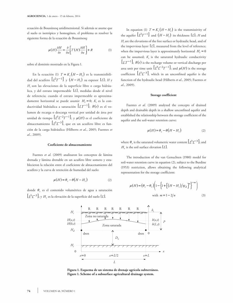
La dinámica del agua en un acuífero libre somero se describe con la ecuación de Boussinesq del drenaje agrícola, que resulta del principio de conservación de masa, la ley de Darcy y la hi-pótesis de Dupuit-Forcheimer concerniente a una distribución hidrostática de presiones. Si las variaciones de la carga hidráulica en la dirección longitudinal de los drenes son despreciables, se puede describir el flujo de agua en el sistema de drenaje con la

radiation boundary conditions in the agricultural drains, assumptions that do not adequately represent the water dynamics in the aquifer. Zavala et al. (2007) have analyzed the behavior of the drainage flow considering the soil and wall of the drain as fractal objects, and they established that the water transference from the soil to inside the drain should be represented with fractal or convex radiation boundary conditions. Also, Fuentes et al. (2009) formally have established the dependency between the storage coefficient and soil-water retention curve in shallow unconfined aquifers. The development of a computer tool that is structured and documented to facilitate the application of relations by Zavala et al. (2007) and Fuentes et al. (2009) is necessary for analysts to specify the study and design of drainage systems. The objective of this study was to develop a computer program with graphic interface to simulate the subsurface agricultural drainage in shallow unconfined aquifers, which had as a basis the one-dimensional Boussinesq equation with a variable storage coefficient of the aquifer, subject in the drains to conditions of fractal or convex radiation. The first version of the program was designed to perform one-dimensional modeling of drainage systems installed in homogenous and isotropic soils, and it is executed in computer systems with Windows system.

mAteRIAls And methods

Base equation

The water dynamic in a shallow unconfined aquifer is described with the Boussinesq equation of agricultural drainage, which results from the principle of mass conservation, the Darcy law and the Dupuit-Forcheimer hypothesis concerning a hydrostatic distribution of pressures. If the variations of the hydraulic head in the longitudinal direction of the drains are insignificant, the water flow in the drainage system can be described with the one-dimensional Boussinesq equation. If, in addition, it is assumed that the soil is isotropic and homogeneous, the problem is solving the following form of the Boussinesq equation:

µ H

Ht x

T HHx

R( )∂

∂=

∂

∂( )

∂

∂

+

(1)

regarding the dominion shown in Figure 1.

74



ecuación de Boussinesq unidimensional. Si además se asume que el suelo es isotrópico y homogéneo, el problema es resolver la siguiente forma de la ecuación de Boussinesq:

µ H

Ht x

T HHx

R( )∂

∂=

∂

∂( )

∂

∂

+

(1)

sobre el dominio mostrado en la Figura 1.

En la ecuación (1) T K H Hs i= −( ) es la transmisibili-

dad del acuífero L T2 1−[ ] y H Hi−( ) su espesor L[ ]; H y

Hi son las elevaciones de la superficie libre o carga hidráu-lica, y del estrato impermeable L[ ], medidas desde el nivel de referencia; cuando el estrato impermeable es aproxima-damente horizontal se puede asumir Hi 0; Ks es la con-

ductividad hidráulica a saturación LT−[ ]1 ; R t( ) es el vo-

lumen de recarga o descarga vertical por unidad de área por

unidad de tiempo L L T3 2 1− −[ ]; y µ H( ) es el coeficiente de

almacenamiento L L3 3−[ ], que en un acuífero libre es fun-

ción de la carga hidráulica (Hilberts et al., 2005; Fuentes et al., 2009).

Coeficiente de almacenamiento

Fuentes et al. (2009) analizaron los conceptos de lámina drenada y lámina drenable en un acuífero libre somero y esta-blecieron la relación entre el coeficiente de almacenamiento del acuífero y la curva de retención de humedad del suelo:

µ θ θH H Hs s( )= − −( ) (2)

donde s es el contenido volumétrico de agua a saturación

L L3 3−[ ]; y Hs es la elevación de la superficie del suelo L[ ].

In equation (1) T K H Hs i= −( ) is the transmissivity of

the aquifer L T2 1−[ ] and H Hi−( ) its thickness L[ ]; H and

Hi are the elevations of the free surface or hydraulic head, and of the impervious layer L[ ], measured from the level of reference; when the impervious layer is approximately horizontal Hi 0

can be assumed; Ks is the saturated hydraulic conductivity

LT−[ ]1 ; R t( ) is the recharge volume or vertical discharge per

area unit per time unit L L T3 2 1− −[ ]; and µ H( ) is the storage

coefficient L L3 3−[ ], which in an unconfined aquifer is the

function of the hydraulic head (Hilberts et al., 2005; Fuentes et al., 2009).

Storage coefficient

Fuentes et al. (2009) analyzed the concepts of drained depth and drainable depth in a shallow unconfined aquifer and established the relationship between the storage coefficient of the aquifer and the soil-water retention curve:

µ θ θH H Hs s( )= − −( ) (2)

where s is the saturated volumetric water content L L3 3−[ ]; and Hs is the soil surface elevation L[ ].

The introduction of the van Genuchten (1980) model for soil-water retention curve in equation (2), subject to the Burdine (1953) restriction, allows obtaining the following analytical representation for the storage coefficient:

µ θ θ ψH H Hs r s dn m

( )= −( ) − + −( ) { }

−1 1

with m n= −1 2 (3)

Figura 1. Esquema de un sistema de drenaje agrícola subterráneo.Figure 1. Scheme of a subsurface agricultural drainage system.

R R R R R R R

Zona no saturada

Zona saturada

dren drenDo

hs

h(x,t)h(L,t)

P

0

0

Hi

Hd

Hs

H(x,t)H(0,t)

x0 xL/2 xL

L

x



La introducción del modelo para la curva de retención de humedad de van Genuchten (1980) en la ecuación (2) sujeto a la restricción de Burdine (1953), permite obtener la siguiente repre-sentación analítica para el coeficiente de almacenamiento:

µ θ θ ψH H Hs r s dn m

( )= −( ) − + −( ) { }

−1 1

con m n= −1 2 (3)

donde r es el contenido volumétrico residual L L3 3−[ ]; m y n parámetros de forma adimensionales; y d parámetro de escala de la presión L[ ].

Condiciones límite

Para estudiar el drenaje agrícola con la ecuación (1) se requie-re definir las condiciones límite en el dominio de solución. La condición inicial se establece directamente a partir de la posición del manto freático en el tiempo inicial:

H x h x Do, ,0 0( )= ( )+ (4)

donde h x,0( ) es la elevación inicial de la superficie libre a lo lar-go de la coordenada horizontal x contada a partir de los drenes; y Do es la profundidad del estrato impermeable medida a partir de la elevación o posición de los drenes.

Condiciones de frontera tipo Dirichlet y Neumann se usan en los drenes para resolver la ecuación (1); en la primera se requie-re conocer la evolución de la carga hidráulica sobre los drenes y en la segunda el flujo de drenaje. Una tercera condición de frontera más general, llamada tipo radiación, es una combinación lineal de las dos condiciones precedentes, e incorpora un parámetro de resistencia al flujo del agua en la interfaz suelo-dren; la resistencia nula corresponde a la condición de Dirichlet y la infinita a la de Neumann:

−∂

∂± =K

Hx

qs d 0 x 0 y x L; t0 (5)

el signo positivo en la ecuación (5) es para el dren en x0, mien-tras que el negativo es para el que está en xL, donde L es la separación entre drenes y qd es el flujo de drenaje.

En el análisis del drenaje agrícola con la ecuación de Boussinesq, Zavala et al. (2007) establecieron que el flujo de dre-naje qd debe ser descrito con una condición de radiación tipo Hooghoudt (convexa) o con una condición de radiación fractal. La radiación tipo Hooghoudt es una combinación convexa de las

where r is the residual volumetric water content L L3 3−[ ]; m and n are dimensionless form parameters; and d is the pressure scale parameter L[ ].

Limit conditions

In order to study the agricultural drainage with equation (1) the limit conditions of the solution dominion need to be defined. The initial condition is established directly starting from the position of the water table at the initial time:

H x h x Do, ,0 0( )= ( )+ (4)

where h x,0( ) is the initial elevation of the free surface along the horizontal coordinate x measured from the drains; and Do is the depth of the impervious layer measured from the elevation or position of the drains.

Boundary conditions of the Dirichlet and Neumann type are used in drains to solve equation (1); in the first one, understanding the evolution of the hydraulic head on the drains is required, and in the second one the drainage flow. A third boundary condition, so-called radiation type, is a linear combination of the two precedent conditions, and incorporates a parameter of resistance to water flow in the soil-drain interface; the null resistance corresponds to Dirichlet’s condition and the infinite to Neumann’s:

−∂

∂± =K

Hx

qs d 0 x 0 y x L; t0 (5)

the positive sign in equation (5) is for the drain in x0,, while the negative one is for that on xL, where L is the separation between drains and qd is the drainage flow.

In the analysis of agricultural drainage with the Boussinesq equation, Zavala et al. (2007) established that the drainage flow qd should be described with a Hooghoudt radiation condition (convex combination), or with a fractal radiation condition. The Hooghoudt radiation type is a convex combination of the conditions of linear and quadratic radiation, which from a probabilistic point of view represents the extreme behaviors possible for the drainage flow:

q qH D

PH D

Pd so o= −( )

−

+

−

12

ω ω (6)

where qs is a particular value of the drainage flow LT−[ ]1 , which can be interpreted as the product of conductivity in the soil-drain

76



condiciones de radiación lineal y cuadrática, que desde el punto probabilista representan los comportamientos extremos posibles para el flujo de drenaje:

q qH D

PH D

Pd so o= −( )

−

+

−

12

ω ω (6)

donde qs es un valor particular del flujo de drenaje LT−[ ]1 , que se puede interpretar como el producto de la conductividad en la interfaz suelo-dren K in( ) y un coeficiente de conductancia adimensional γ( ); P es la profundidad de los drenes L[ ]; es el factor de interpolación tal que 01. Con 0 se tiene la radiación lineal y con 1 la radiación cuadrática; el primer caso corresponde a un movimiento completamente determinístico del agua en el suelo (correlación completa de los capilares) y el segundo a un movimiento completamente aleatorio (encuentro completamente aleatorio de los capilares).

Un segundo modelo que interpola los comportamientos extre-mos del flujo de drenaje fue establecido por Zavala et al. (2007) al considerar el suelo y la pared del dren como objetos fractales:

q qH D

Pd so

s sm d=

−

+

(7)

donde qs es el valor máximo del flujo de drenaje LT−[ ]1 , que puede interpretarse como q Ks in=γ ; sm y sd son la dimensión relativa del suelo y de la pared del dren (razón entre la dimensión fractal del objeto Df y la dimensión del espacio de Euclides, sDf /3). La dimensión cociente de un objeto fractal (s) está re-lacionada con su porosidad volumétrica ():

1 12−( ) + =φ φs s (8)

Se puede demostrar que s1/2 cuando 0, y s1 cuando 1, en otros términos se tiene 1/2s1 cuando 01; la co-rrelación completa se presenta en suelos cuya porosidad tiende a cero y la decorrelación completa en suelos cuya porosidad tiende a la unidad. Considerando que la porosidad areal del objeto fractal está relacionado con su porosidad volumétrica a través de 2s, se obtiene la ecuación que define la relación entre s y :

1 11 1 2−( ) + =ϑ ϑs s (9)

Solución numérica

El sistema de ecuaciones (1-9) se resolvió numéricamente realizando la discretización espacial con el método del elemento

interface K in( ) and a dimensionless conductance coefficient γ( ); P is the depth of the drains L[ ]; is the interpolation

factor so that 01. With 0 there is linear radiation and with 1 quadratic radiation; the first case corresponds to a completely deterministic movement of water in the soil (complete correlation of capillaries) and the second to a completely random movement (completely random encounter of capillaries).

A second model that interpolates the extreme behaviors of the drainage flow was established by Zavala et al. (2007) when considering the soil and the drain-wall as fractal objects:

q qH D

Pd so

s sm d=

−

+

(7)

where qs is the maximum value of the drainage flow LT−[ ]1 , which can be interpreted as q Ks in=γ ; sm and sd are the relative dimension of the soil and the drain-wall (ratio between the fractal dimension of object Df and the Euclides space dimension, sDf /3). The quotient dimension of a fractal object (s) is related to its volumetric porosity ():

1 12−( ) + =φ φs s (8)

It can be demonstrated that s1/2 when 0, and s1 when 1; in other words, there is 1/2s1 when 01; the complete correlation is presented in soils whose porosity tends to zero and the complete decorrelation in soils whose porosity tends to the unit. Considering that the areal porosity of the fractal object is related to its volumetric porosity through 2s, the equation that defines the relationship between s and is obtained:

1 11 1 2−( ) + =ϑ ϑs s (9)

Numerical solution

The system of equations (1-9) was solved numerically by performing the spatial discretization with the finite element Galerkin type method; the temporary discretization was performed with a method of finite differences; the system that results from the discretization process was linearized by employing the Picard method, whereas the algebraic equation system generated in each iteration was solved by using a method of preconditioned conjugated gradient with vectorial storage free of null coefficients. The details of these methods are documented, for example, in Zienkiewicz et al. (2005).



finito tipo Galerkin; la discretización temporal fue con un mé-todo de diferencias finitas; el sistema que resulta del proceso de discretización se linealizó empleando el método de Picard; mien-tras que el sistema de ecuaciones algebraicas generado en cada iteración fue resuelto usando un método de gradiente conjugado precondicionado con almacenamiento vectorial libre de entra-das nulas. Los detalles de estos métodos está documentado, por ejemplo, en Zienkiewicz et al. (2005).

Interfaz gráfica

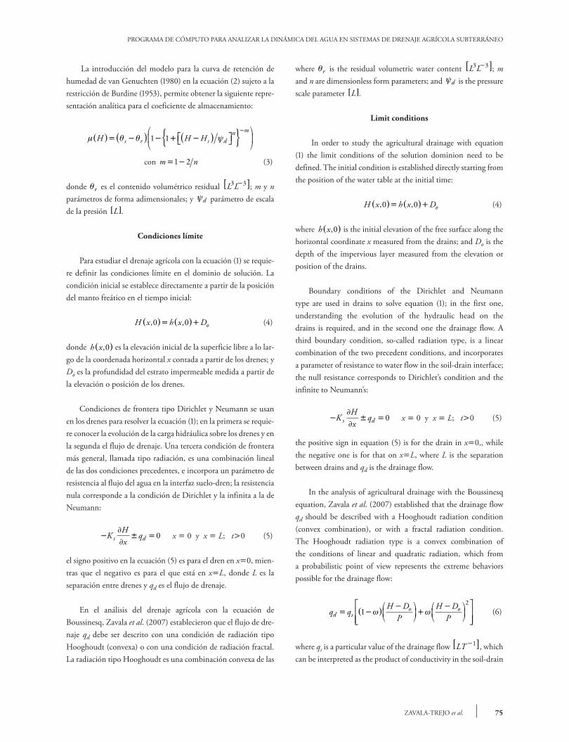
La codificación de la solución numérica y su interfaz gráfica se desarrolló con el lenguaje de programación Visual Basic, y para proporcionar más opciones de análisis y diseño a los usuarios se programó un módulo con soluciones analíticas para el drenaje agrícola. Esta primera versión del programa se denominó DRE-NAS (drenaje agrícola subterráneo) y sus componentes principa-les son: 1) ventana de inicio, y 2) pantalla general que incluye los dos módulos de cálculo, solución numérica y soluciones analíti-cas (Figura 2). Al inicio sólo están activadas las opciones Archivo e Información; en el menú Archivo el usuario debe seleccionar entre las opciones: crear nuevo proyecto, cargar proyecto anterior y salir del programa. Para introducir datos de una nueva simu-lación debe seleccionar la opción nuevo proyecto lo cual activa el fichero Datos, en el cual se definen las unidades de tiempo y espacio a usar en la modelación y después se activan las opciones para seleccionar el modelo numérico o las soluciones analíticas. El acceso directo a las ventanas incluidas en el fichero Datos puede realizarse a través de los íconos colocados en las cintillas

Graphic interface

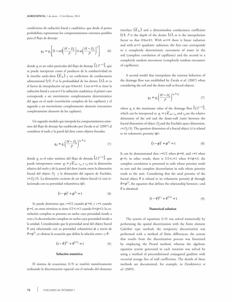
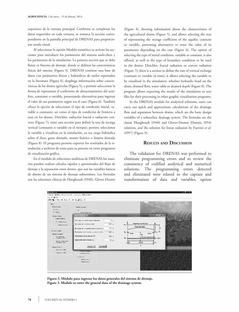
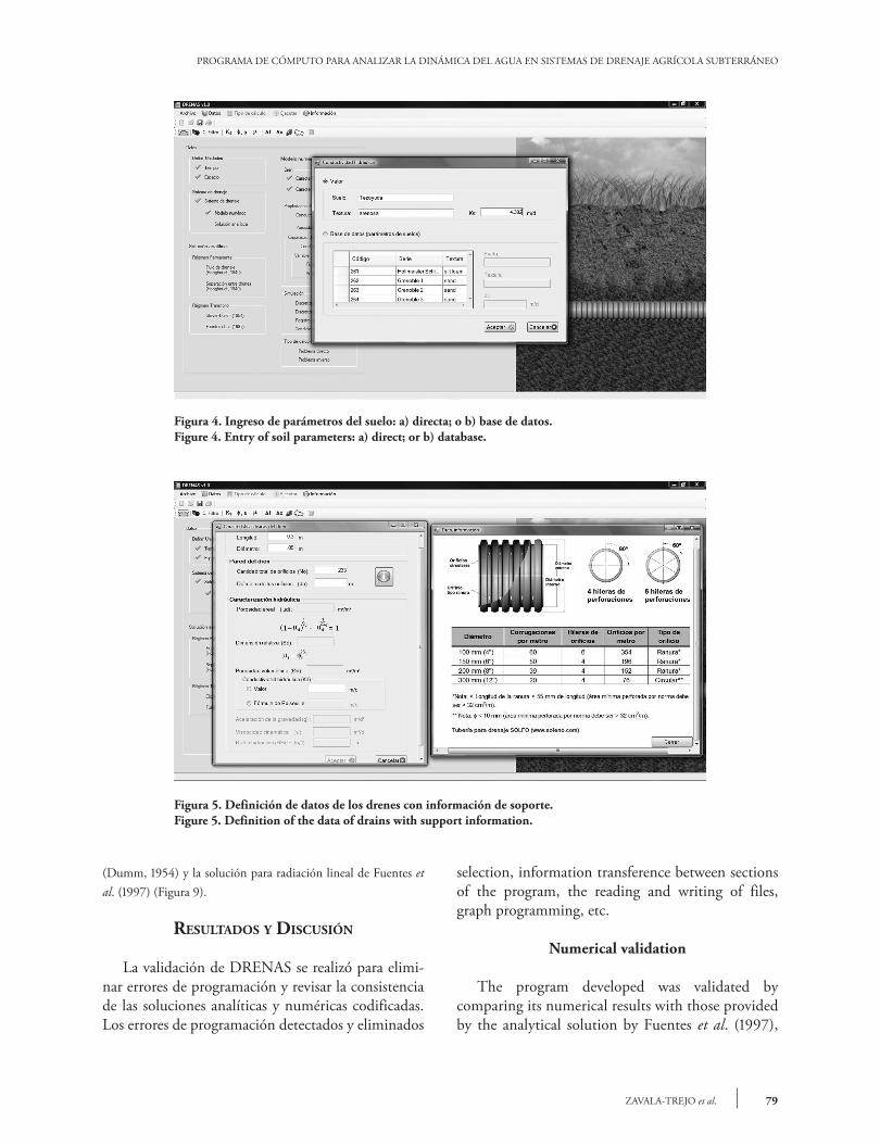
The codification of the numerical solution and its graphic interface was developed with the programming language Visual Basic, and to provide more options for analysis and design to the users, a module was programmed with analytical solutions for agricultural drainage. This first version of the program was called DRENAS (subsurface agricultural drainage, in Spanish), and its main components are: 1) opening window, and 2) general screen that includes the two calculation modules, numerical solution and analytical solutions (Figure 2). At the beginning only the File and Information options are activated; in the File menu the user must select between the options: create new project, load previous project, and exit the program. To introduce data for a new simulation, the option new project must be selected, which activates the Data file, where the units of time and space to be used in the modelling are defined, and later the options for selecting the numerical model or analytical solutions are activated. The direct access to the sections included in the Data file can be done through the icons placed on the upper bands of the main window. As the data required in each form are completed, the corresponding section on the main DRENAS screen is marked to provide visual aid. When selecting the option Numerical Model, the sections to introduce the parameters of the soil-drain system are activated, as well as the simulation parameters. The first section that must be filled is Drainage System, where the physical characteristics of the system are defined (Figure 3). DRENAS contains a database with soil physical and hydraulic parameters reported in the literature

Figura 2. Pantalla general del programa DRENAS.Figure 2. General screen of the DRENAS program.

78



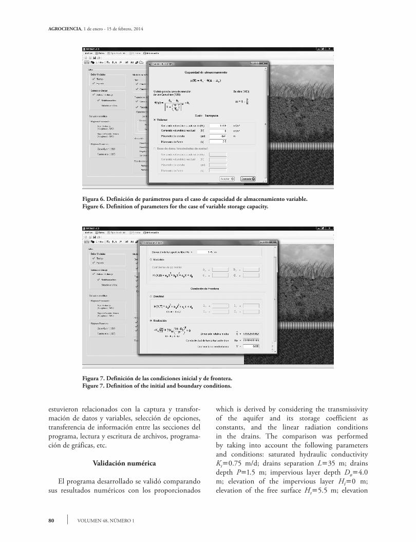
superiores de la ventana principal. Conforme se completan los datos requeridos en cada ventana, se remarca la sección corres-pondiente en la pantalla principal de DRENAS para proporcio-nar ayuda visual. Al seleccionar la opción Modelo numérico se activan las sec-ciones para introducir los parámetros del sistema suelo-dren y los parámetros de la simulación. La primera sección que se debe llenar es Sistema de drenaje, donde se definen las características físicas del sistema (Figura 3). DRENAS contiene una base de datos con parámetros físicos e hidráulicos de suelos reportados en la literatura (Figura 4), despliega información sobre caracte-rísticas de los drenes agrícolas (Figura 5), y permite seleccionar la forma de representar el coeficiente de almacenamiento del acuí-fero, constante o variable, presentando alternativas para ingresar el valor de sus parámetros según sea el caso (Figura 6). También ofrece la opción de seleccionar el tipo de condición inicial, va-riable o constante, así como el tipo de condición de frontera a usar en los drenes, Dirichlet, radiación fractal o radiación con-vexa (Figura 7); tiene una sección para definir la tasa de recarga vertical (constante o variable en el tiempo); permite seleccionar la variable a visualizar en la simulación, ya sea carga hidráulica sobre el dren, gasto drenado, manto freático o lámina drenada (Figura 8). El programa permite exportar los resultados de la si-mulación a archivos de texto para su proceso en otros programas de visualización gráfica. En el módulo de soluciones analíticas de DRENAS los usua-rios pueden realizar cálculos rápidos y aproximados del flujo de drenaje y la separación entre drenes, que son las variables básicas de diseño de un sistema de drenaje subterráneo. Las fórmulas son las relaciones clásicas de Hooghoudt (1940), Glover-Dumm

(Figure 4), showing information about the characteristics of the agricultural drains (Figure 5), and allows selecting the way of representing the storage coefficient of the aquifer, constant or variable, presenting alternatives to enter the value of its parameters depending on the case (Figure 6). The option of selecting the type of initial condition, variable or constant, is also offered, as well as the type of boundary condition to be used in the drains: Dirichlet, fractal radiation or convex radiation (Figure 7); there is a section to define the rate of vertical recharge (constant or variable in time); it allows selecting the variable to be visualized in the simulation, whether hydraulic head on the drain, drained flow, water table or drained depth (Figure 8). The program allows exporting the results of the simulation to text files for their processing in other graphic visualization programs. In the DRENAS module for analytical solutions, users can carry out quick and approximate calculations of the drainage flow and separation between drains, which are the basic design variables of a subsurface drainage system. The formulas are the classic Hooghoudt (1940) and Glover-Dumm (Dumm, 1954) relations, and the solution for linear radiation by Fuentes et al. (1997) (Figure 9).

Results And dIscussIon

The validation for DRENAS was performed to eliminate programming errors and to review the consistency of codified analytical and numerical solutions. The programming errors detected and eliminated were related to the capture and transformation of data and variables, option

Figura 3. Módulo para ingresar los datos generales del sistema de drenaje.Figure 3. Module to enter the general data of the drainage system.



Figura 4. Ingreso de parámetros del suelo: a) directa; o b) base de datos.Figure 4. Entry of soil parameters: a) direct; or b) database.

Figura 5. Definición de datos de los drenes con información de soporte.Figure 5. Definition of the data of drains with support information.

(Dumm, 1954) y la solución para radiación lineal de Fuentes et al. (1997) (Figura 9).

ResultAdos y dIscusIón

La validación de DRENAS se realizó para elimi-nar errores de programación y revisar la consistencia de las soluciones analíticas y numéricas codificadas. Los errores de programación detectados y eliminados

selection, information transference between sections of the program, the reading and writing of files, graph programming, etc.

Numerical validation

The program developed was validated by comparing its numerical results with those provided by the analytical solution by Fuentes et al. (1997),

80



Figura 6. Definición de parámetros para el caso de capacidad de almacenamiento variable.Figure 6. Definition of parameters for the case of variable storage capacity.

Figura 7. Definición de las condiciones inicial y de frontera.Figure 7. Definition of the initial and boundary conditions.

estuvieron relacionados con la captura y transfor-mación de datos y variables, selección de opciones, transferencia de información entre las secciones del programa, lectura y escritura de archivos, programa-ción de gráficas, etc.

Validación numérica

El programa desarrollado se validó comparando sus resultados numéricos con los proporcionados

which is derived by considering the transmissivity of the aquifer and its storage coefficient as constants, and the linear radiation conditions in the drains. The comparison was performed by taking into account the following parameters and conditions: saturated hydraulic conductivity Ks0.75 m/d; drains separation L35 m; drains depth P1.5 m; impervious layer depth Do4.0 m; elevation of the impervious layer Hi0 m; elevation of the free surface Hs5.5 m; elevation



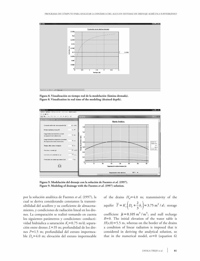
Figura 8. Visualización en tiempo real de la modelación (lámina drenada).Figure 8. Visualization in real time of the modeling (drained depth).

Figura 9. Modelación del drenaje con la solución de Fuentes et al. (1997).Figure 9. Modeling of drainage with the Fuentes et al. (1997) solution.

por la solución analítica de Fuentes et al. (1997), la cual se deriva considerando constantes la transmi-sibilidad del acuífero y su coeficiente de almacena-miento, y condiciones de radiación lineal en los dre-nes. La comparación se realizó tomando en cuenta los siguientes parámetros y condiciones: conducti-vidad hidráulica a saturación Ks0.75 m/d; separa-ción entre drenes L35 m; profundidad de los dre-nes P1.5 m; profundidad del estrato impermea-ble Do4.0 m; elevación del estrato impermeable

of the drains Hd4.0 m; transmissivity of the

aquifer T K D h ds o s= +

=

23

3 75 2. / m ; storage

coefficient µ=0 105 3 3. / m m ; and null recharge R0. The initial elevation of the water table is H(x,0)5.5 m, whereas on the border of the drains a condition of linear radiation is imposed that is considered in deriving the analytical solution, so that in the numerical model, 0 (equation 6)

82



Hi0 m; elevación de la superficie libre Hs5.5 m; elevación de los drenes Hd4.0 m; transmisibili-

dad del acuífero T K D h ds o s= +

=

23

3 75 2. / m ;

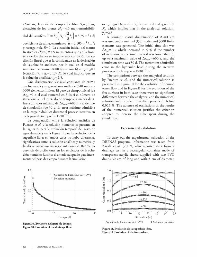
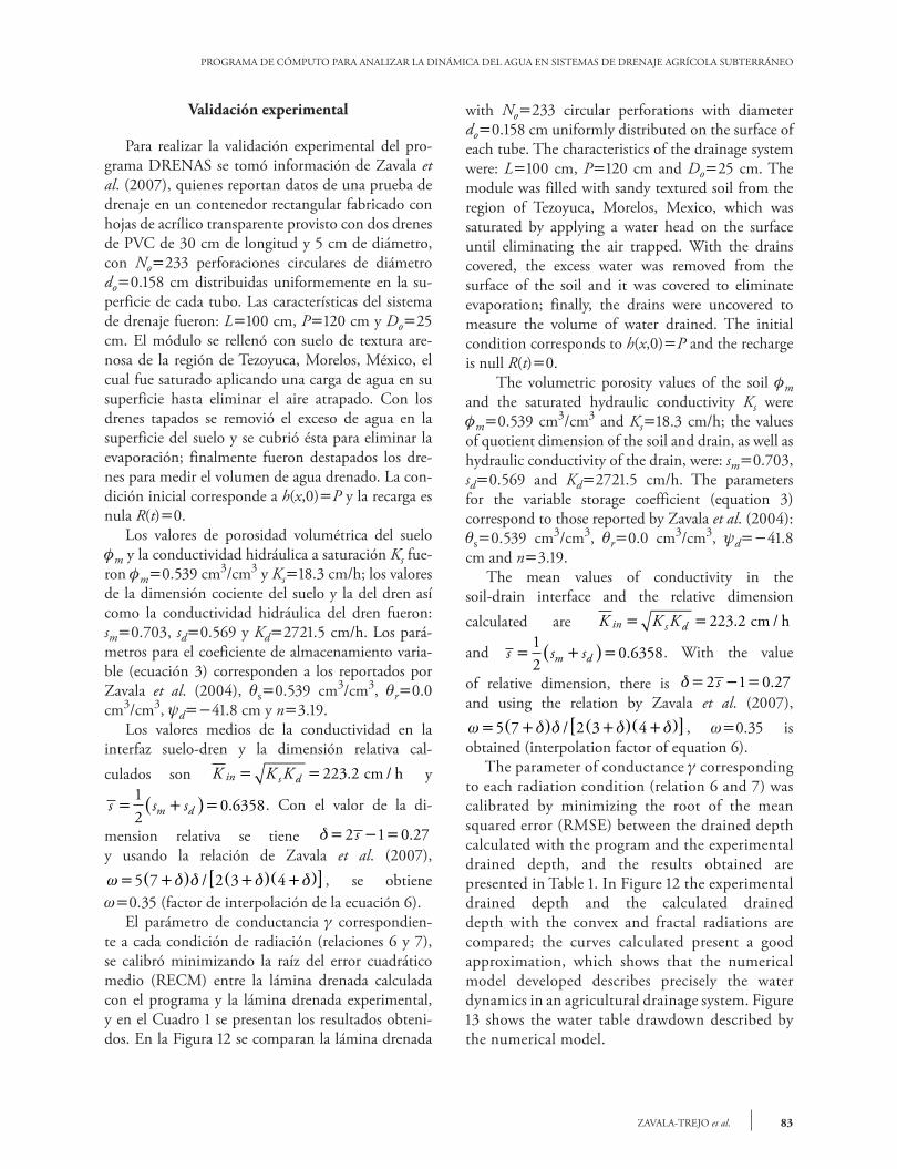
coeficiente de almacenamiento µ=0 105 3 3. / m m ; y recarga nula R0. La elevación inicial del manto freático es H(x,0)5.5 m, mientras que en la fron-tera de los drenes se impone una condición de ra-diación lineal que es la considerada en la derivación de la solución analítica, por lo cual en el modelo numérico se asume 0 (ecuación 6) o smsd1 (ecuación 7) y qs0.107 Ks, lo cual implica que en la solución analítica a2.5. Una discretización espacial constante de x1 cm fue usada y se generó una malla de 3501 nudos y 3500 elementos finitos. El paso de tiempo inicial fue tini1 s, el cual aumentó en 5 % si el número de iteraciones en el intervalo de tiempo era menor de 3, hasta un valor máximo de tmax600 s, y el tiempo de simulación fue 30 d. El error máximo admisible en la carga hidráulica durante el proceso iterativo en cada paso de tiempo fue 1104 m. La comparación entre la solución analítica de Fuentes et al. y la solución numérica se presenta en la Figura 10 para la evolución temporal del gasto de agua drenado y en la Figura 11 para la evolución de la superficie libre; en ambos casos no hubo diferencias significativas entre la solución analítica y numérica, y las discrepancias máximas son inferiores a 0.025 %. La ausencia de oscilaciones en los resultados de la solu-ción numérica justifica el criterio adoptado para incre-mentar el paso de tiempo durante la simulación.

or smsd1 (equation 7) is assumed and qs0.107 Ks, which implies that in the analytical solution, a2.5. A constant spatial discretization of x1 cm was used and a mesh of 3501 nodes and 3500 finite elements was generated. The initial time slot was tini1 s, which increased in 5 % if the number of iterations in the time interval was lower than 3, up to a maximum value of tmax600 s, and the simulation time was 30 d. The maximum admissible error in the hydraulic head during the iterative process of each step was 1104 m. The comparison between the analytical solution by Fuentes et al., and the numerical solution is presented in Figure 10 for the evolution of drained water flow and in Figure 11 for the evolution of the free surface; in both cases there were no significant differences between the analytical and the numerical solution, and the maximum discrepancies are below 0.025 %. The absence of oscillations in the results of the numerical solution justifies the criterion adopted to increase the time spent during the simulation.

Experimental validation

To carry out the experimental validation of the DRENAS program, information was taken from Zavala et al. (2007), who reported data from a drainage test in a rectangular container made of transparent acrylic sheets supplied with two PVC drains 30 cm of long and with 5 cm of diameter,

Figura 11. Evolución de la superficie libre.Figure 11. Evolution of the free surface.

Figura 10. Evolución del gasto de drenaje.Figure 10. Evolution of the drainage flow.



Validación experimental

Para realizar la validación experimental del pro-grama DRENAS se tomó información de Zavala et al. (2007), quienes reportan datos de una prueba de drenaje en un contenedor rectangular fabricado con hojas de acrílico transparente provisto con dos drenes de PVC de 30 cm de longitud y 5 cm de diámetro, con No233 perforaciones circulares de diámetro do0.158 cm distribuidas uniformemente en la su-perficie de cada tubo. Las características del sistema de drenaje fueron: L100 cm, P120 cm y Do25 cm. El módulo se rellenó con suelo de textura are-nosa de la región de Tezoyuca, Morelos, México, el cual fue saturado aplicando una carga de agua en su superficie hasta eliminar el aire atrapado. Con los drenes tapados se removió el exceso de agua en la superficie del suelo y se cubrió ésta para eliminar la evaporación; finalmente fueron destapados los dre-nes para medir el volumen de agua drenado. La con-dición inicial corresponde a h(x,0)P y la recarga es nula R(t)0. Los valores de porosidad volumétrica del suelo m y la conductividad hidráulica a saturación Ks fue-ron m0.539 cm3/cm3 y Ks18.3 cm/h; los valores de la dimensión cociente del suelo y la del dren así como la conductividad hidráulica del dren fueron: sm0.703, sd0.569 y Kd2721.5 cm/h. Los pará-metros para el coeficiente de almacenamiento varia-ble (ecuación 3) corresponden a los reportados por Zavala et al. (2004), s0.539 cm3/cm3, r0.0 cm3/cm3, d41.8 cm y n3.19. Los valores medios de la conductividad en la interfaz suelo-dren y la dimensión relativa cal-culados son K K Kin s d 223 2. / cm h y

s s sm d= +( )=12

0 6358. . Con el valor de la di-

mension relativa se tiene δ= − =2 1 0 27s . y usando la relación de Zavala et al. (2007), ω δ δ δ δ= +( ) +( ) +( )[ ]5 7 2 3 4/ , se obtiene 0.35 (factor de interpolación de la ecuación 6). El parámetro de conductancia correspondien-te a cada condición de radiación (relaciones 6 y 7), se calibró minimizando la raíz del error cuadrático medio (RECM) entre la lámina drenada calculada con el programa y la lámina drenada experimental, y en el Cuadro 1 se presentan los resultados obteni-dos. En la Figura 12 se comparan la lámina drenada

with No233 circular perforations with diameter do0.158 cm uniformly distributed on the surface of each tube. The characteristics of the drainage system were: L100 cm, P120 cm and Do25 cm. The module was filled with sandy textured soil from the region of Tezoyuca, Morelos, Mexico, which was saturated by applying a water head on the surface until eliminating the air trapped. With the drains covered, the excess water was removed from the surface of the soil and it was covered to eliminate evaporation; finally, the drains were uncovered to measure the volume of water drained. The initial condition corresponds to h(x,0)P and the recharge is null R(t)0. The volumetric porosity values of the soil m and the saturated hydraulic conductivity Ks were m0.539 cm3/cm3 and Ks18.3 cm/h; the values of quotient dimension of the soil and drain, as well as hydraulic conductivity of the drain, were: sm0.703, sd0.569 and Kd2721.5 cm/h. The parameters for the variable storage coefficient (equation 3) correspond to those reported by Zavala et al. (2004): s0.539 cm3/cm3, r0.0 cm3/cm3, d41.8 cm and n3.19. The mean values of conductivity in the soil-drain interface and the relative dimension calculated are K K Kin s d 223 2. / cm h

and s s sm d= +( )=12

0 6358. . With the value

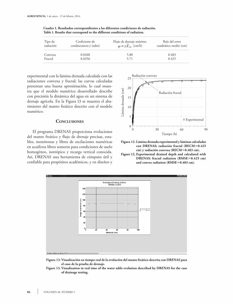
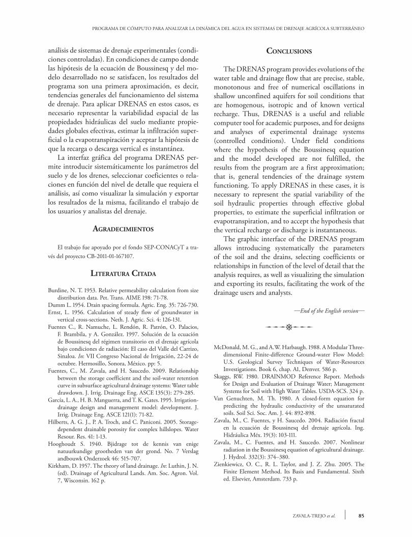
of relative dimension, there is δ= − =2 1 0 27s . and using the relation by Zavala et al. (2007),ω δ δ δ δ= +( ) +( ) +( )[ ]5 7 2 3 4/ , 0.35 is obtained (interpolation factor of equation 6). The parameter of conductance corresponding to each radiation condition (relation 6 and 7) was calibrated by minimizing the root of the mean squared error (RMSE) between the drained depth calculated with the program and the experimental drained depth, and the results obtained are presented in Table 1. In Figure 12 the experimental drained depth and the calculated drained depth with the convex and fractal radiations are compared; the curves calculated present a good approximation, which shows that the numerical model developed describes precisely the water dynamics in an agricultural drainage system. Figure 13 shows the water table drawdown described by the numerical model.

84



experimental con la lámina drenada calculada con las radiaciones convexa y fractal; las curvas calculadas presentan una buena aproximación, lo cual mues-tra que el modelo numérico desarrollado describe con precisión la dinámica del agua en un sistema de drenaje agrícola. En la Figura 13 se muestra el aba-timiento del manto freático descrito con el modelo numérico.

conclusIones

El programa DRENAS proporciona evoluciones del manto freático y flujo de drenaje precisas, esta-bles, monótonas y libres de oscilaciones numéricas en acuíferos libres someros para condiciones de suelo homogéneo, isotrópico y recarga vertical conocida. Así, DRENAS una herramienta de cómputo útil y confiable para propósitos académicos, y en diseños y

Cuadro 1. Resultados correspondientes a las diferentes condiciones de radiación.Table 1. Results that correspond to the different conditions of radiation.

Tipo de radiación

Coeficiente de conductancia (adm)

Flujo de drenaje máximo qs K in=γ (cm/h)

Raíz del error cuadrático medio (cm)

Convexa 0.0260 5.80 0.483Fractal 0.0256 5.71 0.425

Figura 12. Lámina drenada experimental y láminas calculadas con DRENAS: radiación fractal (RECM0.425 cm) y radiación convexa (RECM0.483 cm).

Figure 12. Experimental drained depth and calculated with DRENAS: fractal radiation (RMSE0.425 cm) and convex radiation (RMSE0.483 cm).

Figura 13. Visualización en tiempo real de la evolución del manto freático descrita con DRENAS para el caso de la prueba de drenaje.

Figure 13. Visualization in real time of the water table evolution described by DRENAS for the case of drainage testing.



análisis de sistemas de drenaje experimentales (condi-ciones controladas). En condiciones de campo donde las hipótesis de la ecuación de Boussinesq y del mo-delo desarrollado no se satisfacen, los resultados del programa son una primera aproximación, es decir, tendencias generales del funcionamiento del sistema de drenaje. Para aplicar DRENAS en estos casos, es necesario representar la variabilidad espacial de las propiedades hidráulicas del suelo mediante propie-dades globales efectivas, estimar la infiltración super-ficial o la evapotranspiración y aceptar la hipótesis de que la recarga o descarga vertical es instantánea. La interfaz gráfica del programa DRENAS per-mite introducir sistemáticamente los parámetros del suelo y de los drenes, seleccionar coeficientes o rela-ciones en función del nivel de detalle que requiera el análisis, así como visualizar la simulación y exportar los resultados de la misma, facilitando el trabajo de los usuarios y analistas del drenaje.

AgRAdecImIentos

El trabajo fue apoyado por el fondo SEP-CONACyT a tra-vés del proyecto CB-2011-01-167107.

lIteRAtuRA cItAdA

Burdine, N. T. 1953. Relative permeability calculation from size distribution data. Pet. Trans. AIME 198: 71-78.

Dumm L. 1954. Drain spacing formula. Agric. Eng. 35: 726-730.Ernst, L. 1956. Calculation of steady flow of groundwater in

vertical cross-sections. Neth. J. Agric. Sci. 4: 126-131.Fuentes C., R. Namuche, L. Rendón, R. Patrón, O. Palacios,

F. Brambila, y A. González. 1997. Solución de la ecuación de Boussinesq del régimen transitorio en el drenaje agrícola bajo condiciones de radiación: El caso del Valle del Carrizo, Sinaloa. In: VII Congreso Nacional de Irrigación, 22-24 de octubre. Hermosillo, Sonora, México. pp: 5.

Fuentes, C., M. Zavala, and H. Saucedo. 2009. Relationship between the storage coefficient and the soil-water retention curve in subsurface agricultural drainage systems: Water table drawdown. J. Irrig. Drainage Eng. ASCE 135(3): 279-285.

García, L. A., H. B. Manguerra, and T. K. Gates. 1995. Irrigation-drainage design and management model: development. J. Irrig. Drainage Eng. ASCE 121(1): 71-82.

Hilberts, A. G. J., P. A. Troch, and C. Paniconi. 2005. Storage-dependent drainable porosity for complex hillslopes. Water Resour. Res. 41: 1-13.

Hooghoudt S. 1940. Bjidrage tot de kennis van enige natuurkundige grootheden van der grond. No. 7 Verslag andbouwk Onderzoek 46: 515-707.

Kirkham, D. 1957. The theory of land drainage. In: Luthin, J. N. (ed). Drainage of Agricultural Lands. Am. Soc. Agron. Vol. 7, Wisconsin. 162 p.

conclusIons

The DRENAS program provides evolutions of the water table and drainage flow that are precise, stable, monotonous and free of numerical oscillations in shallow unconfined aquifers for soil conditions that are homogenous, isotropic and of known vertical recharge. Thus, DRENAS is a useful and reliable computer tool for academic purposes, and for designs and analyses of experimental drainage systems (controlled conditions). Under field conditions where the hypothesis of the Boussinesq equation and the model developed are not fulfilled, the results from the program are a first approximation; that is, general tendencies of the drainage system functioning. To apply DRENAS in these cases, it is necessary to represent the spatial variability of the soil hydraulic properties through effective global properties, to estimate the superficial infiltration or evapotranspiration, and to accept the hypothesis that the vertical recharge or discharge is instantaneous. The graphic interface of the DRENAS program allows introducing systematically the parameters of the soil and the drains, selecting coefficients or relationships in function of the level of detail that the analysis requires, as well as visualizing the simulation and exporting its results, facilitating the work of the drainage users and analysts.

—End of the English version—

pppvPPP

McDonald, M. G., and A.W. Harbaugh. 1988. A Modular Three-dimensional Finite-difference Ground-water Flow Model: U.S. Geological Survey Techniques of Water-Resources Investigations. Book 6, chap. A1, Denver. 586 p.

Skaggs, RW. 1980. DRAINMOD Reference Report. Methods for Design and Evaluation of Drainage Water; Management Systems for Soil with High Water Tables. USDA-SCS. 324 p.

Van Genuchten, M. Th. 1980. A closed-form equation for predicting the hydraulic conductivity of the unsaturated soils. Soil Sci. Soc. Am. J. 44: 892-898.

Zavala, M., C. Fuentes, y H. Saucedo. 2004. Radiación fractal en la ecuación de Boussinesq del drenaje agrícola. Ing. Hidráulica Méx. 19(3): 103-111.

Zavala, M., C. Fuentes, and H. Saucedo. 2007. Nonlinear radiation in the Boussinesq equation of agricultural drainage. J. Hydrol. 332(3): 374–380.

Zienkiewicz, O. C., R. L. Taylor, and J. Z. Zhu. 2005. The Finite Element Method. Its Basis and Fundamental. Sixth ed. Elsevier, Amsterdam. 733 p.

PROGRAMA DE CÓMPUTO PARA ANALIZAR LA … · listas precisen el estudio y diseño de los sistemas...

Documents

Transcript of PROGRAMA DE CÓMPUTO PARA ANALIZAR LA … · listas precisen el estudio y diseño de los sistemas...