'Problemas de dominación de aristas: algoritmos, cotas y ...
117
Dirección: Dirección: Biblioteca Central Dr. Luis F. Leloir, Facultad de Ciencias Exactas y Naturales, Universidad de Buenos Aires. Intendente Güiraldes 2160 - C1428EGA - Tel. (++54 +11) 4789-9293 Contacto: Contacto: [email protected] Tesis Doctoral Problemas de dominación de aristas: Problemas de dominación de aristas: algoritmos, cotas y propiedades algoritmos, cotas y propiedades Moyano, Verónica Andrea 2017-03-29 Este documento forma parte de la colección de tesis doctorales y de maestría de la Biblioteca Central Dr. Luis Federico Leloir, disponible en digital.bl.fcen.uba.ar. Su utilización debe ser acompañada por la cita bibliográfica con reconocimiento de la fuente. This document is part of the doctoral theses collection of the Central Library Dr. Luis Federico Leloir, available in digital.bl.fcen.uba.ar. It should be used accompanied by the corresponding citation acknowledging the source. Cita tipo APA: Moyano, Verónica Andrea. (2017-03-29). Problemas de dominación de aristas: algoritmos, cotas y propiedades. Facultad de Ciencias Exactas y Naturales. Universidad de Buenos Aires. Cita tipo Chicago: Moyano, Verónica Andrea. "Problemas de dominación de aristas: algoritmos, cotas y propiedades". Facultad de Ciencias Exactas y Naturales. Universidad de Buenos Aires. 2017-03- 29.
Transcript of 'Problemas de dominación de aristas: algoritmos, cotas y ...

Di r ecci ó n:Di r ecci ó n: Biblioteca Central Dr. Luis F. Leloir, Facultad de Ciencias Exactas y Naturales, Universidad de Buenos Aires. Intendente Güiraldes 2160 - C1428EGA - Tel. (++54 +11) 4789-9293
Co nta cto :Co nta cto : [email protected]
Tesis Doctoral
Problemas de dominación de aristas:Problemas de dominación de aristas:algoritmos, cotas y propiedadesalgoritmos, cotas y propiedades
Moyano, Verónica Andrea
2017-03-29
Este documento forma parte de la colección de tesis doctorales y de maestría de la BibliotecaCentral Dr. Luis Federico Leloir, disponible en digital.bl.fcen.uba.ar. Su utilización debe seracompañada por la cita bibliográfica con reconocimiento de la fuente.
This document is part of the doctoral theses collection of the Central Library Dr. Luis FedericoLeloir, available in digital.bl.fcen.uba.ar. It should be used accompanied by the correspondingcitation acknowledging the source.
Cita tipo APA:
Moyano, Verónica Andrea. (2017-03-29). Problemas de dominación de aristas: algoritmos, cotasy propiedades. Facultad de Ciencias Exactas y Naturales. Universidad de Buenos Aires.
Cita tipo Chicago:
Moyano, Verónica Andrea. "Problemas de dominación de aristas: algoritmos, cotas ypropiedades". Facultad de Ciencias Exactas y Naturales. Universidad de Buenos Aires. 2017-03-29.

UNIVERSIDAD DE BUENOS AIRES
Facultad de Ciencias Exactas y Naturales
Departamento de Matematica
Problemas de dominacion de aristas: algoritmos, cotas y propiedades.
Tesis presentada para optar al tıtulo de Doctor de la Universidad de Buenos Aires en el
area Ciencias Matematicas
Veronica Andrea Moyano
Director de tesis: Min Chih Lin
Consejero de estudios: Guillermo Duran
Lugar de trabajo: Instituto de Calculo, FCEyN, Universidad de Buenos Aires.
Buenos Aires, 2017


Agradecimientos
Quiero agradecer a mi director Oscar por confiar en mı, por todo el empuje y la ayuda en eldoctorado, porque aprendı muchisimas cosas y porque es un excelente director y persona.
A Flavia, Valeria y Luerbio, por revisar esta tesis y por sus valiosos aportes y sugeren-cias.
A Willy por ser mi consejero de estudios. Al Instituto de Calculo, el Departamento deMatematica, la FCEyN y sus profesores a los que debo mi formacion academica. Tambiengracias a Debora por ayudarme en todos mis tramites.
A mis companeros (y amigos) del Instituto, porque realmente hacen que trabajar ahısea un placer. Gracias por los almuerzos, los mates, las charlas y los consejos. GraciasManu B., Pablo T., Chebi, Flor S., Marina, Maru, Andres, Agus, Flor F.S., Nina, Michel,Saveli, Xavi, Manu S., Ines, Stella, Ale, Manu F., Lu, Ale, Maxi, Pablo V. y Lucas.
A mis amigos por bancarme hablando de grafos cada tanto (todo en esta vida se puedeexplicar con grafos) y por compartir la vida conmigo. Gracias Maggie, Pablo B., Juli C.,Neru, Fede F., Marcos C., Maga K., Lucio, Pau, Mati S., Gara, Emilce, Natu, Rochis,Elina, y seguramente me estoy olvidando de algunos. A todos gracias, los quiero fuerte!
A mi familia, en especial a mi hermano Rodrigo, por todo su apoyo.
Finalmente, y no menos importante, gracias a la Agencia Nacional de PromocionCientıfica y Tecnologica y al CONICET por las becas que me permitieron dedicarme,casi exclusivamente, a este trabajo de investigacion.
3


Edge dominating set problems:Algorithms, bounds and properties.
Abstract
In this thesis we study different dominating set problems with two different approaches:combinatoric and algorithmic. The first one consists in understanding the structure of thegraph with respect to the minimum solution, and in counting the number of minimal solu-tions that the graph can contain. The algorithmic approach classifies the domination prob-lem on different graph classes according to its complexity (NP-complete or polynomial-time solvable), while it also tries to develop efficient algorithms for the problems. Thevariants of domination problems we consider in this work are (i) edge domination, (ii) effi-cient edge domination, (iii) perfect edge domination, and (iv) vertex domination. Efficientedge dominating sets are also known in the literature as dominating induced matchings.
For (i) we present a linear time algorithm to find a minimum edge dominating seton proper interval graphs. For (ii) we prove tight bounds for the number of dominat-ing induced matching, while we described the extremal graphs for the classes of general,triangle-free, and connected graphs. For (iii) we present a linear time algorithm to solvethe weighted perfect edge dominating set problem for cubic claw-free graphs, and a robustlinear time algorithm for P5-free graphs.
Problem (i) is equivalent to (iv) restricted to line graphs, which form a subclass of K1,3-free. We prove that (iv) is NP-Hard for well-covered K1,4-free graphs, while it requireslinear time for well-covered K1,3-free graphs, which is a superclass of well-covered linegraphs. Finally, we present polynomial time algorithms to decide if a comparability graphor its complement is well-covered.
5


Problemas de dominacion de aristas:Algoritmos, cotas y propiedades.
Resumen
En esta tesis estudiamos problemas de conjunto dominante mediante dos enfoquesdiferentes: combinatorio y algorıtmico. El primero consiste en entender las esctructurasdel grafo relacionadas con la solucion mınima y tambien contar el numero de solucionesminimales que un grafo puede admitir. El enfoque algorıtmico busca clasificar los prob-lemas de dominacion para diferentes clases de grafos de acuerdo a su complejidad (NP-completo o polinomial), mientras que tambien intenta desarrollar algoritmos eficientes queresuelvan estos problemas. Las variantes de problemas de conjunto dominante que con-sideramos en este trabajo son (i) dominacion de aristas (ii) dominacion eficiente de aristas(iii) dominacion perfecta de aristas y (iv) dominacion de vertices. En la literatura tambiense conoce a los conjuntos eficientemente dominantes con el nombre de matching inducidosdominantes.
Para el problema (i) presentamos un algoritmo de tiempo lineal para encontrar un con-junto dominante de aristas mınimo para los grafos de intervalos propios. Para el problema(ii) probamos cotas ajustadas para el numero de matching inducidos dominantes y tambiendescribimos los grafos maximales para la clase general de grafos, grafos sin triangulos ygrafos conexos. Para el problema (iii) presentamos un algoritmo de tiempo lineal pararesolver el problema de dominacion perfecta de aristas con pesos para los grafos cubicosque no contienen garras, y un algoritmo robusto, tambien de tiempo lineal, para los grafosque no contienen P5.
El problema (i) es equivalente a (iv) cuando nos restringimos a los grafos de lıneas, es-tos grafos forman una subclase de los grafos que no contienen K1,3. En la tesis probamosque el problema (iv) es NP-Hard para los grafos bien cubiertos que no contienen K1,4,mientras el problema se resuelve en tiempo lineal para los grafos bien cubiertos que nocontienen K1,3, la cual es una superclase de los grafos bien cubiertos de lınea. Finalmente,presentamos algoritmos polinomiales para decidir si un grafo de comparabilidad o su com-plemento es bien cubierto.
7


Contents
Introduccion 11
1 Introduction 211.1 Background . . . . . . . . . . . . . . . . . . . . . . . . . . . . . . . . . 23
1.2 Notations and Definitions . . . . . . . . . . . . . . . . . . . . . . . . . . 25
1.3 Overview . . . . . . . . . . . . . . . . . . . . . . . . . . . . . . . . . . 29
2 Edge Domination 312.1 Preliminaries . . . . . . . . . . . . . . . . . . . . . . . . . . . . . . . . 32
2.2 Previous results . . . . . . . . . . . . . . . . . . . . . . . . . . . . . . . 33
2.3 Properties related to edge domination . . . . . . . . . . . . . . . . . . . . 34
2.4 Algorithm for Proper Interval Graphs . . . . . . . . . . . . . . . . . . . . 35
Resumen del Capıtulo 2 . . . . . . . . . . . . . . . . . . . . . . . . . . . . . . 41
3 Efficient Edge Domination 433.1 Preliminaries . . . . . . . . . . . . . . . . . . . . . . . . . . . . . . . . 44
3.2 Previous results . . . . . . . . . . . . . . . . . . . . . . . . . . . . . . . 46
3.3 Colorings associated to a DIM . . . . . . . . . . . . . . . . . . . . . . . 47
3.4 Bounds for the maximum number of DIMs . . . . . . . . . . . . . . . . . 50
3.4.1 General graphs . . . . . . . . . . . . . . . . . . . . . . . . . . . 50
3.4.2 Triangle-free graphs . . . . . . . . . . . . . . . . . . . . . . . . 53
3.4.3 Connected graphs . . . . . . . . . . . . . . . . . . . . . . . . . . 55
Resumen del Capıtulo 3 . . . . . . . . . . . . . . . . . . . . . . . . . . . . . . 64
9
4 Perfect Edge Domination 674.1 3-Colorings associated to a edge dominating set . . . . . . . . . . . . . . 69
4.2 Complexity for H-free graphs . . . . . . . . . . . . . . . . . . . . . . . . 70
4.2.1 Cubic claw-free graphs . . . . . . . . . . . . . . . . . . . . . . . 71
4.3 Graphs without paths of length 5 . . . . . . . . . . . . . . . . . . . . . . 73
4.3.1 Properties of P5-free graphs . . . . . . . . . . . . . . . . . . . . 74
4.3.2 Colorings and vertex dominating subgraphs . . . . . . . . . . . . 78
4.3.3 Robust linear algorithm for P5-free graphs . . . . . . . . . . . . . 81
Resumen del Capıtulo 4 . . . . . . . . . . . . . . . . . . . . . . . . . . . . . . 85
5 Vertex domination and well-covered graphs 875.1 Preliminaries and previous results . . . . . . . . . . . . . . . . . . . . . 88
5.2 Vertex dominating set problem . . . . . . . . . . . . . . . . . . . . . . . 90
5.2.1 Well covered K1,4-free graphs . . . . . . . . . . . . . . . . . . . . 90
5.3 Recognition problem . . . . . . . . . . . . . . . . . . . . . . . . . . . . 93
5.3.1 Well-covered comparability graphs . . . . . . . . . . . . . . . . . 94
5.3.2 Well-covered co-comparability graphs . . . . . . . . . . . . . . . 95
Resumen del Capıtulo 5 . . . . . . . . . . . . . . . . . . . . . . . . . . . . . . 97
6 Conclusions 99
Conclusiones 103
Bibliografıa 107
10

Introduccion
En la actualidad, la teorıa de grafos es una disciplina dinamica tanto en la teorıa como
en las aplicaciones. Los problemas de cubrimiento forman un campo en continuo creci-
miento dentro de la teorıa de grafos. Muchas de los problemas surgen de las aplicaciones
y otros por intereses teoricos y de las conjeturas cientıficas. Los problemas de conjunto
dominante, en particular dominantes de aristas, son los principales objetos de estudio en
esta tesis.
Los grafos son excelentes herramientas para modelar problemas que pueden venir de
distintos contextos pues sirven como representacion de las relaciones entre objetos. Por
ejemplo, una red de ciudades las cuales son representadas con vertices y sus conexio-
nes representadas con aristas, definen un grafo. En algunos contextos, tambien hay una
funcion de peso definida en los vertices y/o aristas. En el ejemplo anterior, el peso de
una conexion puede representar la distancia entre las ciudades conectadas. El famoso
problema del viajante de comercio busca el recorrido mas corto posible que visite todas
las ciudades exactamente una vez. Los problemas de conjuntos dominantes en grafos son
modelos naturales para los problemas de locacion de resursos en investigacion operativa.
Estos problemas buscan la locacion de una o mas facilidades de manera que se optimice
cierto objetivo que puede ser minimizar el costo de transporte, ofrecer servicio equitativo
a los clientes u obtener la mayor participacion en el mercado. El concepto de dominacion
11

tambien se aplica en la teorıa de codigos como lo muestran Kalbfleisch, Stanton y Horton
en [52] y tambien Cockayne y Hedetniemi en [26]. Si se define un grafo, siendo los
vertices los vectores n-dimensionales con coordenadas elegidas en 1, ..., p, p > 1, y
dos vertices son adyacentes si difieren en una coordenada, entonces los conjuntos que son
(n, p)-cubrimientos, codigos de correccion de errores simples, o los cubrimientos perfectos
son todos conjuntos dominantes del grafo con propiedades adicionales.
Las conjeturas cientıficas son otra fuente de problemas interesantes y han tenido un
impacto importante en el desarrollo de la teorıa de grafos. Por ejemplo, Berge formulo la
Conjetura Fuerte de los Grafos Perfectos en sus libros [3, 4] en los 60s. Por 40 anos, los
intentos por resolver esta conjetura dieron lugar a metodos poderosos, importantes con-
ceptos y resultados interesantes en diferentes areas de la teorıa de grafos. Finalmente,
la conjetura fue probada en 2006 [25] y ahora se conoce como el Teorema Fuerte de los
Grafos Perfectos. En la teorıa de dominacion tenemos que mencionar la famosa y todavıa
abierta conjetura de Vizing formulada en 1963 [83]. La conjetura afirma que el tamano de
un conjunto dominante mınimo, llamado el numero de dominacion, del producto Carte-
siano de dos grafos FG es al menos el producto de los numeros de dominacion de F y
G. Las estrategias para resolver la conjetura incluyen familias de grafos para las cuales
la conjetura es valida, propiedades de un supuesto contraejemplo minimal y conjeturas
relacionadas. Un buen resumen del progreso en este campo se puede encontrar en [15].
Desde el punto de vista computacional, los problemas pueden ser clasificados de acuer-
do a su dificultad siguiendo la teorıa de la NP-completitud formalizada por Cook en [27].
Muchos de los problemas de cubrimiento en teorıa de grafos pertenecen a la clase NP-
completa. El hecho de que no sea posible resolver estos problemas en un tiempo razona-
ble conduce a diferentes estrategias para dar soluciones que puedan servir a propositos
practicos. Una de esas estrategias es restringir el dominio del problema. Debido a que
muchas veces las entradas no son datos arbitrarios, se pueden hacer muchas suposiciones
12

de acuerdo al campo de donde viene el problema y estas restricciones se formalizan con
propiedades estructurales que toda entrada debe satisfacer. Muchas clases de grafos han
sido definas siguiendo propositos practicos y muchas otras surgen de la teorıa. Entre las
primeras podemos mencionar los grafos de interseccion [33] como los grafos de inter-
valos [11, 55], grafos arco circulares [11, 39], pero hay mas. Otras clases de grafos son
definidas con restricciones en parametros como el maximo grado de sus vertices o numero
de independencia. Un resumen bien organizado sobre las familias de grafos estudiadas en
la actualidad es [11]. En esta tesis pusismos especial esfuerzo en disenar los algoritmos
propuestos de manera eficiente y robusta para hacerlos utiles para propositos practicos.
Las preguntas teoricas sobre los problemas de cubrimiento pueden ser muy diferentes.
Un enfoque es acotar el numero de soluciones de un problema. Esto se relaciona con el
punto de vista computacional pues da lugar a una cota natural para la busqueda exhaustiva.
Distintos parametros relacionados y variantes de los problemas de conjunto dominante
han sido definidos y ampliamente estudiados. Tambien, este tipo de analisis es util para
entender las estructuras internas relacionadas y, a veces, desarrollar algoritmos eficientes
para revolver los problemas.
Antecedentes
Las ideas teoricas de grafos se remontan al menos a la decada de 1730, cuando Leonard
Euler publica su trabajo sobre el problema de los siete puentes de Koningsberg [6]. En los
comienzos gran parte de la teorıa de grafos estuvo motivada por el estudio de juegos y la
matematica recreativa. Los grafos son herramientas utiles para modelar relaciones entre
objetos. La convencion usual es que los objeros son representados por vertices (puntos)
y las relaciones entre ellos son representadas por aristas (lıneas) que unen esos vertices.
En general, cualquier objeto matematico que involucre puntos y conexiones entre ellos
13

puede ser llamado un grafo o hipergrafo. No hay restriccion alguna sobre los objetos o sus
relaciones, de esta manera los grafos pueden ser usados en bases de datos, redes fısicas,
flujo de senales, redes sociales o el flujo de un programa de computacion, entre muchas
otras aplicaciones. Normalmente, los problemas de la vida real pueden ser modelados
con grafos que satisfacen varias propiedades, otras clases de grafos han sido definidas con
propositos teoricos. La ventaja de restringir el dominio de los problemas es que sea mas
facil trabajar en una solucion para esas representaciones restringidas. Un resumen acerca
de las clases de grafos incluyendo la teorıa de interseccion se puede encontrar en [11].
Dado que el concepto de dominacion en grafos surge naturalmente, hay referencias a
problemas relacionados con dominacion desde hace cientos de anos. En 1862 de Jaenisch
[29] y en 1892 W.W. Rouse Ball [78] presentaron diferentes problemas de dominacion
en tableros de ajedrez. La teorıa de dominacion fue desarrollada posteriormente en los
1950s y 1960s. En 1958 C. Berge escribio un libro sobre teorıa de grafos [5] en el que
introducıa el coeficiente de estabilidad externa, que ahora es conocido como el numero
de dominacion de un grafo. En el libro de O. Ore [70] los terminos de conjunto domi-
nante y numero de dominacion fueron introducidos, pero fue despues de los avances de
los hermanos Yaglom y Yaglom [86] y el trabajo de recopilacion de Cockayne y Hedet-
niemi [26] que la notacion γ(G) fue usada por primera vez para el numero de dominacion
de un grafo. Desde entonces, los conjuntos dominantes en grafos ha sido ampliamente es-
tudiados. En [38] se demostro que el problema del conjunto dominante mınimo y muchas
de sus interesantes variantes son problemas NP-completos. Resumenes recientes sobre
la teorıa de dominacion son [42, 46–48] y varias aplicaciones de problemas de conjuntos
dominantes se pueden encontrar en [73].
En la siguiente seccion, damos la terminologıa, definiciones y notaciones que usaremos
a lo largo de esta tesis.
14

Notaciones y Definiciones
Un grafo G = (V, E) consiste en un conjunto (finito), notado V(G) o V , de vertices o
nodos, y un conjunto E(G) o E de pares de vertices, llamados aristas o lıneas. Las aristas
representan la relacion entre los vertices. El numero de vertices, |V | = n, es el orden
del grafo, y |E| = m es su tamano. En el caso de grafos no dirigidos, las aristas son
representadas por pares no ordenados de vertices, e = uv ∈ E. En los grafos dirigidos,
cada arista (dirigida) es representada por un par ordenado de vertices e = (u, v) o e =→uv.
Cuando e = uv ∈ E, decimos que los vertices u y v son adyacentes o vecinos. Ademas, la
arista e tiene extremos u y v, y e es incidente en u y en v. Dos aristas son adyacentes si
son incidentes en un mismo vertice. Salvo que indiquemos lo contrario, todos los grafos
que consideramos en esta tesis, son no dirigidos.
El conjunto de vecinos de un vertice v ∈ V(G) se llama su vecindario abierto y se nota
N(v), mientras que N[v] = N(v) ∪ v es su vecindario cerrado. El grado de un vertice
es deg(v) = |N(v)|. El mınimo y maximo grado de los vertices en V(G) son notados con
δ(G) y ∆(G), respectivamente. Un grafo donde todos los vertices tienen el mismo grado
r se llama r-regular. Los grafos 3-regulares tambien reciben el nombre de cubicos. Para
S ⊂ V(G), N(S ) =⋃
v∈S N(v) \ S , y N[S ] =⋃
v∈S N[v]. Un vertice universal es un
vertice que satisface N[v] = V(G). Un conjunto de vertices no adyacentes dos a dos es un
conjunto independiente o estable. Un matching es un conjunto de aristas no adyacentes.
Un subgrafo inducido de un grafo G es un grafo formado por un subconjunto de los
vertices de G y todas las aristas de G con ambos extremos en ese subconjunto. Dado un
subconjunto S ⊂ V(G), notamos con G[S ] al subgrafo inducido por S . Un subgrafo H de
G se dice dominante si los vertices de H, V(H), es un conjunto dominante de G, es decir
que todo vertice en V(G) \ V(H) es adyacente a algun vertice en V(H). Un grafo es sin
H cuando H no es un subgrafo inducido de G. Un conjunto completo en un grafo es un
15
subconjunto de vertices que inducen un grafo completo, esto es que todo par de vertices
son adyacentes. Una clique es un conjunto completo maximal. El grafo completo de orden
n se nota con Kn. El grafo K3 tambien recibe el nombre de triangulo.
Un camino es una sucesion de aristas adyacentes que conectan una sucesion de vertices
distintos entre sı. El numero de aristas es el largo del camino. Un grafo es conexo cuando
hay un camino que conecta u y v para cualquier par de vertices u y v; y una componente
conexa es un subgrafo conexo maximal. Un puente es una arista e tal que si se borra, au-
menta la cantidad de componentes conexas de G. La distancia entre dos vertices, notamos
dist(u, v), es el largo del camino mas corto entre ellos. Analogamente, un ciclo es una
sucesion de vertices adyacentes tal que solo el primero y el ultimo vertices son el mismo.
El numero de aristas es el largo del ciclo. Un camino (ciclo) es inducido cuando ninguna
arista del grafo conecta dos vertices no consecutivos del camino (ciclo). Notamos con Pn
y Cn al camino y al ciclo de n vertices, respectivamente.
Un grafo es bipartito cuando sus vertices se pueden particionar en dos conjuntos dis-
juntos e indepententes. Equivalentemente, G es bipartito cuando no contiene ciclos de
longitud impar. Como siempre, Kn1,n2 denota al grafo completo bipartito; esto es un grafo
bipartito con vertices V1 ∪ V2, |V1| = n1, |V2| = n2 donde todo vertice de V1 es adyacente a
todo vertice de V2. Los grafos K1,d se llaman estrellas, y K1,3 tambien recibe el nombre de
garra.
Seguimos la notacion de [66] para introducir el practico concepto de grafos de inter-
seccion. Dada una familia de conjuntos F = S 1, ..., S n, el grafo de interseccion de F ,
Ω(F ), es el grafo formado por los vertices F donde S i y S j son adyacentes si y solo si
tienen interseccion no vacıa S i ∩ S j , ∅. Un grafo es un grafo de interseccion si existe
una familia F tal que G y Ω(F ) son isomorfos; lo cual significa que hay una biyeccion
entre los conjuntos de vertices que preserva la relacion de adyacencia. En tal caso, F se
llama una representacion de G. Notar que un grafo puede admitir diferentes familias de
16

representaciones.
Dado un grafo G, su grafo de lınea, notado L(G), es el grafo de interseccion de las
aristas de G.
El cuadrado de un grafo G, notado G2, es el grafo con el mismo conjunto de vertices
que G donde dos vertices son adyacentes en G2 si y solo si la distancia entre ellos en el
grafo G es a lo sumo 2.
El complemento de un grafo G = (V, E), es el grafo notado G = (V, E) con el mismo
conjunto de vertices que G y donde dos vertices son adyacentes en G si y solo si no son
adyacentes en G.
Un grafo de comparabilidad G = (V, E) es un grafo no dirigido tal que admite una
orientacion transitiva de sus aristas. Esto es, que cada arista recibe una orientacion→uv
o←uv, y en el grado dirigido que queda definido, siempre que existan las aristas
→uv y
→vw
entonces tambien existe la arista→
uw.
Problemas de grafos
Dado un grafo G, α(G) denota el tamano de un conjunto independiente maximo; es
decir, con la mayor cantidad de vertices. Determinar α(G) es un problema NP-difıcil [38].
Un grafo esta bien cubierto si todos los conjuntos independientes maximales tienen el
mismo tamano. Probar si un grafo contiene dos conjuntos independientes maximales de
diferente tamano es un problema NP-completo; esto significa, complementariamente, que
probar si un grafo esta bien cubierto es coNP-completo [24, 79].
Un cubrimiento de aristas por vertices o cubrimiento de aristas de un grafo G es
un subconjunto de vertices S ⊂ V tal que toda arista incide en al menos un vertice de
S . Equivalentemente, si V \ S es independiente. Entonces, el problema de hallar un
cubrimiento de aristas de mınimo tamano es tambien NP-difıcil.
Decimos que un vertice domina a sı mismo y a cualquier otro vertice adyacente a el.
17

Un conjunto dominante de vertices de un grafo G = (V, E) es un subconjunto D ⊂ V tal que
todo vertice de G esta dominado por algun vertice de D. Equivalentemente, todo vertice
fuera de D es adyacente a al menos un vertice de D. El numero de dominacion γ(G)
es el numero de vertices en un conjunto dominante mınimo. El problema del conjunto
dominante consiste en deteminar si γ(G) ≤ k para un grafo G y k dados.
Analogamente, una arista domina a sı misma y a toda arista adyacente a ella. Un
conjunto dominante de aristas de un grafo G = (V, E) es un subconjunto E′ ⊂ E tal que
toda arista de G esta dominada por al menos una arista en E′. Equivalentemente, si toda
arista fuera de E′ es adyacente a al menos una arista en E′. El problema del conjunto
dominante de aristas consiste en determinar la existencia de un conjunto dominante de
aristas satisfaciendo |E′| ≤ k para un grafo G y k dados. Se probo que ambos problemas
(dominacion de vertices y de aristas) son NP-completos en [38] y [40], respectivamente.
Salvo que indiquemos lo contrario ‘dominacion’ siempre se refiere a la dominacion de
vertices.
A lo largo de esta tesis mencionamos algunas variantes de problemas de conjunto do-
minante. Definimos ahora esas variantes y damos mas detalles y referencias mas adelante.
• Un conjunto perfectamente dominante de un grafo G = (V, E) es un subconjunto
D ⊂ V tal que todo vertice que no esta en D es adyacente a exactamente un vertice
de D. Equivalentemente, todo vertice en V \ D esta dominado por exactamente un
vertice en D.
• Un conjunto eficientemente dominante, o conjunto dominante independiente, es un
conjunto perfectamente dominante D tal que D es tambien un conjunto indepen-
diente. Equivalentemente, todo vertice esta dominado por exactamente un vertice
en D. El numero de dominacion independiente, i(G), es el numero de vertices en un
conjunto dominante indpendiente mınimo de G.
Analogamente, para la dominacion de aristas, tenemos:
18

• Un conjunto perfectamente dominante de aristas de G es un subconjunto E′ ⊂ E(G)
tal que toda arista fuera de E′ es adyacente a exactamente una arista de E′. Equiva-
lentemente, toda arista en E \ E′ esta dominada por exactamente una arista en E′.
• Un conjunto eficientemente dominante de aristas de G es un subconjunto E′ ⊂ E(G)
tal que toda arista de E(G) es adyacente a exactamente una arista de E′. Equivalen-
temente, toda arista esta dominada por exactamente una arista en E′. Los conjuntos
eficientemente dominantes de aristas tambien se conocen como matchings domi-
nantes inducidos (DIM) pues las aristas E′ dominan todas las aristas en G y E′ es un
matching.
Estos problemas tambien admiten una version con pesos. Un grafo pesado es un grafo
G = (V, E) junto con una funcion de pesos w : V → R en el caso de pesos en los vertices,
y/o w : E → R, en el caso de pesos en las aristas. El peso de un conjunto (de vertices o aris-
tas) es la suma de los pesos de sus elementos. La version pesada de un problema pregunta
por la existencia de un conjunto con mınimo/maximo peso en lugar de mınima/maxima
cardinalidad. La version sin pesos es un caso particular de la version pesada, ya que es
equivalente a poner el mismo peso positivo a todos los elementos.
Organizacion
En esta tesis abordamos problemas de conjunto dominante con el objetivo de entender
las estructuras internas y las propiedades relacionadas con la existencia de soluciones.
Tambien estamos interesados en desarrollar algoritmos eficientes para resolver esos pro-
blemas.
En el Capıtulo 2, las nociones y propiedades de la dominacion son discutidas en de-
talle. Tambien estudiamos el problema de conjunto dominante de aristas restringiendo el
dominio a los grafos de intervalos propios y damos un algoritmo lineal para este problema.
19

El Capıtulo 3 esta dedicado a la dominacion eficiente de aristas y los aspectos combi-
natorios del problema DIM. Analizamos las subestructuras relacionadas con la existencia
de una gran cantidad de DIMs diferentes. Estas estructuras se relacionan con parametros
y subgrafos inducidos, y nos permiten abordar el problema de contar la cantidad de DIMs
en diferentes clases de grafos. De esta manera, damos cotas ajustadas para el numero de
DIMs para las siguientes clases: grafos en general, grafos sin triangulos y grafos conexos.
Los grafos extremales, es decir aquellos que tienen la mayor cantidad de DIMs, tambien
son caracterizados para estas clases.
En el Capıtulo 4, estudiamos en detalle la dominacion perfecta de aristas. Un en-
foque usual es dedicir cual es la complejidad del problema cuando se lo restringe a una
cierta clase de grafos. Del manuscrito de Lin y otros [56] se sigue que la complejidad de
este problema para los grafos sin garras de maximo grado 3 es NP-completa y la dico-
tomıa se puede completar para grafos de grado acotado cuando la clase de grafos conside-
rada es aquella en la que se prohıbe exactamente un grafo. En este capıtulo presentamos
propiedades estructurales y algoritmos eficientes (de tiempo lineal) para grafos sin P5 y
grafos cubicos sin garras .
En el Capıtulo 5, centramos nuestra atencion en los grafos bien cubiertos ya que el
problema de conjunto dominante se resuelve facilmente para los grafos bien cubiertos de
lınea y ademas todo conjunto dominante de aristas en un grafo es un conjunto dominante
de vertices en su grafo de lınea. Tanto el problema de reconocimiento como el problema de
conjunto dominante de vertices para grafos bien cubiertos son, en general, coNP-completo
y NP-completo, respectivamente. Nosotros consideramos ambos problemas para algunas
subclases de grafos bien cubiertos: grafos bien cubiertos sin K1,4, grafos bien cubiertos de
comparabilidad y grafos bien cubiertos de co-comparabilidad.
Finalmente, en el Capıtulo 6 resumimos y concluimos el trabajo de esta tesis, y pre-
sentamos una lista completa de nuestros aportes.
20

Chapter 1
Introduction
At the present, graph theory is a dynamic field in both theory and applications. The cov-
ering problems conforms an increasing field in graph theory. Many of the problems arise
from applications and other from theoretical interests and scientific conjectures. Domina-
tion theory, in particular edge domination, and its problems are the main object of study in
this thesis.
Graphs are useful tools for model problems from very different sources since they
serve as a representation of the relations among objects. For instance, a network of cities
which are represented by vertices, and connections among them, represented by edges,
define a graph. In some contexts, there is also a weight function defined on its vertices
and/or its edges. In the above example, the weight of a connection may represent the
distance between connected cities. The well-know traveling salesman problem asks for
the shortest possible tour, which visits all the cities exactly once. The dominating sets in
graphs are natural models for facility location problems in operational research. These
problems seek the location of one or more facilities in a way that optimizes a certain
objective, such as minimizing transportation cost, providing equitable service to customers
21
22 CHAPTER 1. INTRODUCTION
and capturing the largest market share. The concept of domination is also applied in
coding theory as discussed by Kalbfleisch, Stanton and Horton [52] and Cockayne and
Hedetniemi [26]. If one defines a graph, the vertices of which are the n-dimensional
vectors with coordinates chosen from 1, ..., p, p > 1, and two vertices are adjacent if
they differ in one coordinate, then the sets of vectors which are (n, p)-covering sets, single
error correcting codes, or perfect covering sets are all dominating sets of the graph with
determined additional properties.
Scientific conjectures are another source of interesting problems and have had impor-
tant impact in the development of graph theory. For example, Berge formulated the Strong
Perfect Graph Conjecture and introduced perfect graphs in his books [3, 4] in the 1960s.
For 40 years, the attempts to solve his conjecture have given rise to powerful methods,
important concepts and interest results in different areas of graph theory. Finally, the con-
jecture was proved in 2006 [25] and now it is referred to as the Strong Perfect Graph
Theorem. In domination theory, we have to mention the famous, and still open, Vizing’s
conjecture formulated in 1963 [83]. The conjecture affirms that the size of a minimum
dominating set, called the dominating number, of the Cartesian product of two graphs
FG is at least the product of the dominating numbers of F and G. The approaches to
this conjecture include families of graphs for which the conjecture holds, properties of a
minimal counterexample, and related conjectures. A good survey of the progress in this
field can be found in [15].
From the computational point of view, the problems can be classified according to its
hardness following the theory of NP-Completeness formalized by Cook in [27]. Most of
the covering problems in graph theory belong to the NP-complete class. The fact that
it is not currently possible to solve these problems in a reasonable time lead to different
approaches in order to give solutions that may serve for practical purposes. One of these
approaches is to restrict the problem domain. Due to many times the input is not arbitrary

1.1. BACKGROUND 23
data, a lot of assumptions over the input instances can be made according to the field where
the problem came from; and these restrictions can be formalized by structural properties
that every input graph has to satisfy. Several graph classes have been defined following
practical purposes and many others arise from theoretical interests. Among the first ones
we can name set intersection graphs [33] like interval graphs [11, 55], circular-arc graphs
[11, 39], but there are more of them. Other graph classes are defined by restricting the
graph parameters like the maximum degree or independent number, and by forbidding
some internal structures. A well-organized survey in families of graphs studied in the
present time is [11]. In this thesis the algorithms have been designed with special effort in
being efficient and robust in order to make them useful for practical purposes.
The theoretical questions about covering problems might be very different. One ap-
proach is to bound the number of solutions of one problem. This is related to the algo-
rithmic point of view because yields a natural bound for the exhaustive search. Several
related-parameters and variations of domination problems have been defined and exten-
sively studied. Also these kind of analysis is useful to understand the internal structures
and, sometimes, develop efficient algorithms to solve related problems.
1.1 Background
Graph theoretical ideas date back to at least 1730’s, when Leonard Euler published his
paper on the problem of the seven bridges of Koningsberg [6]. In the beginnings the
large part of graph theory has been motivated by the study of games and recreational
mathematics. Graphs are useful tools for modeling relationships among objects. The
usual convention is that objects are represented by vertices (points) and the relationships
between them are represented by edges (lines) that join those vertices. In general, any
mathematical object involving points and connections between them can be called a graph

24 CHAPTER 1. INTRODUCTION
or a hypergraph. There is no restriction on objects and their relationship, thus graphs
can be used in databases, physical networks, signal-flow graphs, social networks or the
flow of a computer program among many other applications. Usually, problems from real
life can be modeled with graphs satisfying several properties, other graph classes have
been defined with theoretical purposes. The advantage of restricting the domains of the
problems is that it is easier to work on solution for these restricted representations. An
overview of graph classes including intersection graph theory can be found in [11].
Since the concept of domination arises naturally, there are some references to domination-
related problem about centuries ago. In 1862 de Jaenisch [29] and in 1892 W.W. Rouse
Ball [78] presented different domination problems in chessboard. Domination theory was
further developed in the 1950s and 1960s. In 1958 C. Berge wrote a book on graph the-
ory [5], in which he introduced the coefficient of external stability, which is now known
as the domination number of a graph. In the book of O. Ore [70] the terms dominating
set and dominating number were introduced, but it was after the advances of the brothers
Yaglom and Yaglom [86] and the survey paper of Cockayne and Hedetniemi [26] that the
notation γ(G) was first used for the domination number of a graph. Since then, domination
in graph have been extensively studied. The minimum dominating set problem and many
of the interesting variations of this problem, were proved to be NP-complete in [38]. Re-
cent surveys of domination theory are [42, 46–48] and several applications of dominating
set problems can be found in [73].
In the next section, we give the terminology, definitions and notations used throughout
this thesis.

1.2. NOTATIONS AND DEFINITIONS 25
1.2 Notations and Definitions
A graph G = (V, E) consists in a (finite) set, denoted by V(G) or V , of vertices or nodes,
and a set E(G) or E of 2-element subset of vertices, called edges or lines. Edges represent
the relation between vertices. The number of vertices, |V | = n, is the order of the graph,
and |E| = m is called its size. In the case of undirected graphs, edges are represented
by unordered pairs of vertices, e = uv ∈ E. For directed graphs, each (directed) edge is
represented by an ordered pair of vertices, e = (u, v) or e =→uv. When e = uv ∈ E, we say
that vertices u and v are adjacent or neighbor.In addition, edge e has endpoints u and v,
and e is incident to u and v. Two edges are adjacent if they are incident to a same vertex.
Unless we indicate otherwise, all graphs considered in this thesis are undirected.
The set of neighbors of a vertex v ∈ V(G) is called the open neighborhood and it is
denoted by N(v), while N[v] = N(v)∪v is the close neighborhood. The degree of a vertex
is deg(v) = |N(v)|. The minimum and maximum degree of vertices in V(G) are denoted by
δ(G) and ∆(G), respectively. A graph where all vertices have the same degree r is called
a r-regular graph. The 3-regular graph also received the name of cubic. For S ⊂ V(G),
N(S ) =⋃
v∈S N(v) \ S , and N[S ] =⋃
v∈S N[v]. An universal vertex is a vertex satisfying
N[v] = V(G). A subset of non-adjacent vertices is called a independent or stable set. A
matching is a subset of non-adjacent edges.
An induced subgraph of a graph G is a graph formed by a subset of the vertices of
G and all edges of G with both endpoints in those vertices. Given a subset S ⊂ V(G),
we noted by G[S ] the subgraph induced by S . An induced subgraph H of G is called
dominating if the vertices of H, V(H), is a dominating set of G, e.i. every vertex in
V(G) \ V(H) is adjacent to some vertex in V(H). A graph G is H-free when H is not an
induced subgraph of G. A complete set in a graph is a subset of vertices that induces a
complete graph; that is, every pair of vertices are adjacent. A clique is a maximal complete

26 CHAPTER 1. INTRODUCTION
set. The complete graph of order n is denoted by Kn. Graph K3 is also called triangle.
A path is a sequence of adjacent edges that connect a sequence of distinct vertices.
The number of edges is the length of the path. A graph is connected if there is a path
joining u and v, for any two vertices u and v; and a connected component is a maximal
connected subgraph. A brigde is an edge e such that its deletion increases the number of
connected components of G. The distance between two vertices is the length of a shortest
path between them, and it is denoted by dist(u, v). Similarly, a cycle is a sequence of
adjacent vertices such that only the first and the last vertex is the same. The number of
edges is the length of the cycle. A path (cycle) is induced when no graph edge connects
two nonconsecutive vertices of the path (cycle). We respectively denoted by Pn and Cn the
path and the cycle of n vertices.
A graph is bipartite when its vertex set can be divided into two disjoint, independent
sets. Equivalently, G is bipartite when does not contains cycles of odd length. As usual,
Kn1,n2 denote the complete bipartite graph; that is, a bipartite graph with vertex set V1∪V2,
|V1| = n1, |V2| = n2 and every vertex of V1 is adjacent to every vertex of V2. Graphs K1,d
are called stars, and K1,3 is also called claw.
We follow the notation in [66] to introduce the useful concept of intersection graphs.
Given a family of sets F = S 1, ..., S n, the intersection graph of F , Ω(F ), is the graph
formed by vertices F where S i and S j are adjacent if and only if they have nonempty
intersection S i ∩ S j , ∅. A graph is an intersection graph if there exists a family F such
that G and Ω(F ) are isomorphic; that is, there is an bijection between their vertex sets
preserving adjacency property. Then F is then called a representation of G. Note that a
graph can admits different representation set families. Given a graph G, the line graph of
G, denoted by L(G), is the intersection graph of the edges of G.
The square of a graph G, denoted by G2, is a graph with the same vertex set than G
where two vertices are adjacent in G2 if the distance between them in the graph G is at

1.2. NOTATIONS AND DEFINITIONS 27
most 2.
The complement of a graph G = (V, E), is a graph denoted by G = (V, E) with the
same vertex set than G and where two vertices are adjacent in G if and only if they are not
adjacent in G.
A comparability graph G = (V, E) is an undirected graph such that admits a transitive
orientation of its edge set. That is, each edge e = uv is oriented as→uv or
←uv, and, in the
directed graph defined, whenever edges→uv and
→vw exist, then there also exists edge
→uw.
Graph problems
Given a graph G, α(G) denote the size of a maximum independent set is an inde-
pendent set; i.e. with the largest number of vertices. Determining α(G) is an NP-hard
problem [38]. A graph is well-covered if all maximal independent set have the same size.
Testing whether a graph contains two maximal independent sets of different sizes is an
NP-complete problem; that is, complementarily, testing whether a graph is well-covered
is coNP-complete [24, 79].
A vertex cover or cover of a graph G is a subset of vertices S ⊂ V such that every edge
is incident to at least one vertex of S . Equivalently, if V \ S is independent. Therefore, the
problem of finding a minimum-size vertex cover is also NP-hard.
We say that a vertex dominates itself and every other vertex adjacent to it. A vertex
dominating set for a graph G = (V, E) is a subset D ⊂ V such that every vertex of G is
dominated by at least one vertex of D. Equivalently, every vertex not in D is adjacent to at
least one vertex of D. The domination number γ(G) is the number of vertices in a smallest
dominating set for G. The dominating set problem concerns testing whether γ(G) ≤ k for a
given graph G and input k. Analogously an edge dominates itself and every edge adjacent
to it. An edge dominating set for a graph G = (V, E) is a subset E′ ⊂ E such that every
edge in G is dominated by at least one edge from E′. Equivalently, if every edge not in

28 CHAPTER 1. INTRODUCTION
E′ is adjacent to at least one edge of E′. The edge dominating set problem asks for the
existence of an edge dominating set satisfying |D′| ≤ k for a given graph G and input k.
Both problems were probed to be NP-complete in [38] and [40], respectively. Unless it is
indicated otherwise ‘domination’ always refers to vertex domination.
Along this thesis we mention several variations of dominating. We define them below
and give more details and references later.
• A perfect dominating set for a graph G = (V, E) is a subset D ⊂ V such that every
vertex not in D is adjacent to exactly one vertex of D. Equivalently, every vertex in
V \ D is dominated by exactly one vertex in D.
• An efficient dominating set, or, independent dominating set, is a perfect dominating
set D such that D is also an independent set. Equivalently, every vertex is dominated
by exactly one vertex in D. The independent domination number, i(G), is the number
of vertices in a smallest independent dominating set for G.
Analogously, for edge domination, we have:
• A perfect edge dominating set of G is a subset E′ ⊂ E(G) such that every edge not
in E′ is adjacent to exactly one edge of E′. Equivalently, every edge in E \ E′ is
dominated by exactly one edge in E′
• A efficient edge dominating set of G is a subset E′ ⊂ E(G) such that every edge of
E(G) is adjacent to exactly one edge in E′. Equivalently, every edge is dominated
by exactly one edge in E′. Efficient edge dominating sets also are known as domi-
nating induced matching (DIM) since edges E′ dominate all edges in G and E′ is a
matching.
These problems also admits a weighted version. A weighted graph is a graph G =
(V, E) and a weight function w : V → R in the case of weighted vertices, and/or w : E → R,
in the case of weighted edges. The weight of a set (of vertices or edges) is the sum of the
weight of its elements. The weighted version of a problem ask for the existence of a set
1.3. OVERVIEW 29
with minimum/maximum weight instead minimum/maximum cardinality. Unweighted
version is a special case of weighted version. It is equivalent to put a same positive weight
to every element.
1.3 Overview
In this thesis we aboard dominating set problems with the objective of understand internal
structures and properties related to the existence of solutions. In addition, we are interested
in developing efficient algorithms to solve these problems.
In Chapter 2, the notions and properties of edge dominating are discussed in detail.
We also study the edge dominating set problem restricting the domain to proper interval
graphs and we give a linear time algorithm for this problem.
Chapter 3 is dedicated to efficient edge domination and the combinatorial aspects of
the DIM problem. We analyze substructures related with the existence of many different
DIMs. These structures are related with graph parameters and induced subgraphs, and
allows us to approach the problem of counting DIMs in different graph classes. Thus,
we give sharp bound for the number of DIMs for the following classes: general graph,
triangle-free, connected graphs. The extremal graphs, i.e. graphs having the maximum
number of DIMs, are also characterized for these classes.
In Chapter 4, we study in detail perfect edge domination. An usual approach is to
decide in which complexity class this dominating problem falls when it is restricted to
a graph class. From the manuscript of Lin et al. [56] it follows that the complexity of
this problem for claw-free graphs of maximum degree at most three is NP-complete and
the dichotomy can be completed for bounded degree graphs where the subgraph classes
considered are those that forbid exactly one graph. We present structural properties and
efficient (linear-time) algorithms for P5-free graphs and cubic claw-free graphs in this

30 CHAPTER 1. INTRODUCTION
chapter.
In Chapter 5, we put our attention on well-covered graphs since the vertex dominating
set problem is nicely resolved for well-covered line graphs and every edge dominating
set for any graph is a vertex dominating set of its line graph. As the recognition problem
and the vertex dominating set problem for general well-covered graphs is coNP-complete
and NP-complete, respectively. We consider both problems for some subclasses of well-
covered graphs: well-covered K1,4-free graphs, well-covered comparability graphs and
well-covered co-comparability graphs.
Finally, Chapter 6 summarizes and concludes the work in this thesis, and presents a
complete list of our contributions.
Chapter 2
Edge Domination
Since it is closely linked with several important graph problems, edge domination has
been extensively studied. The problem of finding a minimum edge dominating set in the
graph G is equivalent to the problem of finding a minimum vertex dominating set in the
line graph L(G). While both the edge dominating set problem and the (vertex) dominating
set problem are NP-complete [40], in some ways the problem restricted to line graphs
is easier. For instance, minimum dominating set problem is hard to approximate [34],
while minimum edge dominating set problem is a constant-factor approximable [22]. Also
from the parametrized point of view, minimum dominating set problem most likely is not
fixed parameter tractable (it is W[2]-complete [31]), while minimum edge dominating set
problem is fixed parameter tractable [35].
As we mentioned before, a possible approach to this problem is to design polynomial-
time algorithms for some families of graphs. In this chapter we present a linear time
algorithm that solves minimum edge dominating set problem for proper interval graphs. It
could be of interest to use the main ideas to yield algorithms for more general classes.
31

32 CHAPTER 2. EDGE DOMINATION
2.1 Preliminaries
We consider simple, finite, undirected graphs G = (V, E). Given an edge e ∈ E, say
that e dominates itself and every edge sharing a vertex with e. A subset D ⊂ E is an
edge dominating set of G if every edge of E is dominated by some edge in D. The edge
dominating set problem is to find a minimum edge dominating set of a given graph.
A matching is a set of non-adjacent edges (Figure 2.1). A dominating matching M is a
matching such that M is also a edge dominating set. A matching M is maximal if no edge
in E(G) \ M satisfies M ∪ e is matching. Note that M is a maximal matching if and only
if M is a dominating matching. See Figure 2.2.
Figure 2.1: A matching in a graph.
Figure 2.2: A dominating matching or maximal matching in graph.
A proper interval graph is the intersection graph of a family of intervals I = Ikk=1,...,n
where the intervals do not contain each other. Then, I is called a proper interval rep-
resentation or model of the graph. See an example in Figure 2.3. It is well known that,

2.2. PREVIOUS RESULTS 33
given graph G, it can be recognized in linear time if G is a proper interval graph and,
in the positive case, a proper interval representation of G can be obtained in the same
time bound [9]. We assume that a proper interval model of G is part of the input for our
linear-time algorithm described in Section 2.4.
I
I1
I2I3
I4I5 G
1
2
3
4
5
Figure 2.3: A proper interval model I of the graph G.
2.2 Previous results
The concept of edge domination was introduced by Mitchell and Hedetniemi [67] in 1977,
and since then, it has been extensively studied. In 1980, M. Yannakaskis and F. Gravil
proved that the problem of finding a minimum edge dominating set is NP-hard even for
planar or bipartite graphs with maximum degree 3 [40]. The classes of graphs for which
its NP-hardness holds were later refined and extended by Horton and Kilakos to planar
bipartite graphs, line and total graphs, perfect claw-free graphs, and planar cubic graphs
[51].
Nevertheless, there are some classes for which the problem can be solved in polyno-
mial time. Linear time algorithms were found for trees [67] and block graphs [50], there
are polynomial time algorithms for claw-free chordal graphs, locally connected claw-free
graphs, line graphs of total graphs, line graphs of chordal graphs [51], bipartite permuta-
tion graphs, and cotriangulated graphs [80]. Also, Nagavamsi presented in [69] a polyno-
mial time algorithm for interval graphs.
34 CHAPTER 2. EDGE DOMINATION
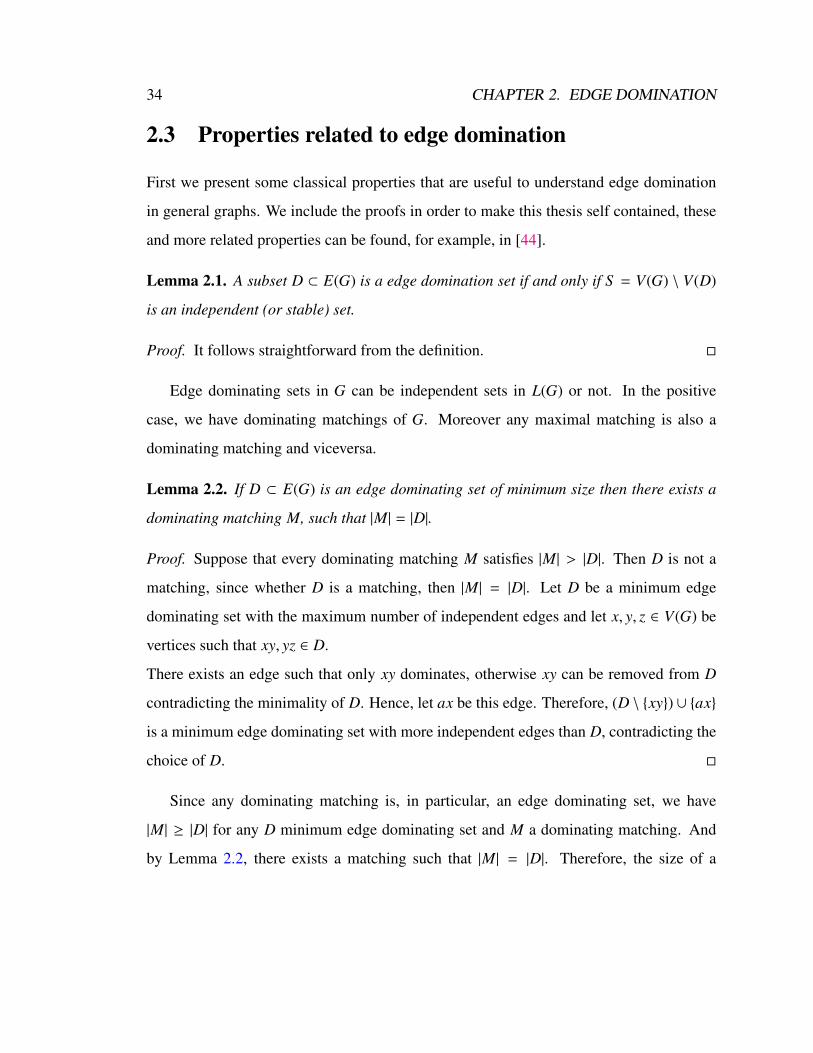
2.3 Properties related to edge domination
First we present some classical properties that are useful to understand edge domination
in general graphs. We include the proofs in order to make this thesis self contained, these
and more related properties can be found, for example, in [44].
Lemma 2.1. A subset D ⊂ E(G) is a edge domination set if and only if S = V(G) \ V(D)
is an independent (or stable) set.
Proof. It follows straightforward from the definition.
Edge dominating sets in G can be independent sets in L(G) or not. In the positive
case, we have dominating matchings of G. Moreover any maximal matching is also a
dominating matching and viceversa.
Lemma 2.2. If D ⊂ E(G) is an edge dominating set of minimum size then there exists a
dominating matching M, such that |M| = |D|.
Proof. Suppose that every dominating matching M satisfies |M| > |D|. Then D is not a
matching, since whether D is a matching, then |M| = |D|. Let D be a minimum edge
dominating set with the maximum number of independent edges and let x, y, z ∈ V(G) be
vertices such that xy, yz ∈ D.
There exists an edge such that only xy dominates, otherwise xy can be removed from D
contradicting the minimality of D. Hence, let ax be this edge. Therefore, (D \ xy) ∪ ax
is a minimum edge dominating set with more independent edges than D, contradicting the
choice of D.
Since any dominating matching is, in particular, an edge dominating set, we have
|M| ≥ |D| for any D minimum edge dominating set and M a dominating matching. And
by Lemma 2.2, there exists a matching such that |M| = |D|. Therefore, the size of a
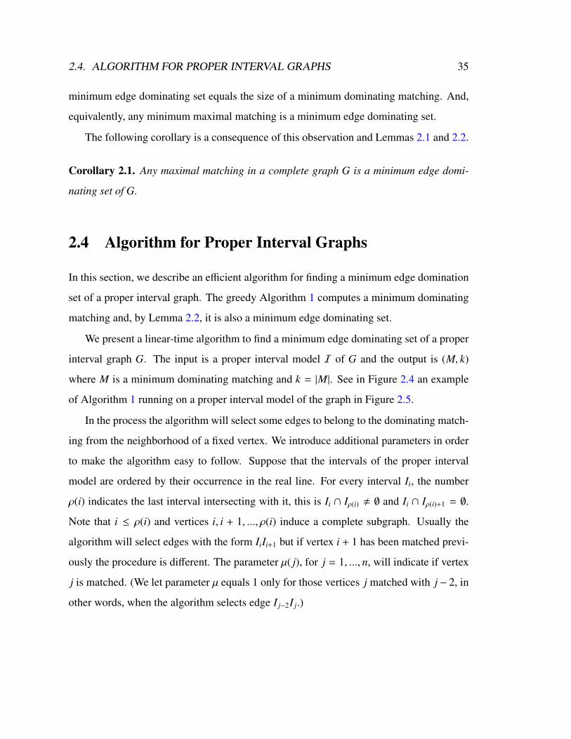
2.4. ALGORITHM FOR PROPER INTERVAL GRAPHS 35
minimum edge dominating set equals the size of a minimum dominating matching. And,
equivalently, any minimum maximal matching is a minimum edge dominating set.
The following corollary is a consequence of this observation and Lemmas 2.1 and 2.2.
Corollary 2.1. Any maximal matching in a complete graph G is a minimum edge domi-
nating set of G.
2.4 Algorithm for Proper Interval Graphs
In this section, we describe an efficient algorithm for finding a minimum edge domination
set of a proper interval graph. The greedy Algorithm 1 computes a minimum dominating
matching and, by Lemma 2.2, it is also a minimum edge dominating set.
We present a linear-time algorithm to find a minimum edge dominating set of a proper
interval graph G. The input is a proper interval model I of G and the output is (M, k)
where M is a minimum dominating matching and k = |M|. See in Figure 2.4 an example
of Algorithm 1 running on a proper interval model of the graph in Figure 2.5.
In the process the algorithm will select some edges to belong to the dominating match-
ing from the neighborhood of a fixed vertex. We introduce additional parameters in order
to make the algorithm easy to follow. Suppose that the intervals of the proper interval
model are ordered by their occurrence in the real line. For every interval Ii, the number
ρ(i) indicates the last interval intersecting with it, this is Ii ∩ Iρ(i) , ∅ and Ii ∩ Iρ(i)+1 = ∅.
Note that i ≤ ρ(i) and vertices i, i + 1, ..., ρ(i) induce a complete subgraph. Usually the
algorithm will select edges with the form IiIi+1 but if vertex i + 1 has been matched previ-
ously the procedure is different. The parameter µ( j), for j = 1, ..., n, will indicate if vertex
j is matched. (We let parameter µ equals 1 only for those vertices j matched with j− 2, in
other words, when the algorithm selects edge I j−2I j.)

36 CHAPTER 2. EDGE DOMINATION
Algorithm 1 Minimum edge dominating set for proper interval graphsInput: A proper interval model I = Ikk=1,...,n of G
Output: (M, k) where M is a minimum dominating matching and k = |M|
1) compute each value of the function ρ : 1, . . . , n → 1, . . . , nwhere ρ(i) = max j/Ii∩
I j , ∅ and the array µ[1..n] with initial values µ[i] = 0 for 1 ≤ i ≤ n,
2) M := ∅, k := 0, i := 1
3) if ρ(i) − i − µ(i + 1) + 1 is odd then
M := M ∪ Iρ(i)Iρ(i)−1, Iρ(i)−2Iρ(i)−3, . . . , Ii+2+µ(i+1)Ii+1+µ(i+1), k := k +ρ(i)−i−µ(i+1)
2 , i :=
ρ(i) + 1 and GOTO (10)
4) end if
5) if ρ(ρ(i)) = ρ(i) then
M := M ∪ Iρ(i)Iρ(i)−1, Iρ(i)−2Iρ(i)−3, . . . , Ii+3+µ(i+1)Ii+2+µ(i+1), Ii+1+µ(i+1)Ii, k := k +
ρ(i)−i−µ(i+1)+12 , i := ρ(i) + 1 and GOTO (10)
6) end if
7) if ρ(i) + 2 ≤ n and ρ(i) + 2 ≤ ρ(ρ(i)) then
M := M ∪ Iρ(i)+2Iρ(i), Iρ(i)−1Iρ(i)−2, . . . , Ii+2+µ(i+1)Ii+1+µ(i+1), k := k +ρ(i)−i−µ(i+1)+1
2 ,
µ(ρ(i) + 2) := 1, i := ρ(i) + 1
8) else
M := M ∪ Iρ(i)+1Iρ(i), Iρ(i)−1Iρ(i)−2, . . . , Ii+2+µ(i+1)Ii+1+µ(i+1), k := k +ρ(i)−i−µ(i+1)+1
2 , i :=
ρ(i) + 2
9) end if
10) if i < n then
GOTO (3)
11) end if
12) return (M, k)
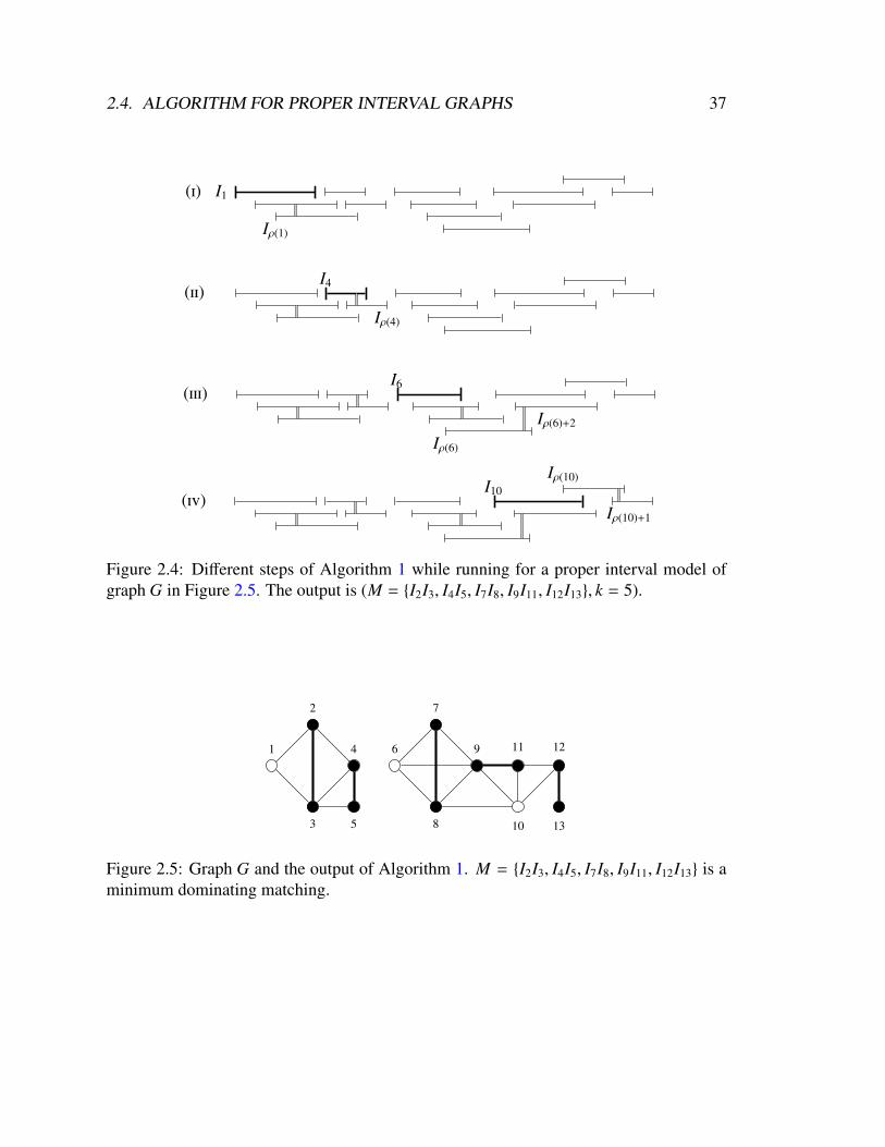
2.4. ALGORITHM FOR PROPER INTERVAL GRAPHS 37
(i) I1
Iρ(1)
(ii)I4
Iρ(4)
(iii)I6
Iρ(6)
Iρ(6)+2
(iv)I10
Iρ(10)
Iρ(10)+1
Figure 2.4: Different steps of Algorithm 1 while running for a proper interval model ofgraph G in Figure 2.5. The output is (M = I2I3, I4I5, I7I8, I9I11, I12I13, k = 5).
1
2
3
4
5
6
7
8
9
10
11 12
13
Figure 2.5: Graph G and the output of Algorithm 1. M = I2I3, I4I5, I7I8, I9I11, I12I13 is aminimum dominating matching.

38 CHAPTER 2. EDGE DOMINATION
We now proceed to prove the correctness and efficiency of the algorithm. Note that
the input can be a disconnected graph, and the algorithm ends because counter i is always
increasing. Let M be the output of Algorithm 1, V(M) the endpoints of edges in M and
S = V(G) \ V(M).
Lemma 2.3. M is a matching, S is an independent set, and if j ∈ S then, in a certain
moment, the algorithm analyze interval I j, i.e. in a certain moment i = j.
Proof. When the algorithm analyzes an interval Ii, all intervals in Ii, Ii+1..., Iρ(i) will be
covered by M, the only exception can be Ii and then i ∈ S . If, in addition, ρ(i) + 1 ∈ V(M)
next interval to be analyzed is Iρ(i)+2, otherwise it is Iρ(i)+1. Since I is a proper interval
model, S results an independent set.
Lemma 2.4. If the algorithm analyze interval Ii then (i) Ii ∈ S or (ii) ρ(i)− i− µ(i + 1) + 1
is even, ρ(ρ(i)) = ρ(i), and there is no edge between G[1, ..., ρ(i)] and G[ρ(i) + 1, ..., n].
Proof. When the algorithm analyzes an interval Ii, vertex i is covered by M only if condi-
tion of Step 5 is met. This is, ρ(i) − i − µ(i + 1) + 1 is even and ρ(ρ(i)) = ρ(i). Therefore,
no vertex from 1, ..., ρ(i) is adjacent to any vertex in ρ(i) + 1, ..., n.
Lemma 2.5. If neither condition of Steps 3, 5 nor 7 is met, then there is no edge between
G[1, ..., ρ(i)] and G[ρ(i) + 2, ..., n].
Proof. When the algorithm analyzes an interval Ii, and neither condition of Steps 3, 5 nor
7 is met, then ρ(i) − i − µ(i + 1) + 1 is even, and ρ(ρ(i)) > ρ(i). This implies that there
exists vertex ρ(i) + 1. If n = ρ(i) + 1, the statement is true. If there exists ρ(i) + 2 then
ρ(i)+2 > ρ(ρ(i)). This implies that no vertex from 1, ..., ρ(i) can be adjacent to any vertex
in ρ(i) + 2, ..., n.
Lemma 2.6. Given a graph G and I j the first interval of any connected component C, then
(i) I j ∈ S or (ii) C is complete and the number of its vertices is even.

2.4. ALGORITHM FOR PROPER INTERVAL GRAPHS 39
Proof. It is easy to see that in one moment of the execution of the algorithm we con-
sider j as i because an interval Ik is skipped only if it intersects with some previous
interval It, t < k. Therefore, by Lemma 2.4, if I j < S then ρ( j) − j − µ( j + 1) + 1
is even and ρ(ρ( j)) = ρ( j). Since I j is the first interval of C, µ( j + 1) = 0 and the
vertices in C are j, ..., ρ( j). Consequently, C is complete and |C| is even. Moreover,
the output of the algorithm contains a minimum dominating matching of C consisting of
I jI j+1, ..., Iρ( j)−1Iρ( j).
Theorem 2.1. The Algorithm 1 computes a minimum dominating matching of G.
Proof. By Lemma 2.3, S is an independent set and M is a dominating matching of G. Let
be Ii the first interval added to S which implies that vertices 1, ..., i − 1 induce complete
components of G and each one has an even number of vertices by previous Lemma 2.6.
Clearly, any maximal matching (minimum dominating matching) has exactly i−12 edges in
these components. Without loss of generality, we can assume that vertex 1 ∈ S .
Suppose that there exists a dominating matching M∗ with |M∗| < |M|, and then |S ∗| >
|S |. We can compare s∗(k) = |S ∗ ∩ 1, .., k| and s(k) = |S ∩ 1, ..., k| for 1 ≤ k ≤ n. It
is clear that s∗(k) ≤ s∗(k + 1) and s(k) ≤ s(k + 1) for any k ∈ 1, ..., n − 1. As s(1) = 1
and s∗(1) ≤ 1, then s(n) = |S | and s∗(n) = |S ∗| > |S |, there is a smallest j that verifies
s∗( j) > s( j) and j ∈ S ∗. Clearly s∗( j) = s( j) + 1. Let i′ and i′∗ be the last vertices in
S ∩ 1, .., j − 1 and S ∗ ∩ 1, .., j − 1, respectively. We have i′ ≤ i′∗, ρ(i′∗) < j (because i∗
and j are non-adjacent vertices, both of them belong to S ∗) and then ρ(i′) < j.
Every interval Ii analyzed by the algorithm with i′ < i ≤ j satisfies Ii < S and there is
at least one. Suppose that i is the first vertex among them such that j ≤ ρ(i). By Lemma
2.4 we have that G[1, ..., ρ(i)] is disconnect with G[ρ(i) + 1, ..., n]. The number of edges in
M ∩ E(G[1, ..., ρ(i)]) is exactly ρ(i)−s( j)2 because any k, i′ ≤ k ≤ j, satisfies k < S , and the
number of edges in M∗ ∩ E(G[1, ..., ρ(i)]) is exactly ρ(i)−s∗( j)2 because any k, j ≤ k ≤ ρ(i),

40 CHAPTER 2. EDGE DOMINATION
k < S ∗, satisfies that Ik and I j intersects. This is an absurd since s∗( j) = s( j) + 1 and the
number of edges should be an integer number.
The other case is that there exists a vertex i, i′ < i ≤ j, such that ρ(i) + 1 = j and
the next vertex analyzed by the algorithm is ρ(i) + 2. This only can occur if neither of
conditions of Steps 3, 5, and 7 was fulfilled for vertex i and then, by Lemma 2.5, there
is no edge between G[1, ..., j − 1] and G[ j + 1, ..., n]. Therefore, the number of edges in
M ∩ E(G[1, ..., j]) and M∗ ∩ E(G[1, ..., j]) is exactly j−s( j)2 and j−s∗( j)
2 , respectively. An
absurd because s∗( j) = s( j) + 1 and the number of edges should be an integer number.
We conclude that M is a minimum dominating matching of G.
It not difficult to see that Algorithm 1 runs in linear time. Then we have proved fol-
lowing theorem.
Theorem 2.2. There exists a linear-time algorithm that solves edge dominating set prob-
lem for proper interval graphs.

2.4. ALGORITHM FOR PROPER INTERVAL GRAPHS 41
Resumen del Capıtulo 2
Como mencionamos anteriormente, una estrategia para tratar un problema NP-completo
como lo es el problema del conjunto dominante de aristas [40] es disenar algoritmos de
tiempo polinomial para algunas familias de grafos. En este capıtulo usamos esta estrategia
para resolver el problema en la clase de los grafos de intervalos propios.
En la Seccion 2.1 damos las definiciones necesarias.
En un grafo no dirigido G = (V, E), una arista e ∈ E se domina a sı misma y a toda
arista que comparte un vertice con ella. Un subconjunto D ⊂ E es un conjunto dominante
de aristas si toda arista de E esta dominada por alguna arista en D. El problema del
conjunto dominante consiste en encontrar un conjunto dominante de tamano mınimo para
un grafo dado.
Un grafo de intervalos propios es el grafo de interseccion de una familia de intervalos
I = Ikk=1,...,n donde los intervalos no se contienen entre sı. En ese caso, la familia I se
llama una representacion o modelo del grafo. Se sabe que, dado un grafo G, se puede
reconocer en tiempo linear si G es un grafo de intervalos propios y, en ese caso, se puede
obtener una representacion de G en intervalos propios en el mismo tiempo [9].
En la Seccion 2.3 damos algunas propiedades clasicas que son utiles para entender la
dominacion de aristas en la clase general de grafos. Entre ellas usaremos especialmente
que el tamano de un conjunto dominante de aristas mınimo equivale al tamano de un
matching maximal mınimo.
En la Seccion 2.4 damos un algoritmo para encontrar un conjunto dominante de aristas
de tamano mınimo en un grafo de intervalos propios. El Algoritmo 1 devuelve un matching
dominante de mınimo tamano y, por el Lema 2.2, es tambien un conjunto dominante de
aristas mınimo. Podemos asumir que un modelo de intervalos propios del grafo es parte
42 CHAPTER 2. EDGE DOMINATION
de la entrada de nuestro algoritmo. Entonces obtenemos que el problema de dominacion
de aristas es lineal para los grafos de intervalos propios (Teorema 2.2).

Chapter 3
Efficient Edge Domination
Packing and covering problems in graphs and their relationships belong to the most fun-
damental topics in combinatorics, and graph algorithms and have a wide spectrum of ap-
plications in computer science, operations research and many other fields. Recently, there
has been an increasing interest in problems combining packing and covering properties.
Among them, there are the efficient edge dominating set problem (also known as dominat-
ing induced matching or DIM for short) and the perfect edge dominating set problem (that
will be discussed in the next chapter). Studies about dominating induced matchings and
some applications related to coding theory, network routing, and resource allocation can
be found in [43, 62].
In the present chapter we give a combinatorial approach to the efficient edge dominat-
ing set problem. We give tight upper bounds on the maximum possible number of DIMs
for a graph G that is either arbitrary, or triangle-free, or connected. Furthermore, we char-
acterize all extremal graphs for these bounds. Our results imply that if G is a graph of
order n and µ(G) is the number of DIMs in the graph, then µ(G) ≤ 3n3 ; µ(G) ≤ 4
n5 provided
G is triangle-free; and µ(G) ≤ 4n−1
5 provided n ≥ 9 and G is connected.
43
44 CHAPTER 3. EFFICIENT EDGE DOMINATION
The structure of this chapter is as follows. First we define the problem in Section 3.1
and dedicate Section 3.2 to present the state of the art. In Section 3.3 we present lemmas
and important observations to understand the problem of counting DIMs. In Section 3.4
we state and prove sharp bounds of the number of DIMs and determine all extremal graphs
when the problem is restricted to the classes of general graphs, triangle-free graphs and
connected graphs.
3.1 Preliminaries
Recall that an edge in E(G) dominates itself and every edge sharing a vertex with it. A
subset E′ ⊂ E(G) is dominating if every edge of G is dominated by at least one edge of
E′. A subset E′ ⊂ E(G) is an efficient dominating set if every edge of G is dominated
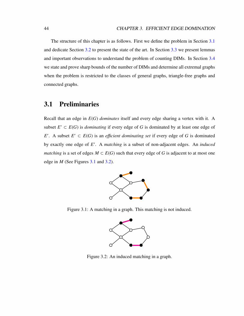
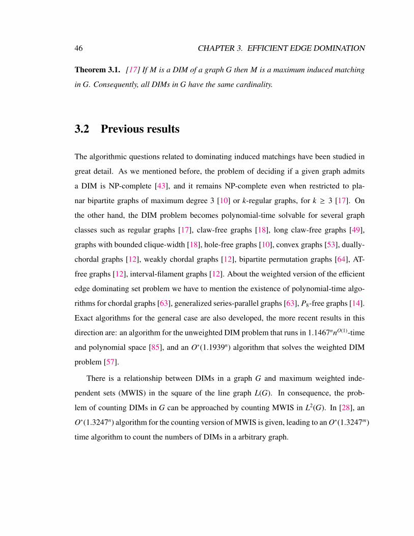
by exactly one edge of E′. A matching is a subset of non-adjacent edges. An induced
matching is a set of edges M ⊂ E(G) such that every edge of G is adjacent to at most one
edge in M (See Figures 3.1 and 3.2).
Figure 3.1: A matching in a graph. This matching is not induced.
Figure 3.2: An induced matching in a graph.

3.1. PRELIMINARIES 45
A dominating induced matching or DIM, for short, is a subset of edges M ⊂ E(G)
which is both dominating and an induced matching. In consecuence, an efficient edge
dominating set is equivalent to a dominating induced matching (see Figure 3.3).
Figure 3.3: A DIM in a graph. Every edge is dominated by exactly one edge in the DIM.
Not every graph has a DIM; for example C4 or any cycle Cn with n , 3k does not
admit DIMs (see Figure 3.4). The problem of deciding whether a given graph admits
it is known in the literature as the efficient edge domination or DIM problem; and it is
NP-complete [43]. Given a weight function w : E(G) → R, the weighted version of the
DIM problem is to find a DIM with minimum sum of the weight of its edges amongs all
DIMs, if any. We denote by µ(G) the number of dominating induced matchings of G. The
problem of compute µ(G) is the counting version of the DIM problem.
Figure 3.4: Induced matching in cycles C4, C5 and C6. Note that only C6 admits a DIM.
In this chapter we use an alternative definition [19] of the DIM problem. It is determine
if exists a partition of the vertex set into two disjoint subsets; one subset, corresponding
to the white vertices, induces an independent set, while the other subset, called the black
vertices, induces an 1-regular graph. Thus, black vertices will induce a matching.
It is not difficult to see that a DIM is also a maximum induced matching [17].
46 CHAPTER 3. EFFICIENT EDGE DOMINATION
Theorem 3.1. [17] If M is a DIM of a graph G then M is a maximum induced matching
in G. Consequently, all DIMs in G have the same cardinality.
3.2 Previous results
The algorithmic questions related to dominating induced matchings have been studied in
great detail. As we mentioned before, the problem of deciding if a given graph admits
a DIM is NP-complete [43], and it remains NP-complete even when restricted to pla-
nar bipartite graphs of maximum degree 3 [10] or k-regular graphs, for k ≥ 3 [17]. On
the other hand, the DIM problem becomes polynomial-time solvable for several graph
classes such as regular graphs [17], claw-free graphs [18], long claw-free graphs [49],
graphs with bounded clique-width [18], hole-free graphs [10], convex graphs [53], dually-
chordal graphs [12], weakly chordal graphs [12], bipartite permutation graphs [64], AT-
free graphs [12], interval-filament graphs [12]. About the weighted version of the efficient
edge dominating set problem we have to mention the existence of polynomial-time algo-
rithms for chordal graphs [63], generalized series-parallel graphs [63], P8-free graphs [14].
Exact algorithms for the general case are also developed, the more recent results in this
direction are: an algorithm for the unweighted DIM problem that runs in 1.1467nnO(1)-time
and polynomial space [85], and an O∗(1.1939n) algorithm that solves the weighted DIM
problem [57].
There is a relationship between DIMs in a graph G and maximum weighted inde-
pendent sets (MWIS) in the square of the line graph L(G). In consequence, the prob-
lem of counting DIMs in G can be approached by counting MWIS in L2(G). In [28], an
O∗(1.3247n) algorithm for the counting version of MWIS is given, leading to an O∗(1.3247m)
time algorithm to count the numbers of DIMs in a arbitrary graph.

3.3. COLORINGS ASSOCIATED TO A DIM 47
3.3 Colorings associated to a DIM
Throughout this section we consider graphs that are not necessary connected. Clearly a
DIM of G is union of DIMs of its connected components. Then the number of DIMs in a
non connected graph is the product of the number of DIMs of its connected components.
Assigning one of two possible colors to vertices of G is called a coloring of G. A
coloring, noted by (G; B,W), splits the set of vertices of G into 3 disjoint subsets, the
black vertices B, the white vertices W and the uncolored vertices V \ (B ∪W). A coloring
is total if all vertices of G have colors assigned, otherwise it is partial.
Let B and W be disjoint subsets of the vertex set V(G), we say that a dominating
induced matching M of G is compatible with the coloring (G; B,W) if B ⊆ V(M) and
W ∩ V(M) = ∅. Let µ(G; B,W) denote the number of dominating induced matchings of G
that are compatible with (G; B,W).
By the definition of DIMs, we have
µ(G; B,W) > 0⇒ G[B] has maximum degree at most 1 and W is independent. (3.1)
Note that if V(G) \ (B ∪W) has at most n elements, then µ(G; B,W) is an integer not
greater than 2n. This implies that for a class G of graphs and a non-negative integer n, the
maximum
sG(n) = maxµ(G; B,W) : G is a graph in G, B and W are disjoint subsets of V(G),
B ∪W , ∅, and |V(G) \ (B ∪W)| ≤ n
is well-defined and finite, even though the maximum is possibly taken over infinitely many
graphs. Note that a total coloring can be compatible with at most one DIM, then sG(0) ≤ 1.
In addition, if G contains a non-empty graph that has a DIM, then sG(n) ≥ 1.

48 CHAPTER 3. EFFICIENT EDGE DOMINATION
We now explain some lemmas for bounding the number of DIMs that are compatible
with a coloring (G; B,W)
Lemma 3.1. If C is the class of connected C3,C4-free graphs of minimum degree at least
2, then sC(n) = 1 for n ∈ 0, 1, 2, 3 and sC(n) ≤ sC(n − 4) + sC(n − 2) for every integer n
with n ≥ 4.
Proof. We prove the statement by induction on n. For n = 0, the statement follows
from the above observations using that C6 has DIMs, µ(C6) > 0 and C6 ∈ C. Now let n ≥ 1.
Clearly, sC(n) ≥ 1 and sC(n− 1) ≤ sC(n). Hence, in view of the desired statement, we may
assume that sC(n) ≥ 2. Let (G; B,W) be a maximizer in the definition of sC(n), that is,
sC(n) = µ(G; B,W). Since sC(n) ≥ 2, the set B ∪W is a proper non-empty subset of V(G).
Since G is connected, there is an edge uv of G such that u ∈ B∪W and v ∈ V(G) \ (B∪W).
If u ∈ W, then sC(n) = µ(G; B,W)(3.1)= µ(G; B ∪ v,W) ≤ sC(n − 1). If u ∈ B and u has
a neighbor in B, then sC(n) = µ(G; B,W)(3.1)= µ(G; B,W ∪ v) ≤ sC(n− 1). If u ∈ B and all
neighbors of u distinct from v belong to W, then sC(n) = µ(G; B,W)(3.1)= µ(G; B∪v,W) ≤
sC(n − 1). In all three cases, we obtain sC(n) ≤ sC(n − 1). By induction, if n − 1 ≤ 3, then
1 ≤ sC(n) ≤ sC(n−1) = 1, and if n−1 ≥ 4, then sC(n) ≤ sC(n−1) ≤ sC(n−5)+ sC(n−3) ≤
sC(n − 4) + sC(n − 2).
Hence we may assume that u belongs to B and that u has a neighbor w in V(G)\(B∪W)
that is distinct from v. Since G is of minimum degree at least 2, the vertex v has a neighbor
v′ distinct from u and the vertex w has a neighbor w′ distinct from u. Since G is C3,C4-
free, the vertices v, v′, w, and w′ are all distinct.
If v′ ∈ W, then sC(n) = µ(G; B,W)(3.1)= µ(G; B ∪ v,W) ≤ sC(n − 1). If v′ ∈ B, then
sC(n) = µ(G; B,W)(3.1)= µ(G; B,W ∪ v) ≤ sC(n − 1). Again we obtain sC(n) ≤ sC(n − 1)
and can argue as above.
Hence we may assume that v′ and w′ belong to V(G) \ (B ∪W), which implies n ≥ 4.
3.3. COLORINGS ASSOCIATED TO A DIM 49
Now
sC(n) = µ(G; B,W)
= µ(G; B ∪ v,W) + µ(G; B,W ∪ v)(3.1)= µ(G; B ∪ v,w′,W ∪ v′,w) + µ(G; B ∪ v′,W ∪ v)
≤ sC(n − 4) + sC(n − 2),
which completes the proof.
If F(n) denotes the n-th Fibonacci number, that is, F(0) = 0, F(1) = 1, and F(n) =
F(n − 2) + F(n − 1) for every integer n with n ≥ 2, then Lemma 3.1 immediately implies
maxsC(2n), sC(2n + 1) ≤ F(n + 1) (3.2)
for every non-negative integer n.
Lemma 3.2. If G is a C3,C4-free graph of order n and minimum degree at least 2, then
µ(G) < 0.928 · φn2 where φ = 1+
√5
2 .
Proof. First, we assume that G is connected. Note that n ≥ 5. If n = 5, then G = C5 and
µ(G) = 0. Hence let n ≥ 6. Let u be a vertex of G. Since u has at least 2 neighbors, we
obtain µ(G) = µ(G; ∅, u) + µ(G; u, ∅)(3.1)= µ(G; N(u), u) + µ(G; u, ∅) ≤ sC(n − 3) +
sC(n − 1). If n is odd, then µ(G) ≤ sC(n − 3) + sC(n − 1)(3.2)≤ F
(n−1
2
)+ F
(n+1
2
)= F
(n+3
2
).
If n is even, then µ(G) ≤ sC(n − 3) + sC(n − 1)(3.2)≤ F
(n−2
2
)+ F
(n2
)= F
(n+2
2
). Using
φ−2 + φ−1 = 1 and maxF(4) · φ−
62 , F(5) · φ−
72 , F(6) · φ−
92
< 0.928, it follows easily by
induction on n that for n ≥ 6, we have
F(
n+32
), if n is odd and
F(
n+22
), if n is even
< 0.928 · φn2
50 CHAPTER 3. EFFICIENT EDGE DOMINATION
and hence µ(G) < 0.928 · φn2 .
If G has components G1, ...,Gk of orders n1, ..., nk, respectively, then µ(G) ≤∏k
i=1 µ(Gi) <
0.928k · φn1+...+nk
2 ≤ 0.928 · φn2 , which completes the proof.
3.4 Bounds for the maximum number of DIMs
We proceed to state and prove tight bounds to µ(G) for the general class of graphs, triangle-
free and connected graphs, in the subsequent Subsections. The general structure of all
three proofs is very similar.
3.4.1 General graphs
Theorem 3.2. If G is a graph of order n, then µ(G) ≤ f (n) where
f (n) =
1 , if n ≤ 2,
3n3 , if n ≥ 3 and n ≡ 0 mod 3,
3n−1
3 , if n ≥ 4 and n ≡ 1 mod 3, and
4 · 3n−5
3 , if n ≥ 5 and n ≡ 2 mod 3.
Furthermore, if the graph G of order n with n ≥ 3 is such that µ(G) = f (n), then G ∈ F
where
F =
n3
K3 : n ≥ 3 and n ≡ 0 mod 3
∪
K1 ∪
n − 13
K3 : n ≥ 4 and n ≡ 1 mod 3
∪
K1,3 ∪
n − 43
K3 : n ≥ 4 and n ≡ 1 mod 3
∪
K1,4 ∪
n − 53
K3 : n ≥ 5 and n ≡ 2 mod 3.

3.4. BOUNDS FOR THE MAXIMUM NUMBER OF DIMS 51
In Figure 3.5 we show the extremal graphs for the general class of graphs.
(i) . . . n ≡ 0 mod 3
(ii) . . . n ≡ 1 mod 3
(iii) . . . n ≡ 1 mod 3
(iv) . . . n ≡ 2 mod 3
Figure 3.5: Family F . Extremal graphs for the general class of graphs.
Proof of Theorem 3.2
Let G be a graph of order n and size m. We prove, by induction on n+m, that µ(G) ≤ f (n),
and for n ≥ 3, µ(G) = f (n) if and only if G belongs to F . Since the result is easily verified
for n ≤ 5, we assume now that n ≥ 6. We establish a series of claims concerning properties
that G can be assumed to have if G has maximum µ(G) among all graphs of order n.
Claim 1. Every edge of G belongs to some DIM of G.
Proof of Claim 1. If G contains an edge e such that no DIM of G contains e, then every
DIM of G is a DIM of G − e and, by induction, µ(G) ≤ µ(G − e) ≤ f (n). If µ(G) = f (n),
then µ(G − e) = f (n) and hence, by induction, G − e ∈ F . It is easily verified that adding
any edge to a graph H in F results in a graph with strictly less DIMs than H. Therefore,
µ(G) < µ(G − e), which is the contradiction µ(G) < f (n).

52 CHAPTER 3. EFFICIENT EDGE DOMINATION
Since no DIM of G can contain an edge that belongs to a cycle of length 4, Claim 1 implies
that G has no such cycle.
Following claims assume that G is an extremal graph and G < F .
Claim 2. The graph G is triangle-free.
Proof of Claim 2. Let T = G[xyz] be a triangle in G. Since every DIM of G contains
exactly one of the three edges of T , no DIM of G contains an edge between a vertex in
V(T ) and a vertex in V(G) \ V(T ). By Claim 1, this implies that T is a component of
G. Now, by induction, µ(G) = 3 · µ(G − V(T )) ≤ 3 · f (n − 3) = f (n). Furthermore, if
µ(G) = f (n), then µ(G − V(T )) = f (n − 3) and hence, by induction, G − V(T ) ∈ F . Since
G is the disjoint union of a triangle and G − V(T ), we obtain G ∈ F .
Claim 3. The graph G has no isolated vertex.
Proof of Claim 3. If u is an isolated vertex of G, then every DIM of G is a DIM of
G − u. Therefore, by induction, µ(G) ≤ µ(G − u) ≤ f (n − 1) ≤ f (n). If µ(G) = f (n), then
f (n − 1) = f (n), which implies that n ≡ 1 mod 3. Furthermore, µ(G − u) = f (n − 1) and
hence, by induction, G − u = n−13 K3. Now G = K1 ∪
n−13 K3 ∈ F .
Claim 4. The graph G has minimum degree at least 2.
Proof of Claim 4. By Claim 3, the graph G has no isolated vertex. If u is a vertex
of degree 1 and v is the unique neighbor of u in G, then every DIM of G contains an
edge incident with v. Hence no DIM contains an edge between a vertex in N[v] and
V(G)\N[v]. By Claim 1 and Claim 2, the closed neighborhood N[v] of v in G is the vertex
set of a component of G and induces a star K1,d where d = dG(v) ≥ 1. Now, by induction,
µ(G) = d · µ(G − N[v]) ≤ d · f (n − (d + 1)).
If d ∈ 1, 2 or d ≥ 5, then it is easily verified that d · f (n − (d + 1)) < f (n) and hence
µ(G) < f (n) in these cases.

3.4. BOUNDS FOR THE MAXIMUM NUMBER OF DIMS 53
If d = 3, then d · f (n − (d + 1)) ≤ f (n) with equality if and only if n ≡ 1 mod 3. Hence
µ(G) ≤ f (n). Furthermore, if µ(G) = f (n), then µ(G − N[v]) = f (n − (d + 1)) and hence,
by induction, G − N[v] = n−43 K3. Now G = K1,3 ∪
n−43 K3 ∈ F .
If d = 4, then d · f (n − (d + 1)) ≤ f (n) with equality if and only if n ≡ 2 mod 3. Hence
µ(G) ≤ f (n). Furthermore, if µ(G) = f (n), then µ(G − N[v]) = f (n − (d + 1)) and hence,
by induction, G − N[v] = n−53 K3. Now G = K1,4 ∪
n−53 K3 ∈ F .
By Claims 1 to 4, the extremal graph G belongs to F or G is a C3,C4-free graph of
minimum degree at least 2. Since f (n) ≥ 4 · 3−53 · 3
n3 and 0.928 · φ
n2 < 4 · 3−
53 · 3
n3 for n ≥ 6,
Lemma 3.2 implies µ(G) < f (n), which completes the proof.
3.4.2 Triangle-free graphs
Theorem 3.3. If G is a triangle-free graph of order n, then µ(G) ≤ g(n) where
g(n) =
1 , if n = 1,
n − 1 , if n ∈ 2, 3, 6, 7,
20 , if n = 11, and
3t · 4n−4t
5 , if n ≥ 4t, n ≡ −t mod 5, for t = 0, 1, 2, 3 and 4.
Furthermore, if the triangle-free graph G of order n with n ≥ 2 is such that µ(G) = g(n),
then G ∈ G where
G = K1,n−1 : 2 ≤ n ≤ 7 ∪ K1,2 ∪ K1,3,K1,4 ∪ K1,5
∪
tK1,3 ∪
n − 4t5
K1,4 : n ≥ 4t, n ≡ −t mod 5, for t = 0, 1, 2, 3 and 4.
Proof of Theorem 3.3
Let G be a triangle-free graph of order n and size m. We prove, by induction on n + m, that

54 CHAPTER 3. EFFICIENT EDGE DOMINATION
K1,n−1 for 2 ≤ n ≤ 7
K1,2 ∪ K1,3 K1,4 ∪ K1,5
t . . . tK1,3 ∪n−4t
5 K1,4, n ≡ −t mod 5
Figure 3.6: Family G. Extremal graphs among triangle-free graphs.
µ(G) ≤ g(n) and, for n ≥ 2, µ(G) = g(n) if and only if G belongs to G. Since the result
is easily verified for n ≤ 8, we assume now that n ≥ 9. We establish a series of claims
concerning properties that G can be assumed to have if G has maximum µ(G) among all
graphs of order n.
Claim 5. Every edge of G belongs to some DIM of G.
Proof of Claim 5. This can be proved exactly as Claim 1.
Claim 5 implies that G is C3,C4-free.
Claim 6. The graph G has no isolated vertex.
Proof of Claim 6. Note that unlike the function f from Theorem 3.2, the function g is
strictly increasing for n ≥ 3. Using this fact, this claim can be proved as Claim 3.
Claim 7. The graph G has minimum degree at least 2.
Proof of Claim 7. By Claim 6, the graph G has no isolated vertex. Let u be a vertex of
degree 1 and let v be the unique neighbor of u in G. Arguing as in the proof of Claim 4, we
obtain that the closed neighborhood N[v] of v in G is the vertex set of a component of G

3.4. BOUNDS FOR THE MAXIMUM NUMBER OF DIMS 55
and induces a star K1,d where d = dG(v) ≥ 1. Now, by induction, µ(G) = d · µ(G − N[v]) ≤
d · g(n − (d + 1)).
It is easy to verify d · g(n − (d + 1)) ≤ g(n) for every n ≥ 9 with equality if and only if
• either d = 3, n . 0 mod 5 and n , 11,
• or d = 4 and n < 12, 16,
• or d = 5 and n = 11.
The proof can now be completed similarly as the proof of Claim 4. We give details only
for d = 3.
Let d = 3. We obtain µ(G) = d ·µ(G−N[v]) ≤ d · g(n− (d + 1)) ≤ g(n). If µ(G) = g(n),
then d · g(n − (d + 1)) = g(n), which implies n mod 5 , 0 and n , 11. Furthermore,
µ(G − N[v]) = g(n − (d + 1)), which implies, by induction, that G − N[v] ∈ G. Since for
every graph H in G of order n′ = n − 4 with n′ ≥ 5, n′ . 1 mod 5, and n′ , 7, we have
K1,3 ∪ H ∈ G, we obtain G ∈ G.
By Claims 5 to 7, the extremal graph G belongs to G or G is a C3,C4-free graph of
minimum degree at least 2. Clearly, g(n) > 0.928 · φn2 for n ∈ 9, 10, 11. Furthermore,
for n ≥ 12, we have g(n) ≥ 81 · 4n−16
5 > 0.956 · 1.319n > 0.928 · φn2 , Lemma 3.2 implies
µ(G) < g(n), which completes the proof.
3.4.3 Connected graphs
For an integer n with n ≥ 11 and n ≡ 1 mod 5, let the graph Hn arise from K1 ∪n−1
5 K1,4 by
adding edges between K1 and each center of the n−15 stars. See Figure 3.7. Let the graph
H8 of order 8 be as shown in Figure 3.8.

56 CHAPTER 3. EFFICIENT EDGE DOMINATION
. . .
Figure 3.7: Graphs Hn for n ≡ 1 mod 5 and n ≥ 11.
u u u u uuuu
AAA @
@@
a
Figure 3.8: The graph H8.
Theorem 3.4. If G is a connected graph of order n, then µ(G) ≤ h(n) where
h(n) =
1 , if n ∈ 1, 2,
3 , if n = 3,
n − 1 , if 4 ≤ n ≤ 8, and
4n−1
5 , if n ≥ 9.
Furthermore, if the connected graph G of order n is such that µ(G) = h(n), then G ∈ H
where
H = K1,K2,K3,K1,3,K1,4,K1,5,K1,6,K1,7,H8 ∪ Hn : n ≥ 11 and n ≡ 1 mod 5.
Proof of Theorem 3.4
Let G be a connected graph of order n and size m. We prove the statement by induction on
n + m. For n ≤ 8, the result is easily verified.
Note that:
for every p ∈ N, we have p · 4−(p+1)
5 ≤ 1 with equality if and only if p = 4. (3.3)

3.4. BOUNDS FOR THE MAXIMUM NUMBER OF DIMS 57
Kn for 1 ≤ n ≤ 3
K1,n for 3 ≤ n ≤ 7
H8. . .
Hn for n ≡ 1 mod 5
Figure 3.9: FamilyH . Extremal graphs among connected graphs.
This implies that if n ≤ 8 and G is neither a star nor a triangle nor H8, then n ≥ 4 and
µ(G) ≤ h(n) − 1 = n − 2 ≤ 4n−1
5 .
We assume now that n ≥ 9. Note that if G′ is a graph of order n′ less than n and no
component of G′ is a star or a triangle or H8, then, by induction, every component K of G
of order n(K) satisfies µ(K) ≤ 4n(K)−1
5 , which implies µ(G′) ≤ 4n′−1
5 . We establish a series
of claims concerning properties that G can be assumed to have if G has maximum µ(G)
among all graphs of order n.
Claim 8. Every edge of G that does not belong to some DIM of G is a bridge.
Proof of Claim 8. If G contains an edge e such that no DIM of G contains e and e is
not a bridge of G, then every DIM of G is a DIM of the connected graph G − e and, by
induction, µ(G) ≤ µ(G − e) ≤ h(n). If µ(G) = h(n), then µ(G − e) = h(n) and hence, by
induction, G − e ∈ H . It is easily verified that adding any edge to a graph H in H results
in a graph with strictly less DIMs than H. Therefore, µ(G) < µ(G − e) = h(n), which is a
contradiction.

58 CHAPTER 3. EFFICIENT EDGE DOMINATION
By Claim 8, the graph G has no cycle of length 4.
Claim 9. No edge of G that does not belong to some DIM of G is incident with a vertex of
degree 1.
Proof of Claim 9. If uv is an edge of G that does not belong to some DIM of G such
that u has degree 1, then µ(G) ≤ µ(G − u) ≤ h(n − 1) < h(n).
Claim 10. The graph G is triangle-free.
Proof of Claim 10. Let T = G[xyz] be a triangle in G. Since G is connected, we may
assume that z has a neighbor z′ that does not lie on T .
First, we assume that y has a neighbor y′ that does not lie on T . Since G has no cycle
of length 4, the vertices y′ and z′ are distinct. For every DIM M of G, the set M contains
an edge of T and M \ E(T ) is a DIM of G − V(T ). This implies, by induction,
µ(G) = µ(G; x, y, ∅) + µ(G; x, z, ∅) + µ(G; y, z, ∅)(Lemma 3.1)
= µ(G; x, y, z′, y′) + µ(G; x, z, y′, z′) + µ(G; y, z, y′, z′)
≤ µ(G − V(T ); z′, y′) + µ(G − V(T ); y′, z′) + µ(G − V(T ); ∅, y′, z′)
≤ µ(G − V(T ))
≤ h(n − 3)
< h(n).
Hence we may assume that for every triangle T of G, exactly one vertex of T has degree
at least 3.
Next, we assume that no component of G−V(T ) is either a star or a triangle or H8. By

3.4. BOUNDS FOR THE MAXIMUM NUMBER OF DIMS 59
x
y z z′...
S
Figure 3.10: Graph determined by a triangle, deg(z) = 3 and a star S .
induction, this implies that µ(G − V(T )) ≤ 4(n−3)−1
5 . Now
µ(G) = µ(G; x, y, ∅) + µ(G; x, z, ∅) + µ(G; y, z, ∅)(3.1)= µ(G; x, y, z′, ∅) + µ(G; x, z, z′) + µ(G; y, z, z′)
≤ µ(G − V(T ); z′, ∅) + 2 · µ(G − V(T ); ∅, z′)
≤ 2 · µ(G − V(T ))
≤ 2 · 4(n−3)−1
5
< 4n−1
5 .
Hence we may assume that for every triangle T of G, some component of G − V(T ) is
either a star or a triangle or H8.
Next, we assume that some component S of G − V(T ) is a star of order s. Since the
edge xy belongs to some DIM of G, we obtain that s ≥ 2. Since the edge xz belongs to
some DIM of G, we obtain that s ≥ 3, that z is adjacent to a leaf z′ of S , and z is not
adjacent to another vertex in S . If z has degree 3, then the graph is completely determined.
See Figure 3.10 Note that the structure of G is similar to H8 in this case. Using n ≥ 9, it
is easy to verify that µ(G) < h(n). Hence we may assume that z has degree at least 4. If
G − V(S ) is H8, then the graph is completely determined. See Figure 3.11 Again it is easy
to verify that µ(G) < h(n). Hence no component of G − V(S ) is a either a star or a triangle
or H8, which implies, by induction, µ(G −V(S )) ≤ 4(n−s)−1
5 . Since every DIM of G contains

60 CHAPTER 3. EFFICIENT EDGE DOMINATION
x
y z z′...
S
Figure 3.11: Graph determined by H8, a star S and deg(z) = 4.
an edge of S , we obtain, by induction,
µ(G) = µ(G; z′, ∅) + µ(G; ∅, z′)(3.1)= µ(G; z′, z) + µ(G; z, z′)
≤ µ(G − V(S ); ∅, z) + (s − 2) · µ(G − V(S ); z, ∅)
≤ (s − 2) · µ(G − V(S ))
≤ (s − 2) · 4(n−s)−1
5
(3.3)< 4
n−15 .
Hence we may assume that for every triangle T of G, no component of G − V(T ) is a star.
Next, we assume that some component T ′ of G − V(T ) is a triangle. Since n ≥ 9, the
degree of z is at least 4. This implies that the connected graph G − V(T ′) is H8. Now the
graph is completely determined, n = 11, and µ(G) = 8 < h(n) (see Figure 3.12 (i)). Hence
we may assume that for every triangle T of G, some component of G − V(T ) is H8. Now
the graph G arises from T ∪ H8 by adding an edge between z and the vertex a in H8 (see
Figure 3.12 (ii)). This implies n = 11 and µ(G) = 13 < h(n), which completes the proof
of the claim.
Claims 8 and 10 imply that G is C3,C4-free. By assumption, G has no isolated vertex.

3.4. BOUNDS FOR THE MAXIMUM NUMBER OF DIMS 61
(i)
x
y z
a
(ii)
x
y z
a
Figure 3.12: Graphs determined by H8 and a triangle.
Claim 11. The graph G has minimum degree at least 2.
Proof of Claim 11. Let v be a vertex of G of degree p+q such that v has p ≥ 1 neighbors
u1, . . . , up of degree 1 and q neighbors w1, . . . ,wq of degree at least 2. If G is a star, then
the theorem is easily verified. Hence we may assume that q ≥ 1. Since every DIM of G
contains an edge incident with v, every edge between a vertex in N[v] and V(G) \N[v] is a
bridge. Since G is triangle-free, this implies that every edge incident with a vertex in N[v]
is a bridge and that N[v] induces a star S . For 1 ≤ j ≤ q, let z j denote a neighbor of w j
that is distinct from v. Let Z = z1, . . . , zq.
We have
µ(G) =
p∑i=1
µ(G; v, ui, ∅) +
q∑j=1
µ(G; v,w j, ∅)
(3.1)=
p∑i=1
µ(G; v, ui ∪ Z, ∅) +
q∑j=1
µ(G; v,w j ∪ (Z \ z j), z j)
≤
p∑i=1
µ(G − V(S ); Z, ∅) +
q∑j=1
µ(G − V(S ); Z \ z j, z j)
= p · µ(G − V(S ); Z, ∅) +
q∑j=1
µ(G − V(S ); Z \ z j, z j)
≤ p · µ(G − V(S )).
62 CHAPTER 3. EFFICIENT EDGE DOMINATION
If q ≥ 2 and some component S ′ of G − V(S ) is a star, then Claim 9 implies that S ′ has
order at least 2 and, by exchanging the roles of S and S ′, we may assume that q = 1.
Hence we may assume that
• either q ≥ 2 and no component of G − V(S ) is a star
• or q = 1.
If q ≥ 2 and no component of G − V(S ) is a star, then, by induction, µ(G − V(S )) ≤
4(n−|V(S )|)−1
5 = 4(n−(p+q+1))−1
5 ≤ 4(n−(p+3))−1
5 and we obtain µ(G) ≤ p · µ(G − V(S )) ≤ p · 4(n−(p+3))−1
5(3.3)<
4n−1
5 . Hence we may assume now that q = 1.
First, we assume that the edge vw1 does not belong to any DIM of G. In this case
µ(G) ≤ p · µ(G − u1, . . . , up, v). If the connected graph G − u1, . . . , up, v is a star,
then the result is easily verified. Hence we may assume that G − u1, . . . , up, v is not
a star. By induction, this implies µ(G − u1, . . . , up, v) ≤ 4(n−(p+1))−1
5 and hence µ(G) ≤
p · µ(G − u1, . . . , up, v) ≤ p · 4(n−(p+1))−1
5(3.3)≤ 4
n−15 . Furthermore, if µ(G) = 4
n−15 , then, by
(3.3), we have p = 4, n ≡ 1 mod 5, and µ(G − u1, . . . , up, v) = 4(n−(p+1))−1
5 . By induction,
this implies G − u1, . . . , up, v = Hn−5, which easily implies G = Hn ∈ H . Hence we may
assume that the edge vw1 belongs to some DIM of G.
Next, we assume that some component S ′ of G − V(S ) is a star of order s′. Since, by
Claim 9, the edge u1v belongs to some DIM of G, we obtain that s′ ≥ 2. Since the edge
vw1 belongs to some DIM of G, we obtain that s′ ≥ 3 and that w1 is adjacent to a leaf z′ of
S ′. If w1 has degree 2, then the graph is completely determined (see Figure 3.13) and it is
easy to verify that µ(G) < h(n). Hence we may assume that w1 has degree at least 3. Since
vw1 belongs to some DIM of G, the graph G − V(S ′) does not belong toH and n − s′ ≥ 6.
By induction, this implies µ(G −V(S ′)) ≤ 4(n−s′)−1
5 . Since every DIM of G contains an edge

3.4. BOUNDS FOR THE MAXIMUM NUMBER OF DIMS 63
u1
u2...
upv w1 z′
...
S S ′
Figure 3.13: Graph determined by stars S and S ′.
of S ′, we obtain
µ(G) = µ(G; z′, ∅) + µ(G; ∅, z′)(3.1)= µ(G; z′, w1) + µ(G; w1, z′)
≤ µ(G − V(S ′); ∅, w1) + (s′ − 2) · µ(G − V(S ′); w1, ∅)
≤ (s′ − 2) · µ(G − V(S ′))
≤ (s′ − 2) · 4(n−s′)−1
5
(3.3)< 4
n−15 .
Hence we may assume that no component of G −V(S ) is a star. By induction, this implies
µ(G − V(S )) ≤ 4(n−(p+2))−1
5 and we obtain µ(G) ≤ p · µ(G − V(S )) ≤ p · 4(n−(p+2))−1
5(3.3)< 4
n−15 ,
which completes the proof of the claim.
By Claims 8 to 11, if the graph G is extremal and G < H , G is a C3,C4-free graph
of minimum degree at least 2. Since 0.928 · φn2 < 4
n−15 for n ≥ 9, Lemma 3.2 implies
µ(G) < h(n), which completes the proof.

64 CHAPTER 3. EFFICIENT EDGE DOMINATION
Resumen del Capıtulo 3
Los problemas que combinan propiedades de cubrimiento y empaquetamiento en grafos
han despertado interes recientemente. Entre ellos se encuentran el problema del conjunto
dominante eficiente de aristas (tambien conocido como matching inducido dominante o
DIM por sus siglas en ingles) y el problema del conjunto perfectamente dominante de
aristas (que sera tratado en el proximo capıtulo).
En este capıtulo damos un enfoque combinatorio al problema de dominacion eficiente
de aristas. Damos cotas ajustadas para el maximo numero posible de DIMs para un grafo
que es arbitrario, sin triangulos o conexo. Mas aun, caracterizamos todos los grafos ex-
tremales para estas clases. Nuestros resultados implican que si G es un grafo de orden n
y µ(G) es la cantidad de DIMs en el grafo, entonces µ(G) ≤ 3n3 ; µ(G) ≤ 4
n5 cuando G no
tiene triangulos; y µ(G) ≤ 4n−1
5 cuando G es conexo y n ≥ 9.
En la Seccion 3.1 repasamos las definiciones necesarias.
Una arista domina a sı misma y a toda arista que comparta un vertice con ella. Un
subconjunto de aristas E′ ⊂ E(G) es dominante si toda arista de G esta dominada por al
menos una arista en E′. Ademas E′ ⊂ E(G) es un conjunto eficientemente dominante de
aristas si toda arista de G es dominada por exactamente una arista en E′. Un matching
inducido es un conjunto de aristas M ⊂ E(G) tal que toda arista en G es adyacente a
lo sumo a una arista en M. Un matching inducido dominante (o DIM por sus siglas en
inges) es un matching inducido que ademas es dominante. En consecuencia, un conjunto
eficientemente dominante de aristas es equivalente a un matching inducido dominante.
No todo grafo tiene un DIM; por ejemplo C4 o cualquier ciclo Cn con n , 3k no
admiten DIMs. El problema de decidir si un grafo admite uno es conocido en la literatura
como el problema de la dominacion eficiente de aristas o problema DIM; y es NP-completo
[43]. Denotamos con µ(G) el numero de matching inducidos dominantes del grafo G. El
3.4. BOUNDS FOR THE MAXIMUM NUMBER OF DIMS 65
problema de hallar µ(G) es la version de conteo del problema DIM.
No es difıcil de ver que un DIM es tambien un matching inducido maximo [17], y por
lo tanto, todos los DIMs tienen el mismo tamano.
Los grafos que consideramos en este capıtulo no son necesariamente conexos. Clara-
mente un DIM en un grafo es la union de un DIM de cada una de sus compenentes conexas.
Entonces, la cantidad de DIMs en un grafo no conexo es el producto del numero de DIMs
en cada una de sus componentes conexas.
In Section 3.3 usamos una definicion alternativa del problema DIM. Esta consiste en
determinar si existe una particion de los vertices en dos subconjuntos disjuntos; de manera
que: un subconjunto, los vertices blancos W, sea un conjunto independiente, mientras que
el otro subconjunto, los vertices negros B, sea un grafo 1-regular.
Usando estos conceptos obtenemos algunos resultados auxiliares entre los que se desta-
ca la cota del Lema 3.2 para la cantidad de DIMs en un grafo sin C3 ni C4 y mınimo grado
por lo menos 2.
En la Seccion 3.4 enunciamos y probamos las cotas ajustadas para µ(G) y caracte-
rizamos los grafos extremales para la clase general de grafos (Teorema 3.2), grafos sin
triangulos (Teorema 3.3) y grafos conexos (Teorema 3.4).

66 CHAPTER 3. EFFICIENT EDGE DOMINATION

Chapter 4
Perfect Edge Domination
Edge dominating set problems have been the focus of considerable attention, in the last few
years. Among the relevant variations of these problems are the perfect edge domination
and efficient edge domination. In the former variation, each edge not in the dominat-
ing set is dominated by exactly one edge, while in the latter, every edge of the graph is
so dominated. (See Figures 4.1 and 4.2.) These two types of dominations may lead to
problems of a quite different nature. To start with, an efficient edge dominating set of a
graph may not exist, while it necessarily exists for the perfect domination (for example,
take all edges of the graph). Furthermore, there are important differences concerning the
complexity status of the problems for classes of graphs although both of them are hard, in
general. In fact, perfect edge dominating set problems seem to be not easier to tackle than
efficient edge dominating set problems. On the other hand, if a graph contains an efficient
edge dominating set then such set is also a minimum cardinality perfect edge dominating
set [41, 63].
There are many results concerning the efficient edge dominating case as we mention in
Chapter 3. Some of them are helpful to approach perfect edge dominating set problems.
67

68 CHAPTER 4. PERFECT EDGE DOMINATION
Figure 4.1: An efficient edge dominating set.
Figure 4.2: A perfect edge dominating set.
Known results for the perfect edge dominating set problem are as follows. Lu, Ko
and Tang [63] proved the problem is NP-complete for bipartite graphs. As for polynomial
time solvable cases, there are linear time algorithms also described by Lu, Ko and Tang,
for generalized series-parallel graphs and chordal graphs. In addition, there is a linear
time algorithm for circular-arc graphs, by Lin, Mizrahi and Szwarcfiter [60]. All of these
algorithms solve the weighted perfect edge dominating set problem.
We point out that our contributions of the chapter form part of Lin et al. [56]. Many
other results of the latest work are also described in this present chapter. This chapter is
organized as follows. In Section 4.1 we recall some definitions and introduce a 3-coloring
of the vertices to classify different types of perfect edge dominating sets. In Section 4.2
we study the complexity of the problem and prove that the weighted version is linear-time
solvable for cubic claw-free graphs (degree exactly three). Note that the problem is NP-
complete for subcubic claw-free graphs (degree at most three) [56]. In Section 4.3 we
use the 3-coloring of the vertices to state properties of Pk-free graphs. We also analyze the

4.1. 3-COLORINGS ASSOCIATED TO A EDGE DOMINATING SET 69
relationship between dominating subgraphs and different types of perfect edge dominating
sets and present a robust linear-time algorithm to solve the weighted version for P5-free
graphs.
4.1 3-Colorings associated to a edge dominating set
A subset of edges E′ ⊆ E(G) is a perfect edge dominating set of G, if every edge of
E(G) \E′ is dominated by exactly one edge of E′. On the other hand if every edge of E(G)
is dominated exactly once by E′ then E′ is an efficient edge dominating set, also called a
dominating induced matching.
The cardinality perfect (efficient) edge dominating set problem is to determine the per-
fect (efficient) edge dominating set of G of least cardinality. The corresponding weighted
problems are defined replacing minimum cardinality by minimum sum of weights of the
dominating edges.
3-Coloring
Let P ⊆ E(G) be a perfect edge dominating set of a connected graph G. Then P defines
a 3-coloring of the vertices of G, as below:
• black vertices, B: those having at least two incident edges of P;
• yellow vertices, Y: those which are incident to exactly one edge of P;
• white vertices, W: the ones not incident to any edge of P.
We call (B,Y,W) the 3-coloring associated to P.
Observation 4.1. W is an independent set.
Observation 4.2. Pendant vertices (vertices of degree 1) in G \W are exactly the yellow
vertices.
Observation 4.3. White vertices have only yellow neighbors.
70 CHAPTER 4. PERFECT EDGE DOMINATION
Observation 4.4. Every vertex of an induced Kt with t ≥ 4 must be black.
Observation 4.5. Every induced triangle has (i) three black vertices or (ii) two yellow
vertices and one white vertex.
It is straightforward to see that any 3-coloring (B,Y,W) of the vertices of G, that verifies
the conditions of Observations 4.1, 4.2 and 4.3, is necessarily associated to some perfect
edge dominating set of G.
On the other hand, an efficient edge dominating set is clearly a perfect edge dominating
set. In this case, the set B is empty. The latter implies that the subset induced by Y is an
induced matching of G.
When B , ∅, P is not an efficient edge dominating set. In particular, E(G) is a perfect
edge dominating set called the trivial perfect edge dominating set. In this case, W = ∅.
Any perfect edge dominating set P which is neither trivial nor an efficient edge dom-
inating set is called proper perfect edge dominating set because W, B,Y , ∅. Similarly,
(B,Y,W) is then called a proper coloring.
Along this chapter, we consider these three types of perfect edge dominating sets:
• efficient, when the 3-coloring associated satisfies B = ∅;
• trivial, when the 3-coloring associated satisfies W = ∅;
• proper, when the 3-coloring associated satisfies B , ∅, Y , ∅, and W , ∅.
4.2 Complexity for H-free graphs
Since the perfect edge dominating set problem is NP-hard in general, in this section we
states some properties that allows us to determine the complexity of the problem in several
graph classes. Lin et al. [56] gave an interesting analysis about the complexity of this

4.2. COMPLEXITY FOR H-FREE GRAPHS 71
problem. We mention below some results from this manuscript with the propose to have
the correct context and motivate the interest to consider these graph classes.
Theorem 4.1. [56] The minimum perfect edge dominating set problem for claw-free
graphs of degree at most 3 is NP-hard.
We will show that for cubic graphs (degree exactly three) the problem becomes linear.
In consequence, it is shown that when the problem is restricted to claw-free graphs, the
complexity strongly depends on the degree of the vertices.
Define a linear forest as a graph whose connected components are induced paths.
The following theorem determine the complexity of the problem on graph classes de-
fined by forbidding a particular subgraph and a restriction on the maximum degree.
Theorem 4.2. [56] Let H be a graph, and G the class of H-free graphs of degree at most
d, for some fixed d ≥ 3. Then the perfect edge dominating set problem is
• polynomial time solvable for graphs in G if H is a linear forest
• NP-complete otherwise.
Corollary 4.1. [56] The perfect edge dominating set problem is NP-complete for H-free
graphs where H is any graph except linear forests.
In last section of this chapter we will analyze the case H = Pk.
4.2.1 Cubic claw-free graphs
In this section, we show that the weighted version of the perfect edge dominating set
problem can be solved in linear time for cubic claw-free graphs. Without loss of generality,
we consider only connected graphs.
We use the following result of [59] concerning efficient edge domination in claw-free
graphs.

72 CHAPTER 4. PERFECT EDGE DOMINATION
Lemma 4.1. [59] There is an algorithm of complexity O(n) which finds the least weight
efficient edge dominating set of a claw-free graph G, or reports that G does not admit
efficient edge dominating sets.
Next properties arise when we additionally restrict the degree of the vertices in a claw-
free graph to be exactly 3 (cubic graph).
Observation 4.6. A graph G is a cubic claw-free graph if and only if G is cubic and every
vertex of it is contained in some triangle.
Lemma 4.2. Let G be a connected cubic claw-free graph. Then G admits no proper perfect
edge dominating set.
Proof. Suppose the contrary and let P be a proper perfect edge dominating set of G, and
(B,Y,W) its corresponding coloring of the vertices of G. The idea is to show that every
vertex of G has black color which implies that P is the trivial perfect edge dominating set,
which is a contradiction.
Since P is proper, G contains some black vertex v. By Observation 4.6, v is contained in
at least one triangle of G. Clearly, any pair of adjacent neighbors of v must have black color
by Observation 4.5. We can apply iteratively the same reasoning to each new considered
black vertex and we call this procedure as black propagation.
If every vertex of G has been considered, we are done. Suppose there is some uncon-
sidered vertex. As G is connected, there must be an edge uw in G such that u has black
color and w not. It is clear that u and w do not have a common neighbor. By Observation
4.6 there is a triangle C′ containing w. Since u has black color, by Observation 4.3, w
cannot be a white vertex. By Observation 4.5, w must have some neighbor with non-white
color in C′. But w has already a black neighbor u which is not in C′. Therefore, w has
black color by Observation 4.2. Again, we can apply the black propagation to w.

4.3. GRAPHS WITHOUT PATHS OF LENGTH 5 73
Repeating iteratively the same argument, we conclude that all vertices of G must be
black, and therefore G cannot contain a proper edge dominating set.
The algorithm follows immediately from the two above lemmas.
Algorithm for minimum weighted perfect edge dominating set
Let G be a connected cubic claw-free graph, whose edges have been assigned weights,
possibly negative. By Lemma 4.2 it does not contain proper perfect edge dominating sets.
Then first, we apply the algorithm described in [59] for claw-free graphs. If G contains
an efficient edge dominating set then the latter algorithm finds the least weighted of such
sets, and the minimum between this set and the trivial perfect edge dominating set E(G) is
the answer of our algorithm. Otherwise, G does not contain an efficient edge dominating
set, and therefore the only perfect edge dominating set of G is E(G) and this is the answer
of the algorithm.
By recalling that |E(G)| = 3n2 , the complexity of the algorithm is therefore O(n). Thus,
we have proved the following theorem.
Theorem 4.3. There is a linear-time algorithm that solves the weighted perfect edge dom-
inating set problem in cubic claw-free graphs.
This linear-time algorithm can be extended easily to claw-free graphs of degree at most
three where every degree two vertex has two adjacent neighbors.
4.3 Graphs without paths of length 5
Motivated by the Corollary 4.1 [56], it is an open problem to determine the complexity
of perfect dominating set problem for H-free graphs with H = Pk, (any line forest F has
some induced subgraph Pk and F is induced subgraph of some Pk′ , k ≤ k′). In this sense,

74 CHAPTER 4. PERFECT EDGE DOMINATION
we have done the work for k = 5. Our main objective is a robust and efficient approach
to the weighted problem. Despite of it, the observations and subroutines described below
have independent interest and can be used for other applications.
We first present structural properties of P5 graph, and describe the theorems in which
the correctness and complexity of the proposed algorithm is based on.
4.3.1 Properties of P5-free graphs
The following definitions are useful. The eccentricity of a vertex v, denoted ε(v) is the
maximum distance between v and any other vertex. A vertex of minimum eccentricity
in the graph is called central. Finally, a vertex having eccentricity at most 2 is named a
principal vertex.
Note that if a connected graph has a vertex with eccentricity at least 4 then it has an
induced P5. Any central vertex of a connected P5-free graph has eccentricity at most 2
(consequence of Theorem 4.4).
The following structural result by Bacso and Tuza is fundamental for our approach.
Theorem 4.4. [2] Every connected graph contains an induced P5, a dominating Kp, or a
dominating P3.
The proposed algorithm needs to determine which of these three subgraphs G contains.
This will be achieved through a principal vertex. Then we need a robust method to compute
such a vertex, if it exists. For a chosen vertex v, call Test(v) the operation that determines
its eccentricity and recognizes the following situations:
(i) ε(v) = ∞, and then G is not connected;
(ii) ε(v) ≥ 4, and then G has an induced P5;
(iii) ε(v) = 3, and then G has an induced P4 starting in v;
(iv) ε(v) ≤ 2, and then v is a principal vertex of G.
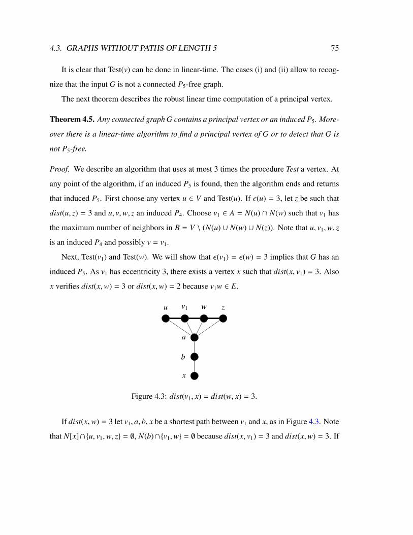
4.3. GRAPHS WITHOUT PATHS OF LENGTH 5 75
It is clear that Test(v) can be done in linear-time. The cases (i) and (ii) allow to recog-
nize that the input G is not a connected P5-free graph.
The next theorem describes the robust linear time computation of a principal vertex.
Theorem 4.5. Any connected graph G contains a principal vertex or an induced P5. More-
over there is a linear-time algorithm to find a principal vertex of G or to detect that G is
not P5-free.
Proof. We describe an algorithm that uses at most 3 times the procedure Test a vertex. At
any point of the algorithm, if an induced P5 is found, then the algorithm ends and returns
that induced P5. First choose any vertex u ∈ V and Test(u). If ε(u) = 3, let z be such that
dist(u, z) = 3 and u, v,w, z an induced P4. Choose v1 ∈ A = N(u) ∩ N(w) such that v1 has
the maximum number of neighbors in B = V \ (N(u) ∪ N(w) ∪ N(z)). Note that u, v1,w, z
is an induced P4 and possibly v = v1.
Next, Test(v1) and Test(w). We will show that ε(v1) = ε(w) = 3 implies that G has an
induced P5. As v1 has eccentricity 3, there exists a vertex x such that dist(x, v1) = 3. Also
x verifies dist(x,w) = 3 or dist(x,w) = 2 because v1w ∈ E.
u v1 w z
a
b
x
Figure 4.3: dist(v1, x) = dist(w, x) = 3.
If dist(x,w) = 3 let v1, a, b, x be a shortest path between v1 and x, as in Figure 4.3. Note
that N[x]∩u, v1,w, z = ∅, N(b)∩v1,w = ∅ because dist(x, v1) = 3 and dist(x,w) = 3. If

76 CHAPTER 4. PERFECT EDGE DOMINATION
N(b)∩ u, z , ∅ there is an induced P5 and we can find it and return it. Otherwise, N(b)∩
u, z = ∅. We can assume wa ∈ E otherwise w, v1, a, b, x is an induced P5. Following
the same idea, x, b, a, v1, u and x, b, a,w, z are possible induced P5’s, then we can assume
that ua, az ∈ E which is a contradiction because dist(u, z) = 3. Therefore, in this case the
algorithm always finds an induced P5.
u v1
a
w z
x
y
Figure 4.4: dist(v1, x) = 3 and dist(w, x) = 2.
If dist(x,w) = 2 let w, a, x be a shortest path between w and x. Note that N[x] ∩
u, v1,w = ∅ because dist(x, v1) = 3. If zx ∈ E then u, v1,w, z, x is an induced P5.
Thus, zx < E and we are in the situation of Figure 4.4. We assume ua ∈ E otherwise
u, v1,w, a, x is an induced P5. This implies that a ∈ A = N(u) ∩ N(w) and it is adjacent
to x ∈ B = V \ (N(u) ∪ N(w) ∪ N(z)). Recall that v1 was chosen as a vertex belonging
to A with maximum degree in B. As v1x < E, then there exists y ∈ B such that v1y ∈ E
and ay < E. It follows that there is a P5 induced either by y, v1, u, a, x if xy < E or by
x, y, v1,w, z if xy ∈ E. Again, the algorithm always finds an induced P5.
Once a principal vertex is obtained, we find an induced P5, or a dominating Kp, or a
dominating P3 following the theorem below. We remark that using a recent characteriza-
tion of Pk-free graphs, by Camby and Schaudt [16], it is possible to obtain a dominating
induced P3 or a dominating Kp in O(n5(n + m)) time when a connected P5-free graph is
given.

4.3. GRAPHS WITHOUT PATHS OF LENGTH 5 77
Theorem 4.6. For any connected graph G, there is a linear-time algorithm to find a dom-
inating induced P3, a dominating Kp, or to detect that G is not a P5-free graph.
Proof. The algorithm searches a dominating set contained in N[v] where v is a principal
vertex of G. Again, at any point of the algorithm, if an induced P5 is found, then the
algorithm ends and returns that induced P5.
1. Find a principal vertex v or an induced P5 of G using the robust linear-time algorithm
of Theorem 4.5.
2. Let X := N[v] be the initial dominating set. Consider iteratively each vertex w ∈
N(v): if X \w is still a dominating set then X := X \w. This can be done in linear-
time using a variable for each vertex of V \ N[v] to count the number of neighbors
in X. A vertex w ∈ N(v) can not be removed from X if only if some of its neighbors
has exactly one dominator in X.
v
v2v1 v3
w1 w2 w3
v
v2v1 v3
w1 w2 w3
v
v2v1 v3
w1 w2 w3
(i) (ii) (iii)
Figure 4.5: Principal vertex v, its neighbors v1, v2, v3 and their proper dominated vertices.
3. If |X| ≤ 3 then G has a dominating P3 or a dominating K|X|. If |X| ≥ 4 and it is not
a complete graph, we will show that G has an induced P5. We can assume that G
has a subgraph like one in Figure 4.5, where v1, v2, v3 ⊂ X and does not induce a
triangle. Each one of them has a proper dominated vertex w1,w2,w3 respectively.
Edges between wi and w j are drawn in order to avoid the induced P5 wi, vi, v, v j,w j.
Nevertheless in (i) and (ii) w2,w1, v1, v,w3 is a induced P5; and in (iii) the vertices
w2, v2, v3,w3,w1 or w2,w1, v1, v,w3 induce a P5.

78 CHAPTER 4. PERFECT EDGE DOMINATION
We remark that the above theorem might be of interest to other P5-free algorithmic
problems, since it represents an algorithmic proof of Bacso and Tuza’s theorem [2].
4.3.2 Colorings and vertex dominating subgraphs
In this section, we describe the remaining algorithms on which the proposed algorithm
is based. The first two theorems show the convenience of using 3-colorings to compute
perfect edge dominating sets.
Theorem 4.7. Given a graph G and W ⊆ V, there is a linear-time algorithm to verify if
there exists some perfect edge dominating set whose associated 3-coloring is (B,Y,W).
Proof. In the affirmative case, using Observation 4.2, we can determine Y in linear-time
and so B = V \ (W ∪ Y). Therefore, we construct a 3-coloring (B,Y,W) in this way and
then test the validity of (B,Y,W) by checking the conditions of Observations 4.1, 4.2 and
4.3. All these computations can be done in linear-time.
Theorem 4.8. Given a connected graph G and Y ⊂ V, there is a linear-time algorithm
to verify if there exists some perfect edge dominating set whose associated 3-coloring is
(B = b,Y,W). Moreover, the algorithm can find a vertex b for which the sum of the
weight of its incident edges is minimum.
Proof. Clearly, if such perfect edge dominating set exists, it verifies
i. G[Y] is a graph with maximum degree 1 and at least one vertex has degree 0.
ii. V \ Y is a independent set.
iii. If s1, s2, ..., sk ⊆ Y are the vertices with degree 0 in G[Y], and y1, y2, ..., yl ⊂ Y are
the vertices of degree 1, the black vertex belongs to⋂k
i=1 N(si) \⋃l
j=1 N(y j).
Therefore, we check conditions (i) and (ii), and construct A =⋂k
i=1 N(si) \⋃l
j=1 N(y j)
in linear-time. Note that all vertices in A are equivalent. If A , ∅, each b ∈ A generates
4.3. GRAPHS WITHOUT PATHS OF LENGTH 5 79
a valid coloring (B,Y,W), B = b,W = V \ (B ∪ Y). Condition (ii) and |B| = 1 imply
that (B,Y,W) satisfies the conditions of Observations 4.1 and 4.3. Condition (i) and b ∈ A
imply that (B,Y,W) satisfies the condition of Observation 4.2. So, the validity of (B,Y,W)
holds.
The next theorem refers to finding an efficient edge dominating set of a graph, given a
fixed size vertex dominating set of it.
Theorem 4.9. [58] Given a graph G and a vertex dominating set of fixed size of G, there is
a linear-time algorithm to solve the minimum weight efficient edge dominating set problem
for G.
The following results relate trivial perfect edge dominating sets of a graph and the
existence of vertex dominating complete subgraphs of certain sizes.
Observation 4.7. Given a graph G, a dominating set D of G, a perfect edge dominating
set P of G and (B,Y,W) the 3-coloring associated to P, if D ⊆ B then P is the trivial
perfect edge dominating set.
Corollary 4.2. Given a connected graph G, if there is a dominating Kp with p ≥ 4 then G
has exactly one perfect edge dominating set P and P is trivial.
Proof. Suppose that there is a non-trivial perfect edge dominating set P. By Observation
4.4, all vertices of Kp must be black and by Observation 4.7, P must be trivial and this is a
contradiction.
Corollary 4.3. Given a connected P5-free graph G, if G admits some non-trivial perfect
edge dominating set P then G has dominating induced P3 or a dominating K3.
Proof. If G has at most 2 vertices, then G has only one perfect edge dominating set which
is trivial. Therefore, G has at least 3 vertices. Now, suppose that G has neither dominating

80 CHAPTER 4. PERFECT EDGE DOMINATION
induced P3 nor dominating K3. By Theorem 4.4, G must have some dominating Kp with
p , 3. In case p ≥ 4, by Corollary 4.2, G has no non-trivial perfect edge dominating set
which is a contradiction. Therefore, p ≤ 2 . As G is connected with at least 3 vertices,
it is always possible to add more vertices to Kp to form a dominating K3 or a dominating
induced P3. Again, a contradiction.
Corollary 4.4. Given a graph G, if G has some vertex dominating K1 or K3 then G has no
proper edge dominating sets.
Proof. First, assume G has a dominating K1 = uwhich means that u is a universal vertex.
Suppose that P is a proper edge dominating set. Let v be any black vertex. By Observation
4.7, v cannot be a universal vertex. As u is a neighbor of v, then u is a yellow vertex
because it is a universal vertex. As v is a black vertex, v has another non-white neighbor
w. Moreover, w is adjacent to the universal vertex u. This contradicts that u is a yellow
vertex.
Next, suppose G contains a dominating K3. Suppose that G has some proper edge
dominating set P and (B,Y,W), its associated 3-coloring, with B,Y,W , ∅. By Obser-
vation 4.5, (i) all vertices of the dominating K3 are black or (ii) exactly two of them are
yellow vertices and the other vertex is white. In case (i), by Observation 4.7, P must be
trivial which is a contradiction. In case (ii), there are no black vertices as consequence of
Observations 4.2 and 4.3. Again, a contradiction.
Finally, we state the relationship between the existence of proper edge dominating sets
and the colorings of a dominating P3.
Theorem 4.10. Given a connected P5-free graph G, if G admits some proper perfect edge
dominating set P, with associated 3-coloring (B,Y,W), then G has a vertex dominating P3
(formed by vertices v1, v2 and v3) with one of the possible combinations of colors of Figure
4.6.

4.3. GRAPHS WITHOUT PATHS OF LENGTH 5 81
(a) orv1 v2 v3 v1 v2 v3
(b) orv1 v2 v3 v1 v2 v3
(c)v1 v2 v3
(d)v1 v2 v3
(e)v1 v2 v3
Figure 4.6: Possible valid colorings of dominating induced P3
Proof. Clearly, by Corollaries 4.3 and 4.4 G has a dominating induced P3. By Observa-
tions 4.1, 4.2 and 4.3, there exists neither two adjacent white vertices, nor yellow vertices
with at least two non-white neighbors nor white vertices with black neighbors. As a con-
sequence, the possible colors of the dominating induced P3 must match to some combina-
tions of Figure 4.6 or some of Figure 4.7. If the combination (f) of Figure 4.7 is matched
then all vertices of the dominating induced P3 are black vertices and by Observation 4.7,
P is a trivial perfect edge dominating set leading to a contradiction. If the combination (g)
of Figure 4.7 is matched, two adjacent vertices of the dominating induced P3 are yellow
vertices and the other one is a white vertex. None of these three vertices can have black
neighbors which implies B = ∅ and P to be an efficient dominating set. Again, this is a
contradiction. Therefore, the only valid options are those of Figure 4.6.
4.3.3 Robust linear algorithm for P5-free graphs
In this section, we describe a robust linear time algorithm for finding minimum weight
perfect edge dominating set of a P5-free graph. Given an arbitrary graph G, in linear time

82 CHAPTER 4. PERFECT EDGE DOMINATION
( f )v1 v2 v3
(g) orv1 v2 v3 v1 v2 v3
Figure 4.7: Invalid colorings of dominating induced P3
the algorithm either finds such edge dominating set or exhibits an induced P5 of the graph.
Let G, |V(G)| > 1, be an arbitrary connected graph. Along the process, the proposed
algorithm constructs a set E containing a few candidates for the minimum weight perfect
edge dominating set of G. At the end, it selects the least of them and returns the minimum
edge dominating set of G,
Algorithm for minimum weighted perfect edge dominating set
1. Define E := E(G)
2. Find a principal vertex of G. If such vertex does not exist, then return an induced P5
and stop.
3. Using the principal vertex v, find (i) an induced P5, or (ii) a dominating Kp, or (iii)
a dominating P3.
4. Case (i): An induced P5 is found. Then return it and stop.
5. Case (ii): A dominating Kp is found. If p ≥ 4 then return E(G) and stop. Otherwise,
p ≤ 3 and using such dominating Kp, find a minimum weight efficient edge domi-
nating set and, if it exists, include it in E. If Kp = v1, v2 and N(v1)∩N(v2) = ∅ then
transform the dominating K2 into a dominating P3 by adding a third vertex to it.
6. Case (iii): A dominating P3 is found. First, again using such a vertex dominating
set, find a minimum weight efficient edge dominating set of G, and include it in E,
if it exists. Then look for a proper perfect edge dominating set of G, by considering

4.3. GRAPHS WITHOUT PATHS OF LENGTH 5 83
every possible coloring of the P3, according to Figure 4.6. In each of the cases (a)-
(b) ((c)-(e)), below, the algorithm determines at most two (one) proper perfect edge
dominating sets (set), which are (is) then included in E.
(a) Without loss of generality, v3 is the yellow vertex of the dominating induced
P3. Clearly, W = N(v3) \ v2 and we can apply the linear-time algorithm
of Theorem 4.7 to determine the proper perfect edge dominating set whose
associated 3-coloring is (B,Y,W). Include it in E, if it exists.
(b) Without loss of generality, v1 is the black vertex of the dominating induced P3.
We can applied the same technique of (a) using W = N(v2) \ v1.
(c) Again, apply the same technique of (a) using W = (N(v1) ∪ N(v3)) \ v2.
(d) In this case, v1 and v3 have only yellow neighbors. As we are looking for proper
perfect edge dominating sets, there is some black vertex somewhere. Clearly,
v2 must have exactly one black neighbor and the other neighbors of v2 are white
vertices. So, Y = N(v1) ∪ N(v3), |B| = 1, and we can apply the linear-time
algorithm of Theorem 4.8 to determine the proper perfect edge dominating set
whose associated 3-coloring is (B,Y,W) with least weight. Again, if successful
include it in E.
(e) In this case, v1 (v3) can have at most one black neighbor. As we are looking for
proper perfect edge dominating sets, there is at least one black vertex. First, we
assume that there are some triangles using edges of the dominating induced P3
(the number of these triangles is exactly |N(v1)∩N(v2)|+ |N(v2)∩N(v3)| which
can be computed in linear-time). If there are at least 2 triangles using the same
edge, without loss of generality v1, v2, x and v1, v2, x′, then the coloring is
invalid. If v1, v2, x and v2, v3, x′ are triangles then the coloring is invalid or
it cannot admit black vertices, which means there are no proper perfect edge
dominating sets. The only possibility for the graph to admit a proper perfect

84 CHAPTER 4. PERFECT EDGE DOMINATION
edge dominating set (which implies the existence of black vertices) is the exis-
tence of exactly one triangle using an edge of the dominating induced P3 and
|B| = 1. Clearly, the yellow vertices are Y = N(v2) and we then proceed as in
Case (d). Next, suppose there is no triangle using an edge of the dominating
induced P3. Clearly, every vertex in A1,3 = N(v1) \ N(v3) has to be adjacent
to every vertex in A3,1 = N(v3) \ N(v1) or there is some induced P5, which
the algorithm returns and then stops. It is not hard to see this can be accom-
plished in linear-time. Suppose that there is only a black vertex b. It has to be
adjacent to v1 and v3, otherwise (without loss of generality, bv1 < E(G)) there
is an induced P5 formed by y, v1, v2, v3, b where y is a yellow neighbor of v1.
Then the yellow vertices are Y = N(v2) and we proceed as in (d). The last case
is that there are two black vertices b1, b3 where b1 ∈ A1,3 and b3 ∈ A3,1, and
the coloring is invalid if |A1,3| > 1 or |A3,1| > 1. The algorithm will check if
(B = b1, b3,Y = N(v2),W = V \ (B∪ Y)) is a valid coloring, and include in E
the corresponding edge dominating set. All these computations can be done in
linear-time.
7. Select the least weight perfect edge dominating set of E, return it and stop.
The correctness and linear time complexity of the algorithm follows directly from the
propositions formulated in the previous subsections.
To summarize we state the main result of this section.
Theorem 4.11. The weighted perfect edge dominating set problem can be solved for P5-
free graphs in linear time in a robust way.

4.3. GRAPHS WITHOUT PATHS OF LENGTH 5 85
Resumen del Capıtulo 4
En este capıtulo estudiamos la complejidad del problema del conjunto perfectamente do-
minante de aristas para algunas subclases de grafos. Si bien el enfoque de este capıtulo es
principalmente algorıtmico, las observaciones y rutinas auxiliares tienen relevancia inde-
pendiente y podrıan ser usados para otras aplicaciones.
Asımismo queremos destacar que nuestras contribuciones forman parte de Lin et al.
[56] y en este capıtulo tambien mencionamos otros resultados de ese trabajo.
En la Seccion 4.1 de este capıtulo damos las definiciones necesarias e introducimos un
3-coloreo para manejar el problema.
Un subconjunto E′ ⊂ E(G) es un conjunto perfectamente dominante de aristas si toda
arista de E(G) \ E′ es adyacente a exactamente una arista en E′. Por otro lado si toda
arista de E(G) es adyacente a exactamente una arista en E′, entonces E′ es un conjunto
eficientemente dominante de aristas.
El problema de cardinalidad de la dominacion perfecta de aristas consiste en determi-
nar el conjunto perfectamente dominante de aristas de menor tamano. El correspondiente
problema pesado se define reemplazando la condicion de menor tamano por mınima suma
de los pesos de las aristas dominantes.
En este capıtulo distinguimos tres tipos de dominacion perfecta de aristas:
• eficiente, cuando el conjunto dominante es tambien eficientemente dominante;
• trivial, cuando el conjunto dominante es E(G);
• propio, cuando el conjunto dominante no cae en ninguna de las opciones anteriores.
En la Seccion 4.2 estudiamos la complejidad del problema como parte del trabajo de
Lin y otros [56]. En ese manuscrito se encuentra la prueba de la NP-completitud del pro-
blema cuando esta restringido a los grafos sin garras de grado menor o igual que 3 (grafos
subcubicos). Y, en consecuencia, un interesante resultado sobre la dicotomıa (polinomial

86 CHAPTER 4. PERFECT EDGE DOMINATION
o NP-difıcil) de la complejidad del problema para grafos definidos con un subgrafo pro-
hibido. En la Subseccion 4.2.1 mostramos que la version pesada del problema es lineal
para la clase de grafos sin garras de grado exactamente 3 (grafos cubicos), Teorema 4.3.
Ademas, este resultado puede extenderse a la clase de grafos sin garras de grado a lo sumo
3 donde cada vertice de grado 2 tiene sus dos vecinos adyacentes. Esto muestra que cuando
restringimos el problema del conjunto perfectamente dominante a la grase de grafos sin
garras, la complejidad depende fuertemente del grado de los vertices.
En la Seccion 4.3 estudiamos las clases de grafos sin P5 motivados por el Corolario
4.1 de [56], que deja como problema abierto establecer la complejidad del problema para
grafos definidos por un subgrafo prohibido H cuando H es un bosque lineal (union de
caminos). Notar que cualquier bosque lineal F contiene un Pk inducido y ademas F es un
subgrafo inducifo de algun Pk′ , k′ ≥ k. En este sentido, hicimos el trabajo para k = 5.
En la Subseccion 4.3.1 presentamos observaciones y rutinas auxiliares para trabajar
con los grapos P5-free de manera robusta: Teoremas 4.5 y 4.6. Este ultimo resultado
constituye una prueba algorıtmica del resultado de Bacso y Tuza [2].
En la Subseccion 4.3.2 enunciamos propiedades que relacionan los posibles 3-coloreos
de subgrafos dominantes y la existencia de los distintos tipos de conjuntos perfectamente
dominantes. El principal resultado en este sentido es el Teorema 4.10.
Finalmente, en la Subseccion 4.3.3 describimos un algoritmo lineal y robusto para
hallar un conjunto de mınimo peso perfectamente dominante de aristas para grafos que no
contienen P5.

Chapter 5
Vertex domination and well-covered
graphs
A natural relation between vertex domination and edge domination, as we mentioned pre-
viously, is throughout line graphs. Recall that the line graph of a graph G, denoted by
L(G), is the graph with vertex set E(G), where x and y are adjacent in the line graph if and
only if edges x and y are adjacent in the original graph. Line graphs allows to make impor-
tant connections between many important areas of graph theory. For example, determining
a maximum matching in a graph is equivalent to finding a maximum independent set in
the corresponding line graph. Similarly, edge coloring is equivalent to vertex coloring in
the line graph. Much research has been done on the study and application of line graphs;
a comprehensive survey is found in [75].
It is well known that the line graph can be obtain from the original graph in linear time.
On the other direction, the determination problem consists in determining the original
graph from its line graph. Whitney in [84] solved this problem by showing that with the
only exception of K1,3 and K3, a graph is uniquely characterized by its line graph.
87

88 CHAPTER 5. VERTEX DOMINATION AND WELL-COVERED GRAPHS
Our main objective in this thesis is to study edge domination. We can consider a
very simple algorithm to find an edge dominating set which is just take any maximal
matching. The greedy algorithm consists in adding edges to a matching until the matching
becomes maximal and, clearly, ends in linear time. It is well known that a minimum
maximal matching is a minimum edge dominating set. In the special case that all maximal
matchings of the graph have the same size, the algorithm always determines a minimum
edge dominating set. This is equivalent to say that, in the line graph, every maximal
independent set has the same size. Graphs having all maximal independent sets of the
same size are known as well-covered graphs. Therefore, there is a linear-time algorithm
to solve vertex dominating set problem for well-covered line graphs.
In this chapter, Section 5.2 is dedicated to the complexity of vertex dominating set
problem for well-covered graphs and its subclasses. We prove that the dominating set
problem is a NP-complete for well-covered K1,4-free graphs. Additionally, in Section 5.3
we address the recognition problem for certain subclasses of well-covered graphs related
with comparability graphs. Since recognition of general well-covered graphs is coNP-
complete, any polynomial time non-robust algorithm that solves vertex dominating set
problem for some subclass of well-covered graphs is useful only if the recognition of such
subclass can be done in polynomial time.
5.1 Preliminaries and previous results
Well-covered graphs were introduced by Plummer [72] in 1970. In the original definition,
a graph is well-covered when every minimal vertex cover is also minimum. A vertex
cover S satisfies that I = V(G) \ S does not contain edges, then I is an independent
set. Moreover, I is a maximal (maximum) independent set if and only S is a minimal
(minimum) vertex cover. Therefore an equivalent definition for well-covered graphs is: a
5.1. PRELIMINARIES AND PREVIOUS RESULTS 89
graph is well-covered if every maximal independent set is also maximum independent set.
In other words, when all maximal independent sets are of the same size.
An independent dominating set is a dominating set of G that is also an independent set
of vertices. Note that the independent dominating sets are exactly the maximal indepen-
dent sets.
Recall that the independent dominating number, i(G), is the minimum size of an in-
dependent dominating set; and the independent number, α(G), is the maximum size of
an independent set of G. By definition, the inequality i(G) ≤ α(G) holds. And we have
i(G) = α(G) for well-covered graphs.
The problem of recognizing whether a graph is well-covered is coNP-complete [24,
79]. That means that deciding if a given graph is not well-covered is NP-complete; usually
by showing two maximal independent set of different sizes. The recognition problem
remains coNP-complete restricted to well-covered K1,4-free graphs [20]. On the other
hand, the recognition problem is polynomial for the following subclasses of well-covered
graphs: claw-free graphs [81, 82], perfect graphs of bounded clique size [30], and graphs
with bounded degree [21, 87], these last results also work for the weighted version of the
problem. Many of the research in this area deals with characterization of some families of
well-covered graphs. For instance, well-covered bipartite graphs [77], well-covered graphs
with girth at least 5 [36], well-covered C4,C5-free graphs [37], well covered simplicial,
chordal and circular arc graphs [76]. In some cases these characterizations leads to efficient
algorithm for recognizing well-covered graphs.
The dominating set problem was proved to be NP-complete for well-covered graphs
by Sankaranarayana and Stewart [79], and for line graph by Yannakakis and Gavril [40].
On the other hand, Allan and Laskar proved that every claw-free graphs have a min-
90 CHAPTER 5. VERTEX DOMINATION AND WELL-COVERED GRAPHS
imum dominating set that is also independent [1]. Therefore in a well-covered claw-free
graph any minimum independent dominating set, i.e. minimum maximal independent set,
is a minimum dominating set. Using the very simple algorithm that adds vertices to an
independent set until it becomes maximal, we can solve dominating set problem in poly-
nomial time for well-covered claw-free graphs. This result implies that the dominating
set problem is also polynomial for well-covered line graphs, since it is a subclass of well-
covered claw-free graphs.
5.2 Vertex dominating set problem
In this section we prove that the dominating set problem is NP-complete for well-covered
K1,4-free graphs.
It is clear that the problem is in NP, because given a set of k vertices D we can verify in
polynomial time whether D dominates the graph. In order to prove the NP-completeness,
we use a version of the SAT problem called the 3-SAT2+1 problem which is also NP-
complete [71] and reduce our problem from it.
3-SAT2+1 Problem: Given variables X1, X2, ..., Xn and a boolean formula written in a
conjunctive normal form C = C1∧C2∧...∧Cm, having 2 or 3 literals per clause, where each
literal is an occurrence of some variable Xi or its negation ¬Xi; determine if it is possible
to assign values true or false to the variables, in such a way that the formula is true. In this
restricted version each variable occurs at most 3 times, twice positive and once negative.
5.2.1 Well covered K1,4-free graphs
The following theorem also implies the NP-completeness of the dominating set problem
restricted to well-covered K1,4-free graphs with maximum degree ∆ ≤ 8.

5.2. VERTEX DOMINATING SET PROBLEM 91
Theorem 5.1. The dominating set problem is NP-complete for well-covered K1,4-free
graphs.
Proof. We already mentioned that the problem is in NP. We shall prove that it is NP-
complete by describing a reduction from 3-SAT2+1.
Let be C = C1 ∧ C2 ∧ ... ∧ Ck an instance of the 3-SAT2+1 problem with variables
X1, ..., Xn. Define a graph GC as follow:
• For each variable Xi define a triangle T with vertices zi, xi,¬xi.
• For each clause C j define a graph L as in Figure 5.1 with distinct vertex c j.
• For each clause C j = Y j1 ∨ Y j2 ∨ Y j3, where each literal can be Xi or ¬Xi, add edges
between c j and the vertices corresponding to Y j1, Y j2, and Y j3, say y j1, y j2, and y j3.
• Add edges between the vertices corresponding to y j1, y j2, and y j3 belonging to the
same clause.
c j
Figure 5.1: Graph L with distinct vertex c j
Clearly, the graph GC has 3n + 7k vertices, maximum degree 8, and can be computed
in polynomial time. See an example in Figure 5.2.
Claim 1. C is satisfiable if an only if GC has a dominating set of size n + 2k.
Proof: (⇒) Vertices corresponding to true literals in a satisfying truth assignment domi-
nate all the copies of triangle T and vertices c j, j = 1, ..., k. The remaining vertices can be
dominated by two additional vertices for each copy of L. Therefore, a dominating set of
size n + 3k is obtained.

92 CHAPTER 5. VERTEX DOMINATION AND WELL-COVERED GRAPHS
c1
u1
v1
c2
u2
v2
z1
z2
z3
Figure 5.2: Example of the graph GC defined by the imput C = (X1 ∨ X2 ∨ X3) ∧ (X1 ∨
¬X2 ∨ ¬X3)
(⇐) Any dominating set must contains at least one vertex from each copy of T since
each zi, i = 1, ..., n, is not adjacent to any vertex outside the triangle T . In addition, any
dominating set must contain at least two vertices from each copy of L since vertices u j, v j,
j = 1, ..., k, have disjoint neighborhoods. Therefore, a dominating set D of size n + 2k
contains exactly one vertex from each T and exactly two vertices from each L. Note that
the distinct vertices c j of the L subgraphs must all be dominated by vertices in the T
triangles; otherwise, more than two dominating vertices would be required from some L.
Thus the variable connectors which are in the dominating set correspond to the true literals
of a satisfying truth assignment. This completes the proof of the claim.
Claim 2. GC is a well-covered K1,4-free graph.
Proof: Clearly there is an induced K1,4 if and only if there is a vertex v with α(G[N(v)]) ≥
4. By construction the only vertices of degree ≥ 4 are c j and possibly xi and ¬xi.
Vertices c j, j = 1, ..., k, satisfies α(G[N[c j]]) ≤ 3 since N[c j] \ u j, v j is complete.
Each vertex ¬xi, i = 1, ..., n, appears in at most one clause, say C j, and then satisfies that
α(G[N[¬xi]]) ≤ 2 since N[¬xi] ∩ N[c j] is complete. Analogous, xi i = 1, ..., n, appears in
5.3. RECOGNITION PROBLEM 93
at most two clauses and then satisfies that α(G[N[xi]]) ≤ 3.
We conclude that GC is K1,4-free.
To see that G is well-covered, let I be a maximal independent set. Clearly, |I∩N[zi]| = 1
for 1 ≤ i ≤ n. In addition, I has exactly 3 vertices in each copy of L indistinctly if
c j belongs to the independent set or not. We have that |I| = n + 3k for every maximal
independent set and GC is well-covered.
This claim completes the proof of the theorem.
5.3 Recognition problem
We have already discuss that the recognition of well-covered graphs is coNP-complete
even under substantial restrictions. In this section we study the problem for well-covered
comparability and well-covered co-comparability graphs. In both cases, we present poly-
nomial time recognition algorithms.
Comparability graphs
A comparability graph is a graph that admits a transitive orientation of its edges. This
is, each edge uv is oriented as→uv or
←uv, and whenever oriented edges
→uv and
→vw exists then
edge uw also exists and has orientation→
uw.
For the recognition problem of comparability graphs, McConnell and Spinrad devel-
oped a linear time algorithm to find a transitive orientation if it exists [65]. However
deciding if a given orientation is transitive requires O(MM(n)) (matrix multiplication).
Morvan and Viennot [68] presented parallel algorithms for the recognition problem and
the computation of a transitive orientation of comparability graphs; their algorithms run in
O(log n) time and require O(∆m) processors on the CRCW PRAM model, where ∆ is the
maximum degree of a vertex in the graph.

94 CHAPTER 5. VERTEX DOMINATION AND WELL-COVERED GRAPHS
A transitive orientation of the edges defines a partial ordering R of the vertices V by
defining u < v if and only if the edge uv is oriented→uv. We also say that v is a predecessor
of u and that u is a successor of v. Note that G is the undirected graph of the directed
(acyclic) graph G(V,R).
Following observations arise straightforward from the definition of a transitive orien-
tation.
Observation 5.1. Vertices in a directed path defines a complete set in G.
Observation 5.2. Every edge of G either (i) belongs to a maximal directed path or (ii) can
be deduced by transitivity from a maximal directed path.
By Observation 5.1, every clique in a comparability graph corresponds with a maximal
directed path in the directed graph G(V,R).
A vertex is called a maximum when it has not predecessors, and a minimum when it
has not successors. In polynomial time, we can find a reduced graph G′ with the same
vertex set than G and edges consisting in the essential directed edges of G. If necessary,
transitivity can be used to transform G′ back to the original graph.
5.3.1 Well-covered comparability graphs
We use a equivalent definition of well-covered graphs described by Dean and Zito in [30].
We present the case of their theorem that we need for our objectives, the complete version
appears in the cited work.
Theorem 5.2. [30] The following statements are equivalent:
(a) G is well-covered.
(b) For every clique C there is no nonmaximum independent set S of such that (i) S∩C =
∅, (ii) |C| ≥ |S |, and (iii) C ⊆ N(S ).

5.3. RECOGNITION PROBLEM 95
Lemma 5.1. If a vertex set S with S ∩C = ∅ dominates a clique in a comparability graph
C, then there are two vertices in S that also dominates C.
Proof. Let p1, p2, ..., pk be the maximal directed path defined by C and oriented by→
p j p j+1,
j = 1, ..., k − 1. Consider a ∈ S such that exists an oriented edge→
pia with maximum i, and
b ∈ S such that exists an oriented edge→
bp j with j minimum. By transitivity, a dominates
vertices p1, p2, ..., pi, and b dominates p j, p j+1, ..., pk. By definition of i and j, vertices ph
with i < h < j, are not adjacent to any vertex in S . Since S dominates C, we obtain
j ≤ i + 1 and a, b dominates C. Note that a and b can not be the same vertex, otherwise
a ∈ C, and may be not unique.
Theorem 5.3. There is a polynomial algorithm to determine whether a given graph is a
well-covered comparability graph.
Proof. We describe the algorithm for a connected graph, if the input is not connected apply
the algorithm in each connected component. Given a graph G, find a transitive orientation
and determine if G is a comparability graph. Next, determine if G satisfies statement
(b) of Theorem 5.2 in the following way. By Lemma 5.1 it is sufficient to verify (b) for
independent sets of size 2. Note that if G is connected then |C| ≥ 2 and condition (ii) is
always satisfied. Since G is well-covered, S is a nonmaximum independent set if and only
if is nonmaximal independent, and this is equivalent to N[S ] , V(G).
Statement (b) is equivalent to say for each pair of non adjacent vertices a, b such that
N(a) ∪ N(b) , V(G), there does not exist maximal paths of G contained in N(a) ∪ N(b).
These verifications can be done in polynomial time.
5.3.2 Well-covered co-comparability graphs
The co-comparability graphs are the complement of comparability graphs. The recogni-
tion problem of co-comparability graphs is polynomial time solvable since so is deciding

96 CHAPTER 5. VERTEX DOMINATION AND WELL-COVERED GRAPHS
if G is a comparability graph.
We will see in this section a simple proof that the problem of recognize well-covered
co-comparability graph is polynomial time solvable. Note that the complexity of dominat-
ing set problem is also polynomial for these graphs [54].
Theorem 5.4. There is a polynomial time algorithm to decide if a given graph is well-
covered co-comparability graph.
Proof. As we have seen in the previous section, a transitive orientation of edges in G can
be obtained and verified in O(MM(n)). We can also check in linear time if all maximal
cliques in G have same cardinality as follows.
By Observation 5.1 a clique in G is a maximal directed path. After finding all sources S
and terminals T in the directed acyclic graph G. In linear time we can determine a shortest
and a longest path between S and T . If these paths have the same length all cliques in G
have the same size.
In this situation, all maximal independent sets of G are of the same size and G is
well-covered.
5.3. RECOGNITION PROBLEM 97
Resumen del Capıtulo 5
En este capıtulo estudiamos la relacion entre la dominacion de vertices y de aristas que
surge naturalmente a traves de los grafos de lıneas. Recordemos que el grafo de lınea de
un grafo G, notado L(G), tiene como vertices a las aristas de G, donde x e y son adyacentes
en L(G) si y solo si las aristas x e y son adyacentes en G.
Podemos considerar un algoritmo simple para encontrar un conjunto dominante de
aristas, que es seleccionar cualquier matching maximal. El algoritmo goloso consiste en
ir agregando aristas a un matching hasta que el matching sea maximal; claramente este
algoritmo termina en tiempo lineal. Se sabe que un matching maximal mınimo es un
conjunto dominante de aristas de tamano mınimo. Si ademas estamos en el caso que todos
los matching maximales tienen el mismo tamano, el algoritmo goloso siempre determina
un conjunto dominante de aristas mınimo. Esta condicion es equivalente a decir que, en
el grafo de lınea, todos los conjuntos independientes maximales tienen el mismo tamano.
Los grafos donde todos los conjuntos independientes maximales tienen el mismo tamano
se llaman grafos bien cubiertos. Por lo tanto hay un algoritmo lineal para resolver el
problema de conjunto dominante de vertices para grafos bien cubiertos.
En la Seccion 5.1 damos algunos resultados relacionados. Entre ellos mencionamos
la prueba de la NP-completitud del problema de conjunto dominante para grafos bien
cubiertos [79] y para grafos de lınea [40]. Por otro lado, en [1] se prueba que todo grafo
sin garras contiene un conjunto dominate mınimo que ademas es independiente. Entonces,
el algoritmo goloso resuelve el problema del conjunto dominante mınimo para grafos bien
cubiertos sin garras (K1,3).
En la Seccion 5.2 probamos que el problema del conjunto dominante es NP-difcil para
grafos bien cubiertos sin K1,4, (Teorema 5.1).
En la Seccion 5.3 discutimos el problema de reconocimiento de grafos bien cubiertos

98 CHAPTER 5. VERTEX DOMINATION AND WELL-COVERED GRAPHS
para subclases relacionadas con grafos de comparabilidad. Notar que el reconocimiento
de los grafos bien cubiertos es un problema coNP-completo [24, 79]. En consecuencia,
cualquier algoritmo polinomial no robusto que resuelva el problema de dominacion de
vertices para alguna subclase de grafos bien cubiertos es util solo si el reconocimiento de
dicha subclase se puede hacer en tiempo polinomial.
Un grafo es de comparabilidad si es posible orientar sus aristas de manera transitiva.
Esto significa que cada arista uv se orienta como→uv o
←uv, y si existen las aristas orientadas
→uv y
→vw entonces tambien existe la arista uw y tiene orientacion
→uw.
Un grafo es de co-comparabilidad si su grafo complemento, G, es de comparabilidad.
Los resultados son dos algoritmos polinomiales, uno para el reconocimiento de grafos
bien cubiertos de comparabilidad (Teorema 5.3) y otro para los grafos bien cubiertos de
co-comparabilidad (Teorema 5.4).

Chapter 6
Conclusions
In this thesis, we have made contributions on several dominating-set related problems.
The analysis of subgraphs and graph parameters related to vertex domination and edge
domination gives a better insight in the relation between different versions of the problems.
In addition, we analyzed the complexity and provided new efficient algorithms for these
problems.
In Chapter 2, we studied edge dominating set problem and give an algorithm that solves
the problem for proper interval graphs. (Theorem 2.2)
The efficient edge dominating set (DIM) problem is addressed in Chapter 3. The col-
oring of the vertices used in this chapter allows us to manage the problem in a simple
way, and to identify the structures related to the existence of many DIMs. This approach
leads to tight bounds for the maximum number of DIMs in the following graph classes:
general (Theorem 3.2), triangle-free (Theorem 3.3) and connected (Theorem 3.4). Also,
the characterization of the extremal graphs naturally arise. These results were published
in the Journal of Graph Theory (2015) [61], and have been presented in a communication
of the Annuals of the Union Matematica Argentina (2015).
99

100 CHAPTER 6. CONCLUSIONS
The perfect edge domination is more general than efficient edge domination. In Chap-
ter 4 we use a 3-coloring of the vertices to represent the solutions of the problem. Then,
different types of perfect edge dominating sets (trivial, efficient, and proper) can be easily
identified, as well as their relation with some induced subgraphs and dominating sub-
graphs. Exploring these structural properties we provided efficient algorithms for some
graph classes. Firstly, we prove that the weighted perfect edge dominating set problem is
linear-time solvable for cubic claw-free graph (Theorem 4.3) and it can be extended easily
for a more general class. Secondly, we proved in Theorem 4.11 that the weighted perfect
edge dominating set problem is linear-time solvable for P5-free graphs in a robust way.
These results are part of the manuscript [56] which is submitted to a journal.
We leave as an open problem the question whether or not there exists some graph class
for which the efficient edge dominating set problem is NP-complete and the perfect edge
dominating set problem can be solved in polynomial time.
Motivated by the relation between vertex and edge domination several graph classes
were been studied in Chapter 5. Some properties of well-covered graphs and compara-
bility graphs are useful to identify certain subclasses of graphs where the vertex domi-
nating set problem and recognition problem are polynomial-time solvable. We stated the
NP-completeness of the dominating set problem for well-covered K1,4-free graphs (Theo-
rem 5.1). This result determines the threshold for the complexity in well-covered graphs,
since dominating set problem is polynomial when restricting to well-covered K1,3-free
graphs. The analysis of the properties also leads to linear-time algorithms for the recog-
nition problem of well-covered comparability graphs (Theorem 5.3) and well-covered co-
comparability graphs (Theorem 5.4).
We leave as an open question if there exists a subclass of well-covered graphs such
that:

101
(i) recognition problem is polynomial and dominating set problem is NP-complete, or
(ii) recognition problem is coNP-complete and dominating set problem is polynomial?
Maybe well-covered comparability graphs are good candidates for (i).
To summarize, we present a list of our contribution.
• A linear time algorithm that solves the edge dominating set problem for proper in-
terval graphs;
• new tight bounds for the number of dominating induced matchings for the class of
general graphs, triangle-free graphs and connected graphs;
• the characterization of the extremal graphs for the studied classes;
• a linear time algorithm for the perfect edge dominating set problem for cubic claw-
free graphs, and an extension of this algorithm for subcubic graphs where every
degree-two vertex has two adjacent neighbors;
• a robust linear time algorithm that solves weighted perfect edge dominating set prob-
lem for P5-free graphs;
• a NP-Completeness proof for vertex dominating set problem restricted to well-
covered K1,4-free graphs;
• a polynomial time algorithm that solves the recognition problem for well-covered
comparability graphs;
• a polynomial time algorithm that solves the recognition problem for well-covered
co-comparability graphs.

102 CHAPTER 6. CONCLUSIONS

Conclusiones
En esta tesis hemos hecho aportes en varios problemas relacionados al conjunto domi-
nante. El analisis de subgrafos y parametros relacionados a la dominacion de vertices y
aristas permiten una mejor comprension de la relacion entre las diferentes versiones de
los problemas. Adicionalmente, analizamos la complejidad y damos nuevos algorithmos
eficientes para resolver estos problemas.
En el Capıtulo 2, estudiamos el problema del conjunto dominante de aristas y damos
un algoritmo que resuelve el problema para los grafos de intervalos propios, Teorema 2.2.
El problema del conjunto eficientemente dominante de aristas (problema DIM) es abor-
dado en el Capıtulo 3. El coloreo de los vertices usado en este capıtulo nos permite manejar
el problema de manera simple e identificar las estructuras relacionadas con la existencia de
muchos DIMs. Esta estrategia nos conduce a cotas ajustadas para el maximo numero de
DIMs de un grafo en las siguientes clases de grafos: clase general (Teorema 3.2), grafos sin
triangulos (Teorema 3.3) y grafos conexos (Teorema 3.4). Adicionalmente, las caracteri-
zaciones de los grafos extremales surgen naturalmente. Estos resultados fueron publicados
en el Journal of Graph Theory (2015) [61], y han sido presentados en una comunicacion
en la Reunion Anual de la Union Matematica Argentina (2015).
La dominacion perfecta de aristas es mas general que la dominacion eficiente. En el
Capıtulo 4 usamos un 3-coloreo de los vertices del grafo para representar las soluciones
103

104 CHAPTER 6. CONCLUSIONS
del problema. Luego, los diferentes tipos de conjuntos perfectamente dominantes (trivial,
eficientes y propios) pueden ser facilmente identificados, ası como su relacion con algunos
subgrafos inducidos y subgrafos dominantes. Explorando estas propiedades estructurales,
damos algoritmos eficientes para algunas clases de grafos. En primer lugar, probamos que
la version pesada del problema del conjunto perfectamente dominante se puede resolver en
tiempo linear para los grafos cubicos sin garras (Teorema 4.3) y ademas se puede extender
facilmente a una clase mas general. En segundo lugar, probamos que la version pesada del
problema del conjunto perfectamente dominante se puede resolver en tiempo lineal para
los grafos sin P5 de manera robusta (Teorema 4.11). Estos resultados forman parte del
manuscrito [56] que fue enviado a una revista para su publicacion.
Dejamos como una pregunta abierta si existe o no alguna clase de grafos para la cual
el problema de la dominacion eficiente sea NP-completo mientras que el problema de la
dominacion perfecta se pueda resolver en tiempo polinomial.
Motivados por la relacion entre la dominacion de vertices y de aristas, distintas clases
de grafos son estudiadas en el Capıtulo 5. Algunas propiedades de los grafos bien cu-
biertos y grafos de comparabilidad son utiles para identificar subclases de grafos donde el
problema del conjunto dominante de vertices y el problema de reconomiento se resuelven
en tiempo polinomial. En el Teorema 5.1 establecemos la NP-completitud del problema
del conjunto dominante para los grafos bien cubiertos sin K1,4. Este resultado determina
un umbral para la complejidad dentro de los grafos bien cubiertos, ya que el problema del
conjunto dominante es polinomial cuando esta restringido a los grafos bien cubiertos sin
K1,3. El analisis de las propiedades tambien conduce a algoritmos de tiempo lineal para el
problema de reconocimiento de grafos bien cubiertos de comparabilidad (Teorema 5.3) y
grafos bien cubiertos de co-comparabilidad (Teorema 5.4).
Dejamos como pregunta abierta la existencia de una subclase de grafos bien cubiertos

105
para la cual:
(i) el problema de reconocimiento sea polinomial y el problema de conjunto dominante
sea NP-completo, o
(ii) el problema de reconocimiento sea coNP-completo y el problema de conjunto domi-
nante sea polinomial?
Quizas los grafos bien cubiertos de comparabilidad sean buenos candidatos para (i).
A modo de sıntesis, presentamos una lista de nuestros aportes.
• Un algoritmo lineal que resuelve el problema de dominacion de aristas para grafos
de intervalos propios;
• nuevas cotas ajustadas para el numero de matching inducidos dominantes para la
clase general de grafos, grafos sin triangulos y grafos conexos;
• las caracterizaciones de los grafos extremales para las clases estudiadas;
• un algortirmo de tiempo lineal para el problema de la dominacion perfecta de aristas
para grafos cubicos sin garras, y una extension de este algoritmo para los grafos
subcubicos donde todo vertice de grado 2 tiene dos vecinos adyacentes;
• un algoritmo robusto de tiempo lineal que resuelve el problema pesado de la domi-
nacion perfecta de aristas para grafos sin P5;
• una prueba de la NP-completitud del problema del conjunto dominante de vertices
restringido a los grafos bien cubiertos sin K1,4;
• un algoritmo de tiempo polinomial que resuelve el problema de reconocimiento de
grafos bien cubiertos de comparabilidad;
• un algoritmo de tiempo polinomial que resuelve el problema de reconocimiento de
grafos bien cubiertos de co-comparabilidad.
106 CHAPTER 6. CONCLUSIONS

Bibliography
[1] R.B. Allan, and R. Laskar, On domination and independent domination numbers of
a graph, Discrete Mathematics. 23 (1978) 73-76. 90, 97
[2] G. Bacso, Zs. Tuza, Dominating cliques in P5-free graphs, Periodica Mathemayica
Hungarica, 21 (1990) 303-308. 74, 78, 86
[3] C. Berge, Les problemes de colorations en theorie des graphes. Publ. Inst. Stat. Univ.
Paris, 9 (1960) 123-160. 12, 22
[4] C. Berge, Farbung von Graphen deren samtliche bzw. deren ungerade Kreise starr
sind (Zusammenfassung), Wissenschaftliche Zeitschrift, Martin Luther Universitat
Halle-Wittenberg, Mathematisch-Naturwissenschaftliche Reihe (1961) 114-115. 12,
22
[5] C. Berge, Theory of Graphs and its Applications. Methuen, London, (1962). 14, 24
[6] N. Biggs, E. Lloyd and R. Wilson, Graph Theory 1736-1936, Clarendon Press,
(1976). 13, 23
[7] H. L. Bodlaender and M. A. Langston, editors, Proceedings 2nd International Work-
shop on Parameterized and Exact Computation, IWPEC 2006, Springer Verlag, Lec-
ture Notes in Computer Science, vol. 4169 (2006). 111
107

108 BIBLIOGRAPHY
[8] B. Bollobfis and E.J. Cockayne, Graph-theoretic parameters concerning domination,
independence and irredundance, Journal of Graph Theory, 3 (1979) 241-249.
[9] K.S. Booth, G.S. Lueker, Testing for the consecutive ones property, interval graphs,
and graph planarity using PQ-tree algorithms. Journal of Computer and System Sci-
ences. 13 (3) (1976) 335-379. 33, 41
[10] A. Brandstadt, C. Hundt, and R. Nevries, Efficient edge domination on hole-free
graphs in polynomial time, Lecture Notes in Computer Science, 6034 (2010) 650-
661. 46
[11] A. Brandstadt, V.B. Le, and J.P. Spinrad, Graph Classes: A Survey. Society for In-
dustrial and Applied Mathematics, Philadelphia, PA, USA (1999). 13, 14, 23, 24
[12] A. Brandstadt, A. Leitert, and D. Rautenbach, Efficient dominating and edge domi-
nating sets for graphs and hypergraphs, Lecture Notes in Comput. Sci. 7676 (2012)
267-277. 46
[13] A. Brandstadt and R. Mosca, Dominating induced matching for P7-free graphs in
linear time, Lecture Notes in Comput. Sci. 7074 (2011) 100-109.
[14] A. Brandstadt and R. Mosca, Finding dominating induced matchings in P8-free
graphs in polynomial time, R. Algorithmica. (2016) doi:10.1007/s00453-016-0150-
y. 46
[15] B. Bresar, P. Dorbec, W. Goddard, B. Hartnell, M. Henning, S. Klavzar, D. Rall,
Vizing’s Conjecture: A survey of Recent Results, Journal of Graph Theory, 69 (1)
(2012) 46-76. 12, 22

BIBLIOGRAPHY 109
[16] E. Camby, O. Schaudt, A new characterization of Pk-free graphs, Graph-Theoretic
Concepts in Computer Science - 40th International Workshop (WG 2014), France,
Revised Selected Papers, (2014) 129-138. 76
[17] D.M. Cardoso, J.O. Cerdeira, C. Delorme, and P.C. Silva, Efficient edge domination
in regular graphs, Discrete Applied Mathematics. 156 (2008) 3060-3065. 45, 46, 65
[18] D.M. Cardoso, N. Korpelainen, and V.V. Lozin, On the complexity of the dominating
induced matching problem in hereditary classes of graphs, Discrete Applied Mathe-
matics. 159 (2011) 521-531. 46
[19] D.M. Cardoso and V.V. Lozin, Dominating induced matchings, Lecture Notes in
Comput. Sci. 5420 (2009) 77-86. 45
[20] Y. Caro, A. Sebo, and M. Tarsi, Recognizing greedy structures, J. Algorithms 20
(1996), 137-156. 89
[21] Y. Caro, M. N. Ellingham, and J.E. Ramey, Local structure when all maximal inde-
pendent sets have equal weight, SIAM Journal of Discrete Mathematics, 11 (1998)
644-654. 89
[22] R. Carr, T. Fujito, G. Konjevod, and O. Parekh, A 21/10 approximation algorithm
for a generalization of the weighted edge-dominating set problem, Journal of Com-
binatorial Optimization, 5 (2001) 317-326. 31
[23] G. Chartrand, M. Jacobson, editors. Surveys in Graph Theory. Congressus Numer-
antium 116 (1996). 115
[24] V. Chvatal, and P.J. Slater, A note on well-covered graphs, in ‘Quo Vadis, Graph
Theory?’, Annals of Discrete Mathematics. 55 (1993) 179-182. 17, 27, 89, 98

110 BIBLIOGRAPHY
[25] M. Chudnovsky, N. Robertson, P. Seymour, and R. Thomas, The strong perfect graph
theorem. Annals of Mathematics 164 (1) (2006) 51-229. 12, 22
[26] E.J. Cockayne and S.T. Hedetniemi, Towards a theory of domination in graphs. Net-
works 7 (1977) 211-219. 12, 14, 22, 24
[27] S.A. Cook, The complexity of theorem-proving procedures. In [45], (1971) 151-158.
12, 22
[28] V. Dahllodtf, and P. Jonsson, An algorithm for counting maximum weighted inde-
pendent sets and its applications. In [32], (2002) 292-298. 46
[29] C. F. de Jaenisch, Applications de l’Analyse mathematique an Jen des Echecs,
(1862). 14, 24
[30] N. Dean and J. Zito, Well-covered graphs and extendability, Discrete Mathematics.
126 (1994) 67-80. 89, 94
[31] R. G. Downey and M. R. Fellows, Fixed-parameter tractability and completeness,
Congressus Numerantium, 87 (1992) 161-178. 31
[32] D. Eppstein, editor. Proceedings of the Thirteenth Annual ACM-SIAM Symposium
on Discrete Algorithms, January 6-8, 2002, San Francisco, CA, USA. ACM/SIAM.
(2002). 110
[33] P. Erdos, A.W. Goodman, and L. Posa, The representation of a graph by set intersec-
tions, Canadian Journal of Mathematics. 18 (1966) 106-112. 13, 23
[34] U. Feige, A threshold of ln n for approximating set cover, Journal ACM, 45 (1998)
634-652. 31

BIBLIOGRAPHY 111
[35] H. Fernau, Edge dominating set: Efficient enumeration-based exact algorithms. In [7]
(2006) 140-151. 31
[36] A. Finbow, B. Hartnell, and R.J. Nowakowski, A characterization of well-covered
graphs of girth 5 or greater, Journal of Combinatorial Theory, Ser B 57 (1993) 44-68.
89
[37] A. Finbow, B. Hartnell, and R.J. Nowakowski, A characterization of well-covered
graphs that contain neither 4- nor 5-cycles, Journal of Graph Theory, 18 (1994) 713-
721. 89
[38] M.R. Garey, and D.S. Johnson. Computers and Intractability; A Guide to the Theory
of NP-Completeness. W. H. Freeman & Co., New York, NY, USA. (1990). 14, 17,
18, 24, 27, 28
[39] F. Gavril, Algorithms on circular-arc graphs, Networks. 4, 4 (1974) 357-369. 13, 23
[40] F. Gavril, and M. Yannakakis, Edge dominating sets in graphs. SIAM Journal of
Discrete Mathematics. 38, 3, (1980) 364-372. 18, 28, 31, 33, 41, 89, 97
[41] J. P. Georges, M. D. Halsey, A. M. Sanaulla, M. A. Whittlesey, Edge domination and
graph structure, Congressus Numerantium 76, (1990) 127-144. 67
[42] W. Goddard, and M. Henning, Independent domination in graphs: A survey and
recent results, Discrete Mathematics. 313 (2013) 839-854. 14, 24
[43] D.L. Grinstead, P.J. Slater, N.A. Sherwani, and N.D. Holmes, Efficient edge dom-
ination problems in graphs, Inform. Process. Lett. 48 (1993) 221-228. 43, 45, 46,
64
[44] F. Harary, Graph theory, Addison-Wesley, Reading, MA, 1969. 34

112 BIBLIOGRAPHY
[45] M.A. Harrison, R.B. Banerji, and J.D. Ullman, editors. Proceedings of the 3rd An-
nual ACM Symposium on Theory of Computing, May 3-5, 1971, Shaker Heights,
Ohio, USA. ACM. (1971). 110
[46] T.W. Haynes, S.T. Hedetniemi, and P.J. Slater, editors. Domination in Graphs: Ad-
vanced Topics, Marcel Dekker, New York, (1998). 14, 24
[47] M. A. Henning, A survey of selected recent results on total domination in graphs,
Discrete Mathematics. 309 (2009) 32-63. 14, 24
[48] M. A. Henning, and A. Yeo, Total domination in graphs, Springer Monographs in
Mathematics (2013). 14, 24
[49] A. Hertz, V. Lozin, B. Ries, V. Zamaraev, D. de Werra, Dominating induced match-
ings in graphs containing no long claw, arXiv:1505.02558. 46
[50] S.F. Hwang, and G.J. Chang, The edge domination problem, Manuscript. 33
[51] J.D. Horton, and K. Kilakos, Minimum edge dominating sets, SIAM Journal of Dis-
crete Mathematics. 6 (1993) 375-387. 33
[52] J. G. Kalbfleisch, R. G. Stanton and J. D. Horton, On covering sets and error-
correcting codes. J. Comb. Theory 11A (1971) 233-250. 12, 22
[53] N. Korpelainen, A polynomial-time algorithm for the dominating induced matching
problem in the class of convex graphs, Electron. Notes Discrete Mathematics. 32
(2009) 133-140. 46
[54] D. Kratsch, and L. Stewart, Domination on cocomparability graphs SIAM Journal of
Discrete Mathematics. 6(3) (1993) 400-417. 96

BIBLIOGRAPHY 113
[55] C. Lekkeikerker, and J. Boland, Representation of a finite graph by a set of intervals
on the real line. Fundamenta Mathematicae, 51(1) (1962) 45-64. 13, 23
[56] M.C. Lin, V.V. Lozin, V. Moyano, and J.L. Szwarcfiter, Perfect Edge Domination:
Hard and Solvable Cases. Manuscript. 20, 29, 68, 70, 71, 73, 85, 86, 100, 104
[57] M.C. Lin, M.J. Mizrahi, and J.L. Szwarcfiter, An O∗(1.1939n) time algorithm for
minimum weighted dominating induced matching, Lecture Notes in Comput. Sci.
8283 (2013) 558-567. 46
[58] M. C. Lin, M. Mizrahi, J. L. Szwarcfiter, Exact algorithms for dominating induced
matching. Corr, abs/1301.7602, (2013). 79
[59] M. C. Lin, M. Mizrahi, J. L. Szwarcfiter, Fast algorithms for some dominating in-
duced matching problems, Information Processing Letters 114, (2014) 524-528. 71,
72, 73
[60] M. C. Lin, M. Mizrahi, J. L. Szwarcfiter, Efficient and perfect domination on circular-
arc graphs, Proceedings of the VIII Latin-American Graphs, Algorithms and Opti-
mization Symposium (LAGOS’ 2015), Beberibe, Brazil, Electronic Notes in Discrete
Mathematics, to appear (2015). 68
[61] M. C. Lin, V. Moyano, D. Rautenbach, J. L. Szwarcfiter, The Maximum Number of
Dominating Induced Matchings, Journal of Graph Theory 78, (2015) 258-268. 99,
103
[62] M. Livingston and Q.F. Stout, Distributing resources in hypercube computers, In
Proc. 3rd Conf. on Hypercube Concurrent Computers and Applications (1988),
ACM, 222-231. 43
114 BIBLIOGRAPHY
[63] C.L. Lu, M.-T. Ko, and C.Y. Tang, Perfect edge domination and efficient edge domi-
nation in graphs, Discrete Applied Mathematics. 119 (2002) 227-250. 46, 67, 68
[64] C.L. Lu and C.Y. Tang, Solving the weighted efficient edge domination problem on
bipartite permutation graphs, Discrete Applied Mathematics. 87 (1998) 203-211. 46
[65] R.M. McConnell, J. Spinrad, Linear-time transitive orientation, 8th ACM-SIAM
Symposium on Discrete Algorithms (1997) 19-25. 93
[66] T.A. McKee, Topics in intersection graph theory. (1999). 16, 26
[67] S. Mitchell, and S. Hedetniemi, Edge Domination in Trees, Congr. Numer. 19 (1977)
489-509. 33
[68] M. Morvan, L. Viennot, Parallel comparability graph recognition and modular de-
composition. In [74], (1996) 169-180. 93
[69] P. Nagavamsi, Domination and related problems on some classes of perfect graphs,
Tech. project report, Dept. of Comp. Sci. and Engr. IIT Madras (1993). 33
[70] O. Ore, Theory of graphs, American Math. Society Colloquium Publications, 38
(1962). 14, 24
[71] C.H. Papadimitriou, Computational Complexity, Addison Wesley, (1994). 90
[72] M.D. Plummer, Some covering concepts in graphs, Journal of Combinatorial Theory,
8 (1970) 91-98. 88
[73] A. Poghosyan, and U. of the West of England, The Probabilistic Method for Up-
per Bounds in Domination Theory. PhD thesis. University of the West of England,
(2010). 14, 24

BIBLIOGRAPHY 115
[74] C. Puech, and R. Reischuk, STACS 96: 13th Annual Symposium on Theoretical
Aspects of Computer Science Grenoble, France, February 22-24, 1996 Proceedings.
Springer Berlin Heidelberg (1996). 114
[75] E. Prisner, Line Graphs and Generalizations. In [23], (1996) 193-229. 87
[76] E. Prisner, J.Topp, and P. D. Vestergaard, Well-covered simplicial, chordal, and cir-
cular arc graphs, Journal of Graph Theory, 21 (1996) 113-119. 89
[77] G. Ravindra, Well-covered graphs, Journal of Combinatorics, Information and Sys-
tem Sciences. 2 (1977) 20-21. 89
[78] W. W. Rouse Ball, Mathematical Recreation and Problems of Past and Present Times,
(1892). 14, 24
[79] R. S. Sankaranarayana and L. K. Stewart, Complexity results for well covered graphs,
Networks 22 (1992), 247-262. 17, 27, 89, 97, 98
[80] A. Srinivasan, K. Madhukar, P. Nagavamsi, C. Pandu Rangan, and M.S. Chang, Edge
domination on bipartite permutation graphs and cotriangulated graphs, Inform. Pro-
cess. Lett., 56 (1995), pp. 165-171. 33
[81] D. Tankus, and M. Tarsi, Well covered claw-free graphs, Journal of Combinatorial
Theory, Ser B 66 (1996) 293-302. 89
[82] D. Tankus, and M. Tarsi, The structure of well-covered graphs and the complexity
of their recognition problems, Journal of Combinatorial Theory, Ser B 69 (1997)
230-233. 89
[83] V.G. Vizing, The Cartesian product of graphs, Vycisl. Sistemy, 9 (1963) 30-43. 12,
22

116 BIBLIOGRAPHY
[84] H. Whitney, Congruent Graphs and the Connectivity of Graphs, American Journal of
Mathematics, 54 (1932) 150-168. 87
[85] M. Xiao, H. Nagamochi, Exact algorithms for dominating induced matching based
on graph partition, Discrete Applied Mathematics, 190-191, (2015) 147-162. 46
[86] A. M. Yaglom and I. M. Yaglom. Challenging mathematical problems with elemen-
tary solutions. Volume 1: Combinatorial Analysis and Probability Theory, (1964).
14, 24
[87] I.E. Zverovich, Weighted well-covered graphs and complexity questions, Moscow
Mathematical Journal, 4 (2004) 523-528. 89