1

Investigation of Flow Patterns, Combustion And The Particles

Transportation In The Calciner “Flash Furnace" Of Cement

Industry

By

Eng. Hisham Mohammed Sameh Abo Elsaud

A Thesis Submitted to the Faculty of

Engineering at Cairo University in partial

Fulfillment of the Requirements for the

Degree of MASTER OF SCIENCE

In

MECHANICAL POWER ENGINEERING

Under Supervision of

Prof. Dr. Essam E. Khalil

Professor

Mechanical Power Engineering

Faculty of Engineering, Cairo University

Prof. Dr. Mahmoud Fouad DR. Hatem Omar Haredi

Professor Assistant Professor

Mechanical Power Engineering Mechanical Power Engineering

Faculty of Engineering, Cairo University Faculty of Engineering, Cairo University

FACULTY OF ENGINEERING, CAIRO UNIVERSITY

GIZA, EGYPT

2014

2

Abstract

In the process of studying, the working is on a calciner at one kiln line in a cement production

plant in Egypt(CEMEX), the problem at the clinker production rate limited in the kiln line

with the normal operating conditions. The CEMEX company had pursued to use alternative

fuels like biomass and coal at the Calciner but that led to more reduction of the kiln clinker

production rates. The company did a lot of calibrations and measurments on the system to

stand on the main reason. By this time I had finished my master primary studies and began to

look for an interesting thesis research point. I did a research on the academic web sites about

interesting points that focuse on the cement industry and I found that the research on calciner

studies is taking more attention. I spoke with my supervisor Prof.\ Essam Khalil and

presented a report on previous research studies regarding the calciner, and another report on

the alciner problem and all the calibrations done by CEMEX where I work. He welcomed the

idea and gave me a lot of advices and support on how we can work and study the problem.

He also gave me good support about the ANSYS program and the problem analysis of the

results. I would like to present all thanks for my supervisor prof.\ Essam Khalil.

A numerical Computational Fluid Dynamics model was developed using the ANSYS 14

software. Due to the complicated physco-chemical processes inside the Calciner, the study

was conducted into three main phases. The first phase was to investigate the effect of the

present Calciner design on the flow and mixing characteristics inside the Calciner without

combustion. The second phase was to investigate the effect of Heavy Fuel Oil (HFO)

viscosity and swirl number on the combustion characteristics inside the Calciner. The HFO

used throughout this study is Bunker C6. The third phase was to study the particulate

transport phenomena and the effect flow behavior on the particles concentration inside the

Calciner. The numerical model is based on the solution of Navier-stockes equation for the gas

flow, and on dynamics model with the influence of turbulence simulated by a two-equation

(k-ε) model. The results of the simulations conducted can be summarized in the following

points. First, the velocity of fresh air entering the Calciner from the Tertiary duct is critically

affecting the flow structure inside the Calciner. Second, The HFO viscosity must be

considered as a function of temperature during the analysis because it significantly affects the

combustion characteristics. Third, a swirl number of 0.6 could be considered optimal from

combustion improvement point of view. Fourth, Design improvements are required to

enhance the fluidization process inside the Calciner.

3

Introduction

Cement is a finely ground, inorganic powder, which when mixed with water forms a paste

that sets and hardens. The Portland cement, the most widely used cement in concrete

construction, was patented in 1824. The cement industry contains many sub-processes chain

starting from quarry, crashing, grinding and preparing of raw materials. The cement

manufacturing sub-processes are included in four main processes routes, the wet processes,

the semi wet processes, the semi dry and the dry processes.The main components of clinker

are lime (CaO), silica sio2), alumina (AL2O3) and iron oxide (fe2O3). Varying amount of these

oxides are found in different mineral compounds such as (limestone, marl and clay) and this

is the specification of the quarry.

Crushing is a size reduction for the main components of the clinker, for the limestone and

clay and iron oxides, reduction sizes of the rocks to be in ranges not exceeding 50 to 100 mm.

Grinding for the raw-mix “the mixture of calcareous and argillaceous material “added with

these corrective materials in suitable proportions and grounded produce raw meal or raw-mix,

and grind for reduction size in ranges by microns.

Raw material preparations, where the corrective additives components and the homogeneous

and blending of the raw-mix for the quality control before the kiln feed.

Clinker burning, the prepared raw material is fed to the kiln system where it is subjected to a

thermal treatment process consisting of the consecutive steps of drying /preheating,

calcination (release of CO2 from limestone), and sintering or “clinkerisation of clinker

minerals at temperature up to1450 ºC and then the clinker is cooled to 100 ºC or 200 ºC and

transported to storage.

The most fuel used in cement industry is the coal followed by heavy oil “Buncker C”, and

natural gas. In Egypt the heavy oil is the most wieldy used.

To produce 1 ton of clinker the typical average consumption of raw materials is 1.57 tons.

The cement industry has a significant effect on the environment. It is responsible for 5% of

the world’s anthropogenic CO2 emissions, and therefore it is an important sector for CO2

mitigation strategies. Around 50% of the CO2 emissions are produced during the cement

manufacturing process comes from the thermal decomposition of limestone; also known as

the calcination process. Additionally 40% comes from the combustion process [1].

The activation energy for the calcination is provided by the combustion heat of the fuel. Dry

heating of raw-mix in vertical suspension preheaters, see Figure 1.1 is mostly used, where

calcination also takes place. The innovation in the entire pyro process in modern cement

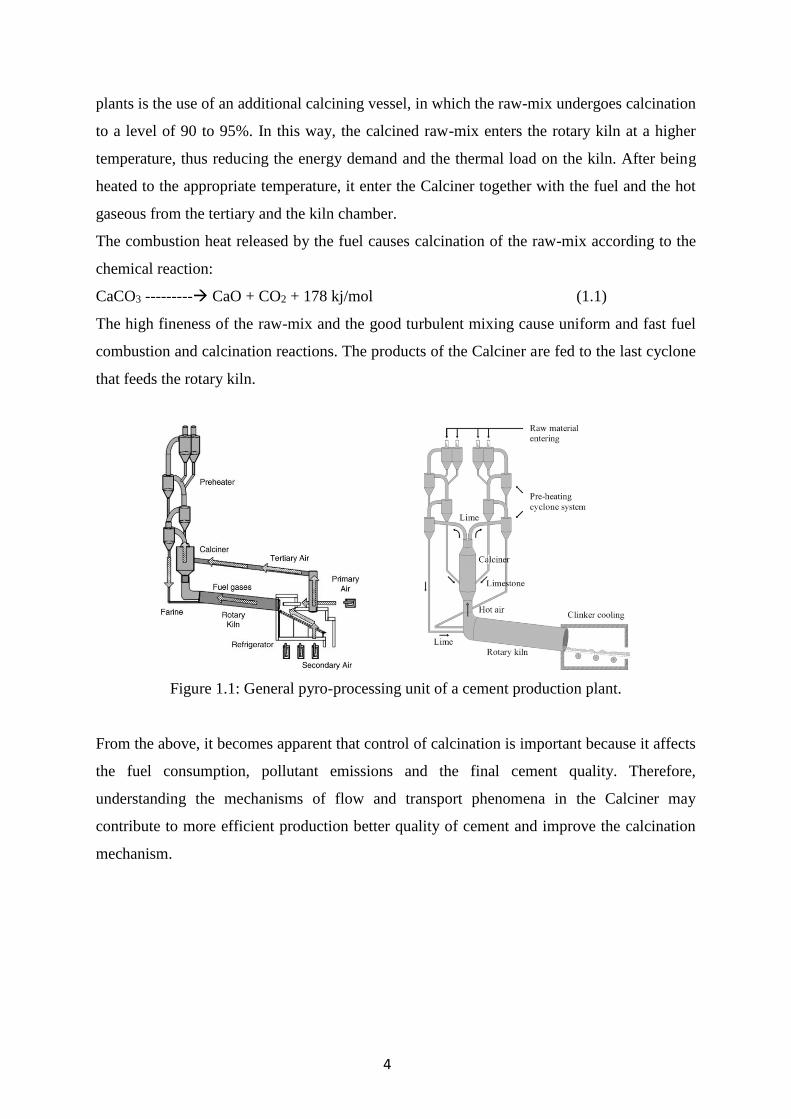
4

plants is the use of an additional calcining vessel, in which the raw-mix undergoes calcination

to a level of 90 to 95%. In this way, the calcined raw-mix enters the rotary kiln at a higher

temperature, thus reducing the energy demand and the thermal load on the kiln. After being

heated to the appropriate temperature, it enter the Calciner together with the fuel and the hot

gaseous from the tertiary and the kiln chamber.

The combustion heat released by the fuel causes calcination of the raw-mix according to the

chemical reaction:

CaCO3 --------- CaO + CO2 + 178 kj/mol (1.1)

The high fineness of the raw-mix and the good turbulent mixing cause uniform and fast fuel

combustion and calcination reactions. The products of the Calciner are fed to the last cyclone

that feeds the rotary kiln.

Figure 1.1: General pyro-processing unit of a cement production plant.

From the above, it becomes apparent that control of calcination is important because it affects

the fuel consumption, pollutant emissions and the final cement quality. Therefore,

understanding the mechanisms of flow and transport phenomena in the Calciner may

contribute to more efficient production better quality of cement and improve the calcination

mechanism.

5

Literature Review

Calciners have been studied with different geometries and operational conditions in 2D and

3D CFD simulations. Huanpeng et al [2] studied the influence of various physical parameters

on the dynamics of gas-solid two phase flow in a preCalciner using kinetic theory of granular

flow to present the transport properties of the solid phase in a 2D model. Hu et al. [3] used a

3D model for a dual combustor and preCalciner using a eulerian fram for the gas phase and

lagrangean one for the solid phase in order to predict the burn-out and the decomposition

ratio during the simultaneous injection of two types of coal and raw material into the device.

Iliuta et al. [4] investigated the influence of operating conditions on the level of calcination,

burn-out and NOx emissions of an in-line low NOx Calciner, and made a sensitivity analysis

of their model with respect to aerodynamic and combustion/calcination parameters.

Fidaros et al. [5] presented a numerical model and a parametric study of flow and transport

phenomena that take place in an industrial Calciner. This work show good prediction

capabilities for velocity, temperature and distribution of particles. Bluhm-Drenhaus et al. [6]

studied the heat and mass transfer related to the chemical conversion of limestone to lime in a

shaft kiln, CFD was used to model the transport of mass, momentum and energy in the

continuous phase, while the discrete element method (DEM) was used to model the

mechanical movement and the conversion reactions of the solid materials.

In addition to studies investigating the chemical and physical processes in cement production,

several studies investigated the potential of CO2 emission reduction. In general, CO2

emissions due to fossil fuel combustion in cement production systems can be reduced by

using more efficient technologies in the existing production process [7, 8]. Fidaros et al. [1]

showed a parametric analysis of solar Calciner, using CFD as a research tool, the study also

showed how CO2 emissions can be decreased because the required heat comes from solar

energy. Therefore, fossil fuels are not needed for the calcination processes. Kääntee et al.[9]

investigated the use of alternative fuels in the cement manufacturing process. This research

provided useful data for optimizing the manufacturing process by using different alternative

fuels with lower calorific value than those used in classical configurations. Sheinbaum and

ozawa [10] reported the energy use and the CO2 emissions in the Mexican cement industry,

concluding that the focus of the energy and CO2 emissions reduction should be on the use of

alternative fuels. Hrvoje Mikulcic and Fidaros [11] present a good application of CFD

modeling to support the reduction of CO2 emissions in cement industry for the same design

Calciner geometry reported in the literature [5].

6

HFO combustion in Calciner is non-premixed Liquid spray combustion where a nozzle is

used to atomize liquid fuel into fine droplets injected in hot gaseous environment in which it

is mixed with the oxidizer. For Calciner combustion applications, the simple swirl nozzle is

one of the most common pressure atomizing nozzles. Transport, dispersion, evaporation and

combustion of liquid fuel droplets and sprays are investigated in [12-14]. A few papers

conducted numerical and experimental studies of heavy fuel oil spray combustion in

cylindrical furnaces [15-17]. Barreiros et al. [15] investigated the effect of the burner

geometry and inlet velocities on the final products temperatures, velocities and concentration

inside the furnace. Byrnes et al. [16] carried out an experimental study on the same furnace to

predict the gas temperatures, CO2, CO, O2 and NO concentrations as well as particulate

emissions for five flames with different air excess ratios, swirl numbers, primary air excess

ratios and atomizer cup speeds. Wu et al. [17] investigated the contribution of the number,

location, type and firing mode of fuel oil atomizers on NO emissions reduction in an

industrial burner with heavy fuel oil combustion and highly preheated air. Furuhata et al. [18]

modeled heavy fuel oil spray flame stabilized by a baffle plate. They obtained good results

for flow field under isothermal conditions.

In computational fluid dynamics (CFD) studies, Physical model performance depends

critically on the accuracy of fuel property values, and the effectiveness of CFD modelling

depends on the precision of fuel thermophysical properties. Kyriakides et al. [19] developed a

model to investigate the effect of HFO thermo physical properties and compared the results

of their model against experimental data of Chryssakis et al. [20]. Recent computational

studies utilizing a simple representation of HFO composition have considered a two-

component approach, with the two components representing a residual (heavy) and a cutter

(light) part, both characterized by vapor pressures which are increasing with temperature, and

constant or temperature-dependent values for dynamic viscosity, density, latent heat, specific

heat capacity and surface tension [21], [22]. Kontoulis et al. [23] presented a good study with

a new detailed model for calculating IFO thermophysical properties that had been developed

in the model for different IFO qualities, the model builds on the assumption that marine HFO

is a heavy petroleum fraction of undefined composition. The effect of injection fuel

temperature on the penetration tip investigated by considering a five temperature values,

while the penetration tip is decreasing with fuel initial temperature, higher penetration with

the cold spray due to its minimal breakup, and illustrating a minimal breakup and evaporation

of the cold spray affected on the spray distribution including Sauter Mean Diameter (SMD)

values.

7

Present Numerical Model

In our present study for the Calciner furnace using the computational fluid dynamics CFD

ANSYS 14, to investigate all parameters and physics phenomenon affecting on the Calciner

performance, flow gaseous, heat and mass transfer, combustion reaction for heavy fuel oil,

and the solid particles transportation are presented with the influence of turbulence simulated

by a two-equation (k–ε) model.

First we will explain the system process and operating condotions as figures 2.1 and 2.2. All

data for setting the numerical models about the gaseous mass flow rate, velocities,

temperatures, air O2 & CO2 concentration, fuel consumption kg/s and solid particles CaCO3

kg/s are measured and calibrated by CEMEX project office.

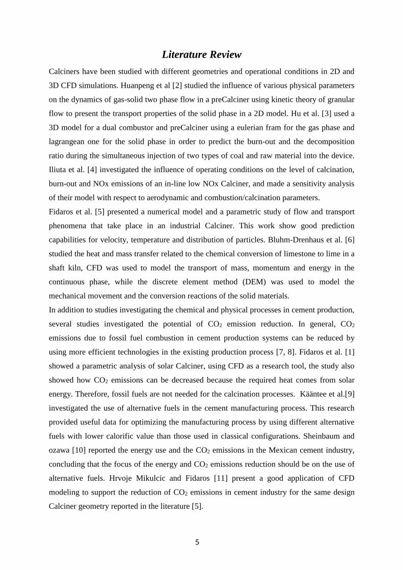
Figure 2.1: show the flow gases stream entering to the Calciner

Coming from the kiln and the tertiary Duct

- The kiln line divides to two string Calciner with Calciner riser duct about 80 m height.

- The flow exhaust gaseous from the kiln enter the kiln chamber and divided to string #1 &

string #2 and by pass flow which is useless gases carried by alkali.

- The gases enter the Calciner come from kiln & tertiary duct.

- The gases from tertiary come from kiln hood, that the clinker outlet from the kiln cooling by

atmospheric air to cooling clinker temperature from 1400 K to 150 k

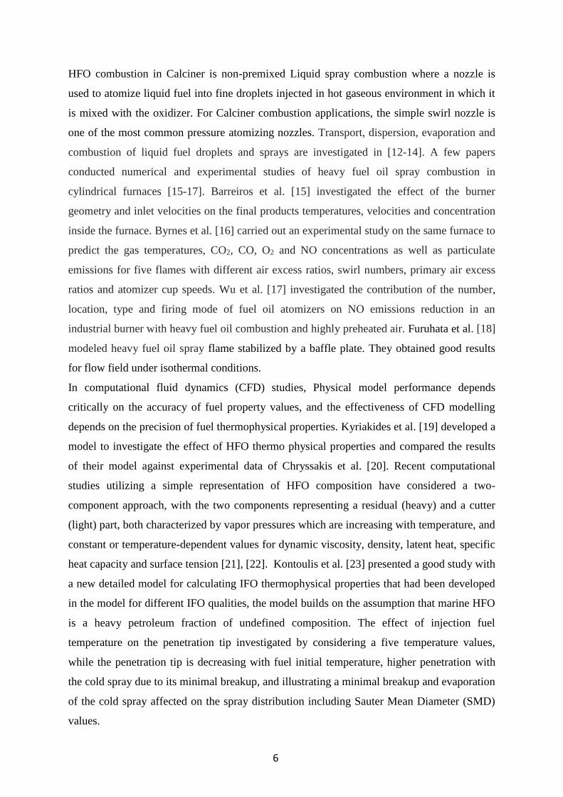
8

- The gaseous enter the Calciner from the kiln chamber (Temperature = 1300 K , O2 = 0.05 ,

CO2=0.12 , N2 = 0.83 )

- The gaseous enter the Calciner from the tertiary duct ( Temperature = 1123 K, O2= 0.23,

N2=0.73)

Figure 2.2: current study Calciner and kiln line section 5 m & kiln chamber explain the flow-

stream gaseous pass from the kiln enter Calciner.

From figure 2.2:

- Show the two string Calciner for one kiln line, and the Calciner geometry structure we going

to study.

- Show the powder tube feeding raw meal to the Calciner to start the calcination mechanism,

the raw meal is completely drying from the past three stage cyclone and enter the Calciner by

gravity approximately 1.5 m/s, mass flow rate 40 kg/s and temperature 800 k for one string.

- Show the powder tube feeding raw meal to the kiln coming from the final stage cyclone

connecting the Calciner after the calcination done.

- The gases flow stream coming from the kiln resulting the combustion from the main burner

fuel and the completely calcination for the raw meal entering the kiln.

- The bypass flow gases contain an alkali compounds, and it useless.

- Show the position for Burner #1 and Burner #2 for fuel atomization inside the Calciner.

9

Objectives:

To Investigate the effect of Calciner Design on the flow stream distribution and on

the mixing rate.

To Study The Granular Transport Phenomena of Solid Particles (CaCo3) inside the

Calciner “the Fluidization process“

To Investigate effect of HFO viscosity on the injection velocity and the resulting

combustion characteristics :-

Case #1 ( constant viscosity = 1.7E-5 kg/m.s)

Case #2 ( Viscosity Function of Temperature )

To Investigate the effect of swirl number variation of the resulting mixing

inside the Calciner and the resulting improvement on the combustion rate

Case studies:

In our numerical study for Calciner we will divide the case study to three sub cases:

Investigate the current design of the Calciner for flow gaseous behaviour enter from

the tertiary duct and the kiln chamber ports.

Investigate the granular transport phenomena inside the Calciner, the solid particles

CaCO3 concentration and distribution. Multi-phase case investigate the influence of the flow

gaseous enter calciner on the turbulence mixing between the gaseous and the particles.

Investigate the effect of swirl and fuel viscosity on the Combustion characteristics

of Heavy Fuel Oils inside the Calciner.

Numerical Model

The Calciner furnace, Fig.2.2, was investigated numerically in the present study. The height

of the Calciner is 25m and volume is 150m3. Exhaust gases from kiln chamber and

atmospheric air from tertiary duct enter the Calciner, Tube diameter 600 mm feed the solid

particles CaCO3 inside Calciner, with two burner nozzles 6 mm diameter, Figs. 2.6 and 2.7,

for the burner nozzle and fuel distributer are placed in the first 8 m height from the Calciner

bottom to spray the HFO inside Calciner. Burner #1 injects the HFO in the opposite (Z) axis

direction while burner #2 injects the HFO in the opposite (X) axis direction. The injection

characteristics are reported in Table 6. 3D model for the Calciner and the mesh was generated

using (ANSYS 14.0 Package), grid approximately 6,500,000 cells.

10

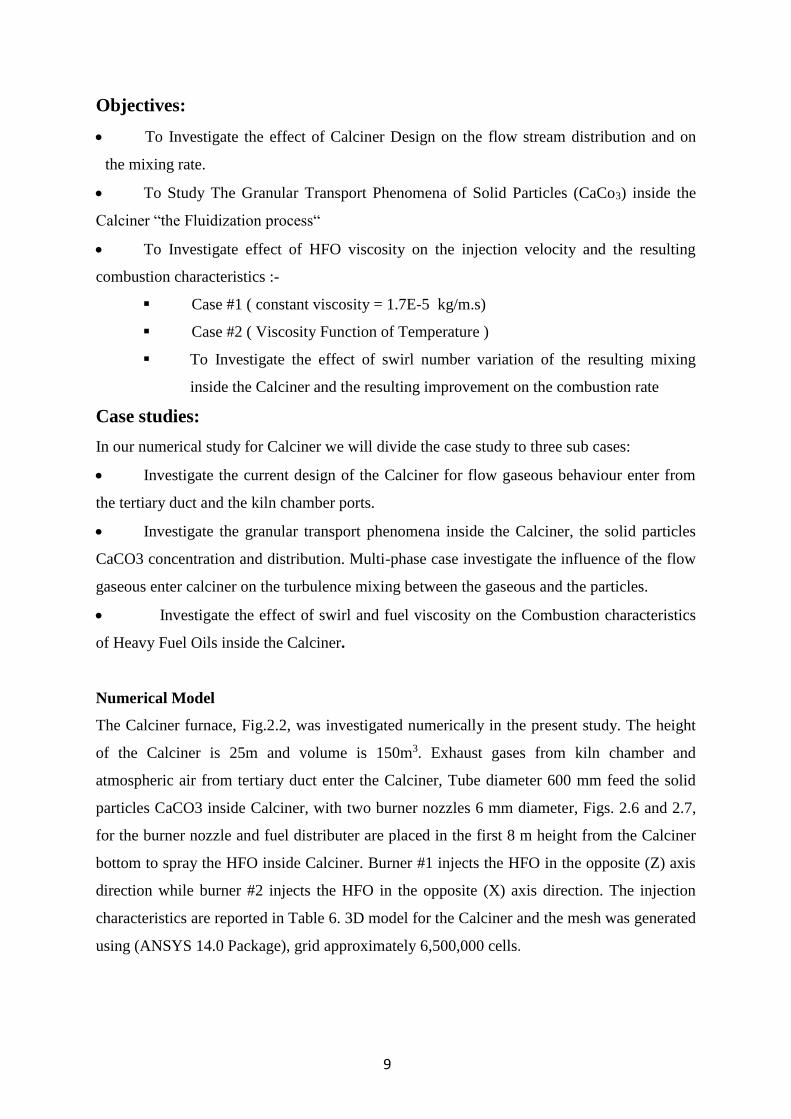
2.1 Calciner Geometry for flow stream gaseous investigation

Fig. 2.3 for the Calciner geometry with complete tertiary duct, to investigate the effect of the tertiary

duct design flow stream distribution and on the mixing rate. The boundary conditions for the

flow velocity enter from the tertiary duct for three cases study from table 1.

Figure 2.3: Calciner geometry with the complete tertiary duct Dimensions

Table 1: Boundary conditions of flow velocity simulation

Inlet Boundary Conditions kiln inlet Tertiary inlet powder tube

Axial velocity (m/s ) “ case # 4.1.1 “ 21 27 1.5

/s3Flow Rate m 40.7 69.5 0.282

Axial velocity (m/s ) “ case # 4.1.2 “ 21 32 1.5

/s3Flow Rate m 40.7 76.5 0.282

Axial velocity (m/s ) “ case # 4.1.3 “ 21 28 1.5

/s3Flow Rate m 40.7 66.5 0.282

11

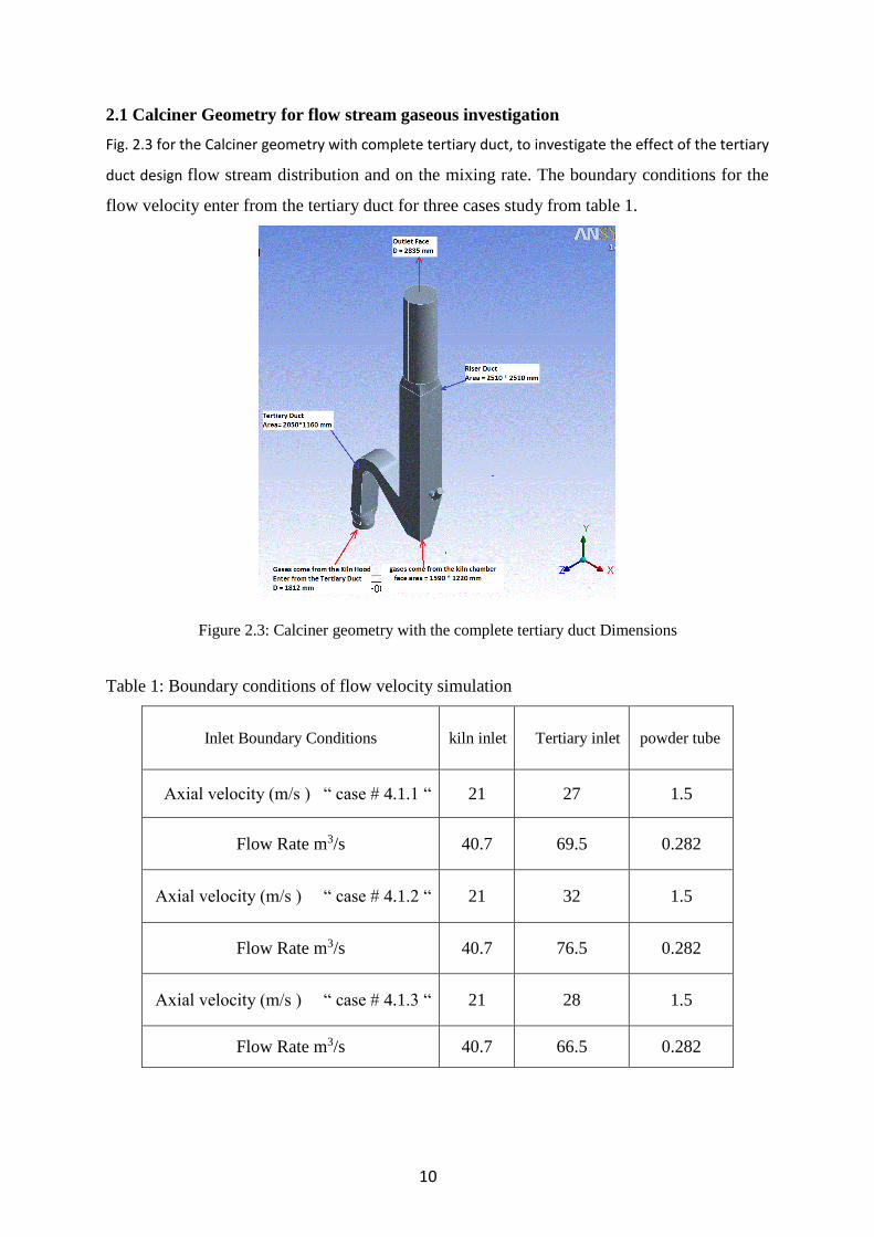
2.2 Calciner Geometry for Granular Transportation Model Investigation

Fig. 2.4 for the Calciner geometry after cut tertiary duct curve, To Study The Granular

Transport Phenomena of Solid Particles (CaCo3) inside the Calciner “The Fluidization

process“. The boundary conditions and case setting for gas phase and solid phase as tables 2,

3 and 4.

Figure 2.4: The Calciner geometry and mesh for the Multi-Phase model granular transportation solid

particles after cut the tertiary duct curve for computational time save

Table 2: Setting case

Setting B.C and Operating Condition CASE

Solver setting Transient, Unsteady Particle Track

Model Multi-Phase Eulerian- DDPM

Turbulent K-ε “ Mixture “

Tracking Scheme Implicit

Primary Phase Gas “ Air “

Secondary Phase Solid “ Granular “ Discrete Phase

Inlet B.C Gas Phase

Kiln Inlet “ Velocity m/s “ 21 m/s

Tertiary Inlet “ Velocity m/s “ 29 m/s

Powder Tube Inlet “ Velocity m/s” 1.5 m/s

Solid Particles Properties “ Density “ 31600 kg/m

12

The discrete phase injection type release by face “powder tube" with injector particles

diameter and mass flow rate as below table 4.2. and the secondary phase setting as table 4.3.

Table 3: Injection characteristics secondary phase “solid”

Discrete Phase

Injection Type

Diameter

Distribution

Particle

Diameter Flow Rate

Injection #1 Face Tube

Powder Rosin-Rammler 70-200 Micron 30kg/s

Total Flow Rate 30 kg/s

Table 4: The Secondary Phase “Solid Particles “

Define Discrete Phase Model & Secondary Phase

Setting

Phase Property

Drag Law Wen-Yu

Granular Viscosity “ kg/m-s” Gidaspow

Granular Bulk Viscosity “ kg/m-s” Lun-et-al

Frictional Viscosity “ kg/m-s “ -----------

Granular Temperature “ m2/s2” algebric

Solid Pressure Pascal Lun-et-al

Packing Limit 0.8

13

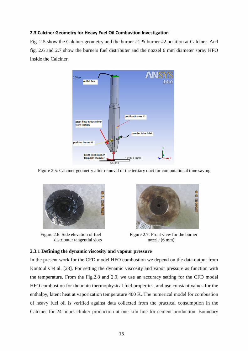
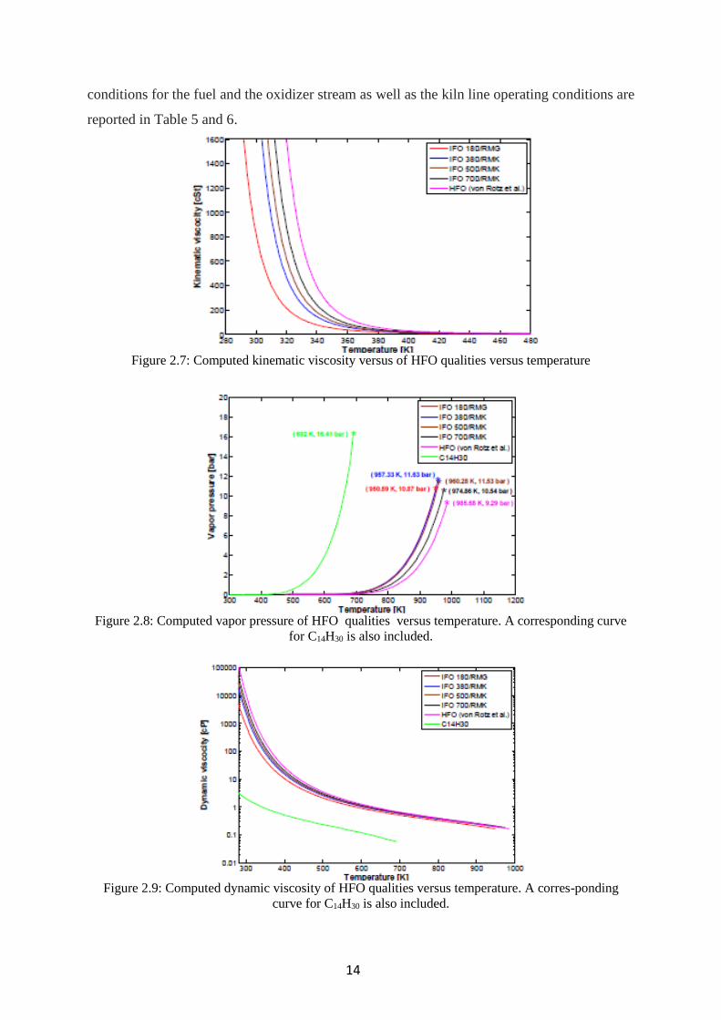
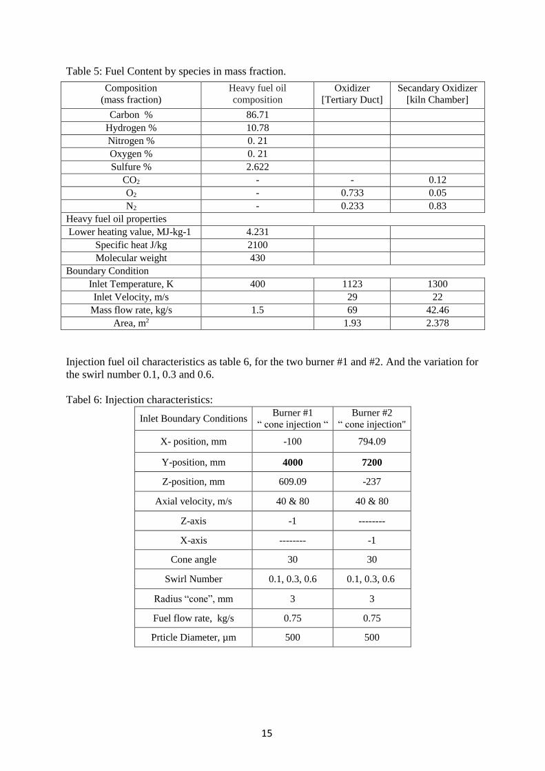
2.3 Calciner Geometry for Heavy Fuel Oil Combustion Investigation

Fig. 2.5 show the Calciner geometry and the burner #1 & burner #2 position at Calciner. And

fig. 2.6 and 2.7 show the burners fuel distributer and the nozzel 6 mm diameter spray HFO

inside the Calciner.

Figure 2.5: Calciner geometry after removal of the tertiary duct for computational time saving

Figure 2.6: Side elevation of fuel Figure 2.7: Front view for the burner

distributer tangential slots nozzle (6 mm)

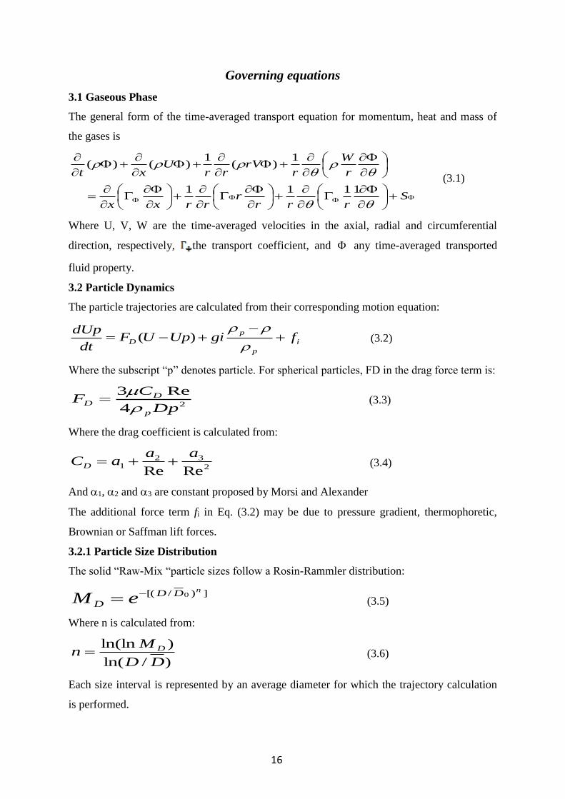
2.3.1 Defining the dynamic viscosity and vapour pressure

In the present work for the CFD model HFO combustion we depend on the data output from

Kontoulis et al. [23]. For setting the dynamic viscosity and vapor pressure as function with

the temperature. From the Fig.2.8 and 2.9, we use an accuracy setting for the CFD model

HFO combustion for the main thermophysical fuel properties, and use constant values for the

enthalpy, latent heat at vaporization temperature 400 K. The numerical model for combustion

of heavy fuel oil is verified against data collected from the practical consumption in the

Calciner for 24 hours clinker production at one kiln line for cement production. Boundary

14

conditions for the fuel and the oxidizer stream as well as the kiln line operating conditions are

reported in Table 5 and 6.

Figure 2.7: Computed kinematic viscosity versus of HFO qualities versus temperature

Figure 2.8: Computed vapor pressure of HFO qualities versus temperature. A corresponding curve

for C14H30 is also included.

Figure 2.9: Computed dynamic viscosity of HFO qualities versus temperature. A corres-ponding

curve for C14H30 is also included.

15

Table 5: Fuel Content by species in mass fraction.

Injection fuel oil characteristics as table 6, for the two burner #1 and #2. And the variation for

the swirl number 0.1, 0.3 and 0.6.

Tabel 6: Injection characteristics:

Composition

(mass fraction)

Heavy fuel oil

composition

Oxidizer

[Tertiary Duct]

Secandary Oxidizer

[kiln Chamber]

Carbon % 86.71

Hydrogen % 10.78

Nitrogen % 0. 21

Oxygen % 0. 21

Sulfure % 2.622

2CO - - 0.12

2O - 0.733 0.05

2N - 0.233 0.83

Heavy fuel oil properties

Lower heating value, MJ-kg-1 4.231

Specific heat J/kg 2100

Molecular weight 430

Boundary Condition

Inlet Temperature, K 400 1123 1300

Inlet Velocity, m/s 29 22

Mass flow rate, kg/s 1.5 69 42.46 2Area, m 1.93 2.378

Inlet Boundary Conditions Burner #1

“ cone injection “

Burner #2

“ cone injection"

X- position, mm -100 794.09

Y-position, mm 4000 7200

Z-position, mm 609.09 -237

Axial velocity, m/s 40 & 80 40 & 80

Z-axis -1 --------

X-axis -------- -1

Cone angle 30 30

Swirl Number 0.1, 0.3, 0.6 0.1, 0.3, 0.6

Radius “cone”, mm 3 3

Fuel flow rate, kg/s 0.75 0.75

Prticle Diameter, µm 500 500

16

Governing equations

3.1 Gaseous Phase

The general form of the time-averaged transport equation for momentum, heat and mass of

the gases is

Srrr

rrrxx

r

W

rrV

rrU

xt

1111

1)(

1)()(

(3.1)

Where U, V, W are the time-averaged velocities in the axial, radial and circumferential

direction, respectively, the transport coefficient, and any time-averaged transported

fluid property.

3.2 Particle Dynamics

The particle trajectories are calculated from their corresponding motion equation:

i

p

p

D fgiUpUFdt

dUp

)( (3.2)

Where the subscript “p” denotes particle. For spherical particles, FD in the drag force term is:

24

Re3

Dp

CF

p

DD

(3.3)

Where the drag coefficient is calculated from:

2

321

ReRe

aaaCD (3.4)

And 1, 2 and 3 are constant proposed by Morsi and Alexander

The additional force term fi in Eq. (3.2) may be due to pressure gradient, thermophoretic,

Brownian or Saffman lift forces.

3.2.1 Particle Size Distribution

The solid “Raw-Mix “particle sizes follow a Rosin-Rammler distribution:

])/[( 0nDD

D eM (3.5)

Where n is calculated from:

)/ln(

)ln(ln

DD

Mn D (3.6)

Each size interval is represented by an average diameter for which the trajectory calculation

is performed.

17

3.3 The Multi-Phase Model “Dense Discrete Phase Gas Solid flow”

The Lagrangian discrete phase model follows the Euler- Lagrange approach. The fluid phase

is treated as a continuum by solving the Navier-Stokes equations, while the dispersed phase is

solved by tracking a large number of particles. The dispersed phase can exchange

momentum, mass, and energy with the fluid phase. ANSYS FLUENT predicts the trajectory

of a discrete phase particle by integrating the force balance on the particle, which is written in

a Lagrangian reference frame. This force balance equates the particle inertia with the forces

acting on the particle as equation 3.2

3.3.1 Mathematical model of gas flow

A. Conservation laws

(1) Continuity equations

(a) Fluid phase

0).()(

ggggg v

t

(3.7)

(b) Particulate phase

0).()(

sssss v

t

(3.8)

(2) Momentum equations

(a) Fluid phase

gsgggggggggggg vvgsgPvvvt

.)().()(

(3.9)

(b) Particulate phase

)(.).()( sgssssssssssss vvgsgPvvvt

(3.10)

(3) Equation of conservation of solids fluctuating energy

gsssssssssssss DkvIPvv

t ).(:)().()(

3

2

(3.11)

B. Constitutive equations

(a) Fluid phase stress

Ivvv gg

T

gggg ).(3

2])([ (3.12)

(b) Gas shear viscosity (SGS)

2/1

2

)(

):()1.0(1.

y

ggggg

(3.13)

18

(c) Solid phase stress:

]).(3

1])([[).( IvvvIvP s

T

sssssss (3.14)

(d) Dissipation fluctuating energy

ssss v

dge .

4)1(3 0

22

(3.15)

(e) Radial distribution function at contact

13/1

max,

0 1

s

sg

(3.16)

(f) Solid pressure

)]1(21[ 0 egP ssss (3.17)

(g) Shear viscosity of solids

2

0

0

0

2 )1(5

41

)1(96

10)1(

5

4

eg

ge

dedg s

s

ssss

(3.18)

(h) Bulk solids viscosity

)1(

3

40

2 edgsss (3.19)

(i) Rate Of Energy Dissipation Per Unit Volume

(3.20)

(j) Exchange of fluctuation energy between gas and particles

(3.21)

(k) Fluid-particulate interphase drag coefficients

(3.22)

(3.23)

(I) Ideal gas equation

19

3.4 Modeling fuel oil spray combustion

In non-premixed combustion, fuel and oxidizer enter the reaction zone in distinct streams.

The present modeling of mixture fraction [24,25] with the method of probability density

function (mixture fraction/PDF) requires the solution of transport equations for one or two

conservative scalar properties. The effect of turbulence is also considered. The method of

mixture fraction with PDF has been developed specifically for turbulent chemically reacting

flow simulations. The chemical reaction is determined by turbulent mixing, which controls

the limits of the kinetic rates. The method is economic, because it does not require the

solution of a large number of transport equations for each chemical species. Moreover, it

allows precise determination of auxiliary variables such as density, and it does not use

average values, in contrast to the method of finite reaction rate. The mixture fraction is as:

0

0

kkF

kk

zz

zzf

(3.24)

The value of ƒ is calculated from the solution of a time averaged transport equation

m

ii

i

i

i

i

Sx

f

xf

xf

t

)()( (3.25)

The source term Sm is present only when particle mass transport to the gaseous phase takes

place. Simultaneously with the solution of Eq. (2), a conservative equation for the variance of

mixture fraction, 2f describing the interaction between chemistry and turbulence, is solved:

2

2

222 )()(

fk

Cx

fC

x

f

xf

xf

t

d

i

ig

it

i

i

i

i

(3.26)

The turbulence flow of the gas phase in the furnace is governed by the equations for the

conservation of mass, momentum and energy, The renormalization group (RNG) k-ε model

include the swirling effects were applied. Radiative heat transfer in the furnace is solved

using P1 radiation model. P1 gives resonable accuracy with less effort and account for

radiation exchange between gas and particulates. Fuel droplets evaporate relatively quickly

and influence radiative heat transfer only in the near-burner region. The weighted sum-of-

gray-gases (WSGGM) model is used to determine the absorption coefficient of the gas phase.

20

3.4.1 Heavy fuel oil droplets

droplet size distributions were assumed uniform droplet size 500 µm, injected from the cone

atomizer with angle 30º and nozzel diameter 6 mm figur 5, The particle trajectories are

calculated from their corresponding motion equation:

i

p

p

D fgiUpUFdt

dUp

)( (3.27)

Where the subscript “p” denotes particle, ρp , up is the droplet density and velocity

respectively, For spherical particles, u and ρ is the gas phase velocity and density

respectively. The right hand side are the drag force per unit of droplet mass and force of

gravity on the droplet, respectively.

3.4.2 Particle Heat transfer

Convection / Diffusion controlled model

To predict the vaporization from a discrete phase droplet, when the temperature of the droplet

reaches the vaporization temperature Tvap, and continues until the droplet reaches the boiling

point Tbp, or until the droplet volatile fraction is completely consumed

0,0, )1( pvp

bppvap

mfm

TTT

(3.28)

The effect of the convection flow of the evaporating from the droplet surface to the bulk gas

phase (Stefan flow), and the vapor flux from the equation below becomes a source of species

I in the gas phase species transport equation.

)( ,, isici CCkN (3.29)

Where Ni is the molar flux of vapor into the gas phase (kmol/m2-s), Kc is convective mass

transfer coefficient (m/s), Ci,s and Ci,∞stand for the vapor concentration at the deroplet

surface (kmol/m3) and in the bulk gas (kmol/m3). The boiling point Tpb and the latent heat hfg

are defined as constant property inputs for the droplet particle materials. In the evaporation

process, as the particle change its temperature, the latent heat will vary according to:

bp

p

bp

p

T

T

pp

T

T

bpfggpfg dTchdTch ... (3.30)

Include the droplet temperature effects on the latent heat by selecting the “temperature

dependent latent heat “option in the discrete phase model. The droplet temperature is updated

according to a heat balance that relates the sensible heat change in the droplet to the

convective and latent heat transfer between the droplet and the continuous phase:

21

)()(44

pRppfg

p

pp

p

pp TAhdt

dmTThA

dt

dTcm (3.31)

Where CP is the droplet heat capacity (j/kg-k), Tp is the droplet temperature (k), h is the

convective heat transfer coefficient (W/m2-k), T∞ the temperature of continuous phase, dmp/dt

is rate of evaporation (kg/s), hfg is latent heat ( j/kg), εp is particle emissivity (dimensionless),

σ is stefan-boltzmann constant (5.67×10-8 W/m2-k4), θR is radiation temperature. Radiation

heat transfer to the particle is included by enable the P-1, using the “particle radiation

interaction“ When the vaporization rate is computed by the convection/diffusion controlled

model, the convection heat transfer coefficient “h” is calculated with a modified Nu number

as follows

)PrRe6.02()1ln( 3/12/1

d

p

B

B

k

hdNu

(3.32)

Where dp is the particle diameter, K∞ is the thermal conductivity of the contiuous phase

(w/m-k), Pr is prandtl number of the continuous phase (CPu/K∞), BT is the spalding heat

transfer and is equal to the spalding mass transfer number Bm. To predict the convective

boiling of a discrete phase droplet when the temperature of the droplet has reached the

boiling temperature Tbp, and while the mass of the droplet exceed the nonvolatile fraction,

( 1-ƒv,0 ):

Tp ≥ Tbp and mp > ( 1-ƒv,0 ) mp,0 (3.33)

When the droplet temperature reaches the boiling point, a boiling rate equation is applied, the

mass transfer from the droplet to the gas phase is computed from the following equation

)()(44

pRppppfg

pTATThAh

dt

dm (3.34)

vaporization and the boiling point temperature are 400 K and 589 K, respectively.

22

Computational Results

4.1 Flow distribution inside the Calciner and the effect of entrance ducts

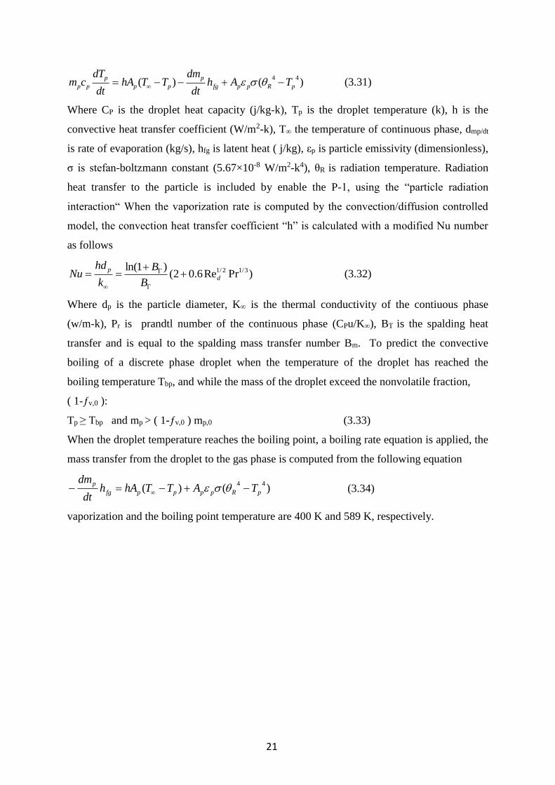
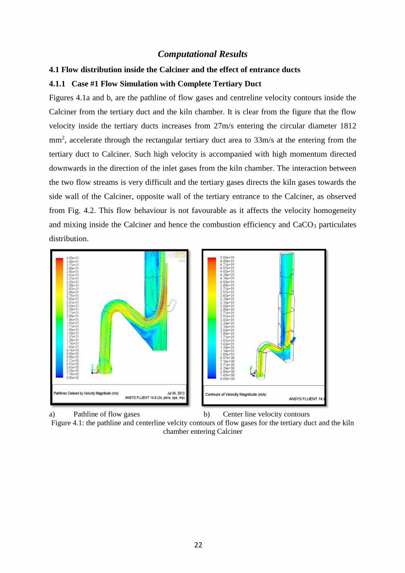
4.1.1 Case #1 Flow Simulation with Complete Tertiary Duct

Figures 4.1a and b, are the pathline of flow gases and centreline velocity contours inside the

Calciner from the tertiary duct and the kiln chamber. It is clear from the figure that the flow

velocity inside the tertiary ducts increases from 27m/s entering the circular diameter 1812

mm2, accelerate through the rectangular tertiary duct area to 33m/s at the entering from the

tertiary duct to Calciner. Such high velocity is accompanied with high momentum directed

downwards in the direction of the inlet gases from the kiln chamber. The interaction between

the two flow streams is very difficult and the tertiary gases directs the kiln gases towards the

side wall of the Calciner, opposite wall of the tertiary entrance to the Calciner, as observed

from Fig. 4.2. This flow behaviour is not favourable as it affects the velocity homogeneity

and mixing inside the Calciner and hence the combustion efficiency and CaCO3 particulates

distribution.

a) Pathline of flow gases b) Center line velocity contours

Figure 4.1: the pathline and centerline velcity contours of flow gases for the tertiary duct and the kiln

chamber entering Calciner

23

Figure 4.2: the pathline flow gases velocity from kiln inlet

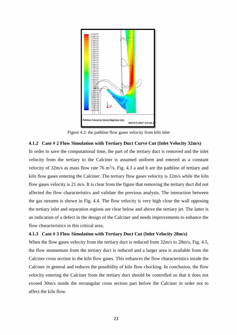
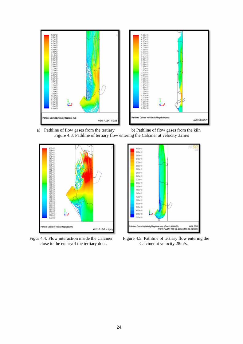
4.1.2 Case # 2 Flow Simulation with Tertiary Duct Curve Cut (Inlet Velocity 32m/s)

In order to save the computational time, the part of the tertiary duct is removed and the inlet

velocity from the tertiary to the Calciner is assumed uniform and entered as a constant

velocity of 32m/s as mass flow rate 76 m3/s. Fig. 4.3 a and b are the pathline of tertiary and

kiln flow gases entering the Calciner. The tertiary flow gases velocity is 32m/s while the kiln

flow gases velocity is 21 m/s. It is clear from the figure that removing the tertiary duct did not

affected the flow characteristics and validate the previous analysis. The interaction between

the gas streams is shown in Fig. 4.4. The flow velocity is very high close the wall opposing

the tertiary inlet and separation regions are clear below and above the tertiary jet. The latter is

an indication of a defect in the design of the Calciner and needs improvements to enhance the

flow characteristics in this critical area.

4.1.3 Case # 3 Flow Simulation with Tertiary Duct Cut (Inlet Velocity 28m/s)

When the flow gases velocity from the tertiary duct is reduced from 32m/s to 28m/s, Fig. 4.5,

the flow momentum from the tertiary duct is reduced and a larger area is available from the

Calciner cross section to the kiln flow gases. This enhances the flow characteristics inside the

Calciner in general and reduces the possibility of kiln flow chocking. In conclusion, the flow

velocity entering the Calciner from the tertiary duct should be controlled so that it does not

exceed 30m/s inside the rectangular cross section part before the Calciner in order not to

affect the kiln flow.

24

a) Pathline of flow gases from the tertiary b) Pathline of flow gases from the kiln

Figure 4.3: Pathline of tertiary flow entering the Calciner at velocity 32m/s

Figur 4.4: Flow interaction inside the Calciner Figure 4.5: Pathline of tertiary flow entering the

close to the entaryof the tertiary duct. Calciner at velocity 28m/s.

25

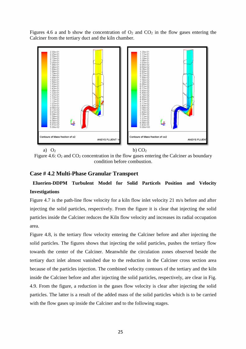
Figures 4.6 a and b show the concentration of O2 and CO2 in the flow gases entering the

Calciner from the tertiary duct and the kiln chamber.

a) O2 b) CO2

Figure 4.6: O2 and CO2 concentration in the flow gases entering the Calciner as boundary

condition before combustion.

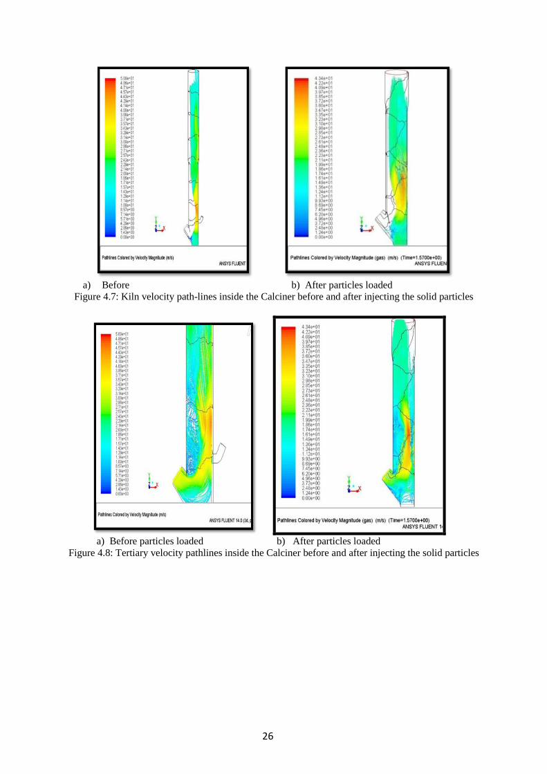
Case # 4.2 Multi-Phase Granular Transport

Eluerien-DDPM Turbulent Model for Solid Particels Position and Velocity

Investigations

Figure 4.7 is the path-line flow velocity for a kiln flow inlet velocity 21 m/s before and after

injecting the solid particles, respectively. From the figure it is clear that injecting the solid

particles inside the Calciner reduces the Kiln flow velocity and increases its radial occupation

area.

Figure 4.8, is the tertiary flow velocity entering the Calciner before and after injecting the

solid particles. The figures shows that injecting the solid particles, pushes the tertiary flow

towards the center of the Calciner. Meanwhile the circulation zones observed beside the

tertiary duct inlet almost vanished due to the reduction in the Calciner cross section area

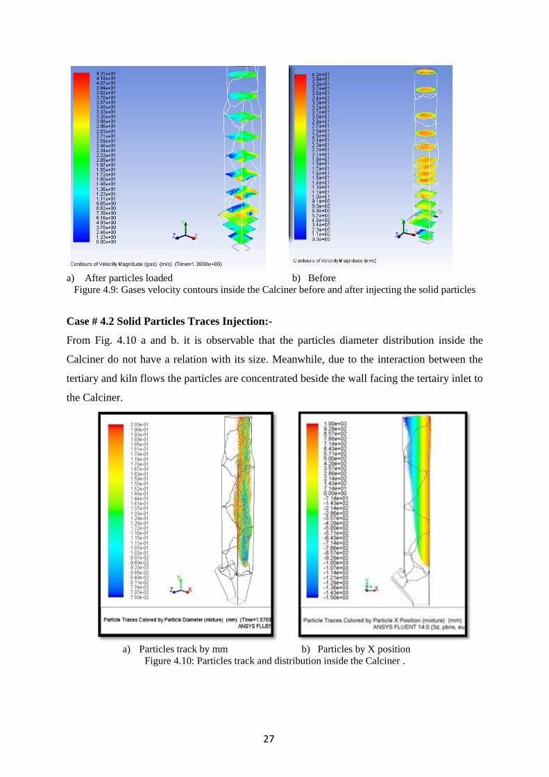
because of the particles injection. The combined velocity contours of the tertiary and the kiln

inside the Calciner before and after injecting the solid particles, respectively, are clear in Fig.

4.9. From the figure, a reduction in the gases flow velocity is clear after injecting the solid

particles. The latter is a result of the added mass of the solid particles which is to be carried

with the flow gases up inside the Calciner and to the following stages.

26

a) Before b) After particles loaded

Figure 4.7: Kiln velocity path-lines inside the Calciner before and after injecting the solid particles

a) Before particles loaded b) After particles loaded

Figure 4.8: Tertiary velocity pathlines inside the Calciner before and after injecting the solid particles

27

a) After particles loaded b) Before

Figure 4.9: Gases velocity contours inside the Calciner before and after injecting the solid particles

Case # 4.2 Solid Particles Traces Injection:-

From Fig. 4.10 a and b. it is observable that the particles diameter distribution inside the

Calciner do not have a relation with its size. Meanwhile, due to the interaction between the

tertiary and kiln flows the particles are concentrated beside the wall facing the tertairy inlet to

the Calciner.

a) Particles track by mm b) Particles by X position

Figure 4.10: Particles track and distribution inside the Calciner .

28

4.3 HFO Combustion Numerical Investigation

HFO combustion in calciner is investigated in 3D model with two setting for dynamic

viscosity and injection velocity. Constant viscosity value 1.7×10-5 kg/m.s with injection

velocity 40 m/s and viscosity function as temperature start value 0.02 kg/m.s at the

vaporization temperature 400 K [23], with injection velocity 80 m/s and 40 m/s. Spray

combustion of HFO is modeled using cone angle 30º, particles diameter 500 µm, and the

swirl number is varied as 0.1, 0.3, 0.6.

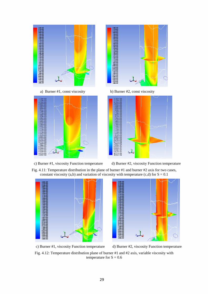
4.3.1 The influence of viscosity grade on the HFO combustion characteristics.

Figure 4.11 compare the combustion characteristics for the two cases viscosity variation for

swirl number 0.1. Temperature distribution plane Y and Z at the center burner #1 (a, c), and

plane Y and X at the center burner #2 (b, d). It is obvious from the figure 6 (c), the delay time

of the combustion starting especially with spray fuel oil injected from burner #1 for the

viscosity function as temperature. This delay is a result of the injection of the fuel with high

viscosity at the vaporization temperature. The high viscosity value at the evaporation

temperature and its variation with temperature as Fig.2.9 [23], adds a delay time before the

start of the combustion process to change the phase of the fuel from liquid phase to vapor

phase. In the constant viscosity case figure 4.11 (a), the fuel is defined to be injected in the

vapor phase directly. Also, from the figure 4.11 (c, d) it is observable that only small portion

of the injected fuel is combusted while the rest is combusted in the area surrounding burner

#2. Also, it is observable that the maximum temperature inside the Calciner, 2200K, is higher

than the corresponding maximum temperature in the case of constant viscosity which was

2000K only. This is a result of the delay in the combustion of burner #1 and the concentration

of the combustion in the area surrounding burner #2. This in turn maximizes the heat released

in this region. Close to Burner #2, the temperature is higher than that around burner #1 and

the evaporation process takes place more rabidly.

4.2 Influence of the swirl number on combustion characteristics.

High swirl number (S) strenghtens the circulation zone and enhances mixing. By comparing

Fig.4.11 it is observiable that the circulation zone is narrow with S= 0.1 which leads to

elongated flame. Meanwhile, with S = 0.6, Fig.4.12, the circulation zone is wider than that

observed with S = 0.1 and the mixing is better. The latter leads to improved temperature

distribution inside the Calciner with S = 0.6 case. And disapperance of the flame shape when

compared with the cases of S= 0.1 and 0.3.

29

a) Burner #1, const viscosity b) Burner #2, const viscosity

c) Burner #1, viscosity Function temperature d) Burner #2, viscosity Function temperature

Fig. 4.11: Temperature distribution in the plane of burner #1 and burner #2 axis for two cases,

constant viscosity (a,b) and variation of viscosity with temperature (c,d) for S = 0.1

c) Burner #1, viscosity Function temperature d) Burner #2, viscosity Function temperature

Fig. 4.12: Temperature distribution plane of burner #1 and #2 axis, variable viscosity with

temperature for S = 0.6

30

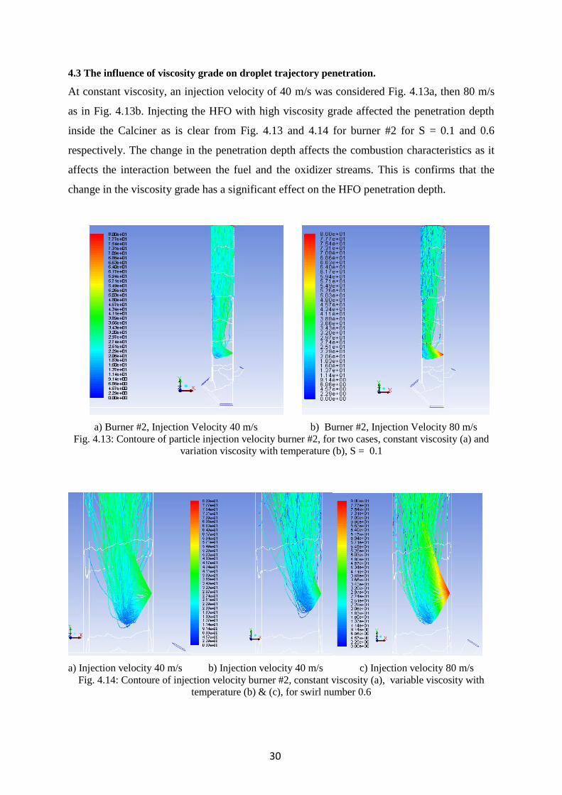
4.3 The influence of viscosity grade on droplet trajectory penetration.

At constant viscosity, an injection velocity of 40 m/s was considered Fig. 4.13a, then 80 m/s

as in Fig. 4.13b. Injecting the HFO with high viscosity grade affected the penetration depth

inside the Calciner as is clear from Fig. 4.13 and 4.14 for burner #2 for S = 0.1 and 0.6

respectively. The change in the penetration depth affects the combustion characteristics as it

affects the interaction between the fuel and the oxidizer streams. This is confirms that the

change in the viscosity grade has a significant effect on the HFO penetration depth.

a) Burner #2, Injection Velocity 40 m/s b) Burner #2, Injection Velocity 80 m/s Fig. 4.13: Contoure of particle injection velocity burner #2, for two cases, constant viscosity (a) and

variation viscosity with temperature (b), S = 0.1

a) Injection velocity 40 m/s b) Injection velocity 40 m/s c) Injection velocity 80 m/s

Fig. 4.14: Contoure of injection velocity burner #2, constant viscosity (a), variable viscosity with

temperature (b) & (c), for swirl number 0.6

31

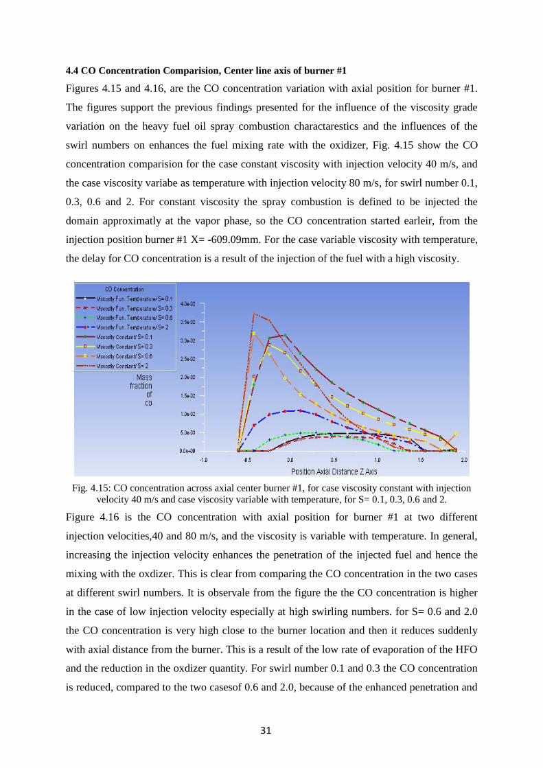
4.4 CO Concentration Comparision, Center line axis of burner #1

Figures 4.15 and 4.16, are the CO concentration variation with axial position for burner #1.

The figures support the previous findings presented for the influence of the viscosity grade

variation on the heavy fuel oil spray combustion charactarestics and the influences of the

swirl numbers on enhances the fuel mixing rate with the oxidizer, Fig. 4.15 show the CO

concentration comparision for the case constant viscosity with injection velocity 40 m/s, and

the case viscosity variabe as temperature with injection velocity 80 m/s, for swirl number 0.1,

0.3, 0.6 and 2. For constant viscosity the spray combustion is defined to be injected the

domain approximatly at the vapor phase, so the CO concentration started earleir, from the

injection position burner #1 X= -609.09mm. For the case variable viscosity with temperature,

the delay for CO concentration is a result of the injection of the fuel with a high viscosity.

Fig. 4.15: CO concentration across axial center burner #1, for case viscosity constant with injection

velocity 40 m/s and case viscosity variable with temperature, for S= 0.1, 0.3, 0.6 and 2.

Figure 4.16 is the CO concentration with axial position for burner #1 at two different

injection velocities,40 and 80 m/s, and the viscosity is variable with temperature. In general,

increasing the injection velocity enhances the penetration of the injected fuel and hence the

mixing with the oxdizer. This is clear from comparing the CO concentration in the two cases

at different swirl numbers. It is observale from the figure the the CO concentration is higher

in the case of low injection velocity especially at high swirling numbers. for S= 0.6 and 2.0

the CO concentration is very high close to the burner location and then it reduces suddenly

with axial distance from the burner. This is a result of the low rate of evaporation of the HFO

and the reduction in the oxdizer quantity. For swirl number 0.1 and 0.3 the CO concentration

is reduced, compared to the two casesof 0.6 and 2.0, because of the enhanced penetration and

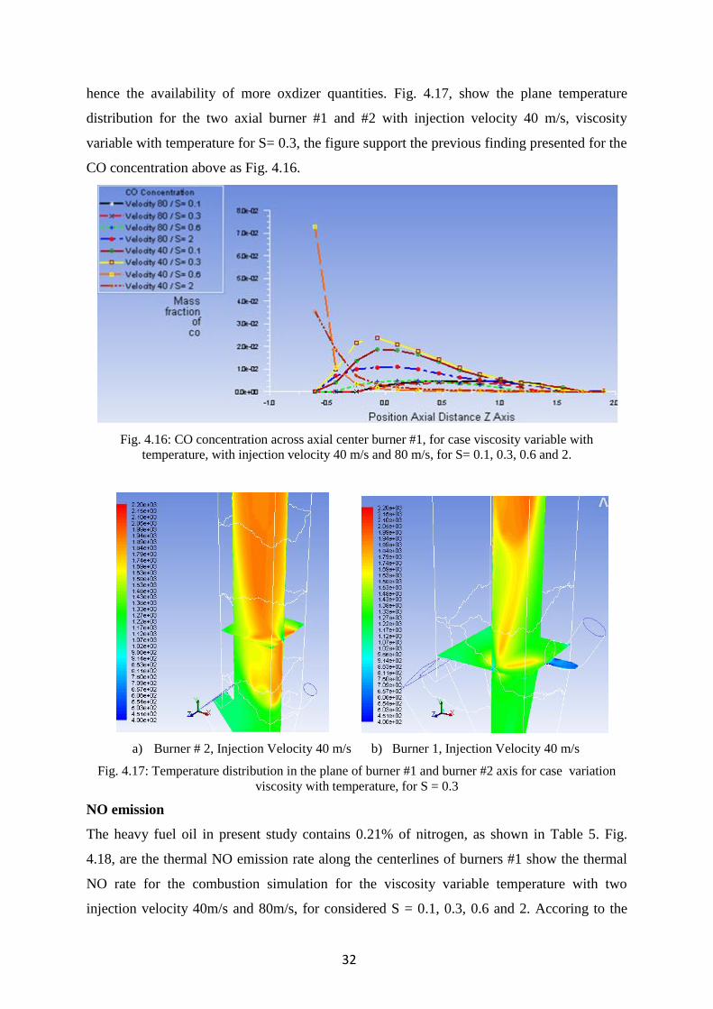
32

hence the availability of more oxdizer quantities. Fig. 4.17, show the plane temperature

distribution for the two axial burner #1 and #2 with injection velocity 40 m/s, viscosity

variable with temperature for S= 0.3, the figure support the previous finding presented for the

CO concentration above as Fig. 4.16.

Fig. 4.16: CO concentration across axial center burner #1, for case viscosity variable with

temperature, with injection velocity 40 m/s and 80 m/s, for S= 0.1, 0.3, 0.6 and 2.

a) Burner # 2, Injection Velocity 40 m/s b) Burner 1, Injection Velocity 40 m/s

Fig. 4.17: Temperature distribution in the plane of burner #1 and burner #2 axis for case variation

viscosity with temperature, for S = 0.3

NO emission

The heavy fuel oil in present study contains 0.21% of nitrogen, as shown in Table 5. Fig.

4.18, are the thermal NO emission rate along the centerlines of burners #1 show the thermal

NO rate for the combustion simulation for the viscosity variable temperature with two

injection velocity 40m/s and 80m/s, for considered S = 0.1, 0.3, 0.6 and 2. Accoring to the

33

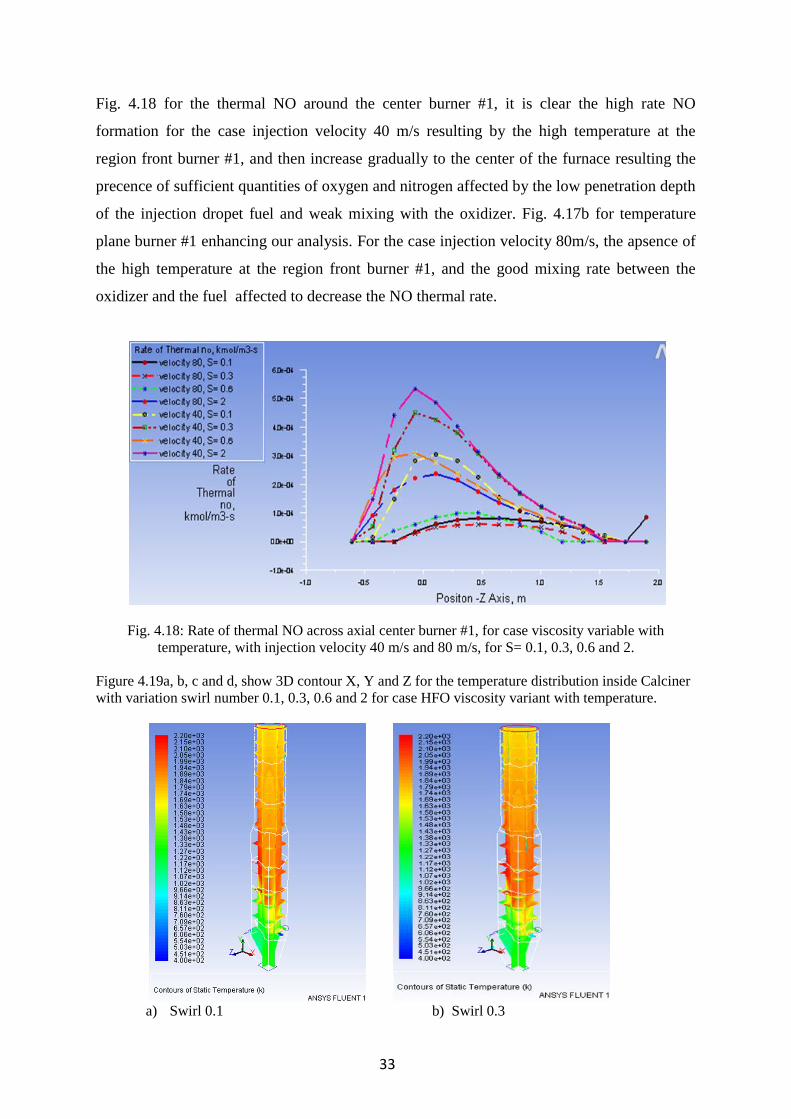
Fig. 4.18 for the thermal NO around the center burner #1, it is clear the high rate NO

formation for the case injection velocity 40 m/s resulting by the high temperature at the

region front burner #1, and then increase gradually to the center of the furnace resulting the

precence of sufficient quantities of oxygen and nitrogen affected by the low penetration depth

of the injection dropet fuel and weak mixing with the oxidizer. Fig. 4.17b for temperature

plane burner #1 enhancing our analysis. For the case injection velocity 80m/s, the apsence of

the high temperature at the region front burner #1, and the good mixing rate between the

oxidizer and the fuel affected to decrease the NO thermal rate.

Fig. 4.18: Rate of thermal NO across axial center burner #1, for case viscosity variable with

temperature, with injection velocity 40 m/s and 80 m/s, for S= 0.1, 0.3, 0.6 and 2.

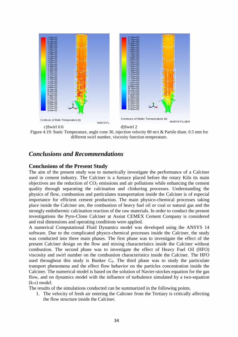
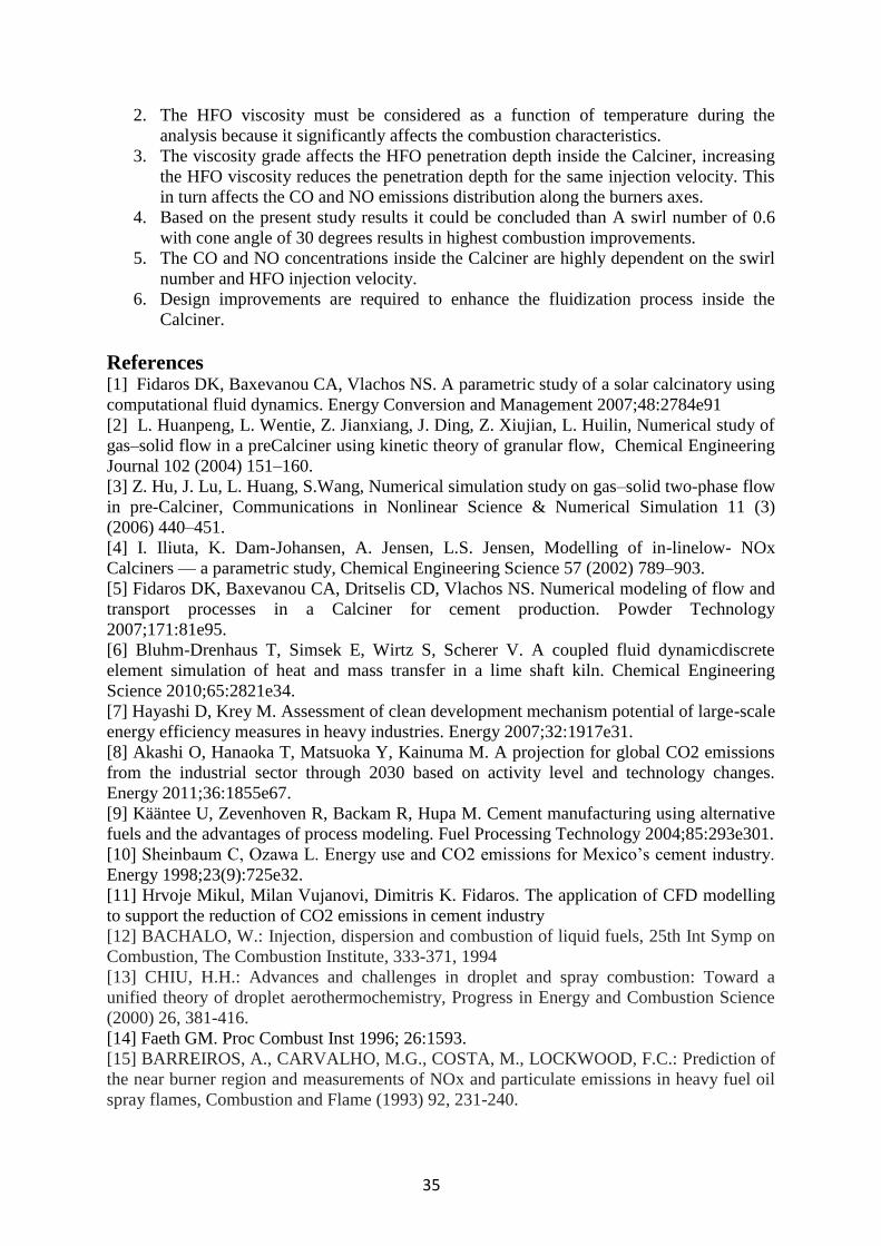
Figure 4.19a, b, c and d, show 3D contour X, Y and Z for the temperature distribution inside Calciner

with variation swirl number 0.1, 0.3, 0.6 and 2 for case HFO viscosity variant with temperature.

a) Swirl 0.1 b) Swirl 0.3

34

c)Swirl 0.6 d)Swirl 2

Figure 4.19: Static Temperature, angle cone 30, injection velocity 80 m/s & Partile diam. 0.5 mm for

different swirl number, viscosity function temperature.

Conclusions and Recommendations

Conclusions of the Present Study The aim of the present study was to numerically investigate the performance of a Calciner

used in cement industry. The Calciner is a furnace placed before the rotary Kiln its main

objectives are the reduction of CO2 emissions and air pollutions while enhancing the cement

quality through separating the calcination and clinkering processes. Understanding the

physics of flow, combustion and particulates transportation inside the Calciner is of especial

importance for efficient cement production. The main physico-chemical processes taking

place inside the Calciner are, the combustion of heavy fuel oil or coal or natural gas and the

strongly endothermic calcination reaction of the raw materials. In order to conduct the present

investigations the Pyro-Clone Calciner at Assiut CEMEX Cement Company is considered

and real dimensions and operating conditions were applied.

A numerical Computational Fluid Dynamics model was developed using the ANSYS 14

software. Due to the complicated physco-chemical processes inside the Calciner, the study

was conducted into three main phases. The first phase was to investigate the effect of the

present Calciner design on the flow and mixing characteristics inside the Calciner without

combustion. The second phase was to investigate the effect of Heavy Fuel Oil (HFO)

viscosity and swirl number on the combustion characteristics inside the Calciner. The HFO

used throughout this study is Bunker C6. The third phase was to study the particulate

transport phenomena and the effect flow behavior on the particles concentration inside the

Calciner. The numerical model is based on the solution of Navier-stockes equation for the gas

flow, and on dynamics model with the influence of turbulence simulated by a two-equation

(k-ε) model.

The results of the simulations conducted can be summarized in the following points.

1. The velocity of fresh air entering the Calicner from the Tertiary is critically affecting

the flow structure inside the Calciner.

35

2. The HFO viscosity must be considered as a function of temperature during the

analysis because it significantly affects the combustion characteristics.

3. The viscosity grade affects the HFO penetration depth inside the Calciner, increasing

the HFO viscosity reduces the penetration depth for the same injection velocity. This

in turn affects the CO and NO emissions distribution along the burners axes.

4. Based on the present study results it could be concluded than A swirl number of 0.6

with cone angle of 30 degrees results in highest combustion improvements.

5. The CO and NO concentrations inside the Calciner are highly dependent on the swirl

number and HFO injection velocity.

6. Design improvements are required to enhance the fluidization process inside the

Calciner.

References [1] Fidaros DK, Baxevanou CA, Vlachos NS. A parametric study of a solar calcinatory using

computational fluid dynamics. Energy Conversion and Management 2007;48:2784e91

[2] L. Huanpeng, L. Wentie, Z. Jianxiang, J. Ding, Z. Xiujian, L. Huilin, Numerical study of

gas–solid flow in a preCalciner using kinetic theory of granular flow, Chemical Engineering

Journal 102 (2004) 151–160.

[3] Z. Hu, J. Lu, L. Huang, S.Wang, Numerical simulation study on gas–solid two-phase flow

in pre-Calciner, Communications in Nonlinear Science & Numerical Simulation 11 (3)

(2006) 440–451.

[4] I. Iliuta, K. Dam-Johansen, A. Jensen, L.S. Jensen, Modelling of in-linelow- NOx

Calciners — a parametric study, Chemical Engineering Science 57 (2002) 789–903.

[5] Fidaros DK, Baxevanou CA, Dritselis CD, Vlachos NS. Numerical modeling of flow and

transport processes in a Calciner for cement production. Powder Technology

2007;171:81e95.

[6] Bluhm-Drenhaus T, Simsek E, Wirtz S, Scherer V. A coupled fluid dynamicdiscrete

element simulation of heat and mass transfer in a lime shaft kiln. Chemical Engineering

Science 2010;65:2821e34.

[7] Hayashi D, Krey M. Assessment of clean development mechanism potential of large-scale

energy efficiency measures in heavy industries. Energy 2007;32:1917e31.

[8] Akashi O, Hanaoka T, Matsuoka Y, Kainuma M. A projection for global CO2 emissions

from the industrial sector through 2030 based on activity level and technology changes.

Energy 2011;36:1855e67.

[9] Kääntee U, Zevenhoven R, Backam R, Hupa M. Cement manufacturing using alternative

fuels and the advantages of process modeling. Fuel Processing Technology 2004;85:293e301.

[10] Sheinbaum C, Ozawa L. Energy use and CO2 emissions for Mexico’s cement industry.

Energy 1998;23(9):725e32.

[11] Hrvoje Mikul, Milan Vujanovi, Dimitris K. Fidaros. The application of CFD modelling

to support the reduction of CO2 emissions in cement industry

[12] BACHALO, W.: Injection, dispersion and combustion of liquid fuels, 25th Int Symp on

Combustion, The Combustion Institute, 333-371, 1994

[13] CHIU, H.H.: Advances and challenges in droplet and spray combustion: Toward a

unified theory of droplet aerothermochemistry, Progress in Energy and Combustion Science

(2000) 26, 381-416.

[14] Faeth GM. Proc Combust Inst 1996; 26:1593.

[15] BARREIROS, A., CARVALHO, M.G., COSTA, M., LOCKWOOD, F.C.: Prediction of

the near burner region and measurements of NOx and particulate emissions in heavy fuel oil

spray flames, Combustion and Flame (1993) 92, 231-240.

36

[16] BYRNES, M.A., FOUMENYA, E.A., MAHMUDA, T., SHARIFAHA, A.S.A.K.,

ABBASB, T., COSTENB, P.G., LOCKWOOD, F.C.: Measurements and predictions of nitric

oxide and particulates emissions from heavy fuel oil spray flames, 26th Int Symp on

Combustion, The Combustion Institute, 2241-2250, 1996.

[17] WW, S.-R., CHANG, W.-C., CHIAO, J.: Low NOx heavy fuel oil combustion with high

temperature air, Fuel (2007) 86, 820-828.

[18] Furuhata T, Tanno S, Miura T, Ikeda Y, Nakajima T. Energy Convers Manage

1997;38:1111.

[19] Kyriakides N., Chryssakis C., Kaiktsis L., SAE 2009-01-1858 (2009).

[20] Chryssakis C., Pantazis K., Kaiktsis L., CIMAC Congress, Bergen, Norway, Jun 2010,

Paper No. 236.

[21] Goldsworthy L., International Journal of Engine Research, 7: pp. 181-199 (2006).

[22] Struckmeier D., Ph.D. Thesis, Kyushu University, Japan (2010).

[23] Panagiotis Kontoulis, Dimitris Kazangas, and Lambros Kaiktsis: A new model for

marine Heavy Fuel Oil thermophysical properties: validation in a constant volume spray

chamber; National Technical University of Athens, Greece. European Conference on Liquid

Atomization and Spray Systems , Chania, Greece, 1-4 September 2013

[24] Y.R. Shivatahnu, G.M. Faeth, Generalized state relationships for scalar properties in

non-premixed hydrocarbon/air flames, Combustion and Flame 82 (1990) 211–230.

[25] W.P. Jones, J.H. Whitelaw, Calculations methods for reacting turbulent flows: a review,

combustion and flame 48 ( 1982 ) I-26