Optimización lineal entera mixta
69
Optimización lineal entera mixta Andrés Ramos Universidad Pontificia Comillas http://www.iit.comillas.edu/aramos/ [email protected] ESCUELA TÉCNICA SUPERIOR DE INGENIERÍA D EPARTAMENTO DE O RGANIZACIÓN I NDUSTRIAL
Transcript of Optimización lineal entera mixta

Optimización lineal entera mixta
Andrés Ramos
Universidad Pontificia Comillashttp://www.iit.comillas.edu/aramos/
ESCUELA TÉCNICA SUPERIOR DE INGENIERÍA
DEPARTAMENTO DE ORGANIZACIÓN INDUSTRIAL
Optimización lineal entera mixta - 1
ESCUELA TÉCNICA SUPERIOR DE INGENIERÍA
DEPARTAMENTO DE ORGANIZACIÓN INDUSTRIAL
CONTENIDO
� INTRODUCCIÓN
�MÉTODOS DE SOLUCIÓN
�MÉTODO DE RAMIFICACIÓN Y ACOTAMIENTO
�DUALITY (master)
�PREPROCESSING (master)
�BRANCH AND CUT METHOD (master)
Optimización lineal entera mixta - 2
ESCUELA TÉCNICA SUPERIOR DE INGENIERÍA
DEPARTAMENTO DE ORGANIZACIÓN INDUSTRIAL
Mixed integer programming problem (MIP)
� Many times we need integer or binary variables. Some decisions can not be modeled with continuous variables� Investment decisions
� Connection of a machine
� Location of a warehouse
� Selection of a product
� Where do you apply radiotherapy to maximize the impact on cancerous cells and minimize the damage to other cells?
Optimización lineal entera mixta - 3
ESCUELA TÉCNICA SUPERIOR DE INGENIERÍA
DEPARTAMENTO DE ORGANIZACIÓN INDUSTRIAL
Introducción
� Un problema de programación lineal entero mixto (MIP) es un problema lineal (LP) con algunas variables enteras� Programación lineal entera mixta (MILP)
• x ∈ R+, y ∈ Z+
� Programación entera pura (PIP)• x ∈ Z+
� Programación binaria (0-1 MIP, 0-1 IP, BIP)• x ∈ { 0,1}: variables de asignación, lógicas
� Son más difíciles de resolver que los problemas LP
� Primer algoritmo de resolución se formuló por Ralph Gomory en 1958
Optimización lineal entera mixta - 4
ESCUELA TÉCNICA SUPERIOR DE INGENIERÍA
DEPARTAMENTO DE ORGANIZACIÓN INDUSTRIAL
CONTENIDO
�INTRODUCCIÓN
�MÉTODOS DE SOLUCIÓN
�MÉTODO DE RAMIFICACIÓN Y ACOTAMIENTO
�DUALITY (master)
�PREPROCESSING (master)
�BRANCH AND CUT METHOD (master)
Optimización lineal entera mixta - 5
ESCUELA TÉCNICA SUPERIOR DE INGENIERÍA
DEPARTAMENTO DE ORGANIZACIÓN INDUSTRIAL
Métodos de solución
� Relajación lineal y discretización
� Enumeración exhaustiva
� Ramificación y acotamiento (branch and bound)
� Método de los planos de corte
� Ramificación y corte (branch and cut)
Optimización lineal entera mixta - 6
ESCUELA TÉCNICA SUPERIOR DE INGENIERÍA
DEPARTAMENTO DE ORGANIZACIÓN INDUSTRIAL
Relajación lineal y discretización (i)
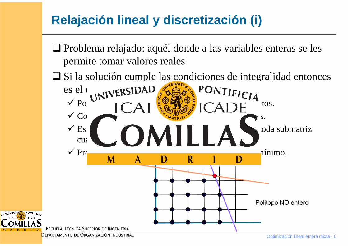
� Problema relajado: aquél donde a las variables enteras se les permite tomar valores reales
� Si la solución cumple las condiciones de integralidad entonces es el óptimo del problema entero� Politopo entero: todos los puntos extremos son enteros.
� Coincide con la envoltura convexa de las soluciones.
� Es entero si la matriz A es totalmente unimodular (toda submatriz cuadrada tiene determinante 1, 0 ó -1).
� Problema de transporte, asignación, flujo de coste mínimo.
Politopo NO entero
Optimización lineal entera mixta - 7
ESCUELA TÉCNICA SUPERIOR DE INGENIERÍA
DEPARTAMENTO DE ORGANIZACIÓN INDUSTRIAL
Relajación lineal y discretización (ii)
� La solución de un problema entero NO es necesariamente la solución del problema relajado discretizada heurísticamente (redondeada a los valores enteros más próximos).� Solución aproximada si las variables enteras toman valores elevados
� Posible pérdida de optimalidad
� Posible pérdida de factibilidad
� Los métodos metaheurísticos son una alternativa a los de programación matemática (algoritmos genéticos, búsqueda heurística, etc.)
Optimización lineal entera mixta - 8
ESCUELA TÉCNICA SUPERIOR DE INGENIERÍA
DEPARTAMENTO DE ORGANIZACIÓN INDUSTRIAL
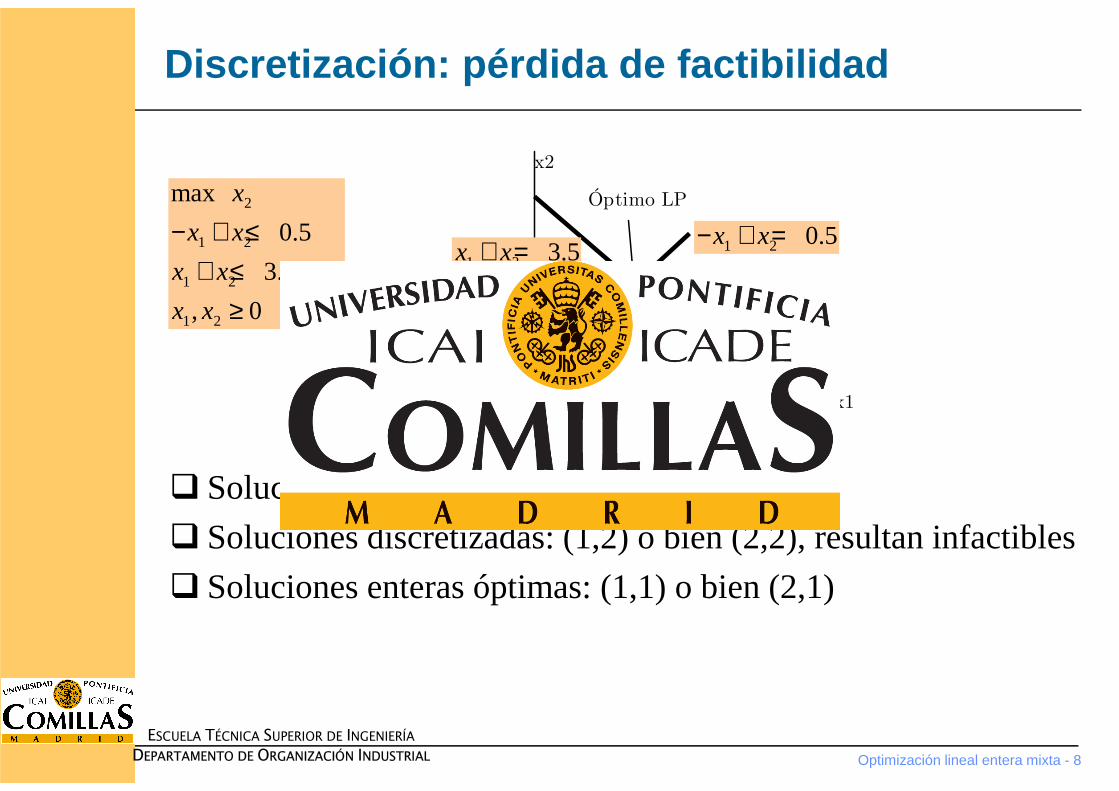
Discretización: pérdida de factibilidad
� Solución LP: (1.5,2)
� Soluciones discretizadas: (1,2) o bien (2,2), resultan infactibles
� Soluciones enteras óptimas: (1,1) o bien (2,1)
2
1 2
1 2
1 2
max
0.5
3.5
, 0 i
x
x x
x x
x x x
− + ≤+ ≤
≥ ∈Z
x2
Óptimo LP
Óptimo IP
Heurístico
x1
1 2 0.5x x− + =1 2 3.5x x+ =

Optimización lineal entera mixta - 9
ESCUELA TÉCNICA SUPERIOR DE INGENIERÍA
DEPARTAMENTO DE ORGANIZACIÓN INDUSTRIAL
Discretización: pérdida de optimalidad
� Solución LP: (2,9/5)
� Solución discretizada: (2,1)
� Solución entera óptima: (0,2)
1 2
1 2
1
1 2
max 5
10 20
2
, 0 i
x x
x x
x
x x x
++ ≤≤
≥ ∈ZÓptimo IP
Óptimo LP
Heurístico
1 2x =
1 210 20x x+ =
1x
2x
Optimización lineal entera mixta - 10
ESCUELA TÉCNICA SUPERIOR DE INGENIERÍA
DEPARTAMENTO DE ORGANIZACIÓN INDUSTRIAL
Enumeración exhaustiva
� No es viable, debido a que el número de soluciones crece exponencialmente
� En un problema BIP de n variables hay 2n posibles soluciones
Optimización lineal entera mixta - 11
ESCUELA TÉCNICA SUPERIOR DE INGENIERÍA
DEPARTAMENTO DE ORGANIZACIÓN INDUSTRIAL
Métodos de solución
� Pérdida de convexidad de la región factible. Los puntos de su interior no se pueden poner como combinación lineal convexa de sus puntos extremos.
� Pérdida de la potencia matemática asociada a variables continuas (derivadas, condiciones de optimalidad, sensibilidades, etc.).
� La solución de un problema MIP es más difícil que la de un problema LP. Requiere más tiempo de cálculo y más requisitos de memoria.
Optimización lineal entera mixta - 12
ESCUELA TÉCNICA SUPERIOR DE INGENIERÍA
DEPARTAMENTO DE ORGANIZACIÓN INDUSTRIAL
CONTENIDO
�INTRODUCCIÓN
�MÉTODOS DE SOLUCIÓN
�MÉTODO DE RAMIFICACIÓN Y ACOTAMIENTO
�DUALITY (master)
�PREPROCESSING (master)
�BRANCH AND CUT METHOD (master)
Optimización lineal entera mixta - 13
ESCUELA TÉCNICA SUPERIOR DE INGENIERÍA
DEPARTAMENTO DE ORGANIZACIÓN INDUSTRIAL
Método de ramificación y acotamiento (branch and bound)
� Enumeración implícita de las soluciones enteras factibles.
� Utiliza el principio de divide y vencerás.� Divide (ramifica) el conjunto de soluciones enteras en subconjuntos
disjuntos cada vez menores.
� Determina (acota) el valor de la mejor solución del subconjunto.• En problema de maximización una cota inferior de la solución óptima de
un problema MIP es la mayor solución entera factible encontrada hasta el momento.
• En problema de maximización una cota superior de la solución óptima de un problema MIP es la solución óptima del problema lineal relajado RMIP o LP.
� Poda (elimina) la rama del árbol si la cota indica que no puede contener la solución óptima.
Optimización lineal entera mixta - 14
ESCUELA TÉCNICA SUPERIOR DE INGENIERÍA
DEPARTAMENTO DE ORGANIZACIÓN INDUSTRIAL
Procedimiento (i)
1. Inicialización� Inicializa la cota superior de la f.o. , en problemas de
maximización
� Resolver una relajación del problema(habitualmente la lineal, aunque pueden usarse otras). Éste es el nodo raíz.
� Aplicar acotamiento o poda y criterio de optimalidad al problema completo.
� Si no se puede etiquetar el problema como no podado, comienza una iteración completa.
2. Iteración� Ramificación
�Seleccionar uno de los nodosentre los no explorados (nodos restantes). Ver criterios de selección
�Seleccionar una variable enteraque tenga valor continuo en la solución óptima del nodo relajado. Ver criterios de selección
*z = −∞
Optimización lineal entera mixta - 15
ESCUELA TÉCNICA SUPERIOR DE INGENIERÍA
DEPARTAMENTO DE ORGANIZACIÓN INDUSTRIAL
Procedimiento (ii)
�Sea el valor óptimo en el problema relajado
�Se ramifica en dos ramasincorporando las restricciones
siendo la parte entera de
�Para variables binarias es fijar el valor de la variable a 0 ó a 1. No se puede repetir la ramificación.
�Cada vez que se ramifica se añade una restricción (análisis de sensibilidadmediante el método simplex dual). El problema primal resulta infactible. El problema dual resulta factible pero no óptimo.
�Cada rama elimina la solución óptima del problema anterior.
� Acotamiento�Para cada nodo se obtiene su f.o. .
*jx
*
*
1
j j
j j
x x
x x
≤
≥ + *jx
*jx
z
Optimización lineal entera mixta - 16
ESCUELA TÉCNICA SUPERIOR DE INGENIERÍA
DEPARTAMENTO DE ORGANIZACIÓN INDUSTRIAL
Procedimiento (ii)
� Poda� Se intentan eliminar nodos (ramas) del árbol. Aplicar los siguientes
criterios de podapara un problema de maximización:1. Solución (entera o no) peorque la solución entera actual , siendo el
valor de la función objetivo para la solución entera actual. Se poda la rama.
2. Solución entera mejorque la actual . nueva solución entera actual
Se aplica el criterio 1 a todos los nodos no podados con la nueva solución entera actual.
3. Infactible. Se poda la rama.
3. Criterio de optimalidad� Parar cuando no existan nodos sin analizar. La solución entera actual
es la óptima.
� Si no, realizar otra iteración.
*z z≤ *z
*z z> *z z=
Optimización lineal entera mixta - 17
ESCUELA TÉCNICA SUPERIOR DE INGENIERÍA
DEPARTAMENTO DE ORGANIZACIÓN INDUSTRIAL
Ejemplo
1 2 3 4
1 3
1 2 3
1 2
1 3 4
max 4 2 7
5 10
1
6 5 0
2 2 3
0 1, ,4
enteras 1, ,3j
j
z x x x x
x x
x x x
x x
x x x
x j
x j
= − + −+ ≤
+ − ≤− ≤
− + − ≤≥ =
=
…
…
Optimización lineal entera mixta - 18
ESCUELA TÉCNICA SUPERIOR DE INGENIERÍA
DEPARTAMENTO DE ORGANIZACIÓN INDUSTRIAL
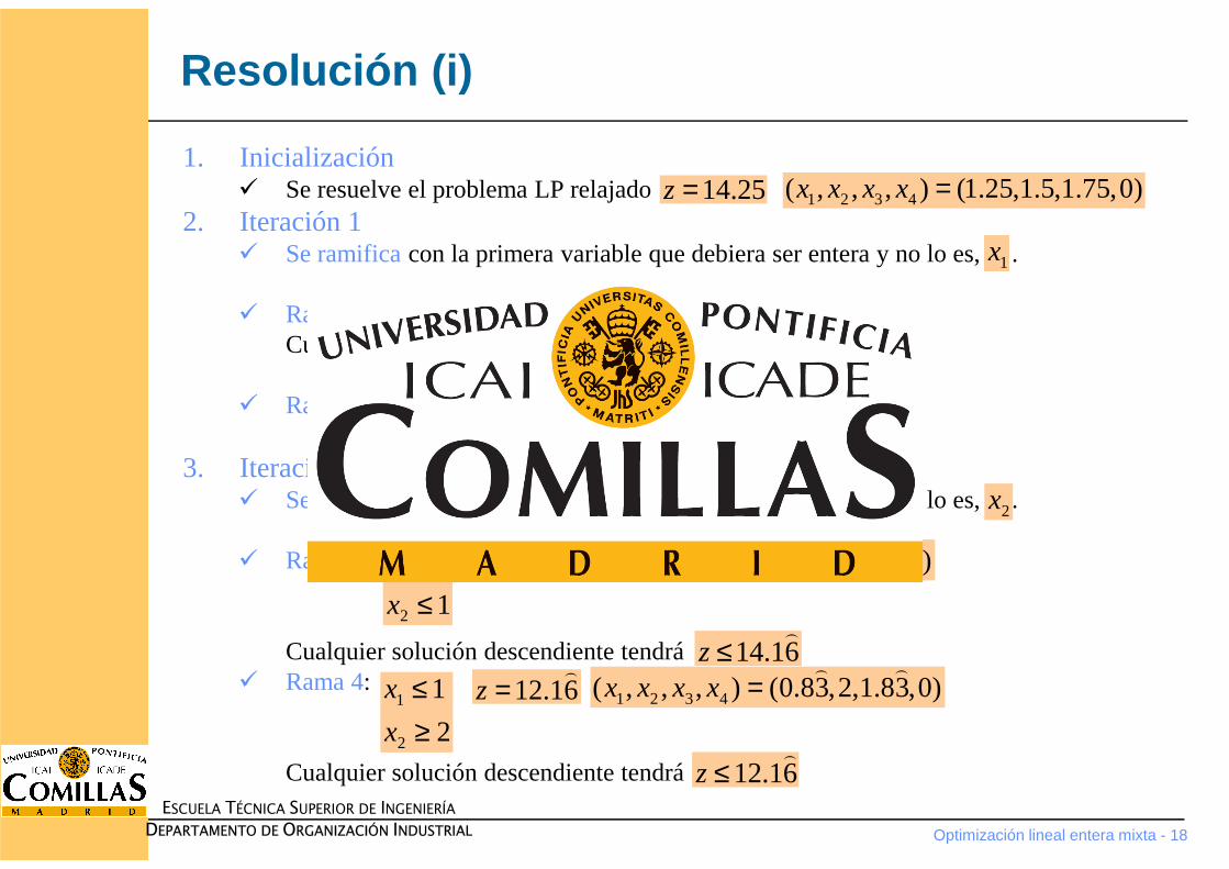
Resolución (i)
1. Inicialización� Se resuelve el problema LP relajado
2. Iteración 1� Se ramificacon la primera variable que debiera ser entera y no lo es, .
� Rama 1:Cualquier solución descendiente tendrá
� Rama 2: infactible. Se poda la rama
3. Iteración 2� Se ramificacon la primera variable que debiera ser entera y no lo es, .
� Rama 3:
Cualquier solución descendiente tendrá� Rama 4:
Cualquier solución descendiente tendrá
14.25z = 1 2 3 4( , , , ) (1.25,1.5,1.75,0)x x x x =
1x
1 2 3 4( , , , ) (1,1.2,1.8,0)x x x x =14.2z =1 1x ≤14.2z ≤
1 2x ≥
2x
1
2
1
1
x
x
≤≤
14.16z =⌢
1 2 3 4( , , , ) (0.83,1,1.83,0)x x x x =⌢ ⌢
14.16z≤⌢
1
2
1
2
x
x
≤≥
12.16z =⌢
1 2 3 4( , , , ) (0.83,2,1.83,0)x x x x =⌢ ⌢
12.16z≤⌢
Optimización lineal entera mixta - 19
ESCUELA TÉCNICA SUPERIOR DE INGENIERÍA
DEPARTAMENTO DE ORGANIZACIÓN INDUSTRIAL
Resolución (ii)
4. Iteración 3� Se selecciona la rama 3por tener la mayor función objetivo.
� Se ramificacon la variable .
� Rama 5:
Primera solución enteradel problema MIP
� Rama 6: infactible
� La rama 4se puede podar porque su función objetivo es menor (en maximización) que la solución entera actual.
5. Criterio de optimalidad� Solución óptima alcanzada por no existir ramas sin explorar.
1x
1
2
1
1
1
0
x
x
x
≤≤≤
13.5z = 1 2 3 4( , , , ) (0,0,2,0.5)x x x x =
* 13.5z =
1
2
1
1
1
1
x
x
x
≤≤≥
Optimización lineal entera mixta - 20
ESCUELA TÉCNICA SUPERIOR DE INGENIERÍA
DEPARTAMENTO DE ORGANIZACIÓN INDUSTRIAL
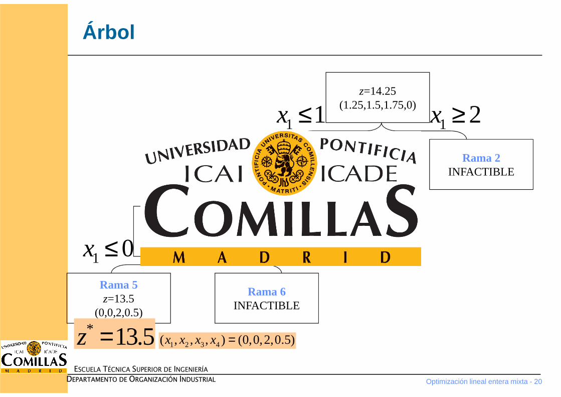
Árbol
z=14.25(1.25,1.5,1.75,0)
Rama 2INFACTIBLE
Rama 1z=14.2
(1,1.2,1.8,0)
Rama 4z=12.16
(0.83,2,1.83,0)
Rama 3z=14.16
(0.83,1,1.83,0)
Rama 5z=13.5
(0,0,2,0.5)
Rama 6INFACTIBLE
1 1x ≤ 1 2x ≥
2 1x ≤ 2 2x ≥
1 1x ≥1 0x ≤
* 13.5z = 1 2 3 4( , , , ) (0,0,2,0.5)x x x x =
Optimización lineal entera mixta - 21
ESCUELA TÉCNICA SUPERIOR DE INGENIERÍA
DEPARTAMENTO DE ORGANIZACIÓN INDUSTRIAL
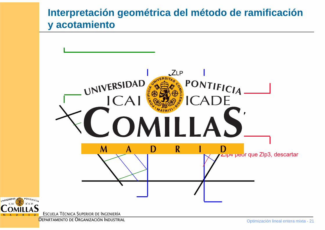
Interpretación geométrica del método de ramificación y acotamiento
ZLP
Zlp1
Zlp2
Zlp4 peor que Zlp3, descartar
Zlp3=entero
Optimización lineal entera mixta - 22
ESCUELA TÉCNICA SUPERIOR DE INGENIERÍA
DEPARTAMENTO DE ORGANIZACIÓN INDUSTRIAL
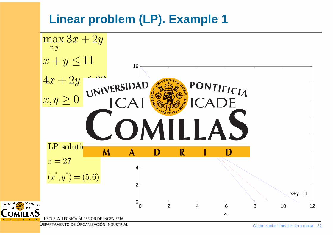
Linear problem (LP). Example 1
,max3 2
11
4 2 32
, 0
x y
x y
x y
x y
x y
+
+ ≤
+ ≤
≥
,max3 2
11
4 2 32
, 0
x y
x y
x y
x y
x y
+
+ ≤
+ ≤
≥
0 2 4 6 8 10 120
2
4
6
8
10
12
14
16
x
y
← 4x+2y=32
← x+y=11
← 3x+2y=27
← (5,6)
* *
LP solution
27
( , ) (5,6)
z
x y
=
=* *
LP solution
27
( , ) (5,6)
z
x y
=
=
Optimización lineal entera mixta - 23
ESCUELA TÉCNICA SUPERIOR DE INGENIERÍA
DEPARTAMENTO DE ORGANIZACIÓN INDUSTRIAL
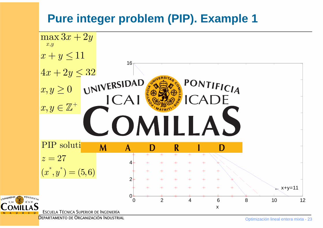
Pure integer problem (PIP). Example 1
,max3 2
11
4 2 32
, 0
,
x y
x y
x y
x y
x y
x y+
+
+ ≤
+ ≤
≥
∈ ℤ
,max3 2
11
4 2 32
, 0
,
x y
x y
x y
x y
x y
x y+
+
+ ≤
+ ≤
≥
∈ ℤ
0 2 4 6 8 10 120
2
4
6
8
10
12
14
16
x
y
← 4x+2y=32
← x+y=11
← 3x+2y=27
← (5,6)
* *
PIP solution
27
( , ) (5,6)
z
x y
=
=* *
PIP solution
27
( , ) (5,6)
z
x y
=
=
Optimización lineal entera mixta - 24
ESCUELA TÉCNICA SUPERIOR DE INGENIERÍA
DEPARTAMENTO DE ORGANIZACIÓN INDUSTRIAL
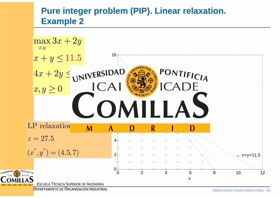
Pure integer problem (PIP). Linear relaxation.Example 2
0 2 4 6 8 10 120
2
4
6
8
10
12
14
16
x
y
← 4x+2y=32
← x+y=11.5
← 3x+2y=27.5
← (4.5,7)
* *
LP relaxation. Problem 0
27.5
( , ) (4.5,7)
z
x y
=
=* *
LP relaxation. Problem 0
27.5
( , ) (4.5,7)
z
x y
=
=
,
11.5
max 3 2
4 2 32
, 0
x y
x y
x y
x y
x y
+
+ ≤
+ ≤
≥
,
11.5
max 3 2
4 2 32
, 0
x y
x y
x y
x y
x y
+
+ ≤
+ ≤
≥
Optimización lineal entera mixta - 25
ESCUELA TÉCNICA SUPERIOR DE INGENIERÍA
DEPARTAMENTO DE ORGANIZACIÓN INDUSTRIAL
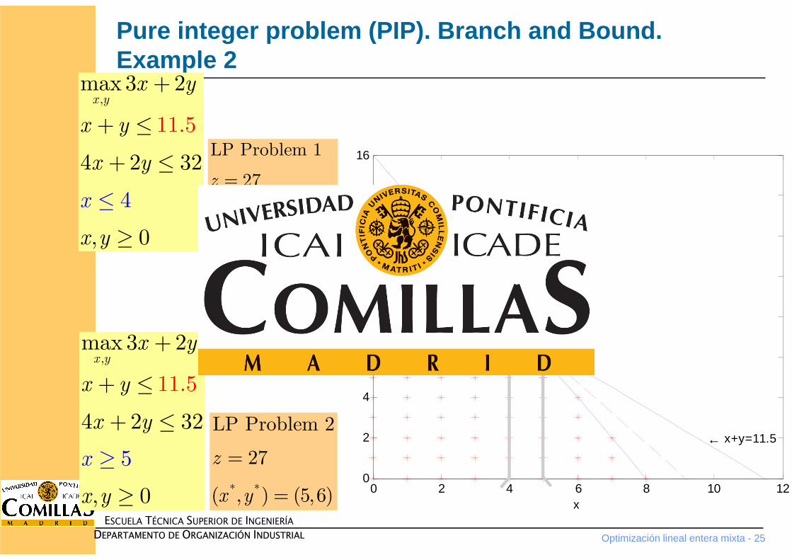
Pure integer problem (PIP). Branch and Bound. Example 2
,
11.
max 3 2
4 2
5
2
, 0
4
3
x y
x y
x y
x y
x y
x
+
+ ≤
+ ≤
≥
≤
,
11.
max 3 2
4 2
5
2
, 0
4
3
x y
x y
x y
x y
x y
x
+
+ ≤
+ ≤
≥
≤
0 2 4 6 8 10 120
2
4
6
8
10
12
14
16
x
y
← 4x+2y=32
← x+y=11.5
← 3x+2y=27.5
← (4.5,7)
* *
LP Problem 1
27
( , ) (4,7.5)
z
x y
=
=* *
LP Problem 1
27
( , ) (4,7.5)
z
x y
=
=
* *
LP Problem 2
27
( , ) (5,6)
z
x y
=
=* *
LP Problem 2
27
( , ) (5,6)
z
x y
=
=
,
11.
max 3 2
4 2
5
2
, 0
5
3
x y
x y
x y
x y
x y
x
+
+ ≤
+ ≤
≥
≥
,
11.
max 3 2
4 2
5
2
, 0
5
3
x y
x y
x y
x y
x y
x
+
+ ≤
+ ≤
≥
≥
Optimización lineal entera mixta - 26
ESCUELA TÉCNICA SUPERIOR DE INGENIERÍA
DEPARTAMENTO DE ORGANIZACIÓN INDUSTRIAL
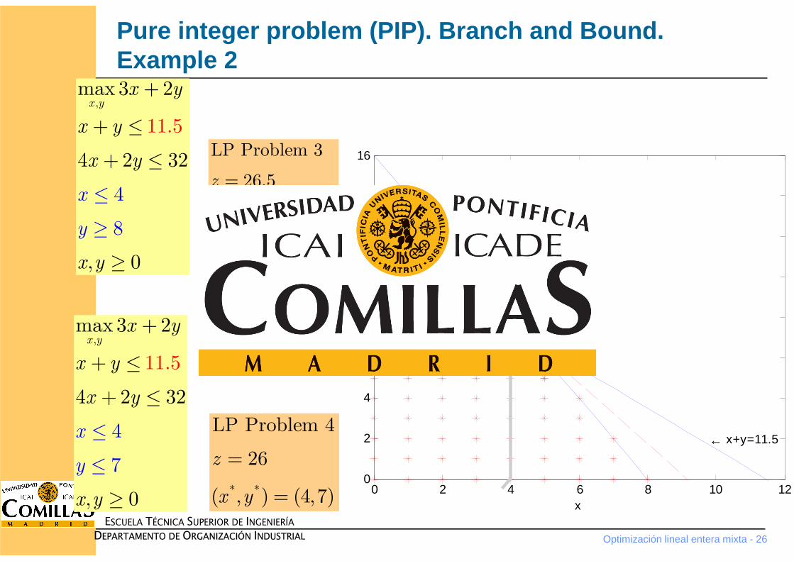
Pure integer problem (PIP). Branch and Bound. Example 2
,max 3 2
4 2
11.5
32
, 0
4
8
x y
x y
x y
x y
x
x
y
y
+
+ ≤
+ ≤
≥
≥
≤
,max 3 2
4 2
11.5
32
, 0
4
8
x y
x y
x y
x y
x
x
y
y
+
+ ≤
+ ≤
≥
≥
≤
0 2 4 6 8 10 120
2
4
6
8
10
12
14
16
x
y
← 4x+2y=32
← x+y=11.5
← 3x+2y=27.5
← (4.5,7)
* *
LP Problem 3
26.5
( , ) (3.5,8)
z
x y
=
=* *
LP Problem 3
26.5
( , ) (3.5,8)
z
x y
=
=
* *
LP Problem 4
26
( , ) (4,7)
z
x y
=
=* *
LP Problem 4
26
( , ) (4,7)
z
x y
=
=
,max 3 2
4 2
11.5
32
, 0
4
7
x y
x y
x y
x y
x
x
y
y
+
+ ≤
+ ≤
≤
≥
≤
,max 3 2
4 2
11.5
32
, 0
4
7
x y
x y
x y
x y
x
x
y
y
+
+ ≤
+ ≤
≤
≥
≤

Optimización lineal entera mixta - 27
ESCUELA TÉCNICA SUPERIOR DE INGENIERÍA
DEPARTAMENTO DE ORGANIZACIÓN INDUSTRIAL
Pure integer problem (PIP). Example 2
* *
PIP solution
27
( , ) (5,6)
z
x y
=
=* *
PIP solution
27
( , ) (5,6)
z
x y
=
=
0 2 4 6 8 10 120
2
4
6
8
10
12
14
16
x
y
← 4x+2y=32
← x+y=11.5
← 3x+2y=27
← (5,6)
,max3 2
4 2
11.5
32
, 0
,
x y
x y
x y
x y
x y
x y+
+
+ ≤
+ ≤
≥
∈ ℤ
,max3 2
4 2
11.5
32
, 0
,
x y
x y
x y
x y
x y
x y+
+
+ ≤
+ ≤
≥
∈ ℤ
Optimización lineal entera mixta - 28
ESCUELA TÉCNICA SUPERIOR DE INGENIERÍA
DEPARTAMENTO DE ORGANIZACIÓN INDUSTRIAL
Estrategias básicas
1. Buscar factibilidad� Ramificación y exploración en profundidad (avariciosa greedy) en el
árbol fijando recursivamente las variables fraccionarias más próximas a su valor entero en el nodo seleccionado.
2. Demostrar optimalidad� Supuesto que se disponga de una solución entera se desea probar que
ésta es óptima. Se seleccionan las variables que tienen un gran impacto en la función objetivo para descartar ramas del árbol lo antes posible.
Optimización lineal entera mixta - 29
ESCUELA TÉCNICA SUPERIOR DE INGENIERÍA
DEPARTAMENTO DE ORGANIZACIÓN INDUSTRIAL
Implantación de estrategias
1. Selección de la variable enteraa ramificar� La encontrada en primer lugar
� La de mayor o menor infactibilidad entera
2. Selección de la ramaa resolver� La más reciente. Bueno para la reoptimización por el método simplex.
� Aquélla con valor de la función objetivo más cercano o alejado al óptimo(mejor o peor cota)
Optimización lineal entera mixta - 30
ESCUELA TÉCNICA SUPERIOR DE INGENIERÍA
DEPARTAMENTO DE ORGANIZACIÓN INDUSTRIAL
Relajación del criterio de poda
� Marca la diferencia entre acabar un problema con una solución cuasióptima dentro de una cierta tolerancia conocida y NO solucionar el problema. Fundamental en la solución de problemas reales.
� Criterio de parada sin explorar exhaustivamente el árbol.
Se añade un criterio de poda (para maximización) con una cierta tolerancia para una solución no entera mejor (pero no significativamente) que la solución entera actual� Relativa
� Absoluta
α (error de tolerancia relativo, por ejemplo 10-3) OPTCRβ (error de tolerancia absoluto), ambas constantes conocidas OPTCA
* * (1 )z z z α≤ ≤ +* *z z z β≤ ≤ +
Optimización lineal entera mixta - 31
ESCUELA TÉCNICA SUPERIOR DE INGENIERÍA
DEPARTAMENTO DE ORGANIZACIÓN INDUSTRIAL
Parámetros de control del B&B (i)
� Prioridad en la selección de variables� Habitualmente se debe ramificar antes en las que más impacto tienen
en la f.o. (por ejemplo, variables de inversión frente a las de operación)
� GUB (generalized upper bound) o SOS(special ordered sets)
� En la ramificación normal cuando una el resto quedan fijadas a 0. En la rama con hay a su vez posibilidades
� La ramificación GUB se hace ordenando las variables pertenecientes al conjunto GUB en dos subconjuntos más equilibrados, hasta que la suma de las variables de un conjunto sobrepasa 0.5
1
1k
jj
x=
=∑
1jx =0jx = 1k −
0 1, ,
0 1, ,i
i
j
j
x i r
x i r k
= =
= = +
…
…{ }*
1min : 0.5
i
t
jir t x
== ≥∑
Optimización lineal entera mixta - 32
ESCUELA TÉCNICA SUPERIOR DE INGENIERÍA
DEPARTAMENTO DE ORGANIZACIÓN INDUSTRIAL
Parámetros de control del B&B (ii)
� Cota inicial(cutoff, incumbent)� Se trata de una cota inicial válida de la f.o. estimada por el usuario
� Método de solución de los problemas LP� Primera iteración (punto interior o simplex)
� Iteraciones sucesivas (simplex primal o dual con diferentes estrategias de selección de VBE)
Optimización lineal entera mixta - 33
ESCUELA TÉCNICA SUPERIOR DE INGENIERÍA
DEPARTAMENTO DE ORGANIZACIÓN INDUSTRIAL
CONTENIDO
�INTRODUCCIÓN
�MÉTODOS DE SOLUCIÓN
�MÉTODO DE RAMIFICACIÓN Y ACOTAMIENTO
�DUALITY (master)
�PREPROCESSING (master)
�BRANCH AND CUT METHOD (master)
Optimización lineal entera mixta - 34
ESCUELA TÉCNICA SUPERIOR DE INGENIERÍA
DEPARTAMENTO DE ORGANIZACIÓN INDUSTRIAL
Pure integer problem (PIP). Dual variables
� We know how to obtain dual variables of an LP problem. They are calculated at the same time than the optimal solution
� But we do not know how to obtain these dual variables in a MIP problem because we have solved many LP problems for reaching the optimal integer solution
Optimización lineal entera mixta - 35
ESCUELA TÉCNICA SUPERIOR DE INGENIERÍA
DEPARTAMENTO DE ORGANIZACIÓN INDUSTRIAL
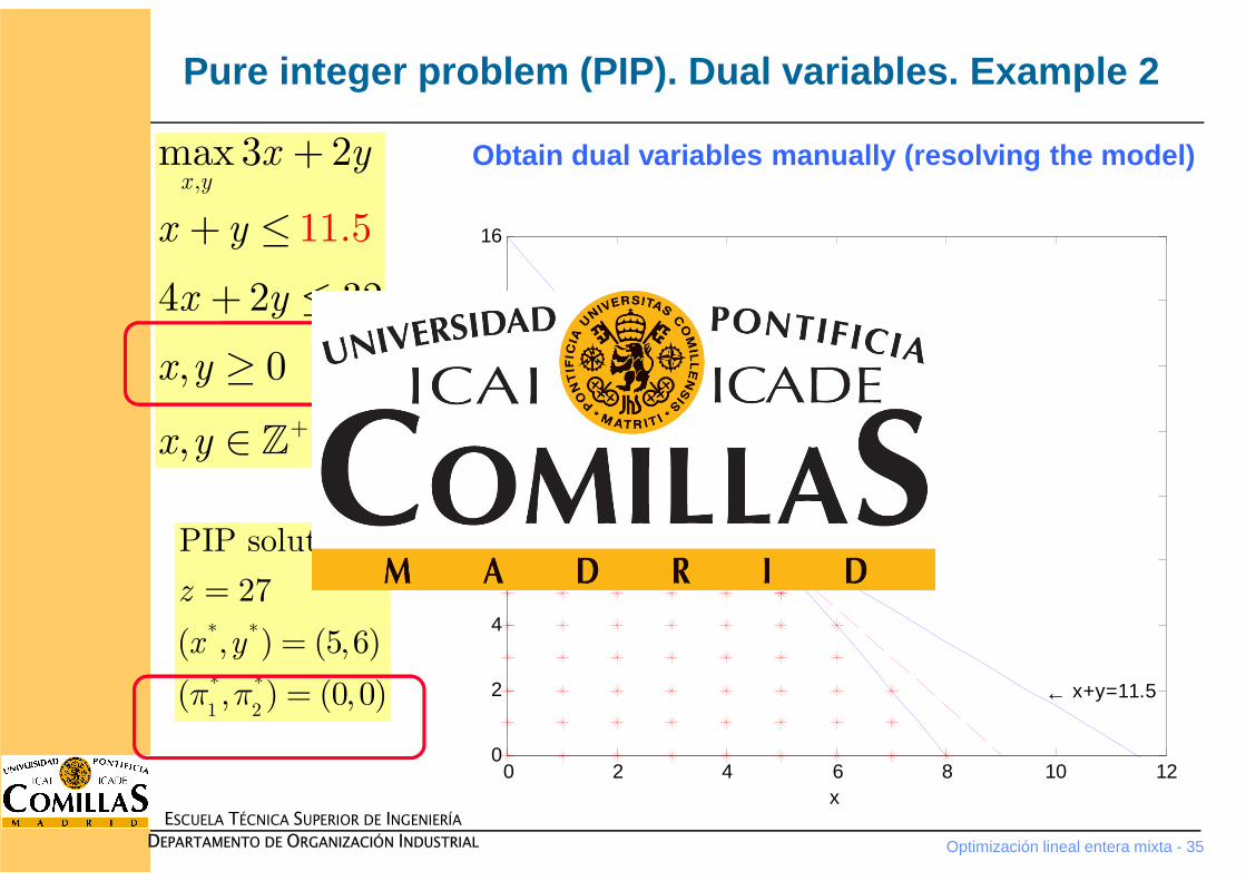
Pure integer problem (PIP). Dual variables. Example 2
* *
* *1 2
PIP solution
27
( , ) (5,6)
( , ) (0, 0)
z
x y
π π
=
=
=
* *
* *1 2
PIP solution
27
( , ) (5,6)
( , ) (0, 0)
z
x y
π π
=
=
=
0 2 4 6 8 10 120
2
4
6
8
10
12
14
16
x
y
← 4x+2y=32
← x+y=11.5
← 3x+2y=27
← (5,6)
Obtain dual variables manually (resolving the model),
max3 2
4 2
11.5
32
, 0
,
x y
x y
x y
x y
x y
x y+
+
+ ≤
+ ≤
≥
∈ ℤ
,max3 2
4 2
11.5
32
, 0
,
x y
x y
x y
x y
x y
x y+
+
+ ≤
+ ≤
≥
∈ ℤ
Optimización lineal entera mixta - 36
ESCUELA TÉCNICA SUPERIOR DE INGENIERÍA
DEPARTAMENTO DE ORGANIZACIÓN INDUSTRIAL
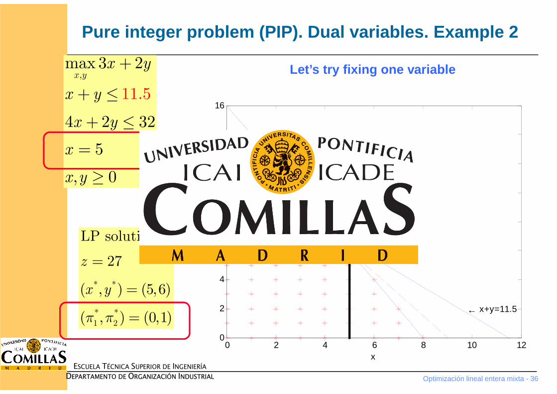
Pure integer problem (PIP). Dual variables. Example 2
,
11.
max 3 2
4 2
5
32
5
, 0
x y
x y
x y
x y
x
x y
+
+ ≤
+ ≤
=
≥
,
11.
max 3 2
4 2
5
32
5
, 0
x y
x y
x y
x y
x
x y
+
+ ≤
+ ≤
=
≥
* *
* *1 2
LP solution
27
( , ) (5,6)
( , ) (0,1)
z
x y
π π
=
=
=
* *
* *1 2
LP solution
27
( , ) (5,6)
( , ) (0,1)
z
x y
π π
=
=
=
0 2 4 6 8 10 120
2
4
6
8
10
12
14
16
x
y
← 4x+2y=32
← x+y=11.5
← 3x+2y=27
← (5,6)
Let’s try fixing one variable
Optimización lineal entera mixta - 37
ESCUELA TÉCNICA SUPERIOR DE INGENIERÍA
DEPARTAMENTO DE ORGANIZACIÓN INDUSTRIAL
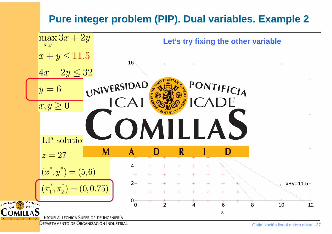
Pure integer problem (PIP). Dual variables. Example 2
,
11.
max 3 2
4 2
5
32
6
, 0
x y
x y
x y
x y
y
x y
+
+ ≤
+ ≤
=
≥
,
11.
max 3 2
4 2
5
32
6
, 0
x y
x y
x y
x y
y
x y
+
+ ≤
+ ≤
=
≥
* *
* *1 2
LP solution
27
( , ) (5,6)
( , ) (0, 0.75)
z
x y
π π
=
=
=
* *
* *1 2
LP solution
27
( , ) (5,6)
( , ) (0, 0.75)
z
x y
π π
=
=
=
0 2 4 6 8 10 120
2
4
6
8
10
12
14
16
x
y
← 4x+2y=32
← x+y=11.5
← 3x+2y=27
← (5,6)
Let’s try fixing the other variable
Optimización lineal entera mixta - 38
ESCUELA TÉCNICA SUPERIOR DE INGENIERÍA
DEPARTAMENTO DE ORGANIZACIÓN INDUSTRIAL
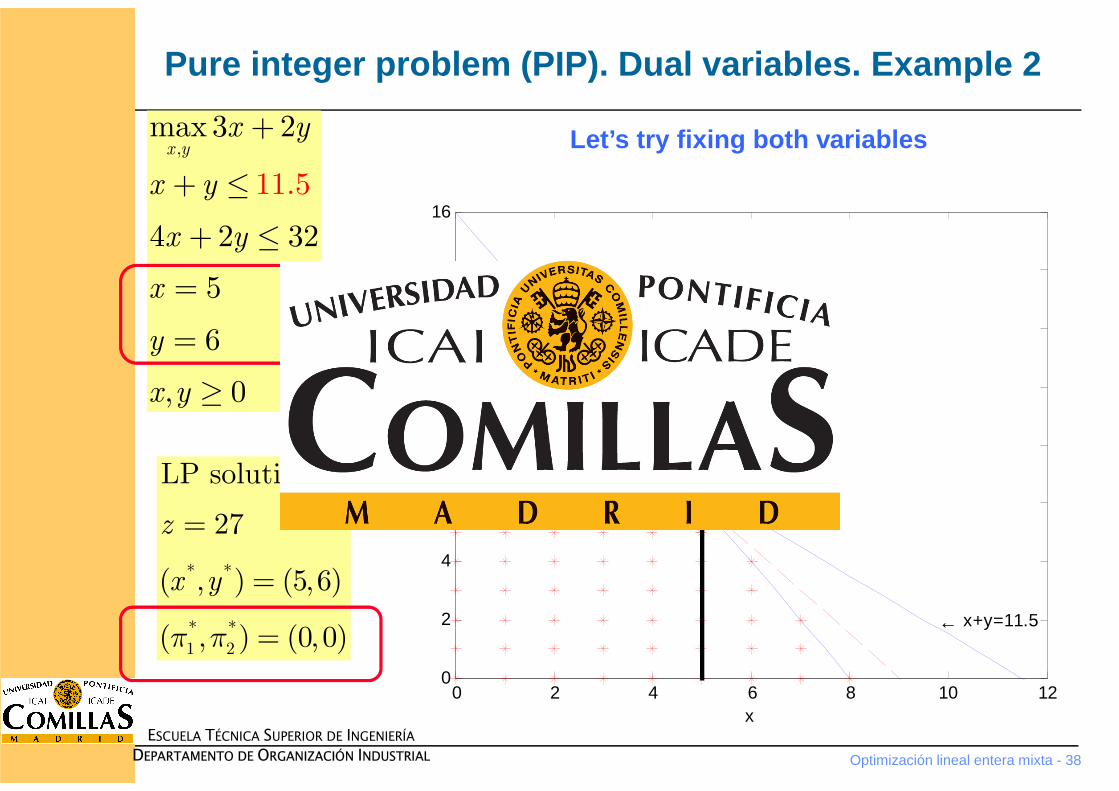
Pure integer problem (PIP). Dual variables. Example 2
,max3 2
4 2
11.5
32
5
6
, 0
x y
x y
x y
x y
x
y
x y
+
+ ≤
+ ≤
=
=
≥
,max3 2
4 2
11.5
32
5
6
, 0
x y
x y
x y
x y
x
y
x y
+
+ ≤
+ ≤
=
=
≥
* *
* *1 2
LP solution
27
( , ) (5,6)
( , ) (0, 0)
z
x y
π π
=
=
=
* *
* *1 2
LP solution
27
( , ) (5,6)
( , ) (0, 0)
z
x y
π π
=
=
=
0 2 4 6 8 10 120
2
4
6
8
10
12
14
16
x
y
← 4x+2y=32
← x+y=11.5
← 3x+2y=27
← (5,6)
Let’s try fixing both variables
Optimización lineal entera mixta - 39
ESCUELA TÉCNICA SUPERIOR DE INGENIERÍA
DEPARTAMENTO DE ORGANIZACIÓN INDUSTRIAL
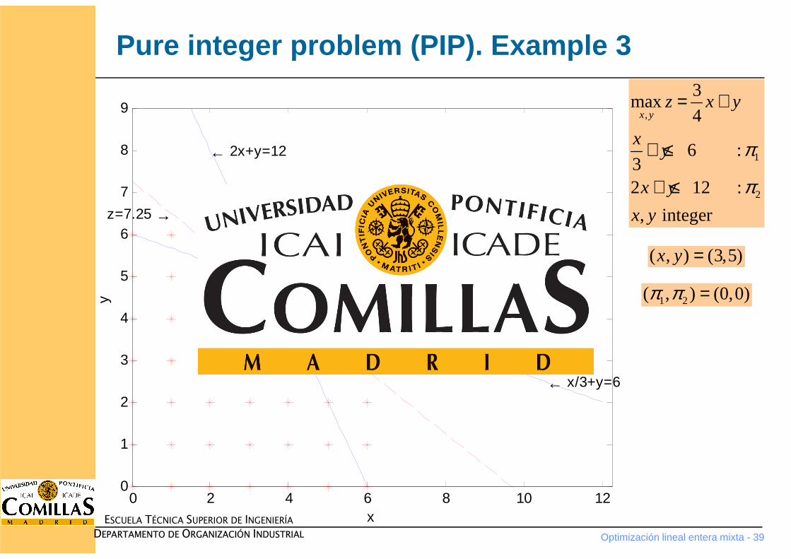
Pure integer problem (PIP). Example 3
,
1
2
3max
4
6 :32 12 :
, integer
x yz x y
xy
x y
x y
π
π
= +
+ ≤
+ ≤
,
1
2
3max
4
6 :32 12 :
, integer
x yz x y
xy
x y
x y
π
π
= +
+ ≤
+ ≤
( , ) (3,5)x y =( , ) (3,5)x y =
1 2( , ) (0,0)π π =1 2( , ) (0,0)π π =
0 2 4 6 8 10 120
1
2
3
4
5
6
7
8
9
x
y
← x/3+y=6
← 2x+y=12
z=7.25 →
Optimización lineal entera mixta - 40
ESCUELA TÉCNICA SUPERIOR DE INGENIERÍA
DEPARTAMENTO DE ORGANIZACIÓN INDUSTRIAL
0 2 4 6 8 10 120
1
2
3
4
5
6
7
8
9
x
y
← x/3+y=6.5
← 2x+y=12
z=7.25 →
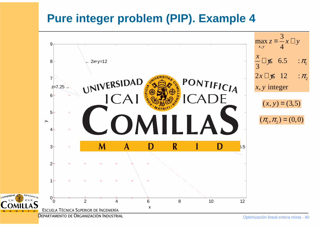
Pure integer problem (PIP). Example 4
,
1
2
3max
4
6.5 :32 12 :
, integer
x yz x y
xy
x y
x y
π
π
= +
+ ≤
+ ≤
,
1
2
3max
4
6.5 :32 12 :
, integer
x yz x y
xy
x y
x y
π
π
= +
+ ≤
+ ≤
( , ) (3,5)x y =( , ) (3,5)x y =
1 2( , ) (0,0)π π =1 2( , ) (0,0)π π =
Optimización lineal entera mixta - 41
ESCUELA TÉCNICA SUPERIOR DE INGENIERÍA
DEPARTAMENTO DE ORGANIZACIÓN INDUSTRIAL
Dual variables in a MIP problem
� In an LP problemthe complementarity slackness condition states:� If constraint is bindingdual variable may be different from 0� If constraint is non bindingdual variable is necessarily 0
� In a MIP problem� It is not clear how to obtain dual variables in a MIP problem� There must be those corresponding to node that has provided the
optimal solution in B&B algorithm� In practice:
• Fixe all the integer variables to their optimal valuesand solve the corresponding LP problem to determine the dual variables

Optimización lineal entera mixta - 44
ESCUELA TÉCNICA SUPERIOR DE INGENIERÍA
DEPARTAMENTO DE ORGANIZACIÓN INDUSTRIAL
CONTENIDO
�INTRODUCCIÓN
�MÉTODOS DE SOLUCIÓN
�MÉTODO DE RAMIFICACIÓN Y ACOTAMIENTO
�DUALITY (master)
�PREPROCESSING (master)
�BRANCH AND CUT METHOD (master)
Optimización lineal entera mixta - 45
ESCUELA TÉCNICA SUPERIOR DE INGENIERÍA
DEPARTAMENTO DE ORGANIZACIÓN INDUSTRIAL
� R. Bixby, M. Fenelon, Z. Gu, E. Rothberg, and R. Wunderling, “MIP: theory and practice–closing the gap,” in System Modelling and Optimization: Methods, Theory and Applications, M. J. D. Powell and S. Scholtes, Eds. Boston: Kluwer Academic Publishers, 2000, vol. 174, p. 19–49.
� F. Vanderbeck and L. A. Wolsey, “Reformulation and decomposition of integer programs,” in 50 Years of Integer Programming 1958-2008, M. Jünger, T. M. Liebling, D. Naddef, G. L. Nemhauser, W. R. Pulleyblank, G. Reinelt, G. Rinaldi, and L. A. Wolsey, Eds. Berlin, Heidelberg: Springer Berlin Heidelberg, 2010, pp. 431–502.
� R. Bixby and E. Rothberg, “Progress in computational mixed integer programming—A look back from the other side of the tipping point,” Annals of Operations Research, vol. 149, no. 1, pp. 37–41, Jan. 2007.
� L. Wolsey, “Strong formulations for mixed integer programs: valid inequalities and extended formulations,” Mathematical programming, vol. 97, no. 1, p. 423–447, 2003.
� G. Morales-España, J.M. Latorre, and A. Ramos Tight and Compact MILP Formulation for the Thermal Unit Commitment ProblemIEEE Transactions on Power Systems (accepted)
� G. Morales-España, J.M. Latorre, and A. Ramos Tight and Compact MILP Formulation of Start-Up and Shut-Down Ramping in Unit Commitment IEEE Transactions on Power Systems (accepted) 10.1109/TPWRS.2012.2222938
Optimización lineal entera mixta - 46
ESCUELA TÉCNICA SUPERIOR DE INGENIERÍA
DEPARTAMENTO DE ORGANIZACIÓN INDUSTRIAL
Preproceso
� Técnicas enfocadas a reducir sustancialmente las dimensiones o fortalecer la formulacióndel problema. Especialmente relevante para resolver problemas MIP� Dos formulaciones de un problema entero se dicen 0-1equivalentessi
tienen las mismas soluciones enteras.
� Dadas dos formulaciones equivalentes de un problema entero, se dice que una es más fuerteque la otra, si la región factible de su relajación lineal está estrictamente contenida en la región factible de la otra. Se encuentran antes soluciones enteras factibles y se pueden podar más ramas del árbol. Las formulaciones más fuertes se realizan, a veces, a costa de incrementar el tamaño del problema (menos compacta).
� Medida: intervalo de integralidad(integrality gap) diferencia entre f.o.de problema MIP y LP.
� G. Morales-España, J.M. Latorre, and A. Ramos Tight and Compact MILP Formulation of Start-Up and Shut-Down Ramping in Unit Commitment IEEE Transactions on Power Systems (accepted)
Optimización lineal entera mixta - 47
ESCUELA TÉCNICA SUPERIOR DE INGENIERÍA
DEPARTAMENTO DE ORGANIZACIÓN INDUSTRIAL
Técnicas de preproceso
� Preproceso general� Reforzamiento de cotas
� Eliminación de restricciones redundantes
� Asignación de variables
� Preproceso mixto 0-1� Reducción de coeficientes
Optimización lineal entera mixta - 48
ESCUELA TÉCNICA SUPERIOR DE INGENIERÍA
DEPARTAMENTO DE ORGANIZACIÓN INDUSTRIAL
Reforzamiento de cotas
� Aumentar cotas inferioresy disminuir cotas superioresmediante inspección de restricciones
� Especialmente para variables enteras
� Puede asignar variables o detectar infactibilidades
Optimización lineal entera mixta - 49
ESCUELA TÉCNICA SUPERIOR DE INGENIERÍA
DEPARTAMENTO DE ORGANIZACIÓN INDUSTRIAL
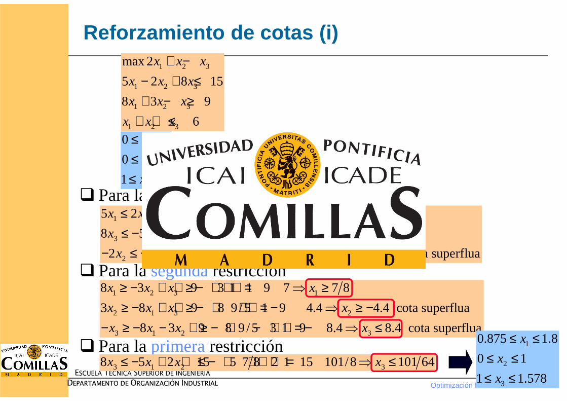
� Para la primerarestricción
� Para la segundarestricción
� Para la primerarestricción
Reforzamiento de cotas (i)1 2 3
1 2 3
1 2 3
1 2 3
max 2
5 2 8 15
8 3 9
6
x x x
x x x
x x x
x x x
+ −− + ≤+ − ≥
+ + ≤
1 2 3 1
3 1 2 3
2 1 3 2
5 2 8 15 2 1 8 1 15 9 9 5
8 5 2 15 5 0 2 1 15 17 17 8
2 5 8 15 5 0 8 1 15 7 7 2 cota superflua
x x x x
x x x x
x x x x
≤ − + ≤ ⋅ − ⋅ + = ⇒ ≤≤ − + + ≤ − ⋅ + ⋅ + = ⇒ ≤
− ≤ − − + ≤ − ⋅ − ⋅ + = ⇒ ≥ −
1 2 3 1
2 1 3 2
3 1 2 3
8 3 9 3 1 1 9 7 7 8
3 8 9 8 9/5 1 9 4.4 4.4 cota superflua
8 3 9 8 9/5 3 1 9 8.4 8.4 cota superflua
x x x x
x x x x
x x x x
≥ − + + ≥ − ⋅ + + = ⇒ ≥≥ − + + ≥ − ⋅ + + = − ⇒ ≥ −
− ≥ − − + ≥ − ⋅ − ⋅ + = − ⇒ ≤
3 1 2 38 5 2 15 5 7 8 2 1 15 101/8 101 64x x x x≤ − + + ≤ − ⋅ + ⋅ + = ⇒ ≤
1
2
3
0 3
0 1
1
x
x
x
≤ ≤≤ ≤≤
1
2
3
0.875 1.8
0 1
1 1.578
x
x
x
≤ ≤≤ ≤≤ ≤
Optimización lineal entera mixta - 50
ESCUELA TÉCNICA SUPERIOR DE INGENIERÍA
DEPARTAMENTO DE ORGANIZACIÓN INDUSTRIAL
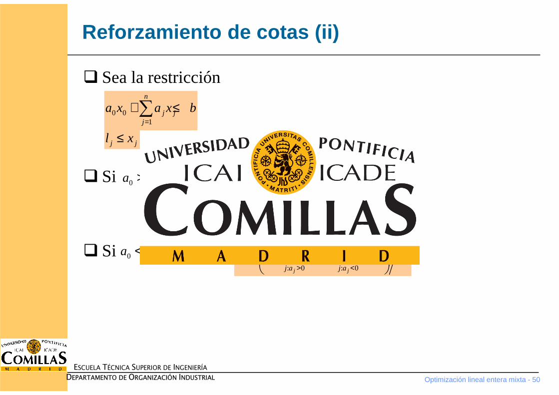
Reforzamiento de cotas (ii)
� Sea la restricción
� Si entonces
� Si entonces
0 01
n
j jj
j j j
a x a x b
l x u
=
+ ≤
≤ ≤
∑
0 0a >
0 0a <
0 0: 0 : 0j j
j j j jj a j a
x b a l a u a> <
≤ − −
∑ ∑
0 0: 0 : 0j j
j j j jj a j a
x b a l a u a> <
≥ − −
∑ ∑
Optimización lineal entera mixta - 51
ESCUELA TÉCNICA SUPERIOR DE INGENIERÍA
DEPARTAMENTO DE ORGANIZACIÓN INDUSTRIAL
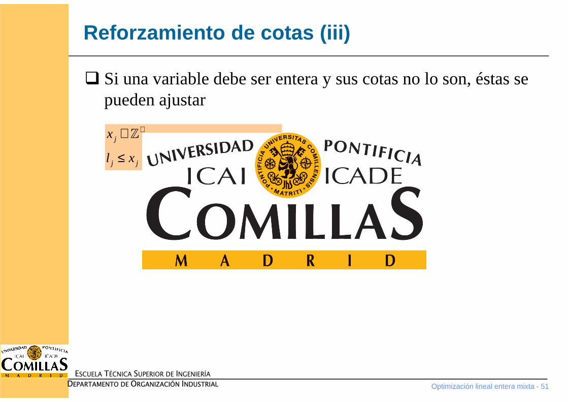
� Si una variable debe ser entera y sus cotas no lo son, éstas se pueden ajustar
Reforzamiento de cotas (iii)
j
j j j j j j
x
l x u l x u
+∈
≤ ≤ ⇒ ≤ ≤
ℤ
Optimización lineal entera mixta - 52
ESCUELA TÉCNICA SUPERIOR DE INGENIERÍA
DEPARTAMENTO DE ORGANIZACIÓN INDUSTRIAL
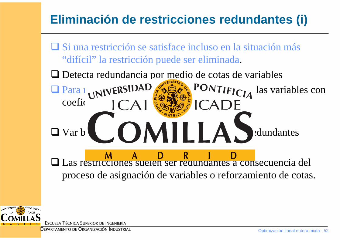
Eliminación de restricciones redundantes (i)
� Si una restricción se satisface incluso en la situación más “difícil” la restricción puede ser eliminada.
� Detecta redundancia por medio de cotas de variables
� Para restricciones ≤ se igualan a cota superior las variables con coeficientes > 0 y a cota inferior las demás.
� Var binarias son redundantes
� Las restricciones suelen ser redundantes a consecuencia del proceso de asignación de variables o reforzamiento de cotas.
1 2
1 2
1 2
3 2 6
3 2 3
3 2 3
x x
x x
x x
+ ≤− ≤− ≥ −
1
2
0 1
0 1
x
x
≤ ≤≤ ≤
Optimización lineal entera mixta - 53
ESCUELA TÉCNICA SUPERIOR DE INGENIERÍA
DEPARTAMENTO DE ORGANIZACIÓN INDUSTRIAL
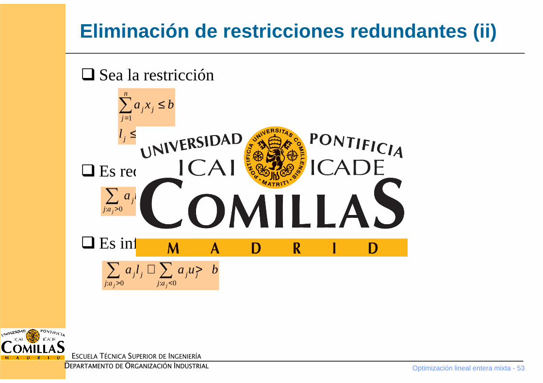
Eliminación de restricciones redundantes (ii)
� Sea la restricción
� Es redundante si
� Es infactible si
1
n
j jj
j j j
a x b
l x u
=
≤
≤ ≤
∑
: 0 : 0j j
j j j jj a j a
a u a l b> <
+ ≤∑ ∑
: 0 : 0j j
j j j jj a j a
a l a u b> <
+ >∑ ∑
Optimización lineal entera mixta - 54
ESCUELA TÉCNICA SUPERIOR DE INGENIERÍA
DEPARTAMENTO DE ORGANIZACIÓN INDUSTRIAL
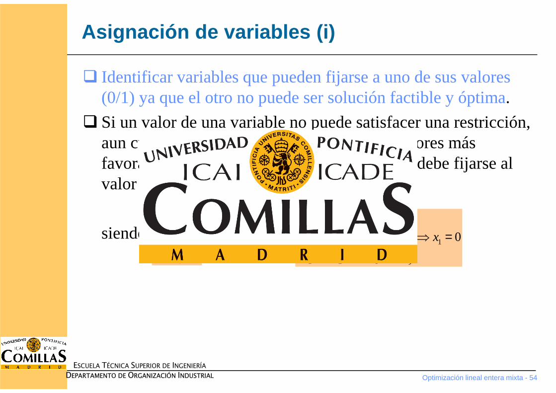
Asignación de variables (i)
� Identificar variables que pueden fijarse a uno de sus valores (0/1) ya que el otro no puede ser solución factible y óptima.
� Si un valor de una variable no puede satisfacer una restricción, aun cuando las demás variables tomen sus valores más favorables para intentar cumplirla, la variable debe fijarse al valor opuesto.
siendo1
1 2 1
1 2 3
3 2
3 2 0
5 2 2
x
x x x
x x x
≤ + ≤ ⇒ =+ − ≤
1
2
3
0 1
0 1
0 1
x
x
x
≤ ≤≤ ≤≤ ≤

Optimización lineal entera mixta - 55
ESCUELA TÉCNICA SUPERIOR DE INGENIERÍA
DEPARTAMENTO DE ORGANIZACIÓN INDUSTRIAL
Asignación de variables (ii)
� Procedimiento para restricciones ≤� Identificar la variable con el mayor coeficiente positivo. Si la suma de
dicho coeficiente y cualquier coeficiente negativo excede la cota de la restricción, la variable debe fijarse a 0.
1
1 2 1
1 2 3
3 2
3 2 1
5 2 2
x
x x x
x x x
≥ + ≥ ⇒ =+ − ≥
1 2 3 32 1 0x x x x+ − ≥ ⇒ =
1 2 3 1 33 3 2 1, 0x x x x x+ − ≥ ⇒ = =
1 2 1 23 2 1 0, 1x x x x− ≤ − ⇒ = =
� Reacción en cadena: el procedimiento se repetirá para las siguientes variables con el mayor coeficiente.
1 2 3 1
1 4 5 4 5
5 6 6
3 2 2 1
1 0, 0
0 0
x x x x
x x x x x
x x x
+ − ≥ ⇒ =+ + ≤ ⇒ = =
− + ≤ ⇒ =
Optimización lineal entera mixta - 56
ESCUELA TÉCNICA SUPERIOR DE INGENIERÍA
DEPARTAMENTO DE ORGANIZACIÓN INDUSTRIAL
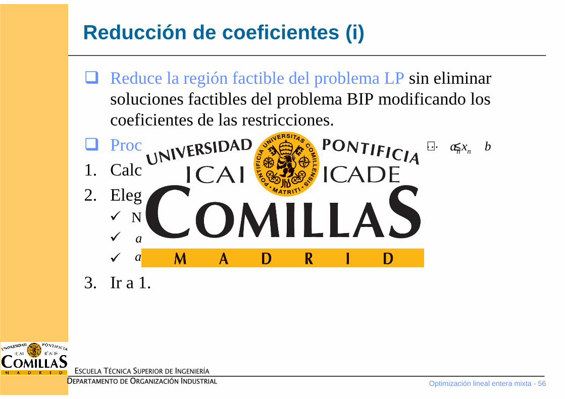
Reducción de coeficientes (i)
� Reduce la región factible del problema LPsin eliminar soluciones factibles del problema BIP modificando los coeficientes de las restricciones.
� Procedimiento para restricciones ≤1. Calcular S = suma de valores aj positivos
2. Elegir cualquier aj ≠ 0 tal que S< b + |aj|� No existe ⇒ no se puede ajustar más la restricción
�
�
3. Ir a 1.
1 1 2 2 n na x a x a x b+ + + ≤⋯
0 j j j j ja a S b b S a a a b b′ ′ ′ ′> = − = − = =0 j j j ja a S b a a′ ′< = − =
Optimización lineal entera mixta - 57
ESCUELA TÉCNICA SUPERIOR DE INGENIERÍA
DEPARTAMENTO DE ORGANIZACIÓN INDUSTRIAL
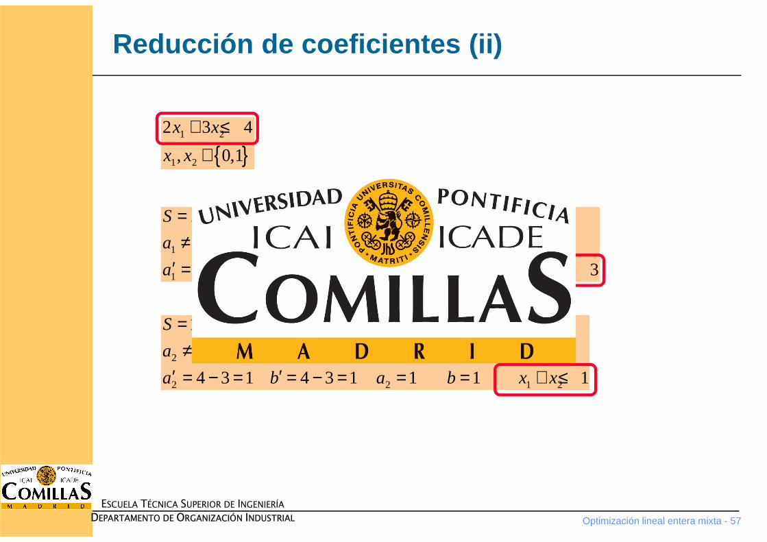
1
1 1 1 2
2 3 5
0 5 4 2
5 4 1 5 2 3 1 3 3 3
S
a
a b a b x x
= + =≠ < +
′ ′= − = = − = = = + ≤
Reducción de coeficientes (ii)
2
2 2 1 2
1 3 4
0 4 3 3
4 3 1 4 3 1 1 1 1
S
a
a b a b x x
= + =≠ < +
′ ′= − = = − = = = + ≤
{ }1 2
1 2
2 3 4
, 0,1
x x
x x
+ ≤∈
Optimización lineal entera mixta - 58
ESCUELA TÉCNICA SUPERIOR DE INGENIERÍA
DEPARTAMENTO DE ORGANIZACIÓN INDUSTRIAL
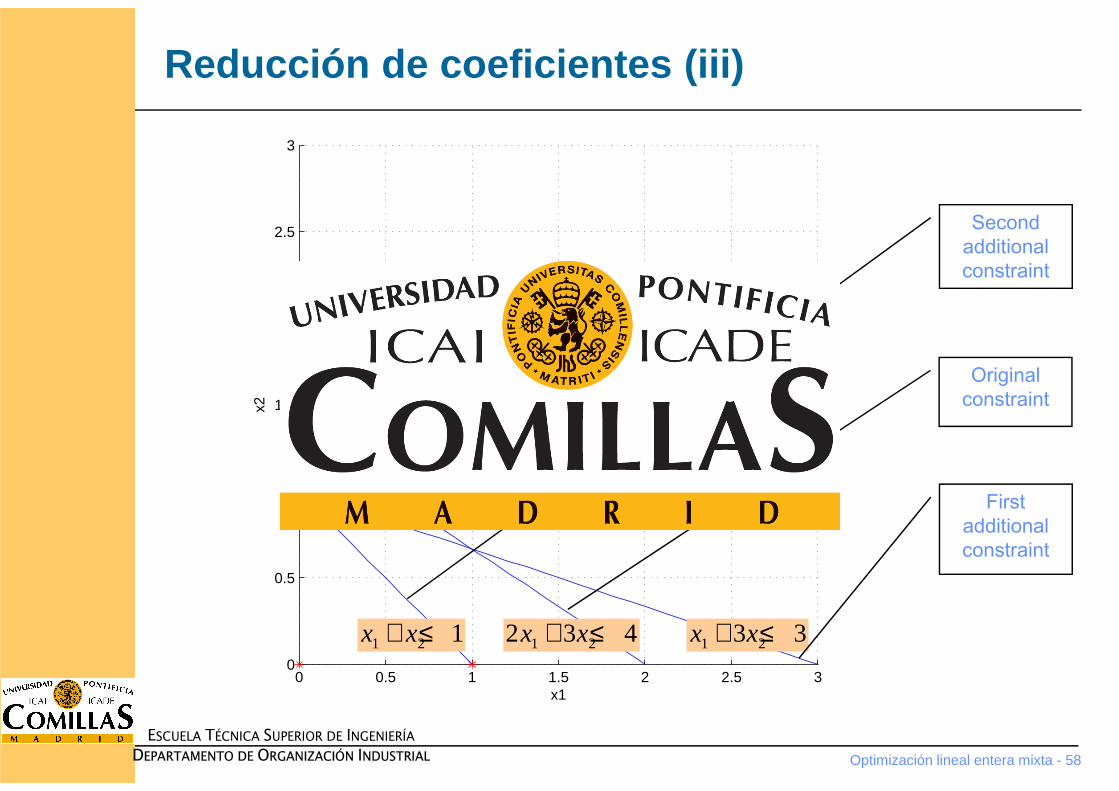
Reducción de coeficientes (iii)
0 0.5 1 1.5 2 2.5 30
0.5
1
1.5
2
2.5
3
x1
x2
1 2 1x x+ ≤ 1 22 3 4x x+ ≤ 1 23 3x x+ ≤
Original constraint
Second additional constraint
First additional constraint
Optimización lineal entera mixta - 59
ESCUELA TÉCNICA SUPERIOR DE INGENIERÍA
DEPARTAMENTO DE ORGANIZACIÓN INDUSTRIAL
CONTENIDO
�INTRODUCCIÓN
�MÉTODOS DE SOLUCIÓN
�MÉTODO DE RAMIFICACIÓN Y ACOTAMIENTO
�DUALITY (master)
�PREPROCESSING (master)
�BRANCH AND CUT METHOD (master)
Optimización lineal entera mixta - 60
ESCUELA TÉCNICA SUPERIOR DE INGENIERÍA
DEPARTAMENTO DE ORGANIZACIÓN INDUSTRIAL
Generación de planos de corte
� Nueva restricción que reduce la región factible del problema LP sin eliminar soluciones factibles del problema IP.
� Deducida válidamentede restricciones del problema
� Procedimiento de método de planos de corte1. Inicializar resolviendo el problema relajado LP
2. Si la solución óptima es entera finalizar. Si no, continuar a paso 3
3. Obtener un plano de corte que viole la solución óptima actual
4. Añadir el plano de corte a las restricciones y reoptimizar. Ir a paso 2.
Optimización lineal entera mixta - 61
ESCUELA TÉCNICA SUPERIOR DE INGENIERÍA
DEPARTAMENTO DE ORGANIZACIÓN INDUSTRIAL
Planos de corte de tipo cubrimiento
� Considera cualquier restricción de tipo ≤ con variables binariascon todos los coeficientes no negativos(restricción tipo mochila)
� Encontrar grupo de variables (cubrimiento minimal) tal que� Se viola la restricción si las variables del cubrimiento son 1 y el resto
son 0
� Se satisface la restricción si una de las variables del cubrimiento se hace 0
� Formación del plano de corte
siendo Nel número de variables del cubrimiento
{ }1 2 3 46 3 5 2 9
0,1i
x x x x
x
+ + + ≤∈
1 2 4
2 3 4
1 3
2
2
1
x x x
x x x
x x
+ + ≤ + + ≤ + ≤
variables del cubrimiento -1N≤∑
Optimización lineal entera mixta - 62
ESCUELA TÉCNICA SUPERIOR DE INGENIERÍA
DEPARTAMENTO DE ORGANIZACIÓN INDUSTRIAL
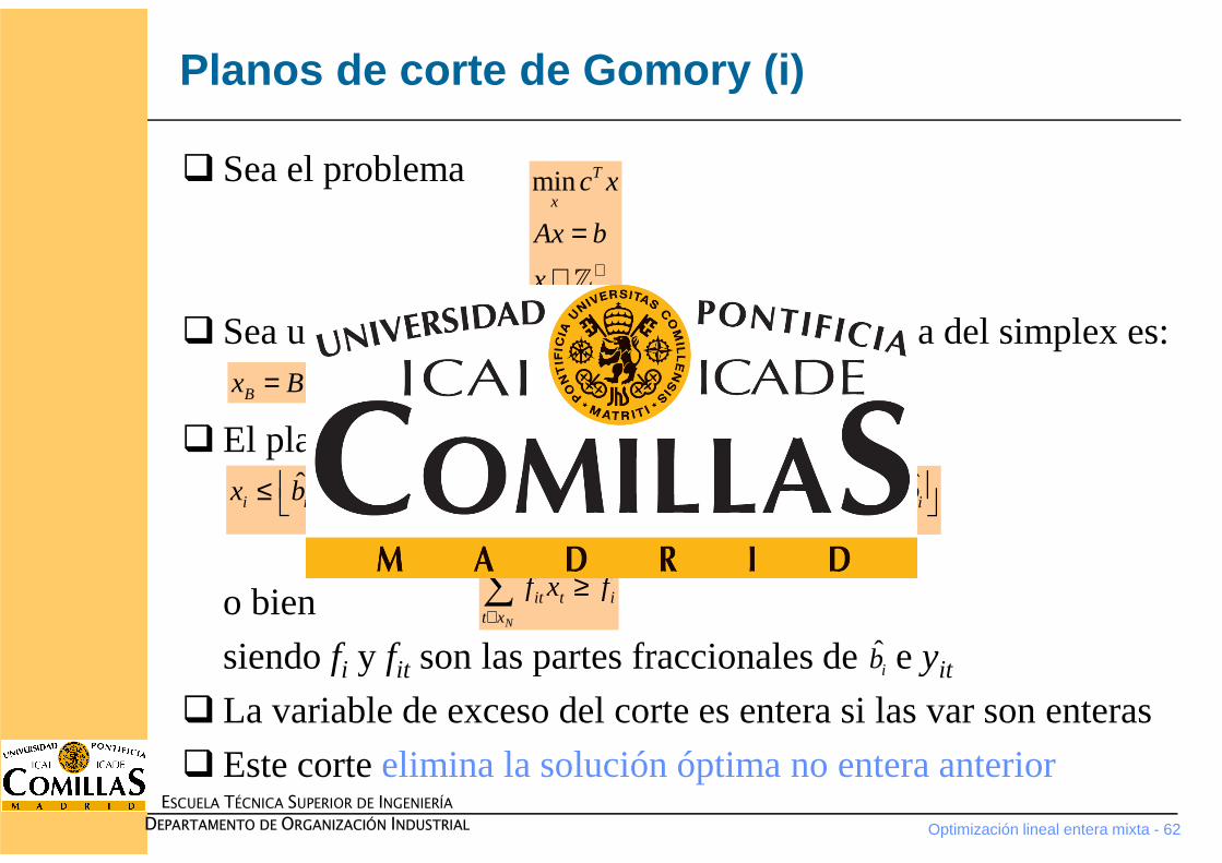
Planos de corte de Gomory (i)
� Sea el problema
� Sea una variable xi no entera. La fila en la tabla del simplex es:
� El plano de corte de Gomory es:
o bien
siendo fi y fit son las partes fraccionales de e yit
� La variable de exceso del corte es entera si las var son enteras
� Este corte elimina la solución óptima no entera anterior
1 1 1( )B N Nx B b Nx B b B Nx− − −= − = −ˆ
N
i i it tt x
x b y x∈
= −∑
min T
xc x
Ax b
x +
=
∈ℤ
ˆ
N
i i it tt x
x b y x∈
≤ − ∑ ˆ ˆ( )N
it it t i it x
y y x b b∈
− ≥ − ∑
N
it t it x
f x f∈
≥∑
ib
Optimización lineal entera mixta - 63
ESCUELA TÉCNICA SUPERIOR DE INGENIERÍA
DEPARTAMENTO DE ORGANIZACIÓN INDUSTRIAL
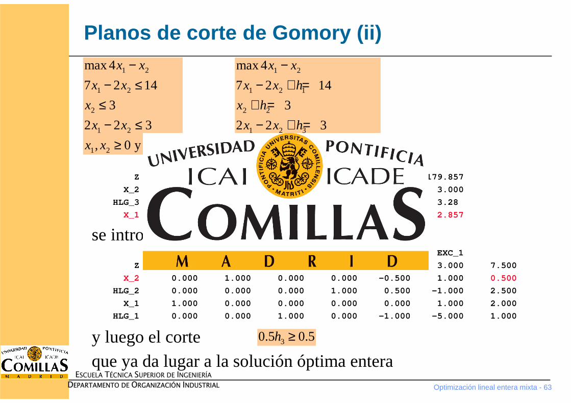
Planos de corte de Gomory (ii)
X_1 X_2 HLG_1 HLG_2 HLG_3
Z 0.000 0.000 9.143 17.286 0.000 179.857
X_2 0.000 1.000 0.000 1.000 0.000 3.000
HLG_3 0.000 0.000 -0.286 1.429 1.000 3.28
X_1 1.000 0.000 0.143 0.286 0.000 2.857
se introduce el corteX_1 X_2 HLG_1 HLG_2 HLG_3 EXC_1
Z 0.000 0.000 0.000 0.000 0.500 3.000 7.500
X_2 0.000 1.000 0.000 0.000 -0.500 1.000 0.500
HLG_2 0.000 0.000 0.000 1.000 0.500 -1.000 2.500
X_1 1.000 0.000 0.000 0.000 0.000 1.000 2.000
HLG_1 0.000 0.000 1.000 0.000 -1.000 -5.000 1.000
y luego el corteque ya da lugar a la solución óptima entera
1 2
1 2
2
1 2
1 2
max 4
7 2 14
3
2 2 3
, 0 y enteras
x x
x x
x
x x
x x
−− ≤
≤− ≤
≥
1 20.143 0.286 0.857h h+ ≥
30.5 0.5h ≥
1 2
1 2 1
2 2
1 2 3
1 2 1 2 3
max 4
7 2 14
3
2 2 3
, , , , 0 y enteras
x x
x x h
x h
x x h
x x h h h
−− + =
+ =− + =
≥
Optimización lineal entera mixta - 64
ESCUELA TÉCNICA SUPERIOR DE INGENIERÍA
DEPARTAMENTO DE ORGANIZACIÓN INDUSTRIAL
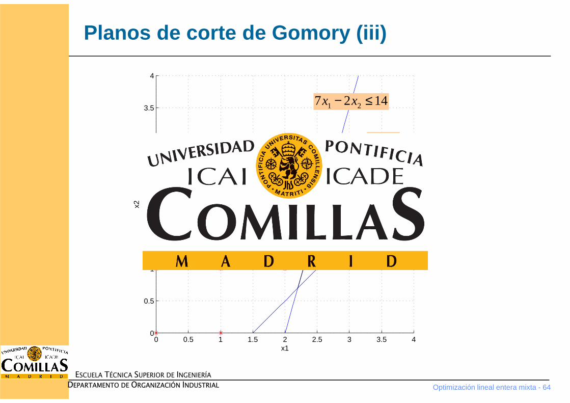
Planos de corte de Gomory (iii)
0 0.5 1 1.5 2 2.5 3 3.5 40
0.5
1
1.5
2
2.5
3
3.5
4
x1
x2 1 22 2 3x x− ≤
1 27 2 14x x− ≤
2 3x ≤
Optimización lineal entera mixta - 65
ESCUELA TÉCNICA SUPERIOR DE INGENIERÍA
DEPARTAMENTO DE ORGANIZACIÓN INDUSTRIAL
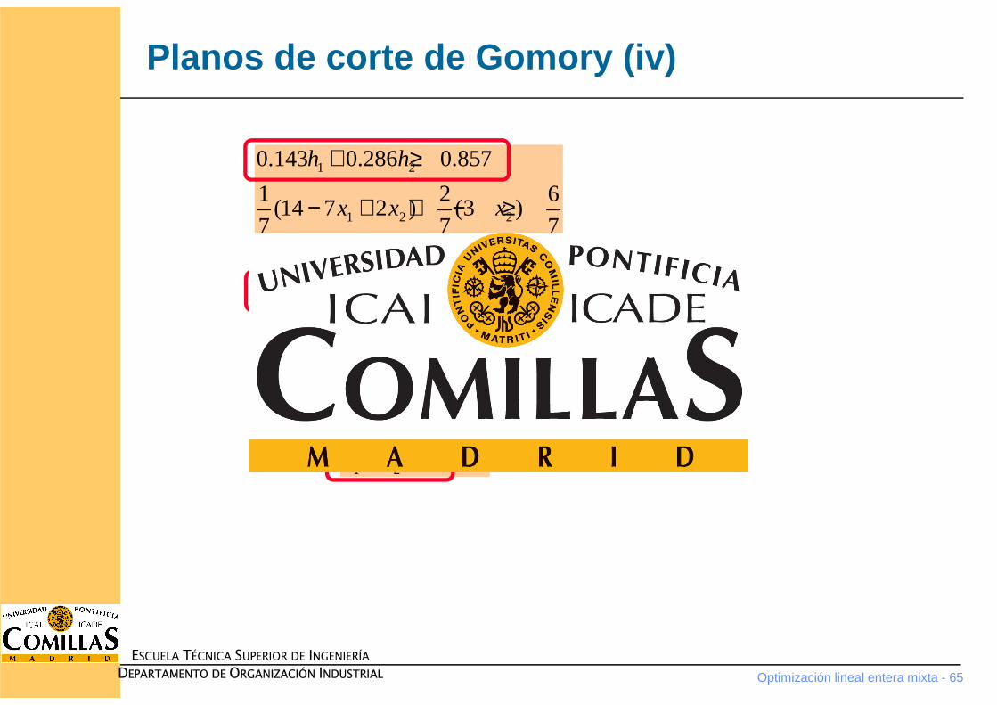
Planos de corte de Gomory (iv)
1 2
1 2 2
1
1
0.143 0.286 0.857
1 2 6(14 7 2 ) (3 )
7 7 77 14
2
h h
x x x
x
x
+ ≥
− + + − ≥
− ≥ −≤
3
1 2
1 2
0.5 0.5
3 2 2 1
1
h
x x
x x
≥− + ≥− ≤
Optimización lineal entera mixta - 66
ESCUELA TÉCNICA SUPERIOR DE INGENIERÍA
DEPARTAMENTO DE ORGANIZACIÓN INDUSTRIAL
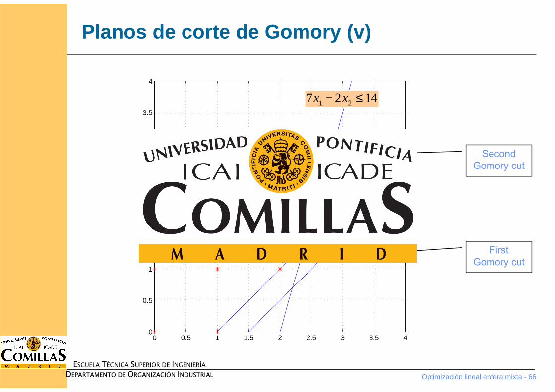
Planos de corte de Gomory (v)
0 0.5 1 1.5 2 2.5 3 3.5 40
0.5
1
1.5
2
2.5
3
3.5
4
1 22 2 3x x− ≤
1 27 2 14x x− ≤
2 3x ≤
1 2x ≤ 1 2 1x x− ≤
First Gomory cut
Second Gomory cut
Optimización lineal entera mixta - 67
ESCUELA TÉCNICA SUPERIOR DE INGENIERÍA
DEPARTAMENTO DE ORGANIZACIÓN INDUSTRIAL
Método de ramificación y corte (branch and cut)
� Método de ramificación y acotamiento + Método de planos de corte en los nodos
� Disminuye mucho el tiempo de resolución
� Procedimiento� Elección de un nodo para evaluar (inicialmente el nodo raíz es el
problema original relajado) y resolución
� Decisión sobre generar o no planos de corte. Si se obtienen se añaden al problema y se resuelve éste.
� Podar y ramificar con los criterios del método de ramificación y acotamiento.
Optimización lineal entera mixta - 68
ESCUELA TÉCNICA SUPERIOR DE INGENIERÍA
DEPARTAMENTO DE ORGANIZACIÓN INDUSTRIAL
CPLEX Performance Tuning for MIP
(http://www-01.ibm.com/support/docview.wss?uid=swg21400023)
� Names no
� NodeFileInd 3
� NodeSel 0
� VarSel 3
� StartAlg 4
� MemoryEmphasis 1
� WorkMem 1000
� MIPEmphasis 2
� MIPSearch 2
� SolveFinal 0
� Solution Polishing
� Solution pool
� FlowCovers
� FeasOptMode 2
� FeasOpt 1
� RINSHeur 0
� FpHeur 2
Pure branch and bround� Cuts -1
� HeurFreq -1
� Solution method of LP problem� First iteration (interior point or simplex
method)
� Successive iterations (primal or dual simplex)
� Priority for variable selection� Select variables that impact the most in the
o.f. (e.g., investment vs. operation variables)
� Initial cutoff or incumbent� Initial valid bound of the o.f. estimated by
the user
Optimización lineal entera mixta - 69
ESCUELA TÉCNICA SUPERIOR DE INGENIERÍA
DEPARTAMENTO DE ORGANIZACIÓN INDUSTRIAL
GUROBI (http://www.gurobi.com/documentation/5.6/reference-manual/ mip_models)
� Most important parameters
� Threads, MIPFocus
� Solution Improvement
� ImproveStartTime,
ImproveStartGap
� Termination
� TimeLimit
� MIPGap, MIPGapAbs
� NodeLimit, IterationLimit,
SolutionLimit
� Cutoff
� Speeding Up The Root Relaxation
� Method
� Heuristics
� Heuristics, SubMIPNodes,
MinRelNodes, PumpPasses,
ZeroObjNodes
� Heuristics
� Heuristics, SubMIPNodes,
MinRelNodes, PumpPasses,
ZeroObjNodes
� Cutting Planes
� Cuts, FlowCoverCuts, MIRCuts
� Presolve
� Presolve, PrePasses, AggFill,
PreSparsify

www.comillas.edu
www.comillas.edu
Andrés Ramos
Universidad Pontificia Comillashttp://www.iit.comillas.edu/aramos/