Localización Dinámica de Robots Móviles Basada en Filtrado ...font/downloads/IMAC_Kalman.pdf ·...
75
Josep Maria Font Llagunes [email protected] Localización Dinámica de Robots Móviles Basada en Filtrado de Kalman y Triangulación Universidad Pública de Navarra 13 de Noviembre de 2008 Departamento de Ingeniería Mecánica, Energética y de Materiales Departamento de Ingeniería Mecánica
Transcript of Localización Dinámica de Robots Móviles Basada en Filtrado ...font/downloads/IMAC_Kalman.pdf ·...
Josep Maria Font [email protected]
Localización Dinámica de Robots Móviles Basada en Filtrado de Kalman y Triangulación
Universidad Pública de Navarra
13 de Noviembre de 2008
Departamento de Ingeniería Mecánica,
Energética y de Materiales
Departamentode Ingeniería Mecánica

Presentation Contents
Introduction
Geometric Localization Using Triangulation
Error Analysis for the Robot Position
Dynamic Localization From Discontinuous Measurements
Experimental Results
Conclusions
A Novel Triangulation Approach
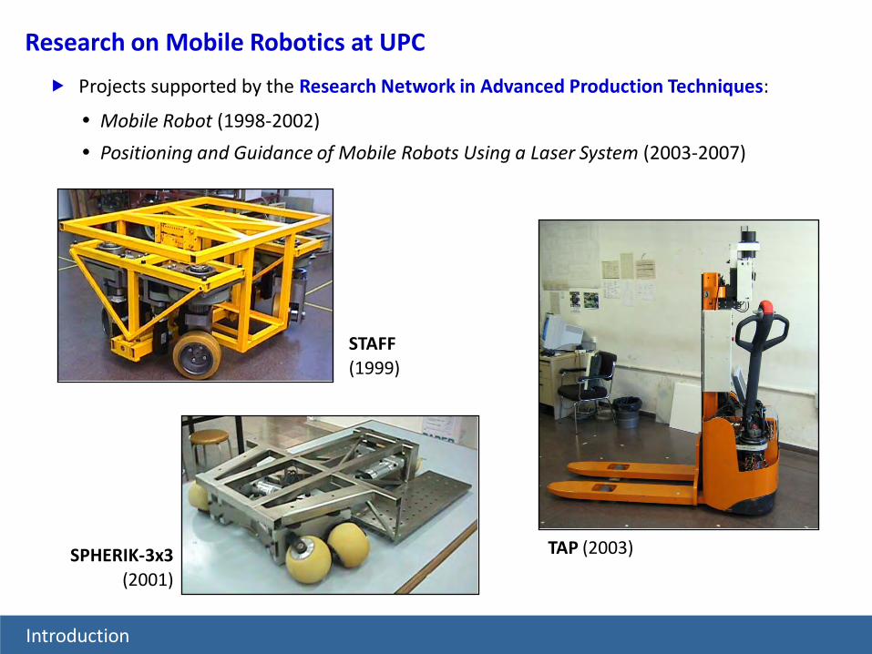
Projects supported by the Research Network in Advanced Production Techniques:
Mobile Robot (1998-2002)
Positioning and Guidance of Mobile Robots Using a Laser System (2003-2007)
SPHERIK-3x3(2001)
STAFF(1999)
TAP (2003)
Research on Mobile Robotics at UPC
Introduction
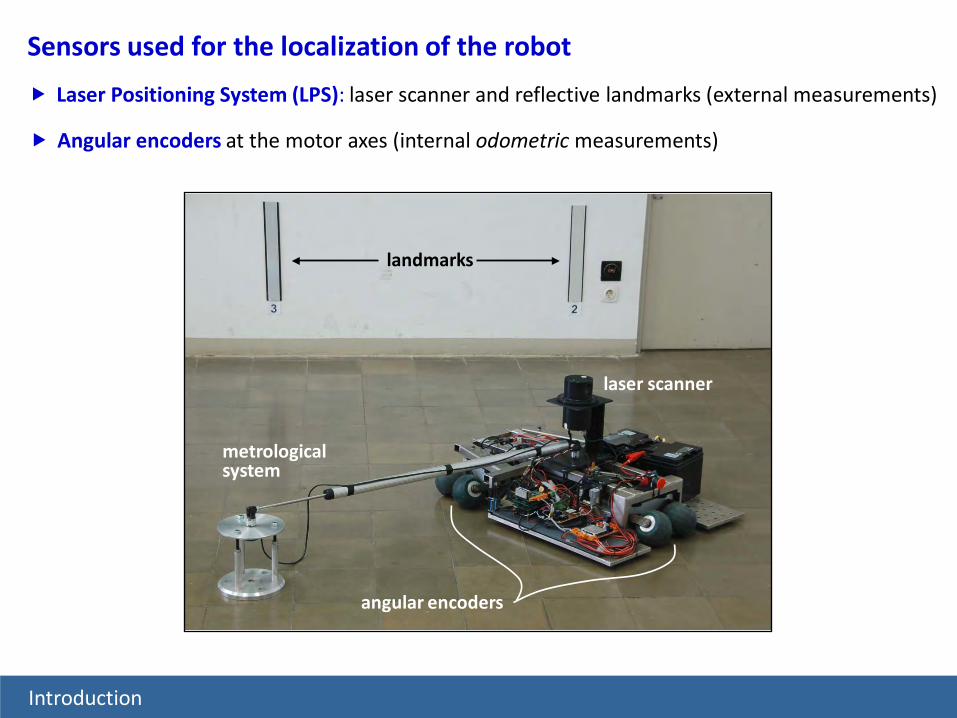
Laser Positioning System (LPS): laser scanner and reflective landmarks (external measurements)
landmarks
laser scanner
angular encoders
metrological system
Sensors used for the localization of the robot
Angular encoders at the motor axes (internal odometric measurements)
Introduction

Laser Positioning System
Introduction
angular encoder
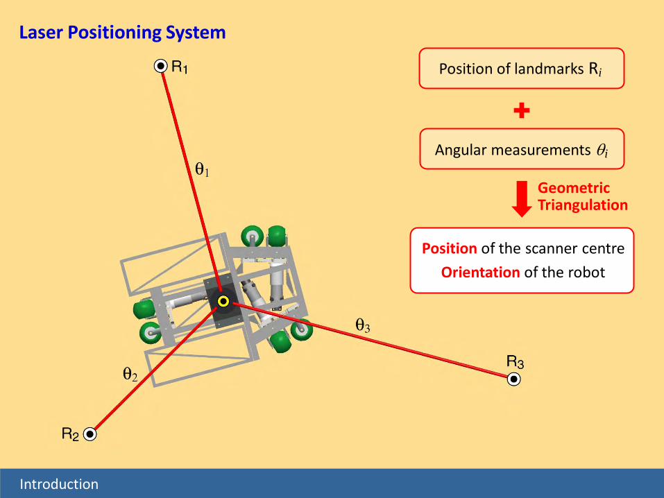
Position of landmarks Ri
Angular measurements θi
Geometric Triangulation
Position of the scanner centre
Orientation of the robot
Introduction
Laser Positioning System
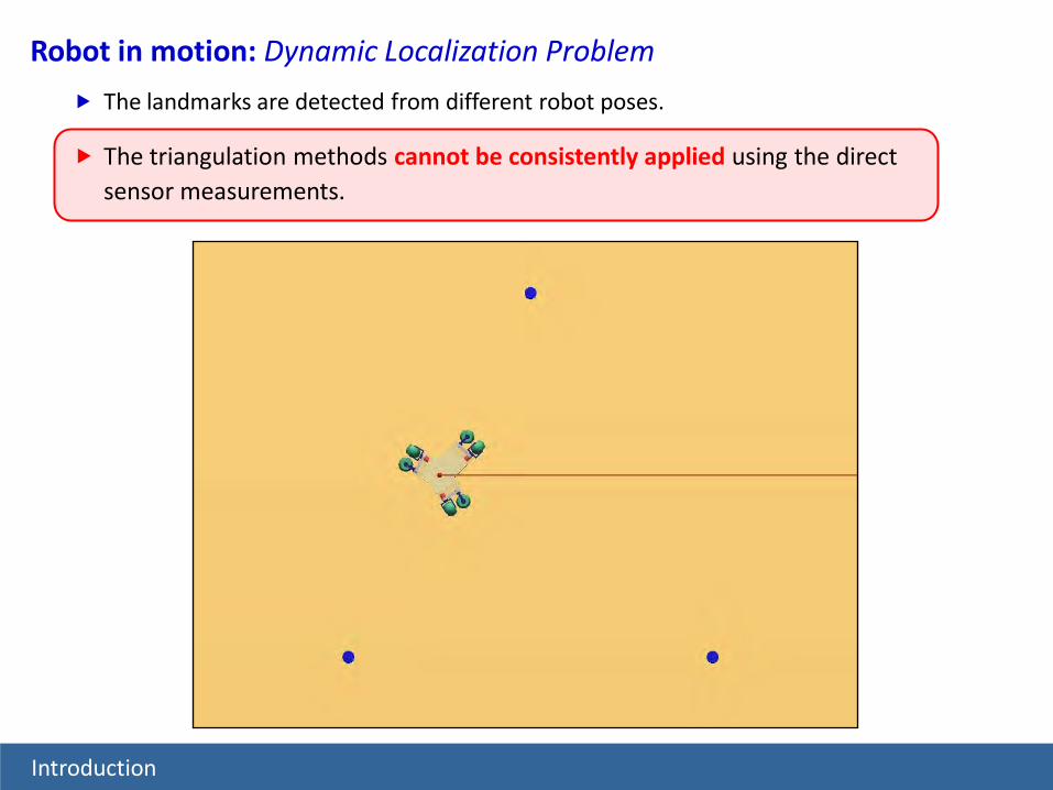
The landmarks are detected from different robot poses.
The triangulation methods cannot be consistently applied using the direct sensor measurements.
Robot in motion: Dynamic Localization Problem
Introduction
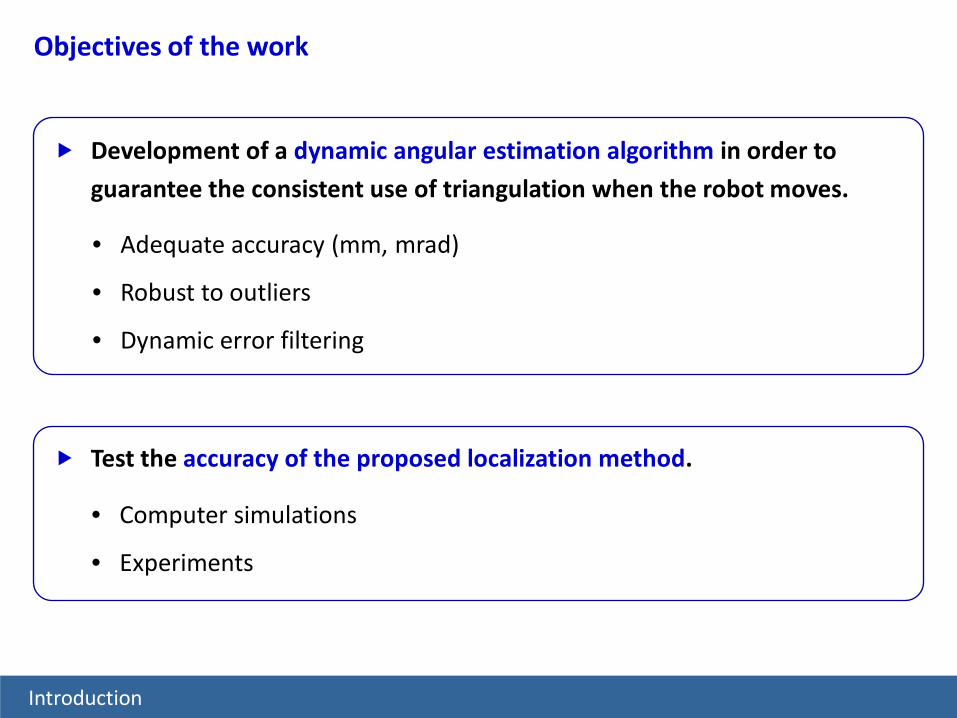
• Adequate accuracy (mm, mrad)
• Robust to outliers
• Dynamic error filtering
Development of a dynamic angular estimation algorithm in order to
guarantee the consistent use of triangulation when the robot moves.
Test the accuracy of the proposed localization method.
• Computer simulations
• Experiments
Objectives of the work
Introduction

Structure of the localization approach
Introduction
Odometers Localization Using Triangulation
Dynamic Angular Estimation
Sensors
( )i tθ ( )
( )( )
x ty t
tψ
Laser Sensor
(1) Data Fusion Problem (2) Geometric Problem
Introduction
Geometric Localization Using Triangulation
Error Analysis for the Robot Position
Dynamic Localization From Discontinuous Measurements
Experimental Results
Conclusions
A Novel Triangulation Approach
Presentation Contents
Definition of the geometric problem
Geometric Localization Using Triangulation
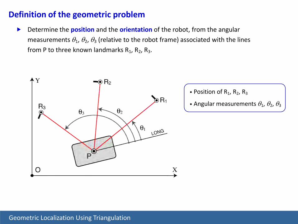
• Position of R1, R2, R3
• Angular measurements θ1, θ2, θ3
Determine the position and the orientation of the robot, from the angular
measurements θ1, θ2, θ3 (relative to the robot frame) associated with the lines
from P to three known landmarks R1, R2, R3.
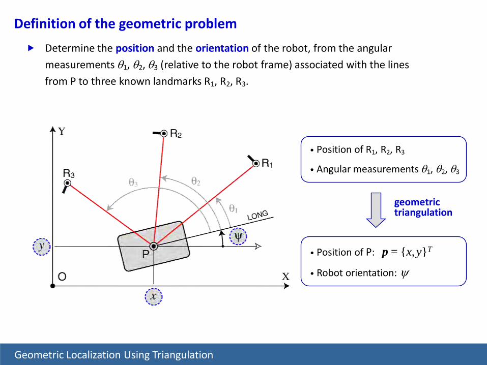
geometric triangulation
• Position of P: p = {x,y}T
• Robot orientation: ψ
• Position of R1, R2, R3
• Angular measurements θ1, θ2, θ3
Definition of the geometric problem
Geometric Localization Using Triangulation
Determine the position and the orientation of the robot, from the angular
measurements θ1, θ2, θ3 (relative to the robot frame) associated with the lines
from P to three known landmarks R1, R2, R3.
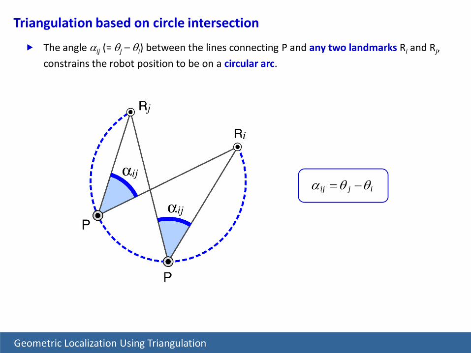
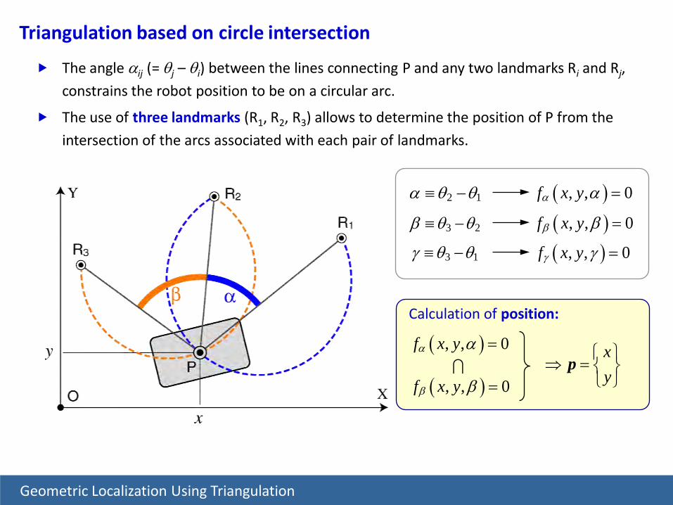
Triangulation based on circle intersection
Geometric Localization Using Triangulation
The angle αij (= θj – θi) between the lines connecting P and any two landmarks Ri and Rj,
constrains the robot position to be on a circular arc.
ij j iα θ θ= −
2 1α θ θ≡ − ( ), , 0f x yα α =
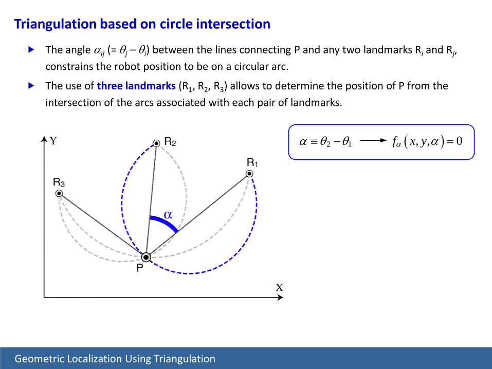
Geometric Localization Using Triangulation
Triangulation based on circle intersection
The angle αij (= θj – θi) between the lines connecting P and any two landmarks Ri and Rj,
constrains the robot position to be on a circular arc.
The use of three landmarks (R1, R2, R3) allows to determine the position of P from the
intersection of the arcs associated with each pair of landmarks.
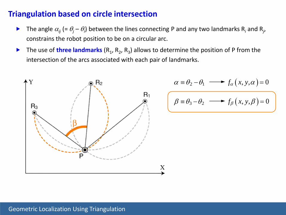
3 2β θ θ≡ − ( ), , 0f x yβ β =
2 1α θ θ≡ − ( ), , 0f x yα α =
Geometric Localization Using Triangulation
Triangulation based on circle intersection
The use of three landmarks (R1, R2, R3) allows to determine the position of P from the
intersection of the arcs associated with each pair of landmarks.
The angle αij (= θj – θi) between the lines connecting P and any two landmarks Ri and Rj,
constrains the robot position to be on a circular arc.

3 1γ θ θ≡ − ( ), , 0f x yγ γ =
3 2β θ θ≡ − ( ), , 0f x yβ β =
2 1α θ θ≡ − ( ), , 0f x yα α =
Geometric Localization Using Triangulation
Triangulation based on circle intersection
The use of three landmarks (R1, R2, R3) allows to determine the position of P from the
intersection of the arcs associated with each pair of landmarks.
The angle αij (= θj – θi) between the lines connecting P and any two landmarks Ri and Rj,
constrains the robot position to be on a circular arc.
Geometric Localization Using Triangulation
Triangulation based on circle intersection
The use of three landmarks (R1, R2, R3) allows to determine the position of P from the
intersection of the arcs associated with each pair of landmarks.
( ), , 0f x yα α =
( ), , 0f x yβ β =
xy
⇒ =
p
Calculation of position:
3 1γ θ θ≡ − ( ), , 0f x yγ γ =
3 2β θ θ≡ − ( ), , 0f x yβ β =
2 1α θ θ≡ − ( ), , 0f x yα α =
The angle αij (= θj – θi) between the lines connecting P and any two landmarks Ri and Rj,
constrains the robot position to be on a circular arc.
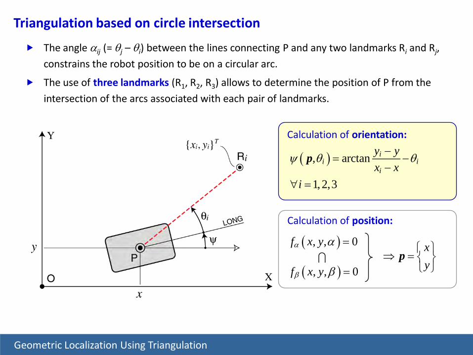
Geometric Localization Using Triangulation
( ), arctan
1,2,3
ii i
i
y yx x
i
ψ θ θ−= −
−∀ =
p
( ), , 0f x yα α =
( ), , 0f x yβ β =
xy
⇒ =
p
Calculation of orientation:
Triangulation based on circle intersection
The use of three landmarks (R1, R2, R3) allows to determine the position of P from the
intersection of the arcs associated with each pair of landmarks.
Calculation of position:
The angle αij (= θj – θi) between the lines connecting P and any two landmarks Ri and Rj,
constrains the robot position to be on a circular arc.
Geometric Localization Using Triangulation
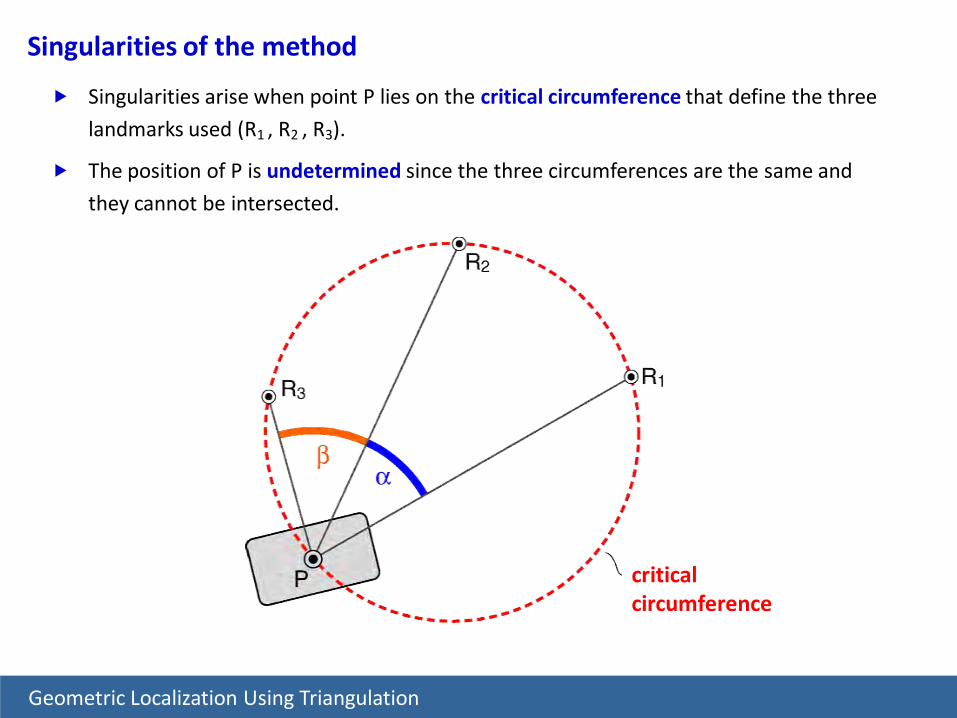
The position of P is undetermined since the three circumferences are the same and
they cannot be intersected.
Singularities of the method
Singularities arise when point P lies on the critical circumference that define the three
landmarks used (R1 , R2 , R3).
criticalcircumference

Introduction
Geometric Localization Using Triangulation
Error Analysis for the Robot Position
Dynamic Localization From Discontinuous Measurements
Experimental Results
Conclusions
A Novel Triangulation Approach
Presentation Contents
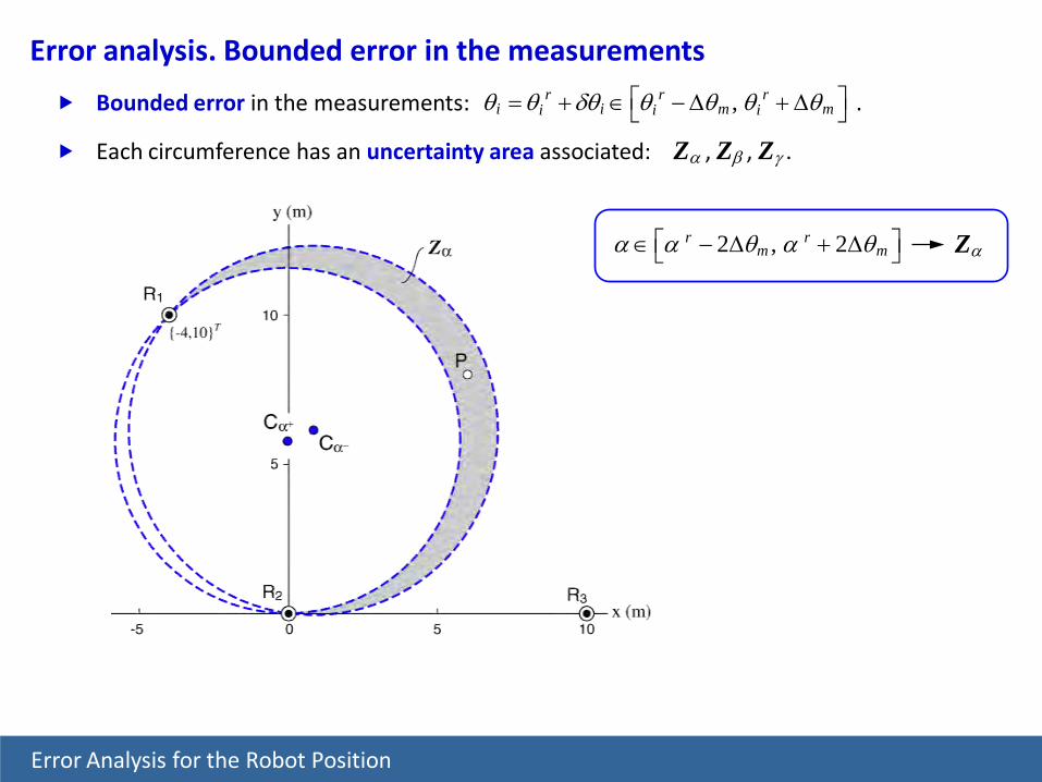
Error analysis. Bounded error in the measurements
Bounded error in the measurements: . ,r r ri i m mi i iθ θ δθ θ θ θ θ = + ∈ − ∆ + ∆
Each circumference has an uncertainty area associated: Zα , Zβ , Zγ .
2 , 2r rm mα α θ α θ ∈ − ∆ + ∆ Zα
Error Analysis for the Robot Position

2 , 2r rm mβ β θ β θ ∈ − ∆ + ∆ Zβ
2 , 2r rm mα α θ α θ ∈ − ∆ + ∆ Zα
Bounded error in the measurements: . ,r r ri i m mi i iθ θ δθ θ θ θ θ = + ∈ − ∆ + ∆
Each circumference has an uncertainty area associated: Zα , Zβ , Zγ .
Error analysis. Bounded error in the measurements
Error Analysis for the Robot Position
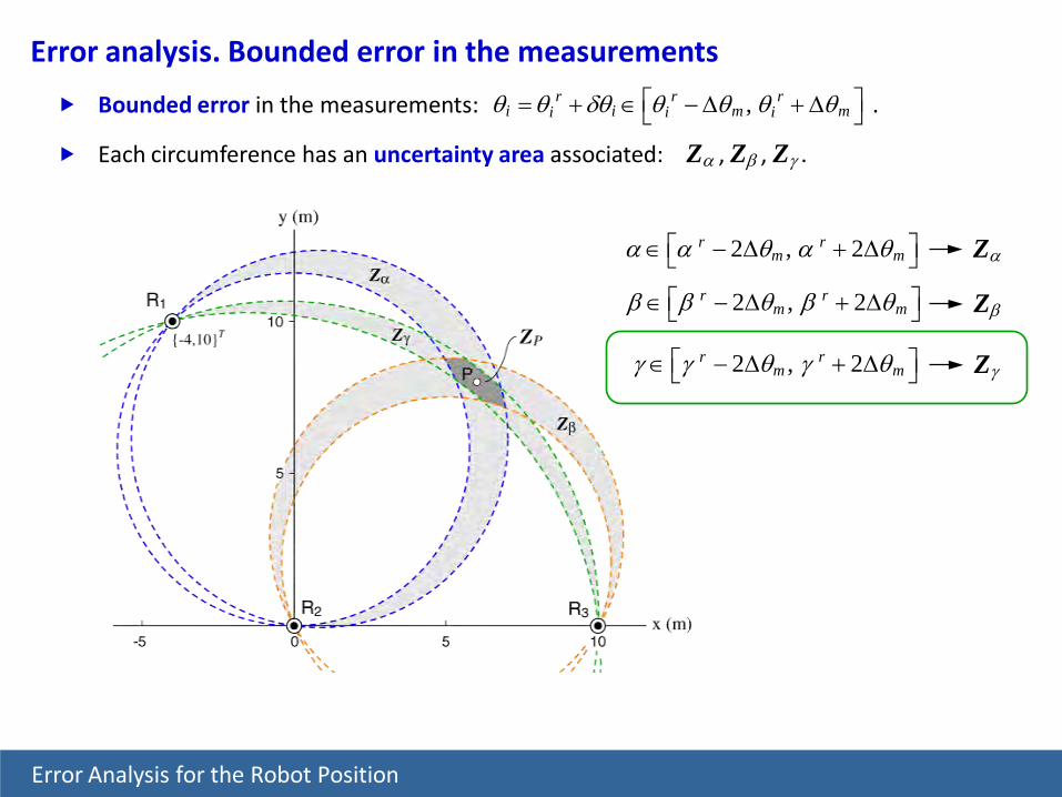
2 , 2r rm mγ γ θ γ θ ∈ − ∆ + ∆ Zγ
2 , 2r rm mβ β θ β θ ∈ − ∆ + ∆ Zβ
2 , 2r rm mα α θ α θ ∈ − ∆ + ∆ Zα
Bounded error in the measurements: . ,r r ri i m mi i iθ θ δθ θ θ θ θ = + ∈ − ∆ + ∆
Each circumference has an uncertainty area associated: Zα , Zβ , Zγ .
Error analysis. Bounded error in the measurements
Error Analysis for the Robot Position

3
, 1ijP
i ji j
α α β γ=
≠
= = ∩ ∩
Z Z Z Z Z
2 , 2r rm mγ γ θ γ θ ∈ − ∆ + ∆ Zγ
2 , 2r rm mβ β θ β θ ∈ − ∆ + ∆ Zβ
2 , 2r rm mα α θ α θ ∈ − ∆ + ∆ Zα
Bounded error in the measurements: . ,r r ri i m mi i iθ θ δθ θ θ θ θ = + ∈ − ∆ + ∆
Each circumference has an uncertainty area associated: Zα , Zβ , Zγ .
Error analysis. Bounded error in the measurements
Error Analysis for the Robot Position
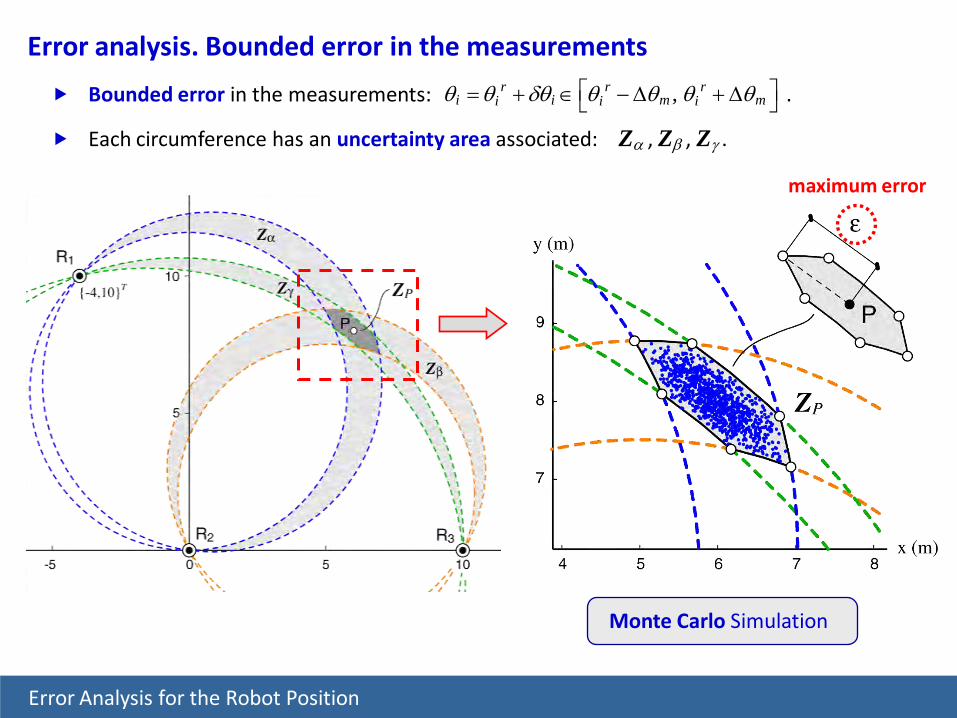
Monte Carlo Simulation
maximum error
Bounded error in the measurements: . ,r r ri i m mi i iθ θ δθ θ θ θ θ = + ∈ − ∆ + ∆
Each circumference has an uncertainty area associated: Zα , Zβ , Zγ .
Error analysis. Bounded error in the measurements
Error Analysis for the Robot Position

x (m)y
(m)
-5 0 5
-2
0
2
4
6
8
10
12
0
5
10
15
20
25
30
x (m)
y (m
)
0 5 10
-2
0
2
4
6
8
10
12
0
2
4
6
8
10
12
14
16
18
20
ε (mm)
Mapping of the Maximum Error (for ∆θm = 0,2 mrad)
Error analysis. Bounded error in the measurements
Error Analysis for the Robot Position
ε (mm)
Error analysis. Gaussian error in the measurements
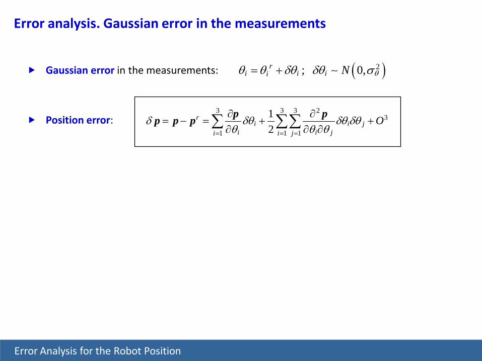
Gaussian error in the measurements:
Position error:
( )2; 0,ri i ii N θθ θ δθ δθ σ= +
3 3 3 23
1 1 1
12
ri i j
i i ji i jOδ δθ δθ δθ
θ θ θ= = =
∂ ∂= − = + +
∂ ∂ ∂∑ ∑∑p pp p p
Error Analysis for the Robot Position

Error analysis. Gaussian error in the measurements
Gaussian error in the measurements:
Position error: 3 3 3 2
3
1 1 1
12
ri i j
i i ji i jOδ δθ δθ δθ
θ θ θ= = =
∂ ∂= − = + +
∂ ∂ ∂∑ ∑∑p pp p p
Expected value of the position error:
{ }2 2 2 2
2 2 21 2 32
E θσδθ θ θ
∂ ∂ ∂= + + ∂ ∂ ∂
p p pp
Error Analysis for the Robot Position
( )2; 0,ri i ii N θθ θ δθ δθ σ= +
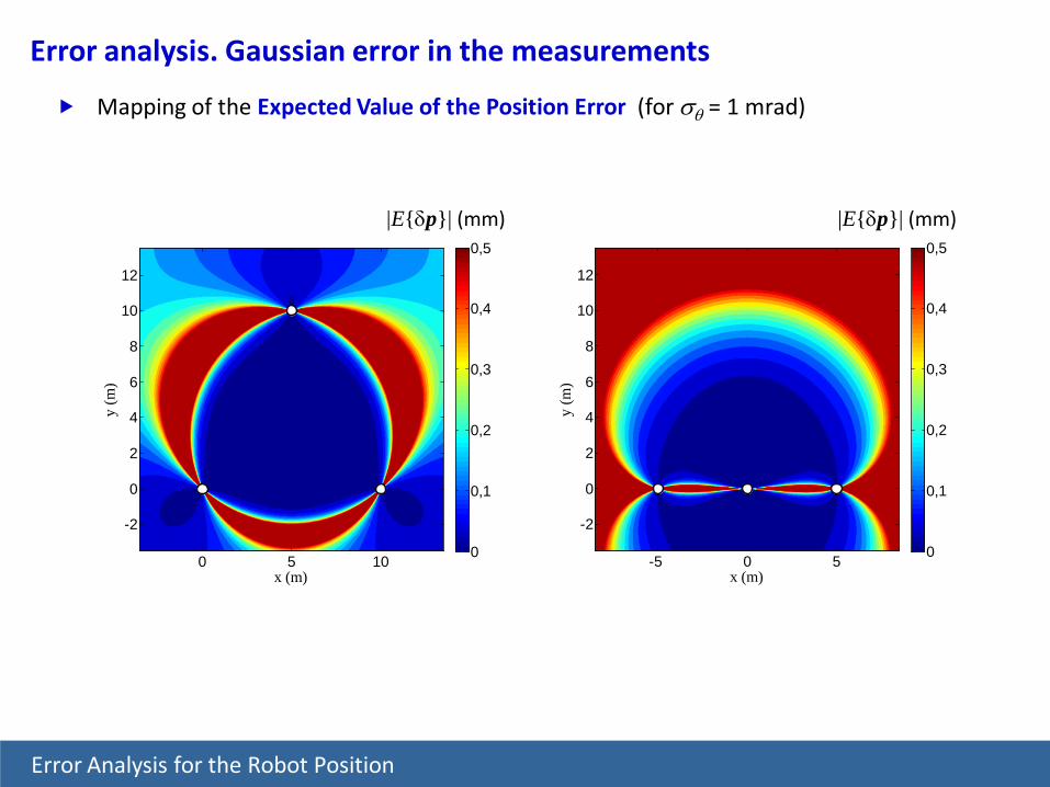
Mapping of the Expected Value of the Position Error (for σθ = 1 mrad)
x (m)
y (m
)
0 5 10
-2
0
2
4
6
8
10
12
0
0,1
0,2
0,3
0,4
0,5
x (m)y
(m)
-5 0 5
-2
0
2
4
6
8
10
12
0
0,1
0,2
0,3
0,4
0,5
|E{δp}| (mm)
Error Analysis for the Robot Position
Error analysis. Gaussian error in the measurements
|E{δp}| (mm)
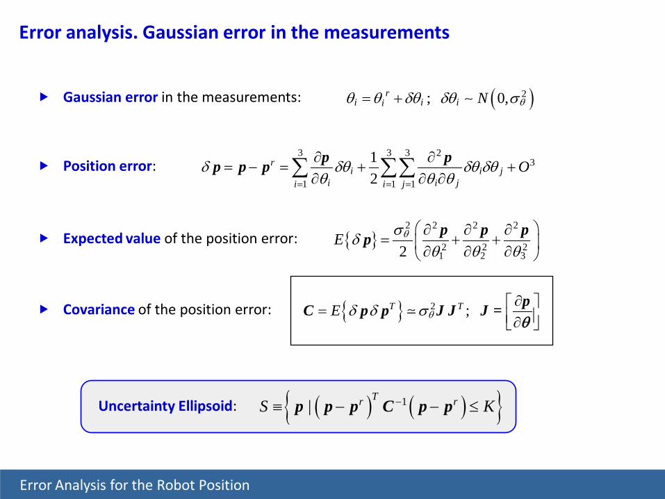
{ } 2 ;T TE θδ δ σ ∂ = ∂
pC p p J J J =θ
Error analysis. Gaussian error in the measurements
Gaussian error in the measurements:
Position error:
( )2; 0,ri i ii N θθ θ δθ δθ σ= +
3 3 3 23
1 1 1
12
ri i j
i i ji i jOδ δθ δθ δθ
θ θ θ= = =
∂ ∂= − = + +
∂ ∂ ∂∑ ∑∑p pp p p
Expected value of the position error:
{ }2 2 2 2
2 2 21 2 32
E θσδθ θ θ
∂ ∂ ∂= + + ∂ ∂ ∂
p p pp
Covariance of the position error:
( ) ( ){ }1Tr rS | K−≡ − − ≤p p p C p pUncertainty Ellipsoid:
Error Analysis for the Robot Position
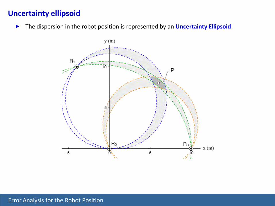
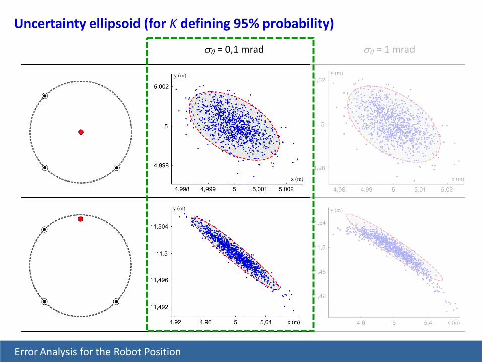
The dispersion in the robot position is represented by an Uncertainty Ellipsoid.
Uncertainty ellipsoid
Error Analysis for the Robot Position
Uncertainty Ellipsoid (S)
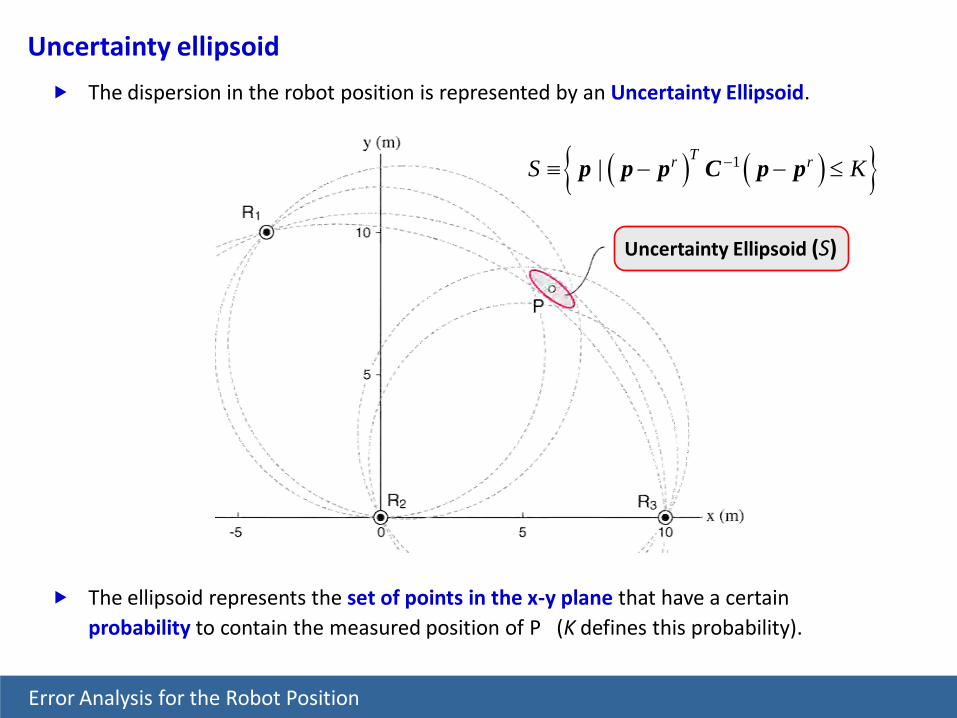
The ellipsoid represents the set of points in the x-y plane that have a certain probability to contain the measured position of P (K defines this probability).
Uncertainty ellipsoid
Error Analysis for the Robot Position
( ) ( ){ }1Tr rS | K−≡ − − ≤p p p C p p
The dispersion in the robot position is represented by an Uncertainty Ellipsoid.
Uncertainty ellipsoid
Error Analysis for the Robot Position
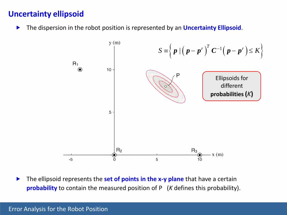
Ellipsoids for different
probabilities (K)
( ) ( ){ }1Tr rS | K−≡ − − ≤p p p C p p
The dispersion in the robot position is represented by an Uncertainty Ellipsoid.
The ellipsoid represents the set of points in the x-y plane that have a certain probability to contain the measured position of P (K defines this probability).
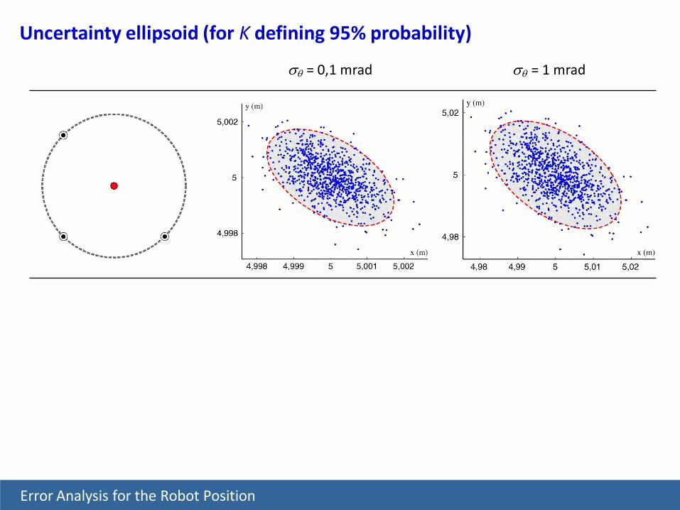
σθ = 0,1 mrad σθ = 1 mrad
Uncertainty ellipsoid (for K defining 95% probability)
Error Analysis for the Robot Position
σθ = 0,1 mrad σθ = 1 mrad
Uncertainty ellipsoid (for K defining 95% probability)
Error Analysis for the Robot Position

Introduction
Geometric Localization Using Triangulation
Error Analysis for the Robot Position
Dynamic Localization From Discontinuous Measurements
Experimental Results
Conclusions
A Novel Triangulation Approach
Presentation Contents
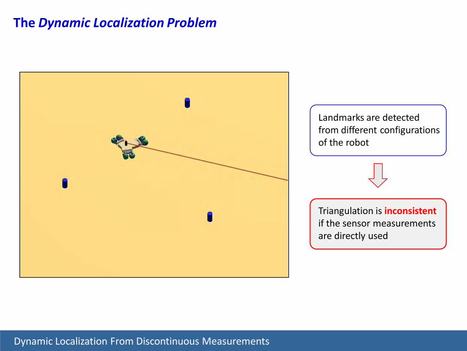
Dynamic Localization From Discontinuous Measurements
Landmarks are detected from different configurations of the robot
Triangulation is inconsistentif the sensor measurements are directly used
The Dynamic Localization Problem

Suggested solution: Dynamic Angular Estimation
Real-time simulation of the landmark angles based on odometric information
Guarantees the consistent use of the triangulation methods using the simulated angles
Dynamic Localization From Discontinuous Measurements

( ) ( )0
0sin cost L i T i
i it i
v vt t dtθ θθ θ ψρ−
= + −∫
Angular odometry
Between actual sensor measurements, angle θi can be predicted integrating the following equation that governs its time rate of change:
( ) sin cosL i T ii
i
v vt
θ θψ θρ
∂ −+ =
∂
Dynamic Localization From Discontinuous Measurements

( ) ( )0
0sin cost L i T i
i it i
v vt t dtθ θθ θ ψρ−
= + −∫
( ) sin cosL i T ii
i
v vt
θ θψ θρ
∂ −+ =
∂
Cumulative error in the odometric prediction
Variables vL , vT , ψ are obtained from the odometric measurements
Error in the discontinuous angular observationsKalman Filtering EKF
Dynamic Localization From Discontinuous Measurements
Angular odometry
Between actual sensor measurements, angle θi can be predicted integrating the following equation that governs its time rate of change:

Angular odometry. Kinematics of the robot SPHERIK-3x3
3-DOF mobile robot with 3 omnidirectional wheels consisting of two spherical rollers. Each wheel is actuated by a single motor.
Motorized motionControlled by the motor
Free motionIt adapts to the kinematics
imposed by the set of motors
Dynamic Localization From Discontinuous Measurements
motorized motion
freemotion

1
2
3
0 11 cos sin
cos sin
L
T
L vs v
rs
Jω
ωω α αω α α ψ
− − = − − −
11
2
3
L
T
vv Jω
ωω
ψ ω
−
=
motor encoders
Dynamic Localization From Discontinuous Measurements
Angular odometry. Kinematics of the robot SPHERIK-3x3
3-DOF mobile robot with 3 omnidirectional wheels consisting of two spherical rollers. Each wheel is actuated by a single motor.

LONGITUDINAL DOF
Dynamic Localization From Discontinuous Measurements

TRANSVERSAL DOF
Dynamic Localization From Discontinuous Measurements

ROTATIONAL DOF
Dynamic Localization From Discontinuous Measurements
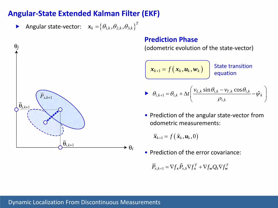
Angular-State Extended Kalman Filter (EKF)
• Prediction of the angular state-vector from odometric measurements:
• Prediction of the error covariance:
, 1 ,T T
x k x k kP f P f f Q f+ = ∇ ∇ + ∇ ∇x x w w
Prediction Phase(odometric evolution of the state-vector)
( )1 , ,k k k kf+ =x x u w
, , , ,
, 1 ,,
sin cosL k i k T k i ki k i k k
i k
v vt θ θθ θ ψρ+
−= + ∆ −
( )1 , ,0k k kf+ = x x u
Angular state-vector: { }1, 2, 3,, , Tk k k kθ θ θ=x
State transition equation
Dynamic Localization From Discontinuous Measurements
• Correction of the odometrically predicted state-vector:
• Estimation of the error covariance:
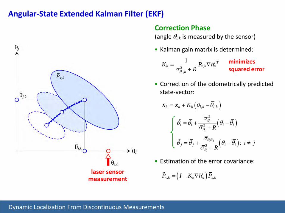
Correction Phase(angle θi,k is measured by the sensor)
( ), ,k k k i k i kK θ θ= + −x x
( )
2
2i
i
i i i iRθ
θ
σθ θ θ θ
σ= + −
+
( )2 ;i j
i
j j i i i jR
θ θ
θ
σθ θ θ θ
σ= + − ≠
+
( ), ,i
x k k x kP I K h P= − ∇ x
• Kalman gain matrix is determined:
,2
,
1
i
i Tk x k
kK P h
Rθσ= ∇
+x
minimizessquared error
laser sensormeasurement
Dynamic Localization From Discontinuous Measurements
Angular-State Extended Kalman Filter (EKF)
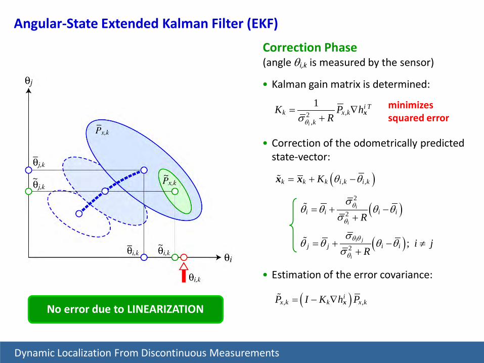
No error due to LINEARIZATION
Dynamic Localization From Discontinuous Measurements
• Correction of the odometrically predicted state-vector:
• Estimation of the error covariance:
Correction Phase(angle θi,k is measured by the sensor)
( ), ,k k k i k i kK θ θ= + −x x
( )
2
2i
i
i i i iRθ
θ
σθ θ θ θ
σ= + −
+
( )2 ;i j
i
j j i i i jR
θ θ
θ
σθ θ θ θ
σ= + − ≠
+
( ), ,i
x k k x kP I K h P= − ∇ x
• Kalman gain matrix is determined:
,2
,
1
i
i Tk x k
kK P h
Rθσ= ∇
+x
minimizessquared error
Angular-State Extended Kalman Filter (EKF)
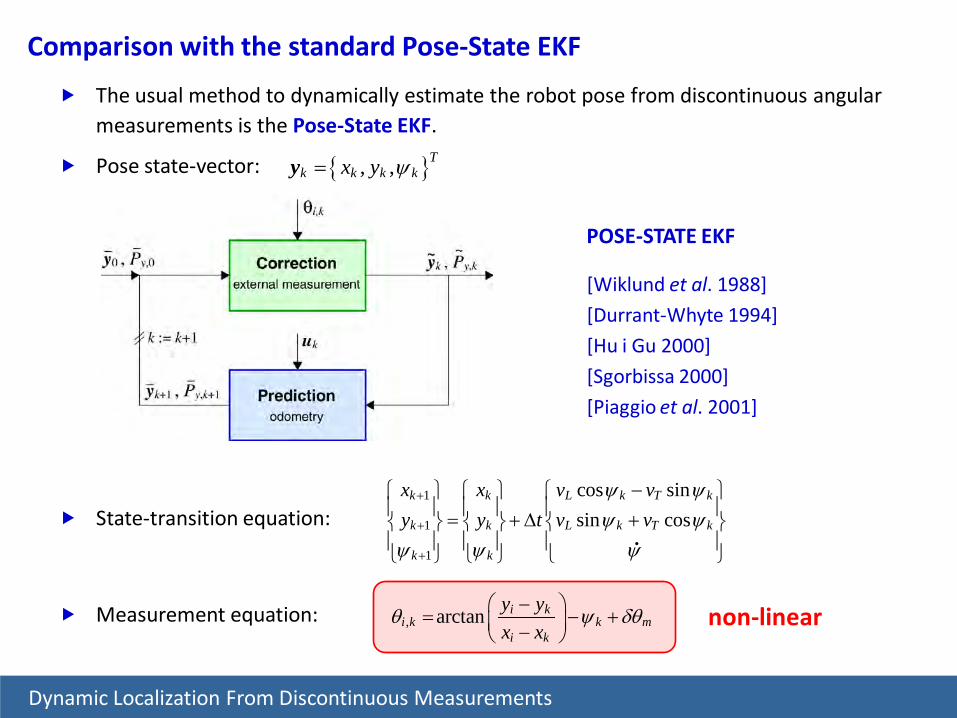
Comparison with the standard Pose-State EKF
POSE-STATE EKF
[Wiklund et al. 1988]
[Durrant-Whyte 1994]
[Hu i Gu 2000]
[Sgorbissa 2000]
[Piaggio et al. 2001]
The usual method to dynamically estimate the robot pose from discontinuous angular measurements is the Pose-State EKF.
State-transition equation:
Measurement equation:
, arctan i ki k k m
i k
y yx x
θ ψ δθ− = − + − non-linear
1
1
1
cos sinsin cos
k k L k T k
k k L k T k
k k
x x v vy y t v v
ψ ψψ ψ
ψ ψ ψ
+
+
+
− = + ∆ +
{ }, , Tk k k kx y ψ=y Pose state-vector:
Dynamic Localization From Discontinuous Measurements

Change of the State Space of the Kalman Filter
Dynamic Localization From Discontinuous Measurements
Comparison with the standard Pose-State EKF
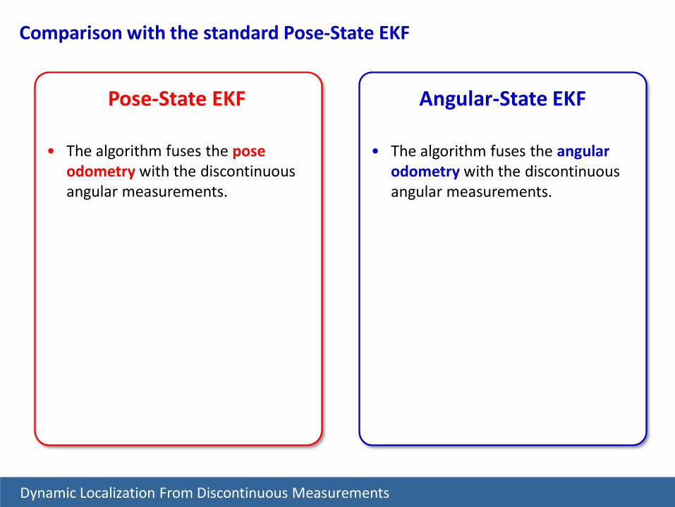
• The algorithm fuses the pose odometry with the discontinuous angular measurements.
• The algorithm fuses the angular odometry with the discontinuous angular measurements.
Pose-State EKF Angular-State EKF
Dynamic Localization From Discontinuous Measurements
Comparison with the standard Pose-State EKF
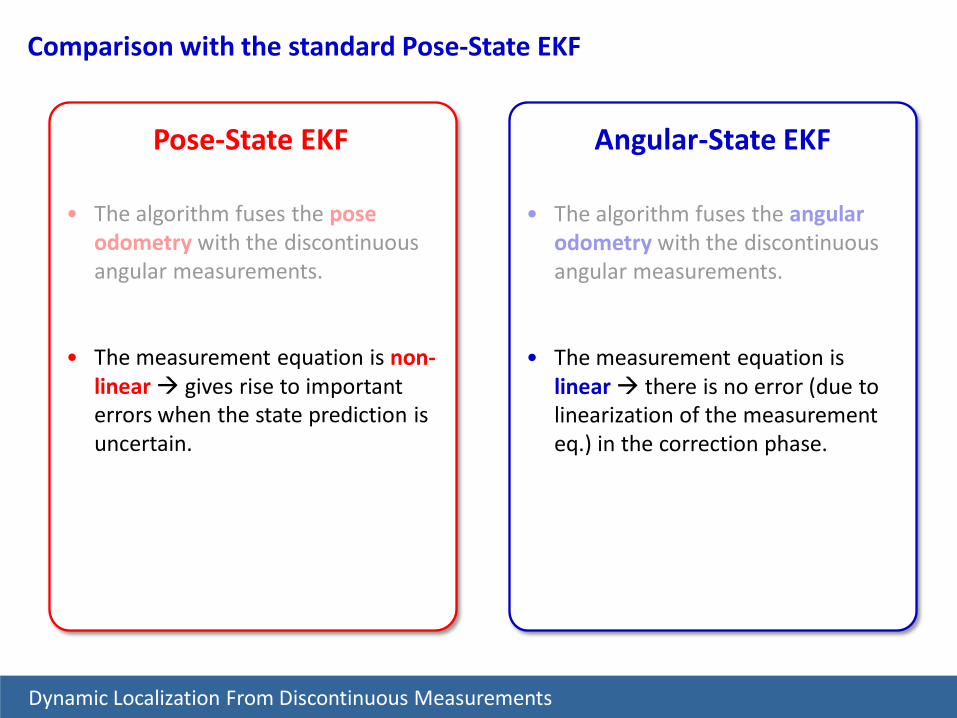
• The algorithm fuses the pose odometry with the discontinuous angular measurements.
• The measurement equation is non-linear gives rise to important errors when the state prediction is uncertain.
• The algorithm fuses the angular odometry with the discontinuous angular measurements.
• The measurement equation islinear there is no error (due to linearization of the measurement eq.) in the correction phase.
Dynamic Localization From Discontinuous Measurements
Pose-State EKF Angular-State EKF
Comparison with the standard Pose-State EKF
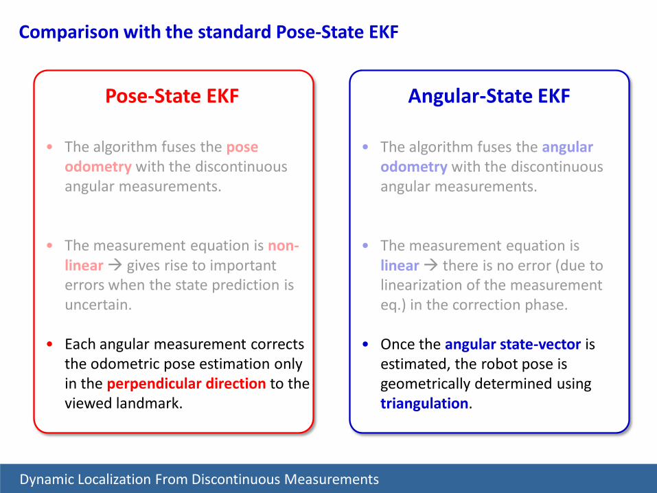
• The algorithm fuses the pose odometry with the discontinuous angular measurements.
• The measurement equation is non-linear gives rise to important errors when the state prediction is uncertain.
• Each angular measurement corrects the odometric pose estimation only in the perpendicular direction to the viewed landmark.
• The algorithm fuses the angular odometry with the discontinuous angular measurements.
• The measurement equation islinear there is no error (due to linearization of the measurement eq.) in the correction phase.
• Once the angular state-vector is estimated, the robot pose is geometrically determined using triangulation.
Dynamic Localization From Discontinuous Measurements
Pose-State EKF Angular-State EKF
Comparison with the standard Pose-State EKF

Introduction
Geometric Localization Using Triangulation
Error Analysis for the Robot Position
Dynamic Localization From Discontinuous Measurements
Experimental Results
Conclusions
A Novel Triangulation Approach
Presentation Contents
1,
1,
cossin
mk kk
mk kk
lxly
ϕϕ
=
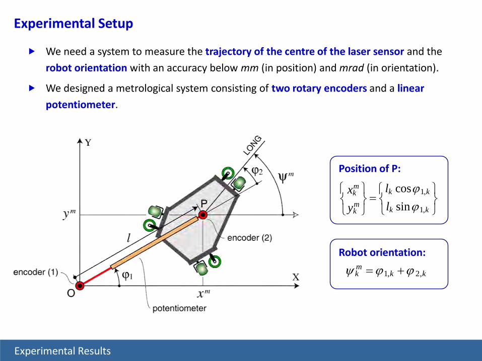
Experimental Setup
We need a system to measure the trajectory of the centre of the laser sensor and the
robot orientation with an accuracy below mm (in position) and mrad (in orientation).
We designed a metrological system consisting of two rotary encoders and a linear
potentiometer.
Position of P:
Robot orientation:
Experimental Results
1, 2,mk k kψ ϕ ϕ= +

Experimental Results
1,
1,
cossin
mk kk
mk kk
lxly
ϕϕ
=
Position of P:
Robot orientation: 1, 2,
mk k kψ ϕ ϕ= +
We need a system to measure the trajectory of the centre of the laser sensor and the
robot orientation with an accuracy below mm (in position) and mrad (in orientation).
We designed a metrological system consisting of two rotary encoders and a linear
potentiometer.
Experimental Setup
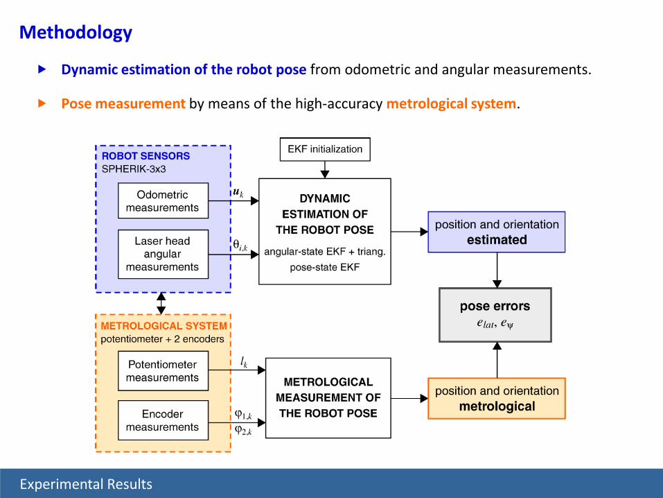
Dynamic estimation of the robot pose from odometric and angular measurements.
Methodology
Experimental Results
Pose measurement by means of the high-accuracy metrological system.

potentiometer
Control system and data adquisition module
Experimental Results
Layout of the electronic components on the robot.
laser head
power amplifiers
DAQ-module and DSP
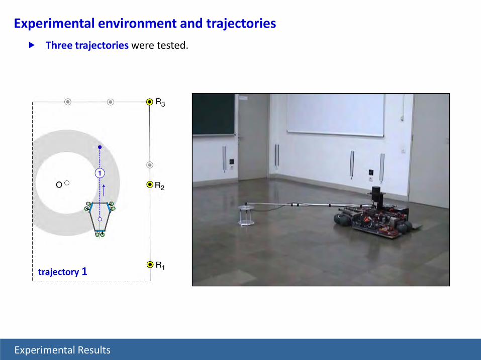
Experimental environment and trajectories Three trajectories were tested.
trajectory 1
Experimental Results

Experimental Results
trajectory 2
Experimental environment and trajectories Three trajectories were tested.
Experimental Results
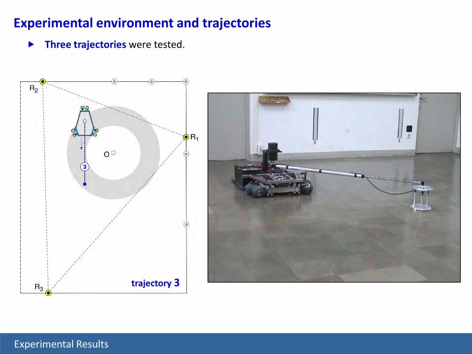
Experimental environment and trajectories Three trajectories were tested.
trajectory 3

Angular-State EKF –4,24 mm
Pose-State EKF –84,31 mm
Results. Lateral error (trajectory 1)
elat
Angular-State EKF 1,30 mm
Pose-State EKF 4,94 mm
RMS (elat)
Experimental Results
3rd detection

Angular-State EKF –1,74 mrad
Pose-State EKF 23,28 mrad
eψ
Pose-State EKF 3,26 mrad
RMS (eψ)
Experimental Results
Angular-State EKF 1,06 mrad
Results. Orientation error (trajectory 1)
3rd detection
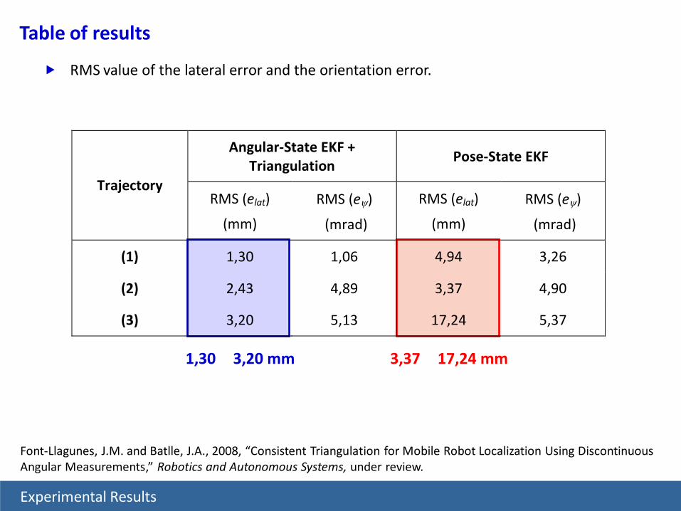
Angular-State EKF + Triangulation
Pose-State EKF
Trajectory RMS (elat)
(mm)
RMS (eψ)
(mrad)
RMS (elat)
(mm)
RMS (eψ)
(mrad)
(1) 1,30 1,06 4,94 3,26
(2) 2,43 4,89 3,37 4,90
(3) 3,20 5,13 17,24 5,37
RMS value of the lateral error and the orientation error.
Table of results
1,30 3,20 mm 3,37 17,24 mm
Experimental Results
Font-Llagunes, J.M. and Batlle, J.A., 2008, “Consistent Triangulation for Mobile Robot Localization Using Discontinuous Angular Measurements,” Robotics and Autonomous Systems, under review.
Experimental Results
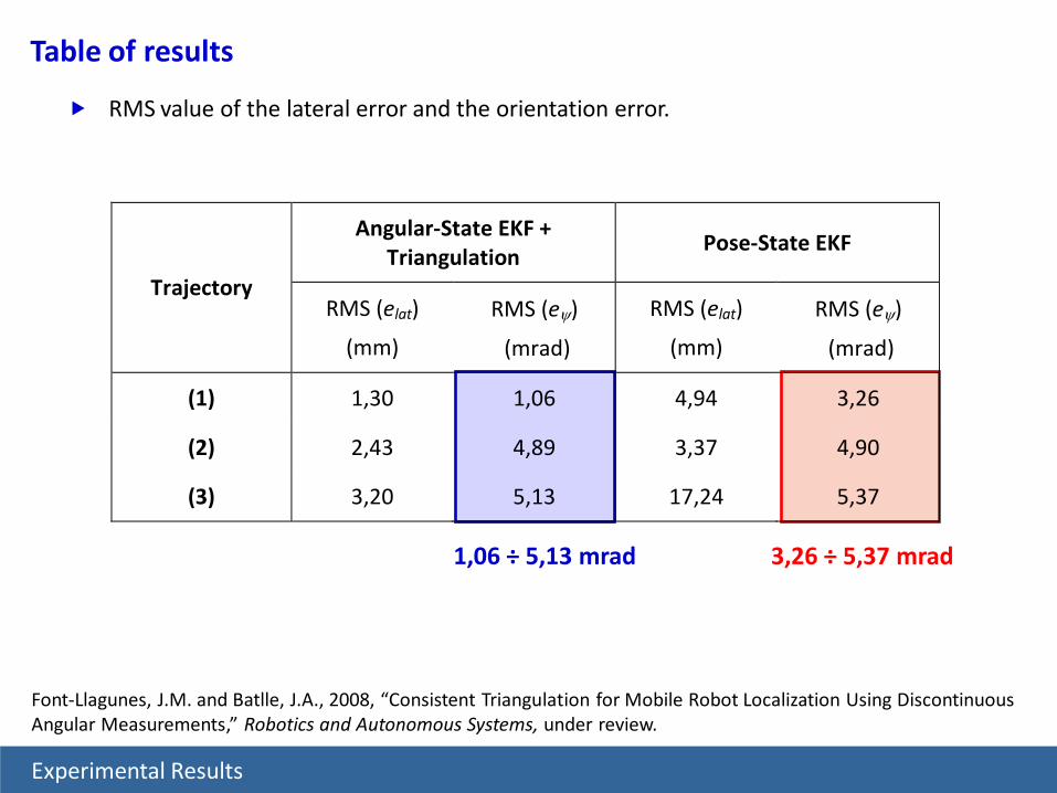
Angular-State EKF + Triangulation
Pose-State EKF
Trajectory RMS (elat)
(mm)
RMS (eψ)
(mrad)
RMS (elat)
(mm)
RMS (eψ)
(mrad)
(1) 1,30 1,06 4,94 3,26
(2) 2,43 4,89 3,37 4,90
(3) 3,20 5,13 17,24 5,37
1,06 ÷ 5,13 mrad 3,26 ÷ 5,37 mrad
RMS value of the lateral error and the orientation error.
Table of results
Font-Llagunes, J.M. and Batlle, J.A., 2008, “Consistent Triangulation for Mobile Robot Localization Using Discontinuous Angular Measurements,” Robotics and Autonomous Systems, under review.

Introduction
Geometric Localization Using Triangulation
Error Analysis for the Robot Position
Dynamic Localization From Discontinuous Measurements
Experimental Results
Conclusions
A Novel Triangulation Approach
Presentation Contents
Conclusions
Conclusions
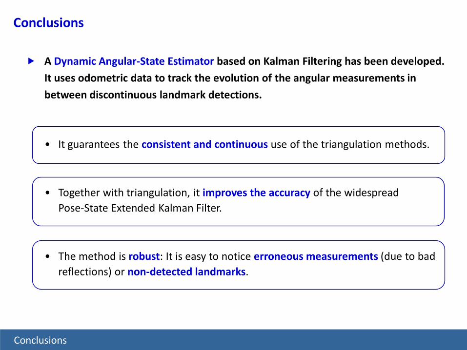
• It guarantees the consistent and continuous use of the triangulation methods.
A Dynamic Angular-State Estimator based on Kalman Filtering has been developed.
It uses odometric data to track the evolution of the angular measurements in
between discontinuous landmark detections.
• Together with triangulation, it improves the accuracy of the widespread Pose-State Extended Kalman Filter.
• The method is robust: It is easy to notice erroneous measurements (due to bad reflections) or non-detected landmarks.

Introduction
Geometric Localization Using Triangulation
Error Analysis for the Robot Position
Dynamic Localization From Discontinuous Measurements
Experimental Results
Conclusions
Presentation Contents
A Novel Triangulation Approach

The method has no singularities if three unaligned landmarks are used.
If the orientation angle ψ is known, the position of P can be determined using straight-line intersection.
Novel triangulation method based on straight-line intersection
P not aligned with Ri i RjP aligned with Ri i Rj a third
unaligned landmark is needed (Rk)
A Novel Triangulation Approach

Before triangulating the orientation ψ is not known, but an approximation of it can be used:
If ψe ≠ ψ , then the lines intersect in three points O12 , O13 , O23 (these define the error triangle).
Triangulation based on straight lines. Error triangle
Orientation Error e ψψ ψ ε≡ +
e ψψ ψ ε≡ +Approximate Orientation
Iterative Method
[Cohen and Koss 1992]
error triangle
A Novel Triangulation Approach

Is there any geometric relationship between the error triangle and εψ
Error triangles for different values of εψ :?
Triangulation based on straight lines. Error triangle
A Novel Triangulation Approach

α sin2εψ
α sinεψ
Area
Perimeter
Is there any geometric relationship between the error triangle and εψ
Error triangles for different values of εψ :?
Triangulation based on straight lines. Error triangle
A Novel Triangulation Approach
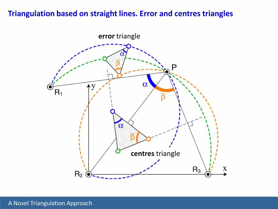
error triangle
centres triangle
Triangulation based on straight lines. Error and centres triangles
A Novel Triangulation Approach

Geometric relationships
Similarity ratio between the triangles:
O
C2sinr ψ
ρ ερ
≡ = O O
arcsin2 C C
ij ik
ij ikψε =
Font-Llagunes, J.M. and Batlle, J.A., 2008, “A new method that solves the three-point resection problem using straight lines intersection,” Journal of Surveying Engineering, to appear.
A Novel Triangulation Approach
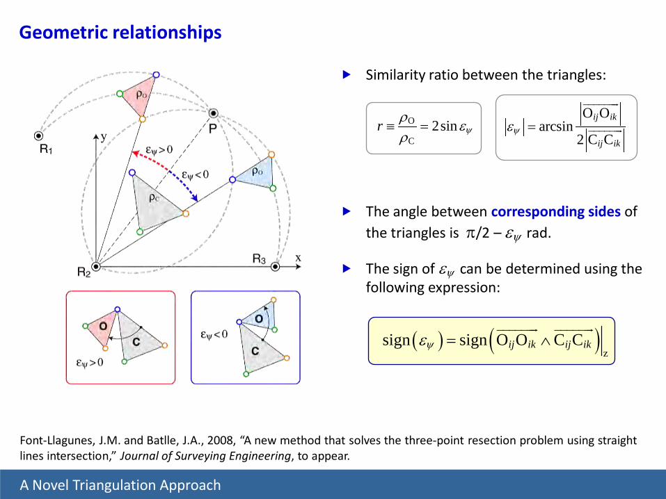
( ) ( )z
sign sign O O C Cij ik ij ikψε = ∧
The angle between corresponding sides of the triangles is π/2 – εψ rad.
The sign of εψ can be determined using the following expression:
Similarity ratio between the triangles:
O
C2sinr ψ
ρ ερ
≡ = O O
arcsin2 C C
ij ik
ij ikψε =
Geometric relationships
Font-Llagunes, J.M. and Batlle, J.A., 2008, “A new method that solves the three-point resection problem using straight lines intersection,” Journal of Surveying Engineering, to appear.
A Novel Triangulation Approach