
Image segmentation integrating colour, texture and boundary ...
234
IMAGE SEGMENTATION INTEGRATING COLOUR, TEXTURE AND BOUNDARY INFORMATION Xavier MUÑOZ PUJOL ISBN: 84-688-4933-2 Dipòsit legal: GI-1601-2003 http://hdl.handle.net/10803/7719 ADVERTIMENT. L'accés als continguts d'aquesta tesi doctoral i la seva utilització ha de respectar els drets de la persona autora. Pot ser utilitzada per a consulta o estudi personal, així com en activitats o materials d'investigació i docència en els termes establerts a l'art. 32 del Text Refós de la Llei de Propietat Intel·lectual (RDL 1/1996). Per altres utilitzacions es requereix l'autorització prèvia i expressa de la persona autora. En qualsevol cas, en la utilització dels seus continguts caldrà indicar de forma clara el nom i cognoms de la persona autora i el títol de la tesi doctoral. No s'autoritza la seva reproducció o altres formes d'explotació efectuades amb finalitats de lucre ni la seva comunicació pública des d'un lloc aliè al servei TDX. Tampoc s'autoritza la presentació del seu contingut en una finestra o marc aliè a TDX (framing). Aquesta reserva de drets afecta tant als continguts de la tesi com als seus resums i índexs. ADVERTENCIA. El acceso a los contenidos de esta tesis doctoral y su utilización debe respetar los derechos de la persona autora. Puede ser utilizada para consulta o estudio personal, así como en actividades o materiales de investigación y docencia en los términos establecidos en el art. 32 del Texto Refundido de la Ley de Propiedad Intelectual (RDL 1/1996). Para otros usos se requiere la autorización previa y expresa de la persona autora. En cualquier caso, en la utilización de sus contenidos se deberá indicar de forma clara el nombre y apellidos de la persona autora y el título de la tesis doctoral. No se autoriza su reproducción u otras formas de explotación efectuadas con fines lucrativos ni su comunicación pública desde un sitio ajeno al servicio TDR. Tampoco se autoriza la presentación de su contenido en una ventana o marco ajeno a TDR (framing). Esta reserva de derechos afecta tanto al contenido de la tesis como a sus resúmenes e índices. WARNING. Access to the contents of this doctoral thesis and its use must respect the rights of the author. It can be used for reference or private study, as well as research and learning activities or materials in the terms established by the 32nd article of the Spanish Consolidated Copyright Act (RDL 1/1996). Express and previous authorization of the author is required for any other uses. In any case, when using its content, full name of the author and title of the thesis must be clearly indicated. Reproduction or other forms of for profit use or public communication from outside TDX service is not allowed. Presentation of its content in a window or frame external to TDX (framing) is not authorized either. These rights affect both the content of the thesis and its abstracts and indexes.
Transcript of Image segmentation integrating colour, texture and boundary ...
IMAGE SEGMENTATION INTEGRATING COLOUR, TEXTURE AND BOUNDARY INFORMATION
Xavier MUÑOZ PUJOL
ISBN: 84-688-4933-2
Dipòsit legal: GI-1601-2003 http://hdl.handle.net/10803/7719
ADVERTIMENT. L'accés als continguts d'aquesta tesi doctoral i la seva utilització ha de respectar els drets de la persona autora. Pot ser utilitzada per a consulta o estudi personal, així com en activitats o materials d'investigació i docència en els termes establerts a l'art. 32 del Text Refós de la Llei de Propietat Intel·lectual (RDL 1/1996). Per altres utilitzacions es requereix l'autorització prèvia i expressa de la persona autora. En qualsevol cas, en la utilització dels seus continguts caldrà indicar de forma clara el nom i cognoms de la persona autora i el títol de la tesi doctoral. No s'autoritza la seva reproducció o altres formes d'explotació efectuades amb finalitats de lucre ni la seva comunicació pública des d'un lloc aliè al servei TDX. Tampoc s'autoritza la presentació del seu contingut en una finestra o marc aliè a TDX (framing). Aquesta reserva de drets afecta tant als continguts de la tesi com als seus resums i índexs. ADVERTENCIA. El acceso a los contenidos de esta tesis doctoral y su utilización debe respetar los derechos de la persona autora. Puede ser utilizada para consulta o estudio personal, así como en actividades o materiales de investigación y docencia en los términos establecidos en el art. 32 del Texto Refundido de la Ley de Propiedad Intelectual (RDL 1/1996). Para otros usos se requiere la autorización previa y expresa de la persona autora. En cualquier caso, en la utilización de sus contenidos se deberá indicar de forma clara el nombre y apellidos de la persona autora y el título de la tesis doctoral. No se autoriza su reproducción u otras formas de explotación efectuadas con fines lucrativos ni su comunicación pública desde un sitio ajeno al servicio TDR. Tampoco se autoriza la presentación de su contenido en una ventana o marco ajeno a TDR (framing). Esta reserva de derechos afecta tanto al contenido de la tesis como a sus resúmenes e índices. WARNING. Access to the contents of this doctoral thesis and its use must respect the rights of the author. It can be used for reference or private study, as well as research and learning activities or materials in the terms established by the 32nd article of the Spanish Consolidated Copyright Act (RDL 1/1996). Express and previous authorization of the author is required for any other uses. In any case, when using its content, full name of the author and title of the thesis must be clearly indicated. Reproduction or other forms of for profit use or public communication from outside TDX service is not allowed. Presentation of its content in a window or frame external to TDX (framing) is not authorized either. These rights affect both the content of the thesis and its abstracts and indexes.
Department of Electronics, Informatics and Automation
PhD Thesis
Image Segmentation Integrating
Colour, Texture and Boundary
Information
Thesis presented by Xavier Munoz Pujol,to obtain the degree of:PhD in Computer Engineering.
Supervisor: Dr. Jordi Freixenet Bosch
Girona, December 2002

2

To those who love me.
Als qui m’estimen.

4
Agraıments
Ja fa dies que esperava que arribes aquest moment. L’hora de donar punt i final a
aquesta memoria i fer-ho, a mes, d’una forma tan maca com es recordar tots aquells
que m’han ajudat, d’una o altra manera, en la realitzacio de la tesis. Pero ara que
soc davant el full en blanc me n’adono que no es tan facil com m’imaginava. Es
tracta de parlar sobre sentiments, i aixo mai es facil. A mes, cada cop que penso en
les persones que es mereixen el meu agraıment em ve un nou nom al cap i em dic:
com es possible que no hi penses? Realment em sabra molt de greu deixar-me algu,
per si de cas, us demano disculpes per avancat.
La primera persona a qui vull sincerament agrair la seva ajuda es al meu supervi-
sor, en Jordi Freixenet. Ell fou el principal responsable que jo, com altres companys,
comences el doctorat contagiats per l’entusiasme que en Jordi transmet quan parla
sobre la recerca. I des d’aquell temps enca, ha deixat de ser per mi en Freixenet
per transformar-se en l’amic Jordi, doncs encara que se que sempre fara tard, que li
haure de pagar el cafe... m’ha demostrat mes d’una vegada que puc comptar amb
ell per qualsevol cosa dins o fora de la universitat. Hem fet un bon equip, no ho
creus Jordi?
Tambe un agraıment especial per en Xevi Cufı, qui fou el meu primer supervisor
i qui, de fet, no ho ha deixat de ser mai del tot doncs sempre he tingut la certesa
que es seguia preocupant per mi i el meu treball. Qui conegui en Xevi m’entendra
quan dic que es una d’aquelles persones a qui val la pena coneixer.
En Joan Martı ha estat tambe, d’alguna manera, el meu tercer supervisor, i sem-
pre he tingut el seu suport i la seva ajuda en tot el que he necessitat. Especialment
esforcada la seva tasca de donar certa bellesa literaria al meu angles.
El meu agraıment a en Joan Batlle per oferir-me la possibilitat de treballar en el
i
ii
seu grup durant aquests anys. Pero especialment per haver-me “ensenyat” a canviar
la bateria del cotxe, una llarga (i surrealista) historia.
Una altra persona que mereix el meu agraıment es la Professora Maria Petrou,
qui em va acollir en el seu grup durant la meva estada a la Universitat de Surrey. La
Maria es una d’aquelles persones que es fan admirar no simplement pel que saben
(i en sap molt i molt), sino sobretot per la seva forma de ser, senzilla i accessible.
De forma general el meu agraıment als membres del Grup de Robotica i Visio per
Computador: en Pere, en Rafa, en Quim, en Marc, en Pep, en Lluıs... especialment
per les bones estones a la maquina de cafe. Aixı com al conjunt de l’equip tecnic,
en Tomas, en Toni i en Magi, qui sempre m’han donat un cop de ma per solucionar
qualsevol tipus de problema.
Deu haver algu en el grup que no hagi d’incloure en Xavier Armangue (no t’he
dit Mangui, eh?) en els seus agraıments? La veritat es m’ha ajudat mes d’una
vegada i cada cop em sorpren mes la seva curiositat per saber coses. Pero per sobre
de la seva ajuda li voldria agrair les estones de xerrera, les escapades a la platja, els
partits de tennis... en definitiva, ser un bon amic.
I la veritat es que si una cosa bona he tret del doctorat es una colla de bons
amics com l’Ela i en Jordi Pages. A l’Ela li puc agrair molts bons moments pero
em quedo amb el seu pastıs de xocolata i taronja pel meu aniversari. I a en Jordi,
gracies per sempre ser al meu costat quan m’atraquen.
No em voldria oblidar d’aquells que han estat companys de doctorat, com en
Monti qui tot i formar part d’un altre grup no ha deixat mai de passar de tant
en tant a fer-la petar, encara que mai he tingut clar si ho feia per nosaltres o per
controlar les noves noies del grup (si soc sincer, de dubte no en tinc cap). I l’Enric,
amb qui, malauradament, darrerament coincideixo massa de tant en tant.
A qui tambe tinc moltes coses a agrair es a en Robert. Primer de tot, per la
seva gran ajuda durant la meva estada a Anglaterra. Si no fos per ell encara estaria
intentant fer-me entendre amb l’home dels bitllets. I com no, per la correccio de
l’angles d’aquesta memoria, which will be taken into account.
El meu agraıment a un altre dels grans culpables que fes el doctorat, en Miquel
Grabulosa. En Quel havia estat un dels inseparables durant la carrera i seguint amb
iii
la tradicio havia de comencar el doctorat amb nosaltres. De fet era el que mes clar
ho tenia de tots. Tan clar que ens va convencer i tot. Llavors pero, el brut diner
va picar a la seva porta i va comencar a treballar. Pero no ens va oblidar, i al cap
de quatre dies va venir a ensenyar-nos el seu cotxe nou ultim model. Tot i aquesta
“traicio” tinc masses practiques a agrair-li per no incloure’l en aquests agraıments.
Tambe un lloc molt especial pel que ha estat el meu company inseparable du-
rant aquests anys de doctorat, en Xavi Llado. Sempre l’he tingut al meu costat,
literalment parlant, i li he d’agrair de veritat haver-me suportat en els moments
diguem-me no tan bons (aquells en que en el meu ordinador sona Creep una i al-
tra vegada), sempre amb un somriure i bon humor. Tambe et puc agrair els mil i
un cops que m’has escoltat, ajudat i aconsellat respecte a la tesis, pero em quedo
amb les vegades que hem rigut plegats, les teves puntuals trucades quan estava a
Anglaterra i, com no, amb els impressionants duels de ping-pong. Gracies per tot,
Xavi.
Vull agraır la col·laboracio dels meus companys-projectistes: en Francisco i
l’Enrique. De ben segur que mai es pensaren que els seus treballs sobre snakes i
textura m’ajudarien tant. Aixı com les estones que m’han dedicat altres persones
com ara en Carles Barcelo o en Josep Antoni Martın, en aconsellar-me sobretot en
aspectes matematics del treball de tesis.
I com no, vull agrair el suport que sempre he tingut de tots els meus amics. La
Martona, en Pitu, en Xevi, en Pau (colla inclosa), i aquells a qui no veig massa pero
no per aixo deixen de ser bons amics: en Roger, en Siso, en Richard. A tots gracies
per la vostra amistat.
Per acabar, em resta donar el meu agraıment a aquells que realment son el
mes important per mi, la meva famılia. Gracies per haver-me permes estudiar
tots aquests anys i per sobre de tot, gracies per estar sempre al meu costat, per
preocupar-vos per mi, per escoltar-me, basicament, per estimar-me.
A tots, moltes gracies.

iv

Acknowledgements
I would like to thank the people from the Computer Vision and Robotics Group at
the University of Girona for their friendship and support along these years.
I would like to specially thank Dr Jordi Freixenet for his supervision and patience,
and for making me appreciate the great experience of research (and also coffees) and
for being, above all, a great friend.
I would like to thank my “other” supervisors, Dr Xavier Cufı and Dr Joan Martı.
Xevi was my first supervisor and, actually, he has always been involved with this
research, as Joan, from whom I have always had his support. Every time I have
needed of them, I have found open the door of their office. To both, thanks for your
help and dedication.
I would like to thank Professor Maria Petrou for offering me the opportunity to
work in her group at the University of Surrey during my stage, and for all her help.
Also, to my PhD-mates Xavier Armangue and Robert Martı. I do not know how
many questions I have asked to Xavi about equations, programs... thank you for
always finding time to help. And thanks to Robert for being my tourist guide in
England, and dedicated english reviser of this work in his short free time.
Special thanks to my PhD-colleague and friend Xavi Llado, who’s comments
have been very useful for the development of this thesis although, luckily, I haven’t
followed all of them. And, moreover, for all the ping-pong breaks (among others)
we took during our stressful research.
Finally, to my family for supporting me in all possible ways and encouraging me
to achieve all those things that are good in life. I dedicate this achievement to them
as a minimal return for what they have done and still do for me.
v

vi
Contents
1 Introduction 1
1.1 Objectives . . . . . . . . . . . . . . . . . . . . . . . . . . . . . . . . . 3
1.2 Related Work . . . . . . . . . . . . . . . . . . . . . . . . . . . . . . . 4
1.3 Thesis Outline . . . . . . . . . . . . . . . . . . . . . . . . . . . . . . . 6
1.4 Basics of Segmentation . . . . . . . . . . . . . . . . . . . . . . . . . . 9
1.4.1 Thresholding or Clustering Segmentation . . . . . . . . . . . . 10
1.4.2 Region-based Segmentation . . . . . . . . . . . . . . . . . . . 13
1.4.3 Boundary-based Segmentation . . . . . . . . . . . . . . . . . . 15
2 Image Segmentation Integrating Region and Boundary Informa-tion 17
2.1 Introduction . . . . . . . . . . . . . . . . . . . . . . . . . . . . . . . . 17
2.1.1 Related Work . . . . . . . . . . . . . . . . . . . . . . . . . . . 20
2.2 Embedded integration . . . . . . . . . . . . . . . . . . . . . . . . . . 21
2.2.1 Control of Decision Criterion . . . . . . . . . . . . . . . . . . 22
2.2.2 Seed Placement Guidance . . . . . . . . . . . . . . . . . . . . 37
2.3 Post-processing integration . . . . . . . . . . . . . . . . . . . . . . . . 41
2.3.1 Over-segmentation . . . . . . . . . . . . . . . . . . . . . . . . 42
2.3.2 Boundary Refinement . . . . . . . . . . . . . . . . . . . . . . . 46
2.3.3 Selection-Evaluation . . . . . . . . . . . . . . . . . . . . . . . 52
2.4 Summary . . . . . . . . . . . . . . . . . . . . . . . . . . . . . . . . . 56
vii
viii CONTENTS
2.4.1 Open questions . . . . . . . . . . . . . . . . . . . . . . . . . . 58
2.5 Conclusions . . . . . . . . . . . . . . . . . . . . . . . . . . . . . . . . 60
3 Unsupervised Image Segmentation 63
3.1 Introduction . . . . . . . . . . . . . . . . . . . . . . . . . . . . . . . . 63
3.1.1 A First Approach . . . . . . . . . . . . . . . . . . . . . . . . . 64
3.2 New Segmentation Strategy . . . . . . . . . . . . . . . . . . . . . . . 71
3.2.1 Initialisation . . . . . . . . . . . . . . . . . . . . . . . . . . . . 73
3.2.2 Active Region Segmentation . . . . . . . . . . . . . . . . . . . 84
3.2.3 Pyramidal Structure . . . . . . . . . . . . . . . . . . . . . . . 93
3.3 Colour Image Segmentation . . . . . . . . . . . . . . . . . . . . . . . 97
3.3.1 Colour Contour Extraction . . . . . . . . . . . . . . . . . . . . 98
3.3.2 Colour Region Information . . . . . . . . . . . . . . . . . . . . 99
3.4 Conclusions . . . . . . . . . . . . . . . . . . . . . . . . . . . . . . . . 100
4 Unsupervised Texture Segmentation 103
4.1 Introduction . . . . . . . . . . . . . . . . . . . . . . . . . . . . . . . . 103
4.2 Texture Segmentation . . . . . . . . . . . . . . . . . . . . . . . . . . 104
4.2.1 Texture Initialisation . . . . . . . . . . . . . . . . . . . . . . . 106
4.2.2 Texture Region Information . . . . . . . . . . . . . . . . . . . 110
4.2.3 Texture Boundary Information . . . . . . . . . . . . . . . . . 110
4.2.4 Pyramidal Structure . . . . . . . . . . . . . . . . . . . . . . . 113
4.3 Colour Texture Segmentation . . . . . . . . . . . . . . . . . . . . . . 115
4.3.1 Proposal Outline . . . . . . . . . . . . . . . . . . . . . . . . . 119
4.3.2 Colour Texture Initialisation: Perceptual Edges . . . . . . . . 119
4.3.3 Colour Texture Region Information . . . . . . . . . . . . . . . 121
4.3.4 Colour Texture Boundary Information . . . . . . . . . . . . . 128
4.3.5 Pyramidal Structure . . . . . . . . . . . . . . . . . . . . . . . 129
CONTENTS ix
4.4 Conclusions . . . . . . . . . . . . . . . . . . . . . . . . . . . . . . . . 130
5 Experimental Results 131
5.1 Introduction . . . . . . . . . . . . . . . . . . . . . . . . . . . . . . . . 131
5.2 Evaluation Methodology . . . . . . . . . . . . . . . . . . . . . . . . . 134
5.3 Image Segmentation Experiments . . . . . . . . . . . . . . . . . . . . 137
5.3.1 Synthetic Images . . . . . . . . . . . . . . . . . . . . . . . . . 137
5.3.2 Real Images . . . . . . . . . . . . . . . . . . . . . . . . . . . . 149
5.4 Colour Texture Segmentation Experiments . . . . . . . . . . . . . . . 155
5.4.1 Synthetic Images . . . . . . . . . . . . . . . . . . . . . . . . . 155
5.4.2 Real Images . . . . . . . . . . . . . . . . . . . . . . . . . . . . 162
6 Conclusions 167
6.1 Contributions . . . . . . . . . . . . . . . . . . . . . . . . . . . . . . . 167
6.2 Future work . . . . . . . . . . . . . . . . . . . . . . . . . . . . . . . . 169
6.3 Related Publications . . . . . . . . . . . . . . . . . . . . . . . . . . . 173
A Texture Features 177
A.1 Introduction . . . . . . . . . . . . . . . . . . . . . . . . . . . . . . . . 177
A.2 Laws’s Texture Energy Filters . . . . . . . . . . . . . . . . . . . . . . 178
A.3 Co-occurrence matrix . . . . . . . . . . . . . . . . . . . . . . . . . . . 179
A.4 Random Fields Models . . . . . . . . . . . . . . . . . . . . . . . . . . 180
A.5 Frequency Domain Methods . . . . . . . . . . . . . . . . . . . . . . . 182
A.6 Perceptive Texture Features . . . . . . . . . . . . . . . . . . . . . . . 184
A.7 Texture Spectrum . . . . . . . . . . . . . . . . . . . . . . . . . . . . . 186
A.8 Comparative Studies . . . . . . . . . . . . . . . . . . . . . . . . . . . 187
Bibliography 191

x CONTENTS
List of Figures
1.1 Image segmentation. . . . . . . . . . . . . . . . . . . . . . . . . . . . 2
1.2 Scheme of the process to obtain the Circumscribed Contours. . . . . . 5
1.3 Histogram examples. . . . . . . . . . . . . . . . . . . . . . . . . . . . 11
1.4 Split-and-merge segmentation. . . . . . . . . . . . . . . . . . . . . . . 14
2.1 Schemes of region and boundary integration strategies according to
the timing of the integration. . . . . . . . . . . . . . . . . . . . . . . 19
2.2 Scheme of the segmentation technique proposed by Bonnin et al. . . . 23
2.3 Segmentation technique proposed by Buvry et al. . . . . . . . . . . . 24
2.4 A scheme of the Control of Decision Criterion approach of the em-
bedded integration strategy. . . . . . . . . . . . . . . . . . . . . . . . 27
2.5 Fuzzy segmentation technique by Steudel and Glesner. . . . . . . . . 31
2.6 Embedded integration by the active region model. . . . . . . . . . . . 34
2.7 Flow diagram for game-theoretic integration proposed by Chakraborty
and Duncan. . . . . . . . . . . . . . . . . . . . . . . . . . . . . . . . . 37
2.8 A scheme of the Seed Placement Guidance approach of the embedded
integration strategy. . . . . . . . . . . . . . . . . . . . . . . . . . . . . 38
2.9 The Sinclair approach using the Voronoi image. . . . . . . . . . . . . 40
2.10 A scheme of the Over-segmentation approach to the post-processing
integration strategy. . . . . . . . . . . . . . . . . . . . . . . . . . . . . 43
2.11 Flowchart of the method proposed by Saber et al. . . . . . . . . . . . 45
xi
xii LIST OF FIGURES
2.12 The general flow of the target segmentation paradigm proposed by
Nair and Aggarwal. . . . . . . . . . . . . . . . . . . . . . . . . . . . . 48
2.13 A scheme of the Boundary Refinement approach of the post-processing
strategy. . . . . . . . . . . . . . . . . . . . . . . . . . . . . . . . . . . 50
2.14 Block diagram of integration proposal using snakes. . . . . . . . . . . 51
2.15 A scheme of the Selection-Evaluation approach of the post-processing
integration strategy. . . . . . . . . . . . . . . . . . . . . . . . . . . . . 53
2.16 Outline of the edge/region integration algorithm proposed by Le Moigne
and Tilton. . . . . . . . . . . . . . . . . . . . . . . . . . . . . . . . . 54
2.17 Scheme of the method proposed by Revol-Muller et al. . . . . . . . . 56
3.1 Scheme showing different phases of our first approach to image seg-
mentation. . . . . . . . . . . . . . . . . . . . . . . . . . . . . . . . . . 65
3.2 Two chromatic feature spaces corresponding to the imaged objects
sky and leaves. . . . . . . . . . . . . . . . . . . . . . . . . . . . . . . 66
3.3 Scheme with the basic steps of the proposed technique. . . . . . . . . 67
3.4 Circumscribed contours of the image. . . . . . . . . . . . . . . . . . . 68
3.5 (a) Two sets of seeds located on both sides of a contour, and (b) the
representation of one set in the chromatic space RGB . . . . . . . . . 69
3.6 Scheme of the whole set of processes involved in the algorithm. . . . . 70
3.7 Scheme of the proposed segmentation strategy. . . . . . . . . . . . . . 73
3.8 Adequacy of the starting seed. . . . . . . . . . . . . . . . . . . . . . . 75
3.9 Gradient magnitude image. . . . . . . . . . . . . . . . . . . . . . . . 76
3.10 Contour image. . . . . . . . . . . . . . . . . . . . . . . . . . . . . . . 77
3.11 Sequence of contour images in automatic threshold determination. . . 78
3.12 Sequence of contour images in automatic adaptive threshold determi-
nation. . . . . . . . . . . . . . . . . . . . . . . . . . . . . . . . . . . . 80
3.13 Desired seed placement. . . . . . . . . . . . . . . . . . . . . . . . . . 81
LIST OF FIGURES xiii
3.14 Seed placement from contour information. . . . . . . . . . . . . . . . 82
3.15 Flow information for seed placement. . . . . . . . . . . . . . . . . . . 83
3.16 Seed placement from gradient information. . . . . . . . . . . . . . . . 85
3.17 Examples of seed placement. . . . . . . . . . . . . . . . . . . . . . . . 86
3.18 Image domains considered by active models. . . . . . . . . . . . . . . 87
3.19 Aggregation of a pixel to a region. . . . . . . . . . . . . . . . . . . . . 92
3.20 Boundary modification. . . . . . . . . . . . . . . . . . . . . . . . . . . 93
3.21 Sequence of the region growing. . . . . . . . . . . . . . . . . . . . . . 94
3.22 Pyramidal structure. . . . . . . . . . . . . . . . . . . . . . . . . . . . 95
3.23 Pyramid of image resolutions. . . . . . . . . . . . . . . . . . . . . . . 96
3.24 Sequence of segmentations by pyramidal structure. . . . . . . . . . . 97
3.25 Scheme of colour gradient magnitude extraction. . . . . . . . . . . . . 100
4.1 Scheme of the proposed texture segmentation strategy. . . . . . . . . 105
4.2 Microedges inside a texture region. . . . . . . . . . . . . . . . . . . . 107
4.3 Texture gradient extraction scheme. . . . . . . . . . . . . . . . . . . . 108
4.4 Seed placement from texture gradient information. . . . . . . . . . . . 109
4.5 Localization of texture edges. . . . . . . . . . . . . . . . . . . . . . . 111
4.6 Texture boundary location. . . . . . . . . . . . . . . . . . . . . . . . 113
4.7 Texture boundary information extraction. . . . . . . . . . . . . . . . 114
4.8 Set of pyramidal structures from texture. . . . . . . . . . . . . . . . . 115
4.9 Fusion of colour and texture segmentations. . . . . . . . . . . . . . . 116
4.10 Smoothing in colour textured images. . . . . . . . . . . . . . . . . . . 121
4.11 Colour distribution in textured regions. . . . . . . . . . . . . . . . . . 123
4.12 Modelling of colour on a textured region. . . . . . . . . . . . . . . . . 126
4.13 Textures with same colour. . . . . . . . . . . . . . . . . . . . . . . . . 127
4.14 Scheme of using average colour as sample of a textured region. . . . . 129

xiv LIST OF FIGURES
5.1 Synthetic images set. . . . . . . . . . . . . . . . . . . . . . . . . . . . 138
5.2 Colour segmentation results obtained by our first approach. . . . . . . 150
5.3 Colour segmentation results on different colour spaces. . . . . . . . . 151
5.4 Colour segmentation results on real images. . . . . . . . . . . . . . . 152
5.5 Colour segmentation results on real images. . . . . . . . . . . . . . . 153
5.6 Application of colour segmentation to medical and underwater images.154
5.7 Set of mosaic colour texture images. . . . . . . . . . . . . . . . . . . . 156
5.8 Segmentation of colour textures with similar colour. . . . . . . . . . . 160
5.9 Colour texture mosaics segmentation results. . . . . . . . . . . . . . . 162
5.10 Texture segmentation results obtained by Zhu et al. and Paragios
and Deriche’s proposals. . . . . . . . . . . . . . . . . . . . . . . . . . 163
5.11 Colour texture segmentation results on real images. . . . . . . . . . . 165
A.1 Texture energy masks by Laws. . . . . . . . . . . . . . . . . . . . . . 179
A.2 Texture features by using texture energy masks. . . . . . . . . . . . . 180
A.3 Texture features by using the co-occurrence matrix. . . . . . . . . . . 181
A.4 Markov random field neighbourhoods. . . . . . . . . . . . . . . . . . . 181
A.5 Texture features by using Gaussian Markov Random Field model. . . 182
A.6 A set of polar-separable Gabor filters covers the spectral halfplane
like a rosette. . . . . . . . . . . . . . . . . . . . . . . . . . . . . . . . 183
A.7 Texture features by using Gabor filters. . . . . . . . . . . . . . . . . . 184
A.8 Texture features by using perceptive texture features. . . . . . . . . . 185
A.9 Computation of LBP and contrast measure. . . . . . . . . . . . . . . 187
A.10 Texture features by using Local Binary Patterns. . . . . . . . . . . . 188
List of Tables
2.1 Summary of approaches to image segmentation integrating region and
boundary information. . . . . . . . . . . . . . . . . . . . . . . . . . . 62
5.1 Region-based evaluation of region and boundary weighting. . . . . . . 139
5.2 Boundary-based evaluation of region and boundary weighting. . . . . 140
5.3 Region-based evaluation of multiresolution levels. . . . . . . . . . . . 142
5.4 Boundary-based evaluation of multiresolution levels. . . . . . . . . . . 143
5.5 Region-based evaluation of integration strategies. . . . . . . . . . . . 146
5.6 Boundary-based evaluation of integration strategies. . . . . . . . . . . 148
5.7 Region-based evaluation of colour texture segmentation over mosaic
images. . . . . . . . . . . . . . . . . . . . . . . . . . . . . . . . . . . . 158
5.8 Boundary-based evaluation of colour texture segmentation over mo-
saic images. . . . . . . . . . . . . . . . . . . . . . . . . . . . . . . . . 159
5.9 Region-based and boundary-based evaluation for the best results of
colour texture segmentation over mosaic images. . . . . . . . . . . . . 161
xv

xvi LIST OF TABLES
Chapter 1
Introduction
It is said that the most important things are those we can not see, but then why
do I like so much watching the moon? Why am I thrilled each time I read those
Neruda’s verses? Why did I wait all that night to see the sunrise? And, why can I
not stand to see her crying and I am happy only when I see her smiling? Actually,
it is difficult to imagine our world without seeing it, there are so many nice things
to see.
Among all the senses of perception that we possess, vision is undebatably the
most important. We are capable of extracting a wealth of information from an image,
which can range from finding objects while we are walking across a room to detect
abnormalities in a medical image. Moreover, things as simple as catching a ball
which is coming towards us requires to extract an incredible amount of information
in a small portion of time: we need to recognise the ball, track its movement, measure
its position and distance, estimate its trajectory... and it is only a child’s game! The
subconscious way that we often look, interpret and ultimately act upon what we
see, belies the real complexity and effectiveness of the Human Visual System. The
comparatively young science of Computer Vision tries to emulate the vision system
by means of an image capture equipment in place of our eyes, and computer and
algorithms in place of our brain. More formally, Computer Vision can be defined
as the process of extracting relevant information of the physical world from images
using a computer to obtain this information [125]. The final goal would be to develop
a system that could understand a picture in much the same way that a human
1
2 Chapter 1. Introduction
(a) (b)
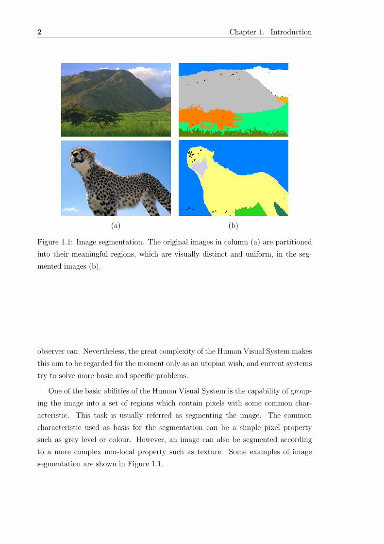
Figure 1.1: Image segmentation. The original images in column (a) are partitioned
into their meaningful regions, which are visually distinct and uniform, in the seg-
mented images (b).
observer can. Nevertheless, the great complexity of the Human Visual System makes
this aim to be regarded for the moment only as an utopian wish, and current systems
try to solve more basic and specific problems.
One of the basic abilities of the Human Visual System is the capability of group-
ing the image into a set of regions which contain pixels with some common char-
acteristic. This task is usually referred as segmenting the image. The common
characteristic used as basis for the segmentation can be a simple pixel property
such as grey level or colour. However, an image can also be segmented according
to a more complex non-local property such as texture. Some examples of image
segmentation are shown in Figure 1.1.
1.1 Objectives 3
1.1 Objectives
The goal of image segmentation is to detect and extract the regions which compose
an image. Note that contrary to the classification problem, recognition of these
regions is not required. In fact, although it is difficult to conceive, we can think
in image segmentation as the first look that we made at the world when we were
newborn. In other words, to look without higher knowledge about the objects that
we can see in the scene. Hence, it is not possible to identify the different objects,
simply because it is the first time that we see them. So, the answer of the image
segmentation process will be something as: “there are four regions in the image” and
an array of the size of the image where each pixel is labelled with the corresponding
region number.
Two of the basic approaches for image segmentation are region and boundary
based. The literature for the last 30 years is full of a large set of proposals which
attempt to segment the image based on one of these approaches. However, based on
the complementary nature of edge and region information, current trends on image
segmentation wage for the integration of both sources in order to obtain better
results and to solve the problems that both methods bear when are used separately.
There are also two basic properties that can be considered for grouping pixels and
define the concept of similarity that would form regions: colour and texture. The
importance of both features in order to define the visual perception is obvious in
images corresponding to natural scenes, which have considerable variety of colour
and texture. However, most of the literature deals with segmentation based on either
colour or texture, and few proposals consider both properties together. Fortunately,
this tendency seems to be changing in the actuality originated by the intuition that
using information provided by both features, one should be able to obtain more
robust and meaningful results.
Taking into account all these considerations we have defined the final objective
of this work as:
To propose an unsupervised image segmentation strategy which inte-
grates region and boundary information from colour and texture properties in
order to perform image segmentation.
4 Chapter 1. Introduction
Along with this final objective, there are some points which need to be considered
in this work:
• Prior knowledge. There are two aspects to consider related to prior knowl-
edge that the system has before starting the image segmentation. First, to
what degree and in what form should higher level knowledge be incorporated
into the segmentation process, and secondly, the problem of parameter esti-
mation which is common to any model-based approach.
How the visual knowledge about what we know influence what we see? This is
a question closer to the realms of psychophysics. Our wish is to make minimal
assumptions and keep the segmentation process mostly at a low level. Hence,
parameter estimation will be also performed in situ.
• Unsupervision. The method should be completely unsupervised. That is,
the user will not be required to intervene in the course of the segmentation
process.
• Computational efficiency. Although the time is not a critical requirement
of this work, the algorithm should be computable and not make unreasonable
demands on CPU time.
• Extensibility. The proposed strategy should be easily extensible to perform
a generalised segmentation. An obvious extension is from regions of homoge-
neous gray level to regions of homogeneous texture. Moreover, our goal is to
propose a strategy capable to be extended to colour texture segmentation.
• Robustness. The method should show a robust behaviour and obtain correct
segmentation results in a large set of images. Besides, the algorithm will be
generally tested over natural images, which are specially rich in variety of
colour and texture.
1.2 Related Work
The work presented in this thesis is not a new subject within the Computer Vision
and Robotics group at the University of Girona, contrarily it can be regarded as a
1.2 Related Work 5
Image
Local Contours
Integrated Contours
Thinning
CP and EP Detection
Orientationin EP
Restoration
Analysis of Separation
Circumscribed Contours
n x
TextureAnalysis
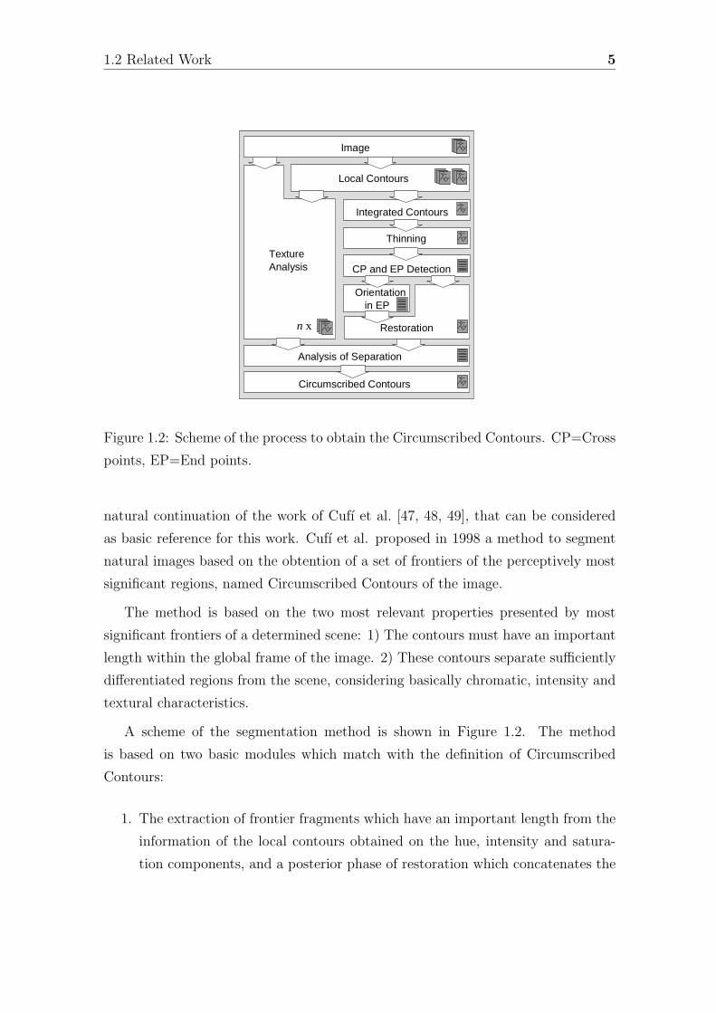
Figure 1.2: Scheme of the process to obtain the Circumscribed Contours. CP=Cross
points, EP=End points.
natural continuation of the work of Cufı et al. [47, 48, 49], that can be considered
as basic reference for this work. Cufı et al. proposed in 1998 a method to segment
natural images based on the obtention of a set of frontiers of the perceptively most
significant regions, named Circumscribed Contours of the image.
The method is based on the two most relevant properties presented by most
significant frontiers of a determined scene: 1) The contours must have an important
length within the global frame of the image. 2) These contours separate sufficiently
differentiated regions from the scene, considering basically chromatic, intensity and
textural characteristics.
A scheme of the segmentation method is shown in Figure 1.2. The method
is based on two basic modules which match with the definition of Circumscribed
Contours:
1. The extraction of frontier fragments which have an important length from the
information of the local contours obtained on the hue, intensity and satura-
tion components, and a posterior phase of restoration which concatenates the
6 Chapter 1. Introduction
contours. They are the contours which are candidates to be Circumscribed
Contours of the image.
2. Study of the relevance of candidate contours considering if they separate (or
not) regions over which a set of textural characteristics are measured. The
candidate contours which have a high valour of relevance are finally considered
the Circumscribed Contours of the image.
1.3 Thesis Outline
The structure of this thesis is on the light of showing the methodology of work used
in order to carry out it. Thus, an introduction to basics of segmentation concludes
this chapter. Chapter 2 reviews different approaches which integrate region and
boundary information for image segmentation. Next, our strategy for unsupervised
image segmentation is proposed in Chapter 3, which is subsequently extended in
Chapter 4 to deal with the problem of texture segmentation and colour texture
segmentation. In Chapter 5 an evaluation and comparison of our proposal with
different algorithms is shown. Finally, the derived conclusions and future work are
discussed in Chapter 6.
Chapter 2
Main approaches for the integration of region and boundary information in image
segmentation are identified. Subsequently, a classification is proposed in which the
philosophy of these different strategies is clearly explained and the most relevant
proposals of segmentation algorithms are detailed. Finally, the characteristics of
these strategies, along with their weak points, are discussed and the lack of attention
that in general is given to the texture is noted.
The contributions of Chapter 2 are:
• The identification of the different strategies used in order to integrate region
and boundary information which results on a proposal of classification of these
approaches.
1.3 Thesis Outline 7
• The assortment and grouping of the most relevant proposals of image segmen-
tation in their corresponding approach according to the underlying philosophy.
• The discussion of the aspects, positive and negative, which characterise the
different approaches and the note of a general lack of specific treatment of
textured images.
Chapter 3
A segmentation strategy which integrates region and boundary information and
uses three approaches identified in the previous chapter is proposed. The proposed
segmentation algorithm consists of two basic stages: initialisation and segmentation.
Thus, in the first stage, the main contours of the image are used to identify the
different regions present in the image and to adequately place a seed for each one in
order to statistically model the region. Then, the segmentation stage is performed
based on the active region model which allows us to take region and boundary
information into account in order to segment the whole image. With the aim of
imitating the Human Vision System, the method is implemented using a pyramidal
representation which allows us to refine the region boundaries from a coarse to a
fine resolution.
Summarising, the contributions of Chapter 3 are:
• The proposal of a segmentation strategy which unifies different approaches for
the integration of region and boundary information for image segmentation.
• A method, which based on boundary information, allows to adequately place
a seed for each region of the image in order to initialise the region models.
• The integration of region and boundary information in order to carry out the
image segmentation based on active regions.
• The implementation of the algorithm using a pyramidal representation which
ensures noise robustness as well as computation efficiency.
Chapter 4
The strategy for image segmentation proposed in Chapter 3, is adapted to solve

8 Chapter 1. Introduction
the problem of texture segmentation. Chapter 4 is structured on two basic parts:
texture segmentation and colour texture segmentation. First, the proposed strategy
is extended to texture segmentation which involves some considerations as the region
modelling and the extraction of texture boundary information. In the second part,
a method to integrate colour and textural properties is proposed, which is based on
the use of texture descriptors and the estimation of colour behaviour. Hence, the
proposed strategy of segmentation is considered for the segmentation taking both
colour and textural properties into account.
The main contributions of this chapter are:
• The extension of the proposed strategy for image segmentation to unsupervised
texture segmentation.
• A proposal for the combination of texture features with the estimation of
colour properties in order to describe colour texture.
• The use of colour and texture properties together for the segmentation of
colour textured images using the proposed strategy.
Chapter 5
Our proposal of image segmentation strategy is objectively evaluated and then com-
pared with some other relevant algorithms corresponding to the different strategies
of region and boundary integration identified in Chapter 2. Moreover, an evaluation
of the segmentation results obtained on colour texture segmentation is performed.
Furthermore, results on a wide set of real images are shown and discussed.
Chapter 5 can be summarized on:
• The objective evaluation of results achieved by our proposal on image segmen-
tation.
• The comparison of our proposal with different algorithms which integrate re-
gion and boundary information for image segmentation.
• The objective evaluation of results obtained on colour texture segmentation.
1.4 Basics of Segmentation 9
Chapter 6
Finally, relevant conclusions extracted from this work are given in Chapter 6 and
different future directions of this work are proposed.
1.4 Basics of Segmentation
Segmentation can be considered the first step and key issue in object recognition,
scene understanding and image understanding. Applications range from industrial
quality control to medicine, robot navigation, geophysical exploration, and military
applications. In all these areas, the quality of the final result depends largely on the
quality of the segmentation [143].
One way of defining image segmentation is as follows [91, 151]. Formally, a set
of regions {R1, R2, . . . , Rn} is a segmentation of the image R into n regions if:
1.⋃n
i=1 Ri = R
2. Ri⋂
Rk = ∅, i �= k
3. Ri is connected, i = 1, 2, . . . , n
4. There is a predicate P that measures region homogeneity,
(a) P (Ri) =TRUE, i = 1, 2, . . . , n
(b) P (Ri⋃
Rk) =FALSE, i �= k and Ri adjacent to Rk
The above conditions can be summarized as follows: the first condition implies
that every image point must be in a region. This means that the segmentation
should not terminate until every point is processed. The second condition implies
that regions are non-intersecting, while the third condition determines regions are
composed by contiguous pixels. Finally, the fourth condition determines what kind
of properties the segmented regions should have, for example, uniform gray levels,
and express the maximality of each region in the segmentation.
During the past years, many image segmentation techniques have been developed
and different classification schemes for these techniques have been proposed [82, 143].
10 Chapter 1. Introduction
We have adopted the classification proposed by Fu and Mui [67], in which segmen-
tation techniques are categorised into three classes: (1) Thresholding or clustering,
(2) region-based and (3) boundary-based.
1.4.1 Thresholding or Clustering Segmentation
1.4.1.1 Thresholding
The most basic segmentation procedure that may be carried out is thresholding of
an image (see [170]). This method consists on comparing the measure associated to
each pixel to one or some thresholds in order to determine the class which the pixel
belongs to. The attribute is generally the grey level, although colour or a simple
texture descriptor can also be used. Thresholds may be applied globally across
the image (static threshold) or may be applied locally so that the threshold varies
dynamically across the image.
Under controlled conditions, if the surface reflectance of the objects or regions
to be segmented are uniform and distinct from the background and the scene is
evenly illuminated then the resulting image will contain homogenous regions with
well defined boundaries that generally lead to a bimodal or multi-modal histogram.
Finding the modes determines the partitions of the space and hence the segmenta-
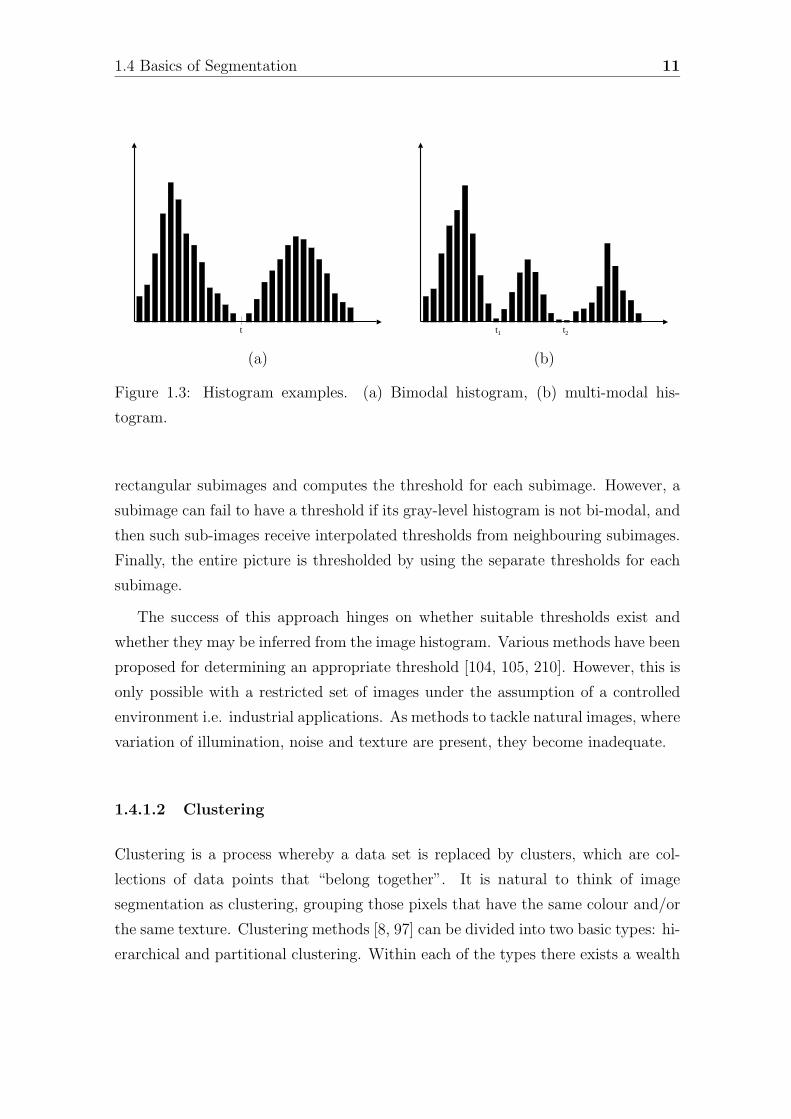
tion. Be an image composed by a bright object on a darker background, thus the
histogram is bimodal, similar to the example shown in Figure 1.3.a. The two peaks
correspond to the relatively large number of points inside and outside the object.
The dip between the peaks corresponds to the relatively few points around the edge
of the object. The threshold is then placed in the valley between both peaks, then
pixels with a grey level higher than the threshold t will be associated to the object,
while the remaining pixels to the background. Figure 1.3.b illustrates a multi-modal
histogram.
Nevertheless, in many cases the background level is not constant, and the contrast
of objects varies within the image. In such cases, a threshold that works well in one
area of the image might work poorly in other areas. Thus, it is convenient to use a
threshold that is slowly varying in function of position in the image [31]. A dynamic
threshold was proposed by Chow an Kaneko [40], which divides the image up into
1.4 Basics of Segmentation 11
t t1 t2
(a) (b)
Figure 1.3: Histogram examples. (a) Bimodal histogram, (b) multi-modal his-
togram.
rectangular subimages and computes the threshold for each subimage. However, a
subimage can fail to have a threshold if its gray-level histogram is not bi-modal, and
then such sub-images receive interpolated thresholds from neighbouring subimages.
Finally, the entire picture is thresholded by using the separate thresholds for each
subimage.
The success of this approach hinges on whether suitable thresholds exist and
whether they may be inferred from the image histogram. Various methods have been
proposed for determining an appropriate threshold [104, 105, 210]. However, this is
only possible with a restricted set of images under the assumption of a controlled
environment i.e. industrial applications. As methods to tackle natural images, where
variation of illumination, noise and texture are present, they become inadequate.
1.4.1.2 Clustering
Clustering is a process whereby a data set is replaced by clusters, which are col-
lections of data points that “belong together”. It is natural to think of image
segmentation as clustering, grouping those pixels that have the same colour and/or
the same texture. Clustering methods [8, 97] can be divided into two basic types: hi-
erarchical and partitional clustering. Within each of the types there exists a wealth
12 Chapter 1. Introduction
of subtypes and different algorithms for finding the clusters.
Hierarchical clustering proceeds successively by either merging smaller clusters
into larger ones (agglomerative algorithms), or by splitting larger clusters (divisive
algorithms). The clustering methods differ in the rule by which it is decided which
two small clusters are merged or which large cluster is split. The final result of the
algorithm is a tree of clusters called a dendogram, which shows how the clusters are
related. By cutting the dendogram at a desired level, a clustering of the data items
into disjoint groups is obtained.
On the other hand, partitional clustering attempts to directly decompose the
data set into a set of disjoint clusters. An objective function expresses how good a
representation is, and then the clustering algorithm tries to minimize this function
in order to obtain the best representation. The criterion function may emphasize the
local structure of the data, as by assigning clusters to peaks in the probability density
function, or the global structure. Typically the global criteria involves minimizing
a measure of dissimilarity for the samples within each cluster, while maximizing
the dissimilarity between different clusters. The most commonly used partitional
clustering method is the K-means algorithm [118], in which the criterion function is
the squared distance of the data items from their nearest cluster centroids.
Clustering methods, even as thresholding methods, are global and do not retain
positional information. The major drawback of this is that it is invariant to spa-
tial rearrangement of the pixels, which is an important aspect of what is meant by
segmentation. Resulting segments are not connected and can be widely scattered.
Some attempts have been made to introduce such information using pixels coor-
dinates as features. However, this approach tends to result in large regions being
broken up and the results so far are no better than those that do not use spatial
information [67]. The need to incorporate some form of spatial information into the
segmentation process, led to the development of methods where pixels are classified
using their context or neighbourhood.
1.4 Basics of Segmentation 13
1.4.2 Region-based Segmentation
The region approach tries to isolate areas of images that are homogeneous according
to a given set of characteristics. We introduce in this section two classical region-
based methods: region growing and split-and-merge.
1.4.2.1 Region Growing
Region growing [2, 229] is one of the most simple and popular region-based segmen-
tation algorithms. It starts by choosing a (or some) starting point or seed pixel.
The most habitual way is to select these seeds by randomly choosing a set of pixels
in the image, or by following a priori set direction of scan of the image. However,
other techniques of selection based on boundary information will be discussed in
next section.
Then, the region grows by successively adding neighbouring pixels that are sim-
ilar, according to a certain homogeneity criterion, increasing step by step the size
of the region. This criterion can be, for example, to require that the variance of a
feature inside the region does not exceed a threshold, or that the difference between
the pixel and the average of the region is small. The growing process is continued
until a pixel not sufficiently similar to be aggregated is found. It means that the
pixel belongs to another object and the growing in this direction is finished. When
there is not any neighbouring pixel which is similar to the region, the segmentation
of the region is complete. Monitoring this procedure gives on the impression of re-
gions in the interior of objects growing until their boundaries correspond with the
edges of the object.
1.4.2.2 Split-and-Merge
As has been above defined, one of the basic properties of segmentation is the exis-
tence of a predicate P which measures the region homogeneity. If this predicate is
not satisfied for some region, it means that that region is inhomogeneous and should
be split into subregions. On the other hand, if the predicate is satisfied for the union
of two adjacent regions, then these regions are collectively homogeneous and should
be merged into a single region [11].
14 Chapter 1. Introduction
(a) (b)
(c) (d)
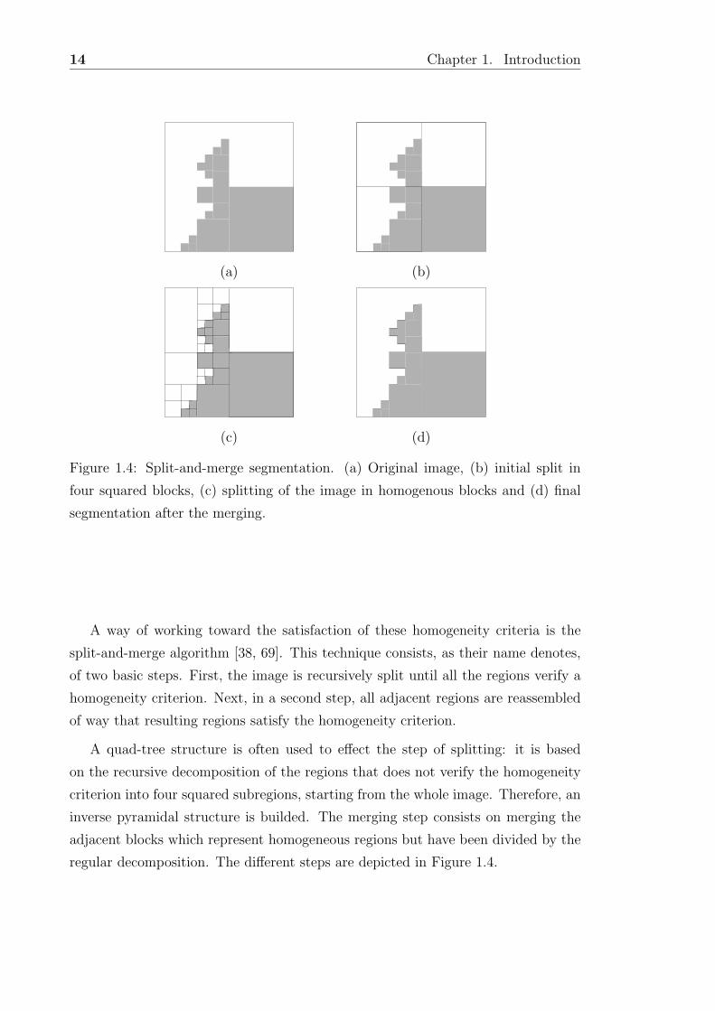
Figure 1.4: Split-and-merge segmentation. (a) Original image, (b) initial split in
four squared blocks, (c) splitting of the image in homogenous blocks and (d) final
segmentation after the merging.
A way of working toward the satisfaction of these homogeneity criteria is the
split-and-merge algorithm [38, 69]. This technique consists, as their name denotes,
of two basic steps. First, the image is recursively split until all the regions verify a
homogeneity criterion. Next, in a second step, all adjacent regions are reassembled
of way that resulting regions satisfy the homogeneity criterion.
A quad-tree structure is often used to effect the step of splitting: it is based
on the recursive decomposition of the regions that does not verify the homogeneity
criterion into four squared subregions, starting from the whole image. Therefore, an
inverse pyramidal structure is builded. The merging step consists on merging the
adjacent blocks which represent homogeneous regions but have been divided by the
regular decomposition. The different steps are depicted in Figure 1.4.
1.4 Basics of Segmentation 15
1.4.3 Boundary-based Segmentation
The last class of methods for image segmentation are related to the detection of
the luminance transitions between regions, i.e. the boundaries (lines or edges).
The fundamental importance of line and edge information in both biological and
Computer Vision systems has long been recognised. Indeed, the biological evidence
showing edge-detection playing a central role in the early stages of visual perception
in mammals (low level vision), such as the Human Visual System, has often been the
motivation for its adoption by researchers in image processing. Local features, such
as lines and edges, can describe the structure of a scene relatively independently on
the illumination. For example, a cartoon drawing consisting only of lines is often
enough for humans to interpret a scene.
Image segmentation techniques based on edge detection have long been in use,
since the early work of Roberts in 1965 [164]. Although a variety of methods of edge
detection have been suggested, there are two basic local approaches: first and second-
order differentiation. The bane of all these methods, however, is noise. Edges, by
definition, are spatially rapidly varying and hence have significant components at
high spatial frequencies. This is also, unfortunately, the characteristic of noise, and
therefore any gradient operator that responds well to the presence of an edge will
also respond well to the presence of noise or textures thus signalling false edges.
1.4.3.1 First order
In the first case, a gradient mask (Roberts [164] and Sobel [182] are well-known
examples) is convolved with the image to obtain the gradient vector ∇f associated
with each pixel. Edges are the places where the magnitude of the gradient vector
‖∇f‖ is a local maximum along the direction of the gradient vector φ(∇f). For
this purpose, the local value of the gradient magnitude must be compared with the
values of the gradient estimated along this orientation and at unit distance on either
side away from the pixel. After this process of non-maxima suppression takes place,
the values of the gradient vectors that remain are thresholded, and only pixels with
a gradient magnitude above that threshold are considered as edge pixels [153].
The Sobel operator introduced a weighting of local averages measures at both
16 Chapter 1. Introduction
sides of the central pixel. Several works have looked for the optimisation of this
weighting factor. Canny [26] proposed the derivative-of-Gaussian filter as a near-
optimal filter with respect to three edge-finding criteria: (a) good localisation of the
edge, (b) one response to one edge and (c) high probability of detecting true edge
points and low probability of falsely detecting non-edge points. Deriche [55], based
on Canny’s criteria, implemented a filter with an impulse response similar to that
of the derivative of Gaussian, but which lends itself to direct implementation as a
recursive filter.
1.4.3.2 Second order
In the second-order derivative class, optimal edges (maxima of gradient magnitude)
are found by searching for places where the second derivative is zero. The isotropic
generalisation of the second derivative to two dimensions is the Laplacian [158].
However, when gradient operators are applied to an image, the zeros rarely fall
exactly on a pixel. It is possible to isolate these zeroes by finding zero crossings:
places where one pixel is positive and a neighbour is negative (or vice versa). Ideally,
edges should correspond to boundaries of homogeneous objects and object surfaces.
Having obtained an edge map, there is usually a second stage to boundary based
segmentation, which is to group the boundary elements to form lines or curves. This
is necessary because, excepting the simplest noise free images, the edge detection will
result in a set of fragmented edge elements. There are three main approaches to this
problem: local linking techniques [47], global methods, such as Hough Transform
(HT) methods [61], or combined approaches, such as the hierarchical HT and the
MFT based methods. The local linking methods use attributes of the edge elements,
such as magnitude, orientation and proximity, to grow the curves in the image. In
the HT methods, the edge elements are transformed to a parameter space, which
is a joint histogram of the parameters of the model of line or curve being detected.
The peaks in this histogram then indicate the presence and location of the lines or
curves being detected.
Chapter 2
Image Segmentation Integrating
Region and Boundary Information
Image segmentation has been, and still is, an important research area in Computer
Vision, and hundreds of segmentation algorithms have been proposed in the last
30 years. However, elementary segmentation techniques based on either boundary
or region information often fail to produce accurate segmentation results on their
own. In the last few years, there has therefore been a trend towards algorithms
that take advantage of their complementary nature. This chapter reviews various
segmentation proposals that integrate edge and region information and highlights
different strategies and methods for fusing such information.
2.1 Introduction
One of the first and most important operations in image analysis and Computer
Vision is segmentation [79, 167]. The aim of image segmentation is the domain-
independent partition of the image into a set of regions, which are visually distinct
and uniform with respect to certain properties, such as grey level, texture or colour.
The problem of segmentation has been, and still is, an important research field,
and many segmentation methods have been proposed in the literature (see the sur-
veys: [67, 82, 136, 143, 163, 230]). Many segmentation methods are based on two
17
18 Chapter 2. Image Segmentation Integrating Region and Boundary Information
basic properties of pixels in relation to their local neighbourhood: similarity and
discontinuity. Pixel similarity gives rise to region-based methods, whereas pixel
discontinuity gives rise to boundary-based methods.
Unfortunately, both boundary-based and region-based techniques often fail to
produce accurate segmentation, although the cases where each method fails are
not necessarily identical. In boundary-based methods, if an image is noisy or if
its attributes differ by only a small amount between regions (and this occurs very
commonly in natural scenarios), edge detection may result in spurious and broken
edges. This is mainly due to the fact that they rely entirely on the local information
available in the image; very few pixels are used to detect the desired features. Edge
linking techniques can be employed to bridge short gaps in such a region boundary,
although this is generally considered a very difficult task. Region-based methods al-
ways provide closed contour regions and make use of relatively large neighbourhoods
in order to obtain sufficient information to decide whether or not a pixel should be
aggregated into a region. Consequently, the region approach tends to sacrifice reso-
lution and detail in the image to gain a sample large enough for the calculation of
useful statistics for local properties. This can result in segmentation errors at the
boundaries of the regions, and in a failure to distinguish regions that would be small
in comparison with the block size used. Furthermore reasonable initial seed points
and stopping criteria are often difficult to choose in the absence of a priori informa-
tion. Finally, as Salotti and Garbay [171] noted, both approaches sometimes suffer
from a lack of information due to the fact that they rely on the use of ill-defined
hard thresholds that may lead to wrong decisions.
It is often difficult to obtain satisfactory results when using only one of these
methods in the segmentation of complex pictures such as outdoor and natural im-
ages, which involve additional difficulties due to effects such as shading, highlights,
non-uniform illumination or texture. By using the complementary nature of edge-
based and region-based information, it is possible to reduce the problems that arise
in each individual method. The trend towards integrating several techniques seems
to be the best way forward. The difficulty lies in the fact that even though the
two approaches yield complementary information, they involve conflicting and in-
commensurate objectives. Thus, as previously observed by Pavlidis and Liow [152],
while integration has long been a desirable goal, achieving this is not an easy task.
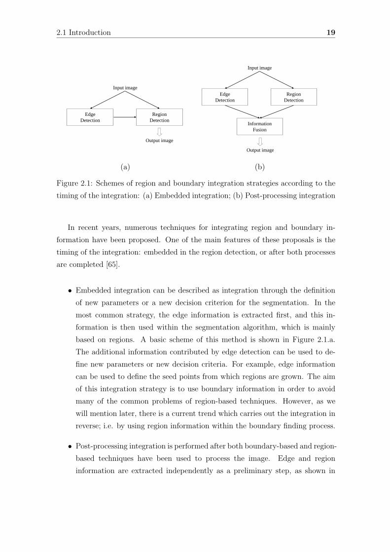
2.1 Introduction 19
Input image
Output image
EdgeDetection
RegionDetection
Input image
Output image
EdgeDetection
RegionDetection
InformationFusion
(a) (b)
Figure 2.1: Schemes of region and boundary integration strategies according to the
timing of the integration: (a) Embedded integration; (b) Post-processing integration
In recent years, numerous techniques for integrating region and boundary in-
formation have been proposed. One of the main features of these proposals is the
timing of the integration: embedded in the region detection, or after both processes
are completed [65].
• Embedded integration can be described as integration through the definition
of new parameters or a new decision criterion for the segmentation. In the
most common strategy, the edge information is extracted first, and this in-
formation is then used within the segmentation algorithm, which is mainly
based on regions. A basic scheme of this method is shown in Figure 2.1.a.
The additional information contributed by edge detection can be used to de-
fine new parameters or new decision criteria. For example, edge information
can be used to define the seed points from which regions are grown. The aim
of this integration strategy is to use boundary information in order to avoid
many of the common problems of region-based techniques. However, as we
will mention later, there is a current trend which carries out the integration in
reverse; i.e. by using region information within the boundary finding process.
• Post-processing integration is performed after both boundary-based and region-
based techniques have been used to process the image. Edge and region
information are extracted independently as a preliminary step, as shown in
20 Chapter 2. Image Segmentation Integrating Region and Boundary Information
Figure 2.1.b. An a posteriori fusion process then tries to exploit the dual in-
formation in order to modify, or refine, the initial segmentation obtained by a
single technique. The aim of this strategy is to improve the initial results and
to produce a more accurate segmentation.
Although many studies have been published on image segmentation, none of
them focuses specifically on the integration of region and boundary information,
which is the aim of this chapter, in which we will discuss the most significant seg-
mentation techniques developed in recent years. We give a description of several
key techniques that we have classified as embedded or post-processing. Among the
embedded methods, we distinguish between those that use boundary information
for seed placement purposes, and those that use this information to establish an
appropriate decision criterion. Among the post-processing methods, we distinguish
between three different approaches: over-segmentation, boundary refinement, and
selection-evaluation. We discuss each one of these techniques in depth, as well as
emphasizing aspects related to the implementation of the methods in some cases
(region-growing or split-and-merge), or the use of fuzzy logic, which has been con-
sidered in a number of proposals.
The chapter is structured as follows: the Introduction is concluded by related
work, Section 2.2 defines and classifies different approaches to the embedded inte-
gration, while Section 2.3 analyses proposals for the post-processing strategy. Sec-
tion 2.4 summarizes the advantages and disadvantages of the various approaches.
Finally, the results of our study are summarized in the Conclusions Section.
2.1.1 Related Work
A brief mention of the integration of region and boundary information for segmen-
tation can be found in the introductory sections of several papers. For instance,
Pavlidis and Liow [152] introduce some earlier papers that emphasise the integra-
tion of such information. In 1994, Falah et al. [65] identified two basic strategies
for achieving the integration of dual information, boundaries and regions. The first
strategy (post-processing) is described as the use of edge information to control or re-
fine a region segmentation process. The other alternative (embedded) is to integrate
2.2 Embedded integration 21
edge detection and region extraction within the same process. The classification
proposed by Falah, Bolon and Cocquerez has been adopted and discussed in this
thesis. LeMoigne and Tilton [112], considerinng data fusion in general, identified
two levels of fusion: pixel and symbol. A pixel-level integration between edges and
regions assumes that the decision regarding integration is made individually for each
pixel, while the symbol-level integration is performed on the basis of selected fea-
tures, thereby simplifying the problem. Furthermore, they discuss embedded and
post-processing strategies and present important arguments concerning the supposed
superiority of the post-processing strategy. They argue that a posteriori fusion pro-
vides a more general approach because, for the initial task, it can employ any type
of boundary and region segmentation. A different point of view of integration of
edge and region information for segmentation consists of using dynamic contours
(snakes). Chan et al. [34] review different approaches, pointing out that integration
is the way to decrease the limitations of traditional deformable contours.
2.2 Embedded integration
The embedded integration strategy usually consists of using previously extracted
edge information, within a region segmentation algorithm. It is well known that in
most of the region-based segmentation algorithms, the manner in which initial re-
gions are formed and their growing criteria are set a priori. Hence, the resulting seg-
mentation will inevitably depend on the choice of initial region growth points [104],
while the region’s shape will depend on the particular growth chosen [105]. Some
proposals try to use boundary information in order to avoid these problems. Ac-
cording to the way in which this information is used, it is possible to distinguish two
trends:
1. Control of Decision Criterion: edge information is included in the defini-
tion of the decision criterion which controls the growth of the region.
2. Seed Placement Guidance: edge information is used as a guide in order to
decide which is the most suitable position to place the seed (or seeds) for the
region-growing process.
22 Chapter 2. Image Segmentation Integrating Region and Boundary Information
2.2.1 Control of Decision Criterion
The most common way of performing integration in the embedded strategy consists
of incorporating edge information into the growing criterion of a region-based seg-
mentation algorithm. The edge information is thus included in the definition of the
decision criterion that controls the growth of the region.
As we have seen in Section 1.4, region growing and split-and-merge are two
typical region-based segmentation algorithms. Although both share the essential
concept of homogeneity, the way the segmentation process is carried out is truly
different in terms of the decisions taken. For this reason, and in order to facili-
tate analysis of this approach, we shall discuss integration into these two types of
algorithms separately (see following Sections 2.2.1.1 and 2.2.1.2).
2.2.1.1 Integration in split-and-merge algorithms
The homogeneity criterion in split-and-merge algorithms is generally based on the
analysis of the chromatic features in the region. When the intensity of the region’s
pixels has a sufficiently small standard deviation, the region is considered homoge-
neous. Moreover, the integration of edge information allows a new criterion to be
defined: a region is considered homogeneous when it is totally free of contours. This
concept can then substitute or be added to the traditional homogeneity criterion.
In 1989, Bonnin et al. [20] proposed a split-and-merge algorithm controlled by
edge detection. The criterion to decide the split of a region takes into account edge
and intensity characteristics. More specifically, if there is no edge point on the patch
and if the intensity homogeneity constraints are satisfied, then the region is stored;
otherwise, the patch is divided into four sub-patches, and the process is recursively
repeated. The homogeneity intensity criterion is rendered necessary because possible
failures of the edge detector. After the split phase, the contours are thinned and
chained into edges relative to the boundaries of the initial regions. Later, a final
merging process takes into account edge information in order to solve possible over-
segmentation problems. In this last step, two adjacent initial regions are merged
only if no edges are found on the common boundary. The general structure of their
method is depicted in Figure 2.2, where it can be observed that edge information
2.2 Embedded integration 23
OriginalImage
Edge Points Edges
InitialRegions
Final Mergeof Regions
Thining &Chaining
Edge PointDetection
Split & Mergeprocedure
InitialControl
1st FeedbackRegion --> Point
2nd FeedbackEdge --> Region
Piecewise LinearSegment Approximation
EdgesRegions
MonocularAnalysis
Graph
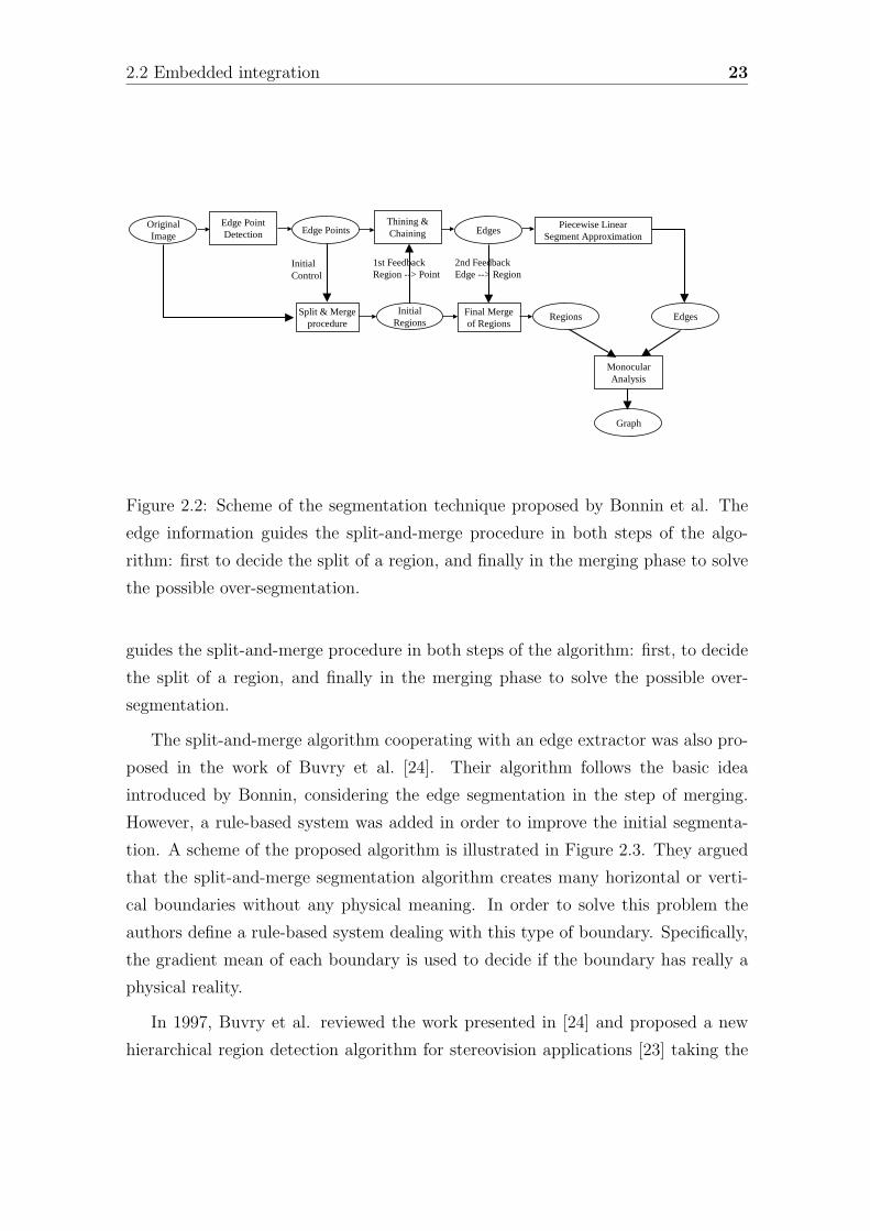
Figure 2.2: Scheme of the segmentation technique proposed by Bonnin et al. The
edge information guides the split-and-merge procedure in both steps of the algo-
rithm: first to decide the split of a region, and finally in the merging phase to solve
the possible over-segmentation.
guides the split-and-merge procedure in both steps of the algorithm: first, to decide
the split of a region, and finally in the merging phase to solve the possible over-
segmentation.
The split-and-merge algorithm cooperating with an edge extractor was also pro-
posed in the work of Buvry et al. [24]. Their algorithm follows the basic idea
introduced by Bonnin, considering the edge segmentation in the step of merging.
However, a rule-based system was added in order to improve the initial segmenta-
tion. A scheme of the proposed algorithm is illustrated in Figure 2.3. They argued
that the split-and-merge segmentation algorithm creates many horizontal or verti-
cal boundaries without any physical meaning. In order to solve this problem the
authors define a rule-based system dealing with this type of boundary. Specifically,
the gradient mean of each boundary is used to decide if the boundary has really a
physical reality.
In 1997, Buvry et al. reviewed the work presented in [24] and proposed a new
hierarchical region detection algorithm for stereovision applications [23] taking the

24 Chapter 2. Image Segmentation Integrating Region and Boundary Information
Modified
ImageImage
Median
Filter
Gradient
Image
Prewitt
Op.
Edge
Image
Edge
Extraction
Regions
Image
Modified
Regions
Final
Regions
Split-and-Merge
Merging of Small Regions
and Curve Approximation
Rules
Application
REGION GROWING ALGORITHM
Figure 2.3: Segmentation technique proposed by Buvry et al. Edge information
is used to guide the split-and-merge region segmentation. Finally, a set of rules
improve the initial segmentation by removing boundaries without corresponding
edge information.
gradient image into account. The method yields a hierarchical coarse-to-fine seg-
mentation where each region is validated by exploiting the gradient information. At
each level of the segmentation process, a threshold is computed and the gradient
image is binarized according to this threshold. Each closed area is labelled by ap-
plying a classical colouring process and defines a new region. Edge information is
also used to determine if the split process is finished or if the next partition must
be computed. So, in order to do that, a gradient histogram of all pixels belonging
to the region is calculated and its characteristics (mean, maximum and entropy) are
analysed.
Healey [86] presented an algorithm for segmenting images of 3-D scenes, which
uses the absence of edge pixels in the region as a homogeneity criterion. Furthermore,
he considers the effects of edge detection mistakes (false positive and false negative)
on the segmentation algorithm, and gives evidence that false negatives have more
serious consequences, so the edge detector threshold should be set low enough to
minimize their occurrence.
A proposal of enriching the segmentation by irregular pyramidal structure by
using edge information can be found in the work of Bertolino and Montanvert [18].
In the proposed algorithm, a graph of adjacent regions is computed and modified
2.2 Embedded integration 25
according to the edge map obtained from the original image. Each graph-edge1 is
weighted with a pair of values (r,c), which represent the number of region elements,
and the contour elements in the common boundary of both regions respectively.
Then, the algorithm goes through the graph and at each graph-edge decides whether
to forbid or favour the fusion between adjacent regions.
The use of edge information in a split-and-merge algorithm may not only be
reduced to the decision criterion. In this sense, Gevers and Smeulders [75] presented,
in 1997, a new technique that extends the possibilities of this integration. Their
proposal uses edge information to decide how the partition of the region should be
made, or in other words, where to split the region. The idea is the adjustment of
this decision to boundary information and to split the region following the edges
contained in it. In reference to previous works, the authors affirmed that although
the quad-tree scheme is simple to implement and computationally efficient, its major
drawback is that the image tessellation process is unable to adapt the tessellation
grid to the underlying structure of the image. For this reason they proposed to
employ the incremental Delaunay triangulation allowing the formation of grid edges
of arbitrary orientation and position. The tessellation grid, defined by the Delaunay
triangulation, is adjusted to the semantics of the image data. In the splitting phase,
if a global similarity criterion is not satisfied, pixels lying on image boundaries are
determined using local difference measures and are used as new vertices to locally
refine the tessellation grid.
2.2.1.2 Integration in region growing algorithms
Region growing algorithms are based on the growth of a region whenever its interior
is homogeneous according to certain features, such as intensity, colour or texture.
This definition is broad enough to allow different variants to be analysed:
1. Region growing: this embraces the traditional implementation of region
growing based on the growth of a region by adding similar neighbours.
2. Watershed: a watershed algorithm effects the growth by simulating a flooding
process, which progressively covers the region.
1In order to avoid confusion, we have called graph-edge an edge that joins two nodes in a graph.
26 Chapter 2. Image Segmentation Integrating Region and Boundary Information
3. Active region model: considered to be a fusion of region growing with the
techniques of active contour models.
2.2.1.2.1 Region growing
Region growing [2, 229] is one of the most simple and popular algorithms for
region-based segmentation. Typically, the first step is to choose a starting point or
seed pixel. The region then grows by adding neighbouring pixels that are similar,
according to a certain homogeneity criterion, increasing the size of the region step-
by-step. So, the homogeneity criterion has the function of determining whether or
not a pixel belongs to the growing region.
The decision to merge is generally based only on the contrast between the current
pixel and the region. However, it is not easy to decide when this difference is small (or
large) enough to make a decision. The edge map provides an additional criterion in
decisions. A scheme of this approach is shown in Figure 2.4. The technique consists
of determining whether or not the pixel under scrutiny is a contour pixel. Finding
a contour means that the growth process has reached the boundary of the region.
The pixel must therefore be discarded and the growth of the region finishes.
One of the first integrations of edge information into a region-growing algorithm
can be found in the work of Xiaohan et al. [217], where edge information is included
in the decision criterion, which consists of the weighted sum of the contrast between
the region and the pixel and the value of the modulus of the gradient of the pixel. The
proposed combination of region-growing and gradient information can be expressed
using the following formula
x(i, j) = |XNa v − f(i, j)|
z(i, j) = (1 − φ)x(i, j) + φG(i, j)(2.1)
where XNa v is the average grey value of the region which is updated pixel by
pixel. The contrast of the current pixel with respect to the region is denoted by
x(i, j). Parameter φ controls the weight of gradient, G(i, j). Finally, the sum of the
local and the global contrast is the final homogeneity measure, z(i, j). Following
this expression the proposed algorithm can be described using only two steps:
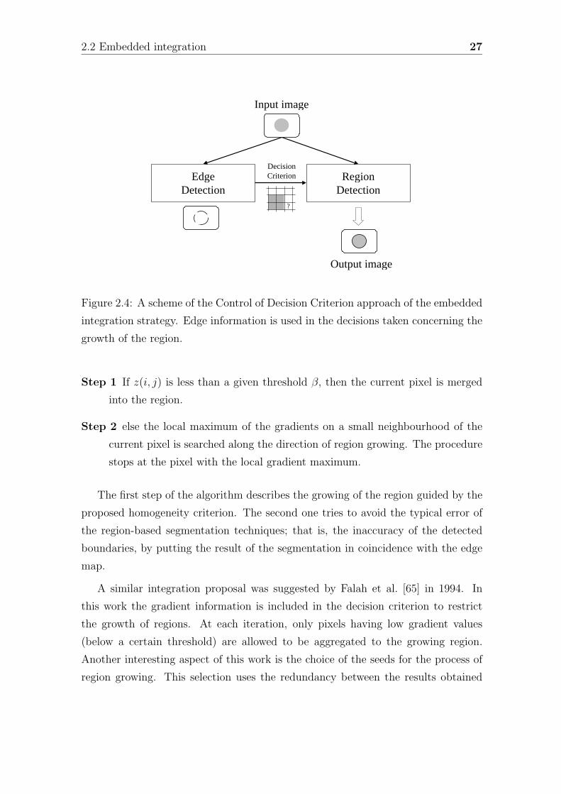
2.2 Embedded integration 27
Input image
EdgeDetection
RegionDetection
?
DecisionCriterion
Output image
Figure 2.4: A scheme of the Control of Decision Criterion approach of the embedded
integration strategy. Edge information is used in the decisions taken concerning the
growth of the region.
Step 1 If z(i, j) is less than a given threshold β, then the current pixel is merged
into the region.
Step 2 else the local maximum of the gradients on a small neighbourhood of the
current pixel is searched along the direction of region growing. The procedure
stops at the pixel with the local gradient maximum.
The first step of the algorithm describes the growing of the region guided by the
proposed homogeneity criterion. The second one tries to avoid the typical error of
the region-based segmentation techniques; that is, the inaccuracy of the detected
boundaries, by putting the result of the segmentation in coincidence with the edge
map.
A similar integration proposal was suggested by Falah et al. [65] in 1994. In
this work the gradient information is included in the decision criterion to restrict
the growth of regions. At each iteration, only pixels having low gradient values
(below a certain threshold) are allowed to be aggregated to the growing region.
Another interesting aspect of this work is the choice of the seeds for the process of
region growing. This selection uses the redundancy between the results obtained
28 Chapter 2. Image Segmentation Integrating Region and Boundary Information
by several region segmentations (with different thresholds and different directions of
image scanning), with the aim to place the seeds in a proper position in which they
have a high degree of certainty of belonging to an homogeneous region.
In 1992 Salotti and Garbay [171] developed a theoretical framework of an inte-
grated segmentation system. The core of the problem of traditional segmentation
methods, as denoted by the authors, relates to the autarchy of the methods and to
the schedule of conditions that are defined with a priori assumptions. In order to
solve this problem, major directives to control each decision are presented: to accu-
mulate local information before taking difficult decisions; to use processes exploiting
complementary information for a successful cooperation; to defer difficult decisions
until more information is made available; and finally, to enable easy context switches
to ensure an opportunistic cooperation. The main idea of these directives is that
each decision must be strongly controlled. This implies that a massive collabora-
tion must be carried out, and that the segmentation task should not be necessarily
achieved before the beginning of the high-level process. Finally, all these principles
are used in a segmentation system with a region-growing process as main module.
Pixels that seem difficult to classify because there is insufficient information for a
sure decision, are given to an edge detection unit that has to respond whether they
correspond to an edge, or not. The same directives were followed in an a posteriori
work of Bellet et al. [14] that presents an edge-following technique which uses region-
based information to compute adaptive thresholds. In such situations, where it is
difficult to follow the high gradient, complementary information is requested and
successfully obtained through the emergence of regions on both sides of the edge. A
child edge process is then created with a threshold adapted to lower gradient values.
Moreover, the authors introduce the adaptability of the aggregation criterion to the
region’s characteristics: several types of region are distinguished and defined. The
region-growing method dynamically identifies the type of the analysed region, and
a specific adapted criterion is used.
Another proposal for the integration of boundary information into the region-
growing process was presented by Gambotto in [73], where edge information was
used to stop the growing process. The algorithm starts with the gradient image and
an initial seed that must be located inside the region. Then, pixels that are adjacent
to the region are iteratively merged if they satisfy a similarity criterion. A second
2.2 Embedded integration 29
criterion is used to stop this growth. They assume that the gradient takes a high
value over a large part of the region boundary. Thus, growth termination is based
on the average gradient, F (n), computed over the region boundary following the
expression
F (n) =∑
G(k, l)/P (n) (2.2)
where P (n) is the perimeter of the region R(n), and G(k, l) is the value of the
modulus of the gradient of pixels on the region boundary. The iterative growing
process is then continued until the maximum of the global contrast function, F ,
is detected. The authors point out that this cooperation between region growing
and contour detection is desirable because the assumption of homogeneous regions
is usually too restrictive. Using this approach, a wider class of regions can be
characterized compared to the use of smooth grey-level variations alone.
The role of fuzzy logic
The fuzzy rule-based homogeneity criterion offers several advantages compared
to ordinary feature aggregation methods and is worth mentioning. It does not take
long to develop because a set of tools and methodologies already exists, and it is
easy to modify or extend the system to meet the specific requirements of a certain
application. Furthermore, it does not require a full knowledge of the process and
can be understood intuitively because of its human-like semantics. It is also possible
to include such linguistic concepts as shape, size and colour, which are difficult to
handle using most other mathematical methods.
A key work in using fuzzy logic was by Steudel and Glesner [185], where the
segmentation is carried out on the basis of a region-growing algorithm that uses a
fuzzy rule-based system for the evaluation of the homogeneity criterion. The authors
affirmed that there are several negative points in just using the intensity difference
for segmentation:
• image over-segmentation
• annoying false contours
• contours that are not sufficiently smooth
30 Chapter 2. Image Segmentation Integrating Region and Boundary Information
Therefore, new features are introduced into the rule-base of the fuzzy rule-based
system, which result in a better and more robust partitioning of the image while
maintaining a small and compact rule-base. The proposed homogeneity criterion is
composed of a set of four fuzzy rules. The main criterion is the difference between
the average intensity A of a region Rj and the pixel in under investigation. The
corresponding fuzzy rule is
R1: IF DIFFERENCE IS SMALL
THEN HOMOGENEOUS
ELSE NOT HOMOGENEOUS
Another quite important feature for the region segmentation is the gradient at
the position of the pixel to be merged. A new pixel may be merged into a region Rj
when the gradient at that location is low. On the other hand, when the gradient
is too high, the pixel definitely does not belong to the region and should not be
merged. In terms of a fuzzy rule
R2: IF GRADIENT IS LOW
THEN PROBABLY HOMOGENEOUS
ELSE NOT HOMOGENEOUS
With this rule, an adjacent pixel in satisfies the premise of rule R2 with a degree
of µLOW (GRADIENT (in)). The two remaining rules refer to the size and the
shape of regions, in order to avoid small regions, and to benefit compact regions
with smooth contours. A complete scheme of this proposal is shown in Figure 2.5.
Krishnan et al. [107] describe a boundary extraction algorithm based on the
integration of fuzzy rule-based region growing and fuzzy rule-based edge detection.
The properties of homogeneity and edge information of each candidate along the
search directions are evaluated and compared with the properties of the seed. Using
the fuzzy output values of the edge detection and a similarity measure between the
candidate pixel and the seed, the test for the boundary pixel can be determined.
This proposal was applied on colonoscopic images for the identification of closed-
boundaries of intestinal lumen, to facilitate diagnosis of colon abnormalities.
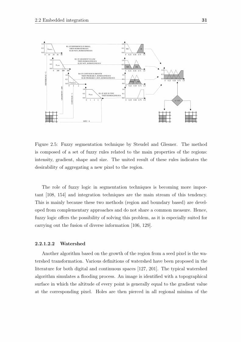
2.2 Embedded integration 31
SIZE = 4
0 10 20 30 40
1.0
0.5
0.0
µSMALL
0 100 200 300
1.0
0.5
0.0
µLOW
0 1 2
1.0
0.5
0.0µSMOOTH
0 1 2 3 4
1.0
0.5
0.0
µTINY
?
DIF
FER
EN
CE
= 5
GR
AD
IEN
T =
200
CO
NT
OU
R =
1
0 0.25 0.50 0.75 1.0
1.0
0.5
0.0
NH H
0 0.25 0.50 0.75 1.0
1.0
0.5
0.0PHNH
0 0.25 0.50 0.75 1.0
1.0
0.5
0.0PHPNH PH
0 0.25 0.50 0.75 1.0
1.0
0.5
0.0
R1: IF DIFFERENCE IS SMALL THEN HOMOGENEOUS ELSE NOT_HOMOGENEOUS
R2: IF GRADIENT IS LOW THEN HOMOGENEOUS ELSE NOT_HOMOGENEOUS
R4: IF CONTOUR IS SMOOTH THEN PROBABLY_HOMOGENEOUS ELSE PROBABLY_NOT_HOMOGENEOUS
R3: IF SIZE IS TINY THEN HOMOGENEOUS
0 0.25 0.50 0.75 1.0
1.0
0.5
0.0
n > 0.5
Figure 2.5: Fuzzy segmentation technique by Steudel and Glesner. The method
is composed of a set of fuzzy rules related to the main properties of the regions:
intensity, gradient, shape and size. The united result of these rules indicates the
desirability of aggregating a new pixel to the region.
The role of fuzzy logic in segmentation techniques is becoming more impor-
tant [108, 154] and integration techniques are the main stream of this tendency.
This is mainly because these two methods (region and boundary based) are devel-
oped from complementary approaches and do not share a common measure. Hence,
fuzzy logic offers the possibility of solving this problem, as it is especially suited for
carrying out the fusion of diverse information [106, 129].
2.2.1.2.2 Watershed
Another algorithm based on the growth of the region from a seed pixel is the wa-
tershed transformation. Various definitions of watershed have been proposed in the
literature for both digital and continuous spaces [127, 201]. The typical watershed
algorithm simulates a flooding process. An image is identified with a topographical
surface in which the altitude of every point is generally equal to the gradient value
at the corresponding pixel. Holes are then pierced in all regional minima of the
32 Chapter 2. Image Segmentation Integrating Region and Boundary Information
relief (connected plateaus of constant altitude from which it is impossible to reach a
location at lower altitude without having to climb). Sinking the whole surface slowly
into a lake, water springs through the holes and progressively immerses the adja-
cent walls. To prevent stream intermingling of water coming from different holes, a
constraint is set up at the meeting points. Once the relief is completely covered by
water, the set of obstacles depicts the watershed image [19].
Although watershed is usually considered as a region-based approach, De Smet
et al. [53] pointed out that the watershed transformation has proven to be a powerful
basic segmentation tool that holds the attributed properties of both edge detection
and region growing techniques.
Nevertheless, the performance of a watershed-based image segmentation method
depends largely on the algorithm used to compute the gradient. With a conven-
tional gradient operator, watershed transformation produces an over-segmented
result, with many irrelevant regions. A region merging algorithm must then be
employed to merge these irrelevant regions requiring a long computational time.
Hence, recent studies focus on improving the gradient image in order to perform the
watershed transformation. Wang [204] proposed a multi-scale gradient algorithm
based on morphological operators for watershed-based image segmentation, which
has the goal of increasing the gradient value for blurred edges above those caused
by noise and quantization error. Recently, Weickert [209] studied the use of par-
tial differential equations (PDEs) for preprocessing the image before segmentation.
These PDE-based regularization techniques lead to simplified images where noise
and unimportant fine-scale details are removed.
2.2.1.2.3 Active region model
Active contour models (ACMs) have emerged as an effective mechanism for seg-
menting and tracking object boundaries in images or image sequences. The im-
plementation of any ACM requires the minimization of a function that describes
the energy of the contour. This energy functional typically has two components:
internal energy, which applies shape constraints to the model, and external energy,
derived from the data to which the model is being applied. Since the original formu-
lation by Kass et al. [102], many variations and improvements have been suggested.
2.2 Embedded integration 33
However, ACMs in general are sensitive to initial conditions.
Recently, some algorithms which combine the techniques of ACMs and region
growing [6] have been developed. The external part of the ACM energy functional
is replaced by a term derived from local region information. Points on the contour
are allowed to expand or contract according to the match between local region in-
formation and a global model of the region derived from the initial configuration.
The resulting active region model (ARM) retains the desirable features of both tech-
niques. The regularity of the contour can be controlled by the shape constraints in
the energy functional. In addition, by examining local region information, bound-
ary points are able to traverse large homogeneous areas of the image, providing the
initial configuration with robustness. As shown in [32] this integration could be
considered as the incorporation of the region information into the boundary finding
process using an active contour model (a scheme of this co-operation is shown in
Figure 2.6).
The origin of region-based energy functionals can be found in global optimisa-
tion approaches based on energy functions. In these approaches to segmentation, an
energy functional includes the desired properties of the resulting segmentation, such
as smoothness within homogeneous regions and the preservation of boundaries be-
tween homogeneous regions. The minimum energy the functional can attain, given
the observation, is chosen as the solution. However, it is often difficult to find their
minima. Mumford and Shah [132, 133] and Shah et al. [176] propose a piecewise
constant energy, in which three terms are kept as small as possible: i) the differ-
ence between the image I and its simplified noiseless version J , ii) the gradient of
J where it is smooth and iii) the length of the curve where J has discontinuities.
This proposal has had a major influence on subsequent works on ARMs such as
the “region competition” algorithm of Zhu and Yuille [227], which incorporates a
statistical criterion into the ideas discussed by Mumford and Shah.
An exemplary work about these integration methods has been developed by
Ivins and Porrill [95, 96]. In their implementation of the active region (called the
“statistical snake”), the energy functional E is specified as
E =α
2
∮A
∣∣∣∣∣δuδλ∣∣∣∣∣2
dλ +β
2
∮A
∣∣∣∣∣δ2u
δλ2
∣∣∣∣∣2
dλ − ρ∫
R
∫G(I(x, y))dxdy (2.3)
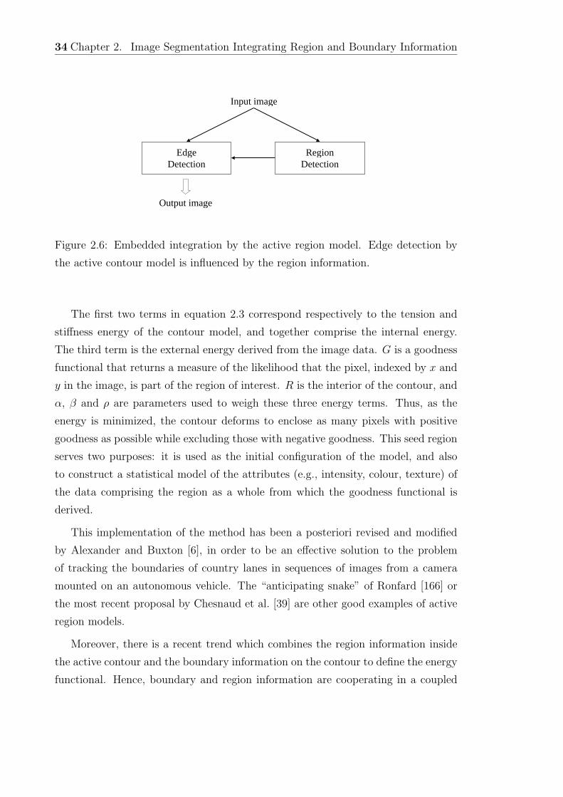
34 Chapter 2. Image Segmentation Integrating Region and Boundary Information
Input image
Output image
EdgeDetection
RegionDetection
Figure 2.6: Embedded integration by the active region model. Edge detection by
the active contour model is influenced by the region information.
The first two terms in equation 2.3 correspond respectively to the tension and
stiffness energy of the contour model, and together comprise the internal energy.
The third term is the external energy derived from the image data. G is a goodness
functional that returns a measure of the likelihood that the pixel, indexed by x and
y in the image, is part of the region of interest. R is the interior of the contour, and
α, β and ρ are parameters used to weigh these three energy terms. Thus, as the
energy is minimized, the contour deforms to enclose as many pixels with positive
goodness as possible while excluding those with negative goodness. This seed region
serves two purposes: it is used as the initial configuration of the model, and also
to construct a statistical model of the attributes (e.g., intensity, colour, texture) of
the data comprising the region as a whole from which the goodness functional is
derived.
This implementation of the method has been a posteriori revised and modified
by Alexander and Buxton [6], in order to be an effective solution to the problem
of tracking the boundaries of country lanes in sequences of images from a camera
mounted on an autonomous vehicle. The “anticipating snake” of Ronfard [166] or
the most recent proposal by Chesnaud et al. [39] are other good examples of active
region models.
Moreover, there is a recent trend which combines the region information inside
the active contour and the boundary information on the contour to define the energy
functional. Hence, boundary and region information are cooperating in a coupled
2.2 Embedded integration 35
active contour model. The exemplary work on this approach is by Paragios and
Deriche [146], where the texture segmentation is obtained by unifying region and
boundary-based information as an improved Geodesic Active Contour Model (orig-
inally proposed by Caselles et al. [30]). Initially, an off-line step is performed that
creates multi-component probabilistic texture descriptors for the given set of tex-
ture patterns. The segmentation problem is then stated under an improved geodesic
active contour model that aims to find the minimal length geodesic curve that best
preserves high boundary probabilities, and creates regions that have maximum a
posteriori segmentation probability with respect to the associated texture hypothe-
sis. This proposal was used subsequently by the same authors to address the problem
of tracking several non-rigid objects over a sequence of frames acquired from a static
observer [147]. Moreover, its use has been analysed by Will et al. [213] to further
enhance the results of a proposed texture edge detector, which can generate precise
maps of highly significant edge-probabilities for the active region model to produce
satisfactory results.
Finally, we want to mention the work of Chakraborty et al. [32, 33], which
has undergone constant evolution in recent years, with the continuous flow of new
ideas and updating of the techniques used, opening up new ways to perform the
integration. In 1994, Chakraborty et al. [32], proposed a segmentation technique for
biomedical image analysis. The proposal uses a Fourier parameterisation to define
the dynamic contour. It expresses a curve in terms of an orthonormal basis, which
for most practical situations, is constrained to a limited number of harmonics. The
curve is thus represented by a set of corresponding Fourier coefficients
p = (a0, c0, a1, b1, c1, d1, ...) (2.4)
The objective function used is a function of conditional probability P (p|Ig, Ir),
or the probability of obtaining the p-contour given the region-classified image Ir and
the image of the scalar magnitude of the grey-level gradient Ig. The function is the
sum of three terms
M(p, Ig, Ir) = Mprior(p) + Mgradient(Ig, p) + Mregion(Ir, p) (2.5)
36 Chapter 2. Image Segmentation Integrating Region and Boundary Information
The first (prior) term biases the boundary toward a particular distribution of
shapes generated from prior experience, while the second term in the equation
(Equation 2.6), Mgradient(Ig, p), depends on the coincidence of the parameterised
boundary, with the image edges appearing as coherent features in the scalar gradi-
ent of the grey levels,
Mgradient(Ig, p) =∫
Cp
Ig[x(p, t), y(p, t)]dt (2.6)
such that the likelihood of p representing the true boundary is proportional to
the sum of the gradient values of all points in Cp.
Finally, term Mregion(Ir, p) (Equation 2.7) measures the goodness of match of the
contour with the perimeter of the segmented interior of the object. This method
rewards the boundary that contains as much of the inside region and as little of
the outside as possible. This function is evaluated by integrating over the area Ap
bounded by the contour p, as expressed in
Mregion(Ir, p) =∫ ∫
Ap
Ir(x, y)dA (2.7)
where pixels inside and outside Ap are set equal to +1 and −1, respectively.
Given that area integral must be evaluated many times, Chakraborty et al. [32]
describe an alternative and faster integration method based on Green’s Theorem.
In their last proposal [33], they suggest a method for integrating region segmen-
tation and active contours using game theory in an effort to form a unified approach.
The novelty of the method is that this is a bi-directional framework, whereby the
results of both computational modules are improved through sharing mutual infor-
mation. Hence, both processes (edge and region detection) use the information from
the co-operative process and the integration carried out is embedded in both seg-
mentation techniques at the same time. The proposed algorithm consists of allowing
the region and boundary modules to assume the roles of individual players who are
trying to optimise their individual cost functions within a game-theory framework.
The flow of information is restricted to passing only the results of the decisions
among the modules. Thus, for any module, the results of the decisions of the other
modules are used as priors, and players try to minimize their cost functions at each
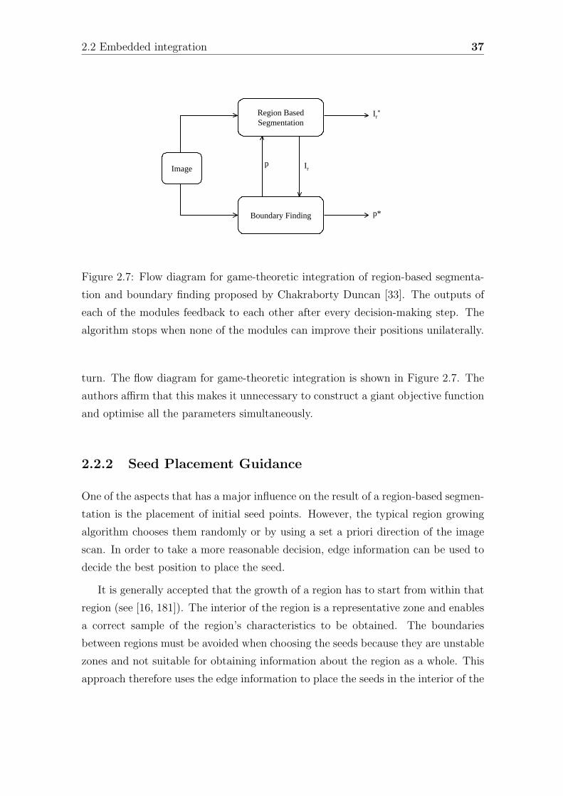
2.2 Embedded integration 37
Region BasedSegmentation
Boundary Finding
Imagep Ir
p*
Ir*
Figure 2.7: Flow diagram for game-theoretic integration of region-based segmenta-
tion and boundary finding proposed by Chakraborty Duncan [33]. The outputs of
each of the modules feedback to each other after every decision-making step. The
algorithm stops when none of the modules can improve their positions unilaterally.
turn. The flow diagram for game-theoretic integration is shown in Figure 2.7. The
authors affirm that this makes it unnecessary to construct a giant objective function
and optimise all the parameters simultaneously.
2.2.2 Seed Placement Guidance
One of the aspects that has a major influence on the result of a region-based segmen-
tation is the placement of initial seed points. However, the typical region growing
algorithm chooses them randomly or by using a set a priori direction of the image
scan. In order to take a more reasonable decision, edge information can be used to
decide the best position to place the seed.
It is generally accepted that the growth of a region has to start from within that
region (see [16, 181]). The interior of the region is a representative zone and enables
a correct sample of the region’s characteristics to be obtained. The boundaries
between regions must be avoided when choosing the seeds because they are unstable
zones and not suitable for obtaining information about the region as a whole. This
approach therefore uses the edge information to place the seeds in the interior of the
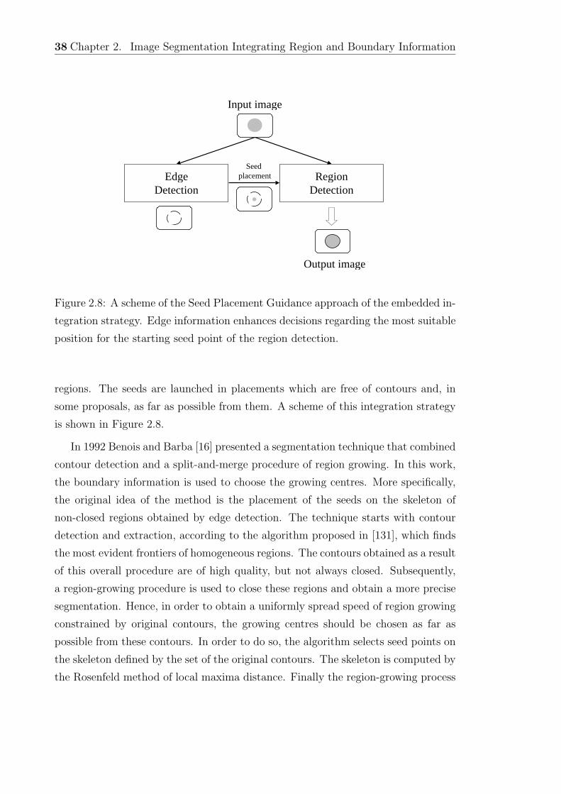
38 Chapter 2. Image Segmentation Integrating Region and Boundary Information
Input image
Output image
EdgeDetection
RegionDetection
Seed placement
Figure 2.8: A scheme of the Seed Placement Guidance approach of the embedded in-
tegration strategy. Edge information enhances decisions regarding the most suitable
position for the starting seed point of the region detection.
regions. The seeds are launched in placements which are free of contours and, in
some proposals, as far as possible from them. A scheme of this integration strategy
is shown in Figure 2.8.
In 1992 Benois and Barba [16] presented a segmentation technique that combined
contour detection and a split-and-merge procedure of region growing. In this work,
the boundary information is used to choose the growing centres. More specifically,
the original idea of the method is the placement of the seeds on the skeleton of
non-closed regions obtained by edge detection. The technique starts with contour
detection and extraction, according to the algorithm proposed in [131], which finds
the most evident frontiers of homogeneous regions. The contours obtained as a result
of this overall procedure are of high quality, but not always closed. Subsequently,
a region-growing procedure is used to close these regions and obtain a more precise
segmentation. Hence, in order to obtain a uniformly spread speed of region growing
constrained by original contours, the growing centres should be chosen as far as
possible from these contours. In order to do so, the algorithm selects seed points on
the skeleton defined by the set of the original contours. The skeleton is computed by
the Rosenfeld method of local maxima distance. Finally the region-growing process
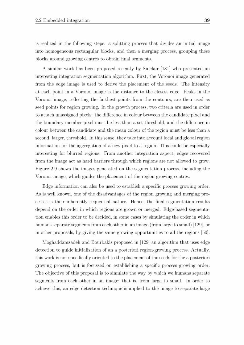
2.2 Embedded integration 39
is realized in the following steps: a splitting process that divides an initial image
into homogeneous rectangular blocks, and then a merging process, grouping these
blocks around growing centres to obtain final segments.
A similar work has been proposed recently by Sinclair [181] who presented an
interesting integration segmentation algorithm. First, the Voronoi image generated
from the edge image is used to derive the placement of the seeds. The intensity
at each point in a Voronoi image is the distance to the closest edge. Peaks in the
Voronoi image, reflecting the farthest points from the contours, are then used as
seed points for region growing. In the growth process, two criteria are used in order
to attach unassigned pixels: the difference in colour between the candidate pixel and
the boundary member pixel must be less than a set threshold, and the difference in
colour between the candidate and the mean colour of the region must be less than a
second, larger, threshold. In this sense, they take into account local and global region
information for the aggregation of a new pixel to a region. This could be especially
interesting for blurred regions. From another integration aspect, edges recovered
from the image act as hard barriers through which regions are not allowed to grow.
Figure 2.9 shows the images generated on the segmentation process, including the
Voronoi image, which guides the placement of the region-growing centres.
Edge information can also be used to establish a specific process growing order.
As is well known, one of the disadvantages of the region growing and merging pro-
cesses is their inherently sequential nature. Hence, the final segmentation results
depend on the order in which regions are grown or merged. Edge-based segmenta-
tion enables this order to be decided, in some cases by simulating the order in which
humans separate segments from each other in an image (from large to small) [129], or
in other proposals, by giving the same growing opportunities to all the regions [50].
Moghaddamzadeh and Bourbakis proposed in [129] an algorithm that uses edge
detection to guide initialisation of an a posteriori region-growing process. Actually,
this work is not specifically oriented to the placement of the seeds for the a posteriori
growing process, but is focussed on establishing a specific process growing order.
The objective of this proposal is to simulate the way by which we humans separate
segments from each other in an image; that is, from large to small. In order to
achieve this, an edge detection technique is applied to the image to separate large
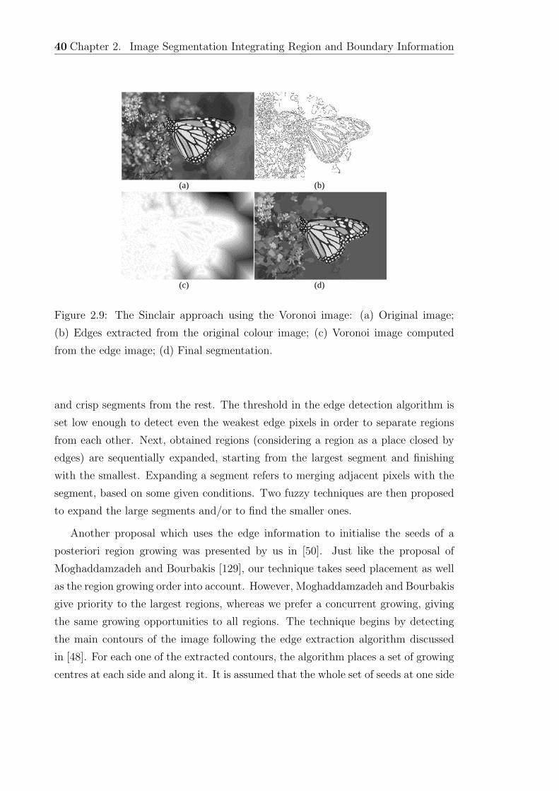
40 Chapter 2. Image Segmentation Integrating Region and Boundary Information
(a) (b)
(c) (d)
Figure 2.9: The Sinclair approach using the Voronoi image: (a) Original image;
(b) Edges extracted from the original colour image; (c) Voronoi image computed
from the edge image; (d) Final segmentation.
and crisp segments from the rest. The threshold in the edge detection algorithm is
set low enough to detect even the weakest edge pixels in order to separate regions
from each other. Next, obtained regions (considering a region as a place closed by
edges) are sequentially expanded, starting from the largest segment and finishing
with the smallest. Expanding a segment refers to merging adjacent pixels with the
segment, based on some given conditions. Two fuzzy techniques are then proposed
to expand the large segments and/or to find the smaller ones.
Another proposal which uses the edge information to initialise the seeds of a
posteriori region growing was presented by us in [50]. Just like the proposal of
Moghaddamzadeh and Bourbakis [129], our technique takes seed placement as well
as the region growing order into account. However, Moghaddamzadeh and Bourbakis
give priority to the largest regions, whereas we prefer a concurrent growing, giving
the same growing opportunities to all regions. The technique begins by detecting
the main contours of the image following the edge extraction algorithm discussed
in [48]. For each one of the extracted contours, the algorithm places a set of growing
centres at each side and along it. It is assumed that the whole set of seeds at one side
2.3 Post-processing integration 41
of the contour belongs to the same region. Then, these seeds are used as samples of
the corresponding regions and analysed in the chromatic space in order to establish
appropriate criteria for the posterior growing processes. The aim is to know a
priori some characteristics of regions in order to adjust the homogeneity criterion to
the region’s characteristics. Finally, seeds simultaneously start a concurrent growth
using the criterion established for each region, which is based on a clustering analysis
and convex hull construction. This proposal is described in depth in Chapter 3.
2.3 Post-processing integration
In contrast to the literature analysed so far, which follows an embedded strategy,
post-processing strategies carry out a posteriori integration, i.e. after the segmenta-
tion of the image by region-based and boundary-based algorithms. Region and edge
information is extracted in a preliminary step, and then the two are integrated. Post-
processing integration is based on fusing results from single segmentation methods,
attempting to combine the region (generally with thick and inaccurate boundaries)
and the edge (generally with fine and sharp lines, but dislocated) maps with the
aim of providing an accurate and meaningful segmentation. We have identified
three different approaches to perform these tasks:
1. Over-segmentation: this approach consists on using a segmentation method
with specifically fixed parameters to obtain an over-segmented result. Addi-
tional information from other segmentation techniques is then used to elimi-
nate false boundaries that do not correspond to regions.
2. Boundary Refinement: this approach considers the region segmentation
result as an initial approach, with well-defined regions, but with inaccurate
boundaries. Information from edge detection is used to refine region bound-
aries and to obtain a more precise result.
3. Selection-Evaluation: in this approach, edge information is used to evaluate
the quality of different region-based segmentation results, with the aim of
choosing the best. This third set of techniques deals with the difficulty of
establishing adequate stopping criteria and thresholds in region segmentation.
42 Chapter 2. Image Segmentation Integrating Region and Boundary Information
2.3.1 Over-segmentation
This approach emerged as a result of the difficulty in establishing an adequate
homogeneity criterion for region growing. As Pavlidis and Liow [152] suggested, the
major reason that region growing produces false boundaries is that the definition of
region uniformity is too strict, such as when they insist on approximately constant
brightness while in reality, brightness may vary linearly within a region. It is very
difficult to find uniformity criteria that exactly match these requirements and do not
generate false boundaries. They concluded that the results could be significantly
improved by checking all the region boundaries that qualify as edges rather than
attempting to fine-tune the uniformity criteria.
The over-segmentation method begins by obtaining an over-segmented result,
which is achieved by properly setting the parameters of the algorithm. This result is
then compared with the result from the dual approach: each boundary is checked to
find out if it is consistent in both results. When this correspondence does not exist,
the boundary is considered false and is removed. In the end, only real boundaries
are preserved. A basic scheme clarifying the ideas of this strategy is shown in
Figure 2.10.
The most common technique consists on obtaining the over-segmented result
using a region-based algorithm. Each initial boundary is checked by analysing its
coherence with the edge map, where real boundaries have high gradient values, while
false boundaries have low values. A first proposal can be found in the work of Monga
et al. [72, 216], where two adjacent regions are merged if the average gradient on
their boundary is lower than a fixed threshold.
In 1992, Kong and Kosko [106] included a fuzzy logic approach in the algorithm
proposed by Monga et al. As Monga et al. proposed, Kong and Kosko computed
gradient information which they refer to as high-frequency characteristics h, to elim-
inate false contours.
h =|high frequency components along the boundary|
length of the boundary(2.8)
For any boundary, if the high-frequency information h is small, the algorithm
concludes the boundary is a false contour and it can be eliminated.
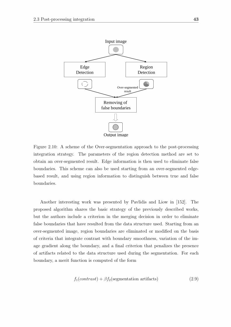
2.3 Post-processing integration 43
Input image
Output image
EdgeDetection
RegionDetection
Over-segmentedresult
Removing of false boundaries
Figure 2.10: A scheme of the Over-segmentation approach to the post-processing
integration strategy. The parameters of the region detection method are set to
obtain an over-segmented result. Edge information is then used to eliminate false
boundaries. This scheme can also be used starting from an over-segmented edge-
based result, and using region information to distinguish between true and false
boundaries.
Another interesting work was presented by Pavlidis and Liow in [152]. The
proposed algorithm shares the basic strategy of the previously described works,
but the authors include a criterion in the merging decision in order to eliminate
false boundaries that have resulted from the data structure used. Starting from an
over-segmented image, region boundaries are eliminated or modified on the basis
of criteria that integrate contrast with boundary smoothness, variation of the im-
age gradient along the boundary, and a final criterion that penalizes the presence
of artifacts related to the data structure used during the segmentation. For each
boundary, a merit function is computed of the form
f1(contrast) + βf2(segmentation artifacts) (2.9)
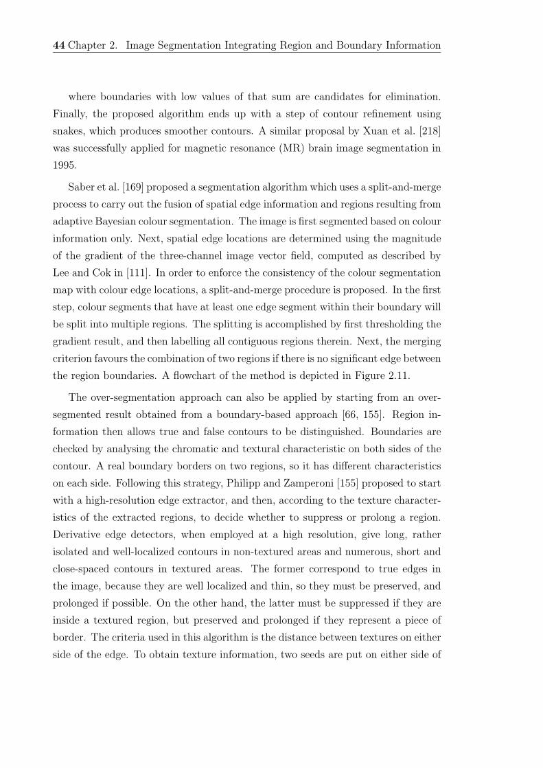
44 Chapter 2. Image Segmentation Integrating Region and Boundary Information
where boundaries with low values of that sum are candidates for elimination.
Finally, the proposed algorithm ends up with a step of contour refinement using
snakes, which produces smoother contours. A similar proposal by Xuan et al. [218]
was successfully applied for magnetic resonance (MR) brain image segmentation in
1995.
Saber et al. [169] proposed a segmentation algorithm which uses a split-and-merge
process to carry out the fusion of spatial edge information and regions resulting from
adaptive Bayesian colour segmentation. The image is first segmented based on colour
information only. Next, spatial edge locations are determined using the magnitude
of the gradient of the three-channel image vector field, computed as described by
Lee and Cok in [111]. In order to enforce the consistency of the colour segmentation
map with colour edge locations, a split-and-merge procedure is proposed. In the first
step, colour segments that have at least one edge segment within their boundary will
be split into multiple regions. The splitting is accomplished by first thresholding the
gradient result, and then labelling all contiguous regions therein. Next, the merging
criterion favours the combination of two regions if there is no significant edge between
the region boundaries. A flowchart of the method is depicted in Figure 2.11.
The over-segmentation approach can also be applied by starting from an over-
segmented result obtained from a boundary-based approach [66, 155]. Region in-
formation then allows true and false contours to be distinguished. Boundaries are
checked by analysing the chromatic and textural characteristic on both sides of the
contour. A real boundary borders on two regions, so it has different characteristics
on each side. Following this strategy, Philipp and Zamperoni [155] proposed to start
with a high-resolution edge extractor, and then, according to the texture character-
istics of the extracted regions, to decide whether to suppress or prolong a region.
Derivative edge detectors, when employed at a high resolution, give long, rather
isolated and well-localized contours in non-textured areas and numerous, short and
close-spaced contours in textured areas. The former correspond to true edges in
the image, because they are well localized and thin, so they must be preserved, and
prolonged if possible. On the other hand, the latter must be suppressed if they are
inside a textured region, but preserved and prolonged if they represent a piece of
border. The criteria used in this algorithm is the distance between textures on either
side of the edge. To obtain texture information, two seeds are put on either side of
2.3 Post-processing integration 45
Merge adjacentregions based oncolor and edge
information
Adaptive Bayesiancolor
segmentationusing GRF
Split regionscontaining edges
Color edgedetection
Color Image
Linkededgemap
Improvedsegmentation
map
Figure 2.11: Flowchart of the method proposed by Saber, Tekalp and Bozdagi.
First, an initial segmentation map is computed. Then, region labels are optimised
by split-and-merge procedures to enforce consistency with the edge map.
the edge and start a recursive growing until N representative pixels are gathered. If
the distance between textures is small, the edge is considered false and regions are
merged. Otherwise, the contour is preserved and prolonged in order to maximize
the distance on either side of the edge.
Fjørtoft et al. [66] presented in 1997 another technique based on over-segmentation
from edge detection, which was applied on SAR images. The authors discussed the
key role of the threshold value to extract the possible edges from an edge strength
map by thresholding. The chosen threshold is related to the probability of false
alarm, i.e., the probability of detecting an edge in a zone of constant reflectivity. In
order to detect all significant edges, a low threshold is set, accepting the detection of
numerous false edges as well. The over-segmentation result provides, as the authors
suggested, a good starting point for the merging process that eliminates false edges
by merging regions. The merging step uses a Likelihood Ratio (LR) criterion to
decide the homogeneity between adjacent regions and the consequent elimination of
46 Chapter 2. Image Segmentation Integrating Region and Boundary Information
their boundary. That is LR is related to the probability that the two regions have
the same reflectivity.
2.3.2 Boundary Refinement
As we have already mentioned, region-based segmentation detects true regions very
well, although, as is well known, the resultant sensitivity to noise causes the bound-
ary of the extracted region to be highly irregular. This approach, which we refer to
as boundary refinement, considers region-based segmentation as an initial approxi-
mation to segmentation. Typically, a region-growing procedure is used to obtain an
initial estimate of a target region, which is then combined with salient edge infor-
mation to achieve a more accurate representation of the target boundary. As in the
over-segmentation proposals, edge information enables an initial result to be refined.
An interesting example of boundary refinement can be found in the work of Had-
don and Boyce [78], where they proposed a segmentation algorithm consisting of two
stages: after an initial region segmentation, a posterior refinement of the generated
regions is performed by means of a relaxation algorithm that uses the edge informa-
tion to ensure local labelling consistency. Nevertheless, the main characteristic of
this work is the postulate that a co-occurrence matrix may be employed as a feature
space, with clusters within the matrix being identified with the regions and bound-
aries of an image. This postulate is proven for nearest neighbour co-occurrence
matrices derived from images whose regions satisfy Gaussian statistics; regions yield
clusters on the main diagonal, and boundaries clusters off the main diagonal.
Chu and Aggarwal presented in [42] an algorithm which integrates multiple re-
gion segmentation and edge maps. The proposed algorithm allows multiple input
maps and applies user-selected weights on various information sources. The first
step consists of transforming all inputs to edge maps, then a maximum likelihood
estimator provides initial solutions of edge positions and strengths from multiple
inputs. An iterative procedure is then used to smooth the resultant edge patterns.
Finally, regions are merged to ensure that every region has the required properties.
The strength of this proposal is that the solution is a negotiated result of all input
maps rather than a selection of them. More recently, Nair and Aggarwal [135] have
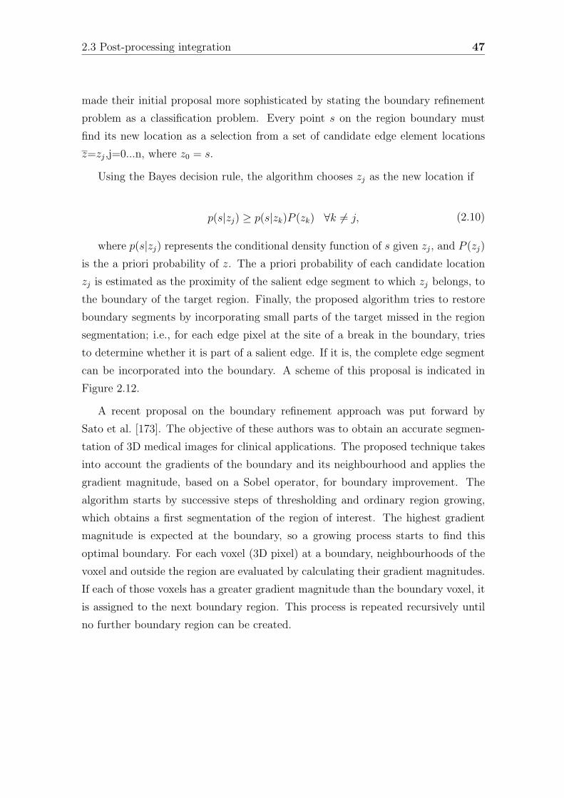
2.3 Post-processing integration 47
made their initial proposal more sophisticated by stating the boundary refinement
problem as a classification problem. Every point s on the region boundary must
find its new location as a selection from a set of candidate edge element locations
z=zj,j=0...n, where z0 = s.
Using the Bayes decision rule, the algorithm chooses zj as the new location if
p(s|zj) ≥ p(s|zk)P (zk) ∀k �= j, (2.10)
where p(s|zj) represents the conditional density function of s given zj, and P (zj)
is the a priori probability of z. The a priori probability of each candidate location
zj is estimated as the proximity of the salient edge segment to which zj belongs, to
the boundary of the target region. Finally, the proposed algorithm tries to restore
boundary segments by incorporating small parts of the target missed in the region
segmentation; i.e., for each edge pixel at the site of a break in the boundary, tries
to determine whether it is part of a salient edge. If it is, the complete edge segment
can be incorporated into the boundary. A scheme of this proposal is indicated in
Figure 2.12.
A recent proposal on the boundary refinement approach was put forward by
Sato et al. [173]. The objective of these authors was to obtain an accurate segmen-
tation of 3D medical images for clinical applications. The proposed technique takes
into account the gradients of the boundary and its neighbourhood and applies the
gradient magnitude, based on a Sobel operator, for boundary improvement. The
algorithm starts by successive steps of thresholding and ordinary region growing,
which obtains a first segmentation of the region of interest. The highest gradient
magnitude is expected at the boundary, so a growing process starts to find this
optimal boundary. For each voxel (3D pixel) at a boundary, neighbourhoods of the
voxel and outside the region are evaluated by calculating their gradient magnitudes.
If each of those voxels has a greater gradient magnitude than the boundary voxel, it
is assigned to the next boundary region. This process is repeated recursively until
no further boundary region can be created.
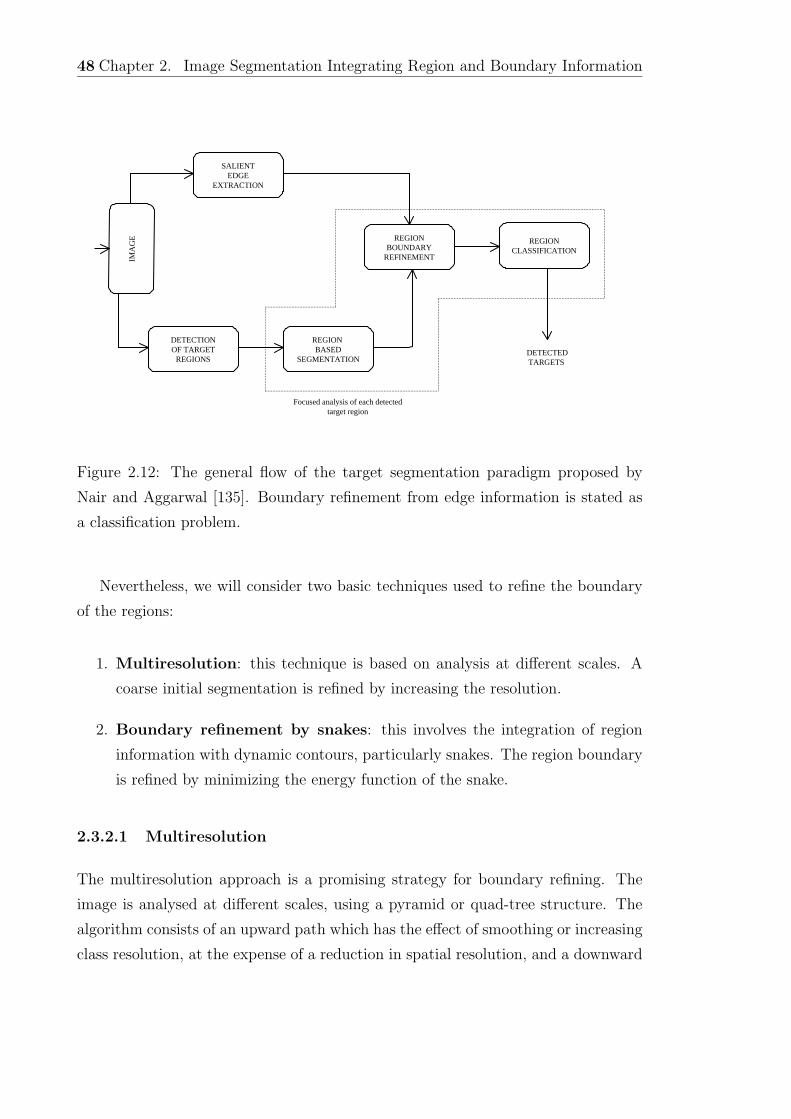
48 Chapter 2. Image Segmentation Integrating Region and Boundary Information
SALIENTEDGE
EXTRACTION
IMA
GE
REGION BASED
SEGMENTATION
DETECTIONOF TARGET
REGIONS
REGIONBOUNDARY
REFINEMENT
REGIONCLASSIFICATION
DETECTEDTARGETS
Focused analysis of each detectedtarget region
Figure 2.12: The general flow of the target segmentation paradigm proposed by
Nair and Aggarwal [135]. Boundary refinement from edge information is stated as
a classification problem.
Nevertheless, we will consider two basic techniques used to refine the boundary
of the regions:
1. Multiresolution: this technique is based on analysis at different scales. A
coarse initial segmentation is refined by increasing the resolution.
2. Boundary refinement by snakes: this involves the integration of region
information with dynamic contours, particularly snakes. The region boundary
is refined by minimizing the energy function of the snake.
2.3.2.1 Multiresolution
The multiresolution approach is a promising strategy for boundary refining. The
image is analysed at different scales, using a pyramid or quad-tree structure. The
algorithm consists of an upward path which has the effect of smoothing or increasing
class resolution, at the expense of a reduction in spatial resolution, and a downward
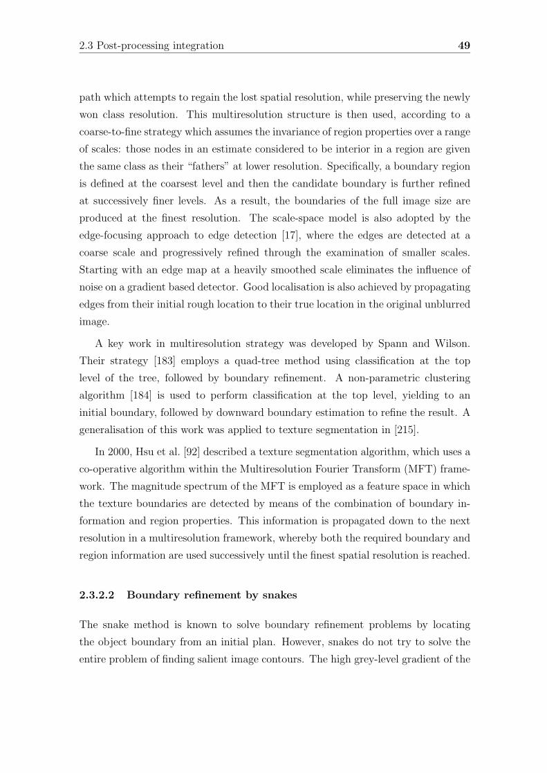
2.3 Post-processing integration 49
path which attempts to regain the lost spatial resolution, while preserving the newly
won class resolution. This multiresolution structure is then used, according to a
coarse-to-fine strategy which assumes the invariance of region properties over a range
of scales: those nodes in an estimate considered to be interior in a region are given
the same class as their “fathers” at lower resolution. Specifically, a boundary region
is defined at the coarsest level and then the candidate boundary is further refined
at successively finer levels. As a result, the boundaries of the full image size are
produced at the finest resolution. The scale-space model is also adopted by the
edge-focusing approach to edge detection [17], where the edges are detected at a
coarse scale and progressively refined through the examination of smaller scales.
Starting with an edge map at a heavily smoothed scale eliminates the influence of
noise on a gradient based detector. Good localisation is also achieved by propagating
edges from their initial rough location to their true location in the original unblurred
image.
A key work in multiresolution strategy was developed by Spann and Wilson.
Their strategy [183] employs a quad-tree method using classification at the top
level of the tree, followed by boundary refinement. A non-parametric clustering
algorithm [184] is used to perform classification at the top level, yielding to an
initial boundary, followed by downward boundary estimation to refine the result. A
generalisation of this work was applied to texture segmentation in [215].
In 2000, Hsu et al. [92] described a texture segmentation algorithm, which uses a
co-operative algorithm within the Multiresolution Fourier Transform (MFT) frame-
work. The magnitude spectrum of the MFT is employed as a feature space in which
the texture boundaries are detected by means of the combination of boundary in-
formation and region properties. This information is propagated down to the next
resolution in a multiresolution framework, whereby both the required boundary and
region information are used successively until the finest spatial resolution is reached.
2.3.2.2 Boundary refinement by snakes
The snake method is known to solve boundary refinement problems by locating
the object boundary from an initial plan. However, snakes do not try to solve the
entire problem of finding salient image contours. The high grey-level gradient of the
50 Chapter 2. Image Segmentation Integrating Region and Boundary Information
Snake placement
Energy optimization
Input image
Output image
EdgeDetection
RegionDetection
Initialcontour
Figure 2.13: A scheme of the Boundary Refinement approach of the post-processing
strategy. Information from edge detection is used to refine the inaccurate boundaries
obtained from the region detection. This process is generally carried out by placing
a snake over the region. The energy minimization process then permits a precise
boundary to be obtained.
image may be due to object boundaries as well as noise and object textures, and
the optimisation functions may therefore have many local optima. Consequently,
active contours are, in general, sensitive to initial conditions and they are only truly
effective when the initial position of the contour in the image is sufficiently close
to the real boundary. For this reason, active contours rely on other mechanisms to
place them somewhere near the desired contour. In early works on dynamic contours,
an expert was responsible for putting the snake close to an intended contour, and
minimizing its energy provided its final position.
However, region segmentation could be the solution to the problem of where
to initialize snakes. Proposals concerning integrated methods consist of using the
region segmentation result as the initial contour of the snake. Here, the segmentation
process is typically divided into two steps (see Figure 2.13). First, a region growing
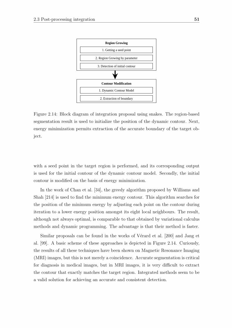
2.3 Post-processing integration 51
1. Getting a seed point
2. Region Growing by parameter
3. Detection of initial contour
1. Dynamic Contour Model
2. Extraction of boundary
Region Growing
Contour Modification
Figure 2.14: Block diagram of integration proposal using snakes. The region-based
segmentation result is used to initialize the position of the dynamic contour. Next,
energy minimization permits extraction of the accurate boundary of the target ob-
ject.
with a seed point in the target region is performed, and its corresponding output
is used for the initial contour of the dynamic contour model. Secondly, the initial
contour is modified on the basis of energy minimization.
In the work of Chan et al. [34], the greedy algorithm proposed by Williams and
Shah [214] is used to find the minimum energy contour. This algorithm searches for
the position of the minimum energy by adjusting each point on the contour during
iteration to a lower energy position amongst its eight local neighbours. The result,
although not always optimal, is comparable to that obtained by variational calculus
methods and dynamic programming. The advantage is that their method is faster.
Similar proposals can be found in the works of Verard et al. [200] and Jang et
al. [99]. A basic scheme of these approaches is depicted in Figure 2.14. Curiously,
the results of all these techniques have been shown on Magnetic Resonance Imaging
(MRI) images, but this is not merely a coincidence. Accurate segmentation is critical
for diagnosis in medical images, but in MRI images, it is very difficult to extract
the contour that exactly matches the target region. Integrated methods seem to be
a valid solution for achieving an accurate and consistent detection.
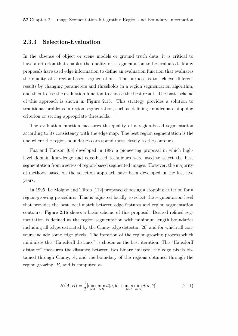
52 Chapter 2. Image Segmentation Integrating Region and Boundary Information
2.3.3 Selection-Evaluation
In the absence of object or scene models or ground truth data, it is critical to
have a criterion that enables the quality of a segmentation to be evaluated. Many
proposals have used edge information to define an evaluation function that evaluates
the quality of a region-based segmentation. The purpose is to achieve different
results by changing parameters and thresholds in a region segmentation algorithm,
and then to use the evaluation function to choose the best result. The basic scheme
of this approach is shown in Figure 2.15. This strategy provides a solution to
traditional problems in region segmentation, such as defining an adequate stopping
criterion or setting appropriate thresholds.
The evaluation function measures the quality of a region-based segmentation
according to its consistency with the edge map. The best region segmentation is the
one where the region boundaries correspond most closely to the contours.
Fua and Hanson [68] developed in 1987 a pioneering proposal in which high-
level domain knowledge and edge-based techniques were used to select the best
segmentation from a series of region-based segmented images. However, the majority
of methods based on the selection approach have been developed in the last five
years.
In 1995, Le Moigne and Tilton [112] proposed choosing a stopping criterion for a
region-growing procedure. This is adjusted locally to select the segmentation level
that provides the best local match between edge features and region segmentation
contours. Figure 2.16 shows a basic scheme of this proposal. Desired refined seg-
mentation is defined as the region segmentation with minimum length boundaries
including all edges extracted by the Canny edge detector [26] and for which all con-
tours include some edge pixels. The iteration of the region-growing process which
minimizes the “Hausdorff distance” is chosen as the best iteration. The “Hausdorff
distance” measures the distance between two binary images: the edge pixels ob-
tained through Canny, A, and the boundary of the regions obtained through the
region growing, B, and is computed as
H(A,B) =1
2[max
aεAminbεB
d(a, b) + maxbεB
minaεA
d(a, b)] (2.11)
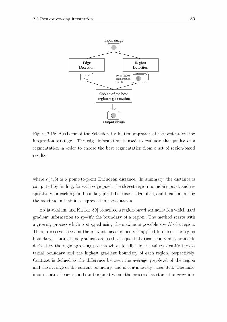
2.3 Post-processing integration 53
Input image
Output image
EdgeDetection
RegionDetection
Set of regionsegmentation results
Choice of the best region segmentation
Figure 2.15: A scheme of the Selection-Evaluation approach of the post-processing
integration strategy. The edge information is used to evaluate the quality of a
segmentation in order to choose the best segmentation from a set of region-based
results.
where d(a, b) is a point-to-point Euclidean distance. In summary, the distance is
computed by finding, for each edge pixel, the closest region boundary pixel, and re-
spectively for each region boundary pixel the closest edge pixel, and then computing
the maxima and minima expressed in the equation.
Hojjatoleslami and Kittler [89] presented a region-based segmentation which used
gradient information to specify the boundary of a region. The method starts with
a growing process which is stopped using the maximum possible size N of a region.
Then, a reserve check on the relevant measurements is applied to detect the region
boundary. Contrast and gradient are used as sequential discontinuity measurements
derived by the region-growing process whose locally highest values identify the ex-
ternal boundary and the highest gradient boundary of each region, respectively.
Contrast is defined as the difference between the average grey-level of the region
and the average of the current boundary, and is continuously calculated. The max-
imum contrast corresponds to the point where the process has started to grow into
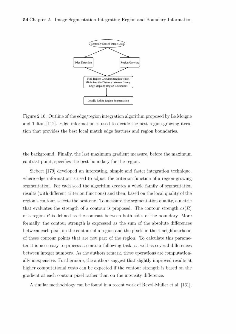
54 Chapter 2. Image Segmentation Integrating Region and Boundary Information
Remotely Sensed Image Data
Edge Detection Region Growing
Find Region Growing Iteration whichMinimizes the Distance between Binary
Edge Map and Region Boundaries
Locally Refine Region Segmentation
Figure 2.16: Outline of the edge/region integration algorithm proposed by Le Moigne
and Tilton [112]. Edge information is used to decide the best region-growing itera-
tion that provides the best local match edge features and region boundaries.
the background. Finally, the last maximum gradient measure, before the maximum
contrast point, specifies the best boundary for the region.
Siebert [179] developed an interesting, simple and faster integration technique,
where edge information is used to adjust the criterion function of a region-growing
segmentation. For each seed the algorithm creates a whole family of segmentation
results (with different criterion functions) and then, based on the local quality of the
region’s contour, selects the best one. To measure the segmentation quality, a metric
that evaluates the strength of a contour is proposed. The contour strength cs(R)
of a region R is defined as the contrast between both sides of the boundary. More
formally, the contour strength is expressed as the sum of the absolute differences
between each pixel on the contour of a region and the pixels in the 4-neighbourhood
of these contour points that are not part of the region. To calculate this parame-
ter it is necessary to process a contour-following task, as well as several differences
between integer numbers. As the authors remark, these operations are computation-
ally inexpensive. Furthermore, the authors suggest that slightly improved results at
higher computational costs can be expected if the contour strength is based on the
gradient at each contour pixel rather than on the intensity difference.
A similar methodology can be found in a recent work of Revol-Muller et al. [161],
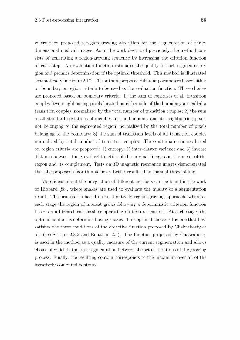
2.3 Post-processing integration 55
where they proposed a region-growing algorithm for the segmentation of three-
dimensional medical images. As in the work described previously, the method con-
sists of generating a region-growing sequence by increasing the criterion function
at each step. An evaluation function estimates the quality of each segmented re-
gion and permits determination of the optimal threshold. This method is illustrated
schematically in Figure 2.17. The authors proposed different parameters based either
on boundary or region criteria to be used as the evaluation function. Three choices
are proposed based on boundary criteria: 1) the sum of contrasts of all transition
couples (two neighbouring pixels located on either side of the boundary are called a
transition couple), normalized by the total number of transition couples; 2) the sum
of all standard deviations of members of the boundary and its neighbouring pixels
not belonging to the segmented region, normalized by the total number of pixels
belonging to the boundary; 3) the sum of transition levels of all transition couples
normalized by total number of transition couples. Three alternate choices based
on region criteria are proposed: 1) entropy, 2) inter-cluster variance and 3) inverse
distance between the grey-level function of the original image and the mean of the
region and its complement. Tests on 3D magnetic resonance images demonstrated
that the proposed algorithm achieves better results than manual thresholding.
More ideas about the integration of different methods can be found in the work
of Hibbard [88], where snakes are used to evaluate the quality of a segmentation
result. The proposal is based on an iteratively region growing approach, where at
each stage the region of interest grows following a deterministic criterion function
based on a hierarchical classifier operating on texture features. At each stage, the
optimal contour is determined using snakes. This optimal choice is the one that best
satisfies the three conditions of the objective function proposed by Chakraborty et
al. (see Section 2.3.2 and Equation 2.5). The function proposed by Chakraborty
is used in the method as a quality measure of the current segmentation and allows
choice of which is the best segmentation between the set of iterations of the growing
process. Finally, the resulting contour corresponds to the maximum over all of the
iteratively computed contours.
56 Chapter 2. Image Segmentation Integrating Region and Boundary Information
Initial ImageInitial Image ParametricalRegion Growing
Segmented ImageEvaluation Function
fev(σ)
σk= σoptσ
fev max
σ0
σ1
σ2
σn
Figure 2.17: Scheme of the method proposed by Revol-Muller et al [161]. A sequence
of segmented regions is obtained by increasing the homogeneity threshold. Then,
an evaluation function determines the optimal threshold automatically.
2.4 Summary
A review of various segmentation proposals integrating edge and region information
has been given, making special emphasis on different strategies and methods used
to fuse such information. The aim of this summary is to point out the features and
the essential differences of such approaches, as well as to discuss some questions that
perhaps have not been properly considered.
Table 2.1 summarizes different methods to perform edge and region integration.
The first column distinguishes the strategy according to the timing of the fusion:
embedded or post-processing. The second column names the approach. The next
two columns describe the problem that the approach tries to solve and a description
of the objective. Finally, the last column summarizes the procedure used to perform
the segmentation task.
As described in Section 2.1, embedded and post-processing integration use differ-
ent principles to perform the task of segmentation. Embedded integration is based
2.4 Summary 57
on the design of a complex, or a superior, algorithm which uses region and edge in-
formation to avoid errors in segmentation. On the other hand, the post-processing
strategy accepts faults in the elemental segmentation algorithms, but an a posteriori
integration module tries to correct them. The key features which characterise and
contrast the two strategies are:
• single algorithm and avoidance of errors (embedded integration)
• multiple algorithms and correction of errors (post-processing integration).
These two essential characteristics lead to the fact that these strategies involve
notable differences. The first aspect to analyse is the complexity of both strategies.
Embedded integration produces, in general, a more complex algorithm as it attempts
not to commit errors or take wrong decisions. The post-processing strategy can be
regarded as the set of many simple algorithms working in parallel and producing
many wrong segmentation results. These errors are solved by a posteriori fusion
module that works on these results. Post-processing complexity is therefore lower
because the quantity of information to process decreases, as only the results are
taken into consideration.
Another aspect which is worth analysing is the independence of these integration
strategies with respect to their implementation in the segmentation algorithm. The
embedded strategy is strongly dependent, because it typically implies the design of
a new algorithm, which incorporates the integration. Hence, any change in the inte-
gration procedure will imply the modification of the algorithm. On the other hand,
the post-processing strategy involves a more general approach as it is independent
of the choice of algorithms for image segmentation. The fusion of the information
only takes the results of the segmentation algorithms into account, so the way they
are obtained is not important, and it is possible to use any established algorithms.
Some researchers, such as LeMoigne and Tilton [112], indicate that post-processing
integration can also be viewed in a general data management framework, where all
incoming data is processed on-line upon acquisition, producing basic features such
as edges and regions.
However, we need to point out that the post-processing strategy is not 100%
independent, and this, in fact, is its weak point. It is true that it is independent in
58 Chapter 2. Image Segmentation Integrating Region and Boundary Information
terms of the chosen method, but obviously if the results achieved by these algorithms
are very poor, post-processing fails. It is undeniable that a posteriori fusion needs
to work on a relatively good set of segmentation results. Final segmentation will
therefore inevitably depend, to a greater or lesser extent, on the initial results of
the segmentation. An initial fault, e.g., the inappropriate selection of seeds in a
region-growing algorithm, will be carried over into the entire segmentation process.
A posteriori integration of edge information may not be able to overcome an error
of this magnitude.
2.4.1 Open questions
Having reviewed the different proposals, we think that some questions still deserve
special attention. First, there are important questions related to the evaluation of
the approaches and the difficulty that it implies. Secondly, there are certain tasks
which are included in many of the reviewed proposals, such as contour or texture
extraction, which are significant research topics by themselves.
• Evaluating the different approaches
Actually, it is not feasible to determine the best approach to segmentation
that integrates boundary and region information. There are several reasons
for this: the lack of a generally accepted and clear methodology for evaluating
segmentation algorithms [143]; the difficulty of obtaining and ground truthing
sufficient real imagery [202]; or the fact that different segmentation algorithms
differ in terms of the properties and objectives they try to satisfy and the
image domain in which they are working [82]. However, the most important
factor is probably the difficulty in implementing other people’s algorithms due
to the lack of necessary details [221]. Obviously, unless a given segmentation
algorithm is specifically implemented and tried out on the data to hand, it is
very difficult to evaluate from the published results how well it will work for
that data [67]. As Hoover et al. [90] indicated the comparative framework is
itself a research issue, and although positive steps have been taken, a guiding
philosophy for the design of such a framework is still lacking. All these points
will be further discussed in Chapter 5.
2.4 Summary 59
• Tasks
Another thing to point out is the high number of very difficult tasks that
are integral parts of the approaches we have reviewed, for example edge map
extraction or thresholding, among others. For instance, a serious difficulty ap-
pears when, as is usual, the most significant edges in the image are required.
Extracting these is not an easy task and the process often includes many pa-
rameters: i.e. an adequate threshold that will result in a reliable binarization
and the subsequent edge map. In this sense, the embedded proposals that
directly use the gradient map as boundary information have an important
advantage. Another question to consider is the lack of attention that, in gen-
eral, the reviewed works devote to texture. Without this property, it is not
possible to distinguish whether a high-magnitude gradient corresponds to a
boundary between regions, or to a textured region. Regrettably, texture is
generally forgotten in the different proposals of embedded integration, with
specific exceptions which have been duly noted. As a consequence, the algo-
rithms are not adapted to segmenting heavily textured areas, resulting in an
over-segmentation of these regions. Segmentation techniques based on post-
processing integration also suffer some deficiencies. Those based on an over-
segmented image must solve a non-trivial problem: What should the threshold
be in order to obtain an over-segmented result? It is well known that images
have different characteristics, so this threshold cannot be a fixed value. An
adequate threshold for one image may not be effective for others, and this
may lead to an irrecoverable loss of boundaries. An initial mistake in such
algorithms could be a serious handicap for the a posteriori fusion, resulting in
an under-segmented result. Moreover, the authenticity of the initial contours
is generally checked under the assumption that real boundaries have high gra-
dients. However, this assumption is not an indispensable characteristic of real
boundaries and this leads to one of the most serious difficulties of the segmen-
tation task. As described in Section 2.3.2, the aim of the boundary refinement
approaches is to obtain reliable smooth boundaries. In order to achieve this,
cooperation between region-based segmentation and snakes, which is the most
common technique, is really a good choice. However, it should be also noted
that the aim of these algorithms is generally to segment not a whole image,

60 Chapter 2. Image Segmentation Integrating Region and Boundary Information
but individual objects from an image. Furthermore, these algorithms have a
deficiency that is shared with the third set of post-processing methods: their
exclusive attention to the boundary. Refining the result is reduced to the re-
gion boundary, so it is not possible to correct any other mistakes inside the
region. The same problem is found in the selection-evaluation approach, where
the quality measure of a segmentation based on boundary information is ex-
clusively based on the external boundary, and not on any inner contour lines
caused by holes. For this reason, regions extracted might contain holes that do
not show up. In short, all these weak points of the post-processing integration
reaffirm the previous assertion about the need for good initial segmentation
results and the inability of the post-processing strategy to correct some initial
mistakes.
2.5 Conclusions
In this chapter we have reviewed some key segmentation techniques that integrate
region and boundary information. Special emphasis has been placed on the strategy
used to carry out the integration process. A classification of cooperative segmenta-
tion techniques has been given and several algorithms described, pointing out their
specific features.
The lack of specific treatment of textured images has been noted, which is one of
the major problems of segmentation [54]. If an image mainly contains homogeneous
colour regions, traditional methods of segmentation working in colour spaces may
be sufficient to attain reasonable results. However, some real images “suffer” from
texture, for example, images depicting natural scenes, which have considerable vari-
ety of colour and texture. Texture, therefore, undoubtedly has a pivotal role to play
in image segmentation. However, there is now some new and promising research
into the integration of colour and texture in segmentation [28, 128, 150, 193, 198].
An attempt to integrate complementary information from the image may follow; it
seems reasonable to assume that a considerable improvement in segmentation will
result from the fusion of colour, texture and boundary information. Segmentation
techniques, in general, are still in need of considerable improvement. The techniques

2.5 Conclusions 61
we have discussed still have some faults and there is, as yet, no perfect segmenta-
tion algorithm, something which is vital for the advancement of Computer Vision
and its applications. However, integration of region and boundary information has
brought improvements to previous results. Work in this field of research has gener-
ated numerous proposals in the last few years. This current interest encourages us
to predict that further work and improvement of segmentation will be focussed on
integrating algorithms and information.
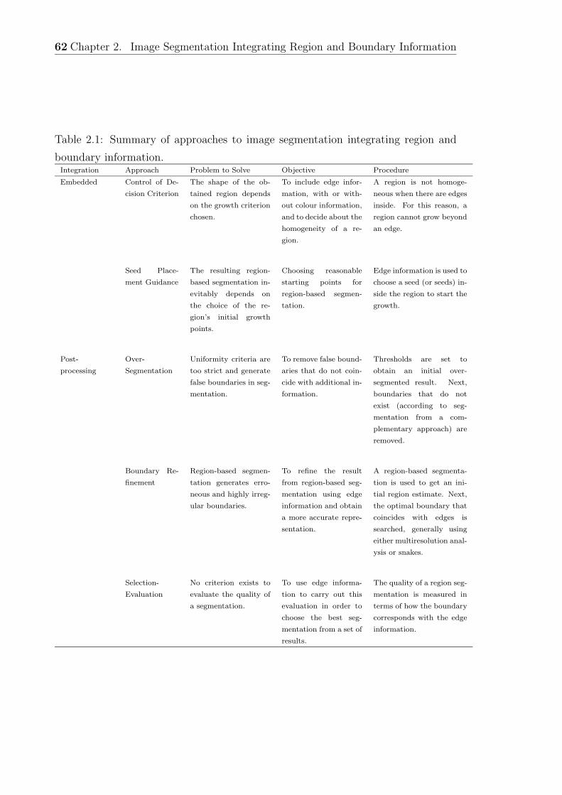
62 Chapter 2. Image Segmentation Integrating Region and Boundary Information
Table 2.1: Summary of approaches to image segmentation integrating region and
boundary information.Integration Approach Problem to Solve Objective Procedure
Embedded Control of De-
cision Criterion
The shape of the ob-
tained region depends
on the growth criterion
chosen.
To include edge infor-
mation, with or with-
out colour information,
and to decide about the
homogeneity of a re-
gion.
A region is not homoge-
neous when there are edges
inside. For this reason, a
region cannot grow beyond
an edge.
Seed Place-
ment Guidance
The resulting region-
based segmentation in-
evitably depends on
the choice of the re-
gion’s initial growth
points.
Choosing reasonable
starting points for
region-based segmen-
tation.
Edge information is used to
choose a seed (or seeds) in-
side the region to start the
growth.
Post-
processing
Over-
Segmentation
Uniformity criteria are
too strict and generate
false boundaries in seg-
mentation.
To remove false bound-
aries that do not coin-
cide with additional in-
formation.
Thresholds are set to
obtain an initial over-
segmented result. Next,
boundaries that do not
exist (according to seg-
mentation from a com-
plementary approach) are
removed.
Boundary Re-
finement
Region-based segmen-
tation generates erro-
neous and highly irreg-
ular boundaries.
To refine the result
from region-based seg-
mentation using edge
information and obtain
a more accurate repre-
sentation.
A region-based segmenta-
tion is used to get an ini-
tial region estimate. Next,
the optimal boundary that
coincides with edges is
searched, generally using
either multiresolution anal-
ysis or snakes.
Selection-
Evaluation
No criterion exists to
evaluate the quality of
a segmentation.
To use edge informa-
tion to carry out this
evaluation in order to
choose the best seg-
mentation from a set of
results.
The quality of a region seg-
mentation is measured in
terms of how the boundary
corresponds with the edge
information.
Chapter 3
Unsupervised Image Segmentation
A strategy for unsupervised image segmentation which fuses region and boundary in-
formation is presented. The proposed approach takes advantage of the combination
of 3 different strategies: the guidance of seed placement, the control of decision cri-
terion, and the boundary refinement. The new algorithm uses boundary information
to initialize a set of active regions which compete for pixels in order to segment the
whole image. The method is designed considering a pyramidal representation which
ensures noise robustness as well as computation efficiency.
3.1 Introduction
In the previous chapter, the main strategies aiming to integrate region and boundary
information in the segmentation process have been presented. Note that, although
they have the common objective of improving the segmentation results using the
basic approaches independently (region or boundary based), they take different ways
to achieve this goal. Each one of these integration strategies attempt to solve a
different problem of the image segmentation, as is summarized in Table 2.1. For
example, the seed placement guidance strategy attempts to handle the choice of
the initial growth points by using the edge information to take this decision. On
the other hand, the boundary refinement strategy tries to improve the segmentation
obtained by a region-based algorithm refining the boundaries to achieve a more
accurate result.
63
64 Chapter 3. Unsupervised Image Segmentation
We consider that it could be greatly attractive to fuse different strategies to
perform the integration of region and boundary information. The fusion of several
approaches will allow to tackle an important number of issues and to exploit at
maximum the possibilities offered by each one. Hence, we propose an image seg-
mentation method which combines the guidance of seed placement, the control of
decision criterion and the boundary refinement approaches.
This chapter has been structured in the following blocks: the Introduction is con-
cluded by the description of our first approach to image segmentation. Subsequently,
Section 3.2 describes the philosophy of the new proposed segmentation strategy con-
sidering the grey level image. The adaption to colour image segmentation is then
explained in Section 3.3. Finally, some conclusions are given in Section 3.4.
3.1.1 A First Approach
In 2000 we proposed an algorithm which follows a guidance of seed placement strat-
egy to carry out the image segmentation. The edges of the image are used to
adequately place a set of seeds. More specifically, main contours (or circumscribed
contours) are detected and then seeds are situated on both sides and along the
contour, which separates two regions. Then, seeds start a concurrent region grow-
ing in order to segment the image. A basic scheme of this proposal is depicted in
Figure 3.1.
The algorithm provides two main advantages to start the region growing process:
• The starting seed points are placed inside the regions, far from the boundaries,
which permits avoiding unstable areas to begin the growing.
• Seeds can be used as region samples to know a priori the characteristics of the
region placed at one side of the contour. This prior knowledge allows the ad-
justment of the region growing algorithm and the resolution of a very common
problem: the difficulty of establishing an adequate criterion of homogeneity.
Classical algorithms base their decision of merging a region with a pixel on a
homogeneity criterion, which usually takes some statistical parameters of the regions
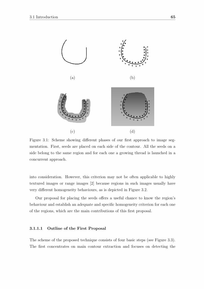
3.1 Introduction 65
(a) (b)
(c) (d)
Figure 3.1: Scheme showing different phases of our first approach to image seg-
mentation. First, seeds are placed on each side of the contour. All the seeds on a
side belong to the same region and for each one a growing thread is launched in a
concurrent approach.
into consideration. However, this criterion may not be often applicable to highly
textured images or range images [2] because regions in such images usually have
very different homogeneity behaviours, as is depicted in Figure 3.2.
Our proposal for placing the seeds offers a useful chance to know the region’s
behaviour and establish an adequate and specific homogeneity criterion for each one
of the regions, which are the main contributions of this first proposal.
3.1.1.1 Outline of the First Proposal
The scheme of the proposed technique consists of four basic steps (see Figure 3.3).
The first concentrates on main contour extraction and focuses on detecting the
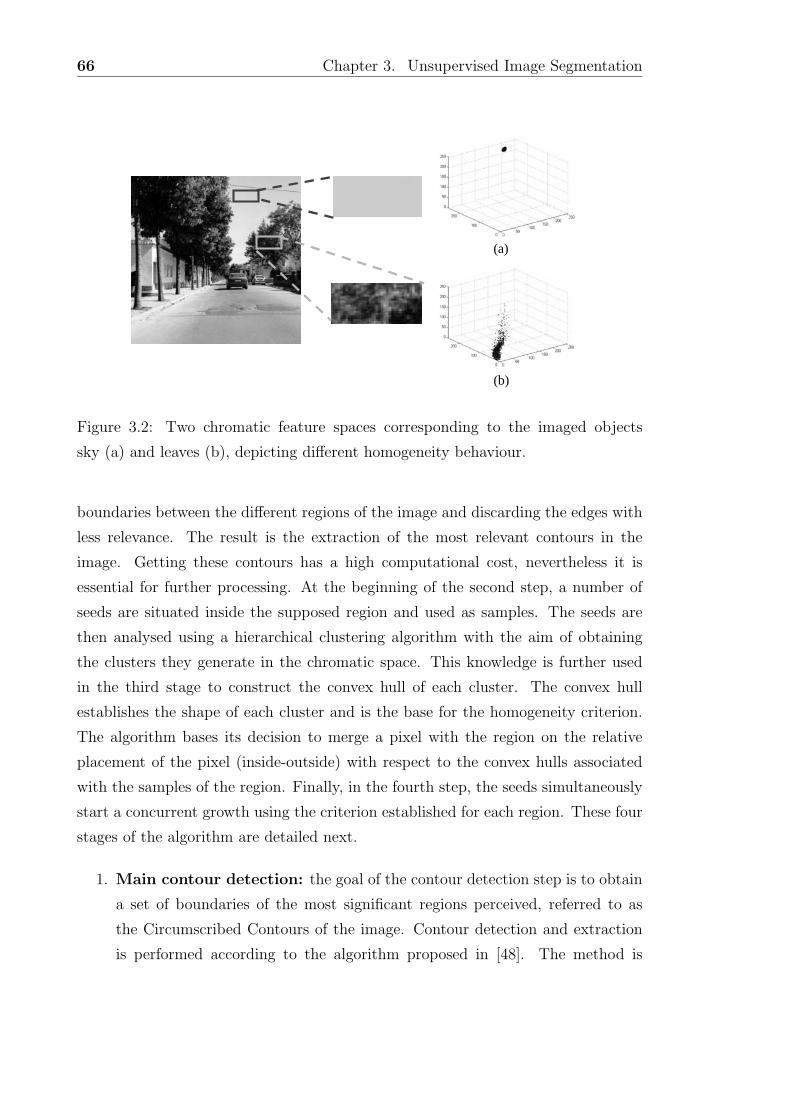
66 Chapter 3. Unsupervised Image Segmentation
(a)
(b)
Figure 3.2: Two chromatic feature spaces corresponding to the imaged objects
sky (a) and leaves (b), depicting different homogeneity behaviour.
boundaries between the different regions of the image and discarding the edges with
less relevance. The result is the extraction of the most relevant contours in the
image. Getting these contours has a high computational cost, nevertheless it is
essential for further processing. At the beginning of the second step, a number of
seeds are situated inside the supposed region and used as samples. The seeds are
then analysed using a hierarchical clustering algorithm with the aim of obtaining
the clusters they generate in the chromatic space. This knowledge is further used
in the third stage to construct the convex hull of each cluster. The convex hull
establishes the shape of each cluster and is the base for the homogeneity criterion.
The algorithm bases its decision to merge a pixel with the region on the relative
placement of the pixel (inside-outside) with respect to the convex hulls associated
with the samples of the region. Finally, in the fourth step, the seeds simultaneously
start a concurrent growth using the criterion established for each region. These four
stages of the algorithm are detailed next.
1. Main contour detection: the goal of the contour detection step is to obtain
a set of boundaries of the most significant regions perceived, referred to as
the Circumscribed Contours of the image. Contour detection and extraction
is performed according to the algorithm proposed in [48]. The method is
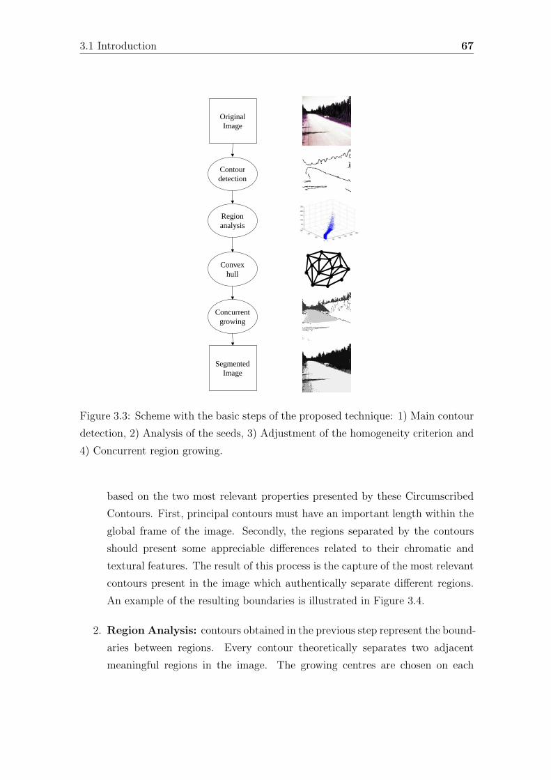
3.1 Introduction 67
OriginalImage
Contourdetection
Regionanalysis
Convexhull
Concurrentgrowing
SegmentedImage
Figure 3.3: Scheme with the basic steps of the proposed technique: 1) Main contour
detection, 2) Analysis of the seeds, 3) Adjustment of the homogeneity criterion and
4) Concurrent region growing.
based on the two most relevant properties presented by these Circumscribed
Contours. First, principal contours must have an important length within the
global frame of the image. Secondly, the regions separated by the contours
should present some appreciable differences related to their chromatic and
textural features. The result of this process is the capture of the most relevant
contours present in the image which authentically separate different regions.
An example of the resulting boundaries is illustrated in Figure 3.4.
2. Region Analysis: contours obtained in the previous step represent the bound-
aries between regions. Every contour theoretically separates two adjacent
meaningful regions in the image. The growing centres are chosen on each
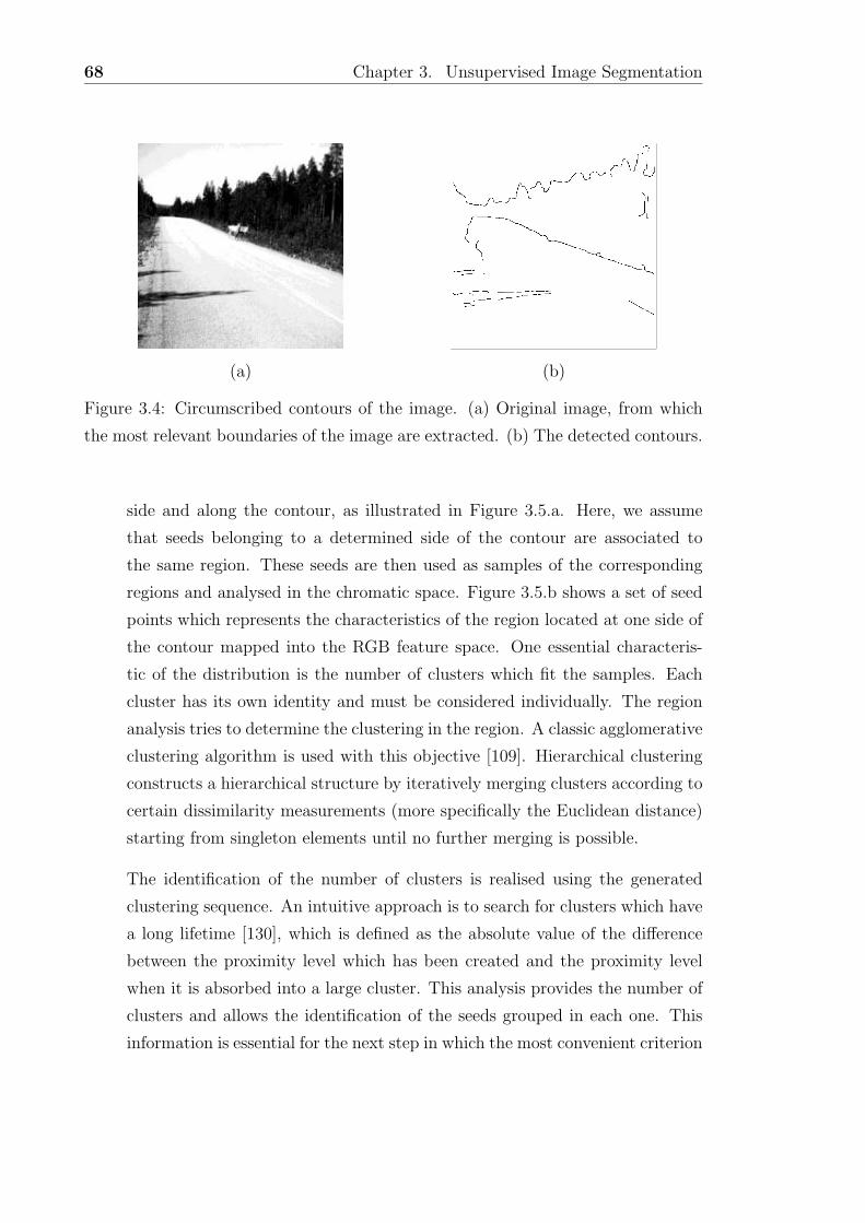
68 Chapter 3. Unsupervised Image Segmentation
(a) (b)
Figure 3.4: Circumscribed contours of the image. (a) Original image, from which
the most relevant boundaries of the image are extracted. (b) The detected contours.
side and along the contour, as illustrated in Figure 3.5.a. Here, we assume
that seeds belonging to a determined side of the contour are associated to
the same region. These seeds are then used as samples of the corresponding
regions and analysed in the chromatic space. Figure 3.5.b shows a set of seed
points which represents the characteristics of the region located at one side of
the contour mapped into the RGB feature space. One essential characteris-
tic of the distribution is the number of clusters which fit the samples. Each
cluster has its own identity and must be considered individually. The region
analysis tries to determine the clustering in the region. A classic agglomerative
clustering algorithm is used with this objective [109]. Hierarchical clustering
constructs a hierarchical structure by iteratively merging clusters according to
certain dissimilarity measurements (more specifically the Euclidean distance)
starting from singleton elements until no further merging is possible.
The identification of the number of clusters is realised using the generated
clustering sequence. An intuitive approach is to search for clusters which have
a long lifetime [130], which is defined as the absolute value of the difference
between the proximity level which has been created and the proximity level
when it is absorbed into a large cluster. This analysis provides the number of
clusters and allows the identification of the seeds grouped in each one. This
information is essential for the next step in which the most convenient criterion
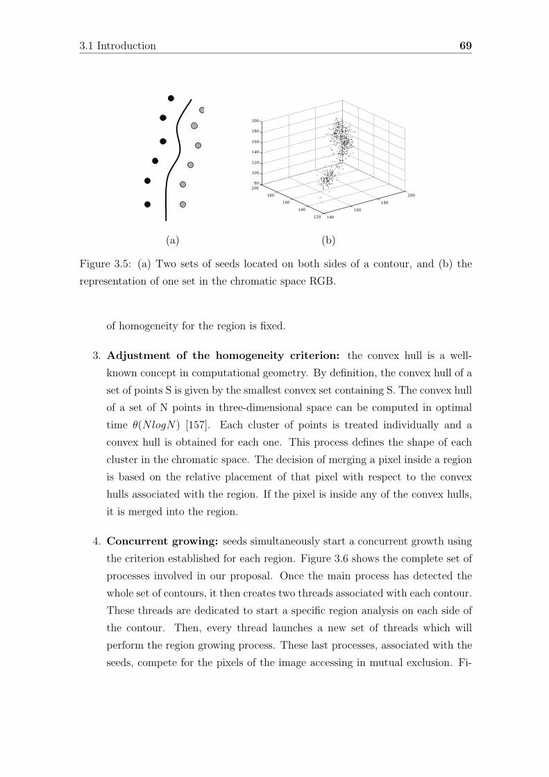
3.1 Introduction 69
140
160
180
200
120
140
160
180
20080
100
120
140
160
180
200
(a) (b)
Figure 3.5: (a) Two sets of seeds located on both sides of a contour, and (b) the
representation of one set in the chromatic space RGB.
of homogeneity for the region is fixed.
3. Adjustment of the homogeneity criterion: the convex hull is a well-
known concept in computational geometry. By definition, the convex hull of a
set of points S is given by the smallest convex set containing S. The convex hull
of a set of N points in three-dimensional space can be computed in optimal
time θ(NlogN) [157]. Each cluster of points is treated individually and a
convex hull is obtained for each one. This process defines the shape of each
cluster in the chromatic space. The decision of merging a pixel inside a region
is based on the relative placement of that pixel with respect to the convex
hulls associated with the region. If the pixel is inside any of the convex hulls,
it is merged into the region.
4. Concurrent growing: seeds simultaneously start a concurrent growth using
the criterion established for each region. Figure 3.6 shows the complete set of
processes involved in our proposal. Once the main process has detected the
whole set of contours, it then creates two threads associated with each contour.
These threads are dedicated to start a specific region analysis on each side of
the contour. Then, every thread launches a new set of threads which will
perform the region growing process. These last processes, associated with the
seeds, compete for the pixels of the image accessing in mutual exclusion. Fi-
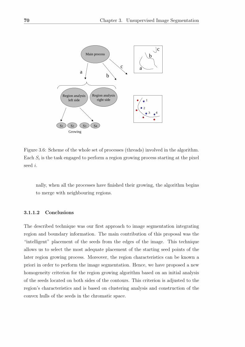
70 Chapter 3. Unsupervised Image Segmentation
Main process
ab
c a
bc
Region analysisleft side
Region analysisright side
S1 S2 S3 S4
Growing
1
42
3
Figure 3.6: Scheme of the whole set of processes (threads) involved in the algorithm.
Each Si is the task engaged to perform a region growing process starting at the pixel
seed i.
nally, when all the processes have finished their growing, the algorithm begins
to merge with neighbouring regions.
3.1.1.2 Conclusions
The described technique was our first approach to image segmentation integrating
region and boundary information. The main contribution of this proposal was the
“intelligent” placement of the seeds from the edges of the image. This technique
allows us to select the most adequate placement of the starting seed points of the
later region growing process. Moreover, the region characteristics can be known a
priori in order to perform the image segmentation. Hence, we have proposed a new
homogeneity criterion for the region growing algorithm based on an initial analysis
of the seeds located on both sides of the contours. This criterion is adjusted to the
region’s characteristics and is based on clustering analysis and construction of the
convex hulls of the seeds in the chromatic space.
3.2 New Segmentation Strategy 71
Furthermore, to ensure an efficient and easy implementation, a standard for
distributed object oriented computing, CORBA [10], has been chosen. Following
this specification, a set of objects-software can be programmed in heterogeneous
programming languages executed at several workstations with different operating
systems which cooperate with each other in order to solve a specific problem by
using a common and simple mechanism.
The technique, as all first approaches, presented some weak points as the high
computational cost related to the extraction of Circumscribed Contours, or the lack
of texture information in the major steps of the segmentation procedure. Never-
theless, it showed that the proposed strategy of placing the seeds offered a useful
platform for the image segmentation procedure. The new segmentation strategy,
described in the next section, tries to correct the weakness of this first proposal and
exploits, at a major level, the possibilities opened by the seed placement strategy.
3.2 New Segmentation Strategy
In Chapter 2 a survey on image segmentation techniques which integrate region and
boundary information has been presented. This work has allowed us to review the
different algorithms which have been proposed to combine both information sources
and, especially, to identify the main strategies to perform the integration.
As it has been noted, the different integration strategies try to solve a different
and specific problem that appears when simple approaches (region or boundary-
based) are used separately. Hence, we consider that these strategies are perfectly
complementary and the cojoint use of them can improve the segmentation process.
The fusion of several approaches will allow us to tackle an important set of issues
and to exploit at maximum the possibilities offered by each one. In fact, the fusion
of different strategies can be found in some of the reviewed works. The algorithm
proposed by Xiaohan et al. [217], which includes edge information in the decision
criterion of a region growing algorithm, adds a second step to refine the segmented
boundary looking for the local gradient maximum. Similarly, the work of Pavlidis
and Liow [152] combines the over-segmentation strategy with a final step of boundary
refinement using snakes. Hibbard [88] proposes, in the framework of a selection-
72 Chapter 3. Unsupervised Image Segmentation
evaluation approach, the use of snakes to evaluate the quality of a segmentation
result.
In this section, we propose an image segmentation method which combines the
guidance of seed placement, the control of decision criterion and the boundary refine-
ment approaches. Roughly, the algorithm uses the boundary information in order
to place a set of starting seeds. Then, these seeds grow taking into account region
and boundary information together. Finally, the technique has been designed on
a pyramidal structure which allows to successively refine the segmentation result
following a multiresolution approach.
The strategy is composed of two basic stages. The first one is related to the
placement of a set of seeds from the boundary information. The second step is the
growing of these regions in order to segment the image, which is based on the active
region model. A scheme of the proposed method is depicted in Figure 3.7. The
method starts by extracting the main contours of the image, which allows: firstly,
to estimate the number of regions which are present in the image, and secondly, to
decide which is the most suitable position for placing the starting seed. Specifically,
the seed is placed in the interior of the region, far away from the boundaries. The
seed is then considered a sample of the region and allows to statistically model its
behaviour.
As stated before, the goal of image segmentation is to partition the image into
subregions with homogeneous properties in its interior and edges at their boundary.
Hence, with the aim of integrating both conditions in an optimal segmentation,
an energy function is defined taking both information sources into account. The
optimisation of the energy function is then performed based on the active region
model. A set of active regions compete for the pixels in order to segment the whole
image.
Finally, the method has been designed considering a pyramidal representation: a
first segmentation is obtained at coarse level, and boundaries are then successively
refined at finer resolutions. This structure improves the computation efficiency and
provides noise robustness, imitating the human vision when a person is slowly ap-
proaching a distant object, as will be discussed in Section 3.2.3.
The main contributions of our proposal of segmentation strategy are:
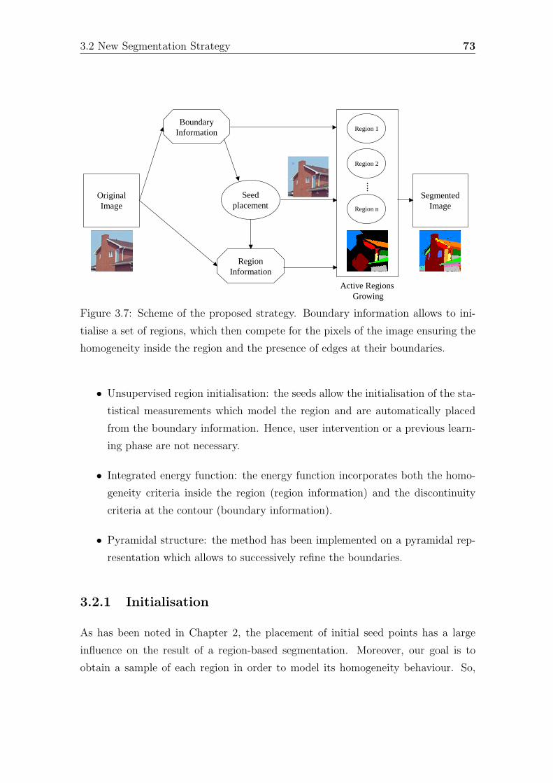
3.2 New Segmentation Strategy 73
OriginalImage
BoundaryInformation
RegionInformation
Seedplacement
Region 1
Region 2
Region n
....
Active Regions Growing
SegmentedImage
Figure 3.7: Scheme of the proposed strategy. Boundary information allows to ini-
tialise a set of regions, which then compete for the pixels of the image ensuring the
homogeneity inside the region and the presence of edges at their boundaries.
• Unsupervised region initialisation: the seeds allow the initialisation of the sta-
tistical measurements which model the region and are automatically placed
from the boundary information. Hence, user intervention or a previous learn-
ing phase are not necessary.
• Integrated energy function: the energy function incorporates both the homo-
geneity criteria inside the region (region information) and the discontinuity
criteria at the contour (boundary information).
• Pyramidal structure: the method has been implemented on a pyramidal rep-
resentation which allows to successively refine the boundaries.
3.2.1 Initialisation
As has been noted in Chapter 2, the placement of initial seed points has a large
influence on the result of a region-based segmentation. Moreover, our goal is to
obtain a sample of each region in order to model its homogeneity behaviour. So,
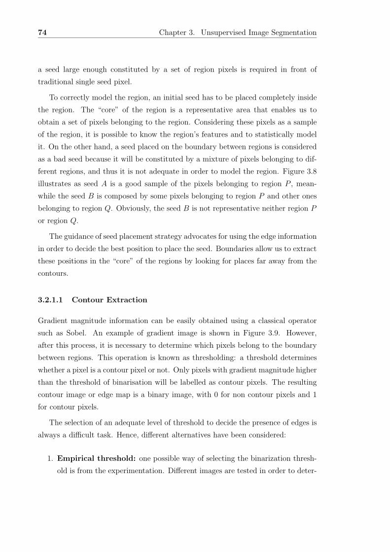
74 Chapter 3. Unsupervised Image Segmentation
a seed large enough constituted by a set of region pixels is required in front of
traditional single seed pixel.
To correctly model the region, an initial seed has to be placed completely inside
the region. The “core” of the region is a representative area that enables us to
obtain a set of pixels belonging to the region. Considering these pixels as a sample
of the region, it is possible to know the region’s features and to statistically model
it. On the other hand, a seed placed on the boundary between regions is considered
as a bad seed because it will be constituted by a mixture of pixels belonging to dif-
ferent regions, and thus it is not adequate in order to model the region. Figure 3.8
illustrates as seed A is a good sample of the pixels belonging to region P , mean-
while the seed B is composed by some pixels belonging to region P and other ones
belonging to region Q. Obviously, the seed B is not representative neither region P
or region Q.
The guidance of seed placement strategy advocates for using the edge information
in order to decide the best position to place the seed. Boundaries allow us to extract
these positions in the “core” of the regions by looking for places far away from the
contours.
3.2.1.1 Contour Extraction
Gradient magnitude information can be easily obtained using a classical operator
such as Sobel. An example of gradient image is shown in Figure 3.9. However,
after this process, it is necessary to determine which pixels belong to the boundary
between regions. This operation is known as thresholding: a threshold determines
whether a pixel is a contour pixel or not. Only pixels with gradient magnitude higher
than the threshold of binarisation will be labelled as contour pixels. The resulting
contour image or edge map is a binary image, with 0 for non contour pixels and 1
for contour pixels.
The selection of an adequate level of threshold to decide the presence of edges is
always a difficult task. Hence, different alternatives have been considered:
1. Empirical threshold: one possible way of selecting the binarization thresh-
old is from the experimentation. Different images are tested in order to deter-
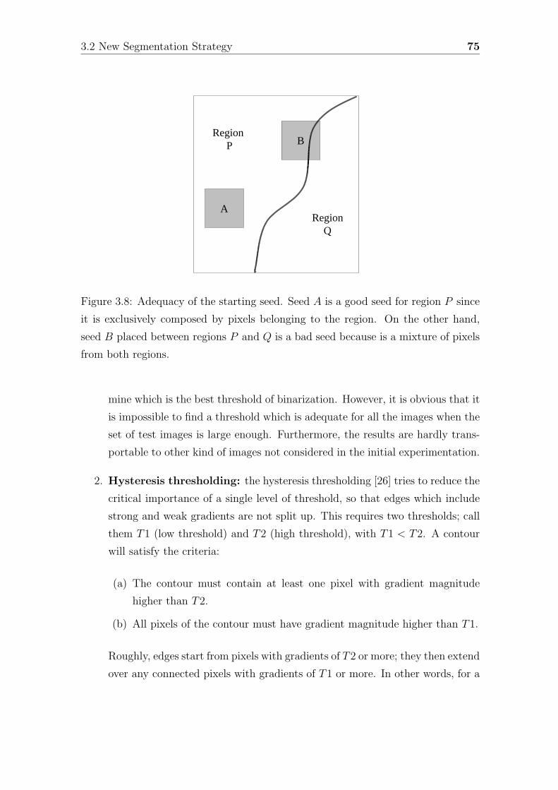
3.2 New Segmentation Strategy 75
BRegion
P
RegionQ
A
Figure 3.8: Adequacy of the starting seed. Seed A is a good seed for region P since
it is exclusively composed by pixels belonging to the region. On the other hand,
seed B placed between regions P and Q is a bad seed because is a mixture of pixels
from both regions.
mine which is the best threshold of binarization. However, it is obvious that it
is impossible to find a threshold which is adequate for all the images when the
set of test images is large enough. Furthermore, the results are hardly trans-
portable to other kind of images not considered in the initial experimentation.
2. Hysteresis thresholding: the hysteresis thresholding [26] tries to reduce the
critical importance of a single level of threshold, so that edges which include
strong and weak gradients are not split up. This requires two thresholds; call
them T1 (low threshold) and T2 (high threshold), with T1 < T2. A contour
will satisfy the criteria:
(a) The contour must contain at least one pixel with gradient magnitude
higher than T2.
(b) All pixels of the contour must have gradient magnitude higher than T1.
Roughly, edges start from pixels with gradients of T2 or more; they then extend
over any connected pixels with gradients of T1 or more. In other words, for a
76 Chapter 3. Unsupervised Image Segmentation
(a) (b)
Figure 3.9: Gradient magnitude image. (a) Original image, (b) obtained gradient
magnitude using Sobel operator.
given pixel, if the gradient magnitude is below T1 it is unconditionally set to
zero (non-contour pixel). If the gradient is at least T2 the pixel is left alone.
If the gradient is between these two, then it is set to zero unless there is a path
from this pixel to a pixel with a gradient above T2; the path must be entirely
through pixels with gradients of at least T1.
Contours extracted using single and hysteresis thresholding are shown in Fig-
ure 3.10. The use of double threshold in the hysteresis thresholding scheme
improves the contour extraction results, considerably solving the problem of
broken and spurious edges. However, it is obvious that the set of the thresholds
level is still a difficult step and has an undeniable influence on the resulting
contour image.
Therefore, we have considered that it was necessary to work on the automatic
determination of the threshold level. We propose an algorithm to automati-
cally find the threshold based on a simple criterion of homogeneity of regions
which compose the image.
3. Automatic thresholding: Our goal in the contour extraction is to find
the boundaries of regions, which are different and homogeneous. Fixing our
attention in the homogeneity property that we demand to the regions it is
possible to redefine the concept of adequate threshold level as the level which
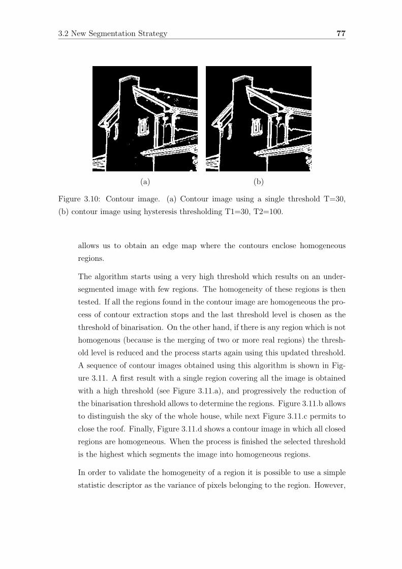
3.2 New Segmentation Strategy 77
(a) (b)
Figure 3.10: Contour image. (a) Contour image using a single threshold T=30,
(b) contour image using hysteresis thresholding T1=30, T2=100.
allows us to obtain an edge map where the contours enclose homogeneous
regions.
The algorithm starts using a very high threshold which results on an under-
segmented image with few regions. The homogeneity of these regions is then
tested. If all the regions found in the contour image are homogeneous the pro-
cess of contour extraction stops and the last threshold level is chosen as the
threshold of binarisation. On the other hand, if there is any region which is not
homogenous (because is the merging of two or more real regions) the thresh-
old level is reduced and the process starts again using this updated threshold.
A sequence of contour images obtained using this algorithm is shown in Fig-
ure 3.11. A first result with a single region covering all the image is obtained
with a high threshold (see Figure 3.11.a), and progressively the reduction of
the binarisation threshold allows to determine the regions. Figure 3.11.b allows
to distinguish the sky of the whole house, while next Figure 3.11.c permits to
close the roof. Finally, Figure 3.11.d shows a contour image in which all closed
regions are homogeneous. When the process is finished the selected threshold
is the highest which segments the image into homogeneous regions.
In order to validate the homogeneity of a region it is possible to use a simple
statistic descriptor as the variance of pixels belonging to the region. However,
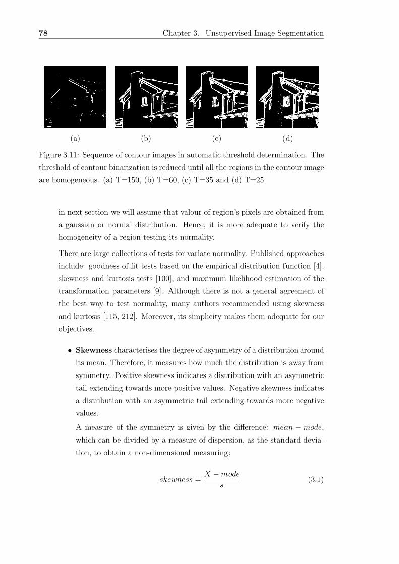
78 Chapter 3. Unsupervised Image Segmentation
(a) (b) (c) (d)
Figure 3.11: Sequence of contour images in automatic threshold determination. The
threshold of contour binarization is reduced until all the regions in the contour image
are homogeneous. (a) T=150, (b) T=60, (c) T=35 and (d) T=25.
in next section we will assume that valour of region’s pixels are obtained from
a gaussian or normal distribution. Hence, it is more adequate to verify the
homogeneity of a region testing its normality.
There are large collections of tests for variate normality. Published approaches
include: goodness of fit tests based on the empirical distribution function [4],
skewness and kurtosis tests [100], and maximum likelihood estimation of the
transformation parameters [9]. Although there is not a general agreement of
the best way to test normality, many authors recommended using skewness
and kurtosis [115, 212]. Moreover, its simplicity makes them adequate for our
objectives.
• Skewness characterises the degree of asymmetry of a distribution around
its mean. Therefore, it measures how much the distribution is away from
symmetry. Positive skewness indicates a distribution with an asymmetric
tail extending towards more positive values. Negative skewness indicates
a distribution with an asymmetric tail extending towards more negative
values.
A measure of the symmetry is given by the difference: mean − mode,
which can be divided by a measure of dispersion, as the standard devia-
tion, to obtain a non-dimensional measuring:
skewness =X − mode
s(3.1)
3.2 New Segmentation Strategy 79
where X is the mean of the population and s is the standard deviation.
In order to avoid the use of the mode, we define the rth moment with
respect to the mean as:
mr =
N∑j=1
(Xj − X)r
N(3.2)
and non-dimensional moments as:
ar =mr
sr=
mr
(√
m2)r=
mr√m2
r(3.3)
an important measure of skewness is given by using the third moment
respect to the mean:
a3 =m3
s3=
m3
(√
m2)3=
m3√m2
3(3.4)
• Kurtosis characterizes the relative peakedness or flatness of a distribu-
tion compared to the normal distribution. Positive kurtosis indicates a
relatively peaked distribution. Negative kurtosis indicates a relatively flat
distribution. A measure of kurtosis uses the fourth moment with respect
to the mean (see Equation 3.3) and is given by
a4 =m4
s4=
m4
m22
(3.5)
For normal distributions a3 = 0 and a4 = 3, although kurtosis is often defined
as (a4 − 3) which is 0 for a normal. Tests of significance for skewness and
kurtosis test the obtained value against a null hypothesis of zero. When the
variable does not come from a normal distribution the hypothesis of normality
is rejected and the region is considered non homogeneous.
4. Adaptive automatic thresholding: There is another difficulty related to
the thresholding of the gradient image that has not been considered in the
above methods. Is a global and single threshold adequate for the whole image?
Obviously, features may vary along the image and the gradient at a boundary
between two regions can be significantly different to the gradient between other
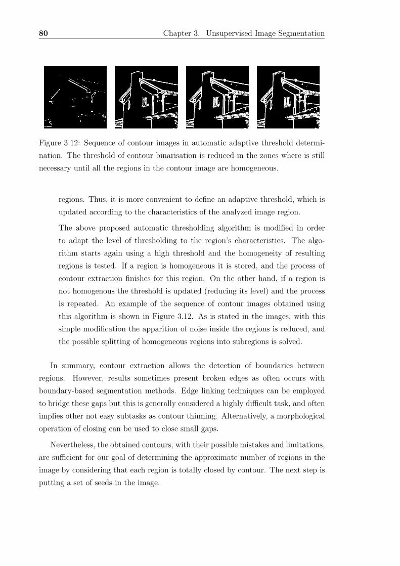
80 Chapter 3. Unsupervised Image Segmentation
Figure 3.12: Sequence of contour images in automatic adaptive threshold determi-
nation. The threshold of contour binarisation is reduced in the zones where is still
necessary until all the regions in the contour image are homogeneous.
regions. Thus, it is more convenient to define an adaptive threshold, which is
updated according to the characteristics of the analyzed image region.
The above proposed automatic thresholding algorithm is modified in order
to adapt the level of thresholding to the region’s characteristics. The algo-
rithm starts again using a high threshold and the homogeneity of resulting
regions is tested. If a region is homogeneous it is stored, and the process of
contour extraction finishes for this region. On the other hand, if a region is
not homogenous the threshold is updated (reducing its level) and the process
is repeated. An example of the sequence of contour images obtained using
this algorithm is shown in Figure 3.12. As is stated in the images, with this
simple modification the apparition of noise inside the regions is reduced, and
the possible splitting of homogeneous regions into subregions is solved.
In summary, contour extraction allows the detection of boundaries between
regions. However, results sometimes present broken edges as often occurs with
boundary-based segmentation methods. Edge linking techniques can be employed
to bridge these gaps but this is generally considered a highly difficult task, and often
implies other not easy subtasks as contour thinning. Alternatively, a morphological
operation of closing can be used to close small gaps.
Nevertheless, the obtained contours, with their possible mistakes and limitations,
are sufficient for our goal of determining the approximate number of regions in the
image by considering that each region is totally closed by contour. The next step is
putting a set of seeds in the image.
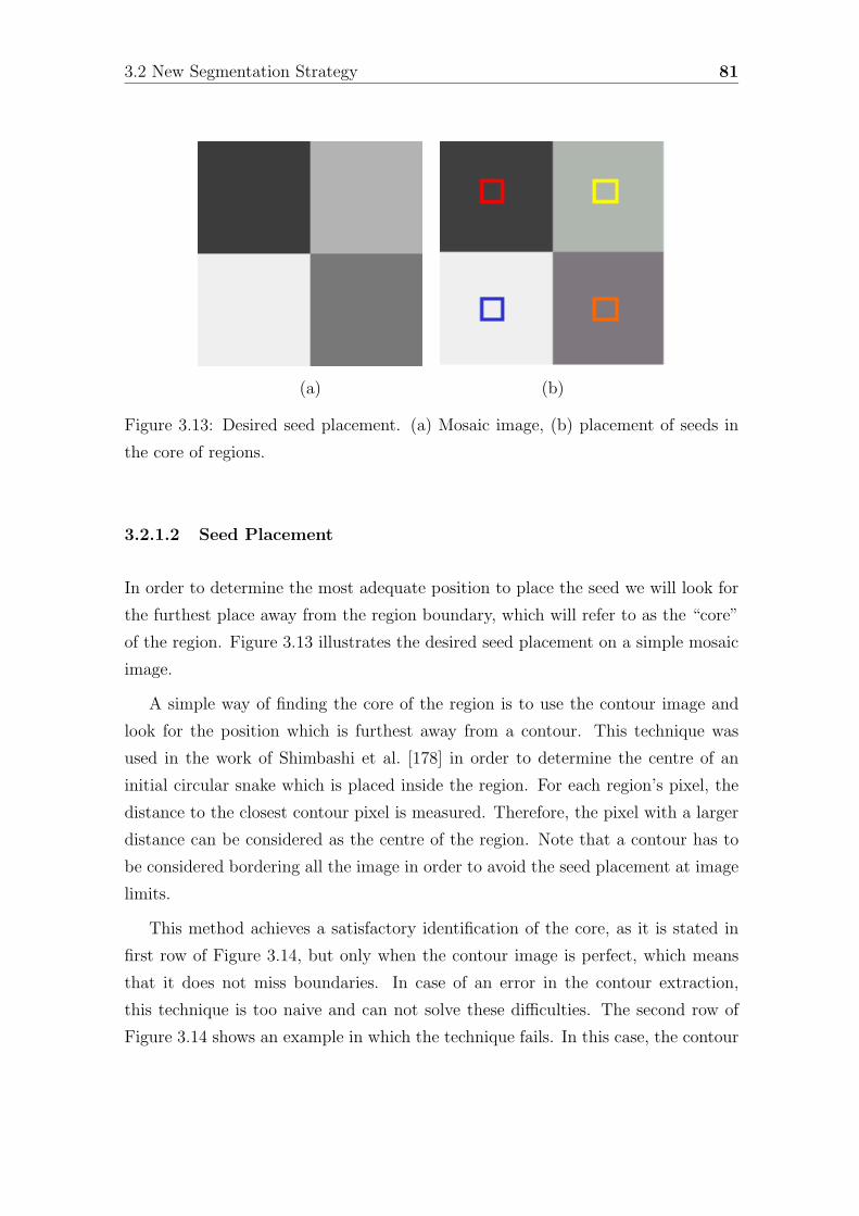
3.2 New Segmentation Strategy 81
(a) (b)
Figure 3.13: Desired seed placement. (a) Mosaic image, (b) placement of seeds in
the core of regions.
3.2.1.2 Seed Placement
In order to determine the most adequate position to place the seed we will look for
the furthest place away from the region boundary, which will refer to as the “core”
of the region. Figure 3.13 illustrates the desired seed placement on a simple mosaic
image.
A simple way of finding the core of the region is to use the contour image and
look for the position which is furthest away from a contour. This technique was
used in the work of Shimbashi et al. [178] in order to determine the centre of an
initial circular snake which is placed inside the region. For each region’s pixel, the
distance to the closest contour pixel is measured. Therefore, the pixel with a larger
distance can be considered as the centre of the region. Note that a contour has to
be considered bordering all the image in order to avoid the seed placement at image
limits.
This method achieves a satisfactory identification of the core, as it is stated in
first row of Figure 3.14, but only when the contour image is perfect, which means
that it does not miss boundaries. In case of an error in the contour extraction,
this technique is too naive and can not solve these difficulties. The second row of
Figure 3.14 shows an example in which the technique fails. In this case, the contour
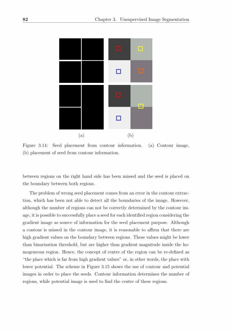
82 Chapter 3. Unsupervised Image Segmentation
(a) (b)
Figure 3.14: Seed placement from contour information. (a) Contour image,
(b) placement of seed from contour information.
between regions on the right hand side has been missed and the seed is placed on
the boundary between both regions.
The problem of wrong seed placement comes from an error in the contour extrac-
tion, which has been not able to detect all the boundaries of the image. However,
although the number of regions can not be correctly determined by the contour im-
age, it is possible to successfully place a seed for each identified region considering the
gradient image as source of information for the seed placement purpose. Although
a contour is missed in the contour image, it is reasonable to affirm that there are
high gradient values on the boundary between regions. These values might be lower
than binarisation threshold, but are higher than gradient magnitude inside the ho-
mogeneous region. Hence, the concept of centre of the region can be re-defined as
“the place which is far from high gradient values” or, in other words, the place with
lower potential. The scheme in Figure 3.15 shows the use of contour and potential
images in order to place the seeds. Contour information determines the number of
regions, while potential image is used to find the centre of these regions.
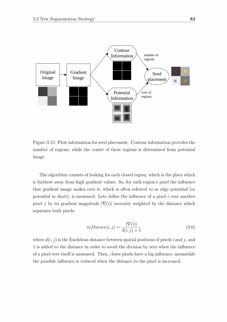
3.2 New Segmentation Strategy 83
Seedplacement
ContourInformation
GradientImage
PotentialInformation
number of regions
core of regions
OriginalImage
Figure 3.15: Flow information for seed placement. Contour information provides the
number of regions, while the centre of these regions is determined from potential
image.
The algorithm consists of looking for each closed region, which is the place which
is furthest away from high gradient values. So, for each region’s pixel the influence
that gradient image makes over it, which is often referred to as edge potential (or
potential in short), is measured. Lets define the influence of a pixel i over another
pixel j by its gradient magnitude |∇(i)| inversely weighted by the distance which
separates both pixels:
influence(i, j) =|∇(i)|
d(i, j) + 1(3.6)
where d(i, j) is the Euclidean distance between spatial positions of pixels i and j, and
1 is added to the distance in order to avoid the division by zero when the influence
of a pixel over itself is measured. Then, closer pixels have a big influence, meanwhile
the possible influence is reduced when the distance to the pixel is increased.
84 Chapter 3. Unsupervised Image Segmentation
Hence, the potential of a pixel j is the maximum which is obtained when the
influence of all the pixels over it is measured:
potential(j) = max(influence(i, j)) ∀iεI (3.7)
where I is the image domain. Note that in order to improve the computational cost
of this measure, the influence over pixel j can be restricted only to pixels belonging
to the same closed region and its boundary. Taking into account that the boundary
is constituted by contour pixels, other pixels outside the region, and consequently
further from pixel j, rarely will have a bigger influence.
Finally, the core of the region will be the place which has a lower potential. An
example of seed placement obtained with this technique is shown in Figure 3.16.
Brighter intensities in the potential image, which indicate a higher potential, are
located at the boundaries between regions. Therefore, seeds are placed on darker
areas of each region, which correspond to the interior of the regions. An error in the
contour extraction involves missing one of the regions, but the use of the potential
image allows us to correctly place one seed for each closed region. Note that again
a high gradient has to be considered bordering all the image in order to avoid the
seed placement at image limits.
The result of this step is the placement of a starting seed for each region, that
allows us to know the region’s features in order to start the growing which will culmi-
nate with the segmentation of the whole image. Some examples of the unsupervised
seed placement provided by this technique are shown in Figure 3.17.
3.2.2 Active Region Segmentation
Active region model is considered the fusion of the active contour model and the
classical region growing. It is usually defined as the incorporation of region-based
information into the active contour model with the aim of finding a partition where
the interior and the exterior of the region preserve the desired image properties.
However, it also can be interpreted as the use of the typical energy function of ac-
tive contours as the decision criterion which guides the growing of a region growing
algorithm. From both points of view, this combination results on a considerable
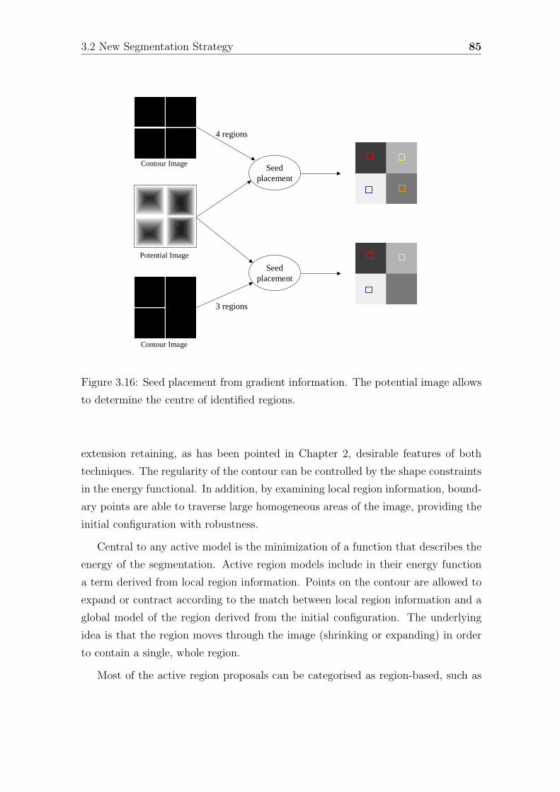
3.2 New Segmentation Strategy 85
Seedplacement
Seedplacement
Potential Image
Contour Image
Contour Image
4 regions
3 regions
Figure 3.16: Seed placement from gradient information. The potential image allows
to determine the centre of identified regions.
extension retaining, as has been pointed in Chapter 2, desirable features of both
techniques. The regularity of the contour can be controlled by the shape constraints
in the energy functional. In addition, by examining local region information, bound-
ary points are able to traverse large homogeneous areas of the image, providing the
initial configuration with robustness.
Central to any active model is the minimization of a function that describes the
energy of the segmentation. Active region models include in their energy function
a term derived from local region information. Points on the contour are allowed to
expand or contract according to the match between local region information and a
global model of the region derived from the initial configuration. The underlying
idea is that the region moves through the image (shrinking or expanding) in order
to contain a single, whole region.
Most of the active region proposals can be categorised as region-based, such as
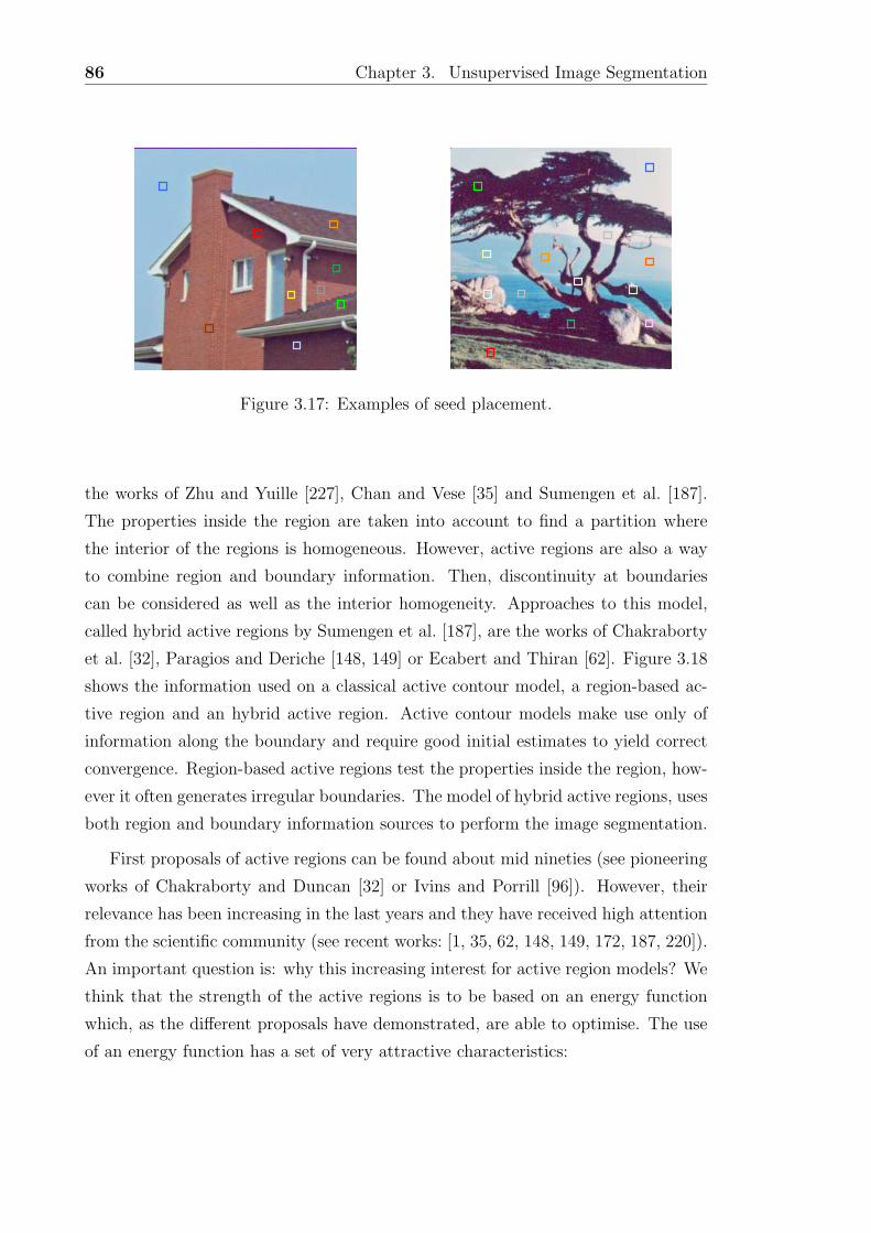
86 Chapter 3. Unsupervised Image Segmentation
Figure 3.17: Examples of seed placement.
the works of Zhu and Yuille [227], Chan and Vese [35] and Sumengen et al. [187].
The properties inside the region are taken into account to find a partition where
the interior of the regions is homogeneous. However, active regions are also a way
to combine region and boundary information. Then, discontinuity at boundaries
can be considered as well as the interior homogeneity. Approaches to this model,
called hybrid active regions by Sumengen et al. [187], are the works of Chakraborty
et al. [32], Paragios and Deriche [148, 149] or Ecabert and Thiran [62]. Figure 3.18
shows the information used on a classical active contour model, a region-based ac-
tive region and an hybrid active region. Active contour models make use only of
information along the boundary and require good initial estimates to yield correct
convergence. Region-based active regions test the properties inside the region, how-
ever it often generates irregular boundaries. The model of hybrid active regions, uses
both region and boundary information sources to perform the image segmentation.
First proposals of active regions can be found about mid nineties (see pioneering
works of Chakraborty and Duncan [32] or Ivins and Porrill [96]). However, their
relevance has been increasing in the last years and they have received high attention
from the scientific community (see recent works: [1, 35, 62, 148, 149, 172, 187, 220]).
An important question is: why this increasing interest for active region models? We
think that the strength of the active regions is to be based on an energy function
which, as the different proposals have demonstrated, are able to optimise. The use
of an energy function has a set of very attractive characteristics:

3.2 New Segmentation Strategy 87
(a) (b) (c)
Figure 3.18: Active models. Shadowed areas show the image domains taken into
account by (a) active contour, (b) region-based active region, and (c) hybrid active
region.
• Goal definition: the energy function allows to exactly define what are the
desired properties of the final segmentation.
• Integration: different concepts (region, boundary, shape, movement...) can be
easily included in the energy function with the aim of taking them into account
in order to segment the image.
• Extensibility: the model becomes very suitable to be extended by adding new
features (e.g. from colour to texture segmentation) or new concepts (e.g. from
segmentation to tracking).
Our proposal of hybrid active region uses these properties integrating region and
boundary information in order to define an optimal segmentation. The next subsec-
tion 3.2.2.1 details the extraction of region and boundary information, which will
be used in subsection 3.2.2.2 in order to define an energy function which describes
the quality of a segmentation taking region and boundary information into account.
Finally, the segmentation process is achieved by optimising this energy function to
find the best segmentation result, as is detailed in subsection 3.2.2.3. Furthermore,
the proposed strategy will be extended to texture segmentation, as we will discuss
in Chapter 4.
88 Chapter 3. Unsupervised Image Segmentation
3.2.2.1 Region and Boundary Information
As hypothesis, each region is modelled by a Gaussian distribution1, so the mean and
the standard deviation, which are initialized from the seeds, describe the homogene-
ity region behaviour. Hence, the probability of a pixel j of belonging to a region Ri
is
PR(j|(µi, σi)) =1√2πσi
exp{−(Ij − µi)2
2σ2i
} (3.8)
where Ij is the intensity of the pixel j, µi is the mean intensity of region Ri and
σi its standard deviation.
The region remaining to be segmented, which we will refer to as the background,
is composed of several objects. Therefore, it can not be modelled using a single
Gaussian distribution and, actually, it is not necessary to model it because our
goal is precisely that finally this region disappears, been gulped by the other grow-
ing regions. Thereby, the background is treated as a single region having uniform
probability distribution P0.
The information regarding to real boundaries of each region can be extracted
by employing an edge detector, thus by seeking for high gradient values. Given
the hypothesis that the image is composed of homogeneous regions, the probability
of a given pixel j being at the real boundary is measured by PB(j), which can be
considered as directly proportional to the value of the magnitude gradient of the
pixel.
3.2.2.2 Energy Function
The goal of image segmentation is to partition the image into subregions with ho-
mogeneous intensity (colour or texture) properties in its interior and a high dis-
continuity with neighbouring regions at its boundary. With the aim of integrating
both conditions in an optimal segmentation, the global energy is defined with two
basic terms. The boundary term measures the probability that boundary pixels are
1This will not always be true. In fact, in textured images region information often can not be
modelled as a Gaussian. Chapter 4 will further discuss this consideration.
3.2 New Segmentation Strategy 89
really edge pixels. The probability of a given pixel j being at the real boundary is
measured by PB(j). Meanwhile, the region term measures the homogeneity in the
interior of the regions by the probability that these pixels belong to each correspond-
ing region. As has been previously defined in Equation 3.8, PR(j|(µ, σ)) measures
the probability that a pixel j belongs to a region modelled by (µ, σ).
Some complementary definitions are required: let ρ(R) = {Ri : iε[0, N ]} be a
partition of the image into N + 1 non-overlapping regions, where R0 is the region
corresponding to the background region. Let ∂ρ(R) = {∂Ri : iε[1, N ]} be the region
boundaries of the partition ρ(R). The energy function is defined as
E(ρ(R)) = (1 − α)N∑
i=1
− log PB(j : jε∂Ri)) + αN∑
i=0
− log PR(j : jεRi|(µi, σi)) (3.9)
where α is a model parameter weighting the two terms: boundary probability and
region homogeneity.
3.2.2.3 Optimisation
The energy function includes the desired properties of the resulting segmentation
considering region and boundary information. Specifically, regions have to be uni-
form in their interior, while boundaries present a high contrast. The desired seg-
mentation is the one with uniform pixels found inside the region and a large edge
probability for pixels at the boundaries. Hence, if we consider both aspects in
Equation 3.9 the optimal segmentation will obtain the minimum energy when this
is measured by the energy function.
The optimisation of the energy function is the process of looking for the parti-
tion of the image in which the minimum energy can be attained. In other words, it
tries to find the best segmentation according to the qualities defined by the energy
function. However, this process is a difficult task and algorithms do not find the
absolute minimum to this problem, neither theoretically nor practically, due to the
non-lineality of the problem and also the existence of local minima. Nevertheless,
as is denoted by Grau [77], it is not a too much worrying problem because there are
solutions which are not the absolute minimum but are sufficiently valid segmenta-
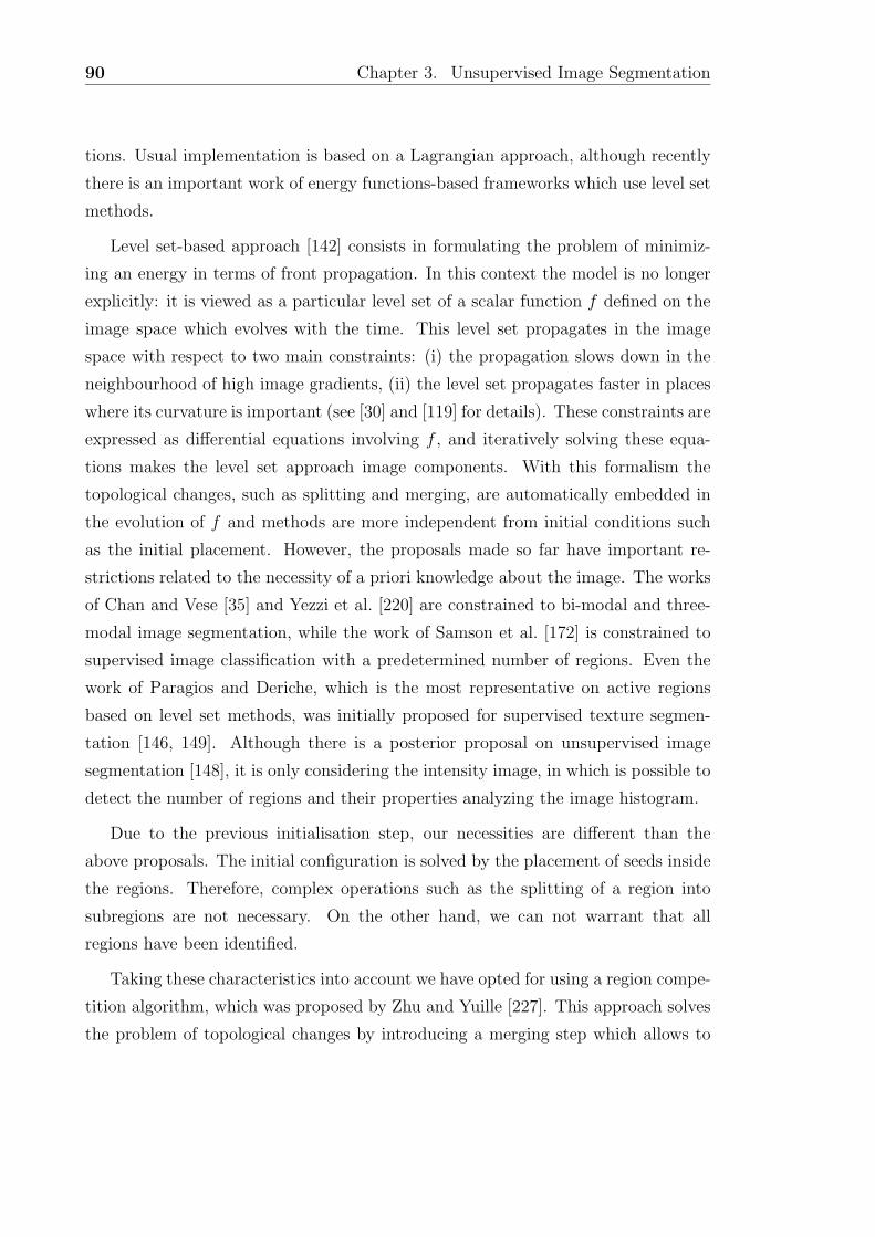
90 Chapter 3. Unsupervised Image Segmentation
tions. Usual implementation is based on a Lagrangian approach, although recently
there is an important work of energy functions-based frameworks which use level set
methods.
Level set-based approach [142] consists in formulating the problem of minimiz-
ing an energy in terms of front propagation. In this context the model is no longer
explicitly: it is viewed as a particular level set of a scalar function f defined on the
image space which evolves with the time. This level set propagates in the image
space with respect to two main constraints: (i) the propagation slows down in the
neighbourhood of high image gradients, (ii) the level set propagates faster in places
where its curvature is important (see [30] and [119] for details). These constraints are
expressed as differential equations involving f , and iteratively solving these equa-
tions makes the level set approach image components. With this formalism the
topological changes, such as splitting and merging, are automatically embedded in
the evolution of f and methods are more independent from initial conditions such
as the initial placement. However, the proposals made so far have important re-
strictions related to the necessity of a priori knowledge about the image. The works
of Chan and Vese [35] and Yezzi et al. [220] are constrained to bi-modal and three-
modal image segmentation, while the work of Samson et al. [172] is constrained to
supervised image classification with a predetermined number of regions. Even the
work of Paragios and Deriche, which is the most representative on active regions
based on level set methods, was initially proposed for supervised texture segmen-
tation [146, 149]. Although there is a posterior proposal on unsupervised image
segmentation [148], it is only considering the intensity image, in which is possible to
detect the number of regions and their properties analyzing the image histogram.
Due to the previous initialisation step, our necessities are different than the
above proposals. The initial configuration is solved by the placement of seeds inside
the regions. Therefore, complex operations such as the splitting of a region into
subregions are not necessary. On the other hand, we can not warrant that all
regions have been identified.
Taking these characteristics into account we have opted for using a region compe-
tition algorithm, which was proposed by Zhu and Yuille [227]. This approach solves
the problem of topological changes by introducing a merging step which allows to
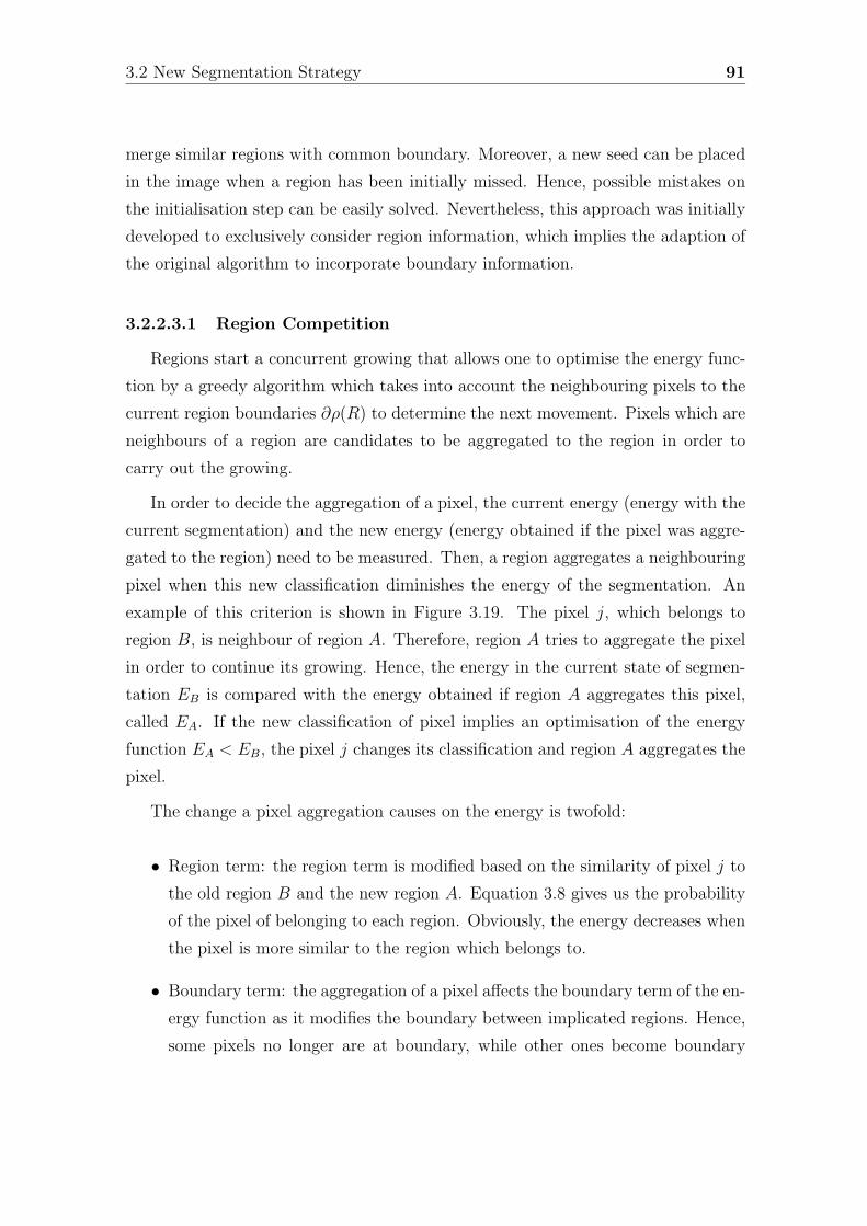
3.2 New Segmentation Strategy 91
merge similar regions with common boundary. Moreover, a new seed can be placed
in the image when a region has been initially missed. Hence, possible mistakes on
the initialisation step can be easily solved. Nevertheless, this approach was initially
developed to exclusively consider region information, which implies the adaption of
the original algorithm to incorporate boundary information.
3.2.2.3.1 Region Competition
Regions start a concurrent growing that allows one to optimise the energy func-
tion by a greedy algorithm which takes into account the neighbouring pixels to the
current region boundaries ∂ρ(R) to determine the next movement. Pixels which are
neighbours of a region are candidates to be aggregated to the region in order to
carry out the growing.
In order to decide the aggregation of a pixel, the current energy (energy with the
current segmentation) and the new energy (energy obtained if the pixel was aggre-
gated to the region) need to be measured. Then, a region aggregates a neighbouring
pixel when this new classification diminishes the energy of the segmentation. An
example of this criterion is shown in Figure 3.19. The pixel j, which belongs to
region B, is neighbour of region A. Therefore, region A tries to aggregate the pixel
in order to continue its growing. Hence, the energy in the current state of segmen-
tation EB is compared with the energy obtained if region A aggregates this pixel,
called EA. If the new classification of pixel implies an optimisation of the energy
function EA < EB, the pixel j changes its classification and region A aggregates the
pixel.
The change a pixel aggregation causes on the energy is twofold:
• Region term: the region term is modified based on the similarity of pixel j to
the old region B and the new region A. Equation 3.8 gives us the probability
of the pixel of belonging to each region. Obviously, the energy decreases when
the pixel is more similar to the region which belongs to.
• Boundary term: the aggregation of a pixel affects the boundary term of the en-
ergy function as it modifies the boundary between implicated regions. Hence,
some pixels no longer are at boundary, while other ones become boundary
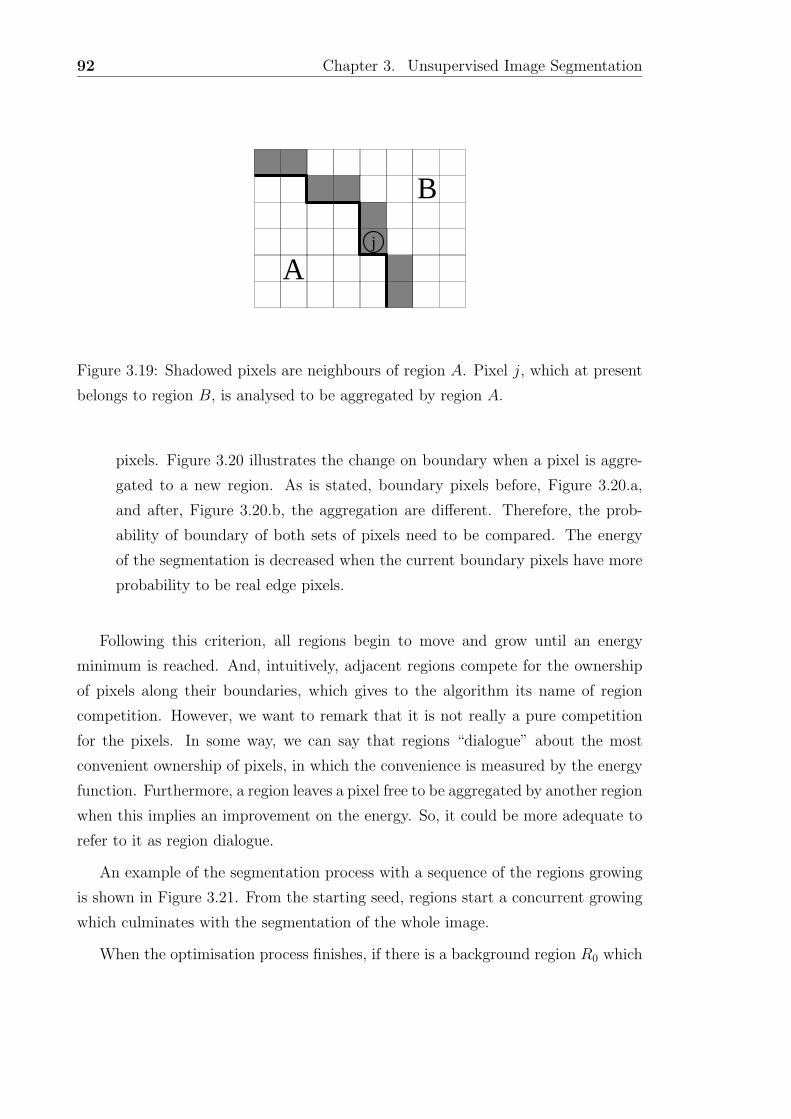
92 Chapter 3. Unsupervised Image Segmentation
j
A
B
Figure 3.19: Shadowed pixels are neighbours of region A. Pixel j, which at present
belongs to region B, is analysed to be aggregated by region A.
pixels. Figure 3.20 illustrates the change on boundary when a pixel is aggre-
gated to a new region. As is stated, boundary pixels before, Figure 3.20.a,
and after, Figure 3.20.b, the aggregation are different. Therefore, the prob-
ability of boundary of both sets of pixels need to be compared. The energy
of the segmentation is decreased when the current boundary pixels have more
probability to be real edge pixels.
Following this criterion, all regions begin to move and grow until an energy
minimum is reached. And, intuitively, adjacent regions compete for the ownership
of pixels along their boundaries, which gives to the algorithm its name of region
competition. However, we want to remark that it is not really a pure competition
for the pixels. In some way, we can say that regions “dialogue” about the most
convenient ownership of pixels, in which the convenience is measured by the energy
function. Furthermore, a region leaves a pixel free to be aggregated by another region
when this implies an improvement on the energy. So, it could be more adequate to
refer to it as region dialogue.
An example of the segmentation process with a sequence of the regions growing
is shown in Figure 3.21. From the starting seed, regions start a concurrent growing
which culminates with the segmentation of the whole image.
When the optimisation process finishes, if there is a background region R0 which
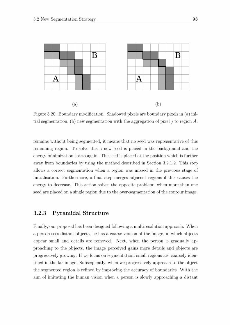
3.2 New Segmentation Strategy 93
A
B
A
B
(a) (b)
Figure 3.20: Boundary modification. Shadowed pixels are boundary pixels in (a) ini-
tial segmentation, (b) new segmentation with the aggregation of pixel j to region A.
remains without being segmented, it means that no seed was representative of this
remaining region. To solve this a new seed is placed in the background and the
energy minimization starts again. The seed is placed at the position which is further
away from boundaries by using the method described in Section 3.2.1.2. This step
allows a correct segmentation when a region was missed in the previous stage of
initialisation. Furthermore, a final step merges adjacent regions if this causes the
energy to decrease. This action solves the opposite problem: when more than one
seed are placed on a single region due to the over-segmentation of the contour image.
3.2.3 Pyramidal Structure
Finally, our proposal has been designed following a multiresolution approach. When
a person sees distant objects, he has a coarse version of the image, in which objects
appear small and details are removed. Next, when the person is gradually ap-
proaching to the objects, the image perceived gains more details and objects are
progressively growing. If we focus on segmentation, small regions are coarsely iden-
tified in the far image. Subsequently, when we progressively approach to the object
the segmented region is refined by improving the accuracy of boundaries. With the
aim of imitating the human vision when a person is slowly approaching a distant
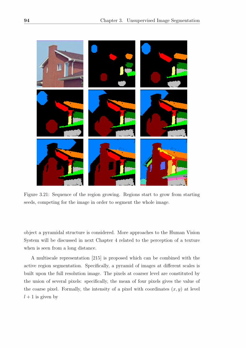
94 Chapter 3. Unsupervised Image Segmentation
Figure 3.21: Sequence of the region growing. Regions start to grow from starting
seeds, competing for the image in order to segment the whole image.
object a pyramidal structure is considered. More approaches to the Human Vision
System will be discussed in next Chapter 4 related to the perception of a texture
when is seen from a long distance.
A multiscale representation [215] is proposed which can be combined with the
active region segmentation. Specifically, a pyramid of images at different scales is
built upon the full resolution image. The pixels at coarser level are constituted by
the union of several pixels: specifically, the mean of four pixels gives the value of
the coarse pixel. Formally, the intensity of a pixel with coordinates (x, y) at level
l + 1 is given by
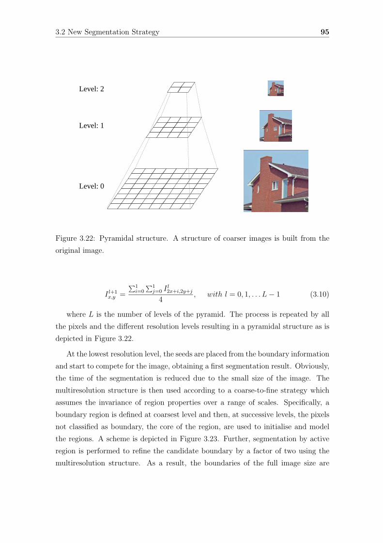
3.2 New Segmentation Strategy 95
Level: 1
Level: 0
Level: 2
Figure 3.22: Pyramidal structure. A structure of coarser images is built from the
original image.
I l+1x,y =
∑1i=0
∑1j=0 I l
2x+i,2y+j
4, with l = 0, 1, . . . L − 1 (3.10)
where L is the number of levels of the pyramid. The process is repeated by all
the pixels and the different resolution levels resulting in a pyramidal structure as is
depicted in Figure 3.22.
At the lowest resolution level, the seeds are placed from the boundary information
and start to compete for the image, obtaining a first segmentation result. Obviously,
the time of the segmentation is reduced due to the small size of the image. The
multiresolution structure is then used according to a coarse-to-fine strategy which
assumes the invariance of region properties over a range of scales. Specifically, a
boundary region is defined at coarsest level and then, at successive levels, the pixels
not classified as boundary, the core of the region, are used to initialise and model
the regions. A scheme is depicted in Figure 3.23. Further, segmentation by active
region is performed to refine the candidate boundary by a factor of two using the
multiresolution structure. As a result, the boundaries of the full image size are
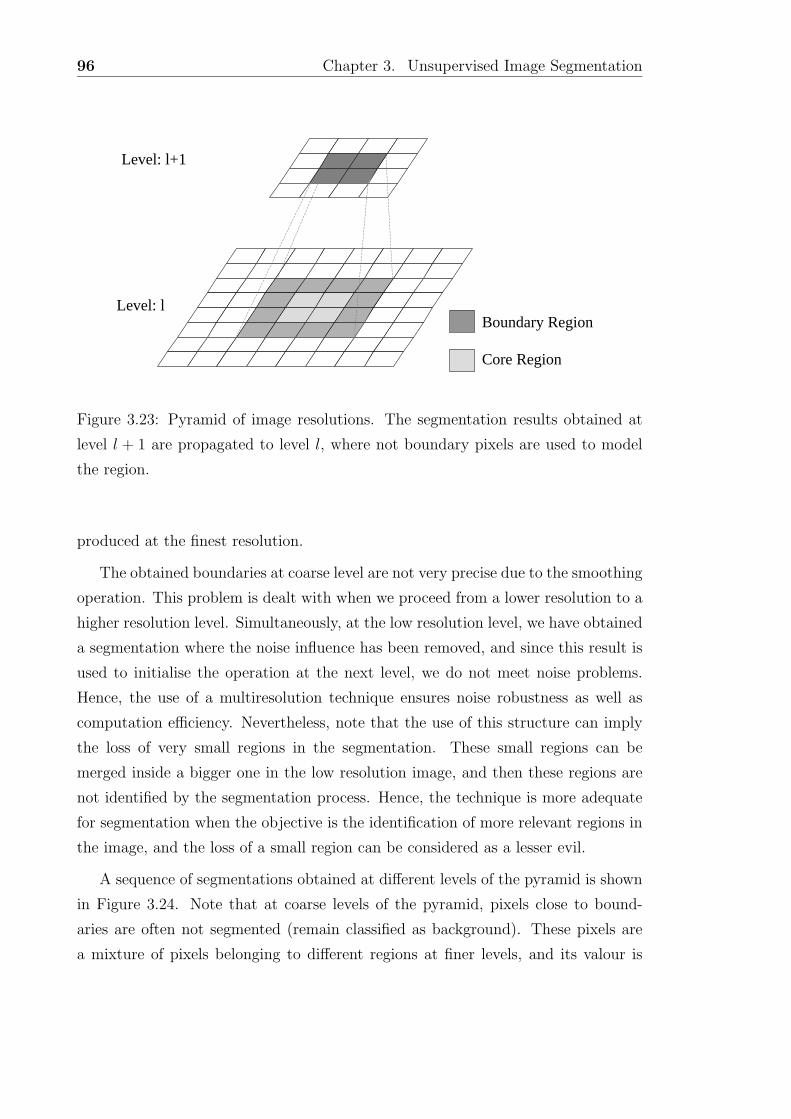
96 Chapter 3. Unsupervised Image Segmentation
Level: l+1
Level: lBoundary Region
Core Region
Figure 3.23: Pyramid of image resolutions. The segmentation results obtained at
level l + 1 are propagated to level l, where not boundary pixels are used to model
the region.
produced at the finest resolution.
The obtained boundaries at coarse level are not very precise due to the smoothing
operation. This problem is dealt with when we proceed from a lower resolution to a
higher resolution level. Simultaneously, at the low resolution level, we have obtained
a segmentation where the noise influence has been removed, and since this result is
used to initialise the operation at the next level, we do not meet noise problems.
Hence, the use of a multiresolution technique ensures noise robustness as well as
computation efficiency. Nevertheless, note that the use of this structure can imply
the loss of very small regions in the segmentation. These small regions can be
merged inside a bigger one in the low resolution image, and then these regions are
not identified by the segmentation process. Hence, the technique is more adequate
for segmentation when the objective is the identification of more relevant regions in
the image, and the loss of a small region can be considered as a lesser evil.
A sequence of segmentations obtained at different levels of the pyramid is shown
in Figure 3.24. Note that at coarse levels of the pyramid, pixels close to bound-
aries are often not segmented (remain classified as background). These pixels are
a mixture of pixels belonging to different regions at finer levels, and its valour is
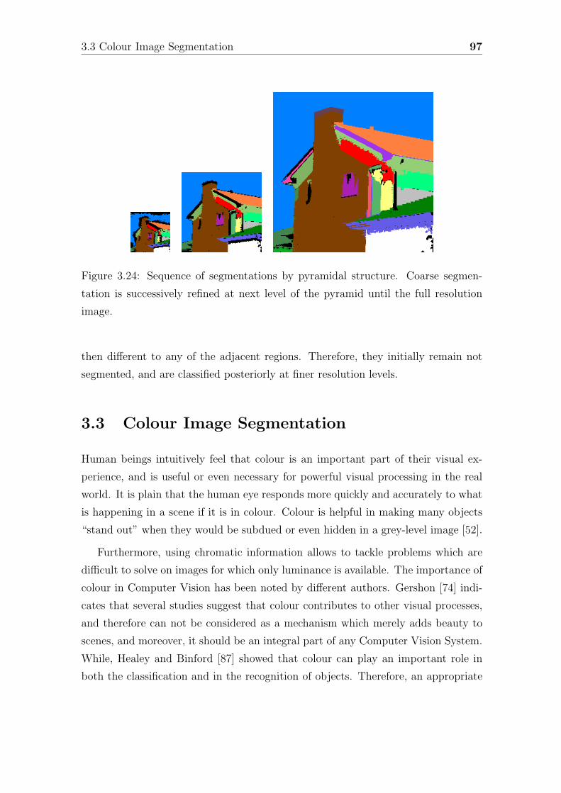
3.3 Colour Image Segmentation 97
Figure 3.24: Sequence of segmentations by pyramidal structure. Coarse segmen-
tation is successively refined at next level of the pyramid until the full resolution
image.
then different to any of the adjacent regions. Therefore, they initially remain not
segmented, and are classified posteriorly at finer resolution levels.
3.3 Colour Image Segmentation
Human beings intuitively feel that colour is an important part of their visual ex-
perience, and is useful or even necessary for powerful visual processing in the real
world. It is plain that the human eye responds more quickly and accurately to what
is happening in a scene if it is in colour. Colour is helpful in making many objects
“stand out” when they would be subdued or even hidden in a grey-level image [52].
Furthermore, using chromatic information allows to tackle problems which are
difficult to solve on images for which only luminance is available. The importance of
colour in Computer Vision has been noted by different authors. Gershon [74] indi-
cates that several studies suggest that colour contributes to other visual processes,
and therefore can not be considered as a mechanism which merely adds beauty to
scenes, and moreover, it should be an integral part of any Computer Vision System.
While, Healey and Binford [87] showed that colour can play an important role in
both the classification and in the recognition of objects. Therefore, an appropriate
98 Chapter 3. Unsupervised Image Segmentation
use of colour, therefore, can significantly extend the capabilities of a vision system.
Considering colour as undoubtedly one of the most interesting characteristics
of the natural world, the difficulty relies on its treatment which can be performed
in many different ways. In many cases, the basic RGB components may provide
very valuable information about the environment. However, the perceptual models,
such as CIE (L,a,b) or HSI, are more intuitive and therefore enable the extraction
of characteristics according to the model of human perception. Furthermore, the
complexity of natural scenes emphasises the need of the system to select a good
colour space, which is of extreme importance to the segmentation tasks. Therefore,
it is necessary to formulate the following question: what is the best colour space to
be applied in order to segment an image representing an outdoor scene? As Batlle et
al. [12] noted, this question has neither a single, nor a perfect solution. The colour
space suitable for one segmentation algorithm is not suitable for others. Hence,
due to the lack of a consolidated colour space, we will deal the problem of colour
segmentation considering the general use of our strategy on any colour space. The
segmentation results obtained using different colour spaces will be further evaluated
in Chapter 5.
The adaption of the proposed strategy to colour image segmentation involves two
basic considerations: the extraction of boundary information over a colour image,
and the modelling of a region taking its colour properties into account.
3.3.1 Colour Contour Extraction
The detection of contours on colour images is specially interesting in scenes present-
ing clearly differentiable chromatic components. Moreover, in a wide set of cases the
use of colour allows to obtain a greater robustness compared to using monochromatic
images [47].
In the work of Carron and Lambert [27] the measure of the gradient on colour
images from the chromatic components of a HSI model variant is referred. The
authors consider that the information of contours on a colour image can be extracted
from the integration of the contours obtained over each chromatic component using a
classical operator as Sobel. There are two basic ways of performing the integration:
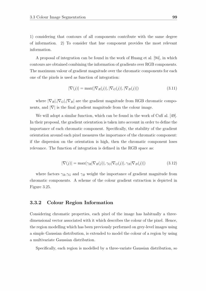
3.3 Colour Image Segmentation 99
1) considering that contours of all components contribute with the same degree
of information. 2) To consider that hue component provides the most relevant
information.
A proposal of integration can be found in the work of Huang et al. [94], in which
contours are obtained combining the information of gradients over RGB components.
The maximum valour of gradient magnitude over the chromatic components for each
one of the pixels is used as function of integration:
|∇(j)| = max(|∇R(j)|, |∇G(j)|, |∇B(j)|) (3.11)
where |∇R|,|∇G|,|∇B| are the gradient magnitude from RGB chromatic compo-
nents, and |∇| is the final gradient magnitude from the colour image.
We will adopt a similar function, which can be found in the work of Cufı al. [49].
In their proposal, the gradient orientation is taken into account in order to define the
importance of each chromatic component. Specifically, the stability of the gradient
orientation around each pixel measures the importance of the chromatic component:
if the dispersion on the orientation is high, then the chromatic component loses
relevance. The function of integration is defined in the RGB space as:
|∇(j)| = max(γR|∇R(j)|, γG|∇G(j)|, γB|∇B(j)|) (3.12)
where factors γR,γG and γB weight the importance of gradient magnitude from
chromatic components. A scheme of the colour gradient extraction is depicted in
Figure 3.25.
3.3.2 Colour Region Information
Considering chromatic properties, each pixel of the image has habitually a three-
dimensional vector associated with it which describes the colour of the pixel. Hence,
the region modelling which has been previously performed on grey-level images using
a simple Gaussian distribution, is extended to model the colour of a region by using
a multivariate Gaussian distribution.
Specifically, each region is modelled by a three-variate Gaussian distribution, so

100 Chapter 3. Unsupervised Image Segmentation
GradientImage
OriginalImage
ChromaticComponent
ChromaticComponent
ChromaticComponent
GradientImage
GradientImage
GradientIntegration
ColourGradientImage
Figure 3.25: The gradient images extracted on chromatic components are integrated
to obtain the colour gradient magnitude image.
the mean vector and the covariance matrix characterises the colour region behaviour.
Hence, the probability of a pixel j of belonging to a region Ri is given by
PR(j|Ri) =1√
(2π)3|Σi|exp{−1
2(−→Ij −−→µi)
T Σ−1i (
−→Ij −−→µi)} (3.13)
where−→Ij is the pixel colour vector, −→µi is the colour mean vector of the region i
and Σi its covariance matrix.
3.4 Conclusions
A new strategy for image segmentation which integrates region and boundary in-
formation has been described. The algorithm uses boundary information in order

3.4 Conclusions 101
to initialise, in an unsupervised way, a set of active regions, which later compete
for the pixels minimizing an energy function taking into account both region and
boundary information. The method has been implemented on a multiresolution
representation.
The algorithm has been directly adapted to perform colour segmentation assum-
ing multivariable Gaussian distributions to model each region. In this sense, future
extensions of this work are the adaption to texture segmentation as well as the in-
tegration of colour and texture cues. Both works will be presented in the following
chapter.

102 Chapter 3. Unsupervised Image Segmentation
Chapter 4
Unsupervised Texture
Segmentation
The proposed strategy of segmentation is extended to deal with texture segmentation
integrating region and boundary information. The method uses a coarse detection of
texture boundaries to initialise a set of active regions. Therefore, the initial unsuper-
vised texture segmentation problem is transformed to a supervised one, which allows
us to accurately extract region and boundary information. Moreover, a technique
for the integration of colour and texture properties is proposed, which allows to ex-
tend the strategy to colour texture segmentation. The method is designed considering
a pyramidal representation which ensures noise robustness as well as computation
efficiency.
4.1 Introduction
Texture is a fundamental characteristic of natural images that, in addition to colour,
plays an important role in human visual perception and provides information for
image understanding and scene interpretation.
The aim of texture segmentation, the problem considered in this chapter, is
the domain-independent partition of the image into a set of regions, which are
visually distinct and uniform with respect to textural properties. We focus on two
103
104 Chapter 4. Unsupervised Texture Segmentation
basic approaches to perform the texture segmentation: region and boundary-based.
Region-based methods try to divide the image into a number of regions such that
each region has the same textural properties [98, 123]. Alternatively, this task is
viewed by boundary-based methods as the problem of accurately extracting the
borders between different texture regions in an image [103, 122].
With the aim of improving the segmentation process, a large number of new
algorithms which integrate region and boundary information have been proposed
over the past few years. However, as has been noted in Chapter 2, texture is gen-
erally forgotten as basic feature in most proposals, probably due to the difficulty of
obtaining accurate boundary information when texture, which is a non-local image
property, is considered. Nevertheless, there are some relevant exceptions and this
tendency seems to be changing in last years (see the works of Hibbard [88], Hsu et
al. [92], Paragios and Deriche [146, 149], Philipp and Zamperoni [155], and Wilson
and Spann [215]).
In this chapter we extend the strategy of image segmentation described in Chap-
ter 3, in order to perform texture segmentation integrating region and boundary
information. Furthermore, a technique for the combination of texture features with
the estimation of colour properties is proposed. Hence, the strategy of segmentation
is finally extended to colour texture segmentation.
This chapter is structured as follows: Section 4.2 describes the adaptation of
the proposed strategy to texture segmentation. The extension to colour texture
segmentation is explained in Section 4.3. Finally, Section 4.4 gives some conclusions.
4.2 Texture Segmentation
Textural properties of the image can be extracted using statistical features, spatial-
frequency models, stochastic models, etc. Surveys on existing texture analysis ap-
proaches may be found in [80, 160, 222], moreover for a short review on texture
extraction methods the reader is referred to Appendix A.
A texture operator describes the texture in an area of the image. Hence, using
a texture operator over the whole image generates a new texture feature image in
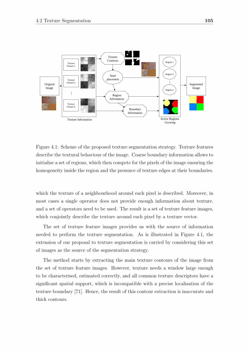
4.2 Texture Segmentation 105
OriginalImage
RegionInformation
Seedplacement
Region 1
Region 2
Region n
....
Active Regions Growing
TextureFeature 1
TextureFeature 2
TextureFeature k
....
TextureContours
Texture Information
BoundaryInformation
SegmentedImage
Figure 4.1: Scheme of the proposed texture segmentation strategy. Texture features
describe the textural behaviour of the image. Coarse boundary information allows to
initialise a set of regions, which then compete for the pixels of the image ensuring the
homogeneity inside the region and the presence of texture edges at their boundaries.
which the texture of a neighbourhood around each pixel is described. Moreover, in
most cases a single operator does not provide enough information about texture,
and a set of operators need to be used. The result is a set of texture feature images,
which conjointly describe the texture around each pixel by a texture vector.
The set of texture feature images provides us with the source of information
needed to perform the texture segmentation. As is illustrated in Figure 4.1, the
extension of our proposal to texture segmentation is carried by considering this set
of images as the source of the segmentation strategy.
The method starts by extracting the main texture contours of the image from
the set of texture feature images. However, texture needs a window large enough
to be characterised, estimated correctly, and all common texture descriptors have a
significant spatial support, which is incompatible with a precise localisation of the
texture boundary [71]. Hence, the result of this contour extraction is inaccurate and
thick contours.
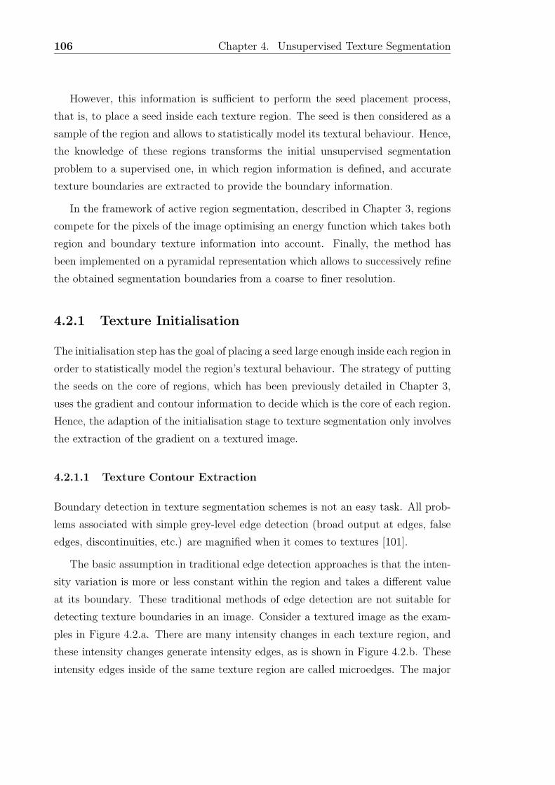
106 Chapter 4. Unsupervised Texture Segmentation
However, this information is sufficient to perform the seed placement process,
that is, to place a seed inside each texture region. The seed is then considered as a
sample of the region and allows to statistically model its textural behaviour. Hence,
the knowledge of these regions transforms the initial unsupervised segmentation
problem to a supervised one, in which region information is defined, and accurate
texture boundaries are extracted to provide the boundary information.
In the framework of active region segmentation, described in Chapter 3, regions
compete for the pixels of the image optimising an energy function which takes both
region and boundary texture information into account. Finally, the method has
been implemented on a pyramidal representation which allows to successively refine
the obtained segmentation boundaries from a coarse to finer resolution.
4.2.1 Texture Initialisation
The initialisation step has the goal of placing a seed large enough inside each region in
order to statistically model the region’s textural behaviour. The strategy of putting
the seeds on the core of regions, which has been previously detailed in Chapter 3,
uses the gradient and contour information to decide which is the core of each region.
Hence, the adaption of the initialisation stage to texture segmentation only involves
the extraction of the gradient on a textured image.
4.2.1.1 Texture Contour Extraction
Boundary detection in texture segmentation schemes is not an easy task. All prob-
lems associated with simple grey-level edge detection (broad output at edges, false
edges, discontinuities, etc.) are magnified when it comes to textures [101].
The basic assumption in traditional edge detection approaches is that the inten-
sity variation is more or less constant within the region and takes a different value
at its boundary. These traditional methods of edge detection are not suitable for
detecting texture boundaries in an image. Consider a textured image as the exam-
ples in Figure 4.2.a. There are many intensity changes in each texture region, and
these intensity changes generate intensity edges, as is shown in Figure 4.2.b. These
intensity edges inside of the same texture region are called microedges. The major
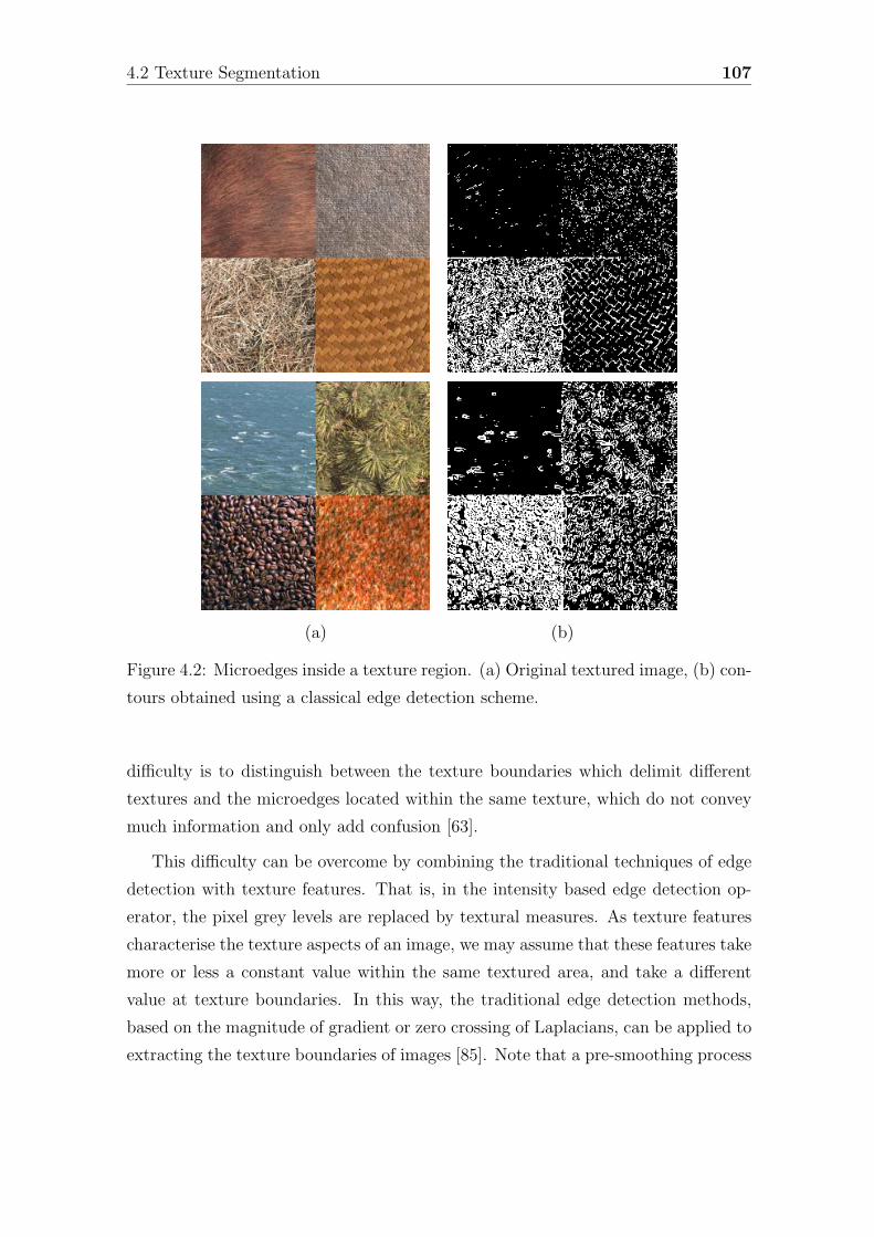
4.2 Texture Segmentation 107
(a) (b)
Figure 4.2: Microedges inside a texture region. (a) Original textured image, (b) con-
tours obtained using a classical edge detection scheme.
difficulty is to distinguish between the texture boundaries which delimit different
textures and the microedges located within the same texture, which do not convey
much information and only add confusion [63].
This difficulty can be overcome by combining the traditional techniques of edge
detection with texture features. That is, in the intensity based edge detection op-
erator, the pixel grey levels are replaced by textural measures. As texture features
characterise the texture aspects of an image, we may assume that these features take
more or less a constant value within the same textured area, and take a different
value at texture boundaries. In this way, the traditional edge detection methods,
based on the magnitude of gradient or zero crossing of Laplacians, can be applied to
extracting the texture boundaries of images [85]. Note that a pre-smoothing process
108 Chapter 4. Unsupervised Texture Segmentation
OriginalImage
GradientIntegration
TextureGradientImage
TextureFeature 1
TextureFeature 2
TextureFeature k
....
Texture Information
GradientTexture
Feature 1
GradientTexture
Feature 2
GradientTexture
Feature k
....
Texture GradientInformation
Figure 4.3: Texture gradient extraction scheme. Gradient magnitudes from each
texture feature are integrated to obtain the texture gradient image.
of the texture features images is often required in order to obtain constant values of
texture descriptors inside regions.
The problem of texture edge detection is considered as a classical edge detection
scheme in the multidimensional set of k texture features which are used to represent
the region characteristics [103]. Hence, a Sobel operator is individually applied to
each texture feature image. The gradient magnitudes of a pixel j from k texture
features are then integrated using the generalisation of Equation 3.12:
|∇(j)| = max(γi|∇i(j)|) ∀i, 1 ≤ i ≤ k (4.1)
where ∇i is the gradient obtained from texture feature ith. A scheme of the
texture gradient extraction procedure is depicted in Figure 4.3.

4.2 Texture Segmentation 109
(a) (b)
Figure 4.4: Seed placement from texture gradient information. (a) Texture contours
and (b) seeds placed inside the texture regions.
Nevertheless, as is well known, texture is an inherently non-local image property.
All common texture descriptors, therefore, have a significant spatial support which
renders classical edge detection schemes inadequate for the detection of texture
boundaries. Hence, the result provided by this simple method are inaccurate and
thick contours. However, this coarse information is enough to perform the seed
placement according to the algorithm described in Section 3.2.1.2, which allows to
place the seeds in the core of regions. Some examples of texture contours obtained
with this techniques, and the posterior seed placement are shown in Figure 4.4.
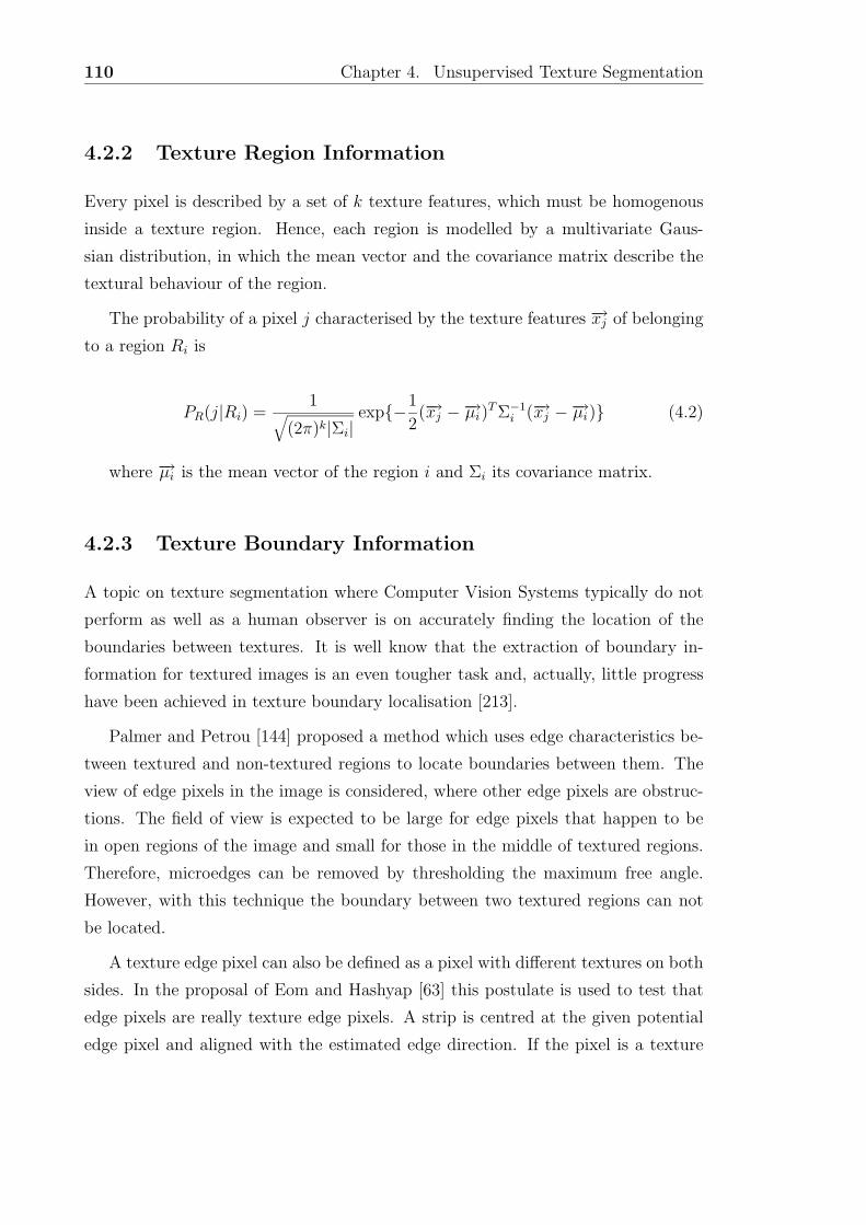
110 Chapter 4. Unsupervised Texture Segmentation
4.2.2 Texture Region Information
Every pixel is described by a set of k texture features, which must be homogenous
inside a texture region. Hence, each region is modelled by a multivariate Gaus-
sian distribution, in which the mean vector and the covariance matrix describe the
textural behaviour of the region.
The probability of a pixel j characterised by the texture features −→xj of belonging
to a region Ri is
PR(j|Ri) =1√
(2π)k|Σi|exp{−1
2(−→xj −−→µi)
T Σ−1i (−→xj −−→µi)} (4.2)
where −→µi is the mean vector of the region i and Σi its covariance matrix.
4.2.3 Texture Boundary Information
A topic on texture segmentation where Computer Vision Systems typically do not
perform as well as a human observer is on accurately finding the location of the
boundaries between textures. It is well know that the extraction of boundary in-
formation for textured images is an even tougher task and, actually, little progress
have been achieved in texture boundary localisation [213].
Palmer and Petrou [144] proposed a method which uses edge characteristics be-
tween textured and non-textured regions to locate boundaries between them. The
view of edge pixels in the image is considered, where other edge pixels are obstruc-
tions. The field of view is expected to be large for edge pixels that happen to be
in open regions of the image and small for those in the middle of textured regions.
Therefore, microedges can be removed by thresholding the maximum free angle.
However, with this technique the boundary between two textured regions can not
be located.
A texture edge pixel can also be defined as a pixel with different textures on both
sides. In the proposal of Eom and Hashyap [63] this postulate is used to test that
edge pixels are really texture edge pixels. A strip is centred at the given potential
edge pixel and aligned with the estimated edge direction. If the pixel is a texture
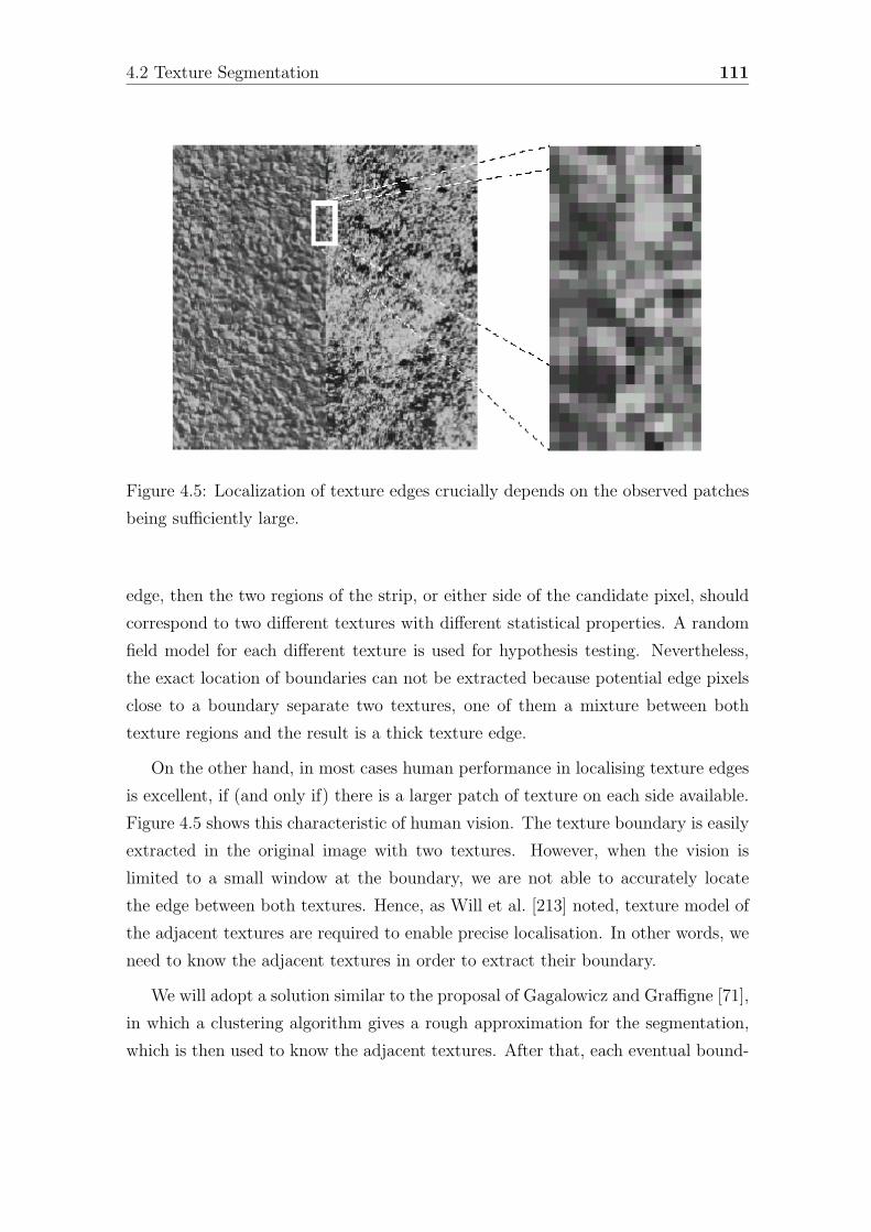
4.2 Texture Segmentation 111
Figure 4.5: Localization of texture edges crucially depends on the observed patches
being sufficiently large.
edge, then the two regions of the strip, or either side of the candidate pixel, should
correspond to two different textures with different statistical properties. A random
field model for each different texture is used for hypothesis testing. Nevertheless,
the exact location of boundaries can not be extracted because potential edge pixels
close to a boundary separate two textures, one of them a mixture between both
texture regions and the result is a thick texture edge.
On the other hand, in most cases human performance in localising texture edges
is excellent, if (and only if) there is a larger patch of texture on each side available.
Figure 4.5 shows this characteristic of human vision. The texture boundary is easily
extracted in the original image with two textures. However, when the vision is
limited to a small window at the boundary, we are not able to accurately locate
the edge between both textures. Hence, as Will et al. [213] noted, texture model of
the adjacent textures are required to enable precise localisation. In other words, we
need to know the adjacent textures in order to extract their boundary.
We will adopt a solution similar to the proposal of Gagalowicz and Graffigne [71],
in which a clustering algorithm gives a rough approximation for the segmentation,
which is then used to know the adjacent textures. After that, each eventual bound-
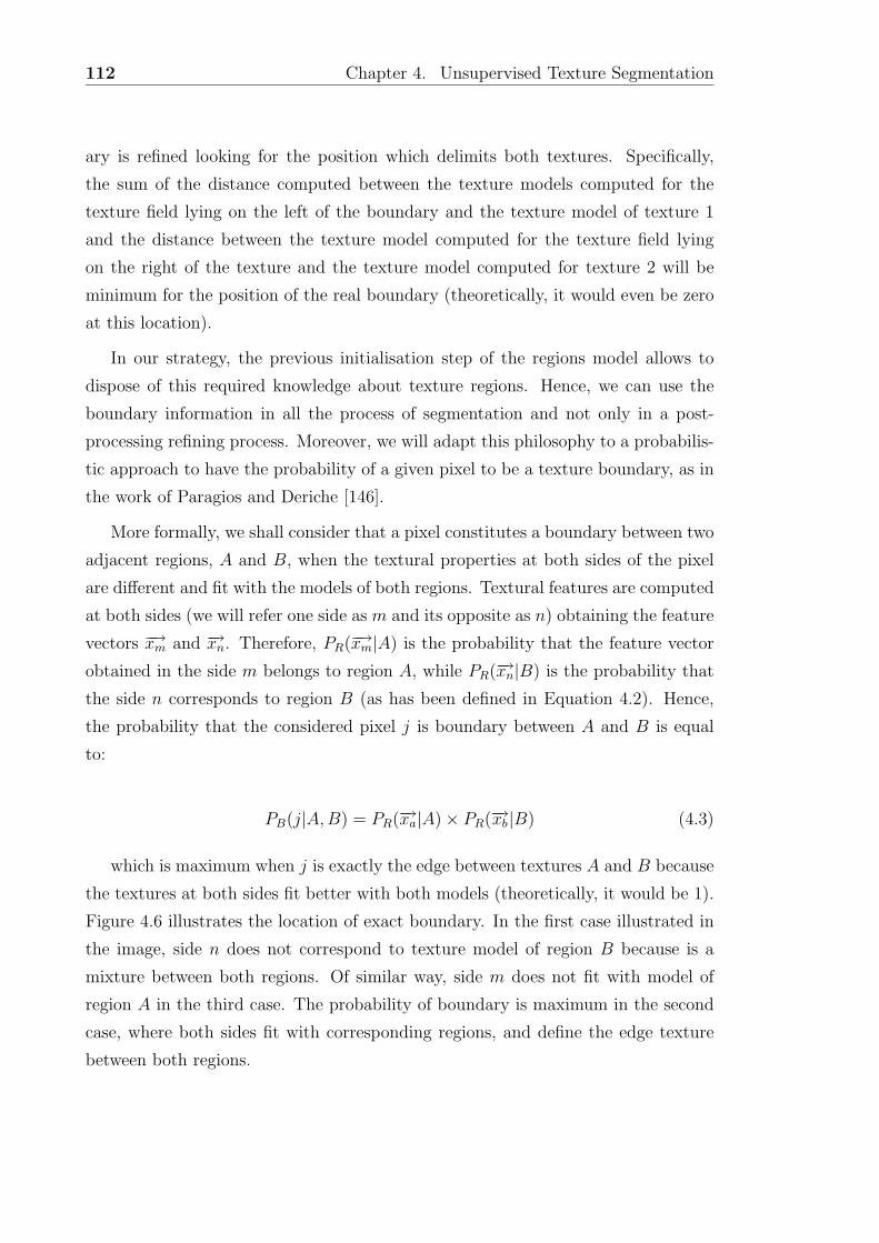
112 Chapter 4. Unsupervised Texture Segmentation
ary is refined looking for the position which delimits both textures. Specifically,
the sum of the distance computed between the texture models computed for the
texture field lying on the left of the boundary and the texture model of texture 1
and the distance between the texture model computed for the texture field lying
on the right of the texture and the texture model computed for texture 2 will be
minimum for the position of the real boundary (theoretically, it would even be zero
at this location).
In our strategy, the previous initialisation step of the regions model allows to
dispose of this required knowledge about texture regions. Hence, we can use the
boundary information in all the process of segmentation and not only in a post-
processing refining process. Moreover, we will adapt this philosophy to a probabilis-
tic approach to have the probability of a given pixel to be a texture boundary, as in
the work of Paragios and Deriche [146].
More formally, we shall consider that a pixel constitutes a boundary between two
adjacent regions, A and B, when the textural properties at both sides of the pixel
are different and fit with the models of both regions. Textural features are computed
at both sides (we will refer one side as m and its opposite as n) obtaining the feature
vectors −→xm and −→xn. Therefore, PR(−→xm|A) is the probability that the feature vector
obtained in the side m belongs to region A, while PR(−→xn|B) is the probability that
the side n corresponds to region B (as has been defined in Equation 4.2). Hence,
the probability that the considered pixel j is boundary between A and B is equal
to:
PB(j|A,B) = PR(−→xa|A) × PR(−→xb |B) (4.3)
which is maximum when j is exactly the edge between textures A and B because
the textures at both sides fit better with both models (theoretically, it would be 1).
Figure 4.6 illustrates the location of exact boundary. In the first case illustrated in
the image, side n does not correspond to texture model of region B because is a
mixture between both regions. Of similar way, side m does not fit with model of
region A in the third case. The probability of boundary is maximum in the second
case, where both sides fit with corresponding regions, and define the edge texture
between both regions.
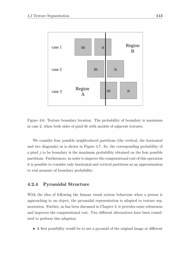
4.2 Texture Segmentation 113
nm
n
Region A
RegionB
m
nm
case 1
case 2
case 3
Figure 4.6: Texture boundary location. The probability of boundary is maximum
in case 2, when both sides of pixel fit with models of adjacent textures.
We consider four possible neighborhood partitions (the vertical, the horizontal
and two diagonals) as is shown in Figure 4.7. So, the corresponding probability of
a pixel j to be boundary is the maximum probability obtained on the four possible
partitions. Furthermore, in order to improve the computational cost of this operation
it is possible to consider only horizontal and vertical partitions as an approximation
to real measure of boundary probability.
4.2.4 Pyramidal Structure
With the idea of following the human visual system behaviour when a person is
approaching to an object, the pyramidal representation is adapted to texture seg-
mentation. Further, as has been discussed in Chapter 3, it provides noise robustness
and improves the computational cost. Two different alternatives have been consid-
ered to perform this adaption:
• A first possibility would be to use a pyramid of the original image at different
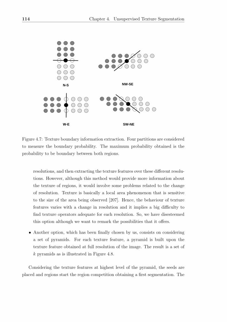
114 Chapter 4. Unsupervised Texture Segmentation
N-S
W-E
NW-SE
SW-NE
Figure 4.7: Texture boundary information extraction. Four partitions are considered
to measure the boundary probability. The maximum probability obtained is the
probability to be boundary between both regions.
resolutions, and then extracting the texture features over these different resolu-
tions. However, although this method would provide more information about
the texture of regions, it would involve some problems related to the change
of resolution. Texture is basically a local area phenomenon that is sensitive
to the size of the area being observed [207]. Hence, the behaviour of texture
features varies with a change in resolution and it implies a big difficulty to
find texture operators adequate for each resolution. So, we have disesteemed
this option although we want to remark the possibilities that it offers.
• Another option, which has been finally chosen by us, consists on considering
a set of pyramids. For each texture feature, a pyramid is built upon the
texture feature obtained at full resolution of the image. The result is a set of
k pyramids as is illustrated in Figure 4.8.
Considering the texture features at highest level of the pyramid, the seeds are
placed and regions start the region competition obtaining a first segmentation. The
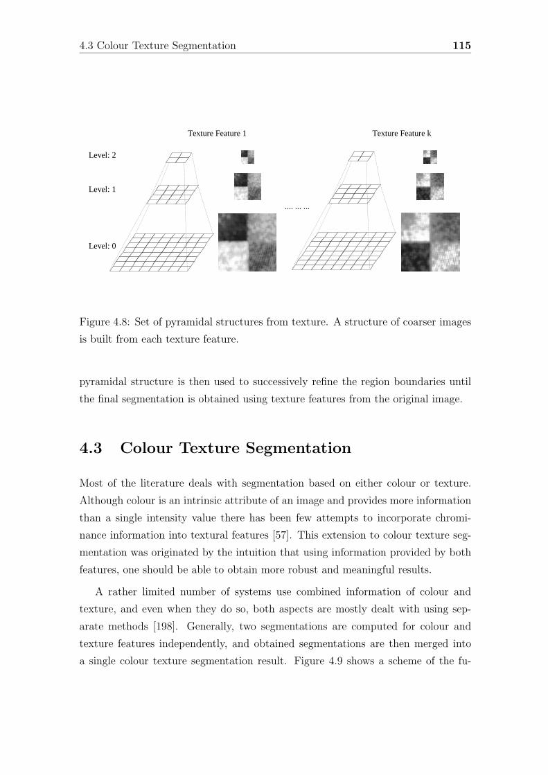
4.3 Colour Texture Segmentation 115
Level: 1
Level: 0
Level: 2
Texture Feature 1 Texture Feature k
.... ... ...
Figure 4.8: Set of pyramidal structures from texture. A structure of coarser images
is built from each texture feature.
pyramidal structure is then used to successively refine the region boundaries until
the final segmentation is obtained using texture features from the original image.
4.3 Colour Texture Segmentation
Most of the literature deals with segmentation based on either colour or texture.
Although colour is an intrinsic attribute of an image and provides more information
than a single intensity value there has been few attempts to incorporate chromi-
nance information into textural features [57]. This extension to colour texture seg-
mentation was originated by the intuition that using information provided by both
features, one should be able to obtain more robust and meaningful results.
A rather limited number of systems use combined information of colour and
texture, and even when they do so, both aspects are mostly dealt with using sep-
arate methods [198]. Generally, two segmentations are computed for colour and
texture features independently, and obtained segmentations are then merged into
a single colour texture segmentation result. Figure 4.9 shows a scheme of the fu-
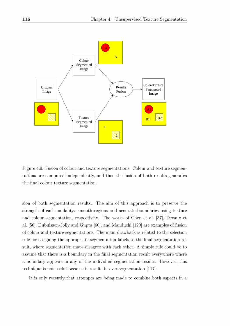
116 Chapter 4. Unsupervised Texture Segmentation
OriginalImage
ColourSegmented
Image
TextureSegmented
Image
B
A
1
2
A1
B1 B2
ResultsFusion
Color-TextureSegmented
Image
Figure 4.9: Fusion of colour and texture segmentations. Colour and texture segmen-
tations are computed independently, and then the fusion of both results generates
the final colour texture segmentation.
sion of both segmentation results. The aim of this approach is to preserve the
strength of each modality: smooth regions and accurate boundaries using texture
and colour segmentation, respectively. The works of Chen et al. [37], Devaux et
al. [56], Dubuisson-Jolly and Gupta [60], and Manduchi [120] are examples of fusion
of colour and texture segmentations. The main drawback is related to the selection
rule for assigning the appropriate segmentation labels to the final segmentation re-
sult, where segmentation maps disagree with each other. A simple rule could be to
assume that there is a boundary in the final segmentation result everywhere where
a boundary appears in any of the individual segmentation results. However, this
technique is not useful because it results in over-segmentation [117].
It is only recently that attempts are being made to combine both aspects in a
4.3 Colour Texture Segmentation 117
single method. Three alternatives to feature extraction for colour texture analysis
appear to be most often used and they consist of: (1) processing each colour band
separately by applying grey level texture analysis techniques, (2) deriving textural
information from luminance plane along with pure chrominance features, and (3) de-
riving textural information from chromatic bands extracting correlation information
across different bands.
• Processing each colour band separately by applying grey level tex-
ture analysis techniques:
This former approach represents a straightforward method of extending the
grey level algorithms to colour images. Caelli and Reye proposed a method [25]
in which they extract texture information from three spectral channels by using
three multiscale isotropic filters. Similarly, Tan and Kittler [189] extracts
features from three channels with a discrete cosine transform. A more recent
work of Thai and Healey [193] uses complex moments computed from the
output of a bank of Gabor filters to define a set of symmetry features which
explain colour texture.
• Deriving textural information from luminance plane along with pure
chrominance features:
This second approach allows a clear separation between texture and colour
features. Nevertheless, the main difficulty is to define a way to correctly de-
scribe the colour of a textured region, which is not homogenous due to textural
behaviour. Tan and Kittler [190] derived six colour features from the colour
histogram of a textured image, which were grouped with eight Discrete Cosine
Transform (DCT) coefficients as texture features computed from the inten-
sity image for classification. Meanwhile, in the proposal of Rui et al. [168], a
simple texture feature as edge intensity and three chromatic HSV coordinates
are directly grouped into a single feature vector. Then, a C-means clustering
allows the segmentation of the image.
In the work of Carson et al. [15, 28] the colour/texture descriptor for a given
pixel consists of six values: three for colour and three for texture. In order to
decouple the colour and texture properties, the three colour components are
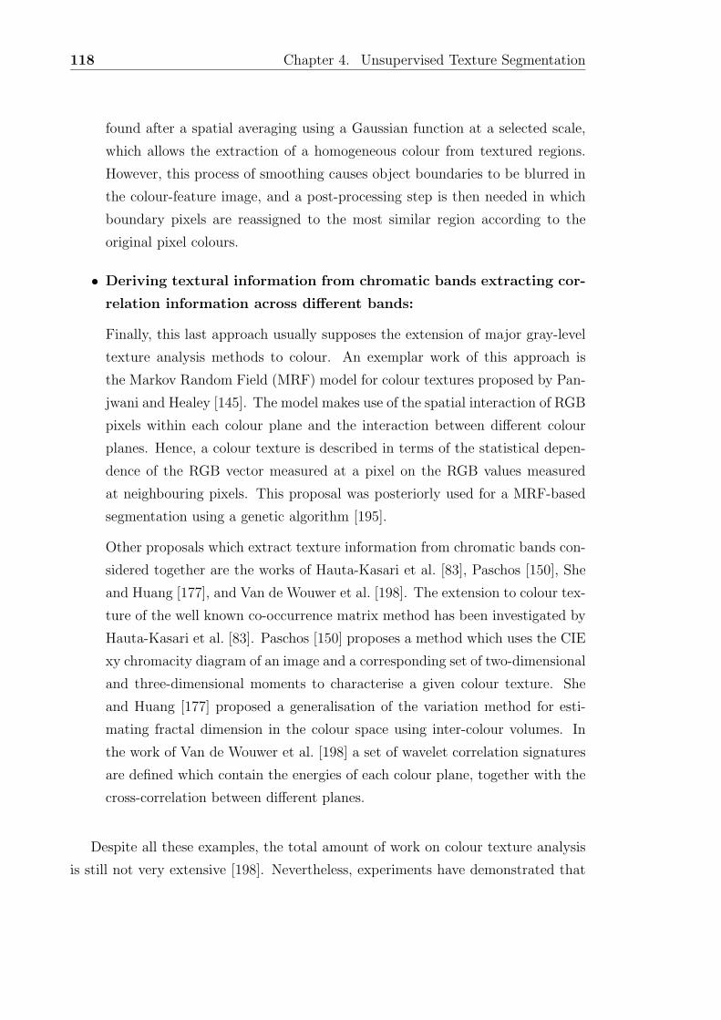
118 Chapter 4. Unsupervised Texture Segmentation
found after a spatial averaging using a Gaussian function at a selected scale,
which allows the extraction of a homogeneous colour from textured regions.
However, this process of smoothing causes object boundaries to be blurred in
the colour-feature image, and a post-processing step is then needed in which
boundary pixels are reassigned to the most similar region according to the
original pixel colours.
• Deriving textural information from chromatic bands extracting cor-
relation information across different bands:
Finally, this last approach usually supposes the extension of major gray-level
texture analysis methods to colour. An exemplar work of this approach is
the Markov Random Field (MRF) model for colour textures proposed by Pan-
jwani and Healey [145]. The model makes use of the spatial interaction of RGB
pixels within each colour plane and the interaction between different colour
planes. Hence, a colour texture is described in terms of the statistical depen-
dence of the RGB vector measured at a pixel on the RGB values measured
at neighbouring pixels. This proposal was posteriorly used for a MRF-based
segmentation using a genetic algorithm [195].
Other proposals which extract texture information from chromatic bands con-
sidered together are the works of Hauta-Kasari et al. [83], Paschos [150], She
and Huang [177], and Van de Wouwer et al. [198]. The extension to colour tex-
ture of the well known co-occurrence matrix method has been investigated by
Hauta-Kasari et al. [83]. Paschos [150] proposes a method which uses the CIE
xy chromacity diagram of an image and a corresponding set of two-dimensional
and three-dimensional moments to characterise a given colour texture. She
and Huang [177] proposed a generalisation of the variation method for esti-
mating fractal dimension in the colour space using inter-colour volumes. In
the work of Van de Wouwer et al. [198] a set of wavelet correlation signatures
are defined which contain the energies of each colour plane, together with the
cross-correlation between different planes.
Despite all these examples, the total amount of work on colour texture analysis
is still not very extensive [198]. Nevertheless, experiments have demonstrated that
4.3 Colour Texture Segmentation 119
the inclusion of colour can increase the segmentation/classification results without
significantly complicating the feature extraction algorithms [57, 116].
4.3.1 Proposal Outline
Texture segmentation approach described in Section 4.2 is directly applicable to the
first and third approach to colour texture analysis described above. In both cases
a set of texture features could be extracted, from independent bands or consider-
ing chromatic bands together, and would be used as source of the segmentation
method. Since at the the moment is still unclear what is the best method to com-
bine colour and texture, in this section we extend the strategy to perform colour
texture segmentation considering textural information from luminance plane along
with chromatic features. Hence, our proposal will also be able to deal with colour
texture segmentation considering the second approach to colour texture analysis.
Moreover, experimental results shown in Chapter 5 demonstrate the correctness of
the proposed method.
The proposed colour texture segmentation strategy follows the scheme for texture
segmentation (see Figure 4.1) but now involving the colour image in all the process.
The source of information is now the set of texture features along with the original
image which provides the colour information. Moreover, the inclusion of colour
information into our texture segmentation proposal involves two major issues:
• First, perceptual edges, which can be derived from colour or texture need to
be extracted in order to place a set of seeds.
• Then, colour and texture of regions need to be modelled in order to define the
region information and allow an accurate extraction of boundary information.
4.3.2 Colour Texture Initialisation: Perceptual Edges
Regions are characterised by colour and texture features. Hence, two regions con-
sisting of the same colour but different texture or the same texture but different
colours are two different colour textures, as well as the obvious case of two regions
120 Chapter 4. Unsupervised Texture Segmentation
with different colour and texture. Boundaries between colour texture regions, which
are combination of colour edges and texture edges can be considered as perceptual
edges, because a human has the ability to detect the boundary between different
textures as well as colour edges [63].
Using an edge detection scheme over the set of texture features we are able to
detect the boundaries between regions which differ in texture, as has been described
in Section 4.2.1. However, we also need to extract the boundaries between regions
with different colour, although they share a same texture. This is a major difficulty
since the use of an edge detector over a colour image results on the detection of
colour boundaries, but also produces the apparition of microedges inside the same
texture.
In order to remove microedges generally the texture at both sides of the contour
is checked, and the edge is removed if it does not separate two different textures [48,
63, 155]. However, it implies that edges between regions with different colours but
a same texture are removed too.
Our proposal is inspired by the work of Mirmehdi and Petrou [128], which present
a method to segment a textured image based on how different textures can be
perceived as separate homogenous regions in the preattentive stage of vision. They
propose a mechanism of segmenting colour textures, by constructing a multiscale
tower of image versions based on perceptual considerations. The levels of the tower
are constructed by using blurring masks (see more details on such masks on the
work of Zhang and Wandell [223]), by assuming that the same colour-textured is
seen at different distances (1,2,3, . . . , metres). Hence, each coarser version of the
image imitates the blurred version the Human Vision System would have seen at
the corresponding distance. The analysis of the image starts at the coarsest level
and proceeds towards the finest level, just like it would have happened if a person
was slowly approaching a distant object.
The underlying philosophy of the work by Mirmehdi and Petrou is that when a
texture is seen from a long distance seems to be a homogenous region. Hence, we
will use this same approach to obtain an image in which colour of textures looks
homogenous, as we would look the texture from far away. In order to obtain this
image a smoothing process is progressively performed starting from the original im-
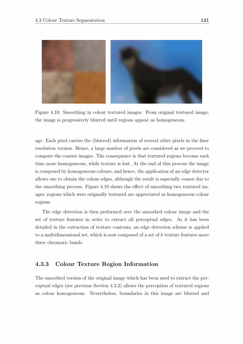
4.3 Colour Texture Segmentation 121
Figure 4.10: Smoothing in colour textured images. From original textured image,
the image is progressively blurred until regions appear as homogeneous.
age. Each pixel carries the (blurred) information of several other pixels in the finer
resolution version. Hence, a large number of pixels are considered as we proceed to
compute the coarser images. The consequence is that textured regions become each
time more homogeneous, while texture is lost. At the end of this process the image
is composed by homogeneous colours, and hence, the application of an edge detector
allows one to obtain the colour edges, although the result is especially coarse due to
the smoothing process. Figure 4.10 shows the effect of smoothing two textured im-
ages; regions which were originally textured are appreciated as homogeneous colour
regions.
The edge detection is then performed over the smoothed colour image and the
set of texture features in order to extract all perceptual edges. As it has been
detailed in the extraction of texture contours, an edge detection scheme is applied
to a multidimensional set, which is now composed of a set of k texture features more
three chromatic bands.
4.3.3 Colour Texture Region Information
The smoothed version of the original image which has been used to extract the per-
ceptual edges (see previous Section 4.3.2) allows the perception of textured regions
as colour homogeneous. Nevertheless, boundaries in this image are blurred and
122 Chapter 4. Unsupervised Texture Segmentation
accurate boundary information can not be extracted to perform the segmentation
process. Therefore, the final segmentation would require a post-processing step to
refine the boundaries using the colour information from the finer original image.
Taking these questions into account, we have opted to extract colour information
directly from the original image.
So far, features inside a region (intensity, colour or texture) have been homoge-
neous and it was possible to model them with a simple Gaussian. However, colour
in a textured region is by definition not homogenous. In fact, different authors ad-
vise about the risk of modelling colour in natural scenes, riches in texture, using a
Gaussian. Enforcing a Gaussian model over such data is doomed to fail (see works
of Roberts [165] and Manduchi [121]), and even the use of a robust approach with
contaminated Gaussian densities [228] cannot be satisfactory for such complex cases.
Figure 4.11 illustrates the behaviour of colour in textured regions. As is stated, the
chromatic bands of textured regions do not follow a Gaussian model. However, the
question is: what model does colour come from?
Colour in texture has a very variable behaviour between different regions of the
image (see Figure 4.11), thus colour in all regions can not be described by a single
model. Methods which implicitly assume the same shape (most often elliptical)
for all the clusters in the space, are not able to handle the complexity of the real
feature space as has been noticed in very recent works [41, 45]. Hence, the feature
space can be regarded as a sample drawn from an unknown probability distribution,
and representing this distribution with a parametric model will introduce severe
artifacts, since the shape of the delineated clusters is predefined [44].
Arbitrarily structured feature spaces can be analysed only by nonparametric
methods since these methods do not have embedded assumptions [45]. We focus
our attention on density estimation from a non-parametric approach. Suppose, that
we have a set of observed data points assumed to be a sample from an unknown
probability density function. Density estimation is the construction of an estimate
of the density function from the observed data. Therefore, using this statistical
technique, we are able to define a probability density function which describes the
behaviour of colour in texture.
To estimate the probability density, several non-parametric techniques are avail-

4.3 Colour Texture Segmentation 123
0
40
80
120
160
0 64 128 192 2560
32
64
96
128
0 64 128 192 2560
40
80
120
160
0 64 128 192 256
0
60
120
180
240
0 64 128 192 2560
100
200
300
400
0 64 128 192 2560
128
256
384
512
0 64 128 192 256
0
32
64
96
128
0 64 128 192 2560
40
80
120
160
0 64 128 192 2560
40
80
120
160
0 64 128 192 256
Figure 4.11: Colour distribution in textured regions. Histograms show that colour
can not be modelled by a Gaussian distribution.
able: multivariate histogram, nearest neighbour and kernel estimation methods [70,
175, 180, 192]. For higher dimensional feature spaces, multivariate histograms are
less useful due to their exponentially growing number of bins with the space dimen-
sions, as well as due to the artifacts introduced by the quantisation. The nearest
neighbour method is prone to local noise and the obtained estimate is not a prob-
ability density, since it integrates to infinity. For low to medium data sizes, kernel
estimation is a good practical choice: it is simple, and for kernels obeying mild the
estimate is asymptotically unbiased, consistent in the mean-square sense, and uni-
formly consisted in probability. Therefore, we adopt the kernel estimation technique
to estimate the probability density function of colour.
124 Chapter 4. Unsupervised Texture Segmentation
4.3.3.1 Kernel Density Estimation
Kernel density estimation is one of the most well known methods to estimate the
density function. Given n data points xi, i = 1, . . . , n in the d-dimensional space
Rd, the multivariate kernel density estimator with kernel K(x) and a symmetric
positive definite d × d bandwidth matrix H, computed in the point x is given by
f(x) =1
n
n∑i=1
KH(x − xi) (4.4)
where
KH(x) = |H|−1/2K(H−1/2x) (4.5)
The d-variate kernel K(x) is a bounded function with compact support satisfy-
ing [203]
∫Rd K(x)dx = 1 lim
||x||→∞||x||dK(x) = 0
∫Rd xK(x)dx = 0
∫Rd xxT K(x)dx = cKI
(4.6)
where cK is a constant. The multivariate kernel can be generated from a sym-
metric univariate kernel K1(x) in two different ways
KP (x) =d∏
i=1K1(xi) KS(x) = ak,dK1(||x||) (4.7)
where KP (x) is obtained from the product of the univariate kernels and KS(x)
from rotating K1(x) in Rd. We are interested only in a special class of radially
symmetric kernels satisfying
K(x) = ck,dk(||x||2) (4.8)
in which case it suffices to define the function k(x) called the profile or the kernel,
only for x ≥ 0. The normalization constant ck,d, which makes K(x) integrate to one,
is assumed strictly positive.
4.3 Colour Texture Segmentation 125
Using a fully parameterised H increases the complexity of the estimation and, in
practice, the bandwidth matrix H is chosen either as diagonal H = diag[h21, . . . , h
2d]
or proportional to the identity matrix H = h2I. The clear advantage of the latter
case is that only one bandwidth parameter h > 0 must be provided. However, the
metric of the feature space has to be Euclidean that imply that colour differences
of human perception can be expressed by Euclidean distance in the colour space.
In this sense the (L∗, a∗, b∗) and (L∗, u∗, v∗) colour spaces were especially designed
to match the sensitivity of human eyes with computer processing [194]. Therefore,
employing only one bandwidth parameter, the kernel density estimator becomes the
expression
f(x) =1
nhd
n∑i=1
KH(x − xi
h) (4.9)
The profile
kN(x) = exp(−12x) x ≥ 0 (4.10)
yields the multivariate normal kernel
KN(x) = (2π)−d/2 exp(−1
2||x||2) (4.11)
Considering colour pixels of a region as a sample from an unknown probability
density function, Equation 4.9 obtains the probability of a colour pixel belonging to
the region. Hence, the use of the kernel density estimator measures the probability of
a given pixel to belong to a region with textured behaviour taking colour properties
into account. The good performance of this technique in front of classical assumption
of Gaussian behaviour is illustrated in Figure 4.12, in which obtained segmentations
are compared. From these results, we show that the typical assumption of Gaussian
behaviour can not be adopted for colour in textured regions, and the use of the
kernel density estimator is more adequate to model the region’s colour.
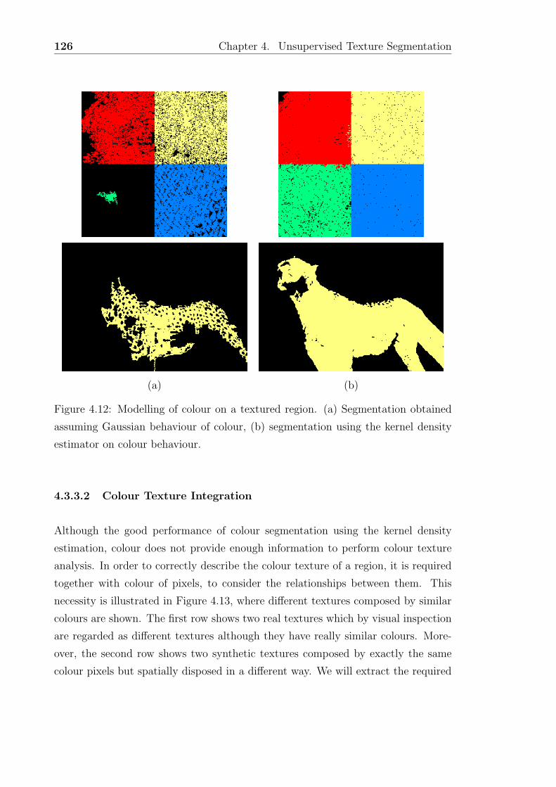
126 Chapter 4. Unsupervised Texture Segmentation
(a) (b)
Figure 4.12: Modelling of colour on a textured region. (a) Segmentation obtained
assuming Gaussian behaviour of colour, (b) segmentation using the kernel density
estimator on colour behaviour.
4.3.3.2 Colour Texture Integration
Although the good performance of colour segmentation using the kernel density
estimation, colour does not provide enough information to perform colour texture
analysis. In order to correctly describe the colour texture of a region, it is required
together with colour of pixels, to consider the relationships between them. This
necessity is illustrated in Figure 4.13, where different textures composed by similar
colours are shown. The first row shows two real textures which by visual inspection
are regarded as different textures although they have really similar colours. More-
over, the second row shows two synthetic textures composed by exactly the same
colour pixels but spatially disposed in a different way. We will extract the required
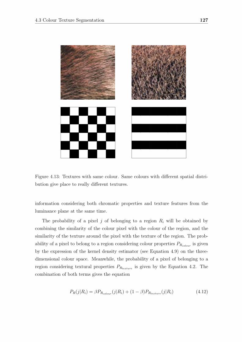
4.3 Colour Texture Segmentation 127
Figure 4.13: Textures with same colour. Same colours with different spatial distri-
bution give place to really different textures.
information considering both chromatic properties and texture features from the
luminance plane at the same time.
The probability of a pixel j of belonging to a region Ri will be obtained by
combining the similarity of the colour pixel with the colour of the region, and the
similarity of the texture around the pixel with the texture of the region. The prob-
ability of a pixel to belong to a region considering colour properties PRcolouris given
by the expression of the kernel density estimator (see Equation 4.9) on the three-
dimensional colour space. Meanwhile, the probability of a pixel of belonging to a
region considering textural properties PRtexture is given by the Equation 4.2. The
combination of both terms gives the equation
PR(j|Ri) = βPRcolour(j|Ri) + (1 − β)PRtexture(j|Ri) (4.12)
128 Chapter 4. Unsupervised Texture Segmentation
where β weights the relative importance of colour and texture terms to evaluate
the region information.
4.3.4 Colour Texture Boundary Information
In order to extract the boundary between two adjacent colour textures we will follow
the scheme detailed in Section 4.2.3. The approach defines the boundary between
two texture regions as the place where the texture at both sides is different and fits
with region’s models. The model is easily extended to colour texture re-defining the
boundary as the place where either colour or texture at both sides are different and
fit with region’s models.
Textural and colour features are computed at both sides (referred as m and its
opposite as n). However, the previously defined Equation 4.12 can not be used to
measure the similarity of these sides with corresponding region because they are
composed by a set of pixels, and we want to measure the similarity of a set of pixels
with the region’s model. A possible naive solution would be to take the colour
mean of pixels as a sample of the colour of a side, but the textured behaviour of
regions implies this value is not representative of colour in a zone. Figure 4.14
shows the possible distribution of colour pixels belonging to a textured region on
a chromatic space. This distribution is bi-modal, composed by two colour clusters
clearly separated and, as is shown in the Figure, the mean is not representative of
the colour in region.
Hence, we will measure the individual similarity of each pixel with respect to the
colour of region and then we will define a global similarity. Specifically, in order to
measure the similarity in terms of colour we use the mean of the probability of pixels
in m to belong to region A, which is given by the Equation 4.9, meanwhile the sim-
ilarity of the side considering the texture of the region is given by the Equation 4.2.
Then, the weighted sum of both measures obtains the fit between the side and the
region. Finally, the probability of a given pixel j to be boundary between regions
A and B is equal to the product of the probability of side m to belong to region A
and the probability of side n to belong to region B, which will be maximum when
j is exactly the edge between both colour textures.
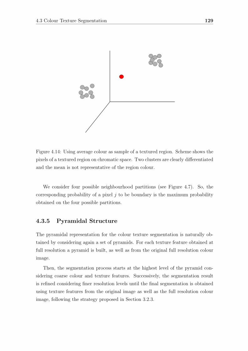
4.3 Colour Texture Segmentation 129
Figure 4.14: Using average colour as sample of a textured region. Scheme shows the
pixels of a textured region on chromatic space. Two clusters are clearly differentiated
and the mean is not representative of the region colour.
We consider four possible neighbourhood partitions (see Figure 4.7). So, the
corresponding probability of a pixel j to be boundary is the maximum probability
obtained on the four possible partitions.
4.3.5 Pyramidal Structure
The pyramidal representation for the colour texture segmentation is naturally ob-
tained by considering again a set of pyramids. For each texture feature obtained at
full resolution a pyramid is built, as well as from the original full resolution colour
image.
Then, the segmentation process starts at the highest level of the pyramid con-
sidering coarse colour and texture features. Successively, the segmentation result
is refined considering finer resolution levels until the final segmentation is obtained
using texture features from the original image as well as the full resolution colour
image, following the strategy proposed in Section 3.2.3.
130 Chapter 4. Unsupervised Texture Segmentation
4.4 Conclusions
The strategy for image segmentation proposed in Chapter 3, has been adapted to
solve the problem of texture segmentation. The method uses a coarse detection of
texture contours to initialise a set of active regions. Therefore, the initial unsuper-
vised texture segmentation problem is transformed to a supervised one, which allows
us to define the region information and to accurately extract boundary information.
Then, in the framework of active region segmentation described in Chapter 3, re-
gions compete for the pixels optimising an energy function which takes both region
and boundary information into account. The method has been implemented on a
pyramidal representation which reduces the computational cost and assures noise
robustness.
Furthermore, a method for the integration of colour and textural properties has
been proposed, which is based on the estimation of the colour behaviour using
statistical techniques of kernel density estimator, and its combination with classical
texture descriptors. Hence, the proposed segmentation strategy is considered for the
segmentation taking into account colour and textural properties together.
Chapter 5
Experimental Results
Evaluation methods to quantify the quality of a segmentation are discussed. The
proposed segmentation strategy as well as the extension to colour texture segmenta-
tion are then evaluated. A set of mosaic images is used to quantitatively evaluate
the proposed strategy, which is then compared with several algorithms (A1-A7) which
integrate region and boundary information. Furthermore, segmentation is performed
on a number of real scenes which are subjectively assessed. Colour texture segmen-
tation is evaluated on a set of collages of real textures, in which the integration of
colour and texture is analysed and segmentations are compared with results of other
researchers. Finally, some results on real scenes riches on texture are shown.
5.1 Introduction
Over the last decades, many segmentation algorithms have been developed, with
the number growing steadily every year. In contrast, relatively little effort has
been spent in attempting to evaluate the effectiveness of such algorithms. In fact,
up to now there is no universally accepted method to quantify the quality of a
segmentation [143].
The main difficulty of evaluating image segmentation algorithms stems from the
ill defined nature of the problem. In his survey on evaluation methods for image
segmentation [224], Zhang proposes this definition of image segmentation:
131
132 Chapter 5. Experimental Results
“Image segmentation consists of subdividing an image into its
constituent parts and extracting these parts of interest (ob-
jects).”
As is noted by Everingham et al. [64], this captures the procedural quality of
segmentation but leaves some questions to be answered, notably how to define “con-
stituent parts” and “parts of interest”, and how to assess the degree of success or
failure of an algorithm in the case that it does not perform optimally. This has led
some researchers [21] to argue that segmentation or grouping performance can be
evaluated only in the context of a task such as object recognition. They relate to
what subsequent stages of processing have to be applied to the segmentation results
in order to achieve the goal of the entire vision system. However, it is rarely feasible
to build entire systems in order to test different segmentation algorithms, because of
expense, and because the properties of the segmentation algorithm will often deter-
mine what form subsequent processing should take. Therefore, it is more interesting
to evaluate segmentation algorithms without implementation of subsequent process-
ing. Then, segmentations are evaluated purely and solely as segmentations [126].
A classification of evaluation methods into analytical, empirical goodness or em-
pirical discrepancy is proposed in [224].
• Analytical methods: these techniques attempt to characterise an algorithm
itself in terms of principles, requirements, complexity, etc. without reference to
a specific implementation of the algorithm or test data. For example, one can
define the time complexity of an algorithm or its response to a theoretical data
model. However, in general the lack of a general theory of image segmentation
limits these methods.
• Empirical goodness methods: algorithms are evaluated by computing a
goodness metric on the segmented image without a priori knowledge of the
desired segmentation result. For example Levine and Nazif [113] used a mea-
sure of intra-region grey-level uniformity as their goodness metric, assuming
that in a well-segmented image regions should have low variance of grey-level.
Similarly, Liu and Yang [114] proposed a function for the quantitative evalu-
ation of the performance of algorithms for the segmentation of colour images.
5.1 Introduction 133
The incorporated criteria are: (1) the regions must be uniform and homoge-
neous, (2) the region’s interiors must be simple, without too many small holes,
and (3) adjacent regions must present significantly different values for uniform
characteristics. This function was posteriorly modified by Borsotti et al. [22]
in order to penalise noisy segmentations featuring many small regions more
heavily.
The advantage of this group of methods is that they only require the definition
of a goodness metric by the user; that is, it does not require manually seg-
mented images to be supplied as ground truth data, and can be used in an on-
line manner so that the effectiveness of an algorithm can be monitored during
actual application. Nevertheless, the great disadvantage is that the goodness
metrics are at best heuristics, and may exhibit strong bias toward a particu-
lar algorithm. For example the intra-region grey-level uniformity metric will
cause any segmentation algorithm which forms regions of uniform texture to
be evaluated poorly. Hence, the definition of a goodness metric which quantify
the quality of a general segmentation is a really difficult objective.
• Empirical discrepancy methods: a third class of evaluation methods are
based on the calculation of a measure of discrepancy between the result and
the desired segmentation for the corresponding input image. In the case of
synthetic images, the correct segmentation can be obtained automatically from
the image generation procedure, while in the case of real images it must be
produced manually or semi-automatically by an experienced operator. Hence,
a human being is the ultimate judge to make an evaluation of the result [143],
which implies a factor of subjectivity. Analogous to the case of the empirical
goodness methods, a discrepancy measure must be explicitly defined, but this
is likely to be easier to do and exhibit less bias than the former methods
because of the availability of ground truth data.
Several discrepancy measures have been proposed. One of the earliest and most
intuitive measures [219] treats the segmentation task as a multi-class classi-
fication problem where each pixel has an associated correct class, and takes
measures of classification error from the pixel-wise class confusion matrix.
Other discrepancy measures calculate the distances between miss-segmented
134 Chapter 5. Experimental Results
pixels and the nearest correctly segmented pixels [219]. Thus, introducing a
spatial component to the measure, or based on differences between feature val-
ues measured from regions of the correctly segmented and output images [226].
More examples of discrepancy measures can be found in the work of Huang
and Dom [93], who proposed a complete set of three performance evaluation
schemes: parameter-based, boundary-based and region-based to be used when
ground truth is available.
In contrast to these works, Everingham et al. [64] proposes not using a sin-
gle metric to capture an algorithm’s effectiveness. The authors argue that in
reality we expect that we always have to make a trade-off between different
properties of a segmentation algorithm, for example the quality of the seg-
mentation versus the execution time, or degree of over-segmentation versus
under-segmentation. Thus, their approach is based on defining a general com-
parison method incorporating multiple measures, rather than advocating the
use of a single particular measure.
The analysis of Zhang [224] suggests that empirical methods are to be preferred,
as there is still no general theory of image segmentation. Furthermore, in the absence
of a specific application requirement, we expect the segmentation of an image to
agree with that performed by own vision system [128]. Hence, we will evaluate our
proposal using an empirical discrepancy approach, comparing our results with the
correct segmentation or ground truth.
5.2 Evaluation Methodology
Although segmentation evaluation and segmentation comparison are closely related,
they are in fact distinct matters [225]. While segmentation evaluation is an intra-
technique process, segmentation comparison is an inter-technique process. The pur-
pose of evaluation for a specific algorithm is to quantitatively recognise its behaviour
in treating various images and/or to help appropriately setting its parameters re-
garding different applications to achieve the best performance of this algorithm. On
the other hand, the purpose of comparison for different algorithms is to rank their
performance and to provide guidelines in choosing suitable algorithms according to
5.2 Evaluation Methodology 135
applications as well as to promote new developments by effectively taking the strong
points of several algorithms into account.
There are different parameters which are involved in our proposal which can
affect the segmentation results. Thus, we perform experiments on a number of
collage images to determine acceptable ranges of values for them. Furthermore,
obtained segmentations are compared to results using well-known proposals in the
literature.
In this stage, we have opted to use synthetic images. The wide range of numerous
and indeterminate characteristics of real images makes it very complicated to achieve
an accurate comparison of the experimental results. The segmentation by hand im-
plies a tedious and subjective task. Furthermore, a manually produced segmentation
of real world images will contain errors, witness the fact that for complex images
two manual segmentations will never be exactly the same [202]. Hence, the use of
carefully designed synthetic images appears to be a more suitable benchmark for an
objective and quantitative evaluation of different segmentation algorithms [225].
The segmentations are evaluated by comparing each result with its ground truth
and recording the error. Specifically, we use both region-based and boundary-based
performance evaluation schemes [93] to measure the quality of a segmentation:
• Region-based evaluation: the region-based scheme evaluates the segmen-
tation accuracy in the number of regions, locations and sizes. Let the seg-
mentation be S and the corresponding ground truth be GS. The goal is to
quantitatively describe the degree of mismatch between them, which can be
measured by the percentage of not-correctly segmented pixels considering the
segmentation as a multi-class classification problem. Note that due to the use
of synthetic images the correct classification is obvious.
More formally, measure is based on the concept of distance from one segmen-
tation S1 = {R11, R
21, . . . R
n1} to another segmentation S2 = {R1
2, R22, . . . R
m2 },
denoted by D(S1, S2). First, the correspondence between the labels of both
segmentation results is established: each region Ri2 from S2 is associated ex-
clusively with a region Rj1 from S1 such that Ri
2 ∩ Rj1 is maximal. Therefore,
the distance from S1 to S2 is defined as:
136 Chapter 5. Experimental Results
D(S1, S2) =∑
Ri2εS2
∑Rk
1 �=Rj1,Rk
1∩Ri2 �=∅ |Ri
2 ∩ Rk1| (5.1)
where |.| denote the size of a set. Therefore, D(S1, S2) is the total area under
the intersections between all Ri2εS2 and their non-maximal intersected regions
from S1. The error on segmentation based on normalised distance is defined as
p = D(S=⇒GS))|S| , where |S| is the image size and 100× p gives us the percentage
of error. The smaller the degree of mismatch, the closer the percentage is to
zero.
• Boundary-based evaluation: the boundary-based scheme is intended to
evaluate segmentation quality in terms of the precision of the extracted region
boundaries. Let B represent the boundary point set derived from the segmen-
tation and GB the boundary ground truth. The distance from ground truth
to the estimated boundary is used to evaluate the segmentation. Define the
distance from an arbitrary point j in set B to GB as the minimum absolute
distance from j to all the points in GB, d(i, GB) = min{dE(i, j)},∀iεGB, where
dE denotes the Euclidean distance between points i and j. The discrepancy
between B and GB is measured by the mean distance from boundary pixels
in the ground truth image to boundary pixels in the segmented image. As a
rule, a near-zero mean indicates high quality of the segmentation.
Furthermore, in a second stage we have opted to evaluate our proposal on a set
of real images. Some authors indicate the use of real images in segmentation eval-
uation as an inevitable necessity. Real images provide useful results when realistic
characteristics arise. Moreover, as Hoover et al. [90] advise, work that stops short
of using real images inspires little confidence in its relevance. Hence, we extend the
test of our proposal to a number of real scenes, whose segmentations are subjectively
judged.
5.3 Image Segmentation Experiments 137
5.3 Image Segmentation Experiments
5.3.1 Synthetic Images
The set of synthetic images generated to test the image segmentation strategy fol-
lows the methodology proposed by Zhang [225]. Different images of size 128 × 128
are designed which are composed by regions of uniform intensity. Next, to make
synthetic images more realistic, a 5×5 average low-pass filter is applied to produce a
smooth transition between the different regions. A zero-mean Gaussian white noise
is then added to simulate noise effect. The noise samples have been generated with
standard deviations of 1, 2 and 4. The set of synthetic images is shown in Figure 5.1.
Note that we have named each image with two numbers. The first one relates to the
original image, while the second describes the level of noise which has been added.
Hence, images I11, I12 and I13 are the result of adding a progressively higher level
of noise to the same original image.
5.3.1.1 Segmentation Evaluation
The relative weight of region and boundary information, as well as the number of
multiresolution levels, are two key parameters involved in our processing which can
affect the result of the segmentation. Hence, we will analyse the role they play in
the segmentation results.
In reference with the first parameter, α, it indicates the weight of region infor-
mation, while 1 − α is the weight given to the boundary information. In the range
between 0 and 1, seven different values have been considered. The evaluation of
segmentations results from a region-based scheme is shown in Table 5.1, in which
the percentage of error on the segmentation of test images is given. Moreover, the
mean, standard deviation and median of percentage error are given as descriptors
of the evaluation on the whole set of test images. A first aspect to note is the
exorbitant error obtained when the parameter α is set to zero and only boundary
information is considered in the segmentation process. Although the performance in
this case is really poor, this result is not surprising because it is due to the problems
of initialisation typical of active contour models, which we have wanted to show.
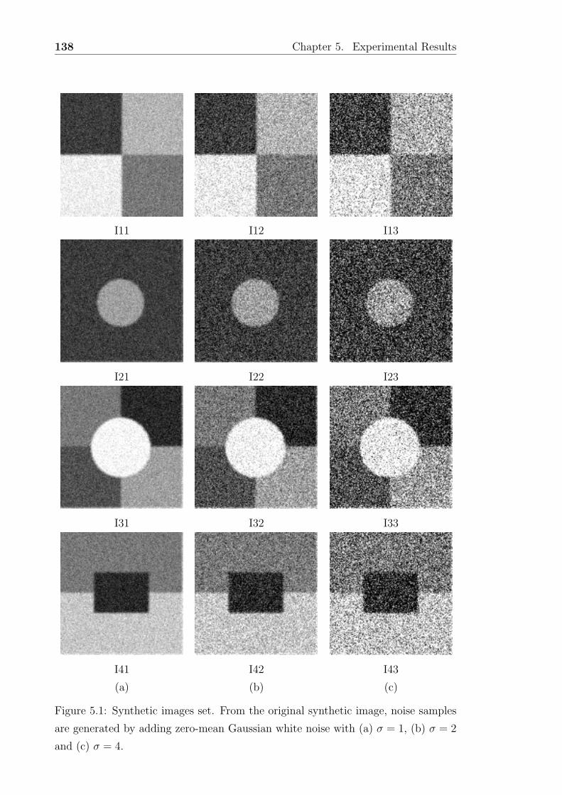
138 Chapter 5. Experimental Results
I11 I12 I13
I21 I22 I23
I31 I32 I33
I41 I42 I43
(a) (b) (c)
Figure 5.1: Synthetic images set. From the original synthetic image, noise samples
are generated by adding zero-mean Gaussian white noise with (a) σ = 1, (b) σ = 2
and (c) σ = 4.
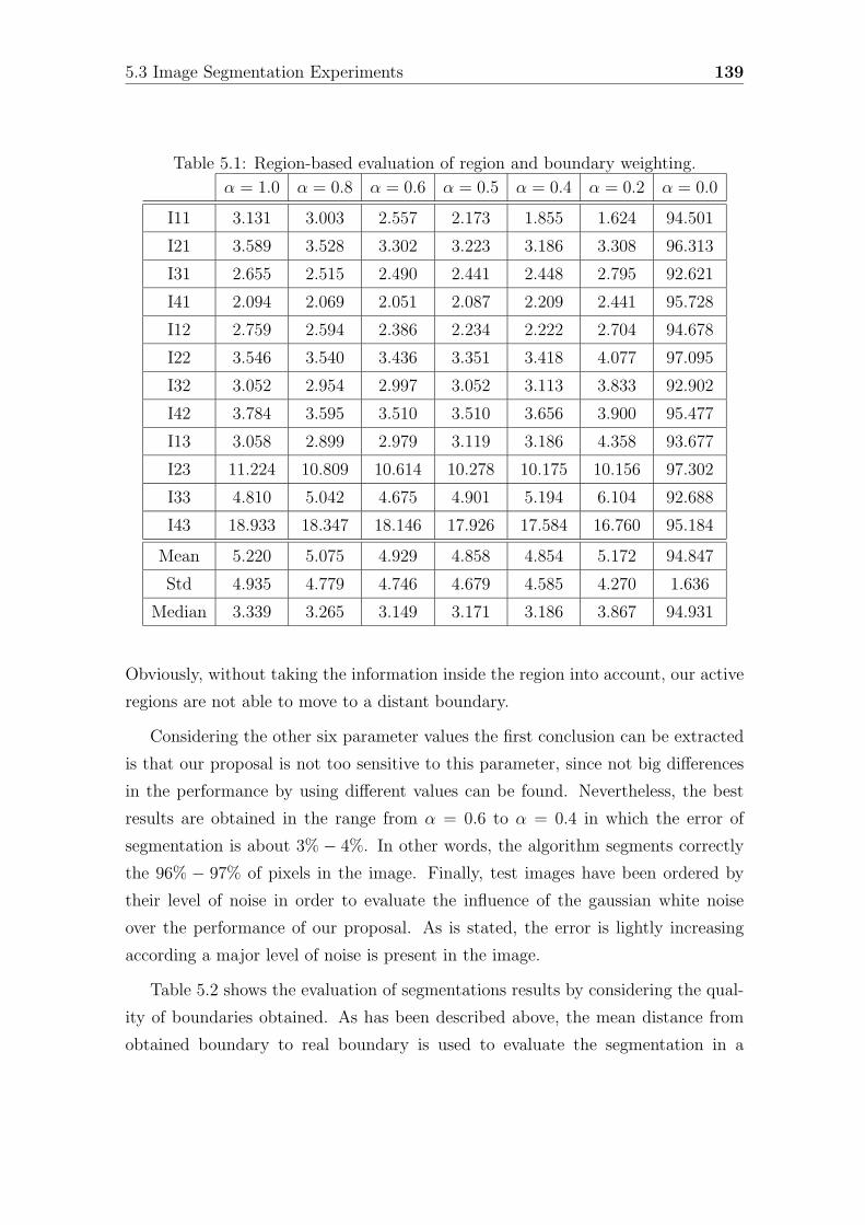
5.3 Image Segmentation Experiments 139
Table 5.1: Region-based evaluation of region and boundary weighting.
α = 1.0 α = 0.8 α = 0.6 α = 0.5 α = 0.4 α = 0.2 α = 0.0
I11 3.131 3.003 2.557 2.173 1.855 1.624 94.501
I21 3.589 3.528 3.302 3.223 3.186 3.308 96.313
I31 2.655 2.515 2.490 2.441 2.448 2.795 92.621
I41 2.094 2.069 2.051 2.087 2.209 2.441 95.728
I12 2.759 2.594 2.386 2.234 2.222 2.704 94.678
I22 3.546 3.540 3.436 3.351 3.418 4.077 97.095
I32 3.052 2.954 2.997 3.052 3.113 3.833 92.902
I42 3.784 3.595 3.510 3.510 3.656 3.900 95.477
I13 3.058 2.899 2.979 3.119 3.186 4.358 93.677
I23 11.224 10.809 10.614 10.278 10.175 10.156 97.302
I33 4.810 5.042 4.675 4.901 5.194 6.104 92.688
I43 18.933 18.347 18.146 17.926 17.584 16.760 95.184
Mean 5.220 5.075 4.929 4.858 4.854 5.172 94.847
Std 4.935 4.779 4.746 4.679 4.585 4.270 1.636
Median 3.339 3.265 3.149 3.171 3.186 3.867 94.931
Obviously, without taking the information inside the region into account, our active
regions are not able to move to a distant boundary.
Considering the other six parameter values the first conclusion can be extracted
is that our proposal is not too sensitive to this parameter, since not big differences
in the performance by using different values can be found. Nevertheless, the best
results are obtained in the range from α = 0.6 to α = 0.4 in which the error of
segmentation is about 3% − 4%. In other words, the algorithm segments correctly
the 96% − 97% of pixels in the image. Finally, test images have been ordered by
their level of noise in order to evaluate the influence of the gaussian white noise
over the performance of our proposal. As is stated, the error is lightly increasing
according a major level of noise is present in the image.
Table 5.2 shows the evaluation of segmentations results by considering the qual-
ity of boundaries obtained. As has been described above, the mean distance from
obtained boundary to real boundary is used to evaluate the segmentation in a
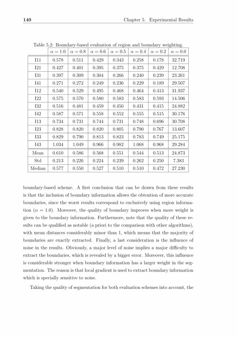
140 Chapter 5. Experimental Results
Table 5.2: Boundary-based evaluation of region and boundary weighting.
α = 1.0 α = 0.8 α = 0.6 α = 0.5 α = 0.4 α = 0.2 α = 0.0
I11 0.578 0.511 0.429 0.343 0.258 0.178 32.719
I21 0.427 0.401 0.395 0.375 0.375 0.429 12.708
I31 0.397 0.309 0.304 0.266 0.240 0.239 23.261
I41 0.271 0.272 0.249 0.236 0.229 0.189 29.507
I12 0.540 0.529 0.495 0.468 0.464 0.413 31.937
I22 0.575 0.570 0.580 0.583 0.583 0.593 14.506
I32 0.516 0.481 0.459 0.450 0.431 0.415 24.882
I42 0.587 0.571 0.558 0.552 0.555 0.515 30.176
I13 0.734 0.731 0.744 0.731 0.748 0.696 30.708
I23 0.828 0.820 0.820 0.805 0.790 0.767 13.607
I33 0.829 0.790 0.813 0.823 0.783 0.749 25.175
I43 1.034 1.049 0.966 0.982 1.068 0.968 29.284
Mean 0.610 0.586 0.568 0.551 0.544 0.513 24.873
Std 0.213 0.226 0.224 0.239 0.262 0.250 7.383
Median 0.577 0.550 0.527 0.510 0.510 0.472 27.230
boundary-based scheme. A first conclusion that can be drawn from these results
is that the inclusion of boundary information allows the obtention of more accurate
boundaries, since the worst results correspond to exclusively using region informa-
tion (α = 1.0). Moreover, the quality of boundary improves when more weight is
given to the boundary information. Furthermore, note that the quality of these re-
sults can be qualified as notable (a priori to the comparison with other algorithms),
with mean distances considerably minor than 1, which means that the majority of
boundaries are exactly extracted. Finally, a last consideration is the influence of
noise in the results. Obviously, a major level of noise implies a major difficulty to
extract the boundaries, which is revealed by a bigger error. Moreover, this influence
is considerable stronger when boundary information has a larger weight in the seg-
mentation. The reason is that local gradient is used to extract boundary information
which is specially sensitive to noise.
Taking the quality of segmentation for both evaluation schemes into account, the
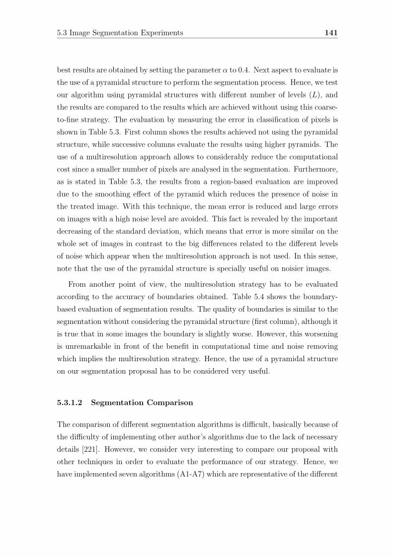
5.3 Image Segmentation Experiments 141
best results are obtained by setting the parameter α to 0.4. Next aspect to evaluate is
the use of a pyramidal structure to perform the segmentation process. Hence, we test
our algorithm using pyramidal structures with different number of levels (L), and
the results are compared to the results which are achieved without using this coarse-
to-fine strategy. The evaluation by measuring the error in classification of pixels is
shown in Table 5.3. First column shows the results achieved not using the pyramidal
structure, while successive columns evaluate the results using higher pyramids. The
use of a multiresolution approach allows to considerably reduce the computational
cost since a smaller number of pixels are analysed in the segmentation. Furthermore,
as is stated in Table 5.3, the results from a region-based evaluation are improved
due to the smoothing effect of the pyramid which reduces the presence of noise in
the treated image. With this technique, the mean error is reduced and large errors
on images with a high noise level are avoided. This fact is revealed by the important
decreasing of the standard deviation, which means that error is more similar on the
whole set of images in contrast to the big differences related to the different levels
of noise which appear when the multiresolution approach is not used. In this sense,
note that the use of the pyramidal structure is specially useful on noisier images.
From another point of view, the multiresolution strategy has to be evaluated
according to the accuracy of boundaries obtained. Table 5.4 shows the boundary-
based evaluation of segmentation results. The quality of boundaries is similar to the
segmentation without considering the pyramidal structure (first column), although it
is true that in some images the boundary is slightly worse. However, this worsening
is unremarkable in front of the benefit in computational time and noise removing
which implies the multiresolution strategy. Hence, the use of a pyramidal structure
on our segmentation proposal has to be considered very useful.
5.3.1.2 Segmentation Comparison
The comparison of different segmentation algorithms is difficult, basically because of
the difficulty of implementing other author’s algorithms due to the lack of necessary
details [221]. However, we consider very interesting to compare our proposal with
other techniques in order to evaluate the performance of our strategy. Hence, we
have implemented seven algorithms (A1-A7) which are representative of the different
142 Chapter 5. Experimental Results
Table 5.3: Region-based evaluation of multiresolution levels.
L=0 L=1 L=2 L=3
I11 1.855 0.214 0.348 0.330
I21 3.186 2.240 2.228 2.222
I31 2.448 2.344 2.332 2.313
I41 2.209 2.100 2.155 2.161
I12 3.186 1.056 0.995 1.031
I22 3.418 2.533 2.478 2.478
I32 3.113 2.826 2.753 2.734
I42 3.656 2.734 2.783 2.771
I13 3.186 1.642 1.910 1.929
I23 10.175 3.113 3.015 3.021
I33 5.194 4.834 4.913 4.797
I43 17.584 4.053 3.632 3.613
Mean 4.854 2.474 2.462 2.450
Std 4.585 1.232 1.166 1.141
Median 3.186 2.438 2.405 2.396
strategies of integration identified in Chapter 2. Lets give a brief description of these
algorithms:
• Algorithm A1 (Control of decision criterion in split-and-merge):
A1 is an algorithm based on the ideas of Bonnin and his colleagues who pro-
posed in [20] a region extraction method based on a split-and-merge algorithm
controlled by edge detection. The criterion to decide the split of a region takes
edge and intensity characteristics into account. More specifically, if there is
no edge point on the patch and if the intensity homogeneity constraints are
satisfied, then the region is stored; otherwise, the patch is divided into four sub-
patches, and the process is recursively repeated. Next, a final merging process
uses edge information in order to solve possible over-segmentation problems.
In this last step, two adjacent initial regions are merged only if there are no
edges on the common boundary.
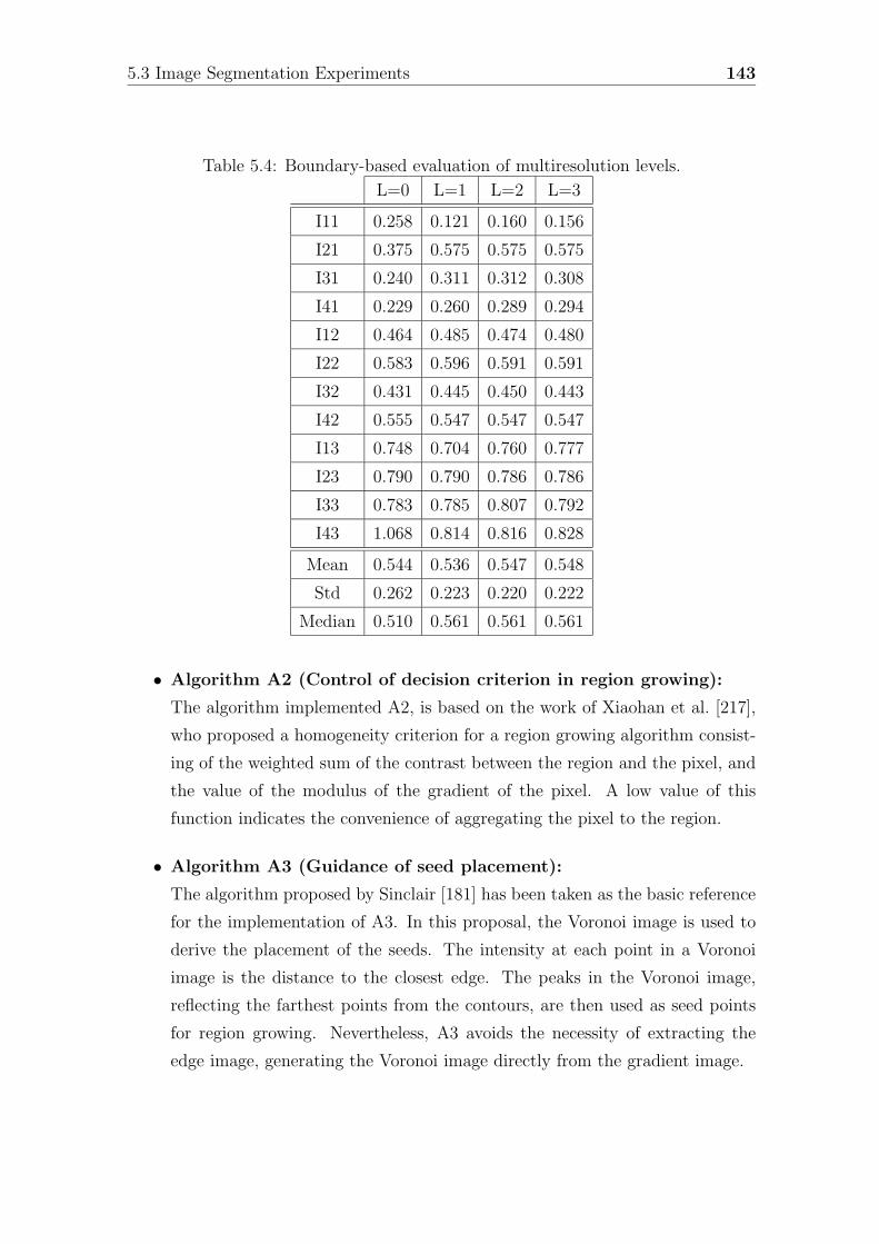
5.3 Image Segmentation Experiments 143
Table 5.4: Boundary-based evaluation of multiresolution levels.
L=0 L=1 L=2 L=3
I11 0.258 0.121 0.160 0.156
I21 0.375 0.575 0.575 0.575
I31 0.240 0.311 0.312 0.308
I41 0.229 0.260 0.289 0.294
I12 0.464 0.485 0.474 0.480
I22 0.583 0.596 0.591 0.591
I32 0.431 0.445 0.450 0.443
I42 0.555 0.547 0.547 0.547
I13 0.748 0.704 0.760 0.777
I23 0.790 0.790 0.786 0.786
I33 0.783 0.785 0.807 0.792
I43 1.068 0.814 0.816 0.828
Mean 0.544 0.536 0.547 0.548
Std 0.262 0.223 0.220 0.222
Median 0.510 0.561 0.561 0.561
• Algorithm A2 (Control of decision criterion in region growing):
The algorithm implemented A2, is based on the work of Xiaohan et al. [217],
who proposed a homogeneity criterion for a region growing algorithm consist-
ing of the weighted sum of the contrast between the region and the pixel, and
the value of the modulus of the gradient of the pixel. A low value of this
function indicates the convenience of aggregating the pixel to the region.
• Algorithm A3 (Guidance of seed placement):
The algorithm proposed by Sinclair [181] has been taken as the basic reference
for the implementation of A3. In this proposal, the Voronoi image is used to
derive the placement of the seeds. The intensity at each point in a Voronoi
image is the distance to the closest edge. The peaks in the Voronoi image,
reflecting the farthest points from the contours, are then used as seed points
for region growing. Nevertheless, A3 avoids the necessity of extracting the
edge image, generating the Voronoi image directly from the gradient image.
144 Chapter 5. Experimental Results
• Algorithm A4 (Over-segmentation):
The implemented algorithm A4 follows the most habitual technique of over-
segmentation approach, which consists of obtaining the over-segmented result
using a region-based algorithm. Every initial boundary is then checked by
analysing its coherence with the edge map, where real boundaries must have
high gradient values, while low values correspond to false contours. Concretely,
A4 is based on the work of Gagalowicz and Monga [72, 216], where two adjacent
regions are merged if the average gradient on their boundary is lower than a
fixed threshold.
• Algorithm A5 (Multiresolution):
The A5 algorithm is based on the work of Spann and Wilson [215], where
the strategy uses a quadtree method using classification at the top level of
the tree, followed by boundary refinement. In our implementation, a region
growing algorithm is used to perform classification at the top level, yielding
an initial boundary, followed by downward boundary estimation to refine the
result.
• Algorithm A6 (Boundary refinement by snakes):
The A6 algorithm is implemented following the ideas of Chan et al. [34] related
to the refinement of boundaries using snakes. An active contour is placed at
the boundary of the regions obtained using a region growing algorithm in order
to refine it. Specifically, a greedy algorithm is used to find the minimum energy
contour. This algorithm searches for the position of the minimum energy by
adjusting each point on the contour during iteration to a lower energy position
amongst its eight local neighbours.
• Algorithm A7 (Selection-Evaluation):
The A7 algorithm is based on the work of Siebert [179] where edge information
is used to adjust the criterion function of a region-growing segmentation. For
each seed, A7 creates a whole family of segmentation results (with different
criterion functions) and then, based on the local quality of the region’s con-
tour, picks the best one. The contrast between both sides of the boundary
is proposed as a measure of contour strength to evaluate the segmentation
quality. More formally, the contour strength is expressed as the sum of the
5.3 Image Segmentation Experiments 145
absolute differences between each pixel on the contour of a region and the
pixels in the 4-neighbourhood of these contour points which are not part of
the region. However, Siebert suggests that slightly improved results at higher
computational costs can be expected if the contour strength is based on the
gradient at each contour pixel rather than on the intensity difference. Hence,
this second option has been the solution adopted in the A7 implementation.
The set of test images (see Figure 5.1) have been then segmented using these 7
algorithms of integration, and the quantitative evaluation of these results is shown
in Tables 5.5 and 5.6. Moreover, last column of these tables shows the results ob-
tained by our proposal considering a pyramidal structure with L = 2. It should be
noted that the results corresponding to algorithms A1-A7 have been obtained by
fine-tuning the parameters of algorithms independently for each image. From these
results, and focusing on the 7 implemented algorithms, some observations can be
noted about the different strategies of integration. The best segmentation consid-
ering the region-based evaluation is achieved by the algorithm A1, which is based
on the inclusion of edge information into a split-and-merge algorithm. The good
performance of this algorithm is related to the nature of the decision criterion of the
split-and-merge, which analyses the homogeneity of a whole region in front of the re-
gion growing algorithm, which is based on the local decision of aggregation of a pixel
to the region. Hence, the split-and-merge becomes more robust to the presence of
noise, always taking into account that parameters have been conveniently set. Nev-
ertheless, the A1 algorithm obtains, at the same time, the worst performance when
is evaluated by a boundary-based scheme. As is well known, the quad-tree struc-
ture used to effect the step of splitting involves the obtention of squared boundaries
which imply a non accurate extraction of regions boundary. It is significative the
perfect segmentation obtained on images I11, I12 and I13, which are composed by
four squared regions, while coarse boundaries are detected in other test images with
different region shapes. Moreover, these three perfect segmentations provoke the
mean error at boundary to be relatively small, but the high standard deviation and
median values show the real problems of this algorithm to extract boundaries.
Taking the region-based evaluation into account, the A5 algorithm (multiresolu-
tion approach) also obtains relevant results, primarily due to the shown robustness
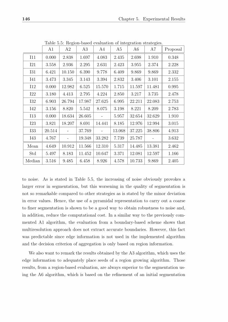
146 Chapter 5. Experimental Results
Table 5.5: Region-based evaluation of integration strategies.
A1 A2 A3 A4 A5 A6 A7 Proposal
I11 0.000 2.838 1.697 4.083 2.435 2.698 1.910 0.348
I21 3.558 2.936 2.295 2.631 2.423 3.955 2.374 2.228
I31 6.421 10.150 6.390 9.778 6.409 9.869 9.869 2.332
I41 3.473 3.345 3.143 3.394 2.832 3.406 3.101 2.155
I12 0.000 12.982 6.525 15.570 1.715 11.597 11.481 0.995
I22 3.180 4.413 2.795 4.224 2.850 3.217 3.735 2.478
I32 6.903 26.794 17.987 27.625 6.995 22.211 22.083 2.753
I42 3.156 8.820 5.542 8.075 3.198 8.221 8.209 2.783
I13 0.000 18.634 26.605 - 5.957 32.654 32.629 1.910
I23 3.821 18.207 8.691 14.441 8.185 12.976 12.994 3.015
I33 20.514 - 37.769 - 13.068 37.225 38.806 4.913
I43 4.767 - 19.348 33.282 7.739 25.787 - 3.632
Mean 4.649 10.912 11.566 12.310 5.317 14.485 13.381 2.462
Std 5.497 8.183 11.452 10.647 3.371 12.081 12.597 1.166
Median 3.516 9.485 6.458 8.926 4.578 10.733 9.869 2.405
to noise. As is stated in Table 5.5, the increasing of noise obviously provokes a
larger error in segmentation, but this worsening in the quality of segmentation is
not so remarkable compared to other strategies as is stated by the minor deviation
in error values. Hence, the use of a pyramidal representation to carry out a coarse
to finer segmentation is shown to be a good way to obtain robustness to noise and,
in addition, reduce the computational cost. In a similar way to the previously com-
mented A1 algorithm, the evaluation from a boundary-based scheme shows that
multiresolution approach does not extract accurate boundaries. However, this fact
was predictable since edge information is not used in the implemented algorithm
and the decision criterion of aggregation is only based on region information.
We also want to remark the results obtained by the A3 algorithm, which uses the
edge information to adequately place seeds of a region growing algorithm. Those
results, from a region-based evaluation, are always superior to the segmentation us-
ing the A6 algorithm, which is based on the refinement of an initial segmentation
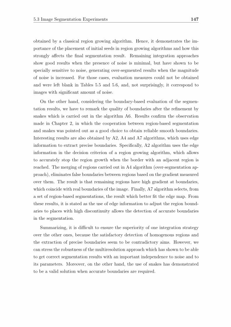
5.3 Image Segmentation Experiments 147
obtained by a classical region growing algorithm. Hence, it demonstrates the im-
portance of the placement of initial seeds in region growing algorithms and how this
strongly affects the final segmentation result. Remaining integration approaches
show good results when the presence of noise is minimal, but have shown to be
specially sensitive to noise, generating over-segmented results when the magnitude
of noise is increased. For those cases, evaluation measures could not be obtained
and were left blank in Tables 5.5 and 5.6, and, not surprisingly, it correspond to
images with significant amount of noise.
On the other hand, considering the boundary-based evaluation of the segmen-
tation results, we have to remark the quality of boundaries after the refinement by
snakes which is carried out in the algorithm A6. Results confirm the observation
made in Chapter 2, in which the cooperation between region-based segmentation
and snakes was pointed out as a good choice to obtain reliable smooth boundaries.
Interesting results are also obtained by A2, A4 and A7 algorithms, which uses edge
information to extract precise boundaries. Specifically, A2 algorithm uses the edge
information in the decision criterion of a region growing algorithm, which allows
to accurately stop the region growth when the border with an adjacent region is
reached. The merging of regions carried out in A4 algorithm (over-segmentation ap-
proach), eliminates false boundaries between regions based on the gradient measured
over them. The result is that remaining regions have high gradient at boundaries,
which coincide with real boundaries of the image. Finally, A7 algorithm selects, from
a set of region-based segmentations, the result which better fit the edge map. From
these results, it is stated as the use of edge information to adjust the region bound-
aries to places with high discontinuity allows the detection of accurate boundaries
in the segmentation.
Summarizing, it is difficult to ensure the superiority of one integration strategy
over the other ones, because the satisfactory detection of homogenous regions and
the extraction of precise boundaries seem to be contradictory aims. However, we
can stress the robustness of the multiresolution approach which has shown to be able
to get correct segmentation results with an important independence to noise and to
its parameters. Moreover, on the other hand, the use of snakes has demonstrated
to be a valid solution when accurate boundaries are required.
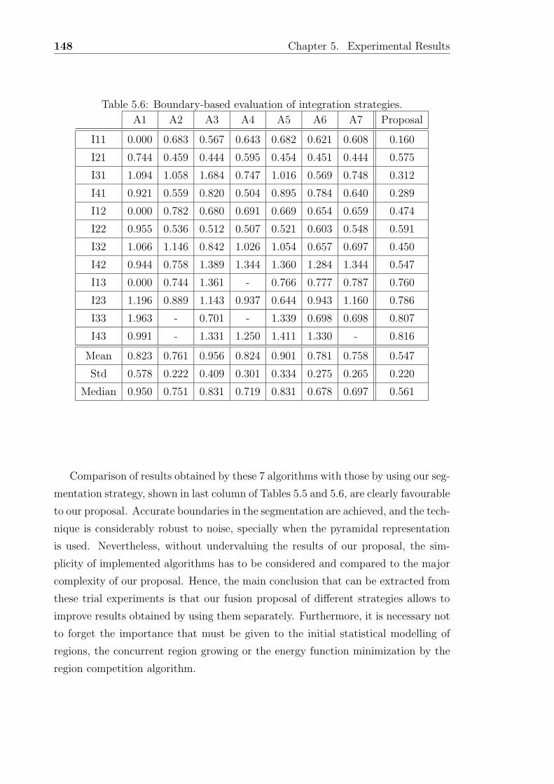
148 Chapter 5. Experimental Results
Table 5.6: Boundary-based evaluation of integration strategies.
A1 A2 A3 A4 A5 A6 A7 Proposal
I11 0.000 0.683 0.567 0.643 0.682 0.621 0.608 0.160
I21 0.744 0.459 0.444 0.595 0.454 0.451 0.444 0.575
I31 1.094 1.058 1.684 0.747 1.016 0.569 0.748 0.312
I41 0.921 0.559 0.820 0.504 0.895 0.784 0.640 0.289
I12 0.000 0.782 0.680 0.691 0.669 0.654 0.659 0.474
I22 0.955 0.536 0.512 0.507 0.521 0.603 0.548 0.591
I32 1.066 1.146 0.842 1.026 1.054 0.657 0.697 0.450
I42 0.944 0.758 1.389 1.344 1.360 1.284 1.344 0.547
I13 0.000 0.744 1.361 - 0.766 0.777 0.787 0.760
I23 1.196 0.889 1.143 0.937 0.644 0.943 1.160 0.786
I33 1.963 - 0.701 - 1.339 0.698 0.698 0.807
I43 0.991 - 1.331 1.250 1.411 1.330 - 0.816
Mean 0.823 0.761 0.956 0.824 0.901 0.781 0.758 0.547
Std 0.578 0.222 0.409 0.301 0.334 0.275 0.265 0.220
Median 0.950 0.751 0.831 0.719 0.831 0.678 0.697 0.561
Comparison of results obtained by these 7 algorithms with those by using our seg-
mentation strategy, shown in last column of Tables 5.5 and 5.6, are clearly favourable
to our proposal. Accurate boundaries in the segmentation are achieved, and the tech-
nique is considerably robust to noise, specially when the pyramidal representation
is used. Nevertheless, without undervaluing the results of our proposal, the sim-
plicity of implemented algorithms has to be considered and compared to the major
complexity of our proposal. Hence, the main conclusion that can be extracted from
these trial experiments is that our fusion proposal of different strategies allows to
improve results obtained by using them separately. Furthermore, it is necessary not
to forget the importance that must be given to the initial statistical modelling of
regions, the concurrent region growing or the energy function minimization by the
region competition algorithm.
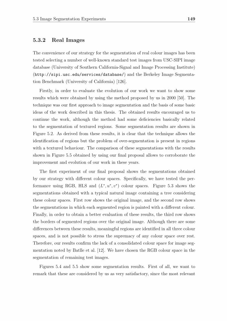
5.3 Image Segmentation Experiments 149
5.3.2 Real Images
The convenience of our strategy for the segmentation of real colour images has been
tested selecting a number of well-known standard test images from USC-SIPI image
database (University of Southern California-Signal and Image Processing Institute)
(http://sipi.usc.edu/services/database/) and the Berkeley Image Segmenta-
tion Benchmark (University of California) [126].
Firstly, in order to evaluate the evolution of our work we want to show some
results which were obtained by using the method proposed by us in 2000 [50]. The
technique was our first approach to image segmentation and the basis of some basic
ideas of the work described in this thesis. The obtained results encouraged us to
continue the work, although the method had some deficiencies basically related
to the segmentation of textured regions. Some segmentation results are shown in
Figure 5.2. As derived from these results, it is clear that the technique allows the
identification of regions but the problem of over-segmentation is present in regions
with a textured behaviour. The comparison of these segmentations with the results
shown in Figure 5.5 obtained by using our final proposal allows to corroborate the
improvement and evolution of our work in these years.
The first experiment of our final proposal shows the segmentations obtained
by our strategy with different colour spaces. Specifically, we have tested the per-
formance using RGB, HLS and (L∗, u∗, v∗) colour spaces. Figure 5.3 shows the
segmentations obtained with a typical natural image containing a tree considering
these colour spaces. First row shows the original image, and the second row shows
the segmentations in which each segmented region is painted with a different colour.
Finally, in order to obtain a better evaluation of these results, the third row shows
the borders of segmented regions over the original image. Although there are some
differences between these results, meaningful regions are identified in all three colour
spaces, and is not possible to stress the supremacy of any colour space over rest.
Therefore, our results confirm the lack of a consolidated colour space for image seg-
mentation noted by Batlle et al. [12]. We have chosen the RGB colour space in the
segmentation of remaining test images.
Figures 5.4 and 5.5 show some segmentation results. First of all, we want to
remark that these are considered by us as very satisfactory, since the most relevant
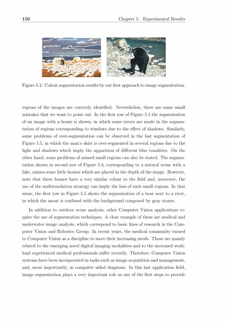
150 Chapter 5. Experimental Results
Figure 5.2: Colour segmentation results by our first approach to image segmentation.
regions of the images are correctly identified. Nevertheless, there are some small
mistakes that we want to point out. In the first row of Figure 5.4 the segmentation
of an image with a house is shown, in which some errors are made in the segmen-
tation of regions corresponding to windows due to the effect of shadows. Similarly,
some problems of over-segmentation can be observed in the last segmentation of
Figure 5.5, in which the man’s shirt is over-segmented in several regions due to the
light and shadows which imply the apparition of different blue tonalities. On the
other hand, some problems of missed small regions can also be stated. The segmen-
tation shown in second row of Figure 5.4, corresponding to a natural scene with a
lake, misses some little houses which are placed in the depth of the image. However,
note that these houses have a very similar colour to the field and, moreover, the
use of the multiresolution strategy can imply the loss of such small regions. In that
sense, the first row in Figure 5.5 shows the segmentation of a bear next to a river,
in which the snout is confused with the background composed by gray stones.
In addition to outdoor scene analysis, other Computer Vision applications re-
quire the use of segmentation techniques. A clear example of these are medical and
underwater image analysis, which correspond to basic lines of research in the Com-
puter Vision and Robotics Group. In recent years, the medical community turned
to Computer Vision as a discipline to meet their increasing needs. Those are mainly
related to the emerging novel digital imaging modalities and to the increased work-
load experienced medical professionals suffer recently. Therefore, Computer Vision
systems have been incorporated in tasks such as image acquisition and management,
and, more importantly, in computer aided diagnosis. In this last application field,
image segmentation plays a very important role as one of the first steps to provide
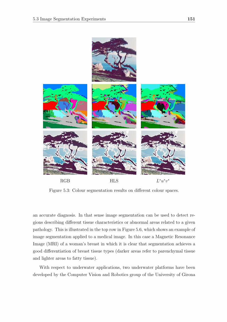
5.3 Image Segmentation Experiments 151
RGB HLS L∗u∗v∗
Figure 5.3: Colour segmentation results on different colour spaces.
an accurate diagnosis. In that sense image segmentation can be used to detect re-
gions describing different tissue characteristics or abnormal areas related to a given
pathology. This is illustrated in the top row in Figure 5.6, which shows an example of
image segmentation applied to a medical image. In this case a Magnetic Resonance
Image (MRI) of a woman’s breast in which it is clear that segmentation achieves a
good differentiation of breast tissue types (darker areas refer to parenchymal tissue
and lighter areas to fatty tissue).
With respect to underwater applications, two underwater platforms have been
developed by the Computer Vision and Robotics group of the University of Girona
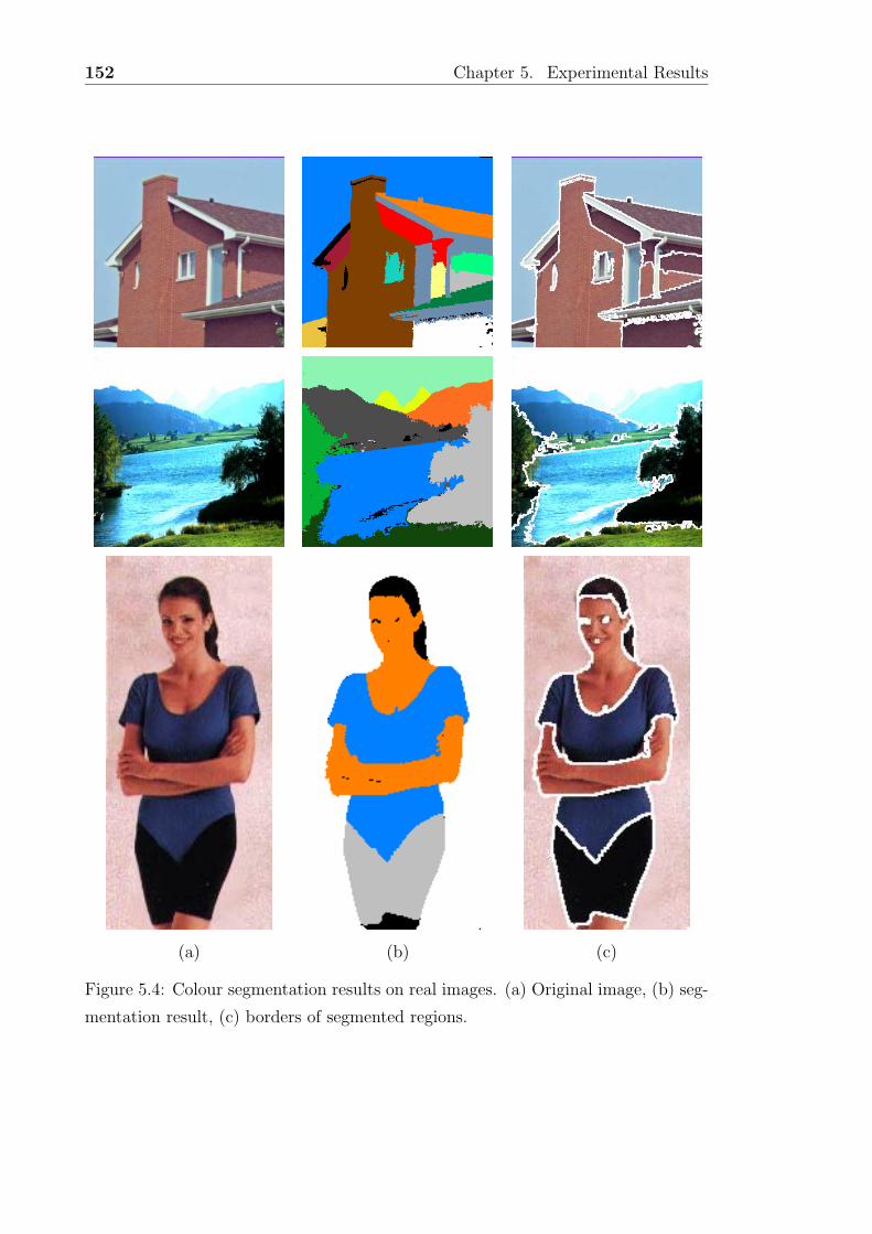
152 Chapter 5. Experimental Results
(a) (b) (c)
Figure 5.4: Colour segmentation results on real images. (a) Original image, (b) seg-
mentation result, (c) borders of segmented regions.
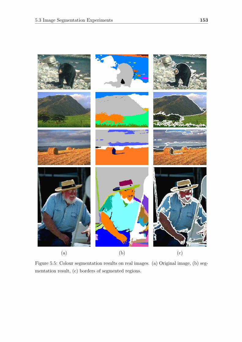
5.3 Image Segmentation Experiments 153
(a) (b) (c)
Figure 5.5: Colour segmentation results on real images. (a) Original image, (b) seg-
mentation result, (c) borders of segmented regions.
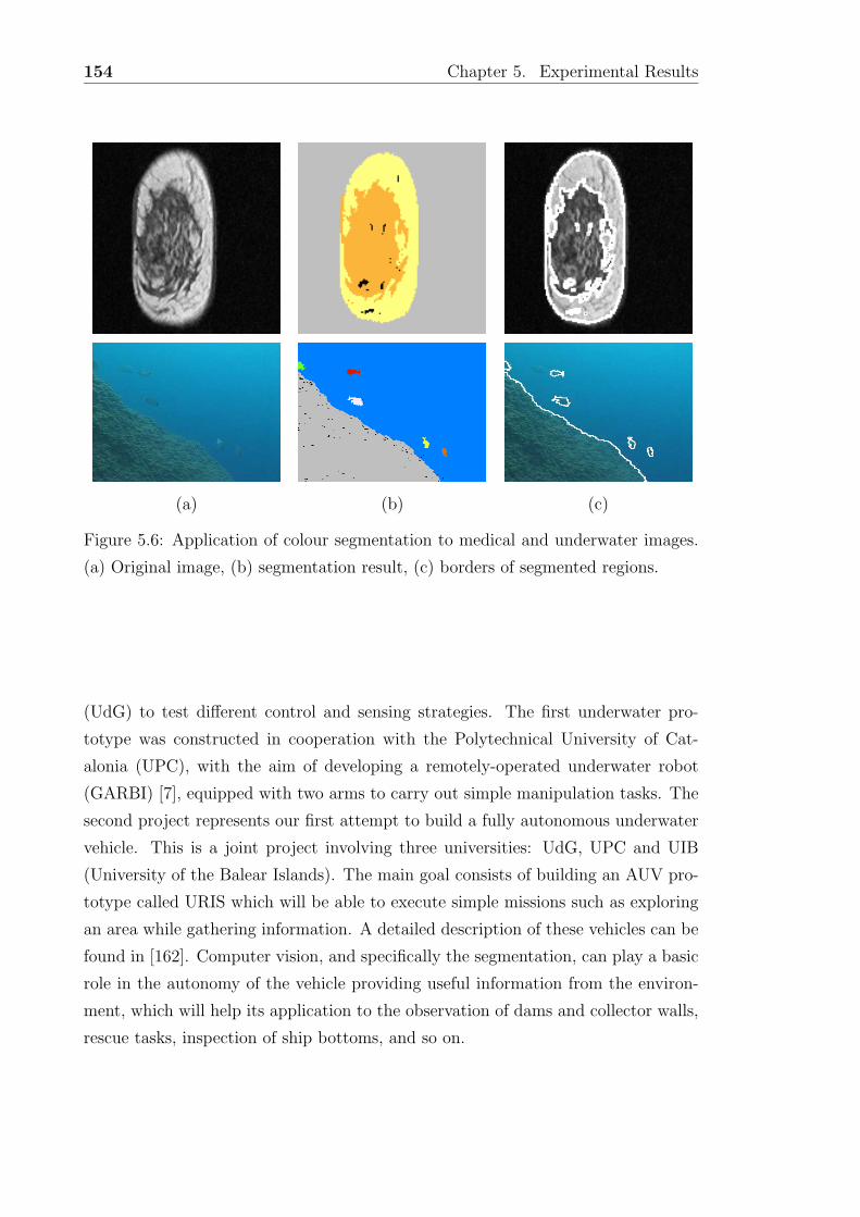
154 Chapter 5. Experimental Results
(a) (b) (c)
Figure 5.6: Application of colour segmentation to medical and underwater images.
(a) Original image, (b) segmentation result, (c) borders of segmented regions.
(UdG) to test different control and sensing strategies. The first underwater pro-
totype was constructed in cooperation with the Polytechnical University of Cat-
alonia (UPC), with the aim of developing a remotely-operated underwater robot
(GARBI) [7], equipped with two arms to carry out simple manipulation tasks. The
second project represents our first attempt to build a fully autonomous underwater
vehicle. This is a joint project involving three universities: UdG, UPC and UIB
(University of the Balear Islands). The main goal consists of building an AUV pro-
totype called URIS which will be able to execute simple missions such as exploring
an area while gathering information. A detailed description of these vehicles can be
found in [162]. Computer vision, and specifically the segmentation, can play a basic
role in the autonomy of the vehicle providing useful information from the environ-
ment, which will help its application to the observation of dams and collector walls,
rescue tasks, inspection of ship bottoms, and so on.
5.4 Colour Texture Segmentation Experiments 155
5.4 Colour Texture Segmentation Experiments
The first consideration to make in order to evaluate the colour texture segmentation
by using our proposal is related to the texture features used to characterise and de-
scribe the regions of the image. Various researchers have attempted to describe and
segment images using statistical features, fractal, stochastic and spatial-frequency
models, etc. These techniques have been largely compared (see the comparative
works of Clausi and Ed Jernigan [43], Conners and Harlow [46], Du Buf et al. [59],
Ojala et al. [140], and Weszka et al. [211]). Nevertheless, the results of comparing
the relative merits of the different types of features have been inconclusive and a
clear winner can not be decided for all cases [159]. For the experimental trials shown
in this section we used the co-occurrence matrices proposed by Haralick et al. [81],
considering a window of size 7×7 centred at the analysed pixel as is described in [59].
Two of the most typical features, contrast and homogeneity, are computed for dis-
tance one and for 0◦, 45◦, 90◦ and 135◦ orientations to constitute a 8-dimensional
feature vector.
5.4.1 Synthetic Images
In order to evaluate the proposed colour texture segmentation technique, we created
nine mosaic images by assembling four subimages of size 128× 128 of textures from
the VisTex natural scene collection by MIT (http://www-white.media.mit.edu/
/vismod/imagery/VisionTexture/vistex.html), which we have called M1 to M9.
Furthermore, we added three mosaics M10, M11 and M12, provided by Dubuisson-
Jolly and Gupta which were used to evaluate their proposal on colour texture seg-
mentation described in [60]. Mosaic M10 contains (clockwise from the top left
corner) water, red crop (observed using an infrared camera), green crop, and light
green crop; M11 contains cage, wall, forest, town; finally M12 contains bushes, for-
est, long grass, grass. The whole set of texture mosaic images is shown in Figure 5.7.
These images were processed by our segmentation algorithm using various set
of parameter values. We considered the weight of colour and texture information
(parameter β), as well as the relative relevance of region and boundary information
in the segmentation process (parameter α), ranging both from 1 to 0. Nevertheless,
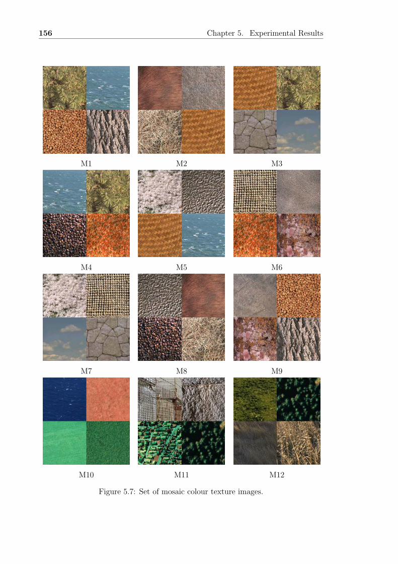
156 Chapter 5. Experimental Results
M1 M2 M3
M4 M5 M6
M7 M8 M9
M10 M11 M12
Figure 5.7: Set of mosaic colour texture images.
5.4 Colour Texture Segmentation Experiments 157
the most interesting results were obtained considering parameter β ranging from 1.0
to 0.4, while parameter α takes values 1.0, 0.75 and 0.5, on a pyramidal structure
with L = 2. Table 5.7 and Table 5.8 show the summarized results of these parameter
settings, using the mean, standard deviation and median as descriptors of results
obtained over the whole set of mosaic images. As has been described above in
Section 5.2, segmentations are evaluated from a region-based scheme by measuring
the percentage of not-correctly segmented pixels considering the segmentation as a
multi-class classification problem (see Table 5.7). On the other hand, the quality of
the extracted region boundaries is evaluated by the distance from ground truth to
the estimated boundary (see Table 5.8).
Main conclusions that can be extracted from the analysis of these summarized
results are:
• Use of texture features is a necessity. As has been theoretically stated in
Chapter 4, using colour as single source of information is not enough for the
segmentation of textures. First, the segmentation when colour is used alone
(β = 1.0) tends to produce noisy segmentations, with several pixels remaining
as background inside the regions. Furthermore, when adjacent textures have
a very similar colour, the colour property is not capable of distinguishing
between them. Hence, big errors are produced at boundaries between these
textures. These errors are revealed in the region-based evaluation shown in
Table 5.7, in which the mean error is significantly larger than the median and
the standard deviation is specially high when colour has a strong importance
(β = 1.0 and β = 0.8). It means that the error, although small for most of
the cases, is very big for some images. Mosaic M11 is the most representative
example of this problem since it is composed by two couples of textures with
almost the same colour, which can not be correctly distinguished using only
colour. Figure 5.8 shows segmentation results obtained over the mosaic image
M11 with α = 0.75 considering colour alone (β = 1.0) and taking colour and
texture properties into account with β = 0.6. As is stated in the Figure, the
inclusion of texture information allows to correctly segment regions although
they have similar colour. These problems imply that the worst performance is
obtained when using colour alone.
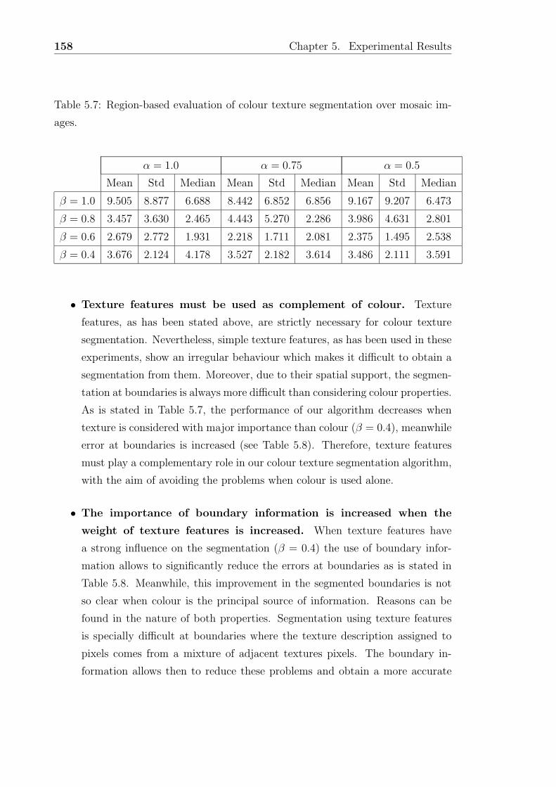
158 Chapter 5. Experimental Results
Table 5.7: Region-based evaluation of colour texture segmentation over mosaic im-
ages.
α = 1.0 α = 0.75 α = 0.5
Mean Std Median Mean Std Median Mean Std Median
β = 1.0 9.505 8.877 6.688 8.442 6.852 6.856 9.167 9.207 6.473
β = 0.8 3.457 3.630 2.465 4.443 5.270 2.286 3.986 4.631 2.801
β = 0.6 2.679 2.772 1.931 2.218 1.711 2.081 2.375 1.495 2.538
β = 0.4 3.676 2.124 4.178 3.527 2.182 3.614 3.486 2.111 3.591
• Texture features must be used as complement of colour. Texture
features, as has been stated above, are strictly necessary for colour texture
segmentation. Nevertheless, simple texture features, as has been used in these
experiments, show an irregular behaviour which makes it difficult to obtain a
segmentation from them. Moreover, due to their spatial support, the segmen-
tation at boundaries is always more difficult than considering colour properties.
As is stated in Table 5.7, the performance of our algorithm decreases when
texture is considered with major importance than colour (β = 0.4), meanwhile
error at boundaries is increased (see Table 5.8). Therefore, texture features
must play a complementary role in our colour texture segmentation algorithm,
with the aim of avoiding the problems when colour is used alone.
• The importance of boundary information is increased when the
weight of texture features is increased. When texture features have
a strong influence on the segmentation (β = 0.4) the use of boundary infor-
mation allows to significantly reduce the errors at boundaries as is stated in
Table 5.8. Meanwhile, this improvement in the segmented boundaries is not
so clear when colour is the principal source of information. Reasons can be
found in the nature of both properties. Segmentation using texture features
is specially difficult at boundaries where the texture description assigned to
pixels comes from a mixture of adjacent textures pixels. The boundary in-
formation allows then to reduce these problems and obtain a more accurate

5.4 Colour Texture Segmentation Experiments 159
Table 5.8: Boundary-based evaluation of colour texture segmentation over mosaic
images.
α = 1.0 α = 0.75 α = 0.5
Mean Std Median Mean Std Median Mean Std Median
β = 1.0 3.277 5.479 0.553 2.036 3.444 0.787 1.958 2.772 0.856
β = 0.8 0.680 0.706 0.475 0.796 0.801 0.497 0.707 0.677 0.482
β = 0.6 0.923 1.060 0.559 0.841 0.940 0.592 0.931 1.048 0.550
β = 0.4 1.930 1.618 1.317 1.701 1.310 1.428 1.437 1.138 1.270
segmentation. On the other hand, colour is an obvious local property and
errors at boundaries tend to be small. Moreover, mosaic images have been
designed without a transition at boundary. Therefore, using the local colour
of pixels is possible to extract the border between adjacent textures (excepting
the commented problems with similar colour textures) and the use of boundary
information is not so necessary.
• Best results have been obtained with β = 0.6 and α = 0.75. From these
experiments, we consider that the best results are obtained by weighting the
colour with 0.6 and texture features with 0.4. Moreover, region information
is weighted with 0.75 and boundary information with 0.25. This setting gives
the best performance considering a compromise between region and boundary-
based quality measures. Moreover, we have considered it to be adequate for
the selection of parameters with a minor mean and standard deviation of error
with the aim of choosing the most robust configuration although the median
value is not the best. In other words, we have looked for a setting which avoids
large errors in the segmentation of any image, although other configurations
can specifically give better results in the remaining images. Table 5.9 shows
the evaluation of segmentation obtained over each individual image using this
parameters setting.
Results of the three last mosaic images (M10, M11 and M12) can be compared
to the segmentation results shown in the work of Dubuisson-Jolly and Gupta [60].
Their proposal is a supervised segmentation algorithm based on the fusion of colour
and texture segmentations obtained independently. Firstly, a number of training
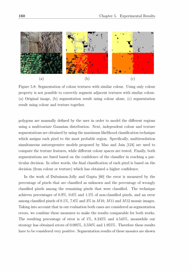
160 Chapter 5. Experimental Results
(a) (b) (c)
Figure 5.8: Segmentation of colour textures with similar colour. Using only colour
property is not possible to correctly segment adjacent textures with similar colour.
(a) Original image, (b) segmentation result using colour alone, (c) segmentation
result using colour and texture together.
polygons are manually defined by the user in order to model the different regions
using a multivariate Gaussian distribution. Next, independent colour and texture
segmentations are obtained by using the maximum likelihood classification technique
which assigns each pixel to the most probable region. Specifically, multiresolution
simultaneous autoregressive models proposed by Mao and Jain [124] are used to
compute the texture features, while different colour spaces are tested. Finally, both
segmentations are fused based on the confidence of the classifier in reaching a par-
ticular decision. In other words, the final classification of each pixel is based on the
decision (from colour or texture) which has obtained a higher confidence.
In the work of Dubuisson-Jolly and Gupta [60] the error is measured by the
percentage of pixels that are classified as unknown and the percentage of wrongly
classified pixels among the remaining pixels that were classified. The technique
achieves percentages of 0.9%, 0.6% and 1.5% of non-classified pixels, and an error
among classified pixels of 0.1%, 7.6% and 3% in M10, M11 and M12 mosaic images.
Taking into account that in our evaluation both cases are considered as segmentation
errors, we combine these measures to make the results comparable for both works.
The resulting percentage of error is of 1%, 8.245% and 4.545%, meanwhile our
strategy has obtained errors of 0.095%, 3.550% and 1.955%. Therefore these results
have to be considered very positive. Segmentation results of these mosaics are shown
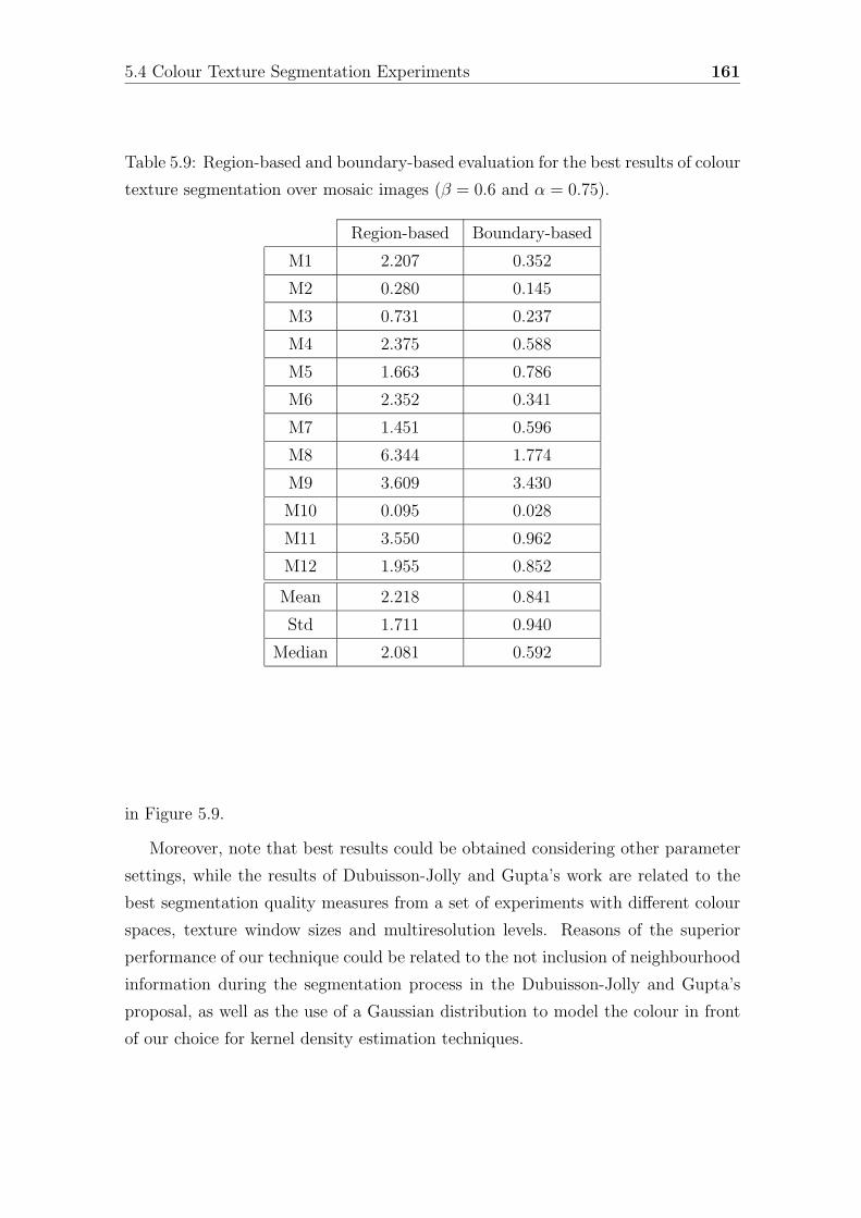
5.4 Colour Texture Segmentation Experiments 161
Table 5.9: Region-based and boundary-based evaluation for the best results of colour
texture segmentation over mosaic images (β = 0.6 and α = 0.75).
Region-based Boundary-based
M1 2.207 0.352
M2 0.280 0.145
M3 0.731 0.237
M4 2.375 0.588
M5 1.663 0.786
M6 2.352 0.341
M7 1.451 0.596
M8 6.344 1.774
M9 3.609 3.430
M10 0.095 0.028
M11 3.550 0.962
M12 1.955 0.852
Mean 2.218 0.841
Std 1.711 0.940
Median 2.081 0.592
in Figure 5.9.
Moreover, note that best results could be obtained considering other parameter
settings, while the results of Dubuisson-Jolly and Gupta’s work are related to the
best segmentation quality measures from a set of experiments with different colour
spaces, texture window sizes and multiresolution levels. Reasons of the superior
performance of our technique could be related to the not inclusion of neighbourhood
information during the segmentation process in the Dubuisson-Jolly and Gupta’s
proposal, as well as the use of a Gaussian distribution to model the colour in front
of our choice for kernel density estimation techniques.
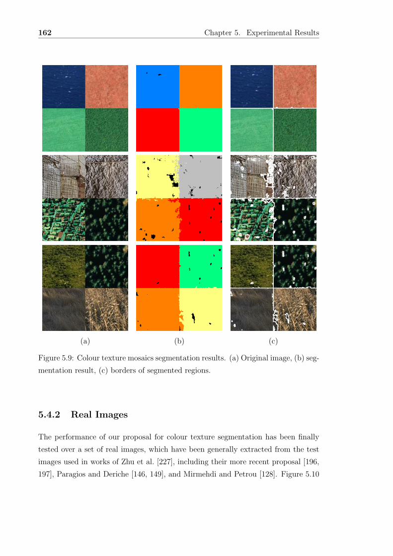
162 Chapter 5. Experimental Results
(a) (b) (c)
Figure 5.9: Colour texture mosaics segmentation results. (a) Original image, (b) seg-
mentation result, (c) borders of segmented regions.
5.4.2 Real Images
The performance of our proposal for colour texture segmentation has been finally
tested over a set of real images, which have been generally extracted from the test
images used in works of Zhu et al. [227], including their more recent proposal [196,
197], Paragios and Deriche [146, 149], and Mirmehdi and Petrou [128]. Figure 5.10
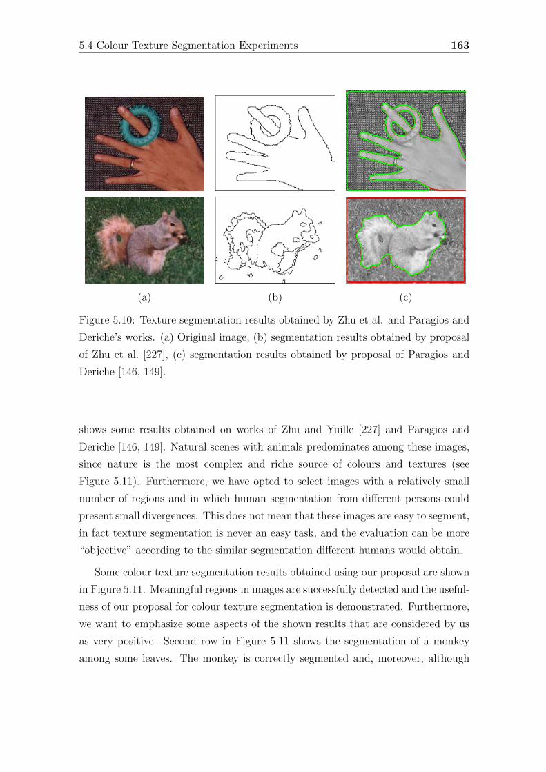
5.4 Colour Texture Segmentation Experiments 163
(a) (b) (c)
Figure 5.10: Texture segmentation results obtained by Zhu et al. and Paragios and
Deriche’s works. (a) Original image, (b) segmentation results obtained by proposal
of Zhu et al. [227], (c) segmentation results obtained by proposal of Paragios and
Deriche [146, 149].
shows some results obtained on works of Zhu and Yuille [227] and Paragios and
Deriche [146, 149]. Natural scenes with animals predominates among these images,
since nature is the most complex and riche source of colours and textures (see
Figure 5.11). Furthermore, we have opted to select images with a relatively small
number of regions and in which human segmentation from different persons could
present small divergences. This does not mean that these images are easy to segment,
in fact texture segmentation is never an easy task, and the evaluation can be more
“objective” according to the similar segmentation different humans would obtain.
Some colour texture segmentation results obtained using our proposal are shown
in Figure 5.11. Meaningful regions in images are successfully detected and the useful-
ness of our proposal for colour texture segmentation is demonstrated. Furthermore,
we want to emphasize some aspects of the shown results that are considered by us
as very positive. Second row in Figure 5.11 shows the segmentation of a monkey
among some leaves. The monkey is correctly segmented and, moreover, although
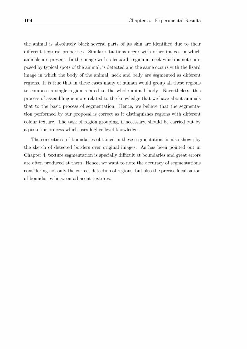
164 Chapter 5. Experimental Results
the animal is absolutely black several parts of its skin are identified due to their
different textural properties. Similar situations occur with other images in which
animals are present. In the image with a leopard, region at neck which is not com-
posed by typical spots of the animal, is detected and the same occurs with the lizard
image in which the body of the animal, neck and belly are segmented as different
regions. It is true that in these cases many of human would group all these regions
to compose a single region related to the whole animal body. Nevertheless, this
process of assembling is more related to the knowledge that we have about animals
that to the basic process of segmentation. Hence, we believe that the segmenta-
tion performed by our proposal is correct as it distinguishes regions with different
colour texture. The task of region grouping, if necessary, should be carried out by
a posterior process which uses higher-level knowledge.
The correctness of boundaries obtained in these segmentations is also shown by
the sketch of detected borders over original images. As has been pointed out in
Chapter 4, texture segmentation is specially difficult at boundaries and great errors
are often produced at them. Hence, we want to note the accuracy of segmentations
considering not only the correct detection of regions, but also the precise localisation
of boundaries between adjacent textures.
5.4 Colour Texture Segmentation Experiments 165
(a) (b) (c)
Figure 5.11: Colour texture segmentation results on real images. (a) Original image,
(b) segmentation result, (c) borders of segmented regions.

166 Chapter 5. Experimental Results
Chapter 6
Conclusions
Conclusions extracted from this work are presented. Moreover, the possible further
work is analysed considering the different directions that this research line could
advance to. Finally, publications which are directly related to this thesis work are
listed.
6.1 Contributions
In this document we have presented an unsupervised image segmentation strategy
which integrates region and boundary information from colour and texture proper-
ties in order to perform the image segmentation. The main contributions of this
thesis work are:
1. Review on image segmentation integrating region and boundary in-
formation. An exhaustive analysis of image segmentation techniques which
integrate region and boundary information has been carried out. Main strate-
gies to perform the integration have been identified and a classification of
these approaches has been proposed. Thus, the most relevant proposals are
assorted and grouped in their corresponding approach. Moreover, character-
istics of these strategies as well as the general lack of attention that is given
to the texture has been noted. The discussion of these aspects has been the
origin of all the work evolved in this thesis, giving rise to two basic conclu-
167
168 Chapter 6. Conclusions
sions: first, the possibility of fusing several approaches to the integration of
both information sources, and second, the necessity of a specific treatment for
textured images.
2. Image segmentation strategy. An unsupervised segmentation strategy
which integrates region and boundary information and incorporates different
approaches identified in the previous review have been proposed. Specifi-
cally, the proposed image segmentation method combines the guidance of seed
placement, the control of decision criterion and the boundary refinement ap-
proaches. The method is composed by two basic stages: initialisation and
segmentation. In the first stage, the main contours of the image are used to
identify the different regions present in the image and to adequately place a
seed for each one which allows to statistically model the region. Then, the seg-
mentation stage is performed based on the active region model which allows
us to take region and boundary information into account in order to segment
the whole image. Furthermore, with the aim of imitating the Human Vision
System when a person is slowly approaching to a distant object, a pyramidal
structure is considered. Hence, the method has been designed on a pyramidal
representation which allows us to refine the region boundaries from a coarse
to a fine resolution, and ensuring noise robustness as well as computation
efficiency.
3. Texture segmentation. The strategy for image segmentation has been ex-
tended to the problem of unsupervised texture segmentation, which involves
the region modelling considering a set of texture descriptors and the extraction
of texture boundary information.
4. Colour texture segmentation. A technique for the combination of colour
and textural properties has been proposed. The colour behaviour is described
by using non-parametric techniques of density estimation, and is then inte-
grated with typical texture descriptors. Hence, proposed strategy of segmen-
tation is considered for the segmentation taking both colour and textural prop-
erties into account.
6.2 Future work 169
5. Comparison of integration strategies. Our proposal of image segmenta-
tion strategy has been objectively evaluated and then compared with different
algorithms corresponding to the identified strategies of region and boundary
integration.
6.2 Future work
The design of an image segmentation system involves the consideration of a wide
set of questions. In addition to the different solutions which have been adopted
and described in this thesis, a lot of ideas have been proposed, discussed and finally
rejected along this thesis work. On the other hand, other questions have remained
as undeveloped ideas, which need to be further analysed and worked in depth, and
we suggest them as future work.
In order to conveniently organise these ideas of future, we have divided them
into two basic blocks. The first one is composed of some possible improvements
which can be analysed in order to refine the proposed segmentation strategy. The
second block suggests some ideas of further work to be considered as future lines of
research.
Further work on the proposed segmentation strategy
• Dynamic behaviour of the region-boundary weighting. Region and
boundary information are combined together in the energy function using a
weighted sum. Therefore, a weighting parameter indicates the relative rele-
vance of both terms along the segmentation process. Although the experimen-
tal results have shown that the proposed algorithm is quite robust to changes
of this parameter it is obvious that the final segmentation result depends on
this value. The dynamic adaption of the weight of region and boundary infor-
mation to the characteristics of the image would solve this problem and has
to be analysed.
• Improvement of the computational cost of the optimisation process.
The cost of the optimisation process which looks for the partition of the image
170 Chapter 6. Conclusions
which best fits with the desired properties of the final segmentation largely de-
pends on the size of the input data. In other words, the cost is higher at higher
resolutions of the image. The pyramidal representation which has been used
in this work allows to considerably reduce the cost of the algorithm. However,
it would be interesting to study the modification of the model to dynamically
adapt its resolution depending on its position in the image. When the active
region is inside a region the optimisation could be coarse (the active region
moves quickly), while a finer optimisation is needed close to the boundaries
(the active regions moves slowly looking for the best segmentation). With
this technique, the complexity of the model would be made significantly more
independent on the image resolution.
• Methods for density estimation. Although the kernel estimation is prob-
ably the most popular non-parametric method of density estimation, other
several nonparametric techniques are available in the literature: multivariate
histogram, the nearest neighbour method, the variable kernel method, etc...
These techniques should be tested in order to compare its performance.
• Texture features. As has been denoted, there are different texture analysis
techniques which allow the extraction of texture information from an image,
and the results of comparing the different types of features have been non-
conclusive and it is not clear which method is the best. Hence, other texture
features should be considered and compared in the integration with colour
properties. Furthermore, techniques which extract textural information from
chromatic bands together should be analysed in order to test its performance
to describe colour texture.
• Automatic determination of smoothing level for colour textures. In
order to perceive textures as regions with homogeneous colour, of similar way
as we would see them if we were far away, an iterative process of smoothing is
performed. Therefore, starting from the original image it is blurred until, at
the end of this process, the image is composed by homogenous colours. The
number of smoothing operations has been experimentally fixed in this work.
Hence, the automatic determination of the smoothing level should be studied
in order to stop this process when the image looks homogeneous and additional
6.2 Future work 171
smoothing is not required and moreover should be avoided.
• Adaptation to smooth transitions. Properties of a region can be not
always strictly homogeneous in the whole region. Besides, smooth transitions
inside a same region imply changes in its colour and/or texture, which is then
not uniform in all the region. The adaption of the region model to these
changes should be studied in order to adjust the model to the current region’s
area.
Further work on research line
• Use of Artificial Intelligence techniques in the optimisation process.
The region competition algorithm which has been used and lightly adapted
to our necessities tries to find the best segmentation optimising an energy
function. Although its performance has been demonstrated, it presents some
limitations: for example, it allows to merge two adjacent regions into a single
one, but it is not possible to split a region into two or more parts. Moreover,
the solution is not guaranteed to be optimal. Precisely, the most recent work
of Tu et al. [196, 197] has been focused to solve these problems dealing the seg-
mentation as a problem of search space using artificial intelligence techniques.
A lot of techniques have been proposed in the field of the Artificial Intelligence
with the aim of optimising a function and we think that their application to
image segmentation is an interesting idea which can apport new possibilities.
• Returning multiple solutions. Traditionally, the goal of image segmenta-
tion has been to produce a single partition of an image. However, it is gen-
erally accepted the complexity inherent to segmentation that, in addition, is
basic as prerequisite of high-level vision algorithms such as object description,
recognition or scene analysis. An alternative is allowing that the segmenta-
tion process returns a set of possible solutions to the segmentation problem,
along with a associated probability for each segmentation as in the work of
Nickels and Hutchinson [137]. Thus, it is possible, for example, to enumerate
the most probable segmentations, which provides more information than the
typical approach, in which only a single segmentation is given. Furthermore,
172 Chapter 6. Conclusions
this set of results can be passed to higher-level algorithms, which taking their
goals and knowledge into account, are more able to interpret the segmentation
results.
• Extension to tracking. Tracking can be defined as the following of an object,
which is moving, along a sequence of images. The segmentation framework
proposed in this thesis can be extended to deal with the tracking problem
incorporating motion as new information source to guide the optimisation
process. Then, the active region would be initialised from the segmentation
of previous image and taking region, boundary and motion information into
account, the optimisation process would allow to follow the movement of the
region along the sequence of images.
• Imitation of the Human Vision System. The aim of most of the Com-
puter Vision Systems is to mimic the extraordinary behaviour of the human
vision, although obviously, they are still far away from this goal so far. In this
thesis we have adopted some solutions which are close to the human behaviour,
more concretely related to the perception of colour objects when a person is
slowly approaching to them. Furthermore, we think that this subject could
be exploited in major depth considering the perception of colour and texture
at different distances, which can provide more and useful information for the
segmentation process.
• Adaption to supervised image segmentation. Although recent image
segmentation algorithms provide excellent results, it is obvious that the seg-
mentation of an image without any a priori knowledge is a really difficult task
which sometimes fails to capture some meaningful parts. Moreover, evidence
from human vision indicates that high-level knowledge play a crucial role in the
ability to segment images in a meaningful manner suggesting that the incor-
poration of such methods would help to improve the results of computer vision
segmentation algorithms. Hence, a logical extension of this thesis is to consider
the image segmentation problem using a supervised approach. Thus, the sys-
tem could incorporate a previous stage in which it would be taught about the
objects which can be present in the image. Furthermore, this knowledge would
permit to select, a priori to the segmentation, the best features (colour and
6.3 Related Publications 173
texture), which allow to characterise and discriminate the different objects, by
using techniques of feature selection.
• Applications: image retrieval, medical applications, underwater im-
age analysis... Finally, the proposed segmentation strategy can be used in
different Computer Vision applications. Image segmentation is incorporated
as a basic step on recent image retrieval systems in order to automatically
describe the content of an image taking the meaningful regions of the image
and their spatial relationships into account. The segmentation has the same
relevant role in several medical applications in which the location and/or iden-
tification of regions of interest is required. Furthermore, its incorporation in
mobile robots, as for example underwater vehicles, can be very useful in order
to improve its autonomy and applications.
6.3 Related Publications
Ideas and projects of this work have evolved from initial stages to obtain the final
version which is presented in this memory of thesis. The following publications are
a direct consequence of the research carried out during the elaboration of the thesis,
and give an idea of the progression that has been achieved.
Book chapters
• X. Cufı, X. Munoz, J. Freixenet, and J. Martı. A review on image segmenta-
tion techniques integrating region and boundary information. In W. Hawkes,
editor, Advances in Imaging and Electron Physics, volume 120, pages 1–39.
Academic Press, 2002.
Journals
• X. Munoz, J. Freixenet, J. Martı, and X. Cufı. Colour texture segmenta-
tion from region-boundary integration. Submitted to IEEE Transactions on
Pattern Analysis and Machine Intelligence.
174 Chapter 6. Conclusions
• X. Munoz, J. Freixenet, X. Cufı, and J. Martı. Strategies for image segmenta-
tion combining region and boundary information. Pattern Recognition Letters,
volume 24:(1-3), pages 383–400, January 2003.
• X. Munoz, J. Freixenet, X. Cufı, and J. Martı. Region-boundary cooperative
image segmentation based on active regions. In Lecture Notes in Artificial
Intelligence, pages 364–374. Springer-Verlag, 2002.
International Conferences
• X. Munoz, J. Martı, X. Cufı, and J. Freixenet. Unsupervised active regions
for multiresolution image segmentation. In IAPR International Conference
on Pattern Recognition, Quebec, Canada, August 2002.
• X. Munoz, J. Freixenet, J. Martı, and X. Cufı. Active regions for unsu-
pervised texture segmentation integrating region and boundary information.
In International Workshop on Texture Analysis and Synthesis, pages 95–98,
Copenhagen, Denmark, June 2002.
• J. Freixenet, X. Munoz, D. Raba, J. Martı, and X. Cufı. Yet another survey
on image segmentation: Region and boundary information integration. In
European Conference on Computer Vision, volume III, pages 408–422, Copen-
hagen, Denmark, May 2002.
• X. Munoz, X. Cufı, J. Freixenet, and J. Martı. A new approach to segmenta-
tion based on fusing circumscribed contours, region growing and clustering. In
IEEE International Conference on Image Processing, volume 1, pages 800–803,
Vancouver, Canada, September 2000.
• X. Cufı, X. Munoz, J. Freixenet, and J. Martı. A concurrent region growing
algorithm guided by circumscribed contours. In IAPR International Con-
ference on Pattern Recognition, volume I, pages 432–435, Barcelona, Spain,
September 2000.
• A. Casals, X. Cufı, J. Freixenet, J. Martı, and X. Munoz. Friendly interface
for objects selection in a robotized kitchen. In IEEE International Conference
6.3 Related Publications 175
On Robotics And Automation, volume 4, pages 4070–4075, San Francisco,
California, April 2000.
National Conferences
• X. Munoz, J. Freixenet, D. Raba, X. Cufı, and J. Martı. Region-boundary
cooperative image segmentation based on active regions. In Catalonian Con-
ference on Artificial Intelligence, Castello de la Plana, Spain, October 2002.
• X. Munoz, J. Freixenet, J. Martı, X. Cufı, and J. Batlle. New strategy of rel-
evance feedback based on specific feature selection. In Catalonian Conference
on Artificial Intelligence, pages 276–282, Barcelona, Spain, October 2001.
• J. Freixenet, X. Munoz, X. Cufı, J. Martı, and X. Llado. Chameleon: a region-
based image retrieval system. In Spanish Symposium on Pattern Recognition
and Image Analysis, volume II, pages 67–72, Benicassim, Spain, May 2001.
• J. Martı, J. Freixenet, X. Llado, X. Munoz, and X. Cufı. A new approach
to natural object labelling in colour aerial images. In Spanish Symposium on
Pattern Recognition and Image Analysis, volume I, pages 67–72, Benicassim,
Spain, May 2001.
• R. Garcia, X. Cufı, X. Munoz, Ll. Pacheco, and J. Batlle. An image mosaick-
ing method based on the integration of grey level and textural features. In
Spanish Symposium on Pattern Recognition and Image Analysis, volume II,
pages 243–248, Benicassim, Spain, May 2001.
• X. Munoz, M. Malagelada, A. Casals, X. Cufı, J. Freixenet, and Ll. Pacheco.
Interfaz para la seleccion de objectos de una cocina adaptada para personas
discapacitadas. In Congreso Aer/Atp “Ano 2000: La Automatizacion Mas
Inteligente Y Facil”, Barcelona, Spain, 1999.
Technical Reports
• X. Munoz and J. Freixenet. Accurate texture segmentation based on ga-
bor phase features. Technical Report 01-13-RR, Institute of Informatics and
Applications. University of Girona, 2001.

176 Chapter 6. Conclusions
• X. Cufı, J. Freixenet, J. Martı, and X. Munoz. A review on image segmentation
techniques integrating region and boundary information. Technical Report 01-
01-RR, Institute of Informatics and Applications. University of Girona, 2001.
Appendix A
Texture Features
Some of the most popular texture extraction methods based on a statistical approach
are reviewed in this appendix. An introduction to the different techniques is given.
Moreover, some results which have been obtained for our implementations are shown.
Finally, conclusions derived from other authors’s comparative studies are contrasted
and discussed.
A.1 Introduction
Before either texture segmentation or classification can take place, some homogene-
ity or similarity criterion must be defined. These criteria are normally specified
in terms of a set of feature measures, which each provide a quantitative measure
of a certain texture characteristic. Haralick provided the classic survey of texture
measures [80]. In this work, a number of texture extraction methods are listed and
divided into two basic types: structural and statistical. This same basic classifi-
cation has been posteriorly adopted by other authors (see works of Al-Janobi [5],
Grau [77], Van Gool et al. [199], Wechsler [208]).
In the structural methods, texture is considered as the repetition of some basic
primitive patterns with a certain rules of placement, which are formally defined
by grammars of various types. Nevertheless, since natural textures are not very
regular, the structural techniques are not very popular at this moment [206]. On the
177

178 Appendix A. Texture Features
other hand, statistical methods are based on the characterisation of the stochastic
properties of the spatial distribution of grey levels in the image.
We focus next brief survey on statistical methods. However, we do not provide
an exhaustive analysis of all texture measures, rather some of the most popular
techniques are reviewed.
A.2 Laws’s Texture Energy Filters
With the main desire to produce a computationally efficient method, Laws developed
a coherent set of texture energy masks [110]. All the masks were derived form three
simple one-dimensional non-recursive filters, which may be convolved with each other
to give a variety of one and two-dimensional filters. The characterisation is carried
out in two steps: firstly, the image is convolved with the set of masks of small size;
secondly, statistics are created from previous convolutions.
Texture energy masks were designed to act as filters of comparison (matched fil-
ters) for specific kind of variations almost-periodic which are often found in textured
images. Typically, these masks have size 7 × 7 or smaller, and try to be sensitive
to structures such as edges, waves and spots. Laws found the most useful to be a
set of seven bandpass and highpass directional filters, implemented as 5 × 5 masks.
Four of these masks with the best discrimination power for mosaic used by Laws are
shown in Figure A.1.
In a second step, with the convolution results a set of statistics are measured,
which consist of a moving window calculation of variance of larger size. Specifically,
Laws used 15 × 15 windows, as a compromise between classification accuracy and
computational cost. Furthermore, considering computational cost Laws proposed
three alternatives to the calculation of standard deviation: a weighing with absolute
values of the convolution (ABSAVE), with positive values (POSAVE) and with
negative values (NEGAVE). ABSAVE, which for areas with mean equal to zero can
be considered as a fast approximation to standard deviation, gave the best results.
Some examples of texture features obtained using the texture energy masks are
shown in Figure A.2. In this the method has been applied over the mosaic image
M2 (see Figure 5.7), which will be used as original image in next examples to show
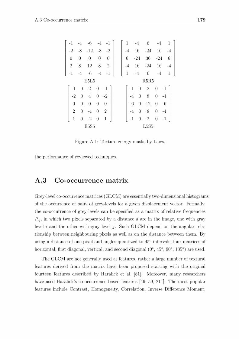
A.3 Co-occurrence matrix 179
-1 -4 -6 -4 -1
-2 -8 -12 -8 -2
0 0 0 0 0
2 8 12 8 2
-1 -4 -6 -4 -1
1 -4 6 -4 1
-4 16 -24 16 -4
6 -24 36 -24 6
-4 16 -24 16 -4
1 -4 6 -4 1
E5L5 R5R5
-1 0 2 0 -1
-2 0 4 0 -2
0 0 0 0 0
2 0 -4 0 2
1 0 -2 0 1
-1 0 2 0 -1
-4 0 8 0 -4
-6 0 12 0 -6
-4 0 8 0 -4
-1 0 2 0 -1
E5S5 L5S5
Figure A.1: Texture energy masks by Laws.
the performance of reviewed techniques.
A.3 Co-occurrence matrix
Grey-level co-occurrence matrices (GLCM) are essentially two-dimensional histograms
of the occurrence of pairs of grey-levels for a given displacement vector. Formally,
the co-occurrence of grey levels can be specified as a matrix of relative frequencies
Pij, in which two pixels separated by a distance d are in the image, one with gray
level i and the other with gray level j. Such GLCM depend on the angular rela-
tionship between neighbouring pixels as well as on the distance between them. By
using a distance of one pixel and angles quantized to 45◦ intervals, four matrices of
horizontal, first diagonal, vertical, and second diagonal (0◦, 45◦, 90◦, 135◦) are used.
The GLCM are not generally used as features, rather a large number of textural
features derived from the matrix have been proposed starting with the original
fourteen features described by Haralick et al. [81]. Moreover, many researchers
have used Haralick’s co-occurrence based features [46, 59, 211]. The most popular
features include Contrast, Homogeneity, Correlation, Inverse Difference Moment,
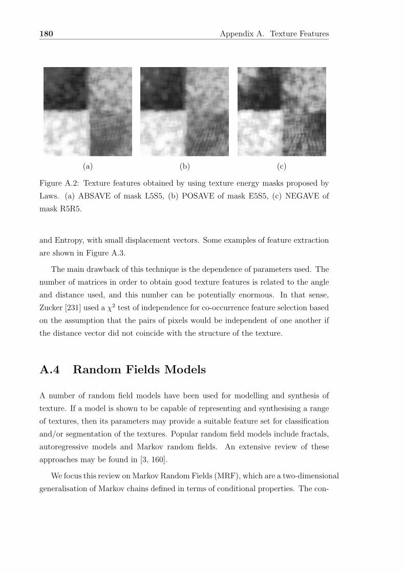
180 Appendix A. Texture Features
(a) (b) (c)
Figure A.2: Texture features obtained by using texture energy masks proposed by
Laws. (a) ABSAVE of mask L5S5, (b) POSAVE of mask E5S5, (c) NEGAVE of
mask R5R5.
and Entropy, with small displacement vectors. Some examples of feature extraction
are shown in Figure A.3.
The main drawback of this technique is the dependence of parameters used. The
number of matrices in order to obtain good texture features is related to the angle
and distance used, and this number can be potentially enormous. In that sense,
Zucker [231] used a χ2 test of independence for co-occurrence feature selection based
on the assumption that the pairs of pixels would be independent of one another if
the distance vector did not coincide with the structure of the texture.
A.4 Random Fields Models
A number of random field models have been used for modelling and synthesis of
texture. If a model is shown to be capable of representing and synthesising a range
of textures, then its parameters may provide a suitable feature set for classification
and/or segmentation of the textures. Popular random field models include fractals,
autoregressive models and Markov random fields. An extensive review of these
approaches may be found in [3, 160].
We focus this review on Markov Random Fields (MRF), which are a two-dimensional
generalisation of Markov chains defined in terms of conditional properties. The con-
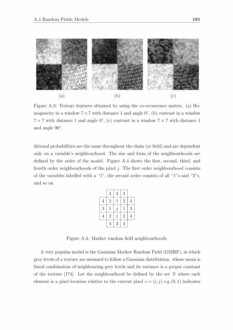
A.4 Random Fields Models 181
(a) (b) (c)
Figure A.3: Texture features obtained by using the co-occurrence matrix. (a) Ho-
mogeneity in a window 7× 7 with distance 1 and angle 0◦, (b) contrast in a window
7 × 7 with distance 1 and angle 0◦, (c) contrast in a window 7 × 7 with distance 1
and angle 90◦.
ditional probabilities are the same throughout the chain (or field) and are dependent
only on a variable’s neighbourhood. The size and form of the neighbourhoods are
defined by the order of the model. Figure A.4 shows the first, second, third, and
fourth order neighbourhoods of the pixel j. The first order neighbourhood consists
of the variables labelled with a “1”, the second order consists of all “1”s and “2”s,
and so on.
4 3 4
4 2 1 2 4
3 1 j 1 3
4 2 1 2 4
4 3 4
Figure A.4: Markov random field neighbourhoods.
A very popular model is the Gaussian Markov Random Field (GMRF), in which
grey levels of a texture are assumed to follow a Gaussian distribution. whose mean is
lineal combination of neighbouring grey levels and its variance is a proper constant
of the texture [174]. Let the neighbourhood be defined by the set N where each
element is a pixel location relative to the current pixel s = (i, j) e.g (0, 1) indicates
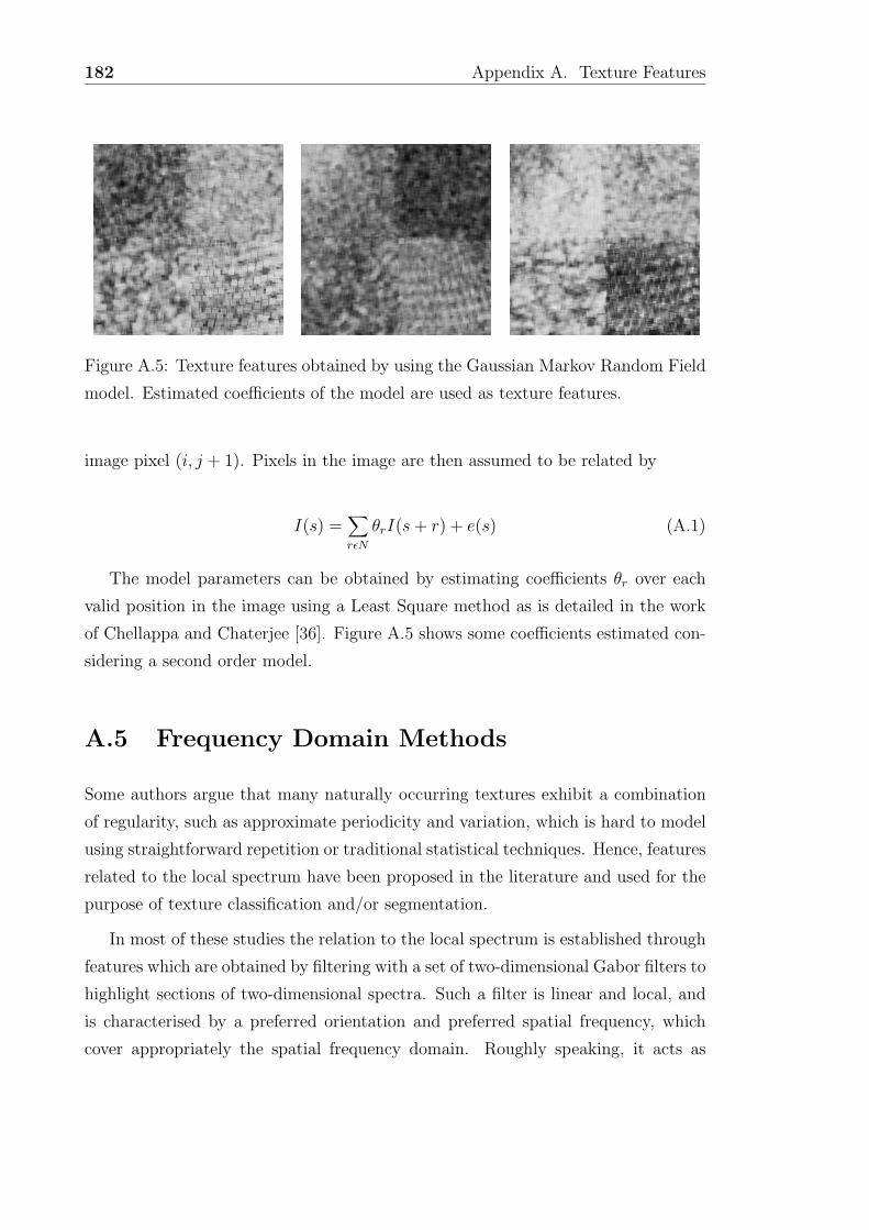
182 Appendix A. Texture Features
Figure A.5: Texture features obtained by using the Gaussian Markov Random Field
model. Estimated coefficients of the model are used as texture features.
image pixel (i, j + 1). Pixels in the image are then assumed to be related by
I(s) =∑rεN
θrI(s + r) + e(s) (A.1)
The model parameters can be obtained by estimating coefficients θr over each
valid position in the image using a Least Square method as is detailed in the work
of Chellappa and Chaterjee [36]. Figure A.5 shows some coefficients estimated con-
sidering a second order model.
A.5 Frequency Domain Methods
Some authors argue that many naturally occurring textures exhibit a combination
of regularity, such as approximate periodicity and variation, which is hard to model
using straightforward repetition or traditional statistical techniques. Hence, features
related to the local spectrum have been proposed in the literature and used for the
purpose of texture classification and/or segmentation.
In most of these studies the relation to the local spectrum is established through
features which are obtained by filtering with a set of two-dimensional Gabor filters to
highlight sections of two-dimensional spectra. Such a filter is linear and local, and
is characterised by a preferred orientation and preferred spatial frequency, which
cover appropriately the spatial frequency domain. Roughly speaking, it acts as
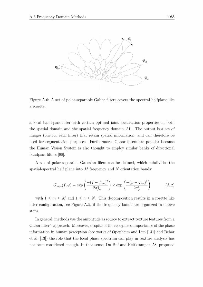
A.5 Frequency Domain Methods 183
ϕoN
ϕo1
ϕo2
σϕ
Figure A.6: A set of polar-separable Gabor filters covers the spectral halfplane like
a rosette.
a local band-pass filter with certain optimal joint localisation properties in both
the spatial domain and the spatial frequency domain [51]. The output is a set of
images (one for each filter) that retain spatial information, and can therefore be
used for segmentation purposes. Furthermore, Gabor filters are popular because
the Human Vision System is also thought to employ similar banks of directional
bandpass filters [98].
A set of polar-separable Gaussian filers can be defined, which subdivides the
spatial-spectral half plane into M frequency and N orientation bands:
Gm,n(f, ϕ) = exp
(−(f − fom)2
2σ2fm
)× exp
(−(ϕ − ϕon)2
2σ2ϕ
)(A.2)
with 1 ≤ m ≤ M and 1 ≤ n ≤ N . This decomposition results in a rosette like
filter configuration, see Figure A.5, if the frequency bands are organized in octave
steps.
In general, methods use the amplitude as source to extract texture features from a
Gabor filter’s approach. Moreover, despite of the recognized importance of the phase
information in human perception (see works of Openheim and Lim [141] and Behar
et al. [13]) the role that the local phase spectrum can play in texture analysis has
not been considered enough. In that sense, Du Buf and Heitktamper [58] proposed
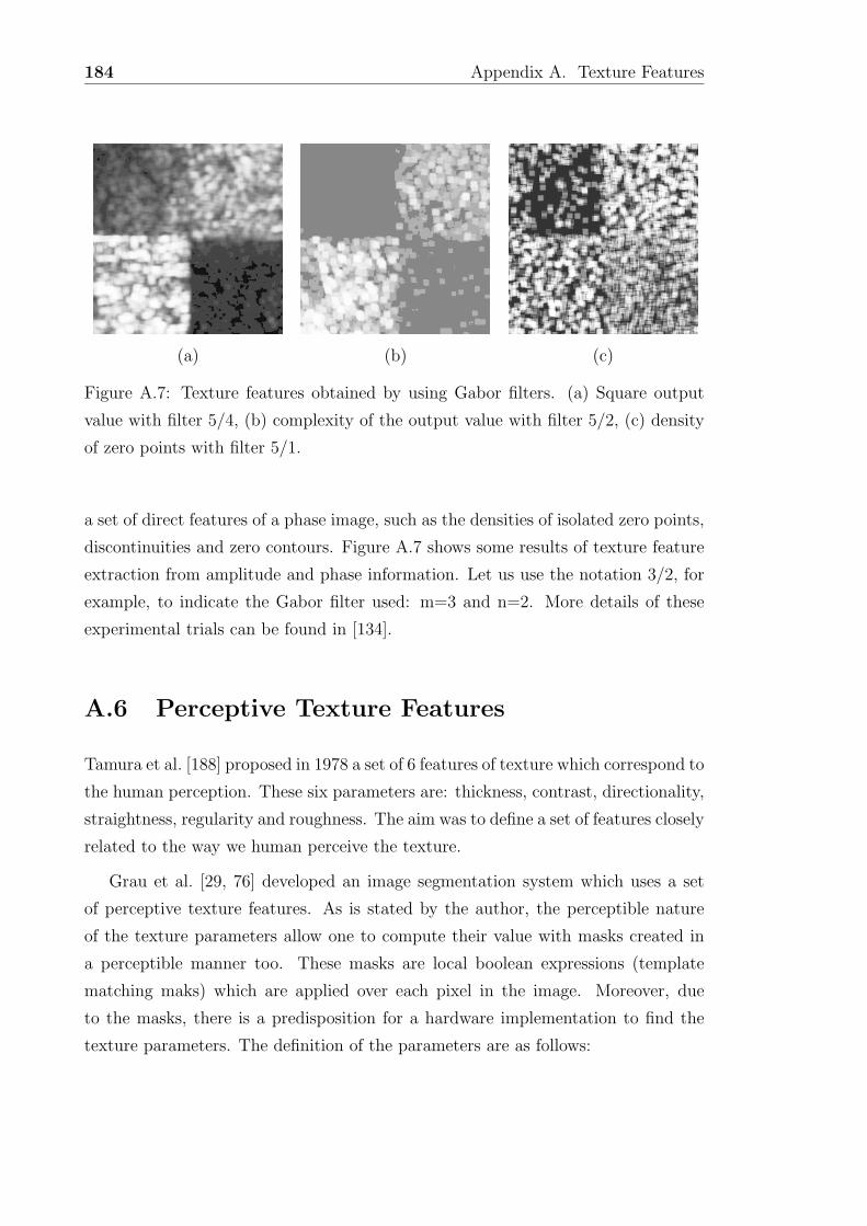
184 Appendix A. Texture Features
(a) (b) (c)
Figure A.7: Texture features obtained by using Gabor filters. (a) Square output
value with filter 5/4, (b) complexity of the output value with filter 5/2, (c) density
of zero points with filter 5/1.
a set of direct features of a phase image, such as the densities of isolated zero points,
discontinuities and zero contours. Figure A.7 shows some results of texture feature
extraction from amplitude and phase information. Let us use the notation 3/2, for
example, to indicate the Gabor filter used: m=3 and n=2. More details of these
experimental trials can be found in [134].
A.6 Perceptive Texture Features
Tamura et al. [188] proposed in 1978 a set of 6 features of texture which correspond to
the human perception. These six parameters are: thickness, contrast, directionality,
straightness, regularity and roughness. The aim was to define a set of features closely
related to the way we human perceive the texture.
Grau et al. [29, 76] developed an image segmentation system which uses a set
of perceptive texture features. As is stated by the author, the perceptible nature
of the texture parameters allow one to compute their value with masks created in
a perceptible manner too. These masks are local boolean expressions (template
matching maks) which are applied over each pixel in the image. Moreover, due
to the masks, there is a predisposition for a hardware implementation to find the
texture parameters. The definition of the parameters are as follows:
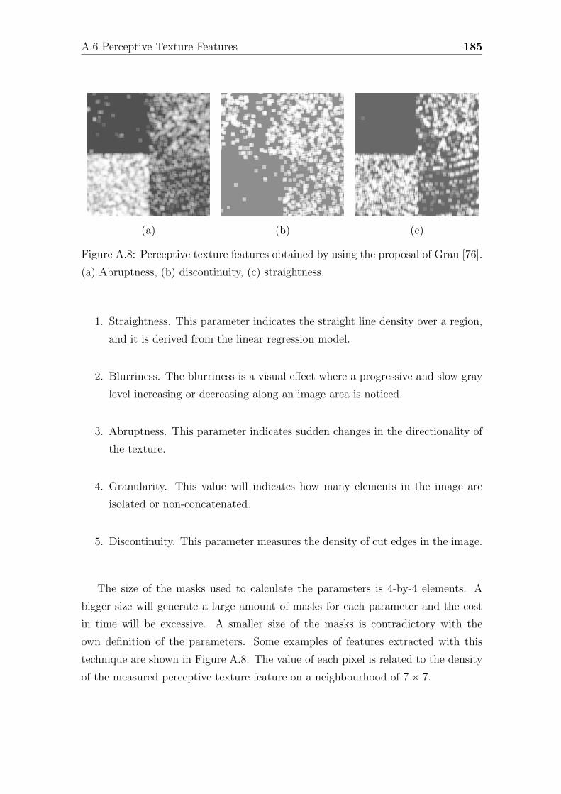
A.6 Perceptive Texture Features 185
(a) (b) (c)
Figure A.8: Perceptive texture features obtained by using the proposal of Grau [76].
(a) Abruptness, (b) discontinuity, (c) straightness.
1. Straightness. This parameter indicates the straight line density over a region,
and it is derived from the linear regression model.
2. Blurriness. The blurriness is a visual effect where a progressive and slow gray
level increasing or decreasing along an image area is noticed.
3. Abruptness. This parameter indicates sudden changes in the directionality of
the texture.
4. Granularity. This value will indicates how many elements in the image are
isolated or non-concatenated.
5. Discontinuity. This parameter measures the density of cut edges in the image.
The size of the masks used to calculate the parameters is 4-by-4 elements. A
bigger size will generate a large amount of masks for each parameter and the cost
in time will be excessive. A smaller size of the masks is contradictory with the
own definition of the parameters. Some examples of features extracted with this
technique are shown in Figure A.8. The value of each pixel is related to the density
of the measured perceptive texture feature on a neighbourhood of 7 × 7.
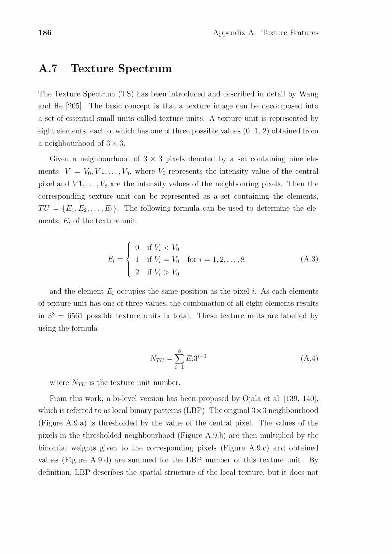
186 Appendix A. Texture Features
A.7 Texture Spectrum
The Texture Spectrum (TS) has been introduced and described in detail by Wang
and He [205]. The basic concept is that a texture image can be decomposed into
a set of essential small units called texture units. A texture unit is represented by
eight elements, each of which has one of three possible values (0, 1, 2) obtained from
a neighbourhood of 3 × 3.
Given a neighbourhood of 3 × 3 pixels denoted by a set containing nine ele-
ments: V = V0, V 1, . . . , V8, where V0 represents the intensity value of the central
pixel and V 1, . . . , V8 are the intensity values of the neighbouring pixels. Then the
corresponding texture unit can be represented as a set containing the elements,
TU = {E1, E2, . . . , E8}. The following formula can be used to determine the ele-
ments, Ei of the texture unit:
Ei =
0 if Vi < V0
1 if Vi = V0 for i = 1, 2, . . . , 8
2 if Vi > V0
(A.3)
and the element Ei occupies the same position as the pixel i. As each elements
of texture unit has one of three values, the combination of all eight elements results
in 38 = 6561 possible texture units in total. These texture units are labelled by
using the formula
NTU =8∑
i=1
Ei3i−1 (A.4)
where NTU is the texture unit number.
From this work, a bi-level version has been proposed by Ojala et al. [139, 140],
which is referred to as local binary patterns (LBP). The original 3×3 neighbourhood
(Figure A.9.a) is thresholded by the value of the central pixel. The values of the
pixels in the thresholded neighbourhood (Figure A.9.b) are then multiplied by the
binomial weights given to the corresponding pixels (Figure A.9.c) and obtained
values (Figure A.9.d) are summed for the LBP number of this texture unit. By
definition, LBP describes the spatial structure of the local texture, but it does not
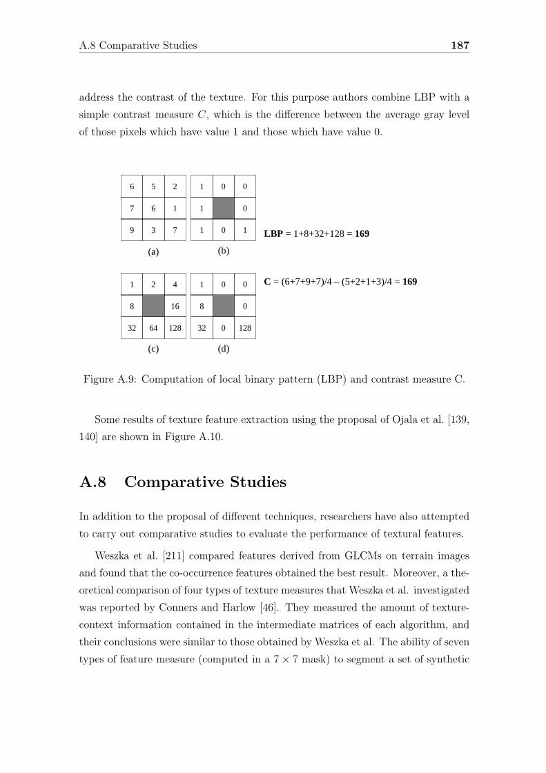
A.8 Comparative Studies 187
address the contrast of the texture. For this purpose authors combine LBP with a
simple contrast measure C, which is the difference between the average gray level
of those pixels which have value 1 and those which have value 0.
6 5 2
7 6 1
9 3 7
1 0 0
1 0
1 0 1
1 2 4
8 16
32 64 128
1 0 0
8 0
32 0 128
(a) (b)
(c) (d)
LBP = 1+8+32+128 = 169
C = (6+7+9+7)/4 – (5+2+1+3)/4 = 169
Figure A.9: Computation of local binary pattern (LBP) and contrast measure C.
Some results of texture feature extraction using the proposal of Ojala et al. [139,
140] are shown in Figure A.10.
A.8 Comparative Studies
In addition to the proposal of different techniques, researchers have also attempted
to carry out comparative studies to evaluate the performance of textural features.
Weszka et al. [211] compared features derived from GLCMs on terrain images
and found that the co-occurrence features obtained the best result. Moreover, a the-
oretical comparison of four types of texture measures that Weszka et al. investigated
was reported by Conners and Harlow [46]. They measured the amount of texture-
context information contained in the intermediate matrices of each algorithm, and
their conclusions were similar to those obtained by Weszka et al. The ability of seven
types of feature measure (computed in a 7 × 7 mask) to segment a set of synthetic
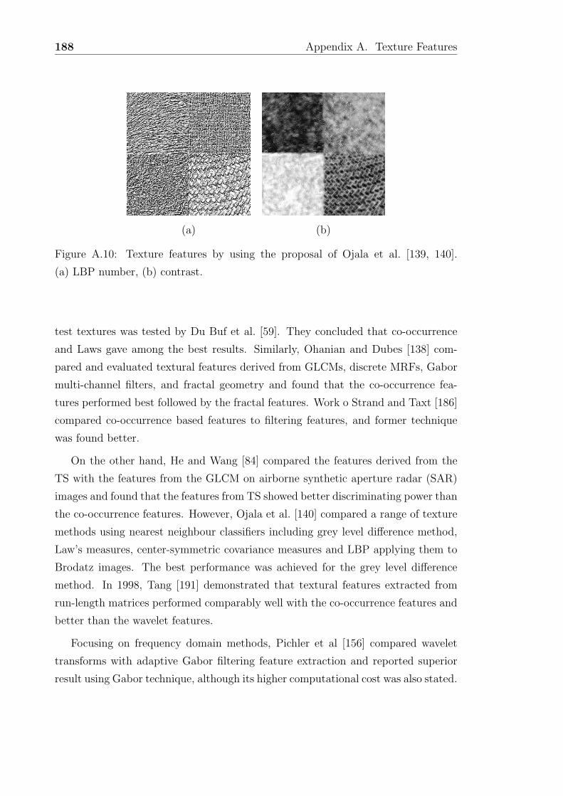
188 Appendix A. Texture Features
(a) (b)
Figure A.10: Texture features by using the proposal of Ojala et al. [139, 140].
(a) LBP number, (b) contrast.
test textures was tested by Du Buf et al. [59]. They concluded that co-occurrence
and Laws gave among the best results. Similarly, Ohanian and Dubes [138] com-
pared and evaluated textural features derived from GLCMs, discrete MRFs, Gabor
multi-channel filters, and fractal geometry and found that the co-occurrence fea-
tures performed best followed by the fractal features. Work o Strand and Taxt [186]
compared co-occurrence based features to filtering features, and former technique
was found better.
On the other hand, He and Wang [84] compared the features derived from the
TS with the features from the GLCM on airborne synthetic aperture radar (SAR)
images and found that the features from TS showed better discriminating power than
the co-occurrence features. However, Ojala et al. [140] compared a range of texture
methods using nearest neighbour classifiers including grey level difference method,
Law’s measures, center-symmetric covariance measures and LBP applying them to
Brodatz images. The best performance was achieved for the grey level difference
method. In 1998, Tang [191] demonstrated that textural features extracted from
run-length matrices performed comparably well with the co-occurrence features and
better than the wavelet features.
Focusing on frequency domain methods, Pichler et al [156] compared wavelet
transforms with adaptive Gabor filtering feature extraction and reported superior
result using Gabor technique, although its higher computational cost was also stated.

A.8 Comparative Studies 189
A classification and comparison of different techniques used to produce texture fea-
tures using Gabor filters is presented in the work of Clausi and Ed Jernigan [43].
Overall, using the Gabor filter magnitude response given a frequency bandwidth of
one octave and orientation bandwidth of 30◦ augmented by a measure of the texture
complexity generated preferred results.
Summarizing, the results of comparing the relative merits of the different types
of features have been nonconclusive and a clear winner has not emerged in all
cases [159]. Comparative works result in different, and sometimes contradictory,
conclusions. The reason can be found in the use of different test images and evalu-
ation methods, as well as some aspects related to code implementation.

190 Appendix A. Texture Features
Bibliography
[1] Y. Abe, T. Matsuzawa. Clustering-based control of active contour model.
In IAPR International Conference on Pattern Recognition, Quebec, Canada,
August 2002.
[2] R. Adams and L. Bischof. Seeded region growing. IEEE Transactions on
Pattern Analysis and Machine Intelligence, 16(6):641–647, June 1994.
[3] N. Ahuja and B.J. Schachter. Image models. Computing Surveys, 13:373–397,
1981.
[4] J. Aitchison. The Statistical Analysis of Compositional Data. Chapman and
Hall, 1986.
[5] A. Al-Janobi. Performance evaluation of cross-diagonal texture matrix method
of texture analysis. Pattern Recognition, 34:171–180, 2001.
[6] D.C. Alexander and B.F. Buxton. Implementational improvements for active
region models. In British Machine Vision Conference, Colchester, UK, 1997.
[7] J. Amat, J. Batlle, A. Casals, and J. Forest. Garbi: A low cost rov, constraints
and solutions. In Proceedings of the 6th IAPR Underwater Robotics, pages 1–
22, Toulon-La Seyne, France, 1996.
[8] M.R. Anderberg. Cluster Analysis for Applications. Academic Press, New
York, 1973.
[9] D.F. Andrews, R. Gnanadesikan, and J.L. Warner. Methods for assessing
multivariate normality. In P.R. Krishnaiah, editor, Multivariate Analysis III,
pages 95–116. Academic Press, New York, 1973.
191
192 BIBLIOGRAPHY
[10] S. Baker. CORBA Distributed Objects Using Orbix. Addison Wesley, Harlow,
UK, 1997.
[11] D.H. Ballard and C.M. Brown. Computer Vision. Prentice-Hall, Englewood
Cliffs, New Jersey, 1982.
[12] J. Batlle, A. Casals, J. Freixenet, and J. Martı. A review on strategies for
recognizing natural objects in colour images of outdoor scenes. Image and
Vision Computing, 18(6-7):515–530, May 2000.
[13] J. Behar, M. Porat, and Y.Y. Zeevi. The importance of localized phase in
vision and image representation. In Society of Photo-Optical Instrumentation
Engineers, volume 1001 Visual Communication and Image Processing, pages
61–68, Cambridge, Massachussets, 1988.
[14] F. Bellet, M. Salotti, and C. Garbay. Low level vision as the opportunist
scheduling of incremental edge and region detection processes. In IAPR In-
ternational Conference on Pattern Recognition, volume A, pages 517–519,
Jerusalem, Israel, September 1994.
[15] S. Belongie, C. Carson, H. Greenspan, and J. Malik. Color and texture-
based image segmentation using em and its application to content-based image
retrieval. In International Conference on Computer Vision, Mumbay, India,
1998.
[16] J. Benois and D. Barba. Image segmentation by region-contour cooperation
for image coding. In IAPR International Conference on Pattern Recognition,
volume C, pages 331–334, The Hague, Netherlands, August 1992.
[17] F. Bergholm. Edge focusing. IEEE Transactions on Pattern Analysis and
Machine Intelligence, 9(6):726–741, 1987.
[18] P. Bertolino and A. Montanvert. Cooperation regions-contours multiresolution
en segmentation d’image. In Congres AFCET de Reconnaissance des Formes
et Intelligence Artificielle, volume 1, pages 299–307, Rennes, France, January
1996.
BIBLIOGRAPHY 193
[19] A. Bieniek and A. Moga. An efficient watershed algorithm based on connected
components. Pattern Recognition, 33(6):907–916, 2000.
[20] P. Bonnin, J. Blanc Talon, J.C. Hayot, and B. Zavidovique. A new edge
point/region cooperative segmentation deduced from a 3d scene reconstruction
application. In SPIE Applications of Digital Image Processing XII, volume
1153, pages 579–591, 1989.
[21] S. Borra and S. Sarkar. A framework for performance characterization of
intermediate-level grouping modules. IEEE Transactions on Pattern Analysis
and Machine Intelligence, 19(11):1306–1312, November 1997.
[22] M. Borsotti, P. Campadelli, and R. Schettini. Quantitative evaluation of color
image segmentation results. Pattern Recognition Letters, 19:741–747, 1998.
[23] M. Buvry, J. Senard, and C. Krey. Hierarchical region detection based on the
gradient image. In Scandinavian Conference on Image Analysis, volume 2,
pages 717–724, Lappeenranta, Finland, June 1997.
[24] M. Buvry, E. Zagrouba, and C.J. Krey. A rule-based system for region segmen-
tation improvement in stereovision. In Society of Photo-Optical Instrumenta-
tion Engineers, volume 2182 Image and Video Processing II, pages 357–367,
San Jose, California, February 1994.
[25] T. Caelli and D. Reye. On the classification of image regions by color, texture
and shape. Pattern Recognition, 26(4):461–470, 1993.
[26] F.J. Canny. A computational approach to edge detection. IEEE Transactions
on Pattern Analysis and Machine Intelligence, 8(6):679–698, 1986.
[27] T. Carron and P. Lambert. Color edge detector using jointly hue, saturation
and intensity. In IEEE International Conference on Image Processing, volume
III, pages 977–981, Ft. Collins, Colorado, 1994.
[28] C. Carson, S. Belongie, H. Greenspan, and J. Malik. Blobworld: Color and
texture-based image segmentation using em and its application to content-
based image retrieval. IEEE Transactions on Pattern Analysis and Machine
Intelligence, 24(8):1026–1038, August 2002.
194 BIBLIOGRAPHY
[29] A. Casals, J. Amat, and A. Grau. Texture parametrization method for image
segmentation. In European Conference on Computer Vision, pages 160–164,
Santa Margherita Ligure, Italy, May 1992.
[30] V. Caselles, R. Kimmel, and G. Sapiro. Geodesic active contours. International
Journal of Computer Vision, 22(1):61–79, 1997.
[31] K.R. Castleman. Digital Image Processing. Prentice-Hall, Englewood Cliffs,
New Jersey, 1996.
[32] A. Chakraborty, L.H. Staib, and J.S. Duncan. Deformable boundary finding
influenced by region homogeneity. In IEEE Computer Society Conference on
Computer Vision and Pattern Recognition, volume 94, pages 624–627, Seattle,
Washington, June 1994.
[33] A. Chakrabory and J.S. Duncan. Game-theoretic integration for image seg-
mentation. IEEE Transactions on Pattern Analysis and Machine Intelligence,
21(1):12–30, January 1999.
[34] F.H.Y. Chan, F.K. Lam, P.W.F. Poon, H. Zhu, and K.H. Chan. Object
boundary location by region and contour deformation. IEE Proceedings-Vision
Image and Signal Processing, 143(6):353–360, December 1996.
[35] T. Chan and L. Vese. An active contour model without edges. In Interna-
tional Conference on Scale-Space Theories in Computer Vision, pages 141–151,
Corfu, Greece, September 1999.
[36] R. Chellappa and S. Chatterjee. Classification of textures using gaussian
markov random fields. IEEE Transactions on Acoustics Speech and Signal
Processing, 33:959–963, 1985.
[37] J. Chen, T.N. Pappas, A. Mojsilovic, and B. Rogowitz. Adaptive image seg-
mentation based on color and texture. In IEEE International Conference on
Image Processing, Rochester, New York, September 2002.
[38] P.C. Chen and T. Pavlidis. Image segmentation as an estimation problem.
Computer Graphics and Image Processing, 12:153–172, 1980.
BIBLIOGRAPHY 195
[39] C. Chesnaud, P. Refregier, and V. Boulet. Statistical region snake-based seg-
mentation adapted to different physical noise models. IEEE Transactions on
Pattern Analysis and Machine Intelligence, 21(11):1145–1157, November 1999.
[40] C.K. Chow and T. Kaneko. Boundary detection and volume determination
of the left ventricle from cineangiograms. Computers in Biomedical Research,
3:13–26, 1973.
[41] C.M. Christoudias, B. Georgescu, and P. Meer. Synergism in low level vision.
In IAPR International Conference on Pattern Recognition, Quebec, Canada,
August 2002.
[42] C.C. Chu and J.K. Aggarwal. The integration of image segmentation maps
using region and edge information. IEEE Transactions on Pattern Analysis
and Machine Intelligence, 15(12):1241–1252, December 1993.
[43] D.A. Clausi and M. Ed Jernigan. Designig gabor filters for optimal texture
separability. Pattern Recognition, 33:1835–1849, 1990.
[44] D. Comaniciu and P. Meer. Distribution free decomposition of multivariate
data. Pattern Analysis & Applications, 2:22–30, 1999.
[45] D. Comaniciu and P. Meer. Mean shift: A robust approach toward feature
space analysis. IEEE Transactions on Pattern Analysis and Machine Intelli-
gence, 24(5):1–18, April 2002.
[46] R.W. Conners and C.A. Harlow. A theoretical comparison of texture algo-
rithms. IEEE Transactions on Pattern Analysis and Machine Intelligence,
2(3):204–222, May 1980.
[47] X. Cufı. Aportacio a la Segmentacio d’Imatges Mitjancant l’Obtencio dels
Contorns Envolupants. PhD thesis, Polytechnical University of Catalonia,
1998.
[48] X. Cufı and A. Casals. A criterion for circumscribed contour determination for
image segmentation. In IAPR Workshoop on Machine Vision Applications,
pages 309–312, Tokyo, Japan, November 1996.
196 BIBLIOGRAPHY
[49] X. Cufı, A. Casals, and J. Batlle. A method to obtain the integrated contour
image in colour scenes. In IEEE International Conference on Image Process-
ing, volume 2, pages 764–767, Santa Barbara, California, October 1997.
[50] X. Cufı, X. Munoz, J. Freixenet, and J. Martı. A concurrent region growing
algorithm guided by circumscribed contours. In IAPR International Con-
ference on Pattern Recognition, volume I, pages 432–435, Barcelona, Spain,
September 2000.
[51] J. Daugman. Uncertainty relation for resolution in space, spatial frequency,
and orientation optimized by two-dimensional visual cortical filters. Journal
of the Optical Society of America, 2(7):1160–1169, 1985.
[52] E.R. Davies. Machine Vision: Theory, Algorithms, Practicalities. Academic
Press, London, UK, 1997.
[53] P. De Smet, R. Pires, D. De Vleeschauwer, and I. Bruyland. Implementa-
tion and analysis of an optimized rainfalling watershed algorithm. Journal of
Electronic Imaging, 8(3):270–278, 1999.
[54] Y. Deng, B.S. Manjunath, and H. Shin. Color image segmentation. In IEEE
Computer Society Conference on Computer Vision and Pattern Recognition,
volume 2, pages 446–451, Ft. Collins, Colorado, June 1999.
[55] R. Deriche. Using canny’s criteria to derive a recursively implemented optimal
edge detector. International Journal of Computer Vision, 1:167–187, 1987.
[56] J. Devaux, P. Gouton, and F. Truchetet. Aerial colour image segmentation
by karhunen-loeve transform. In IAPR International Conference on Pattern
Recognition, volume 3, pages 309–312, Barcelona, Spain, September 2000.
[57] A. Drimbarean and P.F. Whelan. Experiments in colour texture analysis.
Pattern Recognition Letters, 22:1161–1167, 2001.
[58] J.M.H. Du Buf and P. Heitktamper. Texture features based on gabor phase.
Signal Processing, 23(3):227–244, 1991.
[59] J.M.H. Du Buf, M. Kardan, and M. Spann. Texture feature performance for
image segmentation. Pattern Recognition, 23(3/4):291–309, 1990.
BIBLIOGRAPHY 197
[60] M.-P. Dubuisson-Jolly and A. Gupta. Color and texture fusion: Application
to aerial image segmentation and gis updating. Image and Vision Computing,
18:823–832, 2000.
[61] R.O. Duda and P.E. Hart. Use of the hough transform to detect lines and
curves in pictures. Communications of the ACM, 15:11–15, 1972.
[62] O. Ecabert and J.-P. Thiran. Variational image segmentation by unifying re-
gion and boundary information. In IAPR International Conference on Pattern
Recognition, Quebec, Canada, August 2002.
[63] K.B. Eom and R.L. Hashyap. Composite edge detection with random field
models. IEEE Transactions on Systems, Man, and Cybernetics, 20(1):81–93,
February 1990.
[64] M. Everingham, H. Muller, and B. Thomas. Evaluating image segmentation
algorithms using the pareto front. In European Conference on Computer Vi-
sion, pages 34–48, Copenhagen, Denmark, May 2002.
[65] R.K. Falah, P. Bolon, and J.P. Cocquerez. A region-region and region-edge
cooperative approach of image segmentation. In IEEE International Confer-
ence on Image Processing, volume 3, pages 470–474, Austin, Texas, October
1994.
[66] R. FjØrtoft, J. Cabada, A. Lopes, P. Marthon, and E. Cubero-Castan. Com-
plementary edge detection and region growing for sar image segmentation. In
Conference of the Norwegian Society for Image Processing and Pattern Recog-
nition, volume 1, pages 70–72, TromsØ, Norway, May 1997.
[67] K.S. Fu and J.K Mui. A survey on image segmentation. Pattern Recognition,
13:3–16, 1981.
[68] P. Fua and A.J. Hanson. Using generic geometric models for intelligent shape
extraction. In National Conference on Artificial Intelligence, pages 706–711,
Seattle, Washington, July 1987.
[69] Y. Fukada. Spatial clustering procedures for region analysis. Pattern Recog-
nition, 12:395–403, 1980.
198 BIBLIOGRAPHY
[70] K. Fukunaga. Introduction to Statistical Pattern Recognition. Academic Press,
1990.
[71] A. Gagalowicz and C. Graffigne. Blind texture segmentation. In IAPR Inter-
national Conference on Pattern Recognition, pages 46–50, Rome, Italy, 1988.
[72] A. Gagalowicz and O. Monga. A new approach for image segmentation. In
IAPR International Conference on Pattern Recognition, pages 265–267, Paris,
France, November 1986.
[73] J.P. Gambotto. A new approach to combining region growing and edge detec-
tion. Pattern Recognition Letters, 14:869–875, 1993.
[74] R. Gershon. Aspects of perception and computation in color vision. Computer
Vision, Graphics and Image Processing, 32:244–277, 1985.
[75] T. Gevers and A.W.M. Smeulders. Combining region growing and edge detec-
tion through guided delaunay image subdivision. In IEEE Computer Society
Conference on Computer Vision and Pattern Recognition, pages 1021–1026,
Puerto Rico, June 1997.
[76] A. Grau. Metode d’extraccio multiparametrica de caracterıstiques de textura
orientat a la segmentacio d’imatges. 1r Seminari de Treball en Automatica,
Robotica i Percepcio, pages 197–210, 1996.
[77] A. Grau. Metode d’Extraccio Multiparametrica de Caracterıstiques de Textura
Orientat a la Segmentacio d’Imatges. PhD thesis, Departament d’ESAII-UPC,
Universitat Politecnica de Catalunya, May 1997.
[78] J.F. Haddon and J.F. Boyce. Image segmentation by unifying region and
boundary information. IEEE Transactions on Pattern Analysis and Machine
Intelligence, 12(10):929–948, October 1990.
[79] R. Haralick and R. Shapiro. Computer and Robot Vision, volume 1 & 2.
Addison-Wesley Inc, Reading, Massachussets, 1992 & 1993.
[80] R.M. Haralick. Statistical and structural approaches to texture. Proceedings
of the IEEE, 67:786–804, 1979.
BIBLIOGRAPHY 199
[81] R.M. Haralick, K. Shanmugan, and I. Dinstein. Texture features for image clas-
sification. IEEE Transactions on Systems, Man, and Cybernetics, 3(6):610–
621, November 1973.
[82] R.M. Haralick and L.G. Shapiro. Image segmentation techniques. Computer
Vision, Graphics and Image Processing, 29:100–132, 1985.
[83] J. Hauta-Kasari, J. Parkkinen, T. Jaaskelainen, and R. Lenz. Generalized co-
occurrence matrix for multispectral texture analysis. In IAPR International
Conference on Pattern Recognition, pages 785–789, Vienna, Austria, August
1996.
[84] D.C. He and L. Wang. Texture features based on texture spectrum. Pattern
Recognition, 24(5):391–399, 1991.
[85] D.C. He and L. Wang. Detecting texture edges from images. Pattern Recog-
nition, 25(6):595–600, 1992.
[86] G. Healey. Segmenting images using normalized color. IEEE Transactions on
Systems, Man, and Cybernetics, 22(1):64–73, 1992.
[87] G. Healey and T.O. Binford. The role and use of color in a general vision
system. In Image Understanding Workshop, pages 599–613, February 1987.
[88] L.S. Hibbard. Maximum a posteriori segmentation for medical visualization. In
IEEE Workshop on Biomedical Image Analysis, pages 93–102, Santa Barbara,
California, June 1998.
[89] S.A. Hojjatoleslami and J. Kittler. Region growing: A new approach. IEEE
Transactions on Image Processing, 7(7):1079–1084, July 1998.
[90] A. Hoover, G. Jean-Baptiste, X. Jiang, P.J. Flynn, H. Bunke, D.B. Goldgof,
K. Bowyer, and D.W. Eggert. An experimental comparison of range image seg-
mentation algorithms. IEEE Transactions on Pattern Analysis and Machine
Intelligence, 18(7):673–689, July 1996.
[91] S.L. Horowitz and T. Pavlidis. Picture segmentation by a directed split-and-
merge procedure. In International Joint Conference on Pattern Recognition,
pages 424–433, 1974.
200 BIBLIOGRAPHY
[92] T.I. Hsu, J.L. Kuo, and R. Wilson. A multiresolution texture gradient method
for unsupervised segmentation. Pattern Recognition, 32(11):1819–1833, 2000.
[93] Q. Huang and B. Dom. Quantitative methods of evaluating image segmen-
tation. In IEEE International Conference on Image Processing, volume III,
pages 53–56, Washington DC, October 1995.
[94] Q. Huang, B. Dom, D. Steele, J. Ashley, and W. Niblack. Foreground-
background segmentation of color images by integration of multiple cues. In
IEEE International Conference on Image Processing, 1995.
[95] J. Ivins. Statistical Snakes: Active Region Models. PhD thesis, University of
Sheffield, 1996.
[96] J. Ivins and J. Porrill. Active-region models for segmenting textures and colors.
Image and Vision Computing, 13(5):431–438, June 1995.
[97] A. Jain and R. Dubes. Algorithms for Clustering Data. Prentice-Hall, 1988.
[98] A. Jain and F. Farrokhnia. Unsupervised texture segmentation using gabor
filters. Pattern Recognition, 24:1167–1186, 1991.
[99] D.P. Jang, D.S. Lee, and S.I. Kim. Contour detection of hippocampus using
dynamic contour model and region growing. In International Conference of the
IEEE Engineering in Medicine and Biology Society, pages 763–766, Chicago,
Ilinois, October 1997.
[100] J.D. Jobson. Applied Multivariate Data Analysis. Springer-Verlag, 1991.
[101] G. Jones. Image segmentation using texture boundary detection. Pattern
Recognition Letters, 15:533–541, June 1994.
[102] M. Kass, A. Witkin, and D. Terzopoulos. Snakes: Active contour models. In
International Conference on Computer Vision, pages 259–268, London, UK,
June 1987.
[103] A. Khotanzad and J. Chen. Unsupervised segmentation of texture images by
edge detection in multidimensional features. IEEE Transactions on Pattern
Analysis and Machine Intelligence, 11(4):414–421, April 1989.
BIBLIOGRAPHY 201
[104] J. Kittler and J. Illingworth. On threshold selection using clustering criterion.
IEEE Transactions on Systems, Man, and Cybernetics, 15:652–655, 1985.
[105] R. Kohler. A segmentation system based on thresholding. Computer Vision,
Graphics and Image Processing, 15:319–338, 1981.
[106] S.G. Kong and B. Kosko. Image coding with fuzzy image segmentation. In
International Conference on Fuzzy Systems, volume I, pages 213–220, San
Diego, California, March 1992.
[107] S.M. Krishnan, C.S. Tan, and K.L. Chan. Closed-boundary extraction of
large intestinal lumen. In International Conference of the IEEE Engineering
in Medicine and Biology Society, Baltimore, Washington, November 1994.
[108] P. Lambert and T. Carron. Symbolic fusion of luminance-hue-croma features
for region segmentation. Pattern Recognition, 32(11):1857–1872, 1999.
[109] G. Lance and W. Williams. A general theory of classification sorting strategies.
Computer Journal, 9:373–386, 1969.
[110] K.I. Laws. Textured image segmentation. Technical Report 940, Image Pro-
cessing Institute, University of Southern California, Los Angeles, California,
1980.
[111] H.C. Lee and D.R. Cok. Detecting boundaries in a vector field. IEEE Trans-
actions on Signal Processing, 39:1181–1194, May 1991.
[112] J. LeMoigne and J.C. Tilton. Refining image segmentation by integration of
edge and region data. IEEE Transactions on Geoscience and Remote Sensing,
33(3):605–615, May 1995.
[113] M.D. Levine and A.M. Nazif. Dynamic measurement of computer generated
image segmentations. IEEE Transactions on Pattern Analysis and Machine
Intelligence, 7(2):155–164, March 1985.
[114] J. Liu and Y.-H. Yang. Multiresolution color image segmentation. IEEE
Transactions on Pattern Analysis and Machine Intelligence, 16(7):689–700,
1994.
202 BIBLIOGRAPHY
[115] S.W. Looney. How to use tests for univariate normality to assess multivariate
normality. American Statistician, 49:64–70, 1995.
[116] F. Lumbreras, R. Baldrich, M. Vanrell, J. Serrat, and J.J. Villanueva. Mul-
tiresolution colour texture representation for tile classification. In Simposium
Nacional en Reconocimiento de Formas y Analisis de Imagen, volume I, pages
145–152, Bilbao, Spain, May 1999.
[117] J. Luo and A.E. Savakis. Self-supervised texture segmentation using comple-
mentary types of features. Pattern Recognition, 34:2071–2082, 2001.
[118] J.B. MacQueen. Some methods of classification and analysis of multivariate
observations. In Proceedings of the Fifth Berkeley Symposium on Mathematical
Statistics and Probability, volume 1, pages 281–297, 1967.
[119] R. Malladi, J.A. Sethian, and B.C. Vemuri. Shape modelling with front prop-
agation: A level set approach. IEEE Transactions on Pattern Analysis and
Machine Intelligence, 17(2):158–174, February 1995.
[120] R. Manduchi. Bayesian fusion of color and texture segmentations. In Inter-
national Conference on Computer Vision, volume 2, pages 956–962, Corfu,
Greece, September 1999.
[121] R. Manduchi. Mixture models and the segmentation of multimodal textures. In
IEEE Computer Society Conference on Computer Vision and Pattern Recog-
nition, pages 98–104, Hilton Head Island, South Carolina, June 2000.
[122] B. Manjunath and R. Chellapa. A computational approach to boundary detec-
tion. In IEEE Computer Society Conference on Computer Vision and Pattern
Recognition, pages 358–362, Maui, Hawaii, June 1991.
[123] B. Manjunath and R. Chellapa. Unsupervised texture segmentation using
markov random field models. IEEE Transactions on Pattern Analysis and
Machine Intelligence, 13:478–482, 1991.
[124] J Mao and A.K. Jain. Texture classification and segmentation using multires-
olution simultaneous autoregressive models. Pattern Recognition, 25(2):173–
182, 1992.
BIBLIOGRAPHY 203
[125] D. Marr. Vision. W.H. Freeman and Company, New York, 1982.
[126] D. Martin, C. Fowlkes, D. Tal, and J. Malik. A database of human segmented
natural images and its application to evaluating segmentation algorithms and
measuring ecological statistics. In International Conference on Computer Vi-
sion, volume 2, pages 416–423, Vancouver, Canada, July 2001.
[127] F. Meyer and S. Beucher. Morphological segmentation. Journal of Visual
Communication and Image Representation, 1(1):21–46, September 1990.
[128] M. Mirmehdi and M. Petrou. Segmentation of color textures. IEEE Transac-
tions on Pattern Analysis and Machine Intelligence, 22(2):142–159, February
2000.
[129] A. Moghaddamzadeh and N. Bourbakis. A fuzzy region growing approach for
segmentation of color images. Pattern Recognition, 30(6):867–881, 1997.
[130] R. Mojena. Hierarchical grouping methods and stopping rules: An evaluation.
Computer Journal, 20(4):359–363, 1977.
[131] D. Moulet and D. Barba. Temporal following of spatial segmentation in images
sequences. In European Signal Processing Conference, pages 39–42, Grenoble,
France, September 1988.
[132] D. Mumford and J. Shah. Boundary detection by minimizing functionals. In
IEEE Computer Society Conference on Computer Vision and Pattern Recog-
nition, volume 85, pages 22–26, San Francisco, California, June 1985.
[133] D. Mumford and J. Shah. Optimal approximations by piecewise smooth func-
tions and associated variational problems. Communications in Pure and Ap-
plied Mathematics, 42(4):577–685, 1989.
[134] X. Munoz and J. Freixenet. Accurate texture segmentation based on gabor
phase features. Technical Report 01-13-RR, Institute of Informatics and Ap-
plications. University of Girona, 2001.
[135] D. Nair and J.K. Aggarwal. A focused target segmentation paradigm. In Euro-
pean Conference on Computer Vision, volume A, pages 579–588, Cambridge,
UK, April 1996.
204 BIBLIOGRAPHY
[136] R. Nevatia. Image segmentation. In Handbook of Pattern Recognition and
Image Processing, volume 86, pages 215–231, 1986.
[137] K.M. Nickels and S. Hutchinson. Textured image segmentation: Returning
multiple solutions. Image and Vision Computing, 15:781–795, 1997.
[138] P.P. Ohanian and R.C. Dubes. Performance evaluation for four classes of
textural features. Pattern Recognition, 25(8):819–833, 1992.
[139] T. Ojala, M. Pietikainen, and D. Harwood. Performance evaluation of texture
measures with classification based on kullback discrimination of distributions.
In IAPR International Conference on Pattern Recognition, volume A, pages
582–585, Jerusalem, Israel, September 1994.
[140] T. Ojala, M. Pietikainen, and D. Harwood. A comparative study of texture
measures with classification based on feature distributions. Pattern Recogni-
tion, 29:51–59, 1996.
[141] A.V. Openheim and J.S. Lim. The importance of phase in signals. Proceedings
of the IEEE, 69(5):529–541, 1981.
[142] S. Osher and J. Sethian. Fronts propagating with curvature-dependent speed:
Algorithms based on the hamilton-jacobi formulation. Journal of Computa-
tional Physics, 79:12–49, 1988.
[143] N.R. Pal and S.K. Pal. A review on image segmentation techniques. Pattern
Recognition, 26(9):1277–1294, 1993.
[144] P.L. Palmer and M. Petrou. Locating boundaries of textured regions. IEEE
Transactions on Geoscience and Remote Sensing, 35(5):1367–1371, September
1997.
[145] D.K. Panjwani and G. Healey. Markov random field models for unsupervised
segmentation of textured color images. IEEE Transactions on Pattern Anal-
ysis and Machine Intelligence, 17(10):939–954, 1995.
[146] N. Paragios and R. Deriche. Geodesic active regions for supervised texture
segmentation. In International Conference on Computer Vision, volume II,
pages 926–932, Corfu, Greece, September 1999.
BIBLIOGRAPHY 205
[147] N. Paragios and R. Deriche. Unifying boundary and region-based information
for geodesic active tracking. In IEEE Computer Society Conference on Com-
puter Vision and Pattern Recognition, volume II, pages 422–427, Fort Collins,
Colorado, June 1999.
[148] N. Paragios and R. Deriche. Coupled geodesic active regions for image segmen-
tation: A level set approach. In European Conference on Computer Vision,
volume 2, pages 224–240, Dublin, Ireland, 2000.
[149] N. Paragios and R. Deriche. Geodesic active regions and level set methods for
supervised texture segmentation. International Journal of Computer Vision,
46(3):223–247, 2002.
[150] G. Paschos. Fast color texture recognition using chromacity moments. Pattern
Recognition Letters, 21:837–841, 2000.
[151] T. Pavlidis. Structural Pattern Recognition. Springer, New York, 1977.
[152] T. Pavlidis and Y. Liow. Integrating region growing and edge detection. IEEE
Transactions on Pattern Analysis and Machine Intelligence, 12(3):225–233,
March 1990.
[153] M. Petrou and P. Bosdogianni. Image Processing: the fundamentals. John
Wiley & Sons, New York, 1999.
[154] D.L. Pham and J.L. Prince. An adaptive fuzzy c-means algorithm for image
segmentation in the presence of intensity inhomogeneities. Pattern Recognition
Letters, 20(1):57–68, 1999.
[155] S. Philipp and P. Zamperoni. Segmentation and contour closing of textured
and non-textured images using distances between textures. In IEEE Interna-
tional Conference on Image Processing, volume C, pages 125–128, Lausanne,
Switzerland, September 1996.
[156] O. Pichler, A. Teuner, and D.J. Hosticka. A comparison of texture feature ex-
traction using gabor filter, pyramidal and tree structured wavelet transforms.
Pattern Recognition, 29(5):733–742, 1996.
206 BIBLIOGRAPHY
[157] F.P. Preparata and S.J. Hong. Convex hulls of finite sets of points in two and
three dimensions. Communications of the ACM, 2(20):87–93, February 1977.
[158] J. Prewitt. Object enhancement and extraction. In B. Lipkin and A. Ro-
selfed, editors, Picture Processing and Psychopictorics, pages 75–149. Aca-
demic Press, New York, 1970.
[159] T. Randen and J.H. Husoy. Filtering for texture classification. IEEE Trans-
actions on Pattern Analysis and Machine Intelligence, 21:291–310, 1999.
[160] T.R. Reed and J.M.H. Du Buf. A review of recent texture segmentation
and feature extraction techniques. Computer Vision, Graphics and Image
Processing - Image Understanding, 57(3):359–372, 1993.
[161] C. Revol-Muller, F. Peyrin, C. Odet, and Y. Carillon. Automated 3d re-
gion growing algorithm governed by an evaluation function. In IEEE Interna-
tional Conference on Image Processing, volume III, pages 440–443, Vancouver,
Canada, September 2000.
[162] P. Ridao. A Hybrid Control Architecture for an AUV. PhD thesis, University
of Girona, 2001.
[163] E.M. Riseman and M.A. Arbib. Computational techniques in the visual
segmentation of static scenes. Computer Graphics and Image Processing,
6(3):221–276, June 1977.
[164] L.G. Roberts. Machine perception of three-dimensional solids. In J. Tippet,
D. Berkowitz, L. Clapp, C. Koester, and A. Vanderburgh, editors, Optical
and Electro-Optical Information Processing, pages 159–197. MIT Press, Cam-
bridge, Massachussets, 1965.
[165] S.J. Roberts. Parametric and non-parametric unsupervised cluster analysis.
Pattern Recognition, 30:261–272, 1997.
[166] R. Ronfard. Region-based strategies for active contours models. International
Journal of Computer Vision, 13(2):229–251, 1994.
[167] A. Rosenfeld and A. Kak. Digital Picture Processing, volume 2. Academic
Press, Orlando, Florida, 2nd edition, 1982.
BIBLIOGRAPHY 207
[168] Y. Rui, A.C. She, and T.S. Huang. Automated region segmentation using
attraction-based grouping in spatial-color-texture space. In IEEE Interna-
tional Conference on Image Processing, volume 1, pages 53–56, Lausanne,
Switzerland, 1996.
[169] E. Saber, A.M. Tekalp, and G. Bozdagi. Fusion of color and edge information
for improved segmentation and edge linking. Image and Vision Computing,
15(10):769–780, October 1997.
[170] P.K. Sahoo, S. Soltani, A.K.C. Wong, and Y.C. Chen. A survey of thresholding
techniques. Computer Vision, Graphics and Image Processing, 41:233–260,
1988.
[171] M. Salotti and C. Garbay. A new paradigm for segmentation. In IAPR Inter-
national Conference on Pattern Recognition, volume C, pages 611–614, The
Hague, Netherlands, August 1992.
[172] C. Samson, L. Blanc-Feraud, G. Aubert, and J. Zerubia. A level set model for
image classification. In International Conference on Scale-Space Theories in
Computer Vision, pages 306–317, Corfu, Greece, September 1999.
[173] M. Sato, S. Lakare, M. Wan, A. Kaufman, and M. Nakajima. A gradient
magnitude based region growing algorithm for accurate segmentation. In IEEE
International Conference on Image Processing, volume III, pages 448–451,
Vancouver, Canada, September 2000.
[174] B.J. Schachter. Model-based texture measures. IEEE Transactions on Pattern
Analysis and Machine Intelligence, 2(2):169–171, 1980.
[175] D.W. Scott. Multivariate Density Estimation. Wiley, 1992.
[176] J. Shah, H. Pien, and J. Gauch. Recovery of surfaces with discontinuities by
fusing shading and range data within a variatonal framework. IEEE Transac-
tions on Image Processing, 5(8):1243–1251, August 1996.
[177] A.C. She and T.S. Huang. Segmentation of road scenes using color and fractal-
based texture classification. In IEEE International Conference on Image Pro-
cessing, volume 3, pages 1026–1030, Austin, Texas, November 1994.
208 BIBLIOGRAPHY
[178] T. Shimbashi, Y. Kokubo, and N. Shirota. Region segmentation using edge
based circle growing. In IEEE International Conference on Image Processing,
volume C, pages 65–68, Washington D.C., October 1995.
[179] A. Siebert. Dynamic region growing. In Vision Interface, Kelowna, Canada,
May 1997.
[180] B.W. Silverman. Density Estimation for Statistics and Data Analysis. Chap-
man & Hall, London, England, 1986.
[181] D. Sinclair. Voronoi seeded colour image segmentation. Technical Report 3,
AT&T Laboratories Cambridge, 1999.
[182] I.E. Sobel. Camera Models and Machine Perception. PhD thesis, Electrical
Engineering Department, Stanford University, Stanford, California, 1970.
[183] M. Spann and R.G. Wilson. A quad-tree approach to image segmenta-
tion which combines statistical and spatial information. Pattern Recognition,
18(3/4):257–269, 1985.
[184] M. Spann and R.G. Wilson. A new approach to clustering. Pattern Recogni-
tion, 23(12):1413–1425, 1990.
[185] A. Steudel and M. Glesner. Fuzzy segmented image coding using orthonormal
bases and derivative chain coding. Pattern Recognition, 32(11):1827–1841,
1999.
[186] J. Strand and T. Taxt. Local frequency features for texture classification.
Pattern Recognition, 27(10):1397–1406, 1994.
[187] B. Sumengen, B.S. Manjunath, and C. Kenney. Image segmentation using
curve evolution and region stability. In IAPR International Conference on
Pattern Recognition, Quebec, Canada, August 2002.
[188] H. Tamura, S. Mori, and T. Yamawaki. Textural features corresponding to
visual perception. IEEE Transactions on Systems, Man, and Cybernetics,
8(6):460–473, 1978.
BIBLIOGRAPHY 209
[189] S.C. Tan and J. Kittler. On color texture representation and classification. In
IEEE International Conference on Image Processing, pages 390–395, Singa-
pore, September 1992.
[190] S.C. Tan and J. Kittler. Color texture classification using features from color
histogram. In Scandinavian Conference on Image Analysis, Tromsø, Norway,
May 1993.
[191] X. Tang. Texture information in run-length matrices. IEEE Transactions on
Image Processing, 7(11):1602–1609, 1998.
[192] G.R. Terrell and D.W. Scott. Variable kernel density estimation. The Annals
of Statistics, 20(3):1236–1265, 1992.
[193] B. Thai and G. Healey. Modelling and classifying symmetries using a multi-
scale opponent colour representation. IEEE Transactions on Pattern Analysis
and Machine Intelligence, 20(11):1224–1235, 1998.
[194] D.C. Tseng and C.H. Chang. Color segmentation using perceptual attributes.
In IAPR International Conference on Pattern Recognition, volume A, pages
228–231, 1992.
[195] D.C. Tseng and C.C. Lai. A genetic algorithm for mrf-based segmentation
of multi-spectral textured images. Pattern Recognition Letters, 20:1499–1510,
1999.
[196] Z. Tu and S.C. Zhu. Image segmentation by data-driven markov chain monte
carlo. IEEE Transactions on Pattern Analysis and Machine Intelligence,
24(5):657–673, May 2002.
[197] Z. Tu, S.C. Zhu, and H.Y. Shum. Image segmentation by data driven markov
chain monte carlo. In International Conference on Computer Vision, pages
131–138, Vancouver, Canada, July 2001.
[198] G. Van de Wouwer, P. Scheunders, S. Livens, and D. Van Dyck. Wavelet
correlation signatures for color texture characterization. Pattern Recognition,
32(3):443–451, 1999.
210 BIBLIOGRAPHY
[199] L. Van Gool, P. Dewaele, and A. Oosterlinck. Texture analysis anno 1983.
Computer Vision, Graphics and Image Processing, 29:336–357, 1985.
[200] L. Verard, J. Fadili, S. Ruan, and D. Bloyet. 3d mri segmentation of brain
structures. In International Conference of the IEEE Engineering in Medicine
and Biology Society, pages 1081–1082, Amsterdam, Netherlands, November
1996.
[201] L. Vincent and P. Soille. Watersheds in digital spaces: An efficient algorithm
based on immersion simulations. IEEE Transactions on Pattern Analysis and
Machine Intelligence, 13(6):583–589, June 1991.
[202] K.L. Vincken, A.S.E. Koster, and M.A. Viergever. Probabilistic multiscale
image segmentation. IEEE Transactions on Pattern Analysis and Machine
Intelligence, 19(2):109–120, February 1997.
[203] M.P. Wand and M. Jones. Kernel Smoothing. Chapman and Hall, 1995.
[204] D. Wang. A multiscale gradient algorithm for image segmentation using wa-
tersheds. Pattern Recognition, 30(12):2043–2052, 1997.
[205] L. Wang and D. He. Texture classification using texture spectrum. Pattern
Recognition, 23(8):905–910, 1990.
[206] L. Wang and J. Liu. Texture classification using multiresolution markov ran-
dom field models. Pattern Recognition Letters, 20:171–182, 1999.
[207] A.G. Weber. Hierarchical texture segmentation using multiple resolution oper-
ators. Technical Report 111, Signal and Image Processing Institute. University
of Southern California, July 1987.
[208] H. Wechsler. Texture analysis - a survey. Signal Processing, 2:271–282, 1980.
[209] J. Weickert. Efficient image segmentation using partial differential equations
and morphology. Pattern Recognition, 34(9):1813–1824, 2001.
[210] J.S. Weszka. Survey of threshold selection techniques. Computer Graphics
and Image Processing, 7(2):259–265, April 1978.
BIBLIOGRAPHY 211
[211] J.S. Weszka, C.R. Dyer, and A. Rosenfeld. A comparative study of texture
measures for terrain classification. IEEE Transactions on Systems, Man, and
Cybernetics, 6(4):269–285, April 1976.
[212] L. Wilkinson. Statistical methods in psychology journals. American Psychol-
ogist, 54(8):594–604, 1999.
[213] S. Will, L. Hermes, J.M. Buhmann, and J. Puzicha. On learning texture edge
detectors. In IEEE International Conference on Image Processing, volume III,
pages 887–880, Vancouver, Canada, September 2000.
[214] D.J. Williams and M. Shah. A fast algorithm for active contours and cur-
vature estimation. Computer Vision, Graphics and Image Processing. Image
Understanding, 1(55):14–26, 1992.
[215] R.G. Wilson and M. Spann. Finite prolate spheroidial sequences and their ap-
plications ii: Image feature description and segmentation. IEEE Transactions
on Pattern Analysis and Machine Intelligence, 10(2):193–203, 1988.
[216] B. Wrobel and O. Monga. Segmentation d’images naturelles: cooperation
entre un detecteur-contour et un detecteur-region. In Symposium on Signal
and Image Processing, Nice, France, June 1987.
[217] Y. Xiaohan, J. Yla-Jaaski, O. Huttunen, T. Vehkomaki, O. Sipild, and
T. Katila. Image segmentation combining region growing and edge detec-
tion. In IAPR International Conference on Pattern Recognition, volume C,
pages 481–484, The Hague, Netherlands, August 1992.
[218] J. Xuan, T. Adali, and Y. Wang. Segmentation of magnetic resonance brain
image: Integrating region growing and edge detection. In IEEE International
Conference on Image Processing, volume C, pages 544–547, Washington D.C.,
October 1995.
[219] W.A. Yasnoff, J.K. Mui, and J.W. Bacus. Error measures for scenes segmen-
tation. Pattern Recognition, 9:217–231, 1977.
212 BIBLIOGRAPHY
[220] A. Yezzi, A. Tsai, and A. Willsky. A statistical approach to snakes for bimodal
and trimodal imagery. In International Conference on Computer Vision, pages
898–903, Corfu, Greece, September 1999.
[221] X. Yu, T.D. Bui, and A. Krzyzak. Robust estimation for range image seg-
mentation and reconstruction. IEEE Transactions on Pattern Analysis and
Machine Intelligence, 16(5):530–538, May 1994.
[222] J. Zhang and T. Tan. Brief review of invariant texture analysis methods.
Pattern Recognition, 35:735–747, 2002.
[223] X. Zhang and B.A. Wandell. A spatial extension of cielab for digital color
image reproduction. In Society For Information Display Symposium, pages
731–734, 1996.
[224] Y.J. Zhang. A survey on evaluation methods for image segmentation. Pattern
Recognition, 29:1335–1346, 1996.
[225] Y.J. Zhang. Evaluation and comparison of different segmentation algorithms.
Pattern Recognition Letters, 18:963–974, 1997.
[226] Y.J. Zhang and J.J. Gerbrands. Objective and quantitative segmentation
evaluation and comparison. Signal Processing, 39:43–54, 1994.
[227] S.C. Zhu and A. Yuille. Region competition: Unifying snakes, region growing,
and bayes/mdl for multi-band image segmentation. IEEE Transactions on
Pattern Analysis and Machine Intelligence, 18(9):884–900, September 1996.
[228] X. Zhuang, Y. Huang, K. Palaniappan, and Y. Zhao. Gaussian mixture den-
sity modeling decomposition and applications. IEEE Transactions on Image
Processing, 5:1293–1302, 1996.
[229] S.W. Zucker. Region growing: Childhood and adolescence. Computer Graphics
and Image Processing, 5:382–399, 1976.
[230] S.W. Zucker. Algorithms for image segmentation. In Digital Image Processing
and Analysis, pages 169–183, 1977.

BIBLIOGRAPHY 213
[231] S.W. Zucker and D. Terzopoulos. Finding structure in co-occurrence matrices
for texture analysis. Computer Graphics and Image Processing, 12:286–308,
1980.