FEDERAL UNIVERSITY OF PARANA GUILHERME ALEXANDRE …

FEDERAL UNIVERSITY OF PARANA

GUILHERME ALEXANDRE TOMBOLO

TWO ESSAYS IN UNEMPLOYMENT RATE HYSTERESIS

CURITIBA2017




CURITIBA2017

i




Thesis presented as partial requirement forthe degree of Doctor by the Graduate Pro-gram in Economic Development, Sector ofApplied Social Sciences, Federal Univer-sity of Parana.

Advisor: Prof. Dr. Joao Basilio PereimaNeto

CURITIBA2017

ii

FICHA CATALOGRAFICA

Tombolo, Guilherme Alexandre.Two essays in unemployment rate hysteresis / Guilherme

Alexandre Tombolo. - Curitiba/Brasil - 2017.102f: il; tab; graf.

Orientador: Joao Basilio Pereima Neto.Tese (Doutorado) - Universidade Federal do Parana, Setor

de Ciencias Sociais Aplicadas, Curso de Pos-Graduacao emDesenvolvimento Economico.

1. Desemprego. 2. SVAR. 3. DSGE. 4. Brasil. I. Pereima,Joao Basilio. II. Universidade Federal do Parana, Setor deCiencias Sociais Aplicadas, Curso de Pos-Graduacao emDesenvolvimento Economico. III. Tıtulo.

CDD 339.4

iii

MINISTÉRIO DA EDUCAÇÃO U JJ L O r 1 iLU J UNIVERSIDADE FEDERAL DO PARANÁj l j ] r j | |r U T J lT PRÓ-REITORIA DE PESQUISA E PÓS-GRADUAÇÃO

Setor CIÊNCIAS SOCIAIS APLICADASPrograma de Pós-Graduação DESENVOLVIMENTO ECONÔMICOUFPR

TERMO DE APROVAÇÃO

Os membros da Banca Examinadora designada pelo Colegiado do Programa de Pós-Graduação em DESENVOLVIMENTO

ECONÔMICO da Universidade Federal do Paraná foram convocados para realizar a arguição da tese de Doutorado de

GUILHERME ALEXANDRE TOMBOLO intitulada: Two Essays in Unemplayment and Hysteresis, após terem inquirido o aluno e

realizado a avaliação do trabalho, são de parecer pela sua / j f & O ________________ ./

Curitiba, 24 de Abril de 2017.

MARCO ANTONIO FR

^ -----, Avalia

Presidèfrfe da

LLANDA CAVALCANTI

Jor Externo (UFPR)

cr o>0 MO"

Avaliador Interno (UFPR)

\J\cr\CkCT{k) )’ ü |í\)0 - I r>JVAJU<A FERNANDO MOTTA CORRE11' v

lAêim.

Avaliador Externo (UFF)

ARMANDO VA2f SAMPAIO

Avaliador Interno (UFPR)

AV. PREFEITO LOTHARIO MEISSNER, 632 - Curitiba - Paraná - Brasil CEP 80210170 - Tel: (0XX41) 3360-4405 - E-mail: [email protected]

mailto:[email protected]

DEDICATION

Dedico este trabalho a minha amada es-posa Karime que foi fundamental paraque eu superasse as dificuldades e con-cluısse esse trabalho; tambem o dedicoaos meus pais, Aldivino e Celia, que sem-pre apoiaram meus estudos; e aos meusirmaos Fernando, Vinicius (in memoriam)e Matheus.

v

ACKNOWLEDGMENTS

Agradeco ao meu orientador Prof. Dr. Joao Basilio Pereima Neto pelo apoio epaciencia e aos professores integrantes da banca examinadora.

Agradeco aos meus professores do Programa de Pos-graduacao em DesenvolvimentoEcono-mico da UFPR, Prof. Dra .Adriana Sbicca, Prof. Dr. Alexandre AlvesPorsse, Prof. Dr. Armando Dalla Costa, Prof. Dr. Armando Vaz Sampaio, Prof.Dr. Eduardo Angeli, Prof. Dr. Fernando Motta Correia, Prof. Dr. Flavio deOliveira Goncalves, Prof. Dr. Francisco Paulo Cipolla, Prof. Dr. Joao BasilioPereima, Prof. Dr. Junior Ruiz Garcia, Prof. Dr. Luciano Nakabashi, Prof. Dr.Marcelo Curado, Prof. Dr. Marco Antonio R. Cavalieri, Prof. Dr. Mauricio V. L.Bittencourt.

Agradeco ao apoio de meus colegas de curso do Programa de Posgraduacao emDesenvolvimento Economico da UFPR, em especial ao Bernardo P. Medeiros Braga,Eduardo Gelinski, Felipe Madruga e Joaquim Israel Ribas Pereira. Sem o apoiodesses colegas citados eu nao teria sido capaz de chegar ao fim do curso de doutorado.

Agradeco a Coordenacao de Aperfeicoamento de Pessoal de Nıvel Superior (Capes)pelo apoio financeiro (bolsa de estudos). Apoio sem o qual nao seria possıvel arealizacao de meus estudos.

Agradeco aos pagadores de impostos brasileiros pelos recursos que financiam in-stituicoes como a Universidade Federal do Parana (UFPR) e a Coordenacao deAperfeicoamento de Pessoal de Nıvel Superior (Capes), instituicoes das quais devotoda minha formacao de nıvel superior.

vi

RESUMO

O objetivo desta tese e analisar os efeitos da possıvel presenca de histerese sobre a taxa dedesemprego no Brasil. Vamos perseguir este objetivo atraves de dois ensaios ou artigos.No primeiro ensaio ou artigo “Dynamic Effects of Hysteresis in Brazilian Unemployment”,testaremos a hipotese da presenca de histerese total na taxa de desemprego brasileira pormeio de um modelo de cointegracao entre salario real medio, produto real per capita etaxa de desemprego proposta por Balmaseda et al. (2000). De acordo com a hipotese ade-quada dada pelo teste de cointegracao [histerese parcial (fraca) ou histerese total (forte)],estimamos um modelo SVAR para identificar tres choques: produtividade, demanda eoferta de trabalho. Estimado o modelo, analisamos a dinamica do salario real medio, daproduto real per capita e da taxa de desemprego e da variancia dos erros de previsao. Nosegundo ensaio ou artigo, “Hysteresis in a New Keynesian DSGE”, expandimos o mod-elo de desemprego de Galı (2011a,b) para considerar a hipotese de histerese na taxa dedesemprego. Com histerese total, os varios choques que afetam a economia tem um efeitopermanente sobre o emprego e a taxa de desemprego.Em uma economia deste tipo a taxade desemprego nao tende a uma certa media ou a uma ”taxa natural” de desempregono longo prazo. Neste artigo inserimos histerese no modelo Novo-Keynesiano padrao eestimamos dois DSGEs bayesianos, um com histerese e outro sem histerese, e comparamosseus comportamentos em relacao as funcoes de resposta ao impulso e decomposicao davariancia do erro de previsao.

vii

ABSTRACT

The aim of this thesis is to analyze the effects of the possible hysteresis presence onthe Brazilian unemployment rate. We will pursue this objective through two essays orpapers. In the first essay or paper, “Dynamic Effects of Hysteresis in Brazilian Un-employment”, we will test the hypothesis of total hysteresis presence in the Brazilianunemployment rate through a cointegration model between real wage, real output percapita and unemployment rate proposed by Balmaseda et al. (2000). According to theadequate hypothesis given by the cointegration test [partial (weak) hysteresis or total(strong) hysteresis ], we estimated to SVAR model to identify three shocks: productivity,demand and labor-supply. With the SVAR model identified, we analyze the dynamics ofreal wage, real output and unemployment rate and the forecast errors variance (FEV).The sample we have covers the 1982Q3-2015Q4 period. In addition to estimating themodel for the full period, we divide the sample into three parts to deal with the transfor-mations suffered by the Brazilian economy in such period. The splits are: ”before RealPlan” (1982Q3-1994Q2), ”after Real Plan” (1994Q3-2015Q4) and ”Inflation Targeting”regime (1999Q1-2015Q4). In the second essay or paper, “Hysteresis in a New KeynesianDSGE”, we expand the Galı (2011a,b) unemployment model to consider the hysteresisin unemployment rate hypothesis. With full hysteresis, the various shocks affecting theeconomy have a permanent effect on employment and unemployment rate. In an econ-omy of this type the unemployment rate do not tend to a certain mean or to a “naturalrate” of unemployment in the long-run. In this paper we insert hysteresis in the stan-dard New Keynesian Model and estimate two Bayesian DSGEs, one with hysteresis andother without hysteresis, and compare their behaviors in regard to impulse responses anddecomposition of forecast error variance.

viii

LIST OF FIGURES

2.1 LABOR FORCE, EMPLOYMENT, UNEMPLOYMENT RATE, REAL GDPAND REAL WAGE IN BRAZIL - 1980Q1 - 2015Q4 . . . . . . . . . . . . . . . . 17

2.2 ACCUMULATED IMPULSE RESPONSES (IN %) - FULL PERIOD 1982Q3-2015Q4 . . . . . . . . . . . . . . . . . . . . . . . . . . . . . . . . . . . . . . . . . 26

2.3 ACCUMULATED IMPULSE RESPONSES (IN %) - BEFORE REAL PLAN1982Q3-1994Q2 . . . . . . . . . . . . . . . . . . . . . . . . . . . . . . . . . . . . 27

2.4 ACCUMULATED IMPULSE RESPONSES (IN %) - AFTER REAL PLAN1994Q3-2015Q4 . . . . . . . . . . . . . . . . . . . . . . . . . . . . . . . . . . . . 28

2.5 ACCUMULATED IMPULSE RESPONSES (IN %) - INFLATION TARGET-ING 1999Q1-2015Q4 . . . . . . . . . . . . . . . . . . . . . . . . . . . . . . . . . . 29

3.1 DYNAMIC CORRELATION BETWEEN GDP GROWTH, CPI INFLATION,WAGE INFLATION AND UNEMPLOYMENT FIRST DIFFERENCES . . . . 62

3.2 IMPULSE RESPONSE FUNCTIONS IN (%) TO A 1% CONSUMPTION-DEMANDSHOCK - QUARTERS . . . . . . . . . . . . . . . . . . . . . . . . . . . . . . . . 63

3.3 IMPULSE RESPONSE FUNCTIONS IN (%) TO A 1% TEMPORARY PRO-DUCTIVITY SHOCK - QUARTERS . . . . . . . . . . . . . . . . . . . . . . . . 64

3.4 IMPULSE RESPONSE FUNCTIONS IN (%) TO A 1% PERMANENT PRO-DUCTIVITY SHOCK - QUARTERS . . . . . . . . . . . . . . . . . . . . . . . . 65

3.5 IMPULSE RESPONSE FUNCTIONS IN (%) TO A 1% PRICE MARKUPSHOCK - QUARTERS . . . . . . . . . . . . . . . . . . . . . . . . . . . . . . . . 66

3.6 IMPULSE RESPONSE FUNCTIONS IN (%) TO A 1% WAGE MARKUP SHOCK- QUARTERS . . . . . . . . . . . . . . . . . . . . . . . . . . . . . . . . . . . . . 67

3.7 IMPULSE RESPONSE FUNCTIONS IN (%) TO A 1% TEMPORARY LABOR-SUPPLY SHOCK - QUARTERS . . . . . . . . . . . . . . . . . . . . . . . . . . 68

3.8 IMPULSE RESPONSE FUNCTIONS IN (%) TO A 1% MONETARY POLICYSHOCK - QUARTERS . . . . . . . . . . . . . . . . . . . . . . . . . . . . . . . . 69

ix

LIST OF TABLES

2.1 UNIT-ROOT TESTS (LOG REAL GDP, LOG REAL WAGE, UNEMPLOY-MENT RATE): 1980Q1-2015Q4 . . . . . . . . . . . . . . . . . . . . . . . . . . . 19

2.2 P-VALUES OF THE JOHANSEN COINTEGRATION TESTS: 1982Q3-2015Q4 22

2.3 TESTS ON THE VECTOR β1 RESTRICTIONS . . . . . . . . . . . . . . . . . 23

2.4 VAR MODELS ESTIMATED FOR THE MODELS “FULL PERIOD (1982Q3-2015Q4)” AND “BEFORE REAL PLAN (1982Q3-1994Q2) . . . . . . . . . . . . 24

2.5 VAR MODELS ESTIMATED FOR THE MODELS “AFTER REAL PLAN”(1994Q3-2015Q4) AND “INFLATION TARGETING” (1999Q1-2015Q4) . . . . 25

2.6 FORECAST ERROR VARIANCE DECOMPOSITION . . . . . . . . . . . . . 31

2.7 REAL WAGE RIGIDITY (RWR) INDICES . . . . . . . . . . . . . . . . . . . . 32

3.1 CALIBRATED PARAMETERS . . . . . . . . . . . . . . . . . . . . . . . . . . . 60

3.2 ESTIMATED PARAMETERS IN BOTH MODELS . . . . . . . . . . . . . . . . 61

3.3 FORECAST ERROR VARIANCE DECOMPOSITION (%) . . . . . . . . . . . 71

x

CONTENTS

1 THESIS INTRODUCTION 2

2 DYNAMIC EFFECTS OF HYSTERESIS IN BRAZILIAN UNEM-PLOYMENT 7

2.1 INTRODUCTION . . . . . . . . . . . . . . . . . . . . . . . . . . . . . . . . . . . . . . . . 7

2.2 BALMASEDA, DOLADO AND LOPEZ-SALIDO (2000) MODEL . . . . . . . . 11

2.3 VAR IDENTIFICATION METHODOLOGY . . . . . . . . . . . . . . . . . . . . . . . 14

2.4 DATA SOURCES, TRANSFORMATIONS AND UNIT ROOT TESTS . . . . . 16

2.5 MODEL ESTIMATION AND RESULTS . . . . . . . . . . . . . . . . . . . . . . . . . 19

2.5.1 Cointegration tests . . . . . . . . . . . . . . . . . . . . . . . . . . . . . . . . . . . . . . . . . 21

2.5.2 Impulse Responses . . . . . . . . . . . . . . . . . . . . . . . . . . . . . . . . . . . . . . . . . 26

2.5.3 Variance Decomposition . . . . . . . . . . . . . . . . . . . . . . . . . . . . . . . . . . . . . . 30

2.5.4 Measuring the Wage Rigidity . . . . . . . . . . . . . . . . . . . . . . . . . . . . . . . . . . . 32

2.6 CONCLUDING REMARKS . . . . . . . . . . . . . . . . . . . . . . . . . . . . . . . . . . 33

3 HYSTERESIS IN A NEW KEYNESIAN DSGE 34

3.1 INTRODUCTION . . . . . . . . . . . . . . . . . . . . . . . . . . . . . . . . . . . . . . . . 34

3.2 MODELS CHARACTERIZATION . . . . . . . . . . . . . . . . . . . . . . . . . . . . . 37

3.3 CONSUMPTION, LABOR-SUPPLY, WAGE-SETTING AND UNEMPLOY-MENT . . . . . . . . . . . . . . . . . . . . . . . . . . . . . . . . . . . . . . . . . . . . . . . . 42

3.3.1 Consumption . . . . . . . . . . . . . . . . . . . . . . . . . . . . . . . . . . . . . . . . . . . . 44

3.3.2 Desired Labor Supply . . . . . . . . . . . . . . . . . . . . . . . . . . . . . . . . . . . . . . . 44

3.3.3 Wage-Setting . . . . . . . . . . . . . . . . . . . . . . . . . . . . . . . . . . . . . . . . . . . . 46

3.3.4 Unemployment Rate and the New Keynesian Wage Phillips Curve . . . . . . . . . . . . . . 49

3.4 FIRMS BEHAVIOR . . . . . . . . . . . . . . . . . . . . . . . . . . . . . . . . . . . . . . . 53

3.5 MODEL SUMMARY IN LOG-LINEAR FORM . . . . . . . . . . . . . . . . . . . . . 56

3.5.1 Equations of Observation . . . . . . . . . . . . . . . . . . . . . . . . . . . . . . . . . . . . . 58

3.6 ESTIMATION . . . . . . . . . . . . . . . . . . . . . . . . . . . . . . . . . . . . . . . . . . . 60

3.6.1 Impulse Responses . . . . . . . . . . . . . . . . . . . . . . . . . . . . . . . . . . . . . . . . . 63

3.6.2 Forecast Error Variance Decompositions . . . . . . . . . . . . . . . . . . . . . . . . . . . . . 70

3.7 CONCLUDING REMARKS . . . . . . . . . . . . . . . . . . . . . . . . . . . . . . . . . . 72

4 THESIS CONCLUSIONS 73

REFERENCES 75

A DYNARE CODE FOR THE MODEL WITHOUT HYSTERESIS 81

B DYNARE CODE FOR THE MODEL WITH HYSTERESIS 87

1

1 THESIS INTRODUCTION

Most of the modern theory of monetary policy takes into account some concept of

the “natural rate of unemployment” or “NAIRU”1 (Ball, 2009). According to the natural

rate theory there is a point of equilibrium for the unemployment rate and output in the

long-run that depend only on supply side factors such as technology, people’s preferences,

political and social institutions, etc. The natural unemployment rate would not be affected

by aggregate demand factors in the long-run.

Expansionary monetary or fiscal policies could reduce the unemployment rate below

the natural level for some time, which would also raise the price level in some amount. In

the long-run, lower unemployment rate would be incompatible with the economy’s “natu-

ral” equilibrium and therefore unemployment should rise to its “natural” level. After the

adjustment process, the economy would return to the same levels of natural unemploy-

ment rate and output, but with higher inflation rate.

Proponents of the natural rate of unemployment concept admit that it can vary over

time, but influenced by factors such as technology, minimum wages, unions, labor legisla-

tion, etc. Critics of the natural rate idea, meanwhile, say that unemployment rates seem

to be more persistent over time (with delays to mean revert) than the natural rate theory

might suggest. In some periods the unemployment rate would tend to remain low while

in others it would tend to be high, that is, the unemployment rate would be strongly

influenced by its own past values. This property of a process is called “hysteresis”.

The concept of unemployment rate hysteresis was proposed by Blanchard and Sum-

mers (1986, 1987), Layard and Nickell (1987) and Lindbeck and Snower (1988a,b), who

explain hysteresis with an insider-outsider theory of wage bargaining; and by Cross (1987)

and Barro (1988), which explain hysteresis as a result of the “discouragement” of the long-

term unemployed workers. Insider-outsider theories claim that workers already employed

do not take into account the unemployed when negotiating wages and hiring conditions,

which could lead to wage setting incompatible with lower unemployment rates. Dobbie

(2004) makes a great review of the literature on hysteresis and theories of Insider-Outsiders

labors markets.

1The concepts of “natural rate of unemployment” and NAIRU (Non-Accelerating Inflation Rate OfUnemployment) were developed by Friedman (1968) and Phelps (1968).

2

According to Ball (2009), although there is good empirical evidence for the existence

of unemployment rates hysteresis, the same empirical evidence rejects Insider-Outsider

theories. Still according to Ball a more promising explanation would have to do with

long-term unemployment, i.e., with people unemployed long time. Workers unemployed

for a long time lost their skills and productive experiences and become unattractive to

employers. The unemployment for a long time can leave people discouraged and make

them stop searching for a job with determination.

To explain the effect of hysteresis on inflation and the policy challenges that may

emerge, we have developed a small model below.2 In equation below, we make unt represent

the natural rate of unemployment, ut is the unemployment rate, xt are exogenous factors

that affect the natural rate of unemployment, and α and β are parameters:

unt = αut−1 + βxt (1.1)

Below we have a monetarist Phillips curve raised by expectations, where π is the

inflation rate and δ is a parameter:

πt = πt−1 + δ(ut − unt ) (1.2)

Combining equation (1.1) with (1.2) we have:

πt = πt−1 − δ(1− α)ut − δα(ut − ut−1) + δβxt (1.3)

If α = 1, the model results in unemployment rate total hysteresis and is the first

difference of the unemployment rate and not its level that matters for changes in the rate of

inflation. Many authors (Lindbeck, 1991; Layard and Bean, 1989) consider that the total

hysteresis hypothesis is very strong. They argue that realistic theories of unemployment

should include mechanisms that sooner or later will bring unemployment rates to some

“normal” level. Considering the previous equation (1.3), these authors consider the case of

total hysteresis (α = 1) as a special case, and models with ”partial hysteresis” (0 < α < 1)

as the general case. When (α = 1), the unemployment rate is a random walk. When

2This model was taken of Dobbie (2004), which was based in Hargraves-Heap (1980), Gordon (1989)and Franz (1987).

3

(0 < α < 1), the unemployment rate converges to a long-term average. The speed of

convergence to the long-run level is inversely related to the size of α, the closer to 1 is α

the longer will be the delay for unemployment rate convergence to the long-run average.

The implications of hysteresis for economic policy are important. Putting too much

focus on inflation can be dangerous (Ball, 2009), because with hysteresis monetary policy

shocks can leave unemployment rates excessively high for long periods or even indefinitely

high if the hysteresis is total. With total hysteresis, the inflation target may be compatible

with more than one level of the unemployment rate even in the long run. In the case of

recessions, central banks could react more strongly to output and less to inflation for

example. Ball (2009) finds that inadequate responses to recessions have contributed to

high unemployment rates in some countries.

In relation to the Brazilian economy, some studies investigated the hysteresis hypoth-

esis in the unemployment rate. Santos (2006) studies the Brazilian unemployment rate

persistence using fractional integration models of the ARFIMA type (p, q, d), where q is

the order of fractional integration. He concludes that the order of integration q is greater

than one, implying an unemployment rate with full hysteresis. Gomes and Silva (2009)

analyze the regional unemployment rates in six Brazilian metropolitan areas - Sao Paulo,

Rio de Janeiro, Belo Horizonte, Porto Alegre, Salvador and Recife - by means of unit root

tests with structural breaks. They found evidence of hysteresis in all regions except Rio

de Janeiro.

Ayala et al. (2012) analyze the unemployment rate in 18 Latin American countries

using unit root tests and ARFIMA models, both allowing endogenous structural break.s

They found evidence that the unemployment rate is mean reverting in 16 countries in-

cluding Brazil. Ferrari and Brasil (2015) using panel data including all Brazilian regions

reject the unit root hypothesis in unemployment rates, which undermines the total hys-

teresis narrative. Santana et al. (2013) investigate the hysteresis hypothesis by means of

unit root tests with structural breaks in six Brazilian metropolitan regions unemployment

rates. In general, results indicate the existence of multiple breaks in the level and trend

of unemployment rates in Brazil and its regions. For the period 1980:M6-2002:M12, tests

reject the unit root hypothesis only for the unemployment rates of Brazil as whole and

Rio de Janeiro. On the other hand, in the period 2003:M1-2013:M3, the results are fa-

4

vorable to the natural rate hypothesis in Porto Alegre, Rio de Janeiro and Salvador, and

are favorable to the hysteresis hypothesis in Belo Horizonte, Recife and Sao Paulo.

It is difficult to work with the unemployment rate in Brazil because of some issues. One

issue is the short period of data available, beginning in the 1980s generally. Monthly Em-

ployment Survey [Pesquisa Mensal do Emprego (PME) in Portuguese], the main monthly

indicator of unemployment in Brazil, began to be collected in 1980 and covers only 6

metropolitan regions of the country (Recife, Salvador, Belo Horizonte, Rio de Janeiro,

Sao Paulo and Porto Alegre) the working age population (WAP) sum in these regions

is about 25% of the Brazilian (WAP). The GDP share of these metropolitan regions in

Brazilian GDP was around 33% in the late 2000s, i.e., these metropolitan regions pro-

duce about a third of the Brazilian GDP and contain about a quarter of the Brazilian

(WAP). In addition, the PME underwent a methodological reform in 2002 and was closed

in February 2016, when it was replaced by the Continuous National Household Sample

Survey [Pesquisa Nacional por Amostra de Domicılios Contınua (PNAD) in Portuguese]3.

The aim of this thesis is to analyze the effects of the possible hysteresis presence

on the Brazilian unemployment rate. We will pursue this objective through two essays

or papers. In the first essay or paper, “Dynamic Effects of Hysteresis in Brazilian Un-

employment”, we will test the hypothesis of total hysteresis presence in the Brazilian

unemployment rate through a cointegration model between real wage, real output per

capita and unemployment rate proposed by Balmaseda et al. (2000). According to the

adequate hypothesis given by the cointegration test [partial (weak) hysteresis or total

(strong) hysteresis ], we estimated to SVAR model to identify three shocks: productivity,

demand and labor-supply. With the SVAR model identified, we analyze the dynamics of

real wage, real output and unemployment rate and the forecast errors variance (FEV).

The sample we have covers the 1982Q3-2015Q4 period. In addition to estimating the

model for the full period, we divide the sample into three parts to deal with the transfor-

mations suffered by the Brazilian economy in such period. The splits are: ”before Real

Plan” (1982Q3-1994Q2), ”after Real Plan” (1994Q3-2015Q4) and ”Inflation Targeting”

regime (1999Q1-2015Q4).

3The Monthly Employment Survey and the Continuous National Household Sample Survey are carriedout by the Brazilian Institute of Geography and Statistics [Instituto Brasileiro de Geografia e Estatıstica(IBGE) in Portuguese], an agency of the Brazilian federal government.

5

In the second essay or paper, “Hysteresis in a New Keynesian DSGE”, we expand

the Galı (2011a,b) unemployment model to consider the hysteresis in unemployment rate

hypothesis. With full hysteresis, the various shocks affecting the economy have a per-

manent effect on employment and unemployment rate. In an economy of this type the

unemployment rate do not tend to a certain mean or to a “natural rate” of unemployment

in the long-run. In this paper we insert hysteresis in the standard New Keynesian Model

and estimate two Bayesian DSGEs, one with hysteresis and other without hysteresis, and

compare their behaviors in regard to impulse responses and decomposition of forecast

error variance.

There are two main justifications for identifying if hysteresis is an important feature of

the Brazilian unemployment rate. The first is to discover a characteristic of the Brazilian

labor market. The second is related to the role that an unemployment rate with hysteresis

should have in the development of public policies such as monetary and fiscal ones. As

pointed out by Ball (1999, 2009), ignoring the presence of hysteresis in the unemploy-

ment rate when developing public policies can lead to socially harmful outcomes as high

unemployment rates for long periods.

6

2 DYNAMIC EFFECTS OF HYSTERESIS IN BRAZILIAN UNEMPLOY-

MENT

ABSTRACT

In this paper we investigate hysteresis presence in Brazilian unemployment rate measured bythe IBGE’s PME. To this end, we estimate four SVAR models for the period 1982Q3-2015Q,and the subperiods 1982Q3-1994Q2 (before Real Plan), 1994Q3-2015Q4 (after Real Plan) and1999Q1-2015Q4 (Inflation Targeting). We use the model of Balmaseda et al. (2000) to identifythree shocks (productivity, demand and labor-supply). Our many findings are: first, Brazilianunemployment rate measured by IBGE’s PME can be considered a process with full hysteresis(unemployment rate is a I(1) variable) in all the sub-periods. Second, demand shocks play asimilar role in explaining the unemployment rate forecast error variance (FEV) in all sub-periods.Third, productivity shocks was more important in explaining the unemployment rate (FEV) in“before Real Plan” period, while labor-supply shocks were more important in the “after RealPlan” period. Third, real wages seemed be more flexible in “before Real Plan” period comparedwith subsequent periods, mainly compared with “Inflation Targeting” period.

2.1 INTRODUCTION

There are three theories that seek to explain the phenomenon of persistence in eco-

nomic variables such as output and unemployment. These theories are known as “physical

capital”, “human capital” and “insider-outsider” theories or hypothesis to explain the un-

employment persistence. “The physical capital story simply holds that reductions in the

capital stock associated with the reduced employment that accompanies adverse shocks

reduce the subsequent demand for labor and so cause protracted unemployment.” (Blan-

chard and Summers, 1986, p.27). To support this view in the European case, frequently

one quotes that despite the substantial increase in the unemployment rate, capacity uti-

lization rate remained in normal levels on average. Thus it is argued that the existing

capital stock is insufficient to employ the labor force at level of full employment.

In Neudorfer et al. (1990), is supposed that negative demand expectations can reduce

investment and capital formation leading to a long lasting low labor demand. If the

capital-output ratio is relatively fixed in the short term, the capital stock may be a limit

to increase employment. So to Neudorfer et al. (1990) apud (Santos, 2006, p.20), ”high in-

vestment is a necessary precondition to stimulate the labor market conditions”. In Roed

(1997), capacity utilization reduction to a level below what is given by a oligopolistic

market can lead to high unemployment that can be reduced only through a slow capital

7

accumulation. Still in Roed (1997), asymmetric investment decisions can lead persistent

unemployment; in recessions, investments could be orientated to cut costs (with saving

labor technologies), while in expansions investments could be oriented to capacity expan-

sion.

Blanchard and Summers (1986) are skeptical about the physical capital theory of un-

employment hysteresis. They give two reasons. First, there are some possibilities for

labor-capital substitution in the medium-long run, so reductions in capital stock affect

labor demand in the same way as a adverse supply shock. Second, substantial disinvest-

ment during the 1930s did not prevent the recovery associated with rearmament in various

countries.The same way, the civilian capital destruction in WWII did not prevent the full

employment in many countries after the war. A third critique that we could add to those

of Blanchard and Summers (1986), is the fact that physical capital theory is concentrated

in low labor demand as a cause for persistent unemployment.

But labor supply (people willing work at prevailing average wages) also seems to

play an important role in persistence of unemployment rate. The workforce seems to

follow employment over the economic cycles in many countries, decreasing below normal

in recessions and increasing above in expansions, although the labor force decline less

than the employment leading to a rising unemployment rate in recessions. Of course a

combination of the physical capital theory of persistence with other theories of hysteresis,

as those that mark the skills loss of those who are unemployed as a cause of their exit

from labor force, could weaken this third criticism.

A second theory or hypothesis to explain the unemployment persistence is the “Human

Capital” channel. According to this theory, proposed by Phelps (1972) and Hargraves-

Heap (1980) among others, prolonged unemployment can deteriorate the accumulation of

human capital by workers. As stated by Blanchard and Summers (1986), “unemployed

workers lose the opportunity to maintain and update their labor skills.” Long lasting

unemployment can also lead to a detachment from the labor market both through a

discouragement to job seeking or demolition of the individual’s social network, leaving

him increasingly isolated and away from the formal labor market. Another channel that

human capital could affect employability would be the preference of employers for short

term unemployed because they have their skills intact (Roberts and Morin, 1999).

8

Finally, a high unemployment rate leads to a large human capital depreciation of the

workers. This depreciation causes unemployment to remain high which could explain

the unemployment rate persistence or hysteresis. However, once again Blanchard and

Summers (1986) are skeptical that the human capital hypothesis alone can explain the

persistence of unemployment rates. They say that, according to the arguments of human

capital hypothesis, labor force participation should decrease rather than the unemploy-

ment rate increase after adverse shocks. Of course this observation is not valid for all the

arguments in human capital hypothesis. The point of (Blanchard and Summers, 1986,

p. 29) is “that to the extent that there is some irreversibility associated with unemploy-

ment shocks, it becomes more difficult to explain why temporary shocks have such large

short-run effects.”

The third and more popular hypothesis to explain the unemployment persistence is

called ”insider-outsider” theory. Insiders-outsiders models of labor market emphasize the

market division between insiders and outsiders, and how insiders prevail in the process

of wage determination. Initial papers in this issue, besides Blanchard and Summers

(1986), are Gottfries and Horn (1987) and Lindbeck and Snower (1988c). These authors

emphasize an asymmetry in the wage setting process, where outsiders are disregarded

and insiders set wages in view to preserve their own jobs. Recessions reduce the number

of employees and, in turn, reduces the number of insiders. This process can generate

hysteresis in wages, employment and unemployment rates.

In relation to the Brazilian economy, some studies investigated the hysteresis hypoth-

esis in the unemployment rate. Santos (2006) studies the Brazilian unemployment rate

persistence using fractional integration models of the ARFIMA type (p, q, d), where q is

the order of fractional integration. He concludes that the order of integration q is greater

than one, implying an unemployment rate with full hysteresis. Gomes and Silva (2009)

analyze the regional unemployment rates in six Brazilian metropolitan areas - Sao Paulo,

Rio de Janeiro, Belo Horizonte, Porto Alegre, Salvador and Recife - by means of unit root

tests with structural breaks. They found evidence of hysteresis in all regions except Rio

de Janeiro.

Ayala et al. (2012) analyze the unemployment rate in 18 Latin American countries

using unit root tests and ARFIMA models, both allowing endogenous structural break.s

9

They found evidence that the unemployment rate is mean reverting in 16 countries in-

cluding Brazil. Ferrari and Brasil (2015) using panel data including all Brazilian regions

reject the unit root hypothesis in unemployment rates, which undermines the total hys-

teresis narrative. Santana et al. (2013) investigate the hysteresis hypothesis by means of

unit root tests with structural breaks in six Brazilian metropolitan regions unemployment

rates. In general, results indicate the existence of multiple breaks in the level and trend

of unemployment rates in Brazil and its regions. For the period 1980:M6-2002:M12, tests

reject the unit root hypothesis only for the unemployment rates of Brazil as a whole and

Rio de Janeiro. On the other hand, in the period 2003:M1-2013:M3, the results are fa-

vorable to the natural rate hypothesis in Porto Alegre, Rio de Janeiro and Salvador, and

are favorable to the hysteresis hypothesis in Belo Horizonte, Recife and Sao Paulo.

This paper will follow a different route from the ones mentioned above. We will test

the hypothesis of total hysteresis presence in the Brazilian unemployment rate through a

cointegration model between real wage, real output and unemployment rate proposed by

Balmaseda et al. (2000). According to the adequate hypothesis given by the cointegration

test [partial (weak) hysteresis or total hysteresis (strong)], we estimated a SVAR model

to identify three shocks: productivity, demand and labor-supply. With the SVAR model

identified, we will analyze the dynamics of real wage, real output and unemployment rate

and the forecast variance errors (FEV). The sample we have covers the 1982Q3-2015Q4

period. In addition to estimating the model for the full period, we divide the sample into

three parts to deal with the transformations suffered by the Brazilian economy in such

period. The splits are: ”before Real Plan” (1982Q3-1994Q2), ”after Real Plan” (1994Q3-

2015Q4) and “Inflation Targeting” regime (1999Q1-2015Q4).

The remainder of this paper is structured as follows. Section (2.2) presents the insider-

outsider model of hysteresis of Balmaseda et al. (2000). Section (2.3) reviews the long-

run constraint identification methodology of Blanchard and Quah (1989). Section (2.4)

presents the data and its sources and apply conventional univariate unit root tests. Section

(2.5) estimates the models and shows the main results: impulse responses, decomposition

of the forecast variance error (FEV), and calculates a real wage rigidity index proposed

by Layard et al. (1991) and compares it among the subsamples. Finally section (2.6)

concludes.

10

2.2 BALMASEDA, DOLADO AND LOPEZ-SALIDO (2000) MODEL

We adopt the model of Balmaseda et al. (2000) to represent the relation between labor

market and economy. They outlined a small stylized model composed of five equations

to identify three types of shocks: demand, productivity and labor supply. The three first

equations are (in logs):

y = φ (m− p) + αa (2.1)

y = a+ n (2.2)

p = w − a (2.3)

where y is the log real output, (m− p) is the real aggregated demand, m represents shift

factors in nominal aggregated demand elements (fiscal and monetary policies for example),

p is the log of price level, n represents log employment, a is a shift factor in productivity

(technical progress and capital accumulation), and w represents the log of nominal wage.

Equation (2.1) is a aggregate demand function with φ > 0 and α > 0 what permits that

productivity factors affect the demand through consumption and investment decisions

(what is implied by the permanent income theory). Equation (2.2) is a long-run constant

return to scale (CRS) production function. Finally equation (2.3) is a price-setting rule

as function of wages and productivity.

The following two equations describes the labor market supply side of a hysteretic

perspective, one of the distinct contributions of Balmaseda et al. (2000).

l = ϕ (w − p)− δu+ χ (2.4)

w = arg [ne = λl−1 + (1− λ)n−1] (2.5)

where l is the log of labor supply, ne is the log of expected employment, u is the unem-

ployment rate, e χ is a labor supply shift (reflecting preferences and institutional factors).

Equation (2.4) is a labor supply function. The parameter δ is expected to be greater than

zero if the discouragement effect of long term unemployment dominates the offsetting ef-

fect of secondary households members who decide participate more in labor market when

the family’s head becomes discouraged and leaves the labor market, otherwise δ ≤ 0.

Balmaseda et al. (2000) taken equation (2.5) from Blanchard and Summers (1986), this

equation characterizes the wage setting behavior. Targeted nominal wages w are chosen

11

one period in advance in order to equate expected employment to a weighted average of

past labor supply and employment.

The microfoundations of equation (2.5) follow an insider-outsider framework in the

original formulation of Blanchard and Summers (1986), but it can represent other char-

acteristics and theories of wage bargaining. Insiders-outsiders models of labor market

emphasize the market division between insiders and outsiders and how insiders prevail

in the process of wage determination. In this arrangement outsiders are disregarded and

insiders set wages in view to preserve their own jobs. Recessions reduce the number of

employees and, in turn, reduces the number of insiders. This process, in turn, can gen-

erate hysteresis in wages, employment and unemployment rates. Parameter λ ∈ [0, 1] in

equation (2.5) measures the magnitude that insiders affect the wage determination. The

parameterization of equation (2.5) yields partial (weak) hysteresis if 0 < λ < 1 and full

(strong) hysteresis if λ = 0. The system of equations (2.1) to (2.5) is complemented by

the definition of unemployment (2.6) below

u = l − n (2.6)

To close the model, Balmaseda et al. (2000) consider that the shift factors in nominal

aggregated demand elements m (fiscal and monetary policies for example), the shift factor

in productivity a (technical progress and capital accumulation), and the labor supply shift

χ (reflecting preferences and institutional factors) follow random walks like bellow

∆m = εd (2.7)

∆a = εs (2.8)

∆χ = εl (2.9)

Solving the system of equations (2.1)-(2.9) to ∆(w − p) = ∆ω, ∆y and u, where ω is

the real wage rate, one obtains:

∆ω = εs (2.10)

(1− ρL)∆y = φ∆εd + [φ+ α− (1 + c)(1− ρ)] ∆εs

− (1− ρ)∆εl + (1 + ϕ)(1− ρ)εs + (1− ρ)εl (2.11)

(1− ρL)u = (1 + δ)−1 [(1 + ϕ− φ− α) εs − φεd + εl] (2.12)

12

where L is the lag operator (for example LXt = Xt−1), and ρ = (1+δ)−1 (1 + δ − λ). The

parameter ρ measures the unemployment persistence in this model of partial (weak) hys-

teresis. These persistence is a increasing function of both the discouragement parameter

(δ) and the weight of lagged labor force on wage determination λ. In this way, the model

of Balmaseda et al. (2000) nest the both partial (weak) and (strong) full hysteresis. To

see this note that to b <∞, ρ = 1 if λ = 0, in this case the unemployment rate has a unit

root (u is a I(1) variable) and therefore displays full (strong) hysteresis. The output and

real wages are I(1) variables em both cases.

Making L = 1, ∆εd = ∆εs = ∆εl = 0, and 0 < λ < 1 (which implies 0 < |ρ| < 1)

in the system of equations (2.10)-(2.12) we obtain the log-run restrictions embedded in

equations (2.10)-(2.12):

∆ω∆yu

=

c11(1) 0 0c21(1) c22(1) 0c31(1) c32(1) c33(1)

εsεlεd

(2.13)

where c11(1) = 1, c21(1) = (1 + ϕ), c22(1) = 1, c31(1) = (1 + δ)(1 − ρ)(1 − ϕ − φ − α),

c32(1) = [(1 + δ)(1− ρ)]−1, c33(1) = −φ[(1 + δ)(1− ρ)]−1.

Observing equation (2.13) one can see that demand shocks are restricted to have no

permanent effects on both the levels of real output and wages. This is a Blanchard and

Quah (1989) type of VAR identification. Other characteristic of equation (2.13) is that it

conforms with the theory of natural rate of unemployment because the unemployment rate

follows a stationary process (u is a I(0) variable), though with possible large persistence

(weak or partial hysteresis). However, as commented earlier, the model of Balmaseda

et al. (2000) encompasses the case of full (strong) hysteresis on the unemployment rate.

We can permit for full (strong) hysteresis making λ = 0 in equation (2.5); ∆εd = εd,

∆εs = εs, ∆εl = εl in the system of equations (2.10)-(2.12), L = 0 in (2.11) and L = 1

in (2.12). These considerations implies ρ = 1 and u (unemployment rate) becomes a I(1)

rather than a I(0) process; in other words, the unemployment rate has a unit root in this

case. With full (strong) hysteresis, the matrix of long-run multipliers becomes:

∆ω∆y∆u

=

c11(1) 0 0c21(1) c22(1) 0c31(1) c32(1) c33(1)

εsεdεl

(2.14)

where, c11(1) = 1, c21(1) = φ + α, c22(1) = φ, c31(1) = (1 + δ)−1(1 + ϕ − φ − α),

13

c32(1) = −(1 + δ)−1φ, c33(1) = (1 + δ)−1.

In addition to making the unemployment rate a I(1) variable, the full (strong) hystere-

sis switches the role of aggregated demand (εd) and labor supply εl shocks as regards their

permanent effect on real output. Whereas with partial (weak) hysteresis, demand shocks

have not permanent effect on real output, under full (strong) hysteresis is the labor supply

shock that have not permanent effect on real output. Thus considering unemployment

rate stationary or non-stationary is crucial to choose the appropriate way of identifying

the model of Balmaseda et al. (2000).

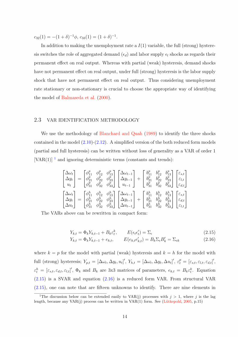
2.3 VAR IDENTIFICATION METHODOLOGY

We use the methodology of Blanchard and Quah (1989) to identify the three shocks

contained in the model (2.10)-(2.12). A simplified version of the both reduced form models

(partial and full hysteresis) can be written without loss of generality as a VAR of order 1

[VAR(1)] 1 and ignoring deterministic terms (constants and trends):

∆ωt∆ytut

=

φp11 φp12 φp13φp21 φp22 φp23φp31 φp32 φp33

∆ωt−1∆yt−1ut−1

+

bp11 bp12 bp13bp21 bp22 bp23bp31 bp32 bp33

εs,tεl,tεd,t

∆ωt

∆yt∆ut

=

φh11 φh12 φh13φh21 φh22 φh23φh31 φh32 φh33

∆ωt−1∆yt−1∆ut−1

+

bh11 bh12 bh13bh21 bh22 bh23bh31 bh32 bh33

εs,tεd,tεl,t

The VARs above can be rewritten in compact form:

Yk,t = ΦkYk,t−1 +Bkεkt , E(εtε

′t) = Σε (2.15)

Yk,t = ΦkYk,t−1 + ek,t, E(ek,te′k,t) = BkΣεB

′k = Σek (2.16)

where k = p for the model with partial (weak) hysteresis and k = h for the model with

full (strong) hysteresis; Yp,t = [∆ωt,∆yt, ut]′, Yh,t = [∆ωt,∆yt,∆ut]

′, εpt = [εs,t, εl,t, εd,t]′,

εht = [εs,t, εd,t, εl,t]′, Φk and Bk are 3x3 matrices of parameters, ek,t = Bkε

kt . Equation

(2.15) is a SVAR and equation (2.16) is a reduced form VAR. From structural VAR

(2.15), one can note that are fifteen unknowns to identify. There are nine elements in

1The discussion below can be extended easily to VAR(j) processes with j > 1, where j is the laglength, because any VAR(j) process can be written in VAR(1) form. See (Lutkepohl, 2005, p.15)

14

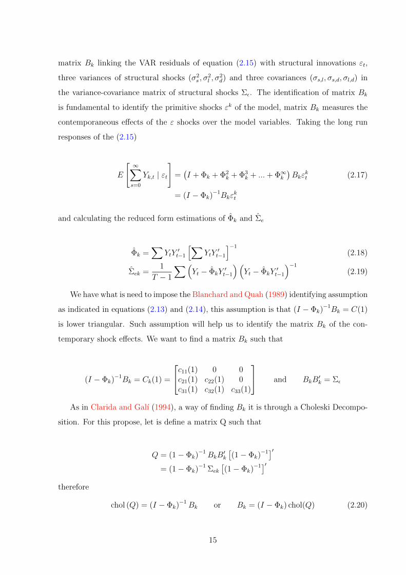
matrix Bk linking the VAR residuals of equation (2.15) with structural innovations εt,

three variances of structural shocks (σ2s , σ

2l , σ

2d) and three covariances (σs,l, σs,d, σl,d) in

the variance-covariance matrix of structural shocks Σε. The identification of matrix Bk

is fundamental to identify the primitive shocks εk of the model, matrix Bk measures the

contemporaneous effects of the ε shocks over the model variables. Taking the long run

responses of the (2.15)

E

[∞∑s=0

Yk,t | εt

]=(I + Φk + Φ2

k + Φ3k + ...+ Φ∞k

)Bkε

kt (2.17)

= (I − Φk)−1Bkε

kt

and calculating the reduced form estimations of Φk and Σe

Φk =∑

YtY′t−1

[∑YtY

′t−1

]−1(2.18)

Σek =1

T − 1

∑(Yt − ΦkY

′t−1

)(Yt − ΦkY

′t−1

)−1(2.19)

We have what is need to impose the Blanchard and Quah (1989) identifying assumption

as indicated in equations (2.13) and (2.14), this assumption is that (I − Φk)−1Bk = C(1)

is lower triangular. Such assumption will help us to identify the matrix Bk of the con-

temporary shock effects. We want to find a matrix Bk such that

(I − Φk)−1Bk = Ck(1) =

c11(1) 0 0c21(1) c22(1) 0c31(1) c32(1) c33(1)

and BkB′k = Σε

As in Clarida and Galı (1994), a way of finding Bk it is through a Choleski Decompo-

sition. For this propose, let is define a matrix Q such that

Q = (1− Φk)−1BkB

′k

[(1− Φk)

−1]′= (1− Φk)

−1 Σek

[(1− Φk)

−1]′therefore

chol (Q) = (I − Φk)−1Bk or Bk = (I − Φk) chol(Q) (2.20)

15

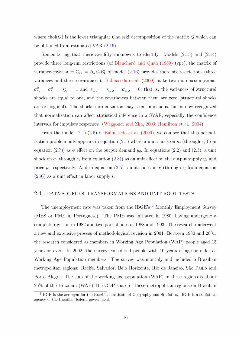
where chol(Q) is the lower triangular Choleski decomposition of the matrix Q which can

be obtained from estimated VAR (2.16).

Remembering that there are fifty unknowns to identify. Models (2.13) and (2.14)

provide three long-run restrictions (of Blanchard and Quah (1989) type), the matrix of

variance-covariance Σek = BkΣεB′k of model (2.16) provides more six restrictions (three

variances and three covariances). Balmaseda et al. (2000) make two more assumptions:

σ2εs = σ2

εl= σ2

εd= 1 and σεs,l = σεs,d = σεl,d = 0, that is, the variances of structural

shocks are equal to one, and the covariances between them are zero (structural shocks

are orthogonal). The shocks normalization may seem innocuous, but is now recognized

that normalization can affect statistical inference in a SVAR, especially the confidence

intervals for impulses responses. (Waggoner and Zha, 2003; Hamilton et al., 2004).

From the model (2.1)-(2.5) of Balmaseda et al. (2000), we can see that this normal-

ization problem only appears in equation (2.1) where a unit shock on m (through εd from

equation (2.7)) as φ effect on the output demand yd. In equations (2.2) and (2.3), a unit

shock on a (through εs from equation (2.8)) as an unit effect on the output supply yd and

price p, respectively. And in equation (2.5) a unit shock in χ (through εl from equation

(2.9)) as a unit effect in labor supply l.

2.4 DATA SOURCES, TRANSFORMATIONS AND UNIT ROOT TESTS

The unemployment rate was taken from the IBGE’s 2 Monthly Employment Survey

(MES or PME in Portuguese). The PME was initiated in 1980, having undergone a

complete revision in 1982 and two partial ones in 1988 and 1993. The research underwent

a new and extensive process of methodological revision in 2001. Between 1980 and 2001,

the research considered as members in Working Age Population (WAP) people aged 15

years or over. In 2002, the survey considered people with 10 years of age or older as

Working Age Population members. The survey was monthly and included 6 Brazilian

metropolitan regions: Recife, Salvador, Belo Horizonte, Rio de Janeiro, Sao Paulo and

Porto Alegre. The sum of the working age population (WAP) in these regions is about

25% of the Brazilian (WAP).The GDP share of these metropolitan regions on Brazilian

2IBGE is the acronym for the Brazilian Institute of Geography and Statistics. IBGE is a statisticalagency of the Brazilian federal government.

16

GDP was about 33% at the end of the 2000s, i.e., these metropolitan regions produce

about one-third of Brazil’s GDP and employ about a quarter of Brazilian (WAP). The

(PME) was closed in February 2016 to be replaced by the Continuous National Household

Sample Survey (Continuous NHSS or PNAD Contınua in Portuguese). The PNAD is also

carried out by the IBGE foundation.

12000

14000

16000

18000

20000

22000

24000

26000

1980q1 1985q1 1990q1 1995q1 2000q1 2005q1 2010q1 2015q1

Labor force old methodology

(thousands)

Labor force new methodology

(thousands)

2

4

6

8

10

12

14

1980q1 1985q1 1990q1 1995q1 2000q1 2005q1 2010q1 2015q1

Unemployment rate old

methodology (%)

Unemployment rate new

methodology (%)

12000

14000

16000

18000

20000

22000

24000

26000

1980q1 1985q1 1990q1 1995q1 2000q1 2005q1 2010q1 2015q1

Employment old methodology

(thousands)

Employment new methodology

(thousands)

2

4

6

8

10

12

14

1980q1 1985q1 1990q1 1995q1 2000q1 2005q1 2010q1 2015q1

Chained unemployment rate (%)

10000

12000

14000

16000

18000

20000

22000

24000

26000

1980q1 1985q1 1990q1 1995q1 2000q1 2005q1 2010q1 2015q1

Chained labor force

(thousands)

Chained employment

(thousands)

40

60

80

100

120

140

160

180

200

1980q1 1985q1 1990q1 1995q1 2000q1 2005q1 2010q1 2015q1

real wage (average 1995 = 100)

real GDP (average 1995 = 100)

Panel A Panel B

Panel C Panel D

Panel E Panel F

FIGURE 2.1 – LABOR FORCE, EMPLOYMENT, UNEMPLOYMENT RATE, REAL GDPAND REAL WAGE IN BRAZIL - 1980Q1 - 2015Q4

NOTE: Seasonally adjusted series (X-13 ARIMA)SOURCE: IBGE Foundation

The labor and employment data of the PME are plotted by the old and new methodol-

ogy in (FIGURE 2.1, PANEL A and C), which were aggregated for the quarterly frequency

by averaging the months within each quarter. On the other hand, the unemployment rate

by the old methodology did not have a break in 1991. The unemployment measured by

the old methodology has a lower level compared to the unemployment measured by the

17

new methodology. Part of this difference can be explained by the higher Working Age

Population considered in the new methodology (people 10 years of age or older). The

unemployment rate data by the old and new PME methodology are plotted in (FIGURE

2.1, PANEL B). To construct our database, we chain the data from the PMEs and correct

a level break in the labor force and employment variables that occurred in 1991 due to

sample modifications of the survey. Chained Labor force and employment data are in

(FIGURE 2.1, PANEL E). Labor force and employment appear to move closely at high

frequencies, but they began to move sharply in the early 1990s and then re-approximated

in the mid-2000s. Chained Unemployment rate seasonally adjusted data are shown in

(FIGURE 2.1, PANEL D).

The values of nominal wages were also taken from IBGE’s PME and chained between

the old and new methodologies to obtain a continuous series of nominal wages covering

the entire period 1982Q3-2015Q4. Then the chained series of nominal wages was deflated

by a consumer price index (INPC from IBGE) to create a series of real wages covering the

period 1982Q3-2015Q4. Real GDP values were also taken from IBGE and were divided

by a series of population to generate the real GDP per capita. In order to obtain a

population series in the quarterly frequency a cubic interpolation method was applied on

the decennial series of population from the Brazilian National Census (data also taken

from IBGE). The graph with the series of real GDP per capita and real wage is shown in

(FIGURE 2.1, PANEL F).

Before estimate the model itself, we apply unit root tests on the three modeled vari-

ables [log of real wage (ω), log of per capita GDP (y) and unemployment rate (u)]. The

unit root tests of DF-GLS and PP in (TABLE 2.1) state that the three variables have a

unit root with significance above 10%, which is in accordance with the consensus on these

variables in the Brazilian economic literature. In the KPSS test on the unemployment

rate one can not reject the null hypothesis of stationarity at 5% of significance, although

this result is not corroborated by the DF-GLS and PP tests, and therefore is not robust.

In the language we are using, the unemployment rate has total hysteresis (strong) ac-

cording to the DF-GLS and PP tests, but on the other hand the unemployment rate has

partial (weak) hysteresis according to the KPSS tests.

18

TABLE 2.1 – UNIT-ROOT TESTS (LOG REAL GDP, LOG REAL WAGE, UNEMPLOY-MENT RATE): 1980Q1-2015Q4

Dickey-Fuller GLS1 (DF-GLS) test

Variable Sample size Constant Trend Lags Test ratio p-value

Log real wage (ω) 131 yes yes 2 -2.2373 0.2436Log real GDP (y) 143 yes yes 0 -1.7699 0.4932Unemployment rate (u) 142 yes no 1 -1.5495 0.1525

Phillips-Perron1 (PP) test


Log real wage (ω) 133 yes yes - -2.9848 0.1404Log real GDP (y) 146 yes yes - -2.7482 0.2192Unemployment rate (u) 143 yes no - -1.4108 0.5755

KPSS2 test


Log real wage (ω) 134 yes yes 2 0.1483 0.0500Log real GDP (y) 147 yes yes 0 1.4577 0.0000Unemployment rate (u) 144 yes no 1 2.6901 0.0000

NOTES: (1) In the tests of Dickey-Fuller GLS and Phillips-Perron the null hypothesis is of unitroot presence. (2) In the KPSS test the null hypothesis is of unit root absence.SOURCE: Calculations made by the Eviews econometric software.

2.5 MODEL ESTIMATION AND RESULTS

Instead of applying a low power univariate unit root test to check if u is a stationary

variable, Balmaseda et al. (2000) use Johansen (1995) cointegration approach which has

more power due to the use of covariates. It is well known that if we have n variables,

there may be at least r ≤ n−1 cointegration vectors. In the model under analysis, n = 3,

and r = 0, or r = 1, or r = 2. In order to apply the Johansen procedure, it is necessary

to write the models (2.15) and (2.16) in form of a error correction model (ECM), without

loss of generality we write a ECM(1) that is the ECM of a VAR(2):

19

∆ωt∆yt∆ut

=

δ10 δ11δ20 δ21δ30 δ31

[1t

]+

α11 α12

α21 α22

α31 α32

[µ10 µ11 β11 β21 β31µ20 µ21 β12 β22 β32

]1t

ωt−1yt−1ut−1

+

λ11 λ12 λ13λ21 λ22 λ23λ31 λ32 λ33


+

ew,tey,teu,t

the above system can be rewritten in compact form

∆Xt = δ0 + δ1t+ α{µ0 + µ1t+ [β′1, β

′2]′Xt−1

}+ Λ∆Xt−1 + et (2.21)

where Xt = [ωt, yt, ut]′; δ0 = [δ10, δ20, δ30]

′ is a vector of unrestricted constants; δ1 =

[δ11, δ21, δ31]′ is a vector of unrestricted trend coefficients; µ0 = [µ10, µ20]

′ is a vector of

restricted constants; µ1 = [µ11, µ21]′ is a vector of restricted trend coefficients; α = [α1, α2]

is a matrix with the vectors of adjustment α1 and α2, with α1 = [α11, α21, α31]′ and

α2 = [α12, α22, α32]′; β = [β1, β2] is a matrix with the cointegration vectors β1 and β2,

with β1 = [β11, β21, β31]′ and β2 = [β12, β22, β32]

′; and et = [ew,t, ey,t, eu,t].

Balmaseda et al. (2000) propose the following scheme to test the unit root hypothesis

on the unemployment rate. If one models a VAR in levels including (ω, y, u) and an

unrestricted linear trend (time) and one can not reject the null hypothesis that r = 1

while the null hypothesis of r = 0 is rejected, and additionally one can not reject the

hypothesis that the cointegration vector is β1 = (0, 0, 1), this will mean that u is a

I(0) variable while ω and y are I(1) processes without cointegration between the three

variables. In this case the model (2.13) specification with partial (weak) hysteresis is

the appropriate specification. On the other hand, if the null hypothesis of presence of

at least one cointegration vector r = 1 is rejected, or if it is not rejected, but the null

hypothesis that the cointegration vector is β1 = (0, 0, 1) is rejected, then the appropriate

specification is (2.14) which describes the model with total (strong) hysteresis. For a

better understanding of what the constraint on the β1 cointegration vector implies, we

will write the ECM (2.21) with this constraint:

20

∆ωt∆yt∆ut

=

δ10 δ11δ20 δ21δ30 δ31

[1t

]+

α11

α21

α31

[0 0 1] ωt−1yt−1

ut−1

+

λ11 λ12 λ13λ21 λ22 λ23λ31 λ32 λ33


+

ew,tey,teu,t

the system above can be rewritten in separated equations:

∆ωt = δ10 + δ11t+ λ11∆ωt−1 + λ12∆yt−1 + (α11 + λ13)ut−1 − λ13ut−2∆yt = δ20 + δ21t+ λ21∆ωt−1 + λ22∆yt−1 + (α21 + λ23)ut−1 − λ23ut−2ut = δ30 + δ31t+ λ31∆ωt−1 + λ32∆yt−1 + (α31 + λ33)ut−1 − λ33ut−2

The system of equations above describe a common VAR and not an ECM, note that

the unemployment rate in this system is represented in levels, which is compatible with

the partial (full) hysteresis model (2.13).

2.5.1 Cointegration tests

The sample we considered in the model estimation covers the period 1982Q3-2015Q4.

The Brazilian economy underwent several transformations and economic policy regimes

in this period. To account for these transformations we estimate four models within this

period (1982-2015). The first estimated model covers the full sample (1982Q3-2015Q4).

The second model covers the ante Real Plan period (1982Q3-1994Q2). The third model

covers the Post-Real Plan period (1994Q3-2015Q4). And, finally, the fourth model covers

the Inflation Targeting Regime (1999Q1-2015Q4).

Between 1980 and 1994, the Brazilian economy alternated periods of very high in-

flation with times of hyperinflation. In 1994 the government implemented an inflation

stabilization plan called “Plano Real” (Real Plan). This plan consisted in exchange the

old currency (Cruzeiro) for a new called Real. This exchange was made in a gradual way

in order to deindex the economy. The currency was changed in July 1994. Months later,

the Real Plan also adopted a Crawling Peg regime in relation to the US dollar exchange

rate.

21

TABLE 2.2 – P-VALUES OF THE JOHANSEN COINTEGRATION TESTS: 1982Q3-2015Q4

Johansen Test 1982Q3 – 2015Q4 - full periodLags = 5 (lags of first differences in cointegration equation)

NoConstant

RestrictConstant

UnrestrictedConstant

RestrictTrend

UnrestrictedTrend

order Trace Lmax Trace Lmax Trace Lmax Trace Lmax Trace Lmax

0 0.00 0.00 0.01 0.01 0.42 0.38 0.16 0.25 0.05 0.211 0.33 0.27 0.39 0.28 0.67 0.78 0.39 0.27 0.11 0.222 0.75 0.75 0.77 0.77 0.22 0.22 0.80 0.80 0.06 0.06

c. vectors 1 1 1 1 0 0 0 0 1 0

Johansen Test 1982Q3 – 1994Q3 – Ante Real PlanLags = 0 (lags of first differences in cointegration equation)

NoConstant

RestrictConstant

UnrestrictConstant

RestrictTrend

UnrestrictTrend

order Trace Lmax Trace Lmax Trace Lmax Traco Lmax Trace Lmax

0 0.57 0.84 0.73 0.66 0.71 0.59 0.27 0.24 0.07 0.171 0.33 0.37 0.82 0.77 0.87 0.90 0.60 0.48 0.21 0.352 0.33 0.33 0.80 0.80 0.36 0.36 0.82 0.82 0.08 0.08

c. vectors 0 0 0 0 0 0 0 0 1 0

Johansen Test 1994Q4 – 2015Q4 - Post Real PlanLags = 1 (lags of first differences in cointegration equation)

NoConstant

RestrictConstant


RestrictTrend

UnrestrictedTrend


0 0.00 0.04 0.00 0.00 0.00 0.00 0.00 0.00 0.00 0.001 0.02 0.02 0.02 0.02 0.48 0.62 0.29 0.30 0.07 0.212 0.37 0.37 0.27 0.27 0.16 0.16 0.53 0.53 0.03 0.03

c. vectors 2 2 2 2 1 1 1 1 3 1

Johansen Test 1999Q1 – 2015Q4 – Inflation TargetingLags = 1 (lags of first differences in cointegration equation)

NoConstant

RestrictConstant


RestrictTrend

UnrestrictedTrend


0 0.00 0.01 0.01 0.04 0.06 0.05 0.09 0.18 0.30 0.571 0.04 0.16 0.09 0.13 0.47 0.67 0.30 0.30 0.28 0.442 0.03 0.03 0.28 0.28 0.12 0.12 0.54 0.54 0.09 0.09

c. vectors 3 1 2 1 1 1 1 0 0 0

SOURCE: Calculations made by the Eviews econometric software.

Foreign currency crises that affected emerging countries in the late of 1990s (Asian

countries, Russia and even Brazil) forced the Brazilian authorities to abandon the Crawl-

ing Peg regime in favor of a Inflation Targeting with floating exchange rate and primary

22

surplus targets for government accounts. This so-called tripod regime (Inflation Target-

ing, Floating Exchange Rate and Primary Surplus Targeting) has been adopted up to

now by the Brazilian authorities. In (TABLE 2.2), we performed cointegration tests be-

tween the three variables - real wage (ω), real per capita GDP (y) and unemployment

rate (u) - for the four periods considered. In most of the results there is evidence of at

least one cointegration vector among the three variables in all periods considered, except

for the post Real Plan period (1994Q3-2015Q4) where the Johansen test identified three

(3) cointegration vectors at 5% of significance and one (1) cointegration vector at 1%

of significance both in the “Unrestricted Trend Case”. In the Inflation Targeting period

(1999Q1-2015Q4) in three cases (“No Constant”, “Restrict Constant”, and “Unrestricted

Constant”) the Johansen test identified two (2) cointegration vectors at 5% of significance.

Based on these results, we now test the constraint proposed by Balmaseda et al.

(2000) on the cointegration vector β1 of the unrestricted trend case. The unrestricted

trend case (or quadratic deterministic trend) is the fifth case of Johansen’s cointegration

schemes. Recalling that if the null hypothesis that the cointegration vector is β1 = (0, 0, 1)

is rejected, then the appropriate specification is (2.14) and the unemployment rate has

total (strong) hysteresis. On the other hand, if the null hypothesis that the cointegration

vector is β1 = (0, 0, 1) is not rejected, then the appropriate specification is (2.13) and

the unemployment rate has partial (weak) hysteresis. The constraints imposed on the

cointegration vector β1 are tested and the results are shown in (TABLE 2.3).

TABLE 2.3 – TESTS ON THE VECTOR β1 RESTRICTIONS

Cointegration case: 5 - unrestricted trend (quadratic deterministic trend)Null Hypothesis β1 = (0, 0, 1)

Period Range Lags Obs. χ2(2) p-value

Full period 1982Q3-2015Q4 5 128 13.0284 0.0015Ante Real Plan 1982Q3-1994Q2 0 47 16.7390 0.0002Post Real Plan 1994Q4-2015Q4 3 82 20.5948 0.0000Inflation Targeting 1999Q1-2015Q4 0 67 40.4416 0.0000

SOURCE: Calculations made by the Eviews econometric software.

According to the tests results shown in (TABLE 2.3), we can not reject the hypothesis

that Brazilian unemployment rate measured by PME has a unit root in all the four periods

analyzed. Thus, we can not reject the hypothesis that Brazilian unemployment rate shows

23

TABLE 2.4 – VAR MODELS ESTIMATED FOR THE MODELS “FULL PERIOD (1982Q3-2015Q4)” AND “BEFORE REAL PLAN (1982Q3-1994Q2)

1982Q3-2015Q4Full Period (Lags = 5)1,2,3

1982Q3-1994Q2Before Real Plan (Lags = 5)1,2,3

∆ωt ∆yt ∆ut ∆ωt ∆yt ∆utconst. −1.195

(−2.30)∗∗0.668

(4.07)∗∗∗0.093

(2.31)∗∗∗−2.193(−1.83)∗∗

−(−)

0.078(1.20)

∆ωt−1 −(−)

−(−)

−0.009(−1.68)∗

0.200(1.78)∗

−(−)

−(−)

∆yt−1 0.519(2.20)∗∗

−(−)

−0.070(−3.99)∗∗∗

−(−)

−(−)

−(−)

∆ut−1 −(−)

−0.677(−1.92)∗

0.145(1.67)∗

−(−)

−(−)

0.464(5.82)∗∗∗

∆ωt−2 −0.239(−3.03)∗∗∗

−(−)

0.010(1.92)∗

−0.419(−3.19)∗∗∗

−(−)

0.012(2.46)∗∗

∆yt−2 0.840(3.4)∗∗∗

−(−)

−0.035(−2.01)∗∗

−(−)

−(−)

−0.065(−4.22)∗∗∗

∆ut−2 −(−)

−(−)

−(−)

−8.414(−3.37)∗∗∗

−(−)

−0.530(−5.19)∗∗∗

∆ωt−3 −(−)

−(−)

−(−)

−0.018(−4.14)∗∗∗

−(−)

−0.018(−4.14)∗∗∗

∆yt−3 −(−)

−0.186(−2.57)∗∗∗

−(−)

−(−)

−(−)

−(−)

∆ut−3 −(−)

−(−)

−(−)

−(−)

−(−)

0.391(4.74)∗∗∗

∆ωt−4 −(−)

−0.077(−2.93)∗∗∗

0.022(3.74)∗∗∗

−(−)

−0.091(−2.31)∗∗

0.030(5.34)∗∗∗

∆yt−4 −(−)

−(−)

−0.044(−2.73)∗∗∗

−1.241(−3.49)∗∗∗

−(−)

−(−)

∆ut−4 −(−)

−(−)

−(−)

−(−)

−(−)

−(−)

∆ωt−5 −(−)

0.079(3.28)∗∗∗

−(−)

−0.232(−2.10)∗∗

−(−)

−(−)

∆yt−5 0.760(3.12)∗∗∗

0.163(1.91)∗

−0.041(−2.13)∗∗

1.082(2.99)∗∗∗

0.317(3.25)∗∗∗

v−(−)

∆ut−5 −(−)

−(−)

−0.199(−2.73)∗∗∗

−(−)

−(−)

−(−)

LM test forautocorrelation

lags = 5; df = 45;t. st. = 34.66; pval. = 0.87

lags = 5; df = 45;t. st. = 45.31; pval. = 0.46

MultivariateARCH LM test

lags = 5; df = 180;t. st. = 220; pval = 0.02

lags = 5; df = 180;t. st. = 187; pval. = 0.34

Test for nonormality

Doornik and Hansen (1994)t. st. = 196; pval. = 0.0000

Doornik and Hansen (1994)t. st. = 2.36; pval. = 0.88

Identified longrun impactmatrix4

∣∣∣∣∣∣∣∣∣5.584[0.981]

0.000[0.000]

0.000[0.000]

1.402[0.404]

1.252[0.193]

0.000[0.000]

−0.283[0.113]

−0.347[0,072]

0.259[0.035]

∣∣∣∣∣∣∣∣∣

∣∣∣∣∣∣∣∣∣∣5.751[1.205]

0.000[0.000]

0.000[0.000]

1.293[0.745]

2, 354[0.551]

0.000[0.000]

−0.335[0.148]

−0.331[0.105]

0.218[0.049]

∣∣∣∣∣∣∣∣∣∣SOURCE: VAR models calculated by the JMulTi times series software (Lutkepohl and Kratzig, 2004).NOTES: (1) Lags selected by the Akaike criterion. (2) No significant lags were excluded from the model(considering a t-value of |1.62| as threshold) through the “system down procedure” function availablein the JMulti software and explained in (Lutkepohl and Kratzig, 2004). (3) Calculated t-values are inparenthesis “(...)”, superscript (***) means significance at 1%, (**) means significance at 5% and (*)means significance at 10% . (4) Values in brackets “[...]” indicates bootstrap standard errors.

24

total (strong) hysteresis, and therefore the appropriate model to estimate the effects of

productivity (εs), demand (εd) and labor supply (εl) shocks on the modeled variables (ω,

y and u) is the model (2.14).

We estimated the four VAR models using the JMulti time series software (Lutkepohl

and Kratzig, 2004). In (TABLE 2.4) we show the models estimated for the “full period”

(1982Q3-2015Q4) and for the “before Real Plan” (1982Q3-1994Q2). Five lags selected

by the Akaike criterion were used in both models. Non-significant lags were excluded

from the model (considering a t-value of |1.62| as threshold) through the “system down

procedure” function available in the JMulti software and explained in (Lutkepohl and

Kratzig, 2004). In (TABLE 2.5) we show the models estimated for the “after Real Plan”

period (1994Q3-2015Q4) and for “Inflation Targeting” period (1999Q1-2015Q4). The two

models of (TABLE 2.5) were estimated with one lag selected by the Akaike criterion.

TABLE 2.5 – VAR MODELS ESTIMATED FOR THE MODELS “AFTER REAL PLAN”(1994Q3-2015Q4) AND “INFLATION TARGETING” (1999Q1-2015Q4)

1994Q3-2015Q4After Real Plan (Lags = 1)1,2

1999Q1-2015Q4Inflation Targeting (Lags = 1)1,2

∆ωt ∆yt ∆ut ∆ωt ∆yt ∆utconst. −0.069

(−0.29)0.406

(2.62)∗∗∗0.077(1.88)∗

−0.158(−0.68)

0.403(2.55)∗∗∗

0.058(1.37)

∆ωt−1 0.142(1.85)∗

0.083(1.62)∗

−0.013(−0.94)

0.304(2.60)∗∗∗

0.095(1.20)

−0.045(−2.12)∗∗

∆yt−1 0.293(1.71)∗

0.267(2.35)∗∗

−0.135(−4.51)∗∗∗

0.209(1.09)

0.372(2.85)∗∗∗

−0.176(−5.00)∗∗∗

∆ut−1 −0.646(−1.15)

0.173(0.47)

0.206(2.10)∗∗

−0.359(−0.60)

−0.136(−0.33)

0.113(1.02)

LM test forautocorrelation

lags = 5; df = 45;t. st. = 65.04; pval. = 0.03

lags = 5; df = 45;t. st. = 52.94; pval. = 0.19

MultivariateARCH LM

lags = 5; df = 180;t. st. = 165; pvalue = 0.78

lags = 5; df = 180;t. st. = 186; pval. = 0.36

Test fornonormality



Identified longrun impactmatrix3

∣∣∣∣∣∣∣∣∣2.576[0.405]

0.000[0.000]

0.000[0.000]

0.840[0.383]

1.522[0.253]

0.000[0.000]

−0.300[0.138]

−0.379[0.107]

0.386[0.057]

∣∣∣∣∣∣∣∣∣

∣∣∣∣∣∣∣∣∣2.830[0.676]

0.000[0.000]

0.000[0.000]

1.216[0.645]

1.723[0.412]

0.000[0.000]

−0.473[0.212]

−0.426[0.133]

0.316[0.046]

∣∣∣∣∣∣∣∣∣SOURCE: VAR models estimated by the JMulTi software (Lutkepohl and Kratzig, 2004).NOTES: (1) Lags selected by the Akaike criterion. (2) Calculated t-values are in parenthesis “(...)”,superscript (***) means significance at 1%, (**) means significance at 5% and (*) means significance at10% . (3) Values in brackets “[...]” indicates bootstrap standard errors.

25

2.5.2 Impulse Responses

In (FIGURE 2.2) the model three variables impulse response functions are shown

in relation to the three identified shocks: productivity, demand and labor supply. In

general, the real wage responses to the three shocks appears to be satisfactory. The real

wage responds pro-cyclically to (positive) shocks of productivity and labor supply, while

responds counter-cyclically to a (positive) shock of demand. This countercyclical response

FIGURE 2.2 – ACCUMULATED IMPULSE RESPONSES (IN %) - FULL PERIOD1982Q3-2015Q4

NOTE: Dashed lines depict approximate 90% confidence intervals computed using 10,000bootstrap replications according to method of Efron (1979).SOURCE: VAR model and impulse responses calculated by the JMulTi times series software(Lutkepohl and Kratzig, 2004).

of real wages also occurs in continental Europe, while wages in the United States appear

to react pro-cyclically to demand shocks (Balmaseda et al., 2000). The real wage response

to a labor supply shock seems to be non-significant (confidence interval passes over the

zero axis). Continuing in (FIGURE 2.2), the three shocks on real per capita GDP have

26

the expected shapes although the labor supply shock on per capita output appears to be

non-significant (confidence interval passes over the zero axis). GDP per capita responds

pro-cyclically to the three shocks. Still in (FIGURE 2.2), unemployment rate responses

to the three shocks have the expected shapes. Unemployment rate responds counter-

cyclically to shocks of productivity and demand, and reacts in a pro-cyclical way to labor

supply shocks.

FIGURE 2.3 – ACCUMULATED IMPULSE RESPONSES (IN %) - BEFORE REAL PLAN1982Q3-1994Q2


The long-run (accumulated) response of unemployment rate to a productivity shock

(of one standard deviation) is about -0.23%, while the long-run response of unemployment

rate to a demand shock (of one deviation Standard) is about -0.35%. These two long-run

multipliers can be identified as coefficients of a modified “Okun” (Okun, 1962) relationship

that separates supply from demand shocks.

27

In (FIGURE 2.3) impulse responses generated by the model “before Real Plan” are

shown. Variables reactions to the shocks have expected shape and are similar to those

responses of the full period model (1982Q3-2015Q4, FIGURE 2.2). It should be noted

that in the model “before Real Plan”, the real wage response to a (positive) demand

shock is not significant at 10% of significance (confidence interval passes over the zero

axis), although it has the countercyclical response as expected. How occurs in the full

period model (1982Q3-2015Q4, FIGURE 2.2), the real wage and real GDP per capita

FIGURE 2.4 – ACCUMULATED IMPULSE RESPONSES (IN %) - AFTER REAL PLAN1994Q3-2015Q4


responses to a (positive) labor supply shock are not significant at 10% level of significance

(confidence interval passes over the zero axis).

In (FIGURE 2.4) we show the impulse responses of the “after Real Plan” model

(1994Q3-2015Q4). Again, responses have the shapes as expected. Comparing with the

28

full period model (1982Q3-2015Q4, FIGURE 2.2) and “before Real Plan” model (1982Q3-

1994Q2, FIGURE 2.3), one can note that the short and long-run impacts of supply shocks

on real wages and on real GDP per capita falls by about one half. Like occurs in the two

previous models (FIGURES 2.2 and FIGURE 2.3), the real wage and real GDP per capita

responses to a (positive) labor supply shock are not significant at 10 % level of significance

axis) in the “after Real Plan” model (1994Q3-2015Q4, FIGURE 2.3).

FIGURE 2.5 – ACCUMULATED IMPULSE RESPONSES (IN %) - INFLATIONTARGETING 1999Q1-2015Q4


Finally, in (FIGURE 2.5), we have the inflation target model (1999Q1-2015Q4) im-

pulse responses. The graphics are similar to what occurs in the “after Real Plan” model

with the expected shapes. But in this Inflation Targeting period (1999Q1-2015Q4), we see

that the long-run real GDP per capita response to a (positive) productivity shock is twice

that of the “after Real Plan” model (1994Q3-2015Q4) one (1.33% vs. 0.62%) and equal

29

to what occurs in the “full period” model (1982Q3-2015Q4). It is also seen that in this

period (1999Q1-2015Q4), the long-run response of the unemployment rate to a (positive)

productivity shock is twice that of the “after Real Plan” model (1994Q3-2015Q4) and

“full period” model (1982Q3-2015Q4) ones (respectively -0.23% and -0.27 % vs. -0.50%).

2.5.3 Variance Decomposition

Analyzing the forecast errors variance decomposition (FEVD) in (TABLE 2.6), for real

wages, productivity shocks dominate the (FEVD) in the short and long-run in the four

models considered, although the models ”Full period” ( 1982Q3-2015Q4) and ”before Real

Plan” (1982Q3-1994Q2) the share of long-run (FEVD) explained by productivity shocks

is lower while demand shocks increase their share. In the real output case, demand shocks

dominate short and long-run (FEVD) in the models “before Real Plan” (1982Q3-1994Q2),

“after Real Plan” (1994Q3-2015Q4) and “Inflation Targeting” (1999Q1- 2015Q4), al-

though this dominance is slight in the ”before real Plan” model (1982Q3-1994Q2). In the

”Full period” model (1982Q3-2015Q4), productivity shocks dominate (FEVD) slightly.

The period covered by the “before Real Plan” model (1982Q3-1994Q2) was marked

by very high inflation (with episodes of hyperinflation) and many nominal shocks from

the external sector and government budget. This combination of nominal shocks can be

responsible for this share difference in productivity and demand shocks in explaining the

real wage and output (FEVD’s) when one compares the models ”Full Period” and ”before

Real Plan” with the other two models.

In the case of our main focus of interest, the unemployment rate, except in the “before

Real Plan” model (1982Q3-1994Q2), labor-supply shocks dominate the short and long-run

(FEVD). In relation to demand shocks, these explain between 5% and 8% of the (FEVD)

at one quarter horizon in all models, except for the “Full Period” model (1982Q3-2015Q4)

where the percentage is 14%; in the long-run demand shocks explain between 19% and

26% of (FEVD) in all models. With regard to productivity shocks, these explain about

75% of the (before Real Plan) model (1982Q3-1994Q2) (FEVD) at one quarter horizon

and only 7% in the “after Real Plan” model (1994Q3 -2015Q4). In the ”Full Period”

model (FEVD), productivity shocks account for about 23% of (FEVD) at one quarter

horizon. In the infinite (long-run) horizon, productivity shocks account for about 59% of

30

TABLE 2.6 – FORECAST ERROR VARIANCE DECOMPOSITION

Model Variable HorizonShocks type

productivity demand labor supply

Full period(1982Q3-2015Q4)

realwage

1 0.69 0.31 0.004 0.62 0.38 0.00∞ 0.60 0.39 0.01

real output(GDP)

1 0.58 0.41 0.014 0.57 0.40 0.03∞ 0.60 0.39 0.01

unemploy-ment rate

1 0.23 0.14 0.634 0.32 0.19 0.49∞ 0.31 0.23 0.46

Before Real Plan(1982Q3-1994Q2)

realwage

1 0.78 0.14 0.084 0.67 0.17 0.16∞ 0.54 0.27 0.19

real output(GDP)

1 0.43 0.57 0.004 0.43 0.57 0.00∞ 0.44 0.54 0.02

unemploy-ment rate

1 0.75 0.05 0.204 0.70 0.12 0.18∞ 0.59 0.19 0.22

After Real Plan(1994Q3-2015Q4)

realwage

1 0.85 0.13 0.024 0.82 0.15 0.03∞ 0.82 0.15 0.03

real output(GDP)

1 0.13 0.87 0.004 0.16 0.84 0.00∞ 0.16 0.84 0.00

unemploy-ment rate

1 0.08 0.08 0.844 0.14 0.26 0.60∞ 0.15 0.26 0.59

Inflation Targeting(1999Q1-2015Q4)

realwage

1 0.90 0.10 0.004 0.90 0.09 0.01∞ 0.90 0.09 0.01

real output(GDP)

1 0.15 0.85 0.004 0.22 0.78 0.00∞ 0.22 0.78 0.00

unemploy-ment rate

1 0.07 0.06 0.874 0.26 0.25 0.49∞ 0.27 0.26 0.47

SOURCE: VAR model and forecast variance error decomposition calculated by the JMulTi timesseries software (Lutkepohl and Kratzig, 2004).

the ”before Real Plan” model (FEVD), 30% in the “Inflation Targeting” model and only

13% in the ”after Real Plan” model (1994Q3-2015Q4).

These differences in the role of productivity shocks in explaining the unemployment

rate (FEVD) among the models are difficult to understand, a possible cause for such

31

differences may be the demographic transformation that Brazil has been experiencing since

the mid-1990s with a demographic pyramid flattening. This flattening implies more people

entering in the working age population. This demographic transformation may have

transferred from productivity to labor supply shocks a part of the Brazilian unemployment

rate (FEVD) explanation.

2.5.4 Measuring the Wage Rigidity

As a final exercise we compute a real wage rigidity index (RWR) from our estimated

models. As Balmaseda et al. (2000), we take the approach of Layard et al. (1991) to

compute a real wage rigidity index computed as the reciprocal of the real wage estimated

responses to the unemployment rate responses. In our estimated models, productivity

shock is the only one that have a permanent effect in real wages, so like in Balmaseda

et al. (2000), a possible definition of RWR is given by

RWR =

∣∣∣∣ limk→∞

∂∑∞

k=0 ∂∆ut+k/∂εs,t∂∑∞

k=0 ∂∆ωt+k/∂εs,t

∣∣∣∣ (2.22)

The interpretation of equation (2.22) is as follows: the larger the RWR value (in modulus),

the greater is the real wage rigidity. In (TABLE 2.7) are the RWR indexes calculated for

the four estimated models. The RWR index is larger in the “after Real Plan” model than

it is in the “before Real Plan” (0.12 vs 0.06 respectively). In the ”Inflation Targeting”

model, the RWR index is 0.17, a wage rigidity almost three times higher than that of

the ”before Real Plan” model (RWR = 0.06). One explanation for this different RWR

indexes would be that the inflation stabilization allowed the nominal wages setting for

longer periods, which increased the real wages rigidity.

TABLE 2.7 – REAL WAGE RIGIDITY (RWR) INDICES

Model RWR

“Full Period” (1982Q3-2015Q4) 0.05“Before Real Plan” (1982Q3-1994Q2) 0.06“After Real Plan” (1994Q3-2015Q4) 0.12“Inflation Targeting” (1999Q1-2015Q4) 0.17

32

2.6 CONCLUDING REMARKS

Analizing the Brazilian economy (1982Q3-2015Q4 period) in this paper, we have

showed evidences that the unemployment rate can be a I(1) variable and, therefore, fol-

low a full hysteresis process. In addition, we have presented empirical evidences about

dynamic responses of real wages, real output per capita and unemployment rate to three

identified shocks, which are productivity, demand and labor supply. To identify these

shocks, we have made use of restrictions stemming from a simple insider-outsider model

of the labor market proposed by Balmaseda et al. (2000).

This model allow us to recover the structural shocks (productivity, demand and labor

supply) through a recursive set of long-run restrictions on the long-run matrix of the

system multipliers [a type of Blanchard and Quah (1989) identification methodology]. As

the Brazilian economy underwent several transformations between 1980 e 2015, we split

our sample in three periods: “before Real Plan” (1982Q3-1994Q2), “After Real Plan”

(1994Q3-2015Q4) and “Inflation Targeting” (1999Q1-2015Q4).

Our many findings are: first, the Brazilian unemployment rate measured by IBGE’s

PME can be considered a process with full hysteresis (unemployment rate is a I(1) vari-

able) in all the sub-periods. Second, demand shocks play a similar role in explaining the

forecast error variance (FEV) of the unemployment rate in all sub-periods. Third, pro-

ductivity shocks was more important in explaining the (FEV) of the unemployment rate

in the “before Real Plan” period, while labor-supply shocks were more important in the

“after Real Plan” period. Third, real wages seemed be more flexible in the “before Real

Plan” period compared with subsequent periods, mainly compared with the “Inflation

Targeting” period.

33

3 HYSTERESIS IN A NEW KEYNESIAN DSGE

ABSTRACT

We expand the Galı (2011a,b) unemployment model to consider the hysteresis inunemployment rate hypothesis. With full hysteresis, the various shocks affecting theeconomy have a permanent effect on employment and unemployment rate. In an econ-omy of this type the unemployment rate do not tend to a certain mean or to a “naturalrate” of unemployment in the long-run. In this paper we insert hysteresis in the stan-dard New Keynesian Model and estimate two Bayesian DSGEs, one with hysteresis andother without hysteresis, and compare their behaviors in regard to impulse responses anddecomposition of forecast error variance.

3.1 INTRODUCTION

The behavior differences between the unemployment rates in Europe (and Latin Amer-

ica) and the United States since the 1980s began to draw the attention of economists.

Since the 1980s, unemployment rates in Europe and Latin America have been higher and

more persistent (with high autocorrelation) than those observed in the United States.

The term ”unemployment rate with hysteresis” was used to describe this phenomenon of

high and persistent unemployment rates observed in these places. There are three theories

that seek to explain the phenomenon of persistence in economic variables such as output

and unemployment. These theories are known as “physical capital”, “human capital” and

“insider-outsider” theories or hypothesis to explain the unemployment persistence.

“The physical capital story simply holds that reductions in the capital stock associated

with the reduced employment that accompanies adverse shocks reduce the subsequent

demand for labor and so cause protracted unemployment.” (Blanchard and Summers,

1986, p.27). A second theory or hypothesis to explain the unemployment persistence

is the “Human Capital” channel. According to this theory, proposed by Phelps (1972)

and Hargraves-Heap (1980) among others, prolonged unemployment can deteriorate the

accumulation of human capital by workers. As stated by Blanchard and Summers (1986),

“unemployed workers lose the opportunity to maintain and update their labor skills.”

34

Long lasting unemployment can also lead to a detachment from the labor market both

through a discouragement to job seeking or demolition of the individual’s social network,

leaving him increasingly isolated and away from the formal labor market. Another channel

that human capital could affect employability would be the preference of employers for

short term unemployed because they have their skills intact (Roberts and Morin, 1999).

Finally, insiders-outsiders models of labor market emphasize the market division be-

tween insiders and outsiders, and how insiders prevail in the process of wage determina-

tion. The seminal papers in this issue were Blanchard and Summers (1987), Gottfries

and Horn (1987) and Lindbeck and Snower (1985, 1988c). These authors emphasize an

asymmetry in the wage setting process, where outsiders are disregarded and insiders set

wages in view to preserve their own jobs. Recessions reduce the number of employees and,

in turn, reduces the number of insiders. This process can generate hysteresis in wages,

employment and unemployment rates.

In the last 10 years or so, many authors have expanded the New Keynesian model

into microfounded and estimated stochastic general equilibrium models (DSGE), exam-

ples of pioneers works are Smets and Wouters (2003, 2007), Dib (2003), Edge et al. (2005),

Fernandez-Villaverde and Rubio-Ramirez (2006), Fukac and Pagan (2006), among others.

Standard versions of New-Keynesian DSGE models abstract the unemployment rate and

only model worked hours varying in intensive margin, i.e., these models only consider the

variation of hours worked and not the total change of employed individuals (extensive

margin). Recently some models have explicitly included the unemployment rate in DSGE

models, as examples we have Gertler and Trigari (2009), Christoffel et al. (2009), Blan-

chard and Galı (2010), Christiano et al. (2010), Galı (2011a,b, 2015, 2016), Galı et al.

(2012), Liu (2014) and others.

As unemployment is included in the DSGE model varies from paper to paper. Gertler

and Trigari (2009), Christoffel et al. (2009), Christiano et al. (2010) and Blanchard and

Galı (2010) introduce the unemployment rate in the DSGE model through labor market

search and matching frictions a la Mortensen and Pissarides (1994). In these models

involuntary unemployment is due to the (inefficient) equilibrium of a search and matching

process. By other side, Galı (2011a,b) and Galı et al. (2012) reinterpret the standard New-

Keynesian model in terms of extensive margin (number of employees) and indivisible

35

work instead of intensive margin (hours worked). Interpreted in this way, according to

the authors, the standard New-Keynesian DSGE model would have an inherent theory

of unemployment. According to this theory, involuntary unemployment results from the

combination of imperfect substitution between the different types of labor with nominal

wage rigidity that give market power to occupations or unions to set wages above the

level of full employment (level of involuntary unemployment absence).

Galı (2015) expands the models in Galı (2011a,b) in order to consider the presence

of a unit root in unemployment rate. He considers three hypothesis: the natural rate

hypothesis, the log-run trade-off hypothesis and the hysteresis hypothesis. In the natural

rate hypothesis, Galı supposes that the natural wage markup follows a random walk.

In this way, the natural rate of unemployment also would be a random walk as well as

the unemployment rate. Under the long run trade-off hypothesis, the unit root in the

unemployment rate results from the presence of a unit root in the wage inflation since

both variables are linked through the wage Phillips Curve. In this case, unit root in wage

inflation is assumed to be inherited, in turn, from a unit root in the central bank inflation

target. Finally, in the hysteresis hypothesis, Galı adapt the insider-outsider model of

unemployment of Blanchard and Summers (1987) into the New Keynesian Model. He

concludes that none of the three hypothesis can, by itself, account for the evidence on

unemployment and wage inflation for the period 1970-2014 in Europe Union, though both

the long run trade-off and hysteresis hypothesis (insider-outsider model) can help interpret

certain aspects of the joint behavior of the unemployment rate and wage inflation.

Following the spirit of Galı (2015), our objective is introduce unemployment rate with

hysteresis into a small New Keynesian DSGE, but through a different mechanism. We sup-

pose that the labor supply path performs in a non-stationary way and is non-cointegrated

with the employment growth. This combination produce a New-Keynesian model with a

non-stationary unemployment rate, i.e., a unemployment rate with full (or strong) hys-

teresis. To demonstrate the implications of our hysteresis model, we estimated two small

Bayesian DSGEs with closed economy and no government applied to the Brazilian econ-

omy. One of them adopts the standard model of Galı (2011a,b) and Galı et al. (2012)

without hysteresis, while the other model adopts the hypothesis of unemployment rate

hysteresis according to the assumption of non-stationary labor supply path that we adopt.

36

Beyond this introduction, the remainder of this paper is structured as follows. Section

(3.2) presents the models with and without hysteresis; section (3.3) derives the relations

of consumption, labor-supply, wage-setting and unemployment; section (3.4) drives the

firms behavior in relation to output, hiring and prices setting; section (3.5) presents a

summary of both models; in section (3.6) we estimate both models applying Bayesian

techniques and analyze results like impulse response functions and forecast error variance

decompositions; finally section (3.7) concludes.

3.2 MODELS CHARACTERIZATION

It is assumed the existence of a large number of identical households, each of them

composed by a continuum of members. The family members are indexed by the pair i, j ∈

[0, 1]×[0, Nt(i)]. The index i represents the type of labor the household member is special-

ized. The j determines the labor disutility which is given by [(X1−σt θt)/(z

lϕt Ht

1+ϕ)]∫ Nt(i)0

jϕdj

if the individual is employed and zero if he is unemployed, Nt(i) =∫ Nt(i)0

jdj is the “effec-

tive” labor supply or employment of workers specialized in labor type i. Household utility

function is separable in consumption and labor and consumption is a CES aggregate of

various goods. Like Galı (2011a,b), we follow Hansen (1985) and Rogerson (1988) in as-

suming that labor is indivisible. Indivisible labor means that in each period an individual

works a fixed number of hours or does not work at all. As observed by (Galı, 2011b, p.

7), extensive margin variations (changes in employment) dominates the observed fluctu-

ations in total hours of work [product of intensive margin (hours) by extensive margin

(employment)]. So the assumption of indivisible labor can be a good approximation. We

also assume there is full risk sharing among workers. Full risk sharing in association with

separable preferences implies the same level of consumption to all individuals, employed

or not. This is a strong assumption, mainly from the welfare viewpoint, but it is useful

for simplify the model. We add external habits formation in consumption as a additional

model feature. The household i utility U in period t is given by:

37

U [C#t , Nt(i)] =

(C#t )1−σ

1− σ− X1−σ

t θt

(zlt)ϕH1+ϕt

∫ 1

0

∫ Nt(i)

0

jϕdjdi

=(C#

t )1−σ

1− σ− X1−σ

t θt

(zlt)ϕH1+ϕt

∫ 1

0

Nt(i)1+ϕ

1 + ϕdi (3.1)

where t is time in quarters; C#t = Ct−hCt−1, is the consumption adjusted by habits1 like

in Boldrin et al. (2001); Ct = [∫ 1

0Ct(v)(εp,t−1)/εp,tdi]εp,t/(εp,t−1) is a basket of differentiated

goods with elasticity of substitution (εp,t); h is the parameter measuring external habit

in consumption; σ is the inverse elasticity of intertemporal substitution of consumption;

Nt(i) is the “effective” labor supply or employment of workers specialized in labor type i;

ϕ is the Frisch inverse elasticity of labor supply in relation to the real wage (Frisch, 1932);

zlt is an exogenous preference shifter that decreases the disutility of labor and affects the

labor supply with zlt = (zl0)(1−ρl)(zlt−1)

ρleεlt , zl0 = 1, ρl ∈ [0, 1] and εlt ∼ i.i.d.(0, σ2

l ) is a

temporary labor supply shock; Xt is a variable which guarantees a balanced growth path

for the model and will be set soon; Ht = (Nt−1)dl(Ht−1)

(1−dl)egn,t is a variable governing

the labor growth rate, dl is a dummy variable that assumes the value zero (0) if the labor

supply is cointegrated with the employment in a such way that makes unemployment

rate stationary, or assumes the value one (1) if the labor supply is no cointegrated with

employment and therefore unemployment rate is not stationary, gn,t = (1 − ρn)gn +

ρngn,t−1 + εnt is the labor supply permanent growth where gn is the steady-state growth

rate of the labor supply and employment, ρn ∈ [0, 1] and εnt ∼ i.i.d.(0, σ2n) is a permanent

labor supply shock; θt is an endogenous preference shifter given by θt = (Zst /C

#t )σ and

Zst = (C#

t )γc(Zst−1)

1−γc .

It is assumed the representative household seeks to maximize the present value of

utility,

maxE0

∞∑k=0

βk

[(C#

t+k)1−σ

1− σ−

X1−σt+k θt+k

(zlt+k)ϕHt+k

1+ϕ

∫ 1

0

Nt+k(i)1+ϕ

1 + ϕdi

](3.2)

1According (Dennis, 2009, p. 1016): “Consumption habits have a long history in macroeconomics.Duesenberry (1949) argues that habit formation can arise through a desire to advance socially or toacquire high quality goods, desires prompted by the ‘...inferiority feelings that are aroused by unfavorablecomparisons between living standards.’ Similarly, Ryder and Heal (1973) argue that the ‘... satisfactionthat a man derives from consuming a given bundle of goods depends not only on that bundle, but also onhis past consumption and on his general social environment.’” (Dennis, 2009, p. 1016)

38

subject to a sequence of flow budget constraints given by

PtCt +P bt B

nt

zct≤ Bn

t−1 +W nt (i)Nt(i) + T nt

where the superscript n denotes nominal variables; Pt is the CPI index; P bt = 1/(1 + rt) is

the market price of government bonds; rt is the nominal interest rate; Bnt is the amount

of government nominal riskless bonds of one period paying a unit of account (money);

W nt , is the nominal wage rate; Nt is the “effective” labor supply or employment; and T nt

represents lump-sum transfers which include dividends paid by firms and unemployment

insurance earned by workers; zct , according Smets and Wouters (2007), represents a wedge

between the interest rate controlled by the central bank and the return on assets held by

the households, a positive shock to this wedge decreases the required return on assets and

reduces current consumption. This wedge also can be seen like a risk premium shock. In

our model this shock is interpreted as generic demand shock with log zct = zct = ρlzct−1+εct ,

ρc ∈ [0, 1] e εct ∼ i.i.d.(0, σ2c ).

The budget constraint can be rewritten as

Ct +P bt

zct

Bnt

Pt≤ Pt−1

Pt

Bnt−1

Pt−1+W nt (i)

PtNt(i) +

T ntPt

Ct +P bt

zctBrt ≤

1

(1 + πt)Brt−1 +W r

t (i)Nt(i) + T rt (3.3)

where the superscript r indicates real variables; Brt = Bn

t /Pt; Wrt = W n

t /Pt; and (1+πt) =

Pt/Pt−1, where πt is the inflation rate.

The firms production function is

Yt(v) = zatAtNt(v)1−α +Φ− 1

Φy (3.4)

where Yt(v) is the real output for the firm (v), zat is a temporary productivity shifter, with

zat = (za0)(1−ρza)(zat−1)ρzaeε

zat , za0 = 1, ρza ∈ [0, 1] and εzat ∼ i.i.d.(0, σ2

za) is a temporary

productivity shock; At is a permanent productivity shifter, with At = At−1ega,t , ga,t =

(1 − ρa)ga + ρaga,t−1 + εat , ρa ∈ [0, 1] and εat ∼ i.i.d.(0, σ2a) is a permanent productivity

shock; Nt is the employment; (1 − α) is the labor elasticity in the production function;

39

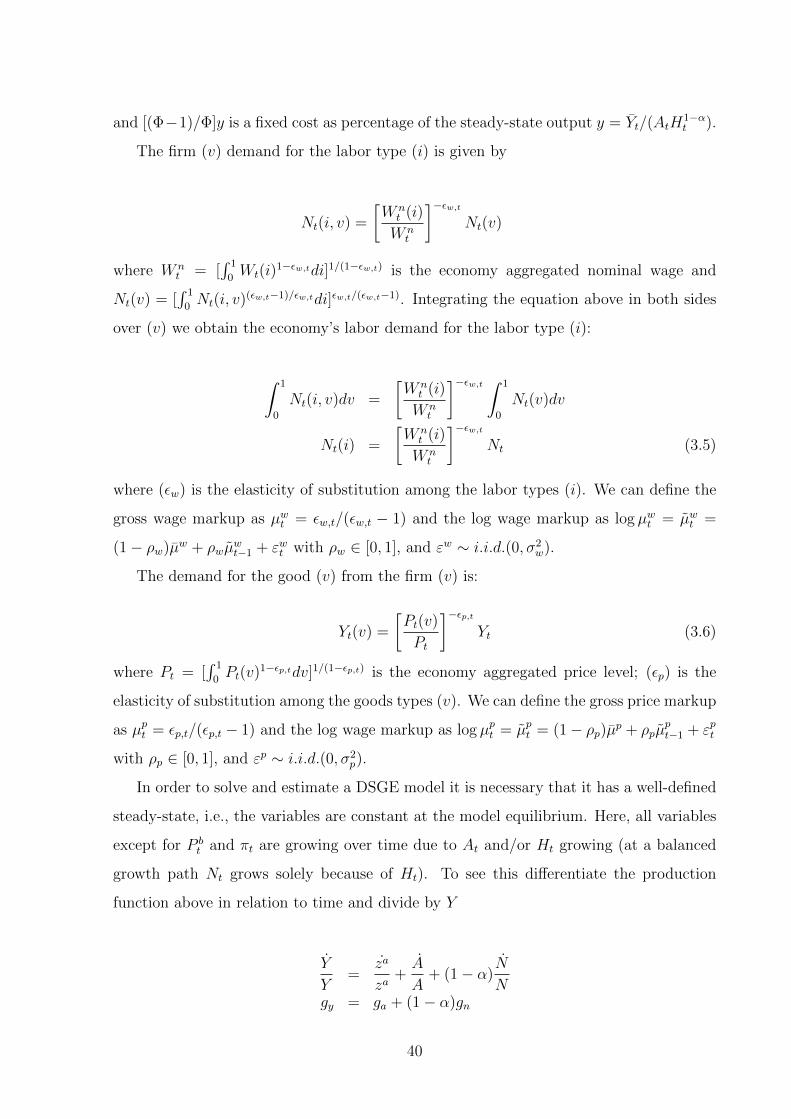
and [(Φ−1)/Φ]y is a fixed cost as percentage of the steady-state output y = Yt/(AtH1−αt ).

The firm (v) demand for the labor type (i) is given by

Nt(i, v) =

[W nt (i)

W nt

]−εw,tNt(v)

where W nt = [

∫ 1

0Wt(i)

1−εw,tdi]1/(1−εw,t) is the economy aggregated nominal wage and

Nt(v) = [∫ 1

0Nt(i, v)(εw,t−1)/εw,tdi]εw,t/(εw,t−1). Integrating the equation above in both sides

over (v) we obtain the economy’s labor demand for the labor type (i):

∫ 1

0

Nt(i, v)dv =

[W nt (i)

W nt

]−εw,t ∫ 1

0

Nt(v)dv

Nt(i) =

[W nt (i)

W nt

]−εw,tNt (3.5)

where (εw) is the elasticity of substitution among the labor types (i). We can define the

gross wage markup as µwt = εw,t/(εw,t − 1) and the log wage markup as log µwt = µwt =

(1− ρw)µw + ρwµwt−1 + εwt with ρw ∈ [0, 1], and εw ∼ i.i.d.(0, σ2

w).

The demand for the good (v) from the firm (v) is:

Yt(v) =

[Pt(v)

Pt

]−εp,tYt (3.6)

where Pt = [∫ 1

0Pt(v)1−εp,tdv]1/(1−εp,t) is the economy aggregated price level; (εp) is the

elasticity of substitution among the goods types (v). We can define the gross price markup

as µpt = εp,t/(εp,t − 1) and the log wage markup as log µpt = µpt = (1− ρp)µp + ρpµpt−1 + εpt

with ρp ∈ [0, 1], and εp ∼ i.i.d.(0, σ2p).

In order to solve and estimate a DSGE model it is necessary that it has a well-defined

steady-state, i.e., the variables are constant at the model equilibrium. Here, all variables

except for P bt and πt are growing over time due to At and/or Ht growing (at a balanced

growth path Nt grows solely because of Ht). To see this differentiate the production

function above in relation to time and divide by Y

Y

Y=

za

za+A

A+ (1− α)

N

Ngy = ga + (1− α)gn

40

where (Y /Y ) = gy is the output balanced path growth rate; (za/za) = 0 is the temporary

productivity growth in the balanced growth path; (A/A) = ga is the balanced path growth

rate of the permanent productivity shifter At; and (N/N) = gn is the labor-supply (and

employment) balanced path growth rate.

Under appropriate conditions a model may have a balanced growth path, a state of

equilibrium in which all the model variables that tend to growth over time (trending

variables) grow at the same rate. As all trending variables grow at the same rate, it

is possible to extract the common trend between them and transform a non-stationary

model into a stationary one, i.e. a model that has a steady-state. To detrend these

variables we follow Pfeifer (2015) denoting with lowercase letters non-trending variables

and writing every generic variable Dt as (Dt = AtH1−αt dt).

2 We will now proceed with

the above equations detrending.

The utility function (3.1) can then be rewritten as

AtH1−αt ut =

{(AtH

1−αt )1−σ(c#t )

1−σ

1− σ− (AtH

1−αt xt)

1−σθt

(zlt)ϕHt

1+ϕ

∫ 1

0

[Htnt(i)]1+ϕ

1 + ϕ

}

ut = (AtH1−αt )−σ

[(c#t )1−σ

1− σ− x1−σt θt

(zlt)ϕ

∫ 1

0

nt(i)1+ϕ

1 + ϕ

]

remembering that At = At−1ega,t with ga,t = (1 − ρa)ga + ρaga,t−1 + εat , and Ht =

(Nt−1)dl(Ht−1)

(1−dl)egn,t with gn,t = (1− ρb)gn + ρngn,t−1 + εnt ; if we make εat = εnt = 0 ∀ t

and dl = 0,3 we have At = At−1ega and Ht = Ht−1e

gn iterating backward these equations

one obtains At = A0egat and Ht = H0e

gnt, normalizing A0 = H0 = 1 results in At = egat

and Ht = egnt. Besides that, we set xt = 1 ∀ t or otherwise Xt = AtH1−αt . This is a

condition sufficient to guarantee a steady-state for the utility function (3.1). To see this

note that in the steady-state c# and n are constants, zlt = θt = 1 and, therefore, x should

be constant as well. As xt is a detrended variable its possible shocks would only have

transitory effects and so it would be indistinguishable of zlt and thus redundant. Substi-

tuting these equations At = eat, Ht = egnt and xt = 1 in the utility function above, we

2In this text we are using the following convention for a generic variable like Xt: a uppercase letterXt means a variable with trend; a lowercase letter xt indicates a detrended variable; a lowercase letter xwithout the subscript t indicates a detrended variable at their steady-state value (except if the letter isrepresenting a parameter)

3Making dl = 0 is not strictly necessary because with εat = εnt = 0 ∀ t the cointegrated and non-cointegrated models for the labor-supply and employment growth both coincide.

41

have

ut =[egate(1−α)gnt

]−σ [(c#t )1−σ

1− σ− θt

(zlt)ϕ

∫ 1

0

nt(i)1+ϕ

1 + ϕ

]

= exp(−σgyt)

[(c#t )1−σ

1− σ− θt

(zlt)ϕ

∫ 1

0

nt(i)1+ϕ

1 + ϕ

](3.7)

where c#t = ct − hct−1 with h = h exp(gy), and gy = ga + (1 − α)gn is the output (Yt)

balanced growth rate.

Looking at the budget constraint (3.3) now, it can be detrended in this way

AtH1−αt ct +

P bt

zctAtH

1−αt brt ≤

1

(1 + πt)AtH

1−αt brt−1 + AtH

1−αt wrt (i)nt(i) + AtH

1−αt trt

ct +P bt

zctbrt ≤

1

(1 + πt)brt−1 + wrt (i)nt(i) + trt (3.8)

the production function (3.4) can be detrended in the same way

AtH1−αt yt(v) = zatAt[Htnt(z)]1−α +

Φ− 1

Φy =⇒ yt(v) = zat nt(v)1−α +

Φ− 1

Φy (3.9)

the labor demand (3.5) detrending is done like this

Nt(i)

Ht

=

[W nt (i)

W nt

]−εw,t Nt

Ht

=⇒ nt(i) =

[W nt (i)

W nt

]−εw,tnt (3.10)

and the output demand (3.6) detrending is

Yt(v)

AtH1−αt

=

[W nt (i)

W nt

]−εp,t Yt

AtH1−αt

=⇒ yt(v) =

[Pt(v)

Pt

]−εp,tyt (3.11)

Now all the models variables as a well defined steady-state and we can write down the

model and calculate its first order conditions.

3.3 CONSUMPTION, LABOR-SUPPLY, WAGE-SETTING AND UNEMPLOYMENT

Following Erceg et al. (2000), it is assumed that in each period only a randomly selected

fraction (1−θw) of occupations has permission to adjust optimally the nominal wage rate

42

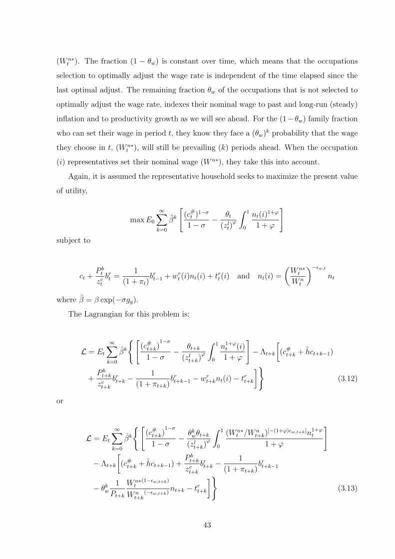
(W n∗t ). The fraction (1 − θw) is constant over time, which means that the occupations

selection to optimally adjust the wage rate is independent of the time elapsed since the

last optimal adjust. The remaining fraction θw of the occupations that is not selected to

optimally adjust the wage rate, indexes their nominal wage to past and long-run (steady)

inflation and to productivity growth as we will see ahead. For the (1−θw) family fraction

who can set their wage in period t, they know they face a (θw)k probability that the wage

they choose in t, (W n∗t ), will still be prevailing (k) periods ahead. When the occupation

(i) representatives set their nominal wage (W n∗), they take this into account.

Again, it is assumed the representative household seeks to maximize the present value

of utility,

maxE0

∞∑k=0

βk

[(c#t )1−σ

1− σ− θt

(zlt)ϕ

∫ 1

0

nt(i)1+ϕ

1 + ϕ

]subject to

ct +P bt

zctbrt =

1

(1 + πt)brt−1 + wrt (i)nt(i) + trt (i) and nt(i) =

(W n∗t

W nt

)−εw,tnt

where β = β exp(−σgy).

The Lagrangian for this problem is:

L = Et

∞∑k=0

βk

{[(c#t+k)

1−σ

1− σ− θt+k

(zlt+k)ϕ

∫ 1

0

n1+ϕt (i)

1 + ϕ

]− Λt+k

[(c#t+k + hct+k−1)

+P bt+k

zct+kbrt+k −

1

(1 + πt+k)brt+k−1 − wrt+knt(i)− trt+k

]}(3.12)

or

L = Et

∞∑k=0

βk

{[(c#t+k)

1−σ

1− σ− θkwθt+k

(zlt+k)ϕ

∫ 1

0

(W n∗t /W n

t+k)[−(1+ϕ)εw,t+k]n1+ϕ

t

1 + ϕ

]

− Λt+k

[(c#t+k + hct+k−1) +

P bt+k

zct+kbrt+k −

1

(1 + πt+k)brt+k−1

− θkw1

Pt+k

W n∗t

(1−εw,t+k)

W nt+k

(−εw,t+k)nt+k − trt+k

]}(3.13)

43

3.3.1 Consumption

The first-order condition of the problem (3.12) in relation to consumption is

∂L∂c#t

= (c#t )−σ − Λt = 0 (3.14)

and the bonds demand first order condition in problem (3.12) is:

∂L∂brt

= −βtΛtP bt

zctbrt + βt+1EtΛt+1

1

(1 + πt+1)brt = 0 (3.15)

Combining equation (3.14) with (3.15), we obtain the consumption Euler equation:

P bt =

1

(1 + rt)= βEt

[(c#t

c#t+1

)σ1

(1 + πt+1)

]zct

where log(zct ) = zct = ρczct−1 + εct , ρc ∈ [0, 1], and εct ∼ (0, σ2

c ). Log linearizing the above

equation around the steady-state yields the New Keynesian IS curve in log deviations:

ct =h

1 + hct−1 +

1

1 + hEtct+1 −

1− h(1 + h)σ

(rt − Etπt+1) + zct (3.16)

where we used the fact that c#t = (ct − hct−1)/(1 − h); h = h exp(gy), where is the

consumption external habit parameter and gy is the output (Y ) balanced growth path.4

3.3.2 Desired Labor Supply

The first order condition of the problem (3.12) in relation to labor supply is

∂L∂lt(i)

=− θt(zlt)

ϕnt(i)

ϕ + Λtwrt (i) = 0

=− θt(zlt)

ϕ

(∫ lt(i)

0

jdj

)ϕ

+ Λtwrt (i) = 0 (3.17)

where lt is the “desired” labor supply in substitution to “effective labor supply” nt, and

4In this text we are using a additional variables representation convention: a lowercase letter witha tilde xt = log(xt) indicates the log of a detrended variable (except if the letter is representing aparameter, e.g., β); a lowercase letter with a bar xt = log(x) indicates the log of a detrended variable attheir steady-state value; and finally a lowercase letter with a hat (xt = log(xt)− log(x) = x− x) indicatesthe log-deviation of a detrended variable from its log steady-state value.

44

the second equality used the fact given in (3.1) that nt(i) =∫ nt(i)0

jdj for the effective

labor supply or lt(i) =∫ lt(i)0

jdj for the desired labor supply.

Now consider an individual specialized in labor type (i) and with marginal rate of

substitution between labor and consumption given by mrst(i), taking the real wage pre-

vailing wrt (i) as given, this individual will be willing to work in period t if and only if

wrt ≥ mrst(i). Combining equation (3.17) with (3.14), we obtain the desired labor supply

lt(i):

wrt (i) ≥ mrst(i) = θt(c#t )σ

(∫ lt(i)

0

jdj

)ϕ

(zlt)−ϕ

wrt (i) = mrst(i) = (zst )σlt(i)

ϕ(zlt)−ϕ (3.18)

where mrst is the marginal rate of substitution between labor and leisure, and the second

equality used the fact that θt = (zst /c#t )σ.

The endogenous preferences shifter (θt) was introduced by Galı et al. (2012) based on

Jaimovich and Rebelo (2009) in order to control the wealth (income) effect strength on

labor supply. Such modification was necessary to overcome a counterfactual prediction

of the standard New-Keynesian model. In the standard model, without the endogenous

preferences shifter θt, the labor supply relation (3.18) - in logs and disregarding the habit

formation in consumption (c#t = ct) and shocks in labor supply (zlt = 0 ∀ t) - is given by:

wrt = σct + ϕlt

where wr is the log of real wage, c is the log of consumption and l is the log of labor

supply.

According to Christiano et al. (2010), this specification leads to counterfactual predic-

tions about the labor force evolution. Evidence suggests labor force decreases in response

to an negative monetary shock, while consumption decreases more than real wages. This

does not occur in the standard model without an endogenous preference shifter. Incor-

porating the preference shifter θt into the model, labor supply now is given by (again

disregarding consumption habits and labor supply shocks):

45

wrt = σzst + ϕlt

= σ[γcct + (1− γc)zst−1] + ϕlt

where γc ∈ [0, 1], controls the wealth effect on labor supply. For sufficiently low values of

γc, the counterfactual predictions of the standard model can be overturned.

Now let’s go back to the equation (3.18). Recalling that log zst = zst = γcc#t +(1−γc)zst−1

and iterating backwards, this relation can be written as zst = γc∑∞

k=0(1 − γc)kc#t−k, then

the labor supply can be written (in logs) as wrt (i) = σγc∑∞

k=0(1− γc)kc#t−k + ϕlt(i)− zlt.

The infinite sum allows us to apply the Koyck (1954) transformation to the relation of

labor supply (in logs) what results in

wrt (i) = (1− γc)wrt−1(i) + σγcc#t + ϕlt(i)− (1− γc)ϕlt−1(i)− ϕ

[zlt − (1− γc)zlt−1

]aggregating the above equation in i and writing it in log deviations from the steady-state,

we have the following aggregate labor supply relation

wrt = (1− γc)wrt−1 +σγc

1− h(ct− hct−1) +ϕlt− (1− γc)ϕlt−1−ϕ

[zlt − (1− γc)zlt−1

](3.19)

where we used the fact that c#t = (ct− hct−1)/(1− h); wrt ≈∫ 1

0wrt (i)di, and lt ≈

∫ 1

0lt(i)di.

3.3.3 Wage-Setting

The first order condition of the problem (3.13) in relation to nominal wage w∗t is:

∂L∂w∗t

=∞∑k=0

βk

{− θkwθt+k

(zlt+k)ϕ

[−(1 + ϕ)εw,t+k](w∗t )−1(wn∗twnt+k

)−εw,t+kn1+ϕt+k

+Λt+kθkw

1

pt+k(1− εw,t+k)

(w∗twnt+k

)−εw,t+knt+k

}= 0

46

=∞∑k=0

(βθw)k

{θt+kεw,t+k

(zlt+k)ϕ

(w∗t )−1(w∗twnt+k

)−εw,t+k(1+ϕ)n1+ϕt+k

−Λt+k1

pt+k(εw,t+k − 1)

(w∗twnt+k

)−εw,t+knt+k

}= 0

=∞∑k=0

(βθw)k

{θt+kεw,t+k(zlt+k)

1+ϕn1+ϕt+k (i)− (c#t+k)

−σ w∗t

pt+k(εw,t+k − 1)nt+k(i)

}= 0

=∞∑k=0

(βθw)k

{w∗tpt+k

− εw,t+k(εw,t+k − 1)

θt+k(zlt+k)

1+ϕ(c#t+k)

σnϕt+k(i)

}= 0

=∞∑k=0

(βθw)k

{w∗tpt+k

− µnw,t+kmrst+k

}= 0 (3.20)

Isolating w∗t in the above equation, we obtain the nominal wage w∗t chosen by the

workers

w∗t = (1− βθw)∞∑k=0

(βθw)k[pt+kµ

nw,t+kmrst+k

](3.21)

where µnw,t+k = εw,t+k/(εw,t+k − 1) is the natural gross wage markup.

Log-linearizing the above equation around the steady-state results in an equation for

the optimal wage w∗t in log deviations

w∗t = (1− βθw)Et

∞∑k=0

(βθw)k[mrst+k(i) + pt+k + µnw,t]

this equation can be written as


∞∑k=0

(βθw)k[mrst+k(i)− mrst+k + mrst+k + pt+k + µnw,t]

considering that µw,t+k = wnt+k − mrst+k − pt+k, the above equation can be rewritten as


∞∑k=0

(βθw)k[mrst+k(i)− mrst+k + wnt+k − (µw,t+k − µnw,t+k)] (3.22)

From equation (3.18), the average marginal rate of substitution for “employed” work-

ers is mrst = (zlt)−ϕ

(zst )σnt(i)

ϕ, where nt =∫ 1

0nt(i)di is the aggregate employment.

47

Multiplying and dividing the equation (3.18) by nϕt , we have:

mrst(i) = (zlt)−ϕ(zst )

σnϕtnt(i)

ϕ

ntϕ

= mrst

[nt(i)

nt

]ϕwhere the last equality used the fact that mrst = (zlt)

−ϕ(zst )σnt(i)

ϕ.

The log-linearization of equation above around the steady-state results in

mrst(i) = mrst + ϕ[nt(i)− nt]

On the other hand, log-linearizing the equation (3.10) around the steady-state [nt(i) =

−εw(wnt − wt)] and substituting this result in equation above results in

mrst(i) = mrst − ϕεw(w∗t − wnt ) (3.23)

Substituting equation (3.23) into (3.22) results in a new equation for the optimal wage

w∗t log deviation

w∗t =(1− βθw)

(1 + ϕεw)Et

∞∑k=0

(βθw)k[(1 + ϕεw)wnt+k − (µw,t+k − µnw,t+k)

]= βθww

∗t+1 + (1− βθw)wnt −

(1− βθw)

(1 + ϕεw)(µw,t − µnw,t) (3.24)

Families that can not optimally adjust wages choose a wage w#t according to a rule-of-

thumb that indexes wages to past prices inflation πpt−1 (Galı et al., 2012), and the balanced

growth path productivity growth rate ga,

w#t = wnt−1(1 + ga)(1 + πpt−1)

γw(1 + πp)(1−γw) (3.25)

log-linearizing the above equation around the steady-state

w#t = wnt−1 + γwπ

pt−1 (3.26)

48

Since a fraction (1 − θw) can choose its wage rate w∗t optimally, and the remaining

fraction θw fixes its wage w#t according to the rule given in (3.25), the average nominal

wage is given by

wnt =[θw(w#

t )1−εw,t + (1− θw)(w∗t )1−εw,t

] 11−εw,t

Log-linearizing the above equation around the steady-state results in

wnt = θww#t + (1− θw)w∗t (3.27)

Substituting equations (3.24) and (3.26) into (3.27), we obtain the following equation

for wage inflation

πwt = βEt(πwt+1 − γwπ

pt

)+ γwπ

pt−1 − λw

(µwt − µnw,t

)(3.28)

where λw = (1−βθw)(1−θw)(1+ϕεw)θw

; µnw,t = (1− ρw)µw + ρwµnw,t−1 + εw,t and εw,t ∼ i.i.d.(0, σ2

w); and

µwt = (wt − pt)− mrst. Without indexation to past inflation (γw = 0), the wage inflation

equation becomes

πwt = βEtπwt+1 − λw

(µwt − µnw,t

)the inflation of wages depends positively on the expected wages inflation rate and nega-

tively on the difference between effective and natural markup.

3.3.4 Unemployment Rate and the New Keynesian Wage Phillips Curve

We will now introduce the unemployment rate into the model and insert it into the

wage inflation equation (3.28). Making (k = 0) in equation (3.21), we have

wntpt

= wrt = µw,tmrst

= µw,t(zlt)−ϕ(zt)

σnϕt

the second equality used the equation (3.18) multiplied by the average gross markup µw,t,

49

and mrst is the marginal rate of substitution between consumption and labor for the

employed workers and nt is the employment. Log-linearization of the above equation

around the steady-state yields

µw,t = wrt − mrst

= wrt − σzst − ϕnt + ϕzlt (3.29)

Equation (3.29) says that the log mean markup is given by the difference (in logs)

between the average real wage and the employed workers marginal rate of substitution

(mrs). Looking back at the equation (3.18) (wrt (i) = mrst(i) = (zst )σlt(i)

ϕ(zlt)−ϕ), the

reasoning behind this equation is that a worker (i) decides to offer work if wrt ≥ mrst.

When mrst 6= zlt(zst )σlϕt , the worker will adjust his labor supply lt to the point where

wrt = mrst. Log-linearizing the equation (3.18) around the balanced growth path yields

wrt = mrst

= σzst + ϕl − ϕzlt (3.30)

Recalling that the observed mean real wage wrt is the same for employed and unem-

ployed workers, we can insert equation (3.29) in equation (3.30) and obtain the following

relation between the wage markup µw,t and the labor-force lt and employment nt log

deviations

µw,t = ϕ(lt − nt) (3.31)

What (lt − nt) will be depends on whether the labor supply L is cointegrated or non-

cointegrated with the employment N . We saw earlier that if the labor supply is cointe-

grated with employment, then (dl = 0) in the utility function (3.1). On the other hand, if

the labor supply is non-cointegrated with employment, then (dl = 1) in the utility function

(3.1). If the labor supply is cointegrated with employment, the unemployment rate will be

stationary and will converge to a long-run mean as predicted by the natural rate hypoth-

50

esis of unemployment rate. To see this consider the detrended labor supply (lt = Lt/Ht)

and detrended employment (nt = Nt/Ht), where Ht = (Nt−1)dl(Ht−1)

(1−dl)egn,t is the

labor-supply and employment common trend. If dl = 0, Ht = Ht−1egn,t and we have

lt =LtHt

=Lt

Ht−1egn,t

or in logs deviations from steady-state

lt = Lt − Ht−1 − gn,t (3.32)

and

nt =Nt

Ht

=Nt

Ht−1egn,t


nt = Nt − Ht−1 − gn,t (3.33)

Subtracting (3.33) from (3.33), we have

ut = lt − nt = Lt − Nt (3.34)

where ut = ut−un is the unemployment rate ut deviation from the long-run natural rate of

unemployment (un) that coincides with the steady-state unemployment rate . In equation

(3.34), we used the fact that log(1− ut) = log(Nt/Lt) ≈ −ut and therefore ut ≈ Lt − Nt.

Substituting (3.34) in (3.31), one obtains

µw,t = ϕ(ut − un), µnw,t = ϕ(unt − un) and µnw = ϕun (3.35)

where µn = log[εw/(εw − 1)].

If the labor supply is no cointegrated with employment, the unemployment rate

will be difference-stationary and its level will be a I(1) process as predicted by the

total (full) hysteresis hypothesis for the unemployment rate. Again consider the de-

trended labor supply (lt = Lt/Ht) and detrended employment (nt = Nt/Ht), where

Ht = (Nt−1)dl(Ht−1)

(1−dl)egn,t is the labor-supply and employment common trend. If

51

dl = 1, Ht = Nt−1egn,t and we have

lt =LtHt

=Lt

Ht−1egn,t


lt = Lt − Lt−1 − gn,t (3.36)

and

nt =Nt

Ht

=Nt

Nt−1egn,t


nt = Nt − Nt−1 − gn,t (3.37)

Subtracting (3.36) from (3.37), we have

∆ut = ∆lt −∆nt = ∆Lt −∆Nt (3.38)

where ∆ut = ut − ut−1 is the unemployment rate first differences. In equation (3.38),

we used the fact that log(1 − ut) = log(Nt/Lt) ≈ −ut ≈ Nt − Lt and therefore ∆ut ≈

∆Lt −∆Nt ≈ ∆lt −∆nt.

In this case substituting equation (3.38) in (3.31) one obtains

µw,t = ϕ∆ut (3.39)

where ∆ut = ut − ut−1 and µw,t = µw,t − µnw.

Substituting equation (3.35) into equation (3.28), we obtain the New Keynesian Wage

Phillips Curve in terms unemployment rate deviations from its natural rate, or the No-

hysteresis Wage Phillips Curve:


pt

)+ γwπ

pt−1 − λwϕ(ut − unt ) (3.40)

where unt = (1/ϕ)µnw,t.

52

Regarding the hysteretic model, substituting equation (3.39) into equation (3.28),

we obtain the New Keynesian Wage Phillips Curve in terms of the unemployment first

differences, or the With Hysteresis Wage Phillips Curve (WHWPC):


pt

)+ γwπ

pt−1 − λwϕ∆ut + λwµ

nw,t (3.41)

3.4 FIRMS BEHAVIOR

We assume there is a continuum v ∈ [0, 1] of monopolistic competitive firms, each of

them producing a differenced good v ∈ [0, 1] with the following production technology:

yt(j) = zat [nt(v)](1−α) +Φ− 1

Φy (3.42)

where, nt(v) =[∫ 1

0nt(i, v)(εw,t−1)/εw,tdi

]εw,t/(εw,t−1), is a CES index of the different types of

labor i employed by the firm v; and zat = (za)(1−ρza)(zat−1)ρzae

εzatt is an exogenous temporary

productivity shifter with ρza ∈ [0, 1], and εzat ∼ i.i.d.(0, σ2za).

Following Calvo (1983), it is assumed that in each period only a randomly selected

fraction (1− θp) of firms has permission to adjust optimally their prices. The fraction

(1− θp) is constant over time, which means that firms selection is independent of the

time elapsed since the last optimal adjust. The remaining fraction θp of firms that is not

selected to optimally adjust their prices, indexes their prices p#t to last inflation rate and

to trend inflation p#t = (1 + πpt )γp(1 + πp)(1−γp), where πp is the trend inflation rate or the

long-run inflation rate. The firm that can optimally adjust its price in period t, set p∗t to

maximize:

maxEt

∞∑k=0

(βθp)k [p∗tyt+k(v)− pt+kyt+k(v)mct+k(v)] (3.43)

subject to

yt+k(v) =

(p∗tpt+k

)−εp,t+kyt+k (3.44)

wheremct(v) is the real marginal cost of the activity v, and εp,t is the substitution elasticity

between the goods yt(v). The first order condition to problem above is:

53

Et

∞∑k=0

(βθp)k

[εp,t+k

εp,t+k − 1pt+kmct+k(v)− p∗t

]yt+k(v) = 0

Solving the equation above to p∗t , we have

p∗t =Et∑∞

k=0(βθp)kµp,t+kpt+kmct+k(v)yt+k(v)

Et∑∞

k=0(βθp)kyt+k(v)

where µp,t = εp,t/(εp,t − 1) is the gross price markup (markup over marginal cost) with

log µp,t = µp,t = (1 − ρp)µp + ρpµp,t−1 + εpt , ρp ∈ [0, 1], εp ∼ i.i.d.(0, σ2p), and µp is the

steady-state markup in log.

Log-linearizing the above equation around the long-run inflation, we obtain an equa-

tion for the optimal log price choice (p∗t ) in terms of long run inflation deviations (in

logs):

p∗t = (1− βθp)Et∞∑k=0

(βθp)k[pt+k + mct+k(v) + µpt+k

](3.45)

Let’s now derive a relationship between the (log deviation form steady-state) marginal

cost of a firm v [mct(v)] and the economy’s average marginal cost (in log deviation from

steady-state) (mct). The latter is defined by mct = wrt − mpnt, where wrt is the (log

deviation form steady-state) real wage (wrt = wnt − pt), mpnt is the economy average

marginal product of labor (in log deviations from steady-state) given by mpnt = zat−αnt =

{1/[Φ(1− α)]} (Φzat − αyt), where the last equality made use of the production function

(3.42) log-linearized around the steady-state. So the economy’s average marginal cost (in

log deviations from steady-state) is

mct = wrt +1

Φ(1− α)[αyt − Φzat ] (3.46)

and a similar relationship holds for the marginal cost (in log deviations from steady-

state) of a firm v: mct(v) = wrt + {1/[Φ(1− α)]} [αyt(v) − Φzat ]. Combining these two

marginal cost relations we obtain a equation relating individual and average marginal

costs: mct(v) = mct + {α/[Φ(1− α)]} [yt(v) − yt], log-linearizing the demand function

(3.11) around the steady-state [yt(v) = −εp[p∗t − pt] + yt] and combining with mct(v) =

mct+{α/[Φ(1− α)]} [yt(v)− yt], we obtain a new relation between individual and average

54

marginal costs:

mct(v) = mct − {αεp/[Φ(1− α)]} (p∗t − pt) (3.47)

Combining the equation (3.47) with (3.45), one obtains another relation to the new

price set by firms allowed to adjust prices:

p∗t = (1− βθp)Et∞∑k=0

(βθp)k

[pt+k +

Φ(1− α)

Φ(1− α) + αεp(mct+k + µpt+k)

]= βθpEtp

∗t+1 + (1− βθp)

[pt +

Φ(1− α)

Φ(1− α) + αεp(mct + µpt )

](3.48)

Following Christiano et al. (2010), firms that can not optimally adjust price choose a

new price p#t according to a rule-of-thumb that indexes prices to past inflation πpt and to

trend inflation πp,

p#t = pt−1(1 + πpt−1)γp(1 + πp)1−γp (3.49)

log-linearization of the above equation around the trend inflation results in

p#t = pt−1 + γpπpt−1 (3.50)

Since a fraction (1− θp) of firms can choose P ∗t optimally, and the remaining fraction

θp adjusts prices according to the rule in (3.50), the average price index of the economy

is given by

pt =[θp(p

#t )1−εp,t + (1− θp)(p∗t )1−εp,t

] 11−εp,t

log-linearization of the above equation around the trend inflation yields

pt = θpp#t + (1− θp) p∗t (3.51)

Substituting the equations (3.48) and (3.50) in (3.51), we finally obtain the New Keynesian

Phillips Curve:

55

πt =γp

1 + βγpπt−1 +

β

1 + βγpEtπt+1 +

λp

1 + βγp(mct + µpt ) (3.52)

where λp = [(1− α)(1− θp)(1− βθp)]/[θp(1− α+ αεp)], and µpt = ρpµpt−1 + εpt is the firms

desired markup log deviation from steady-state with εpt ∼ i.i.d.(0, σ2p).

3.5 MODEL SUMMARY IN LOG-LINEAR FORM

Since our model is a closed economy with no capital and no government, the condition

of equilibrium in the goods market is yt = ct, so Euler’s equation (3.16) (New Keynesian

IS) can be rewritten for both models as:

yt =h

1 + hyt−1 +

1

1 + hEtyt+1 −

1− h(1 + h)σ

(rt − Etπpt+1) + zyt (3.53)

where h = exp(gy)h, gy is the balanced growth path of the output, and zyt = ρyzyt−1 + εyt

with ρy ∈ [0, 1] and εyt ∼ i.i.d.(0, σ2y).

The equation (3.19) reproduced below represents the labor supply or the labor force

in both models, i.e., people willing to work at the current average wage:

wrt = (1− γc)wrt−1 +σγc

1− h(ct − hct−1) + ϕlt − (1− γc)ϕlt−1 − zlt + (1− γc)zlt−1 (3.54)

where h = exp(gy)h, zlt = ρlzlt−1 + εlt with ρl ∈ [0, 1] and εlt ∼ i.i.d.(0, σ2

l ).

Given the equilibrium output, log-linearizing (3.42) and summing up over v, employ-

ment in log deviation from the steady-state is for the model “without hysteresis”:

nt =(yt − zat )

Φ(1− α)(3.55)

For the model without hysteresis, the unemployment rate can be defined has:

ut = lt − nt (3.56)

While for the model with hysteresis, the unemployment rate can be defined has:

56

∆ut = lt − nt (3.57)

The inflation rate for both models is given by equation (3.52) repeated below

πt =γp

1 + βγpπt−1 +

β

1 + βγpEtπt+1 +

λp

1 + βγp(mct + µpt ) (3.58)

where λp = [(1−α)(1−θp)(1−βθp)]/[θp(1−α+αεp)], and µpt = ρpµpt−1+εpt , with ρp ∈ [0, 1]

and εpt ∼ i.i.d.(0, σ2p).

The marginal cost represented in equation (3.46) is reproduced below

mct = wrt +1

Φ(1− α)[αyt − Φzat ] (3.59)

where zat = ρzazat−1 + εzat , with ρza ∈ [0, 1], and εzat ∼ i.i.d.(0, σ2

za).

The real wage log deviations from steady-state wrt can be written has

wrt = wrt−1 + πwt − πpt − ga,t + αgn,t (3.60)

Wage inflation in the model “without” hysteresis given in equation (3.40) is reproduced

below


pt

)+ γwπ

pt−1 − λwϕut + λwµ

nw,t (3.61)

where w1 = β = β exp(gy), λw = [(1−βθw)(1−θw)][(1+ϕεw)θw]

, and µww,t = ρwµww,t−1 + εwt , with ρw ∈ [0, 1],

and εwt ∼ i.i.d.(0, σ2w).

Wage inflation in the model “with” hysteresis given in equation (3.41) is reproduced

below


pt

)+ γwπ

pt−1 − λwϕ∆ut + λwµ

nw,t (3.62)

where ∆ut = ut−ut−1, w1 = β = β exp(gy), λw = [(1−βθw)(1−θw)][(1+ϕεw)θw]

, and µww,t = ρwµww,t−1 +εwt ,

with ρw ∈ [0, 1], and εwt ∼ i.i.d.(0, σ2w).

To close the model, we assume the following Taylor rule:

57

rt = φrrt−1 + (1− φr) (φππpt + φyyt) + zrt (3.63)

where zrw,t = ρwzrw,t−1 + εrt , with ρr ∈ [0, 1], and εrt ∼ i.i.d.(0, σ2

r).

3.5.1 Equations of Observation

In this subsection we show the observation equations, i.e., equations that links the

models theoretical variables to observed variables in the economy. The output observation

equation is:

∆LogGDPt = gyt + yt − yt−1 (3.64)

where ∆dLogGDPt is the log(GDP) first difference, and gyt is the trend growth of GDP

given by:

gyt = gat + (1− α)gnt (3.65)

where gat is the trend growth of the productivity and gnt is the trend growth of the

labor-supply both given by

gat = (1− ρa)ga + ρagat + εat (3.66)

and

gnt = (1− ρa)gn + ρagnt + εnt (3.67)

where ga is the long-run growth rate of the productivity, and gn is the long-run growth

rate of the labor-supply.

The labor-supply observation equation in the model without hysteresis is given by:

∆LogLaSt = gnt + lt − lt−1 (3.68)

where ∆dLaSt is the first difference of the labor-supply (LaS) in logs, and gnt is the trend

growth of the labor-supply.

58

The labor-supply observation equation in the model with hysteresis is given by:

∆LogLaSt = gnt + lt (3.69)

The wage inflation observation equation is:

∆LogWnt = πwt + πp + ga − αgn (3.70)

where ∆LogWnt is the first difference in logs of the average nominal wage and πp is the

long-run mean inflation.

The price inflation observation equation is:

∆LogPt = πp + πpt (3.71)

where ∆LogPt is the first difference in logs of the consumer price index (CPI) and πp is

the long-run mean inflation.

The interest rate observation equation is:

Rt

100=

(1 + πp)

β exp(−σgy)− 1 + rt (3.72)

where Rt is the central bank short-term interest rate and gy is the steady-state growth

rate of output given by

gy = ga + (1− α)gn (3.73)

Finally, the unemployment rate observation equation in the model without hysteresis

is:

∆UnR = ut − ut−1 (3.74)

where UnR is the observed unemployment rate.

While the unemployment rate observation equation in the model with hysteresis is:

∆UnR = ∆ut (3.75)

59

3.6 ESTIMATION

The models were estimated by Bayesian techniques using the software Dynare 4.4.3

(Adjemian et al., 2014) from the 1999Q1 to 2015Q4. Subsequent distributions of the pa-

rameters were computed using the Metropolis-Hastings algorithm ”that uses Monte Carlo

Markov Chain (MCMC) procedures. The quarterly data used in the model estimation

were the first differences in logs of the IBGE’s quarterly GDP, the economically active

population and the unemployment rate of the IBGE Monthly Employment Survey (PME

in Portuguese), wage inflation is measured by the first differences in logs of average income

from the principal labor of IBGE’s (PME), the consumer’s inflation rate measured by the

first differences in logs of the IBGE’s CPI (IPCA in Brazil), and the short-term nominal

interest rate of the Central Bank of Brazil (Selic rate).

All series were seasonally adjusted except the nominal interest rate. In regard of

economically active population, unemployment and wages the source of these data - the

Monthly Employment Survey (PME) - was reformulated in 2002 and some methodolog-

ical aspects were modified. To complete our data set, the new methodology series were

chained to the old methodology series. Priors sources for estimates came mainly from

Castro et al. (2011) who developed the SAMBA5, a DSGE model for the Brazilian econ-

omy used by the Central Bank of Brazil. The prior of the parameter that controls the

wealth effect on labor supply was obtained from Galı et al. (2012). Calibrated parameters

are shown in (TABLE 3.1).

TABLE 3.1 – CALIBRATED PARAMETERS

Parameters and Description Value Source

εp Elasticity of Substitution among goods 11 Castro et al. (2011)α Labor Elasticity in Production Function 0 (zero) -β Quarterly Time Discount Factor 0.99 Standard in Literature

In (TABLE 3.2) are shown the estimated parameters for both models: No-Hysteresis

Model (NHM) and With-Hysteresis Model (WHM). Let’s comment some of them. The

intertemporal consumption elasticity of substitution (σ) and the consumption habits pa-

rameter (h), had similar estimated values in both models (σ = 1.27, h = 0.59 in the NHM

5Stochastic Analytical Model with a Bayesian Approach

60

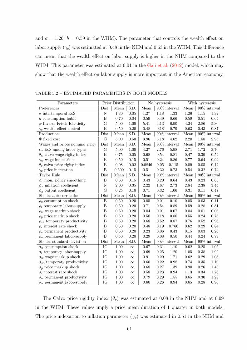
and σ = 1.26, h = 0.59 in the WHM). The parameter that controls the wealth effect on

labor supply (γc) was estimated at 0.48 in the NHM and 0.63 in the WHM. This difference

can mean that the wealth effect on labor supply is higher in the NHM compared to the

WHM. This parameter was estimated at 0.01 in the Galı et al. (2012) model, which may

show that the wealth effect on labor supply is more important in the American economy.

TABLE 3.2 – ESTIMATED PARAMETERS IN BOTH MODELS

Parameters Prior Distribution No hysteresis With hysteresis

Preferences Dist. Mean S.D. Mean 90% interval Mean 90% interval

σ intertemporal EoS N 1.30 0.05 1.27 1.18 1.33 1.26 1.15 1.32h consumption habit B 0.70 0.04 0.59 0.49 0.66 0.59 0.51 0.64ϕ Inverse Frisch Elasticity G 5.00 1.00 5.41 4.13 6.90 4.24 2.86 5.30γc wealth effect control B 0.50 0.20 0.48 0.18 0.79 0.63 0.43 0.87

Production Dist. Mean S.D. Mean 90% interval Mean 90% interval

Φ fixed cost G 5.00 0.50 3.96 3.18 4.62 2.20 1.58 2.95

Wages and prices nominal rigity Dist. Mean S.D. Mean 90% interval Mean 90% interval

εw EoS among labor types G 5.00 1.00 4.27 2.76 5.98 2.71 1.72 3.76θw calvo wage rigity index B 0.75 0.05 0.68 0.54 0.81 0.47 0.39 0.54γw wage indexation B 0.50 0.15 0.51 0.24 0.86 0.77 0.64 0.94θp calvo price rigity index B 0.08 0.02 0.0846 0.05 0.115 0.09 0.05 0.12γp price indexation B 0.500 0.15 0.51 0.32 0.73 0.54 0.32 0.74

Taylor Rule Dist. Mean S.D. Mean 90% interval Mean 90% interval

φr mon. policy smoothing B 0.60 0.15 0.43 0.20 0.64 0.43 0.23 0.63φπ inflation coefficient N 2.00 0.35 2.22 1.67 2.73 2.84 2.38 3.44φy output coefficient G 0.25 0.10 0.71 0.32 1.06 0.31 0.11 0.47

Shocks autocorrelation Dist. Mean S.D. Mean 90% interval Mean 90% interval

ρy consumption shock B 0.50 0.20 0.05 0.01 0.10 0.05 0.03 0.11ρl temporaty labor-supply B 0.50 0.20 0.71 0.54 0.89 0.59 0.28 0.81ρw wage markup shock B 0.50 0.20 0.04 0.01 0.07 0.04 0.01 0.06ρp price markup shock B 0.50 0.20 0.50 0.18 0.80 0.55 0.24 0.76ρza temporaty productivity B 0.50 0.20 0.68 0.52 0.87 0.76 0.52 0.96ρr interest rate shock B 0.50 0.20 0.48 0.19 0.766 0.62 0.29 0.84ρa permanent productivity B 0.50 0.20 0.23 0.06 0.43 0.15 0.03 0.26ρn permanent labor-supply B 0.50 0.20 0.29 0.08 0.50 0.44 0.24 0.79

Shocks standard deviation Dist. Mean S.D. Mean 90% interval Mean 90% interval

σy consumption shock IG 1.00 ∞ 0.67 0.31 1.10 0.62 0.25 1.05σl temporaty labor-supply IG 1.00 ∞ 0.69 0.25 1.20 1.05 0.38 1.92σw wage markup shock IG 1.00 ∞ 0.91 0.29 1.71 0.62 0.29 1.03σza temporaty productivity IG 1.00 ∞ 0.60 0.22 0.98 0.74 0.35 1.10σp price markup shock IG 1.00 ∞ 0.68 0.27 1.39 0.90 0.26 1.43σr interest rate shock IG 1.00 ∞ 0.58 0.23 0.94 1.13 0.34 1.76σa permanent productivity IG 1.00 ∞ 0.79 0.29 1.55 0.65 0.30 1.28σn permanent labor-supply IG 1.00 ∞ 0.60 0.26 0.94 0.65 0.28 0.96

The Calvo price rigidity index (θp) was estimated at 0.08 in the NHM and at 0.09

in the WHM. These values imply a price mean duration of 1 quarter in both models.

The price indexation to inflation parameter (γp) was estimated in 0.51 in the NHM and

61

0.54 in the WHM. The Calvo wage rigidity index (θw) was estimated at 0.68 in the NHM

and at 0.47 in the WHM. These values imply a wage rate mean duration of 3 quarters

in the NHM and 2 quarters in the WHM. The wage indexation to inflation parameter

(γw) was estimated in 0.51 in the NHM and 0.77 in the WHM. In regard to Taylor Rule

parameters, monetary policy smoothing parameter estimates were similar between the

two models, inflation coefficient was 0.71 in the NHM and 0.31 in the WHM and the

output coefficient was 2.22 in the NHM and 2.84 in the WHM.

In (FIGURE 3.1) we show the correlations and autocorrelations implicated by both

models compared to the empirical counterparts. Both models replicate well the correla-

tion between GDP growth with nominal wage inflation, GDP growth with CPI inflation

and GDP growth with unemployment rate first differences. The autocorrelations of CPI

inflation are well approximated by both models. GDP growth and unemployment rate

first differences are poorly approximated by both models.

-0,40

-0,30

-0,20

-0,10

0,00

0,10

0,20

-5 -4 -3 -2 -1 0 1 2 3 4 5

correlation [Δ%GDP (t) , nominal wages inflation (t+k)]

-0,60

-0,40

-0,20

0,00

0,20

-5 -4 -3 -2 -1 0 1 2 3 4 5

correlation [Δ%GDP (t) , cpi inflation (t+k)]

-0,80

-0,60

-0,40

-0,20

0,00

0,20

0,40

-5 -4 -3 -2 -1 0 1 2 3 4 5

correlation [Δ%GDP (t) , Δ(unemploymetnt rate)(t+k)]

-0,10

0,00

0,10

0,20

0,30

0,40

1 2 3 4 5

autocorrelation Δ%GDP (t,t-k)

-0,10

0,10

0,30

0,50

0,70

1 2 3 4 5

Empirical no-hysteresis with-hysteresis

autocorrelation cpi inflation rate(t,t-k)

-0,50

0,00

0,50

1,00

1 2 3 4 5

Empirical no-hysteresis with-hysteresis

autocorrelation Δ(unemploymetnt rate)((t,t-k)

FIGURE 3.1 – DYNAMIC CORRELATION BETWEEN GDP GROWTH, CPI INFLATION,WAGE INFLATION AND UNEMPLOYMENT FIRST DIFFERENCES

62

3.6.1 Impulse Responses

In (FIGURE 3.2) the impulse response functions implied by the models in relation

to a consumption-demand shock are presented. GDP, Wage inflation and CPI inflation

responses are similar for both models. In the model with no hysteresis (WHM), the (log)

real wage increases more than it does in the model with hysteresis (WHM), although the

demand shock has no permanent effect on the real wage in both models. In relation to

the unemployment rate, the demand shock produces a permanent fall in unemployment

rate according to WHM, while in the NHM this fall is only temporary.

-0,20

0,20,40,60,8

11,21,4

1 2 3 4 5 6 7 8

GDP (accumulated response)

-0,005

0

0,005

0,01

0,015

0,02

0,025

0,03

1 2 3 4 5 6 7 8

Nominal Wage Inflation

0

0,1

0,2

0,3

0,4

0,5

0,6

1 2 3 4 5 6 7 8

Interest Rate

-0,0050

0,0050,01

0,0150,02

0,0250,03

1 2 3 4 5 6 7 8

CPI Inflation

-1,5

-1

-0,5

0

0,5

1 2 3 4 5 6 7 8

zero-axis no-hysteresis with-hysteresis

Unemployment Rate (accumulated response)

-0,001

0

0,001

0,002

0,003

1 2 3 4 5 6 7 8zero-axis no-hysteresis with-hysteresis

Average real wage (accumulated response)

FIGURE 3.2 – IMPULSE RESPONSE FUNCTIONS IN (%) TO A 1%CONSUMPTION-DEMAND SHOCK - QUARTERS

63

In (FIGURE 3.3) the impulse response functions implied by the models in relation to

a temporary productivity shock are presented. In the model with hysteresis a temporary

positive productivity shock of 1% a permanent increase of 2.5% in the unemployment

rate in the log-run. In the model without hysteresis, the temporary shock of productivity

has a temporary effect on all variables. The other variables (GDP, wage inflation, CPI

inflation and interest rate) responses is stronger in the model without hysteresis.

-0,2-0,1

00,10,20,30,40,50,6

1 2 3 4 5 6 7 8 9 10 11 12


-0,6-0,5-0,4-0,3-0,2-0,1

00,1

1 2 3 4 5 6 7 8 9 10 11 12


-1,5

-1

-0,5

0

0,5

1 2 3 4 5 6 7 8 9 10 11 12

Interest Rate

-1,2-1

-0,8-0,6-0,4-0,2

00,20,4

1 2 3 4 5 6 7 8 9 10 11 12

CPI Inflation

0

1

2

3

1 2 3 4 5 6 7 8 9 10 11 12 13 14 15 16



0

0,5

1

1 2 3 4 5 6 7 8 9 10 11 12 13 14 15 16



FIGURE 3.3 – IMPULSE RESPONSE FUNCTIONS IN (%) TO A 1% TEMPORARYPRODUCTIVITY SHOCK - QUARTERS

64


a permanent productivity shock are presented. Interest rate, CPI inflation rate, nominal

wage inflation and real wage respond similarly to the permanent shock of productivity

in both models. The GDP and real wage increases permanently in both models. In the

model with hysteresis the unemployment rate decreases permanently by 1.25% in response

to a 1% permanent productivity shock.

0

0,5

1

1,5

2

1 2 3 4 5 6 7 8 9 10 11 12 13 14 15 16


-0,4

-0,3

-0,2

-0,1

0

0,1

1 2 3 4 5 6 7 8 9 10 11 12 13 14 15 16


-1,2-1

-0,8-0,6-0,4-0,2

00,2

1 2 3 4 5 6 7 8 9 10 11 12 13 14 15 16

Interest Rate

-1

-0,8

-0,6

-0,4

-0,2

0

0,2

1 2 3 4 5 6 7 8 9 10 11 12 13 14 15 16

CPI Inflation

-1,5

-1

-0,5

0

0,5

1 2 3 4 5 6 7 8 9 10 11 12 13 14 15 16



0

0,5

1

1,5

1 2 3 4 5 6 7 8 9 10 11 12 13 14 15 16



FIGURE 3.4 – IMPULSE RESPONSE FUNCTIONS IN (%) TO A 1% PERMANENTPRODUCTIVITY SHOCK - QUARTERS

65


a price markup shock are shown. Interest rate, CPI inflation rate, nominal wage inflation

and real wage respond similarly to the price markup shock in both models. Unemployment

rate decreases permanently in the WHM by 0.08% in response to a 1% price markup shock.

-0,08

-0,06

-0,04

-0,02

0

0,02

0,04

1 2 3 4 5 6 7 8 9 10 11 12 13 14 15 16


-0,02

0

0,02

0,04

0,06

0,08

1 2 3 4 5 6 7 8 9 10 11 12 13 14 15 16


-0,1

-0,05

0

0,05

0,1

0,15

1 2 3 4 5 6 7 8 9 10 11 12 13 14 15 16

Interest Rate

-0,1

-0,05

0

0,05

0,1

0,15

0,2

1 2 3 4 5 6 7 8 9 10 11 12 13 14 15 16

CPI Inflation

-0,1

-0,05

0

0,05

1 2 3 4 5 6 7 8 9 10 11 12 13 14 15 16



-0,2

-0,15

-0,1

-0,05

0

1 2 3 4 5 6 7 8 9 10 11 12 13 14 15 16



FIGURE 3.5 – IMPULSE RESPONSE FUNCTIONS IN (%) TO A 1% PRICE MARKUPSHOCK - QUARTERS

66


a wage markup shock are shown. The GDP, interest rate, real wage, CPI inflation and

nominal wage inflation responses are similar in both models. The markup wage shock, as

expected, produces a permanent increase in the unemployment rate of 1% in the model

with hysteresis in response to a 1% wage markup shock, which does not occurs in the

model without hysteresis.

-0,6

-0,5

-0,4

-0,3

-0,2

-0,1

0

0,1

1 2 3 4 5 6 7 8 9 10 11 12 13 14 15 16


-0,2

0

0,2

0,4

0,6

0,8

1

1,2

1 2 3 4 5 6 7 8 9 10 11 12 13 14 15 16


-0,2

0

0,2

0,4

0,6

0,8

1

1,2

1 2 3 4 5 6 7 8 9 10 11 12 13 14 15 16

Interest Rate

-0,2

0

0,2

0,4

0,6

0,8

1

1 2 3 4 5 6 7 8 9 10 11 12 13 14 15 16

CPI Inflation

-0,5

0

0,5

1

1,5

1 2 3 4 5 6 7 8 9 10 11 12 13 14 15 16



-0,05

0

0,05

0,1

0,15

1 2 3 4 5 6 7 8 9 10 11 12 13 14 15 16



FIGURE 3.6 – IMPULSE RESPONSE FUNCTIONS IN (%) TO A 1% WAGE MARKUPSHOCK - QUARTERS

67

In (FIGURE 3.7), the GDP, interest rate, real wage, CPI inflation and nominal wage

inflation responses are stronger in the model without hysteresis when compared with the

no hysteresis model. Regarding unemployment rate, the temporary labor supply shock

produce a permanent increase in the unemployment rate of 1.75% in the model with

hysteresis in response to a 1% temporary labor-supply shock, what do not occur in the

model without hysteresis.

0

0,02

0,04

0,06

0,08

0,1

0,12

0,14

1 2 3 4 5 6 7 8 9 10 11 12 13 14 15 16


-0,12

-0,1

-0,08

-0,06

-0,04

-0,02

0

1 2 3 4 5 6 7 8 9 10 11 12


-0,15

-0,1

-0,05

0

0,05

1 2 3 4 5 6 7 8 9 10 11 12 13 14 15 16

Interest Rate

-0,12

-0,1

-0,08

-0,06

-0,04

-0,02

0

1 2 3 4 5 6 7 8 9 10 11 12 13 14 15 16

CPI Inflation

0

0,5

1

1,5

2

1 2 3 4 5 6 7 8 9 10 11 12



-0,004

-0,003

-0,002

-0,001

0

0,001

1 2 3 4 5 6 7 8 9 10 11 12 13 14 15 16



FIGURE 3.7 – IMPULSE RESPONSE FUNCTIONS IN (%) TO A 1% TEMPORARYLABOR-SUPPLY SHOCK - QUARTERS

68

In (FIGURE 3.8) the impulse response functions implied by the models in relation

to a monetary policy shock are shown. The GDP, CPI inflation, nominal wage inflation

and real wage are stronger in the with hysteresis model compared with the no hysteresis

model. The unemployment rate rises permanently by 5% in the model with hysteresis in

response to a 1 % positive monetary policy shock, while in the model without hysteresis

unemployment increases only temporarily.

-1,5

-1

-0,5

0

1 2 3 4 5 6 7 8 9 10 11 12


-0,2

-0,15

-0,1

-0,05

0

1 2 3 4 5 6 7 8 9 10 11 12 13 14 15 16


-0,2

0

0,2

0,4

0,6

0,8

1 2 3 4 5 6 7 8 9 10 11 12

Interest Rate

-0,2

-0,15

-0,1

-0,05

0

1 2 3 4 5 6 7 8 9 10 11 12 13 14 15 16

CPI Inflation

0

5

10

1 2 3 4 5 6 7 8 9 10 11 12



-0,006

-0,004

-0,002

0

0,002

1 2 3 4 5 6 7 8 9 10 11 12 13 14 15 16



FIGURE 3.8 – IMPULSE RESPONSE FUNCTIONS IN (%) TO A 1% MONETARYPOLICY SHOCK - QUARTERS

In comparing the two models impulse response functions, we can see that in the model

with hysteresis demand, monetary policy and supply shocks can have permanent effects

on the unemployment rate level. But the magnitude of these effects seem exaggerated for

some shocks. We believe this is due to the simplified production function that we adopt

in this our model. It is expected that a model with a production function that includes

capital with variable utilization rate, costs of utilization and labor adjustment costs can

69

produce more realistic impulse response functions for the unemployment rate.

3.6.2 Forecast Error Variance Decompositions

Looking at GDP growth in 1 and 4 quarter horizons, demand shocks explain about

33% (1st quarter) to 38% (4th quarter) of the forecast error variance of GDP growth

(GDP FEV) in the no hysteresis model (NHM) and about 45% (1st quarter) to 49%

(4th quarter) of the FEV in with hysteresis model (WHM). The permanent shocks of

productivity explain about 41% (1st quarter) to 36% (4th quarter) of the GDP FEV in

NHM and about 33% (1st quarter) to 29% (4th quarter) of the GDP FEV in WHM. The

permanent shocks of labor supply, explain about 18% (1st quarter) to 17% (4th quarter)

of GDP FEV in both models. The two models differ in the role of monetary policy shocks

in the GDP FEV in horizons of 1 and 4 quarters . At 1 and 4 periods, the model without

hysteresis about 5.4% and 5.3% of the GDP FEV is explained by monetary shocks, in

the model with hysteresis these values is 17.3% and 16.5. In the long-run demand shocks

play a similar role in the GDP FEV decomposition in both models, while monetary policy

shocks are more important in the model with hysteresis (17.9% vs. 5.6%).

Analyzing the inflation FEV decomposition at the horizon 1, demand shocks explain

about 0.01% of the inflation FEV in the NHM and 0.03% in the WHM. The monetary

policy shock explains about 0.02% of the inflation FEV in the NHM and 0.82% in the

WHM. The combined supply shocks explain 100% of the inflation FEV in the NHM at

horizon 1 and 99% in the WHM at the same horizon. In the long-run, demand and

monetary policy shocks combined explain about 0.09% of the FEV in the NHM and 5.9%

in the WHM, while combined shocks of supply account for about 100% of the FEV in the

NHM and 94% in the WHM.

Looking at the unemployment rate now, in regard to the model without hysteresis

the three groups of shocks have similar weight in explaining the FEV decomposition of

the unemployment rate first differences except the monetary policy shock. Demand and

monetary policy shocks together account for about 20% to 23.5% of the unemployment

rate FEV in the NHM at all horizons. In the hysteresis model (WHM), the combined de-

mand and monetary policy shocks explain about 31% of the FEV at horizon 1 and explain

70

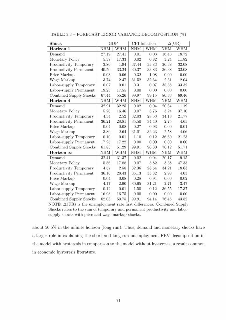
TABLE 3.3 – FORECAST ERROR VARIANCE DECOMPOSITION (%)

Shock GDP CPI Inflation ∆(UR)

Horizon 1 NHM WHM NHM WHM NHM WHM

Demand 27.19 27.41 0.01 0.03 16.43 18.72Monetary Policy 5.37 17.33 0.02 0.82 3.24 11.82Productivity Temporary 3.86 1.94 37.44 33.83 36.38 32.08Productivity Permanent 40.50 33.24 30.37 33.83 36.38 32.08Price Markup 0.03 0.06 0.32 1.08 0.00 0.00Wage Markup 3.74 2.47 31.52 32.64 2.51 2.04Labor-supply Temporary 0.07 0.01 0.31 0.07 38.88 33.32Labor-supply Permanent 19.25 17.55 0.00 0.00 0.00 0.00Combined Supply Shocks 67.44 55.26 99.97 99.15 80.33 69.46

Horizon 4 NHM WHM NHM WHM NHM WHM


Horizon ∞ NHM WHM NHM WHM NHM WHM


NOTE: ∆(UR) is the unemployment rate first differences. Combined SupplyShocks refers to the sum of temporary and permanent productivity and labor-supply shocks with price and wage markup shocks.

about 56.5% in the infinite horizon (long-run). Thus, demand and monetary shocks have

a larger role in explaining the short and long-run unemployment FEV decomposition in

the model with hysteresis in comparison to the model without hysteresis, a result common

in economic hysteresis literature.

71

3.7 CONCLUDING REMARKS

In this paper we expanded the Galı (2011a,b) unemployment model in order to consider

hysteresis in unemployment rate. To introduce hysteresis in the Galı’s model, we suppose

that the labor supply path performs in a non-stationary way and is non-cointegrated

with the employment. This combination produced a New-Keynesian model with a non-

stationary unemployment rate, i.e., a unemployment rate with full (or strong) hysteresis.

To demonstrate the implications of our hysteresis model, we estimated two small Bayesian

DSGEs with closed economy and no government applied to the Brazilian economy. One of

them adopts he standard model of Galı (2011a,b) and Galı et al. (2012) without hysteresis,

while the other model adopts the hypothesis of unemployment rate hysteresis according

to the assumption of non-stationary and no cointegrated with employment labor supply

path that we adopt.

In the model developed in this paper we show that it is feasible to incorporate unem-

ployment rate hysteresis within a New Keynesian model and that in this model demand

shocks can have permanent effects on labor supply, employment and unemployment rate.

To illustrate the applicability of our model we estimate two small Bayesian DSGE models

for the Brazilian economy (closed economy and without government models). One of

our main findings is that the monetary policy has greater weight in the forecast error

variance decomposition in the model with hysteresis in comparison to the model without

hysteresis.

In comparing the two models impulse response functions, we have seen that in the

model with hysteresis demand, monetary policy and supply shocks have permanent effects

on the unemployment rate level. But the magnitude of these effects seem exaggerated for

some shocks. We believe this is due to the simplified production function that we adopt

in this our model. It is expected that a model with a production function that includes

capital with variable utilization rate, costs of utilization and maybe labor adjustment

costs can produce more realistic impulse response functions for the unemployment rate.

These improvements we leave to future research.

72

4 THESIS CONCLUSIONS

The aim of this thesis was to analyze the effects of possible hysteresis presence on the

Brazilian unemployment rate. We pursued this objective through two essays or papers.

In the first essay or paper, “Dynamic Effects of Hysteresis in Brazilian Unemployment”,

we tested the hypothesis of total hysteresis presence in the Brazilian unemployment rate

through a cointegration model between real wage, real output per capita and unemploy-

ment rate proposed by Balmaseda et al. (2000). Our many findings were: first, the

Brazilian unemployment rate measured by IBGE’s PME can be considered a process with

full hysteresis (unemployment rate is a I(1) variable) in all the sub-periods. Second, de-

mand shocks play a similar role in explaining the forecast error variance (FEV) of the

unemployment rate in all sub-periods. Third, productivity shocks was more important in

explaining the (FEV) of the unemployment rate in the “before Real Plan” period, while

labor-supply shocks were more important in the “after Real Plan” period. Third, real

wages seemed be more flexible in the “before Real Plan” period compared with subsequent

periods, mainly compared with the “Inflation Targeting” period.

In the second essay or paper, “Hysteresis in a New Keynesian DSGE”, we expand

the Galı (2011a,b) unemployment model to consider the hysteresis in unemployment rate

hypothesis. With full hysteresis, the various shocks affecting the economy have a per-

manent effect on employment and unemployment rate. In an economy of this type the

unemployment rate do not tend to a certain mean or to a “natural rate” of unemploy-

ment in the long-run. In the model developed in this paper we showed that it is feasible

to incorporate unemployment rate hysteresis within a New Keynesian model and that in

this model demand shocks can have permanent effects on employment and unemployment

rate. To illustrate the applicability of our model we estimated two small Bayesian DSGE

models for the Brazilian economy (closed economy and without government models). One

of our main findings was that the monetary policy has greater weight in the forecast error

variance decomposition in the model with hysteresis in comparison to the model without

hysteresis.

In comparing the two models impulse response functions, we have seen that in the

model with hysteresis demand, monetary policy and supply shocks have permanent effects

73

on the unemployment rate level. But the magnitude of these effects seem exaggerated

for some shocks. We believe this is due to the simplified production function that we

adopt in this our model. It is expected that a model with a production function that

includes capital with variable utilization rate and costs of utilization, fixed production

costs, and labor adjustment costs can produce more realistic impulse response functions

for the unemployment rate.

74

Bibliography

Adjemian, S., Bastani, H., Karame, F., Juillard, M., Maih, J.; Mihoubi, F., Perendia, G.,

Pfeifer, J., Ratto, M., and Villemot, S. (2014). Dynare: Reference manual version 4.

Dynare Working Papers, 1.

Ayala, A., Cunado, J., and Gil-Alana, L. A. (2012). Unemployment hysteresis: empirical

evidence for latina america. Journal of Applied Economics, 15:213–233.

Ball, L. M. (1999). Aggregate demand and lon-run unemployment. Brookings Papers on

Economic Activity, 30(2):189–252.

Ball, L. M. (2009). Hysteresis in unemployment: Old and new evidence. NBER Working

Paper, (14818).

Balmaseda, M., Dolado, J. J., and Lopez-Salido, J. D. (2000). The dynamic effects to

shocks to labour markets: evidence from OECD countries. Oxford Economic Papers,

52:2–23.

Barro, R. (1988). The natural rate of unemployment reconsidered: The persistence of

unemployment. American Economic Review, 78:32–37.

Blanchard, O. and Galı, J. (2010). Labor markets and monetary policy: a new keynesian

model with unemployment. American Economic Journal: Macroeconomics, 2(2):1–30.

Blanchard, O. J. and Quah, D. (1989). The dynamic effects of aggregate demand and

supply disturbances. American Economic Review, 79(4):655–673.

Blanchard, O. J. and Summers, L. H. (1986). NBER Macroeconomics Annual 1986,

Volume 1. In Fischer, S., editor, Hysteresis and the European Unemployment Problem,

pages 15–90. MIT Press, Cambridge, Massachusetts, USA.

Blanchard, O. J. and Summers, L. H. (1987). Hysteresis in unemployment. European

Economic Review, 31:288–295.

Boldrin, M., Christiano, L., and Fisher, J. (2001). Habit persistence, asset returns and

the business cycle. American Economic Review, 91(1):149–166.

75

Castro, M. R. d., Gouvea, S. N., Minella, A., Santos, R. C., and Souza-Sobrinho, N. F.

(2011). Samba: Stochastic analiytical model with a bayesian approach. Working Paper

Series, (239):1–138. Version: June 16, 2011. Central Bank of Brazil.

Christiano, L. J., Trabandt, M., and Walentin, K. (2010). Involuntary unemployment and

the business cycle. NBER Working Papers, 15801.

Christoffel, K., Kuester, K., and Linzert, T. (2009). The role of labor markets for euro

area monetary policy. European Economic Review, 53(8):908–936.

Clarida, R. and Galı, J. (1994). Sources of real exchange rate fluctuations: How important

are nominal shocks? Carnegie-Rochester Conference Series on Public Policy, 41:1–56.

Cross, R. B. (1987). Hysteresis and instability in the natural rate of unemployment.

Scandinavian Journal of Economics, 89:71–89.

Dennis, R. (2009). Consumption habits in a new keynesian business cycle model. Journal

of Money, Credit and Banking, 41(5):1015–1030.

Dib, A. (2003). An estimated canadian dsge model with nominal and real rigidities.

Canadian Journal of Economics, 36:949–972.

Dobbie, M. (2004). Hysteresis and insider-outsider theory: A literature review. Working

Paper, Department Of Economics, Macquarie University, Sidney, Australia.

Duesenberry, J. (1949). Income, Saving and the Theory of Consumer Behavior. Harvard

University Press, Cambridge, MA.

Edge, R., Kiley, M., and Laforte, J. P. (2005). An estimated dsge model of the u.s.

economy.

Efron, B. (1979). Bootstrap methods: Another look at the jackknife. The Annals of

Statistics, 7(1):1–26.

Erceg, C. J., Henderson, D. W., and Levin, A. T. (2000). Optimal monetary policy with

staggered wage and price contracts. Journal of Monetary Economics, 46:281–313.

Fernandez-Villaverde, J. and Rubio-Ramirez, J. F. (2006). Estimating macroeconomic

models: A likelihood approach. University of Pennsylvania.

76

Ferrari, T. K. and Brasil, G. H. (2015). Comportamento do desemprego regional no brasil:

uma aplicacao de teste de convergencia em painel. Nova Economia, 25(3):673–688.

Franz, W. (1987). Hysteresis, persistence and the nairu: An empirical analysis for the

federal republic of germany. In Layard, R. and Calmfors, L., editors, The Fight Against

Unemployment, pages 121–170. MIT Press, MA Cambridge.

Friedman, M. (1968). The role of monetary policy. The American Economic Review,

58(1).

Frisch, R. (1932). New Methods of Measuring Marginal Utility. Mohr, Tubingen.

Fukac, M. and Pagan, A. (2006). Limited information estimation and evaluation of dsge

models. NCER Working Paper No. 6.

Galı, J. (2011a). The return of the wage phillips curve. Journal of the European Economic

Association, 9(3):436–461.

Galı, J. (2011b). Unemployment Fluctuations and Stabilization Policies: A New Keyne-

sian Perspective,. The MIT Press, Cambridge, Massachusetts.

Galı, J. (2015). Hysteresis and the european unemployment problem revisited. NBER

Working Papers 21430.

Galı, J. (2016). Insider-outsider labor markets, hysteresis and monetary policy. CREI,

UPF and Barcelona GSE.

Galı, J., Smets, F., and Wouters, R. (2012). Unemployment in an estimated new keynesian

model. NBER Macroeconomics Annual, 26(1):329–360.

Gertler, M. and Trigari, A. (2009). Unemployment fluctuations with staggered nash wage

bargaining. Journal of Political Economy, 117(1):38–86.

Gomes, F. A. R. and Silva, C. G. (2009). Hysteresis versus nairu and convergence versus

divergence: The behavior of regional unemployment rates in brazil. The Quarterly

Review of Economics and Finance, 49:308–322.

Gordon, R. (1989). Hysteresis in hystory: Was there ever a phillips curve. American

Economic Association: Papers and Proceedings, 79(2):220–225.

77

Gottfries, N. and Horn, H. (1987). Wage formation and the persistence of unemployment.

Economic Journal, 97:877–884.

Hamilton, J., Waggoner, D., and Zha, T. (2004). Normalization in econometrics. Working

Paper.

Hansen, G. D. (1985). Indivisible labor and the business cycle. Journal of Monetary

Economics, 16(3):309–327.

Hargraves-Heap, S. P. (1980). Choosing the wrong natural rate, accelerating inflation or

decelerating unemployment and growth. Economic Journal, 90(september):611–620.

Jaimovich, N. and Rebelo, S. (2009). Can news about the future drive the business cycle?

American Economics Review, 99(4):1097–1118.

Johansen, S. (1995). Likelihood-Based Inference in Cointegrated Vector Autoregressive

Models. Oxford University Press, New York.

Koyck, L. M. (1954). Distributed lags and investment analysis. North-Holland Publishing.

Layard, R. and Bean, C. (1989). Why does unemployment persist? Scandinavian Journal

of Economics, 91(2):371–396.

Layard, R. and Nickell, S. (1987). Unemployment in britain. In Bean, C., Layard, R.,

and Nickell, S., editors, The Rise in Unemployment, pages 121–170. Basil Blackwell,

Oxford.

Layard, R., Nickell, S., and Jacman, R. (1991). Unemployment: Macroeconomic Perfor-

mances and the Labor Market. Oxford University Press, Oxford.

Lindbeck, A. (1991). Unemployment and labor market imperfections. Issues in Contem-

porary Economics, (2):75–101.

Lindbeck, A. and Snower, D. (1985). Explanations of unemployment. Oxford Review of

Economic Policy, 2:34–69.

Lindbeck, A. and Snower, D. (1988a). Cooperation, harassment and involuntary unem-

ployment: An insider-outsider approach. American Economic Review, 78(1):167–188.

78

Lindbeck, A. and Snower, D. (1988b). The Insider-Outsider Theory of Employment and

Unemployment. MIT Press, Cambridge, MA, USA.

Lindbeck, A. and Snower, D. J. (1988c). The Insider-Outsider Theory of Employment

and Unemployment. The MIT Press, Cambridge, Massachusetts.

Liu, Y. (2014). Endogenous labor participation and involuntary unemployment: An

estimated new keynesian model. University of New South Wales.

Lutkepohl, H. (2005). New Introduction to Multiple Time Series Analysis. Springer-

Verlag, Berlin, Germany.

Lutkepohl, H. and Kratzig, M., editors (2004). Applied Time Series Econometrics. Cam-

bridge University Press, Cambridge.

Mortensen, D. T. and Pissarides, C. A. (1994). Job creation and job destruction in the

theory of unemployment. The Review of Economic Studies, 61(3):397–415.

Neudorfer, K., Pichelmann, K., and Wagner, M. (1990). Hysteresis, NAIRU and Long

Term Unemployment in Austria. Empirical Economics, 15:217–299.

Okun, A. M. (1962). Potential gnp, its measurement and significance. Cowles Foundation

Paper 190.

Pfeifer, J. (2015). A guide to specifying observation equations for the estimation of dsge

models. mimeo.

Phelps, E. (1972). Inflation policy and unemployment theory. Norton, New York.

Phelps, E. S. (1968). Money-wage dynamics and labor market equilibrium. Journal of

Political Economy, 76:678–711.

Roberts, J. M. and Morin, N. J. (1999). Is hysteresis important for u.s. unemployment?

FEDS Working Papers, Finance and Economics Discussion Series.

Roed, K. (1997). Hysteresis in Unemployment. Journal of Economic Surveys, 11(4):389–

418.

79

Rogerson, R. (1988). Indivisible labor, lotteries and equilibrium. Journal of Monetary

Economics, 21(1):3–16.

Ryder, H. and Heal, G. (1973). Optimal growth with intertemporally dependent prefer-

ences. Review of Economic Studies, 40:1–33.

Santana, F. L., Souza, W. P. S. d. F., and Aragon, E. K. d. S. B. (2013). Histerese versus

taxa natural do desemprego no brasil e regioes metropolitanas: novas evidencias de

quebras estruturais e raiz unitaria. Working paper n. 14.

Santos, V. A. (2006). Evidencias de Histerese na Taxa de Desemprego do Brasil: uma

Abordagem com Modelos de Longa Persistencia. Master’s thesis, Federal University of

Bahia, Salvador, Brazil.

Smets, F. and Wouters, R. (2003). An estimated dynamic stochastic general equilibrium

model of the euro area. Journal of the European Economic Association, 1(5):1123–1175.

Smets, F. and Wouters, R. (2007). Shocks and frictions in us business cycles: A bayesian

dsge approach. American Economic Review, 97(3):586–606.

Waggoner, D. and Zha, T. (2003). Likelihood preserving normalization in multiple equa-

tion models. Journal of Econometrics, 114:329–347.

80

A DYNARE CODE FOR THE MODEL WITHOUT HYSTERESIS

var y dLnGDP z_y l z_l pi_w dLnWn mu_w n dLnLaS z_a u dUnR pi_p

dLnIPCA mu_p mc w r Selic z_r gy ga gn;

varexo e_y e_l e_w e_za e_a e_n e_p e_r;

parameters h sigma rho_y gamma_c varphi rho_l gamma_w theta_w

ep_w rho_w beta alpha psi rho_za rho_a rho_n gamma_p theta_p

ep_p rho_p phi_r phi_pi phi_y rho_r sigma_ey sigma_el sigma_ew

sigma_eza sigma_ep sigma_er sigma_ea sigma_en ga_bar gn_bar

pip_bar;

h = 0.7;

sigma = 1.3;

rho_y = 0.5;

gamma_c = 0.5;

varphi = 3;

rho_l = 0.5;

gamma_w = 0.65;

theta_w = 0.16;

ep_w = 26;

rho_w = 0.5;

beta = 0.99;

alpha = 0;

psi = 5;

rho_a = 0.5;

rho_za = 0.5;

rho_n = 0.5;

gamma_p = 0.65;

theta_p = 0.25;

ep_p = 5;

rho_p = 0.5;

phi_r = 0.79;

phi_pi = 2.43;

phi_y = 0.16;

rho_r = 0;

sigma_ey = 1;

sigma_el = 1;

sigma_ew = 1;

sigma_eza = 1;

sigma_ep = 1;

sigma_er = 1;

sigma_ea = 1;

81

sigma_en = 1;

ga_bar = 0.002;

gn_bar = 0.005;

pip_bar = 0.016;

model(linear );

// gy_bar (1)

#gy_bar = ga_bar + (1 - alpha)* gn_bar;

// h_tilde (2)

#h_tilde = h*exp(-gy_bar );

// beta_tilde (3)

#beta_tilde = beta*exp(-sigma*gy_bar );

// new keynesian IS curve (5)

y = (1/(1+ h_tilde ))*y(+1) + (h_tilde /(1+ h_tilde ))*y(-1)

- ((1- h_tilde )/( sigma *(1+ h_tilde )))*(r - pi_p (+1)) + z_y;

z_y = rho_y*z_y(-1) + e_y;

// labor supply

w = (1-gamma_c )*w(-1) + sigma *( gamma_c /(1- h_tilde ))*(y

- h_tilde*y(-1)) + varphi*l - (1-gamma_c )* varphi*l(-1)

- varphi*z_l + (1-gamma_c )* varphi*z_l(-1);

z_l = rho_l*z_l(-1) + e_l;

// labor demand

n = (1/( psi *(1 - alpha )))*(y - psi*z_a);

z_a = rho_za*z_a(-1) + e_za;

// unemployment rate

u = l - n;

// cpi inflation (IPCA)

82

pi_p = (beta_tilde /(1+ beta_tilde*gamma_p ))* pi_p (+1)

+ (gamma_p /(1+ beta_tilde*gamma_p ))* pi_p(-1)

+ (((1 - theta_p )*(1 - beta_tilde*theta_p)

*(1 - alpha ))/( theta_p *(1 - alpha + alpha*ep_p )))*mc

+ mu_p;

mu_p = rho_p*mu_p(-1) + e_p;

// marginal cost

mc = w + (1/( psi*(1 - alpha )))*( alpha*y - psi*z_a);

// real wage

w = w(-1) + pi_w - pi_p - (ga - ga_bar) + alpha *(gn - gn_bar );

//wage inflation

pi_w = gamma_w*pi_p(-1) + beta_tilde *(pi_w (+1) - gamma_w*pi_p)

- (((1- beta_tilde*theta_w)

*(1 - theta_w ))/( theta_w *(1 + ep_w*varphi )))* varphi*u + mu_w;

mu_w = rho_w*mu_w(-1) + e_w;

// monetary policy (taylor -rule)

r = phi_r*r(-1) + (1 - phi_r )*( phi_pi*pi_p + phi_y*y) + z_r;

z_r = rho_r*z_r(-1) + e_r;

// observation equations

dLnGDP = gy + y - y(-1);

gy = ga + (1 - alpha )*gn;

ga = (1-rho_a)* ga_bar + rho_a*ga(-1) + e_a;

dLnLaS = gn + l - l(-1);

gn = (1 - rho_n)* gn_bar + rho_n*gn(-1) + e_n;

dLnWn = pip_bar + pi_w + ga_bar - alpha*gn_bar;

dLnIPCA = pip_bar + pi_p;

Selic = ((1+ pip_bar )/( beta*exp(-sigma*gy_bar ))) - 1 + r;

dUnR = u - u(-1);

end;

initval;

y = 0;

83

z_y = 0;

l = 0;

z_l = 0;

pi_w = 0;

mu_w = 0;

n = 0;

z_a = 0;

u = 0;

pi_p = 0;

mu_p = 0;

mc = 0;

w = 0;

r = 0;

z_r = 0;

dLnGDP = ga_bar + (1 - alpha)* gn_bar;

gy = ga_bar + (1 - alpha)* gn_bar;

ga = ga_bar;

dLnLaS = gn;

dLnWn = pip_bar + ga_bar - alpha*gn_bar;

gn = gn_bar;

dLnIPCA = pip_bar;

Selic = ((1+ pip_bar )/( beta*exp(-sigma *( ga_bar

+ (1 - alpha )* gn_bar )))) - 1;

dUnR = 0;

end;

steady;

check;

shocks;

var e_y = 1;

var e_l = 1;

var e_w = 1;

var e_p = 1;

var e_r = 1;

var e_za = 1;

var e_a = 1;

var e_n = 1;

end;

estimated_params;

sigma , normal_pdf , 1.3, 0.05;

84

h, beta_pdf , 0.7, 0.04;

rho_y , beta_pdf , 0.5, 0.2;

varphi , gamma_pdf , 5, 1, 1;

gamma_c , beta_pdf , 0.5, 0.2;

rho_l , beta_pdf , 0.5, 0.2;

psi , gamma_pdf , 5, 0.5, 1;

ep_w , gamma_pdf , 5, 1, 1;

theta_w , beta_pdf , 0.75, 0.05;

gamma_w , beta_pdf , 0.5, 0.15;

rho_w , beta_pdf , 0.5, 0.2;

theta_p , beta_pdf , 0.08, 0.02;

gamma_p , beta_pdf , 0.5, 0.15;

rho_p , beta_pdf , 0.5, 0.2;

rho_za , beta_pdf , 0.5, 0.2;

phi_r , beta_pdf , 0.6, 0.15;

phi_pi , normal_pdf , 2, 0.35;

phi_y , gamma_pdf , 0.25, 0.1;

rho_r , beta_pdf , 0.5, 0.2;

ga_bar , normal_pdf , 0.002, 0.001;

rho_a , beta_pdf , 0.5, 0.2;

gn_bar , normal_pdf , 0.004, 0.002;

rho_n , beta_pdf , 0.5, 0.2;

pip_bar , normal_pdf , 0.0159 , 0.008;

sigma_ey , inv_gamma_pdf , 1, Inf;

sigma_el , inv_gamma_pdf , 1, Inf;

sigma_ew , inv_gamma_pdf , 1, Inf;

sigma_eza , inv_gamma_pdf , 1, Inf;

sigma_ep , inv_gamma_pdf , 1, Inf;

sigma_er , inv_gamma_pdf , 1, Inf;

sigma_ea , inv_gamma_pdf , 1, Inf;

sigma_en , inv_gamma_pdf , 1, Inf;

end;

options_.relative_irf =1;

estimation(datafile=series1 , mh_replic =10000 , mh_nblocks =5,

mh_drop =0.5, mh_jscale =0.8, mode_compute =4, mode_check , order=1,

85

diffuse_filter , moments_varendo , irf =48, ar = 12,

conditional_variance_decomposition = [1:32]) dLnGDP dLnLaS dLnWn

dLnIPCA Selic u;

stoch_simul(periods=0, order = 1, ar = 8,

conditional_variance_decomposition = [1:32]);

varobs dLnGDP dLnLaS dLnWn dLnIPCA Selic dUnR;

disp(’Initial period is $1999Q1 ’)

86

B DYNARE CODE FOR THE MODEL WITH HYSTERESIS

var y dLnGDP z_y l z_l pi_w dLnWn mu_w n dLnLaS z_a du dUnR pi_p

dLnIPCA mu_p mc w r Selic z_r gy ga gn;

varexo e_y e_l e_w e_za e_a e_n e_p e_r;

parameters h sigma rho_y gamma_c varphi rho_l gamma_w theta_w ep_w

rho_w beta alpha psi rho_za rho_a rho_n gamma_p theta_p

ep_p rho_p phi_r phi_pi phi_y rho_r sigma_ey sigma_el sigma_ew

sigma_eza sigma_ep sigma_er sigma_ea sigma_en

ga_bar gn_bar pip_bar;

h = 0.85;

sigma = 1.3;

rho_y = 0.5;

gamma_c = 0.5;

varphi = 5;

rho_l = 0.5;

gamma_w = 0.5;

theta_w = 0.75;

ep_w = 5;

rho_w = 0.5;

beta = 0.99;

alpha = 0;

psi = 5;

rho_a = 0.5;

rho_za = 0.5;

rho_n = 0.5;

gamma_p = 0.5;

theta_p = 0.08;

ep_p = 5;

rho_p = 0.5;

phi_r = 0.5;

phi_pi = 2;

phi_y = 0.25;

rho_r = 0.5;

sigma_ey = 1;

sigma_el = 1;

sigma_ew = 1;

sigma_eza = 1;

sigma_ep = 1;

sigma_er = 1;

sigma_ea = 1;

87

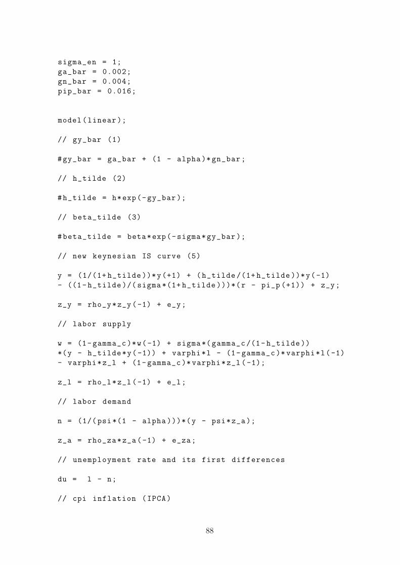
sigma_en = 1;

ga_bar = 0.002;

gn_bar = 0.004;

pip_bar = 0.016;

model(linear );

// gy_bar (1)

#gy_bar = ga_bar + (1 - alpha)* gn_bar;

// h_tilde (2)

#h_tilde = h*exp(-gy_bar );

// beta_tilde (3)

#beta_tilde = beta*exp(-sigma*gy_bar );

// new keynesian IS curve (5)

y = (1/(1+ h_tilde ))*y(+1) + (h_tilde /(1+ h_tilde ))*y(-1)

- ((1- h_tilde )/( sigma *(1+ h_tilde )))*(r - pi_p (+1)) + z_y;

z_y = rho_y*z_y(-1) + e_y;

// labor supply

w = (1-gamma_c )*w(-1) + sigma *( gamma_c /(1- h_tilde ))

*(y - h_tilde*y(-1)) + varphi*l - (1-gamma_c )* varphi*l(-1)

- varphi*z_l + (1-gamma_c )* varphi*z_l(-1);

z_l = rho_l*z_l(-1) + e_l;

// labor demand

n = (1/( psi *(1 - alpha )))*(y - psi*z_a);

z_a = rho_za*z_a(-1) + e_za;

// unemployment rate and its first differences

du = l - n;

// cpi inflation (IPCA)

88

pi_p = (beta_tilde /(1+ beta_tilde*gamma_p ))* pi_p (+1)

+ (gamma_p /(1+ beta_tilde*gamma_p ))* pi_p(-1)

+ (1 - theta_p )*(1 - beta_tilde*theta_p)

*(1/ theta_p )*(1 - alpha )*(1/(1 - alpha + alpha*ep_p))

*(1/(1+ beta_tilde*gamma_p ))*mc + mu_p;

mu_p = rho_p*mu_p(-1) + e_p;

// marginal cost

mc = w + (1/( psi*(1 - alpha )))*( alpha*y - psi*z_a);

// real wage

w = w(-1) + pi_w - pi_p - (ga - ga_bar) + alpha *(gn - gn_bar );

//wage inflation

pi_w = gamma_w*pi_p(-1) + beta_tilde *(pi_w (+1) - gamma_w*pi_p)

- (((1- beta_tilde*theta_w)

*(1 - theta_w ))/( theta_w *(1 + ep_w*varphi )))

*varphi*du + mu_w;

mu_w = rho_w*mu_w(-1) + e_w;

// monetary policy (taylor -rule)

r = phi_r*r(-1) + (1 - phi_r )*( phi_pi*pi_p + phi_y*y) + z_r;

z_r = rho_r*z_r(-1) + e_r;

// observation equations

dLnGDP = gy + y - y(-1);

gy = ga + (1 - alpha )*gn;

ga = (1-rho_a)* ga_bar + rho_a*ga(-1) + e_a;

dLnLaS = gn + l;

gn = (1 - rho_n)* gn_bar + rho_n*gn(-1) + e_n;

dLnWn = pip_bar + pi_w + ga_bar - alpha*gn_bar;

dLnIPCA = pip_bar + pi_p;

Selic = log ((1+ pip_bar )/( beta*exp(-sigma*gy_bar ))) + r;

dUnR = du;

end;

initval;

89

y = 0;

z_y = 0;

l = 0;

z_l = 0;

pi_w = 0;

mu_w = 0;

n = 0;

z_a = 0;

du = 0;

pi_p = 0;

mu_p = 0;

mc = 0;

w = 0;

r = 0;

z_r = 0;

dLnGDP = ga_bar + (1 - alpha)* gn_bar;

gy = ga_bar + (1 - alpha)* gn_bar;

ga = ga_bar;

dLnLaS = gn;

gn = gn_bar;

dLnWn = pip_bar + ga_bar - alpha*gn_bar;

dLnIPCA = pip_bar;

Selic = log ((1+ pip_bar )/( beta*exp(-sigma*( ga_bar + (1 - alpha )* gn_bar ))));

dUnR = 0;

end;

steady;

check;

shocks;

var e_y = 1;

var e_l = 1;

var e_w = 1;

var e_p = 1;

var e_r = 1;

var e_za = 1;

var e_a = 1;

var e_n = 1;

end;

estimated_params;

90

sigma , normal_pdf , 1.3, 0.05;

h, beta_pdf , 0.7, 0.04;

rho_y , beta_pdf , 0.5, 0.2;

varphi , gamma_pdf , 5, 1, 1;

gamma_c , beta_pdf , 0.5, 0.2;

rho_l , beta_pdf , 0.5, 0.2;

psi , gamma_pdf , 5, 1, 1;

ep_w , gamma_pdf , 5, 1, 1;

theta_w , beta_pdf , 0.75, 0.05;

gamma_w , beta_pdf , 0.5, 0.15;

rho_w , beta_pdf , 0.5, 0.2;

theta_p , beta_pdf , 0.08, 0.02;

gamma_p , beta_pdf , 0.5, 0.15;

rho_p , beta_pdf , 0.5, 0.2;

rho_za , beta_pdf , 0.5, 0.2;

phi_r , beta_pdf , 0.6, 0.15;

phi_pi , normal_pdf , 2, 0.35;

phi_y , gamma_pdf , 0.25, 0.1;

rho_r , beta_pdf , 0.5, 0.2;

ga_bar , normal_pdf , 0.002, 0.001;

rho_a , beta_pdf , 0.5, 0.2;

gn_bar , normal_pdf , 0.004, 0.002;

rho_n , beta_pdf , 0.5, 0.2;

pip_bar , normal_pdf , 0.0159 , 0.008;

sigma_ey , inv_gamma_pdf , 1, Inf;

sigma_el , inv_gamma_pdf , 1, Inf;

sigma_ew , inv_gamma_pdf , 1, Inf;

sigma_eza , inv_gamma_pdf , 1, Inf;

sigma_ep , inv_gamma_pdf , 1, Inf;

sigma_er , inv_gamma_pdf , 1, Inf;

sigma_ea , inv_gamma_pdf , 1, Inf;

sigma_en , inv_gamma_pdf , 1, Inf;

end;

options_.relative_irf =1;

estimation(datafile=series2 , mh_replic =10000 , mh_nblocks =5,

mh_drop =0.5, mh_jscale =0.8, mode_compute =4, mode_check , order=1,

91

diffuse_filter , moments_varendo , irf =48, ar = 12,

conditional_variance_decomposition = [1:32]) dLnGDP dLnLaS dLnWn

dLnIPCA Selic l n;

stoch_simul(periods=0, order = 1, ar = 8,

conditional_variance_decomposition = [1:32]);

varobs dLnGDP dLnLaS dLnWn dLnIPCA Selic dUnR;

disp(’Initial period is $1999Q1 ’)

92

FEDERAL UNIVERSITY OF PARANA GUILHERME ALEXANDRE …

Documents

Transcript of FEDERAL UNIVERSITY OF PARANA GUILHERME ALEXANDRE …