Facultad de Ciencias - Universidad de NavarraEn cumplimiento de la normativa para la presentación...
335
Facultad de Ciencias INTEGRATIVE DEMOGRAPHIC INFERENCE IN IBERIAN POND-BREEDING AMPHIBIANS Gregorio Sánchez Montes
Transcript of Facultad de Ciencias - Universidad de NavarraEn cumplimiento de la normativa para la presentación...

F a c u l t a d d e C i e n c i a s
INTEGRATIVE DEMOGRAPHIC INFERENCE IN IBERIAN
POND-BREEDING AMPHIBIANS
Gregorio Sánchez Montes


F a c u l t a d d e C i e n c i a s
INTEGRATIVE DEMOGRAPHIC INFERENCE IN IBERIAN POND-BREEDING AMPHIBIANS
Memoria presentada por D. Gregorio Sánchez Montes para aspirar al grado de Doctor por la Universidad de Navarra
El presente trabajo ha sido realizado bajo nuestra dirección en el Departamento de Biología Ambiental y autorizamos su presentación ante el Tribunal que lo ha de juzgar.
Pamplona, 28 de abril de 2017
Dr. Arturo H. Ariño Plana Dr. Íñigo Martínez-Solano González Profesor Titular Científico Titular
Dpto. Biología Ambiental Dpto. Biodiversidad y Biología Evolutiva
Universidad de Navarra Museo Nacional de Ciencias Naturales CSIC


‘If I have seen further, it is by
standing on the shoulders of giants’
Isaac Newton


Agradecimientos
Llegar a ver publicada esta tesis doctoral ha requerido un intenso camino académico y
personal en el que mucha gente me ha brindado su apoyo, el cual agradezco de corazón.
Agradezco, en primer lugar, a mis directores de tesis, Íñigo y Arturo, por darme
la oportunidad de iniciarme en el camino de la investigación, y por ser un ejemplo de
honestidad, esfuerzo y pasión por la búsqueda constante de la verdad. Cada momento de
los que hemos compartido trabajando juntos (y han sido muchos) han formado parte de
una gran lección en la que ni un solo día he dejado de aprender. Os admiro tanto en lo
académico como en lo humano, porque en ambos aspectos me habéis hecho crecer. Mi
gratitud también para los programas de becas para la formación del personal
investigador y de ayudas para la movilidad de la Asociación de Amigos de la
Universidad de Navarra, que financiaron los estudios de doctorado y parte de una
fructífera estancia predoctoral en el Institute of Zoology de Londres.
También agradezco a los excelentes profesores que, gracias a su ejemplo, desde
el colegio Nuestra Señora de Begoña de Bilbao (Alberto, Félix, Juanjo, Eskolunbe, Javi,
Asier, Aitor, Dori, Ana, Koldo, Ainhoa, Isabel y tantos otros) hasta las Universidades de
Navarra (María, Juanjo, Ricardo, Mª Elena, Enrique, Jordi, Mª Carmen, David, Antonio,
Nieves, Marina, Javier y muchos más), Autónoma y Complutense de Madrid (Juan,
José, Manolo, Ángel, Jesús, por citar algunos) prendieron intensamente en mí la llama
de la búsqueda del conocimiento. Gracias por esas lecciones que nunca he olvidado,
porque me las transmitisteis desde el fondo de vuestro corazón y de vuestro saber,
descubriéndome esta maravillosa comunión de mentes que es la ciencia. Este periodo
predoctoral también me ha permitido conocer a grandes investigadores como David
Galicia, José Luis Vizmanos, Jinliang Wang, Trent Garner, Javier Seoane, Isabel Rey,
Annie Machordom, Marta Barluenga, Mario García-París, David Buckley, Carmen
Díaz-Paniagua, Iván Gómez-Mestre o Ernesto Recuero, de quienes he aprendido
muchas maneras de enfocar los problemas que surgen constantemente en cualquier
camino hacia lo desconocido (porque eso es la investigación, nada menos). Gracias por
tratarme como a uno más y por compartir vuestra experiencia con un joven preguntón.
Agradezco especialmente a Rafa Miranda y Mariano Larraz por darme una oportunidad
en el ámbito de la divulgación de la ciencia y de la evolución, que tanto me apasiona.
En esta tesis también ha habido mucho trabajo de laboratorio, que no habría
podido desarrollar sin la tutela dedicada y afectuosa de los estupendos técnicos que
tanto me han ayudado en el Museo Nacional de Ciencias Naturales (gracias muy
especialmente a Piluchi, Isabel e Iván), en la Estación Biológica de Doñana (agradezco
mucho a Ana, Mónica, María, Antonio y José María por dos intensos meses de trabajo),
de la Universidad de Navarra (Ana, María y Ángel) y el equipo de Morfología del
Centro de Investigación Médica Aplicada (Laura, Paula, Carolina, Elena y Mª Paz). Las
técnicas que he aprendido gracias a vosotros son una formación impagable. Por otro
lado, la labor de docencia ha sido una de las que más satisfacciones me ha dado, y hacia
la que siento una intensa vocación, en buena parte gracias a Eva Montilla, con quien
siempre ha sido una auténtica delicia trabajar. También agradezco muy especialmente al
personal de administración y servicios de los centros que he visitado, por tratarme con
una humanidad y un afecto que nunca pasaron desapercibidos para mí (especialmente a
Carmentxu, Marisol, Naira y Martín, Ángel, Patxi, Justo, Peque, Jorge, José Luis y José
Javier, Marina, Inma, Carolina, Miriam e Irantzu, Jo, Amrit, Raquel, Rebeca y María).

Agradecimientos
Y cómo no, agradezco enormemente a los grandes compañeros que he conocido
durante estos años en las universidades y centros de investigación en los que he tenido
la suerte de ser acogido. Desde aquellos inicios en el Z-428 del Museo de Ciencias
Naturales de Madrid, con Miguel, Merel, Virginia, Luis, Cristina, Carmen, Paloma, Javi
y Alfonso hasta la Universidad de Navarra, donde un día de 2012 entramos como
becarios el gran Iván Vedia y yo. Desde entonces he aprendido mucho de los profesores
del Departamento de Biología Ambiental y también con las experiencias junto a
compañeros como Antonio, Iván, Ibon, Andrea, Ainhoa, Txiki, Javi, María, Rubén,
Nora, Xabi, Imanol y Amaia en Pamplona; Mar, Pablo B, Pablo L, Rosa, Mari, Noa,
Alazne, Antonio y Marina en Sevilla; Jorge, Tania, Michel, Pau, Melinda, Andrés, Iker,
David, Juanes, Miriam, Silvia, Étienne, Carlos, Yolanda, Guillermo, Chechu, Anna,
Violeta y Paula en Madrid y, ya en tierras británicas, en compañía de Chris, Donal,
Sandy y Will. Quisiera tener una mención especial para los grandes compañeros que me
prestaron una ayuda fundamental en largas jornadas de campo, sin importarles lo
complicadas que fueran las condiciones meteorológicas, como Miguel Peñalver y Espe
(siempre dispuestos para la batalla), Jorge, Garazi, Jose, Amaia, Celia, Miguel Rojo,
Luis, Rut, Rafa, Imanol, Nora, Iván, Antonio, Juan y Joaquín. Todos vosotros sabéis tan
bien como yo lo que cuesta conseguir datos en el campo y sin vuestra generosa ayuda
(y, muchas veces, tutela y consejo) no habría sido capaz. También agradezco el
incondicional apoyo de mis amigos (Álex Maestre, Álex Alonso, Ander, Diego, Joseba,
Juan, Iñaki, Lucía, Laura, Txas, Bea, Edu, Pablo Vicente, Carlos, Pablo Bazal,
Guillermo, Andoni, Anica, Mikel, Olaia, Jaime, Miren, María, Sol, MEG, Miri, Dorleta,
Loyola, Teresa, Carmen, Alfredo, Luis, João) y el afecto de las buenas amistades que he
hecho en el coro y orquesta de la Universidad de Navarra, con el gran maestro Ekhi
Ocaña al frente.
Para terminar, pero siempre en la mención más especial, agradezco a mi familia.
A mis padres y a mi hermana, por recordarme siempre quién soy y de dónde vengo; a
mis abuelos, tíos y primos (muy especialmente a Totó, Amama, José, Dioni, Pepe y
Tomás) y a Pilar, por compartir conmigo su compañía, su alegría y su maravillosa
forma de ver el mundo.

Esta tesis doctoral incluye una colección de manuscritos en diferentes estados de
publicación, cada uno de los cuales constituye un capítulo. Los manuscritos se
reproducen íntegros y en el idioma en el que fueron publicados o enviados para su
publicación, incluyendo siempre un resumen en castellano.
En cumplimiento de la normativa para la presentación de tesis doctorales en la Facultad
de Ciencias de la Universidad de Navarra se incluyen los siguientes apartados: (1) un
Resumen integrador del contenido de la tesis doctoral; (2) una Introducción general que
sitúa el trabajo realizado en su contexto teórico, planteando los Objetivos de la tesis
doctoral; (3) una Discusión general, y (4) un apartado de Conclusiones generales.


TABLE OF CONTENTS
GENERAL ABSTRACT ..................................................................................................... 19
CHAPTER I: GENERAL INTRODUCTION ..................................................................... 25
Contribution of genetics to demographic research ............................................... 28 The development of molecular biology ................................................................ 29 Possibilities and misuses of bioinformatics tools ................................................. 32
The theoretical framework of population genetics................................................ 33
Individual-based monitoring programs complementing genetic-based
demographic inferences: the effective/census size ratio ....................................... 39 Challenges faced by amphibians in an anthropized world .................................. 43
The study system: a multi-species, multi-scale approach .................................... 49 Epidalea calamita (Laurenti, 1768) ...................................................................... 50 Hyla molleri Bedriaga, 1889 ................................................................................. 53
Pelophylax perezi (López-Seoane, 1885) ............................................................. 55 Pelobates cultripes (Cuvier, 1829) ....................................................................... 57 A multi-scalar approach ........................................................................................ 59
References ................................................................................................................. 66
CHAPTER II: GENERAL OBJECTIVES ........................................................................ 89
CHAPTER III: SPECIES ASSIGNMENT IN THE PELOPHYLAX RIDIBUNDUS X P. PEREZI
HYBRIDOGENETIC COMPLEX BASED ON 16 NEWLY CHARACTERISED MICROSATELLITE
MARKERS Herpetological Journal (2016), 26 (2): 99-108 ........................................... 93
Abstract ..................................................................................................................... 95 Resumen .................................................................................................................... 97
Introduction .............................................................................................................. 99 Materials and methods .......................................................................................... 100
Results ..................................................................................................................... 105 Discussion ............................................................................................................... 109 References ............................................................................................................... 114
CHAPTER IV: EFFECTS OF SAMPLE SIZE AND FULL SIBS ON GENETIC DIVERSITY
CHARACTERIZATION: A CASE STUDY OF THREE SYNTOPIC IBERIAN POND-BREEDING
AMPHIBIANS Journal of Heredity (2017), esx038. doi: 10.1093/jhered/esx038 ......... 117
Abstract ................................................................................................................... 119 Resumen .................................................................................................................. 121 Introduction ............................................................................................................ 123 Materials and methods .......................................................................................... 126
Tissue sampling ................................................................................................... 126 DNA extraction and genotyping ......................................................................... 128 Characterization of genetic diversity and effect of full sibs ............................... 128
Effect of sample size ........................................................................................... 130
Results ..................................................................................................................... 131 Characterization of genetic diversity and effect of full sibs ............................... 131

Effect of sample size ........................................................................................... 132
Discussion ............................................................................................................... 134 References ............................................................................................................... 139
CHAPTER V: RELIABLE EFFECTIVE/CENSUS POPULATION SIZE RATIOS IN SEASONAL-
BREEDING SPECIES: OPPORTUNITY FOR INTEGRATIVE DEMOGRAPHIC INFERENCES
BASED ON CAPTURE-MARK-RECAPTURE DATA AND MULTILOCUS GENOTYPES
Ecology and Evolution (Accepted, pending minor review) ......................................... 143
Abstract ................................................................................................................... 145
Resumen .................................................................................................................. 147 Introduction ............................................................................................................ 149 Materials and methods .......................................................................................... 152
Study area and CMR monitoring program .......................................................... 152
CMR estimates of Na ........................................................................................... 153 Genetic estimates of Nb ....................................................................................... 156
Results ..................................................................................................................... 159 CMR estimates of Na ........................................................................................... 159
Genetic estimates of Nb ....................................................................................... 159
Discussion ............................................................................................................... 164 Extension to Ne/Nc estimation ............................................................................. 167
References ............................................................................................................... 170
CHAPTER VI: MOUNTAINS AS BARRIERS TO GENE FLOW IN AMPHIBIANS:
QUANTIFYING THE DIFFERENTIAL EFFECT OF A MAJOR MOUNTAIN RIDGE ON THE
GENETIC STRUCTURE OF FOUR SYMPATRIC SPECIES WITH DIFFERENT LIFE HISTORY
TRAITS Journal of Biogeography (Under review) ...................................................... 175
Abstract ................................................................................................................... 177 Resumen .................................................................................................................. 179
Introduction ............................................................................................................ 181
Materials and methods .......................................................................................... 185 Study area, targeted species and dataset collection ............................................. 185
Genetic analyses .................................................................................................. 189
Results ..................................................................................................................... 193 Dispersal potential ............................................................................................... 193
Genetic analyses .................................................................................................. 193
Discussion ............................................................................................................... 200 References ............................................................................................................... 205
CHAPTER VII: GENERAL DISCUSSION .................................................................... 211
References ............................................................................................................... 224
CHAPTER VIII: GENERAL CONCLUSIONS ............................................................... 227
APPENDIX 1: Characterization of the microsatellite sets of H. molleri, E. calamita
and P. perezi ................................................................................................................ 231

APPENDIX 2: Accumulation curves of allelic richness and expected heterozygosity
as a function of sample size ........................................................................................ 263
APPENDIX 3: Empirical and Chao & Jost (2015) profiles .................................... 271
APPENDIX 4: Relationship between FIS and error rate estimates ....................... 279
APPENDIX 5: Effect of sampling excessive close relatives on FIS and deviation
from HWE ................................................................................................................... 283
APPENDIX 6: R scripts for replicated analyses ..................................................... 289
APPENDIX 7: Summary tables of CMR models .................................................... 305
APPENDIX 8: Inferred sibship and parentage relationships ................................ 309
APPENDIX 9: Pairwise FST estimates and migration rates per generation ......... 315
APPENDIX 10: Results of clustering analyses ........................................................ 327

List of abbreviations
6-FAM One of the labelling dyes (blue) used in multiplex reactions for
genotyping with microsatellite markers on the ABI3730 sequencer
95% CI 95% confidence interval
ΔK A statistic based on the second order rate of change of the likelihood
function with respect to K, the number of genetic clusters, devised by
Evanno et al. (2005) and used for exploring the relative likelihood of
different K values in genetic clustering analyses
AICc Akaike Information Criterion corrected for small sample sizes
AR Allelic richness
Avge Average
bp Base pairs (a measure of genetic sequence length)
BPP Bayesian posterior probability
c. circa (Latin for ‘approximately’)
CJS Cormack-Jolly-Seber model of CMR
CMR Capture-mark-recapture
cox1 Mitochondrially encoded gene of cytochrome c oxidase subunit 1
DAPC Discriminant analysis of principal components
DNA Deoxyribonucleic acid
dNTP Deoxyribonucleotide triphosphate
doi Digital object identifier
DS Simpson’s dominance index
e.g. exempli gratia (Latin for ‘for the sake of an example’)
ESS Effective sample size
F1 First generation of hybrid offspring resulting from mating between pure
parentals of two different species
F2 Second generation of hybrid offspring resulting from self or cross mating
among F1 individuals
F-statistics A set of indices (sometimes termed fixation indices) derived by Sewall
Wright to describe the distribution of genetic diversity in a population,
including FIS, FST and FIT
Fig./Figs. Figure(s)
FIS An F-statistic that measures the HE within individuals as compared to HE
within the subpopulations to which they belong
FST An F-statistic that measures the HE within subpopulations as compared to
HE when accounting for all individuals as belonging to a single
population; also employed as a measure of pairwise genetic distance
G-statistics A set of statistics analogue to F-statistics
GST An analogue to FST proposed by Nei (1973)
HE Expected heterozygosity
HO Observed heterozygosity

HWE Hardy-Weinberg equilibrium
IBD Isolation by distance
ID Individual identifier
i.e. id est (Latin for ‘it is’)
IUCN International Union for the Conservation of Nature
K The predefined number of clusters in a clustering analysis
kl. Klepton (from the Greek kleptein, ‘to steal’), a hybrid species that acts as
a sexual parasite for one of its pure parental species by discarding the
complete genomic dotation corresponding to that host parental species
before meiosis (e.g. Pelophylax kl. grafi, see Box 4 and Chapter III)
LD Linkage disequilibrium
Ln Natural logarithm
m.a.s.l. Metres above sea level
MCMC Markov chain Monte Carlo
mtDNA Mitochondrial DNA
n Sample size
Na Number of alleles (used only in Chapter III as a synonym of AR)
Na Adult population size, i.e. the total number of potentially breeding adults
in a population
Nb Effective number of breeders (see Chapter V)
Nc Census population size, i.e. the total number of individuals in a
population
NCBI National Center for Biotechnology Information (website available at:
https://www.ncbi.nlm.nih.gov/)
ND2 Mitochondrially encoded gene of subunit 2 of NADH dehydrogenase
Ne Effective population size (see Chapter V)
NE Northeast
NED One of the labelling dyes (yellow) used in multiplex reactions for
genotyping with microsatellite markers on the ABI3730 sequencer
p Probability value or p-value
PCR Polymerase chain reaction
PET One of the labelling dyes (red) used in multiplex reactions for genotyping
with microsatellite markers on the ABI3730 sequencer
PI Probability of identification
PIDB Probability of identity by descent
PISibs Probability of identification accounting for possible relatives included in
the sample
PIT Passive integrated transponder
q (order) Parameter which determines the sensitivity of different diversity indices
to the relative abundance of the different classes (e.g. alleles or species)
R A free software environment for statistical computing and graphics

R Info Index of marker informativeness for genetic relationship
S In Chapter IV: Expected number of classes (e.g. different alleles or
species) in a set of jackknifed samples, given the reference sample, as
calculated in EstimateS (Colwell & Elsensohn 2014)
In Chapter V: Annual survival parameter in CMR analyses
SD Standard deviation
SE Standard error
SF Sibship frequency (a method for estimating effective population size
from parentage and sibship reconstruction)
SNP Single-nucleotide polymorphism
STR Short tandem repeats (the type of sequences which are characteristic of
microsatellite DNA markers)
SVL Snout-to-vent length
SW Southwest
TBO To be obtained
tyr Nuclearly encoded gene of tyrosinase
UK United Kingdom
VIC One of the labelling dyes (green) used in multiplex reactions for
genotyping with microsatellite markers on the ABI3730 sequencer


GENERAL ABSTRACT


General abstract
21
Many amphibian species across the world face a serious risk of extinction. The main cause of
this global crisis is the destruction and degradation of the habitats they need to forage, breed,
hide, termorregulate or hibernate, although additional factors such as direct human exploitation,
infectious diseases or the introduction of exotic invasive species are contributing to population
eradications worldwide. Different policies are being implemented to counteract amphibian
declines, mainly focused on protecting aquatic and terrestrial habitats, creating and adequating
new breeding sites, reducing pathogen load in the wild or reinforcing population recruitment
with captive breeding and release programs. However, the success and efficiency of these
measures is compromised by wide gaps in the knowledge about the biology and demographic
dynamics of most species. Recent advances in molecular and computational biology are
complementing traditional field-based approaches, opening an unparalleled opportunity for
molecular ecologists and evolutionary biologists to answer key questions about the biology,
demography and natural history of many species. This dissertation takes advantage of
molecular, theoretical and analytical developments in demographic research to explore some
aspects of population dynamics and connectivity in four Iberian pond-breeding anurans:
Epidalea calamita, Hyla molleri, Pelophylax perezi and Pelobates cultripes. An integrative
framework based on 1) genetic data from 15-18 species-specific microsatellite markers, 2) an
extensive sampling design including 13-19 populations per species across both slopes of a major
mountain range in Central Spain and 3) a seven-year monitoring program in an amphibian
assemblage based on capture-mark-recapture (CMR) techniques was implemented to infer some
key demographic parameters including the effective/census size ratio and regional patterns of
gene flow. First, I summarize the contributions and opportunities of molecular and individual-
based CMR methods in demographic research and discuss how the integration of both
approaches can be applied for conservation purposes (Chapter I). Then, I present the objectives
of this dissertation (Chapter II). Chapters III and IV describe the three sets of specific
microsatellite markers optimized for E. calamita, H. molleri and P. perezi, including a
comprehensive summary on their polymorphism, genotyping error rates and information
content, and assess their suitability for demographic research. Furthermore, I demonstrate that
seven of the markers of the P. perezi set are useful for cross amplification and species
assignment in the P. ridibundus x P. perezi hybridogenetic complex, each marker showing
several private alleles for each of the parental species (Chapter III). Also, genetic diversity
characterization in an extensive multi-population genotypic dataset revealed that FIS and tests of
Hardy-Weinberg equilibrium and Linkage Disequilibrium (but not allelic richness and observed
and expected heterozygosity) can be affected by the presence of full sibs in the sample (Chapter
IV), which sheds light into this critical yet unresolved issue in population genetics and
parentage analyses. A more comprehensive dataset obtained in a reference locality allowed
developing a new method for calculating the minimum sample size required for estimating
genetic diversity indexes with individual markers (Chapter IV). Chapters V and VI show that
the application of previously-described molecular tools to adequate sampling designs, coupled
with field-based data and CMR analyses can yield reliable estimates of the effective/census size
ratio (Chapter V) and regional gene flow (Chapter VI). I demonstrate that anuran species with
different life history traits show different local effective/census size ratios (Chapter V) and are
differentially affected by the barrier effect exerted by a major mountain range (Chapter VI).
Finally, I discuss the implications of these findings in the context of demographic and
evolutionary research including possible applications for conservation purposes (Chapter VII)
and outline the main conclusions of this dissertation (Chapter VIII).

Resumen general
23
Muchas especies de anfibios están en riesgo de extinción en el mundo. La causa principal de
esta crisis global es la destrucción y alteración de los hábitats que necesitan para alimentarse,
reproducirse, ocultarse, controlar su temperatura corporal o hibernar, aunque también se
conocen otros factores implicados en la pérdida de poblaciones, tales como la explotación
humana, las enfermedades infecciosas o la introducción de especies alóctonas invasoras. Con el
fin de frenar estas tendencias negativas se están desarrollando diferentes medidas de
conservación, principalmente dirigidas a proteger el hábitat acuático y terrestre, construir
nuevas charcas para la reproducción, reducir la carga de patógenos en el medio o reforzar el
reclutamiento poblacional mediante programas de cría en cautividad y posterior liberación en su
medio. Sin embargo, la falta de conocimiento sobre la biología y dinámicas poblacionales de la
mayoría de especies de anfibios comprometen la eficacia de estas medidas de conservación. Los
últimos avances en biología molecular y en computación están complementando las técnicas
tradicionales basadas en observaciones de campo, lo que supone una gran oportunidad para los
ecólogos moleculares y los biólogos evolutivos para responder algunas preguntas clave sobre la
biología, la demografía y la historia natural de muchas especies. La presente tesis doctoral
pretende aprovechar los avances moleculares, teóricos y analíticos en investigación demográfica
para explorar aspectos sobre las dinámicas poblacionales y la conectividad regional en cuatro
especies de anuros ibéricos que se reproducen en medios temporales: Epidalea calamita, Hyla
molleri, Pelophylax perezi y Pelobates cultripes. Para ello se integran 1) datos genéticos
obtenidos a partir de 15-18 microsatélites específicos, 2) un amplio diseño muestral que incluye
13-19 poblaciones de cada especie en un área comprendida en ambas vertientes de un macizo
montañoso del Sistema Central y 3) un programa de seguimiento durante siete años en una
comunidad de anfibios basado en métodos de captura-marcaje-recaptura (CMR) para estimar
parámetros demográficos relevantes como el cociente entre tamaño efectivo/tamaño de censo y
los patrones de flujo génico. En primer lugar, se comentan las contribuciones respectivas del
campo de la genética y de los métodos CMR basados en datos individuales para la investigación
en demografía, y se discute cómo la integración de ambas técnicas puede ser aprovechada para
planificar medidas de gestión eficaces (Capítulo I). A continuación se resumen los objetivos de
la presente tesis doctoral (Capítulo II). En los Capítulos III y IV se describen los tres conjuntos
de marcadores moleculares específicos (microsatélites) desarrollados para E. calamita, H.
molleri y P. perezi, con información exhaustiva sobre su polimorfismo, tasas de error de
genotipado y contenido informativo de cada marcador y se evalúa su utilidad para investigación
en demografía. Siete de los marcadores del set de P. perezi mostraron además su utilidad para
amplificación cruzada e identificación de especies en el complejo hibridogenético P. ridibundus
x P. perezi, con varios alelos privados por marcador (Capítulo III). Por otro lado, la
caracterización de la diversidad genética en múltiples poblaciones con estos marcadores reveló
que tanto FIS como los tests de equilibrio de Hardy-Weinberg y de desequilibrio de ligamiento
(pero no así la riqueza alélica ni la heterocigosidad esperada ni la observada) pueden verse
afectados por la presencia de hermanos en la muestra genética (Capítulo IV), lo que arroja algo
de luz en este aspecto crítico pero aún no resuelto en análisis poblacionales y de parentesco. Un
conjunto de datos genéticos aún más exhaustivo en una población de referencia permitió
también desarrollar un nuevo método para calcular el tamaño muestral mínimo necesario para
estimar dos índices de diversidad genética con cada marcador individualmente (Capítulo IV).
Los capítulos V y VI demuestran que la aplicación de las herramientas moleculares previamente
descritas en diseños muestrales adecuados, y complementados con datos de campo y análisis de
CMR pueden ofrecer estimas fiables sobre el cociente tamaño efectivo/tamaño de censo
(Capítulo V) y el flujo génico regional (Capítulo VI). En esta tesis se demuestra además que
especies de anuros con distintas características vitales muestran diferentes cocientes entre el

Resumen general
24
tamaño efectivo y el de censo (Capítulo V), y que se ven afectadas de distinta manera por el
efecto de barrera ejercido por un macizo montañoso (Capítulo VI). Finalmente se discuten las
implicaciones de estos resultados en el contexto de la investigación demográfica y evolutiva, y
las posibles aplicaciones que se pueden derivar para medidas de conservación (Capítulo VII) y
se exponen las principales conclusiones de esta tesis doctoral (Capítulo VIII).

CHAPTER I
GENERAL INTRODUCTION


General introduction
27
This dissertation addresses two main aspects of the study of animal populations, namely
their potential to maintain genetic diversity and their connectivity by means of gene
flow. Living creatures interact with other individuals of the same species during their
lifetime (Begon et al. 1990). The consequences of these interactions (competition,
mating, altruism, cannibalism, etc.) are so profound that they condition evolution itself,
with effects at different spatial and temporal scales that ultimately shape the process of
lineage diversification (Posada & Crandall 2001). To understand the evolutionary
mechanisms that are triggered by intraspecific interactions, evolutionary biologists
address the study of populations, or demography. Those individuals of the same species
sharing a geographical area and potentially interacting constitute a population (Begon et
al. 1990). Despite its simple definition, delineation of populations in nature is one of the
most complex challenges in ecology (Waples & Gaggiotti 2006). How can the ‘potential
interaction’ between individuals be measured?
Researchers normally establish an operative threshold for delimiting their target
population, sometimes termed the ‘neighbourhood’ (Wright 1943, 1946; Nunney 2016).
Defining the limits of a population is a necessary step (often just implicitly assumed)
before addressing the parametrization of its demographic features by describing its size,
its structure with regard to different individual traits (e.g. age, size, sex…), its turnover
rate, the survival and reproductive rates of individuals in different age and sex classes,
their mating system, the connectivity with other populations, etc. All these parameters
are crucial to characterize population dynamics, but they can also be complex to
estimate directly in natural populations, because comprehensive information from a
large number of individuals is often required to construct accurate ecological life tables
(Deevey 1947; Millar & Zammuto 1983). To help solving this difficulty, evolutionary
biologists are taking advantage of recent improvements in molecular, computational and
theoretical frameworks that allow indirect estimation of key parameters in demographic
research (Ekblom & Galindo 2011). As a result, integrative studies that both combine
these tools and calibrate indirect results with direct field-based information are
providing valuable insights on how populations are organized in time and space. This,
in turn, is expanding our knowledge about the evolutionary processes experienced by
populations, and how they play a role in shaping biodiversity patterns at broader scales
(Vucetich & Waite 2003).

CHAPTER I
28
Evolutionary biologists may thus be presented with an exciting opportunity,
triggered by unprecedented advances in genetic research such as the widespread access
to next-generation sequencing techniques or specialized software for genetic analyses,
that can certainly encourage the exploration of demographic processes at different
spatial and temporal scales, and across a wide range of species (Excoffier & Heckel
2006; Ekblom & Galindo 2011). In this line, this dissertation capitalizes on recent
advances in genetic analyses, bioinformatics, and statistics and builds on extensive field
work to address the first multi-scale, integrative demographic study about Iberian pond-
breeding amphibians. I combine specifically optimized molecular tools with individual-
based data to investigate demographic, ecological, and evolutionary issues in four
sympatric amphibian species. This integrative approach contributes to fill deep
knowledge gaps in the natural history and population dynamics of amphibians. In
addition, it aims to set the basis for future genetic monitoring programs providing
accurate estimates of relevant demographic parameters, which represent invaluable
information for the design of efficient evidence-based conservation plans.
In the following four sections I introduce the main elements of this integrative
approach. The first two sections summarize recent contributions of genetics and
individual-based field data analyses to the study of demography. The third section
focuses on amphibians as a group of study with emphasis on the need for reliable
demographic inferences to help anticipate and revert population declines and minimize
the risk of local extinctions. Finally, the last section introduces the four target species
studied in this dissertation and presents the different scales of study.
Contribution of genetics to demographic research
The recent emergence of genetic tools has promoted the study of demography to explore
the foundations of lineage diversification, persistence and extinction (Rice et al. 2011;
Seehausen et al. 2014; Gascuel et al. 2015). These foundations are characterized by the
interaction of demographic processes operating at different spatial and temporal scales
and, consequently, genetic approaches have been applied to the study of different
aspects (Alexander et al. 2006; Anderson et al. 2010). On the one hand, despite
significant advances in phylogenetic reconstruction, delineation of operative
taxonomical units, like species, is sometimes problematic. Some examples include
General introduction
29
groups with morphologically conservative taxa, extinct lineages with a limited fossil
record or hybridizing taxa, such as the case presented in Chapter III in this dissertation
(Bickford et al. 2007). Since direct species assignment based on morphological features
is challenging in such scenarios, complementary indirect genetic approaches are playing
an increasingly relevant role in evolutionary studies (Meyer & Zardoya 2003; Frost et
al. 2006; Gissi et al. 2006; San Mauro & Agorreta 2010; Yang & Rannala 2012;
Liedtke et al. 2016). On the other hand, population dynamics, which ultimately drive
lineage persistence and differentiation, remain poorly understood, because direct
quantification of demographic parameters in nature is difficult (Lowe et al. 2017). In
this demographic domain, genetic approaches have also become essential, allowing
invaluable inferences such as estimation of population size and connectivity (Allendorf
1983; England et al. 2010; Luikart et al. 2010; Wang et al. 2016). With the possibility
to account for cryptic diversity and address complex demographic questions, modern
evolutionary biology is greatly benefitting from improving molecular tools and
computational capabilities, as well as from the application of model-based genetic
analyses (Bickford et al. 2007). Thus, the latest blooming of demographic research in
evolutionary biology has been promoted by the parallel development experienced by
three disciplines: molecular biology, bioinformatics and population genetics.
The development of molecular biology
Studies in molecular biology have been measuring genetic variation during the last 50
years (Allendorf 2016). Pioneering studies employed allozymes to assess molecular
variation on the basis of the different size of homologous protein subunits (Prakash et
al. 1969) as an indirect method for the quantification of genetic variation in coding
regions. However, coding regions normally play an important role in cell metabolism,
so they are usually under selection. As a consequence, they often show limited
variability within species. Thus, allozymes were soon replaced in molecular biology by
DNA-based approaches, such as DNA sequences, microsatellites and genome-wide
single nucleotide polymorphisms (SNPs). These techniques have allowed researchers to
measure genetic variation in selectively neutral regions, and thus attaining increasing
levels of resolution (Hedrick 1999; Rice et al. 2011; Fahey et al. 2014; Seehausen et al.
2014). DNA sequencing has become almost universally accessible and applicable to

CHAPTER I
30
non-model species in recent years, and more so since the emergence of next-generation
techniques (Rice et al. 2011; Seehausen et al. 2014). This has greatly promoted
comparative systematics by facilitating the creation of large databases containing
homologous DNA sequences for a huge number of species across the tree of life. These
databases are the basis for some global cooperative research, such as the DNA-
barcoding project, and greatly facilitate the reconstruction of phylogenetic relationships
by comparative analysis of homologous DNA regions (Hajibabaei et al. 2007).
Next-generation sequencing has also allowed the massive characterization of
species-specific markers, such as microsatellites and SNPs, for a wide variety of taxa.
Microsatellites are generally non-coding regions characterized by short tandem repeat
(STR) sequences and a high variability (Kelkar et al. 2010). Their mendelian
inheritance mode and high polymorphism make them excellent tools for the description
of patterns of genetic diversity and for the study of demography (Waples & Do 2010;
Habel et al. 2014). As a consequence, specific microsatellite sets are now available for
hundreds of non-model species in a wide variety of taxonomic groups, and their use has
become widespread in the last 25 years (Guichoux et al. 2011). However, appropriate
optimization of a set of microsatellite loci is not an easy task, and some steps must be
thoroughly followed to guarantee the suitability of selected markers for the research
question of interest (see Box 1). On the other hand, the main advantage of SNPs over
microsatellites relies in their wide distribution across the genome, including coding and
non-coding regions, although their overall variability is often low. This is typically
overcome by genotyping at hundreds or thousands of genome-wide SNPs, thus
achieving a very high power of resolution, even in intraspecific studies (Hauser et al.
2011; Hess et al. 2011). A potential drawback is related to the use of a high number of
markers in a limited number of chromosomes, which implies that many of the markers
are likely to be linked in close chromosomic locations. This non-independence must be
accounted for in the analyses to avoid biases (Waples et al. 2016).
The possibility to characterize neutral genetic diversity with unprecedented
accuracy and efficiency opened the gate to an exciting universe of demographic
research that started to be addressed by exploring the distribution of genetic diversity
among and within species. Since then, thousands of demographic, ecological,
phylogenetic and biogeographic studies have updated our knowledge about evolutionary
patterns and processes in a wide variety of taxa (Meyer & Zardoya 2003; Avise 2009;

General introduction
31
Box 1. Ten steps in the optimization of a microsatellite marker set
A thorough design of the molecular toolkit that will be used for research in
molecular ecology is a fundamental task that will ultimately save time and
budget and ensure efficient work and reliable results (Selkoe & Toonen 2006).
In the case of microsatellite markers, I recommend ten steps for the process of
marker set configuration:
1. Prepare a genomic library enriched with STR sequences from DNA of
one or a few sample individuals (Zane et al. 2002).
2. Select a set of candidate microsatellites from the library, on the basis of
the STR type (e.g. regular tetranucleotides are often preferred because
they are usually frequent in the genome, less likely to be under selection
than codon-like trinucleotides and hardly prone to genotypic errors due to
the distance between alleles), the number of tandem repetitions and the
quality of the reads. Design primer sequences (forward and reverse) for
each selected microsatellite locus (Zane et al. 2002).
3. Visually (in an agarose gel) assess the amplification success, apparent
polymorphism and allele size range of selected markers in a few
selected DNA samples and under different PCR conditions.
4. Make a preliminary marker set list by selecting markers on the basis
of the consistency and intensity of the amplification and the
polymorphism observed in step 3.
5. Use a specialized software (e.g. Multiplex Manager, Holleley & Geerts
2009) to design the optimum number and combination of loci in
multiplex reactions.
6. Dye-label the forward primers of each of the markers in the
preliminary list configured in step 4 according to the best multiplex
configuration.
7. Optimize the PCR conditions for the multiplex reactions.
8. Genotype some samples (from individuals with different geographic
origin, stage and life traits, if possible) to check that all markers in the
preliminary list yield unambiguously identifiable allele peaks in all
samples. If allele identification in some marker(s) is problematic due to
irregular peak patterns, discard the marker(s) from the list and go back to
step 5. If allele ranges of two identically labelled markers within the
same multiplex reaction overlap, update allele size range information and
go back to step 5.
9. Genotype a larger sample of individuals from one or a few populations
(minimum 20-30 individuals per population) and optimize allele scoring
for each marker.
10. Perform a thorough assessment of genetic diversity indexes, mistyping
and error rates and tests for deviations from Hardy-Weinberg equilibrium
(HWE) and Linkage Disequilibrium (LD) for each marker at each sample
population. Identify and control (consider eliminating) markers showing
evidences of null alleles (see Chapter IV).

CHAPTER I
32
Ekblom & Galindo 2011). Although, as stated before, new molecular tools are not free
from data quality control requirements, the production of data is no longer a limiting
factor for geneticists. The challenge resides now in the efficient processing of huge
amounts of information.
Possibilities and misuses of bioinformatics tools
In this respect, bioinformatics is expanding our capacity to manage increasing volumes
of genetic data (Coissac et al. 2012). Current software is capable of efficiently
organizing, filtering, summarizing and analyzing big datasets, thus enlarging our
potential to explore data distributions and hypothesis testing (Kelling et al. 2011;
Hampton et al. 2013). This is also possible by concurrent hardware optimization, which
allows the implementation of powerful computational algorithms at great speed.
Bioinformatics makes use of this increasing analytical power to develop specialized
software implementing model-based analyses. As a consequence, a plethora of
computer programs is now available for researchers interested in characterizing genetic
diversity and studying evolutionary processes such as local demographic dynamics or
population connectivity (Excoffier & Heckel 2006; Broquet & Petit 2009). Scientists
can further utilize programming tools to automate iterative analyses, therefore adapting
available computer routines to customize analytical designs. As a result, simulation and
empirical studies are flourishing worldwide, with broad application to demographic
research (Wang 2016, 2017).
However, inadequate use of genetic programs has sometimes led to
misconceptions and inaccurate applications (Hedrick 1999; Waples 2015). Empirical
genetic analyses usually test the adjustment of different demographic hypotheses to an
observed genetic diversity distribution, which is precisely characterized by means of
microsatellites or other molecular markers. However, the accuracy of these basic
genetic diversity estimates critically relies on the representativeness of the sample,
which is seldom assessed (Meirmans 2015). An extensive genetic dataset will not
produce robust demographic inferences if the data (e.g. some markers in a multilocus
dataset or a proportion of individuals in the sample) do not meet the assumptions of the
analytic model employed (Pompanon et al. 2005; Waples 2015). Although there are
several tests that assess the fit of genetic data to different model assumptions, they are

General introduction
33
often inappropriately used, just as a ‘prerequisite’ demanded by reviewers before
applying sophisticated phylogenetic or demographic analyses (Waples 2015). The
application of genetic analyses to inadequate data has led to severely biased conclusions
in some studies (Pompanon et al. 2005; Waples 2015). Two prevalent sources of bias in
demographic research are insufficient sample size and undetected excess of close
relatives in the sample, but their effects vary among different studies, so it is difficult to
extract general guidelines (Anderson & Dunham 2008; Rodríguez-Ramilo & Wang
2012; Meirmans 2015; Peterman et al. 2016; Waples & Anderson 2017). For that
reason, marker performance and sampling design should always be thoroughly explored
in pilot studies, in order to guarantee the reliability of demographic inferences (Palstra
& Ruzzante 2008; Schwartz & McKelvey 2009). In agreement with this, I present a
method for calculating the minimum sample size required for the characterization of
genetic diversity in empirical studies in Chapter IV. Also, since the effect of excessive
full sibs in the sample has only been documented in specialized downstream analyses, I
explore the basics of this effect on genetic diversity indexes (Anderson & Dunham
2008; Goldberg & Waits 2010; Rodríguez-Ramilo et al. 2014; Waples & Anderson
2017). Thus, this dissertation shows that carefully planned analytic procedures coupled
with optimized sampling strategies are required to improve the robustness of genetic-
based demographic inferences and the progressive refinement of solid theoretical
frameworks.
The theoretical framework of population genetics
The theoretical backbone of demographic research stems from the development of the
Population Genetics Theory (Crow & Kimura 1970; Habel et al. 2015; Lowe et al.
2017). Advances in this discipline are leading to a more thorough understanding of the
four fundamental forces that drive molecular evolution: mutation, migration, selection
and drift (Crow & Kimura 1970; Charlesworth & Charlesworth 2017). In the long term,
population trends are conditioned by the interaction of these forces, and so their
accurate quantification offers an opportunity for understanding demographic patterns
and evolutionary processes (Vucetich & Waite 2003). Among the variables studied in
demographic research, the effective population size (Ne) is a very informative
parameter, because it summarizes the capacity of a population to maintain genetic

CHAPTER I
34
diversity (Crow & Kimura 1970; Hamilton 2009; Husemann et al. 2016). Similarly,
quantification of inter-population migration and genetic connectivity (gene flow) allows
understanding regional demographic processes such as metapopulation dynamics, and
identifying barriers potentially affecting the regional distribution of genetic diversity
(Vences & Wake 2007; Andreasen et al. 2012; Edelaar & Bolnick 2012; Holderegger &
Gugerli 2012; Baguette et al. 2013; Furrer & Pasinelli 2016; Komaki et al. 2016; Laikre
et al. 2016). Therefore, Ne and gene flow are two relevant parameters for characterizing
demographic dynamics, and their integrated study is the main objective of this
dissertation.
Ne measures the rate of loss of genetic diversity in a population due to
inbreeding and genetic drift (Wright 1931, 1938; Nei & Tajima 1981; Ewens 1982;
Crow & Denniston 1988; Charlesworth 2009). It depends on several factors such as the
breeding success of each sex and age class in the population, the mating system of the
species, the generation length, the inheritance pattern and population size fluctuations in
the past (Frankham 1995; Cornuet & Luikart 1996; Balloux & Lehmann 2003; Wang et
al. 2016). Consequently, estimation of Ne can offer valuable insights on the main
evolutionary processes affecting populations (Caballero et al. 2017). Also, the
possibility to assess population status in terms of its effective size and not just by its
presence/absence or census abundance represents a significant improvement for
conservation-oriented studies (Brede & Beebee 2006; Gasca-Pineda et al. 2013; Kajtoch
et al. 2014). In spite of its versatility, calculation of Ne is challenging through direct
methods, because estimation of all the required demographic features is difficult in
natural populations (Caballero 1994; Vucetich & Waite 1998; Waples et al. 2011; Wang
et al. 2016). Alternatively, indirect genetic methods based on the distribution of
genotypes in a sample taken from the population can be employed to estimate Ne
(Schwartz et al. 1998; Wang 2005; Luikart et al. 2010; Hollenbeck et al. 2016; Wang et
al. 2016). However, genetic estimation is complicated in iteroparous species with
overlapping generations because multi-cohort genetic samples are required and
individual (or averaged) trait information is necessary to account for the age and sex-
structure of the population (Wang et al. 2010; Waples et al. 2011, 2014; Grimm et al.
2016; Waples 2016). For that reason, the effective number of breeders (Nb) is usually
estimated in long-lived species (Hoehn et al. 2012; Waples et al. 2013; Waples & Antao
2014; Kamath et al. 2015). This measure accounts only for some of the information of

General introduction
35
Ne but it can be calculated from a single-cohort offspring sample (Box 2). Estimates of
Nb obtained in successive seasons can then be used to approximate Ne (Whiteley et al.
2017).
In Chapter V, I address estimation of Nb by the sibship frequency (SF) method,
which relies on sibship and parentage reconstruction from a sample of genotyped
Box 2. Genetic estimation of the effective population size (Ne) and the
effective number of breeders (Nb)
The quantities Ne and Nb are two relevant demographic parameters that measure
the effective size, which relates to the capacity of the population to maintain
genetic diversity (Ferchaud et al. 2016; Wang et al. 2016). This capacity is
dependent on the number of successful breeders in the population and the
relative genetic contribution of those individuals to the next generation (Wang
2009). While Ne measures the effective size per generation, Nb measures the
effective size in a single breeding season (Waples 2005; Palstra & Fraser 2012).
Various methods have been derived to calculate both parameters from
neutral genetic information. The earliest approach was the temporal method, in
which genetic drift was calculated on the basis of observed allelic frequency
changes among two genetic samples taken from non-overlapping generations
(Waples 1989; Anderson 2005). Unfortunately, this method is difficult to apply
in vertebrates, because many species have long generation times and several
breeding cohorts usually overlap in a single breeding season (Wang et al. 2010;
Waples 2016). For that reason, most recent studies employ single-sample
genetic methods to calculate Ne and Nb (Wang 2005; Luikart et al. 2010). The
parameter Ne can be calculated from a comprehensive adult sample, in which all
adult age and sex classes of the population are represented (Waples et al. 2014).
On the other hand, Nb can be estimated from a representative single-cohort
offspring sample (Ferchaud et al. 2016). However, accounting for life history
traits and the mating system of targeted species is crucial for a correct
interpretation of Ne and Nb estimates, because results may show wide variation
depending on the species’ features and the sampling design (Waples et al. 2013;
Waples 2016).
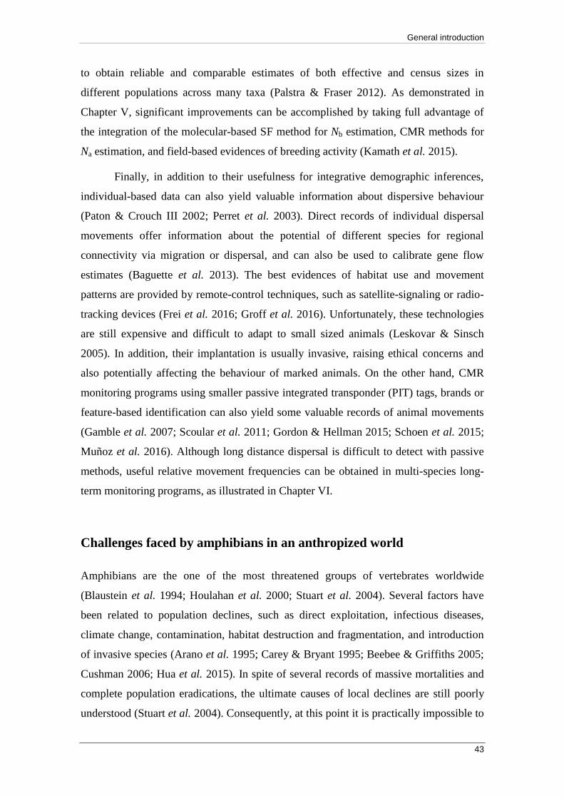
As an example, in Figure B2.1 we depict two schematic cases of an
annual semelparous species (a) and a longer-lived iteroparous species with
overlapping generations (b). At each breeding season (vertical grey bars), Ne can
be calculated from a genetic sample taken among the adult individuals present in
the population (dark horizontal bars crossing the corresponding grey vertical
bar), while Nb can be calculated by sampling among the offspring of the year
(light horizontal bars crossing the corresponding grey vertical bar). It can be
noted that Ne measured at each breeding season in (a) corresponds exactly to Nb
measured in the previous year, because the same individuals contribute to both
parameters. In contrast, this does not occur in (b), where three different adult
breeding cohorts contribute to offspring at each breeding season.
CHAPTER I
36
individuals and estimates Nb on the basis of the relative frequency of siblings inferred in
the sample (Wang 2009). This method is implemented in software COLONY
(Jones & Wang 2010), which is a popular program for molecular ecologists and
population geneticists. One of the main advantages of the SF method is that sibship and
parentage reconstruction can be calibrated with direct pedigree information or evidences
of breeding activity. Such integration of genetic analyses and field observations sets an
unparalleled opportunity to obtain reliable inferences about Nb, as illustrated in Chapter
V. Once protocols for reliable Nb calculation have been optimized, monitoring Nb in a
network of populations through time will allow characterizing population dynamics at
unprecedented rate and accuracy. Demographic inferences obtained from such
Box 2. (Cont.)
While, in this example, Nb varies from year to year due to the different
number of adult breeders generating offspring in each season both in (a) and (b),
Ne experiences an additional interannual source of variation in (b) due to
different overlapping cohorts contributing offspring each year. Also, sampling
design for Ne estimation in (b) should be stratified to include all adult age-
classes present in the breeding season, whereas this is not necessary in (a). The
complexity of both cases in real populations further increases by individual
differences in survival rate, age of maturation and breeding behaviour (Waples
2016).
Figure B2.1. Two schematic representations of an annual semelparous species (a) and an
iteroparous species with overlapping generations (b). Vertical grey bars represent five successive annual breeding seasons. Each horizontal bar symbolizes the lifetime of one individual from its birth, to its juvenile stage (light) and the lifespan after sexual maturation (dark). All individuals in (a) live for one year, attain sexual maturity soon after birth, breed during the following breeding season (when dark horizontal bars cross vertical grey bars), and die after breeding. All individuals in (b) live for three years, reach sexual maturity during the first year and breed in the three following breeding seasons. Note that the number of offspring born in the breeding season is variable from year to year, but is equal in a) and b).
General introduction
37
monitoring programs can readily be applied to address unsolved questions in
evolutionary biology and inform conservation policies (Schwartz et al. 2007; Hinkson
& Richter 2016; Mueller et al. 2016).
In a similar way, current methods for estimating population connectivity are
leading to improved characterization of the spatial and temporal distribution of genetic
variation (Manel et al. 2003; Holderegger & Wagner 2012; Dyer 2015; Greenbaum et
al. 2016). This is important for identifying isolated populations, which face higher risk
of extinction as a result of the genetic impoverishment caused by drift (Allendorf 1983),
but also to find highly diverse populations providing migrant individuals for nearby
localities, thus contributing to the maintenance of the genetic diversity of the species at
a broader scale (Broquet & Petit 2009; Marko & Hart 2011; Albert et al. 2013;
Sundqvist et al. 2016). Characterization of genetic structure patterns, in turn, is essential
for understanding microevolutionary processes such as population differentiation or
hybridization in secondary contact zones (Hewitt 1988; Barton & Hewitt 1989;
Hutchison & Templeton 1999; Anderson & Thompson 2002; Harrison & Larson 2014,
see also Chapter III in this dissertation). These processes operate at different spatial and
temporal scales, so multi-scalar approaches studying the hierarchical levels of
organization of genetic variation offer valuable insights about the foundations of lineage
perpetuation and differentiation (Angelone et al. 2011; Martin et al. 2016). At the same
time, multi-species comparative studies allow identifying features favouring or
hindering gene flow among populations, and assessing the relative effect of these
features in species with different life history traits (Bohonak 1999; Manel et al. 2003;
Richardson 2012; Baguette et al. 2013). The latter issue is addressed in Chapter VI, by
combining different genetic approaches in four species with different life history traits
to evaluate the differential role of a major topographic feature (a mountain range) as a
barrier to gene flow.
The combination of multiple analytic approaches aimed to provide insights
about genetic differentiation, migration rates, genetic structure and landscape-scale
connectivity largely improves gene flow inferences, as illustrated in Chapter VI. Among
these approaches, F-statistics are the classical indexes used for characterization of the
distribution of genetic variation (Rousset 1997). They were originally derived by Sewall
Wright on the basis of the relative amounts of genetic diversity (measured as observed
vs. expected heterozygosity) registered at the individual, population and regional levels

CHAPTER I
38
(Wright 1943, 1951). Since then, F-statistics (in particular, FST) have been applied in a
wide range of studies as an estimate of population differentiation (Wang 2012a). Also,
Bayesian models have been derived for the estimation of migration rates per generation
among populations (Wilson & Rannala 2003; Andreasen et al. 2012). In addition,
genetic clustering methods have become very popular among population geneticists for
the characterization of genetic structure (Evanno et al. 2005; Wang 2017). In genetic
clustering analyses, different algorithms can be applied to evaluate the degree of genetic
admixture of a sample of individuals among some predefined numbers of clusters (K,
Pritchard et al. 2000; Guillot et al. 2005; Jombart et al. 2010). Furthermore, genetic
clustering analyses can be applied in a hierarchical fashion thus aiding in the
identification of the relevant factors operating at different scales to shape observed
genetic structure patterns (Balkenhol et al. 2014; Meirmans 2015). Lastly, landscape
genetic analyses offer an excellent framework to test the relative role of different
landscape patches and putative barrier elements on observed genetic distances, while
also accounting for the effect of geographical distances among populations (Manel et al.
2003; Cushman et al. 2006, 2013; Wasserman et al. 2010; Manel & Holderegger 2013).
Because of their versatility and comprehensive inference possibilities, integrative
genetic studies including multiple analytic approaches can be applied to a wide variety
of taxa and molecular marker types, yielding robust insights about historical and current
connectivity.
In conclusion, combined advances in molecular and computational resources,
along with the continuous expansion of Population Genetics Theory are opening an
exciting field for evolutionary and conservation biologists. Demographic inferences in
all extant (and even some extinct!) species across the tree of life can be obtained as long
as adequate DNA sampling designs are implemented. This will improve critically our
understanding of evolutionary processes and show us how to alleviate the situation of
endangered species (England et al. 2010). Researchers will certainly take advantage of
this great opportunity to attain unprecedented knowledge about how evolution operates
at different spatial and temporal scales.
General introduction
39
Individual-based monitoring programs complementing genetic-based
demographic inferences: the effective/census size ratio
Genetic methods are increasingly used for demographic inferences at the expense of
direct methods, which rely on demographic features that are difficult to estimate in
natural populations (Caballero 1994; Vucetich & Waite 1998). Nevertheless, direct
individual information, evidence of breeding behaviour and population estimates
obtained from individual-based field data are extremely useful for demographic
inferences, and they also provide invaluable information for contextualizing genetic
estimates (Clutton-Brock & Sheldon 2010; Efford & Fewster 2013; Álvarez et al. 2015;
Nunziata et al. 2015, 2017; Bernos & Fraser 2016). For instance, field monitoring
programs can provide estimates of relevant demographic parameters regarding
population structure, density, survival and breeding success (Lebreton et al. 1992;
Tavecchia et al. 2009; Sanz-Aguilar et al. 2016). In the same way, evidence of breeding
success (such as egg mass counts in amphibians or records of nesting in birds or litter
size in mammals) is crucial to calibrate genetic estimates of effective size, supervise
inferred recruitment rates and explore the mating system of species (see Chapter V in
this dissertation). Furthermore, individual-based data can provide inferences about
movement patterns and the dispersal potential of different species. These inferences
require time-consuming fieldwork and are scarce in the literature, but they are useful to
calibrate gene flow estimates and help characterizing connectivity among populations
(Cam et al. 2004; Clark et al. 2008; Luque et al. 2012). All these features play a
fundamental role on population persistence (Keller & Waller 2002; Palstra & Ruzzante
2008).
Importantly, the census (Nc) and the adult population sizes (Na, Frankham 1995)
can be accurately estimated by means of individual-based capture-mark-recapture
(CMR) methods, and both parameters are necessary to refine genetic inferences (Palstra
& Ruzzante 2008; Palstra & Fraser 2012). Capture-mark-recapture techniques are
extensively applied for the estimation of relevant demographic parameters such as
survival, recruitment, migration rates or population size, and different model
formulations have been developed in the last decades to accommodate to different data
types and research interests (Lebreton et al. 1992, 1993, 2003; Kendall et al. 1995;
Pradel 1996; Grosbois & Tavecchia 2003; Tavecchia et al. 2007, 2009; Sanz-Aguilar et

CHAPTER I
40
al. 2016). However, as noted before for genetic analyses, CMR data should also be
structured in a fashion that is adequate to the assumptions of the selected formulation, to
guarantee the accuracy of results (Lebreton et al. 1992; Kendall & Nichols 1995).
Therefore, sampling design is essential to obtain reliable estimates in demographic
CMR studies. If this is carefully planned, multi-year CMR programs can take full
advantage of currently available formulations, such as ‘robust design’ models, to obtain
accurate estimates of parameters like Na (see Box 3), as illustrated in Chapter V.
Na estimates can be further enriched by separate calculation of the number of
adult males and females (White & Burnham 1999). These estimates of adult abundances
can in turn be compared with direct evidences of breeding success to explore the mating
system of species. For example, in Chapter V, the estimated number of females was
found to be similar to egg string counts in an explosive-breeding species (Epidalea
calamita), suggesting that the female breeding success rate in this species is close to
one. Other evidences of breeding behaviour that are typically recorded in monitoring
programs include individual records of time elapsed in the breeding sites and direct
observations of mating events. This information is used in Chapter V to assess the
reliability of family reconstruction in SF analyses, and to describe a within-year
monogamous mating system in E. calamita. Since Nb estimates obtained by SF methods
are directly dependent on accurate sibship reconstruction, independent field-based
information about breeding activity plays a crucial role in the calibration and
supervision of genetic results (Wang 2009). As a consequence, the integration of genetic
and demographic estimates and direct records of breeding activity allow joint
exploration of the demography and mating system of target species, and the assessment
of the reliability of Nb estimates, as illustrated in Chapter V.
Na estimates also complement genetic Nb estimates, by allowing the calculation
of the Nb/Na ratio (Palstra & Fraser 2012). The effective/census size ratio sensu lato (i.e.
Nb/Na or Ne/Nc) offers invaluable insight into population demography and represents the
most useful piece of information for population status assessment, as argued in Chapter
V. The Nb/Na ratio represents the portion of the adult mature population that contributes
to generate a given offspring cohort, whereas Ne/Nc represents the portion of the
population that contributes genetically to the next generation (Waples 2005; Palstra &
Fraser 2012; Whiteley et al. 2017). Low effective/census size ratios have been reported
in many species (Frankham 1995; Brede & Beebee 2006; Palstra & Ruzzante 2008;

General introduction
41
Palstra & Fraser 2012) and can lead to deleterious effects caused by inbreeding and
genetic drift even in large populations (Ruzzante et al. 2016). In contrast, some small
populations seem to mitigate the effect of genetic drift by showing a high Nb/Na ratio
Box 3. Estimation of the number of adults in a population (Na) in seasonal
breeding species using the ‘robust design’ formulation
Individual-based capture-mark-recapture (CMR) monitoring programs are
greatly contributing to demographic research (Pradel 1996; Grosbois &
Tavecchia 2003; Cam et al. 2004; Tavecchia et al. 2009; Clutton-Brock &
Sheldon 2010; Sanz-Aguilar et al. 2016). A wide range of statistical models
(principally based on maximum likelihood approaches) is currently available for
the estimation of demographic parameters, such as Na (Frankham 1995; Kendall
et al. 1995). Software MARK is one of the most popular programs for the
analysis of CMR data, because it includes many formulations that can be applied
for different questions and types of data (White & Burnham 1999). In this
dissertation, we argue that ‘robust design’ models (Pollock 1982), implemented
in software MARK, represent one of the best approaches for annual Na estimation
in iteroparous species with demarcated annual breeding seasons. Nevertheless,
an adequate sampling design accounting for the life traits of the targeted species
is crucial for the reliability of results (Waples et al. 2013).
To illustrate the reasoning behind the robust design method, we represent
an example of the model and its main parameters in Fig. B3.1. The critical
assumption of the model is that Na is constant within each breeding season (or
whatever type of periodic season on which sampling is focused). Consequently,
there should be no mortality, nor migration of adult individuals in the population
throughout the breeding season (Pollock 1982; Kendall et al. 1995). This is
indeed an unrealistic assumption. However, it can be reasonably approximated
by minimizing the timespan between the first and the last CMR sessions.
Unfortunately, excessive concentration of CMR sessions may also introduce a
temporal sampling bias, resulting in unequal capture probabilities among
individuals (Crespin et al. 2008; Kidd et al. 2015). The optimum balance
between these two opposing sources of bias should be studied in each case.
Ultimately, if the within-season population closure can be reasonably
assumed (Stanley & Burnham 1999) and high recapture rates are obtained, the
power of robust design can be fully exploited (Kendall & Nichols 1995; Kendall
et al. 1997). The average probability of capture (p) is then modelled across all
CMR sessions, leading to a Na estimate for each breeding season (see Fig. B3.1).
At the same time, survival and migration rates between consecutive breeding
seasons are estimated, because the model accounts for Na variation across
different breeding seasons (Kendall et al. 1997). In Chapter V, I demonstrate
that this elegant approach is capable of yielding extremely accurate Na estimates
in some cases, and that precision of estimates is improved with cumulative years
of data. If within-season population closure cannot be assumed, alternative open
models can be employed, although at the cost of increased model complexity
(Kendall & Bjorkland 2001; Wagner et al. 2011).

CHAPTER I
42
(Palstra & Ruzzante 2008; Beebee 2009; Hinkson & Richter 2016).
There is still a lot of uncertainty about the range of variance of effective/census
size ratios both within and among species (Frankham 1995; Palstra & Fraser 2012;
Waples et al. 2013; Kamath et al. 2015; Bernos & Fraser 2016; Ferchaud et al. 2016;
Ruzzante et al. 2016). Accurately estimating effective and census size is very time-
consuming, so studies reporting this ratio are still scarce. The problem is further
complicated by impeded comparativeness among studies reporting either Nb/Na or Ne/Nc
(Palstra & Fraser 2012). These two ratios are related, but strong differences can be
found between them in long-lived iteroparous species (see Box 2). In addition, estimates
of Nb (or Ne) and Na (or Nc) obtained by different analytical methods and with different
sampling designs may apply to different time-scales, further complicating comparisons
(Waples 2005; Palstra & Ruzzante 2008). Currently available molecular and statistical
tools allow filling this important gap of knowledge, but an additional effort is required
Box 3. (Cont.)
Figure B3.1. Schematic representation of a ‘robust design’ model applied to an iteroparous species with demarcated breeding seasons (modified from Kendall et al. 1995). Vertical grey areas represent three consecutive annual breeding seasons with different time lengths. The ‘X’s symbolize the CMR sessions (in this example, three CMR sessions were performed during the breeding season of the first year, four during the breeding season of the second year, and two during the breeding season of the third year). The parameter pxy is the average probability of capture in each CMR session, where ‘x’ represents the breeding season and ‘y’, the session within the breeding season. Similarly, Na x represents the parameter Na of each breeding season x. S a
b, emi a
b and imm a
b symbolize annual survival, emigration and immigration rates,
respectively, from breeding season a to breeding season b.
General introduction
43
to obtain reliable and comparable estimates of both effective and census sizes in
different populations across many taxa (Palstra & Fraser 2012). As demonstrated in
Chapter V, significant improvements can be accomplished by taking full advantage of
the integration of the molecular-based SF method for Nb estimation, CMR methods for
Na estimation, and field-based evidences of breeding activity (Kamath et al. 2015).
Finally, in addition to their usefulness for integrative demographic inferences,
individual-based data can also yield valuable information about dispersive behaviour
(Paton & Crouch III 2002; Perret et al. 2003). Direct records of individual dispersal
movements offer information about the potential of different species for regional
connectivity via migration or dispersal, and can also be used to calibrate gene flow
estimates (Baguette et al. 2013). The best evidences of habitat use and movement
patterns are provided by remote-control techniques, such as satellite-signaling or radio-
tracking devices (Frei et al. 2016; Groff et al. 2016). Unfortunately, these technologies
are still expensive and difficult to adapt to small sized animals (Leskovar & Sinsch
2005). In addition, their implantation is usually invasive, raising ethical concerns and
also potentially affecting the behaviour of marked animals. On the other hand, CMR
monitoring programs using smaller passive integrated transponder (PIT) tags, brands or
feature-based identification can also yield some valuable records of animal movements
(Gamble et al. 2007; Scoular et al. 2011; Gordon & Hellman 2015; Schoen et al. 2015;
Muñoz et al. 2016). Although long distance dispersal is difficult to detect with passive
methods, useful relative movement frequencies can be obtained in multi-species long-
term monitoring programs, as illustrated in Chapter VI.
Challenges faced by amphibians in an anthropized world
Amphibians are the one of the most threatened groups of vertebrates worldwide
(Blaustein et al. 1994; Houlahan et al. 2000; Stuart et al. 2004). Several factors have
been related to population declines, such as direct exploitation, infectious diseases,
climate change, contamination, habitat destruction and fragmentation, and introduction
of invasive species (Arano et al. 1995; Carey & Bryant 1995; Beebee & Griffiths 2005;
Cushman 2006; Hua et al. 2015). In spite of several records of massive mortalities and
complete population eradications, the ultimate causes of local declines are still poorly
understood (Stuart et al. 2004). Consequently, at this point it is practically impossible to

CHAPTER I
44
accurately forecast amphibian population trends. The problem is further complicated by
the wide fluctuations in abundance that characterize many species, coupled with
extensive gaps in the knowledge about their diversity and fundamental aspects of their
biology (Pechmann et al. 1991; Green 2003; Pittman et al. 2014; Semlitsch et al. 2017).
Therefore, more taxonomic and demographic studies are urgently required to
understand amphibian diversity and population dynamics and to build an empirical
background that can ultimately provide clues for efficient conservation plans (Paton &
Crouch III 2002; Wang 2012b; McCartney-Melstad & Shaffer 2015). Integrative
molecular and individual-based field methodologies introduced in the previous sections
represent an unprecedented opportunity to address some of the unsolved questions in
amphibian biology (Buckley 2009; Nunziata et al. 2015; Semlitsch et al. 2017).
Regarding taxonomy, amphibian phylogeny is in continuous revision. The
relationships among some major clades remain to be unambiguously resolved, and new
species are still described at a relatively fast rate (Frost et al. 2006; Arntzen et al. 2013;
Liedtke et al. 2016). Reconstructing a robust phylogeny is the first fundamental step for
reliably delineating the operative taxonomic units of study in evolutionary biology.
However, this is an especially complicated issue in contact zones where differentiated
lineages hybridize (Hewitt 1988; Barton & Hewitt 1989; Smith et al. 2013; Harrison &
Larson 2014; Dufresnes et al. 2015; Arntzen et al. 2016). An added difficulty in these
contact zones arises when both lineages contribute differently to the hybridization
process, for instance in hybridogenetic species complexes, such as those in Western
Palearctic waterfrogs (Box 4). Delineation of these hybrid zones is commonly hindered
by the morphological similarity of the species involved (e.g. Rivera et al. 2011; Ferrer
& Filella 2012). For that reason, molecular tools are necessary for characterizing contact
zones in these hybridogenetic complexes, and to perform ecological studies addressing
the demographic implications of this singular evolutionary process (Arano & Llorente
1995; Hotz et al. 2001; Dubey et al. 2014). In this line, the utility of newly developed
genetic tools for species assignment in the Pelophylax ridibundus x P. perezi
hybridogenetic complex is illustrated in Chapter III.
Demographically, very little is known about the factors driving the maintenance
of genetic diversity and regional connectivity (which ultimately determine long-term
persistence) in amphibian populations (Pechmann et al. 1991). For instance, the mating
system plays a crucial role in genetic diversity maintenance, because both Nb and Ne
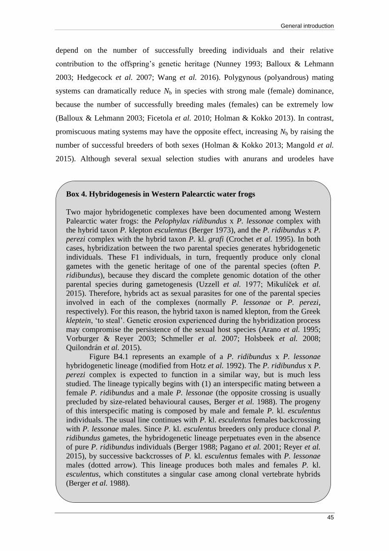
General introduction
45
depend on the number of successfully breeding individuals and their relative
contribution to the offspring’s genetic heritage (Nunney 1993; Balloux & Lehmann
2003; Hedgecock et al. 2007; Wang et al. 2016). Polygynous (polyandrous) mating
systems can dramatically reduce Nb in species with strong male (female) dominance,
because the number of successfully breeding males (females) can be extremely low
(Balloux & Lehmann 2003; Ficetola et al. 2010; Holman & Kokko 2013). In contrast,
promiscuous mating systems may have the opposite effect, increasing Nb by raising the
number of successful breeders of both sexes (Holman & Kokko 2013; Mangold et al.
2015). Although several sexual selection studies with anurans and urodeles have
Box 4. Hybridogenesis in Western Palearctic water frogs
Two major hybridogenetic complexes have been documented among Western
Palearctic water frogs: the Pelophylax ridibundus x P. lessonae complex with
the hybrid taxon P. klepton esculentus (Berger 1973), and the P. ridibundus x P.
perezi complex with the hybrid taxon P. kl. grafi (Crochet et al. 1995). In both
cases, hybridization between the two parental species generates hybridogenetic
individuals. These F1 individuals, in turn, frequently produce only clonal
gametes with the genetic heritage of one of the parental species (often P.
ridibundus), because they discard the complete genomic dotation of the other
parental species during gametogenesis (Uzzell et al. 1977; Mikulíček et al.
2015). Therefore, hybrids act as sexual parasites for one of the parental species
involved in each of the complexes (normally P. lessonae or P. perezi,
respectively). For this reason, the hybrid taxon is named klepton, from the Greek
kleptein, ‘to steal’. Genetic erosion experienced during the hybridization process
may compromise the persistence of the sexual host species (Arano et al. 1995;
Vorburger & Reyer 2003; Schmeller et al. 2007; Holsbeek et al. 2008;
Quilondrán et al. 2015).
Figure B4.1 represents an example of a P. ridibundus x P. lessonae
hybridogenetic lineage (modified from Hotz et al. 1992). The P. ridibundus x P.
perezi complex is expected to function in a similar way, but is much less
studied. The lineage typically begins with (1) an interspecific mating between a
female P. ridibundus and a male P. lessonae (the opposite crossing is usually
precluded by size-related behavioural causes, Berger et al. 1988). The progeny
of this interspecific mating is composed by male and female P. kl. esculentus
individuals. The usual line continues with P. kl. esculentus females backcrossing
with P. lessonae males. Since P. kl. esculentus breeders only produce clonal P.
ridibundus gametes, the hybridogenetic lineage perpetuates even in the absence
of pure P. ridibundus individuals (Berger 1988; Pagano et al. 2001; Reyer et al.
2015), by successive backcrosses of P. kl. esculentus females with P. lessonae
males (dotted arrow). This lineage produces both males and females P. kl.
esculentus, which constitutes a singular case among clonal vertebrate hybrids
(Berger et al. 1988).

CHAPTER I
46
Box 4. (Cont.)
Since males are the heterogametic sex in water frogs, alternative mating
between a male P. kl. esculentus and a female P. lessonae (2) produces only
female P. kl. esculentus offspring, because the parental P. kl. esculentus male
only produces clonal gametes with its P. ridibundus genomic dotation, which is
maternal (Berger et al. 1988). This P. kl. esculentus female offspring might in
turn perpetuate the hybridogenetic lineage by backcrossing with P. lessonae
males, as in the usual line described above (dotted arrow). Conversely, some of
these female hybrids mate with male hybrids from a different lineage (3),
thereby producing only female diploid P. ridibundus offspring. Furthermore,
this progeny would have a pure P. ridibundus nuclear genome, but P. lessonae
mitochondrial DNA, which is matrilineally inherited and irreversibly introduced
in the lineage in (2) (Hotz et al. 1992; Plötner et al. 2008). On the other hand, F1
x F1 crosses between individuals from the same lineage (4) produce inbred
offspring which is often not viable (Vorburger 2001; Guex et al. 2002;
Christiansen et al. 2005). In some cases, this system further complicates
resulting in the generation of polyploid individuals (Berger et al. 1986; Borkin
et al. 2004; Christiansen et al. 2005; Hoffmann et al. 2015; Herczeg et al. 2017).
Figure B4.1. Example of a P. ridibundus (white) x P. lessonae (black) hybridogenetic lineage. Hybrids (P. kl. esculentus) are depicted in dashed grey, while females and
males are symbolized by circles and squares, respectively.
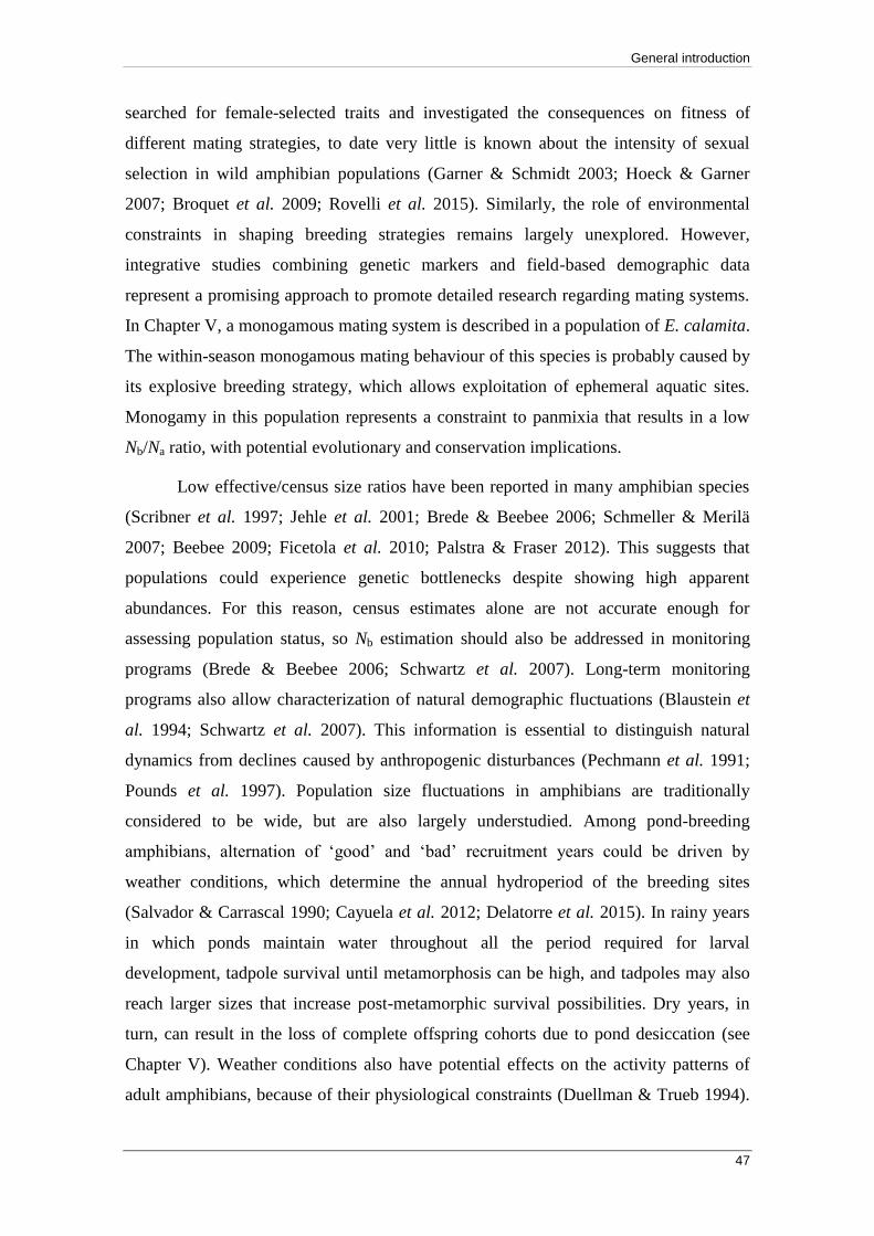
General introduction
47
searched for female-selected traits and investigated the consequences on fitness of
different mating strategies, to date very little is known about the intensity of sexual
selection in wild amphibian populations (Garner & Schmidt 2003; Hoeck & Garner
2007; Broquet et al. 2009; Rovelli et al. 2015). Similarly, the role of environmental
constraints in shaping breeding strategies remains largely unexplored. However,
integrative studies combining genetic markers and field-based demographic data
represent a promising approach to promote detailed research regarding mating systems.
In Chapter V, a monogamous mating system is described in a population of E. calamita.
The within-season monogamous mating behaviour of this species is probably caused by
its explosive breeding strategy, which allows exploitation of ephemeral aquatic sites.
Monogamy in this population represents a constraint to panmixia that results in a low
Nb/Na ratio, with potential evolutionary and conservation implications.
Low effective/census size ratios have been reported in many amphibian species
(Scribner et al. 1997; Jehle et al. 2001; Brede & Beebee 2006; Schmeller & Merilä
2007; Beebee 2009; Ficetola et al. 2010; Palstra & Fraser 2012). This suggests that
populations could experience genetic bottlenecks despite showing high apparent
abundances. For this reason, census estimates alone are not accurate enough for
assessing population status, so Nb estimation should also be addressed in monitoring
programs (Brede & Beebee 2006; Schwartz et al. 2007). Long-term monitoring
programs also allow characterization of natural demographic fluctuations (Blaustein et
al. 1994; Schwartz et al. 2007). This information is essential to distinguish natural
dynamics from declines caused by anthropogenic disturbances (Pechmann et al. 1991;
Pounds et al. 1997). Population size fluctuations in amphibians are traditionally
considered to be wide, but are also largely understudied. Among pond-breeding
amphibians, alternation of ‘good’ and ‘bad’ recruitment years could be driven by
weather conditions, which determine the annual hydroperiod of the breeding sites
(Salvador & Carrascal 1990; Cayuela et al. 2012; Delatorre et al. 2015). In rainy years
in which ponds maintain water throughout all the period required for larval
development, tadpole survival until metamorphosis can be high, and tadpoles may also
reach larger sizes that increase post-metamorphic survival possibilities. Dry years, in
turn, can result in the loss of complete offspring cohorts due to pond desiccation (see
Chapter V). Weather conditions also have potential effects on the activity patterns of
adult amphibians, because of their physiological constraints (Duellman & Trueb 1994).

CHAPTER I
48
This can lead to individuals skipping the breeding season and even to total absence of
population breeding activity in harsh years, as documented in Chapter V (see also
Muths et al. 2006, 2013, Cayuela et al. 2014, 2016). Altogether, extreme variation in
recruitment rates coupled with irregular activity patterns of adults have hindered
accurate population trend characterization, because long-term series are needed to
account for all possible sources of variation (Habel et al. 2014). As a consequence,
monitoring programs integrating molecular and individual-based CMR techniques with
standardized protocols are strongly required to obtain reliable and comparable estimates
of demographic parameters. This information will then be useful for informing
population management actions (Jehle et al. 2001; Paton & Crouch III 2002; Muñoz et
al. 2016).
Amphibians are also traditionally regarded as poorly dispersing, highly
philopatric organisms, although high dispersal capabilities and extensive gene flow have
been reported in many species (Blaustein et al. 1994; Smith & Green 2005, 2006; Wells
2007; Sinsch 2014). Since the emergence of genetic methods, several studies have
described patterns of genetic structure in a wide variety of taxa (Emel & Storfer 2012).
Strong genetic structure has been documented in some species, which is concordant
with low dispersal and reduced gene flow (Martínez-Solano et al. 2005; Gamble et al.
2007; Steele et al. 2009; Richardson 2012; Peterman et al. 2013; Whiteley et al. 2014).
In contrast, genetic homogeneity across large areas has been reported in more vagile
species, suggesting extensive gene flow among populations (Funk et al. 2005; Zamudio
& Wieczorek 2007; Purrenhage et al. 2009; Steele et al. 2009; Richardson 2012;
Whiteley et al. 2014). The existence of gene flow among a network of interconnected
populations can lead to metapopulation dynamics, characterized by local extinction
events that are counteracted by recolonization from nearby areas (Smith & Green 2005;
Albert et al. 2013). The balance of these metapopulation dynamics determines the
probability of regional persistence in many amphibian species (Marsh & Trenham 2001;
Van Buskirk 2005; Fortuna et al. 2006; Heard et al. 2015). Characterization of gene
flow is, therefore, crucial to understand regional evolutionary dynamics (Marko & Hart
2011).
Additionally, studies comparing genetic structure among sympatric species with
different life history traits can offer insights about the role of natural or artificial
features in shaping lineage differentiation (Steele et al. 2009; Goldberg & Waits 2010;

General introduction
49
García-González et al. 2012; Richardson 2012; Espregueira Themudo et al. 2012;
Sotiropoulos et al. 2013). Such studies have improved our knowledge about historical
processes leading to current patterns of amphibian species richness (Veith et al. 2003).
For example, phylogeographic works have inferred the location of glacial refugia for
many species of the European batrachofauna, from which subsequent recolonization of
newly available habitats in formerly glaciated areas proceeded after glacial episodes
(Martínez-Solano et al. 2006; Gonçalves et al. 2009; Abellán & Svenning 2014;
D’Aoust-Messier & Lesbarrères 2015). At the same time, these studies have identified
topographic features that acted as corridors or barriers during range expansion events in
different species (Martínez-Solano et al. 2004; Akın et al. 2010). Optimally, putative
barrier effects should be assessed by combining different genetic approaches, as
illustrated in Chapter VI. Identifying corridors and barriers to gene flow in the present is
also paramount for our understanding of population connectivity (Funk et al. 2005;
Komaki et al. 2016). This information is necessary for implementing efficient landscape
management actions headed to ensure regional persistence of amphibian species.
In conclusion, I argue that integrative demographic studies including genetic
analyses and CMR monitoring programs in multi-scale and multi-species research
designs have great potential to provide accurate insights on amphibian population
dynamics (Schwartz et al. 2007; Bailey & Mazerolle 2010; Helfer et al. 2012). A solid
empirical background on demographic variability within and among different species,
coupled with an accurate quantification of gene flow patterns at local and regional
scales is urgently required for conservation purposes. Hopefully, optimized
management protocols resulting from this strategy will help reverse the current global
amphibian crisis.
The study system: a multi-species, multi-scale approach
This dissertation explores the potential of an integrative, multi-species approach to
address some of the main challenges in amphibian evolutionary and conservation
research. It is focused on different scales to encompass the study of taxonomic and
demographic issues. The species under study are four sympatric pond-breeding anurans:
the natterjack toad Epidalea calamita (Laurenti, 1768); the Iberian treefrog Hyla molleri
Bedriaga, 1889; Perez’s frog Pelophylax perezi (López-Seoane, 1885) and the Western

CHAPTER I
50
spadefoot toad Pelobates cultripes (Cuvier, 1829). These four species co-occur in
extensive areas in their native ranges, where they can be found forming breeding
assemblages (Álvarez & Salvador 1984; Salvador & Carrascal 1990). While previous
studies have described different aspects of their ecology, very little is known about their
local demographic dynamics and patterns of gene flow (García-París et al. 2004). Next I
summarize some aspects of the biology of each species, with a special focus on the
current knowledge about their taxonomy and demography.
Epidalea calamita (Laurenti, 1768)
Epidalea calamita (originally described as Bufo calamita, a nomenclature which was
maintained until recently) is a Palearctic species with a wide European distribution
(Beja et al. 2009b, see also Fig. I.1). The recent designation of this species as the only
member of the genus Epidalea is based on its ancient origin and strong genetic
differentiation with the monophyletic genera Bufo and Bufotes (Frost et al. 2006; Portik
& Papenfuss 2015; Carretero et al. 2016; Liedtke et al. 2016). Among the three species
for which new specific microsatellite sets are described in Chapter IV, E. calamita is the
only one for which additional specific genetic markers have already been published
elsewhere (Rowe et al. 1997, 2000; Rogell et al. 2005; Faucher et al. 2016). These tools
have been used in extensive demographic and phylogeographic research, which has
provided valuable evolutionary inferences in this species. Genetic diversity of
populations of E. calamita decreases with increasing latitude throughout its range,
suggesting that the Iberian Peninsula and some areas of France acted as glacial refugia
from which they expanded to occupy their present range during the Last Interglacial
Period (Beebee & Rowe 2000; Gomez-Mestre & Tejedo 2004; Rowe et al. 2006; Rowe
& Beebee 2007; Oromi et al. 2012). Also, geographic differences in population
connectivity have been reported, with limited gene flow within British and Danish
clusters of populations contrasting with wide connectivity in the Iberian Peninsula
(Gomez-Mestre & Tejedo 2004; Rowe & Beebee 2007; Allentoft et al. 2009; Oromi et
al. 2012). Results presented in Chapter VI also reveal high connectivity between
Central Iberian E. calamita populations, which showed the lowest inter-population
genetic distances among the four studied species. This is concordant with the high
dispersal capability of this species (Denton & Beebee 1993; Miaud et al. 2000; Stevens
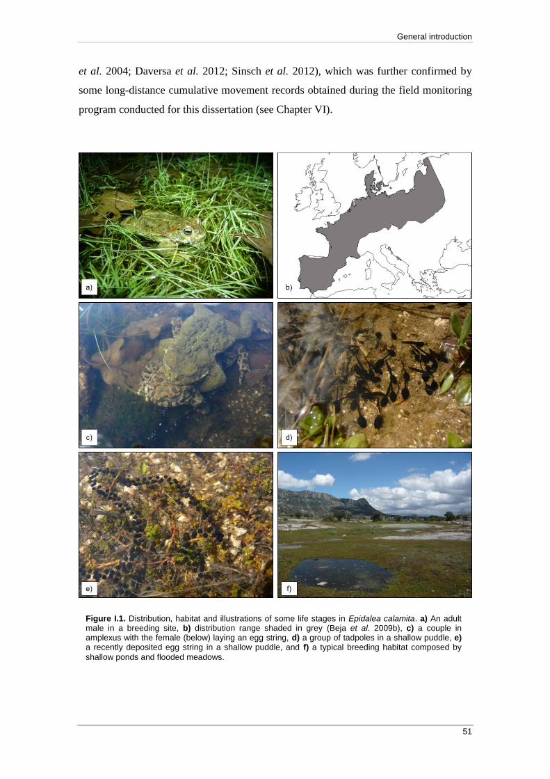
General introduction
51
et al. 2004; Daversa et al. 2012; Sinsch et al. 2012), which was further confirmed by
some long-distance cumulative movement records obtained during the field monitoring
program conducted for this dissertation (see Chapter VI).
Figure I.1. Distribution, habitat and illustrations of some life stages in Epidalea calamita. a) An adult male in a breeding site, b) distribution range shaded in grey (Beja et al. 2009b), c) a couple in amplexus with the female (below) laying an egg string, d) a group of tadpoles in a shallow puddle, e) a recently deposited egg string in a shallow puddle, and f) a typical breeding habitat composed by
shallow ponds and flooded meadows.

CHAPTER I
52
Tadpoles and adults of E. calamita also show a great capacity of adaptation to
different, variable and unpredictable physicochemical and climatic conditions, which
constitutes the main strategy of this species for regional persistence (Beebee 1983,
1985; Sinsch et al. 1992; Romero & Real 1996; Gomez-Mestre & Tejedo 2003, 2004,
2005; García-París et al. 2004; Gomez-Mestre et al. 2004). Accordingly, wide
altitudinal and latitudinal variations have been observed in several life history traits
such as body size, larval tolerance to osmotic stress or traits associated to competitive
capacity against Bufo species (Gomez-Mestre & Tejedo 2002, 2003, 2004; Leskovar et
al. 2006; Marangoni 2006; Marangoni et al. 2008; Oromi et al. 2012). Tadpoles of E.
calamita are in general poor competitors, so interspecific competition usually results in
severe performance drawbacks, especially in the presence of B. bufo or B. spinosus, but
also R. temporaria (Beebee 1991; Beebee & Wong 1992; Griffiths et al. 1993; Bardsley
& Beebee 1998, 2001a, b; Gomez-Mestre & Tejedo 2002; Richter-Boix et al. 2007). To
avoid interspecific competition, E. calamita usually selects temporary or even
ephemeral aquatic sites for breeding, thus taking advantage of the fast development of
tadpoles (Beebee 1983). Nevertheless, this risky strategy usually leads to massive
tadpole mortalities caused by pond desiccation (García-París et al. 2004) resulting in a
high spatial and temporal variance of recruitment rates driven by annual weather
conditions. In this unpredictable scenario, regional persistence of E. calamita is
sustained by adult longevity (up to 10 and even 17 years, Banks et al. 1993; Leskovar et
al. 2006) and early sexual maturation (normally in the second year, Boomsma &
Arntzen 1985; Banks et al. 1993; Denton & Beebee 1993; Tejedo et al. 1997; Leskovar
et al. 2006; Sinsch et al. 2010; Oromi et al. 2012). Populations of E. calamita are
arranged in metapopulation networks driven by juvenile dispersal and female-biased
gene flow (Sinsch 1992a, b).
The particularities of the reproductive strategy of E. calamita make this species
especially interesting for comparative studies of demographic patterns in multiple
populations and exploration of the consequences of the mating system on effective
population size, as addressed in Chapter V. In addition, these studies are also necessary
for adequately responding to current threats for E. calamita persistence, such as pond
destruction, water pollution and road mortality (Lizana 1993; Fleming et al. 1996;
Carretero & Rosell 2000; García-París et al. 2004; García-Muñoz et al. 2010, 2011).
Although this species is globally listed as Least Concern (Beja et al. 2009b),

General introduction
53
endangered populations exist in some areas of northern Spain and Britain, and
management actions are often required for maintaining relict breeding nuclei (Beebee
1983; Denton et al. 1997; Reques & Tejedo 2004; Garin-Barrio et al. 2007; Montori &
Franch 2010). Regional demographic studies are also needed in areas where gene flow
is compromised thus leading to population isolation (Beebee & Rowe 2000; Stevens et
al. 2006; Rowe & Beebee 2007; Allentoft et al. 2009).
Hyla molleri Bedriaga, 1889
Hyla molleri is distributed across the northern, western and central areas of the Iberian
Peninsula, and in southern France (Fig. I.2). Until the last decade, it was still considered
a subspecies of the European taxon H. arborea, due to their high morphological
similarity. However, recent molecular studies have highlighted the differentiation of the
H. molleri lineage and raised its taxonomic status to the species level (Stöck et al. 2008,
2012; Barth et al. 2011; Gvozdík et al. 2015). Interestingly, the sister species of H.
molleri is the geographically distant H. orientalis, and not H. arborea, with which H.
molleri overlaps in southwestern France (Gvozdík et al. 2010, 2015). The extent of this
range overlap is still debated because the two species hybridize (Stöck et al. 2012;
Gvozdík et al. 2015). Similarly, wide contact zones with the other Iberian tree frog
species, H. meridionalis, exist south of the Iberian Central System (Patón 1989; Oliveira
et al. 1991; Barbadillo & Lapeña 2003; Reino et al. 2017). Molecular tools, such as
those presented in Chapter IV for H. molleri, are required for delineating the
distribution ranges of each species and characterizing their contact zones. Additionally,
previous studies have reported low levels of genetic diversity and a very shallow genetic
structure throughout the distribution range of H. molleri (Barth et al. 2011; Gvozdík et
al. 2015). However, the use of the neutral hypervariable nuclear markers described in
Chapter IV in a comprehensive range-wide sample may reveal hidden patterns of
genetic structure (Sánchez-Montes & Martínez-Solano, unpublished data).
There are no published data about population abundances or other demographic
inferences in H. molleri, apart from some phenological studies (García et al. 1987;
Salvador & Carrascal 1990). Nevertheless, García et al. (1987) described the different
breeding strategies of male and female H. molleri, with potentially important
consequences for the relative breeding success rates of both sexes, as argued in Chapter

CHAPTER I
54
V. On the other hand, extensive demographic research has been conducted on H.
arborea, revealing that populations of this species arrange in metapopulations that are
highly susceptible to habitat fragmentation (Carlson & Edenhamn 2000; Arens et al.
2006). Population isolation, in turn, has potential consequences on the fitness of
individuals (Edenhamn et al. 2000; Andersen et al. 2004; Luquet et al. 2011, 2013).
Interestingly, Broquet et al. (2009) found that delayed age of maturity in H. arborea
served as a mechanism compensating for possible additional genetic drift effects caused
by its polygamous mating system (see previous section and Chapter V for discussion
about the effects of the mating system on the effective population size).
Figure I.2. Distribution, habitat and illustrations of some life stages in Hyla molleri. a) An adult female in a breeding site; b) the Iberian distribution range of H. molleri shaded in grey, with diagonal lines showing the range area in southern France, where the distribution limits of H. molleri and H. arborea have not been fully resolved yet (Kaya et al. 2009); c) a couple in amplexus, showing variation in body colouration in this species, and d) a typical breeding pond for H. molleri, with abundant surrounding
shrub and arboreal vegetation.

General introduction
55
The global conservation status of H. molleri has not been assessed yet, but it is
catalogued as Near Threatened in Spain (Márquez 2002). Similarly to H. arborea,
population connectivity is essential for the regional persistence of H. molleri, so
conservation efforts should focus on protecting both the aquatic and terrestrial habitats
of this species (Rosa 1995; Alarcos et al. 2003; Oliveira & Pargana 2010). Populations
throughout the range of H. molleri are experiencing increased isolation, demographic
declines and extinctions caused by anthropogenic disturbances, introduction of exotic
species and climate change (Galán 1997, 1999; Márquez 2002; Martínez-Solano et al.
2003; Cruz et al. 2008; Diego-Rasilla & Ortiz-Santaliestra 2009; Oliveira & Pargana
2010; Araújo et al. 2011). As a consequence, long-term monitoring programs and
integrative demographic studies like the one addressed in Chapter V, are urgently
required to understand population dynamics of H. molleri and to inform efficient
conservation policies.
Pelophylax perezi (López-Seoane, 1885)
Pelophylax perezi distributes natively across the whole Iberian Peninsula and southern
France, and it has been introduced to Britain and to the Madeira, Azores, Balearic and
Canary archipelagos (Llorente et al. 2002; Bosch et al. 2009, see Fig. I.3). It is listed as
Least Concern by the International Union for the Conservation of Nature (IUCN),
because it is common and locally abundant throughout its range, and shows wide
ecological tolerance (Llorente et al. 2002; Bosch et al. 2009). However, direct
exploitation, habitat destruction and alteration, water pollution and the introduction of
exotic species have been associated with severe damages to populations of this species
(Rico et al. 1987; Galán 1997, 1999; Martínez-Solano et al. 2003; Tejedo & Reques
2003; Pastor et al. 2004; Rodríguez et al. 2005). Additionally, P. perezi experiences
genetic erosion when it hybridizes with the European waterfrog P. ridibundus, or with
the hybridogenetic kleptons P. kl. grafi and P. kl. esculentus (Crochet et al. 1995, see
also Box 4). However, at the moment hybridization areas have only been reported in
areas north of the Ebro River (see Chapter III). A deeper understanding about
demographic dynamics and delineation of hybrid zones is thus necessary to anticipate
possible cryptic declines in P. perezi, and to understand the evolutionary consequences
of hybridogenesis. Specific markers characterized in Chapter III open a new field for

CHAPTER I
56
demographic inferences in this species, and for the study of the P. perezi x P.
ridibundus hybridogenetic complex.
Pelophylax perezi is a short-lived species, with a maximum lifespan of 4-6
years, that reaches sexual maturity between the first and the third year (Docampo &
Milagrosa-Vega 1991; Patón et al. 1991; Esteban et al. 1996). Therefore, population
persistence might be based on high turnover rates, enabled by high recruitment and
migration rates, although this has not been ascertained yet (Egea-Serrano 2014). As a
consequence, the basic aspects of population dynamics of P. perezi, as well as its
mating system, need to be further explored empirically to unravel the demographic
strategy of this successful species. Following this line of research, the estimation of the
Nb/Na ratio in a P. perezi population is addressed for the first time in Chapter V,
Figure I.3. Distribution, habitat and illustrations of some life stages in Pelophylax perezi. a) An adult female hidden under dense aquatic vegetation; b) the distribution range shaded in grey (including areas of introduction in the Balearic Archipelago, Bosch et al. 2009), c) an egg mass with developing embryos, still attached to the aquatic vegetation, and d) a breeding pond for P. perezi in a water-filled
quarry, one in the wide variety of natural and anthropogenic aquatic habitats that this species uses for reproduction.

General introduction
57
including an assessment of the reliability of results. The application of this monitoring
framework in a network of populations will offer invaluable information about possible
metapopulation processes driving the regional persistence of P. perezi. Additionally,
genetic structure estimates in Chapter VI represent the first inferences of regional
patterns of gene flow reported for this species. Individual records of dispersive
movements are also provided in Chapter VI, widely expanding previous information
about the species vagility (Sánchez-Montes & Martínez-Solano 2011).
Pelobates cultripes (Cuvier, 1829)
Pelobates cultripes expands across most of the Iberian Peninsula and the southern coast
of France, and is also locally present at the French Atlantic coast, a relict of a formerly
wider distribution (Beja et al. 2009a; Gutiérrez-Rodríguez et al. 2017a, Fig. I.4). Range-
wide phylogeographic structure is shallow (Crottini et al. 2010; Fitó et al. 2011;
Gutiérrez-Rodríguez et al. 2017a). This pattern has been interpreted as the result of
successive postglacial range expansions and contractions leading to overall genetic
homogeneity, with refugia in southern Iberia harbouring most genetic diversity
(Gutiérrez-Rodríguez et al. 2017a). Past demographic inferences could be significantly
improved by calibrating historical migration models with data about contemporary
dynamics of population connectivity. Unfortunately, dispersive behaviour and gene
flow in P. cultripes remain understudied, and direct records of dispersal from marked
individuals are extremely scarce (Valdeón & Sanuy 2016; Gutiérrez-Rodríguez et al.
2017b). In Chapter VI, integrative estimation of contemporary landscape-scale
connectivity is addressed for the first time in this species.
The strong fossorial habits of P. cultripes restrict its presence to habitats with
sandy or loosely compact soils, preferentially at low or intermediate elevations (Cejudo
1990; García-París et al. 2004; Recuero 2014). Although there are records of high local
densities (Petit & Delabie 1951; Cei & Crespo 1971; Rodríguez-Jiménez & Prados
1985), the only reported estimate of effective/census size ratio ranged between 0.25-0.3
(Gutiérrez-Rodríguez et al. 2017b). Reproductive behaviour has only been monitored in
a few populations, where it showed a staggered pattern in which breeding activity was
mainly triggered by weather conditions (Álvarez & Salvador 1984; Salvador &
Carrascal 1990; Lizana et al. 1994; Gutiérrez-Rodríguez et al. 2017b). Demographic

CHAPTER I
58
studies show that P. cultripes can live up to 12 years, while it reaches sexual maturity in
the second year (Talavera 1990; Díaz-Paniagua et al. 2005; Leclair et al. 2005).
However, the recruitment rate and relevant features of its mating system such as the
strength of sexual selection and the degree of polygamy remain unexplored. This
information is essential to predict future population trends and design conservation
programs, as argued before. Pelobates cultripes is catalogued as Near Threatened by the
IUCN (Tejedo & Reques 2002; Beja et al. 2009a), and population declines have already
been reported (Martínez-Solano 2006; Galán et al. 2010). The use of pesticides and
chemical fertilizers, changes in land use and introduction of invasive species are the
main factors potentially challenging population persistence (Beja & Alcazar 2003;
Ortiz-Santaliestra et al. 2006; Galán et al. 2010). Population isolation, which implies an
increased vulnerability to disturbances, has also been noted as a threat for the regional
persistence of this species (Recuero 2014).
Figure I.4. Distribution, habitat and illustrations of some life stages in Pelobates cultripes. a) An adult female (photograph by J. Agüera), b) the distribution range shaded in grey (Beja et al. 2009a), c) an egg string in a shallow pond, and d) a typical breeding pond for P. cultripes, temporary but deep
enough to maintain water throughout the long tadpole stage characteristic of this species.

General introduction
59
A multi-scalar approach
In this dissertation I developed three new sets composed of 15-18 species-specific
microsatellite markers for E. calamita, H. molleri and P. perezi and demonstrated their
utility for demographic and taxonomic research (Chapters III and IV). Additionally, the
two main demographic parameters studied in this dissertation (effective population size
and gene flow) can be quantified at different spatial and temporal scales (Waples 2005;
Anderson et al. 2010). I focused on the landscape scale to quantify patterns of regional
connectivity in a network of populations of the four species (Chapter VI), and also
integrated genetic analyses and CMR methods to explore the Nb/Na ratio at a local scale
(Chapter V).
The three sets of newly developed markers were used to genotype samples of the
three species collected in several populations in Central Spain (total n = 547, 652 and
516 individuals of H. molleri, E. calamita and P. perezi, respectively, see Table IV.1
and Fig. IV.1) and along a transect on a latitudinal gradient encompassing the hybrid
zone of the P. ridibundus x P. perezi hybridogenetic complex in the eastern Iberian
Peninsula and southern France (total n = 30, see Table III.2 and Fig. III.1). I used
different programs to design multiplex reactions, score alleles, characterize genetic
diversity in sampled populations, quantify the quality of genotyping and the informative
content of each marker, and check for departures from theoretically expected genotypic
proportions (see Table I.1). Additionally, specialized software was used for species
identification in the Pelophylax ridibundus x P. perezi complex on the basis of
genotypic and sequence data (see Table I.1 and Chapter III). Finally, I used other
programs to implement sibship and parentage reconstruction to check for the effect of
close relatives in the sample, and to calculate accumulation curves to explore the effect
of sample size on genetic diversity characterization (see Table I.1 and Chapter IV).
Regional genetic connectivity was explored based on an extensive sampling in
Sierra de Guadarrama (see Chapter VI). This mountain ridge corresponds to the
northeastern range of the Iberian Central System (Fig. I.5). The Iberian Central System
is an important biogeographic feature, which marks the distribution limit of some
amphibian species and also represents the contact zone between differentiated lineages
in other species (Martínez-Solano et al. 2006; Arntzen & Espregueira Themudo 2008;
Gonçalves et al. 2009; Díaz-Rodríguez et al. 2015; Gutiérrez-Rodríguez et al. 2017a;
Reino et al. 2017). The orientation of the Iberian Central System along a west-east axis

CHAPTER I
60
had been hypothesized to constrain latitudinal population expansion/contraction events
in response to climatic changes during the Pleistocene, although its role as a barrier to
gene flow had not been explicitly tested before (see Chapter VI). It is, therefore, an
interesting area to explore ongoing evolutionary processes and to identify major
landscape features canalizing gene flow in species with different life history traits. Also,
it is a well preserved natural area that has been recently catalogued as a National Park
(Ministerio de Agricultura y Pesca, Alimentación y Medio Ambiente, 2017). The
regional climate is Mediterranean, with cold winters and mild dry summers, although at
higher elevations the climate is Alpine (López-Sáez et al. 2014). Average annual
rainfall in Navacerrada (see Fig. VI.2) is 1223 mm, although mean values vary
substantially among different months, from 23 mm in July to 176 mm in November
(AEMET, 2017).
Table I.1. List of computer programs and R packages used in this dissertation.
Name Use in this dissertation References
adegenet
(R package) Implement discriminant analyses of principal components (DAPC) to assess genetic structure patterns of E. calamita, H. molleri, P. perezi and P. cultripes in Sierra de Guadarrama (Chapter VI).
Jombart (2008)
BayesAss Estimate migration rates per generation (Chapter VI). Wilson & Rannala (2003)
BEAST Build sequence-based gene trees in the P. ridibundus x P. perezi hybridogenetic complex (Chapter III).
Drummond et al. (2012)
CLUMPAK Summarize graphically the clustering results from program structure (Chapter VI).
Kopelman et al. (2015)
CoDiDi Calculate the correlation between gene diversity and GST (Nei 1973) across markers for each dataset (Chapter VI).
Wang (2015)
COLONY Infer sibship and parentage relationships among genotyped individuals (Chapters IV, V and VI), calculate mistyping rates due to allelic dropout and false allele scoring (Chapter IV) and estimate Nb (Chapter V).
Jones & Wang (2010)
ecodist (R package)
Implement partial Mantel tests to perform causal modelling landscape genetics analyses on sampled populations of E. calamita, H. molleri, P. perezi and P. cultripes in Sierra de Guadarrama (Chapter VI).
Goslee & Urban (2007)
EstimateS Calculate jackknifed accumulation curves for AR and HE estimation with increasing sample size (Chapter
IV).
Colwell & Elsensohn (2014)
GENALEX Calculate allelic richness (AR) and observed and expected heterozygosity (HO and HE, Chapters III and
IV), the probabilities of identity (PI and PISibs, Chapter III), FIS (Chapter IV) and pairwise genetic (FST) and geographic distances between populations and implement tests of Isolation by distance (IBD, Chapter VI).
Peakall & Smouse (2006, 2012)

General introduction
61
Table I.1 (cont.)
Name Use in this dissertation References
GENELAND Implement spatially explicit clustering analyses to assess genetic structure in populations of E. calamita, H. molleri, P. perezi and P. cultripes in Sierra de Guadarrama (Chapter VI).
Guillot et al. (2005)
GeneMapper Allele scoring (Chapters III, IV, V and VI). -
GENEPOP Tests of Hardy-Weinberg equilibrium (HWE) and linkage disequilibrium (LD, Chapters III and IV).
Raymond & Rousset (1995), Rousset (2008)
KinInfor Calculate the informative content of each microsatellite marker (Chapter IV).
Wang (2006)
MARK Implement CMR ‘robust design’ analyses for Na
estimation (Chapter V). White & Burnham (1999)
MICRO-CHECKER Test for null alleles at each microsatellite marker (Chapters III and IV).
Van Oosterhout et al. (2004)
Multiplex Manager
Design multiplex combinations of microsatellite markers (Chapters III and IV).
Holleley & Geerts (2009)
NewHybrids Species assignment in the P. ridibundus x P. perezi hybridogenetic complex based on microsatellite genotypes (Chapter III).
Anderson & Thompson (2002)
PartitionFinder Select optimal partition strategies and models of nucleotide substitution (Chapter III).
Lanfear et al. (2012)
PAST Calculate bootstrapped 95% confidence intervals for HE (Chapter IV).
Hammer et al. (2001)
POPGENREPORT (R package)
Calculate the least cost paths between all pairs of sampled populations in Sierra de Guadarrama at four predefined elevation-based resistance models and construct matrices of genetic and Euclidean distances (Chapter VI).
Adamack & Gruber (2014)
QGIS Elaborate maps of sampling localities and genetic structure in Sierra de Guadarrama (Chapters IV and VI).
Quantum GIS Development Team (2009)
R Inspect graphically accumulation curves for AR and HE estimation with increasing sample size and calculate empirical and Chao & Jost (2015) profiles (Chapter IV), and implement replicated analyses for Nb estimation with different sibship size priors, numbers of markers and sample sizes (Chapter V).
R Development Core Team (2009)
Sequencher Edit genetic sequences (Chapter III). -
structure Implement unsupervised Bayesian clustering analyses to assess genetic structure patterns of E. calamita, H. molleri, P. perezi and P. cultripes in Sierra de Guadarrama (Chapter VI).
Pritchard et al. (2000), Falush et al. (2003)
STRUCTURE
HARVESTER Explore the likelihood of different numbers of clusters (K) in unsupervised Bayesian structure analyses in Sierra de Guadarrama (Chapter VI).
Earl & vonHoldt (2012)
Tracer Check for convergence of parameter estimates and adequate Effective Sample Sizes (ESSs) in BEAST analyses (Chapter III).
Rambaut et al. (2014)
U-CARE Test for ‘transience’ and ‘trap-dependence’ effects in CMR data (Chapter V).
Choquet et al. (2009)
The regional sampling design included tadpole tissue samples from 13-19
populations of E. calamita, H. molleri, P. perezi and P. cultripes located between 850
CHAPTER I
62
and 1720 metres above sea level (m.a.s.l., see Table VI.2), representing all major
landscape types in Sierra de Guadarrama: Mediterranean open forests of Quercus ilex
subsp. ballota in the lowlands, deciduous (Q. pyrenaica) and coniferous (Pinus
sylvestris, P. nigra) forests at mid-elevations, shrubs above 1600 m.a.s.l., and alpine
grasslands and meadows at the top (López-Sáez et al. 2014). Tadpoles were genotyped
at 13-18 microsatellite loci per species, and this genetic dataset was used to explore the
genetic structure of the four species in a shared heterogeneous landscape. A
combination of computer programs implementing a variety of analytical approaches
(see Table I.1) revealed different patterns of connectivity among the four species, which
showed different levels of susceptibility to the barrier effect imposed by Sierra de
Guadarrama that can be partially explained by differences in their life history traits
(Chapter VI).
The regional connectivity study was complemented with a local-scale integrative
(genetic and CMR) monitoring program developed in the locality of Valdemanco
(Sierra de Guadarrama, Madrid, Spain, see Fig. I.5), in an amphibian assemblage
including E. calamita, H. molleri and P. perezi. In this site, seasonal CMR sessions
were performed on a yearly basis from 2010 to 2016, marking adult individuals of these
three species with passive integrated transponders (PIT) tags (the total numbers of
marked individuals during the seven-year period were 1086 E. calamita, 599 H. molleri
and 662 P. perezi, see Chapter VI). CMR sessions were planned as nocturnal visual
surveys in a temporal sampling strategy designed to encompass the breeding seasons of
the targeted species and to meet the statistical requeriments for ‘robust design’ analyses
(see Box 3). The study area of this monitoring program included five amphibian
breeding sites: a natural pond (Laguna de Valdemanco), and several artificial sites,
including a pond resulting from mining activities, a water trough, an abandoned
swimming pool and an old quarry where some ephemeral ponds are formed by seasonal
rainfall (see Fig. VI.1). Laguna de Valdemanco is the main amphibian breeding site in
the area, and it is used by the three species for breeding (see Chapter VI). It is a
temporal shallow pond (maximum depth = 1m) which occupies a large surface (12,800
m2), with an average annual hydroperiod of c. six months (from January to June
approx.), and its adjacent meadows are usually flooded in the spring (Sánchez-Montes
& Martínez-Solano 2011). These flooded meadows are strongly selected by females of
E. calamita for egg deposition. Females of E. calamita lay egg strings in shallow water,

General introduction
63
Figure I.5. Multi-scale map showing the location of Sierra de Guadarrama in the Iberian Central
System (a), a 3D digital elevation model (DEM) of the regional study area encompassing both the northern and southern slopes of Sierra de Guadarrama (b, see sampling locations in Chapters IV and VI), and our local study area (c) including Laguna de Valdemanco (d) and breeding sites nearby.

CHAPTER I
64
facilitating annual counts as an approximation to breeding success (see Chapter V).
Long-term CMR monitoring based on individual marking and ‘robust design’
analyses implemented in the specialized software MARK (see Table I.1) allowed
estimation of annual Na with increasing precision through the years (Chapter V), and
also yielded information of relative frequencies of dispersal among the five breeding
sites (Chapter VI, see also Gutiérrez-Rodríguez et al. 2017b). Additionally, the annual
marking effort also provided a comprehensive adult tissue sample in Valdemanco. Part
of this extensive sample was used to obtain genotypes of adult males and females of the
three species using the molecular tools presented in Chapters III and IV. This genetic
dataset was complemented with larval cohort samples of each species to estimate Nb and
to calculate the Nb/Na ratio (see Table I.1 and Chapter V).
In summary, the multi-species and multi-scale integrative demographic approach
developed in this dissertation provides novel genetic resources and relevant
demographic information for Iberian pond-breeding amphibians. Microsatellite sets
described in this dissertation are the first STR markers designed for H. molleri and P.
perezi, and complement markers previously developed for E. calamita (Rowe et al.
1997; Rogell et al. 2005; Faucher et al. 2016). Combined multilocus polymorphism in
each set of markers was sufficient to allow individual identification and therefore the
three sets proved useful for demographic research. Seven of the markers isolated in P.
perezi were successfully applied for species assignment in the P. ridibundus x P. perezi
hybridogenetic complex and, in combination with mitonuclear sequence information,
allowed us to expand current knowledge about the geographic extent of the area of
hybridization (Chapter III). Furthermore, the comprehensive genetic datasets generated
have allowed exploration of the effect of close relatives and sample size on genetic
diversity characterization, as well as the development of a new method for minimum
sample size calculation (Chapter IV). The newly developed and optimized genetic tools
have also been applied to explore effective population sizes and patterns of gene flow in
the study species (Chapters V and VI). Local-scale CMR monitoring and evidences of
breeding activity (records of mating events and counts of egg strings) combined with
genetic analyses allowed to obtain reliable estimates of the Nb/Na ratio (Chapter V).
Finally, individual-based data offered valuable information about individual movement
patterns, which was useful to help interpret indirect gene flow inferences at a regional
scale (Chapter VI). All this information, in turn, provides invaluable insights into

General introduction
65
population demography in Iberian pond-breeding amphibians, which can now be
applied for the design of efficient conservation plans.
CHAPTER I
66
References
Abellán P, Svenning J-C (2014) Refugia within refugia – patterns in endemism and genetic
divergence are linked to Late Quaternary climate stability in the Iberian Peninsula.
Biological Journal of the Linnean Society, 113, 13–28.
Adamack AT, Gruber B (2014) POPGENREPORT: simplifying basic population genetic analyses
in R. Methods in Ecology and Evolution, 5, 384–387.
AEMET (2017) AEMET (Agencia Estatal de Meteorología). Madrid: AEMET. Servicios
climáticos. Datos climatológicos. Valores climatológicos. Available at:
http://www.aemet.es/es/serviciosclimaticos/datosclimatologicos/valoresclimatologicos?l=2
462&k=mad. Accessed 20 May 2017.
Akın Ç, Can Bilgin C, Beerli P et al. (2010) Phylogeographic patterns of genetic diversity in
eastern Mediterranean water frogs were determined by geological processes and climate
change in the Late Cenozoic. Journal of Biogeography, 37, 2111–2124.
Alarcos G, Ortiz ME, Lizana M, Aragón A, Fernández-Benéitez MJ (2003) La colonización de
medios acuáticos por anfibios como herramienta para su conservación: el ejemplo de
Arribes del Duero. Munibe (Suplemento/Gehigarria), 16, 114–127.
Albert EM, Fortuna MA, Godoy JA, Bascompte J (2013) Assessing the robustness of the
networks of spatial genetic variation. Ecology Letters, 16, 86–93.
Alexander HJ, Taylor JS, Wu SS-T, Breden F (2006) Parallel evolution and vicariance in the
guppy (Poecilia reticulata) over multiple spatial and temporal scales. Evolution, 60, 2352–
2369.
Allendorf FW (1983) Isolation, gene flow and genetic differentiation among populations. In:
Genetics and conservation: a reference for managing wild animal and plant populations
(eds Schonewald-Cox CM, Chambers SM, MacBryde B, Thomas WL), pp. 51–65. Menlo
Park: Benjamin/Cummings.
Allendorf FW (2016) Genetics and the conservation of natural populations: allozymes to
genomes. Molecular Ecology, 38, 42–49.
Allentoft ME, Siegismund HR, Briggs L, Andersen LW (2009) Microsatellite analysis of the
natterjack toad (Bufo calamita) in Denmark: populations are islands in a fragmented
landscape. Conservation Genetics, 10, 15–28.
Álvarez D, Lourenço A, Oro D, Velo-Antón G (2015) Assessment of census (N) and effective
population size (Ne) reveals consistency of Ne single-sample estimators and a high Ne/N
ratio in an urban and isolated population of fire salamanders. Conservation Genetics
Resources, 7, 705–712.
Álvarez J, Salvador A (1984) Cría de anuros en la laguna de Chozas de Arriba (León) en 1980.
Mediterránea, 7, 27–48.
Andersen LW, Fog K, Damgaard C (2004) Habitat fragmentation causes bottlenecks and
inbreeding in the European tree frog (Hyla arborea). Proceedings of the Royal Society B:
Biological Sciences, 271, 1293–1302.
Anderson EC (2005) An efficient Monte Carlo method for estimating Ne from temporally
spaced samples using a coalescent-based likelihood. Genetics, 170, 955–967.
Anderson EC, Dunham KK (2008) The influence of family groups on inferences made with the
program Structure. Molecular Ecology Resources, 8, 1219–1229.
Anderson CD, Epperson BK, Fortin M-J et al. (2010) Considering spatial and temporal scale in
landscape-genetic studies of gene flow. Molecular Ecology, 19, 3565–3575.

General introduction
67
Anderson EC, Thompson EA (2002) A model-based method for identifying species hybrids
using multilocus data. Genetics, 160, 1217–1229.
Andreasen AM, Stewart KM, Longland WS, Beckmann JP, Forister ML (2012) Identification of
source-sink dynamics in mountain lions of the Great Basin. Molecular Ecology, 21, 5689–
5701.
Angelone S, Kienast F, Holderegger R (2011) Where movement happens: scale-dependent
landscape effects on genetic differentiation in the European tree frog. Ecography, 34, 714–
722.
Arano B, Llorente GA (1995) Hybridogenetic processes involving R. perezi: distribution of the
P-RP system in Catalonia. In: Scientia Herpetologica (eds Llorente GA, Montori A,
Santos X, Carretero MA), pp. 41–44. Asociación Herpetológica Española, Barcelona.
Arano B, Llorente GA, García-París M, Herrero P (1995) Species translocation menaces Iberian
waterfrogs. Conservation Biology, 9, 196–198.
Araújo MB, Guilhaumon F, Rodrigues Neto D, Pozo Ortego I, Gómez Calmaestra R (2011)
Impactos, vulnerabilidad y adaptación de la biodiversidad española frente al cambio
climático. 2. Fauna de vertebrados. Dirección General de Medio Natural y Política
Forestal. Ministerio de Medio Ambiente y Medio Rural y Marino, Madrid.
Arens P, Bugter R, Westende WV et al. (2006) Microsatellite variation and population structure
of a recovering tree frog (Hyla arborea L.) metapopulation. Conservation Genetics, 7,
825–835.
Arntzen JW, Espregueira Themudo G (2008) Environmental parameters that determine species
geographical range limits as a matter of time and space. Journal of Biogeography, 35,
1177–1186.
Arntzen JW, Recuero E, Canestrelli D, Martínez-Solano I (2013) How complex is the Bufo bufo
species group? Molecular Phylogenetics and Evolution, 69, 1203–1208.
Arntzen JW, Trujillo T, Butôt R et al. (2016) Concordant morphological and molecular clines in
a contact zone of the Common and Spined toad (Bufo bufo and B. spinosus) in the
northwest of France. Frontiers in Zoology, 13, 52.
Avise JC (2009) Phylogeography: retrospect and prospect. Journal of Biogeography, 36, 3–15.
Baguette M, Blanchet S, Legrand D, Stevens VM, Turlure C (2013) Individual dispersal,
landscape connectivity and ecological networks. Biological Reviews, 88, 310–326.
Bailey LL, Mazerolle MJ (2010) Population estimation methods for amphibians and reptiles. In:
Ecotoxicology of amphibians and reptiles (eds Sparling DW, Linder G, Bishop CA, Krest
SK), pp. 537–546. CRC Press, New York.
Balkenhol N, Holbrook JD, Onorato D et al. (2014) A multi-method approach for analyzing
hierarchical genetic structures: a case study with cougars Puma concolor. Ecography, 37,
552–563.
Balloux F, Lehmann L (2003) Random mating with a finite number of matings. Genetics, 165,
2313–2315.
Banks B, Beebee TJC, Denton JS (1993) Long-term management of a natterjack toad (Bufo
calamita) population in southern Britain. Amphibia-Reptilia, 14, 155–168.
Barbadillo LJ, Lapeña M (2003) Hibridación natural de Hyla arborea (Linnaeus, 1758) e Hyla
meridionalis (Boettger, 1874) en la Península Ibérica. Munibe (Suplemento/Gehigarria),
16, 140–145.
Bardsley L, Beebee TJC (1998) Interspecific competition between Bufo larvae under conditions
of community transition. Ecology, 79, 1751–1759.
CHAPTER I
68
Bardsley L, Beebee TJC (2001a) Strength and mechanisms of competition between common
and endangered anurans. Ecological Applications, 11, 453–463.
Bardsley L, Beebee TJC (2001b) Non-behavioural interference competition between anuran
larvae under semi-natural conditions. Oecologia, 128, 360–367.
Barth A, Galán P, Donaire D et al. (2011) Mitochondrial uniformity in populations of the
treefrog Hyla molleri across the Iberian Peninsula. Amphibia-Reptilia, 32, 557–564.
Barton NH, Hewitt GM (1989) Adaptation, speciation and hybrid zones. Nature, 341, 497–503.
Beebee TJC (1983) The natterjack toad. Oxford University Press, Oxford.
Beebee TJC (1985) Salt tolerances of natterjack toad (Bufo calamita) eggs and larvae from
coastal and inland populations in Britain. Herpetological Journal, 1, 14–16.
Beebee TJC (1991) Purification of an agent causing growth inhibition in anuran larvae and its
identification as a unicellular unpigmented alga. Canadian Journal of Zoology, 69, 2146–
2153.
Beebee TJC (2009) A comparison of single-sample effective size estimators using empirical
toad (Bufo calamita) population data: genetic compensation and population size-genetic
diversity correlations. Molecular Ecology, 18, 4790–4797.
Beebee TJC, Griffiths RA (2005) The amphibian decline crisis: a watershed for conservation
biology? Biological Conservation, 125, 271–285.
Beebee TJC, Rowe G (2000) Microsatellite analysis of natterjack toad Bufo calamita Laurenti
populations: consequences of dispersal from a Pleistocene refugium. Biological Journal of
the Linnean Society, 69, 367–381.
Beebee TJC, Wong AL-C (1992) Prototheca-mediated interference competition between anuran
larvae operates by resource diversion. Physiological Zoology, 65, 815–831.
Begon M, Harper JL, Townsend CR (1990) Ecology - Individuals, populations and
communities. Blackwell Scientific Publications, London, UK.
Beja P, Alcazar R (2003) Conservation of Mediterranean temporary ponds under agricultural
intensification: an evaluation using amphibians. Biological Conservation, 114, 317–326.
Beja P, Bosch J, Tejedo M et al. (2009a) Pelobates cultripes. (errata version published in 2016).
The IUCN Red List of Threatened Species 2009: e.T58052A86242868.
Beja P, Kuzmin SL, Beebee TJC et al. (2009b) Epidalea calamita. (errata version published in
2016). The IUCN Red List of Threatened Species 2009: e.T54598A86640094.
Berger L (1973) Systematics and hybridization in European green frogs of Rana esculenta
complex. Journal of Herpetology, 7, 1–10.
Berger L (1988) An all-hybrid water frog population persisting in agrocenoses of central Poland
(Amphibia, Salientia, Ranidae). Proceedings of The Academy of Natural Sciences of
Philadelphia, 140, 202–219.
Berger L, Hotz H, Roguski H (1986) Diploid eggs of Rana esculenta with two Rana ridibunda
genomes. Proceedings of the Academy of Natural Sciences of Philadelphia, 138, 1–13.
Berger L, Uzzell T, Hotz H (1988) Sex determination and sex ratios in western Palearctic water
frogs: XX and XY female hybrids in the Pannonian Basin? Proceedings of The Academy
of Natural Sciences of Philadelphia, 140, 220–239.
Bernos TA, Fraser DJ (2016) Spatiotemporal relationship between adult census size and genetic
population size across a wide population size gradient. Molecular Ecology, 25, 4472–
4487.
Bickford D, Lohman DJ, Sodhi NS et al. (2007) Cryptic species as a window on diversity and

General introduction
69
conservation. Trends in Ecology and Evolution, 22, 148–155.
Blaustein AR, Wake DB, Sousa WP (1994) Amphibian declines: judging stability, persistence,
and susceptibility of populations to local and global extinctions. Conservation Biology, 8,
60–71.
Bohonak AJ (1999) Dispersal, gene flow, and population structure. Quarterly Review of
Biology, 74, 21–45.
Boomsma JJ, Arntzen JW (1985) Abundance, growth and feeding of natterjack toads (Bufo
calamita) in a 4-year-old artificial habitat. Journal of Applied Ecology, 22, 395–405.
Borkin LJ, Korshunov AV, Lada GA et al. (2004) Mass occurrence of polyploid green frogs
(Rana esculenta complex) in Eastern Ukraine. Russian Journal of Herpetology, 11, 194–
213.
Bosch J, Tejedo M, Beja P et al. (2009) Pelophylax perezi. The IUCN Red List of Threatened
Species 2009: e.T58692A11812894.
Brede EG, Beebee TJC (2006) Large variations in the ratio of effective breeding and census
population sizes between two species of pond-breeding anurans. Biological Journal of the
Linnean Society, 89, 365–372.
Broquet T, Jaquiéry J, Perrin N (2009) Opportunity for sexual selection and effective population
size in the lek-breeding European treefrog (Hyla arborea). Evolution, 63, 674–683.
Broquet T, Petit EJ (2009) Molecular estimation of dispersal for ecology and population
genetics. Annual Review of Ecology, Evolution, and Systematics, 40, 193–216.
Buckley D (2009) Toward an organismal, integrative, and iterative phylogeography. BioEssays,
31, 784–793.
Van Buskirk J (2005) Local and landscape influence on amphibian occurrence and abundance.
Ecology, 86, 1936–1947.
Caballero A (1994) Developments in the prediction of effective population size. Heredity, 73,
657–679.
Caballero A, Bravo I, Wang J (2017) Inbreeding load and purging: implications for the short-
term survival and the conservation management of small populations. Heredity, 118, 177–
185.
Cam E, Oro D, Pradel R, Jimenez J (2004) Assessment of hypotheses about dispersal in a long-
lived seabird using multistate capture-recapture models. Journal of Animal Ecology, 73,
723–736.
Carey C, Bryant CJ (1995) Possible interrelations among environmental toxicants, amphibian
development, and decline of amphibian populations. Environmental Health Perspectives,
103 (Suppl 4), 13–17.
Carlson A, Edenhamn P (2000) Extinction dynamics and the regional persistence of a tree frog
metapopulation. Proceedings of the Royal Society B: Biological Sciences, 267, 1311–
1313.
Carretero MA, Martínez-Solano I, Ayllón E, Llorente GA (2016) Lista patrón de los anfibios y
reptiles de España (actualizada a diciembre de 2016). Asociación Herpetológica Española.
Available at: http://www.herpetologica.es/centrodedocumentacion/137-lista-patron-de-los-
anfibios-y-reptiles-de-espana. Accessed: 18 May 2017.
Carretero MA, Rosell C (2000) Incidencia del atropello de anfibios, reptiles y otros vertebrados
en un tramo de carretera de construcción reciente. Boletín de la Asociación Herpetológica
Española, 11, 39–43.
Cayuela H, Arsovski D, Thirion J-M et al. (2016) Habitat predictability and life history tactics.

CHAPTER I
70
Ecology, 97, 980–991.
Cayuela H, Besnard A, Béchet A, Devictor V, Olivier A (2012) Reproductive dynamics of three
amphibian species in Mediterranean wetlands: the role of local precipitation and
hydrological regimes. Freshwater Biology, 57, 2629–2640.
Cayuela H, Besnard A, Bonnaire E et al. (2014) To breed or not to breed: past reproductive
status and environmental cues drive current breeding decisions in a long-lived amphibian.
Oecologia, 176, 107–116.
Cei JM, Crespo EG (1971) Remarks on some adaptative ecological trends of Pelobates cultripes
from Portugal: thermal requirement, rate of development and water regulation. Arquivos
do Museu Bocage, 2 série, 3, 9–36.
Cejudo D (1990) Nueva altitud máxima para Pelobates cultripes. Boletín de la Asociación
Herpetológica Española, 1, 20.
Chao A, Jost L (2015) Estimating diversity and entropy profiles via discovery rates of new
species. Methods in Ecology and Evolution, 6, 873–882.
Charlesworth B (2009) Effective population size and patterns of molecular evolution and
variation. Nature Reviews Genetics, 10, 195–205.
Charlesworth B, Charlesworth D (2017) Population genetics from 1966 to 2016. Heredity, 118,
2–9.
Choquet R, Lebreton JD, Gimenez O, Reboulet A-M, Pradel R (2009) U-CARE: Utilities for
performing goodness of fit tests and manipulating CApture-REcapture data. Ecography,
32, 1071–1074.
Christiansen DG, Fog K, Pedersen BV, Boomsma JJ (2005) Reproduction and hybrid load in
all-hybrid populations of Rana esculenta water frogs in Denmark. Evolution, 59, 1348–
1361.
Clark RW, Brown WS, Stechert R, Zamudio KR (2008) Integrating individual behaviour and
landscape genetics: the population structure of timber rattlesnake hibernacula. Molecular
Ecology, 17, 719–730.
Clutton-Brock T, Sheldon BC (2010) Individuals and populations: the role of long-term,
individual-based studies of animals in ecology and evolutionary biology. Trends in
Ecology and Evolution, 25, 562–573.
Coissac E, Riaz T, Puillandre N (2012) Bioinformatic challenges for DNA metabarcoding of
plants and animals. Molecular Ecology, 21, 1834–1847.
Colwell RK, Elsensohn JE (2014) EstimateS turns 20: statistical estimation of species richness
and shared species from samples, with non-parametric extrapolation. Ecography, 37, 609–
613.
Cornuet J-M, Luikart G (1996) Description and power analysis of two tests for detecting recent
population bottlenecks from allele frequency data. Genetics, 144, 2001–2014.
Crespin L, Choquet R, Lima M, Merritt J, Pradel R (2008) Is heterogeneity of catchability in
capture-recapture studies a mere sampling artifact or a biologically relevant feature of the
population? Population Ecology, 50, 247–256.
Crochet PA, Dubois A, Ohler A, Tunner H (1995) Rana (Pelophylax) ridibunda Pallas, 1771,
Rana (Pelophylax) perezi Seoane, 1885 and their associated klepton (Amphibia, Anura):
morphological diagnoses and description of a new taxon. Bulletin du Muséum National
d’Histoire Naturelle, 17, 11–30.
Crottini A, Galán P, Vences M (2010) Mitochondrial diversity of Western spadefoot toads,
Pelobates cultripes, in northwestern Spain. Amphibia-Reptilia, 31, 443–448.

General introduction
71
Crow JF, Denniston C (1988) Inbreeding and variance effective population numbers. Evolution,
42, 482–495.
Crow JF, Kimura M (1970) An introduction to Population Genetics Theory. The Blackburn
Press. Caldwell, New Jersey.
Cruz MJ, Segurado P, Sousa M, Rebelo R (2008) Collapse of the amphibian community of the
Paul do Boquilobo Natural Reserve (central Portugal) after the arrival of the exotic
American crayfish Procambarus clarkii. Herpetological Journal, 18, 197–204.
Cushman SA (2006) Effects of habitat loss and fragmentation on amphibians: a review and
prospectus. Biological Conservation, 128, 231–240.
Cushman SA, McKelvey KS, Hayden J, Schwartz MK (2006) Gene flow in complex
landscapes: testing multiple hypotheses with causal modeling. The American Naturalist,
168, 486–499.
Cushman SA, Wasserman TN, Landguth EL, Shirk AJ (2013) Re-evaluating causal modeling
with mantel tests in landscape genetics. Diversity, 5, 51–72.
D’Aoust-Messier A-M, Lesbarrères D (2015) A peripheral view: post-glacial history and
genetic diversity of an amphibian in northern landscapes. Journal of Biogeography, 42,
2078–2088.
Daversa DR, Muths E, Bosch J (2012) Terrestrial movement patterns of the common toad (Bufo
bufo) in Central Spain reveal habitat of conservation importance. Journal of Herpetology,
46, 658–664.
Deevey ES (1947) Life tables for natural populations of animals. The Quarterly Review of
Biology, 22, 283–314.
Delatorre M, Cunha N, Raizer J, Ferreira VL (2015) Evidence of stochasticity driving anuran
metacommunity structure in the Pantanal wetlands. Freshwater Biology, 60, 2197–2207.
Denton JS, Beebee TJC (1993) Density-related features of natterjack toad (Bufo calamita)
populations in Britain. Journal of Zoology, 229, 105–119.
Denton JS, Hitchings SP, Beebee TJC, Gent A (1997) A recovery program for the natterjack
toad (Bufo calamita) in Britain. Conservation Biology, 11, 1329–1338.
Díaz-Paniagua C, Gómez-Rodríguez C, Portheault A, de Vries W (2005) Los anfibios de
Doñana. Organismo Autónomo Parques Nacionales, Madrid.
Díaz-Rodríguez J, Gonçalves H, Sequeira F et al. (2015) Molecular evidence for cryptic
candidate species in Iberian Pelodytes (Anura, Pelodytidae). Molecular Phylogenetics and
Evolution, 83, 224–241.
Diego-Rasilla FJ, Ortiz-Santaliestra ME (2009) Naturaleza en Castilla y León. Los anfibios.
Caja de Burgos, Burgos.
Docampo L, Milagrosa-Vega M (1991) Determinación de la edad en Rana perezi Seoane, 1885.
Aplicación al análisis del crecimiento somático de poblaciones. Doñana, Acta Vertebrata,
18, 21–38.
Drummond AJ, Suchard MA, Xie D, Rambaut A (2012) Bayesian phylogenetics with BEAUti
and the BEAST 1.7. Molecular Biology and Evolution, 29, 1969–1973.
Dubey S, Leuenberger J, Perrin N (2014) Multiple origins of invasive and ‘native’ water frogs
(Pelophylax spp.) in Switzerland. Biological Journal of the Linnean Society, 112, 442–
449.
Duellman W, Trueb L (1994) The Biology of Amphibians. The Johns Hopkins University Press,
Baltimore, Maryland.
Dufresnes C, Brelsford A, Crnobrnja-Isailović J et al. (2015) Timeframe of speciation inferred

CHAPTER I
72
from secondary contact zones in the European tree frog radiation (Hyla arborea group).
BMC Evolutionary Biology, 15, 155.
Dyer RJ (2015) Population graphs and landscape genetics. Annual Review of Ecology,
Evolution, and Systematics, 46, 327–342.
Earl DA, vonHoldt BM (2012) STRUCTURE HARVESTER: a website and program for
visualizing STRUCTURE output and implementing the Evanno method. Conservation
Genetics Resources, 4, 359–361.
Edelaar P, Bolnick DI (2012) Non-random gene flow: an underappreciated force in evolution
and ecology. Trends in Ecology and Evolution, 27, 659–665.
Edenhamn P, Höggren M, Carlson A (2000) Genetic diversity and fitness in peripheral and
central populations of the European tree frog Hyla arborea. Hereditas, 133, 115–122.
Efford MG, Fewster RM (2013) Estimating population size by spatially explicit capture –
recapture. Oikos, 122, 918–928.
Egea-Serrano A (2014) Rana común - Pelophylax perezi. In: Enciclopedia Virtual de los
Vertebrados Españoles (eds Salvador A, Martínez-Solano I). Museo Nacional de Ciencias
Naturales - CSIC, Madrid.
Ekblom R, Galindo J (2011) Applications of next generation sequencing in molecular ecology
of non-model organisms. Heredity, 107, 1–15.
Emel SL, Storfer A (2012) A decade of amphibian population genetic studies: synthesis and
recommendations. Conservation Genetics, 13, 1685–1689.
England PR, Luikart G, Waples RS (2010) Early detection of population fragmentation using
linkage disequilibrium estimation of effective population size. Conservation Genetics, 11,
2425–2430.
Espregueira Themudo G, Nieman AM, Arntzen JW (2012) Is dispersal guided by the
environment? A comparison of interspecific gene flow estimates among differentiated
regions of a newt hybrid zone. Molecular Ecology, 21, 5324–5335.
Esteban M, García-París M, Castanet J (1996) Use of bone histology in estimating the age of
frogs (Rana perezi) from a warm temperate climate area. Canadian Journal of Zoology,
74, 1914–1921.
Evanno G, Regnaut S, Goudet J (2005) Detecting the number of clusters of individuals using the
software STRUCTURE: a simulation study. Molecular Ecology, 14, 2611–2620.
Ewens WJ (1982) On the concept of the effective population size. Theoretical Population
Biology, 21, 373–378.
Excoffier L, Heckel G (2006) Computer programs for population genetics data analysis: a
survival guide. Nature Reviews Genetics, 7, 745–758.
Fahey AL, Ricklefs RE, Dewoody JA (2014) DNA-based approaches for evaluating historical
demography in terrestrial vertebrates. Biological Journal of the Linnean Society, 112, 367–
386.
Falush D, Stephens M, Pritchard JK (2003) Inference of population structure using multilocus
genotype data: linked loci and correlated allele frequencies. Genetics, 164, 1567–1587.
Faucher L, Godé C, Arnaud JF (2016) Development of nuclear microsatellite loci and
mitochondrial single nucleotide polymorphisms for the natterjack toad, Bufo (Epidalea)
calamita (Bufonidae), using next generation sequencing and Competitive Allele Specific
PCR (KASPar). Journal of Heredity, 107, 660–665.
Ferchaud A-L, Perrier C, April J et al. (2016) Making sense of the relationships between Ne, Nb
and Nc towards defining conservation thresholds in Atlantic salmon (Salmo salar).

General introduction
73
Heredity, 117, 1–11.
Ferrer J, Filella E (2012) Atles dels amfibis i els rèptils del Cap de Creus. Treballs de la
Societat Catalana d’Herpetologia, 7, 1–127.
Ficetola GF, Padoa-Schioppa E, Wang J, Garner TWJ (2010) Polygyny, census and effective
population size in the threatened frog, Rana latastei. Animal Conservation, 13, 82–89.
Fitó F, Rivera X, Roca J et al. (2011) Extremely low level of genetic variability in Iberian
Pelobates cultripes (Cuvier, 1829) (Amphibia; Anura; Pelobatidae). Butlletí de la Societat
Catalana d’Herpetologia, 19, 21–28.
Fleming LV, Mearns B, Race D (1996) Long term decline and potential for recovery in a small,
isolated population of natterjack toads Bufo calamita. Herpetological Journal, 6, 119–124.
Fortuna MA, Gómez-Rodríguez C, Bascompte J (2006) Spatial network structure and
amphibian persistence in stochastic environments. Proceedings of The Royal Society B:
Biological sciences, 273, 1429–34.
Frankham R (1995) Effective population size/adult population size ratios in wildlife: a review.
Genetical Research, 66, 95–107.
Frei M, Csencsics D, Brodbeck S et al. (2016) Combining landscape genetics, radio-tracking
and long-term monitoring to derive management implications for natterjack toads
(Epidalea calamita) in agricultural landscapes. Journal for Nature Conservation, 32, 22–
34.
Frost DR, Grant T, Faivovich J et al. (2006) The amphibian tree of life. Bulletin of the American
Museum of Natural History, 297, 1–370.
Funk WC, Blouin MS, Corn PS et al. (2005) Population structure of Columbia spotted frogs
(Rana lueteiventris) is strongly affected by the landscape. Molecular Ecology, 14, 483–
496.
Furrer RD, Pasinelli G (2016) Empirical evidence for source-sink populations: a review on
occurrence, assessments and implications. Biological Reviews, 91, 782–795.
Galán P (1997) Declive de poblaciones de anfibios en dos embalses de La Coruña (noroeste de
España) por introducción de especies exóticas. Boletín de la Asociación Herpetológica
Española, 8, 38–40.
Galán P (1999) Conservación de la herpetofauna gallega. Situación actual de los anfibios y
reptiles de Galicia. Univesidade da Coruña. Servicio de Publicacións, La Coruña.
Galán P, Cabana M, Ferreiro R (2010) Estado de conservación de Pelobates cultripes en
Galicia. Boletín de la Asociación Herpetológica Española, 21, 90–99.
Gamble LR, McGarigal K, Compton BW (2007) Fidelity and dispersal in the pond-breeding
amphibian, Ambystoma opacum: implications for spatio-temporal population dynamics
and conservation. Biological Conservation, 139, 247–257.
García-González C, Campo D, Pola IG, García-Vázquez E (2012) Rural road networks as
barriers to gene flow for amphibians: species-dependent mitigation by traffic calming.
Landscape and Urban Planning, 104, 171–180.
García-Muñoz E, Guerrero F, Parra G (2010) Intraspecific and interspecific tolerance to copper
sulphate in five Iberian amphibian species at two developmental stages. Archives of
Environmental Contamination and Toxicology, 59, 312–321.
García-Muñoz E, Guerrero F, Parra G (2011) Larval escape behavior in anuran amphibians as a
wetland rapid pollution biomarker. Marine and Freshwater Behaviour and Physiology, 44,
109–123.
García-París M, Montori A, Herrero P (2004) Amphibia, Lissamphibia. In: Fauna ibérica (eds

CHAPTER I
74
Ramos MA, Alba J, Bellés i Ros X, et al.). Museo Nacional de Ciencias Naturales - CSIC,
Madrid.
García C, Salvador A, Santos FJ (1987) Ecología reproductiva de una población de Hyla
arborea en una charca temporal de León (Anura: Hylidae). Revista Española de
Herpetología, 2, 33–47.
Garin-Barrio I, San Sebastián O, Océn-Ratón M, Rubio X (2007) Estado de conservación de las
poblaciones de sapo corredor (Bufo calamita) de la costa vasca. Munibe, 26, 292–301.
Garner TWJ, Schmidt BR (2003) Relatedness, body size and paternity in the alpine newt,
Triturus alpestris. Proceedings of the Royal Society B: Biological Sciences, 270, 619–624.
Gasca-Pineda J, Cassaigne I, Alonso RA, Eguiarte LE (2013) Effective population size, genetic
variation, and their relevance for conservation: the bighorn sheep in Tiburon Island and
comparisons with managed artiodactyls. PLoS ONE, 8, 20–22.
Gascuel F, Ferrière R, Aguilée R, Lambert A (2015) How ecology and landscape dynamics
shape phylogenetic trees. Systematic Biology, 64, 590–607.
Gissi C, San Mauro D, Pesole G, Zardoya R (2006) Mitochondrial phylogeny of Anura
(Amphibia): a case study of congruent phylogenetic reconstruction using amino acid and
nucleotide characters. Gene, 366, 228–237.
Goldberg CS, Waits LP (2010) Quantification and reduction of bias from sampling larvae to
infer population and landscape genetic structure. Molecular Ecology Resources, 10, 304–
313.
Gomez-Mestre I, Tejedo M (2002) Geographic variation in asymmetric competition: a case
study with two larval anuran species. Ecology, 83, 2102–2111.
Gomez-Mestre I, Tejedo M (2003) Local adaptation of an anuran amphibian to osmotically
stressful environments. Evolution, 57, 1889–1899.
Gomez-Mestre I, Tejedo M (2004) Contrasting patterns of quantitative and neutral genetic
variation in locally adapted populations of the natterjack toad Bufo calamita. Evolution,
58, 2343–2352.
Gomez-Mestre I, Tejedo M (2005) Adaptation or exaptation? An experimental test of
hypotheses on the origin of salinity tolerance in Bufo calamita. Journal of Evolutionary
Biology, 18, 847–855.
Gomez-Mestre I, Tejedo M, Ramayo E, Estepa J (2004) Developmental alterations and
osmoregulatory physiology of a larval anuran under osmotic stress. Physiological and
Biochemical Zoology, 77, 267–274.
Gonçalves H, Martínez-Solano I, Pereira RJ et al. (2009) High levels of population subdivision
in a morphologically conserved Mediterranean toad (Alytes cisternasii) result from recent,
multiple refugia: evidence from mtDNA, microsatellites and nuclear genealogies.
Molecular Ecology, 18, 5143–5160.
Gordon NM, Hellman M (2015) Dispersal distance, gonadal steroid levels and body condition
in gray treefrogs (Hyla versicolor): seasonal and breeding night variation in females.
Journal of Herpetology, 49, 655–661.
Goslee SC, Urban DL (2007) The ecodist package for dissimilarity-based analysis of ecological
data. Journal Of Statistical Software, 22, 1–19.
Green DM (2003) The ecology of extinction: population fluctuation and decline in amphibians.
Biological Conservation, 111, 331–343.
Greenbaum G, Templeton AR, Bar-David S (2016) Inference and analysis of population
structure using genetic data and network theory. Genetics, 202, 1299–1312.
General introduction
75
Griffiths RA, Denton J, Wong AL-C (1993) The effect of food level on competition in tadpoles:
interference mediated by protothecan algae? Journal of Animal Ecology, 62, 274–279.
Grimm A, Gruber B, Hoehn M et al. (2016) A model-derived short-term estimation method of
effective size for small populations with overlapping generations. Methods in Ecology and
Evolution, 7, 734–743.
Groff LA, Calhoun AJK, Loftin CS (2016) Hibernal habitat selection by wood frogs (Lithobates
sylvaticus) in a northern New England montane landscape. Journal of Herpetology, 50,
559–569.
Grosbois V, Tavecchia G (2003) Modeling dispersal with capture-recapture data: disentangling
decisions of leaving and settlement. Ecology, 84, 1225–1236.
Guex G-D, Hotz H, Semlitsch RD (2002) Deleterious alleles and differential viability in
progeny of natural hemiclonal frogs. Evolution, 56, 1036–1044.
Guichoux E, Lagache L, Wagner S et al. (2011) Current trends in microsatellite genotyping.
Molecular Ecology Resources, 11, 591–611.
Guillot G, Mortier F, Estoup A (2005) GENELAND: a computer package for landscape genetics.
Molecular Ecology Notes, 5, 712–715.
Gutiérrez-Rodríguez J, Barbosa AM, Martínez-Solano I (2017a) Present and past climatic
effects on the current distribution and genetic diversity of the Iberian spadefoot toad
(Pelobates cultripes): an integrative approach. Journal of Biogeography, 44, 245–258.
Gutiérrez-Rodríguez J, Sánchez-Montes G, Martínez-Solano I (2017b) Effective to census
population size ratios in two Near Threatened Mediterranean amphibians: Pleurodeles
waltl and Pelobates cultripes. Conservation Genetics. doi:10.1007/s10592-017-0971-5.
Gvozdík V, Canestrelli D, García-París M et al. (2015) Speciation history and widespread
introgression in the European short-call tree frogs (Hyla arborea sensu lato, H. intermedia
and H. sarda). Molecular Phylogenetics and Evolution, 83, 143–155.
Gvozdík V, Moravec J, Klütsch C, Kotlík P (2010) Phylogeography of the Middle Eastern tree
frogs (Hyla, Hylidae, Amphibia) as inferred from nuclear and mitochondrial DNA
variation, with a description of a new species. Molecular Phylogenetics and Evolution, 55,
1146–1166.
Habel JC, Husemann M, Finger A, Danley PD, Zachos FE (2014) The relevance of time series
in molecular ecology and conservation biology. Biological Reviews, 89, 484–492.
Habel JC, Zachos FE, Dapporto L et al. (2015) Population genetics revisited – towards a
multidisciplinary research field. Biological Journal of the Linnean Society, 115, 1–12.
Hajibabaei M, Singer GAC, Hebert PDN, Hickey DA (2007) DNA barcoding: how it
complements taxonomy, molecular phylogenetics and population genetics. Trends in
Genetics, 23, 167–172.
Hamilton MB (2009) Population genetics. Wiley-Blackwell, Chinchester, West Sussex.
Hammer Ø, Harper DAT, Ryan PD (2001) PAST: Paleontological statistics software package
for education and data analysis. Palaeontologia Electronica, 4, 9pp.
Hampton SE, Strasser CA, Tewksbury JJ et al. (2013) Big data and the future of ecology.
Frontiers in Ecology and the Environment, 11, 156–162.
Harrison RG, Larson EL (2014) Hybridization, introgression, and the nature of species
boundaries. Journal of Heredity, 105, 795–809.
Hauser L, Baird M, Hilborn R, Seeb LW, Seeb JE (2011) An empirical comparison of SNPs and
microsatellites for parentage and kinship assignment in a wild sockeye salmon
(Oncorhynchus nerka) population. Molecular Ecology Resources, 11, 150–161.

CHAPTER I
76
Heard GW, Thomas CD, Hodgson JA et al. (2015) Refugia and connectivity sustain amphibian
metapopulations afflicted by disease. Ecology Letters, 18, 853–863.
Hedgecock D, Launey S, Pudovkin AI et al. (2007) Small effective number of parents (Nb)
inferred for a naturally spawned cohort of juvenile European flat oysters Ostrea edulis.
Marine Biology, 150, 1173–1182.
Hedrick PW (1999) Perspective: highly variable loci and their interpretation in evolution and
conservation. Evolution, 53, 313–318.
Helfer V, Broquet T, Fumagalli L (2012) Sex-specific estimates of dispersal show female
philopatry and male dispersal in a promiscuous amphibian, the alpine salamander
(Salamandra atra). Molecular Ecology, 21, 4706–4720.
Herczeg D, Vörös J, Christiansen DG, Benovics M, Mikulíček P (2017) Taxonomic
composition and ploidy level among European water frogs (Anura: Ranidae: Pelophylax)
in eastern Hungary. Journal of Zoological Systematics and Evolutionary Research, 55,
129–137.
Hess JE, Matala AP, Narum SR (2011) Comparison of SNPs and microsatellites for fine-scale
application of genetic stock identification of Chinook salmon in the Columbia River Basin.
Molecular Ecology Resources, 11, 137–149.
Hewitt GM (1988) Hybrid zones - Natural laboratories for evolutionary studies. Trends in
Ecology and Evolution, 3, 158–167.
Hinkson KM, Richter SC (2016) Temporal trends in genetic data and effective population size
support efficacy of management practices in critically endangered dusky gopher frogs
(Lithobates sevosus). Ecology and Evolution, 6, 2667–2678.
Hoeck PEA, Garner TWJ (2007) Female alpine newts (Triturus alpestris) mate initially with
males signalling fertility benefits. Biological Journal of the Linnean Society, 91, 483–491.
Hoehn M, Gruber B, Sarre SD, Lange R, Henle K (2012) Can genetic estimators provide robust
estimates of the effective number of breeders in small populations? PloS ONE, 7, e48464.
Hoffmann A, Plötner J, Pruvost NBM et al. (2015) Genetic diversity and distribution patterns of
diploid and polyploid hybrid water frog populations (Pelophylax esculentus complex)
across Europe. Molecular Ecology, 24, 4371–4391.
Holderegger R, Gugerli F (2012) Where do you come from, where do you go? Directional
migration rates in landscape genetics. Molecular Ecology, 21, 5640–5642.
Holderegger R, Wagner HH (2012) Landscape genetics. BioScience, 58, 199–207.
Holleley CE, Geerts PG (2009) Multiplex Manager 1.0: a cross-platform computer program that
plans and optimizes multiplex PCR. BioTechniques, 46, 511–517.
Hollenbeck CM, Portnoy DS, Gold JR (2016) A method for detecting recent changes in
contemporary effective population size from linkage disequilibrium at linked and unlinked
loci. Heredity, 117, 207–216.
Holman L, Kokko H (2013) The consequences of polyandry for population viability, extinction
risk and conservation. Philosophical Transactions of the Royal Society B, 368, 20120053.
Holsbeek G, Mergeay J, Hotz H et al. (2008) A cryptic invasion within an invasion and
widespread introgression in the European water frog complex: consequences of
uncontrolled commercial trade and weak international legislation. Molecular Ecology, 17,
5023–5035.
Hotz H, Beerli P, Spolsky C (1992) Mitochondrial DNA reveals formation of nonhybrid frogs
by natural matings between hemiclonal hybrids. Molecular Biology and Evolution, 9, 610–
620.

General introduction
77
Hotz H, Uzzell T, Guex G-D et al. (2001) Microsatellites: a tool for evolutionary genetic studies
of western Palearctic water frogs. Zoosystematics and Evolution, 77, 43–50.
Houlahan JE, Findlay CS, Schmidt BR, Meyer AH, Kuzmin SL (2000) Quantitative evidence
for global amphibian population declines. Nature, 404, 752–755.
Hua J, Jones DK, Mattes BM et al. (2015) The contribution of phenotypic plasticity to the
evolution of insecticide tolerance in amphibian populations. Evolutionary Applications, 8,
586–596.
Husemann M, Zachos FE, Paxton RJ, Habel JC (2016) Effective population size in ecology and
evolution. Heredity, 117, 191–192.
Hutchison DW, Templeton AR (1999) Correlation of pairwise genetic and geographic distance
measures: inferring the relative influences of gene flow and drift on the distribution of
genetic variability. Evolution, 53, 1898–1914.
Jehle R, Arntzen JW, Burke T, Krupa AP, Hödl W (2001) The annual number of breeding
adults and the effective population size of syntopic newts (Triturus cristatus, T.
marmoratus). Molecular Ecology, 10, 839–850.
Jombart T (2008) adegenet: a R package for the multivariate analysis of genetic markers.
Bioinformatics, 24, 1403–1405.
Jombart T, Devillard S, Balloux F (2010) Discriminant analysis of principal components: a new
method for the analysis of genetically structured populations. BMC Genetics, 11, 94.
Jones OR, Wang J (2010) COLONY: a program for parentage and sibship inference from
multilocus genotype data. Molecular Ecology Resources, 10, 551–555.
Kajtoch Ł, Mazur M, Kubisz D, Mazur MA, Babik W (2014) Low effective population sizes
and limited connectivity in xerothermic beetles: implications for the conservation of an
endangered habitat. Animal Conservation, 17, 454–466.
Kamath PL, Haroldson MA, Luikart G et al. (2015) Multiple estimates of effective population
size for monitoring a long-lived vertebrate: an application to Yellowstone grizzly bears.
Molecular Ecology, 24, 5507–5521.
Kaya U, Agasyan A, Avisi A et al. (2009) Hyla arborea. The IUCN Red List of Threatened
Species 2009: e.T10351A3197528.
Kelkar YD, Strubczewski N, Hile SE et al. (2010) What is a microsatellite: a computational and
experimental definition based upon repeat mutational behavior at A/T and GT/AC repeats.
Genome biology and evolution, 2, 620–635.
Keller LF, Waller DM (2002) Interbreeding effects in wild populations. Trends in Ecology and
Evolution, 17, 230–241.
Kelling S, Hochachka WM, Fink D et al. (2011) Data-intensive science: a new paradigm for
biodiversity studies. BioScience, 59, 613–620.
Kendall WL, Bjorkland R (2001) Using open robust design models to estimate temporary
emigration from capture-recapture data. Biometrics, 57, 1113–1122.
Kendall WL, Nichols JD (1995) On the use of secondary capture-recapture samples to estimate
temporary emigration and breeding proportions. Journal of Applied Statistics, 22, 751–
762.
Kendall WL, Nichols JD, Hines JE (1997) Estimating temporary emigration using capture-
recapture data with Pollock’s robust design. Ecology, 78, 563–578.
Kendall WL, Pollock KH, Brownie C (1995) A likelihood-based approach to capture-recapture
estimation of demographic parameters under the robust design. Biometrics, 51, 293–308.
Kidd LR, Sheldon BC, Simmonds EG, Cole EF (2015) Who escapes detection? Quantifying the
CHAPTER I
78
causes and consequences of sampling biases in a long-term field study. Journal of Animal
Ecology, 84, 1520–1529.
Komaki S, Lin S-M, Nozawa M et al. (2016) Fine-scale demographic processes resulting from
multiple overseas colonization events of the Japanese stream tree frog, Buergeria
japonica. Journal of Biogeography. doi:10.1111/jbi.12922.
Kopelman NM, Mayzel J, Jakobsson M, Rosenberg NA, Mayrose I (2015) CLUMPAK: a
program for identifying clustering modes and packaging population structure inferences
across K. Molecular Ecology Resources, 15, 1179–1191.
Laikre L, Olsson F, Jansson E, Hössjer O, Ryman N (2016) Metapopulation effective size and
conservation genetic goals for the Fennoscandian wolf (Canis lupus) population. Heredity,
117, 279–289.
Lanfear R, Calcott B, Ho SYW, Guindon S (2012) PartitionFinder: combined selection of
partitioning schemes and substitution models for phylogenetic analyses. Molecular
Biology and Evolution, 29, 1695–1701.
Lebreton JD, Burnham KP, Clobert J, Anderson DR (1992) Modeling survival and testing
biological hypotheses using marked animals: a unified approach with case studies.
Ecological Monographs, 62, 67–118.
Lebreton JD, Hines JE, Pradel R, Nichols JD, Spendelow JA (2003) Estimation by capture-
recapture of recruitment and dispersal over several sites. Oikos, 101, 253–264.
Lebreton JD, Pradel R, Clobert J (1993) The statistical analysis of survival in animal
populations. Trends in Ecology and Evolution, 8, 91–95.
Leclair MH, Leclair Jr R, Gallant J (2005) Application of skeletochronology to a population of
Pelobates cultripes (Anura : Pelobatidae) from Portugal. Journal of Herpetology, 39, 199–
207.
Leskovar C, Oromi N, Sanuy D, Sinsch U (2006) Demographic life history traits of
reproductive natterjack toads (Bufo calamita) vary between northern and southern
latitudes. Amphibia-Reptilia, 27, 365–375.
Leskovar C, Sinsch U (2005) Harmonic direction finding: a novel tool to monitor the dispersal
of small-sized anurans. Herpetological Journal, 15, 173–180.
Liedtke HC, Müller H, Rödel M-O et al. (2016) No ecological opportunity signal on a
continental scale? Diversification and life-history evolution of African true toads (Anura:
Bufonidae). Evolution, 70, 1717–1733.
Lizana M (1993) Mortalidad de anfibios y reptiles en carreteras: informe sobre el estudio AHE -
CODA. Boletín de la Asociación Herpetológica Española, 4, 37–41.
Lizana M, Márquez R, Martín-Sánchez R (1994) Reproductive biology of Pelobates cultripes
(Anura: Pelobatidae) in Central Spain. Journal of Herpetology, 28, 19–27.
Llorente GA, Montori A, Carretero MA, Santos X (2002) Rana perezi. In: Atlas y Libro Rojo de
los anfibios y reptiles de España (eds Pleguezuelos JM, Márquez R, Lizana M), pp. 126–
128. Dirección General de la Conservación de la Naturaleza – Asociación Herpetológica
Española, Madrid.
López-Sáez JA, Abel-Schaad D, Pérez-Díaz S et al. (2014) Vegetation history, climate and
human impact in the Spanish Central System over the last 9000 years. Quaternary
International, 353, 98–122.
Lowe WH, Kovach RP, Allendorf FW (2017) Population genetics and demography unite
ecology and evolution. Trends in Ecology and Evolution, 32, 141-152.
Luikart G, Ryman N, Tallmon DA, Schwartz MK, Allendorf FW (2010) Estimation of census
and effective population sizes: the increasing usefulness of DNA-based approaches.

General introduction
79
Conservation Genetics, 11, 355–373.
Luque S, Saura S, Fortin M-J (2012) Landscape connectivity analysis for conservation: insights
from combining new methods with ecological and genetic data. Landscape Ecology, 27,
153–157.
Luquet E, David P, Lena J-P et al. (2011) Heterozygosity-fitness correlations among wild
populations of European tree frog (Hyla arborea) detect fixation load. Molecular Ecology,
20, 1877–1887.
Luquet E, Léna J-P, David P et al. (2013) Within- and among-population impact of genetic
erosion on adult fitness-related traits in the European tree frog Hyla arborea. Heredity,
110, 347–354.
Manel S, Holderegger R (2013) Ten years of landscape genetics. Trends in Ecology and
Evolution, 28, 614–621.
Manel S, Schwartz MK, Luikart G, Taberlet P (2003) Landscape genetics: combining landscape
ecology and population genetics. Trends in Ecology and Evolution, 18, 189–197.
Mangold A, Trenkwalder K, Ringler M, Hödl W, Ringler E (2015) Low reproductive skew
despite high male-biased operational sex ratio in a glass frog with paternal care. BMC
Evolutionary Biology, 15, 181.
Marangoni F (2006) Variación clinal en el tamaño del cuerpo a escala microgeográfica en dos
especies de anuros (Pelobates cultripes y Bufo Calamita). Doctoral dissertation.
Universidad de Sevilla.
Marangoni F, Tejedo M, Gomez-Mestre I (2008) Extreme reduction in body size and
reproductive output associated with sandy substrates in two anuran species. Amphibia-
Reptilia, 29, 541–553.
Marko PB, Hart MW (2011) The complex analytical landscape of gene flow inference. Trends
in Ecology and Evolution, 26, 448–456.
Márquez R (2002) Hyla arborea. In: Atlas y Libro Rojo de los anfibios y reptiles de España
(eds Pleguezuelos JM, Márquez R, Lizana M), pp. 114–116. Dirección General de la
Conservación de la Naturaleza – Asociación Herpetológica Española, Madrid.
Marsh DM, Trenham PC (2001) Metapopulation dynamics and amphibian conservation.
Conservation Biology, 15, 40–49.
Martin BT, Czesny S, Wahl DH, Grimm V (2016) Scale-dependent role of demography and
dispersal on the distribution of populations in heterogeneous landscapes. Oikos, 125, 667–
673.
Martínez-Solano I (2006) Atlas de distribución y estado de conservación de los anfibios de la
Comunidad de Madrid. Graellsia, 62, 253–291.
Martínez-Solano I, Barbadillo LJ, Lapeña M (2003) Effect of introduced fish on amphibian
species richness and densities at a montane assemblage in the Sierra de Neila, Spain.
Herpetological Journal, 13, 167–173.
Martínez-Solano I, Gonçalves HA, Arntzen JW, García-París M (2004) Phylogenetic
relationships and biogeography of midwife toads (Discoglossidae: Alytes). Journal of
Biogeography, 31, 603–618.
Martínez-Solano I, Rey I, García-París M (2005) The impact of historical and recent factors on
genetic variability in a mountain frog: the case of Rana iberica (Anura: Ranidae). Animal
Conservation, 8, 431–441.
Martínez-Solano I, Teixeira J, Buckley D, García-París M (2006) Mitochondrial DNA
phylogeography of Lissotriton boscai (Caudata, Salamandridae): evidence for old,
multiple refugia in an Iberian endemic. Molecular Ecology, 15, 3375–3388.

CHAPTER I
80
McCartney-Melstad E, Shaffer HB (2015) Amphibian molecular ecology and how it has
informed conservation. Molecular Ecology, 24, 5084–5109.
Meirmans PG (2015) Seven common mistakes in population genetics and how to avoid them.
Molecular Ecology, 24, 3223–3231.
Meyer A, Zardoya R (2003) Recent advances in the (molecular) phylogeny of vertebrates.
Annual Review of Ecology, Evolution, and Systematics, 34, 311–338.
Miaud C, Sanuy D, Avrillier J-N (2000) Terrestrial movements of the natterjack toad Bufo
calamita (Amphibia, Anura) in a semi-arid, agricultural landscape. Amphibia-Reptilia, 21,
357–369.
Mikulíček P, Kautman M, Kautman J, Pruvost NBM (2015) Mode of hybridogenesis and
habitat preferences influence population composition of water frogs (Pelophylax
esculentus complex, Anura: Ranidae) in a region of sympatric occurrence (western
Slovakia). Journal of Zoological Systematics and Evolutionary Research, 53, 124–132.
Millar JS, Zammuto RM (1983) Life histories of mammals: an analysis of life tables. Ecology,
64, 631–635.
Ministerio de Agricultura y Pesca, Alimentación y Medio Ambiente (2017) Sierra de
Guadarrama: Ficha técnica. Available at: http://www.mapama.gob.es/es/red-parques-
nacionales/nuestros-parques/guadarrama/ficha-tecnica/default.aspx. Accessed 19 May
2017.
Montori A, Franch M (2010) Población relicta de Bufo calamita en el delta del Llobregat (NE
Península Ibérica) donde se creía extinguida. Boletín de la Asociación Herpetológica
Española, 21, 109–111.
Mueller A-K, Chakarov N, Krüger O, Hoffman J (2016) Long-term effective population size
dynamics of an intensively monitored vertebrate population. Heredity, 117, 290–299.
Muñoz DJ, Miller DAW, Sutherland C, Grant EHC (2016) Using spatial capture–recapture to
elucidate population processes and space-use in herpetological studies. Journal of
Herpetology, 50, 570–581.
Muths E, Scherer RD, Bosch J (2013) Evidence for plasticity in the frequency of skipped
breeding opportunities in common toads. Population Ecology, 55, 535–544.
Muths E, Scherer RD, Corn PS, Lambert BA (2006) Estimation of temporary emigration in
male toads. Ecology, 87, 1048–1056.
Nei M (1973) Analysis of gene diversity in subdivided populations. Proceedings of the National
Academy of Sciences of the USA, 70, 3321–3323.
Nei M, Tajima F (1981) Genetic drift and estimation of effective population size. Genetics, 98,
625–640.
Nunney L (1993) The influence of mating system and overlapping generations on effective
population size. Evolution, 47, 1329–1341.
Nunney L (2016) The effect of neighborhood size on effective population size in theory and in
practice. Heredity, 117, 224–232.
Nunziata SO, Lance SL, Scott DE, Lemmon EM, Weisrock DW (2017) Genomic data detect
corresponding signatures of population size change on an ecological time scale in two
salamander species. Molecular Ecology, 26, 1060-1074.
Nunziata SO, Scott DE, Lance SL (2015) Temporal genetic and demographic monitoring of
pond-breeding amphibians in three contrasting population systems. Conservation
Genetics, 16, 1335–1344.
Oliveira ME, Paillette M, Rosa HD, Crespo EG (1991) A natural hybrid between Hyla arborea
General introduction
81
and Hyla meridionalis detected by mating calls. Amphibia-Reptilia, 12, 15–20.
Oliveira ME, Pargana JM (2010) Hyla arborea (Linnaeus, 1758). Rela-comum. In: Atlas dos
Anfíbios e Répteis de Portugal (eds Loureiro A, Ferrand de Almeida N, Carretero MA,
Paulo OS), pp. 116–117. Esfera do Caos, Instituto da Conservação da Natureza, CIBIO,
Lisboa.
Van Oosterhout C, Hutchinson WF, Wills DPM, Shipley P (2004) MICRO-CHECKER: software
for identifying and correcting genotyping errors in microsatellite data. Molecular Ecology
Notes, 4, 535–538.
Oromi N, Richter-Boix A, Sanuy D, Fibla J (2012) Genetic variability in geographic
populations of the natterjack toad (Bufo calamita). Ecology and Evolution, 2, 2018–2026.
Ortiz-Santaliestra ME, Marco A, Fernández MJ, Lizana M (2006) Influence of developmental
stage on sensitivity to ammonium nitrate of aquatic stages of amphibians. Environmental
Toxicology and Chemistry, 25, 105–111.
Pagano A, Lodé T, Crochet PA (2001) New contact zone and assemblages among water frogs of
Southern France. Journal of Zoological Systematics and Evolutionary Research, 39, 63–
67.
Palstra FP, Fraser DJ (2012) Effective/census population size ratio estimation: a compendium
and appraisal. Ecology and Evolution, 2, 2357–2365.
Palstra FP, Ruzzante DE (2008) Genetic estimates of contemporary effective population size:
what can they tell us about the importance of genetic stochasticity for wild population
persistence? Molecular Ecology, 17, 3428–3447.
Pastor D, Sanpera C, González-Solís J, Ruiz X, Albaigés J (2004) Factors affecting the
organochlorine pollutant load in biota of a rice field ecosystem (Ebro Delta, NE Spain).
Chemosphere, 55, 567–576.
Patón D (1989) Nota sobre la coexistencia de Hyla arborea (L. 1758) e Hyla meridionalis
(Boettger 1874) en el valle del Tiétar. Doñana, Acta Vertebrata, 16, 165.
Paton PWC, Crouch III WB (2002) Using the phenology of pond-breeding amphibians to
develop conservation strategies. Conservation Biology, 16, 194–204.
Patón D, Juarranz A, Sequeros E et al. (1991) Seasonal age and sex structure of Rana perezi
assessed by skeletochronology. Journal of Herpetology, 25, 389–394.
Peakall R, Smouse PE (2006) GENALEX 6: genetic analysis in Excel. Population genetic
software for teaching and research. Molecular Ecology Notes, 6, 288–295.
Peakall R, Smouse PE (2012) GENALEX 6.5: genetic analysis in Excel. Population genetic
software for teaching and research-an update. Bioinformatics, 28, 2537–2539.
Pechmann JH, Scott DE, Semlitsch RD et al. (1991) Declining amphibian populations: the
problem of separating human impacts from natural fluctuations. Science, 253, 892–895.
Perret N, Pradel R, Miaud C, Grolet O, Joly P (2003) Transience, dispersal and survival rates in
newt patchy populations. Journal of Animal Ecology, 72, 567–575.
Peterman W, Brocato ER, Semlitsch RD, Eggert LS (2016) Reducing bias in population and
landscape genetic inferences: the effects of sampling related individuals and multiple life
stages. PeerJ, 4, e1813.
Peterman WE, Feist SM, Semlitsch RD, Eggert LS (2013) Conservation and management of
peripheral populations: spatial and temporal influences on the genetic structure of wood
frog (Rana sylvatica) populations. Biological Conservation, 158, 351–358.
Petit G, Delabie J (1951) Remarques à propos de la pullulation de Pelobates cultripes (Cuv.) au
cours de l’été 1951, dans la région de Saint-Cyprien-Canet (Pyrénées-Orientales). Vie et

CHAPTER I
82
Milieu. Bulletin du Laboratoire Arago, 2, 401–405.
Pittman SE, Osbourn MS, Semlitsch RD (2014) Movement ecology of amphibians: a missing
component for understanding population declines. Biological Conservation, 169, 44–53.
Plötner J, Uzzell T, Beerli P et al. (2008) Widespread unidirectional transfer of mitochondrial
DNA: a case in western Palaearctic water frogs. Journal of Evolutionary Biology, 21, 668–
681.
Pollock KH (1982) A capture-recapture design robust to unequal probability of capture. Journal
of Wildlife Management, 46, 757–760.
Pompanon F, Bonin A, Bellemain E, Taberlet P (2005) Genotyping errors: causes,
consequences and solutions. Nature Reviews Genetics, 6, 847–859.
Portik DM, Papenfuss TJ (2015) Historical biogeography resolves the origins of endemic
Arabian toad lineages (Anura: Bufonidae): evidence for ancient vicariance and dispersal
events with the Horn of Africa and South Asia. BMC Evolutionary Biology, 15, 152.
Posada D, Crandall KA (2001) Intraspecific gene genealogies: trees grafting into networks.
Trends in Ecology and Evolution, 16, 37–45.
Pounds JA, Fogden MPL, Savage JM, Gorman GC (1997) Tests of null models for amphibian
declines on a tropical mountain. Conservation Biology, 11, 1307–1322.
Pradel R (1996) Utilization of capture-mark-recapture for the study of recruitment and
population growth rate. Biometrics, 52, 703–709.
Prakash S, Lewontin RC, Hubby J (1969) A molecular approach to the study of genic
heterozygosity in natural populations. IV. Patterns of genic variation in central, marginal
and isolated populations of Drosophila pseudoobscura. Genetics, 61, 841–858.
Pritchard J, Stephens M, Donnelly P (2000) Inference of population structure using multilocus
genotype data. Genetics, 155, 945–959.
Purrenhage JL, Niewiarowski PH, Moore FB-G (2009) Population structure of spotted
salamanders (Ambystoma maculatum) in a fragmented landscape. Molecular Ecology, 18,
235–247.
Quantum GIS Development Team (2009) Quantum GIS Geographic Information System. Open
Source Geospatial Foundation Project. Available at: http://qgis.osgeo.org.
Quilondrán CS, Montoya-Burgos JI, Currat M (2015) Modeling interspecific hybridization with
genome exclusion to identify conservation actions: the case of native and invasive
Pelophylax waterfrogs. Evolutionary Applications, 8, 199–210.
R Development Core Team (2009) R: a language and environment for statistical computing. R
Foundation for Statistical Computing. Vienna, Austria. ISBN 3-900051-07-0, available at:
http://www.R-project.org.
Rambaut A, Suchard MA, Xie D, Drummond AJ (2014) Tracer v1.6, Available at:
http://beast.bio.ed.ac.uk/Tracer.
Raymond M, Rousset F (1995) GENEPOP (version 1.2): population genetics software for exact
tests and ecumenicism. Journal of Heredity, 86, 248–249.
Recuero E (2014) Sapo de espuelas - Pelobates cultripes. In: Enciclopedia Virtual de los
Vertebrados Españoles (eds Salvador A, Martínez-Solano I). Museo Nacional de Ciencias
Naturales - CSIC, Madrid.
Reino L, Ferreira M, Martínez-Solano I et al. (2017) Favourable areas for co-occurrence of
parapatric species: niche conservatism and niche divergence in Iberian tree frogs and
midwife toads. Journal of Biogeography, 44, 88-98.
Reques R, Tejedo M (2004) Bufo calamita. In: Atlas y libro rojo de los anfibios y reptiles de

General introduction
83
España (eds Pleguezuelos JM, Márquez R, Lizana M), pp. 107–109. Dirección General de
la Conservación de la Naturaleza – Asociación Herpetológica Española, Madrid.
Reyer H-U, Arioli-Jakob C, Arioli M (2015) Post-zygotic selection against parental genotypes
during larval development maintains all-hybrid populations of the frog Pelophylax
esculentus. BMC Evolutionary Biology, 15, 131.
Rice AM, Rudh A, Ellegren H, Qvarnström A (2011) A guide to the genomics of ecological
speciation in natural animal populations. Ecology Letters, 14, 9–18.
Richardson JL (2012) Divergent landscape effects on population connectivity in two co-
occurring amphibian species. Molecular Ecology, 21, 4437–4451.
Richter-Boix A, Llorente GA, Montori A (2007) Hierarchical competition in pond-breeding
anuran larvae in a Mediterranean area. Amphibia-Reptilia, 28, 247–261.
Rico MC, Hernández LM, González MJ, Fernández MA, Montero MC (1987) Organochlorine
and metal pollution in aquatic organisms sampled in the Doñana National Park during the
period 1983 - 1986. Bulletin of Environmental Contamination and Toxicology, 39, 1076–
1083.
Rivera X, Escoriza D, Maluquer-Margalef J, Arribas O, Carranza S (2011) Amfibis i rèptils de
Catalunya, País Valencià i Balears. Lynx Edicions, Barcelona.
Rodríguez-Jiménez AJ, Prados A (1985) Sobre productividad anfibia larvaria en cursos
fluviales temporales. Alytes, 3, 177–178.
Rodríguez-Ramilo ST, Toro MA, Wang J, Fernández J (2014) Improving the inference of
population genetic structure in the presence of related individuals. Genetic Research, 96,
e003.
Rodríguez-Ramilo ST, Wang J (2012) The effect of close relatives on unsupervised Bayesian
clustering algorithms in population genetic structure analysis. Molecular Ecology
Resources, 12, 873–884.
Rodríguez CF, Bécares E, Fernández-Aláez M, Fernández-Aláez C (2005) Loss of diversity and
degradation of wetlands as a result of introducing exotic crayfish. Biological Invasions, 7,
75–85.
Rogell B, Gyllenstrand N, Höglund J (2005) Six polymorphic microsatellite loci in the
natterjack toad, Bufo calamita. Molecular Ecology Notes, 5, 639–640.
Romero J, Real R (1996) Macroenvironmental factors as ultimate determinants of distribution
of common toad and natterjack toad in the south of Spain. Ecography, 19, 305–312.
Rosa HD (1995) Estrutura e diferenciação genética de populações de anuros da fauna
portuguesa. Doctoral dissertation. Universidade de Lisboa, Portugal.
Rousset F (1997) Genetic differentiation and estimation of gene flow from F-statistics under
isolation by distance. Genetics, 145, 1219–1228.
Rousset F (2008) GENEPOP’007: a complete re-implementation of the GENEPOP software for
Windows and Linux. Molecular Ecology Resources, 8, 103–106.
Rovelli V, Randi E, Davoli F et al. (2015) She gets many and she chooses the best:
polygynandry in Salamandrina perspicillata (Amphibia: Salamandridae). Biological
Journal of the Linnean Society, 116, 671–683.
Rowe G, Beebee TJC (2007) Defining population boundaries: use of three Bayesian approaches
with microsatellite data from British natterjack toads (Bufo calamita). Molecular Ecology,
16, 785–796.
Rowe G, Beebee TJC, Burke T (1997) PCR primers for polymorphic microsatellite loci in the
anuran amphibian Bufo calamita. Molecular Ecology, 6, 401–402.

CHAPTER I
84
Rowe G, Beebee TJC, Burke T (2000) A further four polymorphic microsatellite loci in the
natterjack toad Bufo calamita. Conservation Genetics, 1, 371–372.
Rowe G, Harris DJ, Beebee TJC (2006) Lusitania revisited: a phylogeographic analysis of the
natterjack toad Bufo calamita across its entire biogeographical range. Molecular
Phylogenetics and Evolution, 39, 335–346.
Ruzzante DE, McCracken GR, Parmelee S et al. (2016) Effective number of breeders, effective
population size and their relationship with census size in an iteroparous species, Salvelinus
fontinalis. Proceedings of the Royal Society B: Biological Sciences, 283, 20152601.
Salvador A, Carrascal LM (1990) Reproductive phenology and temporal patterns of mate access
in Mediterranean anurans. Journal of Herpetology, 24, 438–441.
San Mauro D, Agorreta A (2010) Molecular systematics: a synthesis of the common methods
and the state of knowledge. Cellular & Molecular Biology Letters, 15, 311–341.
Sánchez-Montes G, Martínez-Solano I (2011) Population size, habitat use and movement
patterns during the breeding season in a population of Perez’s frog (Pelophylax perezi) in
central Spain. Basic and Applied Herpetology, 25, 81–96.
Sanz-Aguilar A, Igual JM, Oro D, Genovart M, Tavecchia G (2016) Estimating recruitment and
survival in partially monitored populations. Journal of Applied Ecology, 53, 73–82.
Schmeller DS, Merilä J (2007) Demographic and genetic estimates of effective population and
breeding size in the amphibian Rana temporaria. Conservation Biology, 21, 142–151.
Schmeller DS, Pagano A, Plénet S, Veith M (2007) Introducing water frogs - Is there a risk for
indigenous species in France? Comptes Rendus Biologies, 330, 684–690.
Schoen A, Boenke M, Green DM (2015) Tracking toads using photo identification and image-
recognition software. Herpetological Review, 46, 188–192.
Schwartz MK, Luikart G, Waples RS (2007) Genetic monitoring as a promising tool for
conservation and management. Trends in Ecology and Evolution, 22, 25–33.
Schwartz MK, McKelvey KS (2009) Why sampling scheme matters: the effect of sampling
scheme on landscape genetic results. Conservation Genetics, 10, 441–452.
Schwartz MK, Tallmon DA, Luikart G (1998) Review of DNA-based census and effective
population size estimators. Animal Conservation, 1, 293–299.
Scoular KM, Caffry WC, Tillman JL et al. (2011) Multiyear home-range ecology of common
side-blotched lizards in Eastern Oregon with additional analysis of geographic variation in
home-range size. Herpetological Monographs, 25, 52–75.
Scribner KT, Arntzen JW, Burke T (1997) Effective number of breeding adults in Bufo bufo
estimated from age-specific variation at minisatellite loci. Molecular Ecology, 6, 701–712.
Seehausen O, Butlin RK, Keller I et al. (2014) Genomics and the origin of species. Nature
Reviews Genetics, 15, 176–192.
Selkoe KA, Toonen RJ (2006) Microsatellites for ecologists: a practical guide to using and
evaluating microsatellite markers. Ecology Letters, 9, 615–629.
Semlitsch RD, Walls SC, Barichivich WJ, O’Donnell KM (2017) Extinction debt as a driver of
amphibian declines: an example with imperiled flatwoods salamanders. Journal of
Herpetology, 51, 12–18.
Sinsch U (1992a) Structure and dynamic of natterjack toad metapopulation (Bufo calamita).
Oecologia, 90, 489–499.
Sinsch U (1992b) Sex-biased site fidelity and orientation behaviour in reproductive natterjack
toads (Bufo calamita). Ethology Ecology and Evolution, 4, 15–32.

General introduction
85
Sinsch U (2014) Movement ecology of amphibians: from individual migratory behaviour to
spatially structured populations in heterogeneous landscapes. Canadian Journal of
Zoology, 92, 491–502.
Sinsch U, Marangoni F, Oromi N et al. (2010) Proximate mechanisms determining size
variability in natterjack toads. Journal of Zoology, 281, 272–281.
Sinsch U, Oromi N, Miaud C, Denton J, Sanuy D (2012) Connectivity of local amphibian
populations: modelling the migratory capacity of radio-tracked natterjack toads. Animal
Conservation, 15, 388–396.
Sinsch U, Seine R, Sherif N (1992) Seasonal changes in the tolerance of osmotic stress in
natterjack toads (Bufo calamita). Comparative Biochemical Physiology, 101, 353–360.
Smith MA, Green DM (2005) Dispersal and the metapopulation paradigm in amphibian ecology
and conservation: are all amphibian populations metapopulations? Ecography, 28, 110–
128.
Smith MA, Green DM (2006) Sex, isolation and fidelity: unbiased long-distance dispersal in a
terrestrial amphibian. Ecography, 29, 649–658.
Smith KL, Hale JM, Gay L et al. (2013) Spatio-temporal changes in the structure of an
australian frog hybrid zone: a 40-year perspective. Evolution, 67, 3442–3454.
Sotiropoulos K, Eleftherakos K, Tsaparis D et al. (2013) Fine scale spatial genetic structure of
two syntopic newts across a network of ponds: implications for conservation.
Conservation Genetics, 14, 385–400.
Stanley TR, Burnham KP (1999) A closure test for time-specific capture-recapture data.
Environmental and Ecological Statistics, 6, 197–209.
Steele CA, Baumsteiger J, Storfer A (2009) Influence of life-history variation on the genetic
structure of two sympatric salamander taxa. Molecular Ecology, 18, 1629–1639.
Stevens VM, Polus E, Wesselingh RA, Schtickzelle N, Baguette M (2004) Quantifying
functional connectivity: experimental evidence for patch-specific resistance in the
natterjack toad (Bufo calamita). Landscape Ecology, 19, 829–842.
Stevens VM, Verkenne C, Vandewoestijne S, Wesselingh RA, Baguette M (2006) Gene flow
and functional connectivity in the natterjack toad. Molecular Ecology, 15, 2333–2344.
Stöck M, Dubey S, Klütsch C et al. (2008) Mitochondrial and nuclear phylogeny of circum-
Mediterranean tree frogs from the Hyla arborea group. Molecular Phylogenetics and
Evolution, 49, 1019–1024.
Stöck M, Dufresnes C, Litvinchuk SN et al. (2012) Cryptic diversity among Western Palearctic
tree frogs: postglacial range expansion, range limits, and secondary contacts of three
European tree frog lineages (Hyla arborea group). Molecular Phylogenetics and
Evolution, 65, 1–9.
Stuart SN, Chanson JS, Cox NA et al. (2004) Status and trends of amphibian declines and
extinctions worldwide. Science, 306, 1783–1786.
Sundqvist L, Keenan K, Zackrisson M, Prodöhl P, Kleinhans D (2016) Directional genetic
differentiation and relative migration. Ecology and Evolution, 6, 3461–3475.
Talavera RR (1990) Evolución de Pelobátidos y Pelodítidos (Amphibia, Anura): morfología y
desarrollo del sistema esquelético. Doctoral dissertation. Universidad Complutense de
Madrid.
Tavecchia G, Besbeas P, Coulson T, Morgan BJT, Clutton-Brock TH (2009) Estimating
population size and hidden demographic parameters with state-space modeling. The
American Naturalist, 173, 722–733.

CHAPTER I
86
Tavecchia G, Pradel R, Genovart M, Oro D (2007) Density-dependent parameters and
demographic equilibrium in open populations. Oikos, 116, 1481–1492.
Tejedo M, Reques R (2002) Pelobates cultripes. In: Atlas y libro rojo de los anfibios y reptiles
de España (eds Pleguezuelos JM, Márquez R, Lizana M), pp. 94–96. Dirección General de
la Conservación de la Naturaleza – Asociación Herpetológica Española, Madrid.
Tejedo M, Reques R (2003) Evaluación del efecto del vertido tóxico de las minas de
Aznalcóllar sobre la comunidad de anfibios del río Guadiamar. In: Ciencia y Restauración
del Río Guadiamar, pp. 156–169. Consejería de Medio Ambiente. Junta de Andalucía,
Sevilla.
Tejedo M, Reques R, Esteban M (1997) Actual and osteochronological estimated age of
natterjack toads (Bufo calamita). Herpetological Journal, 7, 81–82.
Uzzell T, Günther R, Berger L (1977) Rana ridibunda and Rana esculenta: a leaky
hybridogenetic system (Amphibia Salientia). Proceedings of The Academy of Natural
Sciences of Philadelphia, 128, 147–171.
Valdeón A, Sanuy D (2016) Preliminary data of the radiotracking of spadefoot toads (Pelobates
cultripes) in Southern Navarre. In: XIV Congreso Luso-Español de Herpetología - XVIII
Congreso Español de Herpetología. Lleida, Spain.
Veith M, Kosuch J, Vences M (2003) Climatic oscillations triggered post-Messinian speciation
of Western Palearctic brown frogs (Amphibia, Ranidae). Molecular Phylogenetics and
Evolution, 26, 310–327.
Vences M, Wake DB (2007) Speciation, species boundaries and phylogeography of amphibians.
In: Amphibian Biology, Vol. 6, Systematics (eds Heatwole HH, Tyler M), pp. 2613–2671.
Surrey Beatty & Sons, Chipping Norton, Australia.
Vorburger C (2001) Fixation of deleterious mutations in clonal lineages: evidence from
hybridogenetic frogs. Evolution, 55, 2319–2332.
Vorburger C, Reyer H-U (2003) A genetic mechanism of species replacement in European
waterfrogs? Conservation Genetics, 4, 141–155.
Vucetich JA, Waite TA (1998) Number of censuses required for demographic estimation of
effective population size. Conservation Biology, 12, 1023–1030.
Vucetich JA, Waite TA (2003) Spatial patterns of demography and genetic processes across the
species’ range: null hypotheses for landscape conservation genetics. Conservation
Genetics, 4, 639–645.
Wagner N, Pellet J, Lötters S, Schmidt BR, Schmitt T (2011) The superpopulation approach for
estimating the population size of ‘prolonged’ breeding amphibians: examples from
Europe. Amphibia-Reptilia, 32, 323–332.
Wang J (2005) Estimation of effective population sizes from data on genetic markers.
Philosophical Transactions of the Royal Society B, 360, 1395–1409.
Wang J (2006) Informativeness of genetic markers for pairwise relationship and relatedness
inference. Theoretical Population Biology, 70, 300–321.
Wang J (2009) A new method for estimating effective population sizes from a single sample of
multilocus genotypes. Molecular Ecology, 18, 2148–2164.
Wang J (2012a) On the measurements of genetic differentiation among populations. Genetics
Research, 94, 275–289.
Wang IJ (2012b) Environmental and topographic variables shape genetic structure and effective
population sizes in the endangered Yosemite toad. Diversity and Distributions, 18, 1033–
1041.

General introduction
87
Wang J (2016) A comparison of single-sample estimators of effective population sizes from
genetic marker data. Molecular Ecology, 25, 4692–4711.
Wang J (2015) Does GST underestimate genetic differentiation from marker data? Molecular
Ecology, 24, 3546–3558.
Wang J (2017) The computer program STRUCTURE for assigning individuals to populations:
easy to use but easier to misuse. Molecular Ecology Resources. doi:10.1111/1755-
0998.12650.
Wang J, Brekke P, Huchard E, Knapp LA, Cowlishaw G (2010) Estimation of parameters of
inbreeding and genetic drift in populations with overlapping generations. Evolution, 64,
1704–1718.
Wang J, Santiago E, Caballero A (2016) Prediction and estimation of effective population size.
Heredity, 117, 193–206.
Waples RS (1989) A generalized approach for estimating effective population size from
temporal changes in allele frequency. Genetics, 121, 379–391.
Waples RS (2005) Genetic estimates of contemporary effective population size: to what time
periods do the estimates apply? Molecular Ecology, 14, 3335–3352.
Waples RS (2015) Testing for Hardy-Weinberg proportions: have we lost the plot? Journal of
Heredity, 106, 1–19.
Waples RS (2016) Life-history traits and effective population size in species with overlapping
generations revisited: the importance of adult mortality. Heredity, 117, 241–250.
Waples RS, Anderson EC (2017) Purging putative siblings from population genetic data sets: a
cautionary view. Molecular Ecology, 26, 1211–1224.
Waples RS, Antao T (2014) Intermittent breeding and constraints on litter size: consequences
for effective population size per generation (Ne) and per reproductive cycle (Nb).
Evolution, 68, 1722–1734.
Waples RS, Antao T, Luikart G (2014) Effects of overlapping generations on linkage
disequilibrium estimates of effective population size. Genetics, 197, 769–780.
Waples RS, Do C (2010) Linkage disequilibrium estimates of contemporary Ne using highly
variable genetic markers: a largely untapped resource for applied conservation and
evolution. Evolutionary Applications, 3, 244–262.
Waples RS, Do C, Chopelet J (2011) Calculating Ne and Ne/N in age-structured populations: a
hybrid Felsenstein-Hill approach. Ecology, 92, 1513–1522.
Waples RS, Gaggiotti O (2006) What is a population? An empirical evaluation of some genetic
methods for identifying the number of gene pools and their degree of connectivity.
Molecular Ecology, 15, 1419–1439.
Waples RK, Larson WA, Waples RS (2016) Estimating contemporary effective population size
in non-model species using linkage disequilibrium across thousands of loci. Heredity, 117,
233–240.
Waples RS, Luikart G, Faulkner JR, Tallmon DA (2013) Simple life-history traits explain key
effective population size ratios across diverse taxa. Proceedings of the Royal Society B:
Biological Sciences, 280, 20131339.
Wasserman TN, Cushman SA, Schwartz MK, Wallin DO (2010) Spatial scaling and multi-
model inference in landscape genetics: Martes americana in northern Idaho. Landscape
Ecology, 25, 1601–1612.
Wells KD (2007) The ecology and behavior of amphibians. University of Chicago Press,
Chicago.

CHAPTER I
88
White GC, Burnham KP (1999) Program MARK : survival estimation from populations of
marked animals. Bird Study, 46 (Suppl 1), 120–139.
Whiteley AR, Coombs JA, O’Donnell MJ, Nislow KH, Letcher BH (2017) Keeping things
local: subpopulation Nb and Ne in a stream network with partial barriers to fish migration.
Evolutionary Applications, 10, 348–365.
Whiteley AR, McGarigal K, Schwartz MK (2014) Pronounced differences in genetic structure
despite overall ecological similarity for two Ambystoma salamanders in the same
landscape. Conservation Genetics, 15, 573–591.
Wilson GA, Rannala B (2003) Bayesian inference of recent migration rates using multilocus
genotypes. Genetics, 163, 1177–1191.
Wright S (1931) Evolution in Mendelian populations. Genetics, 16, 97–159.
Wright S (1938) Size of population and breeding structure in relation to evolution. Science, 87,
430–431.
Wright S (1943) Isolation by distance. Genetics, 28, 114–138.
Wright S (1946) Isolation by distance under diverse systems of mating. Genetics, 31, 39–59.
Wright S (1951) The genetical structure of populations. Annals of Eugenics, 15, 323–354.
Yang Z, Rannala B (2012) Molecular phylogenetics: principles and practice. Nature Reviews
Genetics, 13, 303–314.
Zamudio KR, Wieczorek AM (2007) Fine-scale spatial genetic structure and dispersal among
spotted salamander (Ambystoma maculatum) breeding populations. Molecular Ecology,
16, 257–274.
Zane L, Bargelloni L, Patarnello T (2002) Strategies for microsatellite isolation: a review.
Molecular Ecology, 11, 1–16.

CHAPTER II
GENERAL OBJECTIVES


General Objectives
91
Recent advances in molecular, analytical and theoretical frameworks provide an
unprecedented opportunity for evolutionary demographic research. Taking advantage of
this, the general aim of this dissertation is to optimize protocols for integrative research
in Iberian pond-breeding amphibians, and to apply them in a multi-scale and multi-
species approach to obtain reliable demographic inferences. The particular objectives of
this dissertation aim to contribute to evolutionary, ecological, and conservation research
in four key aspects:
1. Definition of the units of study (Chapter III). I optimized a set of molecular
tools for demographic research in P. perezi (1a), and assessed their usefulness
for species assignment in the P. ridibundus x P. perezi hybridogenetic complex
(1b).
2. Optimum sampling design (Chapter IV). I optimized two additional sets of
molecular tools for demographic research in E. calamita and H. molleri (2a);
explored the effect of unrepresentative sampling caused by excessive relatives in
the sample on genetic diversity characterization (2b), and developed a new
method for calculating the minimum sample size required for accurate
estimation of single-locus genetic diversity indices (2c).
3. Population status assessment (Chapter V). I applied the SF method to calculate
Nb in a breeding assemblage of E. calamita, H. molleri and P. perezi and
assessed the reliability of estimates (3a) by calibration with direct evidences of
breeding activity (3b) and by checking the convergence of results in replicated
subsampled analyses (3c). Additionally, I estimated annual Na for the three
species by means of CMR methods (3d). Finally, I combined both estimates to
calculate the Nb/Na ratio, which is an informative parameter about population
status (3e).
4. Regional connectivity characterization (Chapter VI). I integrated four
complementary genetic approaches to quantify regional patterns of gene flow in
E. calamita, H. molleri, P. perezi and P. cultripes in Central Spain (4a),
recorded individual displacements obtained during a 7-year local monitoring
program to fill knowledge gaps about dispersal potential in these species (4b),
and tested the effect of Sierra de Guadarrama as a current barrier to gene flow
for these four amphibian species (4c).


CHAPTER III
SPECIES ASSIGNMENT IN THE PELOPHYLAX RIDIBUNDUS X P. PEREZI HYBRIDOGENETIC COMPLEX BASED ON 16 NEWLY CHARACTERISED MICROSATELLITE MARKERS
Sánchez-Montes G, Recuero E, Gutiérrez-Rodríguez J, Gomez-Mestre I & Martínez-Solano I
Herpetological Journal (2016), 26 (2): 99-108

Pelophylax microsatellites and hybridisation
95
Abstract
Pelophylax perezi is an Iberian green waterfrog with high tolerance to habitat alteration that at
times shows local population growth and demographic expansion, even where other species
decline. However, pond destruction, invasive predators and hybridisation with other European
waterfrog species (P. ridibundus) threaten many of its populations across its range. Hybrids of
P. perezi and P. ridibundus (P. kl. grafi) can breed successfully with the former parental species
after discarding the whole P. perezi genome in the germinal line, thus representing a sexual
parasite for P. perezi. However, little is known about the extent of the contact zone of this
hybridogenetic complex. Due to the morphological similarity of the three taxa, molecular tools
are needed to delineate their respective ranges. Here we characterise a set of 16 microsatellite
markers specifically developed for P. perezi. These markers showed moderate to high
polymorphism (2–17 alleles/locus) in two populations from central Spain (n = 20 and n = 23),
allowing individual identification of frogs. Seven of these markers cross-amplified in
individuals of P. ridibundus from southern France (3–8 alleles/locus). These markers were used
to genotype samples along a transect from southern France to eastern Spain, encompassing both
pure and hybrid individuals. Sample assignment to each taxon was based on the new
microsatellite loci and compared with nuclear and mitochondrial sequence data. Our results
show that these markers are useful to distinguish P. ridibundus, P. perezi and the hybrid form P.
kl. grafi from each other, even when sample sizes are low. The newly characterised markers will
also be useful in demographic and phylogeographic studies in P. perezi and are thus a valuable
tool for evolutionary and conservation oriented research.
Key words: cross-amplification, hybridisation, microsatellites, Pelophylax kl. grafi, Pelophylax
perezi, Pelophylax ridibundus


Pelophylax microsatellites and hybridisation
97
Resumen
Pelophylax perezi es una especie de rana verde ibérica que muestra una gran tolerancia a la
degradación de hábitats y que, en ocasiones, muestra crecimientos poblacionales y expansión
demográfica en áreas donde otras especies están en declive. Sin embargo, algunas poblaciones a
lo largo de su área de distribución están amenazadas por la destrucción de charcas, la
introducción de especies invasoras y la hibridación con otra especie de rana verde europea (P.
ridibundus). Los híbridos de P. perezi y P. ridibundus (denominados P. kl. grafi) pueden
aparearse con éxito con individuos de P. perezi después de descartar la dotación genómica de P.
perezi en la línea germinal, y por tanto constituyen un parásito sexual para esta especie. Sin
embargo, se sabe muy poco sobre la extensión del área de contacto interespecífico en este
complejo hibridogenético. Debido a la similitud morfológica entre los tres taxones, es necesario
recurrir a herramientas moleculares para delinear sus respectivos rangos de distribución. En este
trabajo caracterizamos un juego de 16 microsatélites específicamente diseñados para P. perezi.
Los marcadores mostraron un polimorfismo medio-alto (2-17 alelos por locus) en dos
poblaciones del centro de España (n = 20 y n = 23), lo que permitió la identificación individual
de las ranas. Siete de estos marcadores amplificaron con éxito en individuos de P. ridibundus
del sur de Francia (3-8 alelos por locus). Estos siete marcadores se utilizaron para genotipar
muestras a lo largo de un transecto desde el sur de Francia al este de España, en el cual se
encontraron tanto híbridos como individuos puros de ambas especies parentales. Se utilizaron
los nuevos microsatélites para asignar cada muestra a uno de los tres taxones, y se compararon
estos resultados con datos de secuencias nucleares y mitocondriales. Los resultados sugieren
que los marcadores descritos son útiles para distinguir individuos pertenecientes a cada uno de
los tres taxones, incluso cuando los tamaños muestrales son pequeños. Estos nuevos marcadores
son útiles también para estudios demográficos y filogeográficos en P. perezi y, por tanto,
constituyen una herramienta valiosa para la investigación en los campos de la biología evolutiva
y la conservación de la biodiversidad.

Pelophylax microsatellites and hybridisation
99
Introduction
Perez’s Frog, Pelophylax perezi (López-Seoane 1885), is a medium sized green
waterfrog endemic to the Iberian Peninsula and southern France. It has been introduced
into the Balearic, Canary and Azores Archipelagos and in two localities in the UK
(Bosch et al. 2009). Pelophylax perezi shows great adaptability to breed in almost every
kind of water body and exhibits tolerance to a wide range of ecological and
physicochemical conditions. Moreover, its larvae respond to predators altering their
behaviour, shape and degree of pigmentation hence improving survival (Gomez-Mestre
& Díaz-Paniagua 2011). This plasticity and degree of tolerance to environmental
degradation may explain the success of this species in humanised areas. It is remarkable
that Perez’s frog persists or even thrives in the same locations where other amphibian
species show dramatic negative trends (Martínez-Solano et al. 2003a, b). However,
despite this resilience, P. perezi is locally also at risk from invasive predators due to
lack of innate recognition and habitat overlap (Cruz & Rebelo 2005; Gomez-Mestre &
Díaz-Paniagua 2011), habitat destruction and hybridisation with other species.
Demographic studies are essential to identify populations at risk of loss of genetic
diversity for conservation purposes. Relevant parameters such as breeding success,
effective population size and gene flow/admixture can be estimated with the help of
molecular markers. Among these, microsatellites are especially useful in local-scale
studies because of their high polymorphism (Hotz et al. 2001).
As in other Pelophylax species, P. perezi is susceptible to hybridisation and
introgression with other green frog species (Graf et al. 1977; Uzzell & Tunner 1983). In
fact, some areas in southern France and north-eastern Spain harbour viable P.
ridibundus x P. perezi hybrids (F1 hemiclones formed through hybridogenesis and
named as Pelophylax klepton grafi) that are found along with one or both parental
species in those locations, thus forming an hybridogenetic complex (Dubois & Ohler
1994; Arano et al. 1995; Crochet et al. 1995). Pelophylax kl. grafi is considered a
synonym of P. perezi by some authors (Frost 2014), but it discards the whole P. perezi
genome in its germinal line and is able to maintain a hybrid lineage by backcrossing
with P. perezi individuals. It thus represents a sexual parasite, capable of reducing
genetic diversity in populations of P. perezi. It originated either from hybridisation of P.
perezi with ancestral, isolated P. ridibundus populations, or from hybridisation with P.
kl. esculentus, another klepton involving P. ridibundus and P. lessonae (Crochet et al.

CHAPTER III
100
1995). Pelophylax kl. grafi is currently listed as ‘Near Threatened’ in IUCN’s Red List
of Threatened Species due to ‘an observed decline as a result of competition from the
introduced species P. ridibundus’ (Tejedo et al. 2009), i.e. by the introduction of P.
ridibundus from central and eastern Europe and Asia. However, the precise distribution
limits of the hybrids and their parental species in their contact zone are mostly unknown
because species identification in the field, based on morphological characters, is
problematic (see for instance, Petitot et al. 2014). Hybridogenesis typically implies
asymmetrical participation of the sexes from the different species of the complex, but its
biological mechanisms, the relative performance of individuals of the three taxa in
different conditions, and the ecological and evolutionary consequences remain largely
unexplored (Berger et al. 1988; Hotz et al. 1992). Molecular tools may thus be a
valuable conservation tool for delineating parental populations and hybrid zones and for
tracing the history of pure and hybrid lineages.
In this paper, we describe a set of 16 microsatellite loci specifically developed
and optimised for P. perezi and evaluate their utility for population studies as general
indicators of genetic diversity. We then assess cross-species amplification success in a
population of P. ridibundus from southern France as well as in additional putative
samples of P. perezi from the eastern part of the Iberian range, including the area north
of the Ebro River, where hybridisation events between the two species have been
previously detected (Arano et al. 1995). With help from additional molecular markers
(sequences of the mitochondrial gene cytochrome oxidase I and the nuclear gene
tyrosinase), we discuss the utility of the newly developed microsatellites in identifying
hybrids (P. kl. grafi) and both parental species of the complex (P. perezi and P.
ridibundus).
Materials and methods
An enriched partial genomic library was generated from DNA of a single tadpole of P.
perezi collected in Valdemanco, central Spain (40°51’ N, 3°38’ W). The library was
constructed at the Sequencing Genotyping Facility, Cornell Life Sciences Core
Laboratory Center (CLC) following the method described in Gutiérrez-Rodríguez et al.
(2014). A total of 60 loci containing microsatellite motifs (30 trimers and 30 tetramers)
between 4 and 10 repetitions long were selected for further screening.

Table III.1. Characterisation of 16 microsatellite loci in Pelophylax perezi, including primer sequences, labelling dye, repeated motif, multiplex reaction and size range.
Annealing temperature was 60°C in all cases. n = sample size, Na = allelic richness, HO and HE = observed and expected heterozygosities in the populations of Santo
Tomé/Cerceda, respectively. Cross-amplification in P. ridibundus (Pr) is indicated with the sign ‘+’. GB: GenBank accession numbers.
Locus Primer sequence Labelling
dye Repeated
motif Multiplex reaction
Size range (bp)
n Na HO HE Pr GB
Pper4.25 5' TCCCTTCTAGTGCTGTAACTTCG 3' 6-FAM (AGAT)8 1 199-385 20/23 11/17 0.8/0.87 0.84/0.92 - KT166015
5' AGTTCATCTGCAGTTCCTACATG 3' Pper4.15 5' ACATATTGTGCTGCTCCATCAAG 3' VIC (AGAT)8 1 177-236 20/23 8/11 0.8/0.96 0.84/0.86 - KT166016
5' AATTTCTTCAGTGCTGTCATGTC 3' Pper4.28 5' CATGTACAGCTGACTTTAGAGCC 3' NED (AAGG)5 1 201-251 20/23 2/5 0.3/0.61 0.48/0.62 - KT166017
5' TTCTTTCCAATTTGAGACTCGGG 3' Pper3.9 5' CAACATATCTTCCCGAATGAGGC 3' PET (AAG)6 1 201-256 20/23 6/7 0.6/0.87 0.56/0.76 - KT166018
5' GTTTCTCTCAGTCTAGTTGGTGC 3' Pper4.5 5' TGTGCGCTATCCTCTGTAGTTAG 3' VIC (AAAC)6 2 147-160 20/23 4/3 0.55/0.7 0.66/0.62 + KT166019
5' TGAATCCTGGCATTGTCATCTTG 3' Pper4.16 5' AGAGCAGATATACCACACTCCAG 3' NED (AGAT)9 2 139-184 20/23 5/10 0.7/0.83 0.74/0.85 - KT166020
5' ACCTCAAGCATTTATAGACCAGC 3' Pper3.24 5' ATGTGGAGACTATCAGCAGACAG 3' PET (AAC)7 2 251-274 20/23 6/7 0.5/0.83 0.61/0.78 + KT166021
5' CAAGTCTTGACTGTTCATACCGG 3' Pper4.20 5' TCTTAGCAGTGACAGATGTGAAC 3' VIC (AAGT)6 3 220-224 19/23 1/2 0/0.43 0/0.49 - KT166022
5' TCTTAGTGCAGATTAGGGACCTG 3' Pper3.22 5' ACTGTCATCTGGTCTGGTATCAC 3' NED (ACT)9 3 359-379 19/23 5/5 0.53/0.61 0.54/0.49 + KT166023
5' ACACTAATTGTCCTCCTGTAGAAC 3' Pper4.13 5' AGAGACCATATATCGGAGCCATC 3' PET (AGAT)10 3 442-494 19/23 5/11 0.79/0.78 0.74/0.87 - KT166024
5' TGGCAAATCACTCCACTTAACAG 3' Pper4.7 5' TACCTCTTCTGCTGATCTCTTGG 3' NED (AGAT)9 4 292-346 20/22 6/15 0.8/1 0.79/0.89 + KT166025
5' AAGCAATTTATCAAGCAGGAGGG 3' Pper3.1 5' TTGCCAGCAGAAGAGAACATTAC 3' PET (AGG)9 4 340-364 20/23 5/6 0.95/0.61 0.69/0.67 - KT166026
5' TCTCACAGACATCGCATTTGATC 3' Pper4.23 5' AGCTGTCAAAGGATGTCATGTTC 3' 6-FAM (AGAT)9 5 440-492 20/23 7/12 0.65/0.7 0.73/0.88 + KT166027
5' TCAGGTGAGAGATCGAAATACCC 3' Pper4.29 5' CTGTGCTACGAGGATTGTAATGG 3' VIC (AAAG)7 5 321-349 20/23 5/8 0.55/0.91 0.51/0.80 + KT166028
5' TTCATTCTCTGTGTCGTGAATGC 3' Pper3.23 5' ACTTGTATCATCTTTCTCTGCGC 3' NED (ACT)6 5 154-181 20/23 3/4 0.45/0.78 0.60/0.70 - KT166029
5' TTTCTGCCCAATTCTACTACTGC 3' Pper4.24 5' TTTCCCTATTGCCTATGAACTGC 3' PET (AGAT)10 5 203-262 20/23 7/9 0.85/0.91 0.80/0.84 + KT166030
5' AGTGCTATGGTTGGGATTTGAAC 3'

CHAPTER III
102
Genomic DNA was extracted from tail tips of larvae and toe tips of newly
metamorphosed froglets and adult frogs with NucleoSpin Tissue-Kits (Macherey-
Nagel). PCR reactions were performed in a total volume of 15 μl, including
approximately 25 ng of template DNA, 5x GoTaq Flexi buffer (Promega), 3.33 mM
MgCl2, 0.33 mM dNTP, 0.33 μM of each primer and 0.5U GoTaq Flexi DNA
polymerase (Promega). PCR cycling consisted of initial denaturation (95°C, 5 min), 40
cycles of denaturation (95°C, 45 s), annealing (60°C, 45 s), and extension (72°C, 45 s),
with a final extension step (72°C, 10 min). PCR products were visualised on 2%
agarose gels.
Figure III.1. Map showing the approximate ranges of P. ridibundus (dotted area), P. perezi (grey),
and P. kl. grafi (mesh), indicating the location of sampled populations. Ranges of the two parental
species are based on IUCN assessments (Bosch et al. 2009; Kuzmin et al. 2009), whereas for P.
kl. grafi we incorporated information from Rivera et al. (2011). The course of the Ebro River, the
major corridor for dispersal of P. kl. grafi in Iberia, is also indicated. The contact between eastern
and western Iberian grafi nuclei through the Ebro River is assumed, but it is not fully documented.
Sampling localities are represented with different symbols based on taxonomic assignment of
individuals analysed: P. perezi (dark circles), P. ridibundus (white circle), and the hybridogenetic
complex (dark asterisks). STO = Santo Tomé, CER = Cerceda, BEA = Beauzelle, DAR = Darnius,
OIX = Oix, PRA = Prades, ULL = Ulldemolins, ARE = Ares del Maestre, NOG = Las Nogueras, PIN
= Pinoso.

Pelophylax microsatellites and hybridisation
103
Of the 60 pairs of primers tested, 20 amplified consistently, showing
unambiguous bands and were chosen for subsequent multiplex reactions. Forward
primers were labelled with fluorescent dyes (6-FAM, VIC, NED and PET) for use in
five multiplex reactions designed with Multiplex Manager v.1.2 (Holleley & Geerts
2009) (see Table III.1). PCR reactions were performed using Type-it Microsatellite
PCR kits (Qiagen). All reactions were run in a total volume of 15 μl, containing 7.5 μl
of Master Mix, 1.2 μl of each primer mix (0.16 μM of each primer, except primers for
Pper4.7, Pper3.1 and Pper4.23, which were added in double concentration, 0.32 μM),
and 5.3 μl of RNase-free H2O. The PCR cycling conditions were: 95°C for 5 min, 30
cycles at 95°C for 30 s, 60°C for 90 s, and 72°C for 30 s, with a final extension at 60°C
for 30 min. Genotyping was performed on an ABI PRISM 3730 sequencer with the
GeneScan 500 LIZ size standard (Applied Biosystems). Allele peaks were assigned
manually in GeneMapper v.4.0 (Applied Biosystems). Four of the 20 loci did not show
assignable peaks and were thus discarded.
These new 16 molecular markers (GenBank accession numbers in Table III.1)
were tested in 43 individuals from two Iberian populations of P. perezi in Central Spain
(Cerceda, Madrid, 40° 43’ N, 3° 57’ W, n = 23, and Santo Tomé del Puerto, Segovia,
41° 12’ N, 3° 35’ W, n = 20) (Fig. III.1). Additionally, samples were collected along a
northsouth transect from southern France, through Catalonia and Comunidad
Valenciana in eastern Spain, in order to capture pure parentals of P. ridibundus and P.
perezi and their hybrids, P. kl. grafi (see Fig. III.1 and Table III.2). Since most samples
were collected from metamorphs or larvae and thus morphological characters could not
be used to unambiguously diagnose species, species assignment was aided by
genotyping with mtDNA (cox1) and one nuclear marker, tyrosinase (tyr). These markers
were amplified using primers and protocols described in Recuero et al. (2007) and
Bossuyt & Milinkovitch (2000). For reference, we used samples of P. ridibundus from
Bosnia and Turkey, one sample of P. saharicus (a close relative of P. perezi, see for
instance Uzzell & Tunner 1983; Akın et al. 2010) from Morocco, and two additional
samples of P. perezi from Galicia (near the type locality of the species) and Madrid, in
central Spain (in this case, samples from two different localities in Madrid were
sequenced, one for each marker, see sample codes in Table III.2). Sequences were
edited with Sequencher v.5.0 (Gene Codes Corp., USA) and aligned by hand. Gene
trees for each marker were inferred with the software BEAST v.1.8.1 (Drummond et al.

CHAPTER III
104
2012). Optimal partitioning strategies for each marker and associated models of
nucleotide substitution were simultaneously selected with the software PartitionFinder
v.1.1.1 (Lanfear et al. 2012). Three partitions were specified for cox1, corresponding to
first (HKY+G), second (TrNef) and third (HKY) codon positions; and two partitions
were defined in tyr sequences, corresponding to first plus third positions (K80+I), and
second positions (HKY+G). Analyses in BEAST were run specifying a Yule coalescent
prior and assuming a strict molecular clock. Parameter estimates were inspected to
check for convergence and adequate Effective Sample Sizes (ESSs) in Tracer v.1.6
(Rambaut et al. 2014); subsequently, after removing 10% of the resulting trees as burn-
in, the remaining trees were summarised with TreeAnnotator v.1.8.1 (distributed as part
of the BEAST package). All new sequences were deposited in GenBank under
accession numbers KT879303-KT879366.
MICRO-CHECKER v.2.2.3 (Van Oosterhout et al. 2004) was used to test for
evidence of stuttering, large allele dropout and presence of null alleles in each
population with sample size > 5. Number of alleles (Na), observed (HO) and expected
(HE) heterozygosity were calculated for each locus and population using GENALEX 6.5
(Peakall & Smouse 2012). We also used GENALEX to estimate the power of resolution
for individual identification of this set of microsatellite loci in the populations of Santo
Tomé and Cerceda by calculating the Probability of Identity (PI) and another, more
conservative estimate that accounts for possible relatives included in the sample
(PISibs) (Waits et al. 2001). Genepop v.4.3 (Raymond & Rousset 1995; Rousset 2008)
was used to test for deviations from Hardy-Weinberg equilibrium (HWE) and for
evidence of linkage disequilibrium (LD). The Markov chain was run with 10,000
dememorisation steps, 1,000 batches and 10,000 iterations per batch. The Bonferroni
sequential correction was applied to account for multiple tests (Rice 1989).
We used the software program NewHybrids (Anderson & Thompson 2002) to
test the utility of the newly developed markers to distinguish P. ridibundus, P. perezi,
and their hybrids. The analyses were performed using all available populations to
estimate the probability of assignment of each individual to three predefined genotypic
category classes: pure species 1, pure species 2, and F1 hybrids. Since P. kl. grafi
discards the whole P. perezi genome in its germ line before meiosis and thus only
includes the unrecombined P. ridibundus clonal genome in the gametes, backcrosses
with both parental species (and eventual F2 hybrids, which have not been reported yet)
Pelophylax microsatellites and hybridisation
105
are indistinguishable from previously defined categories (Graf et al. 1977; Graf & Polls-
Pelaz 1989; Lodé & Pagano 2000). Several short runs were first performed in order to
detect and avoid suboptimal local maximum likelihood regions (following the authors’
indications). Then a longer analysis (> 2.5 million sweeps) was run. Mean assignment
probability values for each individual were computed after a burn-in period of 240,000
sweeps, during which the maximum likelihood value scored in the short runs was
reached. Finally, we used GENALEX to identify private alleles diagnostic for each species
by calculating allele frequencies only in individuals with concordant information at
mitochondrial and nuclear sequences and microsatellites (i.e. excluding samples Rz181,
Rz184, Rz143, Rz144, Rz145, Rz161, Rz162, Rz304, Rz305, Rz308, see Table III.2).
Results
Locus Pper4.20 showed few alleles and was monomorphic in the population of Santo
Tomé. Only one locus showed homozygote excess in one of the central Spanish
populations (locus Pper4.23 in Cerceda). According to MICRO-CHECKER, this excess of
homozygotes was generalised in many allele size classes in this population, possibly
indicating the presence of null alleles rather than large allele dropout. The number of
alleles ranged from 1 to 11 in Santo Tomé and from 2 to 17 in Cerceda (Table III.1).
Mean allelic richness was 5.38 (SE = 0.59) in Santo Tomé and 8.25 (SE = 1.06) in
Cerceda. Observed and expected heterozygosities were generally higher in Cerceda than
in Santo Tomé (see Table III.1). Locus Pper4.23 in Cerceda was the only one to show
significant departure from HWE after applying the sequential Bonferroni correction.
Loci Pper4.13 and Pper4.23 were found to be consistently in linkage disequilibrium in
both populations, whereas locus Pper3.22 was in linkage disequilibrium with loci
Pper4.15 and Pper4.7, but only in Santo Tomé. The set of 16 loci allowed individual
identification, even when accounting for possible relatives included in the sample.
Moreover, just the combination of the five least informative loci was sufficient for
individual recognition with 95% confidence, and seven loci were enough when
accounting for relatives in the sample.

CHAPTER III
106
Table III.2. Results of individual assignment analyses by means of mitochondrial (cox1), nuclear (tyr) and
seven microsatellite loci (prob.: assignment probabilities in NewHybrids analyses). The 14 alleles of each
microsatellite genotype are coded as private P. perezi allele (black), private P. ridibundus allele (white),
shared by P. perezi and P. ridibundus (grey), exclusive of mixed individuals (diagonal) or missing data
(horizontal). (*): for these two samples, mtDNA-based assignment is based on sequences from a different
marker (ND2, unpublished data).
We obtained mtDNA sequences from a total of 33 individuals and nuclear (tyr)
sequences of 31 individuals (Table III.2). Gene trees were well resolved. In the mtDNA
tree, fully supported clades (Bayesian Posterior Probabilities, BPPs: 1.0) included a
sister-group relationship between P. saharicus and a monophyletic group including
reference samples of P. perezi as well as all Iberian samples and two individuals from
Beauzelle (Table III.2, Fig. III.2); and a clade including all the remaining samples from
Sample Population mtDNA tyr Microsatellite (prob.)
Rz179 Beauzelle P. ridibundus P. ridibundus P. ridibundus (>0.99)
Rz181 Beauzelle P. perezi P. ridibundus P. ridibundus (>0.99)
Rz182 Beauzelle P. ridibundus P. ridibundus P. ridibundus (>0.99)
Rz183 Beauzelle P. ridibundus P. ridibundus P. ridibundus (>0.99)
Rz184 Beauzelle P. perezi P. ridibundus P. ridibundus (>0.99)
Rz185 Beauzelle P. ridibundus P. ridibundus P. ridibundus (>0.99)
Rz186 Beauzelle P. ridibundus P. ridibundus P. ridibundus (>0.99)
Rz187 Beauzelle P. ridibundus P. ridibundus P. ridibundus (>0.99)
Rz188 Beauzelle P. ridibundus --- P. ridibundus (>0.99)
Rz143 Oix P. perezi --- P. ridibundus (0.97)
Rz144 Oix P. perezi P. ridibundus P. ridibundus (0.83)
Rz145 Oix P. perezi P. ridibundus P. ridibundus (0.98)
Rz161 Darnius P. perezi --- P. kl. grafi (0.86)
Rz162 Darnius P. perezi P. ridibundus P. kl. grafi (0.93)
Rz304 Prades P. perezi P. ridibundus P. ridibundus (0.64)
Rz305 Prades P. perezi P. ridibundus P. kl. grafi (0.99)
Rz306 Prades P. perezi P. perezi P. perezi (>0.99)
Rz307 Prades P. perezi * P. perezi P. perezi (>0.99)
Rz308 Prades P. perezi * P. ridibundus P. kl. grafi (0.98)
Rz193 Ulldemolins P. perezi P. perezi P. perezi (>0.99)
Rz194 Ulldemolins P. perezi --- P. perezi (>0.99)
Rz295 Ares del Maestre P. perezi P. perezi P. perezi (>0.99)
Rz296 Ares del Maestre P. perezi P. perezi P. perezi (>0.99)
Rz297 Ares del Maestre P. perezi P. perezi P. perezi (>0.99)
Rz279 Las Nogueras P. perezi P. perezi P. perezi (>0.99)
Rz280 Las Nogueras P. perezi P. perezi P. perezi (>0.99)
Rz281 Las Nogueras P. perezi P. perezi P. perezi (>0.99)
Rz273 Pinoso P. perezi P. perezi P. perezi (>0.99)
Rz275 Pinoso P. perezi P. perezi P. perezi (>0.99)
Rz276 Pinoso P. perezi P. perezi P. perezi (>0.99)
Rz18 Madrid --- P. perezi ---
Rz163 Madrid P. perezi --- ---
Rz166 A Coruña P. perezi P. perezi ---
LAR8 Morocco P. saharicus P. saharicus ---
24TU Turkey P. ridibundus P. ridibundus ---
BOS19.1 Bosnia P. ridibundus P. ridibundus ---
Diagnostic alleles

Pelophylax microsatellites and hybridisation
107
Beauzelle plus reference samples from Bosnia and Turkey. This ‘ridibundus’ clade was
further subdivided in two well-supported clades, one including one sample from
Beauzelle and the reference sample from Turkey, and a second clade including the
reference sample from Bosnia and the rest of the samples from Beauzelle. The tyr tree
also recovered a sister group relationship between P. saharicus and P. perezi, although
with low support (BPP: 0.78). The ‘perezi’ clade included reference samples from the
type locality and central Spain and all Iberian samples south of the Ebro River, as well
as the individual from Ulldemolins and two individuals from Prades. The rest of the
Iberian samples north of the Ebro River clustered with reference P. ridibundus samples
and those from Beauzelle (Table III.2, Fig. III.2). Some samples had discordant
mitochondrial and nuclear haplotypes, including two samples from Beauzelle, two
samples from Oix, one from Darnius and three from Prades (Table III.2). In all cases the
discordance involved the presence of ‘perezi’ mtDNA with ‘ridibundus’ nDNA. Three
of these individuals were identified as P. kl. grafi by NewHybrids, another three were
classified as P. ridibundus with high probability (> 0.9) and two additional individuals
had lower assignment probabilities to P. ridibundus (0.83 and 0.64, Table III.2). An
additional individual was identified as P. kl. grafi (Rz161) based on microsatellite data.
This individual had mtDNA of P. perezi, but unfortunately we could not amplify tyr. No
instances of cyto-nuclear discordance were identified south of the Ebro River, where all
individuals were assigned to P. perezi based on both mtDNA and nDNA.
Seven out of the 16 microsatellite loci cross-amplified in the samples from
Beauzelle (P. ridibundus). The number of alleles ranged from 3 to 8. Mean allelic
richness was 2.06 (SE = 0.67, n = 9). Potential null alleles were detected in loci
Pper3.22 and Pper4.24. Most of the 16 loci amplified in the Catalonian (Ulldemolins,
Prades, Oix, Darnius) and Valencian (Pinoso, Las Nogueras, Ares del Maestre) samples
(Fig. III.1). Mean allelic richness estimates were 2.75 in Girona (SE = 0.31, n = 5), 3.75
in Prades (SE = 0.39, n = 5), 2.81 in Ulldemolins (SE = 0.26, n = 2), 2.81 in Ares del
Maestre (SE = 0.36, n = 3), 2.31 in Las Nogueras (SE = 0.27, n = 3) and 2.63 in Pinoso
(SE = 0.32, n = 3).
Only the seven markers that successfully amplified in all populations were used
in the assignment analyses with NewHybrids. All samples from central Spain,
Ulldemolins and south of the Ebro River were consistently assigned to one of the
parental species (P. perezi), with probability > 0.99 in all cases. All samples from

CHAPTER III
108
France were unequivocally identified as the other parental species (P. ridibundus),
including the two individuals with ‘perezi’ mtDNA. In the populations from Oix,
Darnius, and Prades, both parental species as well as some hybrids were detected. These
results were mostly in agreement with data from mitochondrial and nuclear markers,
although based on the distribution of diagnostic alleles (see Table III.2), haplotype
discordance in two individuals from Beauzelle, and in the three samples from Oix and
sample Rz304 from Prades, might indicate the presence of backcrosses of P. kl. grafi
Figure III.2. Gene trees for mitochondrial (cox1, top) and nuclear (tyr, bottom) markers in Pelophylax
samples analysed. Values on relevant nodes are Bayesian Posterior Probabilities. Sample codes as
in Table III.2. Scale in substitutions per site.

Pelophylax microsatellites and hybridisation
109
with P. ridibundus, and of individuals of P. kl. grafi that were misclassified as pure P.
ridibundus by NewHybrids, respectively. There was little overlap in allele frequencies
across species; we identified 78 private alleles (3 to 11 per locus in P. perezi and 2 to 8
in P. ridibundus) and only two alleles shared by both species (Table III.2 and Fig. III.3).
Discussion
The 16 newly characterised microsatellites showed moderate to high levels of
polymorphism in the samples of P. perezi from Cerceda and Santo Tomé, and
evidenced high resolution power as molecular tools in population genetic studies, even
allowing individual recognition. This is essential to provide accurate estimates of
genetic diversity, population structure, and gene flow in fine scale studies and to
calculate effective population sizes and perform parentage analyses. Two of the markers
(Pper4.13 and Pper4.23) were consistently in linkage disequilibrium. Comparison of
the original contigs (see GenBank Accessions) reveals very high similarity, suggesting
they in fact correspond to a single locus. However, Pper4.23 cross-amplified in P.
0
2
4
6
8
10
12
14
16
18
20
Pper4.5 Pper3.24 Pper3.22 Pper4.7 Pper4.23 Pper4.29 Pper4.24
Nu
mb
er
of
all
ele
s
Locus
Figure III.3. Private and shared alleles found in each locus in the subset of individuals consistently assigned to P. perezi (n = 13) or P. ridibundus (n = 7) based on concordance between mitochondrial, nuclear and microsatellite data (see Table III.2). Black bars: private P. perezi alleles, white bars: private P. ridibundus alleles, grey bars: alleles shared by both species.
CHAPTER III
110
ridibundus samples, whereas Pper4.13 did not. Therefore, we decided to report results
from both markers, although it is advisable to exclude Pper4.23, which showed null
alleles in some samples, when studying P. perezi or klepton grafi.
Additionally, these new microsatellites can also help clarify unresolved issues in
the P. perezi x P. ridibundus hybridogenetic complex. Most existing genetic studies on
the P. kl. grafi system are based on allozyme data (Crochet et al. 1995; Lodé & Pagano
2000; Pagano et al. 2001a, b; Schmeller et al. 2007). Microsatellite-based studies can
reveal more genetic diversity than allozymes (Hotz et al. 2001) and do not require
euthanising animals. Monomorphic discriminative markers may be employed to
differentiate between the three taxa, but polymorphic microsatellites can reveal fine
scale reproductive interactions. They thus provide better tools to trace the origin and
frequency of hybridisation and introgression events and to identify taxa in the complex
and delineate their respective ranges. Field discrimination between P. perezi, P.
ridibundus and P. kl. grafi is challenging. Morphological characters based on the shape
of vomerine teeth, the extent of interdigital membranes and some morphometric
characters distinguishing each taxon (Crochet et al. 1995) are used in some field guides
(Rivera et al. 2011; Ferrer & Filella 2012). However, some of these meristic characters
have overlapping ranges across species and so they are not fully discriminant. In
addition, no diagnostic characters consistently differentiating species have been
identified in tadpoles. Dubious reports of P. ridibundus in Catalonia are probably
related to identification problems (Rivera et al. 2011). The use of molecular tools is thus
essential for species assignment and subsequent range delimitation within this complex.
The subset of seven microsatellite loci that crossamplified in all samples was
useful for the assignment of individuals to the three taxa in the complex. In general, we
obtained high assignment probabilities and those assignments were, in most cases, in
concordance with independent mitochondrial and nuclear data (see Table III.2). All the
Iberian samples south of the Ebro River were identified as pure P. perezi by the three
independent molecular marker sets. Results of NewHybrids were consistent with
species identification based on sequences of the nuclear marker tyr, including three
samples identified as P. kl. grafi by NewHybrids that had tyr haplotypes characteristic
of P. ridibundus but mtDNA of P. perezi and are thus either hybrids or backcrosses
(Rz162 from Darnius, and Rz305 and Rz308 from Prades, Table III.2). Other instances
of cyto-nuclear discordance identifying individuals as hybrids or backcrosses include

Pelophylax microsatellites and hybridisation
111
two individuals from Beauzelle (Rz181 and Rz184) that were consistently assigned to
P. ridibundus but had mtDNA characteristic of P. perezi, and three Iberian individuals
assigned with uncertainty to P. ridibundus (samples Rz144-145 from Oix and Rz304
from Prades, see Table III.2). While based on our limited dataset it would be
preliminary to identify taxon-diagnostic alleles, it is worth noting that only in the
inferred area of hybridisation between the Ebro Delta and the southern slopes of the
Pyrenees, private alleles of both parental species appear simultaneously in four putative
P. kl. grafi individuals and in four additional specimens assigned with low probability
to P. ridibundus (in Oix and Prades, see Table III.2). All these individuals have P.
perezi mitochondrial DNA, suggesting they are either hybrids or backcrosses and
indicating that the hybrids might originate preferentially from matings between P.
ridibundus or P. kl. esculentus males and P. perezi females, perhaps for behavioural
reasons. All these eight samples show some alleles that are not found in any of the
individuals that are consistently assigned to either of the parental species (see Table
III.2). These alleles are found mostly in locus Pper3.22, but also in Pper4.23 and
Pper4.29.
It should be noted that our reference sample for P. ridibundus (Beauzelle, near
Toulouse) is geographically close to population 45 in Pagano et al. (2001a, b). These
authors found both P. ridibundus (considered allochthonous to this region) and P. kl.
grafi in this location. Our sample included two individuals with nuclear (tyr and
microsatellites) P. ridibundus genotypes but P. perezi mtDNA (Rz181 and Rz184,
Table III.2). These individuals are either P. kl. grafi that NewHybrids failed to identify
as such, or grafi-ridibundus backcrosses (or perhaps F2 hybrids, which have not been
reported yet in P. kl. grafi although there are some records in P. kl. esculentus, see Hotz
et al. 1992). Lack of P. perezi individuals in this location both in Pagano et al. (2001a,
b) and in our current work could reflect sampling biases but also its displacement by
invasive P. ridibundus. Furthermore, Pagano et al. (2001a, b) reported that some of the
P. ridibundus individuals analysed at this location carried a rare allele (MPI-j), which
occurs in minor to moderate frequency in Pelophylax populations from Anatolia (see
Pagano et al. 1997). This is consistent with our finding of very similar mtDNA
haplotypes in one of the samples from Beauzelle (Rz186) and the reference sample from
Turkey (24TU) (see Fig. III.2). Further testing of these new markers with additional
samples of P. ridibundus across its extensive range, as well as in related taxa, will help

CHAPTER III
112
refine our preliminary assessment of potential species diagnostic alleles and aid in the
tracking of sources of introductions as well as in studies on the outcome of processes of
interspecific hybridisation (Holsbeek & Jooris 2010; Luquet et al. 2011).
In Catalonia, previous studies have reported the presence of P. kl. grafi along
two major river basins, Ebro and Segre, as well as in the Llobregat Delta and other
coastal areas (Alt and Baix Empordà, Arano & Llorente 1995; Rivera et al. 2011; Ferrer
& Filella 2012). Our data confirm the Alt Empordà records (Darnius), and extend the
presence of P. kl. grafi to the neighbouring region of La Garrotxa (Oix, in the Llierca
basin, although microsatellite data were not conclusive in this case) and in upper
reaches of the Llobregat River (Prades), suggesting a more widespread presence of the
klepton along this river. Lack of evidence for P. kl. grafi individuals in the population
of Ulldemolins, north of the Ebro River, may represent a sampling artefact (n = 2), since
it is located within the known range of P. kl. grafi (Fig. III.1). On the other hand, their
absence in this population could also be the consequence of a fragmented distribution,
as a result of ecological and/or anthropic factors.
Previous studies have reported P. kl. grafi hybrids in southern France and in
north-eastern Spain, north of the Ebro River and along its course. There are records in
Catalonia, Basque Country, Navarre and Zaragoza, suggesting that P. kl grafi hybrids
and/or their parental species may have crossed the Pyrenees through two routes, at the
eastern and western ends of these mountains. However, it is unclear whether the hybrid
complex originated in France or in Iberia, with subsequent dispersal across the
Pyrenees, or independently in both regions. In addition, it is still unknown whether the
P. ridibundus genome entered the complex from native or introduced P. ridibundus
populations or even from P. kl. esculentus hybrids. The newly characterised
microsatellites, along with other markers, will help address these questions.
The combination of mitochondrial and the newly developed nuclear markers has
proven useful for species assignment and will help test hypotheses about the origin and
evolutionary history of hybrid lineages. Our preliminary results suggest that the new
microsatellites are useful to distinguish between the two pure lineages of coexisting
waterfrogs, P. ridibundus and P. perezi, as well as the hybrid form P. kl. grafi, even
when sample sizes are low. These markers can be also used to perform demographic
and phylogeographic studies in P. perezi and are thus a valuable tool for evolutionary
and conservation studies.

Pelophylax microsatellites and hybridisation
113
Acknowledgements
B. Álvarez and I. Rey (Tissue and DNA collection, MNCNCSIC), D. Buckley, A. Perdices and
S. Perea provided some reference samples. We thank M. García París, the Grande- Revuelta and
Mayor-Sánchez families, J.C. Monzó, and V. Sancho for help during fieldwork and S.
Bogdanowicz at Cornell University for help with the microsatellite library. The editor and one
anonymous reviewer provided valuable comments on a previous draft. This research was funded
by grants CGL2008-04271-C02-01/BOS, and CGL2011-28300 (Ministerio de Ciencia e
Innovación -MICINN-), Ministerio de Economía y Competitividad -MEC-, Spain, and FEDER)
to IMS. G. Sánchez-Montes is funded by a predoctoral grant provided by the Asociación de
Amigos de la Universidad de Navarra. E. Recuero was supported by a DGAPA-UNAM
postdoctoral fellowship. J. Gutiérrez-Rodríguez was supported by the Consejo Superior de
Investigaciones Científicas of Spain (CSIC) and the European Social Fund (ESF) (JAE-pre PhD
fellowship). IMS was funded by the project ‘Biodiversity, Ecology and Global Change’, co-
financed by North Portugal Regional Operational Programme 2007/2013 (ON.2-O Novo Norte),
under the National Strategic Reference Framework (NSRF), through the European Regional
Development Fund (ERDF) and is currently supported by funding from the Spanish Severo
Ochoa Program (SEV- 2012-0262).

CHAPTER III
114
References
Akın Ç, Can Bilgin C, Beerli P et al. (2010) Phylogeographic patterns of genetic diversity in
eastern Mediterranean water frogs were determined by geological processes and climate
change in the Late Cenozoic. Journal of Biogeography, 37, 2111–2124.
Anderson EC, Thompson EA (2002) A model-based method for identifying species hybrids
using multilocus genetic data. Genetics, 160, 1217–1229.
Arano B, Llorente GA (1995) Hybridogenetic processes involving R. perezi: distribution of the
P-RP system in Catalonia. In: Scientia Herpetologica (eds Llorente GA, Montori A,
Santos X, Carretero MA), pp. 41–44. Asociación Herpetológica Española, Barcelona.
Arano B, Llorente GA, García-París M, Herrero P (1995) Species translocation menaces iberian
waterfrogs. Conservation Biology, 9, 196–198.
Berger L, Uzzell T, Hotz H (1988) Sex determination and sex ratios in western Paleartic water
frogs: XX and XY female hybrids in the Pannonian Basin? Proceedings of the Academy of
Natural Sciences of Philadelphia, 140, 220–239.
Bosch J, Tejedo M, Beja P et al. (2009) Pelophylax perezi. The IUCN Red List of Threatened
Species. Version 2014.2. Available at: http://www.iucnredlist.org. Downloaded 16
October 2014.
Bossuyt F, Milinkovitch MC (2000) Convergent adaptive radiations in Madagascan and Asian
ranid frogs reveal covariation between larval and adult traits. Proceedings of the National
Academy of Sciences of the USA, 97, 6585–6590.
Crochet PA, Dubois A, Ohler A, Turner H (1995) Rana (Pelophylax) ridibunda Pallas, 1771,
Rana (Pelophylax) perezi Seoane, 1885 and their associated klepton (Amphibia, Anura):
morphological diagnoses and description of a new taxon. Bulletin du Museum National
d’Histoire Naturelle, 17, 11–30.
Cruz MJ, Rebelo R (2005) Vulnerability of Southwest Iberian amphibians to an introduced
crayfish, Procambarus clarkii. Amphibia-Reptilia, 26, 293–303.
Drummond AJ, Suchard MA, Xie D, Rambaut A (2012) Bayesian phylogenetics with BEAUti
and the BEAST 1.7. Molecular Biology and Evolution, 29, 1969–1973.
Dubois A, Ohler A (1994) Frogs of the subgenus Pelophylax (Amphibia, Anura, Genus Rana): a
catalogue of available and valid scientific names, with comments on namebearing types,
complete synonymies, proposed common names, and maps showing all type localities.
Zoologica Poloniae, 39, 139–204.
Ferrer J, Filella E (2012) Atles dels amfibis i els rèptils del Cap de Creus. Treballs de la
Societat Catalana d’Herpetologia, 7, 1–127.
Frost DR (2014) Amphibian species of the world: an online reference. Version 6.0. Available at:
http://research. amnh.org/herpetology/amphibia/index.html. American Museum of Natural
History, New York, USA. Accessed: 4 February 2015.
Gomez-Mestre I, Díaz-Paniagua C (2011) Invasive predatory crayfish do not trigger inducible
defences in tadpoles. Proceedings of the Royal Society B: Biological Sciences, 278, 3364–
3370.
Graf JD, Karch F, Moreillon MC (1977) Biochemical variation in the Rana esculenta complex:
a new hybrid form related to Rana perezi and Rana ridibunda. Experientia, 33, 1582–
1584.
Graf JD, Polls-Pelaz M (1989) Evolutionary genetics of the Rana esculenta complex. In
Evolution and Ecology of Unisexual Vertebrates (eds Dawley RM, Bogart JP), pp. 289–
302. The New York State Museum, Albany.

Pelophylax microsatellites and hybridisation
115
Gutiérrez-Rodríguez J, Salvi D, Geffen E, Gafny S, Martínez-Solano I (2014) Isolation and
characterisation of novel polymorphic microsatellite loci in Iberian painted frogs
(Discoglossus galganoi and D. jeanneae), with data on cross-species amplification in
Discoglossus and Latonia (Alytidae). Herpetological Journal, 24, 261–265.
Holleley CE, Geerts PG (2009) Multiplex Manager 1.0: a cross-platform computer program that
plans and optimizes multiplex PCR. BioTechniques, 46, 511–517.
Holsbeek G, Jooris R (2010) Potential impact of genome exclusion by alien species in the
hybridogenetic water frogs (Pelophylax esculentus complex). Biological Invasions, 12, 1–
13.
Hotz H, Beerli P, Spolsky C (1992) Mitochondrial DNA reveals formation of nonhybrid frogs
by natural matings between hemiclonal hybrids. Molecular Biology and Evolution, 9, 610–
620.
Hotz H, Uzzell T, Guex G-D et al. (2001) Microsatellites: a tool for evolutionary genetic studies
of western Palearctic water frogs. Mitteilungen aus dem Museum für Naturkunde in Berlin
- Zoologische Reihe, 77, 43–50.
Kuzmin S, Tarkhnishvili D, Ishchenko V et al. (2009) Pelophylax ridibundus. The IUCN Red
List of Threatened Species. Version 2015.1. Available at: http://www.iucnredlist.org.
Accessed: 5 June 2015.
Lanfear R, Calcott B, Ho SYW, Guindon S (2012) PartitionFinder: combined selection of
partitioning schemes and substitution models for phylogenetic analyses. Molecular
Biology and Evolution, 29, 1695–1701.
Lodé T, Pagano A (2000) Variations in call and morphology in male water frogs: taxonomic
and evolutionary implications. Comptes Rendus Academie des Sciences Paris, 323, 995–
1001.
López-Seoane V (1885) On two new forms of Rana from N.W. Spain. Zoologist: A Monthly
Journal of Natural History. Third Series 1885, 169–172.
Luquet E, Vorburger C, Hervant F et al. (2011) Invasiveness of an introduced species: the role
of hybridization and ecological constraints. Biological Invasions, 13, 1901–1915.
Martínez-Solano I, Barbadillo LJ, Lapeña M (2003a) Effect of introduced fish on amphibian
species richness and densities at a montane assemblage in the Sierra de Neila (Spain).
Herpetological Journal, 13, 167–173.
Martínez-Solano I, Bosch J, García-París M (2003b) Demographic trends and community
stability in a montane amphibian assemblage. Conservation Biology, 17, 238–244.
Van Oosterhout C, Hutchinson WF, Wills DPM, Shipley P (2004) MICRO-CHECKER: software
for identifying and correcting genotyping errors in microsatellite data. Molecular Ecology
Notes, 4, 535–538.
Pagano A, Joly P, Hotz H (1997) Taxon composition and genetic variation of water frogs in the
Mid-Rhône floodplain. Comptes Rendus Academie des Sciences Paris, 320, 759–766.
Pagano A, Crochet PA, Graf J-D, Joly P, Lodé T (2001a) Distribution and habitat use of water
frog hybrid complexes in France. Global Ecology & Biogeography, 10, 433–441.
Pagano A, Lodé T, Crochet PA (2001b) New contact zone and assemblages among water frogs
of Southern France. Journal of Zoological Systematics and Evolutionary Research, 39,
63–67.
Peakall R, Smouse PE (2012) GENALEX 6.5: genetic analysis in Excel. Population genetic
software for teaching and research – an update. Bioinformatics, 28, 2537–2539.

CHAPTER III
116
Petitot M, Manceau N, Geniez P, Besnard A (2014) Optimizing occupancy surveys by
maximizing detection probability: application to amphibian monitoring in the
Mediterranean region. Ecology and Evolution, 4, 3538–3549.
Rambaut A, Suchard MA, Xie D, Drummond AJ (2014) Tracer v1.6, Available at:
http://beast.bio.ed.ac.uk/Tracer.
Raymond M, Rousset F (1995) GENEPOP (version 1.2): population genetics software for exact
tests and ecumenicism. Journal of Heredity, 86, 248–249.
Recuero E, Iraola A, Rubio X, Machordom A, García-París M (2007) Mitochondrial
differentiation and biogeography of Hyla meridionalis (Anura: Hylidae): an unusual
phylogeographical pattern. Journal of Biogeography, 34, 1207–1219.
Rice WR (1989) Analyzing tables of statistical tests. Evolution, 43, 223–225.
Rivera X, Escoriza D, Maluquer-Margalef J, Arribas O, Carranza S (2011) Amfibis i rèptils de
Catalunya, País Valencià i Balears. Lynx Edicions, Barcelona.
Rousset F (2008) GENEPOP’007: a complete re-implementation of the GENEPOP software for
Windows and Linux. Molecular Ecology Resources, 8, 103–106.
Schmeller DS, Pagano A, Plénet S, Veith M (2007) Introducing water frogs – Is there a risk for
indigenous species in France? Comptes Rendus Biologies, 330, 684–690.
Tejedo M, Martínez-Solano I, Salvador A et al. (2009) Pelophylax grafi. The IUCN Red List of
Threatened Species. Version 2014.2. Available at: http://www. iucnredlist.org. Accessed:
20 October 2014.
Uzzell T, Tunner HG (1983) An immunological analysis of Spanish and French water frogs.
Journal of Herpetology, 17, 320–326.
Waits LP, Luikart G, Taberlet P (2001) Estimating the probability of identity among genotypes
in natural populations: cautions and guidelines. Molecular Ecology, 10, 249–256.

CHAPTER IV
EFFECTS OF SAMPLE SIZE AND FULL SIBS ON GENETIC DIVERSITY CHARACTERIZATION: A CASE STUDY OF THREE SYNTOPIC IBERIAN POND-BREEDING AMPHIBIANS
Sánchez-Montes G, Ariño AH, Vizmanos JL, Wang J & Martínez-Solano I
Journal of Heredity (2017), esx038. doi: 10.1093/jhered/esx038


Sample size and full sibs in genetic diversity
119
Abstract
Accurate characterization of genetic diversity is essential for understanding population
demography, predicting future trends and implementing efficient conservation policies. For that
purpose, molecular markers are routinely developed for non-model species, but key questions
regarding sampling design, like calculation of minimum sample sizes or the effect of relatives in
the sample, are often neglected. We used accumulation curves and sibship analyses to explore
how these two factors affect marker performance in the characterization of genetic diversity. We
illustrate this approach with the analysis of an empirical dataset including newly optimized
microsatellite sets for three Iberian amphibian species: Hyla molleri, Epidalea calamita and
Pelophylax perezi. We studied 17-21 populations per species (total n = 547, 652 and 516
individuals, respectively), including a reference locality in which the effect of sample size was
explored using larger samples (77-96 individuals). As expected, FIS and tests for Hardy-
Weinberg equilibrium and linkage disequilibrium were affected by the presence of full sibs, and
most initially inferred disequilibria were no longer statistically significant when full siblings
were removed from the sample. We estimated that to obtain reliable estimates, the minimum
sample size (potentially including full sibs) was close to 20 for expected heterozygosity (HE),
and between 50 and 80 for allelic richness (AR). Our pilot study based on a reference
population provided a rigorous assessment of marker properties and the effects of sample size
and presence of full sibs in the sample. These examples illustrate the advantages of this
approach to produce robust and reliable results for downstream analyses.
Keywords: Accumulation curves, Allelic richness, Diversity profile, Expected heterozygosity,
Minimum sample size, Sibship analysis.


Sample size and full sibs in genetic diversity
121
Resumen
Caracterizar con precisión la diversidad genética de una población es esencial para comprender
su demografía, predecir futuras tendencias poblacionales y planificar medidas de conservación
eficaces. Con el objetivo de caracterizar la diversidad genética de poblaciones naturales, los
investigadores desarrollan marcadores moleculares para especies no modelo, pero en ocasiones
no se tienen en cuenta cuestiones clave relacionadas con el diseño muestral, como el cálculo del
tamaño mínimo de muestra o el efecto que causan sobre las estimas poblacionales los
individuos emparentados presentes en la muestra. En este capítulo utilizamos curvas de
acumulación y análisis de pedigrís para explorar cómo afectan estos dos factores a la utilidad de
los marcadores genéticos para la caracterización de la diversidad genética. Como ejemplo,
analizamos una base de datos empíricos obtenida a partir de microsatélites optimizados para tres
especies de anfibios ibéricos: Hyla molleri, Epidalea calamita y Pelophylax perezi. Estudiamos
17-21 poblaciones de cada especie (con un tamaño muestral total de n = 547, 652 y 516
individuos, respectivamente) incluyendo una localidad de referencia, en la que exploramos el
efecto del tamaño muestral utilizando unas muestras mayores (77-96 individuos). Como
esperábamos, tanto el índice FIS como los tests de equilibrio de Hardy-Weinberg y desequilibrio
de ligamiento se vieron afectados por la presencia de hermanos en la muestra, y la mayor parte
del desequilibrio pierde su significación cuando se eliminan los hermanos de los análisis.
Nuestros cálculos indican que el tamaño mínimo de muestra (incluyendo potenciales hermanos)
necesario para obtener estimas fiables de diversidad genética es cercano a los 20 individuos en
el caso de la heterocigosidad esperada (HE), aunque fueron necesarios entre 50 y 80 individuos
para estimar la riqueza alélica (AR). Nuestro estudio piloto basado en una población de
referencia permite evaluar con rigor las propiedades de cada marcador molecular
individualmente y explorar los efectos del tamaño muestral y de la presencia de hermanos en la
muestra. Estos ejemplos ilustran las ventajas de emplear este método para producir resultados
robustos y fiables en análisis genéticos posteriores.


Sample size and full sibs in genetic diversity
123
Introduction
Accurate characterization of genetic diversity is a key step towards understanding the
ecological and evolutionary histories of populations and, consequently, to predict future
trends and implement efficient conservation measures (Hamilton 2009; Habel et al.
2015). The continuous improvement of molecular techniques and computation power,
associated with the development of model-based statistical analysis methods, are greatly
expanding our ability to estimate demographic parameters and the universe of
hypotheses that can be tested about genetic processes (Excoffier & Heckel 2006;
Buckley 2009; Guichoux et al. 2011). As a consequence, complex questions regarding
the detection of cryptic diversity, quantification of gene flow and population status
assessment have become approachable in recent times (Broquet & Petit 2009;
Segelbacher et al. 2010; Luikart et al. 2010; Marko & Hart 2011; Arntzen et al. 2013;
Fahey et al. 2014). In a scenario of global biodiversity loss, the possibility of early
identification of genetically impoverished and/or isolated populations is paramount for
informing management policies (Tallmon et al. 2004; Scherer et al. 2012). Thus,
accurate evaluation of the amount and spatial distribution of genetic diversity is
essential for research and conservation issues. For that purpose, new molecular markers
are routinely optimized for non-model species (Guichoux et al. 2011; Gallardo et al.
2012; Habel et al. 2014). However, questions of sampling design with potential
consequences on the reliability of inferences, like calculation of the minimum sample
size or the effect of excessive relatives in the sample, are often neglected.
Different indexes are commonly used to summarize genetic diversity. Most of
these indexes rely either on allele counts, like allelic richness (AR), or on allelic
frequencies, like observed and expected heterozygosity (HO and HE). Indeed, AR and
HE represent two particular cases of a potentially continuous diversity measurement
profile, in which rare alleles are more or less accounted for (Chao & Jost 2015). While
AR can be more useful to evaluate the evolutionary potential of populations (Petit et al.
1998; Leberg 2002; Pruett & Winker 2008), accurate estimation of allelic and genotypic
frequencies is more important for many other downstream analyses (Allendorf & Phelps
1981; Cornuet & Luikart 1996; Jones & Wang 2010b). It has been documented that AR
is heavily dependent on sample size (Banks et al. 2000; Foulley & Ollivier 2006;
Miyamoto et al. 2008; Pruett & Winker 2008). Comparing AR across populations with

CHAPTER IV
124
different sample sizes is possible by means of rarefaction methods (El Mousadik & Petit
1996; Kalinowski 2004; Pruett & Winker 2008), but the accuracy of estimates is still
limited by the smallest sample in the dataset. In contrast, 20-30 genetic samples have
proven sufficient for estimating HE in some empirical studies (Miyamoto et al. 2008;
Pruett & Winker 2008; Hale et al. 2012). However, these studies assessed the
‘sufficiency’ of sample either visually for separate markers (Hale et al. 2012) or by
exploring the approximation to final combined multilocus estimates (Miyamoto et al.
2008; Pruett & Winker 2008). To our knowledge, no method has been applied to
calculate threshold-based minimum sample sizes for individual markers, but this
information could improve the efficiency of ecological, evolutionary or conservation
studies (including long-term genetic monitoring programs) by aiding in the process of
marker set selection.
The sufficiency of sample has important implications for the accuracy and
precision of genetic estimates, but it is difficult to assess empirically (Fitzpatrick 2009;
Buerkle & Gompert 2013; Chao & Jost 2015). In fact, the minimum sample size is
marker-, species-, and even population-dependent so it should be addressed through
pilot studies, but these are often expensive and time-consuming (Taberlet & Luikart
1999). Alternatively, the performance of genetic markers can be supervised by
exploring how cumulative curves approach final estimates obtained from a large sample
of a reference population (e.g. Miyamoto et al. 2008). Different measures can be used to
characterize the approximation of subsample estimates to final estimates, such as the
root mean square error of estimates (Miyamoto et al. 2008; Pruett & Winker 2008) or
the successive slopes of the accumulation curve (Ariño et al. 2008, Chao et al. 2013).
Here we adapt a method originally derived for diversity accumulation curves (Ariño et
al. 2002) to calculate the minimum sample size required for each marker to estimate AR
and HE. This method could be routinely performed in reference populations to test the
suitability of molecular markers to address ecological and conservation questions, and
so inform marker set choice and sampling design. We complement this approach with
the calculation of diversity profile curves as proposed in Chao & Jost (2015).
Similarly, the presence of excessive relatives in the sample can also bias
population inferences. All natural populations contain relatives, so including relatives is
necessary for representative sampling. Unfortunately, knowing the exact proportion of
relatives of each class in a wild population is practically impossible. Therefore, it is

Sample size and full sibs in genetic diversity
125
difficult to assess whether a sample, even with known or inferred genealogical
relationships among individuals, represents the population from which it was drawn
(Waples & Anderson 2017). In samples with an excess of relatives, alleles present in
large (or small) families might be over- (or under-) represented, thus leading to
inaccurate estimation of population allelic frequencies (Jourdan-Pineau et al. 2012). An
excess (compared to random sampling) of relatives in the sample is a frequent problem
when tissue sampling is performed among early stage individuals in iteroparous species
with overlapping generations, a scenario in which the aggregation of single cohort
relatives (especially full sibs) is common in many taxa (Goldberg & Waits 2010).
Estimates obtained from such samples may not be representative of the whole
population, which can sometimes lead to biased conclusions (Anderson & Dunham
2008; Goldberg & Waits 2010; Rodríguez-Ramilo & Wang 2012; Rodríguez-Ramilo et
al. 2014). It has been suggested that removing siblings from the samples can reduce bias
in unsupervised Bayesian clustering programs such as STRUCTURE (Anderson &
Dunham 2008; Rodríguez-Ramilo & Wang 2012), although this approach might often
be counter-productive in certain circumstances (Waples & Anderson 2017). However,
the effect of removing full sibs from genetic samples on genetic diversity indexes (such
as AR and HE) and in commonly employed tests of genotypic proportions such as
Hardy-Weinberg equilibrium (HWE) and linkage disequilibrium (LD) has not been
explored in wild populations.
Here we introduce a method for calculating the minimum sample size required
to assess the genetic diversity at each individual marker in a dataset, and explore the
effect of full sibs on genetic diversity characterization. We used specifically optimized
microsatellite markers to score multilocus genotypes for three co-distributed pond-
breeding amphibians: the Iberian treefrog (Hyla molleri), the natterjack toad (Epidalea
calamita) and the Iberian green waterfrog (Pelophylax perezi). These three species are
iteroparous, with overlapping generations, and molecular protocols are required to
obtain information about their demography, mating system and genetic structure. We
estimated several genetic diversity indexes in 17-21 populations per species and
assessed the effect of the presence of full sibs in the samples by comparing results
including or excluding full sibs. We also used large samples (n = 77-96 individuals) in a
reference population where the three species co-occur to explore the effect of sample
size on single-locus AR and HE estimates and to calculate minimum required sample

CHAPTER IV
126
sizes for each marker. We discuss the benefits of this approach for establishing efficient
sampling design protocols in conservation genetics studies.
Materials and methods
Tissue sampling
Between 2010 and 2015 we collected larval tissue samples of H. molleri (n = 547), E.
calamita (n = 652) and P. perezi (n = 516) in 17-21 localities per species along both
slopes of Sierra de Guadarrama, in the Iberian Central System, encompassing different
habitat types and with altitudes ranging between 875 and 1720 m.a.s.l. (see Table IV.1
Figure IV.1. Topographic map showing location of the study area in the Iberian Peninsula and sampling localities. See Table IV.1 for abbreviations.
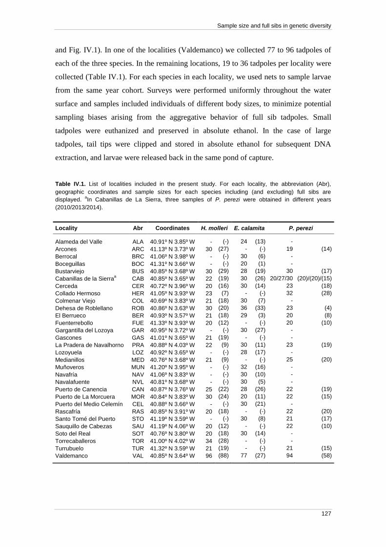
Sample size and full sibs in genetic diversity
127
and Fig. IV.1). In one of the localities (Valdemanco) we collected 77 to 96 tadpoles of
each of the three species. In the remaining locations, 19 to 36 tadpoles per locality were
collected (Table IV.1). For each species in each locality, we used nets to sample larvae
from the same year cohort. Surveys were performed uniformly throughout the water
surface and samples included individuals of different body sizes, to minimize potential
sampling biases arising from the aggregative behavior of full sib tadpoles. Small
tadpoles were euthanized and preserved in absolute ethanol. In the case of large
tadpoles, tail tips were clipped and stored in absolute ethanol for subsequent DNA
extraction, and larvae were released back in the same pond of capture.
Table IV.1. List of localities included in the present study. For each locality, the abbreviation (Abr),
geographic coordinates and sample sizes for each species including (and excluding) full sibs are
displayed. aIn Cabanillas de La Sierra, three samples of P. perezi were obtained in different years
(2010/2013/2014).
Locality Abr Coordinates H. molleri E. calamita P. perezi
Alameda del Valle ALA 40.91º N 3.85º W - (-) 24 (13) -
Arcones ARC 41.13º N 3.73º W 30 (27) - (-) 19 (14)
Berrocal BRC 41.06º N 3.98º W - (-) 30 (6) -
Boceguillas BOC 41.31º N 3.66º W - (-) 20 (1) -
Bustarviejo BUS 40.85º N 3.68º W 30 (29) 28 (19) 30 (17)
Cabanillas de la Sierraa CAB 40.85º N 3.65º W 22 (19) 30 (26) 20/27/30 (20)/(20)/(15)
Cerceda CER 40.72º N 3.96º W 20 (16) 30 (14) 23 (18)
Collado Hermoso HER 41.05º N 3.93º W 23 (7) - (-) 32 (28)
Colmenar Viejo COL 40.69º N 3.83º W 21 (18) 30 (7) -
Dehesa de Roblellano ROB 40.86º N 3.63º W 30 (20) 36 (33) 23 (4)
El Berrueco BER 40.93º N 3.57º W 21 (18) 29 (3) 20 (8)
Fuenterrebollo FUE 41.33º N 3.93º W 20 (12) - (-) 20 (10)
Gargantilla del Lozoya GAR 40.95º N 3.72º W - (-) 30 (27) -
Gascones GAS 41.01º N 3.65º W 21 (19) - (-) -
La Pradera de Navalhorno PRA 40.88º N 4.03º W 22 (9) 30 (11) 23 (19)
Lozoyuela LOZ 40.92º N 3.65º W - (-) 28 (17) -
Medianillos MED 40.76º N 3.68º W 21 (9) - (-) 25 (20)
Muñoveros
MUN 41.20º N 3.95º W - (-) 32 (16) -
Navafría NAV 41.06º N 3.83º W - (-) 30 (10) -
Navalafuente NVL 40.81º N 3.68º W - (-) 30 (5) -
Puerto de Canencia CAN 40.87º N 3.76º W 25 (22) 28 (26) 22 (19)
Puerto de La Morcuera MOR 40.84º N 3.83º W 30 (24) 20 (11) 22 (15)
Puerto del Medio Celemín CEL 40.88º N 3.66º W - (-) 30 (21) -
Rascafría RAS 40.85º N 3.91º W 20 (18) - (-) 22 (20)
Santo Tomé del Puerto STO 41.19º N 3.59º W - (-) 30 (8) 21 (17)
Sauquillo de Cabezas SAU 41.19º N 4.06º W 20 (12) - (-) 22 (10)
Soto del Real SOT 40.76º N 3.80º W 20 (18) 30 (14) -
Torrecaballeros TOR 41.00º N 4.02º W 34 (28) - (-) -
Turrubuelo TUR 41.32º N 3.59º W 21 (19) - (-) 21 (15)
Valdemanco VAL 40.85º N 3.64º W 96 (88) 77 (27) 94 (58)

CHAPTER IV
128
DNA extraction and genotyping
Two enriched partial genomic libraries, one for H. molleri and another for E. calamita,
were prepared at the Sequencing Genotyping Facility, Cornell Life Sciences Core
Laboratory Center (CLC) (New York, NY) following the method described in
Gutiérrez-Rodríguez & Martínez-Solano (2013). They were generated from DNA of
one tadpole of H. molleri collected in Arzila, Portugal (40.20º N, 8.65º W) and one
adult male of E. calamita collected in Valdemanco, central Spain (40.85º N, 3.64º W).
From each of the two libraries, 60 loci containing microsatellite motifs (30 trimers and
30 tetramers) between 5 and 12 repetitions long were selected for further screening.
Although some tri-nucleotides might be under selection, we do not expect that it would
dramatically affect our results, except if selection was very strong, which is highly
unlikely. This expectation is further supported by the similar polymorphism and
diversity profiles shown by the tri- and tetra-nucleotide loci in our study (see Table IV.2
and Appendix 1), and also by other demographic analyses performed with different
subsets of loci (data not shown). For DNA purification, optimization of multiplex
reactions, genotyping and allele scoring, we followed the methods described in
Sánchez-Montes et al. (2016). Final sets of markers consisted of 18 and 16 newly
developed microsatellite loci for H. molleri and E. calamita, respectively (see Appendix
1), and 15 previously optimized markers for P. perezi (Sánchez-Montes et al. 2016).
These sets of markers were used to genotype the samples of each species. We selected a
subsample for repetition of the DNA amplification process (between 3.7% and 17.8% of
the sample in each species) to check for consistency of genotype calling.
Characterization of genetic diversity and effect of full sibs
For characterization of genetic diversity, allelic richness (AR), observed (HO) and
expected (HE) heterozygosity and FIS were calculated for each locus in each population
using GENALEX 6.5 (Peakall & Smouse 2006). Tests for departures from HWE and
evidence of LD were performed with GENEPOP v.4.3 (Raymond & Rousset 1995;
Rousset 2008), with 10,000 dememorisation steps, 1,000 batches and 10,000 iterations
per batch. The Bonferroni sequential correction was applied to account for multiple
testing (Rice 1989). The presence of null alleles was assessed with MICRO-CHECKER
v.2.2.3 (Van Oosterhout et al. 2004). We calculated the information content of the
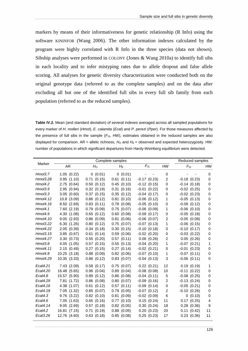
Sample size and full sibs in genetic diversity
129
markers by means of their informativeness for genetic relationship (R Info) using the
software KININFOR (Wang 2006). The other information indexes calculated by the
program were highly correlated with R Info in the three species (data not shown).
Sibship analyses were performed in COLONY (Jones & Wang 2010a) to identify full sibs
in each locality and to infer mistyping rates due to allele dropout and false allele
scoring. All analyses for genetic diversity characterization were conducted both on the
original genotype data (referred to as the complete samples) and on the data after
excluding all but one of the identified full sibs in every full sib family from each
population (referred to as the reduced samples).
Table IV.2. Mean (and standard deviation) of several indexes averaged across all sampled populations for
every marker of H. molleri (Hmol), E. calamita (Ecal) and P. perezi (Pper). For those measures affected by
the presence of full sibs in the sample (FIS, HW), estimates obtained in the reduced samples are also
displayed for comparison. AR = allelic richness, HO and HE = observed and expected heterozygosity. HW:
number of populations in which significant departures from Hardy-Weinberg equilibrium were detected.
Marker Complete samples
Reduced samples
AR HO HE FIS HW
FIS HW
Hmol3.7 1.05 (0.22) 0 (0.01) 0 (0.01) - - 0
- - 0
Hmol3.28 3.95 (1.10) 0.71 (0.15) 0.61 (0.11) -0.17 (0.23) 2
-0.18 (0.23) 0
Hmol4.2 2.75 (0.64) 0.50 (0.12) 0.45 (0.10) -0.12 (0.15) 0
-0.14 (0.18) 0
Hmol3.9 2.95 (0.94) 0.32 (0.19) 0.31 (0.16) -0.01 (0.22) 0
-0.02 (0.25) 0
Hmol3.3 3.05 (0.60) 0.37 (0.15) 0.35 (0.12) -0.04 (0.17) 0
-0.02 (0.23) 0
Hmol4.12 10.8 (3.09) 0.86 (0.12) 0.81 (0.10) -0.06 (0.12) 1
-0.05 (0.13) 0
Hmol4.16 8.50 (2.69) 0.83 (0.11) 0.78 (0.08) -0.05 (0.10) 0
-0.09 (0.12) 0
Hmol4.1 7.60 (2.19) 0.79 (0.09) 0.75 (0.07) -0.06 (0.09) 1
-0.06 (0.10) 0
Hmol4.9 4.30 (1.08) 0.65 (0.12) 0.60 (0.08) -0.09 (0.17) 0
-0.05 (0.18) 0
Hmol4.10 9.05 (2.93) 0.86 (0.09) 0.81 (0.06) -0.06 (0.07) 2
-0.05 (0.08) 0
Hmol3.22 6.30 (1.26) 0.80 (0.12) 0.75 (0.07) -0.07 (0.13) 1
-0.06 (0.15) 0
Hmol4.22 2.05 (0.39) 0.34 (0.18) 0.30 (0.15) -0.10 (0.18) 0
-0.10 (0.17) 0
Hmol3.15 3.85 (0.67) 0.61 (0.14) 0.59 (0.06) -0.02 (0.20) 0
-0.03 (0.22) 0
Hmol4.27 3.30 (0.73) 0.55 (0.20) 0.57 (0.11) 0.06 (0.26) 2
0.05 (0.26) 0
Hmol3.8 4.05 (1.05) 0.57 (0.15) 0.55 (0.13) -0.04 (0.20) 1
-0.07 (0.21) 1
Hmol4.11 2.15 (0.49) 0.27 (0.15) 0.27 (0.14) -0.02 (0.21) 0
-0.01 (0.23) 0
Hmol4.8 10.25 (3.18) 0.88 (0.09) 0.82 (0.06) -0.07 (0.10) 1
-0.07 (0.11) 0
Hmol4.29 10.35 (3.33) 0.86 (0.12) 0.83 (0.07) -0.04 (0.13) 3
-0.06 (0.11) 0
Ecal4.21 7.43 (2.09) 0.58 (0.17) 0.75 (0.07) 0.22 (0.21) 12
0.19 (0.19) 1
Ecal4.20 16.48 (5.65) 0.96 (0.04) 0.89 (0.04) -0.08 (0.08) 10
-0.11 (0.22) 0
Ecal4.8 15.57 (5.90) 0.89 (0.12) 0.86 (0.08) -0.04 (0.11) 5
-0.08 (0.25) 0
Ecal4.29 7.81 (1.72) 0.86 (0.08) 0.80 (0.07) -0.09 (0.16) 2
-0.13 (0.24) 0
Ecal4.16 4.38 (1.07) 0.61 (0.12) 0.57 (0.11) -0.09 (0.14) 0
-0.05 (0.21) 0
Ecal4.18 7.05 (1.32) 0.85 (0.07) 0.79 (0.05) -0.07 (0.12) 2
-0.10 (0.26) 0
Ecal4.3 9.76 (3.22) 0.82 (0.10) 0.81 (0.09) -0.02 (0.09) 6
0 (0.10) 0
Ecal4.6 7.05 (1.63) 0.65 (0.16) 0.77 (0.10) 0.15 (0.24) 11
0.17 (0.25) 4
Ecal4.14 9.05 (2.69) 0.57 (0.18) 0.82 (0.05) 0.30 (0.24) 18
0.28 (0.36) 9
Ecal4.2 16.81 (7.15) 0.71 (0.19) 0.88 (0.05) 0.20 (0.23) 20
0.11 (0.42) 11
Ecal3.26 12.76 (4.60) 0.63 (0.18) 0.85 (0.08) 0.25 (0.23) 17
0.23 (0.36) 11
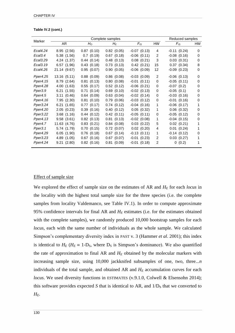
CHAPTER IV
130
Table IV.2 (cont.)
Effect of sample size
We explored the effect of sample size on the estimates of AR and HE for each locus in
the locality with the highest total sample size for the three species (i.e. the complete
samples from locality Valdemanco, see Table IV.1). In order to compute approximate
95% confidence intervals for final AR and HE estimates (i.e. for the estimates obtained
with the complete samples), we randomly produced 10,000 bootstrap samples for each
locus, each with the same number of individuals as the whole sample. We calculated
Simpson’s complementary diversity index in PAST v. 3 (Hammer et al. 2001); this index
is identical to HE (HE 1-DS, where DS is Simpson’s dominance). We also quantified
the rate of approximation to final AR and HE obtained by the molecular markers with
increasing sample size, using 10,000 jackknifed subsamples of one, two, three...n
individuals of the total sample, and obtained AR and HE accumulation curves for each
locus. We used diversity functions in ESTIMATES (v.9.1.0, Colwell & Elsensohn 2014);
this software provides expected S that is identical to AR, and 1/DS that we converted to
HE.
Marker Complete samples Reduced samples
AR HO HE FIS HW FIS HW
Ecal4.24 8.95 (2.56) 0.87 (0.10) 0.82 (0.05) -0.07 (0.13) 4 -0.11 (0.24) 0
Ecal3.4 5.38 (1.56) 0.7 (0.19) 0.67 (0.18) -0.06 (0.11) 2 -0.08 (0.16) 0
Ecal3.29 4.24 (1.37) 0.44 (0.14) 0.48 (0.13) 0.08 (0.21) 3 0.03 (0.31) 0
Ecal3.19 6.57 (1.96) 0.43 (0.18) 0.73 (0.13) 0.42 (0.21) 15 0.37 (0.34) 8
Ecal4.26 21.14 (9.67) 0.95 (0.07) 0.90 (0.05) -0.06 (0.09) 12 -0.09 (0.23) 0
Pper4.25 13.16 (5.11) 0.88 (0.09) 0.86 (0.08) -0.03 (0.09) 2 -0.06 (0.13) 0
Pper4.15 8.79 (2.64) 0.81 (0.13) 0.80 (0.08) -0.01 (0.11) 0 -0.05 (0.11) 0
Pper4.28 4.00 (1.63) 0.55 (0.17) 0.52 (0.12) -0.06 (0.21) 0 -0.07 (0.2) 0
Pper3.9 6.21 (1.55) 0.71 (0.14) 0.69 (0.10) -0.02 (0.13) 0 -0.05 (0.1) 0
Pper4.5 3.11 (0.46) 0.64 (0.09) 0.63 (0.04) -0.02 (0.14) 0 -0.03 (0.16) 0
Pper4.16 7.95 (2.30) 0.81 (0.10) 0.79 (0.06) -0.03 (0.12) 0 -0.01 (0.16) 0
Pper3.24 6.21 (1.65) 0.77 (0.17) 0.74 (0.12) -0.04 (0.16) 1 -0.06 (0.17) 1
Pper4.20 2.05 (0.23) 0.39 (0.16) 0.40 (0.12) 0.05 (0.32) 1 0.06 (0.32) 0
Pper3.22 3.68 (1.16) 0.44 (0.12) 0.42 (0.11) -0.05 (0.11) 0 -0.05 (0.12) 0
Pper4.13 9.58 (3.61) 0.82 (0.13) 0.81 (0.13) -0.02 (0.08) 1 -0.04 (0.15) 0
Pper4.7 11.63 (4.76) 0.83 (0.21) 0.84 (0.08) 0.03 (0.22) 5 0.02 (0.21) 1
Pper3.1 5.74 (1.79) 0.70 (0.15) 0.72 (0.07) 0.02 (0.20) 4 0.01 (0.24) 1
Pper4.29 6.05 (1.90) 0.76 (0.18) 0.67 (0.14) -0.13 (0.11) 1 -0.14 (0.12) 0
Pper3.23 4.89 (1.05) 0.67 (0.16) 0.67 (0.07) -0.01 (0.23) 2 0.03 (0.27) 1
Pper4.24 9.21 (2.80) 0.82 (0.16) 0.81 (0.09) -0.01 (0.18) 2 0 (0.2) 1

Sample size and full sibs in genetic diversity
131
We used R (R Development Core Team 2009) to inspect the accumulation
curves looking for asymptotic stabilization of AR and HE (see Appendix 2). Our
criterion for defining ‘sufficient samples’ was to minimize a Type-II (β) error (Snedecor
& Cochran 1989) by selecting the first point along the section of curve that would
persistently exceed the lower bound of the (bootstrapped) confidence interval of the
final estimate, while no further points would consistently fall below. We summarized in
boxplots the observed minimal sample sizes for each locus necessary to approximate
final estimates of AR and HE. For comparison with our results, we also obtained
empirical and Chao’s diversity profiles for each marker for values 0 ≤ q ≥ 3, by
adapting the R script in Appendix S8 in Chao & Jost (2015). The parameter q defines
the sensitivity of the diversity estimate to the rarest categories in the sample, and most
of the variation in the diversity profile is expected to be comprised within the interval q
= [0,3] (Chao & Jost 2015). The empirical profile at q = 0 corresponds to AR measured
as the total number of alleles (analogous to species richness in Chao & Jost 2015), and
at q = 2 it approximates Simpson’s diversity index (Chao et al. 2015) which, when
calculated as the complement of Simpson’s dominance, is analogous to HE, as stated
above.
Results
Characterization of genetic diversity and effect of full sibs
Almost all microsatellite markers were polymorphic in nearly all sampled populations
(see Appendix 1). The only exception was Hmol3.7, which was monomorphic in all
populations except for CAN (see Appendix 1). Although neither average FIS, nor
minimum sample sizes could be calculated for this locus, we report primer information
and amplification conditions because this marker might result more informative at
larger-scale studies. Genetic diversity measures obtained with the reduced samples were
very similar to those obtained with the complete samples (see Appendix 1), although FIS
estimates changed slightly (see Table IV.2 and Supplementary Appendix 1). FIS and the
allelic dropout rate (inferred from COLONY analyses) were highly correlated in the three
species (H. molleri: Spearman’s rho = 0.57, p = 0.015; E. calamita: rho = 0.85, p <
0.001; P. perezi: rho = 0.70, p = 0.005) although the trend was clearer in E. calamita,
which showed the highest variance in the values of both FIS and allelic dropout rate (see

CHAPTER IV
132
Appendix 4). However, FIS was not correlated with false allele rate in any of the three
species.
Four markers of the H. molleri set and five markers of the P. perezi set showed
significant deviations from HWE in more than one population in the complete samples
(Table IV.2). However, after removing full sibs from the samples, no locus departed
from HWE in more than one population (out of 20 and 17 total localities of H. molleri
and P. perezi, respectively, see Table IV.2 and Appendix 1). Only one marker (out of 18
total loci) in the H. molleri set (Hmol3.15) and four loci (out of 15 total loci) in the P.
perezi set (Pper4.7, Pper3.1, Pper3.23 and Pper4.24) showed evidence of null alleles in
more than one population (three populations at most), and these effects mostly remained
after removing full sibs from the sample (see Appendix 1). In contrast, almost all loci in
the E. calamita set were found to be out of HWE in some populations when using the
complete samples. Five of them (Ecal4.6, Ecal4.14, Ecal4.2, Ecal3.26 and Ecal3.19,
out of 16 total loci) still showed departures from HWE in 4-11 populations after
removing full sibs from the samples (Table IV.2 and Appendix 1). According to MICRO-
CHECKER results, these five loci, as well as Ecal4.21, showed evidence of null alleles in
many populations (see Appendix 1).
A few pairs of loci showed evidence of linkage disequilibrium (LD) across some
populations in the complete datasets after applying the Bonferroni correction. A pair of
loci in the H. molleri set, three pairs of loci in the E. calamita set, and three pairs of loci
in the P. perezi set were in LD in more than 20% of the populations. The most
widespread disequilibrium involved markers Ecal4.20 and Ecal3.26, which were in LD
in 14 populations. However, none of these disequilibria remained significant in the
reduced samples (data not shown).
Effect of sample size
Minimum sample sizes required for approaching final estimates of AR and HE in each
locus are summarized in the boxplots of Fig. IV.2. Median values ranged between 50
and 80 individuals for characterization of AR in each species, while less than 20
individuals were sufficient to estimate HE. Minimum sample sizes required for
estimation of HE were highly correlated with marker polymorphism, measured as AR, in

Sample size and full sibs in genetic diversity
133
the three species (H. molleri: Spearman’s rho = 0.79, p < 0.001; E. calamita: rho = 0.67,
p = 0.005; P. perezi: rho = 0.74, p = 0.002, see Fig. IV.2). In contrast, minimum sample
sizes required for estimation of AR were negatively correlated with marker AR,
although only significantly in the case of E. calamita (H. molleri: rho = -0.28, p =
0.270; E. calamita: rho = -0.61, p = 0.013; P. perezi: rho = -0.09, p = 0.738, see Fig.
IV.2). Loci in the three marker sets showed different diversity profiles (see Appendix
3). The least polymorphic loci in each set showed flat profiles, but the most
polymorphic loci showed a more or less decreasing function along the range of q.
Profiles obtained applying Chao’s correction for sampling bias were very similar to
empirical profiles in most cases, although some highly polymorphic loci showed
differences at q = 0, like Hmol4.8 (15 observed alleles vs. 23 alleles estimated by
Figure IV.2. Minimum sample sizes (i.e. minimum number of individuals) required to obtain final
estimates of HE (grey) and AR (white) in the complete samples from Valdemanco. Scatterplots in the
top panel show the minimum sample sizes (y-axis) required to estimate each parameter for each
marker individually (grey dots: HE, white dots: AR), while each marker is represented in the x-axis by
the polymorphism (AR) shown in Valdemanco. Minimum sample sizes required for estimation of HE
were highly correlated with marker polymorphism, measured as AR, in the three species (H. molleri:
Spearman’s rho = 0.79, p < 0.001; E. calamita: rho = 0.67, p = 0.005; P. perezi: rho = 0.74, p =
0.002). In contrast, minimum sample sizes required for estimation of AR were negatively correlated
with marker AR, although only significantly in the case of E. calamita (H. molleri: rho = -0.28, p =
0.270; E. calamita: rho = -0.61, p = 0.013; P. perezi: rho = -0.09, p = 0.738). Boxplots (bottom panel)
summarize the minimum sample sizes for the marker set of each species.

CHAPTER IV
134
Chao’s correction), Ecal4.26 (42 observed vs. 45 estimated alleles) or Pper4.7 (20
observed vs. 28 estimated alleles, see Appendix 3).
Discussion
A thorough empirical assessment of marker polymorphism and performance is a key
step to evaluate their adequacy for genetic diversity characterization and therefore to
inform marker set choice for future studies (Matson et al. 2008; Queirós et al. 2015).
The moderate to high polymorphism observed in our marker sets (Table IV.2) suggests
that a high power of resolution could be obtained by combining a subset of the most
polymorphic markers in a single (or two) multiplex reaction(s), which might be useful
e.g. for management purposes (Cornuet & Luikart 1996; Holleley & Geerts 2009;
Harrison et al. 2013; Queirós et al. 2015). However, in studies including genetically
impoverished populations, for instance near range borders (Rowe et al. 1999;
Edenhamn et al. 2000; Allentoft et al. 2009), more loci could be necessary to attain a
similar power of resolution, and these loci could be selected from each set after testing
their degree of polymorphism in the area of interest. Marker set composition should
therefore be assessed before conducting the sampling, to guarantee unbiased
comparison among populations (i.e. using the same marker set for all sampling
localities) while also avoiding problems caused by insufficient marker information.
Mistyping rates are also essential to assess the practical utility of newly developed
markers, but this information is often overlooked (Pompanon et al. 2005; Lampa et al.
2013). Inferred error rates in our markers rarely exceeded 0.05, except for the six
markers of E. calamita in which we also detected evidence of null alleles (Appendix 1).
These markers showed dropout rates between 0.09 and 0.32 (Appendix 1). In all three
species, dropout rates inferred by COLONY were highly correlated with FIS, but this trend
was more obvious in the case of E. calamita than in H. molleri and P. perezi, because
larger variance was observed in the former species (Appendix 4). These results
highlight the usefulness of pedigree reconstruction in COLONY for the estimation of error
rates since they are in agreement with HWE tests, which are based on FIS (Waples
2015).
Our analyses of marker genotypes across many populations allowed assessing
the effect of sampling full sibs on estimates of genetic diversity, which may be
Sample size and full sibs in genetic diversity
135
problematic when pedigree information is not available (Allendorf & Phelps 1981;
Goldberg & Waits 2010). We identified full sibs in each population after reconstruction
of one- or two-generation pedigrees (Jones & Wang 2010b) and found that samples
from some localities were mostly composed of full sibs (see Table IV.1), thus
potentially misleading some downstream analyses (Anderson & Dunham 2008;
Jourdan-Pineau et al. 2012; Rodríguez-Ramilo & Wang 2012). However, removing all
relatives from the sample is not always a good solution, because the degree of
nonrandomness (with respect to sibship frequency) in empirical samples is unknown
(Waples & Anderson 2017). More theoretical work, coupled with empirical data, is
needed to derive guidelines about how best to account for this factor. Here we report
some preliminary conclusions drawn from both theoretical (see Appendix 5) and
empirical work, with consistent results across species and populations.
The presence of full sibs in our samples did not significantly affect estimates of
genetic diversity (AR, HO and HE), although there were slight variations in FIS estimates
(Table IV.2). Theoretically, full sibs in the sample are expected to affect the genotype
distributions (see Appendix 5). For this reason, FIS, HWE and LD are most affected,
although the pattern of change is complex and dependent on the mating system
(Goldberg & Waits 2010). As expected, tests for HWE and LD were strongly affected
by the presence of full sibs in the samples (Waples 2015), and most initially inferred
disequilibria were no longer significant after removing full sibs (Table IV.2). While this
could also be caused by the lower statistical power in some reduced samples due to
reduced sample sizes, some consistent departures from HWE were still detected in
many reduced samples of E. calamita (see Appendix 1). Five loci (Ecal4.6, Ecal4.14,
Ecal4.2, Ecal3.26 and Ecal3.19) departed from the expected HWE in more than 15% of
populations in the reduced samples. Disequilibria in these five loci, as well as in
Ecal4.21, were probably due to the presence of null alleles, as indicated by analyses
with MICRO-CHECKER (Appendix 1). These six markers are highly informative and can
be useful in some analyses accounting for genotyping errors (such as sibship analyses in
COLONY), but otherwise they should only be used when downstream analyses are robust
to violation of HWE assumptions. Altogether, these results suggest that genetic
diversity indexes (AR, HO, HE) are not affected by the presence of close relatives in the
sample, at least in the absence of strongly unbalanced data structure (i.e. when there are
not very large families combined with unrelated individuals in the same sample), such

CHAPTER IV
136
as in our case (see also Waples & Anderson 2017). In contrast, the presence of close
relatives in the sample strongly affects the results of tests of HWE and LD, especially in
small samples/populations.
On the other hand, accounting for the minimum sample size required for genetic
diversity characterization is crucial for the accuracy of results and the efficient design of
monitoring programs (Wang 2002). Here we have adapted methods based on diversity
accumulation curves (Ariño et al. 1996; Ariño et al. 2008) by observing the rate at
which jackknifed subsamples approach the confidence interval of bootstrapped
replicates of the entire dataset and can no longer be statistically separated from each
other at a pre-specified significance level (see Appendix 2). Our threshold criterion was
useful for defining a realistic minimum sample size in most markers, although it was
dependent on the width of the 95% confidence interval (CI) of final estimates. As a
consequence, in the case of markers with very narrow 95% CI, large sample sizes were
required to reach the lower bound of the 95% CI. This resulted in an artificially inflated
minimum sample size for AR estimation in some markers (see, for example, Hmol3.3,
Ecal3.19 or Pper3.24 in Appendix 2). Conversely, for some indexes with a very wide
95% CI, inferred minimum sample sizes were artificially low (e.g. HE curves for
Hmol3.9, Ecal3.22 or Pper3.22 in Appendix 2). Too wide (or narrow) 95% CIs in
highly (or very little) polymorphic loci probably caused the negative relationship
between AR and the minimum sample size for AR estimation (Fig. IV.2).
Furthermore, although our total sample sizes in Valdemanco can be considered
large enough to characterize genetic diversity in pond-breeding amphibian populations,
our final estimates cannot be taken as actual population parameters. As a consequence,
these minimum sample sizes cannot be regarded as generally applicable to other
systems. Rather, our goal is double: to encourage the general use of a simple method to
explore the rate of approximation to final genetic diversity estimates with cumulative
sample size (such as those applied in Miyamoto et al. 2008, Pruett & Winker 2008,
Hale et al. 2012, Chao & Jost 2015, or in this paper), and to empirically calculate
minimum sample size. Our method could be easily adapted to sequential sampling
schemes where additional individuals are genotyped, and their alleles added to the pool
at each step. Thus, additional sampling is no longer necessary when the added
individual(s) do not significantly improve the estimates of AR and HE. This way,
minimum sample sizes can be defined when required (e.g. for the design of sampling

Sample size and full sibs in genetic diversity
137
protocols). Nevertheless, since AR and HE are two particular cases of the continuous
diversity measurement, we also followed Chao & Jost (2015)’s proposal of reporting the
continuous diversity profile at the most relevant values of q. As expected, the most
polymorphic loci in our datasets also showed more rare alleles and, as a consequence,
their diversity profile varied through the range of q. In contrast, the profiles of the least
polymorphic loci were largely flat (Appendix 3). This is in agreement with the observed
positive correlation between marker polymorphism and the minimum sample size
required for HE estimation (Fig. IV.2). Empirical profiles were markedly similar to
Chao’s profiles in most markers, suggesting that our empirical accumulation curves of
AR and HE did not dramatically underestimate diversity (Appendix 3). However, we
found differences in the profiles of some markers with alleles at low frequencies, like
Hmol4.8, Ecal4.2, Ecal4.26 or Pper4.7 (Appendix 3), which concordantly showed wide
95% CIs in their corresponding accumulation curves for AR estimation (Appendix 2).
Highly polymorphic loci are usually associated with rare alleles, and therefore higher
sample sizes are required to estimate AR (but not necessary HE) with these markers.
These results support the usefulness of our method for reliable minimum sample size
calculation and also for detecting possible diversity underestimations caused by loci
with rare alleles.
Our results highlight that the presence of full sibs can slightly alter FIS estimates
and affect tests of HWE and LD, but also that AR, HO and HE are not affected by the
presence of small full sib families. We proved that some genotypic disequilibria are no
longer significant after removing full sibs from the samples, therefore allowing
detection of truly problematic markers (e. g. those presenting null alleles). On the other
hand, the minimum sample size is dependent on the marker(s) selected and should also
be assessed in each case for the configuration of the final marker set (Harrison et al.
2013). The required sample size for genetic diversity characterization can be optimized
from an exhaustively sampled population by means of accumulation curves and some
threshold criterion. This methodology is easy to apply to any empirical dataset and can
be readily used to help design sampling protocols for genetic monitoring studies. These
two aspects are basic for the efficient design of ecological studies aiming to obtain
reliable and comparable inferences about demography and genetic diversity distribution
in non-model species.

CHAPTER IV
138
Acknowledgements
We thank M. Peñalver, L. San José, J. Gutiérrez, E. Iranzo, L. Carrera, C. Valero, M. Rojo, G.
Rodríguez, J. Agüera, A. Sabalza, N. Escribano, R. Goñi, R. Santiso and I. Miqueleiz for help
during fieldwork. R. Waples, W. Sherwin and an anonymous reviewer provided valuable
comments on a previous version of this manuscript. Authorizations for animal tissue sampling
were provided by Consejería de Medio Ambiente y Ordenación del Territorio, Comunidad de
Madrid and Consejería de Fomento y Medio Ambiente, Junta de Castilla y León (Spain). This
work was supported by Ministerio de Ciencia e Innovación, Spain, and FEDER (grant number
CGL2008-04271-C02-01/BOS) and Ministerio de Economía y Competitividad, Spain, and
FEDER (grant number CGL2011-28300) to IMS, who was also supported by funding from the
Spanish Ramón y Cajal (RYC-2007-1668) and Severo Ochoa (SEV-2012-0262) programs. G.
Sánchez-Montes was funded by a predoctoral grant provided by the Asociación de Amigos de la
Universidad de Navarra and benefited from funding from the Programa de ayudas de
movilidad de la Asociación de Amigos de la Universidad de Navarra.
Data accessibility
Sequences of contigs containing newly developed microsatellite loci were deposited in the
NCBI GenBank with accession numbers from KY964693 to KY964726. Microsatellite
genotype data for the three species are available from the Dryad Digital
Repository: http://dx.doi.org/10.5061/dryad.f65s7.

Sample size and full sibs in genetic diversity
139
References
Allendorf FW, Phelps SR (1981) Use of allelic frequencies to describe population structure.
Canadian Journal of Fisheries and Aquatic Sciences, 38, 1507–1514.
Allentoft ME, Siegismund HR, Briggs L, Andersen LW (2009) Microsatellite analysis of the
natterjack toad (Bufo calamita) in Denmark: populations are islands in a fragmented
landscape. Conservation Genetics, 10, 15–28.
Anderson EC, Dunham KK (2008) The influence of family groups on inferences made with the
program Structure. Molecular Ecology Resources, 8, 1219–1229.
Ariño AH, Belascoáin C, Jordana R (1996) Determination of minimal sampling for soil fauna
by asymptotic biodiversity accumulation. In: XII International Colloquium on Soil
Zoology. Dublin, Ireland.
Ariño AH, Belascoáin C, Jordana R (2002) Optimal sampling for complexity in soil
ecosystems. InterJournal, 536, 1–9.
Ariño AH, Belascoáin C, Jordana R (2008) Optimal sampling for complexity in soil
ecosystems. In: Unifying themes in complex systems IV (eds Minai AA, Bar-Yam Y), pp.
222–230. Springer, Berlin Heidelberg.
Arntzen JW, Recuero E, Canestrelli D, Martínez-Solano I (2013) How complex is the Bufo bufo
species group? Molecular Phylogenetics and Evolution, 69, 1203–1208.
Banks MA, Rashbrook VK, Calavetta MJ, Dean CA, Hedgecock D (2000) Analysis of
microsatellite DNA resolves genetic structure and diversity of chinook salmon
(Oncorhynchus tshawytscha) in California’s Central Valley. Canadian Journal of
Fisheries and Aquatic Sciences, 57, 915–927.
Broquet T, Petit EJ (2009) Molecular estimation of dispersal for ecology and population
genetics. Annual Review of Ecology, Evolution, and Systematics, 40, 193–216.
Buckley D (2009) Toward an organismal, integrative, and iterative phylogeography. BioEssays,
31, 784–793.
Buerkle CA, Gompert Z (2013) Population genomics based on low coverage sequencing: how
low should we go? Molecular Ecology, 22, 3028–3035.
Chao A, Jost L (2015) Estimating diversity and entropy profiles via discovery rates of new
species. Methods in Ecology and Evolution, 6, 873–882.
Chao A, Ma KH, Hsieh TC, Chiu CH (2015) Online program SpadeR (Species-richness
prediction and diversity estimation in R). Program and user's guide. Available at:
http://chao.stat.nthu.edu.tw/wordpress/software_download/.
Chao A, Wang YT, Jost L (2013) Entropy and the species accumulation curve: a novel entropy
estimator via discovery rates of new species. Methods in Ecology and Evolution, 4, 1091–
1100.
Colwell RK, Elsensohn JE (2014) EstimateS turns 20: statistical estimation of species richness
and shared species from samples, with non-parametric extrapolation. Ecography, 37, 609–
613.
Cornuet J-M, Luikart G (1996) Description and power analysis of two tests for detecting recent
population bottlenecks from allele frequency data. Genetics, 144, 2001–2014.
Edenhamn P, Höggren M, Carlson A (2000) Genetic diversity and fitness in peripheral and
central populations of the European tree frog Hyla arborea. Hereditas, 133, 115–122.
Excoffier L, Heckel G (2006) Computer programs for population genetics data analysis: a
survival guide. Nature Reviews Genetics, 7, 745–758.

CHAPTER IV
140
Fahey AL, Ricklefs RE, Dewoody JA (2014) DNA-based approaches for evaluating historical
demography in terrestrial vertebrates. Biological Journal of the Linnean Society, 112, 367–
386.
Fitzpatrick BM (2009) Power and sample size for nested analysis of molecular variance.
Molecular Ecology, 18, 3961–3966.
Foulley JL, Ollivier L (2006) Estimating allelic richness and its diversity. Livestock Science,
101, 150–158.
Gallardo C, Correa C, Morales P et al. (2012) Validation of a cheap and simple nondestructive
method for obtaining AFLPs and DNA sequences (mitochondrial and nuclear) in
amphibians. Molecular Ecology Resources, 12, 1090–1096.
Goldberg CS, Waits LP (2010) Quantification and reduction of bias from sampling larvae to
infer population and landscape genetic structure. Molecular Ecology Resources, 10, 304–
313.
Guichoux E, Lagache L, Wagner S et al. (2011) Current trends in microsatellite genotyping.
Molecular Ecology Resources, 11, 591–611.
Gutiérrez-Rodríguez J, Martínez-Solano I (2013) Isolation and characterization of sixteen
polymorphic microsatellite loci in the Western Spadefoot, Pelobates cultripes (Anura:
Pelobatidae) via 454 pyrosequencing. Conservation Genetics Resources, 5, 981–984.
Habel JC, Husemann M, Finger A, Danley PD, Zachos FE (2014) The relevance of time series
in molecular ecology and conservation biology. Biological Reviews, 89, 484–492.
Habel JC, Zachos FE, Dapporto L et al. (2015) Population genetics revisited – towards a
multidisciplinary research field. Biological Journal of the Linnean Society, 115, 1–12.
Hale ML, Burg TM, Steeves TE (2012) Sampling for microsatellite-based population genetic
studies: 25 to 30 individuals per population is enough to accurately estimate allele
frequencies. PLoS ONE, 7, e45170.
Hamilton MB (2009) Population genetics. Wiley-Blackwell, Chinchester, West Sussex.
Hammer Ø, Harper DAT, Ryan PD (2001) PAST: Paleontological statistics software package
for education and data analysis. Palaeontologia Electronica, 4, 9pp.
Harrison HB, Saenz-Agudelo P, Planes S, Jones GP, Berumen ML (2013) Relative accuracy of
three common methods of parentage analysis in natural populations. Molecular Ecology,
22, 1158–1170.
Holleley CE, Geerts PG (2009) Multiplex Manager 1.0: a cross-platform computer program that
plans and optimizes multiplex PCR. BioTechniques, 46, 511–517.
Jones OR, Wang J (2010a) COLONY: a program for parentage and sibship inference from
multilocus genotype data. Molecular Ecology Resources, 10, 551–555.
Jones OR, Wang J (2010b) Molecular marker-based pedigrees for animal conservation
biologists. Animal Conservation, 13, 26–34.
Jourdan-Pineau H, Folly J, Crochet PA, David P (2012) Testing the influence of family
structure and outbreeding depression on heterozygosity-fitness correlations in small
populations. Evolution, 66, 3624–3631.
Kalinowski ST (2004) Counting alleles with rarefaction: private alleles and hierachical
sampling designs. Conservation Genetics, 5, 539–543.
Lampa S, Henle K, Klenke R, Hoehn M, Gruber B (2013) How to overcome genotyping errors
in non-invasive genetic mark-recapture population size estimation – A review of available
methods illustrated by a case study. Journal of Wildlife Management, 77, 1490–1511.
Leberg PL (2002) Estimating allelic richnes: effects of sample size and bottlenecks. Molecular
Sample size and full sibs in genetic diversity
141
Ecology, 11, 2445–2449.
Luikart G, Ryman N, Tallmon DA, Schwartz MK, Allendorf FW (2010) Estimation of census
and effective population sizes: the increasing usefulness of DNA-based approaches.
Conservation Genetics, 11, 355–373.
Marko PB, Hart MW (2011) The complex analytical landscape of gene flow inference. Trends
in Ecology and Evolution, 26, 448–456.
Matson SE, Camara MD, Eichert W, Banks MA (2008) P-LOCI: a computer program for
choosing the most efficient set of loci for parentage assignment. Molecular Ecology
Resources, 8, 765–768.
Miyamoto N, Fernández-Manjarrés JF, Morand-Prieur M-E, Bertolino P, Frascaria-Lacoste N
(2008) What sampling is needed for reliable estimations of genetic diversity in Fraxinus
excelsior L. (Oleaceae)? Annals of Forest Science, 65, 403.
El Mousadik A, Petit RJ (1996) High level of genetic differentiation for allelic richness among
populations of the argan tree [Argania spinose (L. Skeels)] endemic to Morocco.
Theoretical and Applied Genetics, 92, 832–839.
Van Oosterhout C, Hutchinson WF, Wills DPM, Shipley P (2004) MICRO-CHECKER: software
for identifying and correcting genotyping errors in microsatellite data. Molecular Ecology
Notes, 4, 535–538.
Peakall R, Smouse PE (2006) GENALEX 6: genetic analysis in Excel. Population genetic
software for teaching and research. Molecular Ecology Notes, 6, 288–295.
Petit RJ, El Mousadik A, Pons O (1998) Identifying populations for consevation on the basis of
genetic markers. Conservation Biology, 12, 844–855.
Pompanon F, Bonin A, Bellemain E, Taberlet P (2005) Genotyping errors: causes,
consequences and solutions. Nature Reviews Genetics, 6, 847–859.
Pruett CL, Winker K (2008) The effects of sample size on population genetic diversity estimates
in song sparrows Melospiza melodia. Journal of Avian Biology, 39, 252–256.
Queirós J, Godinho R, Lopes S et al. (2015) Effect of microsatellite selection on individual and
population genetic inferences: an empirical study using cross-specific and species-specific
amplifications. Molecular Ecology Resources, 15, 747–760.
R Development Core Team (2009) R: a language and environment for statistical computing. R
Foundation for Statistical Computing. Vienna, Austria. ISBN 3-900051-07-0, available at:
http://www.R-project.org.
Raymond M, Rousset F (1995) GENEPOP (Version 1.2): Population genetics software for exact
tests and ecumenicism. Journal of Heredity, 86, 248–249.
Rice WR (1989) Analyzing tables of statistical tests. Evolution, 43, 223–225.
Rodríguez-Ramilo ST, Toro MA, Wang J, Fernández J (2014) Improving the inference of
population genetic structure in the presence of related individuals. Genetic Research, 96,
e003.
Rodríguez-Ramilo ST, Wang J (2012) The effect of close relatives on unsupervised Bayesian
clustering algorithms in population genetic structure analysis. Molecular Ecology
Resources, 12, 873–884.
Rousset F (2008) GENEPOP’007: a complete re-implementation of the GENEPOP software for
Windows and Linux. Molecular Ecology Resources, 8, 103–106.
Rowe G, Beebee TJC, Burke T (1999) Microsatellite heterozygosity, fitness, and demography
in natterjack toads Bufo calamita. Animal Conservation, 2, 85–92.
Sánchez-Montes G, Recuero E, Gutiérrez-Rodríguez J, Gomez-Mestre I, Martínez-Solano I

CHAPTER IV
142
(2016) Species assignment in the Pelophylax ridibundus x P. perezi hybridogenetic
complex based on 16 newly characterised microsatellite markers. Herpetological Journal,
26, 99–108.
Scherer RD, Muths E, Noon BR, Oyler-McCance SJ (2012) The genetic structure of a relict
population of wood frogs. Conservation Genetics, 13, 1521–1530.
Segelbacher G, Cushman SA, Epperson BK et al. (2010) Applications of landscape genetics in
conservation biology: concepts and challenges. Conservation Genetics, 11, 375–385.
Snedecor GW, Cochran WG (1989) Statistical Methods. Iowa State College Press. Ames, Iowa.
Taberlet P, Luikart G (1999) Non-invasive genetic sampling and individual identification.
Biological Journal of the Linnean Society, 68, 41–53.
Tallmon DA, Luikart G, Waples RS (2004) The alluring simplicity and complex reality of
genetic rescue. Trends in Ecology and Evolution, 19, 489–496.
Wang J (2002) An estimator for pairwise relatedness using molecular markers. Genetics, 160,
1203–1215.
Wang J (2006) Informativeness of genetic markers for pairwise relationship and relatedness
inference. Theoretical Population Biology, 70, 300–321.
Waples RS (2015) Testing for Hardy-Weinberg proportions: have we lost the plot? Journal of
Heredity, 106, 1–19.
Waples RS, Anderson EC (2017) Purging putative siblings from population genetic data sets: a
cautionary view. Molecular Ecology, 26, 1211–1224.

CHAPTER V
RELIABLE EFFECTIVE/CENSUS POPULATION SIZE RATIOS IN SEASONAL-BREEDING SPECIES: OPPORTUNITY FOR INTEGRATIVE DEMOGRAPHIC INFERENCES BASED ON CAPTURE-MARK-RECAPTURE DATA AND MULTILOCUS GENOTYPES
Sánchez-Montes G, Wang J, Ariño AH, Vizmanos JL & Martínez-Solano I
Ecology and Evolution (Accepted pending minor review)


Effective/census population size in seasonal breeders
145
Abstract
The ratio of the effective number of breeders (Nb) to the adult census size (Na) approximates the
strength of genetic stochasticity of a population in maintaining genetic diversity in one
reproductive season. This information is relevant for assessing population status, understanding
evolutionary processes operating at local scales and unraveling how life-history traits affect
lineage differentiation. However, our knowledge on Nb/Na ratios in nature is limited because
estimation of both parameters is challenging. The sibship frequency (SF) method is adequate for
reliable Nb estimation because it is based on sibship and parentage reconstruction, thereby
providing demographic inferences that can be compared with field-based information. In
addition, capture-mark-recapture (CMR) robust design methods are well suited for Na
estimation in seasonal-breeding species. Here, we argue that integrating both methods is an
optimum means of estimating the Nb/Na ratio. We illustrate this approach by using tadpole
genotype samples of three pond-breeding amphibian species (Epidalea calamita, Hyla molleri
and Pelophylax perezi, n = 73-96 single-cohort tadpoles per species genotyped at 15-17
microsatellite loci) coupled with candidate parental genotypes (n = 94-300 adult individuals per
species) to estimate Nb by the SF method in a locality in Central Spain. We then assess the
reliability of Nb estimates by comparison of sibship and parentage inferences with field-based
information and check for the convergence of results in replicated subsampled analyses. Finally,
we use CMR data from a 6-year monitoring program to estimate annual Na for the three species
and calculate the Nb/Na ratio. Reliable Nb/Na ratios were obtained for E. calamita (Nb/Na = 0.18-
0.28) and P. perezi (0.5). On the other hand, in the case of H. molleri, Na could not be
appropriately estimated and genetic information proved insufficient for reliable Nb estimation.
This work shows that integrative demographic studies taking full advantage of SF and CMR
methods can provide accurate estimates of the Nb/Na ratio in seasonal-breeding species such as
pond-breeding amphibians. Importantly, the SF method allows for ready evaluation of the
reliability of results. This represents a good opportunity for obtaining reliable demographic
inferences with wide applications for evolutionary and conservation research.
Keywords: COLONY, Demography, Egg string counts, Marker information, Mating system,
Monogamy, Number of mates, Polygamy, Sample size, Sibship size prior.


Effective/census population size in seasonal breeders
147
Resumen
El cociente entre el número efectivo de reproductores (Nb) y el número de adultos de una
población (Na) ofrece información acerca de la intensidad de la estocasticidad genética en el
mantenimiento de la diversidad genética durante una temporada reproductora determinada en
una población. Esta información es importante para evaluar el estado de conservación de las
poblaciones, entender los procesos evolutivos que operan a pequeña escala espacial y temporal
y estudiar cómo afectan las características vitales propias de cada especie a la divergencia de los
linajes a lo largo del tiempo. Sin embargo, tanto Nb como Na son complejos de estimar en
poblaciones silvestres, por lo que nuestro conocimiento sobre el cociente Nb/Na en la naturaleza
es limitado. Afortunadamente, el método de “sibship frequency” (SF) es adecuado para obtener
estimas fiables de Nb, ya que se basa en la reconstrucción de paternidades y otras relaciones de
parentesco, por lo que proporciona inferencias demográficas que pueden ser comparadas con
observaciones directas de campo. Además, los métodos de captura-marcaje-recaptura (CMR)
que utilizan una metodología de “diseño robusto” son adecuados para estimar Na en especies
con reproducción estacional. En este capítulo argumentamos que integrar ambos métodos es una
manera óptima de estimar el cociente Nb/Na. Para ilustrar esta afirmación utilizamos genotipos
de renacuajos de tres especies de anfibios ibéricos (Epidalea calamita, Hyla molleri y
Pelophylax perezi, n = 73-96 individuos de cada especie genotipados en 15-17 microsatelites)
junto con genotipos de individuos adultos como posibles padres y madres (n = 94-300
individuos adultos por especies) para estimar Nb utilizando el método SF en una localidad del
centro de España. Posteriormente evaluamos la fiabilidad de nuestras estimas de Nb mediante la
comparación de los pedigrís reconstruidos durante los análisis con información directa obtenida
en el campo, y mediante la exploración de la convergencia de los resultados en análisis
replicados empleando diferentes tamaños de muestra e información genética. Finalmente,
utilizamos datos de CMR procedentes de un programa de seguimiento desarrollado durante seis
años para estimar Na en las tres especies y calcular el cociente Nb/Na. Se obtuvieron cocientes
Nb/Na fiables para E. calamita (Nb/Na = 0,18-0,28) y P. perezi (0,5). Sin embargo, en el caso de
H. molleri no se pudo estimar Na, y tampoco la información genética fue suficiente para estimar
Nb con precisión. Este trabajo demuestra que los estudios demográficos que integran métodos de
SF y CMR son capaces de proporcionar estimas fiables del cociente Nb/Na en especies de
reproducción estacional, como es el caso de los anfibios que se reproducen en medios
temporales. También es importante destacar que el método SF permite evaluar la fiabilidad de
los resultados de manera eficaz, lo que representa una gran oportunidad para obtener inferencias
demográficas fiables aplicables en investigación evolutiva y de conservación.


Effective/census population size in seasonal breeders
149
Introduction
The effective size and the census size of a population are two conceptually different
demographic parameters. The effective population size (Ne) is a theoretical number that
was proposed to measure the strength of inbreeding and genetic drift experienced by
finite populations (Wright 1931; Crow & Kimura 1970; Waples et al. 2013).
Accordingly, Ne is defined as the size of an ‘idealized population’ that experiences the
same rate of inbreeding or genetic drift as the real population of study (Wright 1931).
Since both effects act to reduce genetic diversity, the absolute value of Ne is directly
proportional to the capacity of the population to maintain genetic diversity
(Charlesworth 2009; Waples & Antao 2014; Ruzzante et al. 2016; Wang et al. 2016).
The census size, in contrast, is the total number of individuals in the population or,
alternatively, the number of potentially-breeding adults (Na) of the population
(Frankham 1995). Therefore, the ratio between Ne and Na can be considered as a
measure of the potential of the population as a genetic reservoir, standardized by the
abundance of adult individuals (Frankham 1995; Palstra & Ruzzante 2008; Palstra &
Fraser 2012; Bernos & Fraser 2016).
The relevance of the Ne/Na ratio in evolutionary and conservation biology is
based on three major facts. First, it measures the relative performance of a population
against inbreeding and genetic drift, thus providing relevant information about its
conservation status (Frankham 1995; Palstra & Fraser 2012). A high ratio (close to a
value of one) suggests that most adults of the population contribute (nearly equally in
expectation) to the next generation, approaching an idealized panmictic scenario. In
contrast, a low Ne/Na ratio (much smaller than one) implies a high variance in breeding
success among adults and leads potentially to genetic impoverishment driven by
stochastic processes (Banks et al. 2013). Second, the Ne/Na ratio is conditioned by life-
history traits that reflect species-specific reproductive constraints, which might
ultimately have implications for lineage differentiation (Waples et al. 2013; Waples
2016). As a consequence, differences in Ne/Na ratios across species might explain part
of the variance in diversification rates among different taxa. Third, in demographically
stable populations, life-history traits can have a major effect on the Ne/Na ratio, and
therefore, species-specific Ne/Na ratios could be used to estimate Ne from adult
abundance data (or vice versa) in these populations (Bernos & Fraser 2016).

CHAPTER V
150
Nevertheless, the Ne/Na ratio tends to increase in small populations due to genetic
compensation, and thus variance in the Ne/Na ratio among different populations can be
informative about the main evolutionary processes affecting them (Palstra & Ruzzante
2008; Beebee 2009; Bernos & Fraser 2016). Because of the broad informative content
of the Ne/Na ratio, a large number of studies have addressed its calculation across a wide
variety of taxa (Frankham 1995; Palstra & Fraser 2012). However, our knowledge about
the variation of Ne/Na ratios in nature is still limited, because estimation and
interpretation of both Ne and Na are challenging (Palstra & Fraser 2012). In addition,
diverse methods are often employed by different researchers to estimate both Ne and Na,
further complicating comparison among studies.
Direct calculation of Ne requires comprehensive demographic information
(Caballero 1994; Vucetich & Waite 1998; Waples et al. 2011) and indirect methods
(like single-sample genetic methods) are widely used (Schwartz et al. 1998; Wang
2005; Luikart et al. 2010; Wang et al. 2016). Especially, the linkage disequilibrium
(LD) and the sibship frequency (SF) methods have proven the most reliable (Beebee
2009; Wang 2016). In species with overlapping generations, estimation of Ne by these
single-sample methods requires additional demographic information difficult to obtain
in wild populations (Nunney 1993; Waples 2005; Wang et al. 2010; Waples et al. 2013,
2014; Waples & Antao 2014). However, if all individuals in the genetic sample belong
to the same cohort, the effective number of breeding individuals (Nb) producing that
cohort can be readily estimated by these methods (Waples 2005; Wang 2009; Waples et
al. 2013, 2014; Waples & Antao 2014). Although Nb retains only part of the information
of Ne (for example, it does not account for age-variation in breeding success), it can be
used to estimate the ability of the population to maintain genetic diversity (Waples
2005; Waples et al. 2013; Waples & Antao 2014; Kamath et al. 2015). Thus, the Nb/Na
ratio can be used as an estimate of a single-season effective/census population size ratio.
Although some methods based on direct counts, acoustic surveys or
extrapolations from evidences of breeding activity have been employed to estimate Na,
individual-based capture-mark-recapture (CMR) methods provide the most accurate
insights about population size variation (Clutton-Brock & Sheldon 2010). CMR studies
are time-consuming, but current techniques include a wide range of sophisticated
sampling designs that can be applied to different types of data (Lebreton et al. 1992;
Tavecchia et al. 2009). In particular, robust design frameworks, which rely on nested
Effective/census population size in seasonal breeders
151
CMR sessions, are especially powerful in the case of Na estimation (Pollock 1982;
Kendall et al. 1995). The efficiency of robust design analyses can be maximized when
the capture of individuals is concentrated in short time periods, during which population
closure can be assumed (Kendall & Nichols 1995; Kendall et al. 1997). This is the case
of seasonal-breeding species, in which adult individuals congregate during a few weeks
every year (e.g. in lekking aggregations); this allows the concentration of sampling
sessions, facilitating annual estimation of Na.
In this regard, pond-breeding amphibians in temperate latitudes represent an
excellent study system because their seasonal aggregative breeding behaviour facilitates
annual Na estimation by robust design CMR methods. Similarly, the spatial and
temporal clustering of tadpoles of the same cohort in the breeding sites makes them
especially suitable for Nb estimation (Waples 2005; Wang 2009; Beebee 2009). The SF
method, implemented in COLONY (Wang 2009; Jones & Wang 2010), is especially
convenient for Nb estimation in seasonal-breeding species. This method has proved
accurate for Nb estimation when sample size is close to, or higher than, real Nb (Beebee
2009; Ackerman et al. 2016; Wang 2016), or when highly informative markers are
used. In addition, the SF method is based on sibship reconstruction, which provides
demographic inferences (e.g. the number of mating pairs or the average polygamy of
each sex) that can be compared with evidences of breeding activity such as egg string
counts, direct mating observations or individual records of permanence in the breeding
sites. This calibration with field information allows the supervision of reconstructed
sibship relationships, on which the estimate of Nb is based. Furthermore, inclusion of
genotype information of candidate sires and dams potentially increases the robustness of
sibship reconstruction, thereby improving Nb estimates. Finally, replicated analyses
varying the analytical settings and the genetic information employed (i.e. the numbers
of sampled markers and individuals) can be used to check for the convergence of
results.
In summary, we argue that demographic approaches integrating SF estimation of
Nb and CMR estimates of Na provide a good opportunity for producing reliable Nb/Na
ratios for seasonal species, such as temperate pond-breeding amphibians. Here we show
the results of such an integrative study, including field- and molecular-based approaches
for three sympatric anuran species differing in their life-history traits: the natterjack toad
Epidalea calamita (Laurenti, 1768); the Iberian treefrog Hyla molleri Bedriaga, 1889

CHAPTER V
152
and Perez’s frog Pelophylax perezi (López-Seoane, 1885). We monitored a breeding
assemblage of the three species in Central Spain with CMR methods, integrating field-
based information with genotype data from newly optimized sets of microsatellite
markers in order to estimate the Nb/Na ratio.
Specifically, we aimed to:
1) Estimate annual Na (number of adult males and females separately) of the
three species in a breeding locality using CMR robust design methods.
2) Estimate Nb of the three species using the SF method and assess the
reliability of these estimates by comparing reconstructed families with
independent information about each species’ phenology and evidences of
breeding activity, and by checking for the consistency of results in replicated
analyses with different priors, number of markers, and sample sizes.
3) Calculate the corresponding Nb/Na ratio for each species.
Materials and methods
Study area and CMR monitoring program
Our area of study comprises the vicinities of Laguna de Valdemanco, a temporary
aquatic system that extends across a maximum surface area of 12,800 m2 (when
adjacent meadows are flooded in early spring), with one meter of maximum depth. This
pond is located in the foothills of La Cabrera ridge, 1055 m above sea level, between the
towns of La Cabrera and Valdemanco (Madrid, Spain). It is surrounded by
Mediterranean forest dominated by gum rockrose (Cistus ladanifer). A 6-year
monitoring program of the amphibian community of this locality was developed
between 2010 and 2015, with CMR sessions performed every year in Laguna de
Valdemanco and in some additional minor breeding sites at a distance between 270 and
800 meters from the main pond (Sánchez-Montes & Martínez-Solano 2011). Six
amphibian species breed regularly in the pond (Pleurodeles waltl, Triturus marmoratus,
Pelobates cultripes, Epidalea calamita, Hyla molleri and Pelophylax perezi), and
dispersive individuals of Alytes cisternasii, Bufo spinosus and Discoglossus galganoi
were also recorded occasionally. We addressed the estimation of the Nb/Na ratio for E.

Effective/census population size in seasonal breeders
153
calamita, H. molleri and P. perezi, three of the species for which CMR work proved
most successful, based on the recapture rates obtained.
The annual number of egg strings of E. calamita was also recorded. Among the
three targeted species, this is the only one that lays clutches mainly in shallow water
thus allowing exhaustive counts (García-París et al. 2004). Counts were performed
every year during the whole E. calamita breeding season, from the appearance of the
first strings to the end of the mating period, when the puddles and shallow areas
selected by this species for egg-laying finally dried. Egg strings were counted
repeatedly during the season, their position was recorded and their development was
revised in subsequent visits to avoid overestimation.
CMR estimates of Na
As part of the monitoring program, nocturnal CMR sessions were performed during the
breeding season of each species every year from 2010 to 2015. The entire water surface
of Laguna de Valdemanco, shores and nearby areas were sampled on foot without time
limit, in order to maximize the number of captures. Adult individuals were captured by
hand or with the help of dip nets, sexed based on external morphological features and
marked with an 8 mm AVID M.U.S.I.C transponder (EzID, Greeley, Colorado, USA),
with a unique identity code readable with an AVID Minitracker II device. Three
phalanges of a toe of every marked individual were clipped and stored in absolute
ethanol for genetic analyses (see below). Toe clipping in these three species did not
affect survival of individuals, as suggested by the observed rapid healing (see also
McCarthy & Parris 2004). Bone samples were also used for skeletochronological
studies (Sánchez-Montes, unpublished data). All individuals were released back in their
place of capture after processing.
CMR sessions were planned to fulfill the assumptions of the robust design
method (Pollock 1982), by minimizing the time span between secondary sampling
occasions (in this case, within each breeding season, with a maximum time span of 46
days, but typically less), relative to the time span between primary samples (in this case,
between different years). Our final CMR datasets included capture histories for 542
adult E. calamita (141 females, 401 males), 415 adult H. molleri (57 females, 358
males), and 190 adult P. perezi (94 females, 96 males) marked between 2010 and 2015.
CHAPTER V
154
The total number of captures was 1,513 for E. calamita (1-17 captures per individual in
26 total CMR sessions), 526 for H. molleri (1-4 captures per individual in 17 sessions)
and 312 for P. perezi (1-6 captures per individual in 19 sessions). Return rates (the
proportion of individuals captured more than once) were 0.58, 0.23 and 0.41 for E.
calamita, H. molleri and P. perezi, respectively.
We analyzed inter-annual variation in Na using the robust design method
implemented in MARK (White & Burnham 1999). Different models were generated by
applying constraints (time and/or sex dependence) to annual survival (S). Since no time
limit was imposed to standardize capture effort in the CMR sessions, individual
probability of capture was always modelled as dependent of sex and time. The
probability of capture was set equal to the probability of recapture in all models (i.e. we
did not introduce a trap-dependence factor in any model). We tested different models
assuming that the probability of temporary emigration/immigration was either 1)
dependent of the last probable state of the individual (Markovian), 2) independent of the
last probable state of the individual (random), or 3) absent (i.e. temporary
emigration/immigration forced to zero). These temporary immigration/emigration
probabilities could reflect actual temporary displacements out of the area of study or
individuals skipping a breeding season (i.e. interannual changes in state between
‘breeder’ and ‘non-breeder’, Muths et al. 2006, 2013; Cayuela et al. 2014, 2016). Since
no optimum goodness-of-fit tests have been proposed for robust design models, we
tested for the most common causes of departures from the Cormack-Jolly-Seber (CJS)
model assumptions among secondary occasions (Schwarz & Stobo 1997). We thus used
U-CARE (Choquet et al. 2009) to test for ‘transience’ and ‘trap-dependence’ effects in
each year in which the required minimum number of three and four CMR sessions,
respectively, were available (i.e. in four, two and three years for E. calamita, H. molleri
and P. perezi, respectively). Models were ranked based on the Akaike Information
Criterion corrected for small sample sizes (AICc, Akaike 1974; Burnham & Anderson
2002), and estimates of Na were obtained by weighted averaging estimates from the
candidate models.

Table V.1. Sample sizes (n) employed for SF analyses and estimates (with 95% CIs) of Nb and Na obtained for each species. Also, the total number of sires and dams inferred
in SF analyses (in parentheses the number of inferred parents included in the genotyped samples of candidate parents) are shown for each species, along with the egg string
counts for E. calamita. Nb/Na was calculated by dividing the point SF estimate of Nb by the sum of Na point estimates for males and females in each species (total Na). Non-
estimable parameters are indicated with ‘-’.
Species Year n
Nb Na Inferred
number of sires
Inferred number of dams
Nb/Na Egg
string counts tadpoles males females males females total
E. calamita 2013 77
198 102 51 (35-78) 138 (133-143) 43 (28-58) 181 23 (15) 23 (16) 0.28 46
2015 73 52 (35-80) 162 (158-165) 125 (78-172) 287 31 (27) 29 (22) 0.18 104
H. molleri 2013 96 48 48 131 (97-179) 126 (102-150) - - 52 (18) 51 (5) - -
P. perezi 2010 94 47 48 69 (49-98) 69 (30-108) 68 (4-133) 137 37 (17) 38 (24) 0.50 -

CHAPTER V
156
Genetic estimates of Nb
We obtained four single-cohort tadpole genotype samples for Nb estimation: two
samples for E. calamita in 2013 and 2015 (n = 77 and 73 tadpoles, respectively), one for
H. molleri in 2013 (n = 96) and one for P. perezi in 2010 (n = 94, Table V.1). Tadpole
genotypes of E. calamita (2013), H. molleri and P. perezi were obtained from Sánchez-
Montes et al. (2017), and we included an additional sample of tadpoles of E. calamita
(2015). Tadpoles were sampled in a comprehensive survey across the entire surface of
the breeding pond (Sánchez-Montes et al. 2017). We also used a subsample of the tissue
collection obtained during the 6-year monitoring program as candidate parents for SF
analyses (Table V.1). This subsample included adult males and females that had been
captured in the area of study within a period from one year before to one year after the
breeding season when tadpoles were collected (including both the 2013 and 2015
breeding seasons in the case of E. calamita, see Table V.1). All individuals were
genotyped using three sets of 15-17 polymorphic microsatellites specifically designed
for each species following the methods described in Sánchez-Montes et al. (2016,
2017). Basic properties of the three sets of markers and genetic diversity estimates
obtained in Laguna de Valdemanco can be found in Sánchez-Montes et al. (2017).
We used tadpole and adult genotypes of each species to reconstruct sibship and
parentage and to obtain estimates of Nb using SF analyses in COLONY Version 2.0.6.1
(Jones & Wang 2010). We calculated the probability that the progenitors of the
offspring samples were among the genotyped adult individuals using Na estimates from
CMR analyses, by dividing the sample size of candidate fathers (mothers) of each
species by the estimated Na of males (females) in the corresponding year. Since no
estimate of Na was available for females of H. molleri, we used the same probability as
for males (i.e. 48/126 = 0.38). We also performed additional analyses with different
probabilities of parents being present in the genotyped samples (0.5 for both sexes of E.
calamita and 0.2 for H. molleri and P. perezi) to check for the dependence of results on
these prior probabilities. Based on previously estimated error rates (Sánchez-Montes et
al. 2017), we used a genotyping error rate of 0.05 for every marker in E. calamita and
of 0.01 in each of the remaining two species. Since offspring samples represent a single
year cohort, the assumption of the mating system of the species required for COLONY
analyses refers to the possibility of multiple matings within a single breeding season.
Low rates of double-clutching females have been reported in some E. calamita
Effective/census population size in seasonal breeders
157
populations in Sweden and UK (Silverin & Andrén 1992; Denton & Beebee 1996) and
double- and multiple-clutching have been observed in some Hyla species in Europe
(Broquet et al. 2009; Cadeddu & Castellano 2012). However, it is unknown whether
females of H. molleri and P. perezi lay more than one clutch per year (sequential
polyandry) or whether there are multiple paternities within each clutch (simultaneous
polyandry), although the former scenario seems more likely (Lengagne & Joly 2010;
Byrne & Roberts 2012). Accordingly, we conservatively performed all analyses by
assuming polygamy in both sexes in the three species, with ‘very long’ run length and
‘very high’ precision settings.
Additionally, we explored the effects of using different sibship size priors,
number of markers and sample sizes on sibship and parentage reconstruction and on Nb
estimates. First, we compared the effect of using different sibship size priors, from an
average sibship size of one up to five, or without any prior information. The average
sibship size is the mean number of offspring sired by each breeding male (paternal
sibship size) and female (maternal sibship size). Setting a low average value for both
sexes (i.e. = 1) may help discourage false full and half sib assignations, improving Nb
estimation, when marker information is insufficient (Wang 2016). High average values
are only expected in samples obtained from a low number of potential breeders or in
cases of strong male (or female) dominance. Second, we explored the effect of marker
information by performing jackknifed replicates for each number of loci in each species
dataset, from one locus to the complete set, either using or not using a prior sibship size
= 1. Third, we performed replicates at different-sized jackknifed offspring (tadpole)
subsamples (but using the complete candidate parental samples), either using or not
using a sibship size prior = 1. For all these analyses, we used custom-generated R (R
Development Core Team 2009) scripts (see Appendix 6) to run COLONY for multiple
input files (settings: ‘medium’ run length, ‘high’ precision, 10 replicates for each
analysis in each species), record estimates of Nb, and calculate the average number of
different mates per inferred breeder of each sex (a measure of the degree of polygamy)
from inferred families. In all analyses using a sibship size prior, we set a ‘weak’ prior in
order to aid but not force family reconstruction.

CHAPTER V
158
Figure V.1. Annual estimates of Na (with 95% CI) obtained in Laguna de Valdemanco for the three
species, by sex (males: black circles; females: grey circles). Some Na could not be estimated (see
Appendix 7). Dark grey bars show annual counts of egg strings of E. calamita. Blue bars show
monthly cumulative rainfall data from the Barajas weather station (Madrid, about 40 km south from
Laguna de Valdemanco). A sharp decrease in precipitation is apparent in 2012, especially in the early
months of the year, when the breeding activity of the three species is concentrated.

Effective/census population size in seasonal breeders
159
Results
CMR estimates of Na
For each species, the top three ranked models encompassed more than 99% of the
weight based on AICc scores (see Appendix 7). We did not detect consistent departures
from CJS model assumptions among secondary occasions in any of the species,
although males of E. calamita showed evidences of ‘transience’ effects in 2011 and
2013 and ‘trap-dependence’ in 2011 (results not shown). Estimates of Na were
concordant in most years across different models (Appendix 7). Values obtained after
weighted averaging across candidate models are shown in Table V.1 (for the year of the
tadpole genetic sampling in each species) and Figure V.1. Estimated number of males of
E. calamita and H. molleri were similar, around 150 individuals every year, although
extreme high and low estimates were also obtained in some years (Fig. V.1).
Unfortunately, the number of females of H. molleri could not be estimated due to their
low recapture rate (0.04). Estimates of Na in E. calamita and H. molleri clearly
outnumbered those in P. perezi. The sex-ratio of P. perezi in 2010 was very close to 1:1,
and in the case of E. calamita it was male-biased in most years, especially in 2013 (Fig
V.1). Precision of Na estimates, based on 95% CIs, improved with cumulative data from
successive years in all three species, but especially in males of E. calamita, for which
highly precise estimates were obtained from 2013 to 2015. For H. molleri and P. perezi,
population declines became apparent in the period from 2012 to 2015. The year 2012
was unusually dry in Laguna de Valdemanco, as reflected in a sharp drop in egg string
counts of E. calamita (from an average of 60 to only five egg strings, Fig. V.1).
Genetic estimates of Nb
Estimates of Nb for E. calamita were slightly over 50 in both years 2013 and 2015
(Table V.1). For H. molleri and P. perezi, Nb estimates were 131 and 69, respectively
(Table V.1). These values, obtained with very long runs of the full datasets, were
concordant with those obtained with medium length runs in the replicated analyses in
the case of E. calamita and P. perezi, but not in H. molleri (as shown by the comparison
of Nb values in Table V.1 with final Nb values in Figs. V.2, V.3 and V.5). Between 46
and 87% of the inferred parents in reconstructed families of E. calamita and P. perezi

CHAPTER V
160
were among the genotyped candidate fathers and mothers, but only 35% of the inferred
sires and 10% of the inferred dams of H. molleri were included in the candidate parental
samples (Table V.1). These values were not affected by the use of a different prior
probability for a true parent being included in the genotyped candidates (results not
shown). The estimated average sibship sizes (and ranges) were 3.35 (1-6) for both sexes
of E. calamita in 2013, 2.35 (1-8) and 2.52 (1-7) for paternal (p) and maternal (m)
sibship sizes of E. calamita in 2015, 1.85 (1-5, p) and 1.88 (1-5, m) for H. molleri and
2.54 (1-7, p) and 2.47 (1-9, m) for P. perezi (Appendix 8). We found low levels of
Figure V.2. Estimates of Nb (dots) and average number of mates per breeder male (black lines) and
female (grey lines) using different sibship size prior values (from one to five) or no prior (no).
Estimates are averaged among ten replicates for each prior value (Nb: harmonic mean; average
number of mates: arithmetic mean). Error bars represent 95% CIs. Note that, in the case of E.
calamita, no variance among replicates was observed in all estimates in 2013 and in most estimates
in 2015.

Effective/census population size in seasonal breeders
161
polygamy in E. calamita both in 2013 and 2015 (Figs. V.2, V.4 and V.6). According to
inferred parentage relationships, 83-90% of the successfully breeding males and 86-
87% of the successfully breeding females of E. calamita mated with only one partner in
each breeding season (Appendix 8). In contrast, higher polygamy levels were inferred in
H. molleri (50% of inferred sires and 49% of inferred dams were polygamous) and P.
perezi (46% of inferred sires and 42% of inferred dams were polygamous, see Figs. V.2,
V.4 and V.6 and Appendix 8).
Nevertheless, parentage assignment errors are possible due to limited parental
sampling and marker information. For this reason, checking for the convergence of
Figure V.3. Harmonic means (with 95% CIs) of point estimates of Nb obtained in ten replicated SF
analyses using a sibship size prior = 1 (white dots) or no prior (black dots) with increasing marker
information.

CHAPTER V
162
results with different analytical settings and different amounts of marker information is
critical to assess the reliability of estimates. Using paternal and maternal sibship size
priors = 1 resulted in an increase in Nb estimates and a proportional decrease in the
average number of mates per breeder in the three species (Fig. V.2). Using prior sibship
size values between two and five yielded similar results to using no sibship size prior
(Fig. V.2). Similar patterns were observed when comparing Nb and polygamy rates
either using a sibship size prior = 1 or no prior at increasing levels of marker
information (Figs. V.3 and V.4): the use of the prior reduced inferred polygamy levels
and increased Nb estimates in the three species. In the case of E. calamita and P. perezi,
using the prior raised estimates of Nb when little marker information was provided (less
Figure V.4. Arithmetic means (with 95% CIs) of the average number of mates per breeder male (dark
lines) and female (grey lines) obtained in ten replicated SF analyses using a sibship size prior = 1
(dashed lines) or no prior (solid lines) with increasing marker information.

Effective/census population size in seasonal breeders
163
than eight markers), thus approaching the convergent final estimates obtained with the
full marker set. However, estimates in analyses with and without the sibship size prior
in H. molleri did not reach convergence (Figs. V.3 and V.4). There was also a clear
convergence of estimates of Nb and (to a lesser extent) polygamy levels in E. calamita
and P. perezi with increasing sample size (Figs. V.5 and V.6). At low sample sizes (less
than 30 larval genotypes, Fig. V.5), Nb estimates remained stable in E. calamita, but
decreased in P. perezi. Results in H. molleri were, again, increasingly divergent with
increasing sample size.
Figure V.5. Harmonic means (with 95% CIs) of point estimates of Nb obtained in ten replicated SF
analyses with different subsample sizes using a sibship size prior = 1 (white dots) or no prior (black
dots).

CHAPTER V
164
Discussion
Estimation of the Nb/Na ratio is critically dependent on the accuracy of estimates of both
Nb and Na. Independent field-based information and replicated analyses play an
invaluable role to assess the reliability of results. In the case of E. calamita we obtained
Nb/Na ratios of 0.28 and 0.18 in 2013 and 2015, respectively (Table V.1). These values
are higher than the effective/census size ratios reported by Rowe & Beebee (2004, they
calculated Ne rather than Nb) and Beebee (2009) for similar census-sized British
populations (i.e. with Na = 100-300), although both studies reported even higher ratios
Figure V.6. Arithmetic means (with 95% CIs) of the average number of mates per breeding male
(dark lines) and female (grey lines) obtained with different subsample sizes in ten replicated SF
analyses using a sibship size prior = 1 (dashed lines) or no prior (solid lines). Note the difference in
axe scales.

Effective/census population size in seasonal breeders
165
for small populations (> 0.5 and 1, respectively). However, these two studies did not
estimate Na by CMR methods, but instead estimated the total number of breeding adults
from counts of egg strings, on the basis that females of E. calamita usually lay a single
egg string per year (Denton & Beebee 1993). In our population, counts of egg strings of
E. calamita provided a minimum estimate for the number of successfully mating
females in the years of tadpole sampling (46 in 2013 and 104 in 2015) that very closely
matched the number of potential breeding females estimated by the CMR method (43 in
2013 and 125 in 2015, see Table V.1). These results are concordant with a female
breeding success close to one in our population, and support the hypothesis that counts
of egg strings are a good surrogate for the number of breeding females. On the other
hand, the estimated number of females and egg string counts clearly outnumbered the
actual number of dams inferred in SF analyses (23 in 2013 and 29 in 2015, Table V.1
and Appendix 8). This indicates that our offspring samples did not include a
comprehensive representation of all the mating pairs of the year, probably because of
the high mortality rate observed at the egg stage, due to early desiccation of the
ephemeral water bodies selected for breeding (we estimated a minimum of 16% of egg
strings lost due to early pond desiccation in our study area, unpublished obs.). The high
risk of breeding failure in E. calamita could result in differences in Nb depending on the
sampling stage (e.g. eggs or metamorphic individuals), in contrast to species with
preference for more predictable breeding sites (Phillipsen et al. 2010).
Effective/census size ratios in ranid frogs are typically higher than those reported
for bufonid species (Hoffman et al. 2004; Schmeller & Merilä 2007). In our P. perezi
population, we obtained an Nb/Na ratio of 0.5 (Table V.1). This value is within the range
reported for other ranid frogs (Brede & Beebee 2006; Schmeller & Merilä 2007;
Phillipsen et al. 2010; Ficetola et al. 2010), although this is the first study integrating
both SF estimates of Nb and CMR estimates of Na. In H. molleri, only the number of
adult males (126) could be estimated (Table V.1, Fig. V.1), so we could not calculate
the Nb/Na ratio in this species. Our sampling design does not seem to be optimally suited
to provide reliable estimates of the number of adult females in H. molleri (see also
Pellet et al. 2007; Broquet et al. 2009). A specific CMR sampling scheme suited to the
elusive breeding behaviour of females of H. molleri should be adopted in the future to
increase recapture rate.

CHAPTER V
166
The accuracy of Nb estimates obtained by SF analyses depends on the correct
reconstruction of families, which can be hindered when genetic information is scarce or
the sample size is small compared to the real (unknown) Nb of the population (Wang
2016). Analyses of such datasets usually lead to unreliable family reconstruction mainly
due to type I error inflation caused by misidentification of unrelated or loosely-related
(e.g. cousins) individuals as full or half sibs (Wang 2016). In fact, false half sib
assignations are far more common than false full sib identifications in cases of low
marker information (Ackerman et al. 2016). This leads to inflated levels of polygamy
and biased Nb estimates. For this reason, both exploration of inferred families and
comparison with field observations of breeding activity are crucial crosscheck points to
identify possible analytical artifacts.
In our study area, inferred levels of polygamy varied among different species.
Oviposition in these three anuran species usually takes place when the female is in
amplexus with only one male (Arak 1988; García-París et al. 2004; Lengagne & Joly
2010). This suggests that each egg mass/string is only sired by one male and one
female, but there is no empirical evidence for this, and thus this question should be
further addressed with the help of markers such as the microsatellites used here. During
our 6-year monitoring program, we detected individual males and females of H. molleri
and P. perezi and males of E. calamita that remained in the breeding site during more
than 30 days in a single breeding season, thereby providing some chances for multiple
mating (Byrne & Roberts 2012). In contrast, we only detected two females of E.
calamita which remained more than eight days in Laguna de Valdemanco in a single
breeding season (11 and 15 days, respectively). Accordingly, we found low levels of
female (but also male) polygamy in the reconstructed families of E. calamita, both in
2013 and 2015 (Figs. V.2, V.4, and V.6). The average full sibship size in reconstructed
families of E. calamita was higher than 2.3 in both years, and most inferred parents
were identified among the genotyped adults (Table V.1 and Appendix 8). These results
were independent of the use of any sibship size prior, thus supporting the reliability of
mating system inferences. Epidalea calamita lays clutches in ephemeral puddles
(therefore reducing interspecific but increasing intraspecific competition), taking
advantage of their fast larval development (Gomez-Mestre & Tejedo 2002). Immediate
occupancy of these ephemeral sites after heavy rainfalls is, therefore, critical for
maximizing the opportunities for larvae to survive until metamorphosis. Within-year

Effective/census population size in seasonal breeders
167
monogamy might be a consequence of this breeding behavior. In contrast, we obtained
higher polygamy rates in P. perezi and H. molleri (Figs. V.2, V.4 and V.6 and Appendix
8), which is concordant with the longer time spent at the breeding site by individuals of
both sexes in these species. In view of the relatively large Nb/Na ratio observed in P.
perezi (Table V.1), polyandry could be interpreted as a strategy that allows this species
to maintain relatively high levels of genetic diversity in scenarios of low abundance
(Lengagne & Joly 2010; Byrne & Roberts 2012). Similar genetic compensation effects
have been previously documented in other anuran species (Beebee 2009; Hinkson &
Richter 2016). Alternatively, polyandry could be a consequence of a risk-spreading
strategy involving spatial and temporal division of clutches (Byrne & Roberts 2012).
In cases of artificially inflated polygamy in family reconstructions, setting a
sibship size prior = 1 could aid sibship reconstruction by preventing false sib
assignments. In the case of E. calamita and P. perezi, replicated analyses with different
sibship size priors, number of markers and sample sizes were highly convergent (Figs.
V.3 to V.6), supporting the reliability of our results. Thus, it was possible to compare
the final results (obtained with the complete dataset and full marker information) with
estimates obtained with subsampled datasets. In both species use of the lowest sibship
size prior (i.e. = 1) led to better Nb estimates (i.e. closer to final estimates) in cases of
both low sample size and low marker information (Figs. V.3 and V.5). In addition, in H.
molleri the use of a low sibship size prior also reduced polygamy levels and increased
the inferred number of parents and the corresponding Nb estimate. However, the lack of
final convergent results calls for caution when interpreting these Nb estimates and
highlights the need of additional genetic information to assess the magnitude of the
effect of using the sibship size prior in this species. Integrative studies addressing Nb
estimation by the SF method complemented with simulation studies will help provide
general guidelines for the use of sibship size priors in SF analyses.
Extension to Ne/Nc estimation
We have focused on the genetic estimate of Nb, a parameter that intuitively relates to the
number of breeders of the season (Waples & Antao 2014). Amphibians are typically
iteroparous breeders but different species show a wide range of variation in longevity
(García-París et al. 2004). Our most time-distant recaptures so far are two years for H.

CHAPTER V
168
molleri, five years for P. perezi and six years for E. calamita. All these individuals were
initially marked as sexually mature adults, so time-distant recaptures are an
underestimate of their actual lifespan (Docampo & Milagrosa-Vega 1991; Patón et al.
1991; Banks et al. 1993; Esteban et al. 1996; Leskovar et al. 2006; Pellet et al. 2006a,
b). The integration of age information (for instance, from skeletochronological studies)
(Esteban et al. 1996; Friedl & Klump 1997; Leskovar et al. 2006; Sinsch 2015) into SF
analyses would allow calculation of key parameters, like generation length and age-
variation in breeding success (Wang et al. 2010). In consequence, the effective size in a
generation (Ne) could be estimated and compared with census size inferences based on
Na estimates (Waples 2005; Waples et al. 2011). Since Na is estimated from captures of
adult individuals in the breeding sites, the variation of Na over time will be due to
mortality/natality processes and the variation in attendance to breeding sites driven by
internal (e.g. energetic state) and environmental (e.g. meteorological conditions) factors
(Muths et al. 2006, 2013; Cayuela et al. 2014, 2016).
The ratio Ne/Na is more informative about evolutionary processes affecting
populations at larger temporal scales. Distinguishing between intrinsic reproductive
features and adaptive demographic strategies will require further exploration of these
patterns in a network of populations. The increasing accessibility to hundreds of
species-specific molecular markers and the analytical versatility of SF analyses in
COLONY for multiple species and mating systems, coupled with unparalleled
computation power, provide great opportunities for integrative demographic research.
This information will be in turn cornerstone for the interpretation of patterns of genetic
structure at larger scales and thus for the implementation of effective conservation
policies.
Acknowledgements
We thank M. Peñalver, L. San José, J. Gutiérrez, E. Iranzo, C. Valero, M. Rojo, G. Rodríguez,
J. Agüera, A. Sabalza, M. E. Guinea, J. Franco, J. Yanes, I. Vedia and A. Vilches for help
during fieldwork. Trent Garner and members of the Ecology, Evolution, and Development
Group at EBD provided valuable feedback on a preliminary draft of the manuscript. G.
Sánchez-Montes was funded by a predoctoral grant provided by the Asociación de Amigos de la
Universidad de Navarra and also benefited from funding from the Programa de ayudas de
movilidad de la Asociación de Amigos de la Universidad de Navarra. This research was funded
by grants CGL2008-04271-C02-01/BOS, and CGL2011-28300 (Ministerio de Ciencia e
Innovación -MICINN-, Ministerio de Economía y Competitividad -MEC-, Spain, and FEDER)

Effective/census population size in seasonal breeders
169
to IMS, who was supported by funding from the Spanish Severo Ochoa Program (SEV-2012-
0262). Authorizations for animal capture, marking and tissue sampling were provided by
Consejería de Medio Ambiente y Ordenación del Territorio. Comunidad de Madrid (Spain).
Data accessibility
The dryad archive (doi: TBO*) contains new microsatellite genotype data of the three species
and the CMR capture histories.
* Provisional repository available at: https://goo.gl/6n3pcu
CHAPTER V
170
References
Ackerman MW, Hand BK, Waples RK et al. (2016) Effective number of breeders from sibship
reconstruction: empirical evaluations using hatchery steelhead. Evolutionary Applications,
10, 146–160.
Akaike H (1974) A new look at the statistical model identification. IEEE Transactions on
Automatic Control, Ac-19, 716–723.
Arak A (1988) Female mate selection in the natterjack toad: active choice or passive attraction?
Behavioral Ecology and Sociobiology, 22, 317–327.
Banks B, Beebee TJC, Denton JS (1993) Long-term management of a natterjack toad (Bufo
calamita) population in southern Britain. Amphibia-Reptilia, 14, 155–168.
Banks SC, Cary GJ, Smith AL et al. (2013) How does ecological disturbance influence genetic
diversity? Trends in Ecology and Evolution, 28, 670–679.
Beebee TJC (2009) A comparison of single-sample effective size estimators using empirical
toad (Bufo calamita) population data: genetic compensation and population size-genetic
diversity correlations. Molecular Ecology, 18, 4790–4797.
Bernos TA, Fraser DJ (2016) Spatiotemporal relationship between adult census size and genetic
population size across a wide population size gradient. Molecular Ecology, 25, 4472–
4487.
Brede EG, Beebee TJC (2006) Large variations in the ratio of effective breeding and census
population sizes between two species of pond-breeding anurans. Biological Journal of the
Linnean Society, 89, 365–372.
Broquet T, Jaquiéry J, Perrin N (2009) Opportunity for sexual selection and effective population
size in the lek-breeding European treefrog (Hyla arborea). Evolution, 63, 674–683.
Burnham KP, Anderson DR (2002) Model selection and multimodel inference: a practical
information-theoretic approach. Springer, New York.
Byrne PG, Roberts JD (2012) Evolutionary causes and consequences of sequential polyandry in
anuran amphibians. Biological Reviews, 87, 209–228.
Caballero A (1994) Developments in the prediction of effective population size. Heredity, 73,
657–679.
Cadeddu G, Castellano S (2012) Factors affecting variation in the reproductive investment of
female treefrogs, Hyla intermedia. Zoology, 115, 372–378.
Cayuela H, Arsovski D, Thirion J-M et al. (2016) Habitat predictability and life history tactics.
Ecology, 97, 980–991.
Cayuela H, Besnard A, Bonnaire E et al. (2014) To breed or not to breed: past reproductive
status and environmental cues drive current breeding decisions in a long-lived amphibian.
Oecologia, 176, 107–116.
Charlesworth B (2009) Effective population size and patterns of molecular evolution and
variation. Nature Reviews Genetics, 10, 195–205.
Choquet R, Lebreton JD, Gimenez O, Reboulet A-M, Pradel R (2009) U-CARE: Utilities for
performing goodness of fit tests and manipulating CApture-REcapture data. Ecography,
32, 1071–1074.
Clutton-Brock T, Sheldon BC (2010) Individuals and populations: the role of long-term,
individual-based studies of animals in ecology and evolutionary biology. Trends in
Ecology and Evolution, 25, 562–573.

Effective/census population size in seasonal breeders
171
Crow JF, Kimura M (1970) An introduction to Population Genetics Theory. The Blackburn
Press. Caldwell, New Jersey.
Denton JS, Beebee TJC (1993) Density-related features of natterjack toad (Bufo calamita)
populations in Britain. Journal of Zoology, 229, 105–119.
Denton JS, Beebee TJC (1996) Double-clutching by natterjack toads Bufo calamita at a site in
Southern England. Amphibia-Reptilia, 17, 159–167.
Docampo L, Milagrosa-Vega M (1991) Determinación de la edad en Rana perezi Seoane, 1885.
Aplicación al análisis del crecimiento somático de poblaciones. Doñana, Acta Vertebrata,
18, 21–38.
Esteban M, García-París M, Castanet J (1996) Use of bone histology in estimating the age of
frogs (Rana perezi) from a warm temperate climate area. Canadian Journal of Zoology,
74, 1914–1921.
Ficetola GF, Padoa-Schioppa E, Wang J, Garner TWJ (2010) Polygyny, census and effective
population size in the threatened frog, Rana latastei. Animal Conservation, 13, 82–89.
Frankham R (1995) Effective population size/adult population size ratios in wildlife: a review.
Genetical Research, 66, 95–107.
Friedl TWP, Klump GM (1997) Some aspects of population biology in the European treefrog,
Hyla arborea. Herpetologica, 53, 321–330.
García-París M, Montori A, Herrero P (2004) Amphibia, Lissamphibia. In: Fauna ibérica (eds
Ramos MA, Alba J, Bellés i Ros X, et al.). Museo Nacional de Ciencias Naturales - CSIC,
Madrid.
Gomez-Mestre I, Tejedo M (2002) Geographic variation in asymmetric competition: a case
study with two larval anuran species. Ecology, 83, 2102–2111.
Hinkson KM, Richter SC (2016) Temporal trends in genetic data and effective population size
support efficacy of management practices in critically endangered dusky gopher frogs
(Lithobates sevosus). Ecology and Evolution, 6, 2667–2678.
Hoffman EA, Schueler FW, Blouin MS (2004) Effective population sizes and temporal stability
of genetic structure in Rana pipiens, the northern leopard frog. Evolution, 58, 2536–2545.
Jones OR, Wang J (2010) COLONY: a program for parentage and sibship inference from
multilocus genotype data. Molecular Ecology Resources, 10, 551–555.
Kamath PL, Haroldson MA, Luikart G et al. (2015) Multiple estimates of effective population
size for monitoring a long-lived vertebrate: an application to Yellowstone grizzly bears.
Molecular Ecology, 24, 5507–5521.
Kendall WL, Nichols JD (1995) On the use of secondary capture-recapture samples to estimate
temporary emigration and breeding proportions. Journal of Applied Statistics, 22, 751–
762.
Kendall WL, Nichols JD, Hines JE (1997) Estimating temporary emigration using capture-
recapture data with Pollock’s robust design. Ecology, 78, 563–578.
Kendall WL, Pollock KH, Brownie C (1995) A likelihood-based approach to capture-recapture
estimation of demographic parameters under the robust design. Biometrics, 51, 293–308.
Lebreton JD, Burnham KP, Clobert J, Anderson DR (1992) Modeling survival and testing
biological hypotheses using marked animals: a unified approach with case studies.
Ecological Monographs, 62, 67–118.
Lengagne T, Joly P (2010) Paternity control for externally fertilised eggs: behavioural
mechanisms in the waterfrog species complex. Behavioral Ecology and Sociobiology, 64,
1179–1186.

CHAPTER V
172
Leskovar C, Oromi N, Sanuy D, Sinsch U (2006) Demographic life history traits of
reproductive natterjack toads (Bufo calamita) vary between northern and southern
latitudes. Amphibia-Reptilia, 27, 365–375.
Luikart G, Ryman N, Tallmon DA, Schwartz MK, Allendorf FW (2010) Estimation of census
and effective population sizes: the increasing usefulness of DNA-based approaches.
Conservation Genetics, 11, 355–373.
Mccarthy MA, Parris KM (2004) Clarifying the effect of toe clipping on frogs with Bayesian
statistics. Journal of Applied Ecology, 41, 780–786.
Muths E, Scherer RD, Bosch J (2013) Evidence for plasticity in the frequency of skipped
breeding opportunities in common toads. Population Ecology, 55, 535–544.
Muths E, Scherer RD, Corn PS, Lambert BA (2006) Estimation of temporary emigration in
male toads. Ecology, 87, 1048–1056.
Nunney L (1993) The influence of mating system and overlapping generations on effective
population size. Evolution, 47, 1329–1341.
Palstra FP, Fraser DJ (2012) Effective/census population size ratio estimation: a compendium
and appraisal. Ecology and Evolution, 2, 2357–2365.
Palstra FP, Ruzzante DE (2008) Genetic estimates of contemporary effective population size:
what can they tell us about the importance of genetic stochasticity for wild population
persistence? Molecular Ecology, 17, 3428–3447.
Patón D, Juarranz A, Sequeros E et al. (1991) Seasonal age and sex structure of Rana perezi
assessed by skeletochronology. Journal of Herpetology, 25, 389–394.
Pellet J, Helfer V, Yannic G (2007) Estimating population size in the European tree frog (Hyla
arborea) using individual recognition and chorus counts. Amphibia-Reptilia, 28, 287–294.
Pellet J, Maze G, Perrin N (2006a) The contribution of patch topology and demographic
parameters to population viability analysis predictions: the case of the European tree frog.
Population Ecology, 48, 353–361.
Pellet J, Schmidt BR, Fivaz F, Perrin N, Grossenbacher K (2006b) Density, climate and varying
return points: an analysis of long-term population fluctuations in the threatened European
tree frog. Oecologia, 149, 65–71.
Phillipsen IC, Bowerman J, Blouin M (2010) Effective number of breeding adults in Oregon
spotted frogs (Rana pretiosa): genetic estimates at two life stages. Conservation Genetics,
11, 737–745.
Pollock KH (1982) A capture-recapture design robust to unequal probability of capture. Journal
of Wildlife Management, 46, 757–760.
R Development Core Team (2009) R: a language and environment for statistical computing. R
Foundation for Statistical Computing. Vienna, Austria. ISBN 3-900051-07-0, available at:
http://www.R-project.org.
Rowe G, Beebee TJC (2004) Reconciling genetic and demographic estimators of effective
population size in the anuran amphibian Bufo calamita. Conservation Genetics, 5, 287–
298.
Ruzzante DE, McCracken GR, Parmelee S et al. (2016) Effective number of breeders, effective
population size and their relationship with census size in an iteroparous species, Salvelinus
fontinalis. Proceedings of the Royal Society B: Biological Sciences, 283, 20152601.
Sánchez-Montes G, Ariño AH, Vizmanos JL, Wang J, Martínez-Solano I (2017) Effects of
sample size and full sibs on genetic diversity characterization: a case study of three
syntopic Iberian pond-breeding amphibians. Journal of Heredity, esx038. doi:
10.1093/jhered/esx038.

Effective/census population size in seasonal breeders
173
Sánchez-Montes G, Martínez-Solano I (2011) Population size, habitat use and movement
patterns during the breeding season in a population of Perez’s frog (Pelophylax perezi) in
central Spain. Basic and Applied Herpetology, 25, 81–96.
Sánchez-Montes G, Recuero E, Gutiérrez-Rodríguez J, Gomez-Mestre I, Martínez-Solano I
(2016) Species assignment in the Pelophylax ridibundus x P. perezi hybridogenetic
complex based on 16 newly characterised microsatellite markers. Herpetological Journal,
26, 99–108.
Schmeller DS, Merilä J (2007) Demographic and genetic estimates of effective population and
breeding size in the amphibian Rana temporaria. Conservation Biology, 21, 142–151.
Schwartz MK, Tallmon DA, Luikart G (1998) Review of DNA-based census and effective
population size estimators. Animal Conservation, 1, 293–299.
Schwarz CJ, Stobo WT (1997) Estimating temporary migration using the robust design.
Biometrics, 53, 178–194.
Silverin B, Andrén C (1992) The ovarian cycle in the natterjack, Bufo calamita, and its relation
to breeding behaviour. Amphibia-Reptilia, 13, 177–192.
Sinsch U (2015) Review: skeletochronological assessment of demographic life-history traits in
amphibians. Herpetological Journal, 25, 5–13.
Tavecchia G, Besbeas P, Coulson T, Morgan BJT, Clutton-Brock TH (2009) Estimating
population size and hidden demographic parameters with state-space modeling. The
American Naturalist, 173, 722–733.
Vucetich JA, Waite TA (1998) Number of censuses required for demographic estimation of
effective population size. Conservation Biology, 12, 1023–1030.
Wang J (2005) Estimation of effective population sizes from data on genetic markers.
Philosophical Transactions of the Royal Society B, 360, 1395–1409.
Wang J (2009) A new method for estimating effective population sizes from a single sample of
multilocus genotypes. Molecular Ecology, 18, 2148–2164.
Wang J (2016) A comparison of single-sample estimators of effective population sizes from
genetic marker data. Molecular Ecology, 25, 4692–4711.
Wang J, Brekke P, Huchard E, Knapp LA, Cowlishaw G (2010) Estimation of parameters of
inbreeding and genetic drift in populations with overlapping generations. Evolution, 64,
1704–1718.
Wang J, Santiago E, Caballero A (2016) Prediction and estimation of effective population size.
Heredity, 117, 193–206.
Waples RS (2005) Genetic estimates of contemporary effective population size: to what time
periods do the estimates apply? Molecular Ecology, 14, 3335–3352.
Waples RS (2016) Life-history traits and effective population size in species with overlapping
generations revisited: the importance of adult mortality. Heredity, 117, 241–250.
Waples RS, Antao T (2014) Intermittent breeding and constraints on litter size: consequences
for effective population size per generation (Ne) and per reproductive cycle (Nb).
Evolution, 68, 1722–1734.
Waples RS, Antao T, Luikart G (2014) Effects of overlapping generations on linkage
disequilibrium estimates of effective population size. Genetics, 197, 769–780.
Waples RS, Do C, Chopelet J (2011) Calculating Ne and Ne/N in age-structured populations: a
hybrid Felsenstein-Hill approach. Ecology, 92, 1513–1522.
Waples RS, Luikart G, Faulkner JR, Tallmon DA (2013) Simple life-history traits explain key
effective population size ratios across diverse taxa. Proceedings of the Royal Society B:

CHAPTER V
174
Biological Sciences, 280, 20131339.
White GC, Burnham KP (1999) Program MARK : survival estimation from populations of
marked animals. Bird Study, 46 (Suppl 1), 120–139.
Wright S (1931) Evolution in Mendelian populations. Genetics, 16, 97–159.

CHAPTER VI
MOUNTAINS AS BARRIERS TO GENE FLOW IN AMPHIBIANS: QUANTIFYING THE DIFFERENTIAL EFFECT OF A MAJOR MOUNTAIN RIDGE ON THE GENETIC STRUCTURE OF FOUR SYMPATRIC SPECIES WITH DIFFERENT LIFE HISTORY TRAITS
Sánchez-Montes G, Wang J, Ariño AH & Martínez-Solano I
Journal of Biogeography (Under review)


Mountains as barriers to gene flow
177
Abstract
Mountains, along with rivers and oceans, are the main topographic factors traditionally
associated with biogeographic breaks. Nevertheless, mountains usually act as more or less
permeable filters, which are more or less restrictive to gene flow in species differing in life
history traits. Studies comparing the genetic structure of species with different life history traits
in a shared landscape can thus provide comprehensive insights into the current and historical
role of mountains as barriers to gene flow. In this chapter, we test the role of a mountain range
(Sierra de Guadarrama, Central Spain) as a major barrier to gene flow in four co-distributed
taxa with different life history traits: Epidalea calamita, Hyla molleri, Pelophylax perezi and
Pelobates cultripes. We used larval genotypes of the four species scored at 15-18 microsatellite
loci (13-19 populations/species and 19-36 individuals/population) sampled on the northern and
southern slopes of Sierra de Guadarrama to describe genetic structure based on FST, migration
rates per generation, clustering algorithms and resistance by elevation surfaces. We also
obtained direct observations of individual displacements as a proxy of dispersal potential during
a seven-year monitoring project based on capture-mark-recapture (CMR). All species traveled
longer distances than those reported in the study area for P. cultripes (0.71 km). Individuals of
E. calamita traveled up to 3.55 km, followed by H. molleri (up to 2.84 km) and P. perezi (1.51
km). Pairwise FST estimates showed lower overall connectivity in P. cultripes. Average
migration rates per generation were low in all species, with some exceptions in populations of
H. molleri and P. cultripes located on the same slope. Clustering algorithms consistently
recovered well-differentiated population groups of P. cultripes in northern vs southern slopes,
but widely admixed areas were observed in the other three species, especially near mountain
passes. Resistance by elevation surfaces showed a strong barrier effect of Sierra de
Guadarrama in P. cultripes and suggested a potential role of topography in the genetic structure
of E. calamita and H. molleri. Altogether, our results show that Sierra de Guadarrama is
currently acting as a strong barrier to gene flow for P. cultripes and, to a lesser extent, for E.
calamita, H. molleri and P. perezi. This differential effect can be at least partly explained in
terms of their different life history traits, including dispersal potential. Our findings support the
general role of the Central System as a key feature shaping population connectivity and the
distribution of genetic variation in amphibian communities.
Keywords: Connectivity, Dispersal, Isolation by distance, Genetic clustering, Landscape
genetics, Migration rates per generation.


Mountains as barriers to gene flow
179
Resumen
Las montañas son, junto con los ríos y los océanos, los principales elementos topográficos
tradicionalmente asociados con discontinuidades biogeográficas. Sin embargo, las montañas
actúan normalmente como filtros semipermeables, que ejercen un efecto barrera al flujo génico
de diferente intensidad en especies con diferentes características vitales. Por tanto, los estudios
que comparan la estructura genética en especies con diferentes características vitales en un
mismo paisaje pueden proporcionar una visión más completa sobre el papel de las montañas
como barreras al flujo génico, tanto en el presente como en el pasado. En este capítulo se
estudia el papel de un sistema montañoso (la Sierra de Guadarrama, en España central) como
barrera al flujo génico en cuatro especies simpátricas con diferentes características vitales:
Epidalea calamita, Hyla molleri, Pelophylax perezi y Pelobates cultripes. Se utilizaron
genotipos de larvas de las cuatro especies (13-19 poblaciones/especie y 19-36
individuos/población genotipados en 15-18 microsatélites) recolectadas en poblaciones situadas
en las laderas norte y sur de la Sierra de Guadarrama para describir su estructura genética
mediante la estima de FST, tasas de migración por generación, análisis de afinidad y modelos
basados en superficies de resistencia por elevación. También se registraron desplazamientos de
individuos de estas especies durante siete años con un proyecto de monitorización basado en
captura-marcaje-recaptura (CMR), para tener una estima de la capacidad de dispersión de cada
especie. Todas las especies mostraron desplazamientos más largos que los registrados en
individuos de P. cultripes en el área de estudio (hasta 0,71 km). Epidalea calamita fue la
especie en la que se registraron mayores desplazamientos individuales (hasta 3,55 km), seguida
por H. molleri (hasta 2,84 km) y P. perezi (1,51 km). Las estimas de FST entre pares de
poblaciones sugieren una menor conectividad regional en el caso de P. cultripes. Las estimas de
tasas de migración por generación fueron bajas en todas las especies, aunque con algunas
excepciones en poblaciones de H. molleri y P. cultripes localizadas en la misma ladera de la
sierra. Los análisis de afinidad mostraron una clara diferenciación entre las poblaciones
localizadas en las laderas norte y sur de la Sierra de Guadarrama en P. cultripes, pero en las
otras tres especies se observaron amplias zonas de mezcla, especialmente en áreas cercanas a los
puertos de montaña. Los análisis de resistencia por elevación mostraron un fuerte efecto barrera
de la Sierra de Guadarrama en P. cultripes y sugieren un posible papel de la topografía en la
estructura genética de E. calamita y H. molleri. En conjunto, los resultados muestran que la
Sierra de Guadarrama actúa como una importante barrera al flujo génico para P. cultripes y, en
menor medida, para E. calamita, H. molleri y P. perezi. Este efecto diferente puede explicarse,
al menos en parte, por las diferentes características vitales que presentan las cuatro especies,
incluyendo su capacidad de dispersión. Por tanto, los resultados sugieren que el Sistema Central

CHAPTER VI
180
es un elemento clave para entender la conectividad regional y la distribución de la variación
genética en comunidades de anfibios.
Mountains as barriers to gene flow
181
Introduction
Identifying long-term barriers to gene flow is a major goal of historical biogeography.
Mountains, along with rivers and oceans, are the main topographic factors traditionally
associated with biogeographic breaks. A significant effect of mountains in restricting
gene flow among populations has been reported in a variety of taxa including plants
(Wei et al. 2013), amphibians (Lougheed et al. 1999; Funk et al. 2005; Emel & Storfer
2012; Vörös et al. 2016), and mammals (Janssens et al. 2008; Zalewski et al. 2009). As
a consequence of this barrier effect, gene flow across mountain ridges is sometimes
directed through mountain passes (Pagacz 2016), thus potentially establishing similar
connectivity corridors for different species.
In amphibians, slope and elevation have been shown to affect population
connectivity (Arntzen 1978; Funk et al. 2005; Martínez-Solano & González 2008;
Richards-Zawacki 2009; Emel & Storfer 2014; McCartney-Melstad & Shaffer 2015;
Pereira et al. 2016). Mountain ridges are commonly regarded as barriers to amphibian
gene flow (Lougheed et al. 1999; Funk et al. 2005; Emel & Storfer 2012), and their
effect may have been especially intense during the peaks of the different glacial periods.
Nevertheless, mountains do not usually act as absolute barriers but rather as more or
less permeable filters, which are more or less restrictive to gene flow in species
differing in life history traits associated with their ecological performance. For example,
species with different dispersal potential, breeding behaviour or physiological
constraints on traits affecting their altitudinal range limits are expected to respond
differently to topography, and in consequence will show some differences in their
patterns of spatial genetic structure across shared landscape features (Steele et al. 2009;
Richardson 2012). In the long term, these differences in patterns of regional
connectivity may scale up, with implications for lineage differentiation and speciation.
Studies comparing the genetic structure of species with different life history traits in a
shared landscape can thus provide comprehensive insights into the current and historical
role of mountains as barriers to gene flow.
The Iberian Peninsula is one of the best examples of the ‘refugia within refugia’
paradigm, where a prominent role of topographic features has been invoked to explain
current patterns of endemism at the specific and intraspecific levels (Gomez & Lunt
2007; Abellán & Svenning 2014). In particular, the orientation of major mountain

CHAPTER VI
182
ranges along west-east axes has been hypothesized to constrain latitudinal population
expansion/contraction events in response to climatic changes during the Pleistocene.
Among these, the Central System mountains have been often considered to represent a
historical barrier to gene flow across different taxonomic groups. For instance, the
ranges of several amphibian species find their distributional limit in the Iberian Central
System (Martínez-Solano et al. 2006; Arntzen & Espregueira Themudo 2008; Díaz-
Rodríguez et al. 2015; Reino et al. 2017). Furthermore, the Central System mountains
separate well differentiated intraspecific clades in other species (Gonçalves et al. 2009;
Gutiérrez-Rodríguez et al. 2017a).
However, concordance between topographic features and genetic breaks does
not unambiguously imply a causal role of the putative barrier in shaping genetic
structure. Similar patterns can arise because of the confluence of lineages near the
hypothesized barrier that underwent previous differentiation in other areas.
Furthermore, despite broad scale concordance in some cases, comparative studies often
reveal differences in the relative strength of putative barriers across taxa, implying
individual responses may be mediated by differences in key life history traits.
Therefore, assessing the differential role of a putative barrier in shaping genetic
structure across taxa requires addressing 1) whether the putative barrier acts as a barrier
in the present, disrupting patterns of population connectivity, and 2) the consistency of
the barrier effect across species with different life history traits (e.g. Richardson 2012).
To answer these questions, several molecular-based approaches have been proposed that
allow testing the relative effect of different landscape features on regional patterns of
gene flow (Cushman et al. 2006; Landguth et al. 2010; Blair et al. 2012). These
approaches will provide more robust inferences under a comparative approach, since
species with differences in life history traits like size, activity patterns, longevity,
reproductive investment or habitat and breeding site preferences are expected to show
different population dynamics and ecological requirements, and therefore will respond
differently to sharp ecological gradients such as those associated with high mountain
ridges. In addition, differences in the dispersal potential across species have an obvious
impact on regional patterns of population connectivity. However, this information is
generally unavailable and thus rarely accounted for. Nevertheless, direct field
observations on individual spatial displacements in wild populations recorded in long-
term capture-mark-recapture (CMR) studies can provide key information to understand

Mountains as barriers to gene flow
183
how local dynamics scale up to shape patterns of regional structure in different species
(Berry et al. 2004; Fedy et al. 2008; Frei et al. 2016; Pagacz 2016; Reid et al. 2016).
Here we explicitly test the potential role of Sierra de Guadarrama (a segment of
the Iberian Central System) as a major barrier to gene flow in four sympatric amphibian
species: the natterjack toad Epidalea calamita, the Iberian treefrog Hyla molleri, Perez’s
frog Pelophylax perezi and the Western spadefoot toad Pelobates cultripes. These four
species have different morphology, life history traits, habitat preferences and altitudinal
distribution limits (see Table VI.1), and thus they are expected to be differentially
affected by Sierra de Guadarrama in terms of regional connectivity. We complement a
previous study providing information on dispersal potential in one of the species (P.
cultripes) with new data on the other three species based on a seven-year CMR study in
a locality in the southern slope of Sierra de Guadarrama, which reveals differences in
dispersal potential among the four species (Fig. VI.1). To further investigate differences
in the relative permeability of Sierra the Guadarrama as a barrier to gene flow, we
sampled 13-19 populations per species and inferred patterns of genetic structure based
on four different genetic approaches: calculation of pairwise genetic distances (FST),
estimation of migration rates per generation and the use of genetic clustering algorithms
and resistance by elevation surfaces. We discuss observed differences in the relative
role of Sierra de Guadarrama in shaping regional patterns of genetic structure in the
four species in regard to their life history traits and dispersal potential.

Table VI.1. Differences in morphology, life history traits, habitat preferences, movement capabilities and topographic distributional limits among E. calamita, H. molleri, P. perezi
and P. cultripes. SVL: snout-to-vent length; Longv.: longevity; Matur.: age of sexual maturation; Veg. cover prefer.: vegetation cover preference; Disp.: maximum recorded
dispersal; Mig.: maximum recorded migration; Alt.: Maximum recorded elevation across the species’ range of distribution (in metres above sea level).
Species SVL
range (mm)
Activity Longv. (years)
Matur. (years)
Breeding site
selection
Length of
larval period
Veg. cover prefer.
Disp. (m)
Mig. (m)
Alt. References
E. calamita 31.3-98 nocturnal 10-17 2-3 lentic 24-54
days grassland 4,411 2,600 2,500
Beebee (1983), Boomsma & Arntzen (1985), Banks & Beebee (1987), Banks et al. (1993), Denton & Beebee (1993), Tejedo et al. (1997), Gomez-Mestre & Tejedo (2002), García-París et al. (2004), Leskovar et al. (2006), Sinsch et al. (2010), Oromi et al. (2012), Trochet et al. (2014).
H. molleri 35-45 preferentially
nocturnal - - lentic
3
months
forest,
shrubland,
grassland
- - 2,140
Barbadillo (1987), García et al. (1987), Márquez-M. de Orense & Tejedo-Madueño (1990), García-París et al. (2004), Márquez et al. (2005), Martínez-Solano (2006).
P. perezi 41.6-110 diurnal and
nocturnal 4-6 1-3
lotic and
lentic
2-4
months
forest,
shrubland,
grassland
- - 2,380
Díaz-Paniagua (1986), Lizana et al. (1987), Docampo & Milagrosa-Vega (1988, 1991), Patón et al. (1991), Real & Antúnez (1991), Báez & Luis (1994), Esteban et al. (1996), Fernández-Cardenete et al. (2000), Díaz-Paniagua et al. (2005), Trochet et al. (2014).
P. cultripes 36.8-125 nocturnal 12 2 lotic and
lentic
3-4
months
shrubland,
grassland 710 - 1,770
Salvador et al. (1986), Álvarez et al. (1990), Cejudo (1990), Talavera (1990), Lizana et al. (1994), Díaz-Paniagua et al. (2005), Leclair et al. (2005), Marangoni & Tejedo (2007), Trochet et al. (2014), Gutiérrez-Rodríguez et al. (2017b).
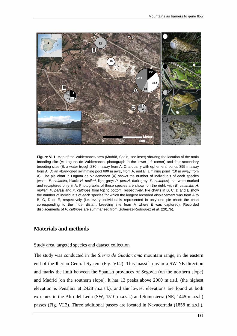
Mountains as barriers to gene flow
185
Materials and methods
Study area, targeted species and dataset collection
The study was conducted in the Sierra de Guadarrama mountain range, in the eastern
end of the Iberian Central System (Fig. VI.2). This massif runs in a SW-NE direction
and marks the limit between the Spanish provinces of Segovia (on the northern slope)
and Madrid (on the southern slope). It has 13 peaks above 2000 m.a.s.l. (the highest
elevation is Peñalara at 2428 m.a.s.l.), and the lowest elevations are found at both
extremes in the Alto del León (SW, 1510 m.a.s.l.) and Somosierra (NE, 1445 m.a.s.l.)
passes (Fig. VI.2). Three additional passes are located in Navacerrada (1858 m.a.s.l.),
Figure VI.1. Map of the Valdemanco area (Madrid, Spain, see inset) showing the location of the main
breeding site (A: Laguna de Valdemanco, photograph in the lower left corner) and four secondary
breeding sites (B: a water trough 230 m away from A, C: a quarry with ephemeral ponds 395 m away
from A, D: an abandoned swimming pool 680 m away from A, and E: a mining pond 710 m away from
A). The pie chart in Laguna de Valdemanco (A) shows the number of individuals of each species
(white: E. calamita, black: H. molleri, light grey: P. perezi, dark grey: P. cultripes) that were marked
and recaptured only in A. Photographs of these species are shown on the right, with E. calamita, H.
molleri, P. perezi and P. cultripes from top to bottom, respectively. Pie charts in B, C, D and E show
the number of individuals of each species for which the longest recorded displacement was from A to
B, C, D or E, respectively (i.e. every individual is represented in only one pie chart: the chart
corresponding to the most distant breeding site from A where it was captured). Recorded
displacements of P. cultripes are summarized from Gutiérrez-Rodríguez et al. (2017b).
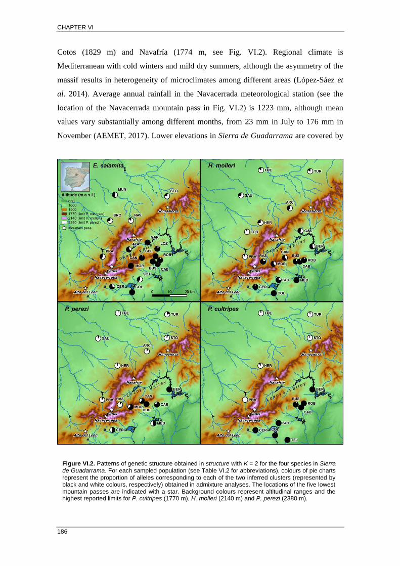
CHAPTER VI
186
Cotos (1829 m) and Navafría (1774 m, see Fig. VI.2). Regional climate is
Mediterranean with cold winters and mild dry summers, although the asymmetry of the
massif results in heterogeneity of microclimates among different areas (López-Sáez et
al. 2014). Average annual rainfall in the Navacerrada meteorological station (see the
location of the Navacerrada mountain pass in Fig. VI.2) is 1223 mm, although mean
values vary substantially among different months, from 23 mm in July to 176 mm in
November (AEMET, 2017). Lower elevations in Sierra de Guadarrama are covered by
Figure VI.2. Patterns of genetic structure obtained in structure with K = 2 for the four species in Sierra de Guadarrama. For each sampled population (see Table VI.2 for abbreviations), colours of pie charts represent the proportion of alleles corresponding to each of the two inferred clusters (represented by black and white colours, respectively) obtained in admixture analyses. The locations of the five lowest mountain passes are indicated with a star. Background colours represent altitudinal ranges and the highest reported limits for P. cultripes (1770 m), H. molleri (2140 m) and P. perezi (2380 m).
Mountains as barriers to gene flow
187
forests of oak trees (Quercus ilex subsp. ballota, Q. pyrenaica) and pines (Pinus
sylvestris, P. nigra). Above 1600 m.a.s.l. the landscape is dominated by shrubs, and
alpine grasslands and meadows occupy the highest altitudes (López-Sáez et al. 2014).
Table VI.2. List of sampled localities for each species (Ecal: E. calamita, Hmol: H. molleri, Pper: P. perezi
and Pcul: P. cultripes), with their abbreviations (Abr), geographic coordinates (Coord), elevation in m.a.s.l.
(Elev), and the number of tadpole tissue samples obtained in each locality (Sample size). Further
information about the E. calamita, H. molleri and P. perezi samples can be found in Sánchez-Montes et al.
(2017).
Locality Abr Coord Elev Sample size
Ecal Hmol Pper Pcul
Alameda del Valle ALA 40.91º N 3.85º W 1104 - 24 - -
Arcones ARC 41.13º N 3.73º W 1142 30 - 19 -
Arroyo Tejada TEJ 40.67º N 3.74º W 850 - - - 30
Berrocal BRC 41.06º N 3.98º W 1098 - 30 - -
Bustarviejo BUS 40.85º N 3.68º W 1092 30 28 30 21
Cabanillas de la Sierra CAB 40.85º N 3.65º W 1009 22 30 20 27
Cerceda CER 40.72º N 3.96º W 1031 20 30 23 30
Collado Hermoso HER 41.05º N 3.93º W 1193 23 - 32 20
Colmenar Viejo COL 40.69º N 3.83º W 854 21 30 - 30
Dehesa de Roblellano ROB 40.86º N 3.63º W 1072 30 36 23 29
El Berrueco BER 40.93º N 3.57º W 927 21 29 20 30
Fuenterrebollo FUE 41.33º N 3.93º W 909 20 - 20 31
Gargantilla del Lozoya GAR 40.95º N 3.72º W 1074 - 30 - -
Gascones GAS 41.01º N 3.65º W 1035 21 - - -
La Pradera de Navalhorno PRA 40.88º N 4.03º W 1192 22 30 23 30
Lozoyuela LOZ 40.92º N 3.65º W 1107 - 28 - -
Medianillos MED 40.76º N 3.68º W 933 21 - 25 -
Muñoveros MUN 41.20º N 3.95º W 906 - 32 - -
Navafría NAV 41.06º N 3.83º W 1180 - 30 - -
Puerto de Canencia CAN 40.81º N 3.68º W 1477 25 28 22 -
Puerto de La Morcuera MOR 40.87º N 3.76º W 1720 30 20 22 -
Puerto del Medio Celemín CEL 40.84º N 3.83º W 1248 - 30 - -
Rascafría RAS 40.88º N 3.66º W 1516 20 - 22 -
Santo Tomé del Puerto STO 40.85º N 3.91º W 1121 - 30 21 30
Sauquillo de Cabezas SAU 41.19º N 3.59º W 911 20 - 22 -
Soto del Real SOT 41.19º N 4.06º W 936 20 30 - 30
Torrecaballeros TOR 40.76º N 3.80º W 1127 34 - - -
Turrubuelo TUR 41.00º N 4.02º W 1042 21 - 21 30
Up to 15 amphibian species can be found in Sierra de Guadarrama, although
many of them become rare above mid elevations (1000-1500 m.a.s.l., Martínez-Solano
2006). We focused our study on four anuran species that are widely distributed across
CHAPTER VI
188
both slopes of Sierra de Guadarrama: E. calamita, H. molleri, P. perezi and P.
cultripes. Populations of the four species in Sierra de Guadarrama have been reported
at maximum altitudes of 2200 m.a.s.l. for E. calamita, 2140 m for H. molleri, 2170 m
for P. perezi and 1470 m for P. cultripes (Martínez-Solano 2006). These altitudinal
limits are surpassed in other areas of the Iberian distribution range of E. calamita (up to
2500 m, García-París et al. 2004), P. perezi (up to 2380 m, Fernández-Cardenete et al.
2000) and P. cultripes (up to 1770 m, Cejudo 1990). These four species show additional
differences in life history traits with potential implications for their regional persistence
and the connectivity of their populations across high mountain ridges (Table VI.1).
Some of these traits, like a larger size, increased longevity, facultative diurnal activity,
fast larval development or high dispersal potential might be advantageous for
maintaining gene flow in alpine environmental conditions, and therefore differences in
regional genetic structure would be expected.
To obtain inferences about individual dispersive patterns, we recorded direct
observations of displacements as part of a seven-year (2010-2016) CMR monitoring
project performed in an assemblage of the four species near the locality of Valdemanco,
Madrid (see Fig. VI.1). Laguna de Valdemanco and other secondary breeding sites
nearby were surveyed on a yearly basis since 2010, with multiple CMR sessions
performed every year for each species. In each CMR session, all sexually mature
individuals found during visual encounter surveys were captured, sexed based on
morphological characters and marked with an AVID M.U.S.I.C transponder (EzID,
Greeley, Colorado, USA), supplied with an identity code readable with an AVID
Minitracker II device. During this seven-year period we performed 219 CMR sessions,
and marked 1086 adult E. calamita (427 of them were further recaptured in at least one
subsequent CMR session, with a maximum of 23 recaptures per individual), 599 H.
molleri (153 were further recaptured, up to a maximum of seven recaptures per
individual) and 662 P. perezi (325 were further recaptured, up to a maximum of 10
recaptures per individual). Dispersal events of marked adults of the three species from
Laguna de Valdemanco to nearby breeding sites were recorded from direct visual
encounters during the monitoring program (see Fig. VI.1). The minimum cumulative
distances covered by each individual were calculated by summing the distances between
consecutive recorded locations. To compute these cumulative distances we only
accounted for movements longer than the longitude of the main axis of the Laguna de

Mountains as barriers to gene flow
189
Valdemanco flooding area (i.e. 125 m). During the same seven-year period, 824 adult P.
cultripes were marked in the study area (440 were further recaptured, up to a maximum
of 17 recaptures per individual); recorded displacements were reported in Gutiérrez-
Rodríguez et al. (2017b).
We used larval genotypes of the four species (15-18 microsatellite loci per
species, n = 19-36 individuals per population) from 13-19 populations per species
across both slopes of Sierra de Guadarrama (Table VI.2, Fig. VI.2). Genotypes of E.
calamita, H. molleri and P. perezi were obtained from the dataset published in Sánchez-
Montes et al. (2017). From that dataset we excluded sample localities containing less
than six non-full sib individuals to avoid unreliable inferences derived from few full sib
families in some genetic samples (Anderson & Dunham 2008; Rodríguez-Ramilo &
Wang 2012; Sánchez-Montes et al. 2017). We also excluded Laguna de Valdemanco
from the dataset because tissue sampling in that locality was more exhaustive than in the
remaining populations to address different research questions (Sánchez-Montes et al.
2017). Additionally, we obtained larval samples of P. cultripes in 13 localities across
the study area (total n = 368, between 20 and 31 individuals per population, see Table
VI.2 and Fig. VI.2) following the survey method described in Sánchez-Montes et al.
(2017). We used 16 published microsatellite loci (Gutiérrez-Rodríguez & Martínez-
Solano 2013) to genotype the samples of P. cultripes following the laboratory and allele
calling procedures described in Sánchez-Montes et al. (2016).
Genetic analyses
Pairwise population genetic distances and tests of IBD
We used the G-statistics subroutine in GENALEX (Peakall & Smouse 2006) to estimate
FST values (Wright 1943, 1951) between all pairs of populations in each species and
performed 9999 permutations to assess the significance of each value after applying the
Bonferroni correction for multiple tests as 0.05/n, where n is the number of pairwise
comparisons in each species. Since individual genotype data in each population were
obtained from single cohort tadpoles, we assessed the possible effect caused by an
excess of full sibs in the samples by recalculating FST estimates after identifying and
removing all but one member of each inferred full sib family using COLONY (Jones &
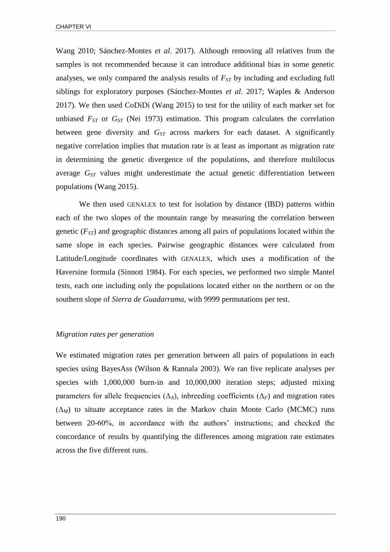
CHAPTER VI
190
Wang 2010; Sánchez-Montes et al. 2017). Although removing all relatives from the
samples is not recommended because it can introduce additional bias in some genetic
analyses, we only compared the analysis results of FST by including and excluding full
siblings for exploratory purposes (Sánchez-Montes et al. 2017; Waples & Anderson
2017). We then used CoDiDi (Wang 2015) to test for the utility of each marker set for
unbiased FST or GST (Nei 1973) estimation. This program calculates the correlation
between gene diversity and GST across markers for each dataset. A significantly
negative correlation implies that mutation rate is at least as important as migration rate
in determining the genetic divergence of the populations, and therefore multilocus
average GST values might underestimate the actual genetic differentiation between
populations (Wang 2015).
We then used GENALEX to test for isolation by distance (IBD) patterns within
each of the two slopes of the mountain range by measuring the correlation between
genetic (FST) and geographic distances among all pairs of populations located within the
same slope in each species. Pairwise geographic distances were calculated from
Latitude/Longitude coordinates with GENALEX, which uses a modification of the
Haversine formula (Sinnott 1984). For each species, we performed two simple Mantel
tests, each one including only the populations located either on the northern or on the
southern slope of Sierra de Guadarrama, with 9999 permutations per test.
Migration rates per generation
We estimated migration rates per generation between all pairs of populations in each
species using BayesAss (Wilson & Rannala 2003). We ran five replicate analyses per
species with 1,000,000 burn-in and 10,000,000 iteration steps; adjusted mixing
parameters for allele frequencies (ΔA), inbreeding coefficients (ΔF) and migration rates
(ΔM) to situate acceptance rates in the Markov chain Monte Carlo (MCMC) runs
between 20-60%, in accordance with the authors’ instructions; and checked the
concordance of results by quantifying the differences among migration rate estimates
across the five different runs.
Mountains as barriers to gene flow
191
Clustering analyses
We employed three different clustering analyses to characterize the genetic structure of
the four species in Sierra de Guadarrama. For each method, we implemented two
different approaches with the aim of a) finding the number of clusters (K) best
explaining the variation in the data and b) focusing on K = 2 to assess the membership
probabilities of each individual (or population) to each of the two main inferred clusters.
First, we performed unsupervised Bayesian clustering analyses in structure
(Pritchard et al. 2000). We explored the maximum likelihood configurations for each
value of K, from one to the total number of sampled localities in each species. For each
K value we performed ten replicates using an admixture model with correlated allele
frequencies and 500,000 burn-in and 1,000,000 iteration steps (Pritchard et al. 2000;
Falush et al. 2003). We summarized clustering results using CLUMPAK (Kopelman et al.
2015) and explored the likelihood of different K values using the original (based on
likelihood scores, Pritchard et al. 2000) and the ΔK (‘Evanno’) methods (Evanno et al.
2005) in STRUCTURE HARVESTER (Earl & vonHoldt 2012). Second, we performed
discriminant analysis of principal components (DAPC, Jombart et al. 2010) using the R
package adegenet (Jombart 2008; R Development Core Team 2009). We selected the
minimum number of principal components required to account for at least 90% of the
variation contained in the data, explored the best value of K between one and 25 (thus
encompassing the total number of populations in each species) and computed individual
membership probabilities to each of the inferred clusters. Third, we used GENELAND
(Guillot et al. 2005) to perform spatially explicit clustering analyses. As in DAPC
analyses, we explored the best value of K between one and 25 to encompass the total
number of populations of each species. Then, we performed ten different runs for each
species with K = 2, each run implementing a correlated allele frequency model with
100000 iterations, a thinning of 100, and an uncertainty of 0.01 in spatial locations to
avoid individuals sampled in the same population being invariably assigned to the same
cluster altogether.
Landscape genetic analyses
We also employed a landscape genetics-based causal modeling approach (Cushman et
al. 2006, 2013) to test for the barrier effect of Sierra de Guadarrama, while also

CHAPTER VI
192
accounting for the roles of elevation and geographical distances on observed genetic
distances among populations. Causal modeling is based on a set of partial Mantel tests
aimed to assess the relative support for different candidate models explaining observed
genetic distances. The set of candidate models typically includes measures based on
Euclidean distances, the absolute barrier effect of a landscape feature and one or more
resistance surfaces assigning different resistance values to the landscape patches in the
area of study. The true model is expected to show significant correlation between the
relevant measure (distance, barrier or resistance) and observed genetic distances after
partialling out the effect of alternative measures, while the correlation of these
alternative measures with genetic distances after partialling out the effect of the true
relevant measure should not be significant (see Cushman et al. 2006, 2013). To
construct our elevation-based resistance measures, we first obtained a digital elevation
model of Sierra de Guadarrama with 200 metres of resolution from the Centro
Nacional de Información Geográfica (Instituto Geográfico Nacional, Ministerio de
Fomento, Gobierno de España, http://centrodedescargas.cnig.es/CentroDescargas/). We
then constructed four different resistance surfaces, all of them assuming a linear
relationship between elevation and resistance (resistance = elevation), but with this
linear effect starting at different minimum altitude thresholds (0, 1000, 1500 and 2000
m.a.s.l.), with elevations below that threshold having a resistance value equal to the
threshold. We used the R package POPGENREPORT (Adamack & Gruber 2014) to
calculate the least cost paths between all pairs of populations in each species with each
of the four pre-defined elevation-based resistance models using an eight-pixel nearest-
neighbour approach, and to construct the matrices of genetic (based on Nei’s GST) and
Euclidean distances. The resistance matrix for the barrier effect was constructed by
assigning a resistance value of ‘0’ to all pairwise comparisons involving populations
located on the same slope, and ‘1’ to all comparisons between populations located on
opposite slopes. Finally, we used the R package ECODIST (Goslee & Urban 2007) to
implement partial Mantel tests to assess the relative support for each model.
Mountains as barriers to gene flow
193
Results
Dispersal potential
In our seven-year CMR monitoring study, long cumulative movements were recorded in
some individuals of E. calamita (Fig. VI.3), but only two marked males were found in a
breeding site more than 400 metres away from Laguna de Valdemanco (see Fig. VI.1).
However, these two individuals moved at least two and five times, respectively,
between Laguna de Valdemanco and a mining pond located more than 700 metres away
during the seven-year period. These two and one additional male summed each one a
cumulative distance of more than 1420 m (up to a maximum of 3550 m), highlighting
the high dispersal capacity of this species (Fig. VI.3). We found several marked
individuals of H. molleri and P. perezi in different breeding sites more than 600 metres
away from Laguna de Valdemanco and not connected by aquatic corridors (see Fig.
VI.1), either in the same season or among different years. One male of H. molleri
moved at least four times between Laguna de Valdemanco and the mining pond in three
years, for a cumulative distance of 2840 m (Fig. VI.3). Several medium- and long-
distance displacements (between 680 and 1510 m) were also recorded in both males and
females of P. perezi (Fig. VI.3). Gutiérrez-Rodríguez et al. (2017b) reported eight
displacements of P. cultripes from Laguna de Valdemanco to nearby breeding sites, five
of them covering a distance of more than 700 metres (710 m, see Table VI.1 and Figs.
VI.1 and VI.3).
Genetic analyses
Pairwise population genetic distances and tests of IBD
We did not find any negative correlation between gene diversity and GST in any of the
four marker sets (results not shown), which supports the reliability of multilocus FST and
GST estimates in the four species. Therefore, FST values were averaged among all loci in
each species to estimate pairwise genetic distances between populations (Wang 2012,
2015). Additionally, FST estimates were not affected by the presence of full sibs in the
P. perezi samples, and only slight over- (in E. calamita and P. cultripes) or
underestimations (in H. molleri) were detected in the other species (see Appendix 9).
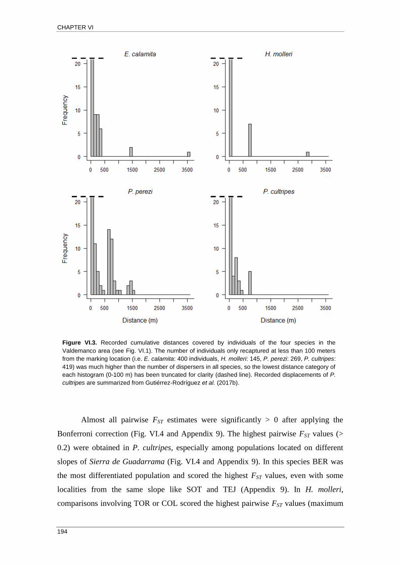
CHAPTER VI
194
Almost all pairwise FST estimates were significantly > 0 after applying the
Bonferroni correction (Fig. VI.4 and Appendix 9). The highest pairwise FST values (>
0.2) were obtained in P. cultripes, especially among populations located on different
slopes of Sierra de Guadarrama (Fig. VI.4 and Appendix 9). In this species BER was
the most differentiated population and scored the highest FST values, even with some
localities from the same slope like SOT and TEJ (Appendix 9). In H. molleri,
comparisons involving TOR or COL scored the highest pairwise FST values (maximum
Figure VI.3. Recorded cumulative distances covered by individuals of the four species in the
Valdemanco area (see Fig. VI.1). The number of individuals only recaptured at less than 100 meters
from the marking location (i.e. E. calamita: 400 individuals, H. molleri: 145, P. perezi: 269, P. cultripes:
419) was much higher than the number of dispersers in all species, so the lowest distance category of
each histogram (0-100 m) has been truncated for clarity (dashed line). Recorded displacements of P.
cultripes are summarized from Gutiérrez-Rodríguez et al. (2017b).

Mountains as barriers to gene flow
195
FST was 0.147), whereas in P. perezi the localities involving higher FST comparisons
with the remaining populations were BER and ARC (maximum FST = 0.142). The
maximum FST value in E. calamita was 0.082, and COL was the most differentiated
population (Appendix 9).
We found significant evidence of IBD within the northern slope (Segovia) in P.
cultripes (R = 0.762, p = 0.020), while E. calamita and H. molleri did not show
evidences of IBD (E. calamita: R = -0.056, p = 0.525; H. molleri: R = -0.302, p =
Figure VI.4. Relation between genetic (FST) and geographic distances among all pairs of populations
located on the southern (dark circles) or the northern slope (white circles) of Sierra de Guadarrama.
Pairwise distances involving CER and the remaining populations in the southern slope are
represented by black triangles.
CHAPTER VI
196
0.166) and P. perezi showed a significant negative relationship between genetic and
geographic distances (R = -0.403, p = 0.025). In the southern slope (Madrid) none of the
four species showed evidences of IBD (E. calamita: R = 0.323, p = 0.094; H. molleri: R
= 0.271, p = 0.088; P. perezi: R = 0.239, p = 0.234; P. cultripes: R = 0.347, p = 0.098),
although removing the extreme southwestern population of CER from the analyses
revealed significant IBD patterns in three of them (E. calamita: R = 0.593, p = 0.001; H.
molleri: R = 0.339, p = 0.044; P. perezi: R = 0.411, p = 0.131; P. cultripes: R = 0.407, p
= 0.018, see Fig. VI.4).
Migration rates per generation
Estimated migration rates per generation were concordant across the five replicate runs
in the four species. Mean (and maximum) differences in the estimated non-migrant
proportion of each population across the five replicates were 0.031 (0.156) in E.
calamita, 0.030 (0.133) in H. molleri, 0.012 (0.100) in P. perezi, and 0.047 (0.225) in P.
cultripes. Average pairwise migration rates were low in all species (~0.01) except
among populations located on the same slope in P. cultripes (mean = 0.03, see
Appendix 9). This high intra-slope average rate in P. cultripes was driven by some
widely connected populations both in the northern (FUE, STO and TUR) and in the
southern (CAB with COL, TEJ and ROB) slopes (see Appendix 9). Migration rates
dropped sharply beyond short geographic distances (c. 10 km) in P. perezi and,
especially, in E. calamita. In contrast, H. molleri and P. cultripes still maintained
migration rates close to 0.2 between some populations up to 40 km away, although these
high rates were only found among populations located within the same slope of Sierra
de Guadarrama (Fig. VI.5 and Appendix 9).
Clustering analyses
Unsupervised Bayesian clustering analyses in structure yielded increasing likelihood
values in models with increasing number of clusters (K), although tending to
stabilization at large K values (see Appendix 10). The ΔK method yielded K = 2 as the
optimal partition for E. calamita, P. perezi and P. cultripes (Fig. A10.1 in Appendix
10). Two clearly differentiated clusters, with little to no genetic admixture, were

Mountains as barriers to gene flow
197
recovered in P. cultripes, each located at either slope of Sierra de Guadarrama (Fig.
VI.2 and Appendix 10). In E. calamita, H. molleri and P. perezi, northern and southern
clusters separated by Sierra de Guadarrama were also recovered at K = 2, with admixed
populations near mountain passes (Fig. VI.2 and Appendix 10). In E. calamita, the
northern cluster was composed by all populations in the northern slope of Sierra de
Guadarrama, with admixed populations including SOT and CER (in the southwest) and
ALA (in the Lozoya Valley). The northern populations of MUN, BRC and PRA also
showed high admixture with the southern cluster (Fig. VI.2 and Appendix 10). In H.
molleri, almost every population clustered with the localities of its respective slope
Figure VI.5. Estimated migration rates as a function of geographic distance between populations
located in the same (dark circles) or on different slopes (white circles) of Sierra de Guadarrama.

CHAPTER VI
198
when K was set to two, although widely admixed populations were also found,
especially near the mountain passes of Somosierra, Cotos and Navacerrada (Fig. VI.2
and Appendix 10). The optimum partition in this species was K = 3, which resulted in
TOR and PRA clustering together differentially within the northern cluster. The
remaining populations received almost the same clustering assignation as with K = 2. In
P. perezi, the inferred northern cluster included all localities in the northern slope along
with RAS in the Lozoya Valley. The southern populations of CER, MED, MOR and
CAN also showed high admixture with the northern cluster (Fig. VI.2 and Appendix
10). Further partitions with K = 3 to 5 showed hierarchical structure in the four species
caused by differentiated populations within each slope of Sierra de Guadarrama, but
with little additional admixture across opposite slopes (Appendix 10).
Table VI.3. Results of the landscape genetic causal modeling approach. Partial Mantel tests evaluate the
effects of four different elevation-based resistance surfaces (Elev, Elev1000, Elev1500 and Elev2000, with
the linear relationship between elevation and resistance starting at 0, 1000, 1500 and 2000 m.a.s.l.,
respectively), a barrier effect (Bar) and Euclidean distances (Eucl) on observed genetic distances (Gen).
Models are named after the dependent variable (Gen) ~ the tested effect | and the partialled out
covariable. Significant results at the 0.05 level are marked in bold.
Model E. calamita H. molleri P. perezi P. cultripes
R p R p R p R p
Gen~Bar | Eucl 0.086 0.242 0.207 0.017 0.125 0.081 0.471 <0.001
Gen~Eucl | Bar 0.169 0.169 0.025 0.419 -0.076 0.653 -0.031 0.552
Gen~Elev | Eucl 0.131 0.229 0.281 0.026 -0.026 0.568 0.209 0.118
Gen~Elev | Bar 0.188 0.116 0.069 0.308 -0.109 0.738 -0.079 0.680
Gen~Eucl | Elev -0.060 0.623 -0.232 0.923 0.022 0.449 -0.131 0.786
Gen~Bar | Elev 0.030 0.404 0.145 0.059 0.147 0.060 0.452 0.001
Gen~Elev1000 | Eucl 0.181 0.141 0.317 0.011 -0.041 0.604 0.218 0.105
Gen~Elev1000 | Bar 0.201 0.100 0.075 0.296 -0.110 0.747 -0.069 0.654
Gen~Eucl | Elev1000 -0.119 0.738 -0.275 0.961 0.037 0.420 -0.150 0.817
Gen~Bar | Elev1000 0.026 0.420 0.146 0.064 0.147 0.065 0.452 0.001
Gen~Elev1500 | Eucl 0.250 0.002 0.175 0.038 -0.029 0.595 0.062 0.330
Gen~Elev1500 | Bar 0.187 0.146 0.033 0.392 -0.083 0.670 -0.044 0.577
Gen~Eucl | Elev1500 -0.231 0.995 -0.162 0.942 0.028 0.415 -0.039 0.609
Gen~Bar | Elev1500 0.067 0.300 0.197 0.022 0.130 0.085 0.470 0.001
Gen~Elev2000 | Eucl 0.120 0.158 -0.010 0.541 0.045 0.339 -0.020 0.556
Gen~Elev2000 | Bar 0.179 0.153 0.021 0.431 -0.075 0.641 -0.039 0.562
Gen~Eucl | Elev 2000 -0.098 0.785 0.024 0.400 -0.046 0.657 0.043 0.371
Gen~Bar | Elev2000 0.078 0.275 0.208 0.018 0.125 0.090 0.473 0.001
Mountains as barriers to gene flow
199
Best K values obtained in DAPC analyses were > 2 for all species, suggesting
strong genetic structure in the four species. The best K value was between four and
seven in E. calamita, K = 8 in H. molleri, between 7-8 in P. perezi and between 10-11 in
P. cultripes (results not shown). These high K values were more in agreement with the
original likelihood-based method in structure than with the ΔK method (see Fig. A10.1
in Appendix 10). Individual admixture results for K = 2 to 5 with DAPC were similar to
those obtained with structure in P. perezi and P. cultripes (see Appendix 10). In
contrast, the strong genetic differentiation of PRA and TOR drove the main clustering
partitions in H. molleri, and no strong structure was observed in E. calamita (Appendix
10).
Best K values obtained with GENELAND were largely concordant with the total
number of populations in each species (results not shown). These high K values were
again consistent with strong genetic structure, as in DAPC analyses and the original
method in structure. Results with K = 2 showed wide variation among different runs for
E. calamita, H. molleri and P. perezi, as shown in Fig. A10.10 in Appendix 10. While
the northern and southern clusters were clearly and consistently discriminated at K = 2
in the case of P. cultripes, results are more variable and inconsistent in the other three
species (Fig. A10.10 in Appendix 10).
Landscape genetic analyses
The landscape-based causal modeling approach revealed a strong effect of Sierra de
Guadarrama as a barrier to gene flow for P. cultripes, since the barrier effect showed
highly significant correlations with genetic distances after partialling out the remaining
candidate measures, while none of the remaining models showed significant support
(Table VI.3). The sets of partial Mantel tests suggested a potential role of elevation on
the genetic structure of E. calamita and H. molleri, although this effect was not fully
supported based on the expectations of causal modeling. In H. molleri, three of the four
resistance surfaces (with resistance = elevation starting at 0, 1000 and 1500 m.a.s.l.,
respectively) yielded significant relationships between genetic and resistance-based
least cost distances after partialling out the effect of Euclidean distances, but not after
partialling out the effect of the barrier (Table VI.3). Furthermore, the barrier effect
showed significant correlation with genetic distances after partialling out the effect of

CHAPTER VI
200
Euclidean distances and also after partialling out the resistance surfaces with the two
highest thresholds (i. e., 1500 and 2000 m.a.s.l., see Table VI.3). In E. calamita, on the
other hand, only the surface in which the linear effect of elevation started at 1500 m of
elevation was significantly supported after partialling out the effect of Euclidean
distances, but not after partialling out the barrier effect. None of the models tested in P.
perezi showed significant results (Table VI.3).
Discussion
Our results show that the effect of mountains in shaping regional patterns of genetic
structure can be quite different even in species that are commonly found in syntopy, like
our four study species, which often form breeding assemblages wherever their ranges
overlap in the Iberian Peninsula (Álvarez & Salvador 1984; Salvador & Carrascal
1990). These differences can be related to historical, intrinsic (life history traits), and/or
extrinsic factors (Wang et al. 2013); comparative studies can provide valuable insights
on their relative importance and illuminate the process of community assemblage.
Mountain systems act as long-term barriers to gene flow; however, their permeability as
barriers can be dynamic through time. Even with essentially the same topography, the
barrier effect of a mountain system may change dramatically from interglacial to glacial
periods (Pereira et al. 2016). Our results indicate that Sierra de Guadarrama is acting as
a current barrier to gene flow for P. cultripes and, to a lesser extent, for E. calamita, H.
molleri and P. perezi. If this effect is significant in the present interglacial period, it is
safe to assume that it was probably stronger during the Pleistocene, when glaciers
covered large areas in Sierra de Guadarrama (Domínguez-Villar et al. 2013). This
long-term effect could explain the phylogeographic breaks found in P. cultripes
(Gutiérrez-Rodríguez et al. 2017a) and H. molleri (Sánchez-Montes & Martínez-Solano,
unpublished data), two species showing a clear north-south subdivision in the Iberian
Peninsula and meeting at the Central System mountains.
All genetic approaches provided evidences of the current effect of Sierra de
Guadarrama as a barrier to gene flow, but the four species showed different patterns of
connectivity across the mountain ridge. Some of these differences can be explained in
terms of variation in some key life history traits, particularly dispersal potential, with
the less vagile species (Pelobates cultripes) showing the most pronounced genetic

Mountains as barriers to gene flow
201
break. Pelobates cultripes is a strictly nocturnal species with a long larval period, and it
shows the narrowest altitudinal range among the study species (Table VI.1). This may
reflect physiological constraints, although other factors, like their dependence on soils
adequate for their fossorial habits cannot be ruled out. Altogether, these traits could
favour a more pronounced phylopatric behaviour in this species, restricting regional
connectivity.
In contrast, we obtained high migration rates per generation at larger geographic
distances (up to 40 km) in P. cultripes, although only among populations located on the
same slope of Sierra de Guadarrama (Fig. VI.5 and Appendix 9). Although some
migration rate estimates could be imprecise due to the high number of populations
analyzed and the relatively low sample sizes, the estimated non-migrant fraction never
switched between the bounds of the prior distribution in none of the analyses, thus
supporting the reliability of our inferences (see Meirmans 2014). These high inferred
migration rates per generation might result from a very low number of migrants per year
in long-lived species, like P. cultripes, which can live up to 12 years in this area
(Talavera 1990, see Table VI.1). In this scenario, rare long dispersal events can easily
pass unnoticed for CMR studies using passive integrated transponder (PIT) tags, like in
our case, because typically large areas cannot be uniformly monitored. In any case, the
strong barrier effect exerted by Sierra de Guadarrama is well supported based on the
high overall population differentiation (Appendix 9) as well as the consistency of results
of the clustering and causal modeling approaches (Table VI.3, Fig. VI.2 and Appendix
10). The barrier effect may explain the absence or rarity of this species at higher (>
1500 m.a.s.l.) elevations (Cejudo 1990) and the strong phylogeographic signal
associated to the Central System (Gutiérrez-Rodríguez et al. 2017a). In fact, mountain
passes in Sierra de Guadarrama are above the higher reported altitudes for this species
except for both extremes (Somosierra and Alto del León, Fig. VI.2). Connectivity of
northern and southern clusters seems only possible through these two passes in
principle, although we did not detect admixed populations (Fig. VI.2).
We also found high migration rates per generation among some distant
populations in H. molleri, although only within the southern slope (Fig. VI.5 and
Appendix 9), probably due to the fragmented distribution of this species in the northern
slope of Sierra de Guadarrama (Márquez 2002), which was also reflected in the high
differentiation of the PRA and TOR populations (Appendix 10). The taxonomy of the
CHAPTER VI
202
Hyla arborea species group was recently revised, resulting in the recognition of the
Iberian H. molleri as a separate taxon at the species level (Stöck et al. 2008, 2012; Barth
et al. 2011; Gvozdík et al. 2015). Several important knowledge gaps about the life
history of this species remain to be filled (see Table VI.1). In this respect, dispersal
distances reported in this study represent the first direct records of medium-distance
dispersal for H. molleri (also for P. perezi) across a terrestrial landscape matrix. It
should be noted that, although reported movements involved adult individuals
displacing between breeding sites and thus potentially implying actual gene flow, we
could not verify that marked individuals bred at both sites, and therefore it is not
possible to properly distinguish between migration and dispersal movements. In any
case, our direct observations of recorded movements revealed the high dispersal
potential of H. molleri (Figs. VI.1 and VI.3), which probably favors regional population
connectivity (Fig. VI.4 and Appendix 9), and the colonization of highlands (more than
2100 m.a.s.l., see Table VI.1). However, our causal modeling analyses suggest a
potential role of elevation (and also of the mountain as a barrier) on the genetic
distances observed in our study area, implying that topography may to some extent
restrict across-slope gene flow in H. molleri (Table VI.3). These results are in
agreement with a role of Sierra de Guadarrama as a semi-permeable barrier to gene
flow in this species, as also suggested by the wide connected areas identified among the
two major (northern and southern) clusters obtained in clustering analyses (Fig. VI.2
and Appendix 10).
A similar scenario of Sierra de Guadarrama as a semi-permeable barrier to gene
flow was inferred for E. calamita and P. perezi. These two species showed high overall
connectivity across the study area (especially E. calamita, see Appendix 9) despite low
inferred migration rates per generation (Appendix 9), and also showed the widest
altitudinal range among the study species (Table VI.1). The high regional connectivity
observed in E. calamita and P. perezi is in line with the high inferred dispersal potential
of both species, based on CMR data (see Table VI.1 and Figs. VI.1 and VI.3). In
addition, two life history traits related to breeding site selection may contribute to
regional connectivity in the two species. On the one hand, E. calamita usually selects
ephemeral ponds for breeding, where competence is low because of the high mortality
risk associated with early drying but they perform well due to their extremely fast larval
development (by far the shortest among the four species, Table VI.1). This trait allows

Mountains as barriers to gene flow
203
E. calamita to successfully exploit extremely small and shallow (but also widely
available, even above the treeline at high altitudes) breeding sites, which represents an
advantage to colonize new areas and probably contributes to maintain high levels of
population connectivity. On the other hand, tadpoles of P. perezi require longer
hydroperiod ponds to complete their development (Table VI.1), but this species uses a
wide variety of breeding sites including streams, natural or artificial ponds, water
troughs and urban, degraded, salty or polluted areas (Egea-Serrano 2014). This
ecological breadth probably represents an advantage, allowing this species to maintain
high regional connectivity.
Overall, the good support for high K values in structure (based on the original
method, Appendix 10) and also in DAPC and GENELAND analyses indicate that the four
species also show different hierarchical levels of genetic substructure at finer spatial
scales (within slopes, Appendix 10). Future studies applying causal modeling
approaches on a broader range of resistance surfaces will yield further insights about the
role of other factors (vegetation cover and heterogeneity, land use/cover) in shaping
amphibian population connectivity at the landscape scale. Our integrative approach
combining field-based and molecular approaches to estimate population connectivity in
four co-distributed anurans allowed us to explicitly test for the first time the role of
Sierra de Guadarrama as a barrier to gene flow. Our results show that these mountains
have played a major role in disrupting historical and current connectivity across
populations on different slopes, but differently so depending on life history traits such as
breeding strategy and dispersal capacity. The mountains act as a full isolating barrier in
one species (P. cultripes), but they are semi-permeable in E. calamita, H. molleri and P.
perezi, with potential corridors located near mountain passes. These results highlight the
major role of the Central System Mountains as a key feature shaping historical patterns
of population connectivity across taxa, promoting population divergence and the
evolution and accumulation of endemicity.
Acknowledgements
We thank P. Gómez, M. Peñalver, L. San José, J. Gutiérrez, E. Iranzo, L. Carrera, C. Valero, M.
Rojo, G. Rodríguez, J. Agüera, A. Sabalza, N. Escribano, R. Goñi, R. Santiso and I. Miqueleiz
for help during fieldwork and J.W. Arntzen, Krystal Tolley and three anonymous reviewers for
useful suggestions to improve the manuscript. G. Sánchez-Montes was funded by a predoctoral
grant provided by the Asociación de Amigos de la Universidad de Navarra and benefited from

CHAPTER VI
204
funding from the Programa de ayudas de movilidad de la Asociación de Amigos de la
Universidad de Navarra. This research was funded by grants CGL2008-04271-C02-01/BOS,
and CGL2011-28300 (Ministerio de Ciencia e Innovación -MICINN-), Ministerio de Economía
y Competitividad -MEC-, Spain, and FEDER) to IMS, who is currently supported by funding
from the Spanish Severo Ochoa Program (SEV-2012-0262).
Data accessibility
The dryad archive (doi: TBO*) contains new microsatellite genotype data of P. cultripes.
* Provisional repository available at: https://goo.gl/6n3pcu
Mountains as barriers to gene flow
205
References
Abellán P, Svenning J-C (2014) Refugia within refugia – patterns in endemism and genetic
divergence are linked to Late Quaternary climate stability in the Iberian Peninsula.
Biological Journal of the Linnean Society, 113, 13–28.
Adamack AT, Gruber B (2014) POPGENREPORT: simplifying basic population genetic analyses
in R. Methods in Ecology and Evolution, 5, 384–387.
AEMET (2017) AEMET (Agencia Estatal de Meteorología). Madrid: AEMET. Servicios
climáticos. Datos climatológicos. Valores climatológicos. Available at:
http://www.aemet.es/es/serviciosclimaticos/datosclimatologicos/valoresclimatologicos?l=2
462&k=mad. Accessed 20 May 2017.
Álvarez J, Salvador A (1984) Cría de anuros en la laguna de Chozas de Arriba (León) en 1980.
Mediterránea, 7, 27–48.
Álvarez J, Salvador A, Martín J, Gutiérrez A (1990) Desarrollo larvario del sapo de espuelas
(Pelobates cultripes) en charcas temporales del NW de la Península Ibérica (Anura,
Pelobatidae). Revista Española de Herpetología, 4, 55–66.
Anderson EC, Dunham KK (2008) The influence of family groups on inferences made with the
program Structure. Molecular Ecology Resources, 8, 1219–1229.
Arntzen JW (1978) Some hypotheses on postglacial migrations of the fire-bellied toad, Bombina
bombina (Linnaeus) and the yellow-bellied toad, Bombina variegata (Linnaeus). Journal
of Biogeography, 5, 339–345.
Arntzen JW, Espregueira Themudo G (2008) Environmental parameters that determine species
geographical range limits as a matter of time and space. Journal of Biogeography, 35,
1177–1186.
Báez M, Luis R (1994) Datos sobre el desarrollo larvario de Rana perezi (Seoane, 1885)
(Anura, Ranidae) en Tenerife (Islas Canarias). Vieraea, 23, 155–164.
Banks B, Beebee TJC (1987) Spawn predation and larval growth inhibition as mechanisms for
niche separation in anurans. Oecologia, 72, 569–573.
Banks B, Beebee TJC, Denton JS (1993) Long-term management of a natterjack toad (Bufo
calamita) population in southern Britain. Amphibia-Reptilia, 14, 155–168.
Barbadillo LJ (1987) La guía de INCAFO de los anfibios y reptiles de la Península Ibérica,
Islas Baleares y Canarias. INCAFO, Madrid.
Barth A, Galán P, Donaire D et al. (2011) Mitochondrial uniformity in populations of the
treefrog Hyla molleri across the Iberian Peninsula. Amphibia-Reptilia, 32, 557–564.
Beebee TJC (1983) The natterjack toad. Oxford University Press, Oxford.
Berry O, Tocher MD, Sarre SD (2004) Can assignment tests measure dispersal? Molecular
Ecology, 13, 551–561.
Blair C, Weigel DE, Balazik M et al. (2012) A simulation-based evaluation of methods for
inferring linear barriers to gene flow. Molecular Ecology Resources, 12, 822–833.
Boomsma JJ, Arntzen JW (1985) Abundance, growth and feeding of natterjack toads (Bufo
calamita) in a 4-year-old artificial habitat. Journal of Applied Ecology, 22, 395–405.
Cejudo D (1990) Nueva altitud máxima para Pelobates cultripes. Boletín de la Asociación
Herpetológica Española, 1, 20.
Cushman SA, McKelvey KS, Hayden J, Schwartz MK (2006) Gene flow in complex
landscapes: testing multiple hypotheses with causal modeling. The American Naturalist,

CHAPTER VI
206
168, 486–499.
Cushman SA, Wasserman TN, Landguth EL, Shirk AJ (2013) Re-evaluating causal modeling
with mantel tests in landscape genetics. Diversity, 5, 51–72.
Denton JS, Beebee TJC (1993) Density-related features of natterjack toad (Bufo calamita)
populations in Britain. Journal of Zoology, 229, 105–119.
Díaz-Paniagua C (1986) Reproductive period of amphibians in the Biological Reserve of
Doñana (SW Spain). In: Studies in Herpetology (Proceedings of the Third Ordinary
General Meeting of the Societas Europaea Herpetologica) (ed Rocek Z), pp. 429–432.
Charles University, Prague.
Díaz-Paniagua C, Gómez-Rodríguez C, Portheault A, de Vries W (2005) Los anfibios de
Doñana. Organismo Autónomo Parques Nacionales, Madrid.
Díaz-Rodríguez J, Gonçalves H, Sequeira F et al. (2015) Molecular evidence for cryptic
candidate species in Iberian Pelodytes (Anura, Pelodytidae). Molecular Phylogenetics and
Evolution, 83, 224–241.
Docampo L, Milagrosa-Vega M (1988) Aplicación de un método estadístico al dimorfismo
sexual del crecimiento relativo de Rana perezi (Seoane, 1885). Cuadernos de
Investigación Biológica, 13, 53–65.
Docampo L, Milagrosa-Vega M (1991) Determinación de la edad en Rana perezi Seoane, 1885.
Aplicación al análisis del crecimiento somático de poblaciones. Doñana, Acta Vertebrata,
18, 21–38.
Domínguez-Villar D, Carrasco RM, Pedraza J et al. (2013) Early maximum extent of
paleoglaciers from Mediterranean mountains during the last glaciation. Scientific Reports,
3, 2034.
Earl DA, vonHoldt BM (2012) STRUCTURE HARVESTER: a website and program for
visualizing STRUCTURE output and implementing the Evanno method. Conservation
Genetics Resources, 4, 359–361.
Egea-Serrano A (2014) Rana común - Pelophylax perezi. In: Enciclopedia Virtual de los
Vertebrados Españoles (eds Salvador A, Martínez-Solano I). Museo Nacional de Ciencias
Naturales - CSIC, Madrid.
Emel SL, Storfer A (2012) A decade of amphibian population genetic studies: synthesis and
recommendations. Conservation Genetics, 13, 1685–1689.
Emel SL, Storfer A (2014) Landscape genetics and genetic structure of the southern torrent
salamander, Rhyacotriton variegatus. Conservation Genetics, 16, 209–221.
Esteban M, García-París M, Castanet J (1996) Use of bone histology in estimating the age of
frogs (Rana perezi) from a warm temperate climate area. Canadian Journal of Zoology,
74, 1914–1921.
Evanno G, Regnaut S, Goudet J (2005) Detecting the number of clusters of individuals using the
software STRUCTURE: a simulation study. Molecular Ecology, 14, 2611–2620.
Falush D, Stephens M, Pritchard JK (2003) Inference of population structure using multilocus
genotype data: linked loci and correlated allele frequencies. Genetics, 164, 1567–1587.
Fedy BC, Martin K, Ritland C, Young J (2008) Genetic and ecological data provide incongruent
interpretations of population structure and dispersal in naturally subdivided populations of
white-tailed ptarmigan (Lagopus leucura). Molecular Ecology, 17, 1905–1917.
Fernández-Cardenete J, Luzón-Ortega J, Pérez-Contreras J, Pleguezuelos JM, Tierno de
Figueroa J (2000) Nuevos límites altitudinales para seis especies de herpetos de la
Península Ibérica. Boletín de la Asociación Herpetológica Española, 11, 20–21.
Mountains as barriers to gene flow
207
Frei M, Csencsics D, Brodbeck S et al. (2016) Combining landscape genetics, radio-tracking
and long-term monitoring to derive management implications for natterjack toads
(Epidalea calamita) in agricultural landscapes. Journal for Nature Conservation, 32, 22–
34.
Funk WC, Blouin MS, Corn PS et al. (2005) Population structure of Columbia spotted frogs
(Rana lueteiventris) is strongly affected by the landscape. Molecular Ecology, 14, 483–
496.
García-París M, Montori A, Herrero P (2004) Amphibia, Lissamphibia. In: Fauna ibérica (eds
Ramos MA, Alba J, Bellés i Ros X, et al.). Museo Nacional de Ciencias Naturales - CSIC,
Madrid.
García C, Salvador A, Santos FJ (1987) Ecología reproductiva de una población de Hyla
arborea en una charca temporal de León (Anura: Hylidae). Revista Española de
Herpetología, 2, 33–47.
Gomez A, Lunt DH (2007) Refugia within refugia: patterns of phylogeographic concordance in
the Iberian Peninsula. In: Phylogeography of Southern European Refugia (eds Weiss S,
Ferrand N), pp. 155–188. Springer Netherlands.
Gomez-Mestre I, Tejedo M (2002) Geographic variation in asymmetric competition: a case
study with two larval anuran species. Ecology, 83, 2102–2111.
Gonçalves H, Martínez-Solano I, Pereira RJ et al. (2009) High levels of population subdivision
in a morphologically conserved Mediterranean toad (Alytes cisternasii) result from recent,
multiple refugia: evidence from mtDNA, microsatellites and nuclear genealogies.
Molecular Ecology, 18, 5143–5160.
Goslee SC, Urban DL (2007) The ecodist package for dissimilarity-based analysis of ecological
data. Journal of Statistical Software, 22, 1–19.
Guillot G, Mortier F, Estoup A (2005) GENELAND: a computer package for landscape genetics.
Molecular Ecology Notes, 5, 712–715.
Gutiérrez-Rodríguez J, Barbosa AM, Martínez-Solano I (2017a) Present and past climatic
effects on the current distribution and genetic diversity of the Iberian spadefoot toad
(Pelobates cultripes): an integrative approach. Journal of Biogeography, 44, 245–258.
Gutiérrez-Rodríguez J, Martínez-Solano I (2013) Isolation and characterization of sixteen
polymorphic microsatellite loci in the Western Spadefoot, Pelobates cultripes (Anura:
Pelobatidae) via 454 pyrosequencing. Conservation Genetics Resources, 5, 981–984.
Gutiérrez-Rodríguez J, Sánchez-Montes G, Martínez-Solano I (2017b) Effective to census
population size ratios in two Near Threatened Mediterranean amphibians: Pleurodeles
waltl and Pelobates cultripes. Conservation Genetics. doi:10.1007/s10592-017-0971-5.
Gvozdík V, Canestrelli D, García-París M et al. (2015) Speciation history and widespread
introgression in the European short-call tree frogs (Hyla arborea sensu lato, H. intermedia
and H. sarda). Molecular Phylogenetics and Evolution, 83, 143–155.
Janssens X, Fontaine MC, Michaux JR et al. (2008) Genetic pattern of the recent recovery of
European otters in southern France. Ecography, 31, 176–186.
Jombart T (2008) adegenet: a R package for the multivariate analysis of genetic markers.
Bioinformatics, 24, 1403–1405.
Jombart T, Devillard S, Balloux F (2010) Discriminant analysis of principal components: a new
method for the analysis of genetically structured populations. BMC Genetics, 11, 94.
Jones OR, Wang J (2010) COLONY: a program for parentage and sibship inference from
multilocus genotype data. Molecular Ecology Resources, 10, 551–555.
Kopelman NM, Mayzel J, Jakobsson M, Rosenberg NA, Mayrose I (2015) CLUMPAK: a

CHAPTER VI
208
program for identifying clustering modes and packaging population structure inferences
across K. Molecular Ecology Resources, 15, 1179–1191.
Landguth EL, Cushman SA, Schwartz MK et al. (2010) Quantifying the lag time to detect
barriers in landscape genetics. Molecular Ecology, 19, 4179–4191.
Leclair MH, Leclair Jr R, Gallant J (2005) Application of skeletochronology to a population of
Pelobates cultripes (Anura: Pelobatidae) from Portugal. Journal of Herpetology, 39, 199–
207.
Leskovar C, Oromi N, Sanuy D, Sinsch U (2006) Demographic life history traits of
reproductive natterjack toads (Bufo calamita) vary between northern and southern
latitudes. Amphibia-Reptilia, 27, 365–375.
Lizana M, Márquez R, Martín-Sánchez R (1994) Reproductive biology of Pelobates cultripes
(Anura: Pelobatidae) in Central Spain. Journal of Herpetology, 28, 19–27.
Lizana M, Pérez-Mellado V, Ciudad MJ (1987) Biometry and relation with the ecology of Rana
iberica and Rana perezi in the Sistema Central (Spain). In: Proceedings of the 4th
Ordinary General Meeting of the Societas Europaea Herpetologica (eds van Gelder JJ,
Strijbosch H, Bergers PJM), pp. 253–258. Faculty of Sciences, Nijmegen.
López-Sáez JA, Abel-Schaad D, Pérez-Díaz S et al. (2014) Vegetation history, climate and
human impact in the Spanish Central System over the last 9000 years. Quaternary
International, 353, 98–122.
Lougheed S, Gascon C, Jones D, Bogart J, Boag P (1999) Ridges and rivers: a test of competing
hypotheses of Amazonian diversification using a dart-poison frog (Epipedobates
femoralis). Proceedings of the Royal Society B: Biological Sciences, 266, 1829–1835.
Marangoni F, Tejedo M (2007) Pelobates cultripes (Iberian spadefoot toad). Maximum size.
Herpetological Review, 38, 189–190.
Márquez R (2002) Hyla arborea. In: Atlas y Libro Rojo de los anfibios y reptiles de España (eds
Pleguezuelos JM, Márquez R, Lizana M), pp. 114–116. Dirección General de la
Conservación de la Naturaleza – Asociación Herpetológica Española, Madrid.
Márquez-M. de Orense R, Tejedo-Madueño M (1990) Size-based mating pattern in the tree frog
Hyla arborea. Herpetologica, 46, 176–182.
Márquez R, Moreira C, do Amaral JPS, Pargana JM, Crespo EG (2005) Sound pressure level of
advertisement calls of Hyla meridionalis and Hyla arborea. Amphibia-Reptilia, 26, 391–
395.
Martínez-Solano I (2006) Atlas de distribución y estado de conservación de los anfibios de la
Comunidad de Madrid. Graellsia, 62, 253–291.
Martínez-Solano I, González EG (2008) Patterns of gene flow and source-sink dynamics in high
altitude populations of the common toad Bufo bufo (Anura: Bufonidae). Biological
Journal of the Linnean Society, 95, 824–839.
Martínez-Solano I, Teixeira J, Buckley D, García-París M (2006) Mitochondrial DNA
phylogeography of Lissotriton boscai (Caudata, Salamandridae): evidence for old,
multiple refugia in an Iberian endemic. Molecular Ecology, 15, 3375–3388.
McCartney-Melstad E, Shaffer HB (2015) Amphibian molecular ecology and how it has
informed conservation. Molecular Ecology, 24, 5084–5109.
Meirmans PG (2014) Nonconvergence in Bayesian estimation of migration rates. Molecular
Ecology Resources, 14, 726–733.
Nei M (1973) Analysis of gene diversity in subdivided populations. Proceedings of the National
Academy of Sciences of the USA, 70, 3321–3323.

Mountains as barriers to gene flow
209
Oromi N, Sanuy D, Sinsch U (2012) Altitudinal variation of demographic life-history traits does
not mimic latitudinal variation in natterjack toads (Bufo calamita). Zoology, 115, 30–37.
Pagacz S (2016) The effect of a major drainage divide on the gene flow of a semiaquatic
carnivore, the Eurasian otter. Journal of Mammalogy, 97, 1164–1176.
Patón D, Juarranz A, Sequeros E et al. (1991) Seasonal age and sex structure of Rana perezi
assessed by skeletochronology. Journal of Herpetology, 25, 389–394.
Peakall R, Smouse PE (2006) GENALEX 6: genetic analysis in Excel. Population genetic
software for teaching and research. Molecular Ecology Notes, 6, 288–295.
Pereira RJ, Martínez-Solano I, Buckley D (2016) Hybridization during altitudinal range shifts:
nuclear introgression leads to extensive cyto-nuclear discordance in the fire salamander.
Molecular Ecology, 25, 1551–1565.
Pritchard J, Stephens M, Donnelly P (2000) Inference of population structure using multilocus
genotype data. Genetics, 155, 945–959.
R Development Core Team (2009) R: a language and environment for statistical computing. R
Foundation for Statistical Computing. Vienna, Austria. ISBN 3-900051-07-0, available at:
http://www.R-project.org.
Real R, Antúnez A (1991) Análisis e interpretación de las dimorfometrías en una población de
Rana perezi. Anales de Biología, 17, 63–69.
Reid BN, Thiel RP, Palsbøll PJ, Peery MZ (2016) Linking genetic kinship and demographic
analyses to characterize dispersal: methods and application to Blanding’s turtle. Journal of
Heredity, 107, 603–614.
Reino L, Ferreira M, Martínez-Solano I et al. (2017) Favourable areas for co-occurrence of
parapatric species: niche conservatism and niche divergence in Iberian tree frogs and
midwife toads. Journal of Biogeography, 44, 88–98.
Richards-Zawacki CL (2009) Effects of slope and riparian habitat connectivity on gene flow in
an endangered Panamanian frog, Atelopus varius. Diversity and Distributions, 15, 796–
806.
Richardson JL (2012) Divergent landscape effects on population connectivity in two co-
occurring amphibian species. Molecular Ecology, 21, 4437–4451.
Rodríguez-Ramilo ST, Wang J (2012) The effect of close relatives on unsupervised Bayesian
clustering algorithms in population genetic structure analysis. Molecular Ecology
Resources, 12, 873–884.
Salvador A, Álvarez J, García C (1986) Reproductive biology of a northern population of the
western spadefoot, Pelobates cultripes (Anura: Pelobatidae). In: Studies in Herpetology
(Proceedings of the Third Ordinary General Meeting of the Societas Europaea
Herpetologica) (ed Rocek Z), pp. 403–408. Charles University, Prague.
Salvador A, Carrascal LM (1990) Reproductive phenology and temporal patterns of mate access
in Mediterranean anurans. Journal of Herpetology, 24, 438–441.
Sánchez-Montes G, Ariño AH, Vizmanos JL, Wang J, Martínez-Solano I (2017) Effects of
sample size and full sibs on genetic diversity characterization: a case study of three
syntopic Iberian pond-breeding amphibians. Journal of Heredity, esx038. doi:
10.1093/jhered/esx038.
Sánchez-Montes G, Recuero E, Gutiérrez-Rodríguez J, Gomez-Mestre I, Martínez-Solano I
(2016) Species assignment in the Pelophylax ridibundus x P. perezi hybridogenetic
complex based on 16 newly characterised microsatellite markers. Herpetological Journal,
26, 99–108.
Sinnott RW (1984) Virtues of the Haversine. Sky and Telescope, 68, 159.

CHAPTER VI
210
Sinsch U, Marangoni F, Oromi N et al. (2010) Proximate mechanisms determining size
variability in natterjack toads. Journal of Zoology, 281, 272–281.
Steele CA, Baumsteiger J, Storfer A (2009) Influence of life-history variation on the genetic
structure of two sympatric salamander taxa. Molecular Ecology, 18, 1629–1639.
Stöck M, Dubey S, Klütsch C et al. (2008) Mitochondrial and nuclear phylogeny of circum-
Mediterranean tree frogs from the Hyla arborea group. Molecular Phylogenetics and
Evolution, 49, 1019–1024.
Stöck M, Dufresnes C, Litvinchuk SN et al. (2012) Cryptic diversity among Western Palearctic
tree frogs: postglacial range expansion, range limits, and secondary contacts of three
European tree frog lineages (Hyla arborea group). Molecular Phylogenetics and
Evolution, 65, 1–9.
Talavera RR (1990) Evolución de Pelobátidos y Pelodítidos (Amphibia, Anura): morfología y
desarrollo del sistema esquelético. Doctoral dissertation. Universidad Complutense de
Madrid.
Tejedo M, Reques R, Esteban M (1997) Actual and osteochronological estimated age of
natterjack toads (Bufo calamita). Herpetological Journal, 7, 81–82.
Trochet A, Moulherat S, Calvez O et al. (2014) A database of life-history traits of European
amphibians. Biodiversity Data Journal, 2, e4123.
Vörös J, Mikulíček P, Major Á, Recuero E, Arntzen JW (2016) Phylogeographic analysis
reveals northerly refugia for the riverine amphibian Triturus dobrogicus (Caudata:
Salamandridae). Biological Journal of the Linnean Society, 119, 974–991.
Wang J (2012) On the measurements of genetic differentiation among populations. Genetics
Research, 94, 275–289.
Wang J (2015) Does GST underestimate genetic differentiation from marker data? Molecular
Ecology, 24, 3546–3558.
Wang IJ, Glor RE, Losos JB (2013) Quantifying the roles of ecology and geography in spatial
genetic divergence. Ecology Letters, 16, 175–182.
Waples RS, Anderson EC (2017) Purging putative siblings from population genetic data sets: a
cautionary view. Molecular Ecology, 26, 1211–1224.
Wei X, Meng H, Jiang M (2013) Landscape genetic structure of a streamside tree species
Euptelea pleiospermum (Eupteleaceae): contrasting roles of river valley and mountain
ridge. PLoS ONE, 8, 2–9.
Wilson GA, Rannala B (2003) Bayesian inference of recent migration rates using multilocus
genotypes. Genetics, 163, 1177–1191.
Wright S (1943) Isolation by distance. Genetics, 28, 114–138.
Wright S (1951) The genetical structure of populations. Annals of Eugenics, 15, 323–354.
Zalewski A, Piertney SB, Zalewska H, Lambin X (2009) Landscape barriers reduce gene flow
in an invasive carnivore: geographical and local genetic structure of American mink in
Scotland. Molecular Ecology, 18, 1601–1615.

CHAPTER VII
GENERAL DISCUSSION

General discussion
213
This dissertation integrates genetic analyses and individual-based monitoring
approaches to obtain reliable demographic inferences regarding local effective/census
size ratio (Nb/Na, Chapter V) and regional patterns of gene flow (Chapter VI). Assessing
the reliability of estimates obtained in wild populations, in which the actual, ‘true’
values are unknown, was possible due to a suited analytic design (replicated SF analyses
for Nb estimation, multi-year robust design analyses for Na estimation and multiple
genetic approaches for gene flow characterization) combined with direct fieldwork-
based records of breeding activity and cumulative movements. Prior to these analyses,
the suitability of the new molecular tools developed and applied in this work (species-
specific microsatellites) to address demographic and taxonomic questions was explored
in Chapters III and IV. In the following paragraphs, I summarize the main findings of
this dissertation and discuss their implications for taxonomic, demographic and
conservation research.
In the last two decades, species-specific microsatellites have proven their
usefulness as versatile tools for evolutionary research, by providing valuable insights on
population dynamics and the distribution of genetic diversity in a wide variety of taxa
(Selkoe & Toonen 2006). While the current trend is to generate large datasets with
thousands of genome-wide markers, like SNPs, microsatellites still play a relevant role
due to their high polymorphism, which provides high power of resolution in a
conveniently sized dataset (Hauser et al. 2011; Hess et al. 2011). This dissertation
contributes to the global toolkit of permanent molecular resources with three sets of new
microsatellite markers specifically optimized for three pond-breeding amphibian
species: E. calamita, H. molleri and P. perezi (n = 16, 18 and 15 markers, respectively,
Chapters III and IV). The optimization of species-specific microsatellites significantly
improves the efficiency of demographic analyses by avoiding problems associated with
cross-amplification of markers from more or less distantly related taxa, like low
amplification success or the presence of null alleles. The sets described in this
dissertation are the first markers specifically designed for H. molleri and P. perezi, and
complement markers previously developed for E. calamita (Rowe et al. 1997; Rogell et
al. 2005; Faucher et al. 2016). All the loci in the three sets were polymorphic in our
regional-scale multi-population sample (17-21 localities per species, 19-96 individuals
per locality), and showed values of mean allelic richness (AR) between 1.05 (marker
Hmol3.7) and 21.14 (marker Bcal4.26, see Table IV.2). Except for the noted case of

CHAPTER VII
214
Pper4.13 and Pper4.23 (Chapter III), no consistent evidences of linkage disequilibrium
(LD) across markers were detected, and therefore they can be regarded as unlinked loci
in population studies. Six of the markers in the E. calamita set showed evidences of null
alleles in some populations (Bcal4.21, Bcal4.6, Bcal4.14, Bcal4.2, Bcal3.26 and
Bcal3.19, Tables A1.1-A1.6), and thus their effect on downstream analyses should be
accounted for (e.g. by replicating analyses with subsampled numbers of markers, see
Chapter V). Combined multi-locus polymorphism in each set of markers was sufficient
to allow individual identification and therefore the three sets proved useful for
addressing fine-scale demographic questions.
In addition to the utility of the three microsatellite sets for demographic studies,
seven of the P. perezi markers also proved useful for taxonomic assignment in the P.
ridibundus x P. perezi hybridogenetic complex (Chapter III). Molecular resources are
essential for delineating the distribution ranges of both parental species and their hybrid
taxon P. kl. grafi, because species identification based on morphological features is
problematic (Crochet et al. 1995; Rivera et al. 2011; Ferrer & Filella 2012). Up to 78
private alleles of the two parental species, distributed among the seven microsatellite
markers, were identified in the dataset analyzed in Chapter III (Fig. III.3), even though
we focused on a relatively small area and sample sizes were small (Table III.2, Fig.
III.1). Although beyond the scope of this dissertation, the combination of the new
microsatellite markers with mitonuclear sequence information allowed us to expand our
knowledge about the geographic extension of the area of hybridization along the
Llobregat river and, probably, the Llierca basin (Chapter III). Future integrative studies
applying the high-resolution genetic tools presented in this dissertation to more
comprehensive sampling designs will shed light on the origin, prevalence and
demographic consequences of hybridogenesis in Western Palearctic waterfrogs.
At the intraspecific level, demographic research has greatly benefited from the
widespread availability of molecular resources, but several practical issues compromise
their application and the reliability of inferences. One example is the problem of
assessing the representativeness of a genetic sample, which is an essential albeit often
neglected requisite to obtain reliable demographic inferences (Waples 2015). Chapter
IV focused on two of the most common sources of bias affecting sample
representativeness, and therefore, compromising the reliability of subsequent
demographic inferences: sampling an excessive proportion of relatives and determining
General discussion
215
the minimum required number of sampled individuals. Regarding the former issue, it is
in fact difficult to establish what would be an ‘appropriate’ proportion of close relatives
in the sample, because the structure of the population is frequently the object of study in
empirical demographic studies, and therefore the real proportion of relatives in the
population is usually unknown (Waples & Anderson 2017). In a recent paper based on
simulations, Waples & Anderson (2017) found that removing all but one of the full
siblings in each full sib family in the sample, as previously suggested (for instance,
Goldberg & Waits 2010) could lead to even more severely biased estimates of allelic
frequencies, population differentiation and effective population size, except when the
original samples included some large families along with unrelated individuals. They
suggested removing relatives in large families but leaving small families intact as a
general guideline, although no solution worked best for all simulated scenarios (Waples
& Anderson 2017). Furthermore, pedigree information is seldom available in empirical
studies, and relatives are usually identified in a probabilistic (and therefore prone to
error) manner. Much insight on this as yet unresolved issue has been made using
computer simulations, but the potential biases associated with sampling excessive
relatives should also be addressed in empirical datasets. This dissertation contributes to
this topic by exploring the effect of close relatives on genetic diversity characterization
in an extensive multi-population dataset.
In Chapter IV of this dissertation, I compared estimates of the basic genetic
diversity indexes commonly used in population genetics studies, both including and
excluding full siblings in samples from 17-21 populations of E. calamita, H. molleri and
P. perezi (Tables A1.4-A1.6). Estimates of both observed (HO) and expected
heterozygosity (HE) and AR remained very similar, and only FIS estimates were slightly
affected by the presence of full sibs in the sample (Table IV.2). The observed effect of
close relatives on FIS estimates was accordingly reflected in the tests for Hardy-
Weinberg equilibrium (HWE) and LD, and could be theoretically explained (Appendix
5). These results reveal that, in the absence of strongly unbalanced data structure (i.e.
when there are not very large families combined with unrelated individuals in the
sample), genetic diversity characterization is robust to the presence of close relatives in
the sample. Nevertheless, the strong differences observed in the tests of HWE and LD in
some populations call for caution when checking for departures from expected
genotypic proportions, especially in small samples (Tables IV.2 and A1.4-A1.6). On the
CHAPTER VII
216
one hand, removing an excessive number of full sibs might improve results of both tests
in some populations, therefore allowing distinction between real departures from
equilibrium and sampling artifacts (Appendix 5). On the other hand, uncertainties
regarding inferences on relatedness caused by both limited genetic information and the
lack of direct pedigree information, coupled with insufficient sample sizes after the
removal of putative siblings, could result in a poor performance of HWE and LD tests in
some cases. Unfortunately, as stated above, no general guidelines can yet be proposed to
control for the effect of excessive relatives in genetic samples from wild populations.
However, it may be a good practice to attempt sibling identification and check their
effect on the particular demographic analyses employed in each study. Pilot studies are
extremely useful in this respect, and might save time and resources in demographic
research by aiding the design of representative sampling schemes, especially by
informing about the size of the effect of close relatives in the sample and providing
insights about the minimum sample size required for accurate genetic diversity
characterization.
In fact, assessing the sufficiency of sample is essential in any statistical
procedure (Cochran 1977). In demographic studies, characterization of genetic diversity
is usually addressed by the estimation of population-level indexes, like AR and HE,
calculated from combined multi-locus genotypes, which then allow further comparison
among populations and testing different demographic hypotheses. However, these basic
indexes of genetic diversity are differently affected by sample size. While samples of
~20 individuals per population have been shown sufficient to obtain consistent
(asymptotical) estimates of HE, AR is strongly dependent on sample size (Miyamoto et
al. 2008; Pruett & Winker 2008; Hale et al. 2012). Our results confirmed this pattern,
since samples of ~20 individuals were sufficient to obtain reliable estimates of HE,
while more than 50 individuals were required for estimating AR in the particular case
study presented in this dissertation (Fig. IV.2). This difference between the two indexes
stems from the fact that HE accounts for allelic frequencies, while AR measures the
number of different allelic classes. Both indexes, in turn, are two particular cases of a
continuous profile of diversity characterization (Chao & Jost 2015, see also Figs. A3.1-
A3.3). This difference between the two genetic diversity indexes must be taken into
account when designing demographic studies, since sample size requirement will
depend on which of the two measures is used to characterize genetic diversity.

General discussion
217
Furthermore, results in Chapter IV revealed that markers with different allelic
frequencies show widely different accumulation curves with increasing sample size,
also leading to differences in the minimum sample size required to approach asymptotic
estimates (Figs. A2.1-A2.3).
As a result, in genetic-based demographic studies, the minimum required sample
size depends on the research focus, the markers employed, and the genetic structure of
the target population(s). Therefore, the sufficiency of sample for the specific
demographic analyses in each case should be carefully checked in pilot studies. Such
studies inform on the minimum sample size required or recommended for the particular
aims of the study, but also aid in the selection of markers for the composition of an
adequate or optimal marker set, by exploring the behaviour of each individual marker in
genetic diversity characterization. This approach was illustrated in Chapter IV, where a
new method for calculating minimum sample size for single-locus genetic diversity
characterization was also introduced (Figs. A2.1-A2.3). Although establishing any
threshold criterion for calculating a minimum sample size implies some degree of
arbitrariness, inspection of accumulation curves to assess the performance of each
marker in estimating each index with increasing sample size represents a revealing
exploratory approach. This procedure allows exploring the structure of the data and also
aids in marker set composition and in making decisions on sample sizes when
necessary, e.g. for demographic studies or monitoring programs.
After exploring the performance of the three marker sets and the effect of full
siblings and sample size in the multi-population datasets, two demographic studies were
addressed in Chapters V and VI. In Chapter V, we demonstrated the advantages of
integrating genetic and individual-based capture-mark-recapture (CMR) data for
estimating local-scale demographic parameters. In particular, I proposed and developed
an integrative approach to estimate the Nb/Na ratio and to assess the reliability of
estimates. As argued in Chapters I and V, this ratio measures the effective size of a
population (in terms of the contribution of adult breeders to a single-cohort offspring)
relative to the abundance of sexually mature adults in that population (Frankham 1995;
Palstra & Fraser 2012). Consequently, it provides invaluable information for the
assessment of population status, because it accounts for possible reproductive
constraints in the population that remain undetected by census estimates because of
time-lag effects. However, estimation of Nb and Na is complicated, requiring intensive

CHAPTER VII
218
field work and genetic analyses to obtain accurate estimates of both parameters (see
Chapters I and V). For that reason, until recently, few studies have reported robust
estimates of the Nb/Na ratio, and as a consequence our knowledge of the variation of the
Nb/Na ratio in natural populations (and therefore its dependence on the life history traits
of different organisms) is fragmentary (Palstra & Fraser 2012).
Fortunately, recent developments in genetic methods for Nb estimation and CMR
formulations for Na estimation provide an excellent opportunity to fill this knowledge
gap, as illustrated in Chapter V, by combining the sibship frequency (SF) method to
estimate Nb (Wang 2009) and robust design models to estimate Na (Pollock 1982;
Kendall et al. 1995). The results presented in Chapter V show that reliable Nb/Na ratios
can be estimated in seasonal-breeding species, for which these two methods are
especially suited (see also Boxes 2 and 3 in Chapter I). Assessing the reliability of Nb
estimates is straightforward provided that field-based evidences of breeding activity can
be obtained to supervise/cross-check the families reconstructed in the SF analytical
procedure. This integrative approach is especially convenient for temperate amphibians,
in which seasonal sampling can be adapted to their breeding phenology. As illustrated in
Chapter V, individual-based data gathered during the CMR sessions provided
information about the average time spent by individuals of each sex in the breeding
sites, which then contributed to interpret the polygamy levels inferred in SF analyses
(Figs. V.4 and V.6). Also, tissue samples obtained at the time of marking adult
individuals allowed creating a dataset of genotyped candidate sires and dams, which
also aided family reconstruction (Appendix 8). Finally, egg string counts provided an
estimate of the maximum number of breeding females of E. calamita, which could then
be compared to the number of breeding males and females inferred in SF analyses
(Table V.1 and Fig. V.1). Comparing this field-based information to inferred sibship
and parentage relationships is a powerful strategy to assess the reliability of inferences,
on which the estimate of Nb is based (Wang 2009). In a similar way, comparison of SF
estimates in replicated subsampled analyses using different analytic settings and levels
of genetic information (i.e. varying the number of markers and the sample size)
represents a complementary approach to assess the reliability of inferences by checking
for the convergence of results, as also illustrated in Chapter V (Figs. V.3-V.6).
This dissertation applies for the first time an integrative demographic approach
for estimating the Nb/Na ratio in an assemblage of three Iberian pond-breeding

General discussion
219
amphibian species (E. calamita, H. molleri and P. perezi, Table V.1). The study yielded
reliable results for E. calamita and P. perezi, but the Nb/Na ratio could not be calculated
for H. molleri because the recapture rate of adult females was insufficient for estimating
Na and, additionally, no reliable Nb estimates could be obtained for this species (Chapter
V). Performing verification protocols capable of assessing the non-reliability of an Nb
estimate is an important checkpoint, but is often neglected. In the case study presented
in Chapter V, polygamy levels inferred for H. molleri in SF analyses (close to an
average of two mates per breeding male and female) were the highest among the three
species. Artificially inflated polygamy levels in reconstructed pedigrees can result from
false half sib assignations in cases of low marker information (Ackerman et al. 2016;
Wang 2016). However, our field-based information provided cues arguing against such
artifacts, because the wide temporal windows along which individuals of both sexes
were recorded at the breeding site offered opportunities for multiple mating. Also, while
we could not obtain direct evidences of multiple mating in H. molleri, and indeed there
is not such information about the mating system of this species in the literature,
polygamous behaviour has been documented in the closely related species H. arborea
(Broquet et al. 2009, see also Chapter I). Consequently, although the high polygamy
levels obtained in H. molleri may be partly caused by inaccurate family reconstruction,
our field-based information did not conclusively challenge the reliability of inferred
polygamy levels. In contrast, replicated subsampled analyses showed high sensitivity to
variations in the analytic settings (i.e. in the use or not of prior information about the
average family sibship size, see Figs. V.3-V.6). Furthermore, estimates of Nb increased
monotonically with increasing marker information and sample size, and did not reach
asymptotic stabilization as in the other two species, indicating sample and marker
information is insufficient to estimate Nb (Figs. V.3 and V.5). Thus, replicated analyses
were crucial to assess the non-reliability of H. molleri estimates, highlighting their
complementary role in the validation of demographic inferences when field-based
evidence is inconclusive.
On the other hand, reliable estimates were obtained for E. calamita and P.
perezi. Estimates of the Nb/Na ratio obtained for E. calamita in the two years of
sampling (0.28 in 2013 and 0.18 in 2015, see Table V.1) were higher than
effective/census size ratios documented for British populations of this species (Rowe &
Beebee 2004; Beebee 2009), although previous studies did not apply the comprehensive

CHAPTER VII
220
integrative approach described and applied here, and results are thus not directly
comparable across studies. The results here support the hypothesis that populations of
some bufonid species often perform far below their breeding potential in terms of the
long-term maintenance of genetic diversity (Scribner et al. 1997; Rowe & Beebee 2004;
Brede & Beebee 2006; Beebee 2009). This may be a consequence of a mating system
that is strongly constrained by their explosive breeding strategy, which is dependent on
unpredictable weather conditions and could favor monogamy within each breeding
season (Chapter V). This is in agreement with the low polygamy levels inferred from
family reconstruction in SF analyses (Figs. V.4 and V.6), which were further confirmed
by field-based evidences of breeding activity (see Chapter V). The possible implications
of this hypothesized weather-mediated reproductive constraint call for further research
to identify the main factors driving local evolutionary processes and long-term
persistence of populations of E. calamita. These constraints could also be more
generally involved in trait-mediated lineage differentiation in bufonids (Van Bocxlaer et
al. 2010; Liedtke et al. 2016). At any rate, observed differences between effective and
census population sizes in E. calamita show that accurate Nb estimation is critical to
properly inform population monitoring efforts in this species, because a high census size
is not necessarily associated with a healthy population in terms of its genetic diversity.
In contrast, a higher Nb/Na ratio was estimated for P. perezi (0.5, see Table V.1).
This ratio is at the upper end of the range reported for ranid frogs (0.06-0.68, see Brede
& Beebee 2006; Schmeller & Merilä 2007; Phillipsen et al. 2010; Ficetola et al. 2010),
although, as stated above, none of these studies applied the comprehensive integrative
approach presented in this dissertation. Inferred polygamy levels (close to an average of
1.5 mates per breeding male and female) were intermediate with respect to E. calamita
and H. molleri, and these values were consistent and convergent in replicated analyses,
and concordant with field-based evidences (Figs. V.4 and V.6). The population of P.
perezi studied in Chapter V showed higher Nb than E. calamita, despite much lower
census abundance (Table V.1). The subsequent question that arises is to what extent the
difference in Nb/Na ratios observed between the two species is caused by taxon-specific
reproductive constraints linked to life history traits or to population-specific genetic
compensation mechanisms (Beebee 2009; Hinkson & Richter 2016). More studies
applying this integrative demographic approach in networks of populations of different

General discussion
221
species will certainly provide key clues on this and related questions regarding natural
variation in Nb/Na ratios and its relationship with life history traits.
The last demographic study included in this dissertation (Chapter VI) employed
a multi-population dataset to explore the regional-scale connectivity of populations of
four pond-breeding amphibian species (the three species previously mentioned plus P.
cultripes, see Chapter I). A combination of genetic approaches was used to obtain
inferences about population differentiation (FST analyses), migration (migration rates
per generation) and genetic structure (clustering analyses), and to test the role of
topography on observed genetic distances among populations (causal modeling).
Altogether, these approaches provided evidences that Sierra de Guadarrama (a major
mountain massif in the Iberian Central System) is acting as a strong barrier to gene flow
for P. cultripes, and as a semi-permeable barrier for E. calamita, H. molleri and P.
perezi (Chapter VI). The Iberian Central System is considered one of the major
biogeographic barriers shaping the distribution of the Iberian batrachofauna (Martínez-
Solano et al. 2006; Arntzen & Espregueira Themudo 2008; Gonçalves et al. 2009; Díaz-
Rodríguez et al. 2015; Gutiérrez-Rodríguez et al. 2017; Reino et al. 2017). However, its
actual role as a current barrier to gene flow had not been assessed before.
Results in this dissertation suggest that gene flow across both slopes of Sierra de
Guadarrama is strongly impeded in P. cultripes (Table VI.3, Fig. VI.2). This is in
agreement with the strong phylogeographic discontinuity associated to the Iberian
Central System in this species (Gutiérrez-Rodríguez et al. 2017). This lack of inter-
slope gene flow may be linked to the fossorial habits and breeding strategy of this
species, or to possible physiological constraints (Table VI.1), since P. cultripes has not
been reported in elevations above 1770 m.a.s.l. (Cejudo 1990). The three major
mountain passes in Sierra de Guadarrama exceed this elevation, and only the passes at
both extremes of the massif are below this threshold altitude (Chapter VI). While
connectivity across slopes is, therefore, possible at these passes, none of our sampled
localities showed significant signs of admixture among populations in different slopes
(Figs. VI.2, A10.8-A10.10). On the other hand, the relatively high migration rates (close
to 0.2 in some cases, Table A9.8) inferred among populations in the same slope suggest
P. cultripes is capable of maintaining non-negligible levels of gene flow among
populations up to 40 km apart (Fig. VI.5). Although these inferred high dispersal
capabilities could not be confirmed with direct long-distance movement records (Fig.
CHAPTER VII
222
VI.3), all genetic evidences suggest that the mountain massif of Sierra de Guadarrama
indeed represents a strong topographic barrier for dispersal in this species.
In contrast, Sierra de Guadarrama acts as a semi-permeable barrier for E.
calamita, H. molleri and P. perezi. Results showed wide areas of genetic admixture
among populations on both slopes in the three species, associated with the main
mountain passes and the Lozoya Valley (Figs. VI.2 and A10.2-A10.7). Populations of
the three species in the Sierra de Guadarrama range have been reported at much higher
altitudes than the elevations of the mountain passes (Fernández-Cardenete et al. 2000;
García-París et al. 2004; Martínez-Solano 2006), and thus the massif was expected to
condition but not fully preclude gene flow across slopes. Accordingly, low average FST
values (< 0.07) were inferred in the three species (especially in E. calamita, see Tables
A9.1-A9.3 and Fig. VI.4), and high migration rates were estimated in some species, like
H. molleri (Tables A9.5-A9.7 and Fig. VI.5). Direct records of long-distance cumulative
movements supported the high dispersal capacity of the three species (Fig. VI.3). In
addition, the breeding strategies of these species could favour regional connectivity by
possibly maintaining metapopulation dynamics (H. molleri, see the case of the close
species H. arborea in Carlson & Edenhamn 2000; Arens et al. 2006), or allowing the
exploitation of ephemeral (E. calamita, see Table VI.1 and Beebee 1983) or a wide
variety of degraded and anthropized breeding sites (P. perezi, Egea-Serrano 2014).
Thus, the findings here support the idea that major topographic features such as
mountain massifs play an important role in shaping regional patterns of genetic structure
in amphibians. Furthermore, differences in regional connectivity between different
species may be associated to life history traits related to reproductive strategies, which
could help explain potential consequences for lineage diversification in the long term.
These results and the approach employed can be applied for the implementation and
validation of ‘biological corridors’ in conservation policies and environmental impact
assessments.
In summary, this dissertation contributes three new sets of highly polymorphic
microsatellite markers for three Iberian pond-breeding amphibian species, and
demonstrates their potential as a research tool for demographic studies. Application of
the three sets to extensive multi-population datasets provided details about the different
performance of individual markers, which represents an important piece of information
for aiding in marker set configuration optimally suited to specific research questions.

General discussion
223
Additionally, a new exploratory analytical method based on cumulative curves with
increasing sample size was proposed for designing sampling protocols in demographic
research, with wide application to different species and types of genetic information.
Finally, two demographic studies were developed in a multi-species, multi-scalar
framework, which illustrated the advantages of integrating multiple genetic- and field,
individual-based approaches to provide reliable inferences of the effective/census size
ratio and gene flow in different species. This novel integrative approach takes full
advantage of the most recent molecular and statistical methods available and proves
useful for addressing major challenges in evolutionary research and biodiversity
conservation.

CHAPTER VII
224
References
Ackerman MW, Hand BK, Waples RK et al. (2016) Effective number of breeders from sibship
reconstruction: empirical evaluations using hatchery steelhead. Evolutionary Applications,
10, 146–160.
Arens P, Bugter R, Westende WV et al. (2006) Microsatellite variation and population structure
of a recovering tree frog (Hyla arborea L.) metapopulation. Conservation Genetics, 7,
825–835.
Arntzen JW, Espregueira Themudo G (2008) Environmental parameters that determine species
geographical range limits as a matter of time and space. Journal of Biogeography, 35,
1177–1186.
Beebee TJC (1983) The natterjack toad. Oxford University Press, Oxford.
Beebee TJC (2009) A comparison of single-sample effective size estimators using empirical
toad (Bufo calamita) population data: genetic compensation and population size-genetic
diversity correlations. Molecular Ecology, 18, 4790–4797.
Van Bocxlaer I, Loader SP, Roelants K et al. (2010) Gradual adaptation toward a range-
expansion phenotype initiated the global radiation of toads. Science, 327, 679–682.
Brede EG, Beebee TJC (2006) Large variations in the ratio of effective breeding and census
population sizes between two species of pond-breeding anurans. Biological Journal of the
Linnean Society, 89, 365–372.
Broquet T, Jaquiéry J, Perrin N (2009) Opportunity for sexual selection and effective population
size in the lek-breeding European treefrog (Hyla arborea). Evolution, 63, 674–683.
Carlson A, Edenhamn P (2000) Extinction dynamics and the regional persistence of a tree frog
metapopulation. Proceedings of the Royal Society B: Biological Sciences, 267, 1311–
1313.
Cejudo D (1990) Nueva altitud máxima para Pelobates cultripes. Boletín de la Asociación
Herpetológica Española, 1, 20.
Chao A, Jost L (2015) Estimating diversity and entropy profiles via discovery rates of new
species. Methods in Ecology and Evolution, 6, 873–882.
Cochran WG (1977) Sampling techniques. John Wiley & Sons, New York.
Crochet PA, Dubois A, Ohler A, Tunner H (1995) Rana (Pelophylax) ridibunda Pallas, 1771,
Rana (Pelophylax) perezi Seoane, 1885 and their associated klepton (Amphibia, Anura):
morphological diagnoses and description of a new taxon. Bulletin du Muséum National
d’Histoire Naturelle, 17, 11–30.
Díaz-Rodríguez J, Gonçalves H, Sequeira F et al. (2015) Molecular evidence for cryptic
candidate species in Iberian Pelodytes (Anura, Pelodytidae). Molecular Phylogenetics and
Evolution, 83, 224–241.
Egea-Serrano A (2014) Rana común - Pelophylax perezi. In: Enciclopedia Virtual de los
Vertebrados Españoles (eds Salvador A, Martínez-Solano I). Museo Nacional de Ciencias
Naturales - CSIC, Madrid.
Faucher L, Godé C, Arnaud JF (2016) Development of nuclear microsatellite loci and
mitochondrial single nucleotide polymorphisms for the natterjack toad, Bufo (Epidalea)
calamita (Bufonidae), using next generation sequencing and Competitive Allele Specific
PCR (KASPar). Journal of Heredity, 107, 660–665.
Fernández-Cardenete J, Luzón-Ortega J, Pérez-Contreras J, Pleguezuelos JM, Tierno de
Figueroa J (2000) Nuevos límites altitudinales para seis especies de herpetos de la

General discussion
225
Península Ibérica. Boletín de la Asociación Herpetológica Española, 11, 20–21.
Ferrer J, Filella E (2012) Atles dels amfibis i els rèptils del Cap de Creus. Treballs de la Societat
Catalana d’Herpetologia, 7, 1–127.
Ficetola GF, Padoa-Schioppa E, Wang J, Garner TWJ (2010) Polygyny, census and effective
population size in the threatened frog, Rana latastei. Animal Conservation, 13, 82–89.
Frankham R (1995) Effective population size/adult population size ratios in wildlife: a review.
Genetical Research, 66, 95–107.
García-París M, Montori A, Herrero P (2004) Amphibia, Lissamphibia. In: Fauna ibérica (eds
Ramos MA, Alba J, Bellés i Ros X, et al.). Museo Nacional de Ciencias Naturales - CSIC,
Madrid.
Goldberg CS, Waits LP (2010) Quantification and reduction of bias from sampling larvae to
infer population and landscape genetic structure. Molecular Ecology Resources, 10, 304–
313.
Gonçalves H, Martínez-Solano I, Pereira RJ et al. (2009) High levels of population subdivision
in a morphologically conserved Mediterranean toad (Alytes cisternasii) result from recent,
multiple refugia: evidence from mtDNA, microsatellites and nuclear genealogies.
Molecular Ecology, 18, 5143–5160.
Gutiérrez-Rodríguez J, Barbosa AM, Martínez-Solano I (2017) Present and past climatic effects
on the current distribution and genetic diversity of the Iberian spadefoot toad (Pelobates
cultripes): an integrative approach. Journal of Biogeography, 44, 245–258.
Hale ML, Burg TM, Steeves TE (2012) Sampling for microsatellite-based population genetic
studies: 25 to 30 individuals per population is enough to accurately estimate allele
frequencies. PLoS ONE, 7, e45170.
Hauser L, Baird M, Hilborn R, Seeb LW, Seeb JE (2011) An empirical comparison of SNPs and
microsatellites for parentage and kinship assignment in a wild sockeye salmon
(Oncorhynchus nerka) population. Molecular Ecology Resources, 11, 150–161.
Hess JE, Matala AP, Narum SR (2011) Comparison of SNPs and microsatellites for fine-scale
application of genetic stock identification of Chinook salmon in the Columbia River Basin.
Molecular Ecology Resources, 11, 137–149.
Hinkson KM, Richter SC (2016) Temporal trends in genetic data and effective population size
support efficacy of management practices in critically endangered dusky gopher frogs
(Lithobates sevosus). Ecology and Evolution, 6, 2667–2678.
Kendall WL, Pollock KH, Brownie C (1995) A likelihood-based approach to capture-recapture
estimation of demographic parameters under the robust design. Biometrics, 51, 293–308.
Liedtke HC, Müller H, Rödel M-O et al. (2016) No ecological opportunity signal on a
continental scale? Diversification and life-history evolution of African true toads (Anura:
Bufonidae). Evolution, 70, 1717–1733.
Martínez-Solano I (2006) Atlas de distribución y estado de conservación de los anfibios de la
Comunidad de Madrid. Graellsia, 62, 253–291.
Martínez-Solano I, Teixeira J, Buckley D, García-París M (2006) Mitochondrial DNA
phylogeography of Lissotriton boscai (Caudata, Salamandridae): evidence for old,
multiple refugia in an Iberian endemic. Molecular Ecology, 15, 3375–3388.
Miyamoto N, Fernández-Manjarrés JF, Morand-Prieur M-E, Bertolino P, Frascaria-Lacoste N
(2008) What sampling is needed for reliable estimations of genetic diversity in Fraxinus
excelsior L. (Oleaceae)? Annals of Forest Science, 65, 403.
Palstra FP, Fraser DJ (2012) Effective/census population size ratio estimation: a compendium
and appraisal. Ecology and Evolution, 2, 2357–2365.

CHAPTER VII
226
Phillipsen IC, Bowerman J, Blouin M (2010) Effective number of breeding adults in Oregon
spotted frogs (Rana pretiosa): genetic estimates at two life stages. Conservation Genetics,
11, 737–745.
Pollock KH (1982) A capture-recapture design robust to unequal probability of capture. Journal
of Wildlife Management, 46, 757–760.
Pruett CL, Winker K (2008) The effects of sample size on population genetic diversity estimates
in song sparrows Melospiza melodia. Journal of Avian Biology, 39, 252–256.
Reino L, Ferreira M, Martínez-Solano I et al. (2017) Favourable areas for co-occurrence of
parapatric species: niche conservatism and niche divergence in Iberian tree frogs and
midwife toads. Journal of Biogeography, 44, 88–98.
Rivera X, Escoriza D, Maluquer-Margalef J, Arribas O, Carranza S (2011) Amfibis i rèptils de
Catalunya, País Valencià i Balears. Lynx Edicions, Barcelona.
Rogell B, Gyllenstrand N, Höglund J (2005) Six polymorphic microsatellite loci in the
Natterjack toad, Bufo calamita. Molecular Ecology Notes, 5, 639–640.
Rowe G, Beebee TJC (2004) Reconciling genetic and demographic estimators of effective
population size in the anuran amphibian Bufo calamita. Conservation Genetics, 5, 287–
298.
Rowe G, Beebee TJC, Burke T (1997) PCR primers for polymorphic microsatellite loci in the
anuran amphibian Bufo calamita. Molecular Ecology, 6, 401–402.
Schmeller DS, Merilä J (2007) Demographic and genetic estimates of effective population and
breeding size in the amphibian Rana temporaria. Conservation Biology, 21, 142–151.
Scribner KT, Arntzen JW, Burke T (1997) Effective number of breeding adults in Bufo bufo
estimated from age-specific variation at minisatellite loci. Molecular Ecology, 6, 701–712.
Selkoe KA, Toonen RJ (2006) Microsatellites for ecologists: a practical guide to using and
evaluating microsatellite markers. Ecology Letters, 9, 615–629.
Wang J (2009) A new method for estimating effective population sizes from a single sample of
multilocus genotypes. Molecular Ecology, 18, 2148–2164.
Wang J (2016) A comparison of single-sample estimators of effective population sizes from
genetic marker data. Molecular Ecology, 25, 4692–4711.
Waples RS (2015) Testing for Hardy-Weinberg proportions: have we lost the plot? Journal of
Heredity, 106, 1–19.
Waples RS, Anderson EC (2017) Purging putative siblings from population genetic data sets: a
cautionary view. Molecular Ecology, 26, 1211–1224.

CHAPTER VIII GENERAL CONCLUSIONS


General conclusions
229
General conclusions
1. The three new sets of microsatellite markers specifically developed for E.
calamita, H. molleri and P. perezi proved useful for fine-scale genetic diversity
characterization, and thus they can be readily applied in evolutionary,
demographic and conservation research.
2. Seven of the microsatellite markers developed for P. perezi also proved useful
for species assignment in the P. ridibundus x P. perezi hybridogenetic complex,
showing several private alleles for each of the two parental species.
3. The combination of microsatellite allele data with mitonuclear sequences
expanded the known distribution of the hybrid taxon P. kl. grafi in northeastern
Spain, along the Llobregat River and, probably, the Llierca basin, and thus
represents a valuable tool to delineate the range of this cryptic, little known
taxon.
4. In the absence of strongly unbalanced data structure, genetic diversity indexes
(AR, HO, HE) are not affected by an excess of close relatives in the genetic
sample.
5. In contrast, the presence of close relatives in the sample strongly affected the
results of tests of HWE and LD in some populations, which calls for caution
when assessing the adjustment of genetic samples to mendelian inheritance
assumptions, especially in small samples/populations.
6. A new method for calculating the minimum sample size required for estimating
AR and HE was devised in this dissertation relying on inspecting the shape of
cumulative curves with increasing sample size. The method provides useful
insights into the performance of individual markers and can be easily applied to
different types of molecular markers and in a wide variety of taxa.
7. The combination of genetic-based SF analyses and individual-based robust
design methods provided reliable estimates of the Nb/Na ratio in E. calamita and
P. perezi, but not in H. molleri, due to insufficient marker and capture-history
information.

CHAPTER VIII
230
8. The estimates of the Nb/Na ratio obtained for E. calamita in the same locality in
two different years were 0.28 and 0.18, and both estimates were associated with
a largely monogamous behaviour of both sexes within each of the two breeding
seasons.
9. The Nb/Na ratio obtained for P. perezi (0.5) was higher than the ratios recorded
in E. calamita (a species with a much larger local census population size), and
was also associated with higher polygamy levels (close to an average of 1.5
mates per breeding male and female).
10. A new extensive analytic design including verification protocols based on direct
field records and replicated analyses was devised in this dissertation and played
a crucial role in checking the reliability of Nb estimates.
11. The combination of genetic approaches based on population differentiation,
migration rates, genetic structure and landscape genetic causal modeling
provided evidences that Sierra de Guadarrama is acting as a strong barrier to
gene flow for P. cultripes, and as a semi-permeable barrier for E. calamita, H.
molleri and P. perezi.
12. Genetic inferences suggested high regional connectivity in E. calamita, H.
molleri and P. perezi, principally among populations located in the same slope
of Sierra de Guadarrama, which is in agreement with the high dispersal
capabilities confirmed by direct field-records of cumulative movements in these
three species.
APPENDIX 1
CHARACTERIZATION OF THE MICROSATELLITE SETS OF H. MOLLERI, E. CALAMITA AND P. PEREZI
Suppl. Material from Sánchez-Montes et al. (2017) Journal of Heredity (doi: 10.1093/jhered/esx038)
(Chapter IV)


Table A1.1. Characterization of the H. molleri microsatellite set, with multiplex combinations, primer sequences, repeated motifs and observed allele size ranges (in base pairs).
Annealing temperature was 60ºC in all cases. The mean (and standard deviation, SD) percentage of missing data, allelic dropout and false allele scoring rates across all
sample populations are shown for each marker. R Info: Informativeness for relationship. GB: GenBank accession numbers.
Locus Multiplex reaction
Primer sequences Repeated
motif Size range
(bp) Missing data (%)
Allele dropout
False alleles
R Info GB
Hmol3.7 1 5' GAAGGAAGGGCATTAAGAGGATG 3' (ACT)7 140 - 149 0.23 (1.02) - - 5.23E-09 KY964709 5' TCCTCTGGATTAACTCAGTAGGG 3' Hmol3.28 1 5' TGTACCAGAGCTTCTCCACTTAG 3' (AAT)10 188 - 203 0.5 (1.63) 0 (0.01) 0.06 (0.06) 0.02 KY964710 5' CCTACATTGGTCAGGATTAGGTAC 3' Hmol4.2 1 5' GCCGAAACGTAACTCTATGTACC 3' (ACAT)6 283 - 311 1.87 (3.75) 0.01 (0.02) 0.01 (0.02) 0.01 KY964711 5' TGACTTGCACTGGGACTTTAAAC 3' Hmol3.9 1 5' AACACAATCACAGTTAGCTTCCC 3' (ACT)7 442 - 451 0.56 (1.39) 0.03 (0.07) 0.01 (0.02) 0.00 KY964712 5' GTTGTCTAGAAGCAGAGTACCAC 3' Hmol3.3 2 5' AATAGGACTGAAAGGAACAACGC 3' (AAT)5 136 - 145 0.23 (1.02) 0.02 (0.04) 0.01 (0.02) 0.00 KY964713 5' AAGTGATCTGATCGGCTACTTTG 3' Hmol4.12 2 5' CTAAGTCATCTAGTGGTCCCTGG 3' (AGAT)8 228 - 344 2.22 (4.29) 0.01 (0.02) 0.04 (0.05) 0.07 KY964714 5' TTTACAAATGCGACGTTTCAACC 3' Hmol4.16 2 5' ATTTACTCAGGGAATGTGCATCC 3' (AGAT)9 147 - 235 0.24 (1.06) 0 (0.02) 0.03 (0.03) 0.05 KY964715 5' TCATGCTAACTGTGTTTATGTTGC 3' Hmol4.1 2 5' TGCAATGTATCTATTAGCCTCCAC 3' (AGAT)9 236 - 292 1.66 (2.67) 0.01 (0.04) 0.04 (0.04) 0.04 KY964716 5' GCCCATTTAAGCATACAGTCTAGC 3' Hmol4.9 3 5' GGACAACGTTCTGCAAGTTAATC 3' (AGAT)10 165 - 221 0.45 (1.23) 0 (0.01) 0.01 (0.02) 0.02 KY964717 5' TGTCTCTTCATGTTGGTGTGATC 3' Hmol4.10 3 5' TATTGCCCATATCCTCCCTTCTC 3' (AGAT)10 103 - 175 0.39 (1.23) 0 (0.01) 0.02 (0.03) 0.06 KY964718 5' ATGACATCACCTCATCAGCCAG 3' Hmol3.22 3 5' GACATCCATCATTCACATCCCTG 3' (AAT)10 294 - 324 0.84 (1.74) 0.01 (0.02) 0.04 (0.04) 0.04 KY964719 5' TTCTGCCTTCTCTTCCCATAGAC 3' Hmol4.22 4 5' GCTTCATCACCACTTAACCTGAG 3' (AAAC)6 236 - 244 0.73 (3.05) 0.01 (0.05) 0.03 (0.05) 0.00 KY964720 5' TGGACATGATCAGAGACCATTAC 3' Hmol3.15 4 5' TTTGTCTAGTGTCAGCCCTCTAG 3' (AAG)5 161 - 169 0 (0) 0.02 (0.03) 0.02 (0.03) 0.02 KY964721 5' AGCATACAGTGGCATATTTCAGC 3' Hmol4.27 4 5' GACGTCAATACCAAGTACGCTAG 3' (AGAT)6 204 - 220 1.21 (2.16) 0.06 (0.09) 0.04 (0.05) 0.02 KY964722 5' GTAAGTCAAGGGCCCTGAAGTC 3' Hmol3.8 4 5' ATAGTCTTATGCTTGTTGGGCTG 3' (ACT)12 258 - 279 1.36 (5.09) 0.03 (0.07) 0.04 (0.05) 0.02 KY964723 5' TATGGGAAACTGCACCACTCTTC 3' Hmol4.11 5 5' TTAAGCCTGAATGTATGGAATTGG 3' (AGAT)10 276 - 292 2.38 (3.44) 0.04 (0.08) 0.03 (0.03) 0.00 KY964724 5' TTTCGAGCATATTGATCCCTCCC 3' Hmol4.8 5 5' GTTGTGCTGACCTTGAAAGTATTG 3' (AGAT)10 384 - 441 2.49 (3.64) 0.01 (0.01) 0.02 (0.03) 0.07 KY964725 5' CTAGGCTTGATAATGGCAGTGTG 3' Hmol4.29 5 5' CTTTCCTTGGCTTCTTTATGCAC 3' (AGAT)6 356 - 461 3.58 (6.22) 0.02 (0.07) 0.04 (0.05) 0.07 KY964726 5' GTATGTGAGCTCTTTACTGCCTG 3'

Table A1.2. Characterization of the E. calamita microsatellite set, with multiplex combinations, primer sequences, repeated motifs and observed allele size ranges (in base
pairs). Annealing temperature was 60ºC in all cases. The mean (and standard deviation, SD) percentage of missing data, allelic dropout and false allele scoring rates across all
sample populations are shown for each marker. R Info: Informativeness for relationship. GB: GenBank accession numbers.
Locus Multiplex reaction
Primer sequences Repeated
motif Size range
(bp) Missing data (%)
Allele dropout
False alleles
R Info GB
Ecal4.21 3 5' CACAGAAGGACAGTAGTTAGACG 3' (AGAT)9 80 - 128 2.61 (3.53) 0.13 (0.12) 0.02 (0.03) 0.04 KY964693 5' AGATCTGCTGGTTTACAAAGTGG 3' Ecal4.20 3 5' TGAGCAAATCCTCCAAACATGAG 3' (AAAG)10 238 - 314 1.3 (2.58) 0 (0) 0.03 (0.05) 0.09 KY964694 5' TTTGGCCTTTCAACCTTAATCCC 3' Ecal4.8 2 5' GACATCTGTTTGCGTTTCATTGG 3' (AGAT)8 362 - 448 0.38 (1.03) 0.01 (0.04) 0.03 (0.05) 0.08 KY964695 5' GCTAGTGTCATTTACTACAACAGC 3' Ecal4.29 2 5' ATGTTGAATGCTAAGCCGAAATG 3' (AGAT)10 122 - 174 0.16 (0.73) 0.01 (0.02) 0.03 (0.04) 0.05 KY964696 5' ACATACCTTCATTTGGCTGTGAG 3' Ecal4.16 2 5' GATAGCCCTCCATTCTAGTCTCC 3' (AAAT)5 164 - 184 0 (0) 0.01 (0.01) 0.01 (0.02) 0.02 KY964697 5' ATGGTTATGAACAGACATGCAAC 3' Ecal4.18 3 5' CTGGAAAGGTCATTGATTCAGGG 3' (AGAT)8 178 - 214 0.16 (0.73) 0.01 (0.01) 0.01 (0.03) 0.04 KY964698 5' AGACCCTGTGTAGTCATATACCC 3' Ecal4.3 2 5' AACAACCACCAGAACTAACATGG 3' (AGAT)6 305 - 357 0 (0) 0.01 (0.01) 0.02 (0.03) 0.06 KY964699 5' TGACGCAGATATGTATACAGTTGG 3' Ecal4.6 1 5' AGGGTGTCTGAATACTTTCCGTC 3' (AGAT)10 145 - 181 1.68 (2.39) 0.09 (0.09) 0.01 (0.01) 0.05 KY964700 5' TTGACAAAGGCCTCATTGAGAAG 3' Ecal4.14 1 5' TTACTTAGGCCCTGAACAGTGTC 3' (AGAT)8 426 - 476 5.05 (5.27) 0.21 (0.19) 0.03 (0.05) 0.06 KY964701 5' AATTGGCAATGATCAACGGTTTG 3' Ecal4.2 1 5' GACTGTTTCCTGGATGTGAATTTC 3' (AGAT)9 311 - 592 5.16 (5.3) 0.16 (0.17) 0.05 (0.09) 0.10 KY964702 5' ACAAGGATGATTACTTTGAGCAGG 3' Ecal3.26 2 5' GTGTATGGGCATCTTTAGAATGAG 3' (AAT)7 270 - 323 5.5 (5.96) 0.17 (0.14) 0.02 (0.04) 0.08 KY964703 5' TATCTGCCACTTTGAACGGTTTC 3' Ecal4.24 3 5' ATCAGGAGCCACTAGTACTGAAC 3' (AGAT)7 302 - 358 1.1 (1.7) 0.01 (0.02) 0.03 (0.05) 0.05 KY964704 5' ATGCCAGATGACACTACTCTTGG 3' Ecal3.4 3 5' TGACTATGGTGGGAAGGGTTAAG 3' (AAC)8 130 - 154 0.16 (0.73) 0 (0.01) 0.02 (0.03) 0.03 KY964705 5' AGGAAATTCTGGGACTCTGAGG 3' Ecal3.29 1 5' GCCAGGAATACTTCTTCACTCTG 3' (ACT)7 222 - 240 1.54 (3.47) 0.06 (0.11) 0.02 (0.03) 0.01 KY964706 5' TATCTGTTtGTTGATGGCAGACC 3' Ecal3.19 1 5' GCCATCCAATCCACAATCTCATC 3' (ACT)9 234 - 270 9.32 (5.46) 0.32 (0.22) 0.02 (0.03) 0.04 KY964707 5' ACCATTCCATACTTTGTGTGACG 3' Ecal4.26 1 5' CGGATCTAACCTTCATGTAACCAC 3' (AGAT)8 155 - 375 1.46 (2.86) 0 (0) 0.03 (0.04) 0.10 KY964708 5' AGAAAGTCTAGCTACACCTTTGG 3'

Table A1.3. Characterization of the P. perezi microsatellite set, with multiplex combinations, primer sequences, repeated motifs and observed allele size ranges (in base pairs).
Annealing temperature was 60ºC in all cases. The mean (and standard deviation, SD) percentage of missing data, allelic dropout and false allele scoring rates across all
sample populations are shown for each marker. R Info: Informativeness for relationship. Primer sequences, repeated motifs and GenBank accession numbers (GB) from
Sánchez-Montes et al. (2016).
Locus Multiplex reaction
Primer sequences Repeated
motif
Size range
(bp)
Missing
data (%)
Allele
dropout
False
alleles R Info GB
Pper4.25 1 5' TCCCTTCTAGTGCTGTAACTTCG 3' (AGAT)8 183 - 403 0.58 (1.48) 0.01 (0.02) 0.05 (0.05) 0.09 KT166015 5' AGTTCATCTGCAGTTCCTACATG 3' Pper4.15 1 5' ACATATTGTGCTGCTCCATCAAG 3' (AGAT)8 177 - 249 0.06 (0.24) 0.01 (0.02) 0.03 (0.04) 0.06 KT166016 5' AATTTCTTCAGTGCTGTCATGTC 3' Pper4.28 1 5' CATGTACAGCTGACTTTAGAGCC 3' (AAGG)5 200 - 260 0.06 (0.24) 0.04 (0.1) 0.04 (0.04) 0.02 KT166017 5' TTCTTTCCAATTTGAGACTCGGG 3' Pper3.9 1 5' CAACATATCTTCCCGAATGAGGC 3' (AAG)6 191 - 262 0.06 (0.24) 0.02 (0.03) 0.03 (0.03) 0.03 KT166018 5' GTTTCTCTCAGTCTAGTTGGTGC 3' Pper4.5 2 5' TGTGCGCTATCCTCTGTAGTTAG 3' (AAAC)6 148 - 164 0.16 (0.72) 0.03 (0.06) 0.04 (0.05) 0.02 KT166019 5' TGAATCCTGGCATTGTCATCTTG 3' Pper4.16 2 5' AGAGCAGATATACCACACTCCAG 3' (AGAT)9 140 - 192 0.22 (0.74) 0.01 (0.02) 0.02 (0.04) 0.05 KT166020 5' ACCTCAAGCATTTATAGACCAGC 3' Pper3.24 2 5' ATGTGGAGACTATCAGCAGACAG 3' (AAC)7 248 - 278 1.18 (2.81) 0.02 (0.06) 0.05 (0.06) 0.04 KT166021 5' CAAGTCTTGACTGTTCATACCGG 3' Pper4.20 3 5' TCTTAGCAGTGACAGATGTGAAC 3' (AAGT)6 220 - 228 0 (0) 0.06 (0.18) 0.02 (0.05) 0.01 KT166022 5' TCTTAGTGCAGATTAGGGACCTG 3' Pper3.22 3 5' ACTGTCATCTGGTCTGGTATCAC 3' (ACT)9 358 - 382 0.42 (1.28) 0.01 (0.03) 0.03 (0.05) 0.01 KT166023 5' ACACTAATTGTCCTCCTGTAGAAC 3' Pper4.13 3 5' AGAGACCATATATCGGAGCCATC 3' (AGAT)10 425 - 513 0.42 (1.28) 0.01 (0.02) 0.06 (0.07) 0.06 KT166024 5' TGGCAAATCACTCCACTTAACAG 3' Pper4.7 4 5' TACCTCTTCTGCTGATCTCTTGG 3' (AGAT)9 280 - 364 1.42 (2.8) 0.05 (0.14) 0.02 (0.04) 0.08 KT166025 5' AAGCAATTTATCAAGCAGGAGGG 3' Pper3.1 4 5' TTGCCAGCAGAAGAGAACATTAC 3' (AGG)9 337 - 376 0.49 (1.35) 0.06 (0.13) 0.04 (0.06) 0.04 KT166026 5' TCTCACAGACATCGCATTTGATC 3' Pper4.29 5 5' CTGTGCTACGAGGATTGTAATGG 3' (AAAG)7 313 - 357 0.34 (1.03) 0 (0.02) 0.02 (0.03) 0.04 KT166028 5' TTCATTCTCTGTGTCGTGAATGC 3' Pper3.23 5 5' ACTTGTATCATCTTTCTCTGCGC 3' (ACT)6 154 - 196 0.34 (1.09) 0.03 (0.06) 0.03 (0.04) 0.03 KT166029 5' TTTCTGCCCAATTCTACTACTGC 3' Pper4.24 5 5' TTTCCCTATTGCCTATGAACTGC 3' (AGAT)10 195 - 339 0.67 (1.62) 0.05 (0.07) 0.05 (0.05) 0.07 KT166030 5' AGTGCTATGGTTGGGATTTGAAC 3'
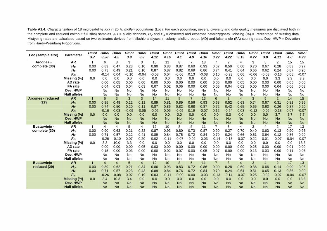
Table A1.4. Characterization of 18 microsatellite loci in 20 H. molleri populations (Loc). For each population, several diversity and data quality measures are displayed both in
the complete and reduced (without full sibs) samples. AR = allelic richness, HO and HE = observed and expected heterozygosity. Missing (%) = Percentage of missing data.
Mistyping rates are calculated based on two estimates derived from sibship analyses in colony: allelic dropout (AD) and false allele (FA) scoring rates. Dev. HWP = Deviation
from Hardy-Weinberg Proportions.
Loc (sample size) Parameter Hmol
3.7 Hmol3.28
Hmol4.2
Hmol3.9
Hmol3.3
Hmol4.12
Hmol4.16
Hmol4.1
Hmol4.9
Hmol4.10
Hmol3.22
Hmol4.22
Hmol3.15
Hmol4.27
Hmol3.8
Hmol4.11
Hmol4.8
Hmol4.29
Arcones - complete (30)
AR 1 6 3 3 3 15 11 8 7 13 7 2 4 3 5 2 15 15 HO 0.00 0.83 0.47 0.23 0.10 0.90 0.83 0.87 0.60 0.93 0.67 0.50 0.60 0.70 0.67 0.28 0.83 0.97
HE 0.00 0.73 0.49 0.21 0.10 0.87 0.87 0.82 0.69 0.86 0.74 0.41 0.64 0.66 0.62 0.24 0.87 0.90
FIS
-0.14 0.04 -0.10 -0.04 -0.03 0.04 -0.06 0.13 -0.08 0.10 -0.23 0.06 -0.06 -0.08 -0.16 0.05 -0.07
Missing (%) 0.0 0.0 0.0 0.0 0.0 0.0 0.0 0.0 0.0 0.0 0.0 0.0 0.0 0.0 0.0 3.3 3.3 3.3
AD rate
0.00 0.05 0.00 0.00 0.00 0.00 0.00 0.00 0.00 0.05 0.00 0.05 0.00 0.00 0.00 0.05 0.00
FA rate
0.04 0.03 0.04 0.03 0.07 0.02 0.06 0.00 0.00 0.05 0.04 0.02 0.00 0.00 0.04 0.06 0.03
Dev. HWP
No No No No No No No No No No No No No No No No No
Null alleles
No No No No No No No No No No No No No No No No No
Arcones - reduced (27)
AR 1 6 3 3 3 14 11 8 7 13 6 2 4 3 5 2 14 15 HO 0.00 0.85 0.48 0.22 0.11 0.89 0.81 0.89 0.56 0.93 0.63 0.52 0.63 0.74 0.67 0.31 0.81 0.96
HE 0.00 0.74 0.50 0.20 0.11 0.87 0.86 0.82 0.68 0.87 0.72 0.42 0.65 0.66 0.63 0.26 0.87 0.90
FIS
-0.16 0.03 -0.09 -0.05 -0.02 0.05 -0.09 0.19 -0.07 0.12 -0.24 0.03 -0.12 -0.06 -0.18 0.07 -0.07
Missing (%) 0.0 0.0 0.0 0.0 0.0 0.0 0.0 0.0 0.0 0.0 0.0 0.0 0.0 0.0 0.0 3.7 3.7 3.7
Dev. HWP
No No No No No No No No No No No No No No No No No
Null alleles
No No No No No No No No No No No No No No No No No
Bustarviejo - complete (30)
AR 1 4 4 5 4 12 10 8 5 11 7 3 4 3 4 2 17 13 HO 0.00 0.90 0.63 0.21 0.33 0.87 0.93 0.80 0.73 0.87 0.90 0.27 0.70 0.40 0.63 0.13 0.90 0.96
HE 0.00 0.71 0.57 0.22 0.41 0.89 0.84 0.75 0.72 0.84 0.79 0.24 0.66 0.51 0.64 0.12 0.86 0.90
FIS
-0.26 -0.10 0.07 0.20 0.02 -0.11 -0.07 -0.02 -0.03 -0.14 -0.13 -0.07 0.22 0.01 -0.07 -0.04 -0.07
Missing (%) 0.0 3.3 10.0 3.3 0.0 0.0 0.0 0.0 0.0 0.0 0.0 0.0 0.0 0.0 0.0 0.0 0.0 13.3
AD rate
0.00 0.00 0.00 0.05 0.03 0.00 0.00 0.00 0.00 0.00 0.00 0.00 0.25 0.00 0.00 0.01 0.00
FA rate
0.15 0.00 0.03 0.00 0.00 0.02 0.07 0.00 0.05 0.07 0.00 0.00 0.13 0.03 0.00 0.11 0.06
Dev. HWP
No No No No No No No No No No No No No No No No No
Null alleles
No No No No No No No No No No No No No No No No No
Bustarviejo - reduced (29)
AR 1 4 4 5 4 12 10 8 5 11 7 3 4 3 4 2 17 13 HO 0.00 0.89 0.62 0.21 0.34 0.86 0.93 0.83 0.72 0.86 0.90 0.28 0.69 0.38 0.66 0.14 0.90 0.96
HE 0.00 0.71 0.57 0.23 0.43 0.89 0.84 0.76 0.72 0.84 0.79 0.24 0.64 0.51 0.65 0.13 0.86 0.90
FIS
-0.26 -0.08 0.07 0.19 0.03 -0.11 -0.09 0.00 -0.03 -0.13 -0.14 -0.07 0.25 -0.02 -0.07 -0.04 -0.07
Missing (%) 0.0 3.4 10.3 3.4 0.0 0.0 0.0 0.0 0.0 0.0 0.0 0.0 0.0 0.0 0.0 0.0 0.0 13.8
Dev. HWP
No No No No No No No No No No No No No No No No No
Null alleles
No No No No No No No No No No No No No No No No No
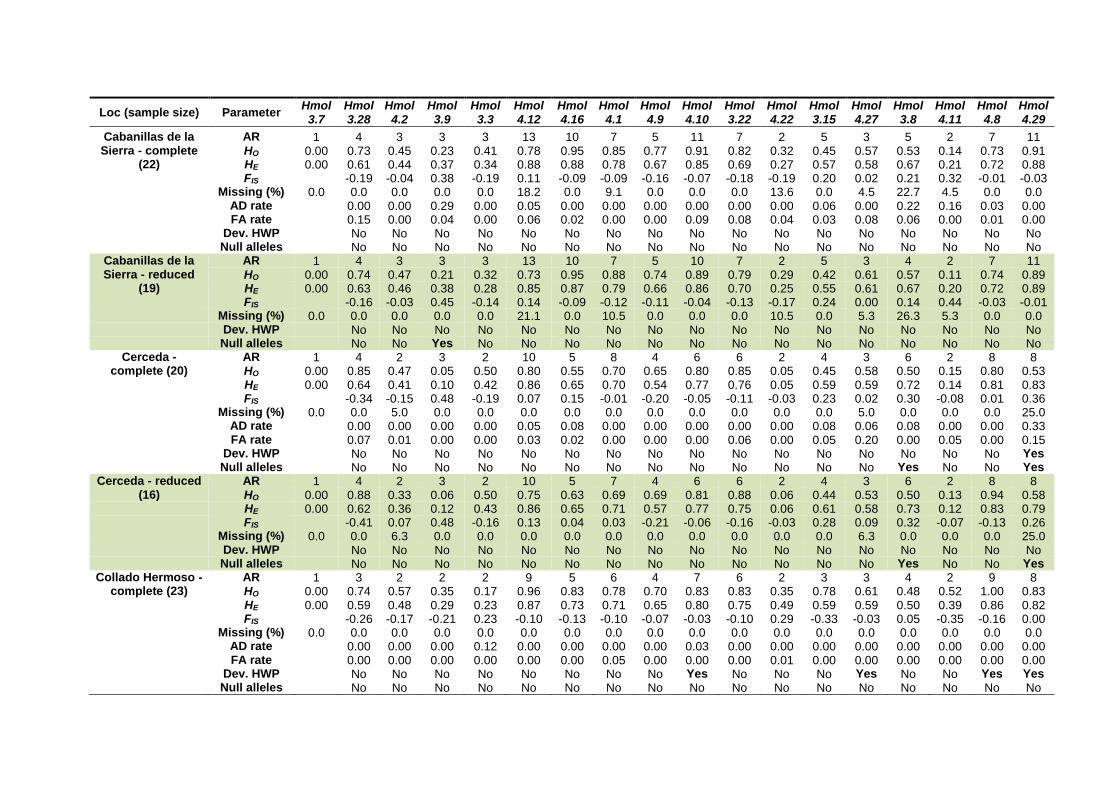
Loc (sample size) Parameter Hmol
3.7 Hmol3.28
Hmol4.2
Hmol3.9
Hmol3.3
Hmol4.12
Hmol4.16
Hmol4.1
Hmol4.9
Hmol4.10
Hmol3.22
Hmol4.22
Hmol3.15
Hmol4.27
Hmol3.8
Hmol4.11
Hmol4.8
Hmol4.29
Cabanillas de la Sierra - complete
(22)
AR 1 4 3 3 3 13 10 7 5 11 7 2 5 3 5 2 7 11 HO 0.00 0.73 0.45 0.23 0.41 0.78 0.95 0.85 0.77 0.91 0.82 0.32 0.45 0.57 0.53 0.14 0.73 0.91 HE 0.00 0.61 0.44 0.37 0.34 0.88 0.88 0.78 0.67 0.85 0.69 0.27 0.57 0.58 0.67 0.21 0.72 0.88
FIS
-0.19 -0.04 0.38 -0.19 0.11 -0.09 -0.09 -0.16 -0.07 -0.18 -0.19 0.20 0.02 0.21 0.32 -0.01 -0.03
Missing (%) 0.0 0.0 0.0 0.0 0.0 18.2 0.0 9.1 0.0 0.0 0.0 13.6 0.0 4.5 22.7 4.5 0.0 0.0
AD rate
0.00 0.00 0.29 0.00 0.05 0.00 0.00 0.00 0.00 0.00 0.00 0.06 0.00 0.22 0.16 0.03 0.00
FA rate
0.15 0.00 0.04 0.00 0.06 0.02 0.00 0.00 0.09 0.08 0.04 0.03 0.08 0.06 0.00 0.01 0.00
Dev. HWP
No No No No No No No No No No No No No No No No No
Null alleles
No No No No No No No No No No No No No No No No No
Cabanillas de la Sierra - reduced
(19)
AR 1 4 3 3 3 13 10 7 5 10 7 2 5 3 4 2 7 11 HO 0.00 0.74 0.47 0.21 0.32 0.73 0.95 0.88 0.74 0.89 0.79 0.29 0.42 0.61 0.57 0.11 0.74 0.89 HE 0.00 0.63 0.46 0.38 0.28 0.85 0.87 0.79 0.66 0.86 0.70 0.25 0.55 0.61 0.67 0.20 0.72 0.89
FIS
-0.16 -0.03 0.45 -0.14 0.14 -0.09 -0.12 -0.11 -0.04 -0.13 -0.17 0.24 0.00 0.14 0.44 -0.03 -0.01
Missing (%) 0.0 0.0 0.0 0.0 0.0 21.1 0.0 10.5 0.0 0.0 0.0 10.5 0.0 5.3 26.3 5.3 0.0 0.0
Dev. HWP
No No No No No No No No No No No No No No No No No
Null alleles
No No Yes No No No No No No No No No No No No No No
Cerceda - complete (20)
AR 1 4 2 3 2 10 5 8 4 6 6 2 4 3 6 2 8 8 HO 0.00 0.85 0.47 0.05 0.50 0.80 0.55 0.70 0.65 0.80 0.85 0.05 0.45 0.58 0.50 0.15 0.80 0.53
HE 0.00 0.64 0.41 0.10 0.42 0.86 0.65 0.70 0.54 0.77 0.76 0.05 0.59 0.59 0.72 0.14 0.81 0.83
FIS
-0.34 -0.15 0.48 -0.19 0.07 0.15 -0.01 -0.20 -0.05 -0.11 -0.03 0.23 0.02 0.30 -0.08 0.01 0.36
Missing (%) 0.0 0.0 5.0 0.0 0.0 0.0 0.0 0.0 0.0 0.0 0.0 0.0 0.0 5.0 0.0 0.0 0.0 25.0
AD rate
0.00 0.00 0.00 0.00 0.05 0.08 0.00 0.00 0.00 0.00 0.00 0.08 0.06 0.08 0.00 0.00 0.33
FA rate
0.07 0.01 0.00 0.00 0.03 0.02 0.00 0.00 0.00 0.06 0.00 0.05 0.20 0.00 0.05 0.00 0.15
Dev. HWP
No No No No No No No No No No No No No No No No Yes
Null alleles
No No No No No No No No No No No No No Yes No No Yes
Cerceda - reduced (16)
AR 1 4 2 3 2 10 5 7 4 6 6 2 4 3 6 2 8 8 HO 0.00 0.88 0.33 0.06 0.50 0.75 0.63 0.69 0.69 0.81 0.88 0.06 0.44 0.53 0.50 0.13 0.94 0.58
HE 0.00 0.62 0.36 0.12 0.43 0.86 0.65 0.71 0.57 0.77 0.75 0.06 0.61 0.58 0.73 0.12 0.83 0.79
FIS
-0.41 0.07 0.48 -0.16 0.13 0.04 0.03 -0.21 -0.06 -0.16 -0.03 0.28 0.09 0.32 -0.07 -0.13 0.26
Missing (%) 0.0 0.0 6.3 0.0 0.0 0.0 0.0 0.0 0.0 0.0 0.0 0.0 0.0 6.3 0.0 0.0 0.0 25.0
Dev. HWP
No No No No No No No No No No No No No No No No No
Null alleles
No No No No No No No No No No No No No Yes No No Yes
Collado Hermoso - complete (23)
AR 1 3 2 2 2 9 5 6 4 7 6 2 3 3 4 2 9 8 HO 0.00 0.74 0.57 0.35 0.17 0.96 0.83 0.78 0.70 0.83 0.83 0.35 0.78 0.61 0.48 0.52 1.00 0.83
HE 0.00 0.59 0.48 0.29 0.23 0.87 0.73 0.71 0.65 0.80 0.75 0.49 0.59 0.59 0.50 0.39 0.86 0.82
FIS
-0.26 -0.17 -0.21 0.23 -0.10 -0.13 -0.10 -0.07 -0.03 -0.10 0.29 -0.33 -0.03 0.05 -0.35 -0.16 0.00
Missing (%) 0.0 0.0 0.0 0.0 0.0 0.0 0.0 0.0 0.0 0.0 0.0 0.0 0.0 0.0 0.0 0.0 0.0 0.0
AD rate
0.00 0.00 0.00 0.12 0.00 0.00 0.00 0.00 0.03 0.00 0.00 0.00 0.00 0.00 0.00 0.00 0.00
FA rate
0.00 0.00 0.00 0.00 0.00 0.00 0.05 0.00 0.00 0.00 0.01 0.00 0.00 0.00 0.00 0.00 0.00
Dev. HWP
No No No No No No No No Yes No No No Yes No No Yes Yes
Null alleles
No No No No No No No No No No No No No No No No No

Loc (sample size) Parameter Hmol
3.7 Hmol3.28
Hmol4.2
Hmol3.9
Hmol3.3
Hmol4.12
Hmol4.16
Hmol4.1
Hmol4.9
Hmol4.10
Hmol3.22
Hmol4.22
Hmol3.15
Hmol4.27
Hmol3.8
Hmol4.11
Hmol4.8
Hmol4.29
Collado Hermoso - reduced (7)
AR 1 3 2 2 2 7 4 6 4 4 5 2 3 3 3 2 7 6 HO 0.00 0.86 0.57 0.57 0.14 0.86 0.86 0.71 0.86 0.71 0.86 0.43 0.86 0.29 0.43 0.29 1.00 0.71
HE 0.00 0.60 0.49 0.41 0.34 0.84 0.66 0.71 0.70 0.70 0.70 0.46 0.57 0.36 0.36 0.24 0.82 0.63
FIS
-0.42 -0.17 -0.40 0.58 -0.02 -0.29 0.00 -0.22 -0.01 -0.22 0.07 -0.50 0.20 -0.20 -0.17 -0.23 -0.13
Missing (%) 0.0 0.0 0.0 0.0 0.0 0.0 0.0 0.0 0.0 0.0 0.0 0.0 0.0 0.0 0.0 0.0 0.0 0.0
Dev. HWP
No No No No No No No No No No No No No No No No No
Null alleles
No No No No No No No No No No No No No No No No No
Colmenar Viejo - complete (21)
AR 1 2 2 2 2 8 7 5 4 6 4 1 4 4 3 1 5 6 HO 0.00 0.48 0.48 0.14 0.57 0.71 0.81 0.81 0.67 0.71 0.75 0.00 0.62 0.52 0.62 0.00 0.81 0.80
HE 0.00 0.36 0.36 0.13 0.41 0.62 0.77 0.70 0.57 0.65 0.71 0.00 0.60 0.59 0.53 0.00 0.70 0.73
FIS
-0.31 -0.31 -0.08 -0.40 -0.16 -0.05 -0.15 -0.18 -0.09 -0.06
-0.02 0.11 -0.18
-0.16 -0.09
Missing (%) 0.0 0.0 0.0 0.0 0.0 0.0 0.0 0.0 0.0 0.0 4.8 0.0 0.0 0.0 0.0 0.0 0.0 4.8
AD rate
0.00 0.00 0.00 0.00 0.00 0.00 0.00 0.00 0.00 0.00
0.00 0.05 0.00
0.00 0.00
FA rate
0.12 0.00 0.01 0.03 0.03 0.08 0.07 0.00 0.00 0.00
0.00 0.00 0.10
0.00 0.00
Dev. HWP
No No No No No No No No No No
No No No
No No
Null alleles
No No No No No No No No No No
No No No
No No
Colmenar Viejo - reduced (18)
AR 1 2 2 2 2 7 7 5 4 6 4 1 4 4 3 1 5 6 HO 0.00 0.50 0.44 0.17 0.61 0.67 0.83 0.78 0.61 0.72 0.72 0.00 0.56 0.56 0.61 0.00 0.83 0.82
HE 0.00 0.38 0.35 0.15 0.42 0.57 0.77 0.71 0.54 0.67 0.71 0.00 0.58 0.57 0.54 0.00 0.69 0.74
FIS
-0.33 -0.29 -0.09 -0.44 -0.17 -0.08 -0.10 -0.13 -0.09 -0.02
0.03 0.03 -0.14
-0.21 -0.11
Missing (%) 0.0 0.0 0.0 0.0 0.0 0.0 0.0 0.0 0.0 0.0 0.0 0.0 0.0 0.0 0.0 0.0 0.0 5.6
Dev. HWP
No No No No No No No No No No
No No No
No No
Null alleles
No No No No No No No No No No
No No No
No No
Dehesa de Roblellano -
complete (30)
AR 1 4 2 4 3 10 6 7 3 10 8 2 3 3 6 2 12 12 HO 0.00 0.75 0.52 0.41 0.40 0.77 0.67 0.67 0.59 0.97 0.76 0.57 0.70 0.67 0.63 0.20 0.93 0.90 HE 0.00 0.62 0.50 0.40 0.34 0.79 0.74 0.72 0.53 0.85 0.79 0.46 0.56 0.65 0.73 0.18 0.86 0.84
FIS
-0.21 -0.04 -0.04 -0.18 0.03 0.10 0.07 -0.11 -0.14 0.04 -0.25 -0.25 -0.03 0.13 -0.11 -0.09 -0.07
Missing (%) 0.0 6.7 3.3 3.3 0.0 0.0 0.0 0.0 3.3 3.3 3.3 0.0 0.0 0.0 0.0 0.0 0.0 0.0
AD rate
0.00 0.00 0.00 0.00 0.01 0.00 0.00 0.00 0.00 0.00 0.00 0.00 0.03 0.09 0.00 0.00 0.01
FA rate
0.07 0.03 0.00 0.00 0.01 0.00 0.05 0.03 0.00 0.02 0.00 0.00 0.00 0.00 0.01 0.04 0.01
Dev. HWP
Yes No No No No No No No No No No No No Yes No No No
Null alleles
No No No No No No No No No No No No No No No No No
Dehesa de Roblellano - reduced (20)
AR 1 3 2 4 3 10 6 7 3 10 7 2 3 3 6 2 12 11 HO 0.00 0.67 0.63 0.37 0.45 0.75 0.75 0.65 0.47 0.95 0.74 0.50 0.70 0.70 0.55 0.25 1.00 0.90 HE 0.00 0.61 0.50 0.36 0.37 0.78 0.78 0.69 0.52 0.83 0.80 0.46 0.58 0.61 0.66 0.22 0.87 0.81
FIS
-0.10 -0.27 -0.02 -0.21 0.04 0.04 0.06 0.10 -0.14 0.07 -0.10 -0.21 -0.15 0.17 -0.14 -0.15 -0.11
Missing (%) 0.0 10.0 5.0 5.0 0.0 0.0 0.0 0.0 5.0 5.0 5.0 0.0 0.0 0.0 0.0 0.0 0.0 0.0
Dev. HWP
No No No No No No No No No No No No No Yes No No No
Null alleles
No No No No No No No No No No No No No No No No No
Loc (sample size) Parameter Hmol
3.7 Hmol3.28
Hmol4.2
Hmol3.9
Hmol3.3
Hmol4.12
Hmol4.16
Hmol4.1
Hmol4.9
Hmol4.10
Hmol3.22
Hmol4.22
Hmol3.15
Hmol4.27
Hmol3.8
Hmol4.11
Hmol4.8
Hmol4.29
El Berrueco - complete (21)
AR 1 4 3 3 3 11 11 7 5 9 5 2 4 4 3 2 9 8 HO 0.00 0.48 0.57 0.29 0.33 0.95 0.90 0.95 0.67 0.86 0.62 0.52 0.57 0.71 0.57 0.33 0.90 0.71
HE 0.00 0.54 0.47 0.25 0.33 0.80 0.86 0.81 0.63 0.82 0.74 0.39 0.56 0.58 0.44 0.28 0.82 0.77
FIS
0.11 -0.21 -0.14 -0.02 -0.20 -0.05 -0.18 -0.05 -0.04 0.16 -0.35 -0.02 -0.23 -0.30 -0.20 -0.11 0.08
Missing (%) 0.0 0.0 0.0 0.0 0.0 0.0 0.0 0.0 0.0 0.0 0.0 0.0 0.0 0.0 0.0 0.0 0.0 0.0
AD rate
0.00 0.00 0.00 0.00 0.00 0.00 0.00 0.00 0.00 0.06 0.00 0.00 0.00 0.00 0.00 0.00 0.03
FA rate
0.00 0.00 0.00 0.00 0.09 0.10 0.02 0.02 0.04 0.00 0.02 0.00 0.00 0.00 0.05 0.00 0.10
Dev. HWP
No No No No No No No No No No No No No No No No No
Null alleles
No No No No No No No No No No No No No No No No No
El Berrueco - reduced (18)
AR 1 4 3 3 3 10 11 7 5 9 5 2 4 4 3 2 9 8 HO 0.00 0.39 0.50 0.28 0.33 0.94 0.94 0.94 0.67 0.89 0.56 0.56 0.50 0.67 0.67 0.39 0.89 0.78
HE 0.00 0.54 0.45 0.25 0.33 0.77 0.85 0.80 0.62 0.83 0.74 0.40 0.54 0.58 0.48 0.31 0.83 0.78
FIS
0.28 -0.11 -0.13 0.00 -0.22 -0.11 -0.19 -0.08 -0.08 0.25 -0.38 0.07 -0.15 -0.39 -0.24 -0.08 0.01
Missing (%) 0.0 0.0 0.0 0.0 0.0 0.0 0.0 0.0 0.0 0.0 0.0 0.0 0.0 0.0 0.0 0.0 0.0 0.0
Dev. HWP
No No No No No No No No No No No No No No No No No
Null alleles
No No No No No No No No No No No No No No No No No
Fuenterrebollo - complete (20)
AR 1 5 3 3 3 12 11 9 5 8 6 2 4 3 3 3 12 11 HO 0.00 0.65 0.45 0.15 0.65 0.90 0.80 1.00 0.85 0.75 0.70 0.35 0.55 0.58 0.30 0.25 1.00 0.95
HE 0.00 0.71 0.47 0.14 0.58 0.89 0.83 0.86 0.59 0.83 0.73 0.35 0.60 0.59 0.30 0.30 0.90 0.84
FIS
0.08 0.03 -0.06 -0.12 -0.02 0.04 -0.17 -0.45 0.09 0.04 0.00 0.08 0.01 0.00 0.16 -0.11 -0.13
Missing (%) 0.0 0.0 0.0 0.0 0.0 0.0 0.0 0.0 0.0 0.0 0.0 0.0 0.0 5.0 0.0 0.0 0.0 0.0
AD rate
0.00 0.00 0.00 0.00 0.00 0.00 0.00 0.00 0.00 0.00 0.00 0.00 0.00 0.00 0.07 0.00 0.00
FA rate
0.00 0.00 0.03 0.00 0.00 0.06 0.00 0.06 0.04 0.01 0.00 0.02 0.00 0.04 0.01 0.00 0.13
Dev. HWP
No No No No No No No No No No No No No No No No No
Null alleles
No No No No No No No No No No No No No No No No No
Fuenterrebollo - reduced (12)
AR 1 5 3 3 3 11 9 9 5 8 6 2 4 3 3 3 12 10 HO 0.00 0.75 0.58 0.25 0.58 0.92 0.75 1.00 0.75 0.75 0.58 0.33 0.50 0.73 0.50 0.33 1.00 0.92
HE 0.00 0.70 0.52 0.23 0.57 0.89 0.85 0.87 0.63 0.84 0.69 0.38 0.60 0.57 0.45 0.39 0.90 0.84
FIS
-0.07 -0.13 -0.11 -0.02 -0.04 0.11 -0.15 -0.19 0.11 0.16 0.11 0.17 -0.28 -0.12 0.15 -0.11 -0.09
Missing (%) 0.0 0.0 0.0 0.0 0.0 0.0 0.0 0.0 0.0 0.0 0.0 0.0 0.0 8.3 0.0 0.0 0.0 0.0
Dev. HWP
No No No No No No No No No No No No No No No No No
Null alleles
No No No No No No No No No No No No No No No No No
Gascones - complete (21)
AR 1 5 3 4 3 12 12 11 5 14 8 2 4 3 4 2 12 14 HO 0.00 0.86 0.55 0.52 0.29 0.95 0.90 0.65 0.86 1.00 0.81 0.29 0.52 0.81 0.43 0.42 0.89 0.84
HE 0.00 0.73 0.41 0.43 0.38 0.91 0.85 0.80 0.71 0.89 0.82 0.36 0.59 0.64 0.67 0.33 0.88 0.88
FIS
-0.17 -0.34 -0.23 0.25 -0.05 -0.06 0.18 -0.21 -0.13 0.01 0.21 0.12 -0.26 0.36 -0.27 -0.02 0.04
Missing (%) 0.0 0.0 4.8 0.0 0.0 4.8 0.0 4.8 0.0 0.0 0.0 0.0 0.0 0.0 0.0 9.5 9.5 9.5
AD rate
0.00 0.00 0.00 0.13 0.01 0.00 0.18 0.00 0.00 0.00 0.21 0.04 0.00 0.18 0.00 0.00 0.01
FA rate
0.15 0.02 0.00 0.00 0.00 0.00 0.17 0.00 0.03 0.00 0.06 0.00 0.04 0.00 0.02 0.04 0.11
Dev. HWP
No No No No No No No No No No No No No No No No No
Null alleles
No No No No No No No No No No No No No Yes No No No

Loc (sample size) Parameter Hmol
3.7 Hmol3.28
Hmol4.2
Hmol3.9
Hmol3.3
Hmol4.12
Hmol4.16
Hmol4.1
Hmol4.9
Hmol4.10
Hmol3.22
Hmol4.22
Hmol3.15
Hmol4.27
Hmol3.8
Hmol4.11
Hmol4.8
Hmol4.29
Gascones - reduced (19)
AR 1 5 3 4 3 12 12 9 5 13 8 2 4 3 4 2 12 13 HO 0.00 0.95 0.50 0.53 0.32 0.94 0.89 0.61 0.84 1.00 0.79 0.26 0.58 0.79 0.42 0.35 0.94 0.88
HE 0.00 0.75 0.39 0.43 0.41 0.91 0.85 0.78 0.72 0.88 0.81 0.36 0.62 0.63 0.68 0.29 0.89 0.88
FIS
-0.27 -0.29 -0.24 0.23 -0.04 -0.05 0.22 -0.17 -0.14 0.03 0.27 0.06 -0.25 0.38 -0.21 -0.05 -0.01
Missing (%) 0.0 0.0 5.3 0.0 0.0 5.3 0.0 5.3 0.0 0.0 0.0 0.0 0.0 0.0 0.0 10.5 10.5 10.5
Dev. HWP
No No No No No No No No No No No No No No No No No
Null alleles
No No No No No No No No No No No No No Yes No No No
La Pradera de Navalhorno - complete (22)
AR 1 2 2 3 3 4 5 4 2 5 4 2 5 2 2 2 7 6 HO 0.00 0.95 0.36 0.76 0.57 0.90 0.82 0.67 0.48 0.71 1.00 0.55 1.00 0.05 0.36 0.50 0.95 1.00 HE 0.00 0.50 0.40 0.56 0.45 0.72 0.68 0.59 0.47 0.74 0.75 0.43 0.67 0.28 0.30 0.42 0.79 0.77
FIS
-0.91 0.08 -0.35 -0.26 -0.25 -0.21 -0.13 -0.01 0.03 -0.34 -0.26 -0.48 0.83 -0.22 -0.20 -0.21 -0.30
Missing (%) 4.5 0.0 0.0 4.5 4.5 4.5 0.0 4.5 4.5 4.5 4.5 0.0 0.0 4.5 0.0 0.0 4.5 4.5
AD rate
0.00 0.00 0.00 0.00 0.00 0.00 0.00 0.00 0.00 0.00 0.00 0.00 0.17 0.00 0.00 0.00 0.00
FA rate
0.00 0.00 0.00 0.00 0.00 0.00 0.00 0.00 0.00 0.00 0.18 0.00 0.00 0.00 0.00 0.06 0.02
Dev. HWP
Yes No No No Yes No Yes No No Yes No No Yes No No No Yes
Null alleles
No No No No No No No No No No No No Yes No No No No
La Pradera de Navalhorno - reduced (9)
AR 1 2 2 3 3 4 5 4 2 5 4 2 5 2 2 2 6 6 HO 0.00 0.89 0.67 0.63 0.63 0.88 0.89 0.63 0.38 0.88 1.00 0.56 1.00 0.13 0.56 0.56 0.88 1.00 HE 0.00 0.49 0.44 0.48 0.46 0.72 0.69 0.55 0.43 0.74 0.74 0.40 0.69 0.30 0.40 0.40 0.81 0.79
FIS
-0.80 -0.50 -0.31 -0.36 -0.22 -0.29 -0.13 0.13 -0.18 -0.35 -0.38 -0.45 0.59 -0.38 -0.38 -0.08 -0.27
Missing (%) 11.1 0.0 0.0 11.1 11.1 11.1 0.0 11.1 11.1 11.1 11.1 0.0 0.0 11.1 0.0 0.0 11.1 11.1
Dev. HWP
No No No No No No No No No No No No No No No No No
Null alleles
No No No No No No No No No No No No No No No No No
Medianillos - complete (21)
AR 1 2 3 3 3 7 5 6 4 7 7 2 3 3 3 2 7 5 HO 0.00 0.52 0.52 0.33 0.24 1.00 0.71 0.71 0.52 0.95 0.90 0.14 0.52 0.33 0.62 0.24 0.76 0.76
HE 0.00 0.39 0.54 0.29 0.22 0.79 0.59 0.67 0.59 0.81 0.77 0.13 0.51 0.52 0.56 0.21 0.68 0.63
FIS
-0.35 0.03 -0.15 -0.10 -0.26 -0.21 -0.07 0.11 -0.18 -0.17 -0.08 -0.03 0.36 -0.10 -0.14 -0.13 -0.20
Missing (%) 0.0 0.0 0.0 0.0 0.0 0.0 0.0 0.0 0.0 0.0 0.0 0.0 0.0 0.0 0.0 0.0 0.0 0.0
AD rate
0.00 0.00 0.00 0.00 0.00 0.00 0.00 0.00 0.00 0.00 0.00 0.00 0.22 0.00 0.00 0.00 0.00
FA rate
0.14 0.00 0.00 0.02 0.02 0.01 0.04 0.00 0.00 0.05 0.00 0.06 0.04 0.00 0.00 0.05 0.00
Dev. HWP
No No No No No No No No Yes No No No No No No No No
Null alleles
No No No No No No No No No No No No No No No No No
Medianillos - reduced (9)
AR 1 2 3 3 3 7 4 5 4 6 5 2 3 2 3 2 5 5 HO 0.00 0.44 0.44 0.44 0.44 1.00 0.67 0.78 0.56 0.89 0.89 0.11 0.67 0.33 0.56 0.22 0.67 0.78
HE 0.00 0.35 0.55 0.37 0.36 0.77 0.50 0.70 0.64 0.78 0.73 0.10 0.59 0.40 0.48 0.20 0.68 0.64
FIS
-0.29 0.19 -0.20 -0.22 -0.30 -0.33 -0.12 0.13 -0.14 -0.22 -0.06 -0.14 0.17 -0.17 -0.13 0.02 -0.22
Missing (%) 0.0 0.0 0.0 0.0 0.0 0.0 0.0 0.0 0.0 0.0 0.0 0.0 0.0 0.0 0.0 0.0 0.0 0.0
Dev. HWP
No No No No No No No No No No No No No No No No No
Null alleles
No No No No No No No No No No No No No No No No No

Loc (sample size) Parameter Hmol
3.7 Hmol3.28
Hmol4.2
Hmol3.9
Hmol3.3
Hmol4.12
Hmol4.16
Hmol4.1
Hmol4.9
Hmol4.10
Hmol3.22
Hmol4.22
Hmol3.15
Hmol4.27
Hmol3.8
Hmol4.11
Hmol4.8
Hmol4.29
Puerto de Canencia -
complete (25)
AR 2 4 3 3 4 11 7 9 4 12 6 2 4 4 4 2 12 14 HO 0.04 0.76 0.60 0.52 0.40 0.96 0.84 0.75 0.44 0.96 0.92 0.48 0.68 0.64 0.68 0.13 0.87 0.96 HE 0.04 0.61 0.49 0.45 0.37 0.80 0.77 0.80 0.46 0.87 0.78 0.40 0.61 0.71 0.62 0.19 0.87 0.90
FIS -0.02 -0.24 -0.24 -0.16 -0.08 -0.19 -0.09 0.07 0.04 -0.10 -0.18 -0.19 -0.11 0.09 -0.10 0.33 0.01 -0.06
Missing (%) 0.0 0.0 0.0 0.0 0.0 4.0 0.0 4.0 0.0 0.0 0.0 0.0 0.0 0.0 0.0 8.0 8.0 0.0
AD rate 0.00 0.00 0.00 0.00 0.00 0.00 0.00 0.01 0.00 0.00 0.00 0.00 0.00 0.04 0.00 0.23 0.00 0.00
FA rate 0.00 0.02 0.03 0.00 0.02 0.08 0.00 0.11 0.00 0.11 0.03 0.03 0.00 0.00 0.06 0.03 0.00 0.09
Dev. HWP No No No No No No No No No No No No No No No No No No
Null alleles No No No No No No No No No No No No No No No No No No
Puerto de Canencia -
reduced (22)
AR 2 4 3 3 4 10 7 9 4 12 6 2 4 4 4 2 12 14 HO 0.05 0.77 0.59 0.45 0.45 1.00 0.86 0.81 0.45 0.95 0.91 0.45 0.68 0.64 0.68 0.15 0.85 0.95 HE 0.04 0.62 0.49 0.42 0.41 0.82 0.79 0.82 0.47 0.88 0.78 0.40 0.63 0.72 0.60 0.22 0.86 0.91
FIS -0.02 -0.24 -0.20 -0.07 -0.11 -0.21 -0.09 0.02 0.03 -0.08 -0.17 -0.15 -0.08 0.11 -0.14 0.31 0.01 -0.05
Missing (%) 0.0 0.0 0.0 0.0 0.0 4.5 0.0 4.5 0.0 0.0 0.0 0.0 0.0 0.0 0.0 9.1 9.1 0.0
Dev. HWP No No No No No No No No No No No No No No No No No No
Null alleles No No No No No No No No No No No No No No No No No No
Puerto de La Morcuera -
complete (30)
AR 1 4 3 2 3 11 11 5 4 10 6 2 3 5 4 2 11 11 HO 0.00 0.67 0.38 0.20 0.43 0.93 0.87 0.80 0.70 0.97 0.87 0.43 0.67 0.73 0.62 0.53 0.77 0.87 HE 0.00 0.58 0.35 0.23 0.50 0.83 0.84 0.70 0.56 0.87 0.80 0.41 0.64 0.59 0.61 0.46 0.81 0.84
FIS
-0.15 -0.09 0.13 0.12 -0.12 -0.03 -0.15 -0.25 -0.11 -0.09 -0.07 -0.04 -0.24 -0.02 -0.15 0.06 -0.04
Missing (%) 0.0 0.0 13.3 0.0 0.0 0.0 0.0 0.0 0.0 0.0 0.0 0.0 0.0 0.0 3.3 0.0 0.0 0.0
AD rate
0.00 0.00 0.10 0.12 0.00 0.00 0.00 0.00 0.00 0.00 0.00 0.00 0.00 0.04 0.00 0.03 0.01
FA rate
0.00 0.04 0.04 0.00 0.07 0.00 0.00 0.00 0.00 0.07 0.00 0.00 0.05 0.12 0.12 0.00 0.00
Dev. HWP
No No No No No No No No No No No No No No No No No
Null alleles
No No No No No No No No No No No No No No No No No
Puerto de La Morcuera -
reduced (24)
AR 1 4 3 2 3 10 11 5 4 9 6 2 3 5 4 2 10 10 HO 0.00 0.67 0.38 0.25 0.38 0.92 0.88 0.79 0.67 0.96 0.83 0.46 0.67 0.71 0.65 0.50 0.71 0.83 HE 0.00 0.55 0.32 0.22 0.50 0.84 0.83 0.70 0.55 0.87 0.80 0.39 0.64 0.56 0.61 0.44 0.80 0.81
FIS
-0.20 -0.20 -0.14 0.25 -0.09 -0.05 -0.14 -0.20 -0.11 -0.04 -0.16 -0.04 -0.27 -0.06 -0.13 0.11 -0.02
Missing (%) 0.0 0.0 12.5 0.0 0.0 0.0 0.0 0.0 0.0 0.0 0.0 0.0 0.0 0.0 4.2 0.0 0.0 0.0
Dev. HWP
No No No No No No No No No No No No No No No No No
Null alleles
No No No No No No No No No No No No No No No No No
Rascafría - complete (20)
AR 1 3 3 1 3 9 7 7 3 6 6 2 3 4 3 3 9 10 HO 0.00 0.55 0.55 0.00 0.35 0.47 0.85 0.79 0.55 0.80 0.75 0.40 0.45 0.60 0.65 0.37 0.89 0.95
HE 0.00 0.55 0.52 0.00 0.34 0.51 0.79 0.73 0.56 0.76 0.77 0.38 0.57 0.58 0.62 0.50 0.79 0.86
FIS
0.01 -0.05
-0.03 0.08 -0.08 -0.08 0.02 -0.05 0.03 -0.07 0.22 -0.04 -0.06 0.26 -0.13 -0.10
Missing (%) 0.0 0.0 0.0 0.0 0.0 5.0 0.0 5.0 0.0 0.0 0.0 0.0 0.0 0.0 0.0 5.0 5.0 0.0
AD rate
0.00 0.05
0.00 0.00 0.00 0.00 0.00 0.00 0.04 0.00 0.00 0.01 0.00 0.09 0.00 0.00
FA rate
0.10 0.00
0.00 0.09 0.00 0.00 0.00 0.05 0.18 0.05 0.00 0.06 0.19 0.02 0.00 0.00
Dev. HWP
No No
No No No No No No No No No No No No No No
Null alleles
No No
No No No No No No No No No No No No No No
Loc (sample size) Parameter Hmol
3.7 Hmol3.28
Hmol4.2
Hmol3.9
Hmol3.3
Hmol4.12
Hmol4.16
Hmol4.1
Hmol4.9
Hmol4.10
Hmol3.22
Hmol4.22
Hmol3.15
Hmol4.27
Hmol3.8
Hmol4.11
Hmol4.8
Hmol4.29
Rascafría - reduced (18)
AR 1 3 3 1 3 9 7 7 3 6 6 2 3 4 3 3 9 10 HO 0.00 0.56 0.50 0.00 0.33 0.47 0.89 0.82 0.56 0.78 0.72 0.39 0.44 0.61 0.61 0.35 0.88 0.94
HE 0.00 0.57 0.52 0.00 0.33 0.52 0.80 0.76 0.57 0.77 0.75 0.38 0.57 0.57 0.59 0.47 0.78 0.86
FIS
0.02 0.03
-0.01 0.10 -0.11 -0.09 0.02 -0.01 0.04 -0.04 0.22 -0.07 -0.03 0.25 -0.13 -0.10
Missing (%) 0.0 0.0 0.0 0.0 0.0 5.6 0.0 5.6 0.0 0.0 0.0 0.0 0.0 0.0 0.0 5.6 5.6 0.0
Dev. HWP
No No
No No No No No No No No No No No No No No
Null alleles
No No
No No No No No No No No No No No No No No
Sauquillo de Cabezas -
complete (20)
AR 1 5 2 3 3 9 9 7 3 9 5 2 4 3 4 2 10 8 HO 0.00 0.85 0.75 0.25 0.15 1.00 1.00 0.75 0.70 0.90 0.95 0.60 0.55 0.40 0.95 0.15 1.00 0.80 HE 0.00 0.74 0.49 0.22 0.14 0.83 0.81 0.68 0.47 0.81 0.73 0.42 0.63 0.46 0.66 0.14 0.83 0.80
FIS
-0.15 -0.53 -0.12 -0.06 -0.20 -0.23 -0.10 -0.49 -0.11 -0.30 -0.43 0.12 0.13 -0.45 -0.08 -0.20 -0.01
Missing (%) 0.0 0.0 0.0 0.0 0.0 0.0 0.0 0.0 0.0 0.0 0.0 0.0 0.0 0.0 0.0 0.0 0.0 0.0
AD rate
0.00 0.00 0.00 0.00 0.00 0.00 0.01 0.00 0.00 0.00 0.00 0.07 0.02 0.00 0.00 0.00 0.00
FA rate
0.01 0.00 0.01 0.04 0.03 0.10 0.05 0.04 0.00 0.00 0.00 0.10 0.00 0.03 0.07 0.04 0.00
Dev. HWP
No No No No No No No No No No No No No No No No No
Null alleles
No No No No No No No No No No No No No No No No No
Sauquillo de Cabezas - reduced
(12)
AR 1 5 2 2 3 8 8 7 3 9 5 2 4 3 4 2 8 8 HO 0.00 0.83 0.67 0.08 0.25 1.00 1.00 0.83 0.75 0.83 0.92 0.50 0.58 0.17 0.92 0.08 1.00 0.92 HE 0.00 0.69 0.44 0.08 0.23 0.84 0.82 0.72 0.50 0.82 0.73 0.38 0.66 0.35 0.66 0.08 0.83 0.84
FIS
-0.20 -0.50 -0.04 -0.11 -0.19 -0.22 -0.16 -0.51 -0.02 -0.25 -0.33 0.11 0.52 -0.40 -0.04 -0.20 -0.09
Missing (%) 0.0 0.0 0.0 0.0 0.0 0.0 0.0 0.0 0.0 0.0 0.0 0.0 0.0 0.0 0.0 0.0 0.0 0.0
Dev. HWP
No No No No No No No No No No No No No No No No No
Null alleles
No No No No No No No No No No No No Yes No No No No
Soto del Real - complete (20)
AR 1 5 3 4 3 13 9 11 5 9 7 2 5 4 5 2 11 10 HO 0.00 0.65 0.30 0.65 0.25 0.85 0.90 0.80 0.65 0.75 0.75 0.10 0.80 0.50 0.75 0.11 0.95 0.79
HE 0.00 0.65 0.27 0.55 0.23 0.85 0.83 0.82 0.65 0.82 0.80 0.10 0.62 0.64 0.66 0.10 0.85 0.86
FIS
0.00 -0.13 -0.18 -0.10 0.00 -0.08 0.03 0.00 0.09 0.07 -0.05 -0.29 0.22 -0.13 -0.06 -0.11 0.09
Missing (%) 0.0 0.0 0.0 0.0 0.0 0.0 0.0 0.0 0.0 0.0 0.0 0.0 0.0 0.0 0.0 10.0 5.0 5.0
AD rate
0.03 0.00 0.00 0.00 0.04 0.00 0.00 0.04 0.00 0.00 0.00 0.00 0.18 0.00 0.00 0.00 0.03
FA rate
0.06 0.04 0.07 0.04 0.21 0.00 0.04 0.04 0.00 0.06 0.00 0.00 0.08 0.00 0.02 0.00 0.00
Dev. HWP
No No No No No No No No No No No No No No No No No
Null alleles
No No No No No No No No No No No No No No No No No
Soto del Real - reduced (18)
AR 1 5 3 4 3 13 9 11 5 8 7 2 5 4 5 2 11 10 HO 0.00 0.61 0.33 0.67 0.28 0.83 0.94 0.78 0.61 0.72 0.78 0.11 0.83 0.44 0.72 0.12 1.00 0.78
HE 0.00 0.63 0.29 0.54 0.25 0.87 0.83 0.82 0.65 0.82 0.80 0.10 0.63 0.63 0.66 0.11 0.86 0.86
FIS
0.03 -0.15 -0.24 -0.12 0.04 -0.14 0.05 0.05 0.12 0.03 -0.06 -0.33 0.30 -0.09 -0.06 -0.16 0.10
Missing (%) 0.0 0.0 0.0 0.0 0.0 0.0 0.0 0.0 0.0 0.0 0.0 0.0 0.0 0.0 0.0 5.6 0.0 0.0
Dev. HWP
No No No No No No No No No No No No No No No No No
Null alleles
No No No No No No No No No No No No No No No No No

Loc (sample size) Parameter Hmol
3.7 Hmol3.28
Hmol4.2
Hmol3.9
Hmol3.3
Hmol4.12
Hmol4.16
Hmol4.1
Hmol4.9
Hmol4.10
Hmol3.22
Hmol4.22
Hmol3.15
Hmol4.27
Hmol3.8
Hmol4.11
Hmol4.8
Hmol4.29
Torrecaballeros - complete (34)
AR 1 4 2 2 3 8 7 5 4 4 5 2 3 2 4 3 6 7 HO 0.00 0.50 0.21 0.41 0.50 0.79 0.68 0.76 0.79 0.79 0.53 0.18 0.47 0.18 0.41 0.27 0.97 0.76
HE 0.00 0.54 0.18 0.50 0.54 0.79 0.69 0.74 0.68 0.71 0.49 0.16 0.39 0.29 0.37 0.44 0.76 0.70
FIS
0.07 -0.11 0.17 0.08 -0.01 0.02 -0.04 -0.16 -0.11 -0.08 -0.10 -0.21 0.39 -0.11 0.38 -0.27 -0.08
Missing (%) 0.0 0.0 0.0 0.0 0.0 0.0 0.0 0.0 0.0 0.0 0.0 0.0 0.0 0.0 0.0 2.9 2.9 2.9
AD rate
0.00 0.00 0.09 0.00 0.02 0.00 0.02 0.00 0.00 0.00 0.00 0.00 0.19 0.00 0.25 0.00 0.00
FA rate
0.00 0.04 0.00 0.00 0.05 0.05 0.00 0.02 0.00 0.00 0.00 0.06 0.00 0.03 0.04 0.02 0.01
Dev. HWP
No No No No No No No No No No No No No No No No No
Null alleles
No No No No No No No No No No No No No No Yes No No
Torrecaballeros - reduced (28)
AR 1 4 2 2 3 8 6 5 4 4 5 2 3 2 3 3 6 6 HO 0.00 0.50 0.21 0.32 0.50 0.79 0.68 0.79 0.79 0.79 0.46 0.14 0.46 0.21 0.46 0.29 0.96 0.71
HE 0.00 0.53 0.19 0.50 0.56 0.79 0.67 0.74 0.70 0.72 0.44 0.13 0.38 0.34 0.40 0.46 0.76 0.69
FIS
0.05 -0.12 0.36 0.11 0.00 -0.01 -0.06 -0.12 -0.09 -0.05 -0.08 -0.21 0.36 -0.15 0.39 -0.27 -0.04
Missing (%) 0.0 0.0 0.0 0.0 0.0 0.0 0.0 0.0 0.0 0.0 0.0 0.0 0.0 0.0 0.0 0.0 0.0 0.0
Dev. HWP
No No No No No No No No No No No No No No No No No
Null alleles
No No No No No No No No No No No No No No Yes No No
Turrubuelo - complete (21)
AR 1 5 3 2 4 14 8 11 5 10 8 2 4 4 4 2 11 13 HO 0.00 0.81 0.57 0.33 0.29 0.85 0.80 0.90 0.57 0.90 0.81 0.38 0.57 0.81 0.48 0.48 0.76 0.95
HE 0.00 0.76 0.54 0.46 0.33 0.89 0.79 0.82 0.65 0.84 0.77 0.41 0.65 0.64 0.39 0.49 0.83 0.89
FIS
-0.07 -0.05 0.27 0.13 0.04 -0.01 -0.10 0.13 -0.08 -0.06 0.07 0.12 -0.27 -0.21 0.03 0.09 -0.06
Missing (%) 0.0 0.0 0.0 0.0 0.0 4.8 4.8 4.8 0.0 0.0 0.0 0.0 0.0 0.0 0.0 0.0 0.0 0.0
AD rate
0.00 0.00 0.14 0.00 0.00 0.00 0.00 0.00 0.00 0.00 0.06 0.00 0.00 0.00 0.02 0.00 0.00
FA rate
0.01 0.00 0.00 0.07 0.00 0.03 0.05 0.00 0.00 0.01 0.07 0.00 0.08 0.07 0.10 0.00 0.00
Dev. HWP
No No No No No No No No No No No No No No No No No
Null alleles
No No No No No No No No No No No No No No No No No
Turrubuelo - reduced (19)
AR 1 5 3 2 3 14 8 11 5 10 8 2 4 4 4 2 11 13 HO 0.00 0.79 0.58 0.32 0.26 0.83 0.83 0.94 0.53 0.89 0.84 0.37 0.63 0.79 0.42 0.42 0.74 0.95
HE 0.00 0.76 0.55 0.47 0.32 0.88 0.81 0.82 0.65 0.84 0.78 0.41 0.64 0.63 0.36 0.49 0.83 0.89
FIS
-0.04 -0.06 0.32 0.17 0.05 -0.03 -0.15 0.19 -0.06 -0.08 0.10 0.01 -0.26 -0.18 0.14 0.11 -0.06
Missing (%) 0.0 0.0 0.0 0.0 0.0 5.3 5.3 5.3 0.0 0.0 0.0 0.0 0.0 0.0 0.0 0.0 0.0 0.0
Dev. HWP
No No No No No No No No No No No No No No No No No
Null alleles
No No No No No No No No No No No No No No No No No
Valdemanco - complete (96)
AR 1 4 4 4 4 18 14 11 5 14 8 3 4 3 5 3 15 17 HO 0.00 0.63 0.54 0.29 0.41 0.88 0.86 0.85 0.57 0.82 0.91 0.24 0.47 0.70 0.47 0.22 0.82 0.98
HE 0.00 0.67 0.55 0.32 0.40 0.89 0.86 0.82 0.64 0.86 0.82 0.22 0.61 0.64 0.50 0.20 0.86 0.91
FIS
0.06 0.02 0.08 -0.01 0.01 -0.01 -0.04 0.11 0.04 -0.12 -0.11 0.23 -0.09 0.06 -0.07 0.05 -0.08
Missing (%) 0.0 0.0 1.0 0.0 0.0 3.1 0.0 1.0 1.0 0.0 4.2 1.0 0.0 5.2 1.0 4.2 11.5 3.1
AD rate
0.01 0.01 0.01 0.00 0.00 0.00 0.00 0.02 0.01 0.01 0.00 0.08 0.00 0.11 0.02 0.00 0.00
FA rate
0.07 0.01 0.01 0.00 0.04 0.01 0.01 0.02 0.01 0.03 0.00 0.03 0.04 0.04 0.00 0.02 0.02
Dev. HWP
No No No No No No No No No No No No No No No No No
Null alleles
No No No No No No No No No No No Yes No No No No No

Loc (sample size) Parameter Hmol
3.7 Hmol3.28
Hmol4.2
Hmol3.9
Hmol3.3
Hmol4.12
Hmol4.16
Hmol4.1
Hmol4.9
Hmol4.10
Hmol3.22
Hmol4.22
Hmol3.15
Hmol4.27
Hmol3.8
Hmol4.11
Hmol4.8
Hmol4.29
Valdemanco - reduced (88)
AR 1 4 4 4 4 17 14 11 5 14 8 3 4 3 5 3 15 17 HO 0.00 0.63 0.55 0.28 0.42 0.89 0.85 0.87 0.57 0.84 0.92 0.24 0.48 0.71 0.49 0.20 0.81 0.98
HE 0.00 0.66 0.55 0.30 0.41 0.89 0.86 0.82 0.64 0.87 0.82 0.22 0.60 0.64 0.52 0.19 0.86 0.90
FIS
0.06 0.00 0.05 -0.01 -0.01 0.01 -0.07 0.10 0.03 -0.12 -0.11 0.20 -0.10 0.05 -0.05 0.06 -0.08
Missing (%) 0.0 0.0 0.0 0.0 0.0 3.4 0.0 1.1 1.1 0.0 4.5 1.1 0.0 5.7 1.1 4.5 11.4 3.4
Dev. HWP
No No No No No No No No No No No No No No No No No
Null alleles
No No No No No No No No No No No Yes No No No No No
Table A1.5. Characterization of 16 microsatellite loci in 21 E. calamita populations (Loc). For each population, several diversity and data quality measures are displayed both in
the complete and reduced (without full sibs) samples. AR = allelic richness, HO and HE = observed and expected heterozygosity. Missing (%) = Percentage of missing data.
Mistyping rates are calculated based on two estimates derived from sibship analyses in colony: allelic dropout (AD) and false allele (FA) scoring rates. Dev. HWP = Deviation
from Hardy-Weinberg Proportions.
Loc (sample size) Parameter Ecal4.21
Ecal4.20
Ecal4.8
Ecal4.29
Ecal4.16
Ecal4.18
Ecal4.3
Ecal4.6
Ecal4.14
Ecal4.2
Ecal3.26
Ecal4.24
Ecal3.4
Ecal3.29
Ecal3.19
Ecal4.26
Alameda del Valle - complete (24)
AR 6 15 12 8 4 6 6 6 8 10 11 10 5 3 7 21 HO 0.83 0.96 0.96 0.83 0.71 0.75 0.79 0.71 0.42 0.43 0.32 0.96 0.63 0.29 0.50 0.96
HE 0.71 0.89 0.87 0.80 0.60 0.80 0.72 0.74 0.78 0.84 0.80 0.77 0.55 0.29 0.83 0.92
FIS -0.17 -0.07 -0.10 -0.04 -0.17 0.06 -0.10 0.05 0.46 0.49 0.60 -0.24 -0.14 0.00 0.40 -0.04
Missing (%) 0.0 0.0 0.0 0.0 0.0 0.0 0.0 0.0 20.8 12.5 8.3 0.0 0.0 0.0 8.3 0.0
AD rate 0.00 0.00 0.00 0.00 0.00 0.01 0.00 0.04 0.24 0.54 0.52 0.00 0.00 0.00 0.22 0.00
FA rate 0.00 0.01 0.00 0.00 0.03 0.00 0.00 0.01 0.00 0.14 0.06 0.05 0.04 0.08 0.00 0.02
Dev. HWP No No No No No No No No Yes Yes Yes No No No Yes Yes
Null alleles No No No No No No No No Yes Yes Yes No No No Yes No
Alameda del Valle - reduced (13)
AR 5 14 12 8 4 6 6 6 7 8 9 9 4 3 7 16 HO 0.85 0.92 0.92 1.00 0.62 0.69 0.62 0.77 0.36 0.38 0.45 1.00 0.54 0.31 0.58 1.00
HE 0.73 0.91 0.89 0.83 0.55 0.82 0.72 0.77 0.70 0.83 0.83 0.76 0.49 0.33 0.82 0.91
FIS -0.16 -0.01 -0.04 -0.21 -0.11 0.15 0.15 0.00 0.48 0.54 0.45 -0.31 -0.10 0.06 0.29 -0.10
Missing (%) 0.0 0.0 0.0 0.0 0.0 0.0 0.0 0.0 15.4 0.0 15.4 0.0 0.0 0.0 7.7 0.0
Dev. HWP No No No No No No No No Yes Yes Yes No No No No No
Null alleles No No No No No No No No Yes Yes Yes No No No No No
Berrocal - complete (30) AR 5 13 11 7 3 6 6 7 9 12 9 9 4 4 4 15
HO 0.50 0.97 0.93 0.70 0.80 0.87 0.57 1.00 0.63 1.00 0.87 1.00 0.50 0.40 0.50 1.00
HE 0.67 0.87 0.81 0.70 0.61 0.74 0.69 0.77 0.86 0.90 0.86 0.84 0.51 0.41 0.61 0.89
FIS 0.26 -0.11 -0.15 0.00 -0.32 -0.17 0.18 -0.29 0.26 -0.12 -0.01 -0.20 0.02 0.03 0.19 -0.12
Missing (%) 0.0 0.0 0.0 0.0 0.0 0.0 0.0 0.0 0.0 0.0 0.0 0.0 0.0 0.0 13.3 0.0
AD rate 0.00 0.00 0.00 0.00 0.00 0.00 0.00 0.00 0.02 0.00 0.00 0.00 0.00 0.00 0.13 0.00
FA rate 0.00 0.00 0.00 0.00 0.00 0.00 0.00 0.00 0.00 0.00 0.00 0.00 0.00 0.00 0.00 0.01
Dev. HWP Yes Yes No No No No Yes Yes Yes Yes Yes No No No No Yes
Null alleles Yes No No No No No No No Yes No No No No No No No
Berrocal - reduced (6) AR 5 9 7 5 2 6 5 7 7 9 9 8 3 3 4 11
HO 0.67 0.83 0.83 0.67 0.67 1.00 0.67 1.00 0.67 1.00 0.67 1.00 0.33 0.33 0.83 1.00
HE 0.61 0.86 0.76 0.76 0.44 0.83 0.67 0.82 0.83 0.88 0.88 0.83 0.29 0.29 0.65 0.90
FIS -0.09 0.03 -0.09 0.13 -0.50 -0.20 0.00 -0.22 0.20 -0.14 0.24 -0.20 -0.14 -0.14 -0.28 -0.11
Missing (%) 0.0 0.0 0.0 0.0 0.0 0.0 0.0 0.0 0.0 0.0 0.0 0.0 0.0 0.0 0.0 0.0
Dev. HWP No No No No No No No No No No No No No No No No
Null alleles No No No No No No No No No No Yes No No No No No

Loc (sample size) Parameter Ecal4.21
Ecal4.20
Ecal4.8
Ecal4.29
Ecal4.16
Ecal4.18
Ecal4.3
Ecal4.6
Ecal4.14
Ecal4.2
Ecal3.26
Ecal4.24
Ecal3.4
Ecal3.29
Ecal3.19
Ecal4.26
Boceguillas - complete (20) AR 3 4 4 3 2 4 3 2 4 4 4 4 1 2 2 4
HO 0.45 1.00 1.00 1.00 0.40 1.00 0.70 0.55 1.00 1.00 1.00 1.00 0.00 0.55 0.18 1.00
HE 0.65 0.75 0.74 0.61 0.32 0.73 0.61 0.40 0.74 0.75 0.74 0.74 0.00 0.40 0.49 0.75
FIS 0.30 -0.34 -0.36 -0.63 -0.25 -0.37 -0.15 -0.38 -0.35 -0.34 -0.34 -0.35
-0.38 0.64 -0.34
Missing (%) 0.0 0.0 0.0 0.0 0.0 0.0 0.0 0.0 0.0 0.0 0.0 0.0 0.0 0.0 15.0 0.0
AD rate 0.28 0.00 0.00 0.00 0.00 0.00 0.00 0.00 0.00 0.00 0.00 0.00
0.00 0.60 0.00
FA rate 0.00 0.00 0.00 0.00 0.00 0.00 0.00 0.00 0.00 0.00 0.00 0.00
0.00 0.02 0.00
Dev. HWP Yes Yes Yes Yes No Yes No No Yes Yes Yes Yes No No No Yes
Null alleles No No No No No No No No No No No No No No Yes No
Boceguillas - reduced (1) AR 1 2 2 2 1 2 1 1 2 2 2 2 1 2 1 2
HO 0.00 1.00 1.00 1.00 0.00 1.00 0.00 0.00 1.00 1.00 1.00 1.00 0.00 1.00 0.00 1.00
HE 0.00 0.50 0.50 0.50 0.00 0.50 0.00 0.00 0.50 0.50 0.50 0.50 0.00 0.50 0.00 0.50
FIS
-1.00 -1.00 -1.00
-1.00
-1.00 -1.00 -1.00 -1.00
-1.00
-1.00
Missing (%) 0.0 0.0 0.0 0.0 0.0 0.0 0.0 0.0 0.0 0.0 0.0 0.0 0.0 0.0 0.0 0.0
Dev. HWP No No No No No No No No No No No No No No No No
Null alleles No No No No No No No No No No No No No No No No
Bustarviejo - complete (28) AR 12 21 22 9 5 8 12 8 10 19 15 11 7 5 8 26
HO 0.59 0.93 0.96 0.93 0.64 0.79 0.93 0.75 0.48 0.74 0.62 0.85 0.71 0.54 0.61 0.96
HE 0.84 0.92 0.90 0.85 0.65 0.84 0.90 0.85 0.85 0.91 0.89 0.83 0.80 0.62 0.85 0.95
FIS 0.30 0.00 -0.07 -0.09 0.00 0.06 -0.04 0.11 0.43 0.19 0.31 -0.02 0.10 0.13 0.29 -0.01
Missing (%) 3.6 3.6 0.0 0.0 0.0 0.0 0.0 0.0 10.7 3.6 7.1 3.6 0.0 0.0 0.0 0.0
AD rate 0.14 0.00 0.00 0.00 0.03 0.01 0.00 0.06 0.45 0.10 0.14 0.01 0.03 0.03 0.19 0.00
FA rate 0.00 0.02 0.10 0.09 0.02 0.00 0.00 0.00 0.15 0.00 0.01 0.03 0.00 0.05 0.00 0.00
Dev. HWP Yes Yes No No No No No No Yes Yes Yes No No No Yes Yes
Null alleles Yes No No No No No No No Yes Yes Yes No No No Yes No
Bustarviejo - reduced (19) AR 11 20 18 9 4 8 12 8 10 19 14 10 7 5 8 26
HO 0.67 0.89 0.95 0.89 0.58 0.84 0.89 0.79 0.56 0.68 0.61 0.79 0.74 0.42 0.63 0.95
HE 0.84 0.92 0.91 0.85 0.60 0.85 0.90 0.85 0.87 0.93 0.89 0.81 0.78 0.59 0.86 0.95
FIS 0.20 0.03 -0.05 -0.05 0.03 0.01 0.00 0.07 0.35 0.26 0.31 0.02 0.06 0.28 0.26 0.00
Missing (%) 5.3 0.0 0.0 0.0 0.0 0.0 0.0 0.0 15.8 0.0 5.3 0.0 0.0 0.0 0.0 0.0
Dev. HWP No No No No No No No No No Yes Yes No No No No No
Null alleles Yes No No No No No No No Yes Yes Yes No No No Yes No
Cabanillas de la Sierra - complete (30)
AR 8 24 24 8 5 8 13 8 11 26 20 12 6 5 7 28 HO 0.47 0.97 0.90 0.90 0.63 0.90 0.83 0.77 0.64 0.81 0.57 0.77 0.77 0.53 0.56 0.93
HE 0.70 0.93 0.92 0.85 0.68 0.85 0.87 0.81 0.86 0.94 0.92 0.84 0.76 0.49 0.81 0.94
FIS 0.33 -0.04 0.02 -0.06 0.07 -0.06 0.04 0.05 0.25 0.14 0.39 0.09 -0.01 -0.10 0.31 0.01
Missing (%) 0.0 0.0 0.0 0.0 0.0 0.0 0.0 0.0 6.7 10.0 0.0 0.0 0.0 0.0 16.7 0.0
AD rate 0.25 0.00 0.00 0.00 0.04 0.00 0.00 0.00 0.18 0.18 0.31 0.08 0.00 0.00 0.24 0.00
FA rate 0.09 0.12 0.17 0.16 0.00 0.07 0.06 0.02 0.07 0.31 0.11 0.13 0.00 0.04 0.10 0.11
Dev. HWP No No No No No No No No Yes Yes Yes No No No No No
Null alleles Yes No No No No No No No Yes Yes Yes No No No No No

Loc (sample size) Parameter Ecal4.21
Ecal4.20
Ecal4.8
Ecal4.29
Ecal4.16
Ecal4.18
Ecal4.3
Ecal4.6
Ecal4.14
Ecal4.2
Ecal3.26
Ecal4.24
Ecal3.4
Ecal3.29
Ecal3.19
Ecal4.26
Cabanillas de la Sierra - reduced (26)
AR 8 23 23 8 5 8 13 8 11 26 18 11 6 5 7 26 HO 0.42 0.96 0.88 0.88 0.62 0.92 0.85 0.77 0.67 0.87 0.58 0.77 0.81 0.50 0.52 0.92
HE 0.69 0.92 0.91 0.86 0.68 0.85 0.86 0.79 0.86 0.95 0.92 0.82 0.77 0.47 0.81 0.94
FIS 0.39 -0.04 0.03 -0.03 0.10 -0.09 0.02 0.03 0.23 0.08 0.38 0.06 -0.05 -0.06 0.36 0.02
Missing (%) 0.0 0.0 0.0 0.0 0.0 0.0 0.0 0.0 7.7 11.5 0.0 0.0 0.0 0.0 19.2 0.0
Dev. HWP No No No No No No No No Yes Yes Yes No No No No No
Null alleles Yes No No No No No No No Yes Yes Yes No No No Yes No
Cerceda - complete (30) AR 8 18 15 8 4 7 12 7 10 22 17 10 7 5 8 23
HO 0.77 1.00 0.97 0.83 0.53 0.80 0.80 0.61 0.59 0.66 0.66 0.93 0.70 0.35 0.19 1.00
HE 0.76 0.91 0.90 0.85 0.53 0.79 0.87 0.74 0.85 0.90 0.91 0.78 0.75 0.42 0.71 0.92
FIS -0.01 -0.10 -0.07 0.02 -0.01 -0.02 0.08 0.18 0.31 0.27 0.28 -0.20 0.06 0.18 0.74 -0.09
Missing (%) 0.0 3.3 0.0 0.0 0.0 0.0 0.0 6.7 3.3 3.3 3.3 0.0 0.0 13.3 10.0 0.0
AD rate 0.00 0.00 0.00 0.00 0.00 0.02 0.00 0.07 0.16 0.12 0.13 0.00 0.00 0.12 0.63 0.00
FA rate 0.00 0.00 0.00 0.00 0.04 0.00 0.00 0.00 0.00 0.00 0.00 0.01 0.00 0.04 0.04 0.03
Dev. HWP No Yes No No No No Yes Yes Yes Yes Yes No No No Yes Yes
Null alleles No No No No No No No No Yes Yes Yes No No No Yes No
Cerceda - reduced (14) AR 8 17 13 8 3 7 11 7 10 16 16 10 7 5 7 20
HO 0.71 1.00 0.93 0.79 0.29 0.64 0.86 0.62 0.46 0.69 0.57 0.93 0.71 0.54 0.31 1.00
HE 0.73 0.92 0.90 0.82 0.43 0.80 0.89 0.75 0.86 0.91 0.91 0.83 0.77 0.54 0.75 0.94
FIS 0.02 -0.09 -0.03 0.04 0.33 0.19 0.04 0.18 0.46 0.24 0.37 -0.11 0.07 0.00 0.59 -0.06
Missing (%) 0.0 0.0 0.0 0.0 0.0 0.0 0.0 7.1 7.1 7.1 0.0 0.0 0.0 7.1 7.1 0.0
Dev. HWP No No No No No No No No Yes Yes Yes No No No Yes No
Null alleles No No No No No No No No Yes Yes Yes No No No Yes No
Colmenar Viejo - complete (30)
AR 6 10 7 7 3 6 10 5 8 10 5 5 4 2 3 12 HO 0.28 0.93 0.43 0.80 0.30 0.73 0.90 0.73 0.33 0.80 0.43 0.83 0.73 0.13 0.14 0.77
HE 0.69 0.85 0.54 0.80 0.27 0.73 0.85 0.69 0.80 0.85 0.56 0.79 0.73 0.39 0.36 0.83
FIS 0.60 -0.09 0.20 0.01 -0.13 -0.01 -0.06 -0.07 0.58 0.06 0.22 -0.05 -0.01 0.66 0.60 0.07
Missing (%) 3.3 10.0 0.0 0.0 0.0 0.0 0.0 0.0 0.0 0.0 23.3 0.0 0.0 0.0 6.7 0.0
AD rate 0.25 0.00 0.06 0.01 0.00 0.00 0.02 0.01 0.29 0.00 0.09 0.00 0.00 0.49 0.37 0.00
FA rate 0.00 0.00 0.00 0.00 0.00 0.00 0.00 0.00 0.00 0.00 0.00 0.00 0.00 0.00 0.00 0.02
Dev. HWP Yes Yes No Yes No No Yes Yes Yes Yes No No No Yes Yes Yes
Null alleles Yes No No No No No No No Yes No No No No Yes Yes No
Colmenar Viejo - reduced (7) AR 6 9 5 6 3 6 9 4 5 9 5 5 4 2 2 9
HO 0.57 1.00 0.43 0.71 0.43 0.86 0.86 0.57 0.43 0.86 0.43 0.86 1.00 0.14 0.00 0.71
HE 0.78 0.87 0.73 0.78 0.36 0.71 0.85 0.66 0.71 0.84 0.62 0.76 0.74 0.34 0.44 0.87
FIS 0.26 -0.15 0.42 0.08 -0.20 -0.20 -0.01 0.14 0.40 -0.02 0.31 -0.14 -0.34 0.58 1.00 0.18
Missing (%) 0.0 0.0 0.0 0.0 0.0 0.0 0.0 0.0 0.0 0.0 0.0 0.0 0.0 0.0 14.3 0.0
Dev. HWP No No No No No No No No No No No No No No No No
Null alleles No No No No No No No No No No No No No No No No

Loc (sample size) Parameter Ecal4.21
Ecal4.20
Ecal4.8
Ecal4.29
Ecal4.16
Ecal4.18
Ecal4.3
Ecal4.6
Ecal4.14
Ecal4.2
Ecal3.26
Ecal4.24
Ecal3.4
Ecal3.29
Ecal3.19
Ecal4.26
Dehesa de Roblellano - complete (36)
AR 9 26 21 10 5 8 14 9 14 31 20 12 7 5 9 42 HO 0.53 0.94 0.89 0.81 0.61 0.83 0.86 0.74 0.64 0.73 0.66 0.86 0.86 0.50 0.59 1.00
HE 0.81 0.94 0.88 0.85 0.60 0.85 0.88 0.81 0.89 0.94 0.91 0.87 0.72 0.46 0.79 0.97
FIS 0.34 -0.01 -0.01 0.05 -0.02 0.02 0.02 0.09 0.29 0.23 0.28 0.01 -0.19 -0.09 0.25 -0.04
Missing (%) 5.6 5.6 0.0 0.0 0.0 0.0 0.0 5.6 8.3 8.3 11.1 2.8 0.0 0.0 11.1 0.0
AD rate 0.25 0.00 0.00 0.04 0.03 0.01 0.00 0.03 0.22 0.15 0.17 0.00 0.00 0.00 0.15 0.00
FA rate 0.06 0.05 0.04 0.05 0.00 0.07 0.00 0.01 0.09 0.07 0.00 0.01 0.00 0.01 0.02 0.05
Dev. HWP Yes No No No No No No No Yes Yes Yes No No No Yes No
Null alleles Yes No No No No No No No Yes Yes Yes No No No Yes No
Dehesa de Roblellano - reduced (33)
AR 9 26 21 10 5 8 14 9 14 29 20 12 7 5 9 40 HO 0.52 0.94 0.88 0.82 0.61 0.82 0.85 0.71 0.60 0.80 0.66 0.84 0.85 0.52 0.59 1.00
HE 0.80 0.94 0.88 0.85 0.59 0.85 0.88 0.80 0.89 0.94 0.92 0.86 0.73 0.47 0.80 0.96
FIS 0.36 0.00 0.00 0.04 -0.03 0.04 0.04 0.12 0.32 0.15 0.29 0.02 -0.17 -0.10 0.27 -0.04
Missing (%) 6.1 6.1 0.0 0.0 0.0 0.0 0.0 6.1 9.1 9.1 12.1 3.0 0.0 0.0 12.1 0.0
Dev. HWP Yes No No No No No No No Yes Yes Yes No No No No No
Null alleles Yes No No No No No No No Yes Yes Yes No No No Yes No
El Berrueco - complete (29) AR 6 11 8 6 4 6 6 6 7 6 8 5 4 4 5 8
HO 0.83 1.00 0.86 0.97 0.66 0.83 0.79 0.93 0.79 0.43 0.71 0.57 0.83 0.48 0.59 1.00
HE 0.77 0.89 0.83 0.78 0.64 0.65 0.79 0.81 0.77 0.82 0.82 0.68 0.66 0.54 0.59 0.85
FIS -0.08 -0.12 -0.04 -0.24 -0.02 -0.27 0.00 -0.15 -0.02 0.47 0.13 0.17 -0.26 0.10 0.00 -0.17
Missing (%) 0.0 0.0 0.0 0.0 0.0 0.0 0.0 0.0 3.4 20.7 3.4 3.4 0.0 6.9 6.9 10.3
AD rate 0.00 0.00 0.00 0.00 0.00 0.00 0.00 0.00 0.04 0.29 0.06 0.00 0.00 0.09 0.09 0.00
FA rate 0.00 0.00 0.00 0.00 0.00 0.00 0.00 0.00 0.00 0.00 0.00 0.00 0.02 0.00 0.08 0.00
Dev. HWP Yes Yes Yes No No No Yes No Yes Yes Yes No Yes No No Yes
Null alleles No No No No No No No No No Yes No No No No No No
El Berrueco - reduced (3) AR 5 6 5 4 2 4 5 4 3 2 2 3 4 3 2 5
HO 0.67 1.00 1.00 1.00 0.33 1.00 1.00 1.00 0.50 1.00 0.50 0.50 1.00 0.67 0.33 1.00
HE 0.78 0.83 0.78 0.72 0.50 0.67 0.78 0.72 0.63 0.50 0.38 0.63 0.72 0.61 0.28 0.78
FIS 0.14 -0.20 -0.29 -0.38 0.33 -0.50 -0.29 -0.38 0.20 -1.00 -0.33 0.20 -0.38 -0.09 -0.20 -0.29
Missing (%) 0.0 0.0 0.0 0.0 0.0 0.0 0.0 0.0 33.3 66.7 33.3 33.3 0.0 0.0 0.0 0.0
Dev. HWP No No No No No No No No No No No No No No No No
Null alleles No No No No No No No No No No No No No No No No
Gargantilla del Lozoya - complete (30)
AR 9 21 20 10 4 9 9 9 8 21 14 13 5 7 7 26 HO 0.77 1.00 0.90 0.90 0.57 0.87 0.83 0.62 0.57 0.50 0.45 0.90 0.83 0.70 0.48 1.00
HE 0.84 0.92 0.88 0.83 0.56 0.83 0.86 0.83 0.78 0.92 0.86 0.87 0.75 0.71 0.84 0.94
FIS 0.08 -0.09 -0.02 -0.08 -0.01 -0.04 0.03 0.25 0.27 0.46 0.48 -0.04 -0.10 0.01 0.42 -0.06
Missing (%) 0.0 0.0 0.0 0.0 0.0 0.0 0.0 3.3 6.7 6.7 3.3 0.0 3.3 0.0 3.3 0.0
AD rate 0.03 0.00 0.00 0.00 0.01 0.00 0.01 0.12 0.17 0.50 0.40 0.00 0.00 0.01 0.26 0.00
FA rate 0.10 0.04 0.12 0.05 0.05 0.01 0.05 0.00 0.00 0.17 0.07 0.17 0.00 0.08 0.00 0.00
Dev. HWP No No No No No No No No Yes Yes Yes No No No Yes No
Null alleles No No No No No No No Yes Yes Yes Yes No No No Yes No

Loc (sample size) Parameter Ecal4.21
Ecal4.20
Ecal4.8
Ecal4.29
Ecal4.16
Ecal4.18
Ecal4.3
Ecal4.6
Ecal4.14
Ecal4.2
Ecal3.26
Ecal4.24
Ecal3.4
Ecal3.29
Ecal3.19
Ecal4.26
Gargantilla del Lozoya - reduced (27)
AR 9 21 20 10 4 9 9 9 8 20 14 12 5 7 7 25 HO 0.78 1.00 0.93 0.89 0.56 0.85 0.81 0.62 0.56 0.54 0.42 0.89 0.81 0.67 0.50 1.00
HE 0.83 0.92 0.90 0.84 0.57 0.83 0.85 0.83 0.76 0.92 0.86 0.86 0.74 0.71 0.83 0.94
FIS 0.07 -0.08 -0.03 -0.06 0.03 -0.03 0.05 0.26 0.27 0.42 0.51 -0.03 -0.08 0.06 0.40 -0.06
Missing (%) 0.0 0.0 0.0 0.0 0.0 0.0 0.0 3.7 7.4 3.7 3.7 0.0 3.7 0.0 3.7 0.0
Dev. HWP No No No No No No No No No Yes Yes No No No Yes No
Null alleles No No No No No No No Yes Yes Yes Yes No No No Yes No
La Pradera de Navalhorno - complete (30)
AR 6 17 17 10 5 7 10 7 7 18 11 10 5 6 6 17 HO 0.57 0.97 1.00 0.80 0.60 0.90 0.93 0.48 0.60 0.70 0.70 0.93 0.83 0.53 0.44 1.00
HE 0.66 0.89 0.87 0.84 0.57 0.77 0.88 0.79 0.80 0.88 0.86 0.81 0.76 0.69 0.80 0.89
FIS 0.14 -0.08 -0.15 0.05 -0.05 -0.16 -0.07 0.39 0.25 0.21 0.18 -0.15 -0.10 0.22 0.44 -0.12
Missing (%) 0.0 0.0 0.0 0.0 0.0 3.3 0.0 3.3 0.0 0.0 0.0 0.0 0.0 0.0 10.0 0.0
AD rate 0.00 0.00 0.00 0.00 0.02 0.00 0.00 0.15 0.18 0.13 0.13 0.00 0.00 0.09 0.29 0.00
FA rate 0.03 0.00 0.00 0.00 0.00 0.00 0.00 0.00 0.00 0.00 0.00 0.00 0.00 0.00 0.00 0.00
Dev. HWP No Yes No No No No Yes Yes Yes Yes Yes No No No Yes Yes
Null alleles No No No No No No No Yes Yes Yes Yes No No No Yes No
La Pradera de Navalhorno - reduced (11)
AR 6 13 14 9 5 6 9 7 7 13 10 8 5 6 5 14 HO 0.55 0.91 1.00 0.82 0.64 0.90 0.82 0.55 0.55 0.45 0.55 0.82 0.73 0.82 0.22 1.00
HE 0.65 0.89 0.90 0.86 0.64 0.75 0.85 0.80 0.81 0.91 0.86 0.83 0.72 0.71 0.71 0.91
FIS 0.16 -0.02 -0.12 0.05 0.01 -0.21 0.04 0.32 0.33 0.50 0.36 0.01 -0.01 -0.14 0.69 -0.10
Missing (%) 0.0 0.0 0.0 0.0 0.0 9.1 0.0 0.0 0.0 0.0 0.0 0.0 0.0 0.0 18.2 0.0
Dev. HWP No No No No No No No No No Yes Yes No No No Yes No
Null alleles No No No No No No No Yes Yes Yes Yes No No No Yes No
Lozoyuela - complete (28) AR 8 19 17 9 5 7 10 6 9 15 11 8 5 4 9 22
HO 0.52 0.89 0.81 0.71 0.64 0.79 0.82 0.75 0.54 0.46 0.48 0.81 0.82 0.46 0.41 0.92
HE 0.77 0.91 0.83 0.82 0.52 0.75 0.83 0.75 0.86 0.88 0.85 0.84 0.73 0.52 0.70 0.93
FIS 0.32 0.02 0.02 0.13 -0.24 -0.05 0.01 0.00 0.37 0.48 0.43 0.03 -0.13 0.11 0.42 0.01
Missing (%) 10.7 3.6 3.6 0.0 0.0 0.0 0.0 0.0 7.1 7.1 10.7 3.6 0.0 7.1 3.6 7.1
AD rate 0.18 0.00 0.05 0.00 0.00 0.03 0.03 0.01 0.17 0.33 0.22 0.05 0.00 0.00 0.33 0.00
FA rate 0.00 0.00 0.06 0.08 0.06 0.07 0.00 0.00 0.00 0.06 0.00 0.00 0.07 0.00 0.06 0.03
Dev. HWP Yes No No No No No No Yes Yes Yes Yes No No No Yes No
Null alleles Yes No No No No No No No Yes Yes Yes No No No Yes No
Lozoyuela - reduced (17) AR 7 17 15 9 4 6 10 5 9 14 11 8 4 4 9 20
HO 0.57 0.81 0.75 0.76 0.71 0.76 0.82 0.59 0.53 0.47 0.43 0.81 0.71 0.47 0.47 0.88
HE 0.70 0.91 0.86 0.81 0.53 0.77 0.85 0.70 0.85 0.91 0.85 0.84 0.72 0.46 0.73 0.92
FIS 0.18 0.11 0.13 0.06 -0.34 0.01 0.03 0.16 0.37 0.49 0.50 0.03 0.02 -0.01 0.35 0.04
Missing (%) 17.6 5.9 5.9 0.0 0.0 0.0 0.0 0.0 11.8 11.8 17.6 5.9 0.0 0.0 0.0 0.0
Dev. HWP No No No No No No No Yes No Yes Yes No No No Yes No
Null alleles No No No No No No No No Yes Yes Yes No No No Yes No

Loc (sample size) Parameter Ecal4.21
Ecal4.20
Ecal4.8
Ecal4.29
Ecal4.16
Ecal4.18
Ecal4.3
Ecal4.6
Ecal4.14
Ecal4.2
Ecal3.26
Ecal4.24
Ecal3.4
Ecal3.29
Ecal3.19
Ecal4.26
Muñoveros - complete (32) AR 8 17 18 8 4 7 13 8 13 19 12 9 7 5 9 27
HO 0.43 1.00 0.84 0.84 0.63 0.75 0.84 0.42 0.72 0.78 0.91 0.94 0.56 0.47 0.14 1.00
HE 0.82 0.90 0.88 0.84 0.54 0.82 0.86 0.83 0.86 0.90 0.88 0.85 0.65 0.55 0.78 0.93
FIS 0.47 -0.12 0.05 0.00 -0.15 0.09 0.02 0.49 0.16 0.13 -0.03 -0.10 0.14 0.15 0.82 -0.07
Missing (%) 6.3 0.0 3.1 0.0 0.0 0.0 0.0 3.1 9.4 0.0 0.0 0.0 0.0 0.0 9.4 0.0
AD rate 0.24 0.00 0.00 0.06 0.00 0.00 0.00 0.33 0.06 0.06 0.00 0.00 0.02 0.00 1.00 0.00
FA rate 0.00 0.00 0.00 0.00 0.00 0.00 0.03 0.00 0.00 0.00 0.00 0.00 0.00 0.00 0.07 0.02
Dev. HWP Yes No No No No No No Yes Yes Yes No No No Yes Yes No
Null alleles Yes No No No No No No Yes Yes Yes No No No No Yes No
Muñoveros - reduced (16) AR 7 15 14 7 3 7 13 7 13 17 12 8 7 5 8 22
HO 0.53 1.00 0.80 0.88 0.56 0.69 0.88 0.25 0.75 0.75 0.88 1.00 0.56 0.50 0.21 1.00
HE 0.80 0.90 0.90 0.83 0.54 0.82 0.89 0.82 0.85 0.91 0.88 0.84 0.65 0.57 0.77 0.94
FIS 0.34 -0.11 0.11 -0.05 -0.04 0.17 0.02 0.69 0.12 0.17 0.01 -0.19 0.14 0.13 0.72 -0.06
Missing (%) 6.3 0.0 6.3 0.0 0.0 0.0 0.0 0.0 0.0 0.0 0.0 0.0 0.0 0.0 12.5 0.0
Dev. HWP No No No No No No No Yes No No No No No No Yes No
Null alleles Yes No No No No No No Yes No Yes No No No No Yes No
Navafría - complete (30) AR 8 16 17 10 4 6 7 7 9 17 12 8 6 4 7 20
HO 0.54 0.90 0.83 0.97 0.67 0.87 0.70 0.53 0.63 0.86 0.85 0.79 0.67 0.43 0.38 1.00
HE 0.73 0.91 0.91 0.85 0.62 0.76 0.71 0.76 0.83 0.92 0.88 0.83 0.55 0.66 0.71 0.93
FIS 0.26 0.01 0.08 -0.13 -0.07 -0.14 0.01 0.30 0.24 0.06 0.04 0.05 -0.21 0.34 0.46 -0.07
Missing (%) 6.7 0.0 0.0 3.3 0.0 0.0 0.0 0.0 0.0 3.3 13.3 3.3 0.0 0.0 3.3 0.0
AD rate 0.14 0.00 0.00 0.00 0.00 0.02 0.03 0.13 0.17 0.00 0.00 0.00 0.00 0.18 0.25 0.00
FA rate 0.00 0.00 0.06 0.00 0.00 0.02 0.00 0.00 0.07 0.04 0.00 0.00 0.05 0.00 0.01 0.03
Dev. HWP Yes Yes Yes No No No No Yes No Yes Yes No No No Yes Yes
Null alleles Yes No No No No No No Yes Yes No No No No Yes Yes No
Navafría - reduced (10) AR 6 15 13 8 4 6 6 6 7 13 9 8 3 4 5 16
HO 0.56 0.90 1.00 1.00 0.80 0.80 0.70 0.70 0.70 0.78 0.88 0.90 0.80 0.40 0.44 1.00
HE 0.79 0.92 0.91 0.86 0.63 0.79 0.75 0.77 0.78 0.91 0.83 0.86 0.59 0.74 0.58 0.93
FIS 0.30 0.02 -0.10 -0.16 -0.28 -0.01 0.07 0.09 0.10 0.14 -0.06 -0.05 -0.37 0.46 0.23 -0.08
Missing (%) 10.0 0.0 0.0 0.0 0.0 0.0 0.0 0.0 0.0 10.0 20.0 0.0 0.0 0.0 10.0 0.0
Dev. HWP No No No No No No No No No No No No No No No No
Null alleles No No No No No No No No No No No No No Yes No No
Navalafuente - complete (30) AR 6 12 12 6 5 6 11 6 6 11 11 8 6 4 8 16
HO 0.83 1.00 0.73 0.90 0.50 0.93 1.00 0.34 0.10 0.60 0.60 0.87 0.87 0.27 0.77 1.00
HE 0.78 0.84 0.85 0.66 0.62 0.77 0.81 0.74 0.72 0.77 0.84 0.83 0.77 0.39 0.83 0.90
FIS -0.07 -0.20 0.13 -0.36 0.19 -0.21 -0.24 0.54 0.86 0.22 0.29 -0.05 -0.12 0.32 0.08 -0.11
Missing (%) 0.0 0.0 0.0 0.0 0.0 0.0 0.0 3.3 0.0 0.0 0.0 0.0 0.0 0.0 0.0 0.0
AD rate 0.00 0.00 0.15 0.00 0.00 0.00 0.00 0.22 0.79 0.04 0.26 0.02 0.00 0.06 0.05 0.00
FA rate 0.02 0.00 0.00 0.03 0.00 0.00 0.04 0.00 0.02 0.00 0.05 0.00 0.00 0.00 0.00 0.06
Dev. HWP Yes Yes Yes No No Yes Yes Yes Yes Yes Yes Yes Yes Yes Yes Yes
Null alleles No No No No No No No Yes Yes Yes Yes No No Yes No No

Loc (sample size) Parameter Ecal4.21
Ecal4.20
Ecal4.8
Ecal4.29
Ecal4.16
Ecal4.18
Ecal4.3
Ecal4.6
Ecal4.14
Ecal4.2
Ecal3.26
Ecal4.24
Ecal3.4
Ecal3.29
Ecal3.19
Ecal4.26
Navalafuente - reduced (5) AR 5 8 7 4 3 6 6 5 4 8 7 6 5 4 7 8
HO 0.80 1.00 1.00 0.80 0.60 1.00 1.00 0.20 0.00 0.80 0.60 0.80 0.80 0.40 1.00 1.00
HE 0.76 0.86 0.84 0.58 0.62 0.80 0.80 0.74 0.72 0.86 0.82 0.80 0.76 0.58 0.84 0.86
FIS -0.05 -0.16 -0.19 -0.38 0.03 -0.25 -0.25 0.73 1.00 0.07 0.27 0.00 -0.05 0.31 -0.19 -0.16
Missing (%) 0.0 0.0 0.0 0.0 0.0 0.0 0.0 0.0 0.0 0.0 0.0 0.0 0.0 0.0 0.0 0.0
Dev. HWP No No No No No No No Yes Yes No No No No No No No
Null alleles No No No No No No No Yes Yes No No No No No No No
Puerto de Canencia - complete (28)
AR 10 23 21 8 6 10 13 8 11 25 18 12 6 6 9 28 HO 0.56 1.00 0.93 0.86 0.61 0.86 0.86 0.57 0.42 0.69 0.67 0.79 0.79 0.56 0.62 0.89
HE 0.82 0.92 0.90 0.83 0.58 0.85 0.89 0.85 0.85 0.94 0.92 0.85 0.75 0.55 0.84 0.95
FIS 0.32 -0.08 -0.03 -0.03 -0.05 -0.01 0.04 0.33 0.50 0.27 0.27 0.08 -0.05 -0.02 0.27 0.06
Missing (%) 3.6 0.0 0.0 0.0 0.0 0.0 0.0 0.0 7.1 7.1 3.6 0.0 0.0 3.6 7.1 3.6
AD rate 0.17 0.00 0.00 0.00 0.00 0.00 0.02 0.18 0.55 0.28 0.23 0.03 0.00 0.00 0.19 0.02
FA rate 0.00 0.14 0.04 0.02 0.00 0.04 0.02 0.00 0.14 0.22 0.13 0.05 0.01 0.02 0.06 0.08
Dev. HWP No No No No No No No Yes Yes Yes No No No No No No
Null alleles Yes No No No No No No Yes Yes Yes Yes No No No Yes No
Puerto de Canencia - reduced (26)
AR 10 22 20 8 6 10 12 8 11 24 17 12 6 5 9 27 HO 0.56 1.00 0.92 0.85 0.62 0.88 0.85 0.54 0.42 0.71 0.68 0.77 0.81 0.52 0.63 0.88
HE 0.84 0.92 0.90 0.84 0.59 0.85 0.89 0.84 0.85 0.94 0.91 0.85 0.75 0.53 0.84 0.95
FIS 0.33 -0.08 -0.03 -0.01 -0.04 -0.04 0.05 0.36 0.51 0.25 0.25 0.10 -0.07 0.02 0.26 0.07
Missing (%) 3.8 0.0 0.0 0.0 0.0 0.0 0.0 0.0 7.7 7.7 3.8 0.0 0.0 3.8 7.7 3.8
Dev. HWP No No No No No No No Yes Yes Yes No No No No No No
Null alleles Yes No No No No No No Yes Yes Yes Yes No No No Yes No
Puerto de La Morcuera - complete (20)
AR 5 11 14 7 3 6 6 7 6 11 8 5 3 2 6 10 HO 0.25 0.90 0.95 0.80 0.55 0.80 0.70 0.65 0.60 0.79 0.33 0.95 0.60 0.15 0.50 0.89
HE 0.62 0.87 0.90 0.75 0.47 0.80 0.65 0.80 0.77 0.85 0.83 0.74 0.52 0.14 0.80 0.85
FIS 0.59 -0.03 -0.06 -0.07 -0.18 0.00 -0.09 0.19 0.22 0.07 0.60 -0.28 -0.15 -0.08 0.38 -0.05
Missing (%) 0.0 0.0 0.0 0.0 0.0 0.0 0.0 0.0 0.0 5.0 10.0 5.0 0.0 0.0 10.0 5.0
AD rate 0.39 0.00 0.00 0.00 0.00 0.00 0.00 0.10 0.06 0.00 0.36 0.00 0.00 0.00 0.24 0.00
FA rate 0.00 0.00 0.00 0.08 0.00 0.00 0.13 0.00 0.02 0.00 0.00 0.00 0.03 0.02 0.03 0.00
Dev. HWP Yes No No No No No No No No No Yes No No No No No
Null alleles Yes No No No No No No No No No Yes No No No Yes No
Puerto de La Morcuera - reduced (11)
AR 4 11 13 6 3 6 5 6 6 9 8 5 3 2 6 9 HO 0.27 0.91 0.91 0.82 0.36 0.73 0.64 0.64 0.64 0.60 0.30 1.00 0.64 0.09 0.60 0.90
HE 0.67 0.87 0.89 0.77 0.37 0.80 0.69 0.77 0.79 0.81 0.85 0.74 0.54 0.09 0.81 0.85
FIS 0.59 -0.04 -0.02 -0.06 0.01 0.09 0.08 0.18 0.19 0.26 0.64 -0.35 -0.18 -0.05 0.25 -0.07
Missing (%) 0.0 0.0 0.0 0.0 0.0 0.0 0.0 0.0 0.0 9.1 9.1 9.1 0.0 0.0 9.1 9.1
Dev. HWP No No No No No No No No No No Yes No No No No No
Null alleles Yes No No No No No No No No No Yes No No No No No

Loc (sample size) Parameter Ecal4.21
Ecal4.20
Ecal4.8
Ecal4.29
Ecal4.16
Ecal4.18
Ecal4.3
Ecal4.6
Ecal4.14
Ecal4.2
Ecal3.26
Ecal4.24
Ecal3.4
Ecal3.29
Ecal3.19
Ecal4.26
Puerto del Medio Celemín - complete (30)
AR 9 18 14 8 5 8 10 9 9 19 14 9 6 5 6 24 HO 0.59 0.97 0.93 0.97 0.53 0.97 0.80 0.70 0.54 0.70 0.50 0.83 0.77 0.57 0.29 0.97
HE 0.79 0.91 0.89 0.86 0.58 0.84 0.86 0.86 0.82 0.92 0.87 0.84 0.78 0.54 0.77 0.93
FIS 0.25 -0.06 -0.05 -0.13 0.07 -0.15 0.07 0.19 0.35 0.23 0.43 0.01 0.02 -0.05 0.62 -0.04
Missing (%) 10.0 0.0 0.0 0.0 0.0 0.0 0.0 0.0 6.7 10.0 6.7 0.0 0.0 0.0 20.0 3.3
AD rate 0.15 0.00 0.00 0.00 0.05 0.00 0.03 0.11 0.21 0.13 0.24 0.00 0.01 0.00 0.48 0.00
FA rate 0.05 0.08 0.00 0.00 0.06 0.00 0.00 0.00 0.01 0.02 0.00 0.09 0.06 0.00 0.02 0.13
Dev. HWP Yes No No No No No No No Yes Yes Yes No No No Yes No
Null alleles Yes No No No No No No Yes Yes Yes Yes No No No Yes No
Puerto del Medio Celemín - reduced (21)
AR 9 17 14 8 5 8 10 9 9 18 14 9 5 5 6 21 HO 0.68 1.00 0.90 1.00 0.62 0.95 0.81 0.76 0.53 0.67 0.53 0.90 0.71 0.57 0.29 0.95
HE 0.76 0.91 0.90 0.86 0.61 0.83 0.87 0.86 0.84 0.92 0.90 0.84 0.78 0.55 0.79 0.92
FIS 0.10 -0.10 -0.01 -0.16 -0.02 -0.14 0.07 0.11 0.37 0.28 0.41 -0.07 0.09 -0.04 0.63 -0.03
Missing (%) 9.5 0.0 0.0 0.0 0.0 0.0 0.0 0.0 9.5 14.3 9.5 0.0 0.0 0.0 19.0 4.8
Dev. HWP No No No No No No No No Yes Yes Yes No No No Yes No
Null alleles No No No No No No No No Yes Yes Yes No No No Yes No
Santo Tomé del Puerto - complete (30)
AR 8 12 11 6 4 8 7 7 9 16 14 9 5 3 5 14 HO 0.73 1.00 1.00 0.83 0.73 0.77 0.83 0.43 0.67 1.00 0.77 0.97 0.60 0.50 0.40 0.80
HE 0.80 0.87 0.88 0.80 0.52 0.82 0.78 0.78 0.76 0.88 0.90 0.83 0.65 0.46 0.79 0.87
FIS 0.08 -0.15 -0.13 -0.04 -0.42 0.06 -0.06 0.45 0.12 -0.14 0.15 -0.17 0.08 -0.08 0.49 0.08
Missing (%) 0.0 0.0 0.0 0.0 0.0 0.0 0.0 6.7 0.0 0.0 0.0 0.0 0.0 0.0 16.7 0.0
AD rate 0.07 0.00 0.00 0.00 0.01 0.03 0.00 0.19 0.12 0.00 0.07 0.00 0.00 0.00 0.26 0.00
FA rate 0.00 0.00 0.00 0.00 0.00 0.00 0.00 0.00 0.00 0.03 0.00 0.01 0.00 0.00 0.00 0.03
Dev. HWP No No Yes No No No No Yes No Yes Yes Yes No No Yes Yes
Null alleles No No No No No No No Yes No No Yes No No No Yes No
Santo Tomé del Puerto - reduced (8)
AR 6 8 8 5 4 8 6 7 8 12 10 7 5 3 5 10 HO 0.75 1.00 1.00 0.88 0.75 0.75 0.75 0.63 0.75 1.00 0.63 1.00 0.63 0.25 0.50 0.88
HE 0.77 0.87 0.84 0.77 0.55 0.84 0.73 0.81 0.79 0.90 0.88 0.83 0.77 0.32 0.76 0.87
FIS 0.02 -0.15 -0.19 -0.13 -0.35 0.11 -0.02 0.23 0.05 -0.11 0.29 -0.21 0.18 0.22 0.35 -0.01
Missing (%) 0.0 0.0 0.0 0.0 0.0 0.0 0.0 0.0 0.0 0.0 0.0 0.0 0.0 0.0 25.0 0.0
Dev. HWP No No No No No No No No No No No No No No No No
Null alleles No No No No No No No No No No Yes No No No No No
Soto del Real - complete (30) AR 6 13 14 7 6 7 13 7 7 13 14 8 7 3 6 19
HO 0.60 0.90 0.93 0.80 0.77 0.87 0.90 0.55 0.43 0.32 0.72 0.90 0.90 0.33 0.22 0.93
HE 0.71 0.83 0.88 0.71 0.71 0.79 0.85 0.79 0.81 0.86 0.87 0.82 0.79 0.37 0.69 0.88
FIS 0.15 -0.09 -0.06 -0.13 -0.08 -0.09 -0.06 0.31 0.47 0.63 0.17 -0.09 -0.13 0.10 0.68 -0.06
Missing (%) 0.0 0.0 0.0 0.0 0.0 0.0 0.0 3.3 6.7 6.7 3.3 0.0 0.0 0.0 10.0 0.0
AD rate 0.08 0.00 0.00 0.02 0.00 0.00 0.00 0.16 0.23 0.46 0.11 0.00 0.00 0.10 0.47 0.00
FA rate 0.00 0.11 0.09 0.05 0.00 0.00 0.05 0.05 0.01 0.02 0.07 0.06 0.07 0.06 0.00 0.11
Dev. HWP No No No No No No No No Yes Yes No No No No Yes No
Null alleles No No No No No No No Yes Yes Yes Yes No No No Yes No

Loc (sample size) Parameter Ecal4.21
Ecal4.20
Ecal4.8
Ecal4.29
Ecal4.16
Ecal4.18
Ecal4.3
Ecal4.6
Ecal4.14
Ecal4.2
Ecal3.26
Ecal4.24
Ecal3.4
Ecal3.29
Ecal3.19
Ecal4.26
Soto del Real - reduced (14) AR 6 9 12 7 6 6 10 6 7 10 9 7 7 3 6 16
HO 0.50 0.93 0.93 0.86 0.79 0.93 0.93 0.69 0.38 0.31 0.71 0.93 0.93 0.36 0.08 1.00
HE 0.74 0.79 0.86 0.68 0.73 0.78 0.86 0.75 0.82 0.85 0.83 0.80 0.80 0.46 0.75 0.90
FIS 0.32 -0.17 -0.08 -0.25 -0.08 -0.19 -0.08 0.08 0.53 0.64 0.14 -0.16 -0.17 0.22 0.90 -0.12
Missing (%) 0.0 0.0 0.0 0.0 0.0 0.0 0.0 7.1 7.1 7.1 0.0 0.0 0.0 0.0 7.1 0.0
Dev. HWP No No No No No No No No Yes Yes No No No No Yes No
Null alleles Yes No No No No No No No Yes Yes No No No No Yes No
Valdemanco - complete (77) AR 10 25 28 9 6 8 14 9 15 28 20 11 7 5 7 42
HO 0.64 0.89 0.93 0.95 0.69 0.91 0.84 0.77 0.56 0.80 0.49 0.86 0.79 0.39 0.48 0.99
HE 0.74 0.92 0.93 0.83 0.71 0.85 0.87 0.83 0.89 0.93 0.93 0.86 0.79 0.41 0.80 0.96
FIS 0.13 0.02 -0.01 -0.14 0.03 -0.07 0.03 0.08 0.37 0.14 0.47 0.01 0.00 0.04 0.40 -0.03
Missing (%) 5.2 1.3 1.3 0.0 0.0 0.0 0.0 0.0 9.1 3.9 7.8 1.3 0.0 1.3 14.3 1.3
AD rate 0.04 0.00 0.00 0.00 0.00 0.00 0.01 0.02 0.11 0.08 0.18 0.00 0.00 0.01 0.19 0.00
FA rate 0.01 0.02 0.01 0.01 0.01 0.00 0.01 0.01 0.01 0.01 0.01 0.00 0.02 0.00 0.00 0.01
Dev. HWP No Yes No No No No No Yes Yes Yes Yes Yes No No Yes Yes
Null alleles Yes No No No No No No No Yes Yes Yes No No No Yes No
Valdemanco - reduced (27) AR 6 22 20 9 5 8 12 8 13 22 19 11 6 5 7 36
HO 0.48 0.93 0.96 0.96 0.63 0.93 0.78 0.70 0.60 0.81 0.42 0.81 0.85 0.44 0.35 0.96
HE 0.69 0.93 0.92 0.85 0.66 0.85 0.85 0.84 0.87 0.92 0.92 0.84 0.77 0.43 0.80 0.96
FIS 0.30 0.00 -0.05 -0.13 0.05 -0.09 0.09 0.16 0.31 0.12 0.54 0.03 -0.11 -0.03 0.57 -0.01
Missing (%) 7.4 0.0 0.0 0.0 0.0 0.0 0.0 0.0 7.4 3.7 3.7 0.0 0.0 0.0 14.8 0.0
Dev. HWP No No No No No No No No Yes No Yes No No No Yes No
Null alleles Yes No No No No No No No Yes Yes Yes No No No Yes No
Table A1.6. Characterization of 15 microsatellite loci in 17 P. perezi populations (Loc). For each population, several diversity and data quality measures are displayed both in
the complete and reduced (without full sibs) samples. AR = allelic richness, HO and HE = observed and expected heterozygosity. Missing (%) = Percentage of missing data.
Mistyping rates are calculated based on two estimates derived from sibship analyses in colony: allelic dropout (AD) and false allele (FA) scoring rates. Dev. HWP = Deviation
from Hardy-Weinberg Proportions.
Loc (sample size) Parameter Pper4.25
Pper4.15
Pper4.28
Pper3.9
Pper4.5
Pper4.16
Pper3.24
Pper4.20
Pper3.22
Pper4.13
Pper4.7
Pper3.1
Pper4.29
Pper3.23
Pper4.24
Arcones - complete (19) AR 4 3 2 3 3 6 2 2 3 4 5 3 4 3 6
HO 0.72 0.53 0.37 0.58 0.74 0.68 0.47 0.32 0.26 0.37 0.29 0.63 0.84 0.53 0.95
HE 0.63 0.60 0.36 0.63 0.59 0.74 0.45 0.39 0.31 0.36 0.68 0.57 0.73 0.49 0.74
FIS -0.15 0.13 -0.02 0.08 -0.25 0.07 -0.05 0.19 0.15 -0.02 0.57 -0.11 -0.16 -0.07 -0.28
Missing (%) 5.3 0.0 0.0 0.0 0.0 0.0 0.0 0.0 0.0 0.0 10.5 0.0 0.0 0.0 0.0
AD rate 0.00 0.00 0.02 0.00 0.00 0.00 0.00 0.09 0.09 0.00 0.30 0.00 0.00 0.04 0.00
FA rate 0.08 0.00 0.13 0.00 0.00 0.00 0.03 0.00 0.04 0.05 0.00 0.19 0.00 0.00 0.07
Dev. HWP No No No No No No No No No No Yes No No No No
Null alleles No No No No No No No No No No Yes No No No No
Arcones - reduced (14) AR 4 3 2 3 3 6 2 2 3 4 4 3 4 3 6
HO 0.85 0.57 0.43 0.64 0.71 0.71 0.50 0.29 0.29 0.36 0.31 0.71 0.79 0.57 0.93
HE 0.66 0.63 0.41 0.63 0.57 0.77 0.48 0.41 0.35 0.36 0.66 0.61 0.74 0.54 0.71
FIS -0.28 0.09 -0.05 -0.02 -0.25 0.07 -0.05 0.30 0.18 0.02 0.54 -0.16 -0.06 -0.06 -0.30
Missing (%) 7.1 0.0 0.0 0.0 0.0 0.0 0.0 0.0 0.0 0.0 7.1 0.0 0.0 0.0 0.0
Dev. HWP No No No No No No No No No No Yes No No No No
Null alleles No No No No No No No No No No Yes No No No No
Bustarviejo - complete (30) AR 7 8 3 6 2 5 6 2 2 8 8 6 5 4 5
HO 0.73 0.73 0.77 0.77 0.50 0.83 0.89 0.77 0.43 0.93 0.90 0.55 0.86 0.53 0.37
HE 0.75 0.78 0.57 0.70 0.50 0.74 0.81 0.49 0.41 0.85 0.81 0.69 0.74 0.64 0.56
FIS 0.02 0.06 -0.35 -0.10 0.00 -0.13 -0.10 -0.58 -0.07 -0.10 -0.11 0.20 -0.16 0.16 0.34
Missing (%) 0.0 0.0 0.0 0.0 0.0 0.0 6.7 0.0 0.0 0.0 3.3 3.3 3.3 0.0 0.0
AD rate 0.00 0.00 0.00 0.00 0.00 0.00 0.00 0.00 0.00 0.00 0.00 0.12 0.00 0.00 0.18
FA rate 0.00 0.05 0.02 0.03 0.00 0.03 0.00 0.00 0.00 0.00 0.07 0.02 0.02 0.00 0.00
Dev. HWP No No No No No No No Yes No No No No No No Yes
Null alleles No No No No No No No No No No No No No No Yes
Bustarviejo - reduced (17) AR 6 5 3 6 2 4 6 2 2 8 6 6 4 4 5
HO 0.71 0.71 0.71 0.71 0.53 0.82 0.88 0.76 0.35 0.88 0.94 0.56 0.81 0.47 0.35
HE 0.75 0.70 0.54 0.70 0.49 0.72 0.79 0.49 0.36 0.84 0.79 0.73 0.71 0.62 0.57
FIS 0.06 -0.01 -0.31 -0.01 -0.07 -0.14 -0.11 -0.55 0.02 -0.05 -0.20 0.23 -0.14 0.24 0.39
Missing (%) 0.0 0.0 0.0 0.0 0.0 0.0 5.9 0.0 0.0 0.0 0.0 5.9 5.9 0.0 0.0
Dev. HWP No No No No No No No No No No No No No No No
Null alleles No No No No No No No No No No No No No No Yes

Loc (sample size) Parameter Pper4.25
Pper4.15
Pper4.28
Pper3.9
Pper4.5
Pper4.16
Pper3.24
Pper4.20
Pper3.22
Pper4.13
Pper4.7
Pper3.1
Pper4.29
Pper3.23
Pper4.24
Cabanillas de la Sierra 2010 - complete (20)
AR 13 9 6 8 3 9 7 2 4 13 16 6 6 5 10 HO 0.95 0.85 0.50 0.80 0.70 0.95 0.78 0.35 0.30 0.90 0.80 0.53 0.85 0.90 0.84
HE 0.90 0.81 0.49 0.77 0.65 0.77 0.81 0.40 0.27 0.90 0.91 0.78 0.73 0.73 0.86
FIS -0.06 -0.04 -0.03 -0.04 -0.08 -0.24 0.04 0.12 -0.11 0.00 0.12 0.32 -0.16 -0.23 0.02
Missing (%) 0.0 0.0 0.0 0.0 0.0 0.0 10.0 0.0 0.0 0.0 0.0 5.0 0.0 0.0 5.0
AD rate 0.00 0.00 0.00 0.04 0.00 0.00 0.04 0.00 0.00 0.01 0.05 0.14 0.00 0.00 0.00
FA rate 0.07 0.08 0.10 0.00 0.00 0.04 0.17 0.00 0.04 0.12 0.00 0.00 0.00 0.00 0.06
Dev. HWP No No No No No No No No No No No No No No No
Null alleles No No No No No No No No No No No Yes No No No
Cabanillas de la Sierra 2010 - reduced (20)
AR 13 9 6 8 3 9 7 2 4 13 16 6 6 5 10 HO 0.95 0.85 0.50 0.80 0.70 0.95 0.78 0.35 0.30 0.90 0.80 0.53 0.85 0.90 0.84
HE 0.90 0.81 0.49 0.77 0.65 0.77 0.81 0.40 0.27 0.90 0.91 0.78 0.73 0.73 0.86
FIS -0.06 -0.04 -0.03 -0.04 -0.08 -0.24 0.04 0.12 -0.11 0.00 0.12 0.32 -0.16 -0.23 0.02
Missing (%) 0.0 0.0 0.0 0.0 0.0 0.0 10.0 0.0 0.0 0.0 0.0 5.0 0.0 0.0 5.0
Dev. HWP No No No No No No No No No No No No No No No
Null alleles No No No No No No No No No No No Yes No No No
Cabanillas de la Sierra 2013 - complete (27)
AR 19 9 6 7 3 10 8 2 5 12 15 8 9 5 12 HO 0.92 0.52 0.59 0.85 0.56 0.81 0.70 0.37 0.48 0.89 0.92 0.67 0.81 0.74 0.89
HE 0.92 0.67 0.57 0.74 0.66 0.82 0.83 0.44 0.40 0.90 0.84 0.73 0.80 0.76 0.86
FIS 0.00 0.23 -0.04 -0.15 0.16 0.00 0.15 0.17 -0.20 0.01 -0.09 0.09 -0.02 0.02 -0.03
Missing (%) 3.7 0.0 0.0 0.0 0.0 0.0 0.0 0.0 0.0 0.0 3.7 0.0 0.0 0.0 0.0
AD rate 0.01 0.09 0.00 0.01 0.15 0.00 0.03 0.02 0.00 0.00 0.00 0.01 0.00 0.00 0.00
FA rate 0.00 0.03 0.07 0.07 0.18 0.08 0.00 0.00 0.04 0.07 0.06 0.05 0.00 0.00 0.13
Dev. HWP No No No No No No No No No No No No No No No
Null alleles No Yes No No No No No No No No No No No No No
Cabanillas de la Sierra 2013 - reduced (20)
AR 19 9 6 7 3 10 8 2 5 12 14 8 9 5 10 HO 0.95 0.60 0.60 0.90 0.45 0.80 0.75 0.40 0.50 0.90 0.95 0.65 0.80 0.75 0.90
HE 0.93 0.70 0.57 0.75 0.66 0.80 0.84 0.48 0.42 0.89 0.86 0.77 0.80 0.75 0.86
FIS -0.02 0.14 -0.05 -0.20 0.32 0.00 0.10 0.17 -0.20 -0.01 -0.10 0.15 0.00 0.00 -0.05
Missing (%) 5.0 0.0 0.0 0.0 0.0 0.0 0.0 0.0 0.0 0.0 5.0 0.0 0.0 0.0 0.0
Dev. HWP No No No No No No No No No No No No No No No
Null alleles No No No No No No No No No No No No No No No
Cabanillas de la Sierra 2014 - complete (30)
AR 15 10 6 7 3 9 7 2 2 14 17 8 7 6 11 HO 0.77 0.90 0.60 0.73 0.77 0.67 0.87 0.30 0.27 0.83 0.90 0.73 0.87 0.73 0.93
HE 0.89 0.81 0.60 0.71 0.64 0.78 0.82 0.50 0.23 0.88 0.91 0.85 0.80 0.76 0.88
FIS 0.14 -0.11 0.00 -0.03 -0.19 0.15 -0.06 0.40 -0.15 0.05 0.02 0.13 -0.08 0.03 -0.06
Missing (%) 0.0 0.0 0.0 0.0 0.0 0.0 0.0 0.0 0.0 0.0 0.0 0.0 0.0 0.0 0.0
AD rate 0.05 0.00 0.04 0.00 0.00 0.06 0.00 0.07 0.00 0.00 0.01 0.02 0.01 0.00 0.00
FA rate 0.10 0.00 0.00 0.00 0.00 0.00 0.05 0.00 0.00 0.05 0.00 0.04 0.00 0.03 0.03
Dev. HWP Yes No No No No No No No No Yes No Yes No No No
Null alleles Yes No No No No No No No No No No No No No No

Loc (sample size) Parameter Pper4.25
Pper4.15
Pper4.28
Pper3.9
Pper4.5
Pper4.16
Pper3.24
Pper4.20
Pper3.22
Pper4.13
Pper4.7
Pper3.1
Pper4.29
Pper3.23
Pper4.24
Cabanillas de la Sierra 2014 - reduced (15)
AR 13 8 6 6 3 9 7 2 2 14 15 8 6 6 10 HO 0.67 0.93 0.53 0.80 0.80 0.67 0.87 0.27 0.27 0.87 0.87 0.73 0.93 0.73 0.87
HE 0.88 0.79 0.56 0.72 0.65 0.82 0.81 0.50 0.23 0.89 0.91 0.82 0.76 0.75 0.87
FIS 0.24 -0.18 0.06 -0.11 -0.23 0.18 -0.07 0.46 -0.15 0.02 0.04 0.11 -0.22 0.02 0.00
Missing (%) 0.0 0.0 0.0 0.0 0.0 0.0 0.0 0.0 0.0 0.0 0.0 0.0 0.0 0.0 0.0
Dev. HWP No No No No No No No No No No No No No No No
Null alleles Yes No No No No No No No No No No No No No No
Cerceda - complete (23) AR 17 11 5 7 3 10 7 2 5 11 15 8 8 4 9
HO 0.87 0.96 0.61 0.87 0.70 0.83 0.83 0.43 0.61 0.78 1.00 0.78 0.91 0.78 0.91
HE 0.91 0.86 0.62 0.76 0.62 0.85 0.78 0.49 0.49 0.87 0.89 0.73 0.80 0.70 0.84
FIS 0.05 -0.12 0.02 -0.14 -0.12 0.02 -0.06 0.12 -0.24 0.10 -0.12 -0.07 -0.14 -0.11 -0.09
Missing (%) 0.0 0.0 0.0 0.0 0.0 0.0 0.0 0.0 0.0 0.0 4.3 0.0 0.0 0.0 0.0
AD rate 0.03 0.00 0.08 0.00 0.00 0.05 0.00 0.00 0.00 0.00 0.00 0.00 0.00 0.00 0.00
FA rate 0.00 0.00 0.07 0.00 0.14 0.00 0.07 0.03 0.06 0.00 0.00 0.00 0.04 0.14 0.00
Dev. HWP No No No No No No No No No No No No No No No
Null alleles No No No No No No No No No No No No No No No
Cerceda - reduced (18) AR 16 11 5 7 3 10 7 2 5 11 14 8 8 4 9
HO 0.89 0.94 0.61 0.83 0.67 0.78 0.89 0.44 0.61 0.78 1.00 0.89 0.89 0.72 0.94
HE 0.90 0.85 0.64 0.78 0.59 0.85 0.79 0.50 0.49 0.87 0.90 0.77 0.81 0.71 0.83
FIS 0.02 -0.11 0.04 -0.07 -0.13 0.08 -0.12 0.11 -0.25 0.10 -0.11 -0.15 -0.10 -0.02 -0.14
Missing (%) 0.0 0.0 0.0 0.0 0.0 0.0 0.0 0.0 0.0 0.0 5.6 0.0 0.0 0.0 0.0
Dev. HWP No No No No No No No No No No No No No No No
Null alleles No No No No No No No No No No No No No No No
Collado Hermoso - complete (32)
AR 14 7 4 6 4 5 6 2 3 11 12 5 4 5 11 HO 0.97 0.91 0.75 0.66 0.68 0.81 0.94 0.28 0.41 0.84 0.97 0.81 0.78 0.66 0.78
HE 0.89 0.81 0.68 0.64 0.68 0.77 0.76 0.32 0.35 0.81 0.89 0.68 0.67 0.62 0.88
FIS -0.09 -0.12 -0.10 -0.02 0.00 -0.04 -0.24 0.13 -0.17 -0.05 -0.09 -0.20 -0.16 -0.06 0.11
Missing (%) 0.0 0.0 0.0 0.0 3.1 3.1 0.0 0.0 0.0 0.0 0.0 0.0 0.0 0.0 0.0
AD rate 0.00 0.00 0.00 0.03 0.00 0.00 0.00 0.00 0.00 0.02 0.00 0.00 0.00 0.04 0.10
FA rate 0.09 0.02 0.02 0.02 0.00 0.10 0.08 0.00 0.01 0.10 0.00 0.06 0.07 0.07 0.00
Dev. HWP No No No No No No No No No No No No No No No
Null alleles No No No No No No No No No No No No No No No
Collado Hermoso - reduced (28)
AR 14 7 4 5 4 5 6 2 3 11 12 5 4 5 11 HO 0.96 0.93 0.75 0.64 0.67 0.81 0.96 0.29 0.43 0.86 0.96 0.79 0.82 0.64 0.82
HE 0.89 0.82 0.67 0.64 0.69 0.78 0.77 0.29 0.36 0.82 0.90 0.68 0.69 0.62 0.89
FIS -0.09 -0.14 -0.12 -0.01 0.03 -0.04 -0.26 0.03 -0.18 -0.04 -0.08 -0.15 -0.19 -0.04 0.08
Missing (%) 0.0 0.0 0.0 0.0 3.6 3.6 0.0 0.0 0.0 0.0 0.0 0.0 0.0 0.0 0.0
Dev. HWP No No No No No No No No No No No No No No No
Null alleles No No No No No No No No No No No No No No No
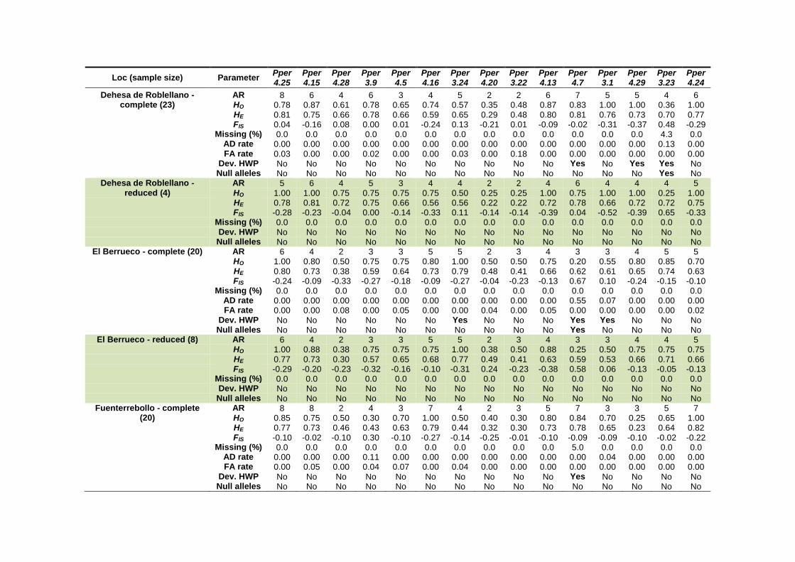
Loc (sample size) Parameter Pper4.25
Pper4.15
Pper4.28
Pper3.9
Pper4.5
Pper4.16
Pper3.24
Pper4.20
Pper3.22
Pper4.13
Pper4.7
Pper3.1
Pper4.29
Pper3.23
Pper4.24
Dehesa de Roblellano - complete (23)
AR 8 6 4 6 3 4 5 2 2 6 7 5 5 4 6 HO 0.78 0.87 0.61 0.78 0.65 0.74 0.57 0.35 0.48 0.87 0.83 1.00 1.00 0.36 1.00
HE 0.81 0.75 0.66 0.78 0.66 0.59 0.65 0.29 0.48 0.80 0.81 0.76 0.73 0.70 0.77
FIS 0.04 -0.16 0.08 0.00 0.01 -0.24 0.13 -0.21 0.01 -0.09 -0.02 -0.31 -0.37 0.48 -0.29
Missing (%) 0.0 0.0 0.0 0.0 0.0 0.0 0.0 0.0 0.0 0.0 0.0 0.0 0.0 4.3 0.0
AD rate 0.00 0.00 0.00 0.00 0.00 0.00 0.00 0.00 0.00 0.00 0.00 0.00 0.00 0.13 0.00
FA rate 0.03 0.00 0.00 0.02 0.00 0.00 0.03 0.00 0.18 0.00 0.00 0.00 0.00 0.00 0.00
Dev. HWP No No No No No No No No No No Yes No Yes Yes No
Null alleles No No No No No No No No No No No No No Yes No
Dehesa de Roblellano - reduced (4)
AR 5 6 4 5 3 4 4 2 2 4 6 4 4 4 5 HO 1.00 1.00 0.75 0.75 0.75 0.75 0.50 0.25 0.25 1.00 0.75 1.00 1.00 0.25 1.00
HE 0.78 0.81 0.72 0.75 0.66 0.56 0.56 0.22 0.22 0.72 0.78 0.66 0.72 0.72 0.75
FIS -0.28 -0.23 -0.04 0.00 -0.14 -0.33 0.11 -0.14 -0.14 -0.39 0.04 -0.52 -0.39 0.65 -0.33
Missing (%) 0.0 0.0 0.0 0.0 0.0 0.0 0.0 0.0 0.0 0.0 0.0 0.0 0.0 0.0 0.0
Dev. HWP No No No No No No No No No No No No No No No
Null alleles No No No No No No No No No No No No No No No
El Berrueco - complete (20) AR 6 4 2 3 3 5 5 2 3 4 3 3 4 5 5
HO 1.00 0.80 0.50 0.75 0.75 0.80 1.00 0.50 0.50 0.75 0.20 0.55 0.80 0.85 0.70
HE 0.80 0.73 0.38 0.59 0.64 0.73 0.79 0.48 0.41 0.66 0.62 0.61 0.65 0.74 0.63
FIS -0.24 -0.09 -0.33 -0.27 -0.18 -0.09 -0.27 -0.04 -0.23 -0.13 0.67 0.10 -0.24 -0.15 -0.10
Missing (%) 0.0 0.0 0.0 0.0 0.0 0.0 0.0 0.0 0.0 0.0 0.0 0.0 0.0 0.0 0.0
AD rate 0.00 0.00 0.00 0.00 0.00 0.00 0.00 0.00 0.00 0.00 0.55 0.07 0.00 0.00 0.00
FA rate 0.00 0.00 0.08 0.00 0.05 0.00 0.00 0.04 0.00 0.05 0.00 0.00 0.00 0.00 0.02
Dev. HWP No No No No No No Yes No No No Yes Yes No No No
Null alleles No No No No No No No No No No Yes No No No No
El Berrueco - reduced (8) AR 6 4 2 3 3 5 5 2 3 4 3 3 4 4 5
HO 1.00 0.88 0.38 0.75 0.75 0.75 1.00 0.38 0.50 0.88 0.25 0.50 0.75 0.75 0.75
HE 0.77 0.73 0.30 0.57 0.65 0.68 0.77 0.49 0.41 0.63 0.59 0.53 0.66 0.71 0.66
FIS -0.29 -0.20 -0.23 -0.32 -0.16 -0.10 -0.31 0.24 -0.23 -0.38 0.58 0.06 -0.13 -0.05 -0.13
Missing (%) 0.0 0.0 0.0 0.0 0.0 0.0 0.0 0.0 0.0 0.0 0.0 0.0 0.0 0.0 0.0
Dev. HWP No No No No No No No No No No No No No No No
Null alleles No No No No No No No No No No No No No No No
Fuenterrebollo - complete (20)
AR 8 8 2 4 3 7 4 2 3 5 7 3 3 5 7 HO 0.85 0.75 0.50 0.30 0.70 1.00 0.50 0.40 0.30 0.80 0.84 0.70 0.25 0.65 1.00
HE 0.77 0.73 0.46 0.43 0.63 0.79 0.44 0.32 0.30 0.73 0.78 0.65 0.23 0.64 0.82
FIS -0.10 -0.02 -0.10 0.30 -0.10 -0.27 -0.14 -0.25 -0.01 -0.10 -0.09 -0.09 -0.10 -0.02 -0.22
Missing (%) 0.0 0.0 0.0 0.0 0.0 0.0 0.0 0.0 0.0 0.0 5.0 0.0 0.0 0.0 0.0
AD rate 0.00 0.00 0.00 0.11 0.00 0.00 0.00 0.00 0.00 0.00 0.00 0.04 0.00 0.00 0.00
FA rate 0.00 0.05 0.00 0.04 0.07 0.00 0.04 0.00 0.00 0.00 0.00 0.00 0.00 0.00 0.00
Dev. HWP No No No No No No No No No No Yes No No No No
Null alleles No No No No No No No No No No No No No No No

Loc (sample size) Parameter Pper4.25
Pper4.15
Pper4.28
Pper3.9
Pper4.5
Pper4.16
Pper3.24
Pper4.20
Pper3.22
Pper4.13
Pper4.7
Pper3.1
Pper4.29
Pper3.23
Pper4.24
Fuenterrebollo - reduced (10) AR 6 7 2 4 3 7 4 2 3 5 7 3 3 5 7
HO 0.80 0.80 0.50 0.30 0.60 1.00 0.60 0.40 0.40 0.70 0.90 0.70 0.30 0.50 1.00
HE 0.76 0.76 0.46 0.35 0.60 0.80 0.48 0.32 0.40 0.71 0.77 0.66 0.27 0.62 0.83
FIS -0.06 -0.05 -0.10 0.13 -0.01 -0.26 -0.26 -0.25 -0.01 0.01 -0.18 -0.06 -0.13 0.19 -0.20
Missing (%) 0.0 0.0 0.0 0.0 0.0 0.0 0.0 0.0 0.0 0.0 0.0 0.0 0.0 0.0 0.0
Dev. HWP No No No No No No No No No No No No No No No
Null alleles No No No No No No No No No No No No No No No
La Pradera de Navalhorno - complete (23)
AR 16 12 6 6 3 10 6 3 3 8 13 7 8 6 11 HO 0.91 0.87 0.83 0.57 0.48 0.78 0.83 0.48 0.39 0.70 0.87 0.83 0.91 0.61 0.57
HE 0.91 0.88 0.59 0.65 0.66 0.84 0.70 0.45 0.40 0.84 0.87 0.82 0.72 0.72 0.87
FIS 0.00 0.01 -0.39 0.13 0.27 0.07 -0.18 -0.06 0.03 0.17 0.00 -0.01 -0.27 0.16 0.35
Missing (%) 0.0 0.0 0.0 0.0 0.0 0.0 0.0 0.0 0.0 0.0 0.0 0.0 0.0 0.0 0.0
AD rate 0.01 0.03 0.00 0.05 0.19 0.05 0.00 0.04 0.01 0.10 0.00 0.01 0.00 0.02 0.25
FA rate 0.12 0.13 0.05 0.06 0.05 0.00 0.00 0.04 0.00 0.08 0.00 0.05 0.05 0.00 0.06
Dev. HWP No No No No No No No No No No No No No No Yes
Null alleles No No No No No No No No No No No No No No Yes
La Pradera de Navalhorno - reduced (19)
AR 16 11 6 6 3 10 6 3 3 8 13 7 8 6 11 HO 0.89 0.89 0.89 0.58 0.58 0.79 0.79 0.42 0.47 0.63 0.84 0.84 0.89 0.53 0.53
HE 0.91 0.87 0.62 0.64 0.66 0.82 0.71 0.45 0.46 0.83 0.87 0.83 0.73 0.73 0.87
FIS 0.01 -0.02 -0.45 0.09 0.12 0.04 -0.12 0.06 -0.03 0.24 0.03 -0.02 -0.23 0.28 0.39
Missing (%) 0.0 0.0 0.0 0.0 0.0 0.0 0.0 0.0 0.0 0.0 0.0 0.0 0.0 0.0 0.0
Dev. HWP No No No No No No No No No No No No No No Yes
Null alleles No No No No No No No No No Yes No No No Yes Yes
Medianillos - complete (25) AR 17 11 6 7 3 10 8 2 4 12 19 8 9 6 12
HO 0.88 0.88 0.76 0.88 0.72 0.72 0.92 0.56 0.32 0.96 1.00 0.76 0.76 0.40 0.64
HE 0.92 0.88 0.63 0.80 0.61 0.81 0.80 0.48 0.34 0.86 0.91 0.79 0.66 0.69 0.89
FIS 0.04 0.00 -0.21 -0.10 -0.19 0.11 -0.15 -0.17 0.06 -0.11 -0.10 0.04 -0.15 0.42 0.28
Missing (%) 0.0 0.0 0.0 0.0 0.0 0.0 0.0 0.0 0.0 0.0 0.0 0.0 0.0 0.0 0.0
AD rate 0.00 0.00 0.00 0.00 0.00 0.00 0.00 0.00 0.00 0.00 0.00 0.10 0.00 0.19 0.16
FA rate 0.00 0.04 0.07 0.07 0.08 0.07 0.00 0.00 0.00 0.09 0.06 0.00 0.07 0.00 0.07
Dev. HWP Yes No No No No No No No No No No Yes No Yes No
Null alleles No No No No No No No No No No No No No Yes Yes
Medianillos - reduced (20) AR 16 10 5 6 3 10 8 2 4 12 18 8 8 6 10
HO 0.90 0.90 0.80 0.90 0.65 0.70 0.95 0.60 0.35 0.95 1.00 0.85 0.75 0.40 0.65
HE 0.92 0.88 0.64 0.79 0.61 0.80 0.79 0.48 0.34 0.86 0.91 0.78 0.67 0.70 0.88
FIS 0.02 -0.03 -0.25 -0.13 -0.06 0.13 -0.20 -0.25 -0.03 -0.11 -0.10 -0.09 -0.12 0.43 0.26
Missing (%) 0.0 0.0 0.0 0.0 0.0 0.0 0.0 0.0 0.0 0.0 0.0 0.0 0.0 0.0 0.0
Dev. HWP No No No No No No No No No No No No No Yes No
Null alleles No No No No No No No No No No No No No Yes Yes

Loc (sample size) Parameter Pper4.25
Pper4.15
Pper4.28
Pper3.9
Pper4.5
Pper4.16
Pper3.24
Pper4.20
Pper3.22
Pper4.13
Pper4.7
Pper3.1
Pper4.29
Pper3.23
Pper4.24
Puerto de Canencia - complete (22)
AR 18 12 4 8 3 11 9 2 6 14 14 5 7 5 11 HO 0.95 0.95 0.64 0.86 0.64 0.91 0.86 0.36 0.50 0.91 0.91 0.59 0.55 0.64 0.77
HE 0.92 0.88 0.52 0.81 0.62 0.85 0.78 0.43 0.51 0.89 0.89 0.67 0.48 0.60 0.88
FIS -0.04 -0.09 -0.23 -0.06 -0.03 -0.07 -0.11 0.16 0.01 -0.02 -0.02 0.12 -0.13 -0.06 0.12
Missing (%) 0.0 0.0 0.0 0.0 0.0 0.0 0.0 0.0 0.0 0.0 0.0 0.0 0.0 0.0 0.0
AD rate 0.00 0.00 0.00 0.00 0.00 0.00 0.00 0.07 0.01 0.00 0.03 0.05 0.00 0.00 0.08
FA rate 0.15 0.07 0.01 0.00 0.00 0.01 0.17 0.00 0.10 0.26 0.14 0.13 0.08 0.03 0.08
Dev. HWP No No No No No No No No No No No No No No No
Null alleles No No No No No No No No No No No No No No No
Puerto de Canencia - reduced (19)
AR 18 11 4 8 3 11 9 2 6 13 14 5 6 5 11 HO 0.95 0.95 0.58 0.89 0.63 0.89 0.84 0.42 0.53 0.95 0.89 0.53 0.58 0.68 0.79
HE 0.92 0.87 0.46 0.81 0.62 0.84 0.79 0.47 0.53 0.90 0.89 0.62 0.47 0.63 0.88
FIS -0.03 -0.09 -0.26 -0.11 -0.01 -0.06 -0.06 0.10 0.01 -0.05 0.00 0.15 -0.23 -0.09 0.11
Missing (%) 0.0 0.0 0.0 0.0 0.0 0.0 0.0 0.0 0.0 0.0 0.0 0.0 0.0 0.0 0.0
Dev. HWP No No No No No No No No No No No No No No No
Null alleles No No No No No No No No No No No No No No No
Puerto de La Morcuera - complete (22)
AR 10 8 2 6 3 7 7 2 4 9 9 3 5 4 6 HO 0.95 0.64 0.27 0.59 0.55 0.77 0.86 0.59 0.55 0.82 0.91 0.50 0.59 0.59 0.71
HE 0.87 0.80 0.24 0.67 0.54 0.80 0.75 0.49 0.56 0.82 0.81 0.64 0.52 0.58 0.78
FIS -0.09 0.20 -0.16 0.11 -0.01 0.04 -0.15 -0.20 0.03 0.01 -0.13 0.22 -0.13 -0.02 0.08
Missing (%) 0.0 0.0 0.0 0.0 0.0 0.0 0.0 0.0 0.0 0.0 0.0 0.0 0.0 0.0 4.5
AD rate 0.00 0.05 0.00 0.00 0.05 0.00 0.00 0.00 0.00 0.00 0.00 0.00 0.00 0.08 0.05
FA rate 0.06 0.00 0.00 0.02 0.00 0.00 0.06 0.19 0.00 0.00 0.00 0.00 0.04 0.07 0.02
Dev. HWP No No No No No No No No No No No No No No No
Null alleles No No No No No No No No No No No No No No No
Puerto de La Morcuera - reduced (15)
AR 10 8 2 6 3 7 7 2 4 9 8 3 4 4 6 HO 0.93 0.60 0.13 0.80 0.53 0.67 0.93 0.60 0.53 0.80 0.87 0.40 0.67 0.60 0.67
HE 0.87 0.78 0.12 0.72 0.58 0.82 0.76 0.49 0.57 0.83 0.76 0.62 0.54 0.56 0.76
FIS -0.08 0.24 -0.07 -0.11 0.09 0.19 -0.22 -0.22 0.07 0.04 -0.14 0.36 -0.24 -0.07 0.12
Missing (%) 0.0 0.0 0.0 0.0 0.0 0.0 0.0 0.0 0.0 0.0 0.0 0.0 0.0 0.0 0.0
Dev. HWP No No No No No No No No No No No No No No No
Null alleles No No No No No No No No No No No No No No No
Rascafría - complete (22) AR 12 7 3 6 3 7 6 2 3 10 12 5 6 5 8
HO 0.82 0.86 0.18 0.64 0.64 0.77 0.50 0.45 0.68 0.77 0.91 0.41 0.64 0.82 0.86
HE 0.81 0.82 0.33 0.64 0.65 0.78 0.80 0.46 0.63 0.80 0.89 0.78 0.63 0.60 0.77
FIS -0.01 -0.05 0.46 0.00 0.01 0.01 0.37 0.02 -0.08 0.03 -0.02 0.48 -0.01 -0.36 -0.13
Missing (%) 0.0 0.0 0.0 0.0 0.0 0.0 0.0 0.0 0.0 0.0 0.0 0.0 0.0 0.0 0.0
AD rate 0.04 0.00 0.42 0.00 0.00 0.02 0.22 0.00 0.00 0.01 0.00 0.56 0.00 0.00 0.00
FA rate 0.10 0.00 0.04 0.04 0.00 0.00 0.00 0.08 0.00 0.00 0.06 0.16 0.00 0.00 0.07
Dev. HWP No No No No No No No No No No No Yes No No No
Null alleles No No Yes No No No Yes No No No No Yes No No No
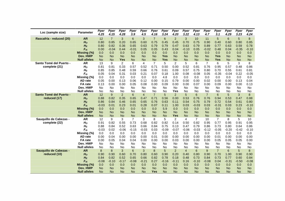
Loc (sample size) Parameter Pper4.25
Pper4.15
Pper4.28
Pper3.9
Pper4.5
Pper4.16
Pper3.24
Pper4.20
Pper3.22
Pper4.13
Pper4.7
Pper3.1
Pper4.29
Pper3.23
Pper4.24
Rascafría - reduced (20) AR 12 7 3 6 3 7 6 2 3 10 11 5 6 5 8
HO 0.80 0.85 0.20 0.65 0.60 0.75 0.45 0.45 0.70 0.75 0.90 0.40 0.60 0.80 0.85
HE 0.80 0.82 0.36 0.65 0.63 0.79 0.79 0.47 0.63 0.79 0.89 0.77 0.63 0.59 0.78
FIS 0.00 -0.04 0.44 -0.01 0.05 0.05 0.43 0.04 -0.10 0.05 -0.02 0.48 0.04 -0.35 -0.10
Missing (%) 0.0 0.0 0.0 0.0 0.0 0.0 0.0 0.0 0.0 0.0 0.0 0.0 0.0 0.0 0.0
Dev. HWP No No No No No No Yes No No No No Yes No No No
Null alleles No No Yes No No No Yes No No No No Yes No No No
Santo Tomé del Puerto - complete (21)
AR 13 9 2 6 4 7 5 2 5 6 7 6 5 3 8 HO 0.81 0.81 0.33 0.57 0.52 0.71 0.50 0.00 0.52 0.81 0.76 0.95 0.57 0.48 0.86
HE 0.85 0.85 0.48 0.59 0.66 0.76 0.61 0.09 0.57 0.75 0.80 0.70 0.55 0.61 0.81
FIS 0.05 0.04 0.31 0.03 0.21 0.07 0.18 1.00 0.08 -0.08 0.05 -0.35 -0.04 0.22 -0.05
Missing (%) 0.0 0.0 0.0 0.0 0.0 0.0 4.8 0.0 0.0 0.0 0.0 0.0 0.0 0.0 0.0
AD rate 0.05 0.00 0.13 0.06 0.12 0.00 0.15 0.79 0.00 0.00 0.02 0.00 0.00 0.13 0.04
FA rate 0.13 0.00 0.00 0.05 0.08 0.00 0.09 0.00 0.00 0.07 0.00 0.09 0.00 0.00 0.13
Dev. HWP No No No No No No No No No No No No No No No
Null alleles No No No No No No No Yes No No No No No No No
Santo Tomé del Puerto - reduced (17)
AR 12 9 2 6 4 7 5 2 5 6 7 6 5 3 8 HO 0.88 0.82 0.35 0.65 0.47 0.71 0.56 0.00 0.53 0.76 0.76 0.94 0.53 0.47 0.88
HE 0.86 0.84 0.46 0.65 0.65 0.76 0.63 0.11 0.54 0.75 0.79 0.72 0.54 0.61 0.80
FIS -0.03 0.01 0.23 0.01 0.28 0.07 0.11 1.00 0.03 -0.03 0.03 -0.31 0.03 0.23 -0.10
Missing (%) 0.0 0.0 0.0 0.0 0.0 0.0 5.9 0.0 0.0 0.0 0.0 0.0 0.0 0.0 0.0
Dev. HWP No No No No No No No No No No No No No No No
Null alleles No No No No No No No Yes No No No No No No No
Sauquillo de Cabezas - complete (22)
AR 12 9 3 7 3 8 5 2 4 7 10 7 8 5 10 HO 0.91 0.82 0.55 0.73 0.68 0.82 0.82 0.14 0.50 0.82 0.95 0.77 0.95 0.91 0.95
HE 0.88 0.84 0.52 0.63 0.66 0.84 0.75 0.13 0.47 0.79 0.86 0.73 0.80 0.64 0.86
FIS -0.03 0.02 -0.06 -0.15 -0.03 0.03 -0.09 -0.07 -0.06 -0.03 -0.12 -0.05 -0.20 -0.42 -0.10
Missing (%) 0.0 0.0 0.0 0.0 0.0 0.0 0.0 0.0 0.0 0.0 0.0 0.0 0.0 0.0 0.0
AD rate 0.00 0.04 0.00 0.00 0.00 0.01 0.00 0.00 0.00 0.00 0.00 0.01 0.00 0.00 0.00
FA rate 0.00 0.05 0.04 0.04 0.00 0.00 0.00 0.03 0.00 0.00 0.00 0.05 0.05 0.05 0.00
Dev. HWP No No No No No No No No No No No No No No No
Null alleles No No No No No No No No No No No No No No No
Sauquillo de Cabezas - reduced (10)
AR 8 8 3 6 3 8 5 2 4 6 9 7 6 5 8 HO 0.90 0.90 0.60 0.70 0.80 0.60 0.90 0.20 0.40 0.80 0.90 0.70 1.00 0.90 0.90
HE 0.84 0.82 0.52 0.65 0.66 0.82 0.78 0.18 0.48 0.73 0.84 0.73 0.77 0.60 0.84
FIS -0.08 -0.10 -0.17 -0.08 -0.21 0.27 -0.16 -0.11 0.16 -0.10 -0.08 0.04 -0.31 -0.50 -0.08
Missing (%) 0.0 0.0 0.0 0.0 0.0 0.0 0.0 0.0 0.0 0.0 0.0 0.0 0.0 0.0 0.0
Dev. HWP No No No No No No No No No No No No No No No
Null alleles No No No No No Yes No No No No No No No No No

Loc (sample size) Parameter Pper4.25
Pper4.15
Pper4.28
Pper3.9
Pper4.5
Pper4.16
Pper3.24
Pper4.20
Pper3.22
Pper4.13
Pper4.7
Pper3.1
Pper4.29
Pper3.23
Pper4.24
Turrubuelo - complete (21) AR 17 12 4 6 3 9 7 2 4 12 12 6 4 7 14
HO 1.00 0.95 0.62 0.76 0.67 1.00 0.86 0.33 0.45 0.90 0.90 0.76 0.57 0.81 0.90
HE 0.91 0.89 0.61 0.80 0.65 0.86 0.81 0.43 0.49 0.89 0.89 0.74 0.67 0.75 0.87
FIS -0.09 -0.07 -0.01 0.05 -0.02 -0.16 -0.05 0.22 0.08 -0.01 -0.01 -0.03 0.15 -0.09 -0.04
Missing (%) 0.0 0.0 0.0 0.0 0.0 0.0 0.0 0.0 4.8 4.8 0.0 0.0 0.0 0.0 0.0
AD rate 0.00 0.00 0.02 0.00 0.01 0.00 0.00 0.13 0.08 0.00 0.00 0.01 0.07 0.00 0.00
FA rate 0.07 0.08 0.12 0.00 0.03 0.11 0.11 0.00 0.00 0.11 0.03 0.01 0.00 0.05 0.12
Dev. HWP No No No No No No No No No No No No No No No
Null alleles No No No No No No No No No No No No No No No
Turrubuelo - reduced (15) AR 14 12 4 6 3 9 7 2 4 11 11 6 4 7 11
HO 1.00 0.93 0.67 0.80 0.73 1.00 0.87 0.40 0.50 0.86 0.87 0.80 0.60 0.80 0.87
HE 0.89 0.89 0.60 0.80 0.66 0.86 0.80 0.39 0.49 0.88 0.86 0.70 0.62 0.75 0.85
FIS -0.13 -0.05 -0.10 0.00 -0.11 -0.16 -0.08 -0.02 -0.03 0.02 0.00 -0.14 0.04 -0.07 -0.02
Missing (%) 0.0 0.0 0.0 0.0 0.0 0.0 0.0 0.0 6.7 6.7 0.0 0.0 0.0 0.0 0.0
Dev. HWP No No No No No No No No No No No No No No No
Null alleles No No No No No No No No No No No No No No No
Valdemanco - complete (94) AR 24 12 6 9 4 12 8 2 5 16 20 7 8 6 13
HO 0.95 0.75 0.52 0.77 0.60 0.83 0.85 0.40 0.41 0.96 0.84 0.81 0.86 0.76 0.92
HE 0.92 0.75 0.52 0.78 0.66 0.87 0.85 0.43 0.39 0.90 0.90 0.78 0.78 0.72 0.91
FIS -0.03 0.00 0.00 0.00 0.10 0.05 0.00 0.07 -0.06 -0.06 0.07 -0.03 -0.10 -0.05 -0.02
Missing (%) 2.1 1.1 1.1 1.1 0.0 1.1 1.1 0.0 3.2 3.2 0.0 1.1 3.2 2.1 3.2
AD rate 0.01 0.00 0.02 0.00 0.01 0.00 0.00 0.01 0.00 0.01 0.02 0.05 0.00 0.00 0.00
FA rate 0.00 0.01 0.00 0.01 0.00 0.03 0.00 0.00 0.00 0.01 0.00 0.01 0.01 0.04 0.03
Dev. HWP No No No No No No No No No No Yes No No No No
Null alleles No No No No No No No No No No Yes No No No No
Valdemanco - reduced (58) AR 23 12 6 9 4 12 8 2 5 15 20 7 8 6 13
HO 0.91 0.77 0.51 0.77 0.60 0.83 0.85 0.40 0.43 0.93 0.88 0.81 0.86 0.73 0.91
HE 0.91 0.73 0.53 0.79 0.67 0.86 0.85 0.43 0.43 0.90 0.91 0.79 0.77 0.74 0.90
FIS 0.00 -0.06 0.05 0.02 0.11 0.04 0.01 0.09 -0.01 -0.03 0.03 -0.03 -0.11 0.00 -0.01
Missing (%) 3.4 1.7 1.7 1.7 0.0 1.7 0.0 0.0 3.4 3.4 0.0 1.7 5.2 3.4 5.2
Dev. HWP No No No No No No No No No No No No No No No
Null alleles No No No No No No No No No No No No No No No


APPENDIX 2
ACCUMULATION CURVES OF ALLELIC RICHNESS AND EXPECTED HETEROZYGOSITY AS A FUNCTION OF SAMPLE SIZE
Suppl. Material from Sánchez-Montes et al. (2017) Journal of Heredity (doi: 10.1093/jhered/esx038)
(Chapter IV)


Accumulation curves
265
Figure A2.1. Accumulation curves of AR (dark lines) and HE (grey lines) as a function of sample size
(measured as number of individuals) for each marker in the H. molleri marker set. Jackknifed curves were
calculated from the complete samples in Valdemanco. Vertical dotted lines show the minimum sample size
at which the lower bound of the 95% confidence interval of each final estimate (shown as horizontal
dashed lines) is reached.
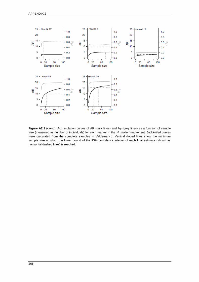
APPENDIX 2
266
Figure A2.1 (cont.). Accumulation curves of AR (dark lines) and HE (grey lines) as a function of sample
size (measured as number of individuals) for each marker in the H. molleri marker set. Jackknifed curves
were calculated from the complete samples in Valdemanco. Vertical dotted lines show the minimum
sample size at which the lower bound of the 95% confidence interval of each final estimate (shown as
horizontal dashed lines) is reached.

Accumulation curves
267
Figure A2.2. Accumulation curves of AR (dark lines) and HE (grey lines) as a function of sample size
(measured as number of individuals) for each marker in the E. calamita marker set. Jackknifed curves
were calculated from the complete samples in Valdemanco. Vertical dotted lines show the minimum
sample size at which the lower bound of the 95% confidence interval of each final estimate (shown as
horizontal dashed lines) is reached.

APPENDIX 2
268
Figure A2.2 (cont.). Accumulation curves of AR (dark lines) and HE (grey lines) as a function of sample
size (measured as number of individuals) for each marker in the E. calamita marker set. Jackknifed curves
were calculated from the complete samples in Valdemanco. Vertical dotted lines show the minimum
sample size at which the lower bound of the 95% confidence interval of each final estimate (shown as
horizontal dashed lines) is reached.

Accumulation curves
269
Figure A2.3. Accumulation curves of AR (dark lines) and HE (grey lines) as a function of sample size
(measured as number of individuals) for each marker in the P. perezi marker set. Jackknifed curves were
calculated from the complete samples in Valdemanco. Vertical dotted lines show the minimum sample size
at which the lower bound of the 95% confidence interval of each final estimate (shown as horizontal
dashed lines) is reached.

APPENDIX 2
270
Figure A2.3 (cont.). Accumulation curves of AR (dark lines) and HE (grey lines) as a function of sample
size (measured as number of individuals) for each marker in the P. perezi marker set. Jackknifed curves
were calculated from the complete samples in Valdemanco. Vertical dotted lines show the minimum
sample size at which the lower bound of the 95% confidence interval of each final estimate (shown as
horizontal dashed lines) is reached.
APPENDIX 3
EMPIRICAL AND CHAO & JOST (2015) PROFILES
Suppl. Material from Sánchez-Montes et al. (2017) Journal of Heredity (doi: 10.1093/jhered/esx038)
(Chapter IV)

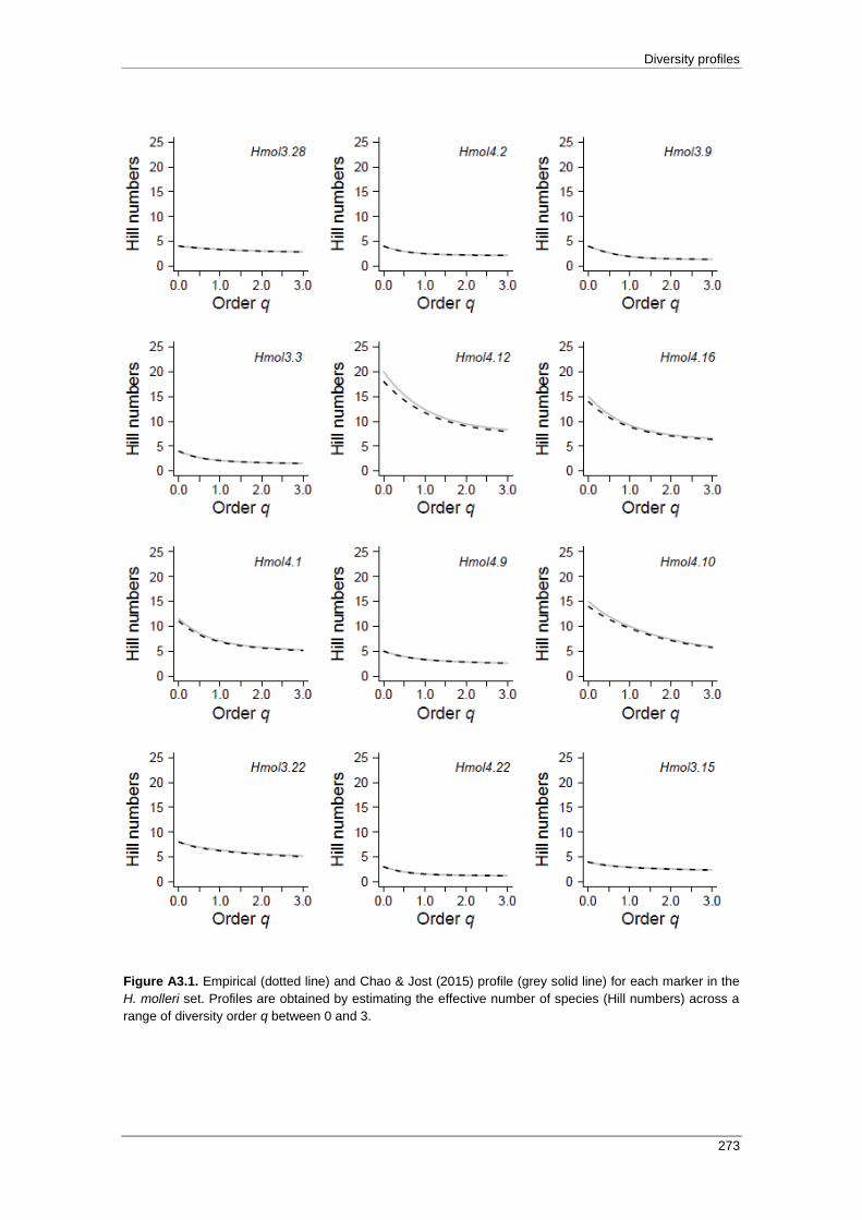
Diversity profiles
273
Figure A3.1. Empirical (dotted line) and Chao & Jost (2015) profile (grey solid line) for each marker in the
H. molleri set. Profiles are obtained by estimating the effective number of species (Hill numbers) across a
range of diversity order q between 0 and 3.

APPENDIX 3
274
Figure A3.1 (cont.). Empirical (dotted line) and Chao & Jost (2015) profile (grey solid line) for each marker
in the H. molleri set. Profiles are obtained by estimating the effective number of species (Hill numbers)
across a range of diversity order q between 0 and 3.

Diversity profiles
275
Figure A3.2. Empirical (dotted line) and Chao & Jost (2015) profile (grey solid line) for each marker in the
E. calamita set. Profiles are obtained by estimating the effective number of species (Hill numbers) across a
range of diversity order q between 0 and 3.

APPENDIX 3
276
Figure A3.2 (cont.). Empirical (dotted line) and Chao & Jost (2015) profile (grey solid line) for each marker
in the E. calamita set. Profiles are obtained by estimating the effective number of species (Hill numbers)
across a range of diversity order q between 0 and 3.
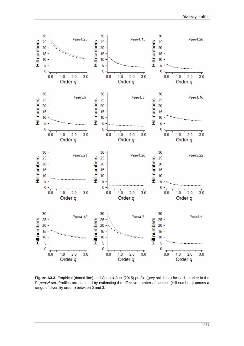
Diversity profiles
277
Figure A3.3. Empirical (dotted line) and Chao & Jost (2015) profile (grey solid line) for each marker in the
P. perezi set. Profiles are obtained by estimating the effective number of species (Hill numbers) across a
range of diversity order q between 0 and 3.

APPENDIX 3
278
Figure A3.3 (cont.). Empirical (dotted line) and Chao & Jost (2015) profile (grey solid line) for each marker
in the P. perezi set. Profiles are obtained by estimating the effective number of species (Hill numbers)
across a range of diversity order q between 0 and 3.

APPENDIX 4
RELATIONSHIP BETWEEN FIS AND ERROR RATE ESTIMATES
Suppl. Material from Sánchez-Montes et al. (2017) Journal of Heredity (doi: 10.1093/jhered/esx038)
(Chapter IV)


Effect of excessive relatives in the sample
281
Figure A4.1. Relationship between FIS and error rate estimates (empty dots: allelic dropout rate, solid
dots: false allele rate) obtained from sibship analyses for each marker in the three species. Note the
difference in axis scales in the E. calamita graph.


APPENDIX 5
EFFECT OF SAMPLING EXCESSIVE CLOSE RELATIVES ON FIS AND DEVIATION FROM HWE
Suppl. Material from Sánchez-Montes et al. (2017) Journal of Heredity (doi: 10.1093/jhered/esx038)
(Chapter IV)


Effect of excessive relatives in the sample
285
Wright’s (1931) FIS is the traditional and most popular statistic used in measuring the
distribution of genetic variation within and among individuals in a population. For a
population at Hardy-Weinberg equilibrium (HWE), homologous allelic copies are
independently distributed within and between individuals. In such a situation, FIS = 0.
For a population with subdivision (e.g. in social groups) or with close relative mating,
the two allelic copies within an individual are more probable to be identical in state than
those in different individuals. In such a situation, the observed homozygosity is higher
than that expected if the population is at HWE, leading to FIS > 0 (since 𝐹𝐼𝑆 = 1 −𝐻𝑂
𝐻𝐸,
where HO and HE are the observed and expected heterozygosity, respectively) (Nei
1977). In contrast, admixture and hybridization lead to FIS < 0.
The FIS of a population is usually unknown, and is estimated by the marker or
pedigree data of a sample of individuals drawn from the population. Here we show
analytically that sampling too many close relatives would lead to a reduced FIS estimate.
For a large population at HWE in which FIS = 0, a sample from it can yield a negative
FIS estimate if it contains excessive close relatives. These predictions are true no matter
whether pedigree or marker data are used in the estimation.
Denoting the probabilities of identity by descent (PIBD) for two homologous
genes drawn at random from an individual and between two individuals in a population
by F and θ, respectively, we have
𝐹𝐼𝑆 =𝐹−𝜃
1−𝜃 , (1)
by definition (Cockerham 1969, eqn 41; Weir 1996, p.176). In (1), F and θ are the
inbreeding coefficient of an individual and the coancestry between two individuals. If a
random sample (random with regard to genealogy) is taken from the population, then
unbiased estimates of F, θ, and thus FIS estimates would be obtained. However, if too
many (excessive) close relatives, such as full or half siblings, are included in a sample,
the PIBD between individuals in the population would be overestimated, from the true
value θ to θ’, while the estimated PIBD within individuals would remain unbiased as F.
As a result, 𝐹𝐼𝑆 would be expected to be decreased to
𝐹𝐼𝑆′ =
𝐹−𝜃′
1−𝜃′ (2)

APPENDIX 5
286
Equation (2) implies that 𝐹𝐼𝑆′ < 𝐹𝐼𝑆, because 𝜃′ > 𝜃. The larger the increase in PIBD
between sampled individuals, 𝜃′, due to the inclusion of a greater proportion of close
relatives, the smaller will be 𝐹𝐼𝑆′ relative to 𝐹𝐼𝑆.
For illustration, let us consider some numerical examples for a dioecious diploid
species in a large random mating population. It is expected that two homologous genes
at an autosomal locus are identical by descent with probabilities 0, 0 and ¼ when they
are in a single individual, in two unrelated individuals, and in two full siblings,
respectively. In a sample of individuals taken at random from the population, the
estimated PIBDs are expected to be F = 0 and 𝜃 = 0, and thus the estimated FIS is also
expected to be zero. In an inadequately drawn sample of individuals with a proportion
of δ full-sib pairs, the estimated PIBDs are expected to be F = 0, 𝜃 = (1 − 𝛿) × 0 +
𝛿 × 1/4 =𝛿
4, and the estimated FIS is expected to be
0−𝛿
4
1−𝛿
4
= −𝛿/(4 − 𝛿). Suppose a
sample has n=50 individuals, with 10 individuals taken from full sib family X, 20
individuals from full sib family Y, and the remaining 20 individuals from 20 different
and unrelated families. The proportion of full sib pairs in the sample is 𝛿 =
10×9/2+20×19/2
50×49/2= 0.1918, the estimated PIBDs are expected to be F = 0, 𝜃 = 0.1918 ×
1
4= 0.048, and the estimated FIS is expected to be
0−0.048
1−0.048= −0.0504, rather than the
expected value of zero.
As it can be seen from the examples, the inclusion of an excessive proportion of
relatives (in this case, full siblings) in a sample causes a reduction in the estimated FIS.
Conversely, including an excessively low proportion of full sibs in the sample (relative
to the true proportion in the population) results in an artificially inflated estimate of FIS.
Depending on the values of F and 𝜃, this bias may lead in some cases to false inferences
of negative inbreeding (and the false conclusion that the population is affected by
admixture (hybridization) or/and avoids close relative matings) or positive inbreeding
(false conclusion of positive assortative mating or population subdivision). For the same
reason, removing all but one of the full sibs in every full sib family in the sample does
not always eliminate the bias caused by unrepresentative proportion of full sibs in the
sample (Waples & Anderson 2017). In fact, it could lead to an underrepresentation of
full sibs in the sample and thus to the opposite bias, with 𝐹𝐼𝑆′ > 𝐹𝐼𝑆.

Effect of excessive relatives in the sample
287
As a result, excessive close relatives in a sample cause an apparent decrease in
observed homozygotes and an apparent increase in observed heterozygotes at each locus
(i.e. higher HO/HE ratio). Excessive close relatives in a sample can also cause apparent
nonrandom associations between alleles in different loci. This leads to an increase in
statistically significant deviations from HWE across loci and evidences of LD, which
disappear when the excess of relatives is removed.
References
Wright S (1931) Evolution in Mendelian populations. Genetics, 16, 97–159.
Cockerham CC (1969) Variance of gene frequencies. Evolution, 23, 72–84.
Nei M (1977) F-statistics and analysis of gene diversity in subdivided populations. Annals of
Human Genetics, 41, 225–233.
Waples RS, Anderson EC (2017) Purging putative siblings from population genetic data sets: a
cautionary view. Molecular Ecology, 26, 1211–1224.
Weir BS (1996) Genetic data analysis II: Methods for discrete population genetic data. Sinauer
Assoc., Inc., Sunderland, MA, USA.


APPENDIX 6
R SCRIPTS FOR REPLICATED ANALYSES
Appendix S1 in Sánchez-Montes et al. Ecology and Evolution (accepted, pending minor review)
(Chapter V)

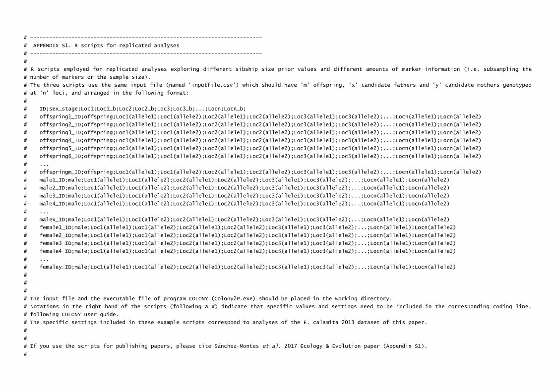
# -------------------------------------------------------------------------
# APPENDIX S1. R scripts for replicated analyses
# -------------------------------------------------------------------------
#
# R scripts employed for replicated analyses exploring different sibship size prior values and different amounts of marker information (i.e. subsampling the
# number of markers or the sample size).
# The three scripts use the same input file (named ‘inputfile.csv’) which should have 'm' offspring, 'x' candidate fathers and 'y' candidate mothers genotyped
# at 'n' loci, and arranged in the following format:
#
# ID;sex_stage;Loc1;Loc1_b;Loc2;Loc2_b;Loc3;Loc3_b;...;Locn;Locn_b;
# offspring1_ID;offspring;Loc1(allele1);Loc1(allele2);Loc2(allele1);Loc2(allele2);Loc3(allele1);Loc3(allele2);...;Locn(allele1);Locn(allele2)
# offspring2_ID;offspring;Loc1(allele1);Loc1(allele2);Loc2(allele1);Loc2(allele2);Loc3(allele1);Loc3(allele2);...;Locn(allele1);Locn(allele2)
# offspring3_ID;offspring;Loc1(allele1);Loc1(allele2);Loc2(allele1);Loc2(allele2);Loc3(allele1);Loc3(allele2);...;Locn(allele1);Locn(allele2)
# offspring4_ID;offspring;Loc1(allele1);Loc1(allele2);Loc2(allele1);Loc2(allele2);Loc3(allele1);Loc3(allele2);...;Locn(allele1);Locn(allele2)
# offspring5_ID;offspring;Loc1(allele1);Loc1(allele2);Loc2(allele1);Loc2(allele2);Loc3(allele1);Loc3(allele2);...;Locn(allele1);Locn(allele2)
# offspring6_ID;offspring;Loc1(allele1);Loc1(allele2);Loc2(allele1);Loc2(allele2);Loc3(allele1);Loc3(allele2);...;Locn(allele1);Locn(allele2)
# ...
# offspringm_ID;offspring;Loc1(allele1);Loc1(allele2);Loc2(allele1);Loc2(allele2);Loc3(allele1);Loc3(allele2);...;Locn(allele1);Locn(allele2)
# male1_ID;male;Loc1(allele1);Loc1(allele2);Loc2(allele1);Loc2(allele2);Loc3(allele1);Loc3(allele2);...;Locn(allele1);Locn(allele2)
# male2_ID;male;Loc1(allele1);Loc1(allele2);Loc2(allele1);Loc2(allele2);Loc3(allele1);Loc3(allele2);...;Locn(allele1);Locn(allele2)
# male3_ID;male;Loc1(allele1);Loc1(allele2);Loc2(allele1);Loc2(allele2);Loc3(allele1);Loc3(allele2);...;Locn(allele1);Locn(allele2)
# male4_ID;male;Loc1(allele1);Loc1(allele2);Loc2(allele1);Loc2(allele2);Loc3(allele1);Loc3(allele2);...;Locn(allele1);Locn(allele2)
# ...
# malex_ID;male;Loc1(allele1);Loc1(allele2);Loc2(allele1);Loc2(allele2);Loc3(allele1);Loc3(allele2);...;Locn(allele1);Locn(allele2)
# female1_ID;male;Loc1(allele1);Loc1(allele2);Loc2(allele1);Loc2(allele2);Loc3(allele1);Loc3(allele2);...;Locn(allele1);Locn(allele2)
# female2_ID;male;Loc1(allele1);Loc1(allele2);Loc2(allele1);Loc2(allele2);Loc3(allele1);Loc3(allele2);...;Locn(allele1);Locn(allele2)
# female3_ID;male;Loc1(allele1);Loc1(allele2);Loc2(allele1);Loc2(allele2);Loc3(allele1);Loc3(allele2);...;Locn(allele1);Locn(allele2)
# female4_ID;male;Loc1(allele1);Loc1(allele2);Loc2(allele1);Loc2(allele2);Loc3(allele1);Loc3(allele2);...;Locn(allele1);Locn(allele2)
# ...
# femaley_ID;male;Loc1(allele1);Loc1(allele2);Loc2(allele1);Loc2(allele2);Loc3(allele1);Loc3(allele2);...;Locn(allele1);Locn(allele2)
#
#
#
# The input file and the executable file of program COLONY (Colony2P.exe) should be placed in the working directory.
# Notations in the right hand of the scripts (following a #) indicate that specific values and settings need to be included in the corresponding coding line,
# following COLONY user guide.
# The specific settings included in these example scripts correspond to analyses of the E. calamita 2013 dataset of this paper.
#
#
# If you use the scripts for publishing papers, please cite Sánchez-Montes et al. 2017 Ecology & Evolution paper (Appendix S1).
#

#-------------------------------------------------------------------
# Analyses for exploring different prior values
#-------------------------------------------------------------------
inputfile<-read.csv(file="inputfile.csv", header=T, sep=";")
outputfile<-"outputfile.txt"
cat("filename","prior","totmal","totfem","Polymal","Polyfem","Avgemal","Avgefem","Ne","Ne_min","Ne_max",file=outputfile,append=TRUE,sep = ",",fill=TRUE)
offspring<-subset(inputfile, inputfile$sex_stage=="offspring")
offspring<-offspring[c(-2)]
cmales<-subset(inputfile, inputfile$sex_stage=="male")
cmales<-cmales[c(-2)]
cfemales<-subset(inputfile, inputfile$sex_stage=="female")
cfemales<-cfemales[c(-2)]
for (i in 1:5) { #Set the desired prior values to explore
for (j in 1:10) { #Set the desired number of replicates for each prior value
filename<-paste("analysis",i,"prior",j,sep="_")
input.file<-paste(filename,".dat", sep="")
options(width=1000)
cat(filename, file=input.file, append=TRUE, sep = "\n")
cat(filename, file=input.file, append=TRUE, sep = "\n")
cat(length(offspring$ID), file=input.file, append=TRUE, sep = "\n")
cat((ncol(offspring)-1)/2, file=input.file, append=TRUE, sep = "\n")
cat(sample(100000, 1), file=input.file, append=TRUE, sep = "\n")
cat(0, file=input.file, append=TRUE, sep = "\n") #0/1=Not updating/updating allele frequency
cat(2, file=input.file, append=TRUE, sep = "\n") #2/1=Dioecious/Monoecious species
cat(0, file=input.file, append=TRUE, sep = "\n") #0/1=Inbreeding absent/present
cat(0, file=input.file, append=TRUE, sep = "\n") #0/1=Diploid species/HaploDiploid species
cat("0 0", file=input.file, append=TRUE, sep = "\n") #0/1=Polygamy/Monogamy for males & females
cat(0, file=input.file, append=TRUE, sep = "\n") #0/1 = Clone inference = No/Yes
cat(0, file=input.file, append=TRUE, sep = "\n") #0/1=Scale full sibship=No/Yes
cat(paste(1, i, i, sep=" "), file=input.file, append=TRUE, sep = "\n") #0/1/2/3/4=No/Weak/Medium/Strong sibship prior; 4=Optimal sibship prior for Ne
cat(0, file=input.file, append=TRUE, sep = "\n") #0/1=Unknown/Known population allele frequency
cat(1, file=input.file, append=TRUE, sep = "\n") #Number of runs
cat(2, file=input.file, append=TRUE, sep = "\n") #1/2/3/4 = Short/Medium/Long/VeryLong run
cat(0, file=input.file, append=TRUE, sep = "\n") #0/1=Monitor method by Iterate#/Time in second
cat("100000", file=input.file, append=TRUE, sep = "\n") #Monitor interval in Iterate# / in seconds
cat(0, file=input.file, append=TRUE, sep = "\n") #0/1=DOS/Windows version
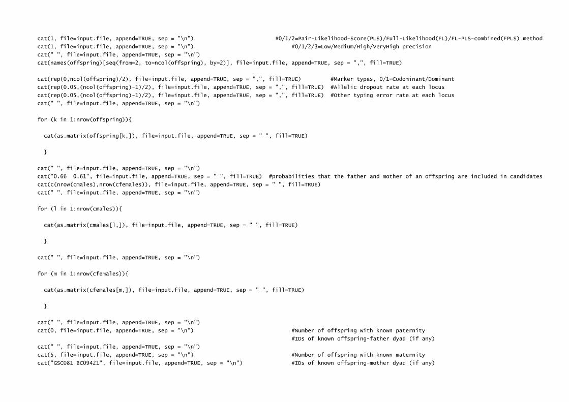
cat(1, file=input.file, append=TRUE, sep = "\n") #0/1/2=Pair-Likelihood-Score(PLS)/Full-Likelihood(FL)/FL-PLS-combined(FPLS) method
cat(1, file=input.file, append=TRUE, sep = "\n") #0/1/2/3=Low/Medium/High/VeryHigh precision
cat(" ", file=input.file, append=TRUE, sep = "\n")
cat(names(offspring)[seq(from=2, to=ncol(offspring), by=2)], file=input.file, append=TRUE, sep = ",", fill=TRUE)
cat(rep(0,ncol(offspring)/2), file=input.file, append=TRUE, sep = ",", fill=TRUE) #Marker types, 0/1=Codominant/Dominant
cat(rep(0.05,(ncol(offspring)-1)/2), file=input.file, append=TRUE, sep = ",", fill=TRUE) #Allelic dropout rate at each locus
cat(rep(0.05,(ncol(offspring)-1)/2), file=input.file, append=TRUE, sep = ",", fill=TRUE) #Other typing error rate at each locus
cat(" ", file=input.file, append=TRUE, sep = "\n")
for (k in 1:nrow(offspring)){
cat(as.matrix(offspring[k,]), file=input.file, append=TRUE, sep = " ", fill=TRUE)
}
cat(" ", file=input.file, append=TRUE, sep = "\n")
cat("0.66 0.61", file=input.file, append=TRUE, sep = " ", fill=TRUE) #probabilities that the father and mother of an offspring are included in candidates
cat(c(nrow(cmales),nrow(cfemales)), file=input.file, append=TRUE, sep = " ", fill=TRUE)
cat(" ", file=input.file, append=TRUE, sep = "\n")
for (l in 1:nrow(cmales)){
cat(as.matrix(cmales[l,]), file=input.file, append=TRUE, sep = " ", fill=TRUE)
}
cat(" ", file=input.file, append=TRUE, sep = "\n")
for (m in 1:nrow(cfemales)){
cat(as.matrix(cfemales[m,]), file=input.file, append=TRUE, sep = " ", fill=TRUE)
}
cat(" ", file=input.file, append=TRUE, sep = "\n")
cat(0, file=input.file, append=TRUE, sep = "\n") #Number of offspring with known paternity
#IDs of known offspring-father dyad (if any)
cat(" ", file=input.file, append=TRUE, sep = "\n")
cat(5, file=input.file, append=TRUE, sep = "\n") #Number of offspring with known maternity
cat("GSC081 BC09421", file=input.file, append=TRUE, sep = "\n") #IDs of known offspring-mother dyad (if any)
cat("GSC082 BC09421", file=input.file, append=TRUE, sep = "\n") #IDs of known offspring-mother dyad (if any)
cat("GSC083 BC09421", file=input.file, append=TRUE, sep = "\n") #IDs of known offspring-mother dyad (if any)
cat("GSC084 BC09421", file=input.file, append=TRUE, sep = "\n") #IDs of known offspring-mother dyad (if any)
cat("GSC085 BC09421", file=input.file, append=TRUE, sep = "\n") #IDs of known offspring-mother dyad (if any)
cat(" ", file=input.file, append=TRUE, sep = "\n")
cat(0, file=input.file, append=TRUE, sep = "\n") #Number of known paternal sibship
#Size of known paternal sibship, and IDs of offspring in the sibship (if any)
cat(" ", file=input.file, append=TRUE, sep = "\n")
cat(0, file=input.file, append=TRUE, sep = "\n") #Number of known maternal sibship
#Size of known maternal sibship, and IDs of offspring in the sibship (if any)
cat(" ", file=input.file, append=TRUE, sep = "\n")
cat(0, file=input.file, append=TRUE, sep = "\n") #Number of offspring with known excluded paternity
#Offspring ID, number of excluded males, the IDs of excluded males
cat(" ", file=input.file, append=TRUE, sep = "\n")
cat(0, file=input.file, append=TRUE, sep = "\n") #Number of offspring with known excluded maternity
#Offspring ID, number of excluded females, the IDs of excluded females
cat(" ", file=input.file, append=TRUE, sep = "\n")
cat(0, file=input.file, append=TRUE, sep = "\n") #Number of offspring with known excluded paternal sibships
#Offspring ID, number of excluded paternal sibships, the IDs of excluded offspring
cat(" ", file=input.file, append=TRUE, sep = "\n")
cat(0, file=input.file, append=TRUE, sep = "\n") #Number of offspring with known excluded maternal sibships
#Offspring ID, number of excluded maternal sibships, the IDs of excluded offspring
system(paste("Colony2p.exe IFN:", input.file, sep=""))
results<-read.delim(file=paste(filename,".BestCluster", sep=""), header=T, sep="")
male.matrix<-as.data.frame.matrix(table(results$FatherID, results$MotherID))
male.matrix$male_matings<-rowSums(male.matrix>0)
male.matrix<-male.matrix[!male.matrix$male_matings==0,]
mal<-data.frame(table(male.matrix$male_matings))
dimnames(mal)[[2]]<-c("N_matings", "N_indiv")
mal$sex<-c(rep("males", nrow(mal)))
female.matrix<-as.data.frame.matrix(table(results$MotherID, results$FatherID))
female.matrix$female_matings<-rowSums(female.matrix>0)
female.matrix<-female.matrix[!female.matrix$female_matings==0,]
femal<-data.frame(table(female.matrix$female_matings))
dimnames(femal)[[2]]<-c("N_matings", "N_indiv")
femal$sex<-c(rep("females", nrow(femal)))
total.males<-sum(mal$N_indiv)
total.females<-sum(femal$N_indiv)
poly.males<-subset(mal, !mal$N_matings==1)
poly.females<-subset(femal, !femal$N_matings==1)
Mult.mating.males<-sum(poly.males$N_indiv)
Mult.mating.females<-sum(poly.females$N_indiv)
Polygamy.rate.males<-Mult.mating.males/total.males
Polygamy.rate.females<-Mult.mating.females/total.females
mal$N_matings<-as.numeric(mal$N_matings)
mal$N_indiv<-as.numeric(mal$N_indiv)
total.matings.males<-sum(mal$N_matings*mal$N_indiv)
femal$N_matings<-as.numeric(femal$N_matings)
femal$N_indiv<-as.numeric(femal$N_indiv)
total.matings.females<-sum(femal$N_matings*femal$N_indiv)
Average.mating.males<-total.matings.males/total.males
Average.mating.females<-total.matings.females/total.females
Ne<-scan(paste(filename,".Ne",sep=""), what=list(character()))
cat(filename,i,total.males,total.females,Polygamy.rate.males,Polygamy.rate.females,Average.mating.males,Average.mating.females,file=outputfile,
Ne[[1]][18],Ne[[1]][21],Ne[[1]][24],append=TRUE,sep = ",",fill=TRUE)
file.remove(list.files(pattern=filename))
}
}

#--------------------------------------------------------------------------
# Analyses for subsampling the number of markers
#--------------------------------------------------------------------------
inputfile<-read.csv(file="inputfile.csv", header=T, sep=";")
outputfile<-"outputfile.txt"
cat("filename","n_loci","totmal","totfem","Polymal","Polyfem","Avgemal","Avgefem","Ne","Ne_min","Ne_max",file=outputfile,append=TRUE,sep = ",",fill=TRUE)
for (i in 1:((ncol(inputfile)-2)/2)){
nloci<-i
for (j in 1:10) { #Set the desired number of replicates for each number of markers
colsample<-sample(seq(from=3, to=ncol(inputfile), by=2), i)
selection<-inputfile[c(1,2, rbind(colsample,colsample+1))]
offspring<-subset(selection, selection$sex_stage=="offspring")
offspring$drop<-rowSums(offspring[,3:ncol(offspring)])
offspring<-subset(offspring, offspring$drop>0)
offspring<-offspring[,1:(ncol(offspring)-1)]
offspring<-offspring[c(-2)]
cmales<-subset(selection, selection$sex_stage=="male")
cmales<-cmales[c(-2)]
cfemales<-subset(selection, selection$sex_stage=="female")
cfemales<-cfemales[c(-2)]
filename<-paste("analysis",i,"loci",j,sep="_")
input.file<-paste(filename,".dat", sep="")
options(width=1000)
cat(filename, file=input.file, append=TRUE, sep = "\n")
cat(filename, file=input.file, append=TRUE, sep = "\n")
cat(length(offspring$ID), file=input.file, append=TRUE, sep = "\n")
cat((ncol(offspring)-1)/2, file=input.file, append=TRUE, sep = "\n")
cat(sample(100000, 1), file=input.file, append=TRUE, sep = "\n")
cat(0, file=input.file, append=TRUE, sep = "\n") #0/1=Not updating/updating allele frequency
cat(2, file=input.file, append=TRUE, sep = "\n") #2/1=Dioecious/Monoecious species
cat(0, file=input.file, append=TRUE, sep = "\n") #0/1=Inbreeding absent/present
cat(0, file=input.file, append=TRUE, sep = "\n") #0/1=Diploid species/HaploDiploid species
cat("0 0", file=input.file, append=TRUE, sep = "\n") #0/1=Polygamy/Monogamy for males & females
cat(0, file=input.file, append=TRUE, sep = "\n") #0/1 = Clone inference = No/Yes

cat(0, file=input.file, append=TRUE, sep = "\n") #0/1=Scale full sibship=No/Yes
cat("1 1 1", file=input.file, append=TRUE, sep = "\n") #0/1/2/3/4=No/Weak/Medium/Strong sibship prior; 4=Optimal sibship prior for Ne
cat(0, file=input.file, append=TRUE, sep = "\n") #0/1=Unknown/Known population allele frequency
cat(1, file=input.file, append=TRUE, sep = "\n") #Number of runs
cat(2, file=input.file, append=TRUE, sep = "\n") #1/2/3/4 = Short/Medium/Long/VeryLong run
cat(0, file=input.file, append=TRUE, sep = "\n") #0/1=Monitor method by Iterate#/Time in second
cat("100000", file=input.file, append=TRUE, sep = "\n") #Monitor interval in Iterate# / in seconds
cat(0, file=input.file, append=TRUE, sep = "\n") #0/1=DOS/Windows version
cat(1, file=input.file, append=TRUE, sep = "\n") #0/1/2=Pair-Likelihood-Score(PLS)/Full-Likelihood(FL)/FL-PLS-combined(FPLS) method
cat(1, file=input.file, append=TRUE, sep = "\n") #0/1/2/3=Low/Medium/High/VeryHigh precision
cat(" ", file=input.file, append=TRUE, sep = "\n")
cat(names(offspring)[seq(from=2, to=ncol(offspring), by=2)], file=input.file, append=TRUE, sep = ",", fill=TRUE)
cat(rep(0,ncol(offspring)/2), file=input.file, append=TRUE, sep = ",", fill=TRUE) #Marker types, 0/1=Codominant/Dominant
cat(rep(0.05,(ncol(offspring)-1)/2), file=input.file, append=TRUE, sep = ",", fill=TRUE) #Allelic dropout rate at each locus
cat(rep(0.05,(ncol(offspring)-1)/2), file=input.file, append=TRUE, sep = ",", fill=TRUE) #Other typing error rate at each locus
cat(" ", file=input.file, append=TRUE, sep = "\n")
for (k in 1:nrow(offspring)){
cat(as.matrix(offspring[k,]), file=input.file, append=TRUE, sep = " ", fill=TRUE)
}
cat(" ", file=input.file, append=TRUE, sep = "\n")
cat("0.66 0.61", file=input.file, append=TRUE, sep = " ", fill=TRUE) #probabilities that the father and mother of an offspring are included in candidates
cat(c(nrow(cmales),nrow(cfemales)), file=input.file, append=TRUE, sep = " ", fill=TRUE)
cat(" ", file=input.file, append=TRUE, sep = "\n")
for (l in 1:nrow(cmales)){
cat(as.matrix(cmales[l,]), file=input.file, append=TRUE, sep = " ", fill=TRUE)
}
cat(" ", file=input.file, append=TRUE, sep = "\n")
for (m in 1:nrow(cfemales)){
cat(as.matrix(cfemales[m,]), file=input.file, append=TRUE, sep = " ", fill=TRUE)

}
cat(" ", file=input.file, append=TRUE, sep = "\n")
cat(0, file=input.file, append=TRUE, sep = "\n") #Number of offspring with known paternity
#IDs of known offspring-father dyad (if any)
cat(" ", file=input.file, append=TRUE, sep = "\n")
cat(5, file=input.file, append=TRUE, sep = "\n") #Number of offspring with known maternity
cat("GSC081 BC09421", file=input.file, append=TRUE, sep = "\n") #IDs of known offspring-mother dyad (if any)
cat("GSC082 BC09421", file=input.file, append=TRUE, sep = "\n") #IDs of known offspring-mother dyad (if any)
cat("GSC083 BC09421", file=input.file, append=TRUE, sep = "\n") #IDs of known offspring-mother dyad (if any)
cat("GSC084 BC09421", file=input.file, append=TRUE, sep = "\n") #IDs of known offspring-mother dyad (if any)
cat("GSC085 BC09421", file=input.file, append=TRUE, sep = "\n") #IDs of known offspring-mother dyad (if any)
cat(" ", file=input.file, append=TRUE, sep = "\n")
cat(0, file=input.file, append=TRUE, sep = "\n") #Number of known paternal sibship
#Size of known paternal sibship, and IDs of offspring in the sibship (if any)
cat(" ", file=input.file, append=TRUE, sep = "\n")
cat(0, file=input.file, append=TRUE, sep = "\n") #Number of known maternal sibship
#Size of known maternal sibship, and IDs of offspring in the sibship (if any)
cat(" ", file=input.file, append=TRUE, sep = "\n")
cat(0, file=input.file, append=TRUE, sep = "\n") #Number of offspring with known excluded paternity
#Offspring ID, number of excluded males, the IDs of excluded males
cat(" ", file=input.file, append=TRUE, sep = "\n")
cat(0, file=input.file, append=TRUE, sep = "\n") #Number of offspring with known excluded maternity
#Offspring ID, number of excluded females, the IDs of excluded females
cat(" ", file=input.file, append=TRUE, sep = "\n")
cat(0, file=input.file, append=TRUE, sep = "\n") #Number of offspring with known excluded paternal sibships
#Offspring ID, number of excluded paternal sibships, the IDs of excluded offspring
cat(" ", file=input.file, append=TRUE, sep = "\n")
cat(0, file=input.file, append=TRUE, sep = "\n") #Number of offspring with known excluded maternal sibships
#Offspring ID, number of excluded maternal sibships, the IDs of excluded offspring
system(paste("Colony2p.exe IFN:", input.file, sep=""))
results<-read.delim(file=paste(filename,".BestCluster", sep=""), header=T, sep="")
male.matrix<-as.data.frame.matrix(table(results$FatherID, results$MotherID))
male.matrix$male_matings<-rowSums(male.matrix>0)
male.matrix<-male.matrix[!male.matrix$male_matings==0,]
mal<-data.frame(table(male.matrix$male_matings))
dimnames(mal)[[2]]<-c("N_matings", "N_indiv")
mal$sex<-c(rep("males", nrow(mal)))
female.matrix<-as.data.frame.matrix(table(results$MotherID, results$FatherID))
female.matrix$female_matings<-rowSums(female.matrix>0)
female.matrix<-female.matrix[!female.matrix$female_matings==0,]
femal<-data.frame(table(female.matrix$female_matings))
dimnames(femal)[[2]]<-c("N_matings", "N_indiv")
femal$sex<-c(rep("females", nrow(femal)))
total.males<-sum(mal$N_indiv)
total.females<-sum(femal$N_indiv)
poly.males<-subset(mal, !mal$N_matings==1)
poly.females<-subset(femal, !femal$N_matings==1)
Mult.mating.males<-sum(poly.males$N_indiv)
Mult.mating.females<-sum(poly.females$N_indiv)
Polygamy.rate.males<-Mult.mating.males/total.males
Polygamy.rate.females<-Mult.mating.females/total.females
mal$N_matings<-as.numeric(mal$N_matings)
mal$N_indiv<-as.numeric(mal$N_indiv)
total.matings.males<-sum(mal$N_matings*mal$N_indiv)
femal$N_matings<-as.numeric(femal$N_matings)
femal$N_indiv<-as.numeric(femal$N_indiv)
total.matings.females<-sum(femal$N_matings*femal$N_indiv)
Average.mating.males<-total.matings.males/total.males
Average.mating.females<-total.matings.females/total.females
Ne<-scan(paste(filename,".Ne",sep=""), what=list(character()))
cat(filename,nloci,total.males,total.females,Polygamy.rate.males,Polygamy.rate.females,Average.mating.males,Average.mating.females,file=outputfile,
Ne[[1]][18],Ne[[1]][21],Ne[[1]][24],append=TRUE,sep = ",",fill=TRUE)
file.remove(list.files(pattern=filename))
}
}

#-------------------------------------------------------------------------------
# Analyses for subsampling the offspring sample size
#-------------------------------------------------------------------------------
inputfile<-read.csv(file="inputfile.csv", header=T, sep=";")
outputfile<-"outputfile.txt"
cat("filename","samplesize","totmal","totfem","Polymal","Polyfem","Avgemal","Avgefem","Ne","Ne_min","Ne_max",file=outputfile,append=TRUE,sep = ",",fill=TRUE)
offspring<-subset(inputfile, inputfile$sex_stage=="offspring")
offspring<-offspring[c(-2)]
cmales<-subset(inputfile, inputfile$sex_stage=="male")
cmales<-cmales[c(-2)]
cfemales<-subset(inputfile, inputfile$sex_stage=="female")
cfemales<-cfemales[c(-2)]
for (i in c(10,20,30,40,60)){ #Set the desired sample sizes to explore
samplesize<-i
for (j in 1:10) { #Set the desired number of replicates for each sample size
rowsample<-offspring[sample(1:nrow(offspring), i, replace=FALSE),]
filename<-paste("analysis",i,"offspring",j,sep="_")
input.file<-paste(filename,".dat", sep="")
options(width=1000)
cat(filename, file=input.file, append=TRUE, sep = "\n")
cat(filename, file=input.file, append=TRUE, sep = "\n")
cat(length(rowsample$ID), file=input.file, append=TRUE, sep = "\n")
cat((ncol(rowsample)-1)/2, file=input.file, append=TRUE, sep = "\n")
cat(sample(100000, 1), file=input.file, append=TRUE, sep = "\n")
cat(0, file=input.file, append=TRUE, sep = "\n") #0/1=Not updating/updating allele frequency
cat(2, file=input.file, append=TRUE, sep = "\n") #2/1=Dioecious/Monoecious species
cat(0, file=input.file, append=TRUE, sep = "\n") #0/1=Inbreeding absent/present
cat(0, file=input.file, append=TRUE, sep = "\n") #0/1=Diploid species/HaploDiploid species
cat("0 0", file=input.file, append=TRUE, sep = "\n") #0/1=Polygamy/Monogamy for males & females
cat(0, file=input.file, append=TRUE, sep = "\n") #0/1 = Clone inference = No/Yes
cat(0, file=input.file, append=TRUE, sep = "\n") #0/1=Scale full sibship=No/Yes
cat("1 1 1", file=input.file, append=TRUE, sep = "\n") #0/1/2/3/4=No/Weak/Medium/Strong sibship prior; 4=Optimal sibship prior for Ne
cat(0, file=input.file, append=TRUE, sep = "\n") #0/1=Unknown/Known population allele frequency
cat(1, file=input.file, append=TRUE, sep = "\n") #Number of runs
cat(2, file=input.file, append=TRUE, sep = "\n") #1/2/3/4 = Short/Medium/Long/VeryLong run
cat(0, file=input.file, append=TRUE, sep = "\n") #0/1=Monitor method by Iterate#/Time in second
cat("100000", file=input.file, append=TRUE, sep = "\n") #Monitor interval in Iterate# / in seconds
cat(0, file=input.file, append=TRUE, sep = "\n") #0/1=DOS/Windows version
cat(1, file=input.file, append=TRUE, sep = "\n") #0/1/2=Pair-Likelihood-Score(PLS)/Full-Likelihood(FL)/FL-PLS-combined(FPLS) method
cat(1, file=input.file, append=TRUE, sep = "\n") #0/1/2/3=Low/Medium/High/VeryHigh precision
cat(" ", file=input.file, append=TRUE, sep = "\n")
cat(names(rowsample)[seq(from=2, to=ncol(rowsample), by=2)], file=input.file, append=TRUE, sep = ",", fill=TRUE)
cat(rep(0,ncol(rowsample)/2), file=input.file, append=TRUE, sep = ",", fill=TRUE) #Marker types, 0/1=Codominant/Dominant
cat(rep(0.05,(ncol(rowsample)-1)/2), file=input.file, append=TRUE, sep = ",", fill=TRUE) #Allelic dropout rate at each locus
cat(rep(0.05,(ncol(rowsample)-1)/2), file=input.file, append=TRUE, sep = ",", fill=TRUE) #Other typing error rate at each locus
cat(" ", file=input.file, append=TRUE, sep = "\n")
for (k in 1:nrow(rowsample)){
cat(as.matrix(rowsample[k,]), file=input.file, append=TRUE, sep = " ", fill=TRUE)
}
cat(" ", file=input.file, append=TRUE, sep = "\n")
cat("0.66 0.61", file=input.file, append=TRUE, sep = " ", fill=TRUE) #probabilities that the father and mother of an offspring are included in candidates
cat(c(nrow(cmales),nrow(cfemales)), file=input.file, append=TRUE, sep = " ", fill=TRUE)
cat(" ", file=input.file, append=TRUE, sep = "\n")
for (l in 1:nrow(cmales)){
cat(as.matrix(cmales[l,]), file=input.file, append=TRUE, sep = " ", fill=TRUE)
}
cat(" ", file=input.file, append=TRUE, sep = "\n")
for (m in 1:nrow(cfemales)){
cat(as.matrix(cfemales[m,]), file=input.file, append=TRUE, sep = " ", fill=TRUE)
}

cat(" ", file=input.file, append=TRUE, sep = "\n")
cat(0, file=input.file, append=TRUE, sep = "\n") #Number of offspring with known paternity
#IDs of known offspring-father dyad (if any)
cat(" ", file=input.file, append=TRUE, sep = "\n")
cat(0, file=input.file, append=TRUE, sep = "\n") #Number of offspring with known maternity
#IDs of known offspring-mother dyad (if any)
cat(" ", file=input.file, append=TRUE, sep = "\n")
cat(0, file=input.file, append=TRUE, sep = "\n") #Number of known paternal sibship
#Size of known paternal sibship, and IDs of offspring in the sibship (if any)
cat(" ", file=input.file, append=TRUE, sep = "\n")
cat(0, file=input.file, append=TRUE, sep = "\n") #Number of known maternal sibship
#Size of known maternal sibship, and IDs of offspring in the sibship (if any)
cat(" ", file=input.file, append=TRUE, sep = "\n")
cat(0, file=input.file, append=TRUE, sep = "\n") #Number of offspring with known excluded paternity
#Offspring ID, number of excluded males, the IDs of excluded males
cat(" ", file=input.file, append=TRUE, sep = "\n")
cat(0, file=input.file, append=TRUE, sep = "\n") #Number of offspring with known excluded maternity
#Offspring ID, number of excluded females, the IDs of excluded females
cat(" ", file=input.file, append=TRUE, sep = "\n")
cat(0, file=input.file, append=TRUE, sep = "\n") #Number of offspring with known excluded paternal sibships
#Offspring ID, number of excluded paternal sibships, the IDs of excluded offspring
cat(" ", file=input.file, append=TRUE, sep = "\n")
cat(0, file=input.file, append=TRUE, sep = "\n") #Number of offspring with known excluded maternal sibships
#Offspring ID, number of excluded maternal sibships, the IDs of excluded offspring
system(paste("Colony2p.exe IFN:", input.file, sep=""))
results<-read.delim(file=paste(filename,".BestCluster", sep=""), header=T, sep="")
male.matrix<-as.data.frame.matrix(table(results$FatherID, results$MotherID))
male.matrix$male_matings<-rowSums(male.matrix>0)
male.matrix<-male.matrix[!male.matrix$male_matings==0,]
mal<-data.frame(table(male.matrix$male_matings))
dimnames(mal)[[2]]<-c("N_matings", "N_indiv")
mal$sex<-c(rep("males", nrow(mal)))
female.matrix<-as.data.frame.matrix(table(results$MotherID, results$FatherID))
female.matrix$female_matings<-rowSums(female.matrix>0)
female.matrix<-female.matrix[!female.matrix$female_matings==0,]
femal<-data.frame(table(female.matrix$female_matings))
dimnames(femal)[[2]]<-c("N_matings", "N_indiv")
femal$sex<-c(rep("females", nrow(femal)))
total.males<-sum(mal$N_indiv)
total.females<-sum(femal$N_indiv)
poly.males<-subset(mal, !mal$N_matings==1)
poly.females<-subset(femal, !femal$N_matings==1)
Mult.mating.males<-sum(poly.males$N_indiv)
Mult.mating.females<-sum(poly.females$N_indiv)
Polygamy.rate.males<-Mult.mating.males/total.males
Polygamy.rate.females<-Mult.mating.females/total.females
mal$N_matings<-as.numeric(mal$N_matings)
mal$N_indiv<-as.numeric(mal$N_indiv)
total.matings.males<-sum(mal$N_matings*mal$N_indiv)
femal$N_matings<-as.numeric(femal$N_matings)
femal$N_indiv<-as.numeric(femal$N_indiv)
total.matings.females<-sum(femal$N_matings*femal$N_indiv)
Average.mating.males<-total.matings.males/total.males
Average.mating.females<-total.matings.females/total.females
Ne<-scan(paste(filename,".Ne",sep=""), what=list(character()))
cat(filename,samplesize,total.males,total.females,Polygamy.rate.males,Polygamy.rate.females,Average.mating.males,Average.mating.females,file=outputfile,
Ne[[1]][18],Ne[[1]][21],Ne[[1]][24],append=TRUE,sep = ",",fill=TRUE)
file.remove(list.files(pattern=filename))
}
}


APPENDIX 7
SUMMARY TABLES OF CMR MODELS
Appendix S2 in Sánchez-Montes et al. Ecology and Evolution (accepted, pending minor review)
(Chapter V)


Table A7.1. Summary table showing the output of the top three ranked models in each species, which cumulated > 99% of Corrected Akaike Information Criterion (AICc) weight. Models were
named following the parameterization of 1) the temporary emigration/immigration (emi/imm) as dependent (‘Markovian’) or independent (‘Random’) on the last state of the individual, or absent (i.e. fixed to zero, ‘No mov’) and 2) the annual survival rate as sex- (s), time- (t) dependent, or both (s*t), or constant (.). For each model, the table shows the total number of parameters (Num. of params.) of the model, and the estimates (with the 95% CI) of the average probability of survival and temporary emigration/immigration rates of males (m) and females (f) between consecutive breeding seasons from 2010 to 2015, and the Na by sex for each year. Estimates showing unreliably small or large standard errors were considered as non-estimable, and are indicated with ‘-’. Slight differences between the average of Na estimates of the models shown in this table and the estimates shown in Table V.1 are caused by the effect of additional models with low AICc weights on model-weighted-average estimates of Table V.1. Estimation of all parameters for females of H. molleri and Na for both sexes of P. perezi in 2012 was not attempted due to low recapture rates. For the same reason, * average probabilities of survival of males and females of P. perezi between the breeding seasons of 2011-2012 and 2012-2013 could not be distinguished, and so the corresponding survival probabilities for the biannual period 2011-2013 were calculated.
E. calamita H. molleri P. perezi
1 2 3 1 2 3 1 2 3
Model name
Random - S(.) Random - S(g) Random - S(t) No mov - S(.) No mov - S(t) Random - S(.) No mov - S(.) No mov - S(g) No mov - S(t) AICc
-693.83 -693.29 -687.79 -1140.06 -1133.92 -1132.82 251.75 253.78 259.61
AICc Weight
0.55 0.42 0.03 0.93 0.04 0.02 0.72 0.26 0.01 Num. of params.
75 76 79 25 29 29 50 51 53
Average survival 2010-2011
m 0.61 (0.56-0.66) 0.6 (0.55-0.66) 0.66 (0.49-0.8) 0.15 (0.11-0.22) 0.17 (0.06-0.4) 0.16 (0.09-0.27) 0.31 (0.25-0.38) 0.28 (0.2-0.38) 0.36 (0.19-0.56) f 0.61 (0.56-0.66) 0.79 (0.36-0.96) 0.66 (0.49-0.8)
0.31 (0.25-0.38) 0.34 (0.25-0.45) 0.36 (0.19-0.56)
Average survival 2011-2012
m 0.61 (0.56-0.66) 0.6 (0.55-0.66) 0.52 (0.42-0.63) 0.15 (0.11-0.22) 0.04 (0.01-0.21) 0.16 (0.09-0.27)
0.31 (0.25-0.38)* 0.28 (0.2-0.38)*
0.34 (0.25-0.45)* 0.29 (0.2-0.41)*
f 0.61 (0.56-0.66) 0.79 (0.36-0.96) 0.52 (0.42-0.63)
Average survival 2012-2013
m 0.61 (0.56-0.66) 0.6 (0.55-0.66) 0.7 (0.55-0.82) 0.15 (0.11-0.22) 0.24 (0.07-0.59) 0.16 (0.09-0.27) f 0.61 (0.56-0.66) 0.79 (0.36-0.96) 0.7 (0.55-0.82)
Average survival
2013-2014 m 0.61 (0.56-0.66) 0.6 (0.55-0.66) 0.6 (0.45-0.73) 0.15 (0.11-0.22) 0.21 (0.1-0.39) 0.16 (0.09-0.27) 0.31 (0.25-0.38) 0.28 (0.2-0.38) 0.34 (0.2-0.52) f 0.61 (0.56-0.66) 0.79 (0.36-0.96) 0.6 (0.45-0.73)
0.31 (0.25-0.38) 0.34 (0.25-0.45) 0.34 (0.2-0.52)
Average survival 2014-2015
m 0.61 (0.56-0.66) 0.6 (0.55-0.66) 0.69 (0-1) 0.15 (0.11-0.22) 0.15 (0.07-0.29) 0.16 (0.09-0.27) 0.31 (0.25-0.38) 0.28 (0.2-0.38) 0.26 (0.12-0.46) f 0.61 (0.56-0.66) 0.79 (0.36-0.96) 0.69 (0-1)
0.31 (0.25-0.38) 0.34 (0.25-0.45) 0.26 (0.12-0.46)
Temporary emi/imm 2010-2011
m 0.14 (0.04-0.36) 0.13 (0.04-0.36) 0.16 (0.05-0.43) 0 (fixed) 0 (fixed) - 0 (fixed) 0 (fixed) 0 (fixed) f - - -
0 (fixed) 0 (fixed) 0 (fixed)
Temporary emi/imm 2011-2012
m 0.04 (0-1) 0.03 (0-1) - 0 (fixed) 0 (fixed) 0.85 (0.22-0.99) 0 (fixed) 0 (fixed) 0 (fixed) f 0.81 (0.37-0.97) 0.85 (0.45-0.97) 0.78 (0.32-0.96)
0 (fixed) 0 (fixed) 0 (fixed)
Temporary emi/imm 2012-2013
m 0.09 (0.02-0.27) 0.08 (0.02-0.27) 0.1 (0.03-0.3) 0 (fixed) 0 (fixed) 0.08 (0-1) 0 (fixed) 0 (fixed) 0 (fixed) f 0.69 (0.35-0.9) 0.8 (0.46-0.95) 0.7 (0.36-0.9)
0 (fixed) 0 (fixed) 0 (fixed)
Temporary emi/imm 2013-2014
m 0.5 (0.38-0.63) 0.5 (0.37-0.63) 0.5 (0.35-0.65) 0 (fixed) 0 (fixed) - 0 (fixed) 0 (fixed) 0 (fixed) f 0.84 (0.52-0.96) 0.9 (0.61-0.98) 0.84 (0.52-0.96)
0 (fixed) 0 (fixed) 0 (fixed)
Temporary emi/imm 2014-2015
m 0.19 (0.06-0.47) 0.17 (0.05-0.47) 0.28 (0-1) 0 (fixed) 0 (fixed) 0.06 (0-1) 0 (fixed) 0 (fixed) 0 (fixed) f 0.34 (0.05-0.82) 0.64 (0.2-0.93) 0.41 (0-1)
0 (fixed) 0 (fixed) 0 (fixed)
Na 2010 m 225 (116-539) 225 (116-539) 225 (116-539) 155 (99-293) 155 (99-293) 155 (99-293) 69 (46-132) 69 (46-132) 69 (46-132) f - - -
68 (36-186) 68 (36-186) 68 (36-186)
Na 2011 m 156 (154-163) 156 (154-163) 156 (154-163) 306 (228-444) 309 (227-455) 308 (228-448) 63 (48-98) 62 (47-97) 65 (48-104) f 159 (76-440) 159 (76-440) 159 (76-440)
76 (61-106) 76 (62-107) 77 (62-108)
Na 2012 m 128 (84-251) 128 (84-251) 120 (93-169) 134 (42-522) 53 (20-239) 39 (17-181) f 12 (7-50) 12 (7-50) 12 (7-50)
Na 2013 m 138 (135-146) 138 (135-146) 138 (135-146) 126 (108-158) 125 (108-157) 126 (108-158) 26 (23-36) 25 (23-36) 25 (23-36) f 43 (34-68) 43 (34-68) 43 (34-68)
27 (23-43) 28 (23-44) 27 (23-43)
Na 2014 m 70 (68-79) 70 (68-79) 70 (68-79) 144 (105-226) 155 (108-259) 146 (105-234) 20 (18-31) 20 (18-30) 20 (18-31) f 16 (12-47) 16 (12-47) 16 (12-47)
11 (9-24) 11 (9-25) 11 (9-26)
Na 2015 m 162 (160-169) 162 (160-169) 162 (160-169) 49 (39-78) 49 (39-81) 49 (39-81) - - - f 125 (94-194) 125 (94-194) 125 (94-194)
11 (10-23) 11 (10-23) 11 (10-22)


APPENDIX 8
INFERRED SIBSHIP AND PARENTAGE RELATIONSHIPS
Appendix S3 in Sánchez-Montes et al. Ecology and Evolution (accepted, pending minor review)
(Chapter V)


Table A8.1. Inferred parentages for the tadpole samples (see ID codes in Dryad TBO1) of the three species (two different cohorts in the case of E. calamita). Inferred parents
included in the genotyped candidate parental samples are identified by their ID codes (see data in Dryad TBO1). Inferred parents which are not among the genotyped candidate
parents are coded with successive numbers (independent among different cohorts) following a * (sires) or a # (dams).
Epidalea calamita 2013
Epidalea calamita 2015
Hyla molleri
Pelophylax perezi Tadpole Inferred sire Inferred dam
Tadpole Inferred sire Inferred dam
Tadpole Inferred sire Inferred dam
Tadpole Inferred sire Inferred dam
GSC049 *1 BC09448
GSC492 BC09723 BC09715
GSH386 HY09379 #1
GS190 RP09060 #1 GSC050 *2 BC09486
GSC493 BC09719 BC09693
GSH387 *1 #2
GS191 *5 RP09086
GSC051 BC09328 BC09467
GSC494 BC09701 BC09726
GSH388 *2 #3
GS192 RP09026 #3 GSC052 BC09453 #1
GSC496 BC09778 BC09752
GSH389 *3 #4
GS193 *4 RP09045
GSC053 *2 BC09486
GSC498 BC09778 BC09728
GSH390 *4 #5
GS194 *14 RP09037 GSC054 BC09328 BC09467
GSC499 BC09574 BC09573
GSH391 *5 HY09374
GS195 RP09003 #13
GSC055 *2 BC09486
GSC500 BC09064 BC09787
GSH392 *6 #6
GS196 RP09061 RP09085 GSC056 BC09328 BC09467
GSC502 BC09776 BC09785
GSH393 *2 #1
GS197 RP09008 #6
GSC057 BC09057 BC09550
GSC504 BC09488 BC09779
GSH394 *1 #7
GS198 *1 RP09030 GSC058 *2 BC09486
GSC505 BC09740 BC09720
GSH395 *7 #8
GS199 *6 RP09158
GSC059 *1 BC09448
GSC506 BC09488 BC09779
GSH396 *8 #9
GS200 RP09060 #1 GSC060 *3 BC09426
GSC508 BC09705 BC09579
GSH397 *9 HY09412
GS201 *6 RP09158
GSC061 *4 BC09433
GSC510 BC09719 BC09693
GSH398 *10 #7
GS202 *13 RP09171 GSC062 BC09057 BC09550
GSC511 BC09705 BC09579
GSH399 HY09394 #10
GS203 *18 RP09067
GSC063 BC09141 BC09429
GSC512 BC09738 BC09762
GSH400 *11 #11
GS204 *14 #2 GSC064 BC09453 #1
GSC514 BC09778 BC09752
GSH401 HY09372 #12
GS205 *4 #9
GSC065 *1 BC09448
GSC516 BC09738 BC09762
GSH402 *6 HY09374
GS206 RP09006 #2 GSC066 BC09453 #1
GSC517 BC09371 BC09787
GSH403 HY09334 #13
GS207 *7 RP09033
GSC067 BC09141 BC09429
GSC518 BC09724 BC09697
GSH404 *9 #9
GS208 RP09064 RP09059 GSC068 BC09057 BC09550
GSC519 BC09738 BC09762
GSH405 *12 #14
GS209 *11 RP09067
GSC069 *3 BC09426
GSC520 BC09738 BC09762
GSH406 HY09399 #15
GS210 RP09060 #1 GSC070 BC09328 BC09467
GSC521 BC09724 BC09697
GSH407 HY09334 #16
GS211 RP09005 RP09066
GSC071 *4 BC09433
GSC522 BC09179 BC09430
GSH408 *13 #17
GS212 *2 #2 GSC072 BC09141 BC09429
GSC523 BC09179 BC09430
GSH409 *11 #14
GS213 *8 RP09067
GSC073 BC09328 BC09467
GSC524 BC09744 BC09755
GSH410 *14 #11
GS214 RP09026 #3 GSC074 *2 BC09486
GSC526 BC09744 BC09755
GSH411 *15 #18
GS215 RP09026 #3
GSC075 *4 BC09433
GSC528 BC09405 BC09790
GSH412 *16 #19
GS216 *8 #6 GSC076 *2 BC09486
GSC529 BC09405 BC09790
GSH413 HY09404 #20
GS217 *10 #10
GSC077 BC09453 #1
GSC530 BC09179 BC09430
GSH414 HY09404 #21
GS218 RP09024 RP09053 GSC078 *3 BC09426
GSC532 BC09405 BC09790
GSH415 *17 #22
GS219 *15 RP09050
GSC079 *1 BC09448
GSC534 BC09731 BC09733
GSH416 *18 #11
GS220 RP09006 #2 GSC080 *1 BC09448
GSC535 BC09179 BC09430
GSH417 HY09377 #23
GS221 RP09026 RP09040
GSC081 *5 BC09421
GSC536 BC09405 BC09790
GSH418 HY09379 #1
GS222 *1 #4 GSC082 *5 BC09421
GSC537 BC09405 BC09790
GSH419 *19 #5
GS223 *6 RP09158
GSC083 *5 BC09421
GSC538 BC09744 BC09755
GSH420 *20 #24
GS224 *10 #3 GSC084 *5 BC09421
GSC539 BC09179 BC09430
GSH421 *21 #25
GS225 RP09012 RP09152
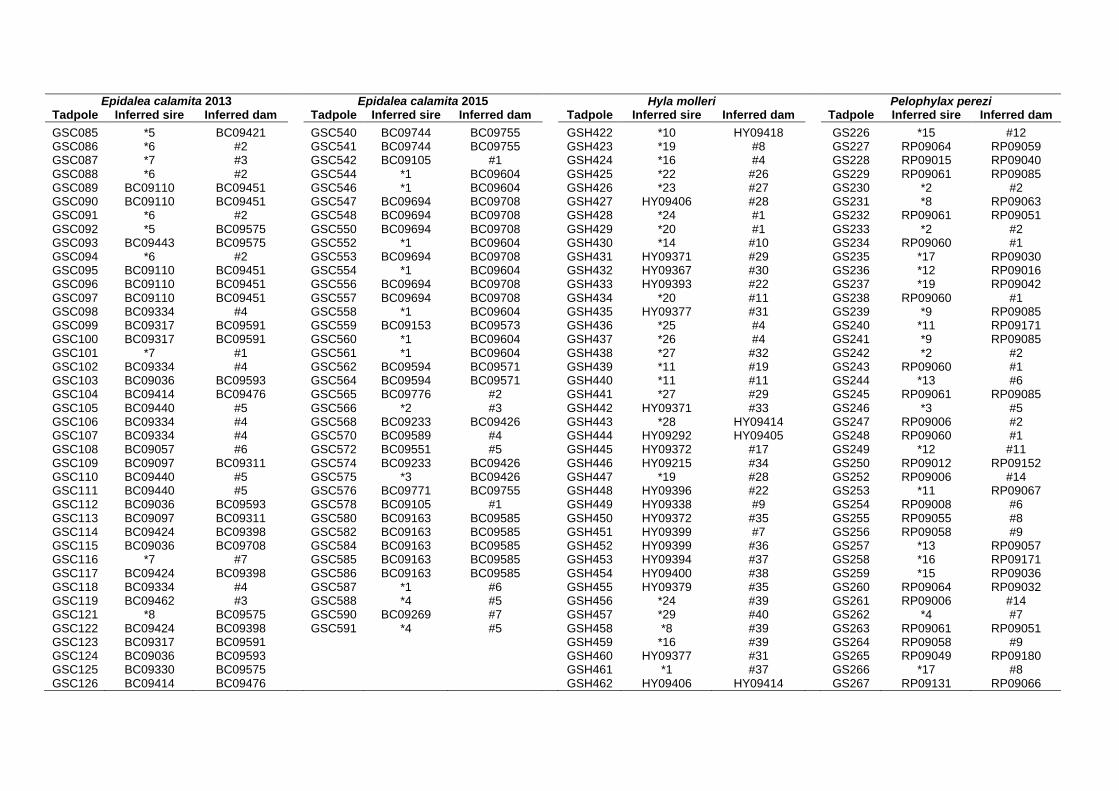
Epidalea calamita 2013 Epidalea calamita 2015 Hyla molleri Pelophylax perezi Tadpole Inferred sire Inferred dam Tadpole Inferred sire Inferred dam Tadpole Inferred sire Inferred dam Tadpole Inferred sire Inferred dam
GSC085 *5 BC09421
GSC540 BC09744 BC09755
GSH422 *10 HY09418
GS226 *15 #12 GSC086 *6 #2
GSC541 BC09744 BC09755
GSH423 *19 #8
GS227 RP09064 RP09059
GSC087 *7 #3
GSC542 BC09105 #1
GSH424 *16 #4
GS228 RP09015 RP09040 GSC088 *6 #2
GSC544 *1 BC09604
GSH425 *22 #26
GS229 RP09061 RP09085
GSC089 BC09110 BC09451
GSC546 *1 BC09604
GSH426 *23 #27
GS230 *2 #2 GSC090 BC09110 BC09451
GSC547 BC09694 BC09708
GSH427 HY09406 #28
GS231 *8 RP09063
GSC091 *6 #2
GSC548 BC09694 BC09708
GSH428 *24 #1
GS232 RP09061 RP09051 GSC092 *5 BC09575
GSC550 BC09694 BC09708
GSH429 *20 #1
GS233 *2 #2
GSC093 BC09443 BC09575
GSC552 *1 BC09604
GSH430 *14 #10
GS234 RP09060 #1 GSC094 *6 #2
GSC553 BC09694 BC09708
GSH431 HY09371 #29
GS235 *17 RP09030
GSC095 BC09110 BC09451
GSC554 *1 BC09604
GSH432 HY09367 #30
GS236 *12 RP09016 GSC096 BC09110 BC09451
GSC556 BC09694 BC09708
GSH433 HY09393 #22
GS237 *19 RP09042
GSC097 BC09110 BC09451
GSC557 BC09694 BC09708
GSH434 *20 #11
GS238 RP09060 #1 GSC098 BC09334 #4
GSC558 *1 BC09604
GSH435 HY09377 #31
GS239 *9 RP09085
GSC099 BC09317 BC09591
GSC559 BC09153 BC09573
GSH436 *25 #4
GS240 *11 RP09171 GSC100 BC09317 BC09591
GSC560 *1 BC09604
GSH437 *26 #4
GS241 *9 RP09085
GSC101 *7 #1
GSC561 *1 BC09604
GSH438 *27 #32
GS242 *2 #2 GSC102 BC09334 #4
GSC562 BC09594 BC09571
GSH439 *11 #19
GS243 RP09060 #1
GSC103 BC09036 BC09593
GSC564 BC09594 BC09571
GSH440 *11 #11
GS244 *13 #6 GSC104 BC09414 BC09476
GSC565 BC09776 #2
GSH441 *27 #29
GS245 RP09061 RP09085
GSC105 BC09440 #5
GSC566 *2 #3
GSH442 HY09371 #33
GS246 *3 #5 GSC106 BC09334 #4
GSC568 BC09233 BC09426
GSH443 *28 HY09414
GS247 RP09006 #2
GSC107 BC09334 #4
GSC570 BC09589 #4
GSH444 HY09292 HY09405
GS248 RP09060 #1 GSC108 BC09057 #6
GSC572 BC09551 #5
GSH445 HY09372 #17
GS249 *12 #11
GSC109 BC09097 BC09311
GSC574 BC09233 BC09426
GSH446 HY09215 #34
GS250 RP09012 RP09152 GSC110 BC09440 #5
GSC575 *3 BC09426
GSH447 *19 #28
GS252 RP09006 #14
GSC111 BC09440 #5
GSC576 BC09771 BC09755
GSH448 HY09396 #22
GS253 *11 RP09067 GSC112 BC09036 BC09593
GSC578 BC09105 #1
GSH449 HY09338 #9
GS254 RP09008 #6
GSC113 BC09097 BC09311
GSC580 BC09163 BC09585
GSH450 HY09372 #35
GS255 RP09055 #8 GSC114 BC09424 BC09398
GSC582 BC09163 BC09585
GSH451 HY09399 #7
GS256 RP09058 #9
GSC115 BC09036 BC09708
GSC584 BC09163 BC09585
GSH452 HY09399 #36
GS257 *13 RP09057 GSC116 *7 #7
GSC585 BC09163 BC09585
GSH453 HY09394 #37
GS258 *16 RP09171
GSC117 BC09424 BC09398
GSC586 BC09163 BC09585
GSH454 HY09400 #38
GS259 *15 RP09036 GSC118 BC09334 #4
GSC587 *1 #6
GSH455 HY09379 #35
GS260 RP09064 RP09032
GSC119 BC09462 #3
GSC588 *4 #5
GSH456 *24 #39
GS261 RP09006 #14 GSC121 *8 BC09575
GSC590 BC09269 #7
GSH457 *29 #40
GS262 *4 #7
GSC122 BC09424 BC09398
GSC591 *4 #5
GSH458 *8 #39
GS263 RP09061 RP09051 GSC123 BC09317 BC09591
GSH459 *16 #39
GS264 RP09058 #9
GSC124 BC09036 BC09593
GSH460 HY09377 #31
GS265 RP09049 RP09180 GSC125 BC09330 BC09575
GSH461 *1 #37
GS266 *17 #8
GSC126 BC09414 BC09476
GSH462 HY09406 HY09414
GS267 RP09131 RP09066
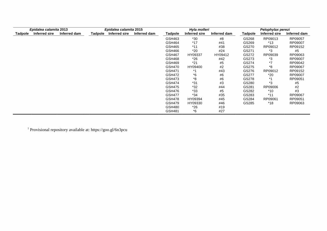
Epidalea calamita 2013 Epidalea calamita 2015 Hyla molleri Pelophylax perezi Tadpole Inferred sire Inferred dam Tadpole Inferred sire Inferred dam Tadpole Inferred sire Inferred dam Tadpole Inferred sire Inferred dam
GSH463 *30 #8
GS268 RP09013 RP09057
GSH464 *17 #41
GS269 *13 RP09007
GSH465 *11 #38
GS270 RP09012 RP09152
GSH466 *20 #24
GS271 *3 #5
GSH467 HY09337 HY09412
GS272 RP09039 RP09063
GSH468 *26 #42
GS273 *3 RP09007
GSH469 *21 #5
GS274 *7 RP09042
GSH470 HY09400 #2
GS275 *8 RP09067
GSH471 *1 #43
GS276 RP09012 RP09152
GSH472 *6 #6
GS277 *20 RP09007
GSH473 *8 #6
GS278 *1 RP09051
GSH474 *31 #3
GS280 *3 #5
GSH475 *32 #44
GS281 RP09006 #2
GSH476 *33 #5
GS282 *10 #3
GSH477 *34 #35
GS283 *11 RP09067
GSH478 HY09394 #45
GS284 RP09061 RP09051
GSH479 HY09330 #46
GS285 *18 RP09063
GSH480 *26 #19
GSH481 *6 #27
1 Provisional repository available at: https://goo.gl/6n3pcu

APPENDIX 9
PAIRWISE FST ESTIMATES AND MIGRATION RATES PER GENERATION
Appendix S1 in Sánchez-Montes et al. Journal of Biogeography (Under review)
(Chapter VI)


Table A9.1. Pairwise FST estimates among populations of E. calamita. FST values significantly > 0 at the Bonferroni penalized level (i.e. p < 0.05/136 = 0.0004) are marked in
bold. Pairwise FST between populations located in different slopes of Sierra de Guadarrama are shaded in grey. See Table VI.2 for abbreviations.
CER COL SOT MOR CAN BUS CAB ROB CEL LOZ GAR ALA PRA BRC NAV MUN STO
CER -
COL 0.058 -
SOT 0.039 0.074 -
MOR 0.052 0.082 0.061 -
CAN 0.026 0.051 0.028 0.041 -
BUS 0.026 0.059 0.029 0.044 0.014 -
CAB 0.026 0.056 0.030 0.046 0.016 0.015 -
ROB 0.022 0.051 0.029 0.042 0.012 0.013 0.013 -
CEL 0.030 0.063 0.030 0.052 0.017 0.018 0.018 0.019 -
LOZ 0.037 0.058 0.039 0.055 0.022 0.026 0.024 0.022 0.032 -
GAR 0.026 0.049 0.033 0.046 0.012 0.015 0.019 0.014 0.021 0.023 -
ALA 0.047 0.082 0.044 0.050 0.030 0.034 0.034 0.032 0.039 0.041 0.036 -
PRA 0.042 0.077 0.047 0.062 0.029 0.031 0.036 0.029 0.033 0.045 0.031 0.049 -
BRC 0.040 0.080 0.047 0.081 0.039 0.043 0.041 0.041 0.036 0.051 0.042 0.066 0.058 -
NAV 0.039 0.080 0.042 0.071 0.034 0.036 0.034 0.034 0.028 0.047 0.035 0.050 0.034 0.046 -
MUN 0.030 0.066 0.044 0.057 0.024 0.024 0.027 0.026 0.023 0.041 0.026 0.047 0.030 0.043 0.029 -
STO 0.041 0.078 0.048 0.071 0.034 0.034 0.037 0.031 0.034 0.044 0.036 0.047 0.042 0.052 0.030 0.032 -

Table A9.2. Pairwise FST estimates among populations of H. molleri. All FST values were significantly > 0 at the Bonferroni penalized level (i.e. p < 0.05/171 = 0.0003, marked in
bold). Pairwise FST between populations located in different slopes of Sierra de Guadarrama are shaded in grey. See Table VI.2 for abbreviations.
CER COL SOT MED RAS MOR CAN BUS CAB ROB BER GAS PRA TOR HER ARC SAU FUE TUR
CER -
COL 0.074 -
SOT 0.051 0.075 -
MED 0.060 0.098 0.064 -
RAS 0.059 0.101 0.060 0.085 -
MOR 0.057 0.077 0.036 0.073 0.038 -
CAN 0.048 0.080 0.032 0.050 0.048 0.035 -
BUS 0.036 0.064 0.028 0.048 0.047 0.035 0.031 -
CAB 0.053 0.066 0.037 0.063 0.057 0.040 0.037 0.025 -
ROB 0.061 0.087 0.048 0.060 0.055 0.044 0.038 0.037 0.037 -
BER 0.069 0.089 0.052 0.069 0.058 0.047 0.043 0.043 0.054 0.053 -
GAS 0.042 0.073 0.027 0.062 0.041 0.028 0.024 0.023 0.028 0.031 0.039 -
PRA 0.104 0.144 0.084 0.117 0.087 0.079 0.075 0.076 0.082 0.085 0.069 0.064 -
TOR 0.119 0.147 0.091 0.135 0.124 0.098 0.086 0.096 0.099 0.102 0.102 0.079 0.095 -
HER 0.089 0.127 0.081 0.100 0.075 0.057 0.063 0.067 0.072 0.068 0.067 0.053 0.092 0.128 -
ARC 0.057 0.087 0.044 0.066 0.049 0.048 0.037 0.029 0.043 0.035 0.051 0.029 0.078 0.087 0.061 -
SAU 0.079 0.118 0.061 0.087 0.065 0.059 0.054 0.049 0.064 0.052 0.065 0.041 0.088 0.120 0.078 0.048 -
FUE 0.063 0.090 0.045 0.085 0.052 0.037 0.039 0.038 0.050 0.051 0.049 0.029 0.078 0.089 0.064 0.039 0.053 -
TUR 0.081 0.103 0.052 0.082 0.062 0.046 0.045 0.052 0.057 0.042 0.054 0.036 0.063 0.085 0.061 0.037 0.061 0.043 -

Table A9.3. Pairwise FST estimates among populations of P. perezi. All FST values were significantly > 0 at the Bonferroni penalized level (i.e. p < 0.05/105 = 0.0005, marked in
bold). Pairwise FST between populations located in different slopes of Sierra de Guadarrama are shaded in grey. See Table VI.2 for abbreviations.
CER MED RAS MOR CAN BUS CAB BER PRA HER ARC STO SAU FUE TUR
CER -
MED 0.033 -
RAS 0.046 0.041 -
MOR 0.057 0.043 0.043 -
CAN 0.049 0.035 0.043 0.040 -
BUS 0.070 0.059 0.074 0.074 0.061 -
CAB 0.042 0.034 0.043 0.050 0.039 0.056 -
BER 0.076 0.069 0.103 0.103 0.096 0.120 0.092 -
PRA 0.031 0.032 0.047 0.056 0.035 0.067 0.037 0.092 -
HER 0.050 0.036 0.050 0.062 0.042 0.081 0.047 0.105 0.030 -
ARC 0.088 0.079 0.099 0.123 0.092 0.120 0.101 0.128 0.077 0.092 -
STO 0.064 0.050 0.054 0.067 0.044 0.100 0.053 0.115 0.044 0.049 0.109 -
SAU 0.050 0.040 0.056 0.066 0.050 0.081 0.052 0.091 0.041 0.043 0.090 0.059 -
FUE 0.075 0.066 0.080 0.089 0.060 0.116 0.085 0.142 0.062 0.082 0.123 0.084 0.071 -
TUR 0.031 0.022 0.043 0.054 0.039 0.067 0.034 0.071 0.029 0.042 0.086 0.051 0.042 0.069 -

Table A9.4. Pairwise FST estimates among populations of P. cultripes. FST values significantly > 0 at the Bonferroni penalized level (i.e. p < 0.05/78 = 0.0006) are marked in
bold. Pairwise FST between populations located in different slopes of Sierra de Guadarrama are shaded in grey. See Table VI.2 for abbreviations.
CER COL TEJ SOT CAB BUS ROB BER STO PRA HER TUR FUE
CER -
COL 0.048 -
TEJ 0.102 0.065 -
SOT 0.088 0.048 0.084 -
CAB 0.066 0.041 0.054 0.059 -
BUS 0.079 0.051 0.089 0.095 0.085 -
ROB 0.055 0.027 0.079 0.068 0.037 0.052 -
BER 0.130 0.117 0.167 0.174 0.130 0.105 0.097 -
STO 0.125 0.097 0.151 0.130 0.110 0.108 0.111 0.198 -
PRA 0.168 0.118 0.137 0.141 0.123 0.122 0.139 0.234 0.087 -
HER 0.105 0.071 0.097 0.093 0.072 0.095 0.074 0.160 0.050 0.057 -
TUR 0.129 0.092 0.136 0.121 0.090 0.115 0.102 0.210 0.020 0.085 0.038 -
FUE 0.107 0.085 0.111 0.107 0.076 0.109 0.091 0.168 0.026 0.066 0.025 0.028 -
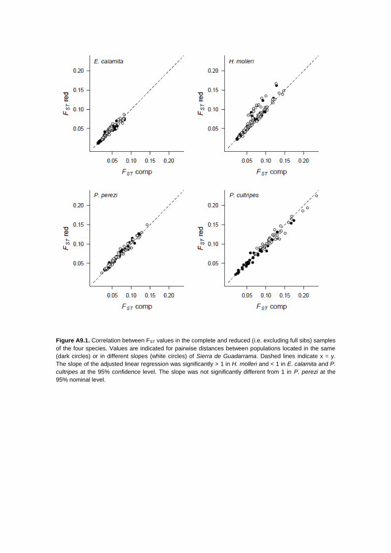
Figure A9.1. Correlation between FST values in the complete and reduced (i.e. excluding full sibs) samples
of the four species. Values are indicated for pairwise distances between populations located in the same
(dark circles) or in different slopes (white circles) of Sierra de Guadarrama. Dashed lines indicate x = y.
The slope of the adjusted linear regression was significantly > 1 in H. molleri and < 1 in E. calamita and P.
cultripes at the 95% confidence level. The slope was not significantly different from 1 in P. perezi at the
95% nominal level.
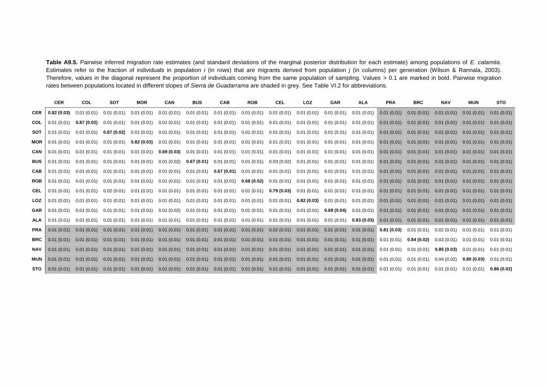
Table A9.5. Pairwise inferred migration rate estimates (and standard deviations of the marginal posterior distribution for each estimate) among populations of E. calamita.
Estimates refer to the fraction of individuals in population i (in rows) that are migrants derived from population j (in columns) per generation (Wilson & Rannala, 2003).
Therefore, values in the diagonal represent the proportion of individuals coming from the same population of sampling. Values > 0.1 are marked in bold. Pairwise migration
rates between populations located in different slopes of Sierra de Guadarrama are shaded in grey. See Table VI.2 for abbreviations.
CER COL SOT MOR CAN BUS CAB ROB CEL LOZ GAR ALA PRA BRC NAV MUN STO
CER 0.82 (0.03) 0.01 (0.01) 0.01 (0.01) 0.01 (0.01) 0.01 (0.01) 0.01 (0.01) 0.01 (0.01) 0.01 (0.01) 0.01 (0.01) 0.01 (0.01) 0.01 (0.01) 0.01 (0.01) 0.01 (0.01) 0.01 (0.01) 0.01 (0.01) 0.01 (0.01) 0.01 (0.01)
COL 0.01 (0.01) 0.87 (0.02) 0.01 (0.01) 0.01 (0.01) 0.01 (0.01) 0.01 (0.01) 0.01 (0.01) 0.01 (0.01) 0.01 (0.01) 0.01 (0.01) 0.01 (0.01) 0.01 (0.01) 0.01 (0.01) 0.01 (0.01) 0.01 (0.01) 0.01 (0.01) 0.01 (0.01)
SOT 0.01 (0.01) 0.01 (0.01) 0.87 (0.02) 0.01 (0.01) 0.01 (0.01) 0.01 (0.01) 0.01 (0.01) 0.01 (0.01) 0.01 (0.01) 0.01 (0.01) 0.01 (0.01) 0.01 (0.01) 0.01 (0.01) 0.01 (0.01) 0.01 (0.01) 0.01 (0.01) 0.01 (0.01)
MOR 0.01 (0.01) 0.01 (0.01) 0.01 (0.01) 0.82 (0.03) 0.01 (0.01) 0.01 (0.01) 0.01 (0.01) 0.01 (0.01) 0.01 (0.01) 0.01 (0.01) 0.01 (0.01) 0.01 (0.01) 0.01 (0.01) 0.01 (0.01) 0.01 (0.01) 0.01 (0.01) 0.01 (0.01)
CAN 0.01 (0.01) 0.01 (0.01) 0.01 (0.01) 0.01 (0.01) 0.69 (0.03) 0.01 (0.01) 0.01 (0.01) 0.01 (0.01) 0.01 (0.01) 0.01 (0.01) 0.01 (0.01) 0.01 (0.01) 0.01 (0.01) 0.01 (0.01) 0.01 (0.01) 0.01 (0.01) 0.01 (0.01)
BUS 0.01 (0.01) 0.01 (0.01) 0.01 (0.01) 0.01 (0.01) 0.01 (0.02) 0.67 (0.01) 0.01 (0.01) 0.01 (0.01) 0.03 (0.02) 0.01 (0.01) 0.01 (0.01) 0.01 (0.01) 0.01 (0.01) 0.01 (0.01) 0.01 (0.01) 0.01 (0.01) 0.01 (0.01)
CAB 0.01 (0.01) 0.01 (0.01) 0.01 (0.01) 0.01 (0.01) 0.01 (0.01) 0.01 (0.01) 0.67 (0.01) 0.01 (0.01) 0.01 (0.01) 0.01 (0.01) 0.01 (0.01) 0.01 (0.01) 0.01 (0.01) 0.01 (0.01) 0.01 (0.01) 0.01 (0.01) 0.01 (0.01)
ROB 0.01 (0.01) 0.01 (0.01) 0.01 (0.01) 0.01 (0.01) 0.01 (0.01) 0.01 (0.01) 0.01 (0.01) 0.68 (0.02) 0.01 (0.01) 0.01 (0.01) 0.01 (0.01) 0.01 (0.01) 0.01 (0.01) 0.01 (0.01) 0.01 (0.01) 0.01 (0.01) 0.01 (0.01)
CEL 0.01 (0.01) 0.01 (0.01) 0.02 (0.01) 0.01 (0.01) 0.01 (0.01) 0.01 (0.01) 0.01 (0.01) 0.01 (0.01) 0.79 (0.03) 0.01 (0.01) 0.01 (0.01) 0.01 (0.01) 0.01 (0.01) 0.01 (0.01) 0.01 (0.01) 0.01 (0.01) 0.01 (0.01)
LOZ 0.01 (0.01) 0.01 (0.01) 0.01 (0.01) 0.01 (0.01) 0.01 (0.01) 0.01 (0.01) 0.01 (0.01) 0.01 (0.01) 0.01 (0.01) 0.82 (0.03) 0.01 (0.01) 0.01 (0.01) 0.01 (0.01) 0.01 (0.01) 0.01 (0.01) 0.01 (0.01) 0.01 (0.01)
GAR 0.01 (0.01) 0.01 (0.01) 0.01 (0.01) 0.01 (0.01) 0.01 (0.02) 0.01 (0.01) 0.01 (0.01) 0.01 (0.01) 0.01 (0.01) 0.01 (0.01) 0.69 (0.04) 0.01 (0.01) 0.01 (0.01) 0.01 (0.01) 0.01 (0.01) 0.01 (0.01) 0.01 (0.01)
ALA 0.01 (0.01) 0.01 (0.01) 0.01 (0.01) 0.01 (0.01) 0.01 (0.01) 0.01 (0.01) 0.01 (0.01) 0.01 (0.01) 0.01 (0.01) 0.01 (0.01) 0.01 (0.01) 0.83 (0.03) 0.01 (0.01) 0.01 (0.01) 0.01 (0.01) 0.01 (0.01) 0.01 (0.01)
PRA 0.01 (0.01) 0.01 (0.01) 0.01 (0.01) 0.01 (0.01) 0.01 (0.01) 0.01 (0.01) 0.01 (0.01) 0.01 (0.01) 0.02 (0.01) 0.01 (0.01) 0.01 (0.01) 0.01 (0.01) 0.81 (0.03) 0.01 (0.01) 0.02 (0.01) 0.01 (0.01) 0.01 (0.01)
BRC 0.01 (0.01) 0.01 (0.01) 0.01 (0.01) 0.01 (0.01) 0.01 (0.01) 0.01 (0.01) 0.01 (0.01) 0.01 (0.01) 0.01 (0.01) 0.01 (0.01) 0.01 (0.01) 0.01 (0.01) 0.01 (0.01) 0.84 (0.02) 0.03 (0.01) 0.01 (0.01) 0.01 (0.01)
NAV 0.01 (0.01) 0.01 (0.01) 0.01 (0.01) 0.01 (0.01) 0.01 (0.01) 0.01 (0.01) 0.01 (0.01) 0.01 (0.01) 0.01 (0.01) 0.01 (0.01) 0.01 (0.01) 0.01 (0.01) 0.01 (0.01) 0.01 (0.01) 0.85 (0.03) 0.01 (0.01) 0.01 (0.01)
MUN 0.01 (0.01) 0.01 (0.01) 0.01 (0.01) 0.01 (0.01) 0.01 (0.01) 0.01 (0.01) 0.01 (0.01) 0.01 (0.01) 0.01 (0.01) 0.01 (0.01) 0.01 (0.01) 0.01 (0.01) 0.01 (0.01) 0.01 (0.01) 0.04 (0.02) 0.80 (0.03) 0.01 (0.01)
STO 0.01 (0.01) 0.01 (0.01) 0.01 (0.01) 0.01 (0.01) 0.01 (0.01) 0.01 (0.01) 0.01 (0.01) 0.01 (0.01) 0.01 (0.01) 0.01 (0.01) 0.01 (0.01) 0.01 (0.01) 0.01 (0.01) 0.01 (0.01) 0.01 (0.01) 0.01 (0.01) 0.86 (0.02)
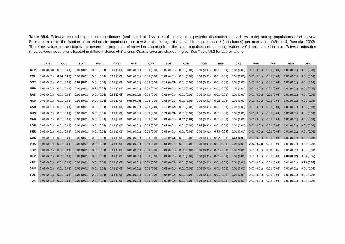
Table A9.6. Pairwise inferred migration rate estimates (and standard deviations of the marginal posterior distribution for each estimate) among populations of H. molleri.
Estimates refer to the fraction of individuals in population i (in rows) that are migrants derived from population j (in columns) per generation (Wilson & Rannala, 2003).
Therefore, values in the diagonal represent the proportion of individuals coming from the same population of sampling. Values > 0.1 are marked in bold. Pairwise migration
rates between populations located in different slopes of Sierra de Guadarrama are shaded in grey. See Table VI.2 for abbreviations.
CER COL SOT MED RAS MOR CAN BUS CAB ROB BER GAS PRA TOR HER ARC
CER 0.81 (0.03) 0.01 (0.01) 0.01 (0.01) 0.01 (0.01) 0.01 (0.01) 0.01 (0.01) 0.01 (0.01) 0.02 (0.01) 0.01 (0.01) 0.01 (0.01) 0.01 (0.01) 0.01 (0.01) 0.01 (0.01) 0.01 (0.01) 0.01 (0.01) 0.01 (0.01)
COL 0.01 (0.01) 0.84 (0.03) 0.01 (0.01) 0.01 (0.01) 0.01 (0.01) 0.01 (0.01) 0.01 (0.01) 0.01 (0.01) 0.01 (0.01) 0.01 (0.01) 0.01 (0.01) 0.01 (0.01) 0.01 (0.01) 0.01 (0.01) 0.01 (0.01) 0.01 (0.01)
SOT 0.01 (0.01) 0.01 (0.01) 0.67 (0.01) 0.01 (0.01) 0.01 (0.01) 0.01 (0.01) 0.01 (0.01) 0.17 (0.03) 0.01 (0.01) 0.01 (0.01) 0.01 (0.01) 0.01 (0.01) 0.01 (0.01) 0.01 (0.01) 0.01 (0.01) 0.01 (0.01)
MED 0.01 (0.01) 0.01 (0.01) 0.01 (0.01) 0.83 (0.03) 0.01 (0.01) 0.01 (0.01) 0.01 (0.01) 0.01 (0.01) 0.01 (0.01) 0.01 (0.01) 0.01 (0.01) 0.01 (0.01) 0.01 (0.01) 0.01 (0.01) 0.01 (0.01) 0.01 (0.01)
RAS 0.01 (0.01) 0.01 (0.01) 0.01 (0.01) 0.01 (0.01) 0.81 (0.03) 0.02 (0.02) 0.01 (0.01) 0.01 (0.01) 0.01 (0.01) 0.01 (0.01) 0.01 (0.01) 0.01 (0.01) 0.01 (0.01) 0.01 (0.01) 0.01 (0.01) 0.01 (0.01)
MOR 0.01 (0.01) 0.01 (0.01) 0.01 (0.01) 0.01 (0.01) 0.01 (0.01) 0.85 (0.03) 0.01 (0.01) 0.01 (0.01) 0.01 (0.01) 0.01 (0.01) 0.02 (0.01) 0.01 (0.01) 0.01 (0.01) 0.01 (0.01) 0.01 (0.01) 0.01 (0.01)
CAN 0.01 (0.01) 0.01 (0.01) 0.01 (0.01) 0.01 (0.01) 0.01 (0.01) 0.01 (0.01) 0.67 (0.01) 0.19 (0.02) 0.01 (0.01) 0.01 (0.01) 0.01 (0.01) 0.01 (0.01) 0.01 (0.01) 0.01 (0.01) 0.01 (0.01) 0.01 (0.01)
BUS 0.01 (0.01) 0.01 (0.01) 0.01 (0.01) 0.01 (0.01) 0.01 (0.01) 0.01 (0.01) 0.01 (0.01) 0.71 (0.03) 0.01 (0.01) 0.01 (0.01) 0.01 (0.01) 0.01 (0.01) 0.01 (0.01) 0.01 (0.01) 0.01 (0.01) 0.01 (0.01)
CAB 0.01 (0.01) 0.01 (0.01) 0.01 (0.01) 0.01 (0.01) 0.01 (0.01) 0.01 (0.01) 0.01 (0.01) 0.01 (0.01) 0.67 (0.01) 0.01 (0.01) 0.01 (0.01) 0.01 (0.01) 0.01 (0.01) 0.01 (0.01) 0.01 (0.01) 0.01 (0.01)
ROB 0.01 (0.01) 0.01 (0.01) 0.01 (0.01) 0.01 (0.01) 0.01 (0.01) 0.01 (0.01) 0.01 (0.01) 0.01 (0.01) 0.01 (0.01) 0.67 (0.01) 0.01 (0.01) 0.01 (0.01) 0.01 (0.01) 0.01 (0.01) 0.01 (0.01) 0.01 (0.01)
BER 0.01 (0.01) 0.01 (0.01) 0.01 (0.01) 0.01 (0.01) 0.01 (0.01) 0.01 (0.01) 0.01 (0.01) 0.01 (0.01) 0.01 (0.01) 0.01 (0.01) 0.83 (0.03) 0.01 (0.01) 0.01 (0.01) 0.01 (0.01) 0.01 (0.01) 0.01 (0.01)
GAS 0.01 (0.01) 0.01 (0.01) 0.01 (0.01) 0.01 (0.01) 0.01 (0.01) 0.01 (0.01) 0.01 (0.01) 0.14 (0.03) 0.01 (0.01) 0.01 (0.01) 0.02 (0.01) 0.68 (0.01) 0.01 (0.01) 0.01 (0.01) 0.01 (0.01) 0.01 (0.01)
PRA 0.01 (0.01) 0.01 (0.01) 0.01 (0.01) 0.01 (0.01) 0.01 (0.01) 0.01 (0.01) 0.01 (0.01) 0.01 (0.01) 0.01 (0.01) 0.01 (0.01) 0.01 (0.01) 0.01 (0.01) 0.83 (0.03) 0.01 (0.01) 0.01 (0.01) 0.01 (0.01)
TOR 0.01 (0.01) 0.01 (0.01) 0.01 (0.01) 0.01 (0.01) 0.01 (0.01) 0.01 (0.01) 0.01 (0.01) 0.01 (0.01) 0.01 (0.01) 0.01 (0.01) 0.01 (0.01) 0.01 (0.01) 0.01 (0.01) 0.88 (0.02) 0.01 (0.01) 0.01 (0.01)
HER 0.01 (0.01) 0.01 (0.01) 0.01 (0.01) 0.01 (0.01) 0.01 (0.01) 0.01 (0.01) 0.01 (0.01) 0.01 (0.01) 0.01 (0.01) 0.01 (0.01) 0.01 (0.01) 0.01 (0.01) 0.01 (0.01) 0.01 (0.01) 0.80 (0.02) 0.06 (0.02)
ARC 0.01 (0.01) 0.01 (0.01) 0.01 (0.01) 0.01 (0.01) 0.01 (0.01) 0.01 (0.01) 0.01 (0.01) 0.05 (0.03) 0.01 (0.01) 0.01 (0.01) 0.01 (0.01) 0.01 (0.01) 0.01 (0.01) 0.01 (0.01) 0.01 (0.01) 0.79 (0.03)
SAU 0.01 (0.01) 0.01 (0.01) 0.01 (0.01) 0.01 (0.01) 0.01 (0.01) 0.01 (0.01) 0.01 (0.01) 0.01 (0.01) 0.01 (0.01) 0.01 (0.01) 0.01 (0.01) 0.01 (0.01) 0.01 (0.01) 0.01 (0.01) 0.01 (0.01) 0.01 (0.01)
FUE 0.01 (0.01) 0.01 (0.01) 0.01 (0.01) 0.01 (0.01) 0.01 (0.01) 0.01 (0.01) 0.01 (0.01) 0.05 (0.02) 0.01 (0.01) 0.01 (0.01) 0.01 (0.01) 0.01 (0.01) 0.01 (0.01) 0.01 (0.01) 0.01 (0.01) 0.01 (0.01)
TUR 0.01 (0.01) 0.01 (0.01) 0.01 (0.01) 0.01 (0.01) 0.02 (0.01) 0.01 (0.01) 0.01 (0.01) 0.02 (0.02) 0.01 (0.01) 0.01 (0.01) 0.01 (0.01) 0.01 (0.01) 0.01 (0.01) 0.02 (0.01) 0.01 (0.01) 0.01 (0.01)

Table A9.6 (cont.). Pairwise inferred migration rate estimates (and standard deviations of the marginal posterior distribution for each estimate) among populations of H. molleri. Estimates refer to the fraction of individuals in population i (in rows) that are migrants derived from population j (in columns) per generation (Wilson & Rannala, 2003). Therefore, values in the diagonal represent the proportion of individuals coming from the same population of sampling. Values > 0.1 are marked in bold. Pairwise migration rates between populations located in different slopes of Sierra de Guadarrama are shaded in grey. See Table VI.2 for abbreviations.
SAU FUE TUR
CER 0.01 (0.01) 0.01 (0.01) 0.01 (0.01)
COL 0.01 (0.01) 0.01 (0.01) 0.01 (0.01)
SOT 0.01 (0.01) 0.01 (0.01) 0.01 (0.01)
MED 0.01 (0.01) 0.01 (0.01) 0.01 (0.01)
RAS 0.01 (0.01) 0.01 (0.01) 0.01 (0.01)
MOR 0.01 (0.01) 0.01 (0.01) 0.01 (0.01)
CAN 0.01 (0.01) 0.01 (0.01) 0.01 (0.01)
BUS 0.01 (0.01) 0.01 (0.01) 0.01 (0.01)
CAB 0.01 (0.01) 0.01 (0.01) 0.01 (0.01)
ROB 0.01 (0.01) 0.01 (0.01) 0.01 (0.01)
BER 0.01 (0.01) 0.01 (0.01) 0.01 (0.01)
GAS 0.01 (0.01) 0.01 (0.01) 0.01 (0.01)
PRA 0.01 (0.01) 0.01 (0.01) 0.01 (0.01)
TOR 0.01 (0.01) 0.01 (0.01) 0.01 (0.01)
HER 0.01 (0.01) 0.01 (0.01) 0.01 (0.01)
ARC 0.01 (0.01) 0.01 (0.01) 0.01 (0.01)
SAU 0.80 (0.03) 0.03 (0.02) 0.01 (0.01)
FUE 0.01 (0.01) 0.78 (0.03) 0.01 (0.01)
TUR 0.02 (0.01) 0.01 (0.01) 0.79 (0.03)
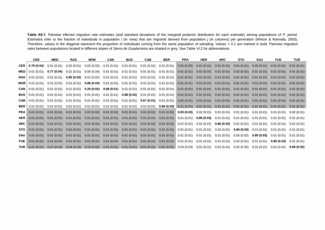
Table A9.7. Pairwise inferred migration rate estimates (and standard deviations of the marginal posterior distribution for each estimate) among populations of P. perezi.
Estimates refer to the fraction of individuals in population i (in rows) that are migrants derived from population j (in columns) per generation (Wilson & Rannala, 2003).
Therefore, values in the diagonal represent the proportion of individuals coming from the same population of sampling. Values > 0.1 are marked in bold. Pairwise migration
rates between populations located in different slopes of Sierra de Guadarrama are shaded in grey. See Table VI.2 for abbreviations.
CER MED RAS MOR CAN BUS CAB BER PRA HER ARC STO SAU FUE TUR
CER 0.79 (0.04) 0.01 (0.01) 0.02 (0.01) 0.02 (0.02) 0.01 (0.01) 0.01 (0.01) 0.01 (0.01) 0.01 (0.01) 0.02 (0.02) 0.01 (0.01) 0.01 (0.01) 0.01 (0.01) 0.02 (0.01) 0.01 (0.01) 0.01 (0.01)
MED 0.01 (0.01) 0.77 (0.04) 0.01 (0.01) 0.06 (0.04) 0.01 (0.01) 0.01 (0.01) 0.01 (0.01) 0.01 (0.01) 0.01 (0.01) 0.02 (0.02) 0.01 (0.01) 0.02 (0.02) 0.01 (0.01) 0.01 (0.01) 0.01 (0.01)
RAS 0.01 (0.01) 0.01 (0.01) 0.85 (0.03) 0.01 (0.01) 0.01 (0.01) 0.01 (0.01) 0.01 (0.01) 0.01 (0.01) 0.01 (0.01) 0.01 (0.01) 0.01 (0.01) 0.01 (0.01) 0.01 (0.01) 0.01 (0.01) 0.01 (0.01)
MOR 0.01 (0.01) 0.01 (0.01) 0.01 (0.01) 0.86 (0.03) 0.01 (0.01) 0.01 (0.01) 0.01 (0.01) 0.01 (0.01) 0.01 (0.01) 0.01 (0.01) 0.01 (0.01) 0.01 (0.01) 0.01 (0.01) 0.01 (0.01) 0.01 (0.01)
CAN 0.01 (0.01) 0.01 (0.01) 0.01 (0.01) 0.20 (0.02) 0.68 (0.01) 0.01 (0.01) 0.01 (0.01) 0.01 (0.01) 0.01 (0.01) 0.01 (0.01) 0.01 (0.01) 0.01 (0.01) 0.01 (0.01) 0.01 (0.01) 0.01 (0.01)
BUS 0.01 (0.01) 0.01 (0.01) 0.01 (0.01) 0.01 (0.01) 0.01 (0.01) 0.88 (0.02) 0.01 (0.01) 0.01 (0.01) 0.01 (0.01) 0.01 (0.01) 0.02 (0.01) 0.01 (0.01) 0.01 (0.01) 0.01 (0.01) 0.01 (0.01)
CAB 0.01 (0.01) 0.01 (0.01) 0.01 (0.01) 0.01 (0.01) 0.01 (0.01) 0.01 (0.01) 0.67 (0.01) 0.01 (0.01) 0.02 (0.01) 0.01 (0.01) 0.01 (0.01) 0.01 (0.01) 0.01 (0.01) 0.01 (0.01) 0.01 (0.01)
BER 0.01 (0.01) 0.01 (0.01) 0.01 (0.01) 0.01 (0.01) 0.01 (0.01) 0.01 (0.01) 0.01 (0.01) 0.86 (0.03) 0.01 (0.01) 0.01 (0.01) 0.01 (0.01) 0.01 (0.01) 0.01 (0.01) 0.01 (0.01) 0.01 (0.01)
PRA 0.01 (0.01) 0.01 (0.01) 0.01 (0.01) 0.02 (0.02) 0.01 (0.01) 0.01 (0.01) 0.01 (0.01) 0.01 (0.01) 0.83 (0.03) 0.02 (0.01) 0.01 (0.01) 0.01 (0.01) 0.01 (0.01) 0.01 (0.01) 0.02 (0.01)
HER 0.01 (0.01) 0.01 (0.01) 0.01 (0.01) 0.01 (0.01) 0.01 (0.01) 0.01 (0.01) 0.01 (0.01) 0.01 (0.01) 0.01 (0.01) 0.88 (0.03) 0.01 (0.01) 0.01 (0.01) 0.01 (0.01) 0.01 (0.01) 0.01 (0.01)
ARC 0.01 (0.01) 0.01 (0.01) 0.01 (0.01) 0.01 (0.01) 0.01 (0.01) 0.01 (0.01) 0.01 (0.01) 0.01 (0.01) 0.01 (0.01) 0.01 (0.01) 0.86 (0.03) 0.01 (0.01) 0.01 (0.01) 0.01 (0.01) 0.01 (0.01)
STO 0.01 (0.01) 0.01 (0.01) 0.01 (0.01) 0.01 (0.01) 0.01 (0.01) 0.01 (0.01) 0.01 (0.01) 0.01 (0.01) 0.01 (0.01) 0.01 (0.01) 0.02 (0.01) 0.84 (0.03) 0.01 (0.01) 0.01 (0.01) 0.01 (0.01)
SAU 0.01 (0.01) 0.01 (0.01) 0.01 (0.01) 0.01 (0.01) 0.01 (0.01) 0.01 (0.01) 0.01 (0.01) 0.01 (0.01) 0.01 (0.01) 0.01 (0.01) 0.01 (0.01) 0.05 (0.02) 0.80 (0.03) 0.01 (0.01) 0.01 (0.01)
FUE 0.01 (0.01) 0.01 (0.01) 0.01 (0.01) 0.01 (0.01) 0.01 (0.01) 0.01 (0.01) 0.01 (0.01) 0.01 (0.01) 0.01 (0.01) 0.01 (0.01) 0.01 (0.01) 0.02 (0.01) 0.01 (0.01) 0.85 (0.03) 0.01 (0.01)
TUR 0.01 (0.01) 0.07 (0.04) 0.04 (0.03) 0.03 (0.02) 0.01 (0.01) 0.01 (0.01) 0.01 (0.01) 0.01 (0.01) 0.04 (0.03) 0.01 (0.01) 0.01 (0.01) 0.02 (0.02) 0.01 (0.01) 0.01 (0.01) 0.69 (0.02)

Table A9.8. Pairwise inferred migration rate estimates (and standard deviations of the marginal posterior distribution for each estimate) among populations of P. cultripes.
Estimates refer to the fraction of individuals in population i (in rows) that are migrants derived from population j (in columns) per generation (Wilson & Rannala, 2003).
Therefore, values in the diagonal represent the proportion of individuals coming from the same population of sampling. Values > 0.1 are marked in bold. Pairwise migration
rates between populations located in different slopes of Sierra de Guadarrama are shaded in grey. See Table VI.2 for abbreviations.
CER COL TEJ SOT CAB BUS ROB BER STO PRA HER TUR FUE
CER 0.89 (0.03) 0.01 (0.01) 0.01 (0.01) 0.01 (0.01) 0.01 (0.01) 0.01 (0.01) 0.01 (0.01) 0.01 (0.01) 0.01 (0.01) 0.01 (0.01) 0.01 (0.01) 0.01 (0.01) 0.01 (0.01)
COL 0.02 (0.02) 0.70 (0.05) 0.01 (0.01) 0.01 (0.01) 0.20 (0.07) 0.01 (0.01) 0.01 (0.02) 0.01 (0.01) 0.01 (0.01) 0.01 (0.01) 0.01 (0.01) 0.01 (0.01) 0.01 (0.01)
TEJ 0.01 (0.01) 0.02 (0.02) 0.79 (0.04) 0.01 (0.01) 0.11 (0.05) 0.01 (0.01) 0.01 (0.01) 0.01 (0.01) 0.01 (0.01) 0.01 (0.01) 0.01 (0.01) 0.01 (0.01) 0.01 (0.01)
SOT 0.01 (0.01) 0.01 (0.01) 0.01 (0.01) 0.90 (0.02) 0.01 (0.01) 0.01 (0.01) 0.01 (0.01) 0.01 (0.01) 0.01 (0.01) 0.01 (0.01) 0.01 (0.01) 0.01 (0.01) 0.01 (0.01)
CAB 0.01 (0.01) 0.01 (0.01) 0.02 (0.01) 0.01 (0.01) 0.87 (0.03) 0.01 (0.01) 0.01 (0.01) 0.02 (0.01) 0.01 (0.01) 0.01 (0.01) 0.01 (0.01) 0.01 (0.01) 0.01 (0.01)
BUS 0.01 (0.01) 0.01 (0.01) 0.01 (0.01) 0.01 (0.01) 0.01 (0.01) 0.69 (0.04) 0.20 (0.06) 0.01 (0.01) 0.01 (0.01) 0.01 (0.01) 0.01 (0.01) 0.01 (0.01) 0.01 (0.01)
ROB 0.01 (0.01) 0.01 (0.01) 0.01 (0.01) 0.01 (0.01) 0.20 (0.05) 0.01 (0.01) 0.70 (0.04) 0.01 (0.01) 0.01 (0.01) 0.01 (0.01) 0.01 (0.01) 0.01 (0.01) 0.01 (0.01)
BER 0.01 (0.01) 0.01 (0.01) 0.01 (0.01) 0.01 (0.01) 0.01 (0.01) 0.01 (0.01) 0.01 (0.01) 0.90 (0.02) 0.01 (0.01) 0.01 (0.01) 0.01 (0.01) 0.01 (0.01) 0.01 (0.01)
STO 0.01 (0.01) 0.01 (0.01) 0.01 (0.01) 0.01 (0.01) 0.01 (0.01) 0.01 (0.01) 0.01 (0.01) 0.01 (0.01) 0.90 (0.02) 0.01 (0.01) 0.01 (0.01) 0.01 (0.01) 0.01 (0.01)
PRA 0.01 (0.01) 0.01 (0.01) 0.01 (0.01) 0.01 (0.01) 0.01 (0.01) 0.01 (0.01) 0.01 (0.01) 0.01 (0.01) 0.01 (0.01) 0.90 (0.02) 0.01 (0.01) 0.01 (0.01) 0.01 (0.01)
HER 0.01 (0.01) 0.01 (0.01) 0.01 (0.01) 0.01 (0.01) 0.02 (0.01) 0.01 (0.01) 0.01 (0.01) 0.01 (0.01) 0.03 (0.02) 0.01 (0.01) 0.68 (0.01) 0.01 (0.01) 0.19 (0.03)
TUR 0.01 (0.01) 0.01 (0.01) 0.01 (0.01) 0.01 (0.01) 0.01 (0.01) 0.01 (0.01) 0.01 (0.01) 0.01 (0.01) 0.23 (0.02) 0.01 (0.01) 0.01 (0.01) 0.67 (0.01) 0.01 (0.01)
FUE 0.01 (0.01) 0.01 (0.01) 0.01 (0.01) 0.01 (0.01) 0.01 (0.01) 0.01 (0.01) 0.01 (0.01) 0.01 (0.01) 0.20 (0.04) 0.02 (0.01) 0.01 (0.01) 0.01 (0.01) 0.70 (0.03)

APPENDIX 10
RESULTS OF CLUSTERING ANALYSES
Appendix S2 in Sánchez-Montes et al. Journal of Biogeography (Under review)
(Chapter VI)


Results of clustering analyses
329
Figure A10.1. Likelihood of clustering partitions obtained with different number of clusters (K). Results of
the ΔK (‘Evanno’) method (blue) are shown along with the mean Ln probabilities, which correspond to the
original method (white dots, bars represent standard deviation), for each K value. Dotted lines mark ΔK =
0.
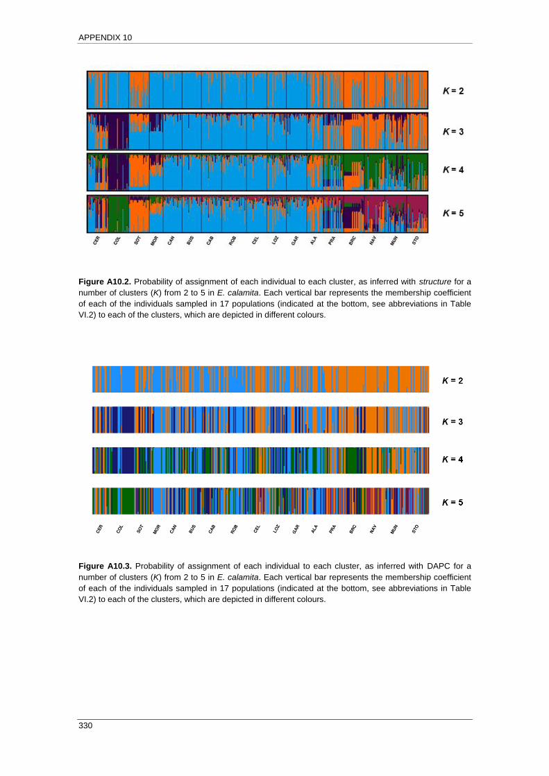
APPENDIX 10
330
Figure A10.2. Probability of assignment of each individual to each cluster, as inferred with structure for a
number of clusters (K) from 2 to 5 in E. calamita. Each vertical bar represents the membership coefficient
of each of the individuals sampled in 17 populations (indicated at the bottom, see abbreviations in Table
VI.2) to each of the clusters, which are depicted in different colours.
Figure A10.3. Probability of assignment of each individual to each cluster, as inferred with DAPC for a
number of clusters (K) from 2 to 5 in E. calamita. Each vertical bar represents the membership coefficient
of each of the individuals sampled in 17 populations (indicated at the bottom, see abbreviations in Table
VI.2) to each of the clusters, which are depicted in different colours.

Results of clustering analyses
331
Figure A10.4. Probability of assignment of each individual to each cluster, as inferred with structure for a
number of clusters (K) from 2 to 5 in H. molleri. Each vertical bar represents the membership coefficient of
each of the individuals sampled in 19 populations (indicated at the bottom, see abbreviations in Table VI.2)
to each of the clusters, which are depicted in different colours.
Figure A10.5. Probability of assignment of each individual to each cluster, as inferred with DAPC for a
number of clusters (K) from 2 to 5 in H. molleri. Each vertical bar represents the membership coefficient of
each of the individuals sampled in 19 populations (indicated at the bottom, see abbreviations in Table VI.2)
to each of the clusters, which are depicted in different colours.

APPENDIX 10
332
Figure A10.6. Probability of assignment of each individual to each cluster, as inferred with structure for a
number of clusters (K) from 2 to 5 in P. perezi. Each vertical bar represents the membership coefficient of
each of the individuals sampled in 15 populations (indicated at the bottom, see abbreviations in Table VI.2)
to each of the clusters, which are depicted in different colours.
Figure A10.7. Probability of assignment of each individual to each cluster, as inferred with DAPC for a
number of clusters (K) from 2 to 5 in P. perezi. Each vertical bar represents the membership coefficient of
each of the individuals sampled in 15 populations (indicated at the bottom, see abbreviations in Table VI.2)
to each of the clusters, which are depicted in different colours.

Results of clustering analyses
333
Figure A10.8. Probability of assignment of each individual to each cluster, as inferred with structure for a
number of clusters (K) from 2 to 5 in P. cultripes. Each vertical bar represents the membership coefficient
of each of the individuals sampled in 13 populations (indicated at the bottom, see abbreviations in Table
VI.2) to each of the clusters, which are depicted in different colours.
Figure A10.9. Probability of assignment of each individual to each cluster, as inferred with DAPC for a
number of clusters (K) from 2 to 5 in P. cultripes. Each vertical bar represents the membership coefficient
of each of the individuals sampled in 13 populations (indicated at the bottom, see abbreviations in Table
VI.2) to each of the clusters, which are depicted in different colours.

APPENDIX 10
334
Figure A10.10. Results of ten different runs of spatial clustering analyses in GENELAND for each species
(Ecal: E. calamita, Hmol: H. molleri, Pper: P. perezi and Pcul: P. cultripes). For each run, the mean
posterior density (mpd) is shown above the map (latitude/longitude decimal geographic coordinates
indicated in the left/bottom axes, respectively) representing the sampled populations (black dots) and the
spatial assignment to each of the two inferred clusters (green or white).
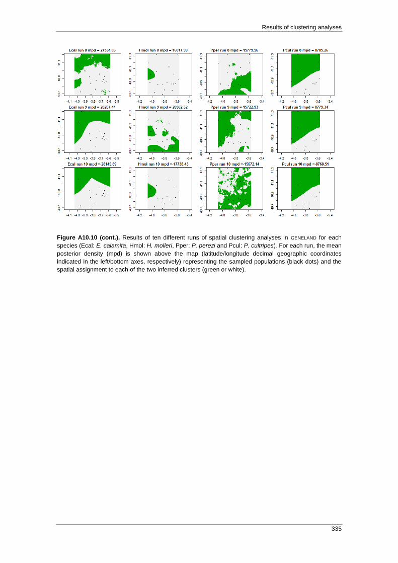
Results of clustering analyses
335
Figure A10.10 (cont.). Results of ten different runs of spatial clustering analyses in GENELAND for each
species (Ecal: E. calamita, Hmol: H. molleri, Pper: P. perezi and Pcul: P. cultripes). For each run, the mean
posterior density (mpd) is shown above the map (latitude/longitude decimal geographic coordinates
indicated in the left/bottom axes, respectively) representing the sampled populations (black dots) and the
spatial assignment to each of the two inferred clusters (green or white).