
Experimental Design to Investigate the Casing Smearing Effect · 2017-10-10 · filter-cake build...
106
Fehler! Kein Text mit angegebener Formatvorlage im Dokument. Fehler! Kein Text mit angegebener Formatvorlage im Dokument. i Daniel Maria Hirschl Master Thesis 2017:E12 supervised by Univ.-Prof. Dipl.-Ing. Dr.mont. Gerhard Thonhauser Experimental Design to Investigate the Casing Smearing Effect
Transcript of Experimental Design to Investigate the Casing Smearing Effect · 2017-10-10 · filter-cake build...
Fehler! Kein Text mit angegebener Formatvorlage im Dokument. Fehler! Kein Text
mit angegebener Formatvorlage im Dokument.
i
Daniel Maria Hirschl Master Thesis 2017:E12 supervised by Univ.-Prof. Dipl.-Ing. Dr.mont. Gerhard Thonhauser
Experimental Design to Investigate the Casing Smearing Effect


iii
This thesis is dedicated to my parents,
Monika and Michael

iv
v
Affidavit I declare in lieu of oath that I wrote this thesis and performed the associated
research myself using only literature cited in this volume.
Eidesstattliche Erklärung Ich erkläre an Eides statt, dass ich diese Arbeit selbständig verfasst, andere
als die angegebenen Quellen und Hilfsmittel nicht benutzt und mich auch
sonst keiner unerlaubten Hilfsmittel bedient habe.
____________________________________
Daniel Maria Hirschl, 07 March 2017

vi
vii
Abstract One of the main reasons why Casing while Drilling (CwD) was growing
more and more interest in the oil and gas industry is the so called “smearing
effect”. Due to the eccentric motion of the casing string crushing of the
cuttings takes place along the string. It is assumed that the casing string
smears the mixture of fine-sized cuttings and mud onto the wellbore wall.
The result in most of the cases is a low permeability layer, which is assumed
to stabilize the wellbore wall and consequently increases the overall drilling
margin.
This is in contrast to the ordinary methods of fluid loss prevention.
Normally a filter cake develops due to the difference in formation and mud
pressure. No mechanical action is involved in the creation of the cake. In
this case, it is not desirable if the drillstring makes contact with the wellbore
wall. Furthermore, the cuttings remain at its original size because no
crushing action takes place. Therefore, the influence of the cuttings on the
filter cake quality is negligible.
The main goal for both methods is the same but the underlying mechanism
is different.
The thesis analyses the underlying mechanisms in theory and defines the
most influential parameters for both methods. Furthermore, the
geomechanical impact on the area surrounding the wellbore regarding CwD
is analysed. Finally, an experimental design is proposed which, if
implemented, enables the user to directly compare filter cakes created by
one of the two methods.

viii
ix
Zusammenfassung Einer der Hauptgründe für die Verwendung von Casing while Drilling ist
der sogenannte “smearing-effect”. Aufgrund der exzentrischen Bewegung
des Bohrstranges, der in diesem Fall aus Verrohrung besteht, wird das
Bohrklein an der Bohrlochwand zerbrochen. Anschließend schmiert der
Bohrstrang die Mischung aus Bohrschlamm und zerkleinertem Bohrklein an
die Wand und erzeugt so einen Filterkuchen mit niedriger Permeabilität.
Dies ist im Gegensatz zu den normalerweise eingesetzten Methoden zur
Vermeidung von Bohrschlammverlust in die Formation. Normalerweise
entsteht alleine durch den Druckunterschied zwischen Bohrschlamm und
Formation ein Filterkuchen an der Bohrlochwand. Der Bohrstrang hat
darauf keinen Einfluss. Das Bohrklein behält seine Originalgröße und hat
auf die Qualität des Filterkuchens keinen Einfluss.
Das Ziel beider Methoden ist das Gleiche. Man möchte verhindern dass es
zu einem Verlust von Bohrschlamm in die Formation kommt. Der zugrunde
liegende Mechanismus ist jedoch unterschiedlich.
Diese Arbeit analysiert den zugrunde liegenden Mechanismus beider
Methoden und jene Parameter die auf das Ergebnis den größten Einfluss
haben. Des Weiteren wird der geomechanische Einfluss von Casing while
Drilling auf die umliegende Formation untersucht. Abschließend wird ein
Design für ein Experiment vorgeschlagen das einen direkten Vergleich der
Filterkuchen beider Methoden ermöglichen soll.

x

xi
Acknowledgements
I would like to thank my parents, Monika and Michael for their continuous
support since the start of my studies.
I would also like to thank my siblings for reminding me that there is also a
life besides studying and for being so patient with a “workaholic”.

xii
xiii
Contents Chapter 1 Introduction .............................................................................................................. 1
Chapter 2 Literature Review .................................................................................................... 2
2.1 Fundamentals of Filter Cake Build-up.......................................................................... 2
2.1.1 Static Filter Cake Description.................................................................................. 2
2.1.1.1 Filter Cake Porosity ........................................................................................... 4
2.1.1.2 Filter Cake Thickness ........................................................................................ 5
2.1.1.3 Filter Cake Permeability ................................................................................... 6
2.1.2 Dynamic Filter Cake Description ........................................................................... 7
2.1.2.1 Filter Cake Porosity and Permeability ........................................................... 8
2.1.2.2 Particle Size Distribution .................................................................................. 8
2.2 Fundamentals of the Smearing Effect ......................................................................... 11
2.2.1 Objectives of Casing while Drilling ..................................................................... 11
2.2.2 Mechanical Parameters Influencing Filter-Cake Build-up in CwD ................. 13
2.2.2.1 Eccentricity ....................................................................................................... 13
2.2.2.2 Pipe Geometry ................................................................................................. 13
2.2.2.3 Contact Angle .................................................................................................. 13
2.2.2.4 Contact Area .................................................................................................... 14
2.2.2.5 Linear Speed of the Pipe before hitting the Wellbore Wall ....................... 14
2.2.2.6 Penetration Depth into the Filter Cake ........................................................ 14
2.2.2.7 Pipe to Wellbore Size Ratio ............................................................................ 14
2.2.2.8 Particle Size Distribution ................................................................................ 15
2.3 Conclusion of the Literature Review .......................................................................... 16
Chapter 3 Geomechanical Aspects ........................................................................................ 17
3.1 The in-situ Stress State .................................................................................................. 17
3.2 Stresses after Drilling a Well ........................................................................................ 17
3.2.1 The Kirsch Equations ............................................................................................. 19
3.2.2 Compressive Wellbore Failure ............................................................................. 20
3.2.3 Tensile wellbore failure ......................................................................................... 21
3.3 Failure Criteria ............................................................................................................... 21
3.3.1 Linearized Mohr Coulomb Failure Criterion ..................................................... 21
3.3.2 Hoek-Brown Failure Criterion .............................................................................. 23
3.4 The Influence of CwD on Wellbore Geomechanics .................................................. 24
3.4.1 Time dependent pore pressure change ............................................................... 24
3.4.2 Stresses during CwD .............................................................................................. 26
3.4.2.1 Change in Hoop Stress with Varying RPM of Casing ............................... 27
3.4.2.2 Change in Hoop Stress with Variation in Annulus to Hole Ratio ........... 29
3.5 Geomechanical Conclusions......................................................................................... 30
xiv
Chapter 4 Existing Laboratory Technologies ....................................................................... 31
4.1 Static Experiments .......................................................................................................... 31
4.1.1 Static filter cake filtration cell ................................................................................ 31
4.1.2 Hassler Cell .............................................................................................................. 32
4.2 Dynamic Experiments ................................................................................................... 32
4.2.1 High Pressure and Temperature filtration cell by Oilfield Instruments Inc. . 32
4.2.2 Multi-Core Dynamic Fluid Loss Equipment ...................................................... 33
4.2.3 Dynamic Filtration Apparatus .............................................................................. 33
4.2.4 Lubricity, Filtration, Drilling Simulator - M2200 ............................................... 34
4.2.5 Dynamic Filtration Unit, US-Patent: 4,790,933 ................................................... 35
4.2.6 Dynamic HPHT® Filtration System by Fann ..................................................... 35
4.2.7 Lubricity Evaluation Monitor ............................................................................... 36
Chapter 5 Experimental Setup ................................................................................................ 37
5.1 Type of Experiments ...................................................................................................... 37
5.2 General Considerations ................................................................................................. 37
5.3 Measurement .................................................................................................................. 38
5.3.1 Filter Cake Porosity and Permeability ................................................................. 39
5.3.2 Filtrate Volume........................................................................................................ 40
5.3.3 Filter Cake Thickness-Equilibrium Thickness .................................................... 41
5.3.3.1 Measuring Filter Cake Thickness .................................................................. 42
5.3.4 Invasion Depth ........................................................................................................ 45
5.3.4.1 Continuous Invasion Depth Measurement.................................................. 45
5.3.4.2 Post-Test Invasion Depth Measurement ...................................................... 46
5.3.5 Fluid Saturation ...................................................................................................... 47
5.3.5.1 Distillation Retort Method ............................................................................. 48
5.3.5.2 Solvent Extraction Method ............................................................................. 49
5.3.6 Return Permeability ............................................................................................... 50
5.3.7 Structural/Compositional Analysis ...................................................................... 52
5.3.7.1 Scanning Electron Microscope Technique ................................................... 52
5.3.7.2 X-Ray Diffraction and X-Ray Fluorescence Analysis ................................. 53
5.3.8 Particle Size Distribution ....................................................................................... 54
5.4 Proposed Experimental Design .................................................................................... 55
5.4.1 Core Holder ............................................................................................................. 56
5.4.1.1 Core Diameter and Core Length ................................................................... 56
5.4.1.2 Confining Pressure .......................................................................................... 57
5.4.1.3 Material ............................................................................................................. 57
5.4.1.4 Design ............................................................................................................... 57
5.4.2 Main body ................................................................................................................ 58
5.4.2.1 Pressure ............................................................................................................. 60
5.4.2.2 Temperature ..................................................................................................... 62
5.4.2.3 Shear Stress ....................................................................................................... 63
5.4.2.4 Material and Dimensions ............................................................................... 65
5.4.3 Drill-Pipe Design .................................................................................................... 65
xv
5.5 Dimensions ..................................................................................................................... 66
Chapter 6 Experimental Procedures ...................................................................................... 70
6.1 General ............................................................................................................................ 70
6.2 Static Filtration Test ....................................................................................................... 71
6.3 Dynamic Filtration Test ................................................................................................ 72
6.4 Pipe Impact Test ............................................................................................................. 73
Chapter 7 Results and Conclusion ......................................................................................... 75
7.1 Results ............................................................................................................................. 75
7.2 Conclusion ...................................................................................................................... 76
Appendix A Equations ............................................................................................................ 77
A.1 Stresses around the wellbore ...................................................................................... 77
A.2 Herschel Bulkley pressure drop ................................................................................. 77

Introduction
1
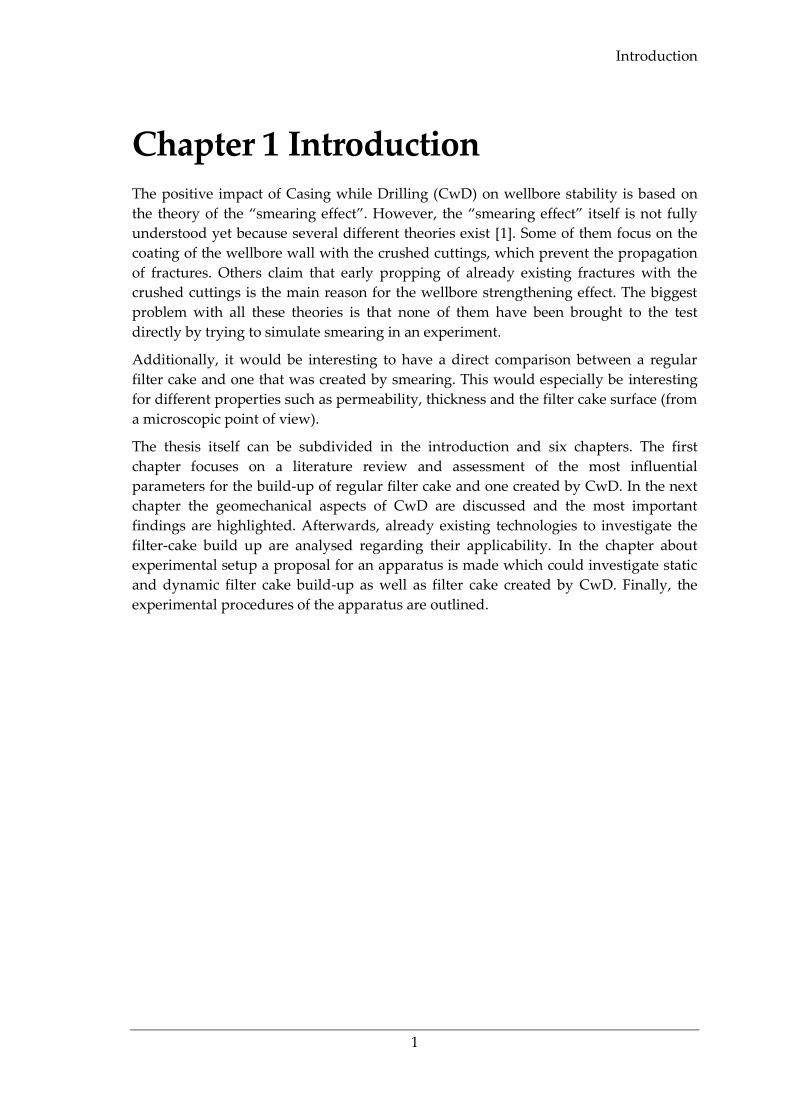
Chapter 1 Introduction The positive impact of Casing while Drilling (CwD) on wellbore stability is based on
the theory of the “smearing effect”. However, the “smearing effect” itself is not fully
understood yet because several different theories exist [1]. Some of them focus on the
coating of the wellbore wall with the crushed cuttings, which prevent the propagation
of fractures. Others claim that early propping of already existing fractures with the
crushed cuttings is the main reason for the wellbore strengthening effect. The biggest
problem with all these theories is that none of them have been brought to the test
directly by trying to simulate smearing in an experiment.
Additionally, it would be interesting to have a direct comparison between a regular
filter cake and one that was created by smearing. This would especially be interesting
for different properties such as permeability, thickness and the filter cake surface (from
a microscopic point of view).
The thesis itself can be subdivided in the introduction and six chapters. The first
chapter focuses on a literature review and assessment of the most influential
parameters for the build-up of regular filter cake and one created by CwD. In the next
chapter the geomechanical aspects of CwD are discussed and the most important
findings are highlighted. Afterwards, already existing technologies to investigate the
filter-cake build up are analysed regarding their applicability. In the chapter about
experimental setup a proposal for an apparatus is made which could investigate static
and dynamic filter cake build-up as well as filter cake created by CwD. Finally, the
experimental procedures of the apparatus are outlined.
Literature Review
2
Chapter 2 Literature Review While drilling a well, one of the main objectives of the drilling mud is to stabilize the
wellbore and ensure safe operations. The drilling mud creates a pressure inside the
wellbore, which hinders fluid to enter the wellbore in an uncontrolled way.
Nevertheless, it is equally important to prevent fluid loss into the formation. When
drilling overbalanced the mud pressure is higher than the formation pressure and
therefore fluid is going to enter the formation anyway. To prevent that it is necessary
that a sufficient filter cake of good consistency is build-up on the wellbore wall.
Furthermore, the filter cake is the only barrier for the fluid between wellbore and
formation. Therefore, it is of vital importance to have a fundamental understanding
about the build-up process and the mud cake properties. The standard process of mud
cake build up has been studied extensively but since CwD has become more popular a
new phenomenon has been observed which is called the “smearing effect”.
The following literature review examines the most important parameters that influence
the build-up and the final properties of a regular filter cake and one created by
smearing. The overall conclusion will then define the parameters which have the most
influence and should be investigated during the experimental research.
2.1 Fundamentals of Filter Cake Build-up The fundamental theory of filter cake build-up is already described in the introduction
of this literature review. Nevertheless it is important to pay attention to the details.
During drilling two different situations are observed in terms of filter cake build-up. If
circulation is stopped only the hydrostatic pressure of the mud forces the build-up of a
filter cake. This can be called a “static” system. During circulation, continuous fluid
flow has a major influence on the filter cake build-up. In this case we are talking about
a “dynamic” system.
2.1.1 Static Filter Cake Description According to Dewan and Chenevert [2, p. 237] a minimum of three parameters are
required to characterize a filter cake. They state that these parameters are porosity,
permeability and a compressibility exponent. The compressibility exponent describes
the dependence of porosity and permeability on pressure across the mud cake.
Porosity and permeability are well known parameters but in the case of filter cake
build-up we are not talking about constant values anymore, as they vary with time due
to compression of the filter cake in the build-up process. The following formulas are
proposed by Dewan and Chenevert [2, p. 239] to describe this behaviour where v is the
compressibility exponent, which ranges typically between 0.4 and 0.9. Additionally,
reference permeability with a differential pressure of 1 psi is defined, which is called
kmc0. The equation for mud cake porosity looks similar, but it includes a multiplier δ,
Fundamentals of Filter Cake Build-up
3
which is in the range of 0.1 to 0.2 and is based on porosity-permeability crossplots for
shaly sands.
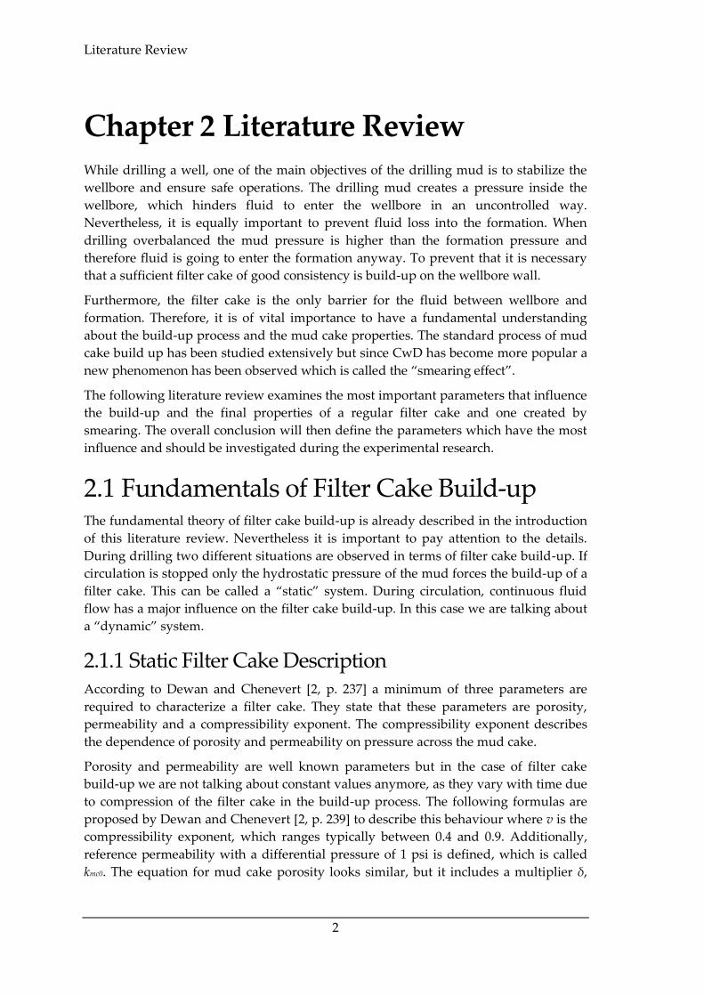
Figure 1: Model of filtration through a core [2, p. 239]
𝑘𝑚𝑐(𝑡) =𝑘𝑚𝑐0
𝑃𝑚𝑐𝑣
Equation 1: Mudcake permeability determination [2, p. 239]
Where Pmc is the pressure across the mudcake, kmc0 is the reference permeability and v is
the compressibility exponent.
𝛷𝑚𝑐(𝑡) =𝛷𝑚𝑐0
𝑃𝑚𝑐𝑣∗𝛿
Equation 2: Mudcake porosity determination [2, p. 240]
Where Φmc is the mudcake porosity, Φmc0 is the reference porosity and δ is the multiplier
based on porosity-permeability crossplots for shaly sands.
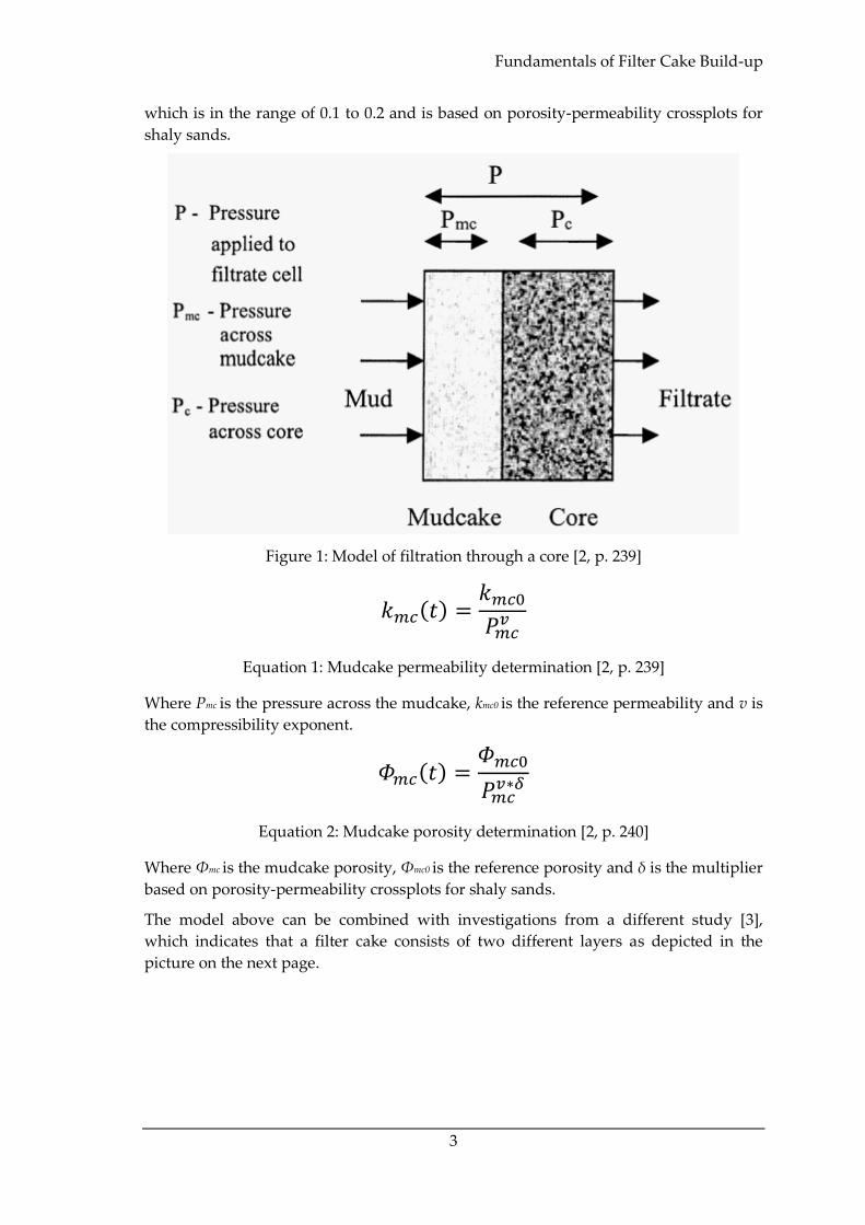
The model above can be combined with investigations from a different study [3],
which indicates that a filter cake consists of two different layers as depicted in the
picture on the next page.
Literature Review
4
Figure 2: CT-Scan of Filter Cake with two-layer structure [3, p. 10]
Furthermore, investigations via SEM showed a clear difference in the composition of
both layers.
Figure 3: SEM-Scan of the internal and the external layer [4, p. 11]
Furthermore, during the process of build-up, the properties of the filter cake are not
constant. Different periods of build-up and compression occur, which result in
changing values for thickness, porosity and permeability of the filter cake.
2.1.1.1 Filter Cake Porosity
Porosity is calculated based on the CT-Number by the following equation.
𝛷 =𝐶𝑇𝑤𝑒𝑡 − 𝐶𝑇𝑑𝑟𝑦
𝐶𝑇𝑤𝑎𝑡𝑒𝑟 − 𝐶𝑇𝑎𝑖𝑟
Equation 3: Porosity calculated from the CT-Number [5, p. 2]
Where CTwet is the CT-Number of the scanned slice saturated with water, CTdry is the
CT-Number of the scanned slice when dry, CTwater is the CT-Number of water and CTair
is the CT-Number of air.
Fundamentals of Filter Cake Build-up
5
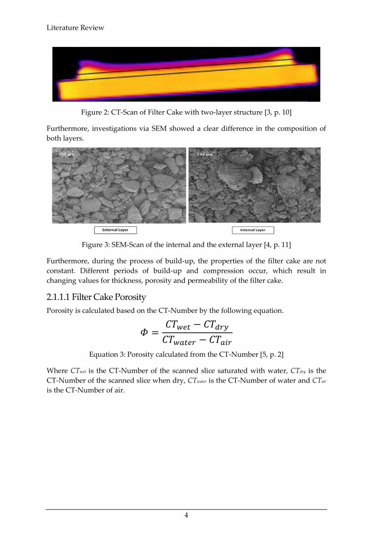
Figure 4: Filter cake porosity as a function of time [5, p. 11]
Before 7.5 minutes, it can be seen that different periods of compression and build-up
are present as the porosity changes very fast from high to low values and vice versa.
After 7.5 minutes, a more or less normal behaviour can be seen as porosity decreases
with time. Additionally, the outer layer of the filter cake can be influenced by the
particle size. As can be seen in Figure 3 the external layer experiences a very poor
sorting resulting in a porosity that drops down to zero in this experiment [5, p. 11].
2.1.1.2 Filter Cake Thickness
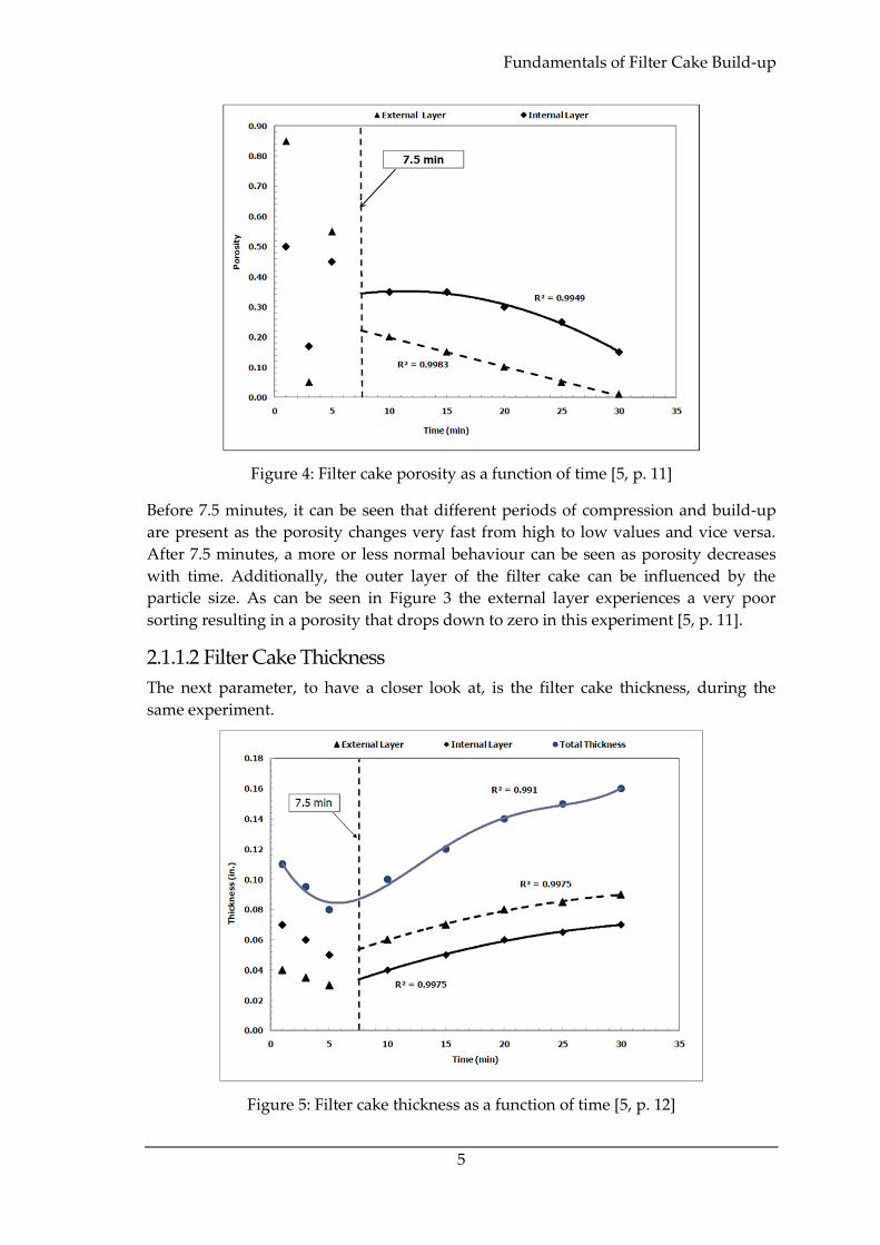
The next parameter, to have a closer look at, is the filter cake thickness, during the
same experiment.
Figure 5: Filter cake thickness as a function of time [5, p. 12]
Literature Review
6
In the compression region, which is before 7.5 minutes, the filter cake thickness
decreases for both layers. Afterwards, as the build-up rate is high enough, a normal
trend can be observed, which shows an increase in filter cake thickness as time goes by.
An interesting observation is the fact that the thickness of the internal filter cake is
higher in the beginning than the external one. This is caused by the precipitation of
large particles in the beginning. Afterwards, as porosity in the external filter cake
decreases, less particles could move through the filter cake and the thickness of the
external filter cake is therefore higher [5, p. 12].
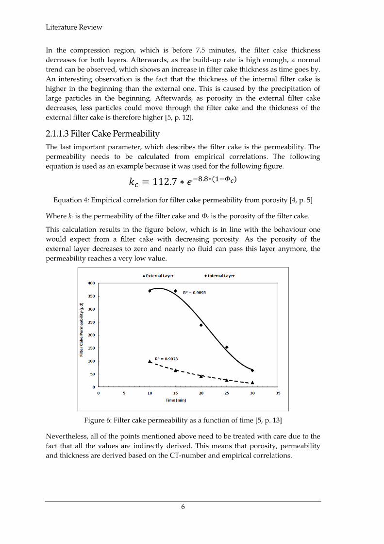
2.1.1.3 Filter Cake Permeability
The last important parameter, which describes the filter cake is the permeability. The
permeability needs to be calculated from empirical correlations. The following
equation is used as an example because it was used for the following figure.
𝑘𝑐 = 112.7 ∗ 𝑒−8.8∗(1−𝛷𝑐)
Equation 4: Empirical correlation for filter cake permeability from porosity [4, p. 5]
Where kc is the permeability of the filter cake and Φc is the porosity of the filter cake.
This calculation results in the figure below, which is in line with the behaviour one
would expect from a filter cake with decreasing porosity. As the porosity of the
external layer decreases to zero and nearly no fluid can pass this layer anymore, the
permeability reaches a very low value.
Figure 6: Filter cake permeability as a function of time [5, p. 13]
Nevertheless, all of the points mentioned above need to be treated with care due to the
fact that all the values are indirectly derived. This means that porosity, permeability
and thickness are derived based on the CT-number and empirical correlations.
Fundamentals of Filter Cake Build-up
7
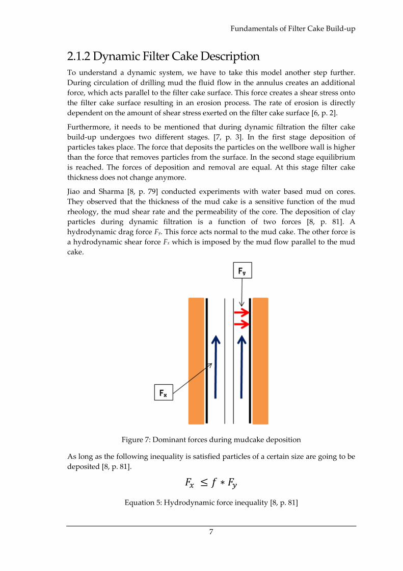
2.1.2 Dynamic Filter Cake Description To understand a dynamic system, we have to take this model another step further.
During circulation of drilling mud the fluid flow in the annulus creates an additional
force, which acts parallel to the filter cake surface. This force creates a shear stress onto
the filter cake surface resulting in an erosion process. The rate of erosion is directly
dependent on the amount of shear stress exerted on the filter cake surface [6, p. 2].
Furthermore, it needs to be mentioned that during dynamic filtration the filter cake
build-up undergoes two different stages. [7, p. 3]. In the first stage deposition of
particles takes place. The force that deposits the particles on the wellbore wall is higher
than the force that removes particles from the surface. In the second stage equilibrium
is reached. The forces of deposition and removal are equal. At this stage filter cake
thickness does not change anymore.
Jiao and Sharma [8, p. 79] conducted experiments with water based mud on cores.
They observed that the thickness of the mud cake is a sensitive function of the mud
rheology, the mud shear rate and the permeability of the core. The deposition of clay
particles during dynamic filtration is a function of two forces [8, p. 81]. A
hydrodynamic drag force Fy. This force acts normal to the mud cake. The other force is
a hydrodynamic shear force Fx which is imposed by the mud flow parallel to the mud
cake.
Figure 7: Dominant forces during mudcake deposition
As long as the following inequality is satisfied particles of a certain size are going to be
deposited [8, p. 81].
𝐹𝑥 ≤ 𝑓 ∗ 𝐹𝑦
Equation 5: Hydrodynamic force inequality [8, p. 81]
Literature Review
8
In the beginning, when the filtration rate is high, bigger particles are going to settle but
when the filtration rate decreases, smaller particles are going to be deposited and
finally, when the drag force is too small the equilibrium state is reached and no more
particles are deposited on the filter cake surface [8, p. 3].
2.1.2.1 Filter Cake Porosity and Permeability
Dynamic conditions in the annulus can have a positive effect on the filter cake porosity.
Due to the shear forces present, they could hinder fine particles to settle on top of the
filter cake surface [4, p. 4]. This has not only a positive effect on the overall porosity but
also on the permeability of the filter cake, which is especially critical if we later want to
produce a reservoir fluid through the filter cake [9, p. 1]. Therefore, special attention
has to be paid to the particle size distribution (PSD) in the drilling mud.
2.1.2.2 Particle Size Distribution
A wrong PSD can lead to an invasion of drilling fluid into the reservoir, which could
actually lead to a positive skin [10, p. 1], which, in return, could result in bad
production rates and costly stimulation operations. Therefore, it is necessary to have an
optimized PSD in the drilling mud.
“It is commonly understood that a reservoir drilling fluid must be compatible with the
reservoir rock, both chemically and physically” [10, p. 1]
The invasion of drilling fluid into the formation is closely related to the pore system
and other fluid-flow channels in the reservoir rock [10, p. 1]. Therefore, it is necessary
to have a fundamental understanding about the type, size and distribution of fluid-
flow channels in the critical interval. Different techniques exist for characterizing these
features. Thin sections, mercury injection, SEM and Micro CT are the most popular
methods [10, pp. 2-4].
Based on the methods mentioned above the most important features to determine the
particle size distribution, are:
• Dominant flow channels in the rock
• Dimension, Distribution and Connectivity of Pores
• Dimension, Distribution and Connectivity of Fractures
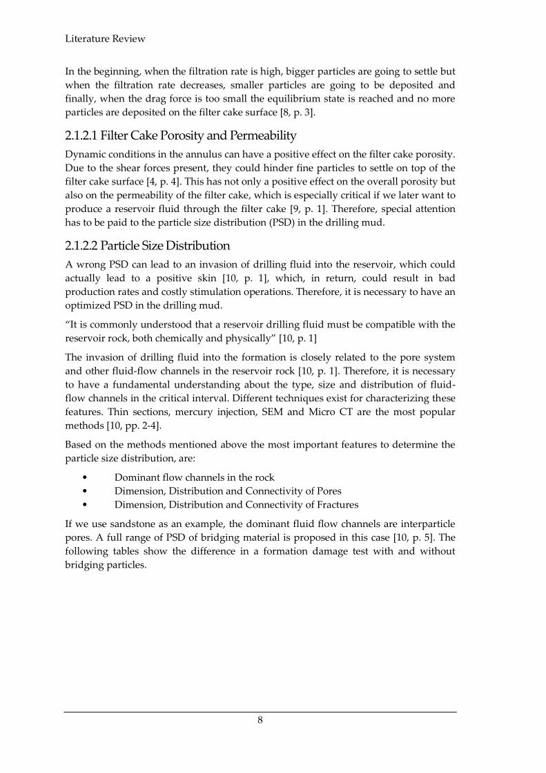
If we use sandstone as an example, the dominant fluid flow channels are interparticle
pores. A full range of PSD of bridging material is proposed in this case [10, p. 5]. The
following tables show the difference in a formation damage test with and without
bridging particles.
Fundamentals of Filter Cake Build-up
9
Test
Fluid
Initial
Permeability
[mD]
Volume of
Filtration [ml] /
[%] Pore
Volume
Return
Permeability
[mD] / [%] Return
Flow
Initiation
Pressure
[psi] 1 230.4 5.7 / 48.9 212.4 / 92.2 6.9
2 250.5 7.0 / 50.4 237.3 / 94.7 9.7
3 258.0 5.8 / 43.3 236.6 / 91.7 6.0
Table 1: Test results for a sandstone using bridging particles [10, p. 6]
Test
Fluid
Initial
Permeability
[mD]
Volume of
Filtration [ml] /
[%] Pore
Volume
Return
Permeability
[mD] / [%] Return
Flow
Initiation
Pressure
[psi] 1 43.2 16.8 / 160.0 4.07 / 12.6 92.7
2 32.2 17.3 / 135.3 4.76 / 11.0 68.9
3 93.4 22.7 / 200.0 23.65 / 25.3 23.5
Table 2: Test results for a sandstone without bridging particles [10, p. 6]
It is obvious from the results above that the correct PSD makes a big difference as, the
return permeability is much smaller and the volume of filtration is much higher.
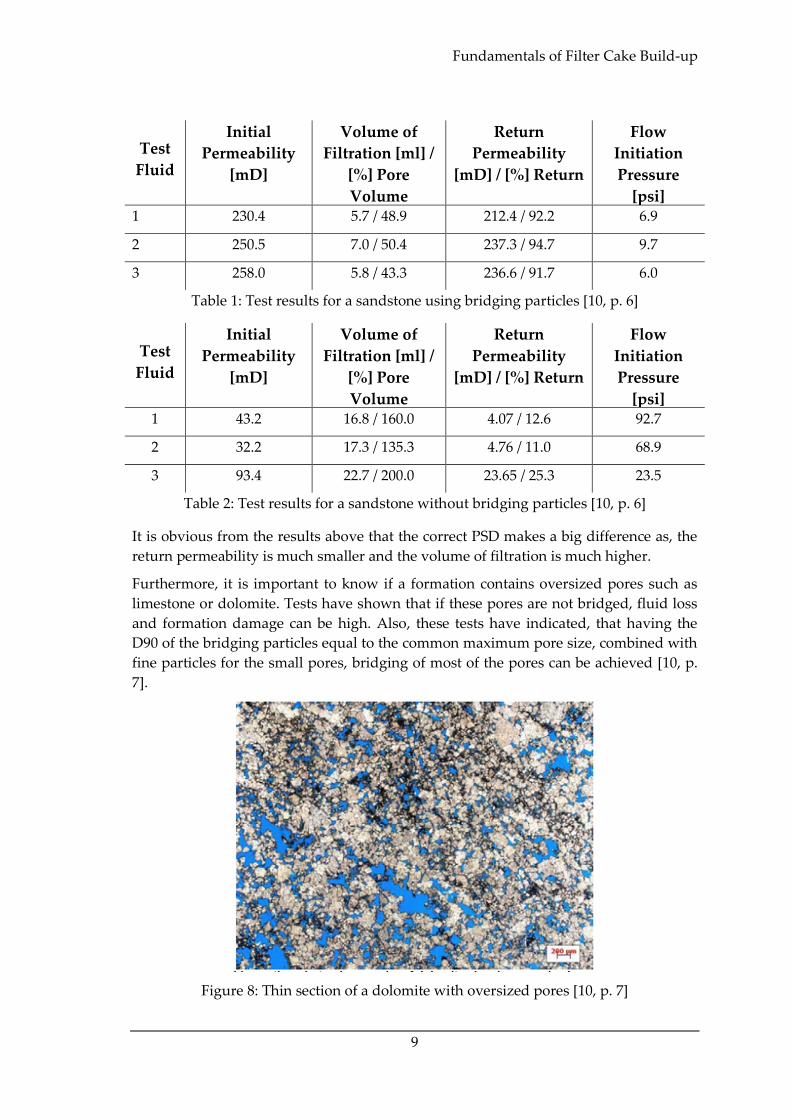
Furthermore, it is important to know if a formation contains oversized pores such as
limestone or dolomite. Tests have shown that if these pores are not bridged, fluid loss
and formation damage can be high. Also, these tests have indicated, that having the
D90 of the bridging particles equal to the common maximum pore size, combined with
fine particles for the small pores, bridging of most of the pores can be achieved [10, p.
7].
Figure 8: Thin section of a dolomite with oversized pores [10, p. 7]
Literature Review
10
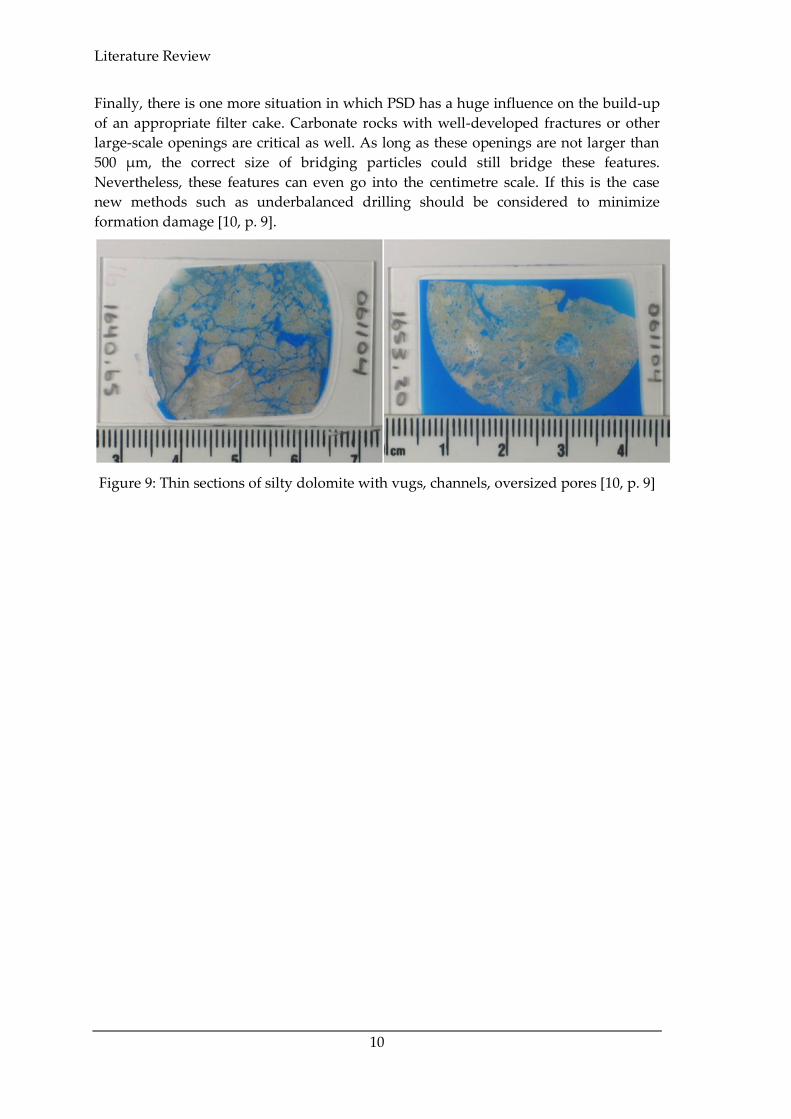
Finally, there is one more situation in which PSD has a huge influence on the build-up
of an appropriate filter cake. Carbonate rocks with well-developed fractures or other
large-scale openings are critical as well. As long as these openings are not larger than
500 µm, the correct size of bridging particles could still bridge these features.
Nevertheless, these features can even go into the centimetre scale. If this is the case
new methods such as underbalanced drilling should be considered to minimize
formation damage [10, p. 9].
Figure 9: Thin sections of silty dolomite with vugs, channels, oversized pores [10, p. 9]
Fundamentals of the Smearing Effect
11
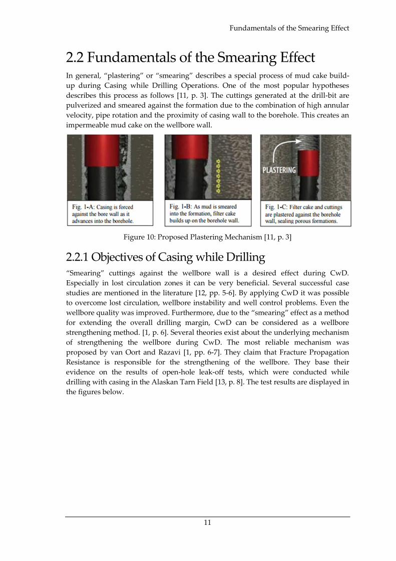
2.2 Fundamentals of the Smearing Effect In general, “plastering” or “smearing” describes a special process of mud cake build-
up during Casing while Drilling Operations. One of the most popular hypotheses
describes this process as follows [11, p. 3]. The cuttings generated at the drill-bit are
pulverized and smeared against the formation due to the combination of high annular
velocity, pipe rotation and the proximity of casing wall to the borehole. This creates an
impermeable mud cake on the wellbore wall.
Figure 10: Proposed Plastering Mechanism [11, p. 3]
2.2.1 Objectives of Casing while Drilling “Smearing” cuttings against the wellbore wall is a desired effect during CwD.
Especially in lost circulation zones it can be very beneficial. Several successful case
studies are mentioned in the literature [12, pp. 5-6]. By applying CwD it was possible
to overcome lost circulation, wellbore instability and well control problems. Even the
wellbore quality was improved. Furthermore, due to the “smearing” effect as a method
for extending the overall drilling margin, CwD can be considered as a wellbore
strengthening method. [1, p. 6]. Several theories exist about the underlying mechanism
of strengthening the wellbore during CwD. The most reliable mechanism was
proposed by van Oort and Razavi [1, pp. 6-7]. They claim that Fracture Propagation
Resistance is responsible for the strengthening of the wellbore. They base their
evidence on the results of open-hole leak-off tests, which were conducted while
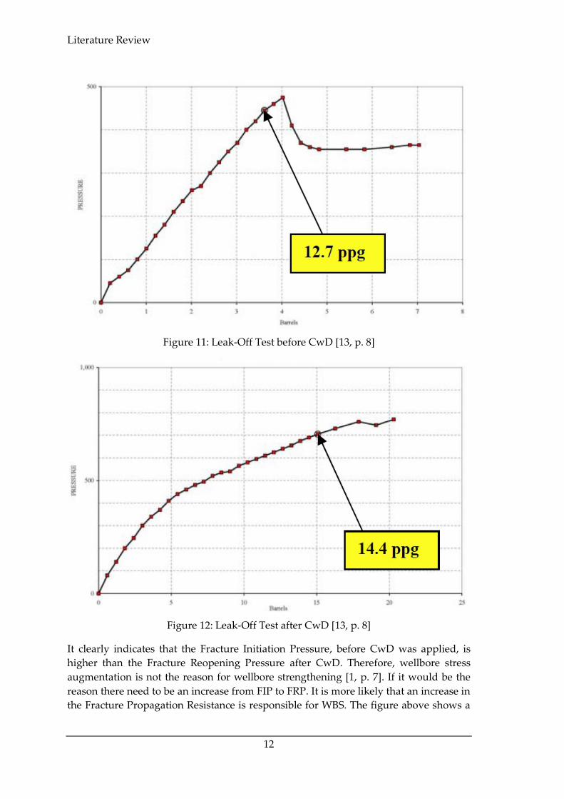
drilling with casing in the Alaskan Tarn Field [13, p. 8]. The test results are displayed in
the figures below.
Literature Review
12
Figure 11: Leak-Off Test before CwD [13, p. 8]
Figure 12: Leak-Off Test after CwD [13, p. 8]
It clearly indicates that the Fracture Initiation Pressure, before CwD was applied, is
higher than the Fracture Reopening Pressure after CwD. Therefore, wellbore stress
augmentation is not the reason for wellbore strengthening [1, p. 7]. If it would be the
reason there need to be an increase from FIP to FRP. It is more likely that an increase in
the Fracture Propagation Resistance is responsible for WBS. The figure above shows a
Fundamentals of the Smearing Effect
13
dramatic increase in the Fracture Propagation Pressure. This means that during CwD it
is much harder for the fractures to propagate. A possible explanation for that is that
tip-screen out occurs during CwD which seals the fracture tips and raises the FPP [1, p.
7].
2.2.2 Mechanical Parameters Influencing Filter-Cake
Build-up in CwD Due to the complexity of this process a variety of parameters have a significant
influence on the smearing effect. The most important ones are discussed in detail in the
sections below.
2.2.2.1 Eccentricity
Eccentricity can be described as how off-centre of the hole a pipe is within the open
hole section [14, p. 10]. If a pipe is concentric it means that the eccentricity is zero.
Nevertheless, it is very unlikely that a pipe is completely concentric, especially in CwD,
it is desired that the pipe moves in an eccentric motion in the wellbore. As recently
mentioned the wellbore strengthening effect of CwD is related to the occurring
fractures. The direction of fracture propagation is related to the stress field.. Due to that
the contact points of the casing with the wellbore should be similar with the direction
of fracture occurrence because this makes a plastering of the induced fractures more
likely. [15, p. 4] Nevertheless, eccentricity can’t be controlled which makes this
influence factor unpredictable.
2.2.2.2 Pipe Geometry
The large diameter of the casing is the primary drive for the “smearing” effect of casing
while drilling [16]. Furthermore, the research of Karimi, Moellendick and Holt [16]
identified the following parameters, with the corresponding explanations mentioned
below, as critical for the success of “smearing” in a CwD operation. Considering the
definition of eccentricity above, the influence of eccentricity is minor if the diameter of
the used pipe gets bigger.
2.2.2.3 Contact Angle
As the tool joint has a bigger diameter than the pipe body and contact with the
wellbore wall is more likely the contact angle is described with regards to the tool joint
diameter. Depending on the diameter of the tool joint the contact angle of the tool joint
is different. With decreasing tool joint diameter, the contact angle gets bigger. This
leads to the problem that a small contact angle is necessary to guarantee a smooth
contact of the tool joint with the wellbore wall. Otherwise there is a significant
potential that contact of the tool joint with the wellbore leads to a damage of the filter
cake. Furthermore, the curvature of the tool joint is another significant factor. If the
curvature of the tool joint is similar to the curvature of the wellbore wall the contact
forces are minimized and the contacting action is smoother.
Literature Review
14
2.2.2.4 Contact Area
A larger contact area is much more beneficial because plastering happens at the contact
area of the pipe. Obviously, the contact area when using casing is much bigger.
Therefore, plastering takes place faster and is much more effective.
2.2.2.5 Linear Speed of the Pipe before hitting the Wellbore Wall
The pipe contact should be as smooth as possible. Therefore, the linear speed should
not be too high because this leads to a forceful momentum transfer onto the filter cake
at the contact area. Due to the fact that the diameter of regular drill pipe is much
smaller than for casing the distance the pipe needs to travel before hitting the wall is
higher. This leads to a higher linear speed in case of the regular drill pipe.
2.2.2.6 Penetration Depth into the Filter Cake
With regards to the differences already mentioned it is obvious that the penetration
depth into the filter cake for regular drill pipe needs to be higher. This is because the
forces when the pipe hits the filter cake are distributed on a much smaller area.
Nevertheless, another observation of Karimi, Moellendick, Holt [16] was that the risk
for differential sticking is still higher for regular drill pipe. This investigation is highly
interesting, because one would expect that the larger contact area of the casing is a
much stronger contributor. They base this phenomenon on the fact that the differential
pressure in case of a filter cake created by ”smearing” is much smaller because of the
high quality of the filter cake.
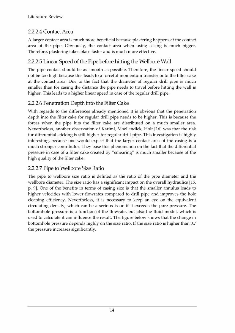
2.2.2.7 Pipe to Wellbore Size Ratio
The pipe to wellbore size ratio is defined as the ratio of the pipe diameter and the
wellbore diameter. The size ratio has a significant impact on the overall hydraulics [15,
p. 9]. One of the benefits in terms of casing size is that the smaller annulus leads to
higher velocities with lower flowrates compared to drill pipe and improves the hole
cleaning efficiency. Nevertheless, it is necessary to keep an eye on the equivalent
circulating density, which can be a serious issue if it exceeds the pore pressure. The
bottomhole pressure is a function of the flowrate, but also the fluid model, which is
used to calculate it can influence the result. The figure below shows that the change in
bottomhole pressure depends highly on the size ratio. If the size ratio is higher than 0.7
the pressure increases significantly.
Fundamentals of the Smearing Effect
15
Figure 13: Bottomhole Pressure vs. Size Ratio [15, p. 11]
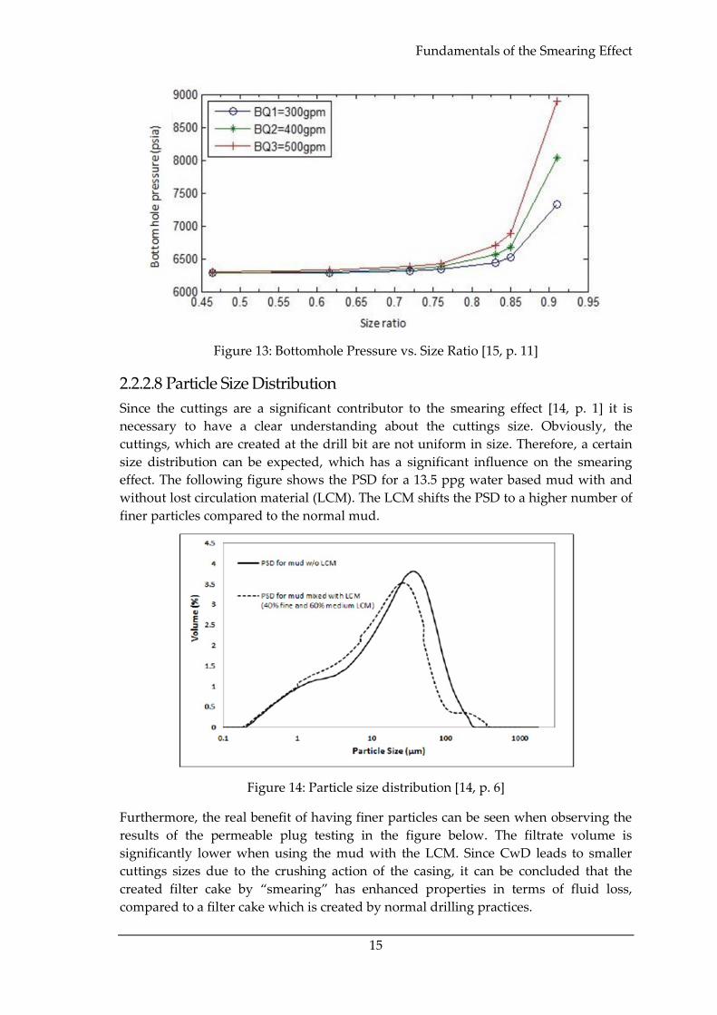
2.2.2.8 Particle Size Distribution
Since the cuttings are a significant contributor to the smearing effect [14, p. 1] it is
necessary to have a clear understanding about the cuttings size. Obviously, the
cuttings, which are created at the drill bit are not uniform in size. Therefore, a certain
size distribution can be expected, which has a significant influence on the smearing
effect. The following figure shows the PSD for a 13.5 ppg water based mud with and
without lost circulation material (LCM). The LCM shifts the PSD to a higher number of
finer particles compared to the normal mud.
Figure 14: Particle size distribution [14, p. 6]
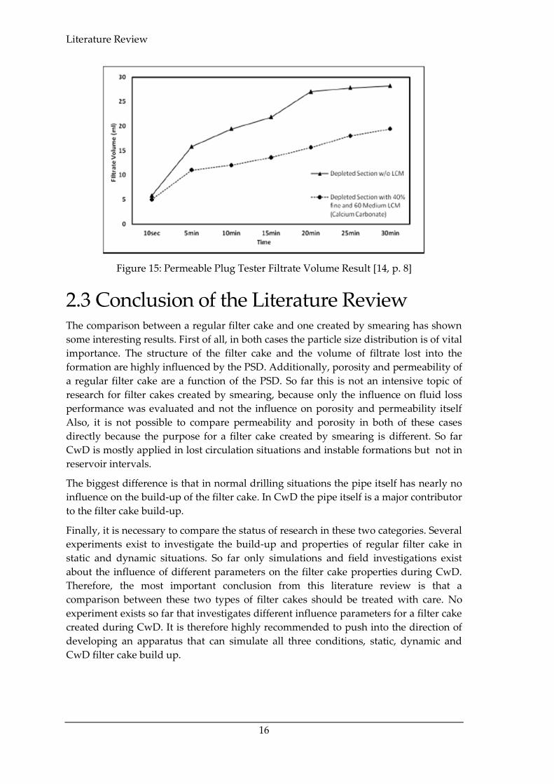
Furthermore, the real benefit of having finer particles can be seen when observing the
results of the permeable plug testing in the figure below. The filtrate volume is
significantly lower when using the mud with the LCM. Since CwD leads to smaller
cuttings sizes due to the crushing action of the casing, it can be concluded that the
created filter cake by “smearing” has enhanced properties in terms of fluid loss,
compared to a filter cake which is created by normal drilling practices.
Literature Review
16
Figure 15: Permeable Plug Tester Filtrate Volume Result [14, p. 8]
2.3 Conclusion of the Literature Review The comparison between a regular filter cake and one created by smearing has shown
some interesting results. First of all, in both cases the particle size distribution is of vital
importance. The structure of the filter cake and the volume of filtrate lost into the
formation are highly influenced by the PSD. Additionally, porosity and permeability of
a regular filter cake are a function of the PSD. So far this is not an intensive topic of
research for filter cakes created by smearing, because only the influence on fluid loss
performance was evaluated and not the influence on porosity and permeability itself
Also, it is not possible to compare permeability and porosity in both of these cases
directly because the purpose for a filter cake created by smearing is different. So far
CwD is mostly applied in lost circulation situations and instable formations but not in
reservoir intervals.
The biggest difference is that in normal drilling situations the pipe itself has nearly no
influence on the build-up of the filter cake. In CwD the pipe itself is a major contributor
to the filter cake build-up.
Finally, it is necessary to compare the status of research in these two categories. Several
experiments exist to investigate the build-up and properties of regular filter cake in
static and dynamic situations. So far only simulations and field investigations exist
about the influence of different parameters on the filter cake properties during CwD.
Therefore, the most important conclusion from this literature review is that a
comparison between these two types of filter cakes should be treated with care. No
experiment exists so far that investigates different influence parameters for a filter cake
created during CwD. It is therefore highly recommended to push into the direction of
developing an apparatus that can simulate all three conditions, static, dynamic and
CwD filter cake build up.
The in-situ Stress State
17
Chapter 3 Geomechanical Aspects The process of drilling a well into the earth leads to an alteration of the original stress
state in the drilled rocks. The same alteration takes place during CwD operations. The
following section is split into two parts. The first section describes the basic
geomechanical concepts which are normally applied for investigating wellbore
stability. The second part investigates the geomechanical conditions in the near
wellbore region while applying CwD and highlights the differences to the normal
conditions.
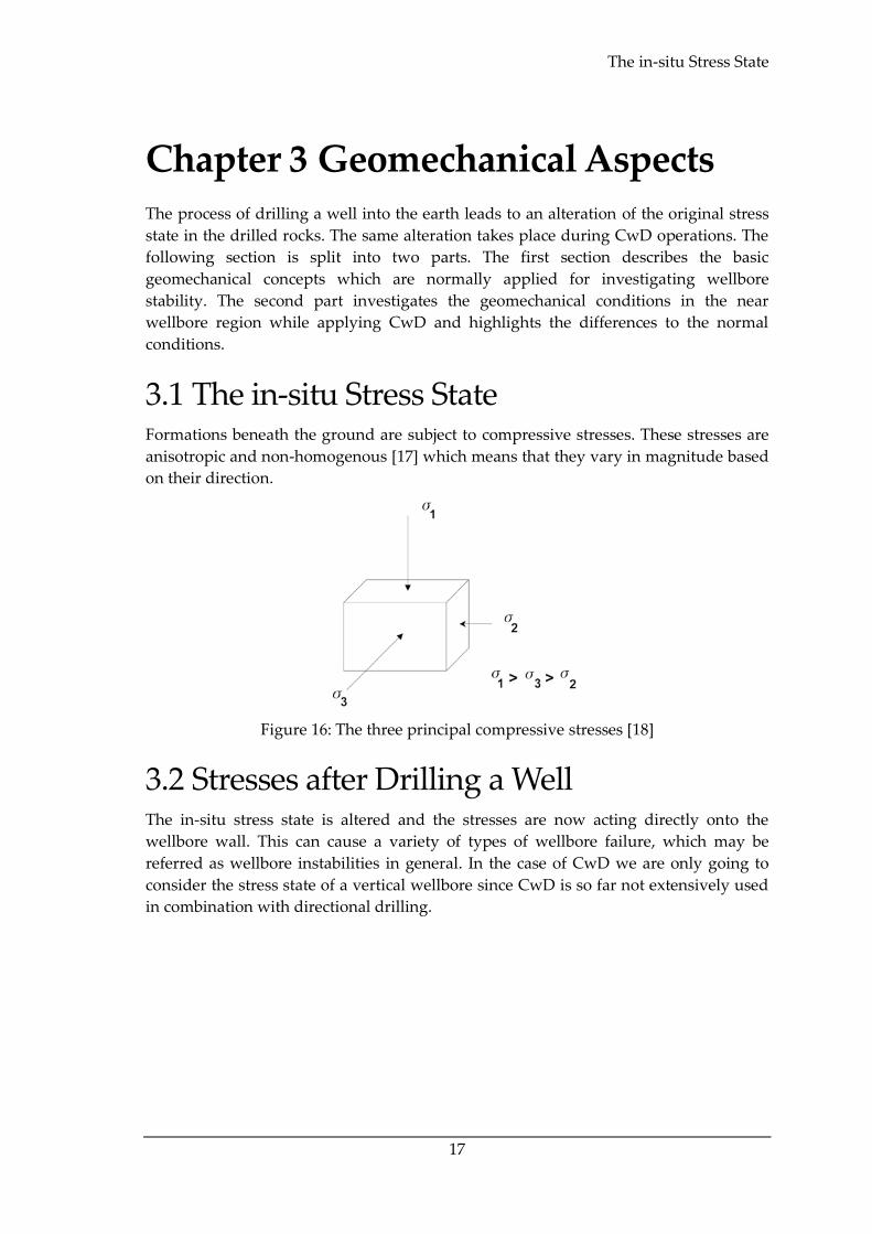
3.1 The in-situ Stress State Formations beneath the ground are subject to compressive stresses. These stresses are
anisotropic and non-homogenous [17] which means that they vary in magnitude based
on their direction.
Figure 16: The three principal compressive stresses [18]
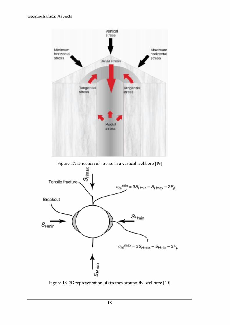
3.2 Stresses after Drilling a Well The in-situ stress state is altered and the stresses are now acting directly onto the
wellbore wall. This can cause a variety of types of wellbore failure, which may be
referred as wellbore instabilities in general. In the case of CwD we are only going to
consider the stress state of a vertical wellbore since CwD is so far not extensively used
in combination with directional drilling.
Geomechanical Aspects
18
Figure 17: Direction of stresse in a vertical wellbore [19]
Figure 18: 2D representation of stresses around the wellbore [20]
Stresses after Drilling a Well
19
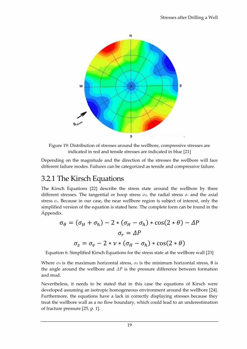
Figure 19: Distribution of stresses around the wellbore, compressive stresses are
indicated in red and tensile stresses are indicated in blue [21]
Depending on the magnitude and the direction of the stresses the wellbore will face
different failure modes. Failures can be categorized as tensile and compressive failure.
3.2.1 The Kirsch Equations The Kirsch Equations [22] describe the stress state around the wellbore by three
different stresses. The tangential or hoop stress σθ, the radial stress σr and the axial
stress σz. Because in our case, the near wellbore region is subject of interest, only the
simplified version of the equation is stated here. The complete form can be found in the
Áppendix.
σ𝜃 = (𝜎𝐻 + 𝜎ℎ) − 2 ∗ (𝜎𝐻 − 𝜎ℎ) ∗ cos(2 ∗ 𝜃) − 𝛥𝑃
𝜎𝑟 = 𝛥𝑃
𝜎𝑧 = 𝜎𝑣 − 2 ∗ 𝜈 ∗ (𝜎𝐻 − 𝜎ℎ) ∗ cos(2 ∗ 𝜃)
Equation 6: Simplified Kirsch Equations for the stress state at the wellbore wall [23]
Where σH is the maximum horizontal stress, σh is the minimum horizontal stress, θ is
the angle around the wellbore and ΔP is the pressure difference between formation
and mud.
Nevertheless, it needs to be stated that in this case the equations of Kirsch were
developed assuming an isotropic homogeneous environment around the wellbore [24].
Furthermore, the equations have a lack in correctly displaying stresses because they
treat the wellbore wall as a no flow boundary, which could lead to an underestimation
of fracture pressure [25, p. 1].
Geomechanical Aspects
20
A possible solution for this problem can be found by introducing a filter cake
permeability coefficient δ [26, p. 913]. If the filter cake is totally sealing the coefficient
becomes zero. For a totally permeable filter cake δ becomes unity. The following
equations account for the additional stress, which acts on the formation due to fluid
seepage through the filter cake.
𝛿 =(𝑃𝑤 − 𝑃0)
(𝑃 − 𝑃0)
Equation 7: Filter cake permeability coefficient [26, p. 913]
Where Pw is the pore pressure at the wellbore wall, P0 is the pore pressure in the far
field formation and P is the fluid column pressure in the borehole.
𝜎𝑟𝑝 = 0
𝜎𝜃𝑝 = 𝛿 ∗𝛼 ∗ (1 − 2 ∗ 𝜈)
1 − 𝜈∗ (𝑃𝑤 − 𝑃0)
𝜎𝑧𝑝 = 𝛿 ∗𝛼 ∗ (1 − 2 ∗ 𝜈)
1 − 𝜈∗ (𝑃𝑤 − 𝑃0)
Equation 8: Additional stresses due to fluid seepage [26, p. 913]
Where σrp is the additional radial stress, σθp is the additional hoop stress, σzp is the
additional axial stress, α is the Biot coefficient and ν is the Poisson’s ratio.
By combining these two methods the influence of fluid seepage into the formation can
be analysed more accurately.
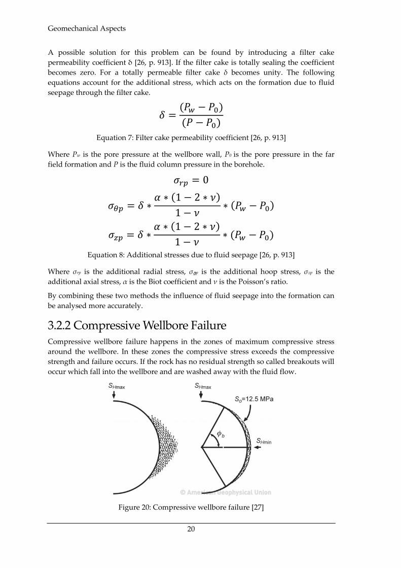
3.2.2 Compressive Wellbore Failure Compressive wellbore failure happens in the zones of maximum compressive stress
around the wellbore. In these zones the compressive stress exceeds the compressive
strength and failure occurs. If the rock has no residual strength so called breakouts will
occur which fall into the wellbore and are washed away with the fluid flow.
Figure 20: Compressive wellbore failure [27]
Failure Criteria
21
3.2.3 Tensile wellbore failure The second type of failure category is the tensile failure resulting in fractures around
the wellbore. In this case the tensile stresses exceed the tensile strength of the rock in
the zone of maximum tensile stresses. The fracture direction is controlled by the
magnitude and direction of the in-situ stress state. Fractures are going to open up
perpendicular to the minimum horizontal stress in direction of the maximum
horizontal stress.
3.3 Failure Criteria Several different wellbore failure criteria exist. There is no universal solution, which
can be applied. The two most common ones are introduced in the next section.
3.3.1 Linearized Mohr Coulomb Failure Criterion This criterion is widely used in different engineering applications. Shear failure takes
place across a plane. The normal stress and the shear stress are associated with a
functional relation characteristic of the material [28, p. 15].
𝜏 = 𝑐 + µ ∗ 𝜎𝑛
Equation 9: Mohr-Coulomb failure criterion [28]
Where τ is the shear stress, c is the cohesion, µ is the tangens of the internal angle of
friction and σn is the normal stress.
The linearized form of the Mohr-Coulomb criterion looks as follows [29]:
𝜎1 = 𝐶0 + 𝑞 ∗ 𝜎3
Equation 10: Linearized Mohr-Coulomb Equation
Where σ1 is the maximum principal stress, σ3 is the minimum principal stress, C0 is the
uniaxial compressive strength of the rock and q is calculated as follows:
𝑞 = [(µ𝑖2 + 1)
12 + µ𝑖]
2
= 𝑡𝑎𝑛2 (𝜋
4+
𝜑
2)
Equation 11: Fitting parameter equation for linearized Mohr Coulomb criterion
𝜑 = tan−1(µ𝑖)
Equation 12: Coefficient of internal friction from angle of internal friction
Based on the equations above it is possible to come up with a failure criterion, which
specifies a critical pressure, which would lead to either wellbore breakouts or
fracturing. Nevertheless, only the two most common stress states for fracturing and
breakout are used for deriving the equation that predicts failure. The two most
common cases according to Gholami et. al [28] are:
Geomechanical Aspects
22
𝜎𝜃 > 𝜎𝑧 > 𝜎𝑟
Equation 13: Most common stress state for wellbore breakout
𝜎𝑟 > 𝜎𝑧 > 𝜎𝜃
Equation 14: Most common stress state for inducing fractures
By analysing the Kirsch equations it is obvious that the tangential and axial stress
equations reach a maximum value at θ is equal to ±π/2 and a minimum value when θ
is equal to 0. As already mentioned breakouts are going to appear at the point of
maximum compressive stress, when the tangential stress reaches a maximum. The
Kirsch equations can then be simplified further to:
σ𝜃𝑚𝑎𝑥 = 3 ∗ 𝜎𝐻 − 𝜎ℎ − 𝛥𝑃
𝜎𝑟 = 𝛥𝑃
𝜎𝑧 = 𝜎𝑣 + 2 ∗ 𝜈 ∗ (𝜎𝐻 − 𝜎ℎ)
Equation 15: Simplified Kirsch equations for predicting wellbore breakouts
If we now consider the most common stress state for wellbore breakouts, as mentioned
above, and substitute the simplified Kirsch equations into the linearized Mohr
Coulomb failure criterion we end up with the following equation.
𝛥𝑃 =3 ∗ 𝜎𝐻 − 𝜎ℎ − 𝜎𝐶
1 + 𝑞
Equation 16: Pressure difference wellbore and formation to avoid breakouts [28]
Where σC is the uniaxial compressive strength.
For predicting the fracture pressure, we follow exactly the same idea as above
considering that fractures or tensile failure occurs at the point of minimum tangential
stress, the Kirsch equations simplify as follows.
σ𝜃𝑚𝑖𝑛 = 3 ∗ 𝜎ℎ − 𝜎𝐻 − 𝛥𝑃
𝜎𝑟 = 𝛥𝑃
𝜎𝑧 = 𝜎𝑣 − 2 ∗ 𝜈 ∗ (𝜎𝐻 − 𝜎ℎ)
Equation 17: Simplified Kirsch equations for predicting fracture initiation in a wellbore
Failure Criteria
23
By substituting the equations into the linearized Mohr-Coulomb failure criterion the
final equation for the allowed pressure difference between wellbore and formation is:
𝛥𝑃 =𝜎𝐶 + 𝑞 ∗ (3 ∗ 𝜎ℎ − 𝜎𝐻)
1 + 𝑞
Equation 18: Pressure difference wellbore and formation to avoid fractures [28]
3.3.2 Hoek-Brown Failure Criterion The Hoek-Brown criterion uses the uniaxial compressive strength of the intact rock
material as a scaling parameter, and it introduces two dimensionless strength
parameters m and s [29]. The maximum principal stress at failure is given as:
𝜎1 = 𝜎3 + 𝜎𝑐 ∗ √𝑚 ∗𝜎3
𝜎𝑐+ 𝑠
Equation 19: Hoek-Brown failure criterion [29]
Hoek and Brown stated [30] that the parameter m depends on the rock type. The
parameter s is dependent on the fact, whether the rock is intact or not. For a completely
intact specimen s is equal to 1. In a completely granulated specimen or a rock aggregate
s is equal to zero [29]. The Hoek-Brown criterion is generally more accepted than the
Mohr-Coulomb failure criterion because it fits a non-linear model to the available data
[28].
The same approach as before is applied to come up with two equations, which describe
the allowable pressure difference between wellbore and formation to avoid fracturing
or breakouts.
The following terms are simplified to shorten the final equation.
𝐷 = 3 ∗ 𝜎𝐻 − 𝜎ℎ
𝑝 = 𝑚 ∗ 𝜎𝑐
𝛥𝑃 =(4 ∗ 𝐷 + 𝑝) ± √(4 ∗ 𝐷 + 𝑝)2 + 16 ∗ (𝜎𝑐
2 − 𝐷2)
8
Equation 20: Pressure difference to avoid breakouts according to Hoek-Brown [28]
Geomechanical Aspects
24
𝐴 = 3 ∗ 𝜎ℎ − 𝜎𝐻
𝑝 = 𝑚 ∗ 𝜎𝑐
𝛥𝑃 =(4 ∗ 𝐴 − 𝑝) ± √(4 ∗ 𝐴 − 𝑝)2 − 16 ∗ (𝐴2 − 𝜎𝑐
2 − 𝑝 ∗ 𝐴)
8
Equation 21: Pressure difference to avoid the fractures according to Hoek-Brown [28]
It needs to be mentioned that several other failure criteria exist. Nevertheless, the scope
of this section is not about stating already known failure criteria. The focus is more on
evaluating the influence of CwD on geomechanical properties such as stresses and
pressure especially in the near wellbore region. To make this point it is sufficient to use
two different failure criteria and describe the impact of CwD based on them.
3.4 The Influence of CwD on Wellbore
Geomechanics One of the main advantages of CwD is that the exposure of the formation to the
drilling fluid is much shorter than in regular drilling operations. It is reported that
formation strength around the wellbore changes with time [31, p. 1]. Furthermore, also
physico-chemical interactions between formation and fluid take place.
Regarding mechanical properties fluid invasion leads to an increase of the near
wellbore pressure [31, p. 1]. But we should not forget that as reported earlier [26], also
the stress state changes and fluid invasion can also create additional stresses in the near
wellbore region.
Another mechanism that should not be underestimated is the frequent contact of the
casing joints with the wellbore wall. This contact is of course intended, but it is also
necessary to understand the possible influence on the geomechanical properties of the
near wellbore region.
3.4.1 Time dependent pore pressure change Pore pressure in the near wellbore region changes with time. This phenomenon has
been addresses in different studies so far [31]. Depending on the permeability of the
filter cake and the formation, this fluid invasion can be very low, but it still has an
impact. Mokhtari, Tutuncu and Teklu [31] performed numerical simulations based on
the following formula.
The Influence of CwD on Wellbore Geomechanics
25
𝑑𝑝
𝑑𝑡=
𝑘
µ𝑓 ∗ 𝛽 ∗ 𝛷∗ [
𝑑2𝑃
𝑑𝑟2+
1
𝑟∗
𝑑𝑝
𝑑𝑟]
Equation 22: Pore pressure changes with time [31]
Where µf is the fluid viscosity, k is the permeability, β is the Biot-coefficient, r is the
distance from the centre of the wellbore and Φ is the porosity.
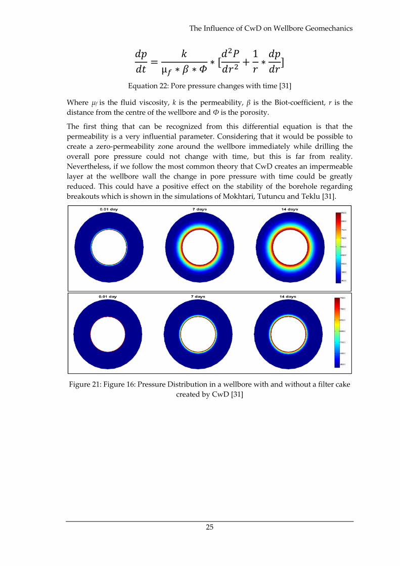
The first thing that can be recognized from this differential equation is that the
permeability is a very influential parameter. Considering that it would be possible to
create a zero-permeability zone around the wellbore immediately while drilling the
overall pore pressure could not change with time, but this is far from reality.
Nevertheless, if we follow the most common theory that CwD creates an impermeable
layer at the wellbore wall the change in pore pressure with time could be greatly
reduced. This could have a positive effect on the stability of the borehole regarding
breakouts which is shown in the simulations of Mokhtari, Tutuncu and Teklu [31].
Figure 21: Figure 16: Pressure Distribution in a wellbore with and without a filter cake
created by CwD [31]
Geomechanical Aspects
26
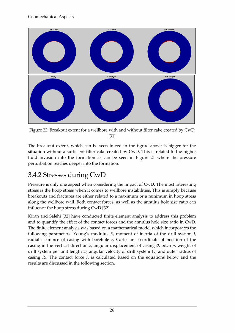
Figure 22: Breakout extent for a wellbore with and without filter cake created by CwD
[31]
The breakout extent, which can be seen in red in the figure above is bigger for the
situation without a sufficient filter cake created by CwD. This is related to the higher
fluid invasion into the formation as can be seen in Figure 21 where the pressure
perturbation reaches deeper into the formation.
3.4.2 Stresses during CwD Pressure is only one aspect when considering the impact of CwD. The most interesting
stress is the hoop stress when it comes to wellbore instabilities. This is simply because
breakouts and fractures are either related to a maximum or a minimum in hoop stress
along the wellbore wall. Both contact forces, as well as the annulus hole size ratio can
influence the hoop stress during CwD [32].
Kiran and Salehi [32] have conducted finite element analysis to address this problem
and to quantify the effect of the contact forces and the annulus hole size ratio in CwD.
The finite element analysis was based on a mathematical model which incorporates the
following parameters. Young’s modulus E, moment of inertia of the drill system I,
radial clearance of casing with borehole r, Cartesian co-ordinate of position of the
casing in the vertical direction z, angular displacement of casing θ, pitch p, weight of
drill system per unit length w, angular velocity of drill system Ω, and outer radius of
casing Ro. The contact force λ is calculated based on the equations below and the
results are discussed in the following section.
The Influence of CwD on Wellbore Geomechanics
27
𝜆 =−𝐸 ∗ 𝐼 ∗ 𝑟 ∗ (𝜃′)4 + 𝑇 ∗ 𝑟 ∗ (𝜃′)3 + 𝐹 ∗ 𝑟 ∗ (𝜃′)2 − µ ∗ 𝑤 ∗ 𝛺2 ∗ 𝑅𝑜 ∗ 𝑠𝑖𝑛2(𝜃)
𝑐𝑜𝑠2(𝜃) + µ ∗ 𝑠𝑖𝑛2(𝜃)+
𝑤 ∗ Ω2 ∗ 𝑅𝑜
𝐹 =8 ∗ 𝜋2 ∗ 𝐸 ∗ 𝐼
𝑝2−
3 ∗ 𝜋 ∗ 𝑇
𝑝
𝐼 =𝜋 ∗ (𝑑𝑜
4 − 𝑑𝑖4)
64
𝜃 =2 ∗ 𝜋 ∗ 𝑧
𝑝
Equation 23: Mathematical model for the FEM analysis [32]
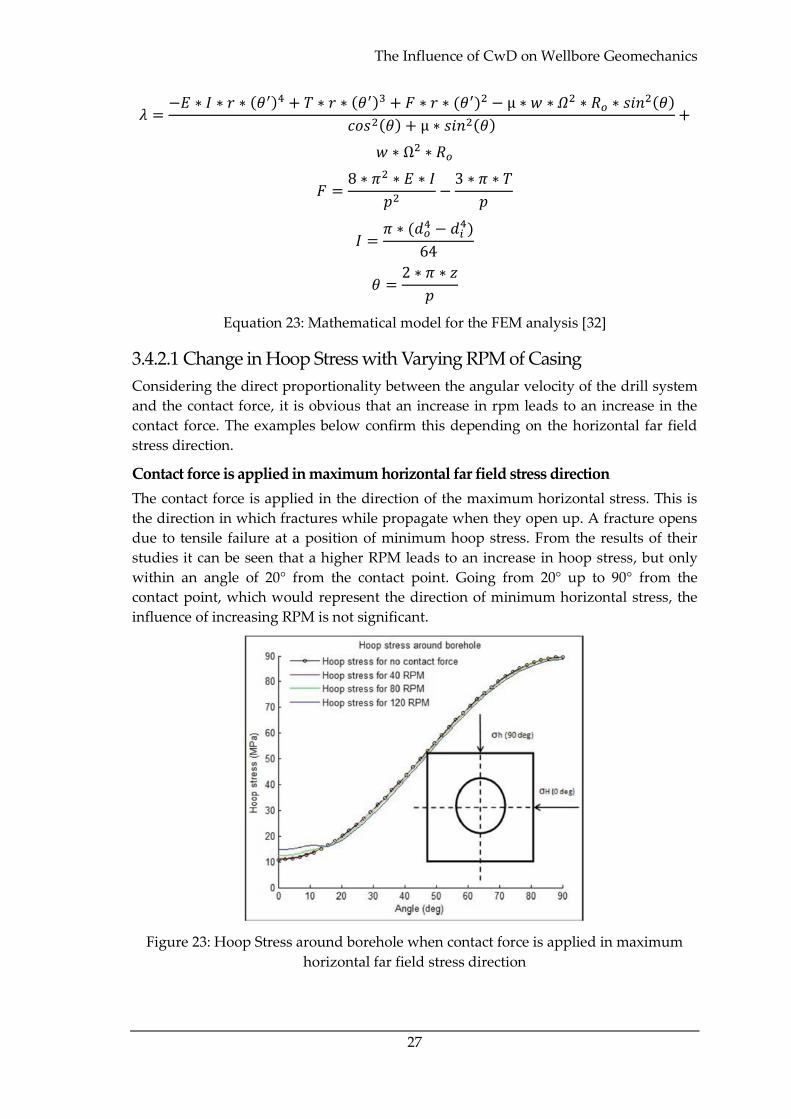
3.4.2.1 Change in Hoop Stress with Varying RPM of Casing
Considering the direct proportionality between the angular velocity of the drill system
and the contact force, it is obvious that an increase in rpm leads to an increase in the
contact force. The examples below confirm this depending on the horizontal far field
stress direction.
Contact force is applied in maximum horizontal far field stress direction
The contact force is applied in the direction of the maximum horizontal stress. This is
the direction in which fractures while propagate when they open up. A fracture opens
due to tensile failure at a position of minimum hoop stress. From the results of their
studies it can be seen that a higher RPM leads to an increase in hoop stress, but only
within an angle of 20° from the contact point. Going from 20° up to 90° from the
contact point, which would represent the direction of minimum horizontal stress, the
influence of increasing RPM is not significant.
Figure 23: Hoop Stress around borehole when contact force is applied in maximum
horizontal far field stress direction
Geomechanical Aspects
28
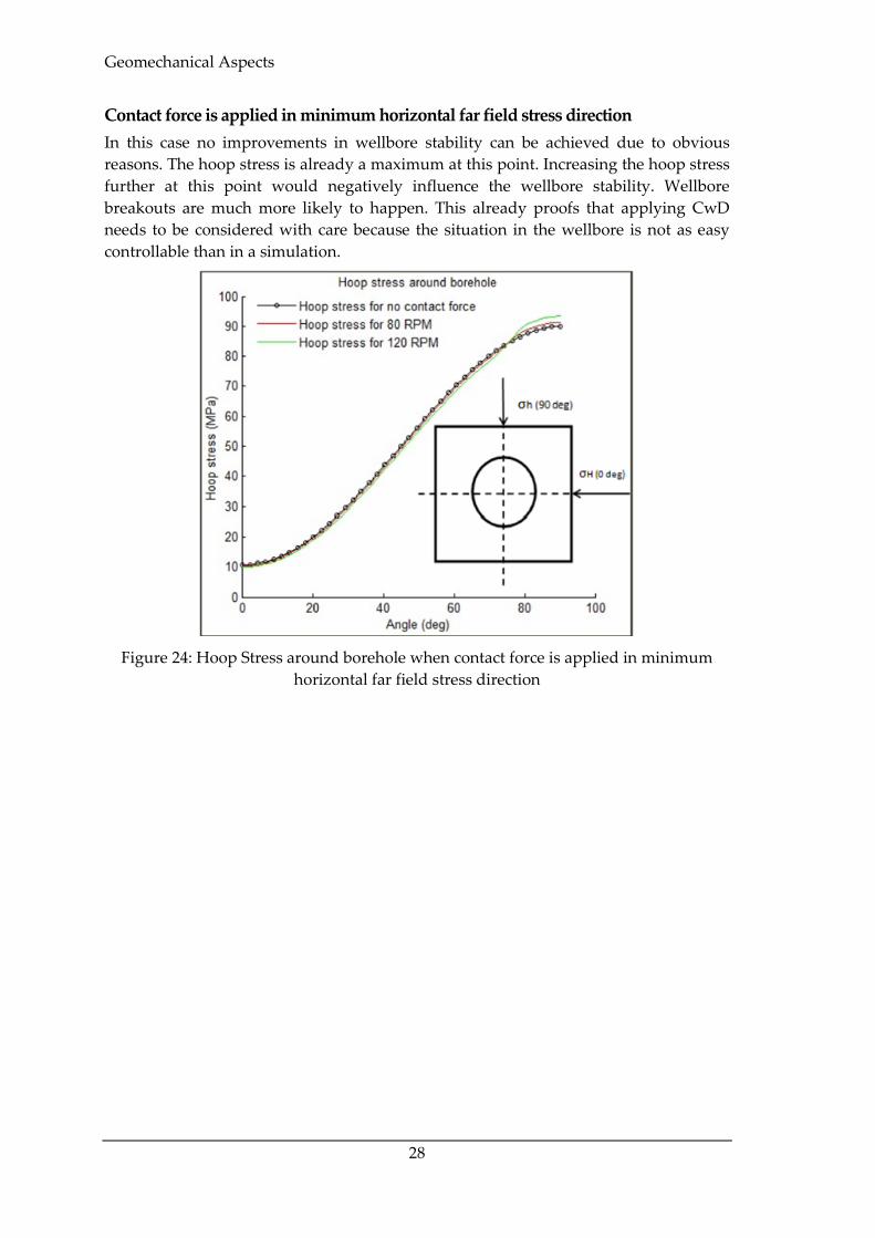
Contact force is applied in minimum horizontal far field stress direction
In this case no improvements in wellbore stability can be achieved due to obvious
reasons. The hoop stress is already a maximum at this point. Increasing the hoop stress
further at this point would negatively influence the wellbore stability. Wellbore
breakouts are much more likely to happen. This already proofs that applying CwD
needs to be considered with care because the situation in the wellbore is not as easy
controllable than in a simulation.
Figure 24: Hoop Stress around borehole when contact force is applied in minimum
horizontal far field stress direction
The Influence of CwD on Wellbore Geomechanics
29
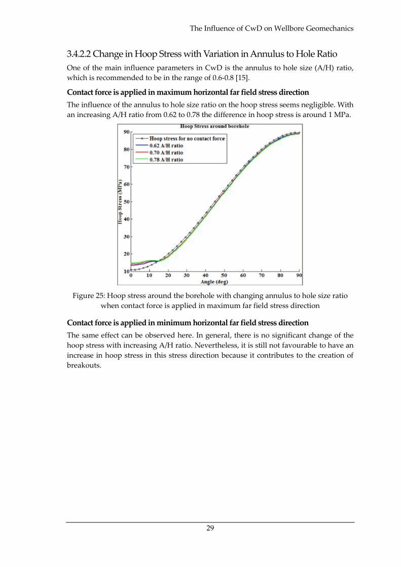
3.4.2.2 Change in Hoop Stress with Variation in Annulus to Hole Ratio
One of the main influence parameters in CwD is the annulus to hole size (A/H) ratio,
which is recommended to be in the range of 0.6-0.8 [15].
Contact force is applied in maximum horizontal far field stress direction
The influence of the annulus to hole size ratio on the hoop stress seems negligible. With
an increasing A/H ratio from 0.62 to 0.78 the difference in hoop stress is around 1 MPa.
Figure 25: Hoop stress around the borehole with changing annulus to hole size ratio
when contact force is applied in maximum far field stress direction
Contact force is applied in minimum horizontal far field stress direction
The same effect can be observed here. In general, there is no significant change of the
hoop stress with increasing A/H ratio. Nevertheless, it is still not favourable to have an
increase in hoop stress in this stress direction because it contributes to the creation of
breakouts.
Geomechanical Aspects
30
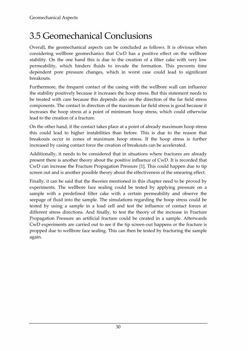
3.5 Geomechanical Conclusions Overall, the geomechanical aspects can be concluded as follows. It is obvious when
considering wellbore geomechanics that CwD has a positive effect on the wellbore
stability. On the one hand this is due to the creation of a filter cake with very low
permeability, which hinders fluids to invade the formation. This prevents time
dependent pore pressure changes, which in worst case could lead to significant
breakouts.
Furthermore, the frequent contact of the casing with the wellbore wall can influence
the stability positively because it increases the hoop stress. But this statement needs to
be treated with care because this depends also on the direction of the far field stress
components. The contact in direction of the maximum far field stress is good because it
increases the hoop stress at a point of minimum hoop stress, which could otherwise
lead to the creation of a fracture.
On the other hand, if the contact takes place at a point of already maximum hoop stress
this could lead to higher instabilities than before. This is due to the reason that
breakouts occur in zones of maximum hoop stress. If the hoop stress is further
increased by casing contact force the creation of breakouts can be accelerated.
Additionally, it needs to be considered that in situations where fractures are already
present there is another theory about the positive influence of CwD. It is recorded that
CwD can increase the Fracture Propagation Pressure [1]. This could happen due to tip
screen out and is another possible theory about the effectiveness of the smearing effect.
Finally, it can be said that the theories mentioned in this chapter need to be proved by
experiments. The wellbore face sealing could be tested by applying pressure on a
sample with a predefined filter cake with a certain permeability and observe the
seepage of fluid into the sample. The simulations regarding the hoop stress could be
tested by using a sample in a load cell and test the influence of contact forces at
different stress directions. And finally, to test the theory of the increase in Fracture
Propagation Pressure an artificial fracture could be created in a sample. Afterwards
CwD experiments are carried out to see if the tip screen-out happens or the fracture is
propped due to wellbore face sealing. This can then be tested by fracturing the sample
again.
Static Experiments
31
Chapter 4 Existing Laboratory
Technologies The next section describes different technologies that were used to simulate dynamic
and static filter cake build-up.
4.1 Static Experiments
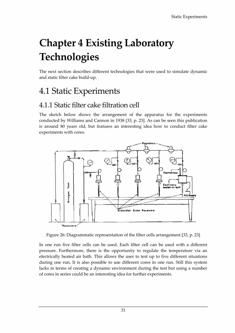
4.1.1 Static filter cake filtration cell The sketch below shows the arrangement of the apparatus for the experiments
conducted by Williams and Cannon in 1938 [33, p. 23]. As can be seen this publication
is around 80 years old, but features an interesting idea how to conduct filter cake
experiments with cores.
Figure 26: Diagrammatic representation of the filter cells arrangement [33, p. 23]
In one run five filter cells can be used. Each filter cell can be used with a different
pressure. Furthermore, there is the opportunity to regulate the temperature via an
electrically heated air bath. This allows the user to test up to five different situations
during one run. It is also possible to use different cores in one run. Still this system
lacks in terms of creating a dynamic environment during the test but using a number
of cores in series could be an interesting idea for further experiments.
Existing Laboratory Technologies
32
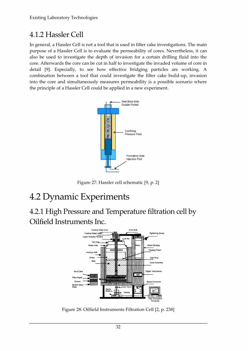
4.1.2 Hassler Cell In general, a Hassler Cell is not a tool that is used in filter cake investigations. The main
purpose of a Hassler Cell is to evaluate the permeability of cores. Nevertheless, it can
also be used to investigate the depth of invasion for a certain drilling fluid into the
core. Afterwards the core can be cut in half to investigate the invaded volume of core in
detail [9]. Especially, to see how effective bridging particles are working. A
combination between a tool that could investigate the filter cake build-up, invasion
into the core and simultaneously measures permeability is a possible scenario where
the principle of a Hassler Cell could be applied in a new experiment.
Figure 27: Hassler cell schematic [9, p. 2]
4.2 Dynamic Experiments
4.2.1 High Pressure and Temperature filtration cell by
Oilfield Instruments Inc.
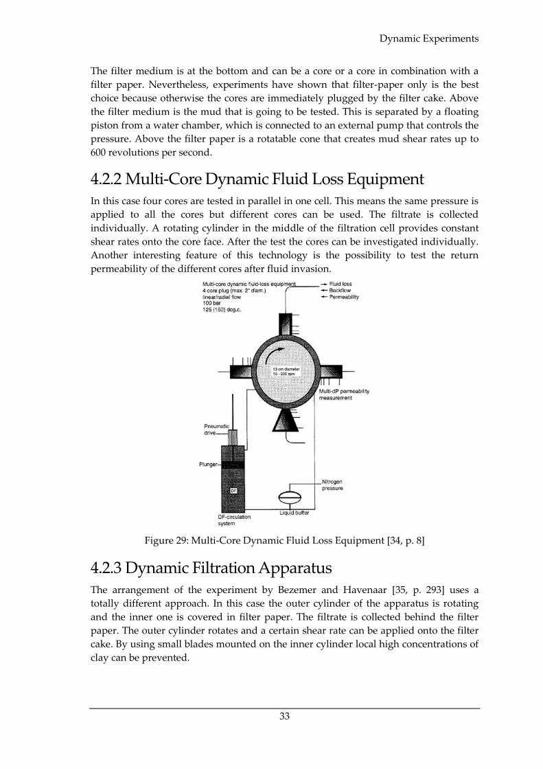
Figure 28: Oilfield Instruments Filtration Cell [2, p. 238]
Dynamic Experiments
33
The filter medium is at the bottom and can be a core or a core in combination with a
filter paper. Nevertheless, experiments have shown that filter-paper only is the best
choice because otherwise the cores are immediately plugged by the filter cake. Above
the filter medium is the mud that is going to be tested. This is separated by a floating
piston from a water chamber, which is connected to an external pump that controls the
pressure. Above the filter paper is a rotatable cone that creates mud shear rates up to
600 revolutions per second.
4.2.2 Multi-Core Dynamic Fluid Loss Equipment In this case four cores are tested in parallel in one cell. This means the same pressure is
applied to all the cores but different cores can be used. The filtrate is collected
individually. A rotating cylinder in the middle of the filtration cell provides constant
shear rates onto the core face. After the test the cores can be investigated individually.
Another interesting feature of this technology is the possibility to test the return
permeability of the different cores after fluid invasion.
Figure 29: Multi-Core Dynamic Fluid Loss Equipment [34, p. 8]
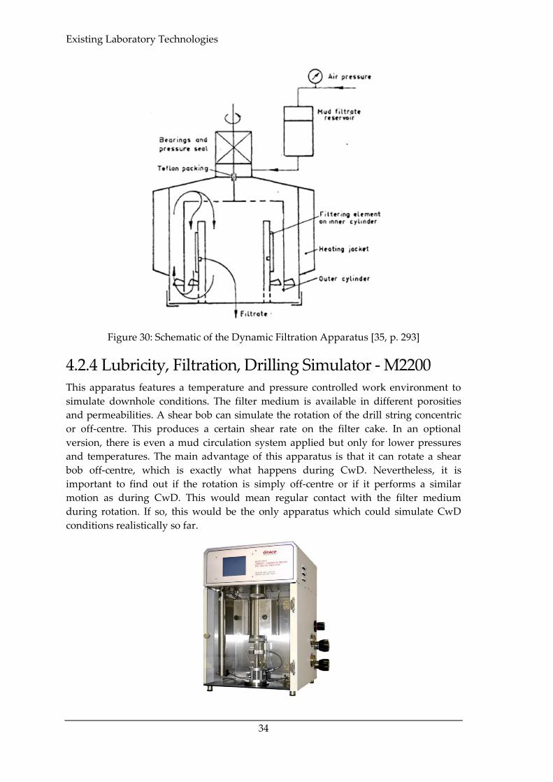
4.2.3 Dynamic Filtration Apparatus The arrangement of the experiment by Bezemer and Havenaar [35, p. 293] uses a
totally different approach. In this case the outer cylinder of the apparatus is rotating
and the inner one is covered in filter paper. The filtrate is collected behind the filter
paper. The outer cylinder rotates and a certain shear rate can be applied onto the filter
cake. By using small blades mounted on the inner cylinder local high concentrations of
clay can be prevented.
Existing Laboratory Technologies
34
Figure 30: Schematic of the Dynamic Filtration Apparatus [35, p. 293]
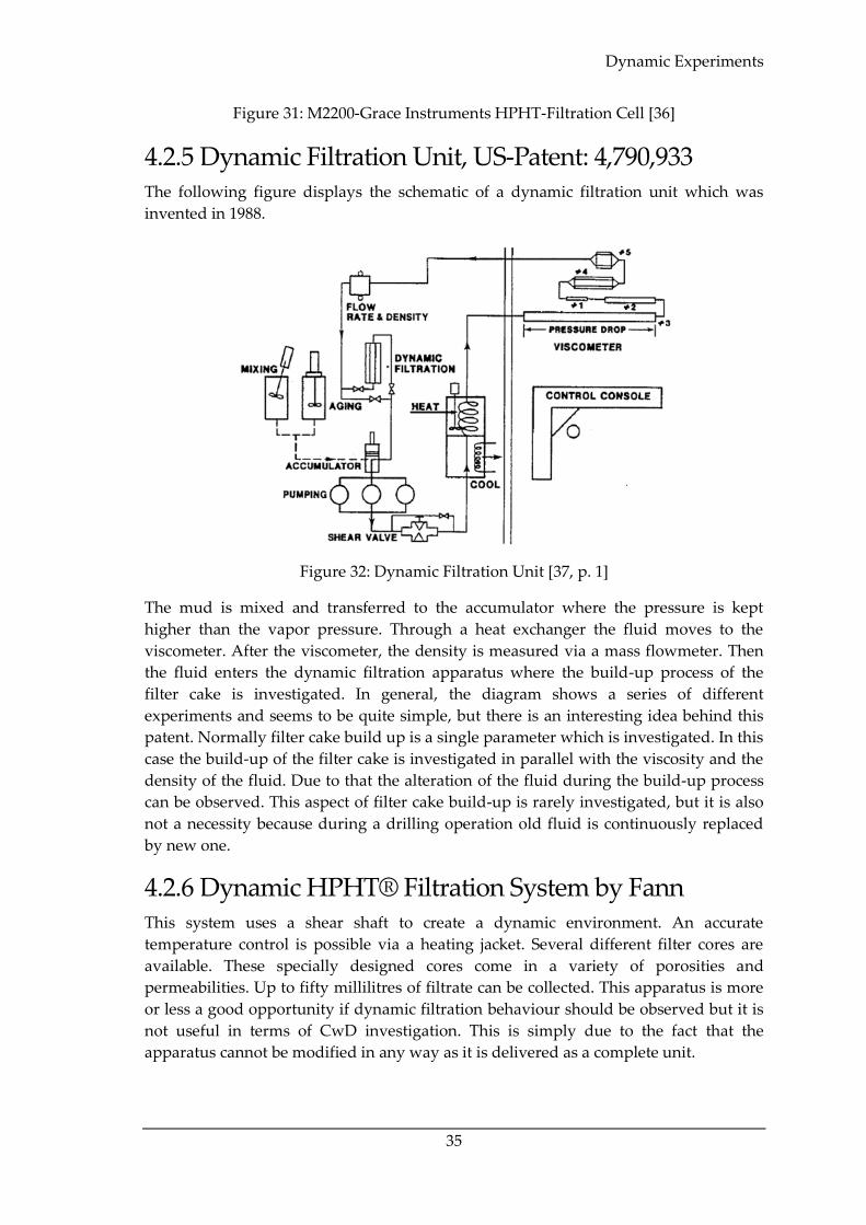
4.2.4 Lubricity, Filtration, Drilling Simulator - M2200 This apparatus features a temperature and pressure controlled work environment to
simulate downhole conditions. The filter medium is available in different porosities
and permeabilities. A shear bob can simulate the rotation of the drill string concentric
or off-centre. This produces a certain shear rate on the filter cake. In an optional
version, there is even a mud circulation system applied but only for lower pressures
and temperatures. The main advantage of this apparatus is that it can rotate a shear
bob off-centre, which is exactly what happens during CwD. Nevertheless, it is
important to find out if the rotation is simply off-centre or if it performs a similar
motion as during CwD. This would mean regular contact with the filter medium
during rotation. If so, this would be the only apparatus which could simulate CwD
conditions realistically so far.
Dynamic Experiments
35
Figure 31: M2200-Grace Instruments HPHT-Filtration Cell [36]
4.2.5 Dynamic Filtration Unit, US-Patent: 4,790,933 The following figure displays the schematic of a dynamic filtration unit which was
invented in 1988.
Figure 32: Dynamic Filtration Unit [37, p. 1]
The mud is mixed and transferred to the accumulator where the pressure is kept
higher than the vapor pressure. Through a heat exchanger the fluid moves to the
viscometer. After the viscometer, the density is measured via a mass flowmeter. Then
the fluid enters the dynamic filtration apparatus where the build-up process of the
filter cake is investigated. In general, the diagram shows a series of different
experiments and seems to be quite simple, but there is an interesting idea behind this
patent. Normally filter cake build up is a single parameter which is investigated. In this
case the build-up of the filter cake is investigated in parallel with the viscosity and the
density of the fluid. Due to that the alteration of the fluid during the build-up process
can be observed. This aspect of filter cake build-up is rarely investigated, but it is also
not a necessity because during a drilling operation old fluid is continuously replaced
by new one.
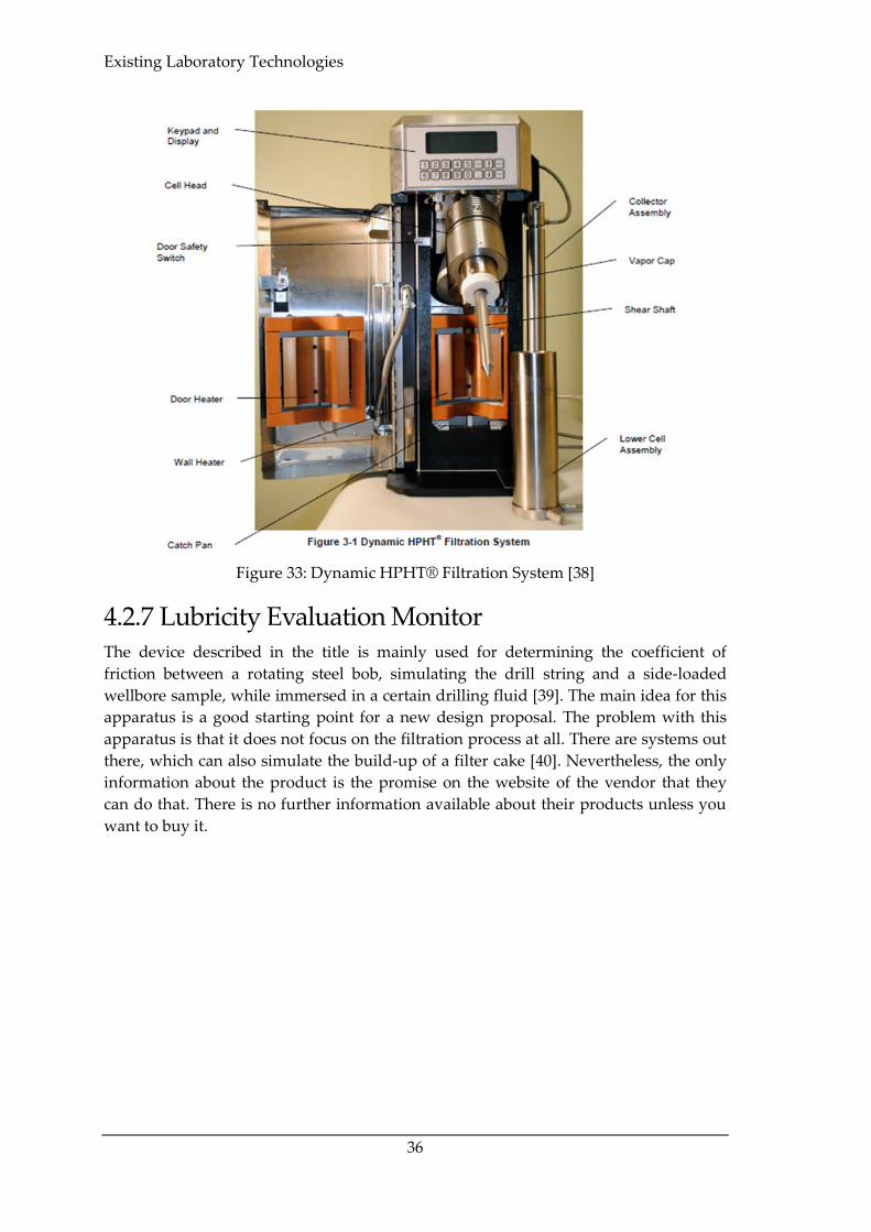
4.2.6 Dynamic HPHT® Filtration System by Fann This system uses a shear shaft to create a dynamic environment. An accurate
temperature control is possible via a heating jacket. Several different filter cores are
available. These specially designed cores come in a variety of porosities and
permeabilities. Up to fifty millilitres of filtrate can be collected. This apparatus is more
or less a good opportunity if dynamic filtration behaviour should be observed but it is
not useful in terms of CwD investigation. This is simply due to the fact that the
apparatus cannot be modified in any way as it is delivered as a complete unit.
Existing Laboratory Technologies
36
Figure 33: Dynamic HPHT® Filtration System [38]
4.2.7 Lubricity Evaluation Monitor The device described in the title is mainly used for determining the coefficient of
friction between a rotating steel bob, simulating the drill string and a side-loaded
wellbore sample, while immersed in a certain drilling fluid [39]. The main idea for this
apparatus is a good starting point for a new design proposal. The problem with this
apparatus is that it does not focus on the filtration process at all. There are systems out
there, which can also simulate the build-up of a filter cake [40]. Nevertheless, the only
information about the product is the promise on the website of the vendor that they
can do that. There is no further information available about their products unless you
want to buy it.
Type of Experiments
37
Chapter 5 Experimental Setup This chapter represents the main part of the thesis and describes the process of
developing the final proposed design for an experimental setup. It starts defining the
types of experiments which should be carried out with this unit. Furthermore, the most
important and critical issues in such an experiment are analysed, based on the idea
how a manual for this apparatus would look like. Finally, these issues are tackled with
different solutions, which are also described in this chapter. In the end the final design
is presented to the reader.
5.1 Type of Experiments The final design should feature a single unit which can be implemented into a flow
loop. The basic version of the design will allow three different experiments to be
carried out on a single unit.
• Static filtration test
• Dynamic filtration test
With drill pipe in the hole
Without drill pipe in the hole
• Pipe Impact Test
Regular drill pipe
Casing while drilling
5.2 General Considerations All the experiments can be conducted under a certain confining pressure. This requires
a new design of a core holder. One side of the core is exposed to the drilling fluid. The
other side of the core can be considered as undamaged by the drilling fluid.
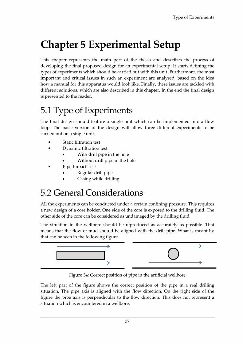
The situation in the wellbore should be reproduced as accurately as possible. That
means that the flow of mud should be aligned with the drill pipe. What is meant by
that can be seen in the following figure.
Figure 34: Correct position of pipe in the artificial wellbore
The left part of the figure shows the correct position of the pipe in a real drilling
situation. The pipe axis is aligned with the flow direction. On the right side of the
figure the pipe axis is perpendicular to the flow direction. This does not represent a
situation which is encountered in a wellbore.
Experimental Setup
38
Furthermore, the setup should feature the possibility to vary pressure and
temperature. For the temperature this would require a heat exchanger, which heats the
drilling mud for the entire loop. The pressure can be regulated by using regulation
valves. Further details are going to be discussed in the different sections of this chapter.
Another important aspect in such an experimental design is the method of measuring
the parameters of interest. Besides operational parameters such as pressure,
temperature, flow rate it is necessary to measure parameters before and after the test
such as permeability of the core sample, filter cake thickness, invasion depth, residual
saturation and also the return permeability. How to measure all the different
parameters will also be discussed in a separate section of this chapter.
Another important aspect is the applicability for a variety of drilling fluids. As drilling
fluids in combination with cuttings can be highly erosive it is critical to choose a
material that can deal with a variety of different situations.
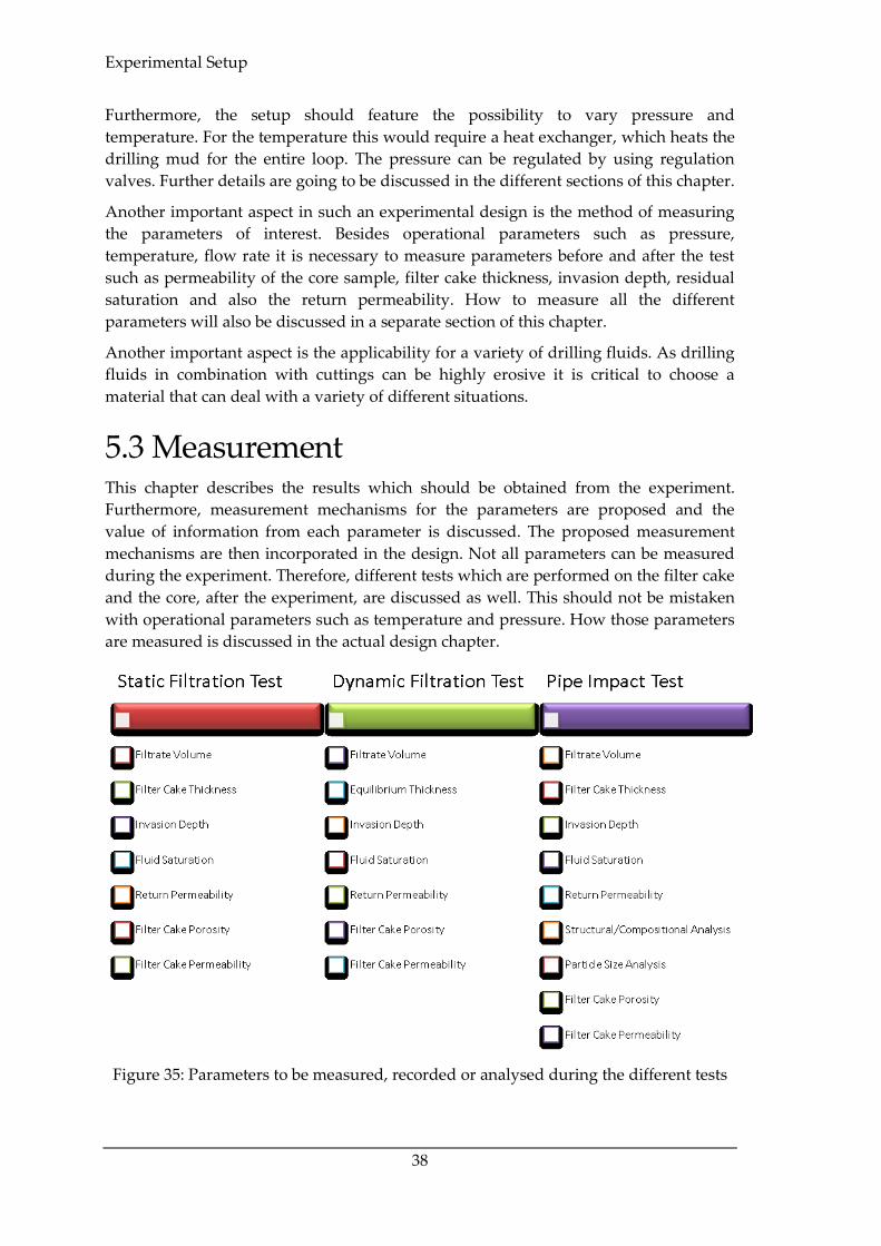
5.3 Measurement This chapter describes the results which should be obtained from the experiment.
Furthermore, measurement mechanisms for the parameters are proposed and the
value of information from each parameter is discussed. The proposed measurement
mechanisms are then incorporated in the design. Not all parameters can be measured
during the experiment. Therefore, different tests which are performed on the filter cake
and the core, after the experiment, are discussed as well. This should not be mistaken
with operational parameters such as temperature and pressure. How those parameters
are measured is discussed in the actual design chapter.
Figure 35: Parameters to be measured, recorded or analysed during the different tests
Measurement
39
5.3.1 Filter Cake Porosity and Permeability Both parameters are already described in the Literature Review Chapter. Porosity can
be measured by using the CT-Scan Technique which uses the CT-Number as described
in Equation 3. Another useful technique is to calculate the porosity by using the dry
and wet weight of the filter cake, the density of the used fluid and an assumption for
the grain density.
𝑉𝑔 =𝑁𝑒𝑡 𝑑𝑟𝑦 𝑤𝑒𝑖𝑔ℎ𝑡 𝑜𝑓 𝑡ℎ𝑒 𝑐𝑎𝑘𝑒
𝜌𝑔
Equation 24: Grain volume of the filter cake
𝑉𝑝 =(𝑁𝑒𝑡 𝑤𝑒𝑡 𝑤𝑒𝑖𝑔ℎ𝑡 − 𝑁𝑒𝑡 𝑑𝑟𝑦 𝑤𝑒𝑖𝑔ℎ𝑡)
𝜌𝑓
Equation 25: Pore volume of the filter cake [6, p. 3]
𝛷𝐶 =𝑉𝑝
𝑉𝑝 + 𝑉𝑔
Equation 26: Filter cake porosity from wet and dry filter cake weight measurements [6]
Where ρg is the grain density and ρf is the fluid density.
This technique is not very accurate because an assumption of the grain density based
on the used material is necessary. There is no absolute proof that the grain density is
exactly the value of the used solids in the drilling fluid because several different
materials could be deposited depending on the composition of the drilling fluid.
Nevertheless, it is an easy method and can be used without the need of a CT-scanner.
Regarding permeability most of the techniques used rely on empirical correlations as
described in Equation 4. Nevertheless, it is possible to use an equation which uses the
continuously measured filtrate volume, the time and the filter cake volume to come up
with a value of permeability. The advantage of this method is that the permeability of
the filter cake is continuously measured during the test. The disadvantage is that this
method was developed for static filtration methods and needs to be verified for
dynamic experiments.
𝐾 = 𝑄𝑤 ∗ 𝑄𝐶 ∗µ
2 ∗ 𝑡 ∗ 𝑝 ∗ 𝐴2
Equation 27: Filter cake permeability calculated continuously [6, p. 5]
Where QW is the filtrate volume in cm3, QC is the volume of the filter cake in cm3, µ is
the viscosity of the filtrate in cp, t is the time in seconds, p is the differential pressure in
atm and A is the filter cake area in cm2.
Experimental Setup
40
5.3.2 Filtrate Volume One of the main parameters in filtration tests is the question how much fluid is lost into
the formation. This is measured by collecting the amount of filtrate which, passes the
filtration surface in a static or dynamic filtration test. For dynamic filtration tests no
standardized testing procedures exist. As basis for the collection of filtrate the API-
Standard API Recommended Practice 13B-1 is used.
The collected filtrate volume is a very important parameter because it gives
information about how fast a certain formation can be sealed by the build-up of a filter
cake. This is necessary to know because the invasion of drilling mud into the formation
is one of the main damage mechanisms and it is especially important in the reservoir
region.
According to API RP 13B-1 the filter press should have a filtration area of 45.2 cm2 up
to 46.4 cm2. The test is carried out at 100 ± 5 psi and the filtrate is collected over a
period of 30 minutes. The filtrate is collected in a graded cylinder.
The filtrate volume is proportional to the square root of the time period used [41, p. 46]
𝑉𝑓 = √2 ∗ 𝑘 ∗ 𝛥𝑝 ∗ (𝑓𝑠𝑐
𝑓𝑠𝑚− 1) ∗ 𝐴 ∗
√𝑡
õ
Equation 28: Filtrate Volume in a static filter press [41, p. 46]
Where k is the permeability of the filter cake, Δp is the pressure differential, fsc is the
volume fraction of solids in the filter cake, fsm is the volume fraction of solids in the
mud, A is the filter area, t is the time and µ is the filtrate viscosity.
In case that the filtrate volume exceeds the volume of the filtrate receiver during a
period of 30 minutes, the API water loss is reported as twice the volume of filtrate after
7.5 minutes. In case that a spurt loss is observed the filtrate volume after 30 minutes is
calculated as follows.
𝑉30 = 2 ∗ (𝑉7.5 − 𝑉𝑠𝑝) + 𝑉𝑠𝑝
Equation 29: API fluid loss after 30 minutes if spurt loss is observed [41, p. 46]
Where Vsp is the spurt loss and V7.5 is the filtrate volume after 7.5 minutes.
The same theory is applied when the tests are carried out at elevated pressure and
temperature. The only difference is a filter cake area which is half the size of the
original test [42]. Furthermore, a backpressure receiver is used to collect the filtrate.
Anyway, this is not comparable to a dynamic situation where the shear force acting on
the formation stops the build-up of the filter cake. Therefore, the filter cake does not
grow anymore and the equilibrium thickness is reached. From that point on the filtrate
loss into the formation increases constantly. The difference in both methods can be
seen in the following figure.
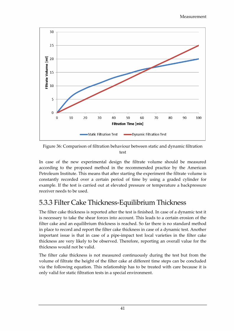
Measurement
41
Figure 36: Comparison of filtration behaviour between static and dynamic filtration
test
In case of the new experimental design the filtrate volume should be measured
according to the proposed method in the recommended practice by the American
Petroleum Institute. This means that after starting the experiment the filtrate volume is
constantly recorded over a certain period of time by using a graded cylinder for
example. If the test is carried out at elevated pressure or temperature a backpressure
receiver needs to be used.
5.3.3 Filter Cake Thickness-Equilibrium Thickness The filter cake thickness is reported after the test is finished. In case of a dynamic test it
is necessary to take the shear forces into account. This leads to a certain erosion of the
filter cake and an equilibrium thickness is reached. So far there is no standard method
in place to record and report the filter cake thickness in case of a dynamic test. Another
important issue is that in case of a pipe-impact test local varieties in the filter cake
thickness are very likely to be observed. Therefore, reporting an overall value for the
thickness would not be valid.
The filter cake thickness is not measured continuously during the test but from the
volume of filtrate the height of the filter cake at different time steps can be concluded
via the following equation. This relationship has to be treated with care because it is
only valid for static filtration tests in a special environment.
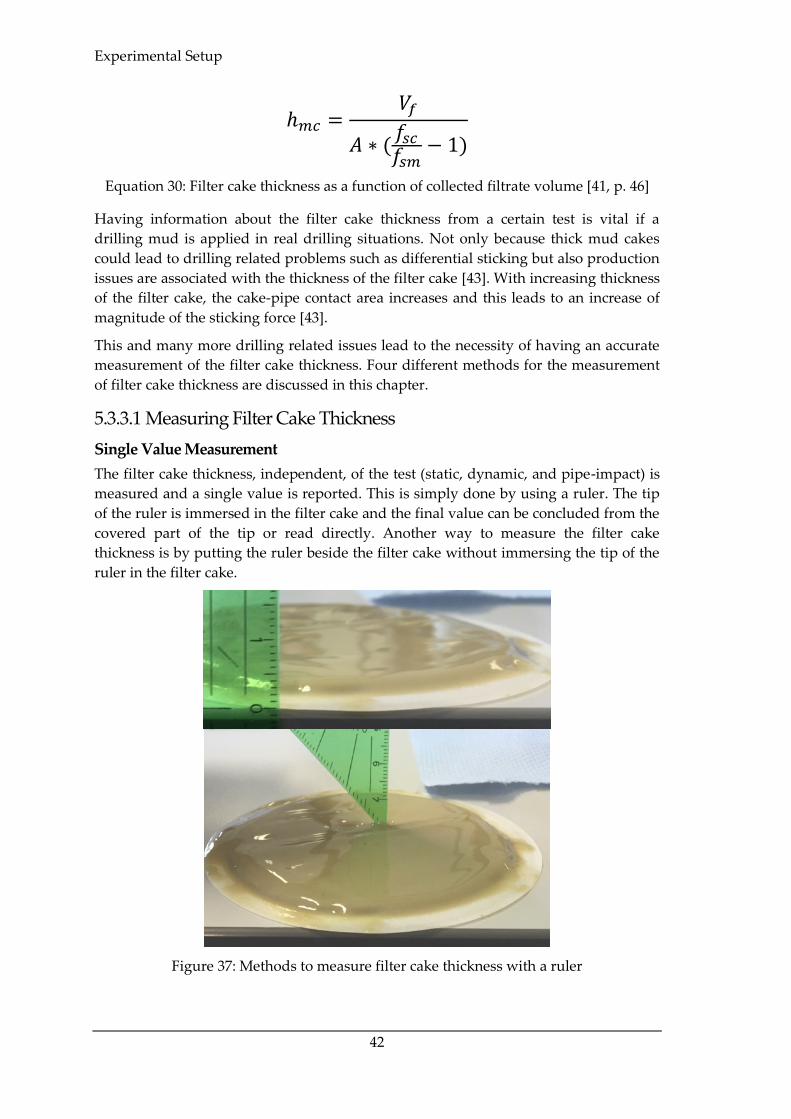
Experimental Setup
42
ℎ𝑚𝑐 =𝑉𝑓
𝐴 ∗ (𝑓𝑠𝑐
𝑓𝑠𝑚− 1)
Equation 30: Filter cake thickness as a function of collected filtrate volume [41, p. 46]
Having information about the filter cake thickness from a certain test is vital if a
drilling mud is applied in real drilling situations. Not only because thick mud cakes
could lead to drilling related problems such as differential sticking but also production
issues are associated with the thickness of the filter cake [43]. With increasing thickness
of the filter cake, the cake-pipe contact area increases and this leads to an increase of
magnitude of the sticking force [43].
This and many more drilling related issues lead to the necessity of having an accurate
measurement of the filter cake thickness. Four different methods for the measurement
of filter cake thickness are discussed in this chapter.
5.3.3.1 Measuring Filter Cake Thickness
Single Value Measurement
The filter cake thickness, independent, of the test (static, dynamic, and pipe-impact) is
measured and a single value is reported. This is simply done by using a ruler. The tip
of the ruler is immersed in the filter cake and the final value can be concluded from the
covered part of the tip or read directly. Another way to measure the filter cake
thickness is by putting the ruler beside the filter cake without immersing the tip of the
ruler in the filter cake.
Figure 37: Methods to measure filter cake thickness with a ruler
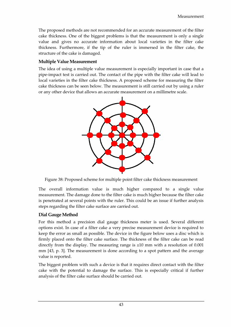
Measurement
43
The proposed methods are not recommended for an accurate measurement of the filter
cake thickness. One of the biggest problems is that the measurement is only a single
value and gives no accurate information about local varieties in the filter cake
thickness. Furthermore, if the tip of the ruler is immersed in the filter cake, the
structure of the cake is damaged.
Multiple Value Measurement
The idea of using a multiple value measurement is especially important in case that a
pipe-impact test is carried out. The contact of the pipe with the filter cake will lead to
local varieties in the filter cake thickness. A proposed scheme for measuring the filter
cake thickness can be seen below. The measurement is still carried out by using a ruler
or any other device that allows an accurate measurement on a millimetre scale.
Figure 38: Proposed scheme for multiple point filter cake thickness measurement
The overall information value is much higher compared to a single value
measurement. The damage done to the filter cake is much higher because the filter cake
is penetrated at several points with the ruler. This could be an issue if further analysis
steps regarding the filter cake surface are carried out.
Dial Gauge Method
For this method a precision dial gauge thickness meter is used. Several different
options exist. In case of a filter cake a very precise measurement device is required to
keep the error as small as possible. The device in the figure below uses a disc which is
firmly placed onto the filter cake surface. The thickness of the filter cake can be read
directly from the display. The measuring range is ±10 mm with a resolution of 0.001
mm [43, p. 3]. The measurement is done according to a spot pattern and the average
value is reported.
The biggest problem with such a device is that it requires direct contact with the filter
cake with the potential to damage the surface. This is especially critical if further
analysis of the filter cake surface should be carried out.
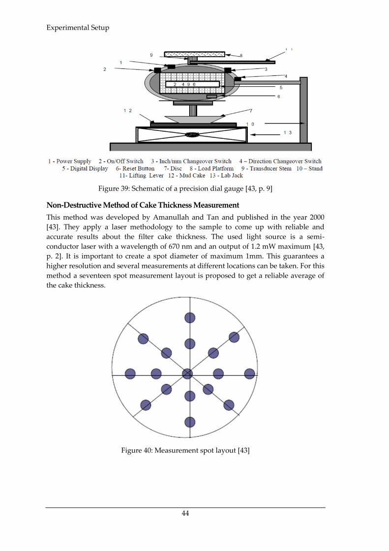
Experimental Setup
44
Figure 39: Schematic of a precision dial gauge [43, p. 9]
Non-Destructive Method of Cake Thickness Measurement
This method was developed by Amanullah and Tan and published in the year 2000
[43]. They apply a laser methodology to the sample to come up with reliable and
accurate results about the filter cake thickness. The used light source is a semi-
conductor laser with a wavelength of 670 nm and an output of 1.2 mW maximum [43,
p. 2]. It is important to create a spot diameter of maximum 1mm. This guarantees a
higher resolution and several measurements at different locations can be taken. For this
method a seventeen spot measurement layout is proposed to get a reliable average of
the cake thickness.
Figure 40: Measurement spot layout [43]
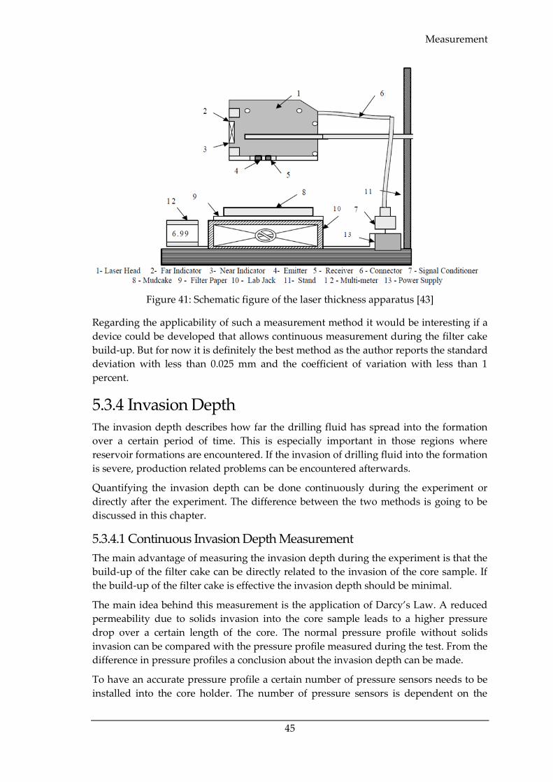
Measurement
45
Figure 41: Schematic figure of the laser thickness apparatus [43]
Regarding the applicability of such a measurement method it would be interesting if a
device could be developed that allows continuous measurement during the filter cake
build-up. But for now it is definitely the best method as the author reports the standard
deviation with less than 0.025 mm and the coefficient of variation with less than 1
percent.
5.3.4 Invasion Depth The invasion depth describes how far the drilling fluid has spread into the formation
over a certain period of time. This is especially important in those regions where
reservoir formations are encountered. If the invasion of drilling fluid into the formation
is severe, production related problems can be encountered afterwards.
Quantifying the invasion depth can be done continuously during the experiment or
directly after the experiment. The difference between the two methods is going to be
discussed in this chapter.
5.3.4.1 Continuous Invasion Depth Measurement
The main advantage of measuring the invasion depth during the experiment is that the
build-up of the filter cake can be directly related to the invasion of the core sample. If
the build-up of the filter cake is effective the invasion depth should be minimal.
The main idea behind this measurement is the application of Darcy’s Law. A reduced
permeability due to solids invasion into the core sample leads to a higher pressure
drop over a certain length of the core. The normal pressure profile without solids
invasion can be compared with the pressure profile measured during the test. From the
difference in pressure profiles a conclusion about the invasion depth can be made.
To have an accurate pressure profile a certain number of pressure sensors needs to be
installed into the core holder. The number of pressure sensors is dependent on the
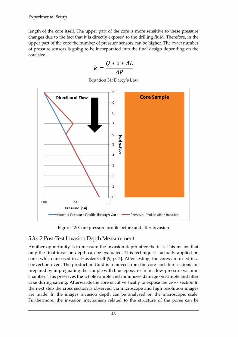
Experimental Setup
46
length of the core itself. The upper part of the core is more sensitive to these pressure
changes due to the fact that it is directly exposed to the drilling fluid. Therefore, in the
upper part of the core the number of pressure sensors can be higher. The exact number
of pressure sensors is going to be incorporated into the final design depending on the
core size.
𝑘 =𝑄 ∗ µ ∗ 𝛥𝐿
𝛥𝑃
Equation 31: Darcy’s Law
Figure 42: Core pressure profile before and after invasion
5.3.4.2 Post-Test Invasion Depth Measurement
Another opportunity is to measure the invasion depth after the test. This means that
only the final invasion depth can be evaluated. This technique is actually applied on
cores which are used in a Hassler Cell [9, p. 2]. After testing, the cores are dried in a
convection oven. The production fluid is removed from the core and thin sections are
prepared by impregnating the sample with blue epoxy resin in a low-pressure vacuum
chamber. This preserves the whole sample and minimizes damage on sample and filter
cake during sawing. Afterwards the core is cut vertically to expose the cross section.In
the next step the cross section is observed via microscope and high resolution images
are made. In the images invasion depth can be analysed on the microscopic scale.
Furthermore, the invasion mechanism related to the structure of the pores can be

Measurement
47
analysed in detail. The technique described above is mentioned in detail in the paper of
Li and He [9, p. 2].
Figure 43: Example picture for investigating invasion depth on a pore size scale in
sandstone [9, p. 4]
In comparison, it can be concluded that both techniques, which are described in this
chapter are a valid solution to measure the invasion depth. In the case of this
experiment the author suggests to use both methods because each method has a value
of information that the other one can’t deliver. Furthermore, the Post-Test method can
be used to validate the results from the continuous measurement method and to
calibrate it. If this combination is successful information about the invasion depth can
be gathered during filter cake build up and over the whole course of the experiment
and afterwards on a pore size scale.
5.3.5 Fluid Saturation The near wellbore is normally altered by the drilling process [44]. This leads to the
problem that in a lot of cases the saturation of the formation is influenced. Especially
invasion into the hydrocarbon leg of the reservoir can dramatically decrease the
hydrocarbon saturation [44]. Nevertheless, filtrate from a water based mud into the
water leg of the reservoir formation won’t change the water saturation. Therefore, it is
necessary to have accurate “before” and “after” measurements of the water and
reservoir fluid saturation in the core sample.
𝑆𝑤 =𝑉𝑤
𝑉𝑝
Equation 32: Water saturation
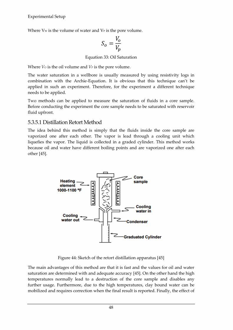
Experimental Setup
48
Where VW is the volume of water and VP is the pore volume.
𝑆𝑜 =𝑉𝑜
𝑉𝑝
Equation 33: Oil Saturation
Where VO is the oil volume and VP is the pore volume.
The water saturation in a wellbore is usually measured by using resistivity logs in
combination with the Archie-Equation. It is obvious that this technique can’t be
applied in such an experiment. Therefore, for the experiment a different technique
needs to be applied.
Two methods can be applied to measure the saturation of fluids in a core sample.
Before conducting the experiment the core sample needs to be saturated with reservoir
fluid upfront.
5.3.5.1 Distillation Retort Method
The idea behind this method is simply that the fluids inside the core sample are
vaporized one after each other. The vapor is lead through a cooling unit which
liquefies the vapor. The liquid is collected in a graded cylinder. This method works
because oil and water have different boiling points and are vaporized one after each
other [45].
Figure 44: Sketch of the retort distillation apparatus [45]
The main advantages of this method are that it is fast and the values for oil and water
saturation are determined with and adequate accuracy [45]. On the other hand the high
temperatures normally lead to a destruction of the core sample and disables any
further usage. Furthermore, due to the high temperatures, clay bound water can be
mobilized and requires correction when the final result is reported. Finally, the effect of
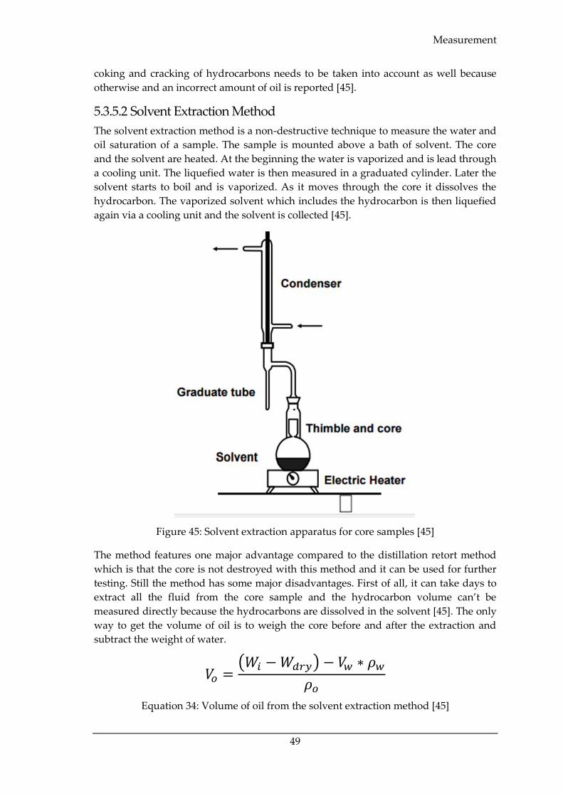
Measurement
49
coking and cracking of hydrocarbons needs to be taken into account as well because
otherwise and an incorrect amount of oil is reported [45].
5.3.5.2 Solvent Extraction Method
The solvent extraction method is a non-destructive technique to measure the water and
oil saturation of a sample. The sample is mounted above a bath of solvent. The core
and the solvent are heated. At the beginning the water is vaporized and is lead through
a cooling unit. The liquefied water is then measured in a graduated cylinder. Later the
solvent starts to boil and is vaporized. As it moves through the core it dissolves the
hydrocarbon. The vaporized solvent which includes the hydrocarbon is then liquefied
again via a cooling unit and the solvent is collected [45].
Figure 45: Solvent extraction apparatus for core samples [45]
The method features one major advantage compared to the distillation retort method
which is that the core is not destroyed with this method and it can be used for further
testing. Still the method has some major disadvantages. First of all, it can take days to
extract all the fluid from the core sample and the hydrocarbon volume can’t be
measured directly because the hydrocarbons are dissolved in the solvent [45]. The only
way to get the volume of oil is to weigh the core before and after the extraction and
subtract the weight of water.
𝑉𝑜 =(𝑊𝑖 − 𝑊𝑑𝑟𝑦) − 𝑉𝑤 ∗ 𝜌𝑤
𝜌𝑜
Equation 34: Volume of oil from the solvent extraction method [45]
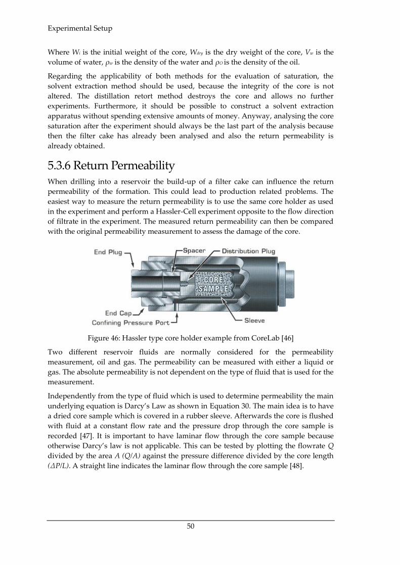
Experimental Setup
50
Where Wi is the initial weight of the core, Wdry is the dry weight of the core, Vw is the
volume of water, ρw is the density of the water and ρO is the density of the oil.
Regarding the applicability of both methods for the evaluation of saturation, the
solvent extraction method should be used, because the integrity of the core is not
altered. The distillation retort method destroys the core and allows no further
experiments. Furthermore, it should be possible to construct a solvent extraction
apparatus without spending extensive amounts of money. Anyway, analysing the core
saturation after the experiment should always be the last part of the analysis because
then the filter cake has already been analysed and also the return permeability is
already obtained.
5.3.6 Return Permeability When drilling into a reservoir the build-up of a filter cake can influence the return
permeability of the formation. This could lead to production related problems. The
easiest way to measure the return permeability is to use the same core holder as used
in the experiment and perform a Hassler-Cell experiment opposite to the flow direction
of filtrate in the experiment. The measured return permeability can then be compared
with the original permeability measurement to assess the damage of the core.
Figure 46: Hassler type core holder example from CoreLab [46]
Two different reservoir fluids are normally considered for the permeability
measurement, oil and gas. The permeability can be measured with either a liquid or
gas. The absolute permeability is not dependent on the type of fluid that is used for the
measurement.
Independently from the type of fluid which is used to determine permeability the main
underlying equation is Darcy’s Law as shown in Equation 30. The main idea is to have
a dried core sample which is covered in a rubber sleeve. Afterwards the core is flushed
with fluid at a constant flow rate and the pressure drop through the core sample is
recorded [47]. It is important to have laminar flow through the core sample because
otherwise Darcy’s law is not applicable. This can be tested by plotting the flowrate Q
divided by the area A (Q/A) against the pressure difference divided by the core length
(ΔP/L). A straight line indicates the laminar flow through the core sample [48].
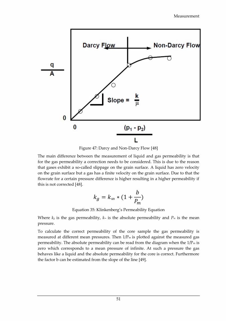
Measurement
51
Figure 47: Darcy and Non-Darcy Flow [48]
The main difference between the measurement of liquid and gas permeability is that
for the gas permeability a correction needs to be considered. This is due to the reason
that gases exhibit a so-called slippage on the grain surface. A liquid has zero velocity
on the grain surface but a gas has a finite velocity on the grain surface. Due to that the
flowrate for a certain pressure difference is higher resulting in a higher permeability if
this is not corrected [48].
𝑘𝑔 = 𝑘∞ ∗ (1 +𝑏
𝑃𝑚)
Equation 35: Klinkenberg’s Permeability Equation
Where kg is the gas permeability, k∞ is the absolute permeability and Pm is the mean
pressure.
To calculate the correct permeability of the core sample the gas permeability is
measured at different mean pressures. Then 1/Pm is plotted against the measured gas
permeability. The absolute permeability can be read from the diagram when the 1/Pm is
zero which corresponds to a mean pressure of infinite. At such a pressure the gas
behaves like a liquid and the absolute permeability for the core is correct. Furthermore
the factor b can be estimated from the slope of the line [49].
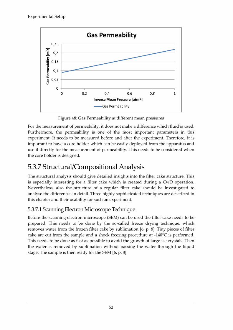
Experimental Setup
52
Figure 48: Gas Permeability at different mean pressures
For the measurement of permeability, it does not make a difference which fluid is used.
Furthermore, the permeability is one of the most important parameters in this
experiment. It needs to be measured before and after the experiment. Therefore, it is
important to have a core holder which can be easily deployed from the apparatus and
use it directly for the measurement of permeability. This needs to be considered when
the core holder is designed.
5.3.7 Structural/Compositional Analysis The structural analysis should give detailed insights into the filter cake structure. This
is especially interesting for a filter cake which is created during a CwD operation.
Nevertheless, also the structure of a regular filter cake should be investigated to
analyse the differences in detail. Three highly sophisticated techniques are described in
this chapter and their usability for such an experiment.
5.3.7.1 Scanning Electron Microscope Technique
Before the scanning electron microscope (SEM) can be used the filter cake needs to be
prepared. This needs to be done by the so-called freeze drying technique, which
removes water from the frozen filter cake by sublimation [6, p. 8]. Tiny pieces of filter
cake are cut from the sample and a shock freezing procedure at -140°C is performed.
This needs to be done as fast as possible to avoid the growth of large ice crystals. Then
the water is removed by sublimation without passing the water through the liquid
stage. The sample is then ready for the SEM [6, p. 8].
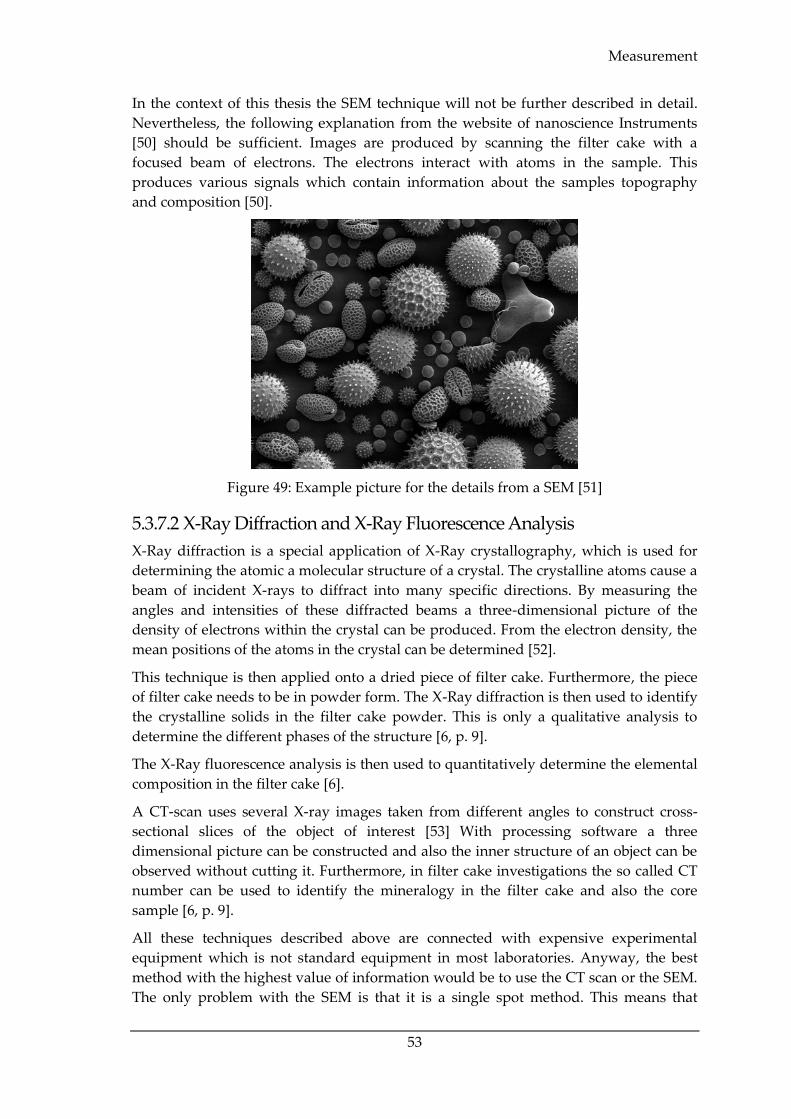
Measurement
53
In the context of this thesis the SEM technique will not be further described in detail.
Nevertheless, the following explanation from the website of nanoscience Instruments
[50] should be sufficient. Images are produced by scanning the filter cake with a
focused beam of electrons. The electrons interact with atoms in the sample. This
produces various signals which contain information about the samples topography
and composition [50].
Figure 49: Example picture for the details from a SEM [51]
5.3.7.2 X-Ray Diffraction and X-Ray Fluorescence Analysis
X-Ray diffraction is a special application of X-Ray crystallography, which is used for
determining the atomic a molecular structure of a crystal. The crystalline atoms cause a
beam of incident X-rays to diffract into many specific directions. By measuring the
angles and intensities of these diffracted beams a three-dimensional picture of the
density of electrons within the crystal can be produced. From the electron density, the
mean positions of the atoms in the crystal can be determined [52].
This technique is then applied onto a dried piece of filter cake. Furthermore, the piece
of filter cake needs to be in powder form. The X-Ray diffraction is then used to identify
the crystalline solids in the filter cake powder. This is only a qualitative analysis to
determine the different phases of the structure [6, p. 9].
The X-Ray fluorescence analysis is then used to quantitatively determine the elemental
composition in the filter cake [6].
A CT-scan uses several X-ray images taken from different angles to construct cross-
sectional slices of the object of interest [53] With processing software a three
dimensional picture can be constructed and also the inner structure of an object can be
observed without cutting it. Furthermore, in filter cake investigations the so called CT
number can be used to identify the mineralogy in the filter cake and also the core
sample [6, p. 9].
All these techniques described above are connected with expensive experimental
equipment which is not standard equipment in most laboratories. Anyway, the best
method with the highest value of information would be to use the CT scan or the SEM.
The only problem with the SEM is that it is a single spot method. This means that
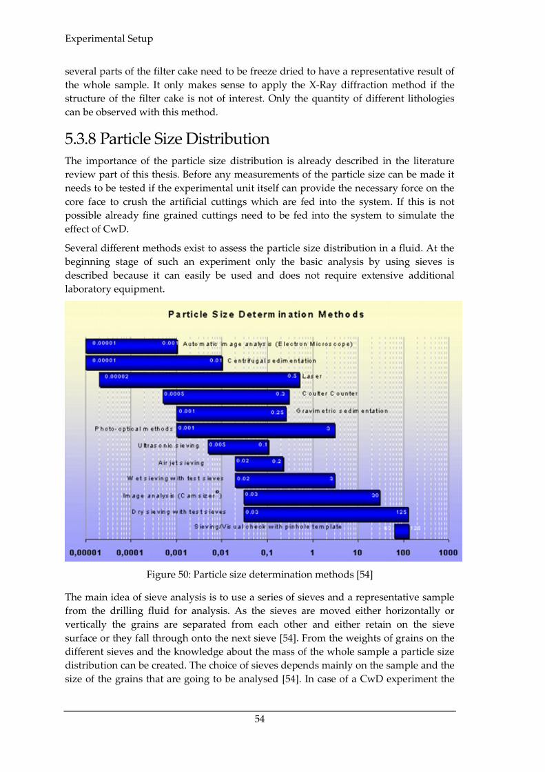
Experimental Setup
54
several parts of the filter cake need to be freeze dried to have a representative result of
the whole sample. It only makes sense to apply the X-Ray diffraction method if the
structure of the filter cake is not of interest. Only the quantity of different lithologies
can be observed with this method.
5.3.8 Particle Size Distribution The importance of the particle size distribution is already described in the literature
review part of this thesis. Before any measurements of the particle size can be made it
needs to be tested if the experimental unit itself can provide the necessary force on the
core face to crush the artificial cuttings which are fed into the system. If this is not
possible already fine grained cuttings need to be fed into the system to simulate the
effect of CwD.
Several different methods exist to assess the particle size distribution in a fluid. At the
beginning stage of such an experiment only the basic analysis by using sieves is
described because it can easily be used and does not require extensive additional
laboratory equipment.
Figure 50: Particle size determination methods [54]
The main idea of sieve analysis is to use a series of sieves and a representative sample
from the drilling fluid for analysis. As the sieves are moved either horizontally or
vertically the grains are separated from each other and either retain on the sieve
surface or they fall through onto the next sieve [54]. From the weights of grains on the
different sieves and the knowledge about the mass of the whole sample a particle size
distribution can be created. The choice of sieves depends mainly on the sample and the
size of the grains that are going to be analysed [54]. In case of a CwD experiment the
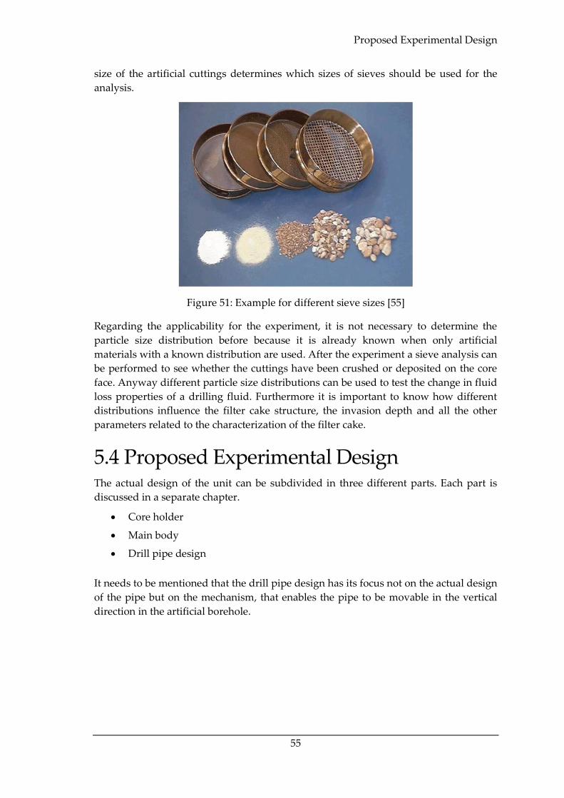
Proposed Experimental Design
55
size of the artificial cuttings determines which sizes of sieves should be used for the
analysis.
Figure 51: Example for different sieve sizes [55]
Regarding the applicability for the experiment, it is not necessary to determine the
particle size distribution before because it is already known when only artificial
materials with a known distribution are used. After the experiment a sieve analysis can
be performed to see whether the cuttings have been crushed or deposited on the core
face. Anyway different particle size distributions can be used to test the change in fluid
loss properties of a drilling fluid. Furthermore it is important to know how different
distributions influence the filter cake structure, the invasion depth and all the other
parameters related to the characterization of the filter cake.
5.4 Proposed Experimental Design The actual design of the unit can be subdivided in three different parts. Each part is
discussed in a separate chapter.
Core holder
Main body
Drill pipe design
It needs to be mentioned that the drill pipe design has its focus not on the actual design
of the pipe but on the mechanism, that enables the pipe to be movable in the vertical
direction in the artificial borehole.
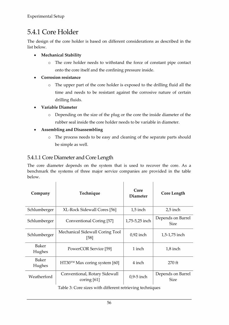
Experimental Setup
56
5.4.1 Core Holder The design of the core holder is based on different considerations as described in the
list below.
Mechanical Stability
o The core holder needs to withstand the force of constant pipe contact
onto the core itself and the confining pressure inside.
Corrosion resistance
o The upper part of the core holder is exposed to the drilling fluid all the
time and needs to be resistant against the corrosive nature of certain
drilling fluids.
Variable Diameter
o Depending on the size of the plug or the core the inside diameter of the
rubber seal inside the core holder needs to be variable in diameter.
Assembling and Disassembling
o The process needs to be easy and cleaning of the separate parts should
be simple as well.
5.4.1.1 Core Diameter and Core Length
The core diameter depends on the system that is used to recover the core. As a
benchmark the systems of three major service companies are provided in the table
below.
Company Technique Core
Diameter Core Length
Schlumberger XL-Rock Sidewall Cores [56] 1,5 inch 2,5 inch
Schlumberger Conventional Coring [57] 1,75-5,25 inch Depends on Barrel
Size
Schlumberger Mechanical Sidewall Coring Tool
[58] 0,92 inch 1,5-1,75 inch
Baker
Hughes PowerCOR Service [59] 1 inch 1,8 inch
Baker
Hughes HT30™ Max coring system [60] 4 inch 270 ft
Weatherford Conventional, Rotary Sidewall
coring [61] 0,9-5 inch
Depends on Barrel
Size
Table 3: Core sizes with different retrieving techniques
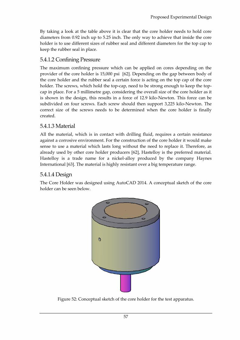
Proposed Experimental Design
57
By taking a look at the table above it is clear that the core holder needs to hold core
diameters from 0.92 inch up to 5.25 inch. The only way to achieve that inside the core
holder is to use different sizes of rubber seal and different diameters for the top cap to
keep the rubber seal in place.
5.4.1.2 Confining Pressure
The maximum confining pressure which can be applied on cores depending on the
provider of the core holder is 15,000 psi [62]. Depending on the gap between body of
the core holder and the rubber seal a certain force is acting on the top cap of the core
holder. The screws, which hold the top-cap, need to be strong enough to keep the top-
cap in place. For a 5 millimetre gap, considering the overall size of the core holder as it
is shown in the design, this results in a force of 12.9 kilo-Newton. This force can be
subdivided on four screws. Each screw should then support 3,225 kilo-Newton. The
correct size of the screws needs to be determined when the core holder is finally
created.
5.4.1.3 Material
All the material, which is in contact with drilling fluid, requires a certain resistance
against a corrosive environment. For the construction of the core holder it would make
sense to use a material which lasts long without the need to replace it. Therefore, as
already used by other core holder producers [62], Hastelloy is the preferred material.
Hastelloy is a trade name for a nickel-alloy produced by the company Haynes
International [63]. The material is highly resistant over a big temperature range.
5.4.1.4 Design
The Core Holder was designed using AutoCAD 2014. A conceptual sketch of the core
holder can be seen below.
Figure 52: Conceptual sketch of the core holder for the test apparatus.
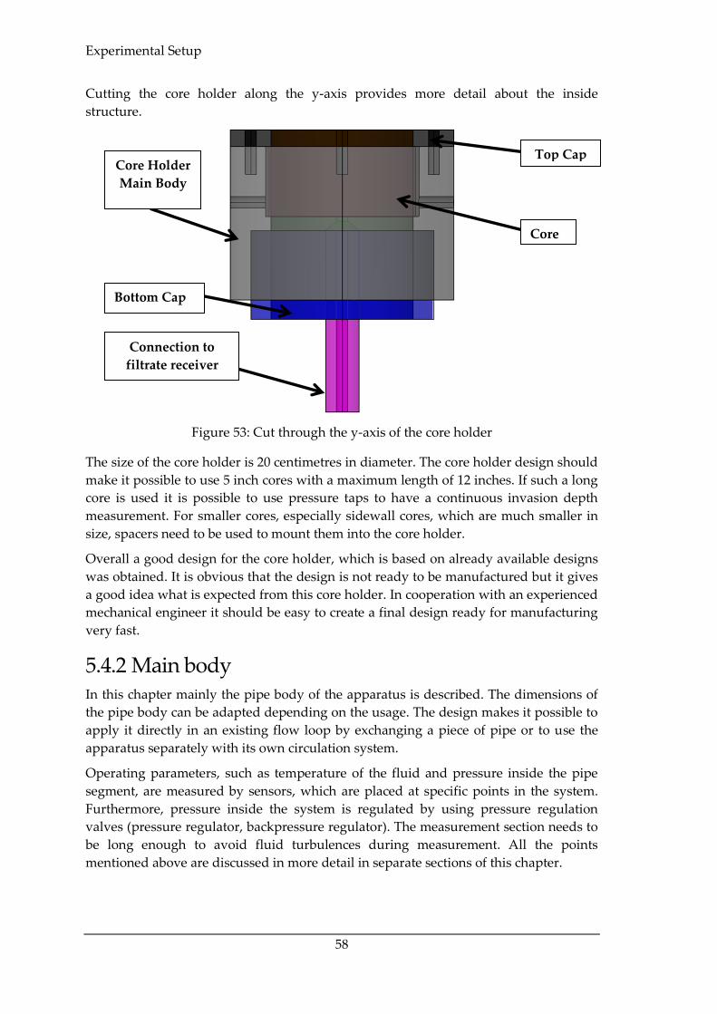
Experimental Setup
58
Cutting the core holder along the y-axis provides more detail about the inside
structure.
Figure 53: Cut through the y-axis of the core holder
The size of the core holder is 20 centimetres in diameter. The core holder design should
make it possible to use 5 inch cores with a maximum length of 12 inches. If such a long
core is used it is possible to use pressure taps to have a continuous invasion depth
measurement. For smaller cores, especially sidewall cores, which are much smaller in
size, spacers need to be used to mount them into the core holder.
Overall a good design for the core holder, which is based on already available designs
was obtained. It is obvious that the design is not ready to be manufactured but it gives
a good idea what is expected from this core holder. In cooperation with an experienced
mechanical engineer it should be easy to create a final design ready for manufacturing
very fast.
5.4.2 Main body In this chapter mainly the pipe body of the apparatus is described. The dimensions of
the pipe body can be adapted depending on the usage. The design makes it possible to
apply it directly in an existing flow loop by exchanging a piece of pipe or to use the
apparatus separately with its own circulation system.
Operating parameters, such as temperature of the fluid and pressure inside the pipe
segment, are measured by sensors, which are placed at specific points in the system.
Furthermore, pressure inside the system is regulated by using pressure regulation
valves (pressure regulator, backpressure regulator). The measurement section needs to
be long enough to avoid fluid turbulences during measurement. All the points
mentioned above are discussed in more detail in separate sections of this chapter.
Core Holder
Main Body
Bottom Cap
Connection to
filtrate receiver
Top Cap
Core
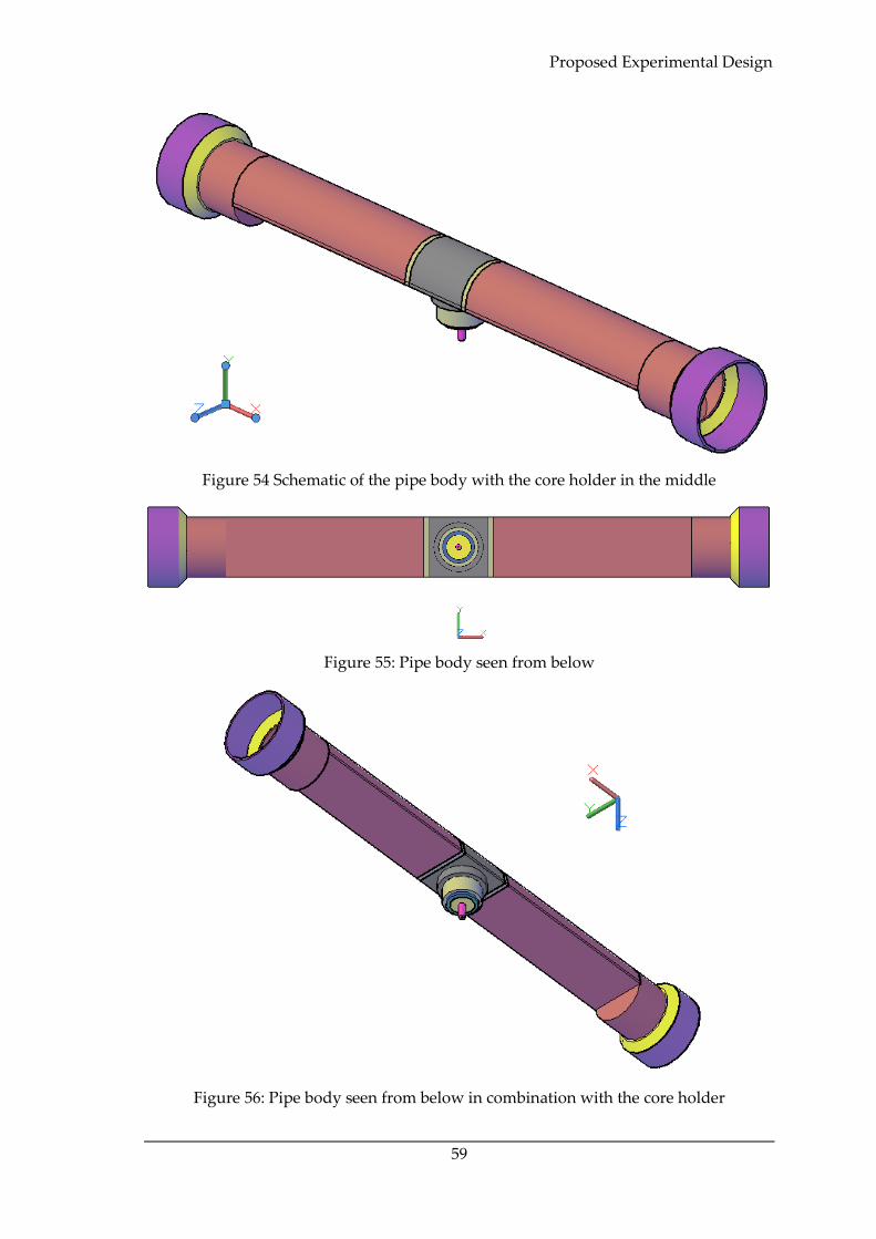
Proposed Experimental Design
59
Figure 54 Schematic of the pipe body with the core holder in the middle
Figure 55: Pipe body seen from below
Figure 56: Pipe body seen from below in combination with the core holder
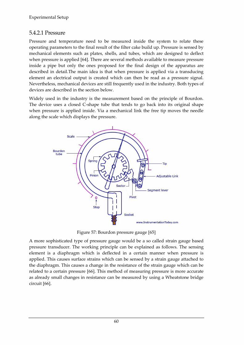
Experimental Setup
60
5.4.2.1 Pressure
Pressure and temperature need to be measured inside the system to relate these
operating parameters to the final result of the filter cake build up. Pressure is sensed by
mechanical elements such as plates, shells, and tubes, which are designed to deflect
when pressure is applied [64]. There are several methods available to measure pressure
inside a pipe but only the ones proposed for the final design of the apparatus are
described in detail.The main idea is that when pressure is applied via a transducing
element an electrical output is created which can then be read as a pressure signal.
Nevertheless, mechanical devices are still frequently used in the industry. Both types of
devices are described in the section below.
Widely used in the industry is the measurement based on the principle of Bourdon.
The device uses a closed C-shape tube that tends to go back into its original shape
when pressure is applied inside. Via a mechanical link the free tip moves the needle
along the scale which displays the pressure.
Figure 57: Bourdon pressure gauge [65]
A more sophisticated type of pressure gauge would be a so called strain gauge based
pressure transducer. The working principle can be explained as follows. The sensing
element is a diaphragm which is deflected in a certain manner when pressure is
applied. This causes surface strains which can be sensed by a strain gauge attached to
the diaphragm. This causes a change in the resistance of the strain gauge which can be
related to a certain pressure [66]. This method of measuring pressure is more accurate
as already small changes in resistance can be measured by using a Wheatstone bridge
circuit [66].
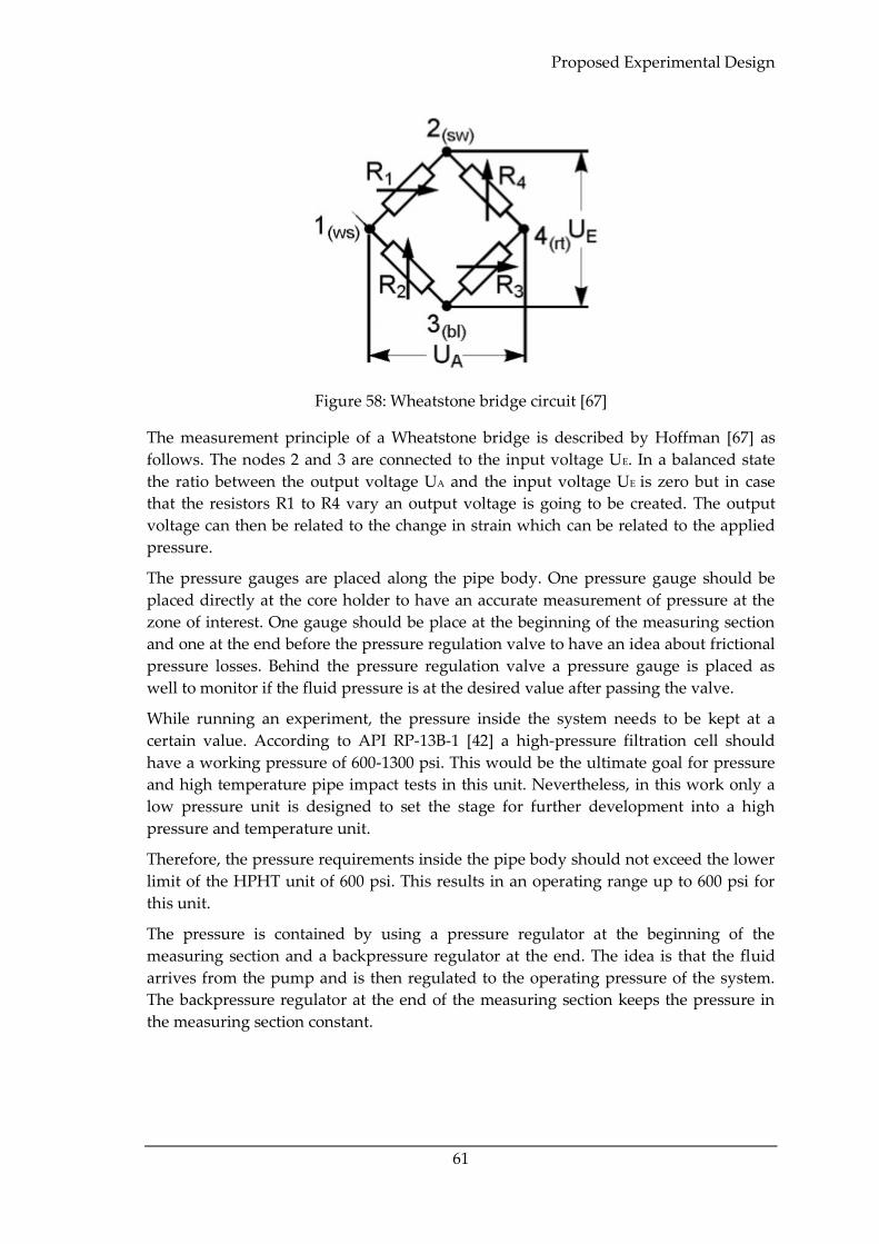
Proposed Experimental Design
61
Figure 58: Wheatstone bridge circuit [67]
The measurement principle of a Wheatstone bridge is described by Hoffman [67] as
follows. The nodes 2 and 3 are connected to the input voltage UE. In a balanced state
the ratio between the output voltage UA and the input voltage UE is zero but in case
that the resistors R1 to R4 vary an output voltage is going to be created. The output
voltage can then be related to the change in strain which can be related to the applied
pressure.
The pressure gauges are placed along the pipe body. One pressure gauge should be
placed directly at the core holder to have an accurate measurement of pressure at the
zone of interest. One gauge should be place at the beginning of the measuring section
and one at the end before the pressure regulation valve to have an idea about frictional
pressure losses. Behind the pressure regulation valve a pressure gauge is placed as
well to monitor if the fluid pressure is at the desired value after passing the valve.
While running an experiment, the pressure inside the system needs to be kept at a
certain value. According to API RP-13B-1 [42] a high-pressure filtration cell should
have a working pressure of 600-1300 psi. This would be the ultimate goal for pressure
and high temperature pipe impact tests in this unit. Nevertheless, in this work only a
low pressure unit is designed to set the stage for further development into a high
pressure and temperature unit.
Therefore, the pressure requirements inside the pipe body should not exceed the lower
limit of the HPHT unit of 600 psi. This results in an operating range up to 600 psi for
this unit.
The pressure is contained by using a pressure regulator at the beginning of the
measuring section and a backpressure regulator at the end. The idea is that the fluid
arrives from the pump and is then regulated to the operating pressure of the system.
The backpressure regulator at the end of the measuring section keeps the pressure in
the measuring section constant.
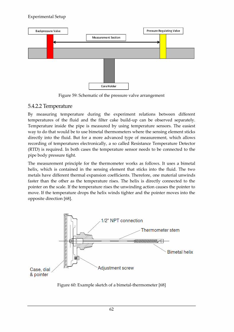
Experimental Setup
62
Figure 59: Schematic of the pressure valve arrangement
5.4.2.2 Temperature
By measuring temperature during the experiment relations between different
temperatures of the fluid and the filter cake build-up can be observed separately.
Temperature inside the pipe is measured by using temperature sensors. The easiest
way to do that would be to use bimetal thermometers where the sensing element sticks
directly into the fluid. But for a more advanced type of measurement, which allows
recording of temperatures electronically, a so called Resistance Temperature Detector
(RTD) is required. In both cases the temperature sensor needs to be connected to the
pipe body pressure tight.
The measurement principle for the thermometer works as follows. It uses a bimetal
helix, which is contained in the sensing element that sticks into the fluid. The two
metals have different thermal expansion coefficients. Therefore, one material unwinds
faster than the other as the temperature rises. The helix is directly connected to the
pointer on the scale. If the temperature rises the unwinding action causes the pointer to
move. If the temperature drops the helix winds tighter and the pointer moves into the
opposite direction [68].
Figure 60: Example sketch of a bimetal-thermometer [68]
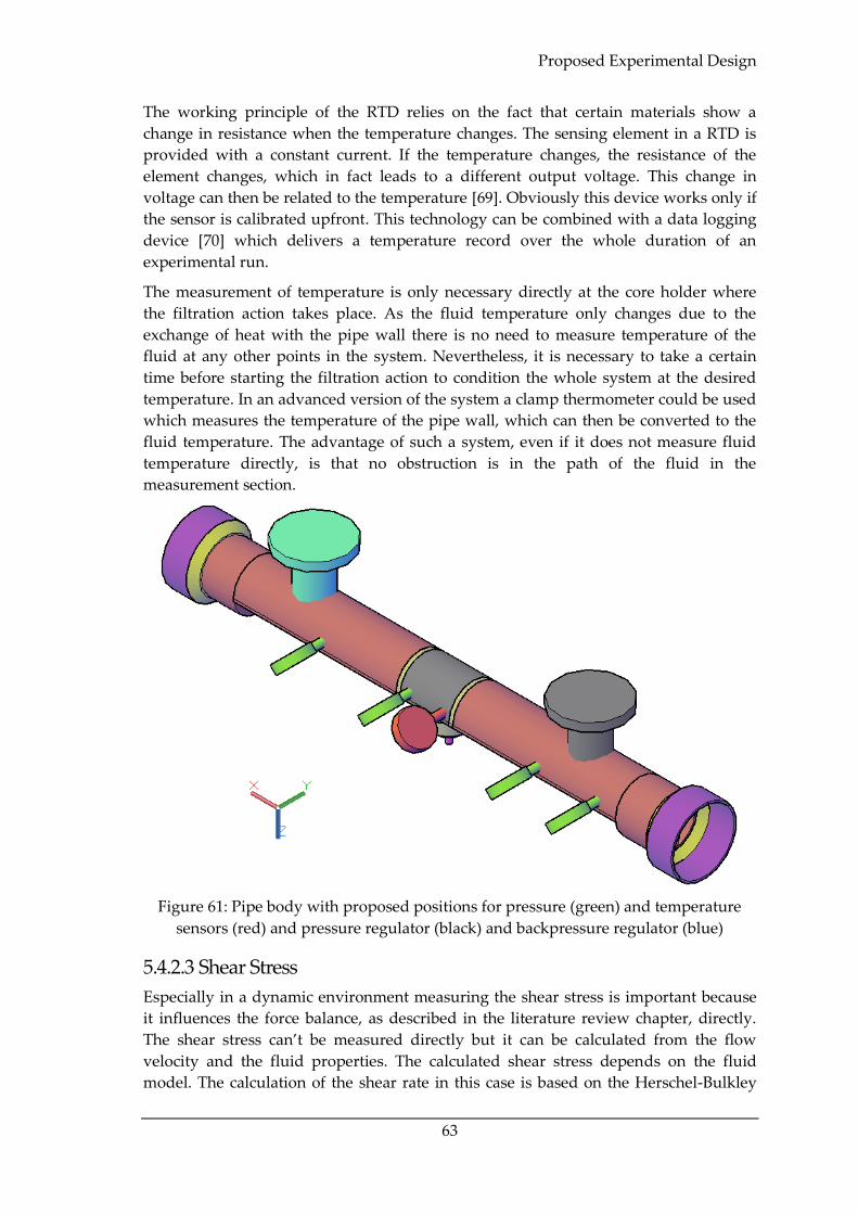
Proposed Experimental Design
63
The working principle of the RTD relies on the fact that certain materials show a
change in resistance when the temperature changes. The sensing element in a RTD is
provided with a constant current. If the temperature changes, the resistance of the
element changes, which in fact leads to a different output voltage. This change in
voltage can then be related to the temperature [69]. Obviously this device works only if
the sensor is calibrated upfront. This technology can be combined with a data logging
device [70] which delivers a temperature record over the whole duration of an
experimental run.
The measurement of temperature is only necessary directly at the core holder where
the filtration action takes place. As the fluid temperature only changes due to the
exchange of heat with the pipe wall there is no need to measure temperature of the
fluid at any other points in the system. Nevertheless, it is necessary to take a certain
time before starting the filtration action to condition the whole system at the desired
temperature. In an advanced version of the system a clamp thermometer could be used
which measures the temperature of the pipe wall, which can then be converted to the
fluid temperature. The advantage of such a system, even if it does not measure fluid
temperature directly, is that no obstruction is in the path of the fluid in the
measurement section.
Figure 61: Pipe body with proposed positions for pressure (green) and temperature
sensors (red) and pressure regulator (black) and backpressure regulator (blue)
5.4.2.3 Shear Stress
Especially in a dynamic environment measuring the shear stress is important because
it influences the force balance, as described in the literature review chapter, directly.
The shear stress can’t be measured directly but it can be calculated from the flow
velocity and the fluid properties. The calculated shear stress depends on the fluid
model. The calculation of the shear rate in this case is based on the Herschel-Bulkley
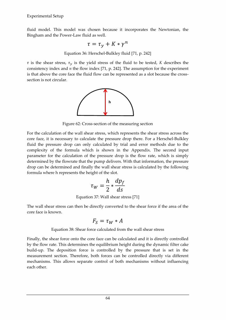
Experimental Setup
64
fluid model. This model was chosen because it incorporates the Newtonian, the
Bingham and the Power-Law fluid as well.
𝜏 = 𝜏𝑦 + 𝐾 ∗ 𝛾𝑛
Equation 36: Herschel-Bulkley fluid [71, p. 242]
𝜏 is the shear stress, 𝜏𝑦 is the yield stress of the fluid to be tested, K describes the
consistency index and n the flow index [71, p. 242]. The assumption for the experiment
is that above the core face the fluid flow can be represented as a slot because the cross-
section is not circular.
Figure 62: Cross-section of the measuring section
For the calculation of the wall shear stress, which represents the shear stress across the
core face, it is necessary to calculate the pressure drop there. For a Herschel-Bulkley
fluid the pressure drop can only calculated by trial and error methods due to the
complexity of the formula which is shown in the Appendix. The second input
parameter for the calculation of the pressure drop is the flow rate, which is simply
determined by the flowrate that the pump delivers. With that information, the pressure
drop can be determined and finally the wall shear stress is calculated by the following
formula where h represents the height of the slot.
𝜏𝑊 =ℎ
2∗
𝑑𝑝𝑓
𝑑𝑠
Equation 37: Wall shear stress [71]
The wall shear stress can then be directly converted to the shear force if the area of the
core face is known.
𝐹𝑆 = 𝜏𝑊 ∗ 𝐴
Equation 38: Shear force calculated from the wall shear stress
Finally, the shear force onto the core face can be calculated and it is directly controlled
by the flow rate. This determines the equilibrium height during the dynamic filter cake
build-up. The deposition force is controlled by the pressure that is set in the
measurement section. Therefore, both forces can be controlled directly via different
mechanisms. This allows separate control of both mechanisms without influencing
each other.
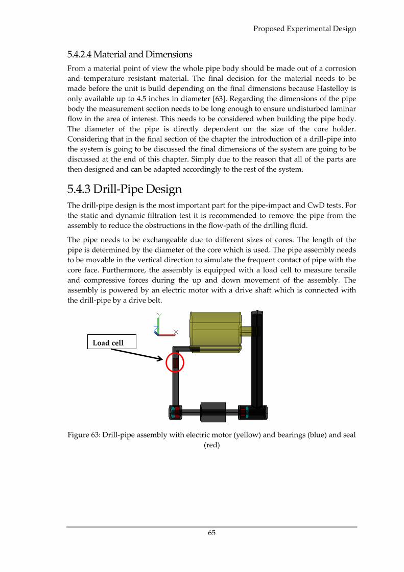
Proposed Experimental Design
65
5.4.2.4 Material and Dimensions
From a material point of view the whole pipe body should be made out of a corrosion
and temperature resistant material. The final decision for the material needs to be
made before the unit is build depending on the final dimensions because Hastelloy is
only available up to 4.5 inches in diameter [63]. Regarding the dimensions of the pipe
body the measurement section needs to be long enough to ensure undisturbed laminar
flow in the area of interest. This needs to be considered when building the pipe body.
The diameter of the pipe is directly dependent on the size of the core holder.
Considering that in the final section of the chapter the introduction of a drill-pipe into
the system is going to be discussed the final dimensions of the system are going to be
discussed at the end of this chapter. Simply due to the reason that all of the parts are
then designed and can be adapted accordingly to the rest of the system.
5.4.3 Drill-Pipe Design The drill-pipe design is the most important part for the pipe-impact and CwD tests. For
the static and dynamic filtration test it is recommended to remove the pipe from the
assembly to reduce the obstructions in the flow-path of the drilling fluid.
The pipe needs to be exchangeable due to different sizes of cores. The length of the
pipe is determined by the diameter of the core which is used. The pipe assembly needs
to be movable in the vertical direction to simulate the frequent contact of pipe with the
core face. Furthermore, the assembly is equipped with a load cell to measure tensile
and compressive forces during the up and down movement of the assembly. The
assembly is powered by an electric motor with a drive shaft which is connected with
the drill-pipe by a drive belt.
Figure 63: Drill-pipe assembly with electric motor (yellow) and bearings (blue) and seal
(red)
Load cell
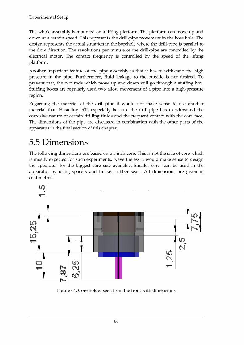
Experimental Setup
66
The whole assembly is mounted on a lifting platform. The platform can move up and
down at a certain speed. This represents the drill-pipe movement in the bore hole. The
design represents the actual situation in the borehole where the drill-pipe is parallel to
the flow direction. The revolutions per minute of the drill-pipe are controlled by the
electrical motor. The contact frequency is controlled by the speed of the lifting
platform.
Another important feature of the pipe assembly is that it has to withstand the high
pressure in the pipe. Furthermore, fluid leakage to the outside is not desired. To
prevent that, the two rods which move up and down will go through a stuffing box.
Stuffing boxes are regularly used two allow movement of a pipe into a high-pressure
region.
Regarding the material of the drill-pipe it would not make sense to use another
material than Hastelloy [63], especially because the drill-pipe has to withstand the
corrosive nature of certain drilling fluids and the frequent contact with the core face.
The dimensions of the pipe are discussed in combination with the other parts of the
apparatus in the final section of this chapter.
5.5 Dimensions The following dimensions are based on a 5 inch core. This is not the size of core which
is mostly expected for such experiments. Nevertheless it would make sense to design
the apparatus for the biggest core size available. Smaller cores can be used in the
apparatus by using spacers and thicker rubber seals. All dimensions are given in
centimetres.
Figure 64: Core holder seen from the front with dimensions
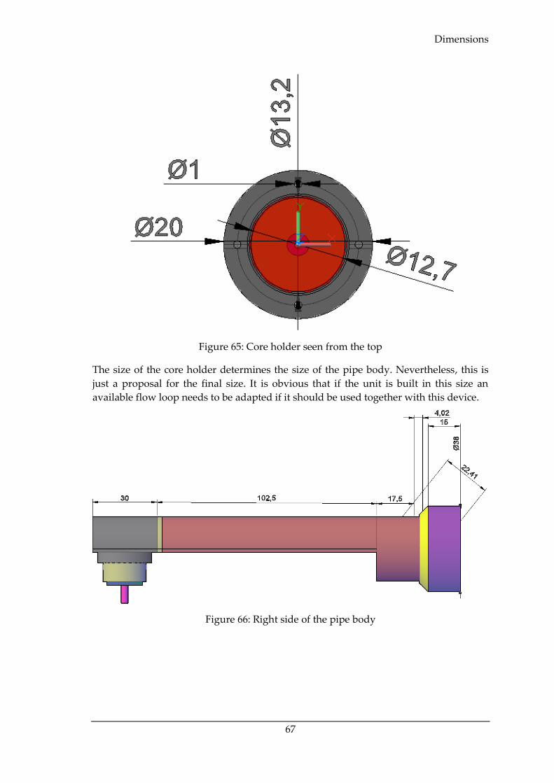
Dimensions
67
Figure 65: Core holder seen from the top
The size of the core holder determines the size of the pipe body. Nevertheless, this is
just a proposal for the final size. It is obvious that if the unit is built in this size an
available flow loop needs to be adapted if it should be used together with this device.
Figure 66: Right side of the pipe body
Experimental Setup
68
Only the right side of the pipe body is displayed here. For the dimensions it makes no
difference because both sides are equal in size. The measurement section itself is 235
centimetres long. The length is based on the concept of the hydrodynamic entrance
length. The entrance length is defined as the necessary distance a fluid needs to travel
inside a pipe to have a fully developed parabolic flow profile [72]. For laminar flow the
following formula defines the required entrance length.
𝐿𝐸 = 0,06 ∗ 𝑅𝑒 ∗ 𝐷𝐻
Equation 39: Definition of the entrance length for laminar flow [72]
Where Re is the Reynolds number and DH is the hydraulic diameter.
𝐷𝐻 =4 ∗ 𝐴
𝑃
Equation 40: Hydraulic Diameter [73]
Where A is the area of the pipe crosssection and P is the wetted perimeter.
Depending on the flowrate, the fluid viscosity, the fluid density, the pipe diameter and
the pipe shape the entrance length varies. For a Reynolds number of 2300 as transition
from laminar to turbulent flow [74] with a pipe radius of 14 centimetres the entrance
length would be 34 metres which is not reasonable at all. Therefore, for the design a
different definition for the entrance length was used.
𝐿𝐸 = 10 ∗ 𝐷
Equation 41: Definition of entrance length for turbulent flow [75]
Considering the half pipe shape and the radius of the pipe the dimensions shown in
Figure 66 were chosen. This entrance length does not mean that the flow inside the
pipe is turbulent. Anyway before building the apparatus a compromise, including the
space specifications need to be considered. Furthermore additional research
considering flow dynamics and streamline simulations is required to avoid problems.
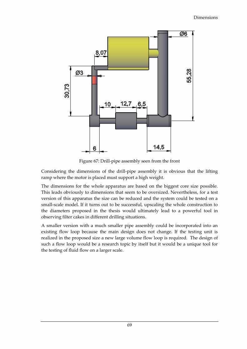
Dimensions
69
Figure 67: Drill-pipe assembly seen from the front
Considering the dimensions of the drill-pipe assembly it is obvious that the lifting
ramp where the motor is placed must support a high weight.
The dimensions for the whole apparatus are based on the biggest core size possible.
This leads obviously to dimensions that seem to be oversized. Nevertheless, for a test
version of this apparatus the size can be reduced and the system could be tested on a
small-scale model. If it turns out to be successful, upscaling the whole construction to
the diameters proposed in the thesis would ultimately lead to a powerful tool in
observing filter cakes in different drilling situations.
A smaller version with a much smaller pipe assembly could be incorporated into an
existing flow loop because the main design does not change. If the testing unit is
realized in the proposed size a new large volume flow loop is required. The design of
such a flow loop would be a research topic by itself but it would be a unique tool for
the testing of fluid flow on a larger scale.
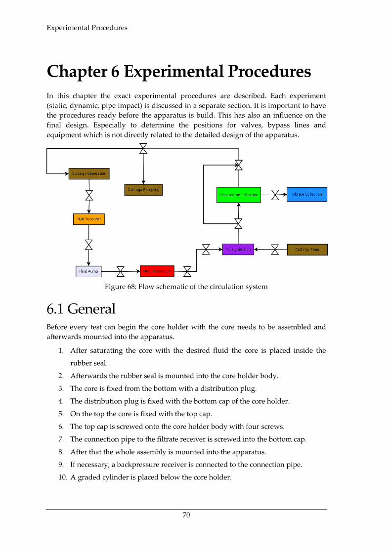
Experimental Procedures
70
Chapter 6 Experimental Procedures In this chapter the exact experimental procedures are described. Each experiment
(static, dynamic, pipe impact) is discussed in a separate section. It is important to have
the procedures ready before the apparatus is build. This has also an influence on the
final design. Especially to determine the positions for valves, bypass lines and
equipment which is not directly related to the detailed design of the apparatus.
Figure 68: Flow schematic of the circulation system
6.1 General Before every test can begin the core holder with the core needs to be assembled and
afterwards mounted into the apparatus.
1. After saturating the core with the desired fluid the core is placed inside the
rubber seal.
2. Afterwards the rubber seal is mounted into the core holder body.
3. The core is fixed from the bottom with a distribution plug.
4. The distribution plug is fixed with the bottom cap of the core holder.
5. On the top the core is fixed with the top cap.
6. The top cap is screwed onto the core holder body with four screws.
7. The connection pipe to the filtrate receiver is screwed into the bottom cap.
8. After that the whole assembly is mounted into the apparatus.
9. If necessary, a backpressure receiver is connected to the connection pipe.
10. A graded cylinder is placed below the core holder.
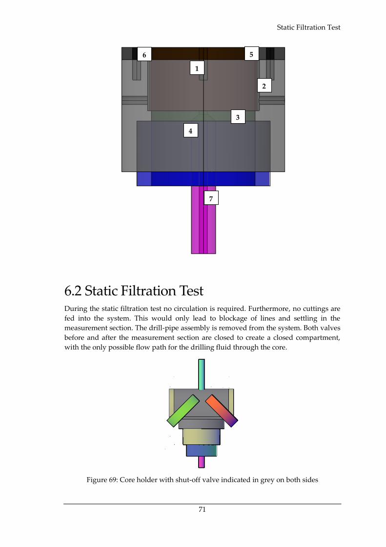
Static Filtration Test
71
6.2 Static Filtration Test During the static filtration test no circulation is required. Furthermore, no cuttings are
fed into the system. This would only lead to blockage of lines and settling in the
measurement section. The drill-pipe assembly is removed from the system. Both valves
before and after the measurement section are closed to create a closed compartment,
with the only possible flow path for the drilling fluid through the core.
Figure 69: Core holder with shut-off valve indicated in grey on both sides
1
2
3
4
5
1
6
7
Experimental Procedures
72
1. The core holder is screwed into the testing apparatus
2. The pressure lines to build up the confining pressure are attached to the core
holder
3. Then the drilling fluid is poured into the sample chamber until it is completely
filled with mud
4. Confining pressure is applied on the core sample up to 5000 psi
5. When the confining pressure has reached a steady value the pressure line to the
sample chamber is attached.
6. A pressure of 100 psi is applied onto the drilling fluid
7. The pressure is kept for 30 minutes and filtrate is collected and every 5 minutes
the volume is recorded
8. After 30 minutes the confining pressure is released from the core holder
9. Then the pressure is released and the drilling fluid is discarded from the
sample chamber
10. The core holder is unscrewed from the apparatus
11. The top cap is removed from the core holder and the core together with the
rubber seal is removed from the core holder
12. The rubber seal is removed from the core and the core and the filter cake are
ready for further analysis
6.3 Dynamic Filtration Test In the dynamic filtration test the fluid is circulated at a certain rate to create the
required shear rate onto the core face. This is controlled by the flowrate that is set at the
pump. Cuttings are not fed into the system as they are not required in these types of
experiment. There is no standard procedure for carrying out a dynamic filtration test
with regards to pressure or time. Nevertheless, the time interval for the experiment
needs to be long enough to reach the equilibrium thickness of the filter cake. The drill
pipe assembly is also removed from the system to avoid obstructions in the flow path.
1. The core holder is assembled as described before
2. The core holder is mounted into the experimental apparatus
3. The pressure lines to build up the confining pressure are attached to the core
holder
4. Meanwhile the drilling fluid is already circulated through the heat exchanger
and the bypass line to heat up the whole system
5. The temperature is measured at several points in the circulation system, when
the temperature is constant the system is ready to be used
Pipe Impact Test
73
6. Then the drilling fluid is circulated through the measurement section without
already setting the working pressure
7. Confining pressure is applied on the core sample up to 5000 psi
8. When the measurement section has reached the required temperature, the
pressure regulator and the backpressure regulator are set to the working
pressure
9. When the pressure is constant, the test duration begins
10. During the test filtrate is collected in a graded cylinder and the volume is
recorded every 5 minutes
11. The test duration depends on the shear rate and the working pressure of the
system
12. When the fluid loss is linear, dynamic fluid loss has stopped and the static
filtration process has started. At this point the experiment can be stopped.
13. The pump is stopped and the heat exchanger is turned off
14. The drilling fluid is discarded from the system and should be stored for further
usage and analysis
15. The core holder is unscrewed from the apparatus
16. The top cap is removed from the core holder and the core together with the
rubber seal is removed from the core holder
17. The rubber seal is removed from the core and the core and the filter cake are
ready for further analysis
6.4 Pipe Impact Test This type of test uses the circulation system and the drill pipe assembly. Depending on
the core size a different size of drill pipe can be used, which matches the core size.
Cuttings are also feed into the system. The cuttings feed starts after the pump and the
cuttings are removed from the circulation system before they enter the mud reservoir.
This should avoid that cuttings of a certain size may damage the pump. The cuttings
are sampled directly after the measurement section.
1. The core holder is assembled as described before
2. The core holder is mounted into the experimental apparatus
3. The pressure lines to build up the confining pressure are attached to the core
holder
4. Meanwhile the drilling fluid is already circulated through the heat exchanger
and the bypass line to heat up the whole system
Experimental Procedures
74
5. The temperature is measured at several points in the circulation system, when
the temperature is constant the system is ready to be used
6. Then the drilling fluid is circulated through the measurement section without
already setting the working pressure
7. Confining pressure is applied on the core sample up to 5000 psi
8. Rotation of the drill pipe is started and the load sensor is activated
9. When the measurement section has reached the required temperature, the
pressure regulator and the backpressure regulator are set to the working
pressure
10. The up and down movement of the pipe is activated at the desired contact
frequency
11. When the pressure is constant, the test duration begins
12. During the test filtrate is collected in a graded cylinder and the volume is
recorded every 5 minutes
13. Every 5 minutes a cuttings sample is taken from the circulation system to see if
it is possible to crush the cuttings with the drill pipe
14. The test duration depends on the shear rate and the working pressure of the
system
15. When the fluid loss is linear, dynamic fluid loss has stopped and the static
filtration process has started. At this point the experiment can be stopped.
16. The pump is stopped and the heat exchanger is turned off
17. The drilling fluid is discarded from the system and should be stored for further
usage and analysis
18. The core holder is unscrewed from the apparatus
19. The top cap is removed from the core holder and the core together with the
rubber seal is removed from the core holder
20. The rubber seal is removed from the core and the core and the filter cake are
ready for further analysis
The proposed experimental procedures are far from complete. When the apparatus is
built, there are several details which are going to be added to the procedures.
Furthermore, the test durations for the static filtration test, the dynamic filtration test
and the pipe impact test need to be determined depending on the applied pressure and
the shear rate. The pipe contact frequency can be set specifically for each experiment.
Results
75
Chapter 7 Results and Conclusion
7.1 Results The main result of this thesis is a design for a multipurpose unit for testing a variety of
situations for filter cake build-up. Depending on its final size the unit could be
implemented into an already existing flow loop. If testing of large diameter cores is
required, a new design for a flow loop, which produces high circulation rates, is
necessary. The design features three different applications, which are static filter cake
build-up, dynamic filter cake build-up and a pipe impact test. CwD can be simulated
by using large diameter pipe, which has regular contact with the core face and by
feeding artificial cuttings into the circulation system.
The final design consists of three parts which are the core holder, the main body and
the drill-pipe assembly. The core holder allows confining pressures up to 5000 psi and
exposes one side of the core to the drilling fluid. The core holder is going to be made
out of Hastelloy.
The main body has a half pipe shape and is equipped with a temperature sensor and
four pressure sensors. Furthermore, two shut-off valves are indicated in the design two
allow static filtration tests. The pressure is regulated by a pressure regulation valve at
the beginning of the measurement section and a backpressure valve at the end for
pressure maintenance.
The drill-pipe assembly is aligned with the flow direction. The design features an
electric motor which drives the pipe rotation. Via two stuffing boxes pressure is
maintained in the pipe body. A load sensor is used to measure the forces during up
and down movement of the assembly. The vertical movement is controlled because the
whole assembly rests on a lifting ramp.
Furthermore, three experimental procedures were developed based on the final design.
These procedures are so far only proposals because they need to be adapted after the
unit is build.
Results and Conclusion
76
7.2 Conclusion Based on the literature review the comparison between regular filter cake and one
created by smearing it can be concluded that the particle size distribution (PSD) is of
vital importance. The PSD has a high influence on the filtrate volume and the filter
cake structure. Furthermore, the porosity and the permeability of the filter cake are
influenced by the PSD.
Considering the geomechanical aspects of CwD it seems that it has a positive effect on
the wellbore stability. This is due to the creation of a filter cake with very low
permeability which hinders fluid to invade the formation. Therefore, time dependent
pore pressure changes are prevented, which in worst case would lead to significant
breakouts.
The frequent contact of the casing with the wellbore wall is also considered as positive,
but it is not verified yet. The contact leads to an increase of the hoop stress and can
prevent the creation of fractures if the contact happens at the point of maximum
horizontal far field stress. If the contact happens at the point of minimum horizontal far
field stress it is more likely to create breakouts due to the increase in hoop stress.
Therefore, it can be concluded that the positive effect of CwD depends highly on the
contact direction in the wellbore.
Regarding the experimental research of filter cake created by smearing, so far, no
experiment exists which simulates the build-up. Also, no experiment exists which
allows a direct comparison between a filter cake created by smearing and a regular
filter cake.
When the experimental design is realized, it will enable the user to test the build-up of
filter cake in different situations in the wellbore. Pressure, temperature, shear rate and
particle size distribution are parameters which can be directly controlled during an
experiment. This should allow the user to test different dependencies of parameters on
the filter cake quality simultaneously.
Finally, it can be concluded that CwD requires additional research regarding the
different influence parameters and the differences of filter cake quality and structure
compared to normal operations. This research can be realized by building the
proposed unit.
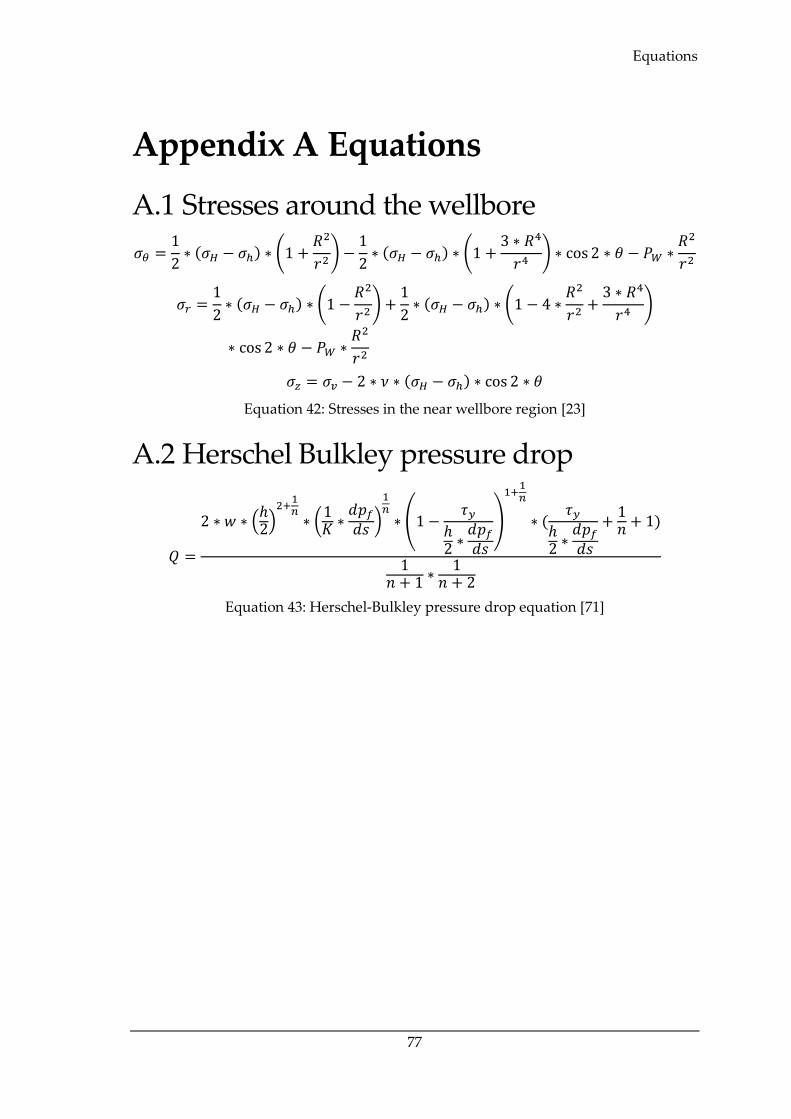
Equations
77
Appendix A Equations
A.1 Stresses around the wellbore
𝜎𝜃 =1
2∗ (𝜎𝐻 − 𝜎ℎ) ∗ (1 +
𝑅2
𝑟2) −
1
2∗ (𝜎𝐻 − 𝜎ℎ) ∗ (1 +
3 ∗ 𝑅4
𝑟4) ∗ cos 2 ∗ 𝜃 − 𝑃𝑊 ∗
𝑅2
𝑟2
𝜎𝑟 =1
2∗ (𝜎𝐻 − 𝜎ℎ) ∗ (1 −
𝑅2
𝑟2) +
1
2∗ (𝜎𝐻 − 𝜎ℎ) ∗ (1 − 4 ∗
𝑅2
𝑟2+
3 ∗ 𝑅4
𝑟4)
∗ cos 2 ∗ 𝜃 − 𝑃𝑊 ∗𝑅2
𝑟2
𝜎𝑧 = 𝜎𝑣 − 2 ∗ 𝜈 ∗ (𝜎𝐻 − 𝜎ℎ) ∗ cos 2 ∗ 𝜃
Equation 42: Stresses in the near wellbore region [23]
A.2 Herschel Bulkley pressure drop
𝑄 =
2 ∗ 𝑤 ∗ (ℎ2
)2+
1𝑛
∗ (1𝐾
∗𝑑𝑝𝑓
𝑑𝑠)
1𝑛
∗ (1 −𝜏𝑦
ℎ2 ∗
𝑑𝑝𝑓
𝑑𝑠
)
1+1𝑛
∗ (𝜏𝑦
ℎ2 ∗
𝑑𝑝𝑓
𝑑𝑠
+1𝑛
+ 1)
1𝑛 + 1 ∗
1𝑛 + 2
Equation 43: Herschel-Bulkley pressure drop equation [71]
Bibliography
78
Bibliography
[1] E. van Oort and S. O. Razavi, “Wellbore Strengthening and Casing Smear: The
Common Underlying Mechanism,” in IADC/SPE Drilling Conference and Exhibition,
Fort Worth, Texas, 2014.
[2] Dewan and Chenevert, “A Model for Filtration of Water-base Mud During
Drilling: Determination of Mudcake Parameters,” in Petrophysics. Vol. 42, Austin,
Texas, Society of Professional Well Log Analysts, 2001, pp. 237-250.
[3] Elkatatny, Mahmoud and Nasr-El-Din, “A New technique to Characterize Drilling
Fluid Filter Cake,” in SPE European Formation Damage Conference, Noordwijk, The
Netherlands, 2011.
[4] Elkatatny and Nasr-El-Din, “Properties of Filter Cake of Water-Based Drilling
Fluid under Dynamic Conditions using Computer Tomography,” in IADC/SPE
Drilling Conference and Exhibition, San Diego, California, 2012.
[5] Elkatatny, Mahmoud and Nasr-El-Din, “A New Approach to Determine Filter
Cake Properties of Water-Based Drilling Fluids,” in SPE/DGS Saudi Arabia Section
Technical Symposium and Exhibition, Al-Khobar, Saudi Arabia, 2011.
[6] Geri, Al-Mutairi and Mahmoud, “Different Techniques for Characterizing the
Filter Cake,” in SPE Middle East Unconventional Gas Conference and Exhibition,
Muscat, Oman, 2013.
[7] Chandler und Dangou, „Potential Increase of Formation Damage at Horizontal
Wells as a Result of Changing Dynamic Filter Cake Properties with the Shear
Rate,“ in SPE European Formation Damage Conference, Scheveningen, The
Netherlands, 2009.
[8] Jiao und Sharma, „Investigation of Dynamic Mud Cake Formation: The Concept
of Minimum Overbalance Pressure,“ in Annual Technical Conference and Exhibition,
Houston, Texas, 1993.
[9] Li und He, „Journey Into Filter Cakes: A Microstructural Study,“ in International
Petroleum Technology Conference, Doha, Qatar, 2015.
[10] M. Stephens und W. He, „Bridging Particle Size Distribution in Drilling Fluid and
Formation Damage,“ in SPE European Formation Damage Conference, Noordwijk,
The Netherlands, 2011.
[11] M. Karimi, A. Ghalambor, M. Montgomery and E. Moellendick, “Formation
Damage and Fluid Loss Reduction due to Plastering Effect of Casing Drilling,” in
SPE European Formation Damage Conference, Noordwijk, The Netherlands, 2011.
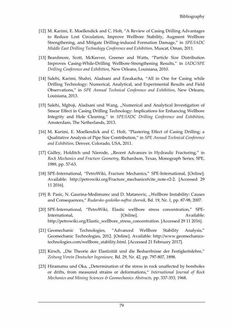
Bibliography
79
[12] M. Karimi, E. Moellendick and C. Holt, “A Review of Casing Drilling Advantages
to Reduce Lost Circulation, Improve Wellbore Stability, Augment Wellbore
Strengthening, and Mitigate Drilling-induced Formation Damage,” in SPE/IADC
Middle East Drilling Technology Conference and Exhibition, Muscat, Oman, 2011.
[13] Beardmore, Scott, McKeever, Greener and Watts, “Particle Size Distribution
Improves Casing-While-Drilling Wellbore-Strengthening Results,” in IADC/SPE
Drilling Conference and Exhibition, New Orleans, Louisiana, 2010.
[14] Salehi, Karimi, Shahri, Aladsani and Ezeakacha, “All in One for Casing while
Drilling Technology: Numerical, Analytical, and Experimental Results and Field
Observations,” in SPE Annual Technical Conference and Exhibition, New Orleans,
Louisiana, 2013.
[15] Salehi, Mgboji, Aladsani und Wang, „Numerical and Analytical Investigation of
Smear Effect in Casing Drilling Technology: Implications for Enhancing Wellbore
Integrity and Hole Cleaning,“ in SPE/IADC Drilling Conference and Exhibition,
Amsterdam, The Netherlands, 2013.
[16] M. Karimi, E. Moellendick and C. Holt, “Plastering Effect of Casing Drilling; a
Qualitative Analysis of Pipe Size Contribution,” in SPE Annual Technical Conference
and Exhibition, Denver, Colorado, USA, 2011.
[17] Gidley, Holditch und Nierode, „Recent Advances in Hydraulic Fracturing,“ in
Rock Mechanics and Fracture Geometry, Richardson, Texas, Monograph Series, SPE,
1989, pp. 57-63.
[18] SPE-International, “PetroWiki, Fracture Mechanics,” SPE-International, [Online].
Available: http://petrowiki.org/Fracture_mechanics#cite_note-r2-2. [Accessed 29
11 2016].
[19] B. Pasic, N. Gaurina-Medimurec und D. Matanovic, „Wellbore Instability: Causes
and Consequences,“ Rudarsko-geološko-naftni zbornik, Bd. 19, Nr. 1, pp. 87-98, 2007.
[20] SPE-International, “PetroWiki, Elastic wellbore stress concentration,” SPE-
International, [Online]. Available:
http://petrowiki.org/Elastic_wellbore_stress_concentration. [Accessed 29 11 2016].
[21] Geomechanic Technologies, “Advanced Wellbore Stability Analysis,”
Geomechanic Technologies, 2012. [Online]. Available: http://www.geomechanics-
technologies.com/wellbore_stability.html. [Accessed 21 February 2017].
[22] Kirsch, „Die Theorie der Elastizität und die Beduerfnisse der Festigkeitslehre,“
Zeitung Verein Deutscher Ingenieure, Bd. 29, Nr. 42, pp. 797-807, 1898.
[23] Hiramatsu und Oka, „Determination of the stress in rock unaffected by boreholes
or drifts, from measured strains or deformations,“ International Journal of Rock
Mechanics and Mining Sciences & Geomechanics Abstracts, pp. 337-353, 1968.
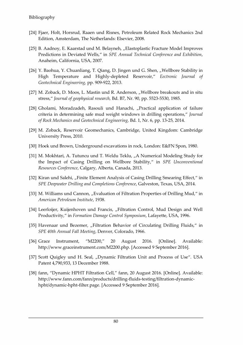
Bibliography
80
[24] Fjaer, Holt, Horsrud, Raaen und Risnes, Petroleum Related Rock Mechanics 2nd
Edition, Amsterdam, The Netherlands: Elsevier, 2008.
[25] B. Aadnoy, E. Kaarstad und M. Belayneh, „Elastoplastic Fracture Model Improves
Predictions in Deviated Wells,“ in SPE Annual Technical Conference and Exhibition,
Anaheim, California, USA, 2007.
[26] Y. Baohua, Y. Chuanliang, T. Qiang, D. Jingen und G. Shen, „Wellbore Stability in
High Temperature and Highly-depleted Reservoir,“ Eectronic Journal of
Geotechnical Engineering, pp. 909-922, 2013.
[27] M. Zoback, D. Moos, L. Mastin und R. Anderson, „Wellbore breakouts and in situ
stress,“ Journal of geophysical research, Bd. B7, Nr. 90, pp. 5523-5530, 1985.
[28] Gholami, Moradzadeh, Rasouli und Hanachi, „Practical application of failure
criteria in determining safe mud weight windows in drilling operations,“ Journal
of Rock Mechanics and Geotechnical Engineering, Bd. 1, Nr. 6, pp. 13-25, 2014.
[29] M. Zoback, Reservoir Geomechanics, Cambridge, United Kingdom: Cambridge
University Press, 2010.
[30] Hoek und Brown, Underground excavations in rock, London: E&FN Spon, 1980.
[31] M. Mokhtari, A. Tutuncu und T. Weldu Teklu, „A Numerical Modeling Study for
the Impact of Casing Drilling on Wellbore Stability,“ in SPE Unconventional
Resources Conference, Calgary, Alberta, Canada, 2013.
[32] Kiran und Salehi, „Finite Element Analysis of Casing Drilling Smearing Effect,“ in
SPE Deepwater Drilling and Completions Conference, Galveston, Texas, USA, 2014.
[33] M. Williams und Cannon, „Evaluation of Filtration Properties of Drilling Mud,“ in
American Petroleum Institute, 1938.
[34] Leerloijer, Kuijenhoven und Francis, „Filtration Control, Mud Design and Well
Productivity,“ in Formation Damage Control Symposium, Lafayette, USA, 1996.
[35] Havenaar und Bezemer, „Filtration Behavior of Circulating Drilling Fluids,“ in
SPE 40th Annual Fall Meeting, Denver, Colorado, 1966.
[36] Grace Instrument, “M2200,” 20 August 2016. [Online]. Available:
http://www.graceinstrument.com/M2200.php. [Accessed 9 September 2016].
[37] Scott Quigley und H. Seal, „Dynamic Filtration Unit and Process of Use“. USA
Patent 4,790,933, 13 December 1988.
[38] fann, “Dynamic HPHT Filtration Cell,” fann, 20 August 2016. [Online]. Available:
http://www.fann.com/fann/products/drilling-fluids-testing/filtration-dynamic-
hpht/dynamic-hpht-filter.page. [Accessed 9 September 2016].
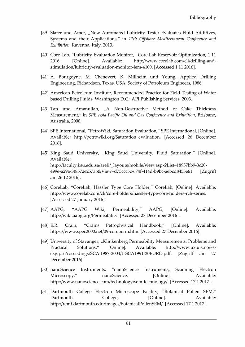
Bibliography
81
[39] Slater und Amer, „New Automated Lubricity Tester Evaluates Fluid Additives,
Systems and their Applications,“ in 11th Offshore Mediterranean Conference and
Exhibition, Ravenna, Italy, 2013.
[40] Core Lab, “Lubricity Evaluation Monitor,” Core Lab Reservoir Optimization, 1 11
2016. [Online]. Available: http://www.corelab.com/cli/drilling-and-
stimulation/lubricity-evaluation-monitor-lem-4100. [Accessed 1 11 2016].
[41] A. Bourgoyne, M. Chenevert, K. Millheim und Young, Applied Drilling
Engineering, Richardson, Texas, USA: Society of Petroleum Engineers, 1986.
[42] American Petroleum Institute, Recommended Practice for Field Testing of Water
based Drilling Fluids, Washington D.C.: API Publishing Services, 2003.
[43] Tan und Amanullah, „A Non-Destructive Method of Cake Thickness
Measurement,“ in SPE Asia Pacific Oil and Gas Conference and Exhibition, Brisbane,
Australia, 2000.
[44] SPE International, “PetroWiki, Saturation Evaluation,” SPE International, [Online].
Available: http://petrowiki.org/Saturation_evaluation. [Accessed 26 December
2016].
[45] King Saud University, „King Saud University, Fluid Saturation,“ [Online].
Available:
http://faculty.ksu.edu.sa/arefi/_layouts/mobile/view.aspx?List=18957bb9-3c20-
499e-a29a-3f8572e257a6&View=d75ccc5c-674f-414d-b9bc-aebcd8453e61. [Zugriff
am 26 12 2016].
[46] CoreLab, “CoreLab, Hassler Type Core Holder,” CoreLab, [Online]. Available:
http://www.corelab.com/cli/core-holders/hassler-type-core-holders-rch-series.
[Accessed 27 January 2016].
[47] AAPG, “AAPG Wiki, Permeability,” AAPG, [Online]. Available:
http://wiki.aapg.org/Permeability. [Accessed 27 December 2016].
[48] E.R. Crain, “Crains Petrophysical Handbook,” [Online]. Available:
https://www.spec2000.net/09-coreperm.htm. [Accessed 27 December 2016].
[49] University of Stavanger, „Klinkenberg Permeability Measurements: Problems and
Practical Solutions,“ [Online]. Available: http://www.ux.uis.no/~s-
skj/ipt/Proceedings/SCA.1987-2004/1-SCA1991-20EURO.pdf. [Zugriff am 27
December 2016].
[50] nanoScience Instruments, “nanoScience Instruments, Scanning Electron
Microscopy,” nanoScience, [Online]. Available:
http://www.nanoscience.com/technology/sem-technology/. [Accessed 17 1 2017].
[51] Dartmouth College Electron Microscope Facility, “Botanical Pollen SEM,”
Dartmouth College, [Online]. Available:
http://remf.dartmouth.edu/images/botanicalPollenSEM/. [Accessed 17 1 2017].
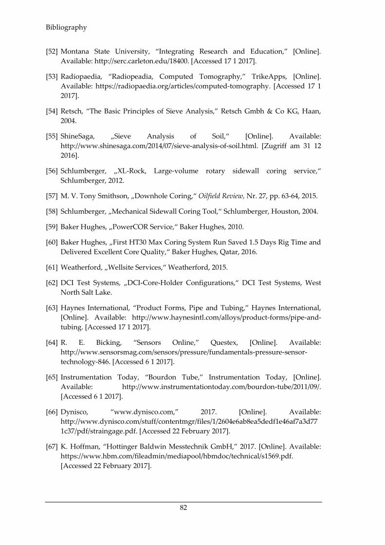
Bibliography
82
[52] Montana State University, “Integrating Research and Education,” [Online].
Available: http://serc.carleton.edu/18400. [Accessed 17 1 2017].
[53] Radiopaedia, “Radiopeadia, Computed Tomography,” TrikeApps, [Online].
Available: https://radiopaedia.org/articles/computed-tomography. [Accessed 17 1
2017].
[54] Retsch, “The Basic Principles of Sieve Analysis,” Retsch Gmbh & Co KG, Haan,
2004.
[55] ShineSaga, „Sieve Analysis of Soil,“ [Online]. Available:
http://www.shinesaga.com/2014/07/sieve-analysis-of-soil.html. [Zugriff am 31 12
2016].
[56] Schlumberger, „XL-Rock, Large-volume rotary sidewall coring service,“
Schlumberger, 2012.
[57] M. V. Tony Smithson, „Downhole Coring,“ Oilfield Review, Nr. 27, pp. 63-64, 2015.
[58] Schlumberger, „Mechanical Sidewall Coring Tool,“ Schlumberger, Houston, 2004.
[59] Baker Hughes, „PowerCOR Service,“ Baker Hughes, 2010.
[60] Baker Hughes, „First HT30 Max Coring System Run Saved 1.5 Days Rig Time and
Delivered Excellent Core Quality,“ Baker Hughes, Qatar, 2016.
[61] Weatherford, „Wellsite Services,“ Weatherford, 2015.
[62] DCI Test Systems, „DCI-Core-Holder Configurations,“ DCI Test Systems, West
North Salt Lake.
[63] Haynes International, “Product Forms, Pipe and Tubing,” Haynes International,
[Online]. Available: http://www.haynesintl.com/alloys/product-forms/pipe-and-
tubing. [Accessed 17 1 2017].
[64] R. E. Bicking, “Sensors Online,” Questex, [Online]. Available:
http://www.sensorsmag.com/sensors/pressure/fundamentals-pressure-sensor-
technology-846. [Accessed 6 1 2017].
[65] Instrumentation Today, “Bourdon Tube,” Instrumentation Today, [Online].
Available: http://www.instrumentationtoday.com/bourdon-tube/2011/09/.
[Accessed 6 1 2017].
[66] Dynisco, “www.dynisco.com,” 2017. [Online]. Available:
http://www.dynisco.com/stuff/contentmgr/files/1/2604e6ab8ea5dedf1e46af7a3d77
1c37/pdf/straingage.pdf. [Accessed 22 February 2017].
[67] K. Hoffman, “Hottinger Baldwin Messtechnik GmbH,” 2017. [Online]. Available:
https://www.hbm.com/fileadmin/mediapool/hbmdoc/technical/s1569.pdf.
[Accessed 22 February 2017].
Bibliography
83
[68] WIKA, “Wika Instrument,” [Online]. Available:
http://www.wika.us/upload/BR_CAT_Mechanical_Temperature_en_us_17803.pdf.
[Accessed 6 1 2017].
[69] AZO Materials, “www.azom.com,” AzoNetwork, 2017. [Online]. Available:
http://www.azom.com/article.aspx?ArticleID=5573. [Accessed 22 February 2017].
[70] Omega, “www.omega.de,” Omega Engineering, 2017. [Online]. Available:
http://www.omega.de/pptst/OM-CP-OCTRTD.html. [Accessed 22 February 2017].
[71] R. Mitchell und S. Miska, Fundamentals of Drilling Engineering, Richardson: SPE,
2011.
[72] University of Sydney, “Aerodynamics for students,” University of Sydney, 2005.
[Online]. Available: http://www-
mdp.eng.cam.ac.uk/web/library/enginfo/aerothermal_dvd_only/aero/fprops/pipef
low/node9.html. [Accessed 22 February 2017].
[73] Native Dynamics, “Neutrium,” Native Dynamics, 2017. [Online]. Available:
https://neutrium.net/fluid_flow/hydraulic-diameter/. [Accessed 22 February 2017].
[74] The Engineering ToolBox, “Reynolds Number,” The Engineering ToolBox, 2017.
[Online]. Available: http://www.engineeringtoolbox.com/reynolds-number-
d_237.html. [Accessed 22 February 2017].
[75] I. B. Misalam, “University Malaysia Pahang,” [Online]. Available:
http://umpir.ump.edu.my/8331/1/cd8228_62.pdf. [Accessed 22 February 2017].

Acronyms
84
Acronyms CwD
WBS
FIP
FRP
FPP
FPR
PSD
LCM
CT
PSD
UBD
SEM
RTD
Casing while Drilling
Wellbore Strengthening
Fracture Initiation Pressure
Fracture Reopening Pressure
Fracture Propagation Pressure
Fracture Propagation Resistance
Particle Size Distribution
Lost Circulation Material
Computer Tomography
Particle Size Distribution
Underbalanced Drilling
Scanning Electron Microscopy
Resistance Temperature Detector

Symbols
85
Symbols σ1 Maximum Principal Stress [Pa]
σ2
σ3
σH
σh
σθ
σr
σz
τ
ΔP
Q
kmc
kmc0
kg
k∞
Φmc
Φmc0
Φf
Pw
P0
ϕ
θ
α,β
µi
µf
ν
Fx
Fy
C
C0
Intermediate Principal Stress
Minimum Principal Stress
Maximum Horizontal Stress
Minimum Horizontal Stress
Hoop Stress
Axial Stress
Radial Stress
Shear Stress
Pressure Difference
Flowrate
Mudcake Permeability
Reference Permeability at 1 psi
Gas Permeability
Absolute Permeability
Porosity of the mudcake
Reference Porosity at 1 psi
Formation Porosity
Pore Pressure on the wellbore wall
Far Field pore pressure
Internal Angle of Friction
Angle of Interest
Biot’s Coefficient
Internal coefficient of friction
Filtrate viscosity
Poisson’s Ratio
Hydrodynamic Force
Pressure Force
Cohesion
Unified Compressive Strength
[Pa]
[Pa]
[Pa]
[Pa]
[Pa]
[Pa]
[Pa]
[Pa]
[Pa]
[m3/s]
[mD]
[mD]
[mD]
[mD]
[ ]
[ ]
[ ]
[Pa]
[Pa]
[°]
[°]
[ ]
[ ]
[cp]
[ ]
[N]
[N]
[Pa]
[Pa]
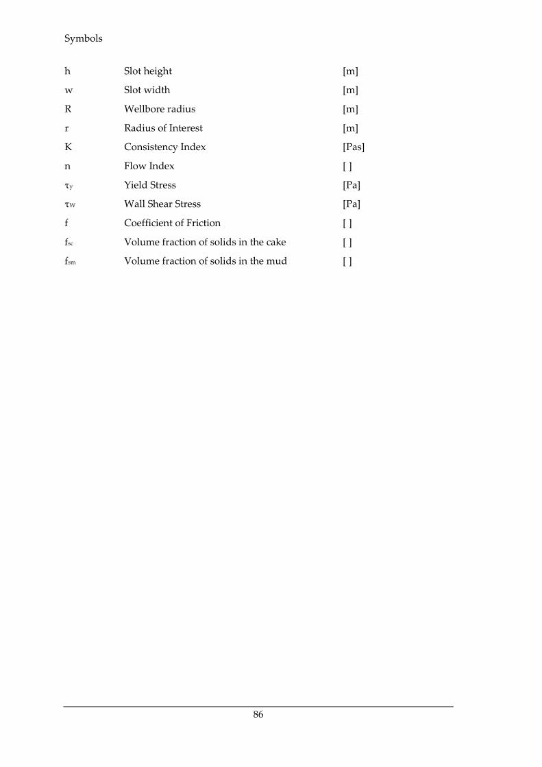
Symbols
86
h
w
R
r
K
n
τy
τW
f
fsc
fsm
Slot height
Slot width
Wellbore radius
Radius of Interest
Consistency Index
Flow Index
Yield Stress
Wall Shear Stress
Coefficient of Friction
Volume fraction of solids in the cake
Volume fraction of solids in the mud
[m]
[m]
[m]
[m]
[Pas]
[ ]
[Pa]
[Pa]
[ ]
[ ]
[ ]
List of Figures
87
List of Figures Figure 1: Model of filtration through a core [2, p. 239] ........................................................................ 3 Figure 2: CT-Scan of Filter Cake with two-layer structure [3, p. 10] .................................................. 4 Figure 3: SEM-Scan of the internal and the external layer [4, p. 11] .................................................. 4 Figure 4: Filter cake porosity as a function of time [5, p. 11] .............................................................. 5 Figure 5: Filter cake thickness as a function of time [5, p. 12] ............................................................. 5 Figure 6: Filter cake permeability as a function of time [5, p. 13] ....................................................... 6 Figure 7: Dominant forces during mudcake deposition ...................................................................... 7 Figure 8: Thin section of a dolomite with oversized pores [10, p. 7] ................................................. 9 Figure 9: Thin sections of silty dolomite with vugs, channels, oversized pores [10, p. 9] ............ 10 Figure 10: Proposed Plastering Mechanism [11, p. 3] ........................................................................ 11 Figure 11: Leak-Off Test before CwD [13, p. 8] ................................................................................... 12 Figure 12: Leak-Off Test after CwD [13, p. 8] ...................................................................................... 12 Figure 13: Bottomhole Pressure vs. Size Ratio [15, p. 11] .................................................................. 15 Figure 14: Particle size distribution [14, p. 6] ...................................................................................... 15 Figure 15: Permeable Plug Tester Filtrate Volume Result [14, p. 8] ................................................. 16 Figure 16: The three principal compressive stresses [18] .................................................................. 17 Figure 17: Direction of stresse in a vertical wellbore [19] .................................................................. 18 Figure 18: 2D representation of stresses around the wellbore [20] .................................................. 18 Figure 19: Distribution of stresses around the wellbore, compressive stresses are indicated in
red and tensile stresses are indicated in blue [21] ..................................................................... 19 Figure 20: Compressive wellbore failure [27] ..................................................................................... 20 Figure 21: Figure 16: Pressure Distribution in a wellbore with and without a filter cake created
by CwD [31] ................................................................................................................................... 25 Figure 22: Breakout extent for a wellbore with and without filter cake created by CwD [31] ..... 26 Figure 23: Hoop Stress around borehole when contact force is applied in maximum horizontal
far field stress direction ................................................................................................................ 27 Figure 24: Hoop Stress around borehole when contact force is applied in minimum horizontal
far field stress direction ................................................................................................................ 28 Figure 25: Hoop stress around the borehole with changing annulus to hole size ratio when
contact force is applied in maximum far field stress direction ............................................... 29 Figure 26: Diagrammatic representation of the filter cells arrangement [33, p. 23] ....................... 31 Figure 27: Hassler cell schematic [9, p. 2] ............................................................................................ 32 Figure 28: Oilfield Instruments Filtration Cell [2, p. 238] .................................................................. 32 Figure 29: Multi-Core Dynamic Fluid Loss Equipment [34, p. 8] .................................................... 33 Figure 30: Schematic of the Dynamic Filtration Apparatus [35, p. 293] .......................................... 34 Figure 31: M2200-Grace Instruments HPHT-Filtration Cell [36] ...................................................... 35 Figure 32: Dynamic Filtration Unit [37, p. 1] ....................................................................................... 35 Figure 33: Dynamic HPHT® Filtration System [38] ........................................................................... 36 Figure 34: Correct position of pipe in the artificial wellbore ............................................................ 37 Figure 35: Parameters to be measured, recorded or analysed during the different tests ............. 38 Figure 36: Comparison of filtration behaviour between static and dynamic filtration test .......... 41 Figure 37: Methods to measure filter cake thickness with a ruler .................................................... 42 Figure 38: Proposed scheme for multiple point filter cake thickness measurement ..................... 43 Figure 39: Schematic of a precision dial gauge [43, p. 9] ................................................................... 44 Figure 40: Measurement spot layout [43] ............................................................................................ 44 Figure 41: Schematic figure of the laser thickness apparatus [43] .................................................... 45 Figure 42: Core pressure profile before and after invasion ............................................................... 46
List of Figures
88
Figure 43: Example picture for investigating invasion depth on a pore size scale in sandstone [9,
p. 4] .................................................................................................................................................. 47 Figure 44: Sketch of the retort distillation apparatus [45].................................................................. 48 Figure 45: Solvent extraction apparatus for core samples [45] ......................................................... 49 Figure 46: Hassler type core holder example from CoreLab [46] ..................................................... 50 Figure 47: Darcy and Non-Darcy Flow [48] ......................................................................................... 51 Figure 48: Gas Permeability at different mean pressures .................................................................. 52 Figure 49: Example picture for the details from a SEM [51] .............................................................. 53 Figure 50: Particle size determination methods [54] .......................................................................... 54 Figure 51: Example for different sieve sizes [55] ................................................................................ 55 Figure 52: Conceptual sketch of the core holder for the test apparatus. ......................................... 57 Figure 53: Cut through the y-axis of the core holder ......................................................................... 58 Figure 54 Schematic of the pipe body with the core holder in the middle...................................... 59 Figure 55: Pipe body seen from below ................................................................................................. 59 Figure 56: Pipe body seen from below in combination with the core holder ................................. 59 Figure 57: Bourdon pressure gauge [65] .............................................................................................. 60 Figure 58: Wheatstone bridge circuit [67] ............................................................................................ 61 Figure 59: Schematic of the pressure valve arrangement .................................................................. 62 Figure 60: Example sketch of a bimetal-thermometer [68] ................................................................ 62 Figure 61: Pipe body with proposed positions for pressure (green) and temperature sensors
(red) and pressure regulator (black) and backpressure regulator (blue) ............................... 63 Figure 62: Cross-section of the measuring section.............................................................................. 64 Figure 63: Drill-pipe assembly with electric motor (yellow) and bearings (blue) and seal (red) . 65 Figure 64: Core holder seen from the front with dimensions ........................................................... 66 Figure 65: Core holder seen from the top ............................................................................................ 67 Figure 66: Right side of the pipe body ................................................................................................. 67 Figure 67: Drill-pipe assembly seen from the front ............................................................................ 69 Figure 68: Flow schematic of the circulation system .......................................................................... 70 Figure 69: Core holder with shut-off valve indicated in grey on both sides ................................... 71

List of Tables
89
List of Tables Table 1: Test results for a sandstone using bridging particles [10, p. 6] ............................................ 9 Table 2: Test results for a sandstone without bridging particles [10, p. 6] ........................................ 9 Table 3: Core sizes with different retrieving techniques ................................................................... 56
List of Equations
90
List of Equations Equation 1: Mudcake permeability determination [2, p. 239] ............................................................. 3 Equation 2: Mudcake porosity determination [2, p. 240] ..................................................................... 3 Equation 3: Porosity calculated from the CT-Number [5, p. 2] ........................................................... 4 Equation 4: Empirical correlation for filter cake permeability from porosity [4, p. 5] ..................... 6 Equation 5: Hydrodynamic force inequality [8, p. 81] ......................................................................... 7 Equation 6: Simplified Kirsch Equations for the stress state at the wellbore wall [23] ................. 19 Equation 7: Filter cake permeability coefficient [26, p. 913] .............................................................. 20 Equation 8: Additional stresses due to fluid seepage [26, p. 913] .................................................... 20 Equation 9: Mohr-Coulomb failure criterion [28] ............................................................................... 21 Equation 10: Linearized Mohr-Coulomb Equation ............................................................................ 21 Equation 11: Fitting parameter equation for linearized Mohr Coulomb criterion ......................... 21 Equation 12: Coefficient of internal friction from angle of internal friction .................................... 21 Equation 13: Most common stress state for wellbore breakout ........................................................ 22 Equation 14: Most common stress state for inducing fractures ........................................................ 22 Equation 15: Simplified Kirsch equations for predicting wellbore breakouts ................................ 22 Equation 16: Pressure difference wellbore and formation to avoid breakouts [28] ....................... 22 Equation 17: Simplified Kirsch equations for predicting fracture initiation in a wellbore ........... 22 Equation 18: Pressure difference wellbore and formation to avoid fractures [28] ......................... 23 Equation 19: Hoek-Brown failure criterion [29] .................................................................................. 23 Equation 20: Pressure difference to avoid breakouts according to Hoek-Brown [28] ................... 23 Equation 21: Pressure difference to avoid the fractures according to Hoek-Brown [28] .............. 24 Equation 22: Pore pressure changes with time [31] ............................................................................ 25 Equation 23: Mathematical model for the FEM analysis [32] ............................................................ 27 Equation 24: Grain volume of the filter cake ....................................................................................... 39 Equation 25: Pore volume of the filter cake [6, p. 3] ........................................................................... 39 Equation 26: Filter cake porosity from wet and dry filter cake weight measurements [6] ........... 39 Equation 27: Filter cake permeability calculated continuously [6, p. 5] .......................................... 39 Equation 28: Filtrate Volume in a static filter press [41, p. 46] .......................................................... 40 Equation 29: API fluid loss after 30 minutes if spurt loss is observed [41, p. 46] ........................... 40 Equation 30: Filter cake thickness as a function of collected filtrate volume [41, p. 46] ................ 42 Equation 31: Darcy’s Law ...................................................................................................................... 46 Equation 32: Water saturation ............................................................................................................... 47 Equation 33: Oil Saturation .................................................................................................................... 48 Equation 34: Volume of oil from the solvent extraction method [45] .............................................. 49 Equation 35: Klinkenberg’s Permeability Equation............................................................................ 51 Equation 36: Herschel-Bulkley fluid [71, p. 242] ................................................................................. 64 Equation 37: Wall shear stress [71] ....................................................................................................... 64 Equation 38: Shear force calculated from the wall shear stress ........................................................ 64 Equation 39: Definition of the entrance length for laminar flow [72] .............................................. 68 Equation 40: Hydraulic Diameter [73] .................................................................................................. 68 Equation 41: Definition of entrance length for turbulent flow [75] .................................................. 68 Equation 42: Stresses in the near wellbore region [23] ....................................................................... 77 Equation 43: Herschel-Bulkley pressure drop equation [71]............................................................. 77