Energía magnetostática – existencia de dominios 9 magnetostatica dominios... · Energía...
71
Energía magnetostática – existencia de dominios
Transcript of Energía magnetostática – existencia de dominios 9 magnetostatica dominios... · Energía...

Energía magnetostática – existencia de dominios

Energía magnetostática
Energía de interación entre los dipolos de un material magnetizado
E1 E2 En
...
?mínME
imr
iii
iii
iii
iM VHMHmBmErrrrrr
⋅−=⋅−=⋅−= ∑∑∑ 222
1 00 µµ
mi
Bi( )iij
ji rBBrrr
∑≠
=
dVHMrv
∫ ⋅−≈2
0µ

Energía magnetostática
Energía de interación entre los dipolos de un material magnetizado
Evaluación de: En ausencia de corrientes:
0
0
=×∇
=⋅∇
H
Brr
rr
además
( )MHB +=rrr
µ
dVHMEM
rv
∫ ⋅−=2
0µ
Dado un cuerpo (forma, volumen V,
superficie S),
Una distribución de magnetización M, ( )
UH
MHB
∇−=
+=rr
0µPotencial escalary las
ecuaciones de Maxwell:
( ) 0=+∇−⋅∇ MUrrr
MUrr
⋅∇=∇ int2
02 =∇ outU
magnetización M,
continuoU

Energía magnetostática
Energía de interación entre los dipolos de un material magnetizado
S
nr
condiciones de contorno
SextSUU =int
nMn
U
n
U
S
ext
S
rr⋅=
∂∂−
∂∂ int
rUAcotadas para
dadarM )(r
MUrr
⋅∇=∇ int2
02 =∇ extU
Ur 2
Acotadas para r → ∞
+)(rUr
Se puede demostrar que el problema tiene
solución única
dVHMEM
rv
∫ ⋅−=2
0µ
UH ∇−=rr

Energía magnetostática
Ejemplo: Esfera de radio R magnetizada uniformemente
0=⋅∇ Mrr
M uniforme
0sin
1sin
sin
112
2
2222
22 =
∂∂+
∂∂
∂∂+
∂∂
∂∂=∇ U
rrrr
rrU
φθθθ
θθ
zM
n
M
R
rn ∂∂=
∂∂
M
n
rθ θcosSMnM =⋅ r
r
solución ( ) θcos3
SMrU =r ×
,r si Rr ≤
2
3
r
Rsi Rr >
( )3
zMrU S=r
( )3
3
=r
RzMrU Sr
θcosintS
S
ext
S
Mr
U
r
U =∂
∂−∂
∂

Energía magnetostática
zM
U S
3int =
intint UH ∇−=rr
33 cos zRMRMU SS == θ
( ) θcos3
SMrU =r ×
,r si Rr ≤
2
3
r
Rsi Rr >
0intint ==yx
HH
3intSM
Hz
−=
( ) 2/3222233
cos
zyx
zRM
r
RMU SS
ext++
== θ
5
3
r
xzRMH S
extx=
5
3
r
yzRMH S
exty=
−=
3
12
2
3
3
r
z
r
RMH S
extz
z
MHD
Hext

Energía magnetostática
Esfera magnetizada uniformemente
energía
esferaSM VHMdVHMEzint
00
22
µµ −=⋅−= ∫rv
3intSM
Hz
−=9
2 20
3S
M
MRE
µπ=
generalizando para otras
9
2
3
4
32
20
330 SS
S
MRRMM
µππµ ==
20 SM MCE µ=
SDMNHz
−=int
para otras geometrías
Factor demagnetizante generalizando
para otras geometrías y
distribuciones de la
magnetización
3/1=⇒= xS NxMM(r
3/1=⇒= yS NyMM(r
3/1=⇒= zS NzMM(r
1=++ zyx NNN
Esfera
si

Energía magnetostática
Cilindro infinito magnetizado uniformemente en dirección perpendicular al eje
02 =∇ U
M
n
φρρρρ
x
0=⋅∇ Mrr
φcosSMnM =⋅ rr
ρ∂∂=
∂∂n
MUrr
⋅∇=∇2
nMn
U
n
U
S
ext
S
rr⋅=
∂∂−
∂∂ int
011
2
2
2
2
2=
∂∂+
∂∂+
∂∂
∂∂
Uzφρρ
ρρρ φ
ρρcosint
S
S
ext
S
MUU =∂
∂−∂
∂
φcos2
SMU = ×
,ρ si R≤ρ
ρ
2Rsi R>ρ
0intint ==yz
HH
2intSM
Hx
−=

Energía magnetostática
Cilindro infinito magnetizado uniformemente en dirección perpendicular a su eje
x
HextM
HD
dSHMM
rv
∫ ⋅−=2
0µε
2intSM
Hx
−=
4
20
2S
M
MR µπε =
Energía magnetostática por unidad de área ⊥ al eje del cilindro
422
20
220 SS
S
MRR
MM
µππµ =−=
4M
20 SM MCµε =
de la forma
SDMNHz
−=int
de la formaFactor
demagnetizante
2/1=⇒= xS NxMM(r
2/1=⇒= yS NyMM(r
0=⇒= zS NzMM(r
1=++ zyx NNN

Energía magnetostática
Otros cuerpos magnetizados uniformemente
M uniforme Caso general Hint NO uniforme
Superficie de 2do grado (cónicas)
Hint uniforme
222
elipsoide
Diagonal si los
M uniforme
1222
=
+
+
c
z
b
y
a
xMNHD
rrˆ−=
Campo demagnetizante
Tensor demagnetizante
Diagonal si los ejes de
coordenadas coinciden con
los del elipsoide
Número si además
=Mr
iM S
r
jM S
r
kM S
r
Traza unitaria
1=++ zyx NNN
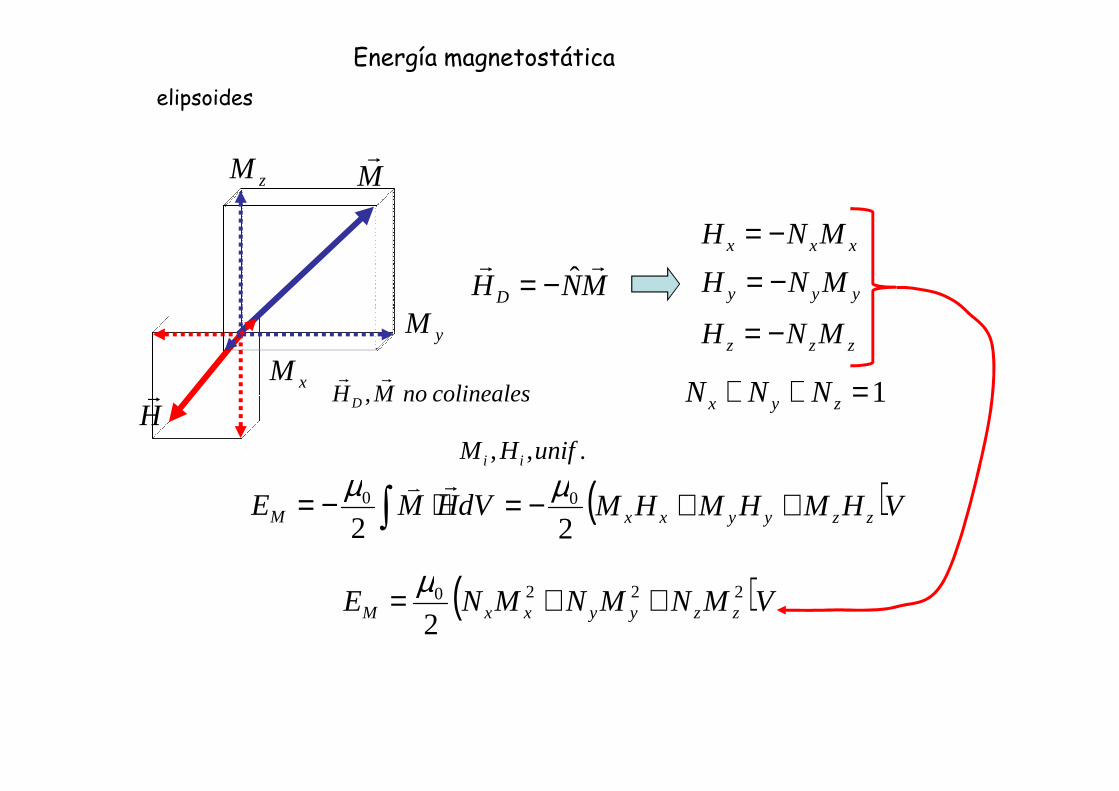
Energía magnetostática
elipsoides
xMyM
zM Mr
r
MNHD
rrˆ−=
xxx MNH −=
yyy MNH −=
zzz MNH −=
1=++ zyx NNNcolinealesnoMHD
rr,
Hr 1=++ zyx NNN
dVHMEM
rv
∫ ⋅−=2
0µ
( )VMNMNMNE zzyyxxM2220
2++= µ
( )VHMHMHM zzyyxx ++−=2
0µ.,, unifHM ii
colinealesnoMHD ,

Energía magnetostática
Elipsoide prolado u oblado prolado
oblado
zyx NNNcba >=⇒<=
zyx NNNcba <=⇒>=z
( )2220
2 zzyyxxM MNMNMNV
E ++= µ
2222 MMMM −=+
( )( )2220
2 zzyxx MNMMNV ++= µ
yx NN =
( ) ( ) cteMNNV
cteMNNV
E SxzzxzM +−=+−= θµµ 22020 cos22
( ) cteKcteMNNV
E SSxzM +=+−−= θθµ 2220 sinsin2
2222zSyx MMMM −=+
θ2sinVKE SM = ( ) 20
2 SzxS MNNK −=µ
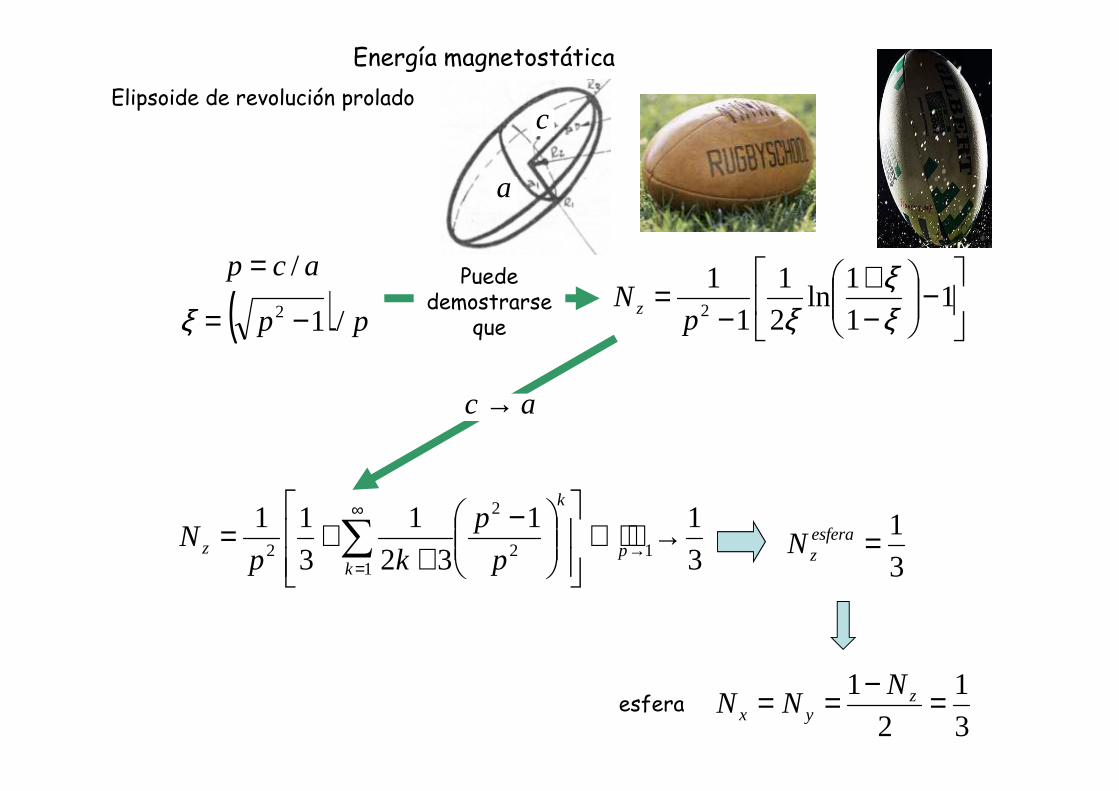
Energía magnetostática
Elipsoide de revolución prolado
acp /=
( ) pp /12 −=ξ
−
−+
−= 1
1
1ln
2
1
1
12 ξ
ξξp
Nz
Puede demostrarse
que
ac →
c
a
3
11
32
1
3
1112
2
12
→
−+
+= →
∞
=∑ p
k
kz p
p
kpN
ac →
3
1=esferazN
3
1
2
1 =−== zyx
NNNesfera

Energía magnetostática - Origen de los dominios
Cilindro infinito con dos dominios perpendiculares a su eje
M
n
φx
-MR
0== zy MM
×= Sx MMπφ <≤↔+ 01
πφπ 21 <≤↔−
Desarrollo en serie de Fourier de la función de Heaviside
( )∑
∞
= ++=
0 12
12sin4
n
Sx n
nMM
φπ
( ) φφπ
φ cos12
12sin4cos
0∑
∞
= ++==
n
Sxn n
nMMM
( ) ( )∑
∞
= +++=
0 12
2sin22sin2
n
Sn n
nnMM
φφπ
0 1 2 3 4 5 6 7
-1,0
-0,5
0,0
0,5
1,0
Σ
φ

nS
ext
S
MnMn
U
n
U =⋅=∂
∂−∂
∂ rrint
Energía magnetostática - Origen de los dominios
Cilindro infinito con dos dominios perpendiculares a su eje
( )( )( )∑
∞
=
∂−∂ int 2sin8 Sext nnMUU φ + 02 =∇ U
M
n
φx
-MR
( ) ( )∑
∞
= +++=
0 12
2sin22sin2
n
Sn n
nnMM
φφπ
( )( )( )∑
== −+=
∂
−∂ 1
int
1212n
S
R
ext
nnπρρ ρ+ 02 =∇ U
( ) ( )∑∞
=
=1
2sinn
n nuU φρ( ) ×= nn cu ρ ( ) RR n ≤↔ ρρ 2/
( ) RR n ≥↔ ρρ 2/
( )( )( )∑
∞
=
−+=
1
2
int 1212
2sin2
n
n
S
Rnn
nRMU
ρφπ

( )( )( )∑
∞
=
−+=
1
2
int 1212
2sin2
n
n
S
Rnn
nRMU
ρφπ
Energía magnetostática - Origen de los dominios
Cilindro infinito con dos dominios perpendiculares a su eje
intint UH ∇−=rr
0intint ==yz
HH
Energía magnetostática por unidad de área ⊥ al eje del cilindro
2Rµµ rv
( )( )( )
12
1int 1212
12sin4−∞
=
−+−−= ∑
n
n
S
Rnn
nnMH
x
ρφπ
20
200
22 SxxM MR
dSHMdSHM µπ
µµε =−=⋅−= ∫∫rv
M
M
-M
4
20
2)1( S
M
MR µπε = 20
2)2(
SM MR µπ
ε =
1 dominio 2 dominios
2
141.0
42)1(
)2(
<≈=πM
M
E
E
nE
E
M
nM 1
)1(
)(
≈
Regla aproximada

Energía magnetostática - Origen de los dominios
monodominio multidominio
monoME
multiE
PDγ
( ) PD
monoMmulti nSn
EE γint+≈
Nro dominios en equilibrio
E magnetostática decrece
E pared dominios crece
Energía de pared por unidad de área
magnetostática
pared
ΕΕ ΕΕmu
lti
n

( )2220
2 zzyyxxM MNMNMNV
E ++= µ
Energía magnetostática - Origen de los dominios
Superficies no cuadráticas
Válido también para cuerpos con superficies no cuadráticas: cubos, prismas, cilindros, octaedros, etc.
(teorema de Brown-Morrish)
Casos particulares
Cubo, octaaedro, tetraedro
3/1=== zyx NNNtetraedro zyx
Prisma regular, cilindro
zyx NNN ≠=

Energía magnetostática – campo efectivo
Hapl
HD M
MNHD
rr−=
MNHHHH aplDaplef
rrrrr−=+=
HMrr
χ=
Cuando se grafica M vs. H debe usarse como abscisa el Hef
efapl HMH ⇒⇒
Si M << MS efHM χ=Si M << MS
efaplef HNHHrrr
χ−=χN
HH apl
ef +=
1
rr
Si M = MS
Saplef NMHH −=
Ejemplo, Ni
TeslamAxM S 6.0/108.4 5 ≈≈HD puede alcanzar valores
considerables dependiendo de la forma de la muestra
aplHN
Mrr
χχ
+=
1

Energía magnetostática – factores demagnetizantes
Cálculos para elipsoides

Energía magnetostática – factores demagnetizantes
Cálculos en prismas

Energía magnetostática – referencias
Fórmulas, tablas y gráficos de factores demagnetizantes, Chen et al. IEEE Trans. Magnetics 27, 3601-19 (1991)
Campo demagnetizante y medidas magnéticas, J.A. Brug y W.P. Wolf, J.Appl.Phys. 57, 4685-701 (1985)
Cálculo de factores demagnetizantes, http://magnet.atp.tuwien.ac.at/dittrich/?http://magnet.atp.tuwien.ac.at/dittrich/cont
ent/tools/magnetostatics/streufeld.htm

MFM
Dominios y paredes de dominio
Pseudo-3d MFM image of a (YSmLaCa)3 (FeGe)5O12 magnetic thin film garnet, 4.5 x 4.5 µm2,
domain walls appear dark;

δ = Na
Pared de Bloch de 180°
Eje
fáci
lE
je fá
cil

Balance energético entre anisotropía e intercambio
∑= N
iK KsenaE1
23 θ
θimi
Eje
fáci
l
i /= πθ i Ni
Anisotropía uniaxialK
Para un prisma de N celdas (base a2)a: parámetro de la celda cúbica
i
1
/
=∆=∆
=
πθ
πθ
i
i
Ni
Ni
2
KNaK ≈ε
iKsenaE iiK ∆= ∑ θ23
Por unidad de área de pared:
θθπ
∆= ∑ iiK senKNa
E 23
2
3
0
23 KNa
dsenKNa
i =≈ ∫π
θθπ

intercambio
1/),/cos(2cos2 22 <<−=∆−= NNNJsNJsEJ ππθ
)2
1(22
22
NNJsEJ
π−−=
)2
1(2
2
2
2
2
Na
NJsJ
πε −−=
22Jsπε =∆
N/πθ =∆
Energía de intercambio por
unidad de área de pared:
Relativa al estdo22NJs−=ε 2Na
JsJ
πε =∆
2
22
2 Na
JsKNaJK
πεεγ +=∆+∆=
Energía por unidad de área de pared
Relativa al estdofundamental: 2
2
a
NJsJ −=ε
γ
intercambio
anisotropía
ε
N

2
22
2 Na
JsKNaJK
πεεγ +=∆+∆=
Optimización energía por unidad de área de pared
02
/22
22
=−=aN
JsKadNd
πγ
2/12
3
2
=
Ka
JsNeq π
Ka
eq
Ka
JsaNeqeq
22πδ ==
KAeq 22πγ =
aJsA /2≈
mJAmJ /10/10 1112 −− ≤≤
Ancho de la pared
K
A2π=
3633 /10/10 mJKmJ ≤≤nmeq 444=δnmeq 4.44=δ
mJA /10 11−=33 /10 mJK =35 /10 mJK =
Cte de stiffness
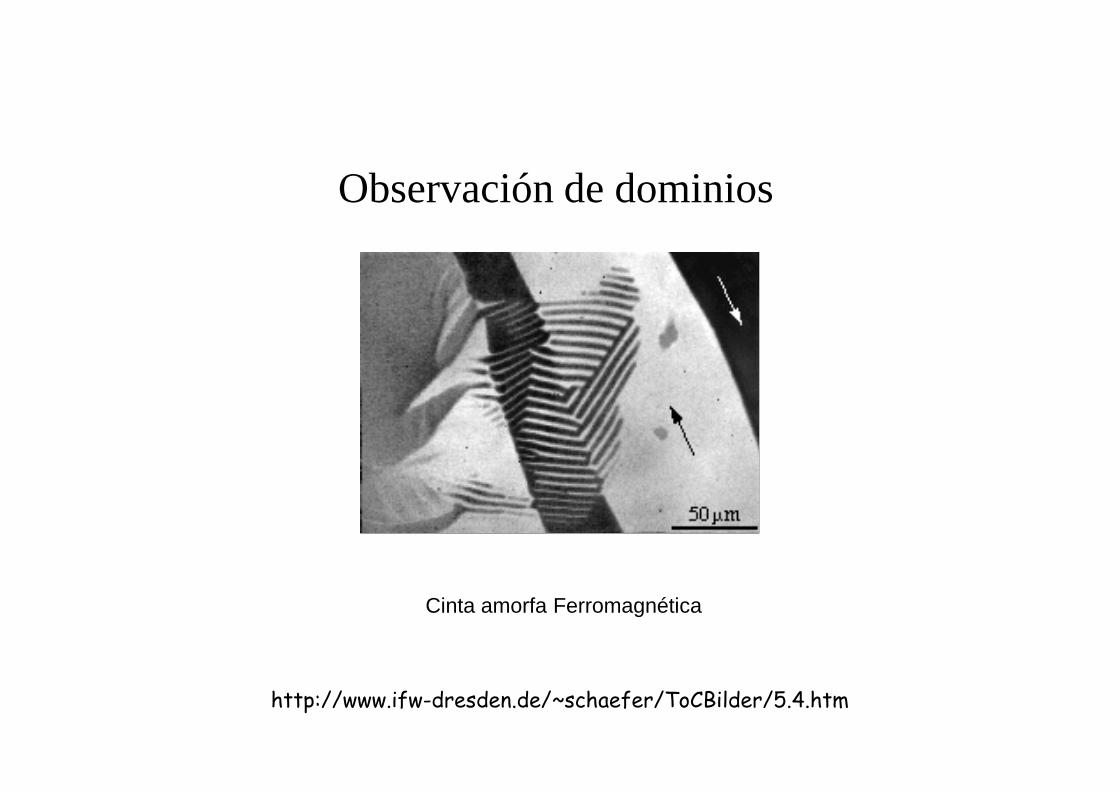
Observación de dominios
Cinta amorfa Ferromagnética
http://www.ifw-dresden.de/~schaefer/ToCBilder/5.4.htm

1 2
MA/m
12
Fig. 6.19a,b: The demagnetized state of sintered NdFeB permanent magnet material depends strongly on magnetic history. (a) shows the thermally demagnetized state in which virtually all grains are demagnetized within themselves. The demagnetized state (b) was achieved by applying a field slightly higher than coercivity after saturation. Here only the average magnetization is zero, while most grains are saturated in either direction
http://www.ifw-dresden.de/~schaefer/ToCBilder/6.3.htm
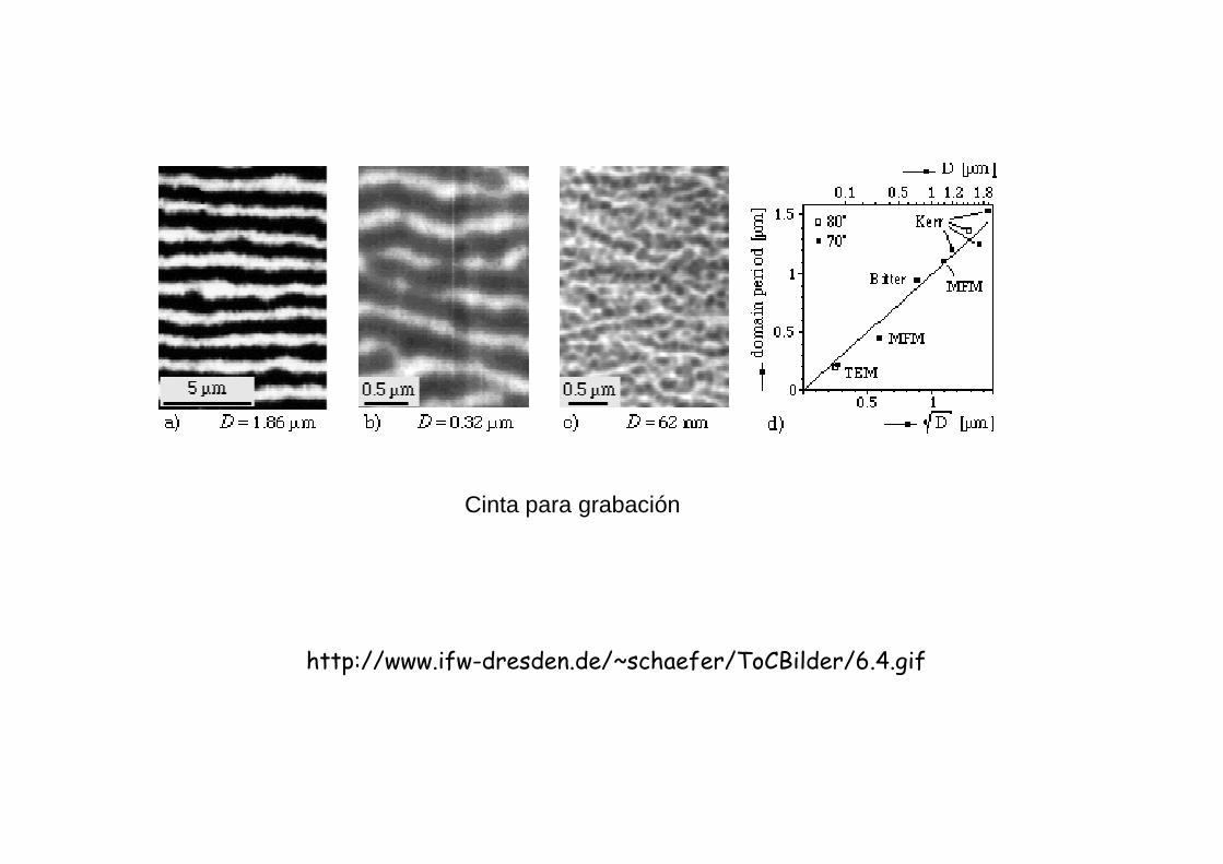
Cinta para grabación
http://www.ifw-dresden.de/~schaefer/ToCBilder/6.4.gif

Fig. 6.13: Magnetostriction-free metallic glasses are unique soft magnetic materials in being insensitive to elastic deformation. The same domain pattern is observed in the flat state (a) and in a strongly bent state (b). In contrast, regular magnetostrictive materials display a complete domain rearrangement on bending (c, d)
http://www.ifw-dresden.de/~schaefer/ToCBilder/6.2.htm

Técnica Bitter
Técnica Bitter(1931): dispersión sobre la muestra de un líquido portador de pequeñas partículas ferromagnéticas. Las partículas se acumulan en zonas de equilibrio. Experimentan fuerzas máximas donde el gradiente de campo es máximo (bordes de dominio). Soluciones coloidales de Fe3O4.
( ) xdx
dBmBmEF
(rrrr⋅=⋅−∇−=∇−=
MM
0≈dx
Bdr
0≈dx
Bdr
0≠dx
Bdr

patrones de dominio en láminas (110) ligeramente
Técnica Bitter
bitter kerr
microscopía
desorientadas de silicio-hierro (c). Los patrones “circulares” oscuros se deben a una acumulación subsuperficial de “carga” magnética la que no se observa en métodos más superficiales como el efecto Kerr magneto-óptico (d)
http://www.ifw-dresden.de/~schaefer/ToCBilder/2.2.htm
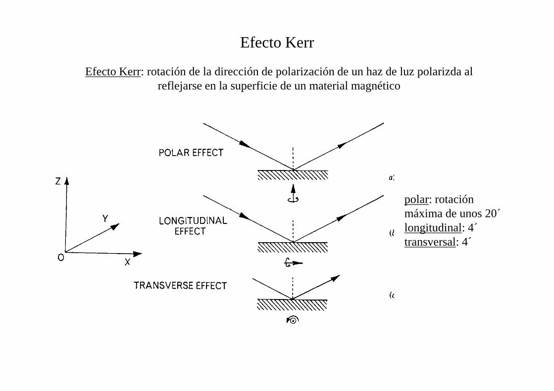
Efecto Kerr
Efecto Kerr: rotación de la dirección de polarización de un haz de luz polarizda al reflejarse en la superficie de un material magnético
polar: rotación polar: rotación máxima de unos 20´longitudinal: 4´transversal: 4´

Efecto Kerr
El principio Kerr es que al reflejarse luz linealmente polarizada por un material magnetizado, rota el plano de polarización. Ello ocurre porque los índices de
refracción de la luz polarizada circularmente a derecha y a izquierda son diferentes en presencia de magnetización. El ángulo de rotación producido por un material ferromagnético es generalmente de aprox. 1E-3 a 1E-2 grados, aunque se han observado ángulos mucho mayores en aleaciones de Tb-Fe-Co (un grado) y en
compuestos de uranio (nueve grados). El ángulo de rotación es mayor cuando se observado ángulos mucho mayores en aleaciones de Tb-Fe-Co (un grado) y en
compuestos de uranio (nueve grados). El ángulo de rotación es mayor cuando se incrementa el ángulo de incidencia. A partir del cambio de la intensidad Kerr
(proporcional a la rotación Kerr y a la magnetización de la muestra) se construye la curva de histéresis en función del campo aplicado.

Microscopía de efecto KerrSi charge-coupled
device

Efecto Kerr
Microscopía - imágenes
Co Fe-Si
(110)

imagen Kerr de dominios magnéticos,
observados en dos lados de un trozo de Fe
Efecto KerrEfecto KerrImágenes de microscopíaImágenes de microscopía
http://www.ifw-dresden.de/~schaefer/ToCBilder/1.1.htm
Dependiendo del plano de incidencia puede observarse el patrón de dominios (b) o la subestructura de las paredes de dominio (a). Sobre un cristal de SiFe
orientado en la dirección (100)

Microscopía Kerr cuantitativa. La magnetización superficial de un vidrio metálico se registra en un microscopio Kerr usando dos ejes con diferente sensibilidad. Se combina la información de ambas observaciones en una computadora y se representan en colores las direcciones de la magnetización
mapas
http://www.ifw-dresden.de/~schaefer/ToCBilder/Colour.htm

Magneto-optical Kerr effect (MOKE)CU - Colorado Springs
Department of Physics and Energy Science
Este sistema usa un electroimán de 1Tesla. Utiliza un láser HeNe ultra-estable y polarizadores de alta calidad. El sistema de adquisición de datos produce las curvas de histéresis de películas delgadas magnéticas.

Magneto-optical Kerr effect at Washington University

Surface Magneto Optic Kerr Effect (SMOKE)
SMOKE: dispositivo para estudiar magnetismo superficial en películas ultradelgadas. Esta técnica fue iniciada por S.D. Bader y E.R. Moog a fines de los '80.'80.
(Moog, E.R. and S.D. Bader. "Superlattices and Microstructures" Vol. 1:543 1985).

Note: (1) Laser, (2) polarizers, (3) mirrors, (4) sample, (5) magnetic core, (6) pulley, (7) photodetector, and (8) band-pass filter. This diagram is the measurement of longitudinal Kerr Effect and the external field is in the plane of sample. The electromagnet can be rotated by means of the pulley through a push-pull rod.


Magneto-optical storage technologyAs implied by the name, these drives use a hybrid of magnetic and optical technologies, employing laser to read data on the disk, while additionally needing magnetic field to write data. An MO disk drive is so designed that an inserted disk will be exposed to a magnet on the label side and to the light (laser beam) on the opposite side. The disks, which come in 3.5in and 5.25in formats, have a special alloy layer that has the property of reflecting laser light at slightly different angles depending on which way it's magnetised, and data can be stored on it as north and south magnetic spots, just like on a hard disk.
While a hard disk can be magnetised at any temperature, the magnetic coating used on MO media is designed to be extremely stable at room temperature, used on MO media is designed to be extremely stable at room temperature, making the data unchangeable unless the disc is heated to above a temperature level called the Curie point, usually around 200 degrees centigrade. Instead of heating the whole disc, MO drives use a laser to target and heat specific regions of magnetic particles. This accurate technique enables MO media to pack in a lot more information than other magnetic devices. Once heated the magnetic particles can easily have their direction changed by a magnetic field generated by the read/write head.

Lectura

Information is read using a less powerful laser, making use of the Kerr Effect, where the polarity of the reflected light is altered depending on the orientation of the magnetic particles. Where the laser/magnetic head hasn't touched the disk, the spot represents a "0", and the spots where the disk has been heated up and magnetically written will be seen as data "1s".
However, this is a "two-pass" process which, coupled with the tendency for MO heads to be heavy, resulted in early implementations being relatively slow. Nevertheless, MO disks can offer very high capacity and fairly cheap media as well as top archival properties, often being rated with an average life of 30 years - far longer than any magnetic media.
Magneto-optical technology received a massive boost in the spring of 1997 with the launch of Plasmon's DW260 drive which used LIMDOW technology to achieve a much increased level of performance over previous MO drives.

Efecto Faraday
Efecto Faraday: Como el Kerr, pero por transmisión. Para láminas delgadas de óxidos ferromagnéticos o películas metálicas.

Microscopía Lorentz-TEM
Microscopía Lorentz-TEM: Para espesores de hasta unos 200 nm. Los electrones transmitidos son deflectados por la fuerza de Lorentz F = -evxB. El ángulo de
deflexión es pequeño (típicamente 0.01° en Fe). Es necesario sobre o sub enfocar la imagen porque al modificar el foco las imágenes de dominios con
magnetizaciones diferentes se mueven en direcciones diferentes. Se pueden obtener resoluciones de hasta 5 nm. La muestra debe apantallarse
magnéticamente.
( )efHMveBveFrrrrrr
+×−=×−= 0µ
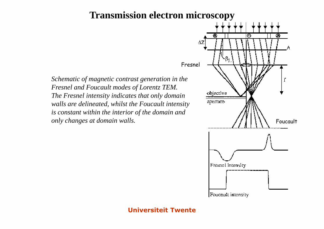
Transmission electron microscopy
Schematic of magnetic contrast generation in the Fresnel and Foucault modes of Lorentz TEM. The Fresnel intensity indicates that only domain walls are delineated, whilst the Foucault intensity is constant within the interior of the domain and
Fresnel
is constant within the interior of the domain and only changes at domain walls.
Universiteit Twente
Foucault

Fresnel image of magnetic domains in a CoNi/Pt multilayer.This maze type domain structure is typical for films with perpendicular anisotropy.
Fresnel image of magnetic domains and ripple contrast in a magnetically soft Co/Cu multilayerwhich exhibits GMR. The ripple is always orthogonal to the direction of magnetisation within a domain.
Universiteit Twente


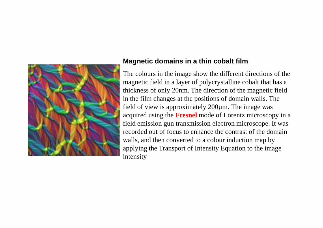
Magnetic domains in a thin cobalt film
The colours in the image show the different directions of the magnetic field in a layer of polycrystalline cobalt that has a thickness of only 20nm. The direction of the magnetic field in the film changes at the positions of domain walls. The field of view is approximately 200µm. The image was acquired using the Fresnel mode of Lorentz microscopy in a acquired using the Fresnel mode of Lorentz microscopy in a field emission gun transmission electron microscope. It was recorded out of focus to enhance the contrast of the domain walls, and then converted to a colour induction map by applying the Transport of Intensity Equation to the image intensity

The image is changing domain patterns of silicon steel according tosuccessively changing magnetic field of +2.4, 0 and -2.4 kA/m.It is dark-field microscopic image of Colloid A-07-dropped specimen. Changes of triangular shapes and sizes of domains are clearly seen.

Fig. 2.30 The Differential Phase Contrast method of transmission electron microscopy offersquantitativeinformationat high resolution. Thepicturesshow thehorizontal (a) and thevertical quantitativeinformationat high resolution. Thepicturesshow thehorizontal (a) and thevertical (b) magnetization components of a closed-flux domain pattern in a thin-film Permalloy element
(J.N. Chapman)
http://www.ifw-dresden.de/~schaefer/ToCBilder/2.4.htm

Electron Reflection and Scattering Methods
SEM: basada también en el efecto de la fuerza de Lorentz

Electron Reflection and Scattering Methods


Fig. 2.43d,e Magnetic force microscopy on the basal plane of a cobalt crystal. Image processing can reveal "susceptibility contrast" (d) and "charge contrast" (e), two imaging modes which are unavailable with other techniques. (d) and (e) are the sum and the difference of images taken with opposite polarity of the tip magnetization, respectively
http://www.ifw-dresden.de/~schaefer/ToCBilder/2.6.htm

Finished magnetic heads can be measured for their performance and response to signal and noise fields. Devices can also be examined using the Bitter Pattern System to locate magnetic domain irregularities.
Magnetic force microscopy images of recorded media (tape, disk, film) made with our scanning probe microscope can provide insight into problems that may exist within a recording system, such as tracking error, head to media spacing, and media jitter.

Magnetic domains in low-coercivity, amorphous CoZrNb film used in emerging, high-Ms thin-film heads. 50µm scan. Visible are Landau-Lifshitz and cross-tie domains, and the effects of edge roughness. Such images surpass the resolution of optical Kerr-effect. Captured with LiftMode (lift height 75nm) and a low-moment tip to prevent domain perturbation.

MFM

Reorientation transition of ultrathin cobalt films on Au(111)
Three MFM images of cobalt deposited on gold. The numbers within theThree MFM images of cobalt deposited on gold. The numbers within theimages indicate the nominal film thickness in monolayers. Tipmagnetization is perpendicular to the surface. At low coverages (2 ML)bright and dark areas, which correspond to out-of-plane domains areobserved. The contrast vanishes at 4.3 ML coverage. At 6 ML coverage themagnetic contrast reappears, but now domain walls are imaged - a typicalsignature of domains with in plane magnetization. The observed contrastchange clearly indicates a thickness dependent reorientation of themagnetization direction in the cobalt film.

Domain Growth on La0,7Ca0,3MnO3
The stability at low temperatures and the careful microscope design enable a
- =
H H+∆∆∆∆H
The stability at low temperatures and the careful microscope design enable adetailed study of domain growth in external magnetic fields. The two imageson the left show the maze type domain structure of an perovskite manganitethin film in two slightly different external magnetic fields. Bright areas indicateregions, where tip and sample magnetization is parallel (attractivemagnetostatic interaction), while dark areas indicate an antiparallelconfiguration (repulsive magnetostatic interaction). It is difficult to detect anydifference. However, after subtracting one image from the other, those areas,which changed their magnetization direction become clearly visible as darkspots in the right image.

Investigation of magnetic bit structures
Two MFM images of closely spaced bit tracks on a tape, which is used as mass data storage device. While the read head can only disinguish "1" and "0" along the tracks, MFM is able resolve the fine structure of the magnetic bit structure. Regarding device optimations the area where neighbouring meet (right image) are of particular importance to increase the bit density.

MFM image showing the bits of a hard disk. Field of view 30µm

Topology and dynamics of magnetic domains
ACHr
In soft magnetic materials with perpendicular anisotropy such as yttrium iron garnets, domains form a labyrinthine structure in the demagnetized state. This structure is also observed in other physical systems, such as ferrofluids, Langmur films, oscillatory chemical reactions, polymers and many other. It appears, that the local mobility of the domain walls is closely related to the domain topology. We do imaging studies of the domain wall responce to a periodic and non-periodic magnetic drive and investigate depinning and creep phenomena in labyrinthine domain structures.


X-ray, Neutron and Other Methods
Fig. 2.48b X-ray topography displays 90°domain walls and dislocations in a silicon
iron sheet at the same time (Courtesy J. Miltat)
http://www.ifw-dresden.de/~schaefer/ToCBilder/2.7.htm

Comparison of Domain Observation Methods
One of several criteria used in the comparison of domain observation techniques. SEM = Scanning (reflection) electron microscopy, TEM = transmission electron microscopy, MFM = magnetic force microscopy