Ecuaciones de la din amica rotacional Movimiento libre Movimiento forzado De niciones previas...
52
Ecuaciones de la din´ amica rotacional Movimiento libre Movimiento forzado Veh´ ıculos Espaciales y Misiles Tema 2: Cinem´ atica y Din´ amica de la Actitud Parte II: Din´ amica y Estabilidad Rafael V´ azquez Valenzuela Departamento de Ingenier´ ıa Aeroespacial Escuela Superior de Ingenieros, Universidad de Sevilla [email protected] 24 de marzo de 2014
Transcript of Ecuaciones de la din amica rotacional Movimiento libre Movimiento forzado De niciones previas...
Ecuaciones de la dinamica rotacionalMovimiento libre
Movimiento forzado
Vehıculos Espaciales y MisilesTema 2: Cinematica y Dinamica de la Actitud
Parte II: Dinamica y Estabilidad
Rafael Vazquez Valenzuela
Departamento de Ingenierıa AeroespacialEscuela Superior de Ingenieros, Universidad de Sevilla [email protected]
24 de marzo de 2014
Ecuaciones de la dinamica rotacionalMovimiento libre
Movimiento forzado
Definiciones previasEcuaciones de Euler
Dinamica de la actitud de un vehıculo
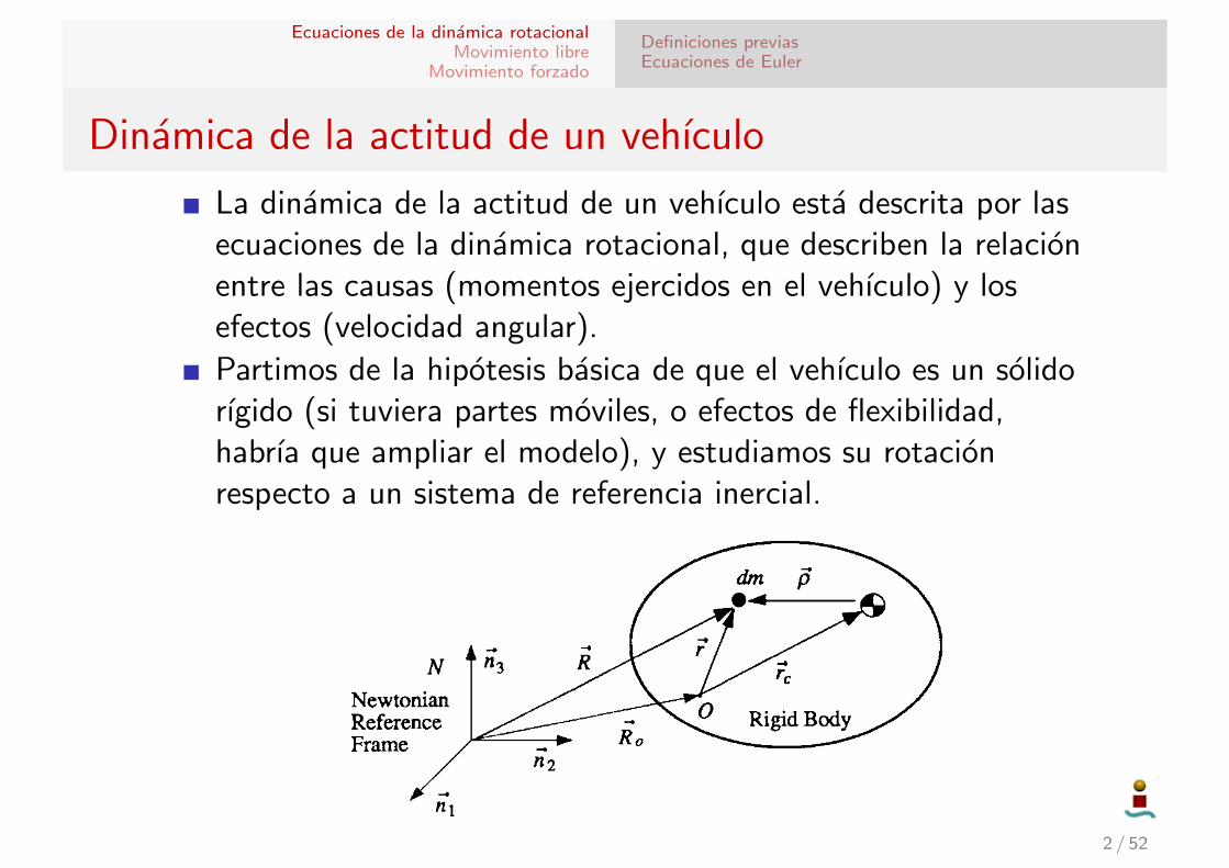
La dinamica de la actitud de un vehıculo esta descrita por lasecuaciones de la dinamica rotacional, que describen la relacionentre las causas (momentos ejercidos en el vehıculo) y losefectos (velocidad angular).
Partimos de la hipotesis basica de que el vehıculo es un solidorıgido (si tuviera partes moviles, o efectos de flexibilidad,habrıa que ampliar el modelo), y estudiamos su rotacionrespecto a un sistema de referencia inercial.
“Chapter06” — 2008/6/6 — 14:34 — page 350 — #2!!
!!
!!
!!
350 SPACE VEHICLE DYNAMICS AND CONTROL
Fig. 6.1 Rigid body in motion relative to a Newtonian reference frame.
where !ho, called the relative angular momentum about point O, is defined as
!ho =!
!r " !r dm (6.4)
Note that the time derivative is taken with respect to an inertial reference frame.Like the relative angular momentum defined as Eq. (6.4), the absolute angular
momentum about point O is defined as
!Ho =!
!r " !R dm (6.5)
Combining Eqs. (6.1) and (6.5), we obtain
!Ho + m !Ro " !rc = !Mo (6.6)
If the reference point O is either inertially fixed or at the center of mass ofthe rigid body, the distinction between !Ho and !ho disappears and the angularmomentum equation simply becomes
!Ho = !Mo or !ho = !Mo (6.7)
Furthermore, if the moment of forces !Mo is zero, then the angular momentumvector becomes a constant vector, that is, the angular momentum of the rigid bodyis conserved. This is known as the principle of conservation of angular momentum.For this reason, the center of mass is often selected as a reference point O of therigid body.
6.2 Inertia Matrix and Inertia Dyadic
Consider a rigid body with a body-fixed reference frame B with its originat the center of mass of the rigid body, as shown in Fig. 6.2. In this figure, !!denotes the position vector of a small mass element dm from the center of mass,!Rc is the position vector of the center of mass from an inertial origin of N , and !R isthe position vector of dm from an inertial origin of N .
2 / 52
Ecuaciones de la dinamica rotacionalMovimiento libre
Movimiento forzado
Definiciones previasEcuaciones de Euler
Momento cinetico relativo y absoluto I
“Chapter06” — 2008/6/6 — 14:34 — page 350 — #2!!
!!
!!
!!
350 SPACE VEHICLE DYNAMICS AND CONTROL
Fig. 6.1 Rigid body in motion relative to a Newtonian reference frame.
where !ho, called the relative angular momentum about point O, is defined as
!ho =!
!r " !r dm (6.4)
Note that the time derivative is taken with respect to an inertial reference frame.Like the relative angular momentum defined as Eq. (6.4), the absolute angular
momentum about point O is defined as
!Ho =!
!r " !R dm (6.5)
Combining Eqs. (6.1) and (6.5), we obtain
!Ho + m !Ro " !rc = !Mo (6.6)
If the reference point O is either inertially fixed or at the center of mass ofthe rigid body, the distinction between !Ho and !ho disappears and the angularmomentum equation simply becomes
!Ho = !Mo or !ho = !Mo (6.7)
Furthermore, if the moment of forces !Mo is zero, then the angular momentumvector becomes a constant vector, that is, the angular momentum of the rigid bodyis conserved. This is known as the principle of conservation of angular momentum.For this reason, the center of mass is often selected as a reference point O of therigid body.
6.2 Inertia Matrix and Inertia Dyadic
Consider a rigid body with a body-fixed reference frame B with its originat the center of mass of the rigid body, as shown in Fig. 6.2. In this figure, !!denotes the position vector of a small mass element dm from the center of mass,!Rc is the position vector of the center of mass from an inertial origin of N , and !R isthe position vector of dm from an inertial origin of N .
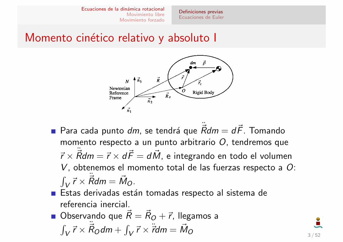
Para cada punto dm, se tendra que ~Rdm = d~F . Tomandomomento respecto a un punto arbitrario O, tendremos que
~r × ~Rdm = ~r × d~F = d ~M, e integrando en todo el volumenV , obtenemos el momento total de las fuerzas respecto a O:∫V ~r × ~Rdm = ~MO .
Estas derivadas estan tomadas respecto al sistema dereferencia inercial.Observando que ~R = ~RO +~r , llegamos a∫V ~r × ~ROdm +
∫V ~r × ~rdm = ~MO
3 / 52
Ecuaciones de la dinamica rotacionalMovimiento libre
Movimiento forzado
Definiciones previasEcuaciones de Euler
Momento cinetico relativo y absoluto II
“Chapter06” — 2008/6/6 — 14:34 — page 350 — #2!!
!!
!!
!!
350 SPACE VEHICLE DYNAMICS AND CONTROL
Fig. 6.1 Rigid body in motion relative to a Newtonian reference frame.
where !ho, called the relative angular momentum about point O, is defined as
!ho =!
!r " !r dm (6.4)
Note that the time derivative is taken with respect to an inertial reference frame.Like the relative angular momentum defined as Eq. (6.4), the absolute angular
momentum about point O is defined as
!Ho =!
!r " !R dm (6.5)
Combining Eqs. (6.1) and (6.5), we obtain
!Ho + m !Ro " !rc = !Mo (6.6)
If the reference point O is either inertially fixed or at the center of mass ofthe rigid body, the distinction between !Ho and !ho disappears and the angularmomentum equation simply becomes
!Ho = !Mo or !ho = !Mo (6.7)
Furthermore, if the moment of forces !Mo is zero, then the angular momentumvector becomes a constant vector, that is, the angular momentum of the rigid bodyis conserved. This is known as the principle of conservation of angular momentum.For this reason, the center of mass is often selected as a reference point O of therigid body.
6.2 Inertia Matrix and Inertia Dyadic
Consider a rigid body with a body-fixed reference frame B with its originat the center of mass of the rigid body, as shown in Fig. 6.2. In this figure, !!denotes the position vector of a small mass element dm from the center of mass,!Rc is the position vector of the center of mass from an inertial origin of N , and !R isthe position vector of dm from an inertial origin of N .
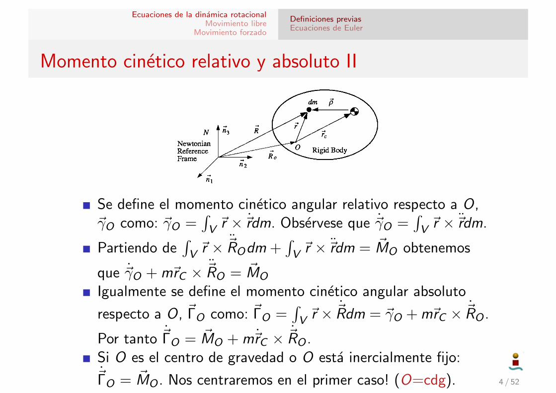
Se define el momento cinetico angular relativo respecto a O,~γO como: ~γO =
∫V ~r × ~rdm. Observese que ~γO =
∫V ~r × ~rdm.
Partiendo de∫V ~r × ~ROdm +
∫V ~r × ~rdm = ~MO obtenemos
que ~γO + m~rC × ~RO = ~MO
Igualmente se define el momento cinetico angular absoluto
respecto a O, ~ΓO como: ~ΓO =∫V ~r × ~Rdm = ~γO + m~rC × ~RO .
Por tanto ~ΓO = ~MO + m~rC × ~RO .Si O es el centro de gravedad o O esta inercialmente fijo:~ΓO = ~MO . Nos centraremos en el primer caso! (O=cdg). 4 / 52
Ecuaciones de la dinamica rotacionalMovimiento libre
Movimiento forzado
Definiciones previasEcuaciones de Euler
Momento cinetico y tensor de inercia I
“Chapter06” — 2008/6/6 — 14:34 — page 351 — #3!!
!!
!!
!!
RIGID-BODY DYNAMICS 351
Fig. 6.2 Rigid body with a body-fixed reference frame B with its origin at the centerof mass.
Let !! " !!B/N be the angular velocity vector of the rigid body in an inertialreference frame N . The angular momentum vector !H of a rigid body about itscenter of mass is then defined as
!H =!
!" # !R dm =!
!" # !" dm =!
!" # ( !! # !") dm (6.8)
as !R = !Rc + !","
!" dm = 0, !R " {d !R/dt}N , and
!" "#
d !"dt
$
N=
#d !"dt
$
B+ !!B/N # !" (6.9)
Note that {d !"/dt}B = 0 for a rigid body.Let !" and !! be expressed as
!" = "1!b1 + "2!b2 + "3!b3 (6.10a)
!! = !1!b1 + !2!b2 + !3!b3 (6.10b)
where {!b1, !b2, !b3} is a set of three orthogonal unit vectors, called basis vectors,of a body-fixed reference frame B. The angular momentum vector described byEq. (6.8) can then be written as
!H = (J11!1 + J12!2 + J13!3)!b1 + (J21!1 + J22!2 + J23!3)!b2
+ (J31!1 + J32!2 + J33!3)!b3 (6.11)
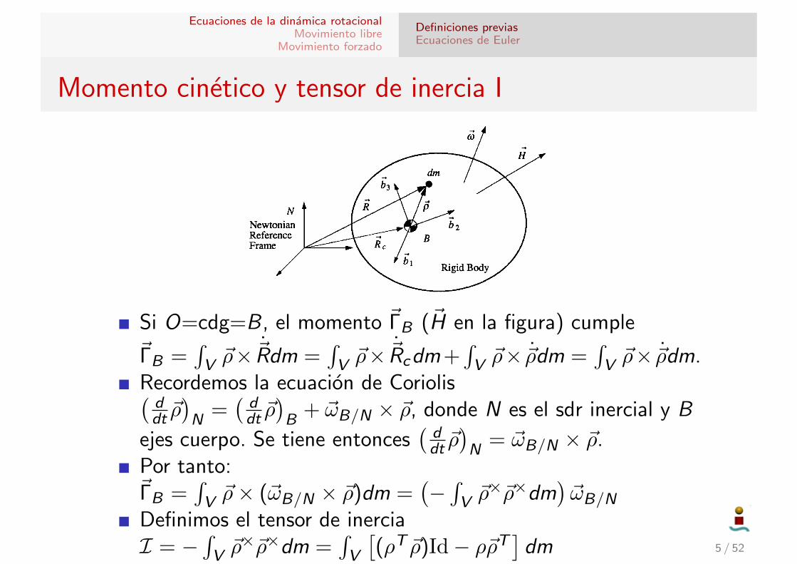
Si O=cdg=B, el momento ~ΓB (~H en la figura) cumple
~ΓB =∫V ~ρ× ~Rdm =
∫V ~ρ× ~Rcdm+
∫V ~ρ× ~ρdm =
∫V ~ρ× ~ρdm.
Recordemos la ecuacion de Coriolis(ddt ~ρ)N
=(ddt ~ρ)B
+ ~ωB/N × ~ρ, donde N es el sdr inercial y B
ejes cuerpo. Se tiene entonces(ddt ~ρ)N
= ~ωB/N × ~ρ.Por tanto:~ΓB =
∫V ~ρ× (~ωB/N × ~ρ)dm =
(−∫V ~ρ×~ρ×dm
)~ωB/N
Definimos el tensor de inerciaI = −
∫V ~ρ×~ρ×dm =
∫V
[(ρT ~ρ)Id− ρ~ρT
]dm 5 / 52
Ecuaciones de la dinamica rotacionalMovimiento libre
Movimiento forzado
Definiciones previasEcuaciones de Euler
Momento cinetico y tensor de inercia II
“Chapter06” — 2008/6/6 — 14:34 — page 351 — #3!!
!!
!!
!!
RIGID-BODY DYNAMICS 351
Fig. 6.2 Rigid body with a body-fixed reference frame B with its origin at the centerof mass.
Let !! " !!B/N be the angular velocity vector of the rigid body in an inertialreference frame N . The angular momentum vector !H of a rigid body about itscenter of mass is then defined as
!H =!
!" # !R dm =!
!" # !" dm =!
!" # ( !! # !") dm (6.8)
as !R = !Rc + !","
!" dm = 0, !R " {d !R/dt}N , and
!" "#
d !"dt
$
N=
#d !"dt
$
B+ !!B/N # !" (6.9)
Note that {d !"/dt}B = 0 for a rigid body.Let !" and !! be expressed as
!" = "1!b1 + "2!b2 + "3!b3 (6.10a)
!! = !1!b1 + !2!b2 + !3!b3 (6.10b)
where {!b1, !b2, !b3} is a set of three orthogonal unit vectors, called basis vectors,of a body-fixed reference frame B. The angular momentum vector described byEq. (6.8) can then be written as
!H = (J11!1 + J12!2 + J13!3)!b1 + (J21!1 + J22!2 + J23!3)!b2
+ (J31!1 + J32!2 + J33!3)!b3 (6.11)
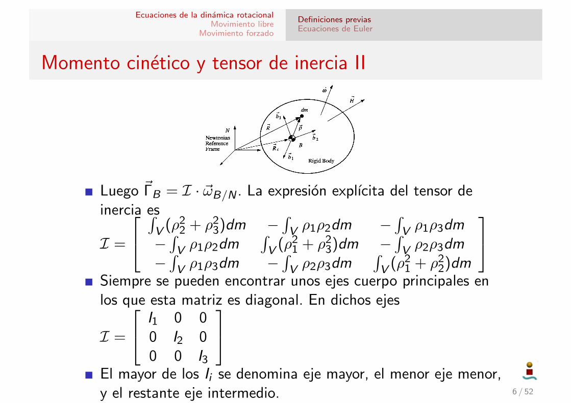
Luego ~ΓB = I · ~ωB/N . La expresion explıcita del tensor deinercia es
I =
∫V (ρ22 + ρ2
3)dm −∫V ρ1ρ2dm −
∫V ρ1ρ3dm
−∫V ρ1ρ2dm
∫V (ρ2
1 + ρ23)dm −
∫V ρ2ρ3dm
−∫V ρ1ρ3dm −
∫V ρ2ρ3dm
∫V (ρ2
1 + ρ22)dm
Siempre se pueden encontrar unos ejes cuerpo principales enlos que esta matriz es diagonal. En dichos ejes
I =
I1 0 00 I2 00 0 I3
El mayor de los Ii se denomina eje mayor, el menor eje menor,y el restante eje intermedio. 6 / 52
Ecuaciones de la dinamica rotacionalMovimiento libre
Movimiento forzado
Definiciones previasEcuaciones de Euler
Energıa cinetica
“Chapter06” — 2008/6/6 — 14:34 — page 351 — #3!!
!!
!!
!!
RIGID-BODY DYNAMICS 351
Fig. 6.2 Rigid body with a body-fixed reference frame B with its origin at the centerof mass.
Let !! " !!B/N be the angular velocity vector of the rigid body in an inertialreference frame N . The angular momentum vector !H of a rigid body about itscenter of mass is then defined as
!H =!
!" # !R dm =!
!" # !" dm =!
!" # ( !! # !") dm (6.8)
as !R = !Rc + !","
!" dm = 0, !R " {d !R/dt}N , and
!" "#
d !"dt
$
N=
#d !"dt
$
B+ !!B/N # !" (6.9)
Note that {d !"/dt}B = 0 for a rigid body.Let !" and !! be expressed as
!" = "1!b1 + "2!b2 + "3!b3 (6.10a)
!! = !1!b1 + !2!b2 + !3!b3 (6.10b)
where {!b1, !b2, !b3} is a set of three orthogonal unit vectors, called basis vectors,of a body-fixed reference frame B. The angular momentum vector described byEq. (6.8) can then be written as
!H = (J11!1 + J12!2 + J13!3)!b1 + (J21!1 + J22!2 + J23!3)!b2
+ (J31!1 + J32!2 + J33!3)!b3 (6.11)
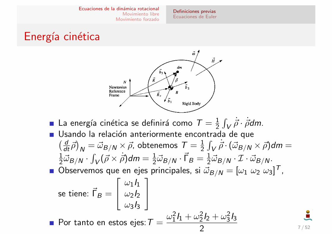
La energıa cinetica se definira como T = 12
∫V ~ρ · ~ρdm.
Usando la relacion anteriormente encontrada de que(ddt ~ρ)N
= ~ωB/N × ~ρ, obtenemos T = 12
∫V ~ρ · (~ωB/N × ~ρ)dm =
12~ωB/N ·
∫V (~ρ× ~ρ)dm = 1
2~ωB/N · ~ΓB = 12~ωB/N · I · ~ωB/N .
Observemos que en ejes principales, si ~ωB/N = [ω1 ω2 ω3]T ,
se tiene: ~ΓB =
ω1I1ω2I2ω3I3
Por tanto en estos ejes:T =
ω21I1 + ω2
2I2 + ω23I3
2 7 / 52
Ecuaciones de la dinamica rotacionalMovimiento libre
Movimiento forzado
Definiciones previasEcuaciones de Euler
Ecuaciones de Euler
Partimos de ~Γ = ~M. Puesto que esta derivada esta tomada enel sistema de referencia inercial, pasando a ejes cuerpo:(
ddt~Γ)N
=(
ddt~Γ)B
+ ~ωB/N × ~Γ = ~M.
Sustituyendo el tensor de inercia:(ddtI · ~ωB/N
)B
+ ~ωB/N ×(I · ~ωB/N
)= ~M
Puesto que bajo la hipotesis de solido rıgido(ddtI)B
= 0, se
tiene: I · ~ωB/N + ~ω×B/NI · ~ωB/N = ~M.
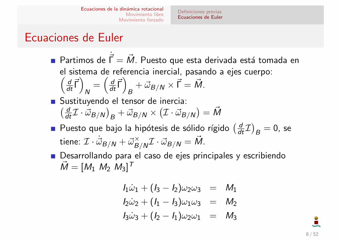
Desarrollando para el caso de ejes principales y escribiendo~M = [M1 M2 M3]T
I1ω1 + (I3 − I2)ω2ω3 = M1
I2ω2 + (I1 − I3)ω1ω3 = M2
I3ω3 + (I2 − I1)ω2ω1 = M3
8 / 52
Ecuaciones de la dinamica rotacionalMovimiento libre
Movimiento forzado
Resolucion analıtica y geometrica.Estabilidad. Regla del eje mayorEfecto de un volante en la dinamica rotacional
Movimiento libre
En primer lugar estudiaremos el movimiento libre, es decir,~M = ~0. En estas circunstancias se conserva el momentocinetico total del sistema.
Si bien en la realidad no se da este caso, ya que siempreexisten momentos perturbadores, estos son pequenos.
Veremos algunas soluciones analıticas pero lo mas interesantesera estudiar la estabilidad del sistema; encontraremos la regladel eje mayor.
Consideraremos dos casos: axilsimetrico (dos ejes de inerciaiguales) y asimetrico (los tres ejes de inercia iguales).
El caso totalmente simetrico (I1 = I2 = I3) desacoplatotalmente las ecuaciones y es trivialmente resoluble (lasvelocidades angulares resultantes son independientes yconstantes).
9 / 52
Ecuaciones de la dinamica rotacionalMovimiento libre
Movimiento forzado
Resolucion analıtica y geometrica.Estabilidad. Regla del eje mayorEfecto de un volante en la dinamica rotacional
Caso axilsimetrico. Resolucion analıtica.Consideremos el caso en el que I1 = I2 = I , I3 6= I .Las ecuaciones se reducen a:
I ω1 + (I3 − I )ω2ω3 = 0
I ω2 + (I − I3)ω1ω3 = 0
I3ω3 = 0
En primer lugar obtenemos ω3 = Cte = n (tasa de rotaciondel VE alrededor de su eje de simetrıa). Definamos λ = I−I3
I n,la llamada “tasa de rotacion relativa”. Las dos primerasecuaciones quedan:
ω1 − λω2 = 0
ω2 + λω1 = 0
Son las ecuaciones de un oscilador armonico, obteniendo:
ω1 = ω1(0) cosλt + ω2(0) senλt
ω2 = ω2(0) cosλt − ω1(0) senλt 10 / 52
Ecuaciones de la dinamica rotacionalMovimiento libre
Movimiento forzado
Resolucion analıtica y geometrica.Estabilidad. Regla del eje mayorEfecto de un volante en la dinamica rotacional
Caso axilsimetrico. Resolucion analıtica.
Es facil ver que ω21 + ω2
2 = Cte = ω212, la llamada velocidad
angular transversal. Por tanto ‖ω‖ =√ω2
12 + n2 = Cte y su
tercera componente (en ejes b) tambien es cte. Por lo que el~ω en ejes cuerpo describe un cono en torno al eje de simetrıadel cuerpo, de angulo γ = arctan
(ω12n
).
Por otro lado, puesto que ~Γ = ~Cte en el sdr inercial alconservarse el momento cinetico, podemos elegir el eje 3 delsistema de referencia inercial apuntado en la direccion de ~Γ(~H en la figura). Ademas su modulo Γ ha de ser constante.
Ademas observemos que en ejes cuerpo, ~Γ = [Iω1 Iω2 I3n]T , y
por tanto ~Γ · ~ebz = I3n = cos θΓ, es decir el angulo entre ~Γ y eleje z cuerpo es constante; este angulo, θ, es el llamado elangulo de nutacion. Ademas:
tan θ =
√1− cos2 θ
cos θ=
√Γ2 − I 2
3 n2
I3n=
Iω12
I3n=
I
I3tan γ
Se puede verificar que el angulo entre ~Γ y ~ω es θ − γ. 11 / 52
Ecuaciones de la dinamica rotacionalMovimiento libre
Movimiento forzado
Resolucion analıtica y geometrica.Estabilidad. Regla del eje mayorEfecto de un volante en la dinamica rotacional
Caso axilsimetrico. Resolucion analıtica.
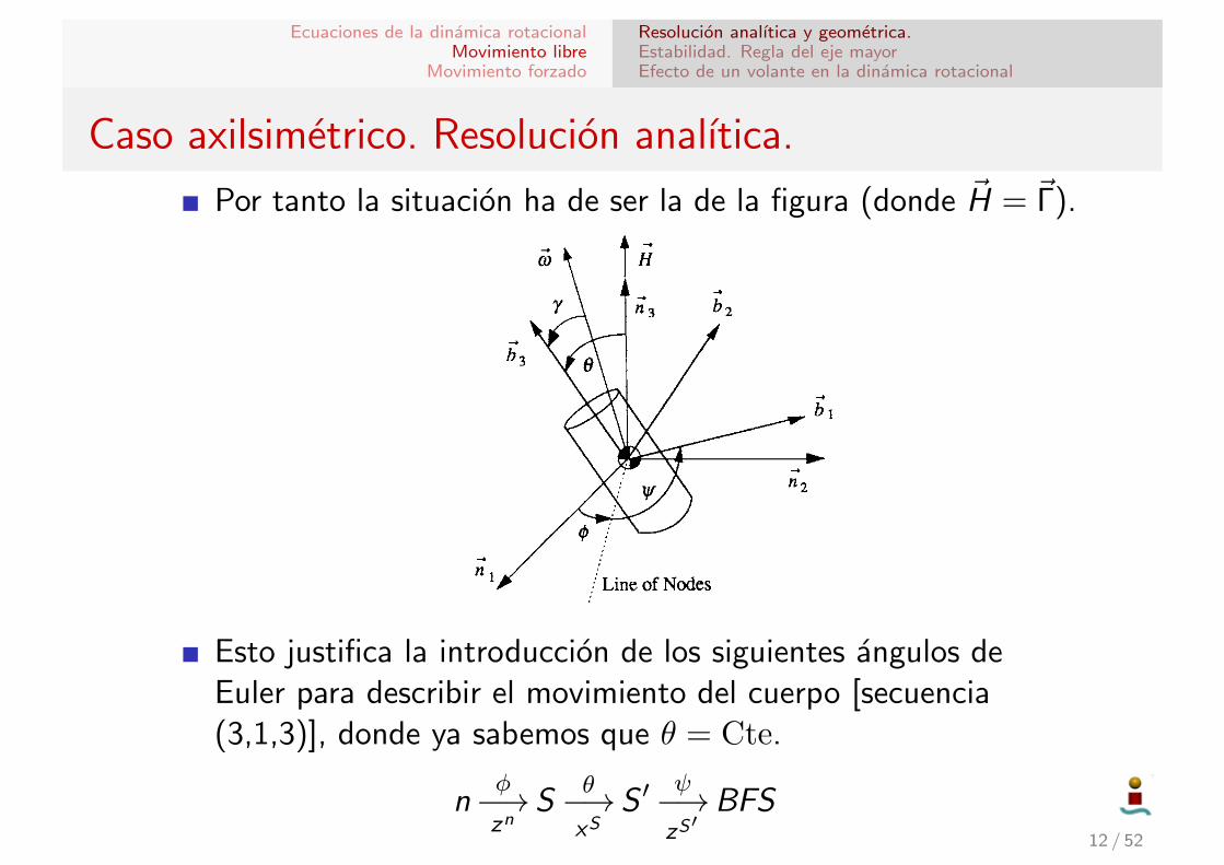
Por tanto la situacion ha de ser la de la figura (donde ~H = ~Γ).
“Chapter06” — 2008/6/6 — 14:34 — page 363 — #15!!
!!
!!
!!
RIGID-BODY DYNAMICS 363
6.5 Torque-Free Motion of an Axisymmetric Rigid Body
Most spin-stabilized spacecraft are nearly axisymmetric, and they rotate aboutone of their principal axes. The stability of torque-free rotational motion ofsuch spin-stabilized spacecraft is of practical importance. The term “torque-free motion” commonly employed in spacecraft attitude dynamics refers to therotational motion of a rigid body in the presence of no external torques.
Consider a torque-free, axisymmetric rigid body with a body-fixed referenceframe B, which has basis vectors {!b1, !b2, !b3}, and which has its origin at the centerof mass, as illustrated in Fig. 6.4. The reference frame B coincides with a set ofprincipal axes, and the !b3 axis is the axis of symmetry; thus, J1 = J2.
Euler’s rotational equations of motion of a torque-free, axisymmetric spacecraftwith J1 = J2 = J become
J!1 " (J " J3)!3!2 = 0 (6.49)
J!2 + (J " J3)!3!1 = 0 (6.50)
J3!3 = 0 (6.51)
where !i # !bi · !! are the body-fixed components of the angular velocity of thespacecraft.
From Eq. (6.51), we have
!3 = const = n (6.52)
where the constant n is called the spin rate of the spacecraft about its symmetryaxis !b3.
Defining the relative spin rate " as
" = (J " J3)nJ
Fig. 6.4 Torque-free motion of an axisymmetric rigid body.Esto justifica la introduccion de los siguientes angulos deEuler para describir el movimiento del cuerpo [secuencia(3,1,3)], donde ya sabemos que θ = Cte.
nφ−→zn
Sθ−→xS
S ′ψ−→zS′
BFS12 / 52
Ecuaciones de la dinamica rotacionalMovimiento libre
Movimiento forzado
Resolucion analıtica y geometrica.Estabilidad. Regla del eje mayorEfecto de un volante en la dinamica rotacional
Caso axilsimetrico. Resolucion analıtica.
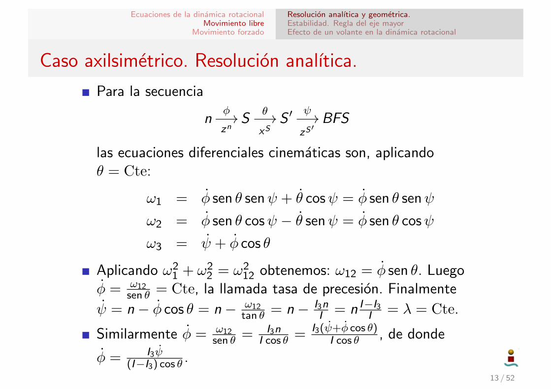
Para la secuencia
nφ−→zn
Sθ−→xS
S ′ψ−→zS′
BFS
las ecuaciones diferenciales cinematicas son, aplicandoθ = Cte:
ω1 = φ sen θ senψ + θ cosψ = φ sen θ senψ
ω2 = φ sen θ cosψ − θ senψ = φ sen θ cosψ
ω3 = ψ + φ cos θ
Aplicando ω21 + ω2
2 = ω212 obtenemos: ω12 = φ sen θ. Luego
φ = ω12sen θ = Cte, la llamada tasa de precesion. Finalmente
ψ = n − φ cos θ = n − ω12tan θ = n − I3n
I = n I−I3I = λ = Cte.
Similarmente φ = ω12sen θ = I3n
I cos θ = I3(ψ+φ cos θ)I cos θ , de donde
φ = I3ψ(I−I3) cos θ .
13 / 52
Ecuaciones de la dinamica rotacionalMovimiento libre
Movimiento forzado
Resolucion analıtica y geometrica.Estabilidad. Regla del eje mayorEfecto de un volante en la dinamica rotacional
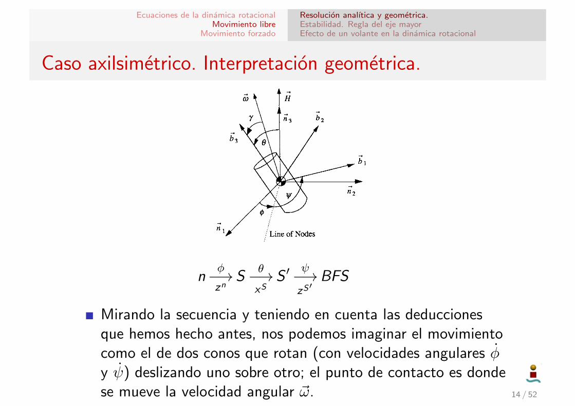
Caso axilsimetrico. Interpretacion geometrica.
“Chapter06” — 2008/6/6 — 14:34 — page 363 — #15!!
!!
!!
!!
RIGID-BODY DYNAMICS 363
6.5 Torque-Free Motion of an Axisymmetric Rigid Body
Most spin-stabilized spacecraft are nearly axisymmetric, and they rotate aboutone of their principal axes. The stability of torque-free rotational motion ofsuch spin-stabilized spacecraft is of practical importance. The term “torque-free motion” commonly employed in spacecraft attitude dynamics refers to therotational motion of a rigid body in the presence of no external torques.
Consider a torque-free, axisymmetric rigid body with a body-fixed referenceframe B, which has basis vectors {!b1, !b2, !b3}, and which has its origin at the centerof mass, as illustrated in Fig. 6.4. The reference frame B coincides with a set ofprincipal axes, and the !b3 axis is the axis of symmetry; thus, J1 = J2.
Euler’s rotational equations of motion of a torque-free, axisymmetric spacecraftwith J1 = J2 = J become
J!1 " (J " J3)!3!2 = 0 (6.49)
J!2 + (J " J3)!3!1 = 0 (6.50)
J3!3 = 0 (6.51)
where !i # !bi · !! are the body-fixed components of the angular velocity of thespacecraft.
From Eq. (6.51), we have
!3 = const = n (6.52)
where the constant n is called the spin rate of the spacecraft about its symmetryaxis !b3.
Defining the relative spin rate " as
" = (J " J3)nJ
Fig. 6.4 Torque-free motion of an axisymmetric rigid body.
nφ−→zn
Sθ−→xS
S ′ψ−→zS′
BFS
Mirando la secuencia y teniendo en cuenta las deduccionesque hemos hecho antes, nos podemos imaginar el movimientocomo el de dos conos que rotan (con velocidades angulares φy ψ) deslizando uno sobre otro; el punto de contacto es dondese mueve la velocidad angular ~ω. 14 / 52
Ecuaciones de la dinamica rotacionalMovimiento libre
Movimiento forzado
Resolucion analıtica y geometrica.Estabilidad. Regla del eje mayorEfecto de un volante en la dinamica rotacional
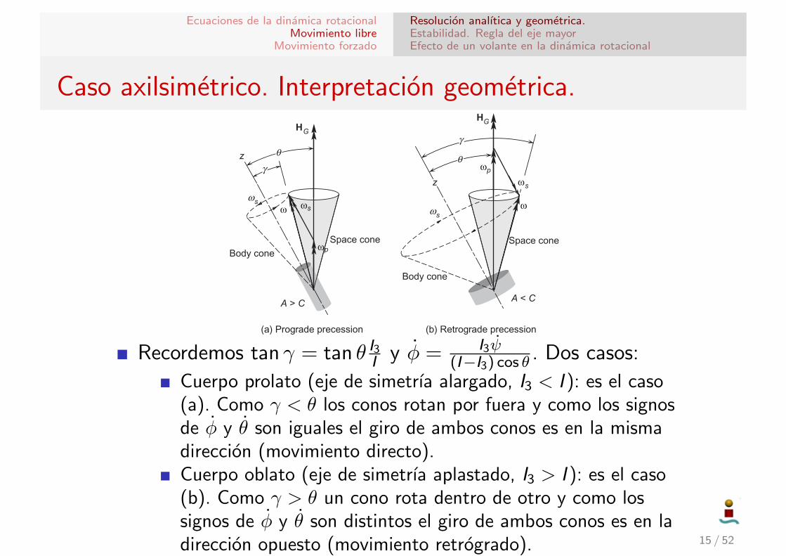
Caso axilsimetrico. Interpretacion geometrica.580 CHAPTER 10 Satellite attitude dynamics
illustrated in Figure 10.4 , which also shows the body cone and space cone . The space cone is swept out in inertial space by the angular velocity vector as it rotates with angular velocity ! p around H G , whereas the body cone is the trace of ! in the body frame as it rotates with angular velocity ! s about the z axis. From inertial space, the motion may be visualized as the body cone rolling on the space cone, with the line of contact being the angular velocity vector. From the body frame it appears as though the space cone rolls on the body cone. Figure 10.4 graphically confi rms our deduction from Equation 10.23, namely, that preces-sion and spin are in the same direction for prolate bodies and opposite in direction for oblate shapes.
Finally , we know from Equations 10.24 and 10.25 that the magnitude HG of the angular momentum is
HG xy oA C! "2 2 2 2! !
Using Equations 10.17 and 10.22, we can write this as
HG p p pA C
AC
A! " ! "2 2 22
2 2 2 2( ) ( )! " ! " ! " "sin cos sin cos!"###
$%&&&&
so that we obtain a surprisingly simple formula for the magnitude of the angular momentum in torque-free motion,
HG pA! ! (10.27)
Example 10.1 A cylindrical shell is rotating in torque-free motion about its longitudinal axis. If the axis is wobbling slightly, determine the ratios of l / r for which the precession will be prograde or retrograde.
z
HG
p
HG
s
Space coneBody cone
Body cone
Space cone
z
s
(a) Prograde precession (b) Retrograde precession
A > C A < C
s
p
!!
"
"
#
s##
##
##
#
FIGURE 10.4 Space and body cones for a rotationally symmetric body in torque-free motion. (a) Prolate body. (b) Oblate body. Recordemos tan γ = tan θ I3I y φ = I3ψ
(I−I3) cos θ . Dos casos:
Cuerpo prolato (eje de simetrıa alargado, I3 < I ): es el caso(a). Como γ < θ los conos rotan por fuera y como los signosde φ y θ son iguales el giro de ambos conos es en la mismadireccion (movimiento directo).Cuerpo oblato (eje de simetrıa aplastado, I3 > I ): es el caso(b). Como γ > θ un cono rota dentro de otro y como lossignos de φ y θ son distintos el giro de ambos conos es en ladireccion opuesto (movimiento retrogrado). 15 / 52
Ecuaciones de la dinamica rotacionalMovimiento libre
Movimiento forzado
Resolucion analıtica y geometrica.Estabilidad. Regla del eje mayorEfecto de un volante en la dinamica rotacional
Movimiento libre de un solido asimetrico
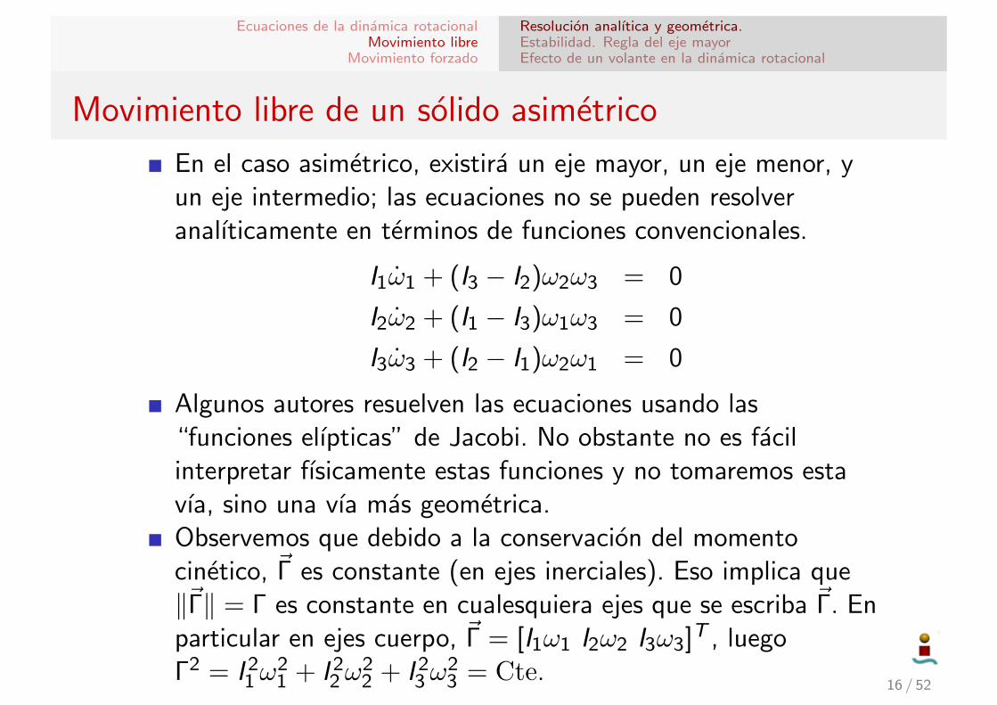
En el caso asimetrico, existira un eje mayor, un eje menor, yun eje intermedio; las ecuaciones no se pueden resolveranalıticamente en terminos de funciones convencionales.
I1ω1 + (I3 − I2)ω2ω3 = 0
I2ω2 + (I1 − I3)ω1ω3 = 0
I3ω3 + (I2 − I1)ω2ω1 = 0
Algunos autores resuelven las ecuaciones usando las“funciones elıpticas” de Jacobi. No obstante no es facilinterpretar fısicamente estas funciones y no tomaremos estavıa, sino una vıa mas geometrica.Observemos que debido a la conservacion del momentocinetico, ~Γ es constante (en ejes inerciales). Eso implica que‖~Γ‖ = Γ es constante en cualesquiera ejes que se escriba ~Γ. Enparticular en ejes cuerpo, ~Γ = [I1ω1 I2ω2 I3ω3]T , luegoΓ2 = I 2
1ω21 + I 2
2ω22 + I 2
3ω23 = Cte.
16 / 52
Ecuaciones de la dinamica rotacionalMovimiento libre
Movimiento forzado
Resolucion analıtica y geometrica.Estabilidad. Regla del eje mayorEfecto de un volante en la dinamica rotacional
Movimiento libre de un solido asimetrico
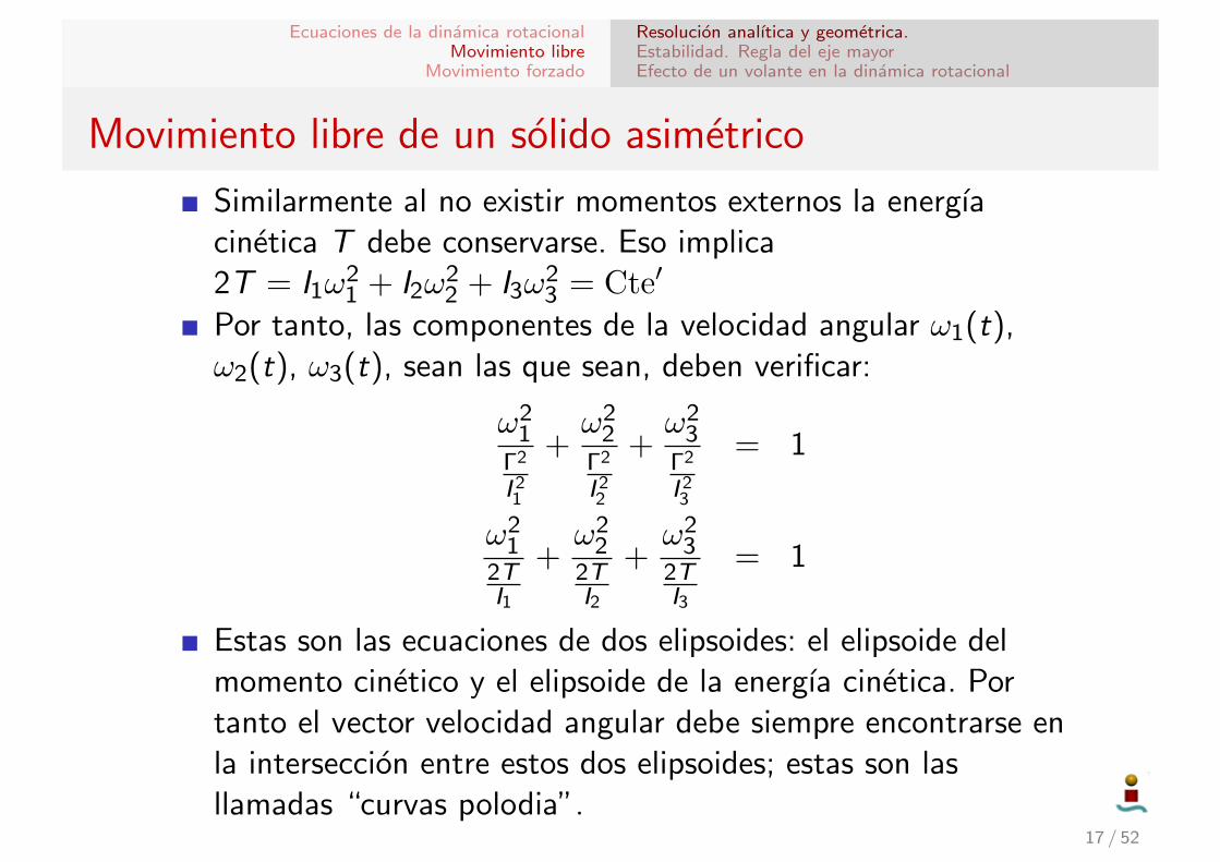
Similarmente al no existir momentos externos la energıacinetica T debe conservarse. Eso implica2T = I1ω
21 + I2ω
22 + I3ω
23 = Cte′
Por tanto, las componentes de la velocidad angular ω1(t),ω2(t), ω3(t), sean las que sean, deben verificar:
ω21
Γ2
I 21
+ω2
2Γ2
I 22
+ω2
3Γ2
I 23
= 1
ω21
2TI1
+ω2
22TI2
+ω2
32TI3
= 1
Estas son las ecuaciones de dos elipsoides: el elipsoide delmomento cinetico y el elipsoide de la energıa cinetica. Portanto el vector velocidad angular debe siempre encontrarse enla interseccion entre estos dos elipsoides; estas son lasllamadas “curvas polodia”.
17 / 52
Ecuaciones de la dinamica rotacionalMovimiento libre
Movimiento forzado
Resolucion analıtica y geometrica.Estabilidad. Regla del eje mayorEfecto de un volante en la dinamica rotacional
Curvas polodia
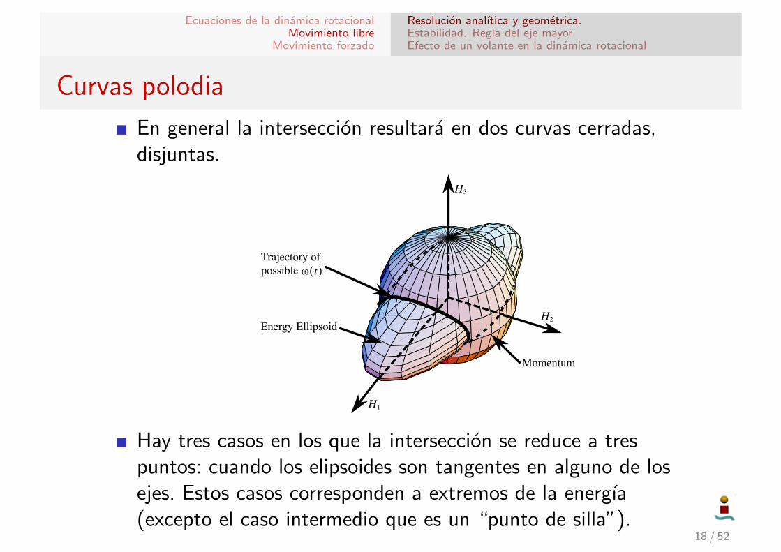
En general la interseccion resultara en dos curvas cerradas,disjuntas.
130 EULERIAN MECHANICS CHAPTER 4
where!
2IiT are the corresponding semi-axes. In order for the torque-freerotation to satisfy both Eqs. (4.60) and (4.61), the energy ellipsoid and the mo-mentum sphere must intersect. The intersection forms a trajectory of feasible!(t) as illustrated in Figure 4.5. This geometrical interpretations is very use-ful to make qualitative studies on the nature and limiting properties of largerotations.
Momentum Sphere
Energy Ellipsoid
Trajectory of possible ( )! t
H1
H2
H3
Figure 4.5: General Intersection of the Momentum Sphere and the En-ergy Ellipsoid
Clearly, for a given |H |, only a certain range of kinetic energy is possible.For the current discussion, let us hold the angular momentum vector magnitudeconstant and sweep the kinetic energy through its two extrema. Also, assumethat the inertia matrix entries Ii are ordered such that
I1 " I2 " I3 (4.62)
With this ordering of inertias, the largest kinetic energy ellipsoid semi-axis!2I1T occurs about the b1 axis as shown in Figure 4.5, and the smallest semi-
axis is about the b3 axis. Eq. (4.61) shows that varying T will only uniformlyscale the corresponding kinetic energy ellipsoid. The overall shape and aspectratio of the ellipsoid will remain the same for each choice in T .
Three special energy cases are shown in Figure 4.6. Since the kinetic energyellipsoid and the momentum sphere must intersect, the smallest possible T wouldbe scaled the energy ellipsoid such that its largest semi-axis is equal to H =|H |. The momentum sphere perfectly envelops the energy ellipsoid as shown inFigure 4.6(i). The only points of intersection are at
BH = ±H b1 (4.63)
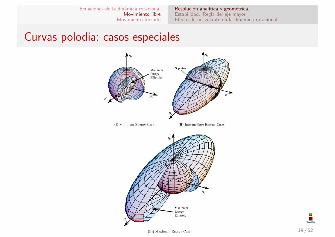
Hay tres casos en los que la interseccion se reduce a trespuntos: cuando los elipsoides son tangentes en alguno de losejes. Estos casos corresponden a extremos de la energıa(excepto el caso intermedio que es un “punto de silla”).
18 / 52
Ecuaciones de la dinamica rotacionalMovimiento libre
Movimiento forzado
Resolucion analıtica y geometrica.Estabilidad. Regla del eje mayorEfecto de un volante en la dinamica rotacional
Curvas polodia: casos especialesSECTION 4.2 TORQUE-FREE RIGID BODY ROTATION 131
H1
H3
H2
MinimumEnergyEllipsoid
(i) Minimum Energy Case
H1
H3
H2
Sepratrix
(ii) Intermediate Energy Case
H1
H3
H2
MaximumEnergyEllipsoid
(iii) Maximum Energy Case
Figure 4.6: Special Cases of Kinetic Energy Ellipsoid and MomentumSphere Intersections
19 / 52
Ecuaciones de la dinamica rotacionalMovimiento libre
Movimiento forzado
Resolucion analıtica y geometrica.Estabilidad. Regla del eje mayorEfecto de un volante en la dinamica rotacional
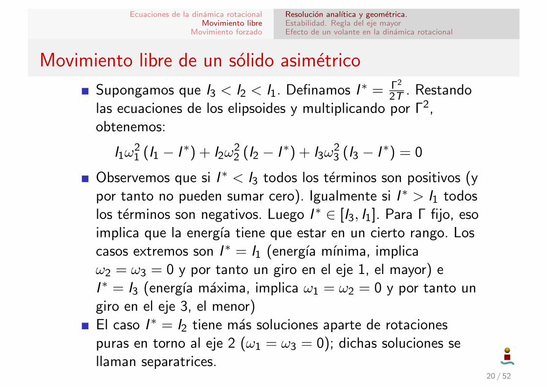
Movimiento libre de un solido asimetrico
Supongamos que I3 < I2 < I1. Definamos I ∗ = Γ2
2T . Restandolas ecuaciones de los elipsoides y multiplicando por Γ2,obtenemos:
I1ω21 (I1 − I ∗) + I2ω
22 (I2 − I ∗) + I3ω
23 (I3 − I ∗) = 0
Observemos que si I ∗ < I3 todos los terminos son positivos (ypor tanto no pueden sumar cero). Igualmente si I ∗ > I1 todoslos terminos son negativos. Luego I ∗ ∈ [I3, I1]. Para Γ fijo, esoimplica que la energıa tiene que estar en un cierto rango. Loscasos extremos son I ∗ = I1 (energıa mınima, implicaω2 = ω3 = 0 y por tanto un giro en el eje 1, el mayor) eI ∗ = I3 (energıa maxima, implica ω1 = ω2 = 0 y por tanto ungiro en el eje 3, el menor)El caso I ∗ = I2 tiene mas soluciones aparte de rotacionespuras en torno al eje 2 (ω1 = ω3 = 0); dichas soluciones sellaman separatrices.
20 / 52
Ecuaciones de la dinamica rotacionalMovimiento libre
Movimiento forzado
Resolucion analıtica y geometrica.Estabilidad. Regla del eje mayorEfecto de un volante en la dinamica rotacional
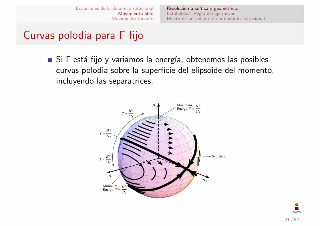
Curvas polodia para Γ fijo
Si Γ esta fijo y variamos la energıa, obtenemos las posiblescurvas polodia sobre la superficie del elipsoide del momento,incluyendo las separatrices.
SECTION 4.2 TORQUE-FREE RIGID BODY ROTATION 133
MinimumEnergy
MaximumEnergy
Sepratrix
H3
H 2
H1
T =H2
2I1
T <H2
2 I2
T =H 2
2I2
T >H2
2 I2
T =H 2
2I3
Figure 4.7: A Family of Energy Ellipsoid and Momentum Sphere Inter-sections
drag. Let’s study what happens if a satellite is spun up about the axis of leastinertia b3. For a given angular momentum, this corresponds to the maximumkinetic energy case. Since any real rigid body will loose energy over time simplydue to internal damping, this satellite’s energy is expected to decrease over time.Figure 4.7 shows how the satellite will start to “wobble” about the b3 axis asthe energy ellipsoid is reduced. After some time the !(t) curves will cross thesepratrix and the satellite will start to “wobble” about the axis of maximuminertia b1. Ultimately, as the energy approaches the minimum energy ellipsoid,the satellite will be spinning purely about the b1 axis. Therefore, under thepresence of a negative energy rate, only the spin about the axis of maximuminertia is a stable spin. The pure spin case about b3 will become unstable overtime.
This behavior is demonstrated in nature in that all planets are essentiallyspinning about their axis of maximum inertia. This fact was rediscovered duringearly space explorations when Explorer 1 was launched into orbit spinning aboutits axis of least inertia. It took less than a fraction of an orbit before it startedto tumble.
4.2.2 General Free Rigid Body Motion
In this section we would like to derive the general rotational equations of motionfor a rigid body free of any external torques. The attitude coordinates are chosento be the (3-2-1) Euler angles, also known as the yaw, pitch and roll angles
21 / 52
Ecuaciones de la dinamica rotacionalMovimiento libre
Movimiento forzado
Resolucion analıtica y geometrica.Estabilidad. Regla del eje mayorEfecto de un volante en la dinamica rotacional
Estabilidad del movimiento libre alrededor de un ejeprincipal
Hemos visto que las soluciones mas sencillas son rotacionespuras en torno a un eje principal. En este apartado, partamosde la solucion de equlibrio ω3 = n = Cte y que ω1 = ω2 = 0.Estudiemos la estabilidad de esta rotacion en funcion de si eleje 3 es mayor, menor o intermedio.Para ello perturbamos las ecuaciones, definiendo ω1 = δω1,ω2 = δω2 y ω3 = n + δω3. Sustituyendo en las ecs de Euler:
I1δω1 + (I3 − I2)δω2(n + δω3) = 0
I2δω2 + (I1 − I3)δω1(n + δω3) = 0
I3δω3 + (I2 − I1)δω2δω1 = 0
Despreciando terminos de segundo orden obtenemos:
I1δω1 + n(I3 − I2)δω2 = 0
I2δω2 + n(I1 − I3)δω1 = 0
I3δω3 = 0 22 / 52
Ecuaciones de la dinamica rotacionalMovimiento libre
Movimiento forzado
Resolucion analıtica y geometrica.Estabilidad. Regla del eje mayorEfecto de un volante en la dinamica rotacional
Estabilidad del movimiento libre en un eje principal
La ecuacion en δω3 es (marginalmente) estable, es decir,estable pero no asintoticamente estable (las perturbaciones nocrecen pero tampoco se disipan).La ecuacion de δω1 y δω2 se puede simplificar en una unicaecuacion:
δω1 +n2(I3 − I2)(I3 − I1)
I1I2δω1 = 0
La estabilidad de esta ecuacion depende del signo de(I3 − I2)(I3 − I1). Si el signo es positivo las soluciones sonoscilatorias (ni crecen ni disminuyen: marginalmente estable).Si el signo es negativo las soluciones son exponenciales (unade las soluciones crece en el tiempo: inestable)
Si I3 eje mayor, (I3 − I2)(I3 − I1) = +×+ > 0: estable.
Si I3 eje menor, (I3 − I2)(I3 − I1) = −×− > 0: estable.
Si I3 eje intermedio, (I3 − I2)(I3 − I1) = +×− < 0: inestable.23 / 52
Ecuaciones de la dinamica rotacionalMovimiento libre
Movimiento forzado
Resolucion analıtica y geometrica.Estabilidad. Regla del eje mayorEfecto de un volante en la dinamica rotacional
Estabilidad del movimiento libre con disipacion de energıa
El calculo anterior es correcto, pero solo si el modeloempleado (Ecuaciones de Euler para el solido rıgido) es unmodelo totalmente exacto.
La realidad no es tan simple, y siempre existe alguna fuente dedisipacion de energıa (efectos de flexibilidad, rozamientos departes moviles, movimiento de combustible en el deposito,etc...). Ello modificara el resultado anterior, ya que el sistemasiempre tendera a permanecer en un mınimo de energıa.
Partiendo de principios fısicos, encontremos el mınimo deenergıa para un momento cinetico determinado, es decir,resolvamos el problema
mın I1ω21 + I2ω
22 + I3ω
23
sujeto a I 21ω
21 + I 2
2ω22 + I 2
3ω23 = Γ2
24 / 52
Ecuaciones de la dinamica rotacionalMovimiento libre
Movimiento forzado
Resolucion analıtica y geometrica.Estabilidad. Regla del eje mayorEfecto de un volante en la dinamica rotacional
Estabilidad del movimiento libre con disipacion de energıa
Usando multiplicadores de Lagrange:
L(ω1, ω2, ω3, λ) = I1ω21 + I2ω
22 + I3ω
23 + λ(I 2
1ω21 + I 2
2ω22 + I 2
3ω23 − Γ2)
Se tiene 0 = ∂L∂ωi
= 2Iiωi (1 + λIi ), i = 1, 2, 3
Por tanto hay tres soluciones:
ω2=ω3=0, λ = − 1I1
, ω1 = ΓI1
. T = Γ2
2I1.
ω1=ω3=0, λ = − 1I2
, ω2 = ΓI2
. T = Γ2
2I2.
ω1=ω2=0, λ = − 1I3
, ω3 = ΓI3
. T = Γ2
2I3.
Claramente el mınimo viene dada por la primera solucion (lasegunda es punto de silla y la tercera maximo). Por tanto launica rotacion matematicamente estable y que a la vez es unmınimo de la energıa son las rotaciones en torno al eje mayor.
En base a este argumento se enuncia la regla del eje mayor:“En presencia de disipacion de energıa, las unicas rotacionesestables son aquellas en torno al eje mayor”.
25 / 52
Ecuaciones de la dinamica rotacionalMovimiento libre
Movimiento forzado
Resolucion analıtica y geometrica.Estabilidad. Regla del eje mayorEfecto de un volante en la dinamica rotacional
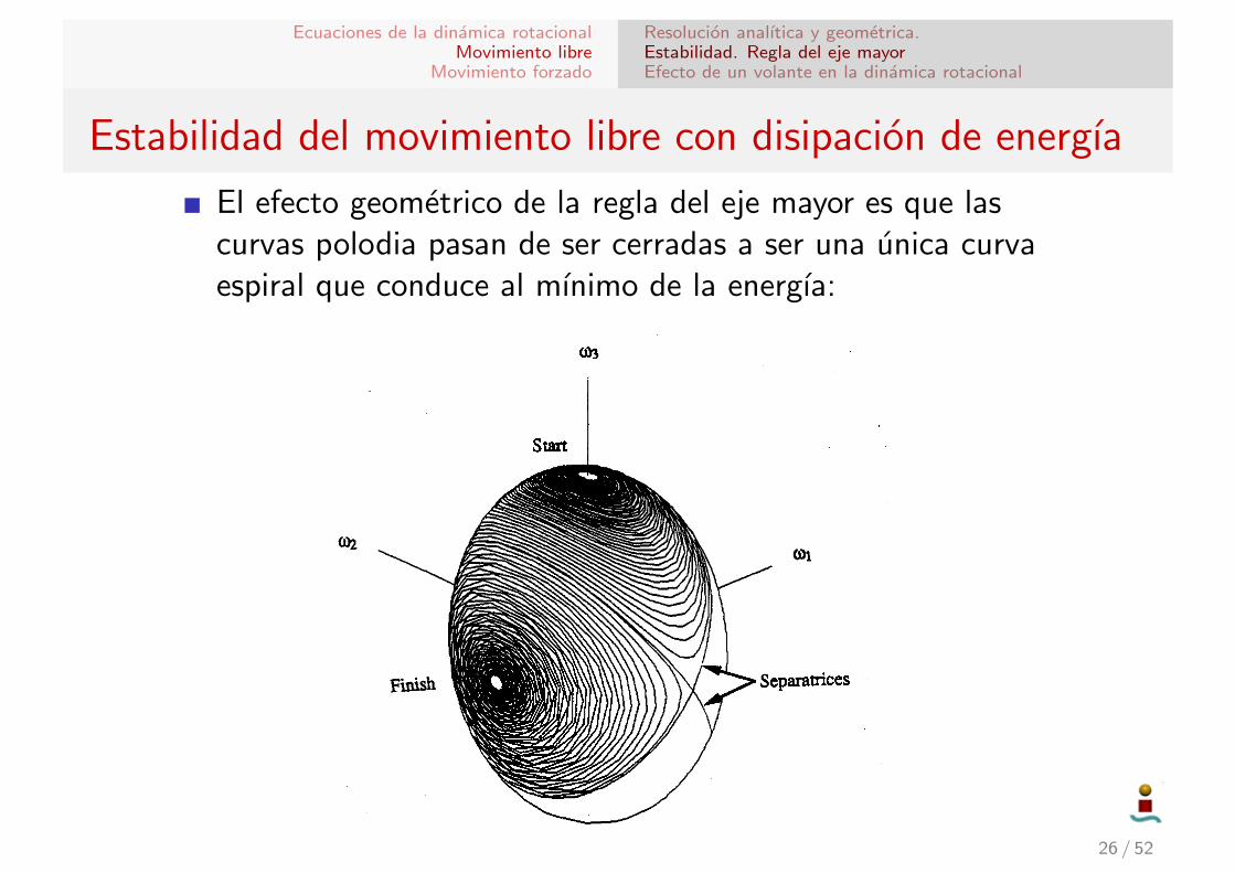
Estabilidad del movimiento libre con disipacion de energıa
El efecto geometrico de la regla del eje mayor es que lascurvas polodia pasan de ser cerradas a ser una unica curvaespiral que conduce al mınimo de la energıa:
724 J. GUIDANCE VOL. 14, NO. 4
Reorientation Maneuver for Spinning Spacecraft
Christopher D. Rahn*University of California, Berkeley, Berkeley, California 94720
andPeter M. Barbaf
Ford Aerospace Corporation, Palo Alto, California 94303
A spacecraft spinning about its minor axis in the presence of energy dissipation is directionally unstable.Eventually, the spacecraft will reorient to a major axis spin. After the maneuver, the major axis spin rate canbe either positive or negative. Correspondingly, the orientation of the spacecraft relative to the inertially fixedangular momentum vector is unpredictable. This paper demonstrates that the maneuver, when augmented withtwo thruster firings based on gyro measurements, provides a desired final orientation.
Introduction
A SINGLE-body spacecraft spinning about its minor axisin the presence of energy dissipation is directionally un-
stable.1 The spacecraft can be stabilized by active control, bythe jet damping of a rocket motor,2 or by dampers on acontrolled, despun platform,3 but removing these stabilizingmechanisms causes the spacecraft to reorient and rotate aboutits major axis due to the energy lost in fuel slosh and vibration.This passive reorientation maneuver is called spin transition.
Spacecraft may rotate about their minor axis for severalreasons. First, launch vehicle fairing constraints often requirethat the long and narrow axis of the spacecraft be aligned with
the longitudinal axis of the launch vehicle. Typically, thelaunch vehicle spins longitudinally prior to separation, result-ing in a minor axis spin for the spacecraft after separation.Second, when a solid rocket motor raises the orbit, the rocketmotor and spacecraft combination spins about its minor axis
to increase stability during the firing. When the firing is com-pleted, the combination undergoes spin transition unless ac-tive control is used.
The spin transition maneuver is subject, however, to a limi-tation. The orientation of the spacecraft relative to the iner-tially fixed angular momentum vector at the end of the maneu-ver cannot be determined a priori. The spacecraft can end upwith either a positive or a negative major axis spin. Physically,this corresponds to two final attitudes that are 180 deg apart.Many spacecraft have sensitive onboard instruments, whichmust be shielded from the sun, or directional communicationequipment, which must point toward the Earth. In these cases,it is desirable to ensure a final spin polarity.
There are techniques of optimally reorienting spacecraftusing thrusters4 and of acquiring attitude using momentumwheels.5'6 In terms of fuel usage, the passive spin transitionmaneuver is optimal, and momentum wheels, with their atten-dant complexity, are not required. To make the maneuvertruly useful, however, the final spin polarity must be con-trolled, requiring some fuel expenditure.
This paper presents a control system that guarantees a finalorientation after spin transition. The control system uses gyrosthat determine when to fire thrusters, providing the desiredorientation.
Presented as Paper AAS 89-392 at the AAS/AIAA AstrodynamicsSpecialist Conference, Stowe, VT, Aug. 7-10,1989; received Sept. 18,1989; revision received Aug. 24, 1990; accepted for publication Sept.10,1990. Copyright © 1990 by the American Institute of Aeronauticsand Astronautics, Inc. All rights reserved.
*Graduate Student.tPrincipal Engineer. Member AIAA.
DynamicsTwo models of the spacecraft dynamics are used. The anal-
ysis model consists of a rigid body with an energy sink. Forsimulation purposes, the spacecraft is modeled as a rigid bodywith a spherical, dissipative fuel slug. The rigid body has threerates o?i, co2, and o>3 about the major, intermediate, and minorbody axes, respectively. The fuel is modeled as a spherical slugof inertia 7, which is surrounded by a viscous layer. Designat-ing the relative rates between the spacecraft body and the fuelslug as <TI, cr2, and a3, the equations of motion are written as
= (72 - /3)co2o>3
(72 -
(73 -
a\ = — o>i —
<72 = - ci2 -
cr3 = - oj3 -
Aa2 + T2
A<73 + T3
-I-
(la)
(Ib)
(Ic)
(Id)
(le)
(If)
where A is the viscous damping coefficient of the slug; /i, 72,and 73 are principal moments of inertia of the spacecraft
0)2
Finish
(01
Separatrices
Fig. 1 Polhode for a typical spin transition. The path of the angularvelocity vector in body axis coordinates starts with a positive minoraxis spin and finishes with a negative major axis spin.
26 / 52
Ecuaciones de la dinamica rotacionalMovimiento libre
Movimiento forzado
Resolucion analıtica y geometrica.Estabilidad. Regla del eje mayorEfecto de un volante en la dinamica rotacional
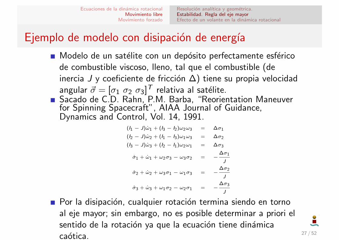
Ejemplo de modelo con disipacion de energıa
Modelo de un satelite con un deposito perfectamente esfericode combustible viscoso, lleno, tal que el combustible (deinercia J y coeficiente de friccion ∆) tiene su propia velocidadangular ~σ = [σ1 σ2 σ3]T relativa al satelite.Sacado de C.D. Rahn, P.M. Barba, “Reorientation Maneuverfor Spinning Spacecraft”, AIAA Journal of Guidance,Dynamics and Control, Vol. 14, 1991.
(I1 − J)ω1 + (I3 − I2)ω2ω3 = ∆σ1
(I2 − J)ω2 + (I1 − I3)ω1ω3 = ∆σ2
(I3 − J)ω3 + (I2 − I1)ω2ω1 = ∆σ3
σ1 + ω1 + ω2σ3 − ω3σ2 = −∆σ1
J
σ2 + ω2 + ω3σ1 − ω1σ3 = −∆σ2
J
σ3 + ω3 + ω1σ2 − ω2σ1 = −∆σ3
J
Por la disipacion, cualquier rotacion termina siendo en tornoal eje mayor; sin embargo, no es posible determinar a priori elsentido de la rotacion ya que la ecuacion tiene dinamicacaotica. 27 / 52
Ecuaciones de la dinamica rotacionalMovimiento libre
Movimiento forzado
Resolucion analıtica y geometrica.Estabilidad. Regla del eje mayorEfecto de un volante en la dinamica rotacional
Ejemplo de modelo con disipacion de energıa
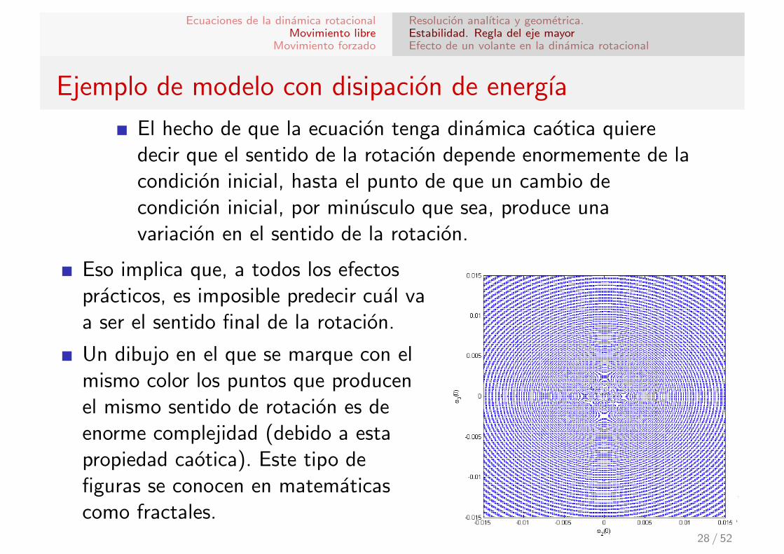
El hecho de que la ecuacion tenga dinamica caotica quieredecir que el sentido de la rotacion depende enormemente de lacondicion inicial, hasta el punto de que un cambio decondicion inicial, por minusculo que sea, produce unavariacion en el sentido de la rotacion.
Eso implica que, a todos los efectospracticos, es imposible predecir cual vaa ser el sentido final de la rotacion.
Un dibujo en el que se marque con elmismo color los puntos que producenel mismo sentido de rotacion es deenorme complejidad (debido a estapropiedad caotica). Este tipo defiguras se conocen en matematicascomo fractales.
28 / 52
Ecuaciones de la dinamica rotacionalMovimiento libre
Movimiento forzado
Resolucion analıtica y geometrica.Estabilidad. Regla del eje mayorEfecto de un volante en la dinamica rotacional
Regla del eje mayor. Consideraciones.
La inestabilidad que surge en el eje menor tiene una escala detiempo muy inferior a la inestabilidad en el eje intermedio;dicha escala dependera de la velocidad con la que la energıase disipa.
Si el movimiento deseado es una rotacion en torno al ejemayor se puede amplificar este efecto anadiendo disipacion:disipadores de nutacion (“pendulos” con friccion anadidos alsistema).
Si puntualmente es necesaria una rotacion en torno al ejemenor, no hay ningun problema mientras se requiera por uncorto periodo de tiempo. Luego se puede volver a una rotacionen torno al eje mayor simplemente dejando pasar el tiempo.
La presencia de partes moviles (p.ej. volantes de inercia)cambia estos resultados teoricos.
29 / 52
Ecuaciones de la dinamica rotacionalMovimiento libre
Movimiento forzado
Resolucion analıtica y geometrica.Estabilidad. Regla del eje mayorEfecto de un volante en la dinamica rotacional
Ecuaciones rotacionales con plataforma/volante de inercia.
Supongamos que el vehıculo posee un volante de inercia en eleje 3, con inercia IR , y que gira a una velocidad ωR relativa alresto del vehıculo. Tambien podrıa tratarse de un sistema derotacion doble, es decir, parte del vehıculo (rotor) gira conrespecto al resto del vehıculo (plataforma) con una velocidadangular relativa.
El momento cinetico del sistema serıaΓ = [I1ω1 I2ω2 I3ω3 + IRωR ]T .
Las ecuaciones de Euler quedan ahora:
I1ω1 + (I3 − I2)ω2ω3 + IRωRω2 = 0
I2ω2 + (I1 − I3)ω1ω3 − IRωRω1 = 0
I3ω3 + IR ωR + (I2 − I1)ω2ω1 = 0
Ademas hay que anadir IR(ω3 + ωR) = J, donde J es el pardel motor que controla el giro relativo del volante.
30 / 52
Ecuaciones de la dinamica rotacionalMovimiento libre
Movimiento forzado
Resolucion analıtica y geometrica.Estabilidad. Regla del eje mayorEfecto de un volante en la dinamica rotacional
Ecuaciones rotacionales con plataforma/volante de inercia.
Podemos usar el motor, por ejemplo, para mantener ωR
constante. En tal caso las ecuaciones se reducen a:
I1ω1 + (I3 − I2)ω2ω3 + IRωRω2 = 0
I2ω2 + (I1 − I3)ω1ω3 − IRωRω1 = 0
I3ω3 + (I2 − I1)ω2ω1 = 0
Ahora aparecen terminos nuevos que modifican el analisis deestabilidad. Por ejemplo el eje intermedio se podrıa hacerestable!! Repitiendo el analisis de estabilidad de antes:
δω1 +(n(I3 − I2) + IRωR) (n(I3 − I1) + IRωR)
I1I2δω1 = 0
Si por ejemplo, el eje 1 es el menor y el eje 2 es el mayor, lacondicion necesaria para la estabilidad esn(I3 − I2) + IRωR > 0, es decir, ωR >
I2−I3IR
n.Se puede realizar un analisis de energıa y encontrarcondiciones para que la estabilidad se verifique incluso enpresencia de disipacion de energıa! 31 / 52
Ecuaciones de la dinamica rotacionalMovimiento libre
Movimiento forzado
Resolucion analıtica y geometrica.Estabilidad. Regla del eje mayorEfecto de un volante en la dinamica rotacional
Disipacion de energıa con plataforma/volante de inercia.
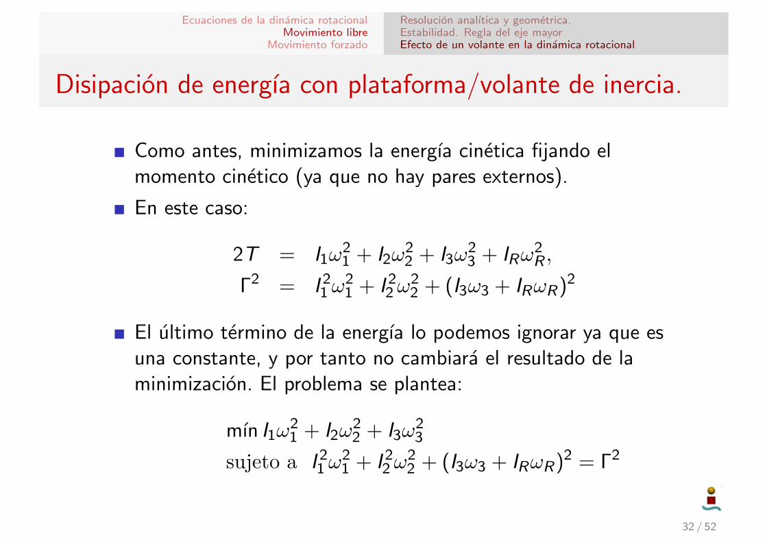
Como antes, minimizamos la energıa cinetica fijando elmomento cinetico (ya que no hay pares externos).
En este caso:
2T = I1ω21 + I2ω
22 + I3ω
23 + IRω
2R ,
Γ2 = I 21ω
21 + I 2
2ω22 + (I3ω3 + IRωR)2
El ultimo termino de la energıa lo podemos ignorar ya que esuna constante, y por tanto no cambiara el resultado de laminimizacion. El problema se plantea:
mın I1ω21 + I2ω
22 + I3ω
23
sujeto a I 21ω
21 + I 2
2ω22 + (I3ω3 + IRωR)2 = Γ2
32 / 52
Ecuaciones de la dinamica rotacionalMovimiento libre
Movimiento forzado
Resolucion analıtica y geometrica.Estabilidad. Regla del eje mayorEfecto de un volante en la dinamica rotacional
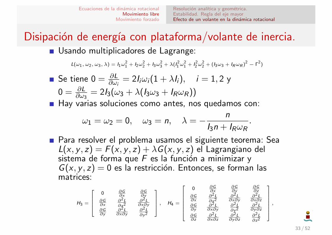
Disipacion de energıa con plataforma/volante de inercia.Usando multiplicadores de Lagrange:
L(ω1, ω2, ω3, λ) = I1ω21 + I2ω
22 + I3ω
23 + λ(I 2
1ω21 + I 2
2ω22 + (I3ω3 + IRωR )2 − Γ2)
Se tiene 0 = ∂L∂ωi
= 2Iiωi (1 + λIi ), i = 1, 2 y
0 = ∂L∂ω3
= 2I3(ω3 + λ(I3ω3 + IRωR))
Hay varias soluciones como antes, nos quedamos con:
ω1 = ω2 = 0, ω3 = n, λ = − n
I3n + IRωR.
Para resolver el problema usamos el siguiente teorema: SeaL(x , y , z) = F (x , y , z) + λG (x , y , z) el Lagrangiano delsistema de forma que F es la funcion a minimizar yG (x , y , z) = 0 es la restriccion. Entonces, se forman lasmatrices:
H3 =
0 ∂G
∂x∂G∂y
∂G∂x
∂2L∂x2
∂2L∂x∂y
∂G∂y
∂2L∂x∂y
∂2L∂y2
, H4 =
0 ∂G
∂x∂G∂y
∂G∂z
∂G∂x
∂2L∂x2
∂2L∂x∂y
∂2L∂x∂z
∂G∂y
∂2L∂x∂y
∂2L∂y2
∂2L∂y∂z
∂G∂z
∂2L∂x∂z
∂2L∂y∂z
∂2L∂z2
,
33 / 52
Ecuaciones de la dinamica rotacionalMovimiento libre
Movimiento forzado
Resolucion analıtica y geometrica.Estabilidad. Regla del eje mayorEfecto de un volante en la dinamica rotacional
Disipacion de energıa con plataforma/volante de inercia.
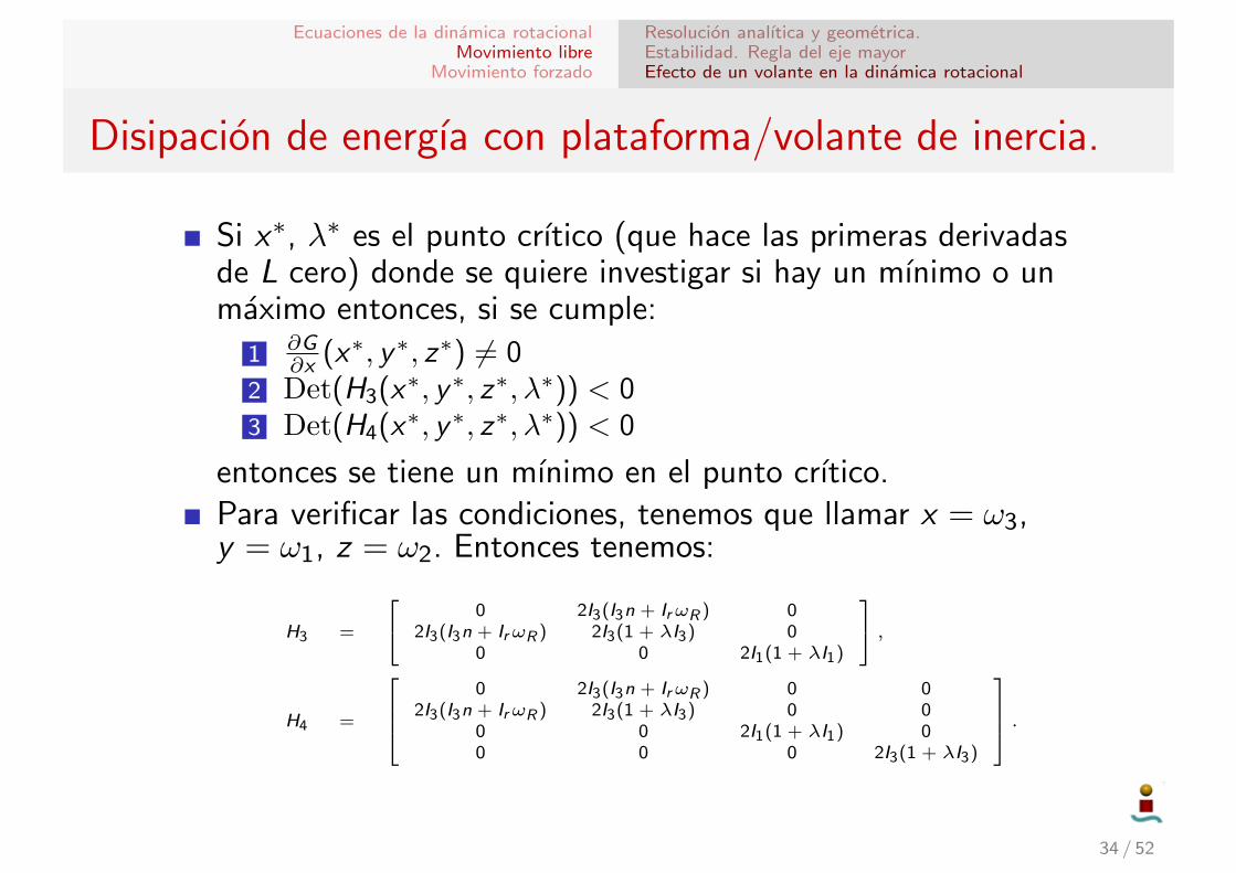
Si x∗, λ∗ es el punto crıtico (que hace las primeras derivadasde L cero) donde se quiere investigar si hay un mınimo o unmaximo entonces, si se cumple:
1 ∂G∂x (x∗, y∗, z∗) 6= 0
2 Det(H3(x∗, y∗, z∗, λ∗)) < 03 Det(H4(x∗, y∗, z∗, λ∗)) < 0
entonces se tiene un mınimo en el punto crıtico.Para verificar las condiciones, tenemos que llamar x = ω3,y = ω1, z = ω2. Entonces tenemos:
H3 =
0 2I3(I3n + IrωR ) 02I3(I3n + IrωR ) 2I3(1 + λI3) 0
0 0 2I1(1 + λI1)
,
H4 =
0 2I3(I3n + IrωR ) 0 0
2I3(I3n + IrωR ) 2I3(1 + λI3) 0 00 0 2I1(1 + λI1) 00 0 0 2I3(1 + λI3)
.
34 / 52
Ecuaciones de la dinamica rotacionalMovimiento libre
Movimiento forzado
Resolucion analıtica y geometrica.Estabilidad. Regla del eje mayorEfecto de un volante en la dinamica rotacional
Disipacion de energıa con plataforma/volante de inercia.
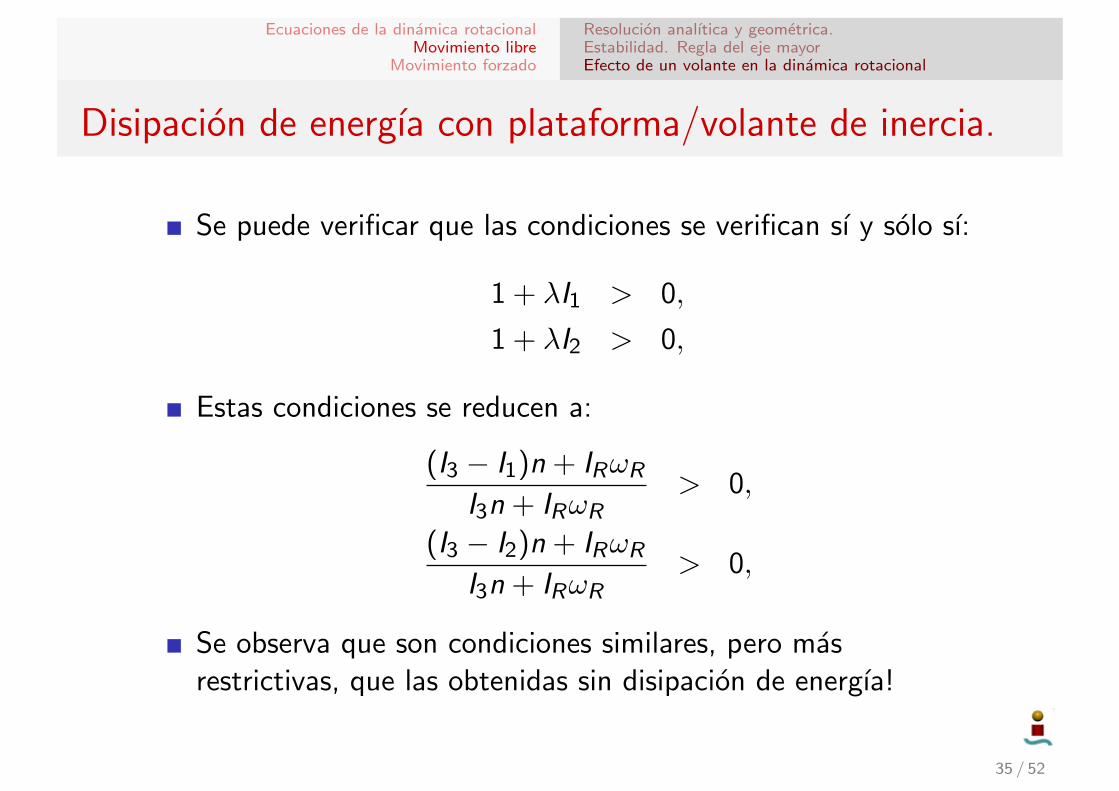
Se puede verificar que las condiciones se verifican sı y solo sı:
1 + λI1 > 0,
1 + λI2 > 0,
Estas condiciones se reducen a:
(I3 − I1)n + IRωR
I3n + IRωR> 0,
(I3 − I2)n + IRωR
I3n + IRωR> 0,
Se observa que son condiciones similares, pero masrestrictivas, que las obtenidas sin disipacion de energıa!
35 / 52
Ecuaciones de la dinamica rotacionalMovimiento libre
Movimiento forzado
Momento externo constanteGradiente gravitatorio. Posicion estable
Movimiento forzado
En la realidad siempre existiran momentos perturbadores.Normalmente son de magnitud pequena pero pueden serpersistentes (como por ejemplo el gradiente gravitatorio queactua a lo largo de toda la orbita). Tambien pueden ser masintensos, como por ejemplo en el caso de toberas propulsivasno perfectamente alineadas durante maniobras.
En esta seccion analizaremos dos casos:
Momento perturbador constante actuando sobre un solido enrotacion (efecto giroscopico).Efecto en la estabilidad del gradiente gravitatorio.
Ademas expondremos un modelo de vehıculo espacial conruedas y volante de inercia que sera necesario para el posteriortema de control.
36 / 52
Ecuaciones de la dinamica rotacionalMovimiento libre
Movimiento forzado
Momento externo constanteGradiente gravitatorio. Posicion estable
Cuerpo en rotacion sujeto a un momento externo constante
Modelamos este caso con las siguientes hipotesis:
Vehıculo axilsimetrico: I1 = I2 = I .Vehıculo rotando con velocidad n en torno a su eje 3, es decir,ω3 = n.Momento perturbador constante M1 en el eje 1. Sin momentoen el resto de los ejes.
Esta situacion modela, por ejemplo, el caso de un vehıculoestabilizado por rotacion que realiza una maniobra propulsiva,pero con la tobera ligeramente desalineada con el eje derotacion. Si el vehıculo no rotara, el momento causarıa el giroinmediato del vehıculo y la maniobra fallarıa.
Veremos que al haber rotacion el vehıculo posee “rigidezgiroscopica” y el momento perturbador lo que finamenteproduce es un movimiento (posiblemente muy pequeno) deprecesion y nutacion del eje de giro.
37 / 52
Ecuaciones de la dinamica rotacionalMovimiento libre
Movimiento forzado
Momento externo constanteGradiente gravitatorio. Posicion estable
Cuerpo en rotacion sujeto a un momento externo constante
Las ecuaciones que modelan el movimiento son:
I ω1 + (I3 − I )ω2ω3 = M1
I ω2 + (I − I3)ω1ω3 = 0
I3ω3 = 0
Encontramos la solucion ω3 = Cte = n y definimos λ = I−I3I n
y µ = M1I . La ecuacion a resolver es:
ω1 − λω2 = µ
ω2 + λω1 = 0
Derivando en la primera ecuacion y sustituyendo la segunda:
ω1 + λ2ω1 = 0
La solucion de esta ecuacion es ω1(t) = A senλt + B cosλt.38 / 52
Ecuaciones de la dinamica rotacionalMovimiento libre
Movimiento forzado
Momento externo constanteGradiente gravitatorio. Posicion estable
Cuerpo en rotacion sujeto a un momento externo constante
Sustituyendo en la 1a ecuacion: ω2(t) = A cosλt − B senλt − µλ .
Usando las condiciones iniciales ω1(0) y ω2(0) encontramos:B = ω1(0), A = ω2(0) + µ
λ . Por tanto:
ω1 =(ω2(0) +
µ
λ
)senλt + ω1(0) cosλt =
µ
λsenλt
ω2 =(ω2(0) +
µ
λ
)cosλt − ω1(0) senλt − µ
λ=µ
λ(cosλt − 1)
donde finalmente se han supuesto ω1(0) = ω2(0) = 0.Para describir la actitud usamos unos angulos de Euler:
Iθ1−→xn
Sθ2−→yS
S ′θ3−→zS′
BFS
En el desarrollo de las ecuaciones cinematicas se llegarıa a:
θ1 =ω1 cos θ3 − ω2 sen θ3
cos θ2
θ2 = ω1 sen θ3 + ω2 cos θ3
θ3 = ω3 + (−ω1 cos θ3 + ω2 sen θ3) tan θ2 39 / 52
Ecuaciones de la dinamica rotacionalMovimiento libre
Movimiento forzado
Momento externo constanteGradiente gravitatorio. Posicion estable
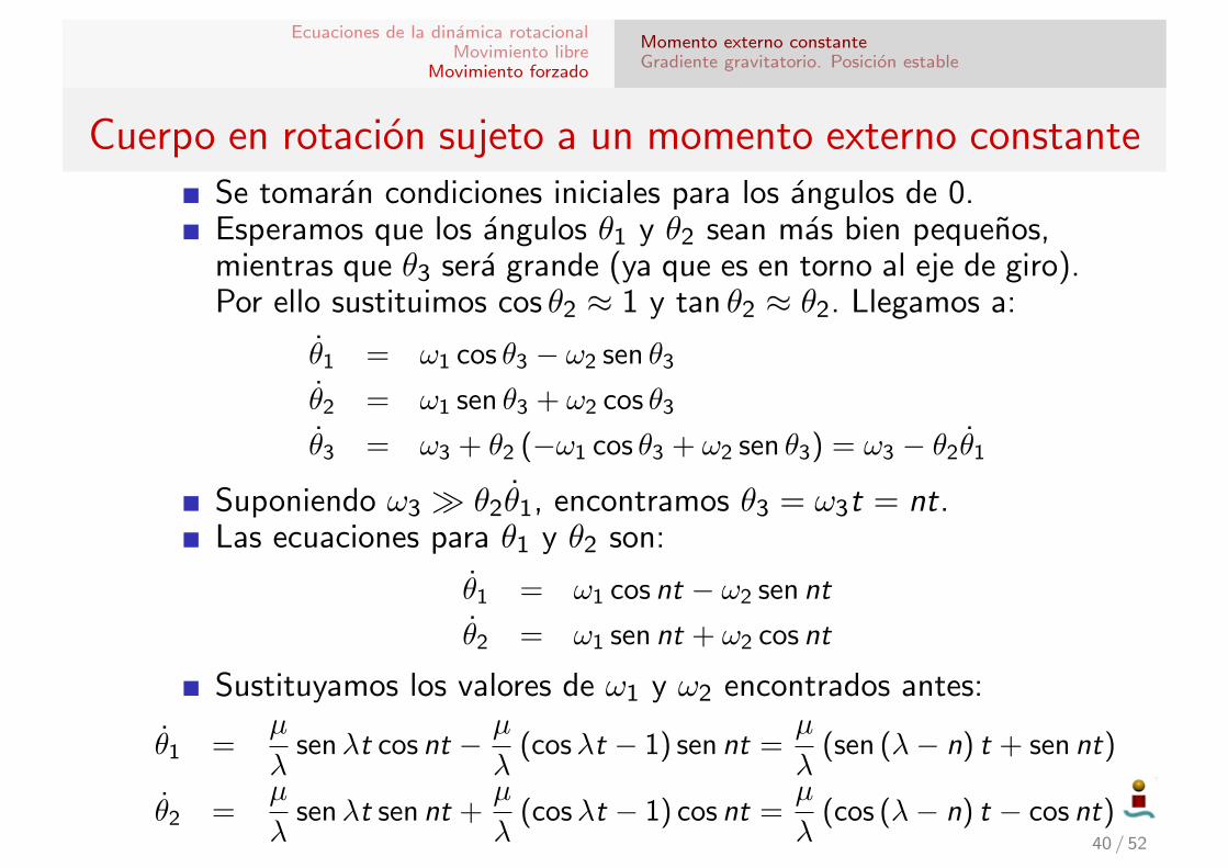
Cuerpo en rotacion sujeto a un momento externo constanteSe tomaran condiciones iniciales para los angulos de 0.Esperamos que los angulos θ1 y θ2 sean mas bien pequenos,mientras que θ3 sera grande (ya que es en torno al eje de giro).Por ello sustituimos cos θ2 ≈ 1 y tan θ2 ≈ θ2. Llegamos a:
θ1 = ω1 cos θ3 − ω2 sen θ3
θ2 = ω1 sen θ3 + ω2 cos θ3
θ3 = ω3 + θ2 (−ω1 cos θ3 + ω2 sen θ3) = ω3 − θ2θ1
Suponiendo ω3 � θ2θ1, encontramos θ3 = ω3t = nt.Las ecuaciones para θ1 y θ2 son:
θ1 = ω1 cos nt − ω2 sen nt
θ2 = ω1 sen nt + ω2 cos nt
Sustituyamos los valores de ω1 y ω2 encontrados antes:
θ1 =µ
λsenλt cos nt − µ
λ(cosλt − 1) sen nt =
µ
λ(sen (λ− n) t + sen nt)
θ2 =µ
λsenλt sen nt +
µ
λ(cosλt − 1) cos nt =
µ
λ(cos (λ− n) t − cos nt)
40 / 52
Ecuaciones de la dinamica rotacionalMovimiento libre
Movimiento forzado
Momento externo constanteGradiente gravitatorio. Posicion estable
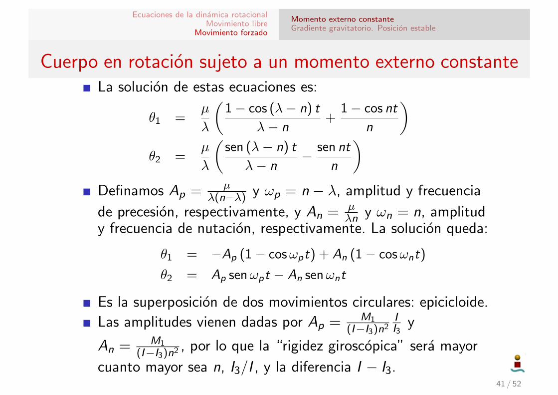
Cuerpo en rotacion sujeto a un momento externo constanteLa solucion de estas ecuaciones es:
θ1 =µ
λ
(1− cos (λ− n) t
λ− n+
1− cos nt
n
)θ2 =
µ
λ
(sen (λ− n) t
λ− n− sen nt
n
)Definamos Ap = µ
λ(n−λ) y ωp = n − λ, amplitud y frecuencia
de precesion, respectivamente, y An = µλn y ωn = n, amplitud
y frecuencia de nutacion, respectivamente. La solucion queda:
θ1 = −Ap (1− cosωpt) + An (1− cosωnt)
θ2 = Ap senωpt − An senωnt
Es la superposicion de dos movimientos circulares: epicicloide.
Las amplitudes vienen dadas por Ap = M1(I−I3)n2
II3
y
An = M1(I−I3)n2 , por lo que la “rigidez giroscopica” sera mayor
cuanto mayor sea n, I3/I , y la diferencia I − I3.41 / 52
Ecuaciones de la dinamica rotacionalMovimiento libre
Movimiento forzado
Momento externo constanteGradiente gravitatorio. Posicion estable
Gradiente gravitatorio.
El par perturbador mas importante es el gradientegravitatorio, puesto que siempre esta presente en orbita.
Vamos a estudiar el caso de un vehıculo espacial asimetrico enorbita circular de radio R en torno a un planeta esferico; lasorbitas elıpticas y las desviaciones de la gravedad esferica(p.ej. el J2) introducen terminos de orden mayor que noanalizaremos.
La velocidad angular se estudiara en ejes cuerpo; sin embargolos angulos de Euler elegidos seran respecto a ejes orbita, queen sı no es un sistema de referencia inercial, lo que tendra quetomarse en cuenta.
La situacion es la de la figura de la transparencia siguiente.Los ejes N son los inerciales, los ejes A son los ejes orbita (quedefiniremos) y los ejes B los ejes cuerpo (en ejes principales deinercia).
42 / 52
Ecuaciones de la dinamica rotacionalMovimiento libre
Movimiento forzado
Momento externo constanteGradiente gravitatorio. Posicion estable
Gradiente gravitatorio.
“Chapter06” — 2008/6/6 — 14:34 — page 387 — #39!!
!!
!!
!!
RIGID-BODY DYNAMICS 387
Fig. 6.8 Rigid body in a circular orbit.
The gravity-gradient torque about the spacecraft’s mass center is thenexpressed as
!M =!
!! " d !f = #µ
! !! " !Rc
| !Rc + !!|3dm (6.143)
and we have the following approximation:
| !Rc + !!|#3 = R#3c
"
1 + 2( !Rc · !!)
R2c
+ !2
R2c
## 32
= R#3c
"
1 # 3( !Rc · !!)
R2c
+ higher-order terms
#
(6.144)
where Rc = | !Rc| and ! = | !!|. Because$
!! dm = 0, the gravity-gradient torqueneglecting the higher-order terms can be written as
!M = 3µ
R5c
!(!Rc · !!) ( !! " !Rc) dm (6.145)
This equation is further manipulated as follows:
!M = #3µ
R5c
!Rc "!
!!( !! · !Rc) dm
= #3µ
R5c
!Rc "!
!! !! dm · !Rc
= #3µ
R5c
!Rc "% !
!2 I dm # J&
· !Rc
= #3µ
R5c
!Rc "!
!2 I dm · !Rc + 3µ
R5c
!Rc " J · !Rc
= 3µ
R5c
!Rc " J · !Rc
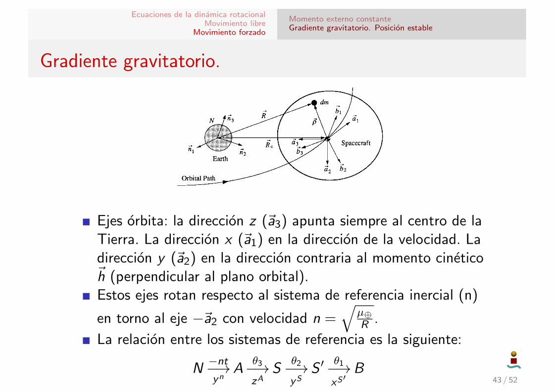
Ejes orbita: la direccion z (~a3) apunta siempre al centro de laTierra. La direccion x (~a1) en la direccion de la velocidad. Ladireccion y (~a2) en la direccion contraria al momento cinetico~h (perpendicular al plano orbital).Estos ejes rotan respecto al sistema de referencia inercial (n)
en torno al eje −~a2 con velocidad n =√
µ⊕R .
La relacion entre los sistemas de referencia es la siguiente:
N−nt−→yn
Aθ3−→zA
Sθ2−→yS
S ′θ1−→xS′
B
La situacion es la de la figura de la transparencia siguiente.Los ejes N son los inerciales, los ejes A son los ejes orbita (quedefiniremos) y los ejes B los ejes cuerpo (en ejes principales deinercia).
43 / 52
Ecuaciones de la dinamica rotacionalMovimiento libre
Movimiento forzado
Momento externo constanteGradiente gravitatorio. Posicion estable
Gradiente gravitatorio.
“Chapter06” — 2008/6/6 — 14:34 — page 387 — #39!!
!!
!!
!!
RIGID-BODY DYNAMICS 387
Fig. 6.8 Rigid body in a circular orbit.
The gravity-gradient torque about the spacecraft’s mass center is thenexpressed as
!M =!
!! " d !f = #µ
! !! " !Rc
| !Rc + !!|3dm (6.143)
and we have the following approximation:
| !Rc + !!|#3 = R#3c
"
1 + 2( !Rc · !!)
R2c
+ !2
R2c
## 32
= R#3c
"
1 # 3( !Rc · !!)
R2c
+ higher-order terms
#
(6.144)
where Rc = | !Rc| and ! = | !!|. Because$
!! dm = 0, the gravity-gradient torqueneglecting the higher-order terms can be written as
!M = 3µ
R5c
!(!Rc · !!) ( !! " !Rc) dm (6.145)
This equation is further manipulated as follows:
!M = #3µ
R5c
!Rc "!
!!( !! · !Rc) dm
= #3µ
R5c
!Rc "!
!! !! dm · !Rc
= #3µ
R5c
!Rc "% !
!2 I dm # J&
· !Rc
= #3µ
R5c
!Rc "!
!2 I dm · !Rc + 3µ
R5c
!Rc " J · !Rc
= 3µ
R5c
!Rc " J · !Rc
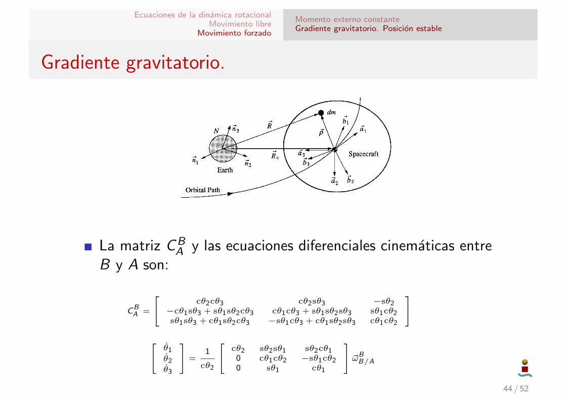
La matriz CBA y las ecuaciones diferenciales cinematicas entre
B y A son:
CBA =
cθ2cθ3 cθ2sθ3 −sθ2−cθ1sθ3 + sθ1sθ2cθ3 cθ1cθ3 + sθ1sθ2sθ3 sθ1cθ2sθ1sθ3 + cθ1sθ2cθ3 −sθ1cθ3 + cθ1sθ2sθ3 cθ1cθ2
θ1
θ2
θ3
=1
cθ2
cθ2 sθ2sθ1 sθ2cθ10 cθ1cθ2 −sθ1cθ20 sθ1 cθ1
~ωBB/A
44 / 52
Ecuaciones de la dinamica rotacionalMovimiento libre
Movimiento forzado
Momento externo constanteGradiente gravitatorio. Posicion estable
Gradiente gravitatorio.
“Chapter06” — 2008/6/6 — 14:34 — page 387 — #39!!
!!
!!
!!
RIGID-BODY DYNAMICS 387
Fig. 6.8 Rigid body in a circular orbit.
The gravity-gradient torque about the spacecraft’s mass center is thenexpressed as
!M =!
!! " d !f = #µ
! !! " !Rc
| !Rc + !!|3dm (6.143)
and we have the following approximation:
| !Rc + !!|#3 = R#3c
"
1 + 2( !Rc · !!)
R2c
+ !2
R2c
## 32
= R#3c
"
1 # 3( !Rc · !!)
R2c
+ higher-order terms
#
(6.144)
where Rc = | !Rc| and ! = | !!|. Because$
!! dm = 0, the gravity-gradient torqueneglecting the higher-order terms can be written as
!M = 3µ
R5c
!(!Rc · !!) ( !! " !Rc) dm (6.145)
This equation is further manipulated as follows:
!M = #3µ
R5c
!Rc "!
!!( !! · !Rc) dm
= #3µ
R5c
!Rc "!
!! !! dm · !Rc
= #3µ
R5c
!Rc "% !
!2 I dm # J&
· !Rc
= #3µ
R5c
!Rc "!
!2 I dm · !Rc + 3µ
R5c
!Rc " J · !Rc
= 3µ
R5c
!Rc " J · !Rc
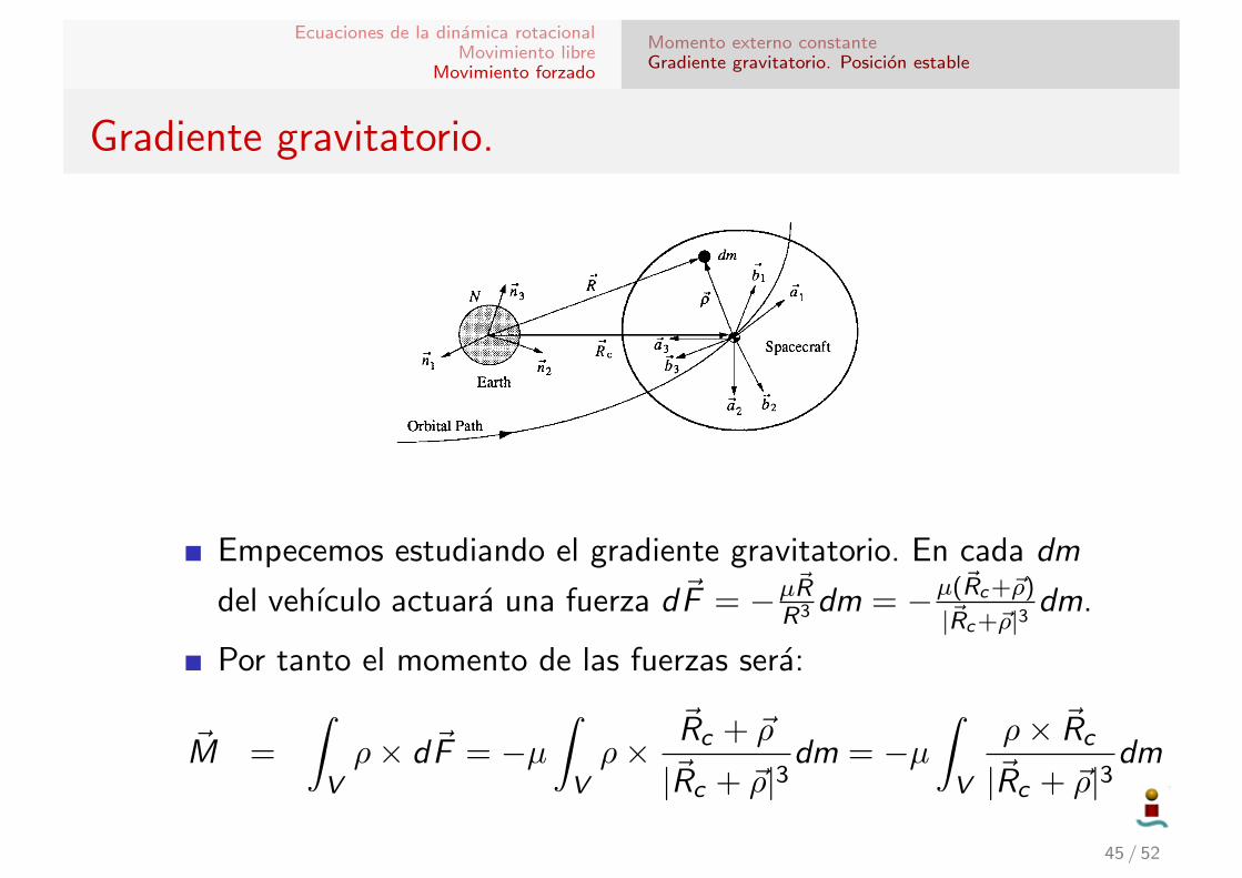
Empecemos estudiando el gradiente gravitatorio. En cada dm
del vehıculo actuara una fuerza d~F = −µ~RR3 dm = −µ(~Rc+~ρ)
|~Rc+~ρ|3dm.
Por tanto el momento de las fuerzas sera:
~M =
∫Vρ× d~F = −µ
∫Vρ×
~Rc + ~ρ
|~Rc + ~ρ|3dm = −µ
∫V
ρ× ~Rc
|~Rc + ~ρ|3dm
45 / 52
Ecuaciones de la dinamica rotacionalMovimiento libre
Movimiento forzado
Momento externo constanteGradiente gravitatorio. Posicion estable
Gradiente gravitatorio.
“Chapter06” — 2008/6/6 — 14:34 — page 387 — #39!!
!!
!!
!!
RIGID-BODY DYNAMICS 387
Fig. 6.8 Rigid body in a circular orbit.
The gravity-gradient torque about the spacecraft’s mass center is thenexpressed as
!M =!
!! " d !f = #µ
! !! " !Rc
| !Rc + !!|3dm (6.143)
and we have the following approximation:
| !Rc + !!|#3 = R#3c
"
1 + 2( !Rc · !!)
R2c
+ !2
R2c
## 32
= R#3c
"
1 # 3( !Rc · !!)
R2c
+ higher-order terms
#
(6.144)
where Rc = | !Rc| and ! = | !!|. Because$
!! dm = 0, the gravity-gradient torqueneglecting the higher-order terms can be written as
!M = 3µ
R5c
!(!Rc · !!) ( !! " !Rc) dm (6.145)
This equation is further manipulated as follows:
!M = #3µ
R5c
!Rc "!
!!( !! · !Rc) dm
= #3µ
R5c
!Rc "!
!! !! dm · !Rc
= #3µ
R5c
!Rc "% !
!2 I dm # J&
· !Rc
= #3µ
R5c
!Rc "!
!2 I dm · !Rc + 3µ
R5c
!Rc " J · !Rc
= 3µ
R5c
!Rc " J · !Rc
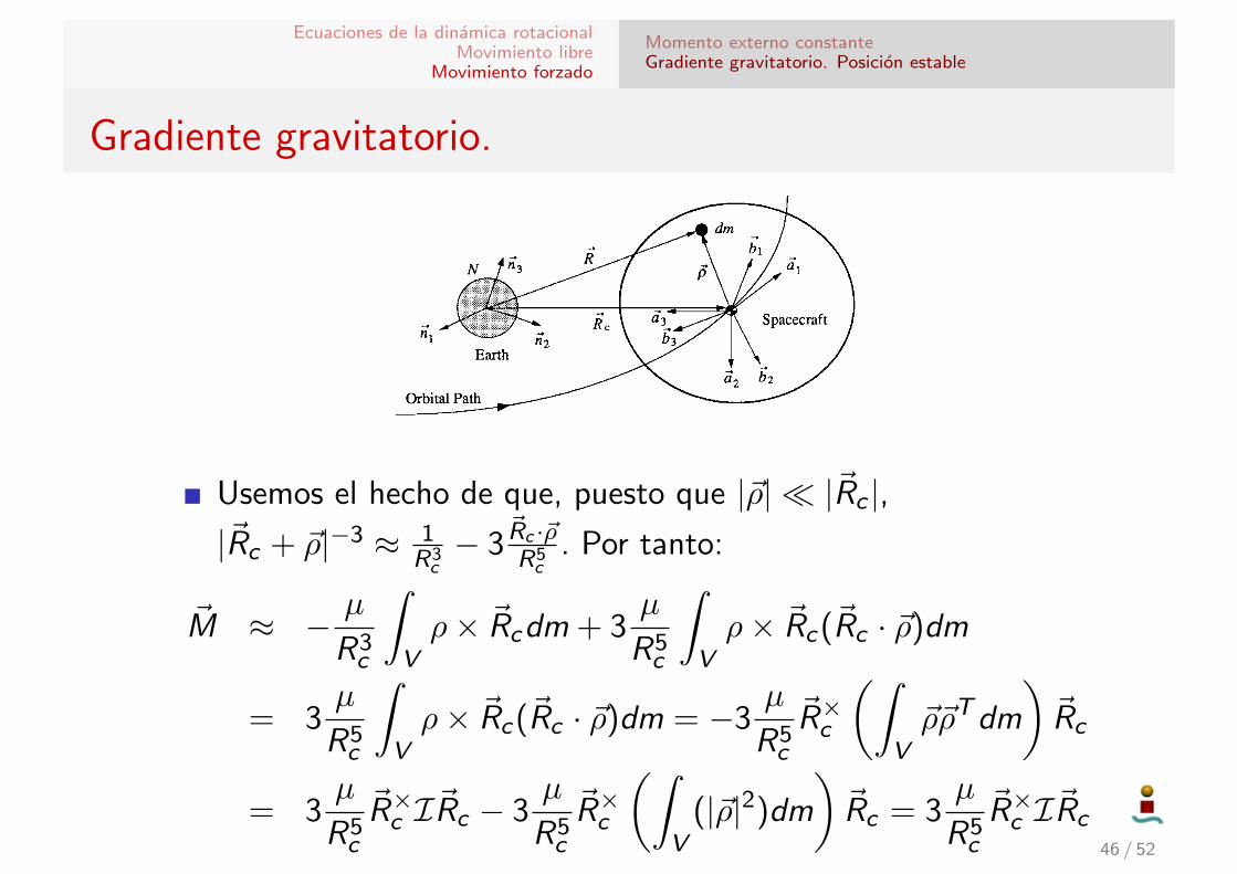
Usemos el hecho de que, puesto que |~ρ| � |~Rc |,|~Rc + ~ρ|−3 ≈ 1
R3c− 3
~Rc ·~ρR5c
. Por tanto:
~M ≈ − µ
R3c
∫Vρ× ~Rcdm + 3
µ
R5c
∫Vρ× ~Rc(~Rc · ~ρ)dm
= 3µ
R5c
∫Vρ× ~Rc(~Rc · ~ρ)dm = −3
µ
R5c
~R×c
(∫V~ρ~ρTdm
)~Rc
= 3µ
R5c
~R×c I~Rc − 3µ
R5c
~R×c
(∫V
(|~ρ|2)dm
)~Rc = 3
µ
R5c
~R×c I~Rc46 / 52
Ecuaciones de la dinamica rotacionalMovimiento libre
Movimiento forzado
Momento externo constanteGradiente gravitatorio. Posicion estable
Gradiente gravitatorio.
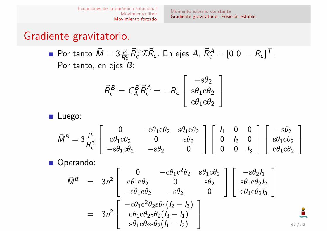
Por tanto ~M = 3 µR5c
~R×c I~Rc . En ejes A, ~RAc = [0 0 − Rc ]T .
Por tanto, en ejes B:
~RBc = CB
A~RAc = −Rc
−sθ2
sθ1cθ2
cθ1cθ2
Luego:
~MB = 3µ
R3c
0 −cθ1cθ2 sθ1cθ2
cθ1cθ2 0 sθ2
−sθ1cθ2 −sθ2 0
I1 0 00 I2 00 0 I3
−sθ2
sθ1cθ2
cθ1cθ2
Operando:
~MB = 3n2
0 −cθ1c2θ2 sθ1cθ2
cθ1cθ2 0 sθ2
−sθ1cθ2 −sθ2 0
−sθ2I1sθ1cθ2I2cθ1cθ2I3
= 3n2
−cθ1c2θ2sθ1(I2 − I3)
cθ1cθ2sθ2(I3 − I1)sθ1cθ2sθ2(I1 − I2)
47 / 52
Ecuaciones de la dinamica rotacionalMovimiento libre
Movimiento forzado
Momento externo constanteGradiente gravitatorio. Posicion estable
Gradiente gravitatorio.
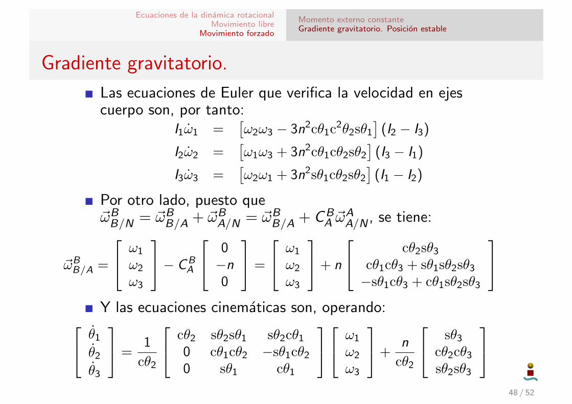
Las ecuaciones de Euler que verifica la velocidad en ejescuerpo son, por tanto:
I1ω1 =[ω2ω3 − 3n2cθ1c
2θ2sθ1
](I2 − I3)
I2ω2 =[ω1ω3 + 3n2cθ1cθ2sθ2
](I3 − I1)
I3ω3 =[ω2ω1 + 3n2sθ1cθ2sθ2
](I1 − I2)
Por otro lado, puesto que~ωBB/N = ~ωB
B/A + ~ωBA/N = ~ωB
B/A + CBA ~ω
AA/N , se tiene:
~ωBB/A =
ω1
ω2
ω3
− CBA
0−n0
=
ω1
ω2
ω3
+ n
cθ2sθ3
cθ1cθ3 + sθ1sθ2sθ3
−sθ1cθ3 + cθ1sθ2sθ3
Y las ecuaciones cinematicas son, operando: θ1
θ2
θ3
=1
cθ2
cθ2 sθ2sθ1 sθ2cθ1
0 cθ1cθ2 −sθ1cθ2
0 sθ1 cθ1
ω1
ω2
ω3
+n
cθ2
sθ3
cθ2cθ3
sθ2sθ3
48 / 52
Ecuaciones de la dinamica rotacionalMovimiento libre
Movimiento forzado
Momento externo constanteGradiente gravitatorio. Posicion estable
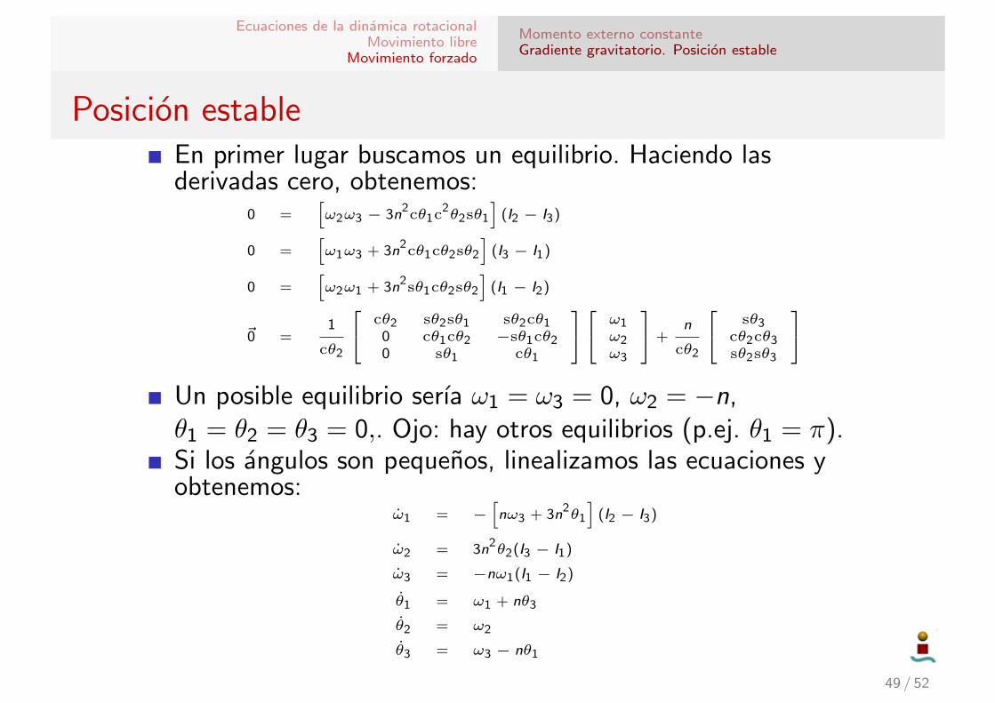
Posicion estableEn primer lugar buscamos un equilibrio. Haciendo lasderivadas cero, obtenemos:
0 =[ω2ω3 − 3n2
cθ1c2θ2sθ1
](I2 − I3)
0 =[ω1ω3 + 3n2
cθ1cθ2sθ2
](I3 − I1)
0 =[ω2ω1 + 3n2
sθ1cθ2sθ2
](I1 − I2)
~0 =1
cθ2
cθ2 sθ2sθ1 sθ2cθ10 cθ1cθ2 −sθ1cθ20 sθ1 cθ1
ω1ω2ω3
+n
cθ2
sθ3cθ2cθ3sθ2sθ3
Un posible equilibrio serıa ω1 = ω3 = 0, ω2 = −n,θ1 = θ2 = θ3 = 0,. Ojo: hay otros equilibrios (p.ej. θ1 = π).Si los angulos son pequenos, linealizamos las ecuaciones yobtenemos:
ω1 = −[nω3 + 3n2
θ1
](I2 − I3)
ω2 = 3n2θ2(I3 − I1)
ω3 = −nω1(I1 − I2)
θ1 = ω1 + nθ3
θ2 = ω2
θ3 = ω3 − nθ1
49 / 52
Ecuaciones de la dinamica rotacionalMovimiento libre
Movimiento forzado
Momento externo constanteGradiente gravitatorio. Posicion estable
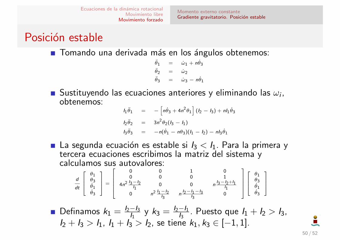
Posicion estableTomando una derivada mas en los angulos obtenemos:
θ1 = ω1 + nθ3
θ2 = ω2
θ3 = ω3 − nθ1
Sustituyendo las ecuaciones anteriores y eliminando las ωi ,obtenemos:
I1θ1 = −[nθ3 + 4n2
θ1
](I2 − I3) + nI1θ3
I2θ2 = 3n2θ2(I3 − I1)
I3θ3 = −n(θ1 − nθ3)(I1 − I2)− nI3θ1
La segunda ecuacion es estable si I3 < I1. Para la primera ytercera ecuaciones escribimos la matriz del sistema ycalculamos sus autovalores:
d
dt
θ1θ3
θ1
θ3
=
0 0 1 00 0 0 1
4n2 I3−I2I1
0 0 nI3−I2+I1
I1
0 n2 I1−I2I3
nI2−I1−I3
I30
θ1θ3
θ1
θ3
Definamos k1 = I2−I3I1
y k3 = I2−I1I3
. Puesto que I1 + I2 > I3,I2 + I3 > I1, I1 + I3 > I2, se tiene k1, k3 ∈ [−1, 1].
50 / 52
Ecuaciones de la dinamica rotacionalMovimiento libre
Movimiento forzado
Momento externo constanteGradiente gravitatorio. Posicion estable
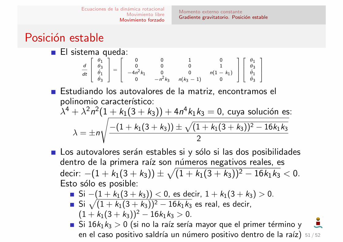
Posicion estableEl sistema queda:
d
dt
θ1θ3
θ1
θ3
=
0 0 1 00 0 0 1
−4n2k1 0 0 n(1− k1)
0 −n2k3 n(k3 − 1) 0
θ1θ3
θ1
θ3
Estudiando los autovalores de la matriz, encontramos elpolinomio caracterıstico:λ4 + λ2n2(1 + k1(3 + k3)) + 4n4k1k3 = 0, cuya solucion es:
λ = ±n
√−(1 + k1(3 + k3))±
√(1 + k1(3 + k3))2 − 16k1k3
2
Los autovalores seran estables si y solo si las dos posibilidadesdentro de la primera raız son numeros negativos reales, esdecir: −(1 + k1(3 + k3))±
√(1 + k1(3 + k3))2 − 16k1k3 < 0.
Esto solo es posible:Si −(1 + k1(3 + k3)) < 0, es decir, 1 + k1(3 + k3) > 0.Si√
(1 + k1(3 + k3))2 − 16k1k3 es real, es decir,(1 + k1(3 + k3))2 − 16k1k3 > 0.Si 16k1k3 > 0 (si no la raız serıa mayor que el primer termino yen el caso positivo saldrıa un numero positivo dentro de la raız) 51 / 52
Ecuaciones de la dinamica rotacionalMovimiento libre
Movimiento forzado
Momento externo constanteGradiente gravitatorio. Posicion estable
Posicion estable
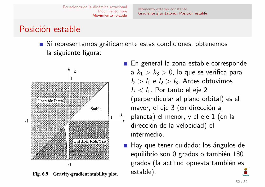
Si representamos graficamente estas condiciones, obtenemosla siguiente figura:
“Chapter06” — 2008/6/6 — 14:34 — page 392 — #44!!
!!
!!
!!
392 SPACE VEHICLE DYNAMICS AND CONTROL
Fig. 6.9 Gravity-gradient stability plot.
The preceding results for linear stability of a rigid body in a circular orbit canbe summarized using a stability diagram in the (k1, k3) plane, as shown in Fig. 6.9.For a further treatment of this subject, see Hughes [2].
Problems
6.10 Consider the sequence of C1(!1) ! C3(!3) ! C2(!2) from the LVLH ref-erence frame A to a body-fixed reference frame B for a rigid spacecraft ina circular orbit.(a) Verify the following relationship:
!
""b1"b2"b3
#
$ =
!
%"c !2 c !3 s !3 #s !2 c !3
#c !1 c !2 s !3 + s !1 s !2 c !1 c !3 c !1 s !2 s !3 + s !1 c !2
s !1 c !2 s !3 + c !1 s !2 #s !1 c !3 #s !1 s !2 s !3 + c !1 c !2
#
&$
!
""a1
"a2
"a3
#
$
where c !i = cos !i and s !i = sin !i.(b) Derive the following kinematic differential equation:
!
"!1!2!3
#
$ = 1cos !3
!
"cos !3 #cos !1 sin !3 sin !1 sin !3
0 cos !1 #sin !1
0 sin !1 cos !3 cos !1 cos !3
#
$
!
""1
"2
"3
#
$ +
!
"0n0
#
$
(c) For small attitude deviations from LVLH orientation, show that the lin-earized dynamic equations of motion, including the products of inertia,
En general la zona estable correspondea k1 > k3 > 0, lo que se verifica paraI2 > I1 e I2 > I3. Antes obtuvimosI3 < I1. Por tanto el eje 2(perpendicular al plano orbital) es elmayor, el eje 3 (en direccion alplaneta) el menor, y el eje 1 (en ladireccion de la velocidad) elintermedio.
Hay que tener cuidado: los angulos deequilibrio son 0 grados o tambien 180grados (la actitud opuesta tambien esestable).
52 / 52