DOCUMENTOS DE TRABAJO - Central Bank of...

DOCUMENTOS DE TRABAJO

An Analysis of the Impact of External Financial Risks on the Sovereign Risk Premium of Latin American Economies

Rodrigo AlfaroCarlos MedelCarola Moreno

N.º 795 Diciembre 2016BANCO CENTRAL DE CHILE

BANCO CENTRAL DE CHILE

CENTRAL BANK OF CHILE

La serie Documentos de Trabajo es una publicación del Banco Central de Chile que divulga los trabajos de investigación económica realizados por profesionales de esta institución o encargados por ella a terceros. El objetivo de la serie es aportar al debate temas relevantes y presentar nuevos enfoques en el análisis de los mismos. La difusión de los Documentos de Trabajo sólo intenta facilitar el intercambio de ideas y dar a conocer investigaciones, con carácter preliminar, para su discusión y comentarios.

La publicación de los Documentos de Trabajo no está sujeta a la aprobación previa de los miembros del Consejo del Banco Central de Chile. Tanto el contenido de los Documentos de Trabajo como también los análisis y conclusiones que de ellos se deriven, son de exclusiva responsabilidad de su o sus autores y no reflejan necesariamente la opinión del Banco Central de Chile o de sus Consejeros.

The Working Papers series of the Central Bank of Chile disseminates economic research conducted by Central Bank staff or third parties under the sponsorship of the Bank. The purpose of the series is to contribute to the discussion of relevant issues and develop new analytical or empirical approaches in their analyses. The only aim of the Working Papers is to disseminate preliminary research for its discussion and comments.

Publication of Working Papers is not subject to previous approval by the members of the Board of the Central Bank. The views and conclusions presented in the papers are exclusively those of the author(s) and do not necessarily reflect the position of the Central Bank of Chile or of the Board members.

Documentos de Trabajo del Banco Central de ChileWorking Papers of the Central Bank of Chile

Agustinas 1180, Santiago, ChileTeléfono: (56-2) 3882475; Fax: (56-2) 3882231

Documento de Trabajo

N° 795

Working Paper

N° 795

AN ANALYSIS OF THE IMPACT OF EXTERNAL

FINANCIAL RISKS ON THE SOVEREIGN RISK PREMIUM

OF LATIN AMERICAN ECONOMIES

Rodrigo Alfaro

Banco Central de Chile

Carlos Medel


Carola Moreno


Abstract

This article presents a quantification of the response of the sovereign risk premium (EMBI) of a

group of Latin American countries, to unexpected changes (shocks) in external financial variables. A

vector autoregressions is estimated for each country (Colombia, Chile, Mexico, and Peru) in monthly

frequency that includes China's and Brazil's EMBI, the global volatility index (VIX), plus the value

of the dollar against a basket of currencies (Broad Index) and a proxy of the slope of the US Treasury

yield curve (Spread US). The VIX and Broad Index shocks turn out to have a relatively homogenous

effect on each country's EMBI, while shocks to the China and Brazil EMBI are more heterogeneous.

For the case of Chile, we further study three alternative risk scenarios, incorporating the copper price

as an additional variable. The most disruptive scenario at the time when the shock hits is the

Volatility driven one. Nevertheless, it is the Emerging market's scenario (namely one with

simultaneous shocks to China’ and Brazil’s EMBI) the one with the most harmful dynamics, as it

dyes out slower. Finally, a Copper price bust scenario, in which the price of copper drops

significantly in addition to a shock to the EMBI China, is the one with the least effect as the price of

copper is relatively less affected by shocks to other variables, displaying lower spillovers.

Resumen

Este artículo cuantifica la respuesta del premio por riesgo soberano (EMBI) de un grupo de países

Latinoamericanos a cambios inesperados (shocks) de variables financieras externas. Se estima un

vector autoregresivo para cada país (Colombia, Chile, México, y Perú) en frecuencia mensual

incluyendo el EMBI de China y Brasil, un índice de volatilidad global (VIX), el precio del dólar con

respecto a una canasta de monedas (Broad Index), y una proxy de la curvatura de la Tasa de Bonos

Soberanos de EEUU (Spread US). Los shocks del VIX y del Broad Index poseen un efecto

relativamente homogéneo sobre el EMBI de cada país, mientras que los shocks del EMBI de China y

Brasil son más heterogéneos. Para el caso de Chile, se analiza también la respuesta en tres escenarios

de riesgo, incorporando el precio del cobre como variable adicional. El escenario más disruptivo al

momento de enfrentar el shock es el denominado Aumento en Volatilidad. Sin embargo, el escenario

We thank for useful suggestions to seminar participants at the Financial Policy Division at the Central Bank of Chile and

an anonymous referee. The views expressed in this paper do not necessarily represent those of the Central Bank of Chile or

its authorities. All errors and omissions are responsibility of the authors. Emails: [email protected], [email protected] y

[email protected].

mailto:[email protected]



denominado Economías Emergentes (esto es, shocks simultáneos al EMBI de China y de Brasil) el

que presenta la dinámica más perjudicial, dado que se diluye más lentamente. Finalmente, el

escenario de Decaimiento del Precio del Cobre, en el cual el precio del cobre cae significativamente

junto a un shock en el EMBI China, es el de menor efecto dado que el precio del cobre afecta

relativamente menos al resto de las variables, exhibiendo un menor efecto derrame.

1

I. Introduction This article presents a quantification of the response of the sovereign risk premium (measured by the Emerging Market Bond Index, EMBI) of a group of Latin American countries (Colombia, Chile, Mexico, and Peru), to unexpected changes (shocks) in external financial variables. These variables are proxies for the main financial risks to which emerging economies have been typically exposed, especially since the most recent financial crisis. In particular, we quantify each country's EMBI response to shocks to China's and Brazil's EMBI, as well as shocks to the global volatility index (VIX), the value of the dollar against a basket of most traded currencies (Broad Index), and to a proxy of the slope of the US Treasury yield curve (Spread US). The impulse response functions are obtained through a vector autoregression (VAR) model estimated at a monthly frequency for each country. For the particular case of Chile, we further quantify the impact on its EMBI after more than one shock occurs simultaneously (scenario). The motivation of this article stems largely from the fact that international financial shocks may lead to a sudden decompression of risk premiums, negatively affecting the cost of external financing for emerging economies (Aizenman et al., 2014; Mishra et al., 2014; Eichengreen and Gupta, 2015). Focusing on external shocks only is an empirical decision as we are concerned on spreads’ dynamics, as well as cross country comparisons, rather than determining the actual level of each country's EMBI. Also, there is a vast literature that shows that global factors explain a large share of the variation in emerging market credit risk, being the VIX and the US Treasury yield the two most significant factors (González-Rozada and Levy Yeyati, 2008; Pan and Singleton, 2008; Longstaff et al., 2011; Kennedy and Palerm, 2014). The events that followed the financial crisis of 2007-8 justify our choice of variables, beyond what has been already tested in the literature. For instance, several of the observed corrections in financial asset prices have been related to news and actual decisions of monetary policy in the US, negatively affecting the US Treasury bond market.1 Both the level and the slope of the yield curve have been affected, motivating the use of the difference between long and short US Treasury bond yields.2 Also, the stock of foreign currency denominated debt has increased substantially, which is per sé a cause of concern. But the current context of enhanced volatility in the foreign exchange market, and high correlation among different asset prices, give additional justification for including the price of the US dollar, as the risk of appreciation has become more relevant (Constâncio, 2015; OFR, 2015b). Finally, the slowdown of large emerging economies combined with financial vulnerabilities, is another channel that might impact the external cost of financing of other emerging countries. In fact, China has been an increasing concern as a source of volatility in international financial markets, even though it maintains a highly controlled capital account. We include both China and Brazil's EMBI as proxies of stress. The results indicate that a shock to Brazil´s EMBI is the most relevant for all countries, reaffirming the fact that regional shocks are a main source of concern. Compared with the average EMBI level observed during 2015, the estimated impact of a one standard deviation (SD) shock ranges between 46 (Chile) and 100 basis points (bp; Colombia), after one quarter. The China shock is also economically relevant for all countries, and particularly more persistent for Peru and Colombia. Interestingly, the VIX shock turned out

1 Market liquidity risk is an additional concern that has been more relevant in the corporate credit market, but increasingly worrisome in the US Treasury market, even though it remains the most liquid market (OFR, 2015a; PwC, 2015). Diminished liquidity during stress events is an element that further aggravates price corrections (BIS, 2015; Brainard, 2015; Joint Staff Report, 2015; Powell, 2015). 2 Other studies use the term spread as a determinant, for instance, Pan and Singleton (2008), and for the case of China Eyssell et al. (2013).

2

to be quantitatively similar to the China shock for the countries in the sample. These three variables are found to be the main external financial risks among the ones considered. In turn, an unexpected appreciation of the US dollar was found to have a more limited impact than the rest of the shocks. Finally, shocks to the US Treasury term spread did not turn out to be statistically significant, except for Chile. In line with previous work, a negative impact is estimated (CBC, 2015).3 For the particular case of Chile we further quantify alternative scenarios that exploit the main spillover channels. A Copper price bust scenario—which requires the inclusion of the price of copper in the specification—results in a cumulative effect on the EMBI Chile that is approximately 37% larger than the one obtained from a shock to the EMBI China. Two other scenarios were analyzed. The Global volatility rise scenario that combines a shock to the VIX and the EMBI Brazil turns out to be the most harmful in the short term, with low spillover to China. Yet, it dyes out quickly. Meanwhile, what we define as an Emerging markets shock scenario—combining EMBI Brazil and China—has the largest cumulative impact. The rest of the article is organized as follows. Section 2 describes the econometric strategy; particularly, the VAR specification, the scenario analysis, and the dataset. Section 3 presents the baseline results for all Latin American countries as well as the scenario analysis for Chile. Finally, Section 4 concludes. II. Econometric setup II.1. Vector autoregression specification We chose to estimate the impact of global financial variables on the sovereign bond spread for a set of Latin American economies, namely Chile, Colombia, Mexico and Peru.4 We do not include any real or fundamental variables as we focus exclusively on the financial channels, and particularly on how the global variables interact. In order to achieve this, we estimate a VAR at monthly frequency. The specification includes the set of global variables discussed above, which are common in the literature as determinants of emerging markets’ sovereign bond spreads (see for instance Hartelius et al., 2008; Bellas et al., 2010; Longstaff et al., 2011; Doshi et al., 2015). These variables have also proven to be relevant causes of financial market stress, especially since the subprime crisis. The set includes the VIX, a measure of exchange rate and one related to the US Treasury bond market. For the latter, we consider the difference between the 10-year US Treasury bond yield and the one-year Treasury bill rate, because of the interpretation we could give to it as the current risk is mostly related to a faster correction on the yield curve more than an increase in the level of the long-term rate.5 In order to capture emerging market risk we include the EMBI of China and Brazil.

3 A simple rolling ordinary least squares estimation shows, for the case of Chile, that the coefficient on US Treasury rates (and alternative measures) is on average negative, but it has been positive at times. For China, Eyssell et al. (2013) estimated a negative relationship as well, between the level of the Credit Default Swap (CDS) and the term structure slope (defined as the difference between the 10-year US Treasury yield and the 3-month US Treasury bill rate). Using a VAR for emerging countries, Uribe and Yue (2006) find that in response to an increase in US interest rates, emerging market sovereign spreads first fall and then display a large delayed overshooting. 4 While using a different specification that includes both real and financial variables, Matheson (2015) studies the response of the Brazilian economy particularly to US monetary policy normalization. He finds that money shocks can put pressure to trigger nominal exchange rate depreciation and output losses. Uribe and Yue (2006) also use a VAR specification for a set of emerging countries, on a quarterly frequency, to study the relationship between emerging market business cycles and sovereign bond spreads. They find that most of the impact of an increase on US interest rates is channeled to the domestic variables through country spreads. 5 The results of the VAR estimations do not vary substantially if the US Treasury yield is included in level rather than as a long-short term difference.

3

The VAR model is estimated for each the four abovementioned countries using a common specification given by:

𝐗𝑡 = �𝑆𝑆𝑆𝑆𝑆𝑆 𝑈𝑆𝑡 ,𝐸𝐸𝐸𝐸 𝐶ℎ𝑖𝑖𝑆𝑡,𝐸𝑆𝐵𝑆𝑆𝑡 ,𝑉𝐸𝑉𝑡,𝐸𝐸𝐸𝐸 𝐸𝑆𝑆𝐵𝑖𝐵𝑡 ,𝐸𝐸𝐸𝐸𝑖,𝑡�′, (1) where 𝐸𝐸𝐸𝐸𝑖,𝑡 corresponds to the logarithm of EMBI of the country i={Chile, Colombia, Mexico, Peru}. Then, for the case of Chile only, we add the copper price to the set of variables in 𝐗𝑡. The model is specified simply as:

𝐗𝑡 = ∑ 𝛉𝑖𝐗𝑡−𝑖 + ε𝑡𝑝𝑖=1 , (2)

where 𝛉𝑖 is 𝑘 × 𝑘 matrix containing the coefficients of the lagged 𝐗𝑡 vector of variables, and ε𝑡 is a vector of errors where 𝜀𝑡~𝑖𝑖𝑆𝑖(0,𝜎𝜀2). The order p is chosen according to the Bayesian Information Criterion (BIC). This specification makes use of a set of financial variables not imposing a particular structure. However, the impulse response function is typically computed using a given Cholesky decomposition of the variance-covariance matrix, i.e. 𝚺 = 𝐏𝐏′, where 𝐏 is a 𝑘 × 𝑘 lower triangular matrix. For that, the ordering of the VAR is of special relevance and standard rule states that most exogenous variables should be in the first place and the most endogenous one to the end. As our variable of interest when studying country i is the 𝐸𝐸𝐸𝐸𝑖,𝑡, it is always kept in the last place, as the most endogenous. To deal with the ordering of the remaining variables, we make use of the Generalized Impulse Response Function (GIRF) which provides IRF estimations robust to the ordering of the variables in the VAR (see Annex A and Pesaran and Shin, 1998, for details). Further, GIRF allows us to interpret the results as scenarios where more than one variable co-move with that shocked. The variable that is shocked is always positioned in first place (to then continue with a Cholesky decomposition), and thus the resulting effect includes the indirect impact of all the other exogenous variables included in the VAR specification, which is captured with the first column of the 𝐏 matrix. A second joint shock is then captured with the second column of 𝐏, and so on, configuring a scenario of shock transmission. II.2. Dataset The source of EMBI variables, VIX, and copper price is Bloomberg, whereas for the Spread US and Broad Index is the New York Fed. The full sample is available from 1999.1 to 2015.9 (201 observations) at a monthly frequency. However, the EMBI Chile starts in 1999.5 after the issuance of the first sovereign bond by the Chilean government. The data is transformed to logarithmic levels, except Spread US measured in percentage, so that all are measured in the same units.6 All variables are depicted in Figure 1 across the full sample, and the descriptive statistics are shown in Table 1. Note that according to Table 1, series are stationary according to the Augmented Dickey-Fuller test at 10% of confidence level (and 12% for EMBI Peru). Figure 1 shows a convergence of spreads until 2007. Then, when the financial crisis hits, all spreads experienced a significant

6 Others like Hartelius et al. (2008), and González-Rozada and Levy Yeyati (2008) also estimate the equation in log terms, being this the long-term specification. The latter also estimate the short-run relationship (error correction model) and find that all variables have a strong contemporaneous impact on spreads but no delayed effect.

4

increase and since then the series are characterized by a strong common component. Yet Chile appears at times less synchronized with its neighbors.7

Table 1: Descriptive statistics of the time series (*)

(*) Sample: 1999.5-2015.9 (197 observations). All variables in logarithm, except for the Spread US, in percent. ADF equation for EMBI series, VIX, and Spread US specified in original levels, and log-level for Broad Index. ADF equations includes a trend and intercept (Broad, EMBI Brazil, China, Colombia, and Peru, and Copper Price), or an intercept only (VIX, EMBI Chile and Mexico). Included lags vary: 2 (EMBI Colombia, and Copper Price), 3 (EMBI Brazil), 4 (EMBI Chile), 6 (EMBI China and Mexico, VIX, and Broad Index), and 8 (Spread US). Source: Authors' elaboration.

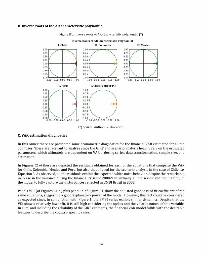
Regarding the global variables, the Spread US is noticeably the most volatile series, followed by the VIX regarding its mean. It is worth mentioning that some movements of these two series are not necessarily associated to co-movements in the remaining global factors. III. Results In this section we present two kinds of results. First, the estimated impact for each country's EMBI faced to alternative external financial shocks. These results allow for a comparison of the relative importance of each shock within economies as well as among them. Then, for the case of Chile only, we report how the EMBI co-moves with external financial variables under alternative risk scenarios which combine shocks. III.1. Latin American economies After estimating specification (1)—whose results suggest stationary according to the inverse roots of the AR characteristic polynomial (Annex B)—, Figure 2 presents the 3-month accumulated GIRF for the same shocks discussed above. We consider this horizon appropriate when analyzing financial markets that

7 In this article we document how different is the reaction among countries, but do not attempt to explain the reasons as to why the differences materialize. Aizenman et al. (2014), Mishra et al. (2014), and Eichengreen and Gupta (2015) explore which variables or country characteristics might explain the different response.

Chile Colombia Mexico Peru EMBI Brazil

EMBI China Spread US VIX Broad Copper

Price Mean 4.92 5.67 5.41 5.59 5.90 4.70 1.71 2.98 4.55 8.34 Median 4.98 5.48 5.32 5.38 5.65 4.83 1.90 2.95 4.55 8.65 Maximum 5.97 6.97 6.47 6.78 7.79 5.80 3.40 4.09 4.73 9.20 Minimum 4.01 4.72 4.53 4.61 4.94 3.61 -0.41 2.34 4.39 7.23 Std. Dev. 0.39 0.58 0.39 0.56 0.67 0.49 1.11 0.35 0.09 0.66 Skewness -0.20 0.31 0.57 0.47 0.65 -0.12 -0.49 0.48 0.21 -0.45 Kurtosis 2.92 1.76 2.80 1.91 2.36 2.06 2.00 2.94 1.87 1.55

Jarque-Bera 1.31 15.74 10.88 16.95 17.19 7.67 16.24 7.52 11.98 23.92 Probability 0.520 0.000 0.004 0.000 0.000 0.022 0.000 0.023 0.003 0.000

Observations 197 197 197 197 197 197 197 197 197 197

ADF Stat. -3.25 -3.39 -4.28 -3.08 -3.49 -3.18 -2.85 -2.72 -22.21 -3.17p -value 0.019 0.055 0.001 0.114 0.044 0.091 0.053 0.073 0.000 0.096

EMBI series Global series

5

usually display a lot of short-lived volatility.8 The estimations show heterogeneity across countries and, most importantly, among shocks within each country.9

Figure 1: EMBI and global variables time series, 1999.1-2015.9 (*)

(*) All variables in logarithms except Spread US in percentage.

Source: Authors' elaboration based on Bloomberg and New York Fed data. An important driver of shocks, as we stated in the introduction, is increased macrofinancial risks in large emerging market economies. It turns out that a shock to the EMBI Brazil is the one that shows the largest percent impact on all countries’ EMBI, being Colombia the most affected. As seen in Figure 2, a 1SD shock (equivalent to a 386 bp increase on the EMBI Brazil) results in a 35% cumulative increase on its (log) EMBI. To have an order of magnitude, if we consider the 2015 average of the EMBI Colombia (240.1 bp), the increase after one quarter would amount to 100 bp. Instead, the same exercise for Mexico and Peru results

8 Note that all GIRF are statistically significant (95% confidence level) at least 12 months after the shock. The lag order of the VAR according to BIC is equal to 1 for all countries. 9 Some diagnostics on the fit of these models to the data—that is, residuals and goodness-of-fit coefficients—are displayed in Annex C. It includes those of the VAR for Chile with the price of copper as part of the set of variables.

4.0

4.5

5.0

5.5

6.0

6.5

7.0

7.5

8.0

99 00 01 02 03 04 05 06 07 08 09 10 11 12 13 14 15

EMBI Chile EMBI Colombia EMBI Mexico EMBI Peru

Loga

rith

mLogarithm

Months

2345678 -1

01234

99 00 01 02 03 04 05 06 07 08 09 10 11 12 13 14 15

Spread US [RHS] EMBI Brazil EMBI China VIX Broad USD IndexCopper Price

Loga

rith

mPercentage

Months

I. EMBI time series

II. Global variables time series

6

in 80 and 78 bp increases, respectively.10 The least affected is Chile, with a 46 bp increase, with respect to its 2015 average level as well.

Figure 2: Estimated 3-month accumulated GIRF of (log) EMBIi to 1SD selected external financial shock (*)

(*) Point estimate in green dots. Bars indicate ±2SD confidence intervals.

Source: Authors' elaboration. China is also of particular interest, and the results give support to the concerns about eventual spillovers from this economy. After a 1SD shock (58 bp increase in the EMBI China), the 3-month cumulative impact on each country's (log) EMBI is approximately 20%. Nevertheless, the instantaneous spillover is larger in Peru and Colombia (near 8%) versus Mexico and Chile (near 5.5%), suggesting different GIRF dynamics.11 With respect to the 2015 average EMBI levels, the Latin American countries cumulative changes range between 54 bp (Colombia) and 34 bp (Chile) after one quarter. The magnitude of this response is larger than the one observed for Brazil when compared with the basis point increase of the EMBI China. Nevertheless, with respect to the standard deviation of each EMBI series, the response to a China shock is smaller, and thus variations in the sovereign risk premium of Brazil are estimated to have relatively more disruptive effects on other countries in the region. The response to a 1SD shock to the VIX (equivalent to 18.23% change in log-levels, or 8.12 percent points in the original units) vary from 20.0% (Chile) to 24.3% (Colombia), though statistically equal between them. These, correspond to a 40 bp response for the EMBI Chile and 67 bp for EMBI Colombia during the first quarter, with respect to the 2015 average. In the cases of Peru and Mexico, the impact reaches 50 and 58 bp, respectively. A more risky and plausible shock would be an increase of the VIX by 16 pp, that is, by 2SD. A shock of this size was observed in the sample period, in July-September 2015, after the stock market in China crashed. For a shock of this size, the estimated increase of the EMBI Colombia and Mexico is 145 and 130 bp,

10 The 2015 average is calculated between January and September 2015. The levels for each country are as follows: 176.1 bp for Chile, 240.1 bp for Colombia, 244.8 bp for Mexico and 196.1 for Peru. 11 This is not the case after a shock to EMBI Brazil, since the dynamics are almost identical for all countries. These results are not shown for countries other than Chile (Figure 3), but are available upon request.

0

10

20

30

40

3-m

onth

acc

. GIR

F

Chile Colombia Mexico Peru

VIX Broad Ind. EMBI Brazil EMBI China

7

respectively. Peru and Chile's basis point increase is lower as the EMBI levels over which the changes are calculated are lower as well. Finally, in the case of an unexpected appreciation of the dollar (a positive shock to the Broad Index of 1SD, equivalent to 1.13%), the results range from 11.6% (Chile) to 16.0% (Colombia). Analogous to the previous case, these percent changes result in an increase of 21 and 42 bp to the EMBI Chile and Colombia, respectively, compared to their average EMBI level during 2015. In the event of a larger appreciation, say 5%, the impact on the Colombian EMBI will be 205 bp. III.2. Chile: Scenario analysis This subsection analyzes the special case of the Chilean economy based on scenario analysis. A slightly different VAR specification is used:

𝐗𝑡 = �𝑆𝑆𝑆𝑆𝑆𝑆 𝑈𝑆𝑡 ,𝐸𝐸𝐸𝐸 𝐶ℎ𝑖𝑖𝑆𝑡,𝐸𝑆𝐵𝑆𝑆𝑡 ,𝑃𝑡𝐶𝐶𝑝𝑝𝐶𝐶,𝑉𝐸𝑉𝑡 ,𝐸𝐸𝐸𝐸 𝐸𝑆𝑆𝐵𝑖𝐵𝑡 ,𝐸𝐸𝐸𝐸 𝐶ℎ𝑖𝐵𝑆𝑡�′ (3),

differing from the previous VAR in that it includes the price of copper (𝑃𝑡

𝐶𝐶𝑝𝑝𝐶𝐶).12 Figure 3 depicts the GIRF of the EMBI Chile to all possible shocks using Equation 3. As expected, a positive shock to the copper price reduces the risk premium in a magnitude that is economically relevant. A 1SD shock to the copper price (which is equivalent to a 6.4% increase) results in an improvement of the Chilean external financing conditions, reducing the EMBI Chile by 3.7% in the next month, and 9.8% accumulated in three months.

Figure 3: GIRF estimates to shocks in the financial VAR for Chile (*)

(*) GIRF statistically significant at 95% of confidence after 3 (Spread US), 6 (Copper Price),

7 (Broad Index), and 13 (EMBI Brazil and China, VIX) months. Source: Authors' elaboration.

12 VAR diagnostics are shown in Figure C1 (Annex C).

-4-3-2-10123456789

2 4 6 8 10 12 14 16 18 20 22 24

EMBI Brazil EMBI China Spread USBroad Index Copper Price VIX

GIRF

Months

GIRF Financial VAR :: (log) EMBI Chile

8

Given that only for Chile the impulse response to a Spread US shock is statistically significant we report it in Figure 3 as well. The estimated GIRF to a 1SD Spread US shock (19.4%) shows a consistent negative point estimate across the 24-month horizon. This result is in line with other estimations done for the Chilean economy and robust to alternative measures as for instance the 10-year Treasury bond yield, or the long term rate term premium, as discussed earlier (CBC, 2015). As we make use of GIRF in a relatively high dimensional VAR, the inclusion of the copper price does not dramatically change the single-shock GIRF estimates reported above, and therefore we do not discuss again the results. Instead, we now present three risk scenarios. First, one we call the Copper price bust scenario, in which a shock to the EMBI China is combined with a shock to the copper price.13 Second, the Emerging markets’ shock scenario that combines unexpected disturbances to the EMBI Brazil and China. And third, the Global volatility rise scenario, in which a shock to the VIX is combined with one to the EMBI Brazil. The rationale for the chosen combination of variables that defines a scenario is related to what the data delivers as spillover channels. For instance, a 1SD shock to the EMBI China, given the data, is in fact a shock in which the EMBI Brazil is simultaneously shocked by 66% of its standard deviation, and the EMBI Chile by 64%. The remaining variables have a less relevant role. This suggests that a China shock is at the end of the day an emerging markets’ shock. Likewise, a VIX shock co-moves mostly with EMBI Brazil and even more materially with Chile (69 and 81% of their standard deviations, respectively). Then, a Global volatility rise shock spills relatively more to the region (Brazil and Chile), and not to China, making it qualitatively different from the Emerging markets’ shock scenario. At this point it is important to recall matrix P, as the different scenarios will be interpreted from here. Technically, a shock in the first variable of the VAR (following the GIRF mechanics) is transmitted through the last variable according to the corresponding, i.e. the first, column of the P matrix (recalling that 𝚺 =𝐏𝐏′). A second shock could then be analyzed making use of the information contained in the corresponding, i.e. the second, column of the P matrix. As P is a lower triangular matrix, it is assumed that the second shock does not affect the first variable. Once is estimated, it is also possible to calibrate the size of the analyzed shocks, which is what we do. Table 2 shows in column (1) the magnitude of the simultaneous shock (spillover) to the corresponding variable in each row, as percent of the standard deviation of each variable's disturbance, when a 1SD shock is applied to the first variable in the scenario. The spillovers reported for each variable are obtained using the information on matrix P. This column simply shows the spillover channels of the shock through the remaining variables of the VAR, but the resulting impact on Chile is quantitatively the same as the one reported in Figure 3.14 Column (2) shows the spillover as well but after adding a second shock by making use of the information on the second column of matrix P. It adds the spillovers from a 1SD shock to the second variable in the VAR, to the spillovers shown in column (1). By construction, since we assumed the second variable does not affect the first one, the spillover is 0, and thus, the shock to the first variable is still 100% of its standard deviation. Again by construction, the shock to the second variable is 100% of its standard deviation, which is added to the spillover estimated after the first variable is shocked. As an example, in the Emerging

13 The Copper price bust scenario is one of special interest for the Chilean economy as not only China is a relevant market of destination—and thus a deterioration of its fundamentals has a direct impact on Chilean copper's demand—but given its size in the commodity markets, the price of copper fluctuates and achieves different equilibrium levels depending on China's demand. 14 The VAR order is different only for the purposes of calculating the GIRF, as stated in the previous section.

9

markets scenario, the spillover from Brazil to China was equivalent to 56% of EMBI China's standard deviation. Therefore, when a 1SD shock is applied to the EMBI China, the variable is affected in a magnitude equivalent to 100+56=156% of its standard deviation.

Table 2: Shock transmission under alternative scenarios (*)

(*) Each cell displays the spillover of the shock to the corresponding variable, as a percentage of its standard deviation, under different scenarios. Column (1) reports the spillovers of a 1SD shock to the first variable in the VAR. Column (2) reports the results from a composite shock of indicated SD shock to the first variable, followed by a shock to the second variable. Source: Authors' elaboration.

The dynamics over the EMBI Chile are plotted in Figure 4, though not scaled by their standard deviation. Under the base case (column 1), and as previously reported, the largest increase of the EMBI Chile result from a shock to Brazil, then VIX, then EMBI China (8, 7, and 5.5%, approximately). Instead, under the stress scenarios, when shocks are combined (column 2), we can see that the Global volatility rise scenario is the most damaging with the largest instantaneous spillover (12%, equivalent to 140% of its standard deviation), but dying out faster than the Emerging markets shock scenario. This means that even though under the latter scenario the instantaneous shock to the EMBI Chile is equivalent to 115% of its standard deviation (10% in Figure 4), it has a higher relevance for the Chilean economy after three to six months as the accumulated effect is larger. In addition, regarding the Global volatility rise shock, it is interesting that the spillover to China, when only the VIX is shocked, is rather small (39% of its standard deviation). Nevertheless, once the Brazil shock is combined with the VIX shock—again, because this was the main channel in the base case, together with the EMBI Chile (69 and 81%, respectively)—the EMBI China spillover increases materially, to 81%. This

Copper price bust (1) (2)VAR Order Shock size Shock sizeEMBI China 100% 100%Copper Price -20% -120%Spread US -7% -18%Broad Index 35% 83%VIX 37% 44%EMBI Brazil 66% 85%EMBI Chile 64% 93%

Emerging markets shock (1) (2)VAR Order Shock size Shock sizeEMBI Brazil 100% 100%EMBI China 56% 156%Spread US 0% -8%Broad Index 36% 53%Copper Price -28% -38%VIX 69% 78%EMBI Chile 94% 115%

Global volatility rise (1) (2)VAR Order Shock size Shock sizeVIX 100% 100%EMBI Brazil 69% 169%Spread US -9% -3%EMBI China 39% 81%Broad Index 24% 51%Copper Price -16% -38%EMBI Chile 81% 140%

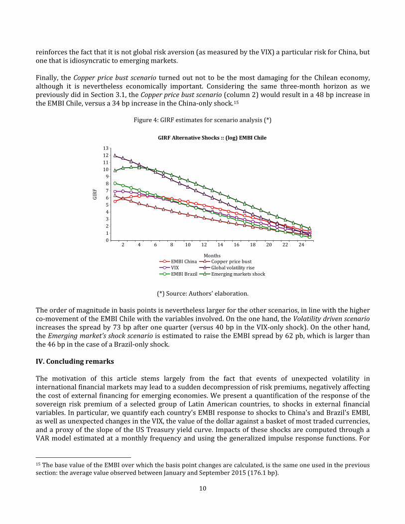
10

reinforces the fact that it is not global risk aversion (as measured by the VIX) a particular risk for China, but one that is idiosyncratic to emerging markets. Finally, the Copper price bust scenario turned out not to be the most damaging for the Chilean economy, although it is nevertheless economically important. Considering the same three-month horizon as we previously did in Section 3.1, the Copper price bust scenario (column 2) would result in a 48 bp increase in the EMBI Chile, versus a 34 bp increase in the China-only shock.15

Figure 4: GIRF estimates for scenario analysis (*)

(*) Source: Authors' elaboration.

The order of magnitude in basis points is nevertheless larger for the other scenarios, in line with the higher co-movement of the EMBI Chile with the variables involved. On the one hand, the Volatility driven scenario increases the spread by 73 bp after one quarter (versus 40 bp in the VIX-only shock). On the other hand, the Emerging market’s shock scenario is estimated to raise the EMBI spread by 62 pb, which is larger than the 46 bp in the case of a Brazil-only shock. IV. Concluding remarks The motivation of this article stems largely from the fact that events of unexpected volatility in international financial markets may lead to a sudden decompression of risk premiums, negatively affecting the cost of external financing for emerging economies. We present a quantification of the response of the sovereign risk premium of a selected group of Latin American countries, to shocks in external financial variables. In particular, we quantify each country's EMBI response to shocks to China's and Brazil's EMBI, as well as unexpected changes in the VIX, the value of the dollar against a basket of most traded currencies, and a proxy of the slope of the US Treasury yield curve. Impacts of these shocks are computed through a VAR model estimated at a monthly frequency and using the generalized impulse response functions. For

15 The base value of the EMBI over which the basis point changes are calculated, is the same one used in the previous section: the average value observed between January and September 2015 (176.1 bp).

0123456789

10111213

2 4 6 8 10 12 14 16 18 20 22 24

EMBI China Copper price bustVIX Global volatility riseEMBI Brazil Emerging markets shock

GIRF

Months

GIRF Alternative Shocks :: (log) EMBI Chile

11

the particular case of Chile, we further quantify the impact on the EMBI Chile after several shocks occur simultaneously, which we refer to as scenarios. The results indicate that a shock to the EMBI Brazil is the most relevant for the countries in the sample, reaffirming the fact that regional shocks are a source of concern. While Chile is the least affected when compared to the rest of the countries, this shock is the most relevant of all with an estimated 46 bp increase on the EMBI Chile after one quarter, as a response to a 1SD of the EMBI Brazil, which is approximately 380 bp. Shocks to the EMBI China and the VIX have quantitatively similar effects, for most countries. With respect to a shock to the Broad Index, capturing a greater appreciation of the dollar, it turns out to have a more limited impact than the rest of the shocks. Finally, shocks to the Spread US turn out to be not significant, except for Chile. The estimated impact is negative, in line with previous estimations for Chile. The three scenarios that we propose for the case of Chile are based on a combination of variables that are relevant to the Chilean economy, and turn out to be important spillover channels given the data. The Emerging market’s shock scenario combines perturbations to the China and Brazil EMBI. It is estimated to raise the EMBI spread by 62 pb after three months, which is larger than the 46 bp in the case of a Brazil-only shock; a Global volatility rise scenario, that in addition to a VIX shock considers that the EMBI Brazil is shocked as well, increases the spread by 73 bp (versus 40 bp in the VIX-only shock) during the same period; and finally a Copper price bust scenario, which required to estimate a specification with the price of copper, combines shocks to the price of copper and the EMBI China. Under this scenario a 48 bp increase in the EMBI Chile is observed, on impact, versus a 34 bp increase in the China-only shock. The results show empirical support for the fact that a deterioration of the risk premium of emerging market economies may have material consequences on the external cost of financing of Latin American countries. In particular, a shock to Brazil's EMBI is estimated as the most disruptive, both in terms of absolute levels (increase in basis points), and as a spillover channel. These effects are estimated controlling for the volatility index that is known to co-move with the spreads. In fact, we found that a scenario of heightened volatility does imply large spillovers to Brazil and Chile, but not necessarily to China. References

1. Aizenman, J., M. Binici, and M.M. Hutchinson (2014). "The Transmission of Federal Reserve Tapering News to Emerging Financial Markets," Working Paper 19980, National Bureau of Economic Research.

2. Bellas, D., M.G. Papaioannou, and I. Petrova (2010). "Determinants of Emerging Market Sovereign Bond Spreads: Fundamentals vs Financial Stress," Working Paper 281/10, International Monetary Fund.

3. Bank for International Settlements (2015). Quarterly Financial Review, March 2015. 4. Brainard, L. (2015). "Recent Changes in the Resilience of Market Liquidity," remarks at Policy Makers'

Panel on Financial Intermediation: Complexities and Risks for "The Future of Financial Intermediation: Banking, Securities Markets, or Something New?" Salzburg Global Forum on Finance in a Changing World, Salzburg Global Seminar, Austria.

5. Central Bank of Chile (2015). Financial Stability Report, Box I.1, First Half 2015. 6. Constâncio, V. (2015). "Divergent Monetary Policies and the World Economy," keynote address by

Vice-President of the ECB at the conference organized by FED/ECB/FED Dallas/HKMA in Hong Kong, 15 October 2015.

7. Doshi, H., K. Jacobs, and C. Zurita (2015). "Economic and Financial Determinants of Credit Risk Premiums in the Sovereign CDS Market," Working Paper 15-01, Institut de la Finance Structurée des Instruments Dérivés de Montréal, Montreal Institute of Structured Finance and Derivatives.

8. Eichengreen, B. and P. Gupta (2015). "Tapering Talk: The Impact of Expectations of Reduced Federal Reserve Security Purchases on Emerging Markets," Emerging Markets Review 25(C): 1-15.

12

9. Eyssell, T., H. Fungb, and G. Zhanga (2013). "Determinants and Price Discovery of China Sovereign Credit Default Swaps," China Economic Review 24: 1-15.

10. González-Rozada, M. and E. Levy Yeyati (2008). "Global Factors and Emerging Market Spreads," The Economic Journal 118: 1917-1936.

11. Hartelius, K., K. Kashiwase, and L.E. Kodres (2008). "Emerging Market Spread Compression: Is it Real or is it Liquidity?" Working Paper 08/10, International Monetary Fund.

12. Joint Staff Report (2015). "The U.S. Treasury Market on October 15, 2014," report by the US Department of the Treasury, Board of Governors of the Federal Reserve System, Federal Reserve Bank of New York, US Securities and Exchange Commission, and US Commodity Futures Trading Commission, 13 July, 2015.

13. Kennedy, M. and A. Palerm (2014). "Emerging Market Bond Spreads: The Role of Global and Domestic Factors from 2002 to 2011," Journal of International Money and Finance 43: 70-87.

14. Longstaff, F.A., J. Pan, L.H. Pedersen, and K.J. Singleton (2011). "How Sovereign is Sovereign Credit Risk?" American Economic Journal: Macroeconomics 3(2): 75-103.

15. Matheson, T. (2015). "Normalization of Global Financial Conditions: The Implications for Brazil," Working Paper 194/15, International Monetary Fund.

16. Mishra, P., K. Moriyama, P. N'Diaye, and L. Nguyen (2014). "Impact of Fed Tapering Announcements on Emerging Markets," Working Paper 109/14, International Monetary Fund.

17. Office of Financial Research (2015a). Financial Stability Report. 18. Office of Financial Research (2015b). "Divergent Monetary Policies Continue to Drive Market Trends,"

Financial Markets Monitor, March 2015. 19. Pan, J. and K.J. Singleton (2008). "Default and Recovery Implicit in the Term Structure of Sovereign

CDS Spread," Journal of Finance LXII(5): 2345-2384. 20. Pesaran, M.H. and J. Shin (1998). "Generalized Impulse Response Analysis in Linear Multivariate

Models," Economic Letters 58(1): 17-29. 21. Powel, J.H. (2015). "Structure and Liquidity in Treasury Markets," remarks at The Brookings

Institution, Washington DC, August 3, 2015. 22. PriceWaterhouseCoopers LLP (2015). "Global Financial Markets Liquidity Study," report prepared

for the Global Financial Markets Association and the Institute of International Finance. 23. Uribe M. and V.Z. Yue (2006). "Country Spreads and Emerging Countries: Who Drives Whom?"

Journal of International Economics 69: 6-36.

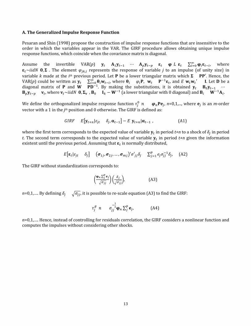
13

A. The Generalized Impulse Response Function Pesaran and Shin (1998) propose the construction of impulse response functions that are insensitive to the order in which the variables appear in the VAR. The GIRF procedure allows obtaining unique impulse response functions, which coincide when the covariance matrix is diagonal. Assume the invertible VAR(p) 𝐲𝑡 = 𝐀1𝐲𝑡−1 + ⋯+ 𝐀𝑝𝐲𝑡−𝑝 + 𝛆𝑡 = 𝛗(𝐿)𝛆𝑡 = ∑ 𝛗𝑖𝛆𝑡−𝑖∞

𝑖=0 , where 𝛆𝑡~𝑖𝑖𝑆𝑖(𝟎,𝚺). The element 𝜑𝑗𝑗,𝑖 represents the response of variable j to an impulse (of unity size) in variable k made at the ith previous period. Let P be a lower triangular matrix which 𝚺 = 𝐏𝐏′. Hence, the VAR(p) could be written as 𝐲𝑡 = ∑ 𝛉𝑖𝐰𝑡−𝑖

∞𝑖=0 , where 𝛉𝑖 = 𝜑𝑖𝐏, 𝐰𝑡 = 𝐏−1𝛆𝑡, and 𝐸[𝐰𝑡𝐰𝑡′] = 𝐈. Let D be a

diagonal matrix of P and 𝐖 = 𝐏𝐃−1. By making the substitutions, it is obtained 𝐲𝑡 = 𝐁0𝐲𝑡−1 +⋯+𝐁𝑝𝐲𝑡−𝑝 + 𝐯𝑡, where 𝐯𝑡~𝑖𝑖𝑆𝑖(𝟎,𝚺𝐯), 𝐁0 = 𝐈𝑗 −𝐖−1 (a lower triangular with 0 diagonal) and 𝐁𝑖 = 𝐖−1𝐀𝑖. We define the orthogonalized impulse response function 𝜏𝑗0(𝑖) = 𝝋𝑛𝐏𝐞𝑗, n=0,1,..., where 𝐞𝑗 is an m-order vector with a 1 in the jth position and 0 otherwise. The GIRF is defined as:

𝐺𝐸𝐺𝐺 = 𝐸�𝐲𝑡+𝑛|𝜀𝑗𝑡 = 𝛿𝑗 ,𝛂𝑡−1� − 𝐸[𝐲𝑡+𝑛|𝛂𝑡−1], (A1) where the first term corresponds to the expected value of variable 𝐲𝑡 in period t+n to a shock of 𝛿𝑗 in period t. The second term corresponds to the expected value of variable 𝐲𝑡 in period t+n given the information existent until the previous period. Assuming that 𝛆𝑡 is normally distributed,

𝐸�𝛆𝑡|𝜀𝑗𝑡 = 𝛿𝑗� = �𝝈1𝑗,𝝈2𝑗, … ,𝝈𝑚𝑗�′𝜎′𝑗𝑗𝛿𝑗 = ∑ 𝑆𝑗𝜎𝑗𝑗−1𝛿𝑗,𝑝𝑗=1 (A2)

The GIRF without standardization corresponds to:

�𝛗𝑛 ∑ 𝐞𝑗

𝑝𝑗

�𝜎𝑗𝑗� � 𝛿𝑗

�𝜎𝑗𝑗�, (A3)

n=0,1,…. By defining 𝛿𝑗 = �𝜎𝑗𝑗, it is possible to re-scale equation (A3) to find the GIRF:

𝜏𝑗𝑔(𝑖) = 𝜎𝑗𝑗

−12𝛗𝑛 ∑ 𝐞𝑗𝑝𝑗 , (A4)

n=0,1,…. Hence, instead of controlling for residuals correlation, the GIRF considers a nonlinear function and computes the impulses without considering other shocks.

14

B. Inverse roots of the AR characteristic polynomial

Figure B1: Inverse roots of AR characteristic polynomial (*)


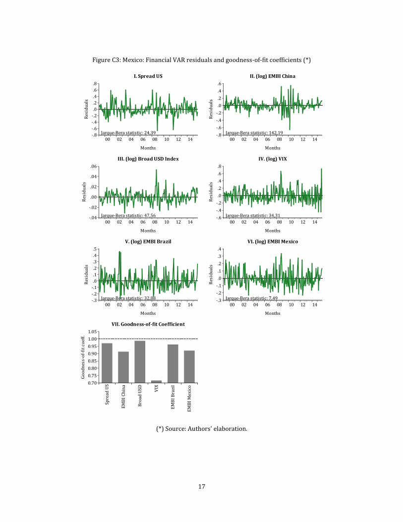
C. VAR estimation diagnostics In this Annex there are presented some econometric diagnostics for the financial VAR estimated for all the countries. These are relevant to analyze since the GIRF and scenario analysis heavily rely on the estimated parameters, which ultimately are dependent on VAR ordering series, data transformation, sample size, and estimation. In Figures C1-4 there are depicted the residuals obtained for each of the equations that comprise the VAR for Chile, Colombia, Mexico and Peru, but also that of used for the scenario analysis in the case of Chile–i.e. Equation 3. As observed, all the residuals exhibit the expected white noise behavior, despite the remarkable increase in the variance during the financial crisis of 2008-9 in virtually all the series, and the inability of the model to fully capture the disturbances reflected in EMBI Brazil in 2002. Panels VIII (of Figures C1-4) plus panel IX of Figure C1 show the adjusted goodness-of-fit coefficient of the same equations, suggesting a good explanatory power of the model. However, this fact could be considered as expected since, in conjunction with Figure 1, the EMBI series exhibit similar dynamics. Despite that the VIX show a relatively lower fit, it is still high considering the spikes and the volatile nature of this variable. In sum, and including the reliability of the GIRF estimates, the financial VAR model fulfils with the desirable features to describe the country-specific cases.

-1.00-0.75-0.50-0.250.000.250.500.751.00

-1.00 -0.50 0.00 0.50 1.00

I. Chile

-1.00-0.75-0.50-0.250.000.250.500.751.00

-1.00 -0.50 0.00 0.50 1.00

II. Colombia

-1.00-0.75-0.50-0.250.000.250.500.751.00

-1.00 -0.50 0.00 0.50 1.00

III. Mexico

-1.00-0.75-0.50-0.250.000.250.500.751.00

-1.00 -0.50 0.00 0.50 1.00

IV. Peru

-1.00-0.75-0.50-0.250.000.250.500.751.00

-1.00 -0.50 0.00 0.50 1.00

V. Chile (Copper P.)

Inverse Roots of AR Characteristic Polynomial

15

Figure C1: Chile: Financial VAR residuals and goodness-of-fit coefficients (*)


-.8

-.4

.0

.4

.8

-.8

-.4

.0

.4

.8

00 02 04 06 08 10 12 14

Resi

dual

s Residuals

Months

Jarque-Bera statistic: 23,52


I. Spread US

-.8

-.4

.0

.4

.8

-.8

-.4

.0

.4

.8

00 02 04 06 08 10 12 14

Resi

dual

s Residuals

Months



II. (log) EMBI China

-.04-.02.00.02.04.06

-.04-.02.00.02.04.06

00 02 04 06 08 10 12 14

Resi

dual

s ResidualsMonths



III. (log) Broad USD Index

-.4-.3-.2-.1.0.1.2.3

00 02 04 06 08 10 12 14

Resi

dual

s Residuals

Months


IV. (log) Copper Price

-.6

-.2

.2

.6-.8-.4.0.4.8

00 02 04 06 08 10 12 14

Resi

dual

s Residuals

Months



V. (log) VIX

-.4-.2.0.2.4.6

-.4-.2.0.2.4.6

00 02 04 06 08 10 12 14

Resi

dual

s Residuals

Months



VI. (log) EMBI Brazil

-.4-.2.0.2.4.6

-.4-.2.0.2.4.6

00 02 04 06 08 10 12 14

Resi

dual

s Residuals

Months



VII. (log) EMBI Chile

0.700.750.800.850.900.951.001.05

Spre

ad U

S

EMBI

Chi

na

Broa

d US

D

VIX

EMBI

Bra

zil

EMBI

Chi

le

Good

ness

-of-f

it co

eff.

VIII. Goodness-of-fit Coefficient

0.700.750.800.850.900.951.001.05

Spre

ad U

S

EMBI

Chi

na

Broa

d US

D

Copp

er P

.

VIX

EMBI

Bra

zil

EMBI

Chi

le

Good

ness

-of-f

it co

eff.

IX. Goodness-of-fit Coefficient

16

Figure C2: Colombia: Financial VAR residuals and goodness-of-fit coefficients (*)


-.8-.6-.4-.2.0.2.4.6.8

00 02 04 06 08 10 12 14

Resi

dual

s

Months


I. Spread US

-.8-.6-.4-.2.0.2.4.6

00 02 04 06 08 10 12 14

Resi

dual

s

Months



-.04

-.02

.00

.02

.04

.06

00 02 04 06 08 10 12 14

Resi

dual

s

Months



-.6-.4-.2.0.2.4.6.8

00 02 04 06 08 10 12 14

Resi

dual

s

Months


IV. (log) VIX

-.3-.2-.1.0.1.2.3.4.5

00 02 04 06 08 10 12 14

Resi

dual

s

Months


V. (log) EMBI Brazil

-.3-.2-.1.0.1.2.3.4.5.6

00 02 04 06 08 10 12 14

Resi

dual

s

Months


VI. (log) EMBI Colombia

0.700.750.800.850.900.951.001.05

Spre

ad U

S

EMBI

Chi

na

Broa

d US

D

VIX

EMBI

Bra

zil

EMBI

Colo

mbi

a

Good

ness

-of-f

it co

eff.

VII. Goodness-of-fit Coefficient

17

Figure C3: Mexico: Financial VAR residuals and goodness-of-fit coefficients (*)


-.8-.6-.4-.2.0.2.4.6.8

00 02 04 06 08 10 12 14

Resi

dual

s

Months


I. Spread US

-.8-.6-.4-.2.0.2.4.6

00 02 04 06 08 10 12 14

Resi

dual

s

Months



-.04

-.02

.00

.02

.04

.06

00 02 04 06 08 10 12 14

Resi

dual

s

Months



-.6-.4-.2.0.2.4.6.8

00 02 04 06 08 10 12 14

Resi

dual

s

Months


IV. (log) VIX

-.3-.2-.1.0.1.2.3.4.5

00 02 04 06 08 10 12 14

Resi

dual

s

Months



-.3-.2-.1.0.1.2.3.4

00 02 04 06 08 10 12 14

Resi

dual

s

Months


VI. (log) EMBI Mexico

0.700.750.800.850.900.951.001.05

Spre

ad U

S

EMBI

Chi

na

Broa

d US

D

VIX

EMBI

Bra

zil

EMBI

Mex

ico

Good

ness

-of-f

it co

eff.


18

Figure C4: Peru: Financial VAR residuals and goodness-of-fit coefficients (*)


-.8-.6-.4-.2.0.2.4.6.8

00 02 04 06 08 10 12 14

Resi

dual

s

Months


I. Spread US

-.8-.6-.4-.2.0.2.4.6

00 02 04 06 08 10 12 14

Resi

dual

s

Months



-.04

-.02

.00

.02

.04

.06

00 02 04 06 08 10 12 14

Resi

dual

s

Months



-.6-.4-.2.0.2.4.6.8

00 02 04 06 08 10 12 14

Resi

dual

s

Months


IV. (log) VIX

-.3-.2-.1.0.1.2.3.4.5

00 02 04 06 08 10 12 14

Resi

dual

s

Months



-.4

-.2

.0

.2

.4

.6

00 02 04 06 08 10 12 14

Resi

dual

s

Months


VI. (log) EMBI Peru

0.700.750.800.850.900.951.001.05

Spre

ad U

S

EMBI

Chin

a

Broa

d US

D

VIX

EMBI

Bra

zil

EMBI

Per

u

Good

ness

-of-f

it co

eff.


Documentos de Trabajo


NÚMEROS ANTERIORES

La serie de Documentos de Trabajo en versión PDF

puede obtenerse gratis en la dirección electrónica:

www.bcentral.cl/esp/estpub/estudios/dtbc.

Existe la posibilidad de solicitar una copia impresa

con un costo de Ch$500 si es dentro de Chile y

US$12 si es fuera de Chile. Las solicitudes se pueden

hacer por fax: +56 2 26702231 o a través del correo

electrónico: [email protected].

Working Papers

Central Bank of Chile

PAST ISSUES

Working Papers in PDF format can be

downloaded free of charge from:

www.bcentral.cl/eng/stdpub/studies/workingpaper.

Printed versions can be ordered individually for

US$12 per copy (for order inside Chile the charge

is Ch$500.) Orders can be placed by fax: +56 2

26702231 or by email: [email protected].

DTBC – 794

Welfare Costs of Inflation and Imperfect Competition in a Monetary Search Model

Benjamín García

DTBC – 793

Measuring the Covariance Risk Consumer Debt Portfolios

Carlos Madeira

DTBC – 792

Reemplazo en Huelga en Países Miembros de la OCDE: Una Revisión de la

Legislación Vigente

Elías Albagli, Claudia de la Huerta y Matías Tapia

DTBC – 791

Forecasting Chilean Inflation with the Hybrid New Keynesian Phillips Curve:

Globalisation, Combination, and Accuracy

Carlos Medel

DTBC – 790

International Banking and Cross-Border Effects of Regulation: Lessons from Chile

Luis Cabezas y Alejandro Jara

DTBC – 789

Sovereign Bond Spreads and Extra-Financial Performance: An Empirical Analysis of

Emerging Markets

Florian Berg, Paula Margaretic y Sébastien Pouget

http://www.bcentral.cl/esp/estpub/estudios/dtbc


http://www.bcentral.cl/eng/stdpub/studies/workingpaper


DTBC – 788

Estimating Country Heterogeneity in Capital-Labor substitution Using Panel Data

Lucciano Villacorta

DTBC – 787

Transiciones Laborales y la Tasa de Desempleo en Chile

Mario Marcel y Alberto Naudon

DTBC – 786

Un Análisis de la Capacidad Predictiva del Precio del Cobre sobre la Inflación Global

Carlos Medel

DTBC – 785

Forecasting Inflation with the Hybrid New Keynesian Phillips Curve: A Compact-

Scale Global Var Approach

Carlos Medel

DTBC – 784

Robustness in Foreign Exchange Rate Forecasting Models: Economics-Based

Modelling After the Financial Crisis

Carlos Medel, Gilmour Camelleri, Hsiang-Ling Hsu, Stefan Kania y Miltiadis

Touloumtzoglou

DTBC – 783

Desigualdad, Inflación, Ciclos y Crisis en Chile

Pablo García y Camilo Pérez

DTBC – 782

Sentiment Shocks as Drivers of Business Cycles

Agustín Arias

DTBC – 781

Precios de Arriendo y Salarios en Chile

Paulo Cox y Víctor Pérez

DTBC – 780

Pass-Through, Expectations, and Risks. What Affects Chilean Banks’ Interest Rates?

Michael Pedersen

DOCUMENTOS DE TRABAJO • Diciembre 2016

DOCUMENTOS DE TRABAJO - Central Bank of...

Documents

Transcript of DOCUMENTOS DE TRABAJO - Central Bank of...