DISEÑO DE MUROS DE CONTENCIÓNDISEÑO DE MUROS DE CONTENCIÓN

Dr. Jorge E. Alva Hurtado

UNIVERSIDAD NACIONAL DE INGENIERUNIVERSIDAD NACIONAL DE INGENIERÍÍAAFACULTAD DE INGENIERÍA CIVIL

SECCIÓN DE POST GRADO

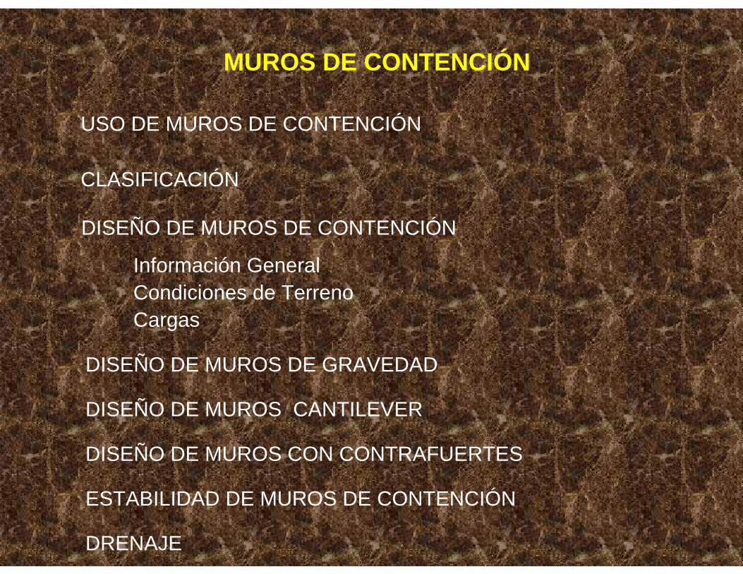
MUROS DE CONTENCIÓN

Información General Condiciones de Terreno Cargas

USO DE MUROS DE CONTENCIÓN

CLASIFICACIÓN

DISEÑO DE MUROS DE CONTENCIÓN

DISEÑO DE MUROS DE GRAVEDAD

DISEÑO DE MUROS CANTILEVER

DISEÑO DE MUROS CON CONTRAFUERTES

ESTABILIDAD DE MUROS DE CONTENCIÓN

DRENAJE

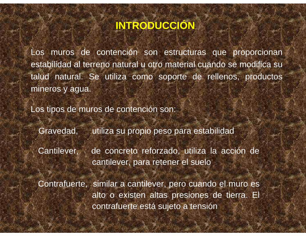
INTRODUCCIÓN

Los muros de contención son estructuras que proporcionan estabilidad al terreno natural u otro material cuando se modifica su talud natural. Se utiliza como soporte de rellenos, productos mineros y agua.

Los tipos de muros de contención son:

Gravedad, utiliza su propio peso para estabilidad

Cantilever, de concreto reforzado, utiliza la acción de cantilever, para retener el suelo

Contrafuerte, similar a cantilever, pero cuando el muro es alto o existen altas presiones de tierra. El contrafuerte está sujeto a tensión

Apoyado, similar a contrafuerte, con apoyo en la parte delantera, trabaja a compresión

Entramado, constituido por elementos prefabricados de concreto, metal o madera

Semigravedad, muros intermedios entre gravedad y cantilever

Los estribos de puentes son muros de contención con alas de extensión para sostener el relleno y proteger la erosión

Los muros de contención deben ser diseñados para resistir el volteo, deslizamiento y ser adecuados estructuralmente.

Relleno

Cuerpo

Base o cimentación

Pie de base

Talón de base

Llave

Inclinación de muro

La terminología utilizada es:

(a)

Keys

Approach siab

Approachfill

Optionalpiles(e) (f)(b)

(c) (d)

Counterforts

HeadersStretcher

Face of wall

Note : Cells to be filled with soil

Figure 12-1 Types of retaining walls. (a) gravity walls of stone masonry, brick or plain concrete. Weight providesoverturning and sliding stability; (b) cantilever wall; (c) counterfort, or buttressed wall. If backfill coverscounterforts, the wall is termed a counterfort; (d) crib wall; (e) semigravity wall (small amount of steel reinforcement is used); (f) bridge abutment

(a)

Fill

Cut

(b)

(e)(d)

Water

Fill

(c)l

Water

(f) (g)

High waterlevel

Cut Fill

Cut

Figure 3.22 Common use of retaining wall : (a) Hill side roads

(b) Elevated and depressed roads, (c) Load scaping

(d) Canals and locks (e) Erosión protection (f) Flood walls

(g) Bridge abutment.

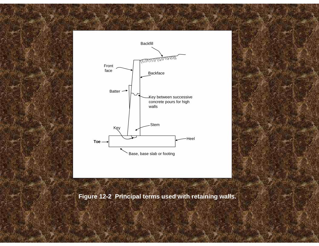
Frontface

Backfill

Backface

BatterKey between successiveconcrete pours for highwalls

Stem

Heel

Base, base slab or footing

Key

ToeToe

Figure 12-2 Principal terms used with retaining walls.

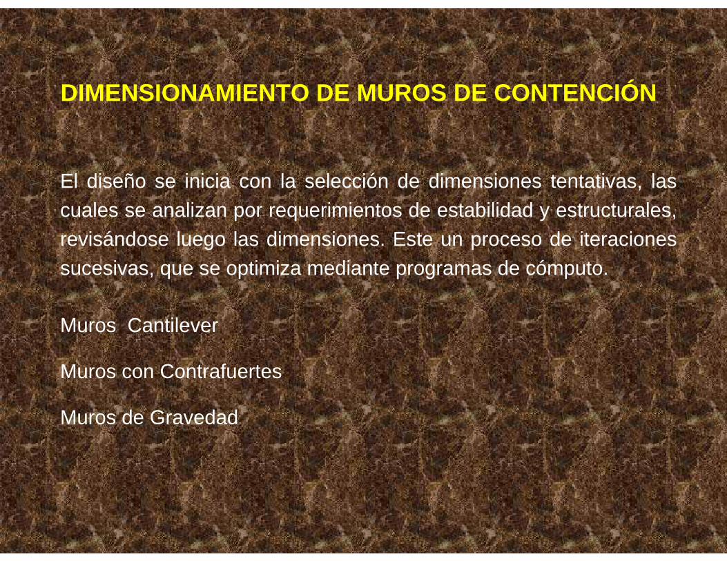
DIMENSIONAMIENTO DE MUROS DE CONTENCIÓN

El diseño se inicia con la selección de dimensiones tentativas, las cuales se analizan por requerimientos de estabilidad y estructurales, revisándose luego las dimensiones. Este un proceso de iteraciones sucesivas, que se optimiza mediante programas de cómputo.

Muros Cantilever

Muros con Contrafuertes

Muros de Gravedad

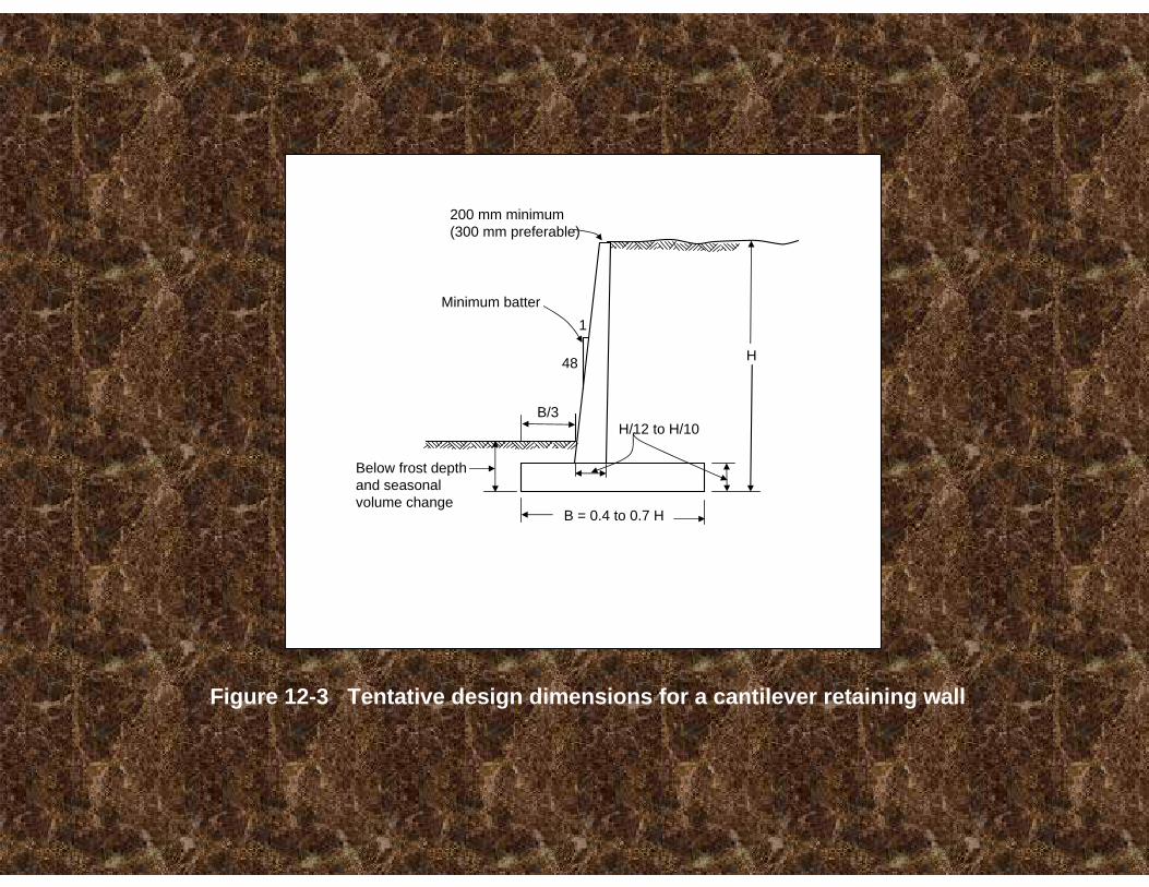
200 mm minimum(300 mm preferable)

Minimum batter

48

1

B/3H/12 to H/10

H

Below frost depthand seasonalvolume change

B = 0.4 to 0.7 H

Figure 12-3 Tentative design dimensions for a cantilever retaining wall

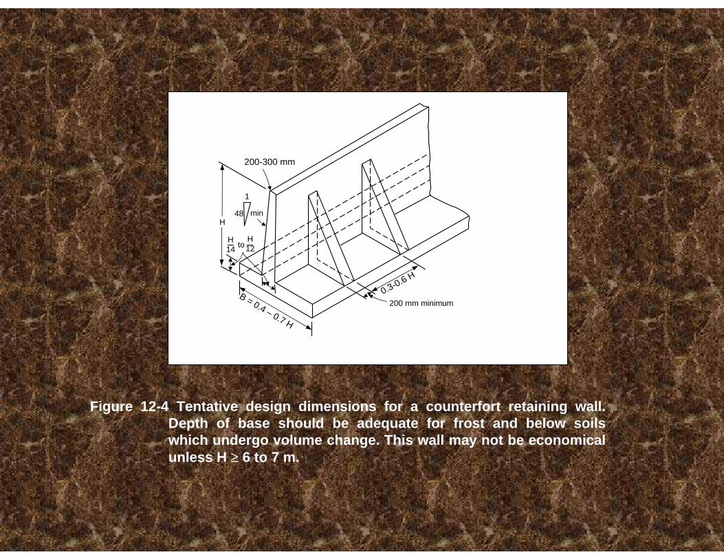
200-300 mm

48

1

minH

H 14

H 12to

B = 0.4 – 0.7 H

200 mm minimum0.3-0.6 H

Figure 12-4 Tentative design dimensions for a counterfort retaining wall. Depth of base should be adequate for frost and below soilswhich undergo volume change. This wall may not be economicalunless H ≥ 6 to 7 m.

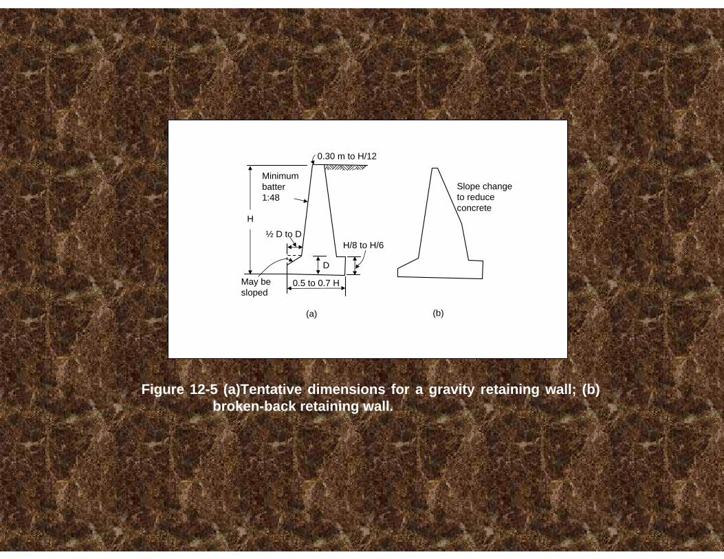
0.30 m to H/12

Minimumbatter1:48

H

½ D to DH/8 to H/6

D

0.5 to 0.7 HMay be sloped

Slope changeto reduce concrete

(a) (b)

Figure 12-5 (a)Tentative dimensions for a gravity retaining wall; (b) broken-back retaining wall.

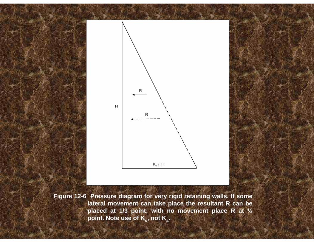
Figure 12-6 Pressure diagram for very rigid retaining walls. If somelateral movement can take place the resultant R can be placed at 1/3 point; with no movement place R at ½point. Note use of Ko, not Ka.

R

R

H

Ko γ H

ESTABILIDAD DE MUROS

Se debe proporcionar un adecuado factor de seguridad contra el deslizamiento. El empuje pasivo delante del muro puede omitirse si ocurrirá socavación.

Se puede utilizar llaves en la cimentación para aumentar la estabilidad . La mejor localización es en el talón.

FSs = suma de fuerzas resistentes suma de fuerzas actuantes

≥ 1.5-2.0

FSv = suma de momentos resistentes suma de momentos actuantes

≥ 1.5-2.0

a

d

β

Pv

Ph

Ws

Wc

b c

This soil may be removed

1 γ Hp Kp = Pp2

2B

β

Fr

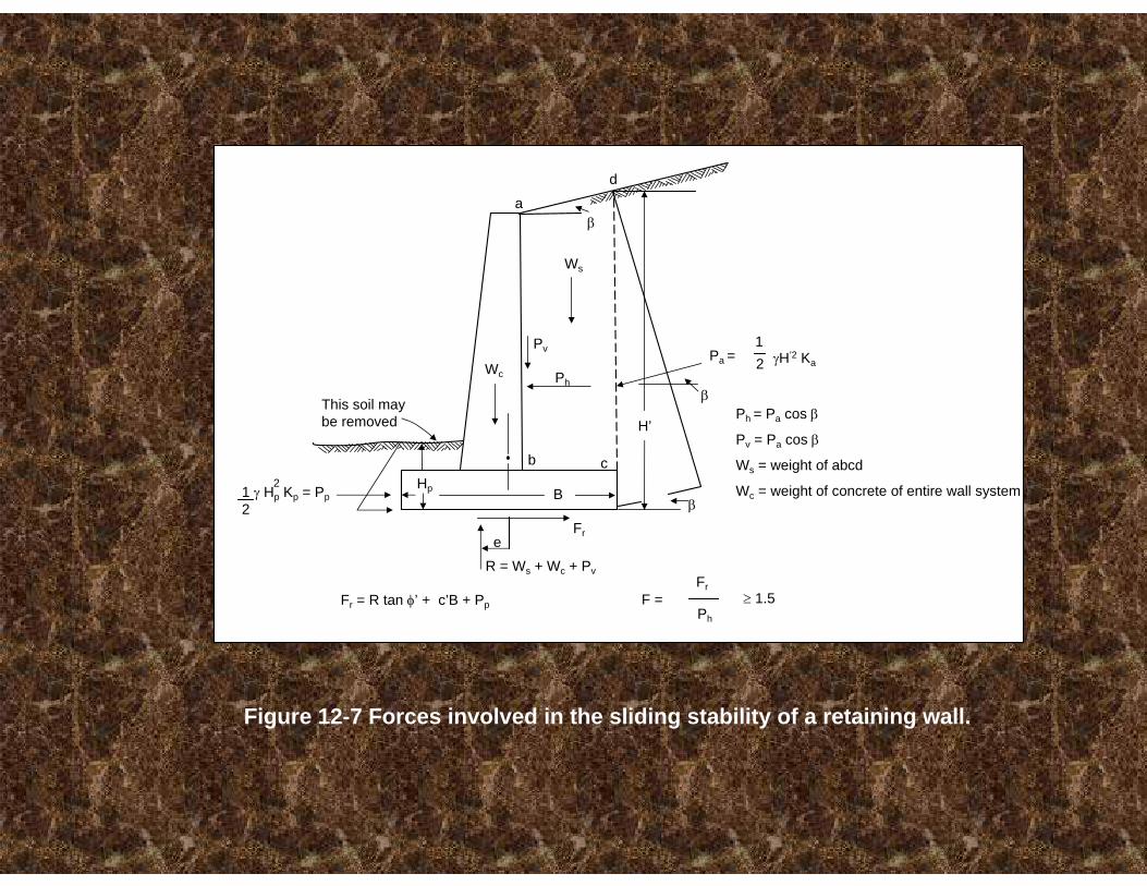
R = Ws + Wc + Pv

Hp

Fr = R tan φ’ + c’B + Pp F =Fr

Ph

≥ 1.5

H’

β

Pa =12 γH’2 Ka

Ph = Pa cos β

Pv = Pa cos β

Ws = weight of abcd

Wc = weight of concrete of entire wall system

Figure 12-7 Forces involved in the sliding stability of a retaining wall.

e

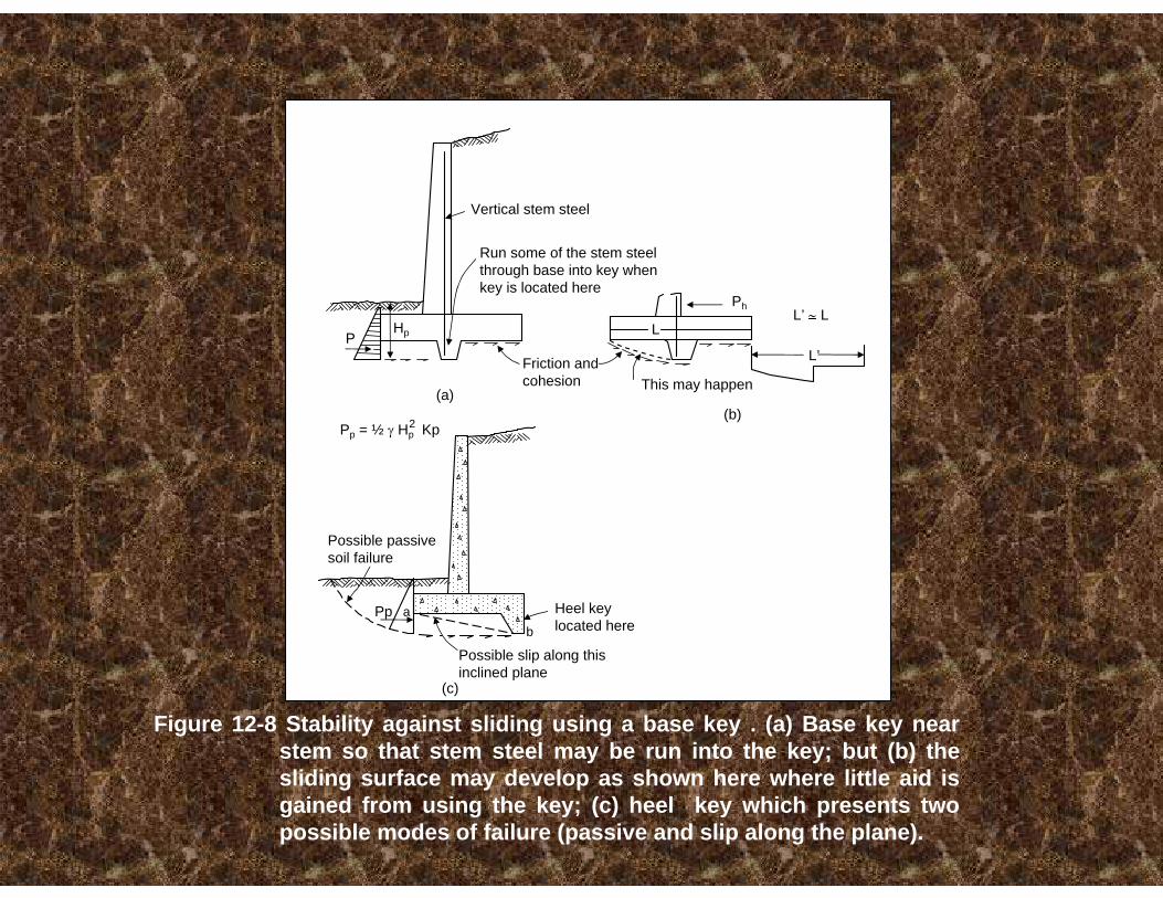
Pp = ½ γ Hp Kp2

PHp

(a)(b)

This may happen

PhL’ ∼ L

Run some of the stem steelthrough base into key whenkey is located here

Vertical stem steel

L’Friction andcohesion

Heel keylocated here

Possible slip along thisinclined plane

Possible passivesoil failure

Pp

(c)

a

Figure 12-8 Stability against sliding using a base key . (a) Base key nearstem so that stem steel may be run into the key; but (b) thesliding surface may develop as shown here where little aid isgained from using the key; (c) heel key which presents twopossible modes of failure (passive and slip along the plane).

L

b

a, meters0.61

Example: φ = 30° ka = 0.33H = 6; take (a+b) = 0.5H = 3 Enter chart with H2kg = 132 andread horizontally to b = 2.10 a= 0.9 These dimensions maybe used for the first trial.

a = H2 kg4 (m+b)

b2

m = 1

–+ 34

b2

(m+b)

m = 2

b = 12

' (3.67

m)

b = 12

' (3.67

m)

b = 10

' (3.05

m)

b = 10

' (3.05

m)

b = 8'

(2.44

m)

b = 8' (2.44 m)

b = 6' (1.83 m)

b = 6' (1.83 m)

b = 4' (1.22 m)

b = 4' (1.22 m)

1.22 1.83

37.2

27.9

18.6

9.3

H2 k

a, m

2

0 1 2 3 4 5 6

a b

m

0

100

200

3000

400

H

Fig. 3.29 Chart for determining approximate dimension ‘a’ and ‘b’ for the base slab, so that the resultant will fall inside the middle third (Bowles, 1968)

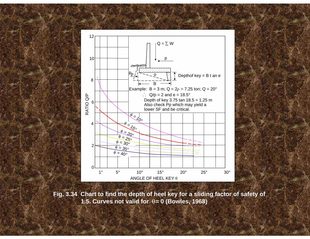
Q = ∑ W

Example: B = 3 m; Q = 2ρ = 7.25 ton; Q = 20°

p

o

B

pp Depthof key = B t an e

Q/p = 2 and e = 18.5°Depth of key 3.75 tan 18.5 = 1.25 m Also check Pp which may yield a lower SF and be critical.

φ = 10°φ = 15°φ = 20°φ = 25°φ = 30°φ = 35°φ = 40°

12

10

8

6

4

2

1° 5° 10° 15° 20° 25° 30°0

RA

TIO

Q/P

ANGLE OF HEEL KEY θ

.. .

Fig. 3.34 Chart to find the depth of heel key for a sliding factor of safety of1.5. Curves not valid for θ= 0 (Bowles, 1968)

FUERZAS EN EL MURO DE CONTENCIÓN

Para los muros de gravedad y cantilever se toman por ancho unitario. Para muros de contrafuerte se considera como unidad entre juntas o como unidad entre apoyos.

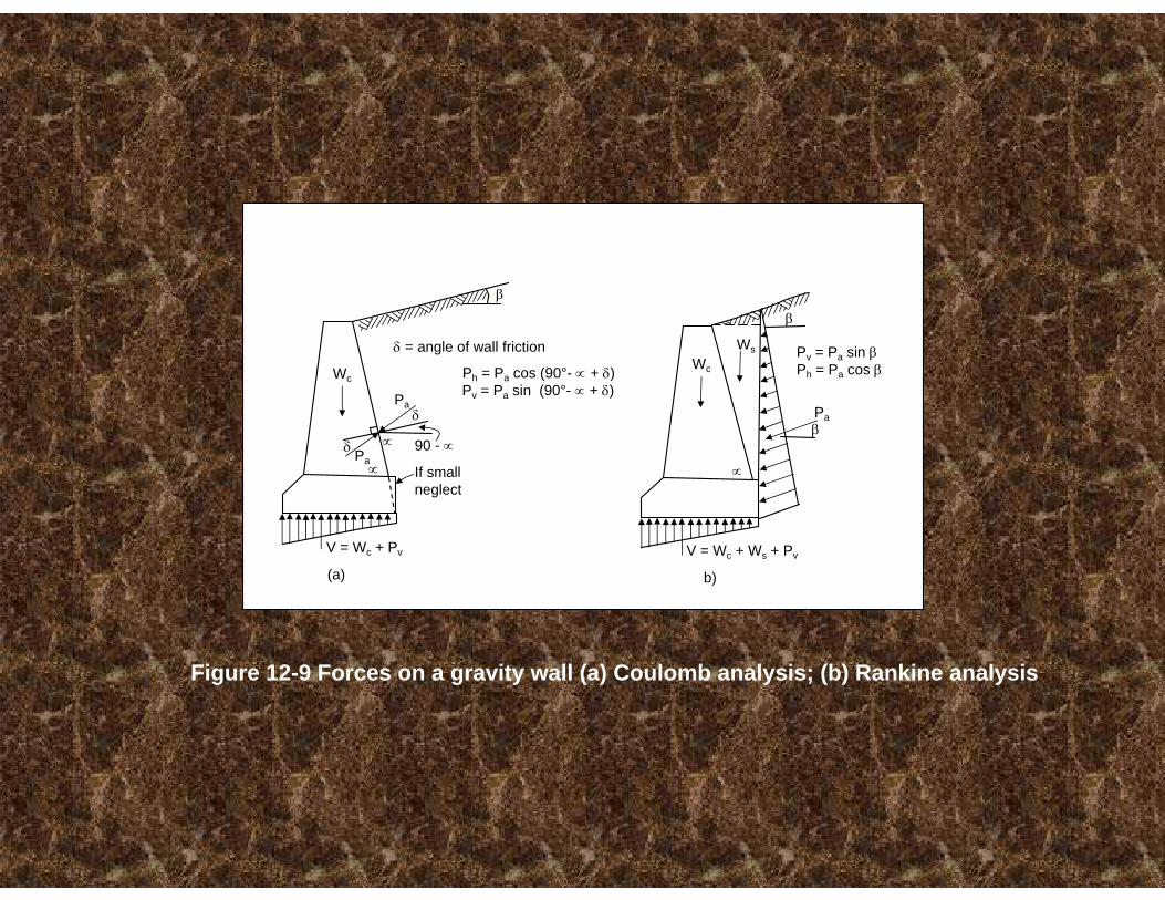
δ = angle of wall friction

Ph = Pa cos (90°- ∝ + δ) Pv = Pa sin (90°- ∝ + δ)Pa

Wc

δ Pa∝

Pa

∝ 90 - ∝

If smallneglect

δ

V = Wc + Pv

(a) b)

Wc

∝

Ws

V = Wc + Ws + Pv

β

β

β

Pv = Pa sin βPh = Pa cos β

Figure 12-9 Forces on a gravity wall (a) Coulomb analysis; (b) Rankine analysis

Ws

WcH

Pa

H 3

qheel (b)

M1

Sometimes omitted

Pa

Pa cos β

Hw

Wc

Hw3

e

V = Ws + Wc + Pa sin β

Omitsoil

γc Df

(weight of concrete

(a)

(c)

Df M2M3

Df

(d)

q heel

qs = (average height of soil)

Neglect vertical component of Pa

Included becauseit is in q

x γs + γc Df

Figure 12-10 Forces on cantilever wall. (a) Entire unit; free bodies for; (b) stem; (c) toe; (d) heel. Note that M1 + M2 + M3 ≅ 0.0.

qtoe

β

V

V

V

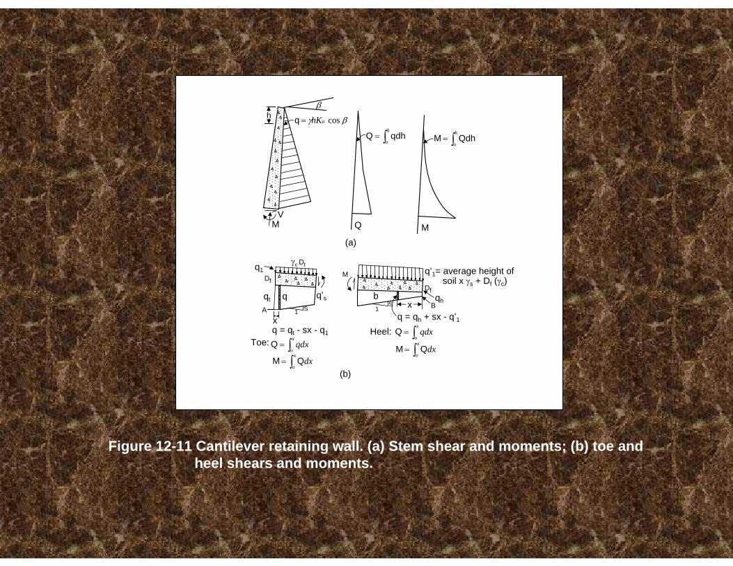
Figure 12-11 Cantilever retaining wall. (a) Stem shear and moments; (b) toe andheel shears and moments.

Q

qdhQ ∫=h

o QdhM ∫=h

o

M(a)

βγ cosahK=q

βh

M

(b)

γc Df

q

Df

q’sqt

q1

A 1 S

x

M

Toe: qdxx

o∫=Q

dxx

oQM ∫=

q = qt - sx - q1

b

qdxx

o∫=QHeel:

dxx

oQM ∫=

q = qh + sx - q’1

q’1= average height of soil x γs + Df (γc)Df

qhBx

V

1S

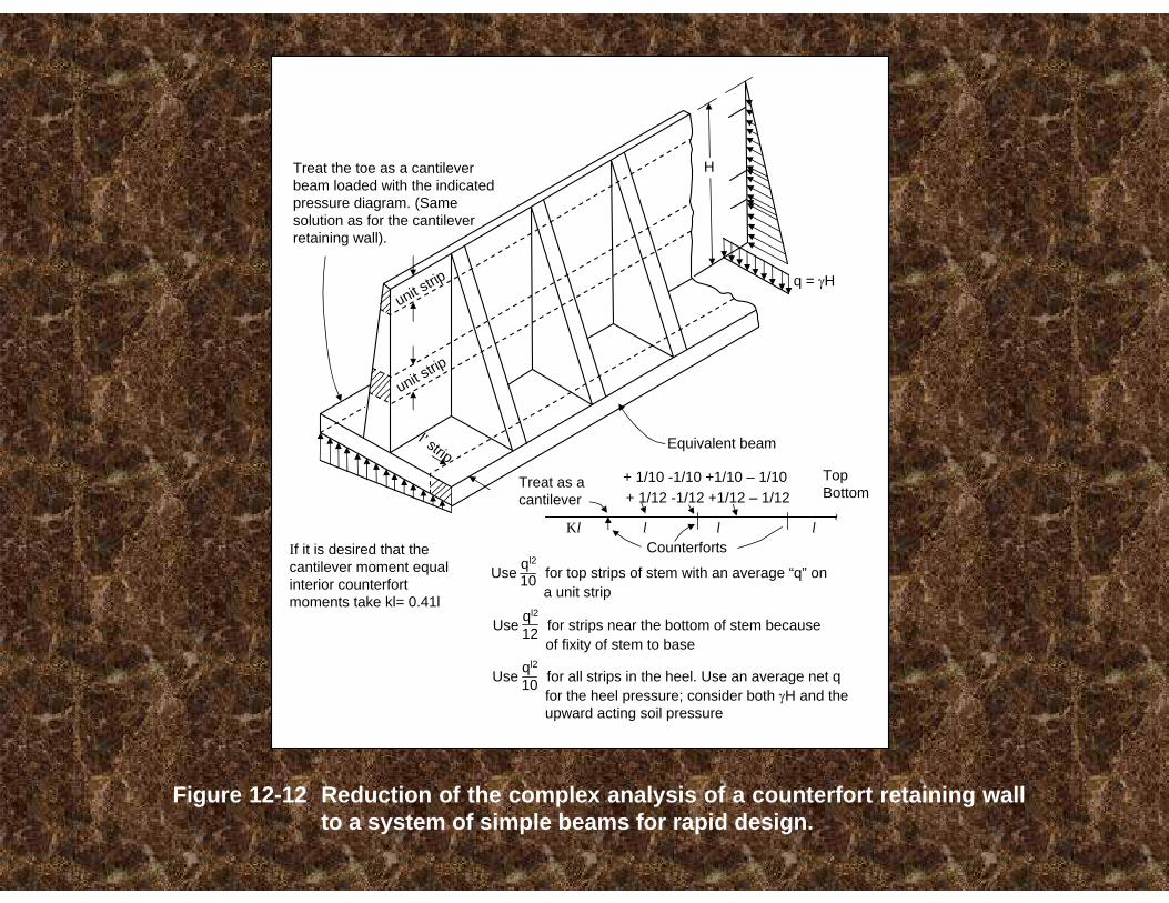
Treat the toe as a cantileverbeam loaded with the indicatedpressure diagram. (Samesolution as for the cantileverretaining wall).

unit strip

unit strip

If it is desired that thecantilever moment equalinterior counterfortmoments take kl= 0.41l

l’ strip

Treat as a cantilever

Equivalent beam

Counterforts

Use for top strips of stem with an average “q” on a unit strip

ql2

10

Use for strips near the bottom of stem becauseof fixity of stem to base

ql2

12

Use for all strips in the heel. Use an average net qfor the heel pressure; consider both γH and the upward acting soil pressure

ql2

10

+ 1/10 -1/10 +1/10 – 1/10+ 1/12 -1/12 +1/12 – 1/12

TopBottom

Kl l l l

∼

q = γH

H

Figure 12-12 Reduction of the complex analysis of a counterfort retaining wallto a system of simple beams for rapid design.

Use this pressure diagramfor positive momentcomputations

q = γHKa

H/2

H/4

H/4

q/2 q/2q’

H/4

H/4

H/4

H/4

H

q’q/2 q/2

(a)

Use this diagram fornegative momentcomputations

l l l l-1/11 -1/11 -1/11 -1/11

+ 1/16 + 1/16 + 1/16

M = q’ l 2

11 M = q’ l 2

16

-1/20

Unit

-1/12 -1/12 -1/12 -1/12 -1/12 -1/12

+ 1/20

M = q’l 2

12 M = q’l 2

20

+ 1/20

0.41 l 0.41 l

- 1/20

Unit

Use q’ from the shaded portions of the pressure diagrams in (a). Moment coefficientes are shown. Compute moments for several strips near top, midheight and near bottom.

(b)

Figure 12-13 Computation of bending moments in the horizontal direction forthe counterfort stem [After Huntington (1957)]

Equivalent beam strip

l

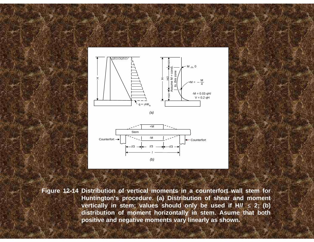
+M

-M

Stem

Counterfort

l/3 l/3 l/3

l

(b)

(a)

Counterfort

q = γHKa

H/4

H H/2

+M = M4

-M = 0.03 qHlV = 0.2 qH

H/4

Ass

ume

M =

con

st.

In t

his

zone

M ∼ 0

H

Figure 12-14 Distribution of vertical moments in a counterfort wall stem forHuntington’s procedure. (a) Distribution of shear and moment vertically in stem; values should only be used if H/l ≤ 2; (b) distribution of moment horizontally in stem. Asume that both positive and negative moments vary linearly as shown.

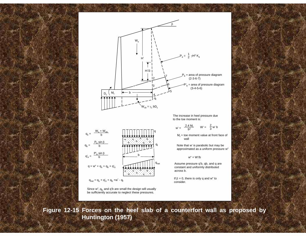
Ws

H’

H’/3

2

3

7

6

54

bDcMt

qf

Wcb = γc bDc

Pb = area of pressure diagram(2-3-6-7)

P’b = area of pressure diagram(3-4-5-6)

The increase in heel pressure dueto the toe moment is:

w' = 2.4 Mt

b2 W' = 23 w' b

Mt = toe moment value at front face ofwall

Note that w' is parabolic but may be approximated as a uniform pressure w"

w" = W'/b

Assume pressure q’b, qb, and q are constant and uniformly distributed across b.

If β = 0, there is only q and w” to consider.qnet = qs + q'b + qb +w" - qf

q = w” + qs + qb + q'bqnet

Since w”, qb, and q’b are small the design will usually be sufficiently accurate to neglect these pressures.

b

qf

qqs =

qb =

q'b =

Ws + Wcbb

Pb sin βb

P'b sin βb

β

Pa = 12 γH2 Ka

Figure 12-15 Forces on the heel slab of a counterfort wall as proposed by Huntington (1957)

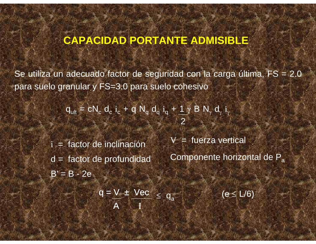
CAPACIDAD PORTANTE ADMISIBLE

Se utiliza un adecuado factor de seguridad con la carga última, FS = 2.0 para suelo granular y FS=3.0 para suelo cohesivo

qult = cNc dc ic + q Nq dq iq + 1 γ B Nγ dγ iγ

2

i = factor de inclinación

d = factor de profundidad

B' = B - 2e

V = fuerza vertical

Componente horizontal de Pa

q = V ± VecA I

(e ≤ L/6)q = V ± VecA I

≤ qa

ASENTAMIENTOS

Los asentamientos en terreno granular se desarrollan durante la construcción del muro y el relleno.

Los asentamientos en terreno cohesivo se desarrollan con la teoría de consolidación.

La resultante debe mantenerse en el tercio central para mantenerasentamiento uniforme y reducir la inclinación. La presión del terreno en el pie es el doble cuando la excentricidad de la resultante es L/6 como cuando la excentricidad es cero.

INCLINACIÓN

Se necesita cierta inclinación para desarrollar el estado activo.

Demasiada inclinación puede estar asociada a la falla de cimentación.

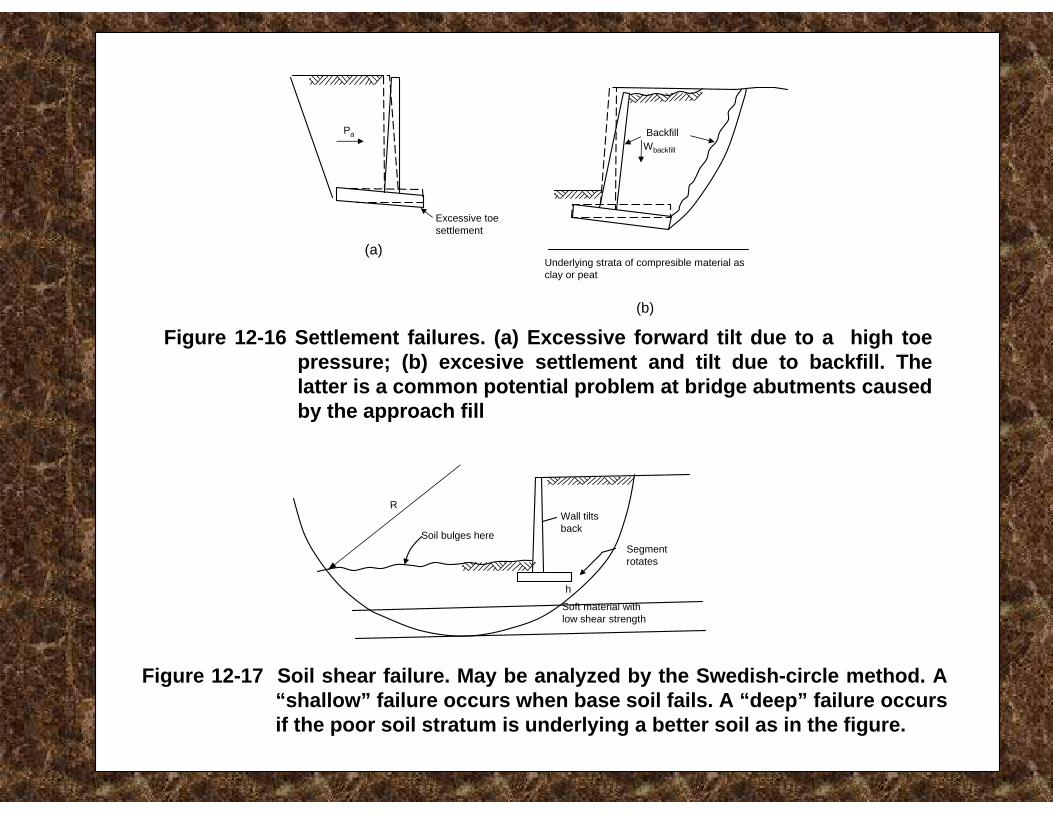
Excessive toe settlement

Underlying strata of compresible material as clay or peat

(b)

(a)

Pa BackfillWbackfill

Wall tiltsback

Segmentrotates

Soft material withlow shear strength

h

Soil bulges here

R

Figure 12-16 Settlement failures. (a) Excessive forward tilt due to a high toe pressure; (b) excesive settlement and tilt due to backfill. Thelatter is a common potential problem at bridge abutments causedby the approach fill

Figure 12-17 Soil shear failure. May be analyzed by the Swedish-circle method. A “shallow” failure occurs when base soil fails. A “deep” failure occurs if the poor soil stratum is underlying a better soil as in the figure.

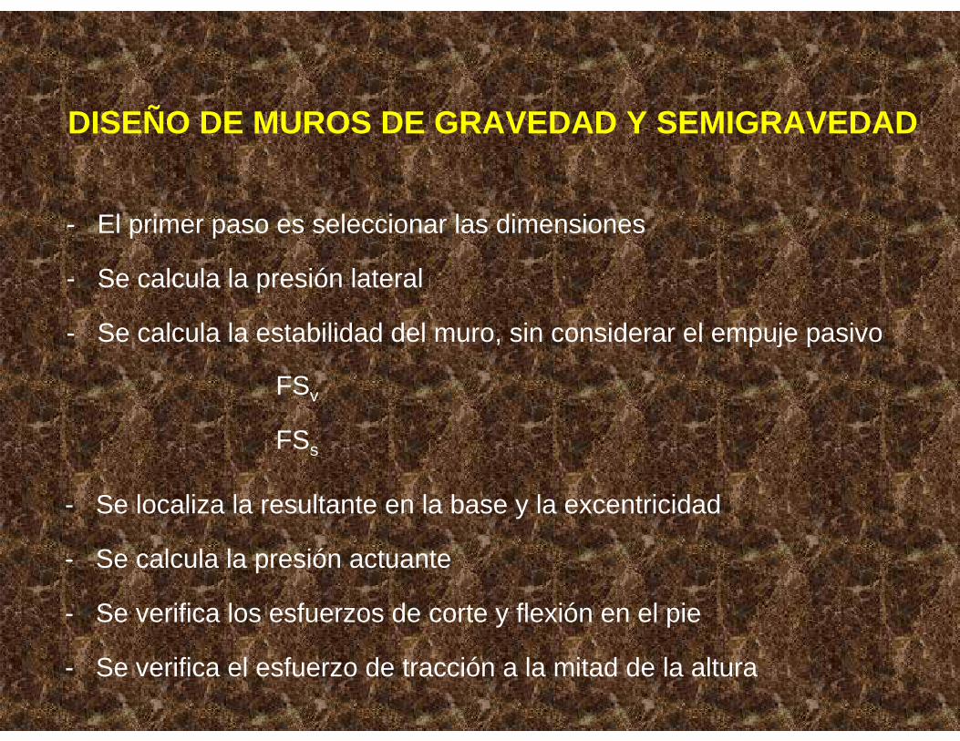
DISEÑO DE MUROS DE GRAVEDAD Y SEMIGRAVEDAD

- El primer paso es seleccionar las dimensiones

- Se calcula la presión lateral

- Se calcula la estabilidad del muro, sin considerar el empuje pasivo

FSv

FSs

- Se localiza la resultante en la base y la excentricidad

- Se calcula la presión actuante

- Se verifica los esfuerzos de corte y flexión en el pie

- Se verifica el esfuerzo de tracción a la mitad de la altura

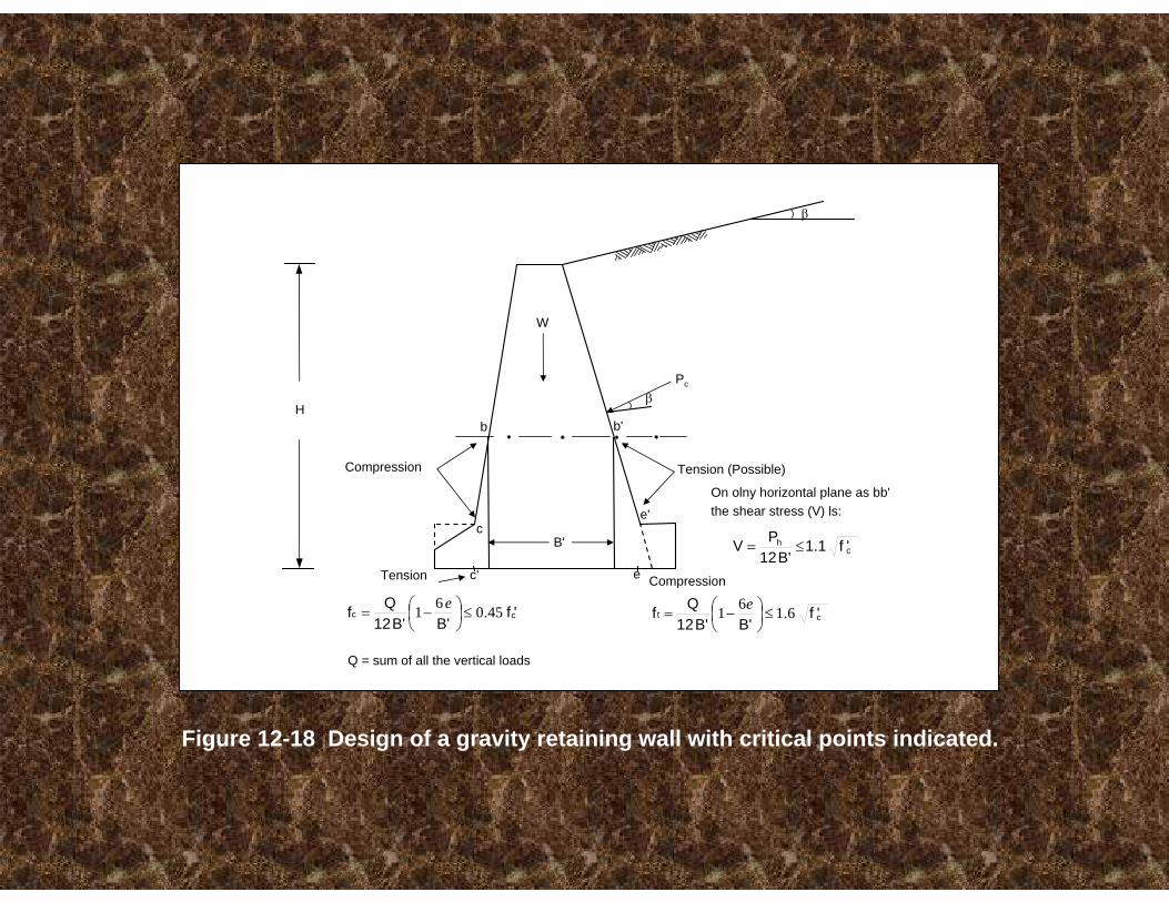
Pc

Tension (Possible)

b'

β

W

β

On olny horizontal plane as bb' the shear stress (V) ls:

ch 'f1.1B'12

PV ≤=

ct 'fB'B'12

Qf 6.161 ≤⎟⎠⎞

⎜⎝⎛ −=

eCompressione

e'

B'

c'

c

b

Compression

cc 'fB'B'12

Qf 45.061 ≤⎟⎠⎞

⎜⎝⎛ −=

e

Tension

Q = sum of all the vertical loads

H

Figure 12-18 Design of a gravity retaining wall with critical points indicated.

JUNTAS EN MUROS

Juntas de Construcción

Juntas de Contracción

Juntas de Expansión

Keys used to tietwo pours togetheror to increaseshear betweenbase and stem

No key use: base surface is cleaned androughened. Steelprovides added shear

Contraction joints: Weakened planes so crack formation is controlled

Expansionjoint

Fig. 12-19 Expansion and contraction joints

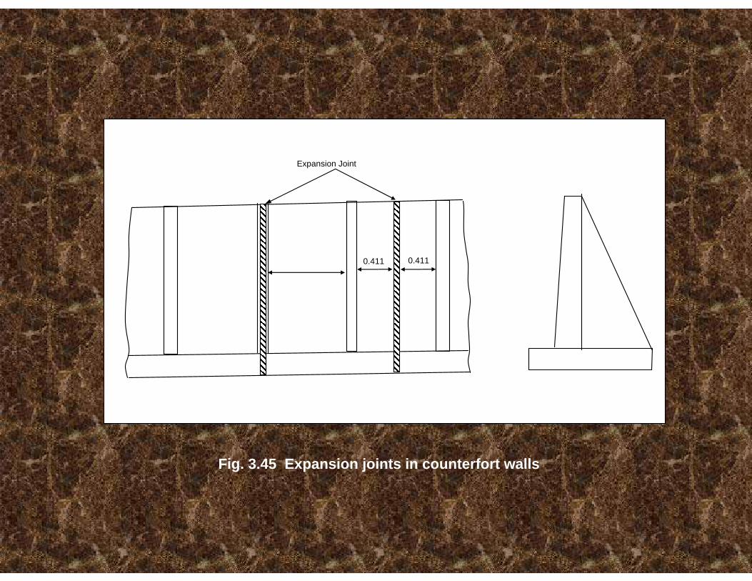
Expansion Joint

0.411 0.411

Fig. 3.45 Expansion joints in counterfort walls

DRENAJE

Lloraderos

Drenes longitudinales

Relleno granular

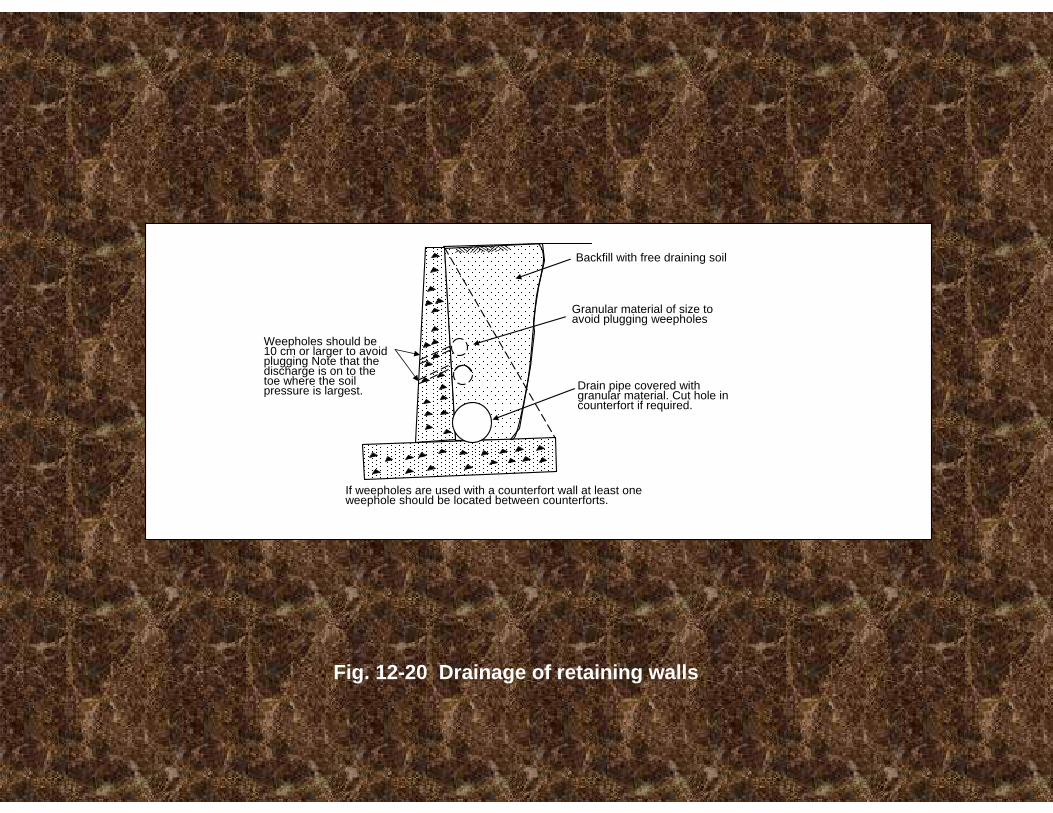
Weepholes should be 10 cm or larger to avoidplugging Note that thedischarge is on to thetoe where the soilpressure is largest.

Backfill with free draining soil

Granular material of size toavoid plugging weepholes

Drain pipe covered withgranular material. Cut hole in counterfort if required.

If weepholes are used with a counterfort wall at least oneweephole should be located between counterforts.

Fig. 12-20 Drainage of retaining walls

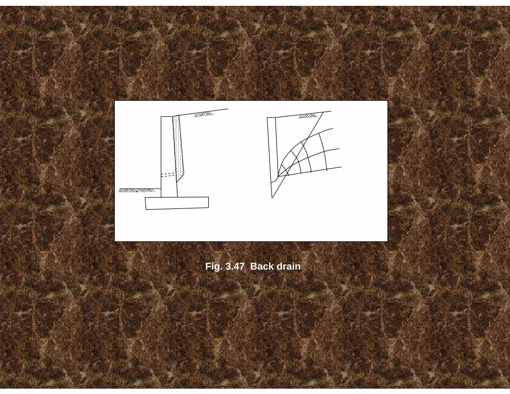
Fig. 3.47 Back drain

Fig. 3.48 (a) Inclined drain (b) Horizontal drain

(a) (b)

ALAS DE ESTRIBO Y MUROS DE CONTENCIÓN DE ALTURA VARIABLE

ALA MONOLITÍCA, la junta debe diseñarse por corte, tracción y

momento

Q = Pww cos α cos α - Pab

2T = Pww sen α

M = Pww Lw2

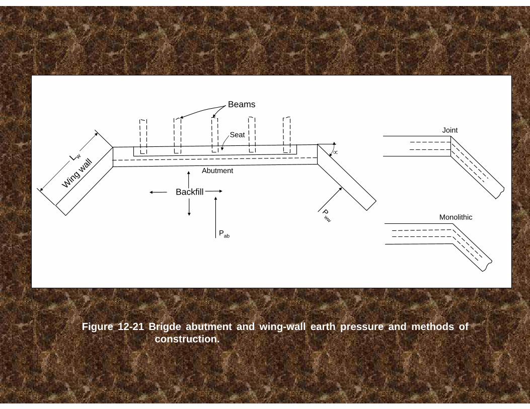
Figure 12-21 Brigde abutment and wing-wall earth pressure and methods ofconstruction.

Abutment

Backfill

Pab

Pww

Seat

∝

Beams

Wing

wall

L w

Joint

Monolithic

DISEÑO DE UN MURO CON CONTRAFUERTES

El diseño es similar al del muro en cantilever. Un diseño aproximado sería:

1) Dividir el cuerpo en varias zonas horizontales para obtener los momentos de flexión longitudinales. Use estos momentos para determinar el acero de refuerzo horizontal.

2) Dividir el cuerpo en varias franjas verticales, calcule los momentos verticales de flexión y el corte en la base del cuerpo y verifique el espesor del cuerpo por corte. Considere puntos decorte para el acero vertical

3) Dividir la losa del talón en varias franjas longitudinales y use los diagramas de presión y las ecuaciones de momento para obtener los momentos de flexión longitudinales. Use estos momentos para determinar el acero longitudinal de refuerzo en la losa.

4) Tratar la losa de cimentación como cantilever y determine el corte en la cara posterior del cuerpo y el momento flector. Revise el espesor de la base si necesita refuerzo de corte. Use el momento de flexión para calcular el acero de refuerzo requerido perpendicular a la losa-talón.

5) Tratar el pie de la losa de cimentación de forma idéntica a un muro en cantilever.

6) Analizar los contrafuertes. Ellos llevan un corte de Qc de

Qtotal = 0.5 q LH por cada espaciamiento

Q' = 0.2 q LH corte en la base del muro

Qc = 0.5 (0.5 q LH – 0.2 q LH) = 0.15 q LH

= corte lateral del muro llenado por contrafuerte

Figure 12-22 Structural design of counterfort wall. Make thickness to containadequate cover.

Pre

ssur

edi

agra

m

Wal

l

Cou

nter

fort

qh

Tens

ion

Qc

c.g.s.

yc.g.s.

Tensionarm

Qc y = As fy φ (arm)

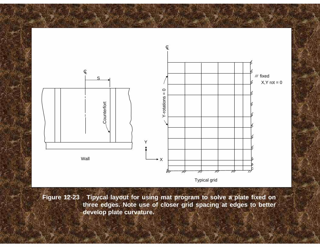
Figure 12-23 Tipycal layout for using mat program to solve a plate fixed onthree edges. Note use of closer grid spacing at edges to betterdevelop plate curvature.

CLS

Wall

Cou

nter

fort

Y

XY

-rota

tions

= 0

Typical grid

fixedX,Y rot = 0

///

CL

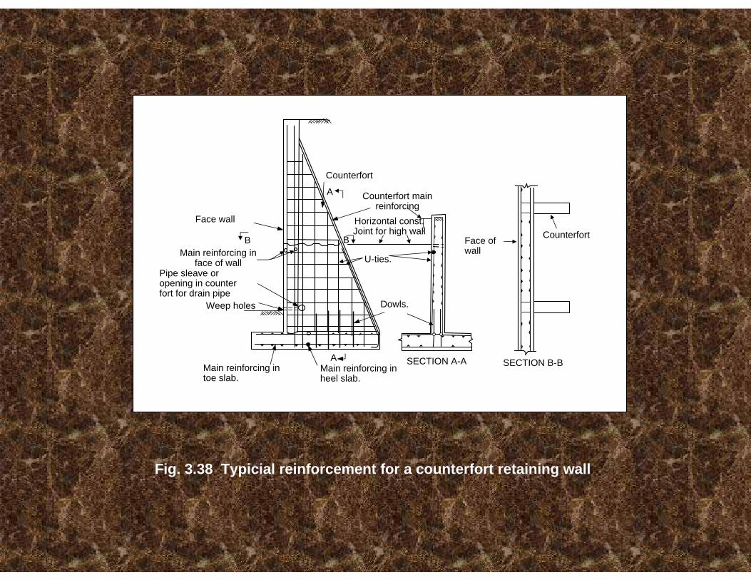
Counterfort

Counterfort mainreinforcing

Horizontal const. Joint for high wall

Face wall

A

B BMain reinforcing in

face of wallPipe sleave oropening in counterfort for drain pipe

Weep holes

U-ties.

Dowls.

Face ofwall

Counterfort

Main reinforcing in heel slab.

Main reinforcing in toe slab.

SECTION A-A SECTION B-BA

Fig. 3.38 Typicial reinforcement for a counterfort retaining wall

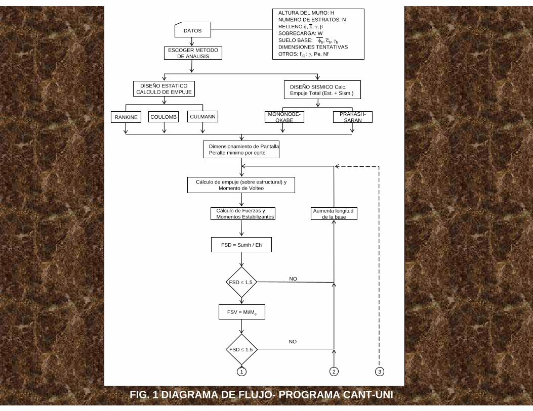
COULOMB

DISEÑO ESTATICOCALCULO DE EMPUJE

ESCOGER METODODE ANALISIS

Dimensionamiento de PantallaPeralte minimo por corte

Cálculo de empuje (sobre estructural) yMomento de Volteo

Cálculo de Fuerzas yMomentos Estabilizantes

Aumenta longitud de la base

FSD = Sumh / Eh

FSD ≤ 1.5

FSD ≤ 1.5

FSV = Mi/Me

21 3

FIG. 1 DIAGRAMA DE FLUJO- PROGRAMA CANT-UNI

NO

NO

DATOS

CULMANNRANKINE MONONOBE-OKABE

PRAKASH-SARAN

DISEÑO SISMICO Calc. Empuje Total (Est. + Sism.)

ALTURA DEL MURO: HNUMERO DE ESTRATOS: N RELLENO φ, c, γ, βSOBRECARGA: WSUELO BASE: φb, cb, γbDIMENSIONES TENTATIVAS OTROS: f'C : γ, Pe, Nf

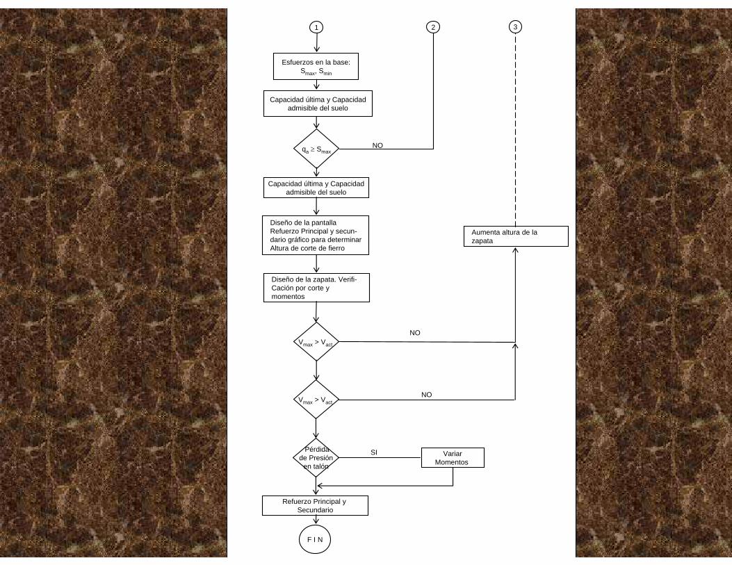
1

Esfuerzos en la base:Smax, Smin

Capacidad última y Capacidadadmisible del suelo

qa ≥ Smax

Capacidad última y Capacidadadmisible del suelo

Vmax > Vact

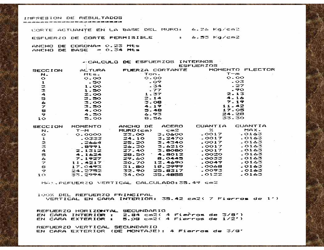
Diseño de la pantallaRefuerzo Principal y secun-dario gráfico para determinarAltura de corte de fierro

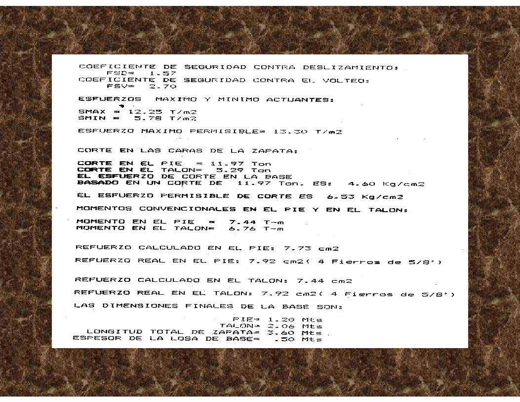
Diseño de la zapata. Verifi-Cación por corte ymomentos

Vmax > Vact

Pérdidade Presión

en talón

Refuerzo Principal y Secundario

F I N

VariarMomentos

Aumenta altura de lazapata

2 3

NO

NO

NO

SI

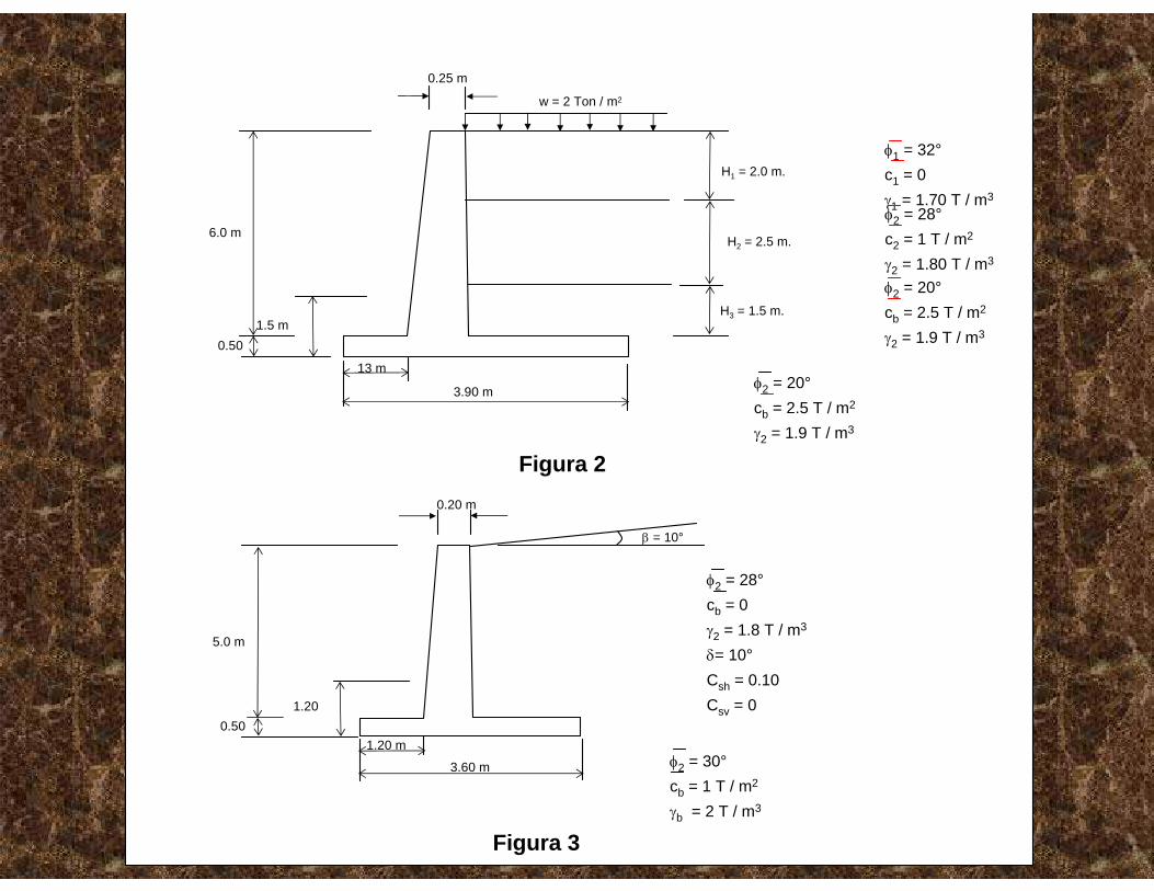
0.25 m

w = 2 Ton / m2

H1 = 2.0 m.

H2 = 2.5 m.

H3 = 1.5 m.

6.0 m

0.501.5 m

13 m

3.90 m

φ1 = 32°c1 = 0γ1 = 1.70 T / m3

φ2 = 28°c2 = 1 T / m2

γ2 = 1.80 T / m3

φ2 = 20°cb = 2.5 T / m2

γ2 = 1.9 T / m3

φ2 = 20°cb = 2.5 T / m2

γ2 = 1.9 T / m3

Figura 20.20 m

β = 10°

5.0 m

1.200.50

1.20 m

3.60 m

φ2 = 28°cb = 0 γ2 = 1.8 T / m3

δ= 10°Csh = 0.10Csv = 0

φ2 = 30°cb = 1 T / m2

γb = 2 T / m3

Figura 3

Microzonificación

geotécnica

del distrito de

trujillo

Primera edición digital

julio, 2011

lima - Perú

© enrique f. luján silva

ProYecto liBro digital

Pld 0114

editor: Víctor lópez guzmán

http://www.guzlop-editoras.com/guzlopster@gmail.com guzlopnano@gmail.com facebook.com/guzlop twitter.com/guzlopster428 4071 - 999 921 348lima - Perú

diseño

de

Muros

de

contención

Primera edición digital

noviembre, 2012

lima - Perú

© jorge e. alva Hurtado

ProYecto liBro digital

Pld 0580

editor: Víctor lópez guzmán

http://www.guzlop-editoras.com/guzlopster@gmail.com guzlopnano@gmail.com facebook.com/guzlop twitter.com/guzlopster731 2457 - 999 921 348lima - Perú