Departamento de Economía

TESIS DOCTORAL

Métodos estadísticos de depuración e

imputación de datos

Pedro Revilla Novella 2013

1

DEPARTAMENTO DE ECONOMÍA Plaza de la Victoria 28802 Alcalá de Henares (Madrid) Teléfonos :91 8854201/ 4202/ 5154 dpto.economia@uah.es

Prof. Dr. D. José Miguel Casas Sánchez, Profesor de la Universidad de Alcalá, como director de la tesis titulada “Métodos estadísticos de depuración e imputación de datos” realizada por D. Pedro Revilla Novella dentro del programa de Economía Aplicada del antiguo departamento de Estadística, Estructura Económica y Organización Económica Internacional de la Universidad de Alcalá. EXPONE: que la citada tesis doctoral, en mi opinión, reúne todas las condiciones

necesarias para el inicio de los tramites destinados a su defensa pública por parte del doctorando. Constituye un trabajo de investigación de ámbito académico, por lo que

AUTORIZA la presentación de la citada tesis doctoral para efectuar los trámites

necesarios conducentes a la defensa pública de la misma. En Alcalá de Henares, a dieciséis de julio de dos mil trece Firmado: Prof. Dr. D. José Miguel Casas Sánchez

2

DEPARTAMENTO DE ECONOMÍA Plaza de la Victoria 28802 Alcalá de Henares (Madrid) Teléfonos :91 8854201/ 4202/ 5154 dpto.economia@uah.es

D. Antonio García Tabuenca, director del departamento de Economía de la Universidad

de Alcalá autoriza, después de su aprobación por el departamento en su reunión de 17

de julio de 2013 la presentación de la tesis titulada “Métodos estadísticos de depuración

e imputación de datos” realizada por D. Pedro Revilla Novella dentro del programa de

Economía Aplicada del antiguo departamento de Estadística, Estructura Económica y

Organización Económica Internacional de la Universidad de Alcalá, una vez efectuados

los trámites oportunos, su defensa ante el tribunal correspondiente.

En Alcalá de henares, a diecisiete de julio de dos mil trece. Fdo.: Dr. Antonio García Tabuenca

3

UNIVERSIDAD DE ALCALÁ

FACULTAD DE CIENCIAS ECONÓMICAS, EMPRESARIALES Y TURISMO

DEPARTAMENTO DE ECONOMÍA

TESIS DOCTORAL

Métodos estadísticos de depuración e imputación

de datos

Pedro Revilla Novella

Director : Prof. Dr. D. José Miguel Casas Sánchez

Alcalá de Henares, Noviembre de 2013

4

A mis padres

Agradecimientos En primer lugar, quiero manifestar mi agradecimiento al profesor Dr. D. José Miguel Casas Sánchez por su generosidad al aceptar, desde un primer momento, dirigir mi tesis con su sólida experiencia y prestigio profesional, en un campo de investigación todavía no demasiado estudiado en el ámbito académico como es la depuración e imputación de datos estadísticos, y por brindarme su continuo apoyo académico y personal. Quería también expresar mi deuda con mis compañeros de investigaciones, de los que aprendo todos los días y además es un placer trabajar, en particular Ignacio Arbués, Pilar Rey y David Salgado. Asimismo, me gustaría mencionar a los colegas del grupo de depuración de las Naciones Unidas, que me han mostrado muchas buenas ideas a lo largo de estos años, en especial a Leopold Granquist y John Kovar.

5

Índice página 1.- Introducción…………………………………………………………………………9 2.- El problema de la depuración e imputación. Panorámica actual…………..…..13

2.1.- El problema de la depuración e imputación …………………………...13 2.2.- Panorámica actual……………………………………………………….16

2.2.1.- Métodos generalizados 2.2.2.- Métodos de depuración selectiva

3.- Planteamiento teórico y desarrollo empírico de nuevas técnicas de

depuración basadas en modelos estadísticos y en técnicas de optimización estocástica. ………………………………….……………….…….23

3.1 Depuración e imputación basada en modelos de series

temporales………………………………………………………………...23 3.1.1.- Introducción 3.1.2.- Construcción de herramientas de depuración e imputación 3.1.3.- Construcción de herramientas de macrodepuración y análisis 3.1.4.- Ejemplo con datos reales

3.1.5.- Conclusiones 3.2.- La depuración selectiva como un problema de optimización

estocástica……………………………………………………………….35 3.2.1.- Introducción 3.2.2.- El problema de la depuración selectiva 3.2.3.- Caso Lineal 3.2.4.- Caso Cuadrático 3.2.5.- Momentos condicionales basados en un modelo 3.2.6.- Caso práctico 3.2.7.- Conclusiones 3.3.- Propuesta y desarrollo de un marco teórico de depuración

e imputación basado en modelos y optimización ……………………42 3.3.1.- Introducción 3.3.2.- El uso de modelos estadísticos 3.3.3.- El problema de optimización

3.3.4.- Caso práctico 3.3.5.- Conclusiones

6

4.- Conclusiones…………………………………………………………………..….59 Referencias ……………………………………………………………………………64 Glosario ……………………………………………………………………………….74 Difusión de esta tesis doctoral………………………………………………..………75 Anexos…………………………………………………………………………………82

7

“Que errar es humano no sólo significa que hemos de luchar constantemente contra el error, sino también que, aún cuando hayamos puesto el máximo cuidado, no podemos estar totalmente seguros de no haber cometido un error”

Karl Popper

8

Capítulo 1

Introducción Esta tesis consiste en un conjunto de investigaciones desarrolladas en el campo de la depuración e imputación de datos. En concreto, se centra en dos principales líneas de investigación interconectadas entre sí: la utilización de modelos estadísticos y de técnicas de optimización. Las oficinas de estadística y otros organismos y empresas recogen y procesan grandes cantidades de datos con el objetivo de producir información estadística. Una parte importante de este proceso de producción consiste en chequear los datos, corregir los errores y dar un tratamiento adecuado a la falta de respuesta. La depuración e imputación de datos es una fase fundamental en el proceso de producción de información estadística. Sin esta fase, la calidad de las estimaciones finales podría reducirse significativamente, y la credibilidad de las encuestas verse seriamente dañada. Por otra parte, constituye una de las tareas más costosas en el proceso de producción estadística. Diversos estudios muestran que suponen por término medio el 20% del coste total de las encuestas a hogares y el 40% del de las encuestas a empresas. La depuración e imputación se centra en la detección y tratamiento de los errores ajenos al muestreo. Estos incluyen un amplio conjunto, como errores de no-respuesta, de medida, sistemáticos, aleatorios, influyentes, outliers, inliers, de unidad de medida, de redondeo, etc. A su vez, esta diversidad ha dado lugar a diferentes técnicas y algoritmos, tales como microdepuración, macrodepuración, depuración selectiva, depuración interactiva, o depuración automática. Una revisión reciente puede verse en de Waal et al. (2011). La importancia de este tema se refleja en la organización por parte de Naciones Unidas de un seminario periódico (Work Session on Statistical Data Editing). El mismo organismo, ha publicado manuales donde se recogen contribuciones en este campo (Statistical Data Editing, 1994, 1997 y 2006). El paradigma de Fellegi-Holt (1976) proporciona la base para la construcción de sistemas generalizados. En estos sistemas las reglas están estandarizadas, programadas y contrastadas y pueden aplicarse a encuestas diferentes. Habitualmente, realizan las siguientes funciones: análisis de los edits para chequear su consistencia, detección de errores, identificación de las variables a imputar e imputación. Sin embargo, no resuelven la especificación de los edits, tarea que se considera un input del sistema y que debe ser realizada en cada caso por los usuarios. Tradicionalmente, los usuarios establecen los edits de acuerdo a su experiencia práctica, sin que exista un marco teórico para los mismos. En este trabajo se propone un marco conceptual para tratar la especificación de los edits y se diseñan herramientas concretas de depuración e imputación de datos, basándose en modelos estadísticos. Al mismo tiempo, en busca de una mayor eficciencia en la depuración, se investiga la forma de resolver el problema de la depuración selectiva, mediante la utilización de técnicas de optimización. Esta tesis se estructura en cuatro capítulos. En el capítulo 1 se realiza la introducción. El capítulo 2, “El problema de la depuración e imputación. Panorámica actual de la

9

depuración e imputación”, plantea el contexto donde se encuadran las investigaciones y presenta el estado del arte en este campo. El capítulo 3, “Planteamiento teórico y desarrollo empírico de nuevas técnicas de depuración e imputación basadas en modelos estadísticos y en técnicas de optimización”, constituye la parte central de esta tesis y en él se describen las investigaciones llevadas a cabo y sus principales resultados y aportaciones. En el subcapítulo 3.1 “Depuración e imputación basada en modelos de series temporales”, están presentes ya las principales líneas de investigación de esta tesis, restringidas al caso de modelos de series temporales y encuestas continuas con datos cuantitativos. Los modelos utilizados, tanto para los microdatos como para los macrodatos son modelos RegARIMA. En las encuestas continuas la principal información para efectuar la depuración e imputación son los datos pasados de la misma encuesta. La depuración e imputación histórica tradicional (tasas de variación, etc.) puede mejorarse si se utilizan modelos de series temporales. A partir de estos modelos pueden determinarse los edits, basados en intervalos de confianza, tanto para la microdepuración como para la macrodepuración. Los datos sospechosos de error son aquellos que se salen de los intervalos. Para llevar a cabo la depuración selectiva se han desarrollado un conjunto de herramientas (que hemos denominado sorpresa, sorpresa estándar, sorpresa estándar ponderada e influencias) basadas en la función de predicción un periodo por delante del modelo. En algunos casos estas herramientas constituyen una función score, utilizadas ampliamente en la literatura (Berthelot y Latouche, 1993). Una aportación de esta tesis consiste en que la función score propuesta se obtiene a partir de los modelos y no por razones de tipo heurístico. Adicionalmente, a partir de los modelos anteriormente mencionados, se ha obtenido información de utilidad para llevar a cabo la macrodepuración, siguiendo la línea del análisis exploratorio de datos (Tukey, 1977). El subcapítulo 3.2, “La depuración selectiva como un problema de optimización estocástica”, se centra en el enfoque de la depuración selectiva. Disponer de métodos eficientes de depuración es un objetivo fundamental, ya que la depuración manual exhaustiva es considerada poco eficiente, puesto que la mayor parte del trabajo de depuración no tiene consecuencias a nivel agregado e incluso puede llegar a deteriorar la calidad de los datos. Los métodos de depuración selectiva son estrategias para seleccionar un subconjunto de los cuestionarios recogidos en una encuesta para someterlos a una depuración minuciosa. Una razón por la que es conveniente seleccionar algunos cuestionarios es que depurando ciertas unidades es más probable que mejore la calidad que si se depuran otras. Esto puede ser debido a que algunas son más sospechosas de contener un error o a que, en caso de tenerlo, probablemente tenga más impacto en los agregados. Una buena estrategia de depuración selectiva persigue compatibilizar dos objetivos: buena calidad de las estimaciones agregadas y reducido trabajo de depuración. El enfoque actualmente predominante es el de calcular algún tipo de función score (FS) que asigne una puntuación a cada unidad, priorizando la depuración de las unidades con mayor puntuación. Cuando para cada unidad se recogen varias variables, se pueden calcular diferentes FS locales y combinarlas en una global. Así, las unidades cuya FS excede un cierto umbral, son depuradas manualmente. Hasta ahora, estas cuestiones han sido tratadas de manera empírica. En Lawrence y McKenzie (2000) se proponen algunas directrices, pero en esencia se depende del criterio del experto. La mayor aportación de la tesis en este terreno es la resolución del problema de depuración selectiva a través de técnicas de optimización estocástica. En este subcapítulo, se plantea y se resuelve formalmente el problema. Posteriormente, se

10

propone un método para calcular ciertos momentos condicionales que se requieren para obtener la solución. También se presentan los resultados de una aplicación práctica. Finalmente, en el subcapítulo 3.3 “Desarrollo de un marco teórico de depuración e imputación basado en modelos y optimización”, se intenta alcanzar un mayor grado de formalización y abstracción y se desarrolla un marco teórico general que pueda ayudar a resolver distintos problemas. Hoy en día se acepta ampliamente que ninguna técnica o algoritmo puede hacer frente a todo tipo de errores. Por lo tanto, deben ser convenientemente combinados en una estrategia global de depuración e imputación. Dentro de este contexto general, este trabajo se centra en dos aspectos principales: el uso de modelos estadísticos para resolver los problemas de la especificación de los edits y aportar un método de imputación, y la utilización de técnicas de optimización para resolver los problemas que presenta la depuración selectiva. Los sistemas generalizados no resuelven la especificación de los edits, y habitualmente los usuarios establecen los edits de acuerdo a su experiencia práctica, sin que exista un marco teórico para los mismos. En este trabajo se aborda la forma en que pueden introducirse modelos estadísticos que relacionan los valores verdaderos, los observados y los depurados construidos a partir de distintos tipos de información disponible. La depuración selectiva se centra en los errores influyentes. En las últimas dos décadas, esta modalidad de depuración ha sido reconocida como un elemento clave en las estrategias de depuración e imputación. Sin embargo, hasta la fecha, se ha tratado de forma heurística. En el subcapítulo anterior se ha intentado dar un marco formal a la depuración selectiva, mediante técnicas de optimización estocástica. En este, se pretende ampliar el marco teórico a un problema de optimización general, del que pueden deducirse dos versiones: un problema de optimización combinatoria y el mencionado problema de optimización estocástica. Se parte de dos principios generales para abordar una depuración selectiva: se debe minimizar la cantidad de recursos utilizados y garantizar la calidad de los datos. Se propone una traducción matemática de estos principios a un problema general de optimización, cuya solución es la selección de unidades a depurar. En nuestra formulación, los recursos utilizados son equivalentes al número de cuestionarios seleccionados para depuración, mientras que la calidad de los datos se refleja en la precisión de los estimadores. Por tanto se toma como objetivo minimizar el número de unidades seleccionadas para depuración, sujetas a restricciones sobre el valor de las funciones de pérdida. Estas funciones se pueden dirigir al sesgo, al error cuadrático medio, a la varianza o a cualquier otra medida de incertidumbre en la estimación, lo que supone una ampliación respecto al subcapítulo anterior, donde sólo se consideraba el error cuadrático. Pueden ser de naturaleza heurística, tales como las medidas relacionadas con el llamado pseudo-sesgo utilizadas tradicionalmente para las funciones score, o pueden derivarse explícitamente a partir de modelos de medición del error. Las dos versiones del problema de optimización anteriormente citadas corresponden a los dos escenarios típicos para la aplicación de la depuración selectiva. En el primer caso, la selección se lleva a cabo unidad por unidad, de tal manera que la selección de una unidad no depende de la de otras unidades. Este modo es adecuado cuando la selección puede hacerse en tiempo real a la llegada de cada cuestionario. Nos referimos a este caso como optimización estocástica, debido a que la obtención en tiempo real de la solución sólo puede establecerse con respecto a hipotéticas repeticiones del proceso de selección. En el segundo caso, la selección se lleva a cabo de manera conjunta para

11

todas (o un grupo de) las unidades. Este modo es adecuado en una etapa posterior de la recogida de datos, cuando ya se dispone de un número suficiente de unidades. Nos referimos a este caso como el problema de optimización combinatoria, donde la solución se puede establecer condicionada a las observaciones reales de la muestra bajo algún modelo especificado de medición del error. Se presenta la forma en que puede resolverse el problema de optimización, para lo que es necesario introducir un modelo multivariante. También se realiza una comparación con funciones score ampliamente utilizadas, usando datos reales Finalmente, en el Capítulo 4, “Conclusiones”, se realizan comentarios finales y se perfilan algunas futuras líneas de investigación.

12

Capítulo 2

El problema de la depuración e imputación. Panorámica actual 2.1 El Problema de la depuración e imputación Las oficinas de estadística y otros organismos y empresas recogen y procesan grandes cantidades de datos con el objetivo de producir información estadística. Una parte importante de este proceso de producción consiste en chequear los datos recogidos, corregir los errores encontrados y dar un tratamiento adecuado a la falta de respuesta. La depuración incide en varias dimensiones de la calidad de la encuesta como la precisión, la puntualidad, la carga de respuesta o la eficiencia. Comprende la detección y el tratamiento de los errores ajenos al muestreo, sobre todo los de falta de respuesta y de medición. . Los errores de muestreo pueden ser más fácilmente controlados y evaluados Existe una abundante literatura que permite contar con un marco teórico abundante y sistemático, que posibilita controlar los errores de muestreo en la fase de diseño muestral y posteriormente evaluarlos una vez finalizada la encuesta. Entre las muchas referencias pueden citarse Cochran (1977), Särndal et al. (1992), Hidiroglou y Srinath (1993), Hidiroglou (1994), Valliant et al. (2000), etc. Contrariamente, los errores ajenos al muestreo encuentran una mayor dificultad en su tratamiento, por su propia definición como categoría residual. Para tratar de encarar esta complejidad, se ha tratado de clasificar los errores ajenos al muestreo en un determinado número de categorías, véase por ejemplo Cochran (1977), Biemer y Fecso (1995) o, más recientemente, Bethlehem (2009). Se ha desarrollado una tipología de errores, incluyendo errores sistemáticos, errores aleatorios, errores influyentes, outliers, inliers, o valores faltantes, por no hablar de los errores particulares dentro de estas clases como los errores de unidad de medida o errores de redondeo. Esta diversidad ha dado lugar a la aparición de diferentes técnicas y algoritmos para detectar y tratarlos, como la depuración interactiva, la depuración automática, la depuración selectiva, y la macrodepuración (véase De Waal et al. (2011) para una revisión completa). Hoy en día se acepta ampliamente que ninguna técnica puede hacer frente a todo tipo de errores. Por lo tanto deben ser convenientemente combinados en una estrategia de depuración e imputación (E & I en adelante), Por otra parte, a pesar de los esfuerzos realizados para automatizarla, y de los instrumentos que proporcionan las nuevas tecnologías, sigue siendo una fase que consume tiempo e intensiva en intervención humana. Esta es una de las razones por las cuales la depuración e imputación se convierte en una de las fases más caras del proceso producción de estadísticas. El uso de ordenadores no ha reducido significativamente su coste (Granquist, 1995). Por su parte, la falta de repuesta está también presente en las encuestas. Habitualmente se clasifica en falta de respuesta total (unit nonresponse), cuando se carece de información de todas las preguntas del cuestionario, y falta de respuesta parcial (item

13

nonresponse), cuando no se dispone de información de tan solo alguna de las preguntas. Por otra parte, la falta de respuesta se clasifica, (por ejemplo, en Rubin, 1987), en falta de respuesta aleatoria y no aleatoria. En general se acepta que en la mayoría de los casos la falta de respuesta no se produce de forma aleatoria y las unidades que no responden tienen un comportamiento diferente respecto a las características de interés: (las pequeñas empresas tienen peores registros contables,etc.). A su vez, la falta de respuesta no aleatoria puede clasificarse en falta de respuesta no aleatoria ignorable y falta de respuesta no aleatoria no ignorable. La falta de respuesta ignorable se produce cuando el mecanismo de la falta de respuesta es independiente del nivel de la variable de la que no se ha obtenido información pero depende en cambio de otras variables de las que sí se tiene información. Por el contrario, la falta de respuesta es no ignorable cuando el mecanismo de la falta de respuesta depende del nivel de la variable de la que no se ha obtenido respuesta. La falta de respuesta representa un grave problema para una encuesta, ya que no sólo supone una disminución del tamaño muestral, sino que suele sesgar las estimaciones, ya que las unidades que no responden rara vez constituyen una submuestra aleatoria de la muestra total. Los dos principales procedimientos para el tratamiento de la falta de respuesta son los métodos de reponderación y de imputación. La reponderación consiste en aumentar los pesos de las unidades que responden y se utiliza principalmente para el tratamiento de la falta de respuesta total. La imputación consiste en reemplazar los datos que faltan por valores “plausibles” y se utiliza fundamentalmente para el tratamiento de la falta de respuesta parcial. El método de reponderación puede, teóricamente, utilizarse también para el tratamiento de la falta de respuesta parcial, aplicándose variable a variable. Sin embargo, en la práctica, el procedimiento se hace complicado, ya que exigiría usar diferentes pesos para cada variable, razón por la cual se prefiere normalmente el método de la imputación. De hecho, en encuestas a empresas se utiliza a veces la imputación para la falta de respuesta total, cuando existe información auxiliar de otras fuentes o de encuestas anteriores. Finalmente, respecto a los outliers o valores atípicos, tienen, igual que los errores y la falta de respuesta, una importante incidencia en la elaboración de datos. Los outliers afectan fundamentalmente en la depuración y en la estimación. El tema de los outliers está presente en prácticamente todas las ramas de la inferencia estadística. Generalmente, en disciplinas estadísticas diferentes al muestreo de poblaciones finitas, se considera que la muestra ha sido generada a partir de un modelo o población que sigue una cierta distribución paramétrica. En este contexto, se considera que los outliers han sido generados a partir de una fuente diferente a dicho modelo o población. Sin embargo, dentro del marco de muestreo de poblaciones finitas basado en diseño, las muestras se seleccionan a partir de poblaciones finitas que son fijas, y los outliers se consideran que son valores legítimos que proceden de la población en estudio. No obstante, son valores extremos, que se encuentran alejados del núcleo central o de la mayoría de los datos. Existe otro tipo de valores que no son extremos, pero que su inclusión o exclusión puede afectar grandemente a las estimaciones. A este tipo de valores se les llama valores influyentes. Según comparten varios autores (por ejemplo, Gambino 1987, Srinath 1987, y Bruce 1991) la distinción entre valores extremos y valores influyentes es muy útil en las encuestas. La influencia de una observación depende del estimador que se está utilizando. Por ejemplo, una observación puede ser influyente para un estimador de

14

expansión y no serlo para uno de la razón y viceversa. De acuerdo a esto, una observación influyente se debe definir respecto a un estimador particular Algunos autores, por ejemplo, Chambers (1986), clasifican los outliers en dos tipos: outliers representativos y outliers no representativos. Los representativos son los que se obtienen sin que exista error en los datos y representan a otras unidades similares en la población. Los outliers no representativos son los que proceden de un error en los datos o son únicos en el sentido de que no existe otra unidad como ellos. Existe una amplia literatura acerca de los outliers en casos paramétricos o en poblaciones infinitas. Por ejemplo, Hawkins (1980) y Barnett y Lewis (1984) describen la detección y tratamiento de outliers para muestras que proceden de poblaciones con distribuciones paramétricas. Belsley et al. (1980) y Cook y Weisberg (1982) revisan métodos para el análisis de regresión. Beckman y Cook (1983) proporcionan una revisión histórica de los outliers incluyendo métodos bayesianos y de regresión robusta. Por su parte, Huber (1981), Hampel et al. (1986), y Rousseeuw y Leroy (1987) presentan distintos aspectos de la teoría de estimación robusta. Por el contrario, se ha escrito mucho menos acerca de los outliers en muestras de poblaciones finitas. En algunas ocasiones, las encuestas que se basan en el muestreo de poblaciones finitas pueden usar métodos que provienen de otras ramas de la estadística. Normalmente puede considerarse que el estudio de los outliers contempla dos aspectos: su detección y su tratamiento. El problema de los outliers en la estimación es esencialmente un problema de estimación robusta. La estimación robusta puede ser abordada mediante el tratamiento de los outliers detectados o por la directa aplicación de técnicas de estimación robustas como el M-estimador. La detección de outliers tiene interés en la depuración, ya que pueden ser legítimos valores de la población pero pueden ser también errores en los datos que deben ser corregidos antes de la estimación. Tradicionalmente, los outliers son detectados usando sus distancias relativas al centro de los datos. El tratamiento de outliers en la etapa de estimación encuentra un conjunto de procedimientos con una base formal. Existen dos enfoques principales para el tratamiento de los outliers en poblaciones finitas. Un primer conjunto de métodos está basado en la sustitución de los valores outliers o en la reducción de sus pesos. La sustitución de los outliers puede llevarse a cabo mediante los métodos de recorte o “winsorización”. Una alternativa a sustituir los valores que se consideran outliers consiste en reducir sus pesos. Una primera versión de este procedimiento se encuentra en Bershad (1960), tras la cual muchos de estos estimadores han sido propuestos. En esta línea pueden destacarse las aportaciones de Searls (1966), Ernst (1980), Hidiroglou y Srinath (1981), Dalén (1987), Tambay (1988), Ghangurde (1989a, 1989b), Fuller (1991), Hidiroglou (1991), Rivest y Hurtubise (1993), Rivest (1993a, 1993b), y Thorburn (1993). Un segundo conjunto de métodos consiste en usar métodos de estimación robustos como la M-estimación. Huber (1964) introdujo el M-estimador como una alternativa robusta a la media muestral para una distribución que sigue una normal en el centro y una doble exponencial en las colas. Desde la publicación de Huber muchos M-estimadores han sido propuestos y estudiados. En esta línea puede verse, por ejemplo, Andrews et al. (1972). Más recientemente, Chambers (1986), Hampel et al. (1986), Lee (1990, 1991a), Bruce (1991), Gwet y Rivest (1992), y Hulliger (1993) realizan importantes contribuciones en esta materia.

15

2.2 Panorámica actual Para afrontar la depuración e imputación existen actualmente multitud de técnicas. Estas técnicas utilizan herramientas teóricas o provienen de la experiencia práctica. Por otra parte, las técnicas pueden haberse diseñado de forma ad hoc para una encuesta determinada o pretender aplicarse de forma general. Inicialmente, los sistemas de depuración consistían en tareas manuales secuenciales, como la construcción de reglas para “detectar y corregir”. Los sistemas resultantes eran a menudo grandes y complejos. 2.2.1 Métodos generalizados A mediados de los 70, Fellegi y Holt (1976) proponen un sistema generalizado de depuración e imputación. Varios sistemas generalizados se han desarrollado a partir de entonces. En los métodos generalizados, las reglas y convenciones están estandarizadas, programadas y contrastadas, y pueden aplicarse a muchas encuestas diferentes. Las ventajas de los métodos generalizados son que utilizan una metodología contrastada y eficiente, que coordinan y sistematizan esfuerzos que se repiten de encuesta en encuesta, que ahorran recursos y tiempo en el estudio y desarrollo de procedimientos específicos y que garantizan la consistencia entre encuestas similares. El paradigma fundamental de los métodos generalizados procede del trabajo de Fellegi y Holt (1976), que propusieron una metodología por la cual un conjunto programas que se ejecutaban en bach llevaban a cabo las siguientes funciones:

1) análisis de los edits 2) detección de errores 3) identificación de las variables a imputar 4) imputación

La labor de los especialistas de la encuesta se limita a proporcionar los diferentes edits. El resto de las labores de depuración e imputación la lleva cabo automáticamente el programa. Los edits se clasifican en explícitos, que son los originalmente especificados por los especialistas de la encuesta y los implícitos, que se deducen lógicamente de los anteriores, y son generados automáticamente por el programa. El corazón de la metodología de Fellegi y Holt es el concepto de conjunto completo de edits, que es el conjunto de todos los edits generados implícitamente a partir del conjunto primitivo de edits explícitos. La generación del conjunto completo de edits, es decir, el conjunto donde se integran los edits explícitos y todos los edits implícitos, es un proceso interactivo. Fellegi y Holt demuestran en su artículo que, si el conjunto de edits explícito cumple unas condiciones bastante generales, el proceso es convergente. El procedimiento actúa siguiendo los siguientes principios: cada registro satisface todos los edits; el sistema minimiza el número de campos a imputar (conocido como principio de cambio mínimo); no es necesario especificar las reglas imputación, sino que se derivan automáticamente de los edits; y las imputaciones mantienen la estructura de frecuencias de los datos sin error.

La metodología de Fellegi y Holt es, en teoría, aplicable tanto a variables cuantitativas como a variables cualitativas. Sin embargo, en su implementación, surgen mayores problemas cuando se aplica a variables cuantitativas. Partiendo del paradigma de Fellegi y Holt se han diseñado otros sistemas generalizados que intentan adaptarse a los

16

problemas de los datos cuantitativos. Entre ellos pueden destacarse el sistema SPEER (Structured Program for Economic Editing and Referral) desarrollado por el Bureau of the Census, y el sistema GEIS (Generalized Edit and Imputation System), desarrollado por la oficina estadística de Canadá. Estos sistemas están descritos por ejemplo, en Pierzala (1990a, 1990b). Las principales características del sistema SPEER, descritas por Draper et al. (1990) y Winkler y Draper (1996), son la utilización de edits de la razón y su fundamentación en la teoría de grafos y en las técnicas estadísticas. Por su parte, las principales características del sistema GEIS, descritas en Kovar (1993) son la utilización de edits lineales, y su fundamentación en técnicas de investigación operativa y de programación lineal. Entre los diferentes métodos generalizados, pueden citarse los siguientes:

a) sistema DIA (Depuración e Imputación Automática), desarrollado por el INE, García et al (1990)

b) sistema SCIA, desarrollado por el ISTAT, Barcaroli et al. (1995) c) sistema NIM (New Imputation Methodology), desarrollado también por la

oficina estadística canadiense, Bankier et al. (1995 y 1996) d) sistema CherryPi, desarrollado por la oficina estadística de Holanda, De Waal

(1996) e) sistema DAISY (Design, Analysis and Imputation System), desarrollado por la

oficina estadística italiana, Barcaroli y Venturi (1997) f) sistema MacroView, desarrollado por la oficina estadística de Holanda, Van de

Pol et al. (1997) g) sistema Plain Vanilla, desarrollado por la oficina estadística de Estados Unidos,

Grahan (1997) h) sistema StEPS(Standard Economic Processing System), desarrollado por la

oficina estadística de Estados Unidos, Sigman (1997) i) sistema AGGIES (Agriculture Generalized Imputation and Edit System),

desarrollado por el ministerio de agricultura de Estados Unidos, Todaro (1998) j) sistema Blaise, desarrollado por la oficina de estadística de Holanda, Blaise

Reference Manual (1998) k) sistema GEIS (Generalized Edit and Imputation System), desarrollado por la

oficina estadística canadiense, Statistics Canada (1998), que ha derivado más recientemente en el sistema Banf

2.2.2 Métodos de depuración selectiva La depuración selectiva constituye actualmente uno de los enfoques más prometedores de la depuración, especialmente en encuestas con datos cuantitativos. Su utilización está recomendada por diversos autores e instituciones, por ejemplo, el Grupo de Trabajo de depuración e imputación de las Naciones Unidas (2006), o las Statistics Canada Quality Guidelines (2009). La depuración selectiva surge como un intento de solución de los problemas de la depuración tradicional. Entre estos problemas puede señalarse, en primer lugar, el elevado coste de la misma. A pesar de los esfuerzos realizados para racionalizar los procesos y a pesar de la ayuda que pueden suponer las herramientas informáticas y de comunicaciones, la experiencia de los distintos países muestra que el coste de la depuración no ha disminuido. En realidad, la facilidad que proporcionan los ordenadores ha sido frecuentemente utilizada para programar más edits de los realmente

17

necesarios o de los que el equipo de depuración es capaz de llevar a cabo. Esos edits adicionales han dado lugar a un incremento en el número de cuestionarios que necesitan una revisión manual. Todo ello ha dado lugar al fenómeno conocido como “sobredepuración”, es decir, los recursos y el tiempo dedicados a la depuración no se justifican por las mejoras resultantes en la calidad de los datos. Cuando se hace referencia al coste de la depuración, no se considera solamente el coste que esta supone para los organismos productores. En realidad, debe valorarse un coste más amplio, integrado además por el coste de los informantes de la encuesta, especialmente en el caso de que exista un número excesivo de recontactos, para discutir y aclarar al depurador la validez de los datos que no pasan los edits. También debe valorarse el coste en términos de tiempo invertido en la depuración, que, o bien recorta tiempo de otras fases del proceso de producción estadístico, o bien alarga el tiempo de difusión de la encuesta, uno de los aspectos de la calidad de una estadística que más interesa habitualmente a los usuarios. Por otra parte, existe un abundante número de estudios en la literatura de la depuración, que muestran que mucho del impacto que la depuración tiene en los datos finales es atribuible tan sólo a un pequeño porcentaje del total de los edits. Por ejemplo, al evaluar la depuración en los censos económicos de los Estados Unidos, Greenberg y Petkunas (1986) encuentran que el 5% de los errores corregidos durante el proceso de depuración da lugar a más del 90% del cambio total en las estimaciones. Del mismo modo, en un estudio de la encuesta anual de cuentas financieras de Suecia, Wahlström (1990) encuentra que el 2% de los errores corregidos da lugar a más del 90% del cambio en las estimaciones. En la encuesta industrial anual sueca, Hedlin (1993) encuentra que el 8% da lugar al 95%. Finalmente, en la encuesta industrial anual canadiense, Boucher (1991) encuentra que después de corregir el 50% de los errores ya se había alcanzado el 100% del cambio en las estimaciones, de manera que la corrección del otro 50% de los errores no producía ninguna ganancia en la acuracidad de las estimaciones. Otro problema de la depuración tradicional consiste en que la mayoría de los datos detectados como sospechosos de error no da lugar a correcciones, una vez que ha sido analizada su validez por parte del equipo de depuración (frecuentemente después de recontactar con el informante). El ratio de impacto (el número de datos que se corrigen respecto al total de datos que los edits señalaban como sospechosos de error) resulta ser demasiado bajo en muchas encuestas, evidenciando que la eficiencia del proceso de depuración podía ser mejorada y el número de recontactos disminuido (con la consiguiente reducción del coste y de la carga de respuesta). Por ejemplo, Lindströn (1991) realiza un estudio en diversas encuestas y encuentra que el ratio de impacto se mueve entre el 28% y el 47%. Por otra parte, la depuración también puede esconder problemas serios en la recogida de datos y dar una falsa impresión de la capacidad de respuesta de los informantes. Dos ejemplos de este problema pueden verse en el Australian Bureau of Statistics (1987). Al revisar los depuradores la sección de las compras, en el Censo del Comercio al por menor de Australia, sistemáticamente deducían una pequeña cantidad a partir de la "compra de bienes" y la insertaban en el espacio dejado en blanco por las empresas de "compras de envases y embalajes" para evitar un mensaje de error en la siguiente fase de depuración de controles previamente grabados por el ordenador. El otro ejemplo ocurría en la encuesta de producción de productos industriales. La clasificación de los bienes que figuraban en el cuestionario, era demasiado detallada para los informantes,

18

que agregaban la producción de algunos epígrafes y la asignaban globalmente en el epígrafe más relevante. El equipo de depuración manual comparaba las respuestas actuales con las respuestas obtenidas en periodos anteriores. A partir de esa información deducían las cantidades de los epígrafes complementados por las empresas, y asignaban los datos de producción a epígrafes que las empresas no habían complementado. Este proceso se conoce en la literatura de depuración como "depuración creativa" porque los depuradores manuales inventan los procedimientos de depuración e imputación mediante unos métodos subjetivos y no homogéneos, dando una falsa impresión de la capacidad de respuesta de los informantes. Otro problema de la depuración tradicional, que con alta frecuencia se ha venido observando en la mayoría de organismos productores de estadística, es que los responsables de encuesta se marcan como objetivo de depuración utilizar el mayor número de contrastes de depuración posibles y los intervalos de aceptación lo más estrechos posibles. La idea que subyace aplicando estos objetivos, es que la calidad de la encuesta mejorará a medida que aumente el número de contrastes y la amplitud de los intervalos de rechazo (siguiendo el principio de" la seguridad lo primero", es decir cuanto más contrastes y más estrechos mejor). Sin embargo, algunas indicaciones de que esta idea no era cierta se tienen ya desde fechas tan tempranas como 1965. Usando datos de la encuesta industrial anual de Noruega de 1982, Nordbotten (1965) implantó una serie de estudios de simulación de un sistema experimental automático de depuración e imputación. Valores detectados como sospechosos de error por contrastes de la razón fueron imputados automáticamente usando un método hot deck. Nordbotten encontró que los intervalos de aceptación más amplios daban lugar a una calidad más alta, porque los intervalos de aceptación demasiado estrechos identificaban incorrectamente muchos datos válidos como erróneos, y entonces reemplazaban innecesariamente esos datos reales por valores imputados. Incluso esos intervalos de aceptación más amplios fueron considerados demasiado estrechos por Fellegi (1965) en su discusión sobre los estudios de simulación de Nordbotten. A partir de entonces, se han llevado a cabo un elevado número de estudios, que muestran que la calidad no siempre mejora cuando se utiliza el mayor número de contrastes de depuración posibles y cuando se utilizan intervalos de aceptación lo más estrechos posibles. Entre estos estudios pueden destacarse, por ejemplo, los de Corby (1984) y Werking et al. (1988). Para solucionar estos problemas de la depuración tradicional, se propusieron los métodos conocidos como métodos de depuración selectiva. Estos métodos fueron introducidos por Granquist en la oficina estadística de Suecia a partir de 1984. En su inicio, estos métodos fueron conocidos como métodos de macrodepuración, ya que partían de los datos agregados y no de los microdatos. Sin embargo, actualmente reciben el nombre de métodos de depuración selectiva, dejando el amplio término de macrodepuración para todo procedimiento que realice los contrastes sobre los datos agregados (Glosario de términos de depuración e imputación, Winkler 1999). La depuración selectiva consiste en la detección y corrección selectiva de errores. Pone en relación los microdatos con los macrodatos, para determinar los errores de los microdatos que tienen influencia en los macrodatos. Su objetivo es agilizar las tareas de depuración e imputación en los datos de la encuesta sin detrimento en la calidad del proceso. Para entender el concepto de depuración selectiva, conviene analizar los errores de una encuesta de la forma en que lo hace Granquist (1984b). En una encuesta, pueden

19

aparecer errores de negligencia y errores sistemáticos no anticipados. Los errores de negligencia se tienen como resultado de la falta de cuidado del informante o del proceso de la encuesta. Lo esencial es que, en una repetición de la encuesta, el mismo error probablemente no sería encontrado para la misma variable del mismo cuestionario. Por su parte, los errores sistemáticos no anticipados, aparecen debido a la ignorancia o a la mala interpretación de las cuestiones, conceptos o definiciones, o son cometidos deliberadamente. Lo esencial es que en una repetición de la encuesta, el mismo error probablemente afectaría a la misma variable del mismo cuestionario. Granquist encuentra que la depuración tradicional: no es eficiente con los errores de negligencia, está lejos de ser aceptable con los errores sistemáticos no anticipados y genera una ilusoria sensación de confianza

En un intento de resolver estos problemas, Granquist (1984a) propone el método de la depuración selectiva, que se basa en: a) Identificar áreas problemáticas, b) Estimar y documentar el impacto en las áreas problemáticas, c) tomar medidas para ajustar los errores sistemáticos no anticipados en la encuesta actual, y d) tomar medidas para mejorar este tipo de errores en futuras encuestas. El método se basa en un proceso selectivo de detección de errores. De acuerdo con ello, no todos los cuestionarios o variables son objeto de investigación. Son objeto de investigación aquellos cuestionarios que son verdaderamente influyentes en los agregados y se ignoran datos cuya magnitud no es significativa o que se cancelan en el proceso de agregación. La depuración selectiva se trata de una filosofía y no de un conjunto de procedimientos cerrados. Se concibe generalmente como un proceso interactivo. Se aplica preferentemente en datos cuantitativos y en encuestas de empresas caracterizadas por la asimetría de sus poblaciones. A partir de los trabajos llevados a cabo por Granquist en la oficina estadística sueca, han aparecido un elevado número de métodos de depuración selectiva. Entre ellos mencionaremos los siguientes: Método de agregación El método de agregación fue desarrollado por Granquist (1988b) para la oficina estadística de Suecia. Versiones posteriores pueden verse en Lindströn (1990a, 1990b). La idea fundamental de este procedimiento es trabajar en dos etapas. En la primera etapa, se pasa los controles de depuración a los datos agregados. En la segunda etapa, se pasan esos mismos controles a los datos individuales, pero únicamente a aquellos pertenecientes a los agregados que no han pasado los controles en la primera etapa. El procedimiento admite dos versiones: en una primera versión, se depurarían en una primera etapa los datos agregados, a un determinado nivel de agregación (por ejemplo sectores de actividad o regiones geográficas de los cuales se quiere obtener información). En una segunda etapa, se depurarían aquellos microdatos de los datos agregados que no han pasado los controles de la primera etapa. En una segunda versión de esta misma idea, se asignaría a los registros de un agregado detectado como sospechoso de error, una señal específica que mostrara cuál de las variables no pasa los controles. Entonces, la depuración al nivel de microdatos, se aplicaría únicamente en aquellos cuestionarios que pertenecen a los agregados que no pasa los controles para esa variable específica.

20

Uno de los rasgos esenciales de los métodos de agregación consiste en que los intervalos de aceptación son determinados manualmente mediante la revisión de listas de observaciones clasificadas de acuerdo a las funciones de los contrastes. Sólo las n más grandes observaciones y las m más pequeñas observaciones de las funciones de chequeo son impresas en las listas. Tanto las funciones de chequeo, que trabajan a nivel agregado, como las funciones de chequeo que trabajan en el nivel desagregado, tienen que ser funciones de los pesos (de acuerdo al diseño muestral). Los estudios de evaluación llevados a cabo por la oficina estadística sueca, concluyeron que el trabajo de verificación de errores se redujo en un 50% sin descenso en la calidad de los datos. Dentro del método de agregación, Anderson (1989b) propone utilizar diagramas de caja para determinar los intervalos de aceptación. Método "top-down" El método "top-down" fue desarrollado por Granquist (1987 y 1991) para la oficina estadística de Suecia. La idea que subyace en este método es clasificar de forma jerárquica los valores de las funciones de chequeo (que son funciones de los valores debidamente ponderados) y comenzar la revisión manual desde arriba o desde abajo y continuar hasta que las correcciones no tengan un efecto significativo en las estimaciones. Por tanto, se seleccionan y ordenan de mayor a menor los n valores extremos de una variable o una función de variables. Por ejemplo, los n mayores cambios positivos, o los n mayores cambios negativos, o las n mayores contribuciones al agregado. De modo interactivo se pueden corregir errores en la pantalla y ver cómo se modifica la lista valores extremos. Se deja de corregir cuando se considera que las correcciones no modifican sustancialmente los totales (Anderson 1989a) Desagregación en cascada de tablas de series Es un procedimiento de macrodepuración desarrollado en el ámbito de las encuestas industriales del INE. Permite agregar o desagregar cualquier conjunto de variables y ratios de variables (habitualmente en forma de series temporales) bajo cualquier condición. Este procedimiento permite buscar el o los cuestionarios iniciales responsables del presunto error. No existe una forma previa, obligatoria de usar para buscar ese o esos cuestionarios sospechosos. Cada persona puede decidir cual es la mejor forma de buscar el error, en función de su experiencia sobre el sector o, simplemente según su costumbre. La esencia del método es que la búsqueda de la información la determina el usuario, y no está prefijada de antemano mediante un conjunto fijo de tablas. Métodos basados en la función score Un enfoque fundamental en los métodos de depuración selectiva es la construcción de una función de tanteo o puntuación para cada dato o para cada unidad informante. Latouche y Berthelot (1990 y 1992) fueron los pioneros en la utilización de funciones score como instrumento de depuración selectiva. En sus investigaciones establecieron las bases de una función score y propusieron tres funciones. Su objetivo es optimizar la estrategia de investigación y recontacto con los informantes. Su metodología es aplicable a encuestas continuas de empresas, caracterizadas por tres elementos:

21

investigan fundamentalmente variables cuantitativas, las variables de interés tienen distribuciones altamente asimétricas, donde unas pocas empresas contribuyen a una parte importante de las características poblacionales a investigar, y se dispone de información histórica de encuestas anteriores. Las funciones tanteo deben tener en cuenta cuatro criterios: el tamaño de la unidad informante, el número de datos sospechosos de error dentro del cuestionario, el tamaño de esos datos sospechosos de error, y la importancia relativa que se asigna a las variables sujetas a posibles errores. Además de estos aspectos teóricos, la función de tanteo debe tener en cuenta aspectos operativos, como que sea fácil de implementar y sea suficientemente flexible para poder ser utilizada en diferentes encuestas. Al mismo tiempo, la fórmula de la función de tanteo debe de tener una interpretación relevante desde el punto de vista del contenido y objeto de la encuesta. Finalmente, otro aspecto operativo a tener en cuenta es que el uso de la función no retrase el proceso de la encuesta. Para ello, las variables utilizadas en la función no deben depender del flujo de respuestas, sino que deben conocerse al comienzo de la encuesta, para que el método pueda aplicarse desde el primer momento, aún cuando la tasa de respuesta sea todavía muy pequeña. Para ello, las variables utilizadas pueden proceder de la misma encuesta en periodos anteriores y, del periodo corriente, solamente sea necesario utilizar los datos proporcionados por el informante que se está depurando. La función Score es una fórmula matemática que asigna una puntuación relativa a cada unidad informante, utilizando como inputs las características de la unidad informante que están relacionadas con el potencial impacto en las estimaciones, combinando los factores (teóricos y operativos) deseables. Primero se calcula una puntuación para cada variable de un cuestionario, luego se suman estas puntuaciones para obtener una puntuación global de cada unidad informante. Las unidades informantes con más alta puntuación se considera que van a tener mayor influencia en los agregados, y deben ser recontactadas con mayor prioridad Significance editing Lawrence y McDavitt (1994), realizan un trabajo pionero aplicándolo a la Encuesta de Ganancias Salariales Semanales de Australia y Lawrence and McKencie, (2000), proponen una metodología general de depuración selectiva. El principio fundamental de significance editing es estimar el efecto en las estimaciones de los agregados de resolver un determinado dato sospechoso de error. Un prerequisito es disponer de un modelo adecuado de depuración, formado por el conjunto de edits. Por tanto, significance editing no mejora un modelo inadecuado de depuración ni detecta errores que no hayan sido detectados por el conjunto de edits. Los elementos que constituyen una estrategia de significance editing son la determinación de un “valor arreglado esperado”, el cálculo de score locales, la combinación de score locales para calcular un score global y el establecimiento de umbrales de corte para los scores. La determinación del “valor arreglado esperado” se hace a partir del conjunto de edits, partiendo de la idea de que los edits expresan un punto de vista predeterminado de cómo la población se tiene que comportar. Aunque no se contempla un método general para generar el valor arreglado esperado a partir del modelo de depuración, en Lawrence and McKencie, (2000), se ofrecen algunos procedimientos concretos aplicables a conjuntos de edits utilizados habitualmente en encuestas de empresas.

22

Capitulo 3

Planteamiento teórico y desarrollo empírico de nuevas técnicas de depuración basadas en modelos estadísticos y en técnicas de optimización estocástica

3.1 Depuración e imputación basada en modelos de series temporales 3.1.1 Introducción Los modelos de series temporales no son de uso común en la depuración e imputación ni en otras fases del proceso de producción de estadísticas, con la excepción del ajuste estacional. Sin embargo, las encuestas continuas dan lugar a un conjunto de observaciones secuenciales recogidas a lo largo del tiempo. Por tanto, el marco teórico no tiene por qué limitarse al de las variables aleatorias, sino que puede ser ampliado al de los procesos estocásticos, y el uso de modelos de series temporales está plenamente justificado. Si existe información sobre periodos anteriores, se debe utilizar al máximo en la depuración e imputación, y ello puede hacerse a través de ese tipo de modelos. Por otra parte, el paradigma de Fellegi-Holt (1976) proporciona la base para la construcción de sistemas generalizados. En los sistemas generalizados las reglas están estandarizadas, programadas y contrastadas y pueden aplicarse a encuestas diferentes. Los sistemas generalizados basados en la filosofía de Fellegi-Holt llevan a cabo el análisis de los edits para chequear su consistencia, la detección de errores, la identificación de las variables a imputar y la imputación. Sin embargo, no resuelven la especificación de los edits, que se considera un input del sistema y deben ser especificados por los usuarios (los responsables de cada encuesta). Habitualmente, los usuarios establecen los edits de acuerdo a su experiencia práctica, sin que exista un marco teórico para los mismos. En este trabajo se propone un procedimiento para tratar la especificación de los edits y se diseñan herramientas concretas de depuración e imputación de datos estadísticos, basándose en la utilización de series temporales y aplicable a encuestas continuas. Como un criterio esencial de la depuración e imputación consideramos que los datos sean consistentes con la información existente. En las encuestas continuas, la principal información suele ser la histórica de la misma encuesta en periodos anteriores. La información existente se resume en un modelo. El modelo debe extraer al máximo la información que contienen los datos. Adicionalmente, debe incorporar la información a priori. Para hacer operativo el concepto de que los datos sean consistentes consideramos que un dato es consistente cuando se acerca a la predicción. Las herramientas de depuración e imputación que aquí se proponen se basan fundamentalmente en las predicciones del modelo. Los valores atípicos, y por tanto sospechosos de error, se definen y se detectan en función de cuánto se alejan los datos observados (a depurar) de la predicción. Los valores imputados se definen como la predicción que se deduce del modelo para ese dato.

23

En este trabajo se hace uso de modelos RegARIMA y se desarrollan a partir de ellos nuevas herramientas de depuración e imputación. Los modelos se utilizan en la microdepuración, en la macrodepuración y en la depuración selectiva. Del mismo modo, se utilizan en la micro y macro imputación. Las propiedades de la depuración e imputación se derivan fundamentalmente a partir de las funciones de predicción de los modelos. Para el trabajo empírico nos centramos en los Índices de producción industrial (IPI). Fórmulas similares pueden derivarse fácilmente si se utilizan para otros indicadores de corto plazo. Este subcapítulo se estructura en cinco apartados. En el 3.1.1 se realiza la introducción. En el 3.1.2 se describen las herramientas desarrolladas de depuración e imputación y en el 3.1.3 las de macrodepuración y análisis. En el 3.1.4 se presenta un ejemplo con datos reales. Finalmente, en el 3.1.5 se formulan algunas conclusiones. 3.1.2 Construcción de herramientas de depuración e imputación Los Índices de producción industrial (IPI) se calculan a través de una encuesta mensual. Se utiliza una muestra panel de cerca de 14.000 empresas. Una sola variable, la producción, en una unidad física particular (toneladas, litros, etc), o en valor monetario, se solicita a cada empresa. Como resultado de la encuesta, tenemos un conjunto de microdatos , es decir, la cifra de producción para el producto informado por la

empresa j en el mes . Desde el conjunto de microdatos , el índice para el producto i se calcula como:

tjiq ,, i

t

j1t,j,i

jt,j,i

1t,it,i q

q

II

Donde j es el conjunto de empresas con valores válidos en tanto t y 1t . Y, a partir de estos índices de productos, los índices de Laspeyres agregados se calculan en los niveles sucesivos de desagregación de la clasificación de actividades económicas ( la parte superior de la agregación es el total de la industria). Se utiliza la siguiente fórmula

i

tiit IwI ,

donde los pesos del año de base se basan en el valor añadido (para las actividades) o el valor de la producción (para los productos). Utilizamos el mismo tipo de modelos (RegARIMA) para las series macrodatos y microdatos. Dado que el número de serie de tiempo para manejar es muy grande y es difícil y costoso construir modelos para todos ellos, es necesario un procedimiento automático. Utilizamos un método automático desarrollado por Revilla, Rey y Espasa que encaja en la estrategia iterativa de modelización de Box-Jenkins de especificación inicial, estimación y comprobación (Box y Jenkins, 1970). Un uso directo de los modelos ARIMA no es suficiente para capturar variaciones de calendario, porque no

24

son exactamente periódicas. Se utilizan modelos de regresión para manejar los efectos de calendario y otras variaciones determinísticas. Para especificar las variables de intervención se necesita algún conocimiento a priori sobre el comportamiento de los datos de producción. Por lo tanto, los modelos globales son la suma de los modelos de regresión y ARIMA (modelos RegARIMA):

ht,h,j,i

h,j,i

h,j,it,j,i12

j,ij,i

12j,ij,i

t,j,i AB

Ba

BB

BBqln

para modelizar los microdatos.

ht,h,i

h,i

h,it,i12

ii

12ii

t,i AB

Ba

BB

BBIln

para modelizar los índices.

donde: • es el logaritmo neperiano de la cifra de producción para el producto i , de la

empresa j. t,j,iqln

• es el logaritmo neperiano del índice de producción industrial para el producto (o

actividad) i . t,iIln

• B es el operador retardos, ktt

k IIB • B,B,B,B,B,B hh

1212 son polinomios en el operador retardos,

para el producto (o actividad) i, o para las empresas i, j. • y son variables ruido blanco i. i. d. t,j,ia t,ia j,i,0N y i,0N respectivamente.

• y son variables de intervención. t,h,j,iA t,h,iA

Para poder utilizar un enfoque de microdepuración se ajusta un modelo RegARIMA para cada serie de datos de empresa.. El modelo se utiliza tanto para la depuración como para la imputación. Un intervalo de confianza (por ejemplo, un intervalo de 95%) puede ser construido a partir del modelo: 95,096,1qq96,1qP j,it,j,it,j,iijt,j,i

donde es la previsión un periodo por delante para qi,j,t, y los valores sospechosos se

pueden definir como los microdatos fuera del intervalo. El valor imputado de qi,j,t sería .

tjiq ,,ˆ

tjiq ,,ˆ

Para el uso de un enfoque macrodepuración, un modelo RegARIMA se ha construido para cada uno de la serie de índices de productos y actividades. El modelo se utiliza

25

para la depuración e imputación. Un intervalo de confianza (por ejemplo, un intervalo de 95%) puede ser construido a partir del modelo:

95,096,1II96,1IP it,it,iit,i

donde t,iI es la previsión un periodo por delante para Ii,t,, y los valores atípicos se puede

definir como los índices fuera del intervalo. El valor imputado de Ii,t sería t,iI .

En el uso de un enfoque de depuración selectiva tenemos que resolver dos problemas: detectar anomalías en los datos macro (los índices) y detectar los microdatos influyentes. Para enfrentar el primer problema hemos diseñado algunas herramientas, las "sorpresas", que son funciones de la previsión del modelo RegARIMA (en particular, de las previsiones un periodo por delante): La sorpresa (o sorpresa simple) para el índice es el cambio relativo entre el valor observado y la previsión:

ti

tititi

I

IIS

,

,,, ˆ

ˆ

Si calculamos la previsión un periodo por delante de la serie en logaritmos para

el error un periodo por delante es: tiI ,

ˆln

tiI ,ln

tititi IIe ,,,ˆlnln

Dado que error de predicción a se distribuye como un proceso de ruido blanco tie ,

iN ,0 y, por otra parte, tititititi IIIIlnI ,,,,,ˆˆln

, tenemos que se distribuye tiS ,

iN ,0 . Por lo tanto, se puede construir un intervalo de confianza (por ejemplo, un

intervalo de 95%) para las sorpresas: 95.096.196.1 , itii SP

y los valores atípicos se pueden definir como los índices cuyos sorpresa está fuera del intervalo. La sorpresa estandarizada para el índice es: tiI ,

iti

titi

i

ti

I

IIS

1

ˆ

ˆ

,

,,,

Esta herramienta permite la comparación directa de índices con diferentes variabilidad.

26

La sorpresa estándar ponderada para el índice es: tiI ,

i

i

ti

titii

i

ti w

I

IIw

S

,

,,,

ˆ

ˆ

Esta herramienta permite la clasificación de los índices teniendo en cuenta no sólo la magnitud de la sorpresa sino también los diferentes pesos. Una vez que hemos detectado y clasificado los índices sorprendentes ( los índices que no son coherentes con su comportamiento en el pasado y por lo tanto pueden ser considerados como valores atípicos) necesitamos para medir el impacto de cada uno de los microdatos de estos índices sorprendentes. Para ello, usamos las "influencias". La influencia de un dato individual sobre una magnitud agregada se define como la diferencia entre la magnitud agregada observada y el valor de esta misma magnitud cuando el punto de referencia individual no está disponible. La influencia del microdato q en el índice de productos es: i j t0 0, , Ii t0 ,

jtji

tjitji

ti

jtji

tjijj

tji

ti

jtji

jtji

ti

I

ji q

qqI

q

qq

Iq

qIINF ti

1,,

,,,,

1,1,,

,,,,

1,1,,

,,

1,,

0

0000

0

0

00

0

0

0

0

0

0

,0

00

ˆˆ

Donde es un valor imputado para el microdato tjiq ,, 00

ˆ tjiq ,, 00

La influencia sobre el índice agregado es: tI

INF w I w I w I

q q

qw I

q q

qi jI

ii

i t i i t i i t

i j tj j

i j t

i j tj

i ii i t

i j t i j t

i j tj

t

0 0 0 0

0

0

0 0

00

0 0

0 0 0 0

0

11

11

, , , ,

, , , ,

, ,,

, , , ,

, ,

Esta expresión mide el impacto de los microdatos en el índice por medio de los siguientes factores: • El peso del producto (o actividad)

0iw

• El índice que "actualiza" el peso anterior. 1,0 tiI

• Una medida de la discrepancia relativa entre el dato observado y el dato imputado (la predicción obtenida del modelo)

jtji

tjitji

q

qq

1,,

,,,,

0

0000ˆ

27

Este resultado está en línea con la metodología de las funciones de puntuación (funciones score) utilizadas en la literatura, por ejemplo en Latouche y Berthelot (1992) o Hedlin (2003). De acuerdo a ella, las funciones score se basan generalmente en dos componentes multiplicativos, el componente influencia y el componente riesgo. El primer componente mide la influencia de una variable en la estimación de un total y el segundo la probabilidad de un potencial error. En nuestro caso los dos primeros factores representan el componente influencia y el tercero el componente riesgo. En los estudios citados anteriormente el componente riesgo se estima mediante la diferencia entre el valor observado y un valor "anticipado". Este valor anticipado es una estimación para el valor verdadero que se habría obtenido después de la depuración interactiva, utilizándose habitualmente el valor del periodo anterior. En nuestro trabajo, utilizamos como valor anticipado la predicción del modelo, que supone una mejora respecto a los procedimientos habituales. De hecho, únicamente en caso que la serie siguiera un proceso camino aleatorio podrían equipararse los dos procedimientos. Puede demostrarse que los microdatos que son más influyentes en el índice agregado también son los más influyentes en las sorpresas de ese índice. Estos "influencias" nos permiten dar prioridad a los microdatos de índices sospechosos con el fin de verificar manualmente y recontactar menos empresas. 3.1.3 Construcción de herramientas de macrodepuración y análisis A partir de los modelos se ha obtenido información muy útil para llevar a cabo la macrodepuración, en línea del análisis exploratorio de datos (Tukey, 1977). Los modelos se utilizan para estimar un conjunto de características de un indicador a corto plazo como el comportamiento tendencial, las variaciones estacionales, las oscilaciones cíclicas, los efectos de calendario y otros efectos determinísticos, los valores atípicos, la volatilidad, (como una huelga), etc. Así, para cada agregado, se construye un vector de valores correspondientes a las características arriba mencionadas. En la macrodepuración y análisis de una encuesta, antes de su difusión, se necesita la mayor cantidad de información posible sobre el fenómeno se trata de medir. Por otra parte, diferentes subconjuntos de datos, procedentes de la misma encuesta, muestran a menudo variabilidades y comportamientos muy diferentes. Por ejemplo, en los índices mensuales de producción industrial español, podemos encontrar los valores muy pequeños (incluso cero) para agosto, debido a las vacaciones de verano se toman generalmente en este mes. Estos datos no deben ser considerados como valores atípicos (es decir, sospechosos de error) si se tiene información sobre este patrón estacional. Sin embargo, este comportamiento estacional en agosto es muy diferente de una rama a otra. Incluso hay ramas en que la producción no disminuye, sino que crece con intensidad en agosto, como en la producción de cerveza. Por esta razón, es de utilidad adquirir información acerca de las diferentes características dinámicas de cada uno de los subconjuntos de datos, tanto para llevar a cabo la macrodepuración y análisis de una encuesta como para mejorar las normas y estrategias de depuración. Aunque, desde un punto de vista teórico, los modelos multivariantes (que recogen la correlación de todas las variables de la encuesta) proporcionarían mayor información, nos restringimos al entorno univariante, debido a las dificultades de construir modelos multivariantes para un conjunto tan elevado de series. Por otra parte, el uso de modelos ARIMA univariantes para describir las características dinámicas de un fenómeno

28

económico tiene una base metodológica sólida. En condiciones bastante generales (ver Prothero y Wallis (1976), Wallis (1977), Zellner (1979)) cualquier variable que se determina dentro de un modelo econométrico simultáneo dinámico estructural (SEM) se genera de manera univariante por un modelo ARIMA con Análisis de Intervención. El componente de análisis de intervención recoge la contribución de las variables ficticias del modelo de SEM y/o el efecto de ciertas intervenciones, que afectan a las variables exógenas de ese modelo. En la medida en que el modelo SEM refleja las características del mundo real, el modelo ARIMA con Análisis de Intervención correspondiente a una variable endógena del modelo SEM incorpora consistentemente, aunque sea de forma parcial, las características de esa variable. Así, para cada uno de los agregados se construye un vector de valores correspondientes a las características anteriormente mencionadas. La metodología propuesta se ha aplicado a los Índices de producción industrial, pudiendo utilizarse de forma análoga con cualquier encuesta continua o indicador de corto plazo, de los que se disponga de una serie temporal suficientemente larga. El IPI se desagrega por ramas de actividad a cinco niveles sucesivos de desglose y por Comunidades Autónomas. Para construir modelos para todos ellos, se ha utilizado un procedimiento automático desarrollado por Revilla, Rey y Espasa (1990), que se enmarca en la estrategia iterativa de modelización de Box-Jenkins, de identificación, estimación y validación. Para especificar las variables de intervención se ha encontrado que los procedimientos automáticos no son adecuados para todas las series y se necesita mejorarlos mediante la modelización manual. A continuación, vamos a considerar los diferentes aspectos que hemos estudiado a partir de los modelos. a) Comportamiento del nivel Una descripción adecuada de la naturaleza de la tendencia a largo plazo de la serie se encuentra en los modelos. Esta tendencia se determina por la contribución en la función de previsión final de las raíces unitarias positivas reales del factor de autorregresivo y por la contribución de la posible media distinta de cero de la serie estacionaria. La presencia de d raíces del tipo mencionado significa que la tendencia a largo plazo es un polinomio temporal de orden (d-1), cuyos coeficientes se determinan por las condiciones iniciales en que se encuentra el sistema. La presencia de una media distinta de cero aumenta el polinomio anterior con un término de orden d con un coeficiente determinista. Por lo tanto, cuando la serie es estacionaria, el modelo no requiere diferencias. Cuando el modelo especifica una diferencia de la serie mostrará oscilaciones locales de nivel, cuando el modelo especifica dos diferencias de la serie tendrá una tendencia casi lineal, etc. b) Comportamiento estacional Los modelos pueden contener también un factor, que recoge un ciclo estacional con un período de 12 unidades de tiempo. Las raíces unitarias complejas y negativas reales del polinomio autorregresivo reflejan este factor. Si ninguna de estas raíces se repite su contribución en la función de predicción final consiste en 12 factores estacionales estables y aditivos, que se determinan por las condiciones iniciales del sistema. Como resultado de ello, la senda a largo plazo de la serie se compone de estos factores estacionales y de la tendencia descrita en a).

29

c) Efectos de calendario. Los índices españoles de producción industrial, como otras series de flujos, se ven afectados por efectos de calendario, ya que contienen variaciones debidas a la longitud y a la composición días de la semana de cada mes. Asimismo, se ven afectados por las vacaciones, incluyendo las vacaciones móviles, por ejemplo la Semana Santa. Adicionalmente, los días festivos varían de un año a otro, y de una Comunidad Autónoma a otra. Para modelizar estos efectos de calendario, incorporamos esta información como variables determinísticas. En lugar de las más frecuentemente utilizadas siete variables de trading day ( Hillmer, Bell y Tiao, 1983) se construye una sola variable, adaptada al comportamiento de la producción industrial española. Esta variable mide el número de días laborables, eliminando los sábados, domingos y festivos. Las fiestas que varían de una Comunidad Autónoma a otra se ponderan por el valor añadido industrial del año base. Al construir el modelo sobra la transformación logarítmica de la serie, el parámetro asociado con esta variable ficticia puede ser interpretado como el aumento proporcional en la producción en comparación con la de un mes similar con un día menos de trabajo. Para completar la descripción de los efectos de calendario, se incluye otra variable determinística que contiene el efecto de Pascua. En marzo y abril toma los valores que indican la proporción de días afectados por estas fiestas y cero en los otros meses (Hillmer, Bell y Tiao, 1983). El parámetro que afecta a esta variable artificial se puede interpretar como la variación proporcional sufrida por la producción como resultado de estas vacaciones. Por lo tanto, los efectos de calendario se resumen utilizando sólo dos variables, lográndose unos modelos más parsimoniosos que con la metodología habitual. d) Otros efectos determinísticos Es posible encontrar contribuciones deterministas en la tendencia y/o en los factores estacionales de la serie, que pueden modelizarse mediante el análisis de intervención. Como ejemplo, en febrero de 1997, el sector transporte se declaró en huelga. Para la mayoría de las ramas industriales, la huelga causó una escasez de materias primas. El efecto esperado es una reducción inmediata en el nivel de producción. Después de algunos períodos de observación, se encuentra en algunas series un aumento en los meses de marzo y abril, que compensa la disminución en febrero. En efecto, algunas fabricas han intentado cumplir con los pedidos de los clientes mediante trabajo adicional en meses siguientes a la huelga. Para captar estos comportamientos, hemos construido dos variables diferentes, según se compense o no el efecto de la huelga en los meses siguientes. 1. La Ht variable, donde:

1997.Abry.Mar.,Feb≠t,0.0

1997Abril=t,4.0

1997Marzo=t,6.0

1997Febrero=t,0.1

=Ht

30

2. La variable de pulso Pt, donde:

1997Febrero≠t,0

1997Febrero=t,1=Pt

Hemos aceptado que la huelga tuvo un efecto sobre una serie de índices de producción industrial cuando el parámetro variable de intervención es significativamente diferente de cero. Cuando los parámetros son significativos para los dos de ellos, hemos elegido la variable de intervención que produce una desviación estándar residual menor del modelo. Como hemos utilizado la transformación logarítmica de la serie, es posible interpretar el valor de los parámetros como un efecto porcentual sobre el nivel de la serie original. e) Valores atípicos

Hemos estudiado la existencia de observaciones inusuales o inesperadas. En función de su naturaleza, hemos detectado tres tipos de valores atípicos, outlier aditivo (AO), Cambio de Nivel(LS), y Cambio Temporal (TC), siguiendo el enfoque de Chang et al. (1988), a partir de los residuos estimados del modelo. El estudio de los valores extremos se puede utilizar para detectar los eventos especiales que puedan afectar a la producción en un período de tiempo determinado, para analizar si aparecen fortuitamente o no en las diferentes ramas, el mes en el que más a menudo aparecen, etc. f) Volatilidad La última característica que hemos considerado es la volatilidad, a través de una medida de la incertidumbre sobre la evolución futura de la serie, expresada por la desviación estándar de errores de predicción un periodo por delante. 3.1.4 Ejemplo con datos reales Las herramientas de depuración e imputación pueden utilizarse con distintas estrategias. Un ejemplo del uso de este método en dos listados de trabajo En la tabla 1 se muestran la tasa de variación anual y las sorpresas simples. Por su uso intuitivo, se muestran los intervalos de confianza construidos a partir de los modelos para las tasas de variación anual en vez de para los índices. En este caso la rama 4 se consideraría sospechosa de error por estar fuera del intervalo del 95%. Descendiendo al siguiente nivel de desagregación se observa que la rama 41 está fuera del intervalo. Del mismo modo, lo está la 411 (y no la 412 ni la 413), por lo que las empresas pertenecientes a esta rama pasarían a depuración manual intereactiva. En la tabla 2, los sectores se clasifican en función de la sorpresa estándar ponderada, lo que permite priorizar las empresas que pasan a depuración interactiva. También puede establecerse un criterio de selección, por ejemplo no depurando las empresas de ramas con sorpresa estándar ponderada que en valor absoluto están por debajo de 1,96.

31

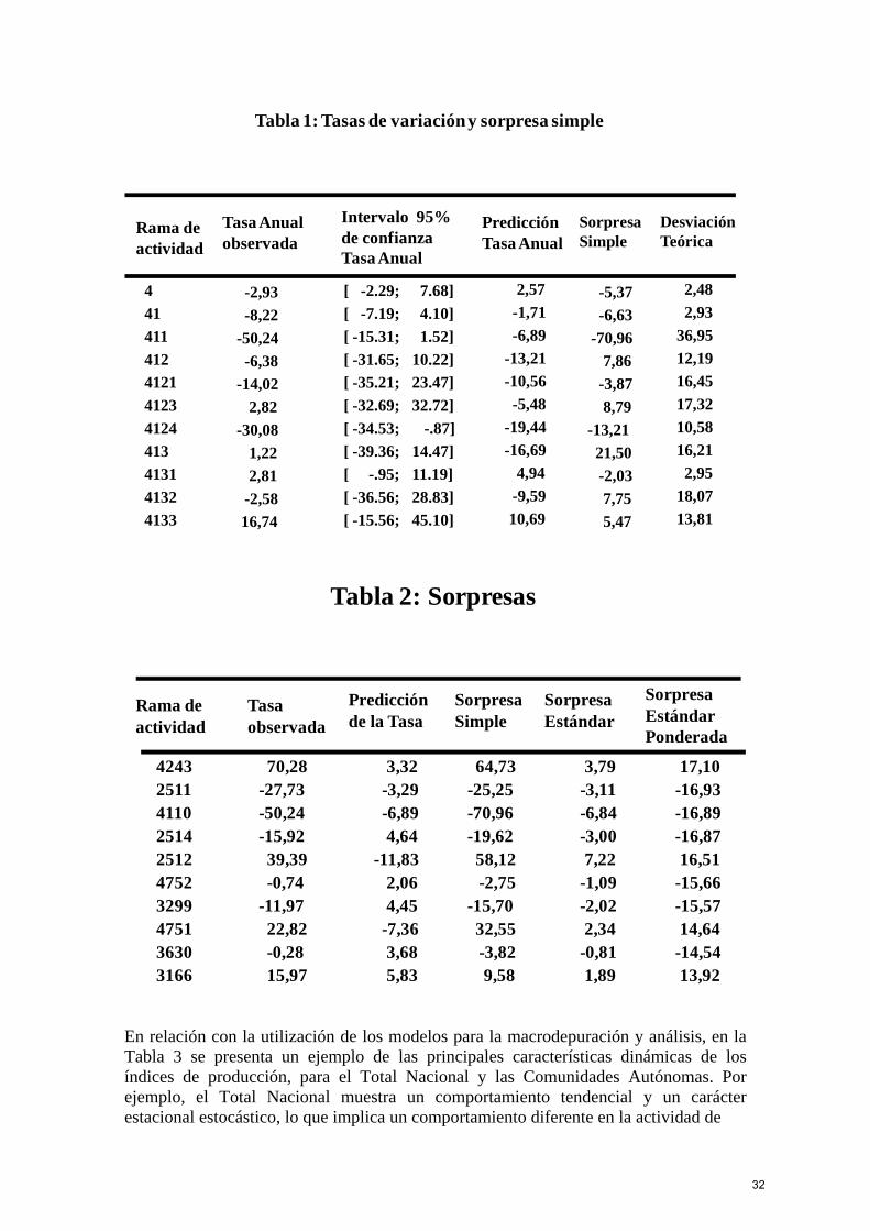
Tabla 1: Tasas de variacióny sorpresa simple

SorpresaSimple

4 -2,93 [ -2.29; 7.68] 2,57 -5,37 2,48

41 -8,22 [ -7.19; 4.10] -1,71 -6,63 2,93

411 -50,24 [ -15.31; 1.52] -6,89 -70,96 36,95

412 -6,38 [ -31.65; 10.22] -13,21 7,86 12,19

4121 -14,02 [ -35.21; 23.47] -10,56 -3,87 16,45

4123 2,82 [ -32.69; 32.72] -5,48 8,79 17,32

4124 -30,08 [ -34.53; -.87] -19,44 -13,21 10,58

413 1,22 [ -39.36; 14.47] -16,69 21,50 16,21

4131 2,81 [ -.95; 11.19] 4,94 -2,03 2,95

4132 -2,58 [ -36.56; 28.83] -9,59 7,75 18,07

4133 16,74 [ -15.56; 45.10] 10,69 5,47 13,81

DesviaciónTeórica

Tasa Anual observada

Predicción Tasa Anual

Intervalo 95% de confianza Tasa Anual

Rama de actividad

Tabla 2: Sorpresas

Tasa observada

Predicción de la Tasa

Sorpresa Simple

Sorpresa Estándar

Sorpresa Estándar Ponderada

4243 70,28 3,32 64,73 3,79 17,102511 -27,73 -3,29 -25,25 -3,11 -16,934110 -50,24 -6,89 -70,96 -6,84 -16,892514 -15,92 4,64 -19,62 -3,00 -16,872512 39,39 -11,83 58,12 7,22 16,514752 -0,74 2,06 -2,75 -1,09 -15,663299 -11,97 4,45 -15,70 -2,02 -15,574751 22,82 -7,36 32,55 2,34 14,643630 -0,28 3,68 -3,82 -0,81 -14,543166 15,97 5,83 9,58 1,89 13,92

Rama de actividad

En relación con la utilización de los modelos para la macrodepuración y análisis, en la Tabla 3 se presenta un ejemplo de las principales características dinámicas de los índices de producción, para el Total Nacional y las Comunidades Autónomas. Por ejemplo, el Total Nacional muestra un comportamiento tendencial y un carácter estacional estocástico, lo que implica un comportamiento diferente en la actividad de

32

producción en diferentes meses del año. La producción industrial es sensible a los efectos de calendario. Más específicamente, la existencia de un día laborable menos da

lugar a una caída de 1,9% en la producción. Del mismo modo, la semana santa provoca una caída de la producción del 4,2%, distribuido entre marzo y abril de acuerdo a la proporción de días afectados por esta fiesta cada año. La huelga de transporte de febrero provocó una reducción de 3,8% en el nivel de producción de este mes, compensado en marzo y abril. No muestra los valores atípicos por encima de tres desviaciones estándar. El grado de incertidumbre en cuanto a la producción para el próximo mes es del 2,1%. Una información similar puede obtenerse para cada una de los Comunidades Autónomas, observándose diferentes patrones de comportamiento.

Tabla 3: Caracterización IPI

Comportamiento del

nivel

Estacio-

nalidad

Efecto día

laborable (%)

Efecto semana

santa (%)

Efecto huelga

(%)

Valores

Atípicos

Incerti-

dumbre

Total Nacional Tendencia Sí 1.9 -4.2 -3,8 2.1

Andalucía Tendencia Sí 1.7 -2.0 (*) +7.5 Ene 1996 (-)

Feb 1997(+)

Feb 1998 (+)

2.7

Aragón Tendencia Sí 2.1 -4.1 (*) -6.6 Dic 1994 (+)

Feb 1997 (-)

2.2

Asturias Tendencia Sí 1.3 -4,3 -4,4 2.3

Baleares Tendencia Sí 1.6 -3,5 2.3

Canarias Oscilaciones locales No 1.8 -3,7 Mar 1994 (+)

Mar 1997 (+)

2.9

Cantabria Tendencia Sí 1.9 -4,2 2.8

Castilla-León Tendencia Sí 1.6 -5,2 (*) -8,1 Feb 1996 (-)

Jul 1995 (-)

Dic 1996 (-)

Feb 1997 (-)

Nov 1997 (-)

2.2

Castilla-La Mancha Tendencia Sí 0.8 -4,0 2.7

Cataluña Tendencia Sí 2.0 -4,7 -4,6 2.4

Comunidad

Valenciana

Tendencia Sí 2.2 -4,6 -4,4 1.7

Extremadura Oscilaciones No 1.3 4.5

Galicia Tendencia Sí 1.9 -3,3 (*) -5.6 Dic 1995 (+)

Feb 1997 (-)

1.9

Madrid Tendencia Sí 1.6 -5,2 3.0

Murcia Tendencia Sí 2.1 -3,2 2.7

Navarra Tendencia Sí 2.4 -4,7 (*) -7.6 Feb 1997 (-) 2.6

País Vasco Tendencia Sí 2.4 -3,8 (*) -7.7 Ago 1993 (-)

Feb 1997 (-)

2.6

Rioja Tendencia Sí 2.5 -4,9 Ene 1994 (-)

Dic 1994 (+)

3.5

33

3.1.5 Conclusiones

modelos ha permitido hacer un uso intensivo de la información xistente de la encuesta en periodos anteriores. Aunque el uso de esta información no es

tradicional basada en el dato del periodos anterior y de los datos isponibles de otras empresas

La utilización de losenuevo en la depuración e imputación de datos, las herramientas que hemos construido a partir de los modelos utilizan de manera más eficiente que los métodos tradicionales todo el pasado de la serie y permiten hacer inferencias probabilísticas y construir intervalos de confianza. Con ello hemos conseguido especificar y establecer los valores extremos de los edits, lo que habitualmente se hacía a partir de la experiencia del experto de la encuesta. Se han construido un conjunto de herramientas de depuración selectiva que permiten detectar y corregir los mayores errores. Se ha experimentado con datos reales del IPI. De acuerdo a estos resultados, el uso de modelos de series temporales puede ser muy útil para ahorrar tiempo en la depuración de los indicadores a corto plazo. Del mismo modo, se han obtenido un conjunto de características del comportamiento dinámico de los índices, de utilidad para la macrodepuración y el análisis exploratorio de datos. Se ha experimentado con tres tipos de imputaciones para manejar la falta de respuesta de uno o más datos de la empresa t,j,i o

q que forman parte

de los índices Ii,t: (i) Un imputaciónd

t,j,iq

o

o

00

jjt,j,i

jj1t,j,it,j,i q

q

(ii) Una microimputación basada en modelos de es decir

es decir

q

t,j,i oq t,j,i o

q

(iii) Una macroimputación basada en modelos para el índice iI t, t,iI

n diversas ircunstancias. Si la tendencia de las empresas dentro de la rama de actividad es similar,

La elección entre los métodos anteriores se puede hacer en funció decla imputación tradicional por lo general funciona correctamente. Sin embargo, si la tendencia no es similar una microimputación basado en el modelo funciona mejor. Por otra parte, si la tasa de no-respuesta es baja, una imputación micro (tradicional o basada en modelos) por lo general funciona correctamente. Por el contrario, si la tasa de no-respuesta para es alta y no hay muchas empresas en el índice es preferible una macroimputación basada en modelos para todo el índice. Queda abierta como línea de investigación el estudio de un enfoque más sistemático para las imputaciones.

34

3.2 La depuración selectiva como un problema de optimización estocástica 3.2.1 Introducción La depuración es una de las fases más costosas del proceso de producción de estadísticas. No sólo consume recursos económicos sino también tiempo. Adicionalmente, si el número de recontactos es grande aumenta de manera significativa la carga de respuesta. Por tanto, disponer de métodos eficientes de depuración es fundamental para los organismos estadísticos. Actualmente, la depuración manual exhaustiva es considerada ineficiente, puesto que la mayor parte del trabajo de depuración no tiene consecuencias en el nivel agregado e incluso puede deteriorar la calidad de los datos (ver Berthelot y Latouche (1993), y Granquist.(1997)). Los métodos de depuración selectiva son estrategias para seleccionar un subconjunto de los cuestionarios recogidos en una encuesta para someterlos a una depuración minuciosa. Esta depuración puede hacerse de formas diversas, pero en general implica la intervención humana y por tanto, un gasto que conviene reducir. Una razón por la que es conveniente seleccionar algunos cuestionarios es que depurando ciertas unidades es más probable que mejore la calidad que si se depuran otras. Esto puede ser debido a que unas son más sospechosas de contener un error o a que en caso de tenerlo, éste probablemente tenga más impacto en los agregados. Por tanto, es razonable suponer que una buena estrategia de depuración selectiva puede permitir que se compatibilicen dos objetivos: buena calidad de las estimaciones agregadas y reducido trabajo de depuración. El enfoque actualmente predominante es el de calcular algún tipo de función score (FS) que asigne una puntuación a cada unidad, priorizando la depuración de las unidades con mayor puntuación. Cuando para cada unidad se recogen varias variables, se pueden calcular diferentes FS locales y combinarlas en una global. Así, las unidades cuya FS excede un cierto umbral, son depuradas manualmente. En consecuencia, es necesario decidir: (a) las FS locales; (b) cómo combinarlas en una global (suma, máximo, etc.) y (c) el umbral. Hasta ahora, estas cuestiones han sido tratadas de manera empírica debido a la falta de una base teórica. En Latouche y Berthelot (1992), Granquist.(1997 ) y Lawrence y McKenzie R. (2000) se proponen algunas directrices, pero en esencia se depende del criterio del experto. Este subcapítulo se estructura en siete apartados. En el 3.2.1 se realiza la introducción En el apartado 3.2.2, se plantea formalmente el problema, en los apartados 3.2.3 y 3.2.4 mostramos como resolver dos variantes del problema, en el 3.2.5 se propone un método para calcular ciertos momentos condicionales que se requieren para obtener la solución, en el 3.2.6 presentamos los resultados de una aplicación práctica y finalizamos en el 3.2.7 con unas conclusiones. 3.2.2 El problema de la depuración selectiva Introduzcamos un poco de notación,

35

• es el valor verdadero de la variable en el cuestionario i en el periodo , con y .

ijtx

1,=

j t

N,i q,1,=j

• ijt

ijt

ijt ε+x=x~ es el valor observado, siendo el error de observación. ij

tε

• es el ijt

kij

kt x=X ∑ k -ésimo estadístico calculado con los valores verdaderos, donde

. p,1,= k

Suponemos que y son variables aleatorias con respecto al espacio

probabilístico . Puede haber otras variables relevantes, como

ijtχ

)P,

ijtε

F,( ijtx~ , para o

incluso variables de otras encuestas. Denotaremos por la -álgebra generada por toda la información disponible hasta t. Para simplificar la notación, omitimos el subíndice t cuando no hay riesgo de ambigüedad.

ijsx t<s

tG

Nuestro objetivo es encontrar una adecuada estrategia de selección, que debería indicar para cada i si el cuestionario va a ser depurado o no, empleando la información disponible. En realidad, vamos a permitir que se determine sólo la probabilidad de depuración de una unidad, dejando una cierta indeterminación. Definición 2. 1. Una estrategia de selección (ES) con respecto a es un vector

aleatorio -medible, tal que . tG

tG TN1 )r,,r(=r [0,1]∈ri

Denotamos por el conjunto de todas las ES con respecto a . La interpretación de )(S tG tG

r es que el cuestionario es depurado con probabilidad . El permitir en lugar de obligar a es conveniente tanto desde el punto de vista teórico como del práctico, porque así el conjunto de estrategias es convexo y podemos emplear técnicas de optimización más sencillas que las de la programación entera. Si para un cierto ,

, la unidad es depurada si , donde es una variable aleatoria uniforme en , e independiente de cualquier otra de las que se consideren. Denotamos por

i ir-1 1≤r≤0 i

ir

0,1∈ri

i

(0,1)∈ri

[0,1]

iit r<χ i

tχ~ la

variable indicatriz del suceso itχ ir y< T

N )r1~,,r~(=r~ . Si una ES cumple que 0∈ri ,1 c.s.,

r=r~ c.s. y decimos que r es entera. En nuestra aplicación, las soluciones son aproximadamente enteras. También es conveniente tener una definición del concepto de función score. Definición 2.2. Sea r una ES, un vector aleatorio y , tal que si y solo si . Entonces, decimos que es una función score que genera

TN1 )δ,,δ(=δ

δ

R∈Θ 1=ri

Θ≤δi r con el umbral . Θ

Para plantear formalmente nuestro problema, suponemos que tras la depuración manual, se obtienen los valores verdaderos. Así, solo tenemos que considerar los valores observados y verdaderos. Definimos el estadístico depurado como el calculado con los valores obtenidos tras depurar los que hayan sido seleccionados y lo denotamos por

. )εr~+x(ω=)r(X ijti

ijt

kij

k ∑

36

La calidad de debe ser medida con arreglo a alguna función de pérdida. En este

trabajo, solo consideramos el error cuadrático, , quedando la adaptación a otras funciones para futuros desarrollos. El valor de la función de pérdida se puede escribir como

)r(Xk

2kk )X-)r(X(

,r~r~∈=)X-)r(X( ïiki

ki

i,i

2kk ∑

(2.1)

donde . En forma matricial como ijt

kijj

ki εω∑=∈ r~Er~=)X-)r(X( k2kk , con

y . i′,ik

i′,i ki′,i =E

k E=E ki′

ki ∈∈

Ahora podemos plantear el problema de la selección como un problema de optimización: ]r~[1max]P[ T

rQ E

p,1,=k,e≤]r~Er~[

)(S∈ra sujeto 2

kkT

t

E

G

Éste es un problema de optimización lineal con restricciones cuadráticas, que tiene la dificultad de que se busca la solución en un espacio de dimensión infinita. En la sección 3.2.4 mostramos como resolverlo. Analicemos ahora la expresión (2.1). Podemos descomponerla como .r~r~r~)(=)X-)r(X( ii

ki

ki

i≠ii

2ki

i

2kk ∑∑

(2.2)

El primer término de la derecha de (2.2) mide el impacto individual de cada error, independientemente de su signo. En el segundo término, los sumandos son negativos cuando los factores tienen signos opuestos. Por tanto, para reducir el error total, sería conveniente dejar sin depurar parejas de unidades con distinto signo. La no-linealidad del segundo término complica los cálculos, así que estudiaremos también la versión despreciando esa parte. Si definimos , con , podemos plantear

TkN

k1

k )D,,D(=D 2ki

ki )ε(=D

]r~[1xám]P[ TrL E

.p,1,=k,e≤]r~D[),(S∈rs.a. 2k

kt EG

En la sección 3.2.3 veremos que la solución viene dada por una cierta FS. Puesto que no hay justificación teórica para despreciar la parte cuadrática, el problema lineal debe justificarse empíricamente mediante su eficacia en la práctica.

37

3.2.3 Caso lineal Vamos a resolver el problema mediante un método de dualidad, pero antes

debemos expresar la función objetivo como y la restricción como ,

donde . Definamos ahora la lagrangiana . En [1], se demuestra que bajo hipótesis no muy restrictivas, si

]P[ L

]r[1E T 2k

k e≤]rΔ[E

]e-r[ 2k

kE]|D[E=Δ tkk G -]r[1=),r(L TT E

λ es una solución del problema dual,

)(min]D[ 0≥

con φ , entonces ),r(max=)( r L ).,(maxarg=r L es una solución del problema primal . Como es conocido, la maximización de L respecto a ]P[ L

kΔ r se reduce al problema determinista

(3.1) )e-r(-r1max2k

kkk

T

r∑

(3.2) [0,1]∈rs.a. i

Aplicando las condiciones de Karush-Kuhn-Tucker (ver [2]) tenemos que,

(3.3)

1>si0

1<si1=r

iT

iT

i

donde . El caso se puede despreciar como un suceso de probabilidad cero, ya que para datos cuantitativos, la distribución de es continua. Por

tanto, la solución a es la ES generada por la FS con el umbral 1.

Tpi

1ii )Δ,,Δ(=Δ

]P[ L

1=Δλ iT

iΔ

iT

i Δλ=δ

En el apartado 3.2.5 describimos como usar un modelo para el cálculo de . Para estimar cambiamos la esperanza por la media muestral, donde la muestra puede ser simulada u obtenida a partir de datos reales si se dispone de ellos. Si tenemos una muestra de valores, usamos la estimación

kΔ

)(

M

)).(r,(LM

1=)(ˆ l

M

1=l

∑

La minimización de φ se hará por métodos numéricos. ˆ

3.2.4 Caso cuadrático El problema cuadrático plantea dificultades particulares. Si intentamos aplicar el método de dualidad como en el apartado anterior, expresamos la restricción como

, donde y 2k

TkkT e≤]r)Δ(+rΓr[E ijkij

k Γ=Γ

38

,j=iif0

j≠iif]|∈∈[= t

kj

kik

ij

GE

pero por desgracia, las matrices son indefinidas, luego la restricción no es convexa. kΓ

Podemos superar esta dificultad reemplazando la restricción por otra convexa y que bajo ciertas hipótesis es equivalente a la original. Consideremos la restricción , donde , ,

. Se puede demostrar (ver Arbúes et al. (2008)) que si r es una solución entera al problema con la nueva restricción y para i , entonces r es

una solución al problema original. Hemos comprobado que la condición de integridad se cumple aproximadamente en nuestra aplicación. La hipótesis sobre la esperanza condicionada es restrictiva y su relajación puede ser estudiada en futuros desarrollos. En el apartado 3.2.5 describimos un método para obtener y . En Arbúes et al. (2008) se describe como resolver con poco coste computacional el problema de programación cuadrática que resulta.

2k

TkkT e≤]r)v(+rMr[E

ki∈[E

kj

ki

kij mm=M

kj

ki mm

kv

]|[=m tki

ki GE

j≠]|∈[V=v t

ki

ki G

tkj =]|∈ G

kΣ

3.2.5 Momentos condicionales basados en un modelo La aplicación práctica de los resultados de las secciones anteriores requiere un método para calcular los momentos condicionales del error que aparecen. En esta sección omitimos el índice para simplificar la notación, pero los resultados son aplicables para el caso en el que hay varias variables por cuestionario.

j

Sea la álgebra generada por toda la información disponible en t a excepción de tH -σ

itx~ . Así, ),x~(σ t

it H

tH

=tG . Sea un predictor de calculado empleando la información

de , es decir, -medible. Denotamos el error de predicción por .

Supongamos que,

itx i

tx

tH it

it

it x-x=

(a) y están distribuidas como normales independientes con media cero y

varianzas y respectivamente.

itξ

itη

σ2iν

2i

(b) , donde tiene una distribución de Bernoulli tomando los valores 1 y 0

con probabilidades

it

it

it eη=ε i

te

p y 1-p y es independiente de y . itξ

itη

(c) , y son conjuntamente independientes de . itξ

itη

ite tH

Bajo estas hipótesis, los momentos condicionales de i

tε con respecto a tG dependen solo

de it =u decir, de la diferencia entre el valor predicho y el observado. En las

fórmulas siguientes, también omitimos i y t por simplicidad.

it

it x~-x , es

39

u=]|[

22

2

GE

(5.1)

2

2

22

2

22

222 u=]|[ GE (5.2)

donde,

.

2

)(u-exp

p

p-11

1=

222

221/2-

22

2

(5.3)

3.2.6 Caso práctico En esta sección presentamos los resultados de la aplicación de los métodos descritos a los datos de la encuesta de Cifras de Negocios y Entradas de Pedidos en la industria que lleva a cabo el Instituto Nacional de Estadística (datos disponibles en http://www.ine.es/inebmenu/mnu_industria.htm). En el momento del estudio, se disponía de datos mensuales desde enero de 2002 hasta septiembre de 2006 ( ) recogidos para una muestra de alrededor de unidades. Solo dos de las variables recogidas fueron consideradas: importe neto de la cifra de negocios ( ) y

nuevos pedidos recibidos ( ). Estas dos variables son agregadas separadamente para

obtener los dos indicadores, así que y ω .

,571=t

1itx

13,500=N

0=ω= 21i

12i

2itx

2=q=p

Para aplicar (5.1)-(5.3) es necesario ajustar un modelo a los datos, pero antes empleamos la transformación , donde )m+x(log=y ij

tijt m es una constante positiva

ajustada por máxima verosimilitud ( € ). Para recuperar los momentos

condicionales de la variable original, se pueden usar las propiedades de la log-normal o un desarrollo de Taylor de primer orden, que resulta

. En nuestra aplicación hemos empleado la

aproximación. También hemos observado que si

510

x

≈m

]| tG)y-y~[(E)m-x~(≈]|)x-x~[(E 2ijt

ijt

2ijtt

2ijt

ijt G

m-~ijt es sustituido por una media de

los últimos 12 valores de ijtx~ el resultado es más robusto frente a valores pequeños de

m-x~ijt .

El modelo que hemos planteado para las variables transformadas es muy simple. Suponemos que y son independientes si . Para cada par

seleccionamos para la serie uno de los siguiente modelos

ijtx j′i′

tx

x

)j′,i′(≠)j,i( )j,i(ijt

(6.1) tijt a=y)B-(1

(6.2) tijt

12 a=y)B-(1

(6.3) tijt

12 a=y)B-)(1B-(1

donde es el operador de retardos y es un proceso de ruido blanco. El criterio de selección es el de mínimo error residual cuadrático. Una vez seleccionado el

B 1-tt u=Bu ta

40

modelo, lo empleamos para calcular la predicción y su desviación típica . La

desviación típica a priori del error de observación y de la probabilidad de error se suponen constantes (la transformación logarítmica hace que tenga sentido suponer que los errores de observación tienen la misma d.t.), los denotamos por y con y

son estimados usando datos históricos de la encuesta. Para ello, nos aprovechamos de que tanto la primera versión recibida de cada dato como las que posteriormente resulten de posibles correcciones quedan almacenadas en una base de datos. Para este estudio, la primera versión es considerada como dato observado y la definitiva como dato verdadero.

ijty ijν

=jjσ jp 1,2

Una vez que hemos calculado , , y , usamos (5.1)-(5.3) para calcular los

momentos condicionales, , y . jσ

k

jp

kv

ijνijtu

kΔ Σ

Pretendemos ahora comparar la eficacia de nuestro método con la función score descrita en Hedlin (2003), |xx~|ω=δ ii

i0i

2ijij )x-x~(

, donde es una predicción de . En Hedlin (2003) se propone usar como predicción el último valor de la misma variable en periodos anteriores. Hemos considerado una modificación de esta función, , simplemente cambiando la predicción por la que se obtiene mediante los modelos (6.1)-(6.3). Finalmente, es la FS calculada usando (5.1)-(5.3). En esta comparación, la combinación de FS locales en una global se ha hecho simplemente sumándolas.

Medimos la efectividad de una FS mediante , con

, donde consideramos las unidades ordenadas

descendentemente según la correspondiente FS. La cantidad puede ser considerada como una estimación del error que queda tras editar unidades. Los resultados incluidos en la tabla 1 muestran que mejora a , que a su vez es más eficaz que .

ix ix

=E j

1

En

∑

)n(

δ

E j

n

2δ

n≥

)n(j

ji

N

i

j =)n(E ∑

0δ

2δ 1δ

Tabla 1. Comparación de FS. FS Cifras de

Negocios Nuevos Pedidos

0δ 0.44 1.33 1δ 0.38 0.45 2δ 0.26 0.37

3.2.7 Conclusiones Hemos descrito un marco teórico para tratar el problema de la depuración selectiva, definiendo el concepto de estrategia de selección. La búsqueda de una adecuada ES se presenta como un problema de optimización lineal con restricciones cuadráticas. Consideramos también una versión modificada con restricciones lineales. Mostramos un método práctico para resolver ambos problemas. La FS correspondiente a la versión lineal mejora la de referencia.

41

3.3 Propuesta y desarrollo de un marco teórico de depuración e imputación basado en modelos y optimización 3.3.1 Introducción La diversidad de errores de medida ha dado lugar a la aparición de diferentes técnicas y algoritmos para su detección y tratamiento, como la depuración interactiva, la depuración automática, la depuración selectiva, o la macrodepuración (véase de Waal et al. (2011) para una revisión completa). Hoy en día se acepta ampliamente que ningún método o enfoque puede hacer frente a todo tipo de errores. Por lo tanto, deben ser combinados en una estrategia global de depuración e imputación. Los sistemas generalizados han supuesto un gran avance. Sin embargo, no resuelven la especificación de los edits, que deben ser introducidos por los usuarios. Habitualmente, los usuarios establecen los edits de acuerdo a su experiencia práctica, sin que exista un marco teórico. Por su parte, la depuración selectiva se centra en los errores influyentes. En las últimas dos décadas, esta modalidad de depuración ha sido reconocida como un elemento clave en las estrategias de depuración e imputación, pero, hasta la fecha, únicamente se ha tratado de forma heurística. Dentro de este contexto, el trabajo que aquí se presenta se centra en dos aspectos principales: el uso de modelos estadísticos para resolver los problemas de la especificación de los edits y la utilización de técnicas de optimización para resolver los problemas que presenta la depuración selectiva. Ambos aspectos están estrechamente relacionados, ya que las técnicas de optimización que proponemos necesitan de modelos para substanciar las restricciones y calcular las matrices de las funciones de pérdida. Adicionalmente, los modelos pueden emplearse en la macrodepuración y en la imputación. En los epígrafes precedentes se han abordado ya estos temas. Así, en el primer bloque de investigaciones (subcapítulo 3.1), se introducen modelos que llevan a cabo todos los objetivos que pretendemos, es decir, la especificación de los edits, y el soporte a la depuración selectiva, la macrodepuración y la imputación. Sin embargo, se hace de una manera parcial, limitándose al uso de modelos univariantes de series temporales y aplicables a datos cuantitativos de encuestas coyunturales. Por su parte, el segundo bloque de investigaciones (subcapítulo 3.2) introduce las técnicas de optimización como solución formal al problema de la depuración selectiva, pero se centra únicamente en la optimización estocástica. En este último bloque de investigaciones, se intenta avanzar en el grado de generalización y formalización, introduciendo un marco general de utilización de modelos y abordando un problema de optimización general, del que se derivan una versión estocástica y otra combinatoria. Este subcapítulo se estructura en cinco apartados. En el 3.3.1 se realiza la introducción. En el 3.3.2 se analizan distintos modelos estadísticos en función de la información auxiliar disponible. En el 3.3.3 se formula el problema de optimización genérica, que nos conduce a una versión de optimización estocástica o combinatoria dependiendo del momento en que se realice y por tanto del flujo de información disponible. En el apartado 3.3.4 se lleva a cabo la comparación de nuestra propuesta con funciones score

42

de uso habitual, utilizando datos reales del Índice de Cifras de Negocio y del Índice de Entrada de Pedidos. Por último, se incluyen unas conclusiones en el apartado 3.3.5. 3.3.2 El uso de modelos estadísticos Como un criterio esencial de la depuración e imputación se considera que los datos a difundir sean consistentes con la información existente hasta la fecha. La información existente se resume en un modelo. El modelo debe extraer al máximo la información que contienen los datos e incorporar la información a priori. Para hacer operativo el concepto de que los datos sean consistentes se considera que un dato es consistente cuando se acerque a la predicción que ofrece este modelo para ese dato. Las herramientas de depuración e imputación se basan fundamentalmente en las predicciones del modelo. Los outliers se definen y se detectan en función de cuánto se alejan los datos observados (a depurar) de la predicción. Los valores imputados se definen como la predicción que se deduce del modelo para ese dato. En este trabajo se desarrollan nuevas herramientas de depuración e imputación basadas en los modelos (fundamentalmente en la función de predicción). Estos modelos se utilizan tanto en la microdepuración como en la macrodepuración y en la depuración selectiva. Las propiedades de la depuración e imputación pueden derivarse a partir de la predicción de los modelos. Al hacer frente a las tareas de depuración e imputación se recurre a la mejor información auxiliar disponible en ese momento. Con plena generalidad, esta incluirá: (i) los valores observados de las variables de análisis para el presente ( ) y el

pasado ( ), (ii) los valores verdaderos de estas variables para aquellas unidades

depuradas en el pasado (iii) y los valores de las covariables auxiliares para los

períodos de los que se dispone de información. Por tanto, tenemos , y

, con y . Téngase en cuenta que alguno de estos valores

puede ser coincidente (por ejemplo, cuando el error de medición es nulo) y que sólo se conoce después de llevar a cabo el trabajo de depuración. También conocemos (por lo menos podemos conocer) una predicción puntual para cada variable en función de estas variables auxiliares. Adicionalmente, se puede eventualmente incorporar información a priori. Por ejemplo, podemos hacer uso de un modelo univariante de series temporales

)t(ky T=t

)t(k

k0k y=y

0ky

T<t

)1t(0,

k

)y,

)t(0,y

T<t

<t1

x)T(

kk y=y )T(0,

)2t(

k1t(

kk x,y=x T T≤t 2

ky

T<t)t(0,

ky

)2t(

k

para hacer una predicción puntual . Surgen diferentes

opciones dependiendo de la cantidad y tipo de información auxiliar. Estas predicciones entrarán en el problema de selección como covariables auxiliares, de modo que

, con y .

)T(ky

)T(k

1t(

kk x,y,y=x)1t(0,

k

)y, T t 2<t1 T≤

Llamemos *m al modelo auxiliar utilizado para hacer las predicciones que no debe confundirse con el modelo de error de medición. Este modelo de error de medición se da como es habitual en términos de (i) la distribución condicional de los valores de predicción de los valores verdaderos y (ii) la distribución de los condicionada a la

información auxiliar disponible . Para una variable supondremos y

En otras palabras, estamos usando el valor predicho calculado de acuerdo

ky

ky

0y 0y

X obsk

0k ε+y=

predkk

0k ε+y=y

43

con el modelo auxiliar *m como una variable exógena para el modelo de relación . En este sentido nos referimos a esta propuesta como un modelo de observación-predicción.

0y

Generalizando estas ideas, consideremos: (i) un modelo de observación ( )0

0|obs y|yP , es decir, una distribución de probabilidad

condicionada para los valores observados, dados los valores verdaderos ; 0y

(ii) un modelo de predicción ( )y|y0

pred|0P , es decir, una distribución de probabilidad

condicionada para los valores verdaderos, dados los valores predichos de acuerdo

con un modelo auxiliar

0y

. *m Ahora vamos a denotar por la distribución de probabilidad de los valores

observados condicionadas a los previstos y por la distribución de

probabilidad de los valores verdaderos condicionada a los valores observados y los valores predichos . Entonces por el teorema de Bayes o una generalización del mismo, podemos escribir

pred|obsP

y pred,obs|0P

0y obsy

y

|obs

|0obspred,obs|0

×=

P

PP

pred

pred|0P (2)

El producto debe ser entendido en una forma generalizada adecuado cuando las distribuciones son completamente generales. Como de costumbre, si las distribuciones de probabilidad son absolutamente continuas con función de densidad, la ecuación (2) puede ser fácilmente reconocida como

).(f

.d)ˆ|(fˆ,|f

)ˆ|(f)ˆ,|(obs

obs

y

yf=)(f 00

00

0|obsR

00

00|obs0

pred,obs|0Q yyyyy

yyyyy

El caso discreto también se reduce a aplicar el teorema de Bayes. Una vez que tenemos la distribución , las matrices de pérdida pueden ser calculadas como pred,obs|0P

[ ].Y

p

,Y,S|Δ=M )q(pred,obs|0

)q( E

(3)

Para ilustrar esta propuesta, consideremos el siguiente ejemplo genérico con una variable continua. Vamos a definir el modelo de observación y de modelos de prediccion

obsk

0k

obsk ε+y=y

predkk

0k ε+y=y ,con las siguientes especificaciones

1. . k

obsk

obsk eη=ε

2. , donde . )p(Bee kk (0,1)∈k

44

3. .

2kkkk

kkk2kobs

kpredk ,N, 0

4. , y son conjuntamente independientes de . predkε

obskη ke co

kZ

5. es independiente de y . ke predkε

obskη

Estas especificaciones equivalen a decir que la unidad tiene una probabilidad de

declarar un valor sin error de medida ( ) y, si informan de un valor erróneo, el error de medida se distribuye como una variable aleatoria normal con media cero y varianza . Por otra parte, el error de predicción se distribuye como una variable

aleatoria normal con media cero y varianza . Ambos errores se distribuyen

conjuntamente como una variable aleatoria normal bivariante con correlación . Informar de un valor erróneo es independiente de los dos tipos de errores.

kp -10kk y=y

2kσ

2kν

kρ

Por el momento, vamos a suponer que los parámetros son conocidos. Centrémonos en la función de pérdida al cuadrado. Arbués et al. (2012a) demuestran que

Tk

2k

2kk )ρ,ν,σ,p(=θ

( )[ ] ,)ν

y-y(ζ)

ν

y-y(

νσρ2+ν+σ

νσρ+σν=y,y,s|y-y

k

kkk

k

kk

kkk2k

2k

kkk2k

kkkk0kkmE (4)

,y-yy-y)2)(-(1

.2

.=y,y,s|y-yk

kkk

2

k

kk2

kkk2k

kkk2k

2k

2k

2k

2

kkk2k

2k

kkk2k2

kkkk

20kkm

E

,l≠k,y,y,s|y-yy,y,s|y-y=y,y,s|y-yy-y kkk0llmkkk

0kkmkkk

0ll

0kkm EEE

donde

2

kkk2k

2k

kkk2k

1/2-

kkk2k

2k

2k

k

k

k

x2

2

2

1-exp

2p

p-11

1=x .

Si nos centramos en la función de pérdida absoluta, bajo las mismas hipótesis, Arbués et al. (2013) demuestran que

y-y.

2

)y-y(;

2

1;

2

1F. .

2=y,y,s|y-y

k

kkk2

k

2kk

11kkkk0kkm

E (5)

Donde denota la función hipergeométrica confluente de la primera clase. )x;b;a(F11

La estimación de los parámetros θ depende del escenario. Para el problema estocástico, como antes, nos vemos obligados a utilizar algunos valores de referencia o medidas heurísticas. Una vez más se recurre a la información auxiliar. La elección depende en gran medida de la cantidad y tipo de la información auxiliar. Desde el histórico de dos conjuntos de datos que comprende períodos de tiempo anteriores (por ejemplo, un panel fijo), podemos calcular

45

,Iτ

1=p )t(0,

ky≠)t(ky

τ

1=tk ∑

,-1-

1=ˆ

2

k)t(

k1=t

2k ∑

,y-y=donde,-1-

1=ˆ )t(0,

k)t(

k)t(

k

2

k)t(

k1=t

2k ∑

.--1-

1=ˆ k

)t(kk

)t(k

=1tk ∑

En el caso de paneles rotatorios o de diseños muestrales con muy corta continuidad de las unidades en la muestra, nos vemos obligados a hacer supuestos simplificadores, como la partición de la muestra y postular si . También podemos adoptar estos supuestos para algunos de los parámetros. El caso extremo sería

para todos , que se puede complementar aún más con hipótesis adicionales, tales como .Por otro lado, para el problema de combinatorio tenemos

(casi) la muestra actual completa, de modo que podamos hacer uso de estos datos, aunque con importantes limitaciones. Es claro que es imposible estimar cada uno utilizando sólo la muestra del periodo corriente. Estamos obligados a hacer algunos supuestos simplificadores, en línea con los anteriores.

iI

1=i s∪=s

s∈

ik θ=θ is∈k

T22k )ρ,ν,σ,p(=θ=θ k

0=ρ

kθ

Alternativamente, el modelo de contaminación propuesto por Di Zio y Guarnera (2013) es un ejemplo relevante de una técnica basada en modelos que utiliza exclusivamente datos del período actual para estimar los parámetros del modelo. 3.3.3 El problema de optimización Antes de identificar las variables, la función objetivo y las restricciones de nuestro problema de optimización, se necesita introducir la siguiente notación. El diseño muestral, según el cual se ha seleccionado una muestra probabilística se denota . El tamaño muestral por n y los pesos muestrales por wks. La dependencia de la muestra de los pesos de muestrales asume implícitamente que no necesitan ser los pesos de

diseño. Por ejemplo, en un estimador de razón de la forma

).(p

HT

HTrat

X

YX=Y donde es una

variable auxiliar conocida del marco muestral, ,es un total poblacional

conocido, y

x

kU∈kx=X ∑

k

k

s∈k

HT

π

y=Y ∑ (análogamente para ) representa el estimador de

Horvitz-Thompson del total poblacional , los pesos de muestreo están dados

por

HTX

kyU∈k

=Y ∑

kHTks π

1

X

X=ω , donde es la probabilidad de inclusión de primer orden para la

unidad k. Situaciones más complejas se encajan en esta notación. Los valores verdaderos, observados y depurados de una variable del cuestionario , (para facilitar la notación se omite el superíndice (q) en adelante, excepto cuando sea estrictamente necesario), para la unidad

kπ

)q(y Q,1,=q

k se indican, respectivamente, por , , e

.

0ky ky

*ky

46

Se asigna una variable binaria a cada unidad k para indicar si se ha

seleccionado para posterior depuración ( ) o no ( ). El vector

definido para los elementos muestrales será denominado la estrategia de selección. Esta asignación nos permite relacionar los valores anteriores por la ecuación

donde hemos hecho explícita la dependencia de los valores

depurados sobre la estrategia de selección. Nótese que estamos asumiendo implícitamente que el trabajo de depuración nos conduce de los valores observados a los valores verdaderos. Si denotamos el error de medida , podemos escribir

. Los valores depurados son los que se utilizan para calcular los estimadores de la encuesta. Es decir, si hemos de estimar el total para un dominio Ud de

la población (se omitirá en adelante el subíndice para facilitar la

notación), el estimador correspondiente será

0,1∈rk

=rk 0 1=rk

=k

ωds∈k

∑

tnrr ),,(= 1 r

kkkkk yryry 0* )(1=)(r

kk0k

*k εr+y=)r(y

0k

dU∈kdU y=Y ∑

0kk yy

U

)r(y*kks

d

=)r(Y* . Nos limitaremos a

totales poblacionales y estimadores lineales. Todas las covariables auxiliares no incluidas en el cuestionario de la unidad k se indican mediante . kx

Conviene señalar que el estimador anterior calculado con los valores depurados pudiera no ser el estimador final para la difusión de la encuesta, ya que eventualmente podrian necesitarse de algunos procedimientos posteriores como el ajuste de los pesos o el tratamiento de valores atípicos. La selección de las unidades divide la muestra en un flujo crítico ( ) y en otro no crítico ( ). Aquí estamos suponiendo que las unidades del flujo critico serán sometidas a depuración manual y las otras se dejarán inalteradas. Sin embargo, este procedimiento de selección puede ser utilizado alternativamente con otras estrategias, como por ejemplo que las unidades del flujo crítico sean sometidas a depuración manual y las otras sean sometidas a un procedimiento de depuración automática.

0=rk 1=rk

Las variables mencionadas anteriormente se consideran variables aleatorias que siguen un modelo m en un espacio de probabilidad . Esta aleatoriedad no se indica específicamente en la notación, a excepción de la estrategia de selección, de manera que R denota la estrategia de selección aleatoria, y

),,Ω( PF

rR =)( con , será una realización numérica particular llamada la selección. La predicción de la variable

según el modelo m se denota por . Cuando se utilizan variables aleatorias en los

estimadores de la encuesta, se escribe indistintamente ,

e .

Ω∈ω

=Y ∑ky

Y

ky

0kksy

ds∈k0 ω=∑Y kks

ds∈kyω

)R(yω=)R( *kks

ds∈k

* ∑ Se denota por Z el conjunto de variables aleatorias utilizadas para seleccionar las unidades destinadas a depuración en la estrategia de D&I. En particular, vamos a considerar dos opciones, a saber, cualquiera de los dos para el problema estocástico o para la versión combinatoria. Cuando esta información auxiliar se limita a la unidad

s≡Z=Z st

Y,X,s≡Z=Z co k vamos a escribir en consecuencia o

. El uso de la información auxiliar actúa condicionando las variables aleatorias correspondientes. Las covariables auxiliares se eligen de acuerdo con el modelo estadístico utilizado en el problema de optimización (ver más abajo). Juegan un

kstk s=Z

kkcok y,x,s=Z k

47

papel similar al de las variables auxiliares en el diseño muestral o en el proceso de calibrado, con las que pueden coincidir parcial o totalmente. El problema de optimización general En el problema de optimización se quiere minimizar el número de cuestionarios a depurar, a condición de que las funciones de pérdida elegidas para los estimadores de la encuesta dirigidos a los valores poblacionales estén acotadas. Para establecer formalmente el problema de optimización es necesario (i) las variables, (ii) la función de optimizar, y (iii) las restricciones. Aparte de la identificación de estos elementos, es importante para mostrar cómo la información auxiliar entra en la formulación del problema. Las variables finales son la estrategia de selección para las unidades de la muestra donde si se ha seleccionado la unidad k y de otro modo.

Sin embargo, ya que el error de medición está concebido para ser de naturaleza aleatoria condicionada a la muestra realizada s y teniendo en cuenta la información auxiliar elegida para realizar la selección de unidades, esta selección puede variar dependiendo de los valores realizados de y, de y de . Por lo tanto

denota la estrategia de selección estocástica, de forma que (i) es una selección particular realizada y (ii)

)r,,r(=r n1T

0kk yy

y

n,1,=s 0=rk 1=rk

Z

(R

k =

Z0

R r=)ω

[ ]Z|RmE es el vector de las probabilidades de no selección en el marco del modelo específico m teniendo en cuenta la información auxiliar . La función objetivo a optimizar, dada la información auxiliar se escribe entonces como

Z Z[ ]ZT |R1mE cuya maximización equivale a reducir al mínimo el número

de unidades seleccionadas. Las restricciones se derivan de la aplicación de una función de pérdida a los estimadores de la encuesta. Vamos a concentrarnos en las dos funciones de pérdidas más utilizadas en la práctica, la pérdida absoluta y la pérdida cuadrática

.

|ba=|)b,a(L=L (1) 2(2) )ba(=)b,a(L=L

Para estas funciones de pérdida, cada restricción siempre se puede escribir como una cota en una forma cuadrática, denotada por [ ]Z|ΔRRT

mE . Las formas particulares adecuadas para los problemas estocásticos y combinatorios serán explicadas mas adelante. La matriz indica las pérdidas potenciales a nivel de unidad. Medidas de sesgo y/o MSE parecen naturales en la práctica. Se derivan de la elección de la función de pérdida absoluta o cuadrática, respectivamente. Estas medidas pueden ser heurísticas por naturaleza, como el pseudo-sesgo para las funciones score tradicionales, o se derivan explícitamente en algunos modelos de medición de error apropiado. En particular, los términos no nulos de fuera de la diagonal de permiten la inclusión de términos cruzadosel en la pérdida "global".

Δ

La elección de la matriz está relacionada de forma natural a la elección de la función de pérdida . Por lo tanto, si Δ es diagonal con entradas , entonces estamos

eligiendo la pérdida absoluta de manera que

ΔL |εω| kks

( )[ ]Z

kl =Δ

|Y),R(YL 0*mE también está acotada por

. Este caso está dirigida al sesgo. Del mismo modo, si entonces η lklsks εεωω

48

estamos eligiendo la pérdida cuadrática de manera que también ( )[ ]Z|Y),R(YL 0*mE está

igualmente acotada. A su vez, está dirigida al error cuadrático medio. En ambos casos, las técnicas basadas en modelos sobre datos del período actual se pueden aplicar en la versión combinatoria, mientras que en la versión estocástica nos vemos obligados a recurrir a la información auxiliar de otros periodos. Por ejemplo, la puntuación (local) para una variable dada es generalmente concebida como el producto de un componente de "riesgo" y un componente de "influencia". Una medida genérica puede darse utilizando un enfoque basado en modelos. Sea

la probabilidad a posteriori de que el valor verdadero sea diferente al

observado. Sea

)y|y≠y(P=p kk0kk

μ )y≠y,y|y(=~k

0kk

0kmEk la esperanza condicionada del valor verdadero,

dado que es diferente del observado. Entonces, tenemos

=)y|y(y=y~py)p(1=)y|y( k0kmkkkkkkk

0km EE )~y(p kkk

kp

Resulta que puede usarse para constuir el score local de la unidad k con respecto a la variable y, que representa el producto del componente riesgo medido por y el

componente influencia medido por

kkδw

kkk~yw donde wk puede ser, por ejemplo el

peso de la muestra. La principal diferencia entre ambas versiones se plantea al considerar su aplicación real. El problema estocástico, complementado con la suposición de ignorar los términos entre unidades, permite la construcción de las funciones score que pueden aplicarse de forma independiente para cada unidad. El supuesto complementario equivale a considerar los términos cruzados más o menos constantes en el tiempo, no jugando ningún papel significativo en la selección. Por el contrario, el problema combinatorio necesita un número suficiente de observaciones disponibles para llevar a cabo la selección en forma conjunta para todas las unidades. Teniendo en cuenta la posibilidad de múltiples restricciones, establecemos el siguiente problema de optimización general:

Z|R1max]P[ Tm0 E

,Q1,2,...,=q,≤|RRs.t. q)q(T

m ZΔE

0Ω∈R

Donde denota el espacio de los comportamientos admisible para y q se refiere a las diferentes restricciones. Las diferentes restricciones pueden surgir del hecho de que existan múltiples variables de interés, o de que las restricciones puedan estar dirigidas a diferentes ámbitos poblacionales. En particular, las matrices de pérdida pueden derivarse bajo un único modelo multivariante para el conjunto de datos, incluso cuando las restricciones estén marginalmente especificadas para cada variable de interés.

0Ω R

(1) ,...,Δ )Q(Δ

49

El problema de optimización estocástica Como se indicó anteriormente, la suposición principal en esta versión del problema es dejar de lado los términos entre unidades en cada restricción. Entonces pueden rescribirse como

0P

[ ] [ ]Z|)Δ(diagR=Z|ΔRR Tm

Tm EE El problema de optimización estocástica

se resuelve en Arbués et al. (2012a) utilizando el principio de dualidad y el de intercambiabilidad. La solución resultante de este problema lineal se da en términos de matrices [ ]co)q(

m Z|ΔE)q( =M . Pero, puesto que este esquema de selección se aplica unidad por unidad al recibir cada cuestionario y no hay información auxiliar más que con respecto a cada unidad k , los condicionamientos formales sobre se pueden reducir eficazmente al condicionamiento de la información auxiliar de

cada unidad. Así que escribimos . Por

otro lado, con el fin de obtener los multiplicadores de Lagrange óptimos

involucrados en el problema dual, se hace necesario disponer de un fichero histórico con datos observados y depurados. De esta forma, podemos llegar a la solución final, que sólo requiere de las entradas diagonales de las matrices :

coZ

ks=

s∈k∑

kkcok y,x,Z

[ ] )q(kkM=[ ] co

k)q(

kkms∈k

co Z|Δ=Z| ∑ E

)q(M

m)q( Δ=M E

*qλ

1.>Msi0

1,Msi1

=R)q(

kk*q

Q

1=q

)q(kk

*q

Q

1=q

k

Téngase en cuenta que, dado que el esquema está "entrenado" en los datos históricos, la evaluación de dadas las observaciones de la muestra actual produce necesariamente un pseudo-medida, independientemente de la definición de las matrices de pérdida.

)q(kkM

Este hecho proporciona una función score para la selección unidad por unidad. En el caso especial de que Q=1, se selecciona la unidad k cuando de modo que la expresión a la izquierda de la desigualdad puede considerarse como el valor del score y el de la derecha como el valor del umbral. Igualmente, se puede considerar como una puntuación "estandarizada", en el sentido de que el valor umbral se establece en forma genérica igual a 1. Esto se extiende directamente a la configuración con múltiples

restricciones, donde cada es un score local estandarizado y es un

score global estandarizado, con el valor del umbral igual a 1.

*kk λ1/>M

kk*Mλ

)q(kk

*q1Mλ

)q(kk

*qMλ

Q

=q∑

El score global se deriva de la estructura lineal del problema dual y se permiten pocas variaciones sin una modificación sustancial del problema . Como excepción, si el score global es inicialmente concebido como la suma ponderada de los score locales, se puede incorporar cada peso en la restricción que genera el correspondiente score local estandarizado.

0P

El problema estocástico clarifica, pues, el hecho de que el rendimiento de selección unidad-por-unidad sólo se puede establecer a través de hipotéticas repeticiones del proceso de selección. Al final de cada proceso de selección, tenemos la estrategia de

50

selección realizada r y la pérdida realizada , que puede ser mayor o menor

que el límite especificado para . En cualquier repetición hipotética del

proceso de selección y variarán, y también lo harán los correspondientes y

. Es sobre tales hipotéticas repeticiones que la restricción

)q(kkk

n

1=kMr∑

Qqη

0ky

1,...,=q

ky )q(kkM

kr [ ] q)q(

m RΔRE η≤Z|

posiblemente pueda ser satisfecha, pero no para cada realización particular del procedimiento de selección. El problema de optimización combinatoria El problema combinatorio trata la selección entre todas (o un grupo de) las unidades. Se permiten ahora los términos entre unidades, y la información auxiliar utilizada es la de la muestra , las covariables auxiliares , y las variables de interés , es decir, por

. Téngase en cuenta que toda esta información está disponible sólo después de que se han recogido todos los cuestionarios, por lo que sólo se puede aplicar al final de este proceso. Se demuestra que cada restricción se reduce a

X YcoZ=Z

rMr=ZΔ )q(Tco)q( |RR TmE , donde [ ]co)q(

m)q( Z|Δ= EM , que puede ahora ser

posiblemente evaluado bajo algún modelo de medición del error. Por consiguiente, se hace posible establecer directamente el rendimiento de la estrategia de selección, considerada como una realización articular. El problema de optimización puede ser reformulado como:

r1max)],η,M(P[ T0co

,Q1,2,...,=q,≤rMrs.a q)q(T

0Ω∈r

Obsérvese que una derivación más directa se puede obtener por no haber promovido el vector de estrategia de selección r a un vector aleatorio, en el momento de modelar los errores de medición.

R

Este problema combinatorio se resuelve en dos formas diferentes utilizando dos algoritmos voraces, véase Salgado et al (2012). La solución de los dos algoritmos no es exacta a priori, sino subóptima con un buen grado de aproximación. El algoritmo más rápido es notablemente menos preciso que el más lento. Esta falta de precisión implica una pequeña cantidad de sobredepuración en la práctica, es decir, que se seleccionarán más unidades de las que hubiera sido necesario depurar de forma óptima. Estos algoritmos heurísticos investigan localmente el óptimo en cada iteración hasta que la solución satisface todas las restricciones. Para ello se introducen las funciones inviabilidad para cada algoritmo (ver Salgado et al. (2012) para más detalles) que indica si una solución satisface todas las restricciones o no Ambos algoritmos comienzan a partir de la solución inicial

)r(hi 1,2=i

0=)r(h 0>)r(h

1=r y en cada iteración seleccionan de manera localmente óptima la siguiente unidad, hasta que se cumplan todas las restricciones. Finalmente, se pueden considerar que las dos versiones en relación con dos enfoques diferentes para el problema de optimización bajo incertidumbre, véase, por ejemplo

51

Wets (2002). La versión combinatoria es consistente con el de “esperar y ver”, ya que se posponen todas las decisiones hasta que toda la información está disponible. La versión estocástica es un enfoque “aquí y ahora” ya que la decisión sobre el procedimiento o regla de selección se realiza antes de la recogida de datos. 3.3.4.- Caso práctico En este apartado, se compara empíricamente la eficiencia de nuestra propuesta con funciones score ampliamente utilizadas. Para ello se emplean datos reales del Índice de Cifras de Negocio (ICN) y del Índice de Entrada de Pedidos (IEP). Como es habitual en los experimentos de depuración selectiva, se trabaja con un fichero de datos doble, que para cada unidad contiene datos observados y datos depurados. Cuando se selecciona una unidad, sus valores observados son sustituidos por sus correspondientes contrapartes depurados, considerados verdaderos. Vamos a denotar por el estimador que se obtiene cuando cuestionarios han sido seleccionados de acuerdo con una técnica de depuración selectiva y se han depurado correspondientemente. Téngase en cuenta que . Como criterio para valorar la selección de

unidades, se utiliza el valor absoluto del pseudo-sesgo de un estimador , dado por

)n(Y edsel

Y

edn

=)n 0ed

sel Y=n(Y

0

0ed

Y

Y-)nsel

edsel (Y

=)n(YB~

R~

A~

.

Se va a comparar ( ))n(YB

~R~

A~

edsel

[ ]( ))n(Y edran

para una técnica de depuración selectiva sel con

donde ran significa una selección aleatoria con igual probabilidad, de la que se toma su esperanza. Es inmediato demostrar que

B~

R~

A~≡)n(B

~R~

A~

ed0 E

(0)YB~

R~

A~ seled

sel

n

n-1=)n(B

~R~

A~

ed0

. Llamemos y las líneas rectas y

poligonales con vértices

)n(γ ed0 )n(γ ed

)n(B~

R~

A~

,n,(0)B~

R~

A~

0)n( ed00ed0 ed y

)n(YB~

R~

A~

,n,,(1)YB~

R~

A~

1,,(0)YB~

R~

A~

0,)n( edsel

Aγ

edsel

)

sel0ed

edn

0

n( ed

sel0 ,

respectivamente. Denotamos por el área de la superficie entre la curva y el eje

horizontal a la izquierda de la línea vertical en (ver figura 1). El área se considera positiva si la línea poligonal se encuentra por debajo de la línea recta y negativa en caso contrario. Proponemos la siguiente definición para la eficiencia de la técnica sel:

.

)n(A

)n(A-1=)n(A/)n(A-)n(A≡)n(

ed0

edsel

ed0edseled0edsel

Téngase en cuenta que esta medida depende del número de unidades para seleccionar. Esto nos permite reconocer aquellas técnicas que dan prioridad a las unidades más influyentes primero. Una situación típica se representa en la figura 1.

52

Figura 1. Seudo-sesgo relativo vs. número de unidades seleccionadas Hemos llevado a cabo una comparación de nuestra propuesta con la obtenida a partir de algunas funciones score en la literatura. Con el fin de evitar posibles interferencias con los datos que faltan y las unidades recién añadidas, hemos utilizado un subconjunto rectangular de los datos de la muestra del ICN y del IEP. Para mayor claridad nos concentraremos en una función score particular, ilustraremos los resultados correspondientes y haremos algunos comentarios sobre el comportamiento similar de todas ellas. Hemos utilizado una versión ligeramente mejorada de la función RATIO de Latouche y Berthelot (1992).

Sea 1)-t(

k

)t(k)t(

k y

y=r

y se define

53

.casootroen)r(mediana

r1

),r(mediana>rsi1-)r(mediana

r

=r

)t(kk

)t(k

)t(kk

)t(k)t(

kk

)t(k

)t(k

Se define también )y,y(maxr=g 1)-t(k

)t(k

)t(kks

)t(k y el score local

)g(RI

)g(mediana-g=s

)t(kk

)t(kk

)t(k)t(

k

Donde RI representa el rango intercuartílico. Para variables, éstas se

combinan en la función score global definida como La

mejora surge debido al hecho de la utilización de los datos sólo desde el período de tiempo t-1 y no desde t-2 como en la propuesta original. Por lo tanto esta función Ratio2 sólo se puede utilizar como una forma de depuración de salida después de que se han recogido todos los datos (como en el enfoque combinatorio, con el que haremos la comparación).

Q,1,=q

)t,k2(ratio)t,q(

k

Q

1=q

)t(k s=S= ∑

En cuanto a la priorización de unidades calculadas bajo el enfoque combinatorio, en primer lugar hay que especificar el modelo auxiliar *m para encontrar las predicciones

. Para cada unidad hemos estimado tres modelos alternativos de series temporales

, y , donde B es el

operador retardos, (

ky

1 : tt a=z)B-(1 tt12

2 a=z)B-(1:)y+m(log=z 0

tt

tt12

3 a=z)BB-(1: -)(1

m siendo un parámetro estimado por máxima verosimilitud) y a ruido blanco. Cada predicción se calcula de acuerdo con el

mejor modelo correspondiente (en términos del error cuadrático medio mínimo estimado). Dado que la muestra es un panel fijo elegido por cut-off, las ponderaciones de muestreo son todas iguales a 1.

t

*ξ

ky

ksω

A continuación, hemos aplicado el modelo de observación-predicción univariante genérico de las transformaciones logarítmicas de la cifra de negocios y las entrada de pedidos de forma independiente. La probabilidad de error y varianza de

observación se han estimado a partir de los últimos tres meses utilizando el

fichero doble de datos. La varianza de predicción se ha calculado de acuerdo con el

modelo elegido correspondiente para cada unidad. Como matrices de pérdida hemos elegido tanto la cuadrática como la absoluta. Por último, para hacer la comparación con una selección aleatoria de unidades, hemos calculado el pseudo-sesgo relativo en valor absoluto para 50 selecciones aleatorias equiprobables. Hemos calculado la media y los cuartiles primero y tercero de la distribución correspondiente. Esto proporciona un intervalo de confianza para cada número de unidades seleccionadas (véase la figura 2). La motivación es proporcionar una visión no sólo respecto de la selección aleatoria promedio, sino también de su distribución.

p=pk

22k σ=σ

2kν

*ξ

54

Figura 2. Seudo Sesgo relativo y eficiencia vs. número de unidades seleccionadas ICN (ITI) e IEP (INORI)

55

Hemos llevado a cabo esta comparación para 23 ramas de actividad, que corresponden a divisiones y subdivisiones de la NACE Rev. 2. En primer lugar, Ratio2 mostró un mejor rendimiento que el resto de las funciones score (RATIO, DIFF, FLAG; ver Latouche y Berthelot 1992) En 15 casos el enfoque de optimización con función de pérdida absoluta daba la priorización más eficiente. En 9 de esos casos Ratio2 resultaba más eficiente que la función de perdida cuadrática (la figura 2 ilustra este comportamiento). En los 5 casos que la función de pérdida cuadrática supera a las otras dos opciones, la pérdida absoluta también hizo mejor que Ratio2. En los restantes 3 casos, Ratio2 superaba ligeramente a la pérdida absoluta, que a su vez se comportó mejor que la pérdida cuadrática. Por lo tanto, en general, la pérdida absoluta es más eficiente que la pérdida cuadrática en términos del seudo-sesgo, como se esperaba. Esto también sucede con Ratio2, ya que está dirigida también al sesgo. En general, la pérdida absoluta es también más eficiente que las funciones score. Sin embargo, en condiciones reales de producción, tanto los datos que faltan como los encuestados que se agregan a la muestra deben ser tenidos en cuenta. En estos casos, en el enfoque de optimización, los valores de predicción deben ser imputados o fijados bajo algún esquema complementario, ya que los modelos de series de tiempo no obtienen esos valores. Como un test primario, se asignó en estos casos. El resultado general fue un ligero deterioro de la actuación de las funciones score para todos los valores de mientras que en el enfoque de la optimización el comportamiento fue tan bueno como antes para las unidades más influyentes ( ), pero notablemente más pobre de las últimas unidades ( ). No hemos considerado estos temas en la comparación anterior, ya que pertenecen a sofisticaciones del modelo de observación- predicción.

ky

kk y=y

edn

1,2,=ned /2n≥ned

Es importante señalar que los resultados anteriores se han obtenido con modelos de series temporales muy elementales y supuestos muy simplificadores, y no incorporan ningún conocimiento a priori. Así, hay espacio para sofisticar los modelos y mejorar el rendimiento de los métodos de optimización. 3.3.5 Conclusiones De acuerdo a las líneas de investigación establecidas de utilización de modelos y optimización, se ha intentado avanzar en el grado de formalización de nuestras propuestas. Se han formulado distintos modelos para las variables de interés, como los valores observados, los verdaderos y los depurados así como para los errores de observación. Hemos introducido el modelo que denominamos de observación-predicción, necesario para resolver las matrices de las funciones de pérdida de los procedimientos de optimización. Hemos generalizado el procedimiento de optimización estocástica, que habíamos obtenido anteriormente, llegando a un marco de optimización general, del que derivan las versiones estocástica y combinatoria Respecto a la limitación que hacemos a estimadores lineales, lo que contrasta con el uso común en la práctica de algunos estimadores no lineales como por ejemplo estimadores de razón o de regresión, puede ser fácilmente superada como sigue. En la práctica la

56

mayoría de los estimadores no lineales son funciones de estimadores lineales

. Entonces, en lugar de considerar la restricción correspondiente

para el MSE de , consideramos una restricción para cada estimador lineal ,

.

nlUd

Y

)Y,,Y(f=Y )M(

dU(1)

dUnl

dU

nl

dUY

M,1,=m

)m(

dUY

Se ha comparado empíricamente nuestra propuesta con las funciones score utilizadas habitualmente, resultando, en general, más eficientes. Se observa que queda camino para refinar las herramientas (usando mejores parámetros, construyendo modelos multivariantes, etc.). Conviene seguir investigando modelos de trabajo que se puedan construir para las variables discretas o semicontinuas, allanando el camino para el uso de técnicas de depuración selectiva también en las encuestas de hogares.

57

Capítulo 4

Conclusiones En esta tesis se han llevado a cabo un conjunto de investigaciones relacionadas con la depuración e imputación. Las principales líneas de trabajo han sido el uso de modelos estadísticos y de técnicas de optimización. Las investigaciones desarrolladas se agrupan en tres bloques, que reflejan la forma en que se han ido realizando en el tiempo. Se ha partido de investigaciones que intentaban resolver problemas concretos para posteriormente ir avanzando en grado de generalización y formalización. Así, en el primer bloque, “Depuración e imputación basada en modelos de series temporales”, se han abordado preocupaciones que están presentes a lo largo de la tesis, como la utilización de modelos y la optimización de recursos mediante la depuración selectiva, pero restringidas al ámbito de las encuestas continuas y al uso de modelos de series temporales. En el segundo bloque, “La depuración selectiva como un problema de optimización estocástica”, se ha intentado dar una solución formal al problema de la depuración selectiva, que hasta ahora había sido tratada de forma heurística en la literatura. Finalmente, en el tercer bloque, “Desarrollo de un marco teórico general de depuración e imputación basado en modelos y optimización”, se han propuesto un conjunto de métodos que sirvan para todo tipo de encuestas y de operaciones estadísticas. En relación con la primera de las investigaciones, “Depuración e imputación basada en modelos de series temporales”, se ha explorado la utilización de modelos de series temporales, en particular modelos RegARIMA, tanto para los distintos enfoques de depuración (microdepuración, macrodepuración y depuración selectiva) como para la imputación. Aunque los modelos de series temporales no son de uso común en la depuración ni en otras fases de la cadena de producción de datos estadísticos (con excepción del ajuste estacional), se parte de la idea de que los sucesivos datos de una encuesta continua pueden ser considerados como una realización particular de un proceso estocástico y la utilización de modelos de series temporales tiene plena justificación teórica. En este trabajo se han utilizado modelos RegARIMA, tanto para los microdatos como para los macrodatos. En el enfoque de microdepuración, los modelos se han utilizado para especificar los edits, mediante la construcción de intervalos de confianza para los datos verdaderos, a partir de las funciones de predicción. Los valores observados definidos como atípicos (y por tanto sospechosos de error) son aquellos que se alejan de los valores esperados según los modelos. En el enfoque de macrodepuración, se ha procedido de forma similar, utilizando los modelos construidos para los macrodatos. Para la depuración selectiva se han desarrollado un conjunto de herramientas (que hemos denominado sorpresas, sorpresas estándar, sorpresas estándar ponderadas, e influencias) basadas en la función de predicción un periodo por delante del modelo. En algunos casos estas herramientas se han utilizado siguiendo una estrategia top-down. En otros, constituyen una función score, como las usadas ampliamente en la literatura. Una aportación de esta tesis es que la función score propuesta se obtiene a partir de los modelos y no por razones de tipo heurístico. Adicionalmente, las funciones score utilizan un valor “anticipado” para compararlo con el valor observado, y se suele emplear para ello el dato del periodo anterior. En la función score basada en los modelos hemos utilizado la predicción un periodo por

58

delante, mejorando el valor anticipado. De hecho, únicamente coincidirían si la serie siguiera un proceso camino aleatorio, lo que es poco habitual en las series de flujos de variables reales. A partir de los modelos, hemos obtenido las imputaciones a través de la predicción un periodo por delante, lo que resulta razonable intuitivamente, ya que coinciden con la esperanza matemática condicionada a la información disponible. En caso de que no hubiera respuesta para dos o más periodos hemos utilizado la predicción dos periodos por delante, tres periodos por delante, etc. Las propiedades de las imputaciones obtenidas por este método se derivan directamente de las propiedades de la predicción en este tipo de modelos. De este modo obtenemos unas imputaciones que son insesgadas y óptimas en el sentido de que minimizan el error cuadrático medio. La utilización de los modelos ha permitido hacer un uso intensivo de la información existente de la encuesta en periodos anteriores. El uso de esta información no es nuevo en la depuración e imputación de datos. Los edits de la razón, las tasas de variación y la imputación histórica se utilizan frecuentemente. Sin embargo, estos métodos se basan en un uso parcial de la información de las encuestas anteriores, en tanto que las herramientas de depuración que hemos construido a partir de los modelos utilizan de manera eficiente todo el pasado de la serie, aprovechando toda la estructura de correlaciones. Otra ventaja del uso de modelos es que permite hacer inferencias probabilísticas y construir, por ejemplo, intervalos de confianza. Con ello hemos conseguido especificar y establecer los valores extremos de los edits, lo que habitualmente se hacía a partir de la experiencia del experto de la encuesta o por otras razones de tipo empiricista. El hecho de utilizar distintos modelos para cada uno de los estratos o unidades de observación permite tener en cuenta el diferente comportamiento y variabilidad de los sectores económicos, productos, empresas, etc. Usando la metodología propuesta basada en modelos de series temporales, se han construido herramientas de depuración que pudieron detectar los valores sospechosos más influyentes. Por lo tanto, los errores más importantes se pueden chequear y corregir de forma rápida, pudiéndose lograr mejoras de puntualidad sin pérdida de acuracidad. De acuerdo a estos resultados, el uso de modelos de series temporales puede ser muy útil para ahorrar tiempo en la depuración de los indicadores a corto plazo. A partir de los modelos anteriormente mencionados, se ha obtenido información de utilidad para llevar a cabo la macrodepuración, siguiendo la línea del análisis exploratorio de datos (Tukey, 1977). Dado que, en condiciones bastante generales, una variable que se determina dentro de un modelo econométrico simultáneo dinámico estructural (SEM) se genera de una manera univariante por un modelo ARIMA con Análisis de Intervención, a partir de los modelos se ha obtenido información del comportamiento dinámico de los agregados de una encuesta, entre ellos comportamiento tendencial, estacionalidad, efectos de calendario y otros efectos determinísticos, distintos tipos de valores atípicos y volatilidad. Esta metodología se ha aplicado a los agregados del IPI tanto por ramas de actividad como por comunidades autónomas. Para captar el efecto de los días laborables, en vez de las siete variables de trading day habitualmente utilizadas (Hillmer, Bell y Tiao, 1983), se ha construido una única variable, denominada días laborables ponderados, consiguiéndose un modelo más parsimonioso y de mejor ajuste.

59

En el segundo bloque de investigaciones, “La depuración selectiva como un problema de optimización estocástica” hemos descrito un marco teórico que permite dar una solución al problema de la depuración selectiva. El objetivo ha sido encontrar una adecuada estrategia de selección, que indique para cada unidad informante si el cuestionario debe ser depurado o no, utilizando la información disponible. Para ello se ha definido formalmente el concepto de estrategia de selección, como un vector aleatorio medible respecto a la sigma-álgebra generada por toda la información disponible hasta el periodo de observación. La búsqueda de una adecuada estrategia de selección la presentamos como un problema de optimización lineal con restricciones cuadráticas, cuya solución es la selección de unidades a depurar. El objetivo es minimizar la carga de trabajo esperada, con la restricción de que el error esperado del estimador calculado con los datos depurados se sitúe por debajo de una cierta constante. En dicho objetivo, se traduce carga de trabajo como número de cuestionarios a depurar. Las funciones de pérdida se restringen aquí al error cuadrático, quedando el estudio de otras funciones para más adelante en la tesis. Adicionalmente, hemos considerado también una versión simplificada con restricciones lineales. En este caso, la solución viene dada por una cierta función score. Puesto que no hay justificación teórica para despreciar la parte cuadrática, el uso de la solución lineal debe justificarse por su analogía con las funciones score o, de forma empírica, mediante su eficacia en la práctica. La principal aportación de nuestro enfoque de optimización estocástica es el desarrollo de un marco teórico para solucionar el problema de la depuración selectiva. Hasta ahora, la función score y los otros procedimientos se basaban en métodos ad hoc. Utilizando datos reales, se ha podido constatar que la función score correspondiente a la versión lineal de optimización mejora la de uso común desarrollada en la literatura. Ambas versiones de optimización producen resultados en los que se satisfacen aproximadamente las restricciones, salvo para valores muy pequeños de las cotas. El método cuadrático parece más conservador y las cotas se satisfacen mejor, pero resultan más unidades a depurar. Por otra parte, la implementación del método lineal es más fácil y computacionalmente menos costoso. En el tercero de los bloques de esta tesis “Desarrollo de un marco teórico de depuración e imputación basado en modelos y optimización” hemos intentado generalizar las dos líneas de investigación descritas anteriormente. Los sistemas generalizados han supuesto un gran avance en la depuración e imputación. Sin embargo, no resuelven la especificación de los edits, que se establecen habitualmente de acuerdo a la experiencia práctica, sin que exista un marco teórico adecuado. En este trabajo se ha abordado la forma en que pueden obtenerse los edits a partir de modelos construidos con toda la información disponible. Adicionalmente, se han utilizado los modelos para calcular las matrices de pérdida presentes en las restricciones del problema de optimización. Hemos asimilado el problema de depuración selectiva a un problema genérico de optimización. A partir de los principios generales de minimización de los recursos garantizando la calidad de los datos, hemos propuesto una traslación matemática de esos principios en un problema de optimización general. Su solución es la selección de unidades a depurar. Se considera que los recursos son equivalentes al número de cuestionarios a depurar y la calidad a la acuracidad de los estimadores. La propuesta consiste en minimizar el número de cuestionarios a depurar, siempre que las funciones de pérdida de los estimadores estén acotadas por un determinado valor.

60

Ampliando el enfoque introducido anteriormente, hemos proporcionado dos versiones de optimización, correspondientes a los dos escenarios habituales para la implementación de la depuración selectiva. En el primer caso, la selección se lleva a cabo unidad por unidad, de forma que la selección de una unidad no depende de la selección de las otras unidades. Este procedimiento es adecuado cuando la selección se lleva a cabo en el momento que se recoge cada cuestionario, sin tener que esperar la llegada de otros cuestionarios. Llamamos a este enfoque depuración selectiva mediante optimización estocástica, porque la solución al problema de optimización puede sólo ser establecida con respecto a hipotéticas repeticiones del proceso de selección. En el segundo enfoque, llevamos a cabo la selección conjuntamente para todas (o al menos un grupo de) las unidades. Este procedimiento es adecuado cuando la selección se lleva a cabo en una etapa avanzada del proceso de recogida y se dispone de todos o al menos un número suficientemente grande de cuestionarios. Llamamos a este enfoque depuración selectiva mediante optimización combinatoria, porque el resultado de la solución puede establecerse condicionado a las observaciones de la muestra bajo algún error de medida. Respecto a la optimización estocástica descrita anteriormente en esta tesis, hemos dado un paso más hacia la generalización, al establecer un problema general de optimización, del que se derivan los enfoques de optimización estocástica y optimización combinatoria. Para la resolución de los problemas de optimización se ha construido un modelo estadístico multivariante para los errores de medida, asistido por un modelo auxiliar para hacer predicciones. A este modelo le hemos denominado el modelo de observación-predicción. Se ha evaluado el enfoque de optimización, en comparación con las funciones score, utilizando datos reales de los Índices de Cifras de negocios e Índices de Entrada de Pedidos, obteniéndose, por lo general, mejores resultados. El enfoque de la función score es hoy en día la técnica más utilizada de depuración selectiva. Por tanto, proporciona un marco adecuado para evaluar las ventajas y desventajas del enfoque aquí propuesto. Anteriormente se ha señalado su carácter empiricista en contraste con la formalización de nuestra propuesta, y se han efectuado comparaciones empíricas entre los dos procedimientos. Otro aspecto a evaluar es el número de decisiones a efectuar. El enfoque de la función score comprende cuatro decisiones (Lawrence y McKenzie 2000): (i) modelo de depuración para la construcción de los valores “anticipados”, (ii) cada una de las funciones score locales, (iii) una función score global, y (iv) un umbral de corte. En el enfoque aquí propuesto, las tres primeras decisiones son sustituidas e integradas conjuntamente en un único paso, la construcción del modelo de observación-predicción, y la última, en la formulación de las restricciones del problema de optimización. La construcción del modelo de observación-predicción es un ejercicio multivariante, por lo que la integración de la selección de las funciones score local y global se hace de manera natural, junto con la construcción del modelo estadístico. Por otra parte, la elección del umbral de corte es ahora sustituido por la elección de los límites en el problema de optimización. En el enfoque de la función score, este umbral debe ser elegido normalmente utilizando datos de las realizaciones anteriores de la encuesta, usando una conexión heurística entre este valor y la función de pérdida de los estimadores de la encuesta. En el nuevo enfoque la elección de los límites hace uso de los valores a priori de las varianzas (o de alguna otra medida similar) como se hace en la etapa de diseño de la encuesta, encajando de forma natural en el proceso de producción de global de la encuesta. Por otra parte, en el enfoque de optimización, ambas versiones se ajustan naturalmente como el comienzo y final de un proceso de depuración en tiempo continuo, en el que las unidades se van

61

depurando a medida que van llegando en el flujo de recogida. La versión estocástica corresponde a la explotación de la información longitudinal y se sitúa al comienzo del proceso, mientras que la versión combinatoria surge como una técnica de depuración centrada en información de sección transversal y por tanto se sitúa al final del proceso. Por el contrario, el enfoque de la función score y las técnicas tradicionales de macrodepuración apenas pueden verse con los mismos criterios metodológicos. Queda abierto para el trabajo futuro encontrar una formulación más general de este proceso de depuración continuo que incorpore las dos versiones de optimización. Un cierto paralelismo puede encontrarse en la metodología de Fellegi-Holt, (en particular, con los diferentes enfoques del problema de localización del error), que también hace un amplio uso de técnicas de optimización. La metodología Fellegi-Holt se centra en cada cuestionario individual, con el objetivo de minimizar el número de campos a imputar satisfaciendo todos los edits. La propuesta de optimización se centra en el conjunto de cuestionarios de la muestra, buscando minimizar el número de unidades a depurar, satisfaciendo restricciones sobre funciones de pérdida y utilizando un modelo estadístico en lugar de edits establecidos a priori. Actualmente los puntos comunes se reducen al hecho de que la optimización matemática aparece como una traducción natural de los principios de depuración propuestos. Sin embargo, ante el uso de modelos para especificar los edits (la única fase de la microdepuración que la metodología de Fellegi-Holt no resuelve) se abre la perspectiva de un proceso de depuración coherente, formado por la metodología de Fellegi-Holt auxiliada por el uso de modelos para encarar la microdepuración, la optimización para abordar la depuración selectiva, y de nuevo los modelos para la macrodepuración. Finalmente, como perspectivas de futuro inmediato, se necesita más investigación metodológica para encontrar modelos multivariantes genéricos que permitan especificar los edits y ajustar el modelo de observación-predicción, y generalizarlos a variables cualitativas y semicontinuas. Desde el punto de vista práctico, todas las aplicaciones se han llevado a cabo con encuestas tradicionales. Sería conveniente investigar los procedimientos con datos administrativos y Big data.

62

REFERENCIAS [1] Anderson, K. (1989b), Enhancing Clerical Cost, Effectiveness in the Average

Weekly Earnigs, Unpublished report, Belconnen: Australian Bureau of Statistics. [2] Andrews, D.F., P.J. Bickel, F.R. Hampel, P.J. Huber, W.H. Rogers, and J.W.

Tukey (1972), Robust Estimates of Location: Survey and Advances, Princeton, NJ: Princeton University Press.

[3] Arbués, I., Revilla, P., and Salgado, D. (2013). An optimization approach to

selective editing. Journal of Official Statistics.Vol, 29 No. 4, pp. 1-23. [4] Arbués I, González M., Revilla P. , A Class of Stochastic Optimization Problems

with Application to Selective Data Editing, documento de trabajo, Instituto Nacional de Estadística.

[5] Arbués, I., González, M., and Revilla, P. (2012a). A class of stochastic

optimization problems with application to selective data editing. Optimization, 61, 265–286.

[6] Arbués, I., Revilla, P., and Salgado, D. (2012b). Optimization as a theoretical

framework to selective editing. UNECE Work Session on Statistical Data Editing, WP1, 1–10.

[7] Banim, J. (2000), An assessment of macro-editing methods. ECE, Work Session

on Statistical Data Editin, Cardiff, working Paper No.7. [8] Bankier, M., Luc, M., Nadeau, C., and Newcombe, P. (1995). Additional Details

on Imputing Numeric and Qualitative Variables Simultaneously. Proceeding of the Section on survey Research Methods, American Statistical Association.

[9] Bankier, M., Luc, M., Nadeau, C., and Newcombe, P. (1996). Imputing Numeric

and Qualitative Variables Simultaneously. Statistics Canada Technical Report, 120 pages

[10] Barcaroli, G. y Venturi, M. (1997): DAISY (Design Analysis and Imputation

System):Structure, Methodology, and First Applications. Statistical Data Editing, Volume II, United Nations Statistical Commission Statistical Standards and Studies.No 48

[11] Barnett, V., and T. Lewis (1984), Outliers in Statistical Data, 2nd ed., New York:

Wiley. [12] Bazaraa M. S., Sherali H.D.y Shetty C.M. (1993), Nonlinear Programming:

Theory and Algorithms, Nueva York: Wiley. [13] Beckman, R. J., and R. D. Cook (1983), Outliers Technometrics, 25, pp. 119-149.

63

[14] Bell, W.R. (1999). An overview of REGARIMA modelling. Forthcoming Research Report. Statistical Research Division. U.S. Census Bureau.

[15] Belsley, D.A., E. Kuh, and R. E. Welsch. (1980), Regression Diagnostics, New

York: Wiley. [16] Bershad, M. A. (1960), Some Observations on Outliers, unpublished report,

Washington, DC: U.S. Bureau of the Census. [17] Berthelot J.y Latouche M. (1993), Improving the efficiency of Data Collection: A

Generic Respondent Follow-Up Strategy for Economic Surveys, Journal of Business and Economic Statistics, 11, 417–424.

[18] Bethlehem, J (2009). Applied Survey Methods: A Statistical Perspective. Journal

of Official Statistics 20, 233–264., Copyright © 2009 John Wiley & Sons [19] Biemer, P.P y Fecso, R.S.(1995). Evaluating and Controlling Measurement

Errors in Business Surveys. Business Survey Methods, John Wiley & Sons. [20] Boucher, L. (1991), Micro-Editing for the Annual Survey of Manufactures. What

is the Value-Added?, Proceedings of the Annual Research Conference, Washington, DC: U.S. Bureau of the Census, pp. 765-781.

[21] Box, G.E.P. and Tiao, G.C. (1975), Intervention Analysis with Applications to

Economic and Environmental Problems, Journal of the American Statistical Association, 349.

[22] Box, G.E.P. and Jenkins, G.M. (1970). Time Series Analysis, Forecasting and

Control, ed. Holden-Day, San Francisco. [23] Bruce, A. G. (1991), Robust Estimation and Diagnostics for Repeated Sample

Surveys, Mathematical Statistics Working Paper 1991/1, Wellington, Statistics New Zealand.

[24] Carling, J (1999): Quality and Statistics. Quality Work and Quality Assurance

within Statistics. Office for Official Publications of the European Communities. [25] Chambers, R. L. (1986), Outlier Robust Finite Population Estimation, Journal of

the American Statistical Association, 81, pp 1063-1069. [26] Chambers R. (2000) Evaluation Criteria for Statistical Editing and Imputation,

T001.05, EUREDIT report. [27] Chang, I., Tiao, G. C. and Chen, C. (1988), Estimation of Time Series Parameters

in the Presence of Outliers, Technometrics, 30, pp.193-204. [28] Chinnppa, N., R. Collins, J. F. Gosselin, T. S. Murray, and S. Simard (1990),

Macro-Editing al Statistics Canada. A Status Report, unpublished report, Ottawa: Statistics Canada

[29] Cochran, W.G. (1977). Sampling Techniques, 3rd edition. New York: Wiley & Sons.

64

[30] Cook, R. D. and S. Weisberg (1982), Residuals and Influence in Regression,

London: Chapman and Hall. [31] Dalén, J. (1987), Practical Estimators of a Population Total Which Reduce the

Impact of Large Observations, R & D Report, Stockholm: Statistics Sweden. [32] De Jong, W. (1996): Designing a Complete Edit Strategy, Combining Techniques,

Statistics Netherlands, Research paper No. 9639. [33] De Vries, W. and Van Braquel, R. (1999): Quality systems and statistical

auditing: A pragmatic approach to statistical quality management. Work and Quality Assurance within Statistics. Office for Official Publications of the European Communities.

[34] De Waal, T. (1996): CherryPi: A computer program for automatic edits and

imputation. Paper presented at the UN Work Session on Statistical Data Editing, Voorburg.

[35] De Waal, T., Pannekoek, J., and Scholtus, S. (2011). Handbook of statistical data

editing and imputation. Wiley. New York [36] Deming (1982): Quality, Productivity and Competitive Position, MIT. [37] Deming (1986): Out of the Crisis, MIT. [38] Di Zio, M., and Guarnera, U. (2013). A contamination model for selective editing.

Journal of Official Statistics, xx, xxx–xxx. [39] Draper, L., Petkunas, T. And Greenberg, B. (1990): On-line Capabilities in

SPEER, Proceedings of Symposium 90, Measurement and Improvement of Data Quality, Ottawa: Statistics Canada, pp. 235-243.

[40] EDIMBUS (2007). Recommended practices for editing and imputation in cross-

sectional business surveys. ISTAT, CBS, SFSO, EUROSTAT. Available from http://epp.eurostat.ec.europa.eu/portal/page/portal/quality/documents/RPM_EDIMBUS.pdf. Accessed January, 10, 2013.

[41] Engström, P. (1996). Monitoring the editing process, Sweden [42] Engströn (1997a) [43] Ernst, L. R. (1980), Comparison of Estimators of the Mean Which Adjust for

Large Observations, Sankhya, Series C, 42, pp. 1-16 [44] Fellegi, I,P. (1965), Invited Discussion paper of the ISI.. Session on: Automatic

Proceedings of the International Statistical Institute Meetings, pp. 468-470. [45] Fellegi, I. P. And Holt, D. (1976), A Systematic Approach to Automatic Editing

and Imputation, Journal of the American Statistical Association, March. Vol. 71,

65

nº 353, pp. 17-35. [46] Fellegi, I.P. (1998) Data Statistics, Information: Some issues of the Canadian

Social Statistics Sscene. Journal of official Statistics [47] Fuller, W. A. (1991), Simple Estimators of the Mean of Skewed Populations,

Statistica Sinica, 1, pp. 137-158. [48] Gambino, J (1987), Dealing with Outliers: A Look at Some Methods Used at

Statistics Canada, paper prepared for the Fifth Meeting of the Advisory Committee on Statistical Methods, Ottawa: Statistics Canada.

[49] Garcia-Rubio, E. and Villan, I. (1990). DIA System: Software for the automatic

imputation of qualitative data. Proceedings of the U.S. Bureau of the Census 1990 Annual Research Conference, pp.525-537.

[50] Garvin (1983): Quality on the line, Harvard Business Review, September-October. [51] Garvin (1987): Competing on the eight dimensions of quality, Harvard Business

Review, November-December. [52] Ghangurde, P. D. (1989a), Outlier Robust Estimation in Finite Population

Sampling, unpublished report, Ottawa: Statistics Canada. [53] Ghangurde, P. D. (1989b), Outliers in Sample Surveys, Proceedings of the Survey

Research Methods Section, American Statistical Association, pp. 736-739. [54] González, M. and Revilla, P. (1997). Total Quality Management and the INE.

Eurostat. [55] Graham, R (1997). Functional Requirements of Plain Vanilla Modules and System

Capabilities Technical report from the U.S. Bureau of the Census. [56] Granquist, L. (1984a), On the Role of Editing, Statistisk Tidskrift, 2. pp. 105-118. [57] Granquist, L. (1984b), Data Editing and Its Impact on the Further Processing of

Statistical Data Proceedings of the Workshop on the SCP, Invite Papers, UNDP/ECE, Statistical Computing Project: ECE/UNDP/SCP/H.3, pp. 25-45.

[58] Granquist, L. (1987). A report of the main features of a macro-editing procedure

which is used in Statistics Sweden for detecting errors in individual observations. Presented at the Data Editing Joint Group Meeting in Madrid, April 22-24,1987.

[59] Granquist, L. (1988). A Report of the Main Features of a Macro-editing Idea

Applied on the Monthly Survey on Employment and Wages in Mining, Quarrying and Manufacturing. Report presented at the Data Editing Joint Group Meeting in Budapest, April 18-22, 1988.Statistics Sweden.

[60] Granquist, L. (1991), Macro-Editing-A Review of Some Methods for Rationalizing

the Editing of Survey Data, Statistical Journal, 8, pp. 137-154.

66

[61] Granquist, L., (1995). Improving the traditional editing process. In: Cox, Binder,

Chinnappa, Christianson, Colledge and Knott, eds., Business Survey Methods (John Wiley, New York), pp.385-401.

[62] Granquist L.(1997), The new view on editing, International Statistics Review, 65,

381–387. [63] Granquist, L. (1999): Improving Quality by Modern Editing. UN/ECE Work

Session on Statistical Data Editing, Working Paper No, 23. Roma. [64] Greenberg, B. (1986). The use of implied edits and set covering in automated data

editing. Statistical Research Division Report Series, U.S. Bureau of the Census. CENSUS/SRD/RR-86-02.

[65] Gwet, J. P., and L.-P. Rivest (1992), Outlier Resistant Alternatives to the Ratio

Estimator, Journal of the American Statistical Association, 87, pp. 1174-1182. [66] Hampel, F. R., E. M. Ronchetti, P. J. Rousseeuw, and W.A. Stahel (1986), Robust

Statistics: The approach Based on Influence Functions, New York: Wiley. [67] Hansen, M.H., Madow, W.G., and Tepping, B.J. (1983). An evaluation of model-

dependent and probability sampling inferences in sample surveys. Journal of the American Statistical Association, 78, 776–793

[68] Hawkins, D. M. (1980), Identification of Outliers, London: Chapman and Hall. [69] Hedlin, D. (1993). Raw data compared with edited data. Presented at the

Conference of European Statisticians' Work Session on Statistical Data Editing, Stockholm.

[70] Hedlin D. (2003), Score Functions to Reduce Business Survey Editing at the U.K.

Office for National Statistics, Journal of Official Statistics, 19, 177–199. [71] Hedayat, A.S. and Sinha, B.K. (1991). Design and Inference in Finite Population

Sampling. Wiley. New York [72] Hidiroglou, M. A., and K. P. Srinath (1981), Some Estimators of a Population

Total Containing Large Units. Journal of the American Statistical Association, 78, pp. 690-695.

[73] Hidiroglou, M. A. (1991), Structure of the Generalized Estimation System (GES).

Statistics Canada. [74] Hidiroglou, M. A., and Srinath, K. P.(1993), Problems Associates with Designing

Sub-Annual Business Surveys. Journal of Economic Statistics, 11, 397-405. [75] Hidiroglou, M. A. (1994), Sampling and Estimation for Establishment Surveys:

Stumbling Blocks and Progress. Proceedings of the Section on Survey Research Methods, American Statistical Association, 153-162.

67

[76] Hillmer, S.C., Bell W.R and Tiao, G.C. (1983), Modeling. Considerations in the

Seasonal Adjustment of Economic Time Series, Applied Time Series Analysis of Economic Data, U.S. Department of Commerce, Bureau of the Census.

[77] Holt, T.and Jones, T. (1999): Quality work and conflicting quality objectives.

Work and Quality Assurance within Statistics. Office for Official Publications of the European Communities.

[78] Huber, P. J. (1964), Robust Estimation of a Location Parameter, Annals of

Mathematical Statistics, 35, pp. 73-101. [79] Huber, P. J. (1981), Robust Statistics, New York: Wiley. [80] Hulliger, B. (1993), Robustified Horvitz-Thompson Estimators, in-house report,

Swiss Federal Statistical Office. [81] INE Spain (2010). Industrial Turnover Indices. Industrial New Orders Received

Indices. Base 2005. CNAE-09. Methodological Manual. [82] Juran, J.M. (1986): The quality trilogy: A universal approach to managing quality,

Quality Progress, August. [83] Juran, J.M. (1988): Juran of Planning for Quality, Free Press. [84] Juran, J.M. (1989): Management of Quality, Juran Institute. [85] Kovar, J. (1997). What to do when an edit fails. Statistical data editing. Volume

No.2. Conference of European Statisticians. Statistical standards and studies-No.48.

[86] Kovar, J.G. (1993): Use of Generalized Systems in Editing of Economic Survey

Data, Bulletin of the International Statistical Institute: Proceedings of the 49th Session, Contributed Papers, Book 2, pp. 77-78.

[87] Latouche M.y Berthelot J. (1992), Use of a score function to prioritize and limit

recontacts in editing business surveys, Journal of Official Statistics, 8, 389–400. [88] Lawrence, D., and McDavitt, C. (1994). Significance Editing in the Australian

Survey of Average Weekly Earnings, Journal of Official Statistics, 10, pp.437-447 [89] Lawrence D. y McKenzie R. (2000), The general application of Significance

Editing, Journal of Official Statistics, 16, 243–253. [90] Lepp, H. and Linacre, S. (1993). Improving the efficiency and effectiveness of

editing in a statistical agency. Bulletin of the 49th session of the International Statistical Institute, Florence, Italy.

[91] Lee, H. (1990), Outlier-Resistant Regression Estimators, presented at the annual

Meeting of the Statistical Society of Canada, St. John’s Newfoundland, Canada.

68

[92] Lee, H. (1991a), Models-Based Estimators That Are Robust to Outliers,

Proceedings of the Annual Research Conference, Washington, DC: U.S. Bureau of the Census, pp. 178-202.

[93] Lee, H., E. Rancourt, and C. –E. Särndal (1991), Experiments with Variance

Estimation from Survey Data with Imputed Values, Proceedings if the Survey Research Methods Section, American Statistical Association, pp. 690-695.

[94] Linacre, S.J. (1991): Approaches to Quality Assurance in the Australian Bureau of

Statistics Business Surveys, Bulletin of the International Statistical Institute: Proceedings of the 48th Session, Cairo, Egypt, Book 2, pp. 237-321.

[95] Lindstrom, K. (1990). Functions of Macro-Editing: The Aggregate Method. [96] Lindstrom, K. (1991). A macro-editing - A review of some methods for

rationalizing the editing of survey data. Statistical Journal of the United Nations Economic Commission for Europe, Vol. 8, No. 2, Special Issue on Data Editing, pp.155-166.

[97] Lyberg, L., Biemer, P., and Japec, L.(1998): Quality Improvement in Surveys – A

Process Perspective, Proceedings of American statistical Association, Dallas. [98] Madsen, B. and Larsen, B. S. (2000). The uses of neural networks in data editing.

Invited paper, International Conference on Establishment Surveys (ICES II), June, Buffalo, N.Y.

[99] Madsen B. and Solheim L. (2000). How to measure the effect of data editing.

UN/ECE Work Session on Statistical Data Editing , Cardiff, October 18-20. [100] Marler, R.T. and Arora, J.S. (2004). Survey of multi-objective optimization

methods for engineering. Structural and Multidisciplinary Optimization, 26, 369–395.

[101] Morganstein, D. y Marker, D.A. (1997). Continuous Quality Improvement in

Statistical Agencies. Survey Measurement and Process Quality, New York, Wiley, pp.475-500.

[102] M. S. Bazaraa, H. D. Sherali y C. M. Shetty (1993), Nonlinear Programming:

Theory and Algorithms, Nueva York: Wiley. [103] Nordbotten, S. (1965), The Efficiency of Automatic Detection and Correction of

Errors in Individual Observations as Compared with Other Means for Improving the Quality of Statistics, Proceedings of the International Statistical Institute Meetings, pp. 442-465.

[104] Norbotten, S. (1998): Estimating Population proportions from imputed data.

Computational Statistics & Data Analysis, Vol.27,pp.291-309.

69

[105] Nordbotten, S. (1998): Improving Editing Strategies, Proceedings of the third International Conference on Methodological Issues in Official Statistics in Stockholm.

[106] Nordbotten, S. (2000): Evaluating Efficiency of Statistical Data Editing: General

Framework, UN/ECE Conference of European Statisticians - Methodological Material, Geneva.

[107] Pannekoek, Scholtus, and van der Loo] Pannekoek, J., Scholtus, S., and Van der

Loo, M. (2013). Automated and manual data editing: a view on process design and methodology. Journal of Official Statistics, xx, xxx–xxx.

[108] Pierzchala, M. (1990a): A Review of the State of the Art in Automated Data

Editing and Imputation, Journal of official Statistics, 6, pp.355-377. [109] Pierzchala, M. (1990b): A Review of Three Editing and Imputation Systems,

Proceedings of the Survey Research Methods Section, American Statistical Associations, pp.111-120

[110] Pritzker, L., Ogus, J. and Hansen M.H. (1965). Computer Editing Methods – Some

Applications and Results. Bulletin of the International Statistical Institute, Proceedings of 35th Session, Belgrade, 41 (September 1965), pp.442-65.

[111] Prothero, D.L. and Wallis, K.F. (1976),Modeling Macroeconomic Time Series,

Journal of the Royal Statistical Society, Series A, 139, Part 4, pp.468-85. [112] Relander, T. (1999): Total Quality Management and Statistics. Work and Quality

Assurance within Statistics. Office for Official Publications of the European Communities.

[113] Revilla, P., Rey, P. and Espasa., A. (1990), Automatic Univariate Modeling of

Time Series: Application to the Industrial Production Indices, unpublished. [114] Revilla, P. and Rey, P. (1999). Selective editing methods based on time series

modeling. UN/ECE Work Session on Statistical Data Editing. Rome. [115] Rey, P. and Revilla. P, (2000). Analysis and quality control from ARIMA

modelling. UN/ECE Work Session on Statistical Data Editing. Cardiff. [116] Rivest, L. -P. (1993b), Winsorization of Survey Data, presented at the 49th

Session of the International Statistical Institute, Firenze, Italy. [117] Rivest, L. -P.(1993a), Statistical Properties of Winsorized Means for Skewed

Distributing, unpublished technical paper, Quebec City, Canada: Department of Statistics, Laval University.

[118] Rivest, L. –P., and D. Hurtubise (1993), Some Sampling Properties of Winsorized

and Truncated Means, unpublished technical paper, Quebec City, Canada: Department of Statistics, Laval University.

70

[119] Rivière, P. (2002), General data editing tools are often unsuitable to use in complex business surveys why, ECE, .Work Session on Statistical Data Editing, Helsinki, working Paper No.30.

[120] Rousseeuw, P. J., and A. M. Leroy (1987), Robust Regression and Outlier

Detection, New York: Wiley. [121] Rubin, D.B. (1987). Multiple Imputation for No response in Surveys. J. Wiley &

Sons, New York. [122] Salgado, D., Arbués, I., and Esteban, M.E. (2012). Two greedy algorithms for a

binary quadratically constrained linear program in survey data editing. INE Spain Working Paper 02/12. January, 10, 2013.

[123] Särndal, C.-E., Swensson, B., and Wretman, J.H. (1992). Model assisted survey

sampling. Springer. [124] Searls, D. T. (1966), The Estimators for a Population Mean Which Reduces the

Effect of Large True Observations, Journal of the American Statistical Association, 61, pp. 1200-1205.

[125] Sigman R. and Wagner, D.(1997).Algorithms for Adjusting Survey Data that Fail

Balance Edits Proceedings of the Section on Survey Research Method, American Statistical Association.

[126] Smith y Weir (2000) [127] Statistics Sweden (2011). User’s Guide to SELEKT 1.1– A Generic Toolbox for

Selective Data Editing. Statistics Sweden document, February 17, 2011. [128] Tambay, J.-L. (1988), An Integrated Approach for the Treatments of Outliers in

Sub-Annual Surveys, Proceedings on the Survey Research Methods Section, American Statistical Association, pp.229-234.

[129] Tate, P., Underwood, C., Thomas, P. and Small, C., (2001) Challenges in

Developing and Implementing New Data Editing Methods for Business Surveys. Proceedings of Statistics Canada Symposium. Achieving Data Quality in a Statistical Agency: a Methodological Perspective.

[130] Thorburn, D. (1993), The Treatment of Outliers in Economic Statistics, paper

presented at the International Conference on Establishment Surveys, Buffalo, NY. [131] Todaro, T.A. (1998). Evaluation of the AGGIES automated Edit and Imputation

System. Technical report from the National Agricultural Statistics Service, U.S. Department of Agriculture.

[132] Tukey, J. W. (1977) Exploratory data analysis. Addison-Wesley Publishing Company,

Reading, Massachusetts.

71

[133] Valliant, R., Dorfman, A and Royal, R. (2000): Finite Population Sampling and Inferences. John Wiley & Sons, INC.

[134] Wallis, K.F (1977), Multiple Time Series Analysis and the Final Form of

Econometric Models, Econometrical, v.45, n.6, September, pp.1481-98. [135] Van de Pol, F., Buijs, A., van der Horst, G., and de Waal, T. (1997). Towards

Integrated Business Survey Processing. New Directions in Surveys And Censuses, Proceedings of the 1997 International Symposium, Statistics Canada.

[136] Wahlström, C. (1990), The Effects of Editing- A Study on the Annual Survey of

Financial Accounts in Sweeden, unpublished report, F-Method No. 27, 1990-02-26, Stockholm: Statistics Sweden (in Swedish).

[137] Wein E. (2000) The planning of data editing processes. UN/ECE [138] Weir, P. (1997): Data Editing Performance Measures, ECE, Work Session on

Statistical Data Editing, Prague, working Paper No.38. [139] Wets, R.-B. (2002). Stochastic programming models: wait-and-see versus here-

and-now. Institute for Mathematics and Its Applications, 128. [140] Winkler, W and Draper, L. (1996). The New SPEER Edit System, in Statistical

policy. Working Paper 25: Data Editing Workshop And Exposition, Washington, DC: Office of Management and Budget, pp. 50-58.

[141] Zellner, A. (1979), Statistical Analysis of Econometric Models, Journal of the

American Statistical Association v.74, n.367, September, pp.628-651.

72

Glosario A.O Aditive outlier

AGGIES Agriculture Generalized Imputation and Edit System

ARIMA Modelos autoregresivos integrados de medias móviles

CAPI Computer Assisted Personal Interview

CATI Computer Assisted Telephone Interview

DAISY Design, Analysis and Imputation System

DIA Depuración e Imputación Automática

D & I Depuración e imputación

ES Estrategía de selección

FS Función Score

GCT Gestión de Calidad Total

GEIS Generalized Edit and Imputation System

ICN Índice de Cifras de Negocios

IEP Índice de Entradas de Pedidos

INE Instituto Nacional de Estadística

LS Level Shift

MSE Error cuadrático medio

NACE Sistema de Clasificación de Actividades Económicas

NIM New Imputation Methodology

OCR Optical Character Recognition

OMR Optical Mark Recognition

RegARIMA Modelo de regresión con residuos ARMA

SEM Modelo econométrico simultáneo dinámico estructural

SPEER Structured Program for Economic Editing and Referal

StEPS Standard Economic Processing System

TC Temporary change

73

Difusión de esta tesis doctoral Algunas de las investigaciones de esta tesis han sido difundidas en varios artículos publicados en revistas especializadas o presentados en congresos científicos. Entre los de revistas especializadas destacan los publicados recientemente en el Journal of Official Statistics (JOS) y en Optimization. Entre los de congresos científicos los presentados en el seminario organizado por Naciones Unidas Work Session on Satistical Data Editing. A continuación se relacionan estos artículos, diferenciando los relacionados directamente con el objeto de esta tesis, los relacionados con otras fases del proceso de producción de estadísticas, y, por otra parte, los presentados a congresos. En el caso de que la autoría del artículo sea compartida se menciona entre paréntesis el resto de los autores. En el Anexo se incluyen cuatro artículos que contienen investigaciones especialmente relevantes para esta tesis.

74

Publicaciones Relacionadas con la depuración e imputación “An optimization approach to selective editing”. Journal of Official Statistics. Vol. 29, No. 4,

2013, pp. 1–23 (con Arbués I. y Salgado D.). “Selective Editing as a Combinatorial Optimization Problem: a General Overview”. UN/ECE

Work Session on Statistical Data Editing. Oslo, Norway, 24-26 September 2012. (con Arbués I. y Salgado D.).

http://www.unece.org/stats/documents/2012.09.sde.htm “Selective Editing as a Stochastic Optimization Problem”. UN/ECE Work Session on Statistical

Data Editing. Ljubljana, Slovenia, 16-18 May 2011. (con Arbués I. y Saldaña S.) http://www.unece.org/stats/documents/2011.05.sde.htm "A class of stochastic optimization problems with application to selective data editing" .2010.

Optimization 61, 265-268. (con Arbues, I. y Gonzalez, M.). http://www.tandfonline.com/doi/abs/10.1080/02331934.2010.511670 “Editing Multimode Data Collections: the Spanish experience”. UN/ECE Work Session on

Statistical Data Editing. Neuchâtel, Switzerland, 5-7 October 2009. (con Arbués, I. y Saldaña, S.) http://www.unece.org/stats/documents/2009.10.sde.htm

La depuración selectiva como un problema de optimización estocástica. Boletín de Estadística e

Investigación Operativa. Vol. 25, No. 1, Febrero 2009, pp. 32-41. (con Arbués I.) http://www.seio.es/BEIO/Selective-editing-as-a-stochastic-optimization-problem.html

“Editing web questionnaires: challenges and opportunities”. UN/ECE Work Session on Statistical Data Editing. Bonn. Sep 2006. (con Arbués, I. y González, M.) http://www.unece.org/stats/documents/2006.9.sde.htm.

“EDR Impacts on Editing” United Nation Statistical Commission. Statistical Data Editing.

Volume 3. United Nation Publication. 2006. “EDR Impacts on Editing” UN/ECE Work Session on Statistical Data Editing. Ottawa. Mayo

2005. (con Arbués, I., González M., González Margarita y Quesada, J.) http://www.unece.org/stats/documents/2005.10.sde.htm. “Data editing by reporting enterprises”. Statistical Journal of the United Nations Economic

Commission for Europe. Volume 21, number 1. 2004. (con Arbués, I., González M., González Margarita y Quesada, J.)

http://www.deepdyve.com/browse/journals/statistical-journal-of-the-united-nations-economic-commission-for-europe/2004/v21/i1

“Encouraging respondents in Spain”. The Statistics Newsletter. OCDE. Diciembre 2002. Issue nº

12. (con González, M.) “An E&I method based on time series modelling designed to improve timeliness”. UN/ECE

Work Session on Statistical Data Editing. Helsinki. Mayo 2002. http://www.unece.org/stats/documents/2002.05.sde.htm

75

“Spanish methods to improve timeliness in the industrial production indices”. Eurostat Seminar on Short-Term Statistics-improving timeliness and cooperation. Marzo 2001. Oficina de publicaciones oficiales de la Comunidad Europea.

"Analysis and quality control from ARIMA modelling". UN/ECE Work Session on Statistical Data

Editing. Cardiff. Octubre 2000. (con Rey, P.) http://www.unece.org/stats/documents/2000.10.sde.htm.

"Selective editing methods based on time series modelling". UN/ECE Work Session on

Statistical Data Editing. Rome. Junio 1999. (con Rey, P.) http://www.unece.org/stats/documents/1999.06.sde.htm

"Characterisation of production in different branches of Spanish industrial activity". Working

Paper 91-28. Universidad Carlos III de Madrid. 1991.(con Espasa, A. y Rey, P.). "Caracterización de la producción en las distintas ramas de actividad industrial, mediante el

análisis de series temporales". Investigaciones Económicas. 1989. Relacionadas con otras fases de la producción estadística “Towards a Corporate-Wide Electronic Data Collection System at the National Statistical

Institute of Spain”. UN/ECE Work Session on Statistical Data Editing. Ljubljana, Slovenia, 16-18 May 2011. (con Bercebal, J. M. y Maldonado, J.L.)

http://www.unece.org/stats/documents/2011.05.sde.htm “El Censo Agrario 2009 retos y oportunidades”. Revista Índice Nº 37. Noviembre 2009. (con

Cortina, F.) http://www.revistaindice.com/numero37/ “Trying to Improve Editing Tasks Through EDR Methods”. Work Session on Statistical Data

Editing Vienna, Austria, 21-23 April 2008. (con Arbués, I., González, M. y Yun, I.) http://www.unece.org/stats/documents/2008.04.sde.htm “Las grandes operaciones estadísticas estructurales del sector agrario”. Revista Índice

Septiembre 2005. http://www.revistaindice.com/numero12/ “Los Indicadores Industriales Coyunturales”. Información económica y técnicas de análisis en el

siglo XXI. Homenaje al Profesor Dr. Jesús B. Pena Trapero. Edición coordinada por José Miguel Casas Sánchez y Antonio Pulido San Román. Publicación del INE. Madrid 2003.

“Data editing by reporting enterprises”. UN/ECE Work Session on Statistical Data Editing.

Madrid. Octubre 2003. (con González, M., González, Margarita y Quesada, J.). http://www.unece.org/stats/documents/2003.10.sde.htm “Using Total Quality Management to improve Spanish industrial statistics”. Statistics Sweden-

Eurostat. The International Conference on Quality in Official Statistics. Stockholm. Mayo 2001. http://www.scb.se/Pages/Standard____299820.aspx “Total quality management and the INE”. Web de Eurostat. Diciembre 1997. (con González,

M.). http://www.forum.europa.eu.int

76

“El IPI como principal indicador económico de oferta”. Fuentes Estadísticas. Nº 30. 1997. "La modernización de las estadísticas industriales". Fuentes Estadísticas. Nº 17. 1996. "La Producción Industrial en 1994". Boletín Coyuntura Industrial. Nº6. 1995. "El INE y EUROSTAT actualizan las encuestas tecnológicas". Fuentes Estadísticas. Nº 4. 1995. "La modernización de las estadísticas industriales. Hacia un sistema integrado de encuestas".

Economía Industrial. Nº 299. 1994. "Principales características de los nuevos índices de producción y precios industriales".

Situación Española. BBV. 1993. "Las nuevas encuestas industriales". Situación Española. BBV. 1993. "La producción y el empleo en el sector industrial". La Gaceta de los negocios. 1991. "La nueva encuesta de salarios". Economía y Sociología del Trabajo. Nº 8/9. 1990. "Algunas reflexiones en torno al Índice de Producción Industrial". Boletín Trimestral de Coyuntura, Nº 21. INE. 1986.

Trabajos Presentados a Congresos

“Selective Editing as a Combinatorial Optimization Problem: a General Overview”. UN/ECE

Work Session on Statistical Data Editing. Oslo, Norway, 24-26 September 2012. (con Arbués, I. y Salgado, D.).

http://www.unece.org/stats/documents/2012.09.sde.htm “Implementing a corporate-wide metadata driven production process at INE Spain”. The

International Conference on Quality in Athens, Greece. June 2012. (con Bercebal, J.M., Hernández, P. y Maldonado, J.L.).

http://www.q2012.gr/default.asp?p=14 “Implementing a Quality Assurance Framework based on the Code of Practice at the National

Statistical Institute of Spain”. The International Conference on Quality in Athens, Greece. June 2012. (con Piñan, A.).

http://www.q2012.gr/default.asp?p=14 “Trying to improve the efficiency of statistical production processes through selective data

editing methods”. The 58rd Session of the International Statistical Institute. Dublin August 2011. (con Arbués, I.).

http://www.isi2011.ie/ “Selective Editing As A Stochastic Optimization Problem”. UN/ECE Work Session on Statistical

Data Editing. Ljubljana, Slovenia, 16-18 May 2011. (con Arbués, I. y Saldaña, S.). http://www.unece.org/stats/documents/2011.05.sde.htm “Towards a Corporate-Wide Electronic Data Collection System at the National Statistical

Institute of Spain”. UN/ECE Work Session on Statistical Data Editing. Ljubljana, Slovenia, 16-18 May 2011. (con Bercebal, J.M. y Maldonado, J.L.).

http://www.unece.org/stats/documents/2011.05.sde.htm

77

“Editing Multimode Data Collections the Spanish”. UN/ECE Work Session on Statistical Data

Editing. Neuchâtel, Switzerland, 5-7 October 2009. (con Arbués, I. y Saldaña, S.). http://www.unece.org/stats/documents/2009.10.sde.htm “A TQM approach for re-engineering business surveys” The 57rd Session of the International

Statistical Institute. Durban. August 2009. http://www.statssa.gov.za/isi2009/

“Offering reporting enterprises free of charge data tailored to their needs”. The International Conference on Quality in Roma. July 2008. (con Arbués, I. y González, M.).

http://q2008.istat.it/papers.html “Trying to Improve Editing Tasks Through Edr Methods”. Work Session on Statistical Data

Editing Vienna, Austria, 21-23 April 2008. (con Arbués, I., González, M. y Yun, I.). http://www.unece.org/stats/documents/2008.04.sde.htm “Data editing methods and strategies in modern business surveys”. The 56rd Session of the

International Statistical Institute. Lisboa. August 2007. (con Arbués, I.) http://isi.cbs.nl/iamamember/CD7-Lisboa2007/default_002.html

“Editing web questionnaires: challenges and opportunities”. UN/ECE Work Session on

Statistical Data Editing. Bonn. Sep 2006. (con Arbués, I. y González, M.) http://www.unece.org/stats/documents/2006.9.sde.htm.

“Forecasting Spanish short-term indicators using factor models”. 26th International Symposium

on Forecasting. Santander. June 2006. (con Arbués, I.) “Using a TQM approach to get high quality incoming data in the Spanish industrial surveys”. The International Conference on Quality in Cardiff. April 2006. (con Arbués, I.,

González, M., González, Margarita y Quesada, J.). http://www.ons.gov.uk/ons/about-ons/user-engagement/events/past-events/q2006---european-

conference-on-quality-in-survey-statistics-24-26-april-2006/index.html “EDR Impacts on Editing” UN/ECE Work Session on Statistical Data Editing. Ottawa. Mayo

2005. (con Arbués, I., González, M., González, Margarita y Quesada, J.). http://www.unece.org/stats/documents/2005.10.sde.htm. “The Measurement of Sustainable Development: The Spanish Experience”. Conference of

European Statisticians. Geneva. June 2005. (con Angulo, A., Berrade, C., Egido, M.L. y Saralegui, J.)

http://www.unece.org/stats/douments/2005.06.ces.htm “Auditing by reporting enterprises. The 55rd Session of the International Statistical Institute.

Sydney. April 2005. http://www.tourhosts.com.au/archive/isi2005/invit.asp “Implementation of Quality Programs at the National Statistical Institute of Spain: some progress

in improving relationship with reporting industrial enterprises”. European Conference on Quality and Methodology in official Statistics. Mainz. May 2004. (con Arribas, C.).

http://q2004.destatis.de/

78

“Data editing by reporting enterprises”. UN/ECE Work Session on Statistical Data Editing. Madrid. Octubre 2003. (González, M., González, Margarita y Quesada, J.).

http://www.unece.org/stats/documents/2003.10.sde.htm “Using a TQM approach to reduce enterprise burden in the Spanish industrial surveys”. The 54rd

Session of the International Statistical Institute. Berlin. August 2003. http://isi.cbs.nl/NLet/NLet023-03.htm “Approaches for improving timeliness in production index: a selective editing method”. Business

Statistics Director Meeting. Luxemburgo. June 2002. “An E&I method based on time series modelling designed to improve timeliness”. UN/ECE

Work Session on Statistical Data Editing. Helsinki. Mayo 2002. http://www.unece.org/stats/documents/2002.05.sde.htm “Time Series modelling as a tool to produce short-term indicators”. The 53rd Session of the

International Statistical Institute. Seul. August 2001. http://www.stat.auckland.ac.nz/~iase/publications.php?show=4 “Using Total Quality Management to improve Spanish industrial statistics”. The International

Conference on Quality in Official Statistics. Stockholm. Mayo 2001. http://www.scb.se/Pages/Standard____299820.aspx “Spanish methods to improve timeliness in the industrial production indices”. Eurostat Seminar

on Short-Term Statistics-improving timeliness and cooperation. Luxemburgo. March 2001. "Analysis and quality control from ARIMA modelling". UN/ECE Work Session on Statistical Data

Editing. Cardiff. Octubre 2000. (con Rey, P.). http://www.unece.org/stats/documents/2000.10.sde.htm.

"Calendar Effects in the Spanish Index of Industrial Production ". The 52rd Session of the

International Statistical Institute. Helsinki. August1999. http://www.stat.fi/isi99/ "Selective editing methods based on time series modelling". UN/ECE Work Session on

Statistical Data Editing. Rome. Junio 1999. (con Rey, P.). http://www.unece.org/stats/documents/1999.06.sde.htm

“Working Day and Seasonal Adjustment in the Spanish Index of Industrial Production”.

International Seminar on Seasonal Adjustment Methods SAM’98. Bucarest. October 1998. http://cordis.europa.eu/fetch?CALLER=MSS_RO_NEWS_EN&ACTION=D&DOC=127&CAT=NEWS&QUERY=012d23a14a88:00a4:6ddbe530&RCN=10096

"A Macroediting Procedure For Short Term Indicators". The 51rd Session of the International Statistical Institute. Estambul . August 1997.

http://www.isi-web.org/publications/proceedings “Desing and Management for the Agricultural Censuses and Structural Surveys: The Spanish

Experience” International Seminar on Taking the first Agricultural Census in China. Beijing. November 1995.

"Reducing Burden on Businesses in the Spanish Industrial Surveys". The 50rd Session of the

International Statistical Institute. Beijing. August 1995.

79

"Automatic Procedures for the construction of Arima models”. INSEE-Eurostat Workshop on Short Term Indicators. Paris. January 1994.

"Automatic procedure for the construction of univariate Arima seasonal models". International Workshop on Seasonal Adjustment method and diagnostics. US Bureau of the Census. Washington. 1992. "Automatic procedure for the construction and use of Arima models with intervention Analysis".

International Symposium on Forecasting. New York. June 1991. "Characterisation of production in different branches of Spanish industrial activity". European Meeting of the Econometric Society. Munich. Septiembre de 1989. NSF/NBER Seminar on Time Series. Madrid. September 1989. "Univariate models as a way to characterise an aggregate economic variable". International Symposium on Forecasting. Vancouver. 1989.

80

STATISTICAL COMMISSION and Working paper No. 13 ECONOMIC COMMISSION FOR EUROPE English only CONFERENCE OF EUROPEAN STATISTICIANS UNECE Work Session on Statistical Data Editing (27 – 29 May 2002, Helsinki, Finland) Topic (ii): Measuring and evaluating data editing quality

AN E&I METHOD BASED ON TIME SERIES MODELLING DESIGNED

TO IMPROVE TIMELINESS

Invited paper

Submitted by the National Statistical Institute, Spain1

Abstract An edit and imputation method, based on time series modelling, is presented in this paper. The method has been designed to improve timeliness, nowadays an essential quality requirement of public statistics (in particular of short-term indicators), maintaining the current levels of accuracy. REGARIMA modelling is used as a tool to carry out both editing and imputation. The method is being implemented to produce Spanish monthly short-term indicators. An example of using this method in the Industrial Production Indices is also presented. KEYWORDS: short- term indicator, TQM, selective data editing, REGARIMA modelling I. INTRODUCTION 1. This paper follows the approach already presented in previous meetings (i.e. using time series modelling for data editing). In Rome we presented a selective editing procedure based on a kind of tools that we named “surprises”, which are functions of ARIMA forecast. In Cardiff, we used time series modelling in a different way: we obtain a set of characteristics from an estimated ARIMA with Intervention Analysis model in order to use them to improve the edits. For this meeting, the focus is on using time series modelling to improve timeliness. 2. Nowadays, public statistical offices are under continuous pressure from society, which demands more and more data, to be produced at a lower cost, with a lower respondent burden, and especially with a shorter delay. Achieving timeliness though with losses of accuracy, by trying to solve the problem in the short term, may be tempting. But it would not be a very good strategy, because public confidence in statistics would probably suffer. Therefore, the only suitable way is trying to reduce dissemination time, without any losses in accuracy. 3. Timeliness and accuracy are usually considered as a major trade-off in the production of statistics. Nevertheless, new IT tools and statistical methodologies offer the opportunity for re-engineering statistical production processes in order to improve timeliness and accuracy simultaneously. 4. Traditionally, data editing is linked with accuracy, but increasingly is also linked with other quality aspects (Kovar, 1997). In this context, some crucial questions arise. For example, what 1 Prepared by Pedro Revilla (previlla@ine.es).

81

2

role should data editing play in achieving timeliness? Or, how can we redesign data editing processes in order to improve timeliness? Or, which new techniques can we introduce to help us to get this target? 5. This paper discusses some of these questions, presenting our experiences in improving timeliness. An edit and imputation method based on time series modeling, in particular, on REGARIMA modeling (Bell, 1999), is a major methodological tool for improving timeliness in short-term indicators. It fits into a more general programme carried out for all the Spanish industrial statistics. The target of the program is to reduce the dissemination dates maintaining the level of quality. The implementation of the programme is a direct consequence of the TQM approach used to produce industrial statistics. 6. In the following section, a general description of the TQM approach and the timeliness programme used is presented. In section III, the use of time series modeling for editing short-term indicators is discussed. An application for the Spanish Industrial Production Indices is presented in section IV. The paper ends with some conclusions. II. TQM APPROACH AND TIMELINESS PROGRAM USED FOR INDUSTRIAL

STATISTICS 7. Trying to follow TQM principles (in particular, customer satisfaction, cornerstone of TQM), the approach used in the industrial statistics (Gonzalez and Revilla, 1997) is quite simple. The starting point is asking customers about our main failures. Then, specific programs and actions are launched to correct those failures and to improve customer satisfaction. 8. Based on our customers’ opinions, we have learned that the main failure of our statistics is the delay in the data production. Eighty percent of customers consider the delay our main failure. Therefore, it should constitute an essential priority to improve our timeliness. 9. To face the problem of timeliness we have launched a general programme for the industrial statistics in order to improve timeliness, maintaining the level of accuracy. Adapting questionnaires to the accounting practices of the enterprises and improving our relationship with enterprises are two key factors in achieving timeliness. Introducing selective editing methods is probably the main technical factor. 10. We have taken several measures in order to adapt questionnaires to the accounting practices of the reporting enterprises (adapting variables and valuation rules, using different models of questionnaires, using personalized questionnaires, etc.). The underlying principle in this approach is that enterprises provide data in the same way they produce them for their own use, and the statistical agency re-elaborates them for analytical purposes, if necessary. Adapting questionnaires to the accounting practices makes answering them easier and quicker. It also results in fewer errors made by the enterprises. All of this leads to an improvement both in accuracy and time of dissemination. 11. Another key success factor in achieving timeliness is improving our relationship with reporting enterprises (our suppliers). We offer tailored data on market share, in exchange for the questionnaires. Hence we change our suppliers into customers. We are trying to work using a new model of relationship with enterprises, that we name the joint venture model. The underlying principle is that our relationship with reporting enterprises should be based on a relationship of mutual use and collaboration, rather than on the legal duty of the enterprises to fill in compulsory questionnaires. Because of the increasing interest of enterprises, they are filling in

82

3

questionnaires sooner and with more care. An important point of using the joint venture model is that both timeliness and accuracy can be improved, reducing the perceived enterprise burden at the same time. 12. Timeliness should be considered a major goal in our production rather than just a small problem. Therefore, we need to save time in all the phases of the statistical process. Data editing is one of the most time-consuming statistical phases. Hence, re-engineering the data editing procedures is a need for improving timeliness. The use of selective editing methods is a key factor to improve timeliness. Using time series modelling joined to the selective editing philosophy is being quite useful to save time in editing short-term indicators. III. THE USE OF TIME SERIES MODELLING FOR EDITING SHORT-TERM

INDICATORS 13. Time series modelling is not commonly used in statistical agencies for producing short-term indicators, with the exception of seasonal adjustment. 14. Nevertheless, continuous surveys lead to a set of sequential observations collected over time. Therefore, in these surveys, the appropriate theoretical framework for their study should not be limited to that of the random variables but should rather be enlarged on random variables varying with time (i.e. the stochastic processes). Therefore, the use of models that have stochastic processes as a theoretical framework (such as time series analysis models) may be very useful. Indeed, if useful information on previous surveys is available, it should be used to the maximum in different phases of the statistical production process. 15. Certainly, the use of information of previous surveys is not new in data editing. One of the most frequent ratio edits is based on the data of the previous survey, and monthly, quarterly and annual rates are of general application. However, these methods are based on a partial use of the information of the previous surveys. It would be convenient to use, in an efficient way, the whole set of available information, that is, the entire past of the series. This means taking advantage of the whole structure of correlation (cross and auto-correlation). Another advantage of using time series modelling is that it enables us to use probabilistic data editing. This is very useful because it allows taking into account the different variability of the economic sectors, products, etc. 16. Time series modelling can be used adopting very different editing strategies. We can either build models for the microdata (or a subset of them, for example the biggest enterprises) for editing microdata and hence use a microediting approach, or we can build models for the macrodata and use a macroediting or a selective editing approach. For a specific survey the best approach would probably be combining all of them in order to improve timeliness. IV. AN APPLICATION FOR THE INDUSTRIAL PRODUCTION INDICES 17. An edit and imputation method based on REGARIMA modelling is being used in the Spanish National Statistical Institute to elaborate industrial short-term indicators. The models are used for microediting, macroediting and selective editing. Micro and macro imputation are also carried out based on the models. In this paper we focus on the Industrial Production Indices. Similar formulas are used for other short-term indicators. 18. A monthly survey is carried out by mail in order to calculate the Industrial Production Indices. A panel sample of about 14000 enterprises is used. One single variable, the production, in a particular physical unit (tons, litres, etc.) or in monetary value, is requested from each

83

4

enterprise. As a result of the survey, we have a microdata set tjiq ,, , that is, the production figure

for the product i , reported by the enterprise j at month t . From the microdata set, the index for product i is calculated as:

∑

∑

−−=

jtji

jtji

titi q

qII

1,,

,,

1,,

Where j is the set of enterprises with valid values at both t and 1−t . And, from these product indices, Laspeyres aggregated indices are calculated at successive levels of breakdown of the economic activities classification (at the top of the aggregation is the total industry). The following formula is used:

∑=i

tiit IwI ,

where the base year weights iw are based on the value added (for activities aggregation) or the

value of the production (for products aggregation). 19. We use the same kind of models (REGARIMA) for the micro and the macrodata series. Since the number of time series to handle is very large and it is difficult and time consuming to build models for all of them we need an automatic procedure. We use an automatic method developed by Revilla, Rey and Espasa that fits into the Box-Jenkins iterative modelling strategy of identify, estimate and diagnostic checking (Box and Jenkins, 1970). A straightforward use of ARIMA models is not sufficient to capture calendar variations, because they are not exactly periodic. Regression models are used to handle calendar effects and other deterministic variations (for example, a strike). To specify the intervention variables we have found that some subject matter knowledge about the behaviour of the production data is needed. 20. Therefore, the overall models are a sum of ARIMA and regression models (REGARIMA models):

( ) ( )( ) ( )

( )( )∑+=

ht,h,j,i

h,j,i

h,j,it,j,i12

j,ij,i

12j,ij,i

t,j,i AB

Ba

BB

BBqln

δα

ΦϕΘθ

for modelling the microdata.

( ) ( )( ) ( )

( )( )∑+=

ht,h,i

h,i

h,it,i12

ii

12ii

t,i AB

Ba

BB

BBIln

δα

ΦϕΘθ

for modelling the indices.

where: • t,j,iqln is the neperian logarithm of the production figure for the product i , reported by the

enterprise j. • t,iIln is the neperian logarithm of the industrial production index for product (or activity) i .

• B is the backshift operator, ( ) kttk IIB −= .

• ( ) ( ) ( ) ( ) ( ) ( )B,B,B,B,B,B hh1212 δαΦΘϕθ are polynomials in the backshift operator, for

the product (or activity) i, or for the enterprises i,j.

84

5

• t,j,ia and t,ia are white noise variables i. i. d. ( )j,i,0N σ and ( )i,0N σ respectively.

• t,h,j,iA and t,h,iA are intervention variables.

21. For using a microediting approach we would have to fit a REGARIMA model for each series of enterprise data. In our application, we do not fit a model for all of the enterprises but only for the most influential ones (usually the biggest enterprises). The model is used for both editing and imputation. A confidence interval (for example a 95% interval) can be constructed from the model:

[ ] 95,096,1qq96,1qP j,it,j,it,j,iijt,j,i =+<<− σσ

Where tjiq ,,ˆ is the one-step forecast for qi,j,t, and the outliers can be defined as the microdata

outside the interval. The imputed value for qi,j,t would be tjiq ,,ˆ

22. For using a macroediting approach, an REGARIMA model has been constructed for each of the index series of products and activities. The model is used for both editing and imputation. A confidence interval (for example a 95% interval) can be constructed from the model:

[ ] 95,096,1II96,1IP it,it,iit,i =+<<− σσ

Where t,iI is the one-step forecast for Ii,t, and the outliers can be defined as the indices outside

the interval. The imputed value for Ii,t would be t,iI

23. In using a selective editing approach we have to solve two problems: to detect outliers in the macrodata (the indices) and to detect the influential microdata. In order to face the first problem we have designed some tools, the “surprises”, that are functions of the REGARIMA model forecast (in particular, from the one-step ahead forecasted values): The Surprise (or simple surprise) tiS , for the index tiI , is the relative change between the

observed and the forecasted data:

ti

tititi

I

IIS

,

,,, ˆ

ˆ−=

If we calculate the one-step ahead forecast tiI ,ˆln for tiI ,ln , the one-step ahead forecast error is:

tititi IIe ,,,ˆlnln −=

Since the one-step ahead forecast error tie , is a ( )iN σ,0 white noise process and

( ) tititititi IIIII ,,,,,ˆˆˆlnln −≅− , we have that tiS , is approximately ( )iN σ,0 . Hence, a confidence

interval (for example, a 95% interval) for the surprises can be constructed: [ ] 95.096.196.1 , =≤<− itii SP σσ

and the outliers can be defined as the indices whose surprise is outside the interval.

85

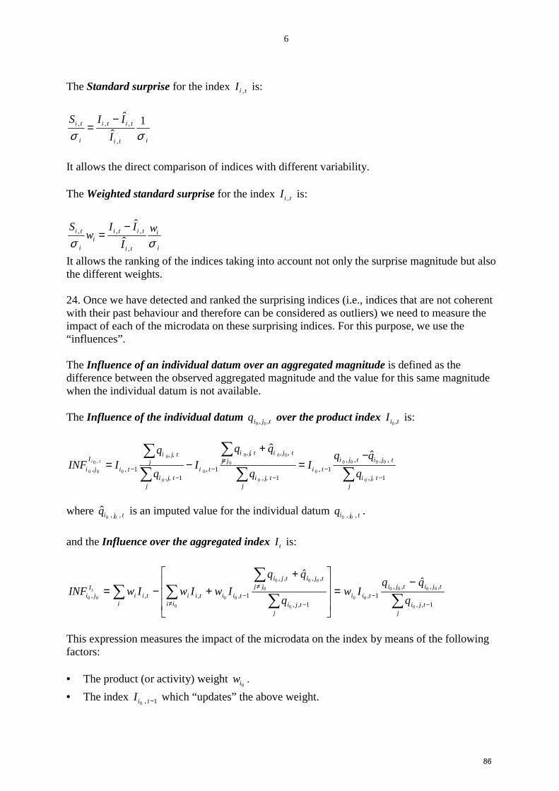
6

The Standard surprise for the index tiI , is:

iti

titi

i

ti

I

IIS

σσ1

ˆ

ˆ

,

,,, −=

It allows the direct comparison of indices with different variability. The Weighted standard surprise for the index tiI , is:

i

i

ti

titii

i

ti w

I

IIw

S

σσ ,

,,,

ˆ

ˆ−=

It allows the ranking of the indices taking into account not only the surprise magnitude but also the different weights. 24. Once we have detected and ranked the surprising indices (i.e., indices that are not coherent with their past behaviour and therefore can be considered as outliers) we need to measure the impact of each of the microdata on these surprising indices. For this purpose, we use the “influences”. The Influence of an individual datum over an aggregated magnitude is defined as the difference between the observed aggregated magnitude and the value for this same magnitude when the individual datum is not available. The Influence of the individual datum qi j t0 0, , over the product index Ii t0 , is:

∑∑

∑

∑

∑

−−

−

≠−

−−

−=

+−=

jtji

tjitji

ti

jtji

tjijj

tji

ti

jtji

jtji

ti

I

ji q

qqI

q

qq

Iq

qIINF ti

1,,

,,,,

1,1,,

,,,,

1,1,,

,,

1,,

0

0000

0

0

00

0

0

0

0

0

0

,0

00

ˆˆ

where tjiq ,, 00

ˆ is an imputed value for the individual datum tjiq ,, 00.

and the Influence over the aggregated index tI is:

INF w I w I w I

q q

qw I

q q

qi jI

ii

i t i i t i i t

i j tj j

i j t

i j tj

i ii i t

i j t i j t

i j tj

t

0 0 0 0

0

0

0 0

00

0 0

0 0 0 0

0

11

11

, , , ,

, , , ,

, ,,

, , , ,

, ,

= − ++

=−

∑∑

∑∑

∑−

≠

−≠−

−

This expression measures the impact of the microdata on the index by means of the following factors: • The product (or activity) weight

0iw .

• The index 1,0 −tiI which “updates” the above weight.

86

7

• A measure of the relative discrepancy between the real and the imputed individual datum

∑ −

−

jtji

tjitji

q

qq

1,,

,,,,

0

0000ˆ

.

It may be proved that the microdata which are more influential on the aggregated index are also the more influential on the surprises of that index. 25. These “influences” allow us to prioritize the suspicious values in the microdata in order to verify and recontact fewer enterprises. Hence improvements in timeliness are achieved. 26. As an example of using this methodology two computer printouts are shown. In table 1 the sectors are ranked according the weighted standard surprise. Sector 4243 is the one with the highest. Looking in table 2 for the enterprises that most influence the index of this sector, we find an enterprise whose influence is not only the highest, but also much higher in comparison with the others. Hence this enterprise should be checked. 27. Using this methodology, the most influential suspicious values could immediately be detected. Hence the most important errors could be checked and corrected before the index is disseminated for first time. 28. Three kinds of imputations would be possible to handle the non-response for one or more enterprise data t,j,i o

q to disseminate the indices Ii,t:

(i) A traditional imputation based on the available enterprise data

∑

∑

≠

≠−=

o

o

00

jjt,j,i

jjt,j,i

1t,j,it,j,i q

q

qq

(ii) A model-based imputation for t,j,i o

q based on its past series, that is t,j,i oq

(iii) A model-based imputation for the whole index t,iI based on its past series,

that is t,iI

29. A choice among the former methods can be made depending on various circumstances. For example, if the trend of the enterprises inside the product (or activity) is similar, the traditional imputation usually works properly. However, if the trend is not very similar a model-based imputation works better. In the same way, if the non-response rate is low for the index, a micro imputation (traditional or model-based) usually works properly. On the contrary, if the non-response rate for the index is high and there are not many enterprises in the index a model-based imputation for the whole index is preferable. Therefore, model-based imputation may improve the estimates of the indices. V. CONCLUSIONS 30. Improving timeliness without any losses in accuracy is a major challenge for public statisticians today. Data editing should not only be linked to accuracy but also to other quality

87

8

aspects, for example timeliness. Data editing is one of the most time-consuming statistical phases. Hence, re-engineering the data editing procedures is a need for improving timeliness. 31. According to our experience, the use of time series modeling is being quite useful to save time in editing short-term indicators. REFERENCES [1] Bell, W.R. (1999). “An overview of REGARIMA modeling”. Forthcoming Research Report.

Statistical Research Division. U.S. Census Bureau. [2] Box, G.E.P. and Jenkins, G.M. (1970). “Time Series Analysis, Forecasting and Control”, ed.

Holden-Day, San Francisco. [3] González, M. and Revilla, P. (1997). “Total Quality Management and the INE”. Eurostat Web,

www.forum.europa.eu.int/. [4] Kovar, J. (1997). “What to do when an edit fails”. Statistical data editing. Volume No.2.

Conference of European Statisticians. Statistical standards and studies-No.48. [5] Revilla, P. and Rey, P. (1999). “Selective editing methods based on time series modelling".

UN/ECE Work Session on Statistical Data Editing. Rome. [6] Rey, P. and Revilla. P, (2000). “Analysis and quality control from ARIMA modelling".

UN/ECE Work Session on Statistical Data Editing. Cardiff.

88

9

Table 1 SURPRISES

Weighted Actual Forecasted Simple Standard Standard Sector Rate Rate Surprise Surprise Surprise

4243 70,28 3,32 64,73 3,79 17,10 2511 -27,73 -3,29 -25,25 -3,11 -16,93 4110 -50,24 -6,89 -70,96 -6,84 -16,89 2514 -15,92 4,64 -19,62 -3,00 -16,87 2512 39,39 -11,83 58,12 7,22 16,51 4752 -0,74 2,06 -2,75 -1,09 -15,66 3299 -11,97 4,45 -15,70 -2,02 -15,57 4751 22,82 -7,36 32,55 2,34 14,64 3630 -0,28 3,68 -3,82 -0,81 -14,54 3166 15,97 5,83 9,58 1,89 13,92

Table 2 INFLUENCES

Enterprise Influence

1 143,41 2 37,60 3 -22,80 4 14,38 5 8,90 6 -7,52 7 7,35 8 6,81

89

STATISTICAL COMMISSION and Working Paper No. 19ECONOMIC COMMISSION FOR EUROPE English only

CONFERENCE OF EUROPEAN STATISTICIANS

UN/ECE Work Session on Statistical Data Editing(Cardiff, United Kingdom, 18-20 October 2000)

Topic III: New techniques and tools for editing imputation

ANALYSIS AND QUALITY CONTROL FROM ARIMA MODELLING

Submitted by the National Statistical Institute and Sociological Research Centre, Spain1

Invited paper

Abstract: In this paper, we use ARIMA modelling to estimate a set of characteristics of a short-termindicator (for example, the index of industrial production), as trends, seasonal variations, cyclicaloscillations, unpredictability, deterministic effects (as a strike), etc. Thus for each sector andproduct (more than 1000), we construct a vector of values corresponding to the above-mentionedcharacteristics, that can be used for data editing.

KEYWORDS: continuous surveys, data editing, ARIMA models, Intervention Analysis.

I. INTRODUCTION

1. This paper follows the approach already presented in the last meeting in Rome (i.e. the use oftime series analysis for data editing). The central idea of this approach is that, if useful information fromprevious surveys is available, it should be used as much as possible in the editing process.

2. In this context, the appropriate theoretical framework for editing continuous surveys should not belimited to that of the static random variables, but should rather be enlarged on that of sequences of randomvariables varying with time. Therefore, stochastic processes and, in particular, time series models may beused.

3. At the previous meeting in Rome, we presented a selective editing procedure based on a kind oftools that we named “surprises”, which are functions of ARIMA forecasts. For this meeting, we use timeseries modelling in a different way. We propose to estimate a univariate ARIMA with InterventionAnalysis model (Box-Tiao, 1975) to describe the characteristics of a short time indicator.

4. The idea comes from the fact that in editing a survey, we need as much information as possibleabout the phenomenon that we try to measure. On the other hand, different subsets of data often show avery different variability and behaviour. For example, when editing the Spanish monthly indices ofindustrial production, we can find extremely small (even zero) production data values for August, becausesummer holidays are usually taken in this month in Spain. Of course, these data must not be considered asoutliers (i.e. suspicious data items) if we have information about this seasonal pattern. But an additionalproblem is that, this seasonal behaviour in August is very different from one branch to another (even thereare branches which production does not decrease but strongly grows in August, as in beer production).For this reason, it is important to acquire information about the different dynamic characteristics of each ofthe branches to improve editing rules and strategies.

1 Prepared by Pedro Revilla and Pilar Rey.

90

2

5. In this paper, we use ARIMA with Intervention Analysis modelling to estimate a set ofcharacteristics of a short term indicator, as trends, cyclical oscillations, seasonal variations, calendareffects, special event effects (as a strike), unpredictability, etc. Thus for each of the branches andproducts (more than 1000), we construct a vector of values corresponding to the characteristics abovementioned, that can be used as a useful tool by the data editing team.

6. Even when, from a theoretical point of view, multivariate models (that picked up the correlation ofall the variables of the survey) would be appropriate, we restrict ourselves to the univariate environment,because of the difficulties in using multivariate time series modelling in practice. On the other hand, theuse of univariate ARIMA models to describe the data characteristics of an economic phenomenon has asound methodological foundation.

7. Under fairly general conditions (see Prothero and Wallis (1976), Wallis (1977), Zellner (1979),etc.) any variable, which is determined within a structural simultaneous and dynamic econometric model(SEM) is generated in a univariate way by an ARIMA with Intervention Analysis model. In the lattermodel, the intervention analysis component picks up the contribution of the dummy variables of the SEMmodel and/or the effect of certain intervention analysis, which affect the exogenous variables of thatmodel.

8. To the extent that the SEM model reflects the characteristics of the real world, the ARIMA withIntervention Analysis model corresponding to an endogenous variable of the SEM model incorporates,inefficiently but certainly consistently, the basic characteristics of that variable.

II. APPLICATION TO THE INDUSTRIAL PRODUCTION INDICES

9. The approach presented here is being used in the National Statistical Institute of Spain for editingthe Industrial Production Indices. It could also be implemented for other short-term indicators. A monthlysurvey is carried out by mail in order to calculate the Industrial Production Indices. A panel sample ofabout 9000 enterprises is used. The response rate is about 95%.

10. One single variable, the production volume, measured in physical units (tons, litres, etc.) or inmonetary value, is requested from each enterprise. The indices for products are calculated as chainindices. From these product indices, Laspeyres aggregated indices are calculated at successive levels ofbreakdown of the economic branches classification (at the top of the aggregation is the total industry). Thefollowing formula is used:

∑=i

tiit IwI ,

where the base year weights iw are calculated using the value added (for branches aggregation) or the

value of the production (for products aggregation). The branches have been studied at five successivelevels of breakdown, in accordance with the National Classification of Economic Activities existing inSpain.

11. In all of the series the sample contains 96 observations, from January 1992 to December 1999.To characterise the evolution of production in the different branches of industrial activity ARIMA modelswith Intervention Analysis (ARIMA-IA) are used.

12. Since the number of time series to handle is very large and it is difficult and time consuming tobuild models for all of them, we need an automatic procedure. We use an automatic method developed byRevilla, Rey and Espasa (1990), that fits into the Box-Jenkins iterative modelling strategy of identify,

91

3

estimate and diagnostic checking. Using this method, an ARIMA model has been constructed for each ofthe series of indices.

13. A straightforward use of ARIMA models is not sufficient to capture calendar effects and otherdeterministic variations (for example, a strike). Regression models are used to handle them. Therefore,the overall models are a sum of ARIMA and regression models:

( ) ( )( ) ( )

( )( )∑+

ΦΘ=

hthi

hi

hiti

ii

iiti A

B

Ba

BBBB

I ,,,

,,12

12

,lnδα

ϕθ

where:

• tiI ,ln is the neperian logarithm of the industrial production index for product (or activity) i .

• B is the backshift operator, ( ) kttk IIB −= .

• ( ) ( ) ( ) ( ) ( ) ( )BBBBBB hihiiiii ,,1212 ,,,,, δαϕθ ΦΘ are polynomials in the backshift operator.

• tia , are white noise variables i. i. d. ( )σ,0N .

• thiA ,, are intervention variables.

14. To specify the intervention variables we have found that automatic procedures are not suitable forall of the series and some subject matter knowledge about the behaviour of the indices is needed.

15. In the following, we will consider one by one the different aspects we have studied in the models,describing how they have been implemented.

A. Level behaviour

16. An adequate description of the nature of the long-term trend of the series is contained in themodels. This trend is determined by the contribution in the final forecast function of the real positive unitroots of the autoregresive factor and by the contribution of the possible non-zero mean of the stationaryseries. The presence of d roots of the type already mentioned means that the long-term trend is a timepolynomial of order (d-1), the coefficients of which are determined by the initial conditions in which thesystem is located. The presence of a non-zero means increases the previous polynomial with a term oforder d with a deterministic coefficient.

17. Thus, whenever the series is stationary, it would not require differences. When the modelspecifies one difference the series will show local oscillations in level; when the model specifies twodifferences the series will have a quasi-linear trend, etc.

B. Seasonal behaviour

18. The models also can contain a factor, which picks up a seasonal cycle with a period of 12 timeunits. The complex unit roots and real negatives of the autoregressive polynomial form this factor. Ifnone of these roots is repeated its contribution in the final forecast function consists of 12 stable, additive,seasonal factors which at all times are determined by the initial conditions of the system. As a result, thelong-term path of the series is made up of these seasonal factors and the trend described in A.

92

4

Whenever a seasonal cycle has been found the seasonal factors of the final forecast function have beencalculated.

C. Calendar effects

19. Spanish Indices of Industrial Production series are strongly affected by calendar effects. Becausethese data are reported monthly and represent a total of the production for each month, they containvariations due to the length and day-of-the-week composition of the month. Monthly production data arealso affected by holidays, in which the levels of production are lower than on ordinary working days.There are holidays that occur each year at the same time, and movable holidays, for example Easter, thatoccur at various dates during March and April. To make the situation more complicated, public holidays inSpain vary from one year to another, and from one “Autonomous Community” to another. In order tohandle these calendar effects, we incorporate this information as deterministic input variables.

20. Instead of the most commonly used (see Hillmer, Bell and Tiao, 1983) seven trading-day variables(number of Mondays, Tuesdays, etc.), we construct one single variable, adapted to the behaviour of theSpanish industrial production. This variable tries to measure the number of working days, removingSaturdays, Sundays and holidays. To achieve a suitable computation, those holidays that vary from one“Autonomous Community” to another have to be weighted by the industrial value added of the base year.

21. By constructing the model on the logarithmic transformation of the series, the parameterassociated with this dummy variable can be interpreted as the proportional increase in production incomparison with that of a similar month with one less working day.

22. Another deterministic variable containing the Easter effect (which takes in March and April thevalues that indicate the proportion of days affected by these holidays and in the other months value zero) isincluded in the model (see Hillmer, Bell and Tiao, 1983). The parameter, which affects this artificialvariable, can be interpreted as the proportional variation suffered by production as a result of this effect.Hence, all calendar effects are summarised using only two variables.

D. Other deterministic effects

23. It is possible to find deterministic contributions in the trend and/or seasonal factors of the seriesfrom the intervention analysis. In February 1997 the transporting sector went on strike. For most of theindustrial branches, this strike caused a shortage of raw materials. The expected effect would have beenan immediate reduction in the level of production. But, in fact, after some periods of observation, wefound in some series an increase in the months of March and April that compensated the decrease inFebruary. After consulting some respondent factories, we learned that they have tried to fulfil the ordersof the clients by working extra in the next two months.

24. So, we have constructed two different variables for peaking up the effects of the strike:

1) The Ht variable, where:

≠=−=−=

=

1997...,,0.0

1997,4.0

1997,6.0

1997,0.1

orAprMarFebt

Aprilt

Marcht

Februaryt

Ht

93

5

2) The Pt pulse variable, where:

≠=

=1997,0

1997,1

Februaryt

FebruarytPt

25. We have accepted that the strike had an effect on an industrial production index series when theintervention variable parameter is significantly different from zero. When the parameters are significantfor the two of them, we have chosen the intervention variable that produces a smaller residual standarddeviation of the ARIMA-IA model. As we have used the logarithmic transformation of the series, it ispossible to interpret the value of the parameters as a percentage effect on the level of the original series.

E. Outliers

26. We have made in the series a detection of unusual or unexpected observations. Depending ontheir nature, we have detected three types of outliers: Additive Outlier (A. O), Level Shift (L. S.), andTemporary Change (T. C.).

27. For defining and detecting the location and type of an outlier, we follow the approach of Chang etal. (1988) using the estimated residuals of the Arima model.

The study of outliers can be used to detect special events which may affect production in aparticular period of time, to analyse if they appear fortuitously or not in the differentbranches, the month in which they often appear, etc.

F. Uncertainty

28. The last characteristic we have considered is a measure of the uncertainty about the futureevolution of the series, expressed by the standard deviation of the one period ahead forecasting errors.Each series at a given time can be broken down into two components: its prediction based on previousobservations and a prediction error. A good measure of uncertainty is given by the standard deviation ofthese prediction errors.

III. RESULTS OF THE STUDY

29. As an example of the information that may be obtained from the models, the main dynamiccharacteristics of the indices for the total industry and for the branches at two digits level are presented inTable 1.

30. The following are shown in the table: 1) Identification of the branch by means of the code of theNational Classification of Economic Activities of Spain, 2) Behaviour of the level, 3) Whether the sectorhas seasonal behaviour or not, 4) A measure of the effect of working days, when it affects the series, 5)A measure of the effect of Easter, when it affects the series, 6) A measure of the effect of the 1997strike, when it affected the series, 7) The outliers, the date when they are produced and their type, 8) Thedegree of uncertainty about future production levels.

31. To illustrate the information that can be obtained from Table 1, the characteristics of total industryare described. Industrial production from 1992 onwards shows a trend in its level and a stochasticseasonal nature, which implies different behaviour in production activity in different months of the year (inparticular, it shows a decrease in the holiday months, especially in August).

94

6

32. The industrial output is sensitive to day-of-the-week composition and periods of holidays. Morespecifically, the existence of one less working day causes a 1,9% drop in production. Likewise, Eastercauses a fall in production of 4,0% distributed in March and April according to the proportion of daysaffected by this holiday in each year.

33. The transport sector strike in February 1997 caused a 3,6% reduction on the level of production ofthis month, compensated in March and April. It does not show outliers above three standard deviations.The degree of uncertainty regarding production for the next month is 2,1%.

34. Likewise, useful information can be gained of the different industrial branches. It is easy to seethat they show very different patterns of behaviour.

REFERENCES

Box, G.E.P. and Tiao, G.C. (1975),"Intervention Analysis with Applications to Economic andEnvironmental Problems", Journal of the American Statistical Association, 349.

Chang, I., Tiao, G. C. and Chen, C. (1988), “Estimation of Time Series Parameters in the Presence ofOutliers”, Technometrics, 30, pp.193-204.

Hillmer, S.C., Bell W.R and Tiao, G.C. (1983), "Modelling. Considerations in the Seasonal Adjustment ofEconomic Time Series", Applied Time Series Analysis of Economic Data, U.S. Department of Commerce,Bureau of the Census.

Prothero, D.L. and Wallis, K.F. (1976),"Modelling Macroeconomic Time Series", Journal of the RoyalStatistical Society, Series A, 139, Part 4, pp.468-85.

Revilla, P., Rey, P. and Espasa., A. (1990), "Automatic Univariate Modelling of Time Series: Applicationto the Industrial Production Indices", unpublished.

Wallis, K.F (1977), "Multiple Time Series Analysis and the Final Form of Econometric Models",Econometrica, v.45, n.6, September, pp.1481-98

Zellner, A. (1979), "Statistical Analysis of Econometric Models", Journal of the American StatisticalAssociation v.74, n.367, September, pp.628-651.

95

7

Table 1

SeriesLevel

BehaviourSeasonalBehaviour

Working-Days Effect

(%)

EasterEffect (%)

Feb 1997Strike

Effect (%)

OutliersDate Type

Uncertainty(%)

0 Trend Yes 1.9 -4.0 -3.6 2.1

11 Local Oscillations No 2.7 8.3

12 Trend Yes 3/942/9510/9510/971/98

A. O.A. O.L. S.L. S.L. S.

13.0

13 Local Oscillations Yes 6.4

14 Local Oscillations Yes 9/9311/935/968/933/9810/9811/9812/99

L. S.A. O.A. O.A. O.A. O.A. O.A. O.A. O.

17.7

15 Trend Yes -5.4 -7.8 3.6

21 Local Oscillations No 6/942/964/9611/963/978/985/98

L. S.T. C.T. C.L. S.T. C.L. S.L. S.

11.4

22 Trend Yes -7.2 -6.7 1/9412/958/969/99

A. O.A. O.A. O.A. O.

3.6

23 Trend Yes 3.1 5.7

24 Trend Yes 1.2 -2.2 2/938/931/9412/949/963/97

A. O.A. O.A. O.A. O.T. C.L. S.

3.7

25 Trend Yes 1.8 -4.1 12/9310/95

L. S.A. O.

3.4

31 Trend Yes 3.2 8/93 T. C. 4.5

32 Trend Yes 2.9 -7.5 8/94 A. O. 6.2

33 Local Oscillations No 5/937/931/94

A. O.A. O.A. O.

20.6

34 Trend Yes 3.3 8/93 A. O. 5.1

35 Trend Yes 13.0

36 Trend Yes 3.5 -4.8 -12.2 8/932/944/948/948/958/964/98

A. O.L. S.A. O.A. O.A. O.A. O.A. O.

3.0

37 Local Oscillations No 5/949/9412/942/969/965/9711/983/99

L. S.L. S.L. S.L. S.T. C.L. S.L. S.T. C.

6.5

96

8

SeriesLevel

BehaviourSeasonalBehaviour

Working-Days Effect

(%)

EasterEffect (%)

Feb 1997Strike

Effect (%)

OutliersDate Type

Uncertainty(%)

38 Trend Yes 2.5 -6.1 5/948/943/97

T. C.T. C.L. S.

7.0

39 Trend Yes 3.0 8/946/99

A. O.L. S.

5.9

41 Trend Yes 2.4 5.3 1/947/951/96

A. O.A. O.T. C.

2.7

43 Trend Yes 3.2 9/938/99

L. S.A. O.

5.2

44 Trend Yes 4.4 4/938/937/976/99

A. O.L. S.L. S.L. S.

5.9

45 Trend Yes 3.1 4/932/949/9412/954/969/975/996/99

T. C.L. S.L. S.T. C.A. O.A. O.T. C.A. O.

2.3

46 Trend Yes 1.6 -5.3 -3.7 8/938/96

A. O.A. O.

3.9

47 Trend Yes 2.1 -3.3 3.0

48 Trend Yes 2.7 -3.2 -10.0 8/938/958/988/99

A. O.A. O.A. O.A. O.

3.7

49 Trend Yes 4.2 -14.5 4/938/935/9410/9412/943/957/9610/9612/966/9711/98

L. S.A. O.A. O.A.O.A. O.A. O.L. S.L. S.A. O.L. S.A. O.

5.4

97

April 23, 2010 13:54 Optimization editingOptimizationVol. 00, No. 00, Month 200x, 119

RESEARCH ARTICLEA Class of stochastic optimization problems with application toselective data editing

Ignacio Arbuesyz, Margarita Gonzalezy and Pedro RevillayyS. G. de Estadsticas Industriales y Agrarias, Instituto Nacional de Estadstica,Castellana 183, 28071, Madrid, Spain(Received 00 Month 200x; in nal form 00 Month 200x)We present a class of stochastic optimization problems with constraints expressed in termsof expectation and with partial knowledge of the outcome in advance to the decision. Theconstraints imply that the problem cannot be reduced to a deterministic one. Since the knowl-edge of the outcome is relevant to the decision, it is necessary to seek the solution in a spaceof random variables. We prove that under convexity conditions, a duality method can beused to solve the problem. An application to statistical data editing is also presented. Thesearch of a good selective editing strategy is stated as an optimization problem in which theobjective is to minimize the expected workload with the constraint that the expected errorof the aggregates computed with the edited data is below a certain constant. We present theresults of real data experimentation and the comparison with a well known method.Keywords: Stochastic Programming; Optimization in Banach Spaces; Selective Editing;Score FunctionAMS Subject Classication: 90C15; 90C46; 90C90

1. IntroductionLet us consider the following elements: a decision variable x under our control; theoutcome ! of a probability space; a function f that depends on x and ! that wewant maximize; and a function g also depending on x and ! that we want in somesense not to exceed zero. Various optimization problems can be posed under theseassumptions.First of all, the problem is quite dierent depending on whether we know !before we take the the decision about x or not. In the rst case (wait and see), !is xed and thus, we have deterministic functions f(; !) and g(; !). Therefore, wecan solve a nonstochastic optimization problem for each outcome !. Consequently,the solution depends on ! and it is a random variable (this case is studied, forexample, in [2]).In the case ! is unknown when x is decided (here and now), the usual approach isto pose a stochastic optimization problem by setting as the new objective functionE[f(x; !)] (see [4] for a discussion on this matter).In this paper, we study problems in which we have a partial knowledge of ! andthus, in that respect, they are in somewhere in the middle between here-and-nowand wait-and-see. In subsequent sections, we will explain in full detail the meaningof "partial knowledge".

ISSN: 0233-1934 print/ISSN 1029-4945 onlinec 200x Taylor & FrancisDOI: 10.1080/0233193YYxxxxxxxxhttp://www.informaworld.com98

April 23, 2010 13:54 Optimization editing2 I Arbues et al.The use of some knowledge about ! to decide about x implies that x will dependon ! and thus it will be a random variable. On the other hand, in our problem wehave also constraints expressed in terms of expectation, that is, E[g(x; !)] 0.We also analyse an application of these problems to statistical data editing. Ef-cient editing methods are critical for the statistical oces. In the past, it wascustomary to edit manually every questionnaire collected in a survey before com-puting aggregates. Nowadays, exhaustive manual editing is considered inecient,since most of the editing work has no consequences at the aggregate level and canin fact even damage the quality of the data (see [1] and [6]).Selective editing methods are strategies to select a subset of the questionnairescollected in a survey to be subject to extensive editing. A reason why this is con-venient is that it is more likely to improve quality by editing some units than byediting some others, either because the rst ones are more suspect to have an erroror because the error if it exists has probably more impact in the aggregated data.Thus, it is reasonable to expect that a good selective editing strategy can be foundthat balances two aims: (i) good quality at the aggregate level and (ii) less manualediting work.This task is often done by dening a score function (SF), which is used to pri-oritise some units. When several variables are collected for the same unit, dierentlocal score functions may be computed and then, combined into a global score func-tion. Finally, those units with score over a certain threshold are manually edited.Thus, when designing a selective editing process it is necessary to decide, Whether to use SF or not. The local score functions. How to combine them into a global score function (sum, maximum, . . . ). The threshold.At this time, the points above are being dealt with in an empirical way becauseof to the lack of any theoretical support. In [8], [9] and [6] some guidelines areproposed to build score functions, but they rely in the criterion of the practitioner.In this paper, we describe a theoretical framework which, under some assumptions,answers the questions above. For this purpose, we will formally dene the conceptof selection strategy. This allows to state the problem of selective editing as anoptimization problem in which the objective is to minimize the expected workloadwith the constraint that the expected remaining error after editing the selectedunits is below a certain bound.We present the general problem in section 2. We also describe how to use a dual-ity method to solve the problem. In section 3, we show the results of a simulationexperiment. In sections 4 through 7 we describe how to apply the method to selec-tive editing. In section 8, results of the application of the method to real data arepresented. Finally, some conclusions are discussed.

2. The general problemLet (;F ; P ) be a probability space and N;m; p 2 N. We consider the functionsf(x; !) : RN 7! R, g1(x) : RN 7! Rm and g2(x; !) : RN 7! Rp. We needsome assumptions.Assumption 2.1 f and g2 are Fmeasurable and integrable in !.Assumption 2.2 f and g2 are convex in x; g1 is convex.The convexity implies that f and g2 are continuous with respect to x (see theorem

99

April 23, 2010 13:54 Optimization editingOptimization 3

2.35 in [12]) and thus, they are Caratheodory functions (that is, continuous in x andmeasurable in !). For the same reason, g1 is continuous. With these assumptions,for any random vector ! 2 7! X(!) 2 RN , f(X(!); !) and g2(X(!); !) areFmeasurable.Let G F be a eld. We denote by O(G) the set of the Gmeasurablefunctions such that E[f(X(!); !)] and E[g2(X(!); !)] exist in R.We can now pose the following problem.[P ] maxX E[f(X(!); !)] (1)X 2 O(G); s:t: g1(X(!)) 0 a:s:;E[g2(X(!); !)] 0: (2)

The fact that we seek X among the Gmeasurable random variables means thatall the information we have about ! is whether ! 2 A, for any A 2 G, that is, ifthe event A happened.In order to prove the existence of solutions to [P ], we make some further assump-tions.Assumption 2.3 For = f; g2, there exists 2 (1;+1) such thatE[(X(!); !)] 2 R when EjXj < +1 and the function X 2 L(;G) 7!E[(X(!); !)] is lower semicontinuous with respect to the strong topology ofL(;G).The semicontinuity condition holds, for example, when the function satisesa Lipschitz condition with respect to the rst argument, say j(x; !) (y; !)j C(!)kx yk, such that C(!) has a nite moment of order greater than one, inwhich case we have not only semicontinuity, but continuity.

Assumption 2.4 The set fx 2 RN : g1(x) 0g is bounded.Assumption 2.5 G is countably generated.Assumption 2.5 is technical and do not seem to imply an important loss ofgenerality for most of practical applications. With these assumptions, we can provean existence result for [P ].

Proposition 2.6: If assumptions 2.12.5 hold then [P] has at least one solution.Proof : From assumption 2.4, it follows that the solutions must be bounded withprobability one, but since the measure of is nite, they must have nite L-norm. Consequently, we can seek a solution in L(;G), which is a Banach space(Theorem 3.11 in [13]). Under assumption 2.5, the closed unit ball B in L(;G) iscompact with respect to the -weak topology (see [3], p.246). On the other, handL(;G) is re exive, so we do not have to distinguish between the -weak topologyand the weak topology.From assumption 2.3 the set M = fX 2 L(;G) : g1(X) 0 a:s:;E[g2(X(!); !)] 0g is strongly closed and convex and then, weakly closed.From assumption 2.4, it is also bounded. Then, there exists some " > 0 such that"M B. Since "M is a weakly closed subset of a weakly compact set, it is weaklycompact itself. M is also weakly compact because is homothetic to "M . On theother hand, X 7! E[f(X(!); !)] is convex and strongly lower semicontinuous.Thus, it is weakly lower semicontinuous and it attains a minimum in M , that is,[P ] has a solution. In the remaining of section 2, we will show a practical way to obtain the solutions.We will analyse in 2.1 the case that G = F (full information) and then, in 2.2 we

100

April 23, 2010 13:54 Optimization editing4 I Arbues et al.will describe how to reduce the general case (partial information) to the formerone.2.1. DualityNow, we assume that G = F . Under this condition, we will establish two results.First, we will show (proposition 2.8) that solutions can be obtained to problem [P ]by solving a dual problem [D] formulated using a Lagrangian function. The secondresult (proposition 2.9) states that the dual problem can be reduced to a family ofdeterministic optimization problems in RN depending on !. For this, we need anadditional assumption.Assumption 2.7 There is a random vector X0 such that g1(X0) 0 a:s: andE[g2(X0(!); !)] < 0.Assumption 2.7 is a classical regularity condition necessary for the duality meth-ods and it is usually known as Slater's condition.Let us dene the Lagrange function,

L(X;) = E[f(X(!); !)] TE[g2(X(!); !)]: (3)We can now dene the problem

[P ()] maxX L(X;)X 2 O(G); s:t: g1(X(!)) 0 a:s: (4)The dual function is dened as '() = supfL(X;) : X 2 O(G); g1(X(!)) 0 a:s:g. If the supremum is a maximum, we denote by X the point where it isattained. The dual problem is,

[D] min '()s:t: 2 Rp; 0:This problem is of great interest for us because of the following proposition.

Proposition 2.8: If the assumptions of proposition 2.6 and assumption 2.7 holdthen,i) There exist solutions to [D].ii) If X is a solution to [P ] and is a solution to [D] then, X is a solution to[P ()].Proof : Since [P ] has a solution, then E[f(X(!); !)] is bounded from above in Mand thus, we can apply theorem 1, p. 224 in [10]. The rst part of the theoremstates that [D] has a solution and the second part implies (ii). Therefore, if we know how to solve [D] and [P ()] for any , we can obtainsolutions to [P ] by solving [P ()], where is a solution to [D]. If we know how tocompute '(), then [D] can be solved by numerical methods since it is a nitedimensional optimization problem, but if X is a solution to [P ()], then '() =L(X; ). Thus, all we need is a method to solve [P ()].The advantage of P [] with respect to [P ] is that the stochastic terms are all inthe objective function. Consequently, the solution can be easily obtained by solving

101

April 23, 2010 13:54 Optimization editingOptimization 5

a deterministic optimization problem for any outcome ! 2 .[PD(; !)] maxx L(x; ; !)s:t: x 2 RN ; g1(x) 0

where L(x; ; !) = f(x; !) T g2(x; !). We can relate this problem to [P ()] byvirtue of the following direct consequence of theorem 14.60 in [12].Proposition 2.9: In the assumptions of proposition 2.6, there exists a solutionX to [P ()] such that for any ! 2 ,i) X(!) is a solution to PD(; !).ii) '() = E[L(X(!); ; !)].The optimal will be obtained maximizing '. Since ' is described in terms ofexpectation, it is necessary either to know the real distribution of the terms in Land compute explicitly its expectation or to estimate it. In practical applications,the explicit computation will usually not be feasible.2.2. Partial informationIn the proof of proposition 2.9, we use the Fmeasurability of f and g2 to obtaina measurable solution X. The validity of this argument depends on the fact thatG = F , so the proposition breaks down if we seek Gmeasurable solutions Xwhile f and g2 are only measurable with respect to a strictly larger eld F .Fortunately, we can still apply the ideas of the previous section with some changes.Before introducing the main results of this section, we will show an example. Letus assume that f is linear with respect to x, that is, we can write f(x; !) = Z(!)Tx,where Z(!) is a N 1 random vector. Then, for a Gmeasurable X, it holds

E[f(X(!); !)] = E[E[f(X(!); !)jG]] = E[E[ZTXjG]] = E[E[ZT jG]X];where the rst identity is a consequence of the Law of Total Expectations and thethird to the Gmeasurability of X. Consequently, if we dene f(x; !) = U(!)Tx,where U = E[ZjG], then we get that E[f(X(!); !)] = E[f(X(!); !)], but now fis Gmeasurable with respect to !. We can dene g2 in the same way and thus wecan express [P ] in such a way that the results of section 2.1 can be directly applied.We will prove that appropriate functions f and g2 can be dened without thelinearity assumption. We will show that if (x; !) is dened as the conditionalexpectation of (x; !) (later, f and g2) with respect to G with x xed, then for anyGmeasurable X it holds that E[(X(!); !)jG] = (X(!); !).In other words, when we calculate the conditional expectation of (X(!); !) withrespect to G and X is Gmeasurable, we can take conditional expectation in thesecond argument as if the rst were deterministic. In order to prove this, we needrst the following generalization of the monotone convergence theorem.Lemma 2.10: Let fngn be a sequence of integrable random variables and G aeld. If n(!)% (!) and is integrable, then E[njG]% E[jG] with probabilityone.Proof : The sequence of random variables n := E[njG] is nondecreasing withprobability one. Consequently, n(!) % (!) with probability one. The randomvariable is Gmeasurable since it is limit of Gmeasurable r.v.'s (corollary to

102

April 23, 2010 13:54 Optimization editing6 I Arbues et al.theorem 1.14, in [13]). On the other hand, for any A 2 G it holds thatZ

A P (d!) = limnZAE[njG]P (d!) = limn

ZA nP (d!) =

ZA P (d!);

where the rst and third identities hold by the monotone convergence theorem andthe second by the denition of the conditional expectation (page 445 in [3]). Then, is a version of E[jG]. With this lemma, we can prove the following proposition.Proposition 2.11: Let (x; !) 2 RN 7! (x; !) 2 R be lower semicontinuousin x and F-measurable in !. If (x; !) = E[(x; !)jG], then for any GmeasurableXE[(X(!); !)jG] = (X(!); !): (5)

Proof : In order to simplify the notation, we will prove it for N = 1 and thearguments can be easily generalized for N > 1. Let us rst assume that for acertain L 2 N, (x; !) = 0 when jxj > L and consider for k = L2n; : : : ; L2n 1,the intervals In;k = [k2n; (k+1)2n). Then, we can dene the functions n;k(!) =infz2Ink (z; !) andn;k(z) = 1 if z 2 In;k0 if z =2 In;k

We can writen(z; !) = n2nX

k=n2n1 n;k(!)n;k(z):Let us see that n(z; !) % (z; !). For any z and n, there exist k; l such thatz 2 In+1;k In;l. Then, n(z; !) n+1(z; !) (z; !). Now, for any > 0, thereexists n0 such that for any n n0, jz z0j 2n implies (z0; !) (z; !) . Consequently, for any n n0, (z; !) n(z; !) (z; !) . Therefore,n(z; !)% (z; !).Now, by lemma 2.10,

(z; !) = E[(z; )jG] = limnn2nX

k=n2n1nk(z)E[n;kjG]:If X(!) is Gmeasurable, then

(X(!); !) = limnn2nX

k=n2n1nk(X(!))E[n;kjG] = limn E[n(X(!); !)jG]and we conclude by using again lemma 2.10. The case that the support of isnot bounded can be dealt with by using (x; !)L(x), where L(x) equals one in[L;L] and has bounded support. By denition of conditional expectation, is Gmeasurable with respect to !. If is convex in x, so is and the identity (5) ensures that if the strong semicontinuity

103

April 23, 2010 13:54 Optimization editingOptimization 7

of assumption 2.3 holds for , then it holds for as well. Consequently, if we denef(x; !) = E[f(x; !)jG] and g2(x; !) = E[g2(x; !)jG], they inherit from f and g2the properties required for the assumptions of proposition 2.8. Let us consider theproblem[P ] max E[f(X(!); !)] (6)X 2 O(G); s:t: g1(X(!)) 0 a:s:;E[g2(X(!); !)] 0: (7)

Proposition 2.11 ensures that [P ] is equivalent to [P ] in the sense that thedomain of the problem, the objective function and the constraints are the same, ifonly expressed in a dierent way. Consequently, every solution to [P ] is solution to[P ] and conversely. However, since f and g2 are measurable with respect to thesame eld as X, we can use the results of subsection 2.1.3. Simulation.Proposition 2.8 provides the optimal solution to [P ], but the dual problem has to besolved by numerical methods in order to obtain the Lagrange multipliers. Thus, wehave designed an example of problem [P ] such that can be computed analyticallyand we have obtained estimate values from simulation in order to compare withthe true ones.Let us consider the following case,f(x; !) = 1Tx; g1(x) = (xT 1T ;xT )T ; g2(x; !) = NX

i=1 i(!)xi d;where figi=1;:::;N are independent and uniformly distributed in [0; 1] and d is apositive constant. It is easy to see that the solution to [P ()] is

Xi = 1 if i < 10 if i > 1 : (8)Then, we can see that for 1, E[Xi] = 1 and E[Xii] = (22)1, whereas for < 1, E[Xi] = 1 and E[Xii] = 1=2. Hence,

'() = N(1 2 ) + d if < 1N2 + d if 1 ;and consequently, for d < N=2 the minimum is attained at = (N2d)1=2.We will estimate by applying the samplepath optimization or sample averageapproximation method (SAA, see [5], [11], [15]). The SAA method can also beapplied to constrained problems (see [14]), but we do not apply this method to theoriginal problem [P ] because there the decision variable is a Gmeasurable randomvariable.We simulate a sample of size M of = (1; : : : ; M ) and then we mini-mize the function '() = M1PMj=1 'j(), where 'j() = L(xj ; ), L(x; ) =1Tx(P ixi d), xj = (xj1; : : : ; xjN ) and xji is dened as in (8) for the j-th sim-ulated value of . The convergence of the solution of the approximate problems isguaranteed, for example, by theorem 3.9 in [5]. The hypotheses of the theorem can

104

April 23, 2010 13:54 Optimization editing8 I Arbues et al.be easily checked for our problem. This method is also applied in our applicationof section 8, where we use a sample of real data instead of a simulated one.The minimization of ' has been performed using the function fmincon of themathematical pack MATLAB.The results for a range of values of N andM are presented in table 1, suggestingthat when N is large, even moderate values of M allow to achieve considerableaccuracy. We have chosen d = N=4 and thus, the theoretical is p2.

N M=1 M=5 M=10 M=25 M=50 M=100 M=25010 0.2052 0.0966 0.0686 0.0413 0.0330 0.0236 0.013250 0.0919 0.0375 0.0313 0.0190 0.0134 0.0104 0.0057100 0.0694 0.0278 0.0224 0.0117 0.0097 0.0062 0.0044500 0.0286 0.0125 0.0097 0.0060 0.0044 0.0030 0.00181,000 0.0177 0.0090 0.0063 0.0047 0.0030 0.0018 0.00145,000 0.0089 0.0041 0.0032 0.0019 0.0014 0.0010 0.000610,000 0.0070 0.0028 0.0024 0.0012 0.0011 0.0007 0.0004Table 1. RMS error in the estimation of .

4. The selective editing problemLet us introduce some notation, xijt is the true value of variable j in questionnaire i at period t, with i = 1; : : : ; Nand j = 1; : : : ; q. ~xijt = xijt + "ijt is the observed value of variable j in questionnaire i at period t,"ijt being the observation error. Xkt = P!kijxijt is the k-th statistic computed with the true values ( ~Xkt is com-puted with the observed ones), according to certain weightings !kij with k rangingfrom 1 to p.The linearity assumption implies a loss of generality, which is nevertheless notvery important in the usual practice of statistical oces. Many statistics are in factlinear aggregates of the data. In some other cases such as indices, they are ratioswhose denominator depends on past values that can be considered as constantwhen editing current values. When the statistic is nonlinear, the applicability ofthe method depends on the accuracy of a rst-order Taylor expansion in fxijt g.Let (;F ; P ) be a probability space. We assume that xijt and "ijt are randomvariables with respect to that space. There can be other random variables relevantto the selection process. Among them, some are known at the moment of theselection, such as ~xijt , xijs with s < t or even variables from other surveys. Theassumption that xijs is known is equivalent to assume that when editing periodt, the data from previous periods have been edited enough and does not containerrors. Deterministic variables such as working days may also be useful to detectanomalous data. We will denote by Gt the eld generated by all the informationavailable up to time t. In order to avoid heavy notation, we omit the subscript twhen no ambiguity arises.Our aim is to nd an adequate selection strategy. A selective editing strategyshould indicate for any i whether questionnaire i will be edited or not and this hasto be decided using the information available. In fact, we will allow the strategy notto determine precisely whether the unit is edited but only with a certain probability.

105

April 23, 2010 13:54 Optimization editingOptimization 9

Definition 4.1: A selection strategy (SS) with respect to Gt is a Gt-measurablerandom vector R = (R1; : : : ; RN )T such that Ri 2 [0; 1].We denote by S(Gt) the set of all the SS with respect to Gt. The interpretationof r is that questionnaire i is edited with probability 1 Ri. To allow 0 Ri 1instead of the more restrictive Ri 2 f0; 1g is theoretically and practically convenientbecause then, the set of strategies is convex and techniques of convex optimizationfrom section 2 can be used. Moreover, it could happen that the optimal value overthis generalized space were better than the restricted case (just as in hypothesistesting a randomized test can have a greater power than any nonrandomized one).If for a certain unit, Ri 2 (0; 1), then the unit is eectively edited dependingon whether it < Ri, where it is a random variable distributed uniformly in theinterval [0; 1], and independent from every other variable in our framework (inorder to accommodate these further random variables, we consider an augmentedprobability space, (;F; P ), which is the product space of the original onetimes the suitable choice of (1;F1; P1); only occasionally we have to refer to theaugmented one). We denote by ~Ri the indicator variable of the event it < Ri and~R = ( ~R1; : : : ; ~RN ). If a SS satises Ri 2 f0; 1g a.s., then ~R = R a.s. and we saythat R is integer. The set of integer SS is denoted by SI(Gt). In our case study, thesolutions obtained are integer or approximately integer.It is also convenient to have a formal denition of a Score Function.

Definition 4.2: Let R be a SS, = (1; : : : ; N )T a random vector and 2 R,such that Ri = 1 if and only if i . Then, we say that is a Score Functiongenerating R with threshold .In order to formally pose the problem, we will assume that after manual editing,the true values of a questionnaire are obtained. Thus, we have to consider only theobserved and true values. We dene the edited statisticXk(R) as the one calculatedwith the values obtained after editing according to a certain choice. We can writeXk(R) =P!kij(xijt + ~Ri"ijt ).The quality of Xk(R) has to be measured according to a certain function. Inthis paper, we consider only the Squared Error, (Xk(R)Xk)2. This choice makeseasier the theoretical analysis. It remains for future research to adapt the methodfor other loss functions. The value of the loss function can be written as

(Xk(R)Xk)2 =Xi;i0 ki ki0 ~Ri ~Ri0 ; (9)

where ki = Pj !kij"ijt or, in matrix form, as (Xk(R) Xk)2 = ~R0Ek ~R, withEk = fEki;i0gi;i0 and Eki;i0 = ki ki0 . We can now state the problem of selection asan optimization problem.[PQ] maxR E[1T ~R]

s:t: R 2 S(Gt);E[ ~RTEk ~R] e2k; k = 1; : : : ; p;with e2k > 0.In section 6 we will see the solution to this problem. The vector in the costfunction can be replaced for another one in case the editing work were considereddierent among units (e.g., if we want to reduce the burden for some respondents;this possibility is not dealt with in this paper).

106

April 23, 2010 13:54 Optimization editing10 I Arbues et al.Let us now analyse the expression (9). We can decompose it as

(Xk(R)Xk)2 =Xi (ki )2 ~Ri +X

i6=i0 ki ki0 ~Ri ~Ri0 : (10)The rst term in the RHS of (10) accounts for the individual impact of each errorindependently of its sign. In the second term the products are negative when thefactors have dierent signs. Therefore, in order to reduce the total error, a strategywill be better if it tends to leave unedited those couples of units with dierentsigns. The nonlinearity of the second term makes the calculations more involved.For that reason, we will also study the problem neglecting the second term.

[PL] maxR E[1T ~R]s:t: R 2 S(Gt);E[Dk ~R] e2k; k = 1; : : : ; p;where Dk = (Dk1 ; : : : ; DkN )T , Dki = (ki )2This problem is easier than PQ because the constraints are linear. In section 5we will see that the solution is given by a certain score function. Since there isno theoretical justication for neglecting the quadratic terms, the SS solution ofthe linear problem has to be empirically justied by the results obtained with realdata.5. Linear caseIn this section, we analyse problem [PL]. The reduction to the full informationcase yields, by virtue of proposition 2.11, f(r; !) = 1T r and g2(r; !) = k(!)r,where k = E[DkjGt]. From now onwards, we write f and g2 instead of f and g2.Therefore, [PL] can be stated as a particular case of [P ] with

X = R G = Gtg1(r) = (rT 1T ;rT )T f(r; !) = 1T rg2(r; !) = (1(!)r e21; : : : ;p(!)r e2p)T (11)In order to avoid heavy notation, the dependence of k on ! will be implicit inthe subsequent analysis. Note that in our application, f does not depend on !.Proposition 5.1: If Ejkj < +1 for all k with > 1 and Gt is countablygenerated, then the assumptions of proposition 2.8 hold for the case dened by(11).Proof : For xed r, g2 is measurable in ! because it is a liner combination of mea-surable functions. Therefore, assumption 2.1 holds. Since f , g1 and g2 are linear,they are convex, so assumption 2.2 holds as well. In order to check assumption 2.3,we set such that 1=+ 1= = 1. Now, for R 2 L, kR 2 L1, so E[gk2 (R(!); !)]is dened, whereas E[f(R(!); !)] is dened because R 2 L implies R 2 L1.The strong lower semicontinuity (in fact, continuity) of g2 is a consequence ofthe following inequalityjE[g2(S(!); !)]E[g2(R(!); !)]j = j Z [gk2 (S(!); !) gk2 (R(!); !)]P (d!)j

Z jgk2 (S(!); !) gk2 (R(!); !)jP (d!) kkkLkS RkL ;

107

April 23, 2010 13:54 Optimization editingOptimization 11

where we have used Holder's inequality.Assumptions 2.4 and 2.5 are obvious. We check 2.7 by setting x0 as the nullvector. The deterministic problem in this case can be expressed as

[PD(; !)] maxr 1T r Xk k(kr e2k)s:t: ri 2 [0; 1]:

By applying the KarushKuhnTucker conditions, we get a solution given byri = 1 if Ti < 10 if Ti > 1; (12)

where i = (1i ; : : : ;pi )T . The case Ti = 1 is a zero-probability event whendealing with quantitative data, given that the distribution of i should be contin-uous. This implies,Proposition 5.2: The solution to [PL] is the SS generated by the Score Functioni = Ti with threshold equal to 1.We describe in section 7 how to use a model for the practical computation of k.In order to estimate the dual function '() = E[L(R; ; )] we replace expectationfor the mean value over a sample as we did in section 3. However, in this casewe can obtain a sample of real data instead of a simulated one because we haverealizations of the variables for several periods. Thus, we can seek the optimum of'() = 1hPt0+h1t=t0 Lt(rt; ).Summarizing the foregoing discussion, we have proved that, The optimum solution to [PL] is a score-function method whose global SF is alinear combination of the local SF of the dierent indicators k = 1; : : : ; p. The local score function of indicator k is given by ki = E[(ki )2jGt]. The coecients k of the linear combination are those which maximize '(). The threshold is 1.

6. Quadratic caseThe outline of this section is similar to that of the previous one, but the quadraticproblem poses some further diculties, in particular, that the constraints are notconvex. Therefore, we will replace them by some convex ones in such a way thatunder some assumptions the solutions remain the same.Lemma 6.1: The following identity holds.

E[ ~RTEk ~RjGt] = RTkR+ (k)TR (13)where k = fkijgij and,

kij = E[ki kj jGt] if i 6= j0 if i = j:

108

April 23, 2010 13:54 Optimization editing12 I Arbues et al.Proof : Since ( ~Ri)2 = ~Ri can write

E[ ~RTEk ~RjGt] =Xi E[(ki )2 ~RijGt] +X

i6=i0 E[ki ki0 ~Ri ~Ri0 jGt]: (14)If we dene Gt = Gt (i) (i0), by using that E[jGt] = E[E[jGt ]jGt], wecan write the right hand side of (14) as

Xi E[E[(ki )2 ~Ri]jGt ]jGt] +X

i6=i0 E[E[ki ki0 ~Ri ~Ri0 ]jGt ]jGt]: (15)Since ~Ri and ~Ri0 are Gtmeasurable, (15) can be expressed as

Xi E[ ~RiE[(ki )2]jGt ]jGt] +X

i6=i0 E[ ~Ri ~Ri0E[ki ki0 ]jGt ]jGt];but i and i0 are independent from F , so E[ki ki0 jGt ] = E[ki ki0 jGt] = kii0 andE[(ki )2jGt ] = E[(ki )2jGt] = ki . Now, kii0 and ki are Gtmeasurable. Finally,using that E[ ~RijG] = Ri and E[ ~Ri ~Ri0 jG] = RiRi0 we get (13). Therefore, [PQ] is a particular case of [P ] withX = R G = Gtg1(r) = (rT 1T ;rT )T f(r; !) = 1T rg2(r; !) = (rT1r + (1)T r e21; : : : ; rTpr + (p)T r e2p)T ; (16)where the dependence of the conditional moments on ! is again implicit. Unfortu-nately, the matrices k are indenite and thus the constraints are not convex. Wewill overcome this diculty by using the following lemma.

Lemma 6.2: Let g2 be a function such that 8R 2 SI(G);E[g2(R(!); !)] =E[g2(R(!); !)] and 8R 2 S(G);E[g2(R(!); !)] E[g2(R(!); !)], and let [P 0Q] bethe problem obtained from [PQ] replacing g2 for g2. Then, if R is a solution to [P 0Q]and R 2 SI(G), then R is a solution to [PQ].Proof : Let us assume that R is a solution to [P 0Q] and it is integer. We know thatR satises E[g2(R(!); !)] e2k for k = 1; : : : ; p. Then, E[g2(R(!); !)] e2k, so Rsatises the constraints of [PQ]. Let S 2 S(Gt) such that E[g2(S(!); !)] e2k. SinceE[g2(R(!); !)] E[g2(R(!); !)] then E[g2(R(!); !)] e2k and then, E[1TS] E[1TS]. We may consider for example the two following possibilities.(i) g2(r; !) = rTk(!)r, where kij = E[ki kj jGt](ii) g2(r; !) = rTMk(!)r + (vk(!))T r, where Mkij = mkimkj , mki = E[ki jGt], vki =V[ki jGt].The function of (ii) can be used only under the assumption that E[ki kj jGt] =mkimkj for i 6= j and this will be the one used in our application (section 8). Lemma6.2 has practical relevance if we check that the solutions of [P 0Q] are integer. Wewill show that this approximately holds in this application.

109

April 23, 2010 13:54 Optimization editingOptimization 13

Problem [P 0Q] is a case of [P ] withX = R G = Gtg1(r) = (rT 1T ;rT )T f(r; !) = 1T rg2(r; !) = (rTA1r + (b1)T r e21; : : : ; rTApr + (bp)T r e2p)T (17)Where Ak = k; bk = 0 or Ak =Mk; bk = vk. Since Ak are positive semidenite,we can state,Proposition 6.3: If EjAkj;Ejbkj < +1 for all k with > 1 and Gt is count-ably generated, then the assumptions of proposition 2.8 hold for the case dened by(17).Proof : The arguments of proposition 5.1 can be easily adapted to the quadraticcase given that the matrices that appear in the denition of g2 are positive semidef-inite. For assumption 2.3 we set such that 2=+ 1= = 1. Then, E[g2(R(!); !)]is dened. On the other hand,

jgk2 (r; !) gk2 (s; !)j = jrTAkr + (bk)T r sTAks (bk)T sj jrTAk(r s)j+ jsTAk(r s)j+ j(bk)T (r s)j:Then,jE[g2(R(!); !)]E[g2(S(!); !)]j nhkRkL+kSkLikAkkL+kbkkLokRSkL :If S ! R in L, the right hand side of the inequality above converges to zero. As in the linear case, R is obtained solving a deterministic optimization problem,in this case a quadratic programming problem.

[PD(; !)] maxr 1T r Xk k(gk2 (r; !) e2k) (18)s:t: ri 2 [0; 1]: (19)

An important dierence with respect to the linear case is that the problem abovedoes not explicitly provide a Score Function generating the SS as when applyingthe KarushKuhnTucker conditions in section 5.We describe in section 7 a practical method to obtain Mk, k and vk. [PD(; !)]was easy to solve in the linear case, but for large sizes (in our case N > 10; 000),the quadratic programming problem becomes computationally heavy if solved bytraditional methods. For g2 dened as in (ii), we can take advantage of the lowrank of the matrix in the objective function to propose (appendix A) an approx-imate method to solve it eciently. In our real data study, we have checked theperformance of this method and the results are presented in subsection 8.1.7. Model-based conditional momentsThe practical application of the results in previous sections requires a method tocompute the conditional moments of the error with respect to Gt. In this section,we drop the index j to reduce the complexity of the notation, but the results canbe adapted to the case of several variables per questionnaire.

110

April 23, 2010 13:54 Optimization editing14 I Arbues et al.Let Ht be a eld generated by all the information available at time t withthe exception of ~xit. Then, Gt = (~xit;Ht). Let xit = ~(xit) be a predictor computedusing the information in Ht, that is a Ht-measurable random variable optimal insome way decided by the analyst. The prediction error is denoted by it = xit xitWe assume that,Assumption 7.1 it and it are distributed as a bivariate Gaussian with zero mean,variances 2i and 2i and correlation i.Assumption 7.2 "it = iteit, where eit is a Bernoulli variable that equals 1 or 0 withprobabilities p and 1 p and it is independent of it and it.Assumption 7.3 it, it and eit are jointly independent of Ht.With these assumptions, the conditional moments of the error with respect to Gtare functions of the sole variable uit = xit ~xit, that is, the dierence between thepredicted and the observed values. In the next proposition we will also drop i andt in order to simplify notation.Proposition 7.4: Under the assumptions 7.17.3, it holds

E["jG] = 2 + 2 + 2 + 2 u (20)E["2jG] = " 22(1 2)2 + 2 + 2 + 2 + 2 + 2 + 2

2 u2# ; (21)where,

= 11 + 1pp 22+2+2 1=2 expf u2(2+2 )22(2+2+2 )g : (22)

Proof : First of all, E["ju] = E[eju] = E[E[eje; u]ju]. Since e is (e; u)measurable, E[eje; u] = E[je; u]e. We can prove thatE[je; u] = (u) e = 12 e = 0 ;

where is such that E[j + ] = ( + ). Therefore, E[je; u]e = (u)e, andthen, E[E[eje; u]ju] = (u)E[eju].It remains to compute E[eju] and (u) for = 1; 2. For this purpose, we canuse the properties of the Gaussian distribution. If (x; y) is a Gaussian-distributedrandom vector with zero mean and covariance matrix (ij)i;j2fx;yg. Then, the con-ditional distribution f(yjx) is a Gaussian with mean and varianceE[yjx] = xyxxx V[yjx] = yy xy2xx :

Then,E[y2jx] = yy + xy2xx

x2xx 1 :Now, we can apply the relations above to y = and x = u = + . Then,

111

April 23, 2010 13:54 Optimization editingOptimization 15

xx = 2 + 2 + 2 and yy = 2, xy = 2 + . Thus, for = 1, (u) = 2 + 2 + 2 + 2 u;

and for = 2, (u) = 2 + (2 + )22 + 2 + 2

u22 + 2 + 2 1 :Let us now compute = E[eju] = P [e = 1ju]. By an argument similar to Bayes'stheorem it can be proved that is equal to P [e = 1]f(uje = 1)=f(u), wheref(uje = 1) is a zero-mean Gaussian density function with variance 2 + 2 +2 and f(u) is a mixture of two Gaussians with variances s21 = 2 + 2 + 2 ands22 = 2 and probabilities p and 1 p respectively. Hence,

= p (2s21)1=2 expf u22s21 gp(2s21)1=2 expf u22s21 g+ (1 p)(2s22)1=2 expf u22s2 g :After simplifying it yields,

= 11 + 1pp 22+2+2 1=2 expf u2(2+2 )22(2+2+2 )g :

Finally, since , and e are independent of Ht, we can conclude by noting thatE["2ju] = E["2ju;Ht] = E["2jGt]. 8. Case StudyIn this section, we present the results of the application of the methods describedin this paper to the data of the Turnover/New Orders Survey. Monthly data fromabout N = 13; 500 units are collected. In the moment of the study, data fromJanuary 2002 to September 2006 were available (t ranges from 1 to 57). Only twoof the variables requested in the questionnaires are considered in our study, namely,Total Turnover and Total New Orders (q = 2). The total Turnover of unit j atperiod t is xi1t and Total New Orders is xi2t . These two variables are aggregatedseparately to obtain the two indicators, so p = 2 and !1i2 = !2i1 = 0.We need a model for the data in order to apply proposition 7.4 and obtain theconditional moments. Since the variables are distributed in a strongly asymmetricway, we use their logarithm transform, yijt = log(xijt +m), where m is a positiveconstant adjusted by maximum likelihood (m 105e). The conditional momentsof the original variable can be recovered exactly by using the properties of thelog-normal distribution or approximately by using a rst-order Taylor expansion,yielding E[(~xijt xijt )2jGt] (~xijt m)2E[(~yijt yijt )2jGt]. In our study, we used theapproximate version. We found that if ~xijt m is replaced by an average of thelast 12 values of ~xijt , the estimate becomes more robust against very small valuesof ~xijt m.The model applied to the transformed variables is very simple. We assume thatthe variables xijt are independent across (i; j) and for any pair (i; j), we choose

112

April 23, 2010 13:54 Optimization editing16 I Arbues et al.

mean 1T r mean 1T jr rappj102 592.8 0.16104 587.6 1.12106 555.3 1.13108 386.3 0.51109 235.8 0.251010 108.7 0.081011 44.0 0.071012 23.8 0.08Table 2. Comparison between the exact (r) and approximate (rapp) quadratic methods.among the following simple models.

(1B)yijt = at; (23)(1B12)yijt = at; (24)

(1B12)(1B)yijt = at: (25)where B is the backshift operator But = ut1 and at are white noise processes. Weobtain the residuals at and then select the model which produces lesser mean ofsquared residuals, P a2t =(T r), where r is the maximum lag in the model. Withthis model, we compute the prediction yijt and the prediction standard deviation ij .The a priori standard deviation of the observation errors and the error probabilityare considered constant across units (that is possible because of the logarithmtransformation). We denote them by j and pj with j = 1; 2 and they are estimatedusing historical data of the survey.A database is maintained with the original collected data and subsequent versionsafter possible corrections due to the editing work. Thus, we consider the rst versionof the data as observed and the last one as true. The coecient i is assumed zero.Once we have computed j , pj , ij and uijt , proposition 7.4 can be used to obtainthe conditional moments and then, k, k and vk.8.1. Accuracy of the Approximate Method to the Quadratic Problem.Before assessing the eciency of the selection, we have used the data to checkthat the approximate method to solve the quadratic problem does not produce asignicant disturbance of the solutions. We have compared the approximate solu-tions to the ones obtained by a usual quadratic programming approach. For thispurpose, we have used the function quadprog of the mathematical pack MATLAB.For the whole sample, quadprog does not converge in a reasonable time |thatis the reason why the approximate method is required| so we have extractedfor comparison a random subsample of 5% (roughly over 600 units) and we havesolved the problem [PQ] for a range of values of with the exact and approximatemethods. In table 2, we present for the dierent values of , the average of thenumber of units edited using the exact method and a measure of the dierencebetween the two methods. We also have used this data to check the validity of theassumption that the solutions (of the exact method) are integer. For this purpose,we computed Piminfri; 1 rig, whose value never exceeded 1, while the numberof units for which minfri; 1 rig > 103 was at most 2. Therefore, the solutioncan be considered as approximately integer.

113

April 23, 2010 13:54 Optimization editingOptimization 17

8.2. Expectation ConstraintsWe will now check that the expectation constraints in [PL] and [PQ] are eectivelysatised. In order to do this, for l = 1; : : : ; b with b = 20 we solve the optimizationproblem with the variance bounds e21l = e22l = e2l = [s((l1)=(b1))0 s((bl)=(b1))1 ]2.The range of standard deviations goes from s0 = 0:025 to s1 = 1.The expectation of the dual function is estimated using a hlength batch of realdata. For any period from October 2005 to September 2006 and for any l = 1; : : : ; b,a selection r(t; l) is obtained according the bound e2k. The average across t of theremaining squared errors is thus computed ase2kl = 112

t0+11Xt=t0 r(t; l)TEkr(t; l):

We repeated these calculations for h = 1; 3; 6 and 12 both using the linear andthe quadratic versions. The results are arranged in tables B1 to B8. For each l wepresent the average number of units edited, the desired bound and for k = 1; 2, thequotient ekl=ekl. In every case, there is a tendency to underestimate the error whenthe constraints are smaller and to overestimate it when the bounds are larger. Thequadratic method produces better results with respect to the bounds but at theprice of editing more units.8.3. Comparison of Score FunctionsWe intend to compare the performance of our method to that of the score-functiondescribed in [7], 0i = !ij~xi xij, where xi is a prediction of x according to acertain criterion. The author proposes to use the last value of the same variablein previous periods. We have also considered the score function 1 dened as 0but using the forecasts obtained through the models in (23)(25). Finally, 2 isthe score function computed using (23)(25) and proposition 7.4. The global SF isjust the sum of the two local ones. We will measure the eectiveness of the scorefunctions by Ejl =PnEjl (n), with

Ej1(n) = NXin(!ji )2(~xij xij)2 Ej2(n) = h NX

in !ji (~xij xij)i2;where we consider units arranged in descending order according to the correspond-ing score function. These measures can be interpreted as estimates of the remainingerror after editing the n rst units. The dierence is that Ej1(n) is the aggregatesquared error and Ej2(n) is the squared aggregate error. Thus, Ej2(n) is the onethat has practical relevance, but we also include the values of Ej2(n) because in thelinear problem [PL], it is the aggregate squared error which appears in the left sideof the expectation constraints. In principle, it could happen that our score functionwas optimal for the Ej1(n) but not for Ej2(n). Nevertheless, the results in table 3show that 2 is better measured both ways.9. Conclusions.We have described a theoretical framework to deal with the problem of selectiveediting, dening the concept of selection strategy. We describe the search for an

114

April 23, 2010 13:54 Optimization editing18 REFERENCES

Turnover OrdersE1 E2 E1 E20 0.43 0.44 1.16 1.331 0.30 0.38 0.36 0.452 0.21 0.26 0.28 0.37Table 3. Comparison of score functions.

adequate selection strategy as an optimization problem. This problem is a linearoptimization problem with quadratic constraints. We show that the score functionapproach is the solution to the problem with linear constraints. We also show howto solve the quadratic problem.The score function obtained outperforms a reference SF. Both the linear and thequadratic versions of our method produce selection strategies that satisfy approxi-mately the constraints but for small values of the constraint. The quadratic methodseems to be more conservative and then, the bounds are better fullled, but moreunits are edited. On the other hand, the implementation of the linear method is eas-ier and computationally less demanding. This suggests that the quadratic methodis more adequate for cases in which the bounds are critical and the linear one forcases in which timeliness is critical.

AcknowledgementsThe authors wish thank Jose Luis Fernandez Serrano and Emilio Cerda for theirhelp and advice.

References[1] J. Berthelot and M. Latouche, Improving the eciency of data collection: A generic respondentfollow-up strategy for economic surveys, J. Bus. Econom. Statist. 11 (1993), pp. 417424.[2] D. Bertsimas and M. Sim, The price of rebustness, Oper. Res. 52 (2004), pp. 3553.[3] P. Billingsley, Probability and measure, John Wiley and Sons, New York, 1995.[4] A.M. Croicu and M.Y. Hussaini, On the expected optimal value and the optimal expected value, Appl.Math. Comput. 180 (2006), pp. 330341.[5] J. Dupacova and R.J.B. Wets, Asymptotic behavior of statistical estimators and of optimal solutionsof stochastic optimization problems, AOS. 16 (1988), pp. 15171549.[6] L. Granquist, The new view on editing, International Statistics Review 65 (1997), pp. 381387.[7] D. Hedlin, Score functions to reduce business survey editing at the U.K. oce for national statistics,Journal of Ocial Statistics 19 (2003), pp. 177199.[8] M. Latouche and J. Berthelot, Use of a score function to prioritize and limit recontacts in editingbusiness surveys, Journal of Ocial Statistics 8 (1992), pp. 389400.[9] D. Lawrence and R. McKenzie, The general application of signicance editing, Journal of OcialStatistics 16 (2000), pp. 243253.[10] D.G. Luenberger, Optimization by vector space methods, John Wiley and Sons, New York, 1969.[11] S.M. Robinson, Analysis of sample-path optimization, Math. Oper. Res. 21 (1996), pp. 513528.[12] R.T. Rockafellar and R.J.B. Wets, Variational analysis, Springer, New York, 1998.[13] W. Rudin, Real and complex analysis, 3rd ed., McGraw-Hill, New York, 1987.[14] A. Shapiro, D. Dentcheva, and A. Ruszczynski, Lectures on stochastic programming: Modelling andtheory, SIAM, Philadelphia, 2009.[15] A. Shapiro and T. Homem-de-Mello, On the rate of convergence of optimal solutions of monte carloapproximations of stochastics programs, SIAM J. Optim. 11 (2000), pp. 7086.

115

April 23, 2010 13:54 Optimization editingREFERENCES 19

Appendix A. Approximate method for the quadratic problemThe KarushKuhnTucker conditions applied to the problem (18)(19) withgk2 (r) = rTMkr + (vk)T r e2k imply that in the optimum, it holds

2Xk kmki (mk)T r + vki 1 = +i i +i ; i 0+i (1 ri) = 0 i ri = 0;

where mk = (mk1; : : : ;mkN )T . The relations above hold when2Pk kmki (mk)T r + vki 1 > 0 if ri = 12Pk kmki (mk)T r + vki 1 < 0 if ri = 0

Let us assume that we know = [(m1)T r; : : : ; (mp)T r]T = Mr, where M =(m1; : : : ;mp)T . Then, we can built r() asri = 1 if 2Pk kmki k + vki > 10 if 2Pk kmki k + vki < 1

If =Mr(), then r() is a solution. We can solve approximately the xed-pointproblem by minimizing k Mr()k2. In our applications p is typically small, sothe dimension of the optimization problem has been strongly reduced.Appendix B. Tables

Table B1. Error bounds of the linear version (h=1).el e1l=el e2l=el n el e2l=el e2l=el n0.0250 2.04 3.15 397.0 0.1742 0.85 1.59 29.90.0304 1.87 2.72 312.2 0.2116 0.75 1.29 21.10.0369 1.61 2.28 245.8 0.2569 0.65 1.05 14.10.0448 1.46 1.99 194.8 0.3120 0.61 0.86 9.50.0544 1.08 1.54 153.6 0.3788 0.56 0.73 6.10.0660 0.90 1.38 119.6 0.4600 0.56 0.69 3.80.0801 0.79 1.19 92.5 0.5585 0.61 0.60 2.10.0973 0.72 1.02 71.9 0.6782 0.47 0.51 1.30.1182 0.74 1.22 54.5 0.8235 0.39 0.42 0.80.1435 0.88 1.63 40.9 1.0000 0.32 0.34 0.8Table B2. Error bounds of the linear version (h=3).el e1l=el e2l=el n el e2l=el e2l=el n0.0250 2.43 3.74 427.9 0.1742 1.26 1.29 33.70.0304 2.45 3.35 338.4 0.2116 1.18 1.18 24.30.0369 2.49 3.09 266.7 0.2569 1.00 1.00 17.50.0448 2.36 2.39 208.8 0.3120 0.87 0.81 12.00.0544 1.86 2.39 165.2 0.3788 0.88 0.70 8.10.0660 1.66 1.99 132.6 0.4600 0.79 0.59 5.40.0801 1.60 1.68 102.2 0.5585 0.67 0.51 3.10.0973 1.50 1.46 79.0 0.6782 0.56 0.44 1.80.1182 1.50 1.38 60.9 0.8235 0.43 0.36 1.10.1435 1.41 1.24 46.0 1.0000 0.35 0.31 0.7

116

April 23, 2010 13:54 Optimization editing20 REFERENCES

Table B3. Error bounds of the linear version (h=6).el e1l=el e2l=el n el e2l=el e2l=el n0.0250 1.89 3.20 414.8 0.1742 0.97 1.31 30.50.0304 1.88 2.63 327.8 0.2116 0.82 1.29 20.70.0369 2.04 2.43 257.6 0.2569 0.71 1.09 15.00.0448 1.83 2.05 202.0 0.3120 0.80 0.85 10.30.0544 1.58 1.87 157.7 0.3788 0.74 0.77 6.80.0660 1.11 1.59 125.7 0.4600 0.71 0.72 4.70.0801 1.10 1.25 95.9 0.5585 0.57 0.57 2.70.0973 0.96 1.01 73.2 0.6782 0.47 0.46 1.70.1182 0.96 1.18 56.2 0.8235 0.42 0.38 1.20.1435 0.96 1.12 41.8 1.0000 0.30 0.31 0.5Table B4. Error bounds of the linear version (h=12).el e1l=el e2l=el n el e2l=el e2l=el n0.0250 1.56 3.38 430.4 0.1742 0.76 0.86 31.30.0304 1.08 2.63 340.7 0.2116 0.64 1.09 20.00.0369 1.02 1.77 268.4 0.2569 0.97 0.91 14.00.0448 1.00 1.30 207.9 0.3120 0.79 0.65 7.60.0544 0.79 1.26 161.0 0.3788 0.78 0.64 4.40.0660 0.72 0.98 129.4 0.4600 0.78 0.65 2.70.0801 0.84 0.78 96.4 0.5585 0.64 0.48 1.30.0973 1.15 0.60 76.1 0.6782 0.53 0.40 0.90.1182 0.96 0.64 57.4 0.8235 0.43 0.33 0.70.1435 0.83 0.68 41.1 1.0000 0.36 0.27 0.6Table B5. Error bounds of the quadratic version (h=1).el e1l=el e2l=el n el e2l=el e2l=el n0.0250 2.41 4.12 507.6 0.1742 0.99 0.82 265.00.0304 1.40 3.01 655.8 0.2116 1.95 0.86 134.80.0369 1.60 2.57 540.8 0.2569 0.98 0.86 54.30.0448 1.32 2.12 541.3 0.3120 1.35 0.73 36.50.0544 0.80 1.71 593.5 0.3788 0.68 0.63 29.20.0660 1.06 1.67 469.8 0.4600 0.55 0.52 20.80.0801 0.81 1.44 460.6 0.5585 0.46 0.73 19.80.0973 0.98 1.21 275.7 0.6782 0.64 0.59 5.90.1182 1.19 1.05 150.8 0.8235 0.53 0.52 5.40.1435 1.21 0.99 272.6 1.0000 0.44 0.41 1.9Table B6. Error bounds of the quadratic version (h=3).el e1l=el e2l=el n el e2l=el e2l=el n0.0250 1.58 2.41 650.3 0.1742 1.24 0.90 85.40.0304 1.44 1.63 563.1 0.2116 1.14 0.86 42.30.0369 1.27 1.81 589.9 0.2569 0.94 0.73 38.10.0448 0.96 1.30 507.3 0.3120 0.80 0.85 26.30.0544 0.98 1.66 388.5 0.3788 0.61 0.70 20.60.0660 1.45 1.49 298.8 0.4600 0.53 0.49 23.90.0801 1.65 1.61 231.4 0.5585 0.59 0.60 15.10.0973 1.35 0.82 171.2 0.6782 0.47 0.46 4.30.1182 1.03 0.62 152.4 0.8235 0.31 0.37 3.60.1435 1.25 0.91 101.5 1.0000 0.31 0.32 2.7Table B7. Error bounds of the quadratic version (h=6).el e1l=el e2l=el n el e2l=el e2l=el n0.0250 1.86 2.50 578.4 0.1742 1.24 0.92 77.80.0304 1.46 2.02 605.9 0.2116 0.99 0.76 59.80.0369 1.42 1.82 401.9 0.2569 0.92 0.67 35.40.0448 0.95 1.35 477.3 0.3120 0.71 0.56 27.70.0544 0.96 1.17 390.5 0.3788 0.64 0.66 28.00.0660 1.41 1.28 278.8 0.4600 0.71 0.59 13.30.0801 1.31 1.30 283.4 0.5585 0.56 0.57 6.80.0973 0.99 0.84 225.8 0.6782 0.46 0.47 6.80.1182 1.32 1.22 140.3 0.8235 0.39 0.38 2.90.1435 1.30 0.95 93.1 1.0000 0.32 0.46 1.6

117

April 23, 2010 13:54 Optimization editingREFERENCES 21

Table B8. Error bounds of the quadratic version (h=12).el e1l=el e2l=el n el e2l=el e2l=el n0.0250 1.38 1.91 703.4 0.1742 1.19 0.95 83.30.0304 1.13 1.77 620.5 0.2116 0.99 0.71 69.30.0369 0.93 1.78 595.8 0.2569 0.82 0.57 50.80.0448 0.83 1.54 515.7 0.3120 0.73 0.51 46.80.0544 0.66 1.38 456.6 0.3788 0.59 0.45 27.80.0660 0.84 1.27 422.5 0.4600 0.55 0.51 18.00.0801 1.09 1.40 284.6 0.5585 0.58 0.61 10.80.0973 1.21 1.05 223.3 0.6782 0.48 0.48 4.50.1182 1.51 1.16 120.3 0.8235 0.39 0.40 1.30.1435 1.19 0.81 86.1 1.0000 0.32 0.32 1.2

118

An Optimization Approach to Selective Editing

Ignacio Arbues1, Pedro Revilla1, and David Salgado1

We set out two generic principles for selective editing, namely the minimization of interactiveediting resources and data quality assurance. These principles are translated into a genericoptimization problem with two versions. On the one hand, if no cross-sectional information isused in the selection of units, we derive a stochastic optimization problem. On the other hand,if that information is used, we arrive at a combinatorial optimization problem. These problemsare substantiated by constructing a so-called observation-prediction model, that is, amultivariate statistical model for the nonsampling measurement errors assisted by an auxiliarymodel to make predictions. The restrictions of these problems basically set upper bounds uponthe modelled measurement errors entering the survey estimators. The bounds are chosen bysubject-matter knowledge. Furthermore, we propose a selection efficiency measure to assessany selective editing technique and make a comparison between this approach and some scorefunctions. Special attention is paid to the relationship of this approach with the editingfieldwork conditions, arising issues such as the selection versus the prioritization of units andthe connection between the selective and macro editing techniques. This approach neatlylinks the selection and prioritization of sampling units for editing (micro approach) withconsiderations upon the survey estimators themselves (macro approach).

Key words: Selective editing; optimization; observation-prediction model; selectionefficiency measure.

1. Introduction

Data editing is a crucial step in the survey statistics production process. It impinges on

several dimensions of survey quality such as accuracy, timeliness, response burden or cost

effectiveness. This production phase comprises both the detection and treatment of

nonsampling errors, mainly of nonresponse and measurement errors. Over time, a

typology of errors has been developed, identifying systematic errors, random errors,

influential errors, outliers, inliers or missing values, not to mention particular errors within

these classes as measurement unit errors or rounding errors. This diversity has given rise to

different techniques and algorithms to detect and treat them, such as interactive editing,

automatic editing, selective editing, macro editing, and so on (see de Waal et al. 2011 for a

comprehensive overview). Nowadays it is widely accepted that no single technique can

q Statistics Sweden

1 D.G. Metodologıa, Calidad y TIC, Instituto Nacional de Estadıstica, Paseo de la Castellana, 28071 Madrid, Spain.Emails: ignacio.arbues.lombardia@ine.es, pedro.revilla.novella@ine.es, david.salgado.fernandez@ine.esAcknowledgments: We acknowledge graphics computing support from S. Saldana. We are indebted toC. Perez-Arriero and M. Herrador for their invaluable suggestions regarding the selection efficiency measure. Theauthors are grateful to T. de Waal, M. Di Zio, U. Guarnera, J. Pannekoek, M. van der Loo and S. Scholtus forcomments and suggestions. We express special thanks to L.-C. Zhang for invaluable suggestions to improve thereadability of the article.

JOS arbues_e—10/10/2013—HARIPRASAD—463958

Journal of Official Statistics, Vol. 29, No. 4, 2013, pp. 1–23, http://dx.doi.org/10.2478/jos-2013-0037

119

deal with all kinds of errors. Thus they must be conveniently combined in so-called editing

and imputation (E&I henceforth) strategies, specifically designed and fine-tuned for a

given survey.

Selective editing focuses upon influential errors so that a selection of influential units is

performed to thoroughly treat their errors (mostly with interactive editing), underlining the

importance of recognizing and analyzing their source in order to prevent them when the

survey is conducted on future occasions (Granquist 1997). In the last two decades, this

editing modality has been recognized as a key element in E&I strategies. However, its

principles are heuristics. By and large, selective editing comprises four stages (Lawrence

and McKenzie 2000), namely (i) the construction of anticipated values yk for each sample

unit k according to an editing model; (ii) the construction of local score functions; (iii) the

construction of a global score function; and (iv) the choice of cut-off values below which

no further unit is selected. In general terms, the rationale is that those questionnaires k

with a large discrepancy between the anticipated values yk and the reported values yk will

be selected.

As a first general remark, our proposal can be succinctly described using the recent

taxonomy of data editing functions by Pannekoek et al. (2013). They identify six types of

editing tasks, called editing functions, according to the accomplishment of either error

detection only (as data quality verification or field/record selection) or including error

treatment. These six editing functions are (i) rule checking, (ii) compute scores, (iii) field

selection, (iv) record selection, (v) amend observations, and (vi) amend unit properties

(see Pannekoek et al. 2013 for details). In this context, our proposal is to be understood as

a record selection editing function.

We set out two general principles to approach selective editing (Arbues et al. 2012b). In

keeping with Latouche and Berthelot (1992), who stated that “in the development of an

effective recontact and follow-up strategy, we have to minimize the amount of resources

used without affecting the overall data quality and timeliness of the survey”, we claim that

i) editing must minimize the amount of resources deployed to recontacts, follow-ups

and interactive tasks, in general;

ii) data quality must be ensured.

This framework is ample enough to give room to the preceding score function approach,

but its rigorous derivation to us seems difficult. In this article we propose a mathematical

translation of these principles into a general optimization problem, whose solution is the

selection of units. In our formulation, interactive editing resources are tantamount to the

number of selected questionnaires, whereas data quality is reduced to the accuracy of

estimators. Thus a general optimization approach is to minimize the number of selected

units subjected to bounds on loss functions defined for a chosen number of variables of

interest. These loss functions may be targeted at the bias, mean squared error (MSE),

variance or other measures of the estimation uncertainty. They may be heuristic in nature,

such as the so-called pseudo-bias related measures traditionally used for score functions,

or they may be explicitly derived under some measurement-error models that are suitable

for the data. One example is the contamination model (Di Zio and Guarnera 2013), which

is specified in terms of the full distribution of the true data and the conditional distribution

of the observations given the true data.

JOS arbues_e—10/10/2013—HARIPRASAD—463958

Journal of Official Statistics2

120

Two versions of the optimization problem are provided, corresponding to the two

typical scenarios for the implementation of selective editing. In the first case, selection is

carried out unit by unit, such that whether a given unit is selected or not does not depend on

Q1

the selection of the other units. This mode of execution is suitable for input editing, where

in principle the selection can be made in real time on arrival of each questionnaire. We

refer to this as the stochastic optimization problem, because the real-time performance of

the solution can only be established with respect to hypothetical repetitions of the selection

process. In the second case, selection is carried out jointly for all (or a group of) units.

This mode of execution is suitable for output (or macro) editing, which takes place

at a later stage of the data collection after a sufficient number of observations have

become available. We refer to this as the combinatorial optimization problem, where the

performance of the solution can be established conditional on the actual sample

observations under some specified measurement-error model.

Selection of units does not produce an order of priority by which the units are sorted

according to their respective “urgency” to be edited. But prioritization of units is helpful

for coping with the contingency of editing fieldwork. It is intrinsically related to selection

since it should be possible in some sense to regard the highest prioritized unit as the

optimal selection of a single unit, the second highest prioritized unit as the optimal

selection of a single unit given that the highest prioritized unit has been selected, and so on.

The combinatorial optimization problem can be adapted to yield prioritization. Not only is

this a useful variation for practice, but sometimes it is theoretically necessary for obtaining

a unique optimization solution, as we shall explain.

To perform a comparison with any other selective editing technique, we propose a

selection efficiency measure. The rationale of this measure is to choose as an input the

number of units to select and to compare our selection with an averaged random

selection of this number of units. The comparison is based on the reduction of the

absolute relative pseudo-bias of the survey estimators. In our view, the sooner the

influential units are selected (hence the faster the reduction of the absolute relative

pseudo-bias), the more efficient the technique will be. We perform a comparison with

some score functions in the literature (Latouche and Berthelot 1992) using real data

from the Spanish Industrial Turnover Index (ITI) and Industrial New Orders Received

Index (INORI) survey.

The article is organized as follows. In section 2 we formulate the generic optimization

problem as a mathematical translation of the above two principles. After fixing the

notation and setting out the problem in general terms in Subsection 2.1, we show how the

choice of the actual information used in this problem drives us either to a stochastic

optimization version (Subsection 2.2) or to a combinatorial optimization version

(Subsection 2.3). In Section 3 we show the general principles of the construct of any

observation-prediction model, as well as a general proposal for continuous variables. In

Section 4 we deal with the editing fieldwork and show how to choose the bounds and how

to go from the selection to the prioritization of units under the combinatorial optimization

approach. In Section 5 a selection efficiency measure is proposed and a comparison with

several score functions is carried out using real data from the Spanish ITI and INORI

survey. Finally we include an ample discussion in Section 6 in an attempt to assess this

proposal in the current framework of selective editing with score functions.

JOS arbues_e—10/10/2013—HARIPRASAD—463958

Arbues, Revilla, and Salgado: An Optimization Approach to Selective Editing 3

121

2. The Optimization Problem

Before identifying the variables, the objective function and the restrictions of our

optimization problem, we need to introduce the following notation. The sampling design

according to which a probability sample s is selected will be denoted by p(·). The sample

size will be denoted by n and the corresponding sampling weights by wks. The sample

dependence of the sampling weights implicitly assumes that they do not need to be the

design weights. For example, in a ratio estimator of the form Y rat ¼ X· Y HT

X HT, where x is a

known auxiliary variable from the sampling frame, X ¼P

k[U xk is a known population

total, and YHT ¼P

k[syk

pk(analogously for XHT ) stands for the Horvitz-Thompson

estimator of the population total Y ¼P

k[U yk, the sampling weights are given by

wks ¼X

X HT

1pk

, where pk is the first-order inclusion probability for unit k. More complex

situations are embedded under this notation. The true, observed and edited values of a

variable y (q), q ¼ 1; : : : ;Q (for ease of notation we drop the superscript (q) hereafter

except when strictly necessary), for unit k will be denoted, respectively, by y0k , yk and y*

k .

We assign a binary variable rk [ 0, 1 to each unit k to indicate whether it is selected

(rk ¼ 0) or not (rk ¼ 1). The vector r ¼ ðr1; : : : ; rnÞt for the whole sample will be referred

to as the selection strategy. The counterintuitive assignment allows us to relate the

preceding three values by the equation y*kðrÞ ¼ ð1 2 rkÞ·y

0k þ rk·yk, where we have made

explicit the dependence of the edited values upon the selection strategy. Note that we are

implicitly assuming that the editing work drives us from the observed to the true values. If

we denote the corresponding measurement error by ek ¼ yk 2 y0k , then we can write

y*kðrÞ ¼ y0

k þ rkek. Note that these edited values are in fact those to be plugged into the

survey estimators at this point of the E&I strategy. That is, if we are to estimate the

population domain total YUd¼P

k[Udy0

k (for ease of notation we will drop the subscript

Ud hereafter), then we denote the corresponding chosen estimator by

Y*ðrÞ ¼P

k[sdwksy

*kðrÞ. However, note that this estimator will not be the final estimator

after the whole E&I strategy has been executed. Some later procedures such as weight

adjustment or outlier treatment may follow. The selection of units proposed herein divides

the sample into a critical and a noncritical stream, the treatments of which are decided

by the statistician. We will restrict ourselves to population totals and linear estimators.

All auxiliary covariates not included in the questionnaire for unit k will be denoted by xk.

So far the preceding variables are numeric. To use statistical modelling techniques, we

promote these numeric variables to random variables according to a model m in a

probability space ðV;F ;PÞ. As usual, this promotion will not be specifically indicated in

the notation, except for the selection strategy, so that R will denote the random selection

strategy, and R(w) ¼ r, with w [ V, will be a particular numeric realization called the

selection. A predicted value of variable yk according to the chosen model m will be

denoted by yk. Note that the statistical model m embraces all promoted random variables

different from the probability sample s itself. When random variables are used in survey

estimators, we write indistinctly Y0 ¼P

k[sdwksy

0k , Y ¼

Pk[sd

wksyk and Y*ðRÞ ¼P

k[sdwksy

*kðRÞ for the survey estimators targeted at Y. We will denote by Z the set of

random variables actually used by the statistician to select the units in the E&I strategy.

In particular, we will consider two options, namely, either Z ¼ Zlong ; s or Zlong ;s;X for the stochastic problem (see below for the difference) or Z ¼ Zcross ; s;X;Y

JOS arbues_e—10/10/2013—HARIPRASAD—463958

Journal of Official Statistics4

122

for the combinatorial version. When this cross-sectional information is restricted to unit k,

we shall write accordingly Zcrossk ¼ s; x; yk. The use of information is represented as

conditioning upon the corresponding random variables. The auxiliary covariates X are

chosen by the statistician according to the chosen statistical model to be used in the

problem (see below). They play a similar role to the auxiliary variables in the sampling

design or the known auxiliary variables in the weight calibrating process. Indeed, they may

coincide partially or totally with these auxiliary variables used in other parts of the

estimation process.

2.1. The General Optimization Problem

As stated in the introduction, we want to minimize the number of questionnaires to edit

provided that the chosen loss functions of the survey estimators Y* targeted at the

population total Y are bounded. To formally set up the optimization problem we need

(i) the variables, (ii) the function to optimize, and (iii) the restrictions. Apart from

identifying these elements, it is important to show how the available information enters

into the formulation of the problem.

The ultimate variables are the selection strategy rT ¼ ðri; : : : ; rnÞ for the sample units

s ¼ 1; : : : ; n, where rk ¼ 0 if the unit k is selected and rk ¼ 1 otherwise. However,

since the measurement error ek ¼ yk 2 y0k is conceived to be random in nature conditional

on the realized sample s, and given the available information Z chosen to make the

selection of units, this selection can vary depending on the realized y, y0 and Z. Thus let R

denote the stochastic selection strategy so that (i) R(w) ¼ r is a realized selection and

(ii) Em½RjZ is the vector of probabilities of nonselection under the specific model m given

the chosen information Z. The objective function to optimize, given the information Z,

is then written as Em½1T RjZ, whose maximization amounts to minimizing the number of

selected units.

The constraints derive from the application of a loss function to the survey estimators.

Let us concentrate on the two loss functions most used in practice, namely the absolute

loss L ¼ L ð1Þða; bÞ ¼ ja 2 bj or the squared loss L ¼ L ð2Þða; bÞ ¼ ða 2 bÞ2. Then it is

straightforward to prove (see appendix A) that Em½LðrÞðY*ðRÞ; YÞjZ # h warrants

Epm½LðrÞðY*ðRÞ; YÞ # h1=r þ E1=r

pm LðY0; YÞ r

, where O(·) stands for the well-known

big O. In other words, each constraint controls the loss of accuracy in terms of the chosen

loss function L due to nonselected units, up to sampling design variability.

For these loss functions, each constraint can be always written as a bound on a quadratic

form, denoted by Em½RTDRjZ (see appendix A). Particular forms suitable for the

stochastic and combinatorial problems will be explained in Subsection 2.2 and 2.3. The

n £ n matrix D specifies the potential losses at the unit level. Measures of bias and/or MSE

seem natural in practice and they stem from the choice of the absolute or the squared loss

function respectively. These measures can be heuristic in nature, such as the pseudo-bias

for traditional score functions, or explicitly derived under some appropriate measurement-

error model. In particular, non-zero off-diagonal terms of D allow for cross-unit terms to

be included in the “overall” loss.

The choice of the matrix D is naturally linked to the choice of the loss function L, hence

the term loss matrix (see appendix A for details). Thus, if D is diagonal with entries jwksekj,

JOS arbues_e—10/10/2013—HARIPRASAD—463958

Arbues, Revilla, and Salgado: An Optimization Approach to Selective Editing 5

123

then we are choosing the absolute loss so that Em½LðY*ðRÞ; Y0ÞjZ is also bounded by h (up

to sampling design factors). This is targeted at the bias. Similarly, if Dkl ¼ wkswlseke l, then

we are choosing the squared loss so that Em½ðLðY*ðRÞ; Y0ÞjZ is also equally bounded. In

turn, this is targeted at the mean squared error. In both cases, model-based techniques

using data from the current time period can be applied in the combinatorial version,

whereas in the stochastic version we are obliged to resort to auxiliary information from

other periods.

For instance, the (local) score for a given y-variable is usually conceived as the product

of a “risk” component and an “influence” component. A generic measure can be given

using a model-based approach. Let pk ¼ P y0k – ykjyk

, that is, the posterior probability

that the true value is different from the observed one. Let ~mk ¼ Em y0k jyk; y

0k – yk

, that is,

the conditional expectation of the true value given that it is different from the observed

one. Then, we have

Em y0kjyk

¼ ð1 2 pkÞyk þ pk ~mk and dk ¼ yk 2 Em y0

k jyk

¼ pkð yk 2 ~mkÞ

It follows that wkdk can be used to construct the local score of unit k with respect to y,

which is the product of “risk” measured by pk and “influence” measured by wkð yk 2 ~mkÞ,

where wk can be the sample weight, for example. Di Zio and Guarnera (2013) derive such a

measure under the contamination model, which is suitable for the combinatorial problem.

For the stochastic problem, where scoring does not use observations other than the unit at

hand, ~mk cannot be evaluated for the current sample data and instead information from

preceding realizations of this survey or similar surveys must be used. It is customary to

replace it with some reference value, such as yk from a previous time point, giving rise to a

pseudo-bias. Nor can the “risk” component be assessed properly, and some heuristics

measure might be used, such as in the SELEKT approach of SCB (Statistics Sweden

2011). The auxiliary information, which we exploit in the observation-prediction model

(see Section 3), is fundamental.

The main difference between both versions arises when considering their actual

application. The stochastic problem, supplemented by the assumption that ignores the

cross-unit terms, allows the construction of score functions to be applied independently to

each unit. The supplementary assumption amounts to considering these cross-terms more

or less constant over time, hence playing no significative role in the selection. Conversely,

the combinatorial problem needs a sufficient number of observations available to carry out

the selection jointly for all units.

Taking into account the possibility of multiple constraints, we now arrive at the

following general optimization problem:

½P0 max Em½1T RjZ

s:t: Em½RTDðqÞRjZ # hq; q ¼ 1; 2; : : : ;Q;

R [ V0

where V0 denotes the admissible outcome space of R, and q refers to the different

constraints. Manipulation of V0 creates extra flexibility for adoption. For instance, the

problem can be recast for selection conditional on the units that have already been

selected, by restricting V0 such that certain Rk s are fixed at 0. The different constraints

JOS arbues_e—10/10/2013—HARIPRASAD—463958

Journal of Official Statistics6

124

may arise from the fact that there are multiple y-variables of interest, or the constraints

may be directed at the different population domains even when there is only a single

y-variable. In particular, the loss matrices Dð1Þ; : : : ;DðQÞ may all be derived under a single

multivariate model for the joint data, even when the bounds are marginally specified for

each target quantity on its own.

Variations of the optimization problem stated above are possible, by either adopting a

different function for optimization and/or different forms of constraints. For instance,

maximization may be changed to minimization as long as suitable alterations of the

selection variables and the loss functions are provided. Alternatively, one may for example

use wkdk in D but state the constraint as Em½jRTDRj jZ # h. We do not explicitly consider

such variations of the problem in this article, but note that (i) it is possible to adapt the

solutions presented below, should such variations be desirable in practice, and (ii) the

expounded optimization approach can be carried out in the same spirit.

2.2. The Stochastic Optimization Problem

As stated above, the main assumption in this version of problem P0 is neglecting the

cross-unit terms in each constraint. Then these constraints can be rewritten as

Em½RTDRjZ ¼ Em½R

T diagðDÞjZ. Furthermore, the distinction between Zlong ¼

s and Zlong ; s;X is a matter of choice. In the former case, the restrictions are required

to be fulfilled only on average for all realizations of the survey, whereas in the latter case

they are imposed on the current realization, given the realizations of preceding time

periods. The deduced stochastic optimization problem is solved in Arbues et al. (2012a) by

using the duality principle, the sample average approximation and the interchangeability

principle. The solution resulting from this linear problem is given in terms of matrices

M ðqÞ ¼ Em½DðqÞjZcross. This dependence on Z cross may seem misleading, but only

momentarily. Since this selection scheme is to be applied unit by unit upon receipt of each

questionnaire and no cross-sectional information except that regarding each unit k

separately will be used effectively, the formal conditioning upon Z cross reduces effectively

to conditioning upon the information Zcrossk ¼ s; x; yk of each unit. Thus we write

M ðqÞ ¼ Em½DjZcross ¼ diag Em D

ðqÞkk jZ

crossk

h i ¼ diag M

ðqÞkk

On the other hand, in order

to obtain the optimal Lagrange multipliers l*q involved in the dual problem, a historic

double-data set with raw and edited values is necessary. Putting it all together we arrive

at the final solution, which only requires the diagonal entries of the matrices M (q):

Rk ¼

1 ifXQ

q¼1l*

qMðqÞkk # 1;

0 ifXQ

q¼1l*

qMðqÞkk . 1:

8>><

>>:ð1Þ

Note that since the scheme is “trained” on the historic data, the evaluation of MðqÞkk given

the observations in the current sample necessarily yields a pseudo-measure, regardless of

the definition of the loss matrices.

This provides a score function for unit-by-unit selection. In the special case of Q ¼ 1,

unit k is selected provided Mkk . 1/l*, so that Mkk can be regarded as a single score and

1/l* as the threshold value. Equivalently, one may consider l*Mkk as a “standardized”

JOS arbues_e—10/10/2013—HARIPRASAD—463958

Arbues, Revilla, and Salgado: An Optimization Approach to Selective Editing 7

125

score, in the sense that the threshold value is generically set to 1. The latter extends in a

straightforward manner to the setting with multiple constraints, where each l*qMðqÞkk is a

standardized local score, andPQ

q¼1l*qMðqÞkk is the standardized global score, with the

generic global threshold value 1.

The global scoring derives from the linear structure of the dual problem and few

variations are allowed without a substantial modification of problem P0. As an exception,

if a global score is initially envisaged as the weighted sum of local scores, then one may

incorporate each weight into the constraint that generates the corresponding standardized

local score to begin with.

The stochastic problem thus clarifies the fact that the performance of unit-by-unit

selection can only be established over hypothetical repetitions of the selection process. At

the end of each selection process, we have the realized selection strategy r, and the

realized lossPn

k¼1rkMðqÞkk , which can either be higher or lower than the specified bound hq,

for q ¼ 1; : : : ;Q. Upon any hypothetical repetition of the selection process, however, yk

and y0k will vary, and so will the corresponding M

ðqÞkk and rk. It is over such hypothetical

repetitions that the constraint Em½RDðqÞRjZ # hq can possibly be satisfied, but not for

each particular realization of the selection process.

2.3. The Combinatorial Optimization Problem

The combinatorial problem deals with the selection among all (or a group of) units. Cross-

unit terms are now allowed and the information actually used is that given by the sample s,

the auxiliary covariates X and the variables of interest Y, that is by Z ¼ Z cross. Notice

that all this information is available only after all questionnaires have been collected, thus

it is only applicable as a form of output editing. It is easily proved that each constraint

reduces to Em½RTDðqÞRjZcross ¼ rTMðqÞr, where MðqÞ ¼ Em½D

ðqÞjZcross, which can now

be possibly evaluated under some measurement-error model. Consequently, it becomes

possible to establish the performance of the realized selection strategy directly. The

optimization problem can be rephrased as

½PcoðM;h;V0Þ max 1T r

s:t: rT MðqÞr # hq; q ¼ 1; 2; : : : ;Q;

r [ V0

Note that a more direct derivation can be obtained by not promoting the selection

strategy vector r to a random vector R when modelling the measurement errors.

This combinatorial problem is solved in two different forms using two greedy

algorithms, which run in n4·Q and n3·Q times, respectively. The solution of both

algorithms is not exact a priori but suboptimal with a good degree of approximation. The

faster algorithm is noticeably less precise than the slower one. This lack of precision

entails a small amount of overediting in practice, that is, more units than those optimally

obtained will be selected. The fourth and third power dependence on n may appear

discouraging for practical applications. However, firstly, the input size P in problem PCO is

actually P ¼ O(n 2), thus the algorithms run in O(P 2) and O(P 3/2), which are acceptable

speeds for combinatorial problems. Secondly, in practice the problem is intended to be

JOS arbues_e—10/10/2013—HARIPRASAD—463958

Journal of Official Statistics8

126

applied not to entire samples but to their breakdowns into publication cells, which are the

figures upon which precision is called for (see Section 6). These heuristic algorithms

locally search the optimum in each iteration until the current solution satisfies all the

restrictions. To do this we introduce infeasibility functions hi(r) for each algorithm i ¼ 1,

2 (see Salgado et al. 2012 for details) indicating whether a solution satisfies all the

restrictions (h(r) ¼ 0) or not (h(r) . 0). Both algorithms start from the initial solution

r ¼ 1 and in each iteration select the next unit in a locally optimal way until all restrictions

are satisfied. The infeasibility functions will also be used later when constructing the

prioritization of units.

Finally, we can regard both versions as related to two different approaches to the

problem of optimization under uncertainty (see e.g., Wets 2002). The combinatorial

version is consistent with the wait-and-see approach, since it puts off all decisions until all

the information is available. The stochastic version is, at least partially, a here-and-now

approach, since the decision about the procedure or rule of selection (although not the

selection itself) is made before the data collection.

3. The Observation-Prediction Model

To substantiate the constraints in both versions of the optimization problem, we need to

compute the loss matrices MðqÞ ¼ Em½DðqÞjZcross and to choose the bounds hq. We now

show how to undertake the former whereas the latter is dealt with in the next section.

To compute the loss matrices we make use of the standard model-based techniques, but

not in a conventional way. Let us digress very briefly. When facing the editing tasks and, in

particular, the selection of units, one resorts to the very best auxiliary information

available at that precise moment. With full generality, this will comprise (i) the reported

values of the variables of analysis yðtÞk for the present (t ¼ T) and preceding (t , T) time

periods, (ii) the true values of these variables y (0, t) for those edited units in the past t , T,

(iii) and the values of auxiliary covariates xðtÞk for all time periods. In the notation of

preceding sections, we have yk ¼ yðTÞk , y0k ¼ yð0;TÞk and xk ¼ yðt1Þ

k ; yð0;t1Þk ; xðt2Þ

k , with t1 , T

and t2 # T. Note that some of these values can be coincidentally equal (e.g., when the

measurement error is null) and that y0k is only known after accomplishing the editing work.

But this is not everything. We also know (at least we can know) a point prediction yk for

each y-variable based on these auxiliary variables. For instance, we can make use of a time

series model yð0;tÞk

n o

t,Tto make a point prediction yðTÞk . Different choices arise depending

on the amount and type of auxiliary information. These predictions will enter into the

selection problem as auxiliary covariates, so that xk ¼ yðt1Þk ; yð0;t1Þ

k ; yðTÞk ; xðt2Þk , with t1 , T

and t2 # T.

Let us denote by m* the auxiliary model used to make the predictions yk, not to be

confused with the measurement error model m considered throughout this paper. This

measurement error model m is given as usual in terms of (i) the conditional distribution of

the predicted values y upon the true values y0, and (ii) the distribution of y0 conditional on

the available auxiliary information X. To be specific, for a y-variable we will assume

yk ¼ y0k þ eobs

k and y0k ¼ yk þ e

predk . In other words, we are using the predicted value

computed according to the auxiliary model m* as an exogenous variable for the model

regarding y 0. In this sense we refer to this proposal as an observation-prediction model.

JOS arbues_e—10/10/2013—HARIPRASAD—463958

Arbues, Revilla, and Salgado: An Optimization Approach to Selective Editing 9

127

Generalizing these ideas, let us consider

i) an observation model Pobsj0ðyjy0Þ, that is, a conditional probability distribution for

the observed values y given the true values y0;

ii) a prediction model P0jpredðy0jyÞ, that is, a conditional probability distribution for the

true values y given the predicted values y0 according to an auxiliary model m*.

Now let us denote by Pobsjpred the probability distribution of y conditional on the predicted

values y and by P0jobs;pred the probability distribution of the true values y0 conditional on

the observed values yobs and the predicted values y. Then by Bayes’ theorem or a

generalization thereof, we can write

P0jobs;pred ¼Pobsj0 £ P0jpred

Pobsjpred

ð2Þ

The product must be understood in a suitable generalized form when the distributions

are completely general. As usual, if the probability distributions are absolutely continuous

with density functions f :ð·Þ, the equation (2) can be easily recognized as

f 0jobs;predðy0Þ ¼

f obsj0ðyjy0; yÞf 0ðy

0jyÞÐRQ f obsj0ðyjy

0; yÞf 0ðy0jyÞdy0:

The discrete case also boils down to applying Bayes’ theorem. Once we have the

distribution P0jobs;pred, the loss matrices can be computed as

MðqÞ ¼ E0jobs;pred½DðqÞjS;Y; Y: ð3Þ

To illustrate this proposal, let us consider the following generic example with a

continuous variable y. Let define the us define the observation model yobsk ¼ y0

k þ eobsk and

the prediction model yobsk ¼ yk þ e

predk , with the following specifications:

1. eobsk ¼ dobs

k ek:

2. ek . Beð pkÞ; where pk [ ð0; 1Þ:

3. epredk ; dobs

k

. N 0;

n2k rksknk

rksknk s2k

0

@

1

A

0

@

1

A:

4. epredk ; dobs

k and ek are jointly independent of Zcrossk .

5. ek is independent of epredk and dobs

k .

These are equivalent to stating that unit k has a probability 1 2 pk of reporting a value

without measurement error yk ¼ y0k

and, when reporting an erroneous value, the

measurement error distributes as a normal random variable with zero mean and variance

s2k . On the other hand, the prediction error distributes as a normal random variable with

zero mean and variance n2k . Both errors distribute jointly as a bivariate normal random

variable with correlation rk. Reporting an erroneous value is independent of both types

of errors.

JOS arbues_e—10/10/2013—HARIPRASAD—463958

Journal of Official Statistics10

128

For the time being let us assume that the parameters u ¼ pk;s2k ; n

2k ; rk

Tare known.

Let us focus on the squared loss function. Then it is easy to prove (Arbues et al. 2012a) that

Em yk 2 y0k

jsk; yk; yk

¼ nk·

s2k þ rksknk

s2k þ n2

k þ 2rksknk

·yk 2 yk

nk

·zk

yk 2 yk

nk

; ð4Þ

Em yk 2 y0k

2jsk; yk; yk

h i¼ n2

k ·s2

k þ rksknk

s2k þ n2

k þ 2rksknk

2

·

s2k 1 2 r2

k

s2

k þ n2k þ 2rksknk

s2k þ rksknk

2þ

yk 2 yk

nk

2" #

·zk

yk 2 yk

nk

;

Em yk 2 y0k

yl 2 y0

l

jsk; yk; yk

¼ Em yk 2 y0

k

jsk; yk; yk

Em yl 2 y0

l

jsk; yk; yk

;

k – l;

where

zkðxÞ ¼1

1þ1 2 pk

pk

n2k

s2k þ n2

k þ 2rksknk

21=2

exp 21

2

s2k þ 2rksknk

s2k þ n2

k þ 2rksknk

x2

:

Should we choose the absolute loss function, then, under the same hypotheses, we

would have (see appendix A):

Em jyk 2 y0kksk; yk; yk

¼

ffiffiffiffi2

p

r

·nk · 1F1 21

2;1

2; 2ð yk 2 ykÞ

2

2n2k

·zk

yk 2 yk

nk

; ð5Þ

where 1F1ða; b; xÞ denotes the confluent hypergeometric function of the first kind.

The estimation of the parameters u depends on the scenario. For the stochastic problem,

as before, we are obliged to use some reference values or heuristic measures. Once more

we resort to the auxiliary information. Our choice depends very much on the amount and

type of auxiliary information. From the historic double-data sets comprising t past time

periods (e.g., a fixed panel) we can compute

pk ¼1

t

Xt

t¼1

IyðtÞk

–yð0;tÞk;

s2k ¼

1

t 2 1

Xt

t¼1

eðtÞk 2 ek

2;

n2k ¼

1

t 2 1

Xt

t¼1

eðtÞk 2 ek

2; where e ðtÞk ¼ yðtÞk 2 y

ð0;tÞk ;

rk ¼1

t 2 1

Xt

t¼1

eðtÞk 2 ek

eðtÞk 2 ek

:

In case of rotating panels or sampling designs with too short a continuity in the sample

for a number of units, we are forced to make simplifying assumptions such as partitioning

JOS arbues_e—10/10/2013—HARIPRASAD—463958

Arbues, Revilla, and Salgado: An Optimization Approach to Selective Editing 11

129

the sample s ¼ <Ii¼1si and positing uk ¼ ui if k [ si. We can also adopt these assumptions

for some of the parameters. The extreme case would uk ¼ u ¼ ð p;s2; n2; rÞT for all

k [ s, which can be further supplemented with extra hypotheses such as r ¼ 0.

On the other hand, for the combinatorial problem we do have (almost) the complete

current sample so that we can make use of these data, although with important limitations.

It is clear that it is impossible to estimate each uk using only the current sample. We are

obliged to make some simplifying assumptions, as above. In practice, however, it is

advisable to use not only data from the current time period (t ¼ T), but also from preceding

periods (t , T). The stationarity across time periods of the response mechanism supports

this course of action.

Alternatively, the contamination model by Di Zio and Guarnera (2013) is a relevant

example of a model-based technique which uses exclusively data from the current period

(except for the covariates for the model) to estimate the model parameters. The usage of

statistical models to make the selection of units allows us to cherish the hope of extending

this approach to qualitative and semicontinuous variables, thus paving the way for the use

of selective editing in household surveys.

4. Fieldwork: Selection and Prioritization of Units

The problem is not completely specified until we choose the bounds hq to formulate the

optimization problem completely. The bound h on a given constraint Em½RtDRjZ # h

can be set either absolutely or relatively in terms of a chosen figure of merit or reference

value. This can be, for example, the a priori variance used in the sampling design phase so

that the constraint establishes a bound for the loss of accuracy as a fraction of the desired

precision. The decision will necessarily involve some subject-matter knowledge.

So far, the formulation of the selective editing problem as an optimization problem is

complete, providing a selection of units expressed by the solution r. However, in practice

having a selection of units must be confronted with the actual conditions of fieldwork. In

particular, both controllability and availability of resources, such as person hours for

example, are important issues in this respect. Given a particular selection, either we may

run out of resources and cannot edit all selected units or we may finish the editing field

work ahead of time and thus miss the opportunity to achieve better accuracy. In this sense

it seems natural to have at our disposal a set of selections to optimize the actual use of

resources. We achieve this by having a prioritization of units. Next we show how to

prioritize units in the optimization approach. In section 6 we discuss in more detail this

issue of the selection/prioritization of units in relation with the fieldwork.

From the preceding sections it is clear that it does not make sense to prioritize units in

the stochastic formulation. On the other hand, to prioritize units in the combinatorial

version we propose combining different selections by choosing a sequence of appropriate

values as bounds. The basic idea is to choose large initial bounds which drive us to select

no unit, then to decrease the bounds until one unit is selected and to flag this unit for future

selections. Then we again decrease the bounds until a new unit is selected and flagged for

future selections. The procedure is repeated until all units have been flagged.

Let f ½k , s ¼ 1; : : : ; n denote the set of flagged units at iteration k and V½k0 the

outcome space of the combinatorial problem at iteration k. For any given strategy vector r

JOS arbues_e—10/10/2013—HARIPRASAD—463958

Journal of Official Statistics12

130

we denote by I21ðrÞ the set of strategy vectors r obtained from r transforming exactly a

component 1 into 0. For example, I21ðð1; 1; 0ÞT Þ ¼ ð0; 1; 0ÞT ; ð1; 0; 0ÞT . Let h denote the

infeasibility function used in the greedy algorithms (see section 2.3).

The algorithm of prioritization reads as follows:

1. Set f ½0 ¼ Ø, V½00 ¼ 0; 1£n, s½0 ¼ and h ½0 ¼ ðs½0TM ð1Þs½0; : : : ; s½0T M ðQÞs½0ÞT .

2. FOR k ¼ 0 TO k ¼ n

i. Set s½kþ1 ¼ arg min s[I21ðs ½kÞðhðsÞÞ. In case of multiple s [kþ1] choose one at

random.

ii. Set l* [ s such that s½kþ1l*

– s½kl*.

iii. Set f ½kþ1 ¼ f ½k < l*,V½kþ10 ¼ V½k0 2 s½k andh½kþ1 ¼ ðs½kþ1T M ð1Þs½kþ1;

: : : ; s½kþ1T M ðQÞs½kþ1ÞT .

3. FOR k ¼ 0 TO k ¼ n

i. Set r½k ¼ arg max ½PcoðM;h;V½k0 Þ.

4. Set s ¼Pn

k¼0rk.

The vector s provides the prioritization: unit k must be edited in the skth place. Notice that

steps 1 and 2 provide a sequence of bounds h [k ] and a sequence of outcome sets V½k0

which are used in step 3 to solve n þ 1 concatenated combinatorial problems. Two

comments are in place here. On the one hand, in practice, Step 3 indeed reduces to the first

point in Step 2 since r [k ] ¼ s [k ] because h is the infeasibility function of the optimization

algorithm.

On the other hand, this invites us to reconsider the role of the infeasibility function in the

prioritization of units: This depends on the choice of h. Should we choose, instead of the

original infeasibility function h1ðrÞ ¼PQ

q¼1 rtMðqÞkl r 2 m2

q

þof algorithm 1, the function

hðrÞ ¼PQ

q¼1wq rtMðqÞkl r 2 m2

q

þ, where wq $ 0 are positive weights expressing the

different priority given to the accuracy of each variable y [q), we would arrive at a different

prioritization. This can also be viewed more geometrically. To produce a sequence of

bounds we begin by having no selected units, that is, by h0 ¼ ð1tM ð1Þ1; : : : ; 1tM ðQÞ1Þt,

and we need to produce a sequence of points in RQ such that its final point is 0. There exist

infinitely many possibilities (see Figure 1). In this context, the prioritization amounts

to choosing a path from h0 to 0. This path expresses the priority which the statistician

gives to the accuracy of the different estimators along the process of prioritization of

units. The original infeasibility functions of the algorithms confer the same relevance on

every estimator Y ðqÞ.

5. A Selection Efficiency Measure: Comparison with the Score Function Approach

To make a comparison of the selection undertaken under any approach, we propose the

following selection efficiency measure for an estimator Y. Beforehand, we need a double

data set with raw and edited values according to a gold standard so that when a unit is

selected, its raw values are substituted by their corresponding edited counterparts,

considered true. We will denote by Y selðnedÞ the estimator obtained when ned

questionnaires have been selected according to a selective editing technique sel and

edited correspondingly. Note that Y selðned ¼ nÞ ¼ Y0. As a figure of merit for the

JOS arbues_e—10/10/2013—HARIPRASAD—463958

Arbues, Revilla, and Salgado: An Optimization Approach to Selective Editing 13

131

selection of units we will focus upon the absolute relative pseudo-bias of an estimator Y,

given by ARB,

ðY selðnedÞÞ ¼Y selðnedÞ2Y 0

Y 0

.

The rationale of the proeosed measure is the comparison with a random selection of

units. The idea is to compare ARB,ðY selðnedÞÞ for a selective editing technique sel with

ARB,ðnedÞ ; ARB

,ðE½Y ranðnedÞÞ, where ran stands for an equal-probability selection and

E is the expectation with respect to this random selection. It is immediate to show

that ARB,

0 ðnedÞ ¼ 1 2 ned

n

ARB,ðY ranð0ÞÞ. Let us denote by g0ðnedÞ and g selðnedÞ the

straight and polygonal lines with vertices g0ðnedÞ . ð0;ARB,

0 ð0ÞÞ; ðned;ARB,

0ÞðnedÞÞ

and g selðnedÞ . ð0;ARB,

0 ðYselð0ÞÞÞ; ð1;ARB

,0 ðY

selð1ÞÞÞ; : : : ; ðned;ARB,

0 ðYselðnedÞÞÞ,

respectively. Let us also denote by AgðnedÞ the signed area of the surface between the

curve g and the horizontal axis to the left of the vertical line at ned (see Figure 2). The area

is agreed to be positive if the polygonal line lies below the straight line and is otherwise

negative. We propose the following definition for the efficiency of the technique sel:

e selðnedÞ ; ðAg0ðnedÞ2 Ag sel ðnedÞÞ=Ag0

ðnedÞ ¼ 1 2Ag sel ðnedÞ

Ag 0 ðnedÞ:

Note that this measure depends on the number of units to select. This allows us to

recognize those techniques which prioritize the most influential units first. A typical

situation is depicted in Figure 2.

We have carried out a comparison of the preceding proposal of prioritization of units

with that obtained from some score functions in the literature. In order to avoid possible

interferences with missing data and units recently added to the sample, we have used a

rectangular subset of the sample data of the Spanish ITI and INORI surveys (INE Spain

2010). For clarity’s sake we shall concentrate on one particular score function, illustrate

the corresponding results and make some comments regarding the similar behavior of all

of them. We have used a slightly enhanced version of the RATIO function of Latouche and

h1

h2

0 = (0,0)

w1 > w2

w2 > w1

Fig. 1. Example of two different sequences of bounds with Q ¼ 2 arising from different choices of the weights wq.

JOS arbues_e—10/10/2013—HARIPRASAD—463958

Journal of Official Statistics14

132

Berthelot (1992). Let rðtÞk ¼yðtÞ

k

yðt21Þk

and define

rðtÞk ¼

rðtÞk

mediank rðtÞk

2 1

if rðtÞk . mediank rðtÞk

;

1 2rðtÞk

mediank rðtÞk

otherwise:

8>>>>>><

>>>>>>:

Also define gðtÞk ¼ wks £ rðtÞk £

ffiffiffiffiffiffiffiffiffiffiffiffiffiffiffiffiffiffiffiffiffiffiffiffiffiffiffiffiffiffiffiffiffimax yðtÞk ; y

ðt21Þk

qand then the local score

sðtÞk ¼jgðtÞ

k2mediank gðtÞ

k

j

IQRk gðtÞk

, where IQR stands for the interquartile range. For q ¼ 1; : : : ;Q

variables, these combine in the global score function defined as

RATIO2ðk; tÞ ¼ SðtÞk ¼PQ

q¼1sðq;tÞk . The enhancement arises due to the fact that only data

from the time period t 2 1 is used and not from t 2 2, as in the original proposal. Thus this

function RATIO2 can only be used as a form of output editing after all data have been

collected (as the combinatorial approach, which we are making the comparison with).

Regarding the prioritization of units computed under the combinatorial approach, firstly

we must specify the auxiliary model m* to find the predicted values yk. For each unit we

have fitted three alternative time series models j1 : ð1 2 BÞzt¼ at, j2 : ð1 2 B12Þzt

¼ at

and j3 : ð1 2 BÞð1 2 B12Þzt¼ at, where B stands for the backshift operator, zt ¼

log mþ y0t

(m being a nuisance parameter estimated by maximum likelihood) and at

denotes white noise. Each predicted value yk is computed according to the corresponding

best model j* (in terms of the minimal estimated mean squared error). Since the sample

is a fixed panel selected by cut-off, the sampling weights wks are all equal to 1.

Next, we have applied the generic univariate observation-prediction model illustrated in

Section 3 to the logarithmic transforms of the turnover and the new orders received

0 50 100 150

Number of selected units n

|(Y

(n)−

Y )

/Y |

(%)

^sel

^

0

0

0

1

2

3

4

5

ARB0

Selectiveediting technique

+

−

Fig. 2. Absolute relative pseudo-bias vs. number of selected units

JOS arbues_e—10/10/2013—HARIPRASAD—463958

Arbues, Revilla, and Salgado: An Optimization Approach to Selective Editing 15

133

independently. The common error probability pk ¼ p and observation variance s2k ¼ s2

have been estimated from the past three months using a double-data set. The prediction

variance n2k has been computed according to the corresponding chosen best model j* for

each unit. As loss matrices, we have chosen both the squared and the absolute loss function

with entries given by Equations (4) and (5), respectively.

Finally, to make the comparison with a random selection of units, we have computed the

absolute relative pseudo-bias for 50 equal-probability random selections. We have

calculated the mean and first and third quartiles of the corresponding distribution. This

provides a confidence-like interval for each number of selected units (see Figure 3). The

motivation is to provide an insight not only against the average random selection but also

of its distribution.

We have carried out this comparison for 23 NACE Rev. 2 divisions and subdivisions

(aggregations of groups according to subject-matter knowledge). Firstly, RATIO2 showed a

better performance than the rest of score functions (RATIO, DIFF, FLAG ITI, FLAG INORI; see

Latouche and Berthelot 1992). In 15 cases the absolute loss yielded the most efficient

prioritization, with 9 of these cases having the RATIO2 score function as more efficient than

the squared loss choice (Figure 3 illustrates this behavior). However in 5 cases it is the

squared loss function that outperforms the other two choices, in which the absolute loss

also did better than the score function. In the remaining 3 cases, RATIO2 slightly overcame

the absolute loss, which in turn performed better than the squared loss.

Thus, in general, the absolute loss is more efficient than the squared loss in terms of the

pseudo-bias, as expected. This also happens with the score function RATIO2, since it is also

targeted at the bias. In general, the absolute loss is also more efficient than the score

functions. However, in actual production conditions, both missing data and respondents

newly added to the sample must be taken into account. In these cases, in the optimization

approach the prediction values yk must be imputed or fixed under some supplementary

scheme, since the considered time series models fail to produce these values. As an

elementary test, we assigned yk ¼ yk in these cases in order for them not to be selected at

first positions. The general result was a slight deterioration of the performance of the score

functions for all values of ned, while in the optimization approach, the behavior was as

good as before for the most influential units ðned ¼ 1; 2; : : :Þ, but noticeably poorer for the

0 10 20 30 40 50 60 70

0.0

0.5

1.0

1.5

2.0

ned

0 10 20 30 40 50 60 70

ned

|IEP

sel (n

ed)−

IEP

ed|/I

EP

ed (

%) Ratio2

INORI absolute relative pseudo−bias vs. number of edited unitsSpanish ITI and INORI Survey. Undisclosed period.

NACE division 15

Selection efficiency vs. number of edited unitsSpanish ITI and INORI Survey. Undisclosed period.

NACE division 15

Squared loss functionAbsolute loss functionRandom (q1,mean,q3)

Ese

l (n

ed)

(%)

0

20

40

60

80

100

Ratio2Squared loss functionAbsolute loss function

Fig. 3. Absolute relative pseudo-bias and editing efficiency vs. number of selected units

JOS arbues_e—10/10/2013—HARIPRASAD—463958

Journal of Official Statistics16

134

last units (ned $ n/2). We have not considered these issues in the preceding comparison,

since they belong to sophistications of the observation-prediction model.

In our opinion it is important to note that the above results have been obtained with crude

time series models and extremely simplified assumptions, and they do not incorporate

any subject-matter knowledge. Thus there is more room to elaborate further on them

(using better parameters, building multivariate models, etc.). In this line of thought the

most attractive point will arise if working models can be built for discrete or

semicontinuous variables, paving the way for the use of selective editing techniques also

in household surveys. The possibility of using well-established tools such as time series

models or statistical models in general, reinforces the statistical defensibility of the data

editing work.

6. Discussion and Concluding Remarks

Once we have detailed the methodological proposal, we now proceed to discuss

several issues regarding this optimization approach from different perspectives. As two

immediate objections, a cautious reader can point out the limitation to linear estimators

and the polynomial running time of the algorithms. Firstly, the limitation to linear

estimators, which contrasts with the common use in practice of some nonlinear estimators

as such as ratio estimators or regression estimators, can be easily overcome as

follows. In practice most non-linear estimators Ynl

Udare functions of linear estimators

Ynl

Ud¼ f Y

ð1Þ

Ud; : : : ; Y

ðMÞ

Ud

. Then instead of considering the corresponding restriction for

the MSE of Ynl

Ud, we consider a restriction for each linear estimator Y

ðmÞ

Ud; m ¼ 1; : : : ;M.

The rationale amounts to expecting an accurate nonlinear estimator if each linear estimator

is accurate. Moreover, a bounded growth in the number of restrictions is expected, since

nonlinear estimators are usually built from different combinations of survey variables,

whose number is fixed by the questionnaire. Secondly, the polynomial running time of the

selection algorithms is not a practical concern, at least in Spanish sampling sizes standards,

as we will now explain. On the one hand, the estimation problem in a finite population U is

essentially a multivariate problem seeking accurate and numerically consistent

estimations in given partitions of the population U. These partitions are fixed according

to the breakdown established by the statistical dissemination plan of each survey. Thus the

selection or prioritization should be applied to each of these publication cells, since no lack

of accuracy is rightfully allowed in any published figure. On the other hand, we have

applied this approach to the Spanish ITI and INORI survey as a pilot experience at INE

Spain (details will be published elsewhere). In these monthly short-term business

statistics, the sampling size amounts to around 12,000 industrial establishments broken

down into 37 publication cells with sizes ranging up to 1,500 units at most. The

prioritization of units in all cells took a total of three hours on a desktop PC, which is a

reasonable working time.

As a deeper concern, one can inquire why the roles of the two basic principles of our

formulation are not interchanged, that is, why data quality is not optimized (minimizing the

loss function) restricting the amount of resources used (number of questionnaires to

recontact). We give two reasons to support our proposal. From a broad perspective, in a

statistical office it appears desirable to minimize the cost of each survey in order to optimize

JOS arbues_e—10/10/2013—HARIPRASAD—463958

Arbues, Revilla, and Salgado: An Optimization Approach to Selective Editing 17

135

resources to face and embrace as many other surveys in the statistical production as

possible. In our view, this is a natural decision given the increasing demand for information

from stakeholders. From a more methodological standpoint, the multivariate feature of the

problem again arises. If we interchanged the roles of both principles, we would need to

minimize the loss function of the different variable estimators corresponding to each

publication cell restricted to the number of questionnaires to be recontacted. As a matter of

fact this is a multiobjective optimization problem, which ineludibly needs some decisions

to compute a solution (see e.g., Marler and Arora 2004). In this respect, our position in

official statistics production is to minimize the number of decisions taken by the survey

conductor, which is clearly expressed in the following citation by Hansen et al. (1983):

“[: : :] it seems desirable, to the extent feasible, to avoid estimates or inferences that need to

be defended as judgments of the analysts conducting the survey”.

As a matter of fact, the question of the number of decisions is a first relevant point to

establish a comparison with the score function approach. Nowadays the score function

approach is undisputedly the favored technique for selecting influential units in the editing

production phase. Thus it provides the framework assessing advantages and disadvantages of

any other technique. Furthermore, in our opinion, a comparison will help us reveal

fundamental aspects of the editing production phase irrespective of the particular techniques.

Regarding the number of decisions let us recall that the score function approach comprises

four main decisions to determine a selection of units (Lawrence and McKenzie 2000),

namely (i) an editing model to construct the anticipated values, (ii) each local score function,

(iii) a global score function, and (iv) a cut-off value. On the one hand, in the optimization

approach the first three decisions are jointly substituted and integrated into a single step: the

construction of the observation-prediction model or an alternative statistical error-modelling

technique, and the subsequent formulation of the optimization constraints. Furthermore, in

our view, this integration renders this selection procedure more natural within the statistical

language, in contrast to a score function, which can seem extraneous. In this sense, let us point

out that the construction of an observation-prediction model is a multivariate exercise, so the

integration of the choices of both local and global score functions comes naturally together

with the construction of the statistical model. On the other hand, the choice of the cut-off

value is now substituted for the choice of the bounds in the optimization problem. In the score

function approach, this value must be chosen normally using data from previous realizations

of the survey and using a heuristic or empirical connection between this value and the chosen

loss function of the survey estimators. In the optimization approach, the choice of the bounds

makes use of a priori values of variances (or some other similar measure) as in the survey

design stage and shows a neater connection with the loss function, thus fitting again more

naturally into the whole survey statistics production process. Indeed, we have shown how the

prioritization of units under the score function approach can be reproduced and slightly

overcome with a very simple model. Furthermore, although admittedly still too far, this

proposal points toward enlarging the traditional sampling strategy (D, T) comprising the

sampling designD and the construction of the estimator T (see e.g., Hedayat and Sinha 1991)

with a selection strategy R, so that we would have a triplet (D, R, T). This follows the spirit of

the total survey design.

The selection/prioritization issue goes hand in hand with the double version of the

optimization approach. This issue arises mainly from resource availability and

JOS arbues_e—10/10/2013—HARIPRASAD—463958

Journal of Official Statistics18

136

controllability, mainly of timeliness and person-hours in the editing fieldwork. When

having a selection of units in practice we face two situations: Either we run out of

resources to accomplish the interactive editing of all selected units or we end up ahead of

time and then we miss the opportunity to gain more accuracy. Now, since editing near the

source is a must for this production phase, it is advisable to have a real-time selection

mechanism on each questionnaire, as pointed out in the introduction, independently of the

rest of the sample. Conversely, on later stages it is preferable to prioritize units to edit

(interactively) the most influential first. In this line of thought, the stochastic approach

suits the selection whereas the combinatorial approach suits the prioritization.

Furthermore, since both approaches derive from a common general framework focused

on the exploitation of auxiliary information, we envisage a more complex, although

unified, editing process. Let us parameterize the auxiliary information used in the editing

work in terms of its longitudinal, cross-sectional and multivariate dimensions. By

longitudinal we mean the value of variables for each unit in previous time periods. By

cross-sectional we refer to the information stemming from the sample at the current

period. Finally, by multivariate we mean the information arising from the multi-

dimensional character of the survey (always several variables are investigated). If we

focus on the longitudinal and cross-sectional dimensions of the auxiliary information,

Figure 4 represents the transition from micro-selective to macro editing as the data

collection stage is completed. In our view, these two editing techniques appear as the head

and tail of a time-continuous process driven by the evolution of the data collection. We

envisage that intermediate techniques combining both the longitudinal and available

cross-sectional information as a time-continuous process during the data collection will be

of practical usefulness.

Regarding the optimization approach, we want to point out that both versions fit

naturally as the head and tail of this time-continuous editing process, so that the stochastic

version corresponds to exploiting longitudinal information as in traditional selective

editing techniques, whereas the combinatorial version arises as a macro editing technique

focusing upon the cross-sectional information. In contrast, the score function approach and

traditional macro editing techniques can hardly be seen under the same methodological

Longitudinal

Cro

ss-s

ecti

on

al

Selective editing

Macro editing

Dat

a co

llect

ion

com

plet

ion

Fig. 4. Schematic representation of the transition from micro-selective to macro editing as data collection is

completed. As data collection is completed, more cross-sectional information is available

JOS arbues_e—10/10/2013—HARIPRASAD—463958

Arbues, Revilla, and Salgado: An Optimization Approach to Selective Editing 19

137

principles. It remains open for future work to find a more general formulation for this

proposed time-continuous process embedding both optimization versions.

A complementary comparison can be made with the automatic data editing techniques

based on the Fellegi- Holt methodology, in particular with the different approaches to the

error localization problem, which also make an extensive use of optimization techniques

(see de Waal et al. 2011). The common points reduce to the fact that mathematical

optimization appears as a natural translation of the proposed data editing principles.

Conversely, the Fellegi-Holt methodology focuses upon each questionnaire, seeking to

minimize the number of items to change satisfying all edits, whereas in this approach we

focus upon the whole sample, seeking to minimize the number of units to be recontacted

satisfying restrictions upon the loss functions using a statistical model instead of edits.

To conclude, as immediate future prospects, we have recently begun to analyze the

inclusion of these techniques in the current E&I strategies in most business surveys in INE

Spain. A pilot experience with the ITI and INORI survey fosters our hope to reduce current

recontact rates and consequently both editing costs and the response burden at our office.

R packages and SAS macros implementing this optimization approach are under intense

development and being tested in these pilot experiences. Apart from this, more

methodological research is needed to find generic multivariate models fitting the

observation-prediction model and to generalize them to both qualitative and

semicontinuous variables. In this context, multivariate models already present in the

literature for data editing (Di Zio and Guarnera 2013) appear as a fruitful alternative. In

addition, we already have a first adaptation of the preceding greedy algorithms to be

applied to surveys with self-weighting samples and qualitative variables. We are

collaborating with experts from the Spanish National Health Survey to produce an

observation-prediction model adapted to these variables.

A. Mathematical Appendix

We include some mathematical proofs. Firstly we prove how the constraints imply a

control on the loss of accuracy. In particular, if L ¼ L (r) denotes the absolute (r ¼ 1) or

squared loss (r ¼ 2) function, we prove that Em½LðY*ðRÞY0ÞjZ # h (where

Z 5 Zst or Zcross) implies Epm½LðY*ðRÞ; YÞ # h1=r þ E1=rpm ½LðY

0; YÞ r

. It is straight-

forward to prove that dðA;BÞ ¼ E1=rpm ½L

ðrÞðA;BÞÞ is a metric. Then, by the triangle

inequality, we have

dðY*ðRÞ; YÞ # dðY*ðRÞ; Y0Þ þ dðY0; YÞ:

Now, using properties of the conditional expectation, we can write

d rðY*ðRÞ; Y0Þ ¼ Epm½Em½LðY*ðRÞ; Y0jZ # h;

where Z 5 Zst or Zcross. The result follows immediately.

Secondly we show the connection between the loss matrices and

the loss function. In the absolute loss case, we have Em½jY*ðRÞ2 Y0j jZ ¼

Em

Pk[s Rkwksek

jz #

Pk[s R2

kjwksekj jZ

, since R2k ¼ Rk. Thus we can write

Em½jY*ðRÞ2 Y0j jZ ¼ Em½RTDRjZ, where D is diagonal with entries Dkk ¼ jwksekj.

In the squared loss case, in turn we have Em½ðY*ðRÞ2 Y0Þ2jZ ¼

JOS arbues_e—10/10/2013—HARIPRASAD—463958

Journal of Official Statistics20

138

Em

Pk[s

Pk[s RkRlwksekwlse ljZ

. Thus, we an also write Em½ðY*ðRÞ2 Y0Þ2jZ ¼

Em½RTDRjZ, where Dkl ¼ wksek·wlse l.

The conditional moments (4) and (5) are found along similar lines. Under

the hypotheses assumed in section 3 regarding the observation-prediction model, it

follows that yk 2 yk ¼ eobsk þ e

predk and Em yk 2 y0

k

rjsk; yk; yk

¼ Em d

ðobsÞrk jsk; yk; yk

.

Em½ekjsk; yk; yk, with r ¼ 1, 2. Conditioning on sk; yk; yk amounts to conditioning on

sk; eobsk ; yk, thus we can rewrite these conditional expectations as Em½·jsk; yk 2 yk; yk. Now

the second term is computed using Bayes’ theorem, so that

Em½ekjsk; yk 2 yk; yk ¼ zk yk2yk

nk

. For the first term, we notice that the random vector

dobsk ; dobs

k þ epredk

T

is normally distributed with expectation m ¼ 0 and variance

S ¼s2

k s2k þ rksknk

s2k þ rksknk s2

k

0

@

1

A. The conditional moments follow then from standard

properties of the multivariate normal distribution.

7. References

Arbues, I., Gonzalez, M., and Revilla, P. (2012a). A Class of Stochastic Optimization

Problems with Application to Selective Data Editing. Optimization, 61, 265–286.

Arbues, I., Revilla, P., and Salgado, D. (2012b). Optimization as a Theoretical Framework

to Selective Editing. UNECE Work Session on Statistical Data Editing, WP1, 1–10.

de Waal, T., Pannekoek, J., and Scholtus, S. (2011). Handbook of Statistical Data Editing

and Imputation. New York: Wiley.

Di Zio, M., and Guarnera, U. (2013). A Contamination Model for Selective Editing.

Journal of Official Statistics, xx, xxx-xxx.Q2

EDIMBUS (2007). Recommended Practices for Editing and Imputation in Cross-sectional

Business Surveys. ISTAT, CBS, SFSO, EUROSTAT. Available at http://epp.eurostat.

ec.europa.eu/portal/page/portal/quality/documents/RPM_EDIMBUS.pdf. (Accessed

January 10, 2013).Q3

Granquist, L. (1997). The New View on Editing. International Statistical Review, 65,

381–387.

Hansen, M.H., Madow, W.G., and Tepping, B.J. (1983). An Evaluation of Model-

dependent and Probability Sampling Inferences in Sample Surveys. Journal of the

American Statistical Association, 78, 776–793.

Hedayat, A.S. and Sinha, B.K. (1991). Design and Inference in Finite Population

Sampling. New York: Wiley.

INE Spain (2010). Industrial Turnover Indices. Industrial New Orders Received Indices.

Base 2005. CNAE-09. Methodological Manual. Available at http://www.ine.es/en/

metodologia/t05/t0530053_en.pdf. (Accessed January 10, 2013).

Latouche, M. and Berthelot, J.M. (1992). Use of a Score Function to Prioritize and Limit

Recontacts in Editing Business Surveys. Journal of Official Statistics, 8, 389–400.

Lawrence, D. and McKenzie, R. (2000). The General Application of Significance Editing.

Journal of Official Statistics, 16, 243–253.

Marler, R.T. and Arora, J.S. (2004). Survey of Multi-objective Optimization Methods for

Engineering. Structural and Multidisciplinary Optimization, 26, 369–395.

JOS arbues_e—10/10/2013—HARIPRASAD—463958

Arbues, Revilla, and Salgado: An Optimization Approach to Selective Editing 21

139

Pannekoek, J., Scholtus, S., and van der Loo, M. (2013). Automated and Manual Data

Editing: a View on Process Design and Methodology. Journal of Official Statistics, xx,

xxx-xxx.Q2

Salgado, D., Arbues, I., and Esteban, M.E. (2012). Two Greedy Algorithms for a Binary

Quadratically Constrained Linear Program in Survey Data Editing. INE Spain Working

Paper 02/12. Available at http://www.ine.es. (Accessed January 10, 2013).

Sarndal, C.-E., Swensson, B., and Wretman, J.H. (1992). Model Assisted Survey

Sampling. New York: Springer.Q3

Statistics Sweden (2011). User’s Guide to SELEKT 1.1 A Generic Toolbox for Selective

Data Editing. Statistics Sweden document, February 17, 2011.

Wets, R.-B. (2002). Stochastic Programming Models: Wait-and-see Versus Here-and-

now. Institute for Mathematics and Its Applications, 128.

Received February 2013

Accepted September 2013

JOS arbues_e—10/10/2013—HARIPRASAD—463958

Journal of Official Statistics22

140