Factor shares, the price markup, and

the elasticity of substitution between

capital and labor.

Xavier Raurich,Hector Sala

11.09

Departament d'Economia Aplicada

Facultat d'Economia i Emp

Aquest document pertany al Departament d'Economia Aplicada.

Data de publicació :

Departament d'Economia AplicadaEdifici BCampus de Bellaterra08193 Bellaterra

Telèfon: (93) 581 1680Fax:(93) 581 2292E-mail: d.econ.aplicada@uab.eshttp://www.ecap.uab.es

Setembre 2011

Factor shares, the price markup, and the elasticity

of substitution between capital and labor∗

Xavier Raurich†

Universitat de Barcelona

and CREB

Hector Sala‡

Universitat Autònoma de

Barcelona and IZA

Valeri Sorolla§

Universitat Autònoma de Barcelona

13 September 2011

Abstract

In a Walrasian labor market, the labor income share is constant under the as-

sumptions of a Cobb-Douglas production function and perfect competition. Given

the observed decline of the labor share in recent decades, this paper relaxes these

assumptions, proposes a time-series calculation of the aggregate price mark-up re-

flecting the degree of imperfect competition in the product market, and provides

estimates of the elasticity of substitution under such product market imperfections.

We focus on Spain and the U.S. and show that the elasticity of substitution is

above one in Spain and below one in the U.S. We also show that the price markup

drives the elasticity of substitution away from one, upwards in Spain, downwards

in the U.S. These results are used to explain the declining path of the labor income

share, common to both economies, and their contrasted patterns in terms of capital

deepening.

JEL Classification: E22, E24, E25.

Keywords: Elasticity of substitution, Price markup, Factor shares, Capital deep-

ening.

∗Acknowledgements: Raurich, Sala, and Sorolla gratefully acknowledge financial support from the

Ministry of Science and Innovation through grants ECO2009-06953, ECO2009-07636, and ECO2009-

09847; and from the Generalitat de Catalunya through grants SGR-1051 and SGR-578.†Departament de Teoria Econòmica, Universitat de Barcelona, Avda. Diagonal 690, 08034 Barcelona,

Spain; tel.: +34-93.402.43.33; email: xavier.raurich@ub.edu.‡Department d’Economia Aplicada, Universitat Autònoma de Barcelona, Edifici B, 08193 Bellaterra,

Spain; tel: +34-93.581.27.79; email: hector.sala@uab.es.§Departament d’Economia i d’Història Econòmica, Universitat Autònoma de Barcelona, Edifici B,

08193 Bellaterra, Spain; tel.: +34-93.581.27.28; e-mail: valeri.sorolla@uab.es.

1

1 Introduction

In a Walrasian labor market, the labor income share (LIS) is constant under the stan-

dard assumptions of a Cobb-Douglas (CD) aggregate production function and perfect

competition in the product market. Although these are widely used assumptions, the

prediction of a constant LIS is at odds with empirical evidence showing that the LIS

is time-varying in most countries at least in the medium run (see, among many others,

Bentolila and Saint-Paul, 2003; Choi and Ríos-Rull, 2008; and Ríos-Rull and Santaeulàlia-

Llopis, 2010). Figure 1 presents the Spanish and U.S. series and makes clear that they

have been far from constant in last decades.1

Figure 1. Labor income shares in Spain and the U.S.

60

62

64

66

68

70

72

60 65 70 75 80 85 90 95 00 05

Spain

62

64

66

68

70

72

74

60 65 70 75 80 85 90 95 00 05

U.S.

The non-constant behavior of the LIS has already been studied, often by considering

a single-departure from the two standard assumptions. For example, departures from the

CD production function are examined in Driver and Muñoz-Bugarín (2010), and Arpaia

et al. (2009), who show the implied dynamics of the LIS when technology is characterized

by a constant elasticity of substitution (CES) production function. In turn, departures

from perfect competition in the product market are explored, among others, in Bentolila

and Saint-Paul (2003) and Estrada (2005), who also appraise the dynamics of LIS when

the price markup is non-constant. The work by Choi and Ríos-Rull (2008) considers

departures from the CD production function and the non frictional world by introducing

matching frictions in the labor market. They investigate whether the dynamics of the LIS

are better explained by labor market frictions or by a non-unit elasticity of substitution,

and find the latter to be more important. This finding is obtained through a stochastic

1To check whether the labor shares in Spain and the U.S. can be treated as stationary or not we use

the Augmented Dickey-Fuller (ADF) and the Kwiatkowski - Phillips - Schmidt - Shin (KPSS) tests. We

obtain consistent results (which available upon request): according to the ADF test the null of a unit

root cannot rejected; according to the KPSS the null of stationarity is rejected. We conclude that during

our sample period these series have not evolved around a constant value.

2

dynamic general equilibrium model where the value of the elasticity of substitution is

assumed and the path of the price markup is calibrated accordingly.

In this paper we also detach from both the assumptions of perfect competition in

the product market and a CD production function. However, rather than targeting the

determinants of the LIS, we contribute to the literature by proposing a time-series cal-

culation of the aggregate price markup, which we take as the aggregate proxy of the

degree of imperfect competition in the product market; and, also, by providing estimates

of the elasticity of substitution under such product market imperfections. We consider

two economies, Spain and the U.S., and uncover a significant empirical feature. Omission

of the degree of imperfect competition produces a significant bias towards a unit elasticity

of substitution between capital and labor and therefore provides spurious support to the

Cobb-Douglas specification.

The calculation of the price markup has attracted attention since the seminal con-

tribution by Rotemberg and Woodford (1999).2 However, their methodology requires

information on the shape of the production function, in particular on the value of the

elasticity of substitution which is obviously unknown and must be estimated ex-ante. To

bypass these information requirements we track Roeger (1995), who obtains the price

markup from the difference between the primal and dual measures of the total factor

productivity (TFP). We follow a similar method and obtain the time path of the price

markup from a dual approach taking advantage of available information on factor prices.

This approach requires the obtainment of the rental price of capital and implies dealing

with data on capital stock, interest rates, and depreciation rates. For this, we rely mainly

on the OECD database to ensure comparable data, and thus comparable results. Once

the price markups are computed, we check their cyclical properties and we find them to

be countercyclical in both countries, with an average value around 31% in Spain and 35%

in the U.S. According to the literature these are standard properties of the price markup

(see Rotemberg and Woodford, 1999; and Estrada, 2005).

Regarding the estimation of the elasticity of substitution between capital and labor,

we assume a CES production function and face two methodological possibilities. On the

one hand, this elasticity can be directly obtained by applying non-linear methods, as done

by Duffy and Papageorgiou (2000), Masanjala and Papageorgiou (2004), and Karagiannis

et al. (2005) in the context of cross-country growth regressions. On the other hand, it can

be obtained from the input demands, as in Antràs (2004), by applying linear methods to

the log-linearization of the CES input demands. We follow this second approach.

We extend Antràs’ work by considering imperfect competition and augment the esti-

mation of the input demands by considering our computation of the price markup as a

2See, among many others, Banerjee and Rusell (2004); Rawn, Schmitt-Grohe, and Uribe (2004); Altug

and Filiztekin (2002); and Jamovich and Floetotto (2007).

3

proxy of the time-varying aggregate degree of product market imperfection. This econo-

metric exercise yields two main findings.

First, the elasticity of substitution is larger than one in Spain and smaller than one

in the U.S. To explain this finding, we show that the elasticity of substitution measures

the effect of capital accumulation on the LIS. In Spain the LIS has decreased while the

ratio of capital to GDP has increased. These two facts imply an elasticity of substitution

larger than one. In contrast, both the ratio of capital to GDP and the LIS have decreased

in the U.S., which implies an elasticity of substitution lower than one.

Our second main finding is that consideration of the price markup drives the value

of the elasticity of substitution away from one and, therefore, provides a further cause

of rejection of the CD specification (Antràs, 2004). We show that if the price markup

is not considered the estimates of the elasticity of substitution are biased because of a

misspecification of the output elasticity of labor. This main result holds both for Spain

and the U.S. but goes in opposite direction: it yields an upward bias in Spain and a

downward bias in the U.S.

To check the robustness of our findings we perform an extra exercise. In the absence of

data measurement errors, a perfect estimation of the elasticity of substitution would yield

the same result no matter the price markup had been computed using the primal or the

dual approach. To have a sense of how far we are from this ideal situation, we derive and

regress a simple equation providing estimates of the values of the elasticity of substitution

that minimize the difference between the primal- and dual-approach calculations of the

price markups. We find these new estimates to be broadly consistent with the ones

obtained by the estimation of the production function, especially in the U.S. where a

robust estimate is obtained.

These results connect our paper with a class of variable elasticity of substitution (VES)

production function for which the substitution parameter varies linearly with the capital-

labor ratio. This class of function, which was first introduced in Revankar (1971), yields

elasticities of substitution above one in Karagiannis et al. (2005) for a sample of 82

countries.

Furthermore, since the time-varying trajectory of the labor share is at the core of the

distributional pattern of growth, it is important to understand the causes of the recent

fall in the LIS. Our analysis allows an examination of the different implications for the

LIS of (i) having an elasticity of substitution above or below one; and (ii) diverging from

a situation of perfect competition in the product market. Moreover, in a final exercise,

we also examine the implications that the value of the elasticity of substitution and the

degree of imperfect competition have for capital accumulation.

In particular, we make use of the computed price markups and estimated values of

the elasticity of substitution to perform two simulations. In the first one we also take

4

data on GDP per worker and simulate the LIS in four different scenarios that are used

to decompose the LIS and examine to what extent the price markup and the elasticity of

substitution account for significant portions of its actual trajectory. Because underlying

this simulation the TFP grows at a constant rate, we look at the permanent components of

the series and abstain from business cycle considerations . We find that the price markup

accounts for 63% of the LIS variation in Spain and 57% in the U.S., whereas the elasticity

of substitution explains, respectively, 27% and 39% of its variation. This implies that the

elasticity of substitution has less than half the explanatory power of the price markup in

Spain, and about two thirds of it in the U.S.

In a second simulation we analyze whether the time paths of GDP, capital accumula-

tion, employment growth and the LIS implied by the estimated values of the elasticity of

substitution and the computed price markup are consistent with the time series of these

variables (the value of the elasticity of substitution determines the relationship between

GDP in efficiency units and capital accumulation, while the value of the price markup

relates these two variables with the LIS and employment growth).3 In this exercise, we

extend the Solow model by considering (i) a CES production function; (ii) product mar-

ket imperfections, which are summarized by the price markup; and (iii) labor market

imperfections, which are introduced through a simple wage equation arising from a stan-

dard efficiency wage model. Accordingly, the labor market does not clear because wages

are set above their competitive value. Moreover, to obtain efficiency units of labor we

compute the Solow residual from an accounting exercise that takes into account that the

Solow residual is affected by the price markup (Hall, 1988). Given that the TFP is not

restricted to grow at constant rate, in this simulation we work with the whole series and

do not abstain from their business cycle component.

This version of the Solow model is solved numerically in a base run scenario of non-

perfect competition and non-unit elasticities of substitution (i.e., in the presence of price

markups) and a scenario of perfect competition and elasticities of substitution close to one

(i.e., in the absence of price markups). The comparison of how the two scenarios predict

the actual trajectories of the main macroeconomic variables reveals how important is to

take into account the degree of imperfect competition and its influence on technology.

When this is overlooked, the LIS displays a constant trajectory and the macroeconomic

predictions are seriously flawed. It it thus important to design carefully the standard

modeling assumptions, specially if the resulting outcomes are used for policy advice.

3The macroeconomic implications of the elasticity of substitution between capital and labor have

been stressed by several authors. For example, Klump and Preisler (2000), Duffy and Papageorgious

(2000), and Acemoglu (2002), examine its implications for capital accumulation and long-run growth. In

turn, Rowthorn (1999) shows that capital accumulation affects the long-run unemployment rate when

the elasticity of substitution differs from one.

5

The plan of the paper is as follows. Section 2 shows the determinants of the LIS.

Section 3 computes the time path of the price markup which is used, in Section 4, for

the estimation of the production function. Section 5 studies the determinants of the LIS.

Section 6 augments the Solow model to examine the consequences of a non-unit elasticity

of substitution and non-perfect competition on capital accumulation and labor market

performance. Section 7 concludes.

2 The labor income share

In this section we derive the equation of the LIS when there is non-perfect competition

and the aggregate technology is characterized by the following CES production function:

= ( ) =h ()

−1 + (1− ) ()

−1

i −1

(1)

where is GDP, is the aggregate stock of capital, is employment, is technological

augmenting labor, and 0 is the elasticity of substitution between capital and efficiency

units of labor. We assume that the output price is equal to one.

Under imperfect competition in the product market, profit maximization implies

= ( ) = (1− )h ()

−1 + (1− ) ()

−1

i −1−1

()−1−1

(2)

where measures the price markup, ≡

is the real wage per unit of labor and

is the marginal product of labor.4

Combining equations (1) and (2), we obtain the following expression for the LIS:

=

=

µ1−

¶µ

¶ 1−

(3)

This equation shows that the LIS depends: (i) on the time path of the price markup

(always); and (ii) on the average labor productivity in efficiency units whenever 6= 1.Using (1), the average productivity can be rewritten as

µ

¶ 1−

=1

³

´−1

+ (1− )

4This equation is presented in Galí (1996) and corresponds to the first order condition for a symmetric

equilibrium. It is derived assuming monopolistic competition with symmetric sectors with = −1

where is the elasticity of substitution of consumers’ and firms’ demand, that we assume to be equal.

6

so that

=

µ1

¶⎛⎜⎝ 1−

³

´−1

+ (1− )

⎞⎟⎠ (4)

Note that average productivity depends on the capital labor ratio in efficiency units

(i.e., the ratio between capital and efficiency units of labor) and, thus, it is related to

capital deepening. Note also that equation (4) implies a relationship between the LIS and

capital deepening that depends on the value of . If the elasticity of substitution is larger

than one, capital deepening reduces the LIS. If it is smaller than one, capital deepening

increases the LIS.

From this perspective it is now easy to see the strong assumptions introduced in

related literature when explaining the dynamics of the LIS. On the one hand, Bils (1987)

and Galí (1995) assume = 1 (i.e., a Cobb-Douglas production function) so that these

dynamics can only arise from the evolution of the price markup. On the other hand,

under the assumption that = 1 (i.e., perfect competitive markets), the price markup

effect vanishes and the dynamics of the LIS are explained just by capital deepening. The

latter is the route followed by Antràs (2004), who assumes perfect competitive markets to

estimate the U.S. production function. In our analysis, which is free from these restrictions

( 6= 1, 1), we use the dynamics of the LIS to estimate the elasticity of substitution

when the price markup is time-varying (Section 4). The main difficulty at this point lies

in the calculation of the time-varying price markup. Section 3 deals with this issue.

3 The price markup

Most of the related literature follows Rotemberg and Woodford (1999) and obtains the

price markup using the Solow residual, which is

∆

=1

∆

−µ1−

¶∆

− ∆

(5)

where is the output elasticity of labor. Given that = (from the first order

conditions of the firms’ problem) and using equation (3) we obtain

∆

+∆

=1

∆

+

µ1− 1

¶µ∆

+∆

¶− ∆

When the latter is combined with equation (5) we have

∆

=

µ + − 1

¶∆

−µ( − 1) (1−)

¶∆

− ∆

− ∆

(6)

7

Although his expression is commonly used in the literature to compute the growth rate of

the price markup, it is not useful for us. The problem lies in the unobservable nature of

the values of the aggregate price markup and the elasticity of substitution. This problem

may be solved by introducing assumptions on these values. However, these unknowns are

precisely the two variables we seek to quantitatively approach in this paper.

In view of these problems, we extend the dual approach by Roeger (1995) and Diewert

and Nakamura (2003) by computing a non-constant markup using Euler’s Theorem and

firms’ first order conditions

=

+

(7)

where is the rental price of capital. In our setting with constant returns to scale,

may be greater than 1 on account, exclusively, of price markups. If increasing returns to

scale were allowed, the size of the increasing returns to scale could also affect . This was

first noted in Basu and Fernald (2001) but does not apply to our CES framework aiming

at the estimation of the constant elasticity of substitution between capital and labor.

From equation (7) we obtain

∆

=∆

−

µ∆

+∆

¶−

µ∆

+∆

¶

so that

∆

=∆

−

µ∆

+∆

¶− (1−)

µ∆

+∆

¶ (8)

Equations (7) and (8) characterize the dual approach to compute the price markup.

Since this is the amount of income that it is not labor nor capital income, this price

markup should be interpreted along the lines of the Solow residual. Note that the path

of the markup can be characterized without any assumption on the aggregate production

function. The only requirement is data availability on GDP, capital stock, employment,

wages and the rental price of capital. The first three variables, the quantities, are directly

available through the OECD database. The latter two, the prices, require some extra

work.

Wages need to be computed because the total compensation of dependent employees

must be adjusted by the share of the pie corresponding to self-employment (Gollin, 2002).

For this, we use the GDP at factor costs and compute self-employed income as effectively

labor income. On this basis, is defined as, where is the (adjusted) LIS.

5

For the rental price of capital, , we have two possibilities. The first one is based

5We have followed the European Comission methodology (Ameco database) and computed the ad-

justed labour share astotal compensation/dependent employmentGDP at factor costs/total employment

8

on the National Accounts so that is computed as the share of payments to capital in

total income divided by the capital-output ratio. This measure is directly at hand since

we have data on and (in real terms), and we have just computed the (adjusted)

LIS, . Thus, the solid line in Figures 2a (for Spain) and 3a (for the U.S.) is just the

rental price of capital computed as(1−)

. Obviously, this measure implies a situation

of perfect competition and no price mark-up.

The second possibility is to compute a price-based measure of following Hsieh

(1999, 2002). In front of the problems of bad national statistics, Hsieh (1999) argues

that price-based estimates have the advantage of being “based on market prices (namely,

wages and interest rates) paid by agents who have every incentive to get the prices right”

[p. 134]. Using this approach, the rental price of capital is obtained from the following

non-arbitrage condition:

=

=

µ − ∆

+

¶

where is the nominal rental price of capital,

is the nominal price of one unit of

capital, is the depreciation rate of capital, is the nominal interest rate, and is a

price index. For capital stock, the OECD database only supplies the aggregate series.

Thus, to compute and we use the FBBVA-IVIE database for Spain and, the NIPA

(National Income and Product Accounts) for the U.S.6 As a measure of the annual interest

rate, for Spain we use the nominal long-term interest rate on government bonds, while

for the U.S. we use the Federal Funds rate.7 Finally, for we use the GDP deflator.

Relying on this data, we obtain a homogeneous and, for our purposes, sufficiently long

time series which we plot as a dotted line in Figures 2a and 3a. Based on this measure of

6These databases provide the following depreciation rates. For Spain (average for 1964-2007): (i)

Residential buildings: 1.10%; (ii) Other construction: 1.53%; (iii) Transport equipment: 14.43%; (iv)

Machinery equipment: 10.97%. Overall, the depreciation rate is 2.49%. For the U.S. (average for

1960-2007), these rates are: (i) Residential buildings: 1.47%; (ii) Nonresidential buildings: 4.68%; (iii)

Structures: 2.32%; Equipment and Software: 12.17%. The overall depreciation rate is 3.34%. Note that

they are consistent with Hsieh’s (1998) reported ones: (i) Residential buildings: 1.3%; (ii) Non-residential

buildings: 2.9%; (iii) Other construction: 2.1%; (iv) Transportation equipment: 18.2%; (v) Machinery

equipment: 13.8%.7For Spain the long-term government bond yield corresponds to the weighted average yields of bonds

with maturities of more than two years, weighting the yield of each operation by the negotiated amount.

This series is originally supplied by the Bank of Spain. We also experimented with various other series.

For Spain, we used a short-run interest rates consisting on the 3-month interbank loans computed as the

average of the 3-month interbank rate weighted by the value of credit granted, which is also originally

supplied by the Bank of Spain. For the U.S., the rental price of capital was also computed for a short

and a long—run interest rate. For the first one, we used the 3-month LIBOR (London Interbank Offered

Rate), which is the rate of interest at which banks offer to lend money to one another in the wholesale

money markets in London, and is a standard financial index used in U.S. capital markets. For the second

one, we used the rate on the 10-year government bonds. It is important to note that all these series yield

a similar picture both in terms of and in terms, consequently, of the price markup. We opted for the

long-run series given that the series on the short-term interest rates for Spain only starts at the end of

the 70s, and we thus loose too many degrees of freedom.

9

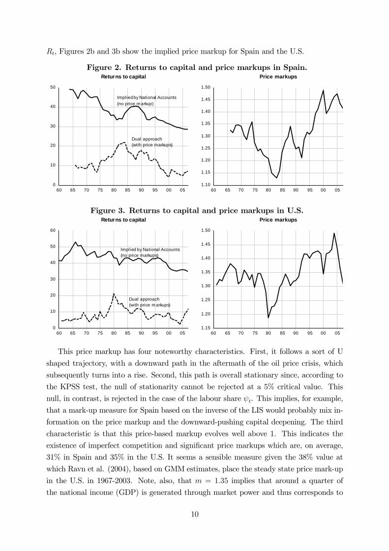
, Figures 2b and 3b show the implied price markup for Spain and the U.S.

Figure 2. Returns to capital and price markups in Spain.

0

10

20

30

40

50

60 65 70 75 80 85 90 95 00 05

Returns to capital

Dual approach(with price markups)

Implied by National Accounts

(no price m arkup)

1.10

1.15

1.20

1.25

1.30

1.35

1.40

1.45

1.50

60 65 70 75 80 85 90 95 00 05

Price markups

Figure 3. Returns to capital and price markups in U.S.

0

10

20

30

40

50

60

60 65 70 75 80 85 90 95 00 05

Returns to capital

Dual approach(with price m arkups)

Implied by National Accounts(no price markups)

1.15

1.20

1.25

1.30

1.35

1.40

1.45

1.50

60 65 70 75 80 85 90 95 00 05

Price markups

This price markup has four noteworthy characteristics. First, it follows a sort of U

shaped trajectory, with a downward path in the aftermath of the oil price crisis, which

subsequently turns into a rise. Second, this path is overall stationary since, according to

the KPSS test, the null of stationarity cannot be rejected at a 5% critical value. This

null, in contrast, is rejected in the case of the labour share . This implies, for example,

that a mark-up measure for Spain based on the inverse of the LIS would probably mix in-

formation on the price markup and the downward-pushing capital deepening. The third

characteristic is that this price-based markup evolves well above 1. This indicates the

existence of imperfect competition and significant price markups which are, on average,

31% in Spain and 35% in the U.S. It seems a sensible measure given the 38% value at

which Ravn et al. (2004), based on GMM estimates, place the steady state price mark-up

in the U.S. in 1967-2003. Note, also, that = 135 implies that around a quarter of

the national income (GDP) is generated through market power and thus corresponds to

10

monopolistic rents³−(+)

= −1

= 026%

´. The fourth characteristic is a counter-

cyclical behavior. As stressed by Rotemberg and Woodford (1999), this countercyclical

behavior reconciles theory and empirical evidence on the procyclical behavior of wages.

We follow these authors and compute the correlation of our cyclical indicator of the price

markup —the growth rate of the price markup— with the HP filtered GDP, the linearly

detrended hours, and the HP filtered hours (HP stands for Hodrick-Prescott). For Spain

we find, respectively, the following correlation coefficients: -0.28, -0.20, and -0.23. For the

U.S., in turn, we find -0.25, -0.08, and -0.04. In view of these results, we conclude that

our price markup time series is countercyclical.

4 The production function

In this section we estimate the production function and obtain the elasticity of substitution

between capital and labor. We follow Antràs’ (2004) methodology, but diverge in one

important respect. Rather than assuming perfect competition, we consider the price

markup as a relevant determinant of the relationships at work. Thus, our contribution

lies in the obtainment of new estimates of the elasticity of substitution under imperfect

competition.

Following Antràs, we assume a functional form of the technological parameters so that

labor efficiency increases at a constant growth rate, i.e. = 0 where is the growth

rate of technological change. From the first order conditions of the firms’ maximization

problem, we obtain the output per unit of labor

= (1− )

µ

¶ 1

()−1 (9)

which can be rewritten as

ln

µ

¶= 1 + ln + (1− ) (10)

or

ln () = 2 +1

ln

µ

¶−µ1−

¶ (11)

where 1 and 2 are constants and (10) and (11) are, respectively, the direct and inverse

output per unit of labor.

4.1 The elasticity of substitution between capital and labor

We next estimate equations (10) and (11) both under perfect competition, as Antràs

(2004), and under imperfect competition by considering the price markup time series

11

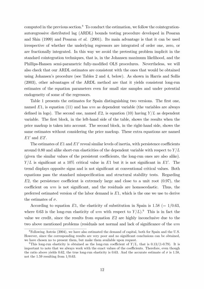
computed in the previous section.8 To conduct the estimation, we follow the cointegration-

autoregressive distributed lag (ARDL) bounds testing procedure developed in Pesaran

and Shin (1999) and Pesaran et al. (2001). Its main advantage is that it can be used

irrespective of whether the underlying regressors are integrated of order one, zero, or

are fractionally integrated. In this way we avoid the pretesting problem implicit in the

standard cointegration techniques, that is, in the Johansen maximum likelihood, and the

Phillips-Hansen semi-parametric fully-modified OLS procedures. Nevertheless, we will

also check that our ARDL estimates are consistent with the ones that would be obtained

using Johansen’s procedure (see Tables 2 and 4, below). As shown in Harris and Sollis

(2003), other advantages of the ARDL method are that it yields consistent long-run

estimates of the equation parameters even for small size samples and under potential

endogeneity of some of the regressors.

Table 1 presents the estimates for Spain distinguishing two versions. The first one,

named 1, is equation (11) and has as dependent variable (the variables are always

defined in logs). The second one, named 2, is equation (10) having as dependent

variable. The first block, in the left-hand side of the table, shows the results when the

price markup is taken into account. The second block, in the right-hand side, shows the

same estimates without considering the price markup. These extra equations are named

10 and 20.

The estimates of1 and10 reveal similar levels of inertia, with persistence coefficients

around 0.80 and alike short-run elasticities of the dependent variable with respect to

(given the similar values of the persistent coefficients, the long-run ones are also alike).

is significant at a 10% critical value in 1 but it is not significant in 10. The

trend displays opposite signs and is not significant at conventional critical values. Both

equations pass the standard misspecification and structural stability tests. Regarding

2, the persistence coefficient is extremely large and close to a unit root (0.97), the

coefficient on is not significant, and the residuals are homoscedastic. Thus, the

preferred estimated version of the labor demand is 1, which is the one we use to derive

the estimates of .

According to equation 1, the elasticity of substitution in Spain is 158 (= 1063,

where 0.63 is the long-run elasticity of with respect to ).9 This is in fact the

value we credit, since the results from equation 2 are highly inconclusive due to the

two above mentioned problems (residuals not normal and lack of significance of the

8Following Antràs (2004), we have also estimated the demand of capital, both for Spain and the U.S.

However, since the corresponding results are very poor and no significant conclusions can be obtained,

we have chosen no to present them, but make them available upon request.9This long-run elasticity is obtained as the long-run coefficient of , that is 0.13/(1-0.79). It is

important to note that we always work with the exact values of the coefficients. Therefore, even though

the ratio above yields 0.62, the true long-run elasticity is 0.63. And the accurate estimate of is 1.58,

not the 1.59 resulting from 1/0.63.

12

coefficient). Its counterpart with no price markup, 10, yields = 121 = 1083, where

0.83 is the long-run elasticity of with respect to .10 We conclude that (i) Spain has

an elasticity of substitution above 1, which we place at 1.58; and, (ii) failure to consider

the price markup generates a downward bias in the estimation of .11

Table 1. Spanish labor demand. 1967-2007.

Price markup considered Price markup not considered

[1] [2] [10] [20] 073

[0273] 014

[0643] 024

[0259] 012

[0513]

ln(−1−1) 079[0000]

ln

³−1−1

´097[0000]

ln(−1) 084[0000]

ln

³−1−1

´085[0000]

ln

³

´013[0095]

ln() 003[0617]

ln

³

´013[0169]

ln() 015[0047]

∆ln³

´091[0002]

∆ln³

´051[0006]

029[0032]

∗ 100 017[0207]

∗ 100 −013[0027]

∗ 100 −007[0241]

∗ 100 001[0803]

2 0988 0998 2 0997 0998

0027 0013 0014 0011

Misspecification tests: Misspecification tests:

111[0292]

187[0171]

012[0734]

241[0121]

064[0423]

0175[0676]

188[017]

132[0250]

100[0606]

193[0381]

051[0775]

144[0487]

158[0208]

587[0015]

176[0185]

333[0068]

Notes: Dependent variables: ln() in 1, ln() in 10, and ln() in 2 and 2

0;∆ is the difference operator; the standard error; p-values in square brackets.

Misspecification tests: Serial correlation , Linearity , Normality ,

and Heteroscedasticity .

Because our interest lies in the implied long-run relationships between and ,

in Table 2 we present the coefficients of the error correction model () and the long-

run relationships (or cointegrating vectors) underlying the estimated equations (they are

10The estimate of the elasticity of substitution could be wrongly placed around 1 in case of ignoring the

price markup. In particular, following equation 20, would be estimated at 098, which is the long-runelasticity of with respect to 11These labor demand equations were also estimated as a system (together with the corresponding

capital demand equations) using SUR and 3SLS. We thank an anonymous referee for this suggestion. No

symptoms of relevant endogeneity problems could be identified. These system estimates place at 1.19

in the presence of the markup and 1.12 in its absence. However, given that the results on the capital

demand equations remained poor, equation 1 was further estimated by 2SLS to evaluate to what extent

potential endogeneity could be distorting our reference . The use of instrumental variables did not

improve the estimation and did not change significantly the estimate of which was placed at 1.49.

13

obtained from the reparameterizing equations 1 and 2 in error correction form). Next

to these results, obtained via the ARDL method, we also present the cointegrating vector

resulting from conducting the same analysis using the Johansen procedure.12 Finally, we

show the results of a likelihood ratio (LR) test following a 2 (·) distribution that restrictsthe Johansen values to take the ARDL values. Non rejection of the LR test provides

evidence on the results’ consistence across econometric methodologies.

In Spain this consistency cannot be rejected for any of the two versions of the labor

demand. However, note that for 2 the second term of the ARDL cointegrating vector

(i.e., the long-run elasticity of elasticity with respect to ) is not significant. These

results reinforce our choice of 158 as our best estimate of .

Table 2. Long-run relationships in Spain.

ARDL Johansen LR Test

−1¡ln () ln

¡

¢ ¢ ¡ln () ln

¡

¢ ¢[1] −021

[0079]

³1 063

[0004]

´ ¡1 054

¢2 (1)=0.35[0553]

−1¡

¢ ¡

¢

[2] −003[0346]

³1 078

[0434]

´ ¡1 263

¢2 (1)=5.34[0021]

Notes: p-values in square brackets; 5% critical value: 2 (1)=3.84.

Tables 3 and 4 are, respectively, the U.S. counterparts of Tables 1 and 2 for Spain.

Regarding the estimation of equation (11), the version with the price markup (3) results

in a much lower persistence coefficient, 0.50, than the version with perfect competition

(30) where it attains 0.73. This would result on different long-run elasticities of

and with respect to for equal short-run coefficients on . However, even

the short-run coefficients, 0.79 and 0.27, differ substantially. As in Spain, the trend (not

significant at conventional critical values) displays opposite signs and both equations pass

the standard misspecification and structural stability tests. The estimation of equation

(10), named 4 yields a very similar picture than its counterpart 3, with a similar

persistence coefficient around 0.50 and a short-run coefficient of with respect to

of 021. This results in relatively close estimates of . However, given that the

residuals in equation 2 are not normal, we credit the elasticity of substitution obtained

12Underlying this exercise is (i) the performance of unit root tests; (ii) the estimation of VAR models

having the same lag structure and containing the same variables than the structural equations; and (iii)

the use of LR tests based on the maximal eigenvalue and the trace of the stochastic matrix to determine

the existence of cointegrating vectors (and its number and values). Given that we estimate VAR models

with unrestricted constants and trends and two I(1) variables, we need to test one restriction. All these

underlying results are available upon request.

14

through 3, which will be compared to the one obtained through 30. Note, also, that

the selected estimates of for Spain and the U.S. are taken from the same specification.

This ensures consistent results across countries and warrants comparability.

Table 3. U.S. labor demand. 1962-2007.

Price markup considered Price markup not considered

[3] [4] [30] [40] −314

[0164] 246

[0000] −012

[0814] 132

[0026]

ln(−1−1) 050[0004]

ln³−1−1

´056[0000]

ln(−1) 073[0000]

ln

³−1−1

´071[0026]

∆ ln () 027[0078]

ln() 021[0000]

∆ ln () 019[0103]

ln() 017[0143]

ln

³

´079[0027]

ln

³

´027[0004]

057[0000]

∆ ln³

´070[0061]

∆ ln³

´021[0107]

∗ 100 −045[0131]

∗ 100 033[0000]

∗ 100 008[0230]

∗ 100 020[0008]

2 0981 0998 2 0997 0997

0025 0009 0008 0010

Misspecification tests: Misspecification tests:

014[0712]

002[0890]

012[0734]

040[0525]

0001[0973]

011[0742]

188[017]

076[0384]

031[0854]

724[0027]

051[0775]

486[0088]

010[0752]

073[0392]

176[0185]

031[0579]

Notes: Dependent variables: ln() in 3, ln() in 30, and ln() in 4 and 4

0;∆ is the difference operator; the standard error; p-values in square brackets.

Misspecification tests: Serial correlation , Linearity , Normality ,

and Heteroscedasticity .

According to equations 3 and 30, the elasticity of substitution between capital and

labor in the U.S. is below 1. When the price markup is considered, we find it to be

063 (= 1158, where 1.58 is the long-run elasticity of with respect to ). In the

absence of the price markup, we find it to be 096 (= 11014, where 1.014 is the long-run

elasticity of with respect to ). Antràs (2004) shows that the estimation of the

equivalent equation in the U.S. yields = 089 when the preferred estimation method

—Saikkonen’s one— is used. Therefore, our results are consistent with those in Antràs

(2004) and, interestingly enough, uncover a new relationship: consideration of the price

markup reduces the elasticity of substitution in the U.S.13

13When the equations are estimated as a system by SUR and 3SLS (together with the capital demand

15

As in the Spanish case, when checking for consistency between our ARDL estimates

and the ones that would be obtained from the Johansen procedure, we cannot reject the

LR test.

Table 4. Long-run relationships in the U.S.

ARDL Johansen LR Test

−1¡

¢ ¡

¢[3] −050

[0004]

³1 158

[0000]

´ ¡1 0405

¢2 (1)=2.59[0108]

−1¡

¢ ¡

¢

[4] −044[0000]

³1 047

[0000]

´ ¡1 0403

¢2 (1)=1.37[0243]

Notes: p-values in square brackets; 5% critical value: 2 (1)=3.84.

This empirical analysis yields two important conclusions. First, the elasticity of sub-

stitution between capital and labor is larger than 1 in Spain and smaller than 1 in the

U.S. Second, consideration of the price markup causes the estimates of this elasticity to

be drawn apart from 1. In other words, the assumption of perfect competition introduces

a bias on its estimate which differs depending on the estimated value. It is a downward

bias in Spain and an upward bias in the U.S.

In what follows we rationalize these two conclusions by using an accounting exercise

based on equation (6) rewritten as

∆

−µ∆

− ∆

¶=

µ1−

¶µ∆

− ∆

¶| {z }

µ1−

¶− ∆

so that the left hand side of the equation coincides with the growth rate of the LIS.

Therefore,∆

=

µ1−

¶− ∆

Note that the growth rate of the LIS depends on capital deepening (as measured by ,

which depends on the difference between the growth rates of capital and GDP)14 and on

the growth rate of the price markup. As mentioned, the effect of capital deepening on the

equations) this feature still holds. When the markup is considered, is placed at 0.89, whereas in its

absence its estimate goes to 1. This conclusion also holds when looking at the estimates derived from the

estimation of equation 4 (047) and 40 (059), which also fit within the range of estimates provided byAntràs (2004). Finally, just to check that our reference value of is not distorted by potential endogeneity

problems, we estimate equation 3 by 2SLS and find a very close estimate of 0.59.14The term provides a direct measure of capital productivity growth rather than capital deepening.

16

LIS depends on the elasticity of substitution. It increases the LIS when this elasticity is

smaller than one, but decreases the LIS when it is larger than one.

The latter expression allows us to rationalize the two main conclusions obtained from

the econometric analysis. To this end, we can rewrite it as follows:

∆

+∆

=

µ1−

¶ (12)

The left hand side of this equation is on average negative both in Spain and the U.S.,

with sample period means at -0.15% and -0.29%, respectively, that are clearly dominated

by the LIS growth rates (the growth rates of the price markup are much smaller and play

a minor role).15 By implication, the right hand side must also take negative values. This

situation is pictured in Figure 4, where the continuous line displays the right hand side of

equation (12) as a function of taking into account that takes a negative value in the

U.S. and a positive one in Spain.16 As it is clear from this Figure, when the LIS shows a

downward path and there is capital deepening, the elasticity of substitution must be larger

than one. In turn, when both the LIS and the ratio GDP/capital falls, the elasticity of

substitution must be smaller than one. This explains the first conclusion above regarding

the elasticity of substitution between capital and labor in Spain and the U.S.

Regarding the effect of the price markup on the estimated , note that omission of the

markup underestimates the value of the labor-output elasticity which, in turn, generates

an overestimation of the absolute value of . The dashed lines in Figure 4 display the

right hand side of equation (12) as a function of when is overestimated due to the

absence of the price markup. As shown in Figure 4, this implies that, in the absence

of the price markup, the estimated value of is biased towards one. This explains the

second conclusion.

Remark 1 An interesting implication of our findings is that the high elasticity of substi-

tution in the Spanish economy implies that higher wages (in efficiency units) will reduce

the labor income share as firms respond to this rise by substituting labor for capital more

than proportionally with respect to the wage rise. On the contrary, the low value of the

elasticity of substitution in the U.S. implies that higher wages (in efficiency units) gener-

ate a less than proportional response by firms, which therefore allows a larger LIS. This

However, the CES production function can be rewritten as

=

∙+ (1− )

³

´ 1−

¸ 1−

to show

the direct relationship between the ratio of capital to GDP and the ratio of capital to labor. Therefore,

the term also provides a measure of capital deepening.15Related with these figures, it is worth recalling that in both cases the LIS behaves as non-stationary

in contrast with the stationary path of the price markup.16Note that is the product of two terms. The first one is positive, whereas the second one is positive

when there is capital deepening and negative otherwise. Data from the OECD shows that during the

period there is capital deepening in the spanish economy, implying a positive value of and there is a

reduction in the ratio capital to GDP in the US economy, implying a negative value of .

17

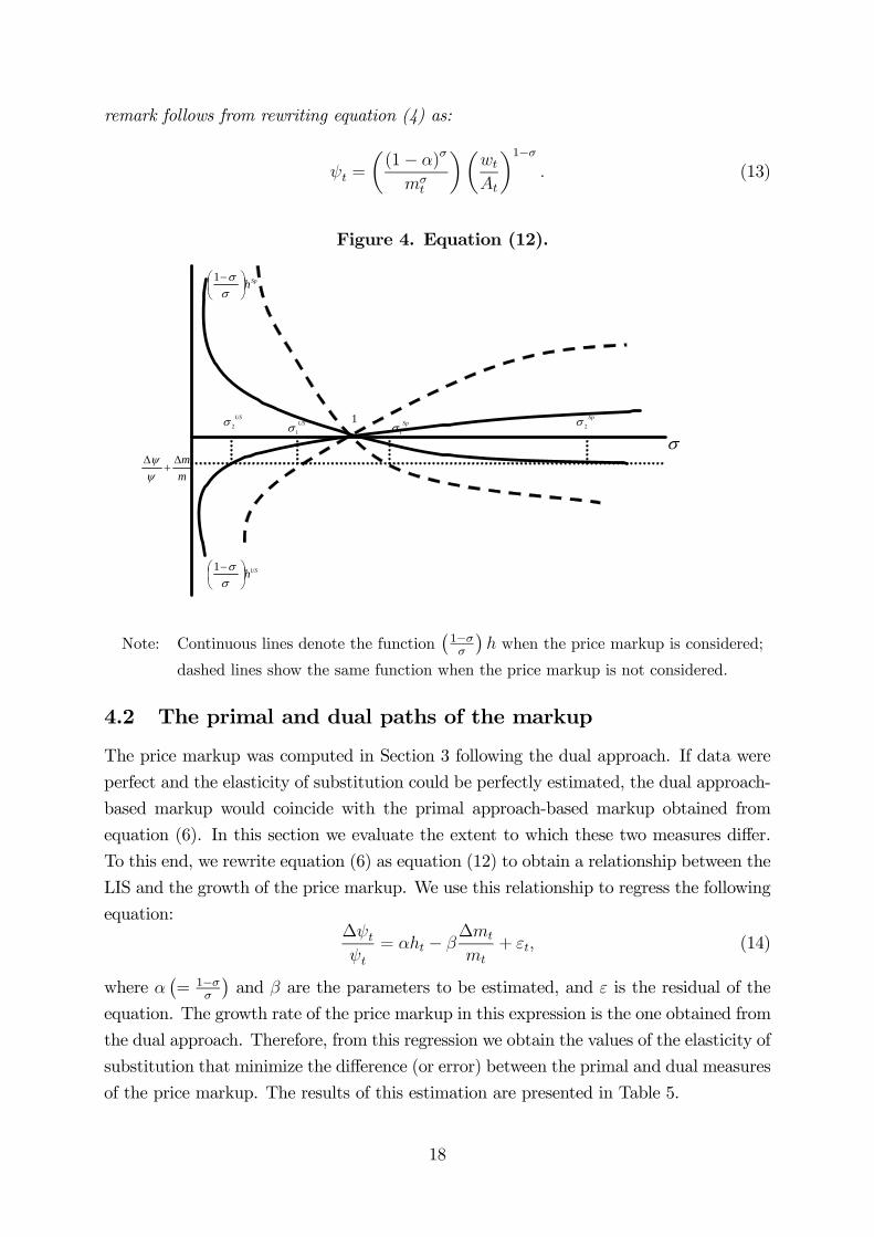
remark follows from rewriting equation (4) as:

=

µ(1− )

¶µ

¶1− (13)

Figure 4. Equation (12).

Sp

2US

2 US

1Sp

1

m

m

Sph

1

USh

1

1

Note: Continuous lines denote the function¡1−

¢ when the price markup is considered;

dashed lines show the same function when the price markup is not considered.

4.2 The primal and dual paths of the markup

The price markup was computed in Section 3 following the dual approach. If data were

perfect and the elasticity of substitution could be perfectly estimated, the dual approach-

based markup would coincide with the primal approach-based markup obtained from

equation (6). In this section we evaluate the extent to which these two measures differ.

To this end, we rewrite equation (6) as equation (12) to obtain a relationship between the

LIS and the growth of the price markup. We use this relationship to regress the following

equation:∆

= − ∆

+ (14)

where ¡= 1−

¢and are the parameters to be estimated, and is the residual of the

equation. The growth rate of the price markup in this expression is the one obtained from

the dual approach. Therefore, from this regression we obtain the values of the elasticity of

substitution that minimize the difference (or error) between the primal and dual measures

of the price markup. The results of this estimation are presented in Table 5.

18

Our estimation is based on equation (14), rather than on equation (12), because the

estimates of are significantly different from -1. When we restrict = −1, which wouldbe the implicit value of in equation (12), we find non-sensible results. However, when

this parameter is left free (as in Table 5), it is interesting to observe that the estimated

values of for Spain and the U.S. are broadly consistent with the estimates of obtained

via the estimation of the production function. Of course, the drawback of this exercise is

the poor performance of the Spanish and U.S. econometric versions of equation (14), with

poor explanatory power and coefficients that in some cases are not significant. However,

we find remarkable that our finding of = −0327 for Spain implies = 149, whereasour estimate of = 0967 for the U.S. implies = 051. Recall that if data were perfect

these values of would coincide, respectively, with 158 and 063.

Table 5. Primal approach-based estimates of .

Spain

∆

= −0327[0492]

−0237[0002]

2 = 019 = 195

U.S.

∆

= 0967[0102]

−0076[0242]

2 = 008 = 180

Note: Probabilities in brackets; =Durbin-Watson statistic.

5 Simulated labor income shares

In this section, we answer some of the questions we were asking at the beginning of the

paper. In particular, we examine how much of the variation of the LIS is explained by the

value of (capital deepening) and how much by the trajectory of the price markup. To

address this question, we use equation (3) to simulate the path of the LIS. As inputs of the

simulation we need the path of GDP per efficiency unit of labor, the value of parameter

, our estimates of , and our dual measure of the price markup. GDP per efficiency unit

of labor is obtained from the ratio between GDP per worker and technology. To obtain

the technological path we assume, as we did in the previous section, that it grows at a

constant rate. This rate is set at the sample period average growth rate of per worker

GDP, which is equal to 2.14% in Spain and 1.55% in the U.S. In turn, the value of is set

so that the simulated LIS coincides with actual LIS in the initial period. Since the growth

rate of the TFP is constant, we abstain from business cycle considerations and conduct

our simulation on the trend component of the actual LIS, which is obtained through the

HP filter. In this way we try to isolate our analysis from cyclical changes resulting from

varying degrees of factor utilization.

We distinguish four different scenarios that combine (i) the presence and absence of

19

the price markup in the simulation; and (ii) the estimates obtained when the price

markup is, and is not, included in the regression. In this way we can infer to what extent

the elasticity of substitution or the price markup play dominant roles in explaining the

actual trajectories of the labor share in Spain and the U.S. The resulting simulations are

plotted in Figure 5 and their fit is evaluated in Table 6.

In Scenarios I and III we consider the estimated obtained in the presence of the price

markup, 1.58 in Spain, and 0.63 in the US. Scenario I, where the simulation is conducted

in the presence of the markup (in contrast to Scenario III), is our base run model. The

resulting time series provide the closest approximation to the actual labor share trajecto-

ries in both economies with residual sum of squares (RSS) and 2 of, respectively, 0.017

and 0.65 in Spain, and 0.007 and 0.93 in the U.S.

Figure 5. Simulated labor shares.

60

62

64

66

68

70

72

74

1970 1975 1980 1985 1990 1995 2000 2005

a. Spain

Simulated I

Simulated II

Simulated III

Simulated IVActual

60

62

64

66

68

70

72

74

1970 1975 1980 1985 1990 1995 2000 2005

b. U.S.

Simulated I

Simulated II

Simulated III

Simulated IV

Actual

Note: Simulations I to IV correspond, respectively, to Scenarios I to IV in Table 6.

The second scenario is one of perfect competition (the price markup is not considered

neither in the estimated regression nor in the simulated time path of the labor share) and

provides the closest situation to the Cobb-Douglas case. It is thus natural to obtain a

relatively constant labor share in both countries with, nevertheless, significant differences:

the simulated path in Spain evolves slightly downwards initially, when the actual labour

share is rising, and upwards subsequently, when the labour share trends downwards. As a

consequence, the correlation coefficient and explanatory power of the simulated series are

virtually null. In contrast, the simulated series in the U.S. behaves more in accordance

with the initially downward and finally constant actual path, thereby resulting in a much

accurate fit than in Spain (see Table 6).

Simulations in Scenario III use the estimated sigma in the presence of the price markup,

but the price markup series is not used when computing the simulated path. Therefore,

the difference between the simulated series under Scenarios I and III accounts for the

20

contribution of the price markup to the LIS trajectory. In turn, in Scenario IV we use the

estimated sigma with no markup, but the price markup is considered in the simulation.

Hence, the difference between the simulated series under Scenarios I and IV accounts for

the contribution of capital deepening to the LIS trajectory. To approximate these two

contributions we follow Karanassou et al. (2003, p. 261) and regress the contribution

of the markup on a constant and the contribution of capital deepening. We save the

residuals and regress the actual LIS over a constant and the saved residuals. The 2

of this regression gives us the portion of the LIS variation explained by the part of the

markup contribution that is uncorrelated with the contribution of capital deepening. We

find it to be 63% in Spain and 57% in the U.S. Similarly, when we regress the actual LIS

on the residuals of a regression of the capital deepening contribution on a constant and

the contribution of the markup, we find the 2 to be 0.27 in Spain and 0.39 in the U.S.

This result indicates that capital deepening, which reacts to , is also a driving force of

the labor share trajectory as it explains 27% and 39% of the LIS variation.

Table 6. Simulated labor shares’ fit.

Spain U.S.

RSS 2 RSS 2

Scenario I 1.58 X 0.017 0.65 0.63 X 0.007 0.93

Scenario II 1.21 0.047 0.03 0.96 0.013 0.47

Scenario III 1.58 0.048 0.03 0.63 0.013 0.47

Scenario IV 1.21 X 0.023 0.53 0.96 X 0.010 0.60

Notes: RSS = Residual sum of squares; the 2 and the RSS are obtained

from regressing the actual trend-component of the LIS

on a constant and the simulated LIS in each scenario.

The conclusion we draw from this exercise is threefold. First, our base run case is able

to proxy the path followed by the LIS in last decades in the two economies considered.

The corresponding 2s are 0.65 in Spain and 0.93 in the U.S. Second, both the price

markup and capital deepening contribute to explain this path, although the price markup

is clearly more determinant in Spain. Third, the explanatory power of , and thus of

capital deepening, is less than half the explanatory power of the price markup in Spain,

but two thirds of it in the U.S. This is consistent with the larger ratio of capital stock per

employee in the U.S.17

17The process of capital deepening has been larger in Spain than in the U.S. However, since the

capital/output is higher in the U.S. throughout the whole sample period, smaller variations in capital

deepening turn out to be more influential than the larger variations of the smaller Spanish ratio.

21

6 Capital accumulation and labor income shareThe elasticity of substitution determines the relationship between GDP (in efficiency units

and capital accumulation), while the price markup relates these two variables with the

LIS and employment growth. This leads us to bring the analysis into a broader macroeco-

nomic context, which we do by adding the Solow model. We then simulate it and compare

the resulting predictions with the actual time-series of GDP, capital accumulation, em-

ployment growth, and the LIS. We consider a base run scenario in the presence of our

price markups (so that there is imperfect competition and the elasticities of substitution

differ from one) and a scenario in their absence (so that there is perfect competition and

the elasticities of substitution are closed to one). Comparison of how the two scenarios

predict the actual trajectories of the main macroeconomic variables informs on the ex-

tent to which the degree of imperfect competition and its influence on technology are

important ingredients of the model.

6.1 The model

We extend the Solow model by including (i) a CES production function; (ii) product

market imperfections, which are summarized by the price markup; and (iii) labor mar-

ket imperfections, which are introduced through a simple wage equation arising from a

standard efficiency wage model and prevent the labor market to clear.

In particular, we assume that the wage is a constant markup over a reference wage

, so that =

.18 For the sake of simplicity, we assume that the reference wage

depends positively on per capita GDP, and the employment rate,

:19

=

µ

¶µ

¶

It is easy to see that the wage equation simplifies to

=

µ

¶µ

¶2

which can be rewritten in efficiency units as

e = e (1− )2 (15)

18This constant mark up can be obtained in an efficiency wage model with effort function =h−

iif

and 0 1, which yields =1

1− .19When wages are set at the firm or sector level, the equilibrium wage depends on unemployment

benefits and the unemployment rate (see, for example, Layard, Nickell and Jackman, 1991, pp.105-106).

If we further relate unemployment benefits with income per capita as, for example, in Daveri and Tabellini

(2000), we obtain a wage equation that depends positively on the employment rate and income per capita

as in our postulated wage equation.

22

where is the unemployment rate, e =

and e = To obtain the equilibrium

unemployment, we use the labor demand equation (2) which can be rewritten in terms of

the capital labor-ratio in efficiency units as follows:

e =(1− )

∙³e´−1

+ (1− )

¸ 1−1

(16)

where e =

Using the wage equation (15) and the labor demand equation (16), we

obtain the unemployment rate in equilibrium:

1− =

sµ1−

¶e( 1−1) (17)

where e arises from rewriting the production function (1) in efficiency units of labor as

e = (e) = ∙³e´−1

+ (1− )

¸ −1

(18)

Assuming an inelastic labor supply, , that grows at the constant rate, , equation (17)

can be rewritten in terms of the growth rate of employment as

+1

= (1 + )

sµ

+1

¶µe+1e¶( 1−1)

(19)

To close the model we characterize capital accumulation. For the sake of simplicity, we

assume a constant savings rate so that capital evolves according to the following equation

+1 = + (1− )

where ∈ (0 1) is the constant savings rate and ∈ (0 1) is the constant depreciationrate. We rewrite this equation in labor efficiency units as

e+1 = µ

+1

¶µ

+1

¶he + (1− )ei (20)

Then, we use equations (18) and (19) to obtain the following difference equation

e+1 = (1 + )−1

vuutµ+1

¶Ã(e+1)(e)

!(1− 1 )µ

+1

¶h(e) + (1− )ei (21)

Equation (21) drives the accumulation of capital in this economy.

23

6.2 Numerical simulation

We first obtain the path of capital accumulation by solving numerically equation (21),

and we then use equations (3), (18), and (19) to simulate the paths of the LIS, the ratio

of capital to GDP, per worker GDP, and the growth rate of employment.

We calibrate the parameters as follows. First of all, we use the estimated values of ,

the average values of and , and the computed values of the price markup for Spain

and the U.S. To obtain efficiency units of labor we compute the Solow residual from an

accounting exercise based on equation (5). We take into account that the Solow residual is

affected by the price markup (Hall, 1988).20 We ensure that the simulated values depart

from the actual values of the variables by setting the value of accordingly, and by

fixing the initial amounts of capital stock and technology (in efficiency units) to match,

respectively, the ratio of capital to GDP and per worker GDP. The values of the savings

rate are set to calibrate the ratio of capital to GDP. To obtain a close simulation we

have had to split the sample period into two. In this way, we are able to deal with the

exceptionally high saving rates of Spain during the first 6 years of the sample, and the

low U.S. rates of the first 10 years.21 This information is summarized in Table 7.

Table 7. Parameter values.

1 2Spain

Scenario I 1.58√

0.043 0.0104 0.12 0.270 0.135

Scenario II 1.21√

0.043 0.0104 0.27 0.240 0.160

U.S.

Scenario I 0.63 X 0.043 0.0144 0.22 0.155 0.185

Scenario II 0.96 X 0.043 0.0144 0.32 0.145 0.150

It is important to emphasize the different nature of the exercise undertaken in this

section relative to the simulation performed in Section 5. Rather than checking the

relative incidence of the price markup and capital deepening on the LIS trajectory, we

have developed a model in which capital accumulation has been made endogenous. Note

that imperfections in the labor market must be introduced to explain the time path of

employment and GDP. This is not the case in Section 5 where the simulations make

direct use of GDP data. By equation (20), our simulations here require the use of Solow’s

residual, as computed by equation (5), which is time-varying and entails the need to pay

20Rotemberg and Woodford (1999), and previously Hall (1988 and 1990), argue that the Solow residual

is biased if the price markup is not considered. Its obtention, therefore, is also important in growth

accounting, specifically when computing the Solow residual.21The values of the saving rates are fixed in each scenario to obtain the best possible fit of the capital

to GDP ratio. Recall that this is the first step of the exercise. The predicted values of this ratio are then

used to simulate the other variables.

24

attention to both the trend and cyclical components of the series. This is the reason

why we do not filter the series under scrutiny. Moreover, there is an important remark

related to the restricted period for which the simulation exercise is conducted, from 1979

to 2007. When the whole sample period is considered, the model fails to produce a good

fit in the 1960s and 1970s. We thus acknowledge that some relevant determinants of the

macroeconomic scene in the first part of the sample are not well captured by our stylized

analysis.22 In contrast, the model performs reasonably well when explaining the evolution

of the labor share, employment, GDP per worker, and the ratio of capital stock to GDP.

This is shown in Figures 6, for Spain, and 7, for the U.S., while Table 8 evaluates these

simulations through the RSS (to check their global fit) and the ratio between the actual

and simulated standard deviations (to check their fit in terms of volatility).

Figure 6. Simulated selected variables in Spain.

55.0

57.5

60.0

62.5

65.0

67.5

70.0

72.5

75.0

1980 1985 1990 1995 2000 2005

a. Labor share

Simulated I

Simulated II

Actual

-6

-4

-2

0

2

4

6

1980 1985 1990 1995 2000 2005

b. Employment growth

Simulated I

Simulated II

Actual

2.8

3.0

3.2

3.4

3.6

3.8

4.0

4.2

4.4

1980 1985 1990 1995 2000 2005

c. GDP per worker

Simulated I

Simulated II

Actual

2.6

2.7

2.8

2.9

3.0

3.1

3.2

1980 1985 1990 1995 2000 2005

d. Capital stock / GDP

Simulated I

Simulated II

Actual

Note: Simulations I and II correspond, respectively, to Scenarios I and II in Table 7.

We find scenario I to track reasonably well the evolution of the labor share, employment

growth, and the ratio of capital stock to GDP in both Spain and the U.S. On the contrary,

22Among other elements, we probably lack (i) the relevant influence of the inflationary oil price shocks

and the subsequent deflationary interest rate shocks; (ii) a more realistic specification of the wage setting

process; and (iii) an explicit specification of labor supply decisions which, in those years, were affected

by demographic changes such as the baby-boom and the baby-bust. Although all of them are clearly

important, consideration of these factors lies beyond the scope of the specific exercise we conduct in this

Section.

25

Scenario II fails to capture the downward trend in the labor share during these years, and

yields unrealistic flat trajectories of the LIS and the growth rate of employment. In terms

of GDP per worker, Scenario I allows a close replication of the actual upward trajectory

in clear contrast with the flawed predictions of Scenario II. In the case of Spain it also

captures the inflection point experienced in the second half of the 1990s, when the wild-

ride years started and produced the unprecedented employment boost in response to the

rapid economic growth that became the trademark of this economy.

Figure 7. Simulated selected variables in the U.S.

56

60

64

68

72

76

1980 1985 1990 1995 2000 2005

a. Labor share

Simulated I

Simulated II

Actual

-2

-1

0

1

2

3

4

5

6

1980 1985 1990 1995 2000 2005

b. Employment growth

Simulated I

Simulated II

Actual

4.8

5.2

5.6

6.0

6.4

6.8

7.2

7.6

8.0

1980 1985 1990 1995 2000 2005

c. GDP per worker

Simulated I

Simulated II

Actual

2.2

2.3

2.4

2.5

2.6

2.7

1980 1985 1990 1995 2000 2005

d. Capital stock / GDP

Simulated I

Simulated II

Actual

Note: Simulations I and II correspond, respectively, to Scenarios I and II in Table 7.

Table 8 confirms that Scenario I provides a better fit than Scenario II. Note that

whenever the RSS is not conclusive (i.e. for the labor share and the ratio between capital

stock and GDP in the U.S., and for employment growth in both economies), their relative

volatilities are closer to 1 due to the low volatility characterizing Scenario II. The close

fit delivered by Scenario II in terms of the volatilities of GDP per worker and the ratio of

capital stock to GDP is remarkable for both economies. This implies that our simulations

under Scenario I, that is when the markup is considered, are specially suitable to account

for the facts when these facts involve a time-varying pattern of the variables. Given that

this is generally the case, the role played by the price markup should not be disregarded.

26

Table 8. Simulated variables’ fit.

∆ ∗∆

RSS RV RSS RV RSS RV RSS RV

Spain

Scenario I 0.007 1.89 0.023 0.55 0.277 1.22 0.215 0.76

Scenario II 0.016 0.09 0.020 0.01 0.959 0.54 0.184 0.50

U.S.

Scenario I 0.003 1.92 0.003 1.43 0.328 0.98 0.060 0.76

Scenario II 0.003 0.02 0.003 0.01 0.810 0.39 0.040 0.38

Notes: RSS=Residual sum of squares; RV=Relative volatility (simulated std. dev.actual std. dev.

).

Scenario I: = 158 in Spain; = 063 in he U.S.; markup considered;

Scenario II: = 121 in Spain; = 096 in he U.S.; markup not considered.

Overall, it seems safe to claim that consideration of the price markup in the analysis

provides a relevant insight when attempting to explain the evolution of the key macro-

economic variables in last decades.

7 Conclusions

We provide estimates of the elasticity of substitution between capital and labor under

imperfect competition in the product market. This elasticity is larger than one in Spain

and lower than one in the U.S.

An important contribution of the paper is the rationale behind these different values.

Both economies have experienced a declining path of the LIS and, at the same time, differ

in the evolution of capital deepening. The paper reconciles these facts by unveiling the

connection between the elasticity of substitution, capital deepening, and the trajectory of

the time-varying LIS.

One important aspect of this connection is that the elasticity of substitution determines

the effect of capital deepening on the LIS which, in turn, depends on the time-varying

price markup. In showing this, the paper uncovers the bias that the assumption of perfect

competition introduces in the estimates of the elasticity of substitution. This bias drives

the estimated elasticity of substitution towards one irrespective of whether this estimate

is placed above or below one. We believe this is an important result of the paper.

The differences in the elasticity of substitution have interesting implications for the

relationship between other aggregate variables. For example, higher wages imply a reduc-

tion of the LIS in Spain, as a result of the large substitution between capital and labor,

while they drive it upwards in the U.S., on account of the small substitutability between

capital and labor.

In the final part of the paper we use the estimated elasticities and the price markups

27

in Spain and the U.S. to conduct two simulation exercises. In the first one, we examine

to what extent the trajectory of the LIS is explained by capital deepening and the price

markup. For Spain we find that the former accounts for 63% of the changes in the

LIS, while the price markup accounts for 27% of them. For the U.S. these values are,

respectively, 57% and 39%.

In the second simulation, we extend the Solow model by considering a CES production

function, and imperfect competition in the labor and product markets. We solve this

model numerically in two relevant scenarios, and we conclude that neglecting the degree

of imperfect competition —in our case measured by the time-series aggregate price markup—

makes the model invalid for predicting the relationship between crucial macroeconomic

variables such as capital, GDP, and the LIS. On the contrary, when the price markup

is taken into account, the model yields predictions that are broadly consistent with the

data.

The empirical findings in this paper open some relevant issues. The first one relates

to the causes behind the different elasticity of substitution in Spain and the U.S. Among

others, some potential candidates are differences in the sectoral composition of GDP, in the

composition of the labor force (skilled/unskilled), and in the institutional environment.23

The second issue relates to the high correlation between capital deepening and the price

markup. The explanation of this finding would obviously require to consider models with

endogenous markups. By extending our econometric methodology to non-linear methods,

these new and interesting research avenues will be the aim of future research.

References

Acemoglu, D.K., 2002. Directed technical change. Review of Economic Studies 69, 781-810.

Altug, S., Filiztekin, A., 2002. Scale effects, time-varying markups, and the cyclical behaviour

of primal and dual productivity. Applied Economics 34, 1687-1702.

Antràs, P., 2004. Is the U.S. aggregate production function Cobb-Douglas? New estimates

of the elasticity of substitution. Berkeley Electronic Journals in Macroeconomics: Contributions

to Macroeconomics 4 (1), article 4.

23We believe that a potentially crucial explanation could be the institutional environment in which

firms have traditionally operated in these two countries. Spain has evolved from a highly rigid and

regulated economy to a liberalized situation with a salient characteristic: its segmented labor market.

Indeed, for the last 25 years, a third of dependent employment has been holding a temporary contract,

while the other two thirds belonged to a highly protected permanent segment (see Dolado et al. 2002).

Together with traditional difficulties in funding access (due to the small firms’ average size and, until

recently, financial markets underdevelopment and scarce competition in the banking system), Spanish

firms have tended to live in a situation of expensive capital and progressively cheap labor. This, we

believe, may have led them to a relatively high sensitivity in factor substitution. On the contrary, the US

economy is the paradigm of a deregulated environment in which firms are less constrained by regulations

and, thus, less sensitive to changes in factor prices: prices in the U.S. have probably been driven by the

market and not that much, as in Spain, by deregulation processes of different intensities in the product,

labor, and financial markets. This provides less incentives to be opportunistic in search of the best factor

combination resulting from changing regulations and institutions.

28

Arpaia, A., Pérez, E., Pichelmann, K., 2009. Understanding labour income share dynamics

in Europe. European Economy Economic Papers 379, European Comission, Brussels.

Banerjee, A., Rusell, B. 2004. A reinvestigation of the markup and the business cycle. Eco-

nomic Modelling, 21, 267-284.

Basu, S., Fernald, J.,2001. Why is productivity procyclical? Why do we care? In: Hulten,

C.R., Dean, E.R., Harper, M.J. (Eds.), New Developments in Productivity Analysis. University

of Chicago Press, pp. 225-302.

Bentolila, S., Saint-Paul, G., 2003. Explaining movements in the labor share. Berkeley

Electronic Journals in Macroeconomics: Contributions to Macroeconomics, 3 (1), article 9.

Bils, C., 1987. The cyclical behavior of marginal cost and price. The American Economic

Review 77 (5), 838-855.

Choi, S., Ríos-Rull, J.V., 2008. Understanding the dynamics of labor share: The role of

noncompetitive factor prices, mimeo.

Daveri, F., Tabellini, G., 2000. Unemployment, growth and taxation in industrial countries.

Economic Policy, 15 (30), 47-104.

Diewert, W. E., Nakamura, A.O. 2003. Index number concepts, measures and decompositions

of productivity growth. Journal of Productivity Analysis 19, 127-159.

Dolado, J.J., García-Serrano, C., Jimeno, J.F., 2002. Drawing lessons from the boom of

temporary jobs in Spain. The Economic Journal, 112 (480), F270-F295.

Driver, C., Muñoz-Bugarín, J., 2010. Capital investment and unemployment in Europe:

Neutrality or not? Journal of Macroeconomics 32, 492-496.

Duffy, J., Papageorgiou, C., 2000. A cross-country empirical investigation of the aggregate

production function specification. Journal of Economic Growth 5, 87-120.

Estrada, Á., López-Salido, J.D., 2005. Sectoral mark-ups dynamics in Spain. Documentos

de Trabajo del Banco de España 0503, Bank of Spain, Madrid.

Galí, J., 1995. Product diversity, endogenous markups, and development traps. Journal of

Monetary Economics 36, 39-63.

Galí, J., 1996. Multiple equilibria in a growth model with monopolistic competition. Eco-

nomic Theory 8, 251-266.

Gollin, D., 2002. Getting income shares right. The Journal of Political Economy 110 (2),

458-474.

Hall, R.E., 1988. The relation between price and marginal cost in U.S. industry. The Journal

of Political Economy 96 (5), 921-947.

Hall, R.E., 1990. Invariance properties of Solow’s productivity residual. In: Diamond, P.

(Ed.), Growth/ Productivity/Unemployment: Essays to Celebrate Bob Solow’s Birthday. MIT

Press, pp. 71-112.

Harris, R., Sollis, R., 2003. Applied Time Series Modelling and Forecasting, Wiley, West

Sussex.

Hsieh, C.T., 1999. Productivity growth and factor prices in East Asia. The American Eco-

nomic Review: Papers and Proceedings 89 (2), 133-138.

Hsieh, C.T., 2002. What explains the industrial revolution in East Asia? Evidence from the

factor markets. The American Economic Review 92 (3), 502-526.

Jaimovich, N., Floetotto, M., 2008. Firm dynamics, markup variations, and the business

cycle. Journal of Monetary Economics 55, 1238-1252.

Karanassou, M., Sala, H., Snower, D.J., 2003. Unemployment in the European Union: A

dynamic reappraisal. Economic Modelling 20 (2), 237-273.

Karagiannis, G., Palivos, T., Papageorgiou, C., 2005. Variable elasticity of substitution and

29

economic growth: Theory and Evidence. In Diebolt, C., Kyrtsou, C. (Eds.), New Trends in

Macroeconomics, Springer-Verlag, Berlin Heidelberg, pp. 21-37.

Klump, R., Preissler, H., 2000. CES production functions and economic growth. Scandina-

vian Journal of Economics 102, 41-56.

Layard, R., Nickell, S.J., Jackman, R., 1991. Unemployment: Macroeconomic Performance

and the Labour Market, Oxford University Press, Oxford.

Masanjala, W.H., Papageorgiou, C., 2004. The Solow model with CES technology: Nonlin-

earities and parameter heterogeneity. Journal of Applied Econometrics 19, 171-201.

Pesaran, M.H., Shin, Y., 1999. An autoregressive distributed-lag modelling approach to

cointegration analysis. In Strom, S. (Ed.), Econometrics and Economic Theory in the Twentieth

Century: The Ragnar Frisch Centennial Symposium, Cambridge University Press, pp. 371-413.

Pesaran, M.H., Shin, Y., Smith, R.J., 2001. Bounds testing approaches to the analysis of

level relationships. Journal of Applied Econometrics 16, 289-326.

Ravn, M., Schmitt-Grohe, S., Uribe, M., 2004. Deep habits. NBER Working Paper 10261,

NBER, Cambridge: MA.

Revankar, N.S., 1971. A class of Variable Elasticity of Substitution production functions.

Econometrica 39 (1), 61-71.

Ríos-Rull, J.V., Santaeulàlia-Llopis, R., 2010. Redistributive shocks and productivity shocks.

Journal of Monetary Economics 57 (8), 931-948.

Roeger, W., 1995. Can imperfect competition explain the difference between primal and dual

productivity measures? Estimates for U.S. manufacturing. The Journal of Political Economy

103 (2), 316-330.

Rotemberg, J.J., Woodford, M., 1999. The cyclical behavior of prices and costs. In: Taylor,

J.B., Woodford, M. (Eds.), Handbook of Macroeconomics, vol. 1B, pp. 1051-1135.

Rowthorn, R., 1999. Unemployment, wage bargaining and capital-labour substitution. Cam-

bridge Journal of Economics 23, 413-425.

30

TÍTOLNUM AUTOR DATA

Setembre 2011

Factor shares, the price markup, and the elasticity of substitution between capital and labor.

11.09 Xavier Raurich,Hector Sala

Juny 2011Crecimiento economico y estructura productiva en un modelo Input-Output: Un analisis alternativo de

sensibilidad de los coeficientes.

11.08 Vicent Alcantara

Maig 2011EXPLANATORY FACTORS OF CO2 PER CAPITA EMISSION INEQUALITY IN THE EUROPEAN UNION

11.07 Emilio Padilla,Juan Antonio Duro

Maig 2011Cross-country polarisation in CO2 emissions per capita in the European Union: changes and explanatory factors

11.06 Juan Antonio Duro,Emilio Padilla

Febrer 2011Economic Growth and Inequality: The Role of Fiscal Policies

11.05 Leonel Muinelo,Oriol Roca-Sagalés

Febrer 2011Homogeneización en un Sistema de tipo Leontief (o Leontief-Sraffa).

11.04 Xose Luis Quiñoa,Laia Pié Dols

Febrer 2011Ciudades que contribuyen a la Sostenibilidad Global11.03 Ivan Muñiz Olivera,Roser Masjuan,

Pau Morera,Miquel-Angel Garcia Lopez

Febrer 2011Medición del poder de mercado en la industria del cobre de Estados Unidos: Una aproximación desde la

perspectiva de la Nueva Organización Industrial

11.02 Andrés E. Luengo

Gener 2011Monetary Policy Rules and Financial Stress: Does

Financial Instability Matter for Monetary Policy?

11.01 Jaromír Baxa,Roman Horváth,Borek Vašícek

Desembre 2010

Is Monetary Policy in New Members States Asymmetric?

10.10 Borek Vasicek

Desembre 2010

CO2 emissions and economic activity: heterogeneity across countries and non stationary series

10.09 Matías Piaggio,Emilio Padilla

Desembre 2010

Inequality across countries in energy intensities: an analysis of the role of energy transformation and final

energy consumption

10.08 Juan Antonio Duro,Emilio Padilla

Setembre 2010

How Does Monetary Policy Change? Evidence on Inflation Targeting Countries

10.07 Jaromír Baxa,Roman Horváth,Borek Vasícek

Juliol 2010The Wage-Productivity Gap Revisited: Is the Labour Share Neutral to Employment?

10.06 Marika Karanassou,Hector Sala

Juliol 2010Oil price shocks and labor market fluctuations10.05 Javier Ordoñez,Hector Sala,Jose I. Silva